Supplement of - STEMMUS-UEB v1.0.0 - GMD
55
Supplement of STEMMUS-UEB v1.0.0: Integrated Modelling of Snowpack and Soil Mass and Energy Transfer with Three Levels of Soil Physical Process Complexities
-
Upload
khangminh22 -
Category
Documents
-
view
2 -
download
0
Transcript of Supplement of - STEMMUS-UEB v1.0.0 - GMD

Supplement of
STEMMUS-UEB v1.0.0: Integrated Modelling of Snowpack and Soil Mass and Energy Transfer with Three Levels of Soil Physical Process Complexities

ii
Contents
1. Overview of Coupled Soil-Snow Modelling Framework: STEMMUS-UEB ............................... 1
1.1 Soil module ................................................................................................................................... 2 1.2 Snowpack module ......................................................................................................................... 2 1.3 Structures ...................................................................................................................................... 3
2 STEMMUS-FT model ........................................................................................................................ 3
2.1 Governing Equations ..................................................................................................................... 4 2.1.1 Soil water transfer .................................................................................................................. 4 2.1.2 Dry air transfer ....................................................................................................................... 4 2.1.3 Energy transfer ....................................................................................................................... 4 2.1.4 Underlying physics and calculation procedure ...................................................................... 5
2.2 Constitutive Equations .................................................................................................................. 7 2.2.1 Unfrozen water content .......................................................................................................... 7 2.2.2 Hydraulic conductivity ........................................................................................................... 8 2.2.3 Temperature dependence of matric potential and hydraulic conductivity .............................. 9 2.2.4 Gas conductivity .................................................................................................................... 9 2.2.5 Gas phase density ................................................................................................................... 9 2.2.6 Vapor diffusivity ................................................................................................................... 10 2.2.7 Gas dispersivity .................................................................................................................... 10 2.2.8 Thermal properties ............................................................................................................... 11 2.2.9 Calculation of surface evapotranspiration ............................................................................ 13
2.3 STEMMUS-FT model framework with three levels of complexity ........................................... 14
3 UEB snowmelt module ..................................................................................................................... 17
3.1 Governing Equations ................................................................................................................... 17 3.1.1 Mass balance equation ......................................................................................................... 17 3.1.2 Energy balance equation ...................................................................................................... 18
3.2 Constitutive Equations ................................................................................................................ 18 3.2.1 Mass balance ........................................................................................................................ 18 3.2.2 Energy balance ..................................................................................................................... 19 3.2.3 Snow temperatures ............................................................................................................... 20 3.2.4 Albedo calculation ................................................................................................................ 21
4 STEMMUS-UEB: Coupling structure, Subroutines and Input Data.......................................... 23
4.1 Coupling procedure ..................................................................................................................... 23 4.2 Subroutines and Inputs/Outputs .................................................................................................. 24

iii
4.3 Setup and Running the model ..................................................................................................... 29 4.4 List of model variables ................................................................................................................ 30
5 Additional results: Understanding the water/heat transfer mechanisms in frozen soil ............. 33
5.1 Water flux analysis ...................................................................................................................... 33 5.2 Heat budget analysis ................................................................................................................... 40
Reference ............................................................................................................................................. 42

1
1. Overview of Coupled Soil-Snow Modelling Framework: STEMMUS-UEB
STEMMUS-UEB simulates water and energy fluxes between the land surface and the atmosphere accounting
for the water and energy exchange across various interfaces, i.e., root-soil, soil-atmosphere, vegetation-
atmosphere, soil-snow, snow-atmosphere. The model is specialized in solving the vadose zone physical
process by interpreting it with multi-level complexity. It describes the vadose zone processes including soil 5 water, vapor, dry air, and energy transfer, root water uptake, and freeze-thaw (STEMMUS-FT component).
Moreover, snowpack processes, snow accumulation, melting, ablation, are implemented via the UEB module.
Multiple processes are interactively represented in the model, reproducing the underlying physics of the soil-
snow-atmosphere system. The interactive dynamics of water and energy across different interfaces are
numerically solved by STEMMUS-UEB with the local meteorological forcing, boundary conditions, and 10 soil/snow/vegetation properties. The operational time scale is flexible from minutes to daily, and further long
term simulations. Currently, local scale simulation is resolved while it has the potential to conduct large scale
simulations taking advantage of the remote sensing and reanalysis data. The conceptual coupling soil-snow-
atmosphere framework is illustrated in Figure 1.1. An outline of the simulated physical processes and model
structure is presented in Figure 1.2. The general development and application of soil and snowpack 15 submodules are briefly introduced in Section 1.1 and 1.2.
Figure 1.1. The conceptual figure of coupled soil-snow-atmosphere modelling framework. The UEB module is adapted from Tarboton and Luce (1996). 𝚫𝚫𝑻𝑻,𝚫𝚫𝒉𝒉,𝚫𝚫𝑷𝑷𝒂𝒂 are the vertical gradient of soil temperature, matric potential, and air pressure, respectively. 20

2
Figure 1.2. The schematic figure illustrating the input/output, boundary conditions, relevant physical 25 processes, and model structure of STEMMUS-UEB.
1.1 Soil module
The detailed physically based two-phase flow soil model (Simultaneous Transfer of Energy, Momentum
and Mass in Unsaturated Soil, STEMMUS) was first developed to investigate the underlying physics of soil
water, vapor, and dry air transfer mechanisms and their interaction with the atmosphere (Zeng et al., 2011b, 30 a; Zeng and Su, 2013). It is realized by simultaneously solving the balance equations of soil mass, energy,
and dry air in a fully coupled way. The mediation effect of vegetation on such interaction was latterly
incorporated via the root water uptake sub-module (Yu et al., 2016) and furthermore by coupling with the
detailed soil and vegetation biogeochemical processes (Wang et al., 2020; Yu et al., 2020a). Implementing
the freeze-thaw process (hereafter STEMMUS-FT, for applications in cold regions), it facilitates our 35 understanding of the hydrothermal dynamics of respective components in frozen soil medium (i.e., soil liquid
water, water vapor, dry air, and ice) (Yu et al., 2018; Yu et al., 2020b; see Section 2).
1.2 Snowpack module
The Utah energy balance (UEB) snowpack model (Tarboton and Luce, 1996) is a single-layer physically-
based snow accumulation and melt model. The snowpack is characterized as the conservation of mass and 40 energy using two primary state variables, snow water equivalent WSWE and the internal energy U (see Section
3). Snowpack temperature is expressed diagnostically as the function of WSWE and U, together with the states
of snowpack (i.e., solid, solid and liquid mixture, and liquid). Given the insulation effect of the snowpack,
snow surface temperature differs from the snowpack bulk temperature, which is mathematically considered

3
using the equilibrium method (i.e., balances energy fluxes at the snow surface). The age of the snow surface, 45 as the auxiliary state variable, is utilized to calculate snow albedo (see Section 3.2.4). The melt outflow is
calculated using Darcy’s law with the liquid fraction as inputs.
UEB is recognized as one simple yet physically-based snowmelt model, which can capture the first order
snow process (e.g., diurnal variation of meltwater outflow rate, snow accumulation, and ablation, see a
general overview of UEB model development and applications in Table S3). It requires little effort in 50 parameter calibration and can be easily transportable and applicable to various locations (e.g., Gardiner et al.,
1998; Schulz and de Jong, 2004; Watson et al., 2006; Sultana et al., 2014; Pimentel et al., 2015; Gichamo
and Tarboton, 2019) especially for data scarce regions as for example Tibetan Plateau.
1.3 Structures
In the following sections, STEMMUS-FT module, including its governing equations, constitutive equations, 55 underlying physics, and the difference among three level of model complexities, is first introduced in Section
2. The description of snowmelt module UEB is followed by in Section 3. Section 4 presents the coupling
procedure of STEMMUS-UEB model and its structure, subroutines and input data. The following Section 5
shows the model capability in understanding the water and heat transfer mechanisms in frozen soils.
2 STEMMUS-FT model 60
The STEMMUS (Simultaneous Transfer of Energy, Momentum and Mass in Unsaturated Soil), detailed in
(Zeng et al., 2011b, a; Zeng and Su, 2013), taking into account the soil Freeze-Thaw process (STEMMUS-
FT, Yu et al., 2018) was developed. Three levels of complexity of mass and heat transfer physics are made
available in the current STEMMUS-FT modelling framework (Yu et al., 2020b). First, the 1-D Richards
equation and heat conduction were deployed in STEMMUS-FT to describe the isothermal water flow and 65 heat flow (termed BCD). In the BCD model, the interaction of soil water and heat transfer is only implicitly
via the parameterization of heat capacity, thermal conductivity and the water phase change effect. For the
advanced coupled water and heat transfer (ACD model), the water flow is affected by soil temperature
regimes. The movement of water vapor, as the linkage between soil water and heat flow, is explicitly
characterized. STEMMUS-FT further enables the simulation of temporal dynamics of three water phases 70 (liquid, vapor and ice), together with the soil dry air component (termed ACD-Air model).
In the following sections, we first present the governing equations, underlying physics, and constitutive
equations of liquid water flow, vapor flow, air flow, and heat flow for the complete STEMMUS-FT (ACD-
Air) model in Section 2.1 and 2.2. The description of BCD, ACD model and the different physics among
three levels of model complexities are given in Section 2.3. 75

4
2.1 Governing Equations
2.1.1 Soil water transfer
𝜕𝜕𝜕𝜕𝜕𝜕
(𝜌𝜌𝐿𝐿𝜃𝜃𝐿𝐿 + 𝜌𝜌𝑉𝑉𝜃𝜃𝑉𝑉 + 𝜌𝜌𝑖𝑖𝜃𝜃𝑖𝑖) = − 𝜕𝜕𝜕𝜕𝜕𝜕
(𝑞𝑞𝐿𝐿ℎ + 𝑞𝑞𝐿𝐿𝐿𝐿 + 𝑞𝑞𝐿𝐿𝐿𝐿 + 𝑞𝑞𝑉𝑉ℎ + 𝑞𝑞𝑉𝑉𝐿𝐿 + 𝑞𝑞𝑉𝑉𝐿𝐿) − 𝑆𝑆
= 𝜌𝜌𝐿𝐿𝜕𝜕𝜕𝜕𝜕𝜕�𝐾𝐾 �
𝜕𝜕ℎ𝜕𝜕𝜕𝜕
+ 1� + 𝐷𝐷𝐿𝐿𝑇𝑇𝜕𝜕𝜕𝜕𝜕𝜕𝜕𝜕
+𝐾𝐾𝛾𝛾𝑤𝑤𝜕𝜕𝑃𝑃𝑔𝑔𝜕𝜕𝜕𝜕
� +𝜕𝜕𝜕𝜕𝜕𝜕�𝐷𝐷𝑉𝑉ℎ
𝜕𝜕ℎ𝜕𝜕𝜕𝜕
+ 𝐷𝐷𝑉𝑉𝐿𝐿𝜕𝜕𝜕𝜕𝜕𝜕𝜕𝜕
+ 𝐷𝐷𝑉𝑉𝐿𝐿𝜕𝜕𝑃𝑃𝑔𝑔𝜕𝜕𝜕𝜕
� − 𝑆𝑆
(2.1)
where ρL, ρV and ρi (kg m−3) are the density of liquid water, water vapor and ice, respectively; θL , θV and θi 80
(m3 m−3) are the volumetric water content (liquid, vapor and ice, respectively); z (m) is the vertical space
coordinate (positive upwards); S (s−1) is the sink term for the root water extraction. K (m s−1) is hydraulic
conductivity; h (m) is the pressure head; T (°C) is the soil temperature; and Pg (Pa) is the mixed pore-air
pressure. 𝛾𝛾𝑊𝑊 (kg m-2 s-2) is the specific weight of water. DTD (kg m-1 s-1 °C-1) is the transport coefficient for
adsorbed liquid flow due to temperature gradient; DVh (kg m-2 s-1) is the isothermal vapor conductivity; and 85 DVT (kg m-1 s-1 °C-1) is the thermal vapor diffusion coefficient. DVa is the advective vapor transfer coefficient
(Zeng et al., 2011b, a). 𝑞𝑞𝐿𝐿ℎ, 𝑞𝑞𝐿𝐿𝐿𝐿, and 𝑞𝑞𝐿𝐿𝐿𝐿, (kg m-2 s-1) are the liquid water fluxes driven by the gradient of
matric potential 𝜕𝜕ℎ𝜕𝜕𝜕𝜕
, temperature 𝜕𝜕𝐿𝐿𝜕𝜕𝜕𝜕
, and air pressure 𝜕𝜕𝑃𝑃𝑔𝑔𝜕𝜕𝜕𝜕
, respectively. 𝑞𝑞𝑉𝑉ℎ, 𝑞𝑞𝑉𝑉𝐿𝐿, and 𝑞𝑞𝑉𝑉𝐿𝐿 (kg m-2 s-1) are the
water vapor fluxes driven by the gradient of matric potential 𝜕𝜕ℎ𝜕𝜕𝜕𝜕
, temperature 𝜕𝜕𝐿𝐿𝜕𝜕𝜕𝜕
, and air pressure 𝜕𝜕𝑃𝑃𝑔𝑔𝜕𝜕𝜕𝜕
,
respectively. 90
2.1.2 Dry air transfer
𝜕𝜕𝜕𝜕𝜕𝜕
[𝜀𝜀𝜌𝜌𝑑𝑑𝐿𝐿(𝑆𝑆𝐿𝐿 + 𝐻𝐻𝑐𝑐𝑆𝑆𝐿𝐿)] =𝜕𝜕𝜕𝜕𝜕𝜕�𝐷𝐷𝑒𝑒
𝜕𝜕𝜌𝜌𝑑𝑑𝐿𝐿𝜕𝜕𝜕𝜕
+ 𝜌𝜌𝑑𝑑𝐿𝐿𝑆𝑆𝐿𝐿𝐾𝐾𝑔𝑔𝜇𝜇𝐿𝐿
𝜕𝜕𝑃𝑃𝑔𝑔𝜕𝜕𝜕𝜕
− 𝐻𝐻𝑐𝑐𝜌𝜌𝑑𝑑𝐿𝐿𝑞𝑞𝐿𝐿𝜌𝜌𝐿𝐿
+ �𝜃𝜃𝐿𝐿𝐷𝐷𝑉𝑉𝑔𝑔�𝜕𝜕𝜌𝜌𝑑𝑑𝐿𝐿𝜕𝜕𝜕𝜕
�
(2.2)
where ε is the porosity; ρda (kg m−3) is the density of dry air; Sa (=1-SL) is the degree of air saturation in the
soil; SL (=θL/ε) is the degree of saturation in the soil; Hc is Henry’s constant; De (m2 s-1) is the molecular
diffusivity of water vapor in soil; Kg (m2) is the intrinsic air permeability; µa ( kg m-2 s-1) is the air viscosity;
qL (kg m-2 s-1) is the liquid water flux; θa (=θV) is the volumetric fraction of dry air in the soil; and DVg (m2 s-95 1) is the gas phase longitudinal dispersion coefficient (Zeng et al., 2011a, b).
2.1.3 Energy transfer
𝜕𝜕𝜕𝜕𝜕𝜕�(𝜌𝜌𝑠𝑠𝜃𝜃𝑠𝑠𝐶𝐶𝑠𝑠 + 𝜌𝜌𝐿𝐿𝜃𝜃𝐿𝐿𝐶𝐶𝐿𝐿 + 𝜌𝜌𝑉𝑉𝜃𝜃𝑉𝑉𝐶𝐶𝑉𝑉 + 𝜌𝜌𝑑𝑑𝐿𝐿𝜃𝜃𝐿𝐿𝐶𝐶𝐿𝐿 + 𝜌𝜌𝑖𝑖𝜃𝜃𝑖𝑖𝐶𝐶𝑖𝑖)(𝜕𝜕 − 𝜕𝜕𝑟𝑟) + 𝜌𝜌𝑉𝑉𝜃𝜃𝑉𝑉𝐿𝐿0 − 𝜌𝜌𝑖𝑖𝜃𝜃𝑖𝑖𝐿𝐿𝑓𝑓� − 𝜌𝜌𝐿𝐿𝑊𝑊
𝜕𝜕𝜃𝜃𝐿𝐿𝜕𝜕𝜕𝜕
=𝜕𝜕𝜕𝜕𝜕𝜕�𝜆𝜆𝑒𝑒𝑓𝑓𝑓𝑓
𝜕𝜕𝜕𝜕𝜕𝜕𝜕𝜕� −
𝜕𝜕𝜕𝜕𝜕𝜕
[𝑞𝑞𝐿𝐿𝐶𝐶𝐿𝐿(𝜕𝜕 − 𝜕𝜕𝑟𝑟) + 𝑞𝑞𝑉𝑉(𝐿𝐿0 + 𝐶𝐶𝑉𝑉(𝜕𝜕 − 𝜕𝜕𝑟𝑟)) + 𝑞𝑞𝐿𝐿𝐶𝐶𝐿𝐿(𝜕𝜕 − 𝜕𝜕𝑟𝑟)] − 𝐶𝐶𝐿𝐿𝑆𝑆(𝜕𝜕 − 𝜕𝜕𝑟𝑟)
(2.3)
where Cs, CL, CV, Ca and Ci (J kg−1 °C−1) are the specific heat capacities of solids, liquid, water vapor, dry air
and ice, respectively; ρs (kg m−3) is the density of solids; θsis the volumetric fraction of solids in the soil; Tr
(°C) is the reference temperature; L0 (J kg−1) is the latent heat of vaporization of water at temperature Tr; Lf 100 (J kg−1) is the latent heat of fusion; W (J kg−1) is the differential heat of wetting (the amount of heat released
when a small amount of free water is added to the soil matrix); and λeff (W m−1 °C−1) is the effective thermal

5
conductivity of the soil; qL, qV, and qa (kg m-2 s-1) are the liquid, vapor water flux and dry air flux.
2.1.4 Underlying physics and calculation procedure
1) Underlying physics of STEMMUS-FT 105 When soil water starts freezing, soil liquid water, ice, vapor, and gas coexist in soil pores. A new
thermodynamic equilibrium system will be reached and can be described by the Clausius Clapeyron equation
(Fig. 2.1). In combination with soil freezing characteristic curve (SFCC), the storage variation of soil water
can be partitioned into the variation of liquid water content θL and ice content θi, and then vapor content θV.
110 Figure 2.1. The underlying physics and calculation procedure of STEMMUS-FT expressed within one time step. n is the time at the beginning of the time step, n+1 is the time at the end. The variables with the superscript (n+1/2) are the intermediate values.
With regard to a unit volume of soil, the change of water mass storage with time can be attributed to the 115 change of liquid/vapor fluxes and the root water uptake S (Eq. 2.1). The fluxes, in the right hand side of Eq.
2.1, can be generalized as the sum of liquid and vapor fluxes. The liquid water transfer is expressed by a
general form of Darcy’s flow (−𝜌𝜌𝐿𝐿𝐾𝐾𝜕𝜕�ℎ+
𝑃𝑃𝑔𝑔𝛾𝛾𝑤𝑤
+𝜕𝜕�
𝜕𝜕𝜕𝜕). According to Kay and Groenevelt (1974), the other source
of liquid flow is induced by the effect of the heat of wetting on the pressure field (−𝜌𝜌𝐿𝐿𝐷𝐷𝐿𝐿𝑇𝑇𝜕𝜕𝐿𝐿𝜕𝜕𝜕𝜕
).
The vapor flow is assumed to be induced in three ways: i) the diffusive transfer (Fick’s law), driven by a 120

6
vapor pressure gradient (−𝐷𝐷𝑉𝑉𝜕𝜕𝜌𝜌𝑉𝑉𝜕𝜕𝜕𝜕
). ii) the dispersive transfer due to the longitudinal dispersivity (Fick’s law,
−𝜃𝜃𝑉𝑉𝐷𝐷𝑉𝑉𝑔𝑔𝜕𝜕𝜌𝜌𝑉𝑉𝜕𝜕𝜕𝜕
). iii) the advective transfer, as part of the bulk flow of air (𝜌𝜌𝑉𝑉𝑞𝑞𝑎𝑎𝜌𝜌𝑑𝑑𝑎𝑎
). As the vapor density is a
function of temperature T and matric potential h (Kelvin’s law, Eq. 2.18), the diffusive and dispersive vapor
flux can be further partitioned into isothermal vapor flux, driven by the matric potential gradient (𝐷𝐷𝑉𝑉ℎ𝜕𝜕ℎ𝜕𝜕𝜕𝜕
),
and the thermal vapor flux, driven by the temperature gradient (𝐷𝐷𝑉𝑉𝐿𝐿𝜕𝜕𝐿𝐿𝜕𝜕𝜕𝜕
). The advective vapor flux, driven by 125
the air pressure gradient, can be expressed as (𝐷𝐷𝑉𝑉𝐿𝐿𝜕𝜕𝑃𝑃𝑔𝑔𝜕𝜕𝜕𝜕
) in Equation 2.1.
Dry air transfer in soil includes four components (Eq. 2.2): 1) the diffusive flux (Fick’s law) 𝐷𝐷𝑒𝑒𝜕𝜕𝜌𝜌𝑑𝑑𝑎𝑎𝜕𝜕𝜕𝜕
, driven
by dry air density gradient; 2) the advective flux (Darcy’s law,𝜌𝜌𝑑𝑑𝐿𝐿𝑆𝑆𝑎𝑎𝐾𝐾𝑔𝑔𝜇𝜇𝑎𝑎
𝜕𝜕𝑃𝑃𝑔𝑔𝜕𝜕𝜕𝜕
), driven by the air pressure gradient;
3) the dispersive flux (Fick’s law, �𝜃𝜃𝐿𝐿𝐷𝐷𝑉𝑉𝑔𝑔�𝜕𝜕𝜌𝜌𝑑𝑑𝑎𝑎𝜕𝜕𝜕𝜕
); and 4) the advective flux due to the dissolved air (Henry’s
law, 𝐻𝐻𝑐𝑐𝜌𝜌𝑑𝑑𝐿𝐿𝑞𝑞𝐿𝐿𝜌𝜌𝐿𝐿
). According to Dalton’s law of partial pressure, the mix soil air pressure 𝑃𝑃𝑔𝑔 is the sum of the 130
dry air pressure and water vapor pressure. Considering dry air as an ideal gas, the dry air density 𝜌𝜌𝑑𝑑𝐿𝐿, can be
expressed as the function of air pressure 𝑃𝑃𝑔𝑔, water vapor density 𝜌𝜌𝑉𝑉, thus the function of three state variables
(h, T, 𝑃𝑃𝑔𝑔) (see Eqs. 2.20 &2.21).
Heat transfer in soils includes conduction and convection. The conductive heat transfer contains contributions
from liquid, solid, gas and ice (𝜆𝜆𝑒𝑒𝑓𝑓𝑓𝑓𝜕𝜕𝐿𝐿𝜕𝜕𝜕𝜕
). The convective heat is transferred by liquid flux −𝐶𝐶𝐿𝐿𝑞𝑞𝐿𝐿(𝜕𝜕 − 𝜕𝜕𝑟𝑟), 135
−𝐶𝐶𝐿𝐿𝑆𝑆(𝜕𝜕 − 𝜕𝜕𝑟𝑟), vapor flux −[𝐿𝐿0𝑞𝑞𝑉𝑉 + 𝐶𝐶𝑉𝑉𝑞𝑞𝑉𝑉(𝜕𝜕 − 𝜕𝜕𝑟𝑟)] and air flow 𝑞𝑞𝐿𝐿𝐶𝐶𝐿𝐿(𝜕𝜕 − 𝜕𝜕𝑟𝑟). The heat storage in soil, the
left hand side of Equation 2.3, includes the bulk volumetric heat content (𝜌𝜌𝑠𝑠𝜃𝜃𝑠𝑠𝐶𝐶𝑠𝑠 + 𝜌𝜌𝐿𝐿𝜃𝜃𝐿𝐿𝐶𝐶𝐿𝐿 + 𝜌𝜌𝑉𝑉𝜃𝜃𝑉𝑉𝐶𝐶𝑉𝑉 +
𝜌𝜌𝑖𝑖𝜃𝜃𝑖𝑖𝐶𝐶𝑖𝑖)(𝜕𝜕 − 𝜕𝜕𝑟𝑟), the latent heat of vaporization (𝜌𝜌𝑉𝑉𝜃𝜃𝑉𝑉𝐿𝐿0), the latent heat of freezing/thawing (−𝜌𝜌𝑖𝑖𝜃𝜃𝑖𝑖𝐿𝐿𝑓𝑓) and
a source term associated with the exothermic process of wetting of a porous medium (integral heat of
wetting) (−𝜌𝜌𝐿𝐿𝑊𝑊𝜕𝜕𝜃𝜃𝐿𝐿𝜕𝜕𝜕𝜕
). 140
2) Calculation procedure of STEMMUS-FT
The mutual dependence of soil temperature and water content makes frozen soils a complicated
thermodynamic equilibrium system. The freezing effect explicitly considered in STEMMUS-FT includes
three parts: i) the blocking effect on conductivities (see Eq. 2.11); ii) thermal effect on soil thermal
capacity/conductivity (see Section 2.2.8); iii) the release/absorption of latent heat flux during water phase 145 change. The calculation procedure of STEMMUS-FT can be summarized as Fig. 2.1.
Step 1. Partition of the soil mass storage
Firstly, applying the Clausius Clapeyron equation, soil temperature 𝜕𝜕 at time step n was utilized to achieve
the initial soil freezing water potential. Given the pre-freezing water matric potential h and liquid water matric
potential hL, the SFCC and SWRC are applied to obtain pre-freezing water content 𝜃𝜃 and liquid water content 150
𝜃𝜃𝐿𝐿 . Then the soil ice content 𝜃𝜃𝑖𝑖 can be derived via total water conservation equation considering the
difference in the density between liquid and ice water. The volumetric fraction of soil vapor 𝜃𝜃𝑉𝑉 in soil pores
is the difference of soil porosity and the total water content.
7
Step 2. Solving the mass balance equation
Taking the soil mass storage variables and matric potentials as inputs, we can solve the mass balance equation 155 successfully. Then a new matric potential can be achieved. Applying Darcy’s law with consideration of the
blocking effect of soil ice on the hydraulic conductivity, we can get liquid water flux 𝑞𝑞𝐿𝐿. The liquid water
matric potential can be updated by applying Clausius Clapeyron equation. Applying the Kelvin’s law (Eq.
2.18), we can update the vapor density 𝜌𝜌𝑉𝑉 at the end of time step. Then the dispersive and diffusive vapor
flux are possible to be calculated according to Fick’s law. Another component of vapor flux is considered as 160 part of the bulk flow of air, which is driven by the air pressure according to Darcy’s law.
Step 3. Solving the dry air balance equation
When considering soil dry air as an independent component in soil pores, the dry air balance equation is
utilized, whose solution provides the new air pressure 𝑃𝑃𝑔𝑔𝑛𝑛+1 . Applying Dalton’s law, air pressure can be
partitioned into vapor pressure and dry air pressure. Given the updated vapor density, the dry air density can 165 be expressed as the function of air pressure, and vapor density (Eqs. 2.20 &2.21). Applying Fick’s law, we
can calculate the diffusive and dispersive components of dry air flux. Applying Darcy’s law, the advective
flux is derived from the air pressure. To maintain the mechanical and chemical equilibrium, a certain amount
of air will dissolve into liquid, such effect is described by Henry’s law. Finally, we can achieve the dry air
flux 𝑞𝑞𝐿𝐿 by the sum of the aforementioned effects. 170
Step 4. Solving the energy balance equation
Given the inputs, updated values of liquid water flux 𝑞𝑞𝐿𝐿𝑛𝑛+1, water vapor flux 𝑞𝑞𝑉𝑉𝑛𝑛+1, soil liquid water content
𝜃𝜃𝐿𝐿𝑛𝑛+1/2 , vapor content 𝜃𝜃𝑉𝑉
𝑛𝑛+1/2 , ice content 𝜃𝜃𝑖𝑖𝑛𝑛+1/2 , and dry air flux 𝑞𝑞𝐿𝐿𝑛𝑛+1 , we can update the thermal
parameters, calculate the latent heat of water phase change, then solve the energy balance equation. A
successful estimate of soil temperature will be obtained, which can be used as inputs for the next time step. 175
2.2 Constitutive Equations
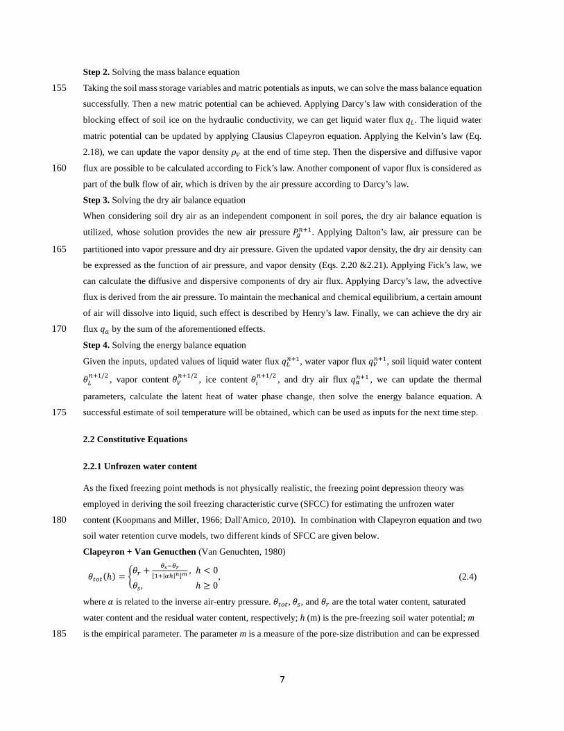
2.2.1 Unfrozen water content
As the fixed freezing point methods is not physically realistic, the freezing point depression theory was
employed in deriving the soil freezing characteristic curve (SFCC) for estimating the unfrozen water
content (Koopmans and Miller, 1966; Dall'Amico, 2010). In combination with Clapeyron equation and two 180 soil water retention curve models, two different kinds of SFCC are given below.
Clapeyron + Van Genucthen (Van Genuchten, 1980)
𝜃𝜃𝜕𝜕𝑡𝑡𝜕𝜕(ℎ) = �𝜃𝜃𝑟𝑟 + 𝜃𝜃𝑠𝑠−𝜃𝜃𝑟𝑟
[1+|𝛼𝛼ℎ|𝑛𝑛]𝑚𝑚, ℎ < 0
𝜃𝜃𝑠𝑠, ℎ ≥ 0, (2.4)
where 𝛼𝛼 is related to the inverse air-entry pressure. 𝜃𝜃𝜕𝜕𝑡𝑡𝜕𝜕, 𝜃𝜃𝑠𝑠, and 𝜃𝜃𝑟𝑟 are the total water content, saturated
water content and the residual water content, respectively; h (m) is the pre-freezing soil water potential; m
is the empirical parameter. The parameter m is a measure of the pore-size distribution and can be expressed 185

8
as m = 1-1/n, which in turn can be determined by fitting van Genuchten’s analytical model (Van
Genuchten, 1980).
The unfrozen water content was estimated by employing soil freezing characteristic curve (SFCC)
(Dall'Amico, 2010)
𝜃𝜃𝐿𝐿(ℎ,𝜕𝜕) = 𝜃𝜃𝑟𝑟 + 𝜃𝜃𝑠𝑠−𝜃𝜃𝑟𝑟[1+|𝛼𝛼(ℎ+ℎ𝐹𝐹𝑟𝑟𝐹𝐹)|𝑛𝑛]𝑚𝑚
, (2.5)
where 𝜃𝜃𝐿𝐿 is the liquid water content, 𝐿𝐿𝑓𝑓 (J kg-1) is the latent heat of fusion, g (m s-2) is the gravity 190
acceleration, T0 (273.15 oC) is the absolute temperature. h (m) is the pre-freezing pressure and 𝛼𝛼, n, and m
are the van Genuchten fitting parameters. ℎ𝐹𝐹𝑟𝑟𝜕𝜕 (m) is the soil freezing potential.
ℎ𝐹𝐹𝑟𝑟𝜕𝜕 = 𝐿𝐿𝑓𝑓𝑔𝑔𝐿𝐿0
(𝜕𝜕 − 𝜕𝜕0) ∙ 𝐻𝐻(𝜕𝜕 − 𝜕𝜕𝐶𝐶𝐶𝐶𝐶𝐶𝐿𝐿), (2.6)
where T (oC) is the soil temperature. H is the Heaviside function, whose value is zero for negative argument
and one for positive argument, 𝜕𝜕𝐶𝐶𝐶𝐶𝐶𝐶𝐿𝐿 (oC) is the soil freezing temperature.
𝜕𝜕𝐶𝐶𝐶𝐶𝐶𝐶𝐿𝐿 = 𝜕𝜕0 + 𝑔𝑔ℎ𝐿𝐿0𝐿𝐿𝑓𝑓
, (2.7)
Clapeyron + Clapp and Hornberger (Clapp and Hornberger, 1978) 195
𝜃𝜃𝐿𝐿(ℎ,𝜕𝜕) = 𝜃𝜃𝑠𝑠( 𝐿𝐿𝑓𝑓𝑔𝑔𝜓𝜓𝑠𝑠
𝐿𝐿−𝐿𝐿𝑓𝑓𝐿𝐿
)−1/𝑏𝑏, (2.8)
where 𝜓𝜓𝑠𝑠 (m) is the air-entry pore water potential, b is the empirical Clapp and Hornberger parameter.
2.2.2 Hydraulic conductivity
According to the pore-size distribution model (Mualem, 1976), the unsaturated hydraulic conductivity
using Clapp and Hornberger, van Genuchten method can be expressed as,
𝐾𝐾𝐿𝐿ℎ = 𝐾𝐾𝑠𝑠(𝜃𝜃/𝜃𝜃𝑠𝑠)3+2/𝛽𝛽, (2.9)
𝐾𝐾𝐿𝐿ℎ = 𝐾𝐾𝑠𝑠𝑆𝑆𝑒𝑒𝑙𝑙[1 − (1 − 𝑆𝑆𝑒𝑒1 𝑚𝑚⁄ )𝑚𝑚]2, (2.10a)
𝑆𝑆𝑒𝑒 = 𝜃𝜃−𝜃𝜃𝑟𝑟𝜃𝜃𝑠𝑠−𝜃𝜃𝑟𝑟
, (2.10b)
𝑚𝑚 = 1 − 1 𝑛𝑛⁄ , (2.10c)
where 𝐾𝐾𝐿𝐿ℎ and 𝐾𝐾𝑠𝑠 (m s-1) are the hydraulic conductivity and saturated hydraulic conductivity. 𝛽𝛽(= 1/𝑏𝑏) is 200 the empirical Clapp and Hornberger parameter. Se is the effective saturation. l, n, and m are the van
Genuchten fitting parameters.
The block effect of the ice presence in soil pores on the hydraulic conductivity is generally characterized by
a correction coefficient, which is a function of ice content (Taylor and Luthin, 1978; Hansson et al., 2004),
𝐾𝐾𝑓𝑓𝐿𝐿ℎ = 10−𝐸𝐸𝐸𝐸𝐾𝐾𝐿𝐿ℎ, (2.11a)
𝑄𝑄 = (𝜌𝜌𝑖𝑖𝜃𝜃𝑖𝑖/𝜌𝜌𝐿𝐿𝜃𝜃𝐿𝐿), (2.11b)
where KfLh (m s−1) is the hydraulic conductivity in frozen soils, KLh (m s−1) is the hydraulic conductivity in 205 unfrozen soils at the same negative pressure or liquid moisture content, Q is the mass ratio of ice to total
water, and E is the empirical constant that accounts for the reduction in permeability due to the formation
of ice (Hansson et al., 2004).
9
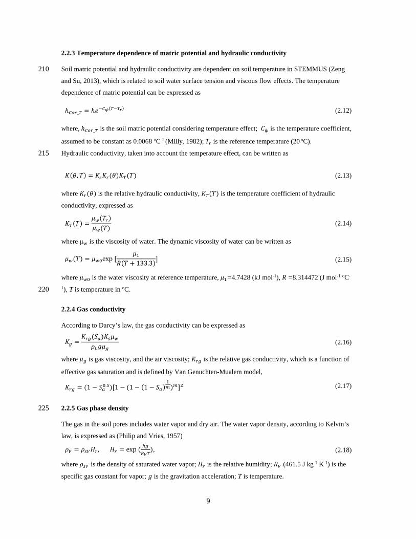
2.2.3 Temperature dependence of matric potential and hydraulic conductivity
Soil matric potential and hydraulic conductivity are dependent on soil temperature in STEMMUS (Zeng 210 and Su, 2013), which is related to soil water surface tension and viscous flow effects. The temperature
dependence of matric potential can be expressed as
ℎ𝐶𝐶𝑡𝑡𝑟𝑟_𝐿𝐿 = ℎ𝑒𝑒−𝐶𝐶𝜓𝜓(𝐿𝐿−𝐿𝐿𝑟𝑟) (2.12)
where, ℎ𝐶𝐶𝑡𝑡𝑟𝑟_𝐿𝐿 is the soil matric potential considering temperature effect; 𝐶𝐶𝜓𝜓 is the temperature coefficient,
assumed to be constant as 0.0068 oC-1 (Milly, 1982); 𝜕𝜕𝑟𝑟 is the reference temperature (20 oC).
Hydraulic conductivity, taken into account the temperature effect, can be written as 215
where 𝐾𝐾𝑟𝑟(𝜃𝜃) is the relative hydraulic conductivity, 𝐾𝐾𝐿𝐿(𝜕𝜕) is the temperature coefficient of hydraulic
conductivity, expressed as
𝐾𝐾𝐿𝐿(𝜕𝜕) =𝜇𝜇𝑤𝑤(𝜕𝜕𝑟𝑟)𝜇𝜇𝑤𝑤(𝜕𝜕)
(2.14)
where μw is the viscosity of water. The dynamic viscosity of water can be written as
𝜇𝜇𝑤𝑤(𝜕𝜕) = 𝜇𝜇𝑤𝑤0exp [𝜇𝜇1
𝑅𝑅(𝜕𝜕 + 133.3)] (2.15)
where 𝜇𝜇𝑤𝑤0 is the water viscosity at reference temperature, 𝜇𝜇1=4.7428 (kJ mol-1), R =8.314472 (J mol-1 oC-
1), T is temperature in oC. 220
2.2.4 Gas conductivity
According to Darcy’s law, the gas conductivity can be expressed as
𝐾𝐾𝑔𝑔 =𝐾𝐾𝑟𝑟𝑔𝑔(𝑆𝑆𝐿𝐿)𝐾𝐾𝑠𝑠𝜇𝜇𝑤𝑤
𝜌𝜌𝐿𝐿𝑔𝑔𝜇𝜇𝑔𝑔 (2.16)
where 𝜇𝜇𝑔𝑔 is gas viscosity, and the air viscosity; 𝐾𝐾𝑟𝑟𝑔𝑔 is the relative gas conductivity, which is a function of
effective gas saturation and is defined by Van Genuchten-Mualem model,
𝐾𝐾𝑟𝑟𝑔𝑔 = (1 − 𝑆𝑆𝐿𝐿0.5)[1 − (1 − (1 − 𝑆𝑆𝐿𝐿)1𝑚𝑚)𝑚𝑚]2 (2.17)
2.2.5 Gas phase density 225
The gas in the soil pores includes water vapor and dry air. The water vapor density, according to Kelvin’s
law, is expressed as (Philip and Vries, 1957)
𝜌𝜌𝑉𝑉 = 𝜌𝜌𝑠𝑠𝑉𝑉𝐻𝐻𝑟𝑟 , 𝐻𝐻𝑟𝑟 = exp ( ℎ𝑔𝑔𝐶𝐶𝑉𝑉𝐿𝐿
),
(2.18)
where 𝜌𝜌𝑠𝑠𝑉𝑉 is the density of saturated water vapor; 𝐻𝐻𝑟𝑟 is the relative humidity; 𝑅𝑅𝑉𝑉 (461.5 J kg-1 K-1) is the
specific gas constant for vapor; 𝑔𝑔 is the gravitation acceleration; T is temperature.
𝐾𝐾(𝜃𝜃,𝜕𝜕) = 𝐾𝐾𝑠𝑠𝐾𝐾𝑟𝑟(𝜃𝜃)𝐾𝐾𝐿𝐿(𝜕𝜕) (2.13)

10
The gradient of the water vapor density with respect to z can be expressed as 230 𝜕𝜕𝜌𝜌𝑉𝑉𝜕𝜕𝜕𝜕
= 𝜌𝜌𝑠𝑠𝑉𝑉𝜕𝜕𝐻𝐻𝑟𝑟𝜕𝜕𝐿𝐿�ℎ
+ 𝜌𝜌𝑠𝑠𝑉𝑉𝜕𝜕𝐻𝐻𝑟𝑟𝜕𝜕ℎ�𝐿𝐿
+ 𝐻𝐻𝑟𝑟𝜕𝜕𝜌𝜌𝑉𝑉𝜕𝜕𝐿𝐿
𝜕𝜕𝐿𝐿𝜕𝜕𝜕𝜕
, (2.19)
Assuming that the pore-air and pore-vapor could be considered as ideal gas, then soil dry air and vapor
density can be given as
𝜌𝜌𝑑𝑑𝐿𝐿 = 𝑃𝑃𝑑𝑑𝑎𝑎𝐶𝐶𝑑𝑑𝑎𝑎𝐿𝐿
, 𝜌𝜌𝑉𝑉 = 𝑃𝑃𝑉𝑉𝐶𝐶𝑉𝑉𝐿𝐿
,
(2.20)
where 𝑅𝑅𝑑𝑑𝐿𝐿 (287.1J kg-1 K-1) is the specific gas constant for dry air; 𝑃𝑃𝑑𝑑𝐿𝐿 and 𝑃𝑃𝑉𝑉 (Pa) are the dry air pressure
and vapor pressure. Following Dalton’s law of partial pressure, the mixed soil air pressure is the sum of the
dry air pressure and the vapor pressure, i.e. 𝑃𝑃𝑔𝑔 = 𝑃𝑃𝑑𝑑𝐿𝐿 + 𝑃𝑃𝑉𝑉. Thus, combining with Eq. 2.20, the soil dry air 235
density can be derived as
𝜌𝜌𝑑𝑑𝐿𝐿 = 𝑃𝑃𝑔𝑔𝐶𝐶𝑑𝑑𝑎𝑎𝐿𝐿
− 𝜌𝜌𝑉𝑉𝐶𝐶𝑉𝑉𝐶𝐶𝑑𝑑𝑎𝑎
, (2.21)
The derivation of dry air density with respect to time and space are 𝜕𝜕𝜌𝜌𝑑𝑑𝑎𝑎𝜕𝜕𝜕𝜕
= 𝑋𝑋𝐿𝐿𝐿𝐿𝜕𝜕𝑃𝑃𝑔𝑔𝜕𝜕𝜕𝜕
+ 𝑋𝑋𝐿𝐿𝐿𝐿𝜕𝜕𝐿𝐿𝜕𝜕𝜕𝜕
+ 𝑋𝑋𝐿𝐿ℎ𝜕𝜕ℎ𝜕𝜕𝜕𝜕
, (2.22)
𝜕𝜕𝜌𝜌𝑑𝑑𝑎𝑎𝜕𝜕𝜕𝜕
= 𝑋𝑋𝐿𝐿𝐿𝐿𝜕𝜕𝑃𝑃𝑔𝑔𝜕𝜕𝜕𝜕
+ 𝑋𝑋𝐿𝐿𝐿𝐿𝜕𝜕𝐿𝐿𝜕𝜕𝜕𝜕
+ 𝑋𝑋𝐿𝐿ℎ𝜕𝜕ℎ𝜕𝜕𝜕𝜕
, (2.23)
where
𝑋𝑋𝐿𝐿𝐿𝐿 = 1𝐶𝐶𝑑𝑑𝑎𝑎𝐿𝐿
, (2.24)
𝑋𝑋𝐿𝐿𝐿𝐿 = � 𝑃𝑃𝑔𝑔𝐶𝐶𝑑𝑑𝑎𝑎𝐿𝐿2
+ 𝐶𝐶𝑉𝑉𝐶𝐶𝑑𝑑𝑎𝑎
�𝐻𝐻𝑟𝑟𝜕𝜕𝜌𝜌𝑠𝑠𝑉𝑉𝜕𝜕𝐿𝐿
+ 𝜌𝜌𝑠𝑠𝑉𝑉𝜕𝜕𝐻𝐻𝑟𝑟𝜕𝜕𝐿𝐿��, (2.25)
𝑋𝑋𝐿𝐿ℎ = −𝜕𝜕𝜌𝜌𝑉𝑉𝜕𝜕ℎ
, (2.26)
2.2.6 Vapor diffusivity
The isothermal vapor diffusivity is followed the simple theory and expressed as 240
𝐷𝐷𝑉𝑉_𝐶𝐶𝑠𝑠𝑡𝑡 = 𝐷𝐷𝑉𝑉𝜕𝜕𝜌𝜌𝑉𝑉𝜕𝜕ℎ
= 𝐷𝐷𝐿𝐿𝜕𝜕𝑚𝑚𝜈𝜈𝜈𝜈𝜃𝜃𝐿𝐿𝜕𝜕𝜌𝜌𝑉𝑉𝜕𝜕ℎ
, (2.27)
where 𝜈𝜈 is set to 1, 𝜈𝜈 = 𝜃𝜃𝐿𝐿2/3, and 𝐷𝐷𝐿𝐿𝜕𝜕𝑚𝑚 = 0.229(1 + 𝐿𝐿
273)1.75 (m2 s-1).
The thermal vapor diffusivity is given by considering the enhancement factor as
𝐷𝐷𝑉𝑉_𝑁𝑁𝑡𝑡𝑛𝑛𝐶𝐶𝑠𝑠𝑡𝑡 = 𝐷𝐷𝑉𝑉𝜕𝜕𝜌𝜌𝑉𝑉𝜕𝜕𝐿𝐿
= 𝐷𝐷𝐿𝐿𝜕𝜕𝑚𝑚𝜂𝜂𝜕𝜕𝜌𝜌𝑉𝑉𝜕𝜕𝐿𝐿
, (2.28)
where 𝜂𝜂 is the thermal enhancement factor.
2.2.7 Gas dispersivity
According to Bear, the gas phase longitudinal dispersivity Dvg is expressed as 245 𝐷𝐷𝑉𝑉𝑔𝑔 = 𝛼𝛼𝐿𝐿_𝑖𝑖𝑞𝑞𝑖𝑖 , 𝑖𝑖 = 𝑔𝑔𝑔𝑔𝑔𝑔 𝑜𝑜𝑜𝑜 𝑙𝑙𝑖𝑖𝑞𝑞𝑙𝑙𝑖𝑖𝑙𝑙, (2.29)
where 𝑞𝑞𝑖𝑖 is the pore fluid flux in phase i, and 𝛼𝛼𝐿𝐿_𝑖𝑖 is the longitudinal dispersivity in phase i, which can be
related to the soil saturation as
𝛼𝛼𝐿𝐿_𝑖𝑖 = 𝛼𝛼𝐿𝐿_𝑆𝑆𝐿𝐿𝜕𝜕 �13.6 − 16 × 𝜃𝜃𝑔𝑔𝜖𝜖
+ 3.4 × �𝜃𝜃𝑔𝑔𝜖𝜖�5�, (2.30)

11
Following Grifoll’s work, the saturation dispersivity can be set to 0.078 m in case of lacking dispersivity
values.
2.2.8 Thermal properties 250
1) Heat capacity
The volumetric heat capacity is the average of the soil component capacity weighted by its fraction.
𝐶𝐶 = �𝐶𝐶𝑗𝑗𝜃𝜃𝑗𝑗
6
𝑖𝑖=1
(2.31)
Where 𝐶𝐶𝑗𝑗 and 𝜃𝜃𝑗𝑗 are the volumetric heat capacity and volumetric fraction of the jth soil constituent (J cm-
3 °C-1). The components are (1) water, (2) air, (3) quartz particles, (4) other minerals, (5) organic matter,
and (6) ice (see Table 2.1). 255
2) Thermal Conductivity
The method used to calculate the frozen soil heat conductivity can be divided into three categories: i)
empirical method (e.g., Campbell method as used in Hansson et al., 2004), ii) Johansen method (Johansen,
1975), and iii) de Vires method (de Vries, 1963). Due to the necessity in the calibration of parameters, the
empirical Campbell method is not easy to adapt and rarely employed in LSMs and thus not discussed in the 260 current context. The other variations of Johansen method and de Vries method, in which the parameters are
based on soil texture information, i.e., Farouki method (Farouki, 1981) and the simplified de Vries method
(Tian et al., 2016), were further incorporated into STEMMUS-FT.
Johansen method (Johansen, 1975)
The soil thermal conductivity is the weighted function of soil dry and saturated thermal conductivity, 265
𝜆𝜆𝑒𝑒𝑓𝑓𝑓𝑓 = 𝐾𝐾𝑒𝑒�𝜆𝜆𝑠𝑠𝐿𝐿𝜕𝜕 − 𝜆𝜆𝑑𝑑𝑟𝑟𝑑𝑑� + 𝜆𝜆𝑑𝑑𝑟𝑟𝑑𝑑, (2.32)
where the 𝜆𝜆𝑠𝑠𝐿𝐿𝜕𝜕 (W m−1 °C−1) is saturated thermal conductivity, 𝜆𝜆𝑑𝑑𝑟𝑟𝑑𝑑 (W m−1 °C−1) is the dry thermal
conductivity, Ke is the Kersten number, which can be expressed as
𝐾𝐾e = �
log (𝜃𝜃/𝜃𝜃𝑠𝑠) + 1.0, 𝜃𝜃/𝜃𝜃𝑠𝑠 > 0.050.7 log �𝜃𝜃
𝜃𝜃𝑠𝑠� + 1.0, 𝜃𝜃/𝜃𝜃𝑠𝑠 > 0.1
𝜃𝜃/𝜃𝜃𝑠𝑠, 𝑓𝑓𝑜𝑜𝑜𝑜𝜕𝜕𝑒𝑒𝑛𝑛 𝑔𝑔𝑜𝑜𝑖𝑖𝑙𝑙 , (2.33)
The saturated thermal conductivity 𝜆𝜆sat is the weighted value of its components (soil particles 𝜆𝜆soil and
water 𝜆𝜆w),
𝜆𝜆sat = 𝜆𝜆soil1−𝜃𝜃𝑠𝑠𝜆𝜆𝑤𝑤
𝜃𝜃𝑠𝑠 , (2.34)
where the solid soil thermal conductivity 𝜆𝜆soil can be described as 270
𝜆𝜆soil = 𝜆𝜆qtzqtz𝜆𝜆o
1−qtz, (2.35)
where the 𝜆𝜆qtz and 𝜆𝜆o (W m−1 °C−1) are the thermal conductivity of the quartz and other soil particles, qtz is
the volumetric quartz fraction.
The dry soil thermal conductivity is a function of dry soil density 𝜌𝜌𝑑𝑑,

12
𝜆𝜆𝑑𝑑𝑟𝑟𝑑𝑑 = 0.135𝜌𝜌𝑑𝑑+64.72700−0.947𝜌𝜌𝑑𝑑
, (2.36)
𝜌𝜌𝑑𝑑 = (1 − 𝜃𝜃𝑠𝑠) ∙ 2700, (2.37)
Farouki method (Farouki, 1981)
Similar to Johansen method, the weighted method between the saturated and dry thermal conductivities is 275 utilized by Farouki method to estimate soil thermal conductivity. The difference between Farouki method
and Johansen method is to express the dry thermal conductivity and solid soil thermal conductivity as the
function of soil texture. Equation can be replaced with,
𝜆𝜆soil = 8.80∙(%sand)+2.92∙(%clay)(%sand)+(%clay)
, (2.38)
where %sand, %clay are the volumetric fraction of sand and clay.
de Vires method (de Vries, 1963) 280
𝜆𝜆𝑒𝑒𝑓𝑓𝑓𝑓 = �� 𝑘𝑘𝑗𝑗𝜃𝜃𝑗𝑗𝜆𝜆j6
𝑗𝑗=1� �� 𝑘𝑘𝑗𝑗𝜃𝜃𝑗𝑗
6𝑗𝑗=1 �
−1, (2.39)
where kj is the weighting factor for each components; 𝜃𝜃𝑗𝑗 the volumetric fraction of the jth constituent; 𝜆𝜆j (W
m−1 °C−1) the thermal conductivity of the jth constituent. The six components are: 1. water, 2. air, 3. quartz
particles, 4. clay minerals, and 5.organic matter, 6, ice. (see Table 2.1).
𝑘𝑘𝑗𝑗 = 23
�1 + �𝜆𝜆j𝜆𝜆1− 1� 𝑔𝑔j�
−1+ 1
3 �1 + �
𝜆𝜆j𝜆𝜆1− 1� �1 − 2𝑔𝑔j��
−1 , (2.40)
and 𝑔𝑔j is the shape factor of the jth constituent (see Table 2.1), of which the shape factor of the air 𝑔𝑔2 can
be determined as follows, 285
𝑔𝑔2 =
⎩⎪⎨
⎪⎧0.013 + � 0.022
𝜃𝜃𝑤𝑤𝑤𝑤𝑤𝑤𝑤𝑤𝑤𝑤𝑛𝑛𝑔𝑔+ 0.298
𝜃𝜃𝑠𝑠� 𝜃𝜃𝐿𝐿 , 𝜃𝜃𝐿𝐿 < 𝜃𝜃𝑤𝑤𝑖𝑖𝑙𝑙𝜕𝜕𝑖𝑖𝑛𝑛𝑔𝑔
0.035 + 0.298𝜃𝜃𝑠𝑠
𝜃𝜃𝐿𝐿 , 𝜃𝜃𝐿𝐿 ≥ 𝜃𝜃𝑤𝑤𝑖𝑖𝑙𝑙𝜕𝜕𝑖𝑖𝑛𝑛𝑔𝑔
, (2.41)
Table 2.1 Properties of Soil Constituents (de Vries, 1963)
Substance j 𝜆𝜆𝑗𝑗 (mcal cm-1 s-1 °C-1) Cj (mcal cm-1 s-1 °C-1) ρj (g cm-3) gj Water 1 1.37 1 1 … Air 2 0.06 0.0003 0.00125 … Quartz 3 21 0.48 2.66 0.125 Clay minerals 4 7 0.48 2.65 0.125 Organic matter 5 0.6 0.6 1.3 0.5 Ice 6 5.2 0.45 0.92 0.125
Simplified de Vries model (Tian et al., 2016)
Tian et al. (2016) proposed the simplified de Vries method as an alternative method of traditional de Vries
method. In this method, the thermal conductivity of soil particles component can be directly estimated 290 based on the relative contribution of measured soil constitutes.
𝜆𝜆𝑒𝑒𝑓𝑓𝑓𝑓 = 𝜃𝜃𝑤𝑤𝜆𝜆𝑤𝑤+𝑘𝑘𝑤𝑤𝜃𝜃𝑤𝑤𝜆𝜆𝑤𝑤+𝑘𝑘𝑎𝑎𝜃𝜃𝑎𝑎𝜆𝜆𝑎𝑎+𝑘𝑘𝑚𝑚𝑤𝑤𝑛𝑛𝜃𝜃𝑚𝑚𝑤𝑤𝑛𝑛𝜆𝜆𝑚𝑚𝑤𝑤𝑛𝑛𝜃𝜃𝑤𝑤+𝑘𝑘𝑤𝑤𝜃𝜃𝑤𝑤+𝑘𝑘𝑎𝑎𝜃𝜃𝑎𝑎+𝑘𝑘𝑚𝑚𝑤𝑤𝑛𝑛𝜃𝜃𝑚𝑚𝑤𝑤𝑛𝑛
, (2.42)
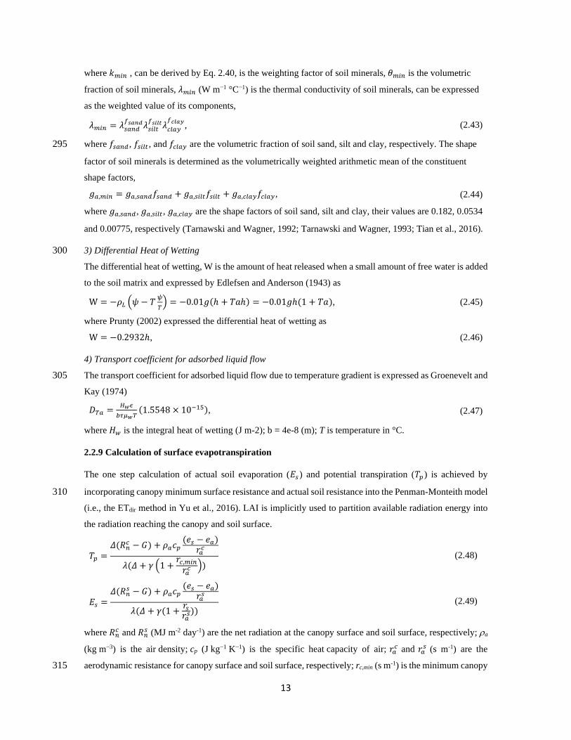
13
where 𝑘𝑘𝑚𝑚𝑖𝑖𝑛𝑛 , can be derived by Eq. 2.40, is the weighting factor of soil minerals, 𝜃𝜃𝑚𝑚𝑖𝑖𝑛𝑛 is the volumetric
fraction of soil minerals, 𝜆𝜆𝑚𝑚𝑖𝑖𝑛𝑛 (W m−1 °C−1) is the thermal conductivity of soil minerals, can be expressed
as the weighted value of its components,
𝜆𝜆𝑚𝑚𝑖𝑖𝑛𝑛 = 𝜆𝜆𝑠𝑠𝐿𝐿𝑛𝑛𝑑𝑑𝑓𝑓𝑠𝑠𝑎𝑎𝑛𝑛𝑑𝑑𝜆𝜆𝑠𝑠𝑖𝑖𝑙𝑙𝜕𝜕
𝑓𝑓𝑠𝑠𝑤𝑤𝑤𝑤𝑤𝑤𝜆𝜆𝑐𝑐𝑙𝑙𝐿𝐿𝑑𝑑𝑓𝑓𝑐𝑐𝑤𝑤𝑎𝑎𝑐𝑐, (2.43)
where 𝑓𝑓𝑠𝑠𝐿𝐿𝑛𝑛𝑑𝑑, 𝑓𝑓𝑠𝑠𝑖𝑖𝑙𝑙𝜕𝜕 , and 𝑓𝑓𝑐𝑐𝑙𝑙𝐿𝐿𝑑𝑑 are the volumetric fraction of soil sand, silt and clay, respectively. The shape 295
factor of soil minerals is determined as the volumetrically weighted arithmetic mean of the constituent
shape factors,
𝑔𝑔𝐿𝐿,𝑚𝑚𝑖𝑖𝑛𝑛 = 𝑔𝑔𝐿𝐿,𝑠𝑠𝐿𝐿𝑛𝑛𝑑𝑑𝑓𝑓𝑠𝑠𝐿𝐿𝑛𝑛𝑑𝑑 + 𝑔𝑔𝐿𝐿,𝑠𝑠𝑖𝑖𝑙𝑙𝜕𝜕𝑓𝑓𝑠𝑠𝑖𝑖𝑙𝑙𝜕𝜕 + 𝑔𝑔𝐿𝐿,𝑐𝑐𝑙𝑙𝐿𝐿𝑑𝑑𝑓𝑓𝑐𝑐𝑙𝑙𝐿𝐿𝑑𝑑, (2.44)
where 𝑔𝑔𝐿𝐿,𝑠𝑠𝐿𝐿𝑛𝑛𝑑𝑑, 𝑔𝑔𝐿𝐿,𝑠𝑠𝑖𝑖𝑙𝑙𝜕𝜕, 𝑔𝑔𝐿𝐿,𝑐𝑐𝑙𝑙𝐿𝐿𝑑𝑑 are the shape factors of soil sand, silt and clay, their values are 0.182, 0.0534
and 0.00775, respectively (Tarnawski and Wagner, 1992; Tarnawski and Wagner, 1993; Tian et al., 2016).
3) Differential Heat of Wetting 300 The differential heat of wetting, W is the amount of heat released when a small amount of free water is added
to the soil matrix and expressed by Edlefsen and Anderson (1943) as
W = −𝜌𝜌𝐿𝐿 �𝜓𝜓 − 𝜕𝜕 𝜓𝜓𝐿𝐿� = −0.01𝑔𝑔(ℎ + 𝜕𝜕𝑔𝑔ℎ) = −0.01𝑔𝑔ℎ(1 + 𝜕𝜕𝑔𝑔), (2.45)
where Prunty (2002) expressed the differential heat of wetting as
W = −0.2932ℎ, (2.46)
4) Transport coefficient for adsorbed liquid flow
The transport coefficient for adsorbed liquid flow due to temperature gradient is expressed as Groenevelt and 305 Kay (1974)
𝐷𝐷𝐿𝐿𝐿𝐿 = 𝐻𝐻𝑤𝑤𝜖𝜖𝑏𝑏𝑏𝑏𝜇𝜇𝑤𝑤𝐿𝐿
(1.5548 × 10⁻¹⁵), (2.47)
where 𝐻𝐻𝑤𝑤 is the integral heat of wetting (J m-2); b = 4e-8 (m); T is temperature in °C.
2.2.9 Calculation of surface evapotranspiration
The one step calculation of actual soil evaporation (𝐸𝐸𝑠𝑠 ) and potential transpiration (𝜕𝜕𝑝𝑝 ) is achieved by
incorporating canopy minimum surface resistance and actual soil resistance into the Penman-Monteith model 310 (i.e., the ETdir method in Yu et al., 2016). LAI is implicitly used to partition available radiation energy into
the radiation reaching the canopy and soil surface.
𝜕𝜕𝑝𝑝 =𝛥𝛥(𝑅𝑅𝑛𝑛𝑐𝑐 − 𝐺𝐺) + 𝜌𝜌𝐿𝐿𝑐𝑐𝑝𝑝
(𝑒𝑒𝑠𝑠 − 𝑒𝑒𝐿𝐿)𝑜𝑜𝐿𝐿𝑐𝑐
𝜆𝜆(𝛥𝛥 + 𝛾𝛾 �1 +𝑜𝑜𝑐𝑐,𝑚𝑚𝑖𝑖𝑛𝑛𝑜𝑜𝐿𝐿𝑐𝑐
�) (2.48)
𝐸𝐸𝑠𝑠 =𝛥𝛥(𝑅𝑅𝑛𝑛𝑠𝑠 − 𝐺𝐺) + 𝜌𝜌𝐿𝐿𝑐𝑐𝑝𝑝
(𝑒𝑒𝑠𝑠 − 𝑒𝑒𝐿𝐿)𝑜𝑜𝐿𝐿𝑠𝑠
𝜆𝜆(𝛥𝛥 + 𝛾𝛾(1 + 𝑜𝑜𝑠𝑠𝑜𝑜𝐿𝐿𝑠𝑠
)) (2.49)
where 𝑅𝑅𝑛𝑛𝑐𝑐 and 𝑅𝑅𝑛𝑛𝑠𝑠 (MJ m-2 day-1) are the net radiation at the canopy surface and soil surface, respectively; ρa
(kg m−3) is the air density; cp (J kg−1 K−1) is the specific heat capacity of air; 𝑜𝑜𝐿𝐿𝑐𝑐 and 𝑜𝑜𝐿𝐿𝑠𝑠 (s m-1) are the
aerodynamic resistance for canopy surface and soil surface, respectively; rc,min (s m-1) is the minimum canopy 315

14
surface resistance; and rs (s m-1) is the soil surface resistance.
The net radiation reaching the soil surface can be calculated using the Beer’s law:
𝑅𝑅𝑛𝑛𝑠𝑠 = 𝑅𝑅𝑛𝑛 𝑒𝑒𝑒𝑒𝑒𝑒( − 𝜈𝜈𝐿𝐿𝜏𝜏𝜏𝜏) (2.50)
And the net radiation intercepted by the canopy surface is the residual part of total net radiation:
𝑅𝑅𝑛𝑛𝑐𝑐 = 𝑅𝑅𝑛𝑛(1 − 𝑒𝑒𝑒𝑒𝑒𝑒( − 𝜈𝜈𝐿𝐿𝜏𝜏𝜏𝜏)) (2.51)
The minimum canopy surface resistance rc,min is given by:
𝑜𝑜𝑐𝑐,𝑚𝑚𝑖𝑖𝑛𝑛 = 𝑜𝑜𝑙𝑙,𝑚𝑚𝑖𝑖𝑛𝑛/𝐿𝐿𝜏𝜏𝜏𝜏𝑒𝑒𝑓𝑓𝑓𝑓 (2.52)
where 𝑜𝑜𝑙𝑙,𝑚𝑚𝑖𝑖𝑛𝑛 is the minimum leaf stomatal resistance; 𝐿𝐿𝜏𝜏𝜏𝜏𝑒𝑒𝑓𝑓𝑓𝑓 is the effective leaf area index, which considers 320
that generally the upper and sunlit leaves in the canopy actively contribute to the heat and vapor transfer.
The soil surface resistance can be estimated following van de Griend and Owe (1994),
𝑜𝑜𝑠𝑠 = 𝑜𝑜𝑠𝑠𝑙𝑙 𝜃𝜃1 > 𝜃𝜃𝑚𝑚𝑖𝑖𝑛𝑛, ℎ1 > −100000 𝑐𝑐𝑚𝑚
(2.53) 𝑜𝑜𝑠𝑠 = 𝑜𝑜𝑠𝑠𝑙𝑙𝑒𝑒𝐿𝐿(𝜃𝜃𝑚𝑚𝑤𝑤𝑛𝑛−𝜃𝜃1) 𝜃𝜃1 ≤ 𝜃𝜃𝑚𝑚𝑖𝑖𝑛𝑛 , ℎ1 > −100000 𝑐𝑐𝑚𝑚
𝑜𝑜𝑠𝑠 = ∞ ℎ1 ≤ −100000 𝑐𝑐𝑚𝑚
where 𝑜𝑜𝑠𝑠𝑙𝑙 (10 s m-1) is the resistance to molecular diffusion of the water surface; a (0.3565) is the fitted
parameter; 𝜃𝜃1 is the topsoil water content; 𝜃𝜃𝑚𝑚𝑖𝑖𝑛𝑛 is the minimum water content above which soil is able to
deliver vapor at a potential rate. 325 The root water uptake term described by Feddes et al. (1978) is:
𝑆𝑆(ℎ) = 𝛼𝛼(ℎ)𝑆𝑆𝑝𝑝 (2.54)
where α(h) (dimensionless) is the reduction coefficient related to soil water potential h; and Sp (s−1) is the
potential water uptake rate.
𝑆𝑆𝑝𝑝 = 𝑏𝑏(𝜕𝜕)𝜕𝜕𝑝𝑝 (2.55)
where Tp is the potential transpiration in Eq. 2.48. b(z) is the normalized water uptake distribution, which
describes the vertical variation of the potential extraction term, Sp, over the root zone. Here the asymptotic 330 function was used to characterize the root distribution as described in (Gale and Grigal, 1987; Jackson et al.,
1996; Yang et al., 2009; Zheng et al., 2015).
2.3 STEMMUS-FT model framework with three levels of complexity
On the basis of STEMMUS modelling framework, the increasing complexity of vadose zone physics in
frozen soils was implemented as three alternative models (Table 2.2). Firstly, STEMMUS enabled isothermal 335 water and heat transfer physics (Eqs. 2.56 & 2.57). The 1-D Richards equation is utilized to solve the
isothermal water transport in variably saturated soils. The heat conservation equation took into account the
freezing/thawing process and the latent heat due to water phase change. The effect of soil ice on soil hydraulic
and thermal properties was considered. It is termed the basic coupled water and heat transfer model (BCD).
Secondly, the fully coupled water and heat physics, i.e., water vapor flow and thermal effect on water flow, 340 was explicitly considered in STEMMUS, termed the advanced coupled model (ACD). For the ACD physics,
the extended version of Richards equation (Richards, 1931) with modifications made by Milly (1982) was

15
used as the water conservation equation (Eq. 2.58). Water flow can be expressed as liquid and vapor fluxes
driven by both temperature gradients and matric potential gradients. The heat transport in frozen soils mainly
includes: heat conduction (CHF, 𝜆𝜆𝑒𝑒𝑓𝑓𝑓𝑓𝜕𝜕𝐿𝐿𝜕𝜕𝜕𝜕
), convective heat transferred by liquid flux (HFL, −𝐶𝐶𝐿𝐿𝑞𝑞𝐿𝐿(𝜕𝜕 − 𝜕𝜕𝑟𝑟), 345
−𝐶𝐶𝐿𝐿𝑆𝑆(𝜕𝜕 − 𝜕𝜕𝑟𝑟)), vapor flux (HFV, −𝐶𝐶𝑉𝑉𝑞𝑞𝑉𝑉(𝜕𝜕 − 𝜕𝜕𝑟𝑟)), the latent heat of vaporization (LHF, −𝑞𝑞𝑉𝑉𝐿𝐿0), the latent
heat of freezing/thawing (−𝜌𝜌𝑖𝑖𝜃𝜃𝑖𝑖𝐿𝐿𝑓𝑓) and a source term associated with the exothermic process of wetting of
a porous medium (integral heat of wetting) (−𝜌𝜌𝐿𝐿𝑊𝑊𝜕𝜕𝜃𝜃𝐿𝐿𝜕𝜕𝜕𝜕
). It can be expressed as Eq. 2.59 (De Vries, 1958;
Hansson et al., 2004).
Lastly, STEMMUS expressed the freezing soil porous medium as the mutually dependent system of liquid 350 water, water vapor, ice water, dry air and soil grains, in which other than air flow all other components kept
the same as in ACD (termed ACD-Air model) (Eqs. 2.60, 2.61, &2.62, Zeng et al., 2011b, a; Zeng and Su,
2013). The effects of air flow on soil water and heat transfer can be two-fold. Firstly, the air flow-induced
water and vapor fluxes (𝑞𝑞𝐿𝐿𝐿𝐿, 𝑞𝑞𝑉𝑉𝐿𝐿) and its corresponding convective heat flow (HFa, −𝑞𝑞𝐿𝐿𝐶𝐶𝐿𝐿(𝜕𝜕 − 𝜕𝜕𝑟𝑟)) were
considered. Secondly, the presence of air flow alters the vapor transfer processes, thus can considerably 355 affects the water and heat transfer in an indirect manner.
STEMMUS utilized the adaptive time-step strategy, with maximum time steps ranging from 1s to 1800s (e.g.,
with 1800s as the time step under stable conditions). The maximum desirable change of soil moisture and
soil temperature within one time step was set as 0.02 cm3 cm-3 and 2 °C, respectively, to prevent too large
change in state variables that may cause numerical instabilities. If the changes between two adjacent soil 360 moisture/temperature states are less than the maximum desirable change, STEMMUS continues without
changing the length of current time step (e.g., 1800s). Otherwise, STEMMUS will adjust the time step with
a deduction factor, which is proportional to the difference between the too large changes and desirable
allowed maximum changes of state variables. Within one single time step, the Picard iteration was used to
solve the numerical problem, and the numerical convergence criteria is set as 0.001 for both soil matric 365 potential (in cm) and soil temperature (in °C).
Table 2.2. Governing equations for different complexity of water and heat coupling physics (See Section 4.4 for notations)
Models Governing equations (water, heat and air) Number
BCD 𝜕𝜕𝜃𝜃𝜕𝜕𝜕𝜕
= −𝜕𝜕𝑞𝑞𝜕𝜕𝜕𝜕− 𝑆𝑆 = 𝜌𝜌𝐿𝐿
𝜕𝜕𝜕𝜕𝜕𝜕�𝐾𝐾 �𝜕𝜕𝜓𝜓
𝜕𝜕𝜕𝜕+ 1�� − 𝑆𝑆 (2.56)
𝐶𝐶𝑠𝑠𝑡𝑡𝑖𝑖𝑙𝑙𝜕𝜕𝜕𝜕𝜕𝜕𝜕𝜕 − 𝜌𝜌𝑖𝑖𝐿𝐿𝑓𝑓
𝜕𝜕𝜃𝜃𝑖𝑖𝜕𝜕𝜕𝜕�������������
𝐻𝐻𝐶𝐶
=𝜕𝜕𝜕𝜕𝜕𝜕 �𝜆𝜆𝑒𝑒𝑓𝑓𝑓𝑓
𝜕𝜕𝜕𝜕𝜕𝜕𝜕𝜕�����
𝐶𝐶𝐻𝐻𝐹𝐹
� (2.57)
ACD 𝜕𝜕𝜕𝜕𝜕𝜕
(𝜌𝜌𝐿𝐿𝜃𝜃𝐿𝐿 + 𝜌𝜌𝑉𝑉𝜃𝜃𝑉𝑉 + 𝜌𝜌𝑖𝑖𝜃𝜃𝑖𝑖) = −𝜕𝜕𝜕𝜕𝜕𝜕
(𝑞𝑞𝐿𝐿 + 𝑞𝑞𝑉𝑉) − 𝑆𝑆
= − 𝜕𝜕𝜕𝜕𝜕𝜕
(𝑞𝑞𝐿𝐿ℎ + 𝑞𝑞𝐿𝐿𝐿𝐿 + 𝑞𝑞𝑉𝑉ℎ + 𝑞𝑞𝑉𝑉𝐿𝐿) − 𝑆𝑆
= 𝜌𝜌𝐿𝐿𝜕𝜕𝜕𝜕𝜕𝜕 �𝐾𝐾𝐿𝐿ℎ �
𝜕𝜕𝜓𝜓𝜕𝜕𝜕𝜕 + 1� + 𝐾𝐾𝐿𝐿𝐿𝐿
𝜕𝜕𝜕𝜕𝜕𝜕𝜕𝜕�+
𝜕𝜕𝜕𝜕𝜕𝜕 �𝐷𝐷𝑉𝑉ℎ
𝜕𝜕𝜓𝜓𝜕𝜕𝜕𝜕 + 𝐷𝐷𝑉𝑉𝐿𝐿
𝜕𝜕𝜕𝜕𝜕𝜕𝜕𝜕� − 𝑆𝑆
(2.58)
16
𝜕𝜕𝜕𝜕𝜕𝜕�(𝜌𝜌𝑠𝑠𝜃𝜃𝑠𝑠𝐶𝐶𝑠𝑠 + 𝜌𝜌𝐿𝐿𝜃𝜃𝐿𝐿𝐶𝐶𝐿𝐿 + 𝜌𝜌𝑉𝑉𝜃𝜃𝑉𝑉𝐶𝐶𝑉𝑉 + 𝜌𝜌𝑖𝑖𝜃𝜃𝑖𝑖𝐶𝐶𝑖𝑖)(𝜕𝜕 − 𝜕𝜕𝑟𝑟) + 𝜌𝜌𝑉𝑉𝜃𝜃𝑉𝑉𝐿𝐿0 − 𝜌𝜌𝑖𝑖𝜃𝜃𝑖𝑖𝐿𝐿𝑓𝑓� − 𝜌𝜌𝐿𝐿𝑊𝑊
𝜕𝜕𝜃𝜃𝐿𝐿𝜕𝜕𝜕𝜕�����������������������������������������������������
𝐻𝐻𝐶𝐶
=𝜕𝜕𝜕𝜕𝜕𝜕 �𝜆𝜆𝑒𝑒𝑓𝑓𝑓𝑓
𝜕𝜕𝜕𝜕𝜕𝜕𝜕𝜕�����
𝐶𝐶𝐻𝐻𝐹𝐹
� −𝜕𝜕𝜕𝜕𝜕𝜕 [𝑞𝑞𝑉𝑉𝐿𝐿0�
𝐿𝐿𝐻𝐻𝐹𝐹+ 𝑞𝑞𝑉𝑉𝐶𝐶𝑉𝑉(𝜕𝜕 − 𝜕𝜕𝑟𝑟)���������
𝐻𝐻𝐹𝐹𝑉𝑉]−
𝜕𝜕𝜕𝜕𝜕𝜕 [𝑞𝑞𝐿𝐿𝐶𝐶𝐿𝐿(𝜕𝜕 − 𝜕𝜕𝑟𝑟)���������]− 𝐶𝐶𝐿𝐿𝑆𝑆(𝜕𝜕 − 𝜕𝜕𝑟𝑟)����������������������������
𝐻𝐻𝐹𝐹𝐿𝐿
(2.59)
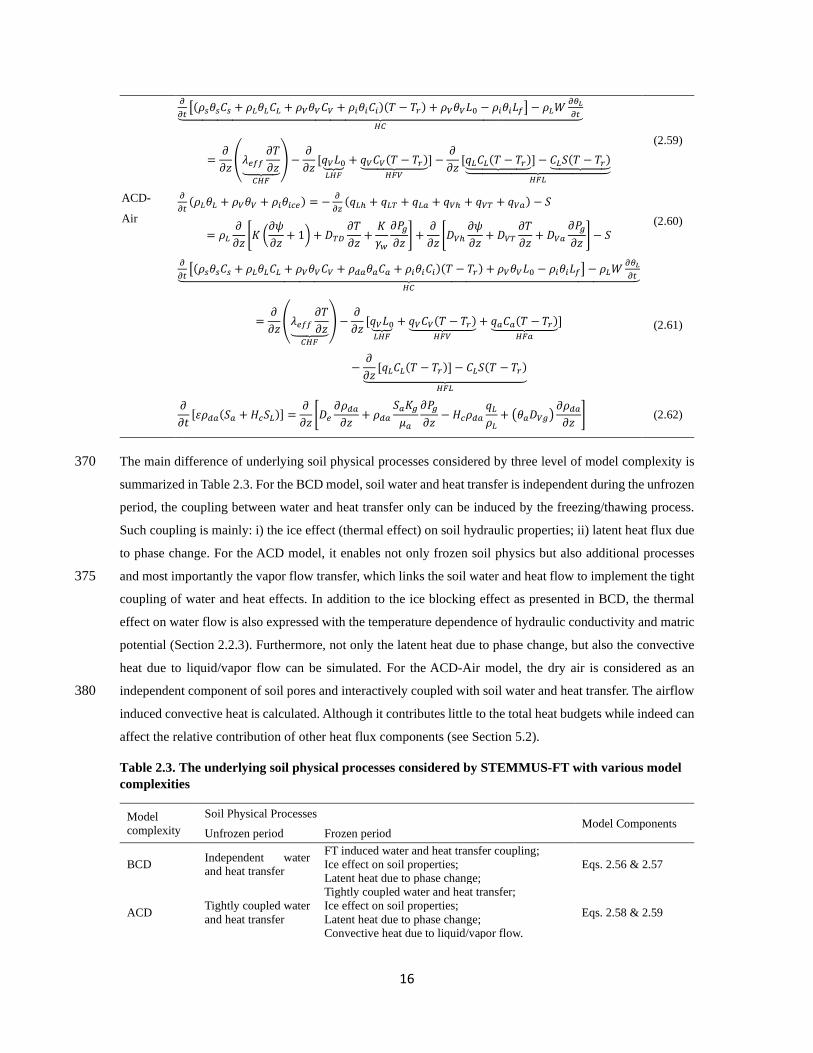
ACD-
Air
𝜕𝜕𝜕𝜕𝜕𝜕
(𝜌𝜌𝐿𝐿𝜃𝜃𝐿𝐿 + 𝜌𝜌𝑉𝑉𝜃𝜃𝑉𝑉 + 𝜌𝜌𝑖𝑖𝜃𝜃𝑖𝑖𝑐𝑐𝑒𝑒) = − 𝜕𝜕𝜕𝜕𝜕𝜕
(𝑞𝑞𝐿𝐿ℎ + 𝑞𝑞𝐿𝐿𝐿𝐿 + 𝑞𝑞𝐿𝐿𝐿𝐿 + 𝑞𝑞𝑉𝑉ℎ + 𝑞𝑞𝑉𝑉𝐿𝐿 + 𝑞𝑞𝑉𝑉𝐿𝐿) − 𝑆𝑆
= 𝜌𝜌𝐿𝐿𝜕𝜕𝜕𝜕𝜕𝜕 �𝐾𝐾 �
𝜕𝜕𝜓𝜓𝜕𝜕𝜕𝜕 + 1� + 𝐷𝐷𝐿𝐿𝑇𝑇
𝜕𝜕𝜕𝜕𝜕𝜕𝜕𝜕 +
𝐾𝐾𝛾𝛾𝑤𝑤
𝜕𝜕𝑃𝑃𝑔𝑔𝜕𝜕𝜕𝜕 � +
𝜕𝜕𝜕𝜕𝜕𝜕 �𝐷𝐷𝑉𝑉ℎ
𝜕𝜕𝜓𝜓𝜕𝜕𝜕𝜕 + 𝐷𝐷𝑉𝑉𝐿𝐿
𝜕𝜕𝜕𝜕𝜕𝜕𝜕𝜕 + 𝐷𝐷𝑉𝑉𝐿𝐿
𝜕𝜕𝑃𝑃𝑔𝑔𝜕𝜕𝜕𝜕 � − 𝑆𝑆
(2.60)
𝜕𝜕𝜕𝜕𝜕𝜕�(𝜌𝜌𝑠𝑠𝜃𝜃𝑠𝑠𝐶𝐶𝑠𝑠 + 𝜌𝜌𝐿𝐿𝜃𝜃𝐿𝐿𝐶𝐶𝐿𝐿 + 𝜌𝜌𝑉𝑉𝜃𝜃𝑉𝑉𝐶𝐶𝑉𝑉 + 𝜌𝜌𝑑𝑑𝐿𝐿𝜃𝜃𝐿𝐿𝐶𝐶𝐿𝐿 + 𝜌𝜌𝑖𝑖𝜃𝜃𝑖𝑖𝐶𝐶𝑖𝑖)(𝜕𝜕 − 𝜕𝜕𝑟𝑟) + 𝜌𝜌𝑉𝑉𝜃𝜃𝑉𝑉𝐿𝐿0 − 𝜌𝜌𝑖𝑖𝜃𝜃𝑖𝑖𝐿𝐿𝑓𝑓� − 𝜌𝜌𝐿𝐿𝑊𝑊
𝜕𝜕𝜃𝜃𝐿𝐿𝜕𝜕𝜕𝜕�������������������������������������������������������������
𝐻𝐻𝐶𝐶
=𝜕𝜕𝜕𝜕𝜕𝜕 �𝜆𝜆𝑒𝑒𝑓𝑓𝑓𝑓
𝜕𝜕𝜕𝜕𝜕𝜕𝜕𝜕�����
𝐶𝐶𝐻𝐻𝐹𝐹
� −𝜕𝜕𝜕𝜕𝜕𝜕 [𝑞𝑞𝑉𝑉𝐿𝐿0�
𝐿𝐿𝐻𝐻𝐹𝐹+ 𝑞𝑞𝑉𝑉𝐶𝐶𝑉𝑉(𝜕𝜕 − 𝜕𝜕𝑟𝑟)���������
𝐻𝐻𝐹𝐹𝑉𝑉+ 𝑞𝑞𝐿𝐿𝐶𝐶𝐿𝐿(𝜕𝜕 − 𝜕𝜕𝑟𝑟)���������
𝐻𝐻𝐹𝐹𝐿𝐿]
−𝜕𝜕𝜕𝜕𝜕𝜕 [𝑞𝑞𝐿𝐿𝐶𝐶𝐿𝐿(𝜕𝜕 − 𝜕𝜕𝑟𝑟)]− 𝐶𝐶𝐿𝐿𝑆𝑆(𝜕𝜕 − 𝜕𝜕𝑟𝑟)���������������������
𝐻𝐻𝐹𝐹𝐿𝐿
(2.61)
𝜕𝜕𝜕𝜕𝜕𝜕
[𝜀𝜀𝜌𝜌𝑑𝑑𝐿𝐿(𝑆𝑆𝐿𝐿 + 𝐻𝐻𝑐𝑐𝑆𝑆𝐿𝐿)] =𝜕𝜕𝜕𝜕𝜕𝜕 �𝐷𝐷𝑒𝑒
𝜕𝜕𝜌𝜌𝑑𝑑𝐿𝐿𝜕𝜕𝜕𝜕 + 𝜌𝜌𝑑𝑑𝐿𝐿
𝑆𝑆𝐿𝐿𝐾𝐾𝑔𝑔𝜇𝜇𝐿𝐿
𝜕𝜕𝑃𝑃𝑔𝑔𝜕𝜕𝜕𝜕 − 𝐻𝐻𝑐𝑐𝜌𝜌𝑑𝑑𝐿𝐿
𝑞𝑞𝐿𝐿𝜌𝜌𝐿𝐿
+ �𝜃𝜃𝐿𝐿𝐷𝐷𝑉𝑉𝑔𝑔�𝜕𝜕𝜌𝜌𝑑𝑑𝐿𝐿𝜕𝜕𝜕𝜕 � (2.62)
The main difference of underlying soil physical processes considered by three level of model complexity is 370 summarized in Table 2.3. For the BCD model, soil water and heat transfer is independent during the unfrozen
period, the coupling between water and heat transfer only can be induced by the freezing/thawing process.
Such coupling is mainly: i) the ice effect (thermal effect) on soil hydraulic properties; ii) latent heat flux due
to phase change. For the ACD model, it enables not only frozen soil physics but also additional processes
and most importantly the vapor flow transfer, which links the soil water and heat flow to implement the tight 375 coupling of water and heat effects. In addition to the ice blocking effect as presented in BCD, the thermal
effect on water flow is also expressed with the temperature dependence of hydraulic conductivity and matric
potential (Section 2.2.3). Furthermore, not only the latent heat due to phase change, but also the convective
heat due to liquid/vapor flow can be simulated. For the ACD-Air model, the dry air is considered as an
independent component of soil pores and interactively coupled with soil water and heat transfer. The airflow 380 induced convective heat is calculated. Although it contributes little to the total heat budgets while indeed can
affect the relative contribution of other heat flux components (see Section 5.2).
Table 2.3. The underlying soil physical processes considered by STEMMUS-FT with various model complexities
Model complexity
Soil Physical Processes Model Components
Unfrozen period Frozen period
BCD Independent water and heat transfer
FT induced water and heat transfer coupling; Ice effect on soil properties; Latent heat due to phase change;
Eqs. 2.56 & 2.57
ACD Tightly coupled water and heat transfer
Tightly coupled water and heat transfer; Ice effect on soil properties; Latent heat due to phase change; Convective heat due to liquid/vapor flow.
Eqs. 2.58 & 2.59

17
ACD-Air Tightly coupled water, dry air, and heat transfer
Tightly coupled water, dry air, and heat transfer; Ice effect on soil properties; Latent heat due to phase change; Convective heat due to liquid/vapor/air flow.
Eqs. 2.60 & 2.61 &2.62
Note: 385 Independent water and heat transfer: Soil water and heat transfer process is independent. FT induced water and heat transfer coupling: Soil water and heat transfer process is coupled only during the freezing/thawing (FT) period. Soil water flow is affected by temperature only through the presence of soil ice content (the impedance effect). Tightly coupled water and heat transfer: Soil water and heat transfer process is tightly coupled; vapor flow, which links 390 the soil water and heat flow, is taken into account; thermal effect on water flow is considered (the hydraulic conductivity and matric potential is dependent on soil temperature; when soil freezes, the hydraulic conductivity is reduced by the presence of soil ice, which is temperature dependent); the convective/advective heat due to liquid/vapor flow can be calculated. Tightly coupled water, dry air, and heat transfer: On the basis of “Tightly coupled water and heat transfer”, the soil dry 395 air transfer is taken into account and simultaneously simulated with water and heat transfer; the convective/advective heat due to liquid/vapor/air flow can be calculated. Ice effect on soil properties: the explicit simulation of ice content and its effect on the hydraulic/thermal properties.
3 UEB snowmelt module
The Utah energy balance (UEB) snowmelt model is a physically-based snow accumulation and melt model 400 (Fig. 3.1). The snowpack is characterized mainly using two primary state variables, snow water equivalent
W and the internal energy U. The snow age is considered as the ancillary state variable. The conservation of
mass and energy, forms the basis of UEB (Tarboton and Luce, 1996), is presented in Section 3.1. The relevant
constitutive equations are given in Section 3.2.
Figure 3.1. The schematic of (a) energy flux involved in snowmelt and snowpack ablation (b) related variables in UEB model. Adapted from Tarboton and Luce (1996).
3.1 Governing Equations 405
3.1.1 Mass balance equation
The increase or decrease of snow water equivalence with time equals the difference of income and outgoing
water flux:
𝑙𝑙𝑊𝑊𝑆𝑆𝑊𝑊𝐸𝐸
𝑙𝑙𝜕𝜕= 𝑃𝑃𝑟𝑟 + 𝑃𝑃𝑠𝑠 − 𝑀𝑀𝑟𝑟 − 𝐸𝐸 (3.1)
where WSWE (m) is the snow water equivalent; 𝑃𝑃𝑟𝑟 (m s-1) is the rainfall rate; 𝑃𝑃𝑠𝑠 (m s-1) is the snowfall rate; 𝑀𝑀𝑟𝑟
(a) (b)
18
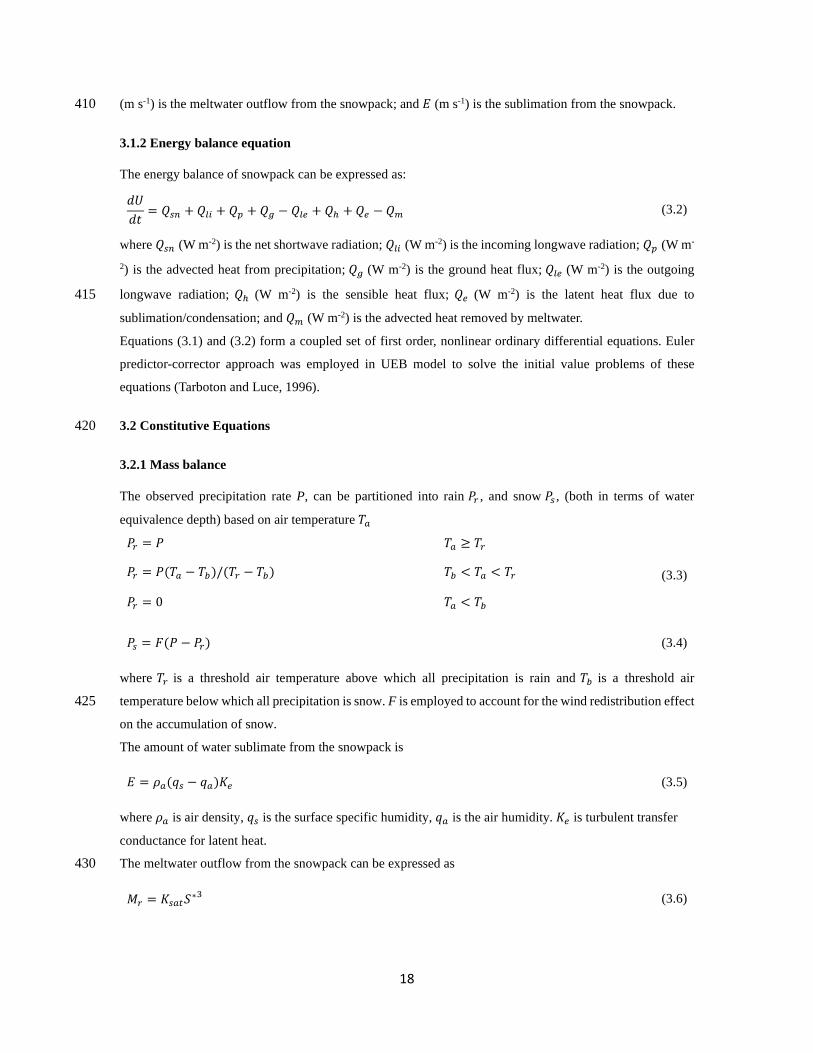
(m s-1) is the meltwater outflow from the snowpack; and 𝐸𝐸 (m s-1) is the sublimation from the snowpack. 410
3.1.2 Energy balance equation
The energy balance of snowpack can be expressed as:
𝑙𝑙𝑈𝑈𝑙𝑙𝜕𝜕
= 𝑄𝑄𝑠𝑠𝑛𝑛 + 𝑄𝑄𝑙𝑙𝑖𝑖 + 𝑄𝑄𝑝𝑝 + 𝑄𝑄𝑔𝑔 − 𝑄𝑄𝑙𝑙𝑒𝑒 + 𝑄𝑄ℎ + 𝑄𝑄𝑒𝑒 − 𝑄𝑄𝑚𝑚 (3.2)
where 𝑄𝑄𝑠𝑠𝑛𝑛 (W m-2) is the net shortwave radiation; 𝑄𝑄𝑙𝑙𝑖𝑖 (W m-2) is the incoming longwave radiation; 𝑄𝑄𝑝𝑝 (W m-
2) is the advected heat from precipitation; 𝑄𝑄𝑔𝑔 (W m-2) is the ground heat flux; 𝑄𝑄𝑙𝑙𝑒𝑒 (W m-2) is the outgoing
longwave radiation; 𝑄𝑄ℎ (W m-2) is the sensible heat flux; 𝑄𝑄𝑒𝑒 (W m-2) is the latent heat flux due to 415
sublimation/condensation; and 𝑄𝑄𝑚𝑚 (W m-2) is the advected heat removed by meltwater.
Equations (3.1) and (3.2) form a coupled set of first order, nonlinear ordinary differential equations. Euler
predictor-corrector approach was employed in UEB model to solve the initial value problems of these
equations (Tarboton and Luce, 1996).
3.2 Constitutive Equations 420
3.2.1 Mass balance
The observed precipitation rate P, can be partitioned into rain 𝑃𝑃𝑟𝑟 , and snow 𝑃𝑃𝑠𝑠 , (both in terms of water
equivalence depth) based on air temperature 𝜕𝜕𝐿𝐿
𝑃𝑃𝑟𝑟 = 𝑃𝑃 𝜕𝜕𝐿𝐿 ≥ 𝜕𝜕𝑟𝑟
(3.3) 𝑃𝑃𝑟𝑟 = 𝑃𝑃(𝜕𝜕𝐿𝐿 − 𝜕𝜕𝑏𝑏)/(𝜕𝜕𝑟𝑟 − 𝜕𝜕𝑏𝑏) 𝜕𝜕𝑏𝑏 < 𝜕𝜕𝐿𝐿 < 𝜕𝜕𝑟𝑟
𝑃𝑃𝑟𝑟 = 0 𝜕𝜕𝐿𝐿 < 𝜕𝜕𝑏𝑏
𝑃𝑃𝑠𝑠 = 𝐹𝐹(𝑃𝑃 − 𝑃𝑃𝑟𝑟) (3.4)
where 𝜕𝜕𝑟𝑟 is a threshold air temperature above which all precipitation is rain and 𝜕𝜕𝑏𝑏 is a threshold air
temperature below which all precipitation is snow. F is employed to account for the wind redistribution effect 425 on the accumulation of snow.
The amount of water sublimate from the snowpack is
𝐸𝐸 = 𝜌𝜌𝐿𝐿(𝑞𝑞𝑠𝑠 − 𝑞𝑞𝐿𝐿)𝐾𝐾𝑒𝑒 (3.5)
where 𝜌𝜌𝐿𝐿 is air density, 𝑞𝑞𝑠𝑠 is the surface specific humidity, 𝑞𝑞𝐿𝐿 is the air humidity. 𝐾𝐾𝑒𝑒 is turbulent transfer
conductance for latent heat.
The meltwater outflow from the snowpack can be expressed as 430
𝑀𝑀𝑟𝑟 = 𝐾𝐾𝑠𝑠𝐿𝐿𝜕𝜕𝑆𝑆∗3 (3.6)

19
where Ksat is the snow saturated hydraulic conductivity and S* is the relative saturation in excess of water
retained by capillary forces. S* is given by:
𝑆𝑆∗ =𝑙𝑙𝑖𝑖𝑞𝑞𝑙𝑙𝑖𝑖𝑙𝑙 𝑤𝑤𝑔𝑔𝜕𝜕𝑒𝑒𝑜𝑜 𝑣𝑣𝑜𝑜𝑙𝑙𝑙𝑙𝑚𝑚𝑒𝑒 − 𝑐𝑐𝑔𝑔𝑒𝑒𝑖𝑖𝑙𝑙𝑙𝑙𝑔𝑔𝑜𝑜𝑐𝑐 𝑜𝑜𝑒𝑒𝜕𝜕𝑒𝑒𝑛𝑛𝜕𝜕𝑖𝑖𝑜𝑜𝑛𝑛
𝑒𝑒𝑜𝑜𝑜𝑜𝑒𝑒 𝑣𝑣𝑜𝑜𝑙𝑙𝑙𝑙𝑚𝑚𝑒𝑒 − 𝑐𝑐𝑔𝑔𝑒𝑒𝑖𝑖𝑙𝑙𝑙𝑙𝑔𝑔𝑜𝑜𝑐𝑐 𝑜𝑜𝑒𝑒𝜕𝜕𝑒𝑒𝑛𝑛𝜕𝜕𝑖𝑖𝑜𝑜𝑛𝑛 (3.7)
3.2.2 Energy balance
The net shortwave radiation is calculated from incident shortwave radiation 𝑄𝑄𝑠𝑠𝑖𝑖 and albedo 𝛼𝛼, which is a
function of snow age and solar illumination angle. 435
𝑄𝑄𝑠𝑠𝑛𝑛 = (1 − 𝛼𝛼)𝑄𝑄𝑠𝑠𝑖𝑖 (3.8)
The Stefan–Boltzmann equation is used to estimate the incoming longwave radiation 𝑄𝑄𝑙𝑙𝑒𝑒 and outgoing
longwave radiation 𝑄𝑄𝑙𝑙𝑖𝑖 based on air temperature 𝜕𝜕𝐿𝐿 and snow surface temperature 𝜕𝜕𝑆𝑆𝑆𝑆, respectively.
𝑄𝑄𝑙𝑙𝑒𝑒 = 𝜀𝜀𝑠𝑠𝜎𝜎𝜕𝜕𝑆𝑆𝑆𝑆4 (3.9)
𝑄𝑄𝑙𝑙𝑖𝑖 = 𝜀𝜀𝐿𝐿𝜎𝜎𝜕𝜕𝐿𝐿4 (3.10)
where 𝜀𝜀𝑠𝑠 is emissivity of snow, 𝜎𝜎 is the Stefan Boltzmann constant. 𝜀𝜀𝐿𝐿 is the air emissivity, which is based
on air vapor pressure, air temperature and cloud cover.
The latent heat flux, 𝑄𝑄𝑒𝑒 and sensible heat flux, 𝑄𝑄ℎ are modeled using bulk aerodynamic formulae: 440
𝑄𝑄ℎ = 𝜌𝜌𝐿𝐿𝐶𝐶𝑝𝑝(𝜕𝜕𝐿𝐿 − 𝜕𝜕𝑆𝑆𝑆𝑆)𝐾𝐾ℎ (3.11)
𝑄𝑄𝑒𝑒 = 𝜌𝜌𝐿𝐿ℎ𝑣𝑣(𝑞𝑞𝑠𝑠 − 𝑞𝑞𝐿𝐿)𝐾𝐾𝑒𝑒 = 𝐾𝐾𝑒𝑒0.622ℎ𝑣𝑣𝑅𝑅𝑑𝑑𝜕𝜕𝐿𝐿
(𝑒𝑒𝐿𝐿 − 𝑒𝑒𝑠𝑠(𝜕𝜕𝑆𝑆𝑆𝑆)) (3.12)
𝐾𝐾ℎ and 𝐾𝐾𝑒𝑒 are turbulent transfer conductance for sensible and latent heat respectively. Under neutral
atmospheric conditions 𝐾𝐾ℎ and 𝐾𝐾𝑒𝑒 can be given by
𝐾𝐾𝑒𝑒 = 𝐾𝐾ℎ =𝑘𝑘𝑣𝑣2𝑙𝑙
[𝑙𝑙𝑛𝑛 (𝜕𝜕𝑚𝑚/𝜕𝜕0]2 (3.13)
where zm is the measurement height for wind speed, air temperature, and humidity, u is the wind speed, kv is
von Kármán’s constant (0.4), and z0 is the aerodynamic roughness.
The heat advected with the snow melt outflow, relative to the solid reference state is: 445
𝑄𝑄𝑚𝑚 = 𝜌𝜌𝑤𝑤ℎ𝑓𝑓𝑀𝑀𝑟𝑟 (3.14)
The advected heat 𝑄𝑄𝑝𝑝 is the energy required to convert precipitation to the reference state (0 °C ice phase).
The temperature of rain and snow is taken as the greater and lesser of the air temperature and freezing
point. With different temperature inherent to snow and rain, this amount of energy can be described as

20
𝑄𝑄𝑝𝑝 = 𝜌𝜌𝑤𝑤𝐶𝐶𝑠𝑠𝑃𝑃𝑠𝑠 ∙ 𝑚𝑚𝑖𝑖𝑛𝑛(𝜕𝜕𝐿𝐿 , 0) + 𝑃𝑃𝑟𝑟�𝜌𝜌𝑤𝑤ℎ𝑓𝑓 + 𝜌𝜌𝑤𝑤𝐶𝐶𝑤𝑤 ∙ 𝑚𝑚𝑔𝑔𝑒𝑒 (𝜕𝜕𝐿𝐿, 0)� (3.15)
3.2.3 Snow temperatures
1) Snowpack temperature, TSN 450 Snowpack temperature TSN, a quantity important for energy fluxes into the snow, is determined diagnostically
from the state variables energy content U, and water equivalence 𝑊𝑊𝑆𝑆𝑊𝑊𝐸𝐸, as follows, recalling that energy
content U is defined relative to 0°C ice phase.
𝜕𝜕𝑆𝑆𝑁𝑁 = 𝑈𝑈𝜌𝜌𝑤𝑤𝑊𝑊𝑆𝑆𝑆𝑆𝑆𝑆𝐶𝐶𝑤𝑤+𝜌𝜌𝑔𝑔𝑇𝑇𝑒𝑒𝐶𝐶𝑔𝑔
, 𝑈𝑈 < 0, all solid phase (3.16)
𝜕𝜕𝑆𝑆𝑁𝑁 = 0, 0 < 𝑈𝑈 < 𝜌𝜌𝑤𝑤𝑊𝑊𝑆𝑆𝑊𝑊𝐸𝐸ℎ𝑓𝑓 , solid and liquid mixture (3.17)
𝜕𝜕𝑆𝑆𝑁𝑁 = 𝑈𝑈−𝜌𝜌𝑤𝑤𝑊𝑊𝑆𝑆𝑆𝑆𝑆𝑆ℎ𝑓𝑓𝜌𝜌𝑤𝑤𝑊𝑊𝐶𝐶𝑤𝑤+𝜌𝜌𝑔𝑔𝑇𝑇𝑒𝑒𝐶𝐶𝑔𝑔
, 𝑈𝑈 > 𝜌𝜌𝑤𝑤𝑊𝑊𝑆𝑆𝑊𝑊𝐸𝐸ℎ𝑓𝑓 , all liquid phase (3.18)
where 𝜌𝜌𝑤𝑤𝑊𝑊𝑆𝑆𝑊𝑊𝐸𝐸𝐶𝐶𝑖𝑖 is the heat capacity of the snow (kJ °C-1 m-2), 𝜌𝜌𝑤𝑤 is the density of water (1000 kg m-3) and
𝐶𝐶𝑖𝑖 is the specific heat of ice (2.09 kJ kg-1 °C-1). 𝜌𝜌𝑔𝑔𝐷𝐷𝑒𝑒𝐶𝐶𝑔𝑔 is the heat capacity of the soil layer (kJ °C-1 m-2), 𝜌𝜌𝑔𝑔 455
is the soil density and 𝐶𝐶𝑔𝑔 the specific heat of soil. 𝐷𝐷𝑒𝑒 is the depth of soil that interacts thermally with the
snowpack. These together determine snowpack temperature TSN when energy content U<0.
Otherwise, 𝜌𝜌𝑤𝑤𝑊𝑊𝑆𝑆𝑊𝑊𝐸𝐸ℎ𝑓𝑓 is the heat required to melt all the snow water equivalence at 0 °C (kJ m-2), ℎ𝑓𝑓 is the
heat of fusion (333.5 kJ kg-1) and U in relation to this determines the solid-liquid phase mixtures. The liquid
fraction 𝐿𝐿𝑓𝑓𝑟𝑟 = 𝑈𝑈/(𝜌𝜌𝑤𝑤𝑊𝑊𝑆𝑆𝑊𝑊𝐸𝐸ℎ𝑓𝑓) quantifies the mass fraction of total snowpack (liquid and ice) that is liquid. 460
Although in Equation (3.17) 𝑊𝑊𝑆𝑆𝑊𝑊𝐸𝐸 is always 0 as a completely liquid snowpack cannot exist, we present this
equation for completeness to keep track of energy content during periods of intermittent snow cover.
𝜌𝜌𝑤𝑤𝑊𝑊𝑆𝑆𝑊𝑊𝐸𝐸𝐶𝐶𝑤𝑤 is the heat capacity of liquid water, 𝐶𝐶𝑤𝑤 is the specific heat of water (4.18 kJ kg-1 °C-1), is included
for numerical consistency during time steps when the snowpack completely melts.
2) Snow Surface Temperature, TSS 465 Snow surface temperature TSS is in general different from snowpack temperature TSN due to the snow
insulation effect. We take into account such temperature difference using an equilibrium approach that
balances energy fluxes at the snow surface. Heat conduction into the snow is calculated using the temperature
gradient and thermal diffusivity of snow, approximated by:
𝑄𝑄𝑆𝑆𝑁𝑁 =𝜅𝜅𝜌𝜌𝑠𝑠𝐶𝐶𝑠𝑠(𝜕𝜕𝑆𝑆𝑆𝑆 − 𝜕𝜕𝑆𝑆𝑁𝑁)
𝑍𝑍𝑒𝑒= 𝐾𝐾𝑆𝑆𝑁𝑁𝜌𝜌𝑠𝑠𝐶𝐶𝑠𝑠(𝜕𝜕𝑆𝑆𝑆𝑆 − 𝜕𝜕𝑆𝑆𝑁𝑁) (3.19)
where 𝜅𝜅 is snow thermal diffusivity (m2 hr-1) and Ze (m) an effective depth over which this thermal gradient 470
acts. 𝐾𝐾𝑆𝑆𝑁𝑁 (𝜅𝜅/𝑍𝑍𝑒𝑒) is termed snow surface conductance, analogous to the heat and vapor conductance. Here
𝐾𝐾𝑆𝑆𝑁𝑁 is used as a tuning parameter, with this calculation used to define a reasonable range. Then assuming
equilibrium at the surface, the surface energy balance gives:

21
𝑄𝑄𝑆𝑆𝑁𝑁 = 𝑄𝑄𝑠𝑠𝑛𝑛 + 𝑄𝑄𝑙𝑙𝑖𝑖 + 𝑄𝑄ℎ(𝜕𝜕𝑆𝑆𝑆𝑆) + 𝑄𝑄𝑒𝑒(𝜕𝜕𝑆𝑆𝑆𝑆) + 𝑄𝑄𝑝𝑝 − 𝑄𝑄𝑙𝑙𝑒𝑒(𝜕𝜕𝑆𝑆𝑆𝑆) (3.20)
where the dependence of Qh, Qe, and Qle on TSS is through equations (3.11), (3.12) and (3.9) respectively.
Analogous to the derivation of the Penman equation for evaporation the functions of TSS in this energy 475 balance equation are linearized about a reference temperature T*, and the equation is solved for TSS:.
𝜕𝜕𝑆𝑆𝑆𝑆 =𝑄𝑄𝑠𝑠𝑛𝑛 + 𝑄𝑄𝑙𝑙𝑖𝑖 + 𝑄𝑄𝑝𝑝 + 𝐾𝐾𝜕𝜕𝐿𝐿𝜌𝜌𝐿𝐿𝐶𝐶𝑝𝑝 −
0.622𝐾𝐾ℎ𝑣𝑣𝜌𝜌𝐿𝐿(𝑒𝑒𝑠𝑠(𝜕𝜕∗) − 𝑒𝑒𝐿𝐿 − 𝜕𝜕∗Δ)𝑃𝑃𝐿𝐿
+ 3𝜀𝜀𝑠𝑠𝜎𝜎𝜕𝜕∗4 + 𝐾𝐾𝑆𝑆𝑁𝑁𝜌𝜌𝑠𝑠𝐶𝐶𝑠𝑠𝜕𝜕𝑆𝑆𝑁𝑁
𝐾𝐾𝑆𝑆𝑁𝑁𝜌𝜌𝑠𝑠𝐶𝐶𝑠𝑠 + 𝐾𝐾𝜌𝜌𝐿𝐿𝐶𝐶𝑝𝑝 + 0.622Δ𝐾𝐾ℎ𝑣𝑣𝜌𝜌𝐿𝐿𝑃𝑃𝐿𝐿
+ 4𝜀𝜀𝑠𝑠𝜎𝜎𝜕𝜕∗3
(3.21)
where Δ = 𝑙𝑙𝑒𝑒𝑠𝑠/𝑙𝑙𝜕𝜕 and all temperatures are absolute in (K). This equation is used in an iterative procedure
with an initial estimate T* = Ta, in each iteration replacing T* by the latest TSS. The procedure converges to
a final TSS which, if less than freezing, is used to calculate surface energy fluxes. If the final TSS is greater 480 than freezing it means that the energy input to the snow surface cannot be balanced by thermal conduction
into the snow. Surface melt will occur and the infiltration of meltwater will account for the energy difference
and TSS is then set to 0°C.
3.2.4 Albedo calculation
1) Ground albedo 485 Instead of the constant bare soil albedo in the original UEB model, the bare soil albedo is expressed as a
decreasing linear function of soil moisture in STEMMUS-UEB.
𝛼𝛼𝑔𝑔,𝑣𝑣 = 𝛼𝛼𝑠𝑠𝐿𝐿𝜕𝜕 + min {𝛼𝛼𝑠𝑠𝐿𝐿𝜕𝜕 , max [(0.11 − 0.4𝜃𝜃), 0]} (3.22)
𝛼𝛼𝑔𝑔,𝑖𝑖𝑟𝑟 = 2𝛼𝛼𝑔𝑔,𝑣𝑣 (3.23)
where 𝛼𝛼𝑔𝑔,𝑣𝑣 and 𝛼𝛼𝑔𝑔,𝑖𝑖𝑟𝑟 are the bare soil/ground albedo for the visible and infrared band, respectively. 𝛼𝛼𝑠𝑠𝐿𝐿𝜕𝜕 is
the saturated soil albedo, depending on local soil color. 𝜃𝜃 is the surface volumetric soil moisture.
2) Vegetation albedo 490 The calculation of vegetation albedo is developed to capture the essential features of a two-stream
approximation model using asymptotic equation. It approaches the underlying surface albedo 𝛼𝛼𝑔𝑔,𝜆𝜆 or the
thick canopy albedo 𝛼𝛼𝑐𝑐,𝜆𝜆 when the 𝐿𝐿𝑆𝑆𝑆𝑆𝐶𝐶 is close to zero or infinity.
𝛼𝛼𝑉𝑉𝑒𝑒𝑔𝑔,𝑏𝑏,𝜆𝜆 = 𝛼𝛼𝑐𝑐,𝜆𝜆 �1 − exp �−𝜔𝜔𝜆𝜆𝛽𝛽𝐿𝐿𝑆𝑆𝑆𝑆𝐶𝐶𝜇𝜇𝛼𝛼𝑐𝑐,𝜆𝜆
�� + 𝛼𝛼𝑔𝑔,𝜆𝜆 exp[−�1 +0.5𝜇𝜇� 𝐿𝐿𝑆𝑆𝑆𝑆𝐶𝐶] (3.24)
𝛼𝛼𝑉𝑉𝑒𝑒𝑔𝑔,𝑑𝑑,𝜆𝜆 = 𝛼𝛼𝑐𝑐,𝜆𝜆 �1 − exp�−2𝜔𝜔𝜆𝜆𝛽𝛽𝐿𝐿𝑆𝑆𝑆𝑆𝐶𝐶𝛼𝛼𝑐𝑐,𝜆𝜆
�� + 𝛼𝛼𝑔𝑔,𝜆𝜆 exp[−2 𝐿𝐿𝑆𝑆𝑆𝑆𝐶𝐶] (3.25)
where subscripts 𝑉𝑉𝑒𝑒𝑔𝑔, 𝑏𝑏,𝑙𝑙, 𝑐𝑐,𝑔𝑔 and 𝜆𝜆 represent vegetation, direct beam, diffuse radiation, thick canopy,

22
ground, and spectrum bands of either visible or infrared bands. 𝜇𝜇 is the cosine of solar zenith angle; 𝜔𝜔𝜆𝜆 is the 495
single scattering albedo, 0.15 for visible and 0.85 for infrared band, respectively; 𝛽𝛽 is assigned as 0.5; 𝐿𝐿𝑆𝑆𝑆𝑆𝐶𝐶
is the sum of leaf area index LAI and stem area index SAI; 𝛼𝛼𝑐𝑐,𝜆𝜆 is the thick canopy albedo dependent on
vegetation types.
The bulk snow-free surface albedo, averaged between bare ground albedo and vegetation albedo, then is
written as: 500
𝛼𝛼𝜂𝜂,𝜆𝜆 = 𝛼𝛼𝑉𝑉𝑒𝑒𝑔𝑔,𝜆𝜆𝑓𝑓𝑉𝑉𝑒𝑒𝑔𝑔 + 𝛼𝛼𝑔𝑔,𝜆𝜆(1 − 𝑓𝑓𝑉𝑉𝑒𝑒𝑔𝑔) (3.26)
where 𝛼𝛼𝜂𝜂,𝜆𝜆 is the averaged bulk snow-free surface albedo; 𝑓𝑓𝑉𝑉𝑒𝑒𝑔𝑔 is the fraction of vegetation cover.
3) Snow albedo
According to Dickinson et al. (1993), snow albedo can be expressed as a function of snow surface age and
solar illumination angle. The snow surface age, which is dependent on snow surface temperature and snowfall,
is updated with each time step in UEB. Visible and near infrared bands are separately treated when calculating 505 reflectance, which are further averaged as the albedo with modifications of illumination angle and snow age.
The reflectance in the visible and near infrared bands can be written as:
𝛼𝛼𝑣𝑣𝑑𝑑 = �1 − 𝐶𝐶𝑣𝑣𝑆𝑆𝐿𝐿𝑔𝑔𝑒𝑒�𝛼𝛼𝑣𝑣𝑡𝑡 (3.27)
𝛼𝛼𝑖𝑖𝑟𝑟𝑑𝑑 = �1 − 𝐶𝐶𝑖𝑖𝑟𝑟𝑆𝑆𝐿𝐿𝑔𝑔𝑒𝑒�𝛼𝛼𝑖𝑖𝑟𝑟𝑡𝑡 (3.28)
where 𝛼𝛼𝑣𝑣𝑑𝑑 and 𝛼𝛼𝑖𝑖𝑟𝑟𝑑𝑑 represent diffuse reflectance in the visible and near infrared bands, respectively. 𝐶𝐶𝑣𝑣 (=
0.2) and 𝐶𝐶𝑖𝑖𝑟𝑟 (=0.5) are parameters that quantify the sensitivity of the visible and infrared band albedo to snow
surface aging (grain size growth), 𝛼𝛼𝑣𝑣𝑡𝑡 (=0.85) and 𝛼𝛼𝑖𝑖𝑟𝑟𝑡𝑡 (=0.65) are fresh snow reflectance in visible and 510
infrared bands, respectively. 𝑆𝑆𝐿𝐿𝑔𝑔𝑒𝑒 is a function to account for aging of the snow surface, and is given by:
𝑆𝑆𝐿𝐿𝑔𝑔𝑒𝑒 =𝜈𝜈
1 + 𝜈𝜈 (3..29)
where τ is the non-dimensional snow surface age that is incremented at each time step by the quantity
designed to emulate the effect of the growth of surface grain sizes.
∆𝜈𝜈 =𝑜𝑜1 + 𝑜𝑜2 + 𝑜𝑜3
𝜈𝜈𝑡𝑡∆𝜕𝜕 (3.30)
where ∆𝜕𝜕 is the time step in seconds with 𝜈𝜈𝑡𝑡 = 106s. r1 is the parameter to represent the effect of grain growth
due to vapor diffusion, and is dependent on snow surface temperature: 515
𝑜𝑜1 = exp [5000(1
273.16−
1𝜕𝜕𝑠𝑠
)] (3.31)
r2 describes the additional effect near and at the freezing point due to melt and refreeze:
𝑜𝑜2 = min (𝑜𝑜110, 1) (3.32)

23
r3=0.03 (0.01 in Antarctica) represents the effect of dirt and soot.
The reflectance of radiation with illumination angle (measured relative to the surface normal) is computed
as:
𝛼𝛼𝑣𝑣 = 𝛼𝛼𝑣𝑣𝑑𝑑 + 0.4 𝑓𝑓(𝜑𝜑)(1 − 𝛼𝛼𝑣𝑣𝑑𝑑) (3.33)
𝛼𝛼𝑖𝑖𝑟𝑟 = 𝛼𝛼𝑖𝑖𝑟𝑟𝑑𝑑 + 0.4 𝑓𝑓(𝜑𝜑)(1 − 𝛼𝛼𝑖𝑖𝑟𝑟𝑑𝑑) (3.34)
where 𝑓𝑓(𝜑𝜑) = �1𝑏𝑏� 𝑏𝑏+11+2𝑏𝑏 cos(𝜑𝜑)
− 1� , 𝑓𝑓𝑜𝑜𝑜𝑜 cos(𝜑𝜑) < 0.5
0, 𝑜𝑜𝜕𝜕ℎ𝑒𝑒𝑜𝑜𝑤𝑤𝑖𝑖𝑔𝑔𝑒𝑒 520
where b is a parameter set at 2 as Dickinson et al. (1993).
When the snowpack is shallow (depth z<h=0.01m), the albedo is calculated by interpolating between the
snow albedo and bare ground albedo with the exponential term approximating the exponential extinction of
radiation penetration of snow.
𝜏𝜏𝑣𝑣/𝑖𝑖𝑟𝑟 = 𝑜𝑜𝛼𝛼𝑔𝑔,𝑣𝑣/𝑖𝑖𝑟𝑟 + (1 − 𝑜𝑜)𝛼𝛼𝑣𝑣/𝑖𝑖𝑟𝑟 (3.35)
where 𝑜𝑜 = �1 − 𝜕𝜕ℎ� 𝑒𝑒−𝜕𝜕/2ℎ. 525
4 STEMMUS-UEB: Coupling structure, Subroutines and Input Data
4.1 Coupling procedure
The coupled process between the snowpack model (UEB) and the soil water model (STEMMUS-FT) is
illustrated in Figure 4.1. The one-way sequential coupling is employed to couple the soil model with the
current snowpack model. The role of the snowpack is explicitly considered by altering the water and heat 530 flow of the underlying soil. The snowpack model takes the atmospheric forcing as the input (precipitation,
air temperature, wind speed and direction, relative humidity, shortwave and longwave radiation) and solves
the snowpack energy and mass balance (Eqs. 3.1 & 3.2, Subroutines: ALBEDO, PARTSNOW,
PREDICORR), provides the melt water flux and heat flux as the surface boundary conditions for the soil
model STEMMUS-FT (Subroutines: h_sub and Enrgy_sub for ACD models; Diff_Moisture_Heat for 535 BCD model). STEMMUS-FT then solves the energy and mass balance equations of soil layers in one
timestep. To highlight the effect of snowpack on the soil water and vapor transfer process, we constrained
the soil surface energy boundary as the Dirichlet type condition (take the specific soil temperature as the
surface boundary condition). Surface soil temperature was derived from the soil profile measurements and
not permitted to be higher than zero when there is snowpack. To ensure the numerical convergence, the 540 adapted timestep strategy was used. The half-hourly meteorological forcing measurements were linearly
interpolated to the running timesteps (Subroutine Forcing_PARM). The precipitation rate (validated at 3-
hour time intervals) was regarded uniformly within the 3-hour duration (see Table S1 for detail). The general

24
description of the subroutines in STEMMUS-UEB, including the main functions, input/output, and its
connection with other subroutines, was presented in Table 4.1 & 4.2 (linked with Table S1 and S2 for the 545 description of model input parameters and outputs for this study).
Figure 4.1. The overview of the coupled STEMMUS-FT and UEB model framework and model structure. SFCC is soil freezing characteristic curve; 𝜽𝜽𝑳𝑳 and 𝜽𝜽𝒊𝒊 are soil liquid water and ice content; 550 𝑲𝑲𝑳𝑳𝒉𝒉 is soil hydraulic conductivity; 𝝀𝝀𝒆𝒆𝒆𝒆𝒆𝒆 is thermal conductivity. 𝝍𝝍,𝑻𝑻,𝑷𝑷𝒈𝒈 are the state variables for soil module STEMMUS-FT (matric potential, temperature, and air pressure, respectively). U, SWE, and τ are the state variables for snow module UEB (snow energy content, snow water equivalent, and snow age, respectively). UEB, Utah Energy Balance module. Precip, Ta, HRa, Rn, and u are the meteorological inputs (precipitation, air temperature, relative humidity, radiation and wind speed). 555 Model subroutines are in red fonts.
4.2 Subroutines and Inputs/Outputs
Table 4.1 and Table 4.2 summarize the main functions, input/output, and code inter-connections of the
primary subroutines and secondary subroutines, which presents the complete Input-Primary Subroutine-560 Secondary Subroutine-Output loop of STEMMUS-UEB modelling framework.
STEMMUS-UEB model subroutines can be generally divided into four groups as identified by different
calling sequential orders or roles/functions in the main program: Initialization Group, Parameterization
Group, Processing Group, and Post-process Group. Note that some subroutines can be categorized into more
than one group, we made the classification based on the functions of the subroutine here. For example, 565 subroutine SOIL2 is called by subroutine StartInit, which belongs to the Initialization Group. Nevertheless,

25
according to the function of SOIL2, it falls into the Parameterization Group. We then label SOIL2 as
Parameterization Group.
Table 4.1. Primary subroutines in STEMMUS-UEB
Model Subroutines
Main functions Main inputs Main outputs Subroutine-Connections Remarks
Soil module
Air_sub
Solves soil dry air balance equation
Water vapor density, diffusivity, dispersion coefficient; dry air density, gas conductivity, flux; liquid water flux; top and bottom boundary conditions
Soil air pressure profile
CondV_DVg, CondL_h, Condg_k_g, Density_V, h_sub --->; --> Enrgy_sub,
Processing Group
CondL_h Calculates soil hydraulic conductivity
Soil hydraulic parameters; soil matric potential; soil temperature
Soil hydraulic conductivity; soil water content
StartInit --->; --> h_sub; Air_sub; Enrgy_sub,
Parameterization Group
CondT_coeff
Calculates soil thermal capacity and conductivity
Thermal properties of soil constituents; soil texture; soil water content; volumetric fraction of dry air; dry air density; vapor density
Soil thermal capacity and conductivity
StartInit, CondL_h, Density_V, Density_DA, EfeCapCond --->; --> Enrgy_sub,
Parameterization Group
CondV_DVg
Calculates flux of dry air and vapor dispersity
Gas conductivity, dry air pressure, volumetric fraction of dry air; saturated soil water content
Dry air flux and vapor dispersion coefficient
StartInit, CondL_h, Condg_k_g --->; --> h_sub; Air_sub; Enrgy_sub,
Parameterization Group
CondL_Tdisp
Calculates transport coefficient for adsorbed liquid flow
Soil porosity, soil water content, temperature, matric potential, volumetric fraction of dry air
Transport coefficient for adsorbed liquid flow and the heat of wetting
StartInit, CondL_h, Condg_k_g --->; --> h_sub; Enrgy_sub,
Parameterization Group
Condg_k_g Calculates gas conductivity
Soil porosity, saturated hydraulic conductivity, volumetric fraction of dry air
Gas conductivity StartInit, CondL_h --->; --> CondV_DVg,
Parameterization Group
Density_DA Calculates dry air density
Soil temperature, matric potential, dry air pressure; vapor density and its derivative with respect to temperature and matric potential
Density of dry air
StartInit, CondL_h, Density_V --->; --> CondT_coeff, Air_sub, Enrgy_sub,
Parameterization Group
Density_V
Calculates vapor density and its derivative with respect to temperature and matric potential
Soil temperature, matric potential
Vapor density and its derivative with respect to temperature and matric potential
CondL_h --->; --> Density_DA, CondT_coeff, h_sub, Air_sub, Enrgy_sub,
Parameterization Group
EfeCapCond
Calculates soil thermal capacity and conductivity
Thermal properties of soil constituents; soil texture; soil water content; volumetric fraction of dry air; dry air density; vapor density
Soil heat capacity; thermal conductivity
StartInit, CondL_h, Density_V, Density_DA --->; --> CondT_coeff,
Parameterization Group
Enrgy_sub
Solves soil energy balance equation
Soil thermal properties, soil hydraulic conductivity, soil matric potential, soil water content, soil temperature, soil dry air pressure, density of dry air, heat of wetting, vapor density, liquid water flux, vapor flux, dry air flux, meterological forcing, top and bottom boundary conditions
Soil temperature profile, liquid water flux, vapor flux, and dry air flux, surface and bottom energy fluxes
Air_sub, h_sub, CondL_h, CondV_DVg, CondL_Tdisp, CondT_coeff, Density_D, Density_DA, PREDICORR --->,
Processing Group
Forcing_PARM
Disaggregates the meteorological forcing into the required time steps
Observed meteorological forcing at hourly/daily time scale
Meteorological forcings at model required time scale
StartInit --->; --> h_sub, Enrgy_sub,
Initialization Group

26
h_sub Solves soil water balance equation
Soil temperature, soil water content, matric potential, soil hydraulic conductivity, heat of wetting, soil dry air pressure, vapor density, diffusivity, dispersity, volumetric fraction of vapor, meteorological forcing, top and bottom boundary conditions
Soil matric potential profile, top and bottom water fluxes, evaporation
StartInit, CondV_DVg, CondL_h, CondV_DE, CondL_Tdisp, Condg_k_g, Density_V, Forcing_PARM, ALBEDO, PARTSNOW, PREDICORR --->; --> Air_sub, Enrgy_sub,
Processing Group
StartInit Initializes model setup
Soil texture, thermal properties of soil constituents, initial soil water content and temperature, top and bottom boundary condition settings
-
--> CondV_DVg, CondL_h, CondV_DE, CondL_Tdisp, Condg_k_g, Density_DA, EfeCapCond, Forcing_PARM, h_sub,
Initialization Group
Diff_Moisture_Heat
Solves soil water and energy balance equations independently
Soil thermal properties, soil hydraulic conductivity, soil matric potential, soil water content, soil temperature, meteorological forcing, top and bottom boundary conditions
Soil water content and temperature profile, liquid water flux, surface and bottom water and energy fluxes
StartInit, CondT_coeff, Forcing_PARM, ALBEDO, PARTSNOW, PREDICORR --->,
Processing Group
Snowpack module
agesn Calculates snow age
Snow surface temperature, snowfall Updated snow age
PARTSNOW, PREDICORR --->; --> ALBEDO,
Parameterization Group
ALBEDO Calculates snow albedo
Fresh snow reflectance at visible and near infrared bands, snow age, bare ground albedo, albedo extinction parameter, snow water equivalent
Snow albedo agesn --->; --> PREDICORR,
Parameterization Group
PARTSNOW
Partitions precipitation into rainfall and snowfall
Precipitation, air temperature, temperature thresholds for rainfall/snowfall
Rainfall, snowfall Forcing_PARM --->; --> PREDICORR,
Parameterization Group
PREDICORR
Solves the snow mass and energy balance equations and updates state variables SWE and U
Air temperature, snow albedo, wind speed, relative humidity, rainfall/snowfall, shortwave/longwave radiation, site parameters
Snow energy content, water equivalent, snow albedo, snow surface temperature, meltwater outflow rate, snow sublimation, snowfall/rainfall
Forcing_PARM --->; --> agesn2, ALBEDO2.
Processing Group
Note: 570 ---> means the relevant subroutines which are incoming to the current one, --> means the relevant subroutines for which the current subroutine is output to; agesn2 and ALBEDO2, means the use of subroutines agesn and ALBEDO after solving the snowpack energy and mass conservation equations, to update the snow age and albedo. 575 580 585

27
Table 4.2. Secondary subroutines in STEMMUS-UEB 590
Model Subroutines Main functions Main inputs Main outputs Subroutine-
Connections Remarks
Soil module
Constants Set the constants
Water vapor density, diffusivity, dispersion coefficient; dry air density, gas conductivity, flux; liquid water flux; top and bottom boundary conditions
Soil air pressure profile
Initializing the following subroutines
Initialization Group
Dtrmn_Z User define the vertical discretization Δz
Soil column depth, layer number
Thickness of each soil layer --> Constants Initialization
Group
SOIL2 Calculate soil moisture θL
Soil hydraulic parameters; soil matric potential; soil temperature
Soil hydraulic conductivity; soil water content
--> StartInit, MainLoop
Parameterization Group
Latent Calculate the latent heat L Soil temperature Latent heat
--> Diff_Moisture_Heat, MainLoop
Parameterization Group
Evap_Cal Calculate albedo, evaporation, and root water uptake
Soil moisture, temperature, meteorological forcing, time
Soil evaporation, resistance, albedo, root water uptake, transpiration
--> h_BC Parameterization Group
SOIL1 Update the wetting history
Soil moisture at previous and current time step, indicator of the wetting/drying status
Updated indicator of the wetting/drying status
--> MainLoop Processing Group
hPARM Calculate the matrices coefficient for liquid equation
Soil temperature, soil water content, matric potential, soil hydraulic conductivity, vapor density, diffusivity, dispersity, volumetric fraction of vapor
Matrices coefficient for liquid equation
StartInit, CondV_DVg, CondL_h, CondV_DE, CondL_Tdisp, Condg_k_g, Density_V, Forcing_PARM--->; --> h_MAT, h_sub,
Processing Group
h_MAT
Assemble the global coefficient matrices of the Galerkin expressions for liquid equation
Matrices coefficient for liquid equation
Global coefficient matrices for liquid equation
hPARM --->; --> h_EQ, h_sub,
Processing Group
h_EQ
Perform the finite difference of the time derivatives in the matrix equation
Global coefficient matrices for liquid equation
Updated right-hand side values
h_MAT --->; --> h_Solve, h_sub,
Processing Group
h_BC Set the boundary condition for solving liquid equation
Soil temperature, soil water content, matric potential, soil hydraulic conductivity, meteorological forcing, top and bottom boundary conditions
Global coefficient matrices at boundary nodes
StartInit, Evap_Cal, h_MAT, ALBEDO, PARTSNOW, PREDICORR --->; --> h_Solve, h_sub,
Processing Group
h_Solve Solve the matrix equation for liquid conservation
Global coefficient matrices of all nodes
Updated soil matric potential profile
h_EQ, h_BC --->; --> h_Bndry_Flux, h_sub,
Processing Group
h_Bndry_Flux
Calculate liquid flux of the boundary node
Updated soil matric potential profile
Top and bottom water fluxes
h_Solve --->; --> h_sub,
Processing Group
AirPARM Calculate the matrices coefficient for dry air equation
Dry air pressure, density, gas conductivity, flux; water vapor density, diffusivity, dispersion coefficient; soil matric potential, water content, temperature, conductivity
Matrices coefficient for dry air equation
CondV_DVg, CondL_h, Condg_k_g, Density_V, h_sub --->; --> Air_MAT, Air_sub,
Processing Group
Air_MAT
Assemble the global coefficient matrices of the Galerkin expressions for dry air equation
Matrices coefficient for dry air equation
Global coefficient matrices for dry air equation
AirPARM --->; --> Air_EQ, Air_sub,
Processing Group

28
Air_EQ
Perform the finite difference of the time derivatives in the matrix equation for dry air
Global coefficient matrices for dry air equation
Updated right-hand side values
Air_MAT, h_sub --->; --> Air_Solve, Air_sub,
Processing Group
Air_BC Set the boundary condition for solving dry air equation
Top and bottom boundary conditions
Global coefficient matrices at boundary nodes
StartInit, Air_MAT --->; --> Air_Solve, Air_sub,
Processing Group
Air_Solve Solve the matrix equation for dry air conservation
Global coefficient matrices of all nodes
Soil air pressure profile
Air_BC, Air_EQ --->; --> Air_sub,
Processing Group
EnrgyPARM
Calculate the matrices coefficient for energy equation
Soil temperature, soil water content, matric potential, soil hydraulic conductivity, vapor density, diffusivity, dispersity, volumetric fraction of vapor, soil thermal properties, soil dry air pressure, conductivity, air flux
Matrices coefficient for energy equation, liquid, vapor, and dry air flux
Air_sub, h_sub, CondL_h, CondV_DVg, CondL_Tdisp, CondT_coeff, Density_D, Density_DA, PREDICORR --->, --> Enrgy_MAT, Enrgy_sub
Processing Group
Enrgy_MAT
Assemble the global coefficient matrices of the Galerkin expressions for energy equation
Matrices coefficient for energy equation
Global coefficient matrices for energy equation
EnrgyPARM --->, --> Enrgy_EQ, Enrgy_sub
Processing Group
Enrgy_EQ
Perform the finite difference of the time derivatives in the matrix equation for energy
Global coefficient matrices for energy equation
Updated right-hand side values
Air_sub, h_sub, Enrgy_MAT --->, --> Enrgy_Solve, Enrgy_sub
Processing Group
Enrgy_BC Set the boundary condition for solving energy equation
Top and bottom boundary conditions
Global coefficient matrices at boundary nodes
StartInit, Enrgy_MAT --->, --> Enrgy_Solve, Enrgy_sub
Processing Group
Enrgy_Solve
Solve the matrix equation for energy conservation
Global coefficient matrices of all nodes
Soil temperature profile
Enrgy_EQ, Enrgy_BC --->, --> Enrgy_Bndry_Flux, Enrgy_sub
Processing Group
Enrgy_Bndry_Flux
Calculate energy flux of the boundary node Soil temperature profile Surface and bottom
energy fluxes Enrgy_Solve --->, --> Enrgy_sub
Processing Group
TimestepCHK
Assessing the change in boundary conditions after one time step
Surface boundary conditions, time step, indicators of the boundary condition change
Updated time step and indicators of the boundary condition change
h_sub, Air_sub, Enrgy_sub, SOIL2 --->,
Post-processing Group
CnvrgnCHK Check the convergence
Soil state variables, convergence criteria, time step, indicators of the boundary condition change
Updated time step and indicators of the boundary condition change
h_sub, Enrgy_sub, SOIL2 --->, --> TimestepCHK
Post-processing Group
PlotResults Plot the results Post-processing Group
Snowpack module
atf Calculate the atmospheric transmissivity
Date, Campbell coefficient Atmospheric transmissivity
--> snow_Calc
Parameterization Group
Cosen Calculate the hourly radiation index Date, slope, latitude Hourly radiation
index --> Eavp_Cal
Parameterization Group
hyri Calculate the hourly radiation index Date, slope, latitude Hourly radiation
index --> snow_Calc
Parameterization Group
FMELT Calculate the melt rate and outflow
Energy content, snow water equivalent, snow saturated hydraulic conductivity, precipitation
Melt outflow rate --> QFM Parameterization Group
JULIAN Convert the real date to julian date Date (mm, dd) Julian date (001-
365/366) --> hyri Parameterization Group

29
PREHELP Correct energy and mass fluxes when numerical overshoots
Rainfall/snowfall, snow equivalent, snow energy components
Corrected snow mass and energy fluxes
QFM --->, --> PREDICORR
Processing Group
QFM Calculate snow mass and energy fluxes
Snow water equivalent, energy content, rainfall/snowfall, meteorological forcing, site information
Snow mass and energy fluxes
FMELT, QPF, SVPW, TAVG, TURBFLUX, SRFTMP --->, --> PREDICORR
Parameterization Group
qlif Compute the incoming longwave radiation
Air temperature, relative humidity, cloud fraction
Incoming longwave radiation --> snow_Calc Parameteriza
tion Group
QPF Calculate the heat advected to the snowpack
Precipitation, air temperature Snow heat advection due to rain
--> QFM Parameterization Group
RKINST Calculate no neutral turbulent transfer coefficient
Wind speed, air temperature, surface temperature
Turbulent transfer coefficient --> TURBFLUX Parameteriza
tion Group
SRFTMP Compute snow surface temperature
Surface energy components, meteorological forcing
Snow surface temperature
surfeb --->, --> QFM
Parameterization Group
surfeb Solve the surface energy balance for surface temperature
Surface energy components, meteorological forcing
Updating surface energy balance --> SRFTMP Parameteriza
tion Group
SVP Calculate the vapor pressure over water or ice
Temperature Vapor pressure --> surfeb Parameterization Group
SVPI Calculate the vapor pressure over ice Temperature Vapor pressure over
ice --> TURBFLUX Parameterization Group
SVPW Calculate the vapor pressure over water Temperature Vapor pressure over
water --> QFM, qlif Parameterization Group
TAVG
Calculate the average temperature of snow and the interacting soil layer
Snow water and energy content, soil and snow heat properties
Average temperature of snow and the interacting soil layer
--> QFM, snow_Calc
Parameterization Group
TURBFLUX Calculate the turbulent heat fluxes
Precipitation, surface temperature, vapor pressure, wind speed, turbulent transfer coefficient
Turbulent heat fluxes and condensation/sublimation
RKINST, SVPI --->, --> QFM
Parameterization Group
UPDATETIME
Update time for each time step Date (yy, mm, dd, hh) Updated time --> snow_Calc Parameteriza
tion Group Note: ---> means the relevant subroutines which are incoming to the current one, --> means the relevant subroutines for which the current subroutine is output to.
4.3 Setup and Running the model
The current STEMMUS-UEB is tested with MATLAB 2019b. STEMMUS-UEB is executed in MATLAB 595 by simply running MainLoop.m after you finish all the model setup and give the input data to STEMMUS-
UEB. Several steps are necessary to build up the model setup.
1. Setting the temporal information and model domain;
2. Setting soil properties and snow properties;
3. Setting the initialization condition for soil and snow submodules, respectively; 600 4. Inputting the meteorological forcing information;
5. Setting the surface/bottom conditions.
Then you are ready to run STEMMUS-UEB by running MainLoop.m.
605
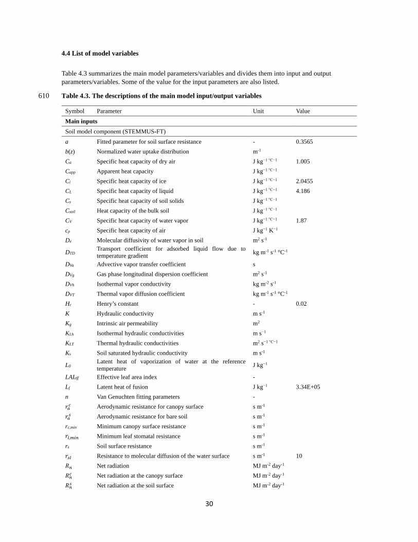
30
4.4 List of model variables
Table 4.3 summarizes the main model parameters/variables and divides them into input and output parameters/variables. Some of the value for the input parameters are also listed.
Table 4.3. The descriptions of the main model input/output variables 610
Symbol Parameter Unit Value
Main inputs Soil model component (STEMMUS-FT) a Fitted parameter for soil surface resistance - 0.3565 b(z) Normalized water uptake distribution m-1
Ca Specific heat capacity of dry air J kg−1 °C−1 1.005 Capp Apparent heat capacity J kg−1 °C−1
Ci Specific heat capacity of ice J kg−1 °C−1 2.0455 CL Specific heat capacity of liquid J kg−1 °C−1 4.186 Cs Specific heat capacity of soil solids J kg−1 °C−1
Csoil Heat capacity of the bulk soil J kg−1 °C−1
CV Specific heat capacity of water vapor J kg−1 °C−1 1.87 cp Specific heat capacity of air J kg−1 K−1
De Molecular diffusivity of water vapor in soil m2 s-1
DTD Transport coefficient for adsorbed liquid flow due to temperature gradient kg m-1 s-1 °C-1
DVa Advective vapor transfer coefficient s
DVg Gas phase longitudinal dispersion coefficient m2 s-1
DVh Isothermal vapor conductivity kg m-2 s-1
DVT Thermal vapor diffusion coefficient kg m-1 s-1 °C-1 Hc Henry’s constant - 0.02 K Hydraulic conductivity m s-1
Kg Intrinsic air permeability m2
KLh Isothermal hydraulic conductivities m s−1
KLT Thermal hydraulic conductivities m2 s−1 °C−1
Ks Soil saturated hydraulic conductivity m s-1
L0 Latent heat of vaporization of water at the reference temperature J kg−1
LAIeff Effective leaf area index -
Lf Latent heat of fusion J kg−1 3.34E+05 n Van Genuchten fitting parameters -
𝑜𝑜𝐿𝐿𝑐𝑐 Aerodynamic resistance for canopy surface s m-1
𝑜𝑜𝐿𝐿𝑠𝑠 Aerodynamic resistance for bare soil s m-1
rc,min Minimum canopy surface resistance s m-1
𝑜𝑜𝑙𝑙,𝑚𝑚𝑖𝑖𝑛𝑛 Minimum leaf stomatal resistance s m-1
rs Soil surface resistance s m-1
𝑜𝑜𝑠𝑠𝑙𝑙 Resistance to molecular diffusion of the water surface s m-1 10 𝑅𝑅𝑛𝑛 Net radiation MJ m-2 day-1
𝑅𝑅𝑛𝑛𝑐𝑐 Net radiation at the canopy surface MJ m-2 day-1
𝑅𝑅𝑛𝑛𝑠𝑠 Net radiation at the soil surface MJ m-2 day-1
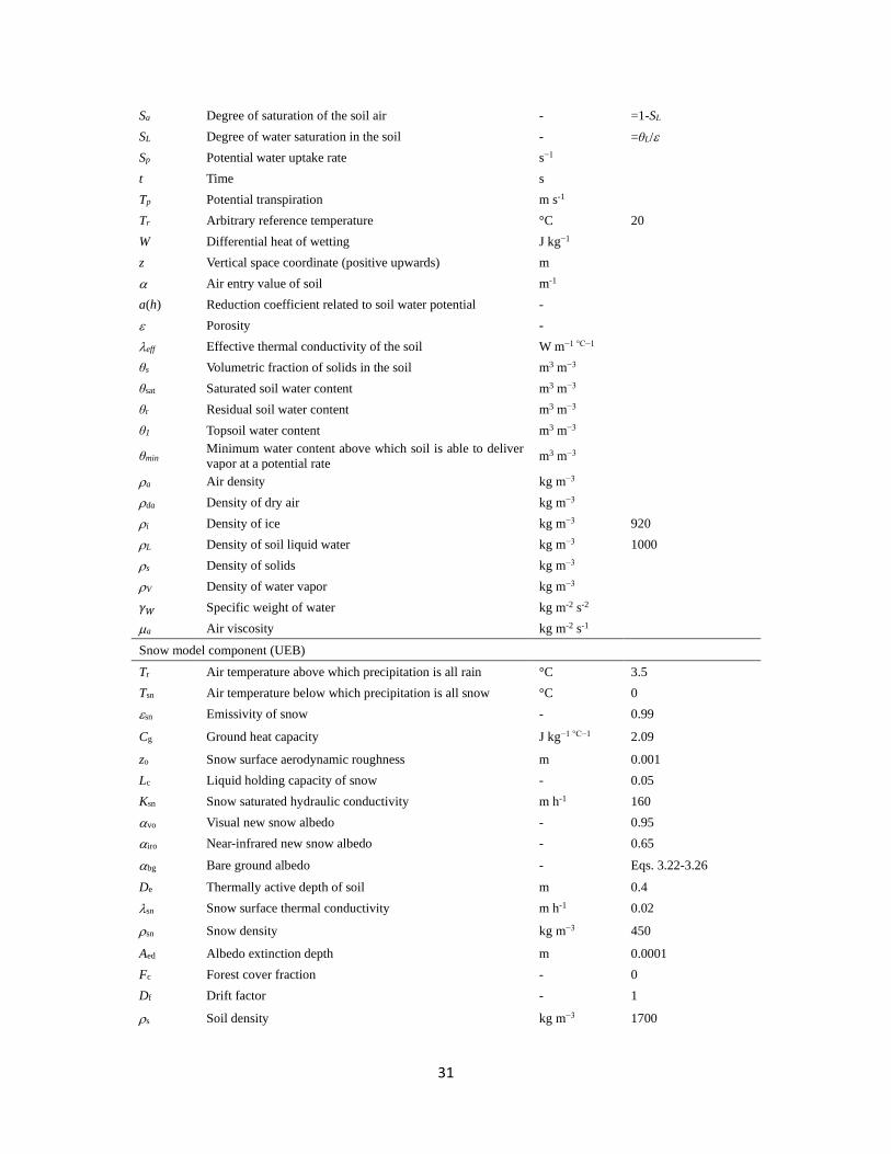
31
Sa Degree of saturation of the soil air - =1-SL SL Degree of water saturation in the soil - =θL/ε Sp Potential water uptake rate s−1
t Time s
Tp Potential transpiration m s-1
Tr Arbitrary reference temperature °C 20 W Differential heat of wetting J kg−1
z Vertical space coordinate (positive upwards) m
α Air entry value of soil m-1
a(h) Reduction coefficient related to soil water potential -
ε Porosity -
λeff Effective thermal conductivity of the soil W m−1 °C−1
θs Volumetric fraction of solids in the soil m3 m−3
θsat Saturated soil water content m3 m−3
θr Residual soil water content m3 m−3
θ1 Topsoil water content m3 m−3
θmin Minimum water content above which soil is able to deliver vapor at a potential rate m3 m−3
ρa Air density kg m−3
ρda Density of dry air kg m−3
ρi Density of ice kg m−3 920 ρL Density of soil liquid water kg m−3 1000 ρs Density of solids kg m−3
ρV Density of water vapor kg m−3
𝛾𝛾𝑊𝑊 Specific weight of water kg m-2 s-2
µa Air viscosity kg m-2 s-1
Snow model component (UEB) Tr Air temperature above which precipitation is all rain °C 3.5 Tsn Air temperature below which precipitation is all snow °C 0 εsn Emissivity of snow - 0.99
Cg Ground heat capacity J kg−1 °C−1 2.09
zo Snow surface aerodynamic roughness m 0.001 Lc Liquid holding capacity of snow - 0.05 Ksn Snow saturated hydraulic conductivity m h-1 160 αvo Visual new snow albedo - 0.95 αiro Near-infrared new snow albedo - 0.65
αbg Bare ground albedo - Eqs. 3.22-3.26
De Thermally active depth of soil m 0.4 λsn Snow surface thermal conductivity m h-1 0.02
ρsn Snow density kg m−3 450
Aed Albedo extinction depth m 0.0001 Fc Forest cover fraction - 0 Df Drift factor - 1
ρs Soil density kg m−3 1700

32
Main outputs Soil model component (STEMMUS-FT)
𝜓𝜓 Soil water potential m
Pg Mixed pore-air pressure Pa
T Soil temperature °C
θ Volumetric water content m3 m-3
θi Soil ice volumetric water content m3 m−3
θL Soil liquid volumetric water content m3 m−3
θV Soil vapor volumetric water content m3 m−3
θa Volumetric fraction of dry air in the soil m3 m−3
q Water flux kg m-2 s-1
qa Dry air flux kg m-2 s-1
qL Soil liquid water fluxes (positive upwards) kg m−2 s−1
𝑞𝑞𝐿𝐿𝐿𝐿 Liquid water flux driven by the gradient of air pressure kg m-2 s-1
𝑞𝑞𝐿𝐿ℎ Liquid water flux driven by the gradient of matric potential kg m-2 s-1
𝑞𝑞𝐿𝐿𝐿𝐿 Liquid water flux driven by the gradient of temperature kg m-2 s-1
qV Soil water vapor fluxes (positive upwards) kg m−2 s−1
𝑞𝑞𝑉𝑉𝐿𝐿 Water vapor flux driven by the gradient of air pressure kg m-2 s-1
𝑞𝑞𝑉𝑉ℎ Water vapor flux driven by the gradient of matric potential kg m-2 s-1
𝑞𝑞𝑉𝑉𝐿𝐿 Water vapor flux driven by the gradient of temperature kg m-2 s-1
S Sink term for transpiration s-1
Sh Latent heat flux density W m-3
Snow model component (UEB) Pr Precipitation in the form of rain m s-1
Ps Precipitation in the form of snow m s-1
WSWE Snow water equivalent m
Qh Surface Sensible Heat Flux W m-2
Qe Surface Latent Heat Flux W m-2
E Surface Sublimation m s-1
TSS Snow Surface Temperature °C
U Energy Content
Mr Melt outflow rate m s-1
Av/ir Surface Albedo -
Qm Heat advected by melt outflow W m-2
Qsn Net shortwave radiation W m-2
Qli Net longwave radiation W m-2 𝜈𝜈 No-dimensional snow age -
615
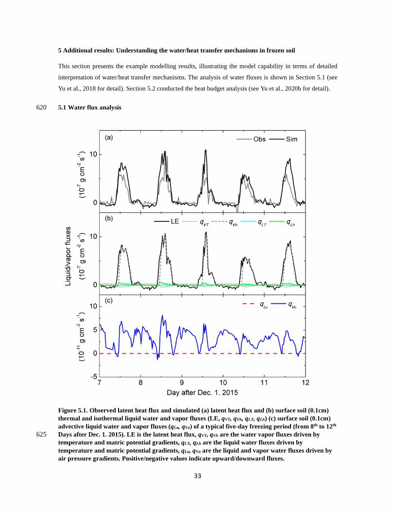
33
5 Additional results: Understanding the water/heat transfer mechanisms in frozen soil
This section presents the example modelling results, illustrating the model capability in terms of detailed
interpretation of water/heat transfer mechanisms. The analysis of water fluxes is shown in Section 5.1 (see
Yu et al., 2018 for detail). Section 5.2 conducted the heat budget analysis (see Yu et al., 2020b for detail).
5.1 Water flux analysis 620
Figure 5.1. Observed latent heat flux and simulated (a) latent heat flux and (b) surface soil (0.1cm) thermal and isothermal liquid water and vapor fluxes (LE, qVT, qVh, qLT, qLh) (c) surface soil (0.1cm) advective liquid water and vapor fluxes (qLa, qVa) of a typical five-day freezing period (from 8th to 12th Days after Dec. 1. 2015). LE is the latent heat flux, qVT, qVh are the water vapor fluxes driven by 625 temperature and matric potential gradients, qLT, qLh are the liquid water fluxes driven by temperature and matric potential gradients, qLa, qVa are the liquid and vapor water fluxes driven by air pressure gradients. Positive/negative values indicate upward/downward fluxes.
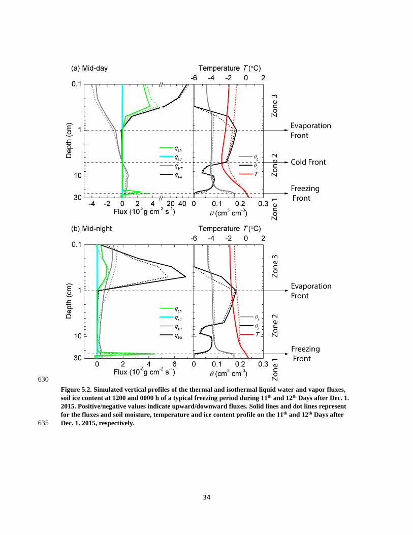
34
630 Figure 5.2. Simulated vertical profiles of the thermal and isothermal liquid water and vapor fluxes, soil ice content at 1200 and 0000 h of a typical freezing period during 11th and 12th Days after Dec. 1. 2015. Positive/negative values indicate upward/downward fluxes. Solid lines and dot lines represent for the fluxes and soil moisture, temperature and ice content profile on the 11th and 12th Days after Dec. 1. 2015, respectively. 635

35
Figure 5.3. Simulated vertical profiles of the air pressure induced liquid water and vapor fluxes, soil air pressure gradient, soil ice content, liquid water content and soil temperature at 1200 and 0000 h 640 of a typical freezing period during 11th and 12th Days after Dec. 1. 2015. Positive/negative values indicate upward/downward fluxes. Solid lines and dot lines represent for the fluxes and soil moisture, temperature and ice content profile on the 11th and 12th Days after Dec. 1. 2015, respectively.
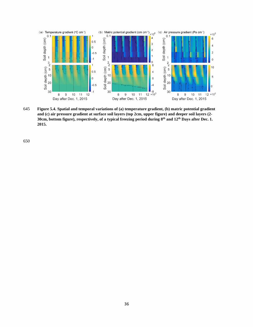
36
Figure 5.4. Spatial and temporal variations of (a) temperature gradient, (b) matric potential gradient 645 and (c) air pressure gradient at surface soil layers (top 2cm, upper figure) and deeper soil layers (2-30cm, bottom figure), respectively, of a typical freezing period during 8th and 12th Days after Dec. 1. 2015.
650
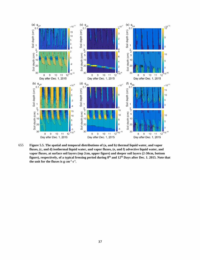
37
Figure 5.5. The spatial and temporal distributions of (a, and b) thermal liquid water, and vapor 655 fluxes, (c, and d) isothermal liquid water, and vapor fluxes, (e, and f) advective liquid water, and vapor fluxes, at surface soil layers (top 2cm, upper figure) and deeper soil layers (2-30cm, bottom figure), respectively, of a typical freezing period during 8th and 12th Days after Dec. 1. 2015. Note that the unit for the fluxes is g cm-2 s-1.

38
660 Figure 5.6. Same as Figure 8 but for a typical five-day thawing period (from 87th to 91th Days after Dec. 1. 2015).

39
Figure 5.7. Simulated vertical profiles of the thermal and isothermal liquid water and vapor fluxes, soil ice content at 1200 and 0000 h of a typical freezing period during 90th and 91th Days after Dec. 1. 665 2015. Positive/negative values indicate upward/downward fluxes. Solid lines and dot lines represent for the fluxes and soil moisture, temperature and ice content profile on the 90th and 91th Days after Dec. 1. 2015, respectively.
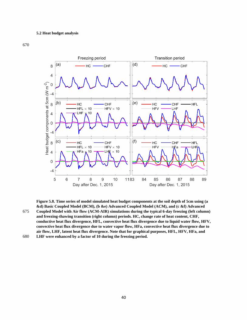
40
5.2 Heat budget analysis
670
Figure 5.8. Time series of model simulated heat budget components at the soil depth of 5cm using (a &d) Basic Coupled Model (BCM), (b &e) Advanced Coupled Model (ACM), and (c &f) Advanced Coupled Model with Air flow (ACM-AIR) simulations during the typical 6-day freezing (left column) 675 and freezing-thawing transition (right column) periods. HC, change rate of heat content, CHF, conductive heat flux divergence, HFL, convective heat flux divergence due to liquid water flow, HFV, convective heat flux divergence due to water vapor flow, HFa, convective heat flux divergence due to air flow, LHF, latent heat flux divergence. Note that for graphical purposes, HFL, HFV, HFa, and LHF were enhanced by a factor of 10 during the freezing period. 680

41
Freezig period Transition period
Figure 5.9. The spatial and temporal distributions of model estimated soil latent heat flux density using (a &d) Advanced Coupled Model (ACM), (b &e) Advanced Coupled Model with Air flow (ACM-AIR) and (c &f) the difference between ACM and ACM-AIR simulations (𝑺𝑺𝒉𝒉,𝑨𝑨𝑨𝑨𝑨𝑨−𝑨𝑨𝑨𝑨𝑨𝑨 −𝑺𝑺𝒉𝒉,𝑨𝑨𝑨𝑨𝑨𝑨) during the typical 6-day freezing and freezing-thawing transition periods. The left and right column are for the freezing and freezing-thawing transition period, respectively. Note that figures for 685 the Basic Coupled Model (BCM) are absent as it can not simulate the subsurface soil latent heat flux density.

42
Reference
Clapp, R. B., and Hornberger, G. M.: Empirical equations for some soil hydraulic properties, Water Resour Res, 14, 601-604, https://doi.org/10.1029/WR014i004p00601, 1978. 690 Clark, M. P., Nijssen, B., Lundquist, J. D., Kavetski, D., Rupp, D. E., Woods, R. A., Freer, J. E., Gutmann, E. D., Wood, A. W., Brekke, L. D., Arnold, J. R., Gochis, D. J., and Rasmussen, R. M.: A unified approach for process-based hydrologic modeling: 1. Modeling concept, Water Resour Res, 51, 2498-2514, https://doi.org/10.1002/2015wr017198, 2015. Dall'Amico, M.: Coupled water and heat transfer in permafrost modeling, University of Trento, 2010. 695 De Vries, D. A.: Simultaneous transfer of heat and moisture in porous media, Eos, Transactions American Geophysical Union, 39, 909-916, https://doi.org/10.1029/TR039i005p00909, 1958. de Vries, D. A.: Thermal properties of soils, Physics of Plant Environment, edited by: van Wijk, W. R., North-Holland Publishing Company, Amsterdam, 210-235 pp., 1963. Dickinson, R. E., Henderson-Sellers, A., and Kennedy, P. J.: Biosphere-atmosphere Transfer Scheme (BATS) 700 Version 1e as Coupled to the NCAR Community Climate Model (No. NCAR/TN-387+STR), University Corporation for Atmospheric Research, 1993. Edlefsen, N., and Anderson, A.: Thermodynamics of soil moisture, Hilgardia, 15, 31-298, 1943. Farouki, O. T.: The thermal properties of soils in cold regions, Cold Regions Sci Tech, 5, 67-75, https://doi.org/10.1016/0165-232X(81)90041-0, 1981. 705 Feddes, R. A., Kowalik, P. J., and Zaradny, H.: Simulation of field water use and crop yield, Centre for Agricultural Publishing and Documentation, Wageningen, the Netherlands, 189 pp., 1978. Gale, M. R., and Grigal, D. F.: Vertical root distributions of northern tree species in relation to successional status, Canadian Journal of Forest Research, 17, 829-834, https://doi.org/10.1139/x87-131, 1987. Gardiner, M. J., Ellis-Evans, J. C., Anderson, M. G., and Tranter, M.: Snowmelt modelling on Signy Island, 710 South Orkney Islands, Ann Glaciol, 26, 161-166, https://doi.org/10.3189/1998aog26-1-161-166, 1998. Gichamo, T. Z., and Tarboton, D. G.: Ensemble Streamflow Forecasting Using an Energy Balance Snowmelt Model Coupled to a Distributed Hydrologic Model with Assimilation of Snow and Streamflow Observations, Water Resour Res, 55, 10813-10838, https://doi.org/10.1029/2019wr025472, 2019. Hansson, K., Šimůnek, J., Mizoguchi, M., Lundin, L. C., and van Genuchten, M. T.: Water flow and heat 715 transport in frozen soil: Numerical solution and freeze-thaw applications, Vadose Zone J, 3, 693-704, 2004. Jackson, R. B., Canadell, J., Ehleringer, J. R., Mooney, H. A., Sala, O. E., and Schulze, E. D.: A Global Analysis of Root Distributions for Terrestrial Biomes, Oecologia, 108, 389-411, 1996. Johansen, O.: Thermal conductivity of soils, PhD, University of Trondheim, 236 pp., 1975. Kay, B. D., and Groenevelt, P. H.: On the Interaction of Water and Heat Transport in Frozen and Unfrozen 720 Soils: I. Basic Theory; The Vapor Phase, Soil Sci Soc Am J, 38, 395-400, https://doi.org/https://doi.org/10.2136/sssaj1974.03615995003800030011x, 1974. Koopmans, R. W. R., and Miller, R. D.: Soil Freezing and Soil Water Characteristic Curves, Soil Sci Soc Am J, 30, 680-685, https://doi.org/10.2136/sssaj1966.03615995003000060011x, 1966. Milly, P. C. D.: Moisture and heat transport in hysteretic, inhomogeneous porous media: A matric head-based 725 formulation and a numerical model, Water Resour Res, 18, 489-498, https://doi.org/10.1029/WR018i003p00489, 1982. Mualem, Y.: New model for predicting the hydraulic conductivity of unsaturated porous media, Water Resour Res, 12, 513-522, 1976. Philip, J. R., and Vries, D. A. D.: Moisture movement in porous materials under temperature gradients, Eos, 730 Transactions American Geophysical Union, 38, 222-232, https://doi.org/10.1029/TR038i002p00222, 1957. Pimentel, R., Herrero, J., Zeng, Y., Su, Z., and Polo, M. J.: Study of Snow Dynamics at Subgrid Scale in Semiarid Environments Combining Terrestrial Photography and Data Assimilation Techniques, J Hydrometeorol, 16, 563-578, https://doi.org/10.1175/jhm-d-14-0046.1, 2015. Prunty, L.: Soil water heat of transport, Journal of Hydrologic Engineering, 7, 435-440, 2002. 735 Richards, L. A.: Capillary Conduction of Liquids Through Porous Mediums, Physics, 1, 318, 1931. Schulz, O., and de Jong, C.: Snowmelt and sublimation: field experiments and modelling in the High Atlas Mountains of Morocco, Hydrol Earth Syst Sci, 8, 1076-1089, https://doi.org/10.5194/hess-8-1076-2004, 2004.

43
Sultana, R., Hsu, K. L., Li, J., and Sorooshian, S.: Evaluating the Utah Energy Balance (UEB) snow model 740 in the Noah land-surface model, Hydrol Earth Syst Sci, 18, 3553-3570, https://doi.org/10.5194/hess-18-3553-2014, 2014. Tarboton, D. G., and Luce, C. H.: Utah Energy Balance Snow Accumulation and Melt Model (UEB), Computer model technical description and users guide, Utah Water Research Laboratory and USDA Forest Service Intermountain Research Station, 1996. 745 Tarnawski, V. R., and Wagner, B.: A new computerized approach to estimating the thermal properties of unfrozen soils, Can Geotech J, 29, 714-720, https://doi.org/10.1139/t92-079, 1992. Tarnawski, V. R., and Wagner, B.: Modeling the thermal conductivity of frozen soils, Cold Regions Sci Tech, 22, 19-31, https://doi.org/10.1016/0165-232X(93)90043-8, 1993. Taylor, G. S., and Luthin, J. N.: A model for coupled heat and moisture transfer during soil freezing, Can 750 Geotech J, 15, 548-555, https://doi.org/10.1139/t78-058, 1978. Tian, Z., Lu, Y., Horton, R., and Ren, T.: A simplified de Vries-based model to estimate thermal conductivity of unfrozen and frozen soil, Eur J Soil Sci, 67, 564-572, https://doi.org/10.1111/ejss.12366, 2016. Van Genuchten, M. T.: A closed-form equation for predicting the hydraulic conductivity of unsaturated soils, Soil Sci Soc Am J, 44, 892-898, https://doi.org/10.2136/SSSAJ1980.03615995004400050002X, 1980. 755 Vandegriend, A. A., and Owe, M.: BARE SOIL SURFACE-RESISTANCE TO EVAPORATION BY VAPOR DIFFUSION UNDER SEMIARID CONDITIONS, Water Resour Res, 30, 181-188, https://doi.org/10.1029/93wr02747, 1994. Wang, Y., Zeng, Y., Yu, L., Yang, P., Van de Tol, C., Cai, H., and Su, Z.: Integrated Modeling of Photosynthesis and Transfer of Energy, Mass and Momentum in the Soil-Plant-Atmosphere Continuum 760 System, Geosci Model Dev Discuss, 2020, 1-37, https://doi.org/10.5194/gmd-2020-85, 2020. Watson, F. G. R., Newman, W. B., Coughlan, J. C., and Garrott, R. A.: Testing a distributed snowpack simulation model against spatial observations, J Hydrol, 328, 453-466, https://doi.org/10.1016/j.jhydrol.2005.12.012, 2006. Yang, K., Chen, Y. Y., and Qin, J.: Some practical notes on the land surface modeling in the Tibetan Plateau, 765 Hydrol Earth Syst Sci, 13, 687-701, https://doi.org/10.5194/hess-13-687-2009, 2009. Yu, L., Zeng, Y., Su, Z., Cai, H., and Zheng, Z.: The effect of different evapotranspiration methods on portraying soil water dynamics and ET partitioning in a semi-arid environment in Northwest China, Hydrol Earth Syst Sci, 20, 975-990, https://doi.org/10.5194/hess-20-975-2016, 2016. Yu, L., Zeng, Y., Wen, J., and Su, Z.: Liquid-Vapor-Air Flow in the Frozen Soil, Journal of Geophysical 770 Research: Atmospheres, 123, 7393-7415, https://doi.org/10.1029/2018jd028502, 2018. Yu, L., Fatichi, S., Zeng, Y., and Su, Z.: The role of vadose zone physics in the ecohydrological response of a Tibetan meadow to freeze–thaw cycles, The Cryosphere, 14, 4653-4673, https://doi.org/10.5194/tc-14-4653-2020, 2020a. Yu, L., Zeng, Y., and Su, Z.: Understanding the mass, momentum, and energy transfer in the frozen soil with 775 three levels of model complexities, Hydrol Earth Syst Sci, 24, 4813-4830, https://doi.org/10.5194/hess-24-4813-2020, 2020b. Zeng, Y., Su, Z., Wan, L., and Wen, J.: Numerical analysis of air-water-heat flow in unsaturated soil: Is it necessary to consider airflow in land surface models?, Journal of Geophysical Research: Atmospheres, 116, D20107, https://doi.org/10.1029/2011JD015835, 2011a. 780 Zeng, Y., Su, Z., Wan, L., and Wen, J.: A simulation analysis of the advective effect on evaporation using a two-phase heat and mass flow model, Water Resour Res, 47, W10529, https://doi.org/10.1029/2011WR010701, 2011b. Zeng, Y. J., and Su, Z. B.: STEMMUS : Simultaneous Transfer of Engery, Mass and Momentum in Unsaturated Soil, ISBN: 978-90-6164-351-7, University of Twente, Faculty of Geo-Information and Earth 785 Observation (ITC), Enschede, 2013. Zheng, D., Van der Velde, R., Su, Z., Wen, J., Booij, M. J., Hoekstra, A. Y., and Wang, X.: Under-canopy turbulence and root water uptake of a Tibetan meadow ecosystem modeled by Noah-MP, Water Resour Res, 51, 5735-5755, https://doi.org/10.1002/2015wr017115, 2015.
790

44
Supplement
Table S1. The description of measurements and its temporal resolution deployed as inputs/outputs of the model
Model/Measurements Time Period Time Interval Notes
Meteorological Inputs
Precipitation 2015/12/1 - 2016/3/15 3 hourly
From weather station, about 12 km away from the study site. In order to meet the input requirement for the adaptive time step simulation, the precipitation was evenly distributed within the three hours.
Air Temperature 2015/12/1 - 2016/3/15 30 min
From the in situ meteorological station. The time disaggregated values, to meet the requirement for the adaptive time step simulation (1 s - 30 mins), were obtained by the linear interpolation between the half-hour measurements.
Air Relative Humidity
2015/12/1 - 2016/3/15 30 min
From the in situ meteorological station. The time disaggregated values, to meet the requirement for the adaptive time step simulation (1 s - 30 mins), were obtained by the linear interpolation between the half-hour measurements.
Wind Speed 2015/12/1 - 2016/3/15 30 min
From the in situ meteorological station. The time disaggregated values, to meet the requirement for the adaptive time step simulation (1 s - 30 mins), were obtained by the linear interpolation between the half-hour measurements.
Air pressure 2015/12/1 - 2016/3/15 30 min
From the in situ meteorological station. The time disaggregated values, to meet the requirement for the adaptive time step simulation (1 s - 30 mins), were obtained by the linear interpolation between the half-hour measurements.
Four component downwelling and upwelling solar and thermal radiation
2015/12/1 - 2016/3/15 30 min
From the in situ meteorological station. The time disaggregated values, to meet the requirement for the adaptive time step simulation (1 s - 30 mins), were obtained by the linear interpolation between the half-hour measurements.
Model STEMMUS/UEB 2015/12/1 - 2016/3/15
From 1 s to 30 mins For all simulations, the adaptive time step was deployed.
Outputs
Soil Moisture 2015/12/1 - 2016/3/15 15 min From the in situ 5TM ECH2O sensors, installed at 5 cm, 10 cm,
20 cm, 40 cm and 80 cm.
Soil Temperature 2015/12/1 - 2016/3/15 15 min From the in situ 5TM ECH2O sensors, installed at 5 cm, 10 cm,
20 cm, 40 cm and 80 cm.
Albedo 2015/12/1 - 2016/3/15 30 min
The albedo was derived as the ration of half-hourly upwelling shortwave radiation to downwelling shortwave radiation measurements. The data during the nighttime was filtered out.
Latent heat flux 2015/12/1 - 2016/3/15 30 min From the installed Eddy Covariance (EC150) system

45
Table S2. Model parameters used for all simulations
Parameter Unit Value Remarks
Soil Clay content %
9.00 @ 0-10 cm;
Soil texture, site-specific (can be obtained from the in-situ measurements, global soil texture maps)
10.12 @ 10-40 cm;
5.59 @ 40-160 cm
Soil sand content %
44.13 @ 0-10 cm;
44.27 @ 10-40 cm;
65.55 @ 40-160 cm
Soil saturated conductivity Ks 10-6 m s-1
1.45 @ 0-10 cm;
Soil hydraulic parameters, site-specific (can be obtained from in-situ/laboratory measurements, or derived from soil texture information)
0.94 @ 10-40 cm;
0.68 @ 40-160 cm
Soil saturated volumetric content θs m3 m-3 0.5
Soil residual water content θr m3 m-3 0.035
Air entry value m-1 0.041
VG fitting parameter n - 1.332
Specific heat of water KJ Kg-1 K-1 4.18
Thermal properties of soil constituents, Constant
Specific heat of ice KJ Kg-1 K-1 2.09
Specific heat of air KJ Kg-1 K-1 1.005
Water heat conductivity W m-1 K-1 0.6
Ice heat conductivity W m-1 K-1 2.2
Air heat conductivity W m-1 K-1 0.026
Temperature threshold for rainfall °C 3.5 Partition precipitation, can be adjusted Temperature threshold for snowfall °C 0
Snow density Kg/m3 450 For the calculation of meltwater outflow, default value
Snow emissivity - 0.99 Snow energy balance components, default value
Reflectance for new snow at visual bands - 0.95 For the calculation of snow albedo,
calibrated locally Reflectance for new snow at near-infrared bands - 0.65
Snow surface roughness m 0.001 For the calculation of energy balance components, calibrated locally
Snow saturated hydraulic conductivity m h-1 160 For the calculation of the meltwater outflow,
calibrated
Snow surface thermal conductance m h-1 0.02 For the calculation of snow energy balance components, default value
Thermally active depth of soil m 0.4 For the calculation of snow energy balance components, default value

46
Table S3. A general overview of Utah energy balance (UEB) snowmelt model related researches from the perspective of model development and applications
Study Research aim, modelling/application perspective
Method/Data used Study region Model capability/utilities/focus/highlights
UEB model development/extension
Tarboton et al. (1995); Tarboton and Luce (1996)
Developing a distributed snowmelt model UEB
Meteorological inputs: air temperature, wind speed, humidity, precipitation and total incoming solar and longwave radiation; site information
Central Sierra Snow Laboratory, California, USA; Reynolds Creek Experimental Watershed, Boise Idaho, USA; and the Utah State University drainage and evapotranspiration research farm, Logan, Utah, USA
Snow surface temperature, bulk temperature, snow water equivalent, melt outflow; snow sublimation/ablation,
Hellstrom (2000)
Developing the forest cover algorithms in UEB and test its performance for coniferous and deciduous forest
Meteorological inputs; canopy architecture measurements: vegetation area index (VAI), sky view factor (SVF), forest canopy closure (FC); site information
Northern Michigan, USA
Canopy processes including attenuation of solar radiation and wind speed, the mixed sky and canopy components of longwave irradiance, and precipitation interception by canopy elements; more realistic atmospheric stability algorithm,
Mahat and Tarboton (2012)
Better estimating the radiation energy within and beneath the forest canopy in UEB
Meteorological inputs, vegetation properties, site information
Rocky Mountains in Utah, USA
Two stream radiation transfer model that explicitly accounts for canopy scattering, absorption and reflection,
Mahat and Tarboton (2014)
Representing the canopy snow interception, unloading and melt in UEB
Meteorological inputs, vegetation properties, site information
Rocky Mountains in Utah, USA
New UEB model algorithms that represent the processes of canopy snow interception, sublimation, mass unloading and melt,
You et al. (2014)
Improve snow surface temperature modelling
Meteorological inputs; site information
Central Sierra Snow Laboratory, CA, Utah State University experimental farm, USA, and subnivean snow laboratory at Niwot Ridge, USA
Modified force-restore approach; adjust effective conductivity considering the presence of ground near to a shallow snow surface; representing the penetration of the refreezing front following melt,
Sen Gupta et al. (2015)
Developing a modelling framework facilitating the integration of UEB, hydrologic model BASINS, and GeoSFM
Gridded meteorological forcing, DEM, vegetation variables, land cover, glacier outlines and albedo, hydrological data
Langtang Khola watershed (Himalaya), Nepal
Hydrological model with topographical effect, surface water and streamflow,
Gichamo and Tarboton (2019)
Coupling UEB to hydrologic model SAC-SMA together with assimilation of snow and streamflow observations
Gridded meteorological forcing, vegetation properties, watershed domain variables (e.g., slope, aspect), hydrological data, and SWE & discharge data for assimilation
Green River watershed, Salt Lake City, USA
UEB snowmelt model with assimilation of SWE using ensemble Kalman filter, Sacramento Soil Moisture Accounting (SAC-SMA), rutpix7 stream routing model with assimilation of streamflow observation using particle filter,
Gichamo and Tarboton (2020)
Developing UEB parallel for the simulation of snow process using parallel computing
Gridded meteorological forcing, vegetation properties, watershed domain variables (e.g., slope, aspect), in NetCDF format
Logan River watershed, Utah, USA
Two parallel versions of UEB model, one using the Message Passing Interface (MPI) and the other using NVIDIA's CUDA code on Graphics Processing Unit (GPU),
UEB model applications (Gardiner et al., 1998)
Testing UEB in terms of SWE
Meteorological inputs, site information
Paternoster Valley, Signy Island, South Orkney Islands, Antarctic
First application of UEB in Antarctic,
Schulz and de Jong (2004)
Testing UEB in terms of snowmelt and sublimation
Meteorological variables, site information
High Atlas Mountains of Morocco, Morocco Snowmelt and sublimation/ablation,
Brown et al. (2014)
Estimating the contribution of glacier and snowmelt to stream flow using integrated modelling system (UEB, GeoSFM, BASINS)
Downscaled NASA satellite based and earth system data products, in-situ hydrologic data
Langtang Khola watershed (Himalaya), Nepal
UEB considering glacier ice melt over clean and debris-covered tongues, Geospatial Stream Flow Model (GeoSFM), BASINS model, streamflow,
Sultana et al. (2014)
Resolve the underestimation of SWE
Meteorological forcing from NLDAS-2, site information
NRCS SNOTEL stations, California, USA; T.W. Daniel
Snow surface temperature, snowmelt event, SWE,

47
by Noah 2.7.1 by incorporating UEB
Experimental Forest site, Utah, USA
Pimentel et al. (2015)
Improving snow cover simulation over mountainous regions with highly irregular distribution
High-frequency images were combined with UEB model to reproduce snow evolution at cell scale (30 m × 30 m) by means of the assimilation of the snow cover fraction observation dataset obtained from terrestrial photography
Sierra Nevada, southern Spain
Terrestrial photography, data assimilation of snow cover observation; Snow cover and snow depth,
Raleigh et al. (2015)
Diagnosing the sensitivity/impact of forcing error characteristics on snow simulations
Site information, meteorological forcing with various error characteristics
Imnavait Creek site in Alaska, USA; the maritime Col de Porte site in the Rhône-Alpes of France, France; the intermountain Reynolds Mountain East sheltered site in the Owyhee Range in Idaho, USA; the continental Swamp Angel Study Plot site in the San Juan Mountains of Colorado, USA
Sobol's global sensitivity analysis,
Watson et al. (2006) Testing distributed UEB
Daily precipitation and temperature data, and 28.5-m maps of mean annual precipitation, terrain, vegetation, and geothermal heat flux
SNOTEL sites, USA
Spatial SWE, requires improvements of snow interception, and snowpack thermal dynamics for tested regions,
Khanduri and Thakur (2020)
Testing UEB in terms of snowmelt runoff
Meteorological data and remotely sensed data from Landsat ETM+, IRS P-6 LISS-III and MODIS 8-day snow cover data product
Himachal Pradesh state, India Snowmelt runoff,
Liu et al. (2020)
Testing UEB in terms of glacier- and snowmelt-driven streamflow
Spatial downscaling of the China meteorological forcing dataset (CMFD) coupled with other parameters, the model simulates the total surface water balance using surface water input from snowmelt, glacial melt and rainfall
Middle Tianshan Mountains, China
A glacier melt model and snow above/below the forest ablation algorithm, streamflow.
5
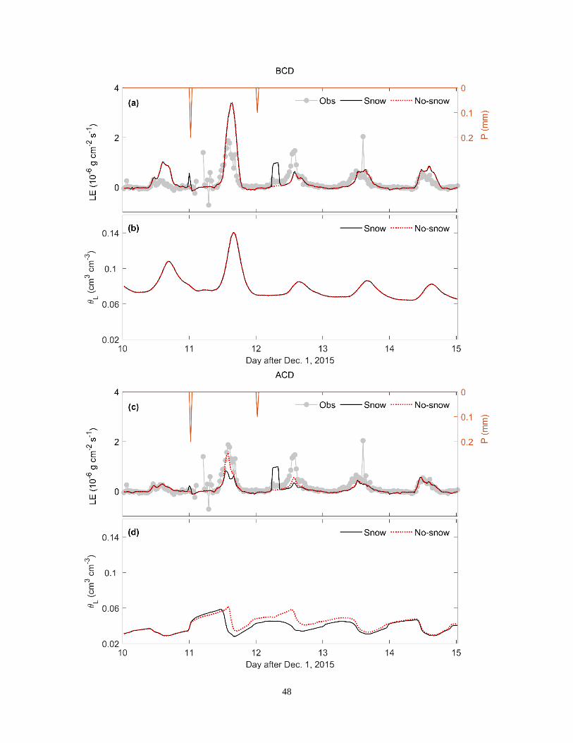
48
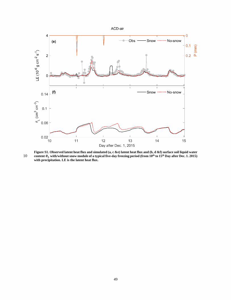
49
Figure S1. Observed latent heat flux and simulated (a, c &e) latent heat flux and (b, d &f) surface soil liquid water content 𝜽𝜽𝑳𝑳 with/without snow module of a typical five-day freezing period (from 10th to 15th Day after Dec. 1. 2015) 10 with precipitation. LE is the latent heat flux.
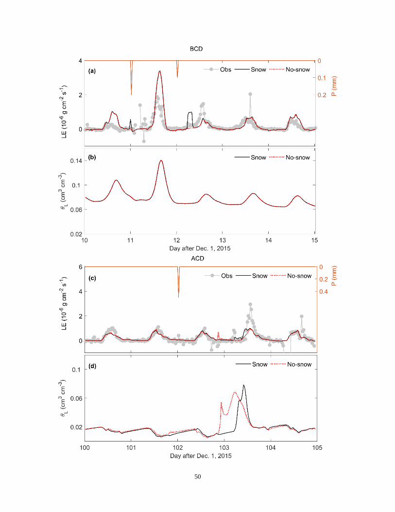
50

51
Figure S2. Observed latent heat flux and simulated (a, c &e) latent heat flux and (b, d &f) surface soil liquid water content 𝛉𝛉𝐋𝐋 with/without snow module of a typical five-day thawing period (from 100th to 105th Day after Dec. 1. 2015) with precipitation. LE is the latent heat flux.

52
Reference
Brown, M. E., Racoviteanu, A. E., Tarboton, D. G., Gupta, A. S., Nigro, J., Policelli, F., Habib, S., Tokay, M., Shrestha, M. S., Bajracharya, S., Hummel, P., Gray, M., Duda, P., Zaitchik, B., Mahat, V., Artan, G., and Tokar, S.: An integrated modeling system for estimating glacier and snow melt driven streamflow from remote sensing and earth system data products in the Himalayas, J Hydrol, 519, 1859-1869, 5 https://doi.org/10.1016/j.jhydrol.2014.09.050, 2014. Gardiner, M. J., Ellis-Evans, J. C., Anderson, M. G., and Tranter, M.: Snowmelt modelling on Signy Island, South Orkney Islands, Ann Glaciol, 26, 161-166, https://doi.org/10.3189/1998aog26-1-161-166, 1998. Gichamo, T. Z., and Tarboton, D. G.: Ensemble Streamflow Forecasting Using an Energy Balance Snowmelt Model Coupled to a Distributed Hydrologic Model with Assimilation of Snow and Streamflow Observations, 10 Water Resour Res, 55, 10813-10838, https://doi.org/10.1029/2019wr025472, 2019. Gichamo, T. Z., and Tarboton, D. G.: UEB parallel: Distributed snow accumulation and melt modeling using parallel computing, Environ Model Software, 125, https://doi.org/10.1016/j.envsoft.2019.104614, 2020. Hellstrom, R. A.: Forest cover algorithms for estimating meteorological forcing in a numerical snow model, Hydrol Processes, 14, 3239-3256, https://doi.org/10.1002/1099-1085(20001230)14:18<3239::aid-15 hyp201>3.0.co;2-o, 2000. Liu, Y., Xu, J. H., Lu, X. Y., and Nie, L.: Assessment of glacier- and snowmelt-driven streamflow in the arid middle Tianshan Mountains of China, Hydrol Processes, 34, 2750-2762, https://doi.org/10.1002/hyp.13760, 2020. Mahat, V., and Tarboton, D. G.: Canopy radiation transmission for an energy balance snowmelt model, Water 20 Resour Res, 48, https://doi.org/10.1029/2011WR010438, 2012. Mahat, V., and Tarboton, D. G.: Representation of canopy snow interception, unloading and melt in a parsimonious snowmelt model, Hydrol Processes, 28, 6320-6336, https://doi.org/10.1002/hyp.10116, 2014. Pimentel, R., Herrero, J., Zeng, Y., Su, Z., and Polo, M. J.: Study of Snow Dynamics at Subgrid Scale in Semiarid Environments Combining Terrestrial Photography and Data Assimilation Techniques, J 25 Hydrometeorol, 16, 563-578, https://doi.org/10.1175/jhm-d-14-0046.1, 2015. Raleigh, M. S., Lundquist, J. D., and Clark, M. P.: Exploring the impact of forcing error characteristics on physically based snow simulations within a global sensitivity analysis framework, Hydrol Earth Syst Sci, 19, 3153-3179, https://doi.org/10.5194/hess-19-3153-2015, 2015. Schulz, O., and de Jong, C.: Snowmelt and sublimation: field experiments and modelling in the High Atlas 30 Mountains of Morocco, Hydrol Earth Syst Sci, 8, 1076-1089, https://doi.org/10.5194/hess-8-1076-2004, 2004. Sen Gupta, A., Tarboton, D. G., Hummel, P., Brown, M. E., and Habib, S.: Integration of an energy balance snowmelt model into an open source modeling framework, Environ Model Software, 68, 205-218, https://doi.org/10.1016/j.envsoft.2015.02.017, 2015. 35 Sultana, R., Hsu, K. L., Li, J., and Sorooshian, S.: Evaluating the Utah Energy Balance (UEB) snow model in the Noah land-surface model, Hydrol Earth Syst Sci, 18, 3553-3570, https://doi.org/10.5194/hess-18-3553-2014, 2014. Tarboton, D. G., Chowdhury, T. G., and Jackson, T. H.: A spatially distributed energy balance snowmelt model, Biogeochemistry of seasonally snow-covered catchments Proc symposium, Boulder, 1995, 228, 141-40 155, 1995. Tarboton, D. G., and Luce, C. H.: Utah Energy Balance Snow Accumulation and Melt Model (UEB), Computer model technical description and users guide, Utah Water Research Laboratory and USDA Forest Service Intermountain Research Station, 1996. Watson, F. G. R., Newman, W. B., Coughlan, J. C., and Garrott, R. A.: Testing a distributed snowpack 45 simulation model against spatial observations, J Hydrol, 328, 453-466, https://doi.org/10.1016/j.jhydrol.2005.12.012, 2006. You, J., Tarboton, D. G., and Luce, C. H.: Modeling the snow surface temperature with a one-layer energy balance snowmelt model, Hydrol Earth Syst Sci, 18, 5061-5076, https://doi.org/10.5194/hess-18-5061-2014, 2014. 50