First of all I would like to thank again the reviewers and the editor for their helpful

comments. I am at their disposal for any further information or needed changes in the

manuscript. I have already addressed the comments of the reviewers in my “Author’s

Response”. After the major restructure of the manuscript, small further changes to the

manuscript and supplement were implemented, slightly changing page and line numbering.

Below I present again the “Author’s Response” which has been updated to have the updated

page and line numbers of the implemented changes.

After the end of the “Author’s Response” (page17) I present the manuscript with highlighted

changes. Since the manuscript is considerably restructured with different sections and figure

numbering and placement I chose to highlight only the changes and additions to the text and

not the text and figures restructuring (change of place and numbering). Otherwise the entire

manuscript would be highlighted making it difficult to track the changes.

Author’s Response

First of all I would like to thank both reviewers for their time reading the manuscript and for their meticulous comments, which have been very helpful and have contributed to the improvement of the manuscript. I responded to all comments and implemented the changes in a new manuscript, which is re-structured and more readable. Below, I provide a short overall description of the manuscript changes and then I proceed to the responses. General changes to the manuscript 1. Restructuring of the Results The structure of the Results (section 3.3) has been altered. Instead of describing the impact on each variable separately we describe the results depending on the interactions enabled: a) Enabling only aerosol-radiation interactions b) Enabling aerosol-radiation interactions in an environment where the aerosol-cloud interactions are also present c) Comparing the Thompson aerosol aware microphysics scheme to the non-aerosol aware Thompson2008 scheme and describing what happens when we implement both the aerosol-aware scheme with aerosol-cloud interactions and aerosol-radiation interactions and compare against control simulation that has no aerosol effects at all. 2. Adding figure, removing tables A new figure (Fig2-in the new manuscript) has been added containing the vertical aerosol profiles of the simulations. Tables 3 and 5 (original manuscript) have been moved to the supplement. Furthermore a new figure has been added in the supplement describing the single scattering albedo of the simulations (Figure S.1). 3. Changing color scale and number of simulations depicted in the main figures We have changed the color scale in the figures (2, 3,4,5,6-original manuscript). The new colorbar has white color in the middle and makes clearer the sign of the small changes. Moreover the number of simulations depicted has been reduced. I understand that the previous figures were too packed with information. Several simulations enabling aerosol-radiation interactions have very similar behavior and are not discussed thoroughly in the manuscript. Now instead of 8 rows of plots the new figures have only 5. We keep simulation ARI_T (Tegen climatology, 1st aerosol option), ARI_Mv1 (Macv1 climatology, 2nd aerosol option), ARI_Mv1urban (urban very absorbing aerosol), the difference ARCI-ACI (indicative of aerosol-radiation interaction when indirect effect is present) and ARCI. We have omitted

simulations ARI_Mv1full, ARI_MC that have very similar behavior to the others enabling aerosol-radiation interaction and also simulation ACI since the depiction of ARCI is enough to state the thing we describe about the Thompson aerosol aware scheme. Now I proceed to answer each reviewer’s comments. The original comments are with bold fonts and each response lies below the respective comment.

Reviewer 1

It is not clear for me the different between all the experiments listed in Table 1 (and section 2.4) (especially ARI_Mv1 ,ARI_Mv1urban, ARI_Mvfull) Answer: Simulations ARI_Mv1, ARI_Mv1urban and ARI_Mv1full have the same AOD field (MACv1) but they have differences in the rest aerosol optical properties (single scattering albedo, asymmetry factor). Changes in the manuscript: I have added this phrase to make it more clear (page 8, line22 new manuscript): “Within the ARI group simulations ARI_Mv1, ARI_Mv1urban and ARI_Mv1full have the same AOD field (MACv1) but they have differences in the rest aerosol optical properties (single scattering albedo, asymmetry factor).” For someone who is not using WRF, would it be possible to explain this in a more general way, how the AOD is distributed into the different types, and what is the consequence of having rural over urban Answer: The consequence of using rural over urban is being described in section 2.4 Model Simulations, page 7, line 8 of the reviewed manuscript. I have included a new figure (S2) with single scattering albedo maps in the supplement that will make the rural over urban difference even clearer. Some more information about the vertical distribution would also be good. Answer: I have added an extra figure (fig2) in the manuscript regarding the vertical distribution and a small text (page 13, lines 5-15).

The results is a bit challenging to read, as there are many acronyms, and also it is refereeing to many figures in the supplementary text, which probably could have been included in the main text, and maybe some figures could be removed, as there are not always so large differences on the horizontal maps (I find figure S5 very useful, would it be possible to replace some of the tables and figures with this type of figure?).

Answer: I believe the restructuring of the Results, described in the beginning, is helping make the results easier to understand. Less maps are included in the main figures. I think the reviewer is referring to figureS6 (not S5) in the supplement. I have included a figure with box plots to the supplement (S3) and moved tables 3 and 5 of the original manuscript to the supplement (Tables S1 and S2). Would it make sense to first present the results where the experiment CON, ARI-T, ARI_Mv1, ARI_Mv1urban, ARI_Mv1full is described, since this is focusing on the more trivial approach to include aerosol in RCMs, and it is just depending on what is having the “best” representation of the different species to represent the direct and semidirect effect. Then a separate section can be presented, where it is shown the effect of including the aerosol-cloud interaction, which is representing the indirect effect. Then these two simulations (ACI and ARCI) can be compared with the “best” aerosol representation from the first part (one of the CON, ARI-T, ARI_Mv1, ARI_Mv1urban,ARI_Mv1full). Now it is a lot of jumping back and forth between the different simulations, and it is not so easy to follow. Answer: The reviewer is suggesting an interesting way to restructure the section of the Results. The restructure described in the beginning is very similar. First only the aerosol-radiation interactions are presented, the trivial approach to include aerosol in RCMs. Then we explore how aerosol-radiation interactions behave if we enable them in an environment where the indirect effect is also present. Finally what is the impact of the Thompson aerosol-aware scheme that enables aerosol-cloud interactions. Two significant notes: Simulation ARI_T uses the option aer_opt=1 to parameterize aerosol-radiation interactions. Simulations ARI_Mv1, ARI_Mv1full, ARI_Mv1urban and ARI_MC use the option aer_opt=2. Thus the impact of aerosol-radiation interactions is not just depending on the aerosol dataset used but also to the option (parameterization) used mainly because they parameterize the aerosol single scattering albedo (SSA) differently. This is why the Tegen climatology used in ARI_T leads to a similar clear-sky shortwave radiation decrease with ARI_Mv1 (for example) despite the fact that the AOD of Tegen is considerably smaller than that of MACv1. The aer_opt=1 parameterization produces smaller (more absorbing) SSA values compared to the “rural” type of aer_opt=2 and thus has a tendency to decrease clear-sky radiation more per unit of AOD (W/m2/AOD). When using the Thompson aerosol aware microphysics scheme, for example in ACI, we do not just implement aerosol-cloud interactions. We introduce a modified microphysics scheme that is designed to work with aerosol. Thus when we compare ACI to control CON (that uses the Thompson2008 non-aerosol microphysics) the impact seen is attributed to the combined effect of the introduction of a different microphysics scheme and to the possible indirect effect taking place.

After reading the manuscript, I am not so sure what is the recommendation from the study, since when there is no aerosol climatology included (as in the CON-experiment), there is a cold bias over Europe, and this cold bias is enhanced when the aerosol is included (e.g. for ARI_T, ARI_Mv1). The ACI and ARCI simulations are warmer than the CON, so there is a potential to remove the cold bias when aerosol-cloud interaction is included, but is this the take-home message that RCMs should aim for having interactive aerosol schemes? However, the impact on precipitation is very small, so in the end the aerosol treatment does not have a large impact? Answer: I am not very worried about whether the aerosol introduction improves or worsens the bias. Of course if aerosol inclusion increased dramatically the bias this would be alarming and an indication that the aerosol parameterizations are probably not working properly. But this is not the case in our study. The final bias is of course a product of many different things such as the RCM structure and setup and the quality of the driving data. The purpose of our study is to identify the impact of the aerosol parameterizations and data used and the general behavior of aerosol implementation in the WRF model over Europe. This impact can improve or worsen the bias depending on the characteristics of each simulation. It is therefore simulation specific. For example the use of a different land scheme in our study could lead to a warm bias in the control simulation and thus enabling aerosol-radiation interactions would end up improving the temperature bias. So it is up to each WRF user to decide whether and what options to enable if they have bias improvement in mind. I can only describe their impact. Therefore I do not want to make general recommendations about using this or the other option or dataset. The same goes for the ACI and ARCI simulations that are mentioned by the reviewer. ACI is indeed slightly warmer than control and can improve the cold bias. But I would not state that it is a take-home message that RCMs should aim for having interactive aerosol schemes only because of the bias improvement. Using a different model setup, different driving data or a different domain could lead to bias increase when using interactive aerosol. It is understandable that people may want to include in their simulations all the physical mechanisms that are available and have a more detailed representation of each phenomenon (e.g. interactive aerosol). This makes the model more complete. However the extra or/and more detailed mechanism does not necessarily improve the bias. Regarding precipitation, indeed aerosol treatment does not seem to have a large impact. To conclude I can make two statements regarding the bias: a) Aerosol introduction can have an impact on bias. However the main biases are not altered considerably. Thus aerosol do not seem to be the main source of the bias.

b) Aerosol introduction does not necessarily improve the bias. In many cases the bias is increased when aerosol are enabled in our study. This does not mean that the aerosol parameterizations have a problem. We have seen that they behave in a physically consistent way. Whether bias is improved or not is specific to each simulation. It depends on each user to decide if and which aerosol treatment to use. If I have understood, there is no yearly change in the aerosol (only monthly or daily data), did the authors consider to include yearly varying aerosol? I guess for 5 years of simulation, the effect is not so large, but in past studies it has been shown that RCMs that don’t have transient aerosol is not representing the change in the surface radiation correctly. (Bartok et al. (2017) ) Answer: The Tegen and MACv1 climatologies do not have yearly variability, only monthly variations. The MACC is a daily dataset and thus there are differences from year to year. However the impact of this year to year variability is minimal. It seems that 5years are indeed a small period to explore the effect of transient aerosol and this was not the intention of this study. It is a very nice suggestion by the reviewer to explore the effect of

transient aerosol. Actually we are working on longer simulations spanning 30 years that indeed show that the inclusion of transient aerosol is important to correctly capture the trends in surface radiation. However this will be the subject of another study.

General comments:

Line 15-17 (p1): “statistical significant “.what is statistical significant (and what is meant by “in some cases”..please rephrase. Answer: We use the phrase “statistically significant” to denote that a result is of statistical significance. As explained in the methodology we use the Mann-Whitney non-parametric test and calculate significance at the 0.05 level. I am under the impression that the phase “statistically significant result” is frequently used. I have rephrased to: “of statistical significance” (page 1, line 28). The use of the phrase “in some cases” was meant to state that the changes that are of statistical significance are not widespread but are seen in some selective cases. I did not want to give more details in the abstract, just state the general behavior. I have added: “which in some cases, mainly close to the Black Sea in autumn” (page 1, line 28). Line 5-6 (p2): This sentence is not so easy to understand, especially if you don’t know the difference between radiative forcing and adjustment (where I assume you mean rapid adjustment). Answer: Yes indeed we mean the rapid adjustments. I do understand that it is hard to follow. I think it is better to keep it simple and just state that both aerosol-radiation and aerosol-cloud interactions add to the uncertainty while the aerosol-cloud interactions do that to a larger degree. Rephrased to: “It states that the uncertainty due to aerosol is attributed to both aerosol-radiation (ari) and aerosol-cloud interactions (aci) with the latter having the largest contribution.” (page 2, line 6) Line 15 (p5): I don’t quite understand how the vertical profile of the different component is distributed in each model level. Is there some weighting doing the distribution? Would it be possible to show the vertical distribution for the different experiment? Answer: I have added a figure depicting the vertical profile of the experiments in the manuscript (Fig.2). The option aer_opt=1 (ARI_T) uses the 3D Tegen climatology and constructs a vertical profile by adding the AOD of each aerosol type in each model level. The option aer_opt=2 (ARI_Mv1 family) assumes a specific function for the vertical profile. This is the same over each grid point and thus the vertical profile has the same shape over each grid point, only the magnitude of AOD changes depending on the total AOD provided at each grid point. Line 21-24 (p5): The distinguishing of rural, urban and maritime component is not clear for me. What is meant that “in this work the first two component has been implemented”? is the maritime not used? And for the experiment where the different components are used (e.g. rural or urban), is this the case for the whole domain? Or can you combine this and set rural for one part, and urban for another part? Answer: The “rural”, “urban” and “maritime” types are different ways that the option aer_opt=2 uses to parameterize the single scattering albedo (SSA) and angstrom exponent (AE) of aerosol. The selected type is indeed used for the entire domain and you cannot chose one type for one part of the domain and another type for the another part. However for the selected aerosol type the produced fields of SSA and AE are not spatially homogenous but present spatial variability over the domain. This is because the parameterization takes into

account the total AOD over each grid point and the relative humidity to calculate the SSA and AE values. The difference between the types lies mainly in how absorbing are the aerosols of each type. The range of the single scattering albedo is given in the manuscript in section 2.4 “Model Simulations”. I have also included a figure depicting the SSA of the simulations after a request of the second reviewer. The main difference of the “rural” and “urban” type is that “urban” is considerably more absorbing all over the domain. Indeed we only used the “rural” and “urban” types and not “maritime”. “Maritime” presents larger scattering compared to “rural” however the differences are not as large as those between “rural” and “urban”. Since we tested the “rural” type which is the most balanced and also used the more realistic SSA of MACv1 in one simulation (MACv1full) we believe that the use of “maritime” would not provide any significant additional value and some early tests gave the same indication. We chose however to test the “urban” type since it represents a completely different situation from the “rural” and “maritime” types and would show the impact of extremely absorbing aerosol, especially the semi-direct effect. I have added the phrase (page 6, line 7 new manuscript): “Only one aerosol “type” can be used for the entire domain.” Line 2-4 (p12): are you describing a specific figure, or just the results in general? Answer: This is indeed a small summary of the overall evaluation. I think it is nice to clearly state the main point in the beginning and then elaborate for each variable. Line 9-10 (p12): does this mean that the model performance is actually better when aerosol is not included in the simulations? Answer: Yes in some cases, not only temperature, model results present smaller biases when aerosols are not included. As I have described in a previous answer I do not think that this is problematic regarding the performance of the aerosol parameterizations used. The fact that the inclusion of an additional physical mechanism in the model (aerosol) fails to improve the bias is quite interesting and reveals how models work. That they have after all a group of different parameterizations that do not always work perfectly with each other and in many cases these parameterizations are calibrated to work well at certain conditions. For example a radiation parameterization might be calibrated to produce small biases without the use of a separate aerosol parameterization in place. IN this case the aerosol impact is indirectly taken into account through the calibration process. However this calibration might be insufficient in another domain (e.g larger AOD values) under different meteorological conditions (e.g. heavy cloudiness) or different aerosol related events (e.g transportation of very absorbing aerosol). Line 7-9 (p13): is this related to a specific figure? Answer: Yes this is related to figure 3 (fig2 original manuscript). It has been added to the manuscript (page 15, line 4). Line 15 (fp13) From this line, it seems as a more general summary about the results is given, so it should maybe not be under section 3.2.4 (which is about the SW). Answer: Yes this is a very helpful comment. This is a general summary about the evaluation of the aerosol including sensitivities. It is under a separate section after finishing with the evaluation of the control simulation. I have moved this text in a new section (3.2.5 Evaluation of the sensitivity simulations) (page 15) to make clear we are talking about the sensitivity simulation evaluation.

Figure2: how about including S1 with Fig 2? Moreover, if possible, how about using a color scale which is white in the middle? (not green). Answer: I understand this point. However the differences in the bias are small (except only for DNI) and there are several maps in the manuscript and supplement explaining the impact of aerosol on each variable. I would prefer to just have this figure alone to give emphasis on the evaluation of the control simulation. I have changed the color scale to a new one having white in the middle. Line 9 (p28): I would be careful with using the word climate (e.g. “aerosol effect on European climate”), since only 5 years of simulation is done. Answer: This is indeed true. 5 years are not a sufficient period to state impact on climate. I have replaced “on European climate” to “over Europe”.

Reviewer 2 Main comments: - The authors present eight different simulations (1 control run and 7 sensitivity experiments) which makes the paper difficult to understand, and the reader can easily get lost in the tables and figures presenting all the simulations. Besides, the author mainly focus only on ARI_T, ARI_Mv1urban, ACI and ARCI. The three other simulations (ARI_Mv1, ARI_Mv1full and ARI_MC) are not discussed in detail. Unless adding more discussions on these different simulations, I would suggest to keep only a few of them in the main text and in the tables and figures, and keep the other ones for supplementary material. - The organization of the paper and in particular of Section 3.3 dealing with the sensitivity experiments should be improved. Indeed, the author present first temperature and precipitation, whereas the direct effect of aerosols concerns first radiation, which then has consequences on temperature. The fact to present cloud fraction at the end may also be a problem as this parameter is needed to explain aerosol effects on temperature and precipitation. I would suggest to reorganize Section 3.3, and notably start by the analysis on radiation. Answer: I do understand the comments regarding the organization off the results and the general readability of the entire manuscript and consider them extremely important since the essence of a paper is to easily communicate information. I have tried to reorganize the entire manuscript and especially the way Results are presented by implementing suggestions by the two reviewers. The main changes are described in the beginning of the author’s reply. To quickly summarize they include two key features: a)The aerosol impact is presented according to the effect explored and not for each variable separately, b) less simulations depicted in the figures and tables 3 and 5 have been moved to the supplement. - The simulations presented in this paper last only 5 years. I wonder if this is enough to study the sensitivity of climate-aerosol interactions, notably as far as cloud-aerosol interactions are concerned. I get the impression on some figures that the signal is quite noisy, notably in terms of cloud cover and precipitation. Answer: Very interesting question. I do believe that 5 years are enough to study the rapid climate responses (or adjustments) due to the forcing of aerosol. According to the IPCC AR5 (section 7.1.3) most of the rapid adjustments are thought to occur within few weeks. The slow adjustments (mainly the full extent of ocean atmosphere interaction) only need much larger simulation time. Other RCM studies have produced results for smaller or similar periods: Da Silva 2018-6 moths for precipitation, Zanis 2009-2 years, Nabat 2015-2 years spin up +6 years simulations. I am not very worried about the somewhat noisy signal in

precipitation and cloud fraction since these variables are highly impacted by differences in the local scale especially terrain elevation. Zanis, P.: A study on the direct effect of anthropogenic aerosols on near surface air temperature over Southeastern

Europe during summer 2000 based on regional climate modeling, Annales Geophysicae, 27, 3977–3988,

https://doi.org/10.5194/angeo-27-3977-2009, http://www.ann-geophys.net/27/3977/2009/, 2009.

Da Silva, N., Mailler, S., and Drobinski, P.: Aerosol indirect effects on summer precipitation in a regional climate

model for the Euro-Mediterranean region, Annales Geophysicae, 36, 321–335, https://doi.org/10.5194/angeo-36-

321-2018, https://www.ann-geophys.net/36/321/2018/, 2018.

Nabat, P., Somot, S., Mallet, M., Sevault, F., Chiacchio, M., andWild, M.: Direct and semi-direct aerosol radiative

effect on the Mediterranean climate variability using a coupled regional climate system model, Climate Dynamics,

44, 1127–1155, https://doi.org/10.1007/s00382-014-2205-6, 2015.

- The presentation of figures should also be improved. Several figures (for example Figures 3 to 6) are composed of too many plots, which make them difficult to read, and not all of them are discussed in the paper. There are also too many references to figures in supplementary material. Some of them have their place in the main paper. Besides, the font used for labels should be higher (notably in Figures 1 and 2). Answer: The number of the plots in the main figures has been reduced. Unfortunately it is difficult to avoid referencing the supplement a few times, I have tried however to reduce their number. The fonts in Figures 1 and 3 (fig2 of original manuscript) have been placed slightly higher. Specific comments : - Abstract: It should be clearly stated in the abstract how are calculated the different numbers which are given, in particular the fact that they rely on a comparison with a control simulation without aerosol scattering and absorption. Answer: I added the phrase (page 1, line19 new manuscript): “The impact of aerosol is calculated by comparing against a simulation that has no aerosol effects.” - Page 2 Line 17-18: “Finally, a minority of the simulations use prognostic aerosol schemes with natural and anthropogenic emissions (dust, sea salt) online driven by meteorology”. Could you precise which model has a fully prognostic aerosol scheme ? I don’t see any model in the table given in footnote 1. Answer: Only one model uses a prognostic scheme. It is UM-WRF361 (third from the bottom in the table). It states that aerosol are estimated online at every time step. I have rephrased to state that it is only one model since the term “a minority” is not precise. Changed to: “Finally only one model uses a prognostic aerosol scheme estimating online the aerosol field.” (page 2, line 19) - Page 2 Line 20: “the aerosol-cloud interactions (indirect aerosol effect) is typically not considered”. This information is not given in table in footnote1. Could you justify this point ? Answer: Indeed this is a good point. The fact that aerosol-cloud interactions are not considered was indirectly inferred by the table and a bit hasty. There is only one model (SMHI-RCA4) that states clearly that has only aerosol-radiation interactions (and of course 5 cases that have no aerosol at all (so no indirect effect) and a couple that are not sure). Most of the models however use climatologies or fixed AOD fields and usually in these cases this indicates simple aerosol sophistication and only aerosol interaction with radiation. Moreover even if aerosol-cloud interactions are considered I do not believe that the full impact of the indirect effect could be captured with a stable in time aerosol field (even with seasonal

variability). Only a prognostic aerosol scheme can modify the aerosol field according to the meteorological conditions and thus fully capture the impact But yes, the point I am trying to make here cannot be strictly justified by the information given in the table in footnote1. This statement has been omitted in the new manuscript. – Page 2 Line 4: Could you precise here the version of WRF that you use ? Answer: I have added: “WRFv3.8.1” (page 3, line 5) - Page 3 Line 13 (and Page 4 Line 19): the limits of the EURO-CORDEX domain given here (25S- 75N, 40W-75E) seem to be very large for Europe (in particular 25S and 40W). Answer: Nice observation. There is a typo in the description of the domain and yes this is not the typical EURO-CORDEX domain but the domain used in the simulations. The southern limit is 25N and not 25S. It has been corrected in the manuscript in the second case stated above. In the first case (section 2.1.1) I have rephrased to simply state that E-OBS cover Europe. The 40W and 75E are not as distanced from the original EURO-CORDEX domain as they seem. Since we use a rotated grid only the domain upper left and right corners stretch to such limits. The domain used in the simulations encompasses completely the EURO-CORDEX domain. - Section 2.1.1: Please give the horizontal resolution of the observation datasets. Answer: It is actually stated that data on a 0.44o rotated pole grid are used. - Page 3 Line 16: What are these cases with an excess of 100% ? It is worth knowing if there is specific situations in which the E-OBS precipitation is not trustworthy. Answer: The largest relative errors in precipitation are found mainly over mountainous areas in the Alps and mountainous parts of Norway, in North Africa due to the very small station density and in areas east to the Baltic sea. Large relative errors are also seen in some grid cells in Italy and Spain. In general results are the best over central Europe and the UK. It must be noted that these “errors” are estimated by comparison against more regional gridded datasets with higher density of stations that are thought to be closer to reality. I have rephrased the sentence in order to be more specific and provide as much information is given in Hofstra et al. (2009) as possible. Hofstra, N., Haylock, M., New, M., and Jones, P. D.: Testing E-OBS European high-resolution gridded data set of

daily precipitation and surface temperature, Journal of Geophysical Research Atmospheres, 114,

https://doi.org/10.1029/2009JD011799, 2009.

Rephrased to: When compared against regional datasets with higher station density (Hofstra et al., 2009) the E-OBS dataset presented a mean absolute error around 0.5oC for temperature whereas for precipitation a general tendency of underestimating precipitation amount is reported, with large (>75%) relative errors found in mountainous regions of the Alps and Norway, over North Africa and in areas east to the Baltic Sea. (page 3, line17)

- Page 3 Line 20: Please give a definition for Direct Normalized Irradiance. Answer: I have added: DNI is the solar radiation received by the direction of the sun’s rays and received by a surface that is perpendicular to that direction. (page 3, line 26) - Section 2.1.2: Please give a reference for the SARAH dataset. Answer: A reference is actually given in the second line: (Müller et al., 2015). I have moved it to the first line in order to state it right away. (page3, line 26) - Page 3 Line 24: “between ± 65° longitude and ± 65° latitude”. Too large domain ? Answer: I have checked this again. It is stated in the CMSAF webpage https://wui.cmsaf.eu/safira/action/viewDoiDetails?acronym=SARAH_V002 and it is actually true regarding the ultimate extent of the domain. There are variations depending on season. - Page 4 Line 5: As the CLARA dataset is not used for the evaluation of radiation but only for cloud cover, it should be discussed if this could have an impact on the evaluation. Answer: I understand your point. Every dataset uses its own information about cloudiness amount to calculate shortwave radiation at the surface. However the use of a different product for radiation and cloud fraction does not necessarily lead to discrepancies as long as these products are good enough in estimating the respective variable. Both SARAH for Rsds (Müller et al., 2015) and CLARA for cloud fraction (Karlsson and Hollmann, 2012) have reasonable accuracy in detecting the respective variable, so I do not believe this has a significant impact on evaluation results. I have added the phrase (page 4, line20): “The use of a different product for cloud fraction (CLARA) than the one used for radiation (SARAH) does not impact the evaluation since both of these products have reasonable accuracy and uncertainty in estimating the respective variables.” - Section 2.2: Please explain more clearly which indirect aerosol effects are taken into account in the different simulations (Twomey, Albrecht, …). Answer: I have added the phrase: “Thus aerosols are free to either change cloud albedo (first indirect or Twomey effect) or/and impact cloud lifetime (second or Albrecht indirect effect).” (Section 2.3.1-aerosol cloud interactions, page 7, line 11) - Sections 2.3.1 and 2.3.2: The titles of these sections are unclear, they should be clarified. Answer: The section 2.3.1 title was changes from: “WRF Aerosol options” to “WRF aerosol parameterizations examined”. The section 2.3.2 title was changed from: “Aerosol data” to “Aerosol datasets used”. - Page 5 Lines 14-15: In the case aer_opt=1, how are other radiative properties (SSA, asymmetry parameter) defined ? Are there common for all aerosol types ? Answer: In aer_opt=1 the other radiative properties (SSA,ASY,) are given for each aerosol type separately in lookup tables the model. Then for each grid cell, each model level and each spectral band of the radiation scheme a final value is calculated by weighing the value of each aerosol type by its AOD and then summing them all together. I have added the phrase (page 6, line 10): “The single scattering albedo and asymmetry factor are given for each aerosol type and a final value is calculated in each model level and for each spectral band of the radiation scheme. This is done by weighting the value of each aerosol type by its respective AOD and aggregating for all five aerosol types.”

- Page 6 Lines 18-23: It is not clear for me how this aerosol scheme is used. Is it a full prognostic aerosol scheme with emissions, transport and deposition ? Answer: The Thompson aerosol-aware scheme is a very interesting idea. It is a microphysics scheme that is prognostic in the sense that it explicitly predicts the number concentration of aerosols and it has emissions, transport and deposition for aerosol. It makes some simplifications (like all schemes do to some extent). It separates aerosol into two general species: droplet nucleating and ice nucleating. It uses an aerosol climatology, derived from multi-year (2001-2007) global model simulations by the Goddard Chemistry Aerosol Radiation and Transport (GOCART) model, to initialize the aerosol field in the model and provide boundary conditions. Moreover a fake surface aerosol emissions/flux/tendency is added at the surface for the droplet-nucleating aerosol. This emission flux is based on near-surface aerosol concentration and a simple mean surface wind. To conclude: The Thompson aerosol-aware scheme is not as complex as schemes with interactive chemistry that contain features like multiple aerosol types, multiples bin sizes, realistic emissions inventory e.t.c. It is a microphysics scheme that tries to have a more simplified aerosol treatment that has no significant extra computational burden. Its purpose is not to predict aerosol concentrations with the best accuracy. It tries to retain some basic climatological features of aerosol while at the same time changing the aerosol field according to the meteorological conditions thus enhancing the realism of aerosol-cloud interactions. I have added(page 7, line 6): “This scheme explicitly predicts aerosol number concentrations.” - Page 7 Lines 6 and 14: what does (and mp=28) mean ? Answer: Indeed this is not explained. This is the symbolism of each microphysics option in the model namelist. I have added (page 8, line 14): (mp=8-in the model namelist) - Page 7 Lines 8-9: “The single scattering albedo (SSA) at 550nm of the ‘’rural” type aerosols ranges in our experiments between 0.92 and 0.98”. How are these values spatially distributed ? Maybe a map in supplementary material could be helpful to understand the spatial distribution of aerosol-radiation effects. Answer: I have added a map of the SSA values on the supplement (Fig S1). - Table 1: For simulation ACI, aerosols are indicated to interact with clouds whereas the option aer_opt=0 is used. How is it possible ? Answer: I see this might be confusing. The “Aerosol option” row in Table1 is for aerosol-radiation interactions only. Aer_opt=0 means that there are no aerosol-radiation interactions. Thus ACI has aerosol-cloud interactions since it uses the Thompson aerosol-aware scheme but the aerosol of the Thompson scheme do not interact with radiation. - Page 9 equation2: The DRE is calculated in clear-sky fluxes, so I suggest to call it rather CDRE (Clear-sky Direct Radiation Effect) to avoid confusion with RE, which is calculated in all-sky confitions. Answer: I think this adds to the clarity of the metric. I have renamed it to Clear-sky Direct Radiation Effect CDRE throughout the manuscript. - Page 10 Line 13: “The climatology of Tegen has a lower AOD compared to SEVIRI, but follows the latter’s seasonal spatial variability”. I don’t understand how the Tegen AOD follows the seasonal spatial variability of SEVIRI AOD, it is not clear from me in Figure 1. Answer: This was meant to state that Tegen has the same main changes in seasonal AOD like SEVIRI. I have completely re-written the Section “3.1 Aerosol optical depth” (page 11)

omitting this sentence. I tried to give more precise information. We have also included the MODIS satellite dataset and use it as the main point of reference. We reanalyzed the SEVIRI dataset taking more care about averaging missing values. - Page 10 Line 15: The use of AOD assimilation in the MACC reanalysis could be mentioned to explain the better agreement of MACC AOD with satellite data. Answer: I have included that MACC uses data assimilation is section 3.1 (page 11 ,line 27 ) - Figure 1: There is strange high AOD in Eastern Europe in SEVIRI data in winter (DJF). Please comment on this pattern. Maybe the use of another satellite product (MODIS for example) could help to ensure the robustness of satellite data. Answer: I have also used the MODIS dataset and this is the main point of reference now. This weird AOD high over Eastern Europe in SEVIRI during winter severely confused me in the beginning. I was unable to find a reference of this. However this AOD high is fake and had to do with the way the missing values were seasonally averaged due to a bug in the code. The SEVIRI monthly mean gridded data have large areas of missing values in winter and autumn over around 45N. Few scattered grid points with valid data can be found however in higher latitudes in each month. By mistake the seasonal averaging happened also above grid points that had very few valid monthly (even one valid monthly values per the entire 5 year period was enough to be included). Thus the averaging over those areas resulted in an aerosol field that cannot be representative of the seasonal mean. In the corrected analysis only grid points that have no missing values at all are used for the seasonal averaging. - Page 12 Lines 2-4: These lines should be rather in the conclusion of the section than at the beginning. The authors could rather introduce Figure 2. Answer: I believe it is nice to have a quick summary in the beginning with the essence of the evaluation and then elaborate more for each variable. - Page 12 Lines 6-7: There is on the contrary a warm bias in northern Scandinavia. Answer: In Scandinavia over winter the averaged bias is negative and almost -1oC. Iunderstand however since the warm bias at the north is not discussed in the manuscript the statement of considerable negative bias in Scandinavia might be confusing. I have rephrased to make it clearer. Changed to (page 13, line 21): In the simulation CON winter temperatures are mostly underestimated (-0.5oC domain average, land only), with higher cold biases over Scandinavia (despite a warm bias at the north), the Mediterranean and the Alps (-1oC) as indicated in the upper panel of (Fig.3). - Page 12 Line 10: Please give a reference for the Noah land surface model. Answer: I have added the reference (page 14, line 1) Niu, G-Y., Yang, Z. L., Mitchell, K. E., Chen, F., Ek, M. B., Barlage, M., ... Xia, Y. (2011). The community Noah land surface model with multiparameterization options (Noah-MP): 1. Model description and evaluation with local-scale measurements. Journal of Geophysical Research: Space Physics, 116(12), [D12109]. https://doi.org/10.1029/2010JD015139

- Page 12 Line 25: Please give a reference for the WDM6 cloud microphysics scheme. Answer: I have added the reference (page 14, line17). Lim, K.S. and S. Hong, 2010: Development of an Effective Double-Moment Cloud Microphysics Scheme with Prognostic Cloud Condensation Nuclei (CCN) for Weather and Climate Models. Mon.Wea.Rev.,138, 1587–1612, https://doi.org/10.1175/2009MWR2968.1 - Section 3.2.3: The bias in cloud fraction in summer could be related to a too zonal circulation ? Besides, the author could discuss if those biases in cloud cover could have an impact on AOD in the case of the simulations with aerosol-cloud interactions. Answer: I have examined the wind field at 850hPa of ERA-Interim and found small differences with that of the control simulation CON in summer. The model does not seem to deviate much from the general circulation seen in the reanalysis dataset.

- Tables 2, 3 and 4: Please explain which domain is used for these averages. In particular, it should be stated if only land points are considered (as the model is not coupled with ocean, it would be more relevant to show only land grid points). Answer: The domain of analysis is given in page 10 line 31. I have added that both land and sea points are considered. I have also added a description in the label of each table: Domain is defined as -10oW, 40oE and 36oN, 70oN. The lack of coupling definitely has an impact. However I believe it is mainly seen in temperature. Thus I have included a column in table 3 that has the impact (annual) on temperature only over land. - Page 15 Line 7: The impact on surface temperature seems to be larger in autumn than in summer, while the AOD is higher in summer. Is there a role of internal variability? Answer: Interesting comment. This is true. For Tegen the domain averaged AOD is indeed larger in summer whereas for Macv1 and MACC the mean AOD is the same for summer and autumn. However in summer it is larger over land for all datasets, where we expect a more strong response in temperature. If we use only land points the temperature impact is still larger in autumn even though not as clearly as was when using both land and sea points. I do not think that this has to do with the internal variability of the model but with the rather complex nature of aerosol impact. Larger AOD does not necessarily mean larger reduction of radiation since clouds also play a role. The relative change in shortwave radiation is slightly larger in autumn (4 out of 5 ARI simulations) compared to summer. And I see that the impact on temperature seems to be more correlated with the relative changes in shortwave radiation (%) and not so much with the change in W/m2. I have added (page 21, line 13): “Despite the larger AOD in summer, the temperature impact is greater in autumn. This is probably related to the fact that the relative Rsds decrease is slightly larger in autumn (except for ARI_Mv1full). “

- Page 15 Line 9: “in cases reaching a decrease of 1.5° C” Please give more details on these cases. Answer: I have added(page 21, line 11): “Cases of such strong reduction are not spatially extended and are seen mainly in summer and autumn within the areas of intense cooling like the Balkans and near of the Black Sea. “ - Page 15 Lines 10-12: This point should be related to a figure. Answer: I referenced figure S5 of the supplement. - Page 15 Lines 13-end: The results using the ARI_Mv1urban simulation should be moderated as the absorption of aerosols is not realist in this simulation. Answer: I have added (page 21, line 30): “We must remind here that ARI_Mv1urban is more of an idealized experiment with unrealistically absorbing aerosol.” - Page 16 Line 5: Could you explain: “Contrary to the ARI group, simulation ACI using the Thompson aerosol-cloud interacting cloud microphysics and accounting for indirect effects only results in a domain averaged temperature increase (0.1 to 0.2 o C) compared to CON for all seasons except autumn” ? Answer: ACI just implements the Thompson aerosol-aware scheme compared to CON and no aerosol-radiation interactions. The aerosol-aware scheme presents less cloudiness than Thompson2008 used in CON thus ACI has temperature increase since aerosol do not interact with radiation to decrease it. I understand that describing ACI after the ARI (aerosol-radiation interactions) simulations for each variable might be confusing. I believe that the reorganizing of the Results per aerosol effect helps to make things clearer. - Page 16 Line 21: It should be mentioned that the Black Sea is not coupled, which could influence the results on precipitation. Answer: Yes it is important to state this especially in this case. I have added the phrase (page 23, line1): “It should be reminded however that the simulations do not have an ocean-atmosphere coupling, something that can influence the results on precipitation over the Black Sea.” - Page 17 Lines 2-4: This point should be related to a figure. Answer: I have pointed to the figure 4 that shows the clear-sky direct radiative effect. - Page 17 Lines 12-13: how is calculated the correlation with AOD in the ARCI simulation (with which AOD) ? The difference in AOD between ARCI and ACI could have an impact ? Answer: Nice point. In the above case correlation is calculated between ARCI and ACI with only the ARCI field being used to determine correlation. The fields of ARCI and ACI (number concentrations, AOD is not available in the model for ACI) are very similar. Since ACI has no aerosol-radiation interactions I believe it makes sense to find the correlation between the AOD field that is active and radiation clear-sky radiation change. I would be more worried about the time evolution of the AOD in ARCI (this is stated in the manuscript), something that could make the mean AOD not sufficient for spatial correlation analysis. - Page 19 Line 14: it is difficult to draw this conclusion as AOD is not the same in all simulations. I suggest that AOD could be added in Table 4 to discuss this point. Answer: The aerosol field in ARCI is the only field that is interacting with radiation. Thus it makes sense to see what happens when I introduce an active I think that comparing ARCI to ACI can give a strong indication as to how the aerosol-radiation interactions are affected

when the aerosol-cloud interactions are also present. Especially when we are talking about domain (and possibly seven subdomain) averages over a large period of time (multi-seasonal or multi-annual averages). The AOD field of ARCI is presented. However since ACI is not provided in the model output since ACI lacks aerosol-radiation interactions and AOD is irrelevant. However the concentrations of aerosol, both droplet nucleating (QNWFA) and ice nucleating (QNIFA) are given for each grid point and model level for both ARCI and ACI. If we calculate the total concentration over each grid point the aerosol fields are almost identical. See below for annual averages. Thus I feel confident that the ARCI to ACI comparison can give valuable information regarding the general behavior of aerosol effect over the domain over large time periods. For much smaller spatial and temporal scales the above comparison could be problematic. Finally the idea to add AOD in table 4 (table 2 –new manuscript) is very good and has been implemented. - Page 19 Lines 21-24: I don’t understand how the author come to this conclusion. Answer: This talks about the simulations ARCI and ACI that use the Thompson aerosol aware microphysics scheme having less cloud amounts and more positive cloud forcing compared to control CON (that uses the Thompson2008 scheme). This point about the aerosol aware scheme is more evident when comparing ACI to CON since the only difference between them is the change in the microphysics scheme. ACI has less cloud fraction amount, more prominently in summer and spring (fig5 original manuscript) and more positive cloud forcing (fig6 and table 4 original manuscript) than CON. Of course these differences cannot be attributed only to aerosol-cloud interactions but mainly to the change of the microphysics scheme. - Page 20 Line 1: what is Aer2urban ? Answer: My apologies. The naming of the simulations was changed after initial submission due to the editors suggestions and an earlier naming remained in the text. It was changed to ARI_Mv1urban. - Page 20 Line 8: Could you explain why the effects are stronger on DNI than on Rsds ? Answer: I have added this phrase(page 18): “Since DNI comes only from the direction of the sun, any interaction with aerosol (scattering, absorption) removes radiation amount from this direction. On the other hand in Rsds radiation is reduced only when it absorbed or scattered in an angle that does not reach the surface. Thus the aerosol direct effect is much stronger in DNI.” - Page 21 Line 5: what is the specific effect of aerosols on diffuse radiation, that could be distinguished from direct radiation ? Answer: I have added the phrase (page 18, line 28): “Diffuse radiation reaches the surface from all angles except from the direction of the sun (direct radiation). Thus when direct radiation is scattered by aerosol a part of it becomes diffuse radiation and reaches the surface increasing diffuse radiation amount. “ - Page 23 Lines 11-12. This result involving LWP seems to be important to understand cloud aerosol interactions. Please explain more this process. Answer: I believe this is connected to the Thompson aerosol-aware microphysics scheme (TE2014) having in general less cloud fraction amount than the Thompson 2008 microphysics scheme and not so much about the aerosol-cloud interactions. When we change from the Thompson 2008 to the aerosol-aware scheme (e.g. simulations ACI-CON) we do not just turn on the aerosol-cloud interactions but we introduce a modified microphysics scheme that explicitly predicts aerosol. Thus the impact seen is attributed to the change of the

microphysics scheme and partially also to possible aerosol-cloud interactions. Since I cannot separate these two I do not think I can attribute the decreased LWP to aerosol-cloud interactions. Moreover the aerosol-cloud interactions also rely of the aerosol field that is being produced by the TE2014 scheme. Thus I believe that the change of microphysics scheme presents the main impact. To conclude it seems that the TE2014 has a tendency to produce smaller LWP amounts than the Thompson2008 (at least in our simulations) and this decrease in LWP also leads to decreased cloud fraction amount. - Page 23 Lines 19-20. In this kind of semi-direct effect, the internal model variability could be important. The author should mention this point. Answer: Yes this is a very interesting comment. We have seen the same behavior (aerosol induced cyclonic anomaly) to some extent in most simulations despite different datasets and aerosol options used. However the impact of different physics parameterizations or/and different initial conditions and period of simulation can be substantial and could substantially modify this effect. I believe that also the real variability of the climate could strongly impact this result, thus longer simulations would be needed to robustly examine this effect. I have added to the manuscript (page19, line 19): “However the internal model variability as well as the real climate variability could be very important in this kind of complex feedback mechanism. The use of different physics parameterizations, initial conditions and even different time periods can have a large impact and could potentially modify this effect. Therefore it would be interesting to see whether these results are modified in a large physics ensemble simulating a more prolonged time period. “ - Page 26 Lines 26-27. I don’t understand how “the introduction of aerosol-radiation interactions” could lead to “more transparent clouds” ? Answer: (This is actually at page 26 lines 6-7). I do understand that the way it is written it is not just confusing but it is also wrong to directly link aerosol-radiation interactions to more transparent clouds (cloud albedo). What is meant is that when aerosol-radiation interactions and/or the Thompson aerosol scheme with aerosol-cloud interactions are implemented the cloud forcing at the surface becomes more positive (more radiation at the surface). This can be due to a change in cloudiness amount due to aerosol semi-direct effect or cloud optical properties due to cloud indirect effect. I have tried to rephrase. Changes in the manuscript (page20, line 3): From: “Thus, the introduction of aerosol-radiation and/or aerosol-cloud interactions leads to more transparent clouds enabling larger amounts of radiation reaching the surface.” To: “Thus, the introduction of aerosol-radiation and/or aerosol-cloud interactions leads to cloudiness enabling larger amounts of radiation reaching the surface. This can happen due to changes in cloudiness amount or in cloud optical properties.” Other corrections: - Abstract line13 and Page 19 line 6: is comprised of (instead of comprises of) - Page 4 Line 10: and underestimation - Page 4 Line 30: incorporates aerosols

- Page 10 Line 15: The MACC reanalysis is in better agreement with the satellite data. - Page 10 Line 16: and the higher generally higher AOD - Figure 1: Please keep the same spelling for MAC-v1 - Page 12 Line 11: In particular northern Europe is … - Page 13 Line 21: error compensation between errors - Figure 4: Space character is missing after (RE) Answer: All these corrections have been implemented in the manuscript

- Page 28 Line 2: please define NWP I chose not to use NWP and just used the more relevant term “regional climate model”

(page 29, line 9)

Additional changes

Finally I have omitted the sentence: “This result is in contrast to other regional downscaling

studies investigating either aerosol-radiation or aerosol-cloud interactions.” from the

abstract (page 1, line 29).

Since I am not aware of many aerosol studies regarding the impact of aerosol-radiation

interactions on precipitation and we mainly refer only to a study of Nabat (2015) in the

manuscript (section 3.3.1, page 22, line 15) that showed precipitation reduction, the

inclusion of this phrase might give the impression of comparison against a large number of

studies in the regional climate modeling over Europe.

Below the revised manuscript with highlighted changes.

Investigating the sensitivity to resolving aerosol

interactions in downscaling regional model experiments

with WRFv3.8.1 over Europe

Vasileios Pavlidis1, Eleni Katragkou1, Andreas Prein2, Aristeidis K. Georgoulias1,

Stergios Kartsios1,

Prodromos Zanis1, and Theodoros Karacostas1

1Department of Meteorology and Climatology, School of Geology, Aristotle University of

Thessaloniki, Thessaloniki, Greece

2National Center for Atmospheric Research, Boulder, CO, USA

Correspondence: Vasileios Pavlidis (vapavlid@physics.auth.gr)

Abstract.

In this work we present downscaling experiments with the Weather Research and Forecasting model

(WRF) to test the sensitivity to resolving aerosol-radiation and aerosol-cloud interactions on simulated

regional climate for the EURO-CORDEX domain. The sensitivities mainly focus on the aerosol-

radiation interactions (direct and semi-direct effects) with 4 different aerosol optical depth datasets

(Tegen, MACv1MAC-v1, MACC, GOCART) being used and changes to the aerosol absorptivity

(single scattering albedo) being examined. Moreover part of the sensitivities also investigates aerosol-

cloud interactions (indirect effect). Simulations have a resolution of 0.44o and are forced by the ERA-

Interim reanalysis. A basic evaluation is performed in the context of seasonal-mean comparisons to

ground based (E-OBS) and satellite-based (CMSAF SARAH, CLARA) benchmark observational

datasets. The impact of aerosol is calculated by comparing against a simulation that has no aerosol

effects. Implementation of aerosol-radiation interactions reduces the direct component of the incoming

surface solar radiation by 20-30% in all seasons, due to enhanced aerosol scattering and absorption.

Moreover the aerosol-radiation interactions increase the diffuse component of surface solar radiation in

both summer (30-40%) and winter (5-8%) whereas the overall downward solar radiation at the surface

is attenuated by 3-8%. The resulting aerosol radiative effect is negative and is compriseds of the net

effect from the combination of the highly negative direct aerosol effect (-17 to –5 W/m2) and the small

positive changes in the cloud forcing (+5 W/m2), attributed to the semi-direct effect. The aerosol

radiative effect is also stronger in summer (-12 W/m2) than in winter (-2 W/m

2). We also show that

modelingmodelling aerosol-radiation and aerosol-cloud interactions can lead to small changes in

cloudiness, mainly regarding low-level clouds, and circulation anomalies in the lower and mid-

troposphere, which in some cases, mainly close to the Black Sea in autumn, can be of statistically

significancet. Precipitation is not affected in a consistent pattern throughout the year by the aerosol

implementation and changes do not exceed ± 105% except for the case of unrealistically absorbing

aerosol. This result is in contrast to other regional downscaling studies investigating either aerosol-

radiation or aerosol-cloud interactions. Temperature, on the other hand, systematically decreases by -

0.1 to -0.5oC due to aerosol-radiation interactions with regional changes that can be up to -1.5

oC.

1 Introduction

Aerosols play an important role in the Earth‟s climate system due to their substantial effects on the

radiation budget and cloud properties (Ramanathan et al., 2001). The 5th Climate assessment report of

the Intergovernmental Panel on Climate Change (IPCC) (Boucher et al., 2013) identifies aerosols

together with clouds as the largest sources of uncertainty in the Earth‟s climate system. It states that the

uncertainty due to aerosol is attributed to both aerosol-radiation (ari) and aerosol-cloud interactions

(aci) with the latter having the largest contribution. This is mainly due to the effects of radiative forcing

from aerosol-radiation (ari) and aerosol-cloud interactions (aci), including the radiative forcing and

adjustments. In the regional climate model experiments of the Coordinated Regional Climate

Experiment (CORDEX) (Giorgi and Gutowski, 2015) covering the European and Mediterranean

regions (EURO-CORDEX, MED-CORDEX), aerosols are treated differently in the various

participating modeling systems. Within the MED-CORDEX community there have been several

studies highlighting the impacts of aerosols (Ruti et al., 2016). The considerable impact of the aerosol

direct and semi-direct effects on the climate of the Euro-Mediterranean region has been clearly

demonstrated (Huszar et al., 2012; Nabat et al., 2015; Zanis, 2009; Zanis et al., 2012). Moreover, long-

term trends in aerosol concentrations have been linked to observed trends in temperature and radiation

over the Euro-Mediterranean region (Nabat et al., 2014) that cannot be reproduced without considering

aerosol effects in RCM simulations. Inclusion of aerosol representation is also considered essential in

solar energy generation (Gutiérrez et al., 2018).

Within EURO-CORDEX co-ordinated experiment the treatment of aerosol depends on the

modelingmodelling system and on the model setup1 : the majority of the models participating in the

experiment takes aerosols into account by using aerosol climatologies either in a time-invariant manner

or with monthly variations that partly include trends while a few models do not include aerosols at all.

Finally, a minority of the simulations use prognostic aerosol schemes with natural and anthropogenic

emissions (dust, sea salt) online driven by meteorology. Finally only one model uses a prognostic

aerosol scheme estimating online the aerosol field. The sophistication of the aerosol-cloud-radiation

implementation also varies between modeling system: while most regional climate models account for

aerosol-radiation interactions (direct and semi-direct aerosol effect), the aerosol-cloud interactions

(indirect aerosol effect) is typically not considered. The aerosol climatologies, used by the majority of

the models, are not consistent and some models use outdated datasets. In a modelingmodelling study

over Europe Zubler et al. (2011) has shown that changing to newer aerosol climatologies can have a

significant impact on model results, specifically on shortwave radiation at the surface. Schultze and

Rockel (2018) have also shown improvement of model performance when using newer aerosol

climatologies on long-term climate simulations over Europe.

The Weather Research

and Forecasting (WRF) model (Powers et al., 2017; Skamarock et al., 2008) has previously been used

to explore the impact of aerosol on weather and climate patterns. (Ruiz-Arias et al. (2014) introduced

an aerosol-radiation interaction parameterization and tested it over the continental U.S. to investigate

1 https://docs.google.com/document/d/1UCCv-DU8hLlZaSPkcndnM0SrJHoX4cvG-yqxbIDZlRc/edit

its impact on radiation. They concluded that the parameterization produces satisfactory results for

predicting shortwave radiation at the surface and its direct and diffuse components. Moreover they

demonstrated that the inclusion of aerosol-radiation interactions significantly reduces prediction errors

in radiation under clear sky conditions, especially in simulating diffuse radiation. Furthermore the

seasonality of the radiation bias is also improved when the seasonal variability of the aerosol optical

depth is taken into account. Similar results were documented by Jimenez et al. (2016) by implementing

aerosol-cloud-radiation feedbacks into WRF with the use of the new Thompson aerosol-aware cloud

aerosol-cloud interacting scheme (Thompson and Eidhammer, 2014) that is computationally

inexpensive enough to support operational weather and solar forecasting. This aerosol-cloud interaction

option is available from WRF3 v3.6 onward. Da Silva et al. (2018) used this aerosol-cloud interacting

cloud microphysics scheme in WRF to estimate the aerosol indirect effect and its impact on summer

precipitation over the Euro-Mediterranean region, concluding that higher aerosol loads lead to

decreased precipitation amounts. Here we use the WRFv3.8.1 model, which is widely used for regional

climate simulations over Europe (Katragkou et al., 2015). The scope of this paper is to first evaluate

model simulations without aerosol treatments (section 3.2) and then examine the impact of different

aerosol parameterizations and model configurations as well as aerosol climatologies on the European

climate (section 3.3). We examine various radiation components, which are commonly not examined in

RCM simulations (total, clear sky, direct, diffuse radiation), clouds, temperature and precipitation.

2 Data and Methodology

2.1 Observational Data

2.1.1 Temperature and Precipitation

The evaluation of the model simulations for temperature (2m) and precipitation is performed against

the E-OBS v16 dataset

(Haylock et al., 2008). Daily mean values are used covering Europethe EURO-CORDEX domain (25S-

75N, 40W-75E) on a 0.44o

rotated pole grid. It is a gridded dataset with good spatial and temporal coverage, however, as with all

datasets, it is not without limitations. When compared against regional datasets with higher station

density (Hofstra et al., 2009) the E-OBS dataset presented a mean absolute error around 0.5oC for

temperature whereas for precipitation a general tendency of underestimating precipitation amount is

reported, with large (>75%) relative errors found in mountainous regions of the Alps and Norway, over

North Africa and in areas east to the Baltic Sea. it exceeded in cases 100%

with a general tendency of underestimating precipitation amount. Moreover, Prein and Gobiet (2017)

showed that uncertainties in European gridded precipitation observations are particularly large in

mountainous regions and snow dominated environments.

2.1.2 Radiation

Shortwave downwelling radiation flux at the surface (Rsds) and Direct Normalized Irradiance at the

surface (DNI) are compared against the Surface Solar Radiation Data Set -Heliosat (SARAH)-Edition1

(Müller et al., 2015). DNI is the solar radiation received by the direction of the sun‟s rays and received

by a surface that is perpendicular to that direction. The SARAH dataset is based on satellite

observations coming from the MVIRI and SEVIRI instruments onboard the geostationary Meteosat

satellites (Muller et al., 2015). SARAH is available as hourly, daily and monthly averages on a regular

grid with a high spatial resolution of 0.05. x 0.05. from 1983 to 2013 between ± 65o longitude and ±

65o latitude. Here we use monthly values. Another satellite product used for Rsds evaluation in this

study is the CLARA-A1 dataset (Karlsson et al., 2013). This is a global dataset which contains a

number of cloud, surface albedo and surface radiation products. In contrast to the SARAH dataset,

CLARA is based on observations from polar orbiting NOAA and Metop satellites carrying the

Advanced Very High Resolution Radiometer (AVHRR). It covers the period from 1982 to 2009

globally on a regular 0.25 degree spacing latitude-longitude grid. Both SARAH and CLARA-A1

satellite datasets were obtained from CMSAF (Satellite Application Facilities for Climate Monitoring),

which is part of the European Organization for the Exploitation of Meteorological Satellites

(EUMETSAT). SARAH has less missing values, better accuracy (< 5W/m2) and less estimated

uncertainty (<10W/m2) for Rsds compared to the CLARA dataset (Karlsson et al., 2013; Müller et al.,

2015). According to our analysis discrepancies between the two datasets do not generally exceed 15%

for most subregions and seasons. Larger differences can be found in Scandinavia during winter,

possibly related to its high latitude, which can be challenging for geostationary satellites as those used

in SARAH (Schulz et al., 2009), and to the high albedo due to extensive snow coverage. Since relative

differences between the two sets are small, and spatial correlation is quite high (0.95 to 0.98 depending

on season) we only use the Rsds observations from the SARAH dataset for model evaluation.

2.1.3 Cloud fraction

Here cloud fraction means total column cloud fraction. Our primary source of cloud fraction data is the

CLARA-A1 satellite

dataset described above (section 2.1.2). In an evaluation (Karlsson and Hollmann, 2012) against global

synoptic cloud observations (for the period 1982-2009) the CLARA cloud fraction product has shown a

small overestimation of 3.6%

whereas against satellite-based observations from the CALIOP/ CALIPSO instrument (for the period

2006-2009) it exhibited and underestimation of -10%. The use of a different product for cloud fraction

(CLARA) than the one used for radiation (SARAH) does not impact the evaluation since both of these

products have reasonable accuracy and uncertainty in estimating the respective variables.

2.1.4 Aerosol optical depth

In order to assess the aerosol data used in our simulations (section 3.1) we use the aerosol optical depth

(AOD) at 550nm of the MODIS Level-3 (L3) Atmosphere Monthly Global Product (Platnick et al.,

2015; Hubanks et al., 2019). This is a satellite gridded dataset of various atmospheric parameters

having global coverage on a 1x1 degree resolution. It monitors AOD for non cloudy conditions in

daytime. We use monthly mean values of AOD. To increase robustness we also use AOD estimates of

the CMSAF climate data record (Clerbaux et al., 2017). This dataset is derived from measurement of

the SEVIRI instrument, on the Meteosat Second Generation satellite, after the incorporation of the

Land Daily Aerosol (LDA) algorithm. Monthly AOD estimates have been used for this study.

2.2 Model

All simulations in this work are performed with WRF/ARW (version 3.8.1) model (Powers et al., 2017;

Skamarock et al., 2008). The domain covers Europe (25NS-75N, 40W-75E) with a resolution of 0.44o

(~50km) following the EURO-CORDEX

specifications (Giorgi and Gutowski, 2015) and domain setup. The simulations are forced by the ERA-

Interim reanalysis (Dee et al., 2011) while the same dataset is used for the imposed sea surface

temperature (SST) variations. The model has 133X130 grid points and 31 vertical levels reaching up to

50 hPa with a 9 grid cells relaxation zone at the model top. The selected time period for the sensitivity

study extends from 2004 to 2008 (2003 used as spin up time) to allow for comparison with the

EUMETSAT satellite datasets. All simulations are conducted with the same model setup and

parameterizations with the only differences being the aerosol options and aerosol data used (see details

in section 2.4).

In our regional climate modelling sensitivity experiments, we use the Thompson cloud microphysics

scheme (Thompson et al., 2008) in six simulations and the Thompson aerosol-cloud interacting cloud

microphysics scheme (Thompson and Eidhammer, 2014) in two simulations (Table 1). The aerosol-

cloud interacting scheme is based on the Thompson bulk scheme, which is double moment regarding

cloud ice and rain and uses five hydrometeor species: cloud water, cloud ice, rain, snow and graupel.

The aerosol-cloud interacting scheme incorporates aerosols in the microphysical processes, thus

enabling aerosol-cloud interactions (indirect aerosol effect) which are absent in the previous Thompson

(2008) cloud microphysics scheme.

All simulations use the land surface model CLM4 (Lawrence et al., 2011; Oleson et al., 2010), the

planetary boundary layer scheme from the Yonsei University (Hong et al., 2006), the revised-MM5

surface layer option (Jiménez et al., 2012) and the Grell-Freitas cumulus scheme (Grell and Freitas,

2014). The RRTMG (Iacono et al., 2008) radiation scheme is used to simulate short and longwave

radiation, which is compatible with the aerosol-radiation interaction implementation in the aerosol-

cloud interacting Thompson cloud microphysics scheme. Model cloud fraction has been calculated

using the method described in (Sundqvist et al., 1989) (icloud=3 option in the namelist). This is based

on a threshold of relative humidity (RH) which is affected by the grid size. The “cu_rad_feedback” flag

is also enabled to allow sub-grid cloud fraction interaction with radiation (Alapaty et al., 2012).

2.3 WRF Aerosol options and input data

2.3.1 WRF Aerosol optionsaerosol parameterizations examined

Aerosol-radiation interactions

All the aerosol-radiation parameterizations examined regard the RRTMG radiation scheme. The WRF

model provides three main aerosol options encompassing aerosol-radiation interactions for the

RRTMG scheme. The first, (aer_opt=1 in the

namelist) uses the aerosol input climatology of Tegen et al. (1997). The spatial resolution of the data is

coarse (5 degrees

in longitude and 4 degrees in latitude) and temporal changes throughout the year are included as

monthly variations. For its

implementation in WRF, AOD is provided in each vertical model level, as an aggregate of the five

aerosol types taken into

account (organic carbon, black carbon, sulfate, sea salt and dust). The single scattering albedo (SSA)

and asymmetry factor (ASY) are given for each aerosol type and a final value is calculated in each

model level and for each spectral band of the radiation scheme. This is done by weighting the value of

each aerosol type by its respective AOD and aggregating for all five aerosol types. SSA values range

from 0.85 over North Africa to 0.98 over the Atlantic with typical values over continental Europe being

around 0.9.

The second aerosol-radiation option (aer_opt=2) (Ruiz-Arias et al., 2014) enables the user to provide

aerosol input data.

The user can either provide non-variable aerosol properties in the namelist or an external aerosol data

file with spatial and

temporal aerosol variations. In the latter option, the user must provide the total column aerosol optical

depth (AOD) at 550nm and can either choose to provide other aerosol optical parameters ( single

scattering albedo (SSA), the asymmetry factor (ASY) and Angstrom exponent (AE) ) or can choose to

parameterize one or all of them through selecting a certain \aerosol type” in the namelist. There are

three aerosol types available, rural, urban and maritime. In this work we use the first two options have

been implemented. The “rural” option considers aerosols as a mixture of 70% water soluble and 30%

dust aerosols. The “urban” type consists of 80% of the above “rural” type aerosols mixed with 20%

soot aerosols, thus making it considerably more absorbing. Only one aerosol “type” can be used for the

entire domain. Finally, the vertical distribution of aerosol AOD is described with a prescribed

exponential profile. This is adequate for assessing the impact of total aerosol load on the radiation at

the surface, but studying aerosol-radiation interactions at vertical levels (possible semi-direct effect)

could possibly be incomplete with this assumption. Using the second aerosol option (aer_opt=2) we

conducted simulations with two aerosol datasets.

The third aerosol option (aer_opt=3) enables aerosols to interact with radiation within the Thompson

aerosol-cloud interacting cloud microphysics scheme. It is based on the second aerosol-radiation option

described above using the “\rural" aerosol type. Further information about the aerosol of the new

Thompson aerosol-cloud interacting cloud microphysics can be found in the next paragraph 2.3.2

Aerosol options one and three can only be used with the RRTMG radiation scheme whereas option two

can also be used with the Goddard radiation scheme.

Aerosol-cloud interactions

The new Thompson aerosol-cloud interacting cloud microphysics scheme has an internal treatment of

aerosols. Aerosols

are separated into cloud droplet nucleating acting as cloud condensation nuclei (CCNs), and cloud-ice

nucleating, acting as

ice nuclei (IN). Cloud-droplet nucleating aerosols include sulfates, sea salt and organic carbon. Cloud-

ice nucleating aerosols

include dust larger than 0.5 µm. Black carbon is not included. This scheme explicitly predicts aerosol

number concentrations. Aerosol initialization and boundary conditions are based on

an aerosol climatology constructed from global simulations spanning the period 2001-2007 (Colarco et

al., 2010) with the

use of the Goddard Chemistry Aerosol Radiation and Transport (GOCART) model (Ginoux et al.,

2001). The two categories

of aerosols are then advected and diffused during the model run. Furthermore, a field representing

cloud-droplet nucleating

surface aerosol emission flux is introduced to the lowest model level at each time step. Surface

emission flux is based on initial aerosol concentrations at the surface and on a constant value of mean

surface wind. Aerosols are free to either change cloud albedo (first indirect or Twomey effect) or/and

impact cloud lifetime (second or Albrecht indirect effect). Moreover, aerosols can be allowed to

interact with radiation (aer_opt=3), enabling aerosol-radiation interactions in addition to the existing

aerosol-cloud interactions, thus providing a complete representation of aerosol interactions.

2.3.2 Aerosol dDatasets used

We use two external aerosol datasets. The first is the Max-Planck-Institute Aerosol Climatology

version 1 (MAC-v1) (Kinne et al., 2013). The MAC-v1 is a global climatology of aerosol that has been

produced by combining global aerosol models and ground-based measurement by sun-photometer

networks. Aerosol optical properties are provided on a global scale at a spatial resolution of 1 degree.

Monthly data regarding total, as well as anthropogenic aerosol properties, are available ranging from

preindustrial times to the end of 21st century. We use a part of this climatology that contains the

merging of monthly statistics of aerosol optical properties to describe current conditions.

The second dataset used is the MACC reanalysis (Inness et al., 2013). Data are provided globally at a

horizontal resolution

of about 80 km for the troposphere and the stratosphere. An advantage of the MACC dataset is its

daily resolution. A study that tested different climatologies (Mueller and Träger-Chatterjee, 2014),

including MAC-v1 and

a climatology based on the MACC reanalysis concluded that the MACC climatology leads to the

highest accuracy in solar

radiation assessments.

The new Thompson aerosol-cloud interacting cloud microphysics scheme has an internal treatment of

aerosols. Aerosols

are separated into cloud droplet nucleating acting as cloud condensation nuclei (CCNs), and cloud-ice

nucleating, acting as

ice nuclei (IN). Cloud-droplet nucleating aerosols include sulfates, sea salt and organic carbon. Cloud-

ice nucleating aerosols

include dust larger than 0.5 µm. Black carbon is not included. Aerosol initialization and boundary

conditions are based on

an aerosol climatology constructed from global simulations spanning the period 2001-2007 (Colarco et

al., 2010) with the

use of the Goddard Chemistry Aerosol Radiation and Transport (GOCART) model (Ginoux et al.,

2001). The two categories

of aerosols are then advected and diffused during the model run. Furthermore, a field representing

cloud-droplet nucleating

surface aerosol emission flux is introduced to the lowest model level at each time step. Surface

emission flux is based on initial aerosol concentrations at the surface and on a constant value of mean

surface wind. The aerosols can be allowed to interact with radiation (aer_opt=3), enabling aerosol-

radiation interactions in addition to the existing aerosol-cloud interactions, thus providing a complete

representation of aerosol interactions.

2.4 Model Simulations

Using the above aerosol options and datasets we performed 7 sensitivity experiments from a control

run with no aerosol

interactions covering the period 2004-2008.

– The control experiment (CON) does not include aerosol-radiation or aerosol-cloud interactions

(aer_opt=0), meaning

the simulation is aerosol-insensitive.

– The second simulation including aerosol-radiation interactions (ARI_T) uses the Tegen (1997)

climatology (aer_opt=1).

The next four experiments, also only account for aerosol-radiation interactions and use the

methodology introduced by

Ruiz-Arias et al. (2014) (aer_opt=2):

– ARI_Mv1 uses AOD from the MACv1MAC-v1 climatology and the “\rural”

aerosol type.

– ARI_Mv1urban uses AOD from the MACv1MAC-v1 climatology as well but assigns all aerosols to

the more absorbing “\urban”

aerosol type.

– ARI_Mv1full uses AOD, single scattering albedo (SSA) and asymmetry factors (ASY) from the

MACv1MAC-v1 climatology

together with the “rural”

aerosol type to parameterize only the Angstrom exponent (AE).

– ARI_MC uses the MACC aerosol optical depth dataset and the “rural”

aerosol type.

All of these simulations use the Thompson (mp=8 in the model namelist) aerosol-cloud interacting

cloud microphysics scheme which will be

referred to as the Thompson2008 scheme. It must be noted here that implementation of aerosol-

radiation interactions in a

simulation enables the impact of both the direct and the semi-direct aerosol effect. The single scattering

albedo (SSA) at

550nm of the „‟rural” type aerosols ranges in our experiments between 0.92 and 0.98 whereas the

„‟urban” type is much more absorbing with SSA starting as low as 0.6, values that are considered

unrealistic (Rodriguez et al ., 2013; Tombette et al., 2008; Witte et al., 2011). Therefore the

ARI_Mv1urban simulation must be considered as an idealized experiment of extremely absorbing

aerosols.

Two additional simulations (ACI, ARCI) have been performed using the new Thompson aerosol-cloud

interacting cloud

microphysics scheme (mp=28), which enables the aerosol indirect effect.

– The ACI simulation does not consider aerosol-radiation interactions.

– Simulation ARCI includes both aerosol-radiation and aerosol-cloud interactions with the passing of

effective radii from

the aerosol-cloud interacting cloud microphysics to the radiation scheme. This simulation presents the

most complete

physical description of aerosol effects in the simulation ensemble.

All the simulations, aerosol sources and options used are presented in Table 1. The simulations that

account for aerosol-radiation interactions are symbolized with ARI in their names. Within the ARI

group simulations ARI_Mv1, ARI_Mv1urban and ARI_Mv1full have the same AOD field (MAC-v1)

but they have differences in the rest aerosol optical properties (single scattering albedo, asymmetry

factor). The simulation with the Thompson aerosol-cloud interacting scheme that accounts for aerosol-

cloud interactions is symbolized as ACI whereas the experiment that accounts both for aerosol-

radiation and aerosol-cloud interactions is symbolized as ARCI. The simulations that account only for

aerosol-radiation interactions will be referred to as the ARI group of experiments. Finally, for brevity,

the Thompson aerosol-cloud interacting scheme is referred to as TE2014 hereafter.

Table 1. Simulations conducted and description of aerosol treatment

Simulation CON

(Control)

ARI_T ARI_Mv1 ARI_Mv1urban ARI_Mv1full ARI_MC ACI ARCI

Cloud

microphysics

scheme

Thompson

2008

Thompson

2008

Thompson

2008

Thompson

2008

Thompson

2008

Thompson

2008 TE2014 TE2014

Aerosol

option - aer_opt=1 aer_opt=2 aer_opt=2 aer_opt=2 aer_opt=2 aer_opt=0 aer_opt=3

Aerosol

source - Tegen MAC-v1 MAC-v1 MACv1 MACC GOCART GOCART

User input

data -

No input by

user

AOD,

”rural”

aerosol

type

AOD,”urban”

aerosol type

AOD,SSA,

ASY, ”rural”

aerosol type

AOD,

”rural”

aerosol type

- -

Aerosol

interacting

with

- radiation radiation radiation radiation radiation clouds radiation

+ clouds

2.5 Methodology

We analyze the following variables: temperature at 2m, precipitation, shortwave down welling

radiation at the surface (Rsds), direct normalized irradiance at the surface (DNI), diffuse irradiance at

the surface (DIF), total cloud fraction (CFRACT) and the wind field at various pressure levels. Besides

total column cloud fraction we also examine cloud fraction regarding low (<2.5 km), medium (2.5<z<6

km) and high (>6 km) level clouds. Cloud fraction for each level, as well as for the total column, is

calculated using the random overlapping method where the total cloud fraction Crand for two layers is

considered as: Crand= ca+cb-cacb where ca, cb are the cloud fraction in each layer (Hogan and Illingworth,

2000).

We also calculate the following metrics:

1. The radiative effect of aerosol on shortwave radiation at the surface (RE). It is the difference in net

shortwave radiation

at the surface (netRsds) between an aerosol simulation and the CON experiment. Thus:

RE = netRsdsAerosol -netRsdsControl

(1)

2. The direct radiative effect of aerosol on shortwave radiation at the surface under clear-sky conditions

(CDRE). This is the

difference in net clear-sky shortwave radiation at the surface (netCRsds) between an aerosol simulation

and the CON experiment. Thus:

CDRE = netCRsdsAerosol -netCRsdsControl

(2)

Since the CDRE is calculated under clear-sky conditions it encompasses only the direct aerosol effect

and not the semi-direct

effect.

3. The effect of clouds on shortwave radiation at the surface (SCRE). It is the difference of the net

shortwave radiation at

the surface (netRsds) and the net clear-sky shortwave radiation at the surface (netCRsds) for a given

experiment:

SCRE = netRsds-netCRsds

(3)

4. In order to assess the impact of the aerosol implementation on the radiative effect of clouds the

difference of SCRE

(ΔSCRE) is calculated between an aerosol experiment and CON. Therefore:

ΔSCRE = SCREAerosol - SCREControl = RE - CDRE

(4)

When comparing the group of simulations that account for the aerosol-radiation interactions only with

CON the calculated

ΔSCRE accounts for the semi-direct effect of aerosols.

Regarding all the variables examined, in order to assess the impact of aerosol implementation we

always compare the aerosol interacting simulation to the non-interacting control simulation CON. To

assess the impact of the aerosol-radiation interactions and the impact of different aerosol

parameterizations, we compare the simulation family ARI, which use the Thompson2008 scheme, to

CON. Comparison of the simulation ACI to CON indicates the impact of the Thompson aerosol-cloud

interacting cloud microphysics scheme which implements the indirect aerosol effect. Comparison of

ARCI to CON indicates the impact of both aerosol-radiation interactions and the Thompson aerosol-

cloud interacting cloud microphysics scheme. Finally the only situation when a comparison is not

performed against CON is when comparing ARCI to ACI, both using the aerosol-cloud interacting

Thompson cloud microphysics. This enables to assess the aerosol direct and semi-direct effect under an

environment where the indirect effect is also present.

The main metrics used for evaluation are Bias (model-reference), Absolute Bias (|model-reference|)

and relative Bias

((model-reference)/reference)* 100. Correlation coefficients between two datasets are computed using

the linear Pearson correlation coefficient. Statistical significance is calculated at the 0.05 level with the

Mann-Whitney non-parametric test since many of the variables examined deviate from a normal

distribution. Mean daily values are used in the above tests since the time span of the simulations is not

sufficient for the use monthly or seasonal values.

In order to enable grid cell comparisons of the model output against observations we use distance

weighted average remapping using the four nearest neighbor values. We always remapped the finer

grid onto the coarser. Therefore, all satellite products were remapped onto the WRF 0.44o grid, whereas

temperature and precipitation model output was remapped onto the E-OBS 0.44o rotated grid.

Furthermore, simulated temperature has been corrected with respect to the E-OBS elevation, using a

temperature lapse rate of 0.65 K/km throughout the domain.

We analyze our data over the whole European domain, which we define as the as the region that

consists of the Prudence

subregions (Christensen et al., 2007) thus lying between -10o and 40

o in longitude and 36

o to 70

o in

latitude. Both land and sea points are considered. Furthermore, the analysis is conducted on a seasonal

basis for all four seasons of the year, winter (DJF), spring (MAM), summer (JJA) and autumn (SON).

Seasonal averages are computed using mean monthly values.

3. Results

3.1 Aerosol optical depth

The mean seasonal fields of aerosol optical depth (AOD) at 550nm used (or produced in the case of

Thompson aerosol-cloud

interacting scheme) in our experiments can be seen in Fig. 1 together with the AOD field of CM SAF

SEVIRI the satellite dataproduct for comparison. The fields of both simulations using the Thompson

aerosol-cloud interacting scheme are very similar thus only the AOD of ARCI is presented.

We mainly compare against MODIS and use the SEVIRI product to increase robustness. Both satellite

datasets do not offer consistent coverage over Europe in winter and autumn.

All datasets present the same basic seasonal characteristics with larger AOD values during summer and

spring. Exception is the field of the ARCI simulation (Thompson) that has a persistent AOD maximum

over Eastern Europe throughout the year and consistently presents larger AOD values (0.22-0.26 range

of seasonal averages) compared to all other products.

The fields of the satellite datasets, MODIS and SEVIRI, are quite similar with MODIS presenting

slightly larger AOD over continental Europe in summer (0.24 compared to 0.22). The MACC

reanalysis (0.13-0.22) and MAC-v1 (0.14-0.24) climatology have larger AOD values than MODIS

(comparison only over the areas with valid satellite data) with MACC being closer to the satellite

product. The fact that MACC uses AOD assimilation could explain this fact. Moreover MAC-v1 has a

strong and extended local maximum over Eastern Europe in summer not seen in either satellite dataset.

Finally the Tegen climatology has the lowest AOD (0.11-0.18) compared to the other products.

The climatology of Tegen has a lower AOD compared to SEVIRI, but follows the latter‟s seasonal

spatial variability. MACv1 has a central European local maximum in JJA, which is not discernible in

any other AOD product and overestimates the North African dust component in spring. The MACC

reanalysis agrees best with the satellite data. Finally, the Thompson aerosol

optical depth has a couple of spurious features: the Eastern European AOD maximum in spring and the

higher generally higher AOD in colder months (DJF and SON) compared to all other products.

Figure 1. Mean seasonal aerosol optical depth at 550nm for (from top to bottom) the MODIS TERRA satellite

dataset, CM SAF SEVIRI satellite datasetrecord, the Tegen climatology, the MACv1MAC-v1climatology, the

MACC reanalysis and the ARCI simulation produced by the Thompson aerosol-cloud interacting scheme.

Figure 2. Annual mean of the domain averaged vertical distribution of aerosol optical depth at 550nm for ARI_T

(indicative of aer_opt=1), ARI_Mv1 (indicative of aer_opt=2) and ARCI (indicative of the TE2014 scheme).

The vertical AOD profiles in all simulations present the same basic characteristics with maximum

AOD values within the lower troposphere (1-4km) and a decrease of AOD at higher altitudes.

Discrepancies however do exist. The Tegen climatology in the model (aer_opt=1) has an AOD peak

around 3.5km. Since this climatology is 3-dimensional the total AOD in each model level is calculated

by the AOD sum of all aerosol types. All the simulations using the second aerosol option (aer_opt=2)

have a prescribed vertical profile that is influenced only the by the vertical profile of humidity. In

essence all the simulations using this option in our study have an almost identical profile that presents a

double peak around 1.5 and 3km. The use of the Thompson aerosol aware microphysics scheme creates

a profile with a prominent maximum close to 1km while a secondary maximum is seen round 3-3.5km.

Regardless of the aerosol option used the shape of the vertical AOD profiles remains very similar for

all seasons. The aerosol aware scheme does present a somewhat larger variability but it also

consistently creates a very similar profile throughout the year.

3.2 Evaluation of the Control Simulation

Despite some biases the control simulation (CON) captures the basic features of the European climate,

which in turn indicates that the main physical processes are represented with a reasonable degree of

fidelity, thus increasing the confidence on the sensitivity results.

3.2.1 Temperature

In the simulation CON winter temperatures are mostly underestimated (-0.5oC domain average, land

only), with higher cold

biases over Scandinavia (despite a warm bias at the north), the Mediterranean and the Alps (-1oC) as

indicated in the upper panel of Fig. 32. Winter cold biases especially over northern Europe are common

in many EURO-CORDEX simulations (Kotlarski et al., 2014). In this study winter biases are reduced

in comparison to previous WRF exercises in EURO-CORDEX hindcast experiments (Katragkou et al.,

2015). Since many of these WRF studies implement the Noah land surface model (Niu et al., 2011), we

contend that the use of the CLM land surface model in this study is a factor for the reduced cold bias.

Especially sinceIn particular northern Europe is largely covered with snow during winter and the

treatment of the snowpack by the land scheme is of particular importance. Also summer features a cold

bias over most of the domain (-0.5oC domain average) with a tendency for minor warm biases in south

and Eastern Europe. This bias pattern -cold in the north and warm in the south -has been detected in

other RCM simulations over Europe such as RCA4, CCLM4, HIRHAM (Kotlarski et al., 2014).

3.2.2 Precipitation

Winter precipitation is overestimated throughout the domain (43% domain average), with pronounced

biases existing over

central (+50% ) and especially over Eastern Europe, locally exceeding 100% (Fig. 32). Wet biases

during DJF in Eastern Europe are common in WRF simulations (Garcia-Diez et al., 2015; Katragkou et

al., 2015; Mooney et al., 2013). The current parameterization (CON) seems to amplify the commonly

simulated wet bias in the eastern part of Europe during winter. In summer biases are smaller and

mostly dry (-3% domain average), which is not very typical for WRF, with most subregions presenting

underestimation around -20 to -30%. However, areas with high positive relative biases are seen at the

southern

parts of Europe, where precipitation amounts are very small during the warm months which amplifies

the relative biases. The

above winter/summer bias patterns are seen in both cloud microphysics schemes used, the

Thompson2008 in CON and Thompson

aerosol-cloud interacting scheme. An additional simulation conducted using the WDM6 (Lim and

Hong, 2010) cloud microphysics (not shown) yielded very similar results regarding precipitation bias

indicating that the cloud microphysics scheme is not the main cause of precipitation bias.

3.2.3 Cloud fraction

Cloud fraction is overestimated in winter at 0.17 (+35%). The relative increase is more pronounced

over the Iberian Peninsula (+60%) (Fig. 32, 3rd panel). In summer, the average overestimation is lower

(0.08 or 12%) but there is a zonal pattern with ~30% overestimation in northern Europe and a 10 %

underestimation in the Mediterranean region. However, relative biases have to be interpreted with

caution in southern Europe during summertime because of the small cloud fraction amount. For both

seasons similar spatial patterns, including the bias magnitudes, have been observed in other WRF

simulations (Katragkou et al., 2015; Garcia-Diez et al., 2015). In the study of Katragkou et al. (2015),

the WRF simulations that had a higher cloud fraction overestimation over the northern part of the

domain were the ones implementing the Grell-Devenyi cumulus parameterization. The Grell-Freitas

scheme used in this study is similar to the Grell-Devenyi scheme, consequently cloud overestimation in

our case could be to some extent linked to the cumulus parameterization selection, especially during

summer.

3.2.4 Shortwave radiation to the surface and direct normalized irradiance

Shortwave downwelling radiation at the surface (Rsds) averaged for the entire European domain is

underestimated for both

winter and summer. In winter Rsds is in general slightly underestimated (-4% average), with some

subdomains like Mid-

Europe, France and British Isles reaching -20 to -40% (Fig.3). In summer the domain averaged Rsds

underestimation is approximately -8%. Larger negative biases are seen in the north and decrease in

intensity as we move to the south following quite closely the cloud fraction bias pattern. The cloud and

Rsds bias patterns are spatially correlated, as expected.

The bias pattern of direct normalized irradiance (DNI) is similar to that of Rsds but intensified. The

underestimation in

winter is around 13% whereas for summer the dual pattern of underestimation to the north (-20% ) and

overestimation to the

south (20-30%) is even more pronounced.

In general, the aerosol-interacting simulations, implementing aerosol-radiation and/or aerosol-cloud

interactions and the

Thompson aerosol-cloud interacting cloud microphysics, present a similar behavior to the control

simulation CON, regarding

the biases of the main variables described above. This indicates that aerosol representation, despite its

considerable impact

seen in the next chapter, is not the main source of bias in our simulations. Moreover, aerosol

introduction, despite making the

representation of physical processes in the model more complete, often does not lead to bias

improvements. Furthermore the improvement of bias does not necessarily mean that the aerosol

representation is correct, since model biases can be the result of error compensation between errors in

the aerosol representation and errors induced by other physical mechanisms. Zubler et al. (2011) in an

RCM study (aerosol-climatology paper) reached similar conclusions, stating that the overestimation of

aerosol optical depth was responsible for masking strong biases in the simulated cloud fraction. Figure

S1 in the supplement presents the basic biases for simulation ARI_T with the Tegen climatology.

3.2.5 Evaluation of the sensitivity simulations

In general, the aerosol-interacting simulations, implementing aerosol-radiation and/or aerosol-cloud

interactions and the

Thompson aerosol-cloud interacting cloud microphysics, present a similar behavior to the control

simulation CON, regarding

the biases of the main variables described above. This indicates that aerosol representation, despite its

considerable impact

seen in the next chapter, is not the main source of bias in our simulations. Moreover, aerosol

introduction, despite making the

representation of physical processes in the model more complete, often does not lead to bias

improvements. Furthermore the improvement of bias does not necessarily mean that the aerosol

representation is correct, since model biases can be the result of error compensation between errors in

the aerosol representation and errors induced by other physical mechanisms (Garcia-Diez et al., 2015).

Zubler et al. (2011) in an RCM study reached similar conclusions, stating that the overestimation of

aerosol optical depth was responsible for masking strong biases in the simulated cloud fraction. Figure

S21 in the supplement presents the basic biases for simulation ARI_T with the Tegen climatology.

Figure 32. Bias plots for control simulation CON for winter (DJF-left) and summer (JJA-right). Biases depicted

from top to bottom for temperature (T), precipitation (Pr), total cloud fraction (Cfract) ,down welling shortwave

radiation to the surface (Rsds) and direct normalized irradiance at the surface (DNI).

3.3 Sensitivities

In this section we explore the impact of the aerosol-radiation and aerosol-cloud interactions

implementation on each variable

separately.

3.3.1 Aerosol-radiation interactions

In this section we explore the impact of only aerosol-radiation interactions implementation in the

model. Thus we present results for the ARI group simulations.

Clear sky radiation at the surface and CDRE

Accounting for the aerosol radiation interactions leads to statistically significant reductions in clear sky

downwelling shortwave radiation to the surface (Crsds). Crsds decreases by -5 to -8% (domain

average), depending on the simulation, during all seasons. . Larger reductions of ~14 % are found in

the ARI_Mv1urban simulation.

Figure 43 shows the CDRE at the surface quantified as the difference of netCrsds between the

experiment and CON. The domain averaged CDRE when aerosol-radiation interactions are enabled is

very similar despite the different aerosol datasets, for all ARI simulations being around -4 to -5W/m2 in

winter and -14 to -17W/m2 in summer (Table 24). ARI_Mv1urban shows twice the reduction than

other aerosol treatments due to the considerably more absorbing nature of “urban” type aerosols.

Spatially the CDRE correlates very well with the AOD field of each simulation, with the AOD maxima

coinciding with the Crsds minima for each experiment. Spatial Ccorrelation coefficients for the ARI

group range between -0.8 and -0.98.

The Tegen climatology used in ARI_T leads to a similar clear-sky shortwave radiation decrease with

the rest ARI group simulations (except ARI_Mv1urban) despite the fact that the AOD of Tegen is

considerably smaller than that of MAC-v1 or MACC. It must be noted however that the ARI_T

simulation has lower single scattering albedo (SSA) values than all the ARI group simulations, (except

ARI_Mv1urban). Because of the lower SSA, the ARI_T simulation produces a larger decrease of clear-

sky radiation per unit of AOD (W/m2/AOD) and thus despite the smaller AOD it presents a similar

direct radiative effect.

Radiation at the surface and RE

Shortwave downwelling radiation at the surface (Rsds) shows significant attenuation almost all over

the domain throughout the year. Domain averaged Rsds reduction lies in the range -3 to -8% for all

seasons, quite similar with the decrease seen in clear-sky Rsds (Table 5). ARI_Mv1urban is again an

exception with higher attenuation around -12 to -16% .

The change in the net shortwave radiation at the surface, constitutes the radiative forcing (RE) of

aerosol (Fig. 54) and comprises of the clear-sky direct radiative forcing (CDRE) and the forcing due to

changes in cloud amount and properties (ΔSCRE). Accounting of aerosol-radiation interactions only,

leads to a negative RE of -2W/m2 in winter and -11 to -13 W/m

2 in summer (-7W/m

2 annual average)

with ARI_Mv1urban roughly doubling these values (Table 24). Compared to other studies our results

present in general a smaller radiative effect over Europe. Nabat et al. (2015) showed an annual average

RE of -10 W/m2. The study of Huszar et al. (2012) calculated a similar to our study RE during summer

(-12 to -15 W/m2) but a considerably larger effect (-7 W/m

2 ) in winter whereas the RegCM3 study of

Zanis (2009) for the year 2000 presented a higher summer radiative effect (-16 W/m2 ). When

implementing aerosol-radiation interactions only, the spatial correlation between radiative forcing RE

(calculated as a difference from CON) and the AOD field is high (-0.6 to -0.9).

It is important to note that aerosol optical properties besides AOD can have a severe impact on seasonal

radiation amounts. For example, simulations ARI_Mv1, ARI_Mv1full and ARI_Mv1urban all use the

MACv1MAC-v1 AOD data but parameterize the other aerosol optical properties differently. ARI_Mv1

and ARI_Mv1full have similar single scattering albedo (SSA) values (0.92 to 0.98) which leads to

similar results in domain averaged Rsds decrease. ARI_Mv1urban however has considerably more

absorbing aerosols (SSA starting from 0.6) leading to an almost doubled impact on Rsds attenuation.

This impact is widespread over the domain with the overall distribution of Rsds decrease being clearly

shifted towards more negative values (Fig. S36). Alexandri et al. (2015) also stressed the importance of

secondary aerosol parameters such as SSA in simulating solar radiation in regional climate simulations.

The ARI group of experiments attenuate the direct normalized irradiance (DNI) more severely than

Rsds. Since DNI comes only from the direction of the sun, any interaction with aerosol (scattering,

absorption) removes radiation amount from this direction. On the other hand in Rsds radiation is

reduced only when it absorbed or scattered in an angle that does not reach the surface. Thus the aerosol

direct effect is much stronger in DNI. Compared to control, domain averaged differences are around -

30% for all seasons (Table 5). At grid scale level attenuation can exceed -50% (Fig.S6) especially

during winter and autumn where DNI levels are low due to large cloud amounts and small overall

radiation levels.

Diffuse radiation reaches the surface from all angles except from the direction of the sun (direct

radiation). Thus when direct radiation is scattered by aerosol a part of it becomes diffuse radiation and

reaches the surface increasing diffuse radiation amount. Thus Ddiffuse radiation at the surface (DIF) is

consistently increased in all simulations with the exception of ARI_Mv1urban (Table 5). The amount

increases varies considerably with seasons. For winter it is around 7 to 20% and for summer it is

around 30 to 40% . The impact of aerosols in winter is generally more pronounced over areas with low

cloud amounts such as southern Europe during summer.

Total cloud fraction and cloud forcing

Changes in total cloud fraction (CFRACT) compared to CON due to aerosol implementation are shown

in Fig. 65. In general, regardless of the type of aerosol implementation changes are quite small.

Therefore, domain averaged differences from CON do not exceed 0.01, (scale of 0 to 1). This partially

happens because cloudiness increases and decreases in parts of the domain. However, the absolute

differences from CON are still quite small with a range of 0.01 to 0.03. Smallest impacts are

seen in winter where cloudiness is mainly affected by synoptic phenomena. In relative values domain

changes are around 1-2% for winter and up to 3-4% (6% for ARI_Mv1urban) during summer. In

ARI_Mv1urban CFRACT changes exceed in some cases 0.15. The aerosol-radiation interaction has a

minor impact on CFRACT.

Some areas show statistically significant differences in CFRACT which follow the pattern of

temperature changes. In several cases Ccloud fraction increase occurs in areas with strong near surface

temperature decrease (e.g. north of the Black Sea in autumn and over central Europe during summer in

ARCI-ACI) whereas decreases in cloud cover are related to areas with strong atmospheric warming

(e.g. ARI_Mv1urban over the Alps in summer). The most pronounced CFRACT increases occur above

the Black Sea and eastern Balkans in autumn (including parts of North Africa and Central-Eastern

Mediterranean in some cases). These changes are present in all the simulations (Fig. 65). They are

probably related to the previously mentionedformation of a cyclonic anomaly in the wind field (both

850 and 500hPa) over the Black Sea region (Fig. S45). The introduction of aerosol-radiation

interactions reduces radiation at the surface, thus decreasing temperature. Close to the maximum of

cooling This in turn leads to the formation of a cyclonic anomaly is formed andthat produces larger

cloud fraction amounts are produced which in turn further decreases radiation levels hence decreasing

temperature, leading indicating a possibleto a feedback mechanism (Fig. S5). However the internal

model variability as well as the real climate variability could be very important in this kind of complex

feedback mechanism. The use of different physics parameterizations, initial conditions and even

different time periods can have a large impact and could potentially modify this effect. Therefore it

would be interesting to see whether these results are modified in a large physics ensemble simulating a

more prolonged time period.

Temperature at the surface (around -1oC) is clearly decreased due to the combined effect of aerosols

and increased cloud amount. Negative temperature changes extend to higher levels (-0.6oC at 850hPa

and -0.2oC at 400hPa). A composite plot showing the ARI_T case using the Tegen climatology is

presented in the supplement (Fig. S8). The impact on cloudiness is more pronounced in

ARI_Mv1urban as a result of extreme absorbing aerosols. Significant changes in CFRACT are found in

extended parts of the domain for all seasons except winter. This highlights the importance of

introducing aerosol optical properties (e.g. SSA) in RCM simulations, as they can affect the

thermodynamics of the lower and mid atmotroposphere (Fig. S36). The patterns of significant changes

in total cloud fraction in our simulations are dominated by changes in low clouds, which are mostly

affected (Fig. S9). Medium level cloud changes are less pronounced in amplitude and area extent,

whereas higher clouds are least impacted by changes in aerosol treatments. This is to be expected, since

our aerosol concentrations are located in the lower part of the troposphere.

We showed that accounting for the aerosol-radiation interactions does not systematically change

CFRACT, whereas the use of the Thompson aerosol-cloud interacting cloud microphysics lowers the

cloudiness. Of particular interest is the impact of aerosol on the ability of clouds to interact with

radiation. To study this effect we calculate the aerosol related change in the cloud forcing regarding

shortwave radiation at the surface (ΔSCRE) (Fig. 76). The domain averaged change in the cloud

forcing is positive in all experiments (Table 24). Thus, the introduction of aerosol-radiation and/or

aerosol-cloud interactions leads to cloudiness enabling larger amounts of radiation reaching the surface.

This can happen due to changes in cloudiness amount or in cloud optical propertiesmore transparent

clouds enabling larger amounts of radiation reaching the surface. For ARI simulations ΔSCRE

represents the impact of semi-direct aerosol effect on radiation, which is positive with annuals averages

around 3 to 4 W/m2 is largest during spring (5-7 W/m

2). Nabat et al. (2015) had calculated a larger

annually averaged semi-direct effect around 5 to 6 W/m2. This effect is counteracting the clear-sky

direct radiative effect (CDREDRE) of aerosol that is clearly negative. The semi-direct effect accounts

for 60% of the direct aerosol effect on radiation (CDRE) during winter, 45% during spring and around

20-35% during summer and autumn. Consequently, the impact of semi-direct effect on radiation is

considerable, and plays an important role in the overall impact of aerosol-radiation interaction

implementation in the model.

Table 24. Domain averages for each season regarding aerosol optival depth (AOD), Radiative effect (RE), clear-

sky direct radiative effect (CDRE) and change in shortwave cloud effect at the surface (ΔSCRE) all calculated as

differences from control CON. For all experiments. At the first column the aerosol effect that is being

implemented is stated above each group of simulations. For simulation ARCI all the above quantities are also

calculated against ACI (e.g. ARCI-ACI) in order to assess the implementation of aerosol-radiation interactions in

the Thompson aerosol-cloud interacting cloud microphysics.

Temperature

Accounting for the aerosol-radiation interactions only (ARI group) leads to surface cooling (Fig. S2),

as expected due to the lower radiation levels reaching the ground. Domain averaged changes compared

to CON are negative and ranges between -0.1 to -0.3 oC (annual averages) with the largest impact seen

Radiation interacting DJF MAM JJA SON DJF MAM JJA SON DJF MAM JJA SON DJF MAM JJA SON

ARI_T 0,11 0,16 0,18 0,15 -2 -7 -13 -7 -5 -13 -16 -9 3 7 4 2

ARI_Mv1 0,14 0,24 0,24 0,19 -2 -8 -12 -5 -4 -13 -15 -8 3 5 4 3

ARI_Mv1urban 0,14 0,24 0,24 0,19 -4 -18 -26 -12 -8 -29 -34 -16 4 11 8 4

ARI_Mv1full 0,14 0,24 0,24 0,19 -2 -8 -13 -5 -5 -14 -17 -9 3 6 4 4

ARI_MC 0,13 0,22 0,22 0,17 -2 -6 -11 -5 -4 -12 -14 -7 2 6 3 2

ARCI-ACI 0,22 0,26 0,24 0,23 -1 -6 -11 -3 -5 -13 -14 -8 4 7 4 5

Cloud interacting +

cloud microphysics

ACI - - - - 2 7 10 3 0 0 0 0 2 6 10 3

Radiation + Cloud

interacting + cloud

microphysics

ARCI 0,22 0,26 0,24 0,23 1 0 -1 0 -5 -13 -14 -8 6 13 13 8

RE CDRE ΔSCREAOD

during summer and autumn (Table 32). These values are very similar to those in the RegCM study over

Europe of Zanis et al. (2012). If we calculate the change only over land then temperature is further

decreased and ranges between -0.2 to -0.4 oC (annual averages). The lack of coupling with an ocean

model limits the effect of temperature change over sea in our simulations. The study of Nabat et al.

(2015) presents a cooling of -0.4 oC (annual average) over land. Finally the temperature impact at grid

point level impact can be considerably higher, in cases reaching a decrease of 1.5 oC. Cases of such

strong reduction are not spatially extended and are seen mainly in summer and autumn within the areas

of intense cooling like the Balkans and near of the Black Sea.

Despite the larger AOD in summer, the temperature impact is greater in autumn. This is probably

related to the fact that the relative Rsds decrease is slightly larger in autumn (except for ARI_Mv1full).

It is also interesting to note that differences in the single scattering albedo can have an effect on

temperature at the surface despite the use of the same AOD field. This is the case not only when

changing considerably the SSA values (e.g. ARI_Mv1urban) but also when more moderate changes are

implemented. For example ARI_Mv1 and ARI_Mv1full have SSA values within a very similar range,

however ARI_Mv1full presents larger temperature decrease (-0.4 oC) compared to ARI_Mv1 (-0.2 oC).

The temperature decrease is not constrained to the surface but is also detected at higher levels, with

decreasing intensity at higher altitudes, usually reaching 850hPa. In the case of autumn over the

Balkans and the Black Sea a decrease of -0.2 oC can be seen almost up to 400hPa (Fig. S5).

In summer ARI_Mv1urban is the only simulation from the ARI group that presents a large area of

statistically significant warming at the surface, seen in summer over parts of the Alps, the Iberian

Peninsula, Italy and the Balkans, coinciding with a decrease in total cloud fraction (CFRACT). This

warming can be attributed to the highly absorbing “urban” type aerosols that warm the atmosphere by

absorbing solar radiation but also can affect temperature through circulation and cloud cover amount

changes (Fig. S63). This temperature increase clearly affects the surface but also reaches higher levels

up to 200hPa. The aerosol absorptivity, expressed through the SSA, can have a strong effect on the

signal of the temperature changes presented. Warming of near surface temperature, including the

pattern described above during summer (with slightly smaller warming), has also been described by

other studies (Huszar et al., 2012; Zanis, 2009) that implemented much more realistic and less

absorbing aerosols compared to ARI_Mv1urban. We must remind here that ARI_Mv1urban is more of

an idealized experiment with unrealistically absorbing aerosol.

Table 32. Domain averaged temperature difference (oC) compared to CON for all experiments and seasons. In

parenthesis the values when only land points are considered. Where stated, for simulation ARCI the above

quantities are also calculated against ACI (ARCI-ACI ) in order to assess the implementation of direct effect in the

Thompson aerosol-cloud interacting cloud microphysics.

(oC) Year DJF MAM JJA SON

ARI_T -0,2 (-0,3) -0,1 (-0,1) -0,1 (-0,2) -0,2 (-0,4) -0,4 (-0,5)

ARI_Mv1 -0,2 (-0,2) -0,1 (-0,1) -0,1 (-0,2) -0,3 (-0,4) -0,2 (-0,3)

ARI_Mv1urban -0,2 (-0,4) -0,2 (-0,3) -0,1 (-0,2) -0,2 (-0,4) -0,4 (-0,6)

ARI_Mv1full -0,3 (-0,4) -0,1 (-0,2) -0,3 (-0,4) -0,3 (-0,5) -0,3 (-0,4)

ARI_MC -0,1 (-0,2) -0,1 (-0,1) 0,0 (-0,1) -0,1 (-0,2) -0,2 (-0,3)

ARCI-ACI -0,1 (-0,2) -0,2 (-0,3) -0,1 (-0,2) -0,2 (-0,3) 0,1 (0,1)

ACI 0,1 (0,1) 0,1 (0,1) 0,1 (0,2) 0,2 (0,3) -0,1 (-0,1)

ARCI 0,0 (0,0) -0,1 (-0,2) 0,0 (0,0) 0,0 (0,0) 0,0 (0,0)

Precipitation

Aerosol related domain averaged changes of precipitation are small in all most experiments

(±0.08mm/day), at most up to ±105% in relative values (Table 3). ARI_Mv1urban again has a more

intense impact with a relative decrease of around -132% (-0.2m/day) in JJA and MAM. All the other

ARI experiments have no specific tendency of precipitation change throughout the year. However in

spring and summer most of the ARI group simulations (except ARI_Mv1full) have a small domain

averaged precipitation decrease (-2 to -5%, -0.02 to -0.09 mm/day). In general winter is the season

which is least impacted by aerosol implementations. The study of Nabat et al. (2015) using a coupled

atmospheric-ocean model showed a decrease in precipitation over Europe. This decrease was attributed

to the aerosol induced cooling of sea surface temperature (SST) that led to decrease latent heat fluxes

consequently decreasing atmospheric humidity and cloud cover. Therefore the use of prescribed SST in

the current study can be seen as a limitation and could particularly affect precipitation results.

The small domain averages are to an extent a product of sign compensation since the spatial pattern of

precipitation differences from control is not homogenous but consists of small areas with increases and

decreases scattered around the domain (Fig. S4). Precipitation changes at a grid scale level in some

cases can exceed ±50% , however this effect can probably be attributed to internal model variability

and not to aerosol implementation.

A common area of significant precipitation increase in all experiments is seen over the Black Sea in

autumn, where a significant CFRACT increase and cyclonic anomaly in the wind field at 850 and

500hPa is present. This characteristic cyclonic anomaly (Fig. S45) is seen in all ARI group

simulations but also to a lesser extent in simulations ACI and ARCI (not shown). There is no clear

spatial correlation between changes in cloud amount and changes in precipitation. Over the Black Sea

in autumn increase in precipitation coincided with increase in CFRACT. It should be reminded

however that the simulations do not have an ocean-atmosphere coupling, something that can influence

the results on precipitation over the Black Sea.

ARI_Mv1urban exhibits the largest and the spatially most extensive impact on precipitation. During

summer and spring large areas of precipitation decrease are seen over Central-Southern Europe and the

Balkans coinciding spatially with CFRACT decrease (see section 3.3.6). Clearly, the warming of the

mid troposphere (Fig. S3) due to the highly absorbing nature of the aerosols in ARI_Mv1urban

stabilizes the atmosphere leading to both precipitation suppression and cloud dissolution.

3.3.2 Aerosol-radiation interactions with aerosol-cloud interactions present

In this section we examine the impact of aerosol-radiation interactions when the aerosol-cloud

interactions are also present. For this purpose we compare simulation ARCI, that has aerosol-radiation

and aerosol-cloud interactions, to simulation ACI that has only aerosol-cloud interactions. Both

simulations use the Thompson aerosol-cloud interacting cloud microphysics (Thompson and

Eidhammer, 2014).

In general the behavior of aerosol-radiation interactions in an environment where the indirect effect is

also present is quite similar to the implementation of only the aerosol-radiation interactions. The main

difference is that the forcing of clouds becomes less intense (positive ΔSCRE) letting more radiation to

reach the surface and thus reducing the direct effect of aerosol.

Clear-sky radiation at the surface is reduced and the CDRE and has comparable values to the ARI

group experiments. However the spatial correlation between the CDRE and the AOD field is lower

than the ARI group, for most seasons (around -0.7 to -0.8) and especially during winter (-0.43). Since

the Thompson aerosol-cloud interacting scheme produces an evolving AOD field, using the mean AOD

pattern might not be sufficient in a correlation analysis, thus partially explaining the decrease in

correlation coefficient described above.

The impact of the aerosol-radiation interactions on shortwave radiation weakens when implementing it

in an environment where the indirect effect is also present. For example, comparing ARCI with ACI

leads to similar behavior as the one from the ARI group, however Rsds attenuation is slightly smaller

and RE less negative (-1W/m2 in DJF, -11W/m

2 in JJA). This is because the change in cloud forcing

ΔSCRE (ARCI-ACI) is positive and increased compared to the ARI experiments (eg ACI-CON) (Table

42). Similary to the CDRE, the spatial correlation between the radiative forcing and the AOD field

decreases compared to the ARI group. Correlation coefficients are quite low (-0.2 to -0.4) for all

seasons. The slightly different AOD field between simulations ARCI and ACI possibly aids this

decrease, however the larger change in the cloud forcing when the indirect effect is enabled further

decreases the correlation.

Direct normalized irradiance is reduced but to a lesser extend (-20% in all seasons) compared to the

implementation of aerosol-radiation interactions only (ARI group). Diffuse radiation is increased (6 to

26%) for all seasons but this increase is smaller than the ARI group.

Cloud fraction changes between ARCI and ACI are small not exceeding the changes seen when

implementing only aerosol-radiation interactions. However the changes in the cloud forcing ΔSCRE

are larger. When introducing aerosol-radiation interaction in ACI where the indirect effect is also

present, the ΔSCRE (ARCI-ACI) represents the combined effect of the semi-direct and indirect effect

changes on cloud forcing. In this case ΔSCRE is slightly larger (4-7 W/m2) compared to the effect in

the ARI group, and its relative importance is also increased, amounting up to 80% of the CDRE in

winter and 65% in autumn. Interestingly the positive changes in the cloud forcing are especially

pronounced over the Atlantic ocean at the north west part of the domain.

In general the decrease of the radiation at the surface leads again to surface cooling. For most seasons

the temperature decrease is very similar to the one seen when only the aerosol-radiation interactions are

implemented. However a different behavior is seen in autumn where a slight increase is seen in domain

averaged temperature (0.08 oC). The overall radiative effect is negative however it is weaker than the

ARI simulations and it seems unable to produce a clear impact on temperature.

In contrast to the ARI group that had no specific behavior, domain averaged precipitation is slightly

reduced for all seasons except spring. This is more pronounced in autumn. However the spatial pattern

of precipitation changes is still quite noisy and does not present a specific behavior over the entire

domain.

3.3.3 The Thompson aerosol aware scheme

In this section we explore the impact of the Thompson aerosol-cloud interacting microphysics scheme

compared to the Thompson 2008 scheme that has no aerosol-cloud interactions.

The choice of microphysics scheme has an impact on cloudiness. The two simulations using the

aerosol-cloud interacting cloud microphysics (ARCI and ACI) have lower cloud fraction amounts

throughout the year compared to control CON and all other simulations using the Thompson2008

scheme. This is probably connected to the fact that the above two simulations also present smaller

liquid water path (LWP) values.

The smaller cloud fraction amount has an impact in the cloud forcing. Of course the changes in cloud

forcing are not only attributed to the change in the microphysics scheme. In the case of ACI they are

also attributed to the enabled aerosol-cloud interactions and in ARCI to both aerosol-cloud and aerosol-

radiation interactions.

Simulation ACI has larger positive cloud forcing at the surface compared to CON throughout the year.

Therefore if we compare ACI, that has no aerosol-radiation interactions, to control simulation (CON)

we see that ACI presents an increase of shortwave radiation at the surface and thus a positive RE (2 to

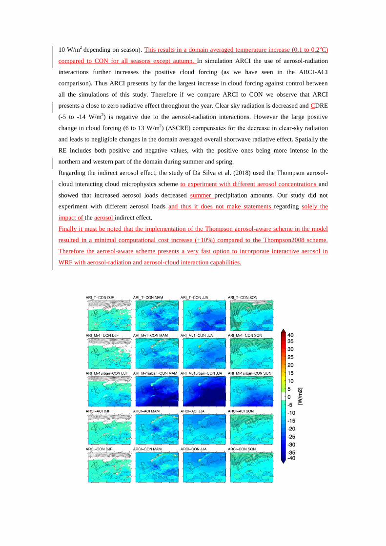
10 W/m2

depending on season). This results in a domain averaged temperature increase (0.1 to 0.2oC)

compared to CON for all seasons except autumn. In simulation ARCI the use of aerosol-radiation

interactions further increases the positive cloud forcing (as we have seen in the ARCI-ACI

comparison). Thus ARCI presents by far the largest increase in cloud forcing against control between

all the simulations of this study. Therefore if we compare ARCI to CON we observe that ARCI

presents a close to zero radiative effect throughout the year. Clear sky radiation is decreased and CDRE

(-5 to -14 W/m2) is negative due to the aerosol-radiation interactions. However the large positive

change in cloud forcing (6 to 13 W/m2) (ΔSCRE) compensates for the decrease in clear-sky radiation

and leads to negligible changes in the domain averaged overall shortwave radiative effect. Spatially the

RE includes both positive and negative values, with the positive ones being more intense in the

northern and western part of the domain during summer and spring.

Regarding the indirect aerosol effect, the study of Da Silva et al. (2018) used the Thompson aerosol-

cloud interacting cloud microphysics scheme to experiment with different aerosol concentrations and

showed that increased aerosol loads decreased summer precipitation amounts. Our study did not

experiment with different aerosol loads and thus it does not make statements regarding solely the

impact of the aerosol indirect effect.

Finally it must be noted that the implementation of the Thompson aerosol-aware scheme in the model

resulted in a minimal computational cost increase (+10%) compared to the Thompson2008 scheme.

Therefore the aerosol-aware scheme presents a very fast option to incorporate interactive aerosol in

WRF with aerosol-radiation and aerosol-cloud interaction capabilities.

Figure 4. Clear-sky Ddirect radiative effect (CDRE) at the surface for simulations implementing aerosol-radiation

interactions for all seasons. CDRE has been calculated as the difference in net Crsds at the surface from control

CON for the ARI group of simulations (rows 1 to 5). The last row depicts the aerosol-radiation interactions in an

environment where the indirect effect is also present and displays the difference of experiment ARCI from ACI.

Stippling indicates areas where the differences are not statistically significant at the 95% level, according to the

Mann-Whitney non-parametric test.

Figure 54. Radiative forcing (RE) calculated against control CON for all experiments and seasons. Furthermore,

the RE of ARCI calculated

against ACI (ARCI-ACI) is given to assess aerosol-radiation interaction implementation in the Thompson aerosol-

cloud interacting cloud

microphysics (TE2014) (row six). First six rows present the impact of direct effect. Last two rows (black box)

present the impact of TE2014 with indirect effect against control (row seven) and TE2014 with aerosol-radiation

interaction enabled against control (row eight). Stippling indicates areas where the differences are not statistically

significant at the 95% level, according to the Mann-Whitney non-parametric test.

Figure 65. Total cloud fraction (CFRACT) difference from control simulation CON for all experiments and

seasons. Furthermore the CFRACT difference of ARCI calculated against ACI (ARCI-ACI) is given to assess

aerosol-radiation interaction implementation in the Thompson aerosol-cloud interacting cloud microphysics

(TE2014) (row six). First six rows present the impact of aerosol-radiation interactions. Last two rows (black box)

present the impact of TE2014 with indirect effect against control (row seven) and TE2014 with aerosol-radiation

interactions enabled against control (row eight). Stippling indicates areas where the differences are not statistically

significant at the 95% level, according to the Mann-Whitney non-parametric test.

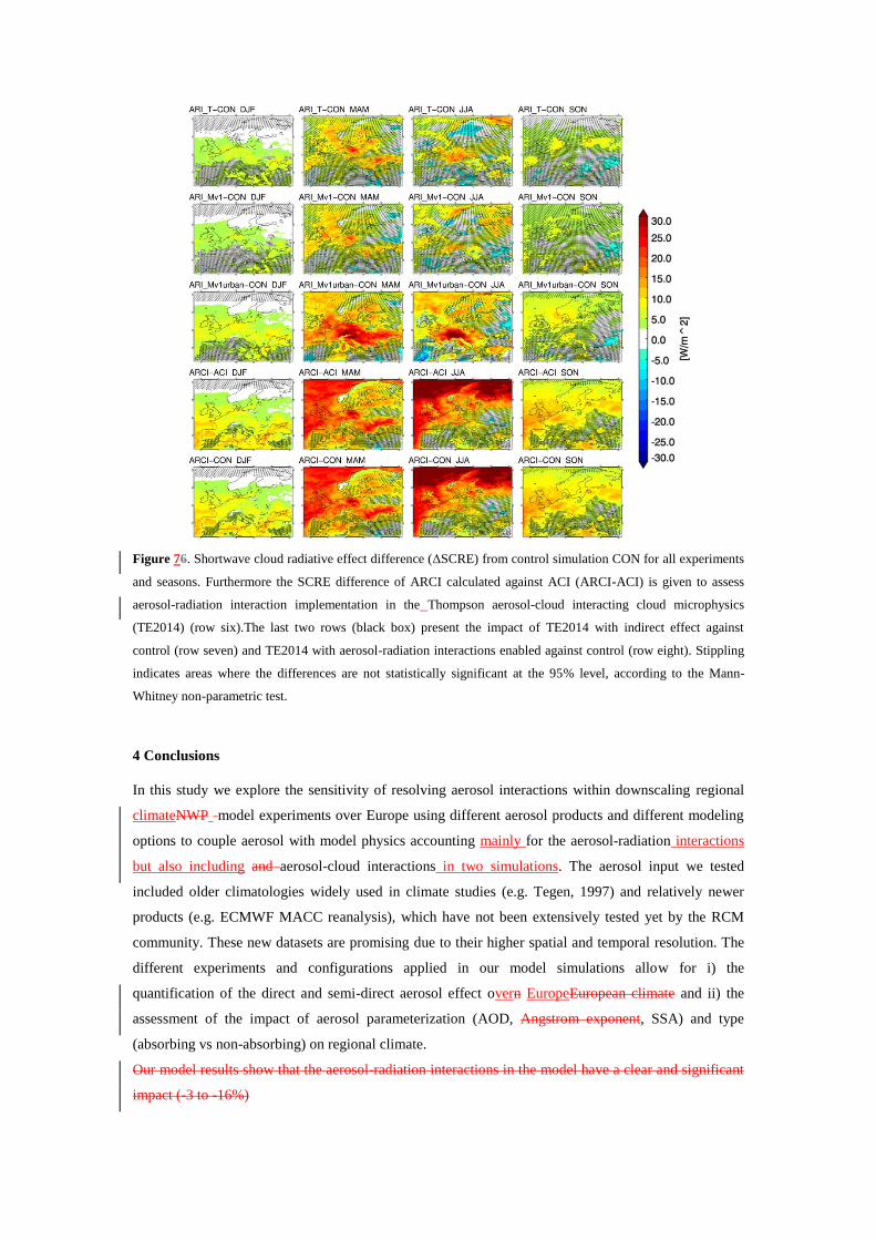
Figure 76. Shortwave cloud radiative effect difference (ΔSCRE) from control simulation CON for all experiments

and seasons. Furthermore the SCRE difference of ARCI calculated against ACI (ARCI-ACI) is given to assess

aerosol-radiation interaction implementation in the Thompson aerosol-cloud interacting cloud microphysics

(TE2014) (row six).The last two rows (black box) present the impact of TE2014 with indirect effect against

control (row seven) and TE2014 with aerosol-radiation interactions enabled against control (row eight). Stippling

indicates areas where the differences are not statistically significant at the 95% level, according to the Mann-

Whitney non-parametric test.

4 Conclusions

In this study we explore the sensitivity of resolving aerosol interactions within downscaling regional

climateNWP model experiments over Europe using different aerosol products and different modeling

options to couple aerosol with model physics accounting mainly for the aerosol-radiation interactions

but also including and aerosol-cloud interactions in two simulations. The aerosol input we tested

included older climatologies widely used in climate studies (e.g. Tegen, 1997) and relatively newer

products (e.g. ECMWF MACC reanalysis), which have not been extensively tested yet by the RCM

community. These new datasets are promising due to their higher spatial and temporal resolution. The

different experiments and configurations applied in our model simulations allow for i) the

quantification of the direct and semi-direct aerosol effect overn EuropeEuropean climate and ii) the

assessment of the impact of aerosol parameterization (AOD, Angstrom exponent, SSA) and type

(absorbing vs non-absorbing) on regional climate.

Our model results show that the aerosol-radiation interactions in the model have a clear and significant

impact (-3 to -16%)

on shortwave radiation at the surface (Rsds) throughout the year, whereas the influence on direct

normalized irradiance (-30

%) and diffuse radiation (+10 to +40%) can be considerably stronger. These findings are particularly

important for solar

applications (e.g., solar power production), since Rsds is often the only available parameter from

ensemble climate projects

(e.g., CORDEX; e.g. Jerez et al., 2015), although it is neither the most sensitive to aerosol properties

nor the most relevant for the impact community (Jimenez et al., 2016).

Accounting for the aerosol-radiation interactions reduces surface radiation by up to -17 (-5) W/m2 in

summer (winter) due

to the clear-sky direct radiative effect (CDRE). This reduction is twice as large for aerosol of highly

absorbing nature (i.e., urban). Clouds responded (semi-direct effect) with a positive forcing,

counteracting the impact of the CDRE by 20 to 60%

(23 to 4 W/m2), depending on season. Thus, the overall radiative effect of aerosols (RE) is clearly

smaller than the CDRE and is approximately -12 (-2) W/m2 in summer (winter). Similar studies

implementing aerosol-radiation interactions have calculated larger values of both overall radiative

effect ( Nabat et al., 2015; Huszar et al., 2012; Zanis, 2009) and semi-direct effect. Furthermore, when

aerosol-radiation interactions are implemented in a simulation where the aerosol-cloud interactions are

also introduced, the combined impact of the semi-direct and indirect effects results in an even more

positive forcing (4 to 7 W/m2), thus further weakening the overall aerosol radiative effect (–1 W/m

2 in

winter and -11 W/m2 in summer).

The decrease of shortwave radiation at the surface due to aerosol-radiation interactions leads to a

widespread temperature decrease with domain averaged cooling reaching -0.5oC over land in summer

and autumn. At grid point level the cooling can be considerably stronger, reaching -1.5oC close to the

maxima of aerosol optical depth. The impact on temperature decreases with height and is detectible at

least up to the 850 hPa pressure level. The idealized experiment with the extremely absorbing “urban”

type aerosols leads to tropospheric warming of more than 2oC at the surface affecting the troposphere

up to 700 hPa. We also show that introducing the aerosol-radiation and aerosol-cloud interactions may

disturb the climate system in a way that affects cloudiness (especially low-level cloudiness) with the

potential to trigger regional circulation anomalies at the lower and the mid-troposphere.

Precipitation was not particularly affected by most of the aerosol perturbations in the 5 year simulations

that were conducted.

The spatial pattern of changes is patchy and some large local changes are probably a result of internal

model variability. However in spring and summer a small domain averaged precipitation decrease (-2

to -5%, -0.02 to -0.09 mm/day) is seen.

This

result is in contrast to other regional downscaling studies. The study of Nabat et al. (2015) investigating

aerosol-radiation

interactions presented a clear precipitation reduction for all seasons due to the decrease of SST which

in turn lead to reduced evaporation and finally reduced cloud fraction and precipitation. That study

however used an RCM coupled with a ocean model, which made possible to simulate changes in the

SST, a component that our study is missing. In our study, considerable precipitation reduction over

extended areas is seen only with the use of highly absorbing aerosols identifying the importance of

implementing realistic aerosol optical characteristics, whenever available. To conclude no significant

changes are seen in precipitation amount over the largest part of the domain with the use of realistic

aerosol optical properties.

Finally the two simulations incorporating aerosol-cloud interactions present reduced liquid water path

and cloud fraction amounts compared to the control experiment that are mainly attributed to the change

of the cloud microphysics scheme.

Code and data availability. The source code of the Weather Research and Forecasting Model (WRF) is

freely available by UCAR/NCAR (http://www2.mmm.ucar.edu/wrf/users/downloads.html). The

satellite data used (SARAH Edition1, CLARA-A1) are provided by EUMETSAT through the Satellite

Application Facility on Climate Monitoring (CM SAF) (www.cmsaf.eu). The E-OBS gridded data set

is provided by ECA&D project (http://www.ecad.eu). The MACv1MAC-v1 aerosol climatology data

can be found at ftp://ftp-projects.zmaw.de. The ERA-Interim reanalysis and MACC aerosol data are

available by the European Centre for Medium-Range Weather Forecasts (ECMWF)

(https://apps.ecmwf.int/datasets/).

Author contributions. VP and EK designed the research. VP performed the experiments and analyzed

the data. SK provided technical assistance to the experiments. VP wrote the paper with inputs from all

coauthors.

Competing interests. The authors declare that they have no conflict of interest

Acknowledgements. This research is co-financed by Greece and the European Union (European Social

Fund- ESF) through the Operational Programme «Human Resources Development, Education and

Lifelong Learning» in the context of the project “Strengthening Human Resources Research Potential

via Doctorate Research” (MIS-5000432), implemented by the State Scholarships Foundation (IKY).

We also acknowledge the support of the Greek Research and Technology Network (GRNET) High

Performance Computing (HPC) infrastructure for providing the computational resources necessary for

the model simulations (pr006005_thin). NCAR is sponsored by the National Science Foundation. We

acknowledge EUMETSAT for providing the satellite data through the Satellite Application Facility on

Climate Monitoring (CM SAF) (www.cmsaf.eu).Furthermore we acknowledge the E-OBS dataset from

the EU-FP6 project ENSEMBLES (http://ensembles-eu.metoffice.com) and the data providers in the

ECA&D project (http://www.ecad.eu) and the use of MACv1MAC-v1 aerosol climatology data

(ftp://ftp-projects.zmaw.de). We also acknowledge ECMWF (www.ecmwf.int) for the provision of

ERA-Interim reanalysis data as well as the MACC aerosol data.

References

Alapaty, K., Herwehe, J. A., Otte, T. L., Nolte, C. G., Bullock, O. R., Mallard, M. S., Kain, J. S. and

Dudhia, J.: Introducing subgrid‐scale cloud feedbacks to radiation for regional meteorological and

climate modeling, Geophys. Res. Lett., 39(24), 2012GL054031, doi:10.1029/2012GL054031, 2012.

Alexandri, G., Georgoulias, A. K., Zanis, P., Katragkou, E., Tsikerdekis, A., Kourtidis, K. and Meleti,

C.: On the ability of RegCM4 regional climate model to simulate surface solar radiation patterns

over Europe: An assessment using satellite-based observations, Atmos. Chem. Phys., 15(22),

13195–13216, doi:10.5194/acp-15-13195-2015, 2015.

Boucher, O., Randall, D., Artaxo, P., Bretherton, C., Feingold, G., Forster, P., Kerminen, V.-M.,

Kondo, Y., Liao, H., Lohmann, U., Rasch, P.,Satheesh, S., Sherwood, S., Stevens, B., and Zhang,

X.: Clouds and Aerosols, book section 7, p. 571–658, Cambridge University Press, Cambridge,

United Kingdom and New York, NY, USA, https://doi.org/10.1017/CBO9781107415324.016,

www.climatechange2013.org, 2013.

Christensen, J. H., Carter, T. R., Rummukainen, M. and Amanatides, G.: Evaluating the perfomance of

regional climate models: The PRUDENCE project, Clim. Change, 81(6), 1–6, doi:10.1007/s10584-

006-9211-6, 2007.

Clerbaux, N., Ipe, A., De Bock Veerle, Urbain, M., Baudrez, E., Velazquez-Blazquez, A., Akkermans,

T., Moreels, J., Hollmann, R., Selbach, N., and Werscheck, M.: CM SAF Aerosol Optical Depth

(AOD) Data Record - Edition 1, https://doi.org/10.5676/EUM_SAF_CM/MSG_AOD/V001,

https://doi.org/10.5676/EUM_SAF_CM/MSG_AOD/V001, 2017.

Colarco, P., Da Silva, A., Chin, M., and Diehl, T.: Online simulations of global aerosol distributions in

the NASA GEOS-4

model and comparisons to satellite and ground-based aerosol optical depth, Journal of Geophysical

Research Atmospheres, 115, https://doi.org/10.1029/2009JD012820, 2010.

Da Silva, N., Mailler, S., and Drobinski, P.: Aerosol indirect effects on summer precipitation in a

regional climate model for the Euro-Mediterranean region, Annales Geophysicae, 36, 321–335,

https://doi.org/10.5194/angeo-36-321-2018, https://www.ann-geophys.net/36/321/2018/, 2018.

Dee, D. P., Uppala, S. M., Simmons, A. J., Berrisford, P., Poli, P., Kobayashi, S., Andrae, U.,

Balmaseda, M. A., Balsamo, G., Bauer, P., Bechtold, P., Beljaars, A. C. M., van de Berg, L., Bidlot,

J., Bormann, N., Delsol, C., Dragani, R., Fuentes, M., Geer, A. J., Haimberger, L., Healy, S. B.,

Hersbach, H., Hólm, E. V., Isaksen, L., Kållberg, P., Köhler, M., Matricardi, M., Mcnally, A. P.,

Monge-Sanz, B. M., Morcrette, J. J., Park, B. K., Peubey, C., de Rosnay, P., Tavolato, C., Thépaut,

J. N. and Vitart, F.: The ERA-Interim reanalysis: Configuration and performance of the data

assimilation system, Q. J. R. Meteorol. Soc., 137(656), 553–597, doi:10.1002/qj.828, 2011.

Garcia-Diez, M., Fernández, J. and Vautard, R.: An RCM multi-physics ensemble over Europe: multi-

variable evaluation to avoid error compensation, Clim. Dyn., 45(11–12), 3141–3156,

doi:10.1007/s00382-015-2529-x, 2015.

Ginoux, P., Chin, M., Tegen, I., Prospero, J., Holben, B., Dubovik, O., and Lin, S.-J.: Sources and

distributions of dust aerosols simulated with the GOCART model, Journal of Geophysical Research

Atmospheres, 106, 20 255–20 273,

https://doi.org/10.1029/2000JD000053,https://www.scopus.com/inward/record.uri?eid=2-s2.0-

0034773231&doi=10.1029%2f2000JD000053&partnerID=40&md5=c7bc8c499c95331edd5c0426

18636232, cited By 1041, 2001.

Giorgi, F. and Gutowski, W.J., J.: Regional Dynamical Downscaling and the CORDEX Initiative,

Annual Review of Environment and Resources, 40, 467–490, https://doi.org/10.1146/annurev-

environ-102014-021217, https://www.scopus.com/inward/record.uri?eid=2-s2.0-

84946838214&doi=10.1146%2fannurev-environ-102014-

021217&partnerID=40&md5=5c58e21370984985752df73f764e63ac, 2015.

Grell, G. A. and Freitas, S. R.: A scale and aerosol aware stochastic convective parameterization for

weather and air quality modeling, Atmos. Chem. Phys., 14(10), 5233–5250, doi:10.5194/acp-14-

5233-2014, 2014.

Gutiérrez, C., Somot, S., Nabat, P., Mallet, M., Gaertner, M. Á. and Perpiñán, O.: Impact of aerosols

on the spatiotemporal variability of photovoltaic energy production in the Euro-Mediterranean area,

Sol. Energy, 174(March), 1142–1152, doi:10.1016/j.solener.2018.09.085, 2018.

Haylock, M. R., Hofstra, N., Klein Tank, A. M. G., Klok, E. J., Jones, P. D. and New, M.: A European

daily high-resolution gridded data set of surface temperature and precipitation for 1950-2006, J.

Geophys. Res. Atmos., 113(20), doi:10.1029/2008JD010201, 2008.

Hofstra, N., Haylock, M., New, M. and Jones, P. D.: Testing E-OBS European high-resolution gridded

data set of daily precipitation and surface temperature, J. Geophys. Res. Atmos., 114(21),

doi:10.1029/2009JD011799, 2009.

Hogan, R. J. and Illingworth, A. J.: Deriving cloud overlap statistics from radar, Q. J. R. Meteorol.

Soc., 126(569), 2903–2909, doi:10.1256/smsqj.56913, 2000.

Hong, S.-Y., Noh, Y. and Dudhia, J.: A New Vertical Diffusion Package with an Explicit Treatment of

Entrainment Processes, Mon. Weather Rev., 134(9), 2318–2341, doi:10.1175/MWR3199.1, 2006.

Hubanks, P., Platnick, S., King, M. and Ridgway, B.: MODIS atmosphere L3 gridded product

algorithm theoretical basis document Collection 6.0 & 6.1 Version 4.4, Tech. Rep. ATBD-MOD-

30, NASA, 2019..

Huszar, P., Miksovsky, J., Pisoft, P., Belda, M. and Halenka, T.: Interactive coupling of a regional

climate model and a chemical transport model: evaluation and preliminary results on ozone and

aerosol feedback, Clim. Res., 51(1), 59–88, doi:10.3354/cr01054, 2012.

Iacono, M. J., Delamere, J. S., Mlawer, E. J., Shephard, M. W., Clough, S. A. and Collins, W. D.:

Radiative forcing by long-lived greenhouse gases: Calculations with the AER radiative transfer

models, J. Geophys. Res. Atmos., 113(13), 2–9, doi:10.1029/2008JD009944, 2008.

Inness, A., Baier, F., Benedetti, A., Bouarar, I., Chabrillat, S., Clark, H., Clerbaux, C., Coheur, P.,

Engelen, R. J., Errera, Q., Flemming, J., George, M., Granier, C., Hadji-Lazaro, J., Huijnen, V.,

Hurtmans, D., Jones, L., Kaiser, J. W., Kapsomenakis, J., Lefever, K., Leitão, J., Razinger, M.,

Richter, A., Schultz, M. G., Simmons, A. J., Suttie, M., Stein, O., Thépaut, J. N., Thouret, V.,

Vrekoussis, M. and Zerefos, C.: The MACC reanalysis: An 8 yr data set of atmospheric

composition, Atmos. Chem. Phys., 13(8), 4073–4109, doi:10.5194/acp-13-4073-2013, 2013.

Jerez, S., Tobin, I., Vautard, R., Montávez, J. P., López-Romero, J. M., Thais, F., Bartok, B.,

Christensen, O. B., Colette, A., Déqué, M., Nikulin, G., Kotlarski, S., Van Meijgaard, E.,

Teichmann, C. and Wild, M.: The impact of climate change on photovoltaic power generation in

Europe, Nat. Commun., 6(1), 10014, doi:10.1038/ncomms10014, 2015.

Jiménez, P. A., Dudhia, J., González-Rouco, J. F., Navarro, J., Montávez, J. P. and Garcia-Bustamante,

E.: A Revised Scheme for the WRF Surface Layer Formulation, Mon. Weather Rev., 140(3), 898–

918, doi:10.1175/MWR-D-11-00056.1, 2012.

Jimenez, P. A., Hacker, J. P., Dudhia, J., Haupt, S. E., Ruiz-Arias, J. A., Gueymard, C. A., Thompson,

G., Eidhammer, T. and Deng, A.: WRF-SOLAR: Description and clear-sky assessment of an

augmented NWP model for solar power prediction, Bull. Am. Meteorol. Soc., 97(7), 1249–1264,

doi:10.1175/BAMS-D-14-00279.1, 2016.

Karlsson, K. G. and Hollmann, R.: Validation Report, Cloud Products, CM SAF Cloud, Albedo,

Radiation dataset, AVHRR-based, Edition 1 (CLARA-A1), Tech. rep., Satellite Application

Facility on Climate Monitoring, https://doi.org/10.5676/EUM_SAF_CM/CLARA_AVHRR/V001,

2012.

Karlsson, K. G., Riihelä, A., Müller, R., Meirink, J. F., Sedlar, J., Stengel, M., Lockhoff, M.,

Trentmann, J., Kaspar, F., Hollmann, R. and Wolters, E.: CLARA-A1: A cloud, albedo, and

radiation dataset from 28 yr of global AVHRR data, Atmos. Chem. Phys., 13(10), 5351–5367,

doi:10.5194/acp-13-5351-2013, 2013.

Katragkou, E., Garciá-Diéz, M., Vautard, R., Sobolowski, S., Zanis, P., Alexandri, G., Cardoso, R. M.,

Colette, A., Fernandez, J., Gobiet, A., Goergen, K., Karacostas, T., Knist, S., Mayer, S., Soares, P.

M. M., Pytharoulis, I., Tegoulias, I., Tsikerdekis, A. and Jacob, D.: Regional climate hindcast

simulations within EURO-CORDEX: Evaluation of a WRF multi-physics ensemble, Geosci. Model

Dev., 8(3), 603–618, doi:10.5194/gmd-8-603-2015, 2015.

Kinne, S., O‟Donnel, D., Stier, P., Kloster, S., Zhang, K., Schmidt, H., Rast, S., Giorgetta, M., Eck, T.

F. and Stevens, B.: MAC-v1: A new global aerosol climatology for climate studies, J. Adv. Model.

Earth Syst., 5(4), 704–740, doi:10.1002/jame.20035, 2013.

Kotlarski, S., Keuler, K., Christensen, O. B., Colette, A., Déqué, M., Gobiet, A., Goergen, K., Jacob,

D., Lüthi, D., Van Meijgaard, E., Nikulin, G., Schär, C., Teichmann, C., Vautard, R., Warrach-Sagi,

K. and Wulfmeyer, V.: Regional climate modeling on European scales: A joint standard evaluation

of the EURO-CORDEX RCM ensemble, Geosci. Model Dev., 7(4), 1297–1333, doi:10.5194/gmd-

7-1297-2014, 2014.

Lawrence, D. M., Oleson, K. W., Flanner, M. G., Thornton, P. E., Swenson, S. C., Lawrence, P. J.,

Zeng, X., Yang, Z.-L., Levis, S., Sakaguchi, K., Bonan, G. B. and Slater, A. G.: Parameterization

improvements and functional and structural advances in Version 4 of the Community Land Model,

J. Adv. Model. Earth Syst., 3(1), n/a-n/a, doi:10.1029/2011MS00045, 2011.

Lim, K.-S. S. and Hong, S.-Y.: Development of an Effective Double-Moment Cloud Microphysics

Scheme with Prognostic Cloud Condensation Nuclei (CCN) for Weather and Climate Models, Mon.

Weather Rev., 138(5), 1587–1612, doi:10.1175/2009MWR2968.1, 2010.

Mooney, P. A., Mulligan., F. J. and Fealy, R.: Evaluation of the sensitivity of the weather research and

forecasting model to parameterization schemes for regional climates of europe over the period

1990-95, J. Clim., 26(3), 1002–1017, doi:10.1175/JCLI-D-11-00676.1, 2013.

Mueller, R. and Träger-Chatterjee, C.: Brief accuracy assessment of aerosol climatologies for the

retrieval of solar surface radiation, Atmosphere (Basel)., 5(4), 959–972,

doi:10.3390/atmos5040959, 2014.

Müller, R., Pfeifroth, U., Träger-Chatterjee, C., Trentmann, J. and Cremer, R.: Digging the

METEOSAT treasure-3 decades of solar surface radiation, Remote Sens., 7(6), 8067–8101,

doi:10.3390/rs70608067, 2015.

Nabat, P., Somot, S., Mallet, M., Sanchez-Lorenzo, A. and Wild, M.: Contribution of anthropogenic

sulfate aerosols to the changing Euro-Mediterranean climate since 1980, Geophys. Res. Lett.,

41(15), 5605–5611, doi:10.1002/2014GL060798, 2014.

Nabat, P., Somot, S., Mallet, M., Sevault, F., Chiacchio, M. and Wild, M.: Direct and semi-direct

aerosol radiative effect on the Mediterranean climate variability using a coupled regional climate

system model, Clim. Dyn., 44(3–4), 1127–1155, doi:10.1007/s00382-014-2205-6, 2015.

Niu, G.-Y., Yang, Z.-L., Mitchell, K. E., Chen, F., Ek, M. B., Barlage, M., Kumar, A., Manning, K.,

Niyogi, D., Rosero, E., Tewari, M. and Xia, Y.: The community Noah land surface model with

multiparameterization options (Noah-MP): 1. Model description and evaluation with local-scale

measurements, J. Geophys. Res., 116(D12), D12109, doi:10.1029/2010JD015139, 2011.

Oleson, K. W., Lawrence, D. M., Gordon, B., Flanner, M. G., Kluzek, E., Peter, J., Levis, S., Swenson,

S. C., Thornton, E., Dai, A., Decker, M., Dickinson, R., Feddema, J., Heald, C. L., Lamarque, J.,

Niu, G., Qian, T., Running, S., Sakaguchi, K., Slater, A., Stöckli, R., Wang, A., Yang, L., Zeng, X.

and Zeng, X.: Technical Description of version 4 . 0 of the Community Land Model ( CLM ), ,

(April), 2010.

Platnick, S., et al., 2015. MODIS Atmosphere L3 Monthly Product. NASA MODIS Adaptive

Processing System, Goddard Space Flight Center, USA:

http://dx.doi.org/10.5067/MODIS/MOD08_M3.006

Powers, J. G., Klemp, J. B., Skamarock, W. C., Davis, C. A., Dudhia, J., Gill, D. O., Coen, J. L.,

Gochis, D. J., Ahmadov, R., Peckham, S. E., Grell, G. A., Michalakes, J., Trahan, S., Benjamin, S.

G., Alexander, C. R., Dimego, G. J., Wang, W., Schwartz, C. S., Romine, G. S., Liu, Z., Snyder, C.,

Chen, F., Barlage, M. J., Yu, W. and Duda, M. G.: The weather research and forecasting model:

Overview, system efforts, and future directions, Bull. Am. Meteorol. Soc., 98(8), 1717–1737,

doi:10.1175/BAMS-D-15-00308.1, 2017.

Prein, A. F. and Gobiet, A.: Impacts of uncertainties in European gridded precipitation observations on

regional climate analysis, Int. J. Climatol., 37(1), 305–327, doi:10.1002/joc.4706, 2017.

Ramanathan, V., Crutzen, P. J., Kiehl, J. T. and Rosenfeld, D.: Atmosphere: Aerosols, climate, and the

hydrological cycle, Science (80-. )., 294(5549), 2119–2124, doi:10.1126/science.1064034, 2001.

Rodriguez, E., Kolmonen, P., Sundström, A.-M., Sogacheva, L., Virtanen, T. and de Leeuw, G.:

Satellite study over Europe to estimate the single scattering albedo and the aerosol optical depth, in

AIP Conference Proceedings, vol. 1531, pp. 196–199., 2013.

Ruiz-Arias, J. A., Dudhia, J. and Gueymard, C. A.: A simple parameterization of the short-wave

aerosol optical properties for surface direct and diffuse irradiances assessment in a numerical

weather model, Geosci. Model Dev., 7(3), 1159–1174, doi:10.5194/gmd-7-1159-2014, 2014.

Ruti, P. M., Somot, S., Giorgi, F., Dubois, C., Flaounas, E., Obermann, A., Dell‟Aquila, A., Pisacane,

G., Harzallah, A., Lombardi, E., Ahrens, B., Akhtar, N., Alias, A., Arsouze, T., Aznar, R., Bastin,

S., Bartholy, J., Béranger, K., Beuvier, J., Bouffies-Cloché, S., Brauch, J., Cabos, W., Calmanti, S.,

Calvet, J.-C., Carillo, A., Conte, D., Coppola, E., Djurdjevic, V., Drobinski, P., Elizalde-Arellano,

A., Gaertner, M., Galàn, P., Gallardo, C., Gualdi, S., Goncalves, M., Jorba, O., Jordà, G.,

L‟Heveder, B., Lebeaupin-Brossier, C., Li, L., Liguori, G., Lionello, P., Maciàs, D., Nabat, P.,

Önol, B., Raikovic, B., Ramage, K., Sevault, F., Sannino, G., Struglia, M. V., Sanna, A., Torma, C.

and Vervatis, V.: Med-CORDEX Initiative for Mediterranean Climate Studies, Bull. Am. Meteorol.

Soc., 97(7), 1187–1208, doi:10.1175/BAMS-D-14-00176.1, 2016.

Schultze, M. and Rockel, B.: Direct and semi-direct effects of aerosol climatologies on long-term

climate simulations over Europe, Clim. Dyn., 50(9–10), 3331–3354, doi:10.1007/s00382-017-3808-

5, 2018.

Schulz, J., Albert, P., Behr, H.-D., Caprion, D., Deneke, H., Dewitte, S., Dürr, B., Fuchs, P., Gratzki,

A., Hechler, P., Hollmann, R., Johnston, S., Karlsson, K.-G., Manninen, T., Müller, R., Reuter, M.,

Riihelä, A., Roebeling, R., Selbach, N., Tetzlaff, A., Thomas, W., Werscheck, M., Wolters, E. and

Zelenka, A.: Operational climate monitoring from space: the EUMETSAT Satellite Application

Facility on Climate Monitoring (CM-SAF), Atmos. Chem. Phys., 9(5), 1687–1709,

doi:10.5194/acp-9-1687-2009, 2009.

Skamarock, W. C., Klemp, J. B., Dudhi, J., Gill, D. O., Barker, D. M., Duda, M. G., Huang, X.-Y.,

Wang, W. and Powers, J. G.: A Description of the Advanced Research WRF Version 3, Tech. Rep.,

(June), 113, doi:10.5065/D6DZ069T, 2008.

Sundqvist, H., Berge, E., and Kristjansson, J.: Condensation and cloud parameterization studies with a

mesoscale numerical weather prediction model, Monthly Weather Review, 117, 1641–1657,

https://doi.org/10.1175/1520-

0493(1989)117<1641:CACPSW>2.0.CO;2,https://www.scopus.com/inward/record.uri?eid=2-s2.0-

0024927328&doi=10.1175%2f1520-

0493%281989%29117%3c1641%3aCACPSW%3e2.0.CO%3b2&partnerID=

0&md5=a923bf53cac2a87ed2ceca4767524373, 1989.

Tegen, I., Hollrig, P., Chin, M., Fung, I., Jacob, D. and Penner, J.: Contribution of different aerosol

species to the global aerosol extinction optical thickness: Estimates from model results, J. Geophys.

Res. Atmos., 102(D20), 23895–23915, doi:10.1029/97JD01864, 1997.

Thompson, G. and Eidhammer, T.: A Study of Aerosol Impacts on Clouds and Precipitation

Development in a Large Winter Cyclone, J. Atmos. Sci., 71(10), 3636–3658, doi:10.1175/JAS-D-

13-0305.1, 2014.

Thompson, G., Field, P. R., Rasmussen, R. M. and Hall, W. D.: Explicit Forecasts of Winter

Precipitation Using an Improved Bulk Microphysics Scheme. Part II: Implementation of a New

Snow Parameterization, Mon. Weather Rev., 136(12), 5095–5115, doi:10.1175/2008MWR2387.1,

2008.

Tombette, M., Chazette, P., Sportisse, B. and Roustan, Y.: Simulation of aerosol optical properties over

Europe with a 3-D size-resolved aerosol model: comparisons with AERONET data, Atmos. Chem.

Phys., 8(23), 7115–7132, doi:10.5194/acp-8-7115-2008, 2008.

Witte, J. C., Douglass, A. R., da Silva, A., Torres, O., Levy, R. and Duncan, B. N.: NASA A-Train and

Terra observations of the 2010 Russian wildfires, Atmos. Chem. Phys., 11(17), 9287–9301,

doi:10.5194/acp-11-9287-2011, 2011.

Zanis, P.: A study on the direct effect of anthropogenic aerosols on near surface air temperature over

Southeastern Europe during summer 2000 based on regional climate modeling, Ann. Geophys., 27(10),

3977–3988, doi:10.5194/angeo-27-3977-2009, 2009.

Zanis, P., Ntogras, C., Zakey, A., Pytharoulis, I. and Karacostas, T.: Regional climate feedback of

anthropogenic aerosols over Europe using RegCM3, Clim. Res., 52(1), 267–278, doi:10.3354/cr01070,

2012.

Zubler, E. M., Lohmann, U., Lüthi, D. and Schär, C.: Intercomparison of aerosol climatologies for use

in a regional climate model over Europe, Geophys. Res. Lett., 38(15), 1–5,

doi:10.1029/2011GL048081, 2011.