S-SOM v1.0: a structural self-organizing map algorithm ... - GMD

Geosci. Model Dev., 14, 2097–2111, 2021https://doi.org/10.5194/gmd-14-2097-2021© Author(s) 2021. This work is distributed underthe Creative Commons Attribution 4.0 License.

S-SOM v1.0: a structural self-organizing mapalgorithm for weather typingQuang-Van Doan1, Hiroyuki Kusaka1, Takuto Sato2, and Fei Chen3

1Center for Computational Sciences, University of Tsukuba, Tsukuba, Ibaraki, Japan2Graduate School of Life and Environmental Sciences, University of Tsukuba, Tsukuba, Ibaraki, Japan3Research Applications Laboratory, National Center for Atmospheric Research, Boulder, CO, USA

Correspondence: Quang-Van Doan ([email protected])

Received: 18 August 2020 – Discussion started: 9 October 2020Revised: 15 January 2021 – Accepted: 17 February 2021 – Published: 22 April 2021

Abstract. This study proposes a novel structural self-organizing map (S-SOM) algorithm for synoptic weathertyping. A novel feature of the S-SOM compared with tradi-tional SOMs is its ability to deal with input data with spatialor temporal structures. In detail, the search scheme for thebest matching unit (BMU) in a S-SOM is built based on astructural similarity (S-SIM) index rather than by using thetraditional Euclidean distance (ED). S-SIM enables the BMUsearch to consider the correlation in space between weatherstates, such as the locations of highs or lows, that is impos-sible when using ED. The S-SOM performance is evaluatedby multiple demo simulations of clustering weather patternsover Japan using the ERA-Interim sea-level pressure data.The results show the S-SOM’s superiority compared with astandard SOM with ED (or ED-SOM) in two respects: clus-tering quality based on silhouette analysis and topologicalpreservation based on topological error. Better performanceof S-SOM versus ED is consistent with results from differ-ent tests and node-size configurations. S-SOM performs bet-ter than a SOM using the Pearson correlation coefficient (orCOR-SOM), though the difference is not as clear as it is com-pared to ED-SOM.

1 Introduction

There has been an increasing number of self-organizing map(SOM) applications for climatology studies in recent years.The SOM was initially developed by Kohonen (1982) as anunsupervised data-mining method. SOMs are used to dis-cover patterns intrinsic to input data by projecting them into

a map (usually two-dimensional), and the nodes on the maprepresent the most important features of the input space. Onestandard application of SOMs in climatology is “objective”synoptic weather typing (Sheridan and Lee, 2011). Here,synoptic circulation data, typically sea-level pressure (SLP)or geopotential height, are used to generate a small-enoughnumber of representative weather states that can be readilyhandled by sequential analysis.

SOMs are used for diverse purposes, from discovering thelinks between synoptic circulation and climatic variabilityto statistical dynamical downscaling, climate prediction, andweather forecasting. For example, with a SOM, Horton etal. (2015) found that changes in the frequency of geopotentialheight patterns since the 1980s have modified extreme tem-perature trends in some Northern Hemisphere regions. Also,SOMs have been used to discover the association betweenrainfall changes and shifts in large-scale circulation patterns(e.g., Alexander et al., 2010; Lennard and Hegerl, 2015;Swales et al., 2016; Nguyen-Le and Yamada, 2019; Luonget al., 2020). SOMs are also used as a statistical downscalingmethod for the future climate by associating the changes inthe frequency of synoptic occurrences with surface variables(e.g., Gibson et al., 2016; Ohba and Sugimoto, 2019). Borahet al. (2013) developed a probabilistic prediction scheme forthe Indian summer monsoon intraseasonal oscillation usinga SOM-based technique. Chang et al. (2014) used a hybridSOM and dynamic neural network for nowcasting rainfall inTaiwan. Nguyen-Le et al. (2017) used a hybrid system of nu-merical weather prediction (NWP) and a SOM to forecastheavy rain for up to a week for Kyushu, Japan. A hybridNWP and a SOM were also used by Ohba et al. (2018) as

Published by Copernicus Publications on behalf of the European Geosciences Union.

2098 Q.-V. Doan et al.: S-SOM v1.0

a system for the medium-range forecasting of wind ramps inJapan. For the first time, Lagerquist et al. (2017) proposed away to obtain a real-time extreme wildfire weather forecastin the US using a SOM technique.

The SOM algorithm consists of repeatedly learning pro-cesses that gradually update the nodes in the output map un-til they converge to a stable solution, which is expected to bethe “best” representative of the input space. At each learningstep, the SOM selects an input vector, usually randomly, andthen searches for a node in a SOM map that best matches thatvector. In this task, nodes in the output map compete to findthe node most “similar” to the input vector. The “winning”node is called the best matching unit (BMU). Next, trainingis implemented by making the BMU and its neighbors closerto the input vector. The learning rate and neighborhood func-tion govern the training task. Searching for the BMU is acrucial part of the SOM algorithm as it affects the sequentialtraining process and the quality of the final SOM outcome.

Traditional SOMs use the Euclidean distance (ED) tosearch for the BMU, where the “closest” node to an inputvector in terms of ED will be assigned as the BMU. Thismethod is simple and computationally effective. Moreover,ED is very popular and widely used as a quantitative simi-larity metric when comparing two objects. ED is commonlyused in many machine learning algorithms. It is also thebasis of many clustering algorithms such as K means andaffinity propagation. Nevertheless, ED has severe shortcom-ings when used to compare “structured” signals, i.e., thosewith spatial or temporal orders, such as time series and two-dimensional images. Despite these shortcomings, ED hasbeen influential and widely used. A reason for its popular-ity is that the prevailing attitudes towards ED seem to rangefrom “it’s easy to use and not so bad” to “everyone else usesit” (Wang and Bovik, 2009).

This weakness of ED becomes crucial in climatology stud-ies where most of the data are spatially and temporally struc-tured, e.g., weather maps, and time series. Intuitively, a simi-larity measure based on ED might lead to the degradation ofthe spatial correlations between air pressure patterns, suchas the location of highs or lows (Fig. A1). Thus, a BMUsearch scheme using ED might result in an incorrect deter-mination of the “winning node”, which would critically af-fect the performance of SOMs. Several alternative versionsof the SOM have been developed since Kohonen (1982).These include the generative topographic map (Kaski, 1997)and the time-adaptive self-organizing map (Shah-Hosseiniand Safabakhsh, 2003; Shah-Hosseini, 2011). However, suchSOM versions have focused on parameterization schemessuch as learning rate or neighborhood functions in the train-ing process. No studies have addressed the fundamental issueof the ED in a BMU search.

Therefore, this study proposes a novel SOM algorithmcalled a structural SOM (S-SOM). The advantage of S-SOMcompared with traditional SOMs is that an S-SOM can dealwith “structural” input data, i.e., data with spatial or temporal

Figure 1. The S-SOM algorithm.

relationships. To accomplish this, the S-SOM incorporates aBMU search scheme that is implemented based on a struc-tural similarity index rather than on the traditional ED.

The structural similarity (S-SIM) index, which was firstintroduced by Wang et al. (2004) and is increasingly beingused in the signal processing field, has an advantage over EDin detecting structural correlations in the pair data. We setup multiple test simulations with different SOM configura-tions to evaluate the S-SOM performance comparing the tra-ditional ED-SOM and the SOM algorithm with the Pearsoncorrelation coefficient, hereafter called COR-ED, for classi-fying sea-level pressure patterns over the Japan region. Quan-tified metrics such as silhouette analysis and topological er-rors are used to assess SOM performance. The remainder ofthis paper is structured as follows. Section 2 describes thenovel S-SOM algorithm; Sect. 3 presents the test simulationconfiguration and evaluation metrics. Results are presentedand discussed in Sect. 4. Concluding remarks are provided inSect. 5.

2 Structural SOM algorithm

Our proposed S-SOM algorithm is shown in Fig. 1. It fol-lows the procedure initially proposed by Kohonen (1982) andused in many application studies. An S-SOM starts with theconfiguration and initialization of SOM nodes and establish-ing the number of training iterations. The training consists ofthree main steps: selecting an input vector, finding the bestmatching unit for the input vector, then updating the weightvectors of SOM nodes by using parameters, i.e., learning rateand neighborhood function. The learning rate is a real num-ber and decreases as the number of iteration steps increases.The difference between S-SOM and traditional SOM imple-mentation is that we propose a new scheme for finding aBMU. In this scheme, we use a similarity index that can dealwith structural data such as two-dimensional air pressure dis-tribution instead of using ED to compare the similarity be-tween vectors.

The new BMU search scheme is based on competitionamong SOM nodes so that a node with the highest S-SIMindex to an input vector will be assigned as the BMU. TheS-SIM was first introduced by Wang et al. (2004) to predict

Geosci. Model Dev., 14, 2097–2111, 2021 https://doi.org/10.5194/gmd-14-2097-2021

Q.-V. Doan et al.: S-SOM v1.0 2099

the perceived quality of digital television and cinematic pic-tures. The basic model was developed in the Laboratory forImage and Video Engineering at the University of Texas atAustin and further developed jointly with the laboratory forComputational Vision at New York University. The S-SIMindex is designed to improve traditional methods such as thepeak signal-to-noise ratio and mean squared error, i.e., meth-ods based on ED, to detect similarities in “structural” signalssuch as images. The S-SIM formula is based on three com-parison measurements between two vectors x, y, luminance(l), contrast (c), and structure (s).

S-SIM(x,y)= [l(x,y)α × c(x,y)β × s(x,y)γ ]. (1)

Here, individual comparison functions are

l(x,y)=2µxµy + c1

µ2x +µ

2y + c1

(2)

c(x,y)=2σxσy + c2

σ 2x + σ

2y + c2

(3)

s(x,y)=σxy + c3

σxσy + c3. (4)

Here, µx , µy are the average, σx , σy are the standard devia-tion, and σ 2

x , σ 2y are the variance of vectors x, y, respectively;

c1, c2, c3 are parameters to stabilize division with a weak de-nominator. Three components of S-SIM, i.e., “luminance”,“contrast”, and “structure”, represent human visual percep-tion. The “luminance” measures the similarity in brightnessvalues; “contrast” quantifies the similarity in illuminationvariability; and “structure” measures the correlation in spa-tial interdependencies between images (Wang and Bovik,2009). To simplify the model, here we set c1 = c2 = c3 = 0and weights α = β = γ = 1 to reduce the original formula to

S-SIM(x,y)=

(2µxµy

)(σxy

)(µ2x +µ

2y)(σ

2x + σ

2y ). (5)

From the definition, S-SIM ranges from −1 to 1, where1 indicates entirely similar, and vice versa. The S-SIM hasbeen repeatedly shown to outperform ED significantly interms of accuracy. Wang and Bovik (2009) pointed outthat an S-SIM provides powerful, easy-to-use, and easy-to-understand alternatives to traditional ED for dealing withspecific kinds of data that are spatially and temporally or-dered. Recently, S-SIM has been attracting attention as a“new-generation” similarity metric in hydrological and mete-orological studies (e.g., Mo et al., 2014; Han and Szunyogh,2018).

3 Model configuration and quality measurements

3.1 Data and experiment settings

ERA-Interim (Dee et al., 2011) reanalysis daily mean sea-level pressure (MSLP) data for 1979–2019 over the Japan

region (latitude 20 to 50◦ N and longitude 115 to 165◦ E;see Fig. 2) are used for demo simulations of S-SOM. Theoriginal MSLP data at a 0.75◦ resolution on a regular gridwere interpolated to an equal-area scalable Earth-type grid ata spatial resolution of 100 km. This interpolation method hasbeen commonly applied in high-latitude regions (Lynch etal., 2016; Gibson et al., 2017). The data are divided accordingto the four seasons: winter (December, January, February;DJF), spring (March, April, May; MAM), summer (June,July, August; JJA), autumn (September, October, November;SON).

The SOM grid topology consists of one-dimensionalnodes. The training was carried out with 5000 iterations andwith the learning rate start point at 0.01 (decreased exponen-tially to 0). The Gaussian function is used as the neighbor-hood function. A random initialization scheme was used. Forcompleteness, we also train our SOMs with various configu-rations of n nodes= 4, 5, . . . , 20. The test for a larger num-ber of nodes (greater than 100) was conducted, but the resultshowed the ineffectiveness of SOMs in clustering into a largenumber of classes. Together with S-SOM, ED- and COR-SOM experiments are also conducted for comparison. ED-and COR-SOM are SOM algorithms using the Euclidean dis-tance and the Pearson correlation coefficient, respectively.For this test, the total of four (seasons)× 17 (node configu-rations)× 3 (S-SOM, COR-SOM, and ED-SOM) yields 204runs that were conducted.

3.2 Quality evaluation

We evaluate the performance of the SOMs, focusing ontwo different aspects. One is the capability as a clusteringmethod, which we investigate by using silhouette analysis;the other is preserving the topology of input space, by an-alyzing topographical error. We select the evaluation metricbased on its widespread use in clustering evaluation (silhou-ette analysis) and the SOM characteristics.

Silhouette refers to a method for the interpretation and val-idation of consistency within clusters of data. The techniqueprovides a succinct graphical representation of how well eachobject has been classified (Rousseeuw, 1987). The silhou-ette value is a measure of how similar an object is to itscluster (cohesion) compared with other clusters (separation).The silhouette coefficient is calculated using the mean intra-cluster distance (a) and the mean nearest-cluster distance (b)for each sample. The silhouette coefficient for a given objectis then defined as s = (b−a)/(max(a,b)). The value rangesfrom−1 to+1, where a high value indicates that the object iswell matched to its cluster and poorly matched to neighbor-ing clusters. If most objects have high values, then the clus-tering configuration is appropriate. If many points have a lowor negative value, then the clustering configuration may havetoo many or too few clusters. Silhouette coefficients near +1indicate that the sample is far from the neighboring clusters.A value of 0 indicates that the object is on or very close to the

https://doi.org/10.5194/gmd-14-2097-2021 Geosci. Model Dev., 14, 2097–2111, 2021


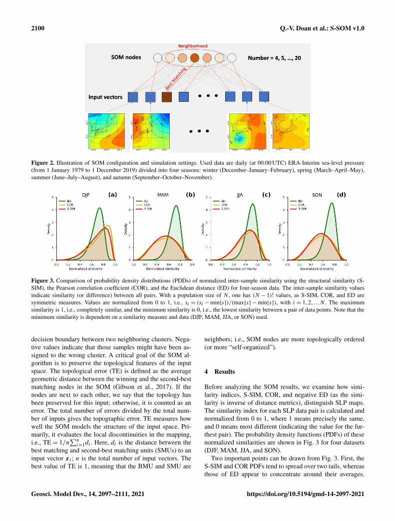
Figure 2. Illustration of SOM configuration and simulation settings. Used data are daily (at 00:00 UTC) ERA-Interim sea-level pressure(from 1 January 1979 to 1 December 2019) divided into four seasons: winter (December–January–February), spring (March–April–May),summer (June–July–August), and autumn (September–October–November).

Figure 3. Comparison of probability density distributions (PDDs) of normalized inter-sample similarity using the structural similarity (S-SIM), the Pearson correlation coefficient (COR), and the Euclidean distance (ED) for four-season data. The inter-sample similarity valuesindicate similarity (or difference) between all pairs. With a population size of N , one has (N − 1)! values, as S-SIM, COR, and ED aresymmetric measures. Values are normalized from 0 to 1, i.e., si = (si −min{s})/(max{s}−min{s}), with i = 1,2, . . .N . The maximumsimilarity is 1, i.e., completely similar, and the minimum similarity is 0, i.e., the lowest similarity between a pair of data points. Note that theminimum similarity is dependent on a similarity measure and data (DJF, MAM, JJA, or SON) used.

decision boundary between two neighboring clusters. Nega-tive values indicate that those samples might have been as-signed to the wrong cluster. A critical goal of the SOM al-gorithm is to preserve the topological features of the inputspace. The topological error (TE) is defined as the averagegeometric distance between the winning and the second-bestmatching nodes in the SOM (Gibson et al., 2017). If thenodes are next to each other, we say that the topology hasbeen preserved for this input; otherwise, it is counted as anerror. The total number of errors divided by the total num-ber of inputs gives the topographic error. TE measures howwell the SOM models the structure of the input space. Pri-marily, it evaluates the local discontinuities in the mapping,i.e., TE= 1/n

∑ni=1di . Here, di is the distance between the

best matching and second-best matching units (SMUs) to aninput vector xi ; n is the total number of input vectors. Thebest value of TE is 1, meaning that the BMU and SMU are

neighbors; i.e., SOM nodes are more topologically ordered(or more “self-organized”).

4 Results

Before analyzing the SOM results, we examine how simi-larity indices, S-SIM, COR, and negative ED (as the simi-larity is inverse of distance metrics), distinguish SLP maps.The similarity index for each SLP data pair is calculated andnormalized from 0 to 1, where 1 means precisely the same,and 0 means most different (indicating the value for the fur-thest pair). The probability density functions (PDFs) of thesenormalized similarities are shown in Fig. 3 for four datasets(DJF, MAM, JJA, and SON).

Two important points can be drawn from Fig. 3. First, theS-SIM and COR PDFs tend to spread over two tails, whereasthose of ED appear to concentrate around their averages.



Table 1. Statistical indices of normalized discrimination distributions.

DJF MAM JJA SON

S-SIM COR ED S-SIM COR ED S-SIM COR ED S-SIM COR ED

Mean 0.70 0.72 0.69 0.53 0.54 0.69 0.61 0.62 0.68 0.55 0.56 0.71Standard deviation 0.17 0.18 0.10 0.18 0.19 0.10 0.16 0.17 0.09 0.17 0.18 0.09Skewness −0.73 −0.89 −0.78 −0.09 −0.12 −0.65 −0.42 −0.47 −0.71 −0.13 −0.19 −0.79Kurtosis 0.04 0.25 0.75 −0.70 −0.78 0.47 −0.31 −0.33 0.70 −0.60 −0.66 0.87

Figure 4. Winter (DJF) MSLP pattern revealed by SOMs. Panels (a)–(d) show S-SOM patterns (with four nodes); panel (e) shows thenumber of daily MSLPs classified as nodes 1 to 4. Panels (f)–(i) show the same result but for COR-SOM; (k)–(o) for ED-SOM.

The standard deviations of S-SIM and COR range 0.17–0.19,consistently higher than those of ED, which is 0.09–0.10 (Ta-ble 1). This result implies a higher ability of S-SIM and CORto recognize the inter-sample difference. Second, S-SIM andCOR PDF shapes tend to vary, whereas ED’s look identicalfor DJF, MAM, JJA, and SON. In other words, an S-SIM andCOR can effectively recognize seasonal variability, but EDdoes not. The PDFs of ED have the mean at about 0.69 to0.71, and skewness at about −0.65 to −0.79 among seasons.Meanwhile, the means of S-SIM and COR range widely from0.53 to 0.72, and skewness from −0.09 to −0.89. In partic-ular, for S-SIM and COR, the skewness is lower in DJF andJJA than in MAM and SON. In MAM and SON, the skew-ness is close to 0, meaning the PDFs are almost symmetric.

Regarding characterizing actual weather patterns, thePDFs of S-SIM and COR make more sense than those of ED.In DJF, Japan’s weather is dominated by the winter-type airpressure (high in the west and low in the east), with few ex-ceptions. This explains why the daily SLP in DJF looks sim-ilar most of the time; the PDFs’ mean is higher than in other

seasons; the skewness is deeply negative. The same weathertrend is observed in the summer months (JJA). Meanwhile, inMAM and SON, which are transition periods between winterand summer, and vice versa, the weather variability is higher,and there are no dominant patterns during these times.

Next, we analyze the outcome of SOMs to ensure that theresults are physically reasonable and match the common per-ception about seasonal weather patterns in Japan. Figure 4shows the SLP patterns typed by SOMs (node number equalto 4) from the winter simulation (DJF). It is well known thatthe Japanese winter is characterized by the Siberian High,which develops over the Eurasian continent, and the AleutianLow, which develops over the northern North Pacific. Pre-vailing northwesterly winds cause the advection of cold airfrom Siberia, bringing heavy snowfall to western Japan andsunny weather to the eastern side (http://www.data.jma.go.jp/gmd/cpd/longfcst/en/tourist_japan.html, last access: 6 Jan-uary 2021). Such a dominant pattern is likely to be well de-tected by S-SOM (Fig. 4a), COR-SOM (Fig. 4g), and ED-SOM (Fig. 4n).


http://www.data.jma.go.jp/gmd/cpd/longfcst/en/tourist_japan.html

http://www.data.jma.go.jp/gmd/cpd/longfcst/en/tourist_japan.html


Figure 5. Silhouette plots for S-, COR-, and ED-SOM clustering for winter months (DJF). Note that these are results from simulations withthe SOM-node size of 4. The vertical dashed red lines in each plot indicate the silhouette score.

An interesting difference between SOMs is that S-SOMappears to estimate a more “ordered” clustering of nodes(Fig. 4e), characterized by a dominant node (N1) accompa-nied by non-dominant ones. Meanwhile, for COR-SOM andED-SOM, the size of clusters is relatively identical, under-lining the presence of more “flat” clustering (Fig. 4j, o). Thisresult is consistently seen in other SOM-node configurations(i.e., node numbers greater than 4). “Ordered” clustering byS-SOM and “flat” clustering by COR- and ED-SOM are alsorecognized for JJA but to a lesser extent (see Fig. A3). Thephysical explanation for this is that two subperiods charac-terize the Japanese summer. The early subperiod is rainy,caused by the stationary Baiu front, where a warm maritimetropical air mass meets a cold polar maritime air mass. Inthe second subperiod, the North Pacific High extends north-westward around Japan, bringing hot and sunny conditions.The number of tropical cyclones passing the country peaksin August. Unlike DJF and JJA, MAM and SON are tran-sition seasons, and the difference (i.e., “ordered” and “flat”clustering) is not apparent among SOMs.

Moreover, silhouette analysis shows that S-SOM andCOR-SOM perform consistently better than ED-SOM inclustering SLP patterns. Figure 5 reveals two crucial points:one is the thickness of clusters (y axis) and the other is thesilhouette coefficient value. As explained above, for DJF, S-SOM estimates one dominant winter-type SLP pattern com-bined with minor exception patterns. This is different fromED-SOM, which predicts more “flat” clusters with the samethickness. Thus, S-SOM clustering makes more sense thanED-SOM, and COR-SOM is somewhere in between them.The dominant Japanese winter-type pattern can be easilyidentified by looking at the S-SOM plot, but this is not thecase with ED-SOM.

An important point here is that despite the “large” clus-ter, the silhouette values of S-SOM tend to be consistentlyhigher than those of COR- and ED-SOM (Fig. 5). This re-sult is highly counterintuitive because generally if the clus-ter is large, there is a higher possibility of data points be-ing assigned to the wrong cluster. Also, Fig. 6 summarizesthe silhouette score, compares three SOMs, and highlightstwo critical points: (i) S-SOM is consistently superior to

ED-SOM for all seasons and all SOM-node configurations,demonstrating that S-SOM offers higher quality clusteringthan ED-SOM, which is consistent and independent of simu-lations; COR-SOM has comparable performance to S-SOMin MAM and SON but scores lower in DJF and partly in JJA;(ii) although not obvious, the scores of S-SOM and COR-SOM vary seasonally, whereas those of ED-SOM are identi-cal among seasons. In particular, S-SOM scores the highestin weather types for DJF than for other seasons. Those areinteresting results, noting that DJF in Japan is experientiallyknown as the season most characterized by weather patternsin comparison to the other seasons.

As a measure of the topology preservation of SOM, TEindicates the lower error (higher topological preservation)of S-SOM, and partly COR-SOM, compared with ED-SOM(Fig. 7). Unlike with the silhouette score (Fig. 6), the differ-ence in the TE values among SOMs is less noticeable andless consistent among SOM-node configurations and inputdata. A lower TE is always seen for MAM and JJA with al-most all SOM size settings. However, for DJF, S-SOM hasa higher TE, especially when it has a small size of 4 or 5.For SON, there is no apparent difference among SOMs. AsTE is known to strongly depend on the neighborhood func-tion (Gibson et al., 2017), the similarity detection schememight have less impact. We also suggest that future stud-ies are needed to clarify the topology preservation ability ofSOMs with different similarity indices.

To confirm the above results, we have conducted addi-tional simulations for wind vectors, a different type of datafrom SLP. As wind vectors consist of two components, i.e.,zonal and meridional, we combine two components into onedata array to feed the SOM models for each input vector. Thetest result shows that the S-SOM and COR-SOM have bet-ter performance over ED-SOM regarding both the silhouettescore and the topographic error (see Figs. A8–A9 for refer-ence). This result is consistent with that of SLP experiments.

Besides, the computational time of SOMs is calculatedand shown in Fig. 8. ED-SOM needs 1–3 s to complete thejobs with node size ranging from 4–20. To do the same jobs,S-SOM needs 8–40 s, which are 10–15 times those of ED-SOM; COR-SOM needs 8–40 s or 8–13 times of ED-SOM.



Figure 6. Comparison of silhouette scores of S-, COR-, and ED-SOM for all SOM size configurations and four seasons, i.e., DJF, MAM,JJA, SON. In each plot, the x axis indicates a different SOM simulation (size configuration), and the y axis indicates silhouette score values.

Figure 7. Comparison of topographic errors of S-, COR-, and ED-SOM for all SOM size configurations and four seasons, i.e., DJF, MAM,JJA, SON. In each plot, the x axis indicates a different SOM simulation (size configuration), and the y axis indicates topographic errors.

Though S-SOM needs more computational cost, it does notproduce a critical issue as total computational time is small(less than 1 min) unlike the numerical weather prediction orclimate change projection.

5 Conclusions and remarks

In this study, we developed a novel SOM algorithm (S-SOM)for synoptic weather typing. The novelty of S-SOM is the uti-lization of the structural similarity index (S-SIM) for search-ing for the best matching unit. The performance of S-SOMhas been evaluated by a series of test simulations to cluster



Figure 8. Computational time of S-SOM, COR-SOM, and ED-SOM. The x axis indicates the SOM size configurations; the y axisrepresents the elapsed time needed to complete the jobs. These arethe results of the DJF experiments. Each experiment has with 3669input samples; the size of each sample is 65× 72 pixels. The num-ber of the SOM iteration steps is 5000.

two-dimensional SLP and wind patterns over the Japan re-gion.

Test results demonstrated the superior performance of S-SOM compared to the traditional ED-SOM (using the Eu-clidean distance). This result is consistent in all tests andSOM-node configurations in two respects: clustering qual-ity in terms of the silhouette analysis and topological preser-vation in terms of the topographic error. The performanceof S-SOM is higher than that of COR-SOM (using the Pear-son correlation coefficient) but not as straightforward as com-pared to ED-SOM.

We highlight the effectiveness of using S-SOM, and partlyCOR-SOM rather than traditional ED-SOM, at least whenspatial distributions feature input data. However, we empha-size that evaluation metrics other than the silhouette scoreand topographic errors should be used to robustify the resultsobtained in this study. Although this study did not assess theperformance of S-SOM on time series, we believe that S-SOM can also be useful for temporally distributed data. TheS-SOM performance with time series should be assessed ina further study. Moreover, although S-SOM has been devel-oped primarily for climatology studies, it can also be usedin other fields. We expect it will constitute the new standardSOM when dealing with “structural” input data.



Appendix A

Figure A1. Example faults with ED when distinguishing data thathave a spatial and temporal correlation. Suppose we have two dis-tributions represented by red and orange lines in each plot (a–c),where “H” and “L” are the locations of a high and a low, respec-tively. In panels (a)–(c), the red and orange lines have the same ED;meanwhile, if using the S-SIM index to compare the lines, one willhave the highest S-SIM value in panel (a), followed by panel (c);the S-SIM values in both panels (a, c) are much higher than that inpanel (b).

Figure A2. Spring (MAM) MSLP pattern revealed by SOMs. Panels (a)–(d) show S-SOM patterns (with four nodes); panel (e) shows thenumber of daily MSLPs classified as nodes 1 to 4. Panels (f)–(i) show the same result but for COR-SOM; (k)–(o) for ED-SOM.



Figure A3. Summer (JJA) MSLP pattern revealed by SOMs. Panels (a)–(d) show S-SOM patterns (with four nodes); panel (e) shows thenumber of daily MSLPs classified as nodes 1 to 4. Panels (f)–(i) show the same result but for COR-SOM; (k)–(o) for ED-SOM.

Figure A4. Autumn (SON) MSLP pattern revealed by SOMs. Panels (a)–(d) show S-SOM patterns (with four nodes); panel (e) shows thenumber of daily MSLPs classified as nodes 1 to 4. Panels (f)–(i) show the same result but for COR-SOM; (k)–(o) for ED-SOM.



Figure A5. Silhouette plot for S-, COR-, and ED-SOM clustering for spring months (MAM). Note that these are results from simulationswith the SOM-node size of 4. The vertical dashed red lines in each plot indicate the silhouette score.

Figure A6. Silhouette plot for S-, COR-, and ED-SOM clustering for summer months (JJA). Note that these are results from simulationswith the SOM-node size of 4. The vertical dashed red lines in each plot indicate the silhouette score.

Figure A7. Silhouette plot for S-, COR-, and ED-SOM clustering for autumn months (SON). Note that these are results from simulationswith the SOM-node size of 4. The vertical dashed red lines in each plot indicate the silhouette score.



Figure A8. Spatial patterns of the winter 500 hPa wind vector pattern revealed by SOMs with the size of 4. Panels (a)–(c) show the S-SOMresults and panel (d) shows the silhouette analysis plot; panels (f)–(j) show the same results but for COR-SOM and (k)–(o) for ED-SOM.Input data are daily base data (at 00:00 UTC) winter months (DJF) from 2009 to 2019.

Figure A9. Performance of S-, COR-, and ED-SOM for winter 500 hPa wind vector clustering. (a) The silhouette scores; (b) topographicerrors of SOMs at different node sizes.



Figure A10. Average silhouette scores of S-, COR-, and ED-SOM.The x axis indicates the SOM size configurations. The y axis showsthe silhouette score, which ranges from−1 to 1. For a given sample,the perfect cluster assignment has the value of 1, and negative valuesindicate the wrong cluster assignment for the sample.



Code and data availability. The exact version of the model usedto produce the results used in this paper is archived on Zenodo(https://doi.org/10.5281/zenodo.4437954, Doan, 2021), as are inputdata and scripts to run the model and make the plots for all the sim-ulations presented in this paper.

Author contributions. QVD designed the model and developed themodel code. HK and TS helped to design the test experiments.HK, TS, and FC helped to analyze the results. QVD prepared themanuscript with contributions from all co-authors.

Competing interests. The authors declare that they have no conflictof interest.

Financial support. This research was funded by the Envi-ronment Research and Technology Development Fund (JP-MEERF20192005) of the Environmental Restoration and Conser-vation Agency of Japan. Quang-Van Doan is grateful for supportfrom JSPS KAKENHI grant nos. JP20K13258 and JP19H01155.Fei Chen is grateful for support from the Water System Pro-gram at the National Center for Atmospheric Research (NCAR),NASA IDS grant no. 80NSSC20K1262, USDA NIFA grantnos. 2015-67003-23508 and 2015-67003-23460, NOAA grantno. NA18OAR4590398, and NSF grant no. 1739705.

Review statement. This paper was edited by David Topping and re-viewed by two anonymous referees.

References

Alexander, L. V., Uotila, P., Nicholls, N., and Lynch, A.: A newdaily pressure dataset for Australia and its application to the as-sessment of changes in synoptic patterns during the last century,J. Climate, 23, 1111–1126, 2010.

Borah, N., Sahai, A., Chattopadhyay, R., Joseph, S., Abhilash, S.,and Goswami, B.: A self-organizing map–based ensemble fore-cast system for extended range prediction of active/break cy-cles of Indian summer monsoon, J. Geophys. Res.-Atmos., 118,9022–9034, 2013.

Chang, L.-C., Shen, H.-Y., and Chang, F.-J.: Regional flood inunda-tion nowcast using hybrid SOM and dynamic neural networks, J.Hydrol., 519, 476–489, 2014.

Dee, D. P., Uppala, S. M., Simmons, A. J., Berrisford, P., Poli,P., Kobayashi, S., Andrae, U., Balmaseda, M. A., Balsamo, G.,Bauer, P., Bechtold, P., Beljaars, A. C. M., van de Berg, I., Biblot,J., Bormann, N., Delsol, C., Dragani, R., Fuentes, M., Greer, A.J., Haimberger, L., Healy, S. B., Hersbach, H., Holm, E. V., Isak-sen, L., Kallberg, P., Kohler, M., Matricardi, M., McNally, A. P.,Mong-Sanz, B. M., Morcette, J.-J., Park, B.-K., Peubey, C., deRosnay, P., Tavolato, C., Thepaut, J. N., and Vitart, F.: The ERA-Interim reanalysis: Configuration and performance of the dataassimilation system, Q. J. Roy. Meteorol. Soc., 137, 553–597,https://doi.org/10.1002/qj.828, 2011.

Doan, Q. V.: S-SOM v1.0: A structural self-organizingmap algorithm for weather typing (Version V1), Zenodo,https://doi.org/10.5281/zenodo.4437954, 2021.

Gibson, P. B., Perkins-Kirkpatrick, S. E., and Renwick, J. A.: Pro-jected changes in synoptic weather patterns over New Zealandexamined through self-organizing maps, Int. J. Climatol., 36,3934–3948, 2016.

Gibson, P. B., Perkins-Kirkpatrick, S. E., Uotila, P., Pepler, A. S.,and Alexander, L. V.: On the use of self-organizing maps forstudying climate extremes, J. Geophys. Res.-Atmos., 122, 3891–3903, 2017.

Han, F. and Szunyogh, I.: A Technique for the Verification of Pre-cipitation Forecasts and Its Application to a Problem of Pre-dictability, Mon. Weather Rev., 146, 1303–1318, 2018.

Horton, D. E., Johnson, N. C., Singh, D., Swain, D. L., Rajaratnam,B., and Diffenbaugh, N. S.: Contribution of changes in atmo-spheric circulation patterns to extreme temperature trends, Na-ture, 522, 465–469, 2015.

Kaski, S.: Data Exploration Using Self-Organizing Maps. ActaPolytechnica Scandinavica, Mathematics, Computing and Man-agement in Engineering Series No. 82, Finnish Academy ofTechnology, Espoo, Finland, ISBN 978-952-5148-13-8, 1997.

Kohonen, T.: A simple paradigm for the self-organized formationof structured feature maps, in Competition and cooperation inneural nets, Springer, 248–266, 1982.

Lagerquist, R., Flannigan, M. D., Wang, X., and Marshall, G. A.:Automated prediction of extreme fire weather from synoptic pat-terns in northern Alberta, Canada, Can. J. For. Res., 47, 1175–1183, 2017.

Lennard, C. and Hegerl, G.: Relating changes in synoptic circula-tion to the surface rainfall response using self-organising maps,Clim. Dynam., 44, 861–879, 2015.

Luong, T. M., Dasari, H. P., and Hoteit, I.: Extreme precipitationevents are becoming less frequent but more intense over Jeddah,Saudi Arabia. Are shifting weather regimes the cause?, Atmos.Sci. Lett., 21, e981, https://doi.org/10.1002/asl.981, 2020.

Lynch, A. H., Serreze, M. C., Cassano, E. N., Crawford, A. D., andStroeve, J.: Linkages between Arctic summer circulation regimesand regional sea ice anomalies, J. Geophys. Res.-Atmos., 121,7868–7880, 2016.

Mo, R., Ye, C., and Whitfield, P. H.: Application potential of fournontraditional similarity metrics in hydrometeorology, J. Hy-drometeorol., 15, 1862–1880, 2014.

Nguyen-Le, D. and Yamada, T. J.: Using weather pattern recog-nition to classify and predict summertime heavy rainfall occur-rence over the Upper Nan river basin, northwestern Thailand,Weather Forecast., 34, 345–360, 2019.

Nguyen-Le, D., Yamada, T. J., and Tran-Anh, D.: Classification andforecast of heavy rainfall in northern Kyushu during Baiu seasonusing weather pattern recognition, Atmos. Sci. Lett., 18, 324–329, 2017.

Ohba, M. and Sugimoto, S.: Differences in climate change im-pacts between weather patterns: possible effects on spatial het-erogeneous changes in future extreme rainfall, Clim. Dynam.,52, 4177–4191, 2019.

Ohba, M., Kadokura, S., and Nohara, D.: Medium-range prob-abilistic forecasts of wind power generation and ramps inJapan based on a hybrid ensemble, Atmosphere, 9, 423,https://doi.org/10.3390/atmos9110423, 2018.


https://doi.org/10.5281/zenodo.4437954

https://doi.org/10.1002/qj.828

https://doi.org/10.5281/zenodo.4437954

https://doi.org/10.1002/asl.981

https://doi.org/10.3390/atmos9110423


Rousseeuw, P. J.: Silhouettes: a graphical aid to the interpretationand validation of cluster analysis, J. Comput. Appl. Math., 20,53–65, 1987.

Shah-Hosseini, H.: Binary tree time adaptive self-organizing map,Neurocomputing, 74, 1823–1839, 2011.

Shah-Hosseini, H. and Safabakhsh, R.: TASOM: a new time adap-tive self-organizing map, IEEE T. Syst. Man. Cy. B, 33, 271–282,2003.

Sheridan, S. C. and Lee, C. C.: The self-organizing map in synopticclimatological research, Prog. Phys. Geogr., 35, 109–119, 2011.

Swales, D., Alexander, M., and Hughes, M.: Examining moisturepathways and extreme precipitation in the US IntermountainWest using self-organizing maps, Geophys. Res. Lett., 43, 1727–1735, 2016.

Wang, Z. and Bovik, A. C.: Mean squared error: Love it or leaveit? A new look at signal fidelity measures, IEEE Signal Process.Mag., 26, 98–117, 2009.

Wang, Z., Bovik, A. C., Sheikh, H. R., and Simoncelli, E. P.: Imagequality assessment: from error visibility to structural similarity,IEEE Trans. Image Process., 13, 600–612, 2004.


S-SOM v1.0: a structural self-organizing map algorithm ... - GMD

Documents

Transcript of S-SOM v1.0: a structural self-organizing map algorithm ... - GMD