an integrated environmental model tuned for - GMD

1

The Brazilian developments on the Regional Atmospheric

Modeling System (BRAMS 5.2): an integrated environmental

model tuned for tropical areas Saulo R. Freitas1,a, Jairo Panetta2, Karla M. Longo1,a, Luiz F. Rodrigues1, Demerval S. Moreira3,4, Nilton E.

Rosário5, Pedro L. Silva Dias6, Maria A. F. Silva Dias6, Enio P. Souza7, Edmilson D. Freitas6, Marcos Longo8, 5

Ariane Frassoni1, Alvaro L. Fazenda9, Cláudio M. Santos e Silva10, Cláudio A. B. Pavani1, Denis Eiras1, Daniela

A. França1, Daniel Massaru1, Fernanda B. Silva1, Fernando Cavalcante1, Gabriel Pereira11, Gláuber

Camponogara5, Gonzalo A. Ferrada1, Haroldo F. Campos Velho12, Isilda Menezes13,14, Julliana L. Freire1,

Marcelo F. Alonso15, Madeleine S. Gácita1, Maurício Zarzur12, Rafael M. Fonseca1, Rafael S. Lima1, Ricardo A.

Siqueira1, Rodrigo Braz1,Simone Tomita1, Valter Oliveira1, Leila D. Martins16 10

[1] Centro de Previsão de Tempo e Estudos Climáticos, Instituto Nacional de Pesquisas Espaciais, Cachoeira

Paulista, SP, Brazil

[2] Divisão de Ciência da Computação, Instituto Tecnológico de Aeronáutica, São Jose dos Campos, SP, Brazil

[3] Departamento de Física, Faculdade de Ciências, Universidade Estadual Paulista, Bauru, SP, Brazil. 15

[4] Centro de Meteorologia de Bauru (IPMet), Bauru, SP, Brazil.

[5] Universidade Federal de São Paulo, Campus Diadema, Diadema, SP, Brasil

[6] Instituto de Astronomia, Geofísica e Ciências Atmosféricas, Universidade de São Paulo, São Paulo, SP,

Brazil

[7] Departamento de Ciências Atmosféricas, Universidade Federal de Campina Grande, Campina Grande, PB, 20

Brazil

[8] Embrapa Informática Agropecuária, Campinas, SP, Brazil

[9] Instituto de Ciências e Tecnologia, Universidade Federal de São Paulo, São Jose dos Campos, SP, Brazil

[10] Centro de Ciências Exatas, Universidade Federal do Rio Grande do Norte, Natal, RN - Brasil

[11] Departamento de Geociências, Universidade Federal de São João del-Rei, MG, Brazil 25

[12] Laboratório Associado de Computação e Matemática Aplicada, Instituto Nacional de Pesquisas Espaciais,

São José dos Campos, SP, Brazil

[13] Instituto de Ciências Agrárias e Ambientais Mediterrânicas, Universidade de Évora, Évora, Portugal.

[14] Centro Interdisciplinar de Desenvolvimento em Ambiente, Gestão Aplicada e Espaço, Universidade

Lusófona de Humanidades e Tecnologia, Campo Grande, Lisboa, Portugal. 30

[15] Faculdade de Meteorologia, Universidade Federal de Pelotas, Pelotas, RS, Brazil

[16] Universidade Tecnológica Federal do Paraná, Londrina, PR, Brazil

aNow at Global Modeling and Assimilation Office, NASA Goddard Space Flight Center and USRA/GESTAR,

Greenbelt, MD, USA 35

Correspondence to: S. R. Freitas ([email protected])

Geosci. Model Dev. Discuss., doi:10.5194/gmd-2016-130, 2016Manuscript under review for journal Geosci. Model Dev.Published: 7 June 2016c© Author(s) 2016. CC-BY 3.0 License.

2

Abstract

We present a new version of the Brazilian developments on the Regional Atmospheric Modeling System where

different previous versions for weather, chemistry and carbon cycle were unified in a single integrated software

system. The new version also has a new set of state-of-the-art physical parameterizations and greater 5

computational parallel and memory usage efficiency. Together with the description of the main features are

examples of the quality of the transport scheme for scalars, radiative fluxes on surface and model simulation of

rainfall systems over South America in different spatial resolutions using a scale-aware convective

parameterization. Besides, the simulation of the diurnal cycle of the convection and carbon dioxide

concentration over the Amazon Basin, as well as carbon dioxide fluxes from biogenic processes over a large 10

portion of South America are shown. Atmospheric chemistry examples present model performance in

simulating near-surface carbon monoxide and ozone in Amazon Basin and Rio de Janeiro megacity. For tracer

transport and dispersion, it is demonstrated the model capabilities to simulate the volcanic ash 3-d redistribution

associated with the eruption of a Chilean volcano. Then, the gain of computational efficiency is described with

some details. BRAMS has been applied for research and operational forecasting mainly in South America. 15

Model results from the operational weather forecast of BRAMS on 5 km grid spacing in the Center for Weather

Forecasting and Climate Studies, INPE/Brazil, since 2013 are used to quantify the model skill of near surface

variables and rainfall. The scores show the reliability of BRAMS for the tropical and subtropical areas of South

America. Requirements for keeping this modeling system competitive regarding on its functionalities and skills

are discussed. At last, we highlight the relevant contribution of this work on the building up of a South 20

American community of model developers.

1 Introduction

The Brazilian developments on the Regional Atmospheric Modeling System version 5.2 (hereafter, BRAMS

5.2) is derived from the Regional Atmospheric Modeling System (RAMS, Cotton et al., 2003) originally

developed at Colorado State University in the USA. BRAMS/RAMS are multipurpose numerical weather 25

prediction models designed to simulate atmospheric circulations spanning from planetary scale waves down to

large eddies of the planetary boundary layer. BRAMS developed its own identity and diverged from RAMS

with several new features and modifications that have been included to improve the numerical representation of

fundamental physical processes on tropical and subtropical regions (Freitas et al., 2005b, 2009). Additionally,

BRAMS includes an urban surface scheme coupled with a photochemical model (Freitas et al., 2005a, 2007), a 30

complete in-line module for atmospheric chemistry and aerosol processes (Longo et al., 2013), as well as a

state-of-the-art surface scheme to simulate the energy, water, carbon and others biogeochemical cycles (Moreira

et al., 2013), which extend RAMS original functionalities towards a fully integrated environmental model.

Back in the 1990’s, a consortium between ATMET (Atmospheric, meteorological, and Environmental

Technologies) company from United States, the Institute of Mathematics and Statistics (IME), the Institute of 35

Astronomy, Geophysics and Atmospheric Sciences (IAG) of the University of São Paulo (USP) and the Center

for Weather Forecasting and Climate Studies of the Brazilian National Institute for Space Research

(CPTEC/INPE) started the BRAMS project funded by the Brazilian Funding Agency of Studies and Projects

(FINEP). Nowadays, BRAMS is one of the models operationally used at CPTEC and in several other regional

weather forecast centers in Brazil. In CPTEC, a previous version of BRAMS has been applied since 2003 for air 40


3

quality forecasting over a domain that encompasses the entire South America with a grid spacing of 25 km.

Simultaneous (in-line) predictions of weather and atmospheric composition are available in real time, including

smoke from vegetation fires. Since the 1st of January, 2013, BRAMS has been running operationally on the

CPTEC’s supercomputer, using 9600 cores, to process twice a day regional weather forecasts on 5 km grid

spacing and over a domain covering the entire South America and neighboring oceans. 5

BRAMS has also been applied for numerical studies in several universities and research centers addressing local

storms, urban heat island, urban and remote (e.g. fire emissions) air pollution, aerosol-cloud-radiation

interactions, carbon and water cycles over the Amazon, volcanic ash dispersion, etc. Numerous Ph.D. thesis and

Master dissertations, including institutions outside Brazil, have been written on BRAMS developments and

applications. 10

From the computational point of view, improved code structure and optimization ensures great scalability in

several architectures. BRAMS runs on massively parallel supercomputers, clusters, and personal x86 systems

with high efficiency. The development follows a modular approach to code design, allowing users to write and

plug in additional modules as necessary. BRAMS and its components are open source and available under the

GNU General Public License at the web page http://brams.cptec.inpe.br. 15

At this point, we believe BRAMS has capabilities analogous to the state-of-the-art limited area integrated

atmospheric chemistry transport models such as WRF-Chem (Grell et al., 2005) and COSMO-ART (Vogel et

al., 2009).

This paper is organized as follows. Section 2 introduces the modeling system focusing on the novelty in

comparison with the original RAMS mode. In Section 3 we highlight the main applications of BRAMS for 20

operational forecast of weather and integrated weather and chemistry on South America. Section 4 will

summary the accomplishments and session 5 will instruct about the code availability.

2 Model system description

BRAMS solves the compressible non-hydrostatic equations described by Tripoli and Cotton (1982), reproduced

here though omitting the horizontal and vertical grid transformations for convenience. The equations of motion 25

are:

∂u∂t

= −u∂u∂x

− v∂u∂y

− w∂u∂z

−θ ∂ ′π∂x

+ fv + ∂∂x

Km

∂u∂x

⎛⎝⎜

⎞⎠⎟+ ∂∂y

Km

∂u∂y

⎛⎝⎜

⎞⎠⎟+ ∂∂z

Km

∂u∂z

⎛⎝⎜

⎞⎠⎟

(1)

∂v∂t

= −u∂v∂x

− v∂v∂y

− w∂v∂z

−θ ∂ ′π∂y

− fu + ∂∂x

Km

∂v∂x

⎛⎝⎜

⎞⎠⎟+ ∂∂y

Km

∂v∂y

⎛⎝⎜

⎞⎠⎟+ ∂∂z

Km

∂v∂z

⎛⎝⎜

⎞⎠⎟

(2)

∂w∂t

= −u∂w∂x

− v∂w∂y

− w∂w∂z

−θ ∂ ′π∂z

−gθv

′

θ0

+ ∂∂x

Km

∂w∂x

⎛⎝⎜

⎞⎠⎟+ ∂∂y

Km

∂w∂y

⎛⎝⎜

⎞⎠⎟+ ∂∂z

Km

∂w∂z

⎛⎝⎜

⎞⎠⎟

(3)

The thermodynamic equation is: 30


4

∂θ il

∂t= −u

∂θ il

∂x− v

∂θ il

∂y− w

∂θ il

∂z+ ∂∂x

Kh

∂θ il

∂x⎛⎝⎜

⎞⎠⎟+ ∂∂y

Kh

∂θ il

∂y⎛⎝⎜

⎞⎠⎟+ ∂∂z

Kh

∂θ il

∂z⎛⎝⎜

⎞⎠⎟+

∂θ il

∂t⎛⎝⎜

⎞⎠⎟ rad

+∂θ il

∂t⎛⎝⎜

⎞⎠⎟ mic

+∂θ il

∂t⎛⎝⎜

⎞⎠⎟ con

(4)

The water species mixing ratio continuity equation reads:

∂rn

∂t= −u

∂rn

∂x− v

∂rn

∂y− w

∂rn

∂z+ ∂∂x

Kh

∂rn

∂x⎛⎝⎜

⎞⎠⎟+ ∂∂y

Kh

∂rn

∂y⎛⎝⎜

⎞⎠⎟+ ∂∂z

Kh

∂rn

∂z⎛⎝⎜

⎞⎠⎟+

∂rn

∂t⎛⎝⎜

⎞⎠⎟ mic

+∂rT

∂t⎛⎝⎜

⎞⎠⎟ con

(5)

Finally, for the mass continuity RAMS solves the equation, expressed in terms of the Exner function: 5

∂ ′π∂t

= −Rπ 0

cvρ0θ0

∂ρ0θ0u∂x

+∂ρ0θ0v∂y

+∂ρ0θ0w∂z

⎛⎝⎜

⎞⎠⎟

(6)

The previous equations are all Reynolds-averaged and the prognostic variables have the usual meaning (see

Table 1). BRAMS is equipped with a multiple-grid one-way nesting scheme to perform downscaling on

computational meshes of increasing spatial resolution. Original capabilities and physical formulations available

within RAMS model and inherited by BRAMS are described in Cotton et al. (2003) and references therein, 10

where the reader is asked to search for further information about RAMS, which shall not discussed here. This

paper will mostly concentrate on BRAMS additional features in comparison with the RAMS model. Table 2

summarizes the main options and characteristics present in BRAMS. The following sections introduce some key

aspects of BRAMS and exemplify its added capabilities.

2.1 Aspects of the Dynamics 15

2.1.1 Complete, mass conservative formulation for the Exner function prognostic equation

BRAMS original prognostic equation for the Exner function was derived by Klemp and Wilhelmson (1978,

hereafter KW78). The prognostic equation was obtained by combining the ideal gas equation with the mass

continuity equation for compressible fluids. Medvigy et al. (2005, hereafter M05) expanded the original Eq. 6,

which now reads 20

∂ ′π∂t

= −Rπ 0

cvρ0θ0

∂ρ0θ0u∂x

+∂ρ0θ0v∂y

+∂ρ0θ0w∂z

⎛⎝⎜

⎞⎠⎟

heat flux

−u∂ ′π∂x

− v∂ ′π∂y

− w∂ ′π∂z

advection

− R ′πcv

∂u∂x

+ ∂v∂y

+ ∂w∂z

⎛⎝⎜

⎞⎠⎟

divregence

+R( ′π +π 0 )

cvθv

dθv

dtheating

(7)

KW78 pointed out that the first term of the right-hand-side of Eq. (7) typically has a higher order of magnitude

than the other terms in studies of cloud dynamics, and the simplified version of Eq. (7) became the standard

solution in both RAMS and BRAMS. However, KW78 also pointed out that the simplified equation violates

mass conservation and deteriorates the accuracy of predicted pressure fields. M05 evaluated the conservation of 25

mass in a regional simulation for New England, and found the loss rates to be as large as 3% day-1, and showed


5

a significant improvement when the full equation was included. In this version of BRAMS, both the native and

the complete form of the prognostic equation are available, and following M05 implementation, in BRAMS 5.2

we also solved the advection, divergence, and heating terms of Eq. (7) using the main time step, whereas the

heat flux term is updated using the acoustic time step.

2.1.2 Time integration schemes 5

RAMS employs a hybrid time integration scheme combining leapfrog scheme for the wind components and

Exner function with forward-in-time for scalars. The computational mode produced by the leapfrog scheme is

damped with the application of the Robert-Asselin time filter (Asselin, 1972), which makes the overall accuracy

of 1st order. Williams (2009) proposed a simple modification in this time filter with few extra lines of coding but

increasing the accuracy of the scheme to 3rd order. This improved time filter is available in BRAMS by 10

appropriate setting of a flag in the RAMSIN namelist input file.

A third option for time integration in BRAMS in based on the work of Wicker and Skamarock (2002, hereafter

WS2002). This scheme has proven to be very robust and efficient being applied in several state-of-the-art non-

hydrostatic atmospheric models (e.g., Skamarock and Klemp, 2008, Baudauf, 2008 and 2010, Skamarock et al.,

2012). The WS2002 scheme is a low storage Runge-Kutta type with 3 stages and 3rd order for linear problems 15

(hereafter RK3). The 3 stages require 3 evaluations of the slow mode tendencies (e.g. advection term), however,

this cost is offset by the larger time step allowed by the scheme when allied with high order advection scheme

(see discussion in Section 2.1.3).

The last option for time integration scheme was described by Wicker (2009). This technique is made by a

combination of 2 schemes applied in 2 steps. A predictor step is performed applying Adams-Bashforth of 2nd 20

order scheme and then a corrector step is completed applying Adams-Moulton of 3rd order scheme (hereafter

ABM3). ABM3 is of 3rd order and requires only 2 evaluations of the slow mode tendencies, demanding,

however, a larger memory footprint than RK3 and a shorter time step. The advantage of using ABM3 over RK3

might arise when the length of the time step required by model stability is not dictated by the advective transport

but by other physical processes (e.g. cloud microphysics). 25

2.1.3 Additional advection schemes

2.1.3.1 Monotonic scheme for advection of scalars

An additional advection scheme, which preserves the initial monotonic characteristics of a scalar field being

transported with simultaneously levying low numerical diffusion, is available in BRAMS. The method

developed by Walcek (2000) is highly accurate and absolutely monotonic. Freitas et al. (2012) reported its 30

implementation in BRAMS and related impacts on the accuracy of the transport of relatively inert tracers as well

as on the formation of secondary species from non-linear chemical reactions of precursors. The results revealed

that the new scheme produces much more realistic transport patterns, without generating spurious oscillations

and under- and overshoots or diffusing mass away from the local peaks. Besides these features, the scheme also

presents good performance on retaining non-linear tracer correlations and conserving mass of multi-component 35

chemical species. The latter feature is not evident since monotonic preserving filters typically make the

numerical advection scheme non-strictly linear.

As an example of the application of this scheme within of BRAMS, the advection of a hypothetical rectangular

parallelepiped tracer field by a realistic 3-D wind flow is discussed as follow. The model was configured with


6

one grid with 10 km horizontal grid spacing covering the southeast part of Brazil and with a time step of 15

seconds. The total length of the time integration was 24 hours. The tracer mass mixing ratio is initiated with 100

au and the background is set to zero. The horizontal domain initially occupied by the tracer is shown on panel A

of Figure 1, while in the vertical the tracer was initially localized between 1.7 and 4.1 km in height (not shown).

The tracer mass mixing ratio distribution 12 hours after and simulated by the monotonic advection scheme is 5

shown on panel B of Figure 1. In this study, the original advection scheme of BRAMS noticeably introduced

spurious oscillations, overshoots and undershoots, the latter with negative values of mass mixing ratio (not

shown here, see Freitas et al 2012 for further details). On the other hand, the simulation produced by the new

scheme is much better at keeping the monotonicity of the distribution without spurious oscillations and negative

mass mixing ratio, even for a real strongly divergent and deformational wind as presented on panel B. 10

2.1.3.2 High order advection schemes

Following WS2002, BRAMS has also a new set of advection schemes to be applied in conjunction with RK3 or

ABM3 time schemes. The set is comprised of first to sixth order spatial approximations for the fluxes at the

edge of the grid cells. Also, exactly the same flux approximation can be applied for advection of scalars and

momentum. Positivity constraint for scalars can be applied following Skamarock (2006). 15

Future versions of BRAMS will include also monotonicity constraints for scalars and an option for the WENO

(Weighted Essentially Non-Oscillatory) 3rd and 5th orders formulation (Baba and Takahashi, 2013) for the

advection operators.

2.2 Physical parameterizations

2.2.1 Microphysics 20

2.2.1.1 Two-moment parameterization from RAMS/CSU

The current version of the two-moment (2M) microphysical parameterization used in RAMS, version 6, has

been implemented into BRAMS. This scheme has prognostic equations for number concentration and mixing

ratio for eight hydrometeors categories (cloud, drizzle, rain, pristine, snow, aggregates, graupel and hail). Each

hydrometeor size spectrum is described by a generalized gamma distribution with a user specified shape 25

parameter (Meyers et al., 1997, Saleeby and Cotton, 2004, 2008).

According to Cotton et al. (2003), the 2M microphysical scheme comes with an efficient and stable algorithm

for heat and vapor diffusion without requiring numerical iteration (Walko et al., 2000), sea salt and dust

treatment and bin sedimentation scheme. Lately, Saleeby and Cotton (2008) developed a binned approach to

cloud-droplet rimming, which computes the collision-coalescence process between ice and cloud particles in a 30

more realistic way.

Cloud and drizzle number concentrations are computed from cloud condensation nuclei (CCN) and Giant CCN

(GCCN) concentrations, respectively. A Look-Up-Table (LUT) is used to obtain the CCN concentration that is

activated as function of aerosol size, concentration, and composition via hygroscopicity parameter (Petters and

Kreidenweis, 2007), as well as updraft velocities, pressure and temperature. On the other hand, GCCN 35

activation does not depend on the environment conditions, being completely used into drizzle nucleation

process. Both aerosol categories may be advected, diffused, depleted and restored (by droplet evaporation) as

well as have their initial concentrations specified by the user as either homogeneous or heterogeneous fields

(Saleeby and Cotton, 2004, 2008).


7

2.2.1.2 Thompson cloud microphysics

The aerosol aware bulk microphysics scheme described in Thompson et al., (2008), and Thompson and

Eidhammer (2014), hereafter GT, was also implemented in BRAMS. The GT scheme treats five separate water

species, mixing single and double moment treatment for different cloud species to minimize computational cost.

It also includes the activation of aerosols as cloud condensation (CCN) and ice nuclei (IN) and, therefore, 5

explicitly predicts the droplet number concentration of cloud water as well as the number concentrations of the

two new aerosol variables, one each for CCN and IN. The aerosol species are lumped into two different groups

according to their hygroscopicity. Hygroscopic aerosols are in the general category of “water friendly” (Nwfa),

and the nonhygroscopic ice-nucleating aerosols are in the group “ice friendly” (Nifa). As a first approximation,

Nifa is assumed to be only mineral dust in the accumulation model; and all the other species (sulfates, sea salts, 10

and organic matter, and black carbon) are assumed to be a mixture of the species in each population and

allocated to the hygroscopic mode Nwfa.

Aerosol activation also uses a LUT of activated fraction determined by temperature, vertical velocity, aerosol

number concentration, and hygroscopicity parameter determined by the model. The lookup table was build

following Köhler activation theory within a parcel model from Feingold & Heymsfield (1992) with additional 15

changes by Eidhammer et al. (2009) to use the hygroscopicity parameter (Petters & Kreidenweis 2007). This

approach is similar to one used by RAMS CSU microphysics previously described (Saleeby and Cotton, 2004,

2008). However, the lookup-table of GT has a coarser variation in the terms of hygroscopicity parameter

compared to RAMS CSU. The coarse resolution of the LUT in terms of aerosol hysgroscopicity contributes to

GT scheme low cost, though also represents a limitation for ambient with high loading of very low hygroscopic 20

aerosols, such as biomass burning affected areas (Gácita et al., 2016).

2.2.1.3 Abdul-Rassack parameterization

As a low-cost option to the explicit aerosol aware microphysics schemes described above, the parameterization

of aerosol particle activation as CCN was also implemented following the approach of Abdul-Razzak and Ghan

(2000, 2002). This scheme, in its form for multiple log-normal distributions, assumes that the particles are in 25

equilibrium with the environment and the terms of curvature and the solute in the growth of the particle after the

activation can be neglected. As a first approach, for applications in a black-carbon rich atmosphere, the aerosol

activation can be done via Abdul-Rassack parameterization and feed either the GT or RAMS CSU microphysics

directly with the CCN number concentration.

2.2.2 Radiation 30

2.2.2.1 CARMA and RRTMG schemes

BRAMS radiation module includes two schemes to treat atmosphere radiative transfer consistently for both

long- and short-wave spectrum. The first scheme is a modified version of the Community Aerosol and Radiation

Model for Atmospheres (CARMA) (Toon et al., 1989), and the second one is the Rapid Radiation Transfer

Model (RRTM) version for GCMs (RRTMG, Mlawer et al. 1997; Iacono et al. 2008). RRTMG shares the same 35

basic physics as RRTM, though it incorporates several modifications (Iacono et al. 2008) in order to improve

computational efficiency. CARMA and RRTMG schemes both solve the radiative transfer using the two-stream

method and include all the major molecular absorbers (water vapor, carbon monoxide, ozone, oxygen) and

aerosol extinction. The RRTMG implementation preserved all the absorption coefficients for molecular species


8

used in the correlated k distribution method, which were based on a line-by-line model (Iacono et al., 2008).

CARMA treats gaseous absorption coefficients using an exponential sum formulation (Toon et al., 1989).

Radiation schemes in BRAMS are both on line coupled with the aerosol and cloud microphysics modules to

provide on line simulations of aerosol-cloud-radiation interactions.

Aerosol extinction is simulated feeding both CARMA and RRTMG radiative schemes with Aerosol Optical 5

Depth (AOD) profiles calculated from forecasted particles mass loading and prescribed aerosol intensive optical

properties, specifically the extinction efficiency, single scattering albedo and asymmetry parameter taken from a

LUT. Aerosol intensive optical parameters prescription is regionally dependent. For South America, the

parameters present in the LUT (Procopio et al. 2001, Rosario et al., 2013) are obtained from off-line Mie

calculations using as input climatological particle size distribution and the complex refractive index from sites 10

of the AErosol RObotic NETwork (AERONET, Holben et al., 1998) distributed across South America.

Cloud physical (ice and liquid water path and particle sizes) and optical properties (optical depth) in CARMA

radiative scheme, have been parameterized according to Sun and Shine (1994), Savijarvi (1997), and Savijarvi

et al. (1997, 1998) using liquid and ice water content profiles provided by BRAMS cloud microphysical module.

In this case, subgrid-scale cloud variability is not taken into account. 15

For RRTMG scheme, the optical properties of liquid and ice water are from Hu and Stamnes (1993) and Ebert

and Curry (1992), respectively, and subgrid-scale cloud variability including cloud overlap is statistically

addressed with McICA (Iacono et al., 2008), the Monte Carlo Independent Column Approximation [Barker et

al., 2002; Pincus et al., 2003].

The MCICA approach presupposes that cloud liquid water and ice, and cloud fraction are prognostic variables. 20

As so, the cloud liquid water effective radius was parameterized in BRAMS following the generalized power-

law expression of Liu et al. (2008):

𝑟!" =!

!!!!

!! 𝛽 !"#

!

!! (8)

where LWC is the liquid water content, and is the water density, and N is the cloud droplets number

concentration. L and N are in CGS units. b is a dimensionless parameter that depends on the spectral shape of 25

the cloud droplet distribution, set based on observation as:

𝛽 = 𝑎!!"#!

!!! (9)

with 𝑎! and 𝑏! equal to 0.07 and 0.14, respectively.

The cloud radiative forcing is very sensitive to the determination of b. According to Liu et al. (2008), b

increases with aerosol loading and leads to a warming effect that acts to substantially offset the cooling of the 30

Twomey effect by a factor of 10 to 80%. A b < 1/3 leads to a weaker dependence of rel on LWC/N and a

smaller indirect aerosol effect, with a better agreement with observation. In principle, this generalized power-

law expression for re, effectively accounts for the increase in droplet concentration and decrease in droplet size

due to aerosol (Twomey, 1974), as well as the reduction on precipitation efficiency, which increases the liquid

water content, the cloud lifetime (Albrecht, 1989), and the cloud thickness (Pincus and Baker, 1994). 35

The ice effective radius was parameterized in BRAMS following (Wyser, 1998), with an explicit dependence on

both ice water content and temperature:

𝑟!" = 377.4 + 203.3𝐵 + 37.91𝐵! + 2.3696𝐵! (10)

𝐵 = −2 + 10!! 273 − 𝑇 !.!𝑙𝑜𝑔!"!"#!"#!

(11)


9

where T is the temperature in Kelvin, IWC is the ice water content in gm-3, and IWC0=50gm-3.

This parameterization assumed the ice crystals consisting of hexagonal columns, and so is compatible with the

ice optical properties from Ebert and Curry (1992) assumed in RRTMG.

In addition, to fulfill MCICA requirements, a cloud fraction representation was also implemented in BRAMS,

based on the parameterization originally from the Community Atmosphere Model (CAM, 5

http://www.cesm.ucar.edu/models/cesm1.2/cam/), which is a generalization of the scheme introduced by Slingo

(1987), with variations described in Kiehl et al. (1998); Hack et al. (1994), and Rasch and Kristjánsson (1998).

In this representation, three types of cloud are diagnosed, depending on relative humidity, atmospheric stability,

and convective mass fluxes: low-level marine stratus, shallow and deep convective clouds, and layered cloud.

The marine stratus clouds are located according to the identification of stable layers between surface and 700 10

mb (> 0.125 K/mb) and using the following empirical relationship from Klein & Hartmann (1993):

𝐶!" = 𝑚𝑖𝑛 1. ,𝑚𝑎𝑥 0. , 𝜃!"" − 𝜃! ∗ .0.057 − 0.5573 (12)

where q700 and qs is the potential temperatures at 700 mb and surface levels, respectively. The stratus clouds are

located just below the strongest stability jump between these two levels.

The convective clouds fraction follows Xu and Krueger (1992) formulation based on the updraft mass flux, both 15

for shallow and deep:

𝐶!!!""#$ = 𝑘!,!!!""#$𝑙𝑛 (1.0 + 𝑘!𝑀!,!!!""#$) (13)

𝐶!""# = 𝑘!,!""#𝑙𝑛 (1.0 + 𝑘!𝑀!,!""#) (14)

With k1,shallow = 0.07 , k1,deep= 0.14, k2 =500, and Mc is the convective mass flux at the given level.

Any other clouds are diagnosed according to the relative humidity: 20

𝐶! = 𝑚𝑖𝑛 0.999, 𝑚𝑎𝑥 !!!!"!"#!!!"!"#

! (15)

𝑅𝐻!"# =𝑅𝐻!"#!"# , 𝑝 ≥ 750 𝑚𝑏𝑅𝐻!"#

!!"! , 𝑝 < 750 𝑚𝑏 (16)

with 𝑅𝐻!"#!"# = 0.90 and 0.80, over water and land, respectively, and 𝑅𝐻!"#!!"! = 0.80.

𝐶! = 𝑚𝑖𝑛 0.999, 𝑚𝑎𝑥 !!!!"!"#!!!"!"#

! (17)

The total cloud fraction in the grid cell is: 25

𝐶!"! = 𝑚𝑖𝑛 1,𝑚𝑎𝑥 𝐶!" ,𝐶!""#,𝐶!!!""#$ ,𝐶! (18)

The total cloud optical depth is given by the contribution from liquid and ice water contents, and as well account

for the cloud fraction.

2.2.3 Turbulence parameterizations

2.2.3.1 Nakanishi & Nino TKE based formulation 30

In BRAMS, as in the original RAMS formulation, the local changes of momentum and scalars due to turbulent

transport depend on the divergence of turbulent fluxes (RAMS, 2003). When the grid resolution is coarser than

the size of the largest eddies (typically coarser than 100m −1km), the eddy covariance fields needed to

determine the turbulent fluxes are determined through the K-theory (Stull, 1988), which requires the

determination of eddy diffusivities for momentum and scalar quantities 35


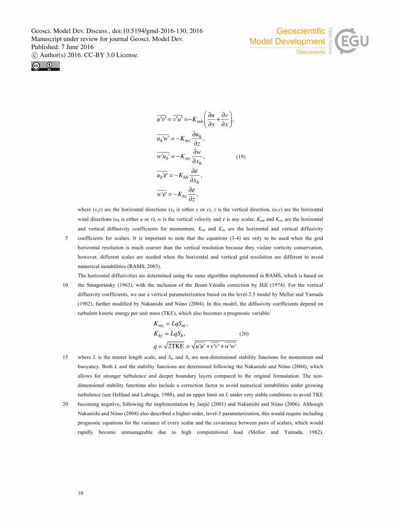
10

′u ′v = ′v ′u =−Kmh∂u∂y+ ∂v∂x

⎛⎝⎜

⎞⎠⎟,

uh'w' = −Kmz∂uh∂z

,

w'uh' = −Kmz∂w∂xh

,

uh'ε' = −Khh∂ε∂xh

,

w'ε' = −Khz∂ε∂z,

(19)

where (x,y) are the horizontal directions (xh is either x or y), z is the vertical direction, (u,v) are the horizontal

wind directions (uh is either u or v), w is the vertical velocity and ε is any scalar, Kmh and Kmz are the horizontal

and vertical diffusivity coefficients for momentum, Khh and Khz are the horizontal and vertical diffusivity

coefficients for scalars. It is important to note that the equations (3-4) are only to be used when the grid 5

horizontal resolution is much coarser than the vertical resolution because they violate vorticity conservation,

however, different scales are needed when the horizontal and vertical grid resolution are different to avoid

numerical instabilities (RAMS, 2003).

The horizontal diffusivities are determined using the same algorithm implemented in RAMS, which is based on

the Smagorinsky (1963), with the inclusion of the Brunt-Väisäla correction by Hill (1974). For the vertical 10

diffusivity coefficients, we use a vertical parameterization based on the level-2.5 model by Mellor and Yamada

(1982), further modified by Nakanishi and Niino (2004). In this model, the diffusivity coefficients depend on

turbulent kinetic energy per unit mass (TKE), which also becomes a prognostic variable:

Kmz = LqSm ,Khz = LqSh,

q = 2TKE = u'u'+v'v'+w'w'

(20)

where L is the master length scale, and Sm and Sh are non-dimensional stability functions for momentum and 15

buoyancy. Both L and the stability functions are determined following the Nakanishi and Niino (2004), which

allows for stronger turbulence and deeper boundary layers compared to the original formulation. The non-

dimensional stability functions also include a correction factor to avoid numerical instabilities under growing

turbulence (see Helfand and Labraga, 1988), and an upper limit on L under very stable conditions to avoid TKE

becoming negative, following the implementation by Janjić (2001) and Nakanishi and Niino (2006). Although 20

Nakanishi and Niino (2004) also described a higher-order, level-3 parameterization, this would require including

prognostic equations for the variance of every scalar and the covariance between pairs of scalars, which would

rapidly become unmanageable due to high computational load (Mellor and Yamada, 1982).


11

2.2.4 Surface interactions:

2.2.4.1 Town Energy Budget (TEB) scheme to simulate urban areas

For model domain including a significant portion of urban area, BRAMS offers the possibility of using a

combination of LEAF surface scheme (Walko et al., 2000) and the Town Energy Budget (TEB) (Masson, 2000;

Freitas et al., 2007). The use of the bare soil formulation or the adjustment in the surface-vegetation-atmosphere 5

transfer (SVAT) scheme parameters is very frequent. However, as stressed out by Masson (2000), such

approximations are satisfactory for large temporal or spatial averages, it is necessary to incorporate a more

detailed scheme when smaller scales are considered. Therefore, the simulation of several mesoscale and local

processes that simultaneously occurs in an urban atmosphere and its surroundings requires a more detailed

surface parameterization. Such processes include the circulations generated by urban heat islands (UHI) and its 10

interaction with other atmospheric phenomena (Freitas et al., 2007, Nair et al., 2004), air pollution (Andrade et

al., 2004, Freitas et al., 2005a), and human comfort conditions (Johansson et al., 2013), among others. In

BRAMS 5.2, the TEB scheme is activated together with LEAF, and the surface fluxes of momentum, moisture

and temperature and the surface albedo and emissivity are calculated by TEB whenever an urban grid point is

identified. LEAF is applied as usual for any other type of land use (e.g., bare soil, water bodies, grass, forest, or 15

any vegetation). TEB considers the interaction of short and long wave radiation with the urban structure,

allowing multiple reflections with walls and roads. In addition to the tridimensional urban structure in TEB

formulation, other advantage is the possibility to simulate the anthropogenic heat and moisture fluxes emitted

both by mobile sources, such as heavy and light duty vehicles, and fixed sources, such as industries, commerce

and domestic activities in general. For large cities, such as Sao Paulo and Rio de Janeiro, the anthropogenic heat 20

sources are a key feature, not only for meteorological reasons, but also for health and public policies

management. As anthropogenic contributions can vary strongly depending on the urban area, the

implementation of TEB in BRAMS allows the user to define those contributions in the model configuration file.

Based on the work of Khan and Simpson (2001), anthropogenic contributions can be estimated by considering

fuel and electricity consumption as well as the population and their related activities in the area of interest. For 25

the Metropolitan Area of Sao Paulo (MASP), Brazil, a region with more than 20 million people and more than 7

million vehicles, Freitas et al. (2007) considered maximum values of 30 and 20 W m-2 for the sensible heat flux

emission in the peak hours for vehicular and industrial contributions, respectively, which was enough to

represent most urban heat island features in the region during idealized simulations of the interaction between

the UHI and the sea-breeze. Nevertheless, higher values can be observed in other urban regions. Therefore, to 30

limber the model use, urban structure and anthropogenic contributions are user specified in the model namelist,

as presented in Table 3.

The diurnal cycle of vehicle activities and other related features (as pollutants emission, for example) are

dependent on local time. Therefore, there is an input file describing local time as function of latitude and

longitude of each grid point. Vehicular activity is defined in the model using a double normal distribution 35

centered on two values of the time of rush hours, which are user defined (Freitas et al., 2005a, 2007).

2.2.4.2 Joint UK Land Environment Simulator (JULES) model

In this section, the coupling between the Joint UK Land Environment Simulator (JULES) surface–atmosphere

interaction model (Best et al., 2011, Clark et al., 2011) and the BRAMS model is concisely described (for


12

further details the reader is referred to Moreira et al., 2013). JULES contains the state-of-the-art numerical

representation of surface processes and is able to simulate a number of soil-vegetation processes such as

vegetation dynamics, photosynthesis and plant respiration and also transport of energy and mass in soils and

plants, including a representation of urban elements. The combination between JULES and BRAMS is fully 2-

way with BRAMS providing atmospheric dynamics, thermodynamics and chemical constituents information to 5

JULES, which in turn responds with fluxes of horizontal momentum, water, energy, carbon and others tracers

exchanged between the atmosphere and the surface beneath. In JULES, the land surface is divided in sub-grid

boxes, which can be occupied by a number of plant functional types (PFTs) and non-functional plant types

(NPFTs). Up to five PFTs are allowed in each sub-grid box: broadleaf trees (BT), needleleaf trees (NT), C3

grasses (C3G), C4 grasses (C4G) and shrubs (Sh). A sub-grid box can also be occupied by up to four NPFTs: 10

urban, inland water, soil and ice. JULES adopts a tiled structure in which the surface processes are calculated

separately for each surface type. Its initialization requires: land cover and soil type classifications, normalized

difference vegetative index (NDVI), sea surface temperature, carbon and moisture soil contents and soil

temperature.

Moreira et al. (2013) indicated that the application of JULES on simulations over South America implied in 15

significant gain of skill compared to the original surface scheme in RAMS (LEAF3). As an example, Figure 4

shows model root-mean-square error (RMSE) of 2-meter temperature, which was calculated using observations

from ground stations distributed all over a large part of this continent. RMSE corresponds to the first 24-hour

forecast averaged over 30 runs on the wet (March, panel A) and dry seasons (September, panel B) of 2010.

During the night, both surface schemes present similar skills, with LEAF3 being slightly better in the dry 20

season. However, during daytime JULES notably improves model skills in both seasons. As daily average,

RMSE decreases by approximately 10% with the latter surface scheme.

2.2.5. Parameterizations of moist convection

2.2.5.1. Shallow convection

The shallow cumulus parameterization scheme in BRAMS is a mass flux type described in details by Souza 25

(1999). The cloud model follows the version of Albrecht et al. (1986) for a single-cloud formulation of the

Arakawa and Schubert (1974) ensemble scheme. The shallow cumulus characteristic in the cloud model is

obtained through an entraining function that gives more weight to the side entrainment as air parcels approach

the cloud top. Therefore, a lifted air parcel from near surface starts with a small entrainment of λ=10-6 m-1, and

this value increases by an order of magnitude each time the parcel reaches a ten-folding height zf, which is the 30

only adjustable parameter of the scheme. The entrainment rate is about 10-3 m-1 at the 2.1 km height and for a zf

of 0.7 km. The cloud top is reached when the total buoyancy of the parcel, integrated from the surface to the top,

becomes zero. The mass-flux formulation is based on the heat engine framework proposed by Rennó and

Ingersoll (1996). The derivation of the convective mass flux follows the rationale that the convective heat

engine, which is driven by surface heat flux, forces the upward motion of air masses. The convective flux is then 35

a result of the total forcing at the surface, namely the sum of the fluxes of sensible and latent heat, which are

converted into kinetic energy accordingly the second law of thermodynamics. Once surface fluxes start forcing

the heat engine, upward convecting air parcels might reach levels where water vapor saturation take place. The

triggering function follows the work of Wilde et al. (1985), which showed that moist parcels could give origin to


13

shallow cumuli only when the entrainment zone, located on top of the mixing layer, is above the lifting-

condensation-level zone.

The scheme is suitable to study the interaction between shallow convection and surface processes. The use of

this scheme in BRAMS improved the representation of the diurnal cycle of temperature and moisture over land.

The shallow scheme produces realistic results for convection associated with heterogeneous surface cover. The 5

impact is more pronounced during the afternoon by enhancing convective rain calculated by the model’s deep

convection scheme. Over the ocean, where the surface fluxes are less sensitive to solar forcing, shallow cumuli

can be activated anytime. This scheme has been applied operationally within BRAMS for the last two decades.

2.2.5.2 Grell and Deveny for deep convection

Grell and Deveny (2002, hereafter GD) deep convection scheme was included in BRAMS in 2002 and its 10

implementation is described in Freitas et al. (2005). One of the reasons for the GD inclusion in BRAMS was the

need of a mass flux scheme for a consistent convective transport of tracers. GD expanded the original

formulation based on Grell (1993) by including stochastic capability through permitting a series of different

assumptions that are widely used in convective parameterizations. The GD scheme can use a very large number

of ensemble members based on five different types of closure formulations, precipitation efficiency and the 15

ability of the source air parcels to overcome the convective inhibition energy.

Dos Santos el at. (2013) developed a method to generate a set of weights related with the closure members of

the GD ensemble to optimize the combination of them. As an inverse problem of parameter estimation, the

optimization problem for retrieving the weights applied a metaheuristic optimization method called Firefly

algorithm (FY, Yang, 2008). The method consists of minimizing an objective function computed with the 20

quadratic difference between BRAMS precipitation forecasts and observation, a measure of the distance

between the observational data and model results. The method demonstrated to be able to produce an ensemble

with improved statistical scores compared with the original ensemble mean calculation (dos Santos et al., 2013,

Santos, 2014). As an example, the categorical verification bias score computed for South America as depicted in

Figure 5. The mean of a set of 30 forecasts of 24-h accumulated precipitation for 120h in advance of 25

precipitation for January 2008 (panel A) and 2010 (panel B) was carried out using both GD ensemble arithmetic

mean (EN) and the ensemble mean using FY method in a 20km model grid configuration. The vertical bars in

Figure 5 refer to a significance test from the bootstrap method (Hamill, 1999). These results indicate a reduction

of bias in the low thresholds of precipitation, as well as an increase of the model skills for higher thresholds, in

agreement with the increase of Equitable Threat Score (not shown) for higher thresholds, both with statistical 30

significance, which demonstrates that FY is a robust method for training the GD ensemble of closures.

In addition, GD scheme in BRAMS contains an alternative option for the convective trigger function (CTF),

which was originally developed by Jakob and Siebesma (2003) and implemented by Santos e Silva et al. (2012).

In this formulation, the CTF is linked with the sensible and latent surface fluxes. Previous results, within both a

global model (Betchold et al., 2004) and BRAMS (Santos e Silva et al., 2012) showed improvements on 35

simulating the diurnal cycle of precipitation over continental areas, especially in tropical South-America.

2.2.5.3 A scale and aerosol aware convective parameterization for deep and shallow cumulus

The Grell and Freitas (2014, hereafter GF) scheme is based on the stochastic approach originally implemented

by GD with several additional features. One new feature is scale dependence formulations for high-resolution


14

runs (or gray-zone for deep convection model configurations) and interaction with aerosols. The scale

dependence was introduced by two approaches. One is based on spreading subsidence to neighboring grid points

instead of in the same model convective column, as usually done by classical convective parameterizations. The

second approach applies methods devised by Arakawa et al. (2011). This work reformulated the eddy fluxes

associated with the convective transports as a function of the updraft area fraction and the eddy fluxes given by 5

a closure of a conventional convective parameterization. The idea is readily applied to the conventional

parameterizations provided that a reliable formulation for the updraft area fraction is achieved. Because of its

simplicity and its capability for an automatic smooth transition as the resolution is increased, Arakawa’s

approach is recommended to the BRAMS users.

A second new feature present in GF is an aerosol awareness capability through a CCN (cloud condensation 10

nuclei number concentration) dependent autoconversion of cloud water to rain, as well as an aerosol dependent

evaporation of cloud drops. However, this feature is still in the experimental stage, so caution when using it is

advised.

Recently, the GF ensemble of closures has been extended to include a new closure inspired in ideas developed

by Bechtold et al., (2008, 2014 - hereafter B2014). In the B2014 paper, the authors derive a diagnostic CAPE 15

based closure where selective boundary layer time scales over land and water are applied. As a consequence,

theirs convective parameterization improved its capability on the representation of non-equilibrium convection

forced by boundary layer processes, with a more realistic phase of the associated diurnal cycle over land. In GF

scheme 2015 version (Freitas and Grell, in prep.), a corresponding closure, although built on the cloud work

function concept, is included. See the following discussion about model performance with this new closure. 20

Additionally, GF version 2015 contains a variant scheme for shallow convection (non-precipitating) with three

options for the closure of mass flux at cloud base (Freitas and Grell, in prep.).

Several experiments with BRAMS, with the Arakawa’s approach (GF-A), using horizontal grid-sizes of 5, 10

and 20 km were carried on to evaluate the performance of the GF scheme as well as its behavior on different

scales. For the 5 km model run we described also the performance of the scheme without applying any scale 25

correction (GF-NS). Each experiment comprised 15 runs from 1 to 15 January for 36-hour forecasts, all starting

at 00UTC. 24-hour precipitation accumulations used for verification are taken from 12 to 36-hour. Also, all

experiments covered the same region and used the same initial and boundary conditions, which were taken from

NCEP/USA Global Forecast System (GFS) analysis and forecast fields. Physical parameterizations included

CARMA radiation, JULES surface scheme, Mellor-Yamada 2.5 turbulence scheme and the single-moment bulk 30

microphysics parameterization from Walko et al. (1995). Model results are presented in Figure 6. Decreasing

the grid spacing from 20 to 5 km (panels A, B and C), detailed precipitation structures shows up, while the

broad precipitation distribution is preserved with the domain averaged precipitation, exhibiting deviation in a

10% range (between 4.1 and 4.5 mm/day). On the other side, the precipitation produced by CP only (lower row,

panels E, F and G) presents a consistent decrease, becoming less significant, from 3.5 to 1.0 mm/day, allowing 35

the dynamics and cloud microphysics be responsible for a much larger fraction of the total precipitation. Instead

of GF-A 5 km run, GF-NS (panel D) resulted in about 20% larger domain average precipitation with much

smoother spatial distribution. In Panel H, is shown that even on 5 km grid spacing, most of the precipitation (~

75%) is generated by the convection scheme. These results demonstrate the ability of the GF-A scheme to

produce a smooth transition across scales within the BRAMS modeling system. 40


15

Figure 7 introduces an exploratory study on the impacts of the B2014 closure (here called “diurnal cycle”

closure) on BRAMS results with respect the diurnal cycle of precipitation over the Amazon Basin. Model

configuration for this study comprised a grid with spacing of 27 km on horizontal and 80 to 850 m on vertical.

The physical parameterizations and initial and boundary condition were the same as of the preceding scale-

dependence experiment, but GF applied the B2014 approach. Again, model was setup to perform several runs 5

resembling the operational mode, comprising fifteen runs (from 1 to 15 February 2011) with 120-hour forecast

each.

Santos e Silva et al. (2009, 2012) discussed in details the diurnal cycle of precipitation over the Amazon Basin

using the TRMM rainfall product (Huffman et al., 2007) and observational data from a S band polarimetric

radar (S-POL) and rain gauges obtained in a field experiment during the wet season of 1999. Their analysis 10

indicated that a peak of rainfall is common late afternoon (between 1700 and 2100 UTC), in spite of variations

existent associated with wind regimes. Figure 7 shows model results with and without the diurnal cycle closure,

both panels depict area average precipitation from GF scheme (mm h-1), as well as downwelling short-wave

radiation (W m-2, DSWR). A sample of 5-day forecast initiating on 00UTC 1 February 2011 is presented on

Panel A. The simulated precipitation from GF scheme not applying the diurnal cycle closure shows a premature 15

peak with both precipitation and DSWR closely in phase. The introduction of the B2014 closure causes a shift

between the two curves delaying the peak of precipitation by about 3 hours, in better agreement with the

observation. The diurnal cycle averaged over the 15 runs with 120-hour forecast each is presented in panel B

clearly showing the rainfall shift, which demonstrates the robustness of the B2014 closure. One potential

drawback of this closure is the systematic reduction of the total amount of precipitation evidenced in panel B. 20

Future work will focus on this issue.

An example of real time rainfall forecast over South America with BRAMS using a different set of physical

parameterizations is discussed as follows. The case is associated with a mid-latitude cold front approach

together with tropical daytime convection over the northwest part of the Amazonia Basin and a weak band of

convection in the Inter-Tropical Convergence Zone (ITCZ) over the Atlantic Ocean. Figure 8 shows an estimate 25

of the 24-hour accumulated rainfall given by the TRMM product for the day 12 October 2015 and depicts

location and rainfall intensities of the cloud systems discussed above. This rainfall estimate is produced on a

grid with 0.25-degree resolution. Model forecast was done on 5 km horizontal grid spacing with the vertical

resolution varied from 50 m up to a maximum value of 850 m, with the top of the model at 19 km. The soil

model was composed of 7 layers distributed within the first 12 meters of the soil depth. Again GFS analysis and 30

forecast fields were used for initial and boundary conditions, while initial soil moisture was supplied following

Gevaerd and Freitas (2006) and the sea surface temperature was prescribed using data from Reynolds et al.

(2002). The physical parameterizations included RRTMG short- and long-wave radiation schemes, GF 2015

version for deep and shallow convection with the diurnal cycle closure, Thompson single-moment on cloud

liquid water (no aerosol aware option) cloud microphysics and the MYNN turbulence parameterization. The 35

model run was completed on a CRAY XE-6 supercomputer using 2400 cores. This configuration took 1.6 hour

to complete 24 hours forecast with 1360 x1480 on horizontal and 45 on vertical grid points and 12 seconds for

time step. The simulation applied the hybrid time integration scheme with RA time filter.

Figure 9 presents the 24-hour accumulated rainfall model forecast for this day. The total (resolved plus from

convection scheme) rainfall is shown on panel A. Visual comparison with TRMM rainfall (Figure 8) shows that 40


16

model properly reproduces the main rainfall patterns over different parts of South America, in spite of the

extreme amount of concentrated rainfall estimated by TRMM on Amazon Basin (around 50 S and 650 W) is

underestimated by the model. Similar model behavior is spotted on the Atlantic Ocean, close to the border

between Brazil and Uruguay. However, in general, model is able of the capture consistently the rainfall intensity

as well. Figure 9 B shows the separated contribution of the cumulus convection scheme on the total rainfall 5

(panel A). Noticeable is the fact that, on 5 km grid spacing, the scale awareness capability of the convection

scheme allows the rainfall associated with the mid-latitude cold front being almost entirely explicitly resolved.

On the other hand, over tropical areas a significant part of the total rainfall is rather generated by the convection

scheme suggesting the existence of much smaller scale rainfall systems, which is not explicitly captured on this

model resolution. 10

2.3 Atmospheric composition related processes and tracer transport

2.3.1 The CCATT in-line emission, deposition, transport and chemical reactivity model

The Coupled Chemistry-Aerosol-Tracer Transport model (Longo et al., 2013, hereafter CCATT) is a Eulerian

transport model coupled with BRAMS and developed to simulate the transport, dispersion, chemical

transformation and removal processes of gases and aerosols for atmospheric composition and air pollution 15

studies. CCATT computes the tracer transport in-line with the simulation of the atmospheric state by BRAMS,

using the same dynamical core, transport scheme and physical parameterizations. The prognostic of tracer mass

mixing ratio includes the effects of sub-grid-scale turbulence in the planetary boundary layer and convective

transports by shallow and deep moist convection, in addition to grid-scale advective transport. The model

includes also gaseous/aqueous chemistry, scavenging and dry depositions and aerosol sedimentation. 20

In a form of tendency, the general mass continuity equation for gas phase tracers solved in CCATT model is

∂s∂t

= ∂s∂t

⎛⎝⎜

⎞⎠⎟ adv

+ ∂s∂t

⎛⎝⎜

⎞⎠⎟ PBLdiff

+ ∂s∂t

⎛⎝⎜

⎞⎠⎟ deepconv

+ ∂s∂t

⎛⎝⎜

⎞⎠⎟ shallowconv

+ ∂s∂t

⎛⎝⎜

⎞⎠⎟ chem

+W + R +Q (21)

where is the grid box mean tracer mixing ratio, the term adv represents the 3-d resolved transport (advection

by the mean wind) and the terms PBL diff, deep conv and shallow conv are for the sub-grid scale turbulence in

the planetary boundary layer (PBL), deep and shallow convection, respectively. The chem term refers either to 25

the simple passive tracers’ lifetime (Freitas at al., 2009) or to the calculation of chemical loss and production

(Longo et al., 2013). The W is the term for wet removal applied only to aerosols, and R is the term for the dry

deposition applied to both gases and aerosol particles. Finally, Q is the emission source term, which for biomass

burning emissions also solves the plume rise mechanism associated with vegetation fires (Freitas et al., 2006,

2007, 2010). 30

In addition to CCATT-BRAMS code itself, the modeling system includes also three pre-processing software

tools for user-defined chemical mechanisms (M-SPACK, Longo et al., 2013), aerosol and trace gas emissions

fields (PREP-CHEM-SRC, Freitas et al., 20011) and the interpolation of initial and boundary conditions for

meteorology and chemistry (BC-PREP) (see Figure 10).

The choice of different chemistry mechanisms in CCATT-BRAMS is possible using a modified version of the 35

pre-processing tool SPACK (Simplified Pre-processor for Atmospheric Chemical Kinetics, Damian-Iordache

and Sandu, 1995; Djouad et al., 2002). The modified- SPACK (called hereafter M-SPACK) basically allow the

�

s


17

passage of a list of species and chemical reactions from symbolic notation (text file) to a mathematical one

(ODEs), automatically preprocesses chemical species aggregation and creates Fortran 90 routines files directly

compatible to be compiled within the main CCATT-BRAMS code. The M-SPACK output feeds also the codes

of the preprocessor tools PREP-CHEM-SRC and BC-PREP of emissions and the initial and boundary fields for

the chemical species, respectively, in order to ensure consistency between the several input database to be used 5

in CCATT-BRAMS and the list of species treated in chemical mechanism.

In principle, M-SPACK allows the use of any chemical mechanism in CCATT-BRAMS, though it requires the

built of emissions interface. The current version of M-SPACK includes three widely used tropospheric

chemistry mechanisms: RACM - Regional Atmospheric Chemistry Mechanism (Stockwell et al., 1997), Carbon

Bond (Yarwood et al., 2005), and RELACS - Regional Lumped Atmospheric Chemical Scheme, (Crassier et al., 10

2000), which considere, respectively, 77, 36 and 37 chemical species. Photolysis calculations are possible via

look-up tables of pre-calculated photolysis rates as well through Fast-J (Wild et al., 2000 and Brian and Prather,

2002) and Fast-TUV (Madronich, 1989, Tie et al., 2003) radiative codes. The latter approach provides on-line

calculation of photolysis rates, including interaction of radiation with aerosols and clouds.

CCATT-BRAMS performance has been extensively evaluated for both urban and biomass burning areas 15

(Freitas et al., 2009; Longo et al., 2009; Alonso et al., 2010; Longo et al., 2013 and Bela et al., 2015). Figure 11

and Figure 12 depict examples of model comparison results with mean daily values of carbon monoxide and

ozone mixing ratio measured near surface level in Porto Velho, Brazil from 14 August to 08 October 2012.

2.3.2 Simple Photochemical Model with TEB 20

BRAMS has also a simpler option for ozone forecasting suitable for urban areas. The Simple Photochemical

Model (SPM) is available in the model together with the TEB scheme (Freitas et al., 2005a). The model is

composed of 15 reactions related to ozone formation and consumption. This small number of reactions was

possible through the lamping of a large number of hydrocarbons, allowing a simplified way to deal with the

photochemical process in the model, which is very convenient to be used in the operational mode. TEB-SPM 25

considers industrial and vehicular emissions of carbon monoxide, volatile organic compounds (VOC), nitrogen

oxides (NOx), sulfur dioxide (SO2), and particulate matter (PM2.5). In spite of its very simple formulation, the

model has been used with relative success to simulate ozone concentrations in São Paulo (Freitas et al., 2005a)

and Rio de Janeiro metropolitan areas in Brazil. Figure 13, adapted from Carvalho (2010), shows a comparison

between model results and ozone observational data in two ground stations (Duque de Caxias and Jardim 30

Primavera) of an automated network maintained by the Rio de Janeiro’s Environmental Agency (INEA). As one

can see, the agreement is relatively high for a period over 7 days.

2.3.3 Carbon Cycle

This section introduces the capability of BRAMS composed with JULES on simulating CO2 fluxes associated

with biogenic activities. Here we discuss an example of model simulation for September 2010 over the Amazon 35

basin. Figure 14 presents the gross primary productivity (GPP, panel A), plant respiration (PR, panel B), soil

respiration (SR, panel C) and the net ecosystem exchange (NEE=PR+SR-GPP, panel D) all as a month average.

September corresponds to the last month of the Austral winter with typically very low amount rainfall over a

large part of Brazil. In this month, the ITCZ stays over positive latitudes inducing rainfall only on the northwest


18

part of South America, with warm temperatures (maximum around 33 C), low moisture and clear skies. The

abundance of photosynthetic active radiation and water availability at root zones of the tropical forest implies in

a large GPP over the region dominated by this land cover. As SR is mostly controlled by the soil humidity, the

larger values are present in the region with higher rainfall amounts, which are in the northwest part of the

domain shown. At the same time, over areas dominated by cerrado and caatinga biomes, dry soil conditions 5

dictate the response of the plants with very low values of GPP and SR. However, the simulated NEE presents a

complex spatial distribution, with values oscillating from around zero and extreme around +/- 10 µmolC m-2s-1,

meaning CO2 in/out- atmospheric fluxes (panel D).

BRAMS simulation of the diurnal cycle of CO2 in the low troposphere over the Amazon Basin is discussed as

follow. Figure 15 shows one-day simulation of CO2 mixing ratio and the turbulent kinetic energy (TKE) in the 10

low troposphere and DSWR at surface. In this figure, TKE is used as a proxy for the depth of the atmospheric

boundary layer, which evolves from a stable layer with less than 200 m depth during the nighttime and early

morning towards a convective and well-mixed boundary layer with maximum heights of 1.2 to 1.5 km on late

afternoon. The results show a realistic nighttime near surface accumulation of CO2 associated with the surface

(soil and vegetation) respiration and the shallow stable boundary layer. After that, with the sunrise and 15

increasing DSWR, the photosynthesis starts to dominate the net flux of CO2, which becomes more negative and

subtracts this gas from the atmosphere. In the same time, the heating of the surface produces buoyant air parcels,

which generates TKE deepening the mixing layer. As a result, CO2 is mixed up and depleted inside of this layer

with its mixing ratio ending smaller than the one of the free atmosphere on late afternoon.

2.3.4 Volcanic ash transport and dispersion 20

The BRAMS tracer transport capability also incorporates emission, transport, dispersion, settling and dry

deposition of volcanic emissions, both for ash and a set of related gases. This capacity represents a critical step

towards a numerical tool suitable not only for research, but also for an emergency, on-demand system for ash

dispersion forecast after a volcanic eruption event, which is required for the safety of the air traffic around

disturbed areas. The volcanic ash module follows closely the system described in Stueffer et al. (2013), and 25

more details of its implementation in BRAMS is provided in Pavani (2014) and Pavani et al. (2016). The input

needed to set up BRAMS for volcanic ash is produced using the PREP-CHEM-SRC (Freitas et al., 2011)

emissions preprocessing tool, which contains a comprehensive database developed by Mastin et al. (2009). This

database has information about 1535 volcanoes, including location (geographical position and height above sea

level of the vent) and a set of historical parameters (e.g., initial plume height, mass eruption rate, volume rate, 30

duration of eruption, and size distribution of the ash particle), which can be used as a first guess for a potential

returned volcanic eruption. However, by default, whenever available, observed real-time information overwrites

the historical ones. In BRAMS simulations, a vertical profile of the ash emission distribution is defined by a

linear detraining of 25% of the total ash mass below the injection height and 75% around it, obeying a parabola

shape. Pavani et al. (2016) adjusted an exponential curve between the rate of ash mass produced during the 35

eruption and the injection height, which is expressed as follow:


19

H = 0.34M 0.24 (22)

where H is the plume height in km (height above the vent) and M is the emission rate in kg/s. This fitting

formula is an additional method to make a first guess of the erupted mass of ash when the injection height is

known.

The model functionality for volcanic ash dispersion has been applied to real cases. One example is the eruption 5

of the Puyehue volcano in Chile, which occurred around 20:15 UTC on 04 June 2011 expelling a huge mass of

ash and gases up to 13 km height above the sea level. This eruptive event caused the closure of numerous

airports for many days and transport disruption in several countries in South America, South Africa, and even

Australia and New Zealand. Additionally, ash scavenging caused harm to agriculture and livestock, besides a

sort of other economical and health-public related issues. Costa et al. (2012) described the development and 10

application of a remote sensing technique for traces of ash retrieval based on METEOSAT-8 satellite data.

Figure 16 shows the location of ash as determined by this technique on 15 UTC on 06 June 2011, about 44

hours after the first eruption event. The eruption introduced material in the jet stream region, which was rapidly

eastward transported following Rossby wave circulation.

BRAMS results for this case study showed significant improvement with the use of the monotonic advection 15

scheme described on section 2.1.3.1, since monotonicity is required to properly model the long distance

transport of tracers associated with sharp, small-scale emission source within low-resolution atmospheric

models. An example of the model performance on simulating the long-range transport of ash is shown in Figure

17 (a more comprehensive analysis can be found in Pavani et al., 2016). Panel A shows the simulated vertically

integrated total mass of ash (mg m-2) for the same time of the remote sensing retrieval image (Figure 16). Panel 20

B presents the total ash mass concentration (µg m-3) at approximately 9,500 m above the surface. At beginning

of the eruption, ash was transported eastward for about 20 degrees, after then assumed an undulating shape

associated with the Rossby waves. The ash layer at 9,500 m constitutes primarily of small size particles, since

the larger and heavier ones quickly falls vertically due the gravitational force. The higher sensitivity of the ash

retrieval in the upper levels explains the better agreement between the ash distribution presented in this panel 25

and the traces of ash retrieved by remote sensing (Figure 16). The wider ash distribution close to the volcanic

vent on panel A is associated mainly with the vertical settling of the large, heavy ash particles that ends getting

different wind circulation and/or are quickly deposited over land.

2.4 Additional features, miscellaneous aspects

2.4.1 Coupling with the STILT Lagrangian Particle Dispersion Modelling 30

The Stochastic Time-Inverted Lagrangian Transport model (STILT, Lin et al., 2003) is a Lagrangian model

framework coupled with surface emission models, and has been used to identify sources and their influence on

receptors in studies with a multitude of scales and chemical components (see Gerbig et al., 2003, Miller et al.,

2008, 2013, Xiang et al., 2013, McKain et al., 2015). The core component of STILT is a Lagrangian particle

dispersion model that has two key features that allows for a realistic representation of dispersion: (1) STILT 35

accounts for sub-grid scale transport and dispersion by incorporating an stochastic component associated with

small-scale turbulence (Lin et al., 2003), (2) STILT also accounts for vertical transport due to parameterized

convective clouds (Nehrkorn et al., 2010). However, in order to take full advantage of BRAMS turbulent and

convective models, additional turbulence- and convection-related quantities are included in BRAMS output so


20

that can be directly used by STILT.

Following Lin et al. (2003), in STILT each wind component ui can be decomposed following a Markov

assumption, i.e. the grid volume average component ui and a turbulent component ui’. The turbulent

component is modeled after Hanna (1982), who defines the autocorrelation coefficient in terms of the

Lagrangian time scale TLi and the standard deviation of wind σui in the mixing layer: 5

ui' t +Δt( )=α i Δt( )ui' t( )+N 0,σ uit( )( ) 1− σ i Δt( )( )2 ,

α i Δt( )= exp −ΔtTLi

⎛

⎝⎜⎜

⎞

⎠⎟⎟,

(23)

where t is the previous time, ∆t is the time step, and N is a random number following the normal distribution

with mean 0 and standard deviation given by σui. For consistency with the turbulence scheme, the standard

deviation is computed following Nakanishi and Niino (2004). The Lagrangian time scale is determined

following the parameterization by Hanna (1982), which also depends on the boundary layer depth. Hanna 10

(1982) parameterization of the boundary layer depth depends on the reciprocal of vertical component of Coriolis

vorticity, which would cause singularities at the Equator. Therefore, we implemented an alternative

parameterization by Vogelezang and Holtslag (1996).

When BRAMS simulations are carried out using the Grell and Dévényi (2002) cumulus parameterizations, all

mass fluxes associated with updrafts and downdrafts (entrainment, detrainment, and vertical motion) are also 15

saved to the output, and can be used to assign both the probability of any particle to be in the environment or in

the cloud (either at the updraft or downdraft), as well as the vertical displacement of particles in case they are in

the updrafts or downdrafts, using the same method described by (Nehrkorn et al., 2010). Besides, the inclusion

of mass flux and turbulence-related variables in the output also allows a seamless integration with different

Lagrangian Particle Dispersion Models. 20

2.4.2 Coupling with an air parcel trajectories model

BRAMS simulated fields can readily be applied as input data to a 3-D air parcel kinematic trajectory model

described in Freitas et al. (1996, 2000). Forward and backward time integrations are allowed using a 2nd order

in time accurate scheme. The trajectories are computed using the same map projection and the vertical

coordinate of BRAMS and also includes a sub-grid scale vertical velocity enhancement associated with sub-grid 25

scale convection not explicitly solved by model dynamics.

2.4.3 Digital filter

A digital filter for model initialization has been implemented in BRAMS and demonstrated capability to reduce

high-order imbalances and inconsistencies among model variables, with potential to improve deterministic

forecasts. 30


21

2.4.4 Model output for GrADS visualization

A new feature present in BRAMS is the possibility of the model output be produced in GrADS

(http://iges.org/grads) format during the run time, simultaneously with the model integration. This feature is

especially important for operational centers by allowing faster generation of operational products.

2.5 Model data structure and code aspects 5

BRAMS code is mostly written in FORTRAN 95, with a few modules written in C. BRAMS has a pure MPI

parallelism. Only the horizontal domain is decomposed over MPI ranks. Prior to version 5, BRAMS had a

master-slave parallelism, where only the slaves advance the state of the atmosphere over time while the master

performs initialization, domain decomposition and I/O.

Around 2007, BRAMS was run on machines with less than 100 computing cores. Parallel scalability of BRAMS 10

on machines with higher core count was unknown. In 2007 CPTEC acquired the SUN-NEC cluster, named

UNA, with 275 nodes, each node with two dual-core AMD Opteron 2218, with a total of 1,100 cores. Each node

addresses 8 GB of central memory and the nodes are connected to a 70TB Lustre parallel file system. UNA was

used to enhance the parallel scalability of BRAMS from about 100 cores to about 1,000 cores. In 2011 CPTEC

acquired a Cray XE6 named “TUPA” with 1304 computing nodes, each node with two 12 cores AMD Opteron 15

Magny Cours with a total of 31,296 cores. Each node addresses 32 GB of central memory and the nodes are

connected to an 866TB Lustre parallel file system. TUPA was used to enhance BRAMS parallel scalability from

about 1,000 cores to about 10,000 cores.

Core count increase was used to enhance resolution. CPTEC’s operational domain covers most of South

America and parts of the surrounding oceans, spanning an area of approximately 6,800 km x 7,400 km. UNA 20

was used to enhance horizontal resolution from the previous operational resolution of 20 km to the new 10 km

resolution, keeping 38 vertical levels at both grids. TUPA was used to enhance horizontal resolution to 5 km and

increase the number of vertical levels to 45. The 5 km grid has about 90 million grid points, about 19 times the

number of grid points of the 20 km grid. To keep numerical stability according to the CFL condition, the time

step integration has to be decreased according to horizontal grid resolution, increasing the total amount of 25

computing from the 20 km grid to the 5 km grid by a factor of about 76 times per forecasting day. This increase

in computing has to be achieved by enhancing parallel scalability by a factor of 100, from about 100 cores to

about 10,000 cores.

Parallel scalability was enhanced by working on four unglamorous computing phases. Input and output

algorithms were sequential. Master-slave parallelism wasted computational resources and created unnecessary 30

synchronization points. Old coding practices used too much memory. Post-processing was offline and used a

sequential algorithm. The work on each of these four directions is summarized hereon.

On BRAMS version 4, input was performed by the master process. The master process input new boundary

conditions every three hours of forecast time, performed domain decomposition and sent the sub-domains to

slaves. This was a sequential algorithm since a single process (master) computed the decomposition and sent the 35

data. Consequently, runtime increased with the number of slaves since the number of data partitions (and

messages) increased with the number of slaves. BRAMS intermediate version 4.2 moved the domain

decomposition to the slaves (Fazenda et al., 2009 and Fazenda et al., 2011). The master process read each input

data field and broadcasted the full field to the slaves. Each slave extracted its own sub-domain from the


22

broadcasted field, parallelizing domain decomposition. Figure 18 contains the impressive execution time

reduction from the original version 4.0 sequential algorithm to the version 4.2 parallel algorithm as a function of

slave processes count. Data of Figure 18 was collected at UNA on a 24 hours forecast over the 20 km resolution

CPTEC’s operational grid.

On BRAMS version 4, the master process performed output. Each slave process sends its sub-domain to the 5

master process, that collected the slave partitions through MPI point-to-point communications, composed the

full field and outputs each field. Again, this was a sequential algorithm since its execution time increases with

the number of slaves. Two solutions were implemented at UNA and incorporated at BRAMS intermediate

version 4.2. The first solution was to use a collective MPI operation to gather all sub-domains of each field at

the master process prior to output. The second solution was to use UNA’s local disk at each node for output: 10

each slave wrote data on its own sub-domain to the local disk, moving the gather phase to post-processing.

Since execution time of MPI_Gather depends on the inter-node network speed, both solutions were kept as user-

selected options at run-time (Fazenda et al., 2009 and Fazenda et al., 2011). Figure 19 compares the execution

time of the output phase of the original version 4.0 sequential algorithm with both version 4.2 parallel

algorithms as a function of slave processes count. Data of Figure 19 was collected at UNA on a 24 hours 15

forecast over the 20 km resolution CPTEC’s operational grid.

Replacing BRAMS version 4 input and output sequential algorithms by version 4.2 parallel algorithms

substantially reduced the workload of the old master process. Thus, there is no reason to distinguish the master

process from slave processes, and all processes can perform the same computation (computing the timestep

phase), although only one of them (the old master, now MPI rank zero) performs I/O operations. 20

Elimination of the master process had a profound impact in code structure, since from the original version

thereon; BRAMS always had one set of procedures for the master process and a distinct set of procedures for

slave processes. It also contained a third set of procedures to connect master and slave codes just for sequential

(non-MPI) runs. BRAMS version 4.2 collapsed these three distinct source codes into a single code, since the

master/slave distinction occurred only at I/O, and a sequential computation can be performed on a single MPI 25

process.

Figure 20 shows the execution time reduction at UNA on 20 and 10 km grids due to input, output and code

structure optimizations just summarized (Fazenda et al., 2009 and Fazenda et al., 2011). These optimizations

increased parallel scalability, allowing execution time reduction by increasing core count.

The availability of TUPA allowed experimentation with the 5 km grid. The first experiments could not use all 30

cores in each node, due to the high memory requirement per MPI process. Only eight of the twenty-four cores

per node could be used at preliminary executions. A detailed analysis showed that the higher memory usage was

due to an old coding practice, from the times when dynamic memory allocation in Fortran was expensive:

allocate large scratch arrays at the beginning of the computation, keep these scratch arrays allocated throughout

the computation and use them whenever scratch areas where required. It turns out that there were just too many 35

and too large scratch areas. A long and tedious work replaced the largest scratch areas by dynamically allocated

and deallocated areas that exist only at required code sections. This procedure reduced the memory requirement

per process from the original 3.84 GB to 1.08 GB, allowing the use of all 24 cores per node (Fazenda et al.,

2012).


23

The left side of Figure 21 contains execution time of the 5 km grid on TUPA with fixed 400 nodes and

increasing core count per node from 1 to 24. It shows execution time stagnation around 4.800 cores. The right

side of the same figure shows execution time explosion on input, timestep and output phases as a percentage of

total execution time. It is clear that the output phase responsibility increases with core count, up to a point where

output dominates the computation. 5

The output phase at TUPA used the MPI_GATHER solution described above. The local disk output solution,

used at UNA, could not be used at TUPA, since TUPA computational nodes are diskless. A new form of output

had to be devised. MPI-IO and parallel HDF-5 were implemented as code options, selected at run-time. Both

forms of parallel I/O scaled correctly. Figure 22 contains the execution time and the parallel efficiency of the 5

km resolution grid on TUPA up to 9,600 cores. Execution time with 9,600 cores was low enough to allow daily 10

operational runs at CPTEC on the 5 km resolution since the end of 2012.

A recent, independent work (Souto et al., 2015) obtained even better scalability of BRAMS version 5 on the 5

km grid on the Santos Dumont cluster. This is an ATOS/BULL machine with 786 nodes, each node containing

two Intel Xeon E5-2695 with 12 cores each, totalizing 18,144 cores. The same grid on the same domain was run

from 1,024 cores to 13,400 cores, achieving a parallel efficiency of 78% on 13,400 cores with respect to the 15

1,024 cores execution.

2.6 Ongoing work features

2.6.1 Spread fire model

The Spread Fire (SFIRE) is a semi-empirical fire propagation model developed by Coen (2005), Clark et al.

(2004) and Mandel et al. (2009, 2011) that was coupled to BRAMS model and is currently under evaluation. 20

SFIRE simulates a fire propagation based on a spread rate S = S x, y, t in an orthogonal direction to the fire

boundary and expressed as a function of the wind 𝑣 = 𝑣 𝑥, 𝑦, 𝑧, 𝑡 and terrain gradient ∇𝑧. The model provides

the sensible and latent heat fluxes associated with the fire propagation (the second terms of RHS of Eq. 23 and

24, respectively) allowing feedbacks between the combustion processes and the surrounding atmosphere. The

total sensible QH and QE latent heat fluxes are given by 25

𝑄! = −𝑐!𝜌!𝑇∗𝑢∗ +𝐹 𝑇 − 𝐹 𝑡 + Δ𝑡

Δ𝑡1

1 +𝑀!𝑤ℎ (23)

𝑄! = −𝜒∗𝜌!𝑢∗ +𝐹 𝑇 − 𝐹 𝑡 + Δ𝑡

Δ𝑡𝑀! + 0.561 +𝑀!

𝑤𝐿 (24)

Here the fluxes are depending on properties of forestry fuels models, following Anderson (1982) categories, and

of an exponential decay function of total fuel fraction, F (see Table 4 for detailed description of the symbols).

The fuel fraction decreases exponentially from the initial ignition time ti (Albini, 1994) and is given by

𝐹 𝑥, 𝑦, 𝑡 =1

𝑎𝑟𝑒𝑎 𝑒!

!,!"#$ !!!! !,!! !,!

(!,!)∈ !(!)

𝑑𝑥𝑑𝑦

1 𝑜𝑡ℎ𝑒𝑟𝑤𝑖𝑠𝑒

(25)


24

To implement a link between SFIRE and BRAMS, an interface code was built inspired on the WRF version.

New modules for the memory allocation and initialization were developed and a new namelist (sfire.in) was

introduced. Currently, the fire spread model run only on a serial mode inside of a BRAMS parallel simulation.

Full parallelization of the SFIRE model is postponed for future versions. 5

The user needs to produce fuel models classes map and topography defined on the refined surface meshes used

by SFIRE, to do so the user must download any necessary high resolution fields (topography raster and FNNL

fuel models (Anderson, 1982)) and convert them into a SIG for ASCII format, through a Euclidean allocation

interpolation. Instead the user can, use topography from BRAMS, although it is highly smoothed for the needs

of sfire, and the code can’t benefit for more accurate fire spread computations, because required a high 10

resolution grid. This high resolution data is interpolated and assimilated by BRAMS-SFIRE in fire mesh

simulations.

The available atmospheric data to BRAMS is limited to around 111 km resolution an should simulated in

downscaling grids, each with a 4 to 5 refinement ratio, and can incorporated weather sounding data. BRAMS

model simulated on 3-D grid covering the Earth surface, and only the downscaling refined atmospheric domain 15

can be activated with the SFIRE model. BRAMS-SFIRE was applied to the region of Alentejo in Portugal, but

can be applied to any other region of the world. The coupled model has a input file named “namelist.fire” where

the user is able to introduce the properties of fuel models of the region of interest (Menezes, 2015).

The average sensible and latent heat fluxes released in the time interval t, t + ∆t , Eqs. 23 and 24, from SFIRE

are passed into the atmospheric model trough fluxes coming from boundary conditions and mixed in boundary 20

layer by the PBL scheme.

One of the results from the BRAMS-SFIRE simulation showed that over three regions, of flat land and low

hilly, the propagation of fireline originated sensible heat fluxes of 28 𝑘𝑊𝑚!! approximately. During its spread

over the fuel models 1 and 2, the fire burned them quickly and burned more slowly the fuel model 4, which

during its combustion was degrading fuel and releasing fluxes of about 2.5 𝑘𝑊𝑚!!, over fuel model 8 was 25

liberating fluxes on the order of 1.6 𝑘𝑊𝑚!! and 1.4 𝑘𝑊𝑚!!, and over fuel model 9 liberating fluxes of the

order of 1.2 𝑘𝑊𝑚!!, which glowed until its extinction which takes place to 0.75 𝑘𝑊𝑚!! values or less. The

spread was influenced by the topography gradient, following dispersion over valleys or down the mountain

(Ossa mountain range, Figure 23) or simply propagating into plain zones. In all three regions, propagation

occurred in an elliptical pattern. In Ossa mountain range region, the wind is anabatic with intensity 4.5 𝑚𝑠!! 30

and changes its pattern when fire outbreak begin to burn, becoming disordered with vortices on the fire which

increased the intensity of the wind to 7.5 𝑚𝑠!!, as the fire develops and fireline spread this pattern extends to

the entire region (Figure 23).

2.6.2 Shallow convection parameterization 35

Ongoing research and development includes the interaction between shallow cumulus and radiation. Preliminary

results show improvements in the representation of the surface radiation budget. It is also in development a

formulation for nighttime mechanically forced clouds.


25

3 Applications for weather and air quality forecasting

3.1 Regional air quality forecast

Since March 2003, previous versions of BRAMS are applied operationally at CPTE/INPE for integrated weather

and air quality forecasts over South America. Besides the traditional meteorological fields, forecast of biomass

burning related aerosols and the main trace gases prejudicial to the health public such as carbon monoxide and 5

ozone are generated once a day with 3-day ahead time window. The forecast is routinely available at the

webpage http://meioambiente.cptec.inpe.br/. For the next months, CPTEC/INPE plans to implement BRAMS

version 5.0 in the operational forecast system, running on 20 km grid spacing.

3.2 Regional and local scale weather forecast

Since January 2013, BRAMS has been applied operationally at CPTEC/INPE to provide up to 3½ days weather 10

forecast. The system ran twice a day on 5 km horizontal grid spacing with the grid domain encompassing the

South America continent and part of the neighbors Oceans. On vertical, model grid spacing starts with 50 m

increasing to 800 m at the upper levels. The numbers of grid points are 1360 x 1489 x 55 (~ 100 million grid

cells) and the model runs over 9600 cores to process the forecast, with initial and boundary conditions taken

from the GFS/NCEP global model, which are pre-processed using the RAMS ISAN analysis software package. 15

The forecast is on-line available at the web page

http://previsaonumerica.cptec.inpe.br/golMapWeb/DadosPages?id=Brams5. Robust evaluations of BRAMS 5

km forecasts are provided by Figure 24 and Figure 25. The former one shows BIAS and RMSE of five near

surface quantities (2-meter temperature and dew-point temperature, 10-meter wind speed, 24-h accumulated

precipitation and the mean sea level pressure). The evaluation was performed using observations from 20

approximately 1000 surface stations distributed all long of South America and for the time period comprising 15

January of 2013 to 15 January of 2015. The evaluated quantities have a BIAS in a numerical range of ~ -1.0 to ~

+1.0, which are consistent with mostly of state-of-the-art NWP models with forecast available for South

America. For RMSE, the 24-h accumulated precipitation shows the lower range of value (~1.75), with wind

speed, dew-point temperature and pressure oscillating around ~2.0. The temperature has the larger RMSE 25

(~2.25 K), with higher values during the dry season (austral winter). Sensitivities studies (not shown) have been

demonstrated that the initial soil moisture field, provided by the Gevaerd and Freitas (2006) technique and

currently used in the operations, has a significant accountability for this larger RMSE. Therefore, improving the

representation of soil moisture in the model would provide further gain in model skill.

Figure 25 shows model skill in terms of the Equitable Threat Scores (ETS) and the BIAS scores of the 24-h 30

accumulated rainfall for 36 and 60-hour time integration and averaged over the period of 15 January of 2013 to

15 January of 2015. The BIAS score measures the ratio of the frequency of forecast events to the frequency of

observed events, binned by certain thresholds. A perfect model would obtain a value of 1 for both ETS and

BIAS scores for any threshold. The forecast skills are very reliable and similar to the state-of-the-art NWP

models. ETS change from ~0.3 to ~0.07 from small to large thresholds. Over the South-Southeast portion of 35

Brazil, which corresponds to the larger amount of inhabitants of South America, the forecast has larger skill.

Regarding BIAS scores, the model tends to overestimate rain amount at the lower and higher thresholds but is

pretty close to the optimal value of 1 in between.


26

4 Conclusions

The original RAMS/CSU model was advanced towards a fully integrated regional atmospheric chemistry

model, which includes carbon and biogenic VOC’s cycles, aerosol effects, urban surfaces and others features,

giving rise to the Brazilian version named BRAMS. Besides, BRAMS runs on massively parallel

supercomputers, clusters, and personal x86 systems with high efficiency. 5

Here the main features of the latest version 5.2 are described which includes a state-of-the-art set of physical and

chemical parameterizations for radiation, cloud microphysics, scale-aware convective parameterization and

turbulence scheme, a land-surface model for urban areas and carbon cycle, and availability of higher order time

integration and advection schemes. BRAMS has being applied for scientific research related to severe weather,

urban heat island, urban and remote (e.g. fire emissions) air pollution, aerosol-cloud-radiation interactions, 10

carbon and water cycles over the Amazonia including aerosol effects, volcanic ash dispersion, and many others

subjects. For the purposes of operational environmental forecast, BRAMS is applied in several regional forecast

centers and at CPTEC/INPE, providing routinely weather and air quality forecasts for South America.

Besides its applications in research and operational forecasting, BRAMS has been a platform of joint model

development in South America, as so playing a great role on helping to build up a South American community 15

of atmospheric modelers. Highlights the participation of young scientists.

Lastly, to maintain and advance its competitive in the select team of limited area regional environmental models

in the world, BRAMS needs to keep expanding the community of user and developers, continue being tested

and evaluated against observations, and improving the sub-model components. Within the list of the

immediately needed improvements, is the introduction of a data assimilation procedure to allows BRAMS has 20

its own initial condition for the integration. This step is essential for a further and significant gain of skill of this

modeling system in both, operational and research areas.

5 Code availability

BRAMS software is available under the GNU Public License. The main code as well as pre- and post-

processing software and input data are available on the website http://brams.cptec.inpe.br/, which is officially 25

maintained by the CPTEC/INPE in Cachoeira Paulista, São Paulo, Brazil.

Acknowledgements

S. R. Freitas acknowledges partial support of this work by CNPq (306340/2011-9) and FAPESP (2014/01563-1

and 2015/10206-0) and K. M. Longo acknowledges partial support of this work by FAPESP (2014/01564-8). 30

This work was partially carried out during the sabbatical year of Dr. S. R. Freitas and Dr. K. M. Longo at the

Earth System Research Laboratory at the National Oceanic and Atmospheric Administration (ESRL/NOAA),

Boulder, USA. Both authors acknowledge the partial support by this institution. The authors acknowledge Drs.

Georg Grell from ESRL/NOAA and Michael Baldauf from Deutscher Wetterdienst (DWD), Germany, for their

collaboration on key aspects of this modeling system. 35

References

Abdul-Razzak, H., and Ghan, S. J.: A parameterization of aerosol activation 2. Multiple aerosol types, J.

Geophys. Res., 105(D5), 6837–6844, doi: 10.1029/1999JD901161, 2000.


27

Abdul-Razzak, H., and Ghan, S. J.: A parameterization of aerosol activation 3. Sectional representation, J.

Geophys. Res., 107(D3), 4026., doi: 10.1029/2001JD 000483, 2002.

Albini, F. A.: PROGRAM BURNUP: A simulation model of the burning of large woody natural fuels, final

Report on Research Grant INT-92754-GR by U.S.F.S. to Montana State Univ., Mechanical Engineering

Dept., 1994. 5

Ackerman, A. S., Hobbs, P. V., and Toon, O. B.: A model for particle microphysics, turbulent mixing, and

radiative transfer in the stratocumulus topped marine boundary layer and comparisons with

measurements, J. Atmos. Sci., 52, 1204 – 1236, 1995.

Albrecht, B. A., Ramanathan, V., and Boville, B. A.: The effects of cumulus moisture transports on the

simulation of climate with a general circulation model. J. Atmos. Sci., 43, 2443-2462, 1986. 10

Albrecht, B. A.: Aerosols, cloud microphysics, and fractional cloudiness, Science, 245(4923), 1227–1230, doi:

10.1126/science.245.4923.1227, 1989.

Anderson, H. E.: Aids to determining fuel models for estimating fire behavior, USDA Forest Service,

Intermountain Forest and Range Experiment Station, Research Report INT-122, 1982.

Alonso, M. F., Longo, K. M., Freitas, S. R., et al.: An urban emissions inventory for South America and its 15

application in numerical modeling of atmospheric chemical composition at local and regional scales.

Atmospheric Environment, 44, 5072, 2010.

Andrade, M.F., Ynoue, R.Y., Harley, R. and Miguel, A.H.: Air quality model simulating photochemical

formation of pollutants: the São Paulo Metropolitan Area, Brazil. International Journal of Environment

and Pollution, 22(4): 460 – 475, 2004. 20

Arakawa, A. and Schubert, W. H.: Interaction of a cumulus cloud ensemble with the large-scale environment.

Part I. J. Atmos. Sci., 31, 674-701, 1974.

Arakawa, A., Jung, J.-H., and Wu, C.-M.: Toward unification of the multiscale modeling of the atmosphere,

Atmos. Chem. Phys., 11, 3731-3742, doi:10.5194/acp-11-3731-2011, 2011.

Asselin, R.: Frequency filter for time integrations. Mon. Wea. Rev., 100, 487–490, 1972. 25

Baba, Y., and Takahashi, K.: Weighted essentially non-oscillatory scheme for cloud edge problem. Q. J. R.

Meteorol. Soc., 139, 1374–1388, doi: 10.1002/qj.2030, 2013.

Barker, H. W., Cole, J. N. S., Morcrette, J.-J., Pincus, R., Räisänen, P., von Salzen, K., and Vaillancourt, P.: The

Monte Carlo Independent Column Approximation: An assessment using several global atmospheric

models. Quart. J. Roy. Meteor. Soc., 134, 1463 – 1478, doi:10.1002/qj.303, 2008. 30

Baldauf, M.: Stability analysis for linear discretisations of the advection equation with Runge-Kutta time

integration, J. Comput. Phys., 227, 6638-6659, 2008.

Baldauf, M.: Linear stability analysis of Runge-Kutta based partial time-splitting schemes for the Euler

equations, Mon. Wea. Rev., 138, 4475-4496, 2010.


28

Ballester, F., Rodriguez, P., Iniguez, C., and et al.: Air pollution and cardiovascular admissions association in

Spain: results within the EMECAS project. J. Epidemiol. Community Health, 60(4): 328 - 336.

doi:10.1136/jech.2005.037978, 2006.

Bechtold, P., Chaboureau, J. P., Beljaars, A., Betts, A. K., Köhler, M., Miller, M., Redelsperger, J. L.: The

simulation of the diurnal cycle of convection precipitations over land in a global model. Quarterly Journal 5

Royal Meteorological Society, v.130, n. 604, p. 3119-3137, 2004.

Bechtold, P., Köhler, M., Jung, T., Doblas-Reyes, F., Leutbecher, M., Rodwell, M. J., Vitart, F. and Balsamo,

G.: Advances in simulating atmospheric variability with the ECMWF model: From synoptic to decadal

time-scales. Q. J. R. Meteorol. Soc., 134, 1337–1351, 2008.

Bechtold, P., Semane, N., Lopez, P., Chaboureau, J.-P., Beljaars, A., and Bormann, N.: Representing 10

equilibrium and nonequilibrium convection in large-scale models. J. Atmos. Sci., 71, 734–753, doi:

http://dx.doi.org/10.1175/JAS-D-13-0163.1, 2014.

Bela, M. M., Longo, K. M., Freitas, S. R., Moreira, D. S., Beck, V., Wofsy, S. C., Gerbig, C., Wiedemann, K.,

Andreae, M. O., and Artaxo, P.: Ozone production and transport over the Amazon Basin during the dry-

to-wet and wet-to-dry transition seasons, Atmos. Chem. Phys., 15, 757-782, doi:10.5194/acp-15-757-15

2015, 2015.

Best, M. J., Pryor, M., Clark, D. B., Rooney, G. G., Essery, R. . L. H., Ménard, C. B., Edwards, J. M., Hendry,

M. A., Porson, A., Gedney, N., Mercado, L. M., Sitch, S., Blyth, E., Boucher, O., Cox, P. M., Grimmond,

C. S. B. and Harding, R. J.: The Joint UK Land Environment Simulator (JULES), model description –

Part 1: Energy and water fluxes, Geosci. Model Dev., 4(3), 677–699, doi:10.5194/gmd-4-677-2011, 20

2011.

Carvalho, V. S. B.: O impacto das megacidades sobre a qualidade do ar: os casos das regiões metropolitanas de

São Paulo e :do Rio de Janeiro. 234 f. Tese de Doutorado – Instituto de Astronomia, Geofísica e Ciências

Atmosféricas, Universidade de São Paulo, São Paulo, 2010.

Carvalho, V. S. B. et al.: Air quality status and trends over the Metropolitan Area of São Paulo, Brazil as a result 25

of emission control policies. Environmental Science & Policy, 47: 68-79, 2015.

Clark, D. B., Mercado, L. M., Sitch, S., Jones, C. D., Gedney, N., Best, M. J., Pryor, M., Rooney, G. G., Essery,

R. L. H., Blyth, E., Boucher, O., Harding, R. J., Huntingford, C. and Cox, P. M.: The Joint UK Land

Environment Simulator (JULES), model description – Part 2: Carbon fluxes and vegetation dynamics,

Geosci. Model Dev., 4(3), 701–722, doi:10.5194/gmd-4-701-2011, 2011. 30

Clark, T. L., Coen, J. L., and Latham, D.: Description of a coupled atmosphere-fire model. International Journal

of Wildland Fire, 13, 49-64, 2004.

Coen, J. L.: Simulation of the Big Elk Fire using coupled atmosphere-fire modeling. International Journal of

Wildland Fire, 14, 49-59, 2005.


29

Cotton, W. R., Pielke Sr., R. A., Walko, R. L., Liston, G. E., Tremback, C. J., Jiang, H., McAnelly, R. L.,

Harrington, J. Y., Nicholls, M. E., Carrio, G. G., McFadden, J. P.: RAMS 2001: Current status and future

directions. Meteorol. Atmos. Phys., 82, 5–29, 2003.

Costa, S. M. S., Lima, W. F. A., Freitas, S. R., Ceballos, J. C., Rodrigues, J. V.: Monitoramento dos Traços de

Cinzas do Vulcão Chileno Puyehue-Cordón Caulle. In: Congresso Brasileiro De Meteorologia, 17. 5

(CBMET), 2012, Gramado. Annals, 1-5, 2012.

Deardorff, J.W.: Stratocumulus-capped mixed layers derived from a three-dimensional model, Boundary Layer

Meteorol., 18, 495-527, 1980.

Dos Santos, A. F., Freitas, S. R., de Mattos, J. G. Z., Campos Velho H. F., Gan, M. A., Luz, E. F. P, and Grell,

G.: Using the Firefly optimization method to weight the ensemble of rainfall forecasts of the Brazilian 10

developments on the Regional Atmospheric Modeling System (BRAMS). Adv. Geosci., 35, 123, 2013.

Ebert, E. E., and Curry, J. A.: A parameterization of ice cloud optical properties for climate models. J. Geophys.

Res., 97, 3831-3836, 1992.

Fazenda, A. L., Panetta, J., Rodrigues, L. F., Katsurayama, D. M., Motta, L. G., Navaux, P. O. A.:

Escalabilidade de aplicação operacional em ambiente massivamente paralelo, WSCAD-SSC, 2009. 15

Fazenda, A. L., Panetta, J., Katsurayama, D. M., Rodrigues, L. F., Motta, L. G., Navaux, P. O. A.: Challenges

and solutions to improve the scalability of an operational regional meteorological forecasting model,

International Journal of High Performance Systems Architecture, v. 3, p. 87, 2011.

Fazenda, A. L., Rodrigues, E. R., Tomita, S. S., Panetta, J., Mendes, C. L.: Improving the scalability of an

operational scientific application on a large multi-core cluster, WSCAD-SSC 2012. 20

Feingold, G., and Heymsfield, A. J.: Parameterizations of condensational growth of droplets for use in general

circulation models. J. Atmos. Sci.,49, 2325–2342, 1992.

Freitas, E. D., Rozoff, C. M., Cotton, W. R. et al.: Interactions of an urban heat island and sea breeze

circulations during winter over the Metropolitan Area of São Paulo - Brazil. Boundary - Layer

Meteorology, 122(1), 43-65, 2007. 25

Freitas, E. D., Martins, L.D., Dias, P.L.D. and Andrade, M.D.: A simple photochemical module implemented in

RAMS for tropospheric ozone concentration forecast in the metropolitan area of Sao Paulo, Brazil:

Coupling and validation. Atmospheric Environment, 39(34): 6352-6361, 2005a.

Freitas, S. R., Dias, M. A. F. S., Dias, P. L. S., Longo, K. M., Artaxo, P., Andreae, M. O., Fischer, H.: A

convective kinematic trajectory technique for low-resolution atmospheric models. Journal of Geophysical 30

Research, 105, D19, 24375-24386, 2000.

Freitas, S. R., Longo, K. M., Dias, M.A. Silva Dias, Artaxo, P.: Numerical modeling of air mass trajectories

from biomass burning areas of the Amazon basin. Anais da Academia Brasileira de Ciências, Brasil, v.

68, p. 193-296, 1996.

Freitas, S. R., Longo, K. M., Silva Dias, M., Silva Dias, P., Chatfield, R., Prins, E., Artaxo, P., Grell, G., and 35

Recuero, F.: Monitoring the transport of biomass burning emissions in South America, Environmental

Fluid Mechanics, 5 (1-2), 135-167, doi:10.1007/s10652-005-0243-7, 2005b.


30

Freitas, S. R., Longo, K. M., Silva Dias, M. A. F., Chatfield, R., Silva Dias, P., Artaxo, P., Andreae, M. O.,

Grell, G., Rodrigues, L. F., Fazenda, A., and Panetta, J.: The Coupled Aerosol and Tracer Transport

model to the Brazilian developments on the Regional Atmospheric Modeling System (CATT-BRAMS) –

Part 1: Model description and evaluation, Atmos. Chem. Phys., 9, 2843-2861, doi:10.5194/acp-9-2843-

2009, 2009. 5

Freitas, S. R., Longo, K. M., Alonso, M. F., Pirre, M., Marecal, V., Grell, G., Stockler, R., Mello, R. F., and

Sánchez Gácita, M.: PREP-CHEM-SRC – 1.0: a preprocessor of trace gas and aerosol emission fields for

regional and global atmospheric chemistry models, Geosci. Model Dev., 4, 419-433, doi:10.5194/gmd-4-

419-2011, 2011.

Freitas, S. R., Rodrigues, L. F., Longo, K. M., and Panetta, J.: Impact of a monotonic advection scheme with 10

low numerical diffusion on transport modeling of emissions from biomass burning, J. Adv. Model. Earth

Syst., 4, M01001, doi:10.1029/2011MS000084, 2012.

Gevaerd, R., and Freitas, S. R.: Estimativa operacional da umidade do solo para inicialização de modelos de

previsão numérica da atmosfera. Parte I: Descrição da metodologia e validação, Rev. Bras. Meteorol., 21,

1–15, 2006. 15

Gerbig, C., Lin, J. C., Wofsy, S. C., Daube, B. C., Andrews, A. E., Stephens, B. B., Bakwin, P. S., and Grainger,

C. A.: Toward constraining regional-scale fluxes of CO2 with atmospheric observations over a continent:

1. Observed spatial variability from airborne platforms, J. Geophys. Res.-Atmos., 108, 4756,

doi:10.1029/2002JD003018, 2003.

Grell, G.A., and Devenyi, D.: A generalized approach to parameterizing convection combining ensemble and 20

data assimilation techniques, Geoph. Res. Let., 29, 14, 10.1029/2002GL015311, 2002.

Grell, G. A.: Prognostic evaluation of assumptions used by cumulus parameterizations within a generalized

framework. Mon. Wea. Rev., 121, 764-787, 1993.

Grell, G.A., Peckham, S., McKeen, S., Schmitz, R., Frost, G., Skamarock, W. C., and Eder, B.: Fully coupled

“online” chemistry within the WRF model. Atmosph. Env., 39, 6957-6975, 2005. 25

Grell, G. A., and Freitas, S.R.: A scale and aerosol aware stochastic convective parameterization for weather and

air quality modeling. Atmos. Chem. Phys., 14, 5233, 2014.

Hack, J. J., Boville, B.A., Briegleb, B.P., Kiehl, J.T., Rasch, P.J., and Williamson, D.L.: Description of the

NCAR Community Climate Model (CCM2). NCAR Technical Note, NCAR/TN-382+STR, 1993.

Hamill, T. M.: Hypothesis Tests for Evaluating Numerical Precipitation Forecasts. Wea. Forecasting, 14, 155-30

167, 1999.

Hanna, S.: Applications in Air Pollution Modeling, in: Atmospheric Turbulence and Air Pollution Modelling,

edited by Nieuwstadt, F. and van Dop, H., vol. 1 of Atmospheric Sciences Library, chap. 7, pp. 275–310,

Springer Netherlands, doi:10.1007/978-94-010-9112-1_7, 1982.

Helfand, H. M., and Labraga, J. C.: Design of a Nonsingular Level 2.5 Second-Order Closure Model for the 35

Prediction of Atmospheric Turbulence, J. Atmos. Sci., 45, 113–132, 1988.


31

Hill, G. E.: Factors Controlling the Size and Spacing of Cumulus Clouds as Revealed by Numerical

Experiments, J. Atmos. Sci., 31, 646–673, 1974.

Holben, B. N., Eck, T. F., Slutsker, I., Tanre´ , D., Buis, J. P., Setzer, A., Vermote, E., Reagan, J. A., Kaufman,

Y. J., Nakajima, T., Lavenu, F., Jankowiak, I., and Smirnov, A.: AERONET – a federated instrument

network and data archive for aerosol characterization, Remote Sens. Environ., 66, 1–16, 5

doi:10.1016/s0034-4257(98)00031-5, 1998.

Hu, Y. X., and Stamnes, K.: An accurate parameterization of the radiative properties of water clouds suitable for

use in climate models. J. Clim. 6:728-742, 1993.

Huffman, G. J., Adler, R. F., Bolvin, D. T., Gu, G. J., Nelkin, E. J., Bowman, K. P., Hong, Y., Stocker, E. F.,

and Wolff, D. B.: The TRMM multi-satellite precipitation analysis (TMPA): Quasi-global, multiyear, 10

combined-sensor precipitation estimates at fine scales. J. of Hydrometeo., 8, 38-55. 2007.

Iacono, M. J., Delamere, J. S., Mlawer, E. J., Shephard, M. W., Clough, S.A., and Collins, W.D.: Radiative

forcing by long-lived greenhouse gases: Calculations with the AER radiative transfer models, J. Geophys.

Res., 113, D13103, doi:10.1029/2008JD009944, 2008.

Jakob, C., and Siebesma, A. P.: A new subcloud model for mass-flux convection schemes: influence on 15

triggering, updrafts properties, and model climate. Monthly Weather Review, 131, 9, 2765-2778, 2003.

Janjić, Z.: Nonsingular implementation of the Mellor-Yamada Level 2.5 Scheme in the NCEP Meso model,

Office note 437, National Center for Environmental Prediction, Boulder, CO, URL http:

//www.lib.ncep.noaa.gov/ncepofficenotes/2000s/, 2001.

Johansson, E., Spangenberg, J., Gouvêa, M.L. and Freitas, E.D.: Scale-integrated atmospheric simulations to 20

assess thermal comfort in different urban tissues in the warm humid summer of São Paulo, Brazil. Urban

Climate, 6(0): 24-43, 2013.

Khan, S. and Simpson, R.: Effect of a heat island on the meteorology of a complex urban airshed. Boundary-

Layer Meteorology, 100(3): 487-506, 2001.

Kiehl, J. T., J.J. Hack, G. B. Bonan, B. A. Boville, D. L. Williamson, and P. L. Rasch.: The National Center for 25

Atmospheric Research Community Climate Model: CCM3, J. Climate, 11, 1131-1149, 1998.

Klein, S. A. and Hartmann, D. L.: The seasonal cycle of low stratiform clouds. J. Climate, 6, 1588-1606, 1993.

Klemp, J. B. and Wilhelmson, R. B.: The Simulation of Three-Dimensional Convective Storm Dynamics, J.

Atmos. Sci., 35, 1070–1096, 1978.

Lin, J. C., Gerbig, C., Wofsy, S. C., Andrews, A. E., Daube, B. C., Davis, K. J., and Grainger, C. A.: A near-30

field tool for simulating the upstream influence of atmospheric observations: The Stochastic Time-

Inverted Lagrangian Transport (STILT) model, J. Geophys. Res.-Atmos., 108, 4493,

doi:10.1029/2002JD003161, 2003.

Liu, Y., Daum, P. H., Guo, H., and Peng, Y.: Dispersion bias, dispersion effect, and the aerosol-cloud

conundrum. Environ. Res. Lett., 3, doi:10.1088/1748-9326/3/4/045021, 2008. 35


32

Longo, K. M., Freitas, S. R., Pirre, M., et al.: The chemistry CATT-BRAMS model (CCATT-BRAMS 4.5): a

regional atmospheric model system for integrated air quality and weather forecasting and research. Geos.

Model Devel., 6, 1389, 2013.

Mandel, J., Beezley, J. D., Kochanski, A. K.: Coupled atmosphere wildland fire modeling with WRF 3.3 and

SFIRE 2011. Geosci. Model Dev., 4, 591–610, 2011. 5

Mandel, J., Beezley, J. D., Coen, J. L., Kim, M.: Data assimilation for wildland fires: Ensemble Kalman filters

in coupled atmosphere-surface models. IEEE Control Systems Magazine, 29, 47{65,

doi:10.1109/MCS.2009.932224, 2009.

Mlawer, E. J., Taubman, S. J., Brown, P. D., Iacono, M.J., and Clough S.A.: Radiative transfer for

inhomogeneous atmospheres: RRTM, a validated correlated-k model for the longwave. J. Geophys. Res., 10

102, 16,663-16,682, 1997.

Masson, V.: A physically-based scheme for the urban energy budget in atmospheric models. Boundary-Layer

Meteorology, 94(3): 357-397, 2000.

Mastin, L., Guffanti, M., Servranckx, R., Webley, P., Barsotti, S., Dean, K., Durant, A., Ewert, J., Neri, A., and

Rose, W.: A multidisciplinary effort to assign realistic source parameters to models of volcanic ash-cloud 15

transport and dispersion during eruptions, J. Volc. and Geoth. Res., 186, 1, 10-21, 2009.

McKain, K., Down, A., Raciti, S. M., Budney, J., Hutyra, L. R., Floerchinger, C., Herndon, S. C., Nehrkorn, T.,

Zahniser, M. S., Jackson, R. B., Phillips, N., and Wofsy, S. C.: Methane emissions from natural gas

infrastructure and use in the urban region of Boston, Massachusetts, Proc. Natl. Acad. Sci. U. S. A., 112,

1941–1946, doi:10.1073/pnas.1416261112, 2015. 20

Medvigy, D., Moorcroft, P. R., Avissar, R., and Walko, R. L.: Mass conservation and atmospheric dynamics in

the Regional Atmospheric Modeling System (RAMS), Environ. Fluid Mech., 5, 109–134,

doi:10.1007/s10652-005-5275-5, 2005.

Mellor, G. L. and Yamada, T.: Development of a turbulence closure model for geophysical fluid problems, Rev.

Geophys. Space Phys., 20, 851–875, doi:10.1029/RG020i004p00851, 1982. 25

Menezes, I. C.: Construção de um modelo de interacção atmosfera/fogo aplicado à gestão florestal e avaliação

de risco de fogos florestais no Alentejo. PhD thesis, University of Évora, Portugal, 2015.

Mercado, L. M., Bellouin, N., Sitch, S., Boucher, O., Hunting- ford, C., Wild, M., and Cox, P. M.: Impact of

changes in diffuse radiation on the global land carbon sink, Nature, 458, 1014– 1017,

doi:10.1038/nature07949, 2009. 30

Meyers, M. P., Walko, R. L., Harrington, J. Y., Cotton, W. R.: New RAMS cloud microphysics

parameterization: Part II. The two-moment scheme. Atmos. Res., 45, 3-39, 1997.

Miller, S. M., Matross, D. M., Andrews, A. E., Millet, D. B., Longo, M., Gottlieb, E. W., Hirsch, A. I., Gerbig,

C., Lin, J. C., Daube, B. C., Hudman, R. C., Dias, P. L. S., Chow, V. Y., and Wofsy, S. C.: Sources of

carbon monoxide and formaldehyde in North America determined from high-resolution atmospheric data, 35

Atmos. Chem. Phys., 8, 7673-7696, doi:10.5194/acp-8-7673-2008, 2008.


33

Miller, S. M., Wofsy, S. C., Michalak, A. M., Kort, E. A., Andrews, A. E., Biraud, S. C., Dlugokencky, E. J.,

Eluszkiewicz, J., Fischer, M. L., Janssens-Maenhout, G., Miller, B. R., Miller, J. B., Montzka, S. A.,

Nehrkorn, T., and Sweeney, C.: Anthropogenic emissions of methane in the United States, Proc. Natl.

Acad. Sci. U. S. A., 110, 20 018–20 022, doi:10.1073/pnas.1314392110, 2013.

Mlawer, E. J., Taubman, S. J., Brown, P. D., Iacono, M. J., and Clough, S. A.: Radiative transfer for 5

inhomogeneous atmosphere: RRTM a validated correlated-k model for the longwave, J. Geophys. Res.,

102, 16 663–16 682, 1997.

Moreira, D. S., Freitas, S. R., Bonatti, J. P., Mercado, L. M., Rosário, N. M. É., Longo, K. M., Miller, J. B.,

Gloor, M., and Gatti, L. V.: Coupling between the JULES land-surface scheme and the CCATT-BRAMS

atmospheric chemistry model (JULES-CCATT-BRAMS1.0): applications to numerical weather 10

forecasting and the CO2 budget in South America. Geos. Model Devel., 6, 1243-1259, 2013.

Nair, K.N. et al.: Dynamics of urban boundary layer over Sao Paulo associated with mesoscale processes.

Meteorology and Atmospheric Physics, 86(1-2): 87-98, 2004.

Nakanishi, M., and Niino, H.: An Improved Mellor–Yamada Level-3 Model with Condensation Physics: Its

Design and Verification, Boundary-Layer Meteorol., 112, 1–31, 15

doi:10.1023/B:BOUN.0000020164.04146.98, 2004.

Nakanishi, M., and Niino, H.: An Improved Mellor–Yamada Level-3 Model: Its Numerical Stability and

Application to a Regional Prediction of Advection Fog, Boundary-Layer Meteorol., 119, 397–407,

doi:10.1007/s10546-005-9030-8, 2006.

Nehrkorn, T., Eluszkiewicz, J., Wofsy, S. C., Lin, J. C., Gerbig, C., Longo, M., and Freitas, S.: Coupled weather 20

research and forecasting–stochastic time-inverted lagrangian transport (WRF–STILT) model, Meteorol.

Atmos. Phys., 107, 51–64, doi:10.1007/s00703-010-0068-x, 2010.

Pavanni, C., Freitas, S. R., Lima, W. F. A., Costa, S. M. S., Yoshida, M. C., Rosario, N. M.: Incluindo

funcionalidades no modelo BRAMS para simular o transporte de cinzas vulcânicas: descrição e análise de

sensibilidade aplicada ao evento eruptivo do Puyehue em 2011. Revista Brasileira de Meteorologia, 2016, 25

(in press).

Pavani, C. A. B.: Modelagem numérica do transporte de emissões vulcânicas: caso do vulcão Puyehue. 2014.

184 p. (sid.inpe.br/mtc-m18/2014/01.20.11.25-TDI). Dissertation (Master in Meteorology) - Instituto

Nacional de Pesquisas Espaciais (INPE), São José dos Campos, 2014. Available in:

<http://urlib.net/8JMKD3MGP8W/3FJUGQ8>. Access in: 27 may 2014. 30

Petters, M. D., and Kreidenweis, S. M.: A single parameter representation of hygroscopic growth and cloud

condensation nucleus activity, Atmos. Chem. Phys., 7(8), 1961–1971, doi: 10.5194/acp-7-1961-2007,

2007.

Pincus, R., and Baker, M. B.: Effect of precipitation on the albedo susceptibility of clouds in the marine

boundary layer. Nature, 372, 250-252, 1994. 35


34

Pincus, R, Barker, H.R., and Morcrette, J.-J.: A fast, flexible, approximate technique for computing radiative

transfer in inhomogeneous cloud fields. Journal of Geophysical Research 108:D13, 2003.

Rasch, P. J., and Kristjansson, J.E.: A comparison of the CCM3 model climate using diagnosed and predicted

condensate parameterizations. J. Clim., 11, 1587-1614, 1998.

Procopio, A. S., Remer, L. A., Artaxo, P., Kaufman, Y. J., and Holben, B. N.: Modeled spectral optical 5

properties for smoke aerosols in Amazonia, Geophys. Res. Lett., 30, 2265, doi:10.1029/2003gl018063,

2003.

RAMS: The Regional Atmospheric Modeling System: Technical Description (Draft), Technical report,

ATMET, Fort Collins, CO, USA., URL http://www.atmet.com/html/docs/ documentation.shtml, 2003.

Rennó, N. O., and Ingersoll, A. P.: Natural convection as a heat engine: A theory for CAPE. J. Atmos. Sci., 53, 10

572-585, 1996.

Reynolds, R. W., Rayner, N. A., T.M. Smith, Stokes, D. C., and Wang, W.: An Improved In Situ and Satellite

SST Analysis for Climate, J. Climate, 1609-1625, 15, 2002.

Rosário, N. E., Longo, K. M., Freitas, S. R., Yamasoe, M. A., and Fonseca, R. M.: Modeling the South

American regional smoke plume: aerosol optical depth variability and surface shortwave flux 15

perturbation, Atmos. Chem. Phys., 13, 2923-2938, doi:10.5194/acp-13-2923-2013, 2013.

Rothermel, R. C.: A Mathematical Model for Predicting Fire Spread in Wildland Fuels, USDA Forest Service,

Intermountain Forest and Range Experiment Station, Research Paper INT–115, Ogden, UT, 1972.

Rozoff, C.M., Cotton, W.R. and Adegoke, J.O.: Simulation of St. Louis, Missouri, Land Use Impacts on

Thunderstorms. Journal of Applied Meteorology, 42(6): 716-738, 2003. 20

Sánchez-Ccoyllo, O. R., Silva Dias, P. L., Andrade, M. F. and Freitas, S. R.: Determination of O3-, CO- and

PM10-transport in the metropolitan area of São Paulo, Brazil through synoptic-scale analysis of back

trajectories. Meteorology and Atmospheric Physics, 92(1): 83-93, 2005.

Sáchez Gácita, M., Longo, K. M., Freire, J. L. M., Freitas, S. R., Martin, S. T.: Impact of mixing state and

hygroscopicity on CCN activity of biomass burning aerosol in Amazonia. Atmos. Chem. Phys. Discuss., 25

doi:10.5194/acp-2016-248, 2016.

Saleeby, S. M., and Cotton, W. R.: A large-droplet mode and prognostic number concentration of cloud droplets

in the Colorado State University Regional Atmospheric Modeling System (RAMS). Part I: Module

descriptions and supercell test simulations. J. Appl. Meteor., 43, 182-195, 2004.

Saleeby, S. M., and Cotton, W.R.: A Binned Approach to Cloud-Droplet Riming Implemented in a Bulk 30

Microphysics Model. J. Appl. Meteo., 47, 694-703, 2008.

Santos, A. F.: Inverse problems using the optimization method firefly applied in the precipitation

parameterization of the model brams over South America. PhD thesis (in Portuguese) - National Institute

for Space Research (INPE), São José dos Campos, 2014.


35

Santos e Silva, C. M., Gielow, R. and Freitas, S. R.: Diurnal and semidiurnal rainfall cycles during the rain

season in SW Amazonia, observed via rain gauges and estimated using S-band radar. Atmosph. Sci. Lett.,

10: 87-93. doi: 10.1002/asl.214, 2009.

Santos e Silva, C. M., Freitas, S. R., Gielow, R.: Numerical simulation of the diurnal cycle of rainfall in SW

Amazon basin during the 1999 rainy season: the role of convective trigger function. Theoretical and 5

Applied Climatology, 109, 473-483, 2012.

Savijarvi, H., Shortwave optical properties of rain. Tellus, 49a, 177–181, 1997.

Savijärvi, H., Arola, A., and Räisänen, P.: Short-wave optical properties of precipitating water clouds, Q. J. Roy.

Meteor. Soc., 123, 883–899, doi:10.1002/qj.49712354005, 1997.

Savijarvi, H., and Raisanen, P.: Long-wave optical properties of water clouds and rain. Tellus, 50A, 1–11, 1998. 10

Skamarock, W. C.: Positive-definite and monotonic limiters for unrestricted-time-step transport schemes. Mon.

Wea. Rev., 134, 2241–2250, 2006.

Skamarock, W.C., and Klemp, J.B.: A time-split non-hydrostatic atmospheric model for weather research and

forecasting applications. J. Comput. Phys., 227, 3465-3485, doi: 10.1016/j.jcp.2007.01.037, 2008.

Skamarock, W. C., Klemp, J. B., Duda, M. G., Fowler, L. D., Park, S.H., and Ringler, T.D.: A multi-scale non-15

hydrostatic atmospheric model using centroidal Voronoi tesselations and C-grid staggering. Mon. Wea.

Rev., 240, 3090-3105, 2012.

Smagorinsky, J.: General circulation experiments with the primitive equations, Mon. Wea. Rev., 91, 99–164,

doi:10.1175/1520-0493(1963)091<0099:GCEWTP>2.3.CO,2, 1963.

Slingo, J. M.: The development and verifcation of a cloud prediction scheme for the ECMWF model. Quart. J. 20

Roy. Meteorol. Soc., 113, 899-927, 1987.

Souto, R. P., Silva Dias, P. L., Vigilant, F.: Parallel Performance Analysis of a Regional Numerical Weather

Prediction Model in a Petascale Machine, in High Performance Computing, Communications in

Computer and Information Science 565, pg 146-150, Springer 2015.

Souza, E. P.: Theoretical and numerical study of the relationship between convection and heterogeneous 25

surfaces in the Amazon region (in Portuguese). 121 p. PhD Dissertation – University of São Paulo, São

Paulo, 1999.

Souza, E. P., Rennó, N. O., and Silva Dias, M. A. F.: Convective circulations induced by surface

heterogeneities. J. Atmos. Sci., 57, 2915-2922, 2000.

Stueffer, M., Freitas, S. R., Grell, G., Webley, P., Peckham, S., Mckeen, S. A., Egan, S. D.: Inclusion of ash and 30

SO2 emissions from volcanic eruptions in WRF-Chem: development and some applications, Geos. Model

Devel., 6, 457, 2013.

Stull, R. B.: An introduction to boundary layer meteorology, Kluwer Academic Publishers, Dordrecht,

Netherlands, 1988.


36

Sun, Z. and Shine, K. P.: Studies of the radiative properties of ice and mixed-phase clouds, Q. J. Roy. Meteor.

Soc., 120, 111–137, doi:10.1002/qj.49712051508, 1994.

Tremback, C., Powell, J., Cotton, W., and Pielke, R.: The forward-in-time upstream advection scheme:

Extension to higher orders. Mon. Wea. Rev., 115, 540-555, 1987.

Thompson, G., and Eidhammer, T.: A study of aerosol impacts on clouds and precipitation development in a 5

large winter cyclone. J. Atmos. Sci., 2014.

Thompson, G., Field, P. R., Rasmussen, R. M., and Hall, W.D.: Explicit forecasts of winter precipitation using

an improved bulk microphysics scheme. Part II: Implementation of a new snow parameterization. Mon.

Wea. Rev., 136, 5095–5115, doi:10.1175/2008MWR2387.1, 2008.

Toon, O. B., McKay, C. P., Ackerman, T. P., and Santhanam, K.: Rapid Calculation of Radiative Heating Rates 10

and Photodissociation Rates in Inhomogeneous Multiple Scattering Atmospheres, J. Geophys. Res., 94,

16287-16301, 10.1029/JD094iD13p16287, 1989.

Tripoli, G. J., and Cotton, W. R.: The Colorado State University three-dimensional cloud/mesoscale model. Part

I: General theoretical framework and sensitivity experiments. J. de Rech. Atmos., 16, 185-220, 1982.

Twomey, S.: Pollution and the planetary albedo. Atmos. Environ. 8 (12): 1251–6. doi:10.1016/0004-15

6981(74)90004-3, 1974.

Vogelezang, D. and Holtslag, A.: Evaluation and model impacts of alternative boundary-layer height

formulations, Boundary-Layer Meteorol., 81, 245–269, doi:10.1007/BF02430331, 1996.

Vogel, B., Vogel, H., Bäumer, D., Bangert, M., Lundgren, K., Rinke, R., Stanelle, T.: The comprehensive model

system COSMO-ART - Radiative impact of aerosol on the state of the atmosphere on the regional scale, 20

Atmos. Chem. Phys., 9, 8661-8680, 2009.

Walko, R. L, W. R. Cotton, J. L. Harrington, M. P. Meyers: New RAMS cloud microphysics parameterization.

Part I: The single-moment scheme. Atmos. Res., 38, 29-62. 1995.

Walko, R. L., Tremback, C. J., Pielke, R. A., Cotton, W. R.: An interactive nesting algorithm for stretched grids

and variable nesting ratios. J. Appl. Meteor., 34: 994–999, 1995. 25

Walko, R., Band, L., Baron, J., Kittel, F., Lammers, R., Lee, T., Ojima, D., Pielke, R., Taylor, C., Tague, C.,

Tremback, C., and Vidale, P.: Coupled atmosphere-biophysics- hydrology models for environmental

modeling, J. Appl. Meteorol., 39, 6, 931–944, 2000.

Wang, T., Kwok, J.Y.H.: Measurement and analysis of a multi-day photochemical smog episode in the Pearl

River Delta of China. Journal of Applied Meteorology 42, 404–416, 2003. 30

Wicker, L. J., and Skamarock, W. C.: A time-splitting scheme for the elastic equations incorporating second-

order Runge-Kutta time differencing. Mon. Wea. Rev., 126, 1992–1999, 1998.

Wicker, L. J., and Skamarock, W. C.: Time-splitting methods for elastic models using forward time schemes.

Mon. Wea. Rev., 130, 2088–2097, 2002.


37

Wicker, L. J.: A two-step Adams-Bashforth-Moulton split-explicit integrator for compressible atmospheric

models, Mon. Wea. Rev., 137, 3588-3595, 2009.

Wilde, N. P., Stull, R. B. and Eloranta, E. W.: The LCL zone and cumulus onset. J. Climate. Appl. Meteor., 24,

640-657, 1985.

Williams, P. D.: A proposed modification to the Robert-Asselin time filter. Monthly Weather Review 137(8), 5

2538-2546, 2009.

Wyser, K., and Yang, P.: Average ice crystal size and bulk single-scattering properties of cirrus clouds. Atmos.

Res., 49, 315-335, 1989.

Xiang, B., Miller, S. M., Kort, E. A., Santoni, G. W., Daube, B. C., Commane, R., Angevine, W. M., Ryerson,

T. B., Trainer, M. K., Andrews, A. E., Nehrkorn, T., Tian, H., and Wofsy, S. C.: Nitrous oxide (N2O) 10

emissions from California based on 2010 CalNex airborne measurements, J. Geophys. Res. Atmos., 118,

2809–2820, doi:10.1002/jgrd.50189, 2013.

Xu, K-M, Arakawa, A., and Krueger, S. K.: The mascroscopic behavior of cumulus ensembles simulated by a

cumulus ensemble model. J. Atmos. Sci., 49, 2402-2420, 1992.

Yang, X.-S.: Nature-Inspired Metaheuristic Algorithms, Luviner Press, 2008. 15

20

25

30


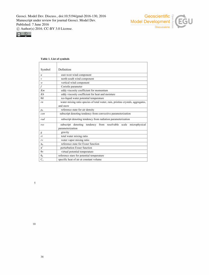
38

Table 1. List of symbols

Symbol

Definition

u east-west wind component v north-south wind component w vertical wind component f Coriolis parameter Km eddy viscosity coefficient for momentum Kh eddy viscosity coefficient for heat and moisture θil ice-liquid water potential temperature rn water mixing ratio species of total water, rain, pristine crystals, aggregates,

and snow ρ0 reference state for air density con subscript denoting tendency from convective parameterization

rad subscript denoting tendency from radiation parameterization

res subscript denoting tendency from resolvable scale microphysical parameterization

g gravity rt total water mixing ratio rv water vapor mixing ratio π0 reference state for Exner function π’ perturbation Exner function θv virtual potential temperature θ0 reference stare for potential temperature Cv specific heat of air at constant volume

5

10


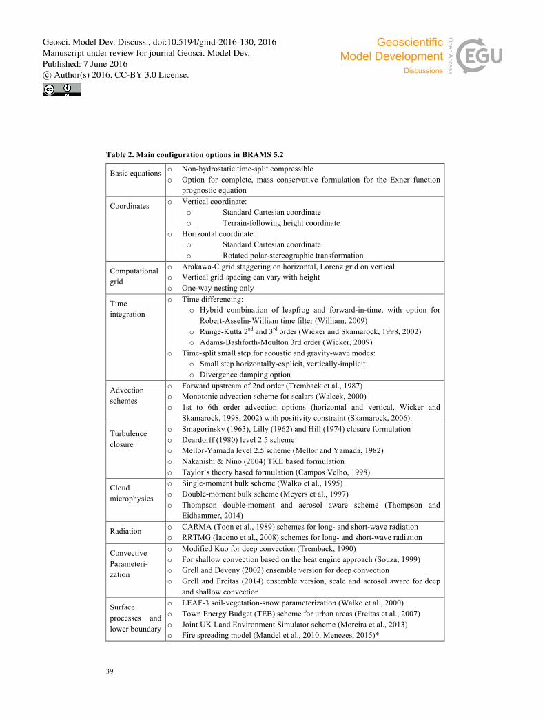
39

Table 2. Main configuration options in BRAMS 5.2

Basic equations o Non-hydrostatic time-split compressible o Option for complete, mass conservative formulation for the Exner function

prognostic equation

Coordinates o Vertical coordinate: o Standard Cartesian coordinate o Terrain-following height coordinate

o Horizontal coordinate: o Standard Cartesian coordinate o Rotated polar-stereographic transformation

Computational grid

o Arakawa-C grid staggering on horizontal, Lorenz grid on vertical o Vertical grid-spacing can vary with height o One-way nesting only

Time integration

o Time differencing: o Hybrid combination of leapfrog and forward-in-time, with option for

Robert-Asselin-William time filter (William, 2009) o Runge-Kutta 2nd and 3rd order (Wicker and Skamarock, 1998, 2002) o Adams-Bashforth-Moulton 3rd order (Wicker, 2009)

o Time-split small step for acoustic and gravity-wave modes: o Small step horizontally-explicit, vertically-implicit o Divergence damping option

Advection schemes

o Forward upstream of 2nd order (Tremback et al., 1987) o Monotonic advection scheme for scalars (Walcek, 2000) o 1st to 6th order advection options (horizontal and vertical, Wicker and

Skamarock, 1998, 2002) with positivity constraint (Skamarock, 2006).

Turbulence closure

o Smagorinsky (1963), Lilly (1962) and Hill (1974) closure formulation o Deardorff (1980) level 2.5 scheme o Mellor-Yamada level 2.5 scheme (Mellor and Yamada, 1982) o Nakanishi & Nino (2004) TKE based formulation o Taylor’s theory based formulation (Campos Velho, 1998)

Cloud microphysics

o Single-moment bulk scheme (Walko et al., 1995) o Double-moment bulk scheme (Meyers et al., 1997) o Thompson double-moment and aerosol aware scheme (Thompson and

Eidhammer, 2014)

Radiation o CARMA (Toon et al., 1989) schemes for long- and short-wave radiation o RRTMG (Iacono et al., 2008) schemes for long- and short-wave radiation

Convective Parameteri-zation

o Modified Kuo for deep convection (Tremback, 1990) o For shallow convection based on the heat engine approach (Souza, 1999) o Grell and Deveny (2002) ensemble version for deep convection o Grell and Freitas (2014) ensemble version, scale and aerosol aware for deep

and shallow convection

Surface processes and lower boundary

o LEAF-3 soil-vegetation-snow parameterization (Walko et al., 2000) o Town Energy Budget (TEB) scheme for urban areas (Freitas et al., 2007) o Joint UK Land Environment Simulator scheme (Moreira et al., 2013) o Fire spreading model (Mandel et al., 2010, Menezes, 2015)*


40

Table 2. Main configuration options in BRAMS 5.2 (continued)

Chemical processes

o Gas/aqueous phase chemistry with CCATT (Longo et al., 2013) and SPM Freitas et al., 2005a) modules.

o Photochemistry with LUT, FAST-TUV and FAST-J photolysis calculation o SPACK chemical mechanism pre-processor o PREP-CHEM-SRC pre-processor emission fields (Freitas et al., 2011) o Rosenbrock 2nd and 3rd order solvers o Dry and wet deposition

Aerosol processes

o Simple aerosol model for volcanic ash, biomass burning, sea salt and urban aerosols (Longo et al., 2013)

o MATRIX aerosol model (Bauer et al., 2008)* o Aerosol direct effect included in CARMA radiation scheme

Upper boundary condition

o Rigid lid o Rigid lid with a high-viscosity layer aloft

Lateral boundary condition

o Klemp and Wilhelmson (1978) radiative condition o Large-scale nudging boundary conditions (Davies, 1983)

Initialization and Data Assimilation

o Horizontally homogeneous from a single sounding o RAMS-ISAN analysis package (Tremback, 1990) with inclusion of tracers o Four-dimensional nudging (Newtonian relaxation) to data analyses with

inclusion of tracers o Digital filter o Soil moisture initialization using real time cycling estimation from an off-line

hydrological model (Gevaerd and Freitas, 2006) * Under development and/or evaluation

Table 3. List of parameters that can be modified by the user when using TEB in the model.

Variable Meaning and Units RUSHH1 Morning Rush Hour (Local Time in hours) RUSHH2 Afternoon/Evening Rush Hour (Local Time in hours) HC_ROOF, HC_ROAD, HC_WALL Heat capacity for Roof, Road, and Wall layers (J m-3 K-1) TC_ROOF, TC_ROAD, TC_WALL Thermal conductivity for Roof, Road, and Wall layers (Wm-1K-1) D_ROOF, D_ROAD, D_WALL Depth for Roof, Road, and Wall layers (m) Z0_TOWN Urban type roughness length (m) BLD Fraction occupied by buildings in the grid cell (%) BLD_HEIGHT Building Height (m) BLD_HL_RATIO Vertical/Horizontal rate (N/D) AROOF, AROAD, AWALL Roof, Road, and Wall albedo (N/D) EROOF, EROAD, EWALL Roof, Road, and Wall emissivity (N/D) HTRAF Maximum value of sensible heat released by Traffic (W m-2) HINDU Maximum value of sensible heat released by Industry (W m-2) PLETRAF Maximum value of latent heat released by Traffic (W m-2) PLEINDU Maximum value of latent heat released by Industry (W m-2) 5


41

Table 4. List of symbols SFIRE model

𝑢∗ scale friction velocity 𝜌! air density 𝑇∗ scale of temperature 𝜒∗ scale of specific moisture 𝑐! specific heat at constant pressure 𝑀! moisture content of the fuel particle 𝑤 total fuel load per unit area ℎ low heat value 𝐿 specific latent heat of water condensation 𝑡 time 𝑄! sensible heat flux 𝑄! latent heat flux

5

10

Figure 1. A 3-D hypothetical case study: transport of a rectangular parallelepiped by a realistic divergent flow

over the Southeast part of Brazil. (A) The tracer concentration field expressed in terms of mass mixing ratio at

initial time and 1900 m height; the horizontal wind flow is also depicted. (B) The correspondent mass mixing

ratio after 12 hours as simulated by the monotonic advection scheme. 15

(A) Tracer Field at initial time (B) Tracer Field at time 12h


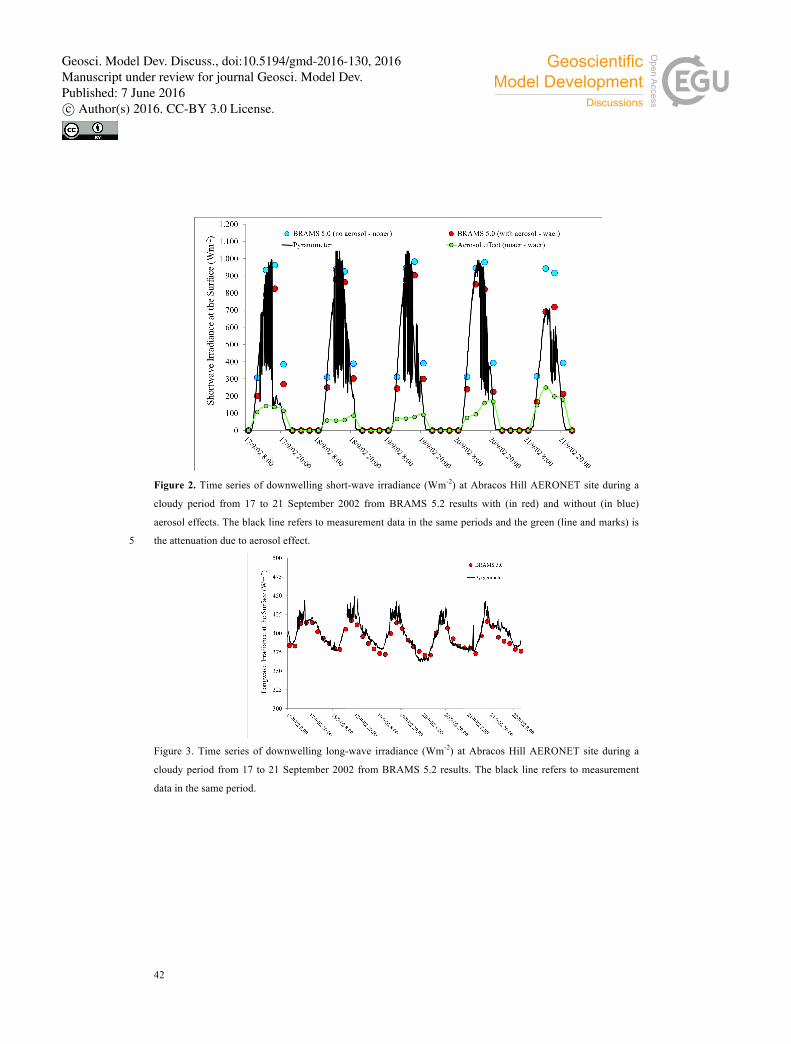
42

Figure 2. Time series of downwelling short-wave irradiance (Wm-2) at Abracos Hill AERONET site during a

cloudy period from 17 to 21 September 2002 from BRAMS 5.2 results with (in red) and without (in blue)

aerosol effects. The black line refers to measurement data in the same periods and the green (line and marks) is

the attenuation due to aerosol effect. 5

Figure 3. Time series of downwelling long-wave irradiance (Wm-2) at Abracos Hill AERONET site during a

cloudy period from 17 to 21 September 2002 from BRAMS 5.2 results. The black line refers to measurement

data in the same period.


43

Figure 4. RMSE of air temperature at 2 meters using JULES (in red) and LEAF3 (in blue) surface schemes with

BRAMS over South America during (A) wet season in March 2010, and (B) dry season in September 2010.

5

Figure 5. Mean bias score versus precipitation thresholds for South America for a set of 30 forecasts

of 24-h accumulated precipitation for 120h in advance for (A) January 2008 and (B) January 2010.

Blue line represents simulations using FY weight method and red line the original EN. Blue bars 10

indicate significance test from the bootstrap method (Hamill, 1999).


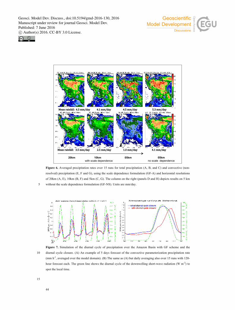
44

Figure 6. Averaged precipitation rates over 15 runs for total precipitation (A, B, and C) and convective (non-

resolved) precipitation (E, F and G), using the scale dependence formulation (GF-A) and horizontal resolutions

of 20km (A, E), 10km (B, F) and 5km (C, G). The column on the right (panels D and H) depicts results on 5 km

without the scale dependence formulation (GF-NS). Units are mm/day. 5

Figure 7. Simulation of the diurnal cycle of precipitation over the Amazon Basin with GF scheme and the

diurnal cycle closure. (A) An example of 5 days forecast of the convective parameterization precipitation rate 10

(mm h-1, averaged over the model domain). (B) The same as (A) but daily averaging also over 15 runs with 120-

hour forecast each. The green line shows the diurnal cycle of the downwelling short-wave radiation (W m-2) to

spot the local time.

15

05km no scale dependence

20km 10km 05km with scale dependence

Mean%rainfall:%%4.3%mm/day%%%%%%%%%%%4.1%mm/day%%%%%%%%%%%%%%%%%%%%4.5%mm/day%%%%%%%%%%%%%%%%%%%%%%%%%5.3%mm/day

Mean%rainfall:%%%3.5%mm/day%%%%%%%%%%%%2.5%mm/day%%%%%%%%%%%%%%%%%%%%1.0%mm/day%%%%%%%%%%%%%%%%%%%%%%%%4.1%mm/day


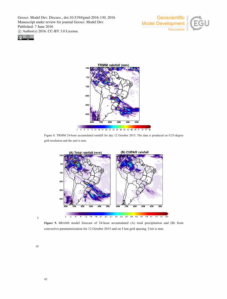
45

Figure 8. TRMM 24-hour accumulated rainfall for day 12 October 2015. The data is produced on 0.25-degree

grid resolution and the unit is mm.

5

Figure 9. BRAMS model forecast of 24-hour accumulated (A) total precipitation and (B) from

convective parameterization for 12 October 2015 and on 5 km grid spacing. Unit is mm.

10


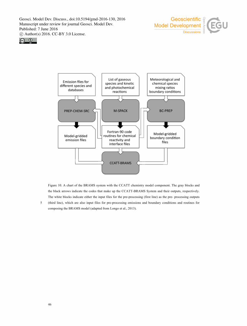
46

Figure 10. A chart of the BRAMS system with the CCATT chemistry model component. The gray blocks and

the black arrows indicate the codes that make up the CCATT-BRAMS System and their outputs, respectively.

The white blocks indicate either the input files for the pre-processing (first line) as the pre- processing outputs

(third line), which are also input files for pre-processing emissions and boundary conditions and routines for 5

composing the BRAMS model (adapted from Longo et al., 2013).


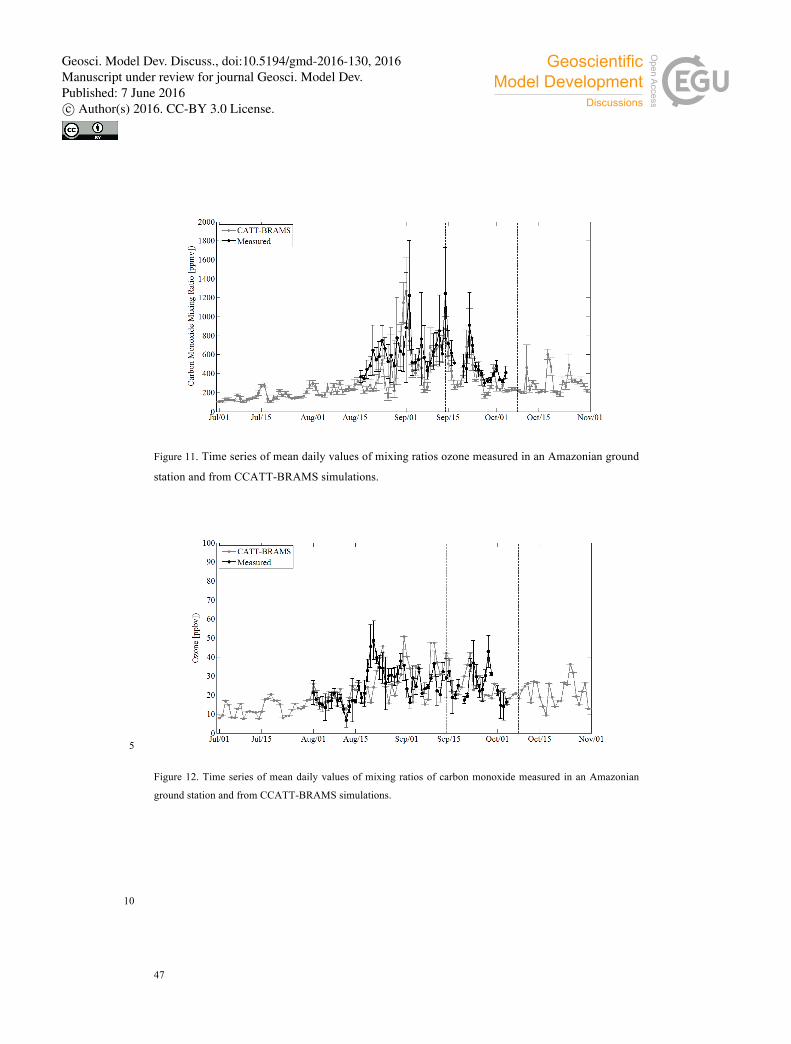
47

Figure 11. Time series of mean daily values of mixing ratios ozone measured in an Amazonian ground

station and from CCATT-BRAMS simulations.

5

Figure 12. Time series of mean daily values of mixing ratios of carbon monoxide measured in an Amazonian

ground station and from CCATT-BRAMS simulations.

10


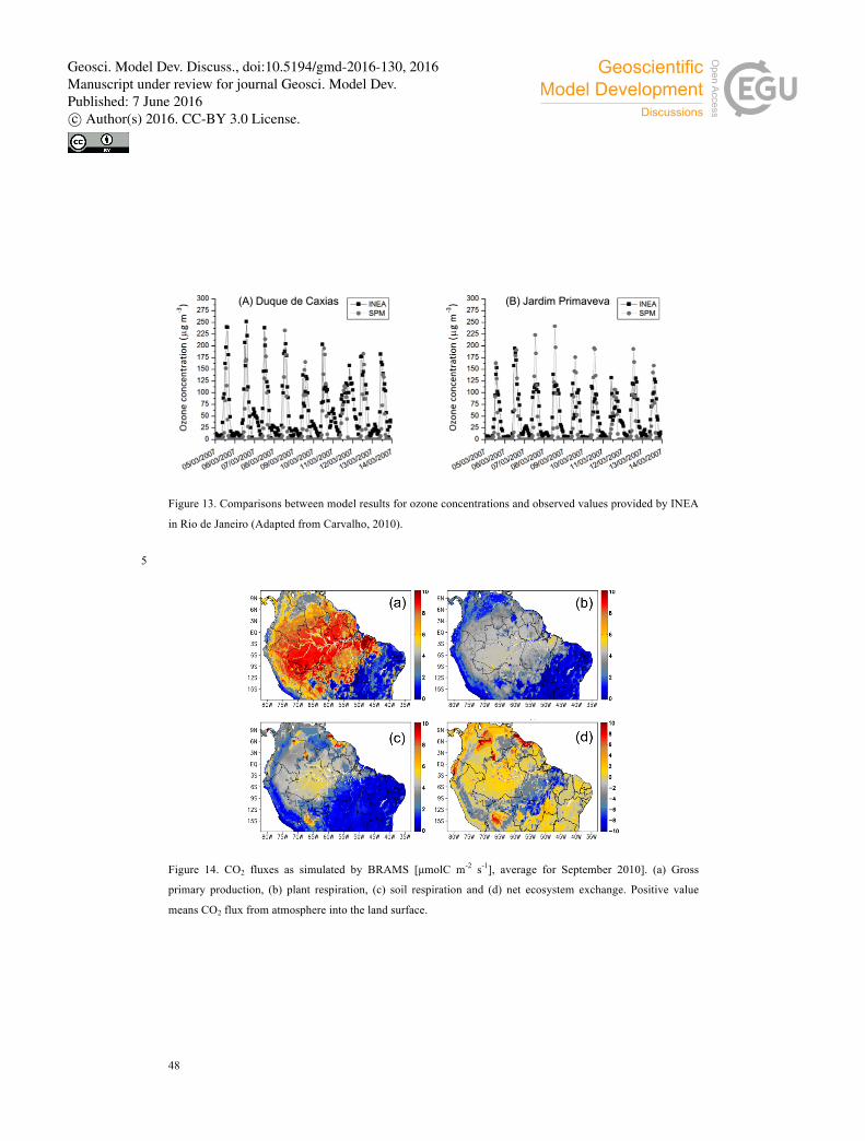
48

Figure 13. Comparisons between model results for ozone concentrations and observed values provided by INEA

in Rio de Janeiro (Adapted from Carvalho, 2010).

5

Figure 14. CO2 fluxes as simulated by BRAMS [µmolC m-2 s-1], average for September 2010]. (a) Gross

primary production, (b) plant respiration, (c) soil respiration and (d) net ecosystem exchange. Positive value

means CO2 flux from atmosphere into the land surface.


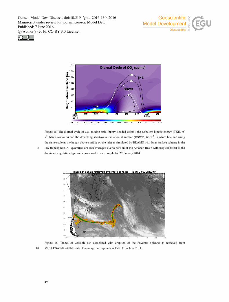
49

Figure 15. The diurnal cycle of CO2 mixing ratio (ppmv, shaded colors), the turbulent kinetic energy (TKE, m2

s-2, black contours) and the dowelling short-wave radiation at surface (DSWR, W m-2, in white line and using

the same scale as the height above surface on the left) as simulated by BRAMS with Jules surface scheme in the

low troposphere. All quantities are area averaged over a portion of the Amazon Basin with tropical forest as the 5

dominant vegetation type and correspond to an example for 27 January 2014.

Figure 16. Traces of volcanic ash associated with eruption of the Puyehue volcano as retrieved from

METEOSAT-8 satellite data. The image corresponds to 15UTC 06 June 2011. 10


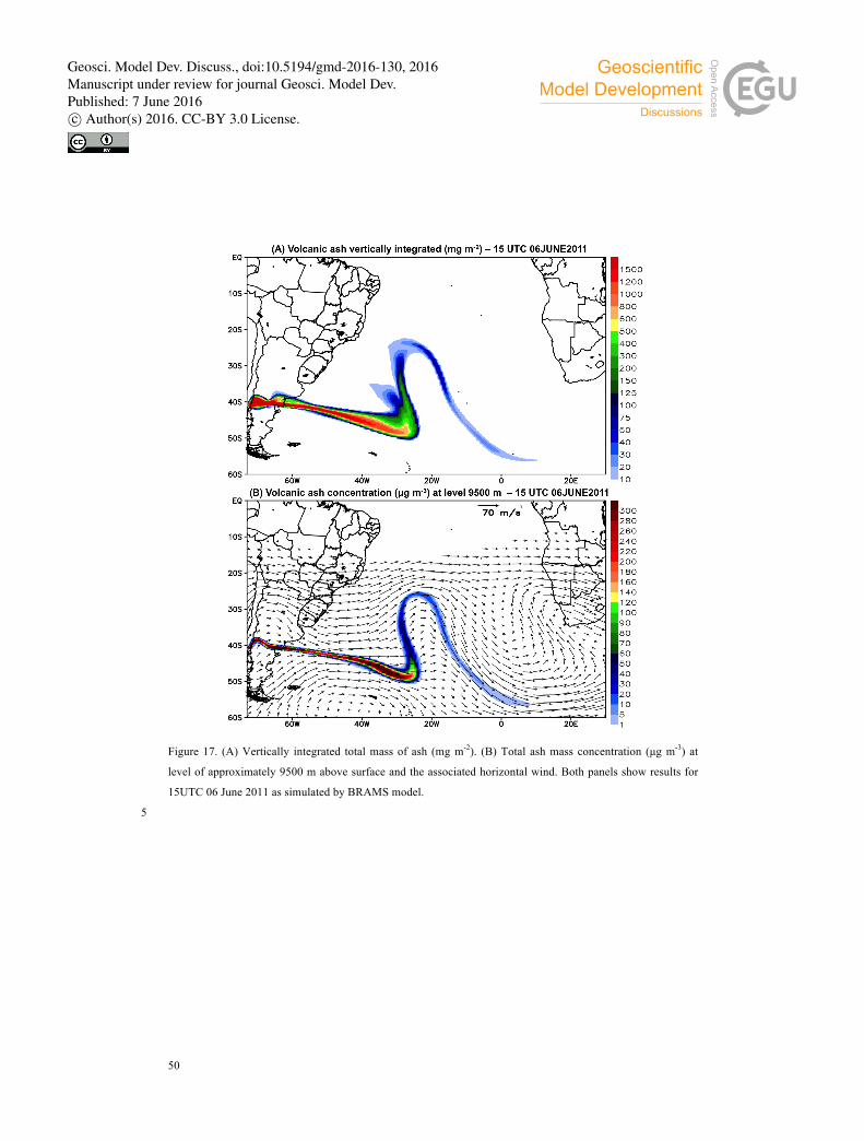
50

Figure 17. (A) Vertically integrated total mass of ash (mg m-2). (B) Total ash mass concentration (µg m-3) at

level of approximately 9500 m above surface and the associated horizontal wind. Both panels show results for

15UTC 06 June 2011 as simulated by BRAMS model.

5


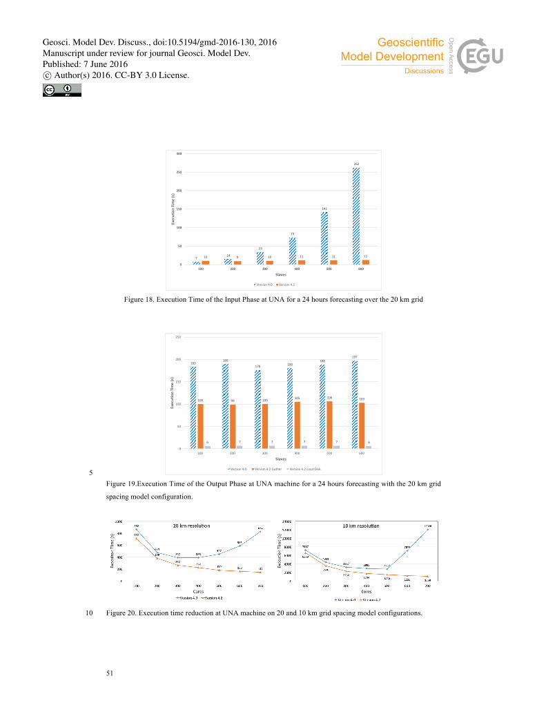
51

Figure 18. Execution Time of the Input Phase at UNA for a 24 hours forecasting over the 20 km grid

5 Figure 19.Execution Time of the Output Phase at UNA machine for a 24 hours forecasting with the 20 km grid

spacing model configuration.

Figure 20. Execution time reduction at UNA machine on 20 and 10 km grid spacing model configurations. 10

714

33

73

141

262

10 9 10 11 11 12

0

50

100

150

200

250

300

100 200 300 400 500 600

ExecutionTime(s)

Slaves

Version4.0 Version4.2

183189

176 180188

197

100 99 100 105 106 103

6 7 7 7 7 6

0

50

100

150

200

250

100 200 300 400 500 600

ExecutionTime(s)

Slaves

Version4.0 Version4.2Gather Version4.2LocalDisk


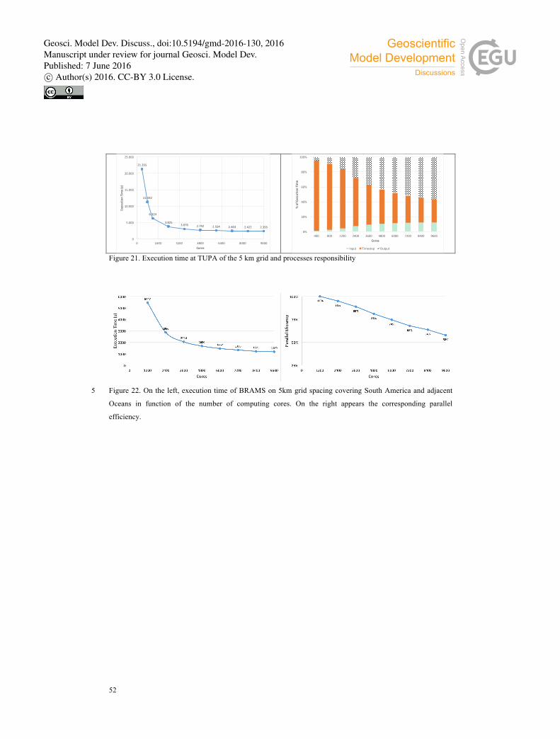
52

Figure 21. Execution time at TUPA of the 5 km grid and processes responsibility

Figure 22. On the left, execution time of BRAMS on 5km grid spacing covering South America and adjacent 5

Oceans in function of the number of computing cores. On the right appears the corresponding parallel

efficiency.

21.355

11.332

6.324

3.8253.076 2.742 2.554 2.463 2.422 2.395

0

5.000

10.000

15.000

20.000

25.000

0 1600 3200 4800 6400 8000 9600

ExecutionTime(s)

Cores

0%

20%

40%

60%

80%

100%

400 800 1200 2400 3600 4800 6000 7200 8400 9600

%ofE

xecutio

nTime

Cores

Input Timestep Output


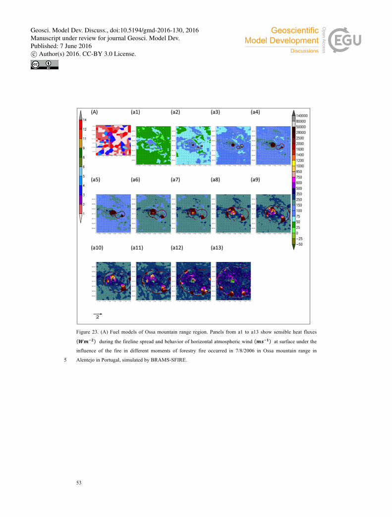
53

Figure 23. (A) Fuel models of Ossa mountain range region. Panels from a1 to a13 show sensible heat fluxes

𝑾𝒎!𝟐 during the fireline spread and behavior of horizontal atmospheric wind 𝒎𝒔!𝟏 at surface under the

influence of the fire in different moments of forestry fire occurred in 7/8/2006 in Ossa mountain range in

Alentejo in Portugal, simulated by BRAMS-SFIRE. 5


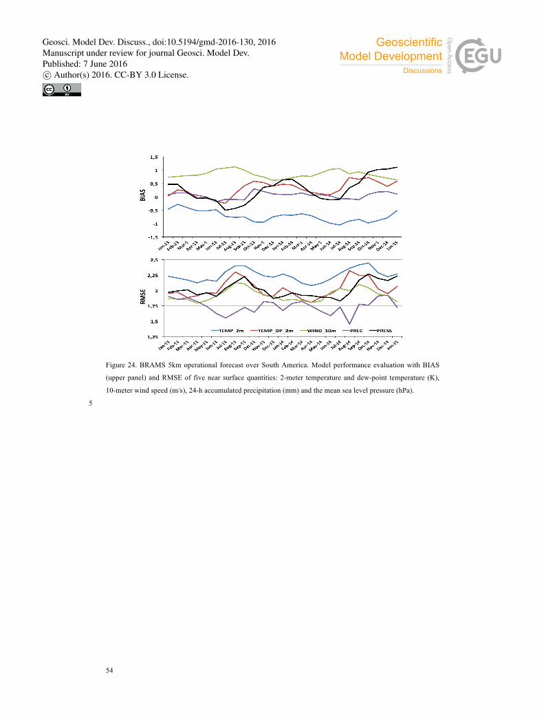
54

Figure 24. BRAMS 5km operational forecast over South America. Model performance evaluation with BIAS

(upper panel) and RMSE of five near surface quantities: 2-meter temperature and dew-point temperature (K),

10-meter wind speed (m/s), 24-h accumulated precipitation (mm) and the mean sea level pressure (hPa).

5


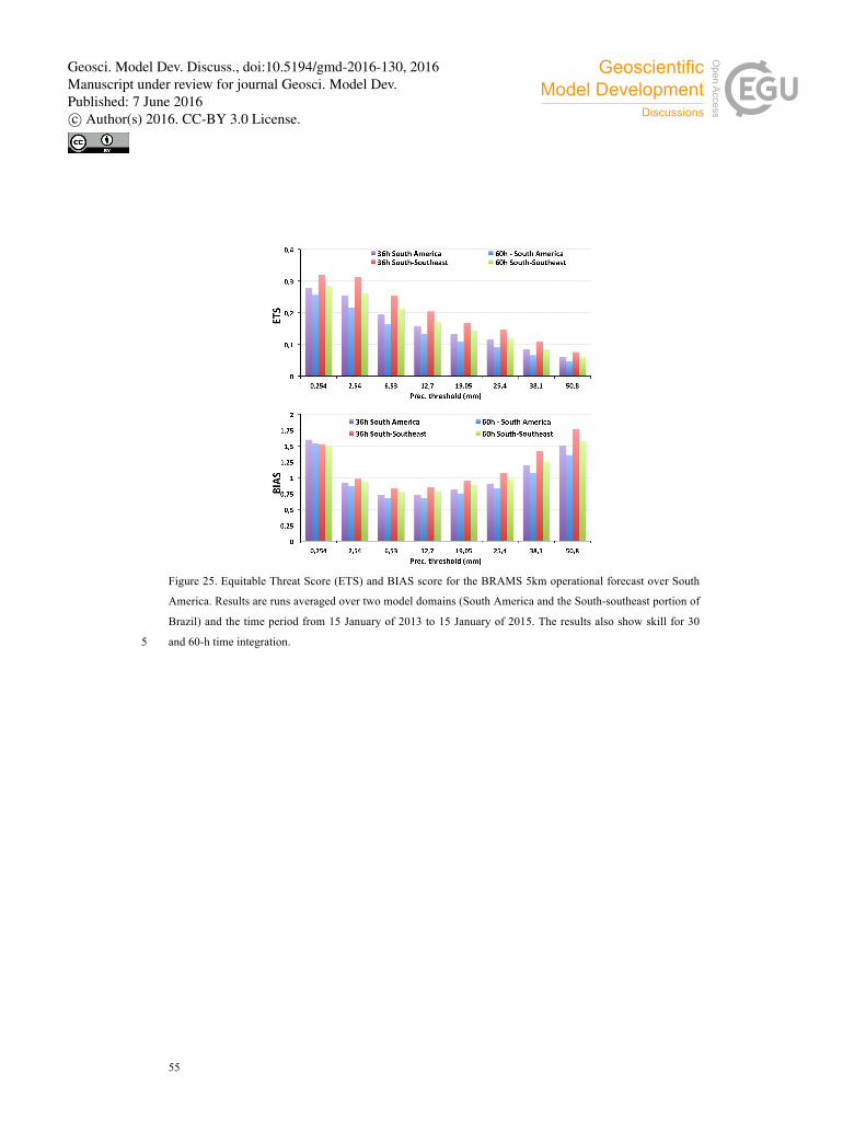
55

Figure 25. Equitable Threat Score (ETS) and BIAS score for the BRAMS 5km operational forecast over South

America. Results are runs averaged over two model domains (South America and the South-southeast portion of

Brazil) and the time period from 15 January of 2013 to 15 January of 2015. The results also show skill for 30

and 60-h time integration. 5


an integrated environmental model tuned for - GMD

Documents

Transcript of an integrated environmental model tuned for - GMD