Author'sResponse

Title:Anopen-sourceMEteoroLOgicalobservationtimeseriesDISaggregationTool

(MELODISTv0.1.0)

Author(s):K.Försteretal.

MSNo.:gmd-2016-51

MSType:Modeldescriptionpaper

Iteration:RevisedSubmission

DearDr.Sander,

Thisdocumentincludesallmodificationstotheabovementionedmanuscript.Thereferees’

commentsfromtheopendiscussionarelistedbelowalongwithourdetailedanswers.

Refereecommentsareinitalics(blue).Ifrequired,weaddedsomeadditionalremarks(red)

notlistedintheopendiscussionsofar.

Inaddition,wesuggestsomefurtherchanges,whicharelistedinaseparatesectionofthis

document.SomechangeshavebeenpersonallycommunicatedbyHannesMüller

(UniversityofHannover)whomadesomeremarksaboutthesymbolsoftheprecipitation

cascademodel.Moreover,hesuggestedaddingsomedetailsregardingthecascademodel

alongwithtwofurtherreferences.Weappreciatehishintswhichwewouldliketo

incorporateintherevisedversionofthemanuscriptifyouacceptthesechanges.

Thankyouverymuchforhandlingourmanuscript.

Bestregards,

KristianFörster

(onbehalfoftheauthors)

TableofContents

Replytoreview#1.............................................................................................................1

Replytoreview#2.............................................................................................................6

Listofadditionalchanges..................................................................................................7

Marked-upmanuscriptversion..........................................................................................9

Replytoreview#1WewouldliketothankDr.InaPohleforherdetailedreviewofourmanuscriptandforher

constructivecommentsandsuggestions.Thepointsraisedinthisreviewarehighly

appreciatedandwillhelpustoimproveourmanuscript.Pleasefindourdetailedresponse

below.

Generalcomments:

ThemanuscriptbyFörsteretal.presentsthesoftwarepackageMELODIST,aframe-workofstateoftheartmethodsfordisaggregatingmeteorologicaltimeseries.Themethodsincludedcomprisedeterministicandstochasticapproacheswithseveraloptionstochoosefortheindividualmeteorologicalvariables.Thedisaggregationmethodsaredescribedconciselywithadequatereferencetotherelevantliterature.Thegeneralapplicabilityofthedisaggregationmethodsisassessedbycomparisonsbetweenobservedhourlydataanddisaggregatedhourlydatabasedondailyvariables.Therefore,fivestationsincontrastingclimateshavebeenchosen.Themodelcodeitselfiswelldocumented,thesoftwarepackageiseasytoapplyandmodifyandthushashighpotentialonbeingusede.g.byhydrologistwhorequirehourlyinputdataformodels.Themanuscriptiswellstructuredandwritten.Themethodsareclearlydocumentedandcriticallyassessedbothwithreferencetotheliteratureandbyownanalysesoftheauthors.Theconclusionsarewellsupportedbytheresults.Irecommendthearticleforpublicationafterminorrevisionforthefollowingissues:

-Introduction:motivatetheneedofadisaggregationtohourlydatamoredirectly–forwhichpurposesaredatainhourlyresolutionneeded(giveexamples)

Basedonavailableliterature,wewilladdsomeexamplesandapplicationsforwhich

disaggregationmethodsarerequired.Wewilladdoneadditionalparagraphinthe

introduction:

“Incontrast,hourlymeteorologicaltimeseriesarerequiredfornumerousapplicationsin

geoscientificmodelling.Typicalapplicationsinhydrologyincludebothderivedflood

frequencyanalyses(e.g.,HaberlandtandRadtke,2014)andwaterbalancesimulations

(WaichlerandWigmosta,2003).Inecologicalmodelling,sub-dailymeteorologicaldataare

requiredfor,e.g.,theestimationofepidemicdynamicsofplantfungalpathogens(Bregaglio

etal.,2010).”

Thankyouforpointingusinthisdirection.

-Introduction:whiletherelevantliteratureconcerningdisaggregationmethodsisaddressed,referencetoothertools/softwarepackagesfordisaggregationofsinglemeteorologicalvariables(e.g.HyetosR)ismissing

WewillrefertotheHyetosRpackagewhichwewerenotawareof.Weappreciatethishint!

Therevisedversionofthemanuscriptwillincludeareferencetothissoftware(pagetwo,

firstbulletpoint):

“Forinstance,therainfalldisaggregationpackage“HyetosR”(Kossierisetal,2012,ITIA,

2016)providesanextensiveparameterestimationmethodologywhichisbasedonobserved

timeseries.”

-Results:Itisofinterest,whetherthedistributionsofthehourlydataarepreserved.Table2givesonlymeanvaluesandstandarddeviations.Dotheparametersofthedistributionfunctionsdifferbetweenobservedanddisaggregatedhourlyvalues?

Weagreethatthecomparisonofmeanvaluesandstandarddeviationsonlygivesa

simplifiedreviewofthedistributionofthesevalues.Thisisavalidpointwhichwehave

discussedintensively.Thevariablesaddressedinthemanuscripthavedifferentdistributions

whichiswhyitisnotpossibletofitonesingletypeofdistributionfunction.Forinstance,

temperaturemightberepresentedbyanormaldistributionformanysites,whereas

precipitationischaracterisedbyalowerlimitofzeroandasymmetry.Tobestpossibly

addresstheneedfordistributionsandtokeepthemanuscriptconcisewithoutextensive

additionsregardingtheoreticaldistributionfunctionsandparameterestimation,wedecided

toaddanadditionalfiguretotherevisedversionofthemanuscriptincludinghistogramsof

bothobservedanddisaggregatedvaluesforeachvariableandeachstation.

Afigureincludinghistogramsofbothobservedanddisaggregatedtimeserieswasadded

(Fig.8intherevisedmanuscript).Histogramsaredisplayedforeachvariableandeach

station(ifapplicable).AnadditionalexplanationisnowaddedtoSect.4.1.:

“Inordertogainsomeinsightonhowwellthedistributionsofdisaggregatedtimeseries

matchtheobservedones,histogramsforeachvariableandeachsitearedisplayedforboth

disaggregatedandobservedvaluesinFig.8.”

-Results:Onwhichbasishavethetimesandlocationsfortheresultfiguresbeenchosen?Arethesethetimes&locationswherethedisaggregationresultsfittheobservationsbest?Itmightbehelpfultoaddperformancemeasuresalsoforthetimeperiodsdisplayed.

Thisquestionseemstorefertotheexamplefigures(Fig.3toFig.7)sinceonlythesefigures

includeresultsofdisaggregationmethodsforselectedtimesandlocations.Infact,the

examplefiguresforeachvariablehavebeenrandomlyselected.Theyhavebeendesignedto

showexemplarilyhoweachofthemethodswork.Youarerighttosaythatthisinformation

needstobeclarified.Intherevisedversionofthemanuscript,wewillexplaininsection3.1

thatthetimesandlocationshavebeenrandomlyselected.Addingperformancemeasures

foreachmethodisagoodpointasthisinformationwouldprovehelpful.Inprinciple,thisis

notaproblematall.However,thiswouldrequireoneadditionaltableforeachexample

plot.Inouropinion,theseadditionaltableswouldgobeyondthescopeoftheexemplary

typeoffigures.Therefore,wesuggestaddingtheRMSerrorforeachmethodtothelegend

inordertogiveanideaofmodelperformanceforeachmethodforthetimesdisplayedin

eachfigure(exceptforprecipitation).

WehaveaddedtheRMSEvaluesforeachmethodtothelegendofFig.3,4,5,and6,

respectively.Insection3.1,wefurtherstate:“Thesubsequentsectionsprovidedetailsfor

eachofthemethodslistedinTab.2.Foreachvariableanexamplefigureisprovidedwhich

givesanideaofhoweachofthemethodsworks.Thetimesandlocationsofthesefigures

havebeenrandomlyselected.”

Minorcomments:

Page1,line1:Maybespecify:“Observationsofhourlytimeseries”/“Monitoringdatainhourlyresolution”

Wewillrewritethissentenceaccordingly:“Meteorologicaltimeserieswithone-hourtime

steparerequiredinmanyapplicationsingeoscientificmodelling.”

Page3,line24-26:Canbedeleted,thereadershouldbefamiliarwiththedifferencebetweendeterministicandstochasticapproaches.

Weagreethatmostofthereadersshouldbefamiliarwiththeseterms.However,sincethe

evaluationofstochasticmethodsrequiresmultiplerunstoperformstatisticalanalyses,we

believethatsomeintroductoryremarksmightimprovecomprehensibilityregardingthe

studydesign.

Page6,line4:replace“smallscale”with“sub-hourly"

Done.

Page6,line5:sentenceunclearWeagreethatthissentenceshouldbeimproved.Wewillrevisethisstatementinthe

followingway:“Thisideabestcorrespondstoaveragesofwindspeedforagivenincrement

oftime(e.g.,onehour)ratherthaninstantaneousmeasurements.”

Page6line25:specifydistribution(uniform)Thisinformationwasmissing:“Thefunctionrndisarandomnumbergeneratorwhichdraws

randomnumbersbetween0and1fromauniformdistribution.”

Generallanguagecomment:checkwhentouse“a”and“an”

Wewillreviewandcorrectthedocumentwithrespecttotheusageof“a”and“an”.Thank

you.

Themanuscripthasbeenupdatedwithrespecttothisissue.

Page10line18:whyisthisapproachnotreferredtoas“inversedistanceweighting”

Atpresent,thismethodsimplytransformsthemasscurvefromonestationtoanother.

Distancemeasures,whichmightberelevantifmorethanonehighlyresolvedstationis

considered,arenotconsideredinthismethodsincethefocusofthemethodspresentedis

onsinglesitesonly.However,adistance-relatedweightingconsideringmorethanone

stationcanbeeasilyappliedtothismethod.Thisfeatureisimplementedinthealready

citedIDWPprogram.

Page13line2:replace“arenotreproducable”with“isnotreproducible”or:“cannotbereproduced”

Done.

Page14line2&line29:theselinesareredundant.

Yes.Weremovedtheredundantsentenceinline29.

Page15line3:canyougiveaballparkfigureoncomputationalcosts,e.g.disaggregationof10yearsoftemperaturedata?

Thankyouforthissuggestion.Thefollowinginformationwillbeaddedtotherevised

version:“disaggregating5yearsofdailyprecipitationrecordingsusingthecascademodel

takeslessthan4secondsonanotebookwitha2GHzi7CPU)”

Page15line5:giveexampleshere(orinintroduction)

Aspointedoutearlier,wewilladdsomeexamplesintheintroduction.

Table1:Pleasestatewhether“dataavailability”referstohourlydata

Yes,“dataavailability”referstohourlydata.Wewilladdthisinformationtothecaption.

Figure2:scaleofthepoints–hardtoperceivedifferences

Weslightlyincreasedthedotsizeinordertoimproveperception.However,thedifference

betweenthetwostationsinCentralEuropeissmall(DeBilt:803mm,Obergurgl:851mm).

ReferencesBregaglio,S.,Donatelli,M.,Confalonieri,R.,Acutis,M.,andOrlandini,S.:Anintegrated

evaluationofthirteenmodellingsolutionsforthegenerationofhourlyvaluesofair

relativehumidity,Theor.Appl.Climatology,102,429–438,doi:10.1007/s00704-010-

0274-y,2010.

Haberlandt,U.andRadtke,I.:Hydrologicalmodelcalibrationforderivedfloodfrequency

analysisusingstochasticrainfallandprobabilitydistributionsofpeakflows,Hydrol.

EarthSyst.Sci.,18,353–365,doi:10.5194/hess-18-353-2014,2014.

ITIA:HyetosR:AnRpackagefortemporalstochasticsimulationofrainfallatfinetimescales,

http://www.itia.ntua.gr/en/docinfo/1200/,accessedon09May2016,2016.

Kossieris,P.,Koutsoyiannis,D.,Onof,C.,Tyralis,H.,andEfstratiadis,A.:HyetosR:AnR

packagefortemporalstochasticsimulationofrainfallatfinetimescales,European

GeosciencesUnionGeneralAssembly,GeophysicalResearchAbstracts,14,11788,

2012.

Waichler,S.R.andWigmosta,M.S.:DevelopmentofHourlyMeteorologicalValuesFrom

DailyDataandSignificancetoHydrologicalModelingatH.J.AndrewsExperimental

Forest,J.Hydrometeorol.,4,251–263,doi:10.1175/1525-

7541(2003)4<251:dohmvf>2.0.co;2,2003.

Replytoreview#2Reviewcommentsforgmd-2016-51Overall,itisawell-doneandusefulpaper.Itbringstogetheranumberofmethodstogetherinoneconvenientplaceandsoftwaretoolforthepractitioner.WhenInextneedtogeneratehourlymeteorologicaldata,IwillrefertothispaperandlikelyusethePythontoolaswell.

WewouldliketothankAnonymousReferee2forforhis/herpositiveevaluationofour

manuscriptandforhis/herconstructivecommentsandsuggestions!Thecommentsare

highlyappreciatedandwillhelpustoimproveourmanuscript.Pleasefindbelowour

detailedresponse.

p.2Inthediscussionofthethreeapproachesusedforgeneratinghourlytimeseries,itwouldbehelpfultopointoutevenmoreexplicitlytowhatdegreeeachmethodcanpotentiallyreproducetheactual,time-specificvaluesthatrepresentactualhistory.Theorderofdecreasingpotentialwouldbe1,3,2

Ourfirstintentionwastolisttheseapproachesaccordingtotheircomplexityinascending

order.Weagreethatsortingthislistaccordingtothepotentialregardingtheircapabilityof

reconstructingtheactual,time-specificvalues(i.e.,theoriginallymeasuredhourlyvalues)

wouldbebeneficial.Wewillre-arrangethelistaccordingly.Moreover,wewilltakeupyour

suggestiontopointoutmoreexplicitlythepotentialofeachmethod.

“Ingeneral,threecompletelydifferentapproachesexist(listedindescendingorder

regardingtheirpotentialtoreconstructtheoriginallymeasuredhourlyvaluesthatare

representativeforagivenlocationandtime):”

• Disaggregation:“Despitetheirsimplicity,disaggregationmethodshavegreat

potentialtoreconstructtheoriginallymeasuredhourlyvaluesforagivendayasthey

areforcedbyactualdailyvaluesvalidforthatspecificday.”

• Dynamicaldownscaling:“Sinceatmospheric(re-)analysisdatarepresenttheactual

weatherforagiventime,dynamicaldownscalingofthiskindofdataisa

sophisticatedwaytoderivehourlyvaluesforthattimeandarbitrarylocationsina

realisticmanner.”

• Weathergenerators:“[...]isdifferentduetoitsrandomnature,whichiswhysub-

dailytimeseriesdonotprovidetheoriginallymeasuredvalues.”

Thankyouforpointingusinthisdirection!

p.6,line14Missingword"always"after"almost"

Done.

p.6,Section3.4.2Suggestastrongerwordthan“overlie”,perhaps“overpower”or“overwhelmorreplace”todescribehowalow-pressuresystemcanbemoreimportantthanlocaleffectsforwindgeneration

Wereplaced“overlie”by“obliterate”.ThistermisusedbyOke(1987)todescribethis

effect.

p.9,line21Misspelling:“releated”

Thistypoisfixed.

p.15,line2Wouldmakemoresenseas“simpleandeasy-to-use”

Yes.Werewrotethiswordingaccordingly.

Table7captionSuggestsaying“parentheses”insteadof“brackets”'

Done.

p.16,line4Insteadof“warranted”abetterphrasewouldbe“inherentinthemethodology”.

Youareright.Thanks!

LiteratureOke,T.R.:Boundarylayerclimates,Routledge,London,2.edn.,1987.

ListofadditionalchangesPageandlinenumbersrefertothemarked-upversionofthemanuscript.

Page1,line22:TobetteracknowledgetheISD,wehaveaddedoneadditionalreference

(Smithetal.,2011).

Page2,line27:LAMdenotes“LimitedAreaModel”insteadof“LocalAtmosphericModel”.

Thistermisupdatednow.

Page8,line13:Wenowstatethattheparametersaandbcanbederivedthrough

optimization.Thisfeaturehasbeenaddedtothesoftware.

Page9,line6:WenowstatethattheparametersAandCcanbederivedthrough

optimization.Thisfeaturehasbeenaddedtothesoftware.

Page9,line15:WenowspecifythatthecascademodelproposedbyOlssonisa

microcanonical,multiplicativecascademodel.

Page9,line22:“timestep”isreplacedby“temporalresolution”

Page9,line24:“equallyspaced”isreplacedby“equidistant”

Page10,line2:theterm“branchinggenerator”isaddedaccordingtoOlsson(1998)

Page10,line17:P(x/x)isreplacedbyP(x/(1-x))sincethisnotationismoreexact,thesame

changewasappliedtow(x/x)whichisnoww(x/(x-1))

Page11,line4:“simplyaggregated”isreplacedby“transformeduniformly”

Page11,line6:thetermmicrocanonicalisspecifiedhere,too

Page11,line9:Wehaveaddedareferencewhichdescribestheeffectdiscussedinthis

paragraph,i.e.thelackofauto-correlation(Lombardoetal.,2012).

Page11,line15:Inordertostatemoreclearlythelimitationsofthisapproach,wehave

addedsomefurtherremarks:“Arealpeakintensitiesatsub-dailytimestepsmightbe

overestimatedduetothisassumptionwhichlimitstheuniversalapplicabilityofthis

approach.However,thisoverestimationmightbeacceptableforsomeapplicationslike,

e.g.,derivedfloodfrequencyanalysesforhydrologicdesignpurposes(Haberlandtand

Radtke,2014).”

Page11,line18:Anewerreferencedescribinganapproachtohandlespatialconsistencyis

added(MüllerandHaberlandt,2016).

Page11,line27:Wenowstatemoreclearlythatthisapproachisrestricted“totheperiodof

timecoveredbyrecordingsatonehourtimestep.”

Page11,line31:Wehaverecognizedthattheoriginofdailydataintheresultssectionwas

notexplainedsofar.Therefore,wehaveaddedthisinformationasfollows:“Thetimeseries

usedfordisaggregationrepresenthourlyobservationsaggregatedtodailyaveragesand

totals,respectively.”

Page13,line14:WenowrefertothenewFig.8inSect.4.2:“Thisfindingisalsosupported

bythegoodagreementofthehistogramsconstructedforbothdisaggregatedandobserved

timeseries(Fig.8,1stcolumn).”

Page14,line1:WenowrefertothenewFig.8inSect.4.3:“Hence,minimumandmaximum

humidityarenotpreservedbythisapproach.Thisfindingbecomesapparentwhen

consideringthemismatchofminimumandmaximumhumidityreconstructionsforsome

sites(e.g.,Tucson,seeFig.8,2ndcolumnforfurtherdetails).”

Page14,line15:WenowrefertothenewFig.8inSect.4.4:“Thisalsobecomesevident

whenobservingthefallinglimbofthehistogramsofdisaggregatedvaluesshowninFig.8

(3rdcolumn).”

Page15,line1:WenowrefertothenewFig.8inSect.4.5:“[…]andthecoincidenceof

histogramscomputedfordisaggregatedandobservedtimeseriesasdisplayedin(Fig.8,4th

column).”

Page15,line11:WenowrefertothenewFig.8inSect.4.6:”Figure8(5th

column)showshistogramsforbothdisaggregatedandobservedtimeseriesforeach

station.Thecomparisonofhistogramsderivedfromdisaggregatedandobservedvalues

revealsthattheempiricaldistributionsaresimilar.Thefallinglimbofthehistogramsisalso

reliablyreconstructedbythecascademodelforwhich100runshavebeenconsideredto

computethe15histograms.”

LiteratureLombardo,F.,Volpi,E.,andKoutsoyiannis,D.:Rainfalldownscalingintime:theoreticaland

empiricalcomparisonbetweenmultifractalandHurst-Kolmogorovdiscreterandom

cascades,Hydrol.Sci.J.,57,1052–1066,doi:10.1080/02626667.2012.695872,2012.

Müller,H.andHaberlandt,U.:Temporalrainfalldisaggregationusingamultiplicative

cascademodelforspatialapplicationinurbanhydrol-ogy,J.Hydrol.,articleinpress,

doi:10.1016/j.jhydrol.2016.01.031,http://dx.doi.org/10.1016/j.jhydrol.2016.01.031,

2016.

Olsson,J.:Evaluationofascalingcascademodelfortemporalrainfalldisaggregation,

Hydrol.EarthSyst.Sci.,2,19–30,doi:10.5194/hess-2-19-1998,1998.

Smith,A.,Lott,N.,andVose,R.:TheIntegratedSurfaceDatabase:RecentDevelopments

andPartnerships,Bull.Amer.Meteor.Soc.,92,704–708,

doi:10.1175/2011bams3015.1,2011.

Marked-upmanuscriptversion

Seenextpage.

An open-source MEteoroLOgical observation time seriesDISaggregation Tool (MELODIST v0.1.0

::.1)

Kristian Förster1,2, Florian Hanzer1,2, Benjamin Winter1,2, Thomas Marke2, and Ulrich Strasser2

1alpS - Centre for Climate Change Adaptation, Grabenweg 68, A-6020 Innsbruck, Austria2Institute of Geography, University of Innsbruck, Innrain 52f, A-6020 Innsbruck, Austria

Correspondence to: Kristian Förster (kristian.foerster@uibk.ac.at)

Abstract. Hourly meteorological time series::::::::::::Meteorological

::::time

:::::series

::::with

::::::::one-hour

::::time

::::step are required in many applica-

tions in geoscientific modelling. These hourly time series generally cover shorter periods of time compared to daily meteoro-

logical time series. We present an open-source MEteoroLOgical observation time series DISaggregation Tool (MELODIST).

This software package is written in Python and comprises simple methods to temporally downscale (disaggregate) daily me-

teorological time series to hourly data. MELODIST is capable of disaggregating the most commonly used meteorological5

variables for geoscientific modelling including temperature, precipitation, humidity, wind speed, and shortwave radiation. In

this way, disaggregation is performed independently for each variable considering a single site without spatial dependencies.

The algorithms are validated against observed meteorological time series for five sites in different climates. Results indicate a

good reconstruction of diurnal features at those sites. This makes the methodology interesting to users of models operating at

hourly time steps who want to apply their models for longer periods of time not covered by hourly observations.10

1 Introduction

Continuous recordings of meteorological data are available since the late 18th century. During the 20th century, observational

networks have been refined intensively, even at remote sites. However, these observations are generally not distributed equally

in space and their temporal resolutions range from some hours (e.g., three measurements of temperature for each day) to one

day (e.g., rain gauges). Later, in the late 20th century, the instrumentation of meteorological stations has been supplemented15

by the installation of automatic weather stations (AWS) which are capable of collecting meteorological data continuously with

a frequency ranging from one hour to one minute or even shorter periods of time (Rassmussen et al., 1993).

Figure 1 depicts the global temporal evolution of data availability for daily and hourly meteorological time series during

the 20th century and beyond. This diagram has been compiled using two freely available datasets through querying the tem-

poral coverage of available data of each dataset: Daily data are collected continuously in the Global Historical Climatology20

Network-Daily Database (GHCN) (Menne et al., 2012; NOAA, 2015b), whereas the Integrated Surface Database (ISD) pro-

vides hourly time series of stations worldwide (NOAA, 2015a)::::::::::::::::::::::::::::(Smith et al., 2011; NOAA, 2015a). This comparison reveals

that the availability of hourly observations as provided by AWS is restricted to a few decades only. When observing Fig. 1, it

becomes obvious that a large number of AWS have only been mounted in the last two or three decades.

1

::In

:::::::contrast,

::::::hourly

:::::::::::::meteorological

::::time

:::::series

:::are

::::::::required

:::for

::::::::numerous

:::::::::::applications

::in

:::::::::::geoscientific

:::::::::modelling.

:::::::Typical

::::::::::applications

::in

::::::::hydrology

:::::::include

::::both

::::::derived

::::flood

:::::::::frequency

:::::::analyses

::::::::::::::::::::::::::::::::(e.g., Haberlandt and Radtke, 2014) and

:::::water

:::::::balance

:::::::::simulations

:::::::::::::::::::::::::::::::(e.g., Waichler and Wigmosta, 2003).

::In

::::::::ecological

:::::::::modelling,

::::::::sub-daily

:::::::::::::meteorological

::::data

:::are

:::::::required

:::for,

::::e.g.,

::the

:::::::::estimation

::of

::::::::epidemic

::::::::dynamics

:::of

::::plant

::::::fungal

::::::::pathogens

::::::::::::::::::::(Bregaglio et al., 2010).

Consequently, the question arises how to generate hourly time series of meteorological variables, e.g., by using available5

daily observations in order to benefit from their longer temporal coverage and higher spatial network density. In general,

three completely different approaches exist:::::(listed

::in

:::::::::descending

:::::order

:::::::::regarding

::::their

::::::::potential

::to

:::::::::reconstruct

:::the

:::::::::originally

::::::::measured

:::::hourly

::::::values

:::that

:::are

::::::::::::representative

:::for

:a:::::given

:::::::location

:::and

:::::time):

1. Temporal disaggregation of daily meteorological observation (e.g., Waichler and Wigmosta, 2003; Schnorbus and Alila,

2004; Debele et al., 2007): This method is the simplest approach among the methods listed here even though more com-10

plex methodologies are also available, especially for precipitation (e.g., Koutsoyiannis et al., 2003). Simplicity holds,

however, mostly true for computational needs as well as for the complexity of the methods itself. Deterministic equations

or simple statistical models are applied to daily time series in order to derive hourly values. For each variable, the disag-

gregation is generally applied independently. Including statistical evaluations might improve results at a specific site com-

pared to simple methods that are independent from station recordings (Waichler and Wigmosta, 2003). Using weather15

generators to derive new synthetic time series that match the statistics of available hourly data: Weather generators

calculate statistics of:::For

:::::::instance,

:::the

::::::rainfall

::::::::::::disaggregation

:::::::package

:::::::::“HyetosR”

::::::::::::::::::::::::::::::::::::(Kossieris et al., 2012; ITIA, 2016) provides

::an

::::::::extensive

::::::::parameter

:::::::::estimation

:::::::::::methodology

::::::which

:is:::::based

:::on observed time seriesand apply these statistics using a

random number generator to obtain new time series with equal statistical characteristics (Haberlandt et al., 2011; Ailliot et al., 2015).

For hourly time steps, resampling techniques are applied in most cases (e.g., Sharif and Burn, 2007; Strasser, 2008).20

Time series derived by weather generators only match the observations statistically. The sequence of events is different

due to its random nature. Weather generators are powerful tools that supplement deterministic modelling by stochastic

methods and thus add a probabilistic component to the elsewise pure mechanistic methodology (mixed deterministic-stochastic models, see, e.g., Pechlivanidis et al., 2011).

Combinations with disaggregation techniques are also possible (Mezghani and Hingray, 2009). .:::::::Despite

::::their

:::::::::simplicity,

::::::::::::disaggregation

:::::::methods

::::have

:::::great

:::::::potential

::to

::::::::::reconstruct

:::the

::::::::originally

::::::::measured

::::::hourly

:::::values

:::for

:a:::::given

::::day

::as

::::they25

::are

::::::forced

:::by

:::::actual

::::daily

::::::values

::::valid

:::for

::::that

::::::specific

::::day.

:

2. Dynamical downscaling using a local atmospheric model (LAM):::::::Limited

::::Area

:::::::Models of the atmosphere

::::::(LAM)

:and

atmospheric (re-)analysis data (e.g., Kunstmann and Stadler, 2005; Liu et al., 2011; Förster et al., 2014). As glob-

ally available data are used (e.g., re-analysis data), this approach is mostly independent of local observations although

these local recordings might have contributed to the global datasets. It is a physically based approach that preserves30

physical consistency among all meteorological variables, which holds not necessarily true for the first and second

::::third methodology. However, due to its physical base, it is more complex and computationally expensive. Small

:::::Since

::::::::::atmospheric

::::::::::(re-)analysis

::::data

::::::::represent

:::the

:::::actual

:::::::weather

:::for

:a:::::given

:::::time,

:::::::::dynamical

::::::::::downscaling

::of

::::this

::::kind

::of

::::data

:is::a:::::::::::sophisticated

::::way

::to

:::::derive

::::::hourly

:::::values

:::for

::::that

::::time

:::and

::::::::arbitrary

:::::::locations

:::in

:a:::::::realistic

:::::::manner.

::::::::However,

:::::small

2

scale precipitation might not be covered as accurate by the LAM in some cases due to the very complex micro-physical

nature of precipitation and its variability (e.g., Förster et al., 2014).

3.:::::Using

:::::::weather

:::::::::generators

::to

:::::derive

::::new

::::::::synthetic

::::time

:::::series

::::that

:::::match

:::the

:::::::statistics

:::of

:::::::available

::::::hourly

:::::data:

:::::::Weather

::::::::generators

::::::::calculate

:::::::statistics

::of

::::::::observed

::::time

:::::series

:::and

:::::apply

::::these

:::::::statistics

:::::using

:a:::::::random

::::::number

::::::::generator

::to

::::::obtain

:::new

::::time

:::::series

::::with

:::::equal

::::::::statistical

::::::::::::characteristics

:::::::::::::::::::::::::::::::::::::(Haberlandt et al., 2011; Ailliot et al., 2015).

:::For

::::::hourly

::::time

:::::steps,5

:::::::::resampling

:::::::::techniques

:::are

:::::::applied

::in

:::::most

:::::cases

::::::::::::::::::::::::::::::::::::(e.g., Sharif and Burn, 2007; Strasser, 2008).

:::::Time

:::::series

:::::::derived

:::by

::::::weather

:::::::::generators

::::only

:::::match

:::the

:::::::::::observations

::::::::::statistically.

:::The

::::::::sequence

::of

::::::events

:is::::::::different

:::due

::to

::its

:::::::random

::::::nature,

:::::which

::is

::::why

::::::::sub-daily

::::time

:::::series

::do

:::not

:::::::provide

:::the

::::::::originally

::::::::measured

::::::values.

:::::::Weather

:::::::::generators

:::are

:::::::powerful

:::::tools

:::that

::::::::::supplement

:::::::::::deterministic

:::::::::modelling

::by

:::::::::stochastic

:::::::methods

:::and

::::thus

::::add

:a:::::::::::probabilistic

:::::::::component

::to:::the

::::::::elsewise

::::pure

:::::::::mechanistic

:::::::::::methodology

::::::::::::::::::::::::::::::::::::::::::::::::::::::::::::::(mixed deterministic-stochastic models, see, e.g., Pechlivanidis et al., 2011).

:::::::::::Combinations10

::::with

::::::::::::disaggregation

:::::::::techniques

:::are

::::also

:::::::possible

:::::::::::::::::::::::::(Mezghani and Hingray, 2009).

:

In this study, we focus on the simplest method among the listed approaches, the disaggregation of daily meteorological data

(# 1). For instance, in hydrological modelling, simple methods are usually sufficient in order to force conceptual, process-based

models (Waichler and Wigmosta, 2003; Debele et al., 2007). To the authors’ knowledge there is neither any “best” way of dis-

aggregating meteorological data to hourly values nor any easy, ready to use and flexible software package that enables this task15

for different meteorological variables including precipitation, temperature, humidity, solar radiation, and wind speed. There-

fore, we propose a robust and fully documented methodology including alternative approaches for all these variables in order to

make the best use of available data. Although there are more complex and sophisticated methods available for obtaining hourly

values, MELODIST can be viewed as good balance among several aspects such as data availability, user’s prior knowledge,

robustness, and computational costs. Therefore, MELODIST addresses practitioners who need to run their model for long pe-20

riods of time at one hour time steps. Here, emphasis is put on single stations rather than considering interdependencies among

different stations. However, the manuscript includes some specific remarks with respect to this restriction.

The paper is organised as follows: First, the study sites investigated herein are briefly presented in Section 2. The next section

gives an overview of the disaggregation methods. In the fourth section, the methods are statistically evaluated with respect to

their accuracy to reconstruct sub-daily features. Finally, Section 5 includes concluding remarks and an outlook for possible25

future work.

2 Study sites

The accuracy of disaggregation methodologies strongly depends on diurnal characteristics of meteorological variables. In turn,

these diurnal characteristics might vary among different climates and environments. To test the robustness of the methods

described in the next section, a small number of sites in different climates has been chosen (see, Fig. 2 and Tab. 1).30

3

Except for Obergurgl, all station data are available for free. For each station, all relevant meteorological variables have

been recorded for at least one decade. Only shortwave radiation and precipitation are not available for Rio de Janeiro and

Ny-Ålesund, respectively (Tab. 1).

The available datasets have been subdivided into two independent periods of time, one for calibration purposes, if required,

and the other for an independent validation of the disaggregation results. This subdivision has been defined in order to enable5

a split-sample test (Klemeš, 1986) which requires an independent validation period for testing models. In this study, the split-

sample test is applied for the disaggregation methods described in the next section.

3 Disaggregation of daily to hourly meteorological values

3.1 Overview

In this section, all disaggregation methods employed in the framework of this paper are described in brief. For each meteorolog-10

ical variable different options are available (Table 2). Deterministic methods generally provide the same output if input remains

unchanged. In contrast, stochastic methods are based on random numbers. This means, that the output differs in consecutive

runs even if the input dataset remains the same. Thus, stochastic methods require multiple runs prior to a sound statistical

evaluation of these runs in order to draw conclusions. Some models require the calibration of model parameters that need to be

adjusted for each site. Split-sample tests (Klemeš, 1986) are applied to test the methods more rigorously.15

:::The

::::::::::subsequent

:::::::sections

:::::::provide

::::::details

:::for

::::each

::of

:::the

::::::::methods

:::::listed

::in

::::Tab.

::2.::::

For::::each

:::::::variable

:::an

:::::::example

::::::figure

::is

:::::::provided

:::::which

:::::gives

::an

::::idea

::of::::how

:::::each

::of

:::the

:::::::methods

::::::works.

:::The

:::::times

::::and

:::::::locations

:::of

::::these

::::::figures

::::have

:::::been

::::::::randomly

:::::::selected.

3.2 Temperature (T1)

Temperature on day i is disaggregated to hourly values j on using a cosine function whose amplitude is defined by the observed20

minimum Tmin,i and maximum temperature Tmax,i on day i (e.g., Debele et al., 2007):

Ti,j

= Tmin,i +Tmin,i +Tmax,i

2

·✓1+ cos

✓⇡ · (t

j

+ a)

12

◆◆(1)

The parameter a is determined either through providing an a priori guess of the temporal difference between the solar noon

and the occurrence of the maximum temperature or through calibration. Three options are provided by MELODIST: Minimum

and maximum temperatures occur at 7 am and 2 pm, respectively (T1a). The second option (T1b) relies on radiation geometry25

in order to calculate sunset as point in local time for minimum temperatures and sun noon + 2 hours as point in time for

maximum temperatures (see, Fig 3). As the temporal shift of 2 hours might not be viewed acceptable as a general rule of

thumb, temporal shifts for each month can be evaluated through statistical evaluation of observed hourly time series (T1c).

In principle, the methodology is based upon the assumption that the diurnal course of temperature simply tracks the di-

urnal course of the incoming shortwave radiative flux with a shift in time. This assumption does not hold true during polar30

4

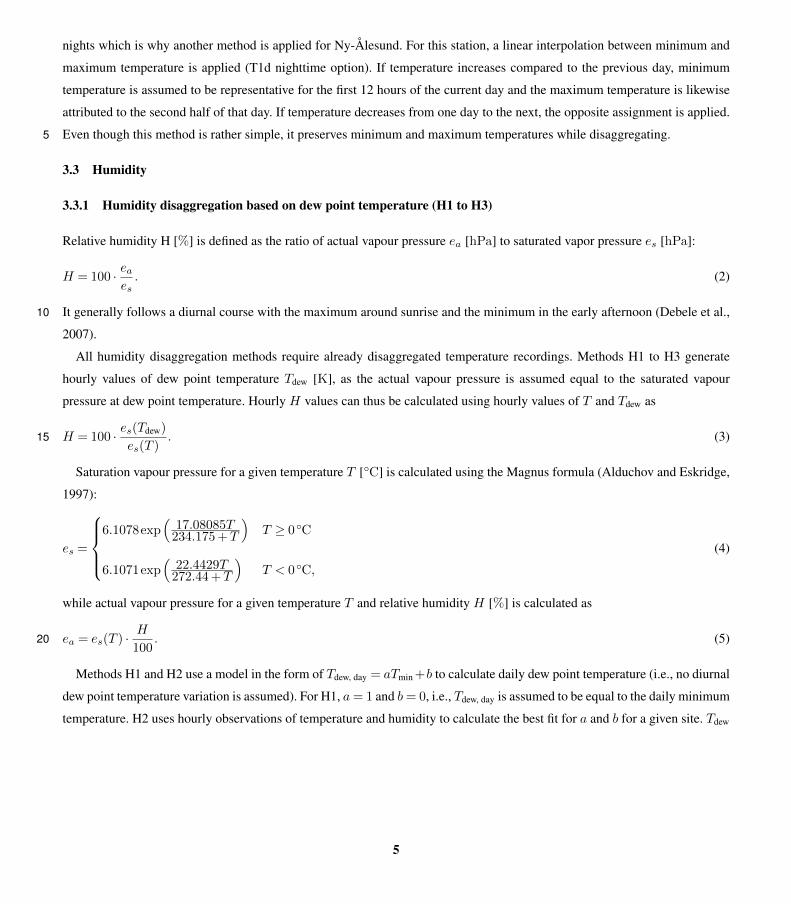
nights which is why another method is applied for Ny-Ålesund. For this station, a linear interpolation between minimum and

maximum temperature is applied (T1d nighttime option). If temperature increases compared to the previous day, minimum

temperature is assumed to be representative for the first 12 hours of the current day and the maximum temperature is likewise

attributed to the second half of that day. If temperature decreases from one day to the next, the opposite assignment is applied.

Even though this method is rather simple, it preserves minimum and maximum temperatures while disaggregating.5

3.3 Humidity

3.3.1 Humidity disaggregation based on dew point temperature (H1 to H3)

Relative humidity H [%] is defined as the ratio of actual vapour pressure ea

[hPa] to saturated vapor pressure es

[hPa]:

H = 100 · eaes

. (2)

It generally follows a diurnal course with the maximum around sunrise and the minimum in the early afternoon (Debele et al.,10

2007).

All humidity disaggregation methods require already disaggregated temperature recordings. Methods H1 to H3 generate

hourly values of dew point temperature Tdew [K], as the actual vapour pressure is assumed equal to the saturated vapour

pressure at dew point temperature. Hourly H values can thus be calculated using hourly values of T and Tdew as

H = 100 · es(Tdew)

es

(T ). (3)15

Saturation vapour pressure for a given temperature T [�C] is calculated using the Magnus formula (Alduchov and Eskridge,

1997):

es

=

8>><

>>:

6.1078exp⇣

17.08085T234.175+T

⌘T � 0

�C

6.1071exp⇣

22.4429T272.44+T

⌘T < 0

�C,

(4)

while actual vapour pressure for a given temperature T and relative humidity H [%] is calculated as

ea

= es

(T ) · H

100

. (5)20

Methods H1 and H2 use a model in the form of Tdew, day = aTmin+b to calculate daily dew point temperature (i.e., no diurnal

dew point temperature variation is assumed). For H1, a= 1 and b= 0, i.e., Tdew, day is assumed to be equal to the daily minimum

temperature. H2 uses hourly observations of temperature and humidity to calculate the best fit for a and b for a given site. Tdew

5

is thereby calculated from T and H by inverting eq. (4):

Tdew =

8>>>>>>>>><

>>>>>>>>>:

234.175lnea

(T,H)

6.1078

17.08085� ln

ea

(T,H)

6.1078

T � 0

�C

272.44lnea

(T,H)

6.1071

22.4429� ln

ea

(T,H)

6.1071

T < 0

�C.

(6)

H3 assumes a diurnal dew point temperature variation based on the assumptions that dew point temperature varies linearly

between consecutive days, and that mean daily dew point temperature occurs around sunrise (Debele et al., 2007). Dew point

temperature for a given day d and hour h is thereby calculated as5

(Tdew)d,h

= (Tdew, day)d

+

h

24

⇣(Tdew, day)

d+1 � (Tdew, day)d

⌘+(Tdew,�)

h

, (7)

where

(Tdew,�)h

=

1

2

sin

✓(h+1)

⇡

kr

� 3⇡

4

◆. (8)

kr

should be set to 6 for sites with average monthly radiation higher than 100Wm

�2, and to 12 otherwise (Debele et al.,

2007). An example application of these methods is shown in Fig. 4.10

3.3.2 Minimum und maximum humidity disaggregation (H4)

Method H4 uses records of daily minimum and maximum temperature and daily minimum and maximum relative humidity as

well as the disaggregated hourly temperature values to generate hourly humidity values:

H =Hmax +T �Tmin

Tmax �Tmin(Hmin �Hmax) . (9)

If Hmin and Hmax are available for each day, this method is the best available option among all available disaggregation15

methods (Waichler and Wigmosta, 2003).

3.4 Wind speed

Wind speed is a meteorological variable subjected to high variability at small temporal scales. This small-scale variability can

be observed, e.g. from eddy-covariance measurements (Stull, 2009). The methods compiled in this study focus on suitable

wind speed time series for hourly time steps without taking into account these small-scale::::::::sub-hourly

:considerations. This idea20

best corresponds to averages of wind speed::for

::a

::::given

:::::::::increment

::of

::::time (e.g., 10 minutes) rather single recordings carried out

every hour, which might be mimicked by peaks related to small-scale variability or processes forced by larger scales:::one

:::::hour)

:::::rather

::::than

:::::::::::instantaneous

::::::::::::measurements.

6

3.4.1 Equal distribution (W1)

As for precipitation, this method applies one unique value for each hour of the considered day. The daily mean value is assumed

to be valid for hourly values as is (W1). For many applications, this assumption might be sufficient.

3.4.2 Cosine function (W2)

Due to local and micro-climatic:::::::::::microclimatic

:conditions, wind speed is subjected to diurnal variations on days with calm5

weather in absence of synoptic-scale weather patterns that overlie:::::::obliterate

:local and microclimatic forcings (Oke, 1987).

Typical diurnal patterns in wind speed (and wind direction as well) are related to mountain-valley or land-sea wind systems.

Besides these local climatic wind systems, wind speed typically increases during daytime and almost:::::always

:diminishes after

sunset. This phenomenon is related to increased radiation-induced momentum flux on fair weather days. Again, synoptic scale

weather patterns such as low pressure systems might overlie::::::::obliterate local-scale effects. These patterns of diurnal wind10

speed variations can be simply represented by a cosine function (W2), which requires calibration using data observed at the

considered site. This model is similar to the temperature disaggregation method T1 (see, Eq. 1, Debele et al., 2007)

vi,t

= aw

· vi

· cos✓⇡ · (t��t

w

)

12

◆+ b

w

· vi

(10)

The wind speed representative for day i is disaggregated to vi,t

for hour t (Fig. 5). aw

, bw

, and�tw

are parameters that need

to be calibrated for each site prior to the application of this method.15

3.4.3 Random wind speed disaggregation (W3)

According to Debele et al. (2007) a random disaggregation of wind speed (W3) might also perform reasonably:

vi,t

= vi

· [� ln(rnd[0,1))]0.3 (11)

The function rnd is a random number generator which draws random numbers between 0 and 1.:1:::::from

:a:::::::uniform

::::::::::distribution.

Figure 5 includes 10 runs (realisations) for this option. The daily average is not necessarily preserved by this method.20

3.5 Shortwave radiation

3.5.1 Radiation model and disaggregation of daily mean shortwave radiation (R1)

Shortwave radiation R0 in W m�2 is computed for hourly time steps using the methodology described by Liston and Elder

(2006), which predicts potential shortwave radiation R0 for each time step. A simplified formula is provided that assumes a

flat surface (Liston and Elder, 2006):25

R0 = 1370W m�2 · cosZ · ( dir + dif) (12)

7

The solar constant (1370 W m�2) is scaled according to the solar zenith angle Z, which depends on time (day of year and

hour measured from local solar noon) and latitude (Liston and Elder, 2006). Details on these calculations as well as on the

direct and diffuse radiation scaling values dir and dif are given by Liston and Elder (2006).

This methodology is applied for all three options. R1 assumes daily averages of shortwave radiation. This type of data is

generally only available if hourly recordings of shortwave radiation have been aggregated prior to the data dissemination. In5

contrast, options R2 and R3 do not require shortwave radiation data as input.

3.5.2 Disaggregation of sunshine duration (R2)

The method R2 builds upon the same methodology as R1 but runs the Ångström (1924) model prior to the disaggregation

computations. This model relates sunshine duration to mean shortwave radiation for daily time steps:

R

R0=

✓a+ b · S

S0

◆(13)10

Relative sunshine duration S/S0 is transformed to relative global radiation R/R0 and then the Liston and Elder (2006)

radiation model is applied using this data.

The parameters a and b are::by

::::::default

:::set

::to 0.25 and 0.75, respectively (Ångström, 1924)

:,:::but

:::can

::::also

:::be

:::::::::determined

:::by

::::::::::optimisation

:::::using

:::::::::::observations

::of

:::::daily

:::::mean

::::solar

::::::::radiation,

::if::::::::available. Figure 6 shows an example based on method R2

for summertime radiation in De Bilt (Fig. 2). The constants a and b have been obtained through linear regression of R and15

S time series covered by the calibration period. If shortwave radiation and sunshine duration recordings are available, it is

recommended to calculate these values for the site of interest.

3.5.3 The Bristow-Campbell model (R3)

If radiation is not available, option R3 might provide reliable radiation estimates based on minimum and maximum temperature.

It is assumed that small differences between maximum and minimum temperatures typically occur on cloudy days. However,20

larger differences are common on sunny days with radiative cooling during nighttime and surface heating caused by shortwave

radiative flux during daytime. The corresponding method is named after its inventors, Bristow and Campbell (1984):

R

R0=A ·

⇥1� exp(�B ·�TC

)

⇤(14)

Here, relative global radiation R/R0 is related to the diurnal temperature range�T , which is estimated using maximum and

minimum temperatures on specific day i and the subsequent day i+1:25

�Ti

= Tmax,i �(Tmin,i +Tmin,i+1)

2

(15)

8

Besides the parameters A= 0.75 and C = 2.4, which might be viewed as constants in a first step, B is a site-specific

parameter:

B = 0.0036 · exp(�0.154 ·�T ) (16)

In contrast to �T , which refers to a certain day, �T is the long-term average of differences between maximum and minimum

temperature for the month of the current day. Based on these computations, radiation estimates are used as input to the radiation5

model R1 (see Fig. 6).::A

::::::::::site-specific

:::::::::adjustment

::of

:::the

::::::::::parameters

::A

:::and

::C

::is

:::::::possible

:::by

::::::::::optimisation

:::::using

:::::::::::observations

::of

::::::::shortwave

::::::::radiation,

:::::daily

::::::::minimum

:::and

:::::::::maximum

:::::::::::temperature.

3.6 Precipitation

3.6.1 Equal redistribution (P1)

Reconstructing sub-daily precipitation intensities from daily values is challenging as precipitation intensities strongly vary10

in time and space. In the framework of this study, three methods are presented. The first method is the simplest way of

disaggregating daily precipitation to hourly intensities by dividing the daily value by 24.

3.6.2 Cascade model (P2)

In order to provide a more sophisticated model that preserves sub-daily precipitation characteristics and is still less complex

than typical weather generators, a simple statistical precipitation disaggregation approach has been set up: The:::::::::::::microcanonical,15

:::::::::::multiplicative

:cascade model by Olsson (1998). Some enhancements proposed in the literature (Güntner et al., 2001), such as

weighting, have been taken into account as well. This method is a probabilistic approach providing different disaggregation

results for each run (realisation). However, the statistical characteristics of each realisation are equal by definition.

The disaggregation is carried out assuming a doubling of temporal resolution for each step. Due to this stepwise doubling

of resolution, the model is referred to as cascade model (see, Fig. 1 in Olsson, 1998). The time series of cascade level i with20

time step �ti

is disaggregated to level i+1 with time step �ti+1 =

12 ·�t

i

. The procedure is applied successively until the

desired time step:::::::temporal

:::::::::resolution

:is reached. The doubling of elements of each subsequently derived time series implies

that each box1 of the higher level’s time series has to be split in the next cascade level. Thus, the question arises how the sepa-

ration of the precipitation volume Pi

into two temporally equally spaced time steps Pi+1,1 = w ·P

i

and Pi+1,2 = (1�w) ·P

i

:::::::::equidistant

::::time

::::steps

:::::::::::::::Pi+1,1 =W1 ·Pi :::

and:::::::::::::::::::::::::::Pi+1,2 = (1�W1) ·Pi

=W2 ·Pi:(branching) is done, whereby w

:::W1 is the rela-25

tive weight of branching for the first box of the subsequent level with respect to the total precipitation volume to be branched1The term box representing one data point, i.e. precipitation intensity for a given increment of time, is introduced by Olsson (1998) and, thus, herein used

as well.

9

:::(W2::

is:::

the:::::::

weight:::::::assigned

::to

:::the

:::::::second

::::box). Three cases are foreseen (Olsson, 1998)

::in

:::the

::::::::so-called

:::::::::branching

::::::::generator

::::::::::::::::::::::::::::::::::::(Olsson, 1998; Müller and Haberlandt, 2015):

wW1,W2::::::

=

8>>>><

>>>>:

0 and 1 with probability P (0/1)

1 and 0 with probability P (1/0)

x and 1�x with probability P (x/(1�x));0< x < 1

(17)

The first case indicates a branching that fills the second box of the subsequent level only, whereas the second case indicates

the opposite. In contrast, the third case accounts for an:a weighted branching into both boxes of the subsequent level. For these5

cases, probabilities are provided for four different types of wet boxes with Pi

> 0:

– starting box: This type of box indicates a dry box in the previous and a wet box in the next time step.

– ending box: An ending box follows a wet box and is followed by a dry box.

– isolated box: In this case, the adjacent boxes of the previous and the next time step are dry.

– enclosed box: The adjacent boxes of the previous and next time step are wet.10

These probabilities for the three different branching possibilities (Eq. 17) can be achieved by an a:reverse scaling procedure.

Highly resolved precipitation time series are aggregated by applying the cascade level branching assumption backwards. Every

two boxes are added in each case representing the respective total volume of the antecedent higher level. Statistics are calculated

for the branching types mentioned above (probabilities are derived through dividing counts of each case by the total number

of elements of the time series). Separate evaluations are prepared for precipitation intensities below and above the mean15

precipitation value.

Additional statistics need to be computed for the case P (x/x)::::::::::::P (x/(1�x)) for which the relative weight w

:x is evaluated

as well. For all box types and both intensity classes, the relative weight ranging from zero to one is simply divided into seven

bins (see, histograms in Olsson, 1998; Güntner et al., 2001) and counted according to the previously mentioned criteria (4

box types, 2 intensity classes, 7 classes of wx/x:

x). This procedure is applied for the aggregation steps 1! 2 h (21 h), 2! 4 h20

(22 h), 4! 8 h (23 h), 8! 16 h (24 h), and 16! 32 h (25 h). According to Güntner et al. (2001), a count releated::::::related

weight is assigned to the probabilities P (0/1), P (1/0), and P (x/x):::::::::::P (x/(1�x))

:in each aggregation step prior to averaging

the probabilities of all steps. The same procedure is applied to the weights. Finally, as a result, matrices of probabilities and

weights are derived that represent the station’s precipitation scaling. The parametrization is done by applying the empirical

distributions of P (0/1), P (1/0), P (x/x), and w(x/x)::::::::::::P (x/(1�x)),

::::and

:x:

to a random number generator (without fitting25

analytical distributions).

In turn, these matrices of probabilities and weights are used to disaggregate daily time series. The type of branching

is determined by drawing random numbers for each branching step incorporating the probabilities P (0/1), P (1/0), and

P (x/x)::::::::::::P (x/(1�x)), which are evaluated cumulatively. If the random number is within the range of P (x/x)

:::::::::::P (x/(1�x)),

10

a similar procedure is applied to determine the weight w::x using another random number. In contrast to the aggregation proce-

dure, disaggregation is applied including the following steps (see Fig. 7): 24! 12 h ! 6 h ! 3 h ! 1.5 h ! 0.75 h (Güntner

et al., 2001). The time series with a 45 minutes time step is equally distributed to time series with a 15 minutes time step.

These, in turn, are simply aggregated::::::::::transformed

::::::::uniformly

:to obtain time series with a one hour time step.

For all disaggregation steps described above, the cascade model preserves mass which means that the precipitation total5

of the disaggregated time series is equal to the respective value of the original time series:::::::::::::(microcanonical

:::::::cascade

::::::model).

Despite its simplicity with respect to model complexity and parameter estimation (Molnar and Burlando, 2005), cascade models

have been already used successfully in different climates (Güntner et al., 2001). In contrast to more sophisticated models, the

autocorrelation structure might not necessarily preserved (Koutsoyiannis, 2003)::::::::::::::::::::::::::::::::::::(Koutsoyiannis, 2003; Lombardo et al., 2012).

Remarks on spatial representativeness: If this procedure is applied to more than one station, the sub-daily temporal distri-10

bution of precipitation is randomly derived for each station. These spatial patterns do not represent the actual spatial structure

of the events at sub-daily time scales. For practical applications at the meso-scale, it is therefore suggested, to redistribute

the sub-daily intensities for each station according to the cumulative relative sum of the station that is subjected to highest

daily precipitation depth (Haberlandt and Radtke, 2014), which can be performed using the method described in the next para-

graph. Areal peak intensities at sub-daily time steps might be overestimated due to this assumption .:::::which

:::::limits

:::the

::::::::universal15

::::::::::applicability

::of

::::this

:::::::::approach.

::::::::However,

::::this

:::::::::::::overestimation

:::::might

:::be

:::::::::acceptable

:::for

:::::some

:::::::::::applications

::::like,

::::e.g.,

:::::::derived

::::flood

:::::::::frequency

:::::::analyses

:::for

:::::::::hydrologic

:::::design

::::::::purposes

::::::::::::::::::::::::::(Haberlandt and Radtke, 2014). A more sophisticated but much more

complex approach that has been developed recently (Müller and Haberlandt, 2015)::::::::::::::::::::::::::::::(Müller and Haberlandt, 2015, 2016) takes

spatial consistency explicitly into consideration.

3.6.3 Redistribution according to another station (P3)20

Finally, a third method is supplied that addresses the generally higher network density of precipitation gauges compared to

other meteorological variables. If a mixed network including hourly and daily observational sites is considered and if the

distance among these stations is small, the relative mass curve of the station recordings at one hour time step can be transferred

to the other sites for which only daily recordings are available. The values for the target sites are obtained through multiplying

the relative mass of the highly resolved station’s curve with the daily precipitation depth observed at the target site. This25

methodology is also applied in the tool IDWP, which is part of the hydrological modelling system WaSiM (Schulla, 2015).:::The

::::::::::applicability

::is

::::::limited

::to

:::the

::::::period

::of

::::time

:::::::covered

::by

:::::::::recordings

::at

:::one

:::::hour

::::time

::::step.

4 Results and Discussion

4.1 Overview

This section follows the same structure as the methodology section. For each variable long-term averages of disaggregated and30

observed time series are presented and evaluated in order to assess the model skill of the disaggregation methods.::::The

::::time

11

:::::series

::::used

:::for

::::::::::::disaggregation

::::::::represent

::::::hourly

:::::::::::observations

:::::::::aggregated

::to:::::

daily::::::::averages

:::and

::::::totals,

::::::::::respectively.

:Emphasis

is put on prediction of diurnal features since most methods described herein are founded upon assumptions that imply a

certain diurnal course for a given variable. This holds especially true for temperature, humidity, wind speed, and radiation. For

precipitation, results are compiled and discussed for the cascade model. Due to the involvement of a random number generator

in this method, evaluations with respect to model skill require the analysis of multiple runs (realisations).5

Not all methods provided by MELODIST are evaluated. We focus on a subset of methods which might be relevant to a

broad range of users with respect to typical data availability settings and typical applications. For each variable, the same

methodology is applied to all stations listed in Section 2.

In order to put light on the model skill in a more quantitative way, statistical parameters have been derived for both the

observed and the disaggregated time series (see, e.g., Tab. 3). All statistical parameters refer to the validation period listed for10

each station in Tab. 1 and have been calculated for hourly time steps. The mean value as well as the standard deviation have

been computed for both time series for each station and each variable. The comparison of mean values gives an idea about

possible biases, whereas the comparison of standard deviations is relevant to assess the comparability of the variability inherent

in both time series. Moreover, the Root Mean Square Error (RMSE), the correlation coefficient r, and the Nash-Sutcliffe model

Efficiency (NSE) have been calculated based on observed and disaggregated time series.15

RMSE is a measure of deviations between observed and disaggregated time series on an hour-to-hour basis. Smaller values

are generally better than larger values. The correlation coefficient is ideally close to one and describes the coincidence of phase

for two series without considering biases. In contrast, NSE can be viewed as a combined measure addressing deviations in

terms of biases and shifts in phase. It ranges from negative infinity indicating a low skill to one indicating a perfect fit. A value

of zero means that the model is a as good as applying the average value.20

::In

::::order

::to

::::gain

:::::some

::::::insight

::on

::::how

::::well

:::the

::::::::::distributions

::of

::::::::::::disaggregated

::::time

:::::series

:::::match

:::the

::::::::observed

::::ones,

::::::::::histograms

::for

::::each

:::::::variable

::::and

::::each

:::site

:::are

::::::::displayed

:::for

::::both

::::::::::::disaggregated

:::and

::::::::observed

:::::values

::in::::Fig.

::8.

:

4.2 Temperature

Despite the fact that only one option is available for temperature (T1), the standard-sine method enables different options to

define the boundary conditions of the sine function (see Fig. 3). This method uses minimum and maximum temperature as25

input data. Here, results using the day length dependent option are presented, where maximum temperature is assumed to

occur two hours after the solar noon. For Ny Ålesund, the modified nighttime option was activated as well in order to reliably

disaggregate nighttime temperatures during polar nights, when the assumption of a distinct diurnal course does not hold true.

Long-term averages of hourly temperature derived for all sites are compiled in Fig. 9 alongside with the corresponding obser-

vations. The disaggregated diurnal course of temperature coincides well with observations for each station. Diurnal features are30

reliably preserved in the disaggregated time series. However, the amplitude is slightly overestimated for each site, attributable

to the fixed assignment of minimum and maximum temperature for a given day of year. This assumption is mostly valid on

fair weather days with surface heating but in some cases, e.g. when fronts cross the site of interest, minimum and maximum

12

temperatures might occur at different times. Thus, minimum and maximum temperatures are more spread throughout the day

in the observed datasets, resulting in a slightly smaller amplitude on average.

Besides this visual comparison, Tab. 3 summarises the model skill of temperature disaggregations for each station. Mean

temperature values are well represented in the dataset given that the mean temperature was assumed to be unknown and only

minimum and maximum temperatures have been involved in the analyses. The differences are smaller than 0.5 K. Due to the5

prescribed difference between minimum and maximum temperature, the standard deviations of observed and disaggregated

time series are very similar. However, the magnitude of RMSE values shows that differences on hour-to-hour base exceed the

average bias. However, given that only two values per day are used as input data, the RMSE values can be viewed as good

model performance. This holds also true for r and NSE, indicating a high model skill.

Disaggregated time series of each station are of similar model performance. Only Rio de Janeiro has a slightly lower model10

skill, which can still be viewed as good model representation. Observations derived at Ny Ålesund indicate that even an

application of average values might be sufficient as disaggregation procedure, which can be explained by the lower impact

of radiation on diurnal features of meteorological variables for that site. To conclude, temperature disaggregation based on

minimum and maximum temperature should provide reliable estimates.::::This

::::::finding

::is

:::also

:::::::::supported

::by

:::the

:::::good

:::::::::agreement

::of

:::the

:::::::::histograms

::::::::::constructed

::for

::::both

::::::::::::disaggregated

:::and

::::::::observed

::::time

:::::series

:::::(Fig.

::8,

::1st

::::::::column).15

4.3 Humidity

As for temperature, Fig. 10 depicts the long-term mean of the diurnal course of relative humidity for all stations (H3 model).

The diurnal patterns of relative humidity are reasonably disaggregated through simulating a drop in humidity in the afternoon,

which is observed at most stations. However, the accordance is less pronounced than for temperature. It is worth noting

that the disaggregation of relative humidity depends on hourly temperature values. For these analyses, the results described20

for temperature in the previous sections have been applied for the disaggregation of relative humidity. Hence, uncertainties

involved in the prior step also contribute to deviations between observation and disaggregation.

A closer look at the statistical evaluations derived for humidity disaggregation as compiled in Tab. 4 shows that the model

performance is lower than the corresponding values obtained for temperature. The mean values are reproduced within a range

of ±5%. Even though no information about daily minimum and maximum values of humidity have been involved in the dis-25

aggregation procedure, the standard deviations computed for observed and disaggregated time series are of similar magnitude.

The RMSE amounts to 20% indicating comparably large differences between observed and disaggregated values even though

the mean bias is substantially lower. For all but one station, the correlation coefficient is higher than 0.5. In Ny Ålesund a

correlation close to zero could be interpreted as inadequate model skill which is underlined when considering the negative

NSE value. It may be assumed that the generally lower impact of radiation on other meteorological variables would suggest to30

use an equal redistribution of humidity values for that station.

However, the model performance achieved for the other stations is better given that the RMSE is lower and r and NSE are

higher, respectively. In contrast to temperature, the humidity disaggregation performs best for Rio de Janeiro. To summarise, the

disaggregation of humidity is reliable considering the fact that disaggregated temperature time series and only one humidity

13

value per day have been used as input.:::::Hence,

:::::::::minimum

:::and

:::::::::maximum

::::::::humidity

:::are

:::not

:::::::::preserved

::by

::::this

::::::::approach.

:::::This

::::::finding

:::::::becomes

::::::::apparent

::::when

::::::::::considering

:::the

::::::::mismatch

:::of

::::::::minimum

:::and

:::::::::maximum

:::::::humidity

:::::::::::::reconstructions

:::for

:::::some

::::sites

::::(e.g.,

:::::::Tucson,

:::see

:::Fig.

::8,:::2nd

:::::::column

::for

::::::further

:::::::details).

:These findings prove previous work that also discussed the accuracy of

humidity disaggregation techniques (Waichler and Wigmosta, 2003; Bregaglio et al., 2010). If daily minimum and maximum

values of relative humidity are available, the redistribution of these values should be pursued (see, Fig. 4 and Bregaglio et al.,5

2010).

4.4 Wind speed

Wind speed disaggregation has been accomplished using the modified sine-curve (W2). In Fig. 11 the long-term averages of

the diurnal course of wind speed is plotted separately for observed and disaggregated wind speed, respectively. In this figure,

wind speed is scaled as ‘normative’ wind speed, i.e. the value for each hour is divided by the mean value. Maximum wind10

speed, which is typically observed during the afternoon hours, is well represented in the disaggregated time series. Small scale

variability, as discussed in the methodology section, are not reproduceable:is:::not

:::::::::::reproducible by this approach.

As the mean value is simply redistributed according to a sine-function, mean values are exactly reproduced by the dis-

aggregation approach. As already mentioned, variability (i.e. fluctuations) is neglected resulting in lower predicted standard

deviations when compared to the corresponding standard deviations derived for the observed time series.:::This

::::also

::::::::becomes15

::::::evident

:::::when

::::::::observing

:::the

::::::falling

::::limb

::of

:::the

:::::::::histograms

:::of

:::::::::::disaggregated

::::::values

::::::shown

::in

:::Fig.

::8:::(3rd

::::::::column).

:If these fluc-

tuations are not relevant for further evaluation, this disaggregation methodology for wind speed has an acceptable model skill

which can be observed from the correlation coefficients and NSE values. Although these values are lower than those derived

for temperature, they indicate a good model performance for all sites. The best model skill is achieved for De Bilt, whereas the

lowest performance is achieved for Tucson, where a secondary wind speed maximum is observed in the morning. This diurnal20

pattern might be related to a local wind system that is subject to a change in wind direction and, hence, to a change in wind

speed. Such phenomena are not addressed by this method.

4.5 Radiation

Even though radiation observations are available to most of the sites investigated in this study, the availability of daily mean

shortwave radiation in absence of sub-daily time series is not so common. One exception is climate model output, which is25

typically aggregated to daily values. A typical real-world-case is, however, a long dataset of sunshine duration recordings.

Therefore, method R2 is applied even though it is only applicable to De Bilt and Ny Ålesund. The diurnal course of mean

hourly values derived through averaging the observed and disaggregated datasets is displayed in Fig. 12.

Given that the disaggregation is based on sunshine duration, the model skill can be viewed as very good for both sites. The

timing of solar noon radiative fluxes as well as the phase of the disaggregated time series track observations very well which30

is also underlined by the performance measures presented in Tab. 6. Deviations between the mean values can be related to

uncertainties involved in the Ångström (1924) model which has been fitted prior to disaggregation for both stations using the

data from the calibration period. However, the disaggregated time series are subjected to similar variabilities as the observed

14

time series which is expressed by the very similar standard deviations .::and

::::the

::::::::::coincidence

::of

::::::::::histograms

:::::::::computed

:::for

:::::::::::disaggregated

:::and

::::::::observed

::::time

:::::series

::as

:::::::::displayed

::in

::::(Fig.

::8,

:::4th

:::::::column).

:As expected, the RMSE is comparably high when

compared to the mean value of the time series since shortwave radiation is subjected to fluctuations due to the presence and

absence of clouds causing rapid changes in shortwave radiation even for small increments in time. Notwithstanding these

restrictions, the model skill expressed through the correlation coefficient and the NSE can be viewed as very good.5

4.6 Precipitation

In contrast to the meteorological variables previously described, precipitation has been disaggregated using the cascade model

(P2), which is a probabilistic model. As already explained, this change from deterministic to probabilistic methods requires

a modified evaluation of model performance. Even though the precipitation total is preserved for each day throughout the

disaggregation procedure, the occurrence and sequence of precipitation intensities differ from run to run. For rigorous testing10

and validation of the method, multiple runs are needed and their results have to be statistically evaluated. Here::::::Figure

:8::::(5th

:::::::column)

:::::shows

::::::::::histograms

:::for

::::both

::::::::::::disaggregated

:::and

::::::::observed

::::time

:::::series

:::for

:::::each

::::::station.

::::The

::::::::::comparison

::of

::::::::::histograms

::::::derived

::::from

::::::::::::disaggregated

::::and

::::::::observed

:::::values

:::::::reveals

:::that

::::the

::::::::empirical

::::::::::distributions

::::are

::::::similar.

::::The

::::::falling

::::limb

:::of

:::the

:::::::::histograms

::is

::::also

:::::::reliably

:::::::::::reconstructed

:::by

:::the

:::::::cascade

::::::model

:::for

::::::which

::::100

::::runs

::::have

:::::been

:::::::::considered

:::to

:::::::compute

::::the

:::::::::histograms.

:15

::In

:::::::addition

::to

:::this

:::::visual

::::::::::comparison, the evaluation has been carried out according to the validation approaches described by

Olsson (1998) and Güntner et al. (2001). Following their ideas, Quantile-Quantile plots (Q-Q plots) of precipitation intensities

are shown in Fig. 13, with close attention paid to the highest 1% of precipitation intensities. Since autocorrelation structure

is not explicitly warranted by the cascade model, this feature is also tested (see, Fig. 14). As the common performance mea-

sures cannot be applied appropriately for random distributions of daily disaggregations, other performance criteria have to be20

considered. An approach similar to that described by Olsson (1998) was chosen for that reason (see Tab. 7).

First, the simulation of peak intensities is studied through comparing observed and disaggregated intensities in a Q-Q plot

(Fig. 13). For each station for which precipitation is available the highest 1% of disaggregated intensity values is plotted against

the corresponding sorted time series of observed values. The cascade model was run 100 times, which is why 100 realisations

are similarly evaluated. The areas shaded in light blue represent the range of values achieved through involving all realisations25

in the analyses. In contrast, the area shaded in dark blue corresponds to the standard deviation of the considered quantile.

Moreover, the mean of all realisations is drawn as black line for each station.

Even though intensity peaks are only represented implicitly through branching probabilities, precipitation peaks are well

captured from a statistical point of view. For Rio de Janeiro, Tucson, and De Bilt, precipitation intensities are slightly underes-

timated. In contrast, an overestimation can be observed in the results of Obergurgl. The range of values indicate that some of30

the highest values in the observed datasets are even exceeded in some realisations, which might underline the need for multiple

runs.

Other characteristics that are also relevant for evaluations of sub-daily precipitation characteristics are summarised in Tab.

7. The mean duration of events ranges from 3 to 5 hours and is overestimated for all stations, which was also found by Olsson

15

(1998) and Güntner et al. (2001). In contrast, the mean precipitation total of events derived through disaggregation is on average

similar to the respective observed value. This finding holds for all stations. It is evident that this value is higher in the subtropics

than in the mid-latitudes. Although the total annual rainfall in Tucson is comparably small and the number of events per year

is low, the average rainfall of events is also higher than in the mid-latitudes. This feature is correctly predicted by the cascade

model. The duration of dry periods is also in good agreement compared to observations. Even though the length of events is5

over-predicted, the characteristics of the observed precipitation time series are captured very well for each site by the cascade

model.

To conclude, the cascade model preserves major characteristics of the observed hourly time series. However, these sub-daily

characteristics can only be statistically evaluated due to the probabilistic nature of the approach. The model skill achieved for

the stations listed in Tab. 7 can be viewed as reasonable reconstruction.10

In addition, the autocorrelation structure is also validated (Fig. 14), as it is not explicitly preserved by the cascade model.

As for the intensity plot, shaded areas are added to the diagrams to show the variability in terms of total range and standard

deviation of values, respectively. The autocorrelation derived for the disaggregated time series match observed values very

well for Rio de Janeiro, Tucson, and De Bilt. For Obergurgl, higher rk

values are observed which are not covered by the

model results. The results derived using the cascade model for these sites can be viewed as good reconstruction of hourly15

precipitation features given that intensities, major characteristics of precipitation events, and the autocorrelation structure of

the disaggregated time series are in good agreement with observation.

5 Conclusions and outlook

The application of a simple but:::and easy-to-use toolbox of disaggregation methods has been presented. Most of the methods

included in MELODIST are parsimonious with respect to theory and computational costs::::::::::::(disaggregating

::5

:::::years

::of

:::::daily20

::::::::::precipitation

:::::::::recordings

:::::using

:::the

:::::::cascade

::::::model

::::takes

::::less

::::than

::4

:::::::seconds

::on

::a::::::::notebook

::::with

:a::

2::::GHz

:::i7

:::::CPU). The basic

levels of complexity have been chosen keeping practitioners in mind who need a package that is capable of disaggregating

all relevant meteorological variables needed for environmental modelling. Available studies on disaggregation often focus on

single variables such as precipitation rather than providing a unified framework for disaggregation. However, the presented

package can be easily extended by more complex methods available in the literature as it provides basic functionalities for25

handling of time series with different temporal resolutions.

A set of methods relevant for real-world cases has been presented based on a split-sample test and statistical evaluations

performed for the validation period. The presented methods perform well for different stations situated in different climates

which underlines the robustness of the methods applied in the framework of this study. The highest model skill is achieved for

temperature. Humidity disaggregation is, however, less reliable given that only one value per day is provided. The availability30

of minimum and maximum relative humidity improves the model skill. Wind speed disaggregation based on diurnal variations

also works well if fluctuations are not required for further analyses. In contrast, the random wind speed function might be an

alternative as it provides higher variabilities. Hourly radiation time series can be obtained with good agreement compared with

16

observations, even if daily recordings of sunshine duration are used as input. Although precipitation was disaggregated using

a stochastic approach which matches observations only in terms of long-term statistical evaluations, major characteristics of

hourly precipitation features coincide well with observations. Based on this validation and the fact that different meteorological

variables and stations have been involved in the validation analyses, MELODIST can be viewed as reliable and robust tool.

Some of the methods provided by MELODIST are based upon analyses of time series for parameter estimation, which re-5

quires a certain quality of data to derive sound parameters for performing the disaggregation runs. In general, it is important to

note that data homogeneity might not always apply to long time series as changes in the instrumentation, micro-climate:::::::::::microclimate,

and processing of data might have caused discontinuities in the time series (see, e.g., Rassmussen et al., 1993). For instance,

Maturilli et al. (2013a) describe trends in the Ny Ålesund datasets, which are also tested herein. This is especially important

if statistical disaggregation methods are applied that have been tuned for small periods of time only. Moreover, the limited10

availability of hourly observations involved in the statistics achieved in this study has to be carefully reviewed with respect to

representativeness from a climatological point of view. In this study, different stations have been considered to investigate the

robustness of methods rather than drawing conclusions in terms of climatic differences.

Homogeneity might be also relevant for disaggregation of time series that are subject to changes in climate. Ideas to cope with

changing climatic conditions for disaggregation approaches are currently investigated. Two examples relevant in this context15

for the statistics based cascade model are a circulation-based parameterization in order to better predict changing weather

patterns related to changing climate (Lisniak et al., 2013) and an intensity-based categorisation (Anis and Rode, 2014). Current

research also focuses on the incorporation of the Clausius-Clapeyron relation to better predict rainfall intensities in future

climates (Bürger et al., 2014). These studies only address single stations or a limited study area without the consideration of

different climates. Hence, the applicability of new methods should also be critically reviewed with respect to transferability.20

In contrast to weather generators and dynamical downscaling approaches, physical consistency among the meteorologi-

cal variables considered in this framework is not warranted:::::::inherent

::in

:::the

:::::::::::methodology. This limitation might restrict the

methodology to derive input data only for conceptual models that are not pure physics-based approaches as the latter are more

demanding with respect to this consistency. However, for most conceptual “grey box” models (see, e.g., Refsgaard, 1996)

the quality of data provided by this disaggregation methods should be sufficient as tested in the framework of other model25

experiments (Waichler and Wigmosta, 2003). A better representation of the dependencies among the most relevant meteoro-

logical variables should be addressed explicitly in the future. Moreover, further emphasis should be on spatial consistency in

disaggregation as already pursued by some authors (see, e.g., Koutsoyiannis, 2003; Müller and Haberlandt, 2015). The ongoing

research on disaggregation methods underlines the need for sound and robust tools for disaggregating meteorological variables.

Even though MELODIST provides robust methods that do not include those very recent developments, it might serve as tool30

for both practitioners and scientists. For the latter group, MELODIST could be viewed as framework for performing future

research on disaggregation since new disaggregations methods can be easily plugged in.

17

Code availability

MELODIST is free open-source software and is licensed under the GNU General Public License version 3 (GPL3). The

software package is written in Python and has been tested under Python 2.7 and 3.5. The packages pandas, numpy, and

scipy are required as dependencies. How to get MELODIST:

– doi:10.5281/zenodo.546765

– https://github.com/kristianfoerster/melodist.git

– run pip install melodist on the command line

Acknowledgements. This work was carried out within the framework of the projects “W01 MUSICALS II - Multiscale Snow/Ice Melt Dis-

charge Simulation for Alpine Reservoirs” and “W03 InsuRe II - Insurance Risk Evaluation of Flooding and Adaptation”, carried out in the

COMET research programme of the alpS - Centre for Climate Change Adaptation in Innsbruck, Austria. The authors want to thank the10

COMET research programme of the Austrian Research Promotion Agency (FFG) and the company partners TIWAG - Tiroler Wasserkraft

AG and VLV - Vorarlberger Landes-Versicherung VaG. We also acknowledge the work of all the institutions that collect meteorologi-

cal data and share these data with the public. ,::::::::especially

::::those

::::::whose

:::data

::::have

::::been

::::used

::in:::

the:::::::::

framework::of

:::this

:::::study:

:::::::::Koninklijk

::::::::Nederlands

::::::::::::Meteorologisch

::::::Instituut

:::::::(KNMI),

::::::Alfred

::::::Wegener

:::::::Institute

:::::(AWI),

:::::::::::Zentralanstalt

::für

::::::::::Meteorologie

::::und

:::::::::Geodynamik

::::::::(ZAMG),

::::Alerta

:::de

::::::Chuvas

::da

::::::::Prefeitura

::do

:::Rio

:::de

::::::Janeiro,

:::::::National

::::::Oceanic

::::and

:::::::::Atmospheric

::::::::::::Administration

:::::::(NOAA)

:/:::::::National

:::::::Climatic

::::Data15

:::::Center

:::::::(NCDC).

:::We

:::::would

:::like

::to:::::thank

::::::Hannes

:::::Müller

:::for

:::the

::::::fruitful

::::::::discussion

::on

::::::rainfall

:::::::::::disaggregation.

:::His

::::::helpful

:::::::remarks

::on

:::the

::::::::discussion

::::paper

::::have

:::been

::::::::addressed

::in

::the

::::final

:::::version

::of

:::this

:::::::::manuscript.

:::Last

:::but

:::not

::::least,

::we

::::wish

::to

::::thank

:::Ina

::::Pohle

:::and

:::one

:::::::::anonymous

:::::referee

:::for

:::their

::::::helpful

:::and

:::::::::constructive

::::::reviews

:::::which

:::::greatly

::::::helped

:to:::::::improve

::the

:::::::::manuscript.

:

18

References

Ailliot, P., Allard, D., Monbet, V., and Naveau, P.: Stochastic weather generators: An overview of weather type models, Journal de la Société

Française de Statistique, 156, 101–113, 2015.

Alduchov, O. and Eskridge, R.: Improved Magnus’ form approximation of saturation vapor pressure, Tech. rep., Department of Commerce,

Asheville, NC (United States), doi:10.2172/548871, http://dx.doi.org/10.2172/548871, 1997.5

Alerta Rio: Dados Meteorológicos do Sistema de Alerta de Chuvas da Prefeitura do Rio de Janeiro (Meteorological data of the urban floods

warning system Alerta Rio of the Prefecture Rio de Janeiro), http://alertario.rio.rj.gov.br/, accessed on 01 Mar 2016, 2015.

Ångström, A.: Solar and terrestrial radiation. Report to the international commission for solar research on actinometric investigations of solar

and atmospheric radiation, Q. J. Roy. Meteor. Soc., 50, 121–126, doi:10.1002/qj.49705021008, 1924.

Anis, M. R. and Rode, M.: A new magnitude category disaggregation approach for temporal high-resolution rainfall intensities, Hydrol.10

Process., 29, 1119–1128, doi:10.1002/hyp.10227, 2014.

Bregaglio, S., Donatelli, M., Confalonieri, R., Acutis, M., and Orlandini, S.: An integrated evaluation of thirteen modelling solutions for the

generation of hourly values of air relative humidity, Theor. Appl. Climatology, 102, 429–438, doi:10.1007/s00704-010-0274-y, 2010.

Bristow, K. L. and Campbell, G. S.: On the relationship between incoming solar radiation and daily maximum and minimum temperature,

Agr. Forest Meteorol., 31, 159–166, doi:10.1016/0168-1923(84)90017-0, 1984.15

Bürger, G., Heistermann, M., and Bronstert, A.: Towards Subdaily Rainfall Disaggregation via Clausius–Clapeyron, J. Hydrometeor., 15,

1303–1311, doi:10.1175/jhm-d-13-0161.1, 2014.

Debele, B., Srinivasan, R., and Yves Parlange, J.: Accuracy evaluation of weather data generation and disaggregation methods at finer

timescales, Adv. Water Resour., 30, 1286–1300, doi:10.1016/j.advwatres.2006.11.009, 2007.

Förster, K., Meon, G., Marke, T., and Strasser, U.: Effect of meteorological forcing and snow model complexity on hydrological simulations20

in the Sieber catchment (Harz Mountains, Germany), Hydrol. Earth Syst. Sci., 18, 4703–4720, doi:10.5194/hess-18-4703-2014, 2014.

Green, H. M. and Kozek, A. S.: Modelling weather data by approximate regression quantiles, ANZIAM J., 44, C229–C248, 2003.

Güntner, A., Olsson, J., Calver, A., and Gannon, B.: Cascade-based disaggregation of continuous rainfall time series: the influence of climate,

Hydrol. Earth Syst. Sci., 5, 145–164, doi:10.5194/hess-5-145-2001, 2001.

Haberlandt, U. and Radtke, I.: Hydrological model calibration for derived flood frequency analysis using stochastic rainfall and probability25

distributions of peak flows, Hydrol. Earth Syst. Sci., 18, 353–365, doi:10.5194/hess-18-353-2014, 2014.

Haberlandt, U., Hundecha, Y., Pahlow, M., and Schumann, A. H.: Rainfall Generators for Application in Flood Studies, in: Flood Risk

Assessment and Management, edited by Schumann, A. H., pp. 117–147, Springer Netherlands, Dordrecht, doi:10.1007/978-90-481-9917-

4_7, 2011.

ITIA: HyetosR: An R package for temporal stochastic simulation of rainfall at fine time scales, http://www.itia.ntua.gr/en/docinfo/1200/,30

accessed on 09 May 2016, 2016.

Klemeš, V.: Operational testing of hydrological simulation models, Hydrol. Sci. J., 31, 13–24, doi:10.1080/02626668609491024, 1986.

KNMI: Uurgegevens van het weer in Nederland (Hourly meteorological data in the Netherlands), https://www.knmi.nl/nederland-nu/

klimatologie/uurgegevens, accessed on 01 Mar 2016, 2015.

Kossieris, P., Koutsoyiannis, D., Onof, C., Tyralis, H., and Efstratiadis, A.: HyetosR: An R package for temporal stochastic simulation of35

rainfall at fine time scales, European Geosciences Union General Assembly, Geophysical Research Abstracts, 14, 11 788, 2012.

19

Koutsoyiannis, D.: Rainfall disaggregation methods: Theory and applications, in: Workshop on Statistical and Mathematical Methods for

Hydrological Analysis, Rome, vol. 5270, pp. 1–23, 2003.

Koutsoyiannis, D., Onof, C., and Wheater, H. S.: Multivariate rainfall disaggregation at a fine timescale, Water Resour. Res., 39, 1–18,

doi:10.1029/2002wr001600, 2003.

Kunstmann, H. and Stadler, C.: High resolution distributed atmospheric-hydrological modelling for Alpine catchments, J. Hydrol., 314,5

105–124, doi:10.1016/j.jhydrol.2005.03.033, 2005.

Lisniak, D., Franke, J., and Bernhofer, C.: Circulation pattern based parameterization of a multiplicative random cascade for disaggregation

of observed and projected daily rainfall time series, Hydrol. Earth Syst. Sci., 17, 2487–2500, doi:10.5194/hess-17-2487-2013, 2013.

Liston, G. E. and Elder, K.: A Meteorological Distribution System for High-Resolution Terrestrial Modeling (MicroMet), J. Hydrometeor.,

7, 217–234, doi:10.1175/jhm486.1, 2006.10

Liu, C., Ikeda, K., Thompson, G., Rasmussen, R. M., and Dudhia, J.: High-Resolution Simulations of Wintertime Precipitation in the

Colorado Headwaters Region: Sensitivity to Physics Parameterizations, Mon. Weather Rev., 139, 3533–3553, doi:10.1175/MWR-D-11-

00009.1, 2011.

Lombardo, F., Volpi, E., and Koutsoyiannis, D.: Rainfall downscaling in time: theoretical and empirical comparison between multifractal and

Hurst-Kolmogorov discrete random cascades, Hydrol. Sci. J., 57, 1052–1066, doi:10.1080/02626667.2012.695872, 2012.15

Maturilli, M., Herber, A., and König-Langlo, G.: Climatology and time series of surface meteorology in Ny-Ålesund, Svalbard, Earth System

Sci. Data, 5, 155–163, doi:10.5194/essd-5-155-2013, 2013a.

Maturilli, M., Herber, A., and König-Langlo, G.: Continuous meteorological observations at station Ny-Ålesund, Alfred Wegener Institute –

Research Unit Potsdam, doi:10.1594/PANGAEA.775296, accessed on 01 Mar 2016, 2013b.

Menne, M. J., Durre, I., Vose, R. S., Gleason, B. E., and Houston, T. G.: An Overview of the Global Historical Climatology Network-Daily20

Database, J. Atmos. Oceanic Technol., 29, 897–910, doi:10.1175/jtech-d-11-00103.1, 2012.

Mezghani, A. and Hingray, B.: A combined downscaling-disaggregation weather generator for stochastic generation of multisite hourly

weather variables over complex terrain: Development and multi-scale validation for the Upper Rhone River basin, J. Hydrol., 377, 245–

260, doi:10.1016/j.jhydrol.2009.08.033, 2009.

Molnar, P. and Burlando, P.: Preservation of rainfall properties in stochastic disaggregation by a simple random cascade model, Atmos. Res.,25

77, 137–151, doi:10.1016/j.atmosres.2004.10.024, 2005.

Müller, H. and Haberlandt, U.: Temporal Rainfall Disaggregation with a Cascade Model: From Single-Station Disaggregation to Spatial

Rainfall, J. Hydrol. Eng., 20, 04015 026, 1–12, doi:10.1061/(asce)he.1943-5584.0001195, 2015.

Müller, H. and Haberlandt, U.: Temporal rainfall disaggregation using a multiplicative cascade model for spatial application in urban hydrol-

ogy, J. Hydrol., article in press, doi:10.1016/j.jhydrol.2016.01.031, http://dx.doi.org/10.1016/j.jhydrol.2016.01.031, 2016.30

NOAA: Integrated Surface Database (ISD), https://www.ncdc.noaa.gov/isd, accessed on 01 Mar 2016, 2015a.

NOAA: Global Historical Climatology Network-Daily Database, ftp://ftp.ncdc.noaa.gov/pub/data/ghcn/daily/, accessed on 01 Mar 2016,

2015b.

NREL: National Solar Radiation Data Base, http://rredc.nrel.gov/solar/old_data/nsrdb/, accessed on 01 Mar 2016, 2015.

Oke, T. R.: Boundary layer climates, Routledge, London, 2. edn., 1987.35

Olsson, J.: Evaluation of a scaling cascade model for temporal rainfall disaggregation, Hydrol. Earth Syst. Sci., 2, 19–30, doi:10.5194/hess-

2-19-1998, 1998.

20

Pechlivanidis, I., Jackson, B., McIntyre, N., and Wheater, H.: Catchment scale hydrological modelling: a review of model types, calibration

approaches and uncertainty analysis methods in the context of recent developments in technology and applications, Global NEST J., 13,

193–214, 2011.

Rassmussen, E. M., Dickinson, R. E., Kutzbach, J. E., and Cleaveland, M. K.: Climate, in: Handbook of Hydrology, edited by Maidment,

D. R., pp. 2.1–2.44, McGraw-Hill, New York (and others), 1993.5

Refsgaard, J. C.: Terminology, Modelling Protocol and Classification of Hydrological Model Codes, in: Distributed hydrological modelling,

edited by Abbott, M. B. and Refsgaard, J. C., vol. 22 of Water science and technology library, pp. 17–39, Kluwer Acad. Publ, Dordrecht,

1996.

Schnorbus, M. and Alila, Y.: Generation of an Hourly Meteorological Time Series for an Alpine Basin in British Columbia for Use in

Numerical Hydrologic Modeling, J. Hydrometeorol., 5, 862–882, doi:10.1175/1525-7541(2004)0050862:GOAHMT2.0.CO;2, 2004.10

Schulla, J.: Model Description WaSiM (Water balance Simulation Model) - completely revised version of 2012 with 2013 to 2015 extensions,

Hydrology Software Consulting J. Schulla, http://www.wasim.ch/downloads/doku/wasim/wasim_2013_en.pdf, accessed on 01 Mar 2016,

2015.

Sharif, M. and Burn, D. H.: Improved K -Nearest Neighbor Weather Generating Model, J. Hydrol. Eng., 12, 42–51, doi:10.1061/(asce)1084-

0699(2007)12:1(42), 2007.15

Smith, A., Lott, N., and Vose, R.: The Integrated Surface Database: Recent Developments and Partnerships, Bull. Amer. Meteor. Soc., 92,

704–708, doi:10.1175/2011bams3015.1, 2011.

Strasser, U.: Modelling of the mountain snow cover in the Berchtesgaden National Park, Tech. Rep. 55, National Park Berchtesgaden,

Berchtesgaden, 2008.

Stull, R. B.: An introduction to boundary layer meteorology, vol. 13 of Atmospheric and oceanographic sciences library, Springer, Dordrecht,20

reprint of the edition published in 1988 edn., 2009.

Waichler, S. R. and Wigmosta, M. S.: Development of Hourly Meteorological Values From Daily Data and Significance to Hydrological

Modeling at H. J. Andrews Experimental Forest, J. Hydrometeorol., 4, 251–263, doi:10.1175/1525-7541(2003)4<251:dohmvf>2.0.co;2,

2003.

21

Year

Num

ber o

f sta

tions

(x 1

000) GHCN daily data ISD hourly data

1900 1910 1920 1930 1940 1950 1960 1970 1980 1990 2000 2010

0

20

40

60

80

100

Figure 1. Time series of the worldwide station data availability in the 20th and 21st century according to the global ISD and the GHCN

datasets.

●

●●

●

Rio de Janeiro − São Cristovão

Tucson Airport

De BiltObergurgl

Ny−Ålesund

●

●

●

●

Mean annualprecipitation

250 mm/yr

500 mm/yr

750 mm/yr

1000 mm/yr

Mea

n an

nual

tem

pera

ture

[°C

]

−5

0

5

10

15

20

Figure 2. Map of stations investigated in this study. Dot size represents the mean annual precipitation, whereas the color of each station

indicates the mean annual temperature.

22

Figure 3. Example application of the temperature disaggregation model T1 performed with different settings for Obergurgl. Observed and

disaggregated time series are shown for temperature. T1a: fixed abscissa values for minimum and maximum temperature; T1b: minimum

and maximum temperature are related to sunrise and sun noon + 2 h, respectively; T1c: similar approach as T1b with an additional empirical

shift of the maximum temperature; T1d: option T1a with modified nighttime option.:::The

:::::::numbers

::in

:::::::::parentheses

::::::indicate

:::the

::::Root

:::::Mean

:::::Square

::::Error

:::::::(RMSE)

:::::::computed

:::for

::::each

::::::method.

Figure 4. Example application of different humidity disaggregation models for Obergurgl. Observed and disaggregated time series are shown

for relative humidity.::The

:::::::numbers

::in

:::::::::parentheses

::::::indicate

:::the

::::Root

::::Mean

::::::Square

::::Error

::::::(RMSE)

::::::::computed

::for

::::each

::::::method.

23

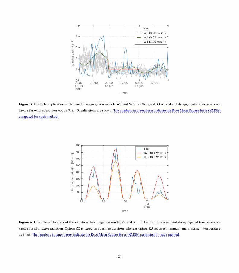
Figure 5. Example application of the wind disaggregation models W2 and W3 for Obergurgl. Observed and disaggregated time series are

shown for wind speed. For option W3, 10 realisations are shown.:::The

:::::::numbers

:in:::::::::parentheses

::::::indicate

:::the

::::Root

:::::Mean

:::::Square

::::Error

:::::::(RMSE)

:::::::computed

:::for

:::each

:::::::method.

Figure 6. Example application of the radiation disaggregation model R2 and R3 for De Bilt. Observed and disaggregated time series are

shown for shortwave radiation. Option R2 is based on sunshine duration, whereas option R3 requires minimum and maximum temperature

as input.::The

:::::::numbers

::in

:::::::::parentheses

::::::indicate

::the

::::Root

:::::Mean

:::::Square

:::::Error

::::::(RMSE)

::::::::computed

::for

::::each

::::::method.

24

Figure 7. Example for precipitation disaggregation using the cascade model: 1h rainfall observed at Rio de Janeiro - São Cristovão on 05 Dec

2010 (blue). Based on statistical evaluations of long-term hourly precipitation series and their aggregation to coarser temporal resolutions,

all relevant steps of the cascade disaggregation applied to daily totals are presented (green). The time series of each cascade level are shown

for three realisations of the model n= 1 (left), n= 2 (centre), and n= 3 (right).

25

Figure 8.:::::::::Histograms

::of

::::::::observed

:::and

:::::::::::disaggregated

::::time

::::::series

:::for

::::each

:::::::variable

::::::::(columns)

::::and

::::each

::::::station

::::::(rows).

::::::::Observed

:::::::::::(disaggregated)

::::time

::::series

:::are

:::::::displayed

::in::::grey

::::::(white).

26

Figure 9. Long-term averages of diurnal courses of observed (dashed) and disaggregated (solid) temperature. Option T1:::T1b has been chosen

and the sine-curve was modelled based on sunset and sun noon computations for minimum and maximum temperature, respectively. The

period of time involved in this analysis is listed in Tab. 1 for each station.

27

Figure 10. Long-term averages of diurnal courses of observed (dashed) and disaggregated (solid) relative humidity::(H3

::::::model). The period

of time involved in this analysis is listed in Tab. 1 for each station.

28

Figure 11. Long-term averages of diurnal courses of (a) observed and (b) disaggregated ‘normative’ wind speed:::(W2

:::::model). The ‘normative’

wind speed indicates the ratio of the long-term mean of the wind speed observed or modelled at a specified hour to the respective value

averaged for the entire day. The period of time involved in this analysis is listed in Tab. 1 for each station.

Figure 12. Long-term averages of diurnal courses of observed (dashed) and disaggregated (solid) shortwave radiation. Diaggregation is based

on daily recordings of sunshine duration:::(R2

::::::model).

29

Figure 13. Modelled (blue) vs. observed (black) precipitation intensities for the 1% highest intensities derived using a split-sample test for

the cascade model:::(P2). For all panels the shaded areas refer to the standard deviation (dark blue) and range of values (light blue) computed

for 100 realisations, respectively.

Figure 14. Autocorrelation rk

as function of time lag k (in hours) plotted for modelled (blue) and observed (black) precipitation time series.

For all panels the shaded areas refer to the standard deviation (dark blue) and range of values (light blue) computed for 100 realisations,

respectively.

30

Table 1. List of AWS investigated in this study. The elevation of each station z is given in meters above sea level. Data availability refers to the

available station recordings:::::(hourly

::::data). The first period of time refers to the calibration period, whereas the second period is preserved for

validation purposes. P=precipitation, T=air temperature, H=humidity, W=wind speed, R=solar radiation, S=sunshine duration. The location

of each station is shown on the map in Fig. 2.

Station z Data availability Source

1 De Bilt 2 1961-1990, 1991-2014, P, T, W, H, R, S KNMI (2015)

2 Ny-Ålesund 11 1993-2004, 2006-2011, T, W, H, R, S Maturilli et al. (2013a, b)

3 Obergurgl 1938 2000-2007, 2008-2014, P, T, W, H, R project data

4 Rio de Janeiro - São Cristovão 5 2003-2008, 2009-2014, P, T, W, H Alerta Rio (2015)

5 Tucson International Airport 779 1973-1993, 1994-2014, P, T, W, H, R NOAA (2015a); NREL (2015)

Table 2. Overview of disaggregation methods included in MELODIST. The fist letter indicates the parameter that is considered by each

method (P=precipitation, T=air temperature, H=humidity, W=wind speed, R=solar radiation, X=all variables). For each method, key refer-

ences are given.

Method Type Calib.

T1 Standard Sine-redistribution with different options (Waichler and Wigmosta, 2003) deterministic no

H1 Tdew = Tmin (Bregaglio et al., 2010; Waichler and Wigmosta, 2003) deterministic no

H2 Tdew = aTmin + b (Bregaglio et al., 2010; Waichler and Wigmosta, 2003) deterministic yes

H3 Linear variation of Tdew overlaid by sine function (Bregaglio et al., 2010) deterministic yes

H4 Hmin, Hmax (Bregaglio et al., 2010; Waichler and Wigmosta, 2003) deterministic no

W1 Equal distribution deterministic no

W2 Cosine function (Debele et al., 2007; Green and Kozek, 2003) deterministic yes

W3 Random distribution (Debele et al., 2007) stochastic no

R1 Scaling of potential shortwave radiation (Liston and Elder, 2006) deterministic no

R2 Ångström (1924) model for sunshine duration S, then R1 deterministic yes

R3 Bristow and Campbell (1984) model, then R1 deterministic yes

P1 Equal distribution “( 124 )” (Waichler and Wigmosta, 2003) deterministic no

P2 Cascade model (Olsson, 1998) stochastic yes

P3 Redistribution according to another station deterministic no

X1 Linear interpolation deterministic no

31

Table 3. Model performance measures for temperature disaggregation::::(T1b

:::::model). x̄

o

and x̄s

are the mean values of observed and disaggre-

gated temperature, respectively. The standard deviation of the observed (�̃o

) and disaggregated (�̃s

) time series are also specified. The Root

Mean Square Error (RMSE), the correlation coefficient r, and the Nash-Sutcliffe model efficiency (NSE) are calculated using the observed

and disaggregated time series for each station.

Station x̄o

x̄s

�̃o

�̃s

RMSE r NSE

(unit of temperature [K]) [-] [-]

De Bilt 283.57 283.45 6.88 6.94 1.74 0.97 0.94

Ny Ålesund 269.55 269.65 7.24 7.27 1.63 0.97 0.95

Obergurgl 275.90 276.36 7.87 8.03 2.00 0.97 0.94

Rio de Janeiro 298.25 298.74 4.03 4.34 1.66 0.93 0.83

Tucson 294.35 294.45 9.53 9.49 2.69 0.96 0.92

Table 4. Model performance measures for humidity disaggregation:::(H3

:::::model). x̄

o

and x̄s

are the mean values of observed and disaggregated

relative humidity, respectively. The standard deviation of the observed (�̃o

) and disaggregated (�̃s

) time series are also specified. The Root

Mean Square Error (RMSE), the correlation coefficient r, and the Nash-Sutcliffe model efficiency (NSE) are calculated using the observed

and disaggregated time series for each station.

Station x̄o

x̄s

�̃o

�̃s

RMSE r NSE

(unit of relative humidity [%]) [-] [-]

De Bilt 81.82 81.63 15.12 15.48 12.67 0.66 0.30

Ny Ålesund 74.96 74.82 12.61 12.30 17.41 0.02 -0.91

Obergurgl 70.83 66.42 17.67 13.40 16.43 0.51 0.14

Rio de Janeiro 70.95 67.45 14.13 10.76 10.39 0.72 0.46

Tucson 35.31 33.31 21.96 10.51 18.52 0.55 0.29

Table 5. Model performance measures for wind speed disaggregation::::(W2

:::::model). x̄

o

and x̄s

are the mean values of observed and disaggre-

gated wind speed, respectively. The standard deviation of the observed (�̃o

) and disaggregated (�̃s

) time series are also specified. The Root

Mean Square Error (RMSE), the correlation coefficient r, and the Nash-Sutcliffe model efficiency (NSE) are calculated using the observed

and disaggregated time series for each station.

Station x̄o

x̄s

�̃o

�̃s

RMSE r NSE

(unit of wind speed [m/s]) [-] [-]

De Bilt 3.49 3.49 1.89 1.59 1.05 0.83 0.69

Ny Ålesund 4.03 4.03 3.23 2.57 1.95 0.80 0.64

Obergurgl 1.38 1.38 1.51 1.06 1.08 0.70 0.49

Rio de Janeiro 1.41 1.41 1.21 0.75 0.85 0.72 0.50

Tucson 3.27 3.27 2.07 1.17 1.70 0.57 0.32

32

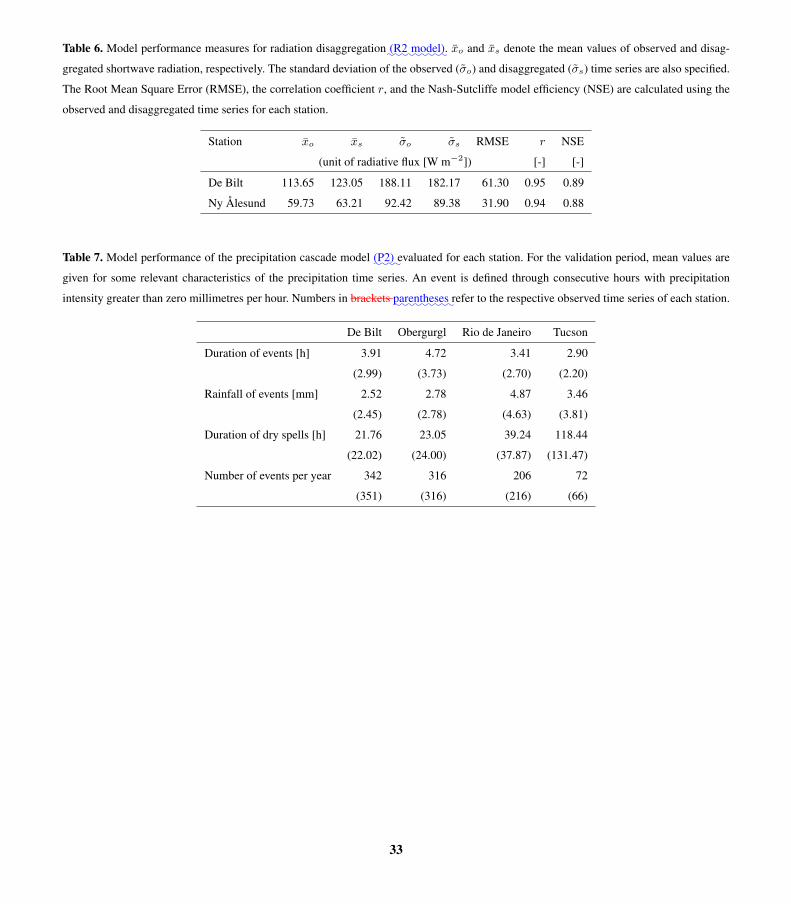
Table 6. Model performance measures for radiation disaggregation:::(R2

::::::model). x̄

o

and x̄s

denote the mean values of observed and disag-

gregated shortwave radiation, respectively. The standard deviation of the observed (�̃o

) and disaggregated (�̃s

) time series are also specified.

The Root Mean Square Error (RMSE), the correlation coefficient r, and the Nash-Sutcliffe model efficiency (NSE) are calculated using the

observed and disaggregated time series for each station.

Station x̄o

x̄s

�̃o

�̃s

RMSE r NSE

(unit of radiative flux [W m�2]) [-] [-]

De Bilt 113.65 123.05 188.11 182.17 61.30 0.95 0.89

Ny Ålesund 59.73 63.21 92.42 89.38 31.90 0.94 0.88

Table 7. Model performance of the precipitation cascade model:::(P2)

:evaluated for each station. For the validation period, mean values are

given for some relevant characteristics of the precipitation time series. An event is defined through consecutive hours with precipitation

intensity greater than zero millimetres per hour. Numbers in brackets::::::::parentheses

:refer to the respective observed time series of each station.

De Bilt Obergurgl Rio de Janeiro Tucson

Duration of events [h] 3.91 4.72 3.41 2.90

(2.99) (3.73) (2.70) (2.20)

Rainfall of events [mm] 2.52 2.78 4.87 3.46

(2.45) (2.78) (4.63) (3.81)

Duration of dry spells [h] 21.76 23.05 39.24 118.44

(22.02) (24.00) (37.87) (131.47)

Number of events per year 342 316 206 72

(351) (316) (216) (66)

33