Limitations of WRF land surface models for simulating ... - GMD

1

Limitations of WRF land surface models for simulating land use and land cover change in Sub-Saharan Africa and development of an improved model (CLM-AF v. 1.0) Timothy Glotfelty1, Diana Ramírez-Mejía2, Jared Bowden3, Adrian Ghilardi2, and J. Jason West1 1Department of Environmental Sciences and Engineering, University of North Carolina at Chapel Hill, Chapel Hill, NC 27599, 5 USA 2Centre for Research in Environmental Geography, Universidad Nacional Autónoma de México, Morelia, 58190, Mexico

3Department of Applied Ecology, North Carolina State University, Raleigh, NC 27695, USA

Correspondence to: Timothy Glotfelty ([email protected])

Abstract. Land use and land cover change (LULCC) impacts local and regional climates through various biogeophysical 10

processes. Accurate representation of land surface parameters in land surface models (LSMs) is essential to accurately predict

these LULCC-induced climate signals. In this work, we test the applicability of the default Noah, Noah-MP, and CLM LSMs

in the Weather Research and Forecasting Model (WRF) over Sub-Saharan Africa. We find that the default WRF LSMs do not

accurately represent surface albedo, leaf area index, and surface roughness in this region due to various flawed assumptions,

including the treatment of the MODIS woody savanna LULC category as closed shrubland. Consequently, we developed a 15

WRF CLM version with more accurate African land surface parameters (CLM-AF), designed such that it can be used to

evaluate the influence of LULCC. We evaluate meteorological performance for the default LSMs and CLM-AF against

observational datasets, gridded products, and satellite estimates. Further, we conduct LULCC experiments with each LSM to

determine if differences in land surface parameters impact the LULCC-induced climate signals. Despite clear deficiencies in

surface parameters, all LSMs reasonably capture the spatial pattern and magnitude of near surface temperature and 20

precipitation. However in the LULCC experiments, inaccuracies in the default LSMs result in illogical localized temperature

and precipitation climate signals. Differences in thermal climate signals between Noah-MP and CLM-AF indicate that the

temperature impacts from LULCC are dependent on the sensitivity of evapotranspiration to LULCC in Sub-Saharan Africa.

Errors in land surface parameters indicate that the default WRF LSMs considered are not suitable for LULCC experiments in

tropical or Southern Hemisphere regions, and that proficient meteorological model performance can mask these issues. We 25

find CLM-AF to be suitable for use in Sub-Saharan Africa LULCC studies, but more work is needed by the WRF community

to improve its applicability to other tropical and Southern Hemisphere climates.

1 Introduction

Land use and land cover change (LULCC) has various biogeophysical impacts on climate by altering land surface albedo,

evapotranspiration, and surface roughness that in turn alter atmospheric circulations, energy budgets, and hydrologic cycles 30

https://doi.org/10.5194/gmd-2020-193Preprint. Discussion started: 19 August 2020c© Author(s) 2020. CC BY 4.0 License.

2

(Pielke et al., 2011; Mahmood et al., 2014; Bright 2015; Smith et al., 2016; Quesada et al., 2017). Results from global

modelling studies indicate a global reduction in surface temperatures due to deforestation, but the impacts of LULCC vary by

region and season (e.g., Zhao and Pitman 2002; Lamptey et al., 2005; Lejune et al., 2017). Such studies have shown a latitudinal

difference in the temperature response to deforestation, where higher latitudes experience cooling in winter as less tree cover

brightens the surface when snow is present, and lower latitude tropical regions experience warming in response to a reduction 35

in evaporation (e.g., Longobardi et al., 2016; Quesada et al., 2017). This LULCC latitudinal dependence has been shown to

occur in observations as well (Zhang et al., 2014).

Impacts of LULCC are simulated in climate and numerical weather prediction models through the land surface model (LSM).

Differences in LSM parameterizations can lead to significantly different climate responses to LULCC in both magnitude and

sign (e.g., Olsen et al., 2004; Boisier et al., 2012; Burakowski et al., 2016), even when little difference exists in the mean 40

simulated climate (Crossly et al., 2000). Errors and uncertainties in LSMs occur in response to errors in LULC classification

maps and the way land use properties, such as vegetation distributions and surface albedo, are prescribed (e.g., Lu and

Shuttleworth, 2002; Olsen et al., 2004; Ge et al., 2007; Boisier et al., 2012; Boisier et al., 2013; Boysen et al., 2014; Meng et

al., 2014; Hartley et al., 2017; Bright et al., 2018). As a result, improving LULC maps and LSM parameters has been shown

to significantly reduce biases and errors within global and regional climate models (RCMs) (e.g., Tian et al., 2004b; Kang et 45

al., 2007; Lawrence and Chase, 2007; Lawrence and Chase, 2009; Moore et al., 2010; Karri et al., 2016; Thackeray et al.,

2019). Having accurate representations of these parameters is especially important in regions with large surface heterogeneity,

such as East Africa (Ge et al., 2008).

Sub-Saharan Africa is a region of particular interest for simulating LULCC because it has already experienced dramatic

LULCC (e.g., Collier et al., 2008), which has been shown to alter the West African monsoon system (e.g., Charney, 1975; Xue 50

and Shakula, 1993; Abiodun et al., 2008; Wang et al., 2017). Various ensembles of RCMs have been applied to study the

climate of Africa as part of both the COordinated Regional climate Downscaling Experiment (CORDEX) (e.g., Nikulin et al.,

2012; Gbobaniyi et al., 2014; Kim et al., 2014; Mounkaila et al, 2015; Endris et al., 2016; Diasso and Abiodun, 2017; Adeniyi

and Dialu, 2018; Odoulami et al., 2019) and the West African Monsoon Modeling and Evaluation Project Experiments

(WAMME) (e.g., Wang et al., 2016; Xue et al., 2016). Included as part of these ensemble modelling projects is the Weather 55

Research and Forecasting (WRF) Model (e.g., Xue et al., 2016; Fita et al., 2019).

The WRF model is a state-of-the-art numerical weather prediction model designed to be applicable in multiple world regions,

across multiple spatial scales, and for short-term forecasting to longer term regional climate simulations (Skamarock and

Klemp, 2008). Multiple studies have tested the sensitivity of the African climate to different ensembles of WRF physics

parameterizations, including LSMs (e.g., Pohl et al., 2011; Hagos et al., 2014; Noble et al., 2014; Alaka and Maloney, 2017; 60

Noble et al., 2017; Igri et al., 2018). Results from these WRF simulations are somewhat contradictory as some studies found

the National Centers for Environmental Prediction, Oregon State University, Air Force, Hydrology Lab (Noah) LSM (Chen

and Dudhia, 2001; Ek et al., 2003) to have superior performance compared to observations and reanalysis (Pohl et al., 2011;

Igri et al., 2018), while others found no unambiguous difference in model performance between different LSMs (Noble et al.,


3

2014; 2017). In terms of LULCC applications, Hagos et al. (2014) found that WRF model configurations that simulate a 65

climate which is too wet or too dry compared to observations and reanalysis do not produce a strong climate signal from

LULCC over Africa. This weak signal is a result of the model falling into erroneous moisture or energy limited regimes.

Despite these uncertainties, the Noah LSM is by far the most common LSM configuration applied in WRF studies over Africa

(e.g., Vigaud et al., 2011; Cretat et al., 2012; Boulard et al., 2013; Ratna et al., 2014; Schepanski et al., 2014; Argent et al.,

2015; Diaz et al., 2015; Klein et al., 2015; Zheng et al., 2015; Arnault et al., 2016; Kerandi et al., 2017; Klein et al., 2017). 70

In this work, we expand upon the current literature by testing five different LSM configurations within the WRF model for the

purpose of evaluating the effects of LULCC over time on regional climate in Sub-Saharan Africa. First, we review four

commonly used LSMs to determine if the LSM configurations reasonably represent land surface parameters such as albedo

and leaf area index (LAI). As shown below, we find that these four LSMs have significant deficiencies which limit their

capabilities in applications to LULCC in this region. Consequently, we then detail how we modify one LSM for use in this 75

study. We then evaluate the five WRF LSM configurations against available meteorological observations, reanalysis, and

satellite estimates to determine how well they simulate the current climate of Sub-Saharan Africa. Finally, we simulate the

effects of LULCC over time on the simulated regional climate, and how these climate responses differ when using different

LSMs. Understanding the deficiencies in how LSMs represent LULCC is key to accurately representing regional climate

signals that impact not only climate change investigations, but also coupled natural and human system research regarding 80

human decision making, air quality, and human/ecosystem health interactions.

2 WRF description and configurations

This study uses the WRF model version 3.9.1.1 (WRFv3.9.1.1), configured as shown in Table 1, to simulate the regional

meteorology and climate within Sub-Saharan Africa. We define a Sub-Saharan Africa domain that ranges from ~19º N - 35º

S latitude and ~19º W - 64º E longitude (Fig. 1) with a horizontal grid spacing of 36 km and 30 vertical layers from the surface 85

to 50 hPa. Physics parameterizations common to all simulations include: the New Tiedtke cumulus parametrization scheme

(Zhang et al., 2011), the aerosol-aware Thompson microphysics scheme (Thompson and Eidhammer, 2014), the RRTMG long

and shortwave radiation schemes (Clough et al., 2005; Iacono et al., 2008), and the MYNN surface/ planetary boundary layer

physics (Nakanishi and Niino, 2004; 2006). These physics combinations were selected because they represent some of the

most advanced science within the WRF model, and these physics options performed the best when validated against 90

observations/satellite estimates relative to other physics options tested (not shown). All simulations also take advantage of the

CLM4.5 lake model, which is calibrated to prognostically simulate lake conditions for the African Great Lakes by adjusting

the lower bound lake temperature from 4℃ to 24℃ consistent with Lake Victoria temperature profiles (Nyamweya et al.,

2016). Meteorological initial and boundary conditions for the simulations are obtained from the European Centre for Medium-

Range Weather Forecasts Interim reanalysis (ERA-Interim) (Dee et al., 2011). Because LULC inputs change each year, each 95


4

model year is modelled individually, preceded by a three-month spin-up period that is discarded to allow the model to reach

equilibrium and minimize the impact of initial conditions on the simulations.

2.1 WRF land surface model descriptions

Here we briefly describe four commonly-used WRF LSM configurations used in this study and differences between them: the

Noah LSM; the Noah LSM using satellite derived albedo and LAI (Noah-Sat); the Noah Multi-Parameterization LSM (Noah-100

MP) (Niu et al., 2011); and the default Community Land Surface model (CLM-D) (Subin et al., 2011; Jin and Wen, 2012; Lu

and Kueppers, 2012). We focus on the different ways in which the LSMs prescribe and treat surface parameters such as LAI,

albedo, and surface roughness length based on the Moderate Resolution Imaging Spectroradiometer (MODIS) 21 land category

data. In addition to the LSMs used in this work, four other LSMs exist in WRF including: the five layer thermal diffusion

scheme (Skamarock et al., 2008), the Rapid Update Cycle (RUC) LSM (Smirnova et al., 2016), the Pleim-Xiu (PX) LSM 105

(Pleim and Xiu, 2003; Gilliam et al., 2007), and the Simplified Single Biosphere Model (SSiB) (Xue et al. 1991; Sun and Xue,

2001). The five layer thermal diffusion scheme is omitted from these experiments because it is overly simplistic and not

appropriate for climate scale studies. The RUC and PX LSMs are primarily designed for weather forecasting and for

retrospective meteorological simulations commonly used as input for downstream air quality simulations, respectively.

Although RUC and PX can be used for other applications, they require extensive detailed input data or data assimilation for 110

peak performance (http://www2.mmm.ucar.edu/wrf/users/docs/user_guide_V3.9/users_guide_chap5.htm#Phys). Since this

detailed level of observational data is not available in Sub-Saharan Africa, both the RUC and PX scheme were excluded. The

SSiB LSM is designed for climate applications, however it is also excluded both because its best performance occurs using its

own LULC dataset and because it is not currently compatible with the MYNN surface/boundary layer parameterizations.

2.1.1 Noah LSM and Noah-Sat 115

In Noah and Noah-Sat are the same LSM with different configurations for how surface albedo and LAI are prescribed. Within

the Noah LSM, surface parameters including surface albedo, roughness length, and LAI are prescribed based on the dominant

MODIS LULC category in each grid cell with temporal interpolation between maximum and minimum values depending on

the time of year. The Noah-Sat configuration uses a monthly average satellite derived climatology of surface albedo and LAI

supplied from the WRF preprocessing system (WPS), as a more detailed replacement of the LULC based prescribed values. 120

Noah and Noah-Sat have no explicit canopy layer, and instead simulate evapotranspiration using a satellite derived green

fraction variable from WPS to weight the contribution of direct soil evaporation and evapotranspiration from vegetation in

each grid cell. The land surface and underlying soil is simulated using 4 soil layers 0.1, 0.3, 0.6, and 1.0 meters thick centered

0.05, 0.25, 0.7, and 1.5 meters below the ground surface, respectively.

Noah-Sat is limited in its ability to simulate LULCC because LAI and surface albedo are decoupled from changes in the LULC 125

categories, and temporally varying satellite LAI and albedo products are influenced by other climate variations or changes

apart from effects of LULCC. Noah is also preferable to Noah-Sat for future climate simulations because the albedo and LAI


5

products Noah-Sat requires would have to be generated as separate independently varying fields from the future LULC

projection.

Additionally, the Noah LSM can be configured using a mosaic tile approach to represent the influence of sub-grid scale 130

variations in LULC. The representation of sub-grid LULC variability can significantly alter the responses of climate models

to LULCC (e.g., Boone et al., 2016), but this functionality is not considered in these experiments since any underlying errors

in albedo, LAI, and surface roughness from Noah would be present in both the mosaic tile and dominant LULC configurations.

Also, this approach has been shown to primarily impact urban regions (Mallard and Spero, 2019), which are not resolved well

at the grid spacing of this study. 135

2.1.2 Noah-MP

The Noah-MP model is an updated version of the Noah LSM with multiple-parameterization options utilizing the same soil

level structure as the default Noah LSM. The major updates in Noah-MP include: the addition of an explicit one-layer

vegetation canopy and three layer snowpack, a tiling scheme that separates vegetation and bare soil to better calculate the

surface energy balance, separating permeable and impermeable frozen soils, new runoff and groundwater schemes, and new 140

dynamic vegetation model options (Niu et al., 2013; Xia et al., 2017 and references therein). In this study, Noah-MP is

configured with the default settings, which are the most similar to the default Noah LSM. With these default settings, dynamic

vegetation is disabled and LAI is prescribed based on the dominant MODIS LULC category in each grid cell using monthly

profile values. Noah-MP simulates surface reflectance using a modified two stream radiation scheme that accounts for gaps

within the vegetation canopy and between canopy crowns (Yang and Friedl, 2003; Niu and Yang, 2004); however, in 145

WRFv3.9.1.1 Noah-MP uses a simplification that assumes all bare soil albedos are comparable to loam soil. As a result, surface

albedo within Noah-MP is solely a function of soil moisture and vegetation cover.

2.1.3 Default CLM (CLM-D)

The default configuration of CLM in WRF divides the land surface into five types: glacier, lake, wetland, urban, and vegetated.

Vegetated land is further split into up to four patches of 16 plant functional types (PFTs) with distinct physiological parameters. 150

Calculations within each vegetated grid are done at the PFT level and then aggregated for atmosphere interactions. CLM

contains a single-layer vegetation parametrization with a sunlit and shaded canopy and uses the two stream approximation

(Sellers 1985) to calculate the energy balance within the canopy. Temperature and humidity varies between the ground surface,

the canopy, and the leaf surface (Subin et al., 2001 and references therein). The land surface and soil properties in CLM are

simulated using 10 layers ~0.018, 0.028, 0.045, 0.075, 0.124, 0.204, 0.336, 0.554, 0.913, and 1.134 meters thick centered at 155

~0.007, 0.028, 0.062, 0.119, 0.212, 0.367, 0.620, 1.038, 1.728, and 2.86 meters below the ground surface.

In the version of CLM available in WRF, each dominant MODIS land use category is assigned a distribution of PFTs with

distinct monthly profiles for LAI that do not vary geographically. A list of the CLM PFTs with the percentages for each


6

vegetated MODIS land use category is shown in Table S1 of the Supplementary Material. Bare soil albedos in CLM are not

constrained like within Noah-MP and therefore a broader range of surface soil albedos is considered. 160

Some simplifications in WRF-CLM lead to difficulties applying the default version for the Sub-Saharan Africa domain. For

example, Table S2 of the Supplementary Material shows the monthly LAI profiles used for each PFT within the default CLM

configuration. These profiles clearly show Northern Hemisphere growing cycles, which is problematic for Sub-Saharan Africa

because it contains regions with bimodal tropical growing cycles and Southern Hemisphere growing cycles. Additionally, the

visible spectrum dry soil albedo for the sandiest soils in the default CLM treatment is 0.24, considerably less than the 0.25-165

0.45 albedo from MODIS satellite estimates over most the Sahara (Wang et al., 2004)..

3 Updated CLM for Sub-Saharan Africa (CLM-AF)

To address these limitations with CLM-D, and deficiencies of other LSMs described in the results section, the WRF-CLM

LSM has been modified to include PFT distributions more representative of the Sub-Saharan Africa domain, regionally varying

monthly profiles for LAI and stem area index (SAI), minor improvements in vegetation optical properties (e.g., leaf 170

reflectance), and scaled surface albedos for sandy soils to better match satellite estimates. Each of these modifications is

described in detail below.

3.1 CLM-AF plant functional type distributions

Updated PFT distributions are derived from a global three arc minute PFT dataset for the year 2001 generated by the National

Center for Atmospheric Research for the Model of Emission of Gases and Aerosols from Nature version 2.1 175

(https://bai.ess.uci.edu/megan/versions/megan21). To determine the percentages of each PFT representative of the various

MODIS land use categories in Sub-Saharan Africa, the global PFT dataset is regridded to the 36 km WRF domain, and the

average coverage of each PFT within each WRF-MODIS 2001 dominant land use category is calculated. Updated PFT

distributions were generated for broad leaf evergreen/deciduous forests, mixed forests, closed and open shrublands, woody

savannas/savannas, grasslands, and cropland/mosaic croplands (i.e., MODIS categories 2,4,5, 6-10, 12, and 14). This limited 180

subset of categories is used because the remaining MODIS categories did not cover a large enough area to be the dominant

land use at 36 km resolution. Since CLM allows for up to four PFT patches, the top four most abundant PFTs within each

MODIS land use category are scaled to represent one hundred percent of the land use category, with an exception for some

inconsistencies that occurred between the PFT and the evergreen broad leaf forest, savanna, and mosaic cropland MODIS

categories (see Supplementary Material). The resulting updated PFT distribution for these CLM vegetated land use categories 185

is shown in Table 2.

Most of the updated PFT distributions in Table 2 are consistent with the MODIS International Geosphere-Biosphere

Programme (IGBP) category descriptions (Table S3, Supplementary Material). However, there are two minor inconsistencies

with the closed shrubland and grassland categories. The closed shrubland category contains slightly less than 60% shrubs and


7

8% deciduous tropical trees, indicating there is some sub-grid scale overlap with nearby woody savannas or forests. The 190

grasslands category contains 18% shrubs, which is higher than the 10% from the description in Table S3, indicating some

overlap with sub-grid scale shrublands. Overall, compared to the CLM-D PFT distributions in Table S1, the updated values in

CLM-AF have greater heterogeneity in plant types and contain more herbaceous cover. The largest deviations from the CLM-

D distribution occur with shrublands and woody savanna. CLM-D prescribes all shrublands as broad leaf evergreen shrubs,

while the global PFT dataset indicates that shrublands in Sub-Saharan Africa contain broad leaf deciduous temperate shrubs. 195

Additionally, the woody savanna category PFT distribution in CLM-D is identical to closed shrubland. This is potentially a

large source of error as woody savanna should have forest cover between 30-60% (Table S3, Supplementary Material). This

error is removed in the CLM-AF PFT distribution with the woody savanna category containing 38% tree cover.

3.2 CLM-AF LAI and SAI profiles

Since the Sub-Saharan Africa domain covers a wide range of tropical and sub-tropical latitudes, a single domain-wide LAI 200

and SAI monthly profile for each PFT is not appropriate. Here, geographically varying monthly LAI profiles are generated by

dividing the Sub-Saharan Africa domain into 17 distinct regions based on bioclimate characteristics used in LULCC modelling

of Sub-Saharan Africa (Fig.1, Table 3).These bioclimate regions were generated because landscape dynamics are known to be

different between broad climatic zones, needing separate modelling parametrizations (Soares-Filho et al 2006). However, the

central wet (CW), central moist (CM), and northeast semi-dry (NESD) bioclimate regions span a large latitudinal range and 205

are subdivided based on latitude to generate more meaningful LAI seasonal profiles (Supplementary Material).

The updated LAI profiles within each bioclimate region are derived from both the 36 km regridded global PFT dataset and the

monthly LAI climatology data, provided by WPS, used in the Noah-Sat configuration. LAI profiles are calculated only from

a subset of grid cells within the WPS Sub-Saharan Africa LAI climatology, where the 36 km regridded PFT data indicates that

a given PFT comprises eighty percent or more of the grid cell (PFT80). For the broad leaf evergreen tree PFTs, the median 210

monthly LAI value of the PFT80 grid cells within each bioclimate or sub-bioclimate region is used as the monthly prescribed

LAI value for that PFT. Median values are used in place of mean values for the broad leaf evergreen tree PFTs because several

small LAI values near the edges of forested regions lead to unrealistically small LAI values for the Congo and other forests

compared to the WPS LAI satellite derived climatology. For the remaining PFTs, the mean monthly LAI value of the PFT80

grid cells within each bioclimate or sub-bioclimate region is used as the monthly prescribed LAI value for that PFT. The 215

monthly LAI profiles for each PFT within each bioclimate and sub-bioclimate region are listed in Tables S4-S10 of the

Supplementary Material. If no grid cells within a bioclimate or sub-bioclimate region meet the PFT80 criteria for a required

PFT, then a reduced threshold of sixty percent of the grid cell is utilized to calculate the monthly LAI profile for that PFT. If

no grid cells meet the sixty percent criteria, the LAI profile for that PFT within the bioclimate or sub-bioclimate region is

assumed to be the same as a nearby comparable bioclimate region. These comparable “alternative” bioclimate regions are 220

listed in Table 4. Some additional adjustments were also required for the broad leaf evergreen tree PFTs to make these areas

more consistent with the satellite derived climatology (Supplementary Material).


8

SAI represents the area of stems and dead leaves. The values of SAI are poorly known, but SAI is generally parameterized to

have a minimum in winter and maximum in autumn for each land cover type (Tian et al., 2004a). Since no readily available

data on SAI exists, SAI within CLM-AF is based on relating decreases in LAI (ΔLAI) from month to month to the SAI values 225

in the CLM-D configuration. This is done by fitting a simple linear regression between ΔLAI and the SAI value in CLM-D. If

the LAI is not decreasing from the previous month then the SAI value is assumed to be the minimum value from CLM-D.

These assumptions are consistent with the definition of SAI as dead leaves/litter will only increase when LAI is decreasing.

However, it was not possible to generate linear regressions for evergreen trees and corn from CLM-D because the evergreen

tree LAI profiles in CLM-D do not change from month to month and the corn SAI profile is equivalent to the corn LAI profile. 230

These assumptions are not appropriate for Sub-Saharan Africa because of the longer tropical growing season and small

seasonal fluctuations in evergreen tree LAI in the satellite climatology. Therefore, corn within CLM-AF is assumed to have

the same SAI profile as C4 grass, and evergreen trees follow a similar equation as C4 grass with an intercept equivalent to the

appropriate evergreen tree minimum SAI value of 0.5. A list of the SAI profile equations and minimum SAI values in the

CLM-AF configuration for the updated PFTs are listed in Table 5. 235

3.3 CLM-AF sandy soil albedo

CLM-D sandy soil albedos and updated values for CLM-AF are listed in Table 6. CLM simulates surface albedo using a look-

up table for different soil color classes with two different radiation streams that differentiate between saturated and dry soils.

Albedo values in the sandy soils of the Sahara range from 0.25-0.45 (Wang et al., 2004), which is larger than the 0.24 dry

sandy soil albedo in CLM-D. Accordingly, we increased the albedo values for sand and sand-loam combination soil types by 240

0.1 and 0.02, respectively. This puts the sandy soil albedos inside the range expected for the Sahara, while not leading to

excessively large albedos in the deserts of southern and eastern Africa.

3.4 CLM-AF vegetation property adjustments

In order to bring the albedo of vegetated areas into better agreement with the satellite climatology from WPS, several

adjustments are made to leaf/vegetation optical properties in CLM-AF. In CLM-D, shrubs in Sub-Saharan Africa are 245

erroneously classified as broad leaf evergreen shrubs rather than temperate deciduous shrubs. In order to maintain a lower

albedo for these African shrubs, the leaf transmittance, leaf angle, and leaf reflectance properties of the deciduous temperate

shrubs are adjusted to match those of broad leaf evergreen shrubs. Additionally, the near-infrared leaf reflectance of all broad

leaf tree species is lowered from 0.45 to 0.35 in CLM-AF, which is in better agreement with near-infrared leaf reflectance

measured by unmanned aerial vehicle mounted hyperspectral imaging instruments over African forest canopies (Thomson et 250

al., 2018).


9

4 Experimental design

This study consists of two experiments (Table 7). The first is a model validation experiment to compare differences between

the WRF LSM configurations and assess their model performance. The second is a LULCC experiment to determine if the

errors and uncertainties of each LSM lead to differences in their climate responses to LULCC. 255

4.1 Model validation experiment

The model validation experiment consists of five simulations conducted for the year 2013, each using one of the five LSM

configurations discussed above. The year 2013 is selected because it is a neutral year for the El Niño Southern Oscillation.

While a single year comparison does not yield climate relevant statistics, it is sufficient to demonstrate differences in the

meteorology between the five LSM configurations and the mechanisms responsible for these differences. The model validation 260

simulations are conducted with default greenhouse gas concentrations and MODIS 21 class land use data. These default

settings are chosen to illustrate the performance that can be expected from the publicly available WRF model.

4.2 Land use and land cover change experiment

The LULCC experiment simulates the period 2010-2015 and represents recent climate responses from LULCC since the year

2001. To accomplish this goal, the LULCC experiment consists of two simulations per LSM configuration. The first simulation 265

for each LSM uses static LULC from the year 2001 for each simulated year (i.e., 2010-2015), hereafter referred to as LU01.

The second uses dynamic LULC each simulated year, hereafter referred to as LUD. Differences between the LU01 and LUD

simulations delineate the climate response to LULCC. These two simulations are carried out using the Noah, Noah-MP, CLM-

D, and CLM-AF LSMs. Noah-Sat is excluded because LAI and albedo parameters derived from satellite data could be

impacted by climatological variability other than LULCC. The LULCC simulations utilize MODIS 21 class land use data that 270

was processed by the Dinamica EGO land use modeling framework (Soares-Filho et al., 2002 – described in more detail

below) and global average greenhouse gas concentrations for each simulation year from the National Oceanic and Atmospheric

Administration’s (NOAA) Earth System Research Laboratory (ESRL) Global Monitoring Division. In the LULCC

experiments, each year is a discreet simulation with a 3-month spin-up in which the model LULC is updated at the start of

each year. This is necessary because the WRF modelling framework treats LULC as a static field. 275

4.3 Land use / land cover data

The LULC dataset for the LULC experiment is extracted from simulated annual maps of land use and land cover spanning

2001 to 2050. These maps are created by means of prospective landscape modelling techniques and while simulations contain

some level of model error, this approach is used to reduce the impact of potential LULC misclassification errors and

uncertainties in the MODIS product that could propagate into the WRF model leading to “noisy” and inconclusive climate 280

impacts.


10

LULC is simulated using the Dinamica EGO environmental modelling platform (Soares-Filho et al., 2002). Dinamica EGO is

a modelling tool designed to construct simple or complex spatiotemporal models involving multiple transitions and iterations,

dynamic feedbacks, sub-region approaches, and several spatial algorithms for the analysis and simulation of a wide variety of

dynamic LULCC phenomena. Dinamica EGO has been used for many applications (Bowman et al., 2012; Cheng et al., 2020; 285

De Almeida et al., 2005; Ghilardi et al., 2016; Merry et al., 2009; Nepstad et al., 2009; Oliveira et al., 2019; Silvestrini et al.,

2011; Soares et al., 2002; Soares et al., 2006; Soares-Filho et al., 2010; Thapa and Murayama, 2011).

For input to our LULCC simulations, we use the MODIS Land Cover Type product (MCD12Q1) consisting of a suite of

datasets that provides global land cover maps at 500 meter spatial resolution and annual temporal coverage from 2001 to 2013,

and includes six different land cover classification schemes (Friedl and Sulla-Menashe, 2015; Friedl et al., 2010). This product 290

is generated using an ensemble of supervised classification algorithms that uses MODIS Nadir BRDF-Adjusted Reflectance

data as input (Schaaf et al., 2002). Specifically, we use the IGBP classification legend since the land cover data ingested by

the WRF model (Skamarock, 2008) is based on MODIS-IGBP classification scheme. The MODIS Land Cover product has a

post-process overall accuracy of 75% (Friedl et al., 2010).

Using this approach, we detected spurious changes that toggle yearly between classes such as woody savannas, savannas, or 295

grasslands. To reduce this temporal noise, we apply a cell-based temporal mode filter that replaces cell values with the most

frequently occurring LULC class selected from a moving but non-overlapping 3-year window; or alternatively, a 6-year

window when no mode is found, and assigning No Data to the entire 12-year time series if still inconclusive. This filter

preserves long lasting changes while drastically reducing short term changes between LULC classes. There is no edge

preservation because windows do not overlap in time, i.e. LULC classes can change for 2001 or 2012. Consequently, the year 300

of a “true” LULC change can be shifted forwards or backwards by one year.

Prospective landscape models covering very large areas need to be regionalized, meaning that during the calibration period,

explanatory variables and their spatial relationships with observed changes can be tuned separately to capture the heterogeneity

of landscape dynamics. Regions do not represent “hard borders” in modelling results, as the amount of projected change and

the probability of change occurrences are not boxed-in within regions, but the proximate causes of observed change can be 305

analysed separately.

Africa is regionalized into 18 regions based on climatic zones, demographic factors, and anthropogenic activity (Fig. S1)

consisting of three overlapping layers: 1) United Nations geographic regions for Africa: Northern, Eastern, Southern, Western

and Central (UNSD, 1999); 2) a bioclimate layer from the modified version of the Global Environmental Stratification (GEnS)

dataset (Metzger et al. 2013); and 3) residential sector emissions hotspots using DICE-Africa emissions (Marais and 310

Wiedinmyer, 2016). The resulting 67 categories are generalized into the final 18 based on neighborhood. The process of

generalization is done by comparing major change trends among regions, trying to avoid as far as possible the presence of

separate regions with similar LULC dynamics. Of these 18 regions, 17 are used in the WRF modelling because the North

Semi-dry region is outside the Sub-Saharan Africa domain.


11

LULC change rates by region are analysed by means of transition probability matrices, in order to quantify the amount of 315

change in km2 for each LULC change transition during the calibration period (2001 – 2007). Matrices are annualized and used

to simulate expected annual LULC changes up to 2013 for validation purposes, and to 2050 for simulation purposes.

While transition matrices project the expected amount of LULC change into the future, they say nothing about where this

change is likely to occur. For each meaningful transition, a map depicting the probability of that transition happening in the

future is built by means of analysing the spatial relationship between observed changes and a set of explanatory variables 320

(Table S11, Fig. S2). Static and dynamic explanatory variables were related by means of conditional probabilities with the

spatial occurrence of observed LULC changes for a subset of meaningful transitions during the calibration period. All maps

were resampled to 1 km2 resolution and projected to the Africa Albers Equal Area Conic coordinate system. Annual transition

matrices (how much change is expected at each year) are integrated with annual probability maps (also generated for each

year) to produce simulated land cover maps. 325

To evaluate the accuracy of simulations within the present time, simulated annual maps outside the calibration period (2008-

2013) are compared with the MODIS product for the same year, using a fuzzy-logic method (Hagen 2003) (Fig S3). This

approach incorporates a moving window neighborhood context, since predicting the location of LULC transition at a pixel

level is virtually impossible. The comparison is done between simulated and observed cells undergoing a certain LULC change

within the windows. To measure the spatial agreement between maps we used window sizes ranging from 1 to 9 cells 330

(corresponding to spatial resolutions between 500 x 500 m and 4,500 x 4,500 m). For most transitions and regions, simulations

correctly predict change within 4,500 x 4,500 m windows 50% and 75% of cases, which is among the range of reported results

in other prospective modelling studies (e.g. Carlson et al., 2012; Soares et al., 2012; Soares et al., 2006; Thapa and Murayama,

2011; Yi et al., 2012).

4.4 Model evaluation datasets and protocol 335

A list of data used to evaluate WRF’s meteorological performance are shown in Table 8, and the WRF model variables

evaluated against these datasets are listed in Table 9. Surface meteorological and climate quantities are validated against both

hourly surface observations from the National Climate Data Center’s Integrated Surface Dataset (NDCD-ISD) and monthly

average gridded estimates from the University of East Anglia’s Climate Research Unit version 4.02 (CRU TS4.02) dataset

(Harris et al., 2014). Precipitation (PRE) is evaluated against CRU TS4.02, monthly average Global Precipitation Climatology 340

Project (GPCP) estimates, and three-hour average Tropical Rainfall Measurement Mission (TRMM) estimates. Cloud fraction

(CF) and precipitable water vapor (PWV) are compared against estimates from the MODIS Terra Aerosol Cloud Water Vapor

Ozone level three product (MOD08_M3). Additionally, radiation balance variables are compared against satellite estimates

from the Clouds and Earth’s Radiant Energy System – Energy Balanced and Filled (CERES-EBAF) dataset.

To compare WRF to the gridded datasets, the WRF output is averaged to the appropriate temporal resolution and regridded to 345

the native horizontal resolution of the gridded products to calculate performance statistics. Comparisons against NCDC-ISD

are made for each hour by pairing the monitoring station values to the value of the WRF 36 km grid cell containing the


12

monitoring station. All comparisons with MOD08_M3 are done by averaging the WRF data during the daytime MODIS Terra

overpass times of Sub-Saharan Africa (i.e., 600 - 1200 UTC). Model performance is determined by calculating the mean bias

(MB) and normalized mean bias (NMB). Statistical quantities are calculated for the domain as a whole and each bioclimate 350

region to show regional variability in model performance. Additionally, spatial patterns for the simulations and observations

are shown.

5 Results - surface parameters

It is important to illustrate the different surface properties from each LSM, within WRF, using the same LULC because these

surface properties differences will drive simulated changes in the meteorology. Figs. 2-4 depict the surface properties for each 355

of the five LSM configurations from the 2013 evaluation simulations. Since the albedo and LAI of Noah-Sat are generated

from satellite estimates, these values can be considered similar to observations.

In general, all of the LSM configurations that prescribe albedo overpredict surface albedo in vegetated areas. However, the

Noah LSM severely overpredicts surface albedo throughout the entirety of the domain with albedo values ranging from ~20-

28% for regions containing woody savanna, savanna, and shrubland (Fig. 2b), compared to 10-20% over the same areas in 360

Noah-Sat (Fig. 2a). This is because Noah’s prescribed albedo values for many of the MODIS-IGBP categories are significantly

larger than those derived from satellites (Table S12, Supplementary Material). The annual average surface albedos prescribed

by Noah-MP (Fig. 2c) and CLM-D (Fig. 2d) are similar in magnitude and spatial pattern, with overpredicted albedo in

vegetated areas and underpredicted albedo in arid regions. However, Noah-MP underpredicts surface albedo in the Sahara to

a greater extent due to the loam soil simplification (Sect. 2.2.2). The Noah, Noah-MP, and CLM-D LSM configurations all 365

contain errors where woody savanna and closed shrubland are treated as either identical or similar. In the Noah LSM, this

leads erroneously to the woody savanna regions having greater surface albedos than nearby savanna regions. In Noah-MP and

CLM-D, this leads to woody savannas erroneously having lower albedos than nearby broad leaf evergreen forests, because

shrubs are assumed to have a lower leaf reflectance than broad leaf trees. In general, CLM-AF is the closest match to the

satellite spatial pattern, despite differences in magnitude (Fig. 2e). The prescribed albedo values in CLM-AF improve the 370

representation of surface albedo in the arid regions of northern and eastern Africa, but the scaled values lead to overpredictions

in southern Africa. Vegetated regions also contain higher albedo values than the satellite estimates. These errors suggest that

better representations of soil color and leaf reflectance are needed in WRF-CLM.

In general, all of the LSM configurations that prescribe LAI overpredict the LAI of arid regions compared to satellite estimates

(Fig. 3). Due to the lack of geographically varying LAI in CLM-D, the seasonality of LAI in Sub-Saharan Africa in this 375

configuration is incorrect with elevated LAI values throughout the entire domain for June, July, and August (JJA) and

minimum LAI values throughout the domain in January, February, and December (JFD). Additionally, woody savanna (see

Fig. 10) LAI in CLM-D is significantly underpredicted because it has the same LAI profile as closed shrubland.


13

Unlike CLM-D, the Noah and Noah-MP configurations account for differences in seasonality in the northern and southern

hemispheres by shifting the northern hemisphere LAI profiles by six months for the southern hemisphere. This approach leads 380

to differentiated northern and southern hemisphere LAI values in Noah and Noah-MP (Fig. 3); however, distinct discontinuities

occur in LAI at the equator. In Noah-MP this LAI discontinuity only impacts East Africa due to the presence of broad leaf

evergreen forest with a time invariant LAI profile (category 2 in Table S13) in Central Africa. This issue is more apparent in

the Noah LSM as the LAI discontinuity occurs in both eastern and central Africa, since all the LULC categories in this region

have time variable maximum and minimum LAI values (Table S14 of Supplementary Material). Additionally, the LAI profiles 385

in Noah-MP (Table S13) have a stronger seasonality than the Noah values due to many LULC categories having much lower

minimum values of ~0.0-0.5 during the winter months. This leads an overall underpredicted LAI during the winter periods in

both hemispheres and overpredicted LAI during the summer periods. The net effect of this error is an overall underprediction

in the annual average LAI of tropical heavily vegetated regions and slightly overpredicted annual LAI in sub-tropical arid

regions. The generally higher minimum and maximum LAI values in the Noah LSM lead to generally accurate annual average 390

LAI values in tropical regions, but significantly overpredicted annual LAI values in sub-tropical arid regions. The errors in the

LAI profiles of Noah and Noah-MP likely occur because they have been developed mainly for application in the Northern

Hemisphere Mid-Latitudes.

CLM-AF, generates annual and seasonal average LAI spatial patterns that largely mimic the satellite estimates (Noah-Sat).

The use of LAI profiles prescribed in smaller regions has eliminated any large and obvious discontinuities and better represents 395

the latitudinal variability and seasonality in LAI compared to the other LSM configurations. CLM-AF slightly underpredicts

LAI values in the south-eastern portion of the domain and slightly overpredicts LAI near the Sahara. These errors likely result

from the lack of spatial heterogeneity that can be expected from a look-up table methodology.

An observational RL dataset is not available for comparison with model estimated RL. However, a comparison of the modelled

RL (Fig. 4) reveals several critical issues with the default representations. Despite having accurate LAI and surface albedo 400

from satellite estimates, the Noah-Sat configuration uses the same methodology as Noah to prescribe RL and therefore both

LSMs possess the same limitations. The values of RL in Noah and Noah-Sat are very low in comparison to other LSMs, with

a maximum value over forested regions of 0.5 m. This is inconsistent with the MODIS-IGBP evergreen broad-leaf forest

definition of canopies larger than 2 m (Table S3), indicating that both of these configurations likely underestimate RL.

Additionally, the spatial patterns in Noah, Noah-Sat, and CLM-D are all incorrect due to prescribing woody savanna regions 405

as having shrubland RL values. The Noah-MP and CLM-AF LSMs have the most realistic spatial patterns and magnitudes of

RL. The key differences are higher RL values for herbaceous land cover types in Noah-MP and larger maximum RL values

over forested regions in CLM-AF.


14

6 Results - 2013 meteorological evaluation

The primary meteorological variable impacted by surface albedo is the upwelling surface shortwave radiation flux at the 410

Earth’s surface (USRS), shown for comparison with CERES-EBAF estimates (Fig. 5). The annual average surface plots

illustrate that the Noah-Sat configuration, with satellite albedo estimates, has the best agreement between simulated USRS and

CERES-EBAF. The performance of the remaining LSMs follows their agreement with the satellite albedo climatology (Fig.

2), where CLM-AF has the best performance and Noah the worst. Model performance is further quantified using soccer plots

(Fig. 6) of domain-wide and African bioclimate region NMB and NME statistics for simulated USRS and T2 compared to 415

CERES-EBAF and CRU/NCDC-ISD observations. These statistics confirm that Noah-Sat has the best overall USRS

performance and that Noah significantly overpredicts USRS in nearly all regions with overpredicted surface albedo. The

statistical performance of CLM-D, Noah-MP, and CLM-AF are similar in many African bio-climate regions, with CLM-AF

generally having the best overall agreement. In particular, CLM-AF simulates USRS more accurately in the arid ND and ED

regions than both Noah-MP and CLM-D, which indicates that the increased sandy soil albedos in CLM-AF improve model 420

performance. Additional radiative budget variables are evaluated against CERES-EBAF estimates in the supplementary

material (Figs. S4-S6). We find that most other radiative parameters have minimal differences between LSMs, with most errors

resulting from underestimated cloud radiative forcing consistent with other WRF experiments in Africa (e.g., Diaz et al., 2015).

Interestingly, despite clear deficiencies in surface parameters and USRS in many of the LSMs, all LSMs reasonably capture

the spatial distribution and magnitude of annual T2 as compared to CRU estimates (Fig. 7). The only clear impact of surface 425

albedo inaccuracy on annual average T2 is the relatively stronger cold bias in the Noah LSM (Fig. 7d). A closer inspection of

T2 within Fig. 6 for the CRU dataset indicate that Noah-Sat, Noah, and Noah-MP all contain a domain-wide cold bias in annual

average T2, while CLM-D and CLM-AF have minimal domain-wide T2 biases due to offsetting warm and cold biases in

various regions. Several prior studies illustrate similar simulated T2 biases for African regions using WRF (e.g., Kerandi et

al., 2017; Li et al., 2015). The evaluation differences above indicate that the mean T2 bias/errors likely result from differences 430

in the way radiative and surface energy fluxes are parameterized in the LSMs, since the patterns in T2 predictions do not follow

differences in surface parameters and incoming solar radiation is roughly equivalent for all LSMs. This is further illustrated

by the evaluation of T2MAX and T2MIN (Fig. S7). T2MAX is generally similar amongst all LSMs, except for Noah which

contains a cold bias from the albedo overpredictions. The cold bias in Noah propagates to T2MIN, likely due to thermal inertia

from underestimated daytime heating. Both Noah-Sat and Noah-MP have various offsetting cold and warm T2MIN biases in 435

the African-bioclimate regions, but CLM-D and CLM-AF both distinctly overpredict T2MIN. The overprediction of T2MIN

in CLM-D and CLM-AF likely arises from the larger latent heat flux and upward surface long wave fluxes predicted by these

LSMs (not shown), which may be related to the vegetation canopy approximation in CLM that does not account for gaps

within the canopy or between vegetation crowns. These T2MIN overpredictions for CLM-D and CLM-AF also account for

the lack of annual average cold bias in these simulations. Additionally, the underpredicted T2MAX in the Noah LSM and 440

overpredicted T2MIN in CLM-D and CLM-AF result in underpredicted DTR for these three LSMs.


15

The WRF comparison with the hourly NCDC-ISD dataset confirms the presence of a cold bias for the Noah LSM, but provides

more insight into regional model performance. Across all the LSMs the wetter regions (e.g., MAD, WW, WWN, CW, LVW,

EW) contain the strongest cold biases, while the semi-arid regions (e.g., SESD, WSD, NESD, SSD) contain the strongest warm

biases. This would appear to indicate that hourly temperature biases are modulated by inaccuracies in cloud radiative forcing 445

or evaporative cooling.

The evaluation of the moisture variables PWV, CF, and PRE against MODIS and TRMM estimates (Fig. 8) and the spatial

comparison of WRF PRE to observations (Fig. 9) show a more muted impact from LSM differences compared to temperature

variables. Most regions have reasonable agreement in moisture variables with observations and satellite estimates, with a few

select regions experiencing very poor agreement (Fig 8). All LSM simulations overpredict PWV and CF, while underpredicting 450

PRE. This indicates a possible underrepresentation of moisture recycling in this WRF configuration, whereby insufficient

moisture convergence or insufficient activation of the cumulus parameterization fails to trigger precipitation, leading to excess

water vapor that forms cloud cover. These findings are consistent with underpredictions in precipitation from the modified

Tiedtke cumulus parametrization found by Igri et al. (2018), indicating that this cumulus scheme may be less efficient at

removing moisture from the atmosphere. The evaluation of Td2 and E2 against NCDC-ISD and CRU (supplementary Figs. 455

S9 and S10) provide further evidence to support the possibility of insufficient moisture recycling as surface humidity is

underpredicted, likely as a result of underpredicted PRE.

All LSM simulations reasonably capture the spatial pattern and magnitude of PRE compared to CRU, GPCP, and TRMM

estimates (Fig. 9). Across all LSMs, PRE is better simulated in the wetter regions of West and Central Africa. The greatest

underpredictions occur in arid regions (ND, ED, SD, NESD, and WSD) and portions of East Africa (EM, CM, and LVW), 460

while regions in South Africa (SSD and SM) and EW typically experience the strongest overprediction across the LSMs.

Similar regional model biases have been reported in other studies (Alaka and Maloney, 2017; Argent et al., 2015; Cretat et al.,

2012; Ratnam et al., 2018), indicating that our results are comparable to the large body of work utilizing WRF to study African

precipitation. More details regarding moisture variable evaluation can be found in the Supplementary Material.

Lastly, comparisons of WSP10 to NCDC-ISD observations (Fig. S9 supplementary material) show a few key differences in 465

WSP10 performance between LSMs. Noah and Noah-Sat have nearly identical overpredictions in the magnitude of WSP10,

associated with an underestimation of RL. CLM-D also underpredicts the magnitude of WSP10, associated with the

underrepresentation of RL in woody savannas and the inaccurate seasonal profile of RL. Both Noah-MP and CLM-AF have

offsetting overpredictions and underpredictions in various regions, but both LSMs underpredict WSP10 in equatorial forested

areas, moderately underpredict or overpredict WSP10 in most moist vegetated regions, and largely overpredict WSP10 in more 470

arid regions. The LSM regional model performance distribution may indicate that RL values in the forested regions are too

large and the RL values in more semi-arid regions are too small in the Noah-MP and CLM-AF configurations.

Overall, the model validation experiments reveal little impact from inaccurate surface parameters on most meteorological

parameters. The lack of poor meteorological performance may indicate that errors in surface parameters have minimal impacts


16

on African meteorology for certain applications. However, these errors can impact the trajectory of LULCC-induced climate 475

signals as demonstrated in Sect. 7.

7 Results - impact of LULCC on regional climate using different LSMs

Changes in land use and land cover, as represented by Dinamica Ego, between 2001 and 2015 are shown in Fig. 10. Broadly,

the LULC changes can be broken down into three categories: agricultural expansion, deforestation/degradation, and greening.

Agricultural expansion is defined here as the change in the LULC category from a natural vegetation type to either the MODIS 480

cropland or cropland/natural mosaic category. This LULCC is most prevalent across the northern and central portions of the

domain. In West Africa, a loss of evergreen broadleaf forest is found along the coasts of Ghana and Côte d'Ivoire, with woody

savanna significantly lost in Nigeria to cropland/natural vegetation mosaic. There are losses of savanna and grasslands to

cropland in Ethiopia, Sudan, and South Sudan, while losses of woody savanna to cropland/natural vegetation occur in the

western Republic of the Congo, western Democratic Republic of the Congo, and northwestern Angola. 485

Deforestation/degradation, defined here as the transition from a more forested MODIS natural vegetation type to a less forested

natural vegetation type, is commonly found in the southern and eastern portions of the domain. Major

deforestation/degradation transitions include: a loss of woody savanna to savanna (e.g., central Angola, Mozambique, Zambia,

and Tanzania), loss of savanna to grasslands (e.g., Somalia and Kenya), and loss of savanna to open shrubland (e.g., Namibia,

Botswana, and Madagascar). Finally, greening, defined here as the reclamation of the barren MODIS category by a vegetated 490

category or a transition from a less forested vegetation category to a more forested vegetation category, is found along the

Saharan border, the boundary of the Namib Desert, within the Horn of Africa, and along the eastern coast of Madagascar.

7.1 LULCC impact on surface properties

A comparison of surface albedo changes between the LU01 and LUD simulations using the Noah, Noah-MP, CLM-D, and

CLM-AF LSMs is shown in Fig. 11. The CLM-AF LSM is consistent with expected changes. Regions with a loss in vegetation 495

from either agricultural expansion or deforestation/degradation experience surface albedo increases, while areas with greening

experience albedo decreases. However, Noah, Noah-MP, and CLM-D all deviate from expected changes because of errors and

differences in their treatment of surface albedo. Additionally, due to the increased PFTs per LULC category in the CLM-AF

treatment there is greater overlap in PFTs between LULC categories, which results in albedo changes between vegetation

categories that are less extreme than the other LSMs. 500

The LULCC-induced albedo changes in Noah deviate the most from the other LSMs. This is largely because of the erroneous

treatment of woody savanna albedo as higher than croplands, cropland/natural vegetation mosaic, and savanna (Table S12).

The result of this flawed treatment is an erroneous albedo decrease in areas where woody savanna is lost to agricultural

expansion or deforested/degraded to savanna. While both CLM-D and Noah-MP also have inaccurate treatments for woody

savanna, these LSMs do not have erroneous albedo responses. For Noah-MP, this is because the savanna and cropland 505


17

categories are prescribed albedos less than woody savanna. In CLM-D, this is a result of the shrub leaf reflectance being less

than that of grass and broad leaf deciduous trees. Noah-MP and CLM-D predict reductions in surface albedo for savanna to

open shrubland transitions because both LSMs prescribe shrubs as having much lower leaf reflectance than grasses. In CLM-

AF, the impact of lower shrub leaf reflectance is not as strong on the savanna to open shrubland transitions because open

shrublands contain more bare soil than savannas (Table 2), leading to albedo increases for savanna to open shrubland 510

transitions. Noah-MP also does not show a change in albedo from the greening around the Sahara because its flawed soil color

treatment does not simulate a significant difference in the albedo of grasslands and bare soil in that region (Fig. 2).

Among LSMs, there is greater similarity in LAI projections (Fig. 12) than for surface albedo (Fig. 11). The LAI projections

from LULCC for CLM-AF and Noah-MP have the same spatial pattern and direction with slightly different magnitudes. The

projected LAI changes from CLM-D are also very similar to CLM-AF and Noah-MP across the northern half of the domain, 515

but CLM-D has erroneous increases in LAI for woody savanna to savanna transitions. Again, these LAI errors are caused by

erroneously treating woody savanna as a closed shrubland with a temporally uniform 1.0 m2 m-2 LAI (Table S2). The Noah

LSM shows the greatest deviations from the other LSMs. This is mostly a result of erroneous increases in prescribed LAI

values associated with agricultural expansion because croplands are prescribed higher LAI values than natural vegetation.

Additionally, the LAI of the woody savanna and savanna categories in Noah have the same prescribed values, hence this 520

transition shows no change (see Table S14).

7.2 LULCC impact on 2 m temperature

Changes in T2 between the LU01 and LUD simulations for each LSM are shown in Fig. 13. Locations that have the largest

magnitude differences in T2 align with the more localized changes in LAI and albedo. Similar T2 patters occur across the

northern half of the domain when comparing Noah-MP, CLM-D, and CLM-AF simulations, while Noah predicts the most 525

unique changes. To further investigate the LULCC impacts, T2 differences are calculated for grid cells with different LULC

transitions (see Table 10). Similarly, differences in the surface sensible and latent heat fluxes for these LULCCs are provided

in supplementary tables S15 and S16.

Agricultural expansion induces annual average localized warming of ~0.1-0.2 ℃ using Noah-MP, CLM-D, and CLM-AF, but

a localized cooling of -0.12 ℃ using Noah because of its erroneous increase in LAI (Fig. 12) and subsequent enhanced 530

evaporative cooling and cloud radiative forcing (not shown) in cropland transitions. The strongest warming response from

agricultural expansion results from the loss of evergreen broad leaf forest to mosaic cropland along the coasts of Ghana and

Côte d'Ivoire. This LULCC results in an average 0.6 ℃ warming using Noah-MP and ~1.3-1.4 ℃ of warming using CLM-D

and CLM-AF, due to reductions in evapotranspiration (Table S16). Noah-MP predicts less warming amongst agricultural

expansion LULC transitions than CLM-AF. This is caused by the relative insensitivity of the surface latent heat fluxes (Table 535

S16) to agricultural expansion, which allows for a loss in energy as the albedo increases (Fig. 11) along with other secondary

feedbacks such as changes in cloud cover and precipitation discussed more below. CLM-AF consistently predicts reduced

latent heat fluxes across the various agricultural expansion LULC transitions, resulting in the most overall warming. The


18

behaviour of CLM-AF is also consistent with the global remote sensing work of Duvellier et al. (2018), which indicates losses

in latent heat flux for all natural vegetation to cropland transitions. CLM-D has many T2 changes similar to CLM-AF with 540

some exceptions. For instance, the erroneous treatment of albedo for woody savanna in CLM-D, being too high, reduces the

surface sensible heat flux (Table S15) resulting in minor cooling.

Deforestation/degradation grid cells experience an average 0.22 ℃ warming using CLM-AF, while the remaining LSMs

predict almost no change in T2 for these grid cells (e.g., -0.03 – 0.04 ℃). The strong warming signal in CLM-AF is again

related to larger evapotranspiration reductions with surface latent heat reductions exceeding 2 W m-2 for all transitions (Table 545

S16), while Noah-MP has smaller changes in evaporation with surface latent heat reductions below 2 W m-2 for all transitions.

CLM-D has the smallest overall change in T2 associated with deforestation/degradation due to offsetting changes in different

LULC transitions. This offsetting behaviour is primarily related to the woody savanna error that increases LAI and the latent

heat flux in woody savanna to savanna transitions. Since woody savanna to savanna transitions comprise a substantial portion

of the total deforestation/degradation grid cells, this signal cancels the warming from other transitions. Noah also experiences 550

offsetting impacts from different deforestation/degradation transitions; however, these changes are primarily driven by albedo

and changes in the surface sensible heat flux (Table S15). Noah predicts warming in the woody savanna to savanna transitions

because of significant erroneous albedo reductions, which causes substantial increases in the surface sensible heat flux. Noah

predicts cooling for the other dominant deforestation/degradation transitions due to albedo increases that are not sufficiently

compensated for by latent heat reductions. This behaviour indicates that the overpredicted albedo in Noah may substantially 555

shift the thermal sensitivity of LULCC to shortwave radiative effects rather than evapotranspiration effects.

Grid cells that experience greening have annual average cooling using Noah-MP, CLM-D, and CLM-AF. The strong cooling

in CLM-AF (-0.41 ℃) and CLM-D (-0.33 ℃) is the result of enhanced evapotranspiration, with CLM-D predicting less cooling

due to inaccurate surface property changes in savanna to woody savanna transitions. Noah-MP predicts much weaker cooling

(-0.13 ℃) because vegetated to vegetated transitions experience little to no latent heat sensitivity, as discussed above. Finally, 560

the Noah simulations continue to be an outlier with almost no change (0.02 ℃) due to offsetting inaccurate surface property

changes in different greening LULC transitions.

The three types of transition-based changes discussed above lead to very different spatial T2 changes (Fig. 13). The T2 changes

using the Noah LSM are largely incoherent due to various surface parameter errors. The T2 changes using Noah-MP are much

weaker than CLM-D or CLM-AF because only the starkest LULC transitions using Noah-MP impact local temperatures (i.e., 565

transition from broad leaf evergreen forest to mosaic cropland within West Africa, transition from grassland to cropland in

northeastern Africa, and transition from barren soil to grassland along the Sahara border). The simulated T2 changes associated

with LULCC in CLM-D and CLM-AF are largely the same above the equator, but improper treatment of woody savannas and

southern hemisphere growing cycles result in erroneous cooling in southern Africa using CLM-D. CLM-AF is the only LSM

that captures warming from agricultural expansion in Nigeria, as well as the large-scale annual average warming associated 570

with deforestation/degradation in south-western Africa (e.g., Angola, Namibia, and Botswana).


19

7.3 LULCC impact on precipitation

In general, PRE changes between the LU01 and LUD simulations for each LSM (Fig. 14, Table 11) are more regional and

much more chaotic than changes in temperature. However, there are a few localized changes in PRE from LULCC. Along the

coast of Ghana and Côte d'Ivoire, the lost broad leaf evergreen forest decreases PRE in all four LSMs by 0.12-0.45 mm day-1 575

on average. This is in response to reduced moisture availability due to reduced evapotranspiration, enhanced stability from

increased surface albedo, and possible reduced moisture convergence from reduced surface roughness. Additionally, both

Noah-MP and CLM-D also predict reduced PRE for grid cells that experience woody savanna to mosaic cropland transitions

(e.g., Nigeria), due to enhanced atmospheric stability from erroneous reductions in surface albedo.

The most significant regional PRE changes occur within southern Africa. During the southern Africa rainy season (October – 580

March), the Angola Low is assumed to form in response to dry convection processes associated with surface heating in Angola

(Mulenga 1998), however, the exact processes responsible for the Angola Low’s formation are poorly understood (Munday

and Washington, 2017). The strength and position of the Angola Low have been shown to significantly alter the gradients and

magnitude of precipitation over southern Africa (e.g., Cook et al., 2004; Cretat et al., 2019). All LSMs predict excess heating

from deforestation/degradation between the LU01 and LUD simulations in Angola. This heating results in a persistent 585

reduction of surface sea level pressure (Fig. S11), during southern Africa’s rainy season (JFD), within Angola and nearby

countries. The sea level pressure changes strengthens either the Angola Low or the associated Kalahari thermal low, which

induces a stronger cyclonic circulation (Fig. S12) over southern Africa that opposes moist on-shore flow over Mozambique.

This reduces moisture transport into south-western Africa, leads to drying in Angola and surrounding areas, and enhances

moisture convergence in south-eastern Africa increasing PRE in Mozambique and surrounding areas. The exact location and 590

strength of this LULCC-induced PRE climate signal varies between LSMs due to differences in the strength and spatial location

of maximum heating, but this feature appears robust.

8 Summary and conclusions

In this work the applicability of commonly used WRF LSMs (i.e., Noah, Noah-MP, and CLM-D) with WRF’s default MODIS

LULC data are explored in Sub-Saharan Africa. Each default WRF LSM is found to have unique deficiencies in representing 595

African surface parameters including: 1) significantly overestimated surface albedo and underestimated surface roughness

using the Noah LSM, 2) the same underestimated surface roughness as Noah using Noah-Sat, 3) significantly underestimated

surface albedo in arid areas due to inaccurate soil albedo treatments using Noah-MP, and 4) geographically invariable surface

parameters using CLM-D that make it unsuitable for use outside the Northern Hemisphere Mid-Latitudes. Additionally, all

default WRF LSMs inaccurately treat the MODIS woody savanna land use category as closed shrubland. These deficiencies 600

likely have a minimal impact on simulations in middle or high latitudes of the Northern Hemisphere, but lead to substantial

inaccuracies in Africa. Consequently, we developed a version of the CLM LSM in WRF that more accurately represents these

properties in Africa (CLM-AF).


20

Despite clear deficiencies in surface parameters, all WRF LSMs reasonably capture the spatial pattern and magnitudes of

precipitation and T2. The only detectable impact of inaccurate surface parameters is the slightly stronger cold and dry bias 605

using the Noah LSM that occurs because of its overestimated albedo. The WRF model with each LSM reasonably captures

the climate of Sub-Saharan Africa, despite errors with cloud parameters and radiative forcing that are common to most climate

models (e.g., Lauer and Hamilton 2013).

Regardless of the similar meteorological performance, the land surface parameter errors amongst the default WRF LSMs

substantially impact the magnitude and direction of LULCC-induced changes in temperature and to a lesser extent localized 610

changes in precipitation. The surface parameters in the Noah LSM and CLM-D are the most flawed, and as a result neither

LSM is suitable for LULCC experiments in Africa. Additionally, great care should be taken when utilizing these LSMs for

other scientific applications in these regions. Noah-MP is least flawed of the default LSMs and with several updates may also

be suitable for use in tropical regions (e.g., Spera et al., 2018).

Although several of the default LSMs produced erroneous LULCC-induced climate signals, there are several common features 615

that stand out as potentially robust. Losses of broad leaf evergreen forest along the coasts of Ghana and Côte d'Ivoire to

agricultural expansion between 2001 and 2015 appear to have caused warming and drying in this region for LSMs that

accurately treat this transition. Additionally, warming from deforestation in Angola, Namibia, and Botswana are modelled to

have altered the JFD average atmospheric circulations in this region, decreasing precipitation in south-western Africa and

increasing precipitation in south-eastern Africa. Important mechanistic differences also stand out between the Noah-MP and 620

CLM-AF LSMs. Noah-MP predicts little change in latent heat flux between vegetated to vegetated LULC transitions unless

they are particularly stark (e.g., broad leaf evergreen forest to mosaic cropland), while CLM-AF consistently predicts latent

heat flux change between vegetation transitions resulting in stronger thermal changes from gains or losses in evaporative

cooling. This indicates that the accuracy of the latent heat sensitivity of LSMs to LULCC is crucial to the accuracy of LULCC

climate signal predictions in the tropics. Additionally, the incoherent temperature and moisture climate signals in the Noah 625

LSM indicate that albedo accuracy may play a role in determining whether evapotranspiration or shortwave radiative effects

will dominate LULCC climate signals.

Overall, this study serves as a cautionary tale to illustrate that proficient meteorological performance can mask severe flaws in

model treatments, and that special care is needed to evaluate LSM parameters when conducting LULCC studies in Africa.

While this study focuses on Africa, we expect that these LSMs would encounter similar problems in applications to other 630

regions of the tropics or Southern Hemisphere. More work is required by the scientific and model development communities

to not only improve meteorological model processes, but to ensure that these scientific improvements are applicable to as many

climate regimes and localities as possible. Additionally, this work documents the development of the WRF CLM-AF

configuration for use in LULCC studies of Sub-Saharan Africa. Future companion manuscripts will explore the climate change

signals attributable to LULCC in Sub-Saharan Africa, their statistical significance, and their impact on air quality. This 635

development is a first step towards better global LULC representations in WRF, but additional improvements are needed to

accurately represent land surface and vegetation parameters across the various global climate regimes.


21

Code and data availability. The default WRF model is publically available for download from the WRF website

(https://www2.mmm.ucar.edu/wrf/users/downloads.html). The CLM-AF code, additional code to recreate the experiments 640

shown here, the African bio-climate region data, the Dinamica EGO generated land use and land cover data, and instructions

for using these codes and input data are all available on the UNC Dataverse Archive (https://dataverse.unc.edu/dataverse/CLM-

AF1). The ERA-Interim reanalysis data for meteorological initial and boundary conditions can be found on the NCAR

Research Data Archive website (https://rda.ucar.edu/datasets/ds627.0/). All observational data used to evaluate the WRF

model are publically available from the websites listed in Table 8. 645

Author contributions. Timothy Glotfelty developed and tested the CLM-AF code, conducted all WRF simulations, and wrote

the manuscript. Jared Bowden and J. Jason West provided scientific input on the code development and experimental design.

Jared Bowden processed and refined the manuscript figures. Diana Ramirez and Adrian Ghilardi designed the land use

modelling framework. Diana Ramirez generated all the land use and land cover modelling products. All authors reviewed and 650

modified the manuscript.

Competing interests. The authors declare that they have no conflict of interest

Acknowledgements. Special thanks are due to Tanya Spero, Jonathan Pleim, and Limei Ran of the United States Environmental 655

Protection Agency for their valuable feedback on the development of CLM-AF. This work is sponsored by the National Science

Foundation Coupled Natural Human Systems program grant 1617359 and the National Institute for Environmental Health

Sciences institutional training grant T32ES007018. Computational resources were provided by Extreme Science and

Engineering Discovery Environment (XSEDE), which is supported by National Science Foundation grant number ACI-

1548562. Simulations were conducted on the XSEDE stampede2 cluster provided by the Texas Advanced Computing Center, 660

through allocation TG-ATM180014.

References

Abiodun, B. J., Pal, J. S., Afiesimama, E. A., Gutowski, W. J., and Adedoyin, A.: Simulation of West African monsoon using

REgCM3 Part II: impacts of deforestation and desertification, Theor. Appl. Climatol., 93, 245-261,

https://doi.org/10.1007/s00704-007-0333-1, 2008. 665

Adeniyi, M. O., and Dilau, K. A.: Assessing the link between Atlantic Nino 1 and drought over Africa using CORDEX regional

climate models, Theor. Appl. Climatol., 131, 937-949, https://doi.org/10.1007/s00704-016-2018-0, 2018.

Alaka, G. J., and Maloney, E. D.: Internal intraseasonal variability of the West African Monsoon in WRF, J. Clim., 30, 5815-

5832, https://doi.org/10.1175/JCLI-D-16-0750.1, 2017.


22

Argent, R., Sun, X., Semazzi, F., Xie, L., and Liu, B.: The development of a customization framework for the WRF model of 670

the Lake Victoria Basin, Eastern Africa on Seasonal Timescales, Advances in Meteorology, 2015, 653473,

http://dx.doi.org/10.1155/2015/653473, 2015.

Arnault, J., Knoche, R., Wei, J., and Kuntsmann, H.: Evaporation tagging and atmospheric water budget analysis with WRF:

A regional precipitation recycling study for West Africa, Water Resour. Res., 52, 1544-1567,

http://dx.doi.org/10.1002/2015WR017704, 2016. 675

Boisier, J. P., de Noblet-Ducoudre, N., Pitman, A. J., Cruz, F. T., Delire, C., van den Hurk, B. J. J. M., van der Molen, M. K.,

Muller, C., and Voldoire, A.: Attributing the impacts of land-cover changes in temperate regions on surface temperature and

heat fluxes to specific causes: Results from the first LUCID set of simulations, J. Geophys. Res., 117, D12116,

https://doi.org/10.1029/2011JD017106, 2012.

Boisier, J. P., de Noblet-Ducoudre, N., and Ciais, P.: Inferring past land use-induced changes in surface albedo from satellite 680

observations: a useful tool to evaluate model simulations, Biogeosciences, 10, 1501-1516, https://doi.org/10.5194/bg-10-1501-

2013, 2013.

Boone, A. A., Xue, Y., De Salesm F., Comer, R. E., Hagos, S., Mahanama, S., Schiro, K., Song, G., Wang, G., Li, S., and

Mechoso, C. R.: The regional impact of land-use land-cover change (LULCC) over West Africa from and ensemble of global

climate models under the auspices of the WAMME2 project, Clim. Dyn., 47, 3547-3573, https://doi.org/10.1007/s00382-016-685

3252-y, 2016.

Boulard, D., Pohl, B., Cretat, J., Vigaud, N., and Pham-Xuan, T.: Downscaling large-scale climate variability using a regional

climate model: the case of ENSO over Southern Africa, Clim. Dyn., 40, 1141-1168, https://doi.org/10.1007/s00382-012-1400-

6, 2013.

Bowman, M. S., Soares-Filho, B. S., Merry, F. D., Nepstad, D. C., Rodrigues, H. O., and Almeida, O.T.: Persistence of cattle 690

ranching in the Brazilian Amazon: A spatial analysis of the rationale for beef production, Land Use Policy, 29, 558-568,

https://doi.org/10.1016/j.landusepol.2011.09.009, 2012.

Boysen, L. R., Brovkin, V., Arora, V. K., Cadule, P., de Noblet-Ducoudre, N., Kato, E., Pongratz, J., and Gayler, V.: Global

and regional effects of land-use change on climate in 21st century simulations with interactive carbon cycle, Earth Syst.

Dynam., 5, 309-319, https://doi.org/10.5194/esd-5-309-2014, 2014. 695

Bright, R. M.: Metrics for biogeophysical climate forcings from land use and land cover Changes and their inclusion in life

cycle assessment: A critical review, Environ. Sci. Technol., 49, 3291-3303, https://doi.org/10.1021/es505465t, 2015.

Bright, R. M., Eisner, S., Lund, M. T., Majasalmi, T., Myhre, G., and Astrup, R.: Inferring surface albedo prediction error

linked to forest structure at high latitudes, J. Geophys. Res. Atmos., 123, 4910-4925, https://doi.org/10.1029/2018JD028293,

2018. 700

Burakowski, E. A., Bonan, S. V., Wake, G. B., Dibb, C. P., and Hollinger, J. E.: Evaluating the climate effects of reforestation

in New England using a Weather Research and Forecasting (WRF) model multiphysics ensemble, J. Clim., 5141-5156,

https://doi.org/10.1175/JCLI-D-15-0286.1, 2016.


23

Carlson, K. M., Curran, L. M., Ratnasari, D., Pittman, A. M., Soares-Filho, B. S., Asner, G. P., Trigg, S. N., Gaveau, D. A.,

Lawrence, D., and Rodrigues, H. O.: Committed carbon emissions, deforestation, and community land conversion from oil 705

palm plantation expansion in West Kalimantan, Indonesia, P Natl Acad Sci USA, https://doi.org/10.1073/pnas.1200452109,

2012.

Charney, J. G.: Dynamics of deserts and drought in the Sahel, Quart. J. R. Met. Soc., 101, 193-202,

https://doi.org/10.1002/qj.49710142802, 1975.

Chen, F. and Dudhia, J.: Coupling an advanced land-surface/hydrology model with the Penn state/NCAR MM5 modeling 710

system. Part I: model description and implementation, Mon Weather Rev, 129, 569–585,

https://doi.org/10.1175/15200493(2001)129<0569:CAALSH>2.0.CO;2, 2001.

Cheng, L. L., Liu, M., and Zhan, J. Q.: Land use scenario simulation of mountainous districts based on Dinamica EGO model,

J Mt Sci-Engl, 17, 289-303, https://doi.org/10.1007/s11629-019-5491-y, 2020.

Clough, S. A., Shephard, M. W., Mlawer, J. E., Delamere, J. S., Iacono, M. J., Cady-Pereira, K., Boukabara, S., and Brown, 715

P. D.: Atmospheric radiative transfer modeling: a summary of the AER codes, J. Quant. Spectrosc. Radiat. Transfer, 91, 233–

244, https://doi.org/10.1016/j.jqsrt.2004.05.058, 2005.

Collier, P., Conway, G., and Venables, T.: Climate change and Africa, Oxf. Rev. Econ. Policy, 24, 337-353,

https://doi.org/10.1093/oxrep/grn019, 2008.

Cook, C., Reason, C.J.C., Hewitson, B.C.: Wet and dry spells within particularly wet and dry summers in the South African 720

summer rainfall region, Clim. Res., 26, 17–31, https://doi.org/10.3354/cr026017, 2004.

Cretat, J., Pohl, B., Richard, Y., and Drobinski, P.: Uncertainties in simulating regional climate of Southern Africa: sensitivity

to physical parameterizations using WRF, Clim. Dyn., 38, 613-634, https://doi.org/10.1007/s00382-011-1055-8, 2012.

Cretat, J., Pohl, B., Dieppois, B., Berthou, S., and Pergaud, J.: The Angola Low: relationship with southern Africa rainfall and

ENSO, Clim. Dyn., 52, 1783-1803, https://doi.org/10.1007/s00382-018-4222-3, 2019. 725

Crossley, J. F., Polcher, J., Cox, P. M., Gedney, N., and Planton, S.: Uncertainties linked to land-surface processes in climate

change simulations, Clim. Dyn., 16, 949-961, https://doi.org/ 10.1007/s003820000092, 2000.

De Almeida, C. M., Monteiro, A. M. V., Soares, G. C. B. S., Cerqueira, G. C., Pennachin, C. L., and Batty, M.: GIS and remote

sensing as tools for the simulation of urban land-use change, Int J Remote Sens, 26, 759-774,

https://doi.org/10.1080/01431160512331316865, 2005. 730

Dee, D. P., Uppala, S. M., Simmons, A. J., Berrisford, P., Poli, P., Kobayashi, S., Andrae, U., Balmaseda, M. A., Balsamo, G.,

Bauer, P., Bechtold, P., Beljaars, A. C. M., van de Berg, L., Bidlot, J., Bormann, N., Delsol, C., Dragani, R., Fuentes, M.,

Geer, A. J., Haimberger. L., Healy, S. B., Hersbach, H., Holm, E. V., Isaksen, L., Kallberg, P., Kohler, M., Matricardi, M.,

McNally, A. P., Monge-Sanz, B. M., Morcrette, J.-J., Park, B.-K., Peubey, C., de Rosnay, P., Tavolato, C., Thepaut, J.-N., and

Vitart, F.: The ERA-Interim reanalysis: configuration and performance of the data assimilation system, Q. J. R. Meteorol. Soc., 735

137, 553-597, https://doi.org/10.1002/qj.828, 2011.


24

Diasso, U., and Abiodun, B. J.: Drought modes in West Africa and how well CORDEX RCMs simulate them, Theor. Appl.

Climatol., 128, 223-240, https://doi.org/10.1007/s00704-015-1705-6, 2017.

Diaz, J. P., Gonzalez, A., Exposito, F. J., Perez, J. C., Fernandez, J., Garcia-Diez, M., and Taima, D.: WRF multi-physics

simulation of clouds in the African region, Q. J. R. Meteorol. Soc., 141, 2737-2749, https://doi.org/10.1002/qj.2560, 2015. 740

Duveiller, G., Hooker, J., and Cescatti, A.: The mark of vegetation change on Earth’s surface energy balance, Nat. Commun.,

9, 679, https://doi.org/10.1038/s41467-017-02810-8, 2018.

Ek, M., Mitchell, K., Lin, Y., Rogers, E., Grunmann, P., Koren, V., Gayno, G., Tarpley, J.: Implementation of NOAH land

surface model advances in the national centers for environmental prediction operational mesoscale eta model, J. Geophys.

Res., 108, (D22):8851, https://doi.org/10.1029/2002JD003296, 2003. 745

Endris, H. S., Lennard, C., Hewitson, B., Dosio, A., Nikulin, G., and Panitz, H.-J.: Teleconnection responses in multi-GCM

driven CORDEX RCMs over Eastern Africa, Clim. Dyn., 46, 2821-2846, https://doi.org/10.1007/s00382-015-2734-7, 2016.

Fita, L., Polcher, J., Giannaros, T. M., Lorenz, T., Milovac, J., Sofiadis, G., Katragkou, E., and Bastin, S.,: CORDEX-WRF v

1.3: development of a module for the Weather Research and Forecasting (WRF) model to support the CORDEX community,

Geosci. Model Dev., 12, 1029-1066, https://doi.org/10.5194/gmd-12-1029-2019, 2019. 750

Friedl, M., and Sulla-Menashe, D.: MCD12Q1 MODIS/Terra+Aqua Land Cover Type Yearly L3 Global 500m SIN Grid

V006, NASA EOSDIS Land Processes DAAC, US, 2015.

Friedl, M. A., Sulla-Menashe, D., Tan, B., Schneider, A., Ramankutty, N., Sibley, A., and Huang, X. M.: MODIS Collection

5 global land cover: Algorithm refinements and characterization of new datasets, Remote Sensing of Environment, 114, 168-

182, https://doi.org/10.1016/j.rse.2009.08.016, 2010. 755

Gbobaniyi, E., Sarr, A., Sylla, M. B., Diallo, I., Lennard, C., Dosio, A., Dhiediou, A., Kamga, A., Klutse, N. A. B., Hewitson,

B., Nikulin, G., and Lamptey, B.: Climatology, annual cycle and interannual variability of precipitation and temperature in

CORDEX simulations over West Africa, Int. J. Climatol., 34, 2241-2257, https://doi.org/10.1002/joc.3834, 2014.

Ge, J., Qi, J., Lofgren, B. M., Moore, N., Torbick, N., and Olson, J. M.: Impacts of land use/cover classification accuracy on

regional climate simulations, J. Geophys. Res., 112, D05107, https://doi.org/10.1029/2006JD007404, 2007. 760

Ge, J., Qi, J., and Lofgren, B.: Use of vegetation properties from EOS observations for land-climate modeling in East Africa,

J. Geophys. Res., 113, D15101, https://doi.org/10.1029/2007JD009628, 2008.

Ghilardi, A., Bailis, R., Mas, J. F., Skutsch, M., Elvir, J. A., Quevedo, A., Masera, O., Dwivedi, P., Drigo, R., and Vega, E.:

Spatiotemporal modeling of fuelwood environmental impacts: Towards improved accounting for non-renewable biomass,

Environ Modell Softw, 82, 241-254, https://doi.org/10.1016/j.envsoft.2016.04.023, 2016. 765

Gilliam, G., Pleim, J., and Xiu, A.: Implementation of the Pleim-Xiu Land Surface Model and Asymmetric Convective Model

inthe WRF Model, presentation at the 8th Annual WRF User’sWorkshop, Boulder, CO, 11–15 June, 2007.

Gu, H., Jin, J., Wu, Y., Ek, M. B., and Subin, Z. M.: Calibration and validation of lake surface temperature simulations with

the coupled WRF-lake model, Clim. Change, 129, 471-483, https://doi.org/10.1007/s10584-013-0978-y, 2015.


25

Hagen, A.: Fuzzy set approach to assessing similarity of categorical maps, Int. J. of Geogr. Inf. Sci., 17, 235-249, 770

https://doi.org/10.1080/13658810210157822, 2003.

Hagos, S., Leung, L. R., Xue, Y., Boone, A., de Sales, F., Neupane, N., Huang, M., and Yoon, J.-H.: Assessment of

uncertainties in the response of the African monsoon precipitation to land use change simulated by a regional model, Clim.

Dyn., 43, 2765-2775, https://doi.org/10.1007/s00382-014-2092-x, 2014.

Harris, I., Jones, P. D., Osborn, T. J., and Lister, D. H.: Updated high-resolution grids of monthly climatic observations – the 775

CRU TS3.10 Dataset, Int. J. Climatol., 34, 623-642, https://doi.org/10.1002/joc.3711, 2014.

Hartley, A. J., MacBean, N., Georgievski, G., and Bontemps, S.: Uncertainty in plant functional type distributions and its

impact on and surface models, Remote Sens. Environ., 203, 71-89, https://doi.org/10.1016/j.rse.2017.07.037, 2017.

Iacono, M. J., Delamere, J. S., Mlawer, E. J., Shephard, M. W., Clough, S. A., and Collins, W. D.: Radiative forcing by long–

lived greenhouse gases: Calculations with the AER radiative transfer models. J. Geophys. Res., 113, D13103, 780

https://doi.org/10.1029/2008JD009944, 2008.

Igri, P. M., Tanessong, R. S., Vondou, D. A., Panda, J., Garba, A., Mkankam, F. K., and Kamga, A.: Assessing the performance

of the WRF model in predicting high-impact weather conditions over Central and Western Africa: an ensemble-based

approach, Nat. Hazards, 93, 1565-1587, https://doi.org/10.1007/s11069-018-3368-y, 2018.

Jin, J., and Wen, L.: Evaluation of snowmelt simulations in the Weather Research and Forecasting Model, J. Geophys. Res., 785

117, D10110, https://doi.org/10.1029/2011JD016980, 2012.

Kang, H.-S., Xue, Y., Collatz, G. J.: Impact assessment of satellite-derived lead area index datasets using a general circulation

model, J. Clim., 20, 993-1015, https://doi.org/10.1175/JCLI4054.1, 2007.

Karri, S., Gharai, B., Sai Krishna, S. V. S., and Rao, P. V. N.: Impact of AWiFS derived land cover on simulation of heavy

rainfall, Proc. SPIE 9882, Remote Sensing and Modeling of the Atmosphere, Oceans, and Interactions VI, SPIE Asia-Pacific 790

Remote Sensing, New Delhi, India, 3 May 2016, 98821M, doi:10.1117/12.2223627, 2016.

Kerandi, N. M., Laux, P., Arnault, J., and Kunstmann, H.: Performance of the WRF model to simulate the seasonal and

interannual variability of hydrometeorological variables in East Africa: a case study for the Tana River basin in Kenya, Theor.

Appl. Climatol., 130, 401-418, https://doi.org/10.1007/s00704-016-1890-y, 2017.

Kim, J., Waliser, D. E., Mattmann, C. A., Goodale, C. E., Hart, A. F., Zimdars, P. A., Crichton, D. J., Jones, C., Nikulin, G., 795

Hewitson, B., Jack, C., Lennard, C., and Farve, A.: Evaluation of the CORDEX-Africa multi-RCM hindcast: systematic model

errors, Clim. Dyn., 42, 1189-1202, https://doi.org/10.1007/s00382-013-1751-7, 2014.

Klein, C., Heinzeller, D., Bliefernicht, J., and Kunstmann, H.: Variability of West African monsoon patterns generated by a

WRF multi-physics ensemble, Clim. Dyn., 45, 2733-2755, https://doi.org/10.1007/s00382-015-2505-5, 2015.

Klein, C., Bliefernicht, J., Heinzeller, D., Gessner, U., Klein, I., and Kunstmann, H.: Feedback of observed interannual 800

vegetation change: a regional climate model analysis for the West African monsoon, Clim. Dyn., 48, 2837-2858,

https://doi.org/10.1007/s00382-016-3237-x, 2017.


26

Lamptey, B.L., Barron, E. J., and Pollard, D.: Simulation of the relative impact of land cover and carbon dioxide to climate

change from 1700 to 2100, J. Geophys. Res., 110, D20103, https://doi.org/10.1029/2005JD005916, 2005.

Lauer, A., and Hamilton K,: Simulating clouds with global climate models: a comparison of CMIP5 results with CMIP3 and 805

satellite data, J. Clim., 26, 3833-3845, https://doi.org/10.1175/JCLI-D-12-00451.1, 2013.

Lawrence, P. J., and Chase, T. N.: Representing a new MODIS consistent land surface in the Community Land Model (CLM

3.0), J. Geophys. Res., 112, G01023, https://doi.org/10.1029/2006JG000168, 2007.

Lawrence, P. J., and Chase, T. N.: Climate impacts of making evapotranspiration in the Community Land Model (CLM3)

consistent with the Simple Biosphere Model (SiB), J. Hydrometeorol., 10, 374-394, https://doi.org/10.1175/2008JHM987.1, 810

2009.

Lejeune, Q., Seneviratne, S. I., and Davin, E. L.: Historical land-cover change impacts on climate: Comparative assessment of

LUCID and CMIP5 multimodel experiments, J. Clim., 30, 1439-1459, https://doi.org/10.1175/JCLI-D-16-0213.1, 2017.

Longobardi, P., Montenegro, A., Beltrami, H., and Eby, M.: Deforestation induced climate change: Effects of spatial scale,

PLoS ONE, 11, e0153357, https://doi.org/10.1371/journal.pone.0153357, 2016. 815

Lu, L., and Shuttleworth, W. J.: Incorporating NDVI-Derived LAI into the climate versions of RAMS and its impact on

regional climate, J. Hydrometeorol., 3, 347-362, https://doi.org/10.1175/1525-7541(2002)003<0347:INDLIT>2.0.CO;2,

2002.

Lu, Y., and Kueppers, L. M.: Surface energy partitioning over four dominant vegetation types across the United States in a

coupled regional climate model (Weather Research and Forecasting Model 3-Community Land Model 3.5), J. Geophys. Res., 820

117, D06111, https://doi.org/10.1029/2011JD016991, 2012.

Mahmood, R., Pielke, R. A., Hubbard, K. G., Niyogi, D., Dirmeyer, P. A., McAlpine, C., Carleton, A. M., Hale, R., Gameda,

S., Beltran-Przekurat, A., Baker, B., McNider, R., Legates, D. R., Shepherd, M., Du, J., Blanken, P. D., Frauenfeld, O. W.,

Nair, U. S., and Fall, S.: Land cover changes and their biogeophysical effects on climate, Int. J. Climatol., 34, 929-953,

https://doi.org/10.1002/joc.3736, 2014. 825

Mallard, M. S., and T. L. Spero: Effects of mosaic land use on dynamically downscaled WRF simulations of the contiguous

United States, J. Geophys. Res. Atmos., 124, 9117– 9140, https://doi.org/10.1029/2018JD029755, 2019.

Marais, E. A., and Wiedinmyer, C.: Air Quality Impact of Diffuse and Inefficient Combustion Emissions in Africa (DICE-

Africa), Environ Sci Technol, 50, 10739-10745, https://doi.org/10.1021/acs.est.6b02602, 2016.

Meng, X. H., Evans, J. P., and McCabe, M. F.: The influence of inter-annually varying albedo on regional climate and drought, 830

Clim. Dyn., 42, 787-803, https://doi.org/10.1007/s00382-013-1790-0, 2014.

Merry, F., Soares-Filho, B. S., Nepstad, D., Aamacher, G., and Rodrigues, H: Balancing Conservation and Economic

Sustainability: The Future of the Amazon Timber Industry, Environ. Manage., 44, 395-407, https://doi.org/10.1007/s00267-

009-9337-1, 2009.


27

Metzger, M. J., Bunce, R. G. H., Jongman, R. H. G., Sayre, R., Trabucco, A., and Zomer, R.: A high‐resolution bioclimate 835

map of the world: a unifying framework for global biodiversity research and monitoring, Global Ecol Biogeogr, 22, 630-638,

https://doi.org/10.1111/geb.12022, 2013.

Moore, N., Torbick, N., Lofgren, B., Wang, J., Pijanowski, B., Andresen, J., Kim, D.-Y., and Olson, J.: Adapting MODIS-

derived LAI and fractional cover into the RAMS in East Africa, Int. J. Climatol., 30, 1954-1969,

https://doi.org/10.1002/joc.2011, 2010. 840

Mounkaila, M. S., Abiodun, B. J., and Omotosho, J. B.: Assessing the capability of CORDEX models in simulating onset of

rainfall in West Africa, Theor. Appl. Climatol., 119, 255-272, https://doi.org/10.1007/s00704-014-1104-4, 2015.

Mulenga, H.M.: Southern African climatic anomalies, summer rainfall and the Angola low. Dissertation, University of Cape

Town, South Africa, 1998.

Nakanishi, M., and Niino. H.: An improved Mellor–Yamada level-3 model with condensation physics: its design and 845

verification, Boundary-Layer Meteorol., 112, 1–31, https://doi.org/10.1023/B:BOUN.0000020164.04146.98, 2004.

Nakanishi, M., and Niino, H.: An improved Mellor–Yamada level-3 model: Its numerical stability and application to a regional

prediction of advection fog, Boundary-Layer Meteorol., 119, 397–407, https://doi.org/10.1007/s10546-005-9030-8, 2006.

Nepstad, D., Soares-Filho, B. S., Merry, F., Lima, A., Moutinho, P., Carter, J., Bowman, M., Cattaneo, A., Rodrigues, H.,

Schwartzman, S., Mcgrath, D., Stickler, C., Lubowski, P. P., Rivero, S., Alencar, A., Almeida, O., and Stella, O.: The End of 850

Deforestation in the Brazilian Amazon, Science, 326, 1350-1351, https://doi.org/10.1126/science.1182108, 2009.

Nikulin, G., Jones, C., Giogi, F., Asrar, G., Buchner, M., Cerezo-Mota, R., Christensen, O. B., Deque, M., Fernandez, J.,

Hansler, A., van Meijgaard, E., Samuelsson, P., Sylla, M. B., and Sushama, L.: Precipitation climatology in an ensemble of

CORDEX-Africa regional climate simulations, J. Clim., 25, 6057-6078, https://doi.org/10.1175/JCLI-D-11-00375.1, 2012.

Niu, G.-Y., and Yang, Z.-L.: Effects of vegetation canopy processes on snow surface energy and mass balances, J. Geophys. 855

Res., 109, D23111, https://doi.org/10.1029/2004JD004884, 2004.

Niu, G.-Y., Yang, Z.-L., Mitchell, K. E., Chen, F., Ek, M. B., Barlage, M., Kumar, A., Manning, K., Niyogi, D., Rosero, E.,

Tewari, M., and Xia, Y.: The community Noah land surface model with multiparameterization options (Noah-MP): 1. Model

description and evaluation with local-scale measurements, J. Geophys. Res., 116, D1209,

https://doi.org/10.1029/2010JD015139, 2011. 860

Noble, E., Druyan, L. M., and Fulakeza, M.: The sensitivity of WRF daily summertime simulations over West Africa to

alternative parameterizations. Part I: African wave circulation, Mon. Wea. Rev., 142, 1588-1608,

https://doi.org/10.1175/MWR-D-13-00194.1, 2014.

Noble, E., Druyan, L. M., and Fulakeza, M.: The sensitivity of WRF daily summertime simulations over West Africa to

alternative parameterizations. Part II: Precipitation, Mon. Wea. Rev., 145, 215-233, https://doi.org/10.1175/MWR-D-15-865

0294.1, 2017.


28

Nyamweya, C., Desjardins, C., Sigurdsson, S., Tomasson, T., Taabu-Munyaho, A., Sitoki, L., and Stefansson, G.: Simulations

of Lake Victoria circulation patterns using the Regional Ocean Modeling System (ROMS), PLoS ONE, 11, e0151272.

doi:10.1371/journal.pone.0151272, 2016.

Odoulami, R. C., Abiodun, B. J., and Ajayi, A. E.: Modelling the potential impacts of afforestation on extreme precipitation 870

over West Africa, Clim. Dyn., 52, 2185-2198, https://doi.org/10.1007/s00382-018-4248-6, 2019.

Oliveira, U., Soares, B., Leitao, R. F. M., and Rodrigues, H. O.: BioDinamica: a toolkit for analyses of biodiversity and

biogeography on the Dinamica-EGO modelling platform, Peerj, 7, Artn E7213 https://doi.org/10.7717/Peerj.7213, 2019.

Olsen, K. W., Bonan, G. B., Levis, S., and Vertenstein, M.: Effects of land use change on North American climate: Impact of

surface datasets and model biogeophysics, Clim. Dyn., 23, 117-132, https://doi.org/10.1007/s00382-004-0426-9, 2004. 875

Pielke, R. A., Pitman, A., Niyogi, D., Mahmood, R., McAlpine, C., Houssain, F., Goldewijk, K. K., Nair, U., Betts, R., and

Fall, S.: Land use/land cover changes and climate: modeling analysis and observational evidence, WIRES Clim. Change, 2,

828-850, https://doi.org/10.1002/wcc.144, 2011.

Pleim, J. E., and Xu, A.: Development of a land surface model Part II: Data assimiliation, J. Appl. Meteorol. Climatol., 42,

1811-1822, https://doi.org/10.1175/1520-0450(2003)042<1811:DOALSM>2.0.CO;2, 2003. 880

Pohl, B., Cretat, J., and Camberlin, P.: Testing WRF capability in simulating the atmospheric water cycle over Equatorial East

Africa, Clim. Dyn., 2011, 37, 1357-1379, https://doi.org/10.1007/s00382-011-1024-2, 2011.

Quesada, B., Arneth, A., and de Noblet-Docoudre, N.: Atmospheric, radiative, and hydrologic effects of land use and land

cover changes: A global and multimodel picture, J. Geophys. Res. Atmos., 122, 5113-5131,

https://doi.org/10.1002/2016JD025448, 2017. 885

Ratna, S. B., Ratnam, J. V., Behera, S. K., deW. Rautenbach, C. J., Ndarana, T. Takahashi, K., and Yamagata, T.: Performance

assessment of three convective parameterization schemes in WRF for downscaling summer rainfall over South Africa, Clim.

Dyn, 42, 2931-2953, https://doi.org/10.1007/s00382-013-1918-2, 2014.

Schaaf, C. B., Gao, F., Strahler, A. H., Lucht, W., Li, X. W., Tsang, T., Strugnell, N. C., Zhang, X. Y., Jin, Y. F., Muller, J.

P., Lewis, P., Barnsley, M., Hobson, P., Disney, M., Roberts, G., Dunderdale, M., Doll, C., d'Entremont, R. P., Hu, B. X., 890

Liang, S. L., Privette, J. L., and Roy, D.: First operational BRDF, albedo nadir reflectance products from MODIS, Remote

Sensing of Environment, 83, 135-148, Pii S0034-4257(02)00091-3 https://doi.org/10.1016/S0034-4257(02)00091-3, 2002.

Sellers, P. J.: Canopy reflectance, photosynthesis and transpiration, Int. J. Remote Sensing, 6, 1335-1372,

https://doi.org/10.1080/01431168508948283, 1985.

Shepanski, K., Knippertz, P., Fiedler, S., Timouk, F., and Demarty, J.: The sensitivity of nocturnal low-level jets and near 895

surface winds over the Sahel to model resolution, initial conditions and boundary-layer set-up, Q. J. R. Meteorol. Soc., 141,

1442-1456, https://doi.org/10.1002/qj.2453, 2015.

Silvestrini, R. A., Soares-Filho, B. S., Nepstad, D., Coe, M., Rodrigues, H. O. and Assunção, R.: Simulating fire regimes in

the Amazon in response to climate change and deforestation, Ecol. Appl., 21, 1573-1590, https://doi.org/10.1890/10-0827.1,

2011. 900


29

Skamarock, W. C., and Klemp, J. B.: A time-split nonhydrostatic atmospheric model for weather research and forecasting

applications, J. Comput. Phys., 227, 3465-3485, https://doi.org/10.1016/j.jcp.2007.01.037, 2008.

Smirnova, T. G., Brown, J. M., Benjamin, S. G., and Kenyon, J. S.: Modification to the Rapid Update Cycle Land Surface

Model (RUC LSM) available in the Weather Research and Forecasting (WRF) Model, Mon. Wea. Rev., 144, 1851-1865,

https://doi.org/10.1175/MWR-D-15-0198.1, 2016. 905

Soares-Filho, B. S., Pennachin, C. L., and Cerqueira. G.: DINAMICA – a stochastic cellular automata model designed to

simulate the landscape dynamics in an Amazonian colonization frontier, Ecol. Model., 154, 217-235,

https://doi.org/10.1016/S0304-3800(02)00059-5, 2002.

Soares-Filho, B. S., Nepstad, D., Curran, L., Voll, E., Cerqueira, G., Garcia, R. A., Ramos, C. A., Mcdonald, A., Lefebvre, P.

and Schlesinger, P.: Modeling conservation in the Amazon basin, Nature, 440, 520-523, https://doi.org/10.1038/nature04389, 910

2006.

Soares-Filho, B. S., Moutinho, P., Nepstad, D., Anderson, A., Rodrigues, H., Garcia, R., Dietzsch, L., Merry, F., Bowman,

M., Hissa, L., Silvestrini, R. and Maretti, C.: Role of Brazilian Amazon protected areas in climate change mitigation, Proc.

Natl. Acad. Sci. U. S. A., 107, 10821–10826, https://doi.org/10.1073/pnas.0913048107, 2010.

Spera, S. A., Winter, J. M., & Chipman, J. W.: Evaluation of agricultural land cover representations on regional climate model 915

simulations in the Brazilian Cerrado, J. Geophys. Res. Atmos., 123, 5163–5176, https://doi.org/10.1029/2017JD027989, 2018.

Subin, Z. M., Riley, W. J., Jin, J., Christianson, D. S., Torn, M. S., and Kueppers, L. M., Ecosystem feedbacks to climate

change in California: Development, Testing, and Analysis Using a Coupled Regional Atmosphere and Land Surface Model

(WRF3-CLM3.5), Earth Interactions, 15, 15, https://doi.org/10.1175/2010EI331.1, 2011.

Subin, Z. M., Riley, W. J., and Mironov, D.: An improved lake model for climate simulations: Model structure, evaluation, 920

and sensitivity analyses in CESM1, J. Adv. Model. Earth Syst., 4, MO2001, https://doi.org/10.1029/2011MS000072, 2012.

Sun, S., and Xue, Y.: Implementing a new snow scheme in Simplified Simple Biosphere Model (SSiB), Adv. Atmos. Sci., 18,

335-354, https://doi.org/10.1007/BF02919314, 2001.

Thackeray, C. W., Flectcher, C. G., and Derksen, C.: Diagnosing the impacts of Northern Hemisphere surface albedo on

simulated climate, J. Clim., 32, 1777-1795, https://doi.org/10.1175/JCLI-D-18-0083, 2019. 925

Thapa, R.B. and Murayama, Y.: Urban growth modeling of Kathmandu metropolitan region, Nepal, Comput. Environ. Urban,

35, 25-34, https://doi.org/10.1016/j.compenvurbsys.2010.07.005, 2011.

Thompson, G., and Eidhammer, T.: A study of aerosol impacts on clouds and precipitation development in a large winter

cyclone, J. Atmos. Sci., 71, 3636-3658, https://doi.org/10.1175/JAS-D-13-0305.1, 2014.

Thomson, E. R., Malhi, Y., Bartholomeus, H., Oliveras, I., Gvozdevaite, A., Abraham, A. J., Herold, M., Adu-Bredu, S., and 930

Doughty. C. E.: Mapping the leaf economic spectrum across West African tropical forests using UAV-acquired hyperspectral

imagery, Remote Sens., 10, 1532, https://doi.org/10.3390/rs10101532, 2018.

Tian, Y., Dickinson, R. E., Zhou, L., Zeng, Z., Dai, Y., Myneni, R. B., Knyazikhin, Y., Zhang, Z., Friedl, M., Yu, H., Wu, W.,

and Shaikh, M.: Comparison of seasonal and spatial variations of leaf area index and fraction of absorbed photosynthetically


30

active radiation from Moderate Resolution Imaging Spectroradiometer (MODIS) and Common Land Model, J. Geophys. Res., 935

109, D01103, https://doi.org/10.1029/2003JD003777, 2004a.

Tian, Y., Dickinson, R. E., Zhou, L., and Shaikh, M.: Impact of new land boundary conditions from Moderate Resolution

Imaging Spectroradiometer (MODIS) data on the climatology of land surface variables, J. Geophys. Res., 109, D20115,

https://doi.org/10.1029/2003JD004499, 2004b.

UNSD: Standard Country or Area Codes for Statistics Use, 1999 (Revision 4), United Nations, New York, 1999. 940

Wang, G., Yu, M., and Xue, Y.: Modeling the potential contribution of land cover changes to the late twentieth century Sahel

drought using a regional climate model: impact of lateral boundary conditions, Clim. Dyn., 47, 3457-3477,

https://doi.org/10.1007/s00382-015-2812-x, 2016.

Wang, G., Ahmed, K. F., You, L., Yu, M., Pal, J., and Li, Z.: Projecting regional climate and cropland changes using a linked

biogeophysical-socioeconomic modeling framework: 1. Model description and an equilibrium application over West Africa, 945

J. Adv. Model. Earth Syst., 9, 354-376, https://doi.org/10.1002/2016MS000712, 2017.

Wang, Z., Zeng, X., Barlage, M., Dickenson, R. E., Gao, F., and Schaaf, C. B.: Using MODIS BRDF and albedo data to

evaluate global model land surface albedo, J. Hydrometeoro., 5, 3-14, https://doi.org/10.1175/1525-

7541(2004)005<0003:UMBAAD>2.0.CO;2, 2004.

Vigaud, N., Roucou, P., Fontaine, B., Sijikumar, S., and Tyteca, S.: WRF/APPEGE-CLIMAT simulated climate trends over 950

West Africa, Clim. Dyn., 36, 925-944, https://doi.org/10.1007/s00382-009-0707-4, 2011.

Xia, Y., Mocko, D., Huang, M., Li, B., Rodell, M., Mitchell, K. E., Cai, X., and Ek, M. B.: Comparison and assessment of

three advanced land surface models in simulating terrestrial water storage components over the United States, J.

Hydrometeorol., 18, 625-649, https://doi.org/10.1175/JHM-D-16-0112.1, 2017.

Xue, T., and Shukla, J.: The influence of land surface properties on Sahel Climate. Part 1: Desertification, J. Clim., 6, 2232-955

2245, https://doi.org/10.1175/15200442(1993)006<2232:TIOLSP>2.0.CO;2, 1993.

Xue, Y., Sellers, P. J., Kinter, J. L., and Shukla, J.: A Simplified Biosphere Model for Global Climate Studies, J. Clim., 4, 345-

164, https://doi.org/10.1175/1520-0442(1991)004<0345:ASBMFG>2.0.CO;2, 1991.

Xue, Y., De Sales, F., Lau, W. K.-M., Boone, A., Kim, K.-M., Mechoso, C. R., Wang, G., Kucharski, F., Schiro, K., Hosaka,

M., Li, S., Druyan, L. M., Sanda, I. S., Thiaw, W., and Zeng, N.: West African monsoon decadal variability and surface related 960

forcing: second West African Monsoon Modeling and Evaluation Project Experiment (WAMME II), Clim. Dyn., 47, 3517-

3545, https://doi.org/10.1007/s00382-016-3224-2, 2016.

Yang, R., and Friedl, M. A.: Modeling the effects of three-dimensional vegetation structure on surface radiation and energy

balance in boreal forests, J. Geophys. Res., 108, D16, https://doi.org/10.1029/2002JD003109, 2003.

Yi, W., Gao, Z. Q., Li, Z. H., and Chen, M. S.: Land-use and land-cover sceneries in China: an application of Dinamica EGO 965

model, Proc Spie, 8513, Artn 85130i https://doi.org/10.1117/12.927782, 2012.


31

Zhang, C., Wang, Y. and Hamilton, K.: Improved representation of boundary layer clouds over the Southeast Pacific in ARW-

WRF using a modified Tiedtke cumulus parameterization scheme, Mon. Weather Rev., 139, 3489-3513,

https://doi.org/10.1175/MWR-D-10-05091.1, 2011.

Zhang, M., Lee, X., Yu, G., Han, S., Wang, H., Yan, J., Zhang, Y., Li, Y., Ohta, T., Hirano, T., Kim, J., Yoshifuji, N., and 970

Wang, W.: Response of surface air temperature to small-scale land clearing across latitudes, Environ. Res. Lett., 9, 034003,

https://doi.org/10.1088/1748-9326/9/3/034002, 2014.

Zhao, M., and Pitman, A. J.: The regional scale impact of land cover change simulated with a climate model, Int. J. Climatol.,

22, 271-290, https://doi.org/10.1002/joc.727, 2002.

Zheng, Y., Kumar, A., and Niyogi, D.: Impacts of land-atmosphere coupling on regional rainfall and convection, Clim. Dyn., 975

44, 2383-2409, https://doi.org/10.1007/s00382-014-2442-8, 2015.

980


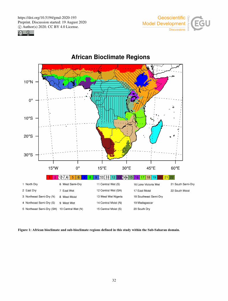
32

Figure 1: African bioclimate and sub-bioclimate regions defined in this study within the Sub-Saharan domain.


33

Figu

re 2

: Com

pari

son

of a

nnua

l ave

rage

alb

edo

(%)

betw

een

LSM

con

figur

atio

ns.

Sinc

e N

oah-

Sat i

s bas

ed o

n sa

telli

te o

bser

vatio

ns, i

t can

be

trea

ted

as o

bser

vatio

ns.


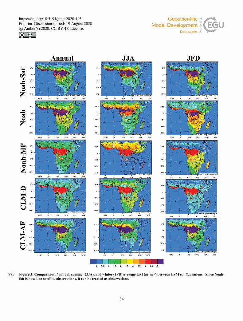
34

Figure 3: Comparison of annual, summer (JJA), and winter (JFD) average LAI (m2 m-2) between LSM configurations. Since Noah-985 Sat is based on satellite observations, it can be treated as observations.


35

Figu

re 4

: Com

pari

son

of a

nnua

l ave

rage

surf

ace

roug

hnes

s len

gth

(m) b

etw

een

LSM

con

figur

atio

ns.


36

Figu

re 5

: 201

3 an

nual

ave

rage

upw

ellin

g sh

ortw

ave r

adia

tion

at th

e Ear

th’s

surf

ace (

W m

-2) f

or C

ER

ES-

EB

AF

estim

ates

and

WR

F si

mul

atio

ns.


37

Figu

re 6

: Nor

mal

ized

mea

n er

ror

and

mea

n bi

as st

atis

tics o

f USR

S an

d T

2 re

lativ

e to

obs

erva

tions

, CE

RE

S-E

BA

F U

SRS

estim

ates

and

CR

U/N

CD

C

T2.


38

990

Figu

re 7

: 201

3 an

nual

ave

rage

2 m

tem

pera

ture

(°C

) fro

m C

RU

and

WR

F si

mul

atio

ns w

ith fi

ve d

iffer

ent L

SMs.

NC

DC

-ISD

2 m

tem

pera

ture

obse

rvat

ions

are

ove

rlai

d.


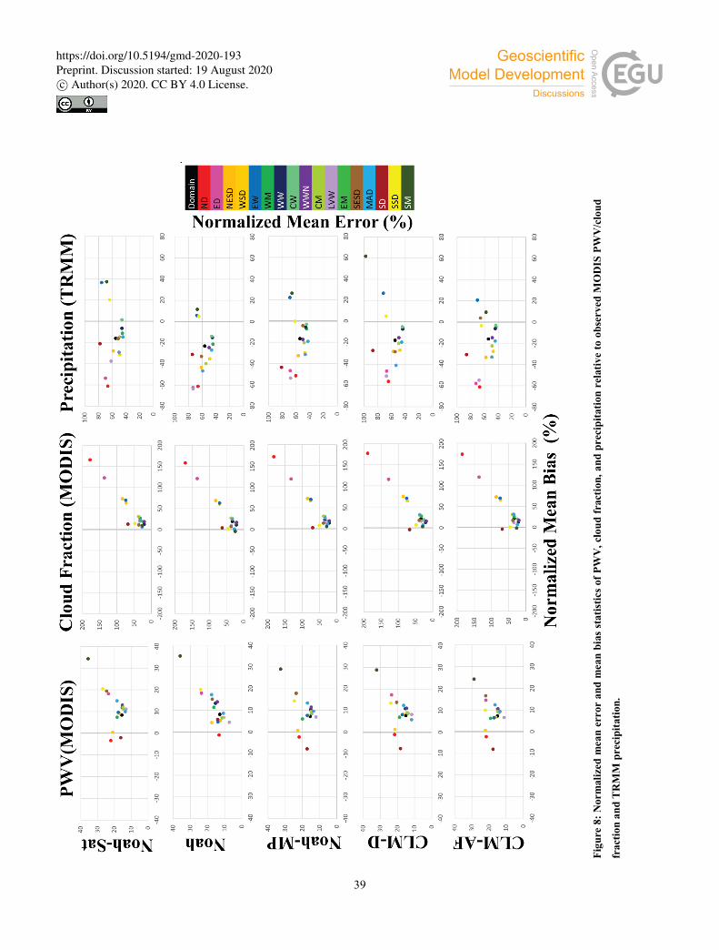
39

Figu

re 8

: Nor

mal

ized

mea

n er

ror

and

mea

n bi

as s

tatis

tics

of P

WV

, clo

ud fr

actio

n, a

nd p

reci

pita

tion

rela

tive

to o

bser

ved

MO

DIS

PW

V/c

loud

frac

tion

and

TR

MM

pre

cipi

tatio

n.


40

995

Figure 9: 2013 annual average precipitation rate (mm day-1) from CRU, GPCP, TRMM, and the five WRF LSM simulations.


41

1000

Figure 10: Processed MODIS land use and land cover categories for 2001, simulated categories for 2015, and grid cells that experience transitions due to agricultural expansion, deforestation/degradation, and greening.1005


42

1010

Figure 11: Differences in albedo (%) between LUD and LU01 simulations using Noah, Noah-MP, CLM-D, and CLM-AF.


43

1015

Figure 12: Differences in leaf area index (m2 m-2) between the LUD and LU01 simulations using Noah, Noah-MP, CLM-D, and CLM-AF.


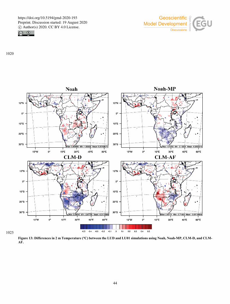
44

1020

1025 Figure 13: Differences in 2 m Temperature (℃) between the LUD and LU01 simulations using Noah, Noah-MP, CLM-D, and CLM-AF.


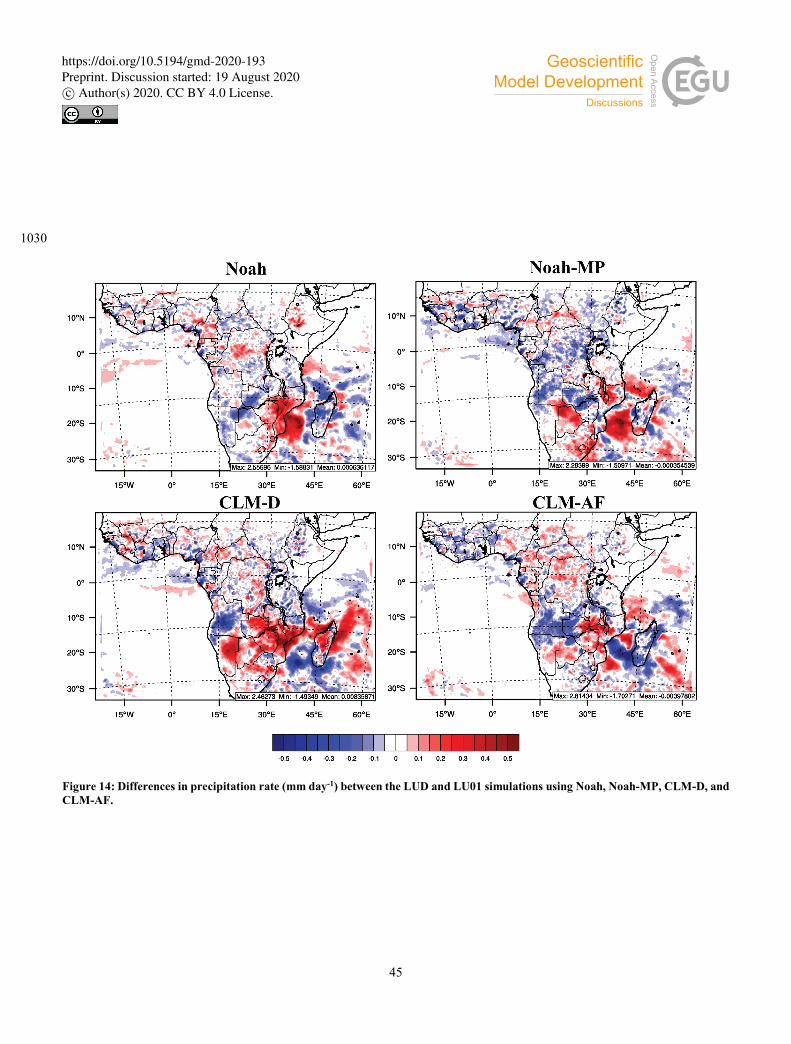
45

1030

Figure 14: Differences in precipitation rate (mm day-1) between the LUD and LU01 simulations using Noah, Noah-MP, CLM-D, and CLM-AF.


46

Table 1: Model Configurations 1035 Simulation Configuration Setting

Domain Sub-Saharan Africa Horizontal Resolution 36 km

Vertical Layers 30 Layers from the Surface to 50 mb Initial/Boundary Conditions ERA-Interim (D11) Physics Parameterization Option

Cumulus New Tiedtke Scheme (Z11) Cloud Microphysics Aerosol-Aware Thompson Scheme (TE14)

Radiation RRTMG (C05; I08) Planetary Boundary Layer MYNN (NN04; NN06)

Surface Layer MYNN (NN04; NN06) Land Surface Models Noah (CD01; E03)

Noah-MP (N11) CLM 4.5 (S11; JW12; LK12)

Lake Model CLM 4.5 (S12; G13) Acronyms: ERA-Interim – European Centre for Medium-Range Weather Forecasting Interim reanalysis; RRTMG – Rapid Radiative Transfer Model for General Circulation Models; MYNN – Mellor Yamada Nakanishi Niino; Noah - National Centers for Environmental Prediction, Oregon State University, Air Force, Hydrology Lab; Noah-MP – Noah Multi-patameterization options; CLM 4.5 – Community Land Model version 4.5 1040 References: D11 – Dee et al., (2011); Z11 – Zhang et al., (2011); TE14 – Thompson and Eidhammer,

(2014); C05- Clough et al., (2005); I08 – Iacono et al., (2008); NN04 – Nakanishi and Niino, (2004); NN06 – Nakanishi and Niino, (2006); CD01 – Chen and Dudhia (2001); E03 – Ek et al., (2003); N11 – Niu et al., (2011); S11 – Subin et al., (2011); JW12 – Jin and Wen, (2012); 1045 LK12 – Lu and Kueppers, (2012); S12 – Subin et al., (2012); G13 – Gu et al., (2013)

1050 1055


47

1060 Table 2: Percentage of Plant Functional Types Assigned to MODIS Land Use Categories in the Updated

CLM-AF MODIS Land Use Category 2 4 5 6 7 8 9 10 12 14

Bare Soil - 3 - 14 48 - - 21 10 - Broad Leaf Evergreen Tropical Tree 82 - 20 - - 12 - - - -

Broad Leaf Evergreen Temperate Tree 18 - 15 - - - - - - - Broad Leaf Deciduous Tropical Tree - 55 - 8 - 26 21 - - 24

Broad Leaf Deciduous Temperate Shrub - 18 - 57 31 - - 18 - - C3 Non-Artic Grass - - 40 - 8 27 31 36 24 17

C4 Grass - 24 25 21 13 35 48 25 15 33 Corn - - - - - - - - 51 26

MODIS Land Use Categories: 2 – Evergreen Broad Leaf Forest; 4 – Deciduous Broad Leaf Forest; 5 – Mixed Forest; 6 – Closed Shrublands; 7 – Open Shrublands; 8 – Woody Savanna; 9 – Savannas; 10 – Grasslands; 12 – Croplands; 14 –Cropland/Natural Mosaic 1065 Table 3: Dominant MODIS-IGBP Land Use Categories within African Bioclimate Regions at 36 km Resolution

Region MODIS-IGBP Category Name Acronym 2 4 5 6 7 8 9 10 12 14

North Dry ND - - - - Y - - Y Y Y East Dry ED - Y - - Y - - Y - Y

Northeast Semi-Dry* NESD - - - Y Y Y Y Y Y Y West Semi-Dry WSD - - - - Y - Y Y Y Y

East Wet EW Y - - - - Y Y Y Y Y West Moist WM - - - - - Y Y - Y Y West Wet WW Y - - - - Y Y Y - Y

Central Wet* CW Y - - - Y Y Y Y - Y West Wet Nigeria WWN Y - - - - Y Y - Y Y

Central Moist* CM Y - - - - Y Y Y Y Y Lake Victoria Wet LVW Y - - - - Y Y Y Y Y

East Moist EM Y - Y - - Y Y Y - Y Southeast Semi-Dry SESD - - - - Y Y Y - - -

Madagascar MAD Y Y - - Y Y Y Y - Y South Dry SD - - - - Y - - - - -

South Semi-Dry SSD Y - - Y Y Y Y Y Y - South Moist SM Y - - - Y Y Y Y Y Y

*: Indicates bioclimate regions that are subdivided into a north, a south, or other sub-bioclimate regions 1070 for better LAI geographical distributions.


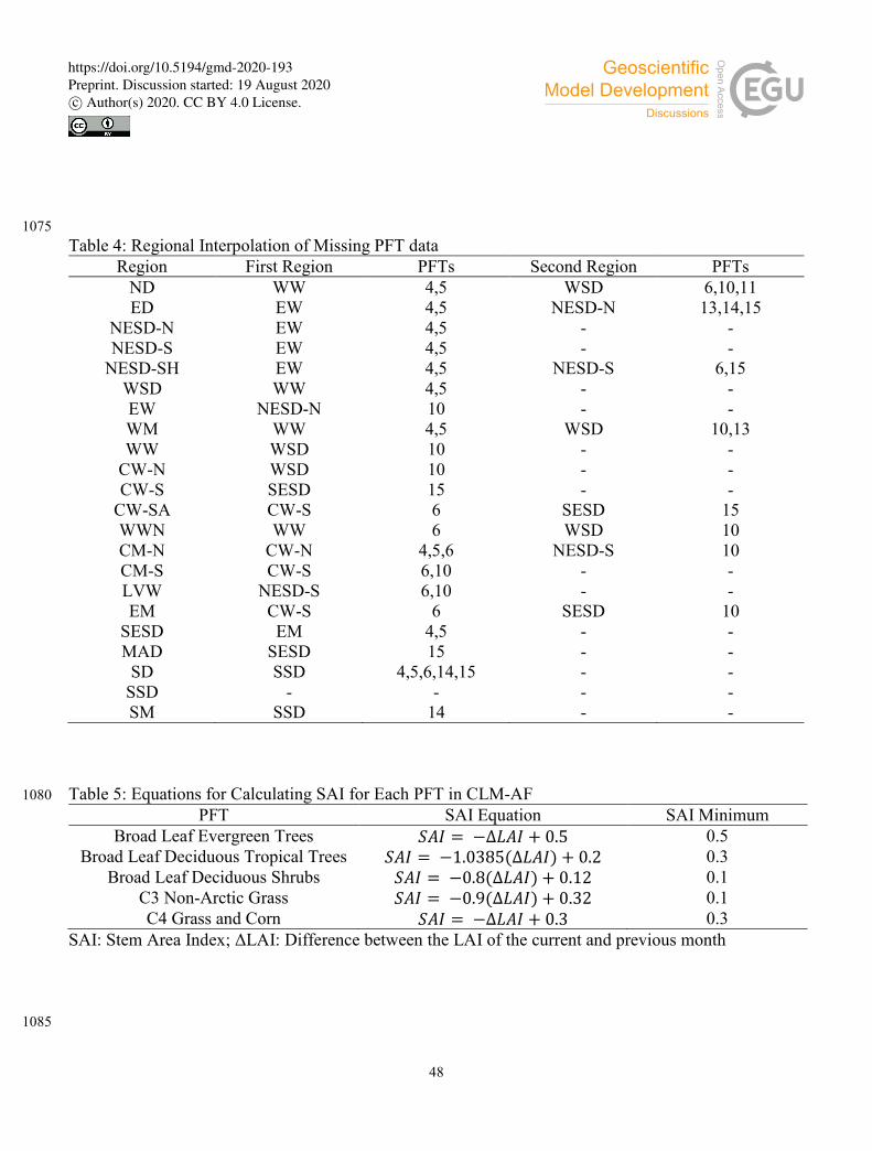
48

1075 Table 4: Regional Interpolation of Missing PFT data

Region First Region PFTs Second Region PFTs ND WW 4,5 WSD 6,10,11 ED EW 4,5 NESD-N 13,14,15

NESD-N EW 4,5 - - NESD-S EW 4,5 - -

NESD-SH EW 4,5 NESD-S 6,15 WSD WW 4,5 - - EW NESD-N 10 - - WM WW 4,5 WSD 10,13 WW WSD 10 - -

CW-N WSD 10 - - CW-S SESD 15 - -

CW-SA CW-S 6 SESD 15 WWN WW 6 WSD 10 CM-N CW-N 4,5,6 NESD-S 10 CM-S CW-S 6,10 - - LVW NESD-S 6,10 - - EM CW-S 6 SESD 10

SESD EM 4,5 - - MAD SESD 15 - -

SD SSD 4,5,6,14,15 - - SSD - - - - SM SSD 14 - -

Table 5: Equations for Calculating SAI for Each PFT in CLM-AF 1080

PFT SAI Equation SAI Minimum Broad Leaf Evergreen Trees 𝑆𝑆𝑆𝑆𝑆𝑆 = −∆𝐿𝐿𝑆𝑆𝑆𝑆 + 0.5 0.5

Broad Leaf Deciduous Tropical Trees 𝑆𝑆𝑆𝑆𝑆𝑆 = −1.0385(∆𝐿𝐿𝑆𝑆𝑆𝑆) + 0.2 0.3 Broad Leaf Deciduous Shrubs 𝑆𝑆𝑆𝑆𝑆𝑆 = −0.8(∆𝐿𝐿𝑆𝑆𝑆𝑆) + 0.12 0.1

C3 Non-Arctic Grass 𝑆𝑆𝑆𝑆𝑆𝑆 = −0.9(∆𝐿𝐿𝑆𝑆𝑆𝑆) + 0.32 0.1 C4 Grass and Corn 𝑆𝑆𝑆𝑆𝑆𝑆 = −∆𝐿𝐿𝑆𝑆𝑆𝑆 + 0.3 0.3

SAI: Stem Area Index; ΔLAI: Difference between the LAI of the current and previous month 1085


49

Table 6: Sandy Soil CLM Albedo Values

1090

1095

1100

Table 7: Model Experiments and Simulations Experiment Period Land Use LSM Model Validation 2013 Default Noah Noah-Sat Noah-MP CLM-D CLM-AF Land Use Land Cover Change 2010-2015 MODIS 2001 (LU01) Noah Noah-MP CLM-D CLM-AF Dinamica EGO 2010-2015 (LUD) Noah Noah-MP CLM-D CLM-AF

1105 1110

Moisture Radiation Band CLM-D CLM-AF Sand Sand-Loam Sand Sand-Loam

Saturated Visible 0.12 0.11 0.22 0.13 Infrared 0.24 0.22 0.34 0.24

Dry Visible 0.24 0.22 0.34 0.24 Infrared 0.48 0.44 0.58 0.46


50

Table 8: Datasets for Model Validation

Datasets Temporal Resolution

Spatial Resolution

Website

CRU TS4.02a Monthly 0.5º×0.5º https://crudata.uea.ac.uk/cru/data/hrg/cru_ts_4.02/

NCDC-ISDb Hourly n/a https://www.ncdc.noaa.gov/land-based-station-data/integrated-surface-database-isd

CERES-EBAFc Monthly 1º×1º https://ceres.larc.nasa.gov/

GPCPd Monthly 2.5º×2.5º http://www.esrl.noaa.gov/psd/data/gridded/data.gpcp.html

TRMMe 3-Hour 0.25º×0.25º https://pmm.nasa.gov/data-access/downloads/trmm

MOD08_M3f Monthly 1º×1º https://modaps.modaps.eosdis.nasa.gov/services/about/products/c61/MOD08_M3.html

a: University of East Anglia, Climate Research Gridded Climate Data version 4.02; b: National Climate Data Center – Integrated Surface Data; c: Clouds and Earth’s Radiant Energy System – Energy Balanced 1115 and Filled; d: Global Precipitation Climatology Project; e: Tropical Rainfall Measuring Mission; f: MODIS/Terra Aerosol Cloud Water Vapor Ozone Monthly L3 Global 1Deg CMG

1120 Table 9: Evaluated Variables and Evaluation Datasets

Variable Acronym Evaluation Dataset 2 m Temperature T2 CRU TS4.02 and NCDC-ISD

Daily Maximum Temperature TMAX CRU TS4.02 Daily Minimum Temperature TMIN CRU TS4.02 Diurnal Temperature Range DTR CRU TS4.02

2m Vapor Pressure E2 CRU TS4.02 2 m Dew point Temperature Td2 NCDC-ISD

Precipitable Water Vapor PWV MOD08_M3 Cloud Fraction CF CRU TS4.02 and MOD08_M3 Precipitation PRE CRU TS4.02, GPCP, and TRMM

10 m Wind Speed WS10 NCDC-ISD Dowelling Shortwave Radiation (Surface) DSR CERES-EBAF Dowelling Longwave Radiation (Surface) DLR CERES-EBAF Upwelling Shortwave Radiation (TOA*) USRT CERES-EBAF

Upwelling Shortwave Radiation (Surface) USRS CERES-EBAF Upwelling Longwave Radiation (TOA*) ULR CERES-EBAF

Shortwave Cloud Forcing SWCF CERES-EBAF Longwave Cloud Forcing LWCF CERES-EBAF

*: Top of the Atmosphere 1125


51

1130 Table 10: Annual Average 2 m Temperature Change (℃) in WRF Grid Cells that experience LULCCs between 2001 and 2010-2015 1135

Transition Noah Noah-MP CLM-D CLM-AF Agricultural Expansion* -0.12 0.1 0.1 0.17

10 to 12 -0.09 0.16 0.18 0.17 2 to 14 -0.3 0.6 1.34 1.38 8 to 14 -0.06 0.01 -0.12 0.15 10 to 14 -0.1 0.06 0.03 0.07

Deforestation/Degradation* 0.04 -0.01 -0.03 0.22 8 to 9 0.17 -0.03 -0.22 0.18 9 to 7 -0.16 -0.04 0.12 0.36 9 to 10 -0.11 -0.05 0.1 0.11

Greening* 0.02 -0.13 -0.33 -0.41 9 to 8 -0.12 0.0 0.08 -0.13 10 to 9 0.18 -0.02 -0.28 -0.26 16 to 7 -0.01 -0.13 -0.39 -0.40 16 to 10 0.09 -0.2 -0.81 -0.8

*: Shows average difference for a broad class of LULCC followed by the average difference in the major MODIS LULC transitions that comprise that class. MODIS Land Use Categories: 2 – Evergreen Broad Leaf Forest; 7 – Open Shrublands; 8 – Woody Savanna; 9 – Savannas; 10 – Grasslands; 12 – Croplands; 14 –Cropland/Natural Mosaic; 16 – Barren/ Sparsely Vegetated 1140 1145 1150


52

1155 1160 Table 11: Annual Average Precipitation Rate Change (mm day-1) in WRF Grid Cells that experience LULCCs between 2001 and 2015

Transition Noah Noah-MP CLM-D CLM-AF Agricultural Expansion* 0.02 -0.13 -0.08 -0.03

10 to 12 0.02 -0.04 0.05 -0.02 2 to 14 -0.12 -0.25 -0.45 -0.38 8 to 14 0.07 -0.18 -0.10 0.00 10 to 14 0.04 -0.01 0.04 -0.02

Deforestation/Degradation* 0.02 -0.01 -0.04 -0.08 8 to 9 0.07 -0.03 -0.01 -0.04 9 to 7 -0.05 0.05 0.12 -0.05 9 to 10 -0.01 -0.01 -0.02 -0.04

Greening* 0.00 0.03 0.15 0.05 9 to 8 -0.02 0.03 0.14 -0.03 10 to 9 -0.03 0.06 0.01 0.02 16 to 7 -0.01 0.02 0.05 0.00 16 to 10 0.05 -0.01 0.02 0.02

*: Shows average difference for a broad class of LULCC followed by the average difference in the major MODIS LULC transitions that comprise that class. MODIS Land Use Categories: 2 – Evergreen Broad Leaf Forest; 7 – Open Shrublands; 8 – Woody Savanna; 9 – Savannas; 10 – Grasslands; 12 – 1165 Croplands; 14 –Cropland/Natural Mosaic; 16 – Barren/ Sparsely Vegetated


Limitations of WRF land surface models for simulating ... - GMD

Documents

Transcript of Limitations of WRF land surface models for simulating ... - GMD