Simulating pedestrian dynamics

Technische Universität MünchenFakultät für Informatik

Lehrstuhl für Wissenschaftliches Rechnen

Simulating pedestrian dynamics:Towards natural locomotion and psychological

decision making

Michael J. Seitz

Vollständiger Abdruck der von der Fakultät für Informatik der TechnischenUniversität München zur Erlangung des akademischen Grades eines

Doktors der Naturwissenschaften (Dr. rer. nat.)

genehmigten Dissertation.

Vorsitzender: Univ.-Prof. Alfons Kemper, Ph.D.Prüfer der Dissertation: 1. Univ.-Prof. Dr. Hans-Joachim Bungartz

2. Prof. Dr. Gerta Köster (Hochschule München)

Die Dissertation wurde am 23.03.2016 bei der Technischen Universität Müncheneingereicht und durch die Fakultät für Informatik am 18.05.2016 angenommen.

Abstract

Social interactions and collective dynamics are ubiquitous in our lives and are increas-ingly being studied in computational science and engineering. Pedestrian dynamicsfocuses on the interactions and movements of humans on foot in a great variety ofcontexts, including public transportation systems and mass events. Computer simu-lation can serve both for studying pedestrian behaviour and as part of an informationsystem – the former focusing on scientific scrutiny and the latter on engineering.

Due to the complexity of human behaviour, building a scientifically credible com-puter simulation is a great challenge for mathematical modelling and software engin-eering. Known approaches mostly focus on selected phenomena and do not incorporatefindings from other disciplines, such as crowd psychology and biomechanics. Perhapsbecause of this, they lack a plausible representation of the decision making and phys-ical process.

At first, I present a software framework that facilitates the development of newsimulation approaches for pedestrian dynamics. I then discuss known approaches,and introduce the optimal steps model, which represents decision making throughutility optimisation and locomotion as a discrete stepping process. The approachovercomes the limitations of the grid in cellular automata and is the first model ofpedestrian dynamics representing the natural stepping process. However, accordingto findings in behavioural sciences, humans make decisions with heuristic reasoning,not mathematical optimisation. Therefore, I use a representation in separate layersfor physics, psychology, and social behaviour in the second part of this work andpropose dedicated simulation models drawing on findings from the respective fields.This approach constitutes a shift towards psychological and physical models that notonly predict pedestrian behaviour but also serve as an explanation of the underlyingprocesses. Specifically, I demonstrate how simple heuristics can be used to reproducecrowd phenomena and allow for new insights into pedestrian behaviour. The newconcept facilitates interdisciplinary exchange and provides a basis for research in manydirections, including psychology and biology.

iii

Zusammenfassung

Soziale Interaktionen und kollektive Dynamiken sind allgegenwärtig in unserem Lebenund werden zunehmend in Simulationswissenschaften untersucht. Fußgängerdynamikbeschreibt die Interaktionen und Bewegungen von Menschen, die zu Fuß gehen, in ei-ner Fülle von Kontexten, einschließlich öffentlicher Verkehrssysteme und Massenveran-staltungen. Computersimulationen können zur Untersuchung von Fußgängerverhaltenoder als Teil eines Informationssystems dienen, wobei Ersteres auf naturwissenschaft-lichen und Letzteres auf ingenieurswissenschaftlichen Erkenntnisgewinn abzielt.

Auf Grund der Komplexität menschlichen Verhaltens ist es für die mathematischeModellbildung und Software-Entwicklung eine große Herausforderung, eine wissen-schaftlich glaubwürdige Computersimulation zu entwickeln. Bekannte Ansätze konzen-trieren sich zumeist auf ausgewählte Phänomene und vernachlässigen die Forschungauf anderen Gebieten, wie etwa der Sozialpsychologie oder Biomechanik. Eventuellfehlt ihnen deswegen eine plausible Repräsentation des Entscheidungsverhaltens undder physikalischen Prozesse von Fußgängern.

Zuerst wird in dieser Arbeit ein Software-Framework vorgestellt, das die Entwick-lung von neuen Simulationsansätzen in der Fußgängerdynamik ermöglicht und unter-stützt. Danach werden bekannte Ansätze diskutiert und das Optimal Steps Modeleingeführt. Das Optimal Steps Model repräsentiert die Entscheidungsfindung durchNutzenoptimierung und die Fortbewegung als diskreten Schrittprozess. Der Ansatzbeseitigt die Beschränkungen des Gitters in zellulären Automaten und ist das ers-te Modell für Fußgängerdynamiken, das den natürlichen Schrittprozess von Fußgän-gern abbildet. Der Forschung in Verhaltenswissenschaften zufolge treffen MenschenEntscheidungen mit Heuristiken und nicht durch mathematische Optimierung. Daherwird im zweiten Teil dieser Arbeit eine Darstellung in drei verschiedenen Schichtenverwendet, jeweils eine für Physik, Psychologie und soziales Verhalten. Zudem werdendedizierte Modelle, die auf Forschungsergebnissen der jeweiligen Gebiete aufbauen,vorgeschlagen. Dieser Ansatz stellt einen grundlegenden Wechsel in Richtung psycho-logischer und physikalischer Modelle dar, die nicht nur das Verhalten von Fußgängernsondern auch der zugrundeliegenden Prozesse erklären. Insbesondere wird gezeigt, wieeinfache Heuristiken verwendet werden können, um bekannte Phänomene zu repro-duzieren und neue Einsichten in Fußgängerverhalten zu gewinnen. Die Darstellung inverschiedene Schichten fördert den interdisziplinären Austausch und bietet eine Grund-lage für neue Forschung in viele weitere Richtungen, unter anderem in der Psychologieund der Biologie.

v

Contents

1 Introduction 11.1 Computational science and engineering . . . . . . . . . . . . . . . . . . 31.2 Pedestrian dynamics . . . . . . . . . . . . . . . . . . . . . . . . . . . . 51.3 Challenges in simulating pedestrian dynamics . . . . . . . . . . . . . . 71.4 Scope and overview of this work . . . . . . . . . . . . . . . . . . . . . . 10

I Microscopic pedestrian stream simulation 13

2 Simulation framework 142.1 Software requirements . . . . . . . . . . . . . . . . . . . . . . . . . . . 162.2 Development process and toolchain . . . . . . . . . . . . . . . . . . . . 182.3 Software design . . . . . . . . . . . . . . . . . . . . . . . . . . . . . . . 192.4 Functionality . . . . . . . . . . . . . . . . . . . . . . . . . . . . . . . . 222.5 Software architecture . . . . . . . . . . . . . . . . . . . . . . . . . . . . 262.6 Utilisation and future directions . . . . . . . . . . . . . . . . . . . . . . 352.7 Summary . . . . . . . . . . . . . . . . . . . . . . . . . . . . . . . . . . 37

3 Modelling approaches 383.1 Cellular automata . . . . . . . . . . . . . . . . . . . . . . . . . . . . . . 403.2 Velocity-based models . . . . . . . . . . . . . . . . . . . . . . . . . . . 463.3 Force-based models . . . . . . . . . . . . . . . . . . . . . . . . . . . . . 493.4 Alternative approaches . . . . . . . . . . . . . . . . . . . . . . . . . . . 523.5 Similarities and differences . . . . . . . . . . . . . . . . . . . . . . . . . 563.6 Summary . . . . . . . . . . . . . . . . . . . . . . . . . . . . . . . . . . 60

4 The optimal steps model 624.1 Utility functions . . . . . . . . . . . . . . . . . . . . . . . . . . . . . . . 62

4.1.1 Parameter calibration . . . . . . . . . . . . . . . . . . . . . . . . 654.1.2 Navigation fields . . . . . . . . . . . . . . . . . . . . . . . . . . 68

4.2 Local optimisation . . . . . . . . . . . . . . . . . . . . . . . . . . . . . 684.2.1 Step length to speed relation . . . . . . . . . . . . . . . . . . . . 714.2.2 Numerical discretisation . . . . . . . . . . . . . . . . . . . . . . 734.2.3 Constrained movement direction . . . . . . . . . . . . . . . . . . 76

4.3 Update schemes . . . . . . . . . . . . . . . . . . . . . . . . . . . . . . . 804.3.1 Nonparallel unit-clock updates . . . . . . . . . . . . . . . . . . . 834.3.2 Event-driven update . . . . . . . . . . . . . . . . . . . . . . . . 84

vii

4.3.3 Parallel unit-clock update . . . . . . . . . . . . . . . . . . . . . 864.3.4 Impact on simulation outcomes . . . . . . . . . . . . . . . . . . 86

4.4 Implementation details . . . . . . . . . . . . . . . . . . . . . . . . . . . 884.5 Simulation results . . . . . . . . . . . . . . . . . . . . . . . . . . . . . . 894.6 Further developments and utilisation . . . . . . . . . . . . . . . . . . . 914.7 Summary . . . . . . . . . . . . . . . . . . . . . . . . . . . . . . . . . . 94

II Towards a natural physical and psychological process 97

5 The physical layer: Pedestrian locomotion 985.1 Aspects from biomechanics . . . . . . . . . . . . . . . . . . . . . . . . . 1005.2 Aspects from robotics . . . . . . . . . . . . . . . . . . . . . . . . . . . . 1045.3 Locomotion models for pedestrians . . . . . . . . . . . . . . . . . . . . 105

5.3.1 Discrete stepping process . . . . . . . . . . . . . . . . . . . . . . 1055.3.2 Continuous force-based process . . . . . . . . . . . . . . . . . . 107

5.4 Summary . . . . . . . . . . . . . . . . . . . . . . . . . . . . . . . . . . 111

6 The psychological layer: Heuristic decision making 1136.1 Aspects from behavioural sciences . . . . . . . . . . . . . . . . . . . . . 114

6.1.1 Aspects from psychology . . . . . . . . . . . . . . . . . . . . . . 1156.1.2 Aspects from animal behaviour . . . . . . . . . . . . . . . . . . 1176.1.3 Decision making and bounded rationality . . . . . . . . . . . . . 118

6.2 Aspects from artificial intelligence . . . . . . . . . . . . . . . . . . . . . 1226.3 Decision-making models for pedestrians . . . . . . . . . . . . . . . . . . 124

6.3.1 Cognitive heuristics . . . . . . . . . . . . . . . . . . . . . . . . . 1266.3.2 Implementation details . . . . . . . . . . . . . . . . . . . . . . . 1316.3.3 Simulation results . . . . . . . . . . . . . . . . . . . . . . . . . . 1336.3.4 Future directions . . . . . . . . . . . . . . . . . . . . . . . . . . 140

6.4 Remaining, waiting, and queueing . . . . . . . . . . . . . . . . . . . . . 1416.5 Summary . . . . . . . . . . . . . . . . . . . . . . . . . . . . . . . . . . 146

7 The social layer: Collective behaviour 1497.1 Aspects from social psychology and collective behaviour . . . . . . . . . 1507.2 Sub-group coherence . . . . . . . . . . . . . . . . . . . . . . . . . . . . 152

7.2.1 Models of sub-group behaviour . . . . . . . . . . . . . . . . . . 1527.2.2 Implementation details . . . . . . . . . . . . . . . . . . . . . . . 155

7.3 Towards the integration of crowd psychology into computer simulation 1577.4 Summary . . . . . . . . . . . . . . . . . . . . . . . . . . . . . . . . . . 159

8 Summary, conclusions, and future directions 1608.1 Summary . . . . . . . . . . . . . . . . . . . . . . . . . . . . . . . . . . 1608.2 Conclusions . . . . . . . . . . . . . . . . . . . . . . . . . . . . . . . . . 1638.3 Future directions . . . . . . . . . . . . . . . . . . . . . . . . . . . . . . 165

Bibliography 167

viii

Chapter 1

Introduction

Social interactions are ubiquitous in our lives. Humans and animals show a greatvariety of social interactions in different contexts and to different ends. Especially aspedestrians, we often face others in daily routines such as commuting or when crossingthe street but also during events, including music festivals with a large number ofpeople. We interact with others by evading them, staying away with a certain distance,or staying close to chat with our friends while walking.

Although behaviours vary across animal species, certain similarities can be found.In particular, locomotion and navigation in the environment are common tasks foranimals (e.g., McNeill Alexander, 2003). In the case of humans, the most natural formof locomotion is walking. As pedestrians, we cover many distances every day. Walkingcan have a recreational aspect or the specific purpose of reaching a destination. Togive an example of the importance of walking: “Nearly 32% of all commuter trips inDelhi are walking trips” Tiwari (2003).

Pedestrian dynamics (e.g., Navin and Wheeler, 1969; Gipps and Marksjö, 1985;Helbing and Molnár, 1995; Schadschneider et al., 2009) mainly describes phenomenathat result from the interaction of multiple pedestrians but may also study individualbehaviour without social interactions. For example, the distance we keep to walls canbe an important aspect in pedestrian dynamics. The study of crowd behaviour (e.g.,Sime, 1995; Reicher, 1996; Faria et al., 2010; Drury and Stott, 2011) clearly stressesthe social aspect of many humans interacting. Crowd behaviour can also be studiedwhen humans are not walking or even are not physically in the same environment,which is the case in social media platforms. In this work, I study the behaviour ofpedestrians who may or may not be in a crowd.

In computational science (e.g., Strang, 2007; Bader et al., 2013), natural phe-nomena are studied through computational methods. Mainly descriptive models aredeveloped that explain known behaviour and generate additional hypotheses. Thesemodels may also be used for engineering problems and are of particular value forthem if the models are well-validated, that is, produce reliable predictions. In com-putational engineering, descriptive and normative models are used. For example, insafety science, traffic optimisation, and the planning of built environments, a systemthat supports decision making is often desired. The motivations for the simulationof pedestrian dynamics are as plentiful as the disciplines involved. At first, studyingpedestrian dynamics is an end in itself as basic research. Applications can be classified

1

into improvements in safety, efficiency, and comfort for pedestrians.A prominent example of safety applications is the study of mass events. A series

of infamous crowd crushes (e.g., Elliott and Smith, 1993; Ahmed et al., 2006; Ngaiet al., 2009) has drawn attention to the possible hazards in large agglomerations ofpeople. The hope is to improve the safety of mass events with the help of simulations.For this, the layout of the environment, the number of visitors, and other parametershave to be known to produce meaningful predictions. Due to the complexity of humanbehaviour and the many parameters at such an event, a simulation model can revealhazards but not exclude the possibility of additional, unknown ones.

The optimisation of technological systems is important economically, ecologically,and for safety reasons. At mass events, the efficient operation of services supports bothsafety and the satisfaction of visitors. In transportation systems (e.g., Vuchic, 2005),efficiency directly relates to the quality of the service from the customers’ perspective.In these systems, passengers often move on foot a considerable portion of the time.Pedestrian simulations can be used for studies of railway stations or the design oftrains (e.g., Köster et al., 2011a). Finally, well-designed public transportation systemspromote their use through the comfort they provide.

Both the safety and comfort of pedestrians are issues in urban planning (Pucherand Dijkstra, 2000). Figure 1.1 illustrates how pedestrians in an urban setting ofteninteract with each other and alternative modes of transportation. Pedestrian facilitiesare important for the attractiveness of cities, and walking has positive effects on sociallife and health (Leyden, 2003; Gehl, 2010). Transportation in big cities only seems tostay effective when functional public transportation systems are implemented and atthe same time walking and cycling is promoted (Vuchic, 1999). There are approachesfor the improvement of urban spaces to encourage people to walk (Southworth, 2005;Patton, 2007). Simulation studies may aid in design choices (Helbing et al., 2005) oreven provide a virtual reality simulation as a visualisation tool for future developments.

Much of the work I present in this thesis was funded through the research pro-ject MultikOSi on assistance systems for urban events – multi-criteria integration foropenness and safety. In the research group of Gerta Köster at the Munich Univer-sity of Applied Sciences, we studied and developed simulation models of pedestriandynamics. The main focus of the simulation approaches was on safety and efficiencyissues in urban contexts. My work reflects this at some points, for example, with thestudy of shuttle-bus systems and of a railway station platform (in chapter 6). How-ever, the discussions and simulation models are general and are not limited to theseapplications.

The simulation of pedestrian dynamics is a highly interdisciplinary field. Aspectsof it are studied in many domains of the natural and life sciences, including phys-ics, biomechanics, social psychology, and animal behaviour. The formal sciences andengineering contribute with mathematics, statistics, and computer science. Relevantdisciplines in computer science are artificial intelligence, robotics, and scientific com-puting. Two main categories of research activities are empirical studies and modeldevelopment. Both can stand on their own, but the combination of the two seemsbeneficial. Empirical studies without a theory that is being tested or developed outof them remain observations of singular events. Formal models that are not based on

2

Figure 1.1: Herald Square, 34th and Broadway, Manhattan. (Figure: From The NewYork Public Library, Abbott, 1935)

and tested with empirical observation remain theoretical.Independent research in both categories is justified to a certain degree. Only from

reliable experimental procedures and field observations can we deduce general state-ments. The formal models have to be consistent, translated into efficient algorithmsthat can be computed, and finally, they must be implemented correctly. Every one ofthese steps can be a great challenge. For a valid simulation model, the two directionsof empirical and formal research must be combined. It is also crucial to study findingsfrom related fields to complement the knowledge from the core discipline. Gigerenzerand Selten (2001, p. 10) write, “The lack of information flow between disciplines canhardly be underestimated.” Nevertheless, interdisciplinary research is also challengingbecause of the different methodology, terminology, and other factors. I discuss thisissue in section 1.3.

1.1 Computational science and engineering“A model is a representation of an event and/or thing that is real (a case study)or contrived (a use-case)” (Banks and Sokolowski, 2009). In this work, I focus oncomputational approaches for the study of pedestrian and crowd dynamics. Althoughinterdisciplinary, the emphasis is on model development and simulation. Bungartzet al. (2014) give a general introduction to modelling and simulation. In this section,I discuss aspects of computational science and engineering that are relevant for thesimulation of pedestrian dynamics. My intention is to give some background withoutthe pretence of completeness.

It is difficult or not even possible to compare models and decide which one is bet-

3

ter (Oberheim and Hoyningen-Huene, 2013). A model that may not yield the mostexact prediction (e.g., Lattice Boltzmann and lattice gas models) may be preferredover a more precise model (the Navier-Stokes equations) because the latter can becomputationally intractable. The quality of an approach is not only determined bythe precision of the model but also by the usefulness, which can vary depending onthe research question and application. Therefore, the objective of the undertaking hasto be specified first. For example, scientific studies in psychology may have anotherfocus than in biomechanics, and applications in safety engineering can have differentrequirements entirely, even if the research subject is the same. Some general dimen-sions for the quality of a model can be defined, which must be weighted according tothe application.

For scientific progress, the falsifiability and testability of models are important(Popper, 2002), which is one reason why models must be parsimonious (section 1.3).Theories should be accurate and general at the same time. Neither a very generalbut imprecise model nor a detailed account of one specific event are useful theories.To allow for predictions, models must be theoretically and practically computable. Atheory that does not allow for predictions because of its computational complexitycannot be tested. The model must be appropriate: it should predict what the user isinterested in. Finally, the cost-benefit ratio has to be considered.

Models in science play an important role, but the meaning of the term is not thatclear (Frigg and Hartmann, 2012). Since a model can also be a cardboard represent-ation of a building in architecture, it is not necessarily a scientific theory. A modelbecomes a theory as soon as someone describes phenomena of reality with it. Forexample, a system of differential equations is only mathematical formalism, but assoon as someone claims it describes the movement of objects, it is a theory. In thephilosophy of science, once a theory has been falsified, it is discarded (Popper, 2002).A model, on the other hand, may still be useful. A well-known example is Newtonianmechanics, which does not describe reality in all of its details and more precise modelsexist, but yet it is still useful.

To obtain meaningful simulation results, errors have to be excluded. “Sources forerrors lurk in the model, in the algorithm, in the code or in the interpretation of theresults” (Bungartz et al., 2014). Tests at different stages of the development processensure that the model is correct. Two major categories of testing can be defined:verification and validation (Oberkampf and Roy, 2010). In short, verification ensures“solving the equations right” and validation “solving the right equations” (Strang,2007, p. 714).

Verification makes sure that the model is computed correctly and should be un-dertaken at various stages. Given a formal model of equations, a numerical algorithmmust be used to simulate the system in a computer. The algorithm is verified toguarantee that it produces results within a certain error range compared to the ana-lytical solution of the equations. After the algorithm has been realised in software,the implementation has to be verified. Finally, the visualisation, statistical analysis,and other representations of the results must be verified, too.

Validation always compares model predictions with the real world. Validationrelies on data obtained from empirical observations or controlled experiments. The

4

empirical method can also be a source of errors. Especially in experiments with humansubjects, the behaviour is easily influenced by the experimenter, the experimentaldesign, or simply by the awareness of taking part in an experiment. These issues areaddressed by a sound experimental design (e.g., Hinkelmann and Kempthorne, 2008).

In science, theories are tested by experiment in attempts to falsify them (Popper,2002). If the theory does not withstand these attempts, it is discarded. In validation,models are compared to empirical data too, but the objective is to demonstrate thevalidity. Therefore, validation can be seen as the opposite of falsification, but a failedattempt to falsify a hypothesis is not automatically a good validation. A statisticaltest, such as the t-test, can only demonstrate that a hypothesis is wrong with acertain probability. The test does not provide the necessary information to showthat the hypothesis is true and therefore is unreliable for validation. The unreflectedapplication of statistical tests has also been criticised in general (Ioannidis, 2005).An alternative could be the application of equivalence tests (Robinson and Froese,2004; Wellek, 2010). However, equivalence tests are not widely used in the scientificcommunity and hence may not be accepted as evidence.

Empirical research serves both for the development and the validation of models.A sound experimental design is necessary to minimise errors (e.g., Hinkelmann andKempthorne, 2008; Bailey, 2008). In computational science, experimental data isespecially important to provide evidence for the validity of the model. In addition,the models sometimes have parameters that must be calibrated. The calibration of theparameters can be realised by using empirical data. In this case, a different data set isnecessary for validation to prevent an overfitting effect (e.g., Hastie et al., 2009). Thecalibration of parameters can also be criticised in general: by simply recalibrating themodel for every scenario one can evade falsification. Therefore, the parameters shouldbe considered as part of the model. Every recalibration leads to a new model. If theparameters are not considered part of the model, model predictions have to be validwith any set of parameters or any parameter within a specified range of values. Mostly,this can only be shown analytically, and then the predictions tend to be unspecific.

1.2 Pedestrian dynamicsA series of phenomena is studied in pedestrian dynamics (e.g., Navin and Wheeler,1969; Gipps and Marksjö, 1985; Helbing and Molnár, 1995; Schadschneider et al.,2009). They can describe both the behaviour of individuals and of any size of ped-estrian agglomerations. In safety applications, mainly measurements of egress timesand crowd densities are of interest. In studies on efficiency, mostly the time necessaryto reach a certain state is studied. Examples are passenger exchange times or the timeit takes to board an aeroplane.

Important phenomena are the lane formation in contra-flow scenarios (Helbingand Molnár, 1995; Kretz et al., 2006a) and the characteristic density-speed relation,often called fundamental diagram (Navin and Wheeler, 1969; Seyfried et al., 2005;Jelić et al., 2012a), which are both well-documented in controlled experiments andin simulation studies. Particularly relevant for evacuation scenarios is the faster-is-slower effect (Kelley et al., 1965; Helbing et al., 2000a; Garcimartín et al., 2014;

5

Figure 1.2: Simulation snapshots from typical scenarios. On the top, simulated pedes-trians walk from left to right (red) and right to left (blue) and form lanes, which facilitatesflow. On the bottom, simulated pedestrians egress from the room on the right through acorridor. A congestion forms in front of the corridor. This scenario is especially interestingsince bottlenecks can be the decisive part of the environment that determines evacuationtimes. (Figure: Seitz et al., 2016)

Pastor et al., 2015), which suggests that increasing motivation to leave a room fasteventually leads to slower egress. This may be due to phenomena of arching andclogging at bottlenecks that are well-known in granular flow (Pöschel, 1994; To et al.,2001). Empirical evidence for this effect is sparse: it is difficult to conduct experimentswith a very competitive behaviour of participants (Pastor et al., 2015). In figure 1.2,two typical scenarios, contra flow and egress through a bottleneck, are shown withdata from a simulation.

Other phenomena include stop-and-go waves (Helbing et al., 2007), turbulencesin very dense crowds (Helbing et al., 2007), oscillations at bottlenecks (Helbing andMolnár, 1995; Kretz et al., 2006b), and circulating flows at intersections (Helbinget al., 2005). A behaviour on a smaller scale is the coherence of social sub-groups(James, 1953; Coleman and James, 1961; Aveni, 1977; Singh et al., 2009; Moussaïdet al., 2010). On the individual level, effects such as the distances pedestrian keepto walls and each other as well as walking speeds can be of interest (Moussaïd et al.,2009b). It seems difficult to find a general law for pedestrian dynamics as even thewalking speed is different between cities (Bornstein and Bornstein, 1976; Levine andNorenzayan, 1999). Considering this, it is not surprising that Chattaraj et al. (2009)found that the density-speed relation varies across cultures.

Guidelines for the validation of pedestrian stream simulations exist. RiMEA(Richtlinie für Mikroskopische Entfluchtungs-Analysen1, RiMEA, 2009) is a German

1German, guidelines for microscopic evacuation analyses.

6

guideline maintained by an association of research institutes and organisations fromthe private sector. It provides basic tests for the verification and validation of evac-uation simulations. Another guideline is the NIST Technical Note 1822 on “TheProcess of Verification and Validation of Building Fire Evacuation Models” (Ronchiet al., 2013), published by the National Institute of Standards and Technology (NIST)in the United States.

A variety of conceptual modularisations for models of pedestrian dynamics hasbeen proposed. In artificial intelligence, the agent components are often divided intosensing, planning, and acting (Russell and Norvig, 2010). Another separation is thepath-velocity decomposition from robotics in “(1) planning a path to avoid collisionwith static obstacles and (2) planning the velocity along the path to avoid collisionwith moving obstacles” (Kant and Zucker, 1986). Gipps and Marksjö (1985) separatedthe model in route choice and locomotion (“movement along a link”), which is not thelocomotion as I understand it in this work but rather local navigation. Hoogendoornand Bovy (2004) defined three levels: strategic (1), tactical (2), and operational (3).Each of the levels gathers certain functionality: “(1) activity choice behaviour andactivity area choice, (2) wayfinding to reach activity areas and (3) walking behaviour”(Hoogendoorn and Bovy, 2003). However, it is not always clear what a strategic,tactical, or operational decision is. For example, local walking behaviour includeskeeping a certain distance to obstacles, which is also a strategic decision. Wijermans(2011) proposed “three levels of description: the group level (inter-individual), theindividual level and the cognitive level (intra-individual)”. Reynolds (1999) used aseparation into action selection, steering, and locomotion, and Hoogendoorn (2007)separated physical and control models.

1.3 Challenges in simulating pedestrian dynamicsThe simulation of pedestrian dynamics poses an interdisciplinary challenge. Humanbehaviour is highly complex and varies depending on the individual and the context(e.g., Matsumoto, 2012). Behaviour can often only be predicted stochastically, thatis, on average. Different scientific disciplines have different approaches to the studyof behaviour: while psychologists also consider internal aspects such as motivation,biologists mostly have to rely on observed behaviour.

There are controlled experiments that can reproduce certain crowd phenomenaand allow for measurements, including density and speed (Steffen and Seyfried, 2010).The methodology is rather quantitative, relying on the analysis of video footage. Thisapproach mainly describes behaviour, and hence, the simulation models based on themcan be considered phenomenological descriptions of pedestrian dynamics. The sameis usually true for field observations. In psychology, on the other hand, models areoften less formal and not in closed form. A different methodology is employed, suchas interviews and questionnaires, which may reveal internal factors like motivation.

Mathematical modelling and simulation are in part formal sciences since they dealwith equations and algorithms. This is also true for physics, which is a natural sciencebut heavily makes use of mathematical formalism. In psychology, many theories arenot formalised. Carrying them over to computer simulation may not seem possible at

7

first. If that were truly the case, it would be a fundamental problem for the simulationof pedestrian dynamics because it describes human behaviour as does psychology.

Mathematical modelling as the basis of computer simulation relies on certain prin-ciples2. Perhaps most important are abstractions from the real world, also referred toas Aristotelian and Galilean idealisations (Frigg and Hartmann, 2012). Aristotelianidealisation means that features of reality are deliberately left out of the model. Ga-lilean idealisations describe the deliberate distortion of the real world. Both can bethought of as simplifications or abstractions. An example of an Aristotelian idealisa-tion in pedestrian dynamics is that we do not consider the hair colour of individualsbecause we expect it to have little impact on the phenomena we want to describe.The representation in the two-dimensional transverse plane could also be consideredan Aristotelian idealisation as it omits a whole dimension. An example of a Galileanidealisation is the representation of pedestrians as circles, which clearly is a distortionof the real world.

The simplification through idealisations is the principal method to come up withmodels that describe phenomena formally and finally mathematically. For the simula-tion in a computer, the mathematical model has to be closed, and every parameter hasto be fixed. In some cases, methods such as uncertainty quantification (e.g., Smith,2014) may help to study a whole distribution of parameters, but the simulation itselfis always run with one specific set of parameters. The formal description and finallythe implementation in software allows for the study of emergent phenomena predictedby the model.

In computational science, the model encodes a theory that can now be testedand possibly be falsified if the prediction contradicts empirical observation. Thisis of utmost importance because falsification is the basic principle of the scientificmethod (Popper, 2002). With too many parameters in a model, it can be easy toevade falsification by simply adapting the parameter every time the prediction did notmatch empirical observation. Therefore, the model with its specified set of parametershas to be considered a theory that is being tested and potentially falsified.

A model with a set of possible parameters can still be considered a theory undercertain circumstances: the prediction must be tested for all of them. Then statementsof the form “theory X (the model with a specific parameter or a set of possibleparameters) predicts P” can be formed and tested. In contrast, statements like “thereis a parameter for theory X that predicts P” may also be interesting but do notrepresent scientific theories. Those statements do not match the structure of a scientifictheory because they cannot be falsified unless all parameters are tested. In fact, if allparameters are tested or a parameter is found that verifies the statement, it is not atheory anymore but a singular statement, which is not a scientific theory by definition(Popper, 2002).

Whenever two models are known that both predict the same phenomenon, onehas to be selected. In practice, the model that matches the purpose best is chosen.Then the criterion can be, for example, faster computation. In science, the moreparsimonious model is preferable, although this criterion is not always clearly defined.

2The following ideas and the line of argument in this section were partly developed in collaborativework with researchers at the University of Sussex (Seitz et al., 2015d).

8

Popper (2002, sections 41–46) discusses this issue and proposes to use the “degree offalsifiability” instead of “simplicity” as a criterion: “The degree of universality and ofprecision of a theory increases with its degree of falsifiability” (Popper, 2002, p. 127).Thus, the requirement of parsimony or degree of falsifiability is important. It allows todiscriminate among models and will ultimately lead to the most accurate and generaltheories.

Social psychologists (e.g., Drury and Stott, 2011), on the other hand, criticisethat the approach mathematical modelling has taken for the explanation of crowdphenomena is reductionist. When comparing simulation outcomes to real events, theyfound that simulation models neglect crucial features of the crowd’s behaviours. Socialpsychology deals with open systems that strongly depend on the context. This poses achallenge for mathematical modelling. However, the principles of the scientific processhold, and hence, there is no underlying contradiction between the requirement ofparsimony and avoiding reductionism in explaining crowd phenomena. The challengerather lies in formalising models from social psychology without distorting them toomuch and selecting scenarios that can be simulated in a meaningful way. Whensuccessful, mathematical modelling and computer simulation can also help to testtheories from social psychology.

Although there may not be a fundamental contradiction, there are still problems ona more practical level. The scientific language and applied methodology are differentand it takes time to overcome this barrier. Nevertheless, surprising similarities can befound and new aspects discovered. Others have already worked at closing the gapsbetween disciplines, and we can draw on their experience. We are still at an earlystage when it comes to simulating human behaviour and the models we have are farfrom perfect. This should not prevent us from working on it, but the resulting modelsmust be treated with the necessary care and should not be understood as definiterepresentations of human behaviour.

Most simulation models of pedestrian dynamics do not make this step and remainmerely phenomenological descriptions. It can be a limitation when the underlyingprocesses are not studied. Moussaïd et al. (2011) and Moussaïd and Nelson (2014)argued for process-oriented simulation models in pedestrian dynamics. These modelsdo not only describe phenomenologically but also try to represent the underlyingprocess. In the case of pedestrian dynamics, this is mainly locomotion, decision-making, and collective behaviour. The hope is that this perspective allows for moreaccurate predictions as well as a better understanding of pedestrian behaviour.

In order to develop a simulation model that represents a plausible underlyingprocess, it is necessary to refer to the disciplines that study them, which are physics,psychology, and biology, among others. And here the real challenge lies: it is hardlypossible to integrate the whole body of knowledge in any one model. Models have to bekept simple for a variety of reasons, including computability. Therefore, it is essentialto look at other disciplines but also to select focal aspects for the integration into asimulation approach. This is reflected in my thesis as I select important aspects fromdomains such as biomechanics, artificial intelligence, cognitive sciences, and socialpsychology without the claim of completeness.

9

1.4 Scope and overview of this workIn this thesis3, I develop models that aim at a better understanding of pedestriandynamics, especially the underlying processes. Given the many interactions in ped-estrian crowds, a computer simulation is necessary for model predictions. The hopeis that with understanding and representing the underlying mechanisms, I obtain re-liable simulation results, better understand the described phenomena, and provide asuitable basis for future directions in model development. The motivation is mainlyscientific scrutiny but also includes a series of applications, such as transportationresearch and safety engineering.

Computer simulations are developed in computational science and engineering(e.g., Banks and Sokolowski, 2009). In this field, computational methods are usedto provide tools for studies in science and engineering. Therefore, the computationaltools are a strong focus. In my work, I focus on model development, especially from aconceptual perspective. Other important areas in mathematics and computer scienceinclude scientific computing, analysis, statistics, and software engineering, which arenot the focus of this work but are necessary for the study of simulation models.

When developing a simulation approach, it is important to choose the right scalethat captures the features of interest. To better understand the underlying processesin pedestrian dynamics, I study individual-based approaches, often called microscopicsimulations. Simulations that do not represent the individual, often called macro-scopic simulations, are inapt for the representation of the underlying processes. Theydo not provide the necessary resolution and, for example, make it impossible to studyphenomena such as the stepping behaviour or other biomechanical features of walk-ing. Too detailed models, on the other hand, are also not a good choice. For example,a neuronal model of the brain is not suitable for pedestrian dynamics since the de-tails obstruct the view on the mechanisms of interest. Nevertheless, some detailedapproaches, for example, models from biomechanics or wider perspectives on a group-level, can complement the models I propose.

I focus on two-dimensional simulations in the transverse plane (top-down view).The transverse plane allows for the study of pedestrian motion without the overheadof the three-dimensional world we live in. This idealisation of the real world seemsjustified as pedestrians mainly move in the transverse plane. For biomechanical fea-tures, a three-dimensional representation could be of interest but is not developed inthis work.

The simulated individuals – pedestrians in this case – are called agents through-out this work to clearly differentiate them from the real world. Agents are also acommon concept in artificial intelligence that I refer to (in section 6.2, chapter 6).Some phenomena of group behaviour can be reproduced by the interactions of indi-viduals without a group-layer perspective. Gipps and Marksjö (1985) formulated thisdirection:

3Whenever I use the personal pronoun we in the context of my work, I refer to myself together withcolleagues, which means the specific work was either collaborative or has been published together. Icreated all figures used in this work with the exception of figures 1.1, 5.2, 5.4, 6.15, and 6.16. Moredetailed credit is given in the respective references cited in the text, captions, and footnotes.

10

The simulation is tackled at the level of the individual pedestrian under thehypothesis that if the behaviour of individuals is modelled adequately, andthe appropriate distribution of pedestrian types employed, the corporatebehaviour of the simulated pedestrians will be realistic. Further, by work-ing at the level of the individual it is possible to collect data on individualtravel times and diversions, and subsequently to analyse the variabilitybetween different types of pedestrian. (Gipps and Marksjö, 1985)

There is some criticism concerning this rationale. Especially the reality of groups andtheir impact on the world should not be neglected:

Cognitive scientists tend to focus on the behavior of single individualsthinking and perceiving on their own. However, interacting groups ofpeople also create emergent organizations at a higher level than the indi-vidual. (Goldstone and Janssen, 2005)

My thesis is divided into two parts: part I describes approaches for the simulationof pedestrian dynamics from a classical perspective; part II is dedicated to a modellingapproach towards a natural process-oriented representation of underlying mechanisms.Many of the tools and topics I discuss in the first part form the basis for the secondpart. At the same time, I point out the limitations of the models in part I in referenceto part II.

In the next chapter, I start by describing a simulation framework that forms thetechnological basis for the implementation of models from pedestrian dynamics. Theparticular focus of this chapter is the modular design that promotes changes and newdevelopments. In chapter 3, I review microscopic simulation models of pedestriandynamics. I classify the models, identify commonalities and differences, and discusstheir limitations. In chapter 4, I present the optimal steps model, an approach thatcaptures the natural stepwise motion of pedestrians and uses it as discretisation schemein the simulation. The optimal steps model overcomes limitations of cellular automataand represents an advancement towards a natural locomotion process. It relies onutility optimisation for decision making, a coherent concept that is accessible to awide range of disciplines.

I use a separation of the underlying processes of pedestrian dynamics in part II.From an engineering perspective, the modularisation in artificial intelligence and ro-botics are reasonable. The strategic, tactical, and operational level used by Hoogen-doorn and Bovy (2004) are useful if sub-models fit into the categories. However, inthis work, I try to capture the underlying mechanisms. I choose a separation in layersthat reflects the processes involved. Moussaïd et al. (2011) used a locomotion layerfor the physical process and a decision-making layer for the psychological process. Ifollow this separation. Additionally, I introduce a social layer that describes modelsthat build on the underlying two layers. This can be additional aspects of individualsocial interactions or – going beyond it – models of collective behaviour on the grouplevel. The layers and their composition are illustrated in figure 1.3.

The chapters in part II map onto this separation: chapter 5 is dedicated to thephysical layer, chapter 6 to the psychological layer, and chapter 7 to the social layer.At the beginning of each chapter in the second part, I show a figure with the layers

11

Collective behaviour

Decision making

LocomotionPhysical layer

Psychological layer

Social layer

Figure 1.3: Illustration of the separation into three layers. The physical layer representsthe locomotion of pedestrians and other physical aspects such as contact forces (chapter5). The psychological layer describes individual decision making and builds on a physicallayer (chapter 6). It also provides a basis for the social layer, which contains modelsof collective behaviour and social interactions (chapter 7). The arrows indicate that thelayers on top depend on the ones below.

highlighting the layer the chapter is dedicated to. For the physical layer, I proposea discrete process for efficient computation and a force-based process for detailed,continuous simulations. The core concept on the psychological layer are cognitiveheuristics (e.g., Gigerenzer and Todd, 1999). I present a model for pedestrian naviga-tion in the proximity based on this paradigm. On the social layer, I present simulationapproaches for sub-groups of up to four members and a conceptual treatment of how tointroduce crowd models from social psychology, namely, the social identity approach(e.g., Reicher, 1996; Drury and Reicher, 1999, 2010), into computer simulation.

12

Part I

Microscopic pedestrian streamsimulation

13

Chapter 2

Simulation framework

The software framework Vadere1 (Latin, to walk) has been developed as a platformfor researching pedestrian simulation models. Our main objective was to dispose of anindependent framework that promotes research and provides a basis for educationalpurposes, especially seminars and theses. It had to facilitate model extensions, newmodel developments with as few constraints as possible, and studies comparing models.These objectives entail certain requirements, including tools for visualisation, dataoutput, and collaborative work on code and models. In this chapter, I describe therequirements, the development process and toolchain we use, and the software design,and give reasons for the respective choices. After this preparation, I present thefunctionality and software architecture we implemented in Vadere and point out howit meets the requirements and design.

We need full access to the code in order to verify which algorithms are used and howthey are implemented. The source code must also be accessible for educational reasonsto instructors and students. We must be able to change and extend the software inall of its aspects. Existing software that is not published as open source is unfit forour purpose, and thus, only open source projects are considered in the following. Weplan on publishing our own framework as open source project in the future and withthis provide other research groups full access to the framework.

There are a number of open source software projects available for microscopic ped-estrian and traffic simulation. Table 2.1 and 2.2 summarise them in their alphabeticalorder. All of them are available with their source code and hence are in principlesuitable for our purpose. The main objective of MATSim (MATSim Contributors,2015) and SUMO (SUMO Contributors, 2015) is traffic simulation. Implementations

1Vadere has been developed in the research group of Gerta Köster at the Munich University ofApplied Sciences. I gave the principal direction for the requirements, development process, softwaredesign, and software architecture. Felix Dietrich and I implemented the core framework starting withlegacy code by Swen Stemmer and myself. Felix Dietrich contributed to many of the results presentedin this chapter. Specifically, he put forward the use of JSON as a markup language for the simulationparameters and implemented the respective routines, implemented core functionality and geometricaloperations, and contributed to the design of the software architecture. Benedikt Zönnchen and FelixDietrich gave the principal direction for the graphical user interface and the post-processing units andimplemented the greatest portion of it. Isabella von Sivers contributed code to the implementationof the optimal steps model. Gerta Köster set the basic objective of providing a software frameworkto research modelling and simulation of human behaviour, in particular, pedestrian motion.

14

Name Initiating institutions LicenceFDS+Evac VTT Finland Public domainJuPedSim Jülich Forschungszentrum LGPLMATSim ETH Zürich, TU Berlin, Senozon GPLv2Menge UNC Chapel Hill customPEDSIM ETH Zürich, TU Berlin GPLv3SUMO DLR Berlin GPLv3

Table 2.1: Available open source simulation software that could be used as a basis forthe simulation of pedestrian dynamics. The second and third column list the institutionsthat initiated the project and the licence information.

Name Simulation model Language ReferenceFDS+Evac social force, FDS Fortran FDS Evac contributors (2015)JuPedSim force-based, routeing C++ JuPedSim Contributors (2015)MATSim agent-based, queueing Java MATSim Contributors (2015)Menge multi-layered, generic C++ Curtis et al. (2015)PEDSIM social force C++ PEDSIM Contributors (2015)SUMO car following C++ SUMO Contributors (2015)

Table 2.2: Open source simulation software with implemented simulation models andprogramming language used.

of the social force model can be found in PEDSIM (PEDSIM Contributors, 2015)and FDS+Evac (FDS Evac contributors, 2015). FDS itself is primarily a fire simu-lator that also features crowd simulation in the extension Evac. JuPedSim (JuPedSimContributors, 2015) has two force-based models as concrete implementations so farand offers algorithms for the routeing of simulated pedestrians. Menge (Curtis et al.,2015) is designed to be generic and feature arbitrary models, but the software designimposes a certain model structure not all models fit into (Curtis et al., 2016).

When assessing the available frameworks, all of them show some features thatcould be built on. Only MATSim is written in Java but is rather dedicated to trafficsimulations than to pedestrian dynamics. SUMO is also mainly a framework fortraffic simulations. PEDSIM is not necessarily designed as a framework but rather adedicated implementation of the social force model. JuPedSim and Menge are indeeddesigned as frameworks but were not available when we started the project.

In the following section (section 2.1), I develop and collect requirements. In aresearch project, there are particular requirements – not only for the code itself butalso the development process and toolchain. I describe the process and toolchainwe adopted in section 2.2 and discuss the software design and explain the choicesmade in section 2.3. Given this background, I outline the functionality (section 2.4)and software architecture (section 2.5). This may serve as a documentation but alsosuggest solutions for similar problems. Finally, I summarise the chapter and give anoutlook on possible future developments in section 2.7.

15

2.1 Software requirementsAccording to the scope of this work (section 1.4 in the introduction), the simulationframework aims at studying microscopic simulations of pedestrian crowds. Therefore,it must facilitate the investigation of simulation models, including the comparisonof models, the assessment of suitability for application, and the study of similaritiesand differences. It is necessary that the framework be suitable for the fast-changingrequirements in a research project and hence allow flexible model development. Forexample, it should be easy to extend, exchange, or remove models from the softwarewithout changing the framework. Comparing models requires the possibility to main-tain a variety of simulation models at the same time without them interfering witheach other. These demands pose an immense practical challenge and are the mainnon-functional requirement. In fact, the non-functional requirements are as import-ant as the functional ones in this situation. Balzert (2009) gives a general introductionto requirements engineering.

To illustrate the purpose of the software, I outline the functional requirementsfirst. The overall function of the software is to run simulations of pedestrian crowdbehaviour using a variety of models, including the social force model, cellular auto-mata, and the optimal steps model. The parameters, which are the scenario, modelparameters, and output parameters, have to be specified and stored in an accessibleformat so that the simulation can be replicated. The software has to produce outputdescribing the trajectories of individuals in the simulation that can be used to visualiseor analyse the simulation outcome. The framework has to offer online processing ofthe simulation such as density and speed measures for individual agents or within ameasurement area. An online visualisation must be available to indicate the currentstate of the simulation, which also allows for immediate visual, qualitative verificationand validation of simulation outcomes. A post-visualisation based on the simula-tion output is necessary and must allow for observing the simulation with differentspeeds and for jumping in simulation time. This also includes features such as takingsnapshots and storing them in different formats or capturing videos of the runningsimulation. Finally, all features that require user interactions should be integratedinto one graphical user interface (GUI).

The users of the simulation are university students and researchers. Almost everyuser is also a developer as studying simulation models mostly means to modify partsof it or, at least, understand its implementation. Therefore, only open source softwarecan be used. This excludes any other framework with a proprietary licence and soft-ware packages that are not available as open source. Apart from the accessibility ofopen source software, it is also usually available free of charge and can be distributed(under the respective licence). This is especially important for educational purposes.

To allow developers to perform simulations independently and quickly assess theresults of their implementation, the software has to run on desktop hardware. Mak-ing the software available for desktop hardware is also important as students aredesignated users of the software. Due to the variety of users and developers, theframework should be platform independent – especially run on Microsoft Windows,Linux desktop environments, and Mac OS. This also facilitates large-scale simulationson high-performance platforms in addition to small studies on desktop hardware.

16

Software requirementsFunctional - run simulations of pedestrian crowd behaviour

- specify and store parameters in text files with a simple format- generate output that describes the trajectories of individuals- online processing of the simulation- online and post-visualisation- integrated graphical user interface

Non-functional - only use open source software- run on modern desktop hardware- platform independence- object-oriented, high-level programming language- implement new models without changing the framework- framework must not impose any model concept or structure- modular design and architecture- reusability of basic algorithms and data structures

Table 2.3: Functional and non-functional software requirements.

The programming language used must be a widely known, object-oriented, and ahigh-level language that facilitates a modular and effective style. For the simulationframework Vadere, we decided on Java (Oracle, 2015a) for a variety of reasons. Thecompiler and runtime environment are available for many operating systems, especiallyWindows, Linux, and Mac OS. It is open source and has an active community (Cass,2015). Its principle programming paradigm is object-oriented, but newer versions alsoallow for concepts known from functional programming such as lambda calculus. Itis widely used (Cass, 2015), and good practice guidelines are available that facilitatecollaborative software development (Vermeulen et al., 2000; Bloch, 2008).

Apart from the requirements on the basic software infrastructure, there are ad-ditional, more specific demands on the software design. The implementation of newmodels should be possible without changing the framework, and at the same time, theframework must not impose any modelling concept or structure that could hinder newmodel developments. It should be possible to combine models or parts of models –an objective that can be realised on demand. Basic functionality, including numericalalgorithms, and geometrical data structures and routines, should be available to allmodels independently. Table 2.3 summarises the requirements.

General code and software requirements such as readability, conciseness, reusabil-ity, flexibility, genericity, and moderate implementation time are difficult to meet atthe same time or may even contradict each other. Therefore, one has to fulfil themost important requirement and try to meet the rest as well as possible given thespecific case. When there is a conflict of goals, it may even be necessary to ignoresome requirements. The whole process can be considered a multi-objective optimisa-tion: finding a suitable solution to a software problem is a Pareto optimisation (of themultiple requirements), and the objective is to find a solution in the Pareto optimalset. In practice, whether the requirements are met is not as clearly defined and oftendepends on individual judgement.

17

2.2 Development process and toolchainThe purpose of the simulation framework is to provide a platform for researching ped-estrian simulation models. I derived requirements from this objective, which are takeninto consideration in the software design (section 2.3). The focus on a research plat-form also has implications for the development process and toolchain. The followingconcepts are common in software engineering in general but seem especially importantfor the required flexibility in research.

We consider the framework as a tool to study models of pedestrian crowd beha-viour. It is not a product or a prototype of a product for end-users. The users arerather students and researchers who study simulation models and hence are usuallydevelopers at the same time. Since we study simulation models, extensions and newmodels are introduced frequently. Therefore, the requirements on the platform canchange too and are difficult to foresee. This led us to the conclusion that an agilesoftware development process is suitable for our project.

With agile software development (Dingsøyr et al., 2010), responding to change isemphasised and valued more than the pre-planned software design. For example, newrequirements can be implemented quickly to produce working functionality and thenthe software design is adapted accordingly. A change in design is usually carried outin a refactoring process rather than before new features are implemented, which isespecially reasonable when requirements are not known before. Moreover, I tried notto impose patterns on parts of the software that are researched because we cannotassume that we know future developments. Imposing a structure may inhibit theflexibility in studying new concepts.

To support collaborative software development, we used the distributed versioncontrol system Git (Git Contributors, 2015). The remote repository is provided by aserver. As the full history of the repository is always stored locally too, we implicitlymaintain a distributed backup system. The revision number of the software is storedin the simulation output, which makes it easy to replicate simulation runs. For this,the current revision number is written into a file by a Git hook that is triggered afterthe current version has been checked out. The file with the revision number must notbe in the repository because the version number is based on a hash of the currentstate of the repository. It either has to be placed outside of the repository folder orset to be ignored by Git. We chose the latter option. The framework reads the fileand writes the revision number into the output document.

For programming, I used the integrated development environment (IDE) Eclipse(Eclipse Foundation, 2015) with the build automation tool Maven (Apache SoftwareFoundation, 2015). Eclipse is open source, provides tools for refactoring, and comeswith an integrated debugging environment. For code profiling, I used Java VisualVM(Oracle, 2015b), which integrates tools from the Java Development Kit (JDK).

Eclipse also provides an interface for JUnit tests, which we employed to test im-portant basic computations, such as algorithms for geometrical computations. Thoughnot test-driven, our development process relies on the correctness of basic parts of thesoftware, which we tried to cover with unit tests. However, 100% of the code canrarely be covered by tests – and if possible, the effort is likely to be disproportionateto the gains. We apply unit tests where they appear necessary or helpful, especially

18

for self-contained functionality that is used by other parts. Critical parts that areused by simulation models are reviewed by another developer after their implement-ation. This concerns almost all computations offered by the utility package, the coresimulation loop, and the post-processing routines. The post-processing routines arehighly critical because if they are flawed, the simulation model may be correct, butthe analysis and hence the conclusions drawn from the results are erroneous.

2.3 Software designIn this section, I discuss the software design of the framework. We decided to developour framework with Java and only use open source packages. The principle program-ming paradigm is object-oriented. The software should be as modular as possible butat the same time not impose any structure on the mathematical simulation models.We tried to compartmentalise functionality and offer it but do not impose any softwarepattern for the simulation models themselves. Nevertheless, a certain frame aroundthe simulation controllers is predefined and must be, if necessary, extended to meetnew requirements.

The requirements outlined in section 2.1 already indicate a certain workflow thatcomprises software components and artefacts (shown in figure 2.1). At first, a scenariohas to be specified, which can be done with a dedicated user interface (the scenariocreator) or directly in the scenario specification file. The model parameters haveto be set, which is done directly in the model parameters file. These files are readby the simulator. Then the simulation is run and finally produces the simulationoutput (the third artefact). The output is used by the post-visualisation and the post-processing component. Both produce artefacts themselves. The post-visualisationprovides functionality to take snapshots and capture videos. The post-processingcomponent generates statistical data such as density measurements over time in apreviously specified area. Technically, this requires another artefact with specificationsfor the post-processing, which is not shown in the figure.

For the principle structure of the software, we followed the model-view-controller(MVC) pattern (e.g., Gamma et al., 1994; Balzert, 2011). This means that the sim-ulation state and simulated objects – the model, in software terms – are independentof the controlling simulation model – the controller. The controller, however, doesdepend on the model and accesses and modifies its state. The view both triggers thesimulation as well as reads the simulation state. It depends on the software modeland controller. The (software) model and controller do not depend on the view. Asimplified version of the model-view-controller pattern is shown in figure 2.2. Thesoftware model is referred to as State, the controller Simulator, and the view UserInterface.

This pattern allows for the independent development of user interfaces withoutchanging the Simulator or State of the framework. Furthermore, the simulationstate can be used by different mathematical simulation models. Sometimes, it may benecessary to extend the state with additional features for new simulation approaches,but these changes must not affect previous implementations. Therefore, this patternis suitable for the coarse structure of the framework and meets the non-functional

19

Statistical dataImages and videos

Simulation output

Model parameters

Scenario specification

Post-processingPost-visualistation

Simulator

Scenario creator

Figure 2.1: Workflow from scenario creation to output analysis through software partsand artefacts. The user has to provide a scenario specification and the model parametersto run the simulation. The simulation output can be used in the post-visualisation or forpost-processing and generation of statistical data such as the density and speed of agentsin a measurement area.

Simulator

Controller

State

Model

User Interface

View

Figure 2.2: Simplified illustration of the model-view-controller (MVC) pattern for thesimulation framework. The software parts model, view, and controller translate in ourterminology to State, User Interface, and Simulator, respectively. The mathematicalsimulation model is located in the software part controller and not in the software partmodel. Different views are possible, including a command line user interface and a graph-ical user interface. The view has access to both the controller and model. The controller,that is, the simulator reads and modifies the state of the simulation, whereas the state ispassive and does not have access to the other software parts.

20

requirements. Namely, it is modular, separates parts of the framework from the ped-estrian model, does not impose any structure on the pedestrian model, and allows forthe common use of the simulation state and views in all simulation models.

Another requirements was, that algorithms and data structures be available for allsoftware parts and not depend on any specific model. In object-oriented programming,this extends to class structures and packages such as representations of geometricalobjects. Therefore, we decided to create another package with utilities that can beused everywhere but does not depend on any other part of the software.

A generic simulation loop advances the time with a fixed time step ∆t. Thisimplements a time-slicing approach to simulation (e.g., Robinson, 2004) and seemsto contradict event-driven simulation (section 4.3, chapter 4). Within the discretetime steps, events can still be arranged according to their order of occurrence, whichemulates event-driven simulation. Numerical solutions of continuous models can usethis generic loop by choosing small time steps ∆t. Using a generic simulation loop hasthe advantage that the view and data processing can be called consistently after eachtime step (using a call-back pattern). However, this pattern does impose a structureon the pedestrian model by predefining the update scheme. Therefore, it may benecessary to change the implementation of the simulation loop if truly event-drivensimulation – not only the same outcome but also the algorithmic implementation – isnecessary. So far, this was not necessary for our applications.

Given the generic simulation loop, the models describing pedestrian movementcan be implemented independently. The simulation loop calls the model to updatethe agent positions in the simulation. The model itself does not have access to thesimulation loop. In addition to the pedestrian model, the loop also calls other con-trollers, including source and target controllers that add and remove agents in thescenario. The simulation loop triggers post-processing units that create simulationoutput. The post-processing routines do not change the state of the simulation butonly read it. Therefore, they could be interpreted as a view to the simulation state.The relationships between software parts are shown in figure 2.3.

It may be argued that with an agent-based software structure arbitrary simulationmodels can be implemented (in section 3.4, chapter 3, I discuss agent-based models).However, this would also impose a certain software structure for simulation models.The imposed structure may impede the implementation of models that do not natur-ally fit into the concept of agent-based modelling, such as models based on ordinarydifferential equations. Models based on ordinary differential equations rather consideragents as passive elements that are moved through the environment, and the motionis described by mathematical formulas (in sections 3.2 and 3.3, chapter 3, I discussmodels based on ordinary differential equations). Differential equation models arebetter described by vectors that contain the states of agents. While this may still befit into an agent-based software structure, it would definitely not be the most conciseand logic approach to implementing it.

Curtis et al. (2016) separated the simulation process of agents in goal selection, plancomputation, and plan adaptation. The authors also referred to Ulicny and Thalmann(2002), who had used this abstraction before. This concept is fairly broad and mayaccommodate many models. Nevertheless, it may still not be the best representation

21

Post-processing

UtilitiesSimulation State

Simulation Models

User Interface

Simulation Loop

calls

modifies uses

calls

modifies

initialises

starts

Figure 2.3: Relationship between software parts. The user interface both sets the initialsimulation state and triggers the simulation loop. It may also interrupt the simulation,which is not shown here. The simulation loop calls the model to change the simulationstate. It also changes the state directly by advancing the simulation time. After thesimulation model has been run, post-processing is called. The simulation models useutilities, which offer general algorithms and data structures. Source and target controllersare not considered in this figure but are also triggered by the simulation loop and modifythe state.

for many models that do not naturally use the same separation. For example, theoptimal steps model can be implemented more concisely without it. Similar argumentshold true as for agent-based modelling.

The main purpose of our framework is to study simulation models. Implement-ing them in a way that represents the formal model is important for experimentingwith them. A predefined structure can impede creativity in model development. Incontrast, a natural implementation facilitates it and is advantageous for educationalpurposes. Flexible software development for models also allows for efficient algorithmicimplementation. For example, parallel processing requires specific algorithms and datastructures. Our framework does not predefine any agent-based software structure or,even less, impose it on models, but agent-based patterns can still be defined, offered,and used within it.

In addition to the software design, we developed a concept for the graphical userinterface. The whole procedure of specifying a scenario, running the simulation, andanalysing the output should be integrated in one graphical surface. Based on legacycode for individual solutions, an interface for the management of various scenarios andoutputs was available. A graphical interface for the creation of topographies and apost-visualisation should be integrated in the graphical user interface. The result ispresented in the next section.

2.4 FunctionalityIn this section, I briefly review the functionality of the framework and demonstrate thatthe functional requirements defined in section 2.1 are met. The principle function ofthe software is to simulate microscopic pedestrian dynamics. Agents are represented as

22

Figure 2.4: Vadere graphical user interface. The top left side of the interface provides alist of scenario definitions. Below that, a list of output files is displayed. Output files canbe opened and contain all parameters. The GUI has an integrated post-visualisation andgraphical scenario creator.

two-dimensional circles (other shapes could easily be implemented). They are createdin a source or at arbitrary predefined positions in the scenario. They either have notarget and only move based on the influences of other agents and obstacles or try toreach a target. Their behaviour is described by simulation models that are the focusof later chapters in this work. The scenarios and model parameters have to be setbefore the simulation begins. During and after the simulation, the simulation outcomecan be recorded and processed for later analysis.

A typical use case begins with the specification of a scenario and the model para-meters. Both can be considered parameters to the simulation. We separated thespecification of the model, the topography, the simulated pedestrians (agents), andother simulation parameters. Together, they form the input to the simulation and de-termine which model is used. Given the software and the parameters, the simulationcan be exactly replicated assuming a random seed was set.

The whole specification is stored in one file using the open standard format JSON(“JavaScript Object Notation”, JSON Contributors, 2015). JSON is a widely usedstandard with minimal syntactic overhead. It can easily be learned and read, also byusers who are not proficient in programming. We decided against XML as it requiresmore notation, and parsing XML in Java is less convenient than parsing JSON. Foreach part of the specification, a separate JSON block is defined.

Code listing 2.1 provides an example of a small topography definition in JSON.Names are on the left in quotation marks and values on the right, separated by a colon.Values can be numbers (in blue), text (in red), lists of the same type of values (insquare brackets), or other name-value pairs (in curly brackets). For example, obstaclesis a list of obstacle definitions, and each obstacle has a geometrical shape. Sources and

23

targets have a similar structure with additional parameters. For example, the sourcestores a list with IDs of the targets the agent has to reach in the same order.

Listing 2.1: Example of a topography definition in JSON. Information is structured in alist of name-value pairs. The names are on the left, and the values on the right (separatedby a colon). Values can be lists of other values, and name-value pairs can also be nested.In this case, numerical values are given in metres and seconds.

{" attributes ": {

" finishTime ": 500.0 ," bounds ": {

"x": 0.0 ,"y": 0.0 ,"width": 10.0 ," height ": 10.0

}," boundingBoxWidth ": 0.5 ," bounded ": true

}," obstacles ": [

{"shape": {

"x": 5.0 ,"y": 2.0 ,"width": 2.0 ," height ": 2.0 ,"type": " RECTANGLE "

},"id": 1

},{

"shape": {"x": 1.0 ,"y": 7.0 ,"width": 2.0 ," height ": 2.0 ,"type": " RECTANGLE "

},"id": 2

}]," targets ": [

{"id": 1," absorbing ": false ,"shape": {


}," waitingTime ": 0.0 ," waitingTimeYellowPhase ": 0.0 ,

24

" parallelWaiters ": 0," individualWaiting ": true ," deletionDistance ": 0.1 ," startingWithRedLight ": false

}]," sources ": [

{"id": 1,"shape": {


}," spawnDelay ": 1.0 ," spawnNumber ": 10 ," startTime ": 0.0 ," endTime ": 0.0 ," spawnAtRandomPositions ": false ," useFreeSpaceOnly ": false ," targetIds ": [

1]," dynamicElementType ": " PEDESTRIAN "

}]," pedestrians ": []

}

The whole specification of a simulation run can be carried out in a text editor,which was one of the functional requirements. Additionally, we developed a graphicaluser interface (GUI) that integrates a JSON editor and separates the various parts ofthe scenario and model definition. A snapshot of the graphical interface is shown infigure 2.4. The GUI offers a topography creator and a post-visualisation tool. Thetopography creator allows for visually creating and editing the scenario. The scenariospecification is encoded into the JSON format and displayed directly. Multiple scenariofiles can be managed (on the left), and the respective output files can be opened inthe post-visualisation.

Online visualisation allows for the immediate visual validation of a simulation run.The simulation can be aborted if there is an obvious mistake causing erroneous output– a feature which is very time saving. The online visualisation provides information onthe current progress of the simulation and is imperative for validation. Visualisationdoes not provide a proof of correctness in terms of validity, but it is crucial to detecterrors in the implementation or aid in basic validation (Gipps, 1986). Without it,some problems are very hard to detect in numerical data and might never be spotted.

The GUI provides a wizard for the specification of output processors. The outputprocessor definition is also stored in the JSON format and can be specified in a texteditor. The format of the data generated by the output processor is part of the

25

specification and may be adjusted according to the data analysis requirements.The simulation framework meets the functional requirements defined in section

2.1. Namely, the framework runs simulations of pedestrian crowd behaviour. Para-meters are specified and stored in text files with the JSON format. The GUI allowsfor the graphical creation of topography layouts and provides an integrated text editorfor the specification of all parameters. The framework stores output that describesthe trajectories of individual agents. Statistical data is generated in online processingmodules. With the integrated post-visualisation, the simulation output can be ana-lysed visually.

2.5 Software architectureI give a more detailed description of the software architecture and how it meets the non-functional requirements in this section. The architecture was developed based on thedesign presented above. In the implementation, some details are not as emphasisedas in the design but are still compatible with it. At first, I describe the overallpackage structure that has already been introduced in the software design (section2.3). Secondly, the topography class and its dependencies are outlined. Thirdly, Idescribe the controllers that change the topography and the simulation models, whichcan also be seen as controllers. Relevant software design patterns are considered.Finally, I demonstrate how the main simulation loop uses all these parts and how itis related to them in the class structure.

According to the non-functional software requirements (section 2.1), only opensource software was used for the framework. The framework is written in Java, which isa platform independent, high-level, object-oriented programming language. Through-out the development, special attention was paid to modularity, reusability, and theindependence of simulation models.

Figure 2.5 shows the principal package structure that separates the frameworkinto parts similar to the model-view-controller pattern (section 2.3 and figure 2.2).In the following, the software model is referred to as State, the software controllerSimulator, and the view GUI. The GUI has access to both the classes of the simulatorand the state. Through the graphical interface, the user can start and stop the simula-tion. The GUI offers an interface to modify the simulation parameters that are storedin the state. The simulator reads these parameters from the state, builds the objectsnecessary for the simulation, and modifies their state in the course of the simulation.

The elements contained in the package Simulator are the controllers, which modifythe simulation state, more specifically, the topography. The simulation models area special type of controller that include the mathematical description of the beha-viour of agents. The scenario element controllers create and remove agents from thetopography. Post-processing controllers and routines handle the input and output.The state holds the parameters, which were set in the GUI and are referred to asAttributes in the software implementation. ScenarioElements describe the topo-graphy of the simulation. The GUI has a parameter editor, scenario creator, an onlineand post-visualisation. I do not discuss the GUI in detail as it does not belong to thecore of the simulation framework. Nevertheless, it is important for the usability of the

26

simulation controllersimulation modelsscenario elements controllersdata processinginput and output controllers

Simulator

attributesszenario elementsenum types

State

parameter editorscenario creatoronline visualizationpost-visualization

GUInotifies

triggers simulationreads and

modifies parameters

changes scenario elements

Figure 2.5: Vadere design pattern for the simulation framework. The architecture isinspired by the model-view-controller (MVC) pattern (section 2.3). The State holds boththe attributes, which can be modified in the GUI, and the scenario elements, which arecreated and used by the Simulator. The simulator controls the state. The GUI is notifiedby the simulator when the simulation state has changed, and then reads and displays thesimulation state in the online visualisation.

software, and a visualisation is an essential tool for verification and validation.The separation of the three packages ensures modularity on a coarse level. This

is important to meet the requirements listed in section 2.1, namely, the modularityand reusability of basic algorithms and data structures. The packages State andGUI usually do not have to be changed much when new models are introduced andnormally do not have to be changed at all when existing models are altered. Theseparation of the three packages does not impose any structure on the simulationmodels themselves.

Figure 2.6 shows the structure of the state in more detail. Every element, simu-lation model, and processor has an additional class Attributes. The attributes canbe set in the GUI or directly in a text editor with the JSON notation described insection 2.4. They are later used to create the simulation model and represent the datastructure of the parameters. The scenario elements are defined in the state too withdedicated classes, which are interface definitions for scenario elements (all elements),dynamic elements (moving elements), and concrete implementations. Concrete classimplementations include Pedestrian, Target, Source, and Obstacle. Obstacles donot actively change the scenario or contain any routines of the simulation model.Finally, several types are defined and collected in the state.

In addition to the packages described in the model-view-controller pattern, wemaintain one package for other utilities. The package Utils can be used by all otherpackages but does not depend on any of them itself. It provides classes for geomet-rical objects that are implementations of the interface Shape, such as Rectangle andPolygon. Every source or target has one shape object that describes its geometricalrepresentation and position in the scenario. Furthermore, the package Utils collects

27

ModelTypeShapeTypeTopographyElementTypeOptimizationTypeUpdateTypeIntegratorType...

types

ScenarioElementDynamicElementPedestrianTargetSourceObstacle...

scenario

...

processors

attributes

AttributesPedestrianAttributesSourceAttributesTargetAttributesObstacle...

scenario

AttributesOSMAttributesBHMAttributesPotentialAttributesSFM...

models

Figure 2.6: State package diagram. Attributes represent the data structure that storesinput parameters for later use in the simulation. For example, the classes AttributesOSM,AttributesBHM, and AttributesSFM store the parameters for the respective pedestrianmotion models. The package Scenario contains a series of classes that is used by theclass Topography. The package Types contains enum classes that define pedestrian mod-els, geometrical shapes, and scenario elements. For example, ModelType has values suchas GRADIENT_NAVIGATION_MODEL and OPTIMAL_STEPS_MODEL for each pedestrian motionmodel.

28

Scenario Element

+getShape(): VShape+getId(): int+getAttributes(): Attributes

Topography

+getPedestrians(): List<Pedestrian>+getSources(): List<Source>+getTargets(): List<Target>+getObstacles(): List<Obstacle>

1 *

Figure 2.7: Topography class diagram. The object of type Topography contains allelements in the scenario. It provides methods that return the respective elements. Thetopography does not change its state but provides methods for that purpose which can becalled from controllers.

data structures and numerical computations, such as cell lists. Cell lists is a spatialdata structure for determining neighbours in the proximity (Allen, 1987, section 5.3).In contrast to iterating through all other objects, the complexity of cell lists doesnot depend on the total number of other objects in the scenario. With the utilitiespackage, the requirement of reusable code, especially numerical computations, is met.

An object of type Topography contains all elements present in the scenario (fig-ure 2.7). The various controllers and the simulation model modify the topographyobject. The topography never changes itself, and, therefore, it is passive, which is inaccordance with the notion of a software model. The interface ScenarioElement onlyrequires basic access methods for the shape object it contains, its attributes, and itsID.

ScenarioElement implementations are Source, Target, and Obstacle (figure2.8). Each of these classes provides the information for a specific functionality inthe simulation. Sources create agents, targets attract agents and remove them fromthe scenario, and obstacles are inaccessible areas that do not actively affect the agents,but the agents do consider them in their behaviour. The classes in the package Stateonly provide the information on what these objects are meant to do and do not changethe topography. Instead, the topography is changed by the respective controllers inthe Simulator, which use the information. Therefore, the information stored in thescenario elements indirectly affects the topography.

DynamicElement is a derivative of ScenarioElement and represents objects thatactively move in the simulated environment (figure 2.8). These are agents of thetype Pedestrian, but other implementations such as Car are possible and fit into theclass hierarchy. Pedestrian is a concrete class that can be used directly, but it canalso be derived in a simulation model implementation if an agent-based perspectiveis preferred. For example, the optimal steps model and the heuristic approach topedestrian behaviour both implement their own derivative of Pedestrian. In thesecases, the pedestrian objects are not passive but also contain routines that describetheir behaviour. This derived, active pedestrian is not part of the state any more butof the simulation model in the simulator.

The classes belonging to the topography are used by the GUI and in the simula-tion models. Usually, this collection of classes does not have to be changed when newmodels are introduced. Therefore, this part of the framework is largely independent

29

PedestrianBHM

PedestrianOSM

Car

Obstacle

Source

Target

DynamicElement

ScenarioElement

+getShape(): VShape+getId(): int+getAttributes(): Attributes

Pedestrian

+getPosition(): VPoint

Figure 2.8: Class diagram of ScenarioElement and its derived classes. The objectsof type Source, Target, and Obstacle embed specific information on what these ele-ments do in the scenario. This information is used by the respective controllers. Objectsof type DynamicElement are elements that actively move in the simulated environment.Pedestrian is the most important implementation, but other implementations such asCar are possible. For some models, it can be convenient to have an agent representationthat contains the description of their behaviour. For this, the class Pedestrian can bederived and used in the Simulator. For example, the optimal steps model (OSM) has itsown derivative called PedestrianOSM.

30

and reusable, which were important requirements in section 2.1. The classes also donot impose any structure on the modelling approaches. In some cases, additional scen-ario elements may be necessary for new simulation scenarios or models, for example, amodel of stairs. Due to the generic interface ScenarioElement, extending the existingcollection of concrete scenario elements is facilitated.

The classes Source and Target have controllers that read the information storedin them and carry out the encoded tasks, that is, create and remove agents in thescenario. The scenario elements and the topography in the state do not have accessto their respective controllers but provide methods for them. The source controller isgeneric and does not know what type of agent it has to create. The simulation model,which contains the description of the agent behaviour, has to provide the specificationof the agent. For this, we use a factory pattern (e.g., Gamma et al., 1994) that createsconcrete objects of type DynamicElement. The interface OperationModel is derivedfrom the factory specification and must be implemented by concrete simulation models,such as the social force model and the optimal steps model. The source controllercalls the factory whenever it has to create agents in the scenario, receives the objects,and adds them to the topography. With this pattern, the topography and the sourcecontroller are independent of the simulation model. New models can be added withoutchanging or adding code to the state or generic simulation routines. The whole patternis shown in figure 2.9.

In addition to being a factory for the generation of agents, the operation modelis also an active callback. The interface ActiveCallback requires methods that canbe called by the simulation loop. These methods represent the interface between thegeneric simulation loop and functionality and the simulation model, which determinesthe behaviour of agents. Therefore, every simulation model has to implement theinterface OperationModel. The class structure is shown in figure 2.10. This architec-ture allows for the introduction of new models without changing the general structureof the framework, which was one of the software requirements.

The whole parameter specification for the simulation model has to be given in theJSON format. The JSON source is interpreted, and the required objects are createdin the framework. For this process, it is necessary that the software knows how tocreate the simulation model. The class ModelCreator (figure 2.11) encapsulates thenecessary logic and routines for the process of building the simulation model. This isalso necessary because some models may use other models and hence must be createdin a predefined order. The order is specified by the model creator and later used bythe simulation loop. The model creator is not generic and has to be adapted whenevera new model is included in the framework.

The object of type Simulation uses all components defined so far. It is genericand does not have to be changed when new models are implemented. Figure 2.12shows its class diagram with the relations to the other classes. The simulation objectholds one topography object, one topography controller, and an arbitrary number ofsource and target controllers. In every simulation loop, the simulation iterates overall active and passive callbacks it stores. The active callbacks can change the stateof the simulation, that is, the topography object. The order of the active callbacksis predefined by the model creator and encoded in the order of the list they are held

31

TopographySourceController

PedestrianOSM

Pedestrian

DynamicElement

SocialForceModel

+createElement(): Pedestrian

OptimalStepsModel

+createElement(): PedestrianOSM

OperationModel

DynamicElementFactory<T>

+createElement(): T

delivers elements

receives

*

1

storescalls

produces

Figure 2.9: Class diagram of DynamicElementFactory. The class SourceControllercalls an implementation of DynamicElementFactory, which generates objects of the typeDynamicElement. It then delivers the objects to the topography. Operation models, suchas the optimal steps model, implement the factory and create objects of type Pedestrianor objects derived from this class. With this pattern, new simulation models can beadded without changing the code of the generic simulation routine, especially the scenariocontrollers and the state.

32

ActiveCallback

+preLoop(): void+postLoop(): void+update(): void

CarMovementModel

+createElement(): Car

BehaviouralHeuristicsModel

+createElement(): PedestrianBHM

OptimalStepsModel

+createElement(): PedestrianOSM

SocialForceModel

+createElement(): Pedestrian

DynamicElementFactory<T>

+createElement(): T

OperationModel

Figure 2.10: OperationModel class diagram. The interface OperationModel inheritsthe requirements from both the interface ActiveCallback and DynamicElementFactory.It represents the interface between the generic simulation loop and routines and the con-crete simulation model implementations, such as the class OptimalStepsModel. There-fore, every simulation model has to implement the requirements given by the interfaceOperationModel.

DynamicElementFactory<T>ActiveCallback

ModelCreator

+getDynamicElementFactory(): DynamicElementFactory<T>+getActiveCallbackModels(): List<ActiveCallback>

1

1

*

1

Figure 2.11: ModelCreator class diagram. The model creator builds the simulationmodel objects, which are active callbacks and one object of type DynamicElementFactory.The model creator ensures that all required parts are created and embeds the order ofcreation.

33

TopographyController

Topography

OutputWriter


DynamicElementFactory

+createElement(): T

TargetController

SourceController

ActiveCallback


Simulation

+run(): void

PassiveCallback

+preLoop(): void+postLoop(): void+preUpdate(): void+postUpdate(): void

1

1

1

1

1

*

1

1

1

1

11

1

*

1 *

1 *

Figure 2.12: Simulation class diagram. The simulation calls the active callbacksin a predefined order. Passive callbacks and output writers do not change the stateof the simulation and thus do not have to be ordered explicitly. The objects of typeSourceController, TargetController, and TopographyController are called in thesimulation loop before the active callbacks. The class Simulation is generic and de-pends on the chosen simulation model only through the interfaces ActiveCallback andDynamicElementFactory.

34

in. The most important active callbacks are the simulation models. Passive callbacksand output writers do not change the state of the simulation and thus do not have tobe ordered explicitly. The output processors are implemented as passive callbacks.

The procedure of the simulation main loop is illustrated with an activity diagramin figure 2.13. The simulation needs the topography, attributes, scenario elements,controllers, active and passive callbacks, and the dynamic element factory. The call-backs have to implement a method named preLoop, which is called before the startof the simulation, and a method postLoop, which is called after the simulation run.Passive callbacks have additional methods that are called before and after each loopiteration. At first, the source and target controllers are called. Then, the active call-backs can change the scenario, their order being specified in the list they are held in.After that, output writers are triggered before the simulation time is incremented. Ifthe simulation has come to an end according to some criterion, the postLoop methodsare called. Otherwise, the loop is entered again.

The simulation loop builds on the previously defined classes. They were all designwith the specific goal of modularity and independence of the concrete simulation mod-els. When introducing new models, the simulation loop, topography with scenarioelements, GUI, and the scenario element controllers do not have to be changed. Thatmeans, the respective parts of the software are modular and reusable, and when imple-menting new simulation models, the framework does not have to be changed. Finally,the framework does not impose much structure on the simulation models and can easilybe extended if additional scenario elements are required. Therefore, the architecturemeets the requirements and the design from sections 2.1 and 2.3.

2.6 Utilisation and future directionsThe software framework has already been used for teaching seminars on computersimulation and mathematical modelling. Students writing their Bachelor’s and Mas-ter’s theses have used the framework to conduct simulation studies, to extend andinvestigate existing simulation models, or to develop their own model. For example,the implementation of a model of granular flow has demonstrated the flexibility ofthe framework. One student investigated a scenario where pedestrians interact withcar traffic at a crossroad scenario. For this, he implemented a velocity-based carsimulation model in Vadere.

We intend to publish the framework as an open source project. This would allowother research groups to directly use our software for their own studies. Simulatingpedestrian dynamics always relies on a software implementation, which can be time-consuming and challenging to realise. The availability of the software with the sourcecode eases collaboration for studies and publications and allows for the reproducib-ility of results. Therefore, we consider an open-source publication of the softwareframework Vadere a worthwhile scientific contribution.

35

Attributes

incrementsimulation time

updateActive Callbacks

updateTarget Controllers

postUpdatePassive Callbacks

postLoopall Callbacks

updateSource Controllers

preUpdatePassive Callbacks

updateOutput Writers

Dynamic ElementFactory

Output Writers(Callbacks)

Topography

Scenario ElementControllers

Active- andPassive Callbacks

preLoopall Callbacks

run Simulation

yes

no

is end ofsimulation?

Figure 2.13: Simulation activity diagram. Objects that are provided for the simulationare shown in blue rectangles. The decision whether the simulation is continued or stoppedis represented with a yellow diamond. The start of the programme is shown as a blackfilled circle and the end as two concentric circles with the inner one being filled. Thesimulation loop calls scenario controllers and active and passive callbacks in a predefinedorder.

36

2.7 SummaryIn this chapter, I presented and discussed the software framework Vadere, which wedeveloped for the purpose of studying pedestrian crowd simulation models. I identi-fied principal requirements that address the objective of scientific model developmentand discussed other open source software projects for the simulation of pedestriandynamics, which did not meet our demands.

I specified the requirements for our framework in section 2.1. The principle func-tional requirement was to run microscopic simulations of pedestrian crowd behaviour.The non-functional requirements were just as important because the framework spe-cifically targets the development and study of new models. The software design hadto be flexible so that it allows for fast changes and new developments.

Based on the requirements, I argued for an agile development process in section2.2. Because of the necessary flexibility, the software architecture could only be pre-designed to a certain degree. We used a toolchain that supports this process andallows for collaborative software development. Namely, we used the distributed versioncontrol system Git and the IDE Eclipse complemented with other tools like Mavenand Java VisualVM.

The software design aimed at modularity and flexibility (section 2.3). The principlestructure of the framework was inspired by the model-view-controller pattern andseparates the generic simulation routines from the concrete simulation models thatdetermine how agents in the simulation behave. Additionally, a package with utilitiesfor generic computational tasks was provided. The design must allow for unobstructedmodel development and, therefore, cannot impose any software structure on them.

After the specification of the requirements and design, I described how we realisedthis concept in terms of software functionality (section 2.4) and architecture (section2.5). Vadere provides functionality for the specification of simulation parameters,management of simulation runs, and visualisation and analysis of the simulation out-put. The parameters that determine the simulation are specified in JSON and canbe edited directly with a text editor. A graphical user interface offers a graphicalscenario creator and separate sections in which the parameters can be viewed andchanged. The simulation output can be viewed in an online and post-visualisation.The principle architecture is based on the software design, which emphasises genericityof the simulation loop and the topography definitions. New models can be implemen-ted without changing this part of the framework. The simulation loop accesses anduses the simulation model classes through predefined interfaces. I argued that therequirements and the software design are met with this functionality and architecture.

Finally, I described how the software framework has been used for research andteaching in section 2.6. The various model extensions and implementations that havebeen realised in Vadere demonstrate that the architecture is flexible and suitable forresearch. To allow others full access to the software, we intend to publish it as opensource in the future.

37

Chapter 3

Modelling approaches

I review modelling approaches that are particularly relevant in microscopic pedestriancrowd simulation in this chapter. The focus lies on the conceptual features, butemergent phenomena are also considered. I assess and classify the models by theiruse of scalar fields (Seitz et al., 2016). Scalar fields are a concept used in many of theapproaches, although they are usually not called that way explicitly. The perspectiveof scalar fields, also referred to as the superposition principle, is a starting point fromwhich similarities and differences can be explored.

The aim of this chapter is to discuss known approaches, critically review them,and assess their suitability for representing the underlying processes of pedestriandynamics. This discussion is particularly relevant for the next chapter, which describesthe optimal steps model. The optimal steps model builds on the concept of scalarfields but otherwise departs from previous approaches. In part II of this work, I arguethat none of the existing approaches meets the requirements of a plausible process-oriented simulation (Moussaïd and Nelson, 2014). However, every approach has itsown interesting modelling mechanisms and may meet the demands of some application.Considering the historical context, the authors of the respective studies have laid thefoundation for new developments.

All approaches discussed in this chapter simulate pedestrian dynamics in the two-dimensional transverse plane (top-down view). With some exceptions, simulated ped-estrians (agents) are represented with a circular shape. Obstacles are abstract shapesthat cannot be stepped on, sources are areas where agents are created, and targetsare areas agents try to reach. The origin-destination (OD) relations from the sourcesto the targets are known, which means that the distribution of agents created in thesources and the walking destinations are given. Both the source and the target aresimple geometrical shapes. In some cases, every agent may be placed at a specificposition at the beginning of the simulation instead of being created in a source overtime.

Planning and decision making on a larger spatial scale are out of scope in thischapter, which is, in principle, also the case for the rest of this work. Two exceptionsare navigation fields and graph-based routeing, which allow for navigation aroundobstacles in large scenarios. I treat both of these approaches mainly as backgroundinformation and hence do not discuss them in detail. I also do not intend to provide afull review of published models, because there are reviews available by various authors

38

(Zheng et al., 2009; Papadimitriou et al., 2009; Duives et al., 2013). In addition,Bellomo and Dogbe (2011) review the literature from a mathematical perspective andTempleton et al. (2015) from the perspective of social psychology.

When choosing a model, many choices have to be made. To facilitate these choicesand to get an overview of the available options, some classification can be helpful.Zheng et al. (2009) identify seven classes: cellular automata, lattice gas models, socialforce models, fluid-dynamic models, agent-based models, game-theoretic models, and“approaches based on experiments with animals”. In contrast, I classify models bywhat is being modelled rather than by analogies used for them. Three major classescan be found. The first class are cellular automata, which are determined by rules thatdescribe the transition from one state to the next (section 3.1). Other approaches,such as the optimal steps model, have a similar discrete process. The second classare velocity-based models (section 3.2). Here, the velocity (the speed and direction)of agents is directly described by a first-order ordinary differential equation. What isbeing modelled is the velocity. The third class are force-based models (section 3.3). Inthese models, the forces acting on agents are manipulated to obtain motion. Mathem-atically, a second-order ordinary differential equation has to be solved to obtain thepositions of agents.

This coarse classification already determines other aspects of the simulation model.Rule-based models are usually discrete in time and space. Velocity and force-basedmodels are continuous, although discretisation is still necessary for numerical com-putation. Other choices remain to be taken, for example, whether a deterministic orprobabilistic approach is chosen. Most models have the common basis of scalar fields,which I investigate in section 3.5. I also discuss some emergent behaviours of modelsthat use scalar fields in the same section.

Looking beyond the concept of scalar fields and the three classes described, othermodels can be found (section 3.4). In computer animation and game development,agent-based modelling is well-known, although it is not always easy to distinguish thisclass from others. In agent-based models, the individual’s goals are the main focus,and hence, sometimes a physical layer or physics engine realises the actual locomotionin the simulated environment. This is also the case in models that aim to describeperception and decision making in agents, which I summarise as cognitive models.Both approaches seem to allow for new modelling possibilities, such as anticipatorybehaviour. Agent-based models can become difficult to validate for applications thatrequire accurate predictions of density, speed, and other measures.

Finally, apart from the locomotion layer, path planning can be realised with manydifferent algorithms and models of decision making. For example, navigation fieldscan be used to represent the shortest, quickest, or most attractive path (Kretz, 2009;Hartmann, 2010). As an alternative, a variety of graph-based approaches has beenpresented to solve similar tasks (Arikan et al., 2001; Kneidl et al., 2012; Kneidl, 2013).I focus on motion and interactions in the proximity and hence do not discuss strategicdecision making and route choices in detail.

39

3.1 Cellular automataCellular automata can be used for many applications – traffic and pedestrian simula-tion has only later been one of them. “Cellular automata are examples of mathematicalsystems constructed from many identical components, each simple, but together cap-able of complex behaviour” (Wolfram, 1984). An outline of the historical origin wasalso given by Wolfram (1983):

Cellular automata were originally introduced by von Neumann and Ulam(under the name of “cellular spaces”) as a possible idealization of biologicalsystems (von Neumann, 1963, 1966), with the particular purpose of model-ling biological self-reproduction. They have been applied and reintroducedfor a wide variety of purposes, and referred to by a variety of names, includ-ing “tessellation automata,” “homogeneous structures,” “cellular struc-tures,” “tessellation structures,” and “iterative arrays.” (Wolfram, 1983)1

Cellular automata were first established for car traffic by Nagel and Schreckenberg(1992) and Biham et al. (1992). This approach has since been thoroughly studied(Schadschneider and Schreckenberg, 1993; Schreckenberg et al., 1995) and extended(Emmerich and Rank, 1997; Nishinari et al., 2004), for example, with two-lane traffic(Rickert et al., 1996; Nagel et al., 1998). It has also been applied, for example, in theonline simulation of car traffic (Wahle et al., 2001). There may be certain similaritiesamong car traffic and pedestrian stream models, but in principle, car traffic is stud-ied as a one-dimensional system, whereas pedestrian dynamics is mostly studied asa two-dimensional system. As I discuss below, two-dimensional cellular automata forpedestrian dynamics produce artefacts that are not present in the one-dimensional set-ting. Therefore, the model development is more challenging for pedestrian simulationsthan for car traffic simulations.

Given the variety of applications cellular structures can be used for, it is importantto identify a common basis. The following definition also largely holds true for mostcellular automata in pedestrian dynamics:

Cellular automata are mathematical idealizations of physical systems inwhich space and time are discrete, and physical quantities take on a finiteset of discrete values. A cellular automaton consists of a regular uniformlattice (or “array”), usually infinite in extent, with a discrete variable ateach site (“cell”). The state of a cellular automaton is completely specifiedby the values of the variables at each site. A cellular automaton evolves indiscrete time steps, with the value of the variable at one site being affectedby the values of variables at sites in its “neighborhood” on the previoustime step. The neighborhood of a site is typically taken to be the site itselfand all immediately adjacent sites. The variables at each site are updatedsimultaneously (“synchronously”), based on the values of the variables intheir neighborhood at the preceding time step, and according to a definiteset of “local rules.” (Wolfram, 1983)

1The references in the quote correspond to (von Neumann, 1963, 1966).

40

(a) (b) (c)

Figure 3.1: Cellular automata with different grids: hexagonal grid (a), rectangular grid(b), and triangular grid (c). The (black) points depict the centres of cells and the red pointthe focal position. For each case, the (blue) circle indicates how the movement optionscould be emulated in the optimal steps model given a suitable discretisation. (Figure:Seitz et al., 2016)

Boccara (2010, chapter 6) gave another definition of general cellular automata andstudied them from a formal perspective.

Following the definition by Wolfram (1983), some models discussed below are not,strictly speaking, cellular automata. Specifically, some of the models do not updatethe sites simultaneously, and, more often, the values of sites are determined by morethan just the adjacent sites. The rationale behind the motion process of pedestrianagents also somewhat contradicts the idea of cellular automata in general. In pedes-trian dynamics, not the state of the cell is of interest but the position and motion ofthe agent. I use the term cellular automaton loosely for all models in which agentsare represented in a grid of cells and point out where this deviates from the abovedefinition.

At first, I give a short description of how cellular automata can be used for thesimulation of pedestrian flows. In figure 3.1, the possible grid structures for two-dimensional cellular automata are shown: hexagonal cells (Maniccam, 2003; Hart-mann, 2010; Leng et al., 2014), rectangular cells (Gipps and Marksjö, 1985; Blueet al., 1997; Burstedde et al., 2001), and triangular cells (in figure 3.1 a, b, and c,respectively).

Rectangular cells are most common for applications in pedestrian dynamics. Twooptions for defining the neighbourhood and thus the adjacent cells exist with rectangu-lar cells: the von Neumann neighbourhood includes only the four cells with a commonside; the Moore neighbourhood additionally includes diagonal cells connected with acommon vertex. Hexagonal cells have the advantage that all adjacent cells have thesame distance. Triangular cells only have three adjacent cells with a common side,although nine additional neighbours could be defined over the vertices. To my know-ledge, no cellular automata with triangular cells has been presented for pedestriandynamics so far, which may indicate that there are no advantages over the other twooptions.

Another major distinction among cellular automata for pedestrian dynamics iswhether they are based on a deterministic (Gipps and Marksjö, 1985; Blue et al.,

41

1997; Fukui and Ishibashi, 1999) or a probabilistic (Muramatsu and Nagatani, 2000;Burstedde et al., 2001; Tajima and Nagatani, 2001; Klüpfel, 2003) scheme. Further-more, there are great differences among models within these two categories. I describeseveral approaches in the following, mostly in the order of their publication.

Gipps and Marksjö (1985) published the first model that used a cellular grid forpedestrian dynamics. To my knowledge, it was also the first simulation model presen-ted for pedestrian dynamics in general. The authors separated the route choice frommovement along a selected route, which is still a common practice and allows for adedicated decision process for both aspects. In the following, I focus on the movementscheme without the route choice mechanisms. The model can be classified as a cellularautomaton because it uses a grid of squares, only one agent can occupy a cell, andagents can only remain at the current position or move to an adjacent cell. Neverthe-less, some argue it is “not quite” a cellular automaton (Blue and Adler, 2001). Themost important aspects are described by the authors in the following paragraph oftheir paper:

The study region is divided into squares 0.5 metres on each side by arectangular grid. Each cell can be occupied by at most one pedestrian, anda score is assigned to each cell on the basis of its proximity to pedestrians.This score represents the repulsive effects of nearby pedestrians, and hasto be balanced against the gains made by the subject in moving towardshis destination. Where the fields of two pedestrians overlap, the score ineach cell is the sum of the scores generated by the pedestrians individually.(Gipps and Marksjö, 1985)

The score for cells can be interpreted as a scalar field (section 3.5). Hence, thispublication laid the basis for later approaches, including the social force model, thatuse the idea of attractive and repulsive contributions to a value describing the at-tractiveness of positions around the agent. While the authors referred to the repulsiveeffects of other agents as forces, the net benefit they calculate for each cell based onthe score and the gain from getting closer to the target can well be interpreted asutility. This interpretation seems appropriate as agents choose the adjacent cell withthe best score, which can be interpreted as utility optimisation.

In the same paper, the authors identified the problem that agents will prefer di-agonal movement steps because of the cell structure. They proposed to remedy thisproblem “by making the gain from the move dependent on the angle of deviationfrom the desired path rather than the distance of the target cell from the destina-tion” (Gipps and Marksjö, 1985). They also discussed the problem of agents jumpingover or walking through others if they are allowed to move to cells behind the adja-cent ones. Although the authors did not validate simulation outcomes with empiricaldata, the modelling ideas and the issues discussed in the paper remain an importantcontribution.

Blue et al. (1997) proposed a different approach that is based on transition rules.Agents move in the direction of the target and only deviate from this direction whenconflicts with other, oncoming agents occur. If there is a conflict, certain rules de-termine the behaviour of agents. The author later extended this approach and also

42

investigated the density-flow and density-speed relation in the simulation (Blue andAdler, 2001).

Inspired by car traffic models, Fukui and Ishibashi (1999) developed a similarapproach. They considered cells in a row as lanes. Agents move in the direction ofthe lanes, and they only sidestep when the cell in front of them is occupied. If theyhave to change lanes, agents first try to evade diagonally to the front, and if that isnot possible, they evade to the side. This decision rule is somewhat similar to part ofthe heuristics I describe in chapter 6 (section 6.3.1). Weifeng et al. (2003) simulatedcontra flow with the cells in the von Neumann neighbourhood as possible movementoptions for agents, that is, agents only step to the side with a certain probability butnever move diagonally. Both approaches are based on simple local rules that describethe evasion behaviour of agents.

Muramatsu and Nagatani (2000) modelled the behaviour of pedestrians at a cross-ing with a biased random walk. In their first scenario, agents walk in two differentdirections and in the second scenario, agents walk in all four directions. This approachwas inspired by the lattice gas model and is the first cellular automaton for pedestriandynamics that is inherently probabilistic. The next position of agents is drawn fromthe possible movement options, which have transition probabilities that encode thesystem’s behaviour. A similar model was later investigated by Tajima and Nagatani(2001).

Burstedde et al. (2001) presented another model that encodes behaviour in trans-ition probabilities and introduced a concept they referred to as floor field to modellong-range interactions. In addition to local transition probabilities, they use the ana-logy of chemotaxis. Agents follow a virtual trace others have left behind while passinga certain area. With the floor field, they implicitly introduced long-range interactions.They also discussed the difference between a static and dynamic floor field. The staticfloor field stays fixed over time, whereas the dynamic variant is affected by the agentsand hence changes over time. Kretz et al. (2006b) and Kretz (2007) later extendedthe model with the possibility for agents to have different velocities.

In his doctoral thesis, Klüpfel (2003) described a cellular automaton with stochastictransition rules that can also degenerate into deterministic rules if the model paramet-ers are chosen in a certain way. He proposed two methods for the navigation to thetarget. For the first method, the movement direction is assigned directly to each cell,which he suggested is the better option for evacuation scenarios because it requires lessinformation to be stored (Klüpfel, 2003, p. 58). For the second method, the distanceof each cell to the target is stored in the cell itself. The direction of the next cell chosenby agents is then computed as the direction of the gradient. He referred to the valuesstored in cells as potential. The notion of potentials is similar to the one in social forcemodels. However, although agents implicitly chose positions with lower potential, thepotential is not mathematically interpreted as such. If the potential was negated, itcould be interpreted as utility and the motion process as utility optimisation (section4.1, chapter 4).

Varas et al. (2007) presented a deterministic simulation that assigns a value to eachcell based on the distance to the target. The algorithm they used to compute the valuesof this floor field is a variant of Dijkstra’s algorithm (Dijkstra, 1959). Later, Klein

43

et al. (2010) and Köster et al. (2011a) developed and calibrated another deterministicsimulator that builds on the idea of a potential field. In their model, cells are hexagonaland positions are updated sequentially, which deviates from the original definition ofcellular automata. The potential field includes repulsive contributions from nearbyagents and obstacles to ensure that agents keep a certain distance to each other andto the obstacles. Leng et al. (2014) proposed an alternative cellular automaton withhexagonal cells and a floor field. Zhang et al. (2012) used a potential field, which theyinterpreted as cost for the trajectory to the target from the respective cells. Agentscan be expected to choose the cell with the least cost, which, again, resembles utilityoptimisation. In contrast to utility optimisation, the next cell is chosen with stochastictransition rules.

Was et al. (2006) andWas and Lubas (2013) published a modification and extensionof previous cellular automata. In their model, cells have relatively small side lengths of0.25 m. Agents are placed at the centre of cells, while their physical representation isan ellipse that is oriented with the movement direction and reaches over the cell. Theyintroduced a parameter that governs the accepted degree of overlap of two agents ata focal position. If the threshold is exceeded, the focal position cannot be reachedby the agent. Was et al. (2006) used the concept of social space by Hall (1966),which describes several characteristic distances to simulate how pedestrians keep acertain distance to each other. In contrast to the original formulation of social space,Was et al. (2006) suggested that the characteristic distances are asymmetric, thatis, affected by the orientation of pedestrians. Based on the idea of potentials, anincreasingly repulsive force for closer positions around the focal agent is added. Usingthe cellular automaton with the social distance model, Was and Lubas (2014) laterpresented an agent-based simulation approach (section 3.4).

Zhang and Han (2011) described a cellular automaton with rectangular cells thatis based on a floor field. They referred to the floor field as potential field and in-troduced mechanisms to reproduce follower behaviour. The decisions agents make isdeterministic because they choose the adjacent cell in the Moore neighbourhood withthe greatest value. With the simulation, they successfully reproduced lane formationsand oscillations at bottlenecks. Feliciani and Nishinari (2016) used a floor field withstochastic transition rules and a sub-mesh to allow for densities of up to 10 pedestriansper square metre. To avoid unnecessary high densities in normal situations, agents areonly allowed to enter the sub-mesh if they were unable to move forward for a certaintime.

This section demonstrated that there are many different models that use a cellularstructure. Some basic modelling choices stand out: the cellular automaton can bedeterministic or probabilistic; it is based on a floor field or local interaction rules thatdetermine the next step; the cells are rectangular or hexagonal. The cellular automatafor pedestrian dynamics I discussed are grouped according to these categories in table3.1. In addition to the basic set-up of the cellular automaton, many extensions andmodifications can be made, which illustrates the flexibility of this approach.

Cellular automata have the advantage that they are computationally efficient. Thisis due to the inherent discrete structure of time and space in the simulation and theimplicit spatial data structure of cells. The former allows for fast advancement of

44

deterministic probabilisticlocal rules Blue et al. (1997) Muramatsu and Nagatani (2000)

Fukui and Ishibashi (1999) Weifeng et al. (2003)Blue and Adler (2001)Tajima and Nagatani (2001)

floor field Gipps and Marksjö (1985) Burstedde et al. (2001)Was et al. (2006) Klüpfel (2003)Varas et al. (2007) Kretz et al. (2006b)Klein et al. (2010) 7 Kretz (2007)Köster et al. (2011a) 7 Zhang et al. (2012)Zhang and Han (2011) Leng et al. (2014) 7Was and Lubas (2013) Feliciani and Nishinari (2016)

Table 3.1: Classification of cellular automata for the simulation of pedestrian flow.Publications marked with a hexagon (7) use hexagonal cells instead of rectangular cells.Deterministic models may also have some probabilistic aspect such as the choice betweento cells that are equally attractive. In probabilistic models, on the other hand, the nextcell is chosen based on stochastic transition rules. Local rules describe directly which cellis chosen by agents, for example, based on whether the cells ahead are free or not. In floorfield models, agents evaluate the utility, cost, benefit, or potential of the field and choosean adjacent cell accordingly. Some of the models belong to more than one category orare not clearly attributable. In those cases, I assigned them to the category that seemedsalient in the context of this work. The approaches assigned to the category floor fieldmay not have been explicitly described that way by the authors, and the category may bedebatable.

45

the simulation time because of the numerically large steps; the latter provides thestates of neighbouring cells without search. Since no differential equations have to besolved, numerics are rather simple, which allows for fast implementation. The floorfield concept is very flexible and can be extended with other behavioural aspects suchas sub-group behaviour, which we carried over from an extension of the social forcemodel (Moussaïd et al., 2010; Köster et al., 2011a). As a basic locomotion layer,cellular automata can be used for agent-based approaches (Was and Lubas, 2014).

There are certain limitations to the model. The fixed discretisation of space limitsthe study of microscopic motion and interactions in human crowds, such as steppingbehaviour and positions in continuous space. The cell size usually also determines thephysical extension of agents and hence overly limits the maximal density. Smaller cellsmay allow for more detail and show improvements in some phenomena. On the otherhand, smaller cells may also lead to a loss in computational efficiency. The grid itselfleads to movement artefacts that have to be dealt with in order to obtain unbiasedmotion in all directions (Gipps and Marksjö, 1985; Hartmann, 2010). Some of theseissues can be overcome with the optimal steps model (Seitz and Köster, 2012), which iscontinuous in time and space but still allows for large discrete motion steps (chapter4). Other aspects, such as continuous motion, inertia, and contact forces, are notobservable in cellular automata. These aspects are reproducible by models describedin the next sections, especially by velocity-based (section 3.2) and force-based models(section 3.3). Alternatively, a dedicated physical layer can be introduced to addresssuch phenomena (chapter 5 in part II).

3.2 Velocity-based modelsThis section is dedicated to velocity-based simulation approaches. Velocity-basedmodels are formulated in continuous space and time. For simulation in a computer, ithas to be solved numerically and thus be discretised. In contrast to cellular automata,the next position is not chosen according to some rules or transition probabilities.Instead, the velocity is determined through a first-order ordinary differential equation.The velocity can then be numerically integrated to obtain the positions of agents atdiscrete simulation time steps. The basic equation for agent i is given by

xi = vi, (3.1)

where xi is the position, xi the first derivative of the position (the velocity), and vi

the function determining the velocity in the model. To solve a first-order ordinarydifferential equation, initial values for the vectors x and v representing the positionsand velocities of all agents have to be provided at a known time point t0. The resultinginitial value problem is specified by

v(t0) = v0,x(t0) = x0,

(3.2)

where v0 and x0 are vectors containing the initial velocities and positions of all agents.Approaches that have been studied in car traffic simulation for some time are

optimal-velocity models (Newell, 1961; Whitham, 1990; Nakanishi, 2000; Tordeux and

46

Seyfried, 2014), which are also referred to as car-following models. Car following wasfirst studied empirically and theoretically by Chandler et al. (1958) and has sinceinspired model development (Gazis, 2002). In optimal-velocity models, the velocity ofcar i is determined through the (optimal) velocity function V (∆xi) given the distance∆xi = xi+1 − xi to the next car i + 1 ahead. With the velocity function V (∆xi), thespeed can be determined directly:

xi(t) = V (∆xi(t)). (3.3)

To account for reaction times, a relaxation time τ > 0 can be introduced (Newell,1961; Tordeux and Seyfried, 2014), which results in the more complex system

xi(t+ τ) = V (∆xi(t)). (3.4)

In real physical systems, the speed does not change arbitrarily but only throughgradual acceleration. This can be simulated with a second-order equation of theform (Bando et al., 1995; Sugiyama, 1999; Mitarai and Nakanishi, 1999; Tordeux andSeyfried, 2014):

xi(t) = 1τ

[V (∆xi(t))− xi(t)]. (3.5)

Although still an optimal-velocity model, the resulting system has second order and,therefore, does not belong to the velocity-based models but to the force-based models(section 3.3). Tordeux et al. (2015) presented an optimal-velocity model for pedestriandynamics.

In robotics, collision avoidance is a common problem (Kant and Zucker, 1986;Fraichard, 1993), and it is often important that the chosen trajectory be efficient,which is why it has to be optimised in some way. Fiorini and Shiller (1993) proposedto calculate the relative velocity of an obstacle – which can be another agent – to thefocal agent. Given the relative velocity, a collision sector is computed. The collisionsector contains all velocity vectors that lead to a collision. This cone-shaped area canbe transformed back into the space of absolute velocities, and a velocity that doesnot lead to a collision can be chosen outside of it. The computation only takes intoaccount the current velocities. It does not account for changes in speed and directionof motion. Fiorini and Shiller (1993) excluded velocities that lead to a collision aftera certain threshold to facilitate computation and account for the limited credibility oflong-term predictions. They referred to the resulting area as velocity obstacle, whichdescribes that velocities chosen in this area would lead to a collision.

Using the velocity obstacle method, Fiorini and Shiller (1998) later proposed anapproach for motion planning in robotics. Given the set of velocities that lead tocollisions, an agent can select a variety of velocities outside of that area that does notlead to collisions. Shiller et al. (2001) extended the velocity-obstacle method for non-linear motion, and Berg et al. (2011) developed an algorithm that takes into accountthe reaction of other agents. The approach has since been used in robotics to planmotion and in animation to simulate the behaviour of agents in virtual environments(van den Berg et al., 2008; Curtis, 2013). Curtis and Manocha (2014) used an extensionof the velocity-obstacle approach to compute a density-speed diagram, which was an

47

optimal velocity Newell (1961)(car traffic simulations) Whitham (1990)

Nakanishi (2000)Tordeux and Seyfried (2014)

obstacle velocity Fiorini and Shiller (1998)Shiller et al. (2001)van den Berg et al. (2008)Curtis (2013)Curtis and Manocha (2014)

gradient navigation Dietrich and Köster (2014)Dietrich et al. (2015)

Table 3.2: Classification of velocity-based models. The optimal-velocity models listedwere developed for car traffic simulations and hence are one-dimensional. Obstacle-velocitymodels were mainly introduced for robotics (Fiorini and Shiller, 1998) and only latercarried over to animation and computational science (Curtis and Manocha, 2014).

important step for this model in the direction of pedestrian stream simulation inscientific computing.

The gradient navigation model (Dietrich and Köster, 2014) is another velocity-based model. Here, the motion direction of agents is determined through the directionof a gradient on a continuous navigation field. The navigation field can be interpretedas utility, travel cost, or potential at the respective positions in the plane. The speedis determined through a second-order equation that contains a relaxation constant,which also introduces acceleration into the model. Therefore, it is not purely velocity-based but also has aspects of a force-based model. It has been used to investigate theoccurrence of stop-and-go waves in a one-dimensional system with periodic boundaryconditions (Dietrich et al., 2015). The authors found that there is a clear threshold inthe number of agents that determines whether stop-and-go waves occur or not in thegradient navigation model.

An important advantage of velocity-based models is that they are usually con-tinuous in space and time. Nevertheless, they could also be evaluated at coarse timesteps, which would make them discrete in time and space. For example, the gradientnavigation model can be discretised in a way that it yields a discrete steps model sim-ilar to the optimal steps model (Seitz et al., 2016). The formulation of movement inclosed mathematical equations can be advantageous for analysis and reveal interestingfeatures of the model (Dietrich et al., 2015). Using scalar fields – as in the gradientnavigation model – provides modelling flexibility and allows for the introduction ofmechanisms used in cellular automata and the social force model. Not computingforces but determining the velocity directly has the advantage that potentially un-desired effects such as inertia do not occur.

In velocity-based models, the decision making of agents is encoded in the velocityfunction. This poses a certain limitation for modelling advanced behavioural aspects.It can also be questioned whether human movement decision making can be represen-ted with such equations in general. For the simulation of the physical environment, thevelocity function is also limited because physical interactions are typically modelled

48

with forces, which lead to a second-order differential equation. Nevertheless, due totheir conciseness, they may provide a parsimonious alternative to other approaches.The models I discussed in this section are summarised in table 3.2.

3.3 Force-based modelsThe underlying idea of force-based models is “that a pedestrian acts as if he/shewould be subject to external forces” (Helbing and Molnár, 1995). The statementmeans that pedestrians follow attractive potentials and avoid repulsive potentials thatrepresent their motivation to behave in a certain way. Helbing (1991) described it as“some kind of psychic tension, which causes the individual to act toward its aim inorder to diminish this tension”. These motivations or tensions are induced by theenvironment such that they could be seen as external (physical) forces. However, itis a model of decision making and social behaviour, not physics. This can lead tomisunderstandings across disciplines, especially, since the social force model can becombined with physical contact forces.

The idea of social forces was originally introduced by social psychologist Lewin(1951), who was also referenced by Helbing and Molnár (1995) in their publicationintroducing the social force model for pedestrian dynamics. The idea of forces guidingpedestrian motion was described before the social force model had been published assuch:

The model hypothesizes the existence of repulsive forces between pedes-trians so that as the subject approaches another pedestrian the ‘potentialenergy’ of his position rises and the ‘kinetic energy’ of his speed drops.The repulsive forces also deflect him from a straight line. The situationis loosely analogous to that of a body moving through gravitational fieldsgenerated by a number of other objects, except that the forces are repuls-ive rather than attractive, and not necessarily symmetric about the bodiesconcerned. (Gipps and Marksjö, 1985)

Although Gipps and Marksjö (1985) did not implement this concept in differentialequations representing physical forces, the idea behind it seems like the social forcemodel. Reynolds (1987) used a force field to simulate flocks of birds and bird-likeobjects (which they referred to as boids):

The force field model postulates a field of repulsion force emanating fromthe obstacle out into space; the boids are increasingly repulsed as theyget closer to the obstacle. This scheme is easy to model; the geometry ofthe field is usually fairly simple and so an avoidance acceleration can bedirectly calculated from the field equation. (Reynolds, 1987)

In this case, the forces are actually translated into physical forces and motion iscomputed accordingly. In car traffic simulation, some optimal velocity models are alsobased on a second-order differential equation (Bando et al., 1995; Sugiyama, 1999;Mitarai and Nakanishi, 1999; Tordeux and Seyfried, 2014). However, these systemsare one-dimensional in principle (section 3.2).

49

The idea of social forces can be formulated mathematically (Helbing, 1993; Helbingand Molnár, 1995; Molnár, 1996), which leads to equations well-known in physics:

mi × xi = fi, (3.6)

where mi is the mass, xi the acceleration, and fi the forces acting on agent i. Theequations more naturally describe physical behaviour such as granular flow (Rao andNott, 2008). Nevertheless, pedestrians are also subject to physical forces and acceler-ation.

The current position xi is two-dimensional and so are the forces in fi, which aredescribed as vectors. The direction of fi is the direction of acceleration, and its length||fi|| represents the strength of the acceleration. The current velocity of particle i isxi. In a dynamic simulation model, the position xi, the velocity xi, the accelerationxi, and the forces fi can change over time. Thus, they are parametrised by the timet, such that

mi(t)× xi(t) = fi(t). (3.7)This formulation is a second-order ordinary differential equation, which can be solvednumerically to obtain the current position of the agent. As for velocity-based models(section 3.2), initial values at t0 for the positions x and velocities v = x must bespecified to solve the system of equations.

On the right side of equation (3.7), one still has to define the acting forces. Ingranular flow, these are contact forces, gravitation, and so on. For human behaviour,these are the motivations such as the need to keep a certain distance from walls or otherindividuals or the desire to reach a target. Helbing and Molnár (1995) formulated fi

as the sum of the different motivations in a way that the resulting force fi is composedof all these influences:

fi = ft +∑

j

fp,j +∑

k

fo,k, (3.8)

where ft is the attractive force toward the target, fp,j the repulsion induced by anotherpedestrian j, and fo,k the repulsion from obstacle k. Helbing and Molnár (1995)additionally introduced terms for the attraction to others agents such as friends orfamily members and a term for fluctuations – both of which I do not consider here forsimplicity.

Calibration of the model is carried out through the choice of functions and theirparameters within fi. Advanced aspect of pedestrian behaviour such as small group co-herence can be introduced by adding further terms (Moussaïd et al., 2010). Therefore,the behaviour of pedestrians is indirectly described as the result of forces and finallyacceleration in tow-dimensional space. Computing the acceleration given the currentstate of the system results in a dynamical simulation and can finally be interpreted asthe motion of pedestrians.

The social forces conceptionally do not mean that these forces physically exist butare then used in a physical model to accelerate the pedestrians as if they did. Since theforces are used within a physical model to move agents, they can easily be combinedwith actual physical forces such as contact forces. Helbing et al. (2000a) introducedcontact forces to the social force model to simulate dangerous crowd situations withhigh densities. They called the observed behaviour “escape panic”. However, there is

50

considerable doubt that “panic” is the right description for human behaviour at massevents that led to disasters (Johnson, 1987; Aguirre, 2005; Drury et al., 2013).

Contact forces are well known from granular flow and the discrete element method(DEM, Cundall and Strack, 1979). The difference to molecular dynamics is that theforces only become active if the particles touch. In the case of circles, this means thatthe sum of their radii is smaller than the distance between their centres. The DEMalso describes the rotation of a particle with Euler’s equations (Kleinert et al., 2013).Mathematically, the social force model without contact forces could be compared tomolecular dynamics and with contact forces, to a combination of molecular dynamicsand granular flow.

Helbing et al. (2000a) used one circle for the representation of an agent’s body. Ifthe bodies are represented by contact forces, this is a limitation of the model becausethe shape may influence the flow and clogging behaviour. Therefore, Langston et al.(2006) represented the human body with three circles. Two circles form the shouldersand another, bigger one the pedestrian’s torso. They used this model to simulatecontra-flow (Smith et al., 2009) and sub-group behaviour (Singh et al., 2009). Chraibiet al. (2010) used elliptic shapes for the body to simulate flow in a corridor andconsidered the swaying of pedestrians while they walk. In centrifugal force models(Yu et al., 2005; Chraibi et al., 2010), the velocities and not only the positions ofother agents are taken into account. Agents in front are not repulsive to other agentswalking behind them if they walk in the same direction with the same speed. Whenthe agent in front stops, the repulsive forces effect the following individuals again.

The social force model and its derivatives show a series of phenomena, most ofwhich are qualitative. In their original publication, Helbing and Molnár (1995) de-scribed lane formation in contra-flow simulations. Agents form lanes when they walkin opposite directions in a corridor. Additionally, they found oscillations in a scenariowhere two pedestrian flows pass through a bottleneck in opposite directions. After oneindividual has passed through the door, a whole group follows in the same directionuntil the pressure on the other side reaches a certain strength. Yu et al. (2005) alsoobserved lane formation in the centrifugal force model.

Arching and clogging at bottlenecks, which is suddenly released in an avalanche,was later described for an extended model (Helbing et al., 2000a). This phenomenonseems to be present in the simulations because of the analogy to physics as archingand clogging is a phenomenon well-known in granular flow (Pöschel, 1994; To et al.,2001). The authors demonstrated the faster-is-slower effect because of clogging: whenthe crowd moves faster, clogging can occur, which leads to slower egress. There issome evidence supporting the faster-is-slower effect in recent experiments with sheepand students (Garcimartín et al., 2014; Pastor et al., 2015). Clogging was also foundfor the centrifugal force model (Yu et al., 2005). The faster-is-slower effect was furtherinvestigated for social force models by several authors (Lakoba et al., 2005; Parisi andDorso, 2007).

Helbing et al. (2000a) introduced a “panic parameter”, which controls whetherindividuals follow the average direction of others in a certain proximity or their indi-vidual direction when searching for an exit they cannot see. The behaviour of follow-ing others was called “herding behaviour” by the same authors. Other analogies from

51

physics have been investigated for the social force model, such as “freezing by heating”(Helbing et al., 2001). This phenomenon stems from particle physics (Helbing et al.,2000b) and describes how more fluctuations can result in a crystallised state. In thecontext of pedestrian dynamics, they interpreted this as individuals “panicking”.

Another noteworthy extension to the original model is the concept of sub-groupbehaviour with sub-groups of up to four members. Moussaïd et al. (2010) describedhow the desire to communicate with each other and at the same time turn the headas little as possible lets small pedestrian groups walk abreast. Based on this idea, theauthors introduced additional forces that lead to this emergent behaviour. They usedvideo observations for their work and also studied the distribution of the number ofpedestrians usually found in a sub-group.

After the initial development of the social force model, a line of research has focusedon the calibration of parameters and the validation of simulation outcomes (Helbinget al., 2005; Johansson et al., 2007; Moussaïd et al., 2009b; Parisi et al., 2009). Somenumerical issues were identified, and a mollified version was suggested by Köster et al.(2013) as a solution. Although computing force-based models is certainly possible, itposes a greater numerical challenge than cellular automata.

I argue that there is a conceptional difficulty in social force models. At first, theforces are understood as psychological tension or motivation and then used to describephysical motion. In the end, the model’s behaviour is validated through its outcome,that is, the crowd’s movement. However, they lack a meaningful interpretation as apsychological process: social force models neglect the transition from decision makingto actual pedestrian motion because they translate the psychological tension directlyto physical motion. This could be resolved by simply regarding social forces as a modelof the observable motion of pedestrians and crowds. Otherwise, it seems unclear whatis part of the decision-making layer and what is part of the locomotion layer.

While force-based approaches allow for the introduction of physical forces, suchas contact forces between agents, they can also entail other emergent effects that arenot necessarily realistic (Chraibi et al., 2011). For example, inertia is certainly arealistic effect in physics, but social forces also lead to inertia, which is not a desirableeffect. This can be observed in simulations where agents bounce off the walls or passover the target. The concept of forces acting on pedestrians may also be questionedon a conceptual level. The model is clearly inspired by physical systems such asparticles or grains. While appealing at first, the analogy seems to be misleadingfrom a psychological perspective. Pedestrians (like animals and robots) are self-drivenobjects and actively move in the environment or even actively shape it. This factis not well-captured by the conceptual modelling idea. Nevertheless, the social forcemodel has popularised the study of pedestrian dynamics in computational science andhas produced a number of testable hypotheses.

3.4 Alternative approachesIn this section, I describe several approaches that do not belong to one of the otherthree categories discussed in the previous sections. Some of the models in this sectionhave aspects of the previous categories or are even partly based on them. I chose to

52

allocate them to this section when they depart from the original modelling idea as aprincipal concept. The main branches are models based on steering behaviours, agent-based models, and what I refer to as cognitive approaches to modelling pedestrianbehaviour.

Reeves (1983) described particle systems for animation and proposed that indi-vidual particles can be moved by “adding its velocity vector to its position vector”.This seems like a velocity-based approach, but he also suggested that, for more com-plex animations, acceleration can be used, which would mean it is a force-based ap-proach. It is not entirely clear from the paper itself how the velocity and the accel-eration are determined. It seems as if they are rather constants and hence are notmodelled other than by assigning a value once.

Based on particle systems, Reynolds (1987) proposed an animation approach forflocks of birds and bird-like flocks, which he called boids. He described three rulesthat govern the behaviour of the simulated objects. Reynolds (1987) let behaviouraffect the motion process via forces, and hence, it is a force-based approach. However,changes in direction and speed could also be directly integrated into the velocity.

Later, Reynolds (1999) described steering behaviours. The idea is similar to theone presented in his previous paper on flocks: steering behaviours control locomotionbut are not directly translated into it. Steering and locomotion are, in principle,independent. According to his publication, the locomotion layer was realised with aforce-based approach. Ondřej et al. (2010) built on the concept of steering behavioursbut based the mechanisms for collision avoidance on findings in cognitive sciences,namely on the findings from Cutting et al. (1995).

The next category are agent-based models. This category does not seem to bewell-defined as its descriptions are usually rather vague and do not clearly demarcateit from other approaches. I use a definition and classify models as agent-based ifthey show some typical features of it or if the authors put special emphasis on theagent-based approach. Bonabeau (2002) and Goldstone and Janssen (2005) publishedgeneral perspectives on agent-based modelling. The following definition is intended togive a starting point for the discussion:

In agent-based modeling (ABM), a system is modeled as a collection ofautonomous decision-making entities called agents. Each agent individu-ally assesses its situation and makes decisions on the basis of a set of rules.Agents may execute various behaviors appropriate for the system they rep-resent—for example, producing, consuming, or selling. (Bonabeau, 2002)

This is a broad definition and is also met by the models discussed before. The crucialaspect I want to stress is the focus on individual assessment and decision making. Forthis, agents typically have individual attributes such as physical features and personalgoals.

A good example of an extensive agent-based model is the computer game “Cities:Skylines” (Paradox Interactive, 2015), in which gamers build a city. For the simulationof the built city, citizens (the agents in the game) have individual representationswith a name, age, home, and other attributes. The citizens go to work and interactin an extensive traffic system (Lehto et al., 2015). This stresses the agent-basedapproach: individuals in the simulation have different attributes that lead to a variety

53

of behaviours and interactions. The differences go beyond parameters such as preferredspeed. Nevertheless, attributes like preferred speed, body size, and weight could stillbe considered aspects of agent-based modelling.

Feinberg and Johnson (1995) proposed a simulation for the evacuation responseafter a fire alarm. They equipped agents with individual information such as socialties, the entrance they used, and a perception score, which determines how likelyagents are to evacuate quickly. Zarboutis and Marmaras (2004) simulated a tunnelfire in a subway. Apart from the simulation of fire, smoke, and the technical system,they introduced two groups of agents with different features: passenger and the metropersonnel. The behaviour of the personnel was not included in the simulation, andonly for the passenger, concrete behavioural rules were given.

Chu et al. (2011) proposed a model that separates sensors, the cognitive system,and actuators – a representation of agents that is common in artificial intelligence(section 6.2 in chapter 6). The agents have specific social roles and functions, whichthe authors use to simulate social behaviour in emergency situations. This approachseems to be strongly influenced by artificial intelligence (Russell and Norvig, 2010, p.35), but the authors also tried to bring in background form social sciences. A similarmodel was reported by Chu and Law (2013), who separated individual, group, andcrowd behaviours. They introduced an “individual experience profile”, group mem-bership, and social traits. Schneider (2011) aimed to study “human panic behaviour”with simulation. In his doctoral thesis, he developed an extensive simulation withmechanisms that determine the behaviour of agents. He did not, however, validatethe predictions or compare them to empirical data.

The bombings from 2005 in the London underground were simulated by von Siverset al. (2014) using the Vadere simulation framework and the optimal steps model asa basis for decision making and locomotion. The behaviour that supposedly led tohelping strangers in the real events is based on the social identity approach (section7.1, chapter 7). Building on this work, von Sivers et al. (2016) studied the model’sbehaviour quantitatively in order to obtain insights into how helping behaviour affectsevacuation times in such events. Due to the different goals and behaviours representedin the simulation, it can also be considered an agent-based approach.

Dijkstra et al. (2001) and Dijkstra et al. (2006) developed an agent-based simula-tion with a cellular automaton for locomotion. Was and Lubas (2014) used a cellularautomaton with the social distance model (section 3.1), proposed an agent-based sim-ulation framework, and compared competitive and non-competitive behaviours. Alsousing a cellular automaton, we introduced a model for the coherence of small groups(Seitz et al., 2014a) and studied the model’s behaviour by comparing simulation out-comes to a controlled experiment with students (Köster et al., 2011b). Furthermore,we used mechanisms for the separation and reunion of small groups (Seitz et al., 2011),which allows for a more general application of the model in different scenarios (section7.2, chapter 7). As these mechanisms create heterogeneous agents and behaviours,they can be considered agent-based.

Agent-based modelling allows for the introduction of individual features and be-haviours and thus provides great flexibility. At the same time, this is a challengefor validation. The behaviours are not always based on modern, evidence supported

54

background from cognitive sciences, psychology, or other behavioural sciences. Thecombination of a variety of mechanisms makes it intractable to thoroughly test themodel’s behaviour and compare it to empirical data. For some applications such ascomputer games and animation this may not be an issue. In computational science,however, the objective is to provide testable hypotheses through simulation. If theunderlying model is too complex and versatile, this becomes an increasingly challen-ging task. Nevertheless, the idea of individual differences in agents and the technicalmodelling concepts for it may provide useful tools for scientific model development.

Hoogendoorn and Bovy (2003) proposed to represent walking as a differential game.Agents predict the behaviour of others by taking into account their current observa-tion. They later suggested that pedestrians minimise the cost of walking and dividedthe model in a physical part and control part (Hoogendoorn, 2007). Guy et al. (2010)and Guy et al. (2012) also presented a model that lets agents minimise effort to finda collision-free trajectory.

Antonini (2005) and Antonini et al. (2006) proposed a discrete choice model forpedestrian simulation. In discrete choice models, “each alternative in a choice exper-iment can be associated with a latent quantity, called utility. The alternative withthe highest utility is selected” (Antonini et al., 2006). This idea is especially relev-ant for the optimal steps model (discussed in the next chapter) because it makes asimilar assumption. In contrast to the optimal steps model, the utility is a randomvariable. Agents choose from cells around them that correspond to different direc-tions and speeds. Therefore, there is a clear difference between this approach and theoptimal steps model, yet there are also some interesting parallels in basic modellingideas, specifically the notion of utility optimisation.

Pellegrini et al. (2009) described a model in which they assumed that all agentsknow the positions and velocities of all other agents around them. With this informa-tion, the agents predict the movement of other agents. The authors also showed howto train the model’s behaviour with video recordings of real pedestrians. Later, Pel-legrini et al. (2010) extended the model with stochastic decision making for ambiguoussituations. The assumption about the knowledge of all positions and velocities at thesame time seems to exceed realistic cognitive capacities of humans.

Moussaïd et al. (2011) proposed that pedestrians maximise the time to collisionand chose their directions and speeds accordingly. For this, agents predict the motionof others and take into account their future positions. In their publication, the au-thors referred to this as simple rules that determine pedestrian behaviour. The rulesare mathematically simple, but the computation can be costly because of the rathercomplex optimisation problem. It could also be questioned whether optimisation isa plausible model for human cognition in general (subsection 6.1.3, chapter 6). An-other interesting aspect of this approach is that the decision is passed on to a physicallayer that realises the locomotion. The physical layer is basically an adaptation ofthe social force model, which allows for the simulation of crowd turbulences and otherphenomena that are based on physical interactions.

Animation of avatars and crowds is a topic researched in computer science. I dis-cussed some of these approaches that seemed especially relevant for computationalscience. For a more thorough treatment of this field, I refer to the textbooks by Pele-

55

chano et al. (2008) and Thalmann and Musse (2012). Individual-based modelling isalso common in animal behaviour (Grimm and Railsback, 2005). Especially collectiveanimal behaviour (Sumpter, 2006) is an active research field that can give insightsinto human behaviour and provide useful methodology and models for the study ofpedestrian flow. For example, random walk models describe individual motion as a(biased) random walk in the spatial domain (Codling et al., 2008), which is a com-mon approach to simulating individual animal movement. Vicsek and Zafeiris (2012)published a review on collective motion in animals.

The great variety of approaches makes it difficult to decide which are relevant fora specific purpose. Some aim at the introduction of findings from social and cognitivesciences, others do not seem to be based on such criteria or even explicitly do notaim at them. If models are not investigated by many authors, it is also challengingto judge their validity for scientific purposes in general. On the other hand, there is awealth of ideas, methods, and phenomena that can inspire model development acrossdisciplines, which makes it worth looking at other fields.

3.5 Similarities and differencesI investigate the conceptional similarities and differences of pedestrian stream simu-lation models in this section. Some have been made explicit already in the previoussections and are revisited here. I mainly focus on the perspective of scalar fields (Seitzet al., 2016), which allows for a common mathematical basis for many of the models2.Identifying similarities and differences is important to select a suitable model or de-velop a new approach if no other model meets the requirements. I argue that modelsbased on scalar fields can be efficient for practical application but lack a plausiblerepresentation of the natural locomotion and decision-making process.

In the previous sections, I also discussed models of car traffic. These approacheshave established cellular automata and optimal-velocity models for traffic simulationbefore they became a focus in pedestrian dynamics. This may be reasonable becauseof the similarity in phenomena of interest, such as the density-speed relation andstop-and-go waves. However, car traffic is mainly studied as a one-dimensional systemthat may include some lane-changing mechanisms. Some early models of pedestriandynamics used a similar methodology (e.g., Fukui and Ishibashi, 1999), but in general,pedestrian dynamics are better captured with two-dimensional systems. Some pedes-trian phenomena may still be investigated in one-dimensional systems (e.g., Dietrichet al., 2015).

Another major difference between car traffic and pedestrian dynamics is the phys-ical system, which constrains locomotion and behaviour. Cars can be described andare understood well in physical terms because it is a human-built machine. Pedes-trian physics and biomechanics, on the other hand, is more complex and not that wellunderstood (Winter, 2009). For example, no bipedal walking robot to date can walkas skilful as a human (Buschmann et al., 2015). Pedestrians have more freedom intheir motion behaviour than drivers and pedestrian traffic is usually less regulated and

2We developed the perspective of scalar fields and the superposition principle in a collaborativepaper (Seitz et al., 2016). The ideas used in this section are largely based on this publication.

56

(a) (b) (c) (d)

Figure 3.2: Illustration of four microscopic pedestrian stream simulations: force-basedmodels (a), cellular automata (b), the gradient navigation model (c), and the optimalsteps model (d). All of them usually employ scalar fields for the decision-making process,but the interpretation of the scalar fields varies across the models. (Figure: Seitz et al.,2016)

two-dimensional, which leads to more complex interactions. I give more informationon the biomechanics of walking in chapter 5, section 5.1. Walking has come a long wayin evolution (Hunt, 1994) and is the original form of human locomotion. Therefore,human cognition may be more adapted to walking than to driving. Finally, socialnorms may have a greater influence on pedestrian behaviour than in car traffic andlead to variations across cultures (e.g., Chattaraj et al., 2009).

There are certain commonalities between systems of car traffic and pedestrian dy-namics, but there are also major differences. It may be reasonable to start with aone-dimensional system that was adopted from car traffic. For a comprehensive simu-lation model that allows predictions of practical scenarios, a two-dimensional systemis necessary. Extending car traffic simulations with two dimensions may provide agood basis but has other conceptional limitations. Perhaps the similarities could bebetter addressed if the physical layer was separated clearly from the decision-makinglayer. Then, a car traffic simulation could benefit from findings in pedestrian researchon the decision-making layer and vice versa.

The major categories in pedestrian stream simulation – which are also representedin the structure of the previous sections – are force-based models, velocity-based mod-els, and cellular automata (figure 3.2). They have proven to successfully reproducevarious phenomena. Alternative approaches not based on these concepts or extend-ing them have been developed and contain interesting ideas and mechanisms. Apartfrom this classification, some early cellular automata stand out because agents makedecisions based on simple rules (Blue et al., 1997; Fukui and Ishibashi, 1999). Al-though these models are based on a cellular grid, they are conceptionally different toapproaches with scalar fields.

In the following paragraphs, I discuss the perspective of scalar fields and the su-perposition principle, which we proposed in a paper dedicated to this topic (Seitzet al., 2016). The underlying idea of this perspective is that pedestrian motion isguided by attractive and repulsive influences from the social and built environment.Specifically, the target is attractive, and obstacles and other pedestrians are repulsive.

57

It is a simple model of behaviour that can be interpreted as based on approach andavoidance motivation (Elliot, 2006). The concept is very flexible, and many of thepreviously discussed models build on it, although often without explicitly stating it.

The concrete models seem to be very different at first. The idea of attractive andrepulsive forces had been described before the social force model was proposed (section3.3), which shows that there are certain similarities in the basic modelling concepts.Local repulsion and attraction are described by a distance function. In most cases, thisfunction is symmetric around other agents, obstacles, or the target. Either attractionhas negative values and repulsion positive values or the other way around. Which oneof the two is positive depends on the interpretation of the values. If it is interpretedas utility or benefit, attractive contributions are positive and repulsive ones negative.In the case of potential or cost, it is the other way around.

Independently of the interpretation, the individual contributions of elements in theenvironment are usually superposed (summed up). Then, each position in the planehas a scalar value, which is defined by the function

s : (R2,Θ) → R(x, ϑ) 7→ s(x, ϑ), (3.9)

where Θ is the space of possible states, ϑ ∈ Θ the current state, and x ∈ R2 theposition in the plane that is being evaluated. As the output of the function s has onlyone value in R, it is a scalar function. Since s is available for all positions x of thesimulated environment, the function defines a scalar field that can be used for a modelof pedestrian dynamics. The scalar field may be interpreted as utility or potential.

Some models are not based only on a distance function but a more complex al-gorithm. This is the case with floor fields (Burstedde et al., 2001) and navigationfields (Kirik et al., 2009; Kretz, 2009; Hartmann, 2010; Kretz et al., 2011; Hartmannand Hasel, 2014). In the former case, the scalar field can be influenced by the previoustrajectories of other agents; in the latter case, the target attraction can be computedby a propagating wave front. Computing the arrival time of the wave front is numer-ically rather complex (Sethian, 1999, 1996), but the result can still be stored in a grid.Through interpolation between grid points, a value for arbitrary points in the planeis obtained (Hartmann, 2010; Seitz and Köster, 2012). More details on this topic canbe found in chapter 4, subsection 4.1.2.

Models that use the scalar field approach are cellular automata with floor fields,social force models, the gradient navigation model, and the optimal steps model. Theinterpretation of the scalar field and how it is used for decision making and finallylocomotion varies. In cellular automata, it is interpreted as either potential, benefit,or probability. The potential is not translated into forces. Instead, the cell with thesmallest value is chosen, which can be seen as utility, cost, or benefit optimisation.When interpreted as probability, the values of the reachable cells have to be norm-alised. Then, they represent a discrete probability distribution from which the nextposition (or cell) is chosen. In the social force model, the scalar field is interpretedas a potential field, which leads to forces. Usually, not the potential field but theforces are constructed directly, which means they use a vector field. Nevertheless, theunderlying potential is a scalar field. The same is the case in the gradient navigation

58

(a) (c) (d)(b)

Figure 3.3: Emergent effects in a simulation scenario with four simulation approachesbased on scalar fields: a social force model (a), a cellular automaton (b), the gradientnavigation model (c), and the optimal steps model (d). The blue lines show the trajectoriesof agents. Agents are created on the bottom within the green areas (for the cellularautomaton, agents are created on the grid cells). They walk around the (grey) column inthe middle to the yellow target on top. The social force model and the gradient navigationmodel both have a continuous motion process and hence produce smooth trajectories. Thecellular automaton shows the possible motion steps on the grid. With the optimal stepsmodel, arbitrary positions are possible, but steps are discrete. (Figure: Seitz et al., 2016)

model where usually the gradient is constructed directly and is not calculated via thederivative of the scalar field. In the optimal steps model, the scalar field is best in-terpreted as utility, although we referred to it as potential in the original publication(Seitz and Köster, 2012).

The different use of the scalar field produces distinct emergent effects. We presen-ted a paper on this in which we show how motion patterns differ between the socialforce model, the gradient navigation model, a cellular automaton, and the optimalsteps model (Dietrich et al., 2014). In figure 3.3, the motion of individual pedestriansaround a column is shown. It can be seen that a discrete locomotion process also pro-duces coarser trajectories. The social force model and the gradient navigation modelare continuous in time and space and thus yield smooth trajectories. The possiblemovement steps in cellular automata are clearly visible. In the optimal steps model,trajectories are coarser than in the models with a continuous motion process, but themotion of agents and their positions is not bound to a grid.

Given the same scalar field, it can be shown that the deterministic cellular auto-maton, the optimal steps model, and the gradient navigation model differ mainly intheir discretisation (Seitz et al., 2016). I discuss the convergence of the optimal stepsmodel and the cellular automaton in chapter 4, section 4.2; the convergence of theoptimal steps model and the gradient navigation model is outlined briefly here.

In the gradient navigation model, the direction of the next step is calculatedthrough the gradient of the scalar field. This can be understood as local optim-

59

isation with gradient descent. In the optimal steps model, the position of the nextstep is optimised directly on the step circle around the current position, which repres-ents explicit local optimisation. If the direction of the gradient is used in the optimalsteps model, only the discretisation and velocity are different. Hence, increasing mo-tion steps in the gradient navigation model lets it converge towards the optimal stepsmodel. We referred to the model with discrete steps as in the optimal steps model butwith the direction from the gradient navigation model as gradient steps model (Seitzet al., 2016). The convergence illustrates the similarities among the models.

The concept of scalar fields is powerful but also has its limitations (Seitz et al.,2016). For example, the superposition of binary interactions can be questioned (Mous-saïd et al., 2011). The calibration of model parameters is often carried out for specificscenarios, which makes it difficult to find a general model that reflects the behaviour ina variety of situations. Therefore, the extensibility is limited with the superpositionprinciple. Concepts developed for one model can be carried over easily to anothermodel based on scalar fields. For example, we developed a model for small groupcoherence in a cellular automaton (Köster et al., 2011b; Seitz et al., 2014a), whichis based on a model originally proposed for the social force model (Moussaïd et al.,2010).

Simulations that are not based on scalar fields, such as the cellular automata withsimple rules and steering behaviours, have their own challenges. The main reason Ipropose to use another decision making concept in part II is the limited flexibility andthat the scalar field cannot be considered a plausible model of human cognition. It is,however, an approach that can produce certain emergent effects and phenomena andhas inspired a wealth of research into simulation and model development for pedestriandynamics. Therefore, the suitability of scalar field models depends on the applicationand phenomenon of pedestrian dynamics it aims to describe. As a description of thedecision-making process, the models are limited.

3.6 SummaryIn this chapter, I reviewed the literature on microscopic pedestrian stream simulation.I focused on modelling methodology rather than mathematical analysis or emergenteffects and phenomena. The major categories that are reflected in the structure ofthe first sections are cellular automata, velocity-based models, force-based models,and other approaches. In the last section, I discussed similarities and differences –mainly with the perspective of scalar fields. Car traffic models seem to be influentialin the historical context of pedestrian stream simulation, but these systems are alsofundamentally different by nature.

Cellular automata (section 3.1) are mainly characterised by the discretisation ofspace into cells. Originally, the parallel update and the locality of rules were required.Some cellular automata for pedestrian dynamics go beyond this definition. Cellularautomata can be classified based on some characteristic features: deterministic versusprobabilistic, rule-based versus based on a floor field, and rectangular cells versushexagonal cells. Many extensions and modifications have been proposed to captureadditional phenomena. The greatest advantage is their simplicity, which both allows

60

for fast implementation and computation. Their greatest limitation is the coarsediscretisation of space, which leads to certain artefacts that have to be dealt with.

Velocity-based models (section 3.2) have been mainly used in car traffic simula-tions. They are characterised by the explicit modelling of the current velocity. Thisformulation leads to an ordinary differential equation of first order. Some modelscategorised as alternative approach also model the velocity but do not formulate itdirectly with an equation. The gradient navigation model can be seen as velocity-basedmodel that has been used for the simulation of pedestrian dynamics. The definition ofmotion in a velocity equations is concise but may also lack both the advantages of aforce-based process on the locomotion layer and the plausibility of a cognitive processon the psychological layer.

Force-based models (section 3.3) have been probably most influential in the sci-entific debate on pedestrian dynamics. Here, the force acting on agents is explicitlymodelled, which leads to a second-order ordinary differential equation that has to besolved numerically. Especially the social force model has been investigated, extended,and applied in numerous papers. The basic idea had been stated before by variousauthors, who, however, then did not translate the social forces to physical forces inpedestrian simulations. In other cases, they did use them as physical forces but workedin a different field than pedestrian dynamics. I addressed the conceptual difficulty ofdirectly translating social forces to physical forces. A powerful feature of force-basedmodels is that physical forces, such as contact forces, can easily be introduced. Socialforces do not qualify as a plausible decision-making process on the psychological layer.

Alternative models (section 3.4) stem from a variety of fields. In animation androbotics, path planning has been researched for decades. Especially steering beha-viours and velocity-obstacle models have found their way into computational science.Agent-based approaches often use existing locomotion models to introduce individualdifferences among agents in the simulation. However, due to their flexibility, they areoften difficult to validate. Some authors have focused on cognitive and social sciencesand tried to bring in findings or modelling approaches from these fields. There aresome promising approaches that I also refer to later in this work.

Finally, I described similarities and differences, and discussed the concept of scalarfields (section 3.5), which many models have in common. The perspective of scalarfields may be used to help with the choice of an existing model but also to developnew approaches. The limitations found in model flexibility and calibration may haveto be overcome with a different concept. Furthermore, the idea of a scalar field thatis used as potential, cost, utility, benefit, or probability is not a plausible model forhuman decision making. This limitation is also addressed further in chapter 6.

61

Chapter 4

The optimal steps model

The optimal steps model (OSM, Seitz and Köster, 2012) is a microscopic simulationmodel of pedestrian motion1. Agents follow a greedy algorithm to approach a target.Mathematically, it is based on the superposition of scalar fields and a local optimisationscheme. The scalar field is best interpreted as a utility function mapping each pointin the plane to a utility value. The local optimisation can then be interpreted asutility optimisation. Although this interpretation is questionable as a representationof human decision-making processes (Gigerenzer et al., 1999), it is accessible to manydisciplines, especially in social sciences. In contrast, the concept of potentials andforces may be appealing to physicists but is probably not as accessible to psychologists.The area searched for the optimal next position coincides with the reach of the humanstep length. Thus, one movement step of an agent in the simulation represents themovement step of a pedestrian. This is intended to bring closer together the physicalprocess of human walking and pedestrian stream simulations.

The dynamic of pedestrian behaviour is simulated in the two-dimensional trans-verse plane (top-down view). Agents in the simulation are represented as circleswith radius b, which is an idealisation of their bodies’ extension (Seitz et al., 2015d).Obstacles can have an arbitrary two-dimensional geometrical shape. They do not haveany specific height or other attributes. Instead, they are abstract obstacle elementsin the scenario that cannot be passed by pedestrians. Targets are geometrical shapesthat agents try to reach. Targets are abstract too and may represent a safe place inan emergency scenario or an area pedestrians want to reach in order to remain there.

4.1 Utility functionsAgents in the OSM are guided by a scalar field while approaching the target (Seitzet al., 2016). The scalar field assigns a scalar value to every position in the two-dimensional environment. The values are assessed locally by agents to determinetheir next motion step. The scalar field is constructed in a way to reproduce emergenteffects that match pedestrian behaviour, such as approaching a target and maintaining

1Most of the findings I present in this chapter were published as journal articles (Seitz and Köster,2012, 2014; Seitz et al., 2015b). I refer to the respective papers in the text.

62

a certain distance to walls and other pedestrians. In psychological terms, this can beseen as an example of approach-avoidance behaviour in the spatial domain:

Approach motivation may be defined as the energization of behavior by, orthe direction of behavior toward, positive stimuli (objects, events, possib-ilities), whereas avoidance motivation may be defined as the energizationof behavior by, or the direction of behavior away from, negative stimuli(objects, events, possibilities). (Elliot, 2006)

The general idea of local optimisation for pedestrian dynamics was first introducedin a simulation with a cellular grid by Gipps and Marksjö (1985). In this simulation,pedestrians can only move from cell to cell, and thus, the scalar values are calculatedfor the centre of cells, not the whole plane. Gipps and Marksjö (1985) called thevarious contributions to the scalar field forces that keep agents away from each other.The forces are used to calculate a net benefit for each cell. For every movement step,the agent chooses the adjacent cell with the highest net benefit. The interpretation bythe authors as forces ensuring a certain distance between agents is somewhat intuitive,but the interpretation as utility, which is then optimised, seems more accurate. Later,Helbing and Molnár (1995) proposed the social force model, which determines ped-estrian motion through equations of physical forces that accelerate the agents. Thepotentials causing the forces are a scalar field, but in the formulations and implement-ations of the model, usually only the forces are constructed and not the potentialsleading to the forces (Seitz et al., 2016).

In the first publication of the OSM (Seitz and Köster, 2012), we referred to thescalar field as potential. This may be misleading as the scalar field is not interpreted aspotential causing forces that accelerate the agents like in force-based models. There-fore, in this work, I interpret the scalar field in the OSM as utility function (Seitzet al., 2015b)

u : R2 → R. (4.1)

When interpreting the scalar field as utility, repulsive contributions have to be negativeand attractive contributions positive. When interpreting the scalar field as potential,it is the other way around.

Three different types of scenario elements contribute to the utility function u: thetarget, obstacles, and other agents. The overall utility is calculated as the sum of thetarget utility ut, the smallest of the m (negative) obstacle utilities up,j, and the sumof all n pedestrian utilities up,i:

u = ut + minj∈1...m

uo,j +n∑

i=1up,i. (4.2)

The function u can be evaluated for arbitrary points x ∈ R2 in the transverse plane.The contributions from obstacles and other agents only depend on their distance dto the focal position x. Hence, up is symmetric around the position of the pedestrian(figure 4.1).

In the model we proposed first (Seitz and Köster, 2012), contributions from ped-estrians and obstacles to the overall scalar field are based on a negative exponential

63

−1.5 −1.0 −0.5 0.0 0.5 1.0 1.5

−0.

3−

0.2

−0.

10.

0

distanceut

ility

val

ue

Figure 4.1: Schematic depiction of a utility function around other agents in the OSM.An agent is located at distance = 0 having a repulsive effect on other agents in bothdirections: the closer the position, the stronger the repulsion gets. This is represented bya stronger negative utility value for closer positions. Beyond a certain cut-off value (1.0in this case), the agent has no repulsive effect on others, and thus the utility value is 0.In the model, the utility function is two-dimensional and symmetric independently of theorientation. (Figure: Seitz et al., 2015b)

function. This has some disadvantages. First, the function has to be cut off at onepoint since its support is not bounded and hence would lead to computational diffi-culties otherwise. Second, due to the cut-off, the function is not continuous. Third, thefunction has many parameters, which means the model is less parsimonious. Therefore,we employed a function with compact support for both the obstacle and pedestrianutility in a later publication of the OSM (Seitz et al., 2015b), which I discuss in thefollowing.

The distance d ∈ R+ between agent positions xi and xj is d = ‖xi−xj‖−2b, whereb is the radius of agents, assuming they all have the same size. If agents had differentradii bi and bj, the distance would be d = ‖xi − xj‖ − bi − bj. Given the distance, thepedestrian utility is defined using only two parameters h and w (Seitz et al., 2015b):

up(d) =

−1000 if d ≤ 0−h exp

(1

(d/w)2−1

)if 0 < d < w

0 else.(4.3)

If the distance d between agents were negative, they would overlap, and therefore astrongly negative utility is added to prevent this. If 0 < d < w, a negative utility isadded to keep agents away from one another. The parameter w determines the reachof the utility function and h the strength. Outside of the support of the function,the utility is 0 and thus has no effect. Figure 4.1 shows a schematic depiction of thefunction. The function has various advantages: it has compact support, depends onlyon two parameters, and is smooth for d > 0.

The obstacle utility has the same form as equation (4.3). The distance d is definedas the distance to the closest point of the obstacle to x minus the agent’s radius b. Theparameters for up and uo must be calibrated independently for obstacle and pedestrianrepulsion. The target attraction ut can be modelled as the negated distance from xto the target if there are no obstacles on the path. This results in increasing utility

64

when agents get closer to the target. When there are obstacles on the path, agentswould not skirt them properly but move up to them until the obstacle repulsion setsin. In the worst case, they get trapped by the obstacle.

There are two common solutions to this problem. The first is to place intermediatetargets in the scenario so that the path between two targets never crosses an obstacle(Arikan et al., 2001; Kneidl et al., 2012; Kneidl, 2013). This visibility graph can also begenerated automatically (Höcker et al., 2010). The alternative we chose for the OSM isa static navigation field (Kretz, 2009; Hartmann, 2010). To obtain the navigation field,the arrival time of a wave front emanating from the target is computed. The negatedarrival times can be used as utility function and combined with the other utilitycontributions from obstacles and agents. I give more detail on the latter approach insubsection 4.1.2.

4.1.1 Parameter calibrationTwo different methods can be used for the calibration of repulsive and attractive effectsin scalar fields. First, one can employ aggregate measures such as the density-speedrelation or evacuation times in certain scenarios to minimise the difference betweensimulation outcomes and empirical observations (Davidich and Köster, 2012; Davidichand Köster, 2013). Second, one can try to reproduce the individual pedestrian beha-viour in the simulation (Johansson et al., 2007; Moussaïd et al., 2009b; Seer et al.,2014). For the first publication of the OSM (Seitz and Köster, 2012), we chose para-meters in a negative exponential function that yielded plausible qualitative simulationoutcomes. Agents were explicitly decelerated dependent on the local density to matcha density-speed relation from literature. Here, I describe another calibration study(Seitz et al., 2015b) where we used both data from individual motion and aggregatedata to calibrate the compact support function from above.

For the calibration of w and h in the pedestrian utility function, we used thedensity-speed relation. We carried out 25 simulation runs of a corridor scenarioand measured the density and speed (more details on density and speed measure-ment methodology can be found in the publications by Seyfried et al., 2005, Jelićet al., 2012a, and Flötteröd and Lämmel, 2015). All parameter combinations forh ∈ {0.1, 0.58, 1.05, 1.53, 2.0} and w ∈ {0.1, 0.33, 0.55, 0.78, 1.0} were used to produceone diagram for each set of parameters. Finally, we chose the one that matched thereference curve reported by Weidmann (1992) best. The result with the selected valuesw = 0.33 and h = 1.05 is shown in figure 4.2. Our calibration study was a proof ofconcept since the density-speed relation varies across scenarios (Chattaraj et al., 2009).There are many different diagrams, and the parameters may have to be recalibratedfor every scenario.

For the calibration of w and h in the obstacle utility function, we conducted acontrolled experiment with 29 university students. They were instructed to individu-ally walk around a corner of concrete walls in a university building (figure 4.3). Wevideo recorded the scene and later analysed the footage. The resulting trajectories areshown in figure 4.4, and the distance participants kept from the wall is shown in figure4.5. It can be seen that pedestrians kept the least distance at the corner. Before andafter the corner, the distance increases but then seems to converge to a constant value

65

●

●

●

●●

●

●

●

●

●●

●

●

●

●●

●

●

●

●

●

●

●

●

●

●

●

●

●

●

●

●●

●

●●

●

●

●

●

●

●

●

●

●●

●

●

●●

●

●●

●

●●

●

●

●

●

●

●

●●

●

●

●

●

●

●

●

●

●

●

●

●

●

●

●

●●

●●

●

●

●

●

●

●

●

●

●

●

●

●

●

●

●

●

●●

●●●

●

●

●

●

●

●

●

●

●

●

●

●

●

●

●

●

●

●

●

●

●

●

●

●

●

●

●

●●

●

●

●

●

●

●

●

●

●

●●

●

●

●

●

●

●

●

●

●

●●

●

●

●

●

●

●●

●

●

●

●

●

●

●

●

●

●

●

●

●

●

●

●

●

●

●

●

●

●

●

●

●

●

●

●●●●

●

●

●

●●

●

●

●

●

●

●

●

●

●

●

●

●

●

●

●●

●

●●

●●

●

●

●

●

●●

●

●

●

●

●

●

●

●

●

●

●

●

●

●

●

●

●

●

●

●

●

●

●

●

●

●

●

●

●

●●

●

●

●

●●

●

●

●

●

●

●

●

●

●

●

●

●

●

●

●

●

●●

●

●●

●

●

●●

●

●

●

●●

●

●

●●

●

●

●

●

●

●

●

●

●

●

●

●

●

●

●

●

●

●

●●

●

●

●

●

●

●

●

●

●

●

●

●

●●

●

●

●

●

●

●

●

●

●

●

●

●

●●

●

●●

●

●

●

●●

●

●●

●●

●

●

●

●

●

●●●

●

●

●

●

●●

●

●●

●

●

●

●

●

●

●

●

●

●

●

●

●

●

●●

●

●

●

●

●

●

●

●

●

●

●

●

●

●

●

●

●

●

●

●

●

●

●

●

●

●

●

●

●●

●

●

●

●●

●

●

●

●

●

●

●

●●

●

●

●

●

●

●

●

●

●

●

●

●

●

●

●

●

●

●

●

●●

●●●

●

●

●

●

●

●

●

●

●

●

●

●

●●

●

●

●

●

●

●●

●●●

●

●

●

●

●

●

●

●

●

●●

●

●

●

●

●

●

●

●●

●

●

●

●

●

●●

●

●

●

●

●●

●●

●●

●

●

●

●

●

●●

●●

●

●

●

●

●

●

●

●

●

●

●●

●

●

●

●●

●

●

●

●

●

●

●

●

●

●

●

●

●●

●

●●

●

●

●

●

●

●

●

●

●

●

●

●

●

●

●

●

●

●

●

●

●

●

●

●

●

●

●

●●●

●●

●●●

●

●

●

●●

●

●

●

●

●

●

●

●

●

●

●

●

●

●

●

●

●

●●

●

●

●

●

●

●

●

●

●

●●

●

●●

●

●

●

●●●

●

●●

●

●

●

●

●

●

●

●●

●

●

●

●

●

●●●●

●

●

●

●

●

●

●

●

●

●

●

●

●

●

●

●

●

●

●

●

●

●

●

●

●

●

●

●

●

●

●

●

●

●

●

●

●

●

●

●

●

●●

●●

●

●

●

●

●

●

●

●

●

●●

●

●

●

●

●●

●

●

●●●

●

●

●●

●●

●

●

●

●

●

●

●

●

●

●

●

●●

●

●

●

●

●

●●

●

●

●

●

●

●

●

●

●

●

●

●

●

●

●

●

●

●●

●

●●

●

●

●

●

●

●

●

●

●

●

●

●

●●

●

●

●

●

●

●

●

●

●

●

●

●

●

●

●

●

●

●●

●

●

●

●

●

●

●

●

●

●

●

●

●

●

●●

●

●

●

●

●

●

●

●●

●

●

●

●●

●

●

●

●

●

●

●

●

●

●

●●●

●

●

●

●

●

●

●

●

●●

●

●

●

●

●

●

●

●

●

●

●●

●

●

●

●

●●

●

●

●

●

●●

●

●

●

●

●

●

●

●

●

●

●

●

●

●

●

●●

●

●

●

●

●

●

●

●

●

●

●

●

●

●

●

●

●

●

●

●●

●

●

●

●

●

●

●

●

●

●●

●●●●

●

●

●

●●●

●

●

●●

●●

●

●

●

●

●

●●

●●

●

●

●

●

●

●

●

●

●●

●

●

●

●

●

●

●

●●

●

●

●●

●

●

●●

●

●

●

●

●

●

●

●

●

●●

●

●

●

●

●●

●

●

●

●●

●

●

●

●

●

●

●

●

●●

●

●

●

●

●

●

●

●

●

●●

●

●

●

●

●

●

●

●

●

●

●●

●

●

●

●

●

●

●

●

●

●●

●

●

●

●

●

●

●●

●

●

●

●●

●

●

●

●●

●

●

●

●

●

●●

●●●●

●●

●

●

●

●

●

●

●●

●

●

●

●

●●

●●

●

●

●

●

●

●●

●

●

●

●

●

●

●

●

●

●

●

●

●

●

●●

●

●

●

●

●

●

●●

●

●

●

●

●

●

●

●

●

●

●

●

●

●●

●

●

●

●

●

●

●

●

●

●●●

●

●

●

●

●

●

●

●

●

●

●●

●

●

●

●

●

●

●

●●

●

●●

●●

●●

●

●

●

●●

●

●

●●

●

●

●

●

●

●●

●

●

●●

●

●

●

●

●

●

●

●

●

●●

●●

●

●●●

●

●

●

●●

●

●

●

●

●

●

●

●

●

●

●

●

●

●

●

●

●●

●

●

●

●

●

●

●

●

●

●

●●

●

●

●

●

●

●●

●

●

●

●

●

●●

●●

●

●

●

●●

●

●

●

●

●

●

●

●

●

●

●

●

●

●

●

●

●●

●

●

●

●

●

●

●

●

●

●●

●

●

●

●

●

●

●

●●

●●●●

●

●●

●

●

●●

●

●

●

●

●●

●

●

●●

●

●

●

●

●

●

●

●

●

●

●●●

●

●

●

●

●

●●

●

●

●

●

●●●

●

●

●

●

●

●

●

●

●

●

●

●

●●

●

●

●

●

●●●

●

●

●

●

●

●●

●

●●

●

●

●

●

●

●

●●

●

●●

●

●

●●●

●

●

●

●

●

●

●

●●

●

●

●●

●

●

●

●

●

●

●●

●●●●●

●

●

●

●

●

●

●

●

●

●

●

●

●

●

●

●

●

●

●

●

●

●

●●

●

●

●●

●

●

●

●

●●

●

●

●

●●

●

●

●

●

●

●

●

●

●

●

●

●

●

●

●●

●

●

●

●

●

●

●

●

●

●●

●

●

●

●

●

●

●

●

●●●

●●

●

●

●

●

●

●

●

●

●

●

●

●

●

●

●

●

●

●

●

●

●

●

●

●

●

●

●

●

●

●

●

●

●

●

●

●

●

●

●

●

●

●

●

●

●

●

●●

●

●●

●

●

●

●●

●

●

●

●

●

●

●

●●

●

●

●

●

●

●

●

●

●

●

●

●

●

●

●

●

●

●

●

●

●

●

●

●●

●

●

●

●

●

●

●●

●

●

●

●

●

●

●

●

●

●●

●

●●●●●●

●●●

●●

●

●

●

●

●

●

●

●

●

●●

●

●

●●

●

●

●

●

●

●

●

●

●

●

●

●

●

●

●

●

●

●

●

●

●

●

●

●

●

●●

●

●●●●

●

●

●

●

●

●

●

●

●

●

●

●

●●

●

●

●

●

●

●

●

●

●

●

●

●

●

●

●●●

●

●

●

●

●

●

●

●

●

●

●

●

●

●

●

●●●

●

●●

●●

●

●

●

●

●

●●

●

●

●

●

●

●

●

●

●

●

●●

●

●

●●

●●

●

●

●

●

●

●

●

●

●

●

●

●

●

●

●

●●

●

●

●

●

●

●

●

●

●

●

●●

●

●

●

●

●

●

●●●●

●

●●●

●

●

●

●

●

●

●●

●●

●

●●

●●

●●●

●●

●

●●

●

●

●●

●

●

●

●

●

●●●●

●

●

●

●

●

●●

●

●

●

●

●

●

●

●

●

●

●

●

●

●

●

●

●

●

●●

●

●

●

●

●●

●

●

●

●

●

●

●●

●

●

●●

●

●●●

●

●

●

●

●

●

●●●

●

●

●

●●●

●●●

●●

●

●

●

●

●

●

●●

●●

●

●●

●

●●●

●

●

●

●

●

●

●

●

●

●

●

●

●●

●

●

●●

●

●

●

●

●

●●

●

●

●

●

●

●●●●

●

●

●

●

●

●

●

●

●●●●

●

●

●●

●

●

●

●●

●

●

●

●

●

●

●

●

●

●

●

●

●

●

●

●●●

●

●

●

●

●

●

●

●

●●

●

●

●

●

●

●

●

●

●

●

●

●

●

●●●●

●

●

●

●

●

●

●

●

●

●

●

●

●

●

●

●

●●

●

●

●

●

●

●

●

●

●

●

●●

●

●●

●

●●

●

●

●

●●

●●

●●

●

●

●●

●

●●

●

●●●

●●

●

●

●●

●

●

●

●

●●●●●

●

●

●

●

●

●

●●

●

●●

●

●

●

●

●

●

●

●

●

0 1 2 3 4 5

0.0

0.5

1.0

1.5

2.0

2.5

3.0

density [p/m2]

flow

[p/s

](a)

●

●

●

●●

●

●

●

●

●●

●

●

●

●●

●

●

●

●

●

●

●

●

●

●

●

●

●

●

●

●●

●

●

●

●

●

●

●

●

●

●

●

●

●

●

●

●●

●

●●

●

●●

●

●

●

●

●

●

●

●

●

●

●

●

●

●

●

●

●

●

●

●

●

●

●

●

●

●●

●

●

●

●

●

●

●

●

●

●

●

●

●

●

●

●

●●

●●

●

●

●

●

●

●

●

●

●

●

●

●

●

●

●

●

●

●

●

●

●

●

●

●

●

●

●

●

●

●

●

●

●

●

●

●

●

●

●

●●

●

●

●

●

●

●

●

●

●

●●

●

●

●

●

●

●

●

●

●

●

●

●

●

●

●

●

●

●

●

●

●

●

●

●

●

●

●

●

●

●

●

●

●

●

●

●●

●

●

●

●

●

●

●

●

●

● ●

●

●

●

●

●

●

●

●

●

●

●

●

●●

●●

●

●

●

●

●●

●

●

●

●

●

●

●

●

●

●

●

●

●

●

●

●

●

●

●

●

●

●

●

●

●

●

●

●

●

●●

●

●

●

●●

●

●

●

●

●

●

●

●

●

●

●

●

●

●

●

●

●●

●

●

●

●

●

●●

●

●

●

●●

●

●

●

●

●

●

●

●

●

●

●

●

●

●

●

●

●

●

●

●

●

●

●●

●

●

●

●

●

●

●

●

●

●

●

●

●●

●

●

●

●

●

●

●

●

●

●

●

●

●●

●

●

●

●

●

●

●●

●

●●

●●

●

●

●

●

●

●●●

●

●

●

●

●●

●

●●

●

●

●

●

●

●

●

●

●

●

●

●

●

●

●

●

●

●

●

●

●

●

●

●

●

●

●

●

●

●

●

●

●

●

●

●

●

●

●

●

●

●

●

●

●●

●

●

●

●●

●

●

●

●

●

●

●

●●

●

●

●

●

●

●

●

●

●

●

●

●

●

●

●

●

●

●

●

●●

●●●

●

●

●

●

●

●

●

●

●

●

●

●

●●

●

●

●

●

●

●●

●●●●

●

●

●

●

●

●

●

●

●●

●

●

●

●

●

●

●

●●

●

●

●

●

●

●●

●

●

●

●

●●

●●

●●

●

●

●

●

●

●●

●●

●

●

●

●

●

●

●

●

●

●

●●

●

●

●

●●

●

●

●

●

●

●

●

●

●

●

●

●

●

●

●●●

●

●

●

●

●

●

●

●

●

●

●

●

●

●

●

●

●

●

●

●

●

●

●

●

●

●

●

●●●

●●

●●●

●

●

●

●●

●

●

●

●

●

●

●●

●

●

●

●

●

●

●

●

●

●●

●

●

●

●

●

●●

●

●

●●

●

●●

●

●

●

●

●●

●

●●

●

●

●

●

●

●

●

●●

●

●

●

●

●

●●

●●

●

●

●

●

●

●

●

●

●

●

●

●

●

●

●

●

●

●

●

●

●

●

●

●

●

●

●

●

●●

●

●

●

●

●

●

●

●

●

●

●

●●

●●

●●

●

●

●

●

●

●●

●●

●

●

●

●

●●

●

●

●●●

●

●

●●

●●

●

●

●

●

●

●●●

●

●

●●●

●

●

●

●

●

●●

●

●

●

●

●

●

●

●

●

●

●

●

●

●

●

●●

●●

●

●●

●

●

●●

●

●

●

●

●

●

●

●

●●

●

●

●

●

●

●

●

●

●

●

●

●

●

●

●

●

●

●●

●

●

●●

●

●

●

●

●

●

●

●

●

●

●●

●

●

●

●

●

●

●

●●

●

●

●

●●

●

●

●

●

●

●

●

●●

●

●●●

●

●

●

●

●

●

●

●

●●

●

●

●●

●●

●●

●

●

●●

●

●

●

●

●●

●

●

●

●

●●

●

●

●

●

●

●

●

●

●

●●

●

●

●●

●●

●

●

●

●

●

●

●

●

●●

●

●

●

●

●

●

●

●

●

●●

●

●

●

●

●

●

●●

●

●●●●●

●

●

●

●●●●

●

●

●●

●●

●

●

●

●

●

●●

●●

●

●

●

●

●

●

●

●

●●

●

●

●

●

●

●

●●●

●

●

●●

●

●

●●

●

●

●

●

●

●

●

●

●

●●

●

●

●●

●●

●

●

●

●●

●●

●

●●●

●

●

●●

●

●

●

●

●

●●

●

●●●

●

●

●

●

●

●

●

●

●●

●●

●

●

●

●

●

●●

●

●

●●●

●

●

●

●

●

●●

●

●

●

●●

●

●●●●●

●

●●

●

●●●●●●

●●

●

●

●

●●

●

●●

●

●

●

●

●●

●●

●

●●

●

●

●●

●

●

●

●

●

●

●●●●

●

●

●

●

●●

●

●

●●

●

●

●●

●

●

●●

●

●

●

●

●●●

●

●

●●

●

●

●

●

●

●

●

●●

●●●

●

●

●

●

●

●

●●●

●

●●

●●

●

●

●

●

●●●

●

●●

●●

●●●

●

●

●●

●

●●●

●

●

●

●

●

●●

●●

●●●

●

●

●

●

●

●

●

●●●

●●●

●●●●

●●

●●

●

●

●

●●

●

●

●

●

●

●

●●

●

●

●

●●●●

●

●

●●

●

●●

●

●●

●

●

●

●

●

●●

●

●

●

●

●

●●●●●●●

●●

●

●●

●

●

●

●

●●

●

●

●●●

●

●

●●

●

●

●

●

●

●

●

●

●

●●

●

●

●

●

●

●

●

●●

●

●

●●

●

●

●

●

●

●

●

●

●

●

●

●●

●

●

●

●

●

●

●

●

●

●

●

●

●

●

●●●

●

●

●

●

●

●●

●

●

●

●

●●

●

●

●

●

●

●

●

●

●

●

●

●

●

●●

●

●

●

●

●

●

●

●

●

●

●

●

●●

●

●

●

●

●

●

●

●

●

●●

●

●

●

●

●

●

●

●

●

●

●

●

●

●

●●●

●

●

●●

●

●●

●●

●●●●●●●●

●

●

●

●

●●

●

●

●

●

●●

●

●

●

●

●

●●●●●

●●

●

●●●

●

●●

●

●●

●

●

●

●●

●

●●

●

●

●

●●

●

●

●

●

●

●

●●●

●

●●

●●

●●

●●●●●●

●

●●

●

●

●●●

●●

●●●

●

●●●

●

●

●●●●

●●

●

●●

●

●

●

●●

●●

●

●●●

●●●

●●

●

●●

●

●

●

●●●

●

●●●●

●●●●

●

●●●

●

●

●●

●

●

●

●●●

●

●

●●●●

●

●●

●●

●

●

●

●

●●

●

●

●

●

●

●●

●●

●

●

●

●

●●

●

●

●

●●●

●

●●

●●

●

●●●●●●●●●●●●

●

●●

●

●●●●●●●

●●●●

●

●

●●

●

●●

●●●

●

●●

●

●

●●

●

●●

●

●●

●

●●

●

●●●●

●

●

●

●●

●

●

●

●

●

●

●

●●

●

●

●

●●

●

●●

●●●

●●

●●●●

● ●●●●

●

●●

●

●

●●●●

●

●●●

●●●●●

●

●

●

●●

●●●●

●

●●●●●●●

●●

●

●●●●●

●

●●

●

●●●

●

●●

●●●

●

●

●●

●●

●

●

●

●●

●

●

●

●●

●●●

●●

●

●●●●●

●●●●

●

●●●

●●●●●●

●●

●●●●●●●●

●●●●●●

●●●●●●●●●

●

●●●●●●●●●

●

●

●

●●●●●●●●●

●●

●

●●

●

●

●

●●●●●●

●

●

●

●●●

●

●●●●●●●●●●●

●

●●●

●

●

●

●●●●●●●●●●●●●

●●

●

●

●

●

●

●

●

●●

●

●

●

●

●

●

●

●

●

●

●

●

●

●●

●

●

●

●

●

●

●

●

●

●●

●

●

●

●

●

●

●●●

●

●

●

●

●

●

●

●

●●●

●

●

●

●

●

●

●

●

●●

●

●

●

●

●

●

●

●

●

●

●

●

●

●

●

●●

●

●

●

●

●

●

●

●

●

●

●

●

●

●

●

●

●

●

●

●●●●●●●●●●●●●

●●●●

●●●●●●

●

●

●●●●

●

●

●●●●●●●●●●●

●

●●

●●

●

●●●●●●●●

●●●●●●●●●

●●

●

●●●

●●●

●●●●●●●●●

●

●●●●●

●●●●●

●●●●●●

0 1 2 3 4 5

0.0

0.5

1.0

1.5

2.0

2.5

3.0

density [p/m2]

spee

d [m

/s]

(b)

Figure 4.2: Simulated density-flow and density-speed relations for the parameters w =0.33 and h = 1.05 in the pedestrian utility function up for the OSM. The red dashed line isthe reference curve given by Weidmann (1992). The green solid line is a spline regressionthrough the measurement points (blue dots). The measurement was taken in a corridorscenario using methodology described by Steffen and Seyfried (2010) and in our own work(Seitz and Köster, 2014). (Figure: Seitz et al., 2015b)

of about 0.85 m.To reproduce this behaviour, we chose the parameters for the obstacle utility func-

tion accordingly. The Parameter w controls the reach of the obstacle’s influence tothe agent’s edge. Thus, w + b is the reach of the utility when considering the agent’scentre. We set b + w = 0.85 m with b = 0.2 and w = 0.65. To account for individualdifferences, a uniformly distributed error term between −0.2 and 0.2 is added to w forevery agent in the simulation. The second parameter h = 2 determines the strengthof the obstacle repulsion. We chose it in a way that ensures that agents can still passthrough narrow corridors but at the same time keep the distance w when possible. Insection 4.5, figures 4.37 and 4.38, I report simulation results that were produced usingthis calibration.

Figure 4.3: Experimental set-up for the parameter calibration of the obstacle utility.Participants were instructed to walk around the corner in both directions. A start andfinish line was marked with white masking tape on the floor (here, highlighted in red).

66

x [m]

y [m

]

0 1 2 3 4 5 6 7 8

01

23

45

67

8

(a)

x [m]y

[m]

0 1 2 3 4 5 6 7 8

01

23

45

67

8

(b)

Figure 4.4: Trajectory of pedestrians walking around a 90◦ corner of concrete walls ina controlled experiment. In experiment a, participants started on the bottom right and inexperiment b, on the top left. A start and finish line on the floor was marked with whitemasking tape. Figure 4.3 gives more details on the experimental set-up. (Figure: Seitzet al., 2015b)

0.0 0.5 1.0 1.5 2.0 2.5 3.0

0.5

0.6

0.7

0.8

0.9

lateral distance to corner [m]

dist

ance

to w

all [

m]

(a)

(b)

Figure 4.5: Distances pedestrians kept in a controlled experiment when walking arounda corner of concrete walls. In experiment a, participants started on the bottom rightand in experiment b, on the top left. Participants kept the least distance at the corner.Having passed the corner, the distance participants kept increases but remains constantafter about 1 m. Figure 4.4 shows the trajectories of the experiment. (Figure: Seitz et al.,2015b)

67

4.1.2 Navigation fieldsThe target attraction can be obtained by measuring the negated direct distance tothe target (section 4.1), which is based on the assumption that pedestrians choosethe shortest path to the target minimising energy consumption (Kuo, 2001) and time.However, if the direct Euclidean distance is used, agents may get trapped by obstacles(figure 4.6 shows such an obstacle).

As an alternative, one can compute the travel time to the target around obstacles.An efficient method for this is Dijkstra’s algorithm (Dijkstra, 1959) on an equidistantgrid with grid points as the vertices of the graph. Every vertex is connected throughan edge to its neighbours in the von Neumann or Moore neighbourhood. For everygrid point, the travel time to the target is computed with Dijkstra’s algorithm andstored in an array. Bi-linear interpolation can be used to obtain the target utility atarbitrary positions between grid points. The distance between two grid points is aparameter to the discretisation.

Dijkstra’s algorithm does not produce balanced travel times in all directions fromthe target. Obtaining accurate travel times from every point in the plane to thetarget can be achieved by computing the arrival time of a wave front emanatingfrom the target. Mathematically, this is expressed by a non-linear partial differentialequation – the eikonal equation. It can be solved numerically with the fast marchingmethod developed by Sethian (1996, 1999), which is highly accurate and efficient incomputation.

Using such navigation fields for pedestrian motion was first proposed for cellularautomata (Kretz, 2009; Hartmann, 2010). With bi-linear interpolation, they can alsobe used for any other model relying on agent navigation through scalar fields. In theOSM, agents following a navigation field computed with the fast marching algorithmtake the shortest path around obstacles (figure 4.6).

The static navigation field does not take into account other agents, and hence,all agents will try to follow the shortest path ignoring congestions, which can leadto unrealistic behaviour when alternative routes are available. The alternative routesmay be slightly longer (in distance to walk) but are faster for agents if the shortestway is congested. Agents can be made to choose alternative paths if the shortest routeis blocked. For this, the wave front has to propagate slower at densely occupied areas(Kretz, 2009; Hartmann, 2010; Kretz et al., 2011; Hartmann and Hasel, 2014), whichalso mitigates congestions at corners (figure 4.7). Interestingly, rewarding positionsof other agents by making the wave front propagate faster can be used to simulatequeueing behaviour (Zönnchen, 2013; Köster and Zönnchen, 2014).

4.2 Local optimisationGiven the utility values at all positions in the transverse plane, agents follow thescalar field to advance towards the target. The target utility ensures that agents fi-nally reach their destination. Obstacle and pedestrian repulsions may divert agentsfrom the shortest path or delay their arrival. Obtaining the fastest path would requireglobal optimisation taking into consideration other agents’ motion and utility contri-

68

Figure 4.6: Agents following the target utility in the OSM computed with the fastmarching algorithm (Sethian, 1996). The side lengths of the room are both 20 m. Agents(depicted as blue circles) walk from the bottom around the obstacle to the (dashed, yellow)target area. Snapshots from left to right show the simulation state after 10, 50, and 100seconds in simulated time. If the negated direct Euclidean distance to the target were used,agents would get trapped by the obstacle because they ignore that there is no feasible wayapproaching it directly.

Figure 4.7: Comparison of the static navigation field (left) and dynamic navigationfield (right) taking into account other agents on the path (Kretz, 2009; Hartmann, 2010).The side lengths of the room are both 20 m. 200 agents were created on the upper leftand approach the (dashed, yellow) target on the bottom right. The snapshots for bothfigures were taken after 20 s in simulated time. In the left figure, a static navigationfield is computed with the fast marching algorithm (Sethian, 1996) ignoring agents in thescenario. All agents choose the shortest path around the corner, and thus, a considerablecongestion forms. All agents have reached the target after 88 s. In the right figure, thenavigation field is recomputed during the simulation and takes into account other agents.Therefore, travel time is increased for areas that contain other agents. Agents avoid areasthat are already occupied by many others and choose wider paths around the corner. Allagents have reached the target after 47 s and thus are much faster.

69

Figure 4.8: On the left, two possible motion steps in the OSM are shown. The red dotrepresent the position of the agent and the blue circle the step circle to which the agentcan move. The arrows illustrate the motion steps. The grey discs represent the agent’sbody, which cannot be stepped on by other agents. On the right, a grid discretisation aspossible optimisation scheme is shown. The agent can only move to grid points on thestep circle. (Figure: Seitz and Köster, 2012)

butions. Global optimisation is very demanding in terms of computation time andis implausible in terms of necessary cognitive effort in pedestrians (Gigerenzer et al.,1999). Therefore, agents in the OSM follow a greedy strategy to reach their target.

The next movement step of agents in the simulation is searched for locally atdistance r from the current position (Seitz and Köster, 2012). For this, a circle isplaced around the current position of the agent and the next position is chosen onthe circle (figure 4.8, left). When maximising utility, a one-dimensional optimisationproblem with periodic boundary conditions has to be solved.

A robust and computationally efficient numerical solution to this problem canbe obtained by placing an equidistant grid on the circle (Seitz and Köster, 2012).Evaluation of the utility at each grid point and selection of the highest utility yieldsthe next position (figure 4.8, right). The number of grid points q is a parameter tothe numerical solver and can have a systematic effect on emergent behaviour such asevacuation times. Thus, it has to be chosen with care. To prevent systematic effectsbecause of the placement of the grid, it is rotated randomly. I give more details onthe numerical discretisation in subsection 4.2.2.

In cellular automata, there is a fixed number of movement directions. With a gridof squares, there are either four or eight directions: four if movement is allowed inthe von Neumann neighbourhood, that is, to cells in vertical or horizontal directiononly; and eight if movement is allowed in the Moore neighbourhood, that is, to cellsin the von Neumann neighbourhood and to cells in diagonal direction. Six movementdirections are available in cellular automata with hexagonal cells.

The optimisation scheme with step circles in the OSM can be adjusted to reproducethe movement behaviour of agents in cellular automata (figure 4.9). The cellularautomaton with rectangular cells and von Neumann neighbourhood corresponds tothe OSM with one circle and four grid points placed at directions 0, π/2, π, andπ × 3/2. The cellular automaton with Moore neighbourhood correspond to the OSMwith an additional, larger step circle (larger radius r) and four grid points placedat directions π × 1/4, π × 3/4, π × 5/4, and π × 7/4. The cellular automaton withhexagonal cells corresponds to the OSM with one step circle and six grid points placedat directions 0, π × 1/6, π × 2/6, π × 3/6, π × 4/6, and π × 5/6. To reproduce the

70

Figure 4.9: Movement directions in cellular automata with corresponding step circlesand discretisation in the OSM. Movement behaviour in cellular automata can be repro-duced by the OSM if the grid is chosen to match the centre of cells in cellular automataand is not rotated randomly. (Figure: Seitz and Köster, 2012)

Figure 4.10: Trajectories of simulated agents with different step circle optimisation.Agents are created on the left at four sources. In the left part of the figure, 6 grid pointswithout the random offset are used, which corresponds to the behaviour of hexagonalcellular automata. In the middle, 6 grid points with random offset are searched for thenext position. On the right, 50 grid points with random offset are used. The systematicbias due to the fixed directions can be seen when no random offset is used. The samenumber of grid points with the random offset does not produce any directional bias. Withmore grid points, the trajectories become more straight and smooth.

movement of the cellular automaton, the grid must not be rotated randomly. Figure4.10 shows a comparison of emergent trajectories with different grid discretisations.

4.2.1 Step length to speed relationThe natural movement of pedestrians is stepwise. If the step circle’s radius r is chosento match the step length of pedestrians, the motion step length in the simulationcoincides with the one of real pedestrians (Seitz and Köster, 2012). As the step lengthof agents in the OSM is not bound to a grid like in cellular automata, individual agentscan have different step lengths. It is well known that the step length depends on thespeed of motion (Grieve and Gear, 1966; Kirtley et al., 1985; Fukagawa et al., 1995),which we used for the OSM.

The step lengths of pedestrians can easily be measured in controlled experiments.We conducted an experiment in which participants were instructed to walk, jog, and

71

Figure 4.11: Measurement of step lengths in video footage from a controlled experiment.(Figure: Seitz and Köster, 2012)

●

●

●●

● ●●

●

●

●●

●●

●●

●

●

●

●●

●

●● ●●

●●

●●

●

●

●

●

●●

●

●

●●

●

●●

●

●●

●

●

●

●

●●

●

●

●●

●

●

●

●

●

●

●

●●

●

●

●

●

●

●

●

●

●

●

●

●

●

●

●

●●

●

●

●

1.0 1.5 2.0 2.5 3.0

0.7

0.8

0.9

1.0

1.1

speed [m/s]

step

leng

th [m

]

●●

●●●●●●●●●● ●●●●

●●●●●●●●●

●●●●

●

●

●●●●

●●

●●●

●●

●

● ●

●

●

●

●

●●●

●●●

●●

●●

●

●●

●●●

●

●

●

●●

●

●●

●●

●●

●●

● ●●

●

●

1 2 3 4 5 6 7

0.6

1.0

1.4

1.8

speed [m/s]

step

leng

th [m

]

● walkingjoggingrunning

Figure 4.12: Step length to speed relation measured in a controlled experiment. Theleft part of the figure shows data collected from an experiment where participants wereinstructed to walk. The observations show a linear relationship. The right figure showsthe some data and observations where participants had to jog and run the same distance.Here, the relation seems to suggest a non-linear behaviour for higher speeds. However,there are only a few observations in this regime and the variance is higher, and hence, theregression is less reliable. (Figure: Seitz and Köster, 2012)

run a short distance with self-selected speeds (Seitz and Köster, 2012). The wholeexperiment was video recorded from the side (figure 4.11). We measured the parti-cipants’ speeds and step lengths in the video footage and computed a linear regression(figure 4.12). For normal walking speeds, the relation between speed and step lengthis linear (figure 4.12, left). For faster speeds, the step length seems to converge to amaximum, which indicates that faster speeds are the result of higher step frequencies(figure 4.12, right).

In a second experiment, we used a different measurement methodology (Seitz et al.,2014b). Again, participants were instructed to walk a short distance with self-selectedslow and normal speeds. We recorded the experiment from an oblique camera positionabove the measurement area and annotated the positions of the foot and the time whenthe foot first touched the ground (figure 4.19 in subsection 4.2.3). This procedureyields discretised trajectories for the left and right foot. The two trajectories can be

72

(b)(c)

(a)

(d) [m]

0 1 2 3

Figure 4.13: Step interpolation for trajectories of the left and right foot annotatedin a controlled experiment. The left part illustrates how the centre position (black ×) iscomputed given the left (red×) and right (blue×) foot’s position. The right part shows oneparticipant’s movement in the controlled experiment with the three trajectories. (Figure:Seitz et al., 2014b)

merged by calculating the centre between the left and right foot after each step (figure4.13). With this method, the stepwise motion is preserved in the data, both in timeand space.

The interpolated trajectory with the centre positions can be analysed to obtainspeeds and step lengths. These measurements complement the data from the previousexperiment with slower speeds. The results of both experiments are shown togetherin figure 4.14. The linear relationship still matches the data. The parameters of theregression model deviate slightly from the one with the data from the first experimentalone (shown in figure 4.12, on the left). The regression line for both data sets togetherhas a slope of 0.27 and an intercept of 0.38 (Seitz et al., 2014b). Overall, the secondexperiment validates the findings from the first one and vice versa.

In the same study, we asked participants to walk sideways, backwards, and sud-denly stop during walking. We also reported the resulting speed to step length re-lations, which could be used in model extensions for specific walking modes. Therespective plots are shown in chapter 5, figure 5.3.

The relation between speed and step length can be used in the OSM. At first,agents have to be assigned a preferred walking speed, which they adopt when no otheragents and obstacles are present (Seitz and Köster, 2012). The step length is chosenaccording to the speed as the radius r. Therefore, each agent has a fixed preferredspeed and step length. The step length could also be varied according to the currentspeed, which was not done for the simulations reported in this work.

4.2.2 Numerical discretisationFinding the next position on the concentric step circle poses a one-dimensional optim-isation problem. It can be solved efficiently with an equidistant grid (figure 4.8, right).An alternative is to use a numerical optimisation scheme such as Brent’s algorithm(Brent, 1973). Here, I only discuss the equidistant grid because it is very robust andillustrates how the OSM differs from but can also reproduce the motion in cellularautomata (section 4.2 and figure 4.9).

Like in cellular automata, a grid with the same orientation would lead to a sys-tematic bias in some movement directions. To avoid the bias, the whole grid can berotated with a new random offset for every step (Seitz and Köster, 2012). The numer-ical scheme has only one parameter: the number of grid points q. The direction ϕl to

73

●●●●●●

●●

●●

●●

●●

●●

●●

●

●

●●●●

●●●●

●●

●

●

●●●●

●●●●●●

●

●

●●●

●●●

●●●●

●●

●●●●

●●

●●

●●

●●●

●

●●

●●●●

●●

●●

●●

●●●●

●●

●●●●

●●

●●●● ●

●

●●

●●●●●

●

●●●●

●●

●●●●●●

●●

●●●●

●●●●

●●

●●●●●●

●●●

●

●●

●●●●●●

●● ●●

●●

●●●●

●●●●●●

●●●●

●●

●●●●●

●

●●●●●●

●●

●●●●

●●●●●●

●●●●●●

●●

●●●●

0.5 1.0 1.5 2.0 2.5 3.0

0.2

0.4

0.6

0.8

1.0

1.2

speed [m/s]

step

leng

th [m

]

Figure 4.14: Speed to step length relation for normal and slow self-selected speeds ofpedestrians in two controlled experiments. The blue crosses show the data obtained first(Seitz and Köster, 2012) and the green circles the data from a second experiment (Seitzet al., 2014b). The regression line has slope 0.27 and intercept 0.38. The linear relationseems to accurately match the data. Nevertheless, a slight decrease of the slope for higherspeeds may be present.

the grid point with index l is computed with the formula

ϕl = 2πq

(l + λ), (4.4)

where λ is the uniformly distributed offset with λ ∼ U(0, 1). λ has to be re-drawnfor each agent’s motion step to avoid systematic numerical errors. Given the currentposition x0 and the step length r, the absolute positions xl of all grid points can beobtained with

xl = x0 + r × (cos (ϕl), sin (ϕl)) . (4.5)So far, the step length is fixed for each agent. Real pedestrians in dense crowds

tend to adjust their step lengths to the current walking speed. To obtain smallersteps, one can search for the optimal position within the step circle (Seitz and Köster,2012). For example, multiple concentric circles can be used as discretisation togetherwith a grid placed on the circles according to equation 4.4 (von Sivers, 2013; Seitzet al., 2015b). Again, a numerical optimisation scheme such as Nelder-Mead (Nelderand Mead, 1965) may be employed to find the optimum on the disc (von Sivers andKöster, 2015). The two optimisation problems (on the circle and the disc) and thecorresponding grid discretisations are illustrated in figure 4.15.

It is important to note that the number q of grid points on the step circle can havea systematic effect on simulation outcomes, including egress times. Therefore, anycalibration is only valid for the chosen discretisation with q grid points. Alternatively,a sufficiently large number of grid points can be used to ensure that the emergenteffect has converged.

74

(a)

●

(b)

●

(c)

●

●

●

●●

●

●

●

●

●

●

●●

●

●

●

●

(d)

●

●●

●

● ●

●

●

●●●

●

●

●● ●

●

●

●

●

●●

●

●

●

●

●

●

●●

●

●

●

●

Figure 4.15: Illustration of optimisation schemes for positions on the circle (a) andon the disc (b). On the bottom, corresponding grid discretisations are shown in c and d.(Figure: Seitz et al., 2015b)

I illustrate this with the evacuation time of a room egress scenario similar tothe controlled experiment described by Liddle et al. (2009, 2011). In the simulationscenario, 180 agents exit a room through a 2 m wide and 5 m long bottleneck. Thetime of the last pedestrian who egressed was measured for each run. I conductedthe simulation with different numbers q = 8, 16, 24, . . . , 300 of grid points on the stepcircle. The parameters were set according to the calibration in subsection 4.1.1. I ranthe simulation 20 times for each number of grid points q. The result is shown in figure4.16. From 8 to 50 grid points, the egress time decreases rapidly from about 85 s toabout 60 s. From 50 to 200 grid points, the egress time only decreases slightly anddoes not seem to decrease any further for more than 200 grid points.

Using a different approach for selecting the next position may result in funda-mentally different behaviour. Instead of optimising on the circle or disc, it is possibleto choose the next position in the direction of the gradient. This is inspired by thegradient navigation model (Dietrich and Köster, 2014) where the gradient is used tosteer agents in that direction through determining the velocity. In contrast to thegradient navigation model, the gradient is used to determine the next position on thestep circle, which preserves the stepwise motion process and discretisation in time.We referred to this approach as gradient steps model in comparison to the gradientnavigation and optimal steps model (Seitz et al., 2016).

Since evaluating the utility function is the dominant computational load in thesimulation, computational effort goes up with increasing numerical accuracy. There-fore, the complexity of the computation and the computational time necessary torun the simulation strongly depends on the number of function evaluations. Profilingthe software with Java VisualVM revealed a strong dependency of the computationaltime necessary on the number of grid points. I ran the simulation scenario describedabove one time with 50 and 100 grid points each. In both cases, the utility function

75

0 50 100 150 200 250 300

5060

7080

90

q (number of grid points)

egre

ss ti

me

[s]

mean egress time2 * standard deviationmin/max egress time

Figure 4.16: Egress times of 180 agents (time it took till the last agent left the scenario)through a 2 m wide and 5 m long bottleneck for different numbers q of grid points onthe step circle. The simulation was run 20 times for each q = 8, 16, 24, . . . , 300. The solid(black) line shows the mean egress time, the dashed (blue) lines the mean plus/minus twotimes the standard deviation, and the solid (red) lines the minimum and maximum egresstimes of the 20 runs. The figure illustrates how the number of grid points on the stepcircle can have a systematic influence on emergent behaviour. The egress time seems tohave converged at q = 200.

evaluation took over 90% of the computation time necessary to simulate the scenario.Therefore, it may be advisable to use fewer grid points for some applications andcalibrate the model accordingly when computation time is limited.

4.2.3 Constrained movement directionThe step circle with radius r in the OSM represents the range in which humans maytake their next step. Real pedestrians cannot change their direction arbitrarily withany speed. The feasible change of motion direction depends on the current speedof pedestrians. This can be deduced from the fact that a faster change of motiondirection requires stronger forces. The force pedestrians can apply is limited andhence how fast they can change motion direction is too. Under normal conditions,pedestrians try to minimise energy consumption (Kuo, 2001); this may additionallylimit the speed at which they turn. Therefore, the complete step circle may not be anadequate representation of pedestrian stepping behaviour.

To better match the real pedestrian movement process, the step circle in the OSMcan be limited in the direction of the previous motion direction (Seitz et al., 2015b).For slow speeds, the angle of possible directions is greater and for faster speeds it issmaller (figure 4.17). When the pedestrian is not moving, the whole step circle canbe used as it is assumed that an arbitrary next direction is possible from this state.

The possible angle for the next step relative to the previous motion direction canbe measured in controlled experiments or field observations. For the calibration of

76

(a) (b)

Figure 4.17: Step-constraint approach for the OSM. The red dot depicts the agent’scurrent position and the arrow the previous motion direction and speed. The blue areaschematically represents the positions the agent can move to and the dotted white line themaximum angle for the change of direction. With slow speed (a), the agent has a widerpossible angle for the next step. For faster speed (b), the angle for the next step is moreconstrained. (Figure: Seitz et al., 2015b)

Figure 4.18: Experimental set-up for a series of experiments investigating the changeof walking direction. Participants had to walk around the obstacles in both directions. Inexperiment a, the 90o corner was indicated with white masking tape. In experiment b, thesame corner was additionally represented by tables. In experiment c, a straight line wasindicated with white masking tape. (Figure: Seitz et al., 2014b)

this parameter in the OSM, we conducted a controlled experiment with 12 participants(Seitz et al., 2014b, 2015b). The participants had to individually walk around obstaclesmarked with white masking tape on the floor (figure 4.18 shows the experimental set-up). In a control run, they walked a short distance without an obstacle. Then, a90o corner was indicated with white masking tape (figure 4.18 a). We used the samegeometry again, but this time, additional tables where set up to represent the obstacle(figure 4.18 b). Finally, participants had to walk around a straight line on the floor,performing a 180o change of direction (figure 4.18 c).

We video captured the experiment and prepared the trajectories as described insubsection 4.2.1 for the second experiment of measuring the step length. An exampleannotation of the steps is shown in figure 4.19. The resulting central trajectories areshown in figure 4.20. Pedestrians seem to keep slightly less distance to the obstaclebefore they pass it. When marked with white masking tape, participants cut throughthe corner, and they kept more distance to the obstacle when it was additionallyrepresented with tables.

The heatmaps in figure 4.21 show areas where the next step relative to the previousdirection were taken to with higher frequency. The last step was taken to the origin

77

Figure 4.19: Annotation of step positions in the video footage from a controlled experi-ment. Positions of the left foot are marked with red circles, and positions of the right footare marked with blue circles.

0 1 2 3 4 5 6 7

01

23

45

(a)

0 1 2 3 4 5 6 7

01

23

45

(b )

0 1 2 3 4 5 6 7

01

23

45

(c)

0 1 2 3 4 5 6 7

01

23

45

(d )

0 1 2 3 4 5 6 7

01

23

45

(e)

0 1 2 3 4 5 6 7

01

23

45

(f )

Figure 4.20: Trajectories (in blue) of pedestrians walking around obstacles in a con-trolled experiment (figure 4.18 shows the experimental set-up). Participants walked fromleft to right in the upper row, and from right to left in the lower row. The obstacles (inblack) were indicated with white masking tape and additional tables in experiments b ande. Axis values are given in metres. Pedestrians seem to keep slightly less distance to theobstacle before they pass it in experiments a and d. They also kept more distance to theobstacle additionally represented by tables, while they sometimes actually cut throughthe corner when the obstacle was only indicated with white masking tape. (Figure: Seitzet al., 2014b)

78

Figure 4.21: Relative positions of the next step to the last step (from the origin, markedwith a white ×, in the direction of the y-axis). In a, participants walked a short distancewithout encountering an obstacle. In b, participants walked around a 90o corner indicatedwith white masking tape on the floor. In c, participants walked around a straight lineindicated with white masking tape. Figure 4.18 shows the experimental set-up. (Figure:Seitz et al., 2015b)

of the coordinate system in x = 0 and y = 0 (marked with a white ×) in the directionof the y-axis. The results are shown for the experiment where participants walked ashort distance without an obstacle (a), the experiment with a 90o corner as an obstacle(b), and the experiment where participants had to walk around a straight line (c).

The relation of the angle pedestrians changed the direction with to the currentspeed for the same experiments is shown in figure 4.22. The plots show how the anglefor the change of direction increases the more pedestrians have to turn. A linearregression line indicates whether there is a dependency of the change of direction onthe speed. However, since also steps that were taken before and after the corner areincluded, the crucial effect may not be very pronounced in the regression line. Asignificant linear relationship was only found for the last experiment (c).

The data of all three experiments is summarised in figure 4.23. For the stepconstraint in the OSM, I intended to find an upper boundary for the angle given thespeed. The angle must never be greater than π and never smaller than 0. Furthermore,when the speed is 0, the angle must be π to meet the requirement previously statedthat agents may move in an arbitrary direction if their speed is 0. The red line in theplot is defined by

angle = π − speed× sm (4.6)

and meets all these requirements if the angle is set to 0 for speeds greater than π(with speed measured in metres per second). The right side depends on the unit ofthe speed. For example, if measured in kilometres per hour, the equation would be

angle = π − speed3.6 × h

km . (4.7)

This relation can be used for the constraint of direction in the OSM (figure 4.17).In the simulation, the current speed has to be measured through the movement historyof agents. An extension of this model could be to actively slow agents down in order to

79

● ●●●

●●

● ● ●●●●●

●●

●●●●●●● ● ●● ●●●●

●

●●●

●●●●● ●● ●●●●●●● ●●●●

●●●●●

●●●●

●●●●

●●●●●●●

●●●●●

● ●●●

●●●

●

●●● ●●●●

●

●●

●●

●

●●●●●●

●●●● ●●●●

●●●●

● ●●●●●●●●●

●●●● ●● ●● ●●●

●●● ●●●●●● ●● ●●●

●●

● ●● ●●●● ●●● ●●● ●● ●●

●●● ●●●●

●●●● ●●●

●●●

●● ●●●

●●

●● ●●●

●

●●●●●

● ●●●●

● ●●

●●●

●●

●●●● ●●●●●●

●●● ● ●●

●●●

●●●●●

●●●●

●● ●●●●●●

●●

●●●●●●

●● ●●●●

●●●●●

● ●●●● ●● ●●

●●● ●●

●●●

●●●●

●●●●

●●

●●●●●● ●

●●●●

● ●●●● ●

●●●●●●

● ●●●●●

●●●●●● ●

●●●●

●● ●●●

●●●●●●

●●●●●●●●●●● ●●●●

● ●●

●●●● ●● ●●●●●●●● ● ●●●

●●

●●

●● ●●● ●●

●●● ●●

●

●●●●

●●● ●●●

●

●

●●●

●●●●●

●●

●●●● ●●●●●●●●● ●●●●

●● ●●

●● ●●● ●●

●●●●● ●

●●●●●●

●●

●●●

●●● ●●●●●●●

●●●

●● ●●●

● ●●●

● ●● ●●●

●● ●●●●

●●

●●● ●●●●●● ●●

●●●

●●●● ●●

●● ●●●

●●● ●●

●●● ●●●● ●●●

●

● ●●●●●

●●●●

●●

●●●●

●●●●

●

● ●●● ●● ●●●●●

●

●

●●●●●● ●●

●

●

●●●●● ●● ●

●●●

● ●●●

●●●

●●●●●●

●●● ●●●●●●● ●●●●● ●●●

●●

●●●●●

●

●●● ●●

●

0.5 1.0 1.5 2.0 2.5 3.0

0.0

0.5

1.0

1.5

2.0

speed [m/s]

angl

e(a)

●●●

●●

●

●●

●●

●

●

●

●●

●● ●

●

● ●

●

●●

●●

●

●

●

●●●●

●

●

●

●

●

●

●

●

●

●●● ●

●

●

●

●●

●

●

●

●

●● ●

●

●

●

●●

● ●●

●

●

●

●● ●●

●

●●

●● ●

●

●

●

●

● ●

●

●

●

●●

●●

●

●

● ●

●

●

●

●

●●●

●

●

●

●●● ●

●

●

●

●●●

●●●

●

●

●●●

●

●●

●

●

●●● ●

●

●

●

●●●

●

●

●

●●

●●●

●

●●

●

● ●

●

●● ●

●

●

●

●

●●

●● ●

●

●

●

●

●

●

●

●

●●

●●

●

●● ●

●

●●

●

●●

●

●●

●

●●

●

●

●

●

●

● ●●●

●

●

●

●

●● ●●

●

●

●

●● ●

●

●●

●

● ●●

● ●

●

●

●

●

●

●●●

●

●

●

●

●

●

●

●

●

●● ●

●

●

●

●

●

●

●

●

●

●

●●

●

●

●

●

●●●

●

●

●

●

●

●●

●

●

●

●

●● ●

●

●

●

●

●

●

●●

●

●

●

●●

●

●●●

●

●

●

●

●●

●●●●

●

●

●

●● ●

●

●●

●

●

●●

●●

●

●

●

● ● ●

●

● ●

●

●

●

●

●

●

●

●

● ●

● ●

●

●

●

●●

● ●●●●●

●

●

●

●●

●● ●●●

●●

●

●●

● ●● ●

●

●

●

●●

●● ●●

●

●

●

●●●

●

●

●

●

●●

●

●●

●

●

●

●

●●●

●●●

●●

●

●

●

● ●●●

● ●●

●

●●

● ●●● ●

●

●

● ●

●

●●● ●

●

●

●

●

●●

● ●●

●

●

●

●●●

●●●●

●

●

●

●●

●●●● ●●

●

●

●

●

● ●●●

●●

●

●●

●

● ●●●

●●

● ●

●●●

● ●

●

●

●

●●● ●●●

●

●

●

●●●

●

●●

●

●

●

●

●●●●

●

●

●

●

●

●● ●

●

●

●

●

● ●●

●

●

●

● ●●

●

●

●

●

● ●

●

●

●

●●

●●

●

●

●

●●●

●●

●

●●

●●

●

●●

●

●

●

●

●●

●●

●●

● ●

●

●●

●●

●●

●

●

●

●

●

●●

●

●

●

0.5 1.0 1.5 2.0 2.5 3.0

0.0

0.5

1.0

1.5

2.0

speed [m/s]

angl

e

(b)

●

●

●

●

●

●

●

●

●

●

●

●

●

● ●

●

●

●

●

●

●

●

●

●

●

●

●

●

●

●

●

●●

●

●

●●●

●

●

●

●

●●●●●

●

●

●

●

●

●● ●

● ●

●

●

●

●

●●●

●

●

●

●

●● ●

●

●

●

●

●●

●

●

●

●

●●●

●

●

●

●

●●●● ●

●

●

●

●

●

●

●●● ●●

●

●

●

●

●

●●●

●

●

●

●

●

●●● ●

●

●

●

●

● ●●

●

●

●

●

●

●

●

●●

●

●

●

●

●●● ●

●

●

●

●

●●●

●

●

●

●

●●

●

●

●

●

●

●

●

●

●

●

●●

●

●

●

●●

●

●

●

●

●

●

●●●●

●

●●

●

● ●●

●

●

●

●

●

●● ●

●

●●

●

●

●●

●

●

●

●

●●

●

●

●

●

●●

●●

●

●

●

●

●

●●●

●

●

●

●

●

●

●

●

●

●

●

●

●

●

●

●

●

●

●● ●

●

●

●

●

●

●●

●

●

●

●

●

●●

●

●

●

●

●

●

●

●

●

●

●

● ●●

●

●

●

●

●●●

●

●

●

●

●●

●

●

●

●

●●●

●

●

●

●

●●

●●

●

●

●

●

●●●●●●●

●

●

●

●

●

●

●●

●

●●

●

●

●

●

●●

●

●

●

●

●

● ●●

●

●

●

●

●●

●

●

●

●

●●●

●

●

●

●●

●●●

●●●

●

●

●

●

●● ●

●

●

●

●

●

●

● ●

●

●

●

●

●

●

● ●●

●

●

●

●

●●

●

●

●

●

●

●●

●

●

●●

●

●

● ●

●

●

●

●

●

● ●●

●

●

●

●

●●

●

●●

●

●●

●

●

●●

●

● ●●

●

●

●

●

●

●

●

●

●

●

●

●●● ●

●

●

●

●

●●●

●●

●

●

●

●

●●

●

●

●

●

●

● ●

●

●

●

●

●

●

●

●

●

●●

●

●

●

●

●

●●

●

●

●

●

●●

●

●

●●

●

●●

●

●

●

●

●

●

●

●

●

●

●●

●

●

●

●

●

0.5 1.0 1.5 2.0 2.5 3.0

0.0

0.5

1.0

1.5

2.0

speed [m/s]

angl

e

(c)

Figure 4.22: Angle of the next movement step relative to the last step in relation to thecurrent speed for three controlled experiments. In a, participants walked straight ahead,in b, they walked around a 90o corner, and in c, they walked around a straight line, thushad to turn 180o. The black line shows a linear regression. The dependency of the angleon the speed is statistically significant for experiment c and not significant for experimentsa and b, which can also be seen by the slope of the regression line. (Figure: Seitz et al.,2015b)

turn around a pointy corner. This may be a more realistic model of real pedestrians’behaviour, which could also be investigated empirically. In the current model, agentsdo not slow down first and hence might pass the corner more than necessary becausethey cannot turn quickly enough given the constraint. However, figure 4.20 suggeststhat this may actually be the case to a certain degree as pedestrians sometimes seemto keep a greater distance after having passed the corner than before.

The impact of the step direction constraint on egress times in a simple scenariois small. To investigate this, I ran an egress scenario 1000 times for both the modelwith constrained and without constrained movement. For the optimisation, 50 gridpoints were used in all runs. I chose the rest of the parameters exactly the same as insubsection 4.2.2 and for figure 4.16. The results are shown in figure 4.24. The meanegress times are 61.44 s and 61.21 s for the simulation runs without constrained andwith constrained movement, respectively, and show a statistically significant differenceaccording to a t-test (p < 0.01). While the test reveals a significant discrepancy, theirmeans only differ by 0.23 s, which can be considered within a range of indifferenceand thus to be negligible.

Constraining the movement may still have an impact in other scenarios and onmicroscopic emergent behaviour. The model could be extended as discussed above tocapture the dependency of the speed on the changes in direction. Additionally, theconstraint facilitates computation because fewer positions have to be searched for theoptimum while sustaining the same numerical accuracy.

4.3 Update schemesAgents in the simulation have a preferred speed, step length, and next position whichis determined by the local optimisation on the step circle or the whole disc. The time

80

●

●

●

●

●

●

●

●

●

●

●

●

●

● ●

●

●

●

●

●

●

●

●

●

●

●

●

●

●

●

●

●●

●

●

●

●●

●

●

●

●

●● ●●●

●

●

●

●

●

●

● ●● ●

●

●

●

●

●●

●

●

●

●

●

●

● ●

●

●

●

●

●●

●

●

●

●

●●●

●

●

●

●

●●

●● ●

●

●

●

●

●

●

●●● ●

●

●

●

●

●

●

●●

●●

●

●

●

●

●

●● ●

●

●

●

●

● ●

●●

●

●

●

●

●

●

●

●

●

●

●

●

●●● ●

●

●

●

●

●●

●

●

●

●

●

●●

●

●

●

●

●

●

●

●

●

●

●●

●

●

●

●

●●

●

●

●

●

●

●●●●

●

●●

●

● ●●

●

●

●

●

●

●

● ●

●

● ●

●

●

●

●

●

●

●

●

●●

●

●

●

●

●●

●

●

●

●

●

●

●

● ●●

●

●

●

●

●

●

●

●

●

●

●

●

●

●

●

●

●

●

●● ●

●

●

●

●

●

●●

●

●

●

●

●

●

●

●

●

●

●

●

●

●

●

●

●

●

● ●●

●

●

●

●

●

● ●

●

●

●

●

●●

●

●

●

●

●●

●

●

●

●

●

●

●

● ●

●

●

●

●

●● ●●●● ●

●

●

●

●

●

●

●●

●

●●

●

●

●

●

●

●

●

●

●

●

●

● ●●

●

●

●

●

●●

●

●

●

●

●●●

●

●

●

●●

●●●

●●●

●

●

●

●

●● ●

●

●

●

●

●

●

●●

●

●

●

●

●

●

● ●●

●

●

●

●

●●

●

●

●

●

●

●●

●

●

●●

●

●

●●

●

●

●

●

●

● ●

●

●

●

●

●

●●

●

● ●

●

●●

●

●

●●

●

●●

●

●

●

●

●

●

●

●

●

●

●

●

●●● ●

●

●

●

●

●

●●

●

●

●

●

●

●

●●

●

●

●

●

●

● ●

●

●

●

●

●

●

●

●

●

●●

●

●

●

●

●

●

●

●

●

●

●

●●

●

●

● ●

●

●●

●

●

●

●

●

●

●

●

●

●

●

●

●

●

●

●

●

0.5 1.0 1.5 2.0 2.5 3.0

0.0

0.5

1.0

1.5

2.0

speed [m/s]

angl

e

●●

●

●●

●

●●

●●

●

●

●

●

●

●●●

●

● ●

●

●●

●●

●

●

●

●●●

●

●

●

●

●

●

●

●

●

●

●

●● ●

●

●

●

●●

●

●

●

●

●●

●

●

●

●

●●

● ●●

●

●

●

●● ●●

●

●●

●● ●

●

●

●

●

●●

●

●

●

●●

●●

●

●

● ●

●

●

●

●

●●●

●

●

●

●●● ●

●

●

●

●●

●● ●●

●

●

●●●

●

●●

●

●

●

●● ●

●

●

●

●●

●

●

●

●

●●

●●●

●

●

●

●

● ●

●

●● ●

●

●

●

●

●

●●

●●

●

●

●

●

●

●

●

●

●

●

●●

●

●

● ●

●

●

●

●

●

●

●

●

●

●

●●

●

●

●

●

●

● ●●●

●

●

●

●

●● ●

●

●

●

●

●● ●

●

●

●

●

●●

●

● ●

●

●

●

●

●

●●●

●

●

●

●

●

●

●

●

●

●●

●

●

●

●

●

●

●

●

●

●

●

●

●●

●

●

●

●●

●

●

●

●

●

●

●●

●

●

●

●

●●

●

●

●

●

●

●

●

●●

●

●

●

●

●

●

●

●●

●

●

●

●

●●

●●

●●

●

●

●

●● ●

●

●

●

●

●

●●

●●

●

●

●

● ● ●

●

● ●

●

●

●

●

●

●

●

●

● ●

●●

●

●

●

●

●

●●

●●●●

●

●

●

●●

●● ●●

●

●

●

●

●●

● ●● ●

●

●

●

●●

●●

●●

●

●

●

●●

●●

●

●

●

●●

●

●●

●

●

●

●

●●●

●

●

●●●

●

●

●

●●●●

● ●●

●

●

●

●●

●● ●●

●

●●

●

●●

● ●

●

●

●

●

●●

● ●●

●

●

●

●●●

●●●●

●

●

●

●●

●●●● ●

●●

●

●

●

●●

●●

● ●

●

●

●

●

● ●●●

●●

● ●

●

●●● ●

●

●

●

●●● ●●●

●

●

●

●●●

●

●

●

●

●

●

●

●●●

●

●

●

●

●

●

● ● ●

●

●

●

●

● ●●

●

●

●

● ●●

●

●

●

●

● ●

●

●

●

●●

●●

●

●

●

●●

●

●●

●

●

●

●●

●

●

●

●

●

●

●

●●

●●

●

●

● ●

●

●●

●●

●●

●

●

●

●

●

●●

●

●

●

● ●●

●●

●● ● ●

●●

●●

●●

●●●●●●● ● ●

● ●●●●

●

●●

●

●●●

●●● ● ●●●● ● ●● ●●●

●●

●●●●

●● ●

●

●●●

●●

●●●●●

●●

●●●●

● ●●

●●

●●

●

●●● ●●●

●

●

●●

●●

●

● ●●●●●

●●● ● ●

●●●●

●●●

● ●●●

●●● ●●●●

●●●

●● ●● ●●●●●● ●●●●

●●

●● ●●

●●

●● ●●

●●●● ●●

●●

●● ●● ●●

●●● ●●●●

●●●● ●●

●●

●●

●● ●●

●●

●●● ●●●

●

●● ●● ●

● ●●●●

● ●●

●●

●●

●

●●

●●●●●●

●●●

●● ● ●●

●●●

●●●●

●●

●●●

●● ●●●●

●●

●●

●●●●●●

●

●●●●●

●●●

●●● ●

●●● ●● ●●

●●● ●

●●●

●●●●

●●

●●●

●●

●

●●●

●● ●●●

●●

● ●●●

● ●

●●●●●●

● ● ●●

●●●●

●●●● ●

●●●●

●

● ●●●●●●●●●

●●●

●●●● ●●●● ●●● ●● ●

●●●●● ●● ●●●●●

●●● ● ●●●●●

●●

●●

●

●● ●

●●●

● ●●●

●●●●

●● ● ●●●

●

●

●●●

●

●●●●

●

●●●●● ●

●●

●●

●●●● ●● ●●

●●

●●●● ●

●● ●●

●●●●● ●

●●● ●●●

●●

●●●

●●● ●●

●

●●●

●

●●●

●

● ● ●●●

●●

●● ●● ●

●

●

●● ● ●●

●

●●

●●● ●●●●●● ●●

●●●

●●●● ●●

●

● ●

●

●

●

●●

●●●

●● ●●● ● ●●●

●

● ●●●●

●

●

●●

●●

●●●●

●●

●●●

●

● ●●● ●● ●●●●●

●

●

●●●●●●

●●

●

●

●●●●● ●●

●●

●

●

● ●

●

●●●

●●

●●● ●●

●●● ●●●●●●●

●● ●●

● ●●●

●●

●●●●●

●

●●● ●●

●

Figure 4.23: All data collected in three experiments (individual data reported in figure4.22) where participants had to walk around different obstacles, and thus had to turnaround to different degrees. The red line shows an upper boundary, which is defined byangle = π − speed. This relation can be used in the step constraint model for the OSM(figure 4.17). (Figure: Seitz et al., 2015b)

●●●

●

●

●

●

●

●

●

●

arbitrary constrained

5658

6062

6466

68eg

ress

tim

e [s

]

Figure 4.24: Boxplot comparing the simulated egress times for the OSM without move-ment constraint (arbitrary) and with movement constraint (constrained) of 1000 runs for ascenario with 180 agents. The lower boundaries of the boxes show the lower 0.25 quantileand the upper boundary of the boxes the upper 0.25 quantile. A t-test reveals a significantdifference (p < 0.01) between the two groups. Nevertheless, the difference between themean of the two groups is only 0.23 s and thus may be negligible.

81

A B A B

Figure 4.25: Conflict situation where agents A and B both want to move to the centre.The red circles indicate the preferred (counterfactual) position that could not be reached.The solid arrows point to the (factual) next positions. On the left, A moves first and thusB has to evade to the side. On the right, B moves first and thus A has to evade to theside. This illustrates how the order of motion steps in simulated time can have an impacton the individual movement of agents. (Figure: Seitz and Köster, 2014)

A B

A B

Figure 4.26: Another example of a conflict situation with two agents moving behindeach other. The red circles indicate the preferred (counterfactual) position that could notbe reached, and the solid arrows point to the (factual) next positions. A evades to theside if B does not move first (at the bottom). If B moves first, A can assume the preferredposition behind B (at the top). (Figure: Seitz and Köster, 2014)

it takes to make the next step can be calculated by simply dividing the step lengthby the speed. What remains is to determine the order in which steps are taken by theagents in the simulation (Seitz and Köster, 2014). I describe various update schemesand discuss differences in the simulation outcome in this section2.

If two agents A and B who are situated in the same scenario are considered, theymay want to move to the same next position. In this case, the agent moving first willoccupy the position and the other agent will have to move to an alternative one. Thisis illustrated in figures 4.25 and 4.26. In figure 4.25, both A and B want to move tothe central position. On the left, A moves first, and B evades to the right. On theright, B moves first, and A evades to the left. Figure 4.26 shows another situationwhere A and B walk to the right, but A has to step to the side if B does not movefirst.

The examples illustrate that the emergent behaviour of agents in the simulationis influenced by who moves first. Moreover, the collective dynamic of the crowd maychange because of the order by which agents take their steps. For example, whenagents move in a line behind each other, the motion process is fastest if the individualsteps are ordered from front to back.

Robinson (2004) gives a general description of update schemes for computer simu-lations. There are two basic approaches to process the individual steps (figures 4.27,

2The results in this section were published as journal article (Seitz and Köster, 2014).

82

Δt (time step)

timet₁ t₂ t₃

collectiveupdates

Figure 4.27: Illustration of the time-slicing approach for update schemes. The simula-tion time t is advanced by a fixed time step length ∆t. After each time step, all eventsthat occurred in the last time interval are collectively updated (figure 4.28). (Figure: Seitzand Köster, 2014)

timet₁ t₂ t₃

collectiveupdatesevents

Figure 4.28: Illustration of update schemes with a unit clock and individual events thattake place within time intervals. All events in one time interval are collected and updatedafter the simulation has been advances (figure 4.27). (Figure: Seitz and Köster, 2014)

4.28, and 4.29). The first is the time-slicing approach where the simulation time tis advanced by ∆t for all agents. All agents who have finished their previous stepsaccording to their step lengths and speeds within this interval start a new step. Thesecond is the event-driven approach, which is also referred to as discrete-event sim-ulation. Here, agents are moved according to the order of the finish time of theirsteps. The time-slicing method can also be used for parallel updates. I describe theapproaches in the following sections.

4.3.1 Nonparallel unit-clock updatesThe time-slicing approach is illustrated in figure 4.27. The simulation time t0 isadvanced by ∆t in every time step:

t1 = t0 + ∆t,t2 = t1 + ∆t,

...tn = tn−1 + ∆t = t0 + n×∆t.

(4.8)

After n time steps, at tn, the simulation time has advanced by n×∆t relative to thebeginning of the simulation in t0. All stepping events that have taken place in the lastinterval are updated collectively after each time step (figure 4.28).

The time δi agent i needs to take the step is usually not aligned with the unit clock,that is, does not finish exactly when the time step ends. Steps never end exactly withthe time step in the model when preferred speeds are randomly distributed. If δi < ∆t,the agent may move after the first time step from t0 to t1 but will also lose ∆t−δi. Toretain the preferred speed, the lost time has to be accounted for. One solution is to

83

store an individual time credit τi for each agent (Seitz and Köster, 2014). After eachtime step, the time step length ∆t is added to the time credit τn−1 from the last timestep with index n− 1:

τ ′i,n = τi,n−1 + ∆t. (4.9)If τ ′i,n is greater than or equal to the time it takes agent i to make the step (τ ′i,n ≥ δi),the motion step is carried out and δi is subtracted from the time credit. If the timecredit is insufficient for the motion step (τ ′i,n < δi), the motion step cannot be made,and the time credit is retained for the next time step:

τi,n =

τ ′i,n − δi if τ ′i,n ≥ δi

τ ′i,n else.(4.10)

Given the stepping events after the unit time step has finished, one still has todecide in which order the collection of events is processed. In the original publicationof the OSM, we processed events sequentially according to their time of creation,which is a fixed-order sequential update (Seitz and Köster, 2012). This update hasthe advantage that agents in front tend to not block agents coming from behind.However, it may also be considered rather arbitrary. In contrast to that, the randomshuffle update randomly permutes the order in each step (Wölki et al., 2006), whichprevents systematic effects due to an order.

Alternative orders for the unit-clock update are worth mentioning. In the frozenshuffle update (Appert-Rolland et al., 2011), the order is randomly permuted once, atthe beginning of the simulation and not changed after that. The backward-orderedupdate (Evans, 1997; Brankov et al., 2004) explicitly orders events spatially: agentsat the front move first. This may facilitate the motion process (figure 4.26) but atthe same time, it seems questionable whether this update matches natural conflictresolution. The fixed-order sequential update approximates the backward-orderedupdate if agents at the front are created first. Both the backward-ordered update andthe frozen shuffle update are not discussed further in the following.

4.3.2 Event-driven updateThe update schemes I described so far each have some theoretical or practical advant-age. However, the order does not necessarily match the occurrence of events. Theevent-driven update processes the motion steps exactly in the order of occurrence.Conway et al. (1959) presented the general idea for computer simulations. Robinson(2004) described the event-driven update, which he referred to as discrete event sim-ulation, for general applications. Bukáček et al. (2014) used an event-driven update,which they called adaptive time span, for their pedestrian simulation model. We in-troduced the event-driven update to the OSM and as a general update for discretemotion models (Seitz and Köster, 2014). I discuss this approach in the following.

To illustrate the event-driven update, I consider two agents A and B at the begin-ning of the simulation at t0 = 0 s. Agent A takes δA = 0.5 s for a step and B δb = 0.3s. Therefore, A takes one step at t = 0.5, 1.0, 1.5, . . . and B at t = 0.3, 0.6, 0.9, . . .in simulated time. Accordingly, the order of agents taking steps is: B,A,B,B,A,. . .(a similar process is illustrated in figure 4.29). In t = 1.5, both agents would take a

84

A

timet₁t₂ t₃

individualupdates

B

Figure 4.29: Illustration of the event-driven update. Individual motion steps of agentsare placed in simulation time. The order is calculated by the time it takes a pedestrian tomake the step. No unit clock is required for the processing of events. (Figure: Seitz andKöster, 2014)

step at the same time, and hence, the order is chosen randomly. It is important tochoose the order randomly in this case to prevent a systematic effect of the chosendata structure that stores the agents.

The order in which agent steps are processed is their natural order because agentswho finish their steps first also have preference in conflict situations. The event-driven update does not need a unit clock nor has the time credit to be stored. Anappropriate data structure such as a priority queue (e.g., Cormen et al., 2009, section6.5) can be used that orders the events. The elements of the priority queue can simplybe processed sequentially, and the simulation time is advanced with each event.

It is possible to use the event-driven update together with a unit clock. In this case,the unit clock is advanced as for the unit-clock update (subsection 4.3.1). Events areprocessed in the same manner as without the unit clock, but the process is stoppedafter the last event took place within the last time interval. The latter techniquemay be advantageous if other elements in the simulation require a unit clock or thesimulation framework is based on it. In the software framework Vadere, scenarioelements such as sources and targets are updated with a unit clock and the simulationloop is also based on it. Therefore, I implemented the event-driven scheme within theunit-clock update.

Another interesting feature of the event-driven update is that other schemes thatuse a unit clock with collective updates converge to the order of the event-drivenupdate with ∆t → 0 (Seitz and Köster, 2014). This happens because time stepsbecome smaller and smaller until every event has its own time-step slot. Then, theunit clock imposes the order of the events the way they occur in simulated time. Thisbehaviour can also be observed in the simulation study discussed below in subsection4.3.4.

Additional computational effort and memory are necessary for the ordering ofevents in the priority-queue data structure. The calculation of the time of the nextevent is negligible and a similar computation has to be conducted for the time creditin the unit-clock update schemes. Apart from that, there is no additional compu-tational demand for the event-driven update. Therefore, the event-driven update iscomputationally almost as efficient as the fixed-order sequential update.

85

A

B1 2

34

5

Figure 4.30: Possible motion process with a parallel update. Agents A and B both tryto walk in the middle. They do not maintain the minimum distance necessary to avoidcollisions because of the parallel update. In step 2, they both move to the middle. Inthe next step, step 3, they move away from the middle because of the strong repulsionof overlapping physical representations. This can happen multiple times and lead tooscillatory motion. (Figure: Seitz and Köster, 2014)

4.3.3 Parallel unit-clock updateIn our publication on update schemes (Seitz and Köster, 2014), we argued that theevent-driven update reflects natural conflict resolution best and that it is the preferablechoice for the OSM. However, sometimes computational effort can exceed the com-putational capacities or fast computation of many agents may be necessary. Then,parallelisation of the computational tasks can be a solution. Parallelisation is a prob-lem with all of the update schemes discussed so far because they rely on the informa-tion of the steps already taken by other agents. This information is unavailable withparallel updates: agents who are allowed to move in the same time step cannot usethe information of other agents’ next position. The lack of information can lead tocollisions, which can lead to oscillatory motion (figure 4.30).

To prevent collisions, we proposed another mechanism for the OSM (Seitz andKöster, 2014). First, the next positions of all agents allowed to move after a time stepare computed in parallel. At this point, agents do not have the information of thenext position of one another. Second, all collisions that result from this last updatestep are identified. Third, only one of the agents in a particular collision remains atthe new position, the others are repositioned to their previous location. Finally, thetime credit is only reduced by δi for those agents who have actually moved to a newposition. This algorithm prevents collisions: other agents do not step on any of theprevious positions since they use the last state of the simulation for the determinationof their next step. The parallel update converges to the event-driven update with∆t→ 0.

4.3.4 Impact on simulation outcomesTwo simulation studies demonstrate the impact the time step length ∆t and thechosen update scheme can have on simulation outcomes. In the first study, 80 agentsegress from a room through a bottleneck, and the egress times are measured. In thesecond study, a corridor is filled with an increasing number of agents, and the density-speed relation is computed. Details on both simulation scenarios can be found in ourpublication on update schemes (Seitz and Köster, 2014).

I ran the evacuation scenario 500 times for the following update schemes: fixed

86

sequ

entia

l 500

ms

sequ

entia

l 200

ms

even

t−dr

iven

shuf

fle 5

00m

s

shuf

fle 2

00m

s

para

llel

55

60

65

70

75

evac

uatio

n tim

e [s

econ

ds]

Figure 4.31: Boxplot reporting the egress times in the simulation through a bottle-neck with 80 agents for different update schemes. The update schemes yield significantlydifferent evacuation times but they converge to the result of the event-driven scheme forsmaller time step lengths ∆t. (Figure: Seitz and Köster, 2014)

order sequential update with ∆t = 0.5 s, fixed order sequential update with ∆t = 0.2s, the event-driven update, the random shuffle update with ∆t = 0.5 s, the randomshuffle update with ∆t = 0.2 s, and the parallel update presented in subsection 4.3.3with ∆t = 0.2 s. The respective egress times are shown in figure 4.31. The egress timesare significantly different (t-test, p < 0.0001) between all groups. The random shuffleupdate with ∆t = 0.5 s leads to the longest evacuation times. With the event-drivenupdate, agents leave the scenario fastest. In the group of schemes with ∆t = 0.2s, the parallel update leads to the longest evacuation times. Both the fixed ordersequential update and the random shuffle update approach the evacuation times ofthe event-driven scheme for smaller ∆t, which was expected theoretically.

I ran the corridor scenario with different numbers of agents in the scenario tocover a wide range of densities. The density was measured with Voronoi diagrams(Seitz and Köster, 2014). The same simulation runs were computed for the followingupdate schemes: fixed order sequential update with ∆t = 0.5 s, fixed order sequentialupdate with ∆t = 0.2 s, the event-driven update, and the parallel update presentedin subsection 4.3.3 with ∆t = 0.2 s. Figure 4.32 shows the results. On the left, thedensity-speed relation for the event-driven update is compared to a reference curvereported by Weidmann (1992). On the right, the regression curves for the differentupdate schemes are shown. Again, the event-driven update leads to the fastest speed.Only for low densities, the fixed order sequential update seems to yield faster speeds,

87

0 1 2 3 4 5

0.0

0.5

1.0

1.5

2.0

density [p/m2]

spee

d [m

/s]

regressionWeidmann

0 1 2 3 4

0.0

0.5

1.0

1.5

density [p/m2]

spee

d [m

/s]

seq. 500msseq. 200msevent−drivenparallel

Figure 4.32: Density-speed diagram measured in a corridor simulation scenario fordifferent update schemes. On the left, a scatterplot shows individual measurements forthe event-driven scheme and a regression line in comparison to the reference curve reportedby Weidmann (1992). On the right, the regression lines for four different update schemesare shown. The event-driven update led to the fastest speeds, although at low densities,the fixed order sequential update seems to yield slightly faster speeds. The parallel updateled to the slowest speeds of agents. The shape of the curves is almost identical in all cases.(Figure: Seitz and Köster, 2014)

which may because of random effects. The parallel updated leads to the slowest speeds.The shape of the relations is almost identical across the different schemes.

I demonstrated that different update schemes can lead to different emergent beha-viour both on the individual scale as well as in collective measures, including egresstimes and the density-speed relation. Hence, it has to be noted that any calibrationcarried out for a model with one update scheme may become obsolete when anotherupdate scheme is employed.

4.4 Implementation detailsIn this section, I describe the software structure used for the implementation of theOSM in the framework Vadere. The simulation loop triggers the object Optimal-StepsModel to update the agents after each time step by calling the method update.The object of type OptimalStepsModel holds a list with all agents of the type Ped-estrianOSM, which is a derivative of the general pedestrian class. PedestrianOSMhas member variables and methods that determine the behaviour of agents. Namely,the method updateNextPosition determines the position the agent steps to, and themethod makeStep carries out the movement. For the determination of the next step,the agent has to know where other agents and obstacles are. Therefore, they haveaccess to the topography object. These relations are shown in the class diagram infigure 4.33.

88

Pedestrian

Topography

UpdateSchemeOSM

StepCircleOptimizer

AttributesOSM

PedestrianOSM

-stepLength: Double-stepDeviation: Double-timeCredit: Double-timeOfNextStep: Double

+update(): void+updateNextPosition():void+makeStep(): void

OptimalStepsModel

1

1

1

1

*

1

*

Figure 4.33: Class diagram of the optimal steps model implementation. The simula-tion loop triggers the update of all agents by calling the function update of the objectOptimalStepsModel. PedestrianOSM has access to the positions of other agents throughthe topography object. Model parameters are set in the class AttributesOSM. A variety ofoptimisation and update schemes can be set through the interfaces StepCircleOptimizerand UpdateSchemeOSM, respectively.

Different optimisation schemes (section 4.2) and update schemes (section 4.3)can be implemented by using the dedicated interfaces StepCircleOptimizer andUpdateSchemeOSM. The interfaces allow for the use of a variety of models withoutinterference of one another. The update scheme still has to be known in the classOptimalStepsModel because for the event-driven update, an additional priority queueordering the stepping events is necessary. Figure 4.34 shows implementations of theinterfaces that represent schemes I discuss in this work.

4.5 Simulation resultsIn this section, I report simulation results that validate the OSM as model for pedes-trian dynamics. Figures 4.35 and 4.36 show simulation results with the utility func-tions and calibration we presented in the first publication of the OSM (Seitz andKöster, 2012). The trajectories shown in figures 4.37 and 4.38 were generated usingthe utility functions and calibration that I described in section 4.1 (Seitz et al., 2015b).In addition, Seer (2015) conducted verification and validation tests for the OSM inanother simulation framework and compared the results to other simulation models.

Figure 4.35 shows the trajectories of agents egressing from a room (from bottomto top) through a 5 m long corridor of different widths (0.7 m, 1.0 m, and 2.0 m). Thetrajectories demonstrate that a varying number of lanes are formed depending on thewidth of the corridor. A similar behaviour has been observed with real pedestrians(Schadschneider and Seyfried, 2011). When the corridor is very narrow (0.7 m), ped-estrians only form one lane in the middle. With a wider corridor (1.0 m), two lanes onboth sides of the corridor can be observed, and when the corridor is fairly wide (2.0m), a third, more fuzzy lane forms in the middle.

89

UpdateSchemeEventParallel

UpdateSchemeEventDriven

UpdateSchemeSequential

StepCircleOptimizerGradient

StepCircleOptimizerBrent

StepCircleOptimizerDiscrete

UpdateSchemeOSM

+update(): void

StepCircleOptimizer

+getNextPosition(): VPoint

Figure 4.34: Class diagram with implementations of the interfaces StepCircle-Optimizer and UpdateSchemeOSM. The interfaces allow for the use and implementation ofdifferent schemes without changing other classes of the model.

For figure 4.36, a scenario with 180 agents egressing through a bottleneck withtwo different width (2.0 m and 1.0 m) was simulated. The colour maps show a localmeasure of occupancy that takes into account agents and obstacles (Seitz and Köster,2012). Warmer colours indicate higher densities. The panels on the left side show thesame situations with agents represented as black circles. The snapshots where taken(from top to bottom) at t = 10, 20, 30, 40 s for the left side with a corridor width of2.0 m and t = 10, 20, 50, 70 s for the right side with a corridor width of 1.0 m. Thismethodology could be used to investigate the design of buildings and discover possiblehazards due to high crowd densities.

In figure 4.37, the calibration discussed in section 4.1 was used to simulate thecontrolled experiment where participants had to walk around a corner of concretewalls. The trajectories observed in the experiment are shown on the left and thetrajectories of agents in the simulation on the right. One major difference between thetwo groups is that real pedestrians tend to get closer to the corner while simulatedagents tend to sustain the same distance throughout. This could be a limitation of thesimple utility function on complex support. Nevertheless, the average and variance ofdistances are reproduced well in the simulation.

In figure 4.38, another egress scenario was simulated with different numbers ofagents (10, 30, 100). The aim of this study was to demonstrate that agents keep acertain distance to walls but are also able to give up their preferred distance in orderto navigate through a corridor. The latter was expected to be more likely with higherdensities. In experiment a, 10 agents leave the room from bottom to top through thecorridor (with a width of 1.2 m). Only one lane forms in the middle as agents tryto keep 0.85 m distance to both sides. In experiment b, 30 agents mainly stay in themiddle but sometimes accept positions closer to the wall. In experiment c, 100 agentsform two lanes on both sides of the corridor because of the high density.

The studies demonstrate that the optimal steps model can reproduce phenomenathat have been observed in real pedestrian crowds. The validation so far is ratherqualitative and relies on effects that can be identified in the visualisation of the sim-

90

Figure 4.35: Agents egressing from bottom to top through a 5 m wide corridor. Theblack lines represent the walls, and the blue lines show agents’ trajectories. The corridorhas widths of 0.7 m, 1.0 m, and 2.0 m (from left to right). A varying number of lanes formfor the different widths, an effect that has been observed in controlled experiments withreal pedestrians (Schadschneider and Seyfried, 2011). (Figure: Seitz and Köster, 2012)

ulation output. Quantitative measures in pedestrian dynamics are mainly used forthe density-speed relation, which can vary greatly in different scenarios. Therefore, itis important to show that different density-speed relations can be reproduced (Seitzet al., 2015b and section 4.1.1). Nevertheless, visual comparison and qualitative phe-nomena are still crucial validation steps.

4.6 Further developments and utilisationThe optimal steps model has been used for a series of studies, and several furtherdevelopments based on it have been proposed. In their work on social distances, vonSivers and Köster (2015) studied numerical algorithms for the optimisation of thenext step. They optimised for positions within the step circle (section 4.2). Theyalso used a more complex function to represent the repulsion between pedestriansthat is based on the concept of social space according to Hall (1966). Köster et al.(2015) presented a model extension for agents walking on stairs. The assumptionin this model is that the locomotion is strongly influenced by the individual stepson the stairs (Seitz et al., 2014b). Therefore, the optimal steps model is apt torepresent the stepping process on stairs. They also validated the model by comparingit to data collected in a field observation. In his Bachelor’s thesis, Zönnchen (2013)implemented a dynamical navigation field and used the optimal steps model for thelocomotion of agents (subsection 4.1.2). Going beyond the approach of penalising

91

Figure 4.36: Simulation study of 180 agents egressing through a corridor (from left toright) with two different width: 2 m on the left (first and second column) and 1 m onthe right (third and fourth column). The first and third column show the state of thesimulation at t = 10, 20, 30, 40 s (left) and t = 10, 20, 50, 70 s (right), where pedestriansare depicted as black circles. The colour maps in the second and fourth column showthe respective local measures of occupancy taking into account nearby agents and walls.Warmer colours indicate a higher level of occupancy. More details on the methodologyused to compute the measure can be found in our publication (Seitz and Köster, 2012).The results show high levels of occupancy and thus density in the corners of the room andin the narrower corridor. (Figure: Seitz and Köster, 2012)

x [m]

y [m

]

0 1 2 3 4 5 6 7

01

23

45

67

x [m]

y [m

]

0 1 2 3 4 5 6 7

01

23

45

67

Figure 4.37: Comparison of trajectories observed in a controlled experiment (left) withsimulated trajectories (right). For the simulation, the calibration described in subsection4.1.1 was used. Mean and variance of distances to the wall were reproduced by thesimulation. Participants tended to get closer to the walls at the corner in the experiment,which was not reproduced by the simulation model. (Figure: Seitz et al., 2015b)

92

Figure 4.38: Trajectories of a simulated egress scenario. Agents pass from bottom totop through a 1.2 m wide corridor. The number of agents increases from left to right: 10 inpart a, 30 in part b, and 100 in part c. With increasing numbers, agents are more likely toaccept positions closer to the walls. When there are only a few agents in the scenario, suchas in a, they can maintain the preferred distance to both sides of the corridor. (Figure:Seitz et al., 2015b)

areas that are occupied, agents can be rewarded for following the path of others(Zönnchen, 2013; Köster and Zönnchen, 2014). This allows for the simulation ofqueueing behaviours with a variety of shapes. Using this model, behaviours withvarying degree of competitiveness can be simulated in the same scenario (Köster andZönnchen, 2015).

As has been noted many years ago (Sime, 1995), crowd simulation may lack arepresentation of models from psychology. Following up on this criticism, von Siverset al. (2014) used the social identity model to develop behavioural descriptions andsimulated the egress after the bombing of the London underground in 2005. Thescenario was studied empirically, which provided insights into the behaviour of thevictims. The authors late quantified the impact of different behaviours. They showedthat helping others affects egress times but does not change it much after a certainthreshold of the percentage of helping agents is reached (von Sivers et al., 2016). Tosystematically study the impact of a change in the parameters, they used uncertaintyquantification (Smith, 2014), which allows for the efficient estimation of the distribu-tion of an outcome given the distribution of input parameters.

All of the developments mentioned so far were realised in the software frameworkVadere after it had been designed and implemented. The use of Vadere for new modelaspects and extension demonstrate that the framework is suitable for the use in aresearch context. In particular, the developments support the argument that it isextendible, modular, and flexible. Seer (2015) implemented the optimal steps modelin the extensive simulation framework for pedestrian dynamics used and developed atthe Austrian Institute of Technology and ran a series of benchmark scenarios with it.He compared the simulation outcome to other simulation models in his doctoral thesis(Seer, 2015).

93

The consulting company accu:rate (Kneidl and Sesser, 2015) use the optimal stepsmodel to study public transportation systems and events. They developed their ownsimulation software that also includes graph-based routeing in interplay with naviga-tion fields. They have extended the model to allow for the simulation of multiple-storeybuilt environments. They also developed extensions for the movement on stairs fol-lowing Köster et al. (2015), small social sub-groups following our work (section 7.2 inchapter 7), and queueing in front of a service counter. The simulation studies theyhave carried out include the evacuation of a large-scale event in a harbour, pavil-ions at a fair, and a lecture hall. Furthermore, the company supported the capacityplanning of a museum and assisted in the planning phase of the reconstruction of anunderground railway station (Kneidl and Sesser, 2015, description of projects).

4.7 SummaryThe optimal steps model (OSM) is a microscopic pedestrian stream model in the trans-verse plane. It is discrete in both time and space, like cellular automata. In contrastto cellular automata, agents do not move from cell to cell nor is movement bound to aspatial grid of any kind but rather takes place in continuous space. The spatial discret-isation represents the natural human step, and hence, it can be considered a naturaldiscretisation. Mathematically, a circle with radius r is placed around agents. Thisradius has the same size as the step length of real pedestrians and can be determinedthrough controlled experiments (subsection 4.2.1).

To determine where the next step has to be placed on the circle, a scalar field whichis being interpreted as a utility function is evaluated (section 4.1). The scalar field isa combination of various contributions from obstacles, other agents, and the target.The target attracts agents, which can be realised with a navigation field (subsection4.1.2). Navigation fields are scalar fields that have increasing utility when gettingcloser to the target. The fast marching algorithm allows computing the navigationfield efficiently on an equidistant grid. To obtain values for arbitrary positions, bi-linear interpolation is used. Obstacles and other agents contribute with repulsivefunctions. We have published two different functions for the obstacle and pedestrianrepulsion in the OSM, the second of which I described in detail.

The utility function I used for pedestrian and obstacle repulsion has compactsupport and is smooth within a certain range. It is suitable for more advanced op-timisation schemes that rely on the existence of the derivatives of the target function.The functions have only two parameters, which makes the model more parsimoniouscompared to the one in the original publication of the OSM. The parsimony in para-meters facilitates calibration (subsection 4.1.1). We calibrated the parameters for theobstacle utility to match the distance pedestrians keep to a wall while walking arounda corner. For this, we conducted controlled experiments and analysed them statistic-ally. We calibrated the pedestrian utility through a systematic simulation study bymeasuring the density-speed relation. A reference relation was selected, and the para-meters best matching it were chosen. Different parameter sets should be consideredfor other scenarios because the density-speed relation strongly depends on the context.

Since finding the position for the next step can be formalised as an optimisation

94

problem, different numerical solutions are possible. I mainly used an equidistant gridon the step circle (subsection 4.2.2). The grid has to be rotated randomly in order toprevent systematic effects known from cellular automata. If of interest, the movementbehaviour of cellular automata can be emulated with a fixed grid (without randomoffset) and a specific number of grid points (section 4.2). This shows how the OSMcan be considered a generalisation of cellular automata. The only advantage cellularautomata seem to have is that they can be more efficient in computation. The cellulargrid is an implicit spatial data structure that always provides the relevant neighboursin constant time. However, this is not the dominant computational load in the OSM.Utility-function evaluations are the major computational load, and, therefore, theOSM can be considered almost as efficient computationally as cellular automata.

With a sensitivity analysis, I demonstrated the impact the number of grid cellshas on emergent effects (subsection 4.2.2). Egress times through a corridor decreasedwith increasing number of grid cells but seemed to have converged at around 200grid points. This has to be considered when calibrating the model. After calibration,the number of grid points should not be altered arbitrarily as this may introduce asystematic bias. Therefore, either a sufficiently great number of grid points must beused or the number of grid points has to be kept constant after calibration.

Real pedestrians cannot change their direction of motion arbitrarily. They eitherhave to slow down or change the direction slowly. We investigated this in a series ofcontrolled experiments where participants had to walk around obstacles that madethem turn around to different degrees. A descriptive statistical analysis revealed anupper threshold for the angle of the next step relative to the last step, which dependson the speed. I used this relation in the OSM to constrain the step circle in a way toprevent angles greater than those observed empirically (subsection 4.2.3). Althoughthe constraint had little effect on egress times in a simulation study, it is a first stepin introducing biomechanical findings into pedestrian simulation models.

The events of agent steps have to be processed either in parallel or sequentially. Inthe latter case, conflicts can be prevented, but events have to be scheduled somehow(section 4.3). I discussed various update schemes (subsections 4.3.1 to 4.3.3) that alsoshowed a systematic effect on egress times in simulation studies (subsection 4.3.4).The event-driven approach (subsection 4.3.2) processes events in the order of theiroccurrence, which can be considered their natural order. Sequential schemes andrandom shuffle updates converge to the event-driven result for decreasing time steplengths ∆t → 0. Sometimes, real-time or faster-than-real-time requirements maydemand parallel processing of events. I presented an update scheme that reversescollisions that occurred because of a loss of information in parallel updates (subsection4.3.3).

In section 4.4, I described how the OSM was implemented in the software frame-work Vadere. An agent representation allows for collecting the routines necessaryfor computing individual movement steps in the class PedestrianOSM. Two interfacesfacilitate the generic use of a variety of update and optimisation schemes withoutchanging the basic implementation of the model. I discussed simulation results (sec-tion 4.5) that reproduce important phenomena observed in real pedestrian behaviour,which validates the model.

95

Finally, I discussed studies and models that are based on the OSM in section 4.6.A series of extension that has been realised in the framework Vadere illustrates theextendibility, modularity, and flexibility of the software design. The extensions alsoshow that the basic model is apt for a variety of contexts going beyond the originalapplication. Furthermore, the simulation model can be used for the study of builtenvironments to improve their safety, efficiency, ease of use, and comfort, which isdemonstrated by the consulting firm accu:rate, who use the OSM in their simulator.

96

Part II

Towards a natural physical andpsychological process

97

Chapter 5

The physical layer: Pedestrianlocomotion

In the first part of this work, I discussed approaches to microscopic pedestrian streamsimulation based on principles that describe crowd phenomena. The models includedimportant ideas and components that are necessary for any pedestrian simulation, butlimitations were also identified. In this part, I present a simulation approach with threelayers that focuses on capturing the underlying processes of pedestrian dynamics. Thefirst layer – covered in this chapter – is dedicated to the physical representation andmotion of pedestrians (figure 5.1). The second layer (chapter 6) describes individualdecision processes and the third layer (chapter 7) group behaviour.

The second and third layer are interconnected because individual and group beha-viour cannot be separated clearly, which I also discuss in chapter 7. The physical andpsychological layer are interconnected in the real world but can be better separatedin a model representation. As pedestrians, we usually have a good idea of what willhappen when we take a step in a particular direction. Thus, we have intuitive know-ledge about the physical world which, in combination with perceptual cues, affectsour decisions. With our movement decisions, we actively change the physical world,at least, the positions of our own bodies.

The interaction of the mental being with the physical world is a research field

Locomotion

Physical layer

Psychological layer

Social layer

Figure 5.1: Illustration of the model separation into three layers. This chapter focuseson physical aspects and provides a basis for the psychological and social layer.

98

of its own (Clark, 1997). For example, the mind can be seen as extending beyondthe body using the environment (Clark and Chalmers, 1998). More specifically, inembodied cognition (Wilson, 2002; Anderson, 2003; Adenzato and Garbarini, 2006) thefunctioning of cognition in the physical world is investigated. It shows how the mind isstrongly related to the physical world and that a separation in layers is an idealisationof reality. Nevertheless, for the purpose of this work, it is useful and hence justified as amodel. The separation allows for the dedicated investigation of the locomotion processwith known models from physics. Having a separate layer facilitates the introductionof findings from biomechanics and allows for rather independent modelling of thedecision-making process. Computational solutions and software components can bebetter modularised, studied, and exchanged.

The purpose of the physical layer is to represent the physical process of pedestriandynamics. Pedestrians move in the environment with a continuous motion process,which is determined by physical forces. The forces stem from their interaction withthe ground through friction and from gravity. Contact forces may be present whenpedestrians touch an object in the environment or collide with another pedestrian.In very dense crowds, physical contact can entail phenomena like crowd turbulences(Helbing et al., 2007). Looking at the motion process in more detail, pedestrians moveby stepping forward, which also constraints the freedom of motion. Ultimately, thephysics of human movement codetermines the motion of pedestrian crowds.

A variety of domains can be studied to gain insights into the physical movementof pedestrians. Physics describes the motion of objects and how they are affected byforces. The physical basis for biological systems is studied in biophysics (e.g., Cotterill,2002). The mechanics of biological movement processes is studied in biomechanics(section 5.1), also by using computational methods (e.g., Anderson et al., 2007). Inrobotics (section 5.2), biomechanics is of interest when engineering a bipedal robot(e.g., Buschmann et al., 2015) because one has to understand how walking worksbefore it can be replicated in a machine.

Physics, biomechanics, and robotics may provide findings that are useful for aspecific simulation approach in pedestrian dynamics. All of them are extensive fieldsand, therefore, only a fraction of them can be covered in this work. I discuss theaspects that seemed most important to the topic of simulation models in pedestriandynamics. However, I cannot claim completeness in reviewing neither of the fields,and only some aspects can be considered in the simulation models proposed in section5.3. The main reason for this is that the complexity of the models must be kept lowto allow for meaningful verification and validation. It is also a general objective tochoose simple models over complex ones if available (section 1.3 in the introduction).Finally, models should be simple in terms of computational demand to allow for betterinvestigation of the models and for large-scale predictions.

The physical layer is dedicated to the locomotion process of pedestrians. The focuslies on aspects that may affect pedestrian dynamics or aspects that are of interest fora specific scenario. The idea of a separate physical representation of locomotion is notnew. In game development, the use of a physics engine is common, and the physicallayer can be considered a physics engine. For example, Reynolds (1999) describedsuch an approach for the animation of characters.

99

I already introduced the stepwise motion process of humans for the optimal stepsmodel, which I discussed in chapter 4. Discrete stepwise motion is one approach tothe physical representation of the human locomotion process. The second approachis based on forces. When using a force-based model for locomotion, the position,speed, and acceleration is calculated. The forces acting on the body and the mass ofthe body have to be known to calculate the acceleration. Solving the second-orderdifferential equation describing the acceleration yields the speed and position of thebodies. Phenomena like motion and inertia can be observed if the system is simulatedover time.

Once a basic force-based physical layer is realised, models from biomechanics andother force-based models can be introduced. A force-based model allows for detailedstudies that require a physical model or some aspects of it, including crowd turbulencesor the impact of pedestrian behaviour on the built environment (e.g., Bocian et al.,2012; Carroll et al., 2013). In general, such a simulation can be extended for manyapplications. It gives researchers in biomechanics and similar fields a tool to test theirmodels in the context of pedestrian dynamics.

5.1 Aspects from biomechanicsIn this section, I discuss aspects of biomechanics for the simulation of pedestriandynamics. Biomechanics can be defined as “the study of the structure and function ofbiological systems by means of the methods of mechanics” (Hatze, 1974). In pedestriandynamics, only the biomechanics of humans is of interest. Winter (2009), who wrotea textbook on the biomechanics of human movement, writes, “The biomechanics ofhuman movement can be defined as the interdiscipline that describes, analyzes, andassesses the human movement” (Winter, 2009, p. 1).

The focus of this section is on walking. Walking can be considered controlledfalling (e.g., Lacquaniti et al., 1999) because while walking, we position the centreof mass in a way that we move forward mainly because of gravity. “Since the limbs(or segments) are changing their positions while a pedestrian is walking, the center ofmass of the human body does as well” (Winter, 2009, p. 88). This is illustrated bythe idea of passive dynamic walking:

The human frame is built for walking. It has both the right kinematicsand the right dynamics—so much so, in fact, that our legs are capable ofwalking without any motor control. Their gait can be sustained simplyby interaction of gravity and inertia, in a natural limit cycle which we callpassive dynamic walking. (McGeer, 1993)

Bipedalism (moving on two feet) is not exclusive to humans. For example, it canbe observed in other primates and birds. It is still not entirely clear how bipedalismevolved in humans (Hunt, 1994, Richmond et al., 2001, and Schmitt, 2003 investigatedthe evolution of bipedalism in humans). A more recent theory states that bipedalismin primates may also have evolved for the purpose of moving in trees (Thorpe et al.,2007). In any case, walking largely defines our natural locomotion today and thuscodetermines pedestrian dynamics.

100

Sagittal plane

Transverse plane

Coronal plane

Figure 5.2: Body planes (or anatomical planes) commonly used to describe humanmovement (e.g., Knudson, 2007, chapter 3). The simulation of pedestrian dynamics isusually two-dimensional and situated in the transverse plane. The two other planes,however, are more common in simulation models of biomechanics. (Figure: Wikimedia,Bouza, 2012)

Biomechanics can be important in simulation models of pedestrians. However,simulating the whole body with all its features is intractable for pedestrian dynamicswith many individuals. Important aspects of biomechanics have to be selected. Forthis work, I propose two models for the physical layer: a discrete stepping process anda continuous force-based process. The former captures the stepping behaviour of realpedestrians and the latter the continuous motion and abstract forces acting on thebody. The remaining aspects of biomechanics discussed in this section may serve asbackground information or basis for future developments.

Physiological properties of the human body are studied in detail in anthropometry,which is a discipline of biomechanics (Winter, 2009, chapter 4, pp. 82–106). The heightand weight give the most basic description of a person’s physiology. For a force-basedlocomotion model, the mass is especially important because it is necessary to computethe acceleration given the forces acting on the body. For the simulation of pedestrians,other measures can be relevant, such as the physical fitness or any disabilities affectingthe walking capabilities.

Many other properties may have an influence on pedestrian behaviour. Addi-tional physiological properties include age, look, and smell. Dynamic features couldbe exhaustion, alcohol level, or drug influence. If such features are considered, itis important to properly define how they actually affect pedestrian behaviour. Forexample, when considering age, one could assume an older person is slower than ayounger person. In that case, it may be better to directly measure the speed over theconsidered population rather than the age. If only the age distribution in a populationis known, regression could be used to deduce the speed distribution; but again, thesimulation model would only use the speed distribution.

101

According to the scope of my work (section 1.4 in the introduction), only two-dimensional simulation models for pedestrian dynamics are considered. Real humanlocomotion and biomechanics are situated in three-dimensional space. Figure 5.2shows a common definition of body planes (or anatomical planes) that divides thethree-dimensional space into two-dimensional planes (e.g., Knudson, 2007, chapter 3).The top-down view is referred to as the transverse plane, the view from the side asthe sagittal plane, and the view from the front as the coronal plane (or frontal plane).Infinitely many two-dimensional planes could be placed in the three-dimensional space,but these are the ones commonly used in biomechanics. Furthermore, they correspondto a coordinate system that describes arbitrary points in three-dimensional space. Thetransverse plane is usually used for simulations in pedestrian dynamics.

There are various areas in biomechanics that can be of interest when studyingpedestrian dynamics (e.g., Winter, 2009). Kinematics is the study of movement, thatis, the position, velocity, and acceleration. It does not, however, consider forces. Theinternal and external forces are studied in kinetics:

Internal forces come from muscle activity, ligaments, or the friction in themuscles and joints. External forces come from the ground or from externalloads, from active bodies (e.g., those forces exerted by a tackler in football),or from passive sources (e.g., wind resistance). (Winter, 2009, p. 10)

There are two different classes of simulation models (e.g., Winter, 2009). Thefirst are inverse simulation models, which try to reconstruct the forces that led to aparticular movement. Forward models, on the other hand, predict movement basedon the knowledge of the forces. Movement is predicted based on a model of thebody in the synthesis. Given such a model, one can predict the physical behaviour ofindividual pedestrians. For the purpose of pedestrian dynamics, forward models andthe synthesis of human movement are of particular interest.

A variety of simulations for human locomotion has been presented in biomechanicsthat are usually situated in the coronal or sagittal plane. Winter (2009, p. 202–203)gives a brief review of forward solution models. One of the early works simulatingbipedal walking of primates dates back to 1979 (Yamazaki et al., 1979). Probablythe simplest model is the inverted pendulum theory (Cavagna and Margaria, 1966),which can be related to dynamic walking (Kuo, 2007). More complex approachesinclude segment models (Koopman et al., 1995) and detailed muscle models (Martinand Schmiedeler, 2014), which are computationally costly. In contrast to pedestriandynamics, the mechanics of individuals are the focus and not interactions or collectivebehaviour. Nevertheless, a detailed model of individual movement may contribute tothe study of pedestrian dynamics.

The optimal steps model already has some features of biomechanics: it uses thestep lengths of humans for the discrete positions in the transverse plane. The relationbetween speed and step length is considered (subsection 4.2.2, chapter 4), which wemeasured in a controlled experiment (Seitz and Köster, 2012). Furthermore, we con-ducted experiments to investigate the change of direction depending on the speed andused the findings in the optimal steps model (Seitz et al., 2014b, 2015b and subsection4.2.3, chapter 4). These empirical and model studies all concern the kinematics ofpedestrian motion in the transverse plane.

102

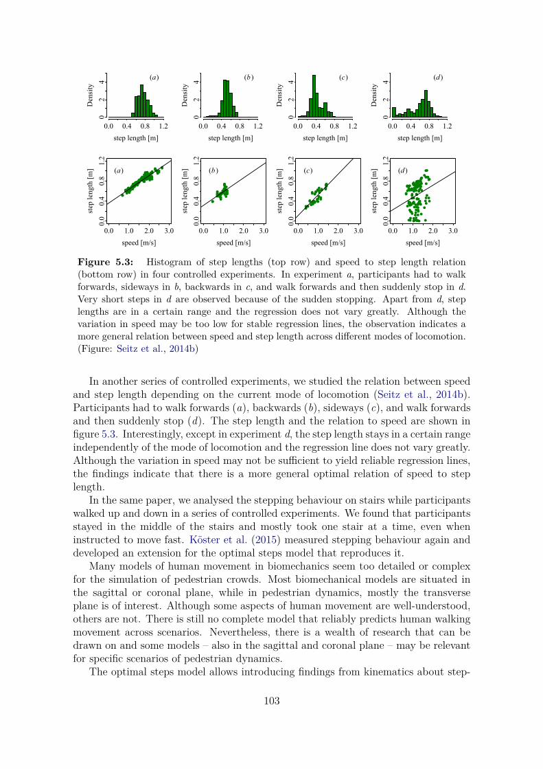
step length [m]

Den

sity

0.0 0.4 0.8 1.2

02

4

(a)

step length [m]

Den

sity

0.0 0.4 0.8 1.2

02

4

(b )

step length [m]

Den

sity

0.0 0.4 0.8 1.2

02

4

(c)

step length [m]

Den

sity

0.0 0.4 0.8 1.2

02

4

(d )

0.0 1.0 2.0 3.0

0.0

0.4

0.8

1.2

speed [m/s]

step

len

gth

[m

] (a)

0.0 1.0 2.0 3.0

0.0

0.4

0.8

1.2

speed [m/s]

step

len

gth

[m

] (b )

0.0 1.0 2.0 3.0

0.0

0.4

0.8

1.2

speed [m/s]

step

len

gth

[m

] (c)

0.0 1.0 2.0 3.0

0.0

0.4

0.8

1.2

speed [m/s]

step

len

gth

[m

] (d )

Figure 5.3: Histogram of step lengths (top row) and speed to step length relation(bottom row) in four controlled experiments. In experiment a, participants had to walkforwards, sideways in b, backwards in c, and walk forwards and then suddenly stop in d.Very short steps in d are observed because of the sudden stopping. Apart from d, steplengths are in a certain range and the regression does not vary greatly. Although thevariation in speed may be too low for stable regression lines, the observation indicates amore general relation between speed and step length across different modes of locomotion.(Figure: Seitz et al., 2014b)

In another series of controlled experiments, we studied the relation between speedand step length depending on the current mode of locomotion (Seitz et al., 2014b).Participants had to walk forwards (a), backwards (b), sideways (c), and walk forwardsand then suddenly stop (d). The step length and the relation to speed are shown infigure 5.3. Interestingly, except in experiment d, the step length stays in a certain rangeindependently of the mode of locomotion and the regression line does not vary greatly.Although the variation in speed may not be sufficient to yield reliable regression lines,the findings indicate that there is a more general optimal relation of speed to steplength.

In the same paper, we analysed the stepping behaviour on stairs while participantswalked up and down in a series of controlled experiments. We found that participantsstayed in the middle of the stairs and mostly took one stair at a time, even wheninstructed to move fast. Köster et al. (2015) measured stepping behaviour again anddeveloped an extension for the optimal steps model that reproduces it.

Many models of human movement in biomechanics seem too detailed or complexfor the simulation of pedestrian crowds. Most biomechanical models are situated inthe sagittal or coronal plane, while in pedestrian dynamics, mostly the transverseplane is of interest. Although some aspects of human movement are well-understood,others are not. There is still no complete model that reliably predicts human walkingmovement across scenarios. Nevertheless, there is a wealth of research that can bedrawn on and some models – also in the sagittal and coronal plane – may be relevantfor specific scenarios of pedestrian dynamics.

The optimal steps model allows introducing findings from kinematics about step-

103

ping behaviour into models of pedestrian dynamics. The decision-making layer couldbe complemented with a more detailed kinematic model of stepping. This may beespecially useful for studying the impact of stepping behaviour on the built environ-ment, such as the excitation of bridges (Macdonald, 2009). The force-based modelpresented in section 5.3 allows for the introduction of kinetic models and could becombined with a more elaborate representation of walking mechanics.

5.2 Aspects from roboticsStudies in biomechanics mostly aim at a better understanding of the mechanical pro-cesses. They do not necessarily target predicting or simulating movement. In robotics,the principle goal is to build a machine that moves in a specific way. Therefore, a strongfocus is put on engineering. In order to build (engineer) a walking robot, one has tounderstand its mechanics and thus understand walking (e.g., Buschmann et al., 2015).In this section, I discuss robotics as a possible source of findings that can be used forthe simulation of pedestrian behaviour on the locomotion layer.

Humanoid robots are a special class of robots that are designed to imitate humanbehaviour. The research objective is to match natural behaviour or aspects of it.Findings in this area can be of interest for pedestrian simulation, especially advancesin bipedal walking, collision avoidance mechanisms, and route choice behaviour. Idiscuss the decision-making aspects of these topics in section 6.2 of the next chapter.An example of a bipedal robot that can walk forwards and backwards, run, andclimb stairs is ASIMO (figure 5.4). It has been developed by Honda Motor Co., Ltd.(2004) since 1986 and was first presented in 2000. Another humanoid robot, Atlas, isdeveloped by Boston Dynamics (2016). The most recent version of this bipedal robotcan walk in rough terrain and interact with the environment. For example, Atlas canopen doors, lift and carry a box, recover balance after having been pushed, and standup after having fallen to the ground.

Robots are based on a similar concept as situated agents in artificial intelligence.They perceive the environment through sensors, make decisions according to somerules, and the robot’s mechanic carries out actions. I cover both perception anddecision making in chapter 6. How to control the legs or other mechanical entities ofthe robot (e.g., Pratt et al., 2001; Westervelt et al., 2007; Hamon et al., 2014) maybe useful knowledge for the simulation of pedestrian locomotion. For example, theconcept of dynamic walking (McGeer, 1993) is interesting as a biomechanical modelfor the locomotion layer of individual agents. The approach has already been used tobuild robots – both passive ones that do not need any motor control and active onesthat can walk forward on even ground (Collins et al., 2005; Iida et al., 2007; Rushdiet al., 2014; Zhu et al., 2014).

Dynamic walking robots seem to capture the natural gait of humans especially well.They built on the fundamental mechanics of walking and are validated through theconstruction of physical models (robots) that actually walk. As I argued is the case formost models in biomechanics, models of dynamic walking are too complex at presentfor the representation on the physical layer of pedestrian dynamics. Nevertheless,findings from robotics could become valuable in future developments.

104

Figure 5.4: An example of a bipedal walking robot. ASIMO can walk, run, walk back-wards and climb stairs. (Figure: Wikimedia, Vanillase, 2011)

5.3 Locomotion models for pedestriansI describe two approaches for a physical layer of pedestrian locomotion in this section.The first one stems from the optimal steps model and is the basis for simulatingpedestrian dynamics with cognitive heuristics (subsection 6.3.1 of the next chapter).This concept does not consider forces but represents the natural stepping processof pedestrians. The second one is a force-based model that simulates continuousmotion in continuous space without considering steps. It can be combined with boththe decision making of the optimal steps model and cognitive heuristic. The twoalternatives demonstrate how the psychological (decision-making) layer is relativelyindependent of the physical (locomotion) layer.

5.3.1 Discrete stepping processThe optimal steps model (chapter 4) is based on a discrete representation of pedestrianstepping behaviour, which is a discrete physical representation of natural pedestriankinematics. The movement is continuous in space and hence does not show any gridartefacts. Cellular automata do not represent the stepwise movement of pedestriansbut only a rather arbitrary discretisation, and the cell size is not chosen to match thehuman step length but their physical dimensions. I first briefly revisit the steppingprocess and discretisation approach and then point out how it can be used by apsychological layer.

In the discrete stepping process, individual pedestrian motion is represented bythe stepping behaviour of humans. The position of the next step is determined by adecision-making process and then the pedestrian is directly moved there. The process

105

current position

step circlepossiblenext move

equidistant grid

random offset

Figure 5.5: Schematic depiction of the step circle in the optimal steps model. Thegreen point represents the current position, the blue circle positions the agents can stepto, and the red arrow one possible movement. The continuous model is shown on the left.Steps are taken instantly at one moment in simulation time. The step length, that is, theradius of the step circle is determined through the speed. On the right, one numericaldiscretisation is depicted with an equidistant grid on the step circle. The grid has to berotated randomly in order to prevent a systematic bias in the step direction. Details onthe optimal steps model can be found in chapter 4. (Figure: Seitz and Köster, 2014)

is discrete because the path from one position to the next is not simulated. The agentis moved there directly and instantly at one point in simulation time. However, itis in continuous space and time as steps can be taken in arbitrary directions in thetransverse plane and at arbitrary points in the simulated time.

The stepwise movement process is exploited for decision making. Decision-makingby agents is only necessary when a step has to be taken by an agent. This is asimplification of the real behaviour of pedestrians because a decision might also betaken between two steps. Nevertheless, it seems likely that the position of the nextstep is already decided on when the person starts carrying out the step, and thedecision only changes in special situations while the step is being made. One exampleof an exception could be the sudden stopping we studied in a controlled experiment,which I reported in section 5.1.

With the event-driven update scheme, conflicts do not occur or, in other words,are solved implicitly. More details on update schemes can be found in chapter 4,section 4.3. The stepping process can be parallelised, although this entails somemodification to the conflict resolution behaviour of agents. The event-driven updatescheme represents a natural discrete model. If two agents want to go to the sameposition, the agent who starts moving there first is allowed to take it, and the otheragents must choose another position.

In the optimal steps model, the next step is determined through utility optimisationon a circle or disc (figure 5.5). Instead of utility optimisation, other methods tochoose the next step can be used. For example, the gradient steps model (section 3.5)determines the direction of the next step through the gradient of the scalar field atthe current position. We used the described representation of the stepping process forcognitive heuristics on the psychological layer (Seitz et al., 2015a): heuristic decisionsare made for every new step. This is efficient in terms of necessary cognitive effort,which is one of the requirements for a plausible representation of human decisionmaking (section 6.1.3), and it is efficient in terms of computational effort.

Due to the separation of layers, findings related to the stepping behaviour usedin the optimal steps model can also be used in combination with cognitive heuristics.For example, it is well-known that the step length of pedestrians is correlated to theirspeed (Grieve and Gear, 1966; Kirtley et al., 1985; Fukagawa et al., 1995; Seitz and

106

Köster, 2012). Other examples are constraints in the direction of movement (Bauerand Kitazawa, 2010; Seitz and Köster, 2012), movement on stairs (Köster et al., 2015),smaller steps (von Sivers and Köster, 2015), and adjusted step lengths for other modesof locomotion such as walking sideways and backwards (Seitz et al., 2014b). Finally,the step length can be related to other measures, including density (Jelić et al., 2012b),which opens up a broad field of research.

The stepping process allows for the introduction of features from biomechanics, yetit is a mere kinematic model with discrete steps. The stepping process can be madecontinuous in several ways, for example, the steps can be interpolated. A force-basedmodel may be used to realise the step to the next position that has been chosen by adecision-making layer. A more concise approach to a force-based locomotion layer doesnot explicitly represent the steps but still uses the decision-making layer that assumesa stepwise movement. Such a concept is proposed in the following subsection.

5.3.2 Continuous force-based processIn this subsection, I propose a force-based model for the locomotion layer. In contrastto the force-based models discussed in chapter 3, my approach does not model thedecision making with forces. Instead, all forces in this model represent physical forces,which are caused by gravity, friction, and physical contact. The model I describe in thefollowing does not capture these forces in detail nor does it implement contact forcesbetween pedestrians. It does, however, provide a basis for a more detailed represent-ation of the physical world with continuous space and time. It is also independent ofthe decision-making layer as it allows for the combination with different models, inparticular with cognitive heuristics (chapter 6). Thus, it is a proof of concept for gen-ericity of the physical layer as well as a continuous alternative to the discrete processof the last subsection.

A requirement for the model is that the decision where to go be already madeand only carried out by the physical layer. Moussaïd et al. (2011) also separatedthe decision-making layer from the physical layer and used a force-based model forlocomotion. The basic formula of mass m times the acceleration x equals the force fis used:

m× x = f ⇒ x = f

m. (5.1)

Given a model of the force and the mass, one can compute the acceleration. Solvingthe differential equation numerically yields the current speed and position. The samebasic model also describes other systems, especially in granular flow (e.g., Rao andNott, 2008).

If the absolute values of the forces and the mass are not of interest in the simulation,the mass can be assumed to be 1. Therefore, I use m = 1 for simplicity, which leadsto x = f . If m 6= 1, the forces have to be adjusted accordingly. Using realistic massesmay be meaningful when additional physical forces are present or the forces themselvesare of interest. If physical forces are measured in experiments, such as the pressure ina dense crowd, they rely on realistic values for the mass too.

For the force-based locomotion model, I assume that the preferred position afterthe next step xp is known. Determining this step can be realised with the heuristic

107

v0 vp

x0

xp

f

Figure 5.6: Illustration of the velocity and force vectors used in the force-based loco-motion model. The current position is denoted by x0 and the current velocity by v0. Thepreferred next position and velocity are denoted by xp and vp, respectively. The forcevector f is calculated by subtracting the current velocity from the preferred velocity. Thepreferred velocity is multiplied by the preferred speed (a scalar value), and the force vectoris scaled by a factor that controls the reaction time. Equations 5.2 and 5.3 describe thiscalculation mathematically.

decision making presented in section 6.3 of the next chapter. Using the decision-making process from the optimal steps model would also be possible, but I did notimplemented it for this work. The bodies of agents are represented as circles as in theoptimal steps model.

Given the preferred position xp and the current position x0, a preferred velocityvector vp is calculated. In order to reach the preferred position, the velocity vectorhas to point in the direction of xp, and the preferred speed has to be known. At first,the velocity vector is normalised by its length ||xp− x0|| and then multiplied with thepreferred speed:

vp = xp − x0

||xp − x0||× preferred speed. (5.2)

Formula 5.2 could already be used for a continuous velocity-based locomotion layer.For a force-based model, another step is necessary.

Acceleration represents the change in velocity and, for m = 1, equals the force. Iuse the difference in the current velocity to the preferred velocity and scale it by afactor. The resulting term is employed directly as the force applied to the agent. Theformula is

f = (vp − v0)× scaling factor. (5.3)

The velocity and force vectors are illustrated in figure 5.6. In other force-based models,such as the social force model (Helbing and Molnár, 1995), the scaling factor is usuallygiven by 1/τ , where τ is a relaxation time. The relaxation time controls how fast thechanges in direction induced by the force are realised. For example, a small τ leadsto greater forces and thus fast changes in direction. The same reasoning holds for thescaling factor in equation 5.3 but with inverted values:

scaling factor = 1τ. (5.4)

With known starting positions x0 and velocities v0 of agents, the system represents

108

vt

xt

vt+1

xt+1

ft+1

Figure 5.7: Illustration of the numerical solution of the force-based locomotion model(figure 5.6) based on the Euler method. The current position xt and the current velocity vt

are used to compute the force ft+1, which is applied for the next step t+1. The numericalscheme integrates the acceleration into the next velocity vt+1 and finally the next positionxt+1.

an initial value problem for differential equations:

x = v,v = f,x(t0) = x0,v(t0) = v0.

(5.5)

The decision process is continuous, that is, the decision of where to go next is updatedconstantly. For the numerical solution, the decision is updated for every time step,and a new system of differential equations has to be solved. The desired position xp

may never actually be reached since it changes as the agent approaches it.With the information of the current time step t, a step of the Euler method is

applied to numerically compute the next time step t+1. For the numerical integration,the position and velocity vectors of the current time step t are used to compute thenext velocity vt+1, and the new velocity vector of t + 1 is used to compute the nextposition xt+1. The force f(xt, vt) is calculated according to equations 5.2 and 5.3.Hence, the numerical step is defined by

vt+1 = vt + f(xt, vt, xp,t)×∆t, (5.6)xt+1 = xt + vt+1 ×∆t, (5.7)

where ∆t is the numerical time step length. The computation is illustrated in figure5.7. Equation 5.6 describes an explicit Euler step and equation 5.7 an implicit Eulerstep. Therefore, taken together, a step of the semi-implicit Euler method is applied(e.g., Deuflhard, 1985).

The preferred position xp is updated for every numerical time step t. Alternatively,one could update xp and then use it until the agent has covered the distance predefinedby the step length. In some initial tests, the latter method led to somewhat unrealisticdetours when agents evaded others. Therefore, I use the continuous update. Withparameter calibration and a more complex decision-making process that does not lead

109

Figure 5.8: Simulated pedestrian trajectories for the comparison of the two locomotionmodels for pedestrians: discrete stepping process on the left and continuous force-basedprocess on the right. For the decision making, the tangential evasion heuristic was used(subsection 6.3.1). Agents are created in the green rectangles on top, one agent every10 seconds for the duration of 10 seconds for each source. They walk towards the yellowrectangle diagonally on the bottom. The whole area of the scenario has side lengths of15 m. For the discrete stepping process (on the left), sudden changes in direction can beobserved. In the continuous locomotion scheme, changes in direction are continuous.

to sudden changes of direction, the stepwise update of xp may be an interesting conceptto represent stepwise motion. Updating the decision only once for each movement stepwould also reduce the computational effort.

Other numerical solutions could be employed for the equation (e.g., Vesely, 2001),but the change of direction in the decision layer and the mechanism for collisionprevention described in the following paragraphs lead to discontinuities, which com-plicate the use of higher-order solvers. With a fixed preferred position xp for sometime, higher-order solvers may be employed. In any case, the sudden stopping in caseof a collision remains an issue.

Although the decision-making layer usually implements some kind of collision eva-sion algorithm, it does not ensure that collisions cannot happen on the physical layer.For example, an agent may choose to step in a direction that leads to a collision.Then the physical layer has to simulate the collision. As a basic model, agents in myapproach simply cannot overlap, that is, they remain at the current position if thenext numerical step would lead to an overlapping.

To realise this, I use a modification of the system described in equations 5.6 and5.7. Instead of setting the next position directly, as in equation 5.7, x′t+1 is computedfor all agents in the simulation first. Then collisions are checked with the updatedpositions x′t+1. For all agents with a collision in x′t+1, the next position xt+1 is set back

110

to xt. Equation 5.7 is replaced by

x′t+1 = xt + ∆t× vt+1, (5.8)

xt+1 ={xt if x′t+1 leads to a collisionx′t+1 else. (5.9)

The distinction of cases introduces discontinuities and hence complicates the use ofhigher-order numerical solutions. A mollification of the model may restore the re-quirements for higher-order numerical schemes (Köster et al., 2013).

The simple stopping of agents in the case of a collision is perhaps the most basicapproach for collision resolution. A more advanced physical model would take intoaccount the forces present in the case of a collision. One approach well-known in thesimulation of granular flow is the discrete element method (DEM, Cundall and Strack,1979; Kleinert et al., 2013), which can consider a variety of forces, such as friction andrecoil. Given that the method described above is based on forces, it could easily beintegrated with a DEM simulation.

Simulation results comparing the discrete stepping process and the force-basedmodel are shown in figure 5.8. For the kinetic model of stepping, sudden changesof direction can be seen. In the continuous, force-based model, changes of directionover time are smooth because of inertia. The two physical processes can be combinedwith either local utility optimisation, heuristic decision making, or other models onthe psychological layer (chapter 6).

5.4 SummaryIn this chapter, I introduced the physical layer – the first of the three layers that,together, cover pedestrian dynamics. Although the physical layer is interconnectedwith the psychological layer, as an idealisation it is useful to separate the two. Thepsychological layer has to provide the decision of where to go next. The resultingposition and possibly also the resulting velocity described in the physical layer is inturn used by the psychological layer.

I drew on the literature from biomechanics in section 5.1. Two perspectives onhuman movement can be taken: kinematics and kinetics. Kinematics describes move-ment without the consideration of forces, whereas in kinetics the various forces leadingto movement are studied. A variety of simulation models has been proposed for theindividual human walking process. Most models are situated in the coronal or sagittalplane. In contrast, pedestrian dynamics usually studies movement in the transverseplane. Moreover, biomechanical models of walking seem to be too complex for a simplerepresentation in simulations of pedestrian dynamics. Nevertheless, there is a wealthof research that can be drawn on when further developing the physical layer.

Robotics (section 5.2) also has to study the mechanical process of movement.Especially walking robots can only be engineered with such knowledge. Findings inrobotics can be of interest for the physical representation of agents in a simulationof pedestrian dynamics. The concept of dynamic walking seems especially promisingbecause based on it, physical models (robots) have been built that exhibit a natural

111

Decision makingUtility optimisation Cognitive heuristics

Locomotion Discrete steps a bForce-based c d

Table 5.1: Possible combinations of locomotion and decision making models for therespective two layers. Combination a corresponds to the optimal steps model, b to thesimulation approach used in subsection 6.3.3, d to the simulations in subsection 5.3.2. Thelocomotion models presented in this chapter are highlighted in yellow.

walking behaviour. As was the case for biomechanics, the models are still to complexfor a basic physical representation but may be of interest in future developments. Idiscuss other aspects of robotics such as decision making in the next chapter.

I presented two models for pedestrian locomotion in section 5.3. The first one isthe discrete stepping process also used in the optimal steps model. It is a kinematicmodel and thus only simulates movement without a representation of forces. It isdiscrete in time and space because agents move forward instantly, but agents canmove to arbitrary positions in space and at arbitrary points in time. Hence, agentsact in continuous space and time. This model opens pedestrian simulation for a varietyof studies, including the impact of crowd movement on the built environment. Themodel can be combined with other decision-making schemes, that is, models on thepsychological layer such as cognitive heuristics.

The second model is force-based but has to be given the decision on where to step.In contrast to the social force model, it does not describe decision making with forcesbut only carries out the locomotion when the decision is already made. The modelis a kinetic approach, which has the advantage that forces are modelled explicitly. Itcan be combined with other forces, such as contact forces.

The model on the locomotion layer has to be selected based on the objectives ofthe simulation. Table 5.1 summarises the options and highlights the two models forlocomotion I discussed in this chapter. The two approaches provide a basis for a widevariety of studies. The discrete stepping process has the additional advantage of animplicit natural discretisation, which allows for efficient computation. The force-basedapproach seems to be more flexible in future developments. For example, the steppingprocess could also be used in a force-based model. Detailed models of biomechanicscould be incorporated, which would lead to additional computational costs. Therefore,one has to weigh the advantages and disadvantages when selecting the respectivemodels.

112

Chapter 6

The psychological layer: Heuristicdecision making

The agents can carry out movement decisions given the locomotion layer introducedin the previous chapter. Models on the psychological layer generate the movementdecisions (figure 6.1). They determine the position where the agent wants to stepnext within the proximity of the agent. In some cases, the locality of this decision isnot that clearly defined, for example, when agents anticipate their motion some stepsahead.

The physical and the psychological layer cannot be separated entirely in the modelas they are strongly linked in the real world too. For simulation, a separation is stillconvenient and justified. The physical layer simulates stepping behaviour, changes ofdirection through forces, the actual speed of movement, and so on using the decisionsmade by the psychological layer. The psychological layer may use the position andvelocity of other agents as input. Some knowledge of the agent about the physicalprocess can also be assumed, especially in real humans. For simplicity, this is largelyignored in the concepts I present but may be an interesting direction of future research.

The overall question that has to be addressed by the psychological layer is where tostep next. This question may entail forward planning or, at least, some local strategic

Decision making

Physical layer

Psychological layer

Social layer

Figure 6.1: Illustration of the model separation into three layers. This chapter focuseson psychological aspects, builds on an existing physical layer, and provides a basis for thesocial layer.

113

component such as what distance the pedestrian wants to keep to other pedestriansand walls. Other motivational influences are what speed the pedestrians want to walkwith and to which target they choose to go. The latter falls into the category ofroute choice or path planning, which I do not treat in detail here. Nevertheless, sometarget must be known in order to make the decision on where to move next. I assumethat the target such as an exit door or any target area is provided by a route choicecomponent (e.g., Kneidl, 2013).

Human behaviour is highly complex and diverse. For pedestrian dynamics, onlythose aspects of psychology are of interest that determine motion. Still, for a varietyof reasons, only a small subset of psychological features can be represented in a model(section 1.3 in the introduction). Specifically, the psychological process has to bemodelled in the simplest way so that it reproduces or describes observed phenomena.

Many relevant psychological differences can be found in pedestrians, includingknowledge of the environment they are in, experience in similar situations, stress level,motivation, sense of security and safety, but also the ability to lead or the tendencyto follow others. I discuss some social aspects and group behaviours in chapter 7.In the present chapter, many abilities and features of humans are excluded from themodel. For example, agents in the simulation do not have psychological differencesor memory and do not plan their movement and that of others forward explicitly.However, some of the concepts used for modelling decision making of pedestrians haveimplicit forward planning. Agents in the model only use local information, which is anapproximation to the perception of humans. More elaborated theories like cognitivemaps are not used. Perceptual constraints may be an interesting extension, especiallyfor the approach with cognitive heuristics.

I first draw on related fields that study decision making, especially in the context oflocal movement. These are the behavioural sciences psychology and animal behaviour(section 6.1). I discuss the concept of bounded rationality and cognitive heuristics(subsection 6.1.3), which is the paradigm the model described in section 6.3 is basedon. Section 6.2 is dedicated to the engineering aspects of decision making, namelyartificial intelligence. In the rest of the chapter, I use this background and present adecision-making model for pedestrian dynamics (section 6.3). An important behaviourin pedestrian scenarios is waiting and remaining, which I cover in section 6.4.

6.1 Aspects from behavioural sciencesThe psychological and the physical layer are interconnected (chapter 5) in the model aswell as in reality. Decision making is an interaction with the physical world that goes inboth directions (Raab et al., 2009; de Oliveira et al., 2009; Green and Heekeren, 2009;Schack and Ritter, 2009). For example, pedestrians visually perceive the environmentand decide on what to do next on the psychological layer using the visual cues. Thismay lead to an action such as taking a step in a specific direction in the physical world.Decision making relates to the physical world on yet another level: mental activitiescan be observed physically in the body, that is, the nervous system. With the physicallayer I propose here, I do not refer to the nervous system and mental activities, whichare exclusively represented by the psychological layer.

114

Every choice that affects the movement of pedestrian crowds can be relevant for thedecision-making layer. Hoogendoorn and Bovy (2004) define three levels of decisionmaking for individual pedestrians – the strategic, tactical, and operational level:

1. Departure time choice, and activity pattern choice (strategic level);2. Activity scheduling, activity area choice, and route-choice to reach activ-ity areas (tactical level);3. Walking behavior (operational level).(Hoogendoorn and Bovy, 2004)

The behaviour I study in the following would best be described as the operationallevel of this model. However, some decisions that affect the walking behaviour couldbe described as strategic too. For example, how much distance pedestrians keep toa wall or other pedestrians is also a strategic decision. Therefore, I use a differentterminology: I refer to the decision models that describe walking behaviour as localdecision making in contrast to route choice or path planning and global strategicdecisions on the overall goal. Examples of decisions that I do not consider local arethe choice of which exit to take, what kind of activity to follow, and so on.

The following subsections are dedicated to aspects from psychology, animal be-haviour, and decision making. I discuss the literature as background for simulationmodels of pedestrian dynamics.

6.1.1 Aspects from psychologyPsychology is the “scientific study of the behavior of individuals and their mentalprocesses” (Gerrig and Zimbardo, 2002). Many aspects of psychology may have animpact on pedestrian and crowd dynamics. For the study of human behaviour in acomputer simulation, a minimal set of aspects has to be selected that describes relevantphenomena. Areas that are of interest for the simulation of individual pedestriansare perception and behaviour, motivation, cognition, and social psychology. In thefollowing, I report definitions for the terms and draw on the literature for relevantbackground. I start by outlining the fields that study the interfaces to the physicalworld: perception and behaviour.

Perception describes the “processes that organize information in the sensory im-age and interpret it as having been produced by properties of objects or events in theexternal, three-dimensional world” (Gerrig and Zimbardo, 2002). This definition firstsays that perception collects information from the physical world and integrates itinto a mental representation of it. Furthermore, perception deals with the interpreta-tion of the input as it represents the information in a coherent picture of the physicalworld. Perception is of great importance for pedestrian dynamics because pedestriansinteract with their environment based on the information they have on it. The currentbehaviour is also determined by other aspects, including memory and learned beha-viour. While these are relatively constant, perception makes the behaviour adaptivefor different situations and contexts.

Important perceptual capacities of pedestrians are the estimation of distances (e.g.,Ziemer et al., 2009; Iosa et al., 2012) and motion (e.g., Johansson, 1973; Albright andStoner, 1995). These abilities allow us to navigate through a fast changing environment

115

in many different contexts. Without them – for example due to vision impairment orbecause of the lighting conditions – we can draw on aural and tactile cues. Neverthe-less, in most cases, impairment of vision also constraints our navigational abilities. Incomplex environments, we may not be able to process all available information andthen have to focus our attention on relevant features such as possible collisions withothers (Jovancevic et al., 2006). It is important to note that perception can be highlyselective and even blend out events that seem hard to ignore (Hastorf and Cantril,1954).

On the other side of the interaction with the physical world stands behaviour. It isdefined as the “actions by which an organism adjusts to its environment” (Gerrig andZimbardo, 2002). The mental process can often only be studied indirectly throughbehaviour, which is the process we can observe directly. General findings on behaviourin psychology can be of interest for the development of pedestrian simulation models.

At the core of all human action stands motivation, the “process of starting, dir-ecting, and maintaining physical and psychological activities; includes mechanismsinvolved in preferences for one activity over another and the vigor and persistence ofresponses” (Gerrig and Zimbardo, 2002). A rough classification of behaviours can beundertaken based on the distinction between approach and avoidance motivation:

Both approach and avoidance motivation are part of our evolutionary her-itage, and we certainly cannot survive, either physically or psychologically,without both types of motivation. Certain tasks in negotiating the envir-onment and our social world require avoidance motivation, and avoidancemotivation is undoubtedly adaptive in some instances. For example, it isimperative that our perceptual system be perpetually vigilant for physicaldanger or it is likely that our lifespan would be greatly truncated . . . (Elliot,2006)

The scalar fields (section 3.5, chapter 3) used in many models of pedestrian dynamicscan be interpreted as a representation of approach and avoidance motivation. Forexample, high potentials in the social force model lead to an avoidance of these areas.However, approach and avoidance motivation is a simple perspective that cannot ex-plain pedestrian behaviour in depth.

Pedestrians usually follow motivations that lead to specific behaviours: avoidingcollisions, reaching a target, keeping a certain distance to others, walking with apreferred speed, staying with a group, communicating with a group, staying in a safearea, and so on. The specific motivations may not seem important for a simulationmodel, but they give the necessary background and can be used to clearly separateaspects of the model. Listing the motivations may also help to make explicit what agiven model does or does not capture and to identify shortcomings of existing models.

Cognitive psychology is the “study of higher mental processes such as attention,language use, memory, perception, problem solving, and thinking” (Gerrig and Zim-bardo, 2002), thus, it comprises perception as well as decision making. Knowledge ofgeneral cognitive abilities and paradigms help to develop plausible models of humanbehaviour. Subsection 6.1.3 is dedicated to the theory of bounded rationality (Simon,1990) and cognitive heuristics (Gigerenzer et al., 1999) as a paradigm, which I alsouse for the model of pedestrian dynamics in section 6.3.

116

Social psychology is the “branch of psychology that studies the effect of social vari-ables on individual behavior, attitudes, perceptions, and motives; also studies groupand intergroup phenomena” (Gerrig and Zimbardo, 2002). The study of pedestriandynamics is also a study of social interactions, and social psychology may provideimportant findings for it. In this work, I separate group behaviour and explicitly so-cial behaviour from proximity navigation. This separation is not entirely successfulbecause interacting agents already describe social behaviour, even if they only try tonavigate around others. The goal is to provide a basic layer for pedestrian navigationin this chapter that can be extended with models of collective and group behaviour inthe next chapter.

Simulation models of pedestrian dynamics are often advertised for the study ofemergency evacuation scenarios (e.g., Gwynne et al., 1999; Pan et al., 2007). Some-times the term “panic” is used (e.g., Helbing et al., 2000a) to describe human groupbehaviour in emergency situations that led to a loss of lives. Since the term “panic”suggests irrational behaviour, it has been dismissed in the scientific literature (e.g.,Johnson, 1987; Aguirre, 2005; Drury et al., 2013). Nevertheless, human behaviouris likely to change in emergency situations because of a variety of factors, includingadditional stress, novelty of the situation, impairment of perception, and the urgency,which pressures individuals to make decisions fast. Behaviour that may seem irra-tional from an outside observer or in retrospect may not be all that irrational whenconsidering the circumstances people were in.

Many other topics in psychology can further the understanding of pedestrian beha-viour in a variety of contexts and from different perspectives. For a concrete simulationapproach, one has to select relevant aspects, otherwise, the model becomes too com-plex for validation. The argument of parsimony becomes even more important whentrying to incorporate theories from social psychology such as the social identity model(section 7.1).

6.1.2 Aspects from animal behaviourA field related to psychology is animal behaviour (e.g., Manning and Dawkins, 2012).In animal behaviour, topics like cognition and decision making are studied, too. Onthe one hand, there are similarities between humans and other species – but one alsohas to make sure not to neglect the differences. In general, humans could be regardedto have higher cognitive abilities. On the other hand, some species may supersede theabilities of humans when faced with certain situations, especially as the physiology ofa species gives them specific abilities.

Most phenomena in pedestrian dynamics can be described as self-organisation, thatis, individuals behave in a way that yields the phenomena without a superordinateindividual controlling or instructing the process. Self-organisation is well-studied inbiology (Couzin and Krause, 2003). An important concept that cannot be separatedclearly from self-organisation and may in fact often cover the same topic is collectivebehaviour and collective motion (e.g., Sumpter, 2006 and Vicsek and Zafeiris, 2012).In these areas, similarities among swarms, flocks, and also pedestrian crowds can befound (Moussaïd et al., 2009a).

Another direction of research treats animal navigation (e.g., Collett and Graham,

117

2004. In navigation, mainly individual movements over longer distances are studiedand not so much the interaction and collective motion of groups. Concepts, such aspath integrations have given insights into how animals forage and find their way backhome (e.g., Etienne et al., 1998; McNaughton et al., 2006). Long-range travels arestudied in the migration of animals (e.g., Dingle and Drake, 2007; Dingle, 2014).

Findings in animal behaviour may contribute to the study of pedestrian dynamics.An example are cognitive or perceptual constraints in the number of neighbouringindividuals that are taken into account for movement decisions (Ballerini et al., 2008;Bode et al., 2010; Strandburg-Peshkin et al., 2013). Moreover, human behaviour isalso studied by researchers in the domain of animal behaviour and may highlightsimilarities among species.

In collective animal behaviour, mostly swarms and flocks are studied. Here, an-imals form a collective for a specific purpose such as protection against predators.Pedestrians usually form crowds for other purposes or even without a purpose in aphysical crowd. I give a definition of psychological and physical crowds in the nextchapter, section 7.1. Therefore, models from biology cannot be used directly for humanbehaviour. When using models from animal navigation, a similar line of argument canbe made: animals typically set out to look for food sources. This is not the case forhumans in a modern environment. Some basic models and mechanisms may still beof use for the study of pedestrian behaviour, including cognitive maps and path integ-ration (Mittelstaedt and Mittelstaedt, 1980; Collett and Graham, 2004; McNaughtonet al., 2006). However, these would mainly be of interest in route choice models, whichare not the focus of my work.

6.1.3 Decision making and bounded rationalityDecision making is defined as the “process of choosing between alternatives; selectingor rejecting available options” (Gerrig and Zimbardo, 2002). There are descriptive andnormative models of decision making. Descriptive models aim at a better understand-ing of natural processes such as animal behaviour. Normative models, on the otherhand, try to aid decision making. For example, a formally defined decision process myhelp medical doctors to efficiently act in emergency situations (Breiman et al., 1984,pp. 1–2).

In computational science, it is of great importance that the two not be confused.When simulating pedestrian dynamics, one tries to understand, reproduce, and predicthuman behaviour. In some cases, a what-if scenario may require looking for normativesolutions such as the question “what behaviour might improve the outcome?” If thatis the case, it has to be clearly separated from the description of human behaviour.Although the ”double role—to describe and to prescribe—does not map easily onto asharp divide between descriptive and normative models” (Gigerenzer and Selten, 2001,p. 1), I argue that the confusion of the two can lead to a severe misrepresentation ofhuman behaviour and ultimately to misguided model predictions.

Decision making is studied in behavioural sciences but also in other fields, includ-ing economics (Simon, 1959). Traditional models in economics assumed unboundedrationality, which means that agents act in a way that allows them to reach optimal-ity according to some criteria (e.g., Gigerenzer and Todd, 1999). To come by such a

118

solution, they may draw on unlimited resources for reasoning. This concept has beencriticised by Simon (1955), who later coined the term bounded rationality as an altern-ative approach for the understanding of human decision making (e.g., Simon, 1990).Bounded rationality suggests that – in contrast to traditional models – resources forreasoning are limited.

Humans and animals make inferences about their world with limited time,knowledge, and computational power. In contrast, many models of ra-tional inference view the mind as if it were a supernatural being possessingdemonic powers of reason, boundless knowledge, and all of eternity withwhich to make decisions. Such visions of rationality often conflict withreality. (Gigerenzer et al., 1999, p. 7)

The proponents of bounded rationality say that it specifically “dispenses with optim-ization, and, for the most part, with calculation of probabilities and utility as well”(Gigerenzer and Selten, 2001, p. 3) as they argue that optimisation is often well outof the boundaries of our cognitive capacities.

As an important example of a model of bounded rationality, I briefly describeaspiration theory (Starbuck, 1963). Aspiration theory presumes that individuals tryto reach a certain level of satisfaction rather than optimality. For example, you maynot continue looking for a vendor of a product after you have found one that offersthe product at a price you deem favourably. In contrast, according to unboundedrationality, you would continue consulting all vendors of the product and select theone that offers it at the lowest price. In reality, this search may not even be feasibleto finish in one lifetime.

Tversky and Kahneman (1974) conducted a series of experiments that show how,under certain conditions, humans tend to make biased decisions that seem to beinconsistent and irrational. For example, they demonstrated the effect of framing(Tversky and Kahneman, 1981). In an experiment, they present two mathematicallyidentical problems to participants. The participants have to decide which of twooptions they would choose. Both option A and B have the same expected value, butoption B has some variance while option B does not. If the problem is described interms of gain, participants prefer option A, which is not associated with uncertainty.If the problem is described in terms of loss, they tend to choose option B, which issubject to variance. This leads to the authors’ statement that “choices involving gainsare often risk averse and choices involving losses are often risk taking” (Tversky andKahneman, 1981). The decisions seem to be highly inconsistent because, formally,both problems are exactly the same, yet participants decided differently because ofthe framing. Rationality would seem to demand the same decision independently ofthe framing. This line of research is also often described as the heuristics and biasesschool (e.g., Kelman, 2011).

Gigerenzer and Goldstein (1996), on the other hand, demonstrated that models ofbounded rationality can even outperform the traditional model of rational inference.Heuristics in this context are algorithms that allow for fast and efficient computa-tion and do not necessarily perform worse than optimisation in real world scenarios.Gigerenzer and Todd (1999, pp. 25–29) give a detailed definition of the term heuristic.This line of research led to the fast and frugal heuristics school, which argues that, in

119

general, bounded rationality works well under many circumstances (Gigerenzer et al.,1999; Todd and Gigerenzer, 2000; Gigerenzer, 2008).

Goldstein and Gigerenzer (2002) propose to design and test cognitive heuristicsthat are “(a) ecologically rational (i.e., they exploit structures of information in theenvironment), (b) founded in evolved psychological capacities such as memory and theperceptual system, (c) fast, frugal, and simple enough to operate effectively when time,knowledge, and computational might are limited, (d) precise enough to be modeledcomputationally, and (e) powerful enough to model both good and poor reasoning”.Particularly, complexity arises out of the behaviour of individuals in interaction withthe environment, but the behaviour itself need not be complex (Simon, 1996).

The two perspective on cognitive heuristics – the heuristics and biases school andthe fast and frugal heuristics school – have led to some dispute between their pro-ponents (Kahneman and Tversky, 1996; Gigerenzer, 1996). Nevertheless, there isagreement on the fundamental principle of cognitive heuristics: “At some level of gen-erality, there is widespread agreement that people are employing heuristics wheneverthey make a judgment or reach a decision without making use of some information thatcould be relevant or some computational abilities that at least some people possess”(Kelman, 2011, p. 3).

In pedestrian dynamics, one has to model both good and poor decision making.In most cases, pedestrian behaviour is highly efficient: accidents are the exceptionand we usually get where we want to go. This does not mean that it is necessarilyoptimal according to whatever criterion. Accidents do occur and probably everyonehas experienced some kind of collision with other pedestrians. This agrees with theprogramme Goldstein and Gigerenzer (2002) propose (above, point c). The algorithmsused in simulation innately have to be precise enough to be modelled computationally(point d). The other requirements of their programme are in line with the goal of aplausible decision-making model, especially that it be based on bounded rationality(point c) and founded in evolved psychological capacities (point b). Therefore, Iconsider this paradigm suitable for model development in pedestrian dynamics.

In biology, a similar direction can be found where behaviour is described by “rulesof thumb”. Hutchinson and Gigerenzer (2005) outline both cognitive heuristics andrules of thumb in biology and discuss similarities among the two. Conlin (2009)reviews heuristic decision making for navigation in humans. McLeod and Dienes(1996) describe how local movement decisions can be made using simple heuristics:fielders who try to catch a ball, instead of calculating the trajectory, only estimatewhether the ball will land before or behind them and adjust their position accordinglyover time. This example also demonstrates how it may seem as if humans computedthe optimal solution but, in fact, can use a simple heuristic that produces a similarresult.

The “adaptive toolbox” (Gigerenzer and Todd, 1999) of behavioural heuristicshas several advantages that are also beneficial to the modelling of navigation de-cisions. First, all computations employed for the heuristics have to be based in capa-cities the considered species possesses, which makes them a plausible representation ofreal cognitive processes. Second, due to its simplicity, the decision process facilitatesthe understanding, modelling, and communication across disciplines without in-depth

120

knowledge of the underlying mathematics and computations. Third, heuristics can beimplemented and tested as hypotheses without necessarily affecting other heuristicsof the same toolbox. Fourth, due to the flexibility, the resulting model can be expan-ded to capture further details or additional aspects of behaviour based on the currentstate of the model development. Fifth, the model parameters represent entities thatare observable in nature, such as the distance swarming fish try to keep to each otheror the number of other pedestrians considered for collision avoidance, in contrast toabstract concepts such as social forces or utility functions. Sixth, the implementationof behavioural heuristics could be automated with code generation facilitating thecreation and testing of new hypotheses. For example, predefined heuristic buildingblocks could be offered and combined in a graphical interface and the code carryingout the operations generated automatically.

One could argue that other models of pedestrian dynamics such as the social forcemodel (Helbing and Molnár, 1995) are already simple enough. However, the correctimplementation of the social force model can still be challenging in spite of its math-ematical simplicity (Köster et al., 2013). Furthermore, they may seem simple andintuitive to mathematicians and physicists, who are familiar with the mathematicalformalism, but also may not to biologists or psychologists. Thus, I argue that cognit-ive heuristics are more intuitive, especially for researchers in the fields of behaviouralsciences. The formal description of cognitive heuristics is not complex, even if theconcrete algorithmic implementation can be. Behavioural scientists can still proposecognitive heuristics with little knowledge of mathematics and computer science be-cause they do not have to know how to implement them.

In contrast to some models of pedestrian dynamics, cognitive heuristics do notoptimise in the sense that they necessarily find the optimal solution. However, theystill optimise the decision in the sense that they strive to find the optimum – whichthey may or may not find. Cognitive heuristics aim to find a “good-enough” solution(e.g., Gigerenzer, 2008). The optimal steps model (Seitz and Köster, 2012) contradictsthis paradigm as it employs numerical optimisation of a utility function to determinethe next step.

Having decided that cognitive heuristics are a suitable paradigm for the simulationof pedestrian dynamics, the question arises of how to practically apply this idea. Thefast and frugal heuristics school suggest the following research agenda:

The program of studying boundedly rational heuristics involves (a) design-ing computational models of candidate simple heuristics, (b) analyzing theenvironmental structures in which they perform well, (c) testing their per-formance in real-world environments, and (d) determining whether andwhen people really use these heuristics. The results of the investigatorystages (b), (c), and (d) can be used to inform the initial theorizing of stage(a). (Gigerenzer and Todd, 1999, p. 16)

Steps a, b, and c are covered in subsections 6.3.1 and 6.3.3 for a model I propose forthe simulation of pedestrian dynamics, and I discuss step d in subsection 6.3.4.

121

Agen

t

Enviro

nmen

t

Sensors

Actuators

Percepts

Actions

Figure 6.2: Schematic representation of an agent in artificial intelligence. The agentperceives the environment through sensors and acts in the environment through actuators.The empty box between sensors and actuators may be understood as the cognition of theagent. (Figure: adapted from Russell and Norvig, 2010, p. 35)

6.2 Aspects from artificial intelligenceThe behavioural sciences study decision making descriptively. When building a ma-chine or programme that makes some kind of decision, on the other hand, the focusis on engineering. In this section, I review literature from artificial intelligence, whichcan be considered to comprise the engineering of decision making. As in robotics (sec-tion 5.2, chapter 5), the objectives in engineering can deviate greatly from scientificmodelling. In engineering, one might just want to build a machine that works wellfor some task but may not be a good model of natural phenomena. Nevertheless, fora computer simulation of human behaviour, one still has to design algorithms andimplement software that describe behaviour, which are also core disciplines of arti-ficial intelligence. Therefore, artificial intelligence can be an important resource fortechnologies that help to develop models of natural phenomena. This is also expressedby the early work on cybernetics by Wiener (1961), which touches on many topics atthe interface between biological systems and artificial intelligence.

A common concept in artificial intelligence are agents: “An agent is anythingthat can be viewed as perceiving its environment through sensors and acting uponthat environment through actuators” (Russell and Norvig, 2010, p. 34). This modelhas parallels to the disciplines of psychology I discussed in subsection 6.1.1. Thesensory organs and the perception can be seen as the sensors and the behaviour canbe described by the actuators and actions of an agent. The basic agent model is shownin figure 6.2. The empty box between sensors and actuators may be understood asthe cognition of the agent.

A variety of agents with different capacities can be defined given the basic agentstructure where the agents differ in what happens within the dashed box (Russelland Norvig, 2010, chapter 2). For example, the reflex agent creates an internal rep-resentation of the environment and decides on an action following condition-actionrules. Other types are model-based, goal-based, utility-based, and learning agents.This classification can be employed for microscopic pedestrian stream models, espe-cially the complexity assessment of simulation approaches. The optimal steps model

122

(chapter 4) can be described as a utility-based agent model. Agents in the optimalsteps model perceive the positions of others around them. Then they define a set ofpossible actions, which are given by the possible next steps on the step circle. Theychoose one of the positions by assessing the respective utilities. Finally, they move tothe position with the highest utility value.

An interacting collection of agents is a multi-agent system (e.g., Shoham andLeyton-Brown, 2008). The game-theoretic foundations can be of interest for pedes-trian dynamics and describe some natural phenomena of self-organisation. However,a general multi-agent system may also be designed to fulfil a specific task in the spiritof engineering an efficient machine and hence does not necessarily describe naturalphenomena.

Another field of artificial intelligence that is important for pedestrian dynamics isplanning (e.g., Russell and Norvig, 2010, chapters 10 and 11). Especially for routechoice, methods such as Dijkstra’s algorithm (Dijkstra, 1959) and Sethian’s fast march-ing algorithm (Sethian, 1996, 1999) can be employed to simulate the behaviour ofpedestrians. An alternative are graph-based approaches (Kneidl, 2013), which arestudied in artificial intelligence, too. However, these algorithms are on the level ofanimal navigation, that is, route choice behaviour, which is not the focus of my work.

In robotics, artificial intelligence is applied for the control of autonomous robots(e.g., Arkin, 1998, and Russell and Norvig, 2010, chapter 25). Topics such as routechoice and path planning have an application for robots that must actively navig-ate through an environment with obstacles. Another area is the avoidance of colli-sions with moving obstacles, which can be solved using the velocity-obstacle approach(Canny and Reif, 1987; Fiorini and Shiller, 1998). Especially interesting is the de-velopment of control mechanisms in robots by Brooks (1989), who designed controlmechanisms in a modular way that can be extended and combined. The approach issomewhat similar to the heuristics toolbox proposed by Gigerenzer and Todd (1999).

For the representation of heuristic building blocks, some of the formalisms used inartificial intelligence may be helpful. For example, “statecharts, extend conventionalstate-transition diagrams with essentially three elements, dealing, respectively, withthe notions of hierarchy, concurrency and communication” (Harel, 1987). Statechartshave some commonalities with Venn diagrams and can be defined as an applicationof higraphs (Harel, 1988). Statecharts also graphically describe finite state machines(e.g., Kohavi and Jha, 2010), a concept that is suitable for the description of agentbehaviour. Extensions of state machines, including hierarchical finite state machines(Alur et al., 1999), allow for the structuring of complex control mechanisms and canstill be analysed formally (Alur and Yannakakis, 1998). The application of hierarchicalfinite state machines for the definition of agent behaviour in pedestrian simulationswas proposed by Kielar et al. (2014) and Kielar and Borrmann (2016).

In the animation of avatars, swarms, flocks, herds, and schools (Reeves, 1983;Reynolds, 1987), simulation methods are used that can be of interest for scientificmodelling. Especially as in animation a certain degree of realism is also desired, andhence, the goal of reproducing phenomena from nature is given in principle. Artificialintelligence and animation are commonly used in the development of computer games(Millington and Funge, 2009). For example, Reynolds’ steering behaviours (Reynolds,

123

1999) have been used to simulate pedestrian behaviour. Reynolds (1987) also describesbehavioural rules that somewhat resemble heuristic decision making or rules of thumb:

1. Collision Avoidance: avoid collisions with nearby flockmates2. Velocity Matching: attempt to match velocity with nearbyflockmates3. Flock Centering: attempt to stay close to nearby flockmates(Reynolds, 1987)

The animation of crowds is covered in the textbooks by Pelechano et al. (2008) andThalmann and Musse (2012).

The representation, classification, and development of agents seem to be suitablefor simulation models in pedestrian dynamics. Software frameworks for intelligentagents could be employed for the simulation of pedestrian behaviour. Furthermore,the formal study of multi-agent systems may provide insights that reflect natural phe-nomena. In the control of robots, a variety of methods is applied that are also relevantto pedestrian simulation, such as route selection and motion planning. Statecharts andfinite state machines seem useful for the description of heuristic building blocks, es-pecially in the future when the described behaviours become more complex. In gamedevelopment and animation some goals are even the same as in scientific modellingsince the simulated behaviour must often, at least, look natural, but entertainment isusually the primary goal. Other specific fields of artificial intelligence such as cognitivesciences (e.g., Stenning and van Lambalgen, 2008) may also provide insights for thestudy of pedestrian behaviour.

In summary, there are differences between scientific model development and ar-tificial intelligence. Namely, the objective of artificial intelligence is engineering andhence not necessarily the description of natural phenomena. Nevertheless, technologiesdeveloped in artificial intelligence can also be used for the development of computersimulations in scientific studies. For example, I use the fast marching algorithm andthe agent perspective in this work.

6.3 Decision-making models for pedestriansIn this section, decision-making is understood as part of the individual psychologicallayer, and both locomotion and group behaviour are not part of it. I point out howthe decision-making process works together with the locomotion layers presented inchapter 5. Every microscopic simulation model of pedestrian dynamics (chapter 3)has some kind of decision-making process for individual agents, although sometimesit is not obvious at first how decision making is represented. In force-based models(section 3.3), decisions are implicitly determined through the potential field that ac-celerates agents. In velocity-based models (section 3.2), decision making is encoded inthe velocity equation. For cellular automata (section 3.1), different decision-makingapproaches exist. While some can be interpreted as utility optimisation (e.g., Gippsand Marksjö, 1985), a common approach is a probabilistic model that only describesbehaviour stochastically (e.g., Burstedde et al., 2001). Although the movement ofagents from cell to cell can be seen as following rules, the rules are often complexand changing over time or describe behaviour stochastically. Another class of cellular

124

automata determines agent behaviour through simple rules (e.g., Blue et al., 1997;Fukui and Ishibashi, 1999), which is somewhat similar to the idea of heuristics butwithout the justification from psychology.

The optimal steps model (chapter 4) is a complete simulation model of pedestriandynamics in the sense that it represents decision making as well as locomotion. Thenext position is chosen based on the scalar field, which is best interpreted as utility.Therefore, the decision-making paradigm in the optimal steps model is local utilityoptimisation. The idea of utility optimisation has been criticised as an implausiblerepresentation of human decision making by Simon (1990) and has later been furtherchallenged by Gigerenzer et al. (1999).

In this part of my work, I try to find simulation models of pedestrian dynamicsthat not only exhibit emergent phenomena of real crowds but at the same time repres-ent a plausible model of the underlying processes. In subsection 6.1.3, I argued thatbounded rationality and cognitive heuristics provide a paradigm that matches the re-quirements of a plausible natural process and has the necessary precision for computersimulation. Moussaïd et al. (2011) proposed to use simple rules for the simulation ofpedestrian dynamics and also referred to “behavioural heuristics” citing Gigerenzeret al. (1999). They also separated the decision-making from the physical layer usinga locomotion process based on the social force model. However, the decision-makingprocess the authors suggested leads to an optimisation problem that makes it compu-tationally demanding. This decision-making model may describe some aspect of thereal process, but I argue that pedestrians make decisions following simple rules thatare computationally less demanding.

A variety of models, including the social force model, was able to reproduce crowdphenomena on the basis of concise equations. In terms of simplicity, this may seema desirable goal. However, the calibration and the extension with more complexbehaviours are still challenging (e.g., Johansson et al., 2007; Moussaïd et al., 2009b).Furthermore, there seems to be a limitation in the number of behaviours that canbe introduced to the model and the manageability of parameters (Gigerenzer et al.,1999). With cognitive heuristics, on the other hand, new behaviours can be introducedeasily and complement or make use of the existing ones. I argue that, for complexbehaviours, cognitive heuristics are better understandable and easier to handle thanprevious models.

Most models discussed in chapter 3 aimed at reproducing a variety of behaviourswith one decision scheme. In contrast, cognitive heuristics “are neither particular norgeneral, but they have some intermediate range of applicability” Gigerenzer (2008).In addition to the computation of the heuristic, another task arises: the selection ofa heuristic based on the context. It may seem as if the complexity was only shiftedaway to this problem. However, this step can also be realised with a heuristic scheme,and thus, simplicity is preserved. The heuristics models presented in the followingsubsection should be seen as hypotheses. The advantage of this modelling techniqueis that some behaviours can be tested and falsified without necessarily affecting theremaining toolbox. The approach provides a framework for modelling pedestrianbehaviour that can be constantly improved.

125

6.3.1 Cognitive heuristicsOptimization is an attractive fiction; it is mathematically elegant, and onecan draw on a well-developed calculus. Compared to the beauty of optim-ization, the actual proximal mechanisms of humans and animals resemblethe tools of a backwoods mechanic. The pleasing ideal of a universal cal-culus may have distracted researchers in many fields from exploring thecontents of the adaptive toolbox. However, there is also another sense ofbeauty: the aesthetics of simplicity. There is a sense of wonder in how sim-plicity can produce robustness and accuracy in an overwhelmingly complexworld. (Gigerenzer and Selten, 2001, p. 11)

Developing a pedestrian stream simulation according to the paradigm of cognitiveheuristics may seem particular at first because many studies into heuristic decisionmaking are based on pen and paper tasks (Gigerenzer et al., 1999). An example ofheuristic movement decision making was given by McLeod and Dienes (1996), whostudied how fielders catch a ball. Conlin (2009) reviewed heuristic decision making inthe context of navigation. Blue et al. 1997 and Fukui and Ishibashi 1999 used simplerules – which are somewhat similar to the heuristics I describe in this section – todetermine agent behaviour in a cellular automaton. Moussaïd et al. (2011) proposeda simulation with simple rules for the decision-making layer that leads to a ratherdemanding optimisation problem. Xu et al. (2012) used a similar line of argumentfor cognitive heuristics referring to literature by Gigerenzer and colleagues. Theirmodel, however, makes use of numerical optimisation, too. No simulation approachto pedestrian dynamics is known to me that explicitly uses heuristic decision makingwithout numerical optimisation.

Gipps and Marksjö (1985) argued that pedestrians integrate all information, whichposes a problem too demanding for simulation in a computer. In contrast, I arguewith Gigerenzer et al. (1999) that pedestrians do not use all available informationbut only need specific bits of it that are necessary for the next decision. Althoughnot many studies on heuristic decision making in pedestrian behaviour can be found,the paradigm seems particularly apt for the description of pedestrian behaviour. Aspedestrians we do not have much time to make a decision. We do not think it throughor consult “system two”, as Kahneman (2012) calls the slower but more thoroughcognitive process.

. . . we consider limited time and limited knowledge as constraints underwhich people have already developed or learned their smart heuristics.This implies that an individual’s repertoire of strategies includes somethat take the constraints into account. We do not assume that a trade-off between effort and accuracy or an evaluation of strategies is computedduring the decision process. Based on an individual’s prior experience ofdecision making, a particular situation could prompt her or him to use aparticular decision strategy. Rieskamp and Hoffrage (1999, p. 147)

A computational model of heuristic decision making can be decomposed into threeparts: “guiding search for alternatives, information, or both, stopping that search, and

126

Step or wait Tangentialevasion

Sidewaysevasion

Follower

Figure 6.3: Illustration of microscopic emergent behaviours by agents following theheuristic-decision-making model. The focal agent is shown in yellow and other agentsblocking the path are red. Dashed circles represent possible next positions of the focalagent. The green circle in the follower heuristic represents an agent walking in the samedirection. (Figure: Seitz et al., 2015a)

making a decision” (Gigerenzer and Todd, 1999, p. 16). “Principles of search directhow information is searched, principles of stopping define when search is terminated,and principles of decision specify how the information searched for is used to makea decision” (Rieskamp and Hoffrage, 1999, pp. 143–144). “The principles of search,stopping, and decision are connected to each other. For example, when a heuristicsearches for only one (discriminating) cue, this constrains the possible decision rulesto those that do not integrate information” (Rieskamp and Hoffrage, 1999, p. 144).

In this section, I present a pedestrian simulation model based on the paradigmof cognitive heuristics1. The agents in this simulation only use information fromtheir proximity. They do not explicitly plan ahead, but the heuristics can be seenas implicitly doing so. This is in line with the notion that heuristics encode efficientdecision making without explicitly optimising for it. Why use complex planning whena simple heuristic also works? It seems more likely that humans and animals employ asimple cognitive process instead of a complex one if they both show the same results.Therefore, I argue it is unlikely that we use optimisation and explicit planning inproximity navigation.

Figure 6.3 illustrates the emergent effects of the heuristics I describe in the following(Seitz et al., 2015a). The step or wait heuristic makes agents approach the target ifthe path is free and remain at the current position if it is not. The tangential evasionheuristic makes agents evade tangentially if another agent is blocking the path. Thesideways evasion heuristic additionally makes agents evade to the sides if tangentialevasion is not possible. The follower heuristic lets agents choose another agent walkingin the same direction to follow if the direct path to the target is blocked by oncomingagents.

The heuristic decision-making model can be combined with two locomotion models.The first one is the discrete stepping process, and the second one is the continuousforce-based process that utilises the next step as target direction (section 5.3). Forthe following discussion in this subsection and the simulation studies in subsection6.3.3, I use the discrete stepping process. A coherent description of the steppingprocess in combination with the heuristics can also be found in our paper describingthe simulation model (Seitz et al., 2015a).

1Most of the ideas in the argumentation, heuristics model, simulation results (subsection 6.3.3),and future directions (subsection 6.3.4) are the result of collaborative work (Seitz et al., 2015a).

127

Anticipate steptowards target.

Leads tocollision?

no

yes

Remain at currentposition.

Take step.

Step or wait heuristic


Leads tocollision?

no

yes

Determine tangentialstep closer to target.

Leads tocollision?

Take step.

no

yes

Determine othertangential step.

Take step.

Step or wait heuristicTangential evasion

heuristic

Figure 6.4: Flow charts of heuristics for pedestrian navigation in the proximity. Bluerectangles represent computational steps or actions, which may also include informationsearch. Blue diamonds represent binary decisions. Yellow boxes with round corners arewhole heuristic building blocks that can also be used within other heuristics. The step orwait heuristic makes agents take steps towards the target or, if the position is not free,remain at the current position. The tangential evasion heuristic lets agents try to evadecollisions tangentially to the side. If tangential evasion is not possible, the step or waitheuristic is used, that is, the agent remains at the current position. (Figure: Seitz et al.,2015a)

In the simulation, agents are assigned a target at first. When they reach the target,they may either go on to the next target or are removed from the scenario if it is thefinal target. The target must allow for direct line of sight: no static obstacles on thepath to it are encountered. This may not be the case in real world scenarios, butthen a visibility graph with intermediate targets can be constructed that provides adirect line of sight between them (Kneidl et al., 2012; Kneidl, 2013). On the way tothe target, agents have to navigate around others, which is described by the heuristicdecision rules.

Figure 6.4 shows the first two, most basic heuristics for navigation in the proximity.The step or wait heuristic makes agents approach the target directly unless theyencounter another agent who occupies a position overlapping with the position of thenext step. In the latter case, agents simply remain at the current position. Thisbehaviour produces an emergent effect similar to queueing because agents do notovertake one another. If all agents approach the same target, no permanent jamsprohibit egress to the target. In contra-flow scenarios, however, two agents moving inopposite directions and facing each other will not evade and hence stall.

The tangential evasion heuristic (shown on the right in figure 6.4) allows agentsto resolve such situations. If a collision is detected for the next step, agents evadetangentially to the side. Therefore, individual encounters of agents moving in oppositedirection do not lead to stalling. When all agents approach the same target, theemergent behaviour seems slightly more competitive as agents tend to evade peers in

128


Leads tocollision?

no

Determine side stepcloser to target.

yes

Leads tocollision?

Take step.

no

yes

Choose othersidestep.

Take step.

Step or wait heuristic

Tangential evasionHeuristic *

Sideways evasionheuristic

Figure 6.5: Flow chart for the sideways evasion heuristic. At first, agents following thisheuristic try to use the tangential evasion heuristic to navigate towards the target. If thatfails, they try to evade to the side. They resort to the step or wait heuristic if the positionsto their sides are unavailable too. (Figure: Seitz et al., 2015a)

front of them although they may not actually be able to overtake. In dense crowdswith different walking directions, agents still block each other and jamming occurs.

To allow for additional flexibility in contra-flow scenarios, the sideways evasionheuristic introduces steps to the side if tangential evasion is not possible. This decisionprocess is shown in figure 6.5. The emergent behaviour when all agents move in thesame directions seems to be even more competitive than with the tangential evasionheuristic. Agents tend to evade more often when the path is not free.

In dense crowds with multi-directional movement, pedestrians may use a differentheuristic altogether. A commonly described phenomenon in these scenarios is laneformation, which has also been reproduced in simulation (e.g., Helbing and Molnár,1995; Moussaïd et al., 2011). In these models, agents implicitly follow the paths usedby others. I propose to make this behaviour explicit. If the path to the target is notfree some steps ahead, agents try to follow a peer walking in the same direction. Ifthe path to this leader is also blocked or no other agent in the proximity walking inthe same direction can be found, the sideways evasion heuristic is used. The followerheuristic is shown in figure 6.6.

For these heuristics, some cognitive capacities are necessary. Individuals have tobe able to know where they are in the environment (e.g., McNaughton et al., 2006),anticipate the next step (e.g., Schiff and Oldak, 1990), and detect collisions (e.g., Schiffand Detwiler, 1979). For the tangential and sideways evasion heuristic, individualsneed the additional capacity of estimating distances (e.g., Ziemer et al., 2009 and Iosaet al., 2012). Finally, in the follower heuristic, the capacity of assessing motion isused (e.g., Warren and Rushton, 2009 and Fajen et al., 2013). All of these capacities

129

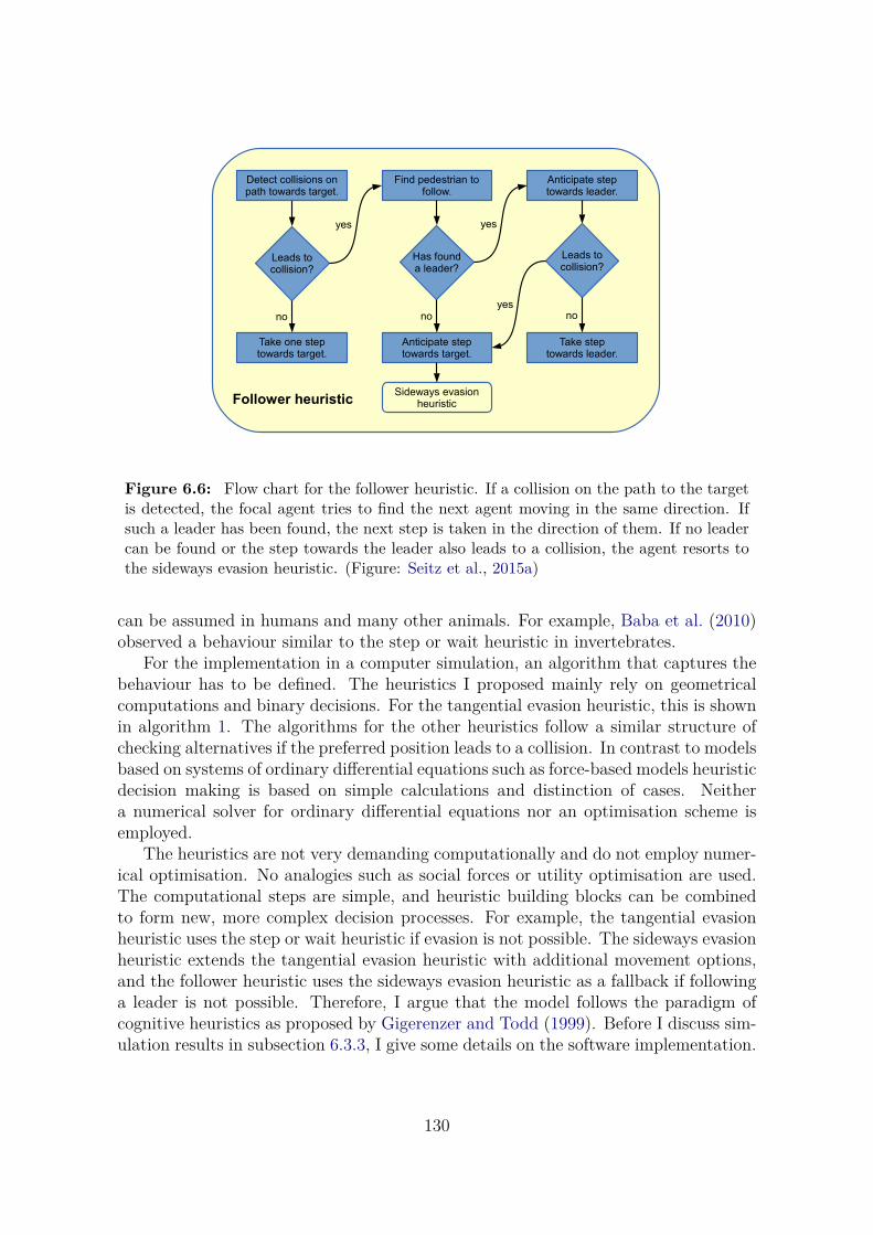
Leads tocollision?

Find pedestrian tofollow.

yes

Anticipate steptowards leader.

Has founda leader?


yes


no

Follower heuristic

Take one steptowards target.

Detect collisions onpath towards target.

Leads tocollision?

Take steptowards leader.

no no yes

Figure 6.6: Flow chart for the follower heuristic. If a collision on the path to the targetis detected, the focal agent tries to find the next agent moving in the same direction. Ifsuch a leader has been found, the next step is taken in the direction of them. If no leadercan be found or the step towards the leader also leads to a collision, the agent resorts tothe sideways evasion heuristic. (Figure: Seitz et al., 2015a)

can be assumed in humans and many other animals. For example, Baba et al. (2010)observed a behaviour similar to the step or wait heuristic in invertebrates.

For the implementation in a computer simulation, an algorithm that captures thebehaviour has to be defined. The heuristics I proposed mainly rely on geometricalcomputations and binary decisions. For the tangential evasion heuristic, this is shownin algorithm 1. The algorithms for the other heuristics follow a similar structure ofchecking alternatives if the preferred position leads to a collision. In contrast to modelsbased on systems of ordinary differential equations such as force-based models heuristicdecision making is based on simple calculations and distinction of cases. Neithera numerical solver for ordinary differential equations nor an optimisation scheme isemployed.

The heuristics are not very demanding computationally and do not employ numer-ical optimisation. No analogies such as social forces or utility optimisation are used.The computational steps are simple, and heuristic building blocks can be combinedto form new, more complex decision processes. For example, the tangential evasionheuristic uses the step or wait heuristic if evasion is not possible. The sideways evasionheuristic extends the tangential evasion heuristic with additional movement options,and the follower heuristic uses the sideways evasion heuristic as a fallback if followinga leader is not possible. Therefore, I argue that the model follows the paradigm ofcognitive heuristics as proposed by Gigerenzer and Todd (1999). Before I discuss sim-ulation results in subsection 6.3.3, I give some details on the software implementation.

130

Algorithm 1 Algorithm for the tangential evasion heuristic, a model of pedestrian decisionmaking. The algorithm is invoked for each individual pedestrian movement step in thediscrete stepping process or for each numerical step in the force-based continuous processon the physical layer (chapter 5). The result in the form of the next preferred position isstored in xp.determine target directioncompute next position xtarget towards the targetif xtarget leads to a collision then

store agent A the collision occurs withcompute both tangential evasion steps xa and xb in relation to Achoose the evasion position xa with smaller distance to the targetif xa leads to a collision then

if xb leads to a collision thenremain at the current position: xp = xcurrent

elsego to the second evasion position: xp = xb

end ifelse

go to the first evasion position: xp = xa

end ifelse

take step towards target: xp = xtarget

end if

6.3.2 Implementation detailsI refer to the software implementation of the cognitive heuristics model as behaviouralheuristics model (BHM). The overall class structure is integrated into the frameworkVadere the same ways as the optimal steps model (section 4.4, chapter 4). The gen-eral class diagram is shown in figure 6.7. The class PedestrianBHM is derived fromPedestrian and reused for all heuristics. It provides the basic functionality for thestepwise motion with the event-driven update scheme. Specific heuristics are im-plemented through the interface Navigation. The interfaces DirectionAddend andSpeedAdjuster are necessary for compromise decision making.

Figure 6.8 shows realisations of the interface Navigation that implement the cog-nitive heuristics model described in the previous subsection. The step or wait heur-istic and the tangential and sideways evasion heuristics are implemented in the classNavigationPorximity together because they share the same basic algorithm. Navi-gationCluster is another heuristic still in development. All navigation schemes usecomputations implemented in static methods of the class UtilsBHM.

Figure 6.9 shows the class diagram for the interfaces DirectionAddend and Speed-Adjuster. Although both are not necessary for the model described in the previoussection, they provide the necessary structure for extensions to the decision-makingmodel. They allow for compromise decisions by adjusting the speed and direction. Themodel of small-group coherence I describe in section 7.2 of the next chapter makes useof these interfaces. The three interfaces specific to the behavioural heuristics model

131

DirectionAddend

SpeedAdjuster

Pedestrian

Topography

Navigation

AttributesBHM

PedestrianBHM

-stepLength: Double-timeOfNextStep: Double-targetDirection: VPoint

+update(): void+makeStep(): void

BehaviouralHeuristicsModel

*

*

1

1

1

*

1

*

Figure 6.7: Class diagram of the behavioural heuristics implementation. The simulationloop triggers the update of all agents by calling the update function of the object oftype BehaviouralHeuristicsModel. The class PedestrianBHM has access to the positionof other agents through the topography object. Model parameters are set in the classAttributesBHM. Different heuristics models can be defined using the interface Navigation.The interfaces DirectionAddend and SpeedAdjuster provide functionality for additionalcompromise decisions in direction and speed, which are not part of the simulation modelyet. These kind of decisions are necessary for small-group behaviour (section 7.2, chapter7) or keeping space between agents and obstacles.

UtilsBHM

static methods

NavigationCluster

NavigationFollower

NavigationProximity

Navigation

+getNavigationPosition(): VPoint

Figure 6.8: Class diagram of the interface Navigation and the class UtilsBHM. Theclass NavigationProximity contains the routines for the step or wait heuristic and thetangential and sideways evasion heuristics. The cluster heuristic is a possible extensionto the model I present in this work. The static methods in UtilsBHM are used by thenavigation classes.

132

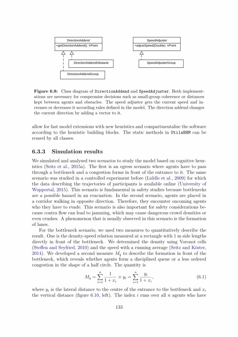
DirectionAddendObstacle

DirectionAddendGroup

SpeedAdjusterGroup

DirectionAddend

+getDirectionAddend(): VPoint

SpeedAdjuster

+adjustSpeed(Double): VPoint

Figure 6.9: Class diagram of DirectionAddend and SpeedAdjuster. Both implement-ations are necessary for compromise decisions such as small-group coherence or distanceskept between agents and obstacles. The speed adjuster gets the current speed and in-creases or decreases it according rules defined in the model. The direction addend changesthe current direction by adding a vector to it.

allow for fast model extensions with new heuristics and compartmentalise the softwareaccording to the heuristic building blocks. The static methods in UtilsBHM can bereused by all classes.

6.3.3 Simulation resultsWe simulated and analysed two scenarios to study the model based on cognitive heur-istics (Seitz et al., 2015a). The first is an egress scenario where agents have to passthrough a bottleneck and a congestion forms in front of the entrance to it. The samescenario was studied in a controlled experiment before (Liddle et al., 2009) for whichthe data describing the trajectories of participants is available online (University ofWuppertal, 2015). This scenario is fundamental in safety studies because bottlenecksare a possible hazard in an evacuation. In the second scenario, agents are placed ina corridor walking in opposite direction. Therefore, they encounter oncoming agentswho they have to evade. This scenario is also important for safety considerations be-cause contra flow can lead to jamming, which may cause dangerous crowd densities oreven crushes. A phenomenon that is usually observed in this scenario is the formationof lanes.

For the bottleneck scenario, we used two measures to quantitatively describe theresult. One is the density-speed relation measured at a rectangle with 1 m side lengthsdirectly in front of the bottleneck. We determined the density using Voronoi cells(Steffen and Seyfried, 2010) and the speed with a running average (Seitz and Köster,2014). We developed a second measure Mq to describe the formation in front of thebottleneck, which reveals whether agents form a disciplined queue or a less orderedcongestion in the shape of a half circle. The quantity is

Mq =n∑

i=1

11 + xi

× yi =n∑

i=1

yi

1 + xi

, (6.1)

where yi is the lateral distance to the centre of the entrance to the bottleneck and xi

the vertical distance (figure 6.10, left). The index i runs over all n agents who have

133

xy x

(a) (b)

Figure 6.10: Schematic illustration of the two simulation scenarios with reference pointsin yellow. Part a of the figure shows the bottleneck scenario where agents are created onthe bottom and pass through the corridor on the top. The distance to the reference point(in yellow) is measured in x and y-direction to obtain the quantity Mq. Part b shows thecontra-flow scenario where agents moved both from right to left and left to tight. Onepossible reference point is highlighted (in yellow). In every time step, multiple referencepoints are chosen on the halfway mark (dashed line), and the quantity Ml is computed forall of them. The distances xi in Ml are calculated with respect to the reference points.

(a) (b) (c)

Figure 6.11: Illustration of different formations in front of a bottleneck. In part a,the queue measure Mq would yield almost 0 because pedestrians do not deviate from thecentre of the corridor laterally. In part b, it would yield a higher value as pedestrians alsowalk to the side of the entrance. In part c, an even higher value is obtained for Mq.

not yet passed the entrance. Hence, when agents tend to walk to the sides of theentrance, the measure Mq becomes greater. Agents farther away from the entrance inthe vertical direction are weighted less. For the shape of the congestion in front of thebottleneck, this means that greater values ofMq correspond to a wider congestion andsmaller values to a more narrow formation. In the extreme, when all agents perfectlyqueue horizontally in the middle of the entrance, Mq would be 0 (figure 6.11).

We simulated a scenario with 180 agents who are created 8 m away from thebottleneck. The bottleneck has a width of 2 m and a length of 5 m. We compared thesimulation outcome to the data from the controlled experiment (Liddle et al., 2009;University of Wuppertal, 2015). Figure 6.12 shows snapshots of the simulation andexperiment in the first row, the queue measureMq in the second row, and the density-speed relation in the third row. The simulation was run for the step or wait heuristic(a), the tangential evasion heuristic (b), and the sideways evasion heuristic (c). Thefollower heuristic yielded very similar behaviour to the sideways evasion heuristic andhence its results are not shown here.

The step or wait heuristic allows for egress without jamming, but it takes thelongest until all agents have left the room. The tangential and sideways evasion heur-istic lead to similar egress times that also match the experimental data. The queuemeasure in the experiment, however, shows greater similarity with the tangential eva-sion heuristics than with the sideways evasion heuristic. The step or wait heuristic

134

(a.1) (b.1) (c.1) (d.1)

●●●●●●

●

●●●●●●●

●●

●●●●●●●●●●●●●●●●●●●●●●●●●●●●●●●●●●●●●●●●●●●●●●●●●●●●●●●●●●●●●●●●●●●●●●●●●●●●●●●●●●●●●●●●●●●●●●●●●

●●●●●●●●●●●●●●●●●●●●●●●●●●●●●●●●●●●●●●●●●●●●●●●●●●●●●●●●●●●●●●●●●●●●●●●●●●●●●●●●●●●●●●●

●●●●●●●●●●●●●●●●●●●●●●●●●●●●●●●●●●●●●●●●●●●●●●●●●●●●●●●●●●●●●●●●●●●●●●●●●●●●●●●●●●●●●●●●●●●●

●●●●●●●●●●●●●●●●●●●●●●●●●●●●●●●●●●●●●●●●●●●●●●●●●●●●●●●●●●●●

●●●●●●●●●●●●●●●●●●●●●●●●●●●●●●●●●●●●●●●●●●●●●●●●●●●●●●●●●●●●●●●●●●●●●●●●●●●●●●●●●●●●●●●●●●●●●●

●●●●●●●●●●●●●●●●●●●●●●●●●●●●●●●●●●●●●●●●●●●

●●●●●●●●●●●●●●●●●●●●●●●●●●●●●●●●●●●●●●●●●●●●●●●●●●●●●●●●●●●●●●●●●●●●●●●●

●●●●●●●●●●●

●●●●●●●●●●●●●●●●●●●●●●●●●●●●●●●●●●

●●●●●●●●●●●●●●●●●●●●●●●●●●●●●●●●●●●●●●●●●●●●●●●●●●●●

●●●●●●●●●●●●●●●●●●●●●●●●●●●●●●●●●●●●●●●●

●●●●●●●●●●●●●●●●●●●●●●●●●●●●●●●●●

●●●●●●●●●●●●●●●●●●●●●●●●●●●●●●●●●●●●●●●●●●●●●●●●●●●●●●●●●●●●●●●●●●●●●●●●●●●●●●●●●●●●●●●●●●●

●●●●●●●●●●●●●●●●●●●●●●●●●●●●●●●●●●●●●●●●●●●●●●●●●●●●●●●●●●●●●●●●●●

●●●●●●●●●●●●●●●●●●●●●●●●●●●●●●●●●●●●●●●●●●●●●●●●●●●●●●●●●●●●●●●●●●●●●●●●●●●●●●●●●●●●●●●●●●●●●●●●●●●●●●●●

●●●●●●●●●●●●●●●●●●●●●●●●●●●●●●●●●●●●●●

●●●●●

●●●●●

●●●●●●●●●●●●●●●●●●

●●●●●●●●●●●●●●●●●●●●●●●●●●●●●●●●●●●●●●●●●●●●●●●●●●●●●●

●●●●●●●●●●●●●●●●●●●●●●●●●●●●●●●●●●●●●●●●●●●●●●●●●●●●●●●●●●●●●●●●●●●●●●●●●●●●●●●●●●●●●●●●●●●●●●●●●●●●●●●●●●●●●●●●●●●●●●●●●●●●●●●●●●●●●●

●●●●●●●●●●●●●●●●●●●●●●●●●●●●●●●●●●●●●●●●●●●●●●●●●●●●●●●●●●●●●●●●●●●●●●●●●●●●●●●●●●●●●●●●●●●●●●●●●●●●●●●

●●●●●●●●●●●●●●●●●●●●●●●●●●●●●●●●●●●●●●●●

●●●●●●●●●●●●●●●●●●●●●●●●●●●●●●●●●●●●●●

●●●●●●●●●●●●●●●●●●●●●●●●●●●●●●●●●●●●●●●●●●●●●●●●●●●●●●●●●●●●●●●●●●●●●●●●●●●●●●●●●●●●●●●●●●●●●●●●●●●●●

●●●●●●●●●●●●●●●●●●●●●●●●●●●●●●●●●●●●●●●●●●●●●●●●●●●●●●●●●●●●●●●●●●●●●●●●●●●●●●

●●●●●●●●●●●●●●●●●●●●●●●●●●●●●●●●●●●●●●●●●●●●●●●●●●●●●●●●●●●●●●●●●●●●●●●●●●●●●●●●●●●●●●●●●●●●●●●●●●●●●●●●●●●●●●●●●●●●●●●●●

●●●●●●●●●●●●●●●●●●●●●●●●●●●●●●●●●●●●●●●●

●●●●●●●●●●●●●●●●●●●●●●●●●●●●●●●●●●●●●●●●●●●●●●●●●●●●●●●●●●●●●●●●●●●●●●●●●●●●●

●●●●●●●●●●●●●●●●●●●●●●●●●●●●●●●●●●●●●●●●●

●●●●●●●●●●●●●●●●●●●●●●●●●●●●●●●●●●●●●●●●●●●●●●●●●●●●●●●●●●●●●●●●●●●●●●●●●●●●●●●●●●●●●●●●●●●●●●●●●●●●●●●●●●●●●●●●●●●●●●●●●●●

●●●●●●●●●●●●●●●●●●●●●●●●●●●●●●●●●●●●●●●●●●●●●●●●●●●●●●●●●●●●●●●●●●●●●●●●●●●●●●●●●●●●●●●●●●●●●●●●●●●●●

●●●●●●●●●●●●●●●●●

●●

●●●●●●

●●

●●●●●●●●●●●

●●●●●●●●●●●●●●●●●●●●●●●●●●●●●●●●●●●●●●●●●●●●●●●●●●●●●●●●●●●●●●

●●

●●●

●●●●●●●●●●●●●●●●●●●●●●●●●●●●●●●●●●●●●●●●●●●●●●●●●●●●●

●●●●●●●●●●●●●●●●●●●●●●●●●●●●●●●●●●●●●●●●●●●●●●●●●●●●●●●●●●●●●●●●●●●●●●●●●●●●

●●●●●●●●●●●●●●●●●●●●●●●●●●●●●●●●●●●●●●●●●●●●●●●●●●●●●●●●●●●●●●●

●●●●●●●●●●●●●●●●●●●●●●●●●●●●●●●●●●●●●●●●●●●●●●●●●●●●●●●●●●●●●●●●●●●●●●●●●●●●●●●●●●●●●●●●●●●●●●●●●●●●

●●●●●●●●●●●●●●●●●●●●●●●●●●●●●●●●●●●●●●●●●●●●●●●●●●●●●●●●●●●●●●●●●●●●●●●●

●●●●●●●●●●●●●●●●●●●●●●●●●●●●●●●●●●●●●●●●●●●●●●●●●●●●●●●●●●●●●●●●●●●●●●●●●●●●●●●●●●●●●●●●●●●●●●●●●●●●●

●●●●●●●●●●●●●●●●●●●●●●●●●●●●●●●●●●●●●●●●●●●●●●●●●●●●●●●●●●●●●●●●●●●●●●●●●●●●●●●●●●●●●●●●●●●●●●●●●●●●●●●●●●●●●●●●●●●

●●●●●●●●●●●●●●●●●●●●●●●●●●●●●●●●●●●●●●●●●●●●●●●●●●●●●●●●●●●●●●●●●●●●●●

●●●●●●●●●●●●●●●●●●●●●●●●●●●●●●●●●●●●●●●●●●●●●●●●

●●●●●●●●●●●●●●●●●●●●●●●●●●●●●●●●●●●●●●●●●●●●●●●●●●●●●●●●●●

●●●●●●●●●●●●●●●●●●●●●●●●●●●●●●●●●●●●●●●●●●●●●●●●●●●●●●●●●

●●●●●●●●●●●●●●●●●●●●●●●●●●●●●●●●●●●●●●●●●●●●●●●●●●●●●●●●●●●●●●●●●●●●●●●

●●●●●●●●●●●●●●●●●●●●●●●●●●●●●●●●●●●●●●●●●●●●●●●●●●●●●●●●●●●●●●●●●●

●●●●●●●●●●●●●●●●●●●●●●●●●●●●●●●●●●●●●●●●●●●●●●●●●●●●●●●●●●●●●●●●●●●●●●●●●●●●●●●●●●●●●●●●●●●●●●●●●●●●●●●●●●●●●●●●●●●●●●●

●●●●●●●●●●

●●●●●●●

●●●●●●●

●●●●●●●●●●●●●●●●●●●●●●●●●●●●●●●●●●●●●●●●●●●●●●●●●●●●●●●●●●●●●●●●

●●●●●●●●●

●●●

●●●●●●●●●●●●●●●●●●●●●●●●●●●●●●●●●●●●●●●●●●●●●●●●●●●●●●●●●●●●●●●●●●●●●

●●●●●●●●●●●●●●●●●●●●●●●●●●●●●●

●●●●●●●●●●●●●●●●●●●●●●●●●●●●●●●●●●●●●●●●●●●●●●●●●

●●●●●●●●●●●●●●●●●●●●●●●●●●●●●●●●●●●●●●●●●●●●●●●●●●●●●●●

●●●●●●●●●●●●●●●●●●●●●●●●●●●●●●●●●●●●●●●●●●●●●●●●●●●●●●●●●●●●●●●●●●●●●●●●●●●●●●●●●●●●●●●●●●●●

●●●●●●●●●●●●●●●●●●●●●●●●●●●●●●●●●●●●●●●●●●●●●●●●●●●●●●●●●●●●●●●●●●●●●●●●●●●●●●●●

●●●●●●●●●●●●●●●●●●●●●●●●●●●●●●●●●●●●●●●●●●●●●●●●●●●●●●●●●●●●

●●●●●●●●●●●●●●●●●●●●●●●●●●●●●●●●●●●●●●●●●●●●●●●●●●●●●●●●●●●●●●●●●●●●●●●

●●●●●●●●●●●●●●●●●●●●●●●●●●●●●●●●●●●●●●●●●●●●●●●●●●●●●●●●●●●●●●●●●●●●●●●●●●●●●●

●●●●●●●●●●●●●●●●●●●●●●●●●●●●●●●●●●●●●●●●●●●●●●●●●●●

●●●●●●●●●●●●●●●●●●●●●●●●●●●●●●●●●●●●●●●●●●●●●●●●●●●●●●●●●●●

●●●●●●●●●●●●●●●●●●●●●●●●●●●●●●●●●●●●●●●●●●

●●●●●●●●●●●●●●●●●●●●●●●●●●●●●●●●●●●●●●●●●●●●●●●●●●●●●●●●●●●●●●●●●●●●●●●●●●●●●●●●●●●●●●●●●●●●●●●●●●●●●●●●●●●●●●●●●●●●●●●

●●●●●●●●●●●●●●●●●●●●●●●●●●●●●●●●●●●●●●●●●●●●●●●●●●●●●●●●●●●●●●●●●●●●●●●●●●●●●●●●●●●●●●●●●●●●●●●●●●●●●●●●●●●●●●●●●●●●●●●●●●●●●●●●●●●●●●●●●●●●●●●●●●●●●●●●●●●●●●●●●●●●●

●●●●●●●●●●●●

●

●●●●●●●●●●

●

●●●●●●●●●●●

●●●●●●●●●●●●●●●●●●●●●●●●●●●●●●●●●●●●●●●●●●●●●●●●●●●●●●●●

●

●

●●●●

●●

●●●●●●●●●●●●●●●●●●●●●●●●●●●●●●●●●●●●●●●

●●●●●●●●●●●●●●●●●●●●●●●●●●●●●●●

●●●●●●●●●●●●●●●●●●●●●●●●●●●●●●●●●●●●●●●●●●●●●●●●●●●●●●●●●●●●

●●●●●●●●●●●●●●●●●●●●●●●●●●●●●●●●●●●●●●●●●●●●●●●●●●●●●●●●●●●●●●●●●●●●●●●●●●●●●●●●●●●●●●●●●●●●●●●●●●●●●●●●●●●●●●●●●●●●●●●●●●●●●●●●●●●●●●●●●●●●●●●●●●●●●●●●●●●●●●●

●●●●●●●●●●●●●●●●●●●●●●●●●●●●●●●●●●●●●●●●●●●●●●

●●●●●●●●●●●●●●●●●●●●●●●●●●●●●●●●●●●●●●●●●●●●●●●●●●●●●●●●●●●●●●●●●●●●●

●●●●●●●●●●●●●●●●●●●●●●●●●●●●●●●●●●●●●●●●●●●●●●●●●●●●●●●●●●●●●●●●●●●●●●●●●●●●●●●●●●●●●●●●●●●●●●●●●●●●●●●●●●●●

●●●●●●●●●●●●●●●●●●●●●●●●●●●●●●●●●●●●●●●●●●●●●●●●●●●●

●●●●●●●●●●●●●●●●●●●●●●●●●●●●●●●●●●●●●●●●●●●●●●●●●●●●●●●●●●●●●●●●●●●●●●●●●●●●●●●●●●●●●●●●●●

●●●●●●●●●●●●●●●●●●●●●●●●●●●●●●●●●●●●●●●●●●●●●●●●●●●●●●●●●●●●●●●●●●●●●●●●●●●●●●●●●●●●●●

●●●●●●●●●●●●●●●●●●●●●●●●●●●●●●●●●●●●●●●●●●●●●●●●●●●●●●●●●●●●●●●●●●●●●●●●●●●●●●●●●●●●●●●●●●●●●●●●●●●●●●●●●●●●●●●●●●●

●●●●●●●●●●●●●●●●●●●●●●●●●●●●●●●●●●●●●●●●●●●●●●●●●●●●●●●●●●

●●●●●●●●●●●●●●●●●●●●●●●●●●●●●●●●●●●●●●●●●●●●●●●●●●●●●●●●●●●●●●●●●●●●●●●●●●●●●●●●●●●●●●●●●●●●●●●●●●●●●●●●●●●●●●●●●●●●●

●●●●●●●●●●●●●●●●●●●●●●●●●●●●●●●●

●●●●●●●●●●●●●●●●●●●●●

●●●●●●●●●●●●●●●●●●

●●●●●●●●●●●●●●●●●●●●●●●●●●●●●●●●●●●●●●●●●●●●●●●●●●●●●●●

●●●●●●●●●●●●●●●●●●●●●●●●●●●●●●●●●●●●●●●●●●●●●●●●●●●●●●●●●●●●●●●●●●●●●●●●●●●●●●●●●●●●●●●●●●●●●●●●●●

●●●●●●●●●●●●●●●●●●●●●●●●●●●●●●●●●●●●●●●●●●●●●●●●●●●●●●●●●●●●●●●●●●●●●●●●●●●●●●●●●●●●●

●●●●●●●●●●●●●●●●●●●●●●●●●●●●●●●●●●●●●●●●●●●●●●●●●●●●●●●●●●●●●●●●●●●●●●●●●●●●●●●●●●●●●●●●●●●●●

●●●●●●●●●●●●●●●●●●●●●●●●●●●●●●●●●●●●●●●●●●●●●●●●●●●●●●●●●●●●●●●●●●●●●

●●●●●●●●●●●●●●●●●●●●●●●●●●●●●●●●●●●●●●●●●●●●●●●

●●●●●●●●●●●●●●●●●●●●●●●●●●●●●●●●●●●●●●●●●●●●●●●●●●●●●●●●●●●●●●●●●●●●

●●●●●●●●●●●●●●●●●●●●●●●●●●●●●●●●●●●●●●●●●●●●●●

●●●●●●●●●●●●●●●●●●●●●●●●●●●●●●●●●●●●●

●●●●●●●●●●●●●●●●●●●●●●●●●●●●●●●●●●●

●●●●●●●●●●●●●●●●●●●●●●●●●●●●●●●●●●●●●●●●●●●●●●●●

●●●●●●●●●●●●●●●●●●●●●●●●●●●●●●●●●●

●●●●●●●●●●●●●●●●●●●●●●●●●●●●●●●●●●●●●●●●●●●●●●●●●●

●●●●●●●●●●●●●●●●●●●●●●●●●●●●●●●●●●●●●●●●●●●●●●●●●●●●●●●●●●●●●●●●●●●●●●●●●●●●●●●●●●●●●●●●●●

●●●●●●●●●●●●●●●●●●●●●●●●●●●●●●●●●●●●●●●●●

●●●●●●●●●●●●●●●●●●●●●●●●●●●●●●●●●●●●●●●●●●●●●●

●●●●●●●●●●●●●●●●●●●●●●●●●●●●●●●●●●●●●●●●●●●●●●●●●●●●●●●●●●●●●●●●●●●●●●●●●●●●●●●●●●●●●●●●●●●●●●●●●●●●●●

●

●●●●●●●●●●●●●

●●●●●●●●●●●●●●●●

●●●●●●●●●●●●●●●●●●●●●●●●

●●●●●●●●●●●

●●●●●

●●●●●●●●●●●●●●●●●●●●●●●●●●●●●●●●●●●●●●●●●●●●●●●●●●●●●●

●

●

●●

●●

●●●●●●●●●●●●●●●●●●●●●●●●●●●●●●●●●●●●●●●●●●●●●●●●●●●●●●●●●●●●

●●●●●●●●●●●●●●●●●●●●●●●●●●●●●●●●●●●●●●●●●●●●●●●●●●●●●●●●●●●●●●●●●●●●

●●●●●●●●●●●●●●●●●●●●●●●●●●●●●●●●●●●●●●●●●●●●●●●●●●●●●●●●●●●●●

●●●●●●●●●●●●●●●●●●●●●●●●●●●●●●●●●●●●●●●●●●●●●●●●●●●●●●●●●●●●●●●●●

●●●●●●●●●●●●●●●●●●●●●●●●

●●●●●●●●●●●●●●●●●●●●●●●●●●●●●●●●●●●●●●●●●●●●●●●●●●●●●●●●●●●●●

●●●●●●●●●●●●●●●●●●●●●●●●●●●●●●●●●●●

●●●●●●●●●●●●●●●●●●●●●●●●●●●●●●●●●●●●●●●●●●●●●●●●●●●●●●●●●●●●●●●●●●●●●●●●●●●●●●●●●●●●●●●●●●●●●●●●

●●●●●●●●●●●●●●●●●●●●●●●●●●●●●●●●●●●●●●●●●●●●●●●●●●●●●●●●●●●●●●●●●●●●●●●●●●●●●●●●●●●●●●●●●●

●●●●●●●●●●●●●●●●●●●●●●●●●●●●●●●●●●●●●●●●●

●●●●●●●●●●●●●●●●●●●●●●●●●●●●●●●●●●●●●●●●●●●●●●●

●●●●●●●●●●●●●●●●●●●●●●●●●●●●●●●

●●●●●●●●●●●●●●●●●●●●●●●●●●●●●●●●●●●●●●●●●●●●●●●●●●●●●●●●●●●●●●●●●●●●●●●●●●●●●●●●●●●●●●●●●●●●●●●

●●●●●●●●●●●●●●●●●●●●●●●●●●●●●●●●●●●●●●●●●●●●●●●●●●●●●●●●●●●●●●●●●●●●●●●●●●●●●●●●●●●●●●●●●●●●●

●●●●●●●●●●●●●●●●●●●●●●●●●●●●●●●●●●●●●●●●●●●●●●●●●●●●●●●●●●●●●●●●●●●●●●●●●●●●●●●●●●●●●●●●●●●●●●●●●●●●●●●●●●●

●●●●●●●●●●●●●●●●●●●●●●

●●●●●●

●●●●●●●●●●●●●●●●●●●●●●●●●●●●●●●●●●●●●●●●●●●●●●●●●●●●●●●●●●●●●●

●

●●●●●●●●●●●●●●●●●●●●●●●●●●●●●●●●●●●●●●●●●●●●●●●●●●●●●●●●●●●●●●●●●●●●●●●●●●●●●●●●●●●●●●

●●●●●●●●●●●●●●●●●●●●●●●●●●●●●●●●●●●●●●●●●●●●●●●

●●●●●●●●●●●●●●●●●●●●●●●●●●●●●●●●●●●●●●●●●●●●●●●●●●●●●●●●●●●●●●●●●●●●●●●●●●●●●●●●●●●●●●●●●●●●●●●●●●●●●●●

●●●●●●●●●●●●●●●●●●●●●●●●●●●●●●●●●●●●●●●●●●●●●●●●●●●●●●●●●●●●●●●●●●●●●●●●●●●●●●●●●●●●●●●●●●●●●●●●●●●●●●●●●●●●●●●●●●●●●●

●●●●●●●●●●●●●●●●●●●●●●●●●●●●●●●●●●●●●●●●●●●●●●●●●●●●●●●●●●●●●●●●●●●●●●●●●●●●●●●●●●●●●●●●●●●●●●●●●●●●●●●

●●●●●●●●●●●●●●●●●●●●●●●●●●●●●●●●●●●●●●●●●●●●●●●●●●●●●●●●●●●●●●●●●●●●●●●●●●●●●●●●●●●●●●●●●●●●●●●●●●●●●●●●●●●●●●●●●●●●●●●●●●●●●●●●●●●●●●●●●●●●●●●●●●●●●●●●●●●●●●●●●●●●●●●●●●●●●●●●●●●●●●●●●

●●●●●●●●●●●●●●●●●●●●●●●●●●●●●●●●●●●●●●●●●●●●●●●

●●●●●●●●●●●●●●●●●●●●●●●●●●●●●●●●●●●●●●●●●●●●●●●●●●●●●●●●●●●●●●●●●●●●●●●●●●●●●●●●●●●

●●●●●●●●●●●●●●●●●●●●●●●●●●●●●●●●●●●●●●●●●●●●●●●●●●●●●●●●●●●●●●●●●●●●●●●●●●●●●●●●●●●●●●●●●●

●●●●●●●●●●●●●●●●●●●●●●●●●●●●●●●●●●●●●●●●●●●●●●●●●

●●●●●●●●●●●●●●●●●●●●●●●●●●●●●●●●●●●●●●●●●●●●●●●●●●●●●●

●●●●●●●●●●●●●●●●●●●●●●●●●●●●●●●●●●●●●●●●●●●●●●●●●●●●●●●●●●●●●●●●●●●●●●●●●●●●●●●●

●●

●●

●●●●●●●●●●●●●●●

●●

●●●●●●●●●●●●●●●●●●●●●●●●●●●●●●●●●●●●●●●●●●●●●●●●●●●●●●●●●●●●●●

●

●

●●●●●●●●●●●●●●●●●●●●●●●●●●●●●●●●●●●●●●●●●●●●●●●●●●●●●●●●●●●●●●●●●●

●●●●●●●●●●●●●●●●●●●●●●●●●●●●●●●●●●●●●●●●●●●●●●●●●●●●●●●●●●●●●●●●●●●●●●●●●●●●●●●●●●●●●

●●●●●●●●●●●●●●●●●●●●●●●●●●●●●●●●●●●●●●●●●●●●●●●●●●●●●●●●●●●●●●●●

●●●●●●●●●●●●●●●●●●●●●●●●●●●●●●●●●●●●●●●●●●●●●●●●●●●●●●●●●●●●●●●●●●●●●●●●●●●●●●●●●●●●●●●●●●●●●●●●●●●●●●●●●●●●●●

●●●●●●●●●●●●●●●●●●●●●●●●●●●●●●●●●●●●●●●●●●●●●●●●●●●●●●●●●●●●●●●●●●●●●●●●●●●●●●●●●●●●●●●●●●●●●●●●●●●●●●●●●●●●●●●●●●●●●●●●●●●●●●●●●●●●●●●●●●●●●●●●●●●

●●●●●●●●●●●●●●●●●●●●●●●●●●●●●●●●●●●●●●●●●●●

●●●●●●●●●●●●●●●●●●●●●●●●●●●●●●●●●●●●●●●●●●●●●●●●●●●●●●●●●●●●●●●●●●●●●●●●●●●●●●●●●●●●●●●●●●

●●●●●●●●●●●●●●●●●●●●●●●●●●●●●●●●●●●●●●●●●●●●●●●●●●●●●●●●●

●●●●●●●●●●●●●●●●●●●●●●●●●●●●●●●●●●●●●●●●●●●●●

●●●●●●●●●●●●●●●●●●●●●●●●●●●●●●●●●●●●●●●●●●●●●●●●●●●●

●●●●●●●●●●●●●●●●●●●●●●●●●●●●●●●●●●●●●●●●●●●●●●●●●●●●●●●●●●●●●●●●●●●●●●●●●●●●●●●●●●●●●●●●●

●●●●●●●●●●●●●●●●●●●●●●●●●●●●●●●●●●●●●●●●●●●●●●●●●●●●●●●●●●●●●●●●●●●●●●●●●●●●●●●●●●●●●●●●●●●●●●●●●●●●●●●●●●●●●●●●●●●●●●●●●●●●●●●●●●●●●●●●●●●●●●●●●●●●●●●●●●●●●●●●●●●●●●●●●●●●●●●●●●●●●●●●●●

●●●●●●

●●●●●●●●●●●●●●●●●●●●●●●●●●●●●●●●●●●●●●●●●●●●●●●●●●●●●●●●●●●●●●●●

●

●●●●●●

●●●●●●●●●●●●●●●●●●●●●●●●●●●●●●●●●●●●●●●●●●●●●●●●

●●●●●●●●●●●●●●●●●●●●●●●●●●●●●●●●●●●●●●●●●●●●●●●●●●●●●●●●●●●●●●●●●●●●●●●●●●●●●●●●●●●●●●●●●●

●●●●●●●●●●●●●●●●●●●●●●●●●●●●●●●●●●●

●●●●●●●●●●●●●●●●●●●●●●●●●●●●●●●●●●●●●●●●●●●●●●●●●●●●●●●●●●●●●●●●●●●●●●●●●●●●●●●●●●●●●●●●●●●●

●●●●●●●●●●●●●●●●●●●●●●●●●●●●●●●●●●●●●●●●●●●●●●●●●●●●●●●●●●●●●●●

●●●●●●●●●●●●●●●●●●●●●●●●●●●●●●●●●

●●●●●●●●●●●●●●●●●●●●●●●●●●●●●●●●●●●●●●●●●●●●●●●●●●●●●●●●●●●●●●●●●●●●●●●●●●●●●●●●●●●●●●●●●●●●●●●●●●

●●●●●●●●●●●●●●●●●●●●●●●●●●●●●●●●●●●●●●●●●●●●●●●●●●●●●●●●●●●●●

●●●●●●●●●●●●●●●●●●●●●●●●●●●●●●●●●●●●●●●●●●●●●●●●●●●●●●●●●●●●●●●●●●●●●●●●●●●●●●●●●●●●●●●●●●●●●●●●●●●●●●●●●●●●

●●●●●●●●●●●●●●●●●●●●●●●●●●●●●●●●●●●●●●●●●●●●●●●●●●●●●●●

●●●●●●●●●●●●●●●●●●●●●●●●●●●●●●●●●●●●●●●●●●●●●●●●●●●

●●●●●●●●●●●●●●●●●●●●●●●●●●●●●●●●●

●●●●●●●●●●●●●●●●●●●●●●●●●●●●●●●●●●●●●●●●●●●●●●●●●●

●●●●●●●●●●●●●●●●●●●●●●●●●●●●●●●●●

●●●●●●●●●●●●●●●●●●●●●●●●●●●●●●●●●●●●●●●●●●●●●●●●●●●●●●●●●●●●●●●●●●●●●●

●●●●●●●●●●●●●●●●●●●●●●●●●●●●

●●●●●●●●●●●●●●●●●●●●●●●●●●●●●●●●●●●●●●●●●●●●●●●●●●●●●●●●●●●●●●●●●

●●●●●●●●●●●●●●●●●●●●●●●●●●●●●●●●●●●●●●●●●●●●●●●●

●●●●●

●●●●●●●●●●●●●●●●●●●●●●●●●●●●

●●●●●●●●●●●

●●●●●●●●●●●●●●●●●●●●●●●●●●●●●●●●●●●●●●●●●●●●●●●●●

0 50 100 150

0.0

0.2

0.4

0.6

0.8

1.0

time [s]

queu

e m

easu

re (a.2 )

●●●●●●

●

●

●●●●●●

●●

●●●●●●●

●●●●●●●●●●●●●●●●●●●●●●●●●●●●●●●●●●●●●●●●●●●●●●●●●●●●●●●●●●●●●●●●●●●●●●●●●●●●●●●●●●●●●●●●●●●●●●●●●●●●●●●●●●●●●●●●●●●●●●●●●●●●●●●●●●●●●●●●●●●●●●●●●●●●●●●●●●●●●●●●●●●●●●●●●●●●●●●●●●●●●●●●●●●●●●●●●●●●●●●●●●●●●●●●●●●●●●●●●●●●●●●●●●●●●●●●●●●●●●●●●●

●●●●●●●●●●●●●●●●●●●●●●●●●●●●●●●●●●●●●●●●●●●●●●●●●●●●●●●●●●●●●●●●●●●●●●●●●●●●●●●●●●●●●●●●

●●●●●●●●●●●●●●●●●●●●●●●●●●●●●●●●●●●●●●●●●●●●●●●●●●●●●●●●●●●●●●●●●●●●●●●●●●●●●●●●●●●●●●●●●●●●●●●●●●●●●●●●●●●●●●●●●●●●●●●●●●●●●●●●●●●●●●●●●●●●●●●●●●●●●●●●●●●●●●●●●●●●●●●

●●●●●

●●

●●●●●

●●●●

●

●●

●

●●●●

●

●●●●●●●

●

●●●●

●●

●●●

●●

●●●

●

●●

●●●●

●●

●

●●

●

●

●●●

●

●

●●

●●

●

●●●●●

●●●●●●

●●●●●

●●●●●●●●●●●●●●●●●●●●●●●●●●●●●●●●●●●●●●●●●●●●●●●●

●●●●●●

●●●●●

●●●●●●

●●●●●●●●●●●●●●●●●●●●●●●●●●●●●●●●●●●●●●●●●●●●●●●●●●●●●●●●●●●●●●●●

●●●●●●●●●●●●●●●●●●●●●●●●●●●●●●●●●●●●●●●●●●●●●●●●●●●●●●●●●●●●●●●●●●●●●●●●●●●●●●●●●●●●●●●●●●●●●●●●●●●●

●●●●●●●●●●●●●●●●●●●●●●●●●●●●●●●●●●●●●●●●●●●●●●●●●●●●●●●●●●●●●●●●●●●●●●●●●●●●●●●●●●●●●●●●●●●●●●●●●●●●●●●●●●●●●●●●●●●●●●●●●●●●●●●●●●●●●●●●●●●●●●●●●●●●●●●●●●●●●●●●

●●●●●●●●●●●●●●●●●●●●●●●●●●●●●●●●●●●●●●●●●●●●●●●●●●●●●●●●●●●●●●●●●●●●●●●●●●●●●●●●●●●●●●●●●●●●●●●●●●●●●●●●●●●●●●●●●●●●●●●●●●●●●●●

●●●●●●●●●●●●●●●●●●●●●●●

●●●●●●●●

●●●●●●●●●●●●●●●

●●●

●

●●

●●●●●

●●●●●●●●

●●●●●

●

●●

●●●●

●

●●

●●●●●●

●●

●

●●

●●

●●●●●●●

●●●

●●●●●●●●●●●●●●●●●●●●●●●●●●●●●●●●●●●●●●●●●●●●●●●●●●●●●●●●●●●●●●●●●●●●●●

●●

●●●●●●●●●●●●●●●●●●●●●●●●●●●●●●●●●●●●●●●●●●●●●●●●●●●●●●●●●●●●●●●●●●●●●●●●●●●●●●●●●●●●●●●●●●●●●●●●●●●●●●●●●●●●●●●●●●●●●●●●●●●●●●●●●●●●●●●●●●●●●●●●●●●●●

●●●●●●●●●●●●●●●●●●●●●●●●●●●●●●●●●●●●●●●●●●●●●●●●●●●●●●●●●

●●●●●●●●●●●●●●●●●●●●●●●●●●●●●●●●●●●●●●●●●●●●●●●●●●●●●●●●●●●●●●●●●●●●●●●●●●●●●●●●●●●●●●●●●●●

●●●●●●●●●●●●●●●●●●●●●●●●●●●●●●●●●●●●●●

●●●●●●●●●●●●●●●●●●●●●●●●●●●●●●●●●●●●●●●●●●●●●●●●●●●●●●●●●●●●●●●●●●●●●●●●●●●●●●●●●●●●●●●●●●●●●●●●●●●●●●●●●●●●●●●●●●●●●●●●●●●●●●●●●●●●●●●●●●●●●●●●●●●●●●●●●●●●●●●●●●●●●

●●

●●

●●●●●●●●●●●●●

●

●●

●●●

●●

●

●●●

●●●●●●●

●

●●●●

●●●●

●

●●●

●●

●●

●●●

●

●●●

●●●

●

●●●

●●●●●●●●●●●●●●●●●●●●●●●●●●●●●●●●●●●●●●●●●●●●●●●●●●●●●●●●●●●●●●●●●

●●●●●●

●●●●●●●●●●●●●●●●●●●●●●●●●●●●●●●●●●●●●●●●●●●●●●●●●●●●●●●●●●●●●●●●●●●●●●●●●●●●●●●●●●●●●●●●●●●●●●●●●●●●●●●●●●●●●●●●●●●●●●●●●●●●●●●●●●●●●●●●●●●●●●●●●●●●●●●●●●●●●●●●●●●●●●●●●●●●●●●●●●●●●●●●●●●●●●●●●●●●●●●●●●●●●●●●●●●●●●●●●●●●●●●●●●●●●●●●●●●●●●●●●●●●●●●●●●●●●●●●●●●●●●●●●●●●

●●●●●●●●●●●●●●●●●●●●●●●●●●●●●●●●●●●●●●●●●●●●●●●●●●●●●●●●●●●●●●●●●●●●●●●●●●●●●●●●●●●●●●●●●●●●●●●●●●●●●●●●●●●●●●●●●●●●●●●●●●●●●●●●●

●●●●●●●●●●●●●●●●●●●●●●●●●●●●●●●●●●●●●●●●●●●●●●●●●●●●●●●●●●●●●●●●●●●●●●●●●●●●●●●●●●●●●●●●

●●●●●●●

●

●●●●●

●

●●●●●

●●

●

●●●

●●●

●

●●●●●●

●●●●

●

●●

●●

●●●●●

●●

●●

●

●●●

●

●●●●●

●●

●●●

●●●●●

●●●●●●

●●●●●●●●●●●●●●●●●●●●●●●●●●●●●●●●●●●●●●●●●●●●●●●●●●●●●●●●●

●

●

●●●●

●●

●●●●●●●●●●●●●●●●●●●●●●●●●●●●●●●●●●●●●●●●●●●●●●●●●●●●●●●●●●●

●●●●●●●●●●●●●●●●●●●●●●●●●●●●●●●●●●●●●●●●●●●●●●●●●●●●●●●●●●●●●●●●●●●●

●●●●●●●●●●●●●●●●●●●●●●●●●●●●●●●●●●●●●●●●●●●●●●●●●●●●●●●●●●●●●●●●●●●●●●●●

●●●●●●●●●●●●●●●●●●●●●●●●●●●●●●●●●●●●●●●●●●●●●●●●●●●●●●●●●●●●●●●●●●●●●●●●●●●●●●●●●●●●●●●●●●●●●●●●●●●●●●●●●●●●●●●●●●●●●●●●●

●●●●●●●●●●●●●●●●●●●●●●●●●●●●●

●●●●●●●●●●●●●●●●●●●●●●●●●●●●●●●

●●●●●●●●●●●●●●●●●●●●●●●●●●●●●●●●●●●●●●●●●●●●●●●●●●●●●●●●●●●●●●●●●●●●●●●●●●●●●●●●●●●●●●●●●●●●●●●●●●●●●●●●●●●●●●●●●●●●●●●●●●●●●●

●●●●●●●●●●●●●

●●●●●

●●●●●●●

●●●●●

●●●●●●

●

●●●●●

●●●●●●

●●●●●●

●●●

●●

●

●●●●●

●

●●●●●●

●●●●●●●●●●●●●●●●●●●●●●●●●●●●●●●●●●●●●●●●●●●●●●●●●●●●●●●●●●●●●

●●

●●●●●●●●●●●●●●●●●●●●●●●●●●●●●●●●●●●●●●●●●●●●●●●●●●●●●●●●●●●●●●●●●●●●●●●●●●●●●●●●●●●●●●●●●●●●●●●●●●●●●●●●●●●●●●●●●●●●●●●●●●●●●●●●●●●●●●●●●●●●●●●●●●●●●●●●●●●●●●●●●●●●●●●●●●●●●●●●●●●●●●●●●●●●●●●●●●●●●●●●●●●●●●●●●●●●●●●●●●●●●●●●●●●●●●●●●●●●●●●●●●

●●●●●●●●●●●●●●●●●●●●●●●●●●●●●●●●●●●●●●●●

●●●●●●●●●●●●●●●●●●●●●●●●●●●●●●●●●●●●●●●●●●●●

●●●●●●●●●●●●●●●●●●●●●●●●●●●●●●●●●●●●●●●●●●●●●●●●●●●●●●●●●●●●●●●●●●●●●●●●●●●●●●●●●●●●●●●●●●●●●●●●●●●●●●●●●●●●●●●●●●●●●●●●●●●●●●●●●

●●●●●●●●●●●●●●●●●●●●●●●●●●●●●●●●●●●

●●●●●●●●●●●●●●●●●●●●●●●●●●●●●

●●●●●●●●●●●●●●●

●●●●

●●●●●●

●●●●●

●

●

●

●●

●●

●●●

●●●

●

●●●

●●

●●

●

●

●●

●●●

●●●●●●●

●●●●●●

●●●●●●●●●●●●●●●●●●●●●●●●●●●●●●●●●●●●●●●●●●●●●●●●●●●●●●●●●●●●●●●●●●●●●●●

●

●

●●

●●

●●●●●

●●●●●●●●●●●●●●●●●●●●●●●●●●●●●●●●●●●●●●●●●●●●●●●●●●●●●●●●●●●●●●●●●●●●●●●●●●●●●●●●●●●●●●●●●●●●●●●●●●●●●●●●●●●●●●●●●●●●●●●●●●●●●●●●●●●●●●●●●●●

●●●●●●●●●●●●●●●●●●●●●●●●●●●●●●●

●●●●●●●●●●●●●●●●●●●●●●●●●●●●●●●●●●●●●●●●●●●●●●●●●●

●●●●●●●●●●●●●●●●●●●●●●●●●●●●●●●●●●●●●●●●●●●●●●●●●●●●●●●●●●●●●●●●●●●●●●●●●●●●●●●●●●●●●●●●●●●●●●●●●●●●●●●●●●●●●●●●●●●●●●●●●●●●●●●●●●●●●●●●●●

●●●●●●●●●●●●●●●●●●●●●●●●●●●●●●●●●●●●●●●●●●●●●●●●●●●●●●●●●●●●●●●●●●●●●●●●●●●●●●●●●●●●●●●●●●●●●●●●●●●●●●●●●●●●●●●●●●●●●●●●●●●●

●●●●●●●●●●●●●●

●●●●●●●●●●

●●●

●●●●●●●

●●●●●

●

●●●●●●●●●

●●●●

●

●●●●

●●●●●●●●

●●

●●●●

●

●●●

●

●●

●●●●●

●●●●●●●●

●

●●●●●

●●●●●●●

●●●●●●●●●●●●●●●●●●●●●●●●●●●●●●●●●●●●●●●●●●●●●●●●●●●●●●●●●●●

●

●●●●●●●●●●●●●●●●●●●●●●●●●●●●●●●●●●●●●●●●●●●●●●●●●●●●●●●●●●●●●●●●●●●●●●●●●●●●●●●●●●●●●●●●●●●●●●●●●●●●●●●●●●●●●●●●●●●●●●●●●●●●●●●●●●●●●●●●●●●●●●●●●●●●●●●●●●●●●●●●●●●●●●●●●●●●●●●●●●●●●●●●●●●●●●●●●●●●●●●●●●●●●●●●●●●●●●●●●●●

●●●●●●●●●●●●●●●●●●●●●●●●●●●●●●●●●●●●●●●●●●●●●●●●●●●●●

●●●●●●●●●●●●●●●●●●●●●●●●●●●●●●●●●●●●●●●●●●●●●●●●●●●●●●●●●●●●●●●●●●●●●●●●●●●●●●●●●●●●●●●●●●●●●●●●●●●●●●●●●●●●●●●●●●●●●●●●●●●●●●●●●●●●●●●●●●●●●●●●●●●●●●●●●●●●●●●●●●●●●●●●●●●●●●●●●●●●●●●●●●●●●●●●●●●●●●●●●●●●●●●●●●●●●●●●●●●●●●●●●●●●●●●●●●●●●●●●●●●●●●●●●●●●●●

●●●●

●●●

●

●●●●●●●

●●●●

●●●●●●●

●●

●

●●●●

●●●●●●●

●●

●

●●

●

●

●

●●

●

●

●

●●

●●●

●●●

●

●●●

●●

●●●●●●

●●●●●●●●●●●●●●●●●●●●●●●●●●●●●●●●●●●●●●●●●●●●●●●●●●●●●●●●●●●●●●●●●●●

●

●

●●

●●●●●●●●●●●●●●●●●●●●●●●●●●●●●●●●●●●●●●●●●●●●●●●●●●●●●●●●●●●●●●●●●●●●●●●●●●●●●●●●●●●●●●●●●●●●●●●●●●●●●●●●●●●●●●●●●●●●●●●●●●●●●●●●●●●●●●●●●●●●●●●●●●●●●●●●●●●●●●●●●●●●●●●●●●●●●●●●●●●●●●●●●●●●●●●●●●●●●●●●●●●●●●●●●●●●●●●●●●●●●●●●●●●●●

●●●●●●●●●●●●●●●●●●●●●●●●●●●●●●●●●●●●●●●●●●●●●●●●●●●●●●●●●●●●●●●●

●●●●●●●●●●●●●●●●●●●●●●●●●●●●●●●●●●●●●●●●●●●●●●●●●●●●●●●●●●●●●●●●●●●●●●●●

●●●●●●●●●●●●●●●●●●●●●●●●●●●●●●●●●●●●●●●●●●●●●●●●●●●●●●●●●●●●●●●●●●●●●●●●●●●●●●●●●●●●●●●●●●●●●●●●●●●●●●●●●●

●●●●●●●●●●●●●●●●●●●●●●●●●●●●●●●●●●●●●●●●●●

●●

●●●●●●

●●●●

●

●●●●

●●●●●●

●●●●●

●●●●

●●

●●

●●●

●●●●●

●

●●●

●●

●●●●●

●●●●●●●●●●●●●●●●●●●●●●●●●●●●●●●●●●●●●●●●●●●●●●●●●●●●●●●●●●●●●●●●●●●●●●●●

●

●

●●●●●

●●●●●

●●●●●●●●●●●●●●●●●●●●●●●●●●●●●●●●●●●●●●●●●●●●●●●●●●●●●●●●●●●●●●●●●●●●●●●●●●●●●●●●●●●●●●●●●●●●●●●●●●●●●●●●●●●●●●●●●●●●●●●●●●●●●●●●●●●●●●●●●●●●●●●●●●●●●●●●●●●●●●●●●●●●●●●●●

●●●●●●●●●●●●●●●●●●●●●●●●●●●●●●●●●●●●●●●●●●●●●●

●●●●●●●●●●●●●●●●●●●●●●●●●●●●●●●●●●●●●●●●●●●●●●●●●●●●●●●●●●●●●●●●●●●●●●●●●●●●●●●●●●●●●●●●●●●●●●●●●●●●●

●●●●●●●●●●●●●●●●●●●●●●●●●●●●●●●●●●●●●●●●●●●●●●●●●●●●●●●●●●●●●●●●●●●●●●●●●●●●●●●●●●●●●●●●●●●●●●●●●●●●●●●●●●●●●●●●●●●●●●●●●●●●●●●●●●●●●●●●●●●●●●●●●●●●●●●

●●●●●●●●●●●●●●●●●●●●●●●●●●●●●●●●●●●●

●●●●●●

●●●●

●●

●●●●●●●●●●

●

●

●●●●●

●●●●

●●

●●●

●

●●

●●●●●●

●●

●●●●●●

●

●●

●●

●●●●●

●●●●●●●●

●

●●●●●●●●●●●●●●●●●●●●●●●●●●●●●●●●●●●●●●●●●●●●●●●●●●●●●●●●●●●●●●●●●●●●●●●●●●●●●●●●●●●

0 50 100 150

0.0

0.2

0.4

0.6

0.8

1.0

time [s]

queu

e m

easu

re (b.2 )

●●●●●●

●

●

●●●●●●

●●●●●●

●●●●●●●●●●●●●●●●●●●●●●●●●●●●●●●●●●●●●●●●●●●●●●●●●●●●●●●●●●●●●●●●●●●●●●●●●●●●●●●●●●●●●●●●●●●●●●●●●●●●●●●●●●●●●●●●●●●●●●●●●●●●●●●●●●●●●●●●●●●●●●●●●●●●●●●●●●●●●●●●●●●●●●●●●●●●●●●●●●●●●●●●●●●●●●●●●●●●●●●●●●●●●●●●●●●●●●●●●●●●●●●●●●●●●●●●●●●●●●●●●●●●●●●●●●●●●●●●●●●●●●●●●●

●●●●●●●●●●●●●●●●●●●●●●●●●●●●●●●●●●●●●●●●●●●●●●●●●●●●●●●●●●●●●●●●●●●●●●●●●●●●●●

●●●●●●●●●●●●●●●●●●●●●●●●●●●●●●●●●●●●●●●

●●●●●●

●●●●●●●●●●●●●●●●●●●●●●●●●●

●●●●●●●●●●●●●●●●●●●●●●●●●●●●●●●●●●●●●●

●●●●●●●

●●●●●●

●●●●●●

●●●●

●●

●●

●●●●

●

●●

●●●●

●●●●●

●

●●●●●

●●

●

●●

●●

●●

●●●

●●●

●

●●●

●

●

●

●●●●

●

●

●●●

●●

●●

●●●

●●●

●●●

●●

●●●●●●●

●●●●●●●●●●●●●●●●●●●●●●●●●●●●●●●●●●●●●●●●●●●●●●●●●●●●●●●●●●●●●●●●●●●●●●●●●

●●●●●●

●●●●

●●●●●●●●●●●●●●●●●●●●●●●●●●●●●●●●●●●●●●●●●●●●●●●●●●●●●●●●●●●●●●●●●●●●●●●●●●●●●●●●●●●●●●●●●●●●●●●●●●●●●●●●●●●●●●●●●●●●●●●●●●●●●●●●●●●●●●●●●●●●●●●●●●●●●●●●●●●●●●●●●●●●●●●●●●●●●●●●●●●●●●●●●●●●●●●●●●●●●●●●●●●●●●●●●●●●●●●●●●●●●●●●●●●●●●●●●●●●●●●●●●●●●●●●●●●●●●●●●●●●●●●●●●●●●●●●●●●●●●●●●●●●●●●●●●●●●●●●●●●●●●●●●●●●●●●●●●●●●●●●●●●●●●●●●●●●●●●●●●●●●●●●●●●●●●●●●●●●●●●●●●●●●●●●●●●●●●●●●●●●●●●●●●●●●●●●●●●●●●●●●●●●●●●●●●●●●●●●●●●●●●●●●●●●●●●●●●●●●●●●●●●●

●

●●●●●●●●●●●●●●●●●●●

●●●●●●

●●●●●●●●●●●●●

●●●●●●●●●●●●●●●

●

●●●

●●

●●●●

●●●●

●●●●●●●●●

●●●●●●●●

●

●●●

●●

●

●●

●

●●

●

●

●●●●

●

●●●●

●●●

●●●●

●

●●

●●

●●

●

●●●●●

●●●●

●●●●

●●

●●●●●●●●●●●●●●●●●●●●●●●●●●●●●●●●●●●●●●●●●●●●●●●●●●●●●●●●●●●●●●●●●●

●●●●●

●●●●●●●●●●●●●●●●●●●●●●●●●●●●●●●●●●●●●●●●●●●●●●●●●●●●●●●●●●●●●●●●●●●●●●●●●●●●●●●●●●●●●●●●●●●●●●●●●●●●●●●●●●●●●●●●●●●●●●●●●●●●●●●●●●●●●●●●●●●●●●●●●●●●●●●●●●●●●●●●●●●●●●●●●●●●●●●●●●●●●●●●●●●●●●●●●●●●●●●●●●●●●●●●●●●●●●●●●●●●●●●●●●●●●●●●●●●●●●●●●●●●●●●●●●●●●●●●●●●●●●●●●●●●●●●●●●●●●●●●●●●●●●●●●●●●●●●●●●●●●●●●●●●●●●●●●●●●●●●●●●●●●●●●●●●●●●●●●●●●●●●●●●●●●●●●●●●●●●●●●●●●●●●●●●●●●●●●●●●●●●●●●●●●●●●●●●●●●●●●●●●●●●●●●●●●●●●●●●●●●●●●●●

●●

●●●●●

●●●●●●●●●●●●●●●●●●●●●●●●●●●●●●●●●●●●●●●●●●

●●●●●

●

●●●●

●●●●

●●●●●●

●●●●●●●●●●●●●●

●●●●

●●

●●●●●●●●●●●

●

●●●●●●

●●

●

●

●

●●

●

●

●●●●●

●●●

●●●●●

●●

●●

●●●

●●●●●

●

●●●●●

●

●

●●●

●●●●●●●●●●●●●●●●●●●●●●●●●●●●●●●●●●●●●●●●●●●●●●●●●●●●●●●●●●●●●●●●●●●●

●●●

●●●●●●●●●●●●●●●●●●●●●●●●●●●●●●●●●●●●●●●●●●●●●●●●●●●●●●●●●●●●●●●●●●●●●●●●●●●●●●●●●●●●●●●●●●●●●●●●●●●●●●●●●●●●●●●●●●●●●●●●●●●●●●●●●●●●●●●●●●●●●●●●●●●●●●●●●●●●●●●●●●●●●●●●●●●●●●●●●●●●●●●●●●●●●●●●●●●●●●●●●●●●●●●●●●●●●●●●●●●●●●●●●●●●●●●●●●●●●●●●●●●●●●●●●●●●●●●●●●●●●●●●●●●●●●●●●●●●●●●●●●●●●●●●●●●●●●●●●●●●●●●●●●●●●●●●●●●●●●●●●●●●●●●●●●●●●●●●●●●●●●●●●●

●●●●●

●●●●●●●●●●●●●●●●●●●●●●●●●●●●●●●●●●●●●●●●●●●●●●●●●●●●●●●●●●●●●●●●●●●●●●●●●●●●●●●●●●●●●●●●●●●●●●●●●●●●●●●●●

●●●●●

●●

●●●●●●●●●●●●●●●●●●●●●●●

●●●●

●●●●●●●●●

●●●

●

●

●●●●●

●

●●●●●●●●●

●●●●●

●●●

●●●●●●

●

●

●●●●

●●●●

●

●

●●●●●●

●

●

●●

●●●

●●

●

●●●

●●●●●

●

●●

●●●

●

●

●●●●●

●

●●●●●

●●

●●●●

●●

●●●●●●

●●●●●●●●●●●●●●●●●●●●●●●●●●●●●●●●●●●●●●●●●●●●●●●●●●●●●

●

●

●●●●

●●

●●●●●●●●●●●●●●●●●●●●●●●●●●●●●●●●●●●●●●●●●●●●●●●●●●●●●●●●●●●●●●●●●●●●●●●●●●●●●●●●●●●●●●●●●●●●●●●●●●●●●●●●●●●●●●●●●●●●●●●●●●●●●●●●●●●●●●●●●●●●●●●●●●●●●●●●●●●●●●●●●●●●●●●●●●●●●●●●●●●●●●●●●●●●●●●●●●●●●●●●●●●●●●●●●●●●●●●●●●●●●●●●●●●●●●●●●●●●●●●●●●●●●●●●●●●●●●●●●●●●●●●●●●●●●●●●●●●●●●●●●●●●●●●●●●●●●●●●●●●●●●●●●●●●●●●●●●●●●●●●●●●●●●●●●●●●●●●●●●●●●●●●●●●●●●●●●●●●●●●●●●●●●●●●●●

●●●●●●●●●●●●●●●●●●●●●●●●●●●

●●●●●●●●●●

●●●●●●●●●●

●●●

●●

●●●

●●●●●●●

●

●●●●●●●

●●●●

●●●●●●●●●●●●●●●●●●●●●●

●●●●●●●●●

●●●

●●●●

●●●

●●●

●●

●●●●●●●

●

●●●●●●

●●●

●●●

●●●●●

●

●●●

●

●

●●

●●●●

●●

●●●●

●●●

●●●●

●

●●●●

●

●●●●●

●●

●●●

●●●●●●●●●●●●●●●●●●●●●●●●●●●●●●●●●●●●●●●●●●●●●●●●●●●●●●●●●

●●●

●

●●

●●●●●●●●●●●●●●●●●●●●●●●●●●●●●●●●●●●●●●●●●●●●●●●●●●●●●●●●●●●●●●●●●●●●●●●●●●●●●●●●●●●●●●●●●●●●●●●●●●●●●●●●●●●●●●●●●●●●●●●●●●●●●●●●●●●●●●●●●●●●●●●●●●●●●●●●●●●●●●●●●●●●●●●●●●●●●●●●●●●●●●●●●●●●●●●●●●●●●●●●●●●●●●●●●●●●●●●●●●●●●●●●●●●●●●●●●●●●●●●●●●●●●●●●●●●●●●●●●●●●●●●●●●●●●●●●●●●●●●●●●●●●●●●●●●●●●●●●●●●●●●●●●●●●●●●●●●

●●●●●●●●●●●●●●●●●●●●●●●●●●●●●●●●●●●●●●●●●●●●●●●●●●●●●●●●●●●

●●●●●●●●●●●●●●●●

●●●●●●●●●●●●●●●●●●●●●●

●●●●●●●●●●●●●●●●●●●●●●●●●●●●●●●●●●●●●●●●●●●●

●●●●

●●●●●●●

●●●●●●●●●●●●●●●●

●●●●●●

●●●●

●

●●●

●

●●●●●●●●●●●●●

●

●●●●●●

●

●●

●

●

●

●●●●

●●●●●

●

●●●●

●●

●

●

●

●●

●●●●

●

●

●●●●

●●●●●●●

●●●●●●●●●●●●●●●●●●●●●●●●●●●●●●●●●●●●●●●●●●●●●●●●●●●●●●●●●●●●●●

●

●●

●

●●●●●●●●●●●●●●●●●●●●●●●●●●●●●●●●●●●●●●●●●●●●●●●●●●●●●●●●●●●●●●●●●●●●●●●●●●●●●●●●●●●●●●●●●●●●●●●●●●●●●●●●●●●●●●●●●●●●●●●●●●●●●●●●●●●●●●●●●●●●●●●●●●●●●●●●●●●●●●●●●●●●●●●●

●●●●●●●●●●●●●●●●●●●●●●●●●●●●●●●●●●●●●●●●●●●●●●●●●●●●●●●●●●●●●●●●●●●●●●●●●●●●●●●●●●●●●●●●●●●●●●●●●●●●●●●●●●●●●●●●●●●●●●●●●●●●●●●●●●●●●●●●●●●●●●●●●●●●●●●●●●●●●●●●●●●●●●●●●●

●●●●●●●

●●●●●●●●●●●●●●●●●●●●●●●●●●●●●●

●●●●●●●●●●●●●●●●●●●●●●●●●●●●●●●●●●●●●●●●●●●●●●●●●●●●●●●●●●●●●●●●●●●●●●●●●●●●●●●●●

●●●●●●●●●●●●●

●●●●●●●●●

●●

●●●●●●●●●●●●

●●●

●●●

●

●

●

●●

●●●●

●●●●●

●

●

●●

●

●●●●●

●●●

●●●

●●●●●●●

●

●●●●

●●

●

●●

●●

●

●

●

●●

●●●

●●

●●●●

●

●●●●

●●

●●●●

●●●●●●●●●●●●●●●●●●●●●●●●●●●●●●●●●●●●●●●●●●●●●●●●●●●●●●●●

●

●●●●●●

●●●●●●●●●●●●●●●●●●●●●●●●●●●●●●●●●●●●●●●●●●●●●●●●●●●●●●●●●●●●●●●●●●●●●●●●●●●●●●●●●●●●●●●●●●●●●●●●●●●●●●●●●●●●●●●●●●●●●●●●●●●●●●●●●●●●●●●●●●●●●●●●●●●●●●●●●●●●●●●●●●●●●●●●●●●●●●●●●●●●●●●●●●●●●●●●●●●●●●●●●●●●●●●●●●●●●●●●●●●●●●●●●●●●●●●●●●●●●●●●●●●●●●●●●●●●●●●●●●●●●●●●●●●●●●●●●●●●●●●●●●●●●●●●●●●●●●●●●●●●●●●●●●●●●●●●●●●●●●●●●●●●●●●●●●●●●●●●●●●●●●●●

●●●●●●●●●●●●●●●●●●●●●●●●●●●●●●●●●●●●●●●●●●●●●●●●●●●●●●●●●●●●●●●●●●●●●●●●●●●●●●●●●●●●●●●●●●●●●●●●●

●●●●●●●●●●●●●●●●●●●●●●●

●●●●●●●●●●●●●●●●●●●●●

●●●●●●●●

●●●●●●●●●●

●

●●

●●

●●

●●●●●●●●●●

●●●●●

●●

●

●

●●●●●

●

●●●●●

●

●●

●

●●●●●●●●

●●

●

●●●●

●

●

●●●

●

●

●●●●●●

●●●●●●●●●●●●●●●●●●●●●●●●●●●●●●●●●●●●●●●●●●●●●●●●●●●●●●●●●●●●●●●●●●●●●●●●●●●●●●●●●●●●●●●●●●●●●●●●●●●●●

●

●

●

●●●●●●●●●●●●●●●●●●●●●●●●●●●●●●●●●●●●●●●●●●●●●●●●●●●●●●●●●●●●●●●●●●●●●●●●●●●●●●●●●●●●●●●●●●●●●●●●●●●●●●●●●●●●●●●●●●●●●●●●●●●●●●●●●●●●●●●●●●●●●●●●●●●●●●●●●●●●●●●●●●●●●●●●●●●●●●●●●●●●●●●●●●●●●●●●●●●●●●●●●●●●●●●●●●●●●●●●●●●●●●●●●●●●●●●●●●●●●●●●●●●●●●●●●●●●●●●●●●●●●●●●●●●●●●●●●●●●●●●●●●●●●●●●●●●●●●●●●●●●●●●●●●●●●●●●●●●●●●●●●●●●●●●●●●●●●●●●●●●●●●●●●●●●●●●●●●●●●●●●●●●●●●●●●●●●●●●●●●●●●●●●●●●●●●●●●●●●

●●●●●●●●●●●●●●●●●●●●●●●●●

●●●●●●

●●●●●●●●●●●●●●●●●●●●●●●●●●●●●●●●

●●●●●●●●●●

●●●●●●●●●●●●

●●●●●●●●●●●

●●

●●●●●●●

●

●

●●●●●●

●

●

●

●●●

●

●

●●

●

●●●

●

●●●

●●

●

●●

●

●●●

●●

●●

●

●●●●

●●●

●●

●●●

●●

●●●●●

●●

●●●●●●●●●●●●●●●●●●●●●●●●●●●●●●●●●●●●●●●●●●●●●●●●●●●●●●●●●●●●●●●●●●●●●●●●●●●●●

●

●●●

●●●●●●●●

●●●●●●●●●●●●●●●●●●●●●●●●●●●●●●●●●●●●●●●●●●●●●●●●●●●●●●●●●●●●●●●●●●●●●●●●●●●●●●●●●●●●●●●●●●●●●●●●●●●●●●●●●●●●●●●●●●●●●●●●●●●●●●●●●●●●●●●●●●●●●●●●●●●●●●●●●●●●●●●●●●●●●●●●●●●●●●●●●●●●●●●●●●●●●●●●●●●●●●●●●●●●●●●●●●●●●●●●●●●●●●●●●●●●●●●●●●●●●●●●●●●●●●●●●●●●●●●●●●●●●●●●●●●●●●●●●●●●●●●●●●●●●●●●●●●●●●●●●●●

●●●●●●●●●●●●●●●●●●●●●●●●●●●●●●●●●●●●●●●●●●●●●●●●●●●●●●●●

●●●●●●●●

●●●●●●●●●●●●●●●

●●●●●●●●●●●●●●

●●●●●

●●●●●●●

●●●●●●●●●●●●●●●●●●●●●●●●●●●●●●●

●●●●●●●●●●●●●●●●●●●●●●●

●●●●●●●●●

●●●●●●●●●●●

●●

●●

●●●●●

●●●

●●●●●

●

●●●●●

●●

●●●●●●

●●

●

●●●

●●

●

●●

●●●●●

●●●

●

●●

●

●●●●

●

●●

●●

●●

●

●●●

●

●

●●

●

●●●●●●

●●●●●●●●●●●●●●●●●●●●●●●●●●●●●●●●●●●●●●●●●●●●●●●●●●●●●●●●●●●●●

0 50 100 150

0.0

0.2

0.4

0.6

0.8

1.0

time [s]

queu

e m

easu

re (c.2 )

●●●

●●●

●●●●●●●●●●●●●●

●●

●●●●●●●●●●●

●●●●●●●●●●●●●●●●●●●

●●

●●●●●●●●●●●●●●●●●●●●●●●●●●●●●●●●●●●●●●●●●●●●●●●●●●●●●●●●●●●●●●●●●●●●●

●●●●●●●●●●●●●●●●●●●●●●●●●●●●●●●●●●●●●●●●●●●●●●●●●●●●●●●●●●●●●●●●●●●●●●●●●●●●●●●●●●●●●●●●●●●●●●●●●●●

●●●●●●●●●●●●●●●●●●●●●●●●●●●●●●●●●●●●●●●●●●●●●●●●●●●●●●●●●●●●●●●●●●●●●●●●●●●●●●●●●●●●●●●●●●●●●●●●●●●●●●●●●●●●●●●●

●●●●●●●●●●●●●●●●●●●●●●●●●●●●●●●●●●●●●●●●●●●●●●●●●●●●●●●●●●●●●●●●●●●●●●●●●●●●●●●●●●●●●●●●●●●●●●●●●●●●●●●●●●●●●●

●●●●●●●●●●●●●●●●●●●●●●●●●●●●●●●●●●●●●●●●●●●●●●●●●●●●●●●●●●●●●●●●●●●●●●●●●●●●●●●●●●●●●●●●●●●●●●●●●●●●●●●●●●●●●●●●●●●●●●●●●●●●●●●●●●●●●●●●●●●●●●●●●●●●●●●●●●●●●●●●

●●●●●●●●●●●●●●●●●●●●●●●●●●●●●●●●●●●●●●●●●●●●●●●●●●●●●●●●●●●●●●●●●●●●●●●●●●●●●●●●●●●●●●●●●●●●●●●●●●●●●●●●●●●●●●●●●●●●●●●●●●●●●●●●●●●●●●●●●●●●●●●●●●●●●●●●●●●●●●●●●●●●●●●●●●●●●●●●●●●●●●●●●●●●●●●●●●●●●●●●●●●●●●●●●●●●●●●●●●●●●●●●●●●●●●●●●●●●●●●●●●●●●●●●●●●●●●●●●●●●●●●●●

●●●●●●●●●●●●●●●●●●●●●●●●●●●●●●●●●●●●●●●●●●●●●●●●●●●●●●●●●●●●●●●●●●●●●

●●●●●●●●●●●●●●●●●●●●●●●●●●●●●●●●●●●●●●●●●●●●●●●●●●●●●●●●●●●●●●●●●●●●●●●●●●●●●●●●●●●●●●●●●●●●●●●●●●●●●●●●●●●●●●●●●●●●●●●●●●●●●●●●●●●●●●●●●●●●●●●●●●●●●●●●●●●●●●●●●●●●●●●●●●

●●●●●●●●●●●●●●●●●●●●●●●●●●●●●●●●●●●●●●●●●●●●

●●●●●●●●●●●●●●●●●●●●●●●●●

●●●●●●●●●●●●●●

●●●●●●●●●●●●●●●●●●●

●●●●●●●●●

●●●●●●●●●●●●●●●●●●●●●●●●●●●●●●●●●

●●●●●●●●●●●●●●●●●●●

●●●●●●●●●●●●●●●●●●●●●●

●●●●●●●●●●●●●●●●●●●●●●●●●●●●●●●●●●●●●●●●●●●●●●●●●●●●●●●●●●●●●●●●●●●●●●●●●●●●●●●●●●●●●●●●●●●●●●●●●●●●●●●●●●●●●●●●●●●●●●●●●●●●●●●●●●●●●●●●●●●●●●●●●●●●●●●●●●●●●●●●●●●●●●●●●●●●●●●●●●●●●●●●●●

0 50 100 150

0.0

0.2

0.4

0.6

0.8

1.0

time [s]qu

eue

mea

sure (d.2 )

● ●

●●●● ●●

●●

●●

●●

●●●●●

●

●

●

●

● ●

●●

●●● ●

●

●● ● ●●●●●●●●

●●●●

●●●●●

●● ●●●●

●●●●●●●●●

●●●

●●● ● ●●●●●●

●●●●●●●

●●● ●●●

● ●●●●●●

●●●●●● ●

●● ●●●●●●● ●●●●●●●●●●●

●

●●●●

●●● ●●

●●●●● ●● ●

●●●●●●●

●●●

●● ●●●●●● ●●●

● ●●●

●●●● ●●●●

●●● ●●●

●●●●●●

●●●●●●●●●●●●●●●● ●● ● ●●●

● ●●●●● ●●●●●●

●●●● ●●

●●

●●● ●●●

●●●● ●●

●●●

●● ●●●●●●●●●●●●●

●●

●●

●●●

●

●●

●●●

●

●●

●● ●●

●

●●●●●

●● ●

●●● ●● ●

●●● ●●●●● ●●●●●

●●●● ●●

●

●●●●● ●●●●●●

●

●●● ●●●

●

●●●●● ●

●●●●●●● ●●●●●●

●●●●●●● ●●●

●●●● ● ●●●●●●

●●

●●● ● ●

● ●● ●●●●●●●●●●

●●

● ●●●●●

●●●●●●● ●

●●

●●●●●●●

●●●●●●●●●●●

●●●●●●●●●●●●●●●●

●●● ●●

●● ●●●●●

●●●●●●●

●●

●●●● ●

●●

●● ●●●

●● ●

●●●

●●●●● ●●●●●●

●●●●●●

● ●●●●●●●●

●●●● ●●

●●●●

●

● ●

●●●

●●●

●●●●●

●

●

●●

●●

●●

●● ●●●

●●●●●● ●

●

●●● ●●

●

●●● ● ●●

●●●●●

●●

●●●●

●●

●● ●

●●

●●●● ●●●●●●●●●●

●●●

● ●●●

●●● ●●●

●

●●● ●●

●●●●

●

●●●● ●●

●●● ●●●●●●

●●●

●● ●●●●●●●●●

●●

●●●●●●●

●●

● ●

●

● ●

●●●●

●● ● ●● ●●●●●●●●●

● ●●●●●● ●●●●●●●●●●

●●●●●

●●●●●●

● ●●● ● ●●●● ●● ●●●●●●●●●

●●●●

●

●●

●

●●●●●●●●

●●● ●

●●●●●●

●●●●●●●● ●●

●●● ●

●

●●●● ●

●

●●

●●

●●

●

●● ●

●●●●●●

●●●

●● ●

●●●●●●● ●●

●

●● ●●●●●●

●

● ●● ●●●●●

●

●●●●●●

●

●

●●● ●●●● ●●

●●

●● ●●● ●●● ●●●●

●●

●

● ●● ● ●●●●●

●●●● ●●●●●●●

●●●●●●●●●●

● ●●● ●

●●●●●●●●●●●●●●●●●

●

●●●●●

●● ●●●●

●●●● ● ●

● ●●●●●●●

●●●●●●

●●●●●●●●●●●●●●●●●●●●●●●

● ● ●●●●

●●●●●●●● ●●●●●●●● ●●●

●●●●

●● ●●●●●●●

●●●●●●●●

● ●●●●

●●

●●●●

●

● ●● ●●●

●●●●●●● ●●

●

●●●

● ●●●●● ●●

●●●●●●

●● ●

●●●●

●

●●●●●●●●●●

● ●

●●● ● ●●●●●●●●●●●●●●●● ●●●

● ●●●●●●

●●●●●

●

●●

●●●

●●

●

●●●●●

●

●●●●●●

●● ●●●●

●

●●●●●

● ●● ●●●

●●●●●

●● ●●●●●

●●●● ●●

●● ●●

●

● ●●

●●●●●●●●●

●●●●●●●●

● ●●●●●●● ●●●●●● ●●● ●●●●●

●●● ●●●●● ●●●●●●● ●●

●●●

●●

●●● ●●●

●●●●●● ●

● ●●●●●●

●●●●●●●●●●●●●●●●●●●●●

●●●●● ●●

●●●●●

●●● ●●●

● ●●●●●

● ●●

●

●●●●●

●

●●●

●●●●● ● ●●●●●

● ●●●●

●

●●

●●●

●●●●●

●●● ●●●●●●●

●●● ●●

●●●●●●

●

● ● ●●●●●●●●●●●●

●

● ●●

●●●●

●

●●● ●

●

●●

● ●●●●

●●●●●●●●

●●●

●●

●●

●●●● ●●●●●●● ●●●●●●●

●●●●●●●● ●

●● ●●●● ●● ●●●●●

●●●●●●● ● ●●

●●●●●● ●

●●●

● ●

●

●

●

●

●●●●●●●●●

● ●●●●●

● ● ● ●

●●●●

● ●●● ●●

●●●●●●●●

●●●

●●

●●

● ●● ●●●

●●●

● ●●●●●● ●●

●●

● ●●

●●

●●●●

● ●●●●

●●●●●● ●●● ●●●●●

● ●●● ●●●●●

●

● ●●●●

●● ● ●●●

●●

●●●●●●

● ●●●●

● ●●

●●● ● ●●●

●●● ●

●

●●●●●●●●●●●●●● ●

●●

●

●●

● ●

●●●●● ●

●●●●

●●●● ●

●●●

● ●●

●●●

●●●

●●

●● ●●

● ●●●

● ●

●● ●●● ●

●

●●●●●●●

●●● ●●●●●

●●●●●●●●●●

● ●

● ●●●

●● ●●●

●

●● ●●

●●●●

●● ●

● ● ●

●●●●●

●

●●

●

● ●●●●

● ●●●●●

●

●●●

● ●● ●●●

●●●●●

●●●●●●

●● ●●●●●

●● ●●●●● ●●●●●●●● ●●●● ●●●●●●●●● ●●

●●● ●● ●●●

●●●

●●●●●●

●●●●●●

●●

●●●●●●●

●●●●● ●●

●●●●●●

●●● ●●●●

●●●●●● ●●●●●● ●

●● ●●●

●●

● ● ●

●●●●●

●● ●●

●●●●

●●

●●●●●●● ●●●●●●

●●●●●●● ●●●●●

●●●●●●● ●●●●●●●● ● ●●●●●●

● ● ●●●●●●

●●●●

●●●●●●●●●●●●●●

●● ●●●●

●● ●●●●

●●●● ●

●●●

● ●

●●●

● ●●

●●

●●●●

●●

●●●●●●

●●

● ●●●●● ●●●●●●●●

●●●●●●

●●● ●●

●●●● ●●● ●

● ●● ●●

● ●●● ●●●●●

●●●●●●

●●●●●

●●●●

●●● ●●●● ●●●●●●●●●

● ● ●●●●

●●● ●

● ●●●●

●●

●●●

●

●●●●●

●

●●●●●

●

●● ●

●●●●●

● ●

●●●●

●

●●●●● ●

●●●

●●●●●●

●●●●● ●

●●●●●

● ●●

● ● ●●●

● ●●●● ●●●●

●●

● ●●●●●●●● ● ●●●

●

●● ●●●●

●● ●●●●

●

● ●●●●

●●●●● ●●●●●●●●●

●●●●

●●●

●●

●●●●●

● ●●

●●●

● ●●●●●●

●●●●●●●

●●●

●●●

●● ●●●

●● ●●● ●●●●●●●●

●● ●●●●●●● ●●●●●● ●●●●●●●

0 1 2 3 4 5 6

0.0

0.5

1.0

1.5

2.0

2.5

density [p/m2]

spee

d [m

/s]

(a.3 )●●

●

●

●●● ●

●●

● ●●

●

●

● ●●●

●

●

●

●●●

●●

●● ●●

● ●● ●● ●

●●●

●●

● ●●●●●

●●● ●●

●

●●

● ●●●

●●

●●

●●●

●●

● ●

● ●

●

●●●●

● ●●

●●

●●●●●

● ●

● ●●●●●●●

●●

●●

●

● ●●●●●●

● ●●

●●● ●●●●

●

●●

●

●● ●

●●

● ●

●

●●●

●

●

●●● ●●

●● ●●

●

●●● ●●●

●●

●●●●●

● ● ●●●

●

●●

●●

●

●●●

● ●

●●●●●●

●

●● ●●●

●●● ● ●●●●● ● ●●●● ●

●● ● ●●●●

●●

●●●●● ●

●

●

●●●

● ●

●

● ●

●

●●

●●●● ●●●●●●●

●

● ●●●●●●●●●●

●●

●●●●

●●

●●

●

●●●●

●●●●

● ●●●●●●●

● ●●

●●●●

● ●●●●●●●

●●

●●

●

● ●

●●●

●●

●

● ●

●●● ●●●●

● ●●

●●● ●●

●●●

●●●

● ●●●●

●●●

●● ●●●●

●

● ●●

●●●●●● ●●●●●●

●●●

●●●●

●

●● ●

●●

●

●

●●● ●●● ●●

●● ●●

●●

●●●●

●

●

●●●●●

●

●

●

● ●

●●● ●

●●●●

●

● ●

●

●

●●●●

●

●● ●●●

●●●●●

●

● ●

●●● ●●●●●

●●

●

●●● ●●● ●●●●

●

●●●●●

●●●●

● ●

●●

●●●●●

●

●

●

●

●●●

● ●

●● ●

●●

●●●●● ●●●●●●●

●●●● ●●

●●

●●●

●●●

●●●●●●

●

●●●●●●

●●●

● ● ●

●

● ●

●●

● ●

●

● ●

●●

●

●●● ● ● ●

●●

●●●● ●

●● ●

●●● ●

●● ●●●● ●●●●●●● ●● ●

●●

●● ●● ●●

●●●

●●

●●● ●●●

●● ●

● ●●●●●●

●●

●●●●

●

●

●●●●

●●● ●

●● ● ●●●●●●●

●●

● ●

● ●

●●

●●●●●

●●

●●

●●●●●

●

●●●

●

●●● ●●●●

●

●

●●●

●●

●●

●

●●●●●● ●●●

●

●●●●●

●●●●●

●● ●●●

● ●●

●●

●●

●●●

● ● ●

●●●●●●

●●

●● ●●

● ●●●●

●●●● ●●●

● ●●

●●●●●●

● ●

●●●

●●●

● ●

● ●●●●

●●● ●

●

●

●●

● ●

●●●

●●●●●

●

●●● ● ●●●

●

●●●●

●●● ●●

●●

● ●●●

●

●● ●● ● ●

●●●●●

●●

●●

● ●

●●●

●●●●●●●●●

●

●

●●● ●●

●●

●

●● ● ●●●

●●●

●

●●●● ●● ● ●

●● ●●●

● ●●

●●●

●

●

●

● ●●

●●

●●● ●●●●●

●

●●●

●●●● ●

●●●

●●●

●●●●●●

● ●

●●●●

●●●●●●

●●●● ●●●●

●●●

●●●

●●

● ●

● ●●

●●

●●●●

● ●●●

●●●●●

●● ●

●●

● ●●

●●●●●

●● ●●●●●

●●

●

● ●●

●●●

●●● ●●●

●●●●

●

●

●●●

●●●●●

●●●●● ●●●●●

●

●●●●

●

●●●

●

●●

●

●

●●●

●●●

●●●

●●●●

●●●●●●●

●

●● ●●

●●

●●

● ●

●●

●●

●●● ●

●●●

●●

●●

●

●● ●

●●●

●

●● ● ● ●

●●●●

●

● ●

●●

●●● ●

●●

●●●

●

●●● ●●

●●●

●●

● ● ●●●●

●●●●

●● ●●●●●

●

● ●● ●

●●●

●●● ●●●●

●●● ●●●●●●● ●●●●● ●

● ●●●●●

●

●

●●●

●●

●

● ● ●

●

●

●●

●●

● ●●

●●●

● ●

●●

●●

●

●

●●

●●

●

●●●●●●

● ●

●●●●● ●●●●●

●●

● ●●●●●● ●●●

●●

●●● ●●●

●● ●●

●●●●

●

●●●● ●

●●●●●●●●●●

●●●●

● ●

●●●

● ●●●

●●●●●●●

●●●●● ● ●● ●●● ●

●

● ●●●●●

●●●

●●

●

●●● ●

●

●

●●

●

●●

●

● ●●●●

●

● ●●●●●●●●●

●

●●

●

●

●●●●●●● ●● ●●●● ●

●●

●

●●● ●●●● ●

● ● ●● ● ●●●●●●●

●●●

● ●●●

●●

●●● ●●

● ● ● ●●●●●

●●●●●●

●

●●●●●

●

●●●●●●●●●

●●●●

●●●● ● ●

●● ●●●● ● ● ● ●●●●●●

●●●●●

●●●●●●●

●●●●●●

●

●●●● ●●●

●

● ●●●●

●

●●●

●

●

●●●●

●●●●●●●

●●

●

●●

●●● ●●

●●● ● ●●●

●

● ●

● ●● ●●●

●

●●●

●●●

●

●●

●●●

●●●●●

●

● ●●●●●

●●●

●●●

●●

●●●●●●

●●

●

●●

●●●●

●●● ●

●

●●●●

●

●●● ●

●

●

●●●●● ●

● ●●

●●●

●

●

● ●

●●

●●●●

● ●

●

● ● ●●● ●●●●

●●●●

●●

●●●

●● ●

●● ●●

●

●● ● ●●●●● ●

●

●●●

●●

●●●●●●●

●●●●●●

●●

●●●

●●

●●●●● ●

●●●●● ●●●

●

●●●

● ●● ●●●

●●●

●●●●●●●

● ●●●

●●●●

●●

●●●●● ●●●

●

●●● ●

●● ●

●●●●●●

● ●●●●

●

●

●●●● ● ● ●●●●

● ●

●●●●● ●●●

●●

●●

● ● ●●●●●

●●●●●

●

●●

● ●●●

● ●

●

●●●

● ●

● ●● ● ●●

●●●●●

●●●●●●●●●

●

●●

●●●●●●

●

● ●

●●●

●

●

● ●●●●●●

●●●●●● ●●●●●●●●

● ●●

●

●●

● ●

●●●●

●● ●

● ●●●

●● ● ●●●

●

●

●

●●●●

●●

● ● ● ●●●●● ●●●●●●

●

●

●●

●●●

●●● ●●●●

●●●

●● ●

●

●●●●● ●●● ●

●●●

● ● ●●●●●●

●

●●

●●

●

●● ●●

●●

●●

●●●

●

● ●

●

●● ●● ●

● ●●●●● ●●●●●●●●

●

●●

●

●●●

●●

●●● ● ●●

● ● ●●●●●

●

●●●

●●

●●● ● ●

●●●●

●

●●●●●

●●●● ●

●

●● ●●●●

●

●●

●● ●●●

●●

● ●

●

● ● ●●●

●●

●● ●●●●

●●

● ●●●

●●●

●●●

●●●●

●

● ●

●●●●● ●●●●●●●●

●●●●●●●

●●●●

●

● ●

●

●●●

●●●

●

● ●●

● ●

●●

● ●

●●●

●

●●

●● ●●●

● ●

●●●●

●

●

●

● ●

●●●●●●●●●

●

●● ● ●●

●

● ●●

●●●●●●●

●●●●

●●●

●● ●● ●●

●

●●

●●● ●●●●●

● ●

●●●● ●●●●●●

●●●● ●

●

●

●● ●● ●●●

● ●

●●●

●●●●●●

●● ●● ●

●

●

●● ● ●● ●●●● ●● ● ●● ●●●●

●

●●

●●●

● ●●● ●

● ●●

●●● ●●●●

●●

● ●●

●●

●●●●●●

●● ●●

●

● ●●●

●

●

●●●●●●●●●●

●●

●●● ●●

● ●

●●●●● ●●●

●

●●● ●●●●●●

● ●●

●●●●●

●

●● ● ●●●

●● ●●●

●●●●●

●

●

●

●●●

●

●●

●●

●●●●

●●

● ●●

●●●

● ●● ●●●

●●

●●● ●

●

●●●●

●●●

●

● ●●●●●●● ●●●

●

●● ●●●

●●● ●● ● ●●●

●●●

●● ●●

●●

●●●●●●

●●●●●●

●

●

●● ●●●

●●●●●

●●● ●●●●●

●

●●

● ●●● ● ●●

●

●●●●

●

●●●●●●●●

●●●●

●●

● ●●●●●●●●●

●

●●●●● ●

●●●● ●

●

●

● ●●● ●● ●

●●

●●●●

● ●● ●●●●

● ●●●

●●●● ●●●●

● ● ●●●●●

●●●●●●● ●

●●●

●● ●●●●●●●

●● ●●

●●●●●●

●●

●●●●●●

●●

●●

● ● ●●●●●

● ● ●●●●●

●●●● ●●●

●●●

●

●

●

●●●

●

●

●●●●

●●●

●●●

●● ● ●

●

● ●●

● ●●

●

●●●

●●●

●●●

●●

●

●●

●

●

●

●

●●●

●●

● ●● ●●●

● ●●● ●

●●

●●●

● ●●●●

●●●●

●

●●●● ●● ●● ●

●

●

●●●

● ● ●●●

●

●●● ●●●●

●

●● ●● ●

●

●● ●●●●●

●

● ●●●●

●●●

● ●●● ●●

●●●●●●●

●●●

●

●●

● ●●●

●●●

●● ●●●●●

●●

● ● ●●●●●●● ●●

●●● ●●●● ●●●●●●●●

●● ●● ●●●

●

●

●●● ●●●

●

●

●●●●

●●● ●●●●●●

●

●

● ●

●

●● ●

●●●●●●

●●●

●●● ●●●●

●●●●●●●●

●

●

●● ●

● ●

●

●

●●

●●●●●

●

●●●●

●

●

● ● ●●●●●●●●●●

●

●● ●●

●●●

●

● ● ●● ●●

●●●● ●●●●

●●

●●●

●● ●●●

●●

●

●●● ●●●●●● ● ● ●●●

●●●● ●

●●●●●

●●●

●●

●● ● ●●●

●● ●

●●●●

●●

● ●

●●

●●●●●●●

● ●●●●

●●●

●

●

● ●●●●

●● ●●● ●●

●●●●●●●●● ●

●●●

● ●

●

●●

●●●

●

●●

●

●

●●●●●●

●●

● ●

●●●●●

● ●

● ●●●●●●●●

●

●

●

●

●●●

●

●●

●●●●

●●●

●●●● ●●●

●●

●● ●●

●●●

●●

●●●

●●●●●

●

●

●●●

●●

●●

●

●●●

●●

●

●●● ●●●

●●● ●●●●●●●

● ●●●

●●●●

●●●●●

●

● ● ●●●●●

● ●●● ●●

●

●●●●●

●●●●●●●●●

●

●●●● ●●●●

●

●

●

●●

●

●

●

●

●●

●

●

●

●●

●

●●

●

●

●●

●

●●

●

●●●

● ●

●

● ●

●

●●

●●●●●

●

●●●

●●●

●●

●

● ●

●●●●●●●●●●

●●●

●●

● ●●

●●●●●

●

●●●●

●● ● ●●●

● ●

●● ●●●●

●

●

●

●●● ●●

●●●● ● ● ● ●●●●● ●●●●

●●

●

● ●● ● ●●

● ●●●●●●●

●●

●●●●●●●●

● ●●●●●

●●

●

●● ●

●

● ●●●●●

●●●

●●●

● ●●

●●●●● ●

●

● ●●●●

●●●●●

●●●●●●●●●●●●●●●●●●●● ●●

●●●

●●

●● ● ●●●●● ● ●●●●●

●●●●

●

●●●

● ●●●

●●

●● ●●

●●●●●●●

●●●● ● ●●● ●●●●

●

●●

● ●●●●

●● ●

●●●

●

● ● ●●●●

●● ●●●●●●●●

●●● ●●● ● ●●

● ●

● ●●●● ●●●●●●●

●

●●●●●●

●

● ●●●● ● ●●●● ●●

●● ●●

●●●●●●

● ●

●

●●●●●●●

●●●●●

● ●

●● ●●

● ●

●

● ●

●

●●●●●●●●●●

●

●

●●●●●

●●

●●●●

● ●

●

● ●●●

●● ●

●●● ●●

●●

●●●●●●●

●●

●

● ●●●●

●

●●●●

●

●

● ●●●

●●

●

●

●

● ●

●

●●●

●

●●●●

●

●●●

● ●

● ●

●●

●

●

●●●●

●●

●●●● ●

●●●●●

●●●●●●● ●●●

●●●●

●● ●

●● ●● ●●

●●●●●●

●●●●●●

●

●●●●

●●

●●●●

●●

●

●●●

●●●

● ●●

●

●

●●●● ●

●●●●●

● ●●● ●

●

●●

● ●

●

●● ●

●

●●

●● ●●

●

●

●●●

●● ●●●● ●●●

● ●●●●●

●●●●●●●●

●

●●●●

●● ●●

●●●●●● ●●●●●●

●●● ●●●

●● ●●●●●

●

●●●●●●●●●

●● ●●●●●●●

●

●●● ●● ●

●

●●●● ●

●●

●●●●●●

●●●

●● ●

●●●

●●●●● ● ●●

●●●●

●

● ●

●●

●

●●●● ●●●

●●

● ●●●●

●●

● ●●●

●●●●

●

●

●● ● ●

●●●●●●

●●●●●

●●●●●

●●●

●●

● ● ●●● ●●●●●●

●

●

●●

●

● ●●

●●

●●

●●

●●●●

●●●● ●

●●

●●●●

●

●● ●●●●

●● ●●

●● ●●●

●●

●●●●●

●●●

●

●●

●

●

●

●

●●

●

●●●● ●

●

●

●●●●

●●●●●●●

●●●●●

●

●

●

●●

●●●

●● ●

● ●●●

● ●●●●

●

●●

●●●●● ●●

●

●●●●

●

● ●●● ●

● ●●●●

●●

●●●

●●●

●●

●●

●

●

●

●●●● ●●●

●●

●●●

●

●●● ●●●

●

●●●

●●●

●●

●

●●●

●●

●●

●●●

● ●● ●●●

●●●

●

●

●

●

●●● ●

● ●

●● ●●● ●●●● ●●● ●● ●●●●●

●

●● ●●

●●●●●

●●●●●●

●●●● ●

●●●●

●●

●●●●

●●

●●

●●

●

● ● ●●●

●

●● ●●●●●

●●●

●●

●●●

●●●●●

●●●

●●

●●

●●●

●

●●●●●●

●●●●●●●

●●

●●●●

●●

●

● ●

●●●

●

●

●

●●

●●

●● ●

●

●●●● ●

●

●●

●●● ●●

●

●●

●●

●●●●

● ●●● ●●●●

●● ●

●

●●● ● ●

●

●●●

●●●

●

●

● ●

●●

●

●●

●

●●●●●

●

●●

●●●

●

● ●

●●●

●

● ●●●●●●●●●●

●●

● ●

●●

●●

● ●● ●●

●●●

● ●

●●●●

●●●●

●●●

●

●

●● ●

●●●●

●●

● ●

●●●

●●●●

●●

●●●●

●●

●●●●●●

●

●● ●●●●●● ●●●

●●●

●●●●●●●

● ●● ● ●●●●●●

●

●●●●

● ●●

●●●

●

●

● ●●●

●

●

●●●●●

●

● ●

● ●●● ● ●●●●●

●●●●●●●●

● ●

●

●●●●● ●●●●

●●

●

● ●●●●●

●●●

● ●●●●

●

●●● ●

●●

●●●●

●

● ●

●

●

●●

●●

●

●●●●●●●●

●●●●●

●

●●●

●●

●● ● ●●

●

●●

●

●● ●●

●●●●

●

●●●

●

●●

●●●

●

●●●●

●●●●●●●

●●● ●●● ●

●●

●

●

●

●● ●●

●

● ● ●

●● ●●●●●

●●●●

●

● ●

● ●

●●●●●

●

●●●

●

●●●●●

●●

● ●●

●●●

●●

●●●

●●●

●● ●

●

●●●●●

●

●

●●●

●●

●

●●●

●●●● ●● ●●●●●

●

●●

●●●

● ●

● ● ●

●

● ●●●●●●

●●●●

● ●●

●

●●●● ●●●●●

●

●●●

●

●●

●●●●●●

●●●●● ●

●●● ●●

●●●●●●

●●

●

●●●

● ●● ●●

●●●●

●●●●

●●

●●

●

●

●

●

●

●

●

● ●●●

●

●

●

●

●●

●●● ●

●●●

●● ●●●●●●

●

● ● ●●●

●●

●●●●●● ●● ●●

●●

●●●

●● ●●● ●●●●

●● ●●●●● ●

●●●

● ●●● ●●●●● ●●

●

●●● ●●●●●●

●● ●

●

●●●●

● ● ●●●●

●● ●●●

●●● ● ●●●●●

● ● ● ●●

●●●●

●●●

●

●

●

●●

●● ●●

●●

●●●●●●

● ●●●●●●●●●●●●

●● ● ●●

●

●● ●● ●●●●● ●●● ●●●●●●●●

●●●●

●●● ●

● ●●●

●

●●

●●●

● ●●●●●

● ●●● ●●●●

●●●●●●

●

●●

●● ●

●●

●

●

●●●●

●

●●●● ●●

●●

●●●

●

●● ●●● ●●

●

● ●●●●●●●●●●●●●●

●

●●

●

● ●●●

●●

●

● ●●

● ●●●●●

●

●● ●●

●●●●●

●●●●

●●●●

●●

●●

●●●●●● ●

●●● ●●●●●

●●●●

●●

●●● ●●●●●●●●●●●●●●●●●

●

●●●● ● ●●

●●

●●●● ●●●●●

●●●●●●●●●●●●● ●●

●●●●

●●

●● ●● ●●●● ●●

●●●

●● ● ●● ●●

●● ●●●

●●

● ●

●●●●

● ●●● ●● ●●

● ●

●

●●●●

● ●●● ●

●

●●

● ●●●●

●●●

● ●● ●

●

●

●●●●● ●

●●●

●● ●● ●

●●

●●●●

●●

●●●

●

●●●●●

●●

●●●

●●

●●

●●●●●

●●

●●●●●

●

●●●●●●●●

0 1 2 3 4 5 6

0.0

0.5

1.0

1.5

2.0

2.5

density [p/m2]

spee

d [m

/s]

(b.3 )●●

●

●

●●● ●

●●

●●

●●

● ●

●

●●●●

●●

●

●

●●

●

●●

● ● ●

●●●

●●

●

●

● ●

●●

●

●●●●●

●●

●

●

●

●●●

●

● ●●

●

● ●●

●●●●●●●

●●●●●●●●

● ●

●●

●●●●

●●

●●●●●

●●

● ●●●● ●

●

●●● ●●●

●●●●●

● ●●●●●●●●

● ●●●

●

●●●

●

●●

●

●●●●●●

●●

●

●●

●●●●●●

●●

●

● ●●

●●●●●

● ●●

●

●●

● ●●●●● ●●●

●●●●

●

● ●

●●●● ●

●

●●●

●●

●●

●●●●

●●

● ●●●●

●

●

●●●●●●●●

●●●

●●●●

●● ●●●●●●●●●

●●●

●●●

● ●●●

●●●● ●●●

●●●●●●

●●●●

●● ● ●

●● ●

●

●●● ●●●

●●●

● ●● ●●●●

●●● ●

●●

●●

●●●●

●

●

●●●

●

●●●● ●

●●●●● ●

●● ●

●●●●

●

●●●●

●●●● ●

●

●●●●●● ● ● ●● ●● ●●

●

●●●● ●

●●

●●●

●

● ● ●●

●

●●●●● ●●●●●●

●

●●

●●

●●●

●●●●

●●● ●

●●●

●

●●●●●●●●● ●●●

●

●

●●

●●

●●●●●

●●●

● ●●●●

●●

●

●

●● ●

●●

●●●

●

●● ●●

●●●

● ●

●●●●●

● ●●●● ●

●●● ●●

●●●●●

●●

●● ●●●●●●●●●

●●

● ● ●●●●●

● ●● ●●

●

●● ●●●

●

●●●●●

●●

●●

●●● ●●●●●●●●

●

●●●

●

● ●

●●●

● ●●

●●

●

●●●

●

●●

● ●●●●●

●●●

● ●●

●●

●

●●

●●●

●

●

●●●●

● ●●●●●●

●●●●

●

●

●

●

● ● ●●

●●

●●●●

●●●

●●●

●

●

●

●●●●

●

●

●

● ●● ●

●●● ●

●●

●

●

●●●

●● ●

● ●●

●●●

●●●

● ●●

●●●●●●●●

●●●

●● ●●

●● ●●●●● ●●●

●

●

●●●

●

●

● ●● ●●●●●

● ●●●●●●

●●

●

●

●

●●

●●●

●●●

●●●●●●

●●●●

● ●

● ●●

●●●●●

●

● ●●

●●●

●

●● ●●

●●● ●● ●●●●

●●

●

●●●●●

●

●

●●●

●

●

●

●

● ●●●●

●●●●●●●

● ●● ●

● ●●●●●

●

●●●●

●●●● ● ●●

●

●

●●● ● ●

●

●● ●●

●●●● ● ●●●●●●●●

●●

●●●●●

●●●●●●

●

●●

●●

●●

●●

●●

● ●●●●

●●

●

●●●●

●●

●●●

●●

●

●

●●●●●

● ●●●

●● ●●●

●●●●

● ●●

●●●

●●●●

● ● ●

●●

●●●

●

●●●●●●●●●

●●●●● ●

●●●● ●●●● ●●● ●

●● ●●●●●

●

●

● ●● ● ●●●

● ●●

●●●●●●

●●●●●●● ●●● ●●●●●●●●

● ●

●●●●

●●●

●●

● ●

●●● ● ●● ● ●●

●●●●●

● ●

●●●●

●

●

●●●●●●

● ●● ●●●●●

●

●●● ●●

●●● ●●●

●

●●●●●●

●

●●●●●

●●

●

●● ●●●

●●

●●●●●

●●●●●●●

● ●●●

●●●● ●

●●

●

● ●●

●●

●

● ●●

●●

●

●●

●

● ●●●●●

●

● ●●●●

●●

●●●

●

●

●●●●●

● ●●●

●●

●●

●●●

●●

●●

●

●● ●

●●

● ● ●

●

●●●

●●●●●

●●

●●

●

●

●●●● ●●●●●●

●●●●●

●●●

●

●● ● ●

● ●● ●●●● ●●

●●●●

●

● ●●●● ●

●●●

● ●●

●●

●●

●● ●●● ●●

●●●●●

●●

●●●●

●

●●

●●●●●

●●

●

●● ●●

●●●●

● ●●●●●● ●●

●

●●

● ●

●

●●●

● ●●●● ●●●

●●●●●

●

●

● ●●

● ●●●●●●●●

● ●●●●●

● ●●

●

●●●

●

● ●●

● ●●●

● ●● ●●●

●●

● ●●●●● ●

●

●●●●

●

●

●●●●●●●● ●●●●

● ●

●● ●●●●

●

●●●●

● ●●●

●

●● ●●

●

●●●

●●●●

●

●● ●

●●●●

●

● ●●●

●●●●

●●●●●●●

●

● ●

●●●

●●●

●

●●● ●●

●

●●●●● ●●●●●●●

●

●● ●● ●●●●

● ●●

●●●●●

●●● ●

●●●

●●●●●●●

●

●●●●

●

●●

●

●●●

●●

●●●● ●●

●●●●●●●● ●●●●

●●

●●●●●●●

●

● ●●●●●●●

● ●● ●●●●

● ●●

●●

●●●●●●

●

●●●●

●

●●●

●

●●

●

●●

●●

●●

●●●●●● ●●●

●

●●●●

●●●●

●

●● ●●

●● ●

●

●●

●● ● ● ●

●● ●●●●●●

●

● ●●●

●●

●●

●●● ●●

●●●

●●

●●●

● ●●

●

●●● ●

●

●●●●

●●●

●● ●

●

●

●

● ●●●

●

●● ●

●●

●

● ●●

●●●●

●

●●

●

●

●

●

●●●●

● ●●●● ●●

● ●●

● ●●●

●● ●●

●

●● ●●●

●●●●

●●

●

●● ●●●

●●●

●● ●

●●

●●●●

●●●●

●●

●●●●●

●

● ●

●● ●

●●●●●●●●

●●

● ●

●●●

●●●●●●●●

●●●● ● ● ●

●●

●●●

●

●

●●

●●●

●

●

●●

● ●●●●●

●

●● ●

●●●

●

●

●●

●● ●

●●●●●●

●

● ●

●

●●●

●●

●●●●● ●

●●●●● ● ●●● ●●●●

●● ●●●●●●

●

●●●●●

●●●

●●●●●●●

●●

●

● ●●●●●●●

● ●●●●●● ●

●●●●

●

●●●

●

●●●

●

●●

●●●●

●

●●

● ●

●●●●

●

●

●●●●●

●

●●●●● ●●● ●●●●●●

●●

● ●●● ●●●●

●● ●

●

●●

●

● ●

●●●● ● ●●

●●●●●●

●●●●●●●●●●●●●

●● ●● ●●●

●●

●●

●●●●●● ●● ●●●●●

● ●●

●●●●

●●●●

●●

●

●

●●●●●

●●● ●●●

●

●●●● ● ●

●●

●●●●●●●

●●●●●

●●

●

●

●●●●

●

● ● ●●●

●

●●●

●●●

● ●●● ●

●

●●●●

● ● ●●●●●●

●●

●●

●●

●●

●●● ●●

●●●● ●●●

●●●●●●

●●●

●

●

●

●

● ●● ●

●●

●

●● ●●

●

●●●

●

● ●●

●

●●

●●

●●

●●

● ●●

●

●

● ●

●●

●●●●●●●●●●●●●●●●●●●

●●●●

●●●●●●

●●●●●

●●●●

● ●●

●

●

●●

● ●

●

●

●

●

●●

● ●●

●

●●

● ●

●

●

● ●●

●

● ● ●

●●●●●●

●●

●●

●●●●

●●● ●

●

●●●

●●

●●●●

●

●

●●

●●

●

● ●●

●

●●

●●●●●

●●

●●

● ●●●● ●

●●●● ●

● ● ●● ●●●●

●

●●●●

●●

●●● ●● ●● ●● ●●

●

●●●● ●

●

●

●●●●● ●●●●●●●●

●●●

●

●

●●● ●

●●

●●●●●

●●

●●●●● ●

●● ●●

●●●

●●●●●●

●

●●●●

●

●

●●

● ●●

●●●●●

●●

●● ●●●

●●●

●●

●●●● ●●

●●●

● ● ●●

●●●●●●●● ●●

●

● ●●●●

●

●

● ● ●●●●

●●● ●

●

●●

●●●●●●●●

●●●

●●●●●●

●

●

●

●●●

●

●●●●

●●●● ●

●●●●●●● ●

●

●

●●●●

●

●

●

●●● ●● ●

●●●

●●

●●

● ● ● ●●●● ●

●● ●●●

●

●

●●

●●●●

●●●

●●●●

●

● ● ●

●

●●●

●●●● ● ●● ●

●●●

● ● ●●

●●●

● ● ●●● ●●●●

● ●●●● ●●●

●● ●●

●

●●

●●●

●●●●

●●

●●● ● ●●

●

●

●●●● ●●●

●●●

●●●

●●●●●●●

●

●●●●●

●● ●●

●●

● ●●●●●

● ●● ●●●●

●●●● ●

●● ●

●●

●●●●●● ●

●●●●●

●

●●●●

●

●

●

●● ● ●●

●● ●●●●●●● ●●●● ●

●●●●●

●●●●●

● ● ●●

●

●●●

●●●

●●●

●

●●

●

●●●

●●

●

●●

●

●●●

●●● ●●

● ● ●

●●

●

●●

●

●● ●●●

●

●●

●●● ●●

●

●●

●●●●

●●

● ●

●

●●●●●

●●●●●●●

●●●●● ●●

●●

●●●

●

●● ● ●●●

●

●● ●

●● ●

●● ●●

●

●

●●● ●●●

● ●●

●●●●● ●

● ●●●

●

●

●●● ●

●● ●●●

●

●

●● ●● ●

●●

●●●●●●

● ●●●●●●●

●

●

●●

● ●

●

● ●●●●

●●●

● ●

●●●●●● ●

●● ●●●●●

●●●●●

●

●●●●●

●●● ● ●●●●

● ●●●●● ●

●

● ●● ●●●●●

●●●●

●●

●●●●

●●●

●●●●●●

●●●●●

●● ●●●●●●●

●●●●●●●

●●

●●●●

●●

●●●●

●●●● ●●●

●●●

●●●

●● ●●●● ●

●●

●●●●

●●●●

●●●●

●●

●●●

●

●●

●●●

●

●

●

●

● ●●

●●●

● ● ●●●●●

●

●

●

●●●●

●

●●

● ●●●● ●● ●●●●●●

●●●●

●

● ●

●●●●●● ●●●

●●

●●●●

●

●●●●●●●●●

●● ●

●●● ●

●●

●● ●●●●●

●●●●●● ●●

●●

●

●● ● ●

●

●●● ●● ● ●

●

● ●●●

●

●●●●●

●●●

●●●●

●●

●●

●

●

●●●

●

●● ●●

●● ●●●●●

●

●●●●●●

●

●

●● ●

●

●

●

●

●●●

●● ●●

● ●●

●●

●● ●

●●●● ●

●●●●●●

●

●

● ●●● ●

●

●

●●●

● ●

●

●●

●

●●●

●●●● ●●●

●●●

● ●●●●●

●

●

● ●●● ●●●

●●●●●●●●

●

●●●●●

● ●●●

●●●

●●

● ●

● ●●●● ●

●

●

●●●●●●

●●●

●

●

●

●●

● ●

●

● ●●

●

● ●● ●●●●●●

●●●●

●

●

●●

●●●●●

●● ●●

●●

●●

●●●

●●

●

● ●● ● ●

●●

● ●● ●●

●●●● ●●

●

●

● ●

●

●●●● ●

●

● ●

●●

●●●●● ●●●●●●

●●●●●

●●

●●●●●

●●

●●

● ●● ●●●●

●

● ●●●

●

●●

●●

●●●

●●●●●●●●●●●

●

●●●

●

● ●●●●● ●●●●●●●

●

● ●●● ●●● ● ●

● ●●

●

●●●

● ●●●

●●

●

●

●●

●●

●●●●●● ●●●●

●

● ●● ●●●

● ●

●●●●●

●

●● ●●●●

●

●●●● ●●

●●

●●

●

● ●

●●● ●

●●● ●● ●●

● ●●●●● ●●●

●●

● ●●●●

●●●●

●

●● ●

●●●●●

●

● ●● ●●

●

●●

●● ●●●

●

●●●●● ●●●

●●●●

●●● ●●

●●

●

● ●●●●● ●●●●●●●

●

●

●●●●●

●

●● ●

●●●●●

●● ●●●

●●●

●●

●●

●

●

●●●●

●● ● ●

● ●●●●●

●● ●●● ●

●●

●●●●●●●●●●

●●●● ●●●

●

●●

●●

●●

●● ●●● ●●

●●

●●● ● ●●

●●●●

●

●●●●●

●●●●●●

●●●●●●

●●●

●●●

● ●●

●

●●●●

●●

●●●●●

●

●●

● ●

●

●

●● ●●

●

●

●

●● ● ●●

● ●●● ●

●

●

●

●●

●●

●●●●

●

●

●

●

●

●●●

●● ● ● ●●● ●● ● ● ●●

●●

●

●●

●

●●●

●● ●

●●●●●

●●●

●

● ●

●●●●●

●

●●●●● ●●●

●●●●● ●●●●●

●

●●

●●●

●

●

● ●● ●● ●●●●●●

● ●●●●●

●●●●

●

●●

●●

●●● ●●● ●●●● ●●

● ●● ●●●

●

●●● ●●

●●●

●●

●

●

●

●

● ●●●●

●●●

●●

● ● ●

●●

●

●●●● ● ●●●

●●●●

● ●

●

●

●

● ●

●●●● ●●●

●●●

●●●●●

●

●●

●●

●

●●●● ●●●

●●●● ● ●

●●

● ●

●●

●●●●

● ●●●

●●● ●●●

●●●

●

●●●

●●

● ●●●●●

●●●●●

●●●●●

●●● ●●●

●●●

●●●

●●● ●●●●

●

●● ●●

●

●● ●●

●●

● ●

●●●●●

●●

●●● ●●

●●●●●

●●

●

●

●●●

●●●●

●

●●●●●

●●●●

●●

●●●●

●●●●●●

●●●●

●

●

●● ●●

●●●●

●●

●

●●

●

●●

● ●●●●● ●●

●●

●●●● ●● ●●

●●●●

●●●●●● ●●●●

●●● ●

●●

●●●

● ● ●●●●●●

●●●

●●●●

●●

●●●

●

● ●●●●●

● ●

●●

●● ●●●●●●

●●●●●

●● ●

● ●●●

●●

● ●●●

●

●

●●●● ●

●●

●●●●●●

●●

●●●●

●●●●

●

●●●●

●●●●●

●●

●

●●

●

● ●

●

●

●

●●

●●●●●●

●● ●●

●

●●●

●●●

● ●● ●●

●

●

●● ●●

●●●● ●●

● ●●

●

●●

● ● ● ●

●●

● ● ●●●●●

●

●

●● ●

●

● ●●●●

●●●●●●● ● ●

●● ●●

●●●

●●●●●●

●●● ●●

●●●

●●

●●●●●

●

●● ●●●●

●● ●

●● ●

●●● ●

●

●●

●●●

●●

●● ●●

●

● ●●●●●● ●●

●●

●●

●●●●●●

●

●●

●

●

●

●●

●

● ●

●●●●

●

●●●●●●●●

●●●

●●●

●

●●● ● ●●

●●

●● ● ●●●●●

●● ●●●●

● ● ●●●●●●●●●●

● ●●●

●

●

●

●

●

●

●●●●

●●

●●●●

●

●●●

●●●●●

●●

● ● ●●●

●

●●●

●●●

●●● ●

●●●

●

●●●●

● ●●

●●

●● ●

●

●●● ●●●● ●

●●●●●

●●●

●

●●● ●●

● ●

●● ● ●● ●

●●●●●

●●

●●●●●●●●●●●●

●●

●●

●● ● ●● ●●●

● ● ●●

●●●●

●●

●● ●● ●●

●

●● ●●

●●●

● ● ●●●●●●●●●●●

● ●●●● ●

●●●● ●●● ●●●

●●●●●●

●●

●● ●●●

●●● ●●● ●

●●●●●●

● ●●●●●●

● ● ●●●●

●●

●●

● ●●● ●●●

● ●

●●●●●

●●●

● ●●

●●

●

●●

● ●●

●●

●●

●

●

● ●●

● ● ●●

●

●● ●●●

●

●●●

●●●

●

●●●●●●

●●

●

●●●●●●

● ●●●●

●●

●

●●

●●

● ●

●●

●●

●●

●

●●●

●

●

●● ●●

●

●

●

●●

●

●●●●

●●●

●●●

● ●

●● ●

● ●●

●● ● ●●●●

● ●

● ●●

●

●●●●●●●● ●●● ●●● ●

●● ●● ●●●

●●●●●●● ●●

● ●●

●●

●●

● ●●●●● ●

● ●●●● ●●

●●●● ●●●●●●●●●●

● ● ●●●

●●● ● ●●●●●● ●●●●

●● ●●

●●● ●

●●

●●●

● ●● ● ●●●●

●

● ●● ●●●●

●

● ●

●

●

● ● ●●●●●●●● ●●●

●●●●●

●

●● ● ●●●

●

●●● ●

●

●●

●●

●

●

●● ●●

● ●

●●●●●●

●

●

●●●●

●●●

●

●●●●●●●●

● ● ●●

●●●●

●

●

●●●●●

●●

●●●●●

● ●

●●●●●

●●●●● ●

●● ●

● ●●●

●● ●

●●

●●●●●●●●

●

●●●● ●●●●● ● ●●

●

●●●●● ●● ● ●●●●

●●● ●●●● ●●●●

● ●●●● ●● ●●●●●●

●

●● ●●●●

●●● ●●

●●

● ●●

●●● ●

●●●●

●●

●●●●●●●●●

●● ●

●●●●●●● ●●

●● ●

●● ●●

●

●●

●●● ●●●● ●●

●●● ●

●●●●●

●●●●●●●●

●

●●●●●

●● ●●●●

●●●●●●●●

●●

● ● ●●

●●●

●

●●

●● ●

●●

●● ●●●●

●●

●● ●●●

●

●●

●●● ●

●

●●●●●●●

●

●● ●

●●●●●●

●●

●

●●

●●●

●●●●●●●●●●

0 1 2 3 4 5 6

0.0

0.5

1.0

1.5

2.0

2.5

density [p/m2]

spee

d [m

/s]

(c.3 )

● ● ●●●● ● ●

●● ●

●● ● ●● ● ●

● ● ●● ● ● ●

● ● ●● ●● ● ● ●● ●●●

● ● ●● ●●●

● ● ●● ●

●●●

●● ● ● ● ● ● ●●

● ●●● ●●● ●●● ●●● ●

● ● ● ● ● ●

●● ● ● ●●●●● ● ● ● ●●●● ●●● ● ● ● ●●●●●● ● ●● ●●●

●● ●●● ●● ● ●● ●● ●

●● ●●● ● ●

●●●●●●

● ● ●● ●● ●● ● ● ● ● ●

● ●●●●●●●●● ● ●● ● ● ● ●● ● ● ●● ●● ●●● ●● ● ● ●●

●● ● ● ●●● ● ●● ● ● ● ● ● ●

●●●●●●●● ● ●● ●●● ● ● ● ● ● ●●●● ● ● ● ● ● ●

● ●● ● ● ● ●● ●●●● ● ●● ●●●● ● ● ● ● ●●●●● ● ● ● ● ● ● ● ●●●●●●●● ●● ● ● ● ● ● ● ●●●●●●● ●●● ●● ● ● ● ● ●

●●●●●●●●●●●● ● ● ● ● ●●●●●●●● ● ● ● ● ●●● ● ●● ● ●● ●●●●●● ● ● ● ●● ●● ● ● ●● ● ● ●●●●●●

●●● ● ●● ● ●

●●●●

● ●●●●● ●●● ●● ● ● ● ●●●

●●●●●●●● ●●●●●●●●●●● ● ● ●●●●●

●●●●●●●●●●●●●●●● ● ● ●●●●●●●●●●● ● ● ●● ● ● ●

● ● ●●●●●●●● ●● ● ●●●●●● ● ● ●●● ● ● ● ● ● ●●●●●●●●●●●●●●●●

●●●●●●●● ●

●●● ●●●●● ●●●●●

●●●

●●●●

●●●

●●●●●

●●●●

●●●●

●●●●

● ● ● ●● ●

● ● ● ●

●●●●●●●●● ●●●●●●

●●●●●●●●●●● ● ● ●●●●●●●●

●●●●●●●●●

●●●●●

●●●●●●●●●●●●

0 1 2 3 4 5 6

0.0

0.5

1.0

1.5

2.0

2.5

density [p/m2]

spee

d [m

/s]

(d.3 )

Figure 1: Snapshots taken at t = 30. a) step or wait heuristic, b) tangential evasion heuristic, c) sideways evasionheuristic, d) experiment.

1

Figure 6.12: Simulation results for a bottleneck scenario compared to a controlledexperiment with similar set-up. the first row shows snapshots of the simulation and ex-periment after 30 s. The second row reports the queue measure Mq described in the text.The third row shows the density-speed relation measured in a square rectangle directlyin front of the bottleneck. The simulation was run for the step or wait heuristic (a),the tangential evasion heuristic (b), and the sideways evasion heuristic (c). The followerheuristic showed very similar behaviour to the sideways evasion heuristic and hence is notshown here. With increasing tendency to evade other agents in front to the side, the queuemeasure takes greater values. The experimental data is matched best with the tangentialevasion heuristic. (Figure: Seitz et al., 2015a. Snapshot and data in panels d: Universityof Wuppertal, 2015)

135

produces the least competitive emergent behaviour because agents do not overtake.Therefore, the congestion in front of the bottleneck is narrow. With increasing tend-ency to overtake in the tangential and sideways evasion heuristic, the queue measurebecomes greater and the congestion broader.

In different situations, pedestrians may behave differently and thus use differentheuristics to make decisions. Specifically, the step or wait heuristic seems cooperativein the sense that agents do not try to overtake but wait when the path in front of themis blocked. In an emergency situation, individuals may become more competitive and,therefore, try to overtake others. This actually leads to faster egress in the simulation,although egress times do not improve for even higher competitiveness with the side-ways evasion heuristic. Since the heuristics contain each other, the potential cognitivedemand is increasing from a to d, that is, more cognitive effort seems necessary formore competitive behaviour.

The different formations in front of the bottleneck seem to reflect the degree ofcompetitiveness. Similar shapes have been observed recently in an experiment whereparticipants were instructed in a way that they behaved very competitively (Pastoret al., 2015). Interestingly, the degree of competitiveness and the shape of the con-gestion in the controlled experiment agrees with the interpretation of the tangentialevasion heuristic being less competitive than the sideways evasion heuristic.

For the contra-flow scenario, we simulated a 48 m long and 6 m wide corridor.Agents are created at both ends of the corridor and try to reach a target placed at theother end. Agents are introduced into the corridor at different creation delays to obtaina variety of densities (one agent on both sides every 0.5, 1.0, or 1.5 seconds). Again,we used two measures to describe the simulation outcome. For the first quantity,we recorded the flow of agents at the halfway mark. This allowed us to comparethe efficiency of the heuristics. The second quantity Ml measures the degree of laneformation in the corridor. The crossings of agents at the halfway mark are weighted,and contributions of one direction are assigned positive signs and the other directionnegative signs. The individual contributions are weighted both in time and space:

Ml =n∑

i=1Ii × exp

(− ti

10

)× exp (−xi), (6.2)

where Ii indicates the direction of agent i with 1 or −1, ti the time distance of thecrossing of agent i to the measurement point, and xi the lateral distance to the meas-urement point when agent i crossed the halfway mark (figure 6.10, right). The quantityMl is recorded and changes over time and lateral distance.

Figure 6.13 reports the simulation results for the step or wait heuristic (a), thetangential evasion heuristic (b), the sideways evasion heuristic (c), and the followerheuristic (d). The first row shows snapshots taken after 100 s with a delay of 0.5 s.The second row shows the flow rate at the halfway mark averaged over 10 simulationruns. The third row reports the queue measure for one simulation run with a delay of1.0 s.

The step or wait heuristic leads to immediate jamming in the corridor when theagents walking in opposite direction meet because they do not evade to the side. Thiscan be seen in the snapshot (a.1 ) as well as in the flow rate (a.2 ) and lane formation

136

(a.1)

(b.1)

(c.1)

(d.1)

0 50 150 250

01

23

45

time [s]

flow

[p/s

]

(a.2 )delay [s]

0.51.01.5

0 50 150 250

01

23

45

time [s]

flow

[p/s

]

(b.2 )

0 50 150 250

01

23

45

time [s]

flow

[p/s

]

(c.2 )

0 50 150 250

01

23

45

time [s]

flow

[p/s

]

(d.2 )

0 1 2 3 4 5 6

−15

−5

05

10

x position [m]

mov

emen

t dire

ctio

n

0 150 300

time [t]

(a.3 )

0 1 2 3 4 5 6

−15

−5

05

10

x position [m]

mov

emen

t dire

ctio

n

(b.3 )

0 1 2 3 4 5 6

−15

−5

05

10

x position [m]

mov

emen

t dire

ctio

n

(c.3 )

0 1 2 3 4 5 6

−15

−5

05

10

x position [m]

mov

emen

t dire

ctio

n

(d.3 )

Figure 1: Snapshots taken with spawn delay 0.5 s. Corridor with 50 m length and 6 m width. One agent is spawnedat each end of the corridor walking into the opposite direction. solid line (red): spawn delay 0.5 s, dashed line(green): spawn delay 1.0 s, dotted line (blue): spawn delay 1.5 s. For each line 10 simulation runs were computed.a) step or wait heuristic, b) tangential evasion heuristic, c) sideways evasion heuristic, d) follower heuristic withproximity evasion. Regression is shown with 95% confidence intervals.

1

Figure 6.13: Simulation results for a corridor scenario with a length of 48 m and widthof 6 m. Agents are introduced into the scenario at the ends of both sides and try to reachthe target located on the other end of the corridor. One agent is created on each sidewith a delay of 0.5, 1.0, or 1.5 seconds. The first row shows snapshots at 100 s afterthe start of the simulation with a delay of 0.5 s. The second row shows the flow rateaveraged over 10 simulation runs for each delay. The third row reports the lane formationmeasure Ml described in the text for one run with a delay of 1.0 s. The simulations wereconducted with the step or wait heuristic (a), the tangential evasion heuristic (b), thesideways evasion heuristic (c), and the follower heuristic (d). The step or wait heuristicleads to an immediate jam when pedestrians walking in different directions meet becausethey do not evade but remain at the current position. Occasional jams occur with allheuristic at the highest density (delay of 0.5 s). However, the sideways evasion heuristicled to only one jam over 10 simulation runs. Although the follower heuristic is more likelyto produce jams, it shows the highest degree of lane formation. (Figure: Seitz et al.,2015a)

137

measure (a.3 ). The tangential evasion heuristic and follower heuristic also lead tooccasional jams with the highest rate (delay of 0.5 s). Only the sideways evasionheuristic allows for flow without jams – except for one case with a delay of 0.5 s wherea jam occurred, too. Although with the follower heuristic jams are more likely thanwith the sideways evasion heuristic, it produces a higher degree of lane formation, aphenomenon that can be observed in real crowds (Kretz et al., 2006a; Moussaïd et al.,2012).

The step or wait heuristic does not seem to describe a plausible behaviour in thisscenario. Nevertheless, it produced plausible results for the bottleneck scenario, whichsuggests that different pedestrian behaviours apply in different situations. This con-clusion is also supported by the follower heuristic and the sideways evasion heuristic.They did not show much difference in the bottleneck scenario, but in the corridor, thefollower heuristic is the only one that produces a considerable degree of lane formation.

In terms of cognitive effort, the follower heuristic is potentially more demandingthan the other three. However, following a leader in front may also reduce cognitivedemand when successful. In that case, following another person in front may, in fact,be less demanding than the two evasion heuristics. The simplest behaviour, the stepor wait heuristic, does not allow for continuing flow in the corridor and hence mustbe dismissed for this scenario. This suggests that cognitive demand in contra-flowscenarios is higher for the least demanding behaviour that still allows ongoing flow.

Table 6.1 summarises the heuristics with the emergent behaviours in the two scen-arios, the potential cognitive effort, and the cognitive capacities necessary for theircomputation. The results demonstrate that simple heuristics that do not rely on nu-merical optimisation can produce emergent phenomena of pedestrian dynamics. Theheuristics describe behaviour more directly and thus are accessible to researchers notproficient in formal sciences. This is an important aspect because pedestrian dy-namics is a very interdisciplinary field. Cognitive heuristics allow for the study ofhypotheses beyond mere pedestrian dynamics, such as considerations of cognitive de-mand and effort. This shows how representing the underlying processes is beneficialfor scientific studies in new directions. Since we demonstrated that the paradigm ofcognitive heuristics can be used to reproduce known phenomena, facilitates extensionsand new developments based on findings in other domains, can be tested well in ex-periments, and generates new hypotheses both in pedestrian dynamics and beyondit, I consider the approach suitable for the simulation of pedestrian dynamics. In thenext subsection, I discuss remaining challenges, extensions, and future directions.

138

Heuristic Definition

Emergentbehaviour inBottleneckscenario

Emergentbehaviour inContra-Flowscenario

Potentialcognitive effort(ordinal scale)

Cognitivedemand

Step or waitheuristic

Pedestriansanticipate the nextstep but only takeit if it does notlead to a collision.

Pedestrians do notovertake or walkaround others,passive queueing.

Immediatecongestion whenpedestrianswalking in oppositedirection meet.

1Anticipate steptowards target,detect collisions

Tangential evasionheuristic

If the next stepleads to a collision,pedestrians try toavoid ittangentially.

Pedestrianssometimes try toovertake and walkaround others, noqueueing.

Congestion withhigher densities,minor laneformations

2 (contains step orwait heuristic)

+ determinetangential evasiondirections, estimatedistances


If tangentialevasion fails,pedestrians thentry to avoid thecollision to thesides.

Pedestrians veryfrequently overtakeand walk aroundothers, noqueueing.

Least likelihood ofcongestions, leastlane formations

3 (containstangential evasionheuristic)

+ determinesideways evasiondirections

Follower heuristic

If a collision on thepath towards thetarget is detected,pedestrians followanother individualwalking in thesame direction.

Similar to thechosen proximityevasion heuristic,active queueing ifno proximityevasion is used.

Moderatelikelihood ofcongestion withhigh densities,strongest laneformations

4 (containssideways evasionheuristic)

+ determinewalking directionsof otherpedestrians, selectanother pedestrianto follow

Table 6.1: Summary and comparison of heuristics for pedestrian behaviour. (Table: Seitz et al., 2015a)

139

6.3.4 Future directionsThe simulation approach with heuristics has proven to be suitable for the simulation ofpedestrian dynamics. The paradigm is backed by research in psychology and providesvast flexibility for new directions. However, some issues exist that I discuss in thissubsection and for which I suggest solutions.

Different heuristics may apply in different situations. Therefore, the question ariseshow the correct heuristic is selected. Gigerenzer (2008) discussed this question andsuggested that the most likely way is through reinforcement learning. Perhaps themind can be seen as one great combination of heuristics and selecting an appropriateone depending on the context is a heuristic that uses other heuristics as building blockstoo.

In model development, this flexibility makes it hard to falsify the paradigm, becausenew heuristics can easily be introduced to extend existing ones. Therefore, everyconcrete heuristic should be seen has a theory, and once it has been shown to bewrong, it either must be dismissed or changed. The paradigm of heuristics has to bestudied on another level, such as through experiments in psychology and neurologyor by evolutionary consideration. Furthermore, cognitive heuristics have already beenstudied thoroughly, which makes them a reliable theory that can be built on.

How can we study whether a model of decision-making actually describes a realprocess? So far, we have defined a model, simulated emergent behaviour, and com-pared it to controlled experiments. Additional studies of the same kind should beconducted to further evaluate the proposed heuristics. This way, whether the respect-ive heuristics are used can only be deduced from the emergent phenomena. There aretwo general approaches for collecting evidence of a specific heuristics being used ascognitive strategy:

Two main research approaches have been developed to investigate andidentify people’s strategies. One, the process-oriented approach, focuseson the predecisional process by looking, for example, at the order of in-formation acquisition; the other, the outcome-oriented approach, focuseson the outcomes of the decision process and builds models that predictthese outcomes. (Rieskamp and Hoffrage, 1999, p. 142)

Information retrieval can be captured in situations where people have to activelyobtain the information or by monitoring their eye movement (Rieskamp and Hoffrage,1999). The former seems less suitable for microscopic pedestrian decisions but couldbe applied for route choice tasks where information is distributed in the environmentand people have to actively move around in order to obtain it. Another possibilitycould be controlled virtual environments (Bode et al., 2014; Bode and Codling, 2013)where every decision is recorded, which may reveal the information search process.Monitoring eye movement seems to be technically challenging for pedestrians walk-ing in real environments but is already feasible for immersive virtual environments(Steptoe et al., 2008).

In general, verbal descriptions could be given during the decision process or after it.While both options have the limitation that subjects might not be able to give accurateaccounts of their own decision process, the latter seems to be even more susceptible

140

to obfuscation (Rieskamp and Hoffrage, 1999). The method is problematic in generalconsidering that decisions are not necessarily made consciously (Nisbett and Wilson,1977) and, therefore, are not accessible for verbalisation. In fact, even our goals andmotivations are often unconscious (Custers and Aarts, 2010). Intuitively, it seemsthat we do not know how we make movement decisions. Usually, we just make them.Decisions about route choice, on the other hand, could be seen as more rational andmight be based on conscious decisions. Nevertheless, whether we think that we knowhow we decide is not a trustworthy indicator: experiments have shown that subjectstend to invent narratives that are evidently wrong whenever they do not know howthey made the decision (Nisbett and Wilson, 1977).

For some emergent behaviours, another kind of computation may be necessary thathas not been used for the heuristics I proposed in this chapter. For example, it can beobserved that pedestrians keep a certain distance to obstacles and other pedestrians(e.g., Moussaïd et al., 2009b; Seitz et al., 2014b). The distance pedestrians keep toeach other also correlates with the density and flow of pedestrian streams and thus isan important aspect of pedestrian dynamics. To reproduce this behaviour, agents haveto compromise between keeping a distance to obstacles or other agents and movingforward fast. This tradeoff is easily observable at corners where pedestrians want topass as fast as possible but also do not want to get too close to the wall (Seitz et al.,2015b). Hence, they stay away from the wall but get closer at the corner because thissaves time.

Another example is the behaviour of small social groups. It has been shown thatindividuals who want to communicate with each other tend to walk in a specificformation (Moussaïd et al., 2010). By adjusting the speed and direction of agents, theformation can be reproduced implicitly in a simulation without explicitly imposing it(section 7.2 of the next chapter). To realise this behaviour with a heuristics model, acompromise decision between keeping the formation and moving forward is necessary.For instance, if the group formation does not fit into a corridor, it has to be given upin order to pass through.

6.4 Remaining, waiting, and queueingPedestrians are usually understood as moving and, therefore, measures such as theflow are used in pedestrian dynamics. However, in many scenarios, pedestrians remainat a position for a variety of reasons. For example, they may be waiting for the busor a train. Queueing can be seen as a special form of waiting without necessarilyremaining at one position for longer time intervals. Other forms of remaining mayhave ends in themselves, including stopping to chat with someone or dancing at anopen air festival. I argue that the aspect of waiting and, more generally, remaining isan important niche in the study of pedestrian dynamics.

For an observation of shuttle buses, we statistically analysed the time it tookpassengers to board the bus (Torchiani et al., 2015). In the observation, we registeredthe time points whenever a passenger entered the bus. We analysed the data froma series of observations and found that there is a tendency of a group of passengersentering quickly and additional groups entering with some delay (figure 6.14). To

141

0 50 100 150 200

05

1015

2025

30

delta t [seconds]

num

ber

of p

assa

nger

s

●●●●●●

●●

●●

●●●●●●●●●

●●●●●●●

●●

●●●

●●●●

●●●

●●●

●●●●●●●●●●●●

●●●

●●

●●

●●

●●

●●●

●●●

●●door 1

door 2door 3

Figure 6.14: Descriptive statistical analysis of an observation of passengers enteringa shuttle bus. Each circle represents one passenger entering the bus. At first, waitingpassengers who queue at the door enter the bus quickly. Then, other groups enter thebus with delays. This finding can be used for the optimisation of public transportationsystems. (Figure: Torchiani et al., 2015)

describe this phenomenon, we proposed two linear regressions, one for the first groupand one for the following ones that arrive after some time threshold. This finding hasan impact on the capacity utilisation because not all passengers enter immediatelyafter the bus has arrived but some rather with delay. In our report, we also proposedideas on how this kind of data can be used in microscopic simulation together with agraph-based network optimisation for scheduling the bus arrivals and departures.

Waiting behaviour seems particularly relevant in transportation systems. Know-ledge about how passengers wait can help to improve capacity utilisation, comfort,and even safety. Therefore, we dedicated a conference contribution2 to the analysis ofwaiting behaviour at a railway station platform. Figure 6.15 shows an impression ofthe platform at which the data was collected. For our analysis, we defined “waiting asa type of behavior by individuals remaining at a position to pass time until an eventthey expect occurs” (Seitz et al., 2015c). This definition excludes queueing and otherforms of remaining at one position, including any leisure activities.

At first, we drew on the literature in social sciences as background for the study ofwaiting behaviour. For example, we referred to Ruesch and Kees (1956) and Rapoport(1977), who studied the meaning of space and the impact the built environment canhave on our behaviour. Hall (1966) proposed characteristic social distances we keepdepending on our relation to the other person – namely, the intimate, personal, social,and public distance around us at up to 0.45, 1.2, 3.5, and 7.6 metres, respectively.

After reviewing the background from social sciences, we analysed data collectedat a railway station platform to complement the considerations. The observation areawas a railway station platform in Vienna. The data had been collected by annotating

2The remaining section is based on this collaborative work (Seitz et al., 2015c).

142

Figure 6.15: Impression of the railway station platform. The photo was taken froma different position than the position of the camera which recorded the data. (Figure:courtesy of Stefan Seer)

the positions of passengers in the video footage that was captured from an obliquelocation above. Thus, the coordinates had to be transformed. A transformed snapshotof the camera view is shown in figure 6.16. The platform had been observed twice,once in the morning at 7:00 am (38 passengers) and once in the evening 6:30 pm (91passengers). The platform is 7 m wide.

To summarise which areas were used for waiting, we counted the number of pas-sengers in cells with 1 m side lengths every second, summed the count up, and dividedthe sum by the overall observation time in seconds. This gave us a measure of occu-pancy shown in figure 6.17 (left panels). The colour map reveals that passengers didnot wait close to the escalators on the left nor did they get too close to the platformedge. In addition to the location, we were interested in the time passengers remainedat one position, that is, the remain time. We averaged the remain time over the cells,which is shown in figure 6.17 (right panels). We did not find a systematic distributionof remain times.

In a second step, we examined the data in more detail with a series of histogramsshown in figure 6.18. The first row reports the positions chosen by passengers measuredfrom the lower platform edge. Again, it can be seen that passengers stayed clear ofthe platform edge, and mostly maintained a minimum distance of 1 m. The secondrow shows the distribution of remain times of all passengers, which resembles anexponential distribution. The minimal distances to the next passengers are reportedin the third row. In the evening, the distances seem to be lower, which could bebecause more people knew each other than in the morning. However, it could alsosimply be an effect of the higher crowd density in the evening. The last row showsthe absolute distance to the closest platform edge, which supports the finding thatpassengers mostly kept a minimum distance of 1 m.

Waiting pedestrians have largely been ignored in pedestrian dynamics and espe-cially in simulation models. Johansson et al. (2015) presented a mechanism for thesocial force model that makes agents wait at a specific position. However, they do not

143

Figure 6.16: Transformed view of the camera that was used to record the data weanalysed. The escalators can be seen on the left; the two parallel, white horizontal linesare the tactile pavement; the yellow lines indicate a safety distance to the train. (Figure:courtesy of Stefan Seer)

Measure of occupancy - Morning

x [m]0 5 10 15

y [m

]

0

2

4

6

0

0.1

Mean dwell time [s] - Morning

x [m]0 5 10 15

y [m

]

0

2

4

6

0

50

Measure of occupancy - Evening

x [m]0 5 10 15

y [m

]

0

2

4

6

0

0.1

Mean dwell time [s] - Evening

x [m]0 5 10 15

y [m

]

0

2

4

6

0

50

Figure 6.17: Colour maps of the railway station platform in cells with 1 m side lengths.On the left, we summed up the number of passengers in one cell every second and divided itby the overall observation time. On the right, we averaged the remain time of individualpassengers over the cells. In general, passengers stayed clear of the area next to theescalators on the left and the platform edge on the top and bottom of the colour maps.No systematic distribution can be observed for the remain times. (Figure: Seitz et al.2015c)

144

chosen y position [m]0 2 4 6

freq

uenc

y

0

5

10

15a) - Morning

chosen y position [m]0 2 4 6

freq

uenc

y

0

5

10

15a) - Evening

time remained [s]0 20 40 60 80

freq

uenc

y

0

10

20b) - Morning

time remained [s]0 20 40 60 80

freq

uenc

y0

10

20b) - Evening

social distance [m]0 2 4 6 8 10

freq

uenc

y

0

20

40c) - Morning

social distance [m]0 2 4 6 8 10

freq

uenc

y

0

20

40c) - Evening

distance to edge [m]0 1 2 3

freq

uenc

y

0

5

10

15d) - Morning

distance to edge [m]0 1 2 3

freq

uenc

y

0

5

10

15d) - Evening

Figure 6.18: Histograms describing the behaviour of passengers at a railway stationplatform in the morning (left column) and the evening (right column). The first row showsthe distance they kept from the lower platform edge, and the last row shows the distancethey kept to the closest edge. The second row reports the times passengers remainedat one position. The third row shows the distances to the next waiting passengers atthe position they remained. These statistics support the finding that passengers stayedaway from the platform edge. The distribution of remain times resembles an exponentialdistribution. In the evening, passenger appeared to keep less distance, which could bebecause of more social groups, such as friends, but may also simply be a result of higherdensities. The data, particularly the distances and remain times can be used in models ofwaiting behaviour. (Figure: Seitz et al. 2015c)

145

provide a model of how agents choose this position. Davidich et al. (2013) studied asimulation scenario at a large railway station. They introduce polygonal waiting zonesin a cellular automaton, which have to be explicitly defined and arranged for everysimulation scenario. Pedestrians who reach the waiting zone and wait there choose arandom position within the waiting zone.

In public transportation systems, waiting behaviour may have a great impact onthe overall performance, capacity utilisation, and comfort of passengers. Thus, it seemsespecially important that waiting behaviour be included in simulations studying thesescenarios. The findings from the analysis we conducted may be used to develop a modelfor the simulation of pedestrian behaviour. The measures can be employed for thevalidation and comparison of the simulation outcome with empirical data. The findingsthemselves may serve for the optimisation of existing systems, and the methodologycan be applied for future studies of waiting behaviour in different scenarios.

To go in the direction of simulation models, we proposed four heuristics that maydescribe a more general behaviour of passengers at railway station platforms:

a) passengers get close to where the train arrives; b) they keep a safetydistance to the platform edge; c) passengers keep a social distance to otherpassengers; d) they stay away from the escalators. (Seitz et al., 2015c)

Although this is still a rather informal description of behaviour, specific parameterscould be set given our quantitative analysis or by measuring them explicitly at thestudied site. Once a formal model has been developed, it can be used for the simulationof waiting behaviour employing existing locomotion and proximity navigation models,including the optimal steps model (chapter 4) and the behavioural heuristics model(subsection 6.3.1, chapter 6). While still at an early stage, the introduction of waitingagents in pedestrian stream simulations seems an important niche. With our empiricalstudies, we laid the necessary basis for simulation models of waiting pedestrians.

6.5 SummaryI covered the psychological layer of microscopic crowd simulation in this chapter. Thislayer explicitly does not represent the locomotion process but the decision-makingaspects of pedestrian behaviour. Every pedestrian simulation has a representation ofthe decision-making process although it is often not made explicit. The separation oflocomotion and decision making allows for more flexibility and detail in the respectivedomains.

In section 6.1, I drew on the literature that provides insights into individual be-haviour, namely psychology and animal behaviour. I discussed important generalconcepts of psychology, including perception, decision making, and behaviour. Thereis a wealth of research on all of these topics, and especially perception could be aninteresting direction of future research. Psychology is a broad field and relevant as-pects have to be identified for a pedestrian stream simulation. In animal behaviour,two research areas seem to be particularly relevant for pedestrian dynamics. The firstis collective behaviour and self-organisation. Here, also simulation models of swarms,

146

flocks, and schools have been proposed. The second is animal navigation, although itmay be concerned more with route choice than proximity navigation.

I discussed the concepts of bounded rationality and cognitive heuristics in subsec-tion 6.1.3. Although there is some debate on how heuristics are used and whetherthey work well or not, the fundamental paradigm is widely accepted. The fast andfrugal heuristics school has come up with a specification of what a cognitive modelconstitutes. Specifically, they dismiss numerical optimisation as a plausible conceptfor human decision making. Because of its wide acceptance and aptitude to developa flexible decision-making model, I chose the paradigm of cognitive heuristics for thedevelopment of the decision-making layer.

The behavioural sciences aim to describe and predict natural behaviour. In arti-ficial intelligence (section 6.2), the objective is to engineer a programme that showsintelligent behaviour. This area can also be of interest for the development of ped-estrian simulations. Especially the agent concept seems to provide a good start forindividual-based simulation approaches. Some other fields in artificial intelligence maybe interesting for the study of pedestrian dynamics, such as planning, animation, androbotics.

In section 6.3, I discussed decision-making models for the simulation of pedes-trian dynamics. The optimal steps model (chapter 4) uses local utility optimisation,a concept that may not agree with modern psychology. However, it can still be auseful model because of its conciseness, efficiency, and validity in emergent phenom-ena. Following the paradigm of bounded rationality, I proposed four heuristics thatdescribe individual behaviour in pedestrian crowds (subsection 6.3.1). The heuristicsuse computational steps that can be assumed as human cognitive capacities. Theyare modular and may be used as building blocks in other heuristics. This allows forthe flexible development of new models but also makes it easy to test parts withoutnecessarily changing the rest of the model. The implementation of the behaviouralheuristics model in the simulation framework Vadere is modular, too, which facilitatescode reuse and extension (subsection 6.3.2).

The simulation results of a bottleneck scenario and a contra-flow scenario (sub-section 6.3.3) provide evidence that the paradigm is suitable for simulation studies inpedestrian dynamics. Different heuristics seem to apply in different contexts, whichled to hypotheses about the cognitive demand associated with different scenarios.More competitive behaviour seems to entail potentially greater cognitive effort. Thestep or wait heuristic, which has minimal cognitive effort, was dismissed as a plausiblemodel of contra flow in a corridor because it led to immediate jams even for very lowdensities.

The possible combinations of locomotion and decision making models I developedare summarised in table 6.2. The optimal steps model corresponds to combinationa and the simulation approach for the results shown in subsection 6.3.3 to b. I usedcombination d for the simulations in subsection 5.3.2. The group-level models in thenext chapter can be combined with different locomotion and decision-making models.

The discussion raised some issues that I covered in subsection 6.3.4. An openquestion remained how heuristics are selected depending on the context, which isan interesting direction of research. Another issue was that it may seem as if the

147

Decision makingUtility optimisation Cognitive heuristics

Locomotion Discrete steps a bForce-based c d

Table 6.2: Possible combinations of locomotion and decision-making models for therespective two layers. Combination a corresponds to the optimal steps model, b to thesimulation approach used in subsection 6.3.3, d to the simulations in subsection 5.3.2. Thedecision-making models presented in this chapter are highlighted in yellow.

model could not be falsified because of its flexibility. It is true that the paradigmof heuristic decision making must be studied on another level, but the heuristicsproposed can be tested very well as has been shown in the simulation study. I gave anoutlook on how the question whether these particular heuristics not only reproduceemergent effects but also are actually used by humans can be studied. In the future,compromise decisions may be necessary to simulate some phenomena, including smallgroup coherence. This aspect is discussed again in the next chapter on social andgroup behaviours.

In pedestrian dynamics, mostly the motion of crowds is studied. In reality, ped-estrians often remain at a position. Especially waiting and queueing is common inpublic transportation systems, which I discussed in section 6.4. Remaining for leisureactivities such as dancing or chatting can be observed at mass events. In an observa-tion of a shuttle bus station, we analysed how long it took passengers to get on thebus. Using data from another observation of a railway station platform, we studiedthe waiting behaviour of passengers. We proposed informal heuristics that describethe behaviour of pedestrians in the observation. The measurement methodology andfindings can be used to develop a simulation model.

148

Chapter 7

The social layer: Collectivebehaviour

The social layer covers various aspects that build on the psychological and physicallayer (figure 7.1). The psychological and physical layer have to provide the basicfunctionality so that agents can navigate in their proximity of the environment. Theseparation of the social and psychological layer may not be necessary for all studies.In some sense, the behaviours described in the previous section are social interactionstoo and cannot be clearly separated from the models in this chapter. Nevertheless,the separation remains helpful for the modularity of the overall concept.

For the scientific background of this chapter, I mainly draw on social psychologyand studies in collective behaviour from biology, which sometimes deal with the sametopics. It is a great challenge to formalise concepts from social psychology for computersimulation, especially, since social behaviour heavily depends on the context. Modelsfrom computational biology can be useful as they are already formalised. However,the disparity among species must not be neglected: humans live in a complex socialenvironment that is not matched by any other animal.

The studies in this chapter cover aspects of social behaviour that can be seenas extensions to existing simulation approaches. This modularity has the advantagethat the aspects can be investigated separately, and they may be integrated into one

Collective behaviour

Physical layer

Psychological layer

Social layer

Figure 7.1: Illustration of the model separation into three layers. This chapter focuseson social aspects and builds on an existing psychological and physical layer.

149

coherent simulation approach afterwards. For example, in our work on how peoplesearch for others in a building (von Sivers et al., 2015), the locomotion and proximitynavigation model is the optimal steps model. We complemented it with a graph-basednavigation layer that lets agents search through the building. Different strategies canbe used for the search: the optimal route, a random route, or a route generated by aheuristic. The heuristic selects the closest room to the current position that has notbeen visited yet. We argued that this is the most plausible model of human decisionmaking compared to the other strategies. Real human behaviour has many facets, butthis model is a first step in the direction of a full simulation describing how humanssearch a building.

In the first section of this chapter, I review aspects from social psychology andcollective behaviour. The review gives some general background from which the socialidentity model is revisited in section 7.3. In section 7.2, I cover sub-group behaviour,meaning the spatial formation small groups of up to four pedestrians exhibit within acrowd. The sub-group behaviour influences the overall pedestrian stream (Moussaïdet al., 2010; Köster et al., 2011b) and hence is an important extension to individualinteractions. In addition, I show how the somewhat looser coherence of larger groupscan be reproduced. In section 7.3, I discuss how concepts of crowd psychology couldbe integrated into a computer simulation and what theoretical challenges this poses.

Simulating social and collective behaviour is especially challenging. The complexityof human behaviour (section 1.3 in the introduction) becomes even more pronouncedin social psychology. Here, behaviour strongly depends on the context and thus isdifficult to predict. Furthermore, to simulate collective behaviour of pedestrians, areliable locomotion and decision-making model has to be available. The models ofsmall-group coherence are concrete and have been used in simulations of pedestriandynamics. The results discussed in the study on how to introduce models from socialpsychology are still preliminary.

7.1 Aspects from social psychology and collectivebehaviour

Social psychology is the “branch of psychology that studies the effect of social variableson individual behavior, attitudes, perceptions, and motives; also studies group andintergroup phenomena” (Gerrig and Zimbardo, 2002). Therefore, it is highly relevantfor pedestrian dynamics. In biology, collective behaviour is mostly studied based onthe concept of self-organisation. “The central tenet of self-organization is that simplerepeated interactions between individuals can produce complex adaptive patterns atthe level of the group” (Sumpter, 2006). However, the view of biology on collectivebehaviour as being the result of simple interactions has sparked criticism from socialpsychology:

The crowd in whatever guise is often an object of controversy in the widersociety. Consequently, there is a clear ideological function now, as therewas a century ago, in attributing to the crowd some essential primitivequality explained in terms of the conceptual frameworks of the biological

150

sciences rather than the social sciences, which sets the crowd apart fromother forms of social life. Rendering the crowd a primitive, biological ob-ject, an elemental force, deprives the behaviour of its members of meaning,agency, and legitimacy. In academia, psychology’s inferiority complex inrelation to its ‘hard science’ neighbours, and the rise of cognitive science,neuroscience, evolutionary psychology and complexity science, have keptalive the fantasy of a unifying ‘life science’, whereby the behaviour of hu-man crowds and all other collective phenomena—from bee swarms to so-cial innovations—can be adequately captured by a single set of biologicallygrounded simple rules. (Drury and Stott, 2011, p. 276)

To better understand this criticism: a general distinction between physical andpsychological crowds can be made. Physical crowds are a collective of individuals whodo not necessarily have a common goal or intention to cooperate but are a “mere ag-gregate of individuals or small groups” (Drury et al., 2009). The behaviours simulatedin the previous chapter emerge out of merely individual goals. Cooperation was onlyan emergent result, that is, individuals did not explicitly cooperate. The membersof a psychological crowd, on the other hand, do have a conception of the group theyare in on some level (e.g., Drury et al., 2009). Discussing collective behaviour, Searle(2002) argues that “collective intentionality presupposes a background sense of theother as a candidate for cooperative agency, i.e. it presupposes a sense of others asmore than mere conscious agents, but as actual or potential members of a cooperativeactivity.” The distinction is important in crowd psychology because in this field, acrowd is usually understood as a psychological crowd and not a mere aggregate ofindividuals.

Human behaviour depends on the context: whether we go for a walk as a leisureactivity or find ourselves in an emergency evacuation makes a difference. Especially thepublic character of crowds – whether physical or psychological – is an important factor.Matsumoto (2012) found that “being in the public eye” has the greatest impact on ourbehaviour. Group behaviour is determined by the context, too. A group that is notconfronted by outsiders may not even recognise itself as a group (Turner et al., 1994).When confronted with outsiders, the group identity can become salient. The concretebehaviours may then be determined by social norms, that is, the “expectation a grouphas for its members regarding acceptable and appropriate attitudes and behaviors”(Gerrig and Zimbardo, 2002).

One of the first authors who popularised crowd psychology was Le Bon, who wrotein his book La Psychologie des Foules from 1895:

What constitutes a crowd from the psychological point of view—A nu-merically strong agglomeration of individuals does not suffice to form acrowd—Special characteristics of psychological crowds—The turning in afixed direction of the ideas and sentiments of individuals composing sucha crowd, and the disappearance of their personality—The crowd is al-ways dominated by considerations of which it is unconscious—The disap-pearance of brain activity and the predominance of medullar activity—The lowering of the intelligence and the complete transformation of thesentiments—The transformed sentiments may be better or worse than

151

those of the individuals of which the crowd is composed—A crowd is aseasily heroic as criminal. (Le Bon, 1996)

This excerpt illustrates some important points. Le Bon described members of a crowdas not having a personality or even “brain activity”, which seems intuitively a distor-ted image of crowds and highly biased towards a negative perspective on collectiveaction. Consequently, this view has been criticised as depicting the crowd as inherentlypathological (Stott and Reicher, 1998). Le Bon’s ideas, although never substantiated,can still be found in discussions on crowd behaviour today.

In contrast to the notion of “panic behaviour” (e.g., Helbing et al., 2000a), mod-ern crowd psychology suggests that individuals in crowds can show high solidarityand cooperative behaviour (Drury et al., 2009). They assert that “mass emergencybehaviour is both social (rather than antisocial or asocial) and cognitive (i.e., based onreasonable beliefs rather than non-cognitive emotions or instincts)” (Drury and Stott,2011, p. 283). An explanation for this behaviour can be found in the social identityapproach described in the following paragraph. Drury and Stott (2011) give a conciseoverview of crowd science in the context of emergency behaviour.

The social identity approach (e.g., Reicher, 1996; Drury and Reicher, 1999, 2010)presumes multiple social identities in addition to the individual identity we have. Thesocial identities describe the group memberships such as profession, nationality, and soon. However, they are not all salient at the same time but rather can become salientdepending on the context. For example, when confronted with out-group members, asense of the group membership may become stronger. In order for the group to act asa collective, some requirements are necessary, such has group members knowing whobelongs to the group and what behaviour is endorsed by the group. The process ofhow social identities become salient is described by self-categorisation theory (Turner,1982). We categorise ourselves into social groups depending on the context, andthereby, the social identity of the respective group becomes salient.

7.2 Sub-group coherenceThe approaches I discussed in the previous chapter on the psychological layer sim-ulate individual behaviour neglecting any social structure of the crowd. A series ofempirical studies has shown that crowds usually consist of sub-groups with up to fourmembers (James, 1953; Coleman and James, 1961; Aveni, 1977; Singh et al., 2009;Moussaïd et al., 2010). Larger groups may also be present in the crowd but perhapsare more difficult to identify because of their loose coherence. Moussaïd et al. (2010)demonstrated that the formation of small groups is caused by the desire of members tocommunicate with each other. It seems likely that larger groups cannot maintain sucha formation and hence decompose into smaller units with loose coherence (Moussaïdet al., 2010; Reuter et al., 2014).

7.2.1 Models of sub-group behaviourSome approaches for sub-groups in microscopic simulations of pedestrian dynamicshave been proposed. Singh et al. (2009) used attractor points around the group’s centre

152

direction

attraction to leader

speed

target

deceleration acceleration

target

Figure 7.2: Illustration of the mechanisms in the sub-group model for groups of up tofour members. The group formation is maintained through the manipulation of directionand speed. The direction is adjusted by agents following the most advanced group memberwhile they also still move towards the target (left part of the figure). The leader is not onefixed agent but instead changes if another member becomes the one closest to the target.In addition, the speed is adjusted so that members falling behind slightly speed up andmembers ahead slow down (right part of the figure). (Figure: Seitz et al., 2014a)

to make members stay in the group formation. Qiu and Hu (2010) employed a matrixthat describes the group relations among members. This flexible structure allows fordifferent group behaviours, including linear and leader-follower formations. Moussaïdet al. (2010) used the social force model and introduce an additional accelerationterm that makes agents adjust their position. The formation itself is not modelledexplicitly but implicitly through the desire of individuals to communicate with others.The communication is the more comfortable the less pedestrians have to turn theirheads. Therefore, agents try to minimise the head turn angle. With this model,the authors obtained the empirically observed formations. Zanlungo et al. (2014)proposed a potential that produces similar shapes. In animal behaviour, Langrocket al. (2014) studied the group formations of reindeer and proposed a model to describetheir movement behaviour. Apart from scientific studies, group formations are also atopic of artificial intelligence, especially animation and gaming. Pottinger (1999a,b)described the model used in the real-time strategy game Age of Empires.

Inspired by the model of Moussaïd et al. (2010), we proposed an approach thatwe implemented for cellular automata (Köster et al., 2011b; Seitz et al., 2014a). Wealso assumed that group members want to communicate with each other. Insteadof an attraction to the centre of the group, we let agents falling behind follow thegroup member most advanced towards the target (the leader). To restore the groupformation, members ahead slow down and members behind slightly speed up. Theattraction to the leader is realised by an additional attractive scalar field around theleader. The mechanisms for this approach are illustrated in figure 7.2. This modelrepresents a simplification compared to the original model of Moussaïd et al. (2010) butat the same time reproduces the formations to a certain degree. In terms of cognition,this may even be a more plausible model as the behavioural rules are simple anddescribe behaviour explicitly. The model can be summarised with two rules: speedup if fallen behind and slow down when leading ahead of the centre of the group (firstrule); follow the most advanced member of the group (second rule).

The agents simulated with this behaviour show visually realistic behaviour. They

153

separation backtracking graph routing

follower follower

followerleader

leaderleader

Figure 7.3: Illustration of the three resolutions when a group member is lost. Separationlets agents act as if the lost member were not part of the group anymore, which is com-putationally the most convenient solution that prevents unrealistic stalling of separatedgroups. Backtracking lets lost members go back to the position where they saw the leaderlast and try to rejoin the group from there. With graph-bases routeing, the whole groupchooses the same path to navigate around the obstacle, which prevents separations. Thelast option seems to be the most likely behaviour in real pedestrian dynamics. (Figure:Seitz et al., 2014a)

stay together and form empirically observed formations when the path is free. Theformation is not imposed explicitly but is an emergent effect induced by the beha-vioural rules encoded in the manipulation of direction and speed. When in a densecrowd or faced with a narrowing, the agents are able to give up the group formationto navigate more efficiently.

When the group is separated by an obstacle, the behaviour becomes unrealistic ifthe group members try to maintain the formation because they are still attracted tothe leader. Since the attraction is calculated by using the Euclidean distance, theytry to approach the leader through the target, which they cannot. Leading agentsaround the obstacle directly to the leader does not seem realistic either because it isimplausible to assume that they know where the leader is exactly. Consequently, theleader and other group members ahead will wait for the lost member, and the wholegroup stalls. In this case, some mechanism has to adjust the behaviour to eitherseparate the lost member from the group, let lost members track back to find theleader again, or prevent separation by assigning one path around the obstacle to thewhole group (Seitz et al., 2011).

The first option, separating lost members, is the simplest solution and preventsunrealistic stalling of separated groups. Backtracking requires members to keep trackof the position where they saw the leader last and setting the target to this positionif the leader is lost. Assigning one path to the whole group can be realised withgraph-based routeing (e.g., Kneidl, 2013). All of the options describe behaviour thatmay occur in reality. It seems most likely that group members, whether explicitlyor implicitly, communicate the way around the obstacle among each other and thenchoose the same path. Figure 7.3 illustrates the three options.

In addition to the coherence of groups of up to four members, we proposed a modelof larger groups (Seitz et al., 2014a). The larger groups comprise small groups and onlythe leaders of the larger groups are attracted to the most advanced member. Figure7.4 shows simulation results using this approach. Larger groups in the simulation ledto more jamming in a cross road simulation. We also studied the behaviour of groups

154

Figure 7.4: Simulation of agents in a cellular automaton walking from the top left andright corners to the corners diagonally across at the bottom. Group sizes are (from leftto right): individuals, two to four members, groups of 14 members, and groups of 24members. The groups are indicated with different shades. For the simulations, the modelof small and large groups was used to achieve group coherence. Members of a group staytogether, and with increasing group sizes, the congestion in the middle becomes morepronounces. (Figure: Seitz et al., 2014a)

comparing the simulation with empirical findings together with sociologists (Reuteret al., 2014). We proposed validation tests and scenarios for sub-group behaviour as astep in the direction of benchmark tests for microscopic pedestrian stream simulations(Köster et al., 2014).

The number and size of sub-groups vary across scenarios. For example, at a rail-way station at peak hour, probably fewer groups of families and friends are presentthan at a football match. Therefore, the distribution is a scenario specific parameterand ideally measured for the scenario before simulation studies are conducted. Whenthe parameter is known, the models I discussed can be used for simulation studies.Sub-groups are an important extension of microscopic pedestrian stream simulationafter it has been demonstrated that real crowds do not consist only of individuals.Furthermore, sub-groups are a first step in the direction of a more realistic represent-ation of crowds with social relations among its members instead of a mere aggregateof individuals.

7.2.2 Implementation detailsOriginally, I implemented the approach described so far in this section for a cellularautomaton that employed a scalar field. Since the optimal steps model also buildson the concept of scalar fields, the group model can easily be adapted for it. Fig-ures 7.5 and 7.6 show the implementation in the software framework Vadere. Theinterfaces GroupModel and Group allow for the use of different group models. Themodel I presented above realises the interfaces in the classes CentroidGroupModeland CentroidGroup. The latter class also determines the group leader after eachtime step. Implementations of the group model interface create groups but are not apedestrian factory. Instead, they are notified whenever a new pedestrian is created.

In the case of the optimal steps model, the group coherence is achieved by manip-ulating the scalar field (or “potential field”) and the speed. Every object of typePedestrianOSM has an object of type PotentialFieldPedestrian describing thescalar field for the influence of other pedestrians and an object of type SpeedAdjuster.

155

ActiveCallback

GroupModel

+getGroup(Pedestrian): Group+registerMember(Pedestrian): void+getNewGroup(Integer): Group

Group

+getSize(): Integer+isMember(): Boolean+getMembers(): List<Pedestrian>+isFull(): Boolean

CentroidGroup

+getControid: VPoint+getLeader: PedestrianCentroidGroupModel

creates

creates

Figure 7.5: Group model class diagram. The interface GroupModel extends the interfaceActiveCallback. Objects of type GroupModel register as listeners to the topographyand are notified whenever a new Pedestrian is created. The interface definitions allowfor the generic use of different group models. The object of type GroupModel createsobjects of type Group. The model I presented in this section is implemented in the classesCentroidGroupModel and CentroidGroup.

PedestrianOSM

CentroidGroupSpeedAdjuster

SpeedAdjuster

+getAdjustedSpeed(Pedestrian): Double

CentroidGroupPotential

PotentialFieldPedestrian

+getPedestrianPotential(VPoint): Double

11

Figure 7.6: Class diagram for groups in the optimal steps model. Objects of typePedestrianOSM use one object of each type PotentialFieldPedestrian, which providesthe scalar field taking into account other agents, and SpeedAdjuster. The group co-herence is achieved through the manipulation of the scalar field and the speed. Thisis realised through the two group model implementations CentroidGroupPotential andControidGroupSpeedAdjuster. They use the information stored in the objects of typeGroup, which store the group memberships of individual agents.

156

The group model manipulates both the scalar field and the speed through these ob-jects to achieve the group coherence. For this, the classes use the information providedby the objects of type Group, which store the group memberships of individual agents.The influence of the group leader is introduced by the addition of an attractive func-tion to the scalar field implemented in PotentialFieldPedestrian, which usuallyonly has repulsive contributions from other agents.

In the optimal steps model, the group formations tend to be more precise than incellular automata because of the movement in continuous space. For the behaviouralheuristics model proposed in the last chapter, the adaptation seems more difficult atfirst as the model does not use scalar fields. However, the introduction of compromisedecisions can be used to realise it. The vector pointing in the direction of the next stephas to be combined with the vector pointing to the leader. The speed can be adjustedthe same way as in the optimal steps model since both can use an event-driven updatescheme with discrete steps (section 5.3, chapter 5). I describe the software structure forthe behavioural heuristics model with compromise decisions in chapter 6, subsection6.3.2.

7.3 Towards the integration of crowd psychologyinto computer simulation

So far, I have proposed models of locomotion and individual navigation in the prox-imity. Based on the models for individuals, I discussed mechanisms for the coherenceof small groups. The notion of humans following simple rules has been criticised insocial psychology (section 7.1). Social psychologists argue that human behaviour isdriven by processes that neither ignore the individual as acting being nor the grouplevel structures as fact. The following quote characterises this issue:

For an adequate formulation of the individual-group relation, we need away of describing group action that neither reduces the individual to amere target of group forces of mystical origin, nor obliterates the organizedcharacter of group forces in the welter of individual activities. We needa way of understanding group processes that retains the prime reality ofindividual and group, the two permanent poles of all social processes.We need to see group forces arising out of the actions of individuals andindividuals whose actions are a function of the group forces that theythemselves (or others) have brought into existence. We must see groupphenomena as both the product and condition of actions of individuals.We cannot resolve the difficulty by merging the two extreme views in somejudicious way. To overcome the apparent contradictions it is necessary totake into account what both positions lack: an understanding of the factof psychological interaction and the mutually shared field that it produces.(Asch, 1952, pp. 250–251)

157

In this section1, I discuss the interface between computer simulation and socialsciences in the context of crowd behaviour, especially crowd psychology. Sime (1995)pointed out the importance of social psychology for engineering over 20 years ago.Since then, many simulation approaches have been proposed that are also used for thesimulation of evacuation scenarios. However, most of them still focus on individualsand not so much on the group level (Templeton et al., 2015). Perhaps this is the casebecause there are still great challenges in developing a reliable pedestrian simulationon the individual level so that valid group-level behaviour, which requires a basiclocomotion and navigation layer, was too difficult to implement.

Nevertheless, some authors have taken steps in this direction. Aguirre et al. (2011),proposed to use agent-based models (ABM) as basis: “Contemporary ABM computerprogramming emphasising the characteristics of individuals and their propensities toact should be supplemented with codes informed by group level dimensions such asnorms, values, commitments to lines of action, leadership, and a sense of identificationand membership in meaningful groups.” Using the optimal steps model, von Siverset al. (2014) simulated an emergency scenario with agents helping others, that is,walking back to them and finally egressing together. Later, they used the simulationto study the impact of the tendency to help on evacuation times with uncertaintyquantification (von Sivers et al., 2016). Uncertainty quantification renders it possibleto systematically study the distribution of the outcome given a probability distributionof the input parameters (e.g., Smith, 2014).

In general, simulation approaches seem to lack a group level representation thatis also recognised by agents (Seitz et al., 2015d). The sub-group models discussedin section 7.2 are a first step in that direction. However, they reproduce only localemergent behaviour and are inapt for generic collective mechanisms. For example,two groups of football fans that both share a social identity within their respectivegroups and act accordingly cannot be captured with the previous models. An emergentbehaviour of the social identity one group shares could be that they accept smallerdistances to in-group members (Novelli et al., 2010).

I argued that there is no theoretical contradiction that makes introducing conceptsfrom psychology to computational sciences impossible (section 1.3 in the introduction).While simulation models have to be defined in a strictly formal way with mathemat-ical equations or algorithms, models and theories in psychology may be less formal.Nevertheless, both fields rely on testing theories and validating models; both aim atdescribing the same world we live in. The challenge lies on a more practical level: howcan models from psychology be formalised and captured in an algorithm? This maynot be possible practically when the model is too extensive or unclear, but it shouldbe possible in principle unless the theories are contradictory.

A possible avenue for future research could be the separation in layers that helps tofocus on the respective fields of expertise. On the psychological layer, the paradigm ofbounded rationality and cognitive heuristics may facilitate the formalisation of modelsfrom social sciences as it provides a basis that agrees with a modern understanding ofhuman cognition. More specific requirements for the integration of group processes in

1Some of the ideas and the line of argument in this section were developed in collaborative workwith researchers at the University of Sussex (Seitz et al., 2015d).

158

crowd simulations could be a mental representation of the group, its members, norms,and other features in every agent. I end this section with a quote from a philosophicalperspective on collective behaviour that may also inspire future work in mathematicalmodel development:

Ask yourself what you must take for granted in order that you can everhave or act on collective intentions. What you must suppose is that theothers are agents like yourself, and that they have a similar awareness ofyou as an agent like themselves, and that these awareness coalesce into asense of us as possible or actual collective agents. And these conditionshold even for total strangers. (Searle, 2002)

7.4 SummaryThis final main chapter dealt with the social layer. The social layer builds on anexisting locomotion and decision-making model. The psychological layer could notbe clearly separated from it because every pedestrian interaction has social aspects.Nevertheless, the distinction seemed useful to modularise modelling approaches andseparate aspects of behaviour that build on existing models of pedestrian navigationsuch as the optimal steps model.

I discussed background from social psychology and collective behaviour in section7.1. How collective behaviour is demarcated from other social interactions could notbe clearly defined. In biology, any emergent group phenomenon based on local rulesseems to be considered collective behaviour. In social psychology, some authors spe-cifically criticised the view that collective behaviour arises out of mere simple and localinteractions. Additionally, historic work on crowd psychology such as that of Le Bon,who claimed humans in a crowd show a “disappearance of brain activity”, has beenrejected as out-dated. A theory in social psychology that provides a broader view ofcollective behaviour is the social identity approach.

In section 7.2, I presented models of sub-group behaviour, that is, groups of upto four members. Empirical research has shown that people in a crowd often movein groups. The group size distribution depends on the scenario. The simulationapproaches build on an existing locomotion and decision-making model for pedestriansand complement them with mechanisms that lead to agents within the group stayingtogether. Originally, our models were developed for a cellular automaton but can alsobe integrated with the optimal steps and behavioural heuristics model. I outlined thesoftware implementation in our framework.

In section 7.3, I discussed how crowd psychology can be introduced in computersimulations. Specifically, the criticism from some social psychologist that computersimulations are reductionist was considered. Finally, I suggested that the separationinto layers and the paradigm of cognitive heuristics may facilitate the introduction ofconcepts from social psychology.

159

Chapter 8

Summary, conclusions, and futuredirections

This final chapter is divided into three sections. In section 8.1, I summarise the workpresented in the previous chapters and review what has been accomplished. In section8.2, I critically discuss the work, especially revisit the challenges of capturing humanbehaviour (section 1.3 in the introduction). Finally, I address open questions and givean outlook on possible future directions in section 8.3.

8.1 SummaryThe aim of this work was to investigate and develop pedestrian stream simulationsthat capture both emergent phenomena and the underlying processes. I implementedthe models in software, ran simulations, compared the outcome to empirical data, andinvestigated the models conceptionally to assess their suitability for the representationof the natural processes. For model development, I drew on the literature from therespective domains, including biomechanics, cognitive sciences, and social psychology.Where necessary, I initiated controlled experiments or used available empirical datafor the calibration and validation of the models.

In the introduction (chapter 1), I gave general background on computational sci-ence and engineering with a focus on model development. Although it is not alwaysclear how to compare competing models, their usefulness for a specific purpose canindicate how to choose a model. My work focused on computational methods for ped-estrian dynamics with a special focus on the underlying natural processes. A series ofphenomena has been reported in pedestrian dynamics both from simulation studiesand empirical observations. Most important measures are the density-speed relation,the degree of lane formation in contra-flow scenarios, and egress times. There are chal-lenges when trying to model human behaviour because it is complex and can oftenonly be described stochastically. Furthermore, the methodology and terminology varyacross disciplines. However, no fundamental contradiction could be identified thatwould prevent using models from psychology for simulating pedestrian behaviour. Forthis work, I chose a separation of modelling aspects in a physical, psychological, andsocial layer. The separation is clearly an idealisation of the real world but is justified

160

and helpful for model development and implementation.In chapter 2, I presented the software framework Vadere, which I developed to-

gether with colleagues. Our objective with the framework was to provide a researchplatform that allows for fast model changes and new developments. We chose anagile development process and a clear separation of the pedestrian models from otherelements in the simulation. This way, it is possible to maintain an arbitrary numberof simulation models without interference of one another. The simulator was com-plemented with a graphical user interface that allows for parameter specification, filemanagement, graphical scenario creation, and visualisation of the simulation outcome.The software architecture has proven to be suitable for the fast changing requirementsin a research project through a series of model developments, including the ones Ipresented in this work.

The next chapter (chapter 3) was dedicated to a review of existing approaches forthe simulation of pedestrian dynamics. I only considered microscopic models sincemacroscopic representations of pedestrian behaviour did not seem detailed enoughto capture the underlying processes. I classified the modelling concepts in cellularautomata, velocity-based models, force-based models, and other approaches. Cellu-lar automata are highly efficient in computation but do not provide a high-resolutionaccount of pedestrian dynamics. Especially the cell structure leads to artefacts thathave to be dealt with. Velocity-based and force-based models represent motion con-tinuously and determine behaviour through a system of ordinary differential equations.Both are mathematically concise, which also limits their capacity to capture a varietyof behaviours with the same set of parameters. Alternative approaches stem fromartificial intelligence and animal behaviour. I carried out an assessment of a class ofmodels with the perspective of scalar fields. This allowed identifying the superpositionprinciple as a common feature of a majority of models. However, I also pointed outconceptual limitations of this approach.

In chapter 4, I presented the optimal steps model. It is based on the stepwisemovement of pedestrians, which is used for a natural discretisation of locomotion anddecision-making. The step length of real pedestrians is also the motion step length ofagents in the simulation. Through controlled experiments, we obtained the step lengthin relation to the speed of movement and used it as a parameter in the simulation.The possible steps in all directions from the current position define a circle aroundthe agent. The next position on this circle is chosen by optimising a utility function.This approach is in line with the superposition principle of scalar fields. For thenumerical solution, an equidistant grid was employed because of its robustness andefficiency in computation. In controlled experiments, we observed a constraint in thechange of direction depending on the speed. We used the empirical upper bound inthe change of direction as a constraint in the step circle. With an event-driven updatescheme, the individual steps of agents can be ordered naturally. The implementationof the optimal steps model in Vadere allows for the study of different optimisation andupdate schemes. A series of validation experiments demonstrated the suitability ofthe optimal steps model for simulation studies. The limitations of cellular automatabecause of the cell structure are overcome while computational efficiency is maintained.Moreover, various extensions and developments showed that the model is both flexible

161

and able to capture features of real pedestrian behaviour.The first chapter (chapter 5) of part II was dedicated to the physical layer. I re-

viewed some background from biomechanics and robotics. Both disciplines are heavilyresearched, and hence, I cannot claim having identified every aspect that might be ofrelevance. I discussed some interesting concepts, such as dynamic walking, forwardand inverse models, and body planes. For pedestrian dynamics, the transverse plane isused while in biomechanics mostly models in the sagittal or coronal plane are studied.Models in biomechanics are usually still too complex for pedestrian dynamics whereoften a large number of pedestrians is simulated. I presented two approaches for thesimulation of pedestrian dynamics on the physical layer. The first is the discrete,step-wise motion scheme from the optimal steps model. The second is a force-basedmodel that explicitly does not represent decision making but locomotion. The de-cision of where to step next has to be provided and, based on it, the force vectorsaccelerating the agents are constructed. This model allows for the introduction ofother physical forces, such as contact forces, and yields a continuous motion process.Both models can be used on the physical layer in combination with different decision-making schemes. Specifically, the discrete stepping model can be combined with otherdecision-making models than utility optimisation, and the force-based model can becombined with both utility optimisation or heuristic decision making.

In chapter 6, I drew on the background from psychology, animal behaviour, cog-nitive sciences, and artificial intelligence to model the decision making of pedestrians.Again, all of these fields are extensive and I could not review them exhaustively. Keyaspects had to be selected to keep the resulting models parsimonious. Psychologyand animal behaviour provide findings for important aspects such as perception andemergency behaviour. In cognitive sciences, the idea of utility optimisation and othermodels of unbounded rationality have been criticised as an implausible representationof human decision making. Therefore, I followed the direction of bounded rationalityand cognitive heuristics as a modelling paradigm. Here, decisions are made with simplerules that employ evolved biological capacities. Consequently, I proposed a model thatcaptures decision making with heuristics and argued for each computational step thathumans are capable of it. In two simulation studies, we validated the model and ar-gued that it matches the requirements to be considered a plausible representation ofhuman decision making, which was not the case for any other model discussed before.Waiting behaviour is an important aspect of pedestrian dynamics in many situations.We observed this behaviour in different scenarios, particularly the waiting behaviourof passengers on a railway station platform. Informal heuristic rules described thefindings. The behaviour of waiting persons has been largely neglected in pedestrianstream simulation but is important, particularly for transportation systems.

In the last chapter (chapter 7), I discussed models of group behaviour that buildon an existing physical and psychological layer. The scientific background was foundin social psychology and collective behaviour. Social psychology deals with manyaspects of human behaviour that are not all relevant for pedestrian dynamics. Thereis some debate about what collective behaviour is. Biologists tend to see it as self-organisation that emerges from local interactions while some psychologists argue thatthis view is reductionist and neglects the reality of groups. It is well-documented that

162

crowds consist of sub-groups of up to four members in many scenarios. I presenteda model for the coherence of sub-groups, described the implementation, and reportedsimulation results. I finally studied crowd models from social psychology and identifiedchallenges in using them for pedestrian dynamics. The core issue does not seem tobe a fundamental contradiction but the challenge of formalising models from socialpsychology.

The whole work represents an advancement towards a natural representation ofpedestrian behaviour on different layers. The necessary tools and the modelling basiswere laid out in part I. Specifically, an effective software framework and the knowledgeof existing approaches is necessary to make progress in this discipline. The optimalsteps model represents an improvement of cellular automata and introduced steppingbehaviour as discretisation. I dedicated one section to each of the three layers andproposed different models that aim at capturing the underlying processes in part II.The following list summarises the models I presented for the respective layers:

Models on the physical layer:

• discrete stepping process

• continuous force-based process

Models on the psychological layer:

• utility optimisation

• heuristic decision making

• remaining, waiting, and queuing (conceptual)

Models on the social layer:

• sub-group coherence

• social identity approach (conceptual)

Every layer can now be studied independently by experts in the respective domains,and resulting models can be fit into the overall simulation. In the next section, I pointout the achievements and remaining challenges and assess the results.

8.2 ConclusionsI implemented the models proposed in chapters 4 to 7 in the software frameworkVadere. We developed the framework specifically for the purpose of research andteaching. The requirements were that it be flexible and provide as many reusableparts as possible. The implementation of the models in this work and the use of theframework for seminars and bachelor, master, and doctoral theses demonstrates thesuccess of the software design (section 2.6).

The perspective of scalar fields helped to classify simulation approaches and identifysimilarities and differences (section 3.5). Although the superposition principle seems

163

to have limitations, it has allowed for the reproduction of emergent crowd phenomena.The optimal steps model also follows the superposition principle but goes beyond pre-vious approaches. It is discrete in time and space but not bound to a cellular grid. Itis computationally efficient and exploits the natural process of stepping. This allowsfor the study of pedestrian stepping behaviour, which had not been introduced to sim-ulations for pedestrian dynamics before. Although utility optimisation was criticisedas an implausible representation of human decision making, it is still an accessible andconcise concept. For the prediction of pedestrian flows without the need to understandthe underlying process, the optimal steps model is an effective simulation approach.

I proposed two models for the physical layer: the discrete stepping process of theoptimal steps model and a force-based process. Both can be combined with differentdecision-making concepts. For computationally efficient simulation, the discrete pro-cess is advantageous. If continuous motion or the combination with contact forces isdesirable, the force-based process can be used. On the psychological layer, cognitiveheuristics are a plausible concept for human decision making. We successfully usedit to reproduce crowd phenomena in simulation studies, and it allowed us to developnovel hypotheses on cognitive effort. An open question that remained was how heur-istics for specific behaviours are selected based on the context. A possible solutioncould be another heuristic that also decides on which behaviour to follow based oncues from the environment. Waiting and other forms of remaining are still a neglectedniche in pedestrian dynamics. I argued that it should not be neglected in simulationstudies both in safety engineering as well as in transportation science as pedestriansoften remain at a position a great portion of the time. We proposed preliminary rulesthat describe the waiting behaviour of passengers at a railway station platform.

On the social layer, small-group coherence is an important extension to individualbehaviour because it is frequently observed in real crowds. In addition, it may benecessary to introduce models from social psychology in order to capture advancedaspects of collective behaviour since there are some phenomena that cannot be ex-plained well otherwise. With a theoretical treatment of the topic, we laid the found-ations for this direction. Although challenges remain, the collaboration with socialpsychologists seems to be promising as the principle objective of understanding andpredicting crowd behaviour is the same in both disciplines.

Simulation results have to be treated with care because individual human be-haviour often cannot be predicted precisely. Our understanding of human decisionmaking is still at an early stage in computational science and engineering, and hence,the models I proposed are a venture into largely unknown territory. However, thoughchallenging, this also makes it interesting. For the use of the simulations, it is import-ant to notice that hazards and problems can be found with simulation studies, but itis not possible to prove that no other unknown ones exist. This said, the applicationof the optimal steps model by the start-up company accu:rate has demonstrated itsusefulness in a series of studies on safety and efficiency issues.

164

8.3 Future directionsThe software framework Vadere is constantly being extended and refined. The ba-sic architecture, however, remains unchanged. Extensions of the software frameworkcould be a representation of additional scenario elements, including stairs, obstacles ofdifferent heights, agents with additional attributes, or cars and other vehicles. Someof these elements have already been tested in student projects. For a better exchangewithin the scientific community, we plan on publishing the framework as open sourceproject.

The optimal steps model has already been extended in various projects (section4.6). Studies that investigate the stepping behaviour of pedestrians are especiallypromising as this represents a unique feature of the model. For example, walking onstairs can be captured well since it clearly depends on the stepping behaviour. Onthe implementation side, some improvements are possible. For instance, the parallelalgorithm we proposed could be realised for computation in a graphics processing uniton a video card. Alternative data structures and algorithms may further improve thecomputational performance.

The force-based model on the physical layer can be extended by contact forces tocapture phenomena such as crowd turbulences. This would be important for the studyof crowds with high densities. The physical representation of agents in the environmentcould be refined with ovals or more complex shapes. Models from biomechanics may beused to represent the locomotion process in greater detail. Also models in the sagittalor coronal plane are of interest for this as they capture specific features of pedestrianmovement. For example, the swaying of heads is important for the analysis of videofootage because, often, the heads of pedestrians are tracked, which leads to a sinusoidaltrajectory.

To consolidate the modelling approach with cognitive heuristics, additional valida-tion studies are necessary both with more empirical data for similar scenarios but alsoother scenarios. Not all aspects of pedestrian motion have been captured with theproposed heuristics. Examples of other behaviours are the evasion of whole groups ofpeople, which would allow for a more forward-looking behaviour of agents. This pointsinto the direction of graph-based routeing. The combination of heuristic decision mak-ing and a graph representation of possible paths could be an interesting development.For instance, in our study on how people search a building, we already proposed heur-istic decision making as one solution. Another important issue is the selection of aheuristic based on the context. With additional background from literature in biologyand psychology, such as on perception, new model aspects and refinements may bedeveloped.

The hypotheses of necessary cognitive effort by pedestrians could be tested in otherfields. Findings on cognitive effort and demand may help to improve the built envir-onment – make it safer, more efficient, and comfortable. Whether specific heuristicsare actually used by pedestrians can also be tested by other methods than video ob-servation. For example, technologies for immersive virtual reality could help studyingindividual behaviour in fully controlled environments. This may also allow for theinvestigation of information-search strategies through eye tracking.

We proposed conceptual heuristics for waiting behaviours. Considering how im-

165

portant this behaviour is in real scenarios, the introduction of dedicated simulationmodels seems to be an interesting niche. The models could be combined with theoptimal steps model, which would allow for general adaptation in many approachesbased on scalar fields. Most interesting seems the formulation with cognitive heur-istics as these directly state the decision rules and represent a plausible model of theunderlying process. Additional empirical studies are necessary to deduce more generalmodels that apply in a variety of scenarios. For example, cross-cultural studies mayreveal differences in the waiting behaviour.

Some behaviours cannot be captured well without a group-level model. The socialidentity approach explains a variety of crowd behaviours. However, it still has tobe formalised on a conceptual level to reproduce more than some specific behaviourspredicted by it. Initial steps have been undertaken. Important next steps includethe identification of requirements for an agent representation, the formalisation of themodel, and the selection of suitable empirical data for validation. Cognitive heuristicscould be one possibility to describe behaviours that result from a self-categorisationprocess in the social identity approach.

Finally, there are numerous fields that study further aspects that are relevant forpedestrian dynamics. Every direction provides findings that can be used for modeldevelopment. One example are interdisciplinary studies in the direction of collect-ive behaviour from a biological perspective. Promising applications are the study oftransportation systems and urban spaces with the aid of pedestrian simulations.

166

Bibliography

Abbott, B. (1935). Herald Square, 34th and Broadway, Manhattan. Online:digitalcollections.nypl.org. From The New York Public Library (Reference :CNY# 145). Accessed: 8. January 2016.

Adenzato, M. and Garbarini, F. (2006). The as if in cognitive science, neuroscienceand anthropology: A journey among robots, blacksmiths and neurons. Theory &Psychology, 16(6):747–759.

Aguirre, B. E. (2005). Commentary on “understanding mass panic and other col-lective responses to threat and disaster”: Emergency evacuations, panic, and socialpsychology. Psychiatry, 68(2):121–129.

Aguirre, B. E., El-Tawil, S., Best, E., Gill, K. B., and Fedorov, V. (2011). Contribu-tions of social science to agent-based models of building evacuation. ContemporarySocial Science, 6(3):415–432.

Ahmed, Q. A., Arabi, Y. M., and Memish, Z. A. (2006). Health risks at the Hajj. TheLancet, 367(9515):1008–1015.

Albright, T. D. and Stoner, G. R. (1995). Visual motion perception. Proceedings ofthe National Academy of Sciences, 92:2433–2440.

Allen, M. P. (1987). Computer Simulation Of Liquids. Oxford Science Publications.Oxford University Press, Oxford.

Alur, R., Kannan, S., and Yannakakis, M. (1999). Communicating hierarchical statemachines. In Wiedermann, J., Emde Boas, P., and Nielsen, M., editors, Automata,Languages and Programming, volume 1644 of Lecture Notes in Computer Science,pages 169–178. Springer, Berlin Heidelberg.

Alur, R. and Yannakakis, M. (1998). Model checking of hierarchical state machines. InProceedings of the 6th ACM SIGSOFT International Symposium on Foundations ofSoftware Engineering, SIGSOFT ’98/FSE-6, pages 175–188, New York, NY. ACM.

Anderson, A. E., Ellis, B. J., and Weiss, J. A. (2007). Verification, validation and sens-itivity studies in computational biomechanics. Computer Methods in Biomechanicsand Biomedical Engineering, 10(3):171–184.

Anderson, M. L. (2003). Embodied cognition: A field guide. Artificial Intelligence,149(1):91–130.

167

digitalcollections.nypl.org

Antonini, G. (2005). A Discrete Choice Modeling Framework for Pedestrian WalkingBehavior with Application to Human Tracking in Video Sequences. PhD thesis,École polytechnique fédérale de Lausanne.

Antonini, G., Bierlaire, M., and Weber, M. (2006). Discrete choice models of pedes-trian walking behavior. Transportation Research Part B: Methodological, 40(8):667–687.

Apache Software Foundation (2015). Apache Maven. Online: maven.apache.org.Accessed 18. December 2015.

Appert-Rolland, C., Cividini, J., and Hilhorst, H. J. (2011). Frozen shuffle updatefor an asymmetric exclusion process on a ring. Journal of Statistical Mechanics:Theory and Experiment, 2011(7):P07009.

Arikan, O., Chenney, S., and Forsyth, D. (2001). Efficient multi-agent path planning.In Magnenat-Thalmann, N. and Thalmann, D., editors, Computer Animation andSimulation 2001, Eurographics, pages 151–162, Vienna. Springer.

Arkin, R. C. (1998). Behavior-Based Robotics. MIT Press, Cambridge, MA.

Asch, S. E. (1952). Social psychology. Prentice Hall, New Jersey.

Aveni, A. F. (1977). The not-so-lonely crowd: Friendship groups in collective behavior.Sociometry, 40(1):96–99.

Baba, Y., Tsukada, A., and Comer, C. M. (2010). Collision avoidance by running in-sects: antennal guidance in cockroaches. Journal of Experimental Biology, 213:2294–2302.

Bader, M., Bungartz, H.-J., and Weinzierl, T., editors (2013). Advanced Computing,volume 93 of Lecture Notes in Computational Science and Engineering. Springer,Berlin Heidelberg.

Bailey, R. A. (2008). Design of Comparative Experiments. Cambridge Series in Stat-istical and Probabilistic Mathematics. Cambridge University Press, Cambridge.

Ballerini, M., Cabibbo, N., Candelier, R., Cavagna, A., Cisbani, E., Giardina, I.,Lecomte, V., Orlandi, A., Parisi, G., Procaccini, A., Viale, M., and Zdravkovic, V.(2008). Interaction ruling animal collective behavior depends on topological ratherthan metric distance: Evidence from a field study. Proceedings of the NationalAcademy of Sciences, 105(4):1232–1237.

Balzert, H. (2009). Lehrbuch der Softwaretechnik: Basiskonzepte und RequirementsEngineering. Springer Spektrum, Heidelberg, 3rd edition.

Balzert, H. (2011). Lehrbuch der Softwaretechnik: Entwurf, Implementierung, Install-ation und Betrieb. Springer Spektrum, Heidelberg, 3rd edition.

168

maven.apache.org

Bando, M., Hasebe, K., Nakayama, A., Shibata, A., and Sugiyama, Y. (1995). Dy-namical model of traffic congestion and numerical simulation. Physical Review E,51:1035–1042.

Banks, C. M. and Sokolowski, J. A., editors (2009). Principles of Modeling and Sim-ulation: A Multidisciplinary Approach. John Wiley & Sons, Hoboken, NJ.

Bauer, D. and Kitazawa, K. (2010). Using laser scanner data to calibrate certainaspects of microscopic pedestrian motion models. In Klingsch, W. W. F., Rogsch,C., Schadschneider, A., and Schreckenberg, M., editors, Pedestrian and EvacuationDynamics 2008, pages 83–94, Berlin Heidelberg. Springer.

Bellomo, N. and Dogbe, C. (2011). On the modeling of traffic and crowds: A surveyof models, speculations, and perspectives. SIAM Review, 53(3):409–463.

Berg, J., Guy, S. J., Lin, M., and Manocha, D. (2011). Reciprocal n-body collisionavoidance. Springer Tracts in Advanced Robotics, 70:3–19.

Biham, O., Middleton, A. A., and Levine, D. (1992). Self-organization and a dynamicaltransition in traffic-flow models. Physical Review A, 46:R6124–R6127.

Bloch, J. (2008). Effective Java. Addison-Wesley, Upper Saddle River, NJ, 2nd edition.

Blue, V. J. and Adler, J. L. (2001). Cellular automata microsimulation for modeling bi-directional pedestrian walkways. Transportation Research Part B: Methodological,35:293–312.

Blue, V. J., Embrechts, M. J., and Adler, J. L. (1997). Cellular automata modelingof pedestrian movements. In IEEE International Conference on Systems, Man, andCybernetics, pages 2320–2323.

Boccara, N. (2010). Modeling Complex Systems. Graduate Texts in Physics. Springer,New York, 2nd edition.

Bocian, M., Macdonald, J., and Burn, J. (2012). Biomechanically inspired modellingof pedestrian-induced forces on laterally oscillating structures. Journal of Soundand Vibration, 331(16):3914–3929.

Bode, N. W. F. and Codling, E. A. (2013). Human exit route choice in virtual crowdevacuations. Animal Behaviour, 86(2):347–358.

Bode, N. W. F., Franks, D. W., and Wood, A. J. (2010). Limited interactions inflocks: relating model simulations to empirical data. Journal of The Royal SocietyInterface.

Bode, N. W. F., Kemloh Wagoum, A. U., and Codling, E. A. (2014). Human responsesto multiple sources of directional information in virtual crowd evacuations. Journalof The Royal Society Interface, 11(91):20130904.

169

Bonabeau, E. (2002). Agent-based modeling: Methods and techniques for simulatinghuman systems. Proceedings of the National Academy of Sciences, 99(suppl 3):7280–7287.

Bornstein, M. H. and Bornstein, H. G. (1976). The pace of life. Nature, 259:557–559.

Boston Dynamics (2016). Atlas - the agile anthropomorphic robot. Online: www.bostondynamics.com/robot_Atlas.html. Accessed 24. February 2016.

Bouza, J. P. (2012). Planes of human anatomy. Wikimedia Commons.commons.wikimedia.org/wiki/File:Human_anatomy_planes.svg. Accessed 18.August 2014. Creative Commons Attribution 3.0 Unported (creativecommons.org/licenses/by/3.0/deed.en).

Brankov, J. G., Priezzhev, V. B., and Shelest, R. V. (2004). Generalized determinantsolution of the discrete-time totally asymmetric exclusion process and zero-rangeprocess. Physical Review E, 69:066136.

Breiman, L., Friedman, J., Stone, C. J., and Olshen, R. A. (1984). Classification andRegression Trees. Chapman & Hall.

Brent, R. P. (1973). Algorithms for Minimization without Derivatives. Prentice-Hall,Englewood Cliffs, N.J.

Brooks, R. A. (1989). Robot that walks; emergent behaviors from a carefully evolvednetwork. Neural Computation, 1(2):253–262.

Bukáček, M., Hrabák, P., and Krbálek, M. (2014). Cellular model of pedestrian dy-namics with adaptive time span. In Wyrzykowski, R., Dongarra, J., Karczewski, K.,and Waśniewski, J., editors, Parallel Processing and Applied Mathematics, volume8385 of Lecture Notes in Computer Science, pages 669–678. Springer, Berlin Heidel-berg.

Bungartz, H.-J., Zimmer, S., Buchholz, M., and Pflüger, D. (2014). Modeling andSimulation: An Application-Oriented Introduction. Springer Undergraduate Textsin Mathematics and Technology. Springer, Berlin Heidelberg.

Burstedde, C., Klauck, K., Schadschneider, A., and Zittartz, J. (2001). Simulationof pedestrian dynamics using a two-dimensional cellular automaton. Physica A:Statistical Mechanics and its Applications, 295:507–525.

Buschmann, T., Ewald, A., von Twickel, A., and Büschges, A. (2015). Controllinglegs for locomotion—insights from robotics and neurobiology. Bioinspiration &Biomimetics, 10(4):041001.

Canny, J. and Reif, J. (1987). New lower bound techniques for robot motion planningproblems. In Foundations of Computer Science, 1987., 28th Annual Symposium on,pages 49–60.

170

www.bostondynamics.com/robot_Atlas.html

www.bostondynamics.com/robot_Atlas.html

commons.wikimedia.org/wiki/File:Human_anatomy_planes.svg

creativecommons.org/licenses/by/3.0/deed.en

creativecommons.org/licenses/by/3.0/deed.en

Carroll, S. P., Owen, J., and Hussein, M. F. M. (2013). A coupled biomechanical/dis-crete element crowd model of crowd-bridge dynamic interaction and application tothe clifton suspension bridge. Engineering Structures, 49(0):58–75.

Cass, S. (2015). The 2015 top ten programming languages. On-line on IEEE Spectrum: spectrum.ieee.org/computing/software/the-2015-top-ten-programming-languages. Accessed 16. December 2015.

Cavagna, G. A. and Margaria, R. (1966). Mechanics of walking. Journal of AppliedPhysiology, 21(1):271–278.

Chandler, R. E., Herman, R., and Montroll, E. W. (1958). Traffic dynamics: Studiesin car following. Operations Research, 6(2):165–184.

Chattaraj, U., Seyfried, A., and Chakroborty, P. (2009). Comparison of pedestrianfundamental diagram across cultures. Advances in Complex Systems, 12(3):393–405.

Chraibi, M., Kemloh, U., Schadschneider, A., and Seyfried, A. (2011). Force-basedmodels of pedestrian dynamics. Networks and Heterogeneous Media, 6(3):425–442.

Chraibi, M., Seyfried, A., and Schadschneider, A. (2010). Generalized centrifugal-forcemodel for pedestrian dynamics. Physical Review E, 82(4):046111.

Chu, M. and Law, K. (2013). Computational framework incorporating human beha-viors for egress simulations. Journal of Computing in Civil Engineering, 27(6):699–707.

Chu, M., Pan, X., and Law, K. (2011). Incorporating social behaviors in egresssimulation. In Computing in Civil Engineering, chapter 67, pages 544–551. AmericanSociety of Civil Engineers.

Clark, A. (1997). Being there: Putting brain, body and world together again. BradfordBooks. MIT Press, Cambridge, MA.

Clark, A. and Chalmers, D. (1998). The extended mind. Analysis, 58:7–9.

Codling, E. A., Plank, M. J., and Benhamou, S. (2008). Random walk models inbiology. Journal of The Royal Society Interface, 5(25):813–834.

Coleman, J. S. and James, J. (1961). The equilibrium size distribution of freely-forminggroups. Sociometry, 24(1):36–45.

Collett, T. S. and Graham, P. (2004). Animal navigation: Path integration, visuallandmarks and cognitive maps. Current Biology, 14(12):R475–R477.

Collins, S., Ruina, A., Tedrake, R., and Wisse, M. (2005). Efficient bipedal robotsbased on passive-dynamic walkers. Science, 307(5712):1082–1085.

Conlin, J. A. (2009). Getting around: making fast and frugal navigation decisions.In Raab, M., Johnson, J. G., and Heekeren, H. R., editors, Mind and Motion: TheBidirectional Link between Thought and Action, volume 174 of Progress in BrainResearch, pages 109–117. Elsevier.

171

spectrum.ieee.org/computing/software/the-2015-top-ten-programming-languages

spectrum.ieee.org/computing/software/the-2015-top-ten-programming-languages

Conway, R. W., Johnson, B. M., and Maxwell, W. L. (1959). Some problems of digitalsystems simulation. Management Science, 6(1):92–110.

Cormen, T. H., Leiserson, C. E., Rivest, R. L., and Stein, C. (2009). Introduction toalgorithms. MIT Press, Cambridge, MA, 3rd edition.

Cotterill, R. (2002). Biophysics: An Introduction. Wiley.

Couzin, I. D. and Krause, J. (2003). Self-organization and collective behavior invertebrates. volume 32 of Advances in the Study of Behavior, pages 1–75. AcademicPress.

Cundall, P. and Strack, O. (1979). A discrete numerical model for granular assemblies.Geotechnique, 29(1):47–65.

Curtis, S. (2013). Pedestrian velocity obstacles: Pedestrian simulation through reas-oning in velocity space. PhD thesis, University of North Carolina at Chapel Hill.

Curtis, S., Best, A., and Manocha, D. (2015). Menge. Online: gamma.cs.unc.edu/Menge. Accessed 16. December 2015.

Curtis, S., Best, A., and Manocha, D. (2016). Menge: A modular framework forsimulating crowd movement. Collective Dynamics. To be published.

Curtis, S. and Manocha, D. (2014). Pedestrian simulation using geometric reasoningin velocity space. In Weidmann, U., Kirsch, U., and Schreckenberg, M., editors,Pedestrian and Evacuation Dynamics 2012, pages 875–890. Springer InternationalPublishing.

Custers, R. and Aarts, H. (2010). The unconscious will: How the pursuit of goalsoperates outside of conscious awareness. Science, 329(5987):47–50.

Cutting, J. E., Vishton, P. M., and Braren, P. A. (1995). How we avoid collisions withstationary and moving objects. Psychological Review, 102:627–651.

Davidich, M., Geiss, F., Mayer, H. G., Pfaffinger, A., and Royer, C. (2013). Waitingzones for realistic modelling of pedestrian dynamics: A case study using two majorgerman railway stations as examples. Transportation Research Part C: EmergingTechnologies, 37:210–222.

Davidich, M. and Köster, G. (2012). Towards automatic and robust adjustment ofhuman behavioral parameters in a pedestrian stream model to measured data. SafetyScience, 50(5):1253–1260.

Davidich, M. and Köster, G. (2013). Predicting pedestrian flow: A methodology anda proof of concept based on real-life data. PLoS ONE, 8(12):1–11.

de Oliveira, R. F., Damisch, L., Hossner, E.-J., Oudejans, R. R. D., Raab, M., Volz,K. G., and Williams, A. M. (2009). The bidirectional links between decision making,perception, and action. In Markus Raab, J. G. J. and Heekeren, H. R., editors,

172

gamma.cs.unc.edu/Menge

gamma.cs.unc.edu/Menge

Mind and Motion: The Bidirectional Link between Thought and Action, volume 174of Progress in Brain Research, pages 85–93. Elsevier.

Deuflhard, P. (1985). Recent progress in extrapolation methods for ordinary differen-tial equations. SIAM Review, 27(4):505–535.

Dietrich, F., Disselnkötter, S., and Köster, G. (2015). How to get a model in pedestriandynamics to produce stop and go waves? In Traffic and Granular Flow ’15. Springer.

Dietrich, F. and Köster, G. (2014). Gradient navigation model for pedestrian dynam-ics. Physical Review E, 89(6):062801.

Dietrich, F., Köster, G., Seitz, M., and von Sivers, I. (2014). Bridging the gap: Fromcellular automata to differential equation models for pedestrian dynamics. Journalof Computational Science, 5(5):841–846.

Dijkstra, E. W. (1959). A note on two problems in connexion with graphs. NumerischeMathematik, 1(1):269–271.

Dijkstra, J., Jessurun, J., and Timmermans, H. (2001). A multi-agent cellular auto-mata model of pedestrian movement. In Schreckenberg, M. and Sharma, S. D.,editors, Pedestrian and Evacuation Dynamics, pages 173–181. Springer.

Dijkstra, J., Jessurun, J., Vries, B., and Timmermans, H. (2006). Agent architec-ture for simulating pedestrians in the built environment. In Agents in Traffic andTransportation, pages 8–16.

Dingle, H. (2014). Migration: The Biology of Life on the Move. Oxford UniversityPress, Oxford, 2nd edition.

Dingle, H. and Drake, V. A. (2007). What is migration? BioScience, 57(2):113–121.

Dingsøyr, T., Dybå, T., and Moe, N. B., editors (2010). Agile Software Development:Current Research and Future Directions. Springer, Berlin Heidelberg.

Drury, J., Cocking, C., and Reicher, S. (2009). Everyone for themselves? A comparat-ive study of crowd solidarity among emergency survivors. British Journal of SocialPsychology, 28:487–506.

Drury, J., Novelli, D., and Stott, C. (2013). Representing crowd behaviour in emer-gency planning guidance: ’mass panic’ or collective resilience? Resilience: Interna-tional Policies, Practices and Discourses, 1:18–37.

Drury, J. and Reicher, S. (1999). The intergroup dynamics of collective empowerment:Substantiating the social identity model of crowd behavior. Group Processes &Intergroup Relations, 2(4):381–402.

Drury, J. and Reicher, S. (2010). Collective action and psychological change: Theemergence of new social identities. British Journal of Social Psychology, 39(4):579–604.

173

Drury, J. and Stott, C. (2011). Contextualising the crowd in contemporary socialscience. Contemporary Social Science, 6(3):275–288.

Duives, D. C., Daamen, W., and Hoogendoorn, S. P. (2013). State-of-the-art crowdmotion simulation models. Transportation Research Part C: Emerging Technologies,37(0):193–209.

Eclipse Foundation (2015). Eclipse. Online: eclipse.org. Accessed 18. December2015.

Elliot, A. J. (2006). The hierarchical model of approach-avoidance motivation. Mo-tivation and Emotion, 30(2):111–116.

Elliott, D. and Smith, D. (1993). Football stadia disasters in the united kingdom:learning from tragedy? Organization & Environment, 7:205–229.

Emmerich, H. and Rank, E. (1997). An improved cellular automaton model for trafficflow simulation. Physica A: Statistical Mechanics and its Applications, 234(3-4):676–686.

Etienne, A. S., Maurer, R., Berlie, J., Reverdin, B., Rowe, T., Georgakopoulos, J., andSeguinot, V. (1998). Navigation through vector addition. Nature, 396(6707):161–164.

Evans, M. R. (1997). Exact steady states of disordered hopping particle models withparallel and ordered sequential dynamics. Journal of Physics A: Mathematical andGeneral, 30(16):5669.

Fajen, B. R., Parade, M. S., and Matthis, J. S. (2013). Humans perceive object motionin world coordinates during obstacle avoidance. Journal of Vision, 13(8):1–13.

Faria, J. J., Dyer, J. R. G., Tosh, C. R., and Krause, J. (2010). Leadership and socialinformation use in human crowds. Animal Behaviour, 79(4):895–901.

FDS Evac contributors (2015). FDS+Evac website. Online: virtual.vtt.fi/virtual/proj6/fdsevac/documents/FDS+Evac_textbased_homepage.txt. Ac-cessd 18. January 2016.

Feinberg, W. E. and Johnson, N. R. (1995). Firescap: A computer simulation modelof reaction to a fire alarm. The Journal of Mathematical Sociology, 20(2–3):247–269.

Feliciani, C. and Nishinari, K. (2016). An improved cellular automata model to simu-late the behavior of high density crowd and validation by experimental data. PhysicaA: Statistical Mechanics and its Applications, 451:135–148.

Fiorini, P. and Shiller, Z. (1993). Motion planning in dynamic environments using therelative velocity paradigm. In Robotics and Automation, 1993. Proceedings., 1993IEEE International Conference on, volume 1, pages 560–565.

Fiorini, P. and Shiller, Z. (1998). Motion planning in dynamic environments usingvelocity obstacles. The International Journal of Robotics Research, 17(7):760–772.

174

eclipse.org

virtual.vtt.fi/virtual/proj6/fdsevac/documents/FDS+Evac_textbased_homepage.txt

virtual.vtt.fi/virtual/proj6/fdsevac/documents/FDS+Evac_textbased_homepage.txt

Flötteröd, G. and Lämmel, G. (2015). Bidirectional pedestrian fundamental diagram.Transportation Research Part B: Methodological, 71(0):194 – 212.

Fraichard, T. (1993). Dynamic trajectory planning with dynamic constraints: A ‘state-time space’ approach. In Intelligent Robots and Systems ’93, IROS ’93. Proceedingsof the 1993 IEEE/RSJ International Conference on, volume 2, pages 1393–1400.

Frigg, R. and Hartmann, S. (2012). Models in science. In Zalta, E. N., editor, TheStanford Encyclopedia of Philosophy. Metaphysics Research Lab, Center for theStudy of Language and Information, Stanford University, fall 2012 edition.

Fukagawa, N. K., Wolfson, L., Judge, J., Whipple, R., and King, M. (1995). Strengthis a major factor in balance, gait, and the occurrence of falls. The Journals of Geron-tology Series A: Biological Sciences and Medical Sciences, 50A(Special Issue):64–67.

Fukui, M. and Ishibashi, Y. (1999). Self-organized phase transitions in cellular auto-maton models for pedestrians. Journal of the Physical Society of Japan, 68(8):2861–2863.

Gamma, E., Helm, R., Johnson, R., and Vlissides, J. (1994). Design Patterns: Ele-ments of Reusable Object-Oriented Software. Addison-Wesley, Boston, MA.

Garcimartín, A., Zuriguel, I., Pastor, J. M., Martín-Gómez, C., and Parisi, D. R.(2014). Experimental evidence of the “faster is slower” effect. In The Conferencein Pedestrian and Evacuation Dynamics 2014, Transportation Research Procedia,pages 760–767, Delft, The Netherlands.

Gazis, D. C. (2002). The origins of traffic theory. Operations Research, 50(1):69–77.

Gehl, J. (2010). Cities for People. Island Press, Washington, DC.

Gerrig, R. J. and Zimbardo, P. G. (2002). Psychology And Life, chapter Glossaryof Psychological Terms. Allyn and Bacon, 16th edition. Published online bythe American Psychological Association: http://www.apa.org/research/action/glossary.aspx. Accessed 11. April 2014.

Gigerenzer, G. (1996). On narrow norms and vague heuristics: A reply to Kahnemanand Tversky. Psychological Review, 103(3):592–596.

Gigerenzer, G. (2008). Why heuristics work. Perspectives on Psychological Science,3(1):20–29.

Gigerenzer, G. and Goldstein, D. G. (1996). Reasoning the fast and frugal way: Modelsof bounded rationality. Psychological Review, 103(4):650–669.

Gigerenzer, G. and Selten, R. (2001). Rethinking rationality. In Gigerenzer, G. andSelten, R., editors, Bounded Rationality: The Adaptive Toolbox, chapter 1. MITPress, Cambridge, MA.

175

http://www.apa.org/research/action/glossary.aspx

http://www.apa.org/research/action/glossary.aspx

Gigerenzer, G. and Todd, P. M. (1999). Fast and frugal heuristics: The adpativetoolbox. In Simple Heuristics That Make Us Smart, chapter 1, pages 3–34. OxfordUniversity Press, Oxford.

Gigerenzer, G., Todd, P. M., and A.B.C. Research Group (1999). Simple HeuristicsThat Make Us Smart. Oxford University Press, Oxford.

Gipps, P. (1986). The role of computer graphics in validating simulation models.Mathematics and Computers in Simulation, 28(4):285–289.

Gipps, P. and Marksjö, B. (1985). A micro-simulation model for pedestrian flows.Mathematics and Computers in Simulation, 27(2–3):95–105.

Git Contributors (2015). Git. Online: git-scm.com. Accessed 18. December 2015.

Goldstein, D. G. and Gigerenzer, G. (2002). Models of ecological rationality: Therecognition heuristic. Psychological Review, 109(1):75–90.

Goldstone, R. L. and Janssen, M. A. (2005). Computational models of collectivebehavior. Trends in Cognitive Sciences, 9(9):424–430.

Green, N. and Heekeren, H. R. (2009). Perceptual decision making: a bidirectionallink between mind and motion. In Markus Raab, J. G. J. and Heekeren, H. R.,editors, Mind and Motion: The Bidirectional Link between Thought and Action,volume 174 of Progress in Brain Research, pages 207–218. Elsevier.

Grieve, D. W. and Gear, R. J. (1966). The relationships between length of stride, stepfrequency, time of swing and speed of walking for children and adults. Ergonomics,9(5):379–399.

Grimm, V. and Railsback, S. F. (2005). Individual-based Modeling and Ecology. Prin-ceton Series in Theoretical and Computational Biology. Princeton University Press.

Guy, S. J., Chhugani, J., Curtis, S., Dubey, P., Lin, M., and Manocha, D. (2010).Pledestrian: A least-effort approach to crowd simulation. In Eurographics/ACMSIGGRAPH Symposium on Computer Animation. The Eurographics Association.

Guy, S. J., Curtis, S., Lin, M. C., and Manocha, D. (2012). Least-effort trajectorieslead to emergent crowd behaviors. Physical Review E, 85:016110.

Gwynne, S., Galea, E., Owen, M., Lawrence, P., and Filippidis, L. (1999). A reviewof the methodologies used in the computer simulation of evacuation from the builtenvironment. Building and Environment, 34(6):741–749.

Hall, E. T. (1966). The Hidden Dimension. Doubleday, New York.

Hamon, A., Aoustin, Y., and Caro, S. (2014). Two walking gaits for a planar bipedalrobot equipped with a four-bar mechanism for the knee joint. Multibody SystemDynamics, 31(3):283–307.

176

git-scm.com

Harel, D. (1987). Statecharts: a visual formalism for complex systems. Science ofComputer Programming, 8(3):231–274.

Harel, D. (1988). On visual formalisms. Communications of the ACM, 31(5):514–530.

Hartmann, D. (2010). Adaptive pedestrian dynamics based on geodesics. New Journalof Physics, 12:043032.

Hartmann, D. and Hasel, P. (2014). Efficient dynamic floor field methods for micro-scopic pedestrian crowd simulations. Communications in Computational Physics,16(1):264–286.

Hastie, T., Tibshirani, R., and Friedman, J. (2009). The Elements of Statistical Learn-ing: Data Mining, Inference, and Prediction. Springer Series in Statistics. Springer,New York.

Hastorf, A. H. and Cantril, H. (1954). They saw a game; a case study. The Journalof Abnormal and Social Psychology, 49(1):129–134.

Hatze, H. (1974). The meaning of the term ‘biomechanics’. Journal of Biomechanics,7(2):189–190.

Helbing, D. (1991). A mathematical model for the behavior of pedestrians. BehavioralScience, 36(4):298–310.

Helbing, D. (1993). Stochastic and boltzmann-like models for behavioral changes, andtheir relation to game theory. Physica A: Statistical Mechanics and its Applications,193(2):241–258.

Helbing, D., Buzna, L., Johansson, A., and Werner, T. (2005). Self-organized pedes-trian crowd dynamics: Experiments, simulations, and design solutions. Transport-ation Science, 39(1):1–24.

Helbing, D., Farkas, I., and Vicsek, T. (2000a). Simulating dynamical features ofescape panic. Nature, 407:487–490.

Helbing, D., Farkas, I. J., and Vicsek, T. (2000b). Freezing by heating in a drivenmesoscopic system. Physical Review Letters, 84:1240–1243.

Helbing, D., Johansson, A., and Al-Abideen, H. Z. (2007). Dynamics of crowd dis-asters: An empirical study. Physical Review E, 4(75):046109.

Helbing, D. and Molnár, P. (1995). Social Force Model for pedestrian dynamics.Physical Review E, 51(5):4282–4286.

Helbing, D., Molnár, P., Farkas, I. J., and Bolay, K. (2001). Self-organizing pedestrianmovement. Environment and Planning B: Planning and Design, 28:361–383.

Hinkelmann, K. and Kempthorne, O. (2008). Design and Analysis of Experiments:Volume 1, Introduction to Experimental Design. Wiley, Hoboken, NJ, 2nd edition.

177

Höcker, M., Berkhahn, V., Kneidl, A., Borrmann, A., and Klein, W. (2010). Graph-based approaches for simulating pedestrian dynamics in building models. In Scherer,R., editor, Proceedings of the European Conference on Product and Process Model-ling 2010, pages 389–394, Cork, Republic of Ireland. CRC Press.

Honda Motor Co., Ltd. (2004). Honda ASIMO robot fact sheet. Online: asimo.honda.com/downloads/pdf/honda-asimo-robot-fact-sheet.pdf. Accessed 18.August 2014.

Hoogendoorn, S. P. (2007). Pedestrian flow modeling by adaptive control. Transport-ation Research Record, 1878:95–103.

Hoogendoorn, S. P. and Bovy, P. H. L. (2003). Simulation of pedestrian flows byoptimal control and differential games. Optimal Control Applications and Methods,24(3):153–172.

Hoogendoorn, S. P. and Bovy, P. H. L. (2004). Pedestrian route-choice and activityscheduling theory and models. Transportation Research Part B: Methodological,38(2):169–190.

Hunt, K. D. (1994). The evolution of human bipedality: ecology and functionalmorphology. Journal of Human Evolution, 26(3):183–202.

Hutchinson, J. M. C. and Gigerenzer, G. (2005). Simple heuristics and rules of thumb:Where psychologists and behavioural biologists might meet. Behavioural Processes,69(2):97–124. Proceedings of the meeting of the Society for the Quantitative Ana-lyses of Behavior (SQAB 2004).

Iida, F., Rummel, J., and Seyfarth, A. (2007). Bipedal walking and running with com-pliant legs. In 2007 IEEE International Conference on Robotics and Automation,pages 3970–3975.

Ioannidis, J. P. A. (2005). Why most published research findings are false. PLOSMedicine, 2(8):e124.

Iosa, M., Fusco, A., Morone, G., and Paolucci, S. (2012). Walking there: Envir-onmental influence on walking-distance estimation. Behavioural Brain Research,226(1):124–132.

James, J. (1953). The distribution of free-forming small group size. American Soci-ological Review, 18(5):569–570.

Jelić, A., Appert-Rolland, C., Lemercier, S., and Pettré, J. (2012a). Properties of ped-estrians walking in line: Fundamental diagrams. Physical Review E, 85(3):036111.

Jelić, A., Appert-Rolland, C., Lemercier, S., and Pettré, J. (2012b). Properties ofpedestrians walking in line. ii. stepping behavior. Physical Review E, 86(4):046111.

Johansson, A., Helbing, D., and Shukla, P. (2007). Specification of the social forcepedestrian model by evolutionary adjustment to video tracking data. Advances inComplex Systems, 10:271–288.

178

asimo.honda.com/downloads/pdf/honda-asimo-robot-fact-sheet.pdf

asimo.honda.com/downloads/pdf/honda-asimo-robot-fact-sheet.pdf

Johansson, F., Peterson, A., and Tapani, A. (2015). Waiting pedestrians in the socialforce model. Physica A: Statistical Mechanics and its Applications, 419:95–107.

Johansson, G. (1973). Visual perception of biological motion and a model for itsanalysis. Perception & Psychophysics, 14(2):201–211.

Johnson, N. R. (1987). Panic and the breakdown of social order: Popular myth, socialtheory, empirical evidence. Sociological Focus, 20(3):171–183.

Jovancevic, J., Sullivan, B., and Hayhoe, M. (2006). Control of attention and gaze incomplex environments. Journal of Vision, 6(12):1431–1450.

JSON Contributors (2015). JSON (JavaScript Object Notation). Online: www.json.org. Accessed 18. December 2015.

JuPedSim Contributors (2015). Jupedsim. Online: www.fz-juelich.de/ias/jsc/EN/Research/ModellingSimulation/CivilSecurityTraffic/PedestrianDynamics/Activities/JuPedSim/jupedsimNode.html. Accessed16. December 2015.

Kahneman, D. (2012). Thinking, Fast and Slow. Penguin Books, London.

Kahneman, D. and Tversky, A. (1996). On the reality of cognitive illusions. Psycho-logical Review, 103:582–591.

Kant, K. and Zucker, S. W. (1986). Toward efficient trajectory planning: The path-velocity decomposition. The International Journal of Robotics Research, 5(3):72–89.

Kelley, H. H., Jr., J. C. C., Dahlke, A. E., and Hill, A. H. (1965). Collective behavior ina simulated panic situation. Journal of Experimental Social Psychology, 1(1):20–54.

Kelman, M. (2011). The Heuristics Debate. Oxford University Press, Oxford.

Kielar, P. M. and Borrmann, A. (2016). Modeling pedestrians’ interest in locations: Aconcept to improve simulations of pedestrian destination choice. Simulation Mod-elling Practice and Theory, 61:47–62.

Kielar, P. M., Handel, O., Biedermann, D. H., and Borrmann, A. (2014). Concurrenthierarchical finite state machines for modeling pedestrian behavioral tendencies.In The Conference in Pedestrian and Evacuation Dynamics 2014, TransportationResearch Procedia, pages 576–584, Delft, The Netherlands.

Kirik, E. S., Yurgelyan, T. B., and Krouglov, D. V. (2009). The shortest time and/orthe shortest path strategies in a CA FF pedestrian dynamics model. Mathematicsand Physics, 2(3):271–278.

Kirtley, C., Whittle, M. W., and Jefferson, R. (1985). Influence of walking speed ongait parameters. Journal of Biomedical Engineering, 7(4):282–288.

179

www.json.org

www.json.org

www.fz-juelich.de/ias/jsc/EN/Research/ModellingSimulation/CivilSecurityTraffic/PedestrianDynamics/Activities/JuPedSim/jupedsimNode.html



Klein, W., Köster, G., and Meister, A. (2010). Towards the calibration of pedestrianstream models. In Wyrzykowski, R., Dongarra, J., Karczewski, K., and Wasniewski,J., editors, Parallel Processing and Applied Mathematics, volume 6068 of LectureNotes in Computer Science, pages 521–528. Springer.

Kleinert, J., Obermayr, M., and Balzer, M. (2013). Modeling of large scale granularsystems using the discrete element method and the non-smooth contact dynam-ics method: A comparison. Technical Report 238 (2013), Fraunhofer-Institut fürTechno- und Wirtschaftsmathematik (Fraunhofer ITWM).

Klüpfel, H. L. (2003). A Cellular Automaton Model for Crowd Movement and EgressSimulation. PhD thesis, Universität Duisburg-Essen.

Kneidl, A. (2013). Methoden zur Abbildung menschlichen Navigationsverhaltens bei derModellierung von Fußgängerströmen. PhD thesis, Technische Universität München.

Kneidl, A., Borrmann, A., and Hartmann, D. (2012). Generation and use of sparsenavigation graphs for microscopic pedestrian simulation models. Advanced Engin-eering Informatics, 26(4):669–680.

Kneidl, A. and Sesser, F. (2015). accu:rate Website. Online: www.accu-rate.de.Accessed 23. December 2015.

Knudson, D. (2007). Fundamentals of Biomechanics. Springer, New York, 2nd edition.

Kohavi, Z. and Jha, N. K. (2010). Switching and Finite Automata Theory. CambridgeUniversity Press, Cambridge, 3rd edition.

Koopman, B., Grootenboer, H. J., and de Jongh, H. J. (1995). An inverse dynamicsmodel for the analysis, reconstruction and prediction of bipedal walking. Journalof Biomechanics, 28(11):1369–1376.

Köster, G., Hartmann, D., and Klein, W. (2011a). Microscopic pedestrian simulations:From passenger exchange times to regional evacuation. In Hu, B., Morasch, K.,Pickl, S., and Siegle, M., editors, Operations Research Proceedings 2010: SelectedPapers of the Annual International Conference of the German Operations ResearchSociety, pages 571–576. Springer.

Köster, G., Lehmberg, D., and Dietrich, F. (2015). Is slowing down enough to modelmovement on stairs? In Traffic and Granular Flow ’15, Nootdorp, the Netherlands.27–30 October 2015.

Köster, G., Seitz, M., Treml, F., Hartmann, D., and Klein, W. (2011b). On mod-elling the influence of group formations in a crowd. Contemporary Social Science,6(3):397–414.

Köster, G., Treml, F., and Gödel, M. (2013). Avoiding numerical pitfalls in socialforce models. Physical Review E, 87(6):063305.

180

www.accu-rate.de

Köster, G., Treml, F., Seitz, M., and Klein, W. (2014). Validation of crowd models in-cluding social groups. In Weidmann, U., Kirsch, U., and Schreckenberg, M., editors,Pedestrian and Evacuation Dynamics 2012, pages 1051–1063. Springer InternationalPublishing.

Köster, G. and Zönnchen, B. (2014). Queuing at bottlenecks using a dynamic floorfield for navigation. In The Conference in Pedestrian and Evacuation Dynamics2014, Transportation Research Procedia, pages 344–352, Delft, The Netherlands.

Köster, G. and Zönnchen, B. (2015). A queuing model based on social attitudes. InTraffic and Granular Flow ’15. Springer.

Kretz, T. (2007). Pedestrian Traffic - Simulation and Experiments. PhD thesis,Universität Duisburg Essen.

Kretz, T. (2009). Pedestrian traffic: on the quickest path. Journal of StatisticalMechanics: Theory and Experiment, 2009(03):P03012.

Kretz, T., Große, A., Hengst, S., Kautzsch, L., Pohlmann, A., and Vortisch, P. (2011).Quickest paths in simulations of pedestrians. Advances in Complex Systems, 10:733–759.

Kretz, T., Grünebohm, A., Kaufman, M., Mazur, F., and Schreckenberg, M. (2006a).Experimental study of pedestrian counterflow in a corridor. Journal of StatisticalMechanics: Theory and Experiment, 2006(10):P10001.

Kretz, T., Wölki, M., and Schreckenberg, M. (2006b). Characterizing correlationsof flow oscillations at bottlenecks. Journal of Statistical Mechanics: Theory andExperiment, 2006(02):P02005.

Kuo, A. D. (2001). A simple model of bipedal walking predicts the preferred speed-steplength relationship. Journal of Biomechanical Engineering, 123(3):264–269.

Kuo, A. D. (2007). The six determinants of gait and the inverted pendulum analogy:A dynamic walking perspective. Human Movement Science, 26(4):617–656.

Lacquaniti, F., Grasso, R., and Zago, M. (1999). Motor patterns in walking.Physiology, 14(4):168–174.

Lakoba, T. I., Kaup, D. J., and Finkelstein, N. M. (2005). Modifications of thehelbing-molnár-farkas-vicsek social force model for pedestrian evolution. Simulation,81(5):339–352.

Langrock, R., Hopcraftzh, J. G. C., Blackwell, P. G., Goodall, V., King, R., Niu, M.,Patterson, T. A., Pedersen, M. W., Skarin, A., and Schick, R. S. (2014). Modellinggroup dynamic animal movement. Methods in Ecology and Evolution, 5(2):190–199.

Langston, P. A., Masling, R., and Asmar, B. N. (2006). Crowd dynamics discreteelement multi-circle model. Safety Science, 44(5):395–417.

181

Le Bon, G. (1996). The Crowd: A Study of the Popular Mind. Project Gutenberg.Available online: www.gutenberg.org/ebooks/445.

Lehto, A., Morello, D., and Korppoo, K. (2015). Game design deep dive: Trafficsystems in Cities: Skylines. Online: Gamasutra, www.gamasutra.com/view/news/239534. Accessed 11. March 2016.

Leng, B., Wang, J., Zhao, W., and Xiong, Z. (2014). An extended floor field modelbased on regular hexagonal cells for pedestrian simulation. Physica A: StatisticalMechanics and its Applications, 402:119–133.

Levine, R. V. and Norenzayan, A. (1999). The pace of life in 31 countries. Journal ofCross-Cultural Psychology, 30(2):178–205.

Lewin, K. (1951). Field theory in social science: Selected theoretical papers. Harper,New York.

Leyden, K. M. (2003). Social capital and the built environment: The importance ofwalkable neighborhoods. American Journal of Public Health, 93(9):1546–1551.

Liddle, J., Seyfried, A., Klingsch, W., Rupprecht, T., Schadschneider, A., andWinkens, A. (2009). An experimental study of pedestrian congestions: Influence ofbottleneck width and length. arXiv, 0911.4350(v2).

Liddle, J., Seyfried, A., Steffen, B., Klingsch, W., Rupprecht, T., Winkens, A., andBoltes, M. (2011). Microscopic insights into pedestrian motion through a bottleneck,resolving spatial and temporal variations. arXiv, 1105.1532(v1).

Macdonald, J. H. (2009). Lateral excitation of bridges by balancing pedestrians. Pro-ceedings of the Royal Society A: Mathematical, Physical and Engineering Science,465:1055–1073.

Maniccam, S. (2003). Traffic jamming on hexagonal lattice. Physica A: StatisticalMechanics and its Applications, 321(3–4):653–664.

Manning, A. and Dawkins, M. S. (2012). An Introduction to Animal Behaviour.Cambridge University Press, Cambridge, 6th edition.

Martin, A. E. and Schmiedeler, J. P. (2014). Predicting human walking gaits with asimple planar model. Journal of Biomechanics, 47(6):1416–1421.

MATSim Contributors (2015). Matsim. Online: matsim.org. Accessed 16. December2015.

Matsumoto, D. (2012). The psychological dimensions of context. Acta de InvestigaciónPsicológica, 2(2):611–622.

McGeer, T. (1993). Dynamics and control of bipedal locomotion. Journal of Theor-etical Biology, 163(3):277–314.

182

www.gutenberg.org/ebooks/445

www.gamasutra.com/view/news/239534

www.gamasutra.com/view/news/239534

matsim.org

McLeod, P. and Dienes, Z. (1996). Do fielders know where to go to catch the ballor only how to get there? Journal of Experimental Psychology: Human Perceptionand Performance, 22(3):531–543.

McNaughton, B. L., Battaglia, F. P., Jensen, O., Moser, E. I., and Moser, M.-B.(2006). Path integration and the neural basis of the ‘cognitive map’. Nature ReviewsNeuroscience, 7(8):663–678.

McNeill Alexander, R. (2003). Principles of Animal Locomotion. Princeton UniversityPress, Princeton, N.J.

Millington, I. and Funge, J. (2009). Artificial Intelligence for Games. MorganKaufmann.

Mitarai, N. and Nakanishi, H. (1999). Stability analysis of optimal velocity model fortraffic and granular flow under open boundary condition. Journal of the PhysicalSociety of Japan, 68(8):2475–2478.

Mittelstaedt, M.-L. and Mittelstaedt, H. (1980). Homing by path integration in amammal. Naturwissenschaften, 67(11):566–567.

Molnár, P. (1996). Modellierung und Simulation der Dynamik von Fußgängerströmen.PhD thesis, Universität Stuttgart.

Moussaïd, M., Garnier, S., Theraulaz, G., and Helbing, D. (2009a). Collective inform-ation processing and pattern formation in swarms, flocks, and crowds. Topics inCognitive Science, 1(3):469–497.

Moussaïd, M., Guillot, E. G., Moreau, M., Fehrenbach, J., Chabiron, O., Lemer-cier, S., Pettré, J., Appert-Rolland, C., Degond, P., and Theraulaz, G. (2012).Traffic instabilities in self-organized pedestrian crowds. PLoS Computational Bio-logy, 8(3):e1002442.

Moussaïd, M., Helbing, D., Garnier, S., Johansson, A., Combe, M., and Theraulaz,G. (2009b). Experimental study of the behavioural mechanisms underlying self-organization in human crowds. Proceedings of the Royal Society B: Biological Sci-ences, 276:2755–2762.

Moussaïd, M., Helbing, D., and Theraulaz, G. (2011). How simple rules determinepedestrian behavior and crowd disasters. Proceedings of the National Academy ofSciences, 108(17):6884–6888.

Moussaïd, M. and Nelson, J. D. (2014). Simple heuristics and the modelling of crowdbehaviours. In Weidmann, U., Kirsch, U., and Schreckenberg, M., editors, Pedes-trian and Evacuation Dynamics 2012, pages 75–90. Springer International Publish-ing.

Moussaïd, M., Perozo, N., Garnier, S., Helbing, D., and Theraulaz, G. (2010). Thewalking behaviour of pedestrian social groups and its impact on crowd dynamics.PLoS ONE, 5(4):e10047.

183

Muramatsu, M. and Nagatani, T. (2000). Jamming transition in two-dimensionalpedestrian traffic. Physica A: Statistical Mechanics and its Applications, 275(1–2):281–291.

Nagel, K. and Schreckenberg, M. (1992). A cellular automaton model for freewaytraffic. Journal de Physique I, 2(12):2221–2229.

Nagel, K., Wolf, D. E., Wagner, P., and Simon, P. (1998). Two-lane traffic rules forcellular automata: A systematic approach. Physical Review E, 58:1425–1437.

Nakanishi, K. (2000). Multibunch solutions of the differential-difference equation fortraffic flow. Physical Review E, 62:3349–3355.

Navin, F. P. and Wheeler, R. J. (1969). Pedestrian flow characteristics. Traffic En-gineering, 19(7):30–33.

Nelder, J. A. and Mead, R. (1965). A simplex method for function minimization.Computer Journal, 7:308–313.

Newell, G. F. (1961). Nonlinear effects in the dynamics of car following. OperationsResearch, 9(2):209–229.

Ngai, K. M., Burkle, F. M., Hsu, A., and Hsu, E. B. (2009). Human stampedes: Asystematic review of historical and peer-reviewed sources. Disaster Medicine andPublic Health Preparedness, 3(4):191–195.

Nisbett, R. E. and Wilson, T. D. (1977). Telling more than we can know: Verbalreports on mental processes. Psychological Review, 84:231–259.

Nishinari, K., Fukui, M., and Schadschneider, A. (2004). A stochastic cellular auto-maton model for traffic flow with multiple metastable states. Journal of Physics A:Mathematical and General, 37(9):3101.

Novelli, D., Drury, J., and Reicher, S. (2010). Come together: Two studies concerningthe impact of group relations on personal space. British Journal of Social Psycho-logy, 49(2):223–236.

Oberheim, E. and Hoyningen-Huene, P. (2013). The incommensurability of scientifictheories. In Zalta, E. N., editor, The Stanford Encyclopedia of Philosophy. Meta-physics Research Lab, Center for the Study of Language and Information, StanfordUniversity, spring 2013 edition. Published online: plato.stanford.edu/archives/spr2013/entries/incommensurability/.

Oberkampf, W. L. and Roy, C. J. (2010). Verification and Validation in ScientificComputing. Cambridge University Press, Cambridge.

Ondřej, J., Pettré, J., Olivier, A.-H., and Donikian, S. (2010). A synthetic-visionbased steering approach for crowd simulation. ACM Transactions on Graphics,29(4):123:1–123:9.

184

plato.stanford.edu/archives/spr2013/entries/incommensurability/

plato.stanford.edu/archives/spr2013/entries/incommensurability/

Oracle (2015a). Java SE documentation. Online: www.oracle.com/technetwork/java/javase/documentation/index.html. Accessed 16. December 2015.

Oracle (2015b). Java VisualVM. Online: visualvm.java.net. Accessed 18. December2015.

Pan, X., Han, C., Dauber, K., and Law, K. (2007). A multi-agent based frameworkfor the simulation of human and social behaviors during emergency evacuations. AI& Society, 22:113–132.

Papadimitriou, E., Yannis, G., and Golias, J. (2009). A critical assessment of ped-estrian behaviour models. Transportation Research Part F: Traffic Psychology andBehaviour, 12(3):242–255.

Paradox Interactive (2015). Cities: Skylines. Video Game.

Parisi, D. R. and Dorso, C. O. (2007). Morphological and dynamical aspects of theroom evacuation process. Physica A: Statistical Mechanics and its Applications,385(1):343–355.

Parisi, D. R., Gilman, M., and Moldovan, H. (2009). A modification of the social forcemodel can reproduce experimental data of pedestrian flows in normal conditions.Physica A: Statistical Mechanics and its Applications, 388(17):3600–3608.

Pastor, J. M., Garcimartín, A., Gago, P. A., Peralta, J. P., Martín-Gómez, C., Ferrer,L. M., Maza, D., Parisi, D. R., Pugnaloni, L. A., and Zuriguel, I. (2015). Exper-imental proof of faster-is-slower in systems of frictional particles flowing throughconstrictions. Physical Review E, 92:062817.

Patton, J. W. (2007). A pedestrian world: Competing rationalities and the calculationof transportation change. Environment and Planning A, 39(4):928–944.

PEDSIM Contributors (2015). Pedsim. Online: pedsim.silmaril.org. Accessed 16.December 2015.

Pelechano, N., Allbeck, J. M., and Badler, N. I. (2008). Virtual Crowds: Methods,Simulation, and Control, volume 3 of Synthesis Lectures on Computer Graphics andAnimation. Morgan & Claypool Publishers.

Pellegrini, S., Ess, A., Schindler, K., and Van Gool, L. (2009). You’ll never walk alone:Modeling social behavior for multi-target tracking. In Computer Vision, 2009 IEEE12th International Conference on, pages 261–268. IEEE.

Pellegrini, S., Ess, A., Tanaskovic, M., and Van Gool, L. (2010). Wrong turn - nodead end: A stochastic pedestrian motion model. In Computer Vision and PatternRecognition Workshops (CVPRW), 2010 IEEE Computer Society Conference on,pages 15–22. IEEE.

Popper, K. (2002). The Logic of Scientific Discovery (1934, 1959). Routledge Classics,London and New York.

185

www.oracle.com/technetwork/java/javase/documentation/index.html

www.oracle.com/technetwork/java/javase/documentation/index.html

visualvm.java.net

pedsim.silmaril.org

Pöschel, T. (1994). Recurrent clogging and density waves in granular material flowingthrough a narrow pipe. Journal de Physique I France, 4(4):499–506.

Pottinger, D. (1999a). Coordinated unit movement. Online: Gamasutra, www.gamasutra.com/view/feature/131720/coordinated_unit_movement.php. Ac-cessed 02. February 2016.

Pottinger, D. (1999b). Implementing coordinated movement. Online: Gamasutra,www.gamasutra.com/view/feature/131721. Accessed 02. February 2016.

Pratt, J., Chew, C.-M., Torres, A., Dilworth, P., and Pratt, G. (2001). Virtual modelcontrol: An intuitive approach for bipedal locomotion. The International Journalof Robotics Research, 20(2):129–143.

Pucher, J. and Dijkstra, L. (2000). Making walking and cycling safer: lessons fromeurope. Transportation Quarterly, 54(3):25–50.

Qiu, F. and Hu, X. (2010). Modeling group structures in pedestrian crowd simulation.Simulation Modelling Practice and Theory, 18(2):190–205.

Raab, M., Johnson, J. G., and Heekeren, H. R., editors (2009). Mind and Motion:The Bidirectional Link between Thought and Action. Progress in Brain Research.Elsevier.

Rao, K. K. and Nott, P. R. (2008). An Introduction to Granular Flow. CambridgeSeries in Chemical Engineering. Cambridge University Press, Cambridge.

Rapoport, A. (1977). Human Aspects of Urban Form: Towards a Man EnvironmentApproach to Urban Form and Design. Pergamon Press, Oxford.

Reeves, W. T. (1983). Particle systems—a technique for modeling a class of fuzzyobjects. ACM Transactions on Graphics (TOG), 2(2):91–108.

Reicher, S. D. (1996). ’The Battle of Westminster’: developing the social identitymodel of crowd behaviour in order to explain the initiation and development ofcollective conflict. European Journal of Social Psychology, 26(1):115–134.

Reuter, V., Bergner, B. S., Köster, G., Seitz, M., Treml, F., and Hartmann, D. (2014).On modeling groups in crowds: Empirical evidence and simulation results includ-ing large groups. In Weidmann, U., Kirsch, U., and Schreckenberg, M., editors,Pedestrian and Evacuation Dynamics 2012, pages 835–845. Springer InternationalPublishing.

Reynolds, C. W. (1987). Flocks, herds and schools: A distributed behavioral model.ACM SIGGRAPH Computer Graphics, 21(4):25–34.

Reynolds, C. W. (1999). Steering behaviors for autonomous characters. In GameDevelopers Conference, pages 763–782, San Jose, CA. Miller Freeman Game Group,San Francisco, CA.

186

www.gamasutra.com/view/feature/131720/coordinated_unit_movement.php

www.gamasutra.com/view/feature/131720/coordinated_unit_movement.php

www.gamasutra.com/view/feature/131721

Richmond, B. G., Begun, D. R., and Strait, D. S. (2001). Origin of human bipedalism:The knuckle-walking hypothesis revisited. American Journal of Physical Anthropo-logy, 116:70–105.

Rickert, M., Nagel, K., Schreckenberg, M., and Latour, A. (1996). Two lane trafficsimulations using cellular automata. Physica A: Statistical Mechanics and its Ap-plications, 231(4):534–550.

Rieskamp, J. and Hoffrage, U. (1999). When do people use simple heuristics, and howcan we tell? In Simple Heuristics That Make Us Smart, chapter 7, pages 141–167.Oxford University Press, Oxford.

RiMEA (2009). Richtlinie für Mikroskopische Entfluchtungsanalysen - RiMEA.RiMEA e.V., 2.2.1 edition. www.rimea.de.

Robinson, A. P. and Froese, R. E. (2004). Model validation using equivalence tests.Ecological Modelling, 176(3–4):349–358.

Robinson, S. (2004). Simulation: The Practice of Model Development and Use. JohnWiley & Sons.

Ronchi, E., Kuligowski, E. D., Reneke, P. A., Peacock, R. D., and Nilsson, D. (2013).The process of verification and validation of building fire evacuation models. Tech-nical Note 1822, National Institute of Standards and Technology (NIST), U. S.Department of Commerce.

Ruesch, J. and Kees, W. (1956). Nonverbal Communication: Notes on the VisualPerception of Human Relations. University of California Press, Berkley and LosAngeles.

Rushdi, K., Koop, D., and Wu, C. Q. (2014). Experimental studies on passive dynamicbipedal walking. Robotics and Autonomous Systems, 62(4):446–455.

Russell, S. J. and Norvig, P. (2010). Artificial Intelligence: A Modern Approach.Prentice Hall, Upper Saddle River, NJ, 3rd edition.

Schack, T. and Ritter, H. (2009). The cognitive nature of action – functional linksbetween cognitive psychology, movement science, and robotics. In Markus Raab,J. G. J. and Heekeren, H. R., editors, Mind and Motion: The Bidirectional Linkbetween Thought and Action, volume 174 of Progress in Brain Research, pages 231–250. Elsevier.

Schadschneider, A., Klingsch, W., Klüpfel, H., Kretz, T., Rogsch, C., and Seyfried,A. (2009). Evacuation dynamics: Empirical results, modeling and applications.In Meyers, R. A., editor, Encyclopedia of Complexity and Systems Science, pages3142–3176. Springer, New York.

Schadschneider, A. and Schreckenberg, M. (1993). Cellular automation models andtraffic flow. Journal of Physics A: Mathematical and General, 26(15):L679.

187

www.rimea.de

Schadschneider, A. and Seyfried, A. (2011). Empirical results for pedestrian dynamicsand their implications for modeling. Networks and Heterogeneous Media, 6(3):545–560.

Schiff, W. and Detwiler, M. L. (1979). Information used in judging impending collision.Perception, 8(6):647–658.

Schiff, W. and Oldak, R. (1990). Accuracy of judging time to arrival: Effects ofmodality, trajectory, and gender. Journal of Experimental Psychology: HumanPerception and Performance, 16(2):303–316.

Schmitt, D. (2003). Insights into the evolution of human bipedalism from experi-mental studies of humans and other primates. Journal of Experimental Biology,206(9):1437–1448.

Schneider, B. (2011). Die Simulation menschlichen Panikverhaltens: Ein Agenten-basierter Ansatz. Vieweg+Teubner, Wiesbaden.

Schreckenberg, M., Schadschneider, A., Nagel, K., and Ito, N. (1995). Discretestochastic models for traffic flow. Physical Review E, 51:2939–2949.

Searle, J. R. (2002). Consciousness and Language, chapter Collective Intentions andActions, pages 90–105. Cambridge University Press, Cambridge.

Seer, S. (2015). A unified framework for evaluating microscopic pedestrian simulationmodels. PhD thesis, Technische Universität Wien, Fakultät für Mathematik undGeoinformation, Institut für Analysis und Scientific Computing. TU Wien OnlineKatalog (AC12656133).

Seer, S., Brändle, N., and Ratti, C. (2014). Kinects and human kinetics: A new ap-proach for studying pedestrian behavior. Transportation Research Part C: EmergingTechnologies, 48(0):212–228.

Seitz, M., Köster, G., and Hartmann, D. (2011). On modeling the separation and re-union of social groups. In Proceedings of the International Conference on EmergencyEvacuation of People from Buildings, Warzaw, Poland.

Seitz, M., Köster, G., and Pfaffinger, A. (2014a). Pedestrian group behavior in acellular automaton. In Weidmann, U., Kirsch, U., and Schreckenberg, M., editors,Pedestrian and Evacuation Dynamics 2012, pages 807–814. Springer InternationalPublishing.

Seitz, M. J., Bode, N., and Köster, G. (submitted 2015a). How cognitive heuristics canexplain social interactions in spatial movement. Royal Society Interface. Submitted.

Seitz, M. J., Dietrich, F., and Köster, G. (2014b). A study of pedestrian steppingbehaviour for crowd simulation. In The Conference in Pedestrian and EvacuationDynamics 2014, Transportation Research Procedia, pages 282–290, Delft, The Neth-erlands.

188

Seitz, M. J., Dietrich, F., and Köster, G. (2015b). The effect of stepping on pedestriantrajectories. Physica A: Statistical Mechanics and its Applications, 421:594–604.

Seitz, M. J., Dietrich, F., Köster, G., and Bungartz, H.-J. (2016). The superpositionprinciple: A conceptual perspective on pedestrian stream simulations. CollectiveDynamics. To be published.

Seitz, M. J. and Köster, G. (2012). Natural discretization of pedestrian movement incontinuous space. Physical Review E, 86(4):046108.

Seitz, M. J. and Köster, G. (2014). How update schemes influence crowd simulations.Journal of Statistical Mechanics: Theory and Experiment, 7:P07002.

Seitz, M. J., Seer, S., Klettner, S., Köster, G., and Handel, O. (2015c). How do wewait? Fundamentals, characteristics, and modeling implications. In Traffic andGranular Flow ’15, Nootdorp, the Netherlands. 27–30 October 2015.

Seitz, M. J., Templeton, A., Drury, J., Köster, G., and Philippides, A. (submitted2015d). Parsimony versus reductionism: How can crowd psychology be introducedto computer simulation? Theory & Psychology. Submitted.

Sethian, J. A. (1996). A fast marching level set method for monotonically advancingfronts. Proceedings of the National Academy of Sciences, 93(4):1591–1595.

Sethian, J. A. (1999). Level Set Methods and Fast Marching Methods: Evolving Inter-faces in Computational Geometry, Fluid Mechanics, Computer Vision, and Mater-ials Science. Cambridge University Press, Cambridge.

Seyfried, A., Steffen, B., Klingsch, W., and Boltes, M. (2005). The fundamentaldiagram of pedestrian movement revisited. Journal of Statistical Mechanics: Theoryand Experiment, 2005(10):P10002.

Shiller, Z., Large, F., and Sekhavat, S. (2001). Motion planning in dynamic en-vironments: obstacles moving along arbitrary trajectories. In IEEE InternationalConference on Robotics and Automation, 2001, volume 4, pages 3716–3721.

Shoham, Y. and Leyton-Brown, K. (2008). Multiagent Systems: Algorithmic, Game-Theoretic, and Logical Foundations. Cambridge University Press, Cambridge.

Sime, J. D. (1995). Crowd psychology and engineering. Safety Science, 21(1):1–14.

Simon, H. A. (1955). A behavioral model of rational choice. The Quarterly Journalof Economics, 69(1):99–118.

Simon, H. A. (1959). Theories of decision-making in economics and behavioral science.The American Economic Review, 49(3):253–283.

Simon, H. A. (1990). Invariants of human behavior. Annual Review of Psychology,41(1):1–20.

Simon, H. A. (1996). The Sciences of the Artificial. MIT Press, Cambridge, MA.

189

Singh, H., Arter, R., Dodd, L., Langston, P., Lester, E., and Drury, J. (2009). Model-ling subgroup behaviour in crowd dynamics DEM simulation. Applied MathematicalModelling, 33(12):4408–4423.

Smith, A., James, C., Jones, R., Langston, P., Lester, E., and Drury, J. (2009). Model-ling contra-flow in crowd dynamics DEM simulation. Safety Science, 47(3):395–404.

Smith, R. C. (2014). Uncertainty Quantification: Theory, Implementation, and Applic-ations. Computational Science and Engineering. Society for Industrial and AppliedMathematics.

Southworth, M. (2005). Designing the walkable city. Journal of Urban Planning andDevelopment, 131(4):246–257.

Starbuck, W. H. (1963). Level of aspiration theory and economic behavior. BehavioralScience, 8(2):128–136.

Steffen, B. and Seyfried, A. (2010). Methods for measuring pedestrian density, flow,speed and direction with minimal scatter. Physica A: Statistical Mechanics and itsApplications, 389(9):1902–1910.

Stenning, K. and van Lambalgen, M. (2008). Human Reasoning and Cognitive Science.MIT Press, Cambridge, MA.

Steptoe, W., Wolff, R., Murgia, A., Guimaraes, E., Rae, J., Sharkey, P., Roberts, D.,and Steed, A. (2008). Eye-tracking for avatar eye-gaze and interactional analysisin immersive collaborative virtual environments. In Proceedings of the 2008 ACMConference on Computer Supported Cooperative Work, pages 197–200, New York,NY. ACM.

Stott, C. and Reicher, S. (1998). Crowd action as intergroup process: introducing thepolice perspective. European Journal of Social Psychology, 28(4):509–529.

Strandburg-Peshkin, A., Twomey, C. R., Bode, N. W., Kao, A. B., Katz, Y., Ioannou,C. C., Rosenthal, S. B., Torney, C. J., Wu, H. S., Levin, S. A., and Couzin, I. D.(2013). Visual sensory networks and effective information transfer in animal groups.Current Biology, 23(17):R709–R711.

Strang, G. (2007). Computational Science and Engineering. Wellesley-CambridgePress.

Sugiyama, Y. (1999). Optimal velocity model for traffic flow. Computer PhysicsCommunications, 121–122:399–401.

SUMO Contributors (2015). SUMO – Simulation of Urban MObility. Online: www.dlr.de/ts/en/desktopdefault.aspx/tabid-9883/16931_read-41000/. Ac-cessed 11. January 2016.

Sumpter, D. J. T. (2006). The principles of collective animal behaviour. PhilosophicalTransactions of the Royal Society of London B: Biological Sciences, 361(1465):5–22.

190

www.dlr.de/ts/en/desktopdefault.aspx/tabid-9883/16931_read-41000/

www.dlr.de/ts/en/desktopdefault.aspx/tabid-9883/16931_read-41000/

Tajima, Y. and Nagatani, T. (2001). Scaling behavior of crowd flow outside a hall.Physica A: Statistical Mechanics and its Applications, 292(1–4):545–554.

Templeton, A., Drury, J., and Philippides, A. (2015). From mindless masses to smallgroups: Conceptualizing collective behavior in crowd modeling. Review of GeneralPsychology, 19(3):215–229.

Thalmann, D. and Musse, S. R. (2012). Crowd Simulation. Springer, London, 2ndedition.

Thorpe, S. K. S., Holder, R. L., and Crompton, R. H. (2007). Origin of human bipedal-ism as an adaptation for locomotion on flexible branches. Science, 316(5829):1328–1331.

Tiwari, G. (2003). Transport and land-use policies in delhi. Bulletin of the WorldHealth Organization, 81(6):444–450.

To, K., Lai, P.-Y., and Pak, H. K. (2001). Jamming of granular flow in a two-dimensional hopper. Physical Review Letters, 86:71–74.

Todd, P. M. and Gigerenzer, G. (2000). Précis of simple heuristics that make us smart.Behavioral and Brain Sciences, 23(5):727–741.

Torchiani, C., Seitz, M. J., Willems, D., Ruzika, S., and Köster, G. (2015). Fahr-gastwechselzeiten von Shuttlebussen: Feldbeobachtung, statistische Auswertungund weitere Verwendung der Daten (Beobachtung vom 06.12.2014 in Kaiserslaut-ern). Technical Report TUM-I1517, Technische Universität München.

Tordeux, A., Chraibi, M., and Seyfried, A. (2015). Collision-free first order model forpedestrian dynamics. In Traffic and Granular Flow ’15, Nootdorp, the Netherlands.27–30 October 2015.

Tordeux, A. and Seyfried, A. (2014). Collision-free nonuniform dynamics within con-tinuous optimal velocity models. Physical Review E, 90:042812.

Turner, J. C. (1982). Towards a cognitive redefinition of the social group. In Tajfel, H.,editor, Social identity and intergroup relations, pages 15–40. Cambridge UniversityPress, Cambridge.

Turner, J. C., Oakes, P. J., Haslam, S. A., and McGarty, C. (1994). Self and collective:Cognition and social context. Personality and Social Psychology Bulletin, 20:454–463.

Tversky, A. and Kahneman, D. (1974). Judgment under uncertainty: Heuristics andbiases. Science, 185:1124–1131.

Tversky, A. and Kahneman, D. (1981). The framing of decisions and the psychologyof choice. Science, 211:435–458.

Ulicny, B. and Thalmann, D. (2002). Towards interactive real-time crowd behaviorsimulation. Computer Graphics Forum, 21(4):767–775.

191

University of Wuppertal (2015). Data set: Bottleneck (flow, density, velocity). On-line: www.asim.uni-wuppertal.de/datenbank/own-experiments/bottleneck/bottleneck-no-2.html. Accessed 02. September 2015. Project funded by theGerman Science Foundation (DFG) under DFG-Grant No. KL 1873/1-1 and SE1789/1-1.

van den Berg, J., Lin, M., and Manocha, D. (2008). Reciprocal velocity obstacles forreal-time multi-agent navigation. In IEEE International Conference on Roboticsand Automation, 2008 (ICRA 2008), pages 1928–1935.

Vanillase (2011). Asimo at a honda factory. Wikimedia Commons. commons.wikimedia.org/wiki/File:ASIMO_4.28.11.jpg. Accessed 18. August 2014.

Varas, A., Cornejo, M. D., Mainemer, D., Toledo, B., Rogan, J., noz, V. M., and Val-divia, J. A. (2007). Cellular automaton model for evacuation process with obstacles.Physica A: Statistical Mechanics and its Applications, 382(2):631–642.

Vermeulen, A., Ambler, S. W., Bumgardner, G., Metz, E., Misfeldt, T., Shur, J., andThompson, P. (2000). The Elements of Java Style. Cambridge University Press,Cambridge.

Vesely, F. J. (2001). Computational Physics: An Introduction. Springer, New York,2nd edition.

Vicsek, T. and Zafeiris, A. (2012). Collective motion. Physics Reports, 517(3–4):71–140.

von Neumann, J. (1963). The general and logical theory of automata. In Taub, A. H.,editor, Collected Works: Design of Computers, Theory of Automata and NumericalAnalysis, volume 5. Pergamon Press.

von Neumann, J. (1966). Theory of Self-Reproducing Automata. University of IllinoisPress.

von Sivers, I. (2013). Numerische Methoden zur Optimierung der Schrittrichtung und -weite in einemModell der Personenstromsimulation. Master’s thesis, Fernuniversitätin Hagen.

von Sivers, I. and Köster, G. (2015). Dynamic stride length adaptation according toutility and personal space. Transportation Research Part B: Methodological, 74:104– 117.

von Sivers, I., Seitz, M. J., and Köster, G. (2015). How do people search: a modellingperspective. In 11th International Conference on Parallel Processing and AppliedMathematics.

von Sivers, I., Templeton, A., Köster, G., Drury, J., and Philippides, A. (2014). Hu-mans do not always act selfishly: Social identity and helping in emergency evacu-ation simulation. In The Conference in Pedestrian and Evacuation Dynamics 2014,Transportation Research Procedia, pages 585–593, Delft, The Netherlands.

192

www.asim.uni-wuppertal.de/datenbank/own-experiments/bottleneck/bottleneck-no-2.html

www.asim.uni-wuppertal.de/datenbank/own-experiments/bottleneck/bottleneck-no-2.html

commons.wikimedia.org/wiki/File:ASIMO_4.28.11.jpg

commons.wikimedia.org/wiki/File:ASIMO_4.28.11.jpg

von Sivers, I., Templeton, A., Künzner, F., Köster, G., Drury, J., Philippides, A.,Neckel, T., and Bungartz, H.-J. (2016). Modelling social identification and helpingin evacuation simulation. arXiv, 1602.00805(v1).

Vuchic, V. R. (1999). Transportation for Livable Cities. Rutgers Center for UrbanPolicy Research.

Vuchic, V. R. (2005). Urban Transit: Operations, Planning and Economics. JohnWiley & Sons.

Wahle, J., Neubert, L., Esser, J., and Schreckenberg, M. (2001). A cellular automatontraffic flow model for online simulation of traffic. Parallel Computing, 27(5):719–735.

Warren, P. A. and Rushton, S. K. (2009). Optic flow processing for the assessment ofobject movement during ego movement. Current Biology, 19(18):1555–1560.

Was, J., Gudowski, B., and Matuszyk, P. (2006). Social distances model of pedestriandynamics. In El Yacoubi, S., Chopard, B., and Bandini, S., editors, Cellular Auto-mata, volume 4173 of Lecture Notes in Computer Science, pages 492–501. SpringerBerlin Heidelberg.

Was, J. and Lubas, R. (2013). Adapting social distances model for mass evacuationsimulation. Journal of Cellular Automata, 8:395–405. Journal of Cellular Automata,Old City Publishing.

Was, J. and Lubas, R. (2014). Towards realistic and effective agent-based models ofcrowd dynamics. Neurocomputing, 146:199–209.

Weidmann, U. (1992). Transporttechnik der Fussgänger, volume 90 of Schriftenreihedes IVT. Institut für Verkehrsplanung, Transporttechnik, Strassen- und Eisenbahn-bau (IVT) ETH, Zürich, 2nd edition.

Weifeng, F., Lizhong, Y., and Weicheng, F. (2003). Simulation of bi-direction pedes-trian movement using a cellular automata model. Physica A: Statistical Mechanicsand its Applications, 321(3–4):633–640.

Wellek, S. (2010). Testing Statistical Hypotheses of Equivalence and Noninferiority.Chapman & Hall/CRC, 2nd edition.

Westervelt, E. R., Grizzle, J. W., Chevallereau, C., Choi, J. H., and Morris, B. (2007).Feedback Control of Dynamic Bipedal Robot Locomotion. Control and Automation.Taylor & Francis / CRC.

Whitham, G. B. (1990). Exact solutions for a discrete system arising in traffic flow.Proceedings of the Royal Society of London A: Mathematical, Physical and Engin-eering Sciences, 428(1874):49–69.

Wiener, N. (1961). Cybernetics, or Control and communication in the Animal and theMachine. MIT Press, Cambridge, MA, 2nd edition.

193

Wijermans, N. (2011). Understanding Crowd Behaviour: Simulating Situated Indi-viduals. PhD thesis, Rijksuniversiteit Groningen.

Wilson, M. (2002). Six views of embodied cognition. Psychonomic Bulletin & Review,9(4):625–636.

Winter, D. A. (2009). Biomechanics and Motor Control of Human Movement. JohnWiley & Sons, Hoboken, NJ, 4th edition.

Wolfram, S. (1983). Statistical mechanics of cellular automata. Review of ModernPhysics, 55:601–644.

Wolfram, S. (1984). Cellular automata as models of complexity. Nature, 311:419–424.

Wölki, M., Schadschneider, A., and Schreckenberg, M. (2006). Asymmetric exclusionprocesses with shuffled dynamics. Journal of Physics A: Mathematical and General,39(1):33.

Xu, Q., Mao, B., Liang, X., and Feng, J. (2012). Simple cognitive heuristics appliedto modeling pedestrian behavior dynamics. In 8th International Conference onTraffic and Transportation Studies (ICTTS 2012), volume 43 of Procedia - Socialand Behavioral Sciences, pages 571–578.

Yamazaki, N., Ishida, H., Kimura, T., and Okada, M. (1979). Biomechanical analysisof primate bipedal walking by computer simulation. Journal of Human Evolution,8(3):337–349.

Yu, W. J., Chen, R., Dong, L. Y., and Dai, S. Q. (2005). Centrifugal force model forpedestrian dynamics. Physical Review E, 72:026112.

Zanlungo, F., Ikeda, T., and Kanda, T. (2014). Potential for the dynamics of pedes-trians in a socially interacting group. Physical Review E, 89:012811.

Zarboutis, N. and Marmaras, N. (2004). Searching efficient plans for emergency res-cue through simulation: the case of a metro fire. Cognition, Technology & Work,6(2):117–126.

Zhang, P., Jian, X.-X., Wong, S. C., and Choi, K. (2012). Potential field cellularautomata model for pedestrian flow. Physical Review E, 85(2-1):021119.

Zhang, Q. and Han, B. (2011). Simulation model of pedestrian interactive behavior.Physica A: Statistical Mechanics and its Applications, 390(4):636–646.

Zheng, X., Zhong, T., and Liu, M. (2009). Modeling crowd evacuation of a buildingbased on seven methodological approaches. Building and Environment, 44(3):437–445.

Zhu, Z. C., Sui, Z., Tian, Y. T., and Jiang, H. (2014). Modeling and control of passivedynamic walking robot with humanoid gait. Applied Mechanics and Materials,461:903–907.

194

Ziemer, C., Plumert, J., Cremer, J., and Kearney, J. (2009). Estimating distance inreal and virtual environments: Does order make a difference? Attention, Perception,& Psychophysics, 71(5):1095–1106.

Zönnchen, B. (2013). Navigation around pedestrian groups and queueing using adynamic adaption of traveling. Bachelor’s thesis, University of Applied SciencesMunich.

195

Simulating pedestrian dynamics

Documents

Transcript of Simulating pedestrian dynamics