HAL Id: tel-01390499https://tel.archives-ouvertes.fr/tel-01390499v2

Submitted on 8 Sep 2017

HAL is a multi-disciplinary open accessarchive for the deposit and dissemination of sci-entific research documents, whether they are pub-lished or not. The documents may come fromteaching and research institutions in France orabroad, or from public or private research centers.

L’archive ouverte pluridisciplinaire HAL, estdestinée au dépôt et à la diffusion de documentsscientifiques de niveau recherche, publiés ou non,émanant des établissements d’enseignement et derecherche français ou étrangers, des laboratoirespublics ou privés.

Simulating the dynamics of harmonically trapped Weylparticles with cold atoms

Daniel Léo Suchet

To cite this version:Daniel Léo Suchet. Simulating the dynamics of harmonically trapped Weyl particles with cold atoms.Quantum Physics [quant-ph]. Université Pierre et Marie Curie - Paris VI, 2016. English. NNT :2016PA066262. tel-01390499v2

THÈSE DE DOCTORATDE L’UNIVERSITÉ PARIS VI

Spécialité : Physique Quantique

École doctorale : Physique en Île-de-France

réalisée

au Laboratoire Kastler Brossel

présentée par

Daniel Léo Suchet

pour obtenir le grade de :

Docteur de l’Université Pierre-et-Marie Curie (Paris VI)

Sujet de la thèse :

Simulating the dynamics of harmonically trapped Weyl particleswith cold atoms

soutenue le 8 Juillet 2016

devant le jury composé de :

M. Frédéric Chevy Co-directeur de thèseM. Leonardo Fallani RapporteurM. Jean-Noël Fuchs ExaminateurM. Jean-Claude Garreau RapporteurM. Philippe Grangier ExaminateurM. Christophe Salomon Directeur de thèse

-Ckarovala Myšicka...A ma famille.

AknowledgementsDon’t be dismayed at good-byes. A farewell is necessary before you can meet again.

And meeting again, after moments or lifetimes, is certain for those who are friends.

Richard Bach, [Bach 1977].

THey say that when you write your PhD, you should keep the hardest part for the end. Andthey say that you should write the acknowledgments last. I guess that is because there are

so many people involved in the four-year long adventure that constitutes a PhD that it’s hardto know even where to start.

I am honored that Leonardo Fallani, Jean-Noël Fuchs, Jean-Claude Garreau and PhilippeGrangier accepted to be part of my jury. I was very impressed to ask researchers who taughtme Physics, directly during lectures or indirectly through talks and papers, to evaluate mywork and I am very grateful for the indulgence of their responses.

I am also extremely grateful to my advisors for welcoming me in the team since my Mastersinternship and for their supervision over the last four (and a half !) years. Their support andtrust also allowed me to gain more autonomy in my project management. Frédéric Chevy hasprobably the broadest knowledge of Physics I know. His insatiable curiosity and uncompro-mising exigence for precision made our discussions extremely insightful for me and broughtnew ideas to move forward more than often. It was at the same time a great pleasure to sharea common interest for speculative fiction - Fred is undoubtedly the geekiest member of ourgroup (besides me?). Christophe Salomon has an incredible familiarity with cold atom experi-ments - with all of them, it seems. He knows the principles and applicability of every method,the order of magnitudes of every signal and of every noise, every Story and every Legend ofthe field. Together with his persistent enthusiasm for our work and for Physics in general, hisknowledge and vision were a force driving the group forward. Tarik and I seem to be stronglyanti-correlated: he had just defended when I joined the lab, and I just started writing when hecame back with a permanent position. I am confident that he will bring with him a renewedenergy for FERMIX and that his experience and involvement will significantly accelerate thedevelopment of the experiment.

Jean Dalibard is probably the reason why I decided to join the cold atom community, andI keep a vivid memory of his lectures on Quantum Mechanics, both at Polytechnique and atCollege de France. He also introduced me to Fred and Christophe. I was lucky enough that healso accepted to mentor my PhD, and we had several appointments which helped me to putinto perspective the work we were performing in the lab.

iii

iv Aknowledgements

I had the opportunity to work with Carlos Lobo and Johnathan Lau (University of Southamp-ton, UK) and Olga Goulko (University of Massachusetts, USA) on Weyl fermions as well asGeorg Bruun and Zhigang Wu (Aarhus University, Denmark) on mixed dimensions, and Iwant to thank all of them for our collaboration. It was not only a stimulating and fruitful ex-change of ideas, but also a chance to promote international teamwork - even though scienceproduction rate seems sometimes limited by Skype connectivity !

I am particularly grateful to my fellow PhD students, with whom I shared the pain and plea-sures of experimental physics. Diogo Fernandes was not only my friend, but also my teacher.I owe him most of the experimental techniques I learnt during my first years of PhD. He was adriving engine for the team and I envy his ability to seize a scientific project, study it and bringit to a realization. I often think of the fun we had in the lab, injecting lasers while competing tofind the worst possible music (and I’m flattered to say that, if Diogo is a worthy opponent onthe matter, Japanese and Korean music gave me a significant advantage). Norman Kretzschmarwill always be remembered as the God of the experiment, and we seriously considered ded-icating to him a small altar we believe would help increasing the overall efficiency. It tookme several months to realize that his unmentioned interventions on the apparatus early in themorning were responsible for the stability of the experiment. I still admire his calm and unwa-vering way to address any technical issue. Franz Sievers showed me the importance of havinga clear lab and a clear investigation methodology. His perseverance resulted in solid results towhich we often refer today.

The new generation is now composed of Mihail Rabinovic, Thomas Reimann and CedricEnesa. Mihail has an impressive level of expectation for the experiment, as for himself. Thequality of the analyses he performs makes his work a solid stone on which the experiment canbe built to last. While our first encounters were not easy, I am proud of the way we learnt towork together and happy to count him today as a friend. Thomas came in the lab as a newPhD with the knowledge of a veteran. His cheerful encouragement on every matter, both pro-fessional and personal, made him a precious support to overcome the torments of the smalldaily frustrations as well as the deeper wounds. His proofreading of this manuscript was aGod-given help for both scientific and English corrections - all remaining mistakes are obvi-ously entirely my fault! I also swore to him that I would thank Scottie: Scottie, thank you, sec-tion 4.3 would not have been the same without your sacrifice. I should also mention BouyguesConstruction, who had a major influence on my work. I had little time to work with Cedric,who joined the team soon before the renovation works shut down the lab, but I could still enjoyhis enthusiasm and broad interest for Physics, which extend way beyond the lab and alreadypushed him to stay long after midnight. I have no doubt that he will not only be dedicated tohis own research, but will also be a fantastic mentor for future newcomers. Guys, I wish youall the best with FERMIX !

I also want to thank the Lithium team for the technical talks, lunches and drinks we shared.Over the years, the composition of the team changed, but the spirit remained: Benno Rem,

v

Igor Ferrier-Barbut, Andrew Grier, Sébastien Laurent, Matthieu Pierce, Shuwei Jin and MarionDelehaye. Marion and I have been working together since our Master degree, sharing ourstudents desks before we shared our office. I was very impressed by the way she managed todeal with the "agrégation" exam while succeeding brilliantly in her PhD. Good luck with yourteachings to come, may the odds be ever in your favor !

École Normale Supérieure and Laboratoire Kastler Brossel are fantastic institutions to workin, and I want to thank the directors of the LKB, Paul Indelicato and Antoine Heidmann, forwelcoming me in the lab. Besides the permanent intellectual stimulation and the impressivefeeling of permanently bumping into the authors of the books from which I learnt everything Iknow about quantum mechanics, their technical services provide a valued comfort for research.I want to express my gratitude to the mechanical, electronical and electrical workshops. A spe-cial award should be given to Didier Courtiade, Catherine Gripe and Célia Ruschinzik for pro-tecting our apparatus (literally with walls) and sustaining the whole building against all odds. Ialso deeply enjoyed working with Florence Thibout on several side projects, taking advantageof our chance to have a permanent glass-blower attached to the lab. Thanks to her, I now knowthat glass is not a fragile material. On the administrative side, Nora Aissous, Delphine Char-bonneau, Dominique Giaferri, Audrey Gohlke and Thierry Tardieu are doing an amazing jobdealing with all the paperwork and we are all eternally thankful for that. Delphine has dozensof ideas to dynamize the institute. She offered me to join the newly created communicationcell, in which I had the opportunity to see how press releases are published and understandbetter the relationships between our administrative controls. This collaboration was not onlyan occasion to know the lab better, but also a precious introduction to the politics of science.

In addition to my research activities presented in this manuscript, I had the opportunity totake part in additional scientific projects which contributed a lot to what I learnt over the lastfour years.

A large part of my side activities were dedicated to science mediation. When I was justan undergraduate student, Master Roland Lehoucq took me as Padawan and trained me tobecome his stunt. I started presenting his conference "Science in Star Wars" and progressivelytransformed it into my own talk. I cannot say enough how grateful I am for his confidence,which got my foot on the ladder of mediation, and for the jedi-knighting he gave me afteryears of collaboration.

My first experience of mediation was soon seriously improved by a first doctoral mission atthe science museum Palais de la Découverte, where Kamil Fadel and Hassan Khlifi welcomedme in the Physics department. Performing physics talks in front of large audiences is a veryinstructive training, not only for debating skills. For instance, I realized that despite my manyyears of prestigious university curriculum, I could not explain satisfyingly why water wasboiling without resorting to equations to hide my lack of understanding of the underlyingphenomena. I learnt a lot by looking at and listening to Julien Babel, Alain de Botton, Marilyne

vi Aknowledgements

Certain, Atossa Jaubert, Jacques Petitpré, Emmanuel Sidot, Guillaume Trap, Marielle Vergesand Sigfrido Zayas, not to mention my fellow junior mediators, and I want to thank all of them.It was a pleasure to share all kind of discussions with everyone from the Physics department,both inside and outside the Palais, and I was very happy we continued our partnership evenlong after I was gone. Manu is not only an excellent mediator, but also a sparring partner anda dear friend. We already had the occasions to develop together three wonderful projects and Iam confident that we will find plenty of new ideas in the future !

I was very lucky that so many people put trust in me and invited me to give talks, a verystressful but extremely insightful training. Antoine Heidmann offered me twice to give a gen-eral presentation on quantum mechanics at the internal seminar of the lab. I have also beeninvited to present this talk at the newcomers seminar (JEPHY 2015) organized by the CNRS.Together with my friend David Elghozi, I answered a call for projects issued by the DiagonaleParis-Saclay on how fiction can be employed as a means to address science1, and presented ourwork in a dozen high schools and on two science festivals. I especially want to thank ElisabethBouchaud, the White Queen, who made me the honor of inviting me twice to take the floor inher theater for a "Scène de Science" and the French Physical Society who accepted to promotethis conference. I believe that this original approach of popular science is an interesting way totalk not only about Physics, but mostly about the scientific method.

During a round table at ICAP 2012 Claude Cohen-Tannoudji said, referring to his famouscourse on quantum mechanics, that the best way to learn something is probably to teach it.Thanks to Manuel Joffre and Christoph Kopper, presidents of the Physics departement at Ecolepolytechnique, I was lucky enough to be accepted as teaching assistant and could experiencedirectly what Claude was talking about during two peculiar teaching missions.

First, I joined Arnd Specka’s team and took part in the preparatory semester for the new for-eign students accepted at Polytechnique. It was an extraordinary opportunity not only to meetstudents from various cultural backgrounds, but also to think about language and methodol-ogy at least as much as about Physics. Arnd is always eager to improve his own work andpromoted a very motivating ambiance in the group. Thanks to the constant support of JeanSouphanplixa and Linda Guevel, we also had very comfortable working conditions and couldfocus entirely on the teaching part of the job. Jean has always been the best to provide me withall sorts of technical and logistical solutions !

Second, Manuel and Christoph offered to me the opportunity to develop the InternationalPhysicists’ Tournament (IPT2) in France, which was an amazing experience. The IPT is a world-wide competition targeting undergraduate students. Teams of six prepare 17 open Physicsproblems given a year in advance: what is the curvature of a curly ribbon scored with a blade ?What is the maximal range of a smoke vortex ring ? How different is the color of a stone onceit is wet ? During the tournament, teams meet 3 by 3: the Reporter presents his or her solution

1The text of the manifesto published after this work is available here: www.penangol.fr/TGCM2Official website: www.iptnet.info

vii

to a problem in 10’, the Opponent criticizes the presentation and the Reviewer moderates theensuing discussion. The IPT demands physics and debating skills as well as team work; it en-courages students to go and talk to researchers and offers them a first chance to see how thesame problem can be tackled very differently by students from different backgrounds. Poly-technique was the first French university ever invited to join the Tournament and Manuel andChristoph decided to take up the challenge. Together with Christophe Clanet, Guilhem Gal-lot and Roland Lehoucq, we trained four teams of students, three of which made their way tothe podium. I also want to call attention to the perfect (and thus discrete) logistical backupof Sylvie Pottier and Patricia Vovard, thanks to whom the whole organization was effortless.Supervising a student research project is by itself a fruitful training, but the specifics of the IPTrequire an additional step back. I was very impressed by the ability of Christophe, Christoph,Guilhem, Manuel and Roland to seize any problem, come quickly to a qualitative analysis andsuggest several ways to investigate quantitatively the phenomenon at stake. Watching themand coaching students, both in preparation and during the competition, actually changed myown perception of Physics. I also want to thank the whole International Organizing Commit-tee, and especially Vivien Bonvin, Vladimir Vanovsky, Dave Farmer, James Sharp, AndreasIsacsson and Ulrich Groenbjerg for the work we have done together. It was awesome to meetyear after year, not knowing whether the tournament would be held the following year, butsatisfied to see our students enjoying and learning so much.

It is often difficult to carry a project by oneself, and I had several opportunities to experiencethat the French Physical Society (SFP) knows how to incubate initiatives and turn them intoa collective effort, teaching young physicists about project management in the mean time. Iam particularly grateful to Samuel Guibal, president of the Paris-centre section, Alain Fontaineand Michel Spiro, successive presidents of the SFP, who trusted me with the crazy project of theTournament and endorsed its responsibility while giving me more than enough elbow room.They also accepted to let me pass the torch to Maxime Harazi, who decided to organize the 8th

edition of the IPT in Paris. Maxime is a real workaholic and brought the Tournament to a newlevel of professionalism - I marvel at his unbelievable efficiency and dedication. I really had agood time working with him and the LOC-team (Erwan Allys, Nathanël Cottet, Cyrille Doux,Charlie Duclut, Marguerite Jossic, Guillaume d’Hardemare and Arnaud Raoux), and I believethat we have done an amazing job. I hope we have proven that a bunch of PhD students couldbe trustworthy to handle a budget over 100 k€ ! I was particularly glad that Arnaud accepted toruin his own PhD to join the gang -not only for his now well-established treasury skills. Sinceour Masters degree, we had a lot of fun carrying out several projects together, and I have thefeeling it is only the beginning.

A PhD is definitely not a solitary task, and in addition to all the professional supports men-tioned above, and to all of those I could not cite, I want to write a few words about some of thepeople who raised and accompanied me throughout the last four years.

viii Aknowledgements

I had the privilege to meet extraordinary scientists who inspired and trained me, duringlectures, collaborations and scientific debates. Damien Jurine proved to me the power of ordersof magnitudes and I can still clearly picture his impersonation of a humming-bird evaluatingthe energetic content of a flower nectar in terms of pasta plates. Dominique Chardon gave mea rock-solid training in classical physics and instilled in me the taste for wave optics. Damienand Dominique also offered me my first teaching experience when they accepted me as TAfor their oral examinations. Jean Souchay welcomed me in his group at the Paris Observatorywhen I was just finished with high-school. Our collaboration on quasars gave me the taste forresearch and continues to produce new projects. With the same generosity, Frédéric Fleuretkindly accepted to work with me when I arrived at École polytechnique, introducing me toparticles physics. I keep fond memories of the dream-team of Frédéric, Olivier Drapier andMichel Gonin, with whom I learnt everything I know about data analysis. I still regret the coffeemachine of the LLR... Ater we first met during a lab visit organized through the association"Boson de HixX", Yves Bréchet regularly took the time to invite me for a drink or a diner,where we talked about science, literature and conspiracy theory. He put in my hands the book[MacKay 2009] that had so far the biggest influence on my life, changing my perspectives onthe environment, inspiring me to dedicate my post doc to the Physics of Energy and bringingme to a Climate March where I eventually met Aline. I owe Sebastien Balibar my first scientificencounter with climate, environment and energy, since he trusted me to proofread his book onthe matter [Balibar 2015]. Thanks to Michèle Leduc and Joachim Nassar, I met Jean-FrançoisGuillemoles and Davide Boschetto, with whom I will have the chance to work in the followingyears, adapting conceptual tools from atomic physics to the field of solar energy.

I cannot say how much support I had from my friends during these years, nor can I thankeach and every one of them as much as I would like to. I still want to mention the commu-nicating enthusiasm of Anne Papillault and Jean-François Dars (everybody is eager to attendtheir suppers!), the diggings undertook with Alexandre Peyre, the countless lunch recreationsoffered by David Elghozi and the unfailing friendship of my brother in arms, my Pal MathieuHemery.

I thought of many people when it came to dedicating this thesis to someone. I then realizedthat all of them were actually part of my family, my unsinkable backing through the turmoilof life and catalyst of its joys. I want to thank especially my mother Anne Rosenberg for herforce of will and of life and Jean-Louis for his demanding interest for all fields of knowledge,as well as his steady concern for the well being of my "little atoms". My father Gérard Suchethas always been an inspiration to imagine and carry out all kind of adventures and I oweValérie Laboue battery-recharging stays at Saint-Ambroix, which I recommend for the mentalsanity of any PhD student. My caring sister Myriam Suchet encourages me to rethink theimaginary borders separating cultures, knowledges and languages ; I am happy and proud ofthe intellectual playground we created together, linear combination of Physics and Literature.I would have also liked to share the pleasure of bringing this thesis to an end with Mami Luis,

ix

Sif Rosenberg-Reiner and Josef Goldstein. I recognize their influence in many of the choices Imade.

Finally, I want to thank my companion, Aline Aurias, for her unconditional love and benev-olence, and for her heart-warming confidence when I felt lost in the icing maze of cold atoms.I admire the courage and honesty with which she makes life-changing decisions. I know wewill keep the magic of that 21st of September going.

Contents

Acknowledgments x

Table of content xiv

1 Introduction 11.1 What are ultracold quantum gases ? . . . . . . . . . . . . . . . . . . . . . . . . . 2

1.1.1 How cold is ultracold ? . . . . . . . . . . . . . . . . . . . . . . . . . . . . . . 21.1.2 A brief history of cold atoms . . . . . . . . . . . . . . . . . . . . . . . . . . . 3

1.2 Why are cold atoms cool ? . . . . . . . . . . . . . . . . . . . . . . . . . . . . . . . 91.2.1 Quantum simulation . . . . . . . . . . . . . . . . . . . . . . . . . . . . . . . 91.2.2 Metrology and applications . . . . . . . . . . . . . . . . . . . . . . . . . . . 13

1.3 Ultracold fermionic mixtures . . . . . . . . . . . . . . . . . . . . . . . . . . . . . . 131.3.1 Fermi-Fermi mixtures over the world . . . . . . . . . . . . . . . . . . . . . . 141.3.2 The FERMIX experiment: a mixture of fermions in mixed dimensions . . . 15

1.4 Outline of this thesis . . . . . . . . . . . . . . . . . . . . . . . . . . . . . . . . . . . 15

2 The FERMIX experiment 172.1 Vacuum chambers . . . . . . . . . . . . . . . . . . . . . . . . . . . . . . . . . . . . 192.2 Optical system . . . . . . . . . . . . . . . . . . . . . . . . . . . . . . . . . . . . . . 212.3 Atomic sources . . . . . . . . . . . . . . . . . . . . . . . . . . . . . . . . . . . . . . 25

2.3.1 Lithium Zeeman slower . . . . . . . . . . . . . . . . . . . . . . . . . . . . . 262.3.2 Potassium 2D-MOT . . . . . . . . . . . . . . . . . . . . . . . . . . . . . . . . 27

2.4 MOT and CMOT . . . . . . . . . . . . . . . . . . . . . . . . . . . . . . . . . . . . . . 292.5 Λ enhanced D1 gray molasses . . . . . . . . . . . . . . . . . . . . . . . . . . . . . 31

2.5.1 Working principle . . . . . . . . . . . . . . . . . . . . . . . . . . . . . . . . . 322.5.2 Experimental implementation . . . . . . . . . . . . . . . . . . . . . . . . . . 34

2.6 Spin polarisation . . . . . . . . . . . . . . . . . . . . . . . . . . . . . . . . . . . . . 352.7 Magnetic system . . . . . . . . . . . . . . . . . . . . . . . . . . . . . . . . . . . . . 36

2.7.1 Magnetic quadrupole trap . . . . . . . . . . . . . . . . . . . . . . . . . . . . 362.7.2 Magnetic transport . . . . . . . . . . . . . . . . . . . . . . . . . . . . . . . . 372.7.3 Magnetic bias . . . . . . . . . . . . . . . . . . . . . . . . . . . . . . . . . . . 39

2.8 Security system . . . . . . . . . . . . . . . . . . . . . . . . . . . . . . . . . . . . . . 402.9 Radio Frequency / Microwave system . . . . . . . . . . . . . . . . . . . . . . . . 41

xi

xii Aknowledgements

2.10 High power lasers . . . . . . . . . . . . . . . . . . . . . . . . . . . . . . . . . . . . 41

2.10.1 532 nm laser . . . . . . . . . . . . . . . . . . . . . . . . . . . . . . . . . . . . 43

2.10.2 1064 nm laser . . . . . . . . . . . . . . . . . . . . . . . . . . . . . . . . . . . 44

2.11 Imaging system . . . . . . . . . . . . . . . . . . . . . . . . . . . . . . . . . . . . . . 46

2.11.1 Absorption imaging . . . . . . . . . . . . . . . . . . . . . . . . . . . . . . . . 46

2.11.2 Time-of-flight expansion of non-interacting particles . . . . . . . . . . . . . 47

2.11.3 Experimental setup . . . . . . . . . . . . . . . . . . . . . . . . . . . . . . . . 49

2.12 Computer control . . . . . . . . . . . . . . . . . . . . . . . . . . . . . . . . . . . . . 50

2.13 Conclusions . . . . . . . . . . . . . . . . . . . . . . . . . . . . . . . . . . . . . . . . 51

3 Quasi-thermalization of fermions in a quadrupole potential 53

3.1 Equilibrium properties of neutral atoms in a quadrupole trap . . . . . . . . . . 55

3.1.1 Quadrupole traps . . . . . . . . . . . . . . . . . . . . . . . . . . . . . . . . . 55

3.1.2 Initial Boltzmann distribution and typical orders of magnitude . . . . . . . 56

3.1.3 Loss mechanisms . . . . . . . . . . . . . . . . . . . . . . . . . . . . . . . . . 57

3.1.4 Density of states and adiabatic compression . . . . . . . . . . . . . . . . . . 60

3.2 Experimental investigations . . . . . . . . . . . . . . . . . . . . . . . . . . . . . . 61

3.2.1 Initial observations: anisotropic effective temperatures . . . . . . . . . . . 61

3.2.2 Further measurements . . . . . . . . . . . . . . . . . . . . . . . . . . . . . . 62

3.2.3 Preliminary conclusions . . . . . . . . . . . . . . . . . . . . . . . . . . . . . 66

3.3 Numerical simulations . . . . . . . . . . . . . . . . . . . . . . . . . . . . . . . . . . 66

3.3.1 Numerical methods . . . . . . . . . . . . . . . . . . . . . . . . . . . . . . . . 67

3.3.2 Comparison with the experiment . . . . . . . . . . . . . . . . . . . . . . . . 69

3.4 A simple model for the effective heating . . . . . . . . . . . . . . . . . . . . . . . 71

3.4.1 General predictions . . . . . . . . . . . . . . . . . . . . . . . . . . . . . . . . 73

3.4.2 In the experiment: direct kick of the cloud . . . . . . . . . . . . . . . . . . . 74

3.4.3 Another excitation: adiabatic displacement . . . . . . . . . . . . . . . . . . 79

3.5 Quasi thermalization in an isotropic trap . . . . . . . . . . . . . . . . . . . . . . 80

3.5.1 Isotropic 2D potential . . . . . . . . . . . . . . . . . . . . . . . . . . . . . . . 80

3.5.2 Isotropic 3D potential . . . . . . . . . . . . . . . . . . . . . . . . . . . . . . . 82

3.6 Influence of the trap anisotropy . . . . . . . . . . . . . . . . . . . . . . . . . . . . 87

3.6.1 Anisotropy of the steady state . . . . . . . . . . . . . . . . . . . . . . . . . . 87

3.6.2 Quasi-thermalization time . . . . . . . . . . . . . . . . . . . . . . . . . . . . 88

3.7 Conclusions . . . . . . . . . . . . . . . . . . . . . . . . . . . . . . . . . . . . . . . . 89

4 Analog simulation of Weyl particles in a harmonic trap 91

4.1 Weyl particles: from high energy Physics to cold atoms . . . . . . . . . . . . . . 92

4.1.1 A paradigm in high energy physics . . . . . . . . . . . . . . . . . . . . . . . 92

4.1.2 Emergent low energy excitations . . . . . . . . . . . . . . . . . . . . . . . . 93

4.1.3 Weyl particles in a trapping potential: the Klein paradox . . . . . . . . . . . 98

CONTENTS xiii

4.2 Analogue simulation of Weyl particles . . . . . . . . . . . . . . . . . . . . . . . . 99

4.2.1 Canonical mapping . . . . . . . . . . . . . . . . . . . . . . . . . . . . . . . . 100

4.2.2 Majorana losses and Klein paradox . . . . . . . . . . . . . . . . . . . . . . . 100

4.2.3 Quasi-thermalization in a harmonic trap . . . . . . . . . . . . . . . . . . . . 101

4.3 Geometric potentials . . . . . . . . . . . . . . . . . . . . . . . . . . . . . . . . . . . 104

4.3.1 Berry phase, scalar and vector potential . . . . . . . . . . . . . . . . . . . . 104

4.3.2 Effect of the geometric potentials . . . . . . . . . . . . . . . . . . . . . . . . 107

4.4 Conclusions and outlooks . . . . . . . . . . . . . . . . . . . . . . . . . . . . . . . . 109

5 Evaporative cooling to quantum degeneracy 111

5.1 Diagnostic tools in the science cell . . . . . . . . . . . . . . . . . . . . . . . . . . 112

5.1.1 Spin selective measurements . . . . . . . . . . . . . . . . . . . . . . . . . . . 112

5.1.2 Spin manipulation . . . . . . . . . . . . . . . . . . . . . . . . . . . . . . . . 117

5.1.3 Calibration of the apparatus . . . . . . . . . . . . . . . . . . . . . . . . . . . 119

5.2 Principle of evaporative cooling . . . . . . . . . . . . . . . . . . . . . . . . . . . . 123

5.3 Evaporative cooling of Potassium . . . . . . . . . . . . . . . . . . . . . . . . . . . 127

5.3.1 Magnetic RF-evaporation . . . . . . . . . . . . . . . . . . . . . . . . . . . . . 127

5.3.2 Loading of the optical trap . . . . . . . . . . . . . . . . . . . . . . . . . . . . 128

5.3.3 Optical evaporation . . . . . . . . . . . . . . . . . . . . . . . . . . . . . . . . 129

5.4 Double evaporative cooling of 6Li and 40K . . . . . . . . . . . . . . . . . . . . . . 132

5.4.1 6Li-40K interactions . . . . . . . . . . . . . . . . . . . . . . . . . . . . . . . . 132

5.4.2 Magnetic RF-evaporation . . . . . . . . . . . . . . . . . . . . . . . . . . . . . 133

5.4.3 Optical evaporation . . . . . . . . . . . . . . . . . . . . . . . . . . . . . . . . 134

5.5 Conclusions . . . . . . . . . . . . . . . . . . . . . . . . . . . . . . . . . . . . . . . . 136

6 Effective long-range interactions in mixed dimensions 139

6.1 Scattering in mixed dimensions . . . . . . . . . . . . . . . . . . . . . . . . . . . . 141

6.2 Mediated long-range interactions . . . . . . . . . . . . . . . . . . . . . . . . . . . 145

6.2.1 Mathematical framework . . . . . . . . . . . . . . . . . . . . . . . . . . . . . 145

6.2.2 Effective interaction: general expression . . . . . . . . . . . . . . . . . . . . 147

6.2.3 Effective interaction for κCoM = 0 . . . . . . . . . . . . . . . . . . . . . . . . 149

6.3 Proposal for an experimental realization . . . . . . . . . . . . . . . . . . . . . . 151

6.3.1 Implementation of an optical lattice . . . . . . . . . . . . . . . . . . . . . . 151

6.3.2 Effective interaction between two layers . . . . . . . . . . . . . . . . . . . . 152

6.3.3 Coupled oscillations between two layers . . . . . . . . . . . . . . . . . . . . 154

6.4 Conclusions . . . . . . . . . . . . . . . . . . . . . . . . . . . . . . . . . . . . . . . . 157

Conclusion 159

Appendix A Appendix 163

A.1 Alkaline atoms in magnetic fields . . . . . . . . . . . . . . . . . . . . . . . . . . . 164

xiv Aknowledgements

A.1.1 Wigner-Eckart theorem and Lande factor . . . . . . . . . . . . . . . . . . . 164A.1.2 Zeeman hamiltonian . . . . . . . . . . . . . . . . . . . . . . . . . . . . . . . 165A.1.3 Asymptotic behaviors . . . . . . . . . . . . . . . . . . . . . . . . . . . . . . . 166A.1.4 Breit-Rabi formula . . . . . . . . . . . . . . . . . . . . . . . . . . . . . . . . 168A.1.5 Remark on notations . . . . . . . . . . . . . . . . . . . . . . . . . . . . . . . 169

A.2 About Boltzmann equation . . . . . . . . . . . . . . . . . . . . . . . . . . . . . . . 170A.2.1 Collisionless Boltzmann equation . . . . . . . . . . . . . . . . . . . . . . . . 170A.2.2 H theorem . . . . . . . . . . . . . . . . . . . . . . . . . . . . . . . . . . . . . 171

A.3 Kohn, virial and Bertrand theorems . . . . . . . . . . . . . . . . . . . . . . . . . . 175A.3.1 Kohn theorem . . . . . . . . . . . . . . . . . . . . . . . . . . . . . . . . . . . 175A.3.2 Virial theorem . . . . . . . . . . . . . . . . . . . . . . . . . . . . . . . . . . . 176A.3.3 Bertrand’s theorem . . . . . . . . . . . . . . . . . . . . . . . . . . . . . . . . 177

A.4 Elements of collision theory . . . . . . . . . . . . . . . . . . . . . . . . . . . . . . 181A.4.1 Mathematical framework . . . . . . . . . . . . . . . . . . . . . . . . . . . . . 182A.4.2 Scattering eigenstates . . . . . . . . . . . . . . . . . . . . . . . . . . . . . . . 183A.4.3 Scattering matrices, amplitude and cross section . . . . . . . . . . . . . . . 183A.4.4 Low energy limit . . . . . . . . . . . . . . . . . . . . . . . . . . . . . . . . . 185A.4.5 Feshbach resonances . . . . . . . . . . . . . . . . . . . . . . . . . . . . . . . 187A.4.6 Getting familiar with a Feshbach resonance . . . . . . . . . . . . . . . . . . 189

A.5 Technical references . . . . . . . . . . . . . . . . . . . . . . . . . . . . . . . . . . . 191A.5.1 AOMs and EOMs . . . . . . . . . . . . . . . . . . . . . . . . . . . . . . . . . 191A.5.2 Power supplies . . . . . . . . . . . . . . . . . . . . . . . . . . . . . . . . . . . 192A.5.3 Optical sources . . . . . . . . . . . . . . . . . . . . . . . . . . . . . . . . . . 192A.5.4 RF system . . . . . . . . . . . . . . . . . . . . . . . . . . . . . . . . . . . . . 193

A.6 Electrical schemes . . . . . . . . . . . . . . . . . . . . . . . . . . . . . . . . . . . . 193

Appendix B Publications 201Simultaneous sub-Doppler laser cooling of fermionic... . . . . . . . . . . . . . . . . . 201Analog Simulation of Weyl Particles with Cold Atoms . . . . . . . . . . . . . . . . . . 213La quête des températures ultrabasses . . . . . . . . . . . . . . . . . . . . . . . . . . . 220

Bibliography 233

Chapter

1 Introduction

Contents1.1 What are ultracold quantum gases ? . . . . . . . . . . . . . . . . . . . . . . . . . . . . . . 2

1.1.1 How cold is ultracold ? . . . . . . . . . . . . . . . . . . . . . . . . . . . . . . . . . . 2

1.1.2 A brief history of cold atoms . . . . . . . . . . . . . . . . . . . . . . . . . . . . . . . 3

1.2 Why are cold atoms cool ? . . . . . . . . . . . . . . . . . . . . . . . . . . . . . . . . . . . . 9

1.2.1 Quantum simulation . . . . . . . . . . . . . . . . . . . . . . . . . . . . . . . . . . . 9

1.2.2 Metrology and applications . . . . . . . . . . . . . . . . . . . . . . . . . . . . . . . 13

1.3 Ultracold fermionic mixtures . . . . . . . . . . . . . . . . . . . . . . . . . . . . . . . . . . 13

1.3.1 Fermi-Fermi mixtures over the world . . . . . . . . . . . . . . . . . . . . . . . . . . 14

1.3.2 The FERMIX experiment: a mixture of fermions in mixed dimensions . . . . . . . 15

1.4 Outline of this thesis . . . . . . . . . . . . . . . . . . . . . . . . . . . . . . . . . . . . . . . 15

If the Earth was suddenly transported into the very cold regions of the solar system,

the water of our rivers and oceans would be changed into solid mountains. The air, or at

least some of its constituents, would cease to remain an invisible gas and would turn into a

liquid state. A transformation of this kind would thus produce new liquids of which we as

yet have no idea.

Antoine Laurent de Lavoisier, [de Lavoisier 1789].

THe elegance of Physics holds perhaps to its universality: few signs combined in an equationcan describe a vast range of seemingly independent phenomena, like Maxwell equations

can reach from light propagation to fridge magnets. Ultracold atoms gases epitomize this uni-versality, not only because they allow for the study of fundamental quantum properties, butalso because their behavior can be largely tailored so as to mimic and help the understandingof many quantum complex systems.

This thesis is dedicated to the FERMIX experiment, which focuses on this idea of quantumsimulation. We aim at cooling to ultra-low temperatures two atomic species in order to investi-gate fundamental problems from quantum and condensed matter physics. In this introduction,we first present the main properties and orders of magnitude that characterize cold atoms, be-fore addressing two of the motivations that drove an increasing interest to the field over the lastdecades. We briefly review state of the art of Fermi-Fermi mixtures apparatus and introducethe FERMIX experiment, which provided the data presented in this manuscript.

1

2 Introduction

1.1 What are ultracold quantum gases ?

Low temperatures alter the surrounding world: as imagined by Lavoisier, Earth would be verydifferent if it was to be brought to an average temperature below 0C. What Lavoisier couldnot envision was that cold does not only produce new liquids, but also new states of matter,where quantum mechanics prevails.

1.1.1 How cold is ultracold ?

At least two typical length scales are required to describe an ensemble of particles (see Fig.1.1). The average interparticle distance d is a classical quantity, related to the spatial densityn. The thermal de-Broglie wavelength λdB accounts for the coherent length of the wave-packetcorresponding to each particle in a quantum description. It can be expressed as a function ofthe particle mass m and the temperature T of the ensemble:

d = n−1/3 λdB =

√2πh2

mkBT, (1.1)

where h is the reduced Planck constant and kB is the Boltzmann constant.

The relevant quantity to distinguish between classical and quantum regime is the dimen-sionless phase-space density (PSD), which accounts for the balance between interparticle dis-tance and thermal de-Broglie wavelength:

PSD = λ3dB/d3 (1.2)

As long as the temperature is high enough for λdB to be negligible compared to d (PSD 1),wavepackets remain well separated from one another and a classical modeling of the ensemblethrough a Maxwell-Boltzmann distribution provides an accurate description of the system. Onthe other hand, if the temperature is decreased so low that λdB becomes comparable or largerthan d (PSD &1), the wavepackets interfere with one another and the quantum nature of thesystem becomes crucial.

Integer spin particles, bosons, interfere constructively. At low temperature, a bosonic ensem-ble undergoes a phase transition as a macroscopic amount of particles accumulate in the samemicroscopic level, forming a Bose-Einstein condensate. Remarkably, this transition is purelystatistical and does not rely on interactions. Half-integer spin particles are called fermions.Since the bosonic or fermionic nature of a system only depends on the spin of its particles,it varies from one atomic isotope to the other: for instance 39K and 41K are bosons while 40K isa fermion. By constrast with bosons, fermions interfere destructively, forbidding the simulta-neous presence of two particles in the same state. At low temperature, this exclusion principleforces the ensemble to form a Fermi sea, in which all accessible states are populated by one

1.1 - What are ultracold quantum gases ? 3

Fermions

Bosons

Maxwell - Boltzmann distribution

Bose-Einstein distribution

Fermi-Dirac distribution

Figure 1.1: Distribution in a harmonic trap. T0 denotes the quantum degeneracy temperature. Left: Athigh temperature, the de Broglie wavelength is small compared to the inter-particle distance. The en-semble follows a classical Maxwell-Boltzmann distribution, corresponding to a Gaussian profile. Right:At low temperature, the wave-packets interfere and the behavior of the system (solid line) becomesquantitatively different from the classical prediction (dashed line): bosons accumulate in the trap groundstate and a form a Bose-Einstein condensate (downscaled by a factor 10), while fermions are distributedamong increasing energy levels up to the Fermi energy EF according to Pauli exclusion principle.

single particle, up to the Fermi energy EF. This fermionic transition from classical regime toquantum degeneracy occurs gradually and, unlike for bosons, does not give rise to a phasetransition.

The temperature below which the system becomes ultracold, usually called condensationtemperature TC for bosons and Fermi temperature TF for fermions, depends on the particlesmass and the ensemble average density. With a light mass and high density, electrons in ametal present a Fermi temperature around 30 000 K and are governed by quantum statistics atroom temperature. Atoms are much heavier and show consequently a much lower quantumdegeneracy temperature. In liquid phase, the critical temperature is reduced to few Kelvins, asexemplified by Helium. As for quantum gases, the thin density further decreases the border ofthe quantum domain and temperatures below 10−6 K must be reached to observe non classicalbehaviors (see Fig. 1.2).

1.1.2 A brief history of cold atoms

The first manifestation of a macroscopic quantum behavior took place in 1911 with the dis-covery of superconductivity by Kamerlingh-Onnes: as soon as mercury is cooled below 4.2 K,its electrical conductivity vanishes with a steepness typical of phase transitions. Two decades

4 Introduction

Lowest temperature at Fermix

Quantum degeneracy for cold atoms

Dillution refrigerator

Cosmic microwave background

Liquid helium

Lowest temperature on Earth

Highest temperature on Earth

Surface of the Sun

Fermi temperature for metal electrons

Absolute zero

ExampleTemp. (K)

0 0.2 0.4 0.6 0.80

0.2

0.4

0.6

Figure 1.2: Orders of magnitude: temperature (in Kelvin) of some reference systems in log scale. Illustra-tions from top to bottom: "A boy and his atom" (electronic density image from a atomic pixel-art movie),surface of the sun, Mojave Desert (hottest place on Earth), Vostok station (coldest place on Earth), liq-uid Helium 4, Boomerang Nebula (coldest place in the Universe), dilution refrigerator, cold Rubidumatoms, degenerate 40K cloud obtained in FERMIX. All pictures except the last one are under CreativeCommons license.

1.1 - What are ultracold quantum gases ? 5

later,Kapitza1 and Allen and Misener2 found that below 2.17 K, liquid Helium 4 becomes su-perfluid as its viscosity suddenly disappears, bringing an additional demonstration of the sur-prising properties that can arise at very low temperature.

Ultra cold bosons

In parallel to those experimental discoveries, following an earlier work by Bose3 on black bodyradiation, Einstein4 derived the conditions for the Bose-Einstein condensation introduced inthe previous section. While Einstein doubted that this theory would have any practical ap-plications ("It is a nice theory, but does it contain any truth ?", he wrote to Paul Ehrenfest beforeleaving this field of research5), it was found by London6 and Tisza7 to be an explanation forHelium 4 superfluidity.

Nevertheless, Einstein’s seminal work did not include interparticles interactions which playa crucial role in Helium 4 superfluidity, notably by limiting the condensed fraction to 10%whereas an ideal gas is supposed to reach full condensation. Over the following decades, neu-tral atoms in gaseous phase appeared to be a promising system for the realization of weaklyinteracting BECs and first attempts focused polarized hydrogen, believed to be an ideal candi-date thanks to its light mass. The cooling strategy relied on evaporative cooling of magneticallytrapped atoms to reduce temperature below few milliKelvins (see chapter 5), but quantum de-generacy remained hindered by dipolar losses and a small atom scattering cross section whichforbid efficient evaporation.

In the mid ’70s, the emergence of adjustable laser light provided the field with powerfultools to manipulate atoms. The optical pumping imagined by Kastler provides a valuable wayto accumulate atoms in a selected internal state8. Lasers also allow to control the outer degreesof freedom of atoms by acting on their internal degrees of freedom. Taking into account notonly energy exchange but also momentum exchange between light and matter, Einstein hadshown indeed that two radiative forces apply on an illuminated atom9: cycles of absorption /spontaneous emission result in a dissipative radiation pressure, pushing the atom along the di-rection of the beam, while cycles of absorption / stimulated emission give rise to a conservativedipole potential, proportional to the light intensity.

Those effects allow for a very efficient cooling of atoms10 and ions11, as soon illustratedby the iconic Magneto-Optical Trap (MOT)12. Together with forced evaporative cooling, theygave rise in 1995 to the first Bose-Einstein condensation of Rubidium 8713 and Sodium 2314.Since then, fifteen bosonic isotopes have been cooled down to degeneracy: hydrogen15, all

1[Kapitza 1938]2[Allen and Misener 1938]3[Bose 1924]4[Einstein 1924]5[Pais 2005]

6[London 1938]7[Tisza 1938, Tisza 1947]8[Kastler 1950]9[Einstein 1917]10[Hänsch and Schawlow 1975]

11[Wineland and Dehmelt 1975]12[Raab et al. 1987]13[Anderson et al. 1995]14[Davis et al. 1995a]15[Fried et al. 1998]

6 Introduction

BCS limit Unitary limit BEC limit

Figure 1.3: BCS-BEC crossover. As the scattering length a describing the interaction between twofermionic species (red and blue) is varied from −∞ to +∞, the system evolves through the BCS-BECcrossover, forming successively a non interacting Fermi gas (1/kFa → −∞, where kF is the Fermiwavevector of the gas), a correlated superfluid of pairs (BCS limit), a strongly interacting ensemble(unitary limit) and a non interacting Bose-Einstein condensate of molecules (1/kFa→ +∞).

alkali metal but Francium, two earth alkali (Calcium, Strontium), a noble gas (metastable He),a transition metal (Chromium) and three Lanthanides (Ytterbium, Erbium, Dysprosium). BECof quasi-particles such as magnons16 and polaritons17 have also been reported.

In addition to the quantum phase transition, many spectacular effects related to phase co-herence were observed in BEC (for a review, see for instance [Ketterle et al. 1999]). Owing totheir wave nature, two BECs can interfere with one anther, resulting in the formation of mat-ter wave interferences18. The superfluid behavior, induced by inter-particle interactions, hasremarkable manifestations, such as the appearance of vortices caused by the quantization ofcirculation19 or the existence of critical velocities, below which an impurity moving at constantspeed can not dissipate energy but rather experience a frictionless environment20. All theseeffects have been observed experimentally.

Ultra cold fermions

Using the same cooling techniques, several groups tried to bring to degeneracy fermionic iso-topes21, the cooling of which is all the more challenging as Pauli principle forbids collisionsbetween indistinguishable particles and prevents evaporation to low temperatures of spin-polarized ensembles. This difficulty could be overcome either by sympathetic cooling, wherea bosonic cloud is actively evaporated and thermalises the fermionic sample to low temper-atures22 or by the simultaneous cooling of two distinct spin-states of the same species23, andthe first degenerate gas of fermionic 40K was obtained four years after the first BEC24. Since16[Nikuni et al. 2000, Demokritovet al. 2006]17[Amo et al. 2009, Balili et al.2007]18[Ketterle 2002]

19[Matthews et al. 1999],[Madison et al. 2000],[Abo-Shaeer et al. 2001]20[Raman et al. 1999, Onofrio et al.2000, Fedichev and Shlyapnikov

2001]21[Cataliotti et al. 1998]22[Schreck et al. 2001]23[Demarco and Jin 1998]24[DeMarco and Jin 1999]

1.1 - What are ultracold quantum gases ? 7

then, fermionic quantum degeneracy has also been reached for Lithium 6, metastable Helium3, three Lanthanides (Dysprosium 161, Erbium 167, Ytterbium 173) and the alkaline earth ele-ment Strontium 87.

Since atoms are neutral, most of the interparticle interactions are short-ranged. Interactionsbetween fermions display a remarkable universal behavior. At low energy, elastic collisionsbetween two particles can be essentially described by a single scalar parameter, the scatteringlength, usually noted a. For fermions, this two body quantity is sufficient to account for thewhole interacting many-body problem. By contrast, additional parameters need to be consid-ered to treat an interacting bosonic system beyond mean-field approaches. The universality offermions appears clearly in the unitary regime, where the scattering length diverges and sat-urates the strength of the interaction. At zero temperature, the chemical potential µ and allcorresponding thermodynamical properties25 are then related to the only available scale set bythe Fermi energy EF and the strongly interacting ensemble scales like an ideal gas:

µ∞ = ξ × EF, (1.3)

where ξ ' 0.37 is a universal parameter called the Bertsch parameter, named after GeorgesBretsch, professor of the Institute of Nuclear Theory, University of Washington, who offered600$ reward for the determination of the sign of ξ26.

The discovery of Feshbach resonances and their adaptation to cold atoms was a turningpoint for the field in general and Fermions in particular. Feshbach resonances provide an ex-perimental way to tune the strength of interactions at will, simply by raising a magnetic bias:the scattering length diverges at resonant values of the field, and can thus be adjusted to arbi-trary values (see section A.4.5). Initially observed on bosonic systems27, Feshbach resonancegave rise to fast losses due to the concomitant enhancement of inelastic collisions. Fortunately,fermions are protected from such three-body losses by the Pauli exclusion principle28.

In addition to enabling the manifestation of the mentioned above universality, Feshbach res-onances opened the way to the study of fermionic superfluidity through the so-called BCS-BECcrossover29 (see Fig. 1.3). While a non-interacting Fermi gas forms a Fermi sea as described be-fore, a small attraction between particles gives rise to weakly coupled pairs with superfluid be-havior, as described by the Bardeen-Cooper-Schrieffer theory30. When the coupling strength in-creases, pairs become more tightly bounded, with maximal correlation as the scattering lengthdiverges in the unitary limit31. In this regime of strong interactions, a superfluid behavior ap-pears as soon as the temperature decreases below ∼17% of the Fermi temperature32, givingrise to vortices33 and critical velocity34 as in the case of bosons. If the coupling strength is fur-

25[Chevy and Salomon 2012]26[Baker 1999]27[Inouye et al. 1998]28[Loftus et al. 2002, Petrov et al.2004]

29[Zwerger 2012]30[Bardeen et al. 1957]31[Zwierlein et al. 2004, Zwierleinet al. 2005b]32[Ku et al. 2012]

33[Zwierlein et al.2005a, Zwierlein et al. 2006]34[Miller et al. 2007],[Delehaye et al. 2015]

8 Introduction

Experimentalmeasurement

Modeling

Analytics

Comparison

Theoretical model

Simulation

Theoretical prediction

PropertiesReal world

Comparison

Realization

Figure 1.4: Quantum simulation. The two pictures were realized by Germain Morisseau.A complex real system (metallic mercury) presents measurable properties (vanishing resistivity at finitetemperature). In physics, the system is described by a simplified theoretical model, which can be ex-pressed in mathematical form (interacting electrons (in red) in a perfect atomic lattice (in blue)). Thereliability of the model is evaluated by comparing its predictions to the properties actually measuredduring experiments. It might be mathematically impossible to reach analytical predictions, and a com-plementary route is to simulate the model, i.e. to realize a synthetic system that follows precisely therules of the model and to compare its properties to that of the real system. If both systems do not exhibitthe same behavior, the model does not contain the elements required to describe the system of study.Quantum simulation suggests to engineer a physical system to perform this verification, and cold atomsprovide unprecedented tools to do so. In our example, fermionic atoms (in red) mimic the behavior ofthe electrons, the atomic lattice is replaced by an optical lattice (in blue) and the interaction betweenatoms is tuned so as to match that of electrons.

1.2 - Why are cold atoms cool ? 9

ther increased, fermions pair in bosonic molecules that have decreasing interactions with oneanother and condense if the temperature is low enough35.

1.2 Why are cold atoms cool ?

The program that Fredkin is always pushing, about trying to find a computer simulation

of physics, seem to me to be an excellent program to follow out. [...] And I’m not happy

with all the analyses that go with just the classical theory, because nature isn’t classical,

dammit, and if you want to make a simulation of nature, you’d better make it quantum

mechanical, and by golly it’s a wonderful problem, because it doesn’t look so easy.

Richard Feynman, [Feynman 1982].

Cold atoms constitute default-free and tailorable systems that can address a vast class ofproblems. At the same time, if cold atoms experiments require a broad range of technologiesfrom ultra-high vacuum to laser optics (and sometimes plumbing), they remain at manageablesize and allow for an extensive knowledge of the apparatus. This unique balance betweenaccuracy and handling makes cold atoms a privileged platform for many applications.

1.2.1 Quantum simulation

If solving theoretical equations describing a many body system can be extremely challenging,performing a quantum numerical simulation on a classical computer is quickly impossible. Afully quantum treatment of a simple 10x10x10 array of spin 1/2 particles requires the simulta-neous manipulation of 21000 coefficients, the storage of which necessitates more bits than thenumber of atoms in the Universe. As suggested by Feynman, one way to circumvent this is-sue is to rely on physical simulation: a tailorable system adjusted so as to mimic the behaviorof a complex problem, allowing its study (see Fig. 1.4). To simulate quantum dynamics, thestatistics of the particles and the shape of the Hamiltonian of the system under scrutiny haveto be reproduced. Owing to their large degree of adaptability, cold atoms have proven to beable to address a broad variety of situations36, offering tools to tackle complex problems fromcondensed matter systems to particle physics, or even black holes physics37!

Tunable interactions

As mentioned before, Feshbach resonances give access to the experimental tuning of interac-tions between two particles. In the weakly attracting limit, cold fermions form a superfluid

35[Greiner et al. 2003, Regal et al.2003, Zwierlein et al. 2003]

36[Jaksch and Zoller 2005, Blochet al. 2012]

37[Garay et al. 2000, Lahav et al.2010]

10 Introduction

of correlated pairs analogous to superconducting electrons in a metal. At unitarity, they allowfor the study of strongly interacting degenerate systems, such as neutron stars38, where nucle-ons are in a deep degenerate regime T = 10−3 × TF despite a temperature around ten millionKelvin. It is also possible to preclude collisions by setting the scattering length to zero, thusrealizing an ideal gas without interactions.

Adjustable population imbalance

With optical pumping and selective spin removal (see section 5.1.2), cold atoms experimentscan adjust the population ratio between spin states within the atomic sample. This featureallowed the study of the Clogston-Chandrasekhar limit39, which states that BCS-pairing in aFermi-Fermi mixture is destroyed by the mismatch of chemical potentials40. Such populationimbalance can also give rise to specific superfluid states, such as the so called Fulde-Ferrell-Larkin-Ovchinnikov (FFLO) phase41.

Designable trapping potential

The potential landscape in which the atoms evolve can also be designed: as the conservativeoptical dipole force is proportional to the light intensity, any interference pattern shone on theensemble will translate in a corresponding energy shift.

Inspired by the periodicity of crystalline structures, optical lattices allowed for the directstudy of the Hubbard model, where interacting atoms can hop from one site to its nearestneighbors. First works focused on bosons42: as the ratio between interaction and tunneling isincreased, particles tend to localize to minimize their energy and the passage from a delocal-ized superfluid to such a Mott insulator state corresponds to a phase transition. There workswere soon followed by the study of Fermi-Hubbard43 and Bose-Fermi Hubbard models44. TheLorentz covariance of the Bose-Hubbard Lagrangian at integer filling even allowed for the ob-servation of a massive Higgs45 mode, amusingly released very few weeks before the CERNannouncement. In parallel, the improvement of data acquisition techniques lead to the emer-gence of dynamical single site imaging, equivalent to the direct observation of single electronsin a condensed matter system46. Such techniques allow for instance for the measurement of allcorrelation functions, providing access to full counting statistics47.

38[Gezerlis and Carlson 2008]39[Clogston 1962, Chandrasekhar1962]40[Ozawa et al. 2014]41[Fulde and Ferrell 1964, Larkinand Ovchinnikov 1965]

42[Greiner et al. 2002]43[Köhl et al. 2005, Strohmaieret al. 2007, Jordens et al.2008, Schneider et al. 2008]44[Gunter et al. 2006, Ospelkauset al. 2006]

45[Endres et al. 2012]46[Bakr et al. 2009, Sherson et al.2010, Haller et al. 2015, Parsonset al. 2015, Cheuk et al. 2015]47[Levitov et al. 1996]

1.2 - Why are cold atoms cool ? 11

Controllable disorder

While optical lattices form perfectly periodic crystalline structures (eventually limited by phasenoise), cold atoms also provide a way to study the effect of disorder48. Notably, the inability ofa wave to propagate in certain disordered potentials (Anderson localization49) was observedin a quasi random lattice generated by the overlap of two beams with incommensurate wave-lengths50 or by a speckle pattern51, as well as in the kicked-rotor equivalent system52.

Dimensionality

As will be seen in chapter 6, dimensionality plays a crucial role in many physical phenomena.For instance, the above mentioned Anderson localization presents a very different behavior in1D (fixed localization length set by the particle’s mean free path), 2D (exponential dependenceof the localization edge with the particle’s momentum) and in 3D (existence of a mobility edgeabove which localization vanishes). Using strong confinements, cold atoms experiments al-low for the realization of systems in reduced dimensions and the simulation of correspondingsituations.

Combining the previous control knobs, cold atoms have been used to investigate the equa-tion of states of thermodynamics ensembles in various conditions. The equation-of-state ofa system is a relation between density (or pressure) and chemical potential, temperature andinternal energy. It constitutes a fundamental statistical tool, completely characterizing the equi-librium properties of the equivalent class of systems, regardless of their nature. The equation ofstate has been measured for dilute bosons as a function of temperature in three dimensions53,in two dimensions54 and in one dimension55. The study of ultracold gases in more than threedimensions is now considered56, considering internal degrees of freedom of the atoms as adiscrete extra dimension.

For fermions in three dimensions, the equation of state has been obtained as a function oftemperature at unitarity57, as a function of interaction strength at zero temperature58 and as afunction of spin imbalance59. The equation of state of the 2D Fermi gas through the BEC-BCScrossover was also recently reported60.

48[Fallani et al. 2008],[Gurarie et al. 2009]49[Anderson 1958]50[Casati et al. 1989], [Roati et al.2008], [Schreiber et al. 2015]51[Billy et al. 2008],[Kondov et al. 2011]52[Grempel et al. 1984, Chabé et al.2008, Manai et al. 2015]53[Ensher et al. 1996, Gerbier et al.

2003, Gerbier et al. 2004]54[Hung et al. 2011, Rath et al.2010, Yefsah et al. 2011]55[Van Amerongen et al.2008, Armijo et al. 2011]56[Boada et al. 2012, Celi et al.2014, Zeng et al. 2015, Price et al.2015]57[Thomas et al. 2005, Stewartet al. 2006, Luo et al.

2007, Nascimbene et al.2010, Horikoshi et al. 2010]58[Shin et al. 2008, Bulgac andForbes 2007, Navon et al. 2010]59[Bausmerth et al. 2009, Chevy2006, Lobo et al. 2006, Zwierleinet al. 2006, Navon et al. 2010]60[Boettcher et al. 2016, Fenechet al. 2016]

12 Introduction

Taking advantage of the different optical response of different atomic species, it is also possi-ble to engineer a species-dependent confinement so as to realize a mixed dimensional system,where one sub part explores more dimensions than the other. This enables for instance thestudy of the Kondo effect, where localized (0D) impurities are immersed in a 3D mixture oftwo spin states61, mimicking the interaction of itinerant fermions with magnetic impurities.More examples are detailed in the last chapter of this manuscript, which is dedicated to thestudy of 2D-3D systems.

Long range interaction

In addition to contact interactions, cold atoms also offer several opportunities to study theinfluence of long-range potentials by engineering inter-particle dipolar forces62. While weakdipolar gases can simply be obtain as spinor BECs with small scattering length63, strongerinteractions can be reached by using highly magnetic atoms such as Chromium, Erbium orDysprosium64, polar hetero molecules65 or Rydberg states66.

The existence of such long-range forces changes drastically the behavior of the gas, inducingspecific dynamics and instabilities67. Those gases also allow for the simulation of a wider rangeof problems inspired by condensed matter systems, such as the ferrofluid-like Rosensweig in-stability68, where horn-shaped crystal droplets self-organize in triangular structures.

Artificial gauge fields

Since atoms are neutral, they do not experience a Lorentz force when immersed in a magneticfield. Several experimental techniques have been found to mimic the behavior of charged par-ticles such as electrons69. One way to do so is to exploit the similarity between the Lorentzand the Coriolis forces, both proportional and orthogonal to the particle velocity, which can bedone by stirring the sample70. Another way is to imprint on the particle the same (Berry) phaseas the one that would have been accumulated over the trajectory through the field (see section4.3). This can be done by laser assisted transitions, as demonstrated both in bulk phase71 andin optical lattices72. Notably, these methods allowed for the study of quantum Hall physics73

and opened the way to the realization of the Hofstadter butterfly74, a fractal organization of theelectronic energy levels as a function of the magnetic flux per plaquette. The equivalent mag-netic field reached in these experiments exceeds the values obtainable on real systems, whichwould require a field of ∼ 105 T in a metallic lattice.

61[Kondo 1964, Bauer et al. 2013]62[Santos 2010]63[Stamper-Kurn and Ueda 2013]64[Griesmaier 2007]65[Ni et al. 2008]66[Weimer et al. 2008, Pohl et al.

2010b, Schauß et al. 2012]67[Lahaye et al. 2009]68[Saito et al. 2009, Kadau et al.2016]69[Dalibard et al. 2011]70[Madison et al. 2000]

71[Lin et al. 2009a]72[Aidelsburger et al. 2011, Strucket al. 2013]73[Mancini et al. 2015]74[Hofstadter 1976, Aidelsburgeret al. 2013, Miyake et al. 2013]

1.3 - Ultracold fermionic mixtures 13

The same techniques can be applied to generate non-Abelian gauge fields75, extending theU(1) symmetry group corresponding to a magnetic field to a SU(2) or SU(3) symmetry. Suchperspectives open the way to the quantum simulation of spin-orbit coupling76, or even of thestandard model of particle physics77.

1.2.2 Metrology and applications

Within 25 years of existence, the field of cold atoms has given rise to some of the most precisemeasurements ever performed. Taking advantage of the very narrow line-width of atomic tran-sitions, several groups realized atomic clocks with unprecedented accuracy78, down to 10−18,paving the way to a new definition of the time unit79. Atomic clocks are already widely usedas time standards, and the launching of project PHARAO will soon provide a direct worldwidesynchronization, besides allowing the fundamental study of quantum mechanics and generalrelativity80. Cold atoms are also used for precision measurements of fundamental constants,such as the fine structure constant81, Cavendish constant82 or the proton radius83.

The maturity of the field also appears through the emergence of cold atom technologiesout of the lab, as epitomized by the Quantum Manifesto, a call upon Member States and theEuropean Commission to launch a €1 billion initiative in quantum technology 84. Several start-ups85 already commercialize plug-and-play sensor systems based on cold atoms to detect weakmagnetic fields, probe local gravity or serve as gyroscopes.

1.3 Ultracold fermionic mixtures

Our experiment is dedicated to the study of fermionic mixtures. The simultaneous manipu-lation of two different species is challenging, but allows for the realization of situations thatcannot be addressed by a simple spin mixture. For instance, atoms can be species-selectivelyconfined86 or assembled in polar molecules. The mass imbalance also results in a mismatchbetween Fermi surfaces, giving rise to a richer low-temperature phase diagram as mentionedin the previous section.

We work with two fermionic alkali, 6Li and 40K. Because of their single electron-like struc-ture, alkali atoms are easier to address with laser light than most other atoms and constitutea privileged choice for cold atoms experiments. Among all alkali, 6Li and 40K are the onlytwo stable fermionic isotopes; besides, both atoms show particularly interesting properties:6Li exhibits a very broad Feshbach resonance around 800 G and a large background scattering

75[Osterloh et al. 2005, Jacob et al.2007]76[Stanescu et al. 2007, Wang et al.2012, Cheuk et al. 2012]77[Ashery 2012]

78[Bloom et al. 2014, Nicholsonet al. 2015]79[Riehle 2015]80[Laurent et al. 2015]81[Bouchendira et al. 2011]

82[Rosi et al. 2014]83[Pohl et al. 2010a]84[QuantumManifesto 2016]85Muquans, ColdQuanta, iXBlue86[Onofrio and Presilla 2004]

14 Introduction

length, while 40K presents an inverted hyperfine structure which makes most of its trappablespin-state stable against collisions. As of today, there are five (soon six) fermion-fermion exper-iments in the world and all of them rely on those two species, with different cooling strategies.

1.3.1 Fermi-Fermi mixtures over the world

Pioneer works were performed in the group of Kai Dickmann, first in Munich (Germany) andlater in Singapore. A triple MOT of 6Li, 40K and 87Rb is loaded87 and transported to a Ioffe-Pritchard trap, where fermions are sympathetically cooled by the forced RF-evaporation ofRibudium88. The system has been used to produce bosonic molecules in rovibrational groundstate89 and to investigate 6Li-40K Feshbach resonances90.

In Amsterdam (Netherlands), the group of Jook Walraven built an apparatus with two 2D-MOT91, one for 6Li and one for 40K. Potassium atoms were evaporatively cooled to degeneracy,first in a magnetic trap, then in an optical trap. The system allowed the thorough study ofFeshbach resonances92, but was closed in before Lithium degeneracy could be attained.

In Boston (USA), the group of Martin Zwierlein implemented two Zeeman slowers to cap-ture simultaneously 6Li and two Potassium isotopes, 40K and 41K. The forced evaporation ofthe bosonic 41K in a magnetic trap cools all three species to degeneracy93. The experimentis now dedicated to the production of Na-K molecules in rovibrational ground state to studydipolar effect94.

In Innsbruck (Austria), the group of Rudi Grimm and Florian Schreck uses a single Zeemanslower to address simultaneously 6Li, 40K and 88Sr. Two species of the three species can beselectively captured in a MOT and loaded in an optical dipole trap. Double degeneracy wasreached by performing a forced evaporative cooling on Lithium at Feshbach resonance95. Theresulting gas presents a strong population imbalance in favor of Lithium, and was used tostudy the collisional stability of the mixture96. Focusing on the strongly interacting limit, thegroup observed the hydrodynamic expansion of the gas97 and the appearance of repulsivepolarons, Potassium impurities dressed by surrounding Lithium atoms98. In this regime, theyalso reported the measurement of the predicted strong atom (40K)-dimer (6Li-40K) attraction99.

In Shanghai (China), the group Yuao Chen is currently building a new apparatus with adesign similar to ours (see below) and addresses 6Li,40K and 41K. Bose-Einstein condensationwas reached for 41K and the system has been proven to be able to address fermionic isotope aswell.

87[Taglieber et al. 2006]88[Taglieber et al. 2008]89[Voigt et al. 2009]90[Costa et al. 2010]91[Tiecke et al. 2009]

92[Tiecke et al. 2010a, Tiecke et al.2010b]93[Wu et al. 2011]94[Park et al. 2012, Park et al. 2015]95[Spiegelhalder et al. 2010]

96[Spiegelhalder et al. 2009]97[Trenkwalder et al. 2011]98[Kohstall et al. 2012]99[Levinsen and Petrov 2011, Jaget al. 2014]

1.4 - Outline of this thesis 15

1.3.2 The FERMIX experiment: a mixture of fermions in mixed dimensions

In Paris, our group, today led by Tarik Yefsah, Frédéric Chevy and Christophe Salomon, hasstarted a new 6Li-40K machine in 2008. We use a Potassium 2D-MOT and a Lithium Zeemanslower to load a double species MOT100. The atoms are magnetically transported to a sciencecell, where forced evaporation is performed first magnetically, then optically, and we reachedquantum degeneracy for 40K for the first time in France in July 2014. In the past, the apparatuswas notably used to study the formation of heteronuclear molecules101. In the future, one ofthe main objective of the experiment is to realize mixed dimensions by confining selectivelyone species while leaving the other one essentially free. To that end, Lithium and Potassiumare particularly well-suited, as their strong mass imbalance helps the selective confinement.

1.4 Outline of this thesis

The thesis presents the work performed during my PhD, from September 2012 to December2015. Our main achievements are twofold: we produced a deeply quantum degenerate Potas-sium sample, notably by developing a new cooling scheme102 based on optical gray molasses,and we simulated the dynamics of harmonically confined non-interacting Weyl particles withLithium atoms in a quadrupole trap103.

Chapter 2 : The FERMIX experiment.

The design, construction and maintenance of the apparatus constitute an important partof the work accomplished on a daily basis.

In this chapter, we present the FERMIX experiment, its typical performance and accessibleknobs so as to give the reader an overview of the possibilities offered by the system andto serve as reference for future developments. We focus on recent improvements of theapparatus and notably the implementation of the so-called Λ-enhanced gray molasses,a new sub-Doppler cooling scheme which allowed us to reach a phase space density of10−4 for both species within the MOT chamber.

Chapter 3 : Quasi-thermalization of fermions in a quadrupole trap.

At low temperature, spin-polarized 6Li atoms behave like an ideal gas, without any in-teraction. Yet we observe that, in a linear potential such as a quadrupole trap, the samplerelaxes towards a steady state as the energy imparted on its center-of-mass is transferredto the inner degrees of freedom of the cloud. This energy redistribution relies on thenon-separability of the confining potential but the momentum distribution in the station-ary state is nevertheless strongly anisotropic, with inhomogenous effective temperatureswhich illustrates the non-Boltzmann nature of the distribution.

100[Ridinger et al. 2011a]101[Ridinger et al. 2011b]

102[Fernandes et al. 2012, Sieverset al. 2015]

103[Suchet et al. 2016]

16 Introduction

This chapter is dedicated to the experimental, numerical and theoretical study of thisphenomenon.

Chapter 4 : Analog simulation of Weyl particles in a harmonic trap

Weyl fermions are massless particles which appear as theoretical elementary particles aswell as low-lying excitations in condensed matter systems. By means of a canonical map-ping, we show that the behavior of such non interacting Weyl particles in a harmonic trapis equivalent to that of cold fermions in a quadrupole potential, which we studied before.We translate our previous results into predictions for the dynamics of a Weyl distribution:unlike massive particles, Weyl particles do not oscillate endlessly in a harmonic trap butrelax towards a non-Boltzmann distribution. Analytical results are derived and predictanisotropic effective temperature even in an isotropic confinement. We also translate inthe language of cold atoms specific properties of relativistic particles, such as the Kleinparadox, equivalent to Majorana losses.

Chapter 5 : Evaporative cooling to quantum degeneracy

Going back to cooling to ultralow temperatures, we present the forced evaporation whichallows us to reach deep quantum degeneracy for 3× 105 Potassium atoms in two spinstates at 62 nK, corresponding to 17% of Fermi temperature. Preliminary results concern-ing the loading of Lithium atoms in the optical trap and numerical simulations for thesimultaneous evaporation of both species are also presented. We also review standardtechniques required to manipulate and monitor a sample of cold atoms and to use it tocalibrate the experimental apparatus.

Chapter 6 : Effective long range interactions in mixed dimensions

Taking advantage of the presence of two species, the FERMIX experiment should be able toaddress systems in mixed dimensions, where Potassium atoms are confined in 2D planeswhile Lithium atoms remain essentially free. We study theoretically such a situation andshow how the presence of a 3D gas gives rise to effective long range interactions, medi-ated from one plane to the other. We suggest an experimental verification of this effectby measuring the beat-note of coupled oscillations of 2D-layers confined in neighboringsites of an optical lattice.

Chapter

2 The FERMIX experiment

Contents2.1 Vacuum chambers . . . . . . . . . . . . . . . . . . . . . . . . . . . . . . . . . . . . . . . . . 19

2.2 Optical system . . . . . . . . . . . . . . . . . . . . . . . . . . . . . . . . . . . . . . . . . . . 21

2.3 Atomic sources . . . . . . . . . . . . . . . . . . . . . . . . . . . . . . . . . . . . . . . . . . . 25

2.3.1 Lithium Zeeman slower . . . . . . . . . . . . . . . . . . . . . . . . . . . . . . . . . . 26

2.3.2 Potassium 2D-MOT . . . . . . . . . . . . . . . . . . . . . . . . . . . . . . . . . . . . 27

2.4 MOT and CMOT . . . . . . . . . . . . . . . . . . . . . . . . . . . . . . . . . . . . . . . . . . 29

2.5 Λ enhanced D1 gray molasses . . . . . . . . . . . . . . . . . . . . . . . . . . . . . . . . . . 31

2.5.1 Working principle . . . . . . . . . . . . . . . . . . . . . . . . . . . . . . . . . . . . . 32

2.5.2 Experimental implementation . . . . . . . . . . . . . . . . . . . . . . . . . . . . . . 34

2.6 Spin polarisation . . . . . . . . . . . . . . . . . . . . . . . . . . . . . . . . . . . . . . . . . 35

2.7 Magnetic system . . . . . . . . . . . . . . . . . . . . . . . . . . . . . . . . . . . . . . . . . . 36

2.7.1 Magnetic quadrupole trap . . . . . . . . . . . . . . . . . . . . . . . . . . . . . . . . 36

2.7.2 Magnetic transport . . . . . . . . . . . . . . . . . . . . . . . . . . . . . . . . . . . . 37

2.7.3 Magnetic bias . . . . . . . . . . . . . . . . . . . . . . . . . . . . . . . . . . . . . . . 39

2.8 Security system . . . . . . . . . . . . . . . . . . . . . . . . . . . . . . . . . . . . . . . . . . 40

2.9 Radio Frequency / Microwave system . . . . . . . . . . . . . . . . . . . . . . . . . . . . . 41

2.10 High power lasers . . . . . . . . . . . . . . . . . . . . . . . . . . . . . . . . . . . . . . . . . 41

2.10.1 532 nm laser . . . . . . . . . . . . . . . . . . . . . . . . . . . . . . . . . . . . . . . . 43

2.10.2 1064 nm laser . . . . . . . . . . . . . . . . . . . . . . . . . . . . . . . . . . . . . . . 44

2.11 Imaging system . . . . . . . . . . . . . . . . . . . . . . . . . . . . . . . . . . . . . . . . . . 46

2.11.1 Absorption imaging . . . . . . . . . . . . . . . . . . . . . . . . . . . . . . . . . . . . 46

2.11.2 Time-of-flight expansion of non-interacting particles . . . . . . . . . . . . . . . . . 47

2.11.3 Experimental setup . . . . . . . . . . . . . . . . . . . . . . . . . . . . . . . . . . . . 49

2.12 Computer control . . . . . . . . . . . . . . . . . . . . . . . . . . . . . . . . . . . . . . . . . 50

2.13 Conclusions . . . . . . . . . . . . . . . . . . . . . . . . . . . . . . . . . . . . . . . . . . . . . 51

17

18 The FERMIX experiment

THe construction and maintenance of the experimental apparatus represents an importantpart of the work carried out over the last four years. As I started my Ph.D., the magnetic

transport had just been implemented in its current version but showed a disappointing effi-ciency due to the high initial temperature of the atomic cloud. I contributed to the conceptionand development of a new cooling scheme, the so called D1 gray molasses, which significantlyimproved this efficiency and eventually allowed the realization of a degenerate 40K cloud. Ialso took part in the construction of the radio-frequency (RF) system for evaporation and popu-lation transfer, installed the high power lasers setup, implemented the high field power supplyand worked on the construction of the security system.

The objective of this chapter is to give a general overview of the system, to describe the mainsteps of the experimental sequence and to show explicitly which knobs are easily accessibleand tunable1. The last steps of cooling, allowing the realization of a quantum degenerate gasof Potassium, are described in chapter 5 together with our calibration methods.

As a convention in the figures, analog controls over the experiment are indicated in boldfont and digital channels are shown in italic font. For the sake of clarity, most of the technicalreferences are presented in annex A.5. The standard values of the main parameters are alsorecorded to present typical orders of magnitudes that are dealt with and to serve a referencefor future developments of the experiment.

The FERMIX experiment in installed two levels below the ground, limiting all perturbationsfrom the outside. It is composed of three separate tables, isolated by opaque panels and con-nected only through optical fibers, in order to avoid any stray light. Two tables are dedicatedto the laser system, to generate the required laser beams, while the third one hosts the vacuumchambers (see Fig. 2.1).

A typical sequence lasts about 60 seconds. A double species magneto optical trap (3D-MOT)is loaded during 18 s, accumulating few 109 Lithium 6 and Potassium 40 atoms coming from aZeeman slower and a two dimensional magneto optical trap (2D-MOT) respectively. After theatomic sources are turned off, the 3D-MOT is magnetically compressed to increase the spatialdensity. A brief phase of optical molasses allows for an important cooling, leading to a signifi-cant increase of the phase space density. The atoms are optically pumped to low-field seekingstates in order to be transferred into a magnetic trap. An ensemble of coils allow for an adia-batic displacement of the confining potential, transporting the atoms from the MOT chamberto a science cell, 65 cm away. While a blue detuned optical plug reduces Majorana losses, an RFevaporation is performed until the cloud is cold enough to be loaded into an optical trap. Anoptical evaporation cools the sample further down to deep degeneracy, producing a cloud of3× 105 Potassium atoms in two spin states as cold as 62 nK, at 17% of the Fermi temperature.Eventually, a resonant beam is sent on the cloud and the image of its shadow is projected on aCCD camera, recording the spatial distribution of the atoms.

1A more detailed description of the construction of the apparatus can be found in the previous thesis of thegroup [Ridinger 2011, Salez 2011].

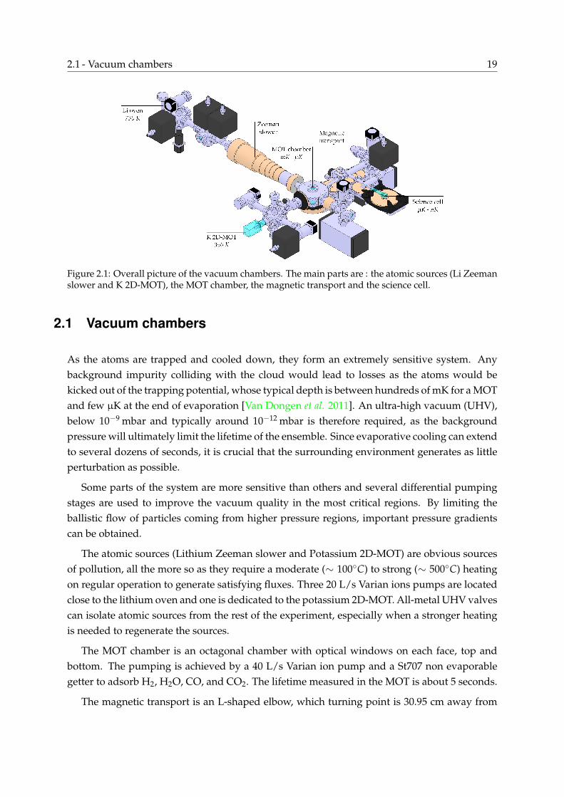
2.1 - Vacuum chambers 19

Figure 2.1: Overall picture of the vacuum chambers. The main parts are : the atomic sources (Li Zeemanslower and K 2D-MOT), the MOT chamber, the magnetic transport and the science cell.

2.1 Vacuum chambers

As the atoms are trapped and cooled down, they form an extremely sensitive system. Anybackground impurity colliding with the cloud would lead to losses as the atoms would bekicked out of the trapping potential, whose typical depth is between hundreds of mK for a MOTand few µK at the end of evaporation [Van Dongen et al. 2011]. An ultra-high vacuum (UHV),below 10−9 mbar and typically around 10−12 mbar is therefore required, as the backgroundpressure will ultimately limit the lifetime of the ensemble. Since evaporative cooling can extendto several dozens of seconds, it is crucial that the surrounding environment generates as littleperturbation as possible.

Some parts of the system are more sensitive than others and several differential pumpingstages are used to improve the vacuum quality in the most critical regions. By limiting theballistic flow of particles coming from higher pressure regions, important pressure gradientscan be obtained.

The atomic sources (Lithium Zeeman slower and Potassium 2D-MOT) are obvious sourcesof pollution, all the more so as they require a moderate (∼ 100C) to strong (∼ 500C) heatingon regular operation to generate satisfying fluxes. Three 20 L/s Varian ions pumps are locatedclose to the lithium oven and one is dedicated to the potassium 2D-MOT. All-metal UHV valvescan isolate atomic sources from the rest of the experiment, especially when a stronger heatingis needed to regenerate the sources.

The MOT chamber is an octagonal chamber with optical windows on each face, top andbottom. The pumping is achieved by a 40 L/s Varian ion pump and a St707 non evaporablegetter to adsorb H2, H2O, CO, and CO2. The lifetime measured in the MOT is about 5 seconds.

The magnetic transport is an L-shaped elbow, which turning point is 30.95 cm away from

20 The FERMIX experiment

Figure 2.2: Energy levels of lithium and potassium. Note that 40K has an inverted hyperfine, renderingits magnetic trappping easier. Values are taken from [Gehm 2003] and [Tiecke 2010].

Lithium 6Li δ Transition δ Potassium 40K6Li crossover + 116MHZ D2 Prcp -593 MHz 39K crossoverZeeman Prcp -76 Γ D2 Prcp -3 Γ 2D MOT PrcpZeeman Rep -76 Γ D2 Rep -2 Γ 2D MOT Rep

3D MOT Prcp -4.5 Γ D2 Prcp -2.9 Γ 3D MOT Prcp3D MOT Rep -2.6 Γ D2 Rep -5.2 Γ 3D MOT Rep

Imaging 0 D2 Prcp 0 ImagingD1 Prcp +4 Γ D1 Prcp +2.3 Γ D1 Prcp

D1 Repump +4 Γ D1 Rep +2.3 Γ D1 Repump

Table 2.1: Optical transitions of 6Li and 40K. The Potassium master laser is locked on 39K crossoverbecause this isotope is predominant in the spectroscopy cell, since its natural abundance of is over 90%.

2.2 - Optical system 21

the MOT center and 33.75 cm away from the science cell center. As the atomic sources, it can beisolated from the MOT chamber with an all-metal valve. The transport is connected to two ionpumps with flows of 20 L/s and 40 L/s and coated with Titanium-Zirconium-Vanadium alloy,a getter technology developed at CERN. Two additional strips of St707 getter are also installed.

The science cell is a glass parallelepiped of 23 mm x 23 mm x 10 mm designed for therequirements of the experiment and manufactured by Hellma GmbH. The glass walls, 4 mmthick, are made of uncoated Vycor, a fused silicon dioxide. It allows a much better opticalaccess than the MOT chamber and benefits from the L-shape of the transport to reduce theballistic trajectories of background particles. The ultra-low vacuum allows for lifetimes up to100 seconds. To avoid magnetic disturbance, the closest ion pump is shielded in a mu-metalbox manufactured by Atelier Soudupin.

2.2 Optical system

Laser light has proven to be an extremely versatile tool, allowing for the trapping, cooling andimaging of atoms. Cycles of absorption / spontaneous emission result in a radiative pressureexerted on the atoms while and cycles of absorption / stimulated emission lead to a conserva-tive dipole force. Laser light also allows for the manipulation of the inner degrees of freedomby optical pumping. To address atomic transitions, it is essential to generate laser beams withadequate frequency, power and polarization; and half of the system is dedicated to this task.Most beam can be injected in a Fabry-Perot cavity (ThorLabs SA-200-5B, FSR : 1.5 GHz) simplyby flipping a mirror, allowing for an easy monitoring which has proven to be extremely usefulto diagnose some issues2.

The technical details are presented in annex A.5. Logical schemes of both Lithium and Potas-sium optical tables are depicted in Fig 2.3 to summarize beam paths and computer controls.

Lithium and Potassium are both alkali atoms and as such they display the same simpleatomic structure (see Fig. 2.1 and the main parameters summarized in table 2.2). Since theS1/2 ground state displays two hyperfine levels, almost every beam has to be doubled by arepumping light, to avoid the accumulation of the atoms in an un-addressed state. All in all,ten beams are shaped for each atomic species.

The D2 transition, from the ground S1/2 level to the excited P3/2 level, is the most commonlyused. Its bandwidth Γ/2π ∼ 6 MHz is almost the same for both atoms and the saturation in-tensity, Isat, on the order of milliwatts per centimeter squared, only differs by the optical wave-lengths. The strategy for generating laser beams addressing the D2 line is the same for both

2For instance, an important instability was found as a back reflection from one beam was accidentally injectedin the TA amplifying another beam, resulting in strong fluctuations of the power ratio between both beams despitean almost constant total power. As the power of each beam was stable as long as the other beam was turned off,the problem was diagnosed by analyzing the light in a Fabry-Perot cavity and solved by dis-injecting the backreflection.

22 The FERMIX experiment

Lynx

Guepard

-240

-436.8

340.2

438

-449.46

-378

20

-90

-80

-350

-585

200

1285.8

Zebra

Gazelle

ON/OFF, Amp, Freq

ON/OFF

ON/OFF, Amp

ON/OFF

ON/OFF, FreqFreq

Freq

Unicorn

Chimpanze

ON/OFF, Amp, Freq

ON/OFF

Spectro

MOT Prcp

Rep com.

2DMOT Prcp

Img sweep

MOT Rep

2DMOT Rep

Img switch

Img High Field

MOT Switch

SpinPol

D1 switch

434.4

-59.81

EOM Spectro

EOM SpectroSpectro

20

EOM D1

ON/OFF, Amp, Freq

ON/OFF

Racoon

Mouse

Eagle

Shiva

Pinguin

ON/OFF, Amp, Freq

ON/OFF, Freq

ON/OFF, Freq

ON/OFF, Freq

ON/OFF

Spectro

MOT Prcp

MOT Rep

Zeeman Prcp

Img sweep

D1 switch

Spinpol

20328.4

188.5

430.3

-228.4

440

100

-109.7 228.2

EOM D1

EOM Spectro

Figure 2.3: Logical scheme of the 40K (top) and 6Li (bottom) optical tables. Analog (digital) controlsover the system are written in bold (italic) font. Optical sources are pictured with rounded box andAOM - EOM are represented with rectangular boxes and the corresponding frequency modulation isindicated in MHz. When relevant, the 0th order of an AOM is picture in dashed line. See annex A.5 fortechnical details. Zig-zag lines represent mechanical shutters.

2.2 - Optical system 23

Units 40K 6Lim u 40 6

Γ/2π [MHz] 6.03 5.87Isat == πhcΓ/3λ3 [mW/cm2] 1.75 2.54

λD2 [nm] 766.7 670.977λD1 [nm] 770.1 670.992

Trec = h2k2D2

/2mkB [µK] 0.4 3.5TDop = hΓ/2kB [µK] 145 141

Table 2.2: Properties of 40K and 6Li. We note kDi = 2π/λDi the wave vector. Values are taken from[Tiecke 2010] and [Gehm 2003] respectively.

species. A master diode is frequency locked on a saturated absorption error signal. Its light isamplified by a tapered amplifier (TA) from few mW to several hundreds of mW and injected ina single mode optical fiber for spatial filtering. The light is further divided by polarizing beamsplitters, each new beam being frequency shifted by acousto-optical modulator (AOM) to reacha controlled detuning with respect to the atomic transition. An additional step of amplificationis required to reach sufficient power. With the exception of the Li-Zeeman beams, principaland repumping lights are injected together in TAs with negligible power losses. This strategyenables a perfect superposition of both beams, before the light is fiber-coupled to the maintable. The frequency of each beam can be adjusted over dozens of MHz by tuning the radio-frequency (RF) driving the AOMs, while their amplitudes can be controlled by attenuating theRF power. It is also crucial to be able to switch off quickly and completely the beams in order toavoid shining stray light onto the atoms, especially during evaporative cooling. AOMs allowfor an attenuation of 10−4 within few tens of nanoseconds; a complete extinction is insured bymechanical shutters, cutting the beam in few hundreds of microseconds.

Optical sources are temperature-stabilized by Peltier elements (Roithner Lasertechnik, ref.TEC1-12705T125) that transfer the heat to the optical table through a thick aluminum plate,allowing an economical air cooling. The current supplies are protected against abrupt powerfailures (which happened quite often during the works in the building) by uninterruptiblepower supplies (Vision UPS Pro Blue 1000 VA).

An independent optical system has been implemented to address the D1 transition, fromthe ground S1/2 level to the excited P1/2 level, and allows for optical gray molasses. For 40K,the transition is 3nm away from the D2 line, too far to be reached by the same master laser.The D1 system follows the exact same structure as the D2 system, with an independent masterlaser. The only difference between both setups is that the D1 repumping beam is obtained notwith an AOM, but as a side band generated by an electro-optical modulator (EOM) tuned atthe hyperfine splitting frequency.

While the system is dedicated to 40K, we could adapt it for the bosonic 41K atoms withminor modifications (see Fig. 2.4). Since the atomic source contains even more 41K than 40K(see section 2.3.2), it is enough to change the light frequencies to address the new species.

24 The FERMIX experiment

Lynx

Guepard

260

210

336.3

435

373.5

453.6

20

-90

-80

425

0

95

254

Zebra

Gazelle

ON/OFF, Amp, Freq

ON/OFF

ON/OFF, Amp

ON/OFF

ON/OFF, FreqFreq

Freq

Unicorn

Chimpanze

ON/OFF, Amp, Freq

ON/OFF

Spectro

MOT Prcp

Rep com.

2DMOT Prcp

Img sweep

MOT Rep

2DMOT Rep

Img switch

Img High Field

MOT Switch

SpinPol

D1 switch

427.6

-59.81

EOM Spectro

EOM SpectroSpectro

20

EOM D1

Figure 2.4: Adaptation of the potassium optical table 41K. For most AOM, it is sufficient to changethe driving frequency. For some AOM (in blue), the order must be changed with respect to 40K setup.Some AOM (in red) must be removed or changed for a model with resonant frequency close to 100 MHz(rempumper commun and D1 setup).

Starting with a working system for 40K, it took about a month to reach ultracold temperatureswith 41K with the same techniques. In particular, the D1 gray molasses described in section2.5 could be readily applied to the bosonic isotope. Eventually, we managed to trap 2× 105

atoms at 55 nK in an optical dipole trap described by ω⊥/2π = 73 Hz and ω‖/2π = 4.8 Hz.Despite a temperature close to the critical value Tc = 72 nK we did not observe the formationof a Bose Einstein condensate, a limitation we attribute to the too small waist of the laser beam,increasing the three-body losses.

By locking the secondary master laser (Unicorn) on the D2 line rather than the D1 line, it iseven possible to manipulate 40K, 41K and 6Li at the same time. However, this configurationdoes not permit to drive D1 transition, limiting the sequence to a triple species MOT in absenceof efficient molasses cooling.

For 6Li, the two transitions are only 10 GHz apart, close enough for an alternative lock-ing strategy instead of using an additional spectroscopy cell3. While the repumping beam isgenerated by an EOM just like on the 40K system, the frequency of the principal beam is con-

3For a more technical description of the system, see [Fernandes 2014].

2.3 - Atomic sources 25

Units 6Li Zeeman slowerP [mW] 50

Islow/Irep - 8δslow [Γ] -75δrep [Γ] -75∆ B [G] 790

Units 40K 2D-MOTP [mW] 350

δcool [Γ] -3.5δrep [Γ] -2.5

Icool/Irep - 2I+/I− - 2.4PPush [mW] 10∂x,yB [G/cm] 11

Table 2.3: Optimised values for the Lithium Zeeman slower and Potassium 2D-MOT.

trolled by an offset lock. This technique is adapted from [Ritt et al. 2004] and relies on the beatnote between the locked D2 beam and the D1 master laser to be locked. The beating signal isrecorded by a fast photo-diode (ref. Newport 1580-A)4 and mixed with a tunable frequencyreference around 9.78 GHz delivered by a dielectric resonator oscillator. The resulting signalis split between two arms, one being fed into a high pass filter while the other one provides afixed attenuation. The comparison between both arms results in a dispersive error signal witha steep slope centered on the cut frequency of the filter. A PID circuit locks the error signal bycontrolling both the current of the D1 master laser (for high frequency corrections) and the posi-tion of the optical grating in the laser cavity (for the low frequency corrections). This techniqueenables an accurate frequency locking (a Lorentzian fit of the mixed down signal spectrum hasa full width at maximum height of 0.39 MHz for a cut frequency of 82 MHz) with a very broadlocking range.

2.3 Atomic sources

As the vacuum system is completely sealed, atomic sources have to be included in the vac-uum chamber to provide a ballistic flux towards the MOT chamber. As long as light inducedinteractions can be neglected, a simple accounting shows that the stationary amount of atomsgathered in the MOT is proportional to the incoming flux and inversely proportional to the life-time of the trapped atoms. A high flux is therefore required to reach a sufficient atom number,a critical parameter to perform an efficient evaporation. Experimentally, we reach in the MOTchamber loading rates of 1.7× 108 6Li/sec and 2× 108 40K/sec. Those values are roughly fivetimes smaller than those presented in previous works of the group and it appears that main-taining an optimal capture rate over long periods of time is very challenging. However, thecurrent values are sufficient to reach quantum degeneracy.

4This photo-diode model is know to be easily damaged in the standard operation and constitutes a weak pointof the setup.

26 The FERMIX experiment

2.3.1 Lithium Zeeman slower

6Li atoms are coming from a Zeeman slower, a standard technique widely used in the coldatom community [Metcalf and van der Straten 1999]. Our design is an improved version ofa previous experiment of the group [Schreck 2002]; the main parameters are summarized intable 2.3 (for a complete description of our system, see [Salez 2011]). Zeeman slowing hasproven to be a robust technique, particularly well suited for Lithium sources. Indeed, Lithiumpresents a very low vapor pressure at room temperature [Nesmeyanov and Margrave 1964]and temperatures above 600 K are required to reach a sufficient ambient pressure, around 10−8

mbar. It might therefore be challenging to reach a compromise between significant heating andsatisfying optical access, rendering difficult the direct loading from of a vapor cell.

The lithium sample, 3g of nearly pure 6Li provided by Cambridge Isotope Laboratory, isheated to ∼ 500 C in a cylindrical tube (the "oven") surrounded by Thermocoax cables. Athermal stream escapes from a 6 mm hole pinched on the oven and a collimation tube reducesthe divergence of the outgoing atomic beam, directed to the MOT chamber. The oven temper-ature plays a critical role on the atomic flux and is regulated by a PID circuit.

Two superimposed laser beams are sent against the atomic stream: the principal beam ad-dresses the D2 transition |F = 3/2〉 → |F = 5/2〉 and the repumping beam drives the D2 tran-sition |F = 1/2〉 → |F = 3/2〉. The slowing strategy relies on the radiative pressure exertedon the atoms by a counter-propagating laser beam. The strength of the interaction depends onthe detuning of the light with respect to the atomic frequencies, which can be affected by boththe Doppler and Zeeman effects. The atoms initially have a high velocity (vthermal ∼ 1000m/s);they thus experience a strong Doppler shift, which decreases as they slow down. In order tomaintain a constant detuning through the cooling process, a spatially variable magnetic fieldgenerates a Zeeman shift. As the atoms move forward, both shifts decrease so as to compensateeach other. Within less than 2m, the atom velocity can be reduced below the capture velocity ofthe MOT: vfinal < vcapture ' 50m/s. The cooling mechanism can only address atoms within avelocity range given by the difference in Zeeman shift between oven and MOT regions; fasteratoms are not sensitive to the laser beams and will follow a ballistic flight unaddressed by thecooling mechanism.

To avoid sending resonant light through the MOT region, we use the so-called "spin-flip"configuration, in which the magnetic bias crosses zero and changes orientation through theslower. The final bias is non-zero and the optimal detuning for the Zeeman beams preventsthem from perturbing the atoms in the MOT. This configuration also reaches a strong magneticfield difference between the two extremities of the slower, measured to 790 G, while maintain-ing reasonable current through the coils.

Only a small fraction of atoms actually escape from the oven and a vast majority hit itswalls and tubes. As they cool down, those atoms can solidify and clog the output of the oven,resulting in a dramatically reduced flux. Luckily, the surface tension of lithium decreases with

2.3 - Atomic sources 27

Figure 2.5: Schematics of the 2D-MOT

temperature [Yakimovich and Mozgovoi 2000] and the capillary forces drag liquid lithium backto the hotter regions, i.e. the oven. To increase this effect, the walls of the collimation tube arecovered with stainless steel mesh, resulting in a larger contact surface. These precautions arenot always sufficient to completely prevent the clogging and it is sometimes necessary to heatthe whole area in order to liquefy solid lithium and facilitate the evacuation of the blockage. Todo so, additional Thermocoax are installed along the output of the oven and the temperatureis slowly increased while maintaining a gradient towards the oven (∼ 25 K/cm). To avoidspreading too much Lithium out of the oven, its temperature remains below 600 C. Duringthe procedure, which usually lasts overnight, the lithium oven is isolated from the rest of thevacuum system to prevent its integrity.

2.3.2 Potassium 2D-MOT

Unlike 6Li, a 40K source needs to be optimized under economical constraints. The naturalabundance of this isotope is below 0.01% and a strong enrichment is necessary. We boughtfrom Technical Glass Inc, Aurora, USA a 100 mg sample containing 4mg of 40K, 89.5mg of 39Kand 6.5mg of 41K, for 4000$. The closure of the company makes it quite challenging to findsatisfying samples on the market nowadays.

In order to avoid wasting all the atoms with an incorrect velocity range, the cooling strategyrelies on a two dimensional magneto-optical trap (2D-MOT). Two pairs of counter-propagatingtransverse beams generate an optical molasses that slows down the atoms (see Fig. 2.5). Ifan atom moves in one direction, a Doppler shift brings the red-detuned facing laser closer toresonance, so that the atom experiences a force opposed to its velocity. In addition, racetrackcoils induce a 2D quadrupole magnetic field with a cylindrical geometry, such that the beams,in σ+ − σ− configuration, also generate an elastic restoring force that drags the atoms towardsa 0 field line centered in the cell. If an atom is away from the magnetic center, a Zeeman

28 The FERMIX experiment

shift brings the laser pushing it towards the center closer to resonance. In one dimension,the resulting radiative pressure, taking into account both Doppler and Zeeman shifts, can bewritten to the lowest order under the form:

F (x, vx) = −Kx−mαvx. (2.1)

It can be shown [Dalibard 2015] that coefficients K and α depend on the light intensity anddetuning, the transition linewidth and the magnetic field gradient, providing as many knobsto tune the capture and cooling efficiency.

A pair of axial beams increases the molasses effect. One of those beams (axial -) hits a 45

mirror with a hole and a part of its power is not therefore reflected. The atoms facing theshadow of the hole are only addressed by the other beam (axial +), which results in a net forcepushing the atoms through the hole and towards the MOT, 55 cm away. A supplementarypushing beam, targeting the mirror hole, allows for a decoupling of powers and has proven toincrease the outgoing flux by a factor 2. The main parameters of the 2D-MOT are summarizedin table 2.3.

The atoms supplying the 2D-MOT are trapped from an ambient potassium pressure of∼ 10−7 mbar. This pressure can be estimated and monitored by measuring the absorptionsignal in the 2D-MOT cell. The light is set at the cooling frequency and attenuated below thesaturation intensity to avoid power broadening and send on a photo diode after it traveled 10.5cm through the cell. By modulating the frequency of the light, it is possible to determine themaximal absorption of the gas, which can be related to the atomic density faced by the beam.In standard operating condition, absorption is around 40%.

It is necessary to heat the sample to generate sufficient vapor pressure. However, this pro-cedure has proven to be tricky, as an overheating has led to a macroscopic migration of thesample towards uncontrolled low temperature regions. Three windings of a water-cooled PVCtube have been installed close to the glass-to-metal connection (see Fig. 2.5) in order to con-trol the deposit of potassium crystals. If the source seems to migrate elsewhere, the rest of thesurrounding cell is heated up to ∼ 180 C so that the atoms are brought back to the cold pointwhere they crystallize. During this procedure, the 2D-MOT is isolated from the rest of the ap-paratus to protect the vacuum quality. The cold point is also set to low temperature (12 C)overnight. During normal operation, the temperature of this cold point is raised to 40 C bya water chiller Termotek5, reaching a stationary regime within 30 minutes and allowing for asatisfying vapor pressure.

5The control module of this chiller model is easily damaged and had to exchange it twice in two years. Equiv-alent models from other companies, such as Thermotek P1020, have shown a better robustness but do not reach asatisfying temperature.

2.4 - MOT and CMOT 29

Units 6Li-MOT 40K-MOTP [mW] 110 220

δprcp [Γ] -5 -3δrep [Γ] -3 -5Iprcp [Isat] 4 12

Iprcp/Irep - 5 20∂B [G/cm] 8→ 45T [mK] 1→ 0.8 0.24→ 2

Natoms [109] 2.1→ 1.9 3.2→ 3n [1011 cm−3] 0.26→ 1.8 0.7→ 3.7

PSD [10−5] 0.03→ 0.3 0.02→ 0.06

Table 2.4: Optimised values for the 3D-MOT and the ensuing CMOT. The phase space density is esti-mated as PSD= nλ3

T and does not take into account the existence of different internal states.

2.4 MOT and CMOT

A magneto-optical trap (MOT) is the starting point of almost all cold atom experiments [Dal-ibard 2015]. Like in a 2D-MOT, a bichromatic optical molasses is combined with a magneticgradient to cool and trap the atoms at the same time. A complete description of our system canbe found in [Ridinger 2011] and the main parameters are presented in table 2.4.

Within 18 seconds, we trap 2.1× 109 6Li-atoms at 1 mK and 3.2× 109 40K-atoms at 240µK.The losses due to interspecies light-induced collisions were reduced to ∼ 10% by using lowmagnetic field gradient and low repumping power. The fluorescence of trapped atoms arerecorded on photodiodes and allow for a real time monitoring of the population of each species.

In a simplified Doppler model, the temperature in the MOT is ultimately limited at low laserintensity by the line-width of the optical transition. The behavior of the atoms can be describedby a random walk as they absorb and re-emit photons [Gordon and Ashkin 1980], leading to adiffusion in momentum space. In steady-state, the final temperature results from the balancebetween the diffusion rate and the damping force and can be shown to be

kBT =h2

δ2 + Γ2/4|δ| ≥ hΓ

2. (2.2)

For both 6Li and 40K, this Doppler limit corresponds to ∼ 150 µK. Even though additionalSisyphus effects decrease the limit set by this toy model [Drewsen et al. 1994], the Dopplertemperature gives a relevant order of magnitude for most experiments.

After the MOT is loaded, the lasers responsible for the atomic flux are turned off. It wasfound optimal to increase the spatial density of the cloud before the following molasses phase(see below). To do so, the magnetic field gradient is increased while the light intensities arereduced and turned closer to resonance. Densities are multiplied by a factor 5, which alsoleads to a higher loss rate. This compressed-MOT (CMOT) phase is therefore limited to less

30 The FERMIX experiment

Energy

Position

a) b)

Figure 2.6: Sisyphus cooling in a bright molasses (a) and a gray molasses (b). In both cases, the spatialmodulation of the energy levels is correlated with the departure rate (pictured as the width of the line),so that the atoms climb up more potential hills than they fall down. In a gray molasses, the opticalpumping brings the atom to a dark state, uncoupled to the light (no light shift). The non adiabaticpassage to a bright state (pictured as a red arrow) is mostly due to motional coupling.

Energy

a) b) c)

Figure 2.7: The energy levels and transitions resulting in the light shifts presented in Fig. 2.6. Thestandard bright Sisyphus effect is described with structure (a) while the simple Λ system (b) gives riseto a gray molasses. For 40K and 6Li, both intra- and inter-hyperfine transitions must be taken intoaccount (c). The Raman detuning ∆ plays an important role in the cooling efficiency, as shown in figure2.8.

2.5 - Λ enhanced D1 gray molasses 31

Units 6Li molasses 40K molassesP [mW] 300 230

δprcp [Γ] + 4 + 2.3δrep [Γ] + 4 + 2.3Iprcp [Isat] 14→ 1 14→ 2.5

Iprcp/Irep - 20 8Capture phase [ms] 2Cooling phase [ms] 3

T [µK] 48 11N [109] 1.2 3.2n [1011 cm−3] 0.7 3

PSD [10−5] 8 10

Table 2.5: Optimised values for the D1 molasses. To ensure a satisfying capture efficiency, we use rel-atively high initial intensities. Their values are decreased during a cooling phase to optimize the finaltemperature.

than 5 ms, a duration found to be short enough to avoid significant losses.

2.5 Λ enhanced D1 gray molasses

After the MOT phase, the atomic cloud is still too hot to perform an efficient magnetic transportor to consider an evaporative cooling. Several ways exist to reduce further down the temper-ature of the cloud. For instance, to decrease the Doppler limit, a transition narrower than theD2 line can be addressed, such as the n = 2 → n = 3 transition for 6Li [Duarte et al. 2011] orthe n = 4 → n = 5 transition for 40K [McKay et al. 2011]. However, the corresponding light isin the near-UV domain and its implementation on the experiment is challenging because of thelimited power delivered by commercially available sources.

Sisyphus cooling provides another way to reach lower temperatures [Lett et al. 1989] bytaking advantage of the degenerate structure of the atomic ground state. Two counter prop-agating red detuned beams are sent on the atoms and generate a periodic modulation of thelight polarization. In this configuration, both the energies of the Zeeman sub-levels and theiroptical pumping rates are spatially modulated (see Fig. 2.6). A positive correlation betweenthose quantities means that atoms in one Zeeman state are most likely to be transferred to theother state when they reach a maximal energy shift. On average, atoms climb potential hills,on the top of which they are optically pumped to the bottom of the hill after they absorbedand spontaneously re-emitted a photon. As a result, they climb up more hills than they rolldown, explaining the name of the mechanism and leading to a net energy loss. Consideringthe same random-walk description as before, the steady-state temperature is given by [Metcalfand van der Straten 1999]:

kBT =hΓ2

16δ× I

Isat, (2.3)

32 The FERMIX experiment

where δ is the detuning of the beam. This can be understood as the value set by the height ofthe potential created by the light shift: if the atoms are too cold and slow to climb up a hill,they stop the Sisyphus cycling. For vanishing intensities, a more detailed approach gives alower bound characterized by the recoil temperature kBTrec = h2/2λ2m (' 3.5µK for 6Li and' 0.4µK 40K).

Unfortunately, the D2 transition of 6Li and 40K feature a too narrow excited P3/2 state toallow an efficient Sisyphus cooling, since non resonant coupling are still strong enough to dis-rupt the required correlations between light shift and optical pumping. For 40K, it is possibleto reach sub-Doppler temperatures as low as 15 µK but with significant atom losses, limitingthe cloud to ∼ 107 atoms [Modugno et al. 1999, Gokhroo et al. 2011]. For 6Li, the excited stateis even narrower, forbidding the use of standard Sisyphus cooling.

We took advantage of the wider hyperfine splitting of the P1/2 state to implement a novelcooling scheme, based on the same ideas but addressing the blue detuned D1 transition [Fer-nandes et al. 2012, Sievers et al. 2015]. Two main ingredients result in a strong cooling togetherwith a good capture efficiency : the existence of dark states among each S1/2 hyperfine levelsand of coherences between them.

The results presented in the section were published in

F. Sievers, N. Kretzschmar, D. R. Fernandes, D. Suchet, M. Rabinovic, S. Wu, C. V. Parker, L.Khaykovich, C. Salomon and F. Chevy. ‘Simultaneous sub-Doppler laser cooling of fermionic

6Li and 40K on the D1 line: Thoery and experiment’, Physical Review A, vol. 91, no. 2, p.023426 (2015)

2.5.1 Working principle

In a grey molasses, like in the previously described Sisyphus cooling, counter propagatingbeams give rise to spatial modulation of the light shift and departure rate. However, whenthe standard description of the Sisyphus effect relies on a F → F′ = F + 1 transition [Dalibardand Cohen-Tannoudji 1989], the D1 line corresponds to the F → F′ = F and F → F′ = F −1 transitions (see Fig. 2.7). As a result, some linear combination of Zeeman sublevels formdark states, which remain uncoupled to the light and whose energy is not modulated. Thisis well known in the text-book Λ system, where two grounds states |g1,2〉 are coupled to anexcited state |e〉 by a potential V described by driving frequencies Ω1,2. A linear combination|ψD〉 = 1√

Ω21+Ω2

2(Ω1 |g1〉 −Ω2 |g2〉) is disconnected from the excited state : 〈e|V |ψD〉 = 0. The

generalization to 3D is not straightforward, but the existence of dark states can still be proven[Ol’shaniî and Minogin 1992].

The presence of dark states leads to two differences with the previous picture. First, oncean atom is pumped from the top of a potential hill to a dark state |ψD〉, it remains there until amotional coupling brings it back to a bright state |ψB〉 (red arrow in Fig. 2.7). The probability

2.5 - Λ enhanced D1 gray molasses 33

0

100

200

Tem

per

atu

re(µ

K)

−0.2 0 0.220

40

60

−6 −4 −2 0 2 40

0.5

1

1.5

2·109

Raman-detuning δ (Γ)

Ato

mnu

mb

er

Figure 2.8: Atom number and final temperature of the 40K cloud as a function of the Raman detuning∆, as measured after 5 ms of D1 molasses. Note the narrow cooling zone near the Raman-conditionlowering the temperature (red triangles) to 20 µK and a flat cooling region below −0.1 Γ and above 2 Γresulting from gray molasses cooling without hyperfine coherence effects. The strong heating peak atsmall and positive Raman detuning can be described by a Fano profile. Picture from [Sievers et al. 2015]

for this non-adiabatic passage can be written perturbatively as [Weidemuller et al. 1994] :

P =

∣∣∣∣1

2m〈ψD| p2 |ψB〉

EB − ED

∣∣∣∣2

(2.4)

The faster the atom, the more likely it is to quit the dark state and resume Sisyphus cycles,provided that its velocity remains smaller than a capture velocity discussed below. On thecontrary, cold and slow atoms accumulate in dark states, uncoupled to the light, hence thename gray molasses. This effective velocity-selective coherent population trapping reduces thefluorescence emitted by the atoms and allows theoretically for final temperatures lower thanthe recoil-limit [Aspect et al. 1988]. The second difference is that the light should be blue-detuned to result in a cooling effect. Equation 2.4 shows indeed that the transition is all themore probable as the energy difference between dark and bright state is small. The bright stateshould therefore be up-shifted for the atoms to climb up-hill, and not fall down-hill.

Since atoms accumulate in uncoupled states, gray molasses could theoretically cool the en-semble even below the recoil temperature. However, except for a F = 1 → F′ = 1 transition,the recoil momentum results in a slight energy mismatch between the atomic states, giving riseto off-resonant light-matter interactions which transfer atoms from dark states back to brightstates and ultimately limit the lowest achievable temperatures.

The principle of gray molasses was presented in the ’90s [Shahriar et al. 1993, Weidemulleret al. 1994] and implemented on the D2 line of Cesium atoms in 1D [Valentin et al. 1992]and 3D [Boiron et al. 1995]. However, unlike the D2 transition, the D1 line does not provideclosed transitions. In such a situation, cooling and repuming designations are not relevant sinceboth transitions play equal roles. We will call principal the beam with the highest intensity,

34 The FERMIX experiment

addressing the hyperfine levels with the greatest angular momentum F, and keep the repumperdesignation for the weakest beam.

In addition to the gray Sisyphus effect induced within each hyperfine manifold by onebeam, the presence of another beam gives rise to coherences between the two hyperfine levels.This feature clearly appears close to the Raman condition (see Fig. 2.8), when both beams havethe same detuning with respect to the excited state (∆ = δprcp− δrepump = 0 in Fig. 2.7). The co-herent driving from one hyperfine level to the other allows new dark states, resulting in a finaltemperature 2 to 4 times lower than out of this condition and justifying the name of the tech-nique. On the other hand, a small red detuning from the Raman condition results in a strongheating, which can be interpreted in terms of Fano-profile [Lounis and Cohen-Tannoudji 1992]:the interference between a broad and a sharp scattering processes (namely scattering from therepumper and principal states) can strongly increase off-resonant transitions.

The theoretical description and numerical simulation of the Λ enhanced D1 gray molassescooling have been performed by our group with the collaboration of Saijun Wu [Sievers et al.2015, Grier et al. 2013], and several experiments tested the main points of the theory.

2.5.2 Experimental implementation

For 40K, the inverted hyperfine structure allows a double gray molasses : the principal |F = 9/2〉→ |F′ = 7/2〉 and repumping |F = 7/2〉 → |F′ = 7/2〉 transitions both exhibit dark states. Thesituation is slightly different for 6Li: while the principal transition |F = 3/2〉 → |F′ = 3/2〉is described by the aforementioned model, the repumping transition |F = 1/2〉 → |F′ = 3/2〉corresponds to the standard Sisyphus cooling presented as introduction to this section. Nev-ertheless, the D1 transition still allows an optical molasses forbidden by the narrow structureof the D2 line and the hyperfine coherences at Raman resonance do improve significantly theachievable temperatures. Moreover, we observed that the robustness of the mechanism allowsfor the simultaneous cooling of both species without significant deterioration of the conditionswith respect to the single species cooling.

We implemented the D1 cooling with minimal modifications of the existing setup. The op-tical system is described in section 2.2. The light is fiber coupled to the main optical table andsuperimposed with the MOT beams by a D-shaped mirror6. The overlap takes place far fromthe MOT chamber, so that both beams are almost parallel as they address the atoms. This way,D1 beams have the correct polarization, position and angle with respect to the atoms trappedin the MOT.

Experimentally, the cooling strategy must strike a balance in terms of light intensity. On theone hand, as long as the temperature is well above the recoil limit, it scales as T ∝ I/δ and alower intensity leads to a lower temperature. On the other hand, the capture velocity, estimated

6This D-shaped mirror constitutes a weak point for the stability of the system and requires minor realignmentevery other month.

2.6 - Spin polarisation 35

Units 6Li molasses 40K molassesδprcp [Γ] +3 +2δrep [Γ] +0.3 +0.3Iprcp [Isat] 0.1 1

Iprcp/Irep - 1/ 12 1/24Duration [µs] 70 50

T [µK] ∼ 300 ∼ 200N [109] 1 3

PSD [10−5] 0.4 3

Table 2.6: Optimised values of the spin-polarisation step for the loading of the magnetic quadrupoletrap. The temperatures are measured in single species operation and atom numbers are measured in themagnetic trap.

as the maximal velocity still allowing an efficient Sisyphus cycling, scales as vc ∝ I/δ2 and alower intensity results in a poor capture efficiency. A balance was found by changing the lightpower through the cooling step: a high initial intensity permits the capture of most of theatoms and a slow ramp down reduces the final temperature. The main parameter values of themolasses are summarized in table 2.5.

The existence of dark states relies on the degeneracy between dressed states. If this condi-tion can be reached between hyperfine levels by tuning the Raman detuning, it must also bepreserved between Zeeman sub-levels by avoiding any kind of magnetic fields. We installedthree large coils, far from the MOT chamber, to generate a homogeneous compensation biasand cancel stray field that could occur due to external conditions.

Since the implementation of the D1 gray molasses on our experiment, it has also been usedin other groups [Burchianti et al. 2014] and proven to work on 39K [Nath et al. 2013, Salomonet al. 2013], 23Na [Colzi et al. 2016] and 7Li [Grier et al. 2013]. We also realized an unpublishedwork on 41K, as mentioned in section 2.2.

2.6 Spin polarisation

After the optical molasses, the spin population of the atoms is completely unpolarized: atomsare distributed among all Zeeman sublevels of both hyperfine ground states. Before applyingany kind of magnetic trapping, it is therefore useful to pump the atoms into low-field seekingstates (see section 2.7.1).

A small magnetic bias (∼ 1G) is applied within 400 µs, so as to select a symmetry axis. Acollinear σ+ light is applied during 70µs for 40K and 50µs for 6Li to pump the atoms intoincreasing mF states. The duration of this step is kept as short as possible: as the atoms areuntrapped, they expand freely, decreasing their density. Furthermore, the size of the cloud alsoimpacts the loading efficiency of the ensuing magnetic trap and a wide distribution results in a

36 The FERMIX experiment

poor mode matching.

Since every absorption / emission cycle increases the temperature of the distribution (seetable 2.2 for recoil temperatures), it is essential to minimize the number of cycles performedby the atoms. To do so, it is useful to accumulate atoms into dark states, which cannot be ad-dressed by the light. For 40K, the σ+ light drives the |F = 9/2〉 → |F′ = 9/2〉 transition (withan additional repuming light addressing the other hyperfine level |F = 7/2〉 → |F′ = 9/2〉) onthe D2 line. Because of the narrow structure of the D2 line of 6Li, we drive the |F = 3/2〉 →|F′ = 3/2〉 transition on the D1 line instead (with a repuming light addressing the |F = 1/2〉 →|F′ = 3/2〉). In both cases, atoms accumulate in stretch states (|F = 9/2, mF = 9/2〉 and |F =

3/2, mF = 3/2〉 respectively), where they can not absorb σ+ photons for the driving transition.Despite this precaution, the final states are not completely decoupled from the light: the polar-ization of the beam is never perfectly σ+ and for 40K, off-resonant coupling to the F′ = F + 1level, enhanced by power broadening, should be taken into account. Those reasons also explainwhy it is important to perform the spin polarization as quickly as possible. Experimentally, wemeasure a temperature increase of ∼ 45µK for 40K and ∼ 170µK for 6Li, together with a verygood pumping efficiency as almost 100% of Potassium atoms and 90% of Lithium atoms areeventually loaded in the magnetic trap.

2.7 Magnetic system

Together with light, magnetic fields provide some of the most useful ways to manipulate coldatoms by taking advantage of the energy shift resulting from the Zeeman effect. A completederivation of the behavior of alkali atoms in a magnetic field is presented in annex A.1.

On the FERMIX apparatus, eleven independent power supplies are used to engineer therequired fields. The value of the output current can be set directly (CC mode) or by controllingthe delivered voltage (CV mode). While the first mode ensures a constant current, independentof the load fluctuations (due to Joule heating, for instance), the second mode permits a fasterresponse and is used when fields must be varied quickly. Both low intensities (MOSFET) andhigh intensities (IGBT) transistors are used as switches to interrupt and dispatch the currentthrough the system, as depicted in figure 2.9.

2.7.1 Magnetic quadrupole trap

As detailed in the following chapter, magnetic trapping requires the existence of a local min-imum of the magnetic field modulus. The easiest way to produce such a field is certainly theanti-Helmholtz configuration, as proposed by Pauli. Two parallel coils of radius R and distantof D carry opposite currents I. Considering an origin between the two coils, the resulting field

2.7 - Magnetic system 37

can be expanded close to the symmetry center [Meyrath 2004]:

B = b

xy−2z

=

32

µDR2

(D2 + R2)5/2 I

xy−2z

+ O(r3), (2.5)

where z is the direction of the coils7. In a proper anti-Helmholtz configuration, D = R andb = 48

25√

5µIR2 . As long as the field is smaller than few Gauss, the resulting energy shift for an

atom in a Zeeman sub-level mF is the so called quadrupole potential :

∆E = µBgFmFb√

x2 + y2 + 4z2, (2.6)

where µB is the Bohr magneton and gF is the Landé factor. For low field seeking states, mF > 0,the potential leads to a restoring force towards the magnetic center, confining the ensemblewithin a volume of typical dimension r0 = kBT/µBb.

After the optical pumping, atoms populate low-field seeking states and can be loaded in themagnetic gradient. However, the loading requires good mode matching between the free cloudand the confined distribution. Furthermore, as long as the trapping gradient is not settled, thegas keeps expanding and the field should thus be ramped as fast as possible to a value suchthat r0 matches the initial size of the cloud.

Experimentally, the temperature of the cloud after the optical molasses is around 20µK andits size is∼ 1.5 mm. We increase the current in the MOT coils as fast as possible until r0 reachesthis value. It should be noted that the ramp-up speed is limited by eddy currents induced inthe metallic structures and it is likely that the field is cannot be reached in less than ∼ 1 ms.Almost 100% of 40K atoms and 90% of 6Li atoms are captured during this step. During thefollowing 450 ms, the field is slowly raised to 80 G/cm to compress adiabatically the ensemble(see section 3.1.4), ensuring a strong confinement for the ensuing magnetic transport.

2.7.2 Magnetic transport

In many experiments, in order to perform an evaporative cooling in optimal conditions, atomsmust be transported from the MOT-chamber to a science cell with better optical access andvacuum. Optical transport relies on deformable [Léonard et al. 2014] or movable [Gustavsonet al. 2002] lenses to trap atoms around the focal point of a laser and displace it from onecell to the other. Magnetic transport consists in displacing the center of a magnetic gradientinstead. This can be done by installing a pair of coils on a translation stage [Lewandowski2002], a simple solution that is nevertheless challenging in terms of mechanical stability andmight impact the optical access to the science cell. Another option is to switch successively

7Note that we define the gradient along the weak directions x and y. Another convention is to define b as thegradient along the strong axis z.

38 The FERMIX experiment

H1 AH2 H/AH AAH

AH1 H2 AAH H/AH

Outer coils

CV

T1/2

CC/CV

CV

Q

A

MOT

B

MOT coils

Inner coils

CC

T1

T4

T9

V2

CV

Push

T2

T5

T7

V1

CV

T3

T6

T8

CC / CV

SpinPol

CV

Comp XY

CV

Zeeman

CV

Comp XY

CV

HF

Coils Axial fieldMOT 0.91 G/A/cm

SpinPol 4.8 G/APush 0.16 G/A - 0.073 G/A/cm

Inner (H) 8.00 G/A + 0.61 G/A/cm2

Inner (AH) 2.5 G/A/cmOutter (H) 2.089 G/A - 0.29 G/A/cm2

Outter (AH) 0.24 G/A/cmV1 2.8 G/A/cmV2 -2.8 G/A/cm

Coils Axial fieldT1/2 0.37 G/cm - 0.29 G/cmT1 3.3 G/A/cmT2 5.5 G/A/cmT3 3.7 G/A/cmT4 5.5 G/A/cmT5 -3.7 G/A/cmT6 -2.6 G/A/cmT7 2.6 G/A/cmT8 3.7 G/A/cmT9 2.6 G/A/cm

Figure 2.9: Electrical system of the experiment. IGBT are pictured as solid switches, MOSFET as dashedswitches. References for the power supplies are given in annex A.5. The utility of the different coils isgiven in the main text. Gradient are given along the strong axis. A description of the IGBT setting forMOT, inner and outer coils in Helmoltz (H) or Anti-Helmoltz (AH) configuration is given in table 2.7.

2.7 - Magnetic system 39

IGBT Helm. Anti Helm. Inv. Helm. Inv. Anti Helm.H 1 0 0 1

AH 0 1 1 0H/AH 1 1 0 0AAH 0 0 1 1

IGBT MOT Helm. Anti Helm.MOT 1 0 0HF 0 1 1A 0 0 1B 0 1 0Q 0 1 0

Table 2.7: IGBT configuration for a versatile control of the magnetic field around the science cell. Theelectrical system is presented in figure 2.9.

overlapping pairs of coils, so as to deform smoothly and continuously the magnetic field.

The latter option has be implemented on the experiment and used to transport the atoms in6 seconds 64 cm away from the MOT, through a a 90 elbow. The transport requires 14 pairsof coils (pairs T1/2 to T9, V1, V2 as well as the inner and outer pairs of coils of the science cell)and an additional push coil, as shown in figure 2.9. The ensemble holds on a metallic coolingplate, the temperature of which is water regulated (Termotek P1020) in order to avoid thermaldilatation.

Even though it represented a major time investment during its conception and realization,the magnetic transport allows for stable and reproducible experiments. For a detailed descrip-tion of the transport, see [Fernandes 2014] and [Sievers 2014]. We estimate that ∼ 80% of the40K atoms and 70% of the 6Liatoms are successfully transported to the science cell, with a tem-perature increase of 130µK for both species. Those values are considerably improved by the D1

molasses, which reduces the spread of the cloud and prevents it from clipping on the differen-tial pumping tube at the entrance of the transport. Without the preceding CMOT and molassessteps, the transport efficiency is limited to ∼ 50% and the heating is increased to 400µK.

2.7.3 Magnetic bias

Once the atoms are trapped in the science cell, it can be necessary to raise an homogeneousmagnetic bias to reach Feschbach resonances or perform spin selective imaging. Bias fieldsare also used to compensate ambient magnetic fields during the molasses step or to select asymmetry axis during the spin polarization step.

When two coils carry the same current, the induced field close to the symmetry center takesthe form:

B = µR2

(D2 + R2)3/2 I

001

+

32

µR2 (4D2 − R2)

(D2 + R2)5/2 I

−zx−zy

z2 − (x2 + y2)/2

+ O(r5). (2.7)

In the Helmholtz configuration, D = R and the curvature described by the last term vanishes,leaving a pure bias up to the fourth order.

40 The FERMIX experiment

Without coils With coilsMOT 0.6 0.3

Science cell 2.2 1.1Zeeman 2.6 2.2

IGBT 1.5 1.5HighFiness 1.1 1Transport 6 2

Table 2.8: Water flux (L/min) cooling most of the coils of the experiment as well as a plate supportinghigh current IGBTs. Transport coils are supported by a water-cooled plate while the other coils havehollow wires allowing a direct cooling.

To allow for a versatile magnetic configuration, two pairs of coils (inner and outer) sur-round the science cell (see table 2.7). The inner coils can be powered either in anti-Helmholtzor Helmholtz configuration by flipping IGBT switches, while the current direction can be setindependently through each of the outer coils, allowing any of the four possible configurations(anti-Helmholtz, Helmholtz or inverted configurations) and thus providing control over themagnetic field curvature.

The inner coils are also dedicated to the tuning of the Feschbach resonances. Notably, theresonance between 6Li and 40K is quite narrow (∆B = 1 G around B0 = 100 G) and a stablefield is required to avoid accidental sweeps across the resonance. A High Finess power supply,with a current stability below 10−5 was purchased for this purpose8.

2.8 Security system

As described above, the experimental setup deals with important electrical currents that mightresult in a strong heating of the coils, leading to a damage or a melting of the insulating plasticcoating. All coils supporting high currents, as well as the magnetic transport and a metallicplate supporting IGBTs, are water-cooled to prevent such dramatic accident (see table 2.8).An additional security system was installed to monitor each water flux through flow-meters(Gems Sensors RFS and Flow Switch FS-926). In addition, several thermistors are glued onseveral coils to measure their temperatures. A supplementary module, dedicated to humiditymeasurement, is not currently used. If any of measured values passes a fixed threshold, thesecurity systems switches off all the power supplies through their Remote Shut-Down (RSD)channel.

All technical drawings of the security system are presented in annex A.6.

8This model presented repeated failures, as an instrumentation amplifier (INA128P) of the command circuitwas easily damaged and had to be exchanged every other day. The problem was solved by installing an analogoptocoupler between the computer control channel and the input port of the power supply.

2.10 - High power lasers 41

2.9 Radio Frequency / Microwave system

While lasers allow the manipulation of optical transitions, radio-frequency (∼MHz) and micro-wave (∼GHz) sources are required to drive transitions both between and within hyperfineZeeman states.

Experimentally, we need to reach three distinct frequency domains. In order to performan evaporative cooling in a magnetic trap, atoms must be selectively transferred from low-fieldseeking states to untrapped high-field seeking states. For 40K, we drive hyperfine |S1/2, F = 9/2〉→ |S1/2, F = 7/2〉 transitions, with frequencies between 1.1 GHz and 1.28 GHz. For 6Li, we ad-dress hyperfine |S1/2, F = 3/2〉 → |S1/2, F = 1/2〉 transitions, with frequencies between 228MHz and 400 MHz. Finally, in order to manipulate the spin population of the sample, it isuseful to drive transitions between Zeeman sublevels. A magnetic bias is applied to lift the de-generacy and an RF signal allows for adiabatic transfer or Rabi oscillations between the states,transferring the atoms from one state to another (as in section 5.1.2). The required frequenciesdepend on the amplitude of the magnetic bias, but typical values stand between 3 MHz (at fewGauss) and 50 MHz (around 200 G).

The strategy used to emit the RF/MW radiations is the same for all three domains (see Fig.2.10). An electrical signal with a selected frequency is amplified and sent to an antenna thatradiates it into electromagnetic waves. Antennae are simple windings of a thin metallic cable,with a size optimized for the emission of the dedicated radiation, placed few centimeters awayfrom the science-cell. The resonant frequency and impedance matching of the antenna arefurther tuned by adapting its electrical properties with an RLC circuit and its geometry with asizable BNC cable (see [DeMarco 2001]).

2.10 High power lasers

The final stages of the experimental sequence take place in an optical trap. Cycles of absorption/ stimulated emission give rise to an energy shift called light shift, proportional to the lightintensity I and depending on its detuning with respect to the atomic transition [Grimm et al.2000] :

U(r) = −3πc2

2ω2

(Γ

ω0 −ω+

Γω0 + ω

)I(r), (2.8)

where ω is the light frequency, ω0 the atomic frequency and Γ ' 2π × 6 MHz the associatedlinewidth. The light intensity profile of Gaussian beam propagating along z takes the form:

I(r) =2P

πw21√

1 + z2/z2R

exp(− x2 + y2

w2(1 + z2/z2R)

), (2.9)

42 The FERMIX experiment

ON/OFF

ON/OFF

CH1 / CH2

Freq

Freq, Amp

Freq, AmpON/OFF

ON/OFF

CH1 / CH2

Amp

CH1 / CH2

Figure 2.10: Radio-frequency and micro-wave components. The construction allows a fast switchingbetween input channels (CH1/CH2) sources. Two Agilent sources are controlled by LAN cable andused for evaporative cooling, while the Rohde-Scwhartz and SRS sources are pre-programmed andtriggered during the sequence. Technical references are given in annex A.7.

ON/OFF

PowerPower

ON/OFF ON/OFF

Science cell

Protective box

ODT2

ODT1

Verdi

Pie

zo m

ou

nt

Figure 2.11: High power lasers close to the science cell. The setup is described in the main text andperformances are detailed in table 2.9. We introduce directions x (along ODT1 beam), y (along transport)and z (opposed to gravity).

2.10 - High power lasers 43

Verdi ODT1 ODT2Units 6Li 40K 6Li 40K 6Li 40K

λ nm 532 1064 1064P W 7 10 5w µm 20 42 340zR mm 2.3 4.3 300U0 µK 780 800 220 410 1.6 3.5

ω⊥/2π kHz i 16.6 i 6.5 4.2 2.2 0.044 0.025ω‖/2π Hz i 100 i 39 29 12.6 - -

Table 2.9: Main parameters of the high power lasers described in figure 2.11.Frequencies are given inthe harmonic approximation (2.10) ; ω‖ is the axial frequency along the propagation of the beam andω⊥ orthogonal to it. For the Verdi, the potential is repulsive and its steepness is given by the imaginaryfrequencies.

where w is the beam waist and zR = πw2/λ is the corresponding Rayleigh length. Conse-quently, a tightly focused laser can generate a strong repulsive potential for blue detuning orattractive potential for red detuning, which can be expressed close to the focal point as:

U(r) = ±(

12

mω2⊥(x2 + y2) +

12

mω2‖z

2)

, (2.10)

with a height (or depth) U0 ' hΓ2

4|δ|I

2Isat(typically between few µK and 1 mK) and frequencies

ω⊥ =√

4U0mw2 perpendicular to the beam propagation (typically between ∼ 100 Hz and ∼ 1

kHz) and ω‖ =√

2U0mz2

Ralong it (typically one hundred times smaller than ω⊥). Both repulsive

and attractive potentials are used in the experiment (see Fig. 2.11 for the implementation andtable 2.9 for the performances.).

2.10.1 532 nm laser

When evaporated in a magnetic quadrupole, atoms can escape the trap as they move throughthe center of the potential, where a vanishing bias prevents them from following the field ori-entation. Those Majorana losses, described in section 3.1.3, can be attenuated by focusing ablue-detuned laser on the central region to prevent atoms from reaching it. A Coherent Verdisingle mode laser is used for this purpose, as its wavelength (532 nm) makes it repulsive forboth 6Li and 40K. 7 watts of power are focused into a waist w ∼ 20µm at the center of themagnetic trap, resulting in an optical plug of ∼ 800µK (see Fig. 2.12).

The beam can be switched off within microseconds by means of an acousto-optical modu-lator. The pointing of the laser is monitored by imaging the focus of the beam on a 4-quadrantphotodiode (Newport Model 2901), delivering a voltage proportional to the distance of the spotto the center of the diode. The position of the focus can be fine tuned by piezo mirrors (New-port AG-M100N) and a LabView script has been developed to bring automatically the spot onthe 4-quadrant diode to a reference position. The root mean squared displacement averaged

44 The FERMIX experiment

0 1 2 30

0.5

1.5

2

Position

Position

Figure 2.12: In situ picture of a 40K cloud in a plugged quadrupole trap. Notice the depletion of atomsin the center of the distribution. The RF evaporation has been pushed to Tcut = 100µK, further than ina normal operating sequence, to reduce the size of the beam and help with the plug alignment.

over 3 minutes is around 1 µm, well smaller than the waist, showing a satisfying stability. Tofurther reduce the sensitivity of the system, the laser beam is directed towards the transportdirection (see Fig. 2.11), so that small displacements due to thermal dilatation of the transportsupport should be compared to the Rayleigh length of the beam zR ' 2 mm rather than to itswaist.

2.10.2 1064 nm laser

Optical traps provide comfortable conditions to perform evaporative cooling to ultralow tem-peratures. The trapping volume is small, and the strong confinement allows a high collisionrate. Besides, unlike in a magnetic quadrupole trap, the confining potential does not dependon the spin state of the atoms and the spin composition of the cloud can thus be freely adjusted,allowing the use of Feschbach resonances.

We first implemented a Verdi Coherent single mode laser at 1064 nm. Unfortunately, thisprototype was quite experimental and failed after few months. The production of this modelwas stopped by the constructor and we advantageously replaced it with a Mephisto Innolightmodule, delivering ∼ 18 W of power. The beam can be switched off within 0.5 µs by an AOMand is injected through a fiber for pointing stability (NKT Photonics LMA-PM-10, with a SMA905 APC connector at the input (7º) and a SMA 906 PC connector at the output). This part ofthe setup is installed in a closed box over-pressurized with filtered air (Walker Filtration) toprevent dust from accumulating close to the optics, where due to high light intensities it mightburn and damage the coatings.

The efficiency of the fiber coupling falls from ∼ 85% at low intensity to ∼ 60% at highpowers, limiting the output power to 11 W. The light is sent along the x direction (see Fig.2.11) on the science cell with a 10 angle to avoid optical interference with retro-reflected light,and focused in a w = 42µm waist (the corresponding Rayleigh length is zR = 4.3 mm). Theoutgoing light is fed into an optical beam dump.

Initially, the potential must be deeper than 200µK to capture atoms from the magneticquadrupole trap. To perform an evaporation, the potential depth is lowered progressively

2.10 - High power lasers 45

0 1 2 3 40

0.5

1

1.5

Position

Position

0 1 2 3 40

0.5

1

1.5

Position

Figure 2.13: 40K in the optical dipole traps. (Left): 7× 106 atoms at 2 µK after 5 ms time-of-flight fromthe single arm ODT. (Right): 4× 106 atoms at 1.2 µK after 5 ms time-of-flight the crossed ODT.

to ∼ 1µK and the light intensity is accordingly varied over 4 orders of magnitude. To maintainthe control and stability of the optical power through the whole range, we monitor the powerof a back reflection on the science cell (Thorlabs SM05PD4A mounted InGaAs-Photodiode(FGA10)) and feed the signal in a logarithmic amplifier (Analog Devices AD8304). A PID con-troller (Stanford Research Systems SIM960) compares the measured value to a reference setby computer and adjust the RF power that feeds the aforementioned AOM to tune the opticalpower. This setup allows a retro-control and a dynamical setting of the light intensity and thusof the potential depth. In addition, taking advantage of the logarithmic amplifier, a linear rampof the control voltage results in an exponential decrease of the optical power.

As the trapping frequency along the beam propagation axis is set by the Rayleigh length,it is much smaller than the transverse frequencies (see Fig. 2.13). In order to increase thesteepness of the axial trapping at low powers, the 0th order of the AOM is recycled and sentperpendicularly to the previous beam (ODT2 beam). The same power monitoring is installedto allow for an independent control of both intensities. The crossed beam position can becontrolled by piezo mirrors to fine tune its overlap with the optical dipole trap.

In the quantum degenerate regime, the trapped atomic cloud is cooled around 100 nK andthe pointing and power stability of the beams are crucial to avoid parasitic heating. Ultimately,the residual heating will be given by spontaneous emissions breaking the cycles of absorptionand stimulated emission. The corresponding rate Γsc can be estimated to:

hΓsc(r) =Γ|δ|UODT(r), (2.11)

underlying the importance of a strong detuning to reduce the scattering rate. Each scatteringevent provides a recoil energy to the atoms and the resulting heating power can be estimatedto

Pheat = 2ErecΓsc (2.12)

where Γsc is the scattering rate averaged over the trap, Erec is the recoil energy of the atom,and the factor 2 comes from the contribution of both longitudinal and transverse directions.Relating the energy of the cloud to its temperature through the virial theorm, we estimate the

46 The FERMIX experiment

heating effect for 40K to T = 0.96 µK/s in the trap at full power and T = 10 nK/s in the trap atthe end of evaporation, a value small enough to be allow holding times of few seconds.

2.11 Imaging system

The standard data acquisition consists in sending a resonant light pulse on the atomic cloud,whose image is recorded on a charge coupled device (CCD) camera.

2.11.1 Absorption imaging

The light intensity reaching a pixel of the camera is attenuated by the optical density of thecloud integrated on the line of sight. Quantitatively, the intensity I captured at position (x, y)on the pixel matrix can be expressed thanks to the Beer-Lambert law as

I(x, y) = I0(x, y) exp

−mσabs

∫

line of sight

dz′ n(x′, y′, z′)

, (2.13)

where I0(x, y) is the incoming intensity, σabs is the absorption cross section, m is the magnifica-tion of the imaging system and n(x′, y′, z′) is the atomic density at the position imaged on thecamera.

For a frequency close to resonance, the absorption cross section can be written as [Cohen-Tannoudji et al. 2001]:

σabs(ω) =3λ2

2π

C2

1 + 4(1 + 2 IIsat

)(

δΓ

)2 , (2.14)

where δ = ω−ω0 is the detuning between the light and the atomic frequencies. When scanningthis detuning around the resonance, the cross section displays a Lorentzian behaviour, withwidth given by the natural linewidth Γ and a power-broadening factor. In most cases, theintensity is low enough for this factor to be negligible.

In this formula, C is the Clebsch-Gordan coefficient corresponding to the optical transition.If an external magnetic field gives a quantization direction, it is possible to address a closedimaging transition and C2 = 1. However, in the some cases, the atomic magnetic moment israndomly distributed and we use a value averaged over all possible transition : C2 = 0.4 for40K and C2 = 0.5 for 6Li.

It is thus possible to estimate the integrated density n2D(x, y) =∫

l.o.s.dz n(x, y, z) from the

ratio between the measured and incoming intensities. From this quantity, it is straightforwardto obtain the total number of atoms, N =

∫dxdy n2D(x, y). Another relevant measurement

is the size σx,y of the 1D distribution along each direction nx1D =

∫dy n2D(x, y) and ny

1D =

2.11 - Imaging system 47

∫dx n2D(x, y), which can be related to the population, temperature and trapping frequencies

of the cloud, as shown in the following paragraph.

2.11.2 Time-of-flight expansion of non-interacting particles

An in-situ image of the cloud can be taken to access directly to its density distribution. How-ever, several non-trivial effects, such as non uniform frequency shifts due to the confining po-tential or remaining magnetic bias, can make the data analysis challenging. What’s more, thesmall size of the sample may result in a too strong optical density and require an extremelygood optical resolution.

An alternative way to acquire image is to perform a time-of-flight experiment: the trappingpotential V0 is abruptly switched off and the released atoms expand in all directions for dura-tion τ without further interactions. Since this method was used to acquire most data in thisthesis, we present it here with some details in order to derive expressions required to analyzea distribution of fermions at any temperature.

Free ballistic expansion

If fermions move freely, without interactions or outer potential, the momentum of each particleis conserved during their ballistic flight and the size of the cloud can give a direct insight onthe temperature of the distribution:

n(r, τ) =∫

dr0dp0 fFD(r0, p0)δ (r− r0 − p0t/m) (2.15)

=1

(2πh)3

∫dp0

1

exp(

βp2

02m + βV0

(r− p0

m t)− βµ

)+ 1

, (2.16)

where fFD is the Fermi-Dirac distribution, β = (kBT)−1 and we introduced the chemical poten-tial µ.

For a harmonic trap V0(r) = ∑i

mω2i x2

i /2, the density can be analytical derived using poly-

logarithm function 9 :

9Polylogarithm function are defined as Lin(z) = 1Γ(n)

+∞∫0

dq qn−1

1z eq−1

→z1

z. As useful relation is+∞∫−∞

dx Lin(ze−x2) =

√πLin+1/2(z)

48 The FERMIX experiment

n(r, τ) = − 1λ3

dB

Π

i

1√1 + ω2

i τ2

Li3/2

[−Z exp

(− m

2kBT ∑i

12

ω2i x2

i1 + ω2

i τ2

)]

n2D(x, y, τ) = −m (kBT)2

2πh3ωz

1√

1 + ω2xτ2√

1 + ω2yτ2

Li2

[−Z exp

(− m

2kBT

(ω2

xx2

1 + ω2xτ2 +

ω2yy2

1 + ω2yτ2

))]

nx1D(x, τ) = −

√m2π

(kBT)5/2

h3ωzωy

1√1 + ω2

xτ2Li5/2

[−Z exp

(−mω2

x2kBT

x2

1 + ω2xτ2

)](2.17)

where we introduced the fugacity Z = eβµ.

In the classical limit, the temperature is large compared to chemical potential. In this regime,the integrated 1D densities (2.17) display a Gaussian distribution, whose width given by:

σ2x(τ) = σ2

0 +kBTm

t2, (2.18)

where σ20 = kBT

mω2x

is the width of the initial Boltzmann distribution. By performing successivetime-of-flight with increasing durations, it is therefore possible to measure the temperature Tas the slope of width squared over time, without any knowledge of the trapping potential.

In the degenerate regime, the complete formula (2.17) is required to fit the non-Boltzmanndistribution of the cloud. Note that the amplitude and width of the distribution are related,reducing to two the fitting parameters if the trapping frequencies are known. This allows for asimultaneous determination of the atom number and cloud temperature.

In both cases, it is remarkable that at long TOF, the isotropy of the initial momentum distri-bution is transferred to the position distribution, regardless of the initial trap geometry. Thissituation can be drastically different when particles are interacting.

Expansion in a surrounding potential

When a time-of-flight is performed at high magnetic bias, a residual curvature may still bepresent and give rise to a weak harmonic potential Vext =

12 m(

ω2ext,xx2 + ω2

ext, yy2 + ω2ext, zz2

),

where ωext,i is real for a confining potential and imaginary for a repulsive potential (see section5.1.3).

This additional effect can be taken into account in the previous expression by changing√1 + ω2

i τ2 to√

cos2 (ωext,iτ) +ω2

iω2

ext,isin2 (ωext,iτ), considering cos (iθ) = cosh(θ).

In the classical regime, the substitution leads to

2.12 - Computer control 49

Absorption Reference Dark noise n2D

Figure 2.14: Raw and treated data from absorption imaging after 5 ms TOF. On the picture, ∼ 107 40Katoms after the optical molasses.

σ2x(τ) =

trap

kBTm

(1

ω2i

cos2 (ωext,iτ) +1

ω2ext,i

sin2 (ωext,iτ)

)(2.19)

=anti

kBTm

(1

ω2i

cosh2 (ωext,iτ) +1

ω2ext,i

sinh2 (ωext,iτ)

)(2.20)

Those formulas were used to characterize the curvature of the inner and outer coils close tothe science cell, as shown in table 2.9.

2.11.3 Experimental setup

As presented in section 2.2, the laser system provides tunable light for imaging 40K and 6Liboth at low magnetic bias and at high field, as the Zeeman shift induces significant changes onthe resonance frequency.

A first imaging picture is taken with a 100 µs light pulse. The measurement is destructive,as atoms are pushed away by the probe beam. During the following 50 ms, the atoms are letto expand at high temperature until they collide with the surrounding chamber. A secondreference picture is taken in the absence of atoms. Two additional background pictures are takenin the same conditions but in the absence of light, in order to measure the dark noise of theCCD camera. The integrated density at each point is then computed as

n2D(x, y) =1

mσabslog(

Iimg − Iimg,bg

Iref − Iref,bg

)(2.21)

Four independent CCD cameras are installed on the experiment to acquire images from theMOT chamber and along three directions around the science cell. We use Pixelfly QE 270XDcameras, with a pixel matrix of 1392 px × 1024 px, a pixel size of 6.45 µm and a quantum effi-ciency of 25% for potassium light and 43% for lithium light. The magnification and numericalaperture of each imaging system are summarized in table 2.10.

50 The FERMIX experiment

System w [mm] m NAMOT Chamber 13.8 0.4 0.12Science cell x 4 1.6 0.039Science cell y 6 0.6 0.056Science cell z 2.7 2.55 0.17

Table 2.10: Imaging system of the MOT chamber and science cell. w is the waist of the imaging beam,m the measured magnification and NA the numerical aperture calculated taking the imaging lenses aslimiting aperture. The calibration procedure is explained in section 5.1.3.

2.12 Computer control

Three computers are dedicated to the control and monitoring of the experiment (see Fig. 2.15).

The main computer runs the user interface of the experiment. We use Cicero Word Gener-ator10, an open source software developed by Aviv Keshet at MIT for cold atom experiments.The suite is composed of two applications with a client / server architecture. The client Cicerois a user-friendly interface, where sequences are designed as a succession of steps with variabledurations. During each step, the value of each digital and analog channel can be controlled.The server Atticus translates those sequences into output buffers that are downloaded to theoutput hardware. The software is mostly adapted for National Instrument cards and NormanKretschmar extended the source code to integrate LAN connection (notably to address AgilentRF generators).

We currently use six analog (NI PXI-6713) and three digital output cards (NI PXI-6533 andNI PXI-6536). Each of the analog cards has 8 BNC outputs delivering 0 to 10 Volts and up to250mA. The digital cards have 24 channels, outputting either 0V or 5V (only 3.3V for NI PXI-6536). When a digital channel is used to flip an IGBT, the fast switching of high intensities mayinduce high voltage in the control channel, destroying the output. To prevent this situation,most digital channels are opto-coupled to isolate them from the experiment (the electrical de-sign of the optocoupler box is given in annex). Note also that while the digital channels providea fixed voltage, some of the devices they control are current-controlled. It is in particular thecase for most of the RF "ZAS" switches, that are notably used to turn on and off optical beams.An additional 50 Ω was installed at the input of those devices to avoid short-cutting the outputcard, which would result in a voltage drop of the whole control system.

Sequence steps might have very different durations: while the loading of the MOT or anevaporation can last several seconds, it takes only ∼ 100µs to take an image of the atoms. Toavoid long redundant buffers, we synchronize the output cards with a variable frequency clock(Opal Kelly, ref. XEM 3001). This FPGA card generates pulses only when an output needs tobe updated, and this variable timebase is used by output cards as sample clock. This reducesconsiderably the buffer size, allowing a faster loading of the sequence and a time resolution

10http://akeshet.github.io/Cicero-Word-Generator/

2.13 - Conclusions 51

Cicero

Atticus

National instrument

Analog cards

Digital cards

Optocouplers

Clock

Experiment CCD Camera

Trig

Pulse

0 - 10 V

0 - 5 V

Raw data

.png

.csv

Trig

LAN

Figure 2.15: Computer control of the experiment. The type of information exchanged between the el-ements is written in italic font. The electronic boards for the optocoupler box are presented in annexA.6.

of ∼ 0.2µs. A better resolution, allowing for instance smoother ramps, can be achieved bypre-setting the device and using the computer signal as a simple trigger.

A second computer controls the cameras installed on the experiment through a Python soft-ware originally coded by Martin Teichmann and further developed by successive generationsof PhD students. It communicates with Atticus, triggers the camera and download the fourseries of raw data (see section 2.11.3). A third computer is used to treat the data, mostly usingMathematica scripts.

Altogether, the computer system allows for an adjustment of most experimental knobs, lim-iting to a minimum the physical tuning of the apparatus. Together with a good stability of themachine, the automation of data acquisition and treatment permits to run repeated sequencesover long periods of time, providing a large amount of results.

2.13 Conclusions

In this chapter, we presented the main parts of the experimental apparatus and the knobs tocontrol them. At the moment of writing, the system is reopening after almost a year of shut-down due to major works in the institute. The previous developments allowed an efficientcooling of∼ 3× 105 Potassium atoms to quantum degeneracy (T = 0.17 TF) within one minute.Lithium has been successfully transported to the science-cell and loaded to the optical dipoletrap, but its evaporation is still challenging.

The FERMIX experiment is a powerful and demanding machine; its construction and main-

52 The FERMIX experiment

tenance are by themselves an important part of the work performed on a daily basis. It is alsoextremely versatile and can be tuned to address a broad variety of situations, some of whichwill be described in the following chapters.

Chapter

3 Quasi-thermalization offermions in a quadrupole

potential

Contents3.1 Equilibrium properties of neutral atoms in a quadrupole trap . . . . . . . . . . . . . . 55

3.1.1 Quadrupole traps . . . . . . . . . . . . . . . . . . . . . . . . . . . . . . . . . . . . . 55

3.1.2 Initial Boltzmann distribution and typical orders of magnitude . . . . . . . . . . . 56

3.1.3 Loss mechanisms . . . . . . . . . . . . . . . . . . . . . . . . . . . . . . . . . . . . . 57

3.1.4 Density of states and adiabatic compression . . . . . . . . . . . . . . . . . . . . . . 60

3.2 Experimental investigations . . . . . . . . . . . . . . . . . . . . . . . . . . . . . . . . . . . 61

3.2.1 Initial observations: anisotropic effective temperatures . . . . . . . . . . . . . . . . 61

3.2.2 Further measurements . . . . . . . . . . . . . . . . . . . . . . . . . . . . . . . . . . 62

3.2.3 Preliminary conclusions . . . . . . . . . . . . . . . . . . . . . . . . . . . . . . . . . 66

3.3 Numerical simulations . . . . . . . . . . . . . . . . . . . . . . . . . . . . . . . . . . . . . . 66

3.3.1 Numerical methods . . . . . . . . . . . . . . . . . . . . . . . . . . . . . . . . . . . . 67

3.3.2 Comparison with the experiment . . . . . . . . . . . . . . . . . . . . . . . . . . . . 69

3.4 A simple model for the effective heating . . . . . . . . . . . . . . . . . . . . . . . . . . . 71

3.4.1 General predictions . . . . . . . . . . . . . . . . . . . . . . . . . . . . . . . . . . . . 73

3.4.2 In the experiment: direct kick of the cloud . . . . . . . . . . . . . . . . . . . . . . . 74

3.4.3 Another excitation: adiabatic displacement . . . . . . . . . . . . . . . . . . . . . . 79

3.5 Quasi thermalization in an isotropic trap . . . . . . . . . . . . . . . . . . . . . . . . . . . 80

3.5.1 Isotropic 2D potential . . . . . . . . . . . . . . . . . . . . . . . . . . . . . . . . . . . 80

3.5.2 Isotropic 3D potential . . . . . . . . . . . . . . . . . . . . . . . . . . . . . . . . . . . 82

3.6 Influence of the trap anisotropy . . . . . . . . . . . . . . . . . . . . . . . . . . . . . . . . 87

3.6.1 Anisotropy of the steady state . . . . . . . . . . . . . . . . . . . . . . . . . . . . . . 87

3.6.2 Quasi-thermalization time . . . . . . . . . . . . . . . . . . . . . . . . . . . . . . . . 88

3.7 Conclusions . . . . . . . . . . . . . . . . . . . . . . . . . . . . . . . . . . . . . . . . . . . . . 89

HOw does an excited system relax, and towards what steady state does it relax ? This ques-tion has been a bone of contention at the core of statistical physics since the emergence of

Boltzmann’s kinetic theory [Vilani 2010]. While the H theorem states that the thermodynamicpotential of the ensemble can only decrease during its spontaneous evolution (see annex A.2),

53

54 Quasi-thermalization of fermions in a quadrupole potential

this constraint is not strong enough to fully dictate the system’s behavior (see annex A.2.2).In most cases, collisions between particles redistribute the energy in such a chaotic way thatthe ensemble eventually reaches a thermal distribution, completely characterized by one singlescalar parameter, its temperature. However, some systems simply don’t relax, such as massiveparticles in a harmonic trap which oscillate endlessly according to Kohn theorem [Kohn 1961].In some systems, such as hard-core bosons in a one-dimensional lattice [Kinoshita et al. 2006],the existence of non trivial integrals of motion restricts the exploration of phase-space in a waythat the relaxation of the initial excitation gives rise to a non-thermal distribution. It has beenproposed that these systems could be described using Generalized Gibbs Ensembles [Chomazet al. 2005, Rigol et al. 2007] that were recently observed experimentally [Langen et al. 2015].

Ensembles of non-interacting particles provide another example of generalized Gibbs en-sembles. Indeed, the energies of each particle are independently conserved and provide asmany constants of motion. This can result in a surprising behavior, despite the apparent sim-plicity of the system. For instance, Landau has shown that in a plasma where collisions betweenthe charged particles are negligibly rare, collective mode of oscillations are damped, restoringan arrow of time in an isentropic evolution [Landau 1946, Ryutov 1999].

This chapter focuses on the relaxation following the excitation of collisionless Lithium atomsin a magnetic quadrupole trap which, despite many years of usage in the community, still ex-hibits non-intuitive behaviors. Although the absence of collisions precludes thermalizationtowards a proper Boltzman distribution, as reported qualitatively in [Davis et al. 1995a], weshow that the ensemble reaches a state of quasi-equilibrium that we characterize by effectivetemperatures corresponding to the width of the momentum distribution. Surprisingly, althoughthe potential is non-separable and should couple the different directions of motion, the dynam-ics along the symmetry axis of the trap appears to be only weakly coupled to the motion in thetransverse plane. By contrast, effect temperatures equilibrate within this plane, correspondingto a quasi-thermalisation.

We first present the Boltzmann equilibrium of an atomic ensemble confined in a magneticquadrupole potential, before we introduce our initial experimental study of the phenomenon.Numerical simulations performed to support the experimental findings are presented in thefollowing section and a simple and robust model, relying on energy conservation and virialtheorem, is presented and tested against several excitation method. We first consider a sim-plified excitation scheme to highlight the main features of the phenomena and then propose amore sophisticated description to account for the experimental results. Finally, we derive ana-lytical predictions for the case of isotropic linear confinement and investigate the impact of thegeometry and dimensionality of the trap.

Most of the experimental results presented in this chapter are to be published in EurophysicsLetters

3.1 - Equilibrium properties of neutral atoms in a quadrupole trap 55

Daniel Suchet, Mihail Rabinovic, Thomas Reimann, Norman Kretzschmar, Franz Sievers,Christophe Salomon, Johnathan Lau, Olga Goulko, Carlos Lobo, and Frederic Chevy, "Analog

simulation of Weyl particles in a harmonic trap with cold atoms", published in EurophysicsLetters, vol. 114, page 26005 (2016).

A second publication, dedicated to the theoretical analysis, is currently under preparation.

3.1 Equilibrium properties of neutral atoms in a quadrupole trap

As an introduction to this chapter, we recall important results required to describe magneticallytrapped atoms and estimate the related orders of magnitude relevant in the experiment.

3.1.1 Quadrupole traps

Magnetic fields provide a powerful way to trap and manipulate neutral particles. Because oftheir angular momentum, atoms present a magnetic moment µ which can be coupled to anapplied external magnetic field B0(r), resulting in a Zeeman shift of the energy levels. Formagnetic field smaller than few Gauss, the corresponding Hamiltonian takes the form:

H0 (r, p) =p2

2m− µ σ.B0(r), (3.1)

where σ is the atomic spin. As long as the spin follows adiabatically the direction of the field,the energy of a mF Zeeman sub-level can be expressed perturbatively as

H0 (mF, r, p) =p2

2m− µBgFmF |B(r)| , (3.2)

where gF is the Landé factor of the hyperfine state and µB = 1.4× h [MHz/G] (see annex A.1for a complete derivation). An inhomogeneous field thus modulates spatially the energy of theparticles, giving rise to a restoring force towards the local minima and expelling particles fromlocal maxima. Since Wing’s theorem [Wing 1984] states that no static maximum of |B| can befound in vacuum, a trapping potential can be obtained only for low-field seeking states, whichspins remain anti-parallel to local direction of the field and will be confined close to the fieldminima1.

The idea of magnetic trapping was introduced as early as 1960 [Heer 1963] and several fieldconfiguration have been proposed over the following years to engineer traps relying on thesame principle. Magnetic trapping quickly became one of the main techniques in the toolboxof the cold-atom community, allowing the first electromagnetical trapping of neutral atoms

1The same kind of situation arises for charged particles in an electrostatic field as Earnshaw’s theorem states theabsence of local maximum for a static potential in the vacuum. The absence of low field seeking states forbids theexistence of electrostatic traps.

56 Quasi-thermalization of fermions in a quadrupole potential

[Migdall et al. 1985] and the first realization of a quantum degenerate gas [Anderson et al.1995].

A simple way to implement a magnetic trap certainly consists in two parallel coils in anti-Helmholtz configuration, as detailed in section 2.7.1. Close to their symmetry center, the fieldcan be expressed up to the fourth order as:

B(r) = b

xy−2z

+ O(r5), (3.3)

where b is the magnetic field gradient, proportional to the electrical current. For low-fieldseeking particles with magnetic moment µ, the Zeeman shift results in a confining quadrupolepotential:

V0(r) = µb√

x2 + y2 + 4z2, (3.4)

displaying a strong trapping axis z and a weak trapping symmetry plane (x, y).

Even though more sophisticated schemes have been developed, the robustness of quadrupoletrap makes them one of the most commonly used technique. In the FERMIX machine, they areused to gather atoms after the optical molasses phase, to transport atoms to the science cell andconfine them during the first steps of evaporation. Nevertheless, despite many years of usage,quadrupole traps still exhibit poorly explored behaviors, as will be shown in this chapter.

3.1.2 Initial Boltzmann distribution and typical orders of magnitude

Let us consider a cloud of atoms in the potential (3.4), which corresponds to the experimentalsituation where Potassium and Lithium atoms (typically ∼ 109) are optically pumped andloaded in the magnetic trap with typical gradients b ' 80 G/cm.

Because of collisions between the two species and among Potassium atoms, the equilibriumdistribution of the ensemble can be described by a Boltzmann distribution characterized by atemperature T:

f0(r, p) =N

(2πh)3

λ3dB

Veexp

(− 1

kBT

(p2

2m+ V0(r)

)), (3.5)

where Ve = 4πr30 is the effective volume of the trap [Walraven 2010] and λdB =

√2πh2/mkBT

is the thermal de-Broglie wavelength. We introduced a typical length scale r0 that describes thespread of the distribution in the potential:

r0 =kBTµBb' 0.55 mm, (3.6)

where the numerical value is estimated for T ∼ 300µK, corresponding to the experimental

3.1 - Equilibrium properties of neutral atoms in a quadrupole trap 57

0 2 4 6 8 100

2 × 107

4 × 107

6 × 107

8 × 107

1 × 108

Tem

per

atu

re

Ato

m n

um

ber

Wait time Wait time

Figure 3.1: Time evolution of a Lithium cloud trapped in the quadrupole trap.Left: the atom numberdecays exponentially, with a lifetime∼ 2.8 s limited by the background pressure. Right: simultaneously,the temperature T slowly increases, with a heating rate estimated by a linear regression to 5.1± 2.1µK/s.Here, we plot mσ2/kBt2

TOF ∝ T, where σ is the measured width of the distribution after time-of-flighttTOF.

situation.

Gravitational energy can also be taken into account, resulting in a tilt of the potential alongthe vertical direction. This leads a modification of the effective volume to Ve =

4πr30

(1−γ2)2 , where

γ = mg2µBb . However, in this chapter, we only consider strong magnetic trapping (γK ' 0.04,

γLi ' 0.006) such that γ 1 and we will neglect this effect.

It will also be useful to introduce a typical velocity v0 and a time scale t0 defined as

v0 =

√kBTm' 0.6 m/s, t0 =

r0

v0' 0.9 ms, (3.7)

where the values are calculated for Lithium atoms. These scales will be used to express mostresults in dimensionless units by setting kBT = m = µBb = 1.

3.1.3 Loss mechanisms

Several mechanisms can lead to a departure of atoms from the quadrupole potential, resultingin a finite lifetime and heating rate of the remaining ensemble. Experimentally we measured inthe magnetic trap a lifetime of ∼ 3 s and a heating rate below 7 µK/s (see figure 3.1).

The most obvious source of losses are collisions with residual background particles, therate of which depends on the quality of the ambient vacuum. In the MOT region, Γvac ∼ 5 scompatible with the measured lifetime.

It should be noted that low-field seeking trappable states are not the states with the lowestenergy. High-field seeking states, expelled from the magnetic potential, have indeed a lowerenergy and any mechanism resulting in a spin flip of the atoms will lead to an expulsion from

58 Quasi-thermalization of fermions in a quadrupole potential

0 2 424

0

1

1

2

Position

Position

Figure 3.2: A simple picture of Majorana losses. Bold blue arrows represent the local direction of themagnetic field while thin red arrows picture the orientation of the atomic angular momentum over atrajectory from left to right. For trapped particles, the spin must remain anti-parallel with the field. In theuppercase, the direction of the magnetic field varies slowly enough for the spin to follow it adiabatically.In the lower case, as the particle moves through region where the field vanishes, the spin cannot followits orientation and might become parallel to it, leading to the expulsion of the particle.

the trap. It is therefore essential to avoid light leaks that could not only heat the ensemble butalso drive optical pumping. Two additional mechanisms can induce such spin-flips.

Majorana losses

Zeeman sublevels are defined according to the orientation of the local magnetic field. As anatom moves through the trap, it remains in the same state only if its spin follows adiabaticallythe direction of the field. Otherwise, the atom undergoes a non-adiabatic passage towardsanother Zeeman sublevel that might be expelled from the potential (see Fig. 3.2), resulting in aso-called Majorana loss [Majorana 1932].

The ability of a spin to follow the field direction depends on the Larmor frequency ωL =

µBB/h. In a quadrupole potential, close to the trap center, the field vanishes and the atom ismore likely to change its orientation. Majorana losses therefore appear as a leak at the bottom ofthe potential well: the colder the atoms, the more likely they are to pass close to the center andthe more prevalent Majorana losses become. A simple estimate can provide insightful ordersof magnitude [Petrich et al. 1995] (for a quantum description, see for instance [Bergeman et al.1989]).

Let us consider an atom in a stretched state gFmF = 1, with velocity v and passing thecenter at a distance d. The typical magnetic field experienced by the atom is given by B ∼ dband varies over a typical time ∼ d/v. If the corresponding rate is larger than the Larmorfrequency, the adiabatic following breaks down; Majorana losses therefore occur if the atom

3.1 - Equilibrium properties of neutral atoms in a quadrupole trap 59

crosses a so-called death radius:

d ∼√

vhµBb

, (3.8)

and the loss rate can be estimated as the flux through the corresponding shell

NN

= −ΓM 'hm

(µBbkBT0

)2

. (3.9)

In addition to the depletion of atoms, Majorana losses also induce a specific amount of heating,as the coldest atoms of the distribution are most likely to leave the trap. If collisions allow fora quasi-thermal equilibrium, the anti-evaporation due to Majorana losses results in a heatingrate [Chicireanu et al. 2007]:

TT

= +49

ΓM, (3.10)

and the temperature increases over time as

T(t) = T0

√1 +

89

ΓM(T0)t. (3.11)

This behavior was used by two groups to estimate the value of the Majorana rate ΓM, found tobe in reasonable agreement with the expression (3.9) up to a geometrical factor C ∼ 0.040 forboth Rubidium 87 [Dubessy et al. 2012] and 23Na [Heo et al. 2010]. In the conditions of thischapter, because of the relatively high temperatures, the corresponding time scale is about oneminute, much longer than the duration of the experiments.

Inelastic collisions

The internal state of an atom can change after a collision, in which case the collision is said tobe inelastic. Since the trappability of an atom depends on its internal state, inelastic collisionscan induce losses in the sample and heat significantly the remaining atoms. A careful choice oftrapped states is therefore necessary.

For 6Li, the only state simultaneously trappable at high temperatures in a magnetic trapand collisionally stable is |F = 3/2, mF = 3/2〉. The linear trapping regime for the |1/2, −1/2〉state extends only up to 27 G, corresponding to a temperature of 0.2 mK, too low to trap asignificant amount of the initial distribution. The other low-field seeking state, |3/2, 1/2〉,can lead to spin-exchange collisions |3/2, 1/2〉+ |3/2, 1/2〉 → |3/2, 3/2〉+ |1/2, −1/2〉. Theresulting heating, corresponding to the hyperfine splitting of the S1/2 level, is strong enough toexpel the atoms out of the trap.

For 40K the situation is less tragic. Thanks to the inverted hyperfine structure, the lowermanifold corresponds to higher momentum and displays several trappable states. Amongthem, |F = 9/2, mF = 9/2〉, |9/2, 7/2〉 and |9/2, 5/2〉 are collisionally stable, as the inelastic

60 Quasi-thermalization of fermions in a quadrupole potential

collision rate of the allowed transitions is very low. For instance, [DeMarco 2001] determined atwo body loss rate L2 = 10−14 cm−3/s as an upper bound for the |7/2〉+ |5/2〉 → |9/2〉+ |3/2〉process within the F=9/2 manifold, whereas for Lithium, the inelastic spin exchange collisionrate is typically around L2 ' 10−9 cm−3/s for [Houbiers et al. 1998].

The case of inter-species spin exchange collisions will be addressed in section 5.4.

3.1.4 Density of states and adiabatic compression

As long as the trapping gradient is increased or decreased slowly enough for the ensemble tofollow its evolution adiabatically, phase-space density is conserved. For instance, in a moreconfined trap, the spatial density is higher and the temperature increases so as to keep nλ3

dB

constant. To express this conservation, we first need to find the density of state ρ(E), which canbe calculated as the integral over phase-space of the quantity δ

(E− p2

2m −U(r))

:

ρ(E) ∝

E7/2

|bxbybz| for U(r) = µB

√b2

xx2 + b2yy2 + b2

zz2

E2

|ωxωyωz| for U(r) = 12 m(

ω2xx2 + ω2

yy2 + ω2z z2) (3.12)

We consider a smooth compression of the trapping potential, as one of the trap parametersis ramped from an initial to a final value. As long as the process is adiabatic, the entropy isconserved through the evolution. In the canonical ensemble, the entropy can be expressed as

S = kB∂ (T log Z)

∂T, (3.13)

where Z =∫

dE ρ(E) exp(− E

KBT

)is the partition function. In a quadrupole trap, the previous

expression of the density of states, with bx = by = bz/2, leads to

Tf = Ti

(b f

bi

)2/3

. (3.14)

The same tools can be used to describe the adiabatic compression of a harmonic trap, whichwill be useful in following chapters to describe the evaporation in an optical dipole trap. Ifonly one trapping frequency is changed, the same calculation leads to

Tf = Ti

(ω f

ωi

)1/3

. (3.15)

3.2 - Experimental investigations 61

Figure 3.3: Thermalization experiment. Temperature of the 6Li atoms as a function of the magnetic trapduration. The magnetic gradient b linearly increases from 20 G/cm to its final value of 80 G/cm in 450ms, resulting in an adiabatic compression and heating of the cloud. Red triangles represent the verticaltemperature, blue circles the temperature in horizontal direction. (a) Spin polarized, fermionic 6Li inthe quadrupole magnetic trap. Intra-species collisions are suppressed and the vertical and horizontaltemperatures can not thermalize. (b) 6Li is trapped together with 40K . Inter-species collisions enablethermalization of the vertical and horizontal temperatures. Picture from [Sievers 2014].

3.2 Experimental investigations

In this section, we report our experimental observations concerning the behavior of cold 6Liatoms in a quadrupole potential and we show that, despite the absence of collisions, the systemrelaxes towards a steady state, though non describable by a Boltzmann distribution. We startby presenting the conditions in which the phenomenon was first observed and introduce amore systematic way to study it.

3.2.1 Initial observations: anisotropic effective temperatures

After the gray optical molasses, atoms are optically pumped into low-field seeking states and amagnetic gradient is raised up to create the quadrupole potential. Once the atoms are trapped,their temperature can be measured by a time-of-flight experiment, as described in section2.11.2: we release the atoms from the trap and record the 2D density of the cloud, as we in-tegrate along the line of sight y. We then measure the width of the distribution along x and zafter various waiting time and deduce the temperature from the expansion speed of the cloud;we define this way two temperatures Tx and Tz.

The initial temperatures of the Lithium cloud measured just after loading are significantlydifferent as Tx ' 150µK and Tz ' 250µK (see Fig. 3.3). This discrepancy is attributed to thespin polarization beam, which is sent on the atoms bottom-up.

62 Quasi-thermalization of fermions in a quadrupole potential

As long as both 40K and 6Li are loaded into the potential, the two temperatures eventuallyequilibrate after few hundreds of milliseconds (see figure 3.3 b): because of collisions, bothdistributions relax towards a Boltzmann distribution (3.5) with a temperature T0 ' 400 µK.The temperature increase between 0 and 500 ms is mostly due to the adiabatic compressionof the cloud which results in the heating described by eq. (3.14). It should be noted that thepreceding simultaneous D1 cooling for both species is necessary to observe this thermalization.Before the molasses was implemented on 6Li, the temperature difference between 40K and 6Liwas so large that the overlap of their respective volumes was too small to allow for a sufficientcollision rate and 6Li essentially behaved as if no 40K atoms were present in the trap.

The situation is drastically different when 6Li is alone in the trap, as pictured in figure 3.3 a.In this case, the temperatures measured along the two directions do not reach the same value;even after 1.5 s, Tx ' 315µK and Tz ' 620µK. This implies that the equilibrium distributionmust be non-Boltzmanian and as such, the notion of temperature should be dealt with morecarefully. A thermal distribution, as for instance eq.(3.5), can be fully described by a well-defined uniform temperature, which is sufficient to calculate all its moments. By contrast, amore general distribution has no reasons to be characterized by a single scalar value. Thequantities measured through the time-of-flight experiment should thus be treated as effectivetemperatures which represent the width of the momentum distribution:

Ti =

⟨p2

i⟩

2m. (3.16)

For a thermal cloud, (3.16) obviously corresponds to the real temperature of the distribution.

3.2.2 Further measurements

In the previous experiment, the temperature discrepancy between Tx and Tz results from thekick delivered by the spin-polarizing beam propagating along z. In order to study more quan-titatively the relaxation of the system, we performed further measurements with controllableexcitations.

We use interspecies interactions to prepare an initial Lithium sample in a thermal equilib-rium. Experimentally, we load 107 Lithium 6 atoms and 109 Potassium atoms in the quadrupoleand wait 500 ms. The reduced amount of Lithium facilitates its thermalization with Potassiumat T0 ∼ 300µK; 40K atoms are then removed from the trap by shining in resonant light, whichleaves 6Li unaffected.

We deliver2 a momentum kick to the cloud by quickly turning on a magnetic bias field B0

2We first attempted to excite the cloud as previously by shining the spin-polarizing beam, with variable durationand / or intensity. However, the resulting optical pumping leads to additional losses and the starting conditions ofthe ensuing thermalization were excitation-dependent.

3.2 - Experimental investigations 63

Current

0 10 20 30 40 50 60 70

0

1

2

3

4

5

0 2 4 6 8 10

0.0

0.5

1.0

1.5

2.0

2.5

3.0

Displacement

Current

Figure 3.4: Displacement δ of the magnetic center along x (blue squares) and z (red circles) in dimen-sionless units as a function of the current used to generate the bias. (Left): the push coil creates a biasalong x, with δx/r0 = 0.07 I. (Right): Along z, the Spinpol coils create a bais along z, with δz/r0 = 0.3 I.In both cases, the displacement along the transverse direction is less than 1% of the displacement alongthe excited direction. For technical details concerning the coils, see section 2.7.

that displaces the center of the trapping potential by a distance δ:

δ =

(B0,x

b,

B0,y

b,

B0,z

2b

)(3.17)

The existing set-up allowed independent displacement along x and z. We calibrated the dis-placement by loading a small sample and raising up slowly the bias, so that the cloud canfollow adiabatically the magnetic center. An in situ image at resonance points out the center ofthe potential (see Fig. 3.4). We could achieve displacements up to δx ∼ 7 r0 and δz ∼ 4 r0.

We let the cloud evolve in the displaced potential for a short time τ. The kick duration istypically a few ms and is limited by the eddy currents in the steel chamber surrounding thecloud. During the kick, the ensemble acquires an overall momentum of magnitude q ∼ µBbτ,similar to free fall in gravity. If the kick is short enough, the displacement of the center-of-massd ∼ µBbτ2/2 can be neglected.

After the duration τ, the bias is abruptly switched off, restoring the trap to its initial config-uration, and we let the cloud evolve during a variable duration t before switching off all fieldsto perform a time of flight measurement. The resulting time evolution of the center-of-massposition is shown in figure 3.5. As expected from the previous observations, the oscillationsare damped and the distribution reaches a quasi-steady state within a few milliseconds. Inthe mean time, we observe an increase of the momentum distribution width, which we take torepresent an effective heating ∆T.

The heating ∆T results from the redistribution of the energy ∆E gathered during the kick,but this quantity is not directly accessible through the experiment. Instead, we measure centerof mass momentum q induced by the excitation. The value of the heating ∆T as a function ofthe kick strength is shown in figure 3.6 and discussed below.

64 Quasi-thermalization of fermions in a quadrupole potential

0 10 20 40Time

30

z-C

oM

po

siti

on

[r0]

1.0

0

-1.0

0 20 40 8060

x-C

oM

po

siti

on

[r0]

2.0

0

-2.0

4.0 a)

b)

Figure 3.5: Center-of-mass oscillations of the Lithium cloud after a kick along z (a) and x (b). Bluesquares (resp. red circles) are experimental data along x (resp. z). Solid lines are exponentially dampedsinusoidal oscillations. Damping results solely from dephasing of single particle trajectories. Here,r0 = kBT/µBb ∼ 0.6 mm and t0 =

√mkBT/µBb ∼ 1 ms.

a)

a) z kick b) x kick

Kick strength η

Tem

per

atu

re in

crea

se ∆

T/ T

0

Kick strength η

0.4

0.2

0.6

1.00.2 0.6-0.2

0

0

0.5

1.0

1.5

1.50.5 1.00

Figure 3.6: Temperature increase ∆T/T0 = (T − T0)T0 along x (blue squares) and z (red circles) asa function of the normalized CoM momentum η acquired during the kick. a) z momentum kick atb = 70 G/cm. b) x momentum kick at b = 55 G/cm. Solid lines are quadratic fits to the experimentaldata with coefficients given in the text. Error bars represent the temperature statistical uncertainty andshaded zones give the 95% confidence level of the fits. Dashed lines are results of numerical simulationspresented in Fig. 3.11

3.2 - Experimental investigations 65

A limitation for the accurate estimation of q originates from eddy currents, which ap-pear when abruptly switching off the quadrupole magnetic trap (gradients are of the orderof 80− 150 G/cm) and last several ms. The transient magnetic field creates inhomogeneoustransitory Zeeman shifts which deform the atomic cloud profile at short TOF duration. Time-of-flights long enough for the eddy current to vanish show a very poor detectivity because ofthe relatively high temperature of the cloud and of the small mass of Lithium atoms. Coolingthe sample further down leads to higher Majorana losses during the 500ms of thermalization,resulting in an additional heating of the cloud. To overcome this obstacle, we used a highlysaturated probe beam with a saturation parameter s = 24, in order to power broaden the ab-sorption resonance to a width Γ′ = Γ

√1 + s, where Γ = 6 MHz is the natural width of the D2

transition. Measurements were made by averaging 10 images for 6 different TOF between 1.5and 3ms. The fit errors are given by the error bars in figure 3.6 and account for our statisticalerrors of typically 0.05/mkB. Performing the experiment with 4 different magnetic gradients,we estimate a systematic uncertainty of 0.2/mkB for the fitted amplitude of the parabolic de-pendence of the heating on the momentum kick.

In addition, eddy currents can result in a potential error in the measurement of the centerof mass momentum, with or without kick. For instance, in the absence of a kick, we observe asmall parasitic velocity v0 which is proportional to the magnetic gradient b and reaches 30 cm/sat b = 85 G/cm. The velocity of the center of mass of the cloud after an excitation is thus givenby:

vtot = v0 + q/m, (3.18a)

v0 =

+∞∫

0

dt F(t, x(t)), (3.18b)

where F is the force due to the eddy currents. If this force varies only slowly with the positionof the cloud, v0 does not depend on q. We estimate v0 by measuring vtot in absence of kick(q = 0). To infer the actual momentum q delivered to the cloud solely by a kick, we thensubtract v0 from the velocity vtot measured right after the kick.

The results presented in figure 3.6 show a very strong anisotropy, as the temperature in-creases much more in the direction of the kick than in the transverse directions. A kick in the zdirection produces strong heating along z, but has very little effect along x. Conversely, a kickin the (x, y) plane results only in small heating in the z direction. Defining the strength of thekick through the dimensionless parameter η as per

η =〈q〉√

mkBT0, (3.19)

we find that for kicks along x the best quadratic fits are given by ∆Tx/T0 = 0.52(5)stat (20)syst×η2 and ∆Tz/T0 = 0.10(4)stat (5)syst × η2. For kicks along the strong axis z, ∆Tz/T0 = 0.63(7)stat

66 Quasi-thermalization of fermions in a quadrupole potential

(20)syst × η2 and ∆Tx/T0 = −0.14(5)stat (8)syst × η2.

3.2.3 Preliminary conclusions

Four main features of the experiment presented above should be emphasized:

(i) A pure 6Li cloud is an ideal gas with no interactions, as proven by the anisotropy ofthe effective temperatures at long times. Indeed, while 6Li-40K interactions allow the Lithiumensemble to relax towards a thermal equilibrium within few collisions [Snoke and Wolfe 1989],6Li alone can not reach a Boltzmann distribution. The absence of collisions between 6Li atomsresults from the Pauli exclusion principle: as all particles are in the only trappable spin state|F = 3/2, mF = +3/2〉, they are indistinguishable and s-wave collisions are forbidden by sym-metry3. At the first finite order, p-wave collisions exhibit a thermal threshold, estimated to 6mK for Lithium [Ketterle and Zwierlein 2008], which is well above the temperatures at stake.Note that for 40K, the p-wave threshold is much lower, around 200 µK [DeMarco et al. 1999].In addition to the simultaneous presence of several spin-states, this prevents Potassium fromexhibiting the same behavior as Lithium.

(ii) Despite the absence of collisions, the ensemble does relax towards a steady state after theexcitation. The relaxation can be attributed to the dephasing of the single particle trajectoriesas they oscillate in the potential. This behavior illustrates that collision-induced relaxationtowards a thermal Boltzmann distribution is not the only way for a system to reach a stationarydistribution.

(iii) The energy acquired by the atoms during the kick is redistributed within the cloud eventhough collisions are absent, as shown by the damping of the oscillations. The energy increaseresults in a spread of the momentum distribution, which appears as an effective heating.

(iv) This redistribution is strongly anisotropic, as the effective temperature increases muchmore along the kick direction than in the transverse direction, even though the trapping poten-tial is non separable. The x and z axes appear to be effectively decoupled. We will show thatthis property, inherited from the trap geometry and dimensionality, is non trivial.

3.3 Numerical simulations

In order to account for those results, we performed numerical simulations on an ensemble of105 particles. Using those simulations, we can understand the observed anisotropy and effec-tive heating, but also study the behavior of quantities that are not accessible in the experimentfor technical reasons (such as the distribution along the imaging axis y) or fundamental reasons

3S-wave and p-wave collisions are presented in annex A.4.4.

3.3 - Numerical simulations 67

(such as a direct measurement of the imparted energy ∆E).

Several ways to excite the initial distribution can be considered. As in the experiment, a kickcan be applied by displacing the trap center by an amount δ for a duration τ before bringingit back to its initial position. A simpler excitation consists of an ideal momentum kick, where amomentum q is added to each of the particles, resulting in a shift of the center-of-mass by theamount q in momentum space. In the same way, an ideal position kick consists in dragging thecenter-of-mass away from the trap center by an distance δ without initial velocity.

3.3.1 Numerical methods

Since the particles do not interact with each other, the trajectory of each single particle can beintegrated independently from all the others and average values are obtained by summing allcontribution.

Step one Generate initial conditions

The initial position (x, y, z) and momentum (px, py, pz) of the particle are drawn at ran-dom from a Boltzmann distribution function f (r, p). Gaussian random generators areimplemented in most programming languages and it is straightforward to generate theinitial momentum. However, the position does not follow a usual statistics and a dedi-cated procedure must be applied.

We define a rescaled position r′ = (x, y, 2z) such that the distribution function f ′(r′) =

f (r) is isotropic. The rescaled position can be generated with two angles ϕ (uniformbetween 0 and 2π) and θ (such that cos θ is uniform between −1 and 1), as well as amodulus r′ = |r′|, which should be drawn at random from the distribution:

f ′(r′) =12

∫d3pdϕdθ r′2 cos θ f (r, p) (3.20a)

=12

(µBbkBT

)3

r′2 exp(−µBb

kBTr′)

(3.20b)

where the 1/2 factor comes from the Jacobian of the transformation r→ r′. It is easier fora computer to generate a random number Y between 0 and 1 with a uniform probabilitythan to generate a radius r′ from f ′. From a realization y of such a random variable, itis thus straightforward to generate ϕ and θ, but a numerical integration is required toestimate r′ [Press et al. 2007].

To do so, we consider r′ = g(y), such that the probability f ′(r′)dr′ for the corrected radiusto be around r′ at dr′ is the probability for Y to be around y at dy. Since Y is uniformly

distributed, this relation leads to f ′(r′)dr′ = dy, which can be integrated as y =r′∫0

f ′(x)dx.

68 Quasi-thermalization of fermions in a quadrupole potential

Noting F′ the primitive function of f ′ with F′(0) = 0

F′(r′) = 1− exp(−µBb

kBTr′)(

1 +µBbkBT

r′ +12

(µBbkBT

r′)2)

, (3.21)

the corrected radius can be expressed as the solution of F′(r′) = y.

In summary, three random variables Y1,2,3 are generated between 0 and 1. The initialrescaled position is defined by ϕ = 2πy1, cos θ = 2y2 − 1 and r′ such that F′(r′) −y3 = 0. From there, the real initial position is calculated as x = r′

√1− cos2 θ cos ϕ,

y = r′√

1− cos2 θ sin ϕ and z = 12 r′ cos θ.

The same reasoning can be applied for a 2D distribution, where the corrected radius fol-

lows the distribution f ′2D(r′) =

(µBbkBT

)2r′2 exp

(− µBb

kBT r′)

. In such a case, the primitivefunction to be inverted is

F′2D(r′) = 1− exp

(−µBb

kBTr′)(

1 +µBbkBT

r′)

. (3.22)

Step two Integrate the equations of motion

Starting from the aforementioned initial conditions, the equation of motion can be easilyintegrated numerically with an applied force F = − µBb

kBT∇r′. We used the Python numer-ical solver odeint from the integrate module of the scipy library and record the positionand velocity of the particle at each time step.

Step three Update the mean value and the mean squared value of the distribution

In order to avoid filling the memory of the computer, we do not keep all the values foreach of the∼ 105 particles of the six coordinates at each of the ∼ 103 time-steps until theend of the simulation. Instead, to estimate the average and the standard deviation of thedistribution, we update the mean value and the mean squared value of the distributionat each time-step after each single particle simulation:

xn(t) =1n(xn(t) + (n− 1) xn−1(t)) (3.23)

x2n(t) =

1n

(x2

n(t) + (n− 1) x2n−1(t)

), (3.24)

where xn(t) is the value taken by the coordinate x at time t for the particle that has justbeen simulated, while xn−1(t) is the average value of this coordinate at time t over theprevious (n − 1) particles. We reduce that way the number of stored variables to thenumber of time steps.

Step four Calculate the standard deviation of the distribution

Once all trajectories have been simulated, we compute the standard deviation of each

3.3 - Numerical simulations 69

coordinate at each time using the stored data:

σ2(t) =N

N − 1

(x2

N(t)− xN2(t)

)(3.25)

3.3.2 Comparison with the experiment

We now present the results obtained with the numerical methods presented above.

For simplicity, we first consider the behavior after an ideal momentum kick q = q0(1, 0, 0),as presented in figure 3.7. The oscillations of the center of mass are completely damped outafter ∼ 30 t0, as in the experiment. This confirms that the experimentally observed dampingis not due to unaccounted interactions. The simulation predicts a relaxation of the effectivetemperatures towards a steady state after ∼ 100 t0 and an effective decoupling between the zand x direction. The y direction also appears to be decoupled from the strong axis z, but reachesthe same final effective temperature as the other weak axis x. Complementary simulations ofkicks along y or z confirm this behavior regardless of the kick orientation. The dynamics thusfeatures a quasi-thermalization within the symmetry plane of the distribution.

Numerics also provide access to the time evolution of higher moments of the momentumdistribution. For instance, figure 3.8 show that the first eight moments converge towards asteady value in about the same time after the same ideal momentum kick. The ensemble doesseem to reach a stationary distribution, in which all measurable quantities are constant overtime.

In the experiment, the momentum kick is not ideal and the shape of the excitation rampmust be taken into account in the numerics. Because of the eddy currents, the rising time of themagnetic field bias shifting the trap center is actually much longer than the current durationcontrolled by computer. Increasing the control duration actually results in increasing the ampli-tude of the displacement δ. The extinction of the bias is also governed by eddy currents, whichset its decay time. To account for these effects, we consider excitations of constant duration τ

and increasing displacement δ (see Fig. 3.9).

After an excitation characterized by a displacement δ and a duration τ, the relation betweenthe imparted center-of-mass momentum and the effective heating in the steady state can beapproximated by a quadratic fit ∆Ti/T = αiη

2 (see Fig. 3.11). The α coefficients depend a priorion δ and τ; however, for short excitation times, their dependence over τ almost vanishes. Theirremaining dependence on δ is depicted in figure 3.10 and is explained in the following section.

For kicks along z, αz does not vary significantly with the trap displacement for the experi-mentally relevant settings δ & 1, in which case αz ' α0 = 0.5. The value of τ essentially setsthe strongest achievable kick η and we take τ = 0.6 t0 in the simulation to cover the experi-mentally accessible range of excitations. The heating coefficient α0 = 0.5 is within error bars in

70 Quasi-thermalization of fermions in a quadrupole potential

0 10010 20 30 40 50 60 70 80 90

0.9

1

1.1

1

0

1

2

Time

Tem

per

atu

reC

oM

po

siti

on

Figure 3.7: Time evolution the center-of-mass position (above) and of the distribution effective tem-perature (below) after a momentum kick q = q0 (1, 0, 0). Results from numerical simulation over 104

particles. Blue, grey and red lines correspond to the x, y and z directions respectively.The motion is only along the kick direction x, but the spread of the momentum distribution affects bothx and y directions. The strong axis z is almost unaffected by the initial excitation, showing at the endof the simulation a very slight cooling with respect to the initial distribution.

0 100 200 300 400 5001

0

1

2

3

4

5

6

Time

Figure 3.8: Relaxation of successive moments of the momentum distribution along x after an ideal kickq = q0 (1, 0, 0). 1st order (blue), 2nd (green), 4th order (grey), 6th order (red), 8th order (black). Forclarity, results are renormalized by their stationary values (〈p2

x〉0 = 1.18, 〈p4x〉0 = 4.17, 〈p6

x〉0 = 24.33and 〈p8

x〉0 = 196.05) and by the indicated offset.All calculated moments converge to a steady value within a few hundred time units. Data points arecalculated from the numerical simulation of 104 particles.

3.4 - A simple model for the effective heating 71

0 1 2 3 40.0

0.5

1.0

1.5

Time

Displacement

(a.u.)

Figure 3.9: Excitation ramp. Solid lines show the time evolution of the displacement δ induced by themagnetic bias, the rise and fall duration of which is set by eddy currents. Increasing the control duration(from black to blue) actually increase the amplitude reached by the displacement δ. We approximatethose kicks by step functions of constant duration τ and increasing amplitude, shown in dashed lines.

agreement with the experimental result αz = 0.63(7)stat(20)syst. The decoupling of the x direc-tion appears more pronounced in the simulation ∆Tx/T0 = −0.006 η2 than in the experiment∆Tx/T0 = −0.14(5)stat(8)syst × η2, a difference we attribute to imperfections of the magneticexcitation procedure.

For kicks along x, αx strongly varies with the kick amplitude δ (blue points in Fig. 3.10)and therefore a quantitative comparison with the experiment requires a detailed knowledge ofthe shape of the transient excitation currents. This would require a complete modeling of allmetallic parts in and around the experiment. Nevertheless, fitting the duration τ = 3t0 leadsto ∆Tx/T0 = 0.48× η2 (to be compared to ∆Tx/T0 = 0.52(5)stat(20)syst × η2) and ∆Tz/T0 =

−0.006× η2 (to be compared to ∆Tz/T0 = 0.10(4)stat(5)syst× η2). The chosen duration of 3 t0 isconsistent with the decay time of the eddy currents in our chamber (∼ 3 ms).

3.4 A simple model for the effective heating

In this section, we present simple and robust arguments to account for the observed non-thermal distribution. Using energy conservation and virial theorem and two additional as-sumptions motivated by the previous observations, we calculate how the energy initially im-parted onto the cloud is redistributed and converts into an effective heating. Within this model,we calculate analytically the expected relation between the kick strength η and the effectiveheating for different modes of excitation, first for the ideal kick, then for more realistic excita-tions.

72 Quasi-thermalization of fermions in a quadrupole potential

Displacement

Rat

io

10 205 15 250 1 2 30.3

0.4

0.5

0.6

0.7

Figure 3.10: Heating coefficient α along the kick direction versus trap center displacement δ for kicksalong x (blue) and z (red). α is defined as α = ∆T/(T0η2), relating excess temperature to kick strengthη (see text). For kicks along z, αz ∼ 0.5 and is almost constant. On the contrary, for kicks along x, αxshows a strong dependence on displacement δ. Solid lines are derived from equations (3.31)-(3.38) and(3.27a)-(3.27b). Filled symbols are results from numerical simulations.

a)

Kick strength η

Tem

per

atu

re in

crea

se ∆

T/ T

0

Kick strength η

0

0.5

0 1.00.5

b) x kick

0.25

a) z kick

0

0.5

0.25

0 1.00.5

Figure 3.11: Numerical simulation of the temperature increase as a function of the normalized CoMmomentum kick η. Data points are obtained by solving the classical equations of motion along x (bluesquares), y (gray triangles) and z (red circles). In the simulation, kick duration is kept constant at τ =0.6 t0 for z and τ = 3 t0 for x, with increasing values of displacement δ. The effective temperaturesalong x and y are equal and almost totally decoupled from z. Solid lines are the best quadratic fits tothe data: ∆Tx/T0 = ∆Ty/T0 = 0.48× η2 and ∆Tz/T0 = −0.006× η2 for a kick along x and ∆Tx/T0 =

∆Ty/T0 = −0.006 η2, ∆T/T0 = 0.52 η2 for a kick along z. The dashed line in (a) is given by equation(3.41), assuming zero cross-thermalization between z and x.

3.4 - A simple model for the effective heating 73

3.4.1 General predictions

In our experiment, the energy transfer from the center-of-mass to the internal degrees of free-dom of the atomic cloud does not rely on interactions between particles. The absence of colli-sions is also responsible for the non-thermal nature of the final distribution. Indeed, accordingto Thermodynamics’ Second Law, Boltzmann’s distribution maximizes the entropy of the sys-tem for a given energy. In our experiment, we start with a thermal cloud characterized by atotal energy E and equilibrium entropy S(E). The excitation delivers an additional energy ∆Eper particle, but does so without increasing the system’s entropy. The latter is also conservedthroughout the ensuing evolution because the ensemble remains collisionless (see annex A.2).The final steady state thus exhibits a larger energy E + ∆E for the same entropy S, in contra-diction to the usual growth of the entropy expected for a collisional system. The lack of fullthermalization is then embodied by the anisotropic temperatures measured in the long timelimit.

The energy transfer relies on the complexity of the single particle trajectories in phase-space,which originates from the non-harmonicity and non-separability of the underlying Hamilto-nian (3.2). The same kind of behavior was reported in a Ioffe-Pritchard trap and leads to adecoupling between directions [Surkov et al. 1994]. A generalization of this result can be ap-plied in our situation to describe the effective decoupling between the weak trapping plane (x,y) and the strong trapping axis z.

Even though the potential (3.4) has a simple form, the classical motion of confined particlesis complex and quickly gives rise to chaotic behavior. For instance, by considering Poincarésections of single particle trajectories, it was shown for instance that islands of stability appearfor low energy excitations, and eventually vanish at higher energies [Bergeman et al. 1989]. Theaccurate dynamical description of the evolution towards a steady state is beyond the scope ofthis study.

It is nevertheless possible to reach predictive results by taking advantage of energy conser-vation and virial theorem4, which states that in a steady distribution, the kinetic and potentialenergies are related by

2 〈T〉 = 〈V〉 , (3.26)

where 〈T〉 =⟨

p2/2m⟩

is the kinetic energy stored in the distribution and 〈V〉 is its potentialenergy. These two conditions are nevertheless not sufficient to predict the final thermodynamicproperties of the system. To calculate the final effective temperature of the cloud, we make twoadditional assumptions motivated by the result of the experiment and simulations:

(i) The symmetry axis z is almost completely decoupled from the symmetry plane (x, y).

(ii) Whatever the kick’s orientation may be, the final temperatures along the x- and y-directions are equal by symmetry.

4A derivation of virial theorem is presented in annex A.3.2.

74 Quasi-thermalization of fermions in a quadrupole potential

Under these conditions one finds for the final temperatures,

z− kick : ∆Tx = ∆Ty ∆Tz & ∆Tz '2

3kB∆E, (3.27a)

x− kick : ∆Tx = ∆Ty ' 13kB

∆E & ∆Tz ∆Tx,y, (3.27b)

where ∆E is the total energy transferred to the cloud through the excitation.

These relations are confirmed by all of our numerical simulations. But, as mentioned before,it is not possible to measure ∆E directly to test the model against the experiment. It is thus nec-essary to relate the imparted energy to accessible parameters, such as the kick strength η. Foran ideal kick, the additional energy ∆E = η2q2

0/2m is straightforward to estimate and providestogether with eq. (3.27) an accurate prediction in agreement with the numerical simulations.

3.4.2 In the experiment: direct kick of the cloud

In a more realistic situation, the relation between ∆E and η is more complicated to estimate. Inthis subsection, we calculate the energy and momentum gained by the atomic ensemble as thetrap is shifted by a distance δ for a duration τ.

Kick strength The momentum gathered by the center-of-mass of the cloud during the excita-tion takes the form

q =∫

drdp f (r, p; τ) p (3.28a)

=∫

dr0dp0 f0(r0, p0) p(r0, p0, τ) (3.28b)

Here, we used the Liouville theorem to express the conservation of volume in phase-space, drdp f (r, p; τ) = dr0dp0 f0(r0, p0), where r0 and p0 were the initial position andmomentum of the particle at position r with momentum p at time τ and the initial distri-bution f0 is given by eq. (3.5).

The momentum p(τ) can be related to p0 using Newton’s law in the displaced trap. Weconsider a series expansion up to the second order, which will be useful to estimate theimparted energy as well:

p(τ) = p0 + τ∂tp +12

τ2∂2t p (3.29)

= p0 + τFδ +12

τ2 (p0.∇r) Fδ (3.30)

As the integration of the first term cancels by symmetry, the kick strength q can be writtenup to first order in τ:

q = τ∫

dr0dp0 f0(r0, p0) Fδ (3.31)

3.4 - A simple model for the effective heating 75

Displacement 0 1 2 3

0

0.5

1

1.5

0 1 2 3

0

0.5

1

1.5

2

Displacement

Figure 3.12: Energy increase ∆E (left) and momentum q (right) gained by the cloud after durationτ in a potential displaced by δ along the x direction (blue) or z direction (red). Axes are scaled indimensionless units. Data points are coming from numerical simulations with 105 particles, solid linesare given by eq (3.38) and eq (3.31) respectively, without free parameter.

The numerical value of the integral (3.31) is plotted in figure 3.12 and shows very goodagreement with the behavior observed in the simulations fort short excitation times τ.

Imparted energy During the excitation, the cloud acquires not only kinetic energy 〈T〉 as thecenter-of-mass falls towards the displaced trap center, but also potential energy 〈V〉, asthe trap displacement reduces the cloud’s confinement, enabling it to expand. To estimatethe total energy given to the cloud, it is necessary to include both contributions.

Using the same strategy as before, the kinetic energy stored in the cloud at time τ can beexpressed as

〈T〉 =∫

dr0dp0 f0(r0, p0)p(τ)2

2m, (3.32)

where the expression of p(τ) is given by (3.30). Up to second order, the kinetic energy ofthe cloud takes the form

〈T〉 = E0kin +

τ2

2m

∫f0(

F2δ + (p0.∇r) (p0.Fδ)

), (3.33)

where the infinitesimal volume dr0dp0 was omitted for clarity. To further simply thisexpression, we define L0 = p0.∇r + F0.∇p that gives the evolution of the ensemble inthe unperturbed trap and use the properties of the Liouville operator,

∫f0 L0 [G] = 0,

obtaining:

〈T〉 = 〈T〉0 +τ2

2m

∫f0 Fδ (Fδ − F0) (3.34)

The potential energy of the cloud as the trap is brought back to its initial position can becalculated in the same way,

〈V〉 =∫

dr0dp0 f0(r0, p0) f (r, p; τ)V0 (r(t)) . (3.35)

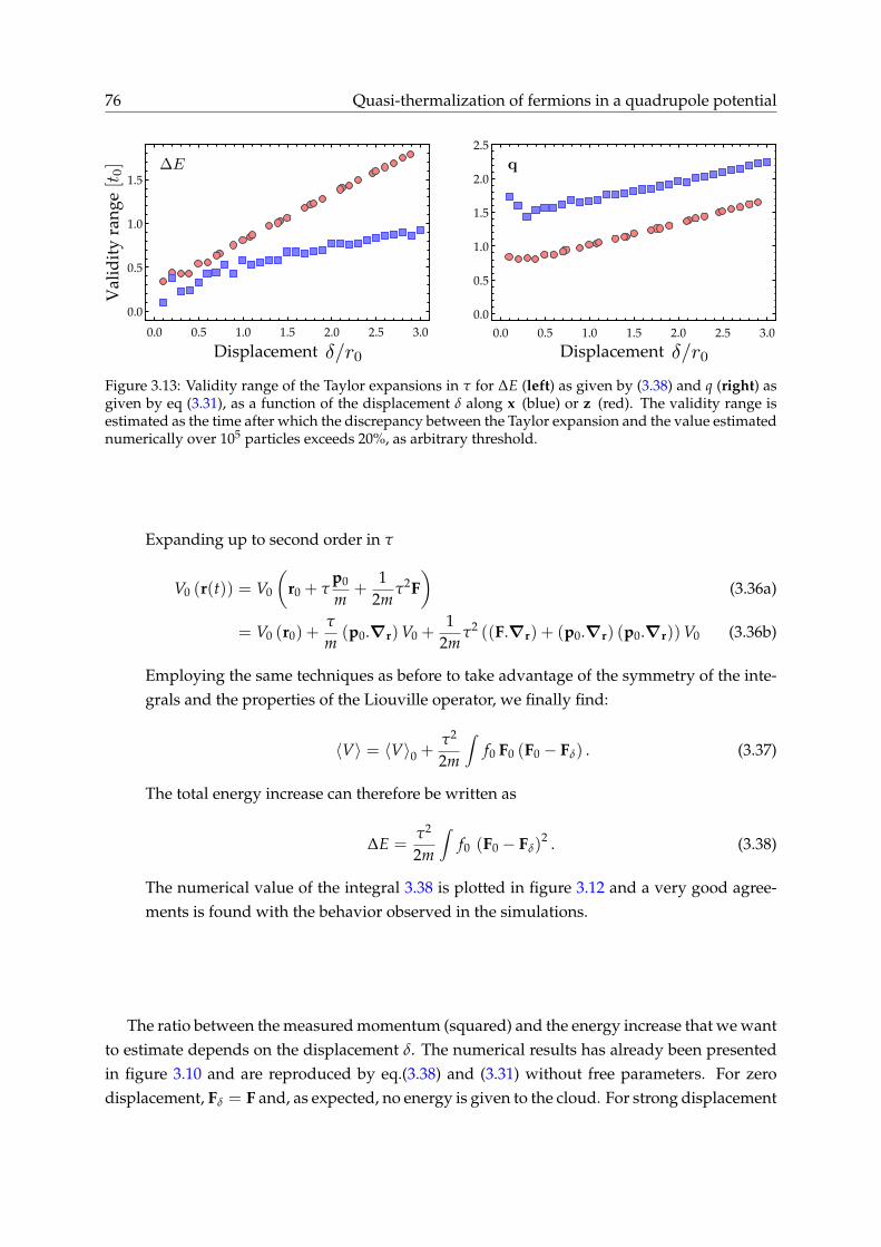
76 Quasi-thermalization of fermions in a quadrupole potentialV

alid

ity

ran

ge

0.0 0.5 1.0 1.5 2.0 2.5 3.0

0.0

0.5

1.0

1.5

0.0 0.5 1.0 1.5 2.0 2.5 3.0

0.0

0.5

1.0

1.5

2.0

2.5

Displacement Displacement

Figure 3.13: Validity range of the Taylor expansions in τ for ∆E (left) as given by (3.38) and q (right) asgiven by eq (3.31), as a function of the displacement δ along x (blue) or z (red). The validity range isestimated as the time after which the discrepancy between the Taylor expansion and the value estimatednumerically over 105 particles exceeds 20%, as arbitrary threshold.

Expanding up to second order in τ

V0 (r(t)) = V0

(r0 + τ

p0

m+

12m

τ2F)

(3.36a)

= V0 (r0) +τ

m(p0.∇r)V0 +

12m

τ2 ((F.∇r) + (p0.∇r) (p0.∇r))V0 (3.36b)

Employing the same techniques as before to take advantage of the symmetry of the inte-grals and the properties of the Liouville operator, we finally find:

〈V〉 = 〈V〉0 +τ2

2m

∫f0 F0 (F0 − Fδ) . (3.37)

The total energy increase can therefore be written as

∆E =τ2

2m

∫f0 (F0 − Fδ)

2 . (3.38)

The numerical value of the integral 3.38 is plotted in figure 3.12 and a very good agree-ments is found with the behavior observed in the simulations.

The ratio between the measured momentum (squared) and the energy increase that we wantto estimate depends on the displacement δ. The numerical results has already been presentedin figure 3.10 and are reproduced by eq.(3.38) and (3.31) without free parameters. For zerodisplacement, Fδ = F and, as expected, no energy is given to the cloud. For strong displacement

3.4 - A simple model for the effective heating 77

δ r0, we can Taylor-expand the expression and obtain

z− kick :∆E =32

q2 =32

E0η2 (3.39)

x− y− kick :∆E =34

q2 =34

E0η2 (3.40)

As mentioned in the introduction of this section, the energy gain is in fact larger than the valueq2/2, because the cloud also expands during the excitation whereby it gains additional poten-tial energy.

Inserting these asymptotic expressions in eq. (3.27), we finally obtain the relative tempera-ture increase along the excitation direction

∆TT0

=η2

2= α0 × η2 (3.41)

Remarkably, although the decoupling between degrees of freedom enhances the temperatureincrease along z for a given energy (eq. (3.27a), the stronger confinement reduces the amountof potential energy acquired during the kick in such way that all three directions show thesame relation between temperature increase and momentum kick. The value α0 = 0.5 is ingood agreement with the measurement performed experimentally.

The validity range of the previous Taylor expansions (3.31) and (3.38) with respect to τ

depends on the value of the displacement δ and the direction of the kick. Figure 3.13 shows thisvalidity range, estimated as the duration after which the discrepancy between the predictionof Taylor expansions and the value obtained in the simulation exceeds 20%.

Along x, the limiting factor is the validity of the Taylor expansion of ∆E, which appearsto be an acceptable estimate only for duration τ shorter than t0. For such shorts kick, themomentum acquired by the center of mass does not exceed q0. As the momentum measuredin the experiment can go up to 1.2 q0, the Taylor expansions (3.31) and (3.38) do not apply toour results. The good agreement between the prediction (3.41) and our experimental findingsshows that the validity range of the Taylor approximation is actually extended for the ∆E/η

ratio.

Along z, the validity range of the approximation is limited to τ ∼ t0 for most values of δ

but this duration is long enough to allow kicks up to q ∼ 2q0, well above the values measuredin the experiment. Consequently, the Taylor expansion can be relevant within experimentallyaccessible parameters and the prediction (3.41) can be applied, in good agreement with themeasured value.

78 Quasi-thermalization of fermions in a quadrupole potential

Hea

tin

g

0 5 10 15 20- 1

0

1

2

3

4

5

6

Displacement 0 2 4 6 8 10

0

2

4

6

8

10

12

Displacement

Figure 3.14: Heating after adiabatic displacement along x (left) and z (right). Results from numericalsimulations over 104 particles. Solid lines are given by (3.44-3.43) and the energy redistribution (3.27),without any free parameter.

0.0 0.2 0.4 0.6 0.8 1.0 1.2 1.4- 0.2

0.0

0.2

0.4

0.6

0.0 0.5 1.0 1.5 2.0 2.5 3.0

0.0

0.2

0.4

0.6

0.8

Hea

tin

g

Displacement Displacement

Figure 3.15: Heating along x (blue squares) and z (red circles) after adiabatic displacement along x(left) and z (right). Experimental results obtained in a trap of gradient b = 80 G/cm. The temperature isestimated by a time-of-flight measurement with 6 different durations. Each measurement is performed10 times and the errors bars indicated the standard error of the fit procedure. The solid lines are fits byequations (3.44) and (3.43) respectively assuming the energy redistribution (3.27), with T0 and b as freeparameter. Dashed lines are obtained without free parameters. Shaded areas give the 95% confidencelevel of the fits.

3.5 - Quasi thermalization in an isotropic trap 79

3.4.3 Another excitation: adiabatic displacement

Another way to provide energy to the distribution is to displace the trap center by slowlyraising up a magnetic field bias, so that the cloud can follow adiabatically the field zero. Oncethe trap has been displaced by a distance δ, the bias is abruptly switched off and the cloud issuddenly exposed to the initial potential. If the extinction is fast enough, no kinetic energy isgiven to the cloud during this process and it is possible to calculate analytically the potentialenergy of the ensemble:

〈V〉 =∫

drdp f0(r, p)V0(r− δ) (3.42)

The energy increase in then the simply the gain in potential energy:

z− kick :∆E = kBT0

(4 + (2δ/r0)2 − e−(2δ/r0)(4 + (2δ/r0))

(2δ/r0)− 1

)(3.43)

x− y− kick :∆E = kBT0

(4 + (δ/r0)2 − e−(δ/r0)(4 + (δ/r0))

(δ/r0)− 1

)(3.44)

Inserting (3.44) and (3.43) into (3.27), we can express the expected heating as a function of thedisplacement δ. The comparison with numerical simulations is shown in figure 3.14. Along z,a slight unpredicted decrease of the effective temperature is observed in the numerics, but doesnot hinder the almost complete decoupling. Within the (x,y) plane, the analytical predictionsare accurately verified by the numerical data.

Experimentally, this method has the advantage that the kick strength, simply given by thedisplacement δ, is easier to estimate. We keep a 40K sample during the excitation, wait 200 ms,and remove it selectively just before releasing the offset bias, so the 6Li ensemble starts from athermal distribution. Measurements are performed in a magnetic gradient set to b = 80 G/cm.

Results are presented in figure 3.15; a fit was performed taking the initial temperature T0

and the gradient b as free parameters. As expected, the heating along the unexcited direction isnegligible compared to the heating of the excited direction. Along x, the best fit is obtained forT0 = 367 µK and b = 109 G/cm. Along z, with a gradient set to to the same value, the best fitis obtained for T0 = 340 µK and b = 62 G/cm. In both cases, the theoretical prediction withoutany free parameter is within the 95% confidence level of the fit.

This additional validation shows that the energy redistribution (3.27), which assume a quasi-thermalization within the weak trapping plane (x,y) and a complete decoupling with the strongaxis z does not depend on the way the system is excited. A perfect momentum kick, a perfectposition kick or the intermediate experimental regime are all compatible with the same redis-tribution of the imparted energy.

80 Quasi-thermalization of fermions in a quadrupole potential

3.5 Quasi thermalization in an isotropic trap

The previous results (3.27) were obtained for an anisotropic trap V0 = µBb√

x2 + y2 + 4z2, con-strained by Maxwell equations. The effective decoupling between directions could be inherentto this specific geometry.

In this section, we study theoretically the quasi-thermalisation of non-interacting particlesin an isotropic potential V = µBb

√x2 + y2 + z2. We show that in such a 3D trap, the effec-

tive heating remains anisotropic as the kick orientation breaks the equivalence between alldirections. Considering ideal kicks, we calculate analytically the expected heating to ∆T‖ =

7∆E/15 along the kick direction, while the two transverse directions are heated by an amount∆T⊥ = ∆E/10. Surprisingly, the result is different in a 2D isotropic potential, where the heating∆T2D = ∆E/3kB is isotropic.

3.5.1 Isotropic 2D potential

We first show that for non interacting massive particles in a two dimensional trap V2D =

µBb√

x2 + z2, the heating resulting from a momentum kick q is isotropic and converges to-wards the value kB∆T2D = q2/6m for both directions. To do so, we show that any trajectory inthis 2D potential is fully characterized by two quantities, its energy E and angular momentumLz. As a consequence, the distribution function must be isotropic. This result strongly relieson Bertrand’s theorem (demonstrated in A.3.3), which states almost all but circular orbits areopen. The isotropy of the heating, along with energy conservation, leads to the result.

Step 1 Two trajectories with the same energy E and angular momentum Lz are arbitrarily close inphase-space, for almost all values of E and Lz.

Consider two initial positions (r0, θ0, pr0, Lz) and (r′0, θ′0, p′r0, Lz) with the same momentumLz and energy E = p2

r /2m + V(r) + L2z/2mr2. We want to show that the two trajectories

starting from those two points will come arbitrarily close to one another.

Since Lz and E are constants of motion, pr(t) is immediately given by r(t). We denote θ1

the value at which the system, starting from (r0, θ0, pr0, Lz), reaches its perihelion r1 forthe first time.

Starting from (r′0, θ′0, p′r0, Lz), since E′ = E, the trajectory will reach the same perihelionr′ = r1 with p′r = 0. From one perihelion to the next one, the systems gathers a constantapside angle θA, which can be expressed in terms of Lz and E:

Lz = mr2dθ/dt (3.45a)

⇒ θA = 2

perihelion∫

aphelion

Lz√2m(

H0 −V(r′)− L2z

2mr′2

)r′2

dr (3.45b)

3.5 - Quasi thermalization in an isotropic trap 81

A B

C

Figure 3.16: Trajectories in a linear potential. We first consider a trajectory starting at point A =(r0, θ0, pr0, Lz). The first perihelion of this trajectory is B. We now consider a second trajectory, start-ing at point C = (r′0, θ′0, p′r0, Lz) with the same energy and orbital momentum. We show that this secondtrajectory will come arbitrarily close to point B, meaning that the two trajectories are one and the same.

According to Bertrand’s theorem, the only central potential where the apside angle isalways commensurate with π are the Coulomb potential and the harmonic potential.For the linear potential considered here, the apside angle is therefore incommensuratewith π, except for an ensemble of trajectories of measure zero. For all other trajectories,Poincaré’s section for θ′[2π] is thus dense in [0, 2π[ and θ′ will come to a value arbitrarilyclose to θ1.

We have therefore proven that there is only one trajectory with a given (E, Lz).

Step 2 The stationary distribution function f (r, p) only depends on the energy E and the angularmomentum Lz.

Consider a trajectory (r(t), p(t)) with r = −∂pH et p = ∂rH. According to Liouville’sequation,

ddt

f (r, p) = r∂r f + p∂p f = −∂pH.∂r f + ∂rH.∂p f = 0 (3.46)

Therefore, for any two points (r1, p1) and (r2, p2) belonging to the same physical trajec-tory, f (r1, p1) = f (r2, p2) holds.

According to the previous step, two points with the same energy and momentum havealmost the same trajectory; by continuity, the distribution function can be expressed as afunction of the energy and momentum only:

f (r, p) = g (E (r, p) , Lz (r, p)) . (3.47)

Step 3 The heating is isotropic.

After the kick, we assume that the system evolves towards a distribution f . As provenbefore, this distribution depends only on the energy and the angular momentum. In

82 Quasi-thermalization of fermions in a quadrupole potential

polar coordinates (r, θ, p, ϕ), we can express the energy as per E = p2

2m +V(r) and angularmomentum as Lz = pr sin (θ − ϕ).

The momentum distribution is therefore given by:

n(p, ϕ) =∫

d2r f (r, p) (3.48a)

=∫

rdrdθ g(

p2

2m+ V(r), pr sin (θ − ϕ)

)(3.48b)

=∫

rdrdθ′ g(

p2

2m+ V(r), pr sin

(θ′))

(3.48c)

n(p) is independent of the angle ϕ and therefore isotropic. The kinetic temperature, ex-pressed as the standard deviation of n(p), does not depend on the direction.

Step 4 The energy redistribution leads to kB∆T2D = ∆E/3.

Using Virial theorem, we can relate the initial and final energies to the kinetic energies,

E = 3〈T〉 = 3 (〈T〉x + 〈T〉z) . (3.49)

We relate the kinetic energy to our definition of the effective temperature: 〈T〉x = kBTx/2.Considering the isotropy of heating and energy conservation, we obtain the result

∆E = 3kB∆T2D. (3.50)

Equation (3.50) is tested against numerical simulation (see Fig. 3.18), showing very good agree-ment with an R-squared value above 0.997 without any free parameter.

3.5.2 Isotropic 3D potential

We show that, even in a fully isotropic 3D potential V = µBb√

x2 + y2 + z2, the heating isanisotropic as the excited direction reaches a higher steady state temperature kB∆T‖ = 7∆E/15as the other two. Those two transverse directions receive a fraction of the input energy andreach the same final temperatures kB∆T⊥ = ∆E/10, thus showing a quasi-thermalization.

To calculate analytically the heating in an isotropic 3D linear trap, we use the property that,in a central potential, all trajectories remain planar. Within each plane, the 2D analysis of theprevious paragraph can be applied. The global behavior is then obtained as the sum over allplanes. The calculation presented below was performed by Jonathan Lau and Carlos Lobo.

Step 0 Coordinate system.

In order to take advantage of the planar nature of the trajectories, we first introduce anadequate coordinate system (see Fig. 3.17). Directions u and v are defined such that the

3.5 - Quasi thermalization in an isotropic trap 83

Figure 3.17: Introducing the coordinate system. We introduce the basis (u, v, w), derived from theCartesian coordinates with two rotations θ and ϕ such that the motion of the particle remains in the(u, v) plane.

plane they generate contains the relevant trajectory. Starting from the Cartesian coordi-nates (x, y, z), we consider a rotation θ around the x direction, followed by a rotation ϕ

around the u direction.

Within the (u, v) plane, we consider polar coordinates (r, αr) for the position and(

p, αp)

for the momentum. We can therefore express Cartesian coordinates as

x = r cos αr sin ϕ + r sin αr sin θ cos ϕ (3.51a)

y = −r cos αr cos ϕ + r sin αr sin θ cos ϕ (3.51b)

z = r sin αr cos θ (3.51c)

and resp. for r → p and αr → αp.

The Jacobian of this transformation is therefore given by |J| = r2 p2∣∣sin

(αr − αp

)cos θ

∣∣

Step 1 Estimation of the energy contained in a plane (θ, ϕ) after a small kick qz along z up to the secondorder.

The initial distribution of the cloud is given by a Maxwell-Boltzmann distribution:

f(r, p, t = 0−

)= A exp

(− 1

kBT

(p2

2m+ µBbr

)). (3.52)

where the constant A normalizes the distribution.

At t = 0, we perturb the ensemble by applying a sudden momentum kick qz:

f(r, p, t = 0+

)= f

(r, p− qzuz, t = 0−

)(3.53)

We calculate the kinetic and potential energies for the particles orbiting in a plane (θ, ϕ)

right after the excitation. Using the aforementioned coordinates, we can express the dis-

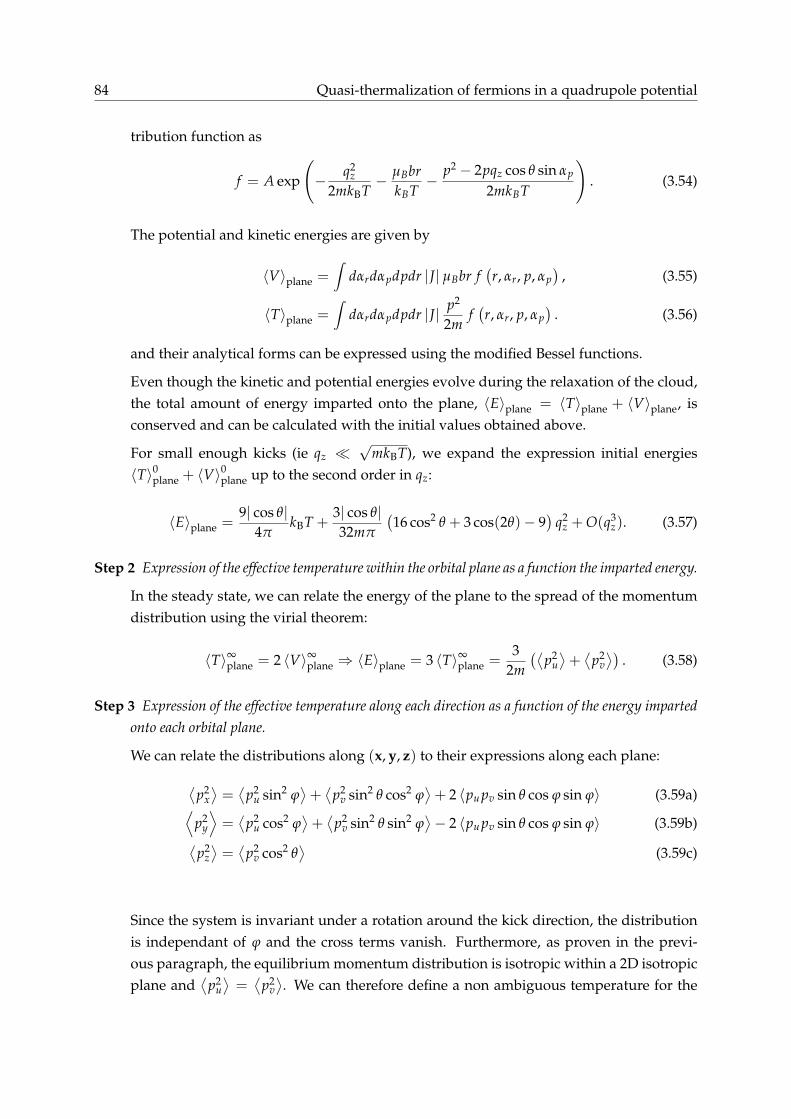
84 Quasi-thermalization of fermions in a quadrupole potential

tribution function as

f = A exp

(− q2

z2mkBT

− µBbrkBT

− p2 − 2pqz cos θ sin αp

2mkBT

). (3.54)

The potential and kinetic energies are given by

〈V〉plane =∫

dαrdαpdpdr |J| µBbr f(r, αr, p, αp

), (3.55)

〈T〉plane =∫

dαrdαpdpdr |J| p2

2mf(r, αr, p, αp

). (3.56)

and their analytical forms can be expressed using the modified Bessel functions.

Even though the kinetic and potential energies evolve during the relaxation of the cloud,the total amount of energy imparted onto the plane, 〈E〉plane = 〈T〉plane + 〈V〉plane, isconserved and can be calculated with the initial values obtained above.

For small enough kicks (ie qz √

mkBT), we expand the expression initial energies〈T〉0plane + 〈V〉0plane up to the second order in qz:

〈E〉plane =9| cos θ|

4πkBT +

3| cos θ|32mπ

(16 cos2 θ + 3 cos(2θ)− 9

)q2

z + O(q3z). (3.57)

Step 2 Expression of the effective temperature within the orbital plane as a function the imparted energy.

In the steady state, we can relate the energy of the plane to the spread of the momentumdistribution using the virial theorem:

〈T〉∞plane = 2 〈V〉∞plane ⇒ 〈E〉plane = 3 〈T〉∞plane =3

2m(⟨

p2u⟩+⟨

p2v⟩)

. (3.58)

Step 3 Expression of the effective temperature along each direction as a function of the energy impartedonto each orbital plane.

We can relate the distributions along (x, y, z) to their expressions along each plane:

⟨p2

x⟩=⟨

p2u sin2 ϕ

⟩+⟨

p2v sin2 θ cos2 ϕ

⟩+ 2 〈pu pv sin θ cos ϕ sin ϕ〉 (3.59a)

⟨p2

y

⟩=⟨

p2u cos2 ϕ

⟩+⟨

p2v sin2 θ sin2 ϕ

⟩− 2 〈pu pv sin θ cos ϕ sin ϕ〉 (3.59b)

⟨p2

z⟩=⟨

p2v cos2 θ

⟩(3.59c)

Since the system is invariant under a rotation around the kick direction, the distributionis independant of ϕ and the cross terms vanish. Furthermore, as proven in the previ-ous paragraph, the equilibrium momentum distribution is isotropic within a 2D isotropicplane and

⟨p2

u⟩=⟨

p2v⟩. We can therefore define a non ambiguous temperature for the

3.5 - Quasi thermalization in an isotropic trap 85

1D 2D isotropic 2D anisotropic 3D isotropic 3D exp. trap (x,y) 3D exp. trap (z)kB∆Tx 2∆E/3 ∆E/3 2∆E/3 7∆E/15 ∆E/3 0kB∆Tz - ∆E/3 0 ∆E/10 0 2∆E/3kB∆Ty - - - ∆E/10 ∆E/3 0

Table 3.1: Heating along each direction for different trap geometries. Results for the 1D, 2D and 3Disotropic traps are analytical calculations verified with numerical simulations (the 1D case can not berealized experimentally due to Majorana losses). Results for the 2D and 3D anisotropic traps assumecomplete decoupling between x, y and z.

Hea

tin

g

Kick Kick 0.0 0.5 1.0 1.5 2.0

- 0.2

0.0

0.2

0.4

0.6

0.8

1.0

0.0 0.5 1.0 1.5 2.0- 0.2

0.0

0.2

0.4

0.6

0.8

1.0

2D 3D

Figure 3.18: Heating as a function of the kick strength after an excitation along x in an isotropic 2Dtrap (left) and 3D trap (right). Temperatures are given along x (blue squares), y (gray triangles) and z(red circles). Points are obtain by numerical simulation over 10 000 particles. Solid lines are given byequations (3.50) and (3.62a-3.62b) with ∆E = q2/2m without any free parameter.

86 Quasi-thermalization of fermions in a quadrupole potentialH

eati

ng

1 1.02 1.04 1.06 1.08 1.1

0

0.1

0.3

0.2

1 2 3 4

0

0.1

0.3

0.2

Trap strengthTrap strength

Figure 3.19: Heating after an excitation of amplitude ∆E along x in an anisotropic potential V =

µBb√

x2 + y2 + γ2z z2, as a function of the anisotropy factor γ2

z . Temperatures are given along x (bluesquares), y (gray triangles) and z (red circles). Points are obtained by numerical simulation over 100 000particles. Dashed lines show the prediction for an isotropic trap as derived in eq. (3.62). Solid lines aregiven by the previous model, assuming a complete decoupling between z and the other two directions.Note that the heating along y brutally jumps from its value in an isotropic trap ∆Ty/T0 = ∆E/10 to avalue close to a strongly anisotropic situation ∆Ty/T0 = ∆E/3 as soon as γ2

z 6= 1.

Trap strength

0 200 400 600 800 1000

1

1.1

1.2

1 1.02 1.04 1.06 1.08 1.10

200

400

800

600

Eff

ecti

ve

tem

per

atu

re

Th

erm

aliz

atio

n t

ime

Time

Figure 3.20: Left: the thermalization time is estimated as the duration after which the unexcited directiony reaches its final value Ty = Tx. Right: Thermalization time as a function of the anisotropy factor γ2

z .The solid line given by the best hyperbolic fit t = 6.67

γ2z−1

t0.

3.6 - Influence of the trap anisotropy 87

plane,1m⟨

p2⟩plane =

13〈E〉plane . (3.60)

The above expressions (3.59) can be therefore further simplified to:

kBTy = kBTx =⟨

p2x⟩=

mπ

6

π∫

0

dθ 〈E〉plane(1 + sin2 θ

), (3.61a)

kBTz =⟨

p2z⟩=

mπ

3

π∫

0

dθ 〈E〉plane cos2 θ. (3.61b)

Step 4 Expression of the effective heating. The expression of 〈E〉plane obtained before can be read-ily integrated to relate the heating in each direction to the kick initially applied to theatoms. Considering that the energy transferred to the cloud is ∆E = q2

z/2m, we canexpress the heating as a function of the kick’s energy:

kBTy = kBTx = ∆E/10, (3.62a)

kBTz = 7∆E/15. (3.62b)

Equations (3.62a-3.62b) are in very good agreement with numerical simulations, reaching R-squared values above 0.9 without any free parameter, as shown in figure 3.18.

Results obtained in this section are summarized in table 3.1. Remarkably, it appears that theexpected heating remains anisotropic even in a 3D isotropic trap, but that this results stronglydepends on the system dimensionality.

3.6 Influence of the trap anisotropy

We have shown that the energy redistribution for non-interacting particles in a strongly anisotropictrap V = µBb

√x2 + y2 + 4z2 is qualitatively different from the one in a isotropic trap V =

µBb√

x2 + y2 + z2. In the first case, the anisotropy is set by the trap while in the second, thesymmetry breaking is induced by the excitation. In this section, we investigate numerically theintermediate regime as we vary the trap geometry by playing with a factor γz > 1:

V = µBb√

x2 + y2 + γ2zz2. (3.63)

3.6.1 Anisotropy of the steady state

We first estimate the effective heating resulting from an initial excitation along x as a function ofthe trap geometry γ2

z . Results are presented in figure 3.19 and show a very flat behavior: as soonas the trap shows the slightest anisotropy γ2

z > 1, the heating along x and y suddenly jump

88 Quasi-thermalization of fermions in a quadrupole potential

from their isotropic value (3.62) to their fully decoupled value (3.27). Along z, the effectiveheating becomes continuously smaller as the confining potential becomes more anisotropic,reaching an almost complete decoupling as soon as γ2

z > 1.1

The energy redistribution thus weakly depends on the confinement geometry: in all anisotropicconfigurations, the symmetry plane is almost decoupled from the symmetry axis and presentsa homogeneous heating. The situation observed in the previous chapter is thus not due to apeculiar geometry but illustrates a broadest kind of behavior.

3.6.2 Quasi-thermalization time

In an isotropic trap, if the steady-state towards which the distribution relaxes scarcely dependson the confinement geometry, the time it takes for the system to relax does.

We estimate the quasi-thermalization time τ as the time it takes for the unexcited directiony to reach 99% of its final value. Results are resented in figure 3.20. The more symmetric thetrap, the longer the relaxation time, which diverges as the confinement becomes isotropic. Arational fit estimates the scaling law to τ ∝ (γ2

z − 1)−1, with an R-squared value of 0.99.

The scaling can be interpreted in terms of precession period. It is well known that in aNewtonian field such as gravity, an anisotropy of the source distribution leads to precession ofthe orbital plane. Jonathan Lau extended the result to a quadrupole potential and showed that,in the (γ2

z − 1) 1 limit, the precession rate of a single particle trajectory can be expressed as:

φ = −E Lz

3L3 (γ2z − 1), (3.64)

where L is the angular momentum of the particle. This scaling suggests that the equipartitionof energy within the (x,y) plane is due to this precession mechanism. This qualitative pictureexplains the abrupt change in behavior for the y heating as well as the progressive evolution ofthe z heating for increasing values of γz. The slower the precession rate, the longer it takes forthe dephasing to redistribute the energy along the two directions of the symmetry plane. For asmall anisotropy, the energy redistribution is first dictated by the isotropic behavior, before theprecession of orbital planes equilibrate temperatures along x and y. The heating along z thusremains close to its isotropic value, while the heating along x and y reach the average valuebetween both directions. As γz increases, the dynamics changes qualitatively as the precessiondispatches the energy faster and faster. For a large anisotropy, the imparted energy is firstredistributed between within the symmetry plane, before other repartitions could take place.

3.7 - Conclusions 89

3.7 Conclusions

In this chapter, we have shown that, even in the absence of interactions, a spin-polarizedLithium cloud in a quadrupole potential can relax towards steady state. We characterize thisnon-Boltzmann equilibrium by effective temperatures corresponding to the spread of the mo-mentum distribution, an experimentally accessible parameter. If the cloud is perturbed by aninitial excitation, the imparted energy is redistributed owing to the dephasing of single parti-cle trajectories and results in an effective heating. The non-thermal nature of the steady stateappears clearly as the final temperatures do not equilibrate between directions, but show a de-coupling between the strong axis z and the symmetry plane (x,y). Yet, within the symmetryplane, the temperatures do equilibrate regardless of the initial excitation, showing a quasither-malization.

Assuming a complete decoupling, general considerations allow for quantitative predictionsof the heating resulting from an initial excitation. Numerical simulations were performed andverified those results in various situations (ideal kick, experimental excitation, adiabatic dis-placement). Their application to experiments requires to estimate the imparted energy frommeasurable parameters, such as the center of mass momentum or position. This estimationdepends on the actual description of the excitation and we propose two different schemes forwhich analytical predictions, numerical simulations and experimental results are in satisfyingagreement.

We demonstrated analytically the value of the effective heating in an isotropic trap and showthat the result strongly depends on the dimensionality of the system. In 2D, the temperatureincrease becomes isotropic regardless of the initial excitation while in 3D, the kick’s directionprovides a symmetry breaking. The isotropic geometry appears as a particular case, as the en-semble evolves towards an almost decoupled steady state as soon as the confinement is slightlyanisotropic, with a relaxation time all the shorter as the anisotropy increases.

In the next chapter, we will show that the exact same behavior appears on an ensemble ofnon-interacting relativistic Weyl particles confined in a harmonic trap.

Chapter

4 Analog simulation of Weylparticles in a harmonic trap

Contents4.1 Weyl particles: from high energy Physics to cold atoms . . . . . . . . . . . . . . . . . . 92

4.1.1 A paradigm in high energy physics . . . . . . . . . . . . . . . . . . . . . . . . . . . 92

4.1.2 Emergent low energy excitations . . . . . . . . . . . . . . . . . . . . . . . . . . . . 93

4.1.3 Weyl particles in a trapping potential: the Klein paradox . . . . . . . . . . . . . . . 98

4.2 Analogue simulation of Weyl particles . . . . . . . . . . . . . . . . . . . . . . . . . . . . . 99

4.2.1 Canonical mapping . . . . . . . . . . . . . . . . . . . . . . . . . . . . . . . . . . . . 100

4.2.2 Majorana losses and Klein paradox . . . . . . . . . . . . . . . . . . . . . . . . . . . 100

4.2.3 Quasi-thermalization in a harmonic trap . . . . . . . . . . . . . . . . . . . . . . . . 101

4.3 Geometric potentials . . . . . . . . . . . . . . . . . . . . . . . . . . . . . . . . . . . . . . . 104

4.3.1 Berry phase, scalar and vector potential . . . . . . . . . . . . . . . . . . . . . . . . 104

4.3.2 Effect of the geometric potentials . . . . . . . . . . . . . . . . . . . . . . . . . . . . 107

4.4 Conclusions and outlooks . . . . . . . . . . . . . . . . . . . . . . . . . . . . . . . . . . . . 109

MAssless Weyl particles constitute one of the paradigms of High Energy Physics and emergein condensed matter systems in the form of low-energy excitations. Unlike massive par-

ticles, they possess a linear dispersion relation around the so called Weyl point. This linearityinduces the conservation of helicity, i.e. the projection of the particle’s spin onto the direction ofits momentum, resulting among other things in remarkable transport properties. The behaviorof Weyl particles in a trap is also highly non-intuitive, as they undergo anomalous tunnelingwhich can lead to a decrease or cancellation of the back-scattering on a potential barrier, asdepicted by the Klein paradox.

Those properties have brought an increasing interest in Weyl particles, even more so asthey have also been suggested to represent possible platforms for quantum computation andquantum information processing. Using a canonical mapping, we show that some propertiesof non-interacting Weyl particles confined in a harmonic trap can be simulated and studiedwith cold atoms in a quadrupole potential. In absence of collisions, all the results presented inthe previous chapter can therefore be applied to describe the evolution of out-of-equilibriumWeyl particles following an initial excitation. We show that, unlike massive particles whichwould oscillate without damping, a distribution of Weyl particles in a harmonic trap relaxes

91

92 Analog simulation of Weyl particles in a harmonic trap

towards a steady state, even in the absence of interactions and that the energy initially impartedonto the cloud is redistributed anisotropically. This analogy also allows us to translate specificproperties of ultra-relativistic particles in the language of cold atoms, interpreting for instancethe Klein paradox as a manifestation of Majorana losses.

In this chapter, we first review some properties of Weyl particles and recent developments inthe field. We introduce the mapping that allows the analog simulation of harmonically trappedWeyl particles with cold atoms and adapt results from the previous chapter to describe the re-laxation dynamics of a Weyl ensemble dragged away from the trap center. We then derivegeometric potentials associated with the Berry phase of the system and study numerically theinfluence of the resulting topological properties on the previous dynamics. Finally, we showthat our approach of analogue simulation can be used to study a much wider variety of prob-lems, such as massive relativistic particles or particles with 2D spin-orbit coupling.

4.1 Weyl particles: from high energy Physics to cold atoms

Recents observations of Weyl particles in condensed matter systems [Huang et al. 2015, Luet al. 2015, Xu et al. 2015b] have brought them under the limelights1. We start this chapter byreviewing the main properties of Weyl fermions that triggered the wide interest for this field ofresearch.

4.1.1 A paradigm in high energy physics

Weyl fermions were first introduced in 1929 as massless solutions to the Dirac equation [Weyl1929] (

ihγµ∂µ −m)

Ψ = 0 (4.1)

where the Dirac matrices γ0,1,2,3 are defined such that the Hamiltonian H = γ0 (γi pi + m)

ishermitian and satisfies the relativistic equation H2 = m2c4 + p2c2. Together with Majorana andDirac fermions [Pal 2010], Weyl fermions provide a description of all possible spin 1/2 matterfields.

Two properties related to the spin of a particle serve as criteria to discriminate betweensolutions of the Dirac equation. The helicity corresponds to the projection of the spin S of aparticle onto its momentum p

h = 2S.p

p. (4.2)

For a spin 1/2 particle, the eigenvalue of such an operator are +1, corresponding to "right-handed" particles and −1, corresponding to "left-handed" particles. The helicity operator com-mutes with the Dirac Hamiltonian (4.1), meaning that helicity is a conserved quantity for free

1And allowed all kinds of puns, as epitomized by the viewpoint "Where the Weyl Things Are" [Vishwanath 2015]or the commentary "It’s been a Weyl coming" [Bernevig 2015]. Nature Physics editorial [Editorial 2015] summarizedthe situation: "Like London buses, you wait for a Weyl then a few come along at once."

4.1 - Weyl particles: from high energy Physics to cold atoms 93

particles. As a dot product, helicity is also obviously invariant under rotations, but not underLorentz boosts. For an observer going faster than the particle, the orientation of the momentumis inverted and the helicity changes sign.

On the other hand, the chirality is defined by the effect of the γ5 = iγ0γ1γ2γ3 matrix, whichanti-commutes with all Dirac matrices. Two projectors L, R = 1

2

(1∓ γ5) can be defined from

this operator, leading to a partition of the Hilbert space as the sum of left-chiral and right-chiralsolutions of the Dirac equation

Ψ = ΨL + ΨR, (4.3)

with ΨL = LΨ, LΨL = ΨL and RΨL = 0, and equivalent relations can be written for ΨR.The chirality has opposite properties with respect to helicity: it is boost invariant, but is notconserved through the evolution of free particles because γ5 anticommutes with the mass termγ0m.

In absence of rest mass, the helicity and chirality of Weyl fermions can be identified andconstitute a well defined quantity, independent of the observer (as the velocity of masslessparticles is invariant under a Lorentz boost) and conserved through the time evolution (as γ5

anti-commutes with all terms of the Hamiltonian). Left and right handed Weyl fermions appearas irreducible representations of the Lorentz group and, remarkably, any massive fermionicfield (Majorana or Dirac) can be expressed as the direct sum of two massless Weyl fields withopposite helicities.

Weyl fermions appear as building blocks of particle physics, but had never been observeddirectly in that field. They were suggested at first to describe neutrinos, but the observation offlavour oscillations implying a non-zero rest mass ruled out this hypothesis.

4.1.2 Emergent low energy excitations

Even though Weyl fermions have no existence of their own in high energy physics, they appearas a relevant description of low energy excitations of electrons in crystalline structures with alinear dispersion relation around a so-called Weyl point. In both low and high energy physics,the Hamiltonian takes the form

HWeyl = h ∑i∈x,y,z

cijkiσj = hc k.σ, (4.4)

where h is the reduced Planck constant, c has dimension of velocity, k is the momentum of theparticle (relative to the Weyl point) and σi are Pauli matrices (in the basis of the bands involved).The latter equality corresponds to an isotropic dispersion relation. Because of this analogyand because of the very small overlap between the valence and conduction bands, condensedmatter systems displaying such a dispersion relation are called Weyl semi metals [Nielsen andNinomiya 1983, Young et al. 2012]. The corresponding dispersion relation is pictured in figure

94 Analog simulation of Weyl particles in a harmonic trap

Figure 4.1: Left: one dimensional dispersion relation around a Weyl point described by (4.4), for spin σoriented along +x (solid line) or along −x (dashed line). Particles with positive helicity (ie spin alignedwith momentum) have positive energies (red) while particles with negative helicity have negative ener-gies (blue). Right: filling of two Weyl points in momentum space. The distance between the nodes is setby the geometric properties of the material. The two bands connect far from the nodes, as indicated bythe dashed lines. The grey plane represents the surface state resulting from the topological propertiesof the system (see main text), with energies in the gap between the nodes. Fermi arcs are the 1D Fermisurface of those states.

4.1.

Equation (4.4) reminds the low energy excitations emerging from 2D Dirac points in graphene[Geim and Novoselov 2007]. However, the difference of dimensionality leads to very distinc-tive properties2. A gap can easily be opened in a graphene Dirac cone by an orthogonal mag-netic field, inducing an additional term µBσz, where µ is the magnetic moment of the particle.By contrast, all three Pauli matrices are involved in (4.4) and the Weyl cone is therefore pro-tected against most perturbations [Turner and Vishwanath 2013].

The robustness of a Weyl point can be related to the existence of a topological quantity, thechirality quantum number [Hosur and Qi 2013], which is defined as

χ = sign[det(cij)] = ±1. (4.5)

The chirality quantum number corresponds to the Chern number of the valence band: as anelectron follows adiabatically the eigenstates of the band |uk〉, it experiences the equivalent ofan effective vector potential A = i〈uk|∇k|uk〉, corresponding to a Berry connection in momen-tum space [Berry 1984]. After a round-trip, the resulting accumulated phase corresponds to an

2Dirac points can also be extended to 3D, where they describe the touching point of four bands. Just like Diracfermions can be expressed as the direct sum of two Weyl fermions, a Dirac point can be seen as the overlap oftwo Weyl points with opposite chirality. The resulting Dirac point has no topological protection as additional 4×4matrices can open a gap, but its robustness can nevertheless be increased by the crystalline symmetries.

4.1 - Weyl particles: from high energy Physics to cold atoms 95

effective magnetic flux of

∫∫d2k.A =

∮

FSdk F(k).dS(k) = 2πχ, (4.6)

where the integral can be carried over any Fermi surface enclosing the Weyl node and F(k) =∇k × A is analogous to a Berry curvature. Equation (4.6) corresponds to the flux that wouldinduce a single magnetic charge, which is why Weyl points are sometimes treated as magneticmonopoles in the momentum space. We will show in section 4.3 that this properties remainstrue for trapped Weyl particles.

In between two separated Weyl points, each 2D slice in momentum space can be thought as atopological insulator with a gap depending on the distance to the nodes. In finite size samples,this results in the existence of edge states whose energies belong to the gap between the nodes(see Fig. 4.1). Those edge states give rise to a characteristic feature of Weyl semimetals, astheir filling up to the chemical potential corresponds to a 1D Fermi surface called Fermi arc.Using angle resolved photo-emission spectroscopy [Behrends et al. 2015], such Fermi arcs wererecently observed in TaAs [Xu et al. 2015a], Na3Bi [Xu et al. 2015b] as well as in photonic crystals[Lu et al. 2015].

The previous discussion shows that every Weyl point has a fixed chirality and radiates aChern flux. This topological property leads to a phenomenon specific to 3D systems: the Adler-Bell-Jackiw chiral anomaly [Adler 1969, Bell and Jackiw 1969], which corresponds to the non-conservation of electric charge. For particles with unit charge e and chirality χ described by(4.4), an electric E and magnetic B fields induce an electromagnetic current jχ such that

∂tnχ + div(jχ) = −χe3

32π2h2 E.B, (4.7)

where nχ is the density of particles with chirality χ. The apparent paradox is solved by consid-ering that, since the total Chern number over all bands should be zero, Weyl points necessarilyexist as pairs with opposite chirality [Nielsen and Ninomiya 1981] and the total current j+ + j−is well conserved as charges are pumped from one point to the other (see Fig. 4.2).

The chiral anomaly 4.7 also induces remarkable transport properties [Burkov 2015], such as

• Negative magneto-resistance

One of the first signatures of the chiral anomaly was suggested in the form of a negativemagneto resistance [Nielsen and Ninomiya 1983]. If the temperature and chemical poten-tial are small enough for the positive Landau levels (n > 0 in Fig. 4.2) not to be populated,collisions between particles with the same chirality are suppressed due to lack of avail-able phase-space. In absence of impurities in a clean sample, the charge imbalance canonly be relaxed through collisions of particles close two different Weyl points. As Weylpoints are well separated in momentum space, such processes require strong momentum

96 Analog simulation of Weyl particles in a harmonic trap

Figure 4.2: Landau levels of a Weyl particle. In an external magnetic field Buz, the energy spectrumof a charged particle in (4.4) is given for n 6= 0 by En = sign(n)c

√2h|n|eB + (hkz)2, where kz is the

momentum from the Weyl node along the direction of the magnetic field. The zeroth Landau levelsn = 0 are highly degenerate (with a factor SeB/h, S being the sample area) and provide one dimensionalchiral levels with different energies for right chiral nodes (E0 = +hckz) and left chiral nodes (E0 =−hckz). The occupancy of the zeroth Landau levels is pictured with filled symbols.An intuitive picture recovers the expression (4.7) of the chiral anomaly [Hosur and Qi 2013]. In presenceof a magnetic field B, the zeroth Landau levels can be pictured as conducting wires parallel to themagnetic field. An external electric field E sets particles in motion through those wires. Because thezeroth Landau Level is chiral, the slope of the relation dispersion is fixed for each Weyl nodes. Particlesare pumped from one node to the other, resulting in a apparent non-conservation of the charge for eachnode taken separately.

transfer and the corresponding relaxation time can be long, improving the conductivityof the electron gas. Furthermore, the degeneracy of the Landau levels contributing tothe current is proportional to the magnetic field’s strength. Those two effects lead to adecrease of the resistance in the direction of an applied magnetic field, proportional tothe field strength, as opposed to the response of an ordinary metal or semiconductor thatshows a weak, positive magneto-resistance independent of the external field orientation.

Observations of such negative magneto-resistance was reported, for instance in Bi0.97Sb0.03

[Kim et al. 2013], HgMnTe [Orlita et al. 2014] and TaAs [Huang et al. 2015]. Most of theseexperiments were performed in a semi-classical regime, without Landau-level quantiza-tion, where intra-node collisions dominate over other relaxation processes. In such cases,the negative magneto-resistance effect still remains but scales with the square of the mag-netic field [Son and Spivak 2013].

• Anomalous Hall effect

As mentioned before (eq. (4.6)), each 2D slice between the Weyl nodes in momentumspace can be thought of as topological insulators with unit Chern number. As a result,charged particles in presence of an electric field give rise to a current J = E×Gh orthog-

4.1 - Weyl particles: from high energy Physics to cold atoms 97

Figure 4.3: A possible setup to probe the existence of a non-local transport. A voltage VSD is applied atone end of the sample. At a distance L much larger than the typical range of the induced current (setby the sample thickness d), the presence of a persistent voltage VNL advertises the existence of a chiralanomaly, which prevents the relaxation of carriers’ populations. Illustration from [Parameswaran et al.2014], where a measurement of this non-ohmic voltage is suggested by taking advantage of an externalmagnetic field.

onal to the field. The Hall conductivity Gh can be expressed as:

GH =e2

2πh ∑i

χiki, (4.8)

where the sum is taken over the Weyl points, χi is the chirality of the node and ki itsposition in momentum space [Burkov 2014]. This conductivity is not proportional to anexternal magnetic field and does not depend on impurities, but relies only on the intrinsicproperties of the material (namely the distance between Weyl nodes), hence the nameintrinsic anomalous Hall effect (AHE) [Nagaosa et al. 2010].

• Non-local transport

Another spectacular behavior related to the chiral anomaly takes the form of non-localtransport properties, as a persistent voltage can be measured much further from the elec-trodes than the standard Ohmic range.

Consider a rectangular piece of ordinary metal with four contacts attached as in figure4.3. Two of those contacts are used as source and drain for an electric current J. The volt-age applied between those points quickly drops away from the contacts, with a typicaldistance given by the mean free path, limited by the width d of the sample.

In a Weyl semimetal in presence of a local magnetic field, the chiral anomaly gives riseto an imbalance between the occupation of the two Weyl nodes. As mentioned above,the relaxation of the imbalance is limited by internode scattering and the correspondingmean free path can be much larger than sample width. At distances L d, the valley

98 Analog simulation of Weyl particles in a harmonic trap

Figure 4.4: Illustration of the Klein paradox. As a Weyl particle arrives on a potential barrier, it canaccess the lowest branch of the dispersion relation. The spin of the particle is conserved as the potentialcommutes with it (the particle remains on a solid line) and the potential thus scatters a particle of positivemomentum to a negative momentum state. The direction of motion, given by ∂pH, is preserved and theparticle keeps moving forward, tunneling through the barrier.

imbalance remains and could be measured with a local probe magnetic field, whereas theOhmic voltage has vanished [Parameswaran et al. 2014].

4.1.3 Weyl particles in a trapping potential: the Klein paradox

Around Weyl- or Dirac points, the linearity of the dispersion relation makes the local density ofcarrier extremely sensitive to electric fields, and opens the way to the engineering of quantumdevices by applying an external confinement. For instance, quantum dots using electrostaticgates could be realized in graphene strips, despite the high density of conduction electronne ' 4× 1015 cm−2 [Castro Neto et al. 2009]. Such quantum dots in semi metal are promis-ing candidates for the realization of quantum dots solar cells, as their reduced gap allows forefficient multiexciton generation [Delerue and Allan 2011].

However, unlike massive particles described by the Schrodinger equation, relativistic-likeparticles have a peculiar ability to escape through potential barrier under certain conditions,rendering the realization of localized states challenging. This effect originates from the Kleinparadox3 [Klein 1929] and is pictured in figure 4.4. As a Weyl particle arrives at a potentialbarrier, it can access the lowest branch of the dispersion relation, where the kinetic energy de-creases with momentum. As a result, the particle tunnels through barriers much higher thanits energy, with perfect transmission for an infinitely high barrier. In the strictly one dimen-

3Historically, Klein paradox was introduced for massive particles facing barriers exceeding twice their rest mass.

4.2 - Analogue simulation of Weyl particles 99

sional case, such as carbon nano-tubes, the Klein paradox leads to a suppression of the back-scattering of relativistic electrons [Ando et al. 1998] and forbids their trapping. In the 2D case,Klein paradox can be extended to show that the quantum tunneling of a particle through a bar-rier possesses resonant incident angles, at which the barrier becomes transparent [Katsnelsonet al. 2006]. Apart from these specific cases (1D and resonant angles at 2D), it is a priori possibleto confine relativistic-like particles despite Klein paradox, for instance by applying a harmonicelectric potential on a layer of graphene [Silvestrov and Efetov 2007].

4.2 Analogue simulation of Weyl particles

Predicted decades ago, the observation of Weyl points was reported only recently. A reasonmight be that the pairing of Weyl points with opposite chiralities makes the experimental real-ization of Weyl semimetals challenging. Indeed, in most materials, Weyl points are degenerateand the resulting Dirac semimetal does not feature the topological properties mentioned above.To lift the degeneracy and separate Weyl points in momentum space, time-reversal or inversionsymmetry must be broken, strongly constraining the exploitable compounds.

Owing to their high degree of control and versatility, ultra-slow cold atoms offer a comple-mentary route for the experimental study of ultra-fast relativistic Weyl particles. For instance,the simulation of Weyl particles has recently been proposed as a 3D extension of the 2D HarperHamiltonian where inversion symmetry breaking, required to generate Weyl points, would beensured by a site-dependent hopping phase [Dubcek et al. 2015]. However, such a realizationrequires a very fine control of the artificial magnetic flux per plaquette, all the more so as thelattice is large: flux fluctuations above 1-2% would destroy the Weyl nodes in a 160×160×160lattice [Lepori et al. 2015]. Ions chains have also been proven able to mimic the behavior solu-tions of Dirac equation [Gerritsma et al. 2010], including Klein paradox [Gerritsma et al. 2011].

In this section, we propose an alternative approach: instead of reproducing the exact Hamil-tonian (4.4), we show that non-interacting Weyl particles confined in a harmonic trap can bemapped onto Lithium atoms in a quadrupole potential. This mapping enables us to apply re-sults presented in the previous chapter to predict the relaxation of Weyl particles which weredragged away from the trap center. We can also interpret properties of Weyl particles in termsof atomic physics, highlighting for instance the parallel between the Klein paradox and Majo-rana losses.

100 Analog simulation of Weyl particles in a harmonic trap

4.2.1 Canonical mapping

Let us first recall the Hamiltonian of a spin 1/2 particle with magnetic moment µ in a magneticfield, as introduced at the beginning of the previous chapter:

H0 (r, p) =p2

2m− µ σ.B0(r), (4.9)

where σ are the Pauli matrices. In a quadrupole trap, the magnetic field takes the form B(r) =b(γxx, γyy, γzz), where z is the symmetry axis of the coils, b denotes the magnetic field gradientand Maxwell’s equations imply γx = γy = 1, γz = −2.

Starting from the above Hamiltonian (4.9), we define X and P by a canonical mapping ex-changing position and momentum:

Xi =cpi

µbγi, Pi = −

µbxiγi

c, (4.10)

with c being an arbitrary velocity scale. These new coordinates verify the commutation relation[X, P] = ih and can be used to rewrite the previous Hamiltonian as:

H = c σ.P +12

k0 ∑i

γ2i X2

i , (4.11)

where k0 = µ2b2/mc2 (note that k0 has the dimension of a spring constant, not of a wavevector). The first term corresponds to the kinetic energy cσ · P of a massless Weyl particlemoving at velocity c while the second one is readily identified as an anisotropic harmonicpotential, characterized by spring constants ki = γ2

i µ2b2/mc2 along each direction i. MasslessWeyl particles in a harmonic trap are thus equivalent to massive atoms in a magnetic fieldgradient. In the following, Weyl particles and massive atoms will be referred to using upper-and lower-case symbols respectively.

4.2.2 Majorana losses and Klein paradox

The single-particle trajectories of the Weyl particles or Lithium atoms can be obtained usingEhrenfest’s theorem, applied to the Hamiltonians (4.11) and (4.9).

Xi = cσi (4.12)

Pi = −k0γ2i Xi (4.13)

σ = 2cσ × P/h. (4.14)

pi = µbγiσi (4.15)

xi = pi/m (4.16)

σ = 2µBσ × B(r)/h. (4.17)

Note that Eq. (4.12) through (4.17) are fully quantum, but since we work in the classicalregime, we will only consider their mean values.

4.2 - Analogue simulation of Weyl particles 101

Equation (4.14) describes the precession of the Weyl particle’s spin around the direction ofits momentum P just like eq. (4.17) does for the well-known atomic spin precession around thelocal magnetic field. Those equations motivate a re-interpretation of Klein paradox in termsof Majorana losses, described in section 3.1.3. For both systems, as long as the rate of changeof the particle’s energy is small enough (i.e. much smaller than 2Pc/h for Weyl particles and2µBB/h for atoms), the spin follows adiabatically the local orientation of the momentum forWeyl particles and of the magnetic field for atoms, and its helicity is conserved throughout thetrajectory.

The breakdown of this adiabatic following leads to spin flips and an helicity inversion, cor-responding to a transfer to negative energy states which are expelled from the trap. This lossprocess corresponds to Majorana losses for magnetically trapped and Klein paradox for Weylparticles, which thus appear as two descriptions of the same phenomenon.

Just like the death radius d describes the distance below which the magnetic field is tooweak for atoms with velocity v to follow adiabatically the local orientation of the field, wecan define a death momentum P below which Weyl particles at distance D from the trap centerare most likely to undergo helicity-flips. Following the same procedure as in section 3.1.3, orsimply using the canonical mapping (4.10) introduced before, we express:

ddeath ∼√

vhµBb

→ Pdeath ∼√

hc

k0D. (4.18)

For a confined ensemble at temperature T, the corresponding loss rate can be estimated to:

ΓMajorana 'hm

(µb

kBT

)2

→ ΓKlein ' hk0

(c

kBT

)2

. (4.19)

Just like Majorana losses prevent the existence of a true thermodynamic equilibrium in aquadrupole trap, Klein paradox prevents the stable trapping of Weyl particles in external po-tentials. In one dimension, particles will necessarily move through regions where the adiabaticfollowing breaks down, rendering their trapping impossible. In higher dimensions, some tra-jectories can avoid the death region and, for sufficiently high temperatures, Klein-Majoranalosses can be neglected. In such conditions, particles of positive and negative helicities aredescribed by the effective Hamiltonians:

H± = ±cP +12 ∑

ikiX2

i . (4.20)

4.2.3 Quasi-thermalization in a harmonic trap

In the previously described experiment, Lithium atoms are spin-polarized in the hyperfinestate |F = 3/2, mF = 3/2〉 and, strictly speaking, are not spin 1/2 particles. However, as long

102 Analog simulation of Weyl particles in a harmonic trap

as Majorana losses can be neglected, they are described by the same Hamiltonian as positivehelicity Weyl particles in absence of Klein paradox (see equation (4.20)) and will consequentlyexhibit similar dynamics, with a magnetic moment µ = µB, where µB is the Bohr Magneton.The results presented in the previous chapter about Lithium atoms can therefore be generalizedto predict the behavior of Weyl particles in a harmonic trap. To do so, we first explicit morecarefully the equivalence between the two systems:

Trapping potential In the previous chapter, we studied the relaxation of collisionless Lithiumatoms in a linear trap V = µBb

√x2 + y2 + γ2

zz2 after being excited out of equilibrium.Those results can be transposed to predict the behavior of Weyl particles in a harmonicpotential:

V =12

k0(x2 + y2 + γ2z z2). (4.21)

Effective temperature For 6Li atoms, we considered an effective kinetic temperature kBTi =

〈p2i 〉/m. Equivalently, we define an effective potential temperature for Weyl particles

corresponding to the spread of the position distribution:

kBTi = ki〈X2i 〉. (4.22)

Excitation For 6Li atoms, we considered an ideal momentum kick, shifting the momentumdistribution by an amount q0. Equivalently, this corresponds to an ideal position kickR0 =

√kBT/k0, dragging the Weyl particles away from the trap center, releasing them

and letting them oscillate in the harmonic potential.

In addition, we also treated ideal position kicks, shifting the position distribution by anamount δ, and a realistic description of the experimental sequence, during which thecloud acquires a momentum q while it evolves in a shifted potential for a duration τ.Equivalently, we consider for Weyl particles an ideal momentum kicks, changing the po-sition of the Weyl point in momentum space, and an intermediate regime, as the Weyldistribution moves by an amount 〈R〉 while evolving for a duration τ in a shifted Weylnode.

Kick strength For 6Li atoms, we defined an experimentally accessible kick strength η, whichcould be used to estimate the energy imparted onto the cloud during the excitation. Totranspose all previous results, we extend equation (3.19) to define a kick strength for Weylfermions:

η =

√∑i ki〈Ri〉2

kBT0(4.23)

We can now translate the conclusions of the previous chapter into predictions for harmoni-cally trapped Weyl particles:

4.2 - Analogue simulation of Weyl particles 103

(i) After an initial excitation, the center of mass of a Weyl distribution does not oscillateendlessly, but stops after oscillations. This behavior contrasts strongly with the one of massiveparticles in the same potential, which would oscillate forever owing to Kohn theorem (seeannex A.3.1). The damping results from the dephasing of single particle trajectories.

Noting that 〈σ〉2 = 1, equation (4.12) shows that even in a harmonic trap, Weyl particlesmove at a constant velocity c, whereas classical massive particles would move with a constantoscillation frequency. As a result, massive particles would remain in phase with each otherand their center of mass would keep oscillating, while the momentum distribution of a Weylparticles cloud spreads in such a way that the center of mass eventually comes to a halt. ForLithium atoms in a quadrupole trap, the dephasing and the resulting damping are due to thelinearity of the potential energy; for Weyl particles, both effects are due to the linearity of thekinetic term.

(ii) The energy ∆E acquired during the excitation is redistributed, increasing internal energyof the Weyl-cloud and leading to a spread in position space. The steady-state distribution isnon-thermal and the relaxation towards it can be interpreted in terms of effective heating. Apartial quasi-thermalization takes place, as some of the directions can reach the same finaltemperature regardless of the kick’s orientation. The relation between the imparted energy ∆Eand the measurable kick strength η depends on the modality of the excitation.

(iii) The spread of the distribution depends on whether the trap is anisotropic and on thedimensionality of the system.

In a 3D isotropic confinement, the kick direction provides a symmetry breaking and thekicked direction reaches a higher temperature as the other two. The situation is completelydifferent in 2D, where both axis reach the same temperature, regardless of the kicks orientation:

∆T3D‖ =

715kB

∆E & ∆T3D⊥ =

110kB

∆E. (4.24)

∆T2D‖ = ∆T2D

⊥ =2

3kB∆E. (4.25)

As soon as the trap presents a slight anisotropy γz > 1, the directions of the symmetry planereach the same final value and are decoupled from the symmetry axis. Taking into accountenergy conservation, virial theorm and assuming a complete decoupling, the correspondingeffective heating ∆T can be related to the imparted energy ∆E by the relations:

z− kick : ∆Tx = ∆Ty ∆Tz & ∆Tz '2

3kB∆E, (4.26)

x− kick : ∆Tx = ∆Ty ' 13kB

∆E & ∆Tz ∆Tx,y, (4.27)

104 Analog simulation of Weyl particles in a harmonic trap

The relaxation time τ also depends on the anisotropy, and will be shorter if the trap is moreanisotropic, with a scaling law expected to be:

τ ∝ (γ2z − 1)−1. (4.28)

4.3 Geometric potentials

As we wrote the expression of the Hamiltonian (4.9) experienced by 6Li in a magnetic gradient,or that of Weyl particles in a harmonic trap (4.21), we assumed that the spin would followadiabatically the local direction of the field. However, this hypothesis induces additional effectsthat we have not taken into account so far [Berry 1984]. When the particle travels through thefield, the adiabatic evolution of its internal state leads to geometric gauge potentials and thephase accumulated during the trip can be expressed as the sum of two contributions [Aharonovand Stern 1992]: a dynamical phase due to the energy of the particle and a geometrical phasedue to its path. This additional term may lead to a higher degree of mixing of the effectivelydecoupled directions.

Indeed, magnetic quadrupoles have already been used to generate non trivial topologicalproperties. For instance, by slowly lowering the magnetic center into an optically trappedcondensate, it is possible to realize an effective magnetic monopole as the spins of the ensemblefollow the direction of the field [Ray et al. 2014]. Berry phases have also been displayed in asimilar system, the so-called time-averaged orbiting potential trap (TOP-trap) [Petrich et al.1995], where the field’s zero describes a circular orbit at a frequency smaller than the Larmorfrequency (for the atoms to follow adiabatically the direction of the field) but larger than theoscillation frequency (so that the atomic motion is mostly dictated by the average value of thepotential). It was shown in [Müller et al. 2000, Franzosi et al. 2004] that the equilibrium positionof an atomic cloud confined in such a trap was slightly tilted depending on the sense of rotationof the zero. In the equivalent picture, the topological properties of Weyl particles could perhapsbe put forward by a periodic displacement of the Weyl point in momentum space, which wouldresult in a finite equilibrium momentum depending on the node path.

In this section, we estimate the Berry potentials of Weyl fermions in a harmonic potentialand determine numerically their influence on the previously studied quasi-thermalization.

4.3.1 Berry phase, scalar and vector potential

A standard way to derive the expression of the geometric potentials consists in assuming theadiabatic following of the internal state of the system and to estimate the time evolution of thewavefunction [Sukumar and Brink 1997]. We follow a similar approach for the Hamiltonian ofWeyl particles in a harmonic trap (4.21).

4.3 - Geometric potentials 105

To simplify the calculations, we consider a set a variable (Z′ = γ−1Z Z, P′Z = γZPZ), such that

the anisotropy is transferred to the kinetic term and the Hamiltonian takes the form:

H =12

k0R′2 + σ.P′c. (4.29)

In momentum space, the local eigenstates are given by the direction of the momentum P:

σ.P′c |±〉P′ = ε±(P′)|±〉P′ , (4.30)

where the eigenenergies are ε± (P′) = ±P′c. In order to refer to a fixed quantification direction,we define a unitary operatorR(P) such that

|±〉P = R(P)|±〉. (4.31)

Considering the position R = ih∇P as an operator, we can write its transformed expression as:

R†(P)RR(P) = R + T(P), (4.32)

where the Hermitian matrix operator T(P) is defined as:

T(P) = ihR†(P) (∇PR(P)) . (4.33)

Within this rotated frame, the transformed Hamiltonian takes the form:

H′ = R†(P′)HR(P′) = 12

k0(R′ + T(P′)

)2+ cR†(P′)

(σ.P′

)R(P′), (4.34)

As long as the energy difference between eigenstates is large enough to prevent non-adiabaticpassage, the system remains polarized along the rotated quantification axis:

|ψ+ (t)〉 =∫

d3P′ϕ+

(P′, t

)|P′〉 ⊗ |+〉P′ . (4.35)

Using Schrödinger equation, we express the time evolution of the amplitude ϕ+:

ih∂

∂tϕ+ =P′ 〈+|Hϕ+ |+〉P′ (4.36a)

= 〈+|H′ϕ+ |+〉 (4.36b)

=

[k0

2(R′ −A(P′)

)2+ ε+ + U(P′)

]ϕ+, (4.36c)

where we introduced the Berry connection A(P), which behaves like a vector potential:

A(P) = −〈+|T(P) |+〉 = −ih× P〈+|∇P|+〉P, (4.37)

106 Analog simulation of Weyl particles in a harmonic trap

and a geometric scalar potential U(P) defined as:

U(P) =k0

2× 〈+|T(P)2 −A(P)2 |+〉 = h2k0

2× |P 〈−|∇P |+〉P|2 . (4.38)

The adiabatic following thus gives rise to two additional terms which must be taken intoaccount when calculating the time evolution of the system. To obtain the explicit expressionof the geometric forces and implement them in the numerical simulations, we decompose thelocal eingenstates |±〉P onto the fixed direction Pz:

|+〉P =

√1 + PZ

2|+〉PZ

+

√1− PZ

2PX + iPY√

P2X + P2

Y

|−〉PZ(4.39a)

|−〉P =

√1− PZ

2PX − iPY√

P2X + P2

Y

|+〉PZ+

√1 + PZ

2|−〉PZ

. (4.39b)

With those expression, we can compute the expression of the scalar potential and of the effec-tive magnetic field corresponding to the Berry curvature BA = ∇P′ ×A(P′):

U(P) =h2k0

2(1 + γ2

Z)P2X + (1 + γ2

Z)P2Y + 2γ2

ZP2Z

4(P2X + P2

Y + γ2ZP2

Z)2

, (4.40a)

BA(P) = hγZ

2P

(P2X + P2

Y + γ2ZP2

Z)3/2

. (4.40b)

Remarkably, the effective magnetic field takes the form of an electric field radiated by a singlecharge; as mentioned in the introduction of this chapter, Weyl points behave like magneticmonopoles in momentum space.

In order to simulate numerically the relaxation of an ensemble in presence of those addi-tional terms, we first introduce dimensionless variables:

X = X0X, P = P0P, t = t0 t, (4.41)

X0 =√

kBT/k0, P0 = kBT/c, t0 =√

kBT/k0c2, (4.42)

The time evolution of the mean values is given by Ehrenfest’s theorem:

ddt

P′i = −X′i , (4.43a)

ddt

Xi =γi Pi√∑ γ2

j P2j

+P3

0

h20k0

FU,i +P2

0k0X0h0

FA,i, (4.43b)

where FU = −∇P′U and FA = k0X× (∇P′ ×A(P′)). We introduced h0 =√(kBT)3/k0c2 so as

4.3 - Geometric potentials 107

to define a dimensionless Planck’s constant:

˜h =hh0

= 0.002× b [G/cm]

(T [µK])3/2 , (4.44)

where the numerical value is given for the equivalent Lithium system. At the temperatureconsidered before, ˜h = 0.0003.

4.3.2 Effect of the geometric potentials

Starting from the same thermal distribution as before,

f0(R0, P0) ∝ exp(− 1

kBT

(k0

2R2

0 + c√

Px2 + Py

2 + γ2z Pz

2))

, (4.45)

we now consider a time evolution dictated by (4.43). Even in the absence of kick, this initialdistribution is not stationary because of the additional geometric terms. However, for dimen-sionless Planck’s constants up to ˜h = 1, their influence is small enough for the effective heatingto remain below 2% of the initial temperature, even after a hold time of 1000 time units. Theabsence of effect was observed both for isotropic and anisotropic confinements.

The manifestation of geometric terms appears more pronounced in the dynamical behaviorof the ensemble. For instance, figure 4.5 (left) shows the dependence over ˜h of the effectiveheating resulting from a ideal kick δ = R0(1, 0, 0) within the symmetry plane of an anisotropictrap. For increasing values of ˜h, an additional coupling appears between directions4: the twoeffective temperatures of the symmetry plane continue to equilibrate, but at a lower value asthe third direction gains a larger part of the imparted energy.

In the experimental conditions of this chapter and the previous one, the mixing due to geo-metric terms can legitimately be neglected. Nevertheless, we can push forward the investiga-tion to see if we can find a configuration that highlights a signature of the Berry terms.

The enhanced heating along the symmetry axis seems to be an promising quantity to displaythe effect of the geometric potentials (see Fig. 4.5, right), all the more as it starts from almostzero background. However, a higher value of ˜h also results in a higher Klein-Majorana loss rate,which can not be neglected anymore. To take those losses into account, we remove particles assoon as their trajectory brings them too close to the death momentum, i.e.

Px2+ Py

2+ γ2

z Pz2< ˜h

√X2 + Y2 + Z2. (4.46)

The number of remaining particles as a function of time is shown in figure 4.6 (left). Remark-ably, the losses saturate within few dozen of time units and the number remains almost con-

4This enhancement of the coupling is much weaker in an isotropic confinement, where the effect appears to belimited to less than few percent for ˜h ≤ 1.

108 Analog simulation of Weyl particles in a harmonic trap

0.0 0.5 1.0 1.5 2.0

0.0

0.2

0.4

0.6

0.8

Hea

tin

g

0.0 0.2 0.4 0.6 0.8 1.0

0.00

0.05

0.10

0.15

2.94.6 2.2 1.87.4 1.6

x kick strength

Hea

tin

g

Temperature

Figure 4.5: Left: Effective heating along x (blue squares), y (gray triangles) and z (red circles) as afunction of ˜h = h/h0. Temperatures corresponding to ˜h for the equivalent 6Li system is a magneticquadrupole b = 100 G/cm are indicated above the graph. The heating is recorded at long times after anideal kick R0×(1,0,0) in an anisotropic confinement (γ2

x = γ2y = 1, γ2

z = 4). The solid lines are given bythe previous predictions in absence of geometric potentials (4.26) and (4.27). The slight discrepancy forz close to ˜h = 0 was already observed in the previous chapter.Right: Effective heating as a function of the kick strength η in the same trap, for ˜h = 1 (same color code).Solid lines are given by the previous predictions in absence of geometric potentials (4.26) and (4.27).Dashed lines are the best quadratic fits to the data. Within the symmetry plane (x,y), the behavior isscarcely affected (∆Tx = ∆Ty = 0.304× ∆E instead of ∆E/3) while the heating along z is significantlyenhanced (∆Tz = 0.1× ∆E instead of ∼ 0 in the absence of coupling).Klein-Majorana losses are not taken into account here.

0 200 400 600 800- 0.2

0.0

0.2

0.4

0.6

Hea

tin

g

Time0 20 40 60 80 100 120 140

0

20 000

40 000

60 000

80 000

100 000

Par

ticl

e n

um

ber

Time

Figure 4.6: Left: Remaining atom number as a function of time, after a unit kick with ˜h = 1. Losses aredefined by the passage through a death-circle in momentum space (4.46). The steady value is close to 22500 particles and decreases by less than 2% between t = 100 t0 and t = 1000 t0. The initial decay, fit byan exponential (black line) corresponds to a rate of ∼ 0.2 per time unit, within the order of magnitudeexpected by the Klein-Majorana loss rate (4.19).Right: Effective heating as a function of time after a kick R0×(1,0,0) with ˜h = 1. Solid lines: takinginto account Klein-Majorana losses. Dashed lines: without losses. Straight lines: previous predictionsin absence of geometric potentials (4.26) and (4.27), for comparison. The effective heating resulting fromthe energy redistribution is overwhelmed by the modification of the distribution due to the losses.

4.4 - Conclusions and outlooks 109

stant up to 1000 t.u. The behavior is due to the absence of collisions: as trajectories are notredistributed, particles whose trajectories are subject to losses are quickly expelled while theother particles might never get even close to the death momentum, at least for small durationscompared to a -possible- ergodicity period of the system.

The effective temperature of the remaining particles is presented in figure 4.6 (right) as afunction of time. The Klein-Majorana losses have a strong impact on the effective heating,changing significantly the shape of the distribution at long times and completely overwhelmingthe previously mentioned signal.

The interplay between Berry phases and Klein-Majorana losses illustrates that both effectscan be seen as two manifestations of the same underlying adiabatic hypothesis [Sukumar andBrink 1997]. In the basis set by the local eigenstates, the Berry potentials correspond to diag-onal matrix elements of the operator (4.33), depicting the continuous following of the samestate, while the Klein-Majorana losses are described by off-diagonal terms, resulting in thebreakdown of the adiabatic following. While an optimal value for ˜h can perhaps be found inour quadrupole-like configuration to observe a maximal influence of the Berry terms, this rela-tion between topological properties and non-adiabatic following has a broader range and willbe investigated in a future work.

4.4 Conclusions and outlooks

Using a canonical mapping, we showed that non-interacting Weyl particles in an anisotropicharmonic trap are equivalent to cold fermionic atoms such as 6Li in a quadrupole potential.Taking benefit of this analogy, we could also interpreted the Klein paradox in terms of Ma-jorana losses and concluded that Weyl particles could be trapped in 2D and 3D potentials atsufficiently high temperatures.

We derived the expression of the topological potentials and showed numerically that theireffects were not significant at the previously considered temperatures. At lower temperatureshowever, they result in a coupling of the symmetry axis z with the symmetry plane (x,y), buttheir signal is hindered by the increased Klein-Majorana losses. The interplay between botheffects highlights the underlying adiabatic hypothesis.

Extending the results obtained in the previous chapter, we showed that Weyl particlesdragged away from the center of a harmonic would not oscillate like massive particles, butrelax towards a non-thermal steady-state as the imparted energy leads to an anisotropic spreadof the distribution. The long-time distribution remains anisotropic in a 3D isotropic trap, butbecomes isotropic in 2D. However, the slightest symmetry breaking of the confinement leadsto an strong decoupling between the symmetry axis and the symmetry plane.

The canonical mapping presented here is not limited to the simulation of Weyl fermions,but can address a broader range of problems, such as the dynamics of harmonically confined

110 Analog simulation of Weyl particles in a harmonic trap

massive relativistic particles. Indeed, in a Ioffe-Pritchard trap, a bias field gives rise to a non-

zero magnetic field at the trap center and the overall field is of the form B =√

B20 + b2 ∑i α2

i x2i .

In this case, the analogue system would be described by the relativistic kinetic energy E =√m2c4 + p2c2 where the mass can be tuned as a function of B0.

The very same mapping allows for the study of spin-orbit coupling [Koller et al. 2015].In a hybrid trap consisting of the superposition of an optical dipole trap and a 2D magneticquadrupole trap, the Hamiltonian takes the form

h =p2

2m+

mω2

2(x2 + y2) +

mω2z z2

2− µBb(σxx− σyy). (4.47)

Applying our mapping to the variables (x, y, px, py) leads to the equivalent Hamiltonian

H =P2

2m+

mω2

2(X2 + Y2) +

mω2z Z2

2− µBb

mω(σxPx + σyPy), (4.48)

which turns out to describe a 2D spin-orbit coupled particle. Finally, in the same trap, it is alsopossible to engineer a Rashba coupling by taking X = py/mω, Px = −mωy, Y = px/mω, Py =

−mωx.

These results illustrate the powerful ability of Physics to take advantage of similarities be-tween systems of very different natures to study a complicated problem with a handier exper-iment.

Chapter

5 Evaporative cooling toquantum degeneracy

Contents5.1 Diagnostic tools in the science cell . . . . . . . . . . . . . . . . . . . . . . . . . . . . . . . 112

5.1.1 Spin selective measurements . . . . . . . . . . . . . . . . . . . . . . . . . . . . . . . 112

5.1.2 Spin manipulation . . . . . . . . . . . . . . . . . . . . . . . . . . . . . . . . . . . . . 117

5.1.3 Calibration of the apparatus . . . . . . . . . . . . . . . . . . . . . . . . . . . . . . . 119

5.2 Principle of evaporative cooling . . . . . . . . . . . . . . . . . . . . . . . . . . . . . . . . 123

5.3 Evaporative cooling of Potassium . . . . . . . . . . . . . . . . . . . . . . . . . . . . . . . 127

5.3.1 Magnetic RF-evaporation . . . . . . . . . . . . . . . . . . . . . . . . . . . . . . . . . 127

5.3.2 Loading of the optical trap . . . . . . . . . . . . . . . . . . . . . . . . . . . . . . . . 128

5.3.3 Optical evaporation . . . . . . . . . . . . . . . . . . . . . . . . . . . . . . . . . . . . 129

5.4 Double evaporative cooling of 6Li and 40K . . . . . . . . . . . . . . . . . . . . . . . . . . 132

5.4.1 6Li-40K interactions . . . . . . . . . . . . . . . . . . . . . . . . . . . . . . . . . . . . 132

5.4.2 Magnetic RF-evaporation . . . . . . . . . . . . . . . . . . . . . . . . . . . . . . . . . 133

5.4.3 Optical evaporation . . . . . . . . . . . . . . . . . . . . . . . . . . . . . . . . . . . . 134

5.5 Conclusions . . . . . . . . . . . . . . . . . . . . . . . . . . . . . . . . . . . . . . . . . . . . . 136

LAser cooling and sub-Doppler techniques opened the way to a significant decrease of theachievable temperatures, but most optical cooling strategies are limited to a phase-space

density of ∼ 10−3, notably because of light induced collisions. An efficient way to overcomethis difficulty and reach ultralow temperatures is the so called evaporative cooling, which wasfirst proposed and applied to magnetically trapped hydrogen [Hess 1986, Hess et al. 1987], andsoon successfully adapted to other alkali atoms [Petrich et al. 1995, Ketterle and Druten 1996].

The working principle of evaporative cooling is known to every one who tried to drink ahot beverage and cooled it by blowing on its surface. As a fraction of the particles is takenaway (mostly particles with highest energies, capable of escaping the liquid phase), the dis-tribution is out of equilibrium, but collisions soon redistribute the remaining energy and theensemble relaxes towards a thermal state. The new equilibrium has a colder temperature thanthe previous one, all the more so as the thermalization required to pay the latent heat to re-store a satisfying vapor pressure. In this way, the temperature can be decreased to extremely

111

112 Evaporative cooling to quantum degeneracy

low values as long as particles can be sacrificed, which already implies that a large initial atomnumber is crucial to reach quantum degeneracy.

This chapter is dedicated to the experimental realization of an ultracold gas of 40K: 1.5×105

atoms in the |9/2,−9/2〉 state and as many in the |9/2,−7/2〉 state were cooled to T = 62 nK,at 17% of the Fermi temperature TF. Lithium atoms have also been transported to the sciencecell and partially loaded in the dipole trap; their cooling to degeneracy is still to be achievedand will be addressed at the end of the chapter.

In the first section, we present the standard techniques which allow for the manipulationand measurement of the internal state of the atoms and show how to use the sample to cali-brate the apparatus, a compulsory step to interpret correctly the experimental data. We thenbriefly illustrate the principles of evaporative cooling to underline the main parameters of thetechnique, which is performed in three steps that we detail: the cloud is first cooled in a mag-netic trap, then transferred into an optical dipole trap and further evaporated to degeneracy.Eventually, we summarize the short and middle term projects that can be addressed by theFERMIX machine as soon as the system will have fully recovered from its long inactivity due tothe major renovation works in the institute.

5.1 Diagnostic tools in the science cell

The realization of an cold atomic sample is at the same time an objective of the FERMIX exper-iment and a means to characterize the apparatus, a precise knowledge of which is required tointerpret any experimental data. The objective of this section is twofold: we introduce standardtechniques used to measure and manipulate spin populations and show how to use them inorder to estimate and calibrate the properties of our experimental setup.

In this section, all examples will deal with 40K, for which the measurements were performedin the experiment.

5.1.1 Spin selective measurements

Thermometry in the quadrupole trap

As the atomic cloud reaches the magnetic quadrupole trap of the science cell, it is too large andhot with respect to the cell size and the field of view of the imaging to allow long time-of-flightexperiments. An alternative way to probe its temperature is to estimate the energy distributionof the ensemble. To do so, it is possible to rely on a so-called radio-frequency knife: RF-radiationof frequency ωcut is sent on the atoms to drive a transition from a trappable |F = 9/2〉 state to a|F = 7/2〉 state which is expelled from the trap. As the Zeeman shift is inhomogeneous withinthe quadrupole magnetic field, only a fraction of the atoms will actually undergo a transition.

5.1 - Diagnostic tools in the science cell 113

Ato

m n

um

ber

Position

0 1 2 3 4

0

0.5 10 8

2 10 8

1 10 8

1.5 10 8

2.5 10 8

0 50 100 150 200

600

400

200

0

200

400

600

En

erg

y

Figure 5.1: Left: RF knife. A radio frequency ωcut selectively removes atoms with an energy higher than∆E = E0 − hωcut = h(δ9/2 − δ7/2), where E0 is the hyperfine splitting of the ground state and δm isthe Zeeman frequency shift of the |m〉 sub-level. The choice of hωcut thus sets the trap depth η = (E0 −hωcut)/kBT = Tcut/T. Right: RF Thermometry: the number of atoms with an energy smaller than kBTcutin a quadrupole trap only depends on the distribution temperature. A fit N(Tcut) = N0× P(9/2, Tcut/T)allows to estimate the temperature T. Here, we measure a temperature of 360±5µK for 2.5× 108 atomsas they arrive in the science cell.

Those atoms are located in a shell of magnetic field Bcut such that

hωcut = E0 + ∆E (Bcut) , (5.1)

where E0 is the hyperfine splitting of the S1/2 state and ∆E (Bcut) = ηkBT is the additionalenergy difference between the two states caused by the Zeeman effect. Assuming that collisionsensure a good redistribution of the trajectories, any atom with an energy higher than ∆E (Bcut)

will cross the shell at some point of its oscillations and will be expelled from the trap. Thispicture motivates the name of the technique (see Fig. 5.1).

Strictly speaking, the height of the cut depends on the atomic spin state. However, atlow temperatures (below few mK), the difference in Zeeman shifts between the |9/2, 9/2〉 →|7/2, 7/2〉 transition and the |9/2, 7/2〉 → |7/2, 7/2〉 transition is small enough to treat alltrappable spin states as the same.

If the duration of RF knife is long enough for all atoms with high enough energy to reach theRF-knife, but short enough to avoid evaporation so that the ensemble’s temperature remainsconstant, the remaining atom number Ncut is given by:

Ncut

N0= P(9/2, Tcut/T), (5.2)

where N0 is the total atom number, P is the normalized incomplete Gamma function1 and we

1We define incomplete Gamma functions as:

Γ(a, η) =

η∫

0

du ua−1e−u.

114 Evaporative cooling to quantum degeneracy

Ato

m n

um

ber

0 5 10 15 20

0

500 000

1.0× 106

1.5× 106

2.0× 106

2.5× 106

3.0× 106

GradientZ-position- 5 - 4 - 3 - 2 - 1 0 1 2

Den

sity

En

ergy

[a.u.]

Figure 5.2: Controlled spilling experiment. Left: Confining potential (solid line) and spatial distribution(dashed line) for Potassium atoms in the |9/2〉 (red lines) and |7/2〉 (blue lines) spin states in the samemagnetic gradient b. Gravity is oriented along -z. The reduced momentum of the |7/2〉 state inducesa reduced confinement and thus a wider spread of the distribution. Right: remaining atom number asa function of the trap opening b. The fit function is given by equation (5.4) for mF ∈ 9/2, 7/2, 5/2.We take N0, α = L/r0b1/3

0 , f9/2 and f7/2 as free parameters and fit their values to f9/2 = 0.25± 0.02,f7/2 = 0.36± 0.03, f5/2 = 1− f7/2 − f9/2 = 0.39± 0.04

used the expression of the density of state ρ(E) ∝ E7/2 demonstrated in section 3.1.4.

By measuring Ncut for decreasing values of Tcut, we obtain a tomographic reconstruction ofthe cloud (see Fig. 5.1), with initial atom number and temperature as the only free parameters.

Controlled spilling from a quadrupole trap

As the RF-knife cannot resolve the difference between |9/2, 9/2〉 and |9/2, 7/2〉 states, it is notappropriate to probe the spin composition of the ensemble. A complementary approach is touse the difference of trapping stiffness experienced by different spin states. While the stretchedlow field seeking state experiences a linear potential with a slope µBb, the other states evolvein a potential of slope (mF/F)× µBb and display a larger spread in the trap.

In a real experiment, the extension of the distribution is ultimately limited by the size ofthe coils or the proximity of obstacles such as the wall of the vacuum chamber. The distanceL to the obstacle imposes a spin-selective cut on the distribution Ecut(mF) = (mF/F) × µBL.Furthermore, gravity results in an effective decrease of the trapping stiffness along z by anamount

bg = mKg/µB ' 7 G/cm. (5.3)

Those functions are related to the standard Euler Gamma function through Γ(a) = Γ(a, ∞) and we introduce thenormalized ratio :

P(a, η) = Γ(a, η)/Γ(a)

5.1 - Diagnostic tools in the science cell 115

These effects can be used to measure the spin population of the cloud by controlled spilling.Starting from a compressed quadrupole trap b0, we decrease the magnetic gradient to b, causingthe distribution to spread. If the trapping force exerted on a spin-state becomes weaker thangravity (ie mF

F µBb < bg), atoms in this state will fall out off the trap. The total remaining numberof atoms is given by:

NN0

= ∑mF>0

fmF × P

(92

,mF/F× b− bg

b2/3b1/30

Lr0

)θ(mF

Fb− bg

), (5.4)

where N0 is the initial atom number, r0 = kBT/µBb0 is the typical extension of the spatialdistribution and fmF is the fraction of atoms in the mF state. The denominator accounts for thecooling induced by the adiabatic decompression of the trap, as demonstrated in section 3.1.4.

An example of this measurement is presented in figure 5.1.

Stern Gerlach experiment

The Stern-Gerlach experiment is one of the most well-known methods to determine the spincomposition of a sample2. As different spin states experience different potential slopes (mF/F)×µBb, a free fall in a magnetic gradient spatially separates the populations of Zeeman sublevels.

Experimentally, we perform Stern-Gerlach measurements to probe the spin composition ofa cloud in the optical dipole trap. We take advantage of the presence of two sets of coils close tothe science cell to switch on simultaneously a magnetic gradient b, which will separate the spinstates, and a magnetic bias, which moves the magnetic zero far from the cloud. As the atomsare released from the optical potential, they fall in a modified gravity g(1 − 2mFµBb/Fbg).For sufficiently long times of flight tTOF, such that the distance between two successive states

∼ µBbt2TOF/2 is larger than the spread of the cloud σ(t) =

√σ2

0 + kBT/m× t2TOF, the population

of each spin state can be resolved as shown in figure 5.3. However, the correct evaluation ofthe spin population may require an additional step: because of the spatial inhomogeneity ofthe magnetic field, all spin-states do not share the same imaging frequency. In addition, theClebsch-Gordan coefficient depends on the addressed transition. Those parameters must betaken into account in the form of corrective factors when calculating the atom number withabsorption imaging.

High field imaging

At high magnetic bias, the Zeeman shift differs enough from one spin state to the other toallow spin-specific imaging. The resonance value of the optical transition can be calculatedanalytically by taking into account the energy shift of both the ground state (as given by the

2And to support legends, as illustrated by the article "Stern and Gerlach: How a Bad Cigar Helped ReorientAtomic Physics" [Friedrich and Herschbach 2003]

116 Evaporative cooling to quantum degeneracy

Position

0 1 2 3 40

0.4

0.8

0 1 2 3 40

0.4

0.8

0 1 2 3 40

0.4

0.8

Position

Figure 5.3: Stern-Gerlach experiment: a time-of-flight in a magnetic gradient separates spatially thepopulations of Zeeman sublevels. Pictures are taken after the first optical evaporation, as atoms arecaptured in the optical dipole trap. Top: atoms in the |9/2〉 and |7/2〉 states, after the evaporation.Bottom: after the adiabatic transfer, the atoms populate the | − 9/2〉 and | − 7/2〉 states. Middle: byramping back and fourth the driving RF frequency, the atoms can be distributed among all 10 Zeemansublevels. The adiabatic passage is described in section 5.1.2.

5.1 - Diagnostic tools in the science cell 117

0.0 0.5 1.0 1.5 2.00.0

0.5

1.0

1.5

2.0

5.6 5.8 6.0 6.2 6.4 6.6 6.8 7.0

0

2

4

6

8

10

12

Zee

man

sh

ift

Figure 5.4: Landau Zener adiabatic sweep. Left: Eigenenergies of the dressed states of a simplified 2levels system. The bare ground state |g〉 is pictured in blue and the bare excited state |e〉 in red. Indashed line, ΩR = 0 does not allow the anti-crossing of the two levels. Right: Eigen-energies of the 10Zeeman sublevels of a 40K atom. A magnetic bias of 20 G leads to an energy shift at zero frequency. Alllevels are coupled by a Rabi frequency ΩR = 700 kHz. Most notably, the low-field seeking state | − 9/2〉is transfered to the other stretch state |+ 9/2〉 by sweeping the RF from low to high frequency.

Breit-Rabi formula) and the excited state (as given by the Paschen-Back formula). As soon asthe magnetic bias exceeds ∼ 100 G, the difference between resonance frequencies are muchlarger than the atomic linewidth and the population of each Zeeman sublevel can be imagedindependently.

In the experiment, we work around the Feschbach resonance of Potassium at 200 G. Thecorresponding detuning is around 300 MHz with respect to the imaging frequency at zerofield, too far to be reached simply by detuning the already installed acousto-optical modulator.A dedicated imaging system was thus installed to address the required transition.

5.1.2 Spin manipulation

Once the atoms are loaded into a spin independent confinement, such as a dipole trap, theirspin states can be manipulated without (or with limited) losses. In this section, we presenttechniques dedicated to the control of the spin composition of the cloud. We will not addressoptical pumping, which was already described in section 2.6.

Landau-Zener adiabatic passage

The adiabatic passage allows for the transfer of atoms from one state to the other (for a peda-gogical derivation, see [Steck 2012]). To get a simplified picture, let us consider a system withonly two energy levels |g〉, |e〉 separated by E0 and coupled by a Rabi frequency ΩR resultingfrom an RF-radiation of frequency ωRF (see figure 5.4). As the radiation frequency increases,the coupling between the two states results in the anti-crossing of the energy levels. At low

118 Evaporative cooling to quantum degeneracy

frequency, in the ground state of the atom + radiation system, the atomic state is essentially|g〉. At high frequency, the ground state of the total system corresponds to an atomic state es-sentially in the |e〉 level. By slowly sweeping the RF frequency from low to high values, thetotal system adiabatically follows its ground state and atoms are transferred from |g〉 to |e〉.

The Landau-Zener formula expresses the probability of successfully following one state dur-ing the transfer. We consider a linear ramp of frequency, performed over a duration T fromωRF = E0/h − ∆/2 to ωRF = E0/h + ∆/2, with ∆ ΩR. The probability for an atom ini-tially in the ground state to end up in the excited state is then given by [Landau 1932, Zener1932, Rubbmark et al. 1981]:

P(g→ e) = 1− exp(−2πΩ2

RT∆

). (5.5)

For the transfer to be efficient, its duration T must be much longer than Ω−1R .

Experimentally, the energy difference E0 is generated by the difference in energy shifts be-tween Zeeman sublevels. Within the F = 9/2 manifold of 40K, 10 sub levels must be takeninto account (see Fig. 5.4) and the complete derivation is more complicated than for the two-levels system. Nevertheless, this simplified picture is still valid if the magnetic bias is strongenough to go beyond the linear Zeeman regime. In that case, the difference between successiveresonant frequencies can be larger than the Rabi frequency and the complete adiabatic passageis then practically reduced to 9 independent passages |9/2〉 → |7/2〉 → ... → | − 9/2〉. Forinstance at 19.2 G, the resonant frequencies of the |9/2〉 → |7/2〉 and |7/2〉 → |5/2〉 transitionsare ∼ 2π × 6.213 MHz and ∼ 2π × 6.151 MHz respectively, while the Rabi frequency is esti-mated to be ΩR ' 10 kHz. With those values, we could transfer more than 90% of Potassiumatoms from the |9/2〉 state to the | − 9/2〉 state (see Fig. 5.3).

Complementary, a fast ramp can be used to flip spins non-adiabtically from one state to theothers. When ramping quickly, the driving frequency back and fourth through the resonance,spin populations of both levels tend to equilibrate in the end (see Fig. 5.3).

Spin selective removal

It is sometimes useful to prepare a fully spin-polarized sample, for instance to measure Rabioscillations towards an empty state or to avoid interspecies interactions. One way to do so is totake advantage of the difference between energy shifts that affect the Zeeman sublevels. If anapplied magnetic bias is strong enough, the separation between optical transitions (|S1/2, F =

9/2, mF〉 → |P3/2, F = 11/2, m′F〉) or RF transitions resonances (|S1/2, F = 9/2, mF〉 → |S1/2, F =

7/2, m′F〉) can be larger than the transition bandwidth and allows to address each sublevel in-dependently. The energy acquired during the transition is large enough to expel the atom fromthe trapping potential and the population of a Zeeman state can thus be selectively removedwith only minor influence on the remaining atoms.

5.1 - Diagnostic tools in the science cell 119

0 2 4 6 8 10

640

650

660

670

680

690

0.10

0.12

0.14

0.16

0.18

0.20

Time

0

100

200

300

400

0 2 4 6 8 10 12 14

Fre

qu

ency

YAG power

Po

siti

on

Wid

th

Figure 5.5: Left: estimation of the radial trapping frequencies by measuring the center-of-mass position(blue points) and the cloud spatial spread (red points). Solid lines are given by sinusoidal fit with

exponential decay. Right: estimation of the beam waist. ω(P) =√

12c2

mω20

Γ∆

Pw4 , where ω0 is the frequency

of the D2 transition, Γ its bandwidth, ∆ its detuning with respect to the laser frequency and m the massof the atom. P is measured with a bolometer and the beam waist w is a free parameter. The best fit isobtained for w = 38.6µm± 0.7.

5.1.3 Calibration of the apparatus

While the previous sections were dedicated to the control and probing of the atomic sample,we show in this section how the sample can be used to calibrate the trapping frequencies of theoptical trap, the Rabi frequency of the RF radiation driving the | − 9/2〉 ↔ | − 7/2〉 transition,the magnetic biases and curvatures as well as the imaging magnification.

Trap frequency

A precise knowledge of the confining frequencies is required to estimate correctly the atomicdensity, which is involved in most physical quantities such as the collision rate or the Fermitemperature. In addition, the measurement of the oscillation frequencies of a cloud, and itscomparison to the bare trap frequency, is an interesting way to put under scrutiny severaleffects, for instance the influence of interactions (see section 6.3.3).

Atoms provide an easy way to measure the frequency ω0 of their confining potential. Kohntheorem, demonstrated in annex A.3.1, states that the oscillation frequency of cloud’s center ofmass is set by ω0, regardless of the atomic interactions. To measure ω0 it is sufficient to kickthe center of mass, for instance by switching quickly off and on the confining potential, suchthat the cloud begins to fall. The ensuing oscillations give access to the trap frequency. Analternative way is to take advantage of the breathing mode: for a non-interacting gas, the spreadof the distribution also oscillates, but at twice the trapping frequency [Guery-Odelin et al. 1999].Both measurements are illustrated in figure 5.5.

By measuring the trapping frequency in an optical dipole trap for several laser powers, it is

120 Evaporative cooling to quantum degeneracy

Sweep time

0 10020 40 60 80

1×104

2×104

3×104

4×104

Ato

m n

um

ber

Figure 5.6: Rabi frequency measurement for Vpp = 0.2. We fit N(t) = N0

(1− exp(−2πΩ2

Rt [ms]

100 [kHz]

)

and estimate ΩR = 0.55 kHz ±0.04.

also possible to estimate the waist of the beam, given that ω ∝√

P/w2. The power dependencepicture on figure 5.5 gives for instance w = 38.6 µm± 0.7, in reasonable agreement with theexpected value of 42 µm based on the parameters of the optical elements used in the setup.

Rabi frequency

The adiabatic passage described before provides a useful way to measure the Rabi frequencyΩR driving the transition induced by the RF radiation. Equation (5.5) shows that the efficiencyof the adiabatic transfer depends on whether the RF sweep is performed faster than the Rabifrequency. By measuring the transfer efficiency for several sweep velocities, it is therefore pos-sible to estimate the value of ΩR.

Experimentally, we prepare a sample in a pure | − 9/2〉 state. We then perform an RF rampof width ∆ = 100 kHz and variable duration T around the resonant frequency of the | − 9/2〉 →| − 7/2〉 transition at 115 G and we measure the number of atoms in the | − 7/2〉 state. Theresult is pictured in figure 5.6 for peak-to-peak voltage of 0.2 V delivered by the RF generator.Given that the Rabi frequency scales as the square root of the RF power, ie linearly with thepeak-to-peak voltage, we can estimate its value for any radiative power. At maximum power,Vpp = 10 V and the corresponding Rabi frequency can be calculated to be ΩR = 27.7 kHz.

Magnetic bias

An accurate calibration of the magnetic bias induced by a set of coils in Helmholtz configura-tion is required to take advantage of Feschbach resonances, all the more so as the resonancesfor 6Li-40K are less than a Gauss wide. An efficient way to perform such a calibration is tomeasure the Zeeman shift of the resonant frequency of a well known transition. The resolutionof the measurement will be ultimately limited by the width of the transition, and it is therefore

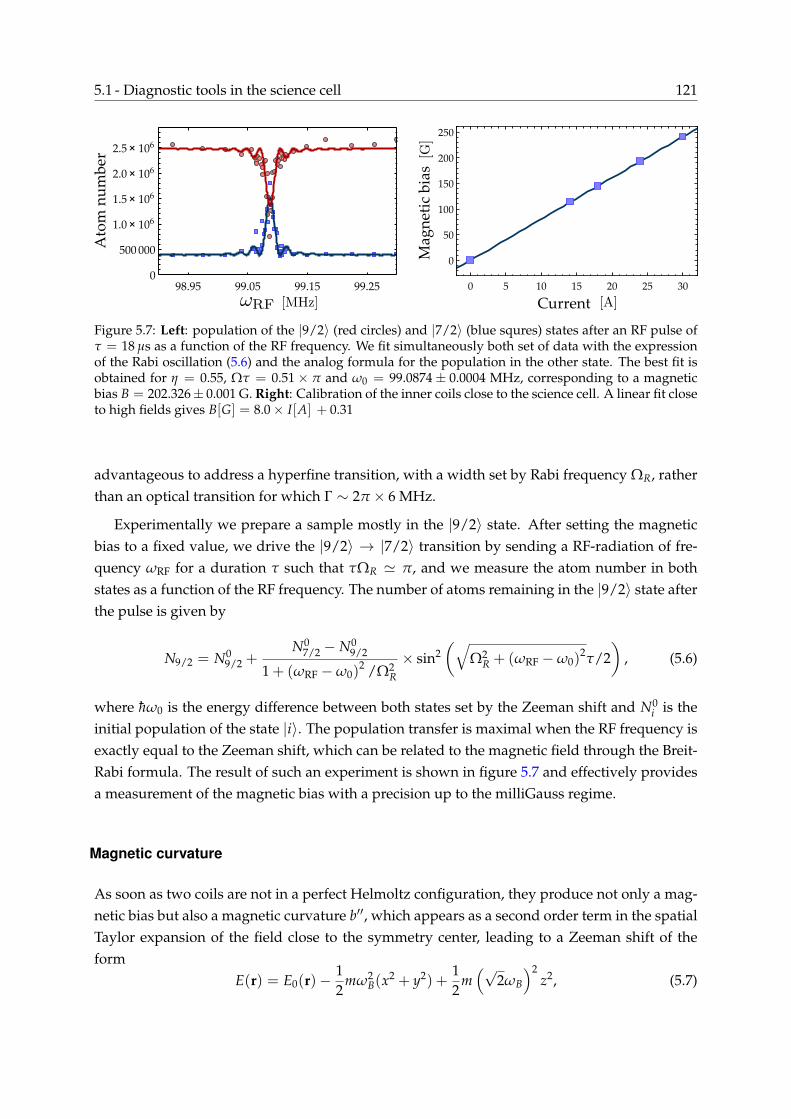
5.1 - Diagnostic tools in the science cell 121A

tom

nu

mb

er

98.95 99.05 99.15 99.250

500 000

1.0× 106

1.5× 106

2.0× 106

2.5× 106

0 5 10 15 20 25 30

0

50

100

150

200

250

Current

Mag

net

ic b

ias

Figure 5.7: Left: population of the |9/2〉 (red circles) and |7/2〉 (blue squres) states after an RF pulse ofτ = 18 µs as a function of the RF frequency. We fit simultaneously both set of data with the expressionof the Rabi oscillation (5.6) and the analog formula for the population in the other state. The best fit isobtained for η = 0.55, Ωτ = 0.51× π and ω0 = 99.0874± 0.0004 MHz, corresponding to a magneticbias B = 202.326± 0.001 G. Right: Calibration of the inner coils close to the science cell. A linear fit closeto high fields gives B[G] = 8.0× I[A] + 0.31

advantageous to address a hyperfine transition, with a width set by Rabi frequency ΩR, ratherthan an optical transition for which Γ ∼ 2π × 6 MHz.

Experimentally we prepare a sample mostly in the |9/2〉 state. After setting the magneticbias to a fixed value, we drive the |9/2〉 → |7/2〉 transition by sending a RF-radiation of fre-quency ωRF for a duration τ such that τΩR ' π, and we measure the atom number in bothstates as a function of the RF frequency. The number of atoms remaining in the |9/2〉 state afterthe pulse is given by

N9/2 = N09/2 +

N07/2 − N0

9/2

1 + (ωRF −ω0)2 /Ω2

R

× sin2(√

Ω2R + (ωRF −ω0)

2τ/2)

, (5.6)

where hω0 is the energy difference between both states set by the Zeeman shift and N0i is the

initial population of the state |i〉. The population transfer is maximal when the RF frequency isexactly equal to the Zeeman shift, which can be related to the magnetic field through the Breit-Rabi formula. The result of such an experiment is shown in figure 5.7 and effectively providesa measurement of the magnetic bias with a precision up to the milliGauss regime.

Magnetic curvature

As soon as two coils are not in a perfect Helmoltz configuration, they produce not only a mag-netic bias but also a magnetic curvature b′′, which appears as a second order term in the spatialTaylor expansion of the field close to the symmetry center, leading to a Zeeman shift of theform

E(r) = E0(r)−12

mω2B(x2 + y2) +

12

m(√

2ωB

)2z2, (5.7)

122 Evaporative cooling to quantum degeneracy

0 10 201020

0

0.1

0.2

TOF duration

Figure 5.8: Time of flight measurement of the magnetic curvature induced by the inner coils close to thescience cell at 30 A. Blue squares (red circles) show the cloud width measured along the x (z) directionas a function of time. For atoms in the | − 9/2〉, the curvature leads to a trapping potential along z andexpulse the atoms along the other two directions. Solid lines are fits given by (5.8), with ωx,y,z, ωB andT as free parameters. We obtain the best fit for ωB = 6.5± 0.1 Hz. Dashed lines are the best fit assumingωB = 0, for comparison.

where E0 denotes the shift due to the magnetic bias alone and ωB =√

µBgFmFb′′/m. Thiscurvature results in a slight modification of the trapping frequency, which might be difficult tomeasure directly. A time of flight experiment provides an alternative way to estimate b′′ as theexpansion of a cloud in such a surrounding potential is given by:

σ2x,y(t) =

kBTm

(1

ω2x,y

cosh(√

2ωBt) +1

2ω2B

sinh(√

2ωBt)

)(5.8a)

σ2z (t) =

kBTm

(1

ω2z

cos(ωBt) +1

ω2B

sin(ωBt))

, (5.8b)

where ωx,y,z are the initial trapping frequencies before the cloud is released. These formulaeare used to fit the expansion dynamics of the cloud as shown in figure 5.8 with ωB as freeparameter, thus allowing for the measurement of the magnetic curvature.

Imaging magnification

A time-of-flight experiment enables one not only to calibrate the magnetic curvature, but alsoto determine the magnification of the imaging system. We first bring the camera into focus bymoving the imaging lens on a translation stage so as to minimize the size of the image of a verysmall cloud. A coarse estimate of the magnification of the system can be obtained by measuringthe size of a calibrated stainless steel mesh of 320×320 µm placed successively close to bothsides of the science cell. To perform a more accurate measurement, we release a small and coldcloud from the optical dipole trap and measure the position of its center of mass as it falls. Itsreal acceleration, set by gravity, is well known in absolute value. The measured acceleration

5.2 - Principle of evaporative cooling 123

0 5 10 15

3.5

4.

4.5

5.

5.5

6.

Time of flight

Co

M p

osi

tio

n

Figure 5.9: Calibration of the imaging magnification along x (blue) and y (red). We record the rawposition (position in pixel × size of a pixel) as a function of time and fit a parabola x(t) = x0 + a0t2/2.The magnification is estimated as m = a0/g. Here, we obtain m = 1.59 for the imaging system along xand m = 0.6 for the imaging system along y.

then depends on the pixel size of the CCD camera (6.45 µm) and on the magnification of theimaging system. The comparison of both values thus allows for a calibration of the opticalsystem. However, this method assumes the absence of any remanent magnetic gradient, whichwould alter the effective gravity. Because of its heavier mass, 40K is naturally a much bettercandidate for those measurements than 6Li.

Now that we introduced the calibrated toolbox required to manipulate and probe the atomicsamples, we turn to the description of the cooling technique that allowed us to reach quantumdegeneracy for 40K.

5.2 Principle of evaporative cooling

The objective of evaporative cooling is to increase above unity the phase-space density of thedistribution, defined as:

PSD = n0λ3dB = N λ3

dB/Ve, (5.9)

where λdB is the de Broglie wavelength already introduced and n0 is the central density. Wealso introduce the trap volume Ve, which corresponds to the volume that would be occupiedby the gas if its density was uniformly n0:

Ve =Nn0

=∫

d3r exp(−U(r)kBT

). (5.10)

We quantify the efficiency of the evaporation using the ratio:

α = −d log(PSD)

d log(N), (5.11)

124 Evaporative cooling to quantum degeneracy

Figure 5.10: Principle of evaporative cooling. Left: in a trap in finite depth, collisions between particlesredistribute the energy. Particles which gathered most of the energy and leave the trap ; the remainingdistribution has therefore less energy and relaxes towards a colder temperature. Spilling and inelas-tic processes induce atom losses without evaporation. Right: starting from a thermal distribution attemperature T1, we consider decrease the trap depth to ηkBT. Atoms with an energy higher than thecut (red) will be spilled and a fraction of the distribution will eventually get evaporated (green). Theremaining atoms (blue) relax towards a thermal distribution at temperature T2 < T1.

which essentially expresses how many atoms must be sacrificed in order to gain one order ofmagnitude in phase-space density.

As mentioned in the introduction of this chapter, evaporative cooling consists in selectivelyremoving a fraction of the ensemble with the highest energies. Inter-particle interactions re-distribute the remaining energy within the sample, causing a relaxation towards a thermaldistribution after few collisions3 and repopulating the high energy wings of the distribution,which can again be evaporated further. This process is an out-of-equilibrium problem withtime dependent parameters and a quantitative treatment can be extremely sophisticated. Inthis section, we present a simple qualitative model with the objective of highlighting the mainparameters that are relevant for an experimental optimization of the process. This approach ismainly inspired by [Davis et al. 1995b] and [Cohen-Tannoudji 1996].

Let us consider a conservative trap U ∝ r3/δ with a finite depth Uc (see Fig. 5.10). Weassume that the atomic distribution is almost thermal, so that a temperature T can be definedfor the distribution. In many approaches, the ensemble is for instance described by a truncatedBoltzmann distribution:

f (r, p) = n0λ3dB exp(−H(r, p)

kBT)× θ(Uc − H(r, p)). (5.12)

A key parameter is the ratio between the trap depth and the cloud temperature η = Uc/kBT:the higher the trap, the more energy particles take away from the ensemble as they evaporate.

3∼ 3 for a uniform single species gas to ∼ 20 for hetero-species gas in a linear trap [Walraven 2010]

5.2 - Principle of evaporative cooling 125

A rule of thumb can be formulated by reducing the problem to a single parameter κ, whichexpresses the average excess of energy taken away by an evaporated atom. If η is lowered, theloss of dN < 0 atoms thus corresponds to an energy variation dE = (η + κ)kBT× dN. Relatingthe energy and temperature of the cloud through the virial theorem E = (3/2 + δ)NkBT, thecooling resulting from this energy loss can be expressed as:

dTT

=

((

32+ δ)(η + κ)− 1

)dNN

. (5.13)

The phase-space density decreases because of atom losses, but increases because of the cool-ing. These two contributions lead to the following balance:

d(PSD)

PSD=

dNN− (

32+ δ)

dTT

= −(

η + κ − (52+ δ)

)dNN

. (5.14)

If the trap remains deep enough, the gain in temperature compensates the atomic losses, andthe phase-space density increases.

According to this simplified picture, it appears as if the deeper the potential, the more effi-cient the evaporation. However, the situation is rendered more complicated by the presence ofadditional inelastic and spilling losses as well as parasitic heating, which constrain the evapo-ration dynamics (see Fig. 5.10). If the trap is too high, very few collisions will result in particlesbeing energetic enough to evaporate and the cooling will be extremely slow, leaving enoughtime for those additional losses to deplete the sample. The evaporation should therefore beforced by actively decreasing the trap depth to accelerate the process.

This analysis points out a second key parameter of any evaporation, namely the ratio be-tween the rate of non-evaporative processes and the actual evaporation rate, which is essen-tially set by the trap depth and geometry as well as the collision rate:

γcoll =1

2(δ+1/2)n0σv, (5.15)

where v =√

8kBTπm is the particles’ average quadratic speed and σ = 4πa2 is the scattering cross

section, related to the scattering length a (see annex A.4.3).

If the dynamical decrease of the trap depth is correctly performed, the collision rate can in-crease during the evaporation and even diverge in finite time (the so called runaway regime),owing to the non linearity of the process. However, this regime can only be attained if the aver-age number of collisions per particle before leaving the trap inelastically (given by γcoll/Γinel)is large enough. Numerically, in a harmonic trap, this number must exceed ∼ 300 for therunaway regime to be achievable [Guery Odelin 1998].

Several refinements can be introduced to improve the toy model presented above. For in-stance, in real evaporations, inelastic processes such as Majorana losses do not occur at a con-

126 Evaporative cooling to quantum degeneracy

c)

e)d)

b)

a)

0 1 2 3 4 50

2

4

6

8

10

12

Log10(N)

Lo

g10

(P

SD

)

Time

0 1 2 3 4 50

2.0 × 108

4.0 × 108

6.0 × 108

8.0 × 108

1.0 × 109

1.2 × 109

1.4 × 109

Ato

m n

um

ber

Time

Tem

per

atu

re

0 1 2 3 4 50

50

100

150

200

250

300

Time

Den

sity

Co

llis

ion

rat

e

0 1 2 3 4 50

2 × 1012

4 × 1012

6 × 1012

8 × 1012

0

20

40

60

80

100

Time

8.2 8.4 8.6 8.8 9.0 9.2- 5.5

- 5.0

- 4.5

- 4.0

- 3.5

Figure 5.11: Magnetic evaporation of 40K: starting from 1.5× 109 atoms at 320 µK, we obtain 2× 108

atoms at 90 µK after 5 seconds of evaporation. All points come from experimental data. a) Trap depthη = Tcut/T, where the cut temperature is set by the RF-knife. b) Atom number through the evapo-ration. c) Temperature, as measured by the RF tomography technique (see section 5.1.1) through theevaporation. d) Density (blue squares) and s-wave collision rate (red circles) through the evaporation.e) Evaporation efficiency, estimated to α ' 1.5.

5.3 - Conclusions 127

stant rate, but are in fact temperature dependent. A more detailed description of the scatteringcross section σ can also be required, notably to take into account p-wave interactions whichplay a predominant role for 40K above ∼ 20 µK [DeMarco et al. 1999, Fernandes 2014]. Whatsmore, we assumed that the trap kept the same steepness throughout the process, which willnot be the case in an optical potential [Ketterle and Druten 1996]. Nevertheless, this simplifiedpicture provides some rule-of-thumb scaling laws and identifies two key parameters as themain experimental knobs to tune the efficiency of the evaporation, namely the ratio betweenthe trap depth and the ensemble temperature, as well as the ratio between the collision rateand the inelastic loss rate.

5.3 Evaporative cooling of Potassium

As Potassium atoms arrive in the magnetic quadrupole trap in the science cell, they form acloud of ∼ 109 atoms at ∼ 320 µK, mostly in the |9/2, 9/2〉 and |9/2, 7/2〉 states. Magneticconfinement offers a large trapping volume as well as a good steepness, and direct evaporativecooling has been proven to be efficient enough to reach quantum degeneracy [DeMarco andJin 1999]. However, in order to manipulate the spin states and to take advantage of Feschbachresonances, atoms must be loaded into an optical trap which, unlike a quadrupole trap, is spin-independent. With the perspective of achieving double degeneracy of 6Li and 40K, the loadingof a dipole trap is therefore not optional. Yet, as the ensemble arrives in the science cell, it is toohot and too large to be efficiently loaded into an optical dipole trap of limited depth. To increasethe mode matching, and hence the loading efficiency, our cooling strategy can be decomposedinto three steps: the Potassium cloud is first evaporatively cooled in the magnetic trap, thentransferred into the optical dipole trap and further evaporated to quantum degeneracy.

5.3.1 Magnetic RF-evaporation

The RF-knife introduced in section 5.1.1 provides a simple means to decrease arbitrarily thetrap depth η of the magnetic confinement by adjusting the driving frequency. Experimentally,we start with a sample of 1.5× 109 atoms at ∼ 320 µK in a quadrupole trap with a magneticfield gradient b = 125 G/cm, corresponding to a PSD of 7× 10−6. We ramp down linearlythe frequency of the RF knife from Tcut = 3.5 mK to Tcut = 0.7 mK in 5 seconds. At the endof the evaporation, the sample contains 10% of the initial atoms at 95 µK, corresponding to aphase-space density of 2× 10−4.

The evaporation efficiency, defined as (5.11), is rather low with α ∼ 1.5, to be comparedto α ∼ 3 for the RF evaporation of Rubidium. As a result, despite excellent initial conditionscompared to other 40K experiment, we can only obtain standard values at the end of this step.The reasons for this limitation are still to be fully understood. The efficiency should be quiterobust with respect to the initial spin composition of the cloud, as both s-wave and p-wave

128 Evaporative cooling to quantum degeneracy

collisions take place [DeMarco et al. 1999]. Losses due to background pressure are moderate,as proven by the long lifetime of the sample in the dipole trap (& 60 s). In a quadrupole trap,special care should also be given to Majorana losses (previously described in section 3.1.3),which strongly reduce the evaporation efficiency.

Majorana losses are indeed equivalent to an anti-evaporation process, as atoms with lowestenergy spend more time close to the magnetic zero and are therefore most likely to leave thetrap. The temperature increases as T0

√1 + t/TM and the corresponding heating rate, propor-

tional to hm (µBb/kBT)2, increases as the temperature is lowered. For 40K at 75 µK, we measure

TM ∼ 9 s, which is comparable with the evaporation time. In order to circumvent this issue,we focus on the trap center a repulsive blue detuned 532nm laser beam so as to prevent atomsfrom reaching the magnetic zero [Davis et al. 1995a, Dubessy et al. 2012]. The setup was pre-sented in section 2.10.1 and results in an optical plug of ∼ 0.8 mK height. Majorana losses arenow strongly suppressed, as illustrated by the increased heating of TM ∼ 70 s.

Despite its moderate efficiency, this sequence is quick and optimized to increase the atomnumber loaded in the optical trap, as described in the following section, allowing for the real-ization of a degenerate cloud.

5.3.2 Loading of the optical trap

During the RF evaporation, a red-detuned 1064nm laser of waist w is shone onto the atoms (seesection 2.10.2 for technical references), resulting in a hybrid optical and magnetic potential4:

Uhybrid = µBb√

x2 + y2 + 4z2 −U0 exp(−2

y2 + (z− z0)2

w2

)+ mgz + E0, (5.16)

where U0 ∼ 0.5 mK is the optical trap depth and E0 is set such that Umin = 0, as shown onfigure 5.12 [Lin et al. 2009b]. To avoid Majorana spinflips, the laser beam does not cross themagnetic center but rather passes at a distance z0 ∼ −100 µm, chosen to optimize the traploading. Along the propagation direction x, the optical confinement set by the Rayleigh lengthis negligible compared to the magnetic trapping set by r0 = kBT/µBb. The resulting trappingfrequency is thus set by the magnetic field gradient:

ω‖ =12

õBbmz0

. (5.17)

The partition of atoms between the magnetic and optical potentials can be pictured by esti-mating the occupied volume (see Fig. 5.12). At high temperatures, the volume is essentiallythat of a magnetic trap while, at low temperature, it is mostly that of the optical trap, meaningthat the atoms are transferred from one to the other. The hybrid trap thus benefits from advan-

4The optical plug is not included in eq.5.16.

5.3 - Conclusions 129

Tra

p v

olu

me

1005020 30 1507010- 14

10- 13

10- 12

10- 11

10- 10

Temperature500 0 500

0

200

400

600

800

1000

1200

En

erg

y

Position

Figure 5.12: Hybrid trap. Left: trapping potential. In red, the magnetic contribution captures a largevolume but is spin dependent. In blue, the optical contribution presents a larger depth but a smallervolume. The position of the optical dipole trap is found to be optimal ∼ 100 µm below the magneticcenter. Right: effective volume of a distribution in (5.16) as a function of the temperature (blue squares).The solid lines are the effective volume in a purely optical (blue) and magnetic (red) potential. As thetemperature goes down, the atoms accumulate in the optical potential.

tages of both trapping strategies (large volume of the magnetic quadrupole trap, broad range ofevaporation and spin independence of the optical dipole trap) without their main drawbacks.

Experimentally, at the end of the RF-evaporation, we ramp down the magnetic gradientadiabatically to ∼ bg = mg/µB = 7 G/cm within 400ms. This step loads 20% of the atoms inthe optical dipole trap, mostly in the |9/2〉 and |7/2〉 states, resulting in a sample of 2.8× 107

atoms at 45µK. Even though the loading is adiabatic, the modification of the trap geometrydoes not conserve the phase-space density [Weber et al. 2003]. This dimple effect leads to anincrease the PSD by a factor 15 to 3× 10−3.

5.3.3 Optical evaporation

Considering a simplified two-levels atom, a laser propagating along x will induce a trappingpotential which can be written close to its focal point as [Grimm et al. 2000]:

UODT(r) =12

mω2⊥(y

2 + z2) +12

mω2‖x

2, (5.18)

where ω⊥ =√

4U0mw2 is the strong trapping frequency and ω‖ =

√2U0mz2

Ris typically one hun-

dred times smaller. Those frequencies depend on the trap depth, which can be expressed as afunction of the light intensity I and of its detuning δ with respect to the atomic transition:

U0 =hΓ2

4|δ|I

2Isat, (5.19)

where Γ is the natural linewidth of the optical transition and Isat is the saturation intensity.

130 Evaporative cooling to quantum degeneracy

Ato

m3n

um

ber

c)

e)d)

b)

a)

0 1 2 3 4 50

5.0 × 106

1.0 × 107

1.5 × 107

2.0 × 107

0 1 2 3 4 50

2

4

6

8

TF

3/3T

Tem

per

atu

re

0.0

0.1

0.2

0.3

0.4

0.5

0 1 2 3 4 50

10

20

30

40

50

60

Time

Time Time

Den

sity

Co

llis

ion

3rat

e

0

200

400

600

800

1000

0 1 2 3 4 50

2 × 1012

4 × 1012

6 × 1012

8 × 1012

1 × 1013

Time Log10(N)

Lo

g10

3(P

SD

)

6.9 7.0 7.1 7.2 7.3

- 2.5

- 2.0

- 1.5

- 1.0

Figure 5.13: Optical evaporation of 40K: starting from 2.8× 107 atoms at 45µK, we obtain 8× 106 atomsat 1.5 µK after 5.5 seconds of evaporation. All points come from experimental data. a) Trap depth η =Tcut/T, where the cut temperature is set by the optical power. b) Atom number through the evaporation.c) Temperature (red circles) and ratio to the Fermi temperature TF (blue square) through the evaporation.d) Density (blue squares) and s-wave collision rate (red circles) through the evaporation. e) Evaporationefficiency, estimated to α ' 3.7.

5.3 - Conclusions 131

To perform the evaporation, we decrease exponentially the optical power from 10 W to 170mW in 5.5 seconds, thereby reducing the trap depth. At the end of this step, the sample iscomposed of 8× 106 atoms at 1.5 µK and the efficiency of the evaporation can be estimated tobe α ∼ 3.7 (see Fig. 5.13).

Unlike in a magnetic trap, the trapping frequencies of an optical dipole trap depend on thelight intensity ω ∝

√I, and both the confinement and the collision rate decrease during the

cooling [O’Hara et al. 2001]. At the end of the evaporation, the axial frequency is reduced toω‖ ∼ 2.5 Hz, which prevents any efficient further cooling.

To increase the axial confinement, a second laser beam with a much larger waist is sent per-pendicularly to the first optical dipole trap (technical details were presented in section 2.10.2).The polarization of both beams are orthogonal to prevent interference and the resulting trap-ping frequencies are given by the superposition of both potentials:

ωx = ω⊥2, ωy = ω⊥1, ωz =√

ω2⊥1 + ω2

⊥2, (5.20)

where ω⊥1,2 denotes the radial trapping frequencies of the first and second laser beam.

Experimentally, we ramp up the second beam with a waist w2 = 340 µm to 4.8W within1.5s, leading to a potential of depth U0 = 3.5 µK and radial frequency ω⊥2/2π = 25 Hz. Theloading rate of the cross trap is kept slow because of the weak axial frequency but shows agood efficiency as, eventually, 4.8× 106 atoms are trapped in the dimple. The finite depth ofthe potential results in an additional evaporation and despite the compression of the cloud, itstemperature decreases to 1.3 µK, showing an increase of the PSD to T/TF = 0.7.

To tune inter-particle interactions by taking advantage of Feschbach resonances (see ap-pendix A.4.5), Potassium atoms must be transferred into the adequate spin states. The adia-batic passage described in section 5.1.2 is used to populate the | − 9/2〉 and | − 7/2〉 states withequal atom number. These states present a s-wave Feschbach resonance at B0 = 202 G, witha width ∆B = 7 G. However, a p-wave resonance is also located around 200 G [Gaebler et al.2007], increasing the inelastic losses and rendering challenging the use of the s-wave resonanceto enhance the evaporation efficiency. For the time being, we performed the final of evapora-tion at the background value of the scattering length, far above the resonance in order to beable to bring the interactions to zero without crossing the unitary regime.

The final step of evaporation takes place in the crossed dipole trap. The axial frequency iskept constant by the second beam while the power of the first beam is decrease from 170 mWto 57 mW in 14 seconds.

To determine the atom number and temperature, we ramp the magnetic bias to 209 G= B0 +

∆B, such that scattering length vanishes and perform a time of flight for the non-interactingensemble. The result for a 20 ms TOF is shown in figure 5.14. We measure 1.5× 105 atoms inthe | − 9/2〉 state, and roughly the same amount in the | − 7/2〉 state, at a temperature of 60

132 Evaporative cooling to quantum degeneracy

0 200 400 600 800

200

400

600

800

1000

0 0.2 0.4 0.6 0.80

0.2

0.4

0.6

Position

Position

Position

Figure 5.14: Left: 2D spatial density of the cloud, averaged over 5 pictures, at the end of evaporationin the |9/2,−9/2〉 state, after 20 ms TOF. Right: corresponding 1D integrated density (solid blue line).The best fit with a polylogarithm function (solid red line) gives an atom number of 1.5 × 105 atoms,a temperature of T = 62 nK and a degeneracy parameter T/TF = 0.16. The corresponding Fermitemperature, TF=400 nK, is in excellent agreement with its theoretical value. For comparision, a nondegenerate gaussian fit (dashed line) gives the same atom number, but a much higher temperatureT = 140 nK. The discrepancy between both fits highlights the non-classical behavior of the sample.

nK.

The ratio to the Fermi temperature can be estimated directly by fitting the 1D-integrateddensity with a Polylogarithm function (see section 2.11.2), or indirectely by calculating theFermi temperature as:

kBTF = hω(6N)1/3 ' 395nK, (5.21)

where ω3 = ωxωyωz is the harmonic average of the trapping frequencies. Both methods are inexcellent agreement and give T/TF = 0.16, implying that the sample was cooled down to thedeeply degenerate regime.

5.4 Double evaporative cooling of 6Li and 40K

One of the objectives of the FERMIX experiment is to produce a double degenerate Fermi gasof 6Li and 40K. At the moment of writing this thesis, we were able to cool 2× 106 6Li atomsdown to 68 µK in the plugged magnetic trap and to load 4.5 × 105 of them at 38 µK in theoptical dipole trap, in which the evaporative cooling is still to be performed. In this section, wepresent these preliminary results and suggest strategies for further cooling to degeneracy.

5.4.1 6Li-40K interactions

The inter-species interactions constitute a key parameter of the simultaneous cooling of 6Liand 40K. If the overlap between the clouds of 6Li and 40K is large enough, collisions will

5.4 - Double evaporative cooling of 6Li and 40K 133

redistribute the energy between the two distributions and facilitate the thermalization of theclouds. This effect was already used in connection with the quasi-thermalization experiments(section 3.2.1) to prepare a thermal Lithium gas in a magnetic trap.

For the 6Li-40K system, the triplet scattering length was reported to be at = 62 a0 and thesinglet scattering length at as = 52 a0, where a0 is Bohr radius [Wille et al. 2008]. The positionsand widths of 6Li-40K Feschbach resonances were thoroughly studied experimentally [Tieckeet al. 2010a] and theoretically [Tiecke et al. 2010b]. It should be noted that Feschbach resonancesalso increase inelastic collisions, resulting in a finite decay rate [Naik et al. 2011].

Far from those enhanced losses, the spin exchange collision rate between 6Li and 40K is rea-sonably small. This results from the inverted hyperfine structure of Potassium, which stronglysuppresses spin relaxation if any of the two interacting atoms is in the lowest Zeeman sublevel[Simoni et al. 2003]. The small difference between the singlet and triplet scattering lengths fur-ther reduces the inelastic collision rate. As a consequence, it has been shown that a mixture of104 40K atoms immersed in a sea of 107 6Li atoms was collisionally stable, with a two body lossrate for Potassium below L2 = 6× 10−13 cm−3/s across the entire Lithium BEC-BCS crossover[Spiegelhalder et al. 2009].

5.4.2 Magnetic RF-evaporation

After the magnetic transport, we obtain 108 Lithium atoms in the science cell at 400 µK. Onlythe |F = 3/2, mF = 3/2〉 spin state is stable against spin exchange collisions and trappablein a magnetic quadrupole. As mentioned in the previous chapters, since s-wave collisions areforbidden by the Pauli principle and p-wave collisions are present only above 6 mK, a cold pure6Li sample behaves like an ideal gas and does not thermalize by itself. To cool and evaporate aLithium sample, it is therefore necessary to consider the sympathetic cooling technique, whichconsists in cooling actively one species (Potassium in our case) while relying on collisions tothermalize the other species with the coolant [Modugno et al. 2001].

The cooling of Lithium represents an additional thermal load for Potassium, whose evapora-tion must dissipate both internal energies. The presence of Lithium thus reduces the efficiencyof the Potassium evaporation and starting from the same initial conditions, much less atomsreach the same final temperature. It was observed in [Tiecke 2009] that the density of Potassiumwas limited to 1012 cm−3, two orders of magnitude below its value for a single species evapora-tion. In our experiment, we reduce the Lithium sample arriving in the science cell to 107 atomsby detuning the Zeeman slower, so as to minimize the detrimental effects for Potassium.

The load can be further reduced by removing Lithium atoms with highest energies. Takingadvantage of the large difference between the 6Li and 40K hyperfine splittings (228 MHz and1.2 GHz respectively), it is indeed possible to utilize two species-specific RF knifes to tuneindependently the trap depth for both species. We found the optimal configuration to be TLi

cut =

134 Evaporative cooling to quantum degeneracy

- 400 - 200 0 200 400

0

500

1000

1500

z position

Lin

ear

den

sity

Figure 5.15: 4.5× 105 Lithium atoms (in red) and 1.9× 105 Potassium atoms (in blue) at ∼38 µK in theoptical dipole trap at the end of the RF evaporation, after 0.5 ms TOF.

1.5× TKcut.

The optical plug plays a crucial role for the evaporation of Lithium, which is much lighterthan Potassium and thus has a ∼ 6 times higher Majorana loss rate. In absence of the plug, theanti-evaporation due to Majorana losses prevents any efficient cooling of the Lithium sampleand also keeps Potassium at higher temperatures. With the plug, we measured a lifetime of∼ 20 s for 2× 106 Lithium atoms at 68 µK at the end of the evaporation. After the magneticquadrupole is switched off, we measure in the optical dipole trap 4.5× 105 Lithium atoms and1.9× 105 Potassium atoms at ∼38 µK, as shown in picture 5.15.

5.4.3 Optical evaporation

The constraints for the optical evaporation are quite different from the ones present in themagnetic trap. As the trapping potential is now spin-independent, we can consider a |1/2〉 −| − 1/2〉 spin mixture of Lithium to take advantage of the large s-wave scattering length. Onthe other hand, the trap geometry can not be tuned independently for both species and it isabout half as deep for Lithium as for Potassium. Lithium atoms will thus have much higherevaporation and spilling rates than Potassium. For instance, in a deep potential ηK = 10, theLithium evaporation rate is e−ηLi /e−ηK ' 150 times faster than the one of Potassium [Fernandes2014]. Moreover, the mass imbalance between the two species is such that Lithium atoms willtake most of the kinetic energy during binary collisions. The sympathetic cooling of Potassiumby Lithium is therefore extremely demanding in terms of initial atom numbers, requiring areduced Potassium sample immersed in a large Lithium cloud [Spiegelhalder et al. 2010].

An alternative approach is being considered in our group to allow the simultaneous coolingof two samples with approximately the same atom numbers [Fernandes 2014].

In an equilibrated mixture, the collision rate between potassium atoms (set by aK = 170 a0)is larger than the interspecies collision rate (aLiK = 63 a0) but smaller than collision rate between

5.4 - Double evaporative cooling of 6Li and 40K 135

0

2

4

6

8

0.0 0.5 1.0 1.5 2.0 2.5 3.00

2

4

6

8

10

12

14

Time

c) d)

b)a)

4.8 5.0 5.2 5.4 5.6 5.8 6.0 6.2

- 3.5

- 3.0

- 2.5

- 2.0

- 1.5

- 1.0

- 0.5

0.0

0.0 0.5 1.0 1.5 2.0 2.5 3.00

500 000

1.0 × 106

1.5 × 106

2.0 × 106

0

100 000

200 000

300 000

400 000

Time

Ato

m.n

um

ber

.(K

)

Ato

m.n

um

ber

..(L

i)

Time

TF

./.T

Tem

per

atu

re

0.0 0.5 1.0 1.5 2.0 2.5 3.00

10

20

30

40

0.0

0.5

1.0

1.5

Log10(N)L

og

10.(

PS

D)

Figure 5.16: Simultaneous optical evaporation of 6Li and 40K: starting from 4.5× 105 Lithium atoms at40µK and 2× 106 Potassium atoms at the same temperature, we obtain 7× 104 atoms at 190 nK and106 Potassium atoms at 200 nK after 3 seconds of evaporation. The scattering lengths are : aK = 1000a0,aLi ∼ −300 a0 and aLiK = 63 a0. Inelastic losses are not taken into account. Numerical simulationsperformed by Cedric Enesa.All data for 6Li are shown in red (resp. blue for 40K). a) Trap depth η = Tcut/T. The trap is abouttwice as deep for 40K as for 6Li. c) Atom number through the evaporation. d) Temperature (solid lines)and ratio to the Fermi temperature TF (dashed lines) through the evaporation. b) Evaporation efficiency,estimated to αLi ' 4.4 and αK ' 13.4.

136 Evaporative cooling to quantum degeneracy

Lithium atoms (aLi ∼ −300 a0). This results in the evaporation rate of Potassium being muchsmaller than the one of Lithium, all the more so as the trap is deeper for 40K than for 6Li. As aconsequence, Potassium is sympathetically cooled by Lithium ; because of the mass imbalance,the resulting thermal load is too heavy for keeping a satisfying amount of 6Li at the end ofevaporation. One strategy to circumvent this issue is to accelerate the evaporation of Potassiumby enhancing its intra-species collision rate. If the scattering lengths are such that

aK aLi aLiK, (5.22)

very few interspecies collisions take place and the dual-species cooling essentially reduces totwo independent single species evaporations. Both evaporations may occur at the same rate,as the higher scattering rate of Potassium compensates the difference in trap depth. In thiscase, Potassium remains as cold as Lithium and the thermalization of both species at the end ofevaporation does not lead to a significant atom loss. Experimentally, this can be done by takingadvantage of the Feschbach resonance of Potassium at 202 G. For instance, provided that theintra-species scattering length is increased to aK = 1000a0, the evaporation rate is almost thesame for both species for a trap depth of ηK ' 8.

A preliminary simulation was performed by Cedric Enesa using a classical model and ne-glecting inelastic losses (see Fig. 5.16) [Enesa 2015]. Starting from 4.5 × 105 Lithium atomsat 40µK and 2 × 106 Potassium atoms at the same temperature, we obtain 7 × 104 Lithiumatoms at 190 nK and 106 Potassium atoms at 200 nK after 3 seconds of evaporation. This modelimplies to a very good cooling efficiency for Lithium with αLi ' 4.4, even in presence of Potas-sium. The evaporation efficiency of Potassium, αK ' 13.4, is due to the high ηK cut ratio. Itsvalue is clearly overestimated, as inelastic losses, which also increase close to the Feschbachresonance, are not taken into account. Nevertheless, these preliminary results are encouragingfor the experimental realization of a double species degeneracy.

5.5 Conclusions

In this chapter, we reviewed standard techniques which were applied to monitor and manip-ulate the internal degrees of freedom of the Potassium cloud, and use it to calibrate our appa-ratus. We have shown that we could produce for the first time in France a cloud of 40K with1.5 × 105 atoms in the | − 9/2〉 state and as many in the | − 7/2〉 state, at a temperature of62 nK corresponding to 17% of the Fermi temperature, in the deeply degenerate regime. Wepresented preliminary works concerning the simultaneous evaporative cooling of 6Li and 40K,resulting in the loading of 2 − 4 × 105 atoms at 40µK in the optical dipole trap. Numericalsimulation were performed to support an innovative cooling strategy, where both species areevaporated independently at similar rates, to avoid a too strong thermal load on the Lithiumcloud.

5.5 - Conclusions 137

As a longer term project, once both 6Li and 40K are brought to degeneracy, the FERMIX

apparatus will focus on the realization of ultra-cold mixtures in mixed dimensions. Takingadvantage on the difference of trapping potential experienced by the two species, it is indeedpossible to engineer a species-selective trap to strongly confine one atomic cloud while keepingthe other one almost free. The next and last chapter is dedicated to some perspectives openedby such systems.

Chapter

6Effective long-rangeinteractions in mixed

dimensions

Contents6.1 Scattering in mixed dimensions . . . . . . . . . . . . . . . . . . . . . . . . . . . . . . . . 141

6.2 Mediated long-range interactions . . . . . . . . . . . . . . . . . . . . . . . . . . . . . . . 145

6.2.1 Mathematical framework . . . . . . . . . . . . . . . . . . . . . . . . . . . . . . . . . 145

6.2.2 Effective interaction: general expression . . . . . . . . . . . . . . . . . . . . . . . . 147

6.2.3 Effective interaction for κCoM = 0 . . . . . . . . . . . . . . . . . . . . . . . . . . . . 149

6.3 Proposal for an experimental realization . . . . . . . . . . . . . . . . . . . . . . . . . . . 151

6.3.1 Implementation of an optical lattice . . . . . . . . . . . . . . . . . . . . . . . . . . . 151

6.3.2 Effective interaction between two layers . . . . . . . . . . . . . . . . . . . . . . . . 152

6.3.3 Coupled oscillations between two layers . . . . . . . . . . . . . . . . . . . . . . . . 154

6.4 Conclusions . . . . . . . . . . . . . . . . . . . . . . . . . . . . . . . . . . . . . . . . . . . . . 157

AT the end of XIXth century, the English theologian Edwin Abbott imagined in a religioussatire how different life would be if we were to live in a two dimensional world [Abbott

1884]. As it turned out, dimensionality plays indeed a crucial role for many physical phe-nomena, which have a completely different behavior in 2D or 1D as compared to the usual3D situation. For instance, in reduced dimensions, thermal fluctuations destroy any longrange order at finite temperature and prevent spontaneous symmetry breaking, as stated bythe Mermin-Wagner theorem [Mermin and Wagner 1966] (see [Hadzibabic and Dalibard 2011]for a pedagogic approach). As a consequence, some phase transitions are forbidden, suchas the ferro/para magnetic transition or Bose Einstein condensation. Instead, systems in re-duced dimensions exhibit peculiar properties, such as the emergence of quasi-long range orderthrough the so called Berezinskii-Kosterlitz-Thouless transition in two dimensions [Berezin-skii 1972, Kosterlitz and Thouless 1973, Minnhagen 1987] or the formation of specific states ofmatter, as epitomized in one dimension by the bosonic Tonks-Girardeau [Girardeau 1960] gaseand the ferminionc Luttinger-Tonomaga liquid [Giamarchi 2004]. Moreover, we have shownin the previous chapters that the anisotropy of Weyl particles quasi-thermalization was alsodimension dependent.

As mentionned in the introduction, cold atoms provide powerful tools for the experimentalstudy of systems in reduced dimensions, allowing the realization of the previously mentioned

139

140 Effective long-range interactions in mixed dimensions

problems1. Furthermore, atomic systems allow for additional methods to tune the elastic in-teractions. Indeed, in experimental realization, systems in reduced dimensions are obtainedfrom confined 3D systems. They therefore always display a finite transverse length l⊥, muchsmaller than both the inter-particle spacing and thermal wavelength (such that transverse de-grees of freedom remain frozen out) but much larger than the range of the van der Waals typeinteractions. Consequently, two-body interactions are unaffected by the confinement at shortdistances and the scattering length2 a is then set by the 3D scattering length a3D and the confine-ment length l⊥ [Petrov and Shlyapnikov 2001]. This also results in so called confinement inducedresonances [Olshanii 1998], which occur when a3D approaches l⊥ and allow to tune interactionswithin the plane from strongly repulsive to strongly attractive [Haller et al. 2010].

Cold atoms could also open the door to a supplementary approach considering mixed di-mensions, where part of the system is confined in 0-, 1- or 2D while the other part evolves withmore degrees of freedom. For instance, the scattering of matter waves off fixed disorderedimpurities, giving rise to the Anderson localization, can be seen as a 0D-3D system[Anderson1958]. The interaction between electrons confined in a graphene layer with freely propagatingphotons comes down to a 2D-3D problem [Novoselov et al. 2005]. In more exotic situations,gravity can be pictured as an 11 dimensional quantity restricted to our 4 dimensional world[Maartens 2004]. Some of those problems can be simulated by the FERMIX experiment, asPotassium atoms can be confined in 2D planes by an optical lattice which will leave Lithiumatoms mostly unaffected.

Effective interactions in mixed dimensions have been previously addressed in the litera-ture. For instance, [Recati et al. 2005, Fuchs et al. 2007] showed that two localized impuritiesimmersed in a 1D quantum liquid present Casimir-like interactions by calculating the actionof the system, from which the free energy is derived. Their results were extended in [Schecterand Kamenev 2014] to the case of mobile impurities. Closer to our situation, the interactionsbetween a 2D and a 3D ideal Fermi gas is described in [Nishida and Tan 2008], and extendedin[Nishida 2010] to estimate with a diagrammatic approach the behavior of two 2D layers con-nected by an ideal 3D Fermi gas.

In this chapter, we propose an approach developed in collaboration with Georg Bruun andZhigang Wu. We first describe 2D-3D interactions between a free atom and a confined one.We then turn to the calculation of the effective long range interaction between two 2D-planesimmersed in a 3D cloud which can carry momentum from one plane to the other. Using thestandard tools of atomic physics, we recover some of the results published in the literature andextend our predictions to unaddressed situations, as the 3D cloud is brought to the BEC side ofthe Feshbach resonance. Finally, we consider an experimental proposal to test the predictions

1The realization of Tonks Girardeau gas was first reported in 2004 [Paredes et al. 2004] and that of Luttingerliquid in 2005 [Moritz et al. 2005]. The BKT transition was observed in 2006 [Hadzibabic et al. 2006].

2The definition of the scattering length requires some precautions. In particular, the scattering amplitude tendsto zero for low energies in 2D, in stark contrast with the 3D behavior, where it can be used to define the scatteringlength [Levinsen and Parish 2015].

6.1 - Scattering in mixed dimensions 141

using Potassium layers confined in an optical lattice and immersed in a 3D Lithium cloud.If a 2D layer is dragged away from equilibrium, the mediated long-range interaction shouldset in motion the neighboring planes and the measurement of the beat-note frequency of theoscillations provides an experimental access to the interlayer interactions.

6.1 Scattering in mixed dimensions

In this section, we introduce a description of a 2D-3D collision, where A-atoms are confined ina 2D plane zA = 0 while B-atoms are free to move in three dimensions. As a first remark, wenotice that the problem is equivalent to a 3D scattering event: while the system has five degreesof freedom, the conservation of momentum along the two dimensions of the confining planereduces the number of independent quantities to three. As in a 3D scattering situation, we willbe able to consider a scattering length to account for the interaction properties.

Notations

In this chapter, we will deal simultaneously with vectors in two and three dimensions.As often as possible, 3D vectors are written with roman letters r and 2D vectors with boldGreek letters ρ. A 3D vector v ∈ R3 can be decomposed as an in-plane vector ν⊥ ∈ R2

and a transverse component vz. Conversely, a 2D vector ν⊥ ∈ R2 and an additionalcomponent vz can be assembled to form a 3D vector v = dν⊥, vzc.

We also also introduce the standard identities to avoid any ambiguity on the choice ofnormalization:

In 3D:

∑k

=

(L

2π

)3 ∫d3k

Id = ∑k|k〉 〈k| =

∫d3r |r〉 〈r|

〈k| r〉 = 1√L3

exp (ik.r)

ψ†(r) =1

L3/2 ∑k

e−ik.rc†k

c†k =

1L3/2

∫d3r eik.rψ†(r)

U(k) =∫

d3r eik.rU(r)

U(r) =1

(2π)3

∫d3k e−ik.rU(k)

In 2D:

∑κ

=

(L

2π

)2 ∫d2κ

Id = ∑κ

|κ〉 〈κ| =∫

d2ρ |ρ〉 〈ρ|

〈κ| ρ〉 = 1√L2

exp (iρ.κ)

ψ†(ρ) =1√L2 ∑

κ

e−iρ.κc†κ

c†κ =

1√L2

∫d2ρ eiρ.κψ†(ρ

U(κ) =∫

d2ρ eiκ.ρU(ρ)

U(ρ) =1

4π2

∫d2κ e−iκ.ρU(κ)

142 Effective long-range interactions in mixed dimensions

Figure 6.1: Scattering in mixed dimension. Left: At lowest order, the scattering eigenstates (6.9) are thesuperposition of a plane wave (in red) and an elliptical wave (in blue). The amplitude f (ki, n) gives theamplitude of probability for incident particle to be scattered in direction n (represented by the shade ofthe blue dashed line). Right: Numerical estimation of the 2D-3D scattering length. Figure from [Nishidaand Tan 2008].

Figure 6.2: Resonance conditions for the a2D−3D scattering length. When the energy of the scatteringstate is equal to that of a bound state (see eq. (6.13), the scattering length diverges. Graphically, thiscorresponds to the crossing of the green dashed line with an energy level of the harmonic oscillator inthe right-hand side of the picture. We denote ω′z =

√mB/µωz the trapping frequency of an 2D-3D

molecule and Eb = h2

2µa2A−B

its binding energy.

6.1 - Scattering in mixed dimensions 143

Our approach follows the description of 3D-3D interactions presented in annex A.4.2. As a2D and a 3D particles are interacting, the corresponding Hamiltonian takes the form:

H =1

2mB

(p2

B⊥ + p2Bz)+

p2A⊥

2mA+ V (rB⊥ − rA⊥, zB) (6.1)

We introduce the center of mass quantities (R, P) and the relative coordinates (r, p) to rewritethe previous equation as:

H =P2⊥

2M+

(p2⊥

2µ+

mA

mA + mB

p2z

2µ

)+ V(r) (6.2a)

= H2DCoM + H0 + V, (6.2b)

where M = mA + mB is the total mass and µ = mAmB/(mA + mB) is the reduced mass. Theeigenstates of H0 are 3D planes waves |k〉with anisotropic masses, such that the correspondingeigenenergies take the following form:

E0k =

h2

2µ(k2

x + k2y +

mA

mA + mBk2

z). (6.3)

To each plane wave |k〉 can be associated a scattering eingenstate |ψ+k 〉with the same energy

E0k. These eigenstates satisfy the Lippman-Schwinger equation:

|ψ+k 〉 = |k〉+ G0+(E0

k)V|ψ+k 〉, (6.4)

with G0(E0k) =

(E0

k − H0 + iη)−1 being the resolvent. The matrix elements of the resolvent are

Green functions and can be estimated by introducing a closure relation over plane waves:

〈r|G0(E0k)|r′〉 =

−µ

2πh2

√mA + mB

mA

exp(

ik× ρ)

ρ, (6.5)

where we introduced the relative position ρ = r− r′ and the deformed vectors

k =

kx

ky√mA

mA+mBkz

(6.6) ρ =

ρx

ρy√mA+mB

mAρz

(6.7)

At distances large compared to the finite range b of the interaction potential, ρ ' r − n.r′,where n = r/r is the direction of the deformed position r. As pictured in figure 6.1, the scatter-ing eigenmodes appear as the superposition of a plane and an ellipsoidal wave:

ψ+k (r) =

exp(ik.r)√L3

+ f (k, n)exp

(ik× r

)

r, (6.8)

144 Effective long-range interactions in mixed dimensions

where the contribution along the direction n is set by the scattering amplitude f :

f (k, n) = − µ

2πh2

√mA + mB

mA

∫d3r′ exp

(−ik× (n.r′)

)V(r′)

ψ+k

(r′)

(6.9)

To simplify this expression, we restrict ourselves to the Born approximation and replacewithin first order of perturbation theory ψ+

k (r) → exp(ik.r)/√

L3 in the integral (6.9). At lowenergies, considering that the length scale set by the wave vector is much smaller than therange of the potential k b−1, the exponential factor in the integral (6.9) is close to 1 and thescattering amplitude takes the isotropic form of a 2D - 3D scattering length:

limk→0

f (k) = − a2D−3D√L3

= − 1√L3

µ

2πh2

√mA + mB

mA

∫d3r′ V

(r′)

. (6.10)

The optical theorem3, stating the conservation of the flux during the scattering, allows us toexpress the scattering eigenstate as

ψ+k (r) =

exp(ik.r)√L3

− a2D−3D

1 + ika2D−3D

exp(

ik× r)

r, (6.11)

where we used k.r = k.r.

It is straightforward to verify that the wave functions (6.11) are also stationary solutions ofSchrödinger equation when the scattering potential V is replaced by the pseudo potential:

U(ρ) = g2D−3D × δ(ρ)∂

∂ρ(ρ.), (6.12)

where g2D−3D = a2D−3D ×√

mAmA+mB

2πh2

µ . Together with (6.14), this expression shows that the2D-3D coupling constant can be replaced by the 3D-3D coupling constant as long as the scatter-ing length is small enough compared to other length scales. For regular functions, the pseudopotential (6.12) is equivalent to a Dirac potential U(ρ) = g2D−3D δ(ρ), which we will use in thefollowing.

To estimate the value of the scattering length and relate it to the 3D-3D scattering lengthbetween A and B atoms, a more detailed description of the system is required [Massignanand Castin 2006]. A-atoms are not purely 2D, but rather confined to the ground state of anharmonic trap of frequency ωz. At distances shorter than the transverse length lz =

√h/mAωz,

the confining potential becomes irrelevant and the interaction only depends on the standard A-B scattering length aA−B. This short-distance condition constraints the long-distance behaviorof scattering states, and the corresponding numerical integration has been reported in [Nishidaand Tan 2008] (see Fig. 6.1). In particular, a2D−3D shows resonances when the energy of the open

3The optical theorem takes the form 4π| f |2 = Im( f ) (see annex A.4.3).

6.2 - Mediated long-range interactions 145

channel (hωz/2) coincides with the energy of a bound state in the closed channel [Lamporesiet al. 2010]:

hωz

2= hωz

√mA

mA + mB

(n′ +

12

)− h2

2µa2A−B

, (6.13)

where the second term of the right-hand expression is the binding energy of the A-B Feshbachmolecule (see annex A.4.5) and the first term results from the confinement of the molecule inpotential µω2

zr2/2 (see Fig. 6.2).

The width of the successive resonances decreases as lz increases and a2D−3D approaches thelimit

a2D−3D −→lz

aA−B→∞

aA−B

√(mA + mB)

mA, (6.14)

which we will use as a numerical estimate to lay down orders of magnitude.

6.2 Mediated long-range interactions

Let us consider two parallel planes of A-atoms (Potassium in our case) separated by a distance∆z. Assuming that there exist only contact interactions, the two layers can naturally not inter-act with one another. An intermediate 3D cloud of B-atoms (Lithium) changes this situation:excitations can now propagate through the B cloud and carry momentum from one layer to theother. In other words, the presence of a 3D cloud allows for a mediated long range interactionbetween the 2D planes (see figure 6.3). In this section, we calculate the effective long-rangepotential experienced by A-atoms in the presence of a B-cloud.

6.2.1 Mathematical framework

Neglecting many body effects within the planes, we consider two single A impurities confinedin facing 2D planes and interacting with the B cloud. The Hamiltonian of the system can bewritten as:

H = HA + HB + V, (6.15)

where HA (resp. HB) accounts for A-atoms (resp. B-atoms) and V = V2D−3D1 + V2D−3D

2 denotesthe local interaction between each 2D plane and the 3D cloud. Each contact interaction can bedescribed as:

V2D−3Dα =

∫d3rd2ρ Uα

(r‖ − ρ

)δ (r⊥ − zα)ψ†

B(r)ψ†A,α(ρ)ψA,α(ρ)ψB(r), (6.16)

where ψ†B(r) (ψB(r)) creates (annihilates) a B-atom at position r and ψ†

A,α(ρ) (ψA,α(ρ)) creates(annihilates) an A-atom at position ρ in the layer α. We consider only a weak coupling between

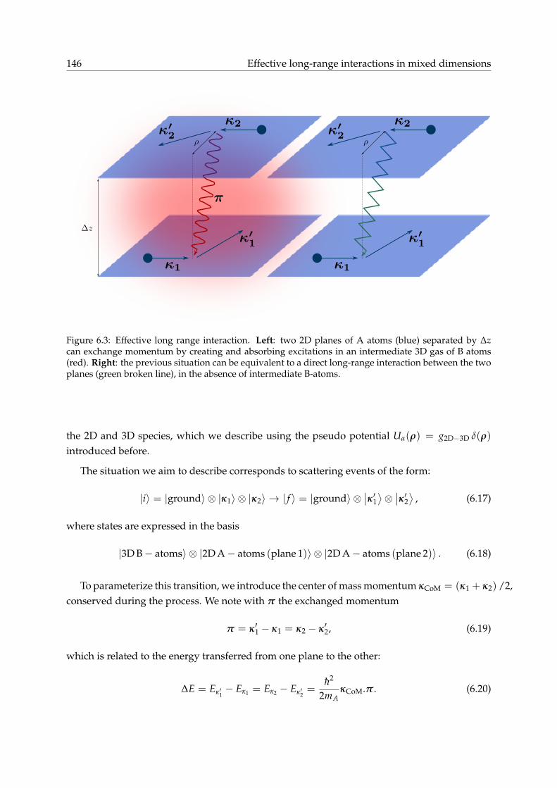
146 Effective long-range interactions in mixed dimensions

Figure 6.3: Effective long range interaction. Left: two 2D planes of A atoms (blue) separated by ∆zcan exchange momentum by creating and absorbing excitations in an intermediate 3D gas of B atoms(red). Right: the previous situation can be equivalent to a direct long-range interaction between the twoplanes (green broken line), in the absence of intermediate B-atoms.

the 2D and 3D species, which we describe using the pseudo potential Uα(ρ) = g2D−3D δ(ρ)

introduced before.

The situation we aim to describe corresponds to scattering events of the form:

|i〉 = |ground〉 ⊗ |κ1〉 ⊗ |κ2〉 → | f 〉 = |ground〉 ⊗∣∣κ′1⟩⊗∣∣κ′2⟩

, (6.17)

where states are expressed in the basis

|3D B− atoms〉 ⊗ |2D A− atoms (plane 1)〉 ⊗ |2D A− atoms (plane 2)〉 . (6.18)

To parameterize this transition, we introduce the center of mass momentum κCoM = (κ1 + κ2) /2,conserved during the process. We note with π the exchanged momentum

π = κ′1 − κ1 = κ2 − κ′2, (6.19)

which is related to the energy transferred from one plane to the other:

∆E = Eκ′1− Eκ1 = Eκ2 − Eκ′2

=h2

2mAκCoM.π. (6.20)

6.2 - Mediated long-range interactions 147

Real case Effective caseH = HA + HB + V Heq = HA + Veff

↓ ↑

Ti f = 〈 f |VG0V|i〉 ⇐⇒ Ti f = 〈 f |Veff|i〉

Table 6.1: Definition of the effective long range interaction Veff. We define the effective interaction be-tween two A-atoms as the potential Veff that leads to the same transition amplitude from the initial state|i〉 to the final state | f 〉 as the first contributing order of the mixed dimensional case (i.e. second order,as shown in section 6.2.2), where the interaction is mediated by the B-cloud.

Scattering properties can be addressed using the S matrix, which expresses this transitionamplitude as the overlap between the initial and final states subjected to the time evolutionoperator UI (t1, t2) = exp (−iV(t2 − t1)/h):

Si f = 〈 f |UI (+∞,−∞) |i〉 = δ f ,i − 2iπδ(E f − Ei

)Ti f (6.21)

The T matrix can in turn be expanded through the Dyson equation

T = V + VG0V + ..., (6.22)

where the resolvent G0 is given by

G0(z) =1

z− (HA + HB). (6.23)

We define the effective long range interaction as the potential Veff which gives rise to thesame T matrix within the Born approximation as the real contact potential V up to first con-tributing order (see table 6.1).

6.2.2 Effective interaction: general expression

We need to estimate the leading order in the expansion of the T matrix. Since we considerscattering events in which the Lithium cloud is eventually and initially in the same state, thefirst order T = V does not contribute and we must therefore estimate:

Ti f = 〈 f |VG0 (Eκ1 + Eκ2)V |i〉 . (6.24)

We calculate only Hartree terms, describing to interlayer exchange interactions, and neglectFock terms, which would correspond to intra-layer forward scattering. The second order of the

148 Effective long-range interactions in mixed dimensions

matrix element Ti f is the sum of two contributions:

Ti f = 〈 f |V2D−3D1 G0 (Eκ1 + Eκ2)V2D−3D

2 |i〉+ 〈 f |V2D−3D2 G0 (Eκ1 + Eκ2)V2D−3D

1 |i〉 . (6.25)

This matrix element is related to the density-density response function of the 3D B-cloud andcan be expressed through its compressibility χB:

Ti f =1

2πL2 g22D−3D ×

∫dkz e−ikz∆z χB

(⌊π

kz

⌉,

h2m

κCoM.π

), (6.26)

where the center of mass momentum κCoM and the exchanged momentum π were alreadydefined above. We will now briefly present the main steps of the calculation.

• Introducing closure relations, we isolate the B-cloud so as to express both terms of (6.25)as matrix elements of an operator A acting only on the 3D gas. Taking Ti f = T(1)

i f + T(2)i f ,

we write for instance:

T(1)i f = 〈B : 0|M |B : 0〉 (6.27a)

M =⟨κ′

1∣∣V1 |κ1〉G(B)

0 (∆E)⟨κ′

2∣∣V2 |κ2〉 (6.27b)

where G(B)0 (z) = 1

∆E−HB. The objective is then to sum over all intermediate states of the

mediating B-cloud.

• Matrix elements of interspecies potentials Vα can be expressed so as to explicitly sum overall transverse momentums:

⟨κ′

1∣∣V1 |κ1〉 =

12πL2 U1

(κ′

1 − κ1) ∫

dpz e−ipzz1

(∫d3r eidκ1−κ′

1,pzc.rψ†B(r)ψB(r)

)(6.28)

• Because of momentum conservation, the T matrix element (6.25) can be simplified to:

Ti f =1

2πL5

∫dpz e−ipz(z1−z2)U2(−π)U1(π)

× 〈0|(

F−pG(B)0 (∆E) Fp + FpG(B)

0 (∆E) F−p

)|0〉 (6.29)

where Fp =∫

d3r eip.rψ†B(r)ψB(r) with p = dπ, pzc.

• The operator appearing in the previous expression can be directly related to the compress-ibility of the B-cloud, which we define in the following way: if a system is perturbed by

6.2 - Mediated long-range interactions 149

an excitation w(r, t) = µ cos (k.r−ωt), its density response is given by:

ρk =1L3

∫d3r e−ik.r

⟨ψ†(r)ψ(r)

⟩(6.30a)

=12

µχ(k, ω)e−iωt. (6.30b)

Expressing the time evolution of the system initially at rest under the influence of W,we can show that χ (p, ∆E/h) = L−3 〈0|

(F−pG0 (∆E) Fp + FpG0 (∆E) F−p

)|0〉, hence the

expression (6.26).

According to our definition of the effective long range potential, the expression (6.26) corre-sponds to the matrix element 〈κ′

1, κ′2|Veff |κ1, κ2〉. To express the effective potential as a func-

tion of the inter-particle distance in real space, we apply a Fourier-transform to this expression:

Veff (κCoM, ρ) =

(L

2π

)2

×∫

d2π Ti f e−iπ.ρ (6.31a)

=1

8π3 g22D−3D ×

∫d3k e−i(k⊥.ρ+kz.∆z) χB

(k,

h2m

k⊥.κCoM

)(6.31b)

6.2.3 Effective interaction for κCoM = 0

The existence of a favored frame, in which the 3D cloud stands still, breaks the Galilean invari-ance of the problem. This results in the explicit dependence of the effective potential (6.31) onthe center of mass momentum κCoM through the exchanged energy ∆E = h2

2m k⊥.κCoM, whichsets the relevant frequency in the compressibility.

In order to get a simplified picture, we first consider the case where the center of mass ofthe two Potassium atom system is at rest κCoM = 0. The effective potential is then given by theFourier transformation of the compressibility at zero frequency:

Veff(ρ) =1

8π3 g22D−3D ×

∫d3k exp

(−ik.

⌊ρ

∆z

⌉)χB (k, 0) (6.32)

Ideal 3D Fermi gas

If the 3D B-cloud is an ideal Fermi gas, the compressibility is well known [Giuliani and Vignale2005] and the long range potential in real space takes the same form as in the Ruderman-Kittel-

150 Effective long-range interactions in mixed dimensions

0.0 0.5 1.0 1.5 2.0- 1.0

- 0.8

- 0.6

- 0.4

- 0.2

0.0

0.0 0.5 1.0 1.5 2.00

1

2

3

4

Figure 6.4: Effective long range interaction. Left: the 3D gas is a Bose-Einstein condensate of dimerswith healing length ξ and the interaction takes the form of a Yukawa potential (6.38). We normalize thepotential with VBEC

0 = −g22D−3DnDmD/πh2ξ. Right: the 3D gas is an ideal Fermi gas with Fermi wave

vector kF and the interaction takes the form of a RKKY potential (6.34). We normalize the potential withVFG

0 = g22D−3DmBk4

F/π3h2.

Kasuya-Yosida (RKKY) interaction:

χFG (k, 0) = − mkF

2π2h2

(12+

k2 − 4k2F

8kFklog∣∣∣∣k− 2kF

k + 2kF

∣∣∣∣)

, (6.33)

VFGeff (ρ) = g2

2D−3DmBk4

F

π3h2 ×2kFR cos (2kFR)− sin (2kFR)

(2kFR)4 , (6.34)

where kF =(6π2nB

)1/3 is the Fermi wave vector of the 3D B-cloud and R =√

ρ2 + ∆z2 thedistance between A-atoms. The expression is the same as the one derived in [Nishida 2010] fora weak 2D-3D coupling.

3D Bose-Einstein condensate

On the BEC side of the crossover, 3D B-fermions form a condensate of strongly bound dimers.Accordingly, the 2D-3D scattering length (6.14) should account for the interaction between A-atoms and B-dimers:

aA−B → aA−D & mB → mD = 2mB. (6.35)

As long as the interspecies scattering length remains small compared to the size of themolecules4, the atom-dimer scattering length can be approximated by the first order Born ap-proximation [Zhang et al. 2014]:

aA−D = 4mA + mB

mA + 2mB× aA−B, (6.36)

4i.e. a2D−3D aB, where aB is the intraspecies scattering length of B.

6.3 - Proposal for an experimental realization 151

by estimating the interaction energy of a particle A with the cloud of dimers to gA−DnD =

gA−BnB.

Using the Bogoliubov description, the compressibility of the B-gas can be expressed analyti-cally [Pethick and Smith 2008] and the long range interaction (6.31) takes the form of a Yukawapotential:

χBEC (k, 0) = − nD

mDc21

1 + 12 ξ2k2

, (6.37)

VBECeff (ρ) = −g2

2D−3DnDmD

πh2ξ×

exp(−√

2|R|/ξ)

|R|/ξ, (6.38)

where nD = nB/2, mD = 2mB are the density and mass of the molecular dimers, c =√

gDnD/mD

is the speed of sound in the condensate and ξ = h/√

2mBc is the corresponding healing length.The dimer-dimer coupling constant gD can be related to the atom-atom coupling constant asgD = 0.6 gB [Petrov et al. 2005].

The calculation in the unitary limit is more challenging, as the compressibility of the B-cloudis not analytical anymore. An estimate could perhaps be obtained from the Fourier transformin real space of the numerical results reported in [Kinnunen and Bruun 2015] and will be thesubject of a future work.

6.3 Proposal for an experimental realization

Once a double degenerate mixture of 6Li and 40K is obtained, the FERMIX experiment shouldbe able to address the study of mixed dimensional systems by confining one species in anoptical lattice and keeping the other species almost free. In order to take advantage of theweaker mass of Lithium, we have chosen to trap Potassium atoms in the lattice.

In this section, we will consider the impact of the effective long-range interaction on twocoupled 2D layers. We first summarize the properties of the optical setup constructed to gener-ate the required lattice. We then extend the description of the effective potential to account forthe interaction between the two layers. Finally, we present a proposal that would enable us totest the previous predictions against experimental results.

6.3.1 Implementation of an optical lattice

The optical setup described in this section has been realized and tested by Mihail Rabinovich.A preliminary signal has been obtained on the atoms, but the setup is not fully implementedyet.

152 Effective long-range interactions in mixed dimensions

6Li 40K

Trap depth U0 [µK] 6.4 39Transverse freq. ω⊥/2π [Hz] 440 380

Axial freq. ω‖/2π [kHz] 170 160Tunneling time τ ∼6 µs ∼60 s

Axial temperature hω‖/kB [µK] 7.9 7.5Fermi temperature TF [µK] - 1.8

Heating rate T [µK/s] 0.053 0.19

Table 6.2: Expected trapping parameters in the optical lattice, assuming a beam power of 150 mW anda waist of 80 µm. The Fermi temperature of Potassium is estimated for 5× 103 atoms per plane. Thetunneling time is estimated with expression (6.39) for 40K and by the truncation of the central equationto 40 terms for 6Li.

The laser source is a commercial photodiode lasing up to 150 mW at 808 nm. The diode isinstalled in a home-made mount with a grating in Littrow configuration, reducing its linewidthbelow 1 MHz. A tapered amplifier increases the optical power and an AOM allows a fastswitching of the beam. At the output of a polarization maintaining fiber, this system deliversup to 500 mW of optical power. Technical details are presented in annex A.6.

To generate the optical lattice, the light will be send along the same direction as the opticaldipole trap (x axis) and retro-reflected. The resulting potentials for 6Li and 40K are presentedin table 6.2. In the ground state, the tunneling time is related to the hopping constant τ = h/4J.In the tight binding limit,

JEr' 4√

π

(V0

Er

)exp

(−2√

V0

Er

), (6.39)

where Er is the recoil energy and V0 the lattice depth [Dalibard 2013]. For Potassium, theassociated time scale is very large, and atoms will essentially remain in the ground state ofeach lattice site since T‖ > TF. By contrast, Lithium displays a short tunneling time, whichmeans that atoms will hop from one site to the other, as an almost free gas with an effectivemass m∗ = 1.22 mLi.

6.3.2 Effective interaction between two layers

We now consider two clouds confined in two separated layers generated by the setup describedin the above section, with 2D densities n1,2(ρ). According to our previous calculations (6.34-6.38), the range of the potential, given by the healing length ξ on the BEC side of the crossover and by the Fermi wave vector kF on the BCS side, is small compared to the size of the2D plane set by the trapping frequency. We can therefore assume that the atomic density witha significant contribution to the interaction energy is almost constant over the range of the

6.3 - Proposal for an experimental realization 153

0 2 4 6 8 10

0

1

2

3

4

0

1

2

3

4

Figure 6.5: Dependence of the coupling constant g∆z characterizing the effective long range interac-tion as a function of the distance ∆z between the two planes. We note kF the wave-vector of the 3Dmediating gas. In blue, the 3D gas in an ideal Fermi gas and we normalize the coupling constant bygFG

0 = g22D−3D ×mk2

F/4π2h2. In red, the 3D gas is a Bose-Einstein condensate of molecules, with soundvelocity c and we normalize the coupling constant by gBEC

0 = −g22D−3DnD/hc.

potential:

∫d2ρ1 n1(ρ1)

(∫d2ρ2 Veff(ρ1, ρ2)n2(ρ2)

)'∫

d2ρ n1(ρ)n2(ρ)× geff. (6.40)

In this approximation, the effective potential (6.31) can be simplified further:

geff(κCoM) =∫

dρ Veff(κCoM, ρ) (6.41a)

=g2

2D−3D

8π3 ×∫

d3k e−ikZ∆z(∫

d2ρe−ik⊥.ρ)

χB

(k,

h2m

k⊥.κCoM

)(6.41b)

=g2

2D−3D

2π×∫

dkz e−ikZ∆z χB (kzez, 0) = g∆z (6.41c)

Remarkably, the coupling constant g∆z does not depend on the center of mass momentum.Its expression can be evaluated on both sides of the BEC-BCS cross over:

gFG∆z = g2

2D−3Dmk2

F

4π2h2 ×(2kF∆z) cos(2kF∆z)− sin(2kF∆z) + (2kF∆z)2 (si(2kF∆z)− π/2)

(2kF∆z)2 ,

(6.42)

gBEC∆z = −g2

2D−3DnD

hc× exp

(−√

2∆zξ

), (6.43)

where si(x) =x∫0

dt sin(t)t is the sine integral function. The behavior of these two terms is de-

picted in figure 6.5.

154 Effective long-range interactions in mixed dimensions

0 20 40 60 80 100- 1.0

- 0.5

0.0

0.5

1.0

Figure 6.6: Coupled oscillations induced by the effective interaction. Left: The blue cloud is initiallydragged to a distance ε0 from the trap center and released. In absence of interactions, its center of masswould simply oscillate at the trap frequency. However, the interplane interaction transfers energy fromthe first plane to the second one, initially at rest. In this situation, the motion of the unexcited plane isa proof of the existence of a long range interaction and the beating period provides a measurement ofthe coupling strength. Right: time evolution of ε1 (blue) and ε2 (red), as given by classical equation ofmotion (6.48) with ωA = 1.1×ω0. Initially, ε1 = ε0 and ε2 = 0.

6.3.3 Coupled oscillations between two layers

One way to test experimentally the previous results would be to measure the in-plane oscilla-tion frequencies of two Potassium layers5 interacting through a 3D Lithium cloud. This methodis inspired by [Matveeva et al. 2011] in which such a situation is considered for dipolar longrange interactions, and has been proven to be very a powerful tool for measuring small cou-plings [Delehaye et al. 2015].

In the optical lattice, the 2D planes of Potassium are not only strongly confined in the axialdirection z, but also weakly in the transverse plane. Dragged away from equilibrium, for in-stance by focusing a laser close to the lattice so as to deform the optical potential, a Potassiumpancake will oscillate in the (x,y) plane. Because of the coupling between consecutive planes,the oscillation of one layer will transfer energy to and induce motion among its neighbors6.The coupled oscillations’ frequency depends on the strength of the coupling and thus providesan experimental access to test of our predictions.

To estimate this frequency, we consider the situation pictured in figure 6.6 with two 2Dclouds filled with N particles, separated by ∆z and confined in the (x,y) plane by the potential:

Vtrap =12

mω20(x2 + y2) . (6.44)

We drag the system away from the trap center, for instance along x, and release it. We denote

5In this section, we restrict the analysis to two interacting layers, but it could be extended to describe the behaviorof several coupled planes stacked on the 1D lattice sites. Rather than a modulation of the oscillation amplitude, thelong-range coupling would then result in the propagation of transverse oscillation along the pile.

6In an equivalent picture, the coupling between planes lifts the degeneracy of individual oscillators, which re-sults in a frequency shift with respect to the bare oscillations.

6.3 - Proposal for an experimental realization 155

εi the small displacement of the center of mass of cloud i. The oscillation frequency can bededuced from the expression of the energy of the system. We first calculate the interactionenergy between both clouds :

Eint =∫

d2r1d2r2 (V (r1 − r2) n1 (r1 − ε1ux) n2 (r2 − ε2ux)) (6.45a)

= Eε=0int + Iε1ε2 −

12

I(ε2

1 + ε22)

, (6.45b)

where we used a Taylor expansion of ni to the second order and introduced

I =∫

d2ρ1 d2ρ2

(Veff (ρ1 − ρ2)

∂n1

∂x∂n2

∂x

). (6.46)

The previous integral can be further simplified using expression (6.41): assuming that Potas-sium atoms constitute an ideal Fermi gas within each plane, (6.46) simply becomes:

I = g∆zNm2ω2

0

2πh2 . (6.47)

The total energy of the system corresponds to the sum of the kinetic, potential and interac-tion energies:

∆E(ε) = Eε0 + I ε1ε2 −

12

I(ε2

1 + ε22)

, (6.48)

where ∆E(ε) is the increase of energy due to the initial excitation and Eε0 is the bare energy in

absence of interaction:

Eε0 =

12

Nmε12 +

12

Nmε22 +

12

Nmω20ε2

1 +12

Nmω20ε2

2. (6.49)

In order to further reduce the problem, we consider separately the two eigenmodes of theoscillations. The energy of the symmetric solution ε1 = ε2 corresponds to a harmonic oscilla-tor with frequency ωS independent of I, while that of the anti-symmetric solution ε1 = −ε2

explicitly relies on the interaction:

ωS = ω0 (6.50) ωA = ω0

√1− mg∆z

πh2 (6.51)

The corresponding values are summarized in table 6.3. Within experimentally realistic pa-rameters, on the BEC side of the resonance, the symmetric and anti-symmetric modes are ex-pected to show a frequency difference of 11 Hz, which should be accessible through measure-ments [Ferrier-Barbut et al. 2014]. By contrast, on the BCS side, the frequency difference is muchsmaller, rendering the measurement of the effects due to long range interactions difficult.

Besides the direct measurement of the oscillation frequencies, the coupled motion providesan easier way to test our predictions. If only one plane is initially excited, the initially impartedenergy will be transferred back and forth between the two oscillators (see Fig. 6.6). The ampli-

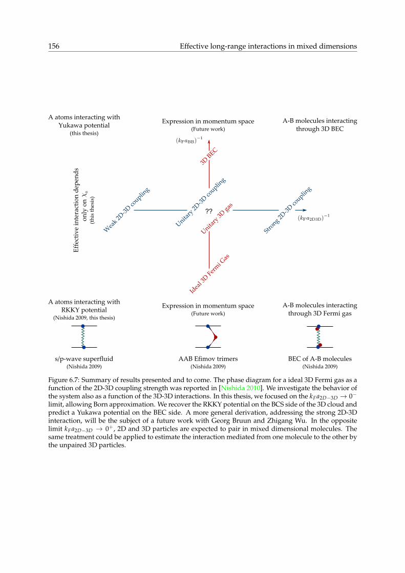
156 Effective long-range interactions in mixed dimensions

A atoms interacting withRKKY potential

(Nishida 2009, this thesis)

A atoms interacting withYukawa potential

(this thesis)

Wea

k 2D

-3D

couplin

g

Stro

ng 2D

-3D

couplin

g

Idea

l 3D

Fer

mi G

as

Unita

ry 2

D-3

D co

upling

Unita

ry 3

D g

as

3D B

EC

Eff

ecti

ve

inte

ract

ion

dep

end

s o

nly

on

(th

is t

hes

is)

s/p-wave superfluid(Nishida 2009)

AAB Efimov trimers(Nishida 2009)

BEC of A-B molecules(Nishida 2009)

Expression in momentum space(Future work)

Expression in momentum space(Future work)

??

A-B molecules interacting through 3D BEC

A-B molecules interacting through 3D Fermi gas

Figure 6.7: Summary of results presented and to come. The phase diagram for a ideal 3D Fermi gas as afunction of the 2D-3D coupling strength was reported in [Nishida 2010]. We investigate the behavior ofthe system also as a function of the 3D-3D interactions. In this thesis, we focused on the kFa2D−3D → 0−

limit, allowing Born approximation. We recover the RKKY potential on the BCS side of the 3D cloud andpredict a Yukawa potential on the BEC side. A more general derivation, addressing the strong 2D-3Dinteraction, will be the subject of a future work with Georg Bruun and Zhigang Wu. In the oppositelimit kFa2D−3D → 0+, 2D and 3D particles are expected to pair in mixed dimensional molecules. Thesame treatment could be applied to estimate the interaction mediated from one molecule to the other bythe unpaired 3D particles.

6.4 - Conclusions 157

BEC

ξ 2.7 µmVBEC

0 0.7 ×10−5 EF

gBEC∆z 6.32 ×10−45 J/m2

ωA −ωS 11.6 Hz

Ideal Fermi Gas

k−1F 0.32 µm

VFG0 7.2 ×10−5 EF

gFG∆z 1.62 ×10−46 J/m2

ωA −ωS -0.07

Table 6.3: Orders of magnitude for the anti-symmetric mode induced by mediated long range in-teraction. The optical lattice parameters are presented in table 6.2. The coupling is expressed inunits of the Potassium Fermi energy EF. The 2D-3D coupling constant is estimated to g2D3D =

gLiK√

mK/(mK + 1.22 mLi), with aLiK = 63× a0.

tude of motion will thus be periodically modulated, the beat note frequency being given by thedifference between the symmetric and anti-symmetric eigenmodes.

6.4 Conclusions

In this chapter, we described interactions in mixed dimensions as the superposition of an inci-dent plane wave and a scattered ellipsoidal wave. We studied the case of effective long rangeinteractions, where the excitations of a 3D system allow for the exchange of momentum be-tween two separated 2D planes. We extended previous theoretical predictions to address thecase where the 3D gas is ramped across over the BEC-BCS crossover. Assuming weak 2D-3Dinteractions, we showed that the mediated long range interaction can be related to the com-pressibility of the 3D gas. Within the Hartree approximation, it approaches asymptotically aYukawa potential on BEC side and a RKKY potential on the BCS side. Those results are pre-sented in figure 6.7.

We then proposed an experimental verification of our model. We presented the setup whichwill give rise to a mixed-dimensional system to lay down relevant orders of magnitudes. Wesuggested to probe the existence of long range interactions by measuring the coupled oscilla-tions of two planes. The frequency of the anti-symmetric mode, which appears as a beat-notefrequency, can be related to the strength of the coupling and provides a way to test our predic-tions.

To conclude this chapter, we recall the main limitations of the previous study:

• All calculations were done at zero temperature. Experimentally, we expect to work attemperatures around 5 to 15% of the Fermi temperature.

• The 2D-3D interaction is supposed to be weak enough to be treated within Born’s approx-imation, and taken into account simply by the coupling constant g2D−3D. This approxi-mation is justified when a2D−3D is the smaller length scale of the problem, which can berealized by taking advantage of Feshbach resonances to tune its value.

158 Effective long-range interactions in mixed dimensions

• A-atoms are treated as single impurities ; their statistics and interactions are not takeninto account, nor is their influence on the 3D cloud. Those effects can be experimentallyminimized by working with dilute 2D gases, such that 3D particles are much more nu-merous.

• When moving through the B-cloud, A-atoms can radiate propagating excitations whichwould take away their energy. Following the Landau criterion, such a situation wouldarise if the velocity of an A particle exceeds the sound velocity in the B superfluid and thiseffect remains negligible as long as the A atoms’ Fermi velocity is small enough [Delehayeet al. 2015].

• The tuning of the interspecies interactions can be experimentally challenging. The Fes-hbach resonances are known to be narrow and display a short lifetime due to enhancedinelastic losses. This will probably limit the reachable scattering length, but we showedthat a measurable signal should be accessible at background value.

Some of these points are currently under investigation in collaboration with Zhigang Wuand Georg Bruun.

ConclusionThe main results presented in this thesis are twofold.

First, we have significantly improved the FERMIX apparatus. We notably developed andimplemented a new cooling scheme, the so-called Λ enhanced gray molasses, which takes ad-vantage of the existence of dark states among and between the hyperfine manifolds addressedby the D1 transition. This technique could be applied simultaneously on both 6Li and 40K, en-abling us to reach a phase-space density of 10−4, the highest value reported for the laser coolingof these two species. It has since then been successfully adapted to the cooling of other isotopes(Lithium 7, Potassium 39, Potassium 41) and species (Sodium 23), proving its broad range ofapplication.

The improvement in phase-space density allowed us to realize the first degenerate 40K gasin France, with 3× 105 atoms in two spin states at 62 nK, corresponding to 17% of the Fermitemperature. Several experiments could be performed with such a sample.

For instance, a highly degenerate fermionic cloud is expected to display dramatically alteredlight scattering properties, as the Pauli principle forbids the decay of an excited state to anoccupied ground state and thus reduces the accessible phase-space [Görlitz et al. 2001]. Twotemperature ratios play a crucial role in this blocking of spontaneous emission, analogous to thePurcell effect [Purcell 1946]. The degree of degeneracy of the ensemble, estimated as the ratioξ = T/TF between the temperature of the cloud and the Fermi temperature, accounts for theoccupancy of phase-space. The recoil strength, expressed as the ratio κ = TR/TF between therecoil temperature and the Fermi temperature, is related to the likelihood for a fermion initiallyimmersed in the Fermi sea to reach a state above the Fermi surface after absorbing and re-emitting a photon. The smaller these two ratios, the stronger the Pauli blocking, and significanteffects above 20% of scattering suppression can be obtained as soon as ξ < 0.2 and κ < 1. Dueto its inverted hyperfine structure, 40K is a promising candidate for the observation of thiseffect [Shuve and Thywissen 2009], as open transitions can be closed by the Pauli blocking,resulting in an apparent increase of the measured atom number.

The long-term objective of the FERMIX experiment is the simultaneous cooling of 6Li to de-generacy. A preliminary measurement showed that both species could be loaded in the opticaldipole trap, but a significant improvement of the atom number is still required to maintain asatisfying efficiency during the last steps of evaporation. In order to reduce the thermal loadfor Lithium and keep balanced populations, we plan to take advantage of the Potassium Fesh-

159

160 CONCLUSION

bach resonance to decouple effectively both evaporations. Hopefully this cooling scheme willsoon make the FERMIX experiment able to study ultra-cold Fermi-Fermi mixtures.

Once both species have been brought to ultra-low temperatures, they could be used to real-ize a mixed-dimensional system. We developed a theoretical analysis of such a situation, where40K is confined in 2D-planes immersed in a 3D 6Li cloud. We demonstrated that an effectivelong range interaction can be mediated from one layer to the next one by the surrounding cloudand derived the expression of the coupling within Born’s approximation on both the BEC andBCS sides of the resonance. We proposed a scheme for an experimental verification of our pre-dictions by measuring the beat-note period of coupled oscillations between pancakes confinedin neighboring sites of an optical lattice.

Besides this proposal, several problems could be studied by relying on such a mixed dimen-sional simulator. For example, mixed dimensions open new perspectives for Efimov physics. Inthe unitary limit, three particles can form Borromean-like trimers, whose binding energies forma geometric series characterized by a universal factor [Efimov 1970, Efimov 1973]. It was longbelieved that these Efimov trimers could only exist in three dimensions, where the short-rangeboundary condition enforces a non trivial interaction at unitarity. However, mixed dimensionsprovide additional ways to generate Efimov bound states, provided that the mass ratio of thetwo involved species belongs to a critical interval [Nishida and Tan 2011]. A fermionic 6Li-40Kdegenerate mixture, such as the one we aim at producing, is well suited for such realizations, astwo 2D Potassium atoms can bind with and through a 3D Lithium atom. Furthermore, the exis-tence of inter-layer configurations helps preventing three-bodies recombinations and increasesthe stability of Efimov trimers with respect to the 3D scenario.

Furthermore, with the appropriate optical configuration, the FERMIX apparatus could beused to engineer alternative mixed-dimensional schemes, for instance 1D-3D or 0D-3D sys-tems. In addition to Efimov physics, these systems offer the opportunity to study specificphenomena, such as the Kondo effect mentioned in the introduction.

Second, we proved that some dynamical properties of non-interacting Weyl particles in aharmonic trap could be simulated with spin-polarized Lithium atoms in a quadrupole trap.Our method relies on a canonical mapping to translate properties of Weyl fermions into thelanguage of atomic physics. For instance, this mapping allowed us to re-interpret the Kleinparadox as Majorana spin-flip losses.

Despite their apparent simplicity, we have shown that these equivalent systems displaynon trivial properties. We showed that an ensemble of Weyl particles dragged away from thetrap center does not oscillate continuously, but relaxes towards a strongly anisotropic steadystate which cannot be described by a Boltzmann distribution. This provides an interestingexample of relaxation in the absence of collisions, midway between harmonically confinedmassive particles, which oscillate without damping, and interacting particles in non harmonicpotentials, which usually relax towards a thermal state.

161

As the oscillations are damped, the energy initially imparted to the center of mass of theensemble is redistributed within the cloud. Defining effective temperatures as the second mo-ments of the distribution, we characterized the heating following the excitation. Even thoughthe Hamiltonian is non separable, the strongly confining axis appears to be almost decoupledfrom the symmetry plane. Yet, within this plane, effective temperatures equilibrate, showinga quasi-thermalization. Using general theorems, we estimated the expected heating and find agood agreement between theory and numerics without free parameters. Experimentally, thesepredictions have been successfully tested against two different excitation methods.

In order to study the influence of the trap geometry, we derived analytical results for therelaxation in an isotropic trap based on Bertrand’s theorem. In 3D, we have shown that theeffective heating remains anisotropic as the excitation breaks the initial symmetry. By con-trast, the effective heating becomes isotropic in 2D. These results were validated and extendedto intermediate trap geometries by numerical simulations, notably allowing an estimation ofthe relaxation time and suggesting an interpretation of the quasi-thermalization based on theprecession of orbital planes.

We derived expressions of the involved Berry phases and showed numerically that the ad-ditional coupling they provide is negligible at the considered temperatures. The simultaneousenhancement of the influence of geometric potentials and of Klein-Majorana losses, while com-promising the ability of quasi-thermalization to illustrate topological properties, illustrates thatboth effects originate from the same adiabatic hypothesis.

Finally, it should be noted that the very same mapping could be used to study various situ-ations. For instance, particles in a Ioffe-Pritchard trap appear as analog to massive relativisticparticles, while in a hybrid magneto-optical trap, they could be used to engineer a Rashbacoupling.

The FERMIX experiment is about to reach its intended operational capacities and demon-strates an increasing ability to address fundamental problems of quantum mechanics. Asshown in this work, the experiment highlights several strengths of Physics. Universality firstof all, as two systems with very different natures, such as ultra-slow cold atoms and ultra-fastrelativistic Weyl particles, can be found to behave in the same way. It also epitomizes the in-terplay between theory and experiment, as both are accessible in the lab: the setup remainson a human scale and standard concepts can be readily derived and tested against data. Butmostly, it illustrates how new lines of research can sometimes emerge by serendipity: evenwell-known and thoroughly studied systems such as the quadrupole magnetic trap can exhibitan un-described behavior, providing new tools for the study of exotic situations and pushingforward the boundaries of understanding.

Chapter

A Appendix

ContentsA.1 Alkaline atoms in magnetic fields . . . . . . . . . . . . . . . . . . . . . . . . . . . . . . . 164

A.1.1 Wigner-Eckart theorem and Lande factor . . . . . . . . . . . . . . . . . . . . . . . . 164

A.1.2 Zeeman hamiltonian . . . . . . . . . . . . . . . . . . . . . . . . . . . . . . . . . . . 165

A.1.3 Asymptotic behaviors . . . . . . . . . . . . . . . . . . . . . . . . . . . . . . . . . . . 166

A.1.4 Breit-Rabi formula . . . . . . . . . . . . . . . . . . . . . . . . . . . . . . . . . . . . . 168

A.1.5 Remark on notations . . . . . . . . . . . . . . . . . . . . . . . . . . . . . . . . . . . 169

A.2 About Boltzmann equation . . . . . . . . . . . . . . . . . . . . . . . . . . . . . . . . . . . 170

A.2.1 Collisionless Boltzmann equation . . . . . . . . . . . . . . . . . . . . . . . . . . . . 170

A.2.2 H theorem . . . . . . . . . . . . . . . . . . . . . . . . . . . . . . . . . . . . . . . . . 171

A.3 Kohn, virial and Bertrand theorems . . . . . . . . . . . . . . . . . . . . . . . . . . . . . . 175

A.3.1 Kohn theorem . . . . . . . . . . . . . . . . . . . . . . . . . . . . . . . . . . . . . . . 175

A.3.2 Virial theorem . . . . . . . . . . . . . . . . . . . . . . . . . . . . . . . . . . . . . . . 176

A.3.3 Bertrand’s theorem . . . . . . . . . . . . . . . . . . . . . . . . . . . . . . . . . . . . 177

A.4 Elements of collision theory . . . . . . . . . . . . . . . . . . . . . . . . . . . . . . . . . . . 181

A.4.1 Mathematical framework . . . . . . . . . . . . . . . . . . . . . . . . . . . . . . . . . 182

A.4.2 Scattering eigenstates . . . . . . . . . . . . . . . . . . . . . . . . . . . . . . . . . . . 183

A.4.3 Scattering matrices, amplitude and cross section . . . . . . . . . . . . . . . . . . . 183

A.4.4 Low energy limit . . . . . . . . . . . . . . . . . . . . . . . . . . . . . . . . . . . . . . 185

A.4.5 Feshbach resonances . . . . . . . . . . . . . . . . . . . . . . . . . . . . . . . . . . . 187

A.4.6 Getting familiar with a Feshbach resonance . . . . . . . . . . . . . . . . . . . . . . 189

A.5 Technical references . . . . . . . . . . . . . . . . . . . . . . . . . . . . . . . . . . . . . . . 191

A.5.1 AOMs and EOMs . . . . . . . . . . . . . . . . . . . . . . . . . . . . . . . . . . . . . 191

A.5.2 Power supplies . . . . . . . . . . . . . . . . . . . . . . . . . . . . . . . . . . . . . . . 192

A.5.3 Optical sources . . . . . . . . . . . . . . . . . . . . . . . . . . . . . . . . . . . . . . 192

A.5.4 RF system . . . . . . . . . . . . . . . . . . . . . . . . . . . . . . . . . . . . . . . . . 193

A.6 Electrical schemes . . . . . . . . . . . . . . . . . . . . . . . . . . . . . . . . . . . . . . . . . 193

THis appendix presents and demonstrates some of the fundamental results used in the maintext of the manuscript. Annex A.1 is dedicated to the Zeeman effect, throughly used in the

field of cold atoms. Annex A.2 introduces Boltzmann equation and illustrates some historicalparadoxes of the H theorem, at the core of the kinetic theory of gases. Annex A.3 demonstrates

163

164 Appendix

the Kohn, virial and Bertrand’s theorem, with an original approach. Annex A.4 summarizeselements of the elastic collisions theory required to address scattering problems. Eventually,annex A.5 provides the technical references of the devices used on the apparatus.

A.1 Alkaline atoms in magnetic fields

The Zeeman effect accounts for the influence of an external magnetic field on the eigenelementsof an atom. The atom is coupled to the field through its magnetic momentum M, which canbe related to the angular momentums (orbital L, intrinsic S and nuclear I) through Wigner-Eckart theorem. As a consequence, a small field will lift the degeneracy of the so called Zeemansublevels which differ only by their projected angular momentum. At a highest order, the im-pact on the hyperfine splitting must be taken into account. In asymptotic regimes, convenientformulae can be derived to estimate the Zeeman shifts. If the magnetic field is small enough,such that its influence is negligible compared to the hyperfine splitting, the energy shift of eachZeeman sublevel is linear with the field and proportional to its projected momentum. If themagnetic field is strong enough, such that the hyperfine splitting can be neglected, the energyshift is still proportional to the field but only depends of the electron intrinsic orientation. Thecalculation can be explicitly carried out for L = 0; the resulting Breit-Rabi formula is thereforeappropriate for the ground states of alkali atoms and plays an important role in our case.

This appendix reviews and summarizes the main results describing the behavior of alkaliatoms such as Lithium and Potassium in a magnetic field.

A.1.1 Wigner-Eckart theorem and Lande factor

The magnetic momentum of an atom is a vectorial operator and follows as such the Wigner-Eckart theorem: The restriction of any vectorial operator V to an eigenspace of the angularmomentum F is proportional to the angular momentum with a coefficient

〈V.F〉FF(F + 1)h2 . (A.1)

Here, a vectorial operator is defined by its commutation relations [Fx, Vx] = 0,[Fx, Vy

]= ihVz

and [Fx, Vz] = −ihVy (and circular permutations) while the mean value can be estimated onany state of the eigenspace.

Three angular momentum are required to describe an atomic state and the magnetic mo-mentum can therefore be expressed as the sum of three contribution. The proportionality fac-tor between a magnetic momentum and the related angular momentum is expressed with Bohrmagneton µB = eh

2me' 1.4× h MHz/G and so called Landé factor, usually noted g.

• The orbital momentum L of the electron is associated to a magnetic momentum ML =

− µBh gLL with gL = 1.

A.1 - Alkaline atoms in magnetic fields 165

δL s p d fLi 0.40 0.04 0 0K 2.19 3.59 2.46 0.02

gJ S1/2 P1/2 P3/2

Li 2 0.666 1.335K 2 2/3 4/3

Table A.1: Landé factors (left) and quantum defects for Lithium and Potassium, as given by [Burkhardtand Leventhal 2010]

40K ahf bhf

42S1/2 -285.730 -42P1/2 -34.523 -42P3/2 -7.585 -3.445

6Li ahf bhf

22S1/2 152.136 -22P1/2 17.386 -22P3/2 -1.155 -0.10

Table A.2: Hyperfine structure of 6Li and 40K, as given by [Arimondo et al. 1977]

• The intrinsic momentum S of the electron (or spin) is associated to a magnetic momen-tum MS = − µB

h gSS with gs ' 2. This value is predicted by Dirac equation; magneticanomalies modify it by ∼ +0.02.

• The nuclear momentum I is associated to a magnetic momentum MI = − µBh gII. The

factor gI depends of the nuclei but is always much smaller than 1 (1.7× 10−4 for 40K and−4.5× 10−4 for 6Li).

It is often useful to consider composed angular momentum, such as J = L+S and F = J+ I.We can therefore introduce the corresponding Landé factors

gJ =gS

2J(J + 1) + S(S + 1)− L(L + 1)

J(J + 1)+

gL

2J(J + 1) + L(L + 1)− S(S + 1)

J(J + 1), (A.2)

gF =gJ

2F(F + 1) + J(J + 1)− I(I + 1)

F(F + 1)+

gI

2F(F + 1) + I(I + 1)− J(J + 1)

F(F + 1). (A.3)

The Wigner-Eckhart theorem is extremely useful as long as the vectorial operator can be cor-rectly approximated by its restriction to a subspace of the angular momentum. This is correctas long as the variations due to the operator are small compared to the difference between twosubspaces. Since S and I are intrinsic quantities, the previous results are always correct. ForL (resp. J, F), they hold until the energy shift becomes comparable to the atomic structure of∼ 100 THz (resp fine structure ∼ 100 GHz, hyperfine structure ∼ 100 MHz)

A.1.2 Zeeman hamiltonian

To account for the Zeeman effect on alkali, we describe an atom with the following Hamiltonian[Cohen-Tannoudji et al. 1997],

H = H0 + Wso + Whf + HZ, (A.4)

166 Appendix

where

• H0 describes a spinless valence electron in the electrostatic potential of the nuclei and coreelectron cloud. For alkali atoms, the energy of an orbit depends not only on the principalquantum n, but also on the angular momentum L, as the orbit can bring the valenceelectron to cross inner electronic layers. This effect can be simply taken into account bythe so-called quantum defect [Hanle 1984]. The eigenenergies then take the form E0(n, L) =−Ry/ (n− δn,L)

2, where Ry is the Rydberg constant and δn,L is the quantum defect, mostlydepending on L (see table A.1).

• Wso describes the coupling between the spin S and the orbital angular momentum L. Itcan be written, as any interaction lifting the degeneracy of the J = S + L levels, under theform:

Wso ∝ L.S ' af (J(J + 1)− L(L + 1)− S(S + 1)) , (A.5)

where af gives the fine structure splitting.

• Whf accounts for the coupling to the angular momentum of the nuclei, generating thehyperfine structure of the atom:

Whf =ahf

h2 I.J +bhf

h2

3(I.J)2 + 32 h(I.J)− I2 J2

2I(2I − 1)J(2J − 1)(A.6a)

=ahf

2(F(F + 1)− I(I + 1)− J(J + 1)) if bhf = 0 (A.6b)

where ahf and bhf are the magnetic dipole and electric quadrupole constants respectively.

• HZ describes the coupling of magnetic momentums to an external magnetic field:

HZ = −(MS + ML + MI

).B (A.7)

A.1.3 Asymptotic behaviors

• At low field: linear Zeeman effect treatment

If the Zeeman shift is much smaller than the hyperfine splitting, the Zeeman effect can betaken into account perturbatively. Atomic states are correctly described by their projectedangular momentum mF and their (degenerate) energies are given by:

E(mF) = E0(n, L) + ahf (F(F + 1)− I(I + 1)− J(J + 1)) /2 (A.8)

Up to first order in perturbation, the Zeeman effect is given by

∆E = 〈mF|HZ |mF〉 =µB

hgFB mF (A.9)

A.1 - Alkaline atoms in magnetic fields 167

0 2 4 6 8 1020

10

0

10

20

0 50 100 150 200

250

500

0

500

250

Magnetic bias Magnetic bias

En

erg

y s

hif

t

Figure A.1: Asymptotic regimes for the Zeeman shift of the P3/2 states of 40K (left) and 6Li (right) as afunction of the magnetic field. The low field regime is given by equation (A.9), where the coupling tothe magnetic field is treated perturbatively. The high field regime is given by equation (A.11b), wherethe hyperfine structure is estimated as a perturbation.

For Lithium as well as Potassium, this regime is only valid as long as the magnetic fielddoes not exceed few Gausses (see Fig. A.1).

• At high field: Paschen-Back regime

If the Zeeman shift is much larger than the hyperfine splitting, the restriction of theHamiltonian to an eigenspace of the angular momentum F is not relevant anymore andthe projected momentum mF is not a good quantum number to describe the situation.The magnetic momentum M cannot be expressed with F but must be described as thesum of MI and MJ , making mI and mJ the relevant quantum numbers.

We therefore consider the eigenstates |n, L, S, J, I, mJ , mI〉 of the Hamiltonian H = H0 +

Wso + HZ, whose energies shift with respect to B = 0 are given by

∆E = µB (gJmJ + gImI) B/h (A.10)

To take into account the hyperfine splitting, we calculate at lowest order

δE = 〈mJ , mI |Hhf |mJ , mI〉 (A.11a)

= ahfmImJ + bhf9m2

I m2J − 3I(I + 1)m2

J − 3J(J + 1)m2I + I J (I + 1) (J + 1)

4I J(2I + 1)(2J + 1)(A.11b)

For Potassium, this regime is valid as soon as B > 50 G for P3/2 states (resp. B > 200 Gfor P1/2 states). For Lithium, this regime is valid as soon as B > 3 G for P3/2 states (resp.B > 30 G for P1/2 states). It is therefore the relevant expression to estimate the shifts attypical biases of the experiment (see A.1).

168 Appendix

Magnetic bias Magnetic bias

En

erg

y s

hif

t

F=7/2

F=9/2

mF=-7/2

mF=-9/2

mF=+3/2

mF=+1/2

F=3/2

F=1/2

0 250 500 750 10002

1.5

1

0.5

0

0.5

1

1.5

2

0 25050 100 150 200

0.25

0.5

0

0.5

0.25

Figure A.2: Zeeman shift of the S1/2 manifold of 40K (left) and 6Li (right) as a function of the magneticfield, as estimated by the Breit Rabi formula (A.15)

A.1.4 Breit-Rabi formula

For S orbitals, as the angular momentum L = 0, the Zeeman effect can be analytical calculatedas show in [Breit and Rabi 1931]. Using standard notations, we rewrite

H = H0 + ahf

(Iz Jz +

12(I+ J− + I− J+)

)/h2 + µBB (gJ Jz + gI Iz) /h (A.12)

Since J = 1/2, we can expand the matrix expression of the Hamiltonian over the basis |n, L =

0, S, J = S, I, mJ , mI〉 = |mJ , mI〉:

H − H0 =

E(mF = −

(I + 1

2

))0 0 0

0 M11(−I) M12(−I) 00 M21(−I) M22(−I) 0

. . .

0 0 0 E(mF =

(I + 1

2

))

(A.13)

where the M matrices have the following form

M11(mI) = ahfmI/2h2 + µBB( gJ

2+ mI gI

)/h, (A.14a)

M22(mI) = −ahf (mI + 1) /2h2 + µBB(− gJ

2+ (mI + 1) gI

)/h, (A.14b)

M12(mI) = ahf

√I(I + 1)− (mI + 1)mI/2h2 = M21(mI). (A.14c)

This block matrix can be easily diagonalized: the stretch states mF = ± (I + 1/2) are alreadyeigenstates and each subspace |−1/2, mI〉 , |+1/2, mI − 1〉 with a constant mF is stable. The

A.1 - Alkaline atoms in magnetic fields 169

corresponding eigenvalues give the Zeeman shift:

∆E =

ahf2h2 I ± µB

h

( gJ2 + gI I

)B for mF = ±

(I + 1

2

)

− ahf4h2 + gIµBmFB± ahf(I+ 1

2 )2

√1 + 2µB(gI−gJ)mF

ahf(I+ 12 )

2 B +µ2

B(gI−gJ)2

a2hf(I+ 1

2 )2 B2 for |mF| <

(I + 1

2

)

(A.15)Their values are plotted on figure A.2.

A.1.5 Remark on notations

As shown in this appendix, the hyperfine states are eigenstates of the system only at zerofield. The projected angular momentum mF is therefore not a good quantum number gen-erally speaking, when arbitrary magnetic field are applied. Nevertheless, we will refer to thosenumbers to label without ambiguity the eigenstates of the Zeeman Hamiltonian. Strictly speak-ing, the spin-state |mF〉 should be understood as the eigenstate adiabatically connected to |mF〉at zero field.

170 Appendix

A.2 About Boltzmann equation

We review and summarize some of the properties of Boltzmann equation used in chapter 3, andpresent two of the historical paradoxes associated to the H-theorem to illustrate the complexityof the relaxation problem. For a more detailed presentation, see for instance [Pottier 2007].

A.2.1 Collisionless Boltzmann equation

We consider a dilute gas of N neutral atoms, which we assume to be described at time t by adistribution f (r, p, t), not necessarily the equilibrium function. f (r, p, t) drdp gives the proba-bility to find at time t a particle in volume dr around r with a momentum as close as dp fromp.

Liouville theorem states that the distribution function is constant along any trajectory inphase space. In absence of interactions between particles, it simply corresponds to particleconservations: the number of particles in the phase-space volume dr′dp′ around (r′, p′) at timet′ used to be in the phase-space volume drdp around (r, p) at time t, provided that

∂tr(t) = p(t)/m, (A.16a)

∂tp(t) = F(r(t)), (A.16b)

where F = −∂rU is the outer potential exerted on the atoms.

In terms of distribution function, Liouville theorem can be written as f (r′, p′, t′) dr′dp′ =f (r, p, t) drdp, which we can express as

(∂t +

pm

∂r + F∂p

)f = 0, (A.17)

and we introduce the Liouville operator L such that ∂t f = −L f :

L =pm

.∇r + F.∇p (A.18)

Equilibrium distribution

Starting from given initial conditions, it is almost impossible to predict from the previous equa-tions the steady state that the system is going to reach. On the other hand, it is straightforwardto verify that a Boltzmann distribution f0 define as:

f0 (r, p) =N

(2πh)3λdB

Veexp

(−β

(p2

2m+ U(r)

)), (A.19)

A.2 - About Boltzmann equation 171

where Ve =∫

dr exp (−βU(r)) is the effective volume occupied by the gas, is an stationarysolution of the collisionless Boltzmann equation (A.17).

Considering a kinetic definition of the temperature as the standard deviation of the momen-tum distribution, we identify β = (kBT)−1 for the Boltzmann distribution (A.19). Remarkably,f0 is completely defined by this single scalar parameter T, which implies that any physicalquantity can be expressed as a function of the temperature. This is not the case for all solu-tions to the Boltzmann equation, and a steady state distribution can require more than oneparameter.

The Boltzmann distribution plays a crucial role in the kinetic theory of gases and we intro-duce two properties of the Liouville operator that are useful to derive the results presented inthis manuscript

• L[ f0] = 0, since Boltzmann’s distribution is a stationary solution of Boltzmann’s equa-tion.

• L is antisymmetric for the scalar product, ie 〈α|L [β]〉 = − 〈L [α] |β〉 with

〈α|β〉 =∫

drdq f0αβ (A.20)

A.2.2 H theorem

General formulation of the Boltzmann equation

If interactions cannot be neglected between atoms, Liouville theorem still applies for the N par-ticles distribution function. Several strategies can be considered to estimate the marginal singleparticle distribution. The BBGKY hierarchy treats the problem iteratively, expressing the singleparticle distribution as the solution of an equation involving the two-particles distribution andso on. The Vlasov equation corresponds to a mean field treatment of the second order of theBBGKY development and serves as framework for most of plasma physics.

Boltzmann approach relies on a series of simplifications:

• Only binary collisions are taken into account. This supposes that the gas is dilute enoughfor three-body events to be extremely rare.

• All collisions are considered as elastic and no internal degrees of freedom are changed.Most of the time, the interactions are treated as independent of the energy of the particles.

• All collisions are micro-reversible: the probability for two colliding atoms with momen-tum p1 and p2 to emerge from the collision with momentum p′1 and p′2 is the same as theprobability of the reverse process.

172 Appendix

• The Stosszahlansatz, or pre-collisional chaos, is probably the strongest hypothesis as itsupposes that, before their interaction, the two particles are completely uncorrelated.

Under those conditions, the time evolution of the distribution function can be expressed as

(∂t +

pm

∂r + F∂p

)f =

(∂ f∂t

)

collisions, (A.21)

where the collision term takes the form(

∂ f∂t

)

collisions=∫

dq∫

dΩ σ (p, q, Ω)∣∣∣ pm− q

m

∣∣∣(

fp′ fq′ − fp fq)

. (A.22)

In the integral, p′ has the same modulus as p but is oriented in the Ω direction and q′ is fixedby the energy and momentum conservation. The cross-section σ(Ω) corresponds to the proba-bility for particles to deviate from their initial trajectories by a solid angle Ω. The value of thecross section depends on the nature of the interactions, as detailed in annex A.4.

H theorem

It is often assumed that, in presence of collisions, the distribution function will eventually re-lax towards f0 (even though particles in a harmonic potential provide a good counter examplethrough the undamped oscillations of both the center-of-mass motion (see Kohn theorem be-low) and the monopole breathing mode [Lobser et al. 2015]). The qualitative idea relies on theH theorem, that plays a key-role in Boltzmann theory and has been a bone of contention sinceits formulation [Vilani 2010].

Boltzmann introduced the quantity H define as

H(t) =∫

drdp f (r, p, t) log f ((r, p, t) (A.23)

which can easily be related to the more familiar entropy S(t) = −kBH(t).

The H-theorem states that this quantity can only decrease during the time evolution of thesystem

ddt

H(t) ≤ 0 (A.24)

or equivalently, the entropy of the isolated system can only increase.

The demonstration relies on the integration of eq.(A.21) and the inequality saturates fordistributions such that the collision term vanishes. In the interacting case, the only distributionsverifying this condition are the local Maxwellians defined as

f (r, p, t) = n(r, t)(

12πmkBT(r, t)

)3/2

exp(− (p−mu(r, t))2

2mkBT(r, t)

), (A.25)

A.2 - About Boltzmann equation 173

where the density n, temperature T and velocity u fields are free parameters. Note that such adistribution may not be a steady state of Boltzmann equation (ieL [ f ] 6= 0). The non-interactingcase, considered in chapter 3 and 4, provides an additional situation of evolution with constantentropy.

Classical paradoxes

• Loschmidt’s reversibility paradox [Loschmidt 1876]

Starting from a given initial condition, H decreases during the evolution of thesystem. At time t, H has reached a value H(t) < H0 and we reverse the speed ofall particles. Since collisions are micro-reversible, the system will resume its initialconfiguration in which H = H0. During this evolution, H has increased, in contra-diction with the H theorem.

This paradox relies on a wrong interpretation of the Stosszahlansatz: as time is reversed, themicro-reversibility implies that particles display pre-collisional correlations, but post-collisionalchaos. Deriving Boltzmann equation with this modified hypothesis inverses the sign of thecollision term: the entropy decreases (or the quantity H increases) during the evolution of thesystem. Qualitatively, the reverse evolution starts with correlated particles and every collisionbrings the system closer to the initial distribution, where all particles were uncorrelated; thedecrease of entropy translates this loss of information. A further objection can then be formu-lated:

The situation presented above shows that Boltzmann equation is not relevant todescribe some systems, such as distributions with initial correlations.

The assessment is true, but does not constitute a paradox of any kind, as illustrated by spinecho experiments. However, these systems with strong initial correlations require a very deli-cate construction and a typical configuration, drawn at random in phase-space, is very unlikelyto display such features. The story says that, as Boltzmann was confronted to Loschmidt’s re-versibility paradox, he answered: “Go ahead then, reverse them !”.

• Poicaré-Zermelo’s recurrent paradox [Zermelo 1896]

Poicaré demonstrated in 1889 the recurrence theorem [Poincaré 1890]:

Let us consider a system which dynamics conserves the phase volume of anyfinite element and which evolution remains contained in a finite phase space vol-ume. Then, after sufficiently long time (the so-called Poincaré recurrence time), thesystem will return to a state arbitrarily close to its initial state.

174 Appendix

Owing to Liouville theorem and energy conservation, the two premesis are verified for mostclosed physical systems. Few years after the publication of Poincaré memoir, Zermelo formu-lated a paradox relying on his theorem:

How can a system returns to its initial configuration, with the initial quantityH0, if H can only increase during its evolution ?

Mathematically, the paradox comes from the applicability of the Poincaré theorem, which con-cerns finite systems of N particles. Boltzmann equation supposes an infinite number of degreesof freedom and is therefore not subject to the theorem.

Physically however, systems do contain a finite number of particles. Nevertheless, the re-currence time scales exponentially with N and for macroscopic samples, the correspondingperiods are much longer than the age of the universe. What’s more, Boltzmann equation re-mains valid only as long as the Stosszahlansatz is relevant. Long before the recurrence timeis reached, the pre-collisional correlations might not be negligible and the system will exit thevalidity range of the H theorem.

A.3 - Kohn, virial and Bertrand theorems 175

A.3 Kohn, virial and Bertrand theorems

In this annex, we present derivations of three theorems used in the main text, namely the Kohn,virial and Bertrand’s theorems. The demonstration of the latter is an original work, inspired byseveral proofs reported in the literature.

A.3.1 Kohn theorem

Kohn’s theorem is a very strong result to study particles trapped in a harmonic potential andwas first formulated to describe the cyclotron motion of particles in a static, uniform magneticfield [Kohn 1961]. It states that regardless of the inter-particles interactions, the center of massof the distribution oscillates at the cyclotron frequencies. Its extension in [Brey et al. 1989]generalized this result to the case of identical particles in a harmonic trap. Later, in [Dobson1994], the "harmonic potential theorem" demonstrates the rigid transport of the many-bodywavefunction.

Proof

We describe trapped particles with the Hamiltonian

H = Hkin + Htrap + Hint = ∑i

p2i

2m+ ∑

i

12

mω2r2i + ∑

i,jw(ri − rj

). (A.26)

We introduce the center of mass variables R = ∑i

ri/N and P = ∑i

pi, as well as the

relative coordinates ξi = ri −R and qi = pi − P/N. With these notations, we can rewritethe Hamiltonian (A.26) as:

H = HCoM + Hrel, (A.27a)

HCoM =P2

2Nm+

12

Nmω2R2, (A.27b)

Hrel = ∑i

q2i

2m+ ∑

i

12

mω2ξ2i + ∑

i,jw(

ξi − ξ j

). (A.27c)

Note that relative- and center of mass- coordinates commute and [R, P] = ih. We havetherefore [Hrel, R] = [Hrel, P] = 0, and the center of mass follows the simple Hamiltonianof a trapped particle with mass Nm in a harmonic potential.

The same proof can be applied for particles with a charge q in an additional static oruniform magnetic field B(r) = ∇×A and uniform electric field E(t). The center of massHamiltonian is then given by

HCoM =(P−QA)2

2M+

12

Mω2R2 + QE(t).R, (A.28)

176 Appendix

with Q = Nq and M = Nm.

The theorem can be further extended to show that the wave function of the N particlessystem can be expressed as the product of a center of mass wave function and an “in-ternal” wave function. To do so, we must introduce the Jacobi coordinates u1 = r1 − r2,u2 = r1+r2

2 − r3, ..., un = r1+...+rnn − rn+1 and the corresponding momenta. Those coordi-

nates do verify the canonical commutation relations and we can show that they can beused to rewrite Hrel, hence the result.

A.3.2 Virial theorem

Virial theorem was formulated by Rudolf Clausis in 1870 [Clausius 1870] and applies to parti-cles in a potential V(r) such that

V(λr) = λnV(r). (A.29)

In particular, this class includes all potential with the form V(r) =(αxxp + αyyp + αzzp)q, with

n = pq.

The theorem can be formulated as follows: for any ensemble submitted to a potential (A.29),the kinetic energy EK and the potential energy EP in the steady states are related through therelation:

2EK = nEP (A.30)

Virial theorem is often used in stellar physics and provides for instance a derivation of Chan-drasekhar limit for the stability of white dwarf stars.

Lemma Euler Theorem

For any potential, if ε 1, we can write V((1 + ε)r) ' V(r) + ε (r.∂r)V(r)

Since V((1 + ε)r) = (1 + ε)nV(r) ' V(r) + nεV(r), this leads to Euler theorm for homo-geneous functions:

(r.∂r)V(r) = nV(r) (A.31)

Proof We describe an ensemble of particles in a potential V with the distribution functionf (r, p, t). The evolution of f is governed by Liouville equation

∂ f = L f ,

with the Liouville operator being L = pm .∂r − (∂rV) .∂p.

Let us consider the quantity C(t) = 〈r.p〉 =∫

f r.p. In steady state, ∂tC = 0 and we canexpress

0 =∫

∂t f r.p =∫L ( f ) r.p = −

∫f L (r.p) (A.32)

A.3 - Kohn, virial and Bertrand theorems 177

Figure A.3: Three orbits in central potentials. In a), the Hook potential results in an apside angleθA = π/2. In b), the Coulomb potential gives θA = π. In c), an arbitrary potential gives a rosette-like trajectory.

where we integrated by parts. Using Euler theorem, we can express L (r.p) = p2/m−nV, and the previous condition leads to

∫f

p2

m= n

∫f V (A.33)

hence the virial theorem.

A.3.3 Bertrand’s theorem

Bertrand’s theorem describes the behaviour of particles trapped in a central force potentialV(r). The theorem states that, even if any arbitrary potential admits a circular orbit, only twoare such that all bound orbits are closed: the Coulomb potential VC(r) = −κ/r and the Hookpotential VH(r) = κ′r2.

The corollary of this theorem is that any potential apart from VC and VC will admit rosette-like orbits, as the particle will cover densely all positions between the aphelion and the perihe-lion (see Fig. A.3)

The theorem was first formulated in 1873 by J. Bertrand [Bertrand 1873] (see [Santos et al.2011] for an english translation) as a general analysis of bound orbits. It was proposed as atool for the study of the three-body problem and can be used as an alternative demonstrationto the shape of Newton’s gravitational potential, since all trajectories observed among celestialbodies are closed.

Several proofs to Bertrand’s theorem can be found nowadays. Most of them have the samestructure and only differ in the last step of the demonstration. The original proof uses a globalapproach; a perturbative method can also be applied [Goldstein et al. 2001] or additionnalconstant of motion can be invoked [Martinez-y Romero et al. 1992]. Many more rely on an

178 Appendix

inverse transform [Grandati et al. 2008, Santos et al. 2009]. Here, we show a global approachinspired by [Arnold et al. 1997].

Few words of vocabulary, illustrated on figure A.3:

• The apside angle θA is the angle AOP between the the aphelion A, the center O et theperihelion P.

• An orbite is closed if the trajectory followed by a particle will eventually loop. Equiva-lently, this condition corresponds to the apside angle being commensurate with π: θA =mn π.

Step 1 If all orbits are closed, than the apside angle must be the same for all trajectories

Let us consider a closed orbit. As mentioned above, this condition requires that the apsideangle of this trajectory is commensurate with π.

If the apside angle was not the same for all orbits, but depended continuously of theenergy or angular momentum of the trajectory, it would necessarily take values incom-mensurate with π according to the intermediate value theorem.

Therefore, if all orbits are closed, they must all have the same apside angle θA.

Step 2 For almost circular orbits, the only central potentials with constant apside angles are V(r) =

κ ln r/r0 and V(r) = κrα with α > −2 and α 6= 0. The corresponding apside angles areθA = π√

2+α

We consider a point-like particle with mass m subject to the force F(r) = −∂rV(r)ur anddecribe its trajectory in polar coordinates (r, θ).

The energy conservation can be expressed as

E =12

mr2 +12

mr2θ2 + V(r). (A.34)

Using the conservation of angular momentum L = mr2θuz, we can express the kineticenergy as a function of the distance r and of its angular dependance:

r2 + r2θ2 =

(Lz

mr2drdθ

)2

+L2

z2mr2 . (A.35)

We follow Binet’s notation u = r−1, so that dudθ = − 1

r2drdθ and we can write eq.(A.34) as

E =L2

z2m

(dudθ

)2

+ Veff(u), (A.36)

A.3 - Kohn, virial and Bertrand theorems 179

Figure A.4: Effective potentials (black line), expressed as the sum of the kinetic (red dashed line) andpotential (green dashed line) energies, for α < 0 (left) and α > 0 (right). For a given energy (bluehorizontal line), the aphelion (rmin) and perihelion (rmax) define the accessible position range.

where we introduced (see Fig. A.4)

Veff(u) =L2

z2m

u2 + V(u−1). (A.37)

Let us consider a circular trajectory u0 with energy E0 and momentum Lz and a stableorbit close to it, such that u = u0 + ρ(θ). Up to the second order, Veff(u) = Veff(u0) +12 ρ2V ′′eff(u0) since V ′eff(u0) = 0 and eq. (A.36) reads

E =L2

z2m

(dρ

dθ

)2

+12

ρ2V ′′eff(u0), (A.38)

which describes an oscillation with the angular frequency

Ω =

√mV ′′eff(u0)

L2z

=

√3V ′(r0) + r0V ′′(r0)

V ′(r0)> 0, (A.39)

where we used V ′eff(u0) = 0⇒ V ′(r0) = L2z/mr3

0 and expressed the stability of the orbit.

Without any loss of generality, we can chose the origin such that u = u0 + A cos Ωθ. Theaphelion is reached for θ = 0 and the perihelion for θ = θA = π/Ω. The conditionexpressed in step 1 thus leads to

3V ′(r) + rV ′′(r)V ′(r)

= 2 + α, . (A.40)

with α > −2. For α = 0, eq. (A.40) leads to V(r) = κ ln r/r0 and θA = π/√

2, and wecan rule out this potential since its aspide angle is incommensurate with π. For α 6= 0, wefind V(r) = κ′rα and

θA =π√

2 + α. (A.41)

180 Appendix

Step 3 The only possible values for the apside angle to be commensurate with π are α = 2 and α = −1,hence Bertrand’s theorem

For each value of α, since the apside angle is the same for all trajectories, we will restrictthe study to a convenient situation and express the apside angle using eq. (A.36)

θA =Lzumax√

2m

1∫

uminumax

dx√E−Veff(xumax)

. (A.42)

For α > 0, we consider an orbit with an energy E → +∞. The aphelion is approachingzero as umax = r−1

min → ∞, while the perihelion as located at umin = 0 (see Fig.A.4). We canthus consider V (1/umax) → 0 and therefore E ' L2

z2m u2

max. We can express the effectivepotential as:

Veff(xumax) = Ex2 +Lα

z

(2m)α/2Eα/2κ

xα'

E→∞Ex2 (A.43)

Considering uminumax→ 0, eq. (A.42) leads to

θA −→E→∞

1∫

0

dx√1− x2

= π/2. (A.44)

Comparing eq. (A.44) and (A.41), the only possible potential is the Hook potential, corre-sponding to a harmonic motion with α = 2.

For α < 0, orbits can exist only if κ < 0 and E < 0. With such prerequisites, we consideran orbit with an energy E → 0−. The aphelion is then given by −κu−α

max = L2z

2m u2max while

the perihelion as located at umin = 0 (see Fig. A.4). The apside angle is thus convergingtowards

θA −→E→0

Lzumax√2m

1∫

0

dx√− L2

z2m u2

maxx2 − κx−αu−αmax

=π

2 + α. (A.45)

Comparing eq. (A.45) and (A.41), the only possible potential is the Coulomb potential,corresponding to an elliptique motion with α = −1.

A.4 - Elements of collision theory 181

A.4 Elements of collision theory

The behavior of a many body system depends crucially on the interactions between particles,as epitomized by the BEC-BCS crossover. In the appendix, we review the main tools used tomodel a two-body elastic interaction.

The study of the interacting and scattering properties of a system is a wide field and caneasily be the object of a dedicated work. The objective of this presentation is simply to explicit,without demonstration, most of the concepts used in the previous chapters (scattering length,Feshbach resonance...) and to introduced the tools required to describe interactions in mixeddimensions (chapter 6).

The approach follows essentially that of [Walraven 2010] and [Cohen-Tannoudji and GueryOdelin 2011] to which we refer for all demonstrations of the results stated here.

??

??

b

Figure A.5: Scattering on a central potential. An incoming plane wave |ki〉 propagates towards a scat-tering center of finite range b. Following adiabatically the potential, the initial state becomes |ψ+

i 〉 closeto the center.. The interaction can project the incoming state onto the outgoing state |ψ−f 〉, which willin turn become a plane wave |kf〉 far from the center. The probability amplitude of such a scattering isgiven by the S-matrix element S f i, which can be estimated thanks’ to the T matrix. The superpositionof all outgoing waves can be described as a spherical wave with the scattering amplitude f . The crosssection dσ(Ω) expresses the size of the effective target that leads to a deviation Ω.

182 Appendix

A.4.1 Mathematical framework

Let us consider two particles traveling towards each other from a far distance (ie larger thanthe interaction range). As they move closer, the interaction disturbs their trajectories. Becauseof energy and momentum conservation, in absence of internal state modification, the particleswill eventually separate from each other and resume their motion. The interaction dictatesthe deviation of the particles or, equivalently, the dephasing of the wavefunction. Those mainingredients are depicted on figure A.5.

We describe the two interacting particles by the wavefunction Ψ and the following Hamil-tonian:

Htot =p2

12m1

+p2

22m2

+ V(r1 − r2) (A.46a)

=P2

2(m1 + m2)+

(p2

2m+ V(r)

), (A.46b)

where we introduced the reduced mass m = m1m2m1+m2

, the center of mass momentum P = p1 +p2,the relative momentum p = 1

m (m2p1 −m1p2), and the relative position r = r1 − r2. Takingadvantage of the commutation of the relative- and center-of-mass quantities, we seperate Ψ as

Ψ (r1, r2) = ϕ (R)ψ(r). (A.47)

In the following, we will concentrate on the scattering problem described by ψ and the Hamil-tonian

H =p2

2m+ V(r), (A.48)

corresponding to the scattering of a particle on a central potential.

We set the universe in a theorist shoe box of size L, allowing the quantification of wavevectors |k〉, eigenstates of H0 = p2/2m. We also consider an adiabatic switching on and off ofthe scattering potential overtime, following Gell-Mann and Goldberger:

V(r, t) = V(r) exp(−η|t|

h

), (A.49)

with η → 0+. Qualitatively, this corresponds to considering that the interaction occurs duringa finite time. Long before the particle arrives close to the potential center, and long after it wasscattered, the interaction is negligible. This allows us to consider quantities long before andlong after the scattering:

f (±∞) = limη→0± η

h

±∞∫

0

f (t)e∓ηt/hdt (A.50)

A.4 - Elements of collision theory 183

A.4.2 Scattering eigenstates

To predict the properties of the interaction, we consider the eigenelements (ψk, Ek) of theHamiltonian and review their main properties:

Hψk = Ekψk. (A.51)

• Each state |k〉with energy εk of the free Hamiltonian H0 is associated to an advanced anddelayed scattering steady state |ψ±k 〉 such that

|ψ±k 〉 ≡ UI (0,∓∞) |k〉 (A.52a)

= (1 + G±(εk)V) |k〉 (A.52b)

H|ψ±k 〉 = εk|ψ±k 〉 (A.53)

G±(E) =1

E− H ± iη(A.54)

where UI(t, t′) = exp(−i t′−t

h V)

is the evolution operator in interaction representation.In other words, starting from a plane wave |k〉 far from the potential, the wave functionbecomes |ψ+

k 〉 close to the scattering center but keeps the same energy εk. Equivalently,a wavefunction |ψ−k′〉 close to the scattering center will eventually become a plane wave|k′〉 far from it.

• The resolvant G(E) satisfies Dyson equation

G(z) = G0(z) + G0(z)VG(z), (A.55)

where G0(E) = 1E−H0±iη is the resolvent, whose matrix elements correspond to Green

functions. This self consistent equation plays a crucial role to expand perturbatively thescattering elements presented below.

• The scattering eigenstates satisfy Lippman-Schwinger equation

|ψ±k 〉 = |k〉+ G0±(Ek)V|ψ±k 〉 (A.56)

A.4.3 Scattering matrices, amplitude and cross section

Because of the scattering, a plane wave |k〉 propagating towards the center will give rise tooutgoing waves in different directions |k′〉 and the properties of the scattering potential dictatesthe amount radiated in each direction. We introduce the main tools used to describe and predictthose deviations.

S Matrix The S matrix characterizes the probability amplitude for an incident state |k〉 to

184 Appendix

emerge as an outgoing state |k′〉 after the collision.

Sk′,k =⟨k′∣∣UI (−∞,+∞) |k〉 (A.57a)

=⟨ψ−k′

∣∣ψ+k

⟩, (A.57b)

ie the probability amplitude is the overlap between the initial state forward propagatedto the potential and the final state retropropagated to the potential (see figure A.5).

T Matrix

The T matrix is directly related to the S matrix by the relation

S f i = δ f ,i − 2iπδ(E f − Ei

)Tf i. (A.58)

The point of this relation is that the T matrix can be easily expanded in terms of the inter-action potential V and the resolvant G, allowing its evaluation. Using Dyson equation,the T matrix takes the following form

T = V + VGV = V + VG0V + VG0VG0V + ... (A.59)

Scattering amplitude

Far away from the scattering center, the scattering eigenstates are plane waves. Closerto the center, they can be expressed as the superposition of a plane wave and a sphericalwave, which amplitude in the direction u is given by the scattering amplitude f (k, u):

ψ+k (ru) ' 1√

L3eik.r +

1√L3

f (k, u)eikr

r(A.60)

where

f (k, u) = −m√

L3

2πh2

∫d3r′ e−ik.r′V(r′)ψ+

k (r′) (A.61)

The scattering amplitude is the natural description of the cross section, presented below.It can be estimated from the T matrix through the relation

f (k, n, u) = − mL3

2πh2 〈ku|T|k〉 (A.62)

Cross sections

The differential cross section dσdΩ express the likelihood for an incoming particle to be

scattered in the solid angle Ω. More quantitatively, with an incoming particle flux φi, theoutgoing flux φs at a distance r in the solid angle Ω with a precision dΩ is set by:

φidσ = φs(r, Ω)r2dΩ. (A.63)

A.4 - Elements of collision theory 185

Taking into account the symmetry properties of indistinguishable particles, the differen-tial cross section corresponding to the scattering from k to k′ is related to the scatteringamplitude through

dσ

dΩ(k→ k′) =

| f (k, θ) + f (k, π − θ)|2 for bosons| f (k, θ)− f (k, π − θ)|2 for fermions

| f (k, θ)|2 for distinguishable particles

(A.64)

where θ is the angle between k and k′. The total cross section expresses the likelyhood fora particle to be deviated in any direction. It is related to the scattering amplitude throughthe optical theorem, which expresses the flux conservation

σtot(k) =∫

dΩdσ

dΩ=

4π

kIm ( f (k, θ = 0)) . (A.65)

A.4.4 Low energy limit

When considering ultracold atoms, further simplifications allow to summarize the effect of theinteraction to few scalar parameters, notably the scattering amplitude, which we introduce inthis section.

Assuming a spherical interaction potential, we decompose the wavefunction into sphericalharmonics with increasing orbital momentum l. Because of energy and momentum conserva-tion, the effect of the scattering is essentially described by the dephasing ηl accumulated beeach partial wave during the process. We express the scattering amplitude and cross section asa sum over all spherical modes:

f (k, θ) =+∞

∑l=0

(2l + 1) flPl(cos(θ)) (A.66a)

fl =1

2ik

(e2iηl(k) − 1

)(A.66b)

σl(k) = 4π∑l(2l + 1)| fl |2 (A.67a)

=4π

k2 ∑l(2l + 1) sin2 ηl (A.67b)

where Pl are Legendre polynomials and ηl(k) is the phase shift of the partial wave l.

For arbitrary potential with a finite range b, this phase can be written in the low energy limitas:

tan ηl 'kr→0− 2l + 1

[(2l + 1)!!]2(kal)

2l+1, (A.68)

where al is the l-wave scattering length. The result can be extended for power-law potentialV ∝ r−s for partial waves l < 1

2 (s− 3).

Each spherical harmonic contributing to the wavefunction has a angular momentum l(l +1)h2. At the range of the interaction potential, this momentum results in a kinetic barrier which

186 Appendix

can be overcome only if the kinetic energy of the colliding particle is high enough:

h2k2

2m>

l(l + 1)h2

b2 ⇔ 2πbλdB

> l (A.69)

As a result, at low energy λdB b, only the first harmonic l = 0, the so-called s-wave, willcontribute to the scattering.

S wave collisions Considering equation (A.68), we introduce the scattering length a and theeffective interaction length re to expand the s-wave phase shift:

cot(η0) = −1ka

+12

kre + ... (A.70)

The scattering amplitude and the cross section for distinguishable particles thus take theform

f0 =1

k cot(η0)− ik' 1− 1

a +12 rek2 − ik

(A.71a)

σ0(k) = 4π| f0|2 =4πa2

(1− 1

2 arek2)+ (ka)2

(A.71b)

If the interaction can be reduced to the single s-wave contribution, it is entirely describedat low energy by the scattering length, which accounts for the dephasing induced by thecollision. The specificities of the potential can then be neglected and the scattering isequivalent to the one caused by a pseudo potential:

U(r) =2πh2

ma× δ(r)

∂

∂rr. (A.72)

Singlet and triplet scattering length To describe the interaction between two alkali atoms,the spin degree of freedom must also be taken into account. Considering onlythe electrons, the spin configuration can be either symmetric (triplet state) or anti-symmetric (singlet). Because of Pauli principle, the symmetry will constrain theorbital wave-function of the electron cloud and thus the interaction experienced bythe atoms at a given internucleus distance r. The interatomic electrostatic potentialshould therefore be expressed as the superposition of a singlet and triplet potential:

Vel(r) = Vs(r) |S = 0〉 〈S = 0|+ Vt(r) |S = 1〉 〈S = 1| (A.73)

= VD(r) + J(r) S1.S2, (A.74)

where S = S1 + S2 is the total electronic spin, VD = 14 (Vs + 3Vt) and J = Vt − Vs.

At low temperature, the singlet and triplet potential result in scattering lengths as

and at respectively. The triplet scattering length notably accounts for the collisions

A.4 - Elements of collision theory 187

6Li-6Li 6Li-40K 40K-40K

as/a0 39 52 104at/a0 -2200 63 169Ref. [Ottenstein et al. 2008] [Falke et al. 2008] [Wille et al. 2008]

Table A.3: singlet and triplet scattering length for the atoms at stake in the FERMIX experiment. Thevalues are expressed in units of Bohr radius a0 = 52.92 pm.

between stretch-states. Their values for Li and K are given in table A.3

P wave collisions For spin polarized fermions, the symmetry of the internal state forbids anysymmetric external wave-function because of Pauli principle. S-wave collisions are thusruled out and the first contributing order is given the so called p-wave collisions,

cot(η1) = −3

k3a31+

1kr1

. (A.75)

The scattering amplitude and the cross section for distinguishable particles take the form

f1 =1

k cot(η1)− ik' 1− 3

k2a31+ 1

r1− ik2

(A.76a)

σ1(k) = 12π| f1|2 =12πa2

1(a1r1− 3

k2a1

)2+ a2

1k2(A.76b)

Note that the first spherical harmonic is anti-symmetric and p-wave collisions are there-fore forbidden for indistinguishable bosons.

Temperature dependence The cross section of s- and p-waves collisions at finite temperaturecan be estimated as

σs,p(T) =∫

d3k n(k, T)σs,p(k) (A.77)

where n(k, T) is the density of particles in momentum space at temperature T. For dis-tinguishable particles, p-waves predominate at high temperatures but vanish at low tem-perature. The crossover regime is around 6 mK for Lithium. For Potassium, p wavescollisions predominates over s-waves until ∼ 100µK and remain significant until 20µK[DeMarco et al. 1999].

A.4.5 Feshbach resonances

Initially introduced in nuclear physics [Feshbach 1962], Feshbach resonances are the experi-mental way to tune the interactions at will; they are one of those magical knobs that make

188 Appendix

cold atoms such a versatile platform. Here, we simply introduce the main concepts behindscattering resonances. For a detailed review, see [Chin et al. 2010].

Because of energy and momentum conservation, two elastically interacting particles cannotform a bound state and will eventually leave as free states. Nevertheless, the existence of boundstates can strongly alter the scattering properties as a virtual coupling between the open andclosed channel will change phase shifts. This coupling is that much stronger as the energy ofboth state are equal, just like the scattering of light by a two levels system is maximal as thelight has the same frequency as the atomic transition. Close to resonance, the energy differencebetween bound and scattering states dictates the value of the scattering length; if this differencecan be adjusted, any scattering length can be achieved.

More quantitatively, considering a zero energy scattering state∣∣ψ+

0⟩

coupled by the Hamil-tonian W to a bound state |ψres〉 of energy Eres close to 0 (see figure A.6), the scattering lengthtakes the form:

a = abg +2π2m

h2

∣∣⟨ψ+0

∣∣W |ψres〉∣∣2

Eres + ∆E, (A.78)

where the background value abg is the scattering length in absence of coupling and ∆E is theenergy shift of the bound state induced by the coupling.

Experimentally, the most usual way to take advantage of this effect is the so-called magneticFeshbach resonance, which plays on the differential Zeeman shift between the singlet and tripletstates. Because they don’t have the same magnetic moment, the singlet and triplet states don’texperience the same energy shift in a given magnetic field. At low energy, only the loweststate is accessible and provides scattering states |ψ+

0 〉 (open channel). However, the magneticinteraction between electronic spins can couple both states and transfer colliding atoms to abound state |ψres〉with an energy close to the scattering state (closed channel). By tuning on themagnetic field, it is possible to adjust the energy difference between |ψ+

0 〉 and |ψres〉, leading toa divergence of the scattering length when the two energies coincides. Close to the resonance,the scattering length takes indeed the form [Moerdijk et al. 1995]:

a = abg

(1− ∆B

B− B0

), (A.79)

where B is the applied magnetic bias, B0 is the field for which both states have the same energy(including the energy shift due to the coupling) and ∆B is the width of the resonance.

In addition to the elastic process considered in this section, inelastic collisions resulting inatom losses are also increased close to Feshbach resonances and should be taken into accountin a more quantitative approach.

The idea of tuning cold atoms interaction through magnetic Feshbach resonances was pro-posed in the early ’90s [Tiesinga et al. 1993] and realized soon after [Inouye et al. 1998]. Thesame strategy can be applied with other means to control the energy difference between a

A.4 - Elements of collision theory 189

0

Closed

Open

Figure A.6: Feshbach resonance. Left: Two channel model. At finite magnetic field, the singlet state(red) is up shifted with respect to the triplet state (blue), which is therefore the only accessible channel(open channel) for scattering states with lowest energy |ψ+

0 〉. The energy difference between the closedchannel bound state |ψres〉 and the scattering state |ψ+

0 〉 determine the value of the scattering length.Right: Resonant scattering. Just like the scattering of light by a two level system, the elastic interaction oftwo atoms is strongly altered when bound and scattering states have equal energy, allowing an efficientvirtual coupling between both states.

bound state in the closed channel and a scattering state in the open channel, such as microwave[Papoular et al. 2010], RF- [Moerdijk et al. 1996] or optical [Theis et al. 2004] dressing. Thosealternatives allow the simultaneous and independent control of several scattering lengths in amulticomponent gas [Zhang et al. 2009].

A.4.6 Getting familiar with a Feshbach resonance

As mentioned before, 40K features a 7 G wide Feshbach resonance at 202 G, allowing a completecontrol over the scattering length between | − 9/2〉 and | − 7/2〉 states. So far, we did not takeadvantage of this resonance on the FERMIX experiment and several text-book measurementscould be useful to develop a better knowledge of our system [Ketterle and Zwierlein 2008].One easy way to observe a resonance is to measure the reduced lifetime due to the increase ofthe inelastic scattering rate [Courteille et al. 1998]. However, a more accurate study shows thatthe maximal three body losses enhancement is located well below the actual resonance.

A more accurate method to determine the position of a Feshbach resonance is to study theformation of Feshbach molecules. At large positive scattering length, two colliding atoms de-scribed by the two channel Hamiltonian present a bound state of energy:

Eb ∼h2

2µa2 , (A.80)

where a > 0 is the scattering length and µ the reduced mass. Atoms can be adiabatically trans-fered to this Feshbach molecule as they follow the lowest energy state through a sweep acrossthe Feshbach resonance, starting from a small negative scattering length [Regal et al. 2003].

190 Appendix

Experimentally, this can be done by ramping the magnetic bias; the sweeping time should beslow compared to the Landau-Zener rate 0.11 G/µs/1013 cm−3 for 40K, but fast enough to limitenhanced losses induced by the resonance. A transfer efficiency up to 90% can be achievedwith this method.

When imaging the cloud at the atomic resonant wavelength λ, molecules are transparent ifa . λ/2π and the formation of molecules appears as a decrease of the atom number. On theother hand, the total atom number is restored by ramping the field back up to its initial value.At colder temperatures, molecules undergo Bose-Einstein condensation and the distributionpresents a characteristic bimodal distribution [Zwierlein et al. 2005b].

A radio-frequency radiation with a frequency resonant with the binding energy (A.80) candissociate the molecules, revealing their presence [Chin et al. 2004]. With such a RF-spectroscopy,it is possible to determine the onset of molecular dissociation and hence the value of the fieldfor which (A.80) vanishes [Bartenstein et al. 2005]. While this method is particularly well suitedfor 6Li, for which the electron and nuclear spins are decoupled as soon as the magnetic fieldexceeds few hundreds of Gauss, rendering the resonant frequency very insensitive to smallmagnetic fluctuations (1.5 kHz/G for the |1/2, 1/2〉 → |1/2,−1/2〉 transition at 800 G). A sat-isfying resolution can thus be achieved without dedicated field stabilization. By contrast, for40K, the resonant frequency of the |9/2,−9/2〉 → |9/2,−7/2〉 transition close to the 202 G Fes-hbach resonance varies by 150 kHz/G, but this increased sensitivity is still sufficient to allowfor measurements with kilohertz resolution.

A.5 - Technical references 191

A.5 Technical references

In this appendix, we present most of the technical references of the elements presented in thefigures of chapter 2.

A.5.1 AOMs and EOMs

Name RF Source Device Ampli Freq (MHz)

LithiumLi Lock VCO CrystalTech 3200-115 ZHL-1-2W 94.26

Li MOT Rep VCO CrystalTech 3200-115 ZHL-1-2W 215.16Li MOT Prcp VCO CrystalTech 3080-125 ZHL-1-2W 94.26Li Zee Prcp VCO CrystalTech 3200-124 ZHL-1-2W 170.11Li Img Sw VCO CrystalTech 3200-124 ZHL-1-2W 126.8

Li D1 VCO CrystalTech 3200-124 ZHL-1-2W -189Li SpinPol VCO CrystalTech 3200-124 ZHL-1-2W -224.73

Li EOM Spectro VCO CrystalTech 3080-122 ZHL-1-2W -80Li EOM D1 VCO CrystalTech 3200-124 ZHL-1-2W -175

PotassimK D2 Lock VCO InterAction ATM 1101A2 ZHL-1-2W -120K 3D Prcp VCO CrystalTech 3200-124 ZHL-1-2W 217.2

K Rep Com VCO CrystalTech 3200-124 ZHL-1-2W -218.44K 2D Prcp VCO CrystalTech 3200-124 ZHL-1-2W 170.11

K Img Sweep VCO CrystalTech 3200-124 ZHL-1-2W 126.8K 3D Rep VCO CrystalTech 3200-124 ZHL-1-2W -189K 2D Rep VCO CrystalTech 3200-124 ZHL-1-2W -224.73

K Img switch VCO CrystalTech 3080-122 ZHL-1-2W -80K Img HF VCO CrystalTech 3200-124 ZHL-1-2W -175

K 3D Switch VCO CrystalTech 3080-122 ZHL-1-2W -90K SP VCO CrystalTech 3080-122 ZHL-1-2W -59.81

K D1 lock VCO CrystalTech 3200-124 ZHL-1-2W -267.93K D1 switch VCO CrystalTech 3200-124 ZHL-1-2W 200

K EOM Spectro VCO Qubig ZHL-1-2W 20

K EOM D1WinfreakTech

SynthNVQubig E0-K40-3M ZHL-5W-2G+ 1285.8

High power lasersYAG1 VCO MCQ80-A2.5-L1064 ZHL-20W-13+ 79.7YAG2 VCO MTS80-A3-1064AC ZHL-1-2W 80.6Verdi VCO MCQ110-A2-VIS ZHL-1-2W 109

Table A.4: AOM and EOM for on the optical tables.

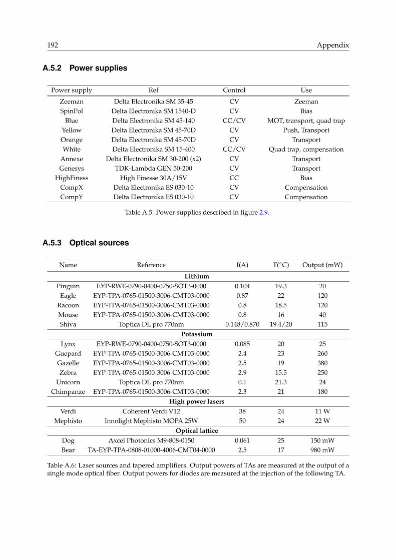
192 Appendix

A.5.2 Power supplies

Power supply Ref Control Use

Zeeman Delta Electronika SM 35-45 CV ZeemanSpinPol Delta Electronika SM 1540-D CV Bias

Blue Delta Electronika SM 45-140 CC/CV MOT, transport, quad trapYellow Delta Electronika SM 45-70D CV Push, TransportOrange Delta Electronika SM 45-70D CV TransportWhite Delta Electronika SM 15-400 CC/CV Quad trap, compensation

Annexe Delta Electronika SM 30-200 (x2) CV TransportGenesys TDK-Lambda GEN 50-200 CV Transport

HighFiness High Finesse 30A/15V CC BiasCompX Delta Electronika ES 030-10 CV CompensationCompY Delta Electronika ES 030-10 CV Compensation

Table A.5: Power supplies described in figure 2.9.

A.5.3 Optical sources

Name Reference I(A) T(C) Output (mW)

LithiumPinguin EYP-RWE-0790-0400-0750-SOT3-0000 0.104 19.3 20

Eagle EYP-TPA-0765-01500-3006-CMT03-0000 0.87 22 120Racoon EYP-TPA-0765-01500-3006-CMT03-0000 0.8 18.5 120Mouse EYP-TPA-0765-01500-3006-CMT03-0000 0.8 16 40Shiva Toptica DL pro 770nm 0.148/0.870 19.4/20 115

PotassiumLynx EYP-RWE-0790-0400-0750-SOT3-0000 0.085 20 25

Guepard EYP-TPA-0765-01500-3006-CMT03-0000 2.4 23 260Gazelle EYP-TPA-0765-01500-3006-CMT03-0000 2.5 19 380Zebra EYP-TPA-0765-01500-3006-CMT03-0000 2.9 15.5 250

Unicorn Toptica DL pro 770nm 0.1 21.3 24Chimpanze EYP-TPA-0765-01500-3006-CMT03-0000 2.3 21 180

High power lasersVerdi Coherent Verdi V12 38 24 11 W

Mephisto Innolight Mephisto MOPA 25W 50 24 22 WOptical lattice

Dog Axcel Photonics M9-808-0150 0.061 25 150 mWBear TA-EYP-TPA-0808-01000-4006-CMT04-0000 2.5 17 980 mW

Table A.6: Laser sources and tapered amplifiers. Output powers of TAs are measured at the output of asingle mode optical fiber. Output powers for diodes are measured at the injection of the following TA.

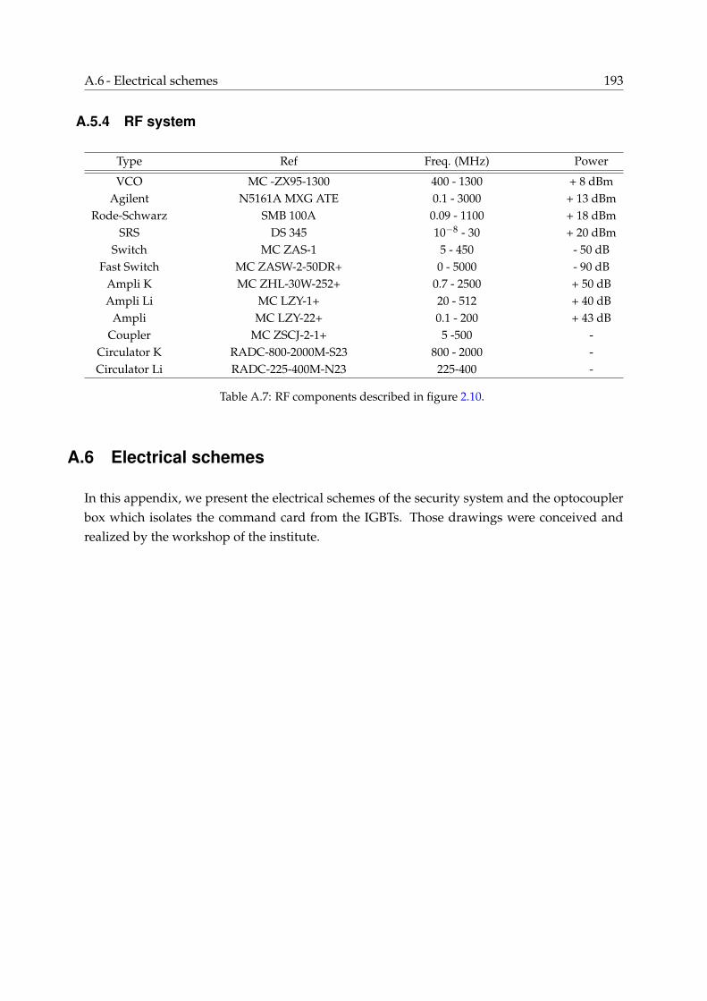
A.6 - Electrical schemes 193

A.5.4 RF system

Type Ref Freq. (MHz) Power

VCO MC -ZX95-1300 400 - 1300 + 8 dBmAgilent N5161A MXG ATE 0.1 - 3000 + 13 dBm

Rode-Schwarz SMB 100A 0.09 - 1100 + 18 dBmSRS DS 345 10−8 - 30 + 20 dBm

Switch MC ZAS-1 5 - 450 - 50 dBFast Switch MC ZASW-2-50DR+ 0 - 5000 - 90 dB

Ampli K MC ZHL-30W-252+ 0.7 - 2500 + 50 dBAmpli Li MC LZY-1+ 20 - 512 + 40 dB

Ampli MC LZY-22+ 0.1 - 200 + 43 dBCoupler MC ZSCJ-2-1+ 5 -500 -

Circulator K RADC-800-2000M-S23 800 - 2000 -Circulator Li RADC-225-400M-N23 225-400 -

Table A.7: RF components described in figure 2.10.

A.6 Electrical schemes

In this appendix, we present the electrical schemes of the security system and the optocouplerbox which isolates the command card from the IGBTs. Those drawings were conceived andrealized by the workshop of the institute.

194 Appendix

2N

70

6

39

0

330

TH

ER

MIS

TA

NC

E

12

02

21

32

24

23

52

46

25

72

68

27

92

81

02

91

13

01

23

11

33

21

43

31

53

41

63

51

73

61

83

71

9

CA

PT

EU

R_

SU

PP

12

02

21

32

24

23

52

46

25

72

68

27

92

81

02

91

13

01

23

11

33

21

43

31

53

41

63

51

73

61

83

71

9

DE

LT

A

1 2 3 4 5 6 7 8

9 10

11

12

13

14

15

T1

R1

R2

T1

0

GN

D

GN

D

GN

D

GN

D

GN

D

GN

D

GN

D

GN

D

GN

D

GN

D

GN

D

GN

D

GN

D

GN

D

GN

D

GN

D

GN

D

GN

D

GN

D

GN

D

GN

D

GN

D

GN

D

GN

D

T1

1

T1

2

T1

3

T1

4

T1

5T

15

T1

6

T1

T3

T4

T5

T6

T9

P1

+5

V

+5

V

+5

V

+5

V

+5

V

+5

V

P3

P4

P5

P6

N7

N8

N9

N1

0

N1

1

N1

2N

12

P2

+2

4V

+2

4V

RE

F

RS

D

T2

T7

T8

SS

_co

nn

ect

s

15

/10

/20

15

10

:03

:14

1/1

Sh

ee

t:

A B C D

12

34

56

A B C D

12

34

56

Co

il T

1/2

Co

il M

OT

X

Co

il Z

ee

ma

n

Co

il P

ush

Co

il Q

ua

d

Co

il T

4

Co

il F

esc

hb

ach

MO

T

MO

T

IGB

T

IGB

T

Tra

nsp

ort

Tra

nsp

ort

Ce

ll co

ils

Ce

ll co

ils

Ze

em

an

Ze

em

an

SO

RT

IE3

RE

F

RS

D

GN

D

Figure A.7: Security system: connections to and from the box. The output is a 0-5V TTL signal providedto the Remote Shut Down circuit of each power supply.

A.6 - Electrical schemes 195

Rest

Sh

un

t

Sh

un

t

Sh

un

t

200k

330

GN

D

GN

D

40

72

N4

07

2N

330G

ND

GN

D

330

GN

D

GN

D330

GN

D

GN

D

330

GN

D

GN

D

330

GN

D

GN

D

330

GN

D

GN

D

330G

ND

GN

D

330

GN

D

GN

D

40

72

N4

07

2N

330

GN

D

GN

D

330

GN

D

GN

D

330

GN

D

GN

D

330

GN

D

GN

D

330

GN

D

GN

D

330

GN

D

GN

D

330

GN

D

GN

D

40

72

N4

07

2N

LM

74

1P

10

K

20

k

GN

D

1k

GN

D

78

05

TV

GN

D

200k

GN

D

1N

41

48

5.1v

GN

D

1k

GN

D

74

14

N

74

14

N

74

14

N

74

14

N

74

14

N

74

14

N

74

14

N

74

14

N

74

14

N

74

14

N

74

14

N

74

14

N

74

14

N

74

14

N

74

14

N

74

14

N

10

0n

f

GND

GND

GN

D

78

15

TV

GN

D

GN

D

H1

5M

L

GN

D

J18

1k

GN

D

200k

GN

D

1N

41

48

5.1v

GN

D

1k

GN

D

1k

GN

D

200k

GN

D

1N

41

48

5.1v

GN

D

1k

GN

D

R1

31

2

T1

12

D1

R2

IC2

A

1

2 3 4 5

IC2

B

13

91

0

11

12

IC2

PVDD VSS714

R3

31

2T

2

12

D2

R4

R5

31

2T

3

12D3

R6

R7

31

2T

4

12

D4

R8

R9

31

2T

5

12

D5

R10

R11

31

2T

6

12

D6

R12

R13

31

2T

7

12

D7

R14

R15

31

2T

8

12

D8

R16

R17

31

2T

9

12D9

R18

IC1

1A

1

2 3 4 5

IC1

1B

13

91

0

11

12

IC1

1P

VDD VSS714

R19

31

2T

10

12

D10

R20

R21

31

2T

11

12

D11

R22

R23

31

2T

12

12

D12

R24

R25

31

2T

13

12

D13

R26

R27

31

2T

14

12

D14

R28

R29

31

2T

15

12

D15

R30

R31

31

2T

16

12

D16

R32

IC1

9A

1

2 3 4 5

IC1

9B

13

91

0

11

12

IC1

9P

VDD VSS714

IC2

0 5

1

236

87 4

R3

3

R3

4

2

6 4

1

5

D1

7

R35

SO

RT

IE1

1 2

IC2

1

GN

D

VI

1

2

VO

3

R36

D1

8

D19

R3

7

31

2

V1

/+U

B

14

V1

/-U

B

7

V1

/1

12

V1

/2

34

V1

/3

56

V1

/4

98

V1

/5

11

10

V1

/6

13

12

V2

/+U

B

14

V2

/-U

B

7

V2

/1

12

V2

/2

34

V2

/3

56

V2

/4

98

V2

/5

11

10

V2

/6

13

12

V3

/+U

B

14

V3

/-U

B

7

V3

/1

12

V3

/2

34

V3

/3

56

V3

/4

98

C1

C2

C3

C4

C5

C6

C7

C8

IC1G

ND

OU

TIN

C1

1C

9

IC3

GN

D

VI

1

2

VO

3

U1

X2

D6

D1

0

D1

4

D1

8

D2

2

D2

6

D3

0

Z4

Z8

Z1

2

Z1

6

Z2

0

Z2

4

Z2

8

Z3

2JP3 1

23

2

6 4

1

5

R38S

OR

TIE

21 2

R39

D2

0

D21

R4

0

31

2

JP4 123

2

6 4

1

5

R41

SO

RT

IE3

1 2

R42

D2

2

D23

R4

3

31

2

JP6 123

GN

D

T1

T1

T2

T2

T3

T3

T4

T4

T5

T5

T6

T6

T7

T7

T8

T8

T9

T9

S1

S1

S2

S2

T1

0

T1

0

T1

1

T1

1

T1

2

T1

2

T1

3

T1

3

T1

4

T1

4

T1

5

T1

5

+5

V

+5V

+5

V

+5V

+5

V

+5V

+5V

+5V

+5V

+5V

+5V

+5V +5V +5V +5V +5V

+5V +5V +5V +5V

+5V +5V +5V +5V

+5V +5V +5V

T1

6

T1

6

S3

S3

S4

S4

S5

S5

-5V

-5V

-5V

+2

4V

+2

4V

-24

V

-24

V

+1

5V

+1

5V

-15

V

-15

V

VE

RS

_C

AR

TE

2

VE

RS

_C

AR

TE

2

S6

S6

ST

ST

ST

ST

VIn

VO

ut

GN

D

Figure A.8: Security system: thermistances monitoring and main output. The value of 8 thermistors iscontinuously compared to reference values set by potentiometers. If one of the monitored temperatureexceeds the threshold, the output signal of the security system is switched off to 0V.

196 Appendix

50k 50k 50k

50k50k 50k

7414N

7414N

7414N

7414N

7414N

7414N

4072N

330330330

100k

100K

2K0.01uf

1uf

Flux1

10K

220k47k

1.7k0.01uf

1uf

Flux2

51k

220k

47k

1.7k0.01uf

1uf

Flux3

51k

330

330

330

H15ML

220k

47k

1.7k0.01uf

1uf

Flux4

51k

330

100nf

100nf

100nf

100nf

7414N

7414N

7414N

7414N

7414N

7414N

7414N

7414N

74AC32N

74AC32N

74AC32N

H1

123

H2

123

H3

123

R1

31

2

R2

31

2R3

31

2

R4R5 R6

V1/+UB

14

V1/-UB

7

V1/1

12

V1/2

34

V1/3

56

V1/4

98

V1/5

11

10

V1/6

13

12

IC1A

1

2 3 4 5

IC1PVDD VSS

714

R7R8R9

D1 D2 D3

LM2907

1 1

2 2

3 3

4 4

55

6(V+)6

77

8(GND)8

R10

31

2

R11R12

C1

C2

JP1

123

R13

LM2907

1 1

2 2

3 3

4 4

55

6(V+)6

77

8(GND)8

R14

31

2

R15R16

C3

C4

JP2

123

R17

LM2907

1 1

2 2

3 3

4 4

55

6(V+)6

77

8(GND)8

R18

31

2

R19R20

C5

C6

JP3

123

R21

IC5

GND

INOUT

IC6

GND

INOUT

C7

R22

FLUX1

R23

FLUX2

R24

FLUX3

X1

D6

D10

D14

D18

D22

D26

D30

Z4

Z8

Z12

Z16

Z20

Z24

Z28

Z32

C8

C9

C10

LM2907

1 1

2 2

3 3

4 4

55

6(V+)6

77

8(GND)8

R25

31

2

R26R27

C11

C12

JP4

123

R28

R29

FLUX4

C13

C14

C15

C16

V2/+UB

14

V2/-UB

7

V2/1

12

V2/2

34

V2/3

56

V2/4

98

V2/5

11

10

V2/6

13

12

V3/+UB

14

V3/-UB

7

V3/1

12

V3/2

34

IC9A

1 23

IC9B

4 56

IC9C

9

10

8

IC9P

GNDVCC714

C17

H1

H1

H2

H2

H3

H3

+5V +5V +5V

+5V

+5V

+5V

+5V

+5V

+5V

+12V

+12V

+12V

+12V

+12V

+12V

+12V

+12V

+12V

+24V

+24V

FLUX1

FLUX1

FLUX2

FLUX2

FLUX3

FLUX3

FLUX

FLUX

VERS_CARTE1

VERS_CARTE1

FLUX4

FLUX4

F1

F1

F2

F2

F3

F3

F4

F4

A B C D E

12

34

56

78

A B C D E

12

34

56

78

+

+

+

+

+

+

+

+

Figure A.9: Security system: humidity monitoring. This card is not currently used in our experiment.

A.6 - Electrical schemes 197

220k

330

GND

GND

220k

330

GND

GND

220k

330

GND

GND

220k

330

GND

GND

220k

330

GND

GND

220k

330

GND

GND

220k

330

GND

220k

330

GND

220k

330

GND

220k

330

GND

220k

330

GND

220k

330

GND

4072N

4072N

4072N

4072N

H15ML

7414N

7414N

7414N

7414N

7414N

7414N

7414N

7414N

7414N

7414N

7414N

7414N

GND

7815TV

7805TV

GND

GND

GND

GND

GND

GND

GND

GND

GND

P1

12

R1

31

2

LED1

R2

P2

12

R3

31

2

LED2

R4

P3

12

R5

31

2

LED3

R6

P4

12

R7

31

2

LED4

R8

P5

12

R9

31

2

LED5

R10

P6

12

R11

31

2

LED6

R12

N7

12

R13

31

2

LED7

R14

N8

12

R15

312

LED8

R16

N9

12

R17

31

2

LED9

R18

N10

12

R19

31

2

LED10

R20

N11

12

R21

31

2

LED11

R22

N12

12

R23

31

2

LED12

R24

IC1A

1

2 3 4 5

IC1B

13

910

1112

IC1PVDD VSS

714

IC2A

1

2 3 4 5

IC2B

13

910

1112

IC2PVDD VSS

714

X1

D6

D10

D14

D18

D22

D26

D30

Z4

Z8

Z12

Z16

Z20

Z24

Z28

Z32

V1/+UB

14

V1/-UB

7

V1/1

12

V1/2

34

V1/3

56

V1/4

98

V1/5

11

10

V1/6

13

12

V2/+UB

14

V2/-UB

7

V2/1

12

V2/2

34

V2/3

56

V2/4

98

V2/5

11

10

V2/6

13

12

C1

C2

C3

C4

IC3

GND

VI

1

2

VO

3

IC4

GND

VI

1

2

VO

3

X1

X1

X2

X2

X3

X3

X4

X4

X5

X5

X6

X6

X7

X7

X8

X8

X9

X9

X10

X10

X11

X11

X12

X12

Y1

Y1

Y2

Y2

Y3

Y3

Y4

Y4

+24V

+24V

+5V

+5V +5V +5V +5V +5V

+5V+5V +5V +5V +5V

+5V +5V

A B C D E

12

34

56

78

A B C D E

12

34

56

78

Figure A.10: Security system: flow monitoring. The water flows of 6 cooling systems are continuouslymonitored. If any of them is below a threshold fixed by a potentiometer incorporated on the fluxmeters,the output signal of the security system is switched off to 0V.

198 Appendix

AC

PL

-31

30

AC

PL

-31

30

AC

PL

-31

30

AC

PL

-31

30

2.2

koh

m

2N

22

22

GN

D

Zener 5.1V

GN

D1N

41

48

+5V 220

2.2

koh

m

2N

22

22

GN

D

Zener 5.1V

GN

D1N

41

48

+5V

220

2.2

koh

m

2N

22

22

GN

D

Zener 5.1V

GN

D1N

41

48

+5V 220

2.2

koh

m

2N

22

22

GN

D

Zener 5.1V

GN

D1N

41

48

+5V 220

VSS3 VSS4 VSS5 VSS6VDD3 VDD4 VDD5 VDD6

0.1

uF

0.1

uF

0.1

uF

0.1

uF

So

rtie

_B

NC

_0

3

So

rtie

_B

NC

_0

4

So

rtie

_B

NC

_0

5

So

rtie

_B

NC

_0

6

GN

D3

GN

D4

GN

D5

GN

D6

En

tré

e_

BN

C_

03

En

tré

e_

BN

C_

04

En

tré

e_

BN

C_

05

En

tré

e_

BN

C_

06

GN

D

GN

D

GN

D

GN

D

AC

PL

-31

30

2.2

koh

m

2N

22

22

GN

D

Zener 5.1V

GN

D1N

41

48

+5V 220

VSS2VDD2

0.1

uF

So

rtie

_B

NC

_0

2G

ND

2

En

tré

e_

BN

C_

02

GN

D

AC

PL

-31

30

2.2

koh

m

2N

22

22

GN

D

Zener 5.1VG

ND1N

41

48

+5V 220

VSS1VDD1

0.1

uF

So

rtie

_B

NC

_0

1G

ND

1

En

tré

e_

BN

C_

01

GN

D

AC

PL

-31

30

AC

PL

-31

30

2.2

koh

m

2N

22

22

GN

D

Zener 5.1V

GN

D1N

41

48

220

2.2

koh

m

2N

22

22

GN

D

Zener 5.1V

GN

D1N

41

48

+5V 220

VSS15 VSS16VDD15 VDD16

0.1

uF

0.1

uF

So

rtie

_B

NC

_1

5

So

rtie

_B

NC

_1

6

GN

D1

5

GN

D1

6

En

tré

e_

BN

C_

15

En

tré

e_

BN

C_

16

GN

D

GN

D

AC

PL

-31

30

AC

PL

-31

30

2.2

koh

m

2N

22

22

GN

D

Zener 5.1V

GN

D1N

41

48

220

2.2

koh

m

2N

22

22

GN

D

Zener 5.1V

GN

D1N

41

48

+5V 220

VSS13VSS14VDD13 VDD14

0.1

uF

0.1

uF

So

rtie

_B

NC

_1

3

So

rtie

_B

NC

_1

4

GN

D1

3

GN

D1

4

En

tré

e_

BN

C_

13

En

tré

e_

BN

C_

14

GN

D

GN

D

AC

PL

-31

30

AC

PL

-31

30

2.2

koh

m

2N

22

22

GN

D

Zener 5.1V

GN

D1N

41

48

220

2.2

koh

m

2N

22

22

GN

D

Zener 5.1V

GN

D1N

41

48

+5V 220

VSS11 VSS12VDD11 VDD12

0.1

uF

0.1

uF

So

rtie

_B

NC

_1

1

So

rtie

_B

NC

_1

2

GN

D1

1

GN

D1

2

En

tré

e_

BN

C_

11

En

tré

e_

BN

C_

12G

ND

GN

D

AC

PL

-31

30

2.2

koh

m

2N

22

22

GN

DZener 5.1V

GN

D1N

41

48

+5V

220

VSS10

VDD10

0.1

uF

So

rtie

_B

NC

_1

0G

ND

10

En

tré

e_

BN

C_

10

GN

D

AC

PL

-31

30

2.2

koh

m

2N

22

22

GN

D

Zener 5.1V

GN

D1N

41

48

+5V 220

VSS9VDD9

0.1

uF

So

rtie

_B

NC

_0

9G

ND

9

En

tré

e_

BN

C_

09

GN

D

AC

PL

-31

30

2.2

koh

m

2N

22

22

GN

D

Zener 5.1V

GN

D1N

41

48

+5V 220

VSS8VDD8

0.1

uF

So

rtie

_B

NC

_0

8G

ND

8

En

tré

e_

BN

C_

08

GN

D

AC

PL

-31

30

2.2

koh

m

2N

22

22

GN

D

Zener 5.1V

GN

D1N

41

48

+5V 220

VSS7VDD7

0.1

uF

So

rtie

_B

NC

_0

7G

ND

7

En

tré

e_

BN

C_

07

GN

D

+5V

+5V

+5V

IC3 N

/C1

1

NC

24

AN

OD

E2

CA

TH

OD

E3

VO

UT

16

VO

UT

27

VC

C8

VE

E5

IC4 N

/C1

1

NC

24

AN

OD

E2

CA

TH

OD

E3

VO

UT

16

VO

UT

27

VC

C8

VE

E5

IC5 N

/C1

1

NC

24

AN

OD

E2

CA

TH

OD

E3

VO

UT

16

VO

UT

27

VC

C8

VE

E5

IC6 N

/C1

1

NC

24

AN

OD

E2

CA

TH

OD

E3

VO

UT

16

VO

UT

27

VC

C8

VE

E5

R2

Q3

D1

D2

R3

R5

Q4

D5

D6

R6

R7

Q5

D7

D8

R8

R9

Q6

D9

D1

0

R10

C1

C2

C3

C4

JP2

31 2

JP2

41 2 JP

25

1 2

JP2

61 2

JP3

12 JP4

12 JP5

12 JP6

12

IC2 N

/C1

1

NC

24

AN

OD

E2

CA

TH

OD

E3

VO

UT

16

VO

UT

27

VC

C8

VE

E5

R4

Q2

D3

D4

R11

C1

1

JP2

21 2

JP2

12

IC1 N

/C1

1

NC

24

AN

OD

E2

CA

TH

OD

E3

VO

UT

16

VO

UT

27

VC

C8

VE

E5

R1

2

Q1

D11

D1

2

R13

C1

2

JP2

11 2

JP1

12

IC1

5

N/C

11

NC

24

AN

OD

E2

CA

TH

OD

E3

VO

UT

16

VO

UT

27

VC

C8

VE

E5

IC1

6

N/C

11

NC

24

AN

OD

E2

CA

TH

OD

E3

VO

UT

16

VO

UT

27

VC

C8

VE

E5

R1

4

Q1

5

D13

D1

4

R15

R1

6

Q1

6

D15

D1

6

R17

C1

3

C1

4

JP3

51 2

JP3

61 2

JP1

5

12

JP1

6

12

IC1

3

N/C

11

NC

24

AN

OD

E2

CA

TH

OD

E3

VO

UT

16

VO

UT

27

VC

C8

VE

E5

IC1

4

N/C

11

NC

24

AN

OD

E2

CA

TH

OD

E3

VO

UT

16

VO

UT

27

VC

C8

VE

E5

R1

8

Q1

3

D17

D1

8

R19

R2

0

Q1

4

D19

D2

0

R21

C1

5

C1

6

JP3

31 2

JP3

41 2

JP1

3

12

JP1

4

12

IC1

1

N/C

11

NC

24

AN

OD

E2

CA

TH

OD

E3

VO

UT

16

VO

UT

27

VC

C8

VE

E5

IC1

2

N/C

11

NC

24

AN

OD

E2

CA

TH

OD

E3

VO

UT

16

VO

UT

27

VC

C8

VE

E5

R2

2

Q1

1

D21

D2

2

R23

R2

4

Q1

2

D23

D2

4

R25

C1

7

C1

8

JP3

11 2

JP3

21 2

JP1

1

12 JP1

2

12

IC1

0

N/C

11

NC

24

AN

OD

E2

CA

TH

OD

E3

VO

UT

16

VO

UT

27

VC

C8

VE

E5

R2

6

Q1

0

D25

D2

6

R27

C1

9

JP3

01 2

JP1

0

12

IC9 N

/C1

1

NC

24

AN

OD

E2

CA

TH

OD

E3

VO

UT

16

VO

UT

27

VC

C8

VE

E5

R2

8

Q9

D27

D2

8

R29

C2

0

JP2

91 2

JP9

12

IC8 N

/C1

1

NC

24

AN

OD

E2

CA

TH

OD

E3

VO

UT

16

VO

UT

27

VC

C8

VE

E5

R3

0

Q8

D29

D3

0

R31

C2

1

JP2

81 2

JP8

12

IC7 N

/C1

1

NC

24

AN

OD

E2

CA

TH

OD

E3

VO

UT

16

VO

UT

27

VC

C8

VE

E5

R3

2

Q7

D31

D3

2

R33

C2

2

JP2

71 2

JP7

12

+ + + +

+

+

+ +

+ +

+ +

+

+

+

+

BO

BIN

E_

LV

_1

BO

BIN

E_

LV

_2

BO

BIN

E_

LV

_3

BO

BIN

E_

LV

_4

BO

BIN

E_

LV

_4

BO

BIN

E_

LV

_4

BO

BIN

E_

LV

_3

BO

BIN

E_

LV

_4

BO

BIN

E_

LV

_3

BO

BIN

E_

LV

_4

BO

BIN

E_

LV

_3

BO

BIN

E_

LV

_4

BO

BIN

E_

LV

_4

BO

BIN

E_

LV

_4

BO

BIN

E_

LV

_4

BO

BIN

E_

LV

_4

Figure A.11: Optocouplers between computer and system (1/2).

A.6 - Electrical schemes 199

AC

PL

-31

30

2.2

koh

m

2N

22

22

GN

D

Zener 5.1V

GN

D1N

41

48

+5V 220

VSS17VDD17

0.1

uF S

ort

ie_

BN

C_

17

GN

D1

7

En

tré

e_

BN

C_

17

GN

D

AC

PL

-31

30

2.2

koh

m

2N

22

22

GN

D

Zener 5.1V

GN

D1N

41

48

+5V 220

VSS18VDD18

0.1

uF S

ort

ie_

BN

C_

18

GN

D1

8

En

tré

e_

BN

C_

18

GN

D

AC

PL

-31

30

2.2

koh

m

2N

22

22

GN

D

Zener 5.1V

GN

D1N

41

48

+5V 220

VSS19

VDD19

0.1

uF So

rtie

_B

NC

_1

9G

ND

19

En

tré

e_

BN

C_

19

GN

D

AC

PL

-31

30

2.2

koh

m

2N

22

22

GN

D

Zener 5.1V

GN

D1N

41

48

+5V 220

VSS20VDD20

0.1

uF S

ort

ie_

BN

C_

20

GN

D2

0

En

tré

e_

BN

C_

20

GN

D

22

00

uF

22

00

uF

RE

CT

IFIE

R-1

KA

B 79

05

10

0n

F

10

0n

F

GN

D2

20

V

10

0u

F

10

0u

F

330ohm

Inte

rru

pte

ur

78

05

TV

GND

+5

V

AL

IM0

1

AL

IM0

2

AL

IM0

3

AL

IM0

4

AL

IM0

5

AL

IM0

6

AL

IM0

7

AL

IM0

8

AL

IM0

9

AL

IM0

10

AL

IM0

11

AL

IM0

12

AL

IM0

13

AL

IM0

14

AL

IM0

15

AL

IM0

16

AL

IM0

17

AL

IM0

18

AL

IM0

19

AL

IM0

20

VDD1

VDD2

VDD3

VDD4

VDD5

VDD6

VDD7

VDD8

VDD9

VDD10

VDD11

VDD12

VDD13

VDD14

VDD15

VDD16

VDD17

VDD18

VDD19

VDD20

VSS1

VSS2

VSS3

VSS4

VSS5

VSS6

VSS7

VSS8

VSS9

VSS10

VSS11

VSS12

VSS13

VSS14

VSS15

VSS16

VSS17

VSS18

VSS19

VSS20

GND1 GND2 GND3 GND4 GND5 GND6 GND7

GND8 GND9 GND10GND11

GND12

GND13

GND14

GND15 GND16

GND17GND18 GND19 GND20

IC1

7

N/C

11

NC

24

AN

OD

E2

CA

TH

OD

E3

VO

UT

16

VO

UT

27

VC

C8

VE

E5

R3

4

Q1

7

D33

D3

4

R35

C2

3

JP3

71 2

JP1

7

12

IC1

8

N/C

11

NC

24

AN

OD

E2

CA

TH

OD

E3

VO

UT

16

VO

UT

27

VC

C8

VE

E5

R3

6

Q1

8

D35

D3

6

R37

C2

4

JP3

81 2

JP1

8

12

IC1

9

N/C

11

NC

24

AN

OD

E2

CA

TH

OD

E3

VO

UT

16

VO

UT

27

VC

C8

VE

E5

R3

8

Q1

9

D37

D3

8

R39

C2

5 JP3

91 2

JP1

9

12

IC2

0

N/C

11

NC

24

AN

OD

E2

CA

TH

OD

E3

VO

UT

16

VO

UT

27

VC

C8

VE

E5

R4

0

Q2

0

D39

D4

0

R41

C2

6

JP4

01 2

JP2

0

12

RT

21 2

6 7 8 9

3 4 5

C2

7

C2

8

B2

IC2

40

GN

D OU

TIN

C2

9

C3

0

JP4

1

12

C3

1

C3

2

R42 LED2

S2

231

IC6

00 G

ND

VI

1

2

VO

3

JP4

21 2 3

JP4

31 2 3

JP4

41 2 3

JP4

51 2 3

JP4

61 2 3

JP4

71 2 3

JP4

81 2 3

JP4

91 2 3

JP5

01 2 3

JP5

11 2 3

JP5

21 2 3

JP5

31 2 3

JP5

41 2 3

JP5

51 2 3

JP5

61 2 3

JP5

71 2 3

JP5

81 2 3

JP5

91 2 3

JP6

01 2 3

JP6

11 2 3

GND

+5

V

-5V

+ ++

+

P1 P2

S1 S2

+ +

+ +

BO

BIN

E_

LV

_4

BO

BIN

E_

LV

_4

BO

BIN

E_

LV

_4

BO

BIN

E_

LV

_4

Figure A.12: Optocouplers between computer and system (2/2).

Chapter

B Publications

ContentsSimultaneous sub-Doppler laser cooling of fermionic... . . . . . . . . . . . . . . . . . . . . . . 201

Analog Simulation of Weyl Particles with Cold Atoms . . . . . . . . . . . . . . . . . . . . . . . 213

La quête des températures ultrabasses . . . . . . . . . . . . . . . . . . . . . . . . . . . . . . . . 220

Simultaneous sub-Doppler laser cooling of fermionic...

Franz Sievers, Norman Kretzschmar, Diogo Rio Fernandes, Daniel Suchet, Michael Rabinovic,Saijun Wu, Colin V. Parker, Lev Khaykovich, Christophe Salomon, and Frédéric Chevy, ’Si-multaneous sub-Doppler laser cooling of fermionic 6Li and 40K on the D1 line: Theory andexperiment’, Physical Review A, vol. 91, issue 2, page 023426 (2015)

201

PHYSICAL REVIEW A 91, 023426 (2015)

Simultaneous sub-Doppler laser cooling of fermionic 6Li and 40K on the D1 line:Theory and experiment

Franz Sievers,1,* Norman Kretzschmar,1 Diogo Rio Fernandes,1 Daniel Suchet,1 Michael Rabinovic,1 Saijun Wu,2,†

Colin V. Parker,3 Lev Khaykovich,4 Christophe Salomon,1 and Frederic Chevy1

1Laboratoire Kastler Brossel, Ecole Normale Superieure, CNRS, UPMC, 24 rue Lhomond, 75005 Paris, France2State Key Laboratory of Surface Physics and Department of Physics, Fudan University, 200433 Shanghai, People’s Republic of China

3James Franck Institute, Enrico Fermi Institute and Department of Physics, University of Chicago, Chicago, Illinois 60637, USA4Department of Physics, Bar-Ilan University, Ramat-Gan 52900, Israel

(Received 30 October 2014; revised manuscript received 30 January 2015; published 23 February 2015)

We report on simultaneous sub-Doppler laser cooling of fermionic 6Li and 40K using the D1 optical transitions.We compare experimental results to a numerical simulation of the cooling process applying a semiclassical MonteCarlo wave-function method. The simulation takes into account the three-dimensional optical molasses setup andthe dipole interaction between atoms and the bichromatic light field driving the D1 transitions. We discuss thephysical mechanisms at play, identify the important role of coherences between the ground-state hyperfine levels,and compare D1 and D2 sub-Doppler cooling. In 5 ms, the D1 molasses phase greatly reduces the temperaturefor both 6Li and 40K at the same time, with final temperatures of 44 and 11 μK, respectively. For both speciesthis leads to a phase-space density close to 10−4. These conditions are well suited to direct loading of an opticalor magnetic trap for efficient evaporative cooling to quantum degeneracy.

DOI: 10.1103/PhysRevA.91.023426 PACS number(s): 37.10.De, 32.80.Wr, 67.85.−d

I. INTRODUCTION

The road towards quantum degeneracy in atomic gasesusually starts with a laser cooling and trapping phase. Theresulting initial phase-space density of the atomic ensembleand the initial collision rate should be as high as possible forinitiating efficient evaporative cooling to quantum degeneracy.Sub-Doppler cooling has proven to be a powerful techniqueto increase the phase-space density of most alkali atoms andother atoms with multiple-level structure [1–3]. However, inthe case of lithium and potassium, the narrow excited-statestructure of the D2 transition compromises the efficiencyof this cooling scheme [4,5]. Both species possess stablefermionic and bosonic isotopes, and they play an important rolein recent experimental studies of strongly correlated quantumgases. Thus, important efforts have been devoted to searchingfor alternative laser cooling schemes.

For instance, it has recently been shown that three-dimensional (3D) Sisyphus cooling for 7Li, some gigahertz reddetuned from the D2 line, can lead to temperatures as low as100 μK, with up to 45% of the atoms in the cooled fraction [6].A second option is to operate the magneto-optical trap (MOT)on a transition with a smaller linewidth to reduce the Dopplertemperature [7–9]. Such transitions exist for 6Li and 40K inthe near-UV and blue regions of the spectrum, respectively,leading to temperatures of 33 μK for 6Li and 63 μK for 40K.Yet, special optics and a coherent source at 323 nm for 6Li andat 405 nm for 40K are needed for this approach. Additionally,at these wavelengthes the available power is still a limitingfactor.

More recently a simpler sub-Doppler cooling scheme usingblue-detuned molasses operating on the D1 line was proposedand demonstrated on 40K [10] and has been extended to other

*franz.sievers@lkb.ens.fr†saijunwu@fudan.edu.cn

atomic species such as 7Li [11], 39K [12,13], and 6Li [14].Using this technique, temperatures as low as 20 μK (40K),50 μK (7Li), 6 μK (39K), and 40 μK (6Li) were reached.

Even though the main ingredients of the D1 cooling schemeare now understood at a qualitative level, in particular, the roleof the coherences between hyperfine ground-state levels [11],a complete picture, taking into account the full level structureof the atoms, is still missing. In this paper, we present a 3Dsemiclassical solution of the optical Bloch equations that takesinto account the full set of relevant energy levels of alkaliatoms and we apply it to the case of 6Li and 40K. The modelfully confirms the experimentally observed cooling behaviorand its robustness with respect to changes in experimentalparameters. The model is validated by a good match betweenthe simulation and the experimentally measured temperatureand fluorescence rate. We recover the important role of theRaman detuning between the main cooling laser and therepumping laser on the achievable temperature. We show here,for both 6Li and 40K, that the gain in temperature of a factorof ∼3 at the exact Raman resonance is well reproduced by thetheoretical model and that the amount of coherence betweenboth hyperfine states shows a pronounced resonance behavior.Beyond individual studies of the two species, we also showexperimentally that simultaneous cooling of 6Li and 40K doesnot lead to any severe trade-off and is technically easy toimplement. We are able to capture more than 1 × 109 atoms ofeach species, with a capture efficiency exceeding 60% from acompressed magneto-optical trap (CMOT), and reach temper-atures as low as 44 μK for 6Li and 11 μK for 40K within 5 ms.

II. D1 COOLING MECHANISM

In a typical D1 cooling setup (Fig. 1), all the D1 hyperfinelevels are involved in the interaction. The sub-Doppler coolingeffects include a mix of Sisyphus cooling, motion-inducedand off-resonant light coupling from gray to bright levels, and

1050-2947/2015/91(2)/023426(11) 023426-1 ©2015 American Physical Society

FRANZ SIEVERS et al. PHYSICAL REVIEW A 91, 023426 (2015)

F = 3/2 (Fh)

F = 1/2 (Fl)

F = 7/2 (Fh)

F = 9/2 (Fl)

FIG. 1. (Color online) Cooling scheme on the 6Li and 40K D1 lines. The cooling beam (blue) is blue detuned by δcool from the |F =3/2〉 → |F ′

h = 3/2〉 (|F = 9/2〉 → |F ′h = 7/2〉) transition, where F ′

h (F ′l ) is the upper (lower) excited-state level. The repumping beam (red) is

blue detuned by δrep from the |F = 1/2〉 → |F ′h = 3/2〉 (|F = 7/2〉 → |F ′

h = 7/2〉) transition. Detuning from the Raman condition is denoted = δrep − δcool.

coherent population trapping of slow atoms in nearly decou-pled states. In this section we first introduce our semiclassicallaser cooling model. We then present and compare the resultsfrom experimental observations and numerical simulationsand, finally, discuss the physical mechanism of D1 cooling.

A. Semiclassical Monte Carlo simulation

The level diagrams of our bichromatic cooling scheme forboth 6Li and 40K are depicted in Fig. 1. The D1 molasses iscomposed of a 3D lattice whose polarization configuration isthe same as that of a six-beam standard MOT, but with twosidebands to address the |F = 3/2〉 and |F = 1/2〉 hyperfineground states of 6Li (respectively, |F = 9/2〉 and |F = 7/2〉for 40K) in the D1 system at positive detunings.

Here, by convention, we refer to the |F = 3/2〉 → |F ′h〉

and |F = 1/2〉 → |F ′h〉 transitions as cooling and repumping

transitions. It is, however, important to note that neither thecooling nor the repumping D1 transitions are actually closed.

Our numerical simulation of the cooling process is basedon a semiclassical Monte Carlo wave-function method. Thesimulation takes into account the 3D optical molasses setupand the dipole interaction between the single atoms and thepolarized light driving the transitions of the D1 manifold,which is spanned by the 4(2I + 1) hyperfine Zeeman sublevels(I > 0 is the nuclear spin). We treat the external states of theatom classically and update its position r(t) and velocity v(t)according to the calculated expectation value of the light force:

f(t) = 〈ψ(t)| − ∇Heff(r(t))|ψ(t)〉〈ψ(t)|ψ(t)〉 . (1)

The atomic internal states |ψ(t)〉 evolve in a dressed basiswith respect to the cooling laser (Fig. 1), according to theMonte Carlo wave-function method [15,16] with the effectiverotating-wave Hamiltonian

Heff = H0 + HF=I−1/2 + HF=I+1/2 − i/2, (2)

where

H0 =∑

m

|F = I − 1/2,m〉〈F = I − 1/2,m|

−∑

F ′m′|F ′,m′〉(δcool + δhfs,F ′ )〈F ′,m′|. (3)

Here H0 operates over the whole D1 manifold and δcool isthe detuning of the cooling laser with respect to the F =I + 1/2 → F ′

h transition, where F ′h (Fig. 1) corresponds to the

excited hyperfine level that is higher in energy, e.g., F ′h = 3/2

for 6Li and F ′h = 7/2 for 40K. = δrep − δcool is the two-

photon detuning for the F = I − 1/2 → F = I + 1/2 Ramantransition, δhfs,F ′ the hyperfine splitting of the excited state forF ′

l , and 0 for F ′h. The 0 of energy is chosen as that of the bare

F = I + 1/2 ground state.The light-atom coupling Hamiltonian

HF=I±1/2 = ∑

m,σ,F ′,m′F,σ cF,m,σ,F ′,m′

× |F,m〉〈F ′,m′| + H.c. (4)

describes the cooling (F = I + 1/2) and repumping (F =I − 1/2) interactions [17]. Here F,σ are the Rabi frequenciesof the repumping and cooling laser beams for F = I − 1/2F = I + 1/2, respectively. cF,m,σ,F ′m′ represent the Clebsch-Gordan coefficients associated with the transitions coupled byσ polarized light. To take into account the radiation dampingwe include the spontaneous emission rate = Pee where

is the excited-state linewidth and Pee = ∑F ′,m′ |F ′m′〉〈F ′m′|.

This leads to a decay of the internal-state wave-function norm〈ψ(t)|ψ(t)〉. The speed of this decay probabilistically dictatesthe collapse of the internal quantum states in the numericalsimulation, which corresponds to spontaneous emission. Wetake into account the polarization of the spontaneous scatteringphoton and follow the standard quantum jump procedure toproject the atomic states to ground states, with the norm

023426-2

SIMULTANEOUS SUB-DOPPLER LASER COOLING OF . . . PHYSICAL REVIEW A 91, 023426 (2015)

reset to unity [15]. To effectively account for heating due toboth absorption and spontaneous emission, we assign a recoilmomentum shift to v(t) twice before continuing to evolve|ψ(t)〉 via Heff(r(t)).

The simulations are performed with parameters matchingthe experimental setup by properly introducing the spatiallydependent F,σ (r), the detunings , δcool, and atomic initialconditions. To reproduce experimental conditions, we fix therelative phases for all 12 cooling and repumping laser beamsat values randomized for each simulation trial. We recordthe evolution of the 3D atomic velocity, the time-stampedfluorescence events corresponding to quantum jumps, andinternal-state properties such as state population and coher-ence. The observables are averaged over multiple simulationtrials for comparison with the experiment.

B. Raman-detuning dependence for 6Li

A critical parameter in the D1 molasses scheme is theRaman detuning (Fig. 1). In the following we investigate theRaman-detuning dependence of the 6Li molasses temperatureand fluorescence rate both theoretically and experimentally,for various cooling and repumping laser intensities.

Our 6Li-40K machine is described in [18]. We first loada lithium MOT using a laser-slowed atomic beam (Zeemanslower). After a compressed MOT phase the magnetic field andthe D2 light are switched off and the D1 molasses is applied

(a more detailed description of the sequence is presented inthe Appendix). To probe the Raman-detuning dependencewe apply a 100-μs D1 molasses pulse with variable toan atomic cloud precooled to 100 μK. Figures 2(a) and 2(b)show the fluorescence rate and the temperature after the pulseas functions of the Raman detuning for the intensities used inthe simulations. We observe a temperature dip at zero Ramandetuning and a heating and fluorescence peak at positive

whose position and amplitude are correlated with the molassesintensity.

In the simulations we set the initial velocity of lithium to0.2 m/s (T ∼ 30 μK). The simulation time is set to 200 μs. Inthe first 100 μs we allow the cooling dynamics to equilibrate,and during the second 100 μs we record the velocity v(t) aswell as the time-stamped quantum jump events to calculate theequilibrium temperature and fluorescence rate. At each Ramandetuning we average over 25 trajectories. The simulationresults for two intensities, Icool = 2.7 Isat, Irep = 0.13 Isat andIcool = 9 Isat, Irep = 0.46 Isat, are shown in Figs. 2(c) and 2(d),respectively (here Isat refers to the saturation intensity of theD2 line).

The simulated heating and fluorescence peak positionsfor low and high intensities (Fig. 2) agree well with theexperimental findings. Also, the shift between the heatingand the fluorescence peak, which increases with the molassesintensity, is numerically reproduced without any freely ad-justable parameters.

−1 −0.5 0 0.5 1

0.2

0.3

0.4

Raman-detuning Δ (units of Γ)

Fluorescen

cerate

(arb.units)

101

102

103

Tem

perature

(μK)

(a)

−1 −0.5 0 0.5 1

3

4

5

Raman-detuning Δ (units of Γ)

Fluorescen

cerate

(arb.units)

102

103

Tem

perature

(μK)

(b)

−1 −0.5 0 0.5 1

0.1

0.2

0.3

0.4

Raman-detuning Δ (units of Γ)

Fluorescen

cerate

(1/μs)

101

102

103

Tem

perature

(μK)

(c)

−1 −0.5 0 0.5 1

0.5

1

Raman-detuning Δ (units of Γ)

Fluorescen

cerate

(1/μs)

102

103

Tem

perature

(μK)

(d)

FIG. 2. (Color online) Fluorescence (squares) and temperature (triangles; logarithmic scale) of the 6Li atomic cloud after a 100-μs pulseof D1 light with variable Raman detuning . Experiment: (a) low intensity; (b) high intensity. Simulation: (c) low intensity; (d) high intensity.Experimental and simulation results (a, c) for Icool = 2.7Isat, Irep = 0.13Isat and (b, d) for Icool = 9 Isat, Irep = 0.46 Isat per beam.

023426-3

FRANZ SIEVERS et al. PHYSICAL REVIEW A 91, 023426 (2015)

−1 0 1101

102

103

Raman-detuning Δ (units of Γ)

Tem

perature

(μK)

(a)

−1 0 1101

102

103

Raman-detuning Δ (units of Γ)

Tem

perature

(μK)

(b)

FIG. 3. (Color online) Temperature of the 6Li D1 molasses aftera 100-μs pulse with variable Raman detuning for differentcooling and repumping intensities. (a) Experiment; (b) simulation.Standard intensities [(red) circles]: Icool = 9 Isat, Irep = 0.46 Isat.Equal cooling/repumping ratio (black squares): Icool = Irep = 9 Isat.Inverted cooling/repumping ratio [(blue) triangles]: Icool = 0.6 Isat,Irep = 4.6 Isat.

Despite the nice match between simulations and experi-ments in Figs. 2 and 3, we observe that the semiclassicalsimulations provide temperatures that are systematically lowerby a factor of 2 to 4 than the measured ones, particularly nearthe Raman-resonance condition = 0. Here the simulationpredicts a temperature of 20 μK, whereas the lowest measuredtemperature is 50 μK. The reason for this is not fullyunderstood and may come from both theory and experimentallimitations. First, the simulation is semiclassical and neglectsthe wave-function extent of the cold atoms. The predictedtemperature of 20 μK corresponds to only six times therecoil energy ER = 1

2mv2recoil = kB × 3.5 μK. Therefore, only

a quantum treatment of the atoms’ external motion can beexpected to give a quantitative equilibrium temperature pre-diction in the low-intensity limit. In the simulation we observethat slow atoms are likely trapped within subwavelengthregions, where the light shift is minimal and the atom is nearlydecoupled from light over a long time without quantum jump.This coherent population trapping effect enhances the coolingat both large and small , although it is most pronounced at theRaman resonance ( = 0) since more choices of decoupled

0

100

200

50

150

Tem

perature

(μK)

−0.2 0 0.220

40

60

−6 −4 −2 0 20

0.5

1

1.5

2

Raman-detuning Δ (units of Γ)

Atom

number

(109)

FIG. 4. (Color online) Experiment: Atom number and equilib-rium temperature of the 40K D1 molasses as functions of the Ramandetuning . δcool = 3 , Icool = 6 Isat, Irep/Icool = 7.6%, tm = 5 ms.In the constant-temperature regions below −0.1 and above 2

gray molasses cooling involves coherences between Zeeman states ina given hyperfine state but not between hyperfine states. At the exactRaman condition = 0, long-lived coherences between hyperfinestates are established, as shown in the simulation in Fig. 5. In anarrow detuning range, the temperature [(red) triangles] drops to20 μK. Inset: Expanded scale.

states emerge. The semiclassical picture clearly exaggeratesthe cooling effect since the wave nature of the atoms’ externalmotion is not included in the model. In fact, the wavefunction of the slow atoms will sample a larger volume ofthe subwavelength traps and will shorten the lifetime of thedark periods.

On the experimental side the residual magnetic fieldcancellation has only been coarsely tuned for the data setpresented in Fig. 2 (as well as in Figs. 3 and 4). With carefultuning of the magnetic field zeroing we were able to lower the40K temperature to 11 μK (Sec. II C, on 40K) for lower-densitysamples. Interestingly, other groups have indeed found on39K lower temperatures (6 μK) than ours under the Ramancondition [12]. Note also that in Fig. 2 for positive Ramandetunings ( ∼ 0.5 at low intensity and ∼ at highintensity) the “temperature” corresponds to out-of-equilibriumsituations as the atoms are quickly heated away and lost fromthe molasses. The notion of temperature should thus be takenwith care in this region, unlike for negative Raman detunings,where a steady-state temperature is reached.

Another reason for shortening the lifetime of dark periodsof the slow atoms is reabsorption of photons emitted byother atoms. We have indeed seen a density-dependent excesstemperature, which we measured to be 4.6 μK × 1011 at/cm3

for 40K. A careful simulation of cooling including photonreabsorption processes is far more complex and is beyondthe scope of this work.

We also study the same Raman-detuning-dependent effects,but for different cooling/repumping ratios. Typical experi-mental and simulation results are presented in Fig. 3. Hereagain, the simulation parameters are chosen according to theexperimental values. The simulation and experiments matchfairly well. In particular, for the usual configuration withIcool/Irep > 1 (Icool = 9Isat and Irep = 0.45Isat), we observe a

023426-4

SIMULTANEOUS SUB-DOPPLER LASER COOLING OF . . . PHYSICAL REVIEW A 91, 023426 (2015)

heating peak at > 0. When inverting the roles of the coolingand repumping light, i.e., Icool/Irep < 1 (Icool = 0.6Isat andIrep = 4.6Isat), the heating peak appears for < 0 instead.In all cases, cooling is most efficient at the Raman resonance( = 0). Finally, for Icool equal to Irep, both as large as 9Isat, weobserve less efficient cooling at = 0, with moderate heatingat blue and red detunings.

C. Raman-detuning dependence for 40K

Typical simulation results for 40K are shown in Fig. 5(a).Compared to 6Li, simulations for 40K require a significantlyhigher computational power due to the larger internal-statedimensions as well as the larger atomic mass and thereforeslower cooling dynamics. To save computation time, we startat a velocity of 0.2 m/s (T ∼ 50 μK) and set the simulationtime to 2 ms. We record the velocity v(t) as well as the time-stamped quantum jump events for t > 1 ms to calculate thefluorescence rate. For each Raman detuning , 13 trajectoriesare simulated.

Experimental results for 40K are presented in Fig. 4, whichshows the temperature and atom number of the D1 molassesas functions of the Raman detuning . The total molasses

(a)

(b)

−6 −4 −2 0 2

0

0.2

0.4

0.6

Raman-detuning Δ (units of Γ)

Hyperfinecoherence

−6 −4 −2 0 20

0.2

0.4

Raman-detuning Δ (units of Γ)

Fluorescence

rate

(1/μ

s)

0

100

200

Tem

perature

(μK)

FIG. 5. (Color online) Simulation: Hyperfine coherence and -enhanced cooling for the 40K D1 molasses. Simulation time,2 ms; δcool = 3 ; Icool = 6Isat; Irep/Icool = 7.6%. (a) Fluorescence(squares) and temperature (triangles) as functions of the Ramandetuning . (b) Coherence 4 · 〈ρ2

F=7/2,F=9/2〉 between the twohyperfine ground states, F = 7/2 and F = 9/2 (see Sec. II E). Thecoherence is peaked under the Raman-resonance condition, with awidth matching the temperature dip.

duration tm = 5 ms. In the last 2 ms a linear intensity rampto Icool = 6Isat is performed. Just like 6Li, we observe asharp temperature drop under the Raman condition, a heatingresonance at ∼0.7 , and constant-temperature regions below−0.1 and above 2 . For the constant-temperature regionsthe temperature T ∼ 45 μK is low compared to the Dopplertemperature TDoppler,K = 145 μK. Under the Raman conditionthe temperature decreases to 23 μK. Under carefully opti-mized conditions we measured temperatures as low as 11 μK.

As for 6Li, the comparison between Fig. 4 and Fig. 5(a)again demonstrates the qualitative agreement between sim-ulations and experimental results and that the heating peakposition is reproduced by the simulation without adjustableparameters. Interestingly, the inverted hyperfine structure inthe ground and excited states of 40K and the different F →F ′ = F − 1 transition for the cooling laser and F → F ′ = F

repumping transition does not significantly modify the D1

cooling scheme compared to 6Li.

D. The D1 cooling mechanism

The agreement between simulation and experiment sug-gests that the semiclassical picture is able to catch the essentialphysics behind the D1 molasses cooling. In particular, themechanisms behind the cooling dips and heating peaks inFigs. 2 to 4, previously interpreted using the dressed atompicture with a simplified three-level model [11], survive in thefull level scheme of the D1 transition.

It is well known that efficient D2 sub-Doppler cooling re-quires isolated excited hyperfine levels for alkaline atoms [4,5].In contrast, D1 gray molasses operates well even when allD1 levels are excited (as in the case of 6Li) and even at zeroexcited-state hyperfine splitting as confirmed numerically. Therobustness of D1 molasses is also seen in its insensitivity tothe relative phase between the “cooling” and the “repumping”lattices, a critical parameter for D2 bichromatic cooling whereno polarization gradient was introduced [19].

In the following we discuss the physics behind the robust-ness of the D1 sub-Doppler cooling. We then revisit the coolingdips and heating peaks in Figs. 2 to 4.

We note that all the dipole-allowed D1 transitions (Fig. 1)are “open”: when addressed with weak off-resonant light, theprobability of inelastic (mF - or F -changing) photon scatteringis comparable to or higher than that of elastic scattering.When blue detuned from the D1 transitions, an off-resonantbichromatic lattice can establish a correlation between thespatially varying light shift (due to virtual elastic scattering)and decay (due to real inelastic scattering) for the dressedground states, since a larger light shift is accompanied by astronger light-atom coupling and typically a larger inelasticscattering cross section.

We verify this idea with the full D1 model for 6Li atomssubjected to a 1D lattice with orthogonal linear polarizations(lin ⊥ lin configuration) with typical cooling parameters. Thespatially varying light shifts ε of the six dressed ground statesof 6Li are plotted in Fig. 6(a). The decay of the dressedstates, due to inelastic light scattering, is characterized bythe decay rate γ , which is plotted versus ε in Fig. 6(d). Wesee a correlation between ε and γ for ε < 1.5 MHz. Thiscorrelation is robustly established for the D1 transitions, as

023426-5

FRANZ SIEVERS et al. PHYSICAL REVIEW A 91, 023426 (2015)

(a)

0 0.2 0.4

0

1

2

Energy

(MHz)

(d)

0 1 2

0

0.5

1

1.5

Decay

rate

γ(1/μs)

0 0.5 1 1.5

−8

−6

−4

−2

0 (g)

0 0.2 0.4

0

1

2

3

Energy

(MHz)

(b) (e)

0 1 2 3

0

0.5

1

1.5

Decay

rate

γ(1/μs)

0 0.2 0.4

−1

0

1

2

Position x/Wavelength λ

Energy

(MHz)

(c) (f)

−1 0 1 2

0

0.5

1

1.5

Energy (MHz)

Decay

rate

γ(1/μs)

0 0.5 1 1.5

−6

−4

−2

0

Velocity v (m/s)

(i)

Δ = 0Γ Δ = 0Γ Δ = 0Γ

Δ = Γ/2 Δ = Γ/2 Δ = Γ/2

Δ = −Γ/4 Δ = −Γ/4 Δ = −Γ/4

Acceleration(104m/s

2)

Acceleration(104m/s

2)

Acceleration(104m/s

2)

(h)

0 0.5 1 1.5

4

2

0

−2

−4

FIG. 6. (Color online) Cooling mechanism around the Raman condition in a simplified model. Optical Bloch equation simulation for 6Lisubjected to a 1D bichromatic lattice with linear orthogonal polarizations near D1 resonance. The cooling lattice and repumping lattice aredisplaced by π (λ/4). Icool = 15Isat, Irep = 0.75Isat, δcool = 4 . (a–c) Dressed states as functions of the position, in units of the D1 opticalwavelength. The two dressed F = 1/2 levels (light blue and orange) are nearly flat in all the graphs due to the small Irep. (d–f) Decay rate ofdressed states as a function of their energy shifts. Here the two dressed F = 1/2 levels span a very small energy range and have a low decayrate. (g–i) Velocity-dependent optical force for an atom dragged at velocity v. (a, d, g) = 0; (b, e, h) = /2; (c, f, i) = −/4. Note thenegative sign of the force in (g) and (i), implying cooling, and the anticooling force for velocities near 0.5 m/s in (h).

verified numerically in the more complicated 3D lattices andfor other atomic species. The correlation even persists fora fictitious atom with vanishing D1 hyperfine splitting andreduced mF -changing light scattering [20].

Such a correlation between the spatially dependent lightshift ε and decay rate γ has two consequences: First, atomswith kv < γ tend to accumulate in dressed states with lowlight shifts, which facilitates cooling through motion-inducedcoupling to higher energy dressed states [21]. This coupling isnonadiabatic as in the famous σ+–σ− 1D velocity selectivecoherent population trapping subrecoil cooling mechanism(VSCPT), where the spatial gradient of the atomic wavefunction induces a coupling to a bright state. Second, for aslowly moving atom that adiabatically follows a particulardressed state, the atom tends to leave the dressed statewhen the light shift is high, leading to Sisyphus cooling.In addition, at locations where ε,γ ∼ 0, slow atoms can beconfined near the local dark states such as those in Fig. 6(a)near x = 0, λ/8, λ/4, 3λ/8 [22]. The resulting optical coolingforce is plotted in Fig. 6(g) and is negative (cooling effect)over a broad range. We emphasize that this simplified 1Danalysis remains valid in the more complex 3D beam geometry

and is not restricted to 6Li atoms. The D1 laser coolingmechanism applies to all alkalis, even those amenable toefficient D2 sub-Doppler cooling such as cesium and rubidium.As D1 laser cooling involves dark states, it is less affected bydensity-dependent photon multiple scattering and heating thanD2 sub-Doppler cooling. Therefore it would be interestingto quantify the gain in phase-space density by applying D1

sub-Doppler cooling for these atoms.In comparison, sub-Doppler cooling on the D2 lines is

significantly different. While the F = I ± 1/2 → F ′ = I ±1/2 transitions are as “open” as in D1, the F = I + 1/2 →F ′ = I + 3/2 and F = I − 1/2 → F ′ = I − 3/2 transitionshave both “closed” and open transitions. Here the closedtransitions are characterized by a greater-than-unity elastic-to-inelastic scattering ratio. If the F = I + 1/2 → F ′ = I + 3/2transitions can be isolated, then by taking advantage of thenearly closed mF − mF ′ transitions, a correlation betweenthe light shift and the decay rate can be established with(instead) a red-detuned lattice, as in standard sub-Dopplercooling [1–3]. However, in the case of small hyperfinesplitting the open hyperfine transitions are as well addressedat red detuning, leading to short-lived potential minima and

023426-6

SIMULTANEOUS SUB-DOPPLER LASER COOLING OF . . . PHYSICAL REVIEW A 91, 023426 (2015)

degraded correlations, contributing to the inefficiency of thesub-Doppler cooling [23].

E. Physical picture of the Raman-detuning effect

We now extend the three-level picture in Ref. [11] tounderstand the details of the experiment. The cooling dipsobserved both experimentally and numerically under theRaman-resonance condition are also fairly easy to understandin the full model: At = 0 the resonant Raman-coupling splitsthe F = I ± 1/2 hyperfine ground states into a bright and adark manifold. The dark manifold is weakly coupled to themolasses. More precisely, the coupling strength of the Ramandark manifold is even weaker than those due to individualcooling-repumping couplings. Therefore the emergence ofthe Raman dark manifold enhances all sub-Doppler coolingeffects.

Since the dark manifold is a coherent superposition ofthe two hyperfine states F1 = I − 1/2 and F2 = I + 1/2,we expect that laser-cooled atoms mostly occupy the darkmanifold and therefore display a hyperfine coherence ρF1,F2

with significant amplitude. To test this picture, we recordthe time-dependent off-diagonal density matrix quantity 4 ·〈ρ2

F1,F2(t)〉 for all the quantum trajectories of the numerical

simulations. The factor 4 ensures the normalization to one forthe maximally coherent situation. To compute the two-photondetuning -dependent quantity 4 · 〈ρ2

F1,F2〉, we average over

both the equilibrium time and many quantum trajectories atfixed . Typical results for 40K are given in Fig. 5, withthe cooling parameters corresponding to Fig. 4. We seethat the coherence 4 · 〈ρ2

F1=7/2,F2=9/2〉 is peaked under theRaman-resonance condition and becomes significant, with awidth matching the temperature dip.

As in Figs. 2 to 4 and [11] we now explain the heating peakswith the full D1 model. We first focus on the case of Icool Irep

so that at large || the dressed F = I − 1/2 hyperfine levelis relatively long-lived and populated. As shown in Figs. 6(b)and 6(c), the Raman detuning determines the energy levelof the dressed F = I − 1/2 hyperfine level, and it is clearthat when < 0, the motion-induced coupling to the dressedF = I + 1/2 level should still contribute to cooling [as inFigs. 6(c), 6(f), and 6(i)] [21], apart from Sisyphus cooling. Onthe contrary, for > max[εF=I+1/2], e.g., a Raman detuningbeyond the maximum light shift of the dressed F = I + 1/2manifold [as in Figs. 6(b), 6(e), and 6(h)], motion-inducedcoupling to the lower energy dressed F = I + 1/2 manifoldwould lead to heating. In addition, the Sisyphus effect at theF = I + 1/2 manifold also contributes to heating, since atomscoupled from F = I − 1/2 are more likely to start at theantitrap positions. The corresponding heating peak is locatedat ∼ max[εF=I+1/2] > 0.

When Icool Irep, the heating peak is shifted to ∼− max[εF=I−1/2] < 0, as in Fig. 3. This is straightforwardto understand, as the roles of the two hyperfine ground statesare now inverted with respect to the previous case. Finally,for Icool ∼ Irep, the two hyperfine ground states have similarlifetimes and therefore similar steady-state populations. Asthe heating effects are balanced by cooling effects, thecorresponding heating peaks in Fig. 3 (black squares) at

TABLE I. Parameters of the simultaneous 6Li and 40K D1 coolingphase.

Parameter Potassium Lithium

P (mW) 230 300δcool () 2.3 4δrep () 2.3 4Icool per beam (Isat) 14 14Icool/Irep 8 20

D-line property 40K 6Li/(2π ) (MHz) 6.04 5.87Isat (mW/cm2) 1.75 2.54

∼ max[εF=I+1/2], ∼ − max[εF=I−1/2] are substantiallysuppressed.

III. SIMULTANEOUS 6Li AND 40K D1 COOLING

Finally, we discuss the simultaneous operation of the6Li and 40K D1 molasses. We found that this simultaneousoperation is required for subsequent efficient thermalizationbetween both species in a quadrupole magnetic trap. The tim-ing sequence and parameters are the same as for single-speciesoperation. Experimental details are given in the Appendix andin [10]. The D1 molasses phase is composed of a 3-ms capturephase and a 2-ms cooling phase. Table I summarizes theoptimal parameters of the dual-species molasses. The presenceof the other species reduces the atom numbers in the MOTsby 4% for 6Li and by 10% for 40K. However, we observe nomutual influence during the CMOT and the D1 molasses phase.The temperatures and relative atom numbers in dual-speciesoperation do not differ from those in single-species operation.There are several reasons for this. First, the D1 resonancesand lasers are ∼100 nm apart in wavelength. Second, theCMOT and molasses phases are short in duration (5 ms) andthe light-induced interspecies collision losses or heating areminimized as atoms are accumulated in dark states. Table IIsummarizes the performance of the different experimental

TABLE II. Performance of the different experimental phasesfor 6Li and 40K, in dual-species operation. We list the optimumtemperature T , the atom number N , the density n, and the phase-spacedensity φ.

T N n φa

(μK) (109) (1010 cm−3) (10−5)

LithiumMOT 1000 2 2.6 0.03CMOT 800 2 18 0.29Molasses 48 1.2 7.6 8.2

PotassiumMOT 240 3.2 7 0.02CMOT 2000 3.2 37 0.06Molasses 11 3.2 30 10.7

aThe given phase-density does not take into account the differentinternal states and is calculated as φ = nλ3

B, where λB is the thermalde Broglie wavelength.

023426-7

FRANZ SIEVERS et al. PHYSICAL REVIEW A 91, 023426 (2015)

phases in dual-species operation. For both 6Li and 40K theD1 molasses phase largely reduces the temperature, while thecloud size after the CMOT phase is conserved. For both speciesthis leads to a phase-space density close to 10−4.

IV. CONCLUSION

In this study we have investigated the properties of D1 lasercooling both experimentally and with numerical simulations.The simulations take into account all relevant Zeeman andhyperfine levels as well as the 3D bichromatic lattice geometry.Simulations and experimental results match fairly well forboth lithium and potassium. Various sub-Doppler coolingeffects [10] are recovered in the full model. We have out-lined the importance of coherences between the ground-statehyperfine levels [11] and interpreted the cooling mechanismsas resulting from a combination of VSCPT-like nonadiabatictransitions between dark and coupled states and Sisyphus-typecooling. The discrepancy (factor of 2 to 4) between thetemperature predicted by the semiclassical model and theexperimentally observed ones calls for further investigationsand the development of a full quantum treatment of theexternal atomic motion using a Monte Carlo wave-functionapproach [15,29].

We have discussed the physics behind the robustness ofthe D1 cooling scheme, in particular, its insensitivity to theexcited-state hyperfine splitting and to the relative phasebetween the cooling and the repumping lattices, which is insharp contrast to its D2 counterpart [4,5,19]. We first suggestand numerically verify that, due to the predominance of the“open transitions” at D1, the bichromatically dressed groundstates exhibit a robust correlation between light shift and decay.We clarify that such a correlation leads to the accumulationof an atomic population in the lowest energy dressed states atRaman resonance for both nonadiabatic and Sisyphus cooling.The picture also helps to explain the enhanced cooling atRaman resonance, as well as the reduced cooling or evenheating at large Raman detunings. Because of the smallerabsorption cross section for atoms cooled in weakly coupledstates, D1 gray molasses should also be less affected by thedensity-dependent heating than its D2 counterpart [24].

Experimentally, using commercial semiconductor lasersources delivering ∼200 mW of CW power, we achieveefficient, simultaneous cooling of 6Li and 40K, resulting ina phase-space density close to 10−4 for both species. This D1

cooling scheme enables efficient direct loading of a dipoleor magnetic trap because of the large gain in temperature.As recently shown in [12] and [14], these conditions arewell suited to direct loading of an optical dipole trap andto the performance of all-optical evaporation to quantumdegeneracy. In our own experiments, we load a magnetictrap, transport the atoms to a separate science cell, andperform evaporative cooling of 40K in two Zeeman stateswith a combined magnetic-optical trap scheme introducedin [25]. Deep quantum degeneracy (T/TF = 0.14) in thedipole trap has been achieved and will be the subject of afuture publication.

Finally, we have also used the D1 gray molasses schemeto cool the bosonic 41K isotope. All of 5 × 109 41K atomsfrom a CMOT were cooled to a final temperature of 20 μK,

leading to a phase-space density of 1.1 × 10−4. This confirmsthe generality of this D1 sub-Doppler cooling method.

ACKNOWLEDGMENTS

We acknowledge useful discussions with A. T. Grier, I.Ferrier-Barbut, B. S. Rem, M. Delehaye, S. Laurent, andJ. V. Porto and support from Region Ile de France (DIMNano-K and IFRAF), the European Union (ERC grantsFerlodim and Thermodynamix), Institut de France (Louis D.Award), and Institut Universitaire de France. D.R.F. acknowl-edges the support of Fundacao para a Ciencia e Tecnologia(FCT-Portugal) through Grant No. SFRH/BD/68488/2010.S.W. acknowledges the support of the Physics Departmentat Swansea University, where part of this research was carriedout.

APPENDIX: EXPERIMENTAL DETAILS

In this section we describe the experimental details, as wellas the results of additional measurements on the D1 molassesscheme, in particular, the single-species operation of 6Li. Ourexperimental setup has been described previously [18]. AZeeman slower for 6Li and a 2D+ MOT for 40K load the 3Ddual-species MOT in the MOT chamber. The D2 laser systemsfor 6Li and 40K comprise master oscillator power amplifiers(MOPAs) to produce light at 671 and 767 nm, respectively.Beamsplitters and acousto-optic modulators generate thecooling and repumping beams, which are combined beforeinjecting tapered amplifiers for the Zeeman slower and 3DMOT for 6Li and, accordingly, the 2D+ MOT and 3D MOTfor 40K.

The D1 laser system for 40K operates at 770 nm andis composed of a MOPA and an electro-optic modulator toproduce the repumping frequency. The total power used forthe 40K cooling is 240 mW, with an intensity per molassesbeam of 14Isat.

The source for the 6Li D1 light at 671 nm used in thiswork is a homemade solid-state laser, the next generationof [26] and [27], with up to 5 W output power. Acousto-opticmodulators allow us to independently tune the frequenciesand powers of the cooling and repumping beams, beforerecombination and injection into an optical fiber. We typicallyuse 300 mW total power for the 6Li D1 cooling. The waistof the 6Li D1 beam after the telescope (Fig. 7) is 8.6 mm.We have also used a commercial 671-nm tapered amplifiersystem (MOPA) with 130 mW available power impinging onthe atoms and obtained similar performances for the captureefficiency and sub-Doppler temperatures.

Our optical scheme superimposes the D1 and D2 lightfor both 6Li and 40K and produces the molasses and 3DMOT beams (Fig. 7). D-shaped mirrors (MD) superimposethe D1 cooling light and the 3D MOT light of each speciesbefore a dichroic mirror (Mdichroic) combines the lithium andpotassium light. The beam containing all eight frequenciesis expanded and distributed to the three pairs of σ+-σ−counter-propagating beams of the 3D MOT and the D1

molasses. The two horizontal axes are retroreflected, and thevertical axis consists of two independent beams. The λ/2plates of order 4 for lithium (λ/2∗

Li) and potassium (λ/2∗K)

023426-8

SIMULTANEOUS SUB-DOPPLER LASER COOLING OF . . . PHYSICAL REVIEW A 91, 023426 (2015)

FIG. 7. (Color online) Optical scheme of the D1 molasses. The3D MOT light and the D1 cooling light are superposed using aD-shaped mirror (MD). Afterwards a dichroic mirror (Mdichroic)combines the lithium and potassium light, which is subsequentlyexpanded and distributed to the three perpendicular axes of the 3DMOT.

allow for independent control of the 6Li and 40K MOT powerdistribution.

The experiment starts with the loading of the dual-speciesMOT. In 10 s we typically load 8 × 108 6Li atoms with aninitial temperature of 1 mK and 3 × 109 40K atoms at 200 μK.Then a CMOT phase [28] increases the density of the atomcloud. The magnetic gradient is linearly ramped from 9 to60 G/cm in 5 ms. Meanwhile the frequencies of the coolingand the repumping beams are tuned closer to resonance andtheir intensities are linearly decreased. The CMOT phaseresults in an increase in the peak density by a factor of 7(5.3) and a temperature of 800 μK (2 mK) for 6Li (40K). Atthe end of the CMOT phase the current of the MOT coils isswitched off within ∼100 μs. We start the D1 molasses phasefor 6Li with a delay of 200 μs in order to wait for transientmagnetic fields to decay. We found that this delay is not neededfor 40K.

1. 6Li D1 molasses

Here we study the cooling dynamics of 6Li alone. We setthe peak intensity of the molasses to 14.6Isat per beam, set thecooling/repumping ratio to Icool/Irep = 20, and fix the globaldetuning to δ = δcool = δrep = 4 . Here Isat = 2.54 mW/cm2

is the saturation intensity of the D2 cycling transition, and =2π × 5.87 MHz the D1 line natural linewidth for 6Li. Figure 8shows the atom number and temperature of the D1 molassesas functions of the molasses duration tm. The temperature isdetermined through time-of-flight measurements. We capture60% of the 8 × 108 CMOT atoms. Within 3 ms the atoms arecooled from 800 μK to the asymptotic temperature of 120 μKwith a 1/e cooling time constant τcool = 0.6 ms. The direct

0 2 4 60

2

4

Molasses duration tm (ms)

Atom

number

100

200

300

Tem

perature

(μK)

×108

FIG. 8. (Color online) Number of atoms captured in the 6Li D1

molasses (circles) and their temperature (triangles) as functions of themolasses duration, with a 1/e cooling time constant τcool = 0.6 ms.The number of atoms in the compressed MOT is 8 × 108.

measurement of the fluorescence shows a very fast decay atthe beginning (τfast < 1 μs), followed by a further decrease byanother factor of 2 within 2 ms. This indicates that the atomsare accumulated in dark states during the cooling process. Wefind the 1/e lifetime of the D1 molasses atom number for theseparameters to be τD1 = 90 ms.

The molasses atom number and temperature as functionsof the global detuning δ are shown in Fig. 9. We observe adecrease in the temperature from 188 to 100 μK for δcool =2 . . . 7. The capture efficiency increases sharply until 4 andstays constant until 7 .

We now study the influence of the D1 light intensity.When increasing the cooling intensity, while keeping themolasses time fixed to 3 ms, we observe an increase in boththe capture efficiency and the temperature (Fig. 10). To takeadvantage of the intensity-dependent temperature, we use twosuccessive phases in the cooling sequence. During the first

2 4 60

2

4

Detuning δ (units of Γ)

Atom

number

100

150

200

Tem

perature

(μK)

×108

FIG. 9. (Color online) Number of atoms captured in the 6Li D1

molasses (circles) and their temperature (triangles) after a 3-mscapture phase at a high intensity, Icool = 14.6Isat, as functions ofthe global detuning δ = δcool = δrep. The number of atoms in thecompressed MOT is 8 × 108.

023426-9

FRANZ SIEVERS et al. PHYSICAL REVIEW A 91, 023426 (2015)

6 8 10 12 140

1

2

3

4

D1 cooling intensity (units of Isat)

Atom

number

60

80

100

120

140

Tem

perature

(μK)

×108

FIG. 10. (Color online) Number of atoms captured in the 6Li D1

molasses (circles) and their temperature (triangles) as functions ofthe D1 cooling beam intensity for δcool = 4 and Irep = Icool/20.The number of atoms in the compressed MOT is 8 × 108. The atomnumber (temperature) increases linearly with a slope of 4 × 107

atoms/Isat (6.5 μK/Isat).

3 ms we capture the atoms at a high intensity, yielding thehighest capture efficiency. Then the intensity is linearly rampedwithin 2 ms to an adjustable final intensity to further lowerthe temperature. Figure 11 shows that the intensity rampreduces the final temperature from 115 to 44 μK without asignificant atom loss, for a final intensity Icool,final = 2.5Isat.For lower intensities we observe heating and atom loss. Thecooling/repumping intensity ratio influences the atom numberand the temperature. We find an optimal temperature forIcool/Irep = 20. For a lower ratio the temperature increases

0 5 10 150

2

4

Final D1 cooling intensity (units of Isat)

Atom

number

40

60

80

100

120

Tem

perature

(μK)

×108

FIG. 11. (Color online) Number of atoms captured in the 6Li D1

molasses (circles) and their temperature (triangles) after a 3-mscapture phase at a high intensity, Icool = 14.6Isat, followed by a2-ms linear intensity ramp to an adjustable value. The temperatureincreases linearly for a higher intensity, with a slope of ∼6 μK/Isat.The detuning is fixed to δcool = 4 . The number of atoms in thecompressed MOT is 8 × 108.

slightly and the atom number starts to drop at aroundIcool/Irep = 7. For Icool/Irep > 33 the cooling mechanismbecomes inefficient, leading to atom loss and heating.

Measuring the atom cloud size at the end of the CMOT andmolasses phases, we see no significant change, proving thatdiffusion during the molasses phase is small. In terms of thephase-space density the atom loss is largely overcompensatedby the 14 times reduction in temperature.

[1] J. Dalibard and C. Cohen-Tannoudji, J. Opt. Soc. Am. B 6, 2023(1989).

[2] P. D. Lett, W. D. Phillips, S. L. Rolston, C. E. Tanner, R. N.Watts, and C. I. Westbrook, J. Opt. Soc. Am. B 6, 2084 (1989).

[3] D. S. Weiss, E. Riis, Y. Shevy, P. J. Ungar, and S. Chu, J. Opt.Soc. Am. B 6, 2072 (1989).

[4] A. Bambini and A. Agresti, Phys. Rev. A 56, 3040 (1997).[5] X. Xu, T. H. Loftus, J. W. Dunn, C. H. Greene, J. L. Hall,

A. Gallagher, and J. Ye, Phys. Rev. Lett. 90, 193002 (2003).[6] P. Hamilton, G. Kim, T. Joshi, B. Mukherjee, D. Tiarks, and

H. Muller, Phys. Rev. A 89, 023409 (2014).[7] P. M. Duarte, R. A. Hart, J. M. Hitchcock, T. A. Corcovilos,

T.-L. Yang, A. Reed, and R. G. Hulet, Phys. Rev. A 84, 061406(2011).

[8] D. C. McKay, D. Jervis, D. J. Fine, J. W. Simpson-Porco, G. J.A. Edge, and J. H. Thywissen, Phys. Rev. A 84, 063420 (2011).

[9] J. Sebastian, C. Gross, K. Li, H. C. J. Gan, W. Li, andK. Dieckmann, Phys. Rev. A 90, 033417 (2014).

[10] D. R. Fernandes, F. Sievers, N. Kretzschmar, S. Wu, C. Salomon,and F. Chevy, EPL (Europhys. Lett.) 100, 63001 (2012).

[11] A. T. Grier, I. Ferrier-Barbut, B. S. Rem, M. Delehaye, L.Khaykovich, F. Chevy, and C. Salomon, Phys. Rev. A 87, 063411(2013).

[12] G. Salomon, L. Fouche, P. Wang, A. Aspect, P. Bouyer, andT. Bourdel, EPL (Europhys. Lett.) 104, 63002 (2013).

[13] D. Nath, R. K. Easwaran, G. Rajalakshmi, and C. S.Unnikrishnan, Phys. Rev. A 88, 053407 (2013).

[14] A. Burchianti, G. Valtolina, J. A. Seman, E. Pace, M. De Pas,M. Inguscio, M. Zaccanti, and G. Roati, Phys. Rev. A 90, 043408(2014).

[15] J. Dalibard, Y. Castin, and K. Mølmer, Phys. Rev. Lett. 68, 580(1992).

[16] H. Carmichael, An Open Systems Approach to Quantum Optics,Lecture Notes in Physics Monographs, Vol. 18 (Springer-Verlag,Berlin, 1993).

[17] By assuming the ground-state hyperfine splitting to be largeenough, the F = I + 1/2 (F = I − 1/2) is dark to the repump-ing (cooling) laser and the associated couplings are ignored inthe Hamiltonian. This approximation allows us to write downthe Hamiltonian in the time-independent form.

[18] A. Ridinger, S. Chaudhuri, T. Salez, U. Eismann, D. R.Fernandes, K. Magalhaes, D. Wilkowski, C. Salomon, andF. Chevy, Eur. Phys. J. D 65, 223 (2011).

[19] R. Gupta, C. Xie, S. Padua, H. Batelaan, and H. Metcalf, Phys.Rev. Lett. 71, 3087 (1993).

[20] W. Happer, Rev. Modern Phys. 44, 169 (1972).

023426-10

SIMULTANEOUS SUB-DOPPLER LASER COOLING OF . . . PHYSICAL REVIEW A 91, 023426 (2015)

[21] C. Cohen-Tannoudji, Atomic Motion in Laser Light, edited byJ. Dalibard, J. Raimond, and J. Zinn Justin (Les Houches,Session LIII, 1990), pp. 1–164.

[22] Exact locations of the dark states depend on the relative phasebetween the cooling and the repumping lattices.

[23] For D2 transitions the complication is also dependent. Acomplete comparison of D1 and D2 cooling will be the subjectof a future publication.

[24] M. Drewsen, P. Laurent, A. Nadir, G. Santarelli, A. Clairon,Y. Castin, D. Grison, and C. Salomon, Appl. Phys. B 59, 283(1994).

[25] Y.-J. Lin, A. R. Perry, R. L. Compton, I. B.Spielman, and J. V.Porto, Phys. Rev. A 79, 063631 (2009).

[26] U. Eismann, F. Gerbier, C. Canalias, A. Zukauskas, G. Trenec,J. Vigue, F. Chevy, and C. Salomon, Appl. Phys. B 106, 25(2011).

[27] U. Eismann, A. Bergschneider, F. Sievers, N. Kretzschmar,C. Salomon, and F. Chevy, Opt. Express 21, 9091 (2013).

[28] M.-O. Mewes, G. Ferrari, F. Schreck, A. Sinatra, andC. Salomon, Phys. Rev. A 61, 011403 (1999).

[29] Y. Castin and K. Mølmer, Phys. Rev. Lett. 74, 3772,(1995).

023426-11

Publications 213

Analog Simulation of Weyl Particles with Cold Atoms

Daniel Suchet, Mihail Rabinovic, Thomas Reimann, Norman Kretschmar, Franz Sievers, ChristopheSalomon, Johnathan Lau, Olga Goulko, Carlos Lobo and Frédéric Chevy, ’Analog Simulationof Weyl Particles with Cold Atoms’, Europhysics Letters, vol. 114, page 26005 (2016)

April 2016

EPL, 114 (2016) 26005 www.epljournal.org

doi: 10.1209/0295-5075/114/26005

Analog simulation of Weyl particles with cold atoms

Daniel Suchet1, Mihail Rabinovic1, Thomas Reimann1, Norman Kretschmar1, Franz Sievers1,Christophe Salomon1, Johnathan Lau2, Olga Goulko3, Carlos Lobo2 and Frederic Chevy1

1 Laboratoire Kastler Brossel, ENS-PSL Research University, CNRS, UPMC, College de France24, rue Lhomond, 75005 Paris, France2 Mathematical Sciences, University of Southampton - Highfield Southampton, SO17 1BJ, UK3 Department of Physics, University of Massachusetts - Amherst, MA 01003, USA

received on 25 April 2016; accepted by G. Shlyapnikov on 1 May 2016published online 18 May 2016

PACS 67.85.-d – Ultracold gases, trapped gasesPACS 05.20.Dd – Kinetic theoryPACS 05.70.Ln – Nonequilibrium and irreversible thermodynamics

Abstract – In this letter we report on a novel approach to study the dynamics of harmonicallyconfined Weyl particles using magnetically trapped fermionic atoms. We find that after a kick ofits center of mass, the system relaxes towards a steady state even in the absence of interactions,in stark contrast with massive particles which would oscillate without damping. Remarkably, theequilibrium distribution is non-Boltzmann, exhibiting a strong anisotropy which we study bothnumerically and experimentally.

editor’s choice Copyright c© EPLA, 2016

Introduction. – Weyl fermions were introduced forthe first time in 1929 as massless solutions of the Diracequation [1]. Despite constituting one of the paradigms ofcontemporary high-energy physics, their existence in Na-ture has remained unconfirmed until very recently. Whileat first suggested to describe neutrinos, the observationof flavor oscillations implying a non-zero rest mass ruledout this hypothesis [2]. It had been pointed out thatthey could be observed in the form of low-energy exci-tations of crystalline structures with a linear dispersionrelation around a so-called Weyl point. The non-trivialtopology of such Weyl semimetals is responsible for theAdler-Bell-Jackiw chiral anomaly [3,4] which leads to re-markable properties such as negative magnetoresistance,anomalous Hall effect and non-local transport [5]. More-over, the confinement of quasiparticles obeying a lineardispersion relation was suggested as a way to engineer in-dividual quantum dots [6], notably for the improvementof multiple exciton generation in solar cells [7].

The mere existence of Weyl points in reciprocal space re-quires a broken time-reversal or inversion symmetry, whichare challenging to implement experimentally. As a con-sequence, observations of Weyl particles were reportedonly recently in 3D compounds such as HgCdTe, HgM-nTe [8], TaAs [9,10] as well as in photonic crystals [11].Owing to their high degree of control and versatility, coldatoms offer a promising and complementary route for theexperimental study of Weyl fermions. Early proposals in

this context were based on the band structure of coldatoms in 3D optical lattices extending the 2D HarperHamiltonian [12]. Yet another approach is analog sim-ulation where one takes advantage of the mathematicalequivalence between two seemingly different physical sys-tems. Such mapping were successfully used in the past torelate, for instance, Anderson localization to the δ-kickedrotor [13–15], quantum magnetism to the filling factor ofan optical lattice [16,17], the solutions of the Dirac equa-tion to the dynamics of ion chains [18,19], or quantumHall edge states to the eigenmodes of classical coupledpendula [20].

In this letter, we report on the analog simulation ofWeyl particles in a harmonic potential using a dilute gasof cold magnetically trapped atoms. Using a canonicalmapping exchanging position and momentum in the sys-tem’s Hamiltonian, we address the dynamics of an ensem-ble of non-interacting Weyl particles after excitation oftheir center of mass (CoM). The system’s ensuing relax-ation towards a steady state exhibits intriguing dynamics,resulting in a strongly anisotropic and non-thermal mo-mentum distribution of the cold gas. Our observations areinterpreted using a kinetic model based on virial theoremand energy conservation.

Mapping. – The magnetic quadrupole trap is a com-mon technique for confining neutral atoms [21]. It is madeup of a pair of coils carrying anti-parallel currents, creating

26005-p1

Daniel Suchet et al.

close to their symmetry center a linear magnetic fieldB0(r) = b(αxx, αyy, αzz), where z is the symmetry axisof the coils. Here b denotes the magnetic-field gradient andMaxwell’s equations imply that αx = αy = 1, αz = −2.For a spin-(1/2) atom of mass m carrying a magneticmoment µ, the coupling to this field leads to the single-particle Hamiltonian

h (r,p) =p2

2m− µσ ·B0(r), (1)

where σ are the Pauli matrices. By means of the canonicalmapping Xi = cpi/µbαi and Pi = −µbαixi/c with c beingan arbitrary velocity scale, the Hamiltonian (1) becomes

H = cσ · P +1

2

∑

i

kiX2i . (2)

The first term corresponds to the kinetic energy cσ · Pof a massless Weyl particle moving at velocity c whilethe second one is readily identified as an anisotropic har-monic potential, characterized by spring constants ki =α2iµ

2b2/mc2 = α2i k along each direction i. This mapping

is at the core of our work and it shows that neutral atomsconfined by a linear potential can be used to simulate ex-perimentally the dynamics of Weyl particles.

The single-particle trajectories of the Weyl particlescan be obtained using Ehrenfest’s theorem applied to theHamiltonian (2). Using uppercase (lowercase) symbols forthe phase-space coordinates of the Weyl particles (spin-(1/2) atoms), we obtain respectively in the Heisenbergrepresentation:

Xi = cσi, pi = µbαiσi, (3)

Pi = −kiXi, xi = pi/m, (4)

σ =2c

hσ × P , σ =

2µ

hσ ×B(r). (5)

Equations (3) to (5) are fully quantum, but in the fol-lowing we will focus on the classical regime, and con-sider the operator mean values. Noting that 〈σ〉2 = 1,The first of eqs. (3) immediately shows that even in aharmonic trap Weyl particles move at a constant veloc-ity c. Equations (5) describe respectively the particle’sspin precession around the momentum P and magneticfield B. The adiabatic following results in the conserva-tion of helicity and of the Zeeman populations, giving riseto topological properties. The analogy existing betweenthese two equations allows to draw a parallel between apeculiar feature of Weyl particles, the Klein paradox [22],and the well-known Majorana losses [23–26] for magnetictraps. The Klein paradox states if the rate of change ofthe particle’s energy is too high (i.e. much larger than2Pc/h for Weyl particles), the spin will not follow themomentum adiabatically and the helicity of the particleis not conserved. The resulting transfer of the particleto negative energy states leads to dramatic effects, suchas the suppression of back-scattering for electrons in 1D

carbon nanotubes [27]. For the equivalent picture of mag-netically trapped atoms, in regions where the Larmor fre-quency 2µB/h is smaller than the rate of change of theZeeman energy, the atomic spin will not follow adiabat-ically the direction of the local magnetic field. This re-sults in Majorana losses. The absence of backscatteringin carbon nanotubes then appears as equivalent to theimpossibility to trap atoms in a 1D magnetic quadrupole.Furthermore, for an ensemble of particles at temperatureT , we can define a Klein loss rate ΓKlein equivalent to theMajorana rate ΓMaj.:

ΓMaj. ≃h

m

(µBb

kBT

)2

, ΓKlein ≃ hk

(c

kBT

)2

. (6)

Just like Majorana losses prevent the existence of a truethermodynamic equilibrium in a quadrupole trap, theKlein paradox prevents stable trapping of Weyl particlesin external potentials [6]. Nevertheless, at high enoughtemperature such as that considered in our experimentsbelow, particles spend little time close to 0 and we canneglect Majorana-Klein losses. Particles of positive andnegative helicities can therefore be described by the effec-tive Hamiltonians

H± = ±c|P |+∑

i

kiX2i

2. (7)

The negative-helicity Hamiltonian H− is not boundedfrom below, which implies diverging trajectories. Thisdirectly corresponds to the anti-trapped high-field seek-ing states of the atomic problem. In the following weshall therefore restrict our study to the case of metastable,positive-helicity particles.

Results. – Using the mapping derived above, we ex-plore the dynamics of Weyl particles using a sample ofspin-polarized 6Li atoms confined in a quadrupole mag-netic trap.The experimental preparation of the sample starts with

a dual species magneto-optical trap which is loaded withfermionic 6Li and 40K [28]. In a second step the cloudsare subjected to blue detuned D1 molasses [29,30], cool-ing both species down to the 50µK regime. Subsequentlythe atoms are optically pumped into their low-field seek-ing stretched Zeeman states |F = 3/2,mF = 3/2〉 and|9/2, 9/2〉, respectively. Finally, we ramp a magneticquadrupole field up to b = 80G/cm within 500ms, cap-turing 107 6Li and 109 40K atoms. Inter-species- as well asp-wave collisions among 40K atoms [31] allow for the com-plete thermalization of the two clouds at approximatelyT0 = 300 µK. This value is high enough to preclude Ma-jorana losses during the experiment’s duration and is wellbelow the p-wave collision threshold. After thermaliza-tion the 40K atoms are removed from the trap by shiningin resonant light, which leaves 6Li unaffected.

We deliver a momentum kick to the cloud by quicklyturning on a magnetic bias field B which shifts the cen-ter of the trapping potential by a distance δ for a short

26005-p2

Analog simulation of Weyl particles with cold atoms

Time (ms)

Co

M p

osi

tio

n x

/r0

Co

M p

osi

tio

n z

/r0

0 10 20 4030

1.0

0

-1.0

a) z kick

0 20 40 8060

2.0

0

-2.0

4.0 b) x kick

Fig. 1: (Colour online) Center-of-mass oscillations of thelithium cloud after a kick along the symmetry axis of the coilsz (a) and along x, within the symmetry plane (b). Blue squares(respectively, red circles) are experimental data along x (re-spectively, z). Solid lines are exponentially damped sinusoidaloscillations. Damping results solely from dephasing of single-particle trajectories. Equivalently, this corresponds to momen-tum oscillations of Weyl particles in a harmonic trap. Here,r0 = kBT/µBb ∼ 0.6mm and t0 =

√mkBT/µBb ∼ 1ms.

time τ . Maximum trap center displacements are of or-der δ ∼ 7 r0 along x and δ ∼ 5 r0 along z, wherer0 = kBT/µBb ∼ 0.6mm is the characteristic thermal sizeof the cloud. The kick duration τ is typically a few ms, be-ing constrained by the coil inductances and eddy currentsin the surrounding vacuum chamber. During the kick,the ensemble acquires an overall momentum of magnitudeq ∼ µBbτ , similar to free fall in gravity. The potentialis then quickly brought back to its initial position, andthe cloud is left to evolve during a variable time t beforeswitching off all fields to perform a time of flight measure-ment of the momentum distribution. Temperatures andkick velocities are measured with a time-of-flight (TOF)technique: the trapping potential is abruptly switched-offand the atomic cloud expands freely during a few ms, be-fore it gets imaged on a CCD camera by resonant lightabsorption. The center-of-mass velocity can be extractedby tracking the center of the distribution during the TOF,while the temperature is measured using the standard de-viation of the position distribution for sufficiently longTOF expansion times. A limitation for the accurate deter-mination of the kick amplitude originates from transientcurrents lasting about 3ms, which appear while abruptlyswitching off the quadrupole magnetic trap with gradi-ents of the order of 100G/cm. The transient magneticfield creates a position-dependent Zeeman effect which de-forms the atomic-cloud profile at short TOF durations.This results in a potential error in the measurement of thecenter-of-mass momentum with or without kick. For in-stance, in the absence of a kick we observe a small parasiticvelocity v0 which is proportional to the magnetic gradientb and reaches 30 cm/s at our highest value b = 165G/cm.Therefore, to infer the actual momentum delivered to thecloud solely by the kick, we subtract v0 measured after

Kick strength η

Tem

pe

ratu

re in

cre

ase

ΔT

/ T

0

Kick strength η

0

0.2

a) z kick

0 0.40.2 0 1.20.4 0.8

0.4

0.6

0

0.4

0.8

b) x kick

-0.2

1.6

1.2

Fig. 2: (Colour online) Temperature increase ΔT/T0 = (T −T0)T0 along x (blue squares) and z (red circles) as a functionof the normalized CoM momentum η acquired during the kick.(a) z momentum kick at b = 70G/cm. (b) x momentum kickat b = 55G/cm. Solid lines are quadratic fits to the exper-imental data with coefficients given in the text. Error barsrepresent the temperature statistical uncertainty and shadedzones give the 95% confidence level of the fits. Dashed linesare results of numerical simulations presented in fig. 3.

the thermalization time of 500ms from the velocity rightafter the kick. The fit errors are given by the error bars infig. 2 and account for our statistical errors of typically0.05/mkB on temperature. Performing the experimentwith 4 different magnetic-field gradients, we estimate asystematic uncertainty of 0.2/mkB for the fitted coeffi-cient of the parabolic dependence of the heating on themomentum kick strength in fig. 2.For Weyl fermions, this excitation corresponds to dis-

placing the Weyl point in momentum space, waiting untilthe distribution has moved by a distance R and switchingthe Weyl point back to its initial position. The resultingtime evolution of the position (respectively, momentum)distribution of the lithium atoms (respectively, Weyl par-ticles) is shown in fig. 1. Even though collisions are absent,oscillations are damped as a consequence of the dephas-ing between single-particle trajectories. The initially im-parted energy is converted into internal energy of the cloudand the distribution reaches a steady state within a fewunits of time t0 =

√mkBT/µBb ∼ 1ms.

To characterize the steady state, we kicked the cloudalong the z- and x-directions and measured i) the center-of-mass velocity right after the kick and ii) the respectivesteady-state momentum distribution after a sufficientlylong relaxation time, typically 250 t0. We define thesteady state’s effective temperature along direction i asthe second moment of the momentum (respectively, posi-tion) distribution:

kBTi =〈p2i 〉m

= ki〈X2i 〉, (8)

where 〈·〉 denotes the statistical average.

26005-p3

Daniel Suchet et al.

Kick strength η

Tem

pe

ratu

re in

cre

ase

ΔT

/ T

0

Kick strength η

0

0.2

a) z kick

0 0.80.4 0 0.60.2 0.4

0.4

0.6

0

0.1

0.2

b) x kick

0.8

0.3

1.0

0.4

1.2

Fig. 3: (Colour online) Numerical simulation of the tempera-ture increase as a function of the normalized CoM momentumkick η. Data points are obtained by solving the classicalequations of motion along x (blue squares), y (gray trian-gles) and z (red circles). In the simulation, kick duration iskept constant at τ = 0.6 t0 for z and τ = 3 t0 for x, withincreasing values of displacement δ. The effective tempera-tures along x and y are equal and almost totally decoupledfrom z. Solid lines are the best quadratic fits to the data:ΔTx/T0 = ΔTy/T0 = 0.48 × η2 and ΔTz/T0 = −0.006 × η2

for a kick along x and ΔTx/T0 = ΔTy/T0 = −0.006 η2,ΔT/T0 = 0.52 η2 for a kick along z. The dashed line in (a) isgiven by eq. (16), assuming zero cross-thermalization betweenz and x.

The heating ∆T and the center-of-mass momentumq induced by the momentum kick are extracted fromthe difference between the corresponding values at quasi-equilibrium and the ones measured right after the kick.While for a fully thermalized system the temperatures inboth directions should be equal, our results presented infig. 2, show a very strong anisotropy, thus demonstratingthat the final distribution is non-thermal. The tempera-ture increases much more in the direction of the kick thanin the transverse directions. A kick in the z-direction pro-duces strong heating along z, but a much weaker energytransfer along x. Conversely, a kick in the (x,y)-planeresults in smaller heating in the z-direction than along x.Quantifying the strength of the kick through the dimen-sionless parameter

η =〈q〉√

mkBT0

=

√∑i ki〈Ri〉2kBT0

, (9)

we find that for kicks along x the best quadratic fits aregiven by ∆Tx/T0 = 0.52(5)stat(20)syst× η2 and ∆Tz/T0 =0.10(4)stat(5)syst × η2. For kicks along the strong axisz, ∆Tz/T0 = 0.63(7)stat(20)syst × η2 and ∆Tx/T0 =−0.14(5)stat(8)syst × η2.

Numerics. In order to interpret these results, we per-formed single-particle dynamics simulations on an ensem-ble of 105 particles. As in the experiment, an excitationis applied to the initial distribution by displacing the trap

0 4 8 12

0.5

0.3

0.1

He

ati

ng

co

ei

cie

nt

α

16

0.7

Displacement δ

2420

Fig. 4: (Colour online) Heating coefficient α along the kickdirection vs. Weyl point displacement δ in momentum space(respectively, trap center displacement in position space) forkicks along x (blue) and z (red). α is defined as α =ΔT/(T0η

2), relating excess temperature to kick strength η(see text). For kicks along z, αz ∼ 0.5 and is almost con-stant. On the contrary, for kicks along x, αx shows a strongdependence on displacement δ. Solid lines are derived fromeqs. (13), (14) and (10), (11). Filled symbols are results fromnumerical simulations.

center (respectively, the Weyl point in momentum space)by an amount δ for a duration τ before bringing it backto its initial position. To simulate the effect of coil re-sponse time and eddy currents, we consider excitations ofconstant duration and increasing displacement. The simu-lation does not include any collisions, and yet we observe,as in the experiment, a relaxation towards a steady stateafter ∼ 100 t0 as all calculated moments of the distributionup to 8th order reach a stationnary value. We also repro-duce the strong anisotropy between the z- and x-direction(see fig. 3). Numerical simulations also provide access tothe y-direction (not measured in the experiment), whichalso appears to be decoupled from the strong axis z, butreaches the same final effective temperature as the otherweak axis x, regardless of the kick direction. The simu-lated dynamics thus features a quasi-thermalization withinthe symmetry plane of the distribution.

More quantitatively, the relation between the center-of-mass momentum (respectively, center-of-mass positionfor Weyl particles) after the kick and the effective tem-perature in the steady state can be approximated by aquadratic relation ∆Tx,y,z/T0 = αx,y,zη

2, where the heat-ing coefficients αi depend on the kick direction, δ and τ .For short excitation times, αi are nearly independent of τ .Their explicit dependence on δ is depicted in fig. 4.

For kicks along z, αz does not vary significantly with thetrap displacement for the experimentally relevant choiceδ > 1, in which case αz = α0 = 0.5. The value of τessentially sets the strongest achievable kick η and we takeτ = 0.6 t0 in the simulation to cover the experimentalrange of excitations. The heating coefficient α0 = 0.5 is inagreement within error bars with the experimental resultαz = 0.63(7)stat(20)syst. The decoupling of the x-directionappears more pronounced in the simulation than in theexperiment with ∆Tx/T0 = −0.006 η2, to be compared tothe experimental value ∆Tx/T0 = −0.14(5)stat(8)syst×η2,

26005-p4

Analog simulation of Weyl particles with cold atoms

a difference we attribute to imperfections of the magneticexcitation procedure.

For kicks along x, αx strongly varies with the kickamplitude δ (blue squares in fig. 4) and, therefore, aquantitative comparison with experiment requires a de-tailed modeling of the shape of the transient excita-tion currents, which is difficult. Nevertheless, fitting theduration τ = 3 t0 leads to ∆Tx/T0 = 0.48 × η2 (tobe compared to ∆Tx/T0 = 0.52(5)stat(20)syst × η2) and∆Tz/T0 = −0.006 × η2 (to be compared to ∆Tz/T0 =0.10(4)stat(5)syst × η2). The chosen duration 3 t0 is con-sistent with the decay time of the eddy currents in ourchamber (∼ 3ms).

A simple model. The heating of Weyl particles alongthe excitation direction can be understood from the con-straints imposed on the dynamics by energy conservationand virial theorem Ekin = 2Epot. Here Ekin = 〈Pc〉 andEpot =

∑i ki〈X2

i 〉/2 are respectively the kinetic and po-tential energy of the Weyl particles, and the relation canbe derived from its equivalent for massive particles in alinear trap. However, these two conditions are not suffi-cient to predict the final thermodynamic properties of thesystem. We therefore make two additional assumptionsmotivated by the results of the experiment and the sim-ulations. i) Heating occurs predominantly along the kickdirection and ii) whatever the kick’s orientation may be,the final temperatures along the x- and y-directions areequal by symmetry. Under these conditions one finds forthe final temperatures,

z-kick: ∆Tx = ∆Ty ≪ ∆Tz, ∆Tz ≃ 2∆E

3kB, (10)

x-kick: ∆Tx = ∆Ty ≃ ∆E

3kB, ∆Tz ≪ ∆Tx,y, (11)

where ∆E is the energy transferred to the cloudthrough the excitation. Our numerical simulations sat-isfy (10), (11) for the redistribution of the impartedenergy.

In order to relate ∆E to the experimental kick strengthη, we describe the dynamics of the cloud during the ex-citation through Liouville’s equation for the phase-spacedensity f(R,P , t),

∂tf (R,P ; t) = −Lf (R,P ; t) . (12)

The Liouville operator is defined as L = ∂PHexc+ · ∂R −

∂RHexc+ · ∂P with Hexc

+ = H+(R,P − δ) being the shiftedWeyl-point Hamiltonian. The formal solution to this equa-tion is f(R,P , τ) = exp(−τL)[f0]; for small excitationtimes τ , we can Taylor-expand this expression and obtain

〈R〉 = τ

∫d3rd3p f0 (Vexc − V ), (13)

∆E =τ2

2

∫d3rd3p f0

∑

i

ki (Vexc − V )2i , (14)

where V = ∂PH+ is the velocity and Vexc = ∂PHexc+ .

The relative scalings of ∆E and 〈R〉 with τ confirm that

α ∝ ∆E/〈R〉2 does not depend on the excitation durationin the short-time limit. The values of α corresponding toeqs. (13), (14) and (10), (11) are presented as solid linesin fig. 4 and confirm the validity of the simulations.For kicks along the z-direction, we estimate the value

of αz by considering large displacements δ, leading to

∆E =3

4E0η

2. (15)

Interestingly, the energy gain is in fact larger than thevalue E0η

2/2 associated with the center-of-mass shift, be-cause the cloud also expands in momentum space duringthe excitation whereby it gains additional kinetic en-ergy. Inserting these asymptotic developments in eqs. (10)and (11), we finally obtain for z kicks the relative temper-ature increase along the excitation direction

∆T

T0=

η2

2, (16)

corresponding to αz = 0.5, as discussed above and foundin fair agreement with the experimental value.

Conclusion. – Contrary to massive particles, Weylfermions do not obey Kohn’s theorem [32] stating thatthe center of mass of an ensemble of non-relativistic mas-sive particles oscillates in a 3D harmonic potential with-out dephasing at frequencies

√ki/m. Instead, after an

excitation, Weyl fermions move at constant speed evenin a quadratic potential. Dephasing of the single-particletrajectories gives rise to damping of the center-of-massmotion and to an anisotropic spread of the position dis-tribution, corresponding to an effective heating. In thesymmetry plane, the steady-state distribution is almostdecoupled from the strong axis but reach the same effec-tive temperature along both directions regardless of thekick orientation, displaying a quasi-thermalization.It should also be pointed out the anisotropic heating is

not specific to our choice of spring constants for harmonictrap (2), which are in turn constrained by the mappingfrom the quadrupole potential. Additional simulationshave shown that the same behavior is observed for arbi-trary anisotropic potentials V (r) = (k0x

2+k0y2+kzz

2)/2.Even in a fully isotropic situation kz = k0, the two unex-cited directions are partially decoupled from the excitedone and reach the same final temperatures, as the kickorientation breaks the overall symmetry.It is crucial to note that in our experiments the energy

transfer from the center of mass to the internal energyof the distribution does not depend on interactions be-tween particles. It is solely due to the complexity of thesingle-particle trajectories in phase-space [33], which orig-inates from the non-harmonicity and non-separability ofthe underlying Hamiltonian (7). This absence of collisionsis responsible for the non-thermal nature of the final dis-tribution. Indeed, according to thermodynamics’ secondlaw, Boltzmann’s distribution maximizes the entropy ofthe system for a given energy. In our experiment, we start

26005-p5

Daniel Suchet et al.

with a thermal cloud characterized by a total energy Eand equilibrium entropy S(E). A perfect momentum kickdelivers an additional energy ∆E per particle, but doesso without increasing the system’s entropy. The latter isthen conserved throughout the ensuing evolution becausethe ensemble remains collisionless. The quasi-equilibriumstate thus exhibits a larger energy E + ∆E for the sameentropy S, in contradiction to the usual entropy growthexpected for a collisional system. The absence of real ther-malization is then revealed by the anisotropic tempera-tures measured in the long-time limit. Weyl particles ina harmonic trap therefore provide an intriguing case ofquasi-thermalization, midway between massive particlesthat do not equilibrate and collisional systems that reacha real Boltzmann thermal equilibrium (like in [34]). Asshown in [35], this situation can nevertheless be describedwithin the framework of generalized Gibbs ensembles asintegrable systems in which a large number of constantsof motion —here, the single-particle Hamiltonian of indi-vidual atoms— prevents true thermalization [36].Finally, the canonical mapping presented here is not

limited to the simulation of Weyl particles, but can ad-dress a broader range of problems. For instance, in aIoffe-Pritchard trap a bias field gives rise to a non-zeromagnetic field at the trap center and the overall field isof the form B =

√B2

0 + b2∑

i α2ix

2i . In this case, the

analog system would be described by the relativistic ki-netic energy E =

√m2c4 + p2c2 where the mass can be

tuned through B0. Another interesting situation arises ina hybrid trap consisting of the superposition of an opti-cal dipole trap and a 2D magnetic quadrupole trap, where

the Hamiltonian takes the form h = p2

2m + mω2

2 (x2 + y2)+mω2

zz2

2 − µBb(σxx − σyy). Applying our mapping to thevariables (x, y, px, py) leads to the equivalent Hamiltonian

H = P 2

2m + mω2

2 (X2 + Y 2) +mω2

zZ2

2 − µBbmω (σxPx + σyPy),

which turns out to describe a 2D spin-orbit coupled par-ticle [37]. Finally, in the same trap, it is also possible toengineer a Rashba coupling by taking X = py/mω, Px =−mωy, Y = px/mω, Py = −mωx.

∗ ∗ ∗

The authors would like to thank J. Dalibard andF. Gerbier for stimulating discussions. We are gratefulto E. Demler for pointing out to us the analogy tomassless relativistic particles. OG acknowledges supportfrom the NSF under the Grant No. PHY-1314735. CSexpresses his gratitude to the A. von Humboldt foun-dation and to Prof. I. Bloch and T. W. Hansch fortheir kind hospitality at LMU and MPQ. This work wassupported by Region Ile de France (Dim nanoK/IFRAF),

Institut de France (Louis D. Prize) and the EuropeanUnion (ERC grant ThermoDynaMix).

Note added in proofs : The authors are grateful toM. Weitz for indicating ref. [38], in which an insight-ful experimental simulation of the 1D Klein paradox withcold atoms in a bichromatic optical lattice is presented.

REFERENCES

[1] Weyl H., I. Z. Phys., 56 (1929) 330.[2] Barger V., Marfatia D. and Whisnant K., Physics

of Neutrinos (Princeton University Press) 2012.[3] Adler S. L., Phys. Rev., 177 (1969) 2426.[4] Bell J. S. and Jackiw R., Nuovo Cimento A, 60 (1969)

47.[5] Hosur P. and Qi X., C. R. Phys., 14 (2013) 857.[6] Silvestrov P. and Efetov K., Phys. Rev. Lett., 98

(2007) 016802.[7] Delerue C. and Allan G., Frontiers in Optics

2011/Laser Science XXVII, LWH (APS) 2011.[8] Zholudev M. S. et al., Nat. Phys., 10 (2014) 233.[9] Xu S. et al., Science, 349 (2015) 613.

[10] Huang S. et al., Nat. Commun., 6 (2015) 7373.[11] Lu L. et al., Science, 349 (2015) 622.[12] Lu L. et al., Phys. Rev. Lett., 114 (2015) 25301.[13] Gremapel D. R. et al., Phys. Rev. A, 29 (1984) 1639.[14] Casati G. et al., Phys. Rev. Lett., 62 (1989) 345.[15] Chabe J. et al., Phys. Rev. Lett., 101 (2008) 255702.[16] Sachdev S. et al., Phys. Rev. B, 66 (2002) 075128.[17] Simon J. et al., Nature, 472 (2011) 307.[18] Gerritsma R. et al., Nature, 463 (2010) 68.[19] Gerritsma R. et al., Phys. Rev. Lett., 106 (2011)

060503.[20] Susstrunk R. and Huber S. D., Science, 349 (2015) 47.[21] Metcalf H. J. et al., Phys. Rev. Lett., 54 (1985) 2596.[22] Klein O., Z. Phys., 53 (1929) 157.[23] Majorana E., Nuovo Cimento, 9 (1932) 43.[24] Bergeman T. H. et al., J. Opt. Soc. Am. B, 6 (1989)

2249.[25] Sukumar C. V. and Brink D. M., Phys. Rev. A, 56

(1997) 2451.[26] Petrich W. et al., Phys. Rev. Lett., 74 (1995) 3352.[27] Ando T. et al., J. Phys. Soc. Jpn., 67 (1998) 2857.[28] Ridinger A. et al., Eur. Phys. J. D, 65 (2011) 223.[29] Sievers F. et al., Phys. Rev. A, 91 (2015) 023426.[30] Fernandes D. et al., EPL, 100 (2012) 63001.[31] DeMarco B. et al., Phys. Rev. Lett., 82 (1999) 4208.[32] Kohn W., Phys. Rev., 123 (1961) 1242.[33] Surkov E. L. et al., Phys. Rev. A, 49 (1994) 4778.[34] Davis K. et al., Phys. Rev. Lett., 75 (1995) 5205.[35] Chomaz P. et al., Ann. Phys., 320 (2005) 135.[36] Rigol M. et al., Phys. Rev. Lett., 98 (2007) 050405.[37] Koller A. P. et al., Phys. Rev. A, 92 (2015) 033608.[38] Salger T. et al., Phys. Rev. Lett., 107 (2011) 240401.

26005-p6

220 Publications

La quête des températures ultrabasses

Daniel Suchet, ’La quête des températures ultrabasses’, in Le Froid, Les Presses de l’Universitédu Québec, coll. « Droit au pôle », to be published in 2016.

This text in the proceeding of a talk given at the colloquium "Le froid : adaptation, pro-duction, représentations, effets", organized by the CEARC laboratory (Versailles Saint-QuentinUniversity, France) and the International Laboratory for the Comparative MultidisciplinaryStudy of Representations of the North (Université du Québec à Montréal, Canada).

La quête des températures ultrabasses

Daniel Suchet, Laboratoire Kastler-Brossel

Résumé – Des vendeurs de glace à l’industrie cryogénique, le froid est souvent perçu comme un produit.

Pour le physicien, le froid, réduction de l’agitation aléatoire des particules, apparaît plutôt comme une force

productrice, capable de faire émerger des structures complexes et de métamorphoser les propriétés des

objets. Les basses températures ont été l’enjeu d’une course effrénée dont la première phase a pris fin en

1908 avec la liquéfaction de l’ensemble des gaz connus. Loin de clore l’aventure, cette étape a fait surgir

des nouveaux états de la matière qui ne peuvent être interprétés que par la mécanique quantique. Pour

étudier la supraconductivité, la superfluidité ou la condensation de Bose-Einstein, les expériences actuelles

visent des températures dites ultrabasses, à quelques milliardièmes de degré au-dessus du zéro absolu.

Cette présentation propose une mise en perspective historique de la recherche des très basses

températures et une introduction aux expériences actuelles d’atomes froids.

Le froid change le monde autour de nous. Il transforme l’eau en glace, la pluie en neige et notre

souffle en brouillard. Mais ces observations quotidiennes ne rendent compte que d’une infime partie

des modifications engendrées par le froid. A très basses températures, des phénomènes nouveaux

apparaissent et le monde change du tout au tout. Dès le XVIIIe siècle, les scientifiques tentent

d’imaginer les conséquences d’une chute brutale de la température. Ainsi, en 1789, Antoine Laurent

de Lavoisier imagine que, tout comme la vapeur d’eau peut se condenser en gouttelettes, l’air

pourrait devenir liquide s’il était soumis à un froid suffisamment intense :

Si la terre se trouvait tout à coup placée dans des régions très froides, l'eau qui forme

aujourd'hui nos fleuves et nos mers, et probablement le plus grand nombre des fluides

que nous connaissons, se transformerait en montagnes solides. […]

L'air, dans cette supposition, ou au moins une partie des substances aériformes qui ie

composent, cesseraient sars doute d'exister dans l’état de vapeurs […], faute d'un degré

de chaleur suffisant; elles reviendraient donc à l'état de liquidité, et il en résulterait de

nouveaux liquides dont nous n'avons aucune idée. 1

Initiée par Lavoisier et ses contemporains, la quête du froid cherche à atteindre des températures

de plus en plus basses et à étudier les propriétés de la matière soumise à ces conditions extrêmes. Si

le domaine de recherche a connu de nombreuses révolutions, il reste particulièrement actif à l’heure

1 Antoine Laurent de Lavoisier, Traité élémentaire de Chimie, Paris, Cuchet, 1789, p33

actuelle et met en évidence l’importance de la mécanique quantique.

En plongeant vers des températures de plus en plus basses, on pourra retracer les grandes étapes

historiques de la quête du froid et mettre en avant les propriétés surprenantes qui surgissent lorsque

le froid devient prédominant. Comme toute plongée, cette exploration se fera par paliers successifs :

nous allons d'abord descendre jusqu'à -269°C, en regardant comment les éléments peuvent passer

d’un état gazeux à un état liquide, puis solide. Un palier intermédiaire jusqu'à -273°C permettra de

faire apparaitre de nouveaux changements d’états, moins familiers, tels que la transition vers la

supraconductivité. Enfin, on pourra s'aventurer au plus près du zéro absolu en abordant le thème des

atomes ultrafroids.

Tout au long de cette exploration des basses températures, on verra comment le froid, en

réduisant l’agitation chaotique des particules, permet l’apparition de structures de plus en plus

complexes.

De 20°C à -269°C. Solide, liquide ou gaz ?

En 1789, la proposition de Lavoisier est extrêmement spéculative : ce n’est que par analogie avec

les quelques gaz connus à l’époque, et en particulier la vapeur d’eau, que Lavoisier formule son

idée. Pour comprendre les mécanismes à l’œuvre derrière la liquéfaction de l’eau et estimer leur

capacité à liquéfier d’autres gaz il nous faut nous entendre sur ce qu'est la température.

Depuis l’antiquité, la question a longtemps été débattue et on trouve les prémisses du consensus

actuel chez Descartes :

Dans un corps échauffé, sont des particules animées d’un mouvement peu ample, mais

très rapide ; de ce mouvement, un corps donné, porté à un degré de chaleur déterminé,

contient une certaine quantité ; cette quantité de mouvement calorifique dans un corps

chaud, c’est la quantité de chaleur qu’il renferme 2

A l’échelle microscopique, la matière est composée d'atomes, éventuellement assemblés en

molécules. Ces particules s'agitent dans tous les sens, se heurtent les unes les autres, rebondissent,

repartent dans d’autres directions, en un mouvement chaotique, désordonné : on parle de

mouvement Brownien, du nom du botaniste Robert Brown qui en observa les conséquences pour la

2 Cité par Pierre Duhem, L’évolution de la mécanique et autres textes, Vrin, Mathesis, 1992, p 7

première fois3. Pour le physicien, la température est une mesure de l’agitation moyenne de ces

particules. Plus les particules bougent vite, plus on dit que la température est élevée. Quand on dit

que l'air de la pièce est à 20°C, cela veut dire que les molécules qui le composent bougent dans tous

les sens à environ 300m/s. De la même manière, les molécules qui composent un solide ou un

liquide bougent en permanence plus ou moins librement, vibrant parfois simplement sur place ; la

force de leur agitation est mesurée par la température.

Cette image de la température est extrêmement riche et fait apparaitre deux idées importantes.

Tout d’abord, elle implique qu'il existe une température minimale. Un corps est d’autant plus froid

que ses particules bougent peu ; la température la plus basse est donc obtenue lorsque toutes les

particules sont immobiles. En effet, comment imaginer ralentir d’avantage des particules

immobiles ? La température qui correspond à l'immobilité de toutes les particules s'appelle le zéro

absolu ; elle a été estimée pour la première fois vers 1702 par Guillaume Amontons4 et on sait

aujourd’hui qu’elle vaut -273.15°C. C'est une limite absolue et on a coutume de s'en servir comme

référence : on compte les températures à partir du 0 absolu et, au lieu d’employer les degrés Celsius

(°C) on parle de kelvin (K) (les kelvins ne sont pas des degrés car ils constituent une mesure

absolue de la température du corps et non une mesure relative.) Comptée en Kelvin, une

température quatre fois plus élevée correspond à des particules bougeant deux fois plus vite.

Cette image de la température permet également de comprendre comment le froid permet

l'émergence de structures. A courte distance, deux particules peuvent interagir et avoir tendance à

s’accrocher l’un à l’autre. Cependant, si les particules bougent trop vite et dans tous les sens, leur

agitation risque de les empêcher de s’associer et donc de former des édifices complexes. Cette

compétition entre l'agitation désordonnée de la température et les interactions entre particules est un

élément central pour comprendre les effets du froid.

On peut illustrer cette idée sur un exemple bien connu : les états de la matière, et en particulier de

l'eau. L'eau liquide est composée de molécules d'eau, H2O, elles-mêmes constituées en deux atomes

d'hydrogène et d'un atome d'oxygène. Sous forme de vapeur, de liquide ou de solide, la formule de

l'eau est toujours la même : H2O. Pourtant, les comportements des trois forment sont radicalement

différents. La différence tient à la présence de liaisons entre les molécules d’eau (voir figure 1). A

3 Robert Brown ; A brief account of microscopical observations made in the months of June, July

and August, 1827, on the particles contained in the pollen of plants; and on the general existence of

active molecules in organic and inorganic bodies., Philosophical Magazine 4 (1828), 161-173 4 Cité par Kurt Mendelssohn, La recherche du Zéro absolu, Hachette, L'Univers des connaissances,

1966, p11

l'état solide, les molécules sont fermement attachées les unes aux autres par des liaisons solides, qui

assurent la cohésion et la rigidité de la glace. Si les molécules bougent trop vite, une partie de ces

liaisons est brisée : l'eau perd en rigidité et devient liquide. Si toutes les liaisons entre les molécules

sont brisées (ou presque), les molécules peuvent s'éparpiller dans tous les sens et on parle de vapeur.

On voit ici comment la compétition entre la température, c'est-à-dire l'agitation des molécules, et

l'ordre issu des liaisons permet d’interpréter les états de la matière.

Figure 1 : les états de l’eau. Qu’elle soit solide (à gauche), liquide (au centre) ou gazeuse (à droite), l’eau

est toujours composée des mêmes molécules. La différence entre les états de la matière vient des liaisons qui

rassemblent ces molécules.

Ce raisonnement peut-il s'appliquer à tous les corps ? Tous les gaz peuvent-ils devenir liquides,

si leur température, ou leur agitation, est suffisamment faible pour que les molécules s'accrochent

un peu les unes aux autres ? Ou existe-t-il des gaz permanents, incapables de devenir liquides ?

Cette question a motivé des générations de physiciens qui ont ouvert la marche vers les

températures les plus basses5.

En 1784, Gaspard Monge devient le premier physicien à liquéfier artificiellement un gaz, en

refroidissant du dioxyde du soufre à -8°C. Pendant un siècle, les physiciens s'attaquent aux éléments

de la classification périodique les uns après les autres, descendant toujours plus bas dans les

températures. En 1877, Pictet et Cailletet liquéfient tous deux l'oxygène à -182°C, soit 77K.

Quelques années plus tard, Olszewski et Wroblewski parviennent à attendre -196°C et à liquéfier

l'azote. Ces résultats répondent à la question soulevée un siècle plus tôt par Lavoisier. En effet, l'air

que nous respirons est composé à 20 % d'oxygène et à 80 % d'azote. Si la Terre se trouvait porter

dans des régions très froides, l'air deviendrait bel et bien liquide et ressemblerait à un mélange

d’oxygène et d’azote liquide.

On peut facilement trouver de nombreuses vidéos sur internet mettant en avant les propriétés

5 Locqueneux, Robert, Histoire de la thermodynamique classique : de Sadi Carnot à Gibbs, Belin

Science, 2009

surprenantes de l’air liquide. Ce liquide est incolore et bout au contact de l’air. Proche de -200°C, il

gèle immédiatement n’importe quel objet immergé et transforme l’humidité ambiante en cristaux de

glace. Versé sur une surface plane, il forme des gouttelettes qui flottent sans frottement et glissent

rapidement.

A la fin du XIXe siècle, tous les gaz sont liquéfiés. Tous ? Non, car l’hélium, particulièrement

récalcitrant, résiste encore et toujours à la communauté scientifique. Pendant quelques années, on

envisage même que l’hélium soit le seul gaz permanent de l’Univers, condamnée à rester gazeux

même aux températures les plus basses. Coup de tonnerre en 1908 : dans son laboratoire de Leide,

Kammerlingh Onnes mène un dernier assaut et, en atteignant la température de 4K, parvient

liquéfier l’hélium et à clore ainsi la première partie de la course vers les basses températures.

De -269°C à -273°C. La supraconductivité

La quête des basses températures n’en est pas restée là. Si le froid peut changer tous les gaz en

liquides, il génère de nombreux autres changements que les physiciens, curieux et armés d’hélium

liquide à -269°C, voulaient explorer.

Après son succès dans la liquéfaction de l’hélium, Kammerlingh Onnes s’est donc tourné vers un

second problème : comment les métaux conduisent-ils le courant électrique lorsqu’ils sont

refroidis ? Des expériences précédentes avaient montré que la résistance électrique diminuait avec

la température : un métal plus froid conduit mieux l’électricité qu’un métal plus chaud. Mais au

début du XXème siècle, plusieurs théories s’affrontaient pour extrapoler ce comportement jusqu’au

plus près du zéro absolu. Certains (dont Lord Dewar6) pensaient que la résistance continuerait à

tendre vers zéro et qu’un métal totalement refroidi pourrait conduire le courant sans aucune perte

(voir figure 2, courbe bleue). D’autres (dont Lord Kelvin7) remarquaient que le courant électrique

correspond au mouvement des électrons, qui courent dans le métal. Si le zéro absolu signifie

l’immobilité parfaite, alors les électrons eux-mêmes doivent être figés et donc incapables de porter

le courant : la résistance doit donc augmenter brutalement à très basse température (voir figure 2,

courbe rouge). D’autres enfin (dont Matthissen8) envisageaient une solution intermédiaire qui

verrait la résistance électrique tendre vers une valeur finie et non nulle (voir figure 2, courbe verte).

6 Stephen Blundell, La supraconductivité, 100 ans après, Belin, Pour la science, 2011, p32 7 Ibid., p32 8 Ibid., p32

Figure 2 : Résistance du mercure en fonction de la température. Les trois courbes en pointillé sont des

modèles théoriques, la courbe pleine décrit le résultat expérimental obtenu par Kammerlingh Onnes en

1911.

Kammerlingh Onnes mène l'expérience en refroidissant du mercure par de l'hélium liquide. Son

résultat est complètement inattendu : la résistance du mercure tombe brutalement à zéro quand la

température atteint 4.2K (voir figure 2, courbe violette) ! Tout à coup, le mercure conduit le courant

sans aucune perte : on dit qu’il est devenu supraconducteur. A l’heure actuelle, on estime qu’un

courant électrique peut tourner en boucle dans un anneau supraconducteur pendant plus de 100 000

ans sans que la moindre perte puisse être mesurée. Il faut également noter que cette transition vers

la supraconductivité est brutale : tout comme l'eau est liquide juste au-dessus de 0°C et solide juste

en dessous, avec des propriétés radicalement différentes, le mercure présente une résistance

électrique juste au-dessus de 4.2K et absolument aucune résistance juste en dessous. Cette

discontinuité des propriétés physiques est caractéristique des changements d’états. On voit ici que

le froid a des effets autre que le passage solide / liquide / gaz : il peut aussi induire une transition

supra / normale.

Un domaine de recherche particulièrement actif vise à produire un matériau supraconducteur à

« haute température critique », c’est-à-dire qui deviendrait supraconducteur en dessous d’une

température relativement élevée (et en tout cas plus facilement atteignable que quelques Kelvin). A

l’heure actuelle, les matériaux les plus performants deviennent supraconducteurs dès qu’ils

atteignent -135°C. Cependant, ces matériaux sont le plus souvent des céramiques, friables et

cassantes, dont les propriétés mécaniques limitent considérablement l’usage industriel.

Une autre conséquence surprenante de la supraconductivité a été découverte par Walther

Meissner et Robert Ochsenfeld en 1933 : un supraconducteur repousse les champs magnétiques. Cet

effet Meissner est à l’origine de la lévitation magnétique, l’une des manifestations les plus

spectaculaires de la supraconductivité. A température ambiante, une pastilla supraconductrice n’a

aucune propriété magnétique remarquable et on peut en approcher un aimant sans effort. Mais si la

pastille est refroidie en dessous de sa température critique, elle devient supraconductrice et repousse

les aimants qui s’en approchent. On peut alors faire voler un aimant au-dessus de la pastille (voir

figure 3) ; cet effet est suffisamment fort pour qu’une équipe du laboratoire Matériaux et

Phénomènes Quantiques construise un MagSurf9, un skate supraconducteur digne de retour vers le

futur qui flotte à quelques centimètres sur un rail d’aimants !

Figure 3 : la lévitation magnétique. La pastille noire posée dans la coupole est un supraconducteur refroidi

par de l’azote liquide. Un aimant est approché : il est repoussé par la pastille et flotte à quelques millimètres

au-dessus du support.

Entre la découverte de ces phénomènes et leur modélisation théorique, il se passe plus de

quarante ans. Le premier modèle complet de la supraconductivité nait en 1957 de la collaboration

de trois physiciens : John Bardeen, Léon Cooper et John Robert Schrieffer. Dans la théorie BCS, les

propriétés des supraconducteurs viennent de la capacité des électrons dans le métal à former des

paires qui présentent un comportement collectif. Une analogie classique compare les électrons à des

poissons dans l’eau. A température ambiante, les électrons se déplacent sans tenir compte les uns

des autres, comme un nuage de poissons désordonné. En dessous de la température critique, les

électrons s’apparient et se comportent comme un banc de poissons, dans lequel chaque individu

ajuste se trajectoire en fonction des autres. Impossible de venir déranger un poisson sans déranger

tout le banc ! De la même manière, dans un métal devenu supraconducteur, il est impossible

d’empêcher la propagation d’un électron sans perturber tous les autres. Il devient alors

énergétiquement couteux de s’opposer au courant électrique et les électrons-poissons peuvent donc

se déplacer sans encombres, ce qui se traduit par la disparition de toute dissipation.

Il peut sembler surprenant que deux électrons puissent former une paire : tous les électrons sont

chargés négativement et par conséquent se repoussent les uns les autres ; comment pourraient-ils

s’attirer au point de s’apparier ? L’explication tient à la présence du réseau atomique dans lequel

évoluent les électrons (voir figure 4) : lors de son déplacement dans le réseau, un électron attire (très

légèrement) vers lui les atomes environnants. Par conséquent, un deuxième électron verra dans le

sillage du premier des atomes légèrement plus rapprochés et sera donc attiré dans cette direction

préférentiellement. Tout se passe comme si le premier électron avait attiré le second à sa suite !

9 http://www.univ-paris-diderot.fr/sc/site.php?bc=accueil&np=pageActu&ref=3658

Figure 4 : théorie BCS : comment deux électrons peuvent-ils s’attirer ?

Cette image permet de comprendre pourquoi un supraconducteur ne peut exister qu’à basse

température. A température ambiante, les atomes vibrent dans tous les sens et le déplacement dû au

passage d’un électron est noyé dans l’agitation moyenne. Il faut diminuer considérablement la

température (et donc l’agitation) pour que le faible effet des électrons sur les atomes ne soit pas

complètement négligeable.

Cependant, comme toutes les images, sa description du phénomène reste limitée : elle n’explique

ni pourquoi l’attraction entre électrons engendrent l’apparition de paires (et pas de triplets etc.), ni

pourquoi les paires d’électrons présentent un comportement collectif si particulier. Pour décrire

correctement le phénomène, il faudrait utiliser une théorie physique plus subtile : la mécanique

quantique, qui s’avère indispensable comprendre ce qui se passe lorsqu’on descend encore plus

proche du zéro absolu.

Vers le zéro absolu. Les atomes ultrafroids.

Les techniques de cryogénie ont considérablement progressé depuis l’époque de Kammerlingh

Onnes. A l’heure actuelle, les meilleurs cryostats sont capables de descendre jusqu’à quelques

miliKelvins, c’est-à-dire quelques millièmes de degrés au-dessus du zéro absolu. Ces températures

sont remarquables : les températures dont nous parlons ici sont cent mille fois plus basses que les

300 kelvins de la température ambiante ! Par comparaison, rappelons que la surface du Soleil,

portée à quelques 5000K, n’est qu’environ dix fois plus chaude que la température ambiante.

C’est à des températures encore bien inférieures que nous allons descendre pour achever notre

plongée. Particulièrement actif depuis une vingtaine d’années, le domaine des atomes froids

s’intéresse à des températures dites « ultrabasses », où la nature quantique des particules, déjà

mentionnée dans la supraconductivité, devient omniprésente.

Figure 5 : les températures ultrabasses. Considérons deux particules, distantes de d. Chacune de ces

particules est décrite par une onde, qui présente une taille λT. Si λT est plus grand que d, les ondes se

superposent le unes aux autres et la nature quantique du système devient prédominante.

A quel point doit-on être froid pour être ultrafroid et d’où viennent ces effets quantiques ? Les

ordres de grandeur apparaissent à l'échelle microscopique (voir figure 5). Pour décrire un nuage de

gaz, une première longueur caractéristique semble évidente : la distance moyenne entre les

particules, qu'on peut noter d. Mais cette longueur ne suffit pas : d’après la mécanique quantique,

les particules ne sont pas ponctuelles mais sont décrites par une onde qui s'étend dans un certain

volume. L'extension de ce paquet d'onde est donnée par la longueur d'onde de de Broglie, notée λT ,

qui dépend de la masse des particules et de la température.

Pour un gaz d'atomes à température ambiante (l'air par exemple), la distance entre particules d

est beaucoup plus grande que la longueur d’onde de de Broglie ; et chaque petit paquet d'onde est

bien isolé des autres. Mais si la température baisse, longueur d’onde de de Broglie augmente ; elle

peut devenir plus grande que la distance qui sépare les particules si la température est assez basse.

Les paquets finissent alors par se superposer et les particules interfèrent les unes avec les autres. On

parle dans ce cas de températures ultrabasses. Pour un gaz d’atomes, il faut atteindre des

températures de l’ordre de 100 nanoKelvins (cent milliardièmes de degrés au-dessus du zéro

absolu) pour rentrer dans ce régime.

Lorsque les paquets d’onde se superposent, les particules ne peuvent plus être isolées les uns des

autres mais présentent au contraire un comportement collectif. On observe alors deux types de

comportements : certaines particules, appelées bosons, ont tendance à toutes s’accumuler dans la

même configuration et forment un nouvel état de la matière appelé condensat de Bose Einstein. A

l’inverse, d’autres particules, les fermions, refusent catégoriquement d’être deux dans la même

configuration et chaque nouvelle particule doit trouver une configuration non occupée. C’est dans

cette seconde catégorie que se rangent entre autres les électrons. La première réalisation

expérimentale d’un condensat de Bose-Einstein en 1995 par l’équipe d’Eric Cornell et Carl Wieman

(voir figure 6) montre la vivacité du domaine.

Figure 6 : formation d’un condensat de Bose Einstein10. Chacune des images présente un nuage d’environ

six milliards d’atomes de Rubidium 87, qui se comporte comme un boson. La seule différence entre les

nuages est leur température (de gauche à droite : 800 nK, 400nK, 200nK et 100nK). Au fur et à mesure que

la température diminue, on voit les atomes s’accumuler dans une seule distribution, qui devient de plus en

plus piquée.

L’un des enjeux majeurs de ce domaine de recherche a été imaginé par l’idole des physiciens,

Richard Feynman, qui évoque en 1982 un simulateur quantique universel11, une machine

susceptible d’être ajustée pour simuler de n’importe quel système physique qu’on souhaite étudier.

Le monde réel est horriblement compliqué et le nombre de facteurs intervenant dans un problème

est quasiment infini. Pour élaborer une théorie, le physicien ne retient que quelques-uns de ces

paramètres et néglige les autres ; il établit ainsi un modèle simplifié qu’il espère néanmoins fidèle à

la réalité. Pour tester sa théorie, le physicien doit s’assurer que le système décrit par son modèle

simplifié se comporte effectivement comme le système réel qu’il veut décrire. Pour ce faire, il peut

calculer certaines propriétés à partir de sa théorie puis comparer ces prédictions aux réactions

réelles du système : réagit-il comme prévu à tels ou tels stimuli ? Se déforme-t-il comme l’affirment

les calculs ? Malheureusement, dans la plupart des cas, les calculs sont complexes au point d’en être

irréalisables, même par ordinateur. C’est là que l’idée de Feynman prend toute sa force : au lieu de

mener ces calculs, on peut simuler les propriétés du modèle en réglant la machine pour qu’elle suive

exactement la théorie. Si le comportement du simulateur ressemble au comportement du système

réel, c’est que la théorie décrit correctement son objet d’étude ; à l’inverse, si le simulateur ne se

comporte pas du tout comme le système réel, c’est qu’il manque dans la théorie des éléments

cruciaux.

Les atomes ultrafroids se prêtent particulièrement bien à ce projet. En effet, ces atomes forment

un système particulièrement ajustable : on peut non seulement dessiner le paysage dans lequel ils

évoluent avec des faisceaux laser mais également ajuster leurs interactions avec un champ

magnétique et les forcer ainsi à s’attirer ou à se repousser les uns les autres, plus ou moins

fortement.

On peut ainsi reproduire des comportements analogues à ceux des supraconducteurs (voir figure

7) : un nuage d’atomes fermioniques joue le rôle des électrons dans le métal et un réseau optique

reproduit le potentiel périodique que les électrons ressentent habituellement. Les interactions entre

10 Equipe BEC, Max Planck Institute, 2003 11 Feynman, Richard, Simulating Physics with Computers, International Journal of Theoretical

Physics 21, 1982

atomes sont réglées de façon à ce que deux atomes s’attirent légèrement – comme les électrons de la

théorie BCS. On observe alors un comportement identique à celui des supraconducteurs, mais dans

un système parfaitement manipulable où on peut varier chacun des paramètres pour étudier son

influence sur l’ensemble du système.

Figure 7 : (à gauche) Dans un métal, les électrons (en rouge) évoluent dans un réseau périodique d’ions (en

bleu) et interagissent entre eux. (à droite) De manière analogue, on peut placer des atomes (en rouge) dans

un réseau optique (en bleu) et ajuster leurs interactions pour qu’elles soient identiques à celles des

électrons.

Vues d’artiste par Germain Morisseau.

Pour le physicien, le froid n’est pas tant un produit qu’une force de production. De la

cristallisation de la glace à la formation des condensats de Bose Einstein en passant par

l’appariement des électrons supraconducteurs, la diminution progressive de l’agitation thermique

permet l’émergence de structures de plus en plus subtiles. L’exploration des basses températures

constitue donc une aventure à la fois technique (comment parvenir à atteindre des températures de

plus en plus basses ?) et fondamentale (que se passe-t-il quand on atteint effectivement ces

températures). Si les questions soulevées et les méthodes employées ont beaucoup évolué depuis le

XVIIIème siècle, ce domaine de recherche reste à l’heure actuelle particulièrement actif et les

expériences d’atomes ultrafroids montrent que, à l’extrême limite du zéro absolu, c’est

l’universalité même de la physique que le froid fait émerger.

Bibliography[Abbott 1884] E. Abbott. Flatland, A Romance of Many Dimensions. SEELEY and Co (1884). ISBN

2264022507 (cited page 139)

[Abo-Shaeer et al. 2001] J. R. Abo-Shaeer, C. Raman, J. M. Vogels and W. Ketterle. ‘Observationof vortex lattices in Bose-Einstein condensates.’ Science, vol. 292, no. 5516, pp. 476–479 (2001)(cited page 6)

[Adler 1969] S. L. Adler. ‘Axial-vector vertex in spinor electrodynamics’. Physical Review, vol.177, no. 5, p. 2426 (1969) (cited page 95)

[Aharonov and Stern 1992] Y. Aharonov and A. Stern. ‘Origin of the geometric forces accom-panying Berrys geometric potentials’. Physical Review Letters, vol. 69, no. 25, p. 3593 (1992)(cited page 104)

[Aidelsburger et al. 2011] M. Aidelsburger, M. Atala, S. Nascimbène, S. Trotzky, Y.-A. Chen andI. Bloch. ‘Experimental Realization of Strong Effective Magnetic Fields in an Optical Lattice’.Physical Review Letters, vol. 107, p. 255301 (2011) (cited page 12)

[Aidelsburger et al. 2013] M. Aidelsburger, M. Atala, M. Lohse, J. T. Barreiro, B. Paredes andI. Bloch. ‘Realization of the hofstadter hamiltonian with ultracold atoms in optical lattices’.Physical Review Letters, vol. 111, no. 18, pp. 1–5 (2013) (cited page 12)

[Allen and Misener 1938] J. F. Allen and A. D. Misener. ‘Flow of Liquid Helium II’. Nature,vol. 141, pp. 75–75 (1938) (cited page 5)

[Amo et al. 2009] A. Amo, J. Lefrère, S. Pigeon, C. Adrados, C. Ciuti, I. Carusotto, R. Houdré,E. Giacobino and A. Bramati. ‘Superfluidity of polaritons in semiconductor microcavities’.Nature Physics, vol. 5, pp. 805 – 810 (2009) (cited page 6)

[Anderson 1958] P. Anderson. ‘Absence of Diffusion in Certain Random Lattices’. PhysicalReview, vol. 109, no. 5, pp. 1492—-1505 (1958) (cites pages 11, 140)

[Anderson et al. 1995] M. H. Anderson, J. R. Ensher, M. R. Matthews, C. E. Wieman and E. A.Cornell. ‘Observation of Bose-Einstein Condensation in a Dilute Atomic Vapor’. Science, vol.269, no. 5221, pp. 198–201 (1995) (cites pages 5, 56)

233

234

[Ando et al. 1998] T. Ando, T. Nakanishi and R. Saito. ‘Berry’s Phase and Absence of BackScattering in Carbon Nanotubes’. Journal of the Physical Society of Japan, vol. 67, no. 8, pp.2857–2862 (1998) (cited page 99)

[Arimondo et al. 1977] E. Arimondo, M. Inguscio and P. Violino. ‘Experimental determinationsof the hyperfine structure in the alkali atoms’. Reviews of Modern Physics, vol. 49, no. 1, p. 31(1977) (cited page 165)

[Armijo et al. 2011] J. Armijo, T. Jacqmin, K. Kheruntsyan and I. Bouchoule. ‘Mapping outthe quasicondensate transition through the dimensional crossover from one to three dimen-sions’. Phys. Rev. A, vol. 83, no. 2, pp. 1–4 (2011) (cited page 11)

[Arnold et al. 1997] V. I. Arnold, A. Weinstein and K. Vogtmann. Mathematical Methods of Clas-sical Mechanics. Springer, 2nd editio ed. (1997). ISBN 0387968903, 520 pp. (cited page 178)

[Ashery 2012] D. Ashery. ‘Physics beyond the standard model with trapped cold atoms’. Jour-nal of Low Temperature Physics, vol. 168, no. 1-2, pp. 1–17 (2012) (cited page 13)

[Aspect et al. 1988] A. Aspect, E. Arimondo, R. Kaiser, N. Vansteenkiste and C. Cohen-Tannoudji. ‘Laser cooling below the one-photon recoil energy by velocity-selective coherentpopulation trapping’. Physical Review Letters, vol. 61, pp. 826–829 (1988) (cited page 33)

[Bach 1977] R. Bach. Illusions: The Adventures of a Reluctant Messiah. Delacorte Press (1977).ISBN 0385285019, 128 pp. (cited page iii)

[Baker 1999] G. A. Baker. ‘Neutron matter model’. Phys. Rev. C, vol. 60, no. 5, p. 054311 (1999)(cited page 7)

[Bakr et al. 2009] W. S. Bakr, J. I. Gillen, A. Peng, S. Folling and M. Greiner. ‘A quantum gasmicroscope for detecting single atoms in a Hubbard-regime optical lattice’. Nature, vol. 462,no. 7269, pp. 74–77 (2009) (cited page 10)

[Balibar 2015] S. Balibar. Climat : Y Voir Clair pour Agir. Le pommier, manifeste ed. (2015). ISBN274650927X, 200 pp. (cited page viii)

[Balili et al. 2007] R. Balili, V. Hartwel, D. Snoke, L. Pfeiffer and K. West. ‘Bose-Einstein Con-densation of Microcavity Polaritons in a Trap’. Science, vol. 316, no. 5827, pp. 1007–1010(2007) (cited page 6)

[Bardeen et al. 1957] J. Bardeen, L. N. Cooper and J. R. Schrieffer. ‘Theory of superconductiv-ity’. Phys. Rev., vol. 108, pp. 1175–1204 (1957) (cited page 7)

[Bartenstein et al. 2005] M. Bartenstein, A. Altmeyer, S. Riedl, R. Geursen, S. Jochim, C. Chin,J. H. Denschlag, R. Grimm, A. Simoni, E. Tiesinga, C. J. Williams and P. S. Julienne. ‘Precisedetermination of 6Li cold collision parameters by radio-frequency spectroscopy on weaklybound molecules’. Phys. Rev. Lett., vol. 94, p. 103201 (2005) (cited page 190)

Bibliography 235

[Bauer et al. 2013] J. Bauer, C. Salomon and E. Demler. ‘Realizing a Kondo-correlated state withultracold atoms’. Physical Review Letters, vol. 111, no. 21, pp. 1–5 (2013) (cited page 12)

[Bausmerth et al. 2009] I. Bausmerth, A. Recati and S. Stringari. ‘Chandrasekhar-Clogston limitand phase separation in Fermi mixtures at unitarity’. Phys. Rev. A, vol. 79, no. 4, pp. 1–7(2009) (cited page 11)

[Behrends et al. 2015] J. Behrends, A. G. Grushin, T. Ojanen and J. H. Bardarson. ‘Visualiz-ing the chiral anomaly in Dirac and Weyl semimetals with photoemission spectroscopy’.arXiv:1503.04329, pp. 1–10 (2015) (cited page 95)

[Bell and Jackiw 1969] J. S. Bell and J. Jackiw. ‘A PCAC Puzzle π0 → γγ in the σ-Model .’ IlNuovo Cimento A, vol. 60, no. 1, p. 47 (1969) (cited page 95)

[Berezinskii 1972] V. L. Berezinskii. ‘Destruction of Long-range Order in One-dimensionaland Two-dimensional Systems Possessing a Continuous Symmetry Group. II. Quantum Sys-tems’. Soviet Journal of Experimental and Theoretical Physics, vol. 34, p. 610 (1972) (cited page139)

[Bergeman et al. 1989] T. H. Bergeman, P. McNicholl, J. Kycia, H. Metcalf and N. L. Balazs.‘Quantized motion of atoms in a quadrupole magnetostatic trap’. Journal of the Optical Societyof America B, vol. 6, no. 11, p. 2249 (1989) (cites pages 58, 73)

[Bernevig 2015] B. A. Bernevig. ‘It’s been a Weyl coming’. Nature Physics, vol. 11, no. 9, p. 698(2015) (cited page 92)

[Berry 1984] M. V. Berry. ‘Quantal Phase Factors Accompanying Adiabatic Changes’. Proceed-ings of the Royal Society of London A: Mathematical, Physical and Engineering Sciences, vol. 392,no. 1802, pp. 45–57 (1984) (cites pages 94, 104)

[Bertrand 1873] J. Bertrand. ‘Théorême relatif au mouvement d’un point attire vers un centrefixe’. Comptes Rendus des Séances de l’Académie des Sciences, vol. 77, p. 849 (1873) (cited page177)

[Billy et al. 2008] J. Billy, V. Josse, Z. Zuo, A. Bernard, B. Hambrecht, P. Lugan, D. Clement,L. Sanchez-Palencia, P. Bouyer and A. Aspect. ‘Direct observation of Anderson localizationof matter waves in a controlled disorder’. Nature, vol. 453, no. 7197, pp. 891–894 (2008) (citedpage 11)

[Bloch et al. 2012] I. Bloch, J. Dalibard and S. Nascimbène. ‘Quantum simulations with ultra-cold quantum gases’. Nature Physics, vol. 8, no. 4, pp. 267–276 (2012) (cited page 9)

[Bloom et al. 2014] B. Bloom, T. Nicholson, J. Williams, S. Campbell, M. Bishof, X. Zhang,W. Zhang, S. Bromley and J. Ye. ‘A new generation of atomic clocks: Total uncertainty andinstability at the 10−18 level.’ Nature, vol. 506, pp. 71–75 (2014) (cited page 13)

236

[Boada et al. 2012] O. Boada, A. Celi, J. I. Latorre and M. Lewenstein. ‘Quantum Simulation ofan Extra Dimension’. Physical Review Letters, vol. 108, p. 133001 (2012) (cited page 11)

[Boettcher et al. 2016] I. Boettcher, L. Bayha, D. Kedar, P. A. Murthy, M. Neidig, M. G. Ries,A. N. Wenz, G. Zürn, S. Jochim and T. Enss. ‘Equation of state of ultracold fermions in the2D BEC-BCS crossover’. Physical Review Letters, vol. 116, no. 4, p. 045303 (2016) (cited page11)

[Boiron et al. 1995] D. Boiron, C. Triché, D. R. Meacher, P. Verkerk and G. Grynberg. ‘Three-dimensional cooling of cesium atoms in four-beam gray optical molasses’. Phys. Rev. A,vol. 52, pp. R3425–R3428 (1995) (cited page 33)

[Bose 1924] S. Bose. ‘Plancks Gesetz und Lichtquantenhypothese’. Zeitschrift für Physik, vol. 26,no. 1, pp. 178–181 (1924) (cited page 5)

[Bouchendira et al. 2011] R. Bouchendira, P. Cladé, S. Guellati-Khélifa, F. Nez and F. Biraben.‘New determination of the fine structure constant and test of the quantum electrodynamics’.Physical Review Letters, vol. 106, p. 080801 (2011) (cited page 13)

[Breit and Rabi 1931] G. Breit and I. I. Rabi. ‘Measurement of Nuclear Spin’. Physical Review,vol. 38, no. 11, pp. 2082–2083 (1931) (cited page 168)

[Brey et al. 1989] L. Brey, N. Johnson and B. Halperin. ‘Optical and magneto-optical absorptionin parabolic quantum wells’. Phys. Rev. B, vol. 40, no. 15, pp. 10647–10649 (1989) (cited page175)

[Bulgac and Forbes 2007] A. Bulgac and M. M. Forbes. ‘Zero-temperature thermodynamics ofasymmetric Fermi gases at unitarity’. Phys. Rev. A, vol. 75, no. 3, pp. 1–4 (2007) (cited page11)

[Burchianti et al. 2014] A. Burchianti, G. Valtolina, J. A. Seman, E. Pace, M. De Pas, M. Inguscio,M. Zaccanti and G. Roati. ‘Efficient all-optical production of large Li6 quantum gases usingD1 gray-molasses cooling’. Phys. Rev. A, vol. 90, no. 4, p. 043408 (2014) (cited page 35)

[Burkhardt and Leventhal 2010] C. E. Burkhardt and J. J. Leventhal. Topics in atomic physics.Springer-Verlag New York Inc (2010). ISBN 1441920684, 288 pp. (cited page 165)

[Burkov 2014] A. A. Burkov. ‘Anomalous hall effect in weyl metals’. Physical Review Letters,vol. 113, p. 187202 (2014) (cited page 97)

[Burkov 2015] A. A. Burkov. ‘Chiral anomaly and transport in Weyl metals.’ Journal of physics.Condensed matter : an Institute of Physics journal, vol. 27, no. 11, p. 113201 (2015) (cited page95)

Bibliography 237

[Casati et al. 1989] G. Casati, I. Guarneri and D. L. Shepelyansky. ‘Anderson Transition in aOne-Dimensional System with Three Incommensurate Frequencies’. Physical Review Letters,vol. 62, no. 4, pp. 345–348 (1989) (cited page 11)

[Castro Neto et al. 2009] a. H. Castro Neto, N. M. R. Peres, K. S. Novoselov, a. K. Geim,F. Guinea and A. Neto. ‘The electronic properties of graphene’. Reviews of Modern Physics,vol. 81, no. 1, pp. 109–162 (2009) (cited page 98)

[Cataliotti et al. 1998] F. Cataliotti, E. Cornell, C. Fort, M. Inguscio, F. Marin, M. Prevedelli,L. Ricci and G. Tino. ‘Magneto-optical trapping of Fermionic potassium atoms’. Phys. Rev.A, vol. 57, no. 2, pp. 1136–1138 (1998) (cited page 6)

[Celi et al. 2014] A. Celi, P. Massignan, J. Ruseckas, N. Goldman, I. B. Spielman, G. Juzeliunasand M. Lewenstein. ‘Synthetic Gauge Fields in Synthetic Dimensions’. Physical Review Let-ters, vol. 112, p. 043001 (2014) (cited page 11)

[Chabé et al. 2008] J. Chabé, G. Lemarié, B. Grémaud, D. Delande, P. Szriftgiser and J. C. Gar-reau. ‘Experimental Observation of the Anderson Metal-Insulator Transition with AtomicMatter Waves’. Physical Review Letters, vol. 101, no. 25, p. 255702 (2008) (cited page 11)

[Chandrasekhar 1962] B. S. Chandrasekhar. ‘A note on the maximum critical field of high-fieldsuperconductors’. Applied Physics Letters, vol. 1, no. 1, pp. 7–8 (1962) (cited page 10)

[Cheuk et al. 2012] L. W. Cheuk, A. T. Sommer, Z. Hadzibabic, T. Yefsah, W. S. Bakr and M. W.Zwierlein. ‘Spin-Injection Spectroscopy of a Spin-Orbit Coupled Fermi Gas’. Physical ReviewLetters, vol. 109, p. 095302 (2012) (cited page 13)

[Cheuk et al. 2015] L. W. Cheuk, M. A. Nichols, M. Okan, T. Gersdorf, V. V. Ramasesh, W. S.Bakr, T. Lompe and M. W. Zwierlein. ‘Quantum-gas microscope for fermionic atoms’. Phys-ical Review Letters, vol. 114, no. 19, pp. 1–5 (2015) (cited page 10)

[Chevy 2006] F. Chevy. ‘Universal phase diagram of a strongly interacting Fermi gas withunbalanced spin populations’. Phys. Rev. A, vol. 74, no. 6, pp. 29–32 (2006) (cited page 11)

[Chevy and Salomon 2012] F. Chevy and C. Salomon. ‘Thermodynamics of Fermi gases’. InW Zwerger, editor, ‘The BCS-BEC crossover and the unitarity Fermi gas’, p. 532. Springer(2012). ISBN 978-3-642-21977-1 (cited page 7)

[Chicireanu et al. 2007] R. Chicireanu, Q. Beaufils, A. Pouderous, B. Laburthe-Tolra,E. Marechal, J. V. Porto, L. Vernac, J. C. Keller and O. Gorceix. ‘Accumulation and ther-malization of cold atoms in a finite-depth magnetic trap’. Phys. Rev. A, vol. 76, no. 2, p. 23406(2007) (cited page 59)

[Chin et al. 2004] C. Chin, M. Bartenstein, A. Altmeyer, S. Riedl, S. Jochim, J. H. Denschlag andR. Grimm. ‘Observation of the pairing gap in a strongly interacting fermi gas’. Science, vol.305, no. 5687, pp. 1128–1130 (2004) (cited page 190)

238

[Chin et al. 2010] C. Chin, R. Grimm, P. Julienne and E. Tiesinga. ‘Feshbach resonances in ul-tracold gases’. Reviews of Modern Physics, vol. 82, no. 2, pp. 1225–1286 (2010) (cited page188)

[Chomaz et al. 2005] P. Chomaz, F. Gulminelli and O. Juillet. ‘Generalized Gibbs ensembles fortime-dependent processes’. Annals of Physics, vol. 320, pp. 135–163 (2005) (cited page 54)

[Clausius 1870] R. Clausius. ‘On a mechanical theorem applicable to heat’. Philosophical Maga-zine Series 4, vol. 40, no. 265, p. 122 (1870) (cited page 176)

[Clogston 1962] a. M. Clogston. ‘Upper limit for the critical field in hard superconductors’.Physical Review Letters, vol. 9, no. 6, pp. 266–267 (1962) (cited page 10)

[Cohen-Tannoudji 1996] C. Cohen-Tannoudji. ‘Atomes ultrafroids - Piégeage non dissipatif etrefroidissement évaporatif’. Cours au College de France (1996) (cited page 124)

[Cohen-Tannoudji and Guery Odelin 2011] C. Cohen-Tannoudji and D. Guery Odelin. Ad-vances In Atomic Physics: An Overview (2011). ISBN 9812774971, 796 pp. (cited page 181)

[Cohen-Tannoudji et al. 1997] C. Cohen-Tannoudji, B. Diu and F. Laloe. Mécanique quantique I.Editions Hermann (1997). ISBN 2705660747, 889 pp. (cited page 165)

[Cohen-Tannoudji et al. 2001] C. Cohen-Tannoudji, J. Dupont-Roc and G. Grynberg. Processusd’interaction entre photons et atomes. EDP Sciences, CNRS édition (2001). ISBN 2868833586,628 pp. (cited page 46)

[Colzi et al. 2016] G. Colzi, G. Durastante, E. Fava, S. Serafini, G. Lamporesi and G. Ferrari.‘Sub-doppler cooling of sodium atoms in gray molasses’. Phys. Rev. A, vol. 93, p. 023421(2016) (cited page 35)

[Costa et al. 2010] L. Costa, J. Brachmann, A.-C. Voigt, C. Hahn, M. Taglieber, T. W. Hänschand K. Dieckmann. ‘s-wave interaction in a two-species fermi-fermi mixture at a narrowfeshbach resonance’. Physical Review Letters, vol. 105, p. 123201 (2010) (cited page 14)

[Courteille et al. 1998] P. Courteille, R. S. Freeland, D. J. Heinzen, F. A. van Abeelen and B. J.Verhaar. ‘Observation of a Feshbach resonance in cold atom scattering’. Physical ReviewLetters, vol. 81, no. 1, pp. 69–72 (1998) (cited page 189)

[Dalibard 2013] J. Dalibard. ‘Des cages de lumière pour les atomes : la physique des pièges etdes réseaux optiques’. Cours au College de France (2013) (cited page 152)

[Dalibard 2015] J. Dalibard. ‘A Brief History of Cold Atoms’. Cours au College de France (2015)(cites pages 28, 29)

[Dalibard and Cohen-Tannoudji 1989] J. Dalibard and C. Cohen-Tannoudji. ‘Laser cooling be-low the Doppler limit by polarization gradients: simple theoretical models’. Journal of theOptical Society of America B, vol. 6, no. 11, p. 2023 (1989) (cited page 32)

Bibliography 239

[Dalibard et al. 2011] J. Dalibard, F. Gerbier, G. Juzeliunas and P. Öhberg. ‘Colloquium: Ar-tificial gauge potentials for neutral atoms’. Reviews of Modern Physics, vol. 83, no. 4, pp.1523–1543 (2011) (cited page 12)

[Davis et al. 1995a] K. Davis, M.-O. Mewes, M. Joffe, M. Andrews and W. Ketterle. ‘Evapora-tive Cooling of Sodium Atoms’. Physical Review Letters, vol. 75, no. 26, p. 5205 (1995) (citespages 5, 54, 128)

[Davis et al. 1995b] K. B. Davis, M. O. Mewes and W. Ketterle. ‘An analytical model for evapo-rative cooling of atoms’. Applied Physics B Laser and Optics, vol. 60, no. 2-3, pp. 155–159 (1995)(cited page 124)

[de Lavoisier 1789] A. L. de Lavoisier. Traité élémentaire de Chimie. Paris (1789) (cited page 1)

[Delehaye et al. 2015] M. Delehaye, S. Laurent, I. Ferrier-Barbut, S. Jin, F. Chevy and C. Sa-lomon. ‘Critical Velocity and Dissipation of an Ultracold Bose-Fermi Counterflow’. PhysicalReview Letters, vol. 115, no. 26, pp. 1–5 (2015) (cites pages 7, 154, 158)

[Delerue and Allan 2011] C. Delerue and G. Allan. ‘Optimization of carrier multiplication inquantum dots for more efficient solar cells: Theoretical aspects’. In ‘Frontiers in Optics2011/Laser Science XXVII’, p. LWH2. Optical Society of America (2011) (cited page 98)

[DeMarco 2001] B. DeMarco. Quantum Behavior of an Atomic Fermi Gas. Ph.D. thesis, JILA (2001)(cites pages 41, 60)

[Demarco and Jin 1998] B. Demarco and D. S. Jin. ‘Exploring a quantum degenerate gas offermionic atoms’. Phys. Rev. A, vol. 58, no. 6, pp. 4267–4270 (1998) (cited page 6)

[DeMarco and Jin 1999] B. DeMarco and D. S. Jin. ‘Onset of Fermi degeneracy in a trappedatomic gas’. Science, vol. 285, no. 5434, pp. 1703–1706 (1999) (cites pages 6, 127)

[DeMarco et al. 1999] B. DeMarco, J. Bohn, J. Burke, M. Holland and D. Jin. ‘Measurement of p-Wave Threshold Law Using Evaporatively Cooled Fermionic Atoms’. Physical Review Letters,vol. 82, no. 21, pp. 4208–4211 (1999) (cites pages 66, 127, 128, 187)

[Demokritov et al. 2006] S. O. Demokritov, V. E. Demidov, O. Dzyapko, G. A. Melkov, A. A.Serga, B. Hillebrands and A. N. Slavin. ‘Bose-Einstein condensation of quasi-equilibriummagnons at room temperature under pumping.’ Nature, vol. 443, no. 7110, pp. 430–433(2006) (cited page 6)

[Dobson 1994] J. F. Dobson. ‘Harmonic-Potential Theorem: Implications for ApproximateMany-Body Theories John’. Physical Review Letters, vol. 73, no. 16, p. 2244 (1994) (citedpage 175)

240

[Drewsen et al. 1994] M. Drewsen, P. Laurent, A. Nadir, G. Santarelli, A. Clairon, Y. Castin,D. Grison and C. Salomon. ‘Investigation of sub-Doppler cooling effects in a cesiummagneto-optical trap’. Applied Physics B, vol. 59, no. 3, pp. 283–298 (1994) (cited page 29)

[Duarte et al. 2011] P. M. Duarte, R. A. Hart, J. M. Hitchcock, T. A. Corcovilos, T.-L. Yang,A. Reed and R. G. Hulet. ‘All-optical production of a lithium quantum gas using narrow-linelaser cooling’. Phys. Rev. A, vol. 84, no. 6, p. 061406 (2011) (cited page 31)

[Dubcek et al. 2015] T. Dubcek, C. J. Kennedy, L. Lu, W. Ketterle, M. Soljacic and H. Buljan.‘Weyl Points in Three-Dimensional Optical Lattices: Synthetic Magnetic Monopoles in Mo-mentum Space’. Physical Review Letters, vol. 114, no. 22, p. 225301 (2015) (cited page 99)

[Dubessy et al. 2012] R. Dubessy, K. Merloti, L. Longchambon, P.-E. Pottie, T. Liennard, A. Per-rin, V. Lorent and H. Perrin. ‘Rubidium-87 Bose-Einstein condensate in an optically pluggedquadrupole trap’. Phys. Rev. A, vol. 85, no. 1, p. 013643 (2012) (cites pages 59, 128)

[Editorial 2015] Editorial. ‘After a Weyl’. Nature Physics, vol. 11, no. 9, p. 697 (2015) (cited page92)

[Efimov 1970] V. Efimov. ‘Energy levels arising from resonant two-body forces in a three-bodyproblem’. Physics Letters B, vol. 33, no. 8, pp. 563–564 (1970) (cited page 160)

[Efimov 1973] V. Efimov. ‘Energy levels of three resonantly interacting particles’. NuclearPhysics A, vol. 210, no. 1, pp. 157–188 (1973) (cited page 160)

[Einstein 1917] A. Einstein. ‘Zur Quantentheorie der Strahlung’. Physikaliche Zeitschrift, vol. 18,p. 121 (1917) (cited page 5)

[Einstein 1924] A. Einstein. ‘Quantentheorie des einatomigen idealen Gases’. Sitzungs- berichteder Preussischen Akademie der Wissenschaften, vol. 6, pp. 261–267 (1924) (cited page 5)

[Endres et al. 2012] M. Endres, T. Fukuhara, D. Pekker, M. Cheneau, P. Schauβ, C. Gross,E. Demler, S. Kuhr and I. Bloch. ‘The ‘Higgs’ amplitude mode at the two-dimensional su-perfluid/Mott insulator transition’. Nature, vol. 487, no. 7408, pp. 454–458 (2012) (cited page10)

[Enesa 2015] C. Enesa. ‘Towards quantum degenerate Fermimixtures’. Master thesis (2015)(cited page 136)

[Ensher et al. 1996] J. Ensher, D. Jin, M. Matthews, C. Wieman and E. Cornell. ‘Bose-EinsteinCondensation in a Dilute Gas: Measurement of Energy and Ground-State Occupation’. Phys-ical Review Letters, vol. 77, no. 25, pp. 4984–4987 (1996) (cited page 11)

[Falke et al. 2008] S. Falke, H. Knöckel, J. Friebe, M. Riedmann, E. Tiemann and C. Lis-dat. ‘Potassium ground-state scattering parameters and Born-Oppenheimer potentials frommolecular spectroscopy’. Phys. Rev. A, vol. 78, no. 1, pp. 1–13 (2008) (cited page 187)

Bibliography 241

[Fallani et al. 2008] L. Fallani, C. Fort and M. Inguscio. ‘Bose–Einstein Condensates in Disor-dered Potentials’. Advances In Atomic, Molecular, and Optical Physics, vol. 56, pp. 119–160(2008) (cited page 11)

[Fedichev and Shlyapnikov 2001] P. O. Fedichev and G. V. Shlyapnikov. ‘Critical velocity incylindrical Bose-Einstein condensates’. Phys. Rev. A, vol. 63, no. 4, pp. 1–3 (2001) (cited page6)

[Fenech et al. 2016] K. Fenech, P. Dyke, T. Peppler, M. G. Lingham, S. Hoinka, H. Hu and C. J.Vale. ‘Thermodynamics of an Attractive 2D Fermi Gas’. Physical Review Letters, vol. 116,no. 4, p. 045302 (2016) (cited page 11)

[Fernandes 2014] D. R. Fernandes. Trapping and cooling of fermionic alkali atoms to quantum degen-eracy . Sub-Doppler cooling of Potassium-40 and Lithium-6 in gray molasses Diogo Rio FernandesTrapping and cooling of fermionic alkali atoms to quantum degeneracy . Sub-Doppler cooling of Pot.Ph.D. thesis, Université Pierre et Marie Curie (2014) (cites pages 24, 39, 127, 134)

[Fernandes et al. 2012] D. R. Fernandes, F. Sievers, N. Kretzschmar, S. Wu, C. Salomon andF. Chevy. ‘Sub-Doppler laser cooling of fermionic 40 K atoms in three-dimensional grayoptical molasses’. Europhysics Letters, vol. 100, p. 63001 (2012) (cites pages 15, 32)

[Ferrier-Barbut et al. 2014] I. Ferrier-Barbut, M. Delehaye, S. Laurent, A. T. Grier, M. Pierce,B. S. Rem, F. Chevy and C. Salomon. ‘A mixture of Bose and Fermi superfluids’. Science, vol.345, no. 6200, p. 1035 (2014) (cited page 155)

[Feshbach 1962] H. Feshbach. ‘A unified theory of nuclear reactions. II’. Annals of Physics,vol. 19, no. 2, pp. 287–313 (1962) (cited page 187)

[Feynman 1982] R. P. Feynman. ‘Simulating Physics with Computers’. International Journal ofTheoretical Physics, vol. 21, pp. 467–488 (1982) (cited page 9)

[Franzosi et al. 2004] R. Franzosi, B. Zambon and E. Arimondo. ‘Nonadiabatic effects in thedynamics of atoms confined in a cylindric time-orbiting-potential magnetic trap’. Phys. Rev.A, vol. 70, p. 053603 (2004) (cited page 104)

[Fried et al. 1998] D. G. Fried, T. C. Killian, L. Willmann, D. Landhuis, S. C. Moss, D. Kleppnerand T. J. Greytak. ‘Bose-Einstein Condensation of Atomic Hydrogen’. Physical Review Letters,vol. 81, p. 3811 (1998) (cited page 5)

[Friedrich and Herschbach 2003] B. Friedrich and D. Herschbach. ‘Stern and Gerlach: How aBad Cigar Helped Reorient Atomic Physics’. Physics Today, vol. 56, no. 12, p. 53 (2003) (citedpage 115)

[Fuchs et al. 2007] J. N. Fuchs, A. Recati and W. Zwerger. ‘Oscillating Casimir force betweenimpurities in one-dimensional Fermi liquids’. Phys. Rev. A, vol. 75, no. 4, pp. 1–6 (2007) (citedpage 140)

242

[Fulde and Ferrell 1964] P. Fulde and R. A. Ferrell. ‘Superconductivity in a Strong Spin-Exchange Field’. Physical Review, vol. 135, no. 3A, p. A550 (1964) (cited page 10)

[Gaebler et al. 2007] J. P. Gaebler, J. T. Stewart, J. L. Bohn and D. S. Jin. ‘p-wave feshbachmolecules’. Phys. Rev. Lett., vol. 98, p. 200403 (2007) (cited page 131)

[Garay et al. 2000] L. J. Garay, J. R. Anglin, J. I. Cirac and P. Zoller. ‘Sonic analog of gravitationalblack holes in Bose-Einstein condensates’. Physical Review Letters, vol. 85, no. 22, pp. 4643–4647 (2000) (cited page 9)

[Gehm 2003] M. Gehm. ‘Properties of 6 Li’. unpublished, pp. 1–33 (2003) (cites pages 20, 23)

[Geim and Novoselov 2007] a. K. Geim and K. Novoselov. ‘The rise of graphene’. NatureMater., vol. 6, pp. 183–191 (2007) (cited page 94)

[Gerbier et al. 2003] F. Gerbier, J. H. Thywissen, S. Richard, M. Hugbart, P. Bouyer and A. As-pect. ‘Critical temperature of a trapped, weakly interacting Bose gas.’ Physical Review Letters,vol. 92, no. 3, p. 030405 (2003) (cited page 11)

[Gerbier et al. 2004] F. Gerbier, J. H. Thywissen, S. Richard, M. Hugbart, P. Bouyer and A. As-pect. ‘Experimental study of the thermodynamics of an interacting trapped Bose-Einsteincondensed gas’. Phys. Rev. A, vol. 70, no. 1, pp. 1–10 (2004) (cited page 11)

[Gerritsma et al. 2010] R. Gerritsma, G. Kirchmair, F. Zähringer, E. Solano, R. Blatt and C. F.Roos. ‘Quantum simulation of the Dirac equation.’ Nature, vol. 463, no. 7277, pp. 68–71(2010) (cited page 99)

[Gerritsma et al. 2011] R. Gerritsma, B. P. Lanyon, G. Kirchmair, F. Zähringer, C. Hempel,J. Casanova, J. J. García-Ripoll, E. Solano, R. Blatt and C. F. Roos. ‘Quantum Simulationof the Klein Paradox with Trapped Ions’. Physical Review Letters, vol. 106, no. 6, p. 060503(2011) (cited page 99)

[Gezerlis and Carlson 2008] A. Gezerlis and J. Carlson. ‘Strongly paired fermions: Cold atomsand neutron matter’. Phys. Rev. C, vol. 77, no. 3, pp. 1–4 (2008) (cited page 10)

[Giamarchi 2004] T. Giamarchi. Quantum Physics in One Dimension. Oxford University Press(2004). ISBN 0198525001, 440 pp. (cited page 139)

[Girardeau 1960] M. Girardeau. ‘Relationship between Systems of Impenetrable Bosons andFermions in One Dimension’. Journal of Mathematical Physics, vol. 1, no. 6, p. 516 (1960) (citedpage 139)

[Giuliani and Vignale 2005] G. Giuliani and G. Vignale. Quantum Theory of the Electron Liquid.Cambridge University Press (2005). ISBN 9780521821124, 777 pp. (cited page 149)

Bibliography 243

[Gokhroo et al. 2011] V. Gokhroo, G. Rajalakshmi, R. K. Easwaran and C. S. Unnikrishnan.‘Sub-Doppler deep-cooled bosonic and fermionic isotopes of potassium in a compact 2D+–3D MOT set-up’. Journal of Physics B: Atomic, Molecular and Optical Physics, vol. 44, no. 11,p. 115307 (2011) (cited page 32)

[Goldstein et al. 2001] H. Goldstein, J. Pool, Charles P and J. L. Safko. Classical Mechanics.Addison-Wesley, 3rd editio ed. (2001). ISBN 0201657023, 680 pp. (cited page 177)

[Gordon and Ashkin 1980] J. P. Gordon and A. Ashkin. ‘Motion of atoms in a radiation trap’.Phys. Rev. A, vol. 21, no. 5, pp. 1606–1617 (1980) (cited page 29)

[Görlitz et al. 2001] A. Görlitz, A. P. Chikkatur and W. Ketterle. ‘Enhancement and suppressionof spontaneous emission and light scattering by quantum degeneracy’. Phys. Rev. A, vol. 63,pp. 1–4 (2001) (cited page 159)

[Grandati et al. 2008] Y. Grandati, A. Bérard and F. Menas. ‘Inverse problem and Bertrand’stheorem’. American Journal of Physics, vol. 76, no. 8, p. 782 (2008) (cited page 178)

[Greiner et al. 2002] M. Greiner, O. Mandel, T. Esslinger, T. Hänsch and I. Bloch. ‘Quantumphase transition from a superfluid to a Mott insulator in a gas of ultracold atoms’. Nature,vol. 415, no. 6867, pp. 39–44 (2002) (cited page 10)

[Greiner et al. 2003] M. Greiner, C. Regal and D. Jin. ‘Emergence of a molecular Bose-Einsteincondensate from a Fermi gas’. Nature, vol. 426, no. 6966, pp. 537–540 (2003) (cited page 9)

[Grempel et al. 1984] D. R. Grempel, R. E. Prange and S. Fishman. ‘Quantum dynamics of anonintegrable system’. Phys. Rev. A, vol. 29, no. 4, p. 1639 (1984) (cited page 11)

[Grier et al. 2013] A. T. Grier, I. Ferrier-Barbut, B. S. Rem, M. Delehaye, L. Khaykovich, F. Chevyand C. Salomon. ‘Λ-enhanced sub-Doppler cooling of lithium atoms in D1 gray molasses’.Phys. Rev. A, vol. 87, no. 6, p. 63411 (2013) (cites pages 34, 35)

[Griesmaier 2007] A. Griesmaier. ‘Generation of a dipolar bose–einstein condensate’. Journalof Physics B: Atomic, Molecular and Optical Physics, vol. 40, no. 14, p. R91 (2007) (cited page12)

[Grimm et al. 2000] R. Grimm, M. Weidemüller and Y. B. Ovchinnikov. ‘Optical dipole trapsfor neutral atoms’. Advances In Atomic, Molecular, and Optical Physics, vol. 42, p. 95 (2000)(cites pages 41, 129)

[Guery Odelin 1998] D. Guery Odelin. Dynamique collisionnelle des gaz d’alcalins lourds : durefroidissement évaporatif à la condensation de Bose Einstein. Ph.D. thesis, Université Pierre etMarie Curie (1998) (cited page 125)

244

[Guery-Odelin et al. 1999] D. Guery-Odelin, F. Zambelli, J. Dalibard and S. Stringari. ‘Collec-tive oscillations of a classical gas confined in harmonic traps’. Phys. Rev. A, vol. 60, no. 6, p. 6(1999) (cited page 119)

[Gunter et al. 2006] K. Gunter, T. Stoferle, H. Moritz, M. Kohl and T. Esslinger. ‘Bose-FermiMixtures in a Three-Dimensional Optical Lattice’. Physical Review Letters, vol. 96, no. 18, p.180402 (2006) (cited page 10)

[Gurarie et al. 2009] V. Gurarie, L. Pollet, N. V. Prokof’ev, B. V. Svistunov and M. Troyer. ‘Phasediagram of the disordered Bose-Hubbard model’. Phys. Rev. B, vol. 80, p. 214519 (2009) (citedpage 11)

[Gustavson et al. 2002] T. L. Gustavson, A. P. Chikkatur, A. E. Leanhardt, A. Görlitz, S. Gupta,D. E. Pritchard and W. Ketterle. ‘Transport of Bose-Einstein Condensates with OpticalTweezers’. Physical Review Letters, vol. 88, no. 2, pp. 3–6 (2002) (cited page 37)

[Hadzibabic and Dalibard 2011] Z. Hadzibabic and J. Dalibard. ‘Two-dimensional Bose fluids:An atomic physics perspective’. Rivista del Nuovo Cimento, vol. 34, no. 6, pp. 389–434 (2011)(cited page 139)

[Hadzibabic et al. 2006] Z. Hadzibabic, P. Krüger, M. Cheneau, B. Battelier and J. Dalibard.‘Berezinskii-Kosterlitz-Thouless crossover in a trapped atomic gas.’ Nature, vol. 441, no.7097, pp. 1118–1121 (2006) (cited page 140)

[Haller et al. 2010] E. Haller, M. J. Mark, R. Hart, J. G. Danzl, V. Melezhik and P. Schmelcher.‘Confinement-Induced Resonances in Low-Dimensional Quantum Systems’. Physical ReviewLetters, vol. 104, no. 15, p. 153203 (2010) (cited page 140)

[Haller et al. 2015] E. Haller, J. Hudson, A. Kelly, D. A. Cotta, B. Peaudecerf, G. D. Bruce andS. Kuhr. ‘Single-atom imaging of fermions in a quantum-gas microscope’. Nature Physics,vol. 11, pp. 738–742 (2015) (cited page 10)

[Hanle 1984] W. Hanle. Progress in Atomic Spectroscopy: Part C. Springer-Verlag New York Inc.(1984). ISBN 146129651X (cited page 166)

[Hänsch and Schawlow 1975] T. W. Hänsch and A. L. Schawlow. ‘Cooling of gases by laserradiation’. Optics Communications, vol. 13, no. 1, pp. 68–69 (1975) (cited page 5)

[Heer 1963] C. V. Heer. ‘Feasibility of Containment of Quantum Magnetic Dipoles’. Review ofScientific Instruments, vol. 34, no. 5, p. 532 (1963) (cited page 55)

[Heo et al. 2010] M.-S. Heo, J.-y. Choi and Y.-i. Shin. ‘Fast production of large 23Na Bose-Einstein condensates in an optically plugged magnetic quadrupole trap’. Phys. Rev. A,vol. 83, no. 1, p. 6 (2010) (cited page 59)

Bibliography 245

[Hess 1986] H. F. Hess. ‘Evaporative cooling of magnetically trapped and compressed spin-polarized hydrogen’. Phys. Rev. B, vol. 34, no. 5, pp. 3476–3479 (1986) (cited page 111)

[Hess et al. 1987] H. F. Hess, G. P. Kochanski, J. M. Doyle, N. Masuhara, D. Kleppner and T. J.Greytak. ‘Magnetic trapping of spin-polarized atomic hydrogen’. Physical Review Letters,vol. 59, no. 6, pp. 672–675 (1987) (cited page 111)

[Hofstadter 1976] D. R. Hofstadter. ‘Energy levels and wave functions of bloch electrons inrational and irrational magnetic fields’. Phys. Rev. B, vol. 14, pp. 2239–2249 (1976) (citedpage 12)

[Horikoshi et al. 2010] M. Horikoshi, S. Nakajima, M. Ueda and T. Mukaiyama. ‘Measurementof Universal Thermodynamic Functions for a Unitary Fermi Gas’. Science, vol. 327, no. 5964,pp. 442–445 (2010) (cited page 11)

[Hosur and Qi 2013] P. Hosur and X. Qi. ‘Recent developments in transport phenomena inWeyl semimetals’. Comptes Rendus Physique, vol. 14, no. 9-10, p. 857 (2013) (cites pages 94,96)

[Houbiers et al. 1998] M. Houbiers, H. T. C. Stoof, W. I. McAlexander and R. G. Hulet. ‘Elasticand inelastic collisions of 6Li atoms in magnetic and optical traps’. Phys. Rev. A, vol. 57, pp.R1497–R1500 (1998) (cited page 60)

[Huang et al. 2015] X. Huang, L. Zhao, Y. Long, P. Wang, D. Chen, Z. Yang, H. Liang, M. Xue,H. Weng, Z. Fang, X. Dai and G. Chen. ‘Observation of the chiral anomaly induced negativemagneto-resistance in 3D Weyl semi-metal TaAs’. Phys. Rev. X, vol. 5, no. 3, p. 031023 (2015)(cites pages 92, 96)

[Hung et al. 2011] C. Hung, X. Zhang, N. Gemelke and C. Chin. ‘Observation of scale invari-ance and universality in two-dimensional Bose gases’. Nature, vol. 470, no. 7333, pp. 236–9(2011) (cited page 11)

[Inouye et al. 1998] S. Inouye, M. R. Andrews, J. Stenger, H.-J. Miesner, D. M. Stamper-Kurnand W. Ketterle. ‘Observation of Feshbach resonances in a Bose-Einstein condensate’. Nature,vol. 392, no. 6672, pp. 151–154 (1998) (cites pages 7, 188)

[Jacob et al. 2007] A. Jacob, P. Öhberg, G. Juzeliunas and L. Santos. ‘Cold atom dynamics innon-Abelian gauge fields’. Applied Physics B, vol. 89, no. 4, pp. 439–445 (2007) (cited page13)

[Jag et al. 2014] M. Jag, M. Zaccanti, M. Cetina, R. S. Lous, F. Schreck, R. Grimm, D. S. Petrovand J. Levinsen. ‘Observation of a strong atom-dimer attraction in a mass-imbalanced fermi-fermi mixture’. Physical Review Letters, vol. 112, p. 075302 (2014) (cited page 14)

[Jaksch and Zoller 2005] D. Jaksch and P. Zoller. ‘The cold atom Hubbard toolbox’. Annals ofPhysics, vol. 315, no. 1, pp. 52 – 79 (2005). Special Issue (cited page 9)

246

[Jordens et al. 2008] R. Jordens, N. Strohmaier, K. Gunter, H. Moritz and T. Esslinger. ‘A Mottinsulator of fermionic atoms in an optical lattice’. Nature, vol. 455, no. 7210, pp. 204–207(2008) (cited page 10)

[Kadau et al. 2016] H. Kadau, M. Schmitt, M. Wenzel, C. Wink, T. Maier, I. Ferrier-Barbut andT. Pfau. ‘Observing the Rosensweig instability of a quantum ferrofluid’. Nature, vol. 530, pp.194–197 (2016) (cited page 12)

[Kapitza 1938] P. Kapitza. ‘Viscosity of liquid helium below the l-point’. Nature, vol. 141, p. 74(1938) (cited page 5)

[Kastler 1950] A. Kastler. ‘Quelques suggestions concernant la production optique et la dé-tection optique d’une inégalité de population des niveaux de quantifigation spatiale desatomes. Application à l’expérience de Stern et Gerlach et à la résonance magnétique’. Journalde Physique et le Radium, vol. 11, no. 1, pp. 255–265 (1950) (cited page 5)

[Katsnelson et al. 2006] M. I. Katsnelson, K. S. Novoselov and A. K. Geim. ‘Chiral tunnelingand the Klein paradox in graphene’. Nature Physics, vol. 2, no. 620, pp. 1–15 (2006) (citedpage 99)

[Ketterle 2002] W. Ketterle. ‘When Atoms Behave As Waves : Bose-Einstein condensation andthe atom laser’. In ‘Les Prix Nobel 2001’, pp. 77–108. The Nobel Foundation (2002). ISBN978-981-4485-34-0 (cited page 6)

[Ketterle and Druten 1996] W. Ketterle and N. V. Druten. ‘Evaporative Cooling of TrappedAtoms’ (1996) (cites pages 111, 127)

[Ketterle and Zwierlein 2008] W. Ketterle and M. Zwierlein. ‘Making, probing and under-standing ultracold Fermi gases’. In M Inguscio, W Ketterle and C Salomon, editors, ‘Ultra-cold Fermi Gases, Proceedings of the International School of Physics "Enrico Fermi", CourseCLXIV’, June 2006, pp. 20–30. IOS Press, Amsterdam (2008). ISBN 158603846X (cites pages66, 189)

[Ketterle et al. 1999] W. Ketterle, S. Durfee and M. Stamper-Kurn. ‘Making, probing and un-derstanding Bose-Einstein condensates’. In M Inguscio, S Stringari and C Wieman, edi-tors, ‘Bose-Einstein condensation in atomic gases, Proceedings of the International School ofPhysics "Enrico Fermi", Course CXL’, pp. 67–176. IOS Press, Amsterdam, (1999) (cited page6)

[Kim et al. 2013] H.-J. Kim, K.-S. Kim, J.-F. Wang, M. Sasaki, N. Satoh, A. Ohnishi, M. Kitaura,M. Yang and L. Li. ‘Dirac versus Weyl Fermions in Topological Insulators: Adler-Bell-JackiwAnomaly in Transport Phenomena’. Physical Review Letters, vol. 111, no. 24, p. 246603 (2013)(cited page 96)

Bibliography 247

[Kinnunen and Bruun 2015] J. J. Kinnunen and G. M. Bruun. ‘Induced interactions in a super-fluid Bose-Fermi mixture’. Phys. Rev. A, vol. 91, no. 4, pp. 1–6 (2015) (cited page 151)

[Kinoshita et al. 2006] T. Kinoshita, T. Wenger and D. S. Weiss. ‘A quantum Newton’s cradle’.Nature, vol. 440, no. April, pp. 900–903 (2006) (cited page 54)

[Klein 1929] O. Klein. ‘Die Reflexion von Elektronen an einem Potentialsprung nach der rela-tivistischen Dynamik von Dirac’. Zeitschrift für Physik, vol. 53, no. 3-4, p. 157 (1929) (citedpage 98)

[Köhl et al. 2005] M. Köhl, H. Moritz, T. Stöferle, K. Günter and T. Esslinger. ‘Fermionic atomsin a three dimensional optical lattice: Observing Fermi surfaces, dynamics, and interactions’.Physical Review Letters, vol. 94, no. 8, pp. 1–4 (2005) (cited page 10)

[Kohn 1961] W. Kohn. ‘Cyclotron resonance and de haas-van alphen oscillations of an inter-acting electron gas’. Physical Review, vol. 123, no. 4, p. 1242 (1961) (cites pages 54, 175)

[Kohstall et al. 2012] C. Kohstall, M. Zaccanti, M. Jag, A. Trenkwalder, P. Massignan, G. M.Bruun, F. Schreck and R. Grimm. ‘Metastability and coherence of repulsive polarons in astrongly interacting Fermi mixture’. Nature, vol. 485, pp. 615–618 (2012) (cited page 14)

[Koller et al. 2015] A. P. Koller, J. Mundinger, M. L. Wall and A. M. Rey. ‘Demagnetizationdynamics of noninteracting trapped fermions’. Physical Review A, vol. 92, no. 3, pp. 1–8(2015) (cited page 110)

[Kondo 1964] J. Kondo. ‘Resistance Minimum in Dilute Magnetic Alloys’. Progress of TheoreticalPhysics, vol. 32, no. 1, pp. 37–49 (1964) (cited page 12)

[Kondov et al. 2011] S. S. Kondov, W. R. McGehee, J. J. Zirbel and B. DeMarco. ‘Three-Dimensional Anderson Localization of Ultracold Matter’. Science, vol. 334, no. 6052, pp.66–68 (2011) (cited page 11)

[Kosterlitz and Thouless 1973] J. M. Kosterlitz and D. J. Thouless. ‘Ordering, metastability andphase transitions in two-dimensional systems’. Journal of Physics C: Solid State Physics, vol. 6,no. 7, p. 1181 (1973) (cited page 139)

[Ku et al. 2012] M. J. H. Ku, A. T. Sommer, L. W. Cheuk and M. W. Zwierlein. ‘Revealing theSuperfluid Lambda Transition in the Universal Thermodynamics of a Unitary Fermi Gas’.Science, vol. 335, no. February, pp. 563–568 (2012) (cited page 7)

[Lahav et al. 2010] O. Lahav, A. Itah, A. Blumkin, C. Gordon, S. Rinott, A. Zayats and J. Stein-hauer. ‘Realization of a sonic black hole analog in a Bose-Einstein condensate’. PhysicalReview Letters, vol. 105, no. 24, pp. 1–4 (2010) (cited page 9)

248

[Lahaye et al. 2009] T. Lahaye, C. Menotti, L. Santos, M. Lewenstein and T. Pfau. ‘The physicsof dipolar bosonic quantum gases’. Reports on Progress in Physics, vol. 72, no. 12, p. 126401(2009) (cited page 12)

[Lamporesi et al. 2010] G. Lamporesi, J. Catani, G. Barontini, Y. Nishida, M. Inguscio and F. Mi-nardi. ‘Scattering in Mixed Dimensions with Ultracold Gases’. Physical Review Letters, vol.104, no. 15, pp. 1–4 (2010) (cited page 145)

[Landau 1932] L. Landau. ‘On the theory of transfer of energy at collisions II’’. Phys. Z. Sowje-tunion, vol. 2, no. 46 (1932) (cited page 118)

[Landau 1946] L. D. Landau. ‘On the vibrations of the electronic plasma’. J. Phys.(USSR),vol. 10, pp. 25–34 (1946). [Zh. Eksp. Teor. Fiz.16,574(1946)] (cited page 54)

[Langen et al. 2015] T. Langen, S. Erne, R. Geiger, B. Rauer, T. Schweigler, M. Kuhnert,W. Rohringer, I. E. Mazets, T. Gasenzer and J. Schmiedmayer. ‘Experimental Observationof a Generalized Gibbs Ensemble’. Science, vol. 348, no. 6231, p. 207 (2015) (cited page 54)

[Larkin and Ovchinnikov 1965] A. Larkin and Y. Ovchinnikov. ‘Nonuniform state of super-conductors’. Sov. Phys. JETP, vol. 20, p. 762 (1965) (cited page 10)

[Laurent et al. 2015] P. Laurent, D. Massonnet, L. Cacciapuoti and C. Salomon. ‘TheACES/PHARAO space mission’. Comptes Rendus Physique, vol. 16, no. 5, pp. 540–552 (2015)(cited page 13)

[Léonard et al. 2014] J. Léonard, M. Lee, A. Morales, T. M. Karg, T. Esslinger and T. Don-ner. ‘Optical transport and manipulation of an ultracold atomic cloud using focus-tunablelenses’. New Journal of Physics, vol. 16, no. 093028 (2014) (cited page 37)

[Lepori et al. 2015] L. Lepori, I. C. Fulga, A. Trombettoni and M. Burrello. ‘PT invariant Weylsemimetals in gauge symmetric systems’. arXiv:1506.04761, pp. 1–6 (2015) (cited page 99)

[Lett et al. 1989] P. D. Lett, W. D. Phillips, S. L. Rolston, C. E. Tanner, R. N. Watts and C. I.Westbrook. ‘Optical molasses’. Journal of the Optical Society of America B, vol. 6, no. 11, p.2084 (1989) (cited page 31)

[Levinsen and Parish 2015] J. Levinsen and M. M. Parish. ‘Strongly interacting two-dimensional Fermi gases’. Annual Review of Cold Atoms and Molecules, vol. 3, no. 1, p. 71(2015) (cited page 140)

[Levinsen and Petrov 2011] J. Levinsen and D. S. Petrov. ‘Atom-dimer and dimer-dimer scat-tering in fermionic mixtures near a narrow Feshbach resonance’. European Physical JournalD, vol. 65, no. 1-2, pp. 67–82 (2011) (cited page 14)

Bibliography 249

[Levitov et al. 1996] L. S. Levitov, H. Lee and G. B. Lesovik. ‘Electron counting statistics andcoherent states of electric current’. Journal of Mathematical Physics, vol. 37, no. 10, pp. 4845–4866 (1996) (cited page 10)

[Lewandowski 2002] H. Lewandowski. Coherences and correlations in an ultracold Bose gas. Ph.D.thesis, JILA (2002) (cited page 37)

[Lin et al. 2009a] Y.-J. Lin, R. L. Compton, K. Jimenez-Garcia, J. V. Porto and I. B. Spielman.‘Synthetic magnetic fields for ultracold neutral atoms’. Nature, vol. 462, no. 7273, pp. 628–632 (2009) (cited page 12)

[Lin et al. 2009b] Y. J. Lin, A. R. Perry, R. L. Compton, I. B. Spielman and J. V. Porto. ‘Rapid pro-duction of R 87 b Bose-Einstein condensates in a combined magnetic and optical potential’.Phys. Rev. A, vol. 79, no. 6, pp. 1–8 (2009) (cited page 128)

[Lobo et al. 2006] C. Lobo, a. Recati, S. Giorgini and S. Stringari. ‘Normal state of a polarizedfermi gas at unitarity’. Physical Review Letters, vol. 97, no. 20, pp. 4–7 (2006) (cited page 11)

[Lobser et al. 2015] D. S. Lobser, A. E. S. Barentine, E. A. Cornell and H. J. Lewandowski. ‘Ob-servation of a persistent non-equilibrium state in cold atoms’. Nature Physics, vol. 11, pp.1009–1012 (2015) (cited page 172)

[Loftus et al. 2002] T. Loftus, C. a. Regal, C. Ticknor, J. L. Bohn and D. S. Jin. ‘Resonant Controlof Elastic Collisions in an Optically Trapped Fermi Gas of Atoms’. Physical Review Letters,vol. 88, no. 17, p. 173201 (2002) (cited page 7)

[London 1938] F. London. ‘The λ-Phenomenon of Liquid Helium and the Bose-Einstein De-generacy’. Nature, vol. 141, pp. 643–644 (1938) (cited page 5)

[Loschmidt 1876] J. Loschmidt. ‘Uber den Zustand des Warmegleichgewichtes eines Systemsvon Körpern mit Rückshicht auf die Scwherkraft’. Wien. Ber., vol. 73, no. 128 (1876) (citedpage 173)

[Lounis and Cohen-Tannoudji 1992] B. Lounis and C. Cohen-Tannoudji. ‘Coherent populationtrapping and Fano profiles’. J. Phys. II France, vol. 2, no. 4, pp. 579–592 (1992) (cited page 34)

[Lu et al. 2015] L. Lu, Z. Wang, D. Ye, L. Ran, L. Fu, J. D. Joannopoulos and M. Solja i. ‘Experi-mental observation of Weyl points’. Science, vol. 349, no. 6248, p. 9273 (2015) (cites pages 92,95)

[Luo et al. 2007] L. Luo, B. Clancy, J. Joseph, J. Kinast and J. E. Thomas. ‘Measurement of theentropy and critical temperature of a strongly interacting fermi gas’. Physical Review Letters,vol. 98, no. 8, pp. 1–4 (2007) (cited page 11)

[Maartens 2004] R. Maartens. ‘Brane-World Gravity’. Living Reviews in Relativity, pp. 1–99(2004) (cited page 140)

250

[MacKay 2009] D. MacKay. Sustainable Energy - Without the Hot Air. UIT Cambridge Ltd (2009).ISBN 0954452933, 384 pp. (cited page viii)

[Madison et al. 2000] K. Madison, F. Chevy and W. Wohlleben. ‘Vortex formation in a stirredBose-Einstein condensate’. Physical Review letters, vol. 84, no. 5, pp. 806–809 (2000) (citespages 6, 12)

[Majorana 1932] E. Majorana. ‘Atomi orientati in campo magnetico variabile’. Il Nuovo Ci-mento, vol. 9, no. 2, pp. 43–50 (1932) (cited page 58)

[Manai et al. 2015] I. Manai, J. F. Clément, R. Chicireanu, C. Hainaut, J. C. Garreau, P. Szriftgiserand D. Delande. ‘Experimental Observation of Two-Dimensional Anderson Localizationwith the Atomic Kicked Rotor’. Physical Review Letters, vol. 115, no. 24, pp. 1–5 (2015) (citedpage 11)

[Mancini et al. 2015] M. Mancini, G. Pagano, G. Cappellini, L. Livi, M. Rider, J. Catani, C. Sias,P. Zoller, M. Inguscio, M. Dalmonte and L. Fallani. ‘Observation of chiral edge states withneutral fermions in synthetic hall ribbons’. Science, vol. 349, no. 6255, pp. 1510–1513 (2015)(cited page 12)

[Martinez-y Romero et al. 1992] R. P. Martinez-y Romero, H. N. Nunez-Yepez and A. L. Salas-Brito. ‘Closed orbits and constants of motion in classical mechanics’. European Journal ofPhysics, vol. 13, no. 1, p. 26 (1992) (cited page 177)

[Massignan and Castin 2006] P. Massignan and Y. Castin. ‘Three-dimensional strong localiza-tion of matter waves by scattering from atoms in a lattice with a confinement-induced reso-nance’. Phys. Rev. A, vol. 74, pp. 1–20 (2006) (cited page 144)

[Matthews et al. 1999] M. R. Matthews, B. P. Anderson, P. C. Haljan, D. S. Hall, C. E. Wiemanand E. A. Cornell. ‘Vortices in a Bose-Einstein Condensate’. Physical Review Letters, vol. 83,no. 13, pp. 2498–2501 (1999) (cited page 6)

[Matveeva et al. 2011] N. Matveeva, A. Recati and S. Stringari. ‘Dipolar drag in bilayer har-monically trapped gases’. European Physical Journal D, vol. 65, no. 1-2, pp. 219–222 (2011)(cited page 154)

[McKay et al. 2011] D. C. McKay, D. Jervis, D. J. Fine, J. W. Simpson-Porco, G. J. A. Edge andJ. H. Thywissen. ‘Low-temperature high-density magneto-optical trapping of potassiumusing the open 4S → 5P transition at 405 nm’. Phys. Rev. A, vol. 84, no. 6, p. 063420 (2011)(cited page 31)

[Mermin and Wagner 1966] N. D. Mermin and H. Wagner. ‘Absence of ferromagnetism orantiferromagnetism in one- or two-dimensional isotropic heisenberg models’. Phys. Rev.Lett., vol. 17, pp. 1133–1136 (1966) (cited page 139)

Bibliography 251

[Metcalf and van der Straten 1999] H. J. Metcalf and P. van der Straten. Laser Cooling and Trap-ping. Springer (1999). ISBN 0387987282, 324 pp. (cites pages 26, 31)

[Meyrath 2004] T. P. Meyrath. ‘Electromagnet Design Basics for Cold Atom Experiments’. Tech.rep. (2004) (cited page 37)

[Migdall et al. 1985] A. L. Migdall, J. V. Prodan and W. D. Phillips. ‘First Observation of Mag-netically Trapped Neutral Atoms’. Physical Review Letters, vol. 54, no. 24, pp. 2596–2599(1985) (cited page 56)

[Miller et al. 2007] D. E. Miller, J. K. Chin, C. a. Stan, Y. Liu, W. Setiawan, C. Sanner and W. Ket-terle. ‘Critical velocity for superfluid flow across the BEC-BCS crossover’. Physical ReviewLetters, vol. 99, no. 7, pp. 1–4 (2007) (cited page 7)

[Minnhagen 1987] P. Minnhagen. ‘The two-dimensional Coulomb gas, vortex unbinding, andsuperfluid-superconducting films’. Reviews of Modern Physics, vol. 59, no. 4, p. 1001 (1987)(cited page 139)

[Miyake et al. 2013] H. Miyake, G. A. Siviloglou, C. J. Kennedy, W. C. Burton and W. Ketterle.‘Realizing the harper hamiltonian with laser-assisted tunneling in optical lattices’. PhysicalReview Letters, vol. 111, no. 18, pp. 1–5 (2013) (cited page 12)

[Modugno et al. 1999] G. Modugno, C. Benko, P. Hannaford, G. Roati and M. Inguscio. ‘Sub-Doppler laser cooling of fermionic 40K atoms’. Phys. Rev. A, vol. 60, no. 5, pp. R3373–R3376(1999) (cited page 32)

[Modugno et al. 2001] G. Modugno, G. Ferrari, G. Roati, R. J. Brecha, a. Simoni and M. Inguscio.‘Bose-Einstein condensation of potassium atoms by sympathetic cooling.’ Science (New York,N.Y.), vol. 294, no. 5545, pp. 1320–1322 (2001) (cited page 133)

[Moerdijk et al. 1995] A. J. Moerdijk, B. J. Verhaar and A. Axelsson. ‘Resonances in ultracoldcollisions of 6Li, 7Li, and 23Na’. Phys. Rev. A, vol. 51, pp. 4852–4861 (1995) (cited page 188)

[Moerdijk et al. 1996] A. Moerdijk, B. Verhaar and T. Nagtegaal. ‘Collisions of dressed ground-state atoms’. Phys. Rev. A, vol. 53, no. 6, pp. 4343–4351 (1996) (cited page 189)

[Moritz et al. 2005] H. Moritz, T. Stöferle, K. Günter, M. Köhl and T. Esslinger. ‘Confinementinduced molecules in a 1D fermi gas’. Physical Review Letters, vol. 94, no. 21, pp. 1–4 (2005)(cited page 140)

[Müller et al. 2000] J. H. Müller, O. Morsch, D. Ciampini, M. Anderlini, R. Mannella and E. Ari-mondo. ‘Atomic micromotion and geometric forces in a triaxial magnetic trap’. Phys. Rev.Lett., vol. 85, pp. 4454–4457 (2000) (cited page 104)

252

[Nagaosa et al. 2010] N. Nagaosa, J. Sinova, S. Onoda, A. H. MacDonald and N. P. Ong.‘Anomalous Hall effect’. Reviews of Modern Physics, vol. 82, no. 2, pp. 1539–1592 (2010) (citedpage 97)

[Naik et al. 2011] D. Naik, A. Trenkwalder, C. Kohstall, F. M. Spiegelhalder, M. Zaccanti,G. Hendl, F. Schreck, R. Grimm, T. M. Hanna and P. S. Julienne. ‘Feshbach resonances inthe 6Li- 40K Fermi-Fermi mixture: Elastic versus inelastic interactions’. European PhysicalJournal D, vol. 65, no. 1-2, pp. 55–65 (2011) (cited page 133)

[Nascimbene et al. 2010] S. Nascimbene, N. Navon, K. J. Jiang, F. Chevy and C. Salomon. ‘Ex-ploring the thermodynamics of a universal Fermi gas’. Nature, vol. 463, no. 7284, pp. 1057–U73 (2010) (cited page 11)

[Nath et al. 2013] D. Nath, R. K. Easwaran, G. Rajalakshmi and C. S. Unnikrishnan. ‘Quantum-interference-enhanced deep sub-Doppler cooling of 39K atoms in gray molasses’. Phys. Rev.A, vol. 88, no. 5, p. 053407 (2013) (cited page 35)

[Navon et al. 2010] N. Navon, S. Nascimbène, F. Chevy and C. Salomon. ‘The equation of stateof a low-temperature Fermi gas with tunable interactions.’ Science, vol. 328, no. 5979, pp.729–732 (2010) (cited page 11)

[Nesmeyanov and Margrave 1964] A. N. Nesmeyanov and J. L. Margrave. ‘Vapour Pressureof the Elements’. J. Chem. Educ., vol. 41, no. 8, p. A590 (1964) (cited page 26)

[Ni et al. 2008] K.-K. Ni, S. Ospelkaus, M. H. G. de Miranda, A. Pe’er, B. Neyenhuis, J. J. Zirbel,S. Kotochigova, P. S. Julienne, D. S. Jin and J. Ye. ‘A high phase-space-density gas of polarmolecules’. Science (2008) (cited page 12)

[Nicholson et al. 2015] T. Nicholson, S. Campbell, R. Hutson, G. Marti, B. Bloom, R. McNally,W. Zhang, M. Barrett, M. Safronova, G. Strouse, W. Tew and J. Ye. ‘Systematic evaluation ofan atomic clock at 2 10−18 total uncertainty’. Nature Communications, vol. 6, p. 6896 (2015)(cited page 13)

[Nielsen and Ninomiya 1981] H. Nielsen and M. Ninomiya. ‘Absence of neutrinos on a lattice’.Nuclear Physics B, vol. 193, no. 1, pp. 173–194 (1981) (cited page 95)

[Nielsen and Ninomiya 1983] H. Nielsen and M. Ninomiya. ‘The Adler-Bell-Jackiw anomalyand Weyl fermions in a crystal’. Physics Letters B, vol. 130, no. 6, p. 389 (1983) (cites pages93, 95)

[Nikuni et al. 2000] T. Nikuni, M. Oshikawa, A. Oosawa and H. Tanaka. ‘Bose-Einstein Con-densation of Dilute Magnons in TlCuCl3’. Physical Review Letters, vol. 84, no. 25, pp. 5868—-5871 (2000) (cited page 6)

[Nishida 2010] Y. Nishida. ‘Phases of a bilayer fermi gas’. Phys. Rev. A, vol. 82, p. 011605 (2010)(cites pages 140, 150, 156)

Bibliography 253

[Nishida and Tan 2008] Y. Nishida and S. Tan. ‘Universal Fermi Gases in Mixed Dimensions’.Physical Review Letters, vol. 101, no. 17, pp. 1–4 (2008) (cites pages 140, 142, 144)

[Nishida and Tan 2011] Y. Nishida and S. Tan. ‘Liberating Efimov Physics from Three Dimen-sions’. Few-Body Systems, vol. 51, no. 2-4, pp. 191–206 (2011) (cited page 160)

[Novoselov et al. 2005] K. S. Novoselov, D. Jiang, F. Schedin, T. J. Booth, V. V. Khotkevich, S. V.Morozov and A. K. Geim. ‘Two-dimensional atomic crystals.’ Proceedings of the NationalAcademy of Sciences of the United States of America, vol. 102, no. 30, pp. 10451–3 (2005) (citedpage 140)

[O’Hara et al. 2001] K. O’Hara, M. Gehm, S. Granade and J. Thomas. ‘Scaling laws for evap-orative cooling in time-dependent optical traps’. Phys. Rev. A, vol. 64, no. 5, pp. 1–4 (2001)(cited page 131)

[Olshanii 1998] M. Olshanii. ‘Atomic Scattering in Presence of an External Confinement and aGas of Impenetrable Bosons’. Physical review letters, vol. 81, no. 5, p. 5 (1998) (cited page 140)

[Ol’shaniî and Minogin 1992] M. Ol’shaniî and V. Minogin. ‘Three-dimensional velocity-selective coherent population trapping of a (3+3)-level atom’. Optics Communications, vol. 89,no. 5-6, p. 393 (1992) (cited page 32)

[Onofrio and Presilla 2004] R. Onofrio and C. Presilla. ‘Ultracold Atomic Fermi–Bose Mixturesin Bichromatic Optical Dipole Traps: A Novel Route to Study Fermion Superfluidity’. Journalof Statistical Physics, vol. 115, no. 1, pp. 57–89 (2004) (cited page 13)

[Onofrio et al. 2000] R. Onofrio, C. Raman, J. M. Vogels, J. R. Abo-Shaeer, A. P. Chikkatur andW. Ketterle. ‘Observation of superfluid flow in a Bose-Einstein condensed gas’. PhysicalReview Letters, vol. 85, no. 11, pp. 2228–2231 (2000) (cited page 6)

[Orlita et al. 2014] M. Orlita, D. M. Basko, M. S. Zholudev, F. Teppe, W. Knap, V. I. Gavrilenko,N. N. Mikhailov, S. a. Dvoretskii, P. Neugebauer, C. Faugeras, A.-L. Barra, G. Martinez andM. Potemski. ‘Observation of three-dimensional massless Kane fermions in a zinc-blendecrystal’. Nature Physics, vol. 10, no. 2, p. 233 (2014) (cited page 96)

[Ospelkaus et al. 2006] S. Ospelkaus, C. Ospelkaus, O. Wille, M. Succo, P. Ernst, K. Seng-stock and K. Bongs. ‘Localization of Bosonic Atoms by Fermionic Impurities in a Three-Dimensional Optical Lattice’. Physical Review Letters, vol. 96, p. 180403 (2006) (cited page10)

[Osterloh et al. 2005] K. Osterloh, M. Baig, L. Santos, P. Zoller and M. Lewenstein. ‘Cold atomsin non-abelian gauge potentials: From the hofstadter "moth" to lattice gauge theory’. PhysicalReview Letters, vol. 95, no. 1, pp. 1–4 (2005) (cited page 13)

254

[Ottenstein et al. 2008] T. B. Ottenstein, T. Lompe, M. Kohnen, a. N. Wenz and S. Jochim. ‘Colli-sional stability of a three-component degenerate fermi gas’. Physical Review Letters, vol. 101,no. November, pp. 1–4 (2008) (cited page 187)

[Ozawa et al. 2014] T. Ozawa, A. Recati, M. Delehaye, F. Chevy and S. Stringari.‘Chandrasekhar-Clogston limit and critical polarization in a Fermi-Bose superfluid mixture’.Phys. Rev. A, vol. 90, no. 4, pp. 1–5 (2014) (cited page 10)

[Pais 2005] A. Pais. Subtle Is the Lord: The Science and the Life of Albert Einstein. Oxford UniversityPress (2005). ISBN 9780192806727, 576 pp. (cited page 5)

[Pal 2010] P. B. Pal. ‘Dirac, Majorana and Weyl fermions’. American Journal of Physics, vol. 79,no. 5, p. 32 (2010) (cited page 92)

[Papoular et al. 2010] D. J. Papoular, G. V. Shlyapnikov and J. Dalibard. ‘Microwave-inducedFano-Feshbach resonances’. Phys. Rev. A, vol. 81, no. 4, p. 041603 (2010) (cited page 189)

[Parameswaran et al. 2014] S. Parameswaran, T. Grover, D. Abanin, D. A. Pesin and A. Vish-wanath. ‘Probing the Chiral Anomaly with Nonlocal Transport in Three-Dimensional Topo-logical Semimetals’. Phys. Rev. X, vol. 4, no. 3, p. 031035 (2014) (cites pages 97, 98)

[Paredes et al. 2004] B. Paredes, a. Widera, V. Murg, O. Mandel, S. Folling, I. Cirac, G. V. Shlyap-nikov, T. W. Hansch and I. Bloch. ‘Tonks – Girardeau gas of ultracold atoms in an opticallattice’. Nature, vol. 429, p. 277 (2004) (cited page 140)

[Park et al. 2012] J. W. Park, C.-H. Wu, I. Santiago, T. G. Tiecke, S. Will, P. Ahmadi and M. W.Zwierlein. ‘Quantum degenerate bose-fermi mixture of chemically different atomic specieswith widely tunable interactions’. Phys. Rev. A, vol. 85, p. 051602 (2012) (cited page 14)

[Park et al. 2015] J. W. Park, S. A. Will and M. W. Zwierlein. ‘Ultracold dipolar gas of fermionic23Na40K molecules in their absolute ground state’. Physical Review Letters, vol. 114, p. 205302(2015) (cited page 14)

[Parsons et al. 2015] M. F. Parsons, F. Huber, A. Mazurenko, C. S. Chiu, W. Setiawan,K. Wooley-Brown, S. Blatt and M. Greiner. ‘Site-Resolved Imaging of Fermionic 6Li in anOptical Lattice’. Physical Review Letters, vol. 114, no. 21, p. 213002 (2015) (cited page 10)

[Pethick and Smith 2008] C. Pethick and H. Smith. Bose-Einstein condensation in dilute gases.Cambridge University Press (2008). ISBN 052184651X, 584 pp. (cited page 151)

[Petrich et al. 1995] W. Petrich, M. Anderson, J. Ensher and E. Cornell. ‘Stable, Tightly Con-fining Magnetic Trap for Evaporative Cooling of Neutral Atoms’. Physical Review Letters,vol. 74, no. 17, pp. 3352–3355 (1995) (cites pages 58, 104, 111)

[Petrov and Shlyapnikov 2001] D. S. Petrov and G. V. Shlyapnikov. ‘Interatomic collisions in atightly confined Bose gas’. Phys. Rev. A, vol. 64, no. 1, p. 12706 (2001) (cited page 140)

Bibliography 255

[Petrov et al. 2004] D. S. Petrov, C. Salomon and G. V. Shlyapnikov. ‘Weakly bound moleculesof fermionic atoms’. Physical Review Letters, vol. 93, no. August, p. 90404 (2004) (cited page7)

[Petrov et al. 2005] D. S. Petrov, C. Salomon and G. V. Shlyapnikov. ‘Scattering properties ofweakly bound dimers of fermionic atoms’. Phys. Rev. A, vol. 71, no. 1, pp. 1–15 (2005) (citedpage 151)

[Pohl et al. 2010a] R. Pohl, A. Antognini, F. Nez, F. D. Amaro, F. Biraben, J. a. M. R. Cardoso,D. S. Covita, A. Dax, S. Dhawan, L. M. P. Fernandes, A. Giesen, T. Graf, T. W. Hänsch, P. In-delicato, L. Julien, C.-Y. Kao, P. Knowles, E.-O. L. Bigot, Y.-W. Liu, J. A. M. Lopes, L. Ludhova,C. M. B. Monteiro, F. Mulhauser, T. Nebel, P. Rabinowitz, J. M. F. dos Santos, L. A. Schaller,K. Schuhmann, C. Schwob, D. Taqqu, J. a. F. C. A. Veloso and F. Kottmann. ‘The size of theproton’. Nature, vol. 466, pp. 213–216 (2010) (cited page 13)

[Pohl et al. 2010b] T. Pohl, E. Demler and M. D. Lukin. ‘Dynamical Crystallization in the DipoleBlockade of Ultracold Atoms’. Physical Review Letters, vol. 104, p. 043002 (2010) (cited page12)

[Poincaré 1890] H. Poincaré. ‘Sur le problème des trois corps et les équations de la dynamique’.Acta mathematica, vol. 13, pp. 1–270 (1890) (cited page 173)

[Pottier 2007] N. Pottier. Physique statistique hors d’équilibre : Processus irréversibles linéaires. EDPSciences, savoirs actuels ed. (2007). ISBN 2868839347, 524 pp. (cited page 170)

[Press et al. 2007] W. H. Press, S. A. Teukolsky, W. T. Vetterling and B. P. Flannery. NumericalRecipes: The Art of Scientific Computing. 0521880688, third edit ed. (2007). ISBN 0521880688,1256 pp. (cited page 67)

[Price et al. 2015] H. M. Price, O. Zilberberg, T. Ozawa, I. Carusotto and N. Goldman. ‘Four-Dimensional Quantum Hall Effect with Ultracold Atoms’. Physical Review Letters, vol. 115,p. 195303 (2015) (cited page 11)

[Purcell 1946] E. M. Purcell. ‘Spontaneous Emission Probabilities at Radio Frequencies’. Phys-ical Review, vol. 69, pp. 674–674 (1946) (cited page 159)

[QuantumManifesto 2016] QuantumManifesto. ‘http://qurope.eu/manifesto’ (2016) (citedpage 13)

[Raab et al. 1987] E. L. Raab, M. Prentiss, A. Cable, S. Chu and D. E. Pritchard. ‘Trapping ofNeutral Sodium Atoms with Radiation Pressure’. Physical Review Letters, vol. 59, no. 23, pp.2631–2634 (1987) (cited page 5)

[Raman et al. 1999] C. Raman, M. Kohl, R. Onofrio, D. S. Durfee, C. E. Kuklewicz, Z. Hadz-ibabic and W. Ketterle. ‘Evidence for a critical velocity in a Bose-Einstein condensed gas’.Physical Review letters, vol. 83, no. 13, p. 4 (1999) (cited page 6)

256

[Rath et al. 2010] S. P. Rath, T. Yefsah, K. J. Günter, M. Cheneau, R. Desbuquois, M. Holzmann,W. Krauth and J. Dalibard. ‘Equilibrium state of a trapped two-dimensional Bose gas’. Phys.Rev. A, vol. 82, no. 1, pp. 2–6 (2010) (cited page 11)

[Ray et al. 2014] M. W. Ray, E. Ruokokoski, S. Kandel, M. Möttönen and D. S. Hall. ‘Observa-tion of Dirac monopoles in a synthetic magnetic field’. Nature, vol. 505, pp. 657–660 (2014)(cited page 104)

[Recati et al. 2005] A. Recati, J. N. Fuchs, C. S. Peça and W. Zwerger. ‘Casimir forces betweendefects in one-dimensional quantum liquids’. Phys. Rev. A, vol. 72, p. 023616 (2005) (citedpage 140)

[Regal et al. 2003] C. a. Regal, C. Ticknor, J. L. Bohn and D. S. Jin. ‘Creation of ultracoldmolecules from a Fermi gas of atoms.’ Nature, vol. 424, no. 6944, pp. 47–50 (2003) (citespages 9, 189)

[Ridinger 2011] A. Ridinger. Towards quantum degenerate Fermi mixtures : Photoassociation ofweakly bound 6 Li 40 K molecules. Ph.D. thesis (2011) (cites pages 18, 29)

[Ridinger et al. 2011a] A. Ridinger, S. Chaudhuri, T. Salez, U. Eismann, D. R. Fernandes,K. Magalhães, D. Wilkowski, C. Salomon and F. Chevy. ‘Large atom number dual-speciesmagneto-optical trap for fermionic 6Li and 40K atoms’. European Physical Journal D, vol. 65,pp. 223–242 (2011) (cited page 15)

[Ridinger et al. 2011b] A. Ridinger, S. Chaudhuri, T. Salez, D. R. Fernandes, N. Bouloufa,O. Dulieu, C. Salomon and F. Chevy. ‘Photoassociative creation of ultracold heteronuclear 6li 40 k * molecules’. EPL (Europhysics Letters), vol. 96, no. 3, p. 33001 (2011) (cited page 15)

[Riehle 2015] F. Riehle. ‘Towards a redefinition of the second based on optical atomic clocks’.Comptes Rendus Physique, vol. 16, no. 5, pp. 506–515 (2015) (cited page 13)

[Rigol et al. 2007] M. Rigol, V. Dunjko, V. Yurovsky and M. Olshanii. ‘Relaxation in a Com-pletely Integrable Many-Body Quantum System: An <i>Ab Initio</i> Study of the Dynam-ics of the Highly Excited States of 1D Lattice Hard-Core Bosons’. Physical Review Letters,vol. 98, no. 5, p. 050405 (2007) (cited page 54)

[Ritt et al. 2004] G. Ritt, G. Cennini, C. Geckeler and M. Weitz. ‘Laser frequency offset lockingusing a side of filter technique’. Applied Physics B, vol. 79, no. 2004, pp. 363–365 (2004) (citedpage 25)

[Roati et al. 2008] G. Roati, C. D/’Errico, L. Fallani, M. Fattori, C. Fort, M. Zaccanti, G. Mod-ugno, M. Modugno and M. Inguscio. ‘Anderson localization of a non-interacting Bose-Einstein condensate’. Nature, vol. 453, no. 7197, pp. 895–898 (2008) (cited page 11)

Bibliography 257

[Rosi et al. 2014] G. Rosi, F. Sorrentino, L. Cacciapuoti, M. Prevedelli and G. M. Tino. ‘Precisionmeasurement of the Newtonian gravitational constant using cold atoms’. Nature, vol. 510,pp. 518–521 (2014) (cited page 13)

[Rubbmark et al. 1981] J. R. Rubbmark, M. M. Kash, M. G. Littman and D. Kleppner. ‘Dy-namical effects at avoided level crossings: A study of the landau-zener effect using rydbergatoms’. Phys. Rev. A, vol. 23, pp. 3107–3117 (1981) (cited page 118)

[Ryutov 1999] D. D. Ryutov. ‘Landau damping: half a century with the great discovery’. PlasmaPhysics and Controlled Fusion, vol. 41, no. 3A, p. A1 (1999) (cited page 54)

[Saito et al. 2009] H. Saito, Y. Kawaguchi and M. Ueda. ‘Ferrofluidity in a two-component dipo-lar bose-einstein condensate’. Phys. Rev. Lett., vol. 102, p. 230403 (2009) (cited page 12)

[Salez 2011] T. Salez. Towards quantum degenerate atomic Fermi mixtures. Ph.D. thesis (2011)(cites pages 18, 26)

[Salomon et al. 2013] G. Salomon, L. Fouché, P. Wang, A. Aspect, P. Bouyer and T. Bourdel.‘Gray-molasses cooling of 39 K to a high phase-space density’. EPL (Europhysics Letters), vol.104, no. 6, p. 63002 (2013) (cited page 35)

[Santos 2010] L. Santos. ‘Theory of dipolar gases’. In C Salomon, GV Shlyapnikov andLF Cugliandolo, editors, ‘Many-Body Physics with Ultracold Gases’, Oxford UniversityPress (2010). ISBN 9780199661886 (cited page 12)

[Santos et al. 2009] F. C. Santos, V. Soares, A. C. Tort and R. D. Janeiro. ‘The determination ofthe apsidal angles and Bertrand’s theorem’. Physical Review E, vol. 79, no. 3, p. 036605 (2009)(cited page 178)

[Santos et al. 2011] F. C. Santos, V. Soares and A. C. Tort. ‘An English translation of Bertrand ’s theorem’. Lat. Am. J. Phys. Educ., vol. 5, no. 4, p. 694 (2011) (cited page 177)

[Schauß et al. 2012] P. Schauß, M. Cheneau, M. Endres, T. Fukuhara, S. Hild, A. Omran, T. Pohl,C. Gross, S. Kuhr and I. Bloch. ‘Observation of spatially ordered structures in a two-dimensional Rydberg gas’. Nature, vol. 491, no. 7422, pp. 87–91 (2012) (cited page 12)

[Schecter and Kamenev 2014] M. Schecter and A. Kamenev. ‘Phonon-Mediated Casimir Inter-action between Mobile Impurities in One-Dimensional Quantum Liquids’. Physical ReviewLetters, vol. 112, no. 2, p. 155301 (2014) (cited page 140)

[Schneider et al. 2008] U. Schneider, L. Hackermüller, S. Will, T. Best, I. Bloch, T. A. Costi, R. W.Helmes, D. Rasch and A. Rosch. ‘Metallic and Insulating Phases of Repulsively InteractingFermions in a 3D Optical Lattice’. Science, vol. 322, no. 5907, pp. 1520–1525 (2008) (citedpage 10)

258

[Schreck 2002] F. Schreck. Mélanges de gaz ultrafroids : mer de Fermi et condensats de Bose Einsteindu Lithium. Ph.D. thesis (2002) (cited page 26)

[Schreck et al. 2001] F. Schreck, G. Ferrari, K. L. Corwin, J. Cubizolles, L. Khaykovich,M. Mewes and C. Salomon. ‘Sympathetic cooling of bosonic and fermionic lithium gasestowards quantum degeneracy’. Phys. Rev. A, vol. 64, pp. 5–8 (2001) (cited page 6)

[Schreiber et al. 2015] M. Schreiber, S. S. Hodgman, P. Bordia, H. P. Lüschen, M. H. Fischer,R. Vosk, E. Altman, U. Schneider and I. Bloch. ‘Observation of many-body localization ofinteracting fermions in a quasirandom optical lattice’. Science, vol. 349, no. 6250, pp. 842–845(2015) (cited page 11)

[Shahriar et al. 1993] M. S. Shahriar, P. R. Hemmer, M. G. Prentiss, P. Marte, J. Mervis, D. P. Katz,N. P. Bigelow and T. Cai. ‘Continuous polarization-gradient precooling-assisted velocity-selective coherent population trapping’. Phys. Rev. A, vol. 48, no. 6, pp. R4035—-R4038 (1993)(cited page 33)

[Sherson et al. 2010] J. F. Sherson, C. Weitenberg, M. Endres, M. Cheneau, I. Bloch and S. Kuhr.‘Single-atom-resolved fluorescence imaging of an atomic Mott insulator.’ Nature, vol. 467,no. 7311, pp. 68–72 (2010) (cited page 10)

[Shin et al. 2008] Y.-I. Shin, C. H. Schunck, A. Schirotzek and W. Ketterle. ‘Phase diagram of atwo-component Fermi gas with resonant interactions.’ Nature, vol. 451, no. 7179, pp. 689–693(2008) (cited page 11)

[Shuve and Thywissen 2009] B. Shuve and J. H. Thywissen. ‘Enhanced Pauli blocking of lightscattering in a trapped Fermi gas’. p. 12 (2009) (cited page 159)

[Sievers 2014] F. Sievers. Ultracold Fermi mixtures and simultaneous sub-Doppler laser cooling offermionic 6Li and 40K. Ph.D. thesis (2014) (cites pages 39, 61)

[Sievers et al. 2015] F. Sievers, N. Kretzschmar, D. R. Fernandes, D. Suchet, M. Rabinovic,S. Wu, C. V. Parker, L. Khaykovich, C. Salomon and F. Chevy. ‘Simultaneous sub-Dopplerlaser cooling of fermionic 6Li and 40K on the D1 line: Thoery and experiment’. Phys. Rev. A,vol. 91, no. 2, p. 023426 (2015) (cites pages 15, 32, 33, 34)

[Silvestrov and Efetov 2007] P. G. Silvestrov and K. B. Efetov. ‘Quantum dots in graphene’.Physical Review Letters, vol. 98, no. 1, pp. 1–4 (2007) (cited page 99)

[Simoni et al. 2003] A. Simoni, F. Ferlaino, G. Roati, G. Modugno and M. Inguscio. ‘MagneticControl of the Interaction in Ultracold K-Rb Mixtures’. Physical Review Letters, vol. 90, no. 16,p. 163202 (2003) (cited page 133)

[Snoke and Wolfe 1989] D. W. Snoke and J. P. Wolfe. ‘Population dynamics of a Bose gas nearsaturation’. Phys. Rev. B, vol. 39, no. 7, pp. 4030–4037 (1989) (cited page 66)

Bibliography 259

[Son and Spivak 2013] D. T. Son and B. Z. Spivak. ‘Chiral anomaly and classical negative mag-netoresistance of Weyl metals’. Phys. Rev. B, vol. 88, no. 10, p. 104412 (2013) (cited page96)

[Spiegelhalder et al. 2009] F. M. Spiegelhalder, A. Trenkwalder, D. Naik, G. Hendl, F. Schreckand R. Grimm. ‘Collisional Stability of K40 Immersed in a Strongly Interacting Fermi Gas ofLi6’. Physical Review Letters, vol. 103, no. 22, pp. 1–4 (2009) (cites pages 14, 133)

[Spiegelhalder et al. 2010] F. M. Spiegelhalder, A. Trenkwalder, D. Naik, G. Kerner, E. Wille,G. Hendl, F. Schreck and R. Grimm. ‘All-optical production of a degenerate mixture of Li6and K40 and creation of heteronuclear molecules’. Phys. Rev. A, vol. 81, no. 4, pp. 1–11 (2010)(cites pages 14, 134)

[Stamper-Kurn and Ueda 2013] D. M. Stamper-Kurn and M. Ueda. ‘Spinor bose gases: Sym-metries, magnetism, and quantum dynamics’. Rev. Mod. Phys., vol. 85, pp. 1191–1244 (2013)(cited page 12)

[Stanescu et al. 2007] T. D. Stanescu, C. Zhang and V. Galitski. ‘Nonequilibrium spin dynamicsin a trapped fermi gas with effective spin-orbit interactions’. Physical Review Letters, vol. 99,no. 11, pp. 1–4 (2007) (cited page 13)

[Steck 2012] D. Steck. ‘Quantum and Atom Optics’. http://steck.us/teaching (2012) (cited page117)

[Stewart et al. 2006] J. T. Stewart, J. P. Gaebler, C. a. Regal and D. S. Jin. ‘Potential Energy of a40K Fermi Gas in the BCS-BEC Crossover’. Physical Review Letters, vol. 97, no. 22, p. 220406(2006) (cited page 11)

[Strohmaier et al. 2007] N. Strohmaier, Y. Takasu, K. Günter, R. Jördens, M. Köhl, H. Moritz andT. Esslinger. ‘Interaction-Controlled Transport of an Ultracold Fermi Gas’. Physical ReviewLetters, vol. 99, p. 220601 (2007) (cited page 10)

[Struck et al. 2013] J. Struck, M. Weinberg, C. Olschlager, P. Windpassinger, J. Simonet, K. Sen-gstock, R. Hoppner, P. Hauke, A. Eckardt, M. Lewenstein and L. Mathey. ‘Engineering Ising-XY spin-models in a triangular lattice using tunable artificial gauge fields’. Nature Physics,vol. 9, no. 11, pp. 738–743 (2013) (cited page 12)

[Suchet et al. 2016] D. Suchet, M. Rabinovic, T. Reimann, Norman, Kretzschmar, F. Sievers,C. Salomon, J. Lau, O. Goulko, C. Lobo and F. Chevy. ‘Analog simulation of Weyl parti-cles with cold atoms’. Europhysics Letters, vol. 114, p. 26005 (2016) (cited page 15)

[Sukumar and Brink 1997] C. V. Sukumar and D. M. Brink. ‘Spin-flip transitions in a magnetictrap’. Phys. Rev. A, vol. 56, pp. 2451–2454 (1997) (cites pages 104, 109)

260

[Surkov et al. 1994] E. L. Surkov, J. T. M. Walraven and G. V. Shlyapnikov. ‘Collisionless motionof neutral particles in magnetostatic traps’. Phys. Rev. A, vol. 49, pp. 4778–4786 (1994) (citedpage 73)

[Taglieber et al. 2006] M. Taglieber, A.-C. Voigt, F. Henkel, S. Fray, T. W. Hänsch and K. Dieck-mann. ‘Simultaneous magneto-optical trapping of three atomic species’. Phys. Rev. A, vol. 73,p. 011402 (2006) (cited page 14)

[Taglieber et al. 2008] M. Taglieber, A. C. Voigt, T. Aoki, T. W. Hänsch and K. Dieckmann.‘Quantum degenerate two-species fermi-fermi mixture coexisting with a Bose-Einstein con-densate’. Physical Review Letters, vol. 100, no. 1, pp. 1–4 (2008) (cited page 14)

[Theis et al. 2004] M. Theis, G. Thalhammer, K. Winkler, M. Hellwig, G. Ruff, R. Grimm andJ. H. Denschlag. ‘Tuning the scattering length with an optically induced feshbach resonance’.Physical Review Letters, vol. 93, no. 12, pp. 10–13 (2004) (cited page 189)

[Thomas et al. 2005] J. E. Thomas, J. Kinast and a. Turlapov. ‘Virial theorem and universality ina unitary fermi gas’. Physical Review Letters, vol. 95, no. 12, pp. 1–4 (2005) (cited page 11)

[Tiecke 2009] T. Tiecke. Feshbach resonances in ultracold mixtures of the fermionic quantum gases.Ph.D. thesis (2009) (cited page 133)

[Tiecke 2010] T. G. Tiecke. ‘Properties of Potassium’. unpublised, pp. 1–14 (2010) (cites pages20, 23)

[Tiecke et al. 2009] T. G. Tiecke, S. D. Gensemer, A. Ludewig and J. T. M. Walraven. ‘High-fluxtwo-dimensional magneto-optical-trap source for cold lithium atoms’. Phys. Rev. A, vol. 80,no. 1, pp. 1–12 (2009) (cited page 14)

[Tiecke et al. 2010a] T. G. Tiecke, M. R. Goosen, A. Ludewig, S. D. Gensemer, S. Kraft, S. J. J.M. F. Kokkelmans and J. T. M. Walraven. ‘Broad feshbach resonance in the Li6-K40 mixture’.Physical Review Letters, vol. 104, no. 5, pp. 1–4 (2010) (cites pages 14, 133)

[Tiecke et al. 2010b] T. G. Tiecke, M. R. Goosen, J. T. M. Walraven and S. J. J. M. F. Kokkelmans.‘Asymptotic-bound-state model for feshbach resonances’. Phys. Rev. A, vol. 82, no. 4, pp.1–11 (2010) (cites pages 14, 133)

[Tiesinga et al. 1993] E. Tiesinga, B. J. Verhaar and H. T. C. Stoof. ‘Threshold and resonancephenomena in ultracold ground-state collisions’. Phys. Rev. A, vol. 47, no. 5, p. 4114 (1993)(cited page 188)

[Tisza 1938] L. Tisza. ‘Transport Phenomena in Helium II’. Nature, vol. 141, pp. 913–913 (1938)(cited page 5)

[Tisza 1947] L. Tisza. ‘The Theory of Liquid Helium’. Phys. Rev., vol. 72, pp. 838–854 (1947)(cited page 5)

Bibliography 261

[Trenkwalder et al. 2011] A. Trenkwalder, C. Kohstall, M. Zaccanti, D. Naik, A. I. Sidorov,F. Schreck and R. Grimm. ‘Hydrodynamic expansion of a strongly interacting fermi-fermimixture’. Physical Review Letters, vol. 106, p. 115304 (2011) (cited page 14)

[Turner and Vishwanath 2013] A. M. Turner and A. Vishwanath. ‘Beyond band insulators:Topology of semimetals and interacting phases’. Contemporary Concepts of Condensed Mat-ter Science, vol. 6, pp. 293–324 (2013) (cited page 94)

[Valentin et al. 1992] C. Valentin, M.-C. Gagné, J. Yu and P. Pillet. ‘One-Dimension Sub-DopplerMolasses in the Presence of Static Magnetic Field’. EPL (Europhysics Letters), vol. 17, no. 2, p.133 (1992) (cited page 33)

[Van Amerongen et al. 2008] A. H. Van Amerongen, J. J. P. Van Es, P. Wicke, K. V. Kheruntsyanand N. J. Van Druten. ‘Yang-Yang thermodynamics on an atom chip’. Physical Review Letters,vol. 100, no. 9, pp. 13–15 (2008) (cited page 11)

[Van Dongen et al. 2011] J. Van Dongen, C. Zhu, D. Clement, G. Dufour, J. L. Booth and K. W.Madison. ‘Trap-depth determination from residual gas collisions’. Phys. Rev. A, vol. 84, no. 2,pp. 1–11 (2011) (cited page 19)

[Vilani 2010] C. Vilani. ‘(Ir)reversibilit et entropie’. Seminaire Poincare XV : Le Temps, pp. 17–75(2010) (cites pages 53, 172)

[Vishwanath 2015] A. Vishwanath. ‘Where the Weyl Things Are’. Physics, vol. 8, no. 84 (2015)(cited page 92)

[Voigt et al. 2009] A.-C. Voigt, M. Taglieber, L. Costa, T. Aoki, W. Wieser, T. W. Hänsch andK. Dieckmann. ‘Ultracold heteronuclear fermi-fermi molecules’. Physical Review Letters, vol.102, p. 020405 (2009) (cited page 14)

[Walraven 2010] J. Walraven. ‘Elements of Quantum Gases : Thermodynamic and CollisionalProperties of Trapped Atomic Gases’. Cold-Atoms PreDoc School (2010) (cites pages 56, 124,181)

[Wang et al. 2012] P. Wang, Z.-Q. Yu, Z. Fu, J. Miao, L. Huang, S. Chai, H. Zhai and J. Zhang.‘Spin-Orbit Coupled Degenerate Fermi Gases’. Physical Review Letters, vol. 109, p. 095301(2012) (cited page 13)

[Weber et al. 2003] T. Weber, J. Herbig, M. Mark, H.-C. Nägerl and R. Grimm. ‘Bose-Einsteincondensation of cesium.’ Science (New York, N.Y.), vol. 299, no. 5604, pp. 232–5 (2003) (citedpage 129)

[Weidemuller et al. 1994] M. Weidemuller, T. Esslinger, M. A. Ol’Shanii, A. Hemmerich andT. W. Hansch. ‘A Novel Scheme for Efficient Cooling below the Photon Recoil Limit .’ Euro-physcs letters, vol. 27, no. 2, p. 109 (1994) (cited page 33)

262

[Weimer et al. 2008] H. Weimer, R. Löw, T. Pfau and H. P. Büchler. ‘Quantum Critical Behaviorin Strongly Interacting Rydberg Gases’. Physical Review Letters, vol. 101, p. 250601 (2008)(cited page 12)

[Weyl 1929] H. Weyl. ‘Elektron und Gravitation. I’. Zeitschrift für Physik, vol. 56, no. 5, p. 330(1929) (cited page 92)

[Wille et al. 2008] E. Wille, F. Spiegelhalder, G. Kerner, D. Naik, a. Trenkwalder, G. Hendl,F. Schreck, R. Grimm, T. Tiecke, J. Walraven, S. Kokkelmans, E. Tiesinga and P. Julienne.‘Exploring an Ultracold Fermi-Fermi Mixture: Interspecies Feshbach Resonances and Scat-tering Properties of Li6 and K40’. Physical Review Letters, vol. 100, no. 5, p. 053201 (2008)(cites pages 133, 187)

[Wineland and Dehmelt 1975] D. J. Wineland and H. Dehmelt. ‘Proposed 1014∆ν < ν laser flu-orescence spectroscopy on Tl+ mono-ion oscillator’. Bulletin of the American Physical Society,vol. 20, p. 637 (1975) (cited page 5)

[Wing 1984] W. Wing. ‘On Neutral Particle Trapping in Quasistatic Electromagnetic Fields.’Prog. Quant. Elect, vol. 8, no. 181 (1984) (cited page 55)

[Wu et al. 2011] C. H. Wu, I. Santiago, J. W. Park, P. Ahmadi and M. W. Zwierlein. ‘Stronglyinteracting isotopic Bose-Fermi mixture immersed in a Fermi sea’. Phys. Rev. A, vol. 84, no. 1,pp. 1–4 (2011) (cited page 14)

[Xu et al. 2015a] S.-y. Xu, I. Belopolski, N. Alidoust, M. Neupane, G. Bian, C. Zhang, R. Sankar,G. Chang, Z. Yuan, C.-c. Lee, S.-m. Huang, H. Zheng, D. S. Sanchez, B. Wang, A. Ban-sil, F. Chou, P. P. Shibayev, H. Lin, S. Jia and M. Z. Hasan. ‘Discovery of a Weyl fermionsemimetal and topological Fermi arcs’. Science, vol. 349, no. 6248, p. 613 (2015) (cited page95)

[Xu et al. 2015b] S.-Y. Xu, C. Liu, S. K. Kushwaha, R. Sankar, J. W. Krizan, I. Belopolski, M. Ne-upane, G. Bian, N. Alidoust, T.-R. Chang, H.-T. Jeng, C.-Y. Huang, W.-F. Tsai, H. Lin, P. P.Shibayev, F.-C. Chou, R. J. Cava and M. Z. Hasan. ‘Observation of Fermi arc surface states ina topological metal’. Science, vol. 347, no. 6219, pp. 294–298 (2015) (cites pages 92, 95)

[Yakimovich and Mozgovoi 2000] K. A. Yakimovich and A. G. Mozgovoi. ‘Experimental in-vestigation of the density and surface tension of molten lithium at temperatures up to 1300K’. High Temperature, vol. 38, no. 4, p. 657 (2000) (cited page 27)

[Yefsah et al. 2011] T. Yefsah, R. Desbuquois, L. Chomaz, K. J. Günter and J. Dalibard. ‘Explor-ing the thermodynamics of a two-dimensional bose gas’. Physical Review Letters, vol. 107,no. 13, pp. 1–5 (2011) (cited page 11)

Bibliography 263

[Young et al. 2012] S. M. Young, S. Zaheer, J. C. Y. Teo, C. L. Kane, E. J. Mele and a. M. Rappe.‘Dirac Semimetal in Three Dimensions’. Physical Review Letters, vol. 108, no. 14, p. 140405(2012) (cited page 93)

[Zener 1932] C. Zener. ‘Non-adiabatic crossing of energy levels’. Proceedings of the Royal Societyof London A: Mathematical, Physical and Engineering Sciences, vol. 137, no. 833, pp. 696–702(1932) (cited page 118)

[Zeng et al. 2015] T.-S. Zeng, C. Wang and H. Zhai. ‘Charge Pumping of Interacting FermionAtoms in the Synthetic Dimension’. Physical Review Letters, vol. 115, p. 095302 (2015) (citedpage 11)

[Zermelo 1896] E. Zermelo. ‘Uber einen Satz der Dynamik und die mechanische Warmetheo-rie’. Annalen der Physik, vol. 293, no. 3, p. 485 (1896) (cited page 173)

[Zhang et al. 2009] P. Zhang, P. Naidon and M. Ueda. ‘Independent Control of ScatteringLengths in Multicomponent Quantum Gases’. Physical Review Letters, vol. 103, no. 13, pp.1–4 (2009) (cited page 189)

[Zhang et al. 2014] R. Zhang, W. Zhang, H. Zhai and P. Zhang. ‘Calibration of the interactionenergy between Bose and Fermi superfluids’. Phys. Rev. A, vol. 90, no. 6, pp. 1–9 (2014) (citedpage 150)

[Zwerger 2012] W. Zwerger, editor. The BCS-BEC Crossover and the Unitary Fermi Gas. Springer-Verlag (2012). ISBN 978-3-642-21977-1, 532 pp. (cited page 7)

[Zwierlein et al. 2003] M. Zwierlein, C. Stan, C. Schunck, S. Raupach, S. Gupta, Z. Hadzibabicand W. Ketterle. ‘Observation of Bose-Einstein Condensation of Molecules’. Physical ReviewLetters, vol. 91, no. 25, p. 250401 (2003) (cited page 9)

[Zwierlein et al. 2004] M. W. Zwierlein, C. A. Stan, C. H. Schunck, S. M. F. Raupach, A. J. Ker-man and W. Ketterle. ‘Condensation of Pairs of Fermionic Atoms near a Feshbach Reso-nance’. Physical Review Letters, vol. 92, no. 12, p. 120403 (2004) (cited page 7)

[Zwierlein et al. 2005a] M. W. Zwierlein, A. Schirotzek, C. H. Schunck and W. Ketterle. ‘Vorticesand superfluidity in a strongly interacting Fermi gas’. Nature, vol. 435, no. June, pp. 1047–1051 (2005) (cited page 7)

[Zwierlein et al. 2005b] M. W. Zwierlein, C. H. Schunck, C. A. Stan, S. M. F. Raupach andW. Ketterle. ‘Formation Dynamics of a Fermion Pair Condensate’. Physical Review Letters,vol. 94, no. 18, p. 180401 (2005) (cites pages 7, 190)

[Zwierlein et al. 2006] M. W. Zwierlein, A. Schirotzek, C. H. Schunck and W. Ketterle.‘Fermionic Superfluidity with Imbalanced Spin Populations’. Science, vol. 311, no. January,pp. 492–496 (2006) (cites pages 7, 11)

Simulating the dynamics of harmonically trapped Weyl particles with cold atoms

Résumé : Au cours de ma thèse, j’ai travaillé à la construction de l’expérience FERMIX, consacrée àl’étude d’un mélange de fermions (6Li-40K) à très basses températures où les effets quantiques sontprédominants. Nous présentons ici deux résultats principaux. Premièrement, nous avons développéune nouvelle méthode de refroidissement sub-Doppler qui tire parti de l’existence d’états noirs dansla raie optique D1. Cette mélasse grise permet d’atteindre une densité de l’espace des phases de 10−4,la valeur la plus élevée rapportée dans la littérature pour le refroidissement laser simultané des deuxespèces. Grâce à cette étape, nous avons pu réaliser un gaz fortement dégénéré de 3× 105 atomesde 40K répartis dans deux états de spins, à une température de 62 nK, soit 17% de la températurede Fermi. D’autre part, nous introduisons une transformation canonique pour montrer l’équivalenceformelle entre le comportement de particules ultra-relativistes sans interactions (particules de Weyl)dans un potentiel harmonique et celui de fermions froids confinés dans un piège quadrupolaire. Nousétudions expérimentalement, numériquement et théoriquement la relaxation de tels systèmes vers unétat stationnaire, non-Botlzmanien, caractérisé par des températures effectives fortement anisotropes.Cette analogie permet également d’interpréter des propriétés caractéristiques des particules rela-tivistes. Ainsi, nous montrons que le paradoxe de Klein est analogue aux pertes Majorana. Pourfinir, nous proposons une étude théorique des interactions médiées à longue distance par un systèmeen dimensions mixtes. Ce système permettra l’étude directe des interactions médiées en mesurant lafréquence de battement entre deux nuages confinés dans les plans voisins d’un réseau optique.

Mots clés : Atomes froids, gaz de fermions dégénéré, mélasses grises, particules de Weyl

Abstract : During my PhD, I contributed to the design and construction of the FERMIX experiment,dedicated to the study of a 6Li-40K fermionic mixture at ultra low temperatures. Our main resultsare twofold. First, we developed a new sub-Doppler laser cooling scheme, taking advantage of theexistence of dark states in the D1 line of alkali atoms. This so-called grey molasses allows for a phasespace density up to 10−4, the highest value reported for the simultaneous laser cooling of those twospecies. The improvement due to this cooling step enabled the production of a quantum degenerate40K gas in a dipole trap, with 3× 105 atoms in two spin states at 62 nK, corresponding to 17% of theFermi temperature. Second, introducing a canonical mapping, we showed that non-interacting ultra-relativistic particles (Weyl fermions) in a harmonic trap can be simulated by cold fermions confinedin a quadrupole potential. We study experimentally, numerically and theoretically the relaxation ofthese systems towards a steady state which can not be described by a Boltzman distribution, butrather presents strongly anisotropic effective temperatures. This analogy also allows us to trans-late fundamental properties of relativistic particles in the language of cold atoms. In particular, wedemonstrate that the Klein paradox is equivalent to Majorana losses. Finally, we present a theoreticalstudy of the long range interactions between particles confined in two 2D layers immersed in a 3Datomic cloud. We show that mediated interactions can be studied experimentally by measuring thebeat-note of two clouds confined in neighboring planes of an optical lattice.

Keywords : ultracold atoms, degenerate Fermi gas, grey optical molasses, Weyl particles