JOURNAL OF FUNCTIONAL ANALYSIS 106, 1-17 (1992)

Weyl Numbers in Sequence Spaces and Sections of Unit Balls

ANT~NIO M. CAETANO*

Departamento de Matemcitica, Universidade de Coimbra, Apartado 3008, 3000 Coimbra, Portugal,

and Mathematics Division, University of Sussex, Falmer, Brighton BNI 9QH, United Kingdom

Communicated by the Editors

Received March 6, 1991

Using techniques of a geometrical nature, the following result is proved: denoting by I,P(M) : 1,” + I$’ the natural embedding and by xk the kth Weyl number, if 0 ip < 4 < 2 there are positive constants c, and c2 such that, for all k, ME N with k<M/2, c,k”q-“P~X~(lqP(M))Qc2k “qm”P, the upper estimate being even valid for all k E { 1, . . . . M}. As a consequence of the approach used, some results about sections of unit balls are also derived, namely Vol,(H n BF) < Volk(B,“) for 0 crp< 2, where Bp”, B: are th e c ose 1 d unit balls centred at zero of the spaces I,” and Ii, respectively, H is a k-dimensional subspace of I,“, and Vol,, Vol,, denote Lebesgue measures in IWk and H, respectively. :c) 1992 Academic Press, Inc.

Due to the recent trends in the theory of function spaces (see [16] and the forthcoming book [ 171) it has been possible to group several scattered results by means of unified proofs. This is the case, in particular, for the results on the asymptotic distribution of (pseudo) s-numbers of embed- dings between more or less classical function spaces, which have been gathered together through proofs where the vast scales of spaces B& and i$, are considered (see [l-4]). One interesting feature of these scales of spaces, which include several classical ones, is the fact that the positive parameters p and q can also be less than 1. This, for example, allows for the inclusion, in these scales of spaces, of the local Hardy spaces.

* Research supported by a grant from the Commission of the European Communities.

1 0022-1236192 $5.00

Copyright 0 1992 by Academic Press, Inc. All rights of reproduction in eny form reserved.

2 ANT6NIO M. CAETANO

However, some of the estimates that have been obtained for the (pseudo) s-numbers mentioned above depend also on knowing estimates for the (pseudo) s-numbers of embeddings between corresponding sequence spaces. This was the case, for example, in [2], where estimates for the Weyl numbers in the case of sequence spaces had to be obtained prior to the proof of the corresponding estimates in the context of function spaces.

The basic sequence space Weyl number estimate in [Z] is

x,(z::(M))Cc(log,(~+l))1’p-1’4k”q-’”, 16k<M, (1)

with 0 < p < q d 2 and c independent of M and k, where Z;(M) : 1: + 1: is the natural embedding. The log factor turns out to be of no influence when going to the function space context, but as far as sequence spaces are concerned, (1) does not agree with what is known in the Banach situation pa 1, for in this case the log factor does not show up. Then, naturally, the question arises of whether (1) can be improved in order to match the known cases.

It is the aim of this paper to answer this question. We are indeed able to prove that

xk(Z;(M)) d ck”q-l’p, l<k<M, (2)

with the above hypotheses. Moreover, (2) cannot be improved in general, for we also show that

xk(Z$(M)) z ck”“- “JJ if l,<k<M/2 (3)

(if 1 <k d A4 when q = 2), and with (2) and (3) we smoothly extend results of Pietsch Cl33 and Lubitz [lo] for the Banach situation 1 <<p <q,<2 (see [9, Theorem 71).

The crucial result is (2) for q = 2, which is obtained by a method com- pletely different from that used by Pietsch and Lubitz for the case p > 1 (see, for example, [7, pp. 8&81 and lOl-1021). Our method is rather geometrical in nature and relies on results or techniques of Meyer and Pajor [fl], Kanter [6], Pietsch [14], and Edmunds and Triebel [3]. Thus, as a consequence of our approach, some new results concerning sections of unit balls are derived, in particular

Vol,(HnB,M)~VOlk(Bpk) for O<p<l, (4)

where Bf, BP” are the closed unit balls centred at zero of the spaces 1,” and lk, respectively, H is a k-dimensional subspace of I,“, and Vol,, Vol, denote Lebesgue measures in Rk and H, respectively. Inequality (4) was already known to hold when p E [ 1,2]-see [ 111.

WEYL NUMBERS AND SECTIONS OF BALLS 3

We thank Professor David Edmunds for providing the best environment in which this research could ever occur.

1. SOME PRELIMINARY FACTS

1.1. We recall first that the only difference between the formal definitions of a Banach space and a quasi-Banach space X is that in the latter one instead of a norm we have a quasi-norm, i.e., a function II.II with the same defining properties of a norm with the exception of the triangle inequality, which is replaced by the following quasi-triangle inequality:

II x + Y II G cc /I x II + II Y II ) for all x, y E X, (1.1)

where C> 1 is independent of x and y. It is well known (see, for example, [7, p. 471) that a quasi-norm ]I . II on

X is always equivalent to a t-norm 111 . 111 on X for t E (0, 11 such that C = 2”‘- ‘. Here equivalent means that there are cl, c2 > 0 such that

Cl II x II d Ill x Ill Q c2 II x II for all x E X, (1.2)

and a t-norm 111 .[I1 has all the defining properties of a norm except again the triangle inequality, this being replaced by the t-triangle inequality:

III x + Y Ill ’ G Ill -xz Ill r + Ill Y III ’ for all x, y E X. (1.3)

The topology in X is defined by the basis of (not necessarily open) neighbourhoods constituted by the sets { y E X: II y-x II < l/n}, x E X, n E N, endowing thus X with a topological vector space structure (cf. with [S, p. 1601). Two quasi-norms are then equivalent (in the sense of ( 1.2)) if and only if they define the same topology in X.

1.2. A linear map T between quasi-Banach spaces is an operator (that is, is continuous) if and only if it is bounded, that is, iff there is a constant M such that (I TX II < M I( x II for every x in the domain 9(T) of T. In this case

II TII := sup II WI =s;~JJ= sup II TxI/ ifs(T)+ {O}) (1.4) II x II G 1 II x I/ = 1

is finite and for fixed quasi-Banach spaces X and Y the map II . II : 9(X, Y) + R defined by (1.4) is a quasi-norm in 9(X, Y), that is, in the linear space of all operators from X into Y. We can even say that the constant in the quasi-triangle inequality for this operator quasi-norm can be taken to be the same as that for the quasi-norm in Y; moreover, if the latter is a t-norm, the former is also a t-norm for the same t E (0, 11.

4 ANTi)NIO M.CAETANO

As a natural extension of the definition of s-function in the context of Banach spaces, we introduced in [2] the following.

1.3. DEFINITION. An s-function is a map assigning to each operator T between quasi-Banach spaces a sequence (sk (T)), verifying, mutatis mutandis, all the defining properties of an (additive) s-function in the con- text of Banach spaces (see, for example, [7, p. 683) except the classical additivity, this being replaced by the following additivity assumption:

for all m, IZ E N, all S, TE 9(X, Y), all quasi-Banach spaces X and t-Banach spaces Y, for all t E (0, 11.

1.4. Examples of s-functions:

1.4.1. (a,(.)),,witha,(T):=inf{IIT-SI(:SE~(X,Y),~~~S<~} the approximation numbers of TE 3(X, Y);

1.4.2. (~,(.))~,withc~(T):=inf{~(TI,+II:M~X,codirnM<k}the Gelfand numbers of TE 9(X, Y), where U means “is a closed subspace of”;

1.4.3. (x~(.))~, with x,(T):=sup {u,(TA):AEL~‘(~,,X), IIAl[<l} the Weyl numbers of TE .9(X, Y).

1.5. PROPOSITION. Given a quasi-Banach space X, a t-Banach space Yfor some t E (0, 11, and TE 9(X, Y),

(a) for every s-function we have sk (T) < ak (T), k E N;

(b) tf X is a Hilbert space then ck (T) = ak (T), k E N;

(c) x,(T)=sup{c,(TA):A~~(1,,X), llAll61).

Proof. Parts (a) and (c) are easy. As to (b), compare with [7, l.b.41.

1.6. PROPOSITION. Zf 0 < p < 2 then

s~(Z;(M))>~~‘*--~‘~ for all k,MEN with k<M,

where Z$ (M) : lp” -+ II is the natural embedding and s stands for any s-function.

Proof 1 = s,(Z:(k)) d l[Z,2(k)ll .s,(Z;(k)) d k”p-1’2s,(Z,P(M)), hence the result.

WEYL NUMBERS AND SECTIONS OF BALLS

2. VOLUME NUMBERS VERSUS WEYL NUMBERS

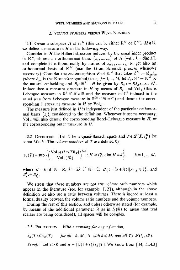
2.1. Given a subspace H of KM (this can be either lRM or C”), MEN, we define a measure in H in the following way.

Consider in H the Hilbert structure induced by the usual inner product in KM, choose an orthonormal basis {z,, . . . . z~} of H (with k = dim H), and complete it orthonormally by means of zk+ L, . . . . zM to get alSO an orthonormal basis of I16”’ (use the Gram-Schmidt process whenever necessary). Consider the endomorphism R of D6”” that takes 6,” := (S,,), (where Sj,,, is the Kronecker symbol) to z,,j= 1, . . . . A4, let Jk: Kk + KM be the natural embedding and Rk: Kk + H be given by R,x= RJ,x, XE Kk. Induce then a measure structure in H by means of R, and Volk (this is Lebesgue measure in Rk if K = R and the measure in Ck induced in the usual way from Lebesgue measure in R Zk if D6 = C) and denote the corre- sponding (Lebesgue) measure in H by Vol,.

The measure just defined in H is independent of the particular orthonor- ma1 bases {z,}~ considered in the definition. Whenever it seems necessary, Vol, will also denote the corresponding Borel-Lebesgue measure in H, or the corresponding outer measure in H.

2.2. DEFINITION. Let X be a quasi-Banach space and TE 9(X, I,“) for some ME N. The volume numbers of T are defined by

u,(T)=sup K

Vol,(Hn TBx) lik’: Hal,u dim H=k volk @‘;) >

27 k = 1, . . . . M,

where k’=k if od=R, k’=2k if K=@, B,:= {xEX: Ilxll,<l}, and B;:= B,;.

We stress that these numbers are not the volume ratio numbers which appear in the literature (see, for example, [ 12]), although in the above definition we also use a ratio between volumes. There is indeed at least a formal duality between the volume ratio numbers and the volume numbers.

During the rest of this section, and unless otherwise stated (for example, by means of the additional parameter [w as in 1* (IF!) to mean that real scalars are being considered), all spaces will be complex.

2.3. PROPOSITION. With s standing for any s-function,

S/c(T)<%(T) for all k, ME N with k d M, and all TE 9(I,, ly).

Proof. Let E>O and v:=(l/(l +&))sk(T). We know from [14, 11.4.31

6 ANTbNIOM.CAETANO

that then there are SE Y(Z:, 1,) and Q E 9’(ZF, I’;) with I( S 11, 11 Q 1) < 1 such that QZS= qZ$(k). We can therefore write

where the last step is justified as follows. The case ye = 0 being trivial, we assume q > 0. From the fact that

QTS= qZi(k) it follows that dim TN: = k. Denote then H:= TSZ$, B, := B,l, use the notation of 2.1, and reason as in the proof of the Carl-Triebel inequality (see, for example, [7, 2.d.11) to write

u/c (QW = Vol, (Q TS B;) Vol,(QI,,(Hn TS Bt))

Vol, (B;) Voh @:I

= Volk(QIHRkR;l(Hn TSB;))

Vol, (B:)

taking into account that 11 R, 11, I/ Q I(, 1) S II < 1. Letting E + O+ in (2.1) we obtain the desired result.

2.4. COROLLARY. x,(Z;(M)) < u,(Z;(M)), for all k, ME N with k < M, and all p E (0, m].

Proof:

since Vol,(Hn Z;(M) AB,) = Vol,(Hn AB,) < Vol,(Hn BF), the latter inequality coming from the fact that XEAB, =+-x = Ay for some ~~B2~lI~ll~~ll~II Il~ll,<l.

2.5. Since the main goal of this paper is the estimation of the Weyl num- bers of embeddings between sequence spaces, in view of the preceding corollary we shall now direct our efforts to the derivation of upper estimates for the volume numbers of the same embeddings. However, it turns out to be convenient to consider these latter numbers when K = R

WEYLNUMBERSANDSECTIONSOFBALLS 7

instead of K = C, so that we will need the following relation, the proof of which uses only straightforward manipulations:

u~(l~(M))~2”min~~~2~--1’2U2k(1~(2M; R)). (2.2)

3. VOLUME ESTIMATES OF SECTIONS OF UNIT BALLS

3.1. Since throughout all this section we deal only with real spaces, and thus no confusion with complex spaces can arise, we drop the parameter R from the previous notation. We also note that the notation developed in Subsection 2.1 (considering, obviously, the case K = R) is in force here; moreover, as a general convention, if something is typed in bold, such as H, and the same symbol in normal italic (If in our example) is also used to denote a subset of FP’, then the bold symbol denotes the inverse image by R of what is denoted by the other symbol (in our example, H = R-‘H).

We begin with a result that, as far as we know, is new. Note that there is no assumption of convexity whatsoever, and that the set B in question can be really nasty.

3.2. PROPOSITION. Let B be a bounded Bore1 subset of IWM and H a k-dimensional subspace of IW”. Assume that Vol,(H A CJB) = 0. Then

V~l,(HnB)=~li+cn+ (~E)~-~VOI~(H(E)~B), (3.1)

where H(E) = {XE IW~: Ib,R6,?)I GE, k+ 1 <j<~}.

3.3. Remark. Since R is an orthogonal transformation of lR”, hence, in particular, a homeomorphism, then 8B = aR-‘B = R-‘aB and therefore Vol,(HnaB) = Vol,((RJ,)-‘(HnaB)) = Volk(Jkl(R-‘HnR-‘8B)); that is, the hypothesis Vol,(Hn 8s) = 0 is equivalent to Vol,(J;’ (H n 8B)) = 0.

Proof of Proposition 3.2. The case B = @ or k = A4 being trivial, we suppose B # 0 and k < M.

Note first that, due to the fact that Lebesgue measure in iRM is invariant under orthogonal transformations,

(2&)k-MVolMW(&)nBB)= (2&)kmM~RM4Hcsjns (Y) dVol,(y), (3.2)

where Q s(y) = 1 if y E S, 0 otherwise.

8 ANTONIO M. CAETANO

Consider a sequence of non-void compact sets, (I&,),, defined in the following way:

K,,,= 1

x&‘:d,(x,8B)>; nnBz, 1

(3.3)

where n E N is such that B c (n - 1) BE (this is possible because B is boun- ded) and d, stands for the distance in RM coming from the I( . I/ co norm.

Use of Tonelli’s theorem in (3.2) gives

(2~)~~“” Vol,(H(s) n B)

= (2&T - A4 jRk jRM-k QH&) Q,(Y) dVol,-,W’) dVol,W)

with y = (Y’, Y”), Y’ = (yl, . . . . yk), Y” = bk+ 1, . . . . y,+,u), and

NY’) = jRMrnk Q,,,,(Y) Q,(Y) dVol,-,W’h (3.5)

the last equality in (3.4) coming from the fact that y’ $ nBk, + 3j~ ( 1, . . . . k} : 1 yi 1 > n a (y’, y”) $ nBg =S (y’, y”) # B.

Denoting by “A the complement of a subset A of R”“, we can write nBE = (K, n B) u (K, n ‘B) u (‘K, n nBt), for every m E N, and, since these are disjoint unions,

Qn,gY’)=Q..,:bw =Q ,v,nd~Y)+Q Kmn&” O)+ QCKmnnBgY’? 0).

Then (3.4) can be written in the form

(2~)~~~ Vol,(H(&)n B)=E, + E,+ E3 (3.6)

with

E,=(2e)kPM~RkQ ~,nd~‘, 0) &‘I dVol,b’),

E,=(~z)“-~~~~Q ~,ndL 0) EW) dVol,W)

and

E, = (2~)~-~ jRk Q cK,nn&~‘, 0) W’) dVoL(y’),

WEYL NUMBERS AND SECTIONS OF BALLS

and from (3.6) we obtain

d I j

~k~,(Y’,O)nVol,(Y’)-E, +E*+&. (3.7)

Before going further note that, by the detinion of Km, {~~[W~:d,(~,K,)<l/m}naB=0.

Analysis of E2. In order that the integrand may be non-zero, we must have (y’, 0) E K,,, n ‘B. If we choose E < l/m we get, on one hand, that (3jE {k + 1, . ..) M} : yi # [ - E, E] ) * 21 H(E) (y ) = 0; on the other hand, WE {k+ 1, . . . . W, yjE C--E, &I)* II Y-(y’,O)ll, = ll(O,~“)ll, GE< l/m, that is, d, (y, Km) < l/m and consequently y # aB. In this latter case we can even say that y $ B, for if y did belong to B then there would be z in the segment joining (y’, 0) to y that would be in 8B; z is of the form (y’, 1~“) with 1 E (0, 1) and thus II z - (y’, O)l[ 3c < I/m: contradiction! This shows that E2 = 0 if E < l/m.

Analysis of El. Here, in order that the integrand may be non-zero, we must have (y’, 0) E K, n B. Choosing again E < l/m, (VIE (k + 1, . . . . M}, yj E [ -E, E]) = 11 y - (y’, 0)/l o. < E < l/m, that is, y 4 aB, and, reasoning in much the same way as above, we must indeed have YE B. Thus Q”,,,(Y) Q.(y)=Q H(E) (y) and in the case of E, the function E equals

j,,-, jj+, Qc-,,,,(yj)dVol,-,(y”)=(2~)M-k. (3.8)

Finally, in E3 consider the upper estimate II u (y) < 1 in E, so that E is bounded above by (3.8).

Putting all this together in (3.7), for all m E N and E < l/m we can write

) Vol,(Hn B) - (2&)k- M VOl,(H(&) n B)I

+s,k Ii w,nne(~‘, O)dVol,(y’) = s Ii Rk x,&Y’~ O)dVol,(~')+ jRk L,nn&y', O)dVol,(y')

<2 21 s Rk vc,,,nng(~‘, 0) dVoL(y’). (3.9)

10 ANTi)NIO M.CAETANO

Observe now that III,,,,,e(y’, O)l 61inB~aJk(~‘)=QnBk (y’), which is integrable with respect to Vol,. And, given ;’ E UP such that (y’, 0) 4 cYB, d, ((y’, 0), aB) > 0, so that there exists m E N such that d, ((y’, 0), cYB) 2 l/m; thus either (y’, 0) 4 nBE, in which case 1 LK,nnB~(y’, 0) = 0, or (y’, 0) E K, (recall the definition (3.3) of K,,,), in which ca;e we also have II CK, n nst (y’, 0) = 0, so that lim, _ co II CK n n~w (y’, 0) = 0. Since the set that we excluded, that is, { y’ E [Wk : (y’, 0) E $5) =?;’ (H n BB), has Vol, equal to 0 (see Remark 3.3), then II CK,nnB~ 0 Jk m _ co) 0 Vol,-a.e.

We can thus use Lebesgue’s dominated convergence theorem to state that

I Q Rk ‘K,nnB; (~‘5 0) dVoL(y’) m+,x’ 0. (3.10)

We are now in a position to conclude the proof. Given q > 0 choose m such that the integral in (3.10) is less than q/2, and

choose 0 < s0 < l/m. For 0 <E <.sO we have then that (3.9) holds and therefore

~Vol,(HnB)-(2&)~~“V01M(H(&)nB)~ <2+

3.4. PROPOSITION. If B is the closed unit ball centred at zero corre- sponding to a t-norm 1) + 11 in R”, t E (0, 11, then B satisfies the hypotheses of Proposition 3.2 for all subspaces H of dimension k of (WM.

ProoJ Since all t-norms in [WM are equivalent (see [S, p. 151) and it can easily be seen that B is closed in its own topology, then B is also closed in the Euclidean sense, and therefore is a Bore1 set. It is also easily seen that B is bounded, so that it only remains to prove that Vol,(H n 8B) = 0.

Due to the continuity of the t-norm, it is easy to see that x~aBoIIx(( =l, therefore aBcB and IBnaB=@ for all ~E[O, 1). Then HnaBc Hn B\(HnAB) and

Vol,(HnaB)<Vol,(HnB)-Vol,(HnAB), (3.11)

since H n LB c H n B, ;1 E [0, l), and Vol,(H n B) < co. Note now that HnIB=A(HnB), i#O, and so Vol,(HnAB)=IkVol,(HnB), ilz=-0. Using this in (3.11) gives

Vol,(HnaB)< (1 -Ak)VolH(Hn B), for all 1 E (0, 1 ),

and letting ,I + 1 - we obtain the desired result.

WEYLNUMBERS AND SECTIONS OF BALLS 11

3.5. PROPOSITION. Let H be a k-dimensional subspace of R”, 11 . 11 a t-norm in R”, t E (0, 11, and B the corresponding closed unit ball centred at zero. Let 0 < p c co. Then we have

exp( - (1 x II “) d Vol, (x),

where H(E) has the same meaning as in (3.1).

ProoJ We follow close to the proof of Lemma II.1 of [Ill], the main modifications being due to the fact that our B is not necessarily convex.

For E > 0 let g(s) = (2~)~~“” JHCEj exp( - 11 x 11”) d Vol,(x) = (2~)~~ M JH(e) f;P*,,pe-r dr dV“lM(X) = t2&jkpM frW e-‘.fRM Q H@)tX) Q ~llxllP, ,) tr) d Vol,(x) dr, where the last identity comes from Tonelli’s theorem. Note that in the first of the iterated integrals above we can replace R! by R +. For each r we now make the change of variables defined by x = rllPy and get

g(E) = (2E)k-M fR+ eprrMlp

X f RM

bdr”py> Q I,llgl,P, m) (r) dVol,(y) dr

=(2E)k~MSR+e-rrMlyf~MII f,(&)(Y) f.tY)dVol~tY)dr

= s ~,,,,,(r)(2~r~“~)~~~Vo~~(H(~r-“~)nB)e-’r~~~dr. (3.12) R

From this the result follows trivially when k = M, so that we suppose k < M in the sequel.

The idea now is to apply Lebesgue’s dominated convergence theorem, since Proposition 3.4 says that we can apply Proposition 3.2 here, and this latter one says that for each r E R! +

lim E-o+

(2Er-“P)k-M Vol,(H(sr-“p) n B) = Vol,(Hn B). (3.13)

However, we need to prove first that the integrand in question is bounded above by an integrable function of r independent of E.

Note that, with y’ = (y, , . . . . yk) and y” = (yk+ i, . . . . yM), y’ E J;’ (B - (0, y”)) o (y’, 0) E B - (0, y”) o (y’, y”) E B. By hypothesis it follows that B is bounded, hence B is bounded, that is, BcnBz for some n E f% Thus

12 ANT6NIO M.CAETANO

( y’, y”) E B * I y, I < n, j = 1, . . . . k, *y’ E nBk, and J; ’ (B Therefore Vol,(J,‘(B-(O,y”)))<nkVolk Bk, =(2r1)~.

We can then write, for every q > 0 and y = (y’, y”),

VolM(H(ul) n 4

(O,y”))cnBk,.

= I II R‘-kxRk [-q,q]M-k (Y”) QB(Y’Y Y”) dVOlM(Y’, Y”)

= s IWM--k Q C-a. VI M-k(Y”)

x Q s Rk B--(oJ’) (Y’, O) dVolk(y’) dVolM-kb”)

= J RM-k Q c-v, rll ~4y”)Vol,(J,‘(B-(O,y”)))dVol,~,(y”)

6 s RM-k Q r-%Sl M-k (y”)(2n)k dvolMek(y”)= (2t’f)“-k (2n)k, and (2~)~~~ Vol,(H(q) n B) < (2n)k, for all q > 0.

The integrand function of (3.12) is then bounded above by IIc0,,,(r)(2n)k ep’rkip, which is independent of E and integrable in R.

Using (3.13) and Lebesgue’s dominated convergence theorem we finally obtain

A&) E-.Ot- Vol,(HnB)e-‘rk’pdr=Vol,(HnB)r

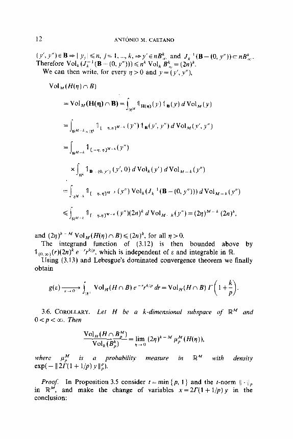
3.6. COROLLARY. Let H be a k-dimensional subspace of RM and O<p< 03. Then

Vol,(Hn BF)

V& (B;) = ,I5 WI)~- M $‘W(rlh

where p,” is a probability measure in R M with density exp( - II 2r(l+ UP) y II;).

Proof. in R”,

In Proposition 3.5 consider t = min {p, 1 } and the t-norm (I . lip and make the change of variables x = 2r( 1 + l/p) y in the

conclusion:

WEYL NUMBERS AND SECTIONS OF BALLS

= lim (2~)~~~ E-o+

X s

13

X J

e-112~(i+l/~)Yl(::dVOlIU(Y)

ff(wxl + l/P))- El

and, recalling the formula for Vol,(Bi) in [3],

Vol,(Hn B,M)

VOlk (E)

That the measure pP M is a probability can be proved easily by using Tonelli’s theorem, reducing thus the task to the calculation of an integral in R.

3.7. We now abandon the methods of [l 11, since these rely on the fact that for p 2 1 the function x I-+ xp is convex on [w +, and we want also (and mainly) to consider the case 0 <p < 1, for which this property does not hold. We are going to use, instead, the results of [6] about unimodality.

Observe first that all $“, 0 <p < co, ME N, are symmetric. If M= 1 we have a symmetric probability measure on R which is unimodal in the standard l-dimensional sense (i.e., the density is monotone on (-co, 0) and on (0, co t-see [S, p. IS]), therefore ,uj is unimodal in the sense of Kanter, more precisely, ,U~E U,-see L-6, sect. 31, where the notation U, is also explained.

Consider now the case ~31, MEN. Given yl,yZ~lT@’ and 1~[0,1], I/~~Zy+(l-~)y2)I,~~)Iy,II,+(1-~)IIy,I),and,sincex~xPisaconvex function on [O, co),

II AYZY, + (1 - 2) Y2 II p”

~~Il~,lI~+~~--l~llY2lI~

*-ll;ly,+~~-~~Y,lI~~~~-llY,11~~+~~-~~~-IIY,II~~,

14 ANTbNIOM.CAETANO

that is, log exp( - II 2f( 1 + l/p) y II g) is concave. Lemma 2.1 of [6] says then that pP M is logarithmically concave, and Lemma 3.1 of [6] applies to derive that ,u,” E UM (we refer to [6] for the explanation of the notation).

We recall here a definition of [6]:

3.8. DEFINITION. Let p and v be measures in II%““. We say that p symmetrically dominates v (and write p > v) if

p(“K) B v(‘K) (3.14)

for all compact, convex, symmetric subsets K of [WM.

3.9. Remark. If p and v are probability measures, (3.14) can be expressed in the equivalent form p(K) < v(K).

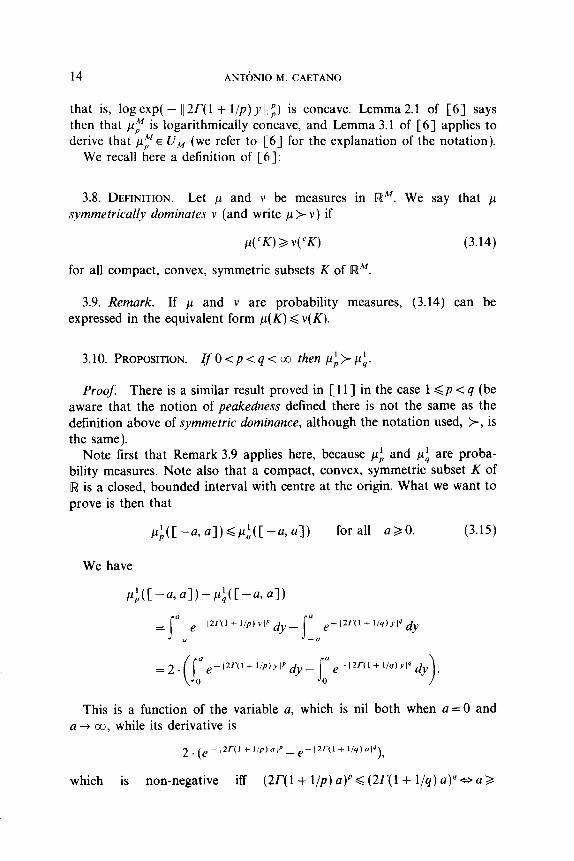
3.10. PROPOSITION. IfO<p<q<co then pi>pfi.

Proof: There is a similar result proved in [ 111 in the case 1 <p -C q (be aware that the notion of peakedness defined there is not the same as the definition above of symmetric dominance, although the notation used, >, is the same).

Note first that Remark 3.9 applies here, because pL:, and pb are proba- bility measures. Note also that a compact, convex, symmetric subset K of Iw is a closed, bounded interval with centre at the origin. What we want to prove is then that

pL(C-4 al)G~f,(C-a, al) for all a B 0. (3.15)

We have

u a

= e-12~(l+b7b’1pdy- e-12r(l + l/Y)Y14 dy

-a --a

-12)“(1+l/P)Y1pdy- e-1=-(1+ l/O)Yi4 dy .

>

This is a function of the variable a, which is nil both when a =0 and a + 00, while its derivative is

2.(e- 12r~1+1/P~rrl~~,-I2rc1+1/4~014) 9

which is non-negative iff (2r(1+l/p)a)Pd(2r(1+l/q)a)40a>

WEYLNUMBERSAND SECTIONSOFBALLS 15

((2r( 1 + l/q))q/(2r( 1 + l/p))“)“‘p~9’, for II > 0 and because p < q. There- fore

P;(C-4 a-P;(ba, al)<0 for ~20,

which proves (3.15) and the proposition.

3.11. PROPOSITION. Zf O<p<q<ac, and qal then py>pf for all ME N.

Proof: We use induction on M. The result is true when M= 1, as we have just proved in the preceding

proposition (even without the restriction q B 1). Suppose now it is true for M = m. Observe that p;‘i = ,ui x p,“,

pL4 m+ ’ = pt x $J and, as we pointed out in 3.1, pj E U, and ,uy E U, (because q 2 1). Moreover, pi > pi (is the case M= 1) and (by the induction hypothesis) ,$‘> ,u;. Corollary 3.2 of [6] therefore applies here to give P;vp-P:xP~.

3.12. Remark. This is a weak generalization of part of Proposition I.6 of [ 111, but it will be enough for our purposes, as we will see in a moment.

3.13. COROLLARY. Let H be a k-dimensional subspuce of [WM and O<p<q<co, 431. Then

VO~,(H~B~M)~V~~,(H~B~)

Voh P,k) Volj@) . (3.16)

In particular, Vol,( H n Br)/Vol, (B,k) d 1 if 0 <p < 2.

Proof: In view of Corollary 3.6, we just need to prove that ppM(H(q))Qpy(H(q)). For each rneN consider H(v])nmB,M. This is, obviously, closed, bounded (hence compact), convex, and symmetric. Since, by Proposition 3.11, p:> cl,“, then, by Definition 3.8 and Remark 3.9, pu,“(H(q) n mBy) < p,M(H(q) n mBy). Note now that H(g)nmB~tH(q) as m-+co, so that pf(H(s)) + p,M(H(q) n m@‘) d #(H(q) nm@‘) -+ #(H(q)) as m + co, and (3.16) follows.

Consideration of the case q = 2 in (3.16) gives the second part of the corollary.

4. ESTIMATES FOR THE WEYL NUMBERS

4.1. We return again to the complex case, unless otherwise specifically stated by means of an additional parameter [w.

580/106/l-2

16 ANT6NIO M.CAETANO

4.2. PROPOSITION. xk(I$(M)) d (2/p)‘/* e(2P+‘)/24k’/2-“p, for all k, ME N with k<M, andallpE(0,2].

Proof: From Corollary 2.4 and (2.2) we have

x&$(M)) d 2”p-“‘2 sup {(

Vol,(Hn P”(R)) ‘/P)

Vol*kMk(w >

:Hal~“‘(R),dimH=2k . I

Using Corollary 3.13 we can thus write

x,(Z;(M)) < 2”p-“2 Vol,,(B~(lR)) 1’(2k)

Vol*k(B:kw) >

and, using the expression (3.1/2) of [3] for these Vol,,,

‘l(X) (2k)

(l/Z- l/p)2k ,~.2k/12+ 1/(12k)

&2P + 1 j/24 k l/2 - l/P

4.3. COROLLARY. x,(zc(M)) < (2/p)9~2e~2P+“9~24k’~y~“p, for all k, ME N with k<M, and all O<p<q<2, where $=(1/p- l/q)/(l/p- l/2).

Proof: Using the same interpolation technique as in [2, Proof 3.1.31, we obtain

-G(z,P(M)) 6 (Xk(z;(M)))‘,

so that application of the preceding proposition gives the required result.

4.4. Remark. Only for the purposes of the next proposition, we note here that the Weyl numbers are multiplicative. The proof is basically the same of [ 15, 2.4.171 for the Banach space situation.

4.5. PROPOSITION. Let 0 <p < q d 2. Then there are cl, c2 >O such that for all k, ME N with k < M/2,

~,k”~~“~~x~(ZgP(M))~c~k~‘~~~‘~, (4.1)

Moreover, if q = 2, (4.1) holds for all k E { 1, . . . . M}.

Proof. The upper estimate comes directly from Corollary 4.3 above, and

WEYL NUMBERS AND SECTIONS OF BALLS 17

from an easy quasi-norm estimate in the case p = q. Using this, Proposi- tion 1.6, and the multiplicativity of the Weyl numbers, we also get

from which (4.1) follows. If q = 2 the lower bound comes directly from Proposition 1.6 without the

restriction k d M/2.

Note added in proof For a self-contained treatment of the results of [6] used here, and also for applications of the results of the present paper to the study of the asymptotics of Weyl numbers in function spaces, we refer to the author’s thesis “Asymptotic distribution of Weyl numbers and eigenvalues,” University of Sussex, 1991.

REFERENCES

1. A. M. CAETANO, Weyl numbers in function spaces, Forum Math. 2 (1990), 249-263. 2. A. M. CAETANO, Weyl numbers in function spaces II, Forum Math. 3 (1991), 613-621. 3. D. E. EDMLJNDS AND H. TRIEBEL, Entropy numbers and approximation numbers in

function spaces, Proc. London Math. Sot. (3) 58 (1989), 137-152. 4. D. E. EDMUNDS AND H. TRIEBEL, Entropy numbers and approximation numbers in

function spaces, II, Proc. London Math. Sot. (3) 64 (1992), 153-169. 5. W. FELLER, “An Introduction to Probability Theory and Its Applications,” Vol. II, Wiley,

New York, 1971. 6. M. KANTER, Unimodality and dominance for symmetric random vectors, Trans. Amer.

Math. Sot. 229 (1977), 65-85. 7. H. K~NIG, “Eigenvalue Distribution of Compact Operators,” Birkhauser-Verlag,

Basel/Boston/Stuttgart, 1986. 8. G. K~THE, “Topological Vector Spaces, I,” Springer-Verlag, Berlin/Heidelberg/New York,

1969. 9. R. LINDE, s-Numbers of diagonal operators and Besov embeddings, Rend. Circ. Mar.

Pulermo (2) Suppl. (1986), 83-110. 10. C. LUBITZ, “Weylzahlen von Diagonaloperatoren und Sobolev-Einbettungen,” Thesis,

University of Bonn, 1982. 11. M. MEYER AND A. PAJOR, Sections of the unit ball of $, J. Funct. Anal. 80 (1988)

109-123. 12. A. PAJOR AND N. TOMCZAK-JAEGERMANN, Volume ratio and other s-numbers of operators

related to local properties of Banach spaces, J. Funct. Anal. 87 (1989) 273-293. 13. A. PIETSCH, Eigenvalues of integral operators, I, Math. Ann. 247 (1980), 169-178. 14. A. PIETSCH, “Operator Ideals,” North-Holland, Amsterdam/New York/Oxford, 1980. 15. A. PIETSCH, “Eigenvalues and s-Numbers,” Cambridge Univ. Press, Cambridge/

New York/Melbourne, 1987. 16. H. TRIEBEL, “Theory of Function Spaces,” Birkhluser-Verlag, Basel/Boston/Stuttgart,

1983. 17. H. TRIEBEL, “Theory of Function Spaces, II,” Birkhluser-Verlag, Base], in press.