
from billiard balls to geometric phase in h + h2 a
212
GAS-PHASE REACTION DYNAMICS: FROM BILLIARD BALLS TO GEOMETRIC PHASE IN H + H 2 A DISSERTATION SUBMITTED TO THE DEPARTMENT OF CHEMISTRY AND THE COMMITTEE ON GRADUATE STUDIES OF STANFORD UNIVERSITY IN PARTIAL FULFILLMENT OF THE REQUIREMENTS FOR THE DEGREE OF DOCTOR OF PHILOSOPHY Justin Jankunas July 2013
-
Upload
khangminh22 -
Category
Documents
-
view
2 -
download
0
Transcript of from billiard balls to geometric phase in h + h2 a
GAS-PHASE REACTION DYNAMICS: FROM BILLIARD BALLS
TO GEOMETRIC PHASE IN H + H2
A DISSERTATION
SUBMITTED TO THE DEPARTMENT OF CHEMISTRY
AND THE COMMITTEE ON GRADUATE STUDIES
OF STANFORD UNIVERSITY
IN PARTIAL FULFILLMENT OF THE REQUIREMENTS
FOR THE DEGREE OF
DOCTOR OF PHILOSOPHY
Justin Jankunas
July 2013

This dissertation is online at: http://purl.stanford.edu/gr567jg0404
© 2013 by Justinas Jankunas. All Rights Reserved.
Re-distributed by Stanford University under license with the author.
ii
I certify that I have read this dissertation and that, in my opinion, it is fully adequatein scope and quality as a dissertation for the degree of Doctor of Philosophy.
Richard Zare, Primary Adviser
I certify that I have read this dissertation and that, in my opinion, it is fully adequatein scope and quality as a dissertation for the degree of Doctor of Philosophy.
Todd Martinez
I certify that I have read this dissertation and that, in my opinion, it is fully adequatein scope and quality as a dissertation for the degree of Doctor of Philosophy.
Robert Pecora
Approved for the Stanford University Committee on Graduate Studies.
Patricia J. Gumport, Vice Provost Graduate Education
This signature page was generated electronically upon submission of this dissertation in electronic format. An original signed hard copy of the signature page is on file inUniversity Archives.
iii

The Rat Pack. On the left with cigar in mouth is Jim Kinsey. Shooting is DudleyHerschbach’s first PhD student, Sam Norris. Next to him is another graduate student,George Kwei. On the extreme right is Dudley Herschbach.
iv

To the pioneers of molecular pool,
humbly
v

Preface
The work described herein is a continuation of the H + H2 saga as told by the differ-
ential cross section measurement - admittedly one of the most sensitive probes of the
interaction potential between a hydrogen atom and a hydrogen molecule. A great deal
of research on this simplest chemical reaction has been carried out in the laboratory
of Richard Zare in the past thirty years. Ten theses, dealing exclusively with the the
H + H2 reaction, have been written since 1988. These tall giant shoulders served as
a platform for me to stand on and to see ever further! As a tribute to my H + H2
predecessors, I would like to list their work:
R. S. Blake, ”Quantitative Fundamental Chemical Reaction Dynamics: the H +
D2 → HD + D Reaction”, 1988.
D. A. V. Kliner, ”The Hydrogen Atom - Hydrogen Molecule Exchange Reaction:
Experimental Tests of Quantum Theory”, 1991.
D. E. Adelman, ”Experimental Investigations of Reactions of Hot Hydrogen Atoms
with Molecular Hydrogen and Water”, 1992.
H. Xu, ”Molecular Rydberg Tagging and Its Application to Chemical Reaction Dy-
namics”, 1998.
F. Fernandez-Alonso, ”Dynamics of the Hydrogen Exchange Reaction Using the Pho-
toloc Technique”, 1999.
vi

B. D. Bean, ”The Hydrogen Atom, Hydrogen Molecule Exchange Reaction. Ex-
perimental Evidence for Dynamical Resonances in Chemical Reactions.”, 2000.
J. D. Ayers, ”An Experimental Cross Section for the Hydrogen Atom, Hydrogen
Molecule Exchange Reaction as a Function of Angle and Energy”, 2003.
A. E. Pomerantz, ”Quantum State Distributions for Reactive and Inelastic H + D2
Collisions”, 2004.
N. T. Goldberg, ”Reactive and Inelastic H + D2 Collisions: Classical Recoil, Quan-
tum Interference, and the Tug-of-War Mechanism”, 2008.
N. C.-M. Bartlett, ”State-to-State Reaction Dynamics of H + D2 and the Align-
ment and Orientation of Hydrogen Molecules”, 2011.
From a practical point of view, these theses were invaluable to my research because of
extensive experimental innovation and optimization reported therein. For example,
technical challenges associated with measuring differential cross sections for the H
+ H2 reaction have been largely overcome; the method started out as a primitive
one-dimensional velocity projection, progressed onto a two-dimensional projection,
and culminated with the state-of-the-art three-dimensional ion imaging technique.
State-specific detection of molecular hydrogen is yet another example of why I am so
grateful to my predecessors. Fernandez-Alonso has an entire chapter dedicated solely
to various ionization schemes of H2!1
The work of the aforementioned Zarelabbers has deepened our understanding of the
H + H2 reaction tremendously. Rotational state distributions, integral and differen-
tial cross sections were the experimental probing tools aimed at understanding the
1Had I read that chapter before deciding to find new ways of ionizing molecular hydrogen, Iwould have saved myself a lot of time...
vii

main features of the hydrogen exchange reaction. Certain findings became ’instant
classics’. An observation that rotationally excited H2(v′, j′) reaction products become
increasingly more side-scattered has been regarded as one of the well-understood hall-
marks of the H + H2 reaction. At the same time, certain questions about the H + H2
reaction remained unanswered. For example, the manifestation of geometric phase
effects in the H3 system is still an unfinished chapter.
Two findings are communicated in this work. The differential cross sections for the
HD(v′, j′) product of the H + D2 → HD(v′, j′) + D reaction show that when the recoil
kinetic energy is low, HD(v′, j′) products become more back-scattered with increasing
rotational quantum number j′. This is the opposite behavior observed and expected
of the H + H2 reaction. The explanation of this peculiar behavior is the focus of
Chapter 3.
Chapter 4 is dedicated to the explanation of geometric phase ’varieties’ in the H3
system, and contains experimental data of a first-ever conscious attempt to measure
the geometric phase effect in the H + HD→ HD + H reaction, wherein the inter-
ference between the reactive and inelastic scattering is altered upon the inclusion of
geometric phase in theoretical calculations.
The first chapter of this work is a brief introduction to the birth of H + H2, and a
tribute to heroic efforts of the physical chemists of the 1920s and 1930s who made the
first measurements of ortho-para interconversion rate in molecular hydrogen. Equally
impressive are theoretical chemists’ ways of simplifying the H3 potential energy sur-
face so as to efficiently calculate experimental observables. Chapter 2 is meant to
be an experimentalist-friendly introduction to the concepts of angular distributions,
Photoloc technique, single- and crossed-beam machines, multiphoton processes in
molecular hydrogen, and other experimentally relevant topics. I hope an uninitiated
reaction dynamicist will benefit the most from Chapter 2.
viii

Acknowledgements
I came to Stanford as an organic chemist, intent on pursuing the C-H activation chem-
istry. A meeting with Dick changed all that. Dick addressed me by saying, ’Justin, I
think you would be a great fit for the fundamental H + H2 studies’. Knowing close
to nothing about the H + H2 reaction, I thought this would be fun, and decided to
join the Zarelab! I am therefore indebted to Dick for his belief in me. I would also
like to thank him for giving me freedom to do things I thought were interesting. In
retrospect, his immense patience with some of the ’projects’ is beyond belief. My ten-
month ’study’ on a two-photon photodissociation of hydrogen bromide and hydrogen
iodide, is one example of his laissez-faire policy. Although nothing substantial came
out of this study, I learned a lot about the spectroscopy of diatomic molecules, and,
more importantly, I appreciated the power of independent problem solving. For this,
and much more, I thank Dick. I could not have hoped for a better advisor.
I remember vividly the first time I entered the lab in the basement of Mudd.2 Optical
tables and their content made me laugh, because I thought I made a huge mistake,
and I would never be able to learn this! Thankfully, Nate Bartlett emerged from
under the table, and greeted me with a smile. He turned out to be the person who
taught me everything I know about reaction dynamics. Lasers, optics, vacuum cham-
bers, nozzles, you name it - Nate introduced me to the world of gas-phase reaction
dynamics laboratory. In addition to being my scientific mentor, Nate also introduced
me to everything Californian. My stay in the Bay Area would not have been as en-
joyable without Nate. Finally, I would like to thank Nate for his patience when it
2AFTER I have joined the lab!
ix

came down to dealing with my ’unstable’ personality. I know I couldn’t spend a day
with myself in the lab, but Nate did it for almost three years. Nate, I don’t think I
can properly express my gratitude.
I would also like to thank Dr. Jianyang Zhang, for constantly reminding me that,
’Of course you can do it! Why can’t you do it?’. I enjoyed working on the D + DBr
→ D2 + Br project with him, my first experiment. I would like to thank Dr. Noah
Goldberg, most notably for his statement, ’Justin, while you were away, we measured
the geometric phase in H + H2’. Soon after that, I became obsessed with the geo-
metric phase... A special thanks goes to Prof. John Harrison from New Zealand. I
interacted with John during his visits to the Zarelab, and took a ’Junior’s’ role in the
time-dependent D2 depolarization experiment. I will always remember John’s defi-
nition of a physical chemist, ’You are not a physical chemist until you start making
your own bolts’. Alas, I am still an apprentice...
I was very fortunate to spend my last year in the Zarelab working with Mahima
Sneha. I have not met a graduate student in the Chemistry Department as enthusi-
astic about research as Mahima. Her prowess in the laboratory is breathtaking. She
has mastered the instrument in less than a year, and is already running experiments
completely independently! I wish her all the best.
In addition, I would like to thank Dr. Wenrui Dong, Dr. Hassan Sabbah, Dr. David
Leahy, Dr. Ali Ismail, Dr. Sam Kim, Dr. Richard Perry, and Dr. Jae Kyoo Lee for
stimulating scientific discussions, not necessarily reaction-dynamics related. I would
also like to thank Daryl Wong, Max Osipov, and Ryan Hadt for our extra curricular
activities... We all shared the view that, ’There is nothing a good night at the Nut-
house could not fix’.
It is difficult to imagine Stanford’s chemistry school without Roger Kuhn. His service
to the department is invaluable, and I am very grateful for his help in navigating the
labyrinth of various university procedures, as well as our ’deep conversations about
x

the meaning life’.
I would also like to thank Prof. Robert Pecora for chocolates and ’Krokodil’... Occa-
sional discussions with Prof. Todd Martinez were also very useful. I am particularly
grateful for those six lectures Todd entrusted me with - this was one of the most
gratifying teaching experiences I have had at Stanford.
Last but not least, I would like to thank my sister and my father for their inter-
est in what I do. Graduate school would have been much more difficult without our
weekly Skype ’conferences’. Thank you for your love and support.
xi

Contents
Preface vi
Acknowledgements ix
1 Introduction 1
1.1 HER - Hydrogen Exchange Reaction . . . . . . . . . . . . . . . . . . 1
1.2 The Birth of H + H2 . . . . . . . . . . . . . . . . . . . . . . . . . . . 4
2 ”The Deets” 16
2.1 Angular Distributions . . . . . . . . . . . . . . . . . . . . . . . . . . . 16
2.2 Measuring Angles . . . . . . . . . . . . . . . . . . . . . . . . . . . . . 28
2.3 Measuring Speed . . . . . . . . . . . . . . . . . . . . . . . . . . . . . 35
2.4 Detection of H2 . . . . . . . . . . . . . . . . . . . . . . . . . . . . . . 39
2.5 Typical Day in the Lab . . . . . . . . . . . . . . . . . . . . . . . . . . 47
2.6 Speed Measurement Calibration . . . . . . . . . . . . . . . . . . . . . 58
2.7 Summary . . . . . . . . . . . . . . . . . . . . . . . . . . . . . . . . . 63
3 H + D2 Differential Cross Sections 65
3.1 Introduction . . . . . . . . . . . . . . . . . . . . . . . . . . . . . . . . 65
3.2 DCS for H + D2 → HD(v′ = 2, j′) + D . . . . . . . . . . . . . . . . . 69
3.2.1 Experiment . . . . . . . . . . . . . . . . . . . . . . . . . . . . 70
3.2.2 Theory . . . . . . . . . . . . . . . . . . . . . . . . . . . . . . . 72
3.2.3 Results . . . . . . . . . . . . . . . . . . . . . . . . . . . . . . . 74
3.2.4 Discussion . . . . . . . . . . . . . . . . . . . . . . . . . . . . . 75
xii

3.3 DCS for H + D2 → HD(v′ = 4, j′) + D . . . . . . . . . . . . . . . . . 82
3.3.1 HD(v′, j′ = 0): Forward Scattering . . . . . . . . . . . . . . . 98
3.4 More DCS for H + D2 → HD(v′, j′) + D . . . . . . . . . . . . . . . . 105
3.5 Trouble in Paradise . . . . . . . . . . . . . . . . . . . . . . . . . . . . 112
3.6 Propensity Rules . . . . . . . . . . . . . . . . . . . . . . . . . . . . . 122
4 Geometric Phase in H + HD → H + HD 125
4.1 Geometric Phase and I . . . . . . . . . . . . . . . . . . . . . . . . . . 125
4.2 What is Geometric Phase? . . . . . . . . . . . . . . . . . . . . . . . . 126
4.3 GP in H + H2 . . . . . . . . . . . . . . . . . . . . . . . . . . . . . . . 135
4.3.1 Hyperspherical Coordinates . . . . . . . . . . . . . . . . . . . 137
4.3.2 GP1: Dynamic Encirclement . . . . . . . . . . . . . . . . . . . 140
4.3.3 GP2: Symmetric Encirclement . . . . . . . . . . . . . . . . . . 143
4.4 DCS for H + HD → HD(v′, j′) + H . . . . . . . . . . . . . . . . . . . 145
5 H + H2: Not Over Yet! 161
A GP in H + HD → HD + H 165
A.1 Symmetric Encirclement of CI . . . . . . . . . . . . . . . . . . . . . . 165
xiii

List of Tables
1.1 Hydrogen isotopomers’ spectroscopic data. . . . . . . . . . . . . . . . 6
1.2 Equilibrium constants for thermal dissociation of H2. . . . . . . . . . 7
2.1 Atomic and molecular [2+1] REMPI transitions used to overlap lasers. 57
2.2 Calculated and measured hydrogen atom speeds and branching ratios
following an HX photodissociation. . . . . . . . . . . . . . . . . . . . 63
3.1 The range of partial waves contributing to the hydrogen exchange and
other reactions. . . . . . . . . . . . . . . . . . . . . . . . . . . . . . . 68
3.2 Main experimental parameters and observables for the H + D2 reaction. 71
4.1 R2 values for experimental fits to |fR|2 + |fNR|2, |fR|2, and |fNR|2
theoretical calculations. . . . . . . . . . . . . . . . . . . . . . . . . . . 154
xiv

List of Figures
1.1 Cartoon depicting an H + H2(v, j) → H2(v′, j′) + H collision. Shown
are the relative initial and final velocities, vi and vf , respectively, be-
tween a hydrogen atom and a hydrogen molecule. Angle θ is the the
angle subtended by the two vectors, cos θ = vi · vi . . . . . . . . . . . 2
1.2 Symmetry correlation diagram for a planar o-H2 + o-H2 → p-H2 +
p-H2 reaction. The symmetry element, a plane of reflection (σv), is
shown in the top panel. Blue and green circles, i.e. color-coded or-
bital phase, represent the four molecular orbitals for reactant (left),
transition state (center) and product (right) side of the reaction. De-
generacies are present; these orbitals are clearly labelled as having the
same energy. The symmetry of each molecular orbital is indicated as
either symmetric (S) or antisymmetric (A) with respect to σv. Reac-
tant and product orbitals are correlated on symmetry grounds, i.e. S
↔ S and A↔ A. It is clear that one of the reactant orbitals correlates
to highly excited, completely repulsive product orbitals. . . . . . . . . 8
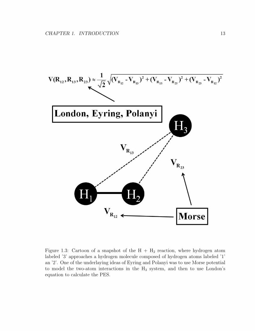
1.3 Cartoon of a snapshot of the H + H2 reaction, where hydrogen atom la-
beled ’3’ approaches a hydrogen molecule composed of hydrogen atoms
labeled ’1’ an ’2’. One of the underlaying ideas of Eyring and Polanyi
was to use Morse potential to model the two-atom interactions in the
H3 system, and then to use London’s equation to calculate the PES. . 13
2.1 An elastic scattering trajectory of a particle (red ball) by a central
force located at O. . . . . . . . . . . . . . . . . . . . . . . . . . . . . 17
xv

2.2 (a) Impact parameter probability distribution function P (b), (b) hard-
sphere deflection function, Eq. 2.3, and (c) the angular probability
distribution function P (θ). Even though P (b) is isotropic, P (θ) is not. 20
2.3 (a) Gaussian impact parameter probability distribution functions P (b)
for head on, b/d = 0.05, and glancing, b/d = 0.95, collisions between
two billiard balls, and (b) the resulting angular distribution functions.
Even though the two impact parameter distribution functions have the
same width, P (θ) distributions for head-on and glancing collisions have
different widths. . . . . . . . . . . . . . . . . . . . . . . . . . . . . . . 23
2.4 Collision between two particles in (a) the LAB frame and (b) the
COM frame. In the LAB frame p0 = p1 + p2; in the COM frame
p0 − p0 = p1 − p1 = 0. . . . . . . . . . . . . . . . . . . . . . . . . . . 24
2.5 Angular probability distribution functions P (ϑ)LAB in the LAB frame
for (a) P (θ)COM from Fig. 2.2c and (b) P (θ)COM from Fig. 2.3b. . . 26
2.6 Illustrative comparison of the H + D2 → HD + D reaction in (a)
crossed-beam and (b) single-beam experiment. LAB velocity vectors
are black, COM vectors are green, with the corresponding green New-
ton sphere, the COM velocity vector is blue, and the relative velocity
vectors are red. The main difference between a single-beam and a
crossed-beam set up is that often one of the particles, in this case D2,
has roughly zero LAB velocity in a single-beam experiment. Angles θ
and Θ are scattering angles in the COM and LAB frames, respectively. 29
2.7 Uncertainty functions for (a) P (cos θ), Eq. 2.33, and (b) P (θ), Eq.
2.34, distributions. The insets are replotted on a reduced scale, where
the original ordinate has been divided by the range of the abscissa.
The reduced plots can be compared to each other. Even though ∆θ
function is large when θ → 0 and 180, ∆θ is, on average, smaller
than ∆(cos θ) in a similar angular space region shown in the insets. . 36
xvi

2.8 Schematic of the experimental set up: Wiley-MacLaren TOF mass
spectrometer consists of extraction and acceleration regions. Usually,
Vext = −15V, and Vacc = −60V. Typically tTOF is several microsec-
onds for ions with m/z = 1 − 4. MCP is normally held at −2450V,while the delay line is held at +460V. . . . . . . . . . . . . . . . . . . 37
2.9 Excited potential energy surfaces of H2. Left panel shows states of g
symmetry; these can only be accessed by an even number of photons.
Panel on the right shows states of u symmetry; these can only be ac-
cessed by an odd number of photons. In the current study H2 was
ionized by [2+1] REMPI, where the first two photons resonantly con-
nect a single rovibrational level in the ground X 1Σ+g electronic state
to a single rovibrational level in the E,F 1Σ+g state. The third photon
takes the system into the H+2 ionic manifold. . . . . . . . . . . . . . . 40
2.10 Experimental layout. NY2 - 2nd harmonic of Nd3+:YAG laser (532
nm), NY3 - 3rd harmonic of Nd3+:YAG laser (355 nm), DL - dye laser,
BBO - nonlinear β−barium borate crystal, L - lens, W - UV window,
BS - beam splitter, DM - dichroic mirror, N - nozzle, D - detector, TDC
- time-to-digital converter, PC - personal computer, S - oscilloscope,
MIX - HX/D2 mixture. . . . . . . . . . . . . . . . . . . . . . . . . . . 48
2.11 HD(v′ = 0, j′ = 14) crushed ion images: (a), (c) and (e) are raw
images, and (b), (d) and (f) are processed images with background
removed. . . . . . . . . . . . . . . . . . . . . . . . . . . . . . . . . . . 50
2.12 HD(v′ = 1, j′ = 3) crushed ion images: (a), (c) and (e) are raw
images, and (b), (d) and (f) are processed images with background
removed. . . . . . . . . . . . . . . . . . . . . . . . . . . . . . . . . . . 51
2.13 Laboratory speed distributions of (a) HD(v′ = 0, j′ = 14) and (b)
HD(v′ = 0, j′ = 14) reaction product. Solid lines indicate the range of
Photoloc allowed speeds. . . . . . . . . . . . . . . . . . . . . . . . . . 52
2.14 Differential cross sections for (a) HD(v′ = 0, j′ = 14) and (b) HD(v′ =
0, j′ = 14) reaction products. . . . . . . . . . . . . . . . . . . . . . . . 55
xvii

2.15 Hydrogen atom ion sphere projection in the x − y plane from a con-
comitant photolysis of HBr and HI at λ = 207.5 nm and λ = 293.3
nm. . . . . . . . . . . . . . . . . . . . . . . . . . . . . . . . . . . . . . 60
2.16 Laboratory speed distribution of hydrogen atoms from a photolysis of
HBr and HI at λ = 207.5 nm and λ = 293.3 nm, as measured by a
two-color Doppler free [2+1] REMPI of a hydrogen atom. . . . . . . . 62
3.1 Caption . . . . . . . . . . . . . . . . . . . . . . . . . . . . . . . . . . 67
3.2 Caption . . . . . . . . . . . . . . . . . . . . . . . . . . . . . . . . . . 73
3.3 Caption . . . . . . . . . . . . . . . . . . . . . . . . . . . . . . . . . . 76
3.4 Caption . . . . . . . . . . . . . . . . . . . . . . . . . . . . . . . . . . 77
3.5 Plots of the most probable scattering angle θmax versus the square of
the rotational quantum number j′ of HD product. So-called LOCNESS
model predicts linear dependence, see Eq. 3.3. Black and brown curves
correspond to data taken by Fernandez-Alonso et al.; red and green
curves come from this work. . . . . . . . . . . . . . . . . . . . . . . . 81
3.6 Energy level diagram for the H + D2 → HD(v′, j′) + D reaction. Solid
black arrows, connecting particular collision energy values with specific
internal states of HD product, indicate the conditions under which the
forward scattering has been observed. Dashed black arrows indicate
experimental conditions under which similar forward scattering is ex-
pected. . . . . . . . . . . . . . . . . . . . . . . . . . . . . . . . . . . . 83
3.7 Caption . . . . . . . . . . . . . . . . . . . . . . . . . . . . . . . . . . 86
3.8 Caption . . . . . . . . . . . . . . . . . . . . . . . . . . . . . . . . . . 89
3.9 Opacity functions for two products of the H + D2 → HD(v′, j′) + D
reaction: HD(v′ = 1, j′ = 3) (black curve), and HD(v′ = 0, j′ = 14)
(red curve), as computed by QCT method. . . . . . . . . . . . . . . . 91
xviii

3.10 A schematic illustration of a potential energy surface for the H + D2 →HD(v′, j′) + D reaction. Certain highly internally excited HD products
do not have sufficient kinetic energy to overcome the centrifugal bar-
rier in the exit channel. Consequently, lower order partial waves must
contribute to the production of these highly internally excited prod-
ucts. The HD2 system does not literally get trapped; such trajectories
become simply non-reactive. . . . . . . . . . . . . . . . . . . . . . . 92
3.11 QCT and TI-QM opacity functions for the HD(v′ = 4, j′) product
vibrational manifold. Both QCT and QM follow the same trend: as
product rotational excitation increases, b and J , on average, decrease. 96
3.12 Caption . . . . . . . . . . . . . . . . . . . . . . . . . . . . . . . . . . 99
3.13 Cartoon illustrating the concept of vibrational angular momentum.
The bending mode in linear H3 is doubly degenerate: bending can take
place in xz and yx planes. The two bent configurations are related by
a simple rotation around the x−axis. . . . . . . . . . . . . . . . . . . 101
3.14 Reaction coordinate diagram showing approximate positions of several
QBSs for the H + D2 → HD(v′, j′) + D reaction. . . . . . . . . . . . 104
3.15 Caption . . . . . . . . . . . . . . . . . . . . . . . . . . . . . . . . . . 106
3.16 Two-dimensional pictorial explanation of nearside and farside scat-
tering. Theoretical calculations yield a scattering angle Θ, where
−180 < Θ < 180. Due to cylindrical symmetry (not shown in this 2D
drawing), experimental measurements yield θ, where 0 < θ < 180.
In other words, θ = |Θ|. (a) Forward scattered products are in a close
proximity in physical angular space, and the conditions for interference
are favorable, i.e. Θnearside ∼ 1 and Θfarside ∼ −1. (b) Sideways
scattered products exhibit minimal interference due to scattering into
opposite parts of the space, i.e. Θnearside ∼ 90 and Θfarside ∼ −90. . 111
3.17 Caption . . . . . . . . . . . . . . . . . . . . . . . . . . . . . . . . . . 114
3.18 QCT and TI-QM opacity functions for the HD(v′ = 3, j′) product
vibrational manifold at Ecoll = 1.97 eV. . . . . . . . . . . . . . . . . . 119
xix

3.19 Pictorial reminder of the vector nature of the L+ j = L′ + j′ equation.
(a) Whilst the orbital angular momentum is conserved in a two-body
system, (b) in a system with internal degrees of freedom, completely
head-on collisions may lead to rotationally excited products. The ro-
tational angular momentum j′ and product orbital angular momentum
L′ are equal and antiparallel in this case. . . . . . . . . . . . . . . . . 123
4.1 Schematic showing the simplest example of a geometric phase. (a)
Classical parallel vector transport along a closed loop on a curved man-
ifold results in a non-zero angle α, whereas (b) an analogous procedure
in a flat space yields α ≡ 0. . . . . . . . . . . . . . . . . . . . . . . . 127
4.2 Illustration of the Aharonov-Bohm (AB) effect, that predicts a change
in the interference pattern between two electron packets (a) without
and (b) with a solenoid present. Even though the magnetic field B is
zero outside solenoid, and electrons experience no forces whilst going
around the current-carrying wire, the presence of a ∇f(r, t) term in
the vector potential does influence the electron’s wavefunction, which
is not gauge invariant. . . . . . . . . . . . . . . . . . . . . . . . . . . 130
4.3 Electronic level correlation diagram for the H3 system as a function
of the bend angle α. At all equilateral triangle geometries the H3
configuration has doubly degenerate electronic state. . . . . . . . . . 133
4.4 Cartoon illustrating the interference between two pathways: a direct
one, wherein the incoming hydrogen atom ’reacts’ with D2 molecule in a
direct manner, and a looping pathway, wherein the H atom comes close
to the deuterium molecule, then goes around the conical intersection
(marked ’x’ in the figure), and then ’reacts’ with the D2 molecule. Note
that the interference will be noticeable only if the two pathways scatter
HD products into the same angular space, as shown in the cartoon. . 136
4.5 Jacobi coordinates for a A + BC collision. . . . . . . . . . . . . . . . 137
4.6 Caption . . . . . . . . . . . . . . . . . . . . . . . . . . . . . . . . . . 139
4.7 Caption . . . . . . . . . . . . . . . . . . . . . . . . . . . . . . . . . . 141
xx

4.8 Caption . . . . . . . . . . . . . . . . . . . . . . . . . . . . . . . . . . 144
4.9 (a) Raw and (b) processed experimentally measured HD(v′ = 2, j′ =
3) laboratory speed distribution. . . . . . . . . . . . . . . . . . . . . . 147
4.10 Caption . . . . . . . . . . . . . . . . . . . . . . . . . . . . . . . . . . 148
4.11 DCSs for (a) HD(v′ = 3, j′ = 4) and (b) HD(v′ = 2, j′ = 5) re-
action products. Although HD(v′ = 3, j′ = 4) product shows more
pronounced GP and NGP differences, the reaction cross section is
prohibitively small. . . . . . . . . . . . . . . . . . . . . . . . . . . . . 156
4.12 The effect of averaging theoretical calculations over (a) the spread in
Ecoll, centered at Ecoll = 1.44 eV, and over (b) the reactant HD(v =
0, j = 0, 1, 2) rotational state distribution. . . . . . . . . . . . . . . . 157
4.13 DCSs for (a) Ha + HbD(v = 0, j = 0, 1, 2) → HaD(v′ = 2, j′ = 3)
+ Hb reactive scattering, and (b) Ha + HbD(v = 0, j = 0, 1, 2) →HbD(v
′ = 2, j′ = 3) + Ha inelastic scattering. The inelastic DCSs
show a tremendous dependence on the initial rotational state of HD
reactant. . . . . . . . . . . . . . . . . . . . . . . . . . . . . . . . . . . 158
4.14 Caption . . . . . . . . . . . . . . . . . . . . . . . . . . . . . . . . . . 160
5.1 Caption . . . . . . . . . . . . . . . . . . . . . . . . . . . . . . . . . . 163
A.1 Caption . . . . . . . . . . . . . . . . . . . . . . . . . . . . . . . . . . 167
A.2 Caption . . . . . . . . . . . . . . . . . . . . . . . . . . . . . . . . . . 169
A.3 Caption . . . . . . . . . . . . . . . . . . . . . . . . . . . . . . . . . . 171
A.4 Caption . . . . . . . . . . . . . . . . . . . . . . . . . . . . . . . . . . 173
xxi

Chapter 1
Introduction
1.1 HER - Hydrogen Exchange Reaction
’How does a chemical reaction occur?’ is perhaps the most misbegotten question in
the field of gas-phase reaction dynamics. The answer is simple: molecules approach
one another, collide, and recede. The above question could be viewed as a rhetorical
one insofar as it encompasses a multitude of theoretically and experimentally relevant
queries. An example of a pertinent question in reaction dynamics is, ’Given a set of
well defined initial conditions, what products, and with what relative probability, can
be formed as a result of a particular reaction?’. Or, ’Given a particular reactant
approach direction, what is the most probable product recoil direction?’. These are
but a few problems central to a reaction dynamicist. An in-depth summary of such
questions can be found in Molecular Reaction Dynamics by Levine and Bernstein, a
classic text in the field of reaction dynamics. [1]. One of the main goals of this work is
to deepen our understanding of the hydrogen exchange reaction (HER) often written
as
H + H2(v, j)→ H2(v′, j′) + H (1.1)
where v and j are vibrational and rotational quantum numbers of a diatomic molecule;
unprimed and primed notation to be used throughout this study refers to reactants
and products, respectively. The focus of experiments described herein is of a vec-
1
CHAPTER 1. INTRODUCTION 2
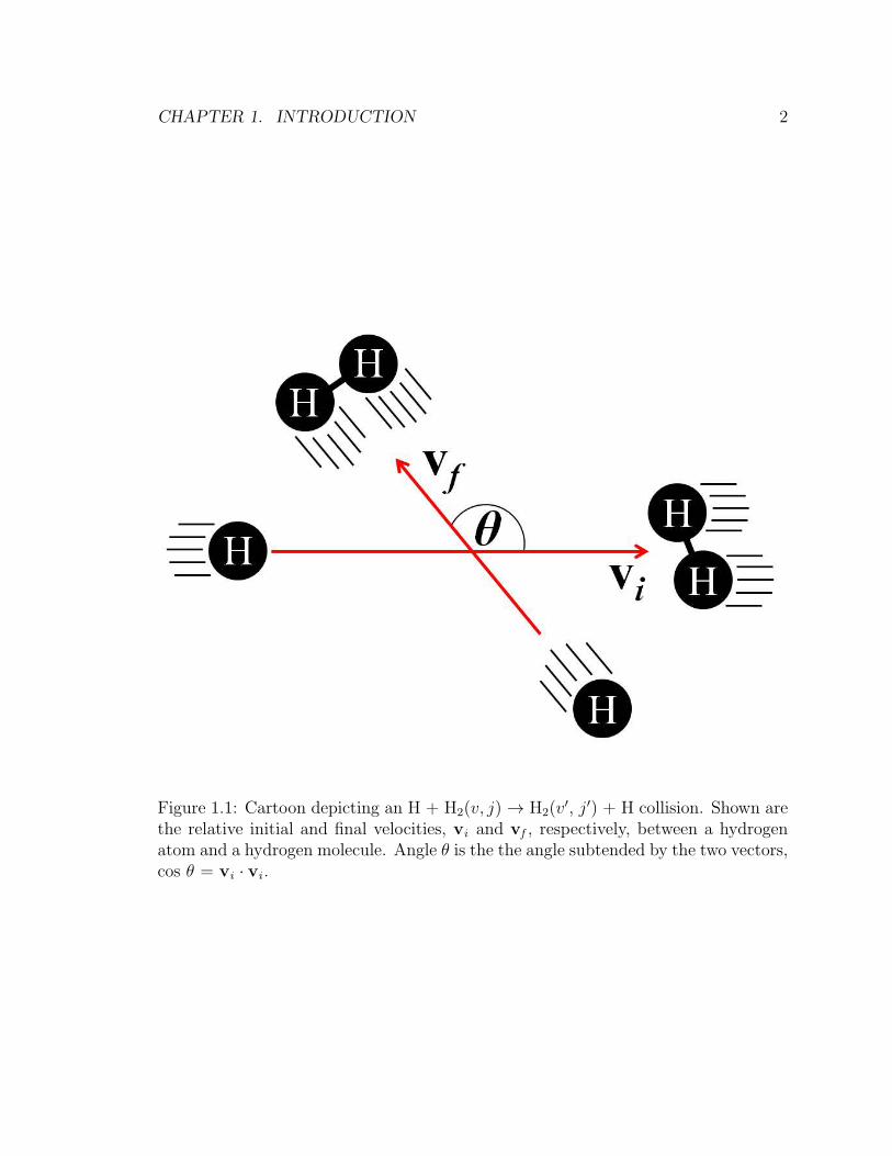
Figure 1.1: Cartoon depicting an H + H2(v, j)→ H2(v′, j′) + H collision. Shown are
the relative initial and final velocities, vi and vf , respectively, between a hydrogenatom and a hydrogen molecule. Angle θ is the the angle subtended by the two vectors,cos θ = vi · vi .

CHAPTER 1. INTRODUCTION 3
torial nature, ’Where do the H2(v′, j′) products recoil with respect to the reactant
approach direction?’. This question is illustrated pictorially in Fig. 1.1. The aim is
to obtain a correlation between the initial reactant velocity vi , and the final product
recoil velocity vf . This is equivalent to measuring the angle θ between these two
vectors, as shown in Fig. 1.1. A distribution of the scattering angle θ is also known
as the differential cross section, or simply DCS, a term that henceforth will be used
frequently. A more formal definition of a DCS will follow shortly.
There are several reasons for studying HER. Although formally a six-body problem,
three nuclei and three electrons, the often invoked Born-Oppenheimer approximation
simplifies theoretical calculations considerably. The resultant three-nuclei system
can nowadays be solved quantum mechanically rather easily. Calculations can then
be compared to experimental measurements. The juxtaposition of experiment and
theory is twofold. First, one would like to see how well theoretical predictions and
experimental data match. The procedure is not as straightforward as one might
think. Neither theory nor experiment are guaranteed to be absolutely correct a pri-
ori. Hence, if a calculation and a measurement disagree, one must usually look for
experimental errors as well as reconsider theoretical calculations. This is an example
of a quantitative approach to data analysis. Equally important is the qualitative
comparison of theory and experiment. In general, one is interested in trends exhib-
ited by experiment and theory, even if there are disagreements between the two. A
great deal has been learned about the H + H2 reaction using both approaches, as
illustrated in subsequent chapters. From the quantitative-fit perspective, the H + H2
reaction is a yardstick for comparing state-of-the-art theory to experiment. In the
qualitative-fit sense, the H + H2 reaction is a ’chemist’s crystal bowl’ enabling one
to predict the outcome of related gas phase reactions. In addition, there are certain
aspects of the H + H2 reaction family that have received virtually zero experimental
attention. High energy collisions between a hydrogen atom and a hydrogen molecule
is one such example. The highest relative collision energy (Ecoll), with which the
hydrogen atom and the hydrogen molecule have been collided is about 2.5 eV. An
important milestone will be H + H2 collisions at Ecoll ≈ 4 eV, because the effect on

CHAPTER 1. INTRODUCTION 4
the nuclear dynamics exerted by the first excited potential energy surface (PES) of
H3 system has not been studied experimentally. Another outstanding experimental
question in the H + H2 dynamics is the so-called mj′-resolved DCS, also known as the
three-vector correlation, wherein the experimental signal is measured as a function of
mutual orientation of reactant approach velocity, product recoil velocity and product
rotational angular momentum, vi , vf and j′, respectively. Until such experiments are
performed our understanding of HER will be incomplete.
1.2 The Birth of H + H2
In the late 1920s and early 1930s molecular hydrogen was a hot molecule. So much
so that the 1932 Nobel Prize in Physics was awarded to Werner Heisenberg, ’for
the creation of quantum mechanics, the application of which has, inter alia, led to
the discovery of the allotropic forms of hydrogen’. The two allotropic forms are, of
course, ortho and para hydrogen, often abbreviated as o-H2 and p-H2, respectively.
Odd rotational levels are populated by o-H2 molecules, i.e. o-H2(v′, j′ = odd), whilst
p-H2(v′, j′ = even). The reason for the existence of odd and even rotational manifolds
in molecular hydrogen is purely quantum mechanical, and is a consequence of identical
fermionic nuclei that force the total molecular wavefunction to be antisymmetric upon
an exchange of the two nuclei. Collision- and photon-induced transitions between the
two species are forbidden, primarily because nuclear spin and molecular rotational
angular momenta couple weakly. In principle, a low-temperature sample of 100%
o-H2 would remain in such a state for a long time, on the order of several years [2, 3].
In the presence of paramagnetic substances however a sample of 100% o-H2 would
rapidly equilibrate with p-H2, with an equilibrium ratio of o-H2:p-H2 = 3:1. Studies
of the so-called ortho-para interconversion in H2 were actually the first experimental
inlands into the H + H2 reaction. If two o-H2 molecules collide and rearrange into
p-H2 species, i.e.
o-H2 + o-H2k−→ p-H2 + p-H2 (1.2)

CHAPTER 1. INTRODUCTION 5
then the reaction velocity is given by
d[p-H2]
dt= k[o-H2]
2 (1.3)
In other words the rate of reaction should exhibit a quadratic dependence on o-H2
concentration. Pioneering experiments of A. Farkas and others, wherein the rate of
appearance of p-H2 was measured as a function of varying o-H2 pressure, suggested
that the order of the reaction with respect to o-H2 was 3/2, rather than 2 [3–5]. (It is
worthwhile pointing out how remarkable these experiments were. The main method
of monitoring the rate of reaction relied on the fact that o-H2 and p-H2 molecules
have different heat capacities, which, in turn, meant that thermal conductivity and
other thermodynamic properties of the two hydrogen allotropes were different. One
of the experimental protocols used was to start with a pure sample of p-H2 at a
given temperature, and then monitor its concentration by employing the Wheatstsone
bridge to measure the resistance of a gas sample as a function of time.) The finding
that the exponent in Eq. 1.3 was 3/2 and not 2 was important because it suggested
that ortho-para interconversion in molecular hydrogen was not due to a single collision
of two H2 molecules, as shown in Eq. 1.2. Instead, the following mechanism is
consistent with the experimental observations:
o-H2
k1−−−−k−1
2H (1.4)
H + o-H2k2−→ p-H2 +H (1.5)

CHAPTER 1. INTRODUCTION 6
Table 1.1: Hydrogen isotopomers’ spectroscopic data.
Species B (cm−1) ω0 (cm−1) θr (K) θv (K) D0 (eV)
H2 60.85 4401 87.65 6340 4.478HD 45.66 3813 65.76 5493 4.514D2 30.44 3116 43.85 4488 4.556
In this case the hydrogen atoms are generated by a thermal dissociation of hydrogen
diatomics.1
Assuming H atoms and H2 molecules are at equilibrium, i.e. Keq = k1k−1
= [H]2
[o-H2],
it is easy to show that the overall rate law for ortho-para interconversion mechanism
1Should a reader think that early kinetic HER studies were easy, or easier than experimentsdescribed herein, please consider the following. The experimental heroes modestly mention thathydrogen atoms come from a thermal dissociation of molecular hydrogen, i.e.
H2 2H (1.6)The density of hydrogen atoms in a cylinder of H2 is small. How small? One can calculate theequilibrium constant for the above reaction from first principles,
Kc(T ) =[H]2
[H2]=
(qH/V )2
qH2/V
(1.7)
where qH/V and qH2/V are hydrogen atom and hydrogen molecule partition functions, given by
qH(T )
V= 2
(2πmHkBT
h2
)3/2
(1.8)
qH2(T )
V=
(2πmH2kBT
h2
)3/2( T
σΘr
) 1
1− exp(−Θv
T )exp
( D0
kBT
)
(1.9)
where the factor of 2 in front of Eq. 1.8 accounts for the doubly degenerate ground state of ahydrogen atom, and σ is the symmetry number, and σ = 2 for H2 and D2, and σ = 1 for HD. Otherquantities have their usual meaning, and are summarized in Table 1.1. Equilibrium constant valuesas a function of temperature are tabulated in Table 1.2. The last two columns of Table 1.2 areparticularly revealing. Studying the H + H2 reaction at room temperature at atmospheric pressure,[H2] ∼ 1025 m−3, is ’difficult’ because the hydrogen atom concentration is some thirty six orders ofmagnitude smaller than the molecular hydrogen number density! Even at a reasonable temperatureof 755 K the hydrogen atom concentration is only 4.2·1012, yet rate constants have been measured- what a tour de force! For comparison, if hydrogen exchange reaction was studied under typicalmolecular beam densities, i.e. [H2] ∼ 1019 m−3, then reasonable count rates would never be achievedat room temperature! These are only rough estimates of course, but they are certainly suggestive,particularly regarding the absolute reactant number densities.

CHAPTER 1. INTRODUCTION 7
Table 1.2: Equilibrium constants for thermal dissociation of H2.
T (K) Kc(T) (m−3) Kc(T) (m
−3) Kc(T) (m−3) [H] (m−3) [H] (m−3)
H2 HD D2 [H2] = 1025 (m−3) [H2] = 1018 (m−3)
100 2.1·10−196 1.6·10−198 2.6·10−199 4.6·10−86 4.6·10−89
300 6.2·10−46 8.3·10−47 8.2·10−47 7.8·10−11 7.8·10−14
500 8.8·10−16 2.1·10−16 3.0·10−16 9.4·104 94755 1.8 0.58 1.0 4.2·1012 4.2·1091000 4.2·107 1.6·107 2.9·107 2.1·1016 2.1·10131500 1.7·1015 7.6·1014 1.4·1015 1.3·1020 1.3·1017
as shown in Eqs. 1.4 and 1.5 is given by
d[p-H2]
dt= k2
√
Keq[o-H2]3/2 (1.10)
which is consistent with the experimental observations, vide supra. These experi-
ments have demonstrated conclusively that in the case of a homogeneous ortho-para
interconversion in molecular hydrogen, the mechanism is not that of two H2 molecules
coming together, Eq. 1.2. In retrospect, this is not surprising. The insight comes
from what is now known as Woodward-Hoffmann rules stating that the orbital sym-
metry is a conserved quantity throughout the reaction [6]. It can be shown that when
two hydrogen molecules, in their ground electronic states, approach one another in a
planar transition state, as shown schematically in Fig. 1.2., the hydrogen exchange
reaction is said to be thermally forbidden, because one of the reactant molecular or-
bitals correlates to a completely repulsive electronic orbital on the product side [7].
More tedious albeit analogous calculations show that the H2 + H2 reaction is for-
bidden for other molecular configurations too, e.g. non-planar and linear approach
geometries [8]. Unlike with pericyclic reactions in organic chemistry, wherein the
thermally forbidden reactions are often photochemically allowed, promoting two elec-
trons into the c molecular orbital (Fig. 1.2) would result in a very fast dissociation of
both hydrogen molecules; presumably this would happen before the electrons in the
c orbital had time to funnel into the bound molecular orbital c′ on the product side.

CHAPTER 1. INTRODUCTION 8
Figure 1.2: Symmetry correlation diagram for a planar o-H2 + o-H2 → p-H2 +p-H2 reaction. The symmetry element, a plane of reflection (σv), is shown in thetop panel. Blue and green circles, i.e. color-coded orbital phase, represent the fourmolecular orbitals for reactant (left), transition state (center) and product (right)side of the reaction. Degeneracies are present; these orbitals are clearly labelled ashaving the same energy. The symmetry of each molecular orbital is indicated aseither symmetric (S) or antisymmetric (A) with respect to σv. Reactant and productorbitals are correlated on symmetry grounds, i.e. S ↔ S and A ↔ A. It is clear thatone of the reactant orbitals correlates to highly excited, completely repulsive productorbitals.
CHAPTER 1. INTRODUCTION 9
The main experimental conclusion was that the homogeneous ortho-para interconver-
sion in H2 occurs via the H + o-H2 → H + p-H2 reaction. These observations were
accompanied by experimentally measured rate constants at a range of temperatures.
The natural thing to have asked at this point was, ’Is it possible to calculate the rate
constant for the H + H2 reaction from first principles? If so, how well do the exper-
iment and theory match?’. This was the beginning of HER story as we know it today.
A fresh and extremely detailed account of the main H + H2 developments up to
1941 can be found in the book by Glasstone, Laidler and Eyring [9]. The theoretical
approach to the H3 system in 1920s and 1930s is quite an inspiring one, as it con-
tains the history of physics in the form of a hydrogen atom, as well as the history of
chemistry, with the hydrogen molecule as a poster child! At the time, spectroscopists
had a good understanding of an H2 molecule and its electronic, vibrational and rota-
tional level structure [10]. Hydrogen atom was understood even better.2 Theoretical
treatment of an H2 molecule, on the other hand, posed serious problems. While the
Schrodinger’s equation for a hydrogen atom is solvable exactly, analytic solutions for
two-electron systems, such as He atom and H2 molecule, do not exist. Any chemical
system with two or more electrons contains terms of the 1|ri−rj |
form in its Hamilto-
nian, where ri and rj are ith and jth electron coordinates, respectively. The resulting
integrals, e.g.∫
ψ∗i
1|ri−rj |
ψjdτ , have no analytic solutions. One must therefore make
approximations that yield tractable integrals. In a way, the doors of chemistry were
opened by Heitler and London who proposed that the ground state of H2 molecule is
a singlet, i.e. electron spins are ’antiparallel’, while the triplet state, electron spins
’parallel’, is repulsive [11]. In this famous paper they wrote down the expressions for
singlet and triplet energies in terms of these integrals, and qualitatively discussed the
main bonding features in H2. Sugiura has subsequently solved, approximately, the
integrals of Heitler and London by using the elliptical coordinates [12]. The results
were ’in a fair agreement with the experimental data’ [9], at least by the standards
of the day: the calculated H2 equilibrium distance and dissociation energy were 0.80
A and 74 kcal/mol (3.21 eV), compared to the experimental values of 0.74 A and
2Perhaps with an exception of a Lamb shift, which was not measured until 1947.

CHAPTER 1. INTRODUCTION 10
108.9 kcal/mol (4.72 eV)3, respectively. Even though that was a whopping 32% dif-
ference between the calculated and measured values of dissociation energy, the work
of London, Heitler and Sugiura served as a stepping stone for gradual improvement
of theoretical methods used in the first-principles treatment of an H2 molecule [15].
It should become obvious, from the preceding discussion on the difficulties associ-
ated with solving a quantum mechanical problem of an H2 molecule, that modeling
of the three protons and three electrons is even more challenging. Shortly after the
1927 paper on bonding in a hydrogen molecule, London proposed, seemingly ad hoc,4
the interaction potential for the H3 system [16]
V (R12, R23, R13) = A(R12) + B(R23) + C(R13)+
+1√2
√
(
α(R12)− β(R23))2
+(
β(R23)− γ(R13))2
+(
γ(R13)− α(R12))2 (1.11)
whereA(R12), B(R23), C(R13) are the familiar Coulomb integrals, and α(R12), β(R23),
γ(R13) are the so-called exchange integrals.5 The three internuclear distances in H3
system are denoted by Rij. Equation 1.11 is in a way a milestone in the field of chem-
ical kinetics. Why? Wigner, one of the founders of the theory of reaction rates, in
its most general form known as the Transition State Theory (TST) has said in 1937,
’According to our present notions, the theory of reaction rates involves three steps.
3The currently accepted value for H2 dissociation energy is 4.478 eV [13, 14].4Equation 1.11 has been derived in 1932 [17].5In the case of a hydrogen molecule, the Coulomb and exchange integrals are given by
Jab =
∫∫
dr1dr2 ψ∗
a(r1)ψ∗
b (r2)1
r12ψa(r1)ψb(r2)
Kab =
∫∫
dr1dr2 ψ∗
a(r1)ψ∗
b (r2)1
r12ψa(r2)ψb(r1)
respectively, where ψa(ri) and ψb(rj) are atomic hydrogen wavefunctions centered on nucleus a andnucleus b, respectively. The Coulomb integral is the energy associated with a (classical) electrostaticinteraction between charge densities centered on nucleus a and nucleus b. The exchange integraldoes not have a classical analogue. It expresses the ’exchange’ energy associated with an interactionbetween electron ”1” being located at nucleus a and nucleus b, and electron ”2” being similarlysmeared out over the two nuclei. The Coulomb contribution to the overall bonding in H2 is minor,on the order of a few percent. The strength of a chemical bond between two hydrogen atoms is thusa quantum mechanical phenomenon.

CHAPTER 1. INTRODUCTION 11
First, one should know the behavior of all molecules present in the system during the
reaction, how they will move, and which products they will yield when colliding with
definite velocities, etc. Practically, this amounts in most cases to the construction
of the energy surface for the reacting system’ [18]. Equation 1.11 is precisely this -
a potential energy surface that gives the energy of H3 system as a function of three
internuclear distances. Conceptually, one could find an activation energy for the H
+ H2 reaction as follows. The asymptotic form of Eq. 1.11 is just the energy of
a hydrogen atom plus the energy of a hydrogen molecule. The difference between
the maximum of Eq. 1.11 and its asymptotic limit is the classical activation energy
of a reaction. As most of today’s undergraduates know, this is the key parameter
in Arrhenius equation that relates the rate of a chemical reaction to the activation
energy. This is the reason why Eq. 1.11 is such an important development in chemi-
cal kinetics - it allows one to calculate the velocities of chemical reactions from first
principles. London’s equation however is not very accurate. Even within the Born-
Oppenheimer approximation, wherein the nuclei are held fixed while the quantum
mechanical problem for electrons is solved, Eq. 1.11 is far from exact. It misses, for
example, the three-body terms, as well as higher order polarization terms, as given by
the perturbation theory [19]. More sophisticated and more accurate techniques are
available today for calculating a PES of the H3 system; the overview of the theoretical
methods is beyond the scope of this work [20].
Even though Eq. 1.11 looks rather simple, its direct use in the computation of reac-
tion rates is cumbersome. Development of the so-called ’semi-empirical method’ by
Eyring and Michael Polanyi has simplified things enough to permit the computation
(without computers!) of a PES for HER with a reasonable number of points [21]. The
’empirical’ in the ’semi-empirical method’ comes from the fact that a Morse function
is used to model the potential of a diatomic molecule, in this case hydrogen, i.e.
V (R) = De[e−2a(R−R0) − 2e−a(R−R0)] (1.12)

CHAPTER 1. INTRODUCTION 12
where R0 is the equilibrium internuclear separation, De is the dissociation energy
plus the zero point energy, and the constant a is defined as a = ω0
√
2µDe
, where ω0
is the normal mode frequency, and µ is the reduced mass of a diatomic molecule.
Although completely empirical, Eq. 1.12 is a good description of the potential energy
for R values close to R0. Computing the potential energy of a hydrogen molecule
for different internuclear separations is rather straightforward by using Eq. 1.12.
The bonding energy of a diatomic molecule, V (R), is a sum Coulomb and exchange
energies, i.e. V (R) = A(R) + α(R), respectively. The Morse function, Eq. 1.12,
does not give individual A(R) and α(R) values that coud be used directly in Eq.
1.11. The approximation of a ’semi-empirical method’ is to assume that the Coulomb
contribution is small and, more importantly, does not vary too much as a function
of internuclear separation. In other words, V (R) ≈ α(R). Thus, the use of Eq. 1.12
together with Eq. 1.11 allowed for a calculation of a first ever PES for the H3 system
[21]:
V (R12, R23, R13) ≈1√2
[
(
V (R12)− V (R23))2
+(
V (R23)− V (R13))2
+
+(
V (R13)− V (R12))2]1/2 (1.13)
This is the celebrated London-Eyring-Polanyi (LEP) PES. The conceptual construc-
tion of LEP surface is shown schematically in Fig. 1.4. The PES contained qualitative
inaccuracies. Calculations suggested the presence of a very shallow minimum close to
the transition state point, what is now known as ’Lake Eyring’. Sato has modified the
potential significantly, e.g. by introducing the omitted overlap terms. This removed
spurious ’lakes at the top of a mountain’, and exhibited better agreement with exper-
imental measurements [22]. Thus was born the so-called London-Eyring-Polanyi-Sato
(LEPS) surface.
After heroic efforts of the LEPS team, there have been numerous new PESs. Truhlar
and Wyatt give a good overview of different PESs for the H + H2 reaction up to
CHAPTER 1. INTRODUCTION 13
Figure 1.3: Cartoon of a snapshot of the H + H2 reaction, where hydrogen atomlabeled ’3’ approaches a hydrogen molecule composed of hydrogen atoms labeled ’1’an ’2’. One of the underlaying ideas of Eyring and Polanyi was to use Morse potentialto model the two-atom interactions in the H3 system, and then to use London’sequation to calculate the PES.

CHAPTER 1. INTRODUCTION 14
1977 [23]. Computers obviously played a major role in this, especially in the ab initio
methods. The most general ab initio scheme is as follows. Energy of a large number
of nuclear configurations is calculated within the Born-Oppenheimer approximation.
These points are then fitted with an analytic function. (Fitting in a multidimen-
sional space is non-trivial, and is an active area of research.) Fitting a finite number
of points invariably leads to some error, often quantified by the root-mean-square
difference between the calculated points and the analytic function. The key point,
however, is that a PES allows one to calculate almost any experimental observable.6
LEP surface, for example, was used to calculate the rate constants of a reaction in
Eq. 1.5. For a temperature range of 283 K to 1023 K, Farkas writes in his book, ’In
view of the excellent agreement between the experimental and theoretical results for
the reaction H + p-H2 → o-H2 + H this simple bimolecular process can be regarded
as completely cleared up’ [3]. What an interesting statement from today’s viewpoint!
Some eighty years later, it is still not true - the H + H2 is not completely understood!
Our short discussion of the first theoretical and experimental steps into HER was
only meant to highlight the formation of a problem: how does one investigate the
H + H2 reaction experimentally, and how does one derive experimental observables
theoretically? First experiments focused on a rate constant of a reaction, by relying
on the fact that ortho and para forms of hydrogen have different thermal conductivity.
During the next eighty years more sophisticated methods have been used to study
the H + H2 reaction. This yielded more detailed information about the reaction,
particularly in the form of cross sections (integral and differential). It is impossible
to discuss all such developments here; a few of these will be mentioned throughout
the rest of this work. Theoretical methods have also improved; there are currently
at least four reasonable PESs for the H3. Where appropriate, some of these will be
6It should be pointed out that there is a different way of treating the dynamics of chemicalreactions. In the so-called ’on-the-fly’ approach, forces are computed as needed (’on-the-fly’) forparticular nuclear configurations. In other words, nuclei are propagated from certain initial condi-tions and the potential (along with forces) is computed after the nuclei have propagated through anarbitrarily small, fixed distance. This method avoids having to compute a global PES before thedynamical calculations are carried out. At the moment, ’on-the-fly’ calculations are computationallyexpensive, and can only be applied to systems of a few atoms.

CHAPTER 1. INTRODUCTION 15
discussed in more detail.

Chapter 2
”The Deets”
2.1 Angular Distributions
As alluded to previously, there are several questions a reaction dynamicist might be
interested in. Of overwhelming interest in this work are angular distributions of the
H + H2 reaction, in other words, ’What is the probability that a reaction product
recoils at a certain angle with respect to the reactant approach direction?’ (see Fig.
1.1). Loosely speaking, an angular distribution is a probability function P (θ), where
θ is the angle subtended by reactant and product velocities,1 i.e. cos θ = vi · vf .
There are also more formal definitions of an angular distribution. A differential cross
section (DCS) is one such example; we shall come back to a definition of a DCS later.
Instead, I would like to present a less sophisticated, and hopefully more intuitive,
approach to angular distributions by discussing the game of billiards (9-ball is my
favorite), and at the same time illustrate a few important scattering theory concepts
through examples that should be familiar to most of the readers.
1The discussion here refers to the center-of-mass (COM) frame. The transformation betweenlaboratory (LAB) and COM reference frames is discussed on p24.
16

CHAPTER 2. ”THE DEETS” 17
It can be shown, that for a two-body system with a spherically symmetric poten-
tial the scattering angle θ, within the realm of classical mechanics, is given by [24]
θ = π − 2b
∫ ∞
RC
dr
r2√
1−(
b2/r2)
−(
V (r)/E)
(2.1)
where b is the impact parameter, V (r) is the interaction potential, and E is the total
energy of the system. The impact parameter b is defined as the distance of closest
approach in the absence of a potential, i.e. V (r) = 0. For V (r) 6= 0 the distance of
closest approach is RC , also known as the classical turning point. All of these variables
are shown graphically in Fig. 2.1. Once again, the answer to any question one may
Figure 2.1: An elastic scattering trajectory of a particle (red ball) by a central forcelocated at O.
possibly have about the scattering of two particles is encoded in the potential V (r).
Once the interaction law is known, Eq. 2.1 can be used to calculate the scattering
angle as a function of impact parameter b. It should be pointed out that only a
handful of potentials yield a closed form expression once plugged into Eq. 2.1. Power
law potentials, i.e. V (r) ∝ rn, yield ’easy’ solutions of Eq. 2.1 for n = ±2, and −1.

CHAPTER 2. ”THE DEETS” 18
’Less easy’ analytic solutions2 are also possible for n = ±6,±4, 1 and −3 [25]. In
a way, the easiest case of all is when n = 0, i.e. no potential. The ’no potential’
condition is reflected in the game of billiards: when two balls miss each other, they
continue in a straight line. When a collision does happen, we can approximate such
an interaction with an infinite potential, because the balls do not penetrate each
other. Assuming all billiard balls have the same diameter d, the ’billiard-ball’, or
’hard-sphere’, potential can be written as
V (r) =
0 if r ≥ d
∞ if r < d.(2.2)
This form of potential can be used to solve Eq. 2.1 exactly. The result is
θ = π − 2 sin−1
(
b
d
)
(2.3)
Equation 2.3, also known as the deflection function, gives a relationship between the
impact parameter b and the scattering angle θ. The fact that Eq. 2.3 is a one-to-one
function is a peculiarity of the hard-sphere potential.3 If V (r) 6= 0, then θ = f(b)
may be one-to-many. We shall come back to this later.
A dream scattering experiment would be one where the scattering angle θ is measured
as a function of the impact parameter b. Currently this is not possible, largely because
controlling the impact parameter of atomic and molecular collisions is difficult. It is,
however, possible to do so with macroscopic billiard balls. Thus, a perfect pool player
would have an absolute control over the impact parameter b. A beginner may not
have a good control over the impact parameter. In both cases the impact parameter
distribution can be modeled with a probability function P (b), akin to P (θ). This is
an important concept not only in billiards but also in molecular collisions: a distri-
bution of impact parameters, P (b), leads to a distribution of scattering angles, P (θ).
2The ’easy’ solutions are circular (trigonometric) functions. The ’less easy’ solutions are theelliptic functions.
3Any purely repulsive potential will have a one-to-one correspondence between b and θ.

CHAPTER 2. ”THE DEETS” 19
Measuring P (b) of microscopic objects is very difficult; measuring P (θ) is relatively
easy. Measurement of P (b) vs. b, however, is more informative than a corresponding
P (θ) vs θ plot. This is because more than one b value can scatter into the same θ
angle.4 Another difference between molecular and billiard ball collisions is that for
the former the P (b) is a dynamic quantity determined by V (r); for the latter, P (b)
can be viewed as an input, determined by a player’s skill set. The scattering angle
distribution P (θ) is the output. In addition, P (b) and P (θ) are related. If the two
are viewed as probability functions, then from elementary probability theory [26]
P (θ) = P(
b(θ))
·∣
∣
∣
db
dθ
∣
∣
∣(2.4)
Equation 2.4 is of limited in molecular scattering, because measuring P (b) is impos-
sible. It can be useful if the form of P (b) is known, as with billiards, vide supra. In
addition, the deflection function for hard sphere collisions has an analytic expression,
Eq. 2.3. Rearranging the latter equation and differentiating it yields
∣
∣
∣
db
dθ
∣
∣
∣=d
2sin
(
θ
2
)
(2.5)
Let us use Eqs. 2.4 and 2.5 to see what can be learned about the hard-sphere scat-
tering. First, let us imagine a novice pool player, who has a terrible control over
the impact parameter. The limit of poor billiard skills corresponds to an isotropic
P (b), i.e. P (b) = c, where c is a constant.5 In other words, the cue ball may hit the
object ball at any impact parameter. What we are after is the angular distribution,
i.e. what is the shape of P (θ)? From Eqs. 2.4 and 2.5 it follows immediately that
P (θ) =1
2sin
(
θ
2
)
(2.6)
Isotropic P (b), P (θ) and the deflection function (Eq. 2.3) are plotted in Fig. 2.2.
The shape of P (θ) may at first glance seem counterintuitive. Even though P (b) is
4Again, this does not happen for the hard-sphere potential scattering; more complex molecularpotentials do result in one-to-many relationship between θ and b.
5If normalized, P (b) = 1d .

CHAPTER 2. ”THE DEETS” 20
Figure 2.2: (a) Impact parameter probability distribution function P (b), (b) hard-sphere deflection function, Eq. 2.3, and (c) the angular probability distributionfunction P (θ). Even though P (b) is isotropic, P (θ) is not.
CHAPTER 2. ”THE DEETS” 21
completely isotropic P (θ) is not! This is solely due to the form of deflection func-
tion, given in Eq. 2.3. Thus, if one was watching the game of a player6 with a truly
isotropic distribution of impact parameters, ’the cue ball would not be flying all over
the place’ - most of the time the projectile would be recoiling at large angles, as shown
in Fig. 2.2c. The convention that will be used throughout this work is as follows:
billiard balls and molecules scattered through large angles, i.e. θ ≈ 180, are said to
be backward, or back-scattered, while forward scattering corresponds to projectiles
being deflected through small angles, i.e. θ ≈ 0.
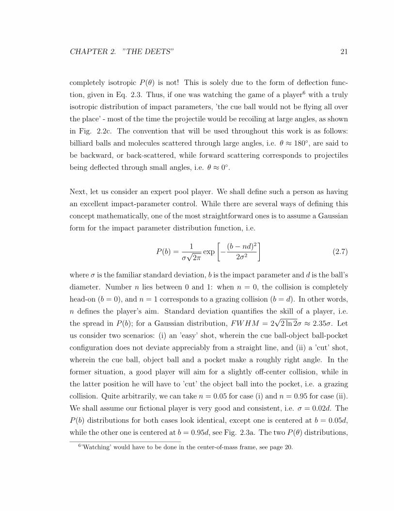
Next, let us consider an expert pool player. We shall define such a person as having
an excellent impact-parameter control. While there are several ways of defining this
concept mathematically, one of the most straightforward ones is to assume a Gaussian
form for the impact parameter distribution function, i.e.
P (b) =1
σ√2π
exp
[
−(b− nd)22σ2
]
(2.7)
where σ is the familiar standard deviation, b is the impact parameter and d is the ball’s
diameter. Number n lies between 0 and 1: when n = 0, the collision is completely
head-on (b = 0), and n = 1 corresponds to a grazing collision (b = d). In other words,
n defines the player’s aim. Standard deviation quantifies the skill of a player, i.e.
the spread in P (b); for a Gaussian distribution, FWHM = 2√2 ln 2σ ≈ 2.35σ. Let
us consider two scenarios: (i) an ’easy’ shot, wherein the cue ball-object ball-pocket
configuration does not deviate appreciably from a straight line, and (ii) a ’cut’ shot,
wherein the cue ball, object ball and a pocket make a roughly right angle. In the
former situation, a good player will aim for a slightly off-center collision, while in
the latter position he will have to ’cut’ the object ball into the pocket, i.e. a grazing
collision. Quite arbitrarily, we can take n = 0.05 for case (i) and n = 0.95 for case (ii).
We shall assume our fictional player is very good and consistent, i.e. σ = 0.02d. The
P (b) distributions for both cases look identical, except one is centered at b = 0.05d,
while the other one is centered at b = 0.95d, see Fig. 2.3a. The two P (θ) distributions,
6’Watching’ would have to be done in the center-of-mass frame, see page 20.

CHAPTER 2. ”THE DEETS” 22
on the other hand, look rather different! By using Eq. 2.4 it is easy to show that the
angular distribution has the following form:
P (θ) =1
σ′√2π
exp
[
−(cos(
θ2
)
− n)22σ′2
]
· sin(
θ
2
)
(2.8)
where σ′ = σ/d. The P (θ) functions with n = 0.05 and n = 0.95 are plotted in
Fig. 2.3b. The FWHM of P (θ)n=0.95 is greater than the width of the P (θ)n=0.05
function, even though FWHM [P (b)n=0.95] = FWHM [P (b)n=0.05]! Two conclusions
can be drawn from this. First, this is a mathematical explanation of why ’cut’ or
’slice’ shots in pool are so much harder than the head-on shots. This is something
anyone, who has played the game, knows intuitively. Another conclusion can be po-
tentially more far-reaching. Although the intermolecular potential between molecules
is not exactly hard-sphere like, especially the attractive part of a potential, at short
internuclear separations atoms do repel one another. Thus, given a scattering system
that interacts through a spherically symmetric potential, which exhibits only shallow
wells, provided the dynamics is to a large degree classical, i.e. quantum effects are
minimal, then the backward peak should be somewhat narrower than the forward one.
An astute pool player may be surprised by the fact that angular distributions in
Figs. 2.2 and 2.3 span a 0−180 range. It seems like the cue ball can either undergo
a grazing collision, b → d and θ → 0, or collide with an object ball in an almost
head-on fashion, b→ 0, in which case the cue ball will be scattered through θ ≈ 90.
In other words, the ’observed’ range of a cue ball scattering angle is 0− 90. This is
because the above discussion of angular distributions referred to the center-of-mass
(COM) coordinate system. This is the reference frame in which the total linear mo-
mentum of the system is zero. Measurements and observations are carried out in a
laboratory (LAB) frame. LAB frames may vary from one experimental setup to an-
other, while the COM system is unique. This is the reason why scattering dynamics,
for example, are often discussed in the COM coordinate system. One therefore needs
to perform a LAB → COM coordinate transformation. Billiard ball collisions in the
LAB and COM reference frames are pictured in Fig. 2.4. It is not difficult to show,

CHAPTER 2. ”THE DEETS” 23
Figure 2.3: (a) Gaussian impact parameter probability distribution functions P (b)for head on, b/d = 0.05, and glancing, b/d = 0.95, collisions between two billiardballs, and (b) the resulting angular distribution functions. Even though the twoimpact parameter distribution functions have the same width, P (θ) distributions forhead-on and glancing collisions have different widths.

CHAPTER 2. ”THE DEETS” 24
Figure 2.4: Collision between two particles in (a) the LAB frame and (b) the COMframe. In the LAB frame p0 = p1 + p2; in the COM frame p0 − p0 = p1 − p1 = 0.

CHAPTER 2. ”THE DEETS” 25
that, in the case of two billiard balls with equal masses, the scattering angle θ in
COM and ϑ in LAB reference frames are related by [27]
ϑ =θ
2(2.9)
It is clear from the above that 0 ≤ θ ≤ 180 in a COM frame, and 0 ≤ ϑ ≤ 90 in
a LAB coordinate system. Angular distributions in the two frames are related by7
P (ϑ)LAB = 4 cos
(
θ
2
)
P (θ)COM (2.10)
Angular distributions in a COM frame for isotropic P (b) (Fig. 2.2c) and Gaussian
P (b) (Fig. 2.3b) can be easily converted to P (ϑ); results are shown in Fig. 2.5.
Up to this point we were careful to call P (θ) as angular distribution functions, and
not DCS. The latter is defined as a ratio of the number of particles, N , scattered into
a solid angle element dΩ, over the incident flux of particles j, i.e.
dσ
dΩ≡ N
j(2.11)
Classically, the number of particles scattered into a solid element dΩ is equal to
the number of particles incident in a particular impact parameter range db, i.e.
2π sin θdθN = 2πbdbj. Rearranging, and substituting into Eq. 2.11 yields
dσ
dΩ=
b
sin θ
∣
∣
∣
db
dθ
∣
∣
∣(2.12)
7If the masses m1 and m2 of the two colliding bodies are unequal, the relationship between θ andϑ is given by
tanϑ =sin(θ)
cos(θ) +m1/m2
and the relationship between angular distributions in COM and LAB frames is
P (ϑ)LAB =
(
1 + (m1/m2)2 + 2(m1/m2) cos(θ)
)3/2
1 + (m1/m2) cos(θ)P (θ)COM
The latter simplifies to Eq. (2.10) when m1 = m2.

CHAPTER 2. ”THE DEETS” 26
Figure 2.5: Angular probability distribution functions P (ϑ)LAB in the LAB frame for(a) P (θ)COM from Fig. 2.2c and (b) P (θ)COM from Fig. 2.3b.

CHAPTER 2. ”THE DEETS” 27
This is the most general expression for a DCS for the case of a centrally symmetric
potential. The difficulty in computing explicit expressions for DCS is often the lack
of analytic forms of the deflection function and, consequently, the∣
∣
∣
dbdθ
∣
∣
∣term. Hard
sphere potential is easy; the∣
∣
∣
dbdθ
∣
∣
∣term is given by Eq. 2.5. Plugging it into Eq. 2.12
and simplifying yields a DCS for hard sphere scattering, i.e.
dσ
dΩ=d2
4(2.13)
The DCS is isotropic. This may seem puzzling at first, bearing in mind the preceding
discussion on angular distributions in pool, see Eq. 2.4. Two important differences
exist between a DCS and angular distributions in pool. First, the DCS is defined
in such a way that the impact parameter distribution function does not appear in
Eq. 2.11. This is reasonable because in molecular collisions P (b) itself is a dynamic
quantity. Calculation of P (θ) and P (b) are equally difficult in molecular collisions.
In pool, on the other hand, P (b) is of a different character altogether - it is set by
the player, and can be viewed as an initial condition of a problem. Second, pool is an
example of a two dimensional scattering. Equations 2.11 and 2.12, however, pertain
to three dimensional scattering. The derivation of an expression for a DCS in two
dimensions is identical to that in three dimensions, i.e. DCS is still given by Eq. 2.11.
In two dimensions, however, one as dθN = dbj. Rearranging this and substituting
N/j into Eq. 2.11 gives
dσ
dΩ
(2D)
=∣
∣
∣
db
dθ
∣
∣
∣(2.14)
It is obvious, by using the expression for∣
∣
∣
dbdθ
∣
∣
∣in Eq. 2.5, that hard sphere scattering
in two dimensions is not isotropic! As it turns out, DCS for hard sphere scattering
in four dimensions is also anisotropic. It seems therefore that three dimensions is a
special case, wherein hard sphere scattering is isotropic. A fact that is almost never
mentioned in scattering textbooks.
This then serves as a ’Dummy’s guide to angular distributions’. In molecular re-
ality, true hard sphere potentials do not exist. In addition, potentials, for which Eq.

CHAPTER 2. ”THE DEETS” 28
2.1 can be solved analytically are very few (see p.17). When more chemically inter-
esting systems are considered, e.g. atom-molecule and molecule-molecule collisions,
potentials are not spherically symmetric and have angular dependence. Equation 2.1
in that case is not valid. Consequently, deflection functions do not have closed form
analytic expressions, and Eq. 2.12 cannot be used to straightforwardly calculate a
DCS. Finally, all of the above was analyzed within the classical mechanics framework
- quantum treatment of scattering phenomenon is even more complex.
2.2 Measuring Angles
While it is rather trivial to measure the deflection angle of a cue ball in the game of
pool, it is difficult to do so when the colliding bodies are molecules. The intuitively
most obvious way, and historically the first method implemented, to measure DCSs
in molecular scattering is the so-called crossed beam technique pioneered by Dudley
Herschbach and Y. T. Lee [28, 29]. The so-called Photoloc (Photoinitiated reaction
analyzed by the law of cosines) method of measuring DCSs was developed by Zare
and co-workers [30], and was the weapon of choice for experiments described herein.
The main ’collision drama actors’ are discussed by means of a comparison between a
crossed-beam and a single-beam experiment.
The details of what follows next can be found in any book on classical mechan-
ics; Goldstein is a good reference [25]. To make things concrete, H + D2 collision is
considered. The main goal of molecular scattering is to understand the dynamics in
the COM frame. Measurements however are carried out in the LAB frame; see Fig.
2.4. The fact that laboratory measurements depend on a particular experimental set-
up while COM quantities do not, is evidenced by Fig. 2.6.: even though the D2 LAB
velocities in crossed-beam and single-beam experiments are very different, i.e. vD2=
0 m/s in a single-beam set-up, the COM velocities of D2 are the same. To relate LAB
and COM vectors of interest, one defines the COM velocity, given by (blue vector in
Fig. 2.6)
uCOM =mHvH +mD2
vD2
mH +mD2
(2.15)

CHAPTER 2. ”THE DEETS” 29
Figure 2.6: Illustrative comparison of the H + D2 → HD + D reaction in (a) crossed-beam and (b) single-beam experiment. LAB velocity vectors are black, COM vectorsare green, with the corresponding green Newton sphere, the COM velocity vector isblue, and the relative velocity vectors are red. The main difference between a single-beam and a crossed-beam set up is that often one of the particles, in this case D2,has roughly zero LAB velocity in a single-beam experiment. Angles θ and Θ arescattering angles in the COM and LAB frames, respectively.

CHAPTER 2. ”THE DEETS” 30
Another key quantity when considering a collision between a hydrogen atom and a
deuterium molecule is the relative velocity vector (red vector in Fig. 2.6)
vrelative = vH − vD2(2.16)
In the absence of external fields, the COM motion is said to be conserved. In other
words, the COM and relative motions are separable. (Other relationships between
the LAB and COM velocities of reactants and products are pictorially illustrated in
Fig. 2.6.) Kinetic energy associated with the relative reactant motion is given by
Ecoll ≡ Erelative =1
2µv2relative (2.17)
where µ =mHmD2
mH+mD2
. The collision energy, Ecoll is the maximum amount of energy that
is available to reactants.8 For the H + D2 → HD(v′, j′) + D reaction, Ecoll dictates
the maximum amount of internal energy that can appear as internal excitation of
HD(v′, j′), i.e. Eint ≤ (Ecoll + ∆D0), where ∆D0 is the bond dissociation energy
difference between the reactants and products, small in the case of D2 and HD. The
complete total energy conservation relationship is
Ecoll + Eint +∆D0 =1
2µ′v′2relative + E ′
int (2.18)
where µ′ = mHDmD
mHD+mD, v′2relative is the product relative recoil velocity, and E ′
int is the
product internal energy. The Eint term accounts for any internal excitation of the
reactants.
Given the above, how does one measure the scattering angle θ (or, in the case of
a crossed-beam experiment, Θ that can later be manipulated to yield θ)? There is
a variety of methods of doing this [31]. One of the ways employed in this work is to
convert an angle-measuring problem into a speed-measuring one. Consider a triangle
spanned by three vectors: uCOM , uHD and vHD (Fig. 2.6). The magnitude of the
8In addition to total energy conservation, total angular momentum conservation may put furtherlimits on how much energy goes into product internal excitation.

CHAPTER 2. ”THE DEETS” 31
uCOM vector is known from Eq. 2.15; the magnitude of the uHD vector can be cal-
culated from the energy conservation relation, Eq. 2.18. Thus, if one measures the
magnitude of the third vector, vHD, the triangle is complete and one can calculate the
scattering angle θ. (In the case of a crossed-beam experiment, often the laboratory
scattering angle Θ is measured first that is then converted into θ.)
Focusing our attention now on a single-beam Photoloc technique, we can derive the
expression for the magnitudes of uCOM and uHD. A typical experimental protocol
followed is as follows:
HX + hf → H+ X/X∗ (2.19)
H + D2 → HD(v′, j′) + D (2.20)
HD(v′, j′) + 3hf → HD+ + e− (2.21)
In here hf denotes a photon, X = Br or I, and X∗ denotes a spin-orbit excited halogen,
i.e. X(2P1/2). (We shall discuss the ionization step, Eq. 2.21, later.) Assuming vD2≈
0 m/s, it follows readily from Eq. 2.15 that
|uCOM | =mH
mH +mD2
√
2EH
mH
(2.22)
where EH = mX
mH+mX(hf − D0(HX)), which follows directly from linear momentum
conservation in the photodissociation of HX. Thus, for a particular reaction, |uCOM |is determined solely by the laser wavelength.
The magnitude of |uHD| is readily obtained from the conservation of total energy,
Eq. 2.18, by using the fact that uHD = − mD
mHD+mDv′rel. Thus, rearranging Eq. 2.18 to
yield |v′rel|,
|uHD| =mD
mHD +mD
√
2(Eint + Ecoll − E ′int −∆D0)
µ′(2.23)
The magnitude of the uHD vector again depends on the laser wavelength used to
photodissociate the HX precursor as well as the internal state of the HD(v′, j′) product

CHAPTER 2. ”THE DEETS” 32
via the E ′int term. Experimental measurement of the |vHD| term completes the triangle
in Fig. 2.6b, and the scattering angle can be obtained via the law of cosines, i.e.
cos θ =|vHD|2 − |uCOM |2 − |uHD|2
2|uCOM ||uHD|(2.24)
In other words, measurement of a distribution of |vHD| can be converted to a distri-
bution of cos θ, or θ - the desired DCS. The more in-depth derivation of Eqs. 2.22
and 2.23 can be found elsewhere [30, 32].
It is worthwhile pointing out a key difference between crossed- and single-beam ex-
periments. The former set-up has well defined reactant LAB velocities, vH and vD2,
as well the COM and relative velocity vectors, see Fig. 2.6a. Consequently, one can
place a detector at a particular spot in the LAB frame and detect products scat-
tered only through a certain angle θ. Single-beam studies of H + D2 → HD(v′, j′)
+ D reaction that often begin with a single photon photodissociation step of an HX
molecule do not have a well defined vH. For a linearly polarized photon, the angular
distribution, or anisotropy, of H atoms in the LAB frame is given by the celebrated
[33]
f(χ) =1
4π(1 + βP2(cosχ)) (2.25)
Here cosχ = vH · ǫ where ǫ is the electric field unit vector of the photodissociating
laser, and P2(cosχ) = 12(3 cos2 χ − 1). As hinted in Eq. 2.19, one photon pho-
todissociation of HX occurs via two channels, at least in the ∼ 200 nm to ∼ 250 nm
wavelength range of experimental relevance. The two photodissociation channels have
different symmetries - the so-called parallel transition, corresponding to the formation
of X(2P1/2), is characterized by β = 2, and the perpendicular transition leading to
X(2P3/2) has β = −1. The important point is that the photodissociation of HX leads
to a distribution of vH velocity vectors in the LAB frame. This, in turn, leads to a
distribution of uCOM and vrel vectors, see Fig. 2.6b. The distribution of these three
vectors is proportional to P2(cosχ). Therefore, a particular direction in the LAB
frame does not correspond to a particular scattering angle θ of the HD product - in
a stark contrast to the crossed-beam set-up. A single-beam Photoloc experiment can

CHAPTER 2. ”THE DEETS” 33
be viewed as ’many’ crossed-beams.
Equations 2.22 - 2.24 are the key formulae in a Photoloc experiment. The last piece
of information needed to complete the uCOM − uHD − vHD triangle in Fig. 2.6 is the
|vHD| - the speed of a reaction product in the LAB frame. Please note that only
the magnitude, and not the direction of the vHD vector is required. Experimental
measurement of molecular speeds in the LAB frame will be discussed shortly, but let
us imagine for now that the P (|vHD|) measurement - speed distribution in the LAB
frame - has been made. Following our Section 2.1 discussion, we would like to relate
two probability distributions, i.e. P (|vHD|) and P (θ) or P (cos θ). In analogy with
Eq. 2.4,
P (cos θ) = P (|vHD|) ·∣
∣
∣
d|vHD|d cos θ
∣
∣
∣(2.26)
P (θ) = P (|vHD|) ·∣
∣
∣
d|vHD|dθ
∣
∣
∣(2.27)
The∣
∣
∣
d|vHD|d cos θ
∣
∣
∣and
∣
∣
∣
d|vHD|dθ
∣
∣
∣terms are easily obtainable from Eq. 2.24, i.e.
P (cos θ) = P (|vHD|) ·|uHD||uCOM ||vHD|
(2.28)
P (θ) = P (|vHD|) ·|uHD||uCOM | sin θ
|vHD|(2.29)
Although cos θ is said to be the ’natural’ variable of a Photoloc experiment, whilst
P (θ) is more often reported in crossed-beam studies, Eq. 2.29 has been employed to
plot the DCSs in this work. The only difference between P (cos θ) vs. cos θ and P (θ)
vs. θ plots is an additional inverse cosine operation in going from cos θ to θ. Most
often it is an innocuous procedure. One must however be aware of certain artifacts
introduced by the transformation. An important example is the uncertainty in the
measurement of |vHD|, and how the error is propagated into the uncertainty in θ.
Suppose there is an experimental uncertainty ∆|vHD| associated with a measurement
of |vHD|. Using the familiar ∆z =
√
(
∂z∂x∆x
)2+(
∂z∂y∆y
)2
+ ... for calculating an error
in the quantity z as a result of uncertainties ∆x and ∆y associated with quantities x

CHAPTER 2. ”THE DEETS” 34
and y, yields
∆(cos θ) =|vHD|
|uHD||uCOM |∆|vHD| (2.30)
∆θ =2|vHD|
√
4|uCOM |2|uHD|2 −(
|uCOM |2 + |uHD|2 − |vHD|2)2∆|vHD| (2.31)
Hence, the uncertainty in ∆(cos θ) increases linearly with |vHD|, whereas the expres-sion in Eq. 2.31 is singular when 9
|vHD| = |uCOM | ± |uHD| (2.32)
The singularity in Eq. 2.31 at θ = 0 and 180 is in a way artificial, as it is due
to the inverse cosine operation. Consequently, for θ angles close to 0 and 180 the
uncertainty will be large; for θ ≈ 90 the uncertainty will be at its smallest. This can
be seen by substituting the expression for |vHD| in terms of cos θ and θ, as given by
Eq. 2.24, into Eqs. 2.30 and 2.31, respectively:
∆(cos θ) =
√
|uCOM |2 + |uHD|2 + 2|uCOM ||uHD| cos θ|uHD||uCOM |
∆|vHD| (2.33)
∆θ =
√
|uCOM |2 + |uHD|2 + 2|uCOM ||uHD| cos θ|uCOM ||uHD| sin θ
∆|vHD| (2.34)
∆(cos θ) vs. cos θ and ∆θ vs. θ are plotted in Fig. 2.7, using |uCOM | = 4000
m/s, |uHD| = 2000 m/s and ∆|vHD| = 200 m/s, typical experimental values. The
singularity of Eq. 2.34 at θ = 0 and 180 is apparent, both from Fig. 2.7 and
9This is not true in the special case when |uCOM | = |uHD|. Equation 2.31 is still singular when|vHD| = |uCOM | + |uHD|, but when |vHD| = |uCOM | − |uHD| = 0, then Eq. 2.31 is of the 0/0indeterminate form. It can be easily shown that the limit exists and is given by
∆θ =1
|uCOM |∆|vHD|
This is in fact the global minimum of the ∆θ function in Eq. 2.31. Hence, for very special caseswhen |uCOM | = |uHD|, experimental points in the backward direction, i.e. θ ≈ 180, will have thelowest possible uncertainty in ∆θ.

CHAPTER 2. ”THE DEETS” 35
Eq. 2.34.10 The insets of Fig. 2.7 show a portion (−0.6 ≤ cos θ ≤ 0.6 for Fig.
2.7a and 60 ≤ θ ≤ 160 for Fig. 2.7b) of the original graph. These have been
replotted on different ordinate axes, so the uncertainty in ∆(cos θ) and ∆θ could be
compared on an equal footing. The normalized ordinate has been obtained by dividing
∆(cos θ) and ∆θ values by the range of abscissa, i.e. (cos θ)range = 1− (−1) = 2 and
θrange = 180 − 0 = 180. Even though ∆θ is large for very forward and very
backward direction, θ < 60 and θ > 160, respectively, ∆θ in the 60 ≤ θ ≤ 160
range is, on average, smaller than ∆(cos θ) in the similar region, see insets. Provided
that most of the features in a DCS are located in this sideways 60 ≤ θ ≤ 160 region,
then plotting DCS in the P (θ) vs. θ form is quite adequate.
2.3 Measuring Speed
As is obvious from Eqs. 2.24, 2.28 and 2.29, the only unknown in these expressions
is the laboratory speed of HD reaction product, |vHD|. The previous paragraph out-
lined how angular information can be obtained once |vHD| is known. The speed of a
molecule is therefore a key quantity measured experimentally.
Products of reactions studied here are all neutral. Perhaps the most widely spread
method of ’seeing’ neutral molecules is parent ionization with the subsequent mass-
spectrometric ion detection, Eq. 2.21. More specifically, ions were formed in the
extraction region of a Wiley-MacLaren time-of-flight (TOF) mass spectrometer, and
accelerated toward a position sensitive delay-line detector, see Fig. 2.8. The main
idea behind the delay-line is as follows. When an ion hits the stack of two microchan-
nel plates (MCP), an electron avalanche impinges on the delay-line, consisting, to
a first approximation, of two perpendicularly-wound copper wires. The signal then
starts traveling to the two ends of a wire, and the signal arrival times are measured, t1
and t2, respectively. As can be seen intuitively, the arrival time difference is directly
10Note that when |uCOM | = |uHD|, Eq. 2.34 tends to the same finite limit as equation in footnote9 (p34) for |vHD| = |uCOM | − |uHD| = 0. This can be shown by using the
√1 + cosx =
√2 cos
(
x2
)
identity.

CHAPTER 2. ”THE DEETS” 36
Figure 2.7: Uncertainty functions for (a) P (cos θ), Eq. 2.33, and (b) P (θ), Eq. 2.34,distributions. The insets are replotted on a reduced scale, where the original ordinatehas been divided by the range of the abscissa. The reduced plots can be comparedto each other. Even though ∆θ function is large when θ → 0 and 180, ∆θ is, onaverage, smaller than ∆(cos θ) in a similar angular space region shown in the insets.

CHAPTER 2. ”THE DEETS” 37
Figure 2.8: Schematic of the experimental set up: Wiley-MacLaren TOF mass spec-trometer consists of extraction and acceleration regions. Usually, Vext = −15V, andVacc = −60V. Typically tTOF is several microseconds for ions with m/z = 1 − 4.MCP is normally held at −2450V, while the delay line is held at +460V.

CHAPTER 2. ”THE DEETS” 38
proportional to the position where electrons (and, indirectly, ion) hit the wire. If
t1 = t2, then the signal originated in the middle of a wire. The two x and y wires will
in combination provide information about the x and y position of an ion, i.e.
x = cx(tx1 − tx2) (2.35)
y = cy(ty1 − ty2) (2.36)
where cx and cy are experimentally determined proportionality constants. Finally,
because there are no fields in the x and y directions, ions experience a free motion in
these directions. Therefore, the measured ion positions x and y are directly propor-
tional to its velocity component in x and y directions, respectively. More precisely,
the duration of the ’free’ motion in x and y directions is dictated by tTOF , i.e. time
interval between the ion creation and its detection, in other words
Vx =cx(tx1 − tx2)
tTOF
(2.37)
Vy =cy(ty1 − ty2)
tTOF
(2.38)
In reality, things are a little bit more complicated, as the delay-line has four, not two
copper wires. The two additional ones serve as reference wires to provide differential
signal reading. The above description of time and position encoding is not altered.
The remaining Vz velocity component of an ion is obtained from tTOF , i.e.
Vz =qEext(tTOF − t0TOF )
m(2.39)
where q is ion’s charge, m its mass, and Eext is the electric field between the grounded
plate and the plate held at Vext, see Figure 2.8. In here, tTOF is the ion’s under
consideration arrival time, and t0TOF is the arrival time of an ion that has Vz = 0 m/s.
The speed of a molecular ion in the LAB frame is simply
|vLAB| =√
V 2x + V 2
y + V 2z (2.40)

CHAPTER 2. ”THE DEETS” 39
Experimental measurement of vLAB has a few inherent uncertainties associated with
it. First, the ionizing laser has a finite volume. This leads to some blurring, but it is a
minor source of error. A more fundamental limitation is the electron recoil imparted
to a molecule, particularly to a light H2 species. Let us consider the ionization scheme
of H2/HD/D2 used in this study.
2.4 Detection of H2
Molecular hydrogen is without a doubt one of the most difficult molecules to study
spectroscopically. A molecule must absorb a photon if it is to be studied by laser-
induced fluorescence (LIF) [34], or by any form of ionization. A homonuclear molecule
does not have a ro-vibrational spectrum via electric dipole transitions. Electric
quadrupole transitions are allowed, but are forbiddingly weak to be useful in the
detection of low number-density reaction products.11 One photon electronic transi-
tions in H2 are allowed, but unfavorable: the lowest electronic level is found 11.4 eV
above the ground state, and requires a 109 nm photon, see Figure 2.9. Generation of
tunable, intense laser beams with wavelengths shorter than 198 nm is cumbersome in
a laboratory. An additional difficulty associated with homonuclear molecules is the
fact that odd number of photons connect g and u states, whereas an even number of
photons induce g ↔ g and u ↔ u transitions. Thus, a one-photon transition from
the ground X1Σ+g state to any gerade state is forbidden.12 The manner in which
an electronically excited state is reached is of crucial importance. For example, the
number of photons used to connect the ground and excited states, as well as photon
polarization influence an electronic absorption spectrum considerably. These so-called
multiphoton processes in atoms and molecules are a painfully complicated area of re-
search in itself, and only a minute glimpse, most pertinent to the detection of H2, will
be given here.
11Electric quadrupole transitions in H2 are routinely observed in the outer space, where lightpropagates through long distances [36]. Equivalently, cavity ring-down spectroscopy can be employedto observe these exceedingly weak transitions [37].
12Note that g and u electronic energy level labeling applies also to HD, even though it is nota homonuclear molecule. This is because the electronic wavefunction, at least within the Born-Oppenheimer approximation, is the same for all molecular hydrogen isotopes.

CHAPTER 2. ”THE DEETS” 40
Figure 2.9: Excited potential energy surfaces of H2. Left panel shows states of gsymmetry; these can only be accessed by an even number of photons. Panel on theright shows states of u symmetry; these can only be accessed by an odd number ofphotons. In the current study H2 was ionized by [2+1] REMPI, where the first twophotons resonantly connect a single rovibrational level in the ground X 1Σ+
g electronicstate to a single rovibrational level in the E,F 1Σ+
g state. The third photon takesthe system into the H+
2 ionic manifold.

CHAPTER 2. ”THE DEETS” 41
First, let us consider qualitatively the absorption of one versus two photons. One-
photon process has a greater cross section than the two-photon absorption. The
figure of merit, however, is the rate at which excited molecules are produced. The
key question is then, ’At what laser intensities do one- and two-photon absorption
rates become comparable?’. One- and two-photon absorption rates are proportional
to σ1I and σ2I2, respectively, where σ1 and σ2 are one- and two-photon absorption
cross sections13, and I is the laser intensity in photons per cm2 per s. An actual value
of a cross section depends of course on a system of interest, and ultimately transition
dipole matrix elements are required to compute σ. There are however several rules
of thumb.14 A resonant one-photon absorption cross section to the B 1Σ+u state in
H2 is on the order of 10−18 cm2 [85]. A resonant two-photon absorption cross sec-
tion to the E,F 1Σ+g state in H2 is about 10−36 cm2 [43].15 When the two rates are
comparable, i.e. σ1I ∼ σ2I2, then I ∼ σ1/σ2 ∼ 1018 photons/cm2· s. Often a value
of 1020 photons/cm2· s is quoted as a threshold for the onset of nonlinear processes.
In the current experiments, nanosecond laser energies of 1 mJ in the 200−230 nm
wavelength range are routinely obtained, yielding about 1027 photons/cm2· s. From
13Please note the units: [σ1] = cm2, but [σ2] = cm4· s. In general, [σN ] = cm2N · sN−1. Strictlyspeaking, these units apply for a bound−free transition. When considering bound−bound transi-tions, the units become [σN ] = cm2N · sN−2, because the formula for the rate of absorption nowspecifies intensity in terms of the number of photons per unit area per unit time per unit bandwidth[40]. We shall ignore the more rigorous formula in this primer on multiphoton processes.
14Another footnote. In the case of N−photon ionization of alkali atoms, i.e. a bound-free transi-tion, σN values are well separated for different N , e.g. σ2 ∼ 10−49±2, σ3 ∼ 10−78±4, σ4 ∼ 10−107±4,σ5 ∼ 10−138±4 [41]. It is immediately obvious, for example, that a non-resonant three photon ion-ization has a cross section many orders of magnitude lower than the corresponding process whereintwo photons are in resonance with an intermediate state and the third photon removes the electron.
15The σ = 10−36 cm4· s value is again far from set in stone. Some authors report a value ofσ = 10−33 cm4· s [85]. Lambropoulos discusses at length such discrepancies [41]. It is worth notinghow Buck et al. went about extracting the two-photon cross section. They used the theoreticalexpression for the number of electronically excited H2 species, see formula 16 of [85], and theningeniously estimated this number by the use of
NH∗
2≈ Φτ/Vlaser
where NH∗
2is the number density of electronically excited H2, Φ is the photon flux, τ is the estimated
lifetime of an excited E,F state, and Vlaser is the laser volume. Using this value in their Eq. 16they were then able to extract the value for a two-photon absorption cross section.

CHAPTER 2. ”THE DEETS” 42
an experimental point of view, intensities for ∼100 nm coherent light are usually
much lower than those corresponding to λ > 200 nm. For example, conversion effi-
ciencies of 10−6 are rather easily achievable when the harmonic generation is carried
out in a supersonic jet. More work is needed to get conversion efficiencies of 10−3 and
more, like colling a gas cell containing a mixture of noble gases in liquid nitrogen.
Qualitatively, the rate of one-photon excitation may become lower than a two-photon
transition rate induced by a laser of greater intensity.
Ultimately one needs to consider the full expression for the rate of excitation. Let us
follow our example of H2(v′, j′) reaction product in a particular rovibrational state of
the ground electronic level. The task is then to ionize the molecule so we can ’see’ it.
One could imagine using one photon to (resonantly) excite H2(v′, j′) into the B 1Σ+
u
state, and then another photon to take the diatomic in the B 1Σ+u state above the
ionization limit. Similarly, one could use two photons two to (resonantly) excite H2
into the E,F 1Σ+g state, and then ionize it with the third photon. The first scenario
would be called a [1+1] resonance-enhanced multiphoton ionization (REMPI) and
the second one would be [2+1] REMPI. To simplify things quite a bit, let us imagine
that the ionization step is saturated.16 In other words, the limiting step in both cases
is the resonant excitation. Such a three level system (ground, excited and ionized),
and the resulting three differential equations can be solved exactly to give NH+2, the
number density of H+2 ions per cm3,17
NH+2(∆t) = σ1NH2(v′,j′)I1∆t (2.41)
16A good assumption in the case of a [2+1] REMPI, but a dubious one for [1+1] REMPI, wherelaser intensities are on the order of 109 photons/cm2· s. Let us assume then a [1+1′] REMPI, wherethe ionization photon is supplied by another laser with a much greater intensity, as was done by Y.T. Lee and co-workers in their study of [1+1′] REMPI of H2 via C 1Π+
u state [44].17Both [1+1] and [2+1] REMPI are an example of a three-level system. The three differential rate
equations can be solved to give, in the case of a [1+1] REMPI
NH+
2
(t) = σ1NH2(v′,j′)I1
(1− e(−σionIiont)
σionIion− 1− e(−σ1I1t)
σ1I1
)
where σion is the ionization cross section and Iion is the ionizing laser intensity. Because Iion ≫ I1,the above equation simplifies to Eq. 2.41. Equation 2.42 is obtained in an analogous manner.

CHAPTER 2. ”THE DEETS” 43
NH+2(∆t) = σ2NH2(v′,j′)I
22∆t (2.42)
where NH2(v′,j′) is the number density of molecules in a particular rovibrational state
of ground electronic level, I1 and I2 are one- and two-photon laser intensities, and ∆t
is the duration of a laser pulse, which could be conveniently taken as ∼ 10 ns in the
present study. Equations 2.41 and 2.42 tell us how many H+2 ions will be produced
per single laser shot of duration ∆t. By knowing a particular experiment’s signal-
to-noise (S/N) ratio, one can estimate NH2(v′,j′), the minimum amount of H2(v′, j′)
molecules that can be detected. Before proceeding to discuss the sensitivity of [1+1]
and [2+1] REMPI of H2, it should be noted that Eq. 2.42 is not entirely correct. It
was assumed that the signal has a quadratic dependence on the laser intensity. Often
this is only realized at very low I2 values. In current experiments, for example, it
was found that NH+2∝ I1.52 . Assuming I2 = 1 mJ, I1 = 100 nJ (assuming a 10−5
conversion efficiency for a 10 mJ pump beam), σ1 = 10−18 cm2 and σ2 = 10−36 cm4·s, and assuming similar S/N ratios for both one- and two-photon detection schemes,
i.e. making Eqs. 2.41 and 2.42 equal, yields
NTPH2(v′,j′)
NOPH2(v′,j′)
∼ 0.01 (2.43)
where NTPH2(v′,j′)
and NOPH2(v′,j′)
are the minimum number of H2(v′, j′) molecules that
can be detected by [2+1] and [1+1] REMPI, respectively. This example, although
rather artificial, gives one a qualitative idea of how a two-photon process can be more
sensitive than the one-photon excitation scheme. In this case, a [2+1] REMPI is
about 100 times more sensitive than a [1+1] REMPI. The values should not be taken
too literally; instead, this is meant to give a future dynamicist an idea of how to think
about various ionization schemes, and useful figures of merit.
While it is useful to compare the efficiency of one- and two-photon absorption in
H2, it is also possible to go the other way, i.e. directly estimate NH2(v′,j′), use Eq.
2.42 to deduce an ion count rate, and see how it fares with the actual experimental
ion count rate. To simplify the notation, let us consider the H + D2 → HD(v′, j′) +

CHAPTER 2. ”THE DEETS” 44
D reaction; we are now interested in the number density of reaction product HD, and
Eq. 2.42 will be rewritten as
NHD+(∆t) = σ2NHD(v′,j′)Ix2∆t (2.44)
where x ≈ 1.5, but can be 1.5 < x < 3, in principle, and other notational changes
are self-explanatory. The key quantity in Eq. 2.44 is obviously NHD(v′,j′) - how many
product molecules in a particular rovibrational state are made? For a reaction be-
tween a hydrogen atom and a deuterium molecule NHD(v′,j′) is encoded in a differential
equationdNHD(v′,j′)
dt= σreacvrelNHND2
(2.45)
where σreac is the reaction cross section, vrel is the relative speed of a collision between
H and D2, and NH and ND2are reactant number densities. The number density of
D2 can be taken as ND2= 1013 cm−3, a reasonable value for a supersonic expansion
with a backing pressure of P = 1500 Torr, and a nozzle diameter of 0.76 mm [45].
Hydrogen atoms are generated via photolysis of HBr diatomic, where NHBr = 1011
cm−3, i.e. 1% seeding in D2. The rate of hydrogen atom production is then
dNH
dt= σphotoNHBrIphoto (2.46)
where σphoto = 10−20 cm2 is the HBr photodissociation cross section18, and Iphoto ≈ 1
mJ = 1027 photons/cm2· s. Equation 2.46 should be integrated with care if the HBr
population is significantly depleted. Assuming NHBr is roughly a constant,
NH(∆t) ≈ σphotoNHBrIphoto∆t (2.47)
Where ∆t = 10 ns is the laser pulse width. Upon substitution of numerical values in
Eq. 2.47 we arrive at NH(∆t) ≈ 1010 cm−3. Clearly, NH ∼ NHBr, so Eq. 2.46 should
18This is another approximation, because (i) σphoto is wavelength dependent, and (ii) estimatinga true photodissociation cross section is difficult. Total wavelength-dependent HBr absorption crosssection, σabs, is rather well known, but the fraction of molecules that then go on to photodissociateis not well known. For example, σabs ∼ 10−18 cm2 at λ = 200 nm [46]. We suppose here thatσphoto ∼ 0.01σabs, which assumes that photoionization and fluorescence in HBr are significant.
CHAPTER 2. ”THE DEETS” 45
be integrated more rigorously. Finally, assuming that the concentrations of H atoms
and D2 molecules do not change appreciably during a chemical reaction, Eq. 2.45 can
integrated to yield
NHD(v′,j′)(∆t) ≈ σreacvrelNHND2∆t (2.48)
Let us consider first the number of all HD products made during a reaction, i.e. es-
timate NHD(∑
v′ v′,∑
j′ j′). The total reaction cross at Ecoll = 1.97 eV is approximately
8.9 A2.19 The relative speed of a collision at Ecoll = 1.97eV is about 2·104 m/s. Sub-
stituting all these values into Eq. 2.48 yields NHD(∑
v′ v′,∑
j′ j′) ≈ 104 molecules/cm3.
Next, let us consider the lowest cross section reaction channel that has been measured
in this work, i.e. NHD(v′=4,j′=6). The calculated reaction cross section for this state is
σ(v′=4,j′=6) = 0.001 A2 at a collision energy of 1.97 eV. This gives NHD(v′=4,j′=6) ≈ 10
molecules/cm3. Assuming a laser beam diameter of 200 µm and an interaction length
of 1 cm (the size of a molecular beam), gives Vlaser ≈ 10−4 cm3. The number of
reaction products per laser volume per laser shot are truly mind-boggling:
NHD(∑
v′ v′,∑
j′ j′) ≈ 10 molecules (2.49)
NHD(v′=4,j′=6) ≈ 10−3 molecules (2.50)
Finally, substituting x ≈ 1.5 into Eq. 2.44, it is clear that the number density of HD+
is almost the same as the number density of a particular HD(v′, j′) product state. In
the case of HD(v′ = 4, j′ = 6) product, for a 10 Hz laser this amounts to just 36 ions
an hour! This is in a rather good agreement with the experimentally observed count
rate of 60−100 ions an hour for this particular state. This rough calculation serves
to illustrate the sensitivities needed to detect reaction products.
It seems therefore that in the absence of an intense synchrotron radiation the use
of at least two (resonant) photons to detect H2 reaction products has been historically
19We are considering a particular collision energy of 1.97 eV, because one of the lowest state-to-state cross sections has been measured at Ecoll = 1.97 eV; see text for details. The reactioncross section values are from theoretical calculations of Stuart Althorpe and Foudhil Bouakline.Theoretical methodology is discussed in later chapters.

CHAPTER 2. ”THE DEETS” 46
more practical. Coherent anti-Stokes Raman spectroscopy (CARS) has been used
to determine the ground electronic level rovibrational state populations by Valentini
and co-workers [35]. These studies are often performed in a gas cell, because the
technique is not sensitive enough to detect reaction products in a molecular beam
experiment. Zare pioneered the use of [2+1] REMPI of H2, most notably via the
X1Σ+g → E,F 1Σ+
g transition, to detect nascent reaction products in molecular beam
experiments [38, 39]. There are numerous other examples of state-selective detection
of H2 molecules, for example the aforementioned [1+1] REMPI via the B 1Σ+u state
[47], C 1Πu state [44, 47], [3+1] REMPI via the B 1Σ+u state [48], as well as [4+2]
REMPI via the E,F 1Σ+g state [49].
The above discussion on one- and two-photon absorption, and the associated sen-
sitivities barely scratches the ’spectroscopic surface’. For example, the [2+1] REMPI
detection scheme of H2 via the E,F 1Σ+g state is quite satisfactory for measuring
the population of a particular reaction product, in other words measuring a scalar
quantity, the X 1Σ+g → E,F 1Σ+
g transition via the Q(j′) branch members has almost
zero sensitivity to rotational angular momentum polarization of a reaction product
in the ground electronic level. In addition, O(j′) and S(j′), the only other allowed
rotational branches for a two-photon Σ→ Σ transition, are exceedingly weak, at least
100 times weaker than than corresponding Q(j′) transitions. On the other hand, one-
photon transitions via B 1Σ+u and C 1Πu states have relatively strong P (j′) and R(j′)
branches. Thus, if more intense coherent light with λ ∼ 100 nm was available, then
[1+1] REMPI schemes could provide dynamic information on H2 reaction products
that the well-established [2+1] E,F 1Σ+g ionization cannot provide. In this respect,
[1+1] and [2+1] interrogation methods of H2 should be viewed as complimentary to
each.
Finally, as mentioned in Section 2.4, the key quantity measured experimentally is
the speed of an ion. The laboratory ion speed distribution is assumed to mirror the
neutral reaction product speed distribution, but this is an approximation. Molecular
H+2 , HD
+ or D+2 ion is imparted a certain recoil velocity by the departing electron.

CHAPTER 2. ”THE DEETS” 47
This recoil distorts the original neutral product velocity. Using HD as an example, it
is trivial to show that the recoil speed is given by
vrecoilHD+ =
√
2(
3hf − IP + E ′int
)
mHD+(1 +mHD+/me)(2.51)
where IP = 15.44 eV is the ionization potential of HD, E ′int is the internal energy
of HD with respect to zero-point energy, and me is the electron mass. For 200 nm
< λ < 230 nm, vrecoilHD+ ∼ 200 m/s.20 This is the origin of ∆|vHD| in Section 2.2.
2.5 Typical Day in the Lab
This section is meant to illustrate the sequence of laboratory events on a typical data
gathering day, as well as show a few representative sets of raw data. For convenience,
let us consider an H + D2 → HD(v′, j′) + D experiment. The experimental set-up
is shown in Fig. 2.10. Experiments that employ only one UV laser beam are often
started as follows. A gaseous mixture of ∼1% HBr in D2 is introduced into the high
vacuum chamber via a supersonic nozzle. The skimmed molecular beam is inter-
sected by a laser beam, the wavelength of which is tuned to a specific [2+1] REMPI
transition of the HD(v′, j′) product. Within the ∆t ≈ 8 ns laser pulse, some of the
HBr molecules are photodissociated by the UV pulse, and the resulting fast hydrogen
atoms go on to collide with D2 molecules to produce HD. Next, a particular HD(v′, j′)
product of interest is ionized via a [2+1] REMPI, the ions are accelerated in a Wiley-
MacLaren TOF, and are detected on a position-sensitive detector. Please note that
in the so-called ’one laser experiment’, a single laser pulse photolytically produces
H atoms and detects the resultant HD(v′, j′) products. Measurement of the arrival
time of each ion, and its position in the x− y plane of the detector (see Section 2.3)
results in a three dimensional velocity sphere. Representative ion images, obtained
20The reason the recoil speed does not vary that much is because the photon frequency and theinternal energy of HD in Eq. 2.51 are related: more internally excited HD(v′, j′) molecules requirephotons of longer wavelengths for [2+1] REMPI.

CHAPTER 2. ”THE DEETS” 48
Figure 2.10: Experimental layout. NY2 - 2nd harmonic of Nd3+:YAG laser (532 nm),NY3 - 3rd harmonic of Nd3+:YAG laser (355 nm), DL - dye laser, BBO - nonlinearβ−barium borate crystal, L - lens, W - UV window, BS - beam splitter, DM - dichroicmirror, N - nozzle, D - detector, TDC - time-to-digital converter, PC - personalcomputer, S - oscilloscope, MIX - HX/D2 mixture.

CHAPTER 2. ”THE DEETS” 49
by scanning the laser wavelength over the Doppler profile of HD(v′, j′) product, typ-
ically ± 7 pm at ∼ 200−220 nm, are shown for H + D2 → HD(v′ = 0, j′ = 14) +
D reaction channel, Fig. 2.11, and for H + D2 → HD(v′ = 1, j′ = 3) + D, Fig.
2.12, both at Ecoll = 1.72 eV. Note how much bigger the HD(v′ = 0, j′ = 14) ion
sphere is compared to the HD(v′ = 1, j′ = 3) image. This immediately suggests
that the magnitude of laboratory HD(v′ = 0, j′ = 14) speed is greater than that of
HD(v′ = 1, j′ = 3) product. From Fig. 2.6b, large |vHD| corresponds to acute θ an-
gles, i.e. more sideways/forward scattering. Conversely, the small HD(v′ = 1, j′ = 3)
image size implies that |vHD| is small, i.e. θ is large, and HD(v′ = 1, j′ = 3) is
backward-scattered.21 One drawback of using one laser to photodissociate HBr and
detect HD products is the fact that background signal is not immediately subtracted.
Background arises primarily from non-resonant ionization of HD molecules. To prop-
erly subtract the background one must detune the laser wavelength off a REMPI
line, and perform an analogous laser wavelength scan, keeping all other parameters
(laser power, scan time etc.) identical to the ’online’ scan. ’Online’ and ’offline’ scans
for HD(v′ = 0, j′ = 14) and HD(v′ = 1, j′ = 3) states are shown in Fig. 2.13. As
predicted from ion images in Figs. 2.11 and 2.12, HD(v′ = 0, j′ = 14) is forward scat-
tered, whereas HD(v′ = 1, j′ = 3) is backward scattered, with respect to the initial
relative velocity (which is parallel to the hydrogen atom velocity, see Fig. 2.6b). The
origin of background is not completely clear, although, as mentioned earlier, it may
be due to a non-resonant ionization of reaction products.22 Note that the ’offline’
signal (black curve) in Fig. 2.13 cannot be due to HD impurities in the molecular
beam - molecular beam consisting of >95% D2 has a terminal speed of ∼ 1100 m/s,
and is in fact evident in Fig. 2.13b. Furthermore, if the background signal arises due
21The correlation between the most probable scattering angle and the rotational excitation ofHD(v′, j′) diatomic will be discussed in more detail in subsequent chapters.
22Looking at Fig. 2.13 it is clear that the background signal extends into ∼ 15000 m/s. The fastestreaction product corresponds to the H + D2 → HD(v′ = 0, j′ = 0) + D collision. At Ecoll = 1.72eV, the maximum allowed speed of HD(v′ = 0, j′ = 0) product in the laboratory frame is 10647 m/s- it is clear from Fig. 2.13a that the background signal extends beyond this maximum allowed value.(Background signal is smaller beyond 10647 m/s for the HD(v′ = 1, j′ = 3) reaction product, Fig.2.13b. Thus, the nature of the background signal remains unclear.

CHAPTER 2. ”THE DEETS” 50
Figure 2.11: HD(v′ = 0, j′ = 14) crushed ion images: (a), (c) and (e) are raw images,and (b), (d) and (f) are processed images with background removed.

CHAPTER 2. ”THE DEETS” 51
Figure 2.12: HD(v′ = 1, j′ = 3) crushed ion images: (a), (c) and (e) are raw images,and (b), (d) and (f) are processed images with background removed.
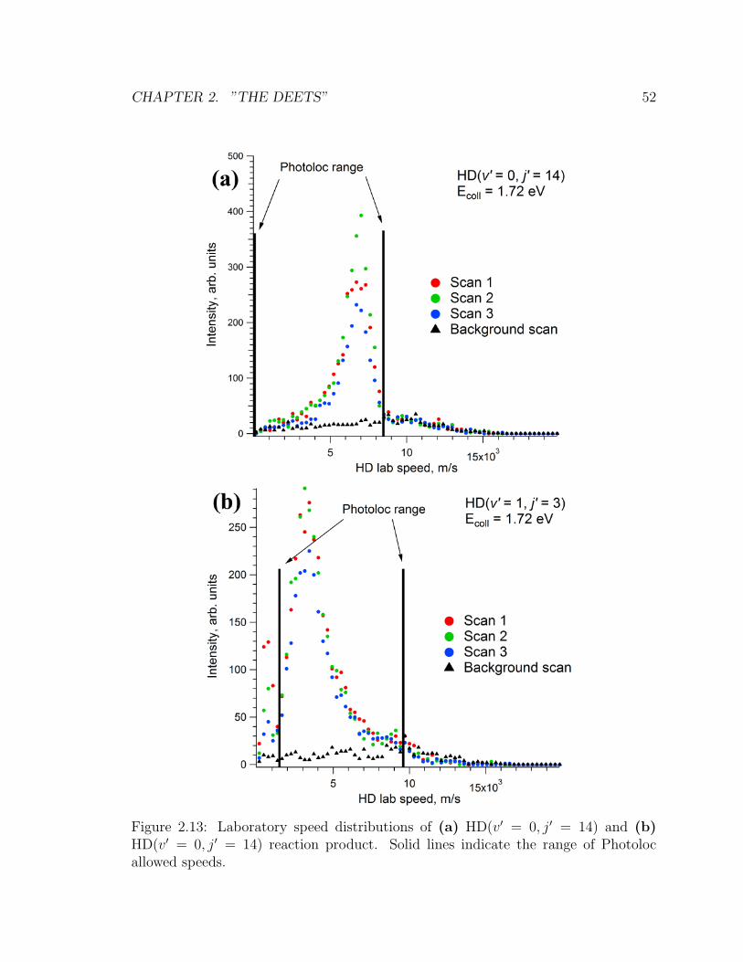
CHAPTER 2. ”THE DEETS” 52
Figure 2.13: Laboratory speed distributions of (a) HD(v′ = 0, j′ = 14) and (b)HD(v′ = 0, j′ = 14) reaction product. Solid lines indicate the range of Photolocallowed speeds.

CHAPTER 2. ”THE DEETS” 53
to a non-resonant ionization of HD reaction products, i.e.
HD(
∑
v′
v′,∑
j′
j′)
+ 3hf → HD+ + e− (2.52)
then it should be possible to obtain a rough estimate of the expected signal to noise
ratio as follows. As per our Section 2.4 discussion on multiphoton processes, the
number density of ’background’ HD+ ions, Sb, or the integrated rate of non-resonant
HD ionization, is given by
Sb ≡ NHD+(∆t) = σ3NHD(∑
v′ v′,∑
j′ j′)I
3∆t (2.53)
where σ3 is the three photon (non-resonant) ionization cross section. Similarly, Eq.
2.44 gives the number density of resonantly and state-selectively ionized HD+ ions,
Ss. The S/N ratio is then given by
Ss
Sb
=σ2NHD(v′,j′)
σ3NHD(∑
v′ v′,∑
j′ j′)
Ix−3 (2.54)
where x ≈ 1.5, see Eq. 2.44. Next,
NHD(v′,j′)
NHD(∑
v′ v′,∑
j′ j′)
=σv′,j′
reac vrelNHND2∆t
(
∑
v′,j′ σv′,j′reac
)
vrelNHND2∆t
=σv′,j′
reac∑
v′,j′ σv′,j′reac
(2.55)
Using theoretical calculations at Ecoll = 1.72 eV,∑
v′,j′ σv′,j′
reac = 9.2 A2, σv′=0,j′=14reac =
0.20 A2, and σv′=1,j′=3reac = 0.15 A2 Three-photon non-resonant absorption cross section
in H2 is a little harder to come by, so we shall assume a typical three-photon ionization
cross section (see footnote 14), i.e. σ3 ∼ 10−78 cm6· s2. Plugging these values into
Eq. 2.54, assuming a 1 mJ laser pulse at 210 nm,
Ss(v′ = 0, j′ = 14)
Sb
∼ 1 (2.56)
Ss(v′ = 1, j′ = 3)
Sb
∼ 1 (2.57)

CHAPTER 2. ”THE DEETS” 54
While the theoretical prediction of S/N ratio is of the right magnitude (experimentalSs(v′=0,j′=14)
Sb≈ 4 and Ss(v′=1,j′=3)
Sb≈ 6), these values should be taken with a grain of
salt, bearing in mind the uncertainty associated with the three-photon absorption
cross section, i.e. σ3 ∼ 10−78±4 cm6· s2! Instead, the calculation could be turned the
other way around, and experimental sensitivity of [2+1] REMPI could be compared
to a ’[3+0] MPI’, i.e. three-photon non-resonant ionization. The sensitivity ratio,
defined here as (σ2Ix)/(σ3I
y), where both ionization schemes may have an unknown
dependence on the laser intensity, is estimated from the two measurements as
v′ = 0, j′ = 14 :σ2σ3Ix−y ≈ 230 (2.58)
v′ = 1, j′ = 3 :σ2σ3Ix−y ≈ 350 (2.59)
with an average value of 290. In order to comment meaningfully on the sensitivity of
the two- and three-photon ionization schemes, a more precise value for σ3 in molecu-
lar hydrogen is needed.
For a one laser experiment, the ’offline’ signal is subtracted from the ’online’ sig-
nal to get the corrected laboratory speed distribution of HD(v′, j′) product. The
corrected laboratory speed distribution is then converted into a DCS by means of Eq.
2.29 for a P (θ) vs. θ graph, or Eq. 2.28 to get a plot of P (cos θ) vs. cos θ. DCSs for
HD(v′ = 0, j′ = 14) and HD(v′ = 1, j′ = 3) products are shown in Fig. 2.14. The
experimental error bars in this case correspond to an average of three independent
scans. As advertised, HD(v′ = 0, j′ = 14) product is sideways/forward scattered,
whereas rotationally colder HD(v′ = 1, j′ = 3) product is backward scattered.
Often two laser experiments were performed. In this case, one laser acts as a pho-
tolysis laser, and the other one is a REMPI, or probe, laser. First, the two lasers
must be overlapped in space and in time. This is usually achieved by leaking small
amounts (P ∼ 2 ·10−5 Torr) of H2, HD or D2 into the chamber through the leak valve
(Varian 951-5106). The leak valve consists of a tungsten filament that can be heated
up to 3000 K. Passing a sample of H2 over the hot filament results in a dissociative

CHAPTER 2. ”THE DEETS” 55
Figure 2.14: Differential cross sections for (a) HD(v′ = 0, j′ = 14) and (b) HD(v′ =0, j′ = 14) reaction products.

CHAPTER 2. ”THE DEETS” 56
surface adsorption, with the the subsequent recombinative desorption. Because many
collisions are needed to equilibrate the vibrational degrees of freedom, particularly so
in H2, molecular hydrogen emerges with an effective vibrational temperature of 3000
K. This enhances the vibrationally excited-state populations through the Boltzmann
factor:N(v = 1)T2
N(v = 1)T1
≈ 18 (2.60)
N(v = 2)T2
N(v = 2)T1
≈ 35 (2.61)
N(v = 3)T2
N(v = 3)T1
≈ 51 (2.62)
N(v = 4)T2
N(v = 4)T1
≈ 65 (2.63)
where T1 = 300 K and T2 = 3000 K. This step was invaluable, for example, in finding
the HD(v = 4, j) REMPI lines: even though HD(v = 4, j) signal was absent at 300 K
(tungsten filament off), it was discernible at 3000 K (filament on). With the gas inside
the chamber, the two lasers are usually overlapped by finding a Doppler free signal of
the transition of interest. Any [2+1] REMPI line in H2/HD/D2 could be used to find a
Doppler free signal. In fact, any [m+n] REMPI scheme could be used, wherem−even,to overlap two lasers.23 Indeed, some experimental arrangements require the use of
species other than molecular hydrogen for a favorable laser overlap. For example, a
very strong [2+1] REMPI transition in atomic hydrogen (1S → 2S, λ = 243.068 nm)
was often used to overlap lasers. Similarly, [2+1] REMPI of HBr and atomic Cl were
also used. Table 1 tabulates the range of [2+1] REMPI lines in different atomic and
molecular species that were used to overlap lasers in current experiments. It is worth
pointing out, that for a Doppler free signal the two laser wavelengths do not have to
be close to the center line of any given transition in Table 2.1. For example, two-color
Doppler free signal of chlorine atom was obtained when λ1 ≈ 280 nm and λ2 ≈ 200
nm, i.e. almost 50 nm away from the center line. Once the lasers are overlapped, their
wavelengths are moved such that one laser becomes the probe laser, i.e. it is parked at
23One could obtain a Doppler free overlap of three lasers for a [m+ n] REMPI, where m is odd.The three laser beams would have to propagate in plane, and make a 120 angle to each other.

CHAPTER 2. ”THE DEETS” 57
Table 2.1: Atomic and molecular [2+1] REMPI transitions used to overlap lasers.
Species OP wavelength, nm Transition
H2(v = 0, j = 0− 3) 201.624 - 201.735 X 1Σ+g → E,F 1Σ+
g , (0, 0), Q(j)H2(v = 1, j = 0− 3) 210.458 - 211.107 X 1Σ+
g → E,F 1Σ+g , (1, 0), Q(j)
H2(v = 2, j = 0− 3) 219.529 - 220.151 X 1Σ+g → E,F 1Σ+
g , (2, 0), Q(j)HD(v = 0, j = 0− 3) 201.345 - 201.851 X 1Σ+
g → E,F 1Σ+g , (0, 0), Q(j)
HD(v = 1, j = 0− 3) 208.994 - 209.482 X 1Σ+g → E,F 1Σ+
g , (1, 0), Q(j)HD(v = 2, j = 0− 3) 216.825 - 217.298 X 1Σ+
g → E,F 1Σ+g , (2, 0), Q(j)
D2(v = 0, j = 0− 3) 201.023 - 201.358 X 1Σ+g → E,F 1Σ+
g , (0, 0), Q(j)D2(v = 1, j = 0− 3) 207.262 - 207.592 X 1Σ+
g → E,F 1Σ+g , (1, 0), Q(j)
D2(v = 2, j = 0− 3) 213.631 - 213.951 X 1Σ+g → E,F 1Σ+
g , (2, 0), Q(j)D2(v = 3, j = 0− 3) 220.115 - 220.426 X 1Σ+
g → E,F 1Σ+g , (3, 0), Q(j)
HBr(v = 0, j = 0 or 1) 268.387 X 1Σ+ → f 3∆2, (0, 0), Q(j)Cl(3s23p5) 234.059 (3s23p5) 2P3/2 → (3s23p44p) 2P3/2
H(1s1) 243.068 (1s1) 2S1/2 → (2s1) 2S1/2
Note: only the first four rotational states of each molecular hydrogen isotopologue are considered,because higher rotational states have too small a population. Wavelength range for H2, HD and D2
is spun by j = 0 (always the shortest wavelength entry) and j = 3 (the longest wavelength). Inother words, the first and the second entry correspond to actual Q(0) and Q(3) REMPI lines, andQ(1) and Q(2) are not shown. The observed HBr signal assignment is tentative; it is either a Q(0)or Q(1) branch [50].
a particular REMPI line, whilst the other laser becomes the photolysis laser. During a
two laser experiment, the background is subtracted on an every-other-shot basis. This
is best understood within the laser pulse timing domain: when a probe laser fires ∼10ns after the photolysis laser had fired, the signal will be a sum of reaction products
due to photolysis laser-induced processes, plus reaction products that were created as
a consequence of HBr photolysis by the probe laser. Of these two, the probe-induced
reaction products should be viewed as a background. Consider now what happens
when the probe laser fires ∼ 10 ns before the photolysis laser: the signal will be purely
due to probe-induced reaction products. Subtracting the signal corresponding to
’probe-before-photolysis’ from the ’probe-after-photolysis’ signal yields the corrected
experimental signal. While the two-laser experiment can be done in half the time it
takes to do a one-laser experiment, in certain cases two-laser experiment may have
poorer S/N levels, particularly when investigating bimolecular reaction products at
CHAPTER 2. ”THE DEETS” 58
collision energies lower than those corresponding to probe-induced reaction products.
On the other hand, two laser experiments are more versatile as they allow one to
study a particular reaction product state at an almost arbitrary collision energy, as
opposed to one laser experiments, where the collision energy is set by the REMPI
wavelength corresponding to the product state in question. Data analysis of a two-
laser experiment is analogous to the one-laser approach, as outlined previously.
2.6 Speed Measurement Calibration
Given the importance of a molecular speed measurement, regular ’speed checks’, or
calibrations, were performed. Photolysis of a diatomic molecule sends two atoms
flying away from each other. Often there is not enough energy to cause electronic
excitation of atoms, hence the speed of an atom in the laboratory frame can be calcu-
lated to a high degree of accuracy. These predictions should match the experimental
measurement closely, save for line broadening caused by electron recoil. Hydrogen
bromide and hydrogen iodide have been employed as ’test systems’, wherein fast hy-
drogen atoms were produced upon a photodissociation of a diatomic precursor, and
H atoms were then detected by means of a [2+1] REMPI:
HX + hfphoto → Hfast +X (2.64)
HX + hfphoto → Hslow +X∗ (2.65)
Hfast + 3hfprobe → H+fast + e− (2.66)
Hslow + 3hfprobe → H+slow + e− (2.67)
where it has been emphasized that the photolysis and probe lasers need not have the
same frequency. Most often X = Br or I, and X∗ is the spin orbit excited species.
Hydrogen atoms corresponding to the production of X∗ will have a lower kinetic
energy, denoted Hslow, than hydrogen atoms produced in coincidence with the ground
state X atom, Hfast. It is easy to show that the speed of ’fast’ and ’slow’ hydrogen

CHAPTER 2. ”THE DEETS” 59
atoms in the laboratory frame is given by
vHfast=
√
2(
hfphoto −D0(HX) + Eint(HX))
mH
(
1 +mH/mX
) (2.68)
vHslow=
√
2(
hfslow −D0(HX)− ES.O.(X∗) + Eint(HX)
)
mH
(
1 +mH/mX
) (2.69)
where D0(HBr) = 3.758 eV, D0(HI) = 3.054 eV [13], ES.O.(Br∗) = 0.457 eV and
ES.O.(I∗) = 0.943 eV; Eint(HBr) = 0.016 eV, and Eint(HI) = 0.019 eV is the experi-
mentally measured residual HX rotational energy from an imperfect molecular beam
cooling. Finally, the electron recoil to the hydrogen atom in the [2+1] REMPI is
given by
vrecoilH+ =
√
2(
3hfprobe − IP )mH+
(
1 +mH+/me
) (2.70)
For a [2+1] REMPI via the 1s → 2s transition, λ = 243.068 nm and IP = 13.6 eV,
so vrecoilH+ = 421 m/s. To measure the hydrogen atom laboratory speed, typically a
few percent HX mixture in a carrier gas (He, Ar or D2) is used. The sensitivity of
a [2+1] REMPI can be appreciated from the fact that when a mixture containing
HI is used, and the HBr mixture is used the following day, H atoms corresponding
to the photolysis of HI can still be detected! This is attributed to HX sticking to
the surface of a gas manifold. Hydrogen atom ion image from a mixture containing,
effectively both HBr and HI, is shown in Fig. 2.15. Hydrogen atoms were detected
in a Doppler free fashion, with λ1 = 207.5 nm and λ2 = 293.3nm. The ’Signal’ (red
trace in Fig. 2.16a) was obtained when the two laser pulses intersected the molecular
beam at the same position and time. Note that both 207.5 nm and 293.3 nm photons
can photolyze hydrogen iodide, and only 207.5 nm can photolyze hydrogen bromide.
The ’Background’ (green trace in Fig. 2.16a) was obtained when the two laser pulses
arrived at different times, typically ∼ 60 ns apart. In that case, hydrogen atoms
cannot be detected via a [2+1] REMPI. The subtracted signal is shown in Fig. 2.16b.
If the detector is in the x− y plane, then the laser polarization is in the x− z plane.
Ion images crushed in the x − y plane, for example, exhibit several rings, Fig. 2.15,

CHAPTER 2. ”THE DEETS” 60
Figure 2.15: Hydrogen atom ion sphere projection in the x−y plane from a concomi-tant photolysis of HBr and HI at λ = 207.5 nm and λ = 293.3 nm.

CHAPTER 2. ”THE DEETS” 61
that correspond to the ’fast’ channel photodissociation, Eq. 2.64. These transitions
are perpendicular, and characterized by a β = −1 value, see Eq. 2.25. In other words,
the H atoms are distributed according to a sin2 χ distribution, where χ is the angle
between the laser polarization vector and hydrogen atom velocity. The ring radius
is proportional to the hydrogen atom speed. Thus, the very faint outermost ring in
Fig. 2.15 corresponds to HI photolysis at 207.5 nm, the more intense smaller ring is
H atoms from HBr photolysis at 207.5 nm, and the innermost ring in Fig. 2.15 is due
to H atoms from HI photolysis at 293.3 nm. Ion sphere projections in the x− z and
y − z directions of poorer quality are not shown. The ion images can be converted
to a speed distribution and these are shown in Fig. 2.16. The origin of each peak
is readily identified, because there are only three photodissociation pathways: (i) HI
photolysis at 207.5 nm, (ii) HI photolysis at 293.3 nm, and (iii) HBr photolysis at
207.5 nm. (HBr does not absorb to any experimentally significant extent at 293.3
nm. Its absorption starts at ∼ 285 nm.) Photodissociation at each wavelength will
give rise to hydrogen atoms with two different laboratory speeds, viz. parallel and
perpendicular transitions. Thus, one expects a total of six peaks in the hydrogen
atom speed spectrum. This is very nearly borne out experimentally (Fig. 2.16) - one
of the peaks, corresponding to a slow channel photodissociation of HI at 207.5 nm,
is obscured by peaks (ii) and (iv) in Fig. 2.16. In addition, the branching ratios,
i.e. the fraction of ’slow’ hydrogen atoms produced at a particular photodissociation
wavelength, i.e. Γ = NX∗
NX∗+NX, are rather well known, both for HBr and HI. Integrating
’slow’ and ’fast’ peaks can therefore give an indication whether there is any appreciable
ion fly-out. In particular, if Γ is much greater than the known/observed values, this
could be an indication of faster-moving hydrogen escaping the laser detection volume.
The results are summarized in Table 2.2. It is clear from Table 2.2 that the laboratory
speed measurements are rather accurate. The branching ratio for hydrogen bromide
at λphoto = 207.5 nm agrees well with previously reported value, whereas Γ for the
photodissociation of hydrogen iodide at λphoto = 293.3 nm is smaller by a factor of
two than what has been measured by Langford et al [52]. This may however be due
to the fact that peak (vi) in Fig. 2.16 is barely within the acceptable S/N ratio of the
experiment. There are however a few curiosities that presently are not completely

CHAPTER 2. ”THE DEETS” 62
Figure 2.16: Laboratory speed distribution of hydrogen atoms from a photolysis ofHBr and HI at λ = 207.5 nm and λ = 293.3 nm, as measured by a two-color Dopplerfree [2+1] REMPI of a hydrogen atom.

CHAPTER 2. ”THE DEETS” 63
Table 2.2: Calculated and measured hydrogen atom speeds and branching ratiosfollowing an HX photodissociation.
Peak λphoto (nm) vcalc (m/s) vmeas (m/s) % error Γlit Γmeas
(i) HI, fast, 207.5 23671 23775 0.4(ii) HBr, fast, 207.5 20584 20925 1.7(iii) HI, slow, 207.5 19513 NR NR 0.19 NR(iv) HBr, slow, 207.5 18360 18525 0.9 0.16 0.17(v) HI, fast, 293.3 15090 15225 0.9(vi) HI, slow, 293.3 6940 6975 0.5 0.18 0.09
Note: NR - not resolved. Data for the HBr branching ratio is taken from the study by Koszinowski[51], and HI branching ratios are compared to the work of Ashfold and co-workers [52].
understood. For example, peak (v) is ∼ 2 times greater than peak (i). This is
surprising, because the absorption cross section of HI at λ = 207.5 nm is about 10
times larger than the one at λ = 293.3 nm [52]. One therefore would expect peak (v)
to be roughly 10 times smaller than peak (i). Experimentally measured peak (v) is
some 20 times larger than expected. This could seemingly be explained by the 293.3
nm laser having considerably larger intensity; both beams however had about 30µJ
of power. In addition, one could argue for a severe fly-out of H atoms moving ∼23km/s (peak (i)) versus much slower ∼15 km/s H atoms (peak (v)). Again, other data
in Fig. 2.16 do not fully support the hypothesis: the ratios peak(iv)/peak(ii) and
peak(vi)/peak(v) fall within the expected range, and do not exhibit any significant
fly-out of the faster moving hydrogen atoms. Clustering of HX in the molecular beam
is unlikely, given that no additional peaks in Fig. 2.16 are present, but cannot be
ruled out completely.
2.7 Summary
This chapter was intended to give one some familiarity with the concepts of (i) an
angular distribution and the precise definition of a DCS. The difference between an
angular distribution P (θ) as given by Eq. 2.4, and the DCS as defined by Eq. 2.12,
is subtle: when dealing with molecular collisions, one rarely has control over the

CHAPTER 2. ”THE DEETS” 64
impact parameter b. Consequently, both P (b) and P (θ) are dynamic quantities. This
is why the P (b) has been left out of the definition of a DCS. On the other hand,
when one can specify or control the impact parameter distribution, as in a game of
pool, then Eq. 2.4 may be used, because P (b) is in a way an initial condition of a
problem. Pool is also a good way to appreciate the difference between the LAB and
COM reference frames. The maximum angle through which an object ball can be
cut is 90, and the scattering angle runs from 0 to 90. These are pool hall, or LAB
frame, observables. Pool tables, however, are in a way identical to each other, and
so one can compare different LAB frame ’experimental observables’ without the need
of a LAB → COM transformation. Molecular collisions are performed in a variety of
ways. Crossed- and single-beam experiments, for example, have very different LAB
frame observables. Transformation to the COM frame makes it possible to compare
systems studied under different experimental conditions, as outlined in Sections 2.1
and 2.2. (ii) Angle measurement problem can be converted to a speed measurement
problem by using the Photoloc technique. The techniques for measuring the three
velocity components of a molecular ion, and the associated (inherent) uncertainties
were discussed in Sections 2.3 and 2.6. One of the ultimate drawbacks of detecting
neutral molecules via multiphoton ionization wherein the photon energy exceeds the
ionization potential of a molecule considerably, is the electron recoil to the ionic
fragment. The resultant speed uncertainty of an ion does not propagate linearly into
the angular space. Different ways of plotting angular information, e.g. P (cos θ) vs.
P (θ), yield different angular uncertainties. This point will be elaborated using a
’real world example’ in Chapter 4. (iii) Finally, exploring HER is impossible without
HIM (hydrogen ionization ’mechanism’)... Section 2.4 has hopefully given a reader
a sense of the complexity associated with multiphoton processes in molecules. The
use of sensitive techniques is mandatory when detecting low number density reaction
products, as illustrated by the back-of-an-envelope calculation for the HD(v′ = 4, j′ =
6) reaction product at Ecoll = 1.97 eV - less than a hundred ions an hour are detected!
To collect one mole of HD(v′ = 4, j′ = 6) molecules at this rate requires on the order of
1029 seconds, which compares unfavorably with a graduate student’s average lifetime
(108 seconds) and with the age of the Universe (1017 seconds).

Chapter 3
H + D2 Differential Cross Sections
3.1 Introduction
The hydrogen exchange reaction is mostly direct in nature. Loosely speaking a di-
rect reaction does not support any long-lived complexes. One could also classify a
reaction as being direct if the collision is ’fast’. It is however dangerous to do so. A
typical direct H + H2 reaction is over in a few tens of femtoseconds. Under certain
circumstances, i.e. particular collision energy and product states, HER exhibits more
complex reaction mechanisms, in addition to the direct one. These more complex
pathways take additional twenty or thirty femtoseconds. One could therefore mis-
leadingly label indirect H + H2 reaction mechanisms as direct if relying solely on
the reaction time. Indirect, sometimes called time-delayed, collisions in the H + H2
reaction family have been properly documented and are relatively well understood.
Joint experimental and theoretical effort uncovered a time-delayed mechanism in the
H + D2 → HD(v′ = 3, j′ = 0) + D reaction at Ecoll = 1.64 eV [53]. Almost simulta-
neously the same mechanism has been observed by Harich et al. in the H + HD→H2(v
′ = 0 and 1, j′ = 0 and 1) + D reaction at Ecoll = 1.20 eV [54]. More experimental
[55, 56] and theoretical [57, 58] work followed to better understand the forward peak
in the DCS - one of the signatures of a time-delayed mechanism. More recently, how-
ever, the same forward peak has been observed in the H + D2 → HD(v′ = 2, j′ = 0)
+ D reaction at Ecoll = 1.25 eV by Bartlett et al. [59]. Although the work has not
65

CHAPTER 3. H + D2 DIFFERENTIAL CROSS SECTIONS 66
received as much theoretical attention, it is likely that the same time-delayed mech-
anism is at work.
In the absence of indirect, time-delayed mechanisms, the H + H2 reaction is of-
ten thought of as an example of a ’molecular pool’ (hence so much attention to
billiards in Chapter 1): hydrogen atom-hydrogen molecule interaction can be crudely
modeled as a hard-sphere system. We state that, ’Small impact-parameter collisions
lead to backward scattering, and glancing encounters yield forward-scattered prod-
ucts’. This will be propensity rule #1. Propensity rule #2 can be stated as follows,
’Small impact-parameter collisions are more effective at producing rotationally cold
H2 product molecules, and large impact-parameter trajectories lead to rotationally
hot H2 diatomics’. Both of these statements, which will be substantiated with a
considerable amount of data, are illustrated pictorially in Fig. 3.1. Propensity #1
is very intuitive and is best exemplified by a game of billiards, discussed in Chapter
1. Propensity rule #2 is also ’reasonable’. A very deceptive way to rationalize the
second rule is to consider the total angular momentum conservation
L+ j = L′ + j′ (3.1)
where L and L′ are reactant approach and product recoil orbital angular momenta,
and j and j′ are reactant and product rotational angular momenta, respectively.1 One
could therefore reason that if j′ is to increase then so must L. This statement ignores
the fact that Eq. 3.1 is a vector, not a scalar, equation. One of the aims of this
chapter is to scrutinize both of these propensity rules. The H + H2 isotopic reactions
have small reduced mass; the number of partial waves contributing to the reaction is
therefore relatively low, compared to heavier reactions, viz.√
L(L+ 1) =(
µvrelb)
/h.
Thus, for a typical H + D2 → HD(v′, j′) + D reaction, Lmax ≈ 24, Table 3.1.
It would be a mistake to think that all chemical reactions in the gas phase can
be modeled as hard sphere interactions. The most notable class of reactions that
1Often j ≈ 0, because H2 is rotationally cooled during the supersonic expansion.

CHAPTER
3.
H+
D2DIFFERENTIA
LCROSSSECTIO
NS
67
Figure 3.1: Cartoon illustrating the relationship between the impact parameter b, the most probable scatteringangle θ, and the diatomic product rotational quantum number j′. (a) Low impact parameter collisions lead torotationally cold, backward-scattered products, and (b) glancing collisions lead to sideways/forward scatteringof rotationally hot HD(v′, v′) products.

CHAPTER 3. H + D2 DIFFERENTIAL CROSS SECTIONS 68
Table 3.1: The range of partial waves contributing to the hydrogen exchange andother reactions.
Reaction vrel (m/s) Lmax Reaction vrel (m/s) Lmax
H + H2 2·104 20 H + O2 2·104 30H + HD 2·104 23 O + O2 2.5·103 41H + D2 2·104 24 Cs + KI 1.5·103 174D + H2 1.4·104 21 OH + H2 2.5·103 6D + HD 1.4·104 26 Ne + ND3 2.5·103 39D + D2 1.4·104 29 Ne + ND3 90 1H + H2 1.4·103 1 Cl + CH4 2.5·103 43
Note: A maximum impact parameter was taken to be bmax = 1 A for all reactions listed. (A moreproper way of estimating the maximum impact parameter is via bmax ≈
√
σrxn/π, where σrxn isthe cross section of a reaction under question. For example, bmax = 1 A is a good estimate for H +H2 reactions, but is an underestimate for larger molecules that have larger σrxn.) The relativespeed for reactions involving hydrogen atoms was taken to be 2·104 m/s, a typical value when Hatoms are generated photolytically. Deuterium atom speeds were chosen in an analogous manner.Relative speeds of other reactions represent typical crossed beam collision energies.
does not fall into the realm of steep, short-range interactions, is the so-called alkali-
halogen reactions of the form M + X2 → MX + X, where M = K, Rb etc., and X
= I, Br etc. These reactions often have cross section greater than 100 A2, and are
mainly forward scattered with respect to the incoming metal atom. It is thought
that the alkali atom uses its weakly bound s electron to ’harpoon in’ the halogen
molecule. The ’harpooning’ happens at relatively large distances, and results in a
forward-peaked DCS in the COM frame, so-called ’stripping mechanism’ [60, 61]. In
general, as long as atoms and molecules have tightly bound electrons one expects the
reaction to proceed through a rebound mechanism, wherein the atoms and molecules
must come close together to ’feel’ each other. This is most likely through low impact-
parameter collisions, which, in turn, result in backward scattering, as illustrated in
Fig. 3.1. On the other hand, such inevitably oversimplifying generalizations, very
pertinent to the ’alkali age’ where products could not be studied state-specifically,
are becoming less relevant in the world of state-resolved DCS. Let us consider H +
H2 as the most classic example of direct rebound reaction. As was hinted at in Sec-
tion 2.5, and shown in Fig. 2.14, the most probable scattering angle of HD(v′, j′)

CHAPTER 3. H + D2 DIFFERENTIAL CROSS SECTIONS 69
product depends principally on j′: rotationally cold HD is backscattered with respect
to the hydrogen atom velocity (Figs. 2.14b and 3.1a), whereas highly rotationally
excited HD products recoil in a sideways/forward direction (Figs. 2.14a and 3.1b).
Thus, while it is still true that the interaction between a hydrogen atom and a hy-
drogen molecule is of a direct, short-ranged nature, one must use the phrase ’direct
rebound mechanism’ cautiously, so as not to imply that all HD(v′, j′) products ’re-
bound’ into the backward direction. The total reactive DCS for H + H2 collisions is
largely backscattered. The resultant DCS however is very broad - it is centered at ∼100 and has a FWHM of ∼ 100! This has been confirmed experimentally and theo-
retically over forty years ago [62–64], as well as more recently by Aldegunde et al. [65].
One of the simplest models used to explain the correlation between the most probable
scattering angle in a H + D2 → HD(v′, j′) + D reaction and the rotational quantum
number of HD product is the so-called LOCNESS model (Line-Of-Centers with Nearly
Elastic Specular Scattering), developed by Zare and co-workers [66]. The model is
simple yet predictive. Its main assumptions are that (i) hydrogen atom and a hydro-
gen molecule interact through a hard sphere potential (Eq. 2.3), and (ii) there is a
direct, linear correlation between the initial reactant orbital angular momentum and
the rotational angular momentum of HD product (akin to Eq. 3.1). While neither
assumption is completely true, Fernandez-Alonso et al. predicted, relying solely on
the LOCNESS model, that the DCS for a H + H2 reaction leading to rotationally cold
H2 products, i.e. j′ = 0 and 1 may exhibit a forward-scattered peak [66]. Just a few
years later such a peak has indeed been observed, vide supra, even if the mechanism
was not the same as predicted by the LOCNESS model! We shall discuss the model
in more detail later in the chapter.
3.2 DCS for H + D2 → HD(v′ = 2, j′) + D
The role of product rotation and collision energy was investigated in the H + D2 →HD(v′ = 2, j′) + D reaction at Ecoll = 1.25 eV (λphoto = 233 nm), 1.61 eV (λphoto = 214

CHAPTER 3. H + D2 DIFFERENTIAL CROSS SECTIONS 70
nm) and 1.97 eV (λphoto = 199 nm).2 Some prior experimental work on the v′ = 2
vibrational manifold had already been done, most notably by Welge and Zare groups.
Schnieder et al. found that the main peak in the DCS for HD(v′ = 2, j′) product
formed at Ecoll = 1.28 eV shifted to a sideways/forward direction (decreasing θ) with
increasing rotational quantum number of HD diatomic [67]. Analogous D atom Ryd-
berg tagging experiments were carried out by Wrede et al. for HD(v′ = 2, j′) products,
this time at a higher collision energy of 2.2 eV. Differential cross sections were recorded
up to HD(v′ = 2, j′ = 14), with more evidence that as diatomic product acquires more
rotational excitation, it scatters into a more sideways/forward direction [68]. Similar
conclusions were drawn by the authors of the LOCNESS model [66, 69, 70]. Current
experiments however afford a resolution superior to the aforementioned studies. For
example, typically only 12 to 15 bins could be obtained during a Photoloc experiment
with one- or two-dimensional velocity projection of the time-of-flight (TOF) axis; 3D
ion imaging allows one to have as many as 40 bins in a single DCS. In addition, the
role of collision energy was investigated systematically. Experimental results were
compared to theoretical time-dependent quantum mechanical (TD QM) calculations
by Stuart Althorpe and Foudhil Bouakline, our ’veteran’ theoretical collaborators.
3.2.1 Experiment
Most of the experimental particulars have been discussed in Section 2.5. Thus, only
the most important differences will be given here. All H + D2 → HD(v′ = 2, j′) +
D experiments were done under two-laser conditions, i.e. a dedicated photolysis and
a separate probe laser. Usually a 1%-3% mixture of HBr in D2 was expanded into
a vacuum chamber through a supersonic nozzle (General Valve, Series 9). Molecular
beam was intersected by a UV photolysis and probe laser in the extraction region
of a Wiley-MacLaren TOF mass spectrometer, see Fig. 2.8. The resulting ions were
collected on a position-sensitive delay line detector to yield a 3D speed distribution
of reaction products (see Fig. 2.3). Main experimental parameters used in the study
are summarized in Table 3.2. Out of ten HD(v′ = 2, j′ = 0, 3, 6, 9) states recorded
2Using HBr as a photolytic H atom precursor.

CHAPTER 3. H + D2 DIFFERENTIAL CROSS SECTIONS 71
Table 3.2: Main experimental parameters and observables for the H + D2 reaction.
HD(v′, j′) Ecoll (eV) # Ions # Bins spacing (m/s) θmeasmax
v′ = 2, j′ = 0 1.25 13893 25 240 144
v′ = 2, j′ = 3 1.25 18725 25 218 118
v′ = 2, j′ = 0 1.61 11282 35 224 155
v′ = 2, j′ = 3 1.61 4981 35 224 138
v′ = 2, j′ = 6 1.61 10882 32 226 110
v′ = 2, j′ = 9 1.61 13229 25 218 84
v′ = 2, j′ = 0 1.97 13784 40 217 163
v′ = 2, j′ = 3 1.97 9470 35 248 143
v′ = 2, j′ = 6 1.97 14246 35 248 113
v′ = 2, j′ = 9 1.97 12775 35 231 88
Note: The spacing between the adjacent bins is determined from ’spacing’ = vrange/(# bins + 1),where vrange is the Photoloc allowed range of speeds for a particular HD(v′, j′) product state. Thenumber of bins was chosen such that the resulting spacing between the bins is less than the HDREMPI recoil. For the four HD(v′, j′) states studied here, vrecoilHD+ ∼ 180 m/s.
at Ecoll = 1.25 eV, 1.61 eV and 1.97 eV (HD(v′ = 2, j′ = 6, 9) DCS at Ecoll =
1.25 eV were not measured), the HD(v′ = 2, j′ = 0, and 3) products at Ecoll =
1.25 eV exhibited the poorest S/N ratio. To understand this better, consider the
generation of an experimental signal step-by-step. The desired signal, from here on
called a ’2-laser’ signal, corresponds to a situation wherein a photolysis laser initiates
the reaction by photodissociating HBr molecules, probe laser arrives 10-15 ns later
and probes reaction products. However, probe laser can also photodissociate the
HBr precursor. The probe laser-generated H atoms can also react with deuterium
molecules to produce HD states under interrogation. Thus, the ’2-laser’ signal is
a sum of photolysis-initiated and probe-initiated processes. To subtract the probe-
initiated signal, we fire the probe laser 50 ns before the arrival of the photolysis
laser pulse on an every-other-shot basis. This is the so-called ’1-laser’ signal. It
corresponds only to probe-initiated processes. By subtracting the latter from the ’2-
laser’ signal, the desired signal from photolysis-initiated molecules is obtained. The
use of HBr for 1.25 eV experiments corresponds to λphoto = 233 nm. The probe laser
wavelength for HD(v′ = 2, j′ = 0) state, for example, is λprobe = 216.825 nm. Thus,

CHAPTER 3. H + D2 DIFFERENTIAL CROSS SECTIONS 72
for λprobe = λphoto = 216.825 nm, the corresponding H + D2 reaction collision energy
is 1.56 eV - greater than the collision energy of interest set by the photolysis laser!
In other words, the HD(v′ = 2, j′ = 0) product will come from the H + D2 reaction
at two different collision energies: 1.25 eV and 1.56 eV. There are therefore three
factors that govern the concentration of this rotationless product from two reaction
channels: (i) HBr continuous absorption cross section at λphoto and λprobe, (ii) H +
D2 → HD(v′ = 2, j′ = 0) reaction cross section at 1.25 eV and 1.56 eV, and (iii) the
ratio of photolysis and probe laser powers. The first two are out of experimentalist’s
control. The HBr absorption cross section at λ = 216.825 nm is larger than the
one at λ = 233 nm, by at least a factor of five [46, 71], and the reaction cross
sections at the two collision energies are nearly equal. Thus, even though higher
photolysis laser powers have been used, probe-initiated HD(v′ = 2, j′ = 0) products
have concentrations comparable to photolysis-initiated HD(v′ = 2, j′ = 0) molecules.
Typically, Pprobe = 300µJ − 500µJ , and Pphoto ∼ 1mJ , both operated at a 10 Hz
repetition rate. From the above it should be clear that the S/N ratio for the j′ = 0
reaction product at 1.25 eV should be the poorest of all the states studied. This was
confirmed experimentally - raw and processed data for HD(v′ = 2, j′ = 0) state at
1.25 eV (Fig. 3.2) shows that the S/N ratio is about 1.2.
3.2.2 Theory
Experimental DCS were compared to theoretical calculations using the wavepacket
method [72]. Very briefly, a time-dependent wavepacket is propagated from the reac-
tant to product regions on an improved Boothroyd-Keogh-Martin-Peterson (BKMP2)
potential energy surface, and, ”...the triatomic wavefunction is projected onto the
product atom-diatom wavefunction. The latter is a product of three wavefunctions,
one describing vibration of the diatomic molecule, the other describing its rotation
(and orientation), and the third describing translation (the atom-diatom relative mo-
tion). For the last part (translation), it is usual to project the triatomic wavefunction
taken at a fixed large atom-diatom distance Rf only on the rovibrational wavefunc-
tion, but in our method, we prefer to project it also on a Gaussian function centered

CHAPTER
3.
H+
D2DIFFERENTIA
LCROSSSECTIO
NS
73
Figure 3.2: Speed and angular distributions for HD(v′ = 2, j′ = 0) product state at Ecoll = 1.25 eV (a) Raw LABspeed distribution. Red and green traces are the ’2-laser’ and ’1-laser’ signals, respectively (see text for details). When thebackground is subtracted, the corrected speed distribution is obtained, shown in panel (b). Notice that most of the reactivesignal falls within the Photoloc allowed speed range (vertical red lines). (c) An average of eight independent measurementsof what is shown in (b). The ordinate error bars correspond to one standard deviation of eight measurements. Abscissaerror bars are the HD recoil imparted by the photoelectron. (d) DCS obtained from the LAB speed distribution via Eq.2.29.

CHAPTER 3. H + D2 DIFFERENTIAL CROSS SECTIONS 74
around Rf , for convergence reasons.” Cross sections converged to better than 1% by
using partial waves up to J = 40. Three separate calculations were performed for
three initial states of D2(v = 0, j = 0, 1, 2). Various nonadiabatic effects were ignored.
Theoretical results underwent two stages of blurring, to simulate experimental con-
ditions: (i) Gaussian collision energy blurring with a FWHM of 0.05 eV, and (ii) D2
reactant initial rotational state blurring, i.e. 39% in j = 0, 30% in j = 1 and 29% in
j = 2. The only noticeable effect of the blurring procedure is to smooth fast oscilla-
tions present in a theoretical DCS. A representative blurring of a calculated DCS for
HD(v′ = 2, j′ = 0) at Ecoll = 1.61 eV is shown in Fig. 3.3. In the past, an additional
blurring of theoretical results was carried out in order to account for the instrumental
resolution function. In current experiments, however, we add explicit experimental
uncertainties in the scattering angle θ, rather than blur theoretical results, by taking
into account the photoelectron recoil.
3.2.3 Results
A typical spectrum of ’2-laser’ and ’1-laser’ HD laboratory speed signals, and their
difference, are shown in Figs. 3.2a and 3.2b. Figure 3.2c shows that most of the
reactive signal falls within the Photoloc-allowed speed range; ordinate error bars for
the particular case of HD(v′ = 2, j′ = 0) at Ecoll = 1.25 eV correspond to 1 standard
deviation of eight independent measurements. (More typically 3 to 5 measurements
were performed.) The abscissa error bars are based on the HD recoil imparted by the
photoelectron (see Section 2.2 for more details). Finally, a laboratory speed distri-
bution is converted to a COM DCS by use of Eq. 2.29. The result is shown in Fig.
3.2d. The HD(v′ = 2, j′ = 0) DCS at Ecoll = 1.25 eV has a clear forward peak, in
addition to the backward one associated with the direct recoil mechanism.
The blurring of theoretical data is shown in Fig. 3.3. It seems like averaging over the
collision energy tends not to wash out fast oscillations as much as averaging over the
initial rotational states of D2 reactant does. On the other hand, the shape of DCS in
the sideways region, i.e. 70 < θ < 140, is almost identical for the three rotational

CHAPTER 3. H + D2 DIFFERENTIAL CROSS SECTIONS 75
states of deuterium (Fig. 3.3b), whereas the same region of DCS differs appreciably
for collision energies clustered around 1.61 eV (Fig. 3.3a). Ten experimentally mea-
sured and theoretically calculated DCS of HD(v′ = 2, j′) products are shown in Fig.
3.4.
3.2.4 Discussion
Differential cross sections in Fig. 3.4 have a clear trend - as the rotational excitation
of the HD(v′ = 2, j′) product increases, the scattering shifts from a predominantly
backward to a sideways/forward scattering. This is most apparent at Ecoll = 1.61
eV and Ecoll = 1.97 eV; two states recorded at Ecoll = 1.25 eV also exhibit this
behavior, and the additional peak at ∼ 70 present in the DCS for HD(v′ = 2, j′ = 0)
at Ecoll = 1.25 eV arises from the aforementioned indirect mechanism, and as such
should not be included in the j′ − θmax correlation. (This ’special’ state will be
discussed separately.) Such a negative j′ − θmax correlation, i.e. as j′ increases, θ
decreases, is not surprising. Zare and co-workers, for example, have modeled direct
interactions in the H + H2 reaction as a hard sphere scattering, the LOCNESS model,
wherein one supposes a one-to-one hard sphere deflection function, Eq. 2.3 [66, 69].
By assuming that there exists a linear relationship between the initial orbital angular
momentum and the rotational angular momentum of HD product, i.e.
b ≈ δ · j′ (3.2)
where δ is a proportionality constant, they plotted cos θmax vs. j′2 and found good
linear fits to their data.3 We do the same, i.e. using the hard-sphere formula
cos θmax = 2δ2j′2
d2− 1 (3.3)
3From Eq. 2.3 one has cos(θ/2) = b/d. Squaring both sides and using the fact that cos2 θ =
1/2(cos θ+1), one arrives at cos θ = 2 b2
d2 − 1, the formula Fernandez-Alonso et al. used to plot theirdata. It is not entirely clear to me why cos(θ/2) could not be plotted against j′ instead of cos θ vs.j′2.
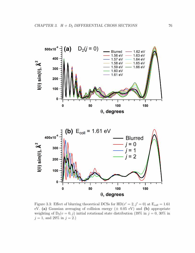
CHAPTER 3. H + D2 DIFFERENTIAL CROSS SECTIONS 76
Figure 3.3: Effect of blurring theoretical DCSs for HD(v′ = 2, j′ = 0) at Ecoll = 1.61eV. (a) Gaussian averaging of collision energy (± 0.05 eV) and (b) appropriateweighting of D2(v = 0, j) initial rotational state distribution (39% in j = 0, 30% inj = 1, and 29% in j = 2.)

CHAPTER
3.
H+
D2DIFFERENTIA
LCROSSSECTIO
NS
77
Figure 3.4: DCSs for HD(v′ = 2, j′) vibrational manifold at several collision energies. Red dots are experimental measure-ments, black curve is the theoretical TD-QM calculations.

CHAPTER
3.
H+
D2DIFFERENTIA
LCROSSSECTIO
NS
78
Figure 3.4 (continued): DCSs for HD(v′ = 2, j′) vibrational manifold at several collision energies. Red dots are experimentalmeasurements, black curve is the theoretical TD-QM calculations.
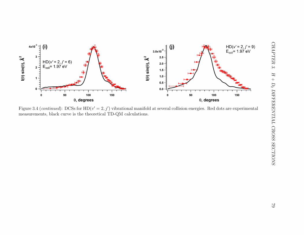
CHAPTER
3.
H+
D2DIFFERENTIA
LCROSSSECTIO
NS
79
Figure 3.4 (continued): DCSs for HD(v′ = 2, j′) vibrational manifold at several collision energies. Red dots are experimentalmeasurements, black curve is the theoretical TD-QM calculations.

CHAPTER 3. H + D2 DIFFERENTIAL CROSS SECTIONS 80
we plot cos θmax vs. j′2, where θmax is the most probable scattering angle, given in
Table 3.2. The results are shown in Fig. 3.5, along with the results of Fernandez-
Alonso et al. Reasonable linear fits are obtained, although not as good as observed
by Fernandez-Alonso et al. where only three points were used to fit straight lines.
Based on different slopes of their v′ = 1 and v′ = 2 linear fits, 0.013 and 0.023, re-
spectively,4 Fernandez-Alonso et al. stated that, ’... this result [arises] from a smaller
hard sphere radius d for v′ = 2 compared to v′ = 1...’ [66]. Interestingly enough,
we find that our v′ = 2 linear fit slopes at both collision energies are very similar to
the slope of the v′ = 1 fit by Fernandez-Alonso et al. This would suggest that the
hard sphere radii for v′ = 2 and v′ = 1 vibrational manifolds are similar, and do not
change appreciably with the vibrational quantum number. Of course, this can be
due to sparse data presently available, or, even more plausibly, due to the extreme
simplicity of the model.
Negative j′ − θ correlation in the H + H2 reaction has been observed on numerous
occasions [51, 66–68]. In all cases the unanimous conclusion is that, ’As the product
rotational excitation increases, the DCSs shift from backward to sideways scattering,
as expected.’ [74]. Again, this should not be taken as a universal dogma that applies
to all chemical reactions. The Cl + CH4 → HCl(v′ = 1, J ′) + CH3 reaction, for exam-
ple, is characterized by forward-scattered HCl(v′ = 1, J ′ = 1) product, with respect
to the incident Cl atom direction. More rotationally excited HCl(v′ = 1, J ′ = 3) di-
atomic is scattered to a more backward direction, compared to the HCl(v′ = 1, J ′ = 1)
reaction channel [75]. Halogen reactions with methane however are rather complex.
For example, formation of vibrationally cold HCl(v′ = 0, J ′) proceeds via a direct
recoil mechanism, while vibrationally excited HCl(v′ = 1, J ′) products are formed via
glancing collisions and are thus forward scattered. In addition, angular distribution of
HCl product can be broad, making ’backward’ or ’forward’ labeling difficult [76, 77].
Other chlorine atom reaction, e.g. Cl + C(CH3)3 → HCl(v′, J ′) + C(CH2)(CH3)3,
are best described by forward scattered HCl(v′ = 0, J ′) products, and the shape of
4Please note that the slope of these plots is m = δ2/d2. Thus, if δ truly a constant of propor-tionality, then a greater slope of a linear v′ = 2 fit implies a smaller hard sphere radius d for v′ = 2compared to v′ = 1.

CHAPTER 3. H + D2 DIFFERENTIAL CROSS SECTIONS 81
Figure 3.5: Plots of the most probable scattering angle θmax versus the square of therotational quantum number j′ of HD product. So-called LOCNESS model predictslinear dependence, see Eq. 3.3. Black and brown curves correspond to data taken byFernandez-Alonso et al.; red and green curves come from this work.
CHAPTER 3. H + D2 DIFFERENTIAL CROSS SECTIONS 82
the DCS does not change noticeably in going from HCl(v′, J ′ = 0) to HCl(v′, J ′ = 4)
[78]. In other words, not all chemical reactions have as pronounced j′ − θ correlation
as the H + H2 reaction. The negative j′ − θ correlation has been confirmed by the
work Koszinowski et al. for HD(v′ = 1, j′) manifold [74], Fernandez-Alonso et al. for
HD(v′ = 1, 2, j′) states [66, 79], and by Welge and co-workers for HD(v′ = 0, 1, 2, 3, j′)
vibrational manifolds [67, 68]. After such a vast amount of work it seemed like nega-
tive j′ − θ correlation was HER modus operandi.
3.3 DCS for H + D2 → HD(v′ = 4, j′) + D
To tell the full HD(v′ = 4, j′) saga I have to detour into the double-peaked DCS for
HD(v′ = 2, j′ = 0) at Ecoll = 1.25 eV, Fig. 3.4a. After a while we have realized
that the forward peak is analogous to the one observed in the H + D2 → HD(v′ =
3, j′ = 0) + D reaction at Ecoll = 1.64 eV [31, 53–56, 58, 80]. We have employed
a completely ’scalar’ reasoning, because even to this day no theoretical studies have
been undertaken to definitively establish the origin of the second peak in the DCS
for HD(v′ = 2, j′ = 0) at Ecoll = 1.25 eV. Briefly, the internal energy of HD(v′ =
3, j′ = 0) is 1.282 eV above the zero-point energy (ZPE). The forward peak was most
prominent at Ecoll ≈ 1.64 eV [56]. The internal energy of HD(v′ = 2, j′ = 0) is
0.877 above the ZPE, and the peak was very pronounced at Ecoll = 1.25 eV. What
seemed very suggestive to us was the fact that the internal energy difference between
HD(v′ = 3, j′ = 0) and HD(v′ = 2, j′ = 0) states (0.40 eV) was almost identical to
the collision energy difference of the two experiments (0.39 eV). Right at the end
of the HD(v′ = 2, j′ = 0) experiment Nate Bartlett has graduated and I was left
alone in the lab. Dick was on an extensive travel in the late summer/early autumn of
2011. Alone in the lab, and not knowing what to do, I decided to be a true chemist,
i.e. to ’predict and verify’: if it is true that the forward peak is of the same origin
in both HD(v′ = 3, j′ = 0) and HD(v′ = 2, j′ = 0) states but done at different
collision energies, then it must be true that other rotationless HD states should also
exhibit similar forward scattering when done at an appropriate collision energy. Fig.
3.6 makes the foregoing discussion more pictorial. There are two obvious choices:

CHAPTER 3. H + D2 DIFFERENTIAL CROSS SECTIONS 83
Figure 3.6: Energy level diagram for the H + D2 → HD(v′, j′) + D reaction. Solidblack arrows, connecting particular collision energy values with specific internal statesof HD product, indicate the conditions under which the forward scattering has beenobserved. Dashed black arrows indicate experimental conditions under which similarforward scattering is expected.
CHAPTER 3. H + D2 DIFFERENTIAL CROSS SECTIONS 84
HD(v′ = 1, j′ = 0) and HD(v′ = 4, j′ = 0) states. According to the above reasoning,
in order to see the forward peak in the DCS for the H + D2 → HD(v′ = 1, j′ = 0) +
D reaction, it would have to be done at Ecoll = 0.82 eV, i.e. the difference in internal
energy between HD(v′ = 1, j′ = 0) and HD(v′ = 2, j′ = 0), i.e. 0.427 eV. Generating
slow enough ∼ 1 eV H atoms is difficult, at least not using HBr as a hydrogen atom
precursor, as hydrogen bromide’s experimentally significant absorption starts at ∼250 nm.5 The other sensible choice was therefore HD(v′ = 4, j′ = 0) at Ecoll ≈ 2.02
eV, i.e. the energy difference between HD(v′ = 4, j′ = 0) and HD(v′ = 2, j′ = 0)
(0.382 eV), or HD(v′ = 4, j′ = 0) and HD(v′ = 2, j′ = 0) (0.786 eV). Generating ∼2.5 eV H atoms is a routine experiment. Hydrogen iodide is the best choice for the
task, with easily achievable λphoto = 220 nm. Hydrogen bromide, on the other hand,
is less ideal - the shortest wavelength that can be generated with BBO crystals in the
LAB is about 199 nm.6 This corresponds to Ecoll = 1.97 eV, a wee bit short of the
desired 2.02 eV. Given that HI was not (and still is not) readily available in the LAB,
I decided to use HBr to hunt for the forward peak in the DCS for the HD product of
the H + D2 → HD(v′ = 4, j′ = 0) + D reaction at Ecoll = 1.97 eV. To make a very long
story short - I failed! I could not use the HD(v′ = 4, j′ = 0) [2+1] REMPI wavelength
at λprobe = 232.968 nm because of immense D atom background. This is a notorious
problem in our experiments, particularly when detecting HD molecules - deuterium
atom signal can at times be so large so as to ’spill’ into the HD collection window
and even distort the TOF baseline of HD diatomics. We have not tried to elucidate
the exact origins of this heightened D atom signal as a function of laser wavelength,
but we suspect it may involve either dissociative ionization of electronically excited
5Continuous absorption into repulsive electronically excited states of HBr starts at about 285nm, but the absorption cross section, and consequently H atom concentration, diminish rapidly. Forexample, the absorption cross section at λ = 260 nm (corresponding to Ecoll = 0.82 eV) is at least 10times smaller than at λ = 233 nm, corresponding to Ecoll = 1.25 eV [81, 82]. Bearing in mind thatHD(v′ = 2, j′ = 0) state at Ecoll = 1.25 eV had the worst S/N ∼ 1.2, it is quite likely that measuringthe HD(v′ = 1, j′ = 0) DCS at Ecoll = 0.82 eV is impossible, at least using HBr as a hydrogen atomprecursor. With the probe laser wavelength tuned to HD(v′ = 1, j′ = 0) [2+1] REMPI line, theprobe-initiated H + D2 reaction collision energy is 1.73 eV. This compares even more unfavorablywith the photolysis-initiated reaction at 0.82 eV; see the discussion in Section 1.2.1.
6Radiation of lower wavelengths can be generated using BBO crystals. Even under the bestconditions, however, I never managed to get more than 100µJ of laser power at 197.5 nm. Forexperiments described in this section, at least 500µJ are needed.

CHAPTER 3. H + D2 DIFFERENTIAL CROSS SECTIONS 85
D2, i.e.
D2 + nhf → D∗2 (3.4)
D∗2 + hf → D+D+ + e− (3.5)
or dissociation of D∗2 into neutral fragments with a subsequent D∗ ionization, i.e.
D∗2 + hf → D(n=1) + D∗ (3.6)
D∗ + hf → D+ + e− (3.7)
Additional processes are of course possible, like ion-pair formation etc. Proton forma-
tion from multiphoton excitation of molecular hydrogen is a well known phenomenon,
and the above processes have been studied in detail [39, 83–86]. It was found, for
example, that the proton production does depend sensitively on the laser wavelength
[39, 85]. This is consistent with our observation, that for some λprobe H or D atom
signals becomes so intense that it can ’bury’ the neighboring HD signal. To get an
idea of just how big the D atom signal can be, Fig. 3.7 shows the TOF spectrogram,
centered at m/z = 3. Huge deuterium atom signal is clearly seen to ’invade’ the HD
collection window. Ion images, particularly in the Vx/Vz and Vy/Vz directions, are
also revealing: they show D atoms ’flying into’ the HD ion sphere. The HD laboratory
speed is also shown: it is clear that the D atom signal has completely overshadowed
any HD(v′ = 4, j′ = 0) signal, to be looked for in the Photoloc allowed range (vertical
red bars).
Upset, I decided to see what other HD(v′ = 4, j′) states look like. After record-
ing the DCS for HD(v′ = 4, j′ = 2) and HD(v′ = 4, j′ = 5) products I thought I
had accidentally switched the raw data files, i.e. the HD(v′ = 4, j′ = 2) DCS was
actually that of HD(v′ = 4, j′ = 5), and vice versa. After convincing myself that
this was no mistake, I became even more upset, as I decided that I made a blun-
der somewhere, because more rotationally excited HD(v′ = 4, j′ = 5) product was
more backward scattered than the HD(v′ = 4, j′ = 2)! The exactly opposite behavior
scientific community was familiar with! Within the next few weeks I had DCSs for

CHAPTER
3.
H+
D2DIFFERENTIA
LCROSSSECTIO
NS
86
Figure 3.7: Raw experimental signal (or lack thereof) of HD molecule, when λprobe is tuned to the REMPI line of HD(v′ =4, j′ = 0). (a) Deuterium hydride appears at tTOF ≈ 6.2µs, and D atom is centered at tTOF ≈ 5.1µs; the peak of the Datom signal is not shown. Deuterium atom signal is so big that it completely obscures any signal from HD. (b) Laboratoryspeed measurement in the search for HD(v′ = 4, j′ = 0) reactive signal at Ecoll = 1.97 eV. As is evident from panel (c), theS/N ratio is too poor to pick out any signal corresponding to the HD(v′ = 4, j′ = 0) reaction product, as indicated by thePhotoloc speed range.

CHAPTER 3. H + D2 DIFFERENTIAL CROSS SECTIONS 87
Figure 3.7 (continued): Experimental ion images in search of HD(v′ = 4, j′ = 0)reaction product. Panel (d) looks deceptively innocuous. Images along Vy/Vz andVx/Vz directions, panels (e) and (f), respectively, show a tip of the D atom iceberg.

CHAPTER 3. H + D2 DIFFERENTIAL CROSS SECTIONS 88
HD(v′ = 4, j′ = 1, 2, 3, 5, 6), and the trend was clear - as the rotational excitation of
HD(v′ = 4, j′) product increased, the product was scattered into a more backward
direction. Positive j′− θ correlation was not confined to the v′ = 4 vibrational mani-
fold. It was found that the HD(v′ = 3, j′ = 10) state was slightly more backscattered
than rotationally cooler HD(v′ = 3, j′ = 8) product at Ecoll = 1.97 eV. The DCS are
shown in Fig. 3.8: the fact that theory and experiment exhibit the same trend of
more backward scattering with increasing j′, is very reassuring.
Why do the DCS of these highly internally excited HD(v′, j′) products exhibit posi-
tive j′− θ correlation, seemingly defying our ’reasonable’ application of total angular
momentum conservation, conveyed in Eq. 3.1? Let us examine the two propen-
sity rules set out in Section 3.1. The first ’rule’ states that small impact-parameter
collisions lead to backward scattering, whereas glancing encounters favor forward-
scattered products. The idea seems sound in the context of H + H2 scattering. The
other propensity rule says that small impact parameter collisions are more effective
at producing rotationally cold H2 products, and large impact parameter collisions
tend to favor rotationally excited products. The statement also seems sound. But
surely something must be amiss, as is evident from Fig. 3.8! It turns out, that the
latter rule is true only most of the time. Under normal circumstances (which shall be
defined shortly) higher partial waves or impact parameters are responsible for rota-
tionally excited products in the H + D2 reaction. A typical example is shown in Fig.
3.9. More forward scattered, highly rotationally excited HD(v′ = 0, j′ = 14) product
state is a result of, on average, higher order partial waves, or impact parameters, as
indicated by quasiclassical trajectory (QCT) calculations, compared to rotationally
colder HD(v′ = 1, j′ = 3) reaction channel. In fact, the so-called opacity functions in
Fig. 3.9 give the first clue as to why the second propensity rule in the H + H2 reac-
tion is only approximate: P (b) are not delta functions! They are broad. Physically,
these graphs should be interpreted as follows: the greatest probability of producing
HD(v′ = 0, j′ = 14) diatomic is when the hydrogen atom and a deuterium molecule

CHAPTER
3.
H+
D2DIFFERENTIA
LCROSSSECTIO
NS
89
Figure 3.8: DCS for HD(v′ = 3, 4, j′) vibrational manifold at Ecoll = 1.97 eV. Red dots are experimental measurements,black curve is the theoretical TD-QM calculations.

CHAPTER
3.
H+
D2DIFFERENTIA
LCROSSSECTIO
NS
90
Figure 3.8 (continued): DCS for HD(v′ = 3, 4, j′) vibrational manifold at Ecoll = 1.97 eV. Red dots are experimentalmeasurements, black curve is the theoretical TD-QM calculations. Panels (h) and (i) show that experimentally andtheoretically the more rotationally excited HD(v′ = 3, j′ = 10) product is more backscattered than the rotationally coolerHD(v′ = 3, j′ = 8) reaction product.

CHAPTER 3. H + D2 DIFFERENTIAL CROSS SECTIONS 91
Figure 3.9: Opacity functions for two products of the H + D2 → HD(v′, j′) + Dreaction: HD(v′ = 1, j′ = 3) (black curve), and HD(v′ = 0, j′ = 14) (red curve), ascomputed by QCT method.
collide with b ∼ 1.18 A. The key is that even for b < 1.18 A, HD(v′ = 0, j′ = 14) prod-
uct state can still be made, albeit with a lower probability.7 Thus, highly rotationally
excited states like HD(v′ = 0, j′ = 14) can be produced via low impact-parameter
collisions, say up to 0.5 A in Fig. 3.9a. Crucially, the DCS peak will shift to a more
backward direction, if higher impact parameters are no longer contributing to the
reaction. To pursue this line of reasoning, let us qualitatively consider a model of
how higher order partial waves can be ’blocked out’, Fig. 3.10. The potential energy
surface for the H + H2 system can be plotted as a function of distance between the
atom and the molecule’s center of mass.8 For a head-on collision, L = b = 0 (black
7Another way of looking at this problem is to consider individual partial waves or impact pa-rameters, and ask what is the probability to end up in a particular product HD(v′, j′) state? Theanswer is that for low L or b the probability of producing HD(v′, low j′) is greater than makingHD(v′, high j′) state. The key however is that the probability for HD(v′, high j′) at low L or b issmall but not zero.
8A plot like the one in Fig. 3.10 effectively freezes the other two degrees of freedom in H3.

CHAPTER 3. H + D2 DIFFERENTIAL CROSS SECTIONS 92
Figure 3.10: A schematic illustration of a potential energy surface for the H + D2 →HD(v′, j′) + D reaction. Certain highly internally excited HD products do not havesufficient kinetic energy to overcome the centrifugal barrier in the exit channel. Conse-quently, lower order partial waves must contribute to the production of these highlyinternally excited products. The HD2 system does not literally get trapped; suchtrajectories become simply non-reactive.
curve in Fig. 3.10), the system experiences no barriers.9 For L 6= b 6= 0 collisions the
PES exhibits a centrifugal barrier, given by
V QMcentr =
L(L+ 1)h2
2µR2(3.8)
or classically
V CMcentr =
b2
R2Ecoll (3.9)
where µ is the reduced of the reactants. As L or b increases, so does the centrifugal
barrier. This is shown schematically in Fig. 3.10. Let us now consider a particular H
+ D2 → HD(v′, j′) + D reaction channel, at a specified Ecoll, and, most importantly,
for a particular partial wave. Let us first consider a collision with an orbital angular
9We ignore here the chemical barrier in the H + H2 reaction, commonly estimated to be 0.412eV.

CHAPTER 3. H + D2 DIFFERENTIAL CROSS SECTIONS 93
momentum magnitude of L2. This is shown schematically in Fig. 3.10: hydrogen
atom and deuterium molecule approach one another, at some distance R the ’reac-
tion happens’, i.e. a particular HD(v′, j′) state is populated, and the products start
recoiling away from one another. The recoil energy is clearly lower than the reac-
tant translational energy, and is given by EprodT ≈ Ecoll − EHD(v′,j′)
int , because D0 ≈ 0
eV for the H + D2 → HD + D reaction. So imagine a situation when the product
translational energy is not high enough to overcome the centrifugal barrier in the exit
channel of the H + D→ HD(v′, j′) + D reaction. The products, or, more precisely,
HD2 system, becomes ’trapped’. We say that a particular H + D2 → HD(v′, j′)
+ D reactive channel at Ecoll at L2 is not possible. There is however another way
to ’make’ HD(v′, j′) product at the same collision energy. Consider what happens
when the reactants approach one another in a more head-on fashion, with L1 amount
of orbital angular momentum. Due to a lower centrifugal barrier the products can
now ’escape’ the transition state. The bottom line is that such products would be
more backscattered with respect to less internally excited HD(v′, j′) products that
had enough energy to overcome the L2 centrifugal barrier.
This is a very crude and qualitative model meant to illustrate how the presence
of a centrifugal barrier in the exit channel of a reaction may force the reactants to
collide with less orbital angular momentum.10 Lower order partial waves mean more
backward scattering, in accord with our propensity rules. This is, of course, only a
crude model. It works qualitatively for HER, but not quantitatively. For example, for
the model to function one needs an actual centrifugal barrier. The latter is obtained
by adding a repulsive centrifugal term given in Eqs. 3.8 or 3.9 to an attractive term.
In the absence of a significantly attractive term, the effective potential,
Veff =L(L+ 1)h2
2µR2− C
Rn(3.10)
10More precisely, ’less than an ideal amount of orbital angular momentum’. Remember, it is stilltrue that high impact-parameter collisions are more effective at producing rotationally excited HDproducts.

CHAPTER 3. H + D2 DIFFERENTIAL CROSS SECTIONS 94
where C > 0 is a constant, will not have a local maximum!11 From Eq. 3.9 it
is clear that for b = 0.5, a typical impact parameter, and at R = 2, for example,
Vcentr ∼ 0.1Ecoll, i.e. the centrifugal barrier can be comparable to the collision en-
ergy. The H3 system is completely repulsive, i.e. does not contain attractive wells.
The only attractive well is the van der Waals attraction out at R ≈ 3.5 A, with a
well depth of meager 0.002 eV [87, 88]. Such a shallow well will yield Veff that is
essentially Vcentr. The barrier will be barely discernible.
The above reasoning is unapologetically classical. There are more abstract ways
to explain things, but they are harder to understand and visualize. Lastly, I would
like to quote one of the world’s leading experts on reactive scattering, Prof. Stuart
Althorpe, a theorist at Cambridge University, ”I’m inclined to think that the best
way to think of the effect [positive j′ − θ correlation] on a reaction like H + H2 is
the ’throttling-off’ model. One can visualize the potential at a given bending angle
(acknowledging that all angles will be present in a real 3-D system), then visualize the
effect of the centrifugal potential, which will peak at the origin and die off on going
outwards: as this grows it will ’throttle off’ the accessible space at the saddlepoint on
the potential, by pushing the system further out, thereby increasing the effective bar-
rier height.” [89] Admittedly, these ideas have been also communicated by Aquilanti
and Cavalli [90]. I personally struggle to understand any argument that seeks to
explain non-reactivity of higher partial waves in the H + H2 scattering based solely
on the reactant barrier height. Our evidently ’flawed’ picture12 of reaction dynamics
in Fig. 3.10 suggests that a trajectory with L2 amount of orbital angular momentum
will ’see’ the same barrier in the entrance channel, regardless of which internal HD
state will be produced. For HD(v′ = 4, j′ = 2) state, the recoil kinetic energy may
be high enough for products to overcome the higher barrier in the exit channel and
for products to separate. For HD(v′ = 4, j′ = 5) state, on the other hand, the L2
trajectory will be non-reactive, but, I believe, not due to the centrifugal barrier in the
11Inverse power law is assumed here, but the attraction may be of any functional form.12Drawing pictures is good! In his wonderful book How to Solve It [91] Polya outlines four steps
how to approach a problem: step 1 is, ”Draw a picture”. Step 2 is, ”If you cannot solve the proposedproblem try to solve first some related problem”. I adhered to his advice!

CHAPTER 3. H + D2 DIFFERENTIAL CROSS SECTIONS 95
entrance channel - otherwise how could have HD(v′ = 4, j′ = 2) products been made?
- but due to insufficient recoil kinetic energy to surpass the exit channel centrifugal
barrier. In summary, the ’cut off’ of ’throttling off’ effect of higher partial waves as ob-
served in the DCS of HD(v′ = 4, j′) products with increasing j′, is not a clear-cut one.
To illustrate the point that, on average, the impact parameter/partial wave order
decreases with increasing j′ rotational quantum number for the HD(v′ = 4, j′) vibra-
tional manifold, we show bP (b) vs. b and (2J + 1)P (J) vs. J plots in Fig. 3.11,
that were obtained using QCT (Gaussian binning), and time-independent QM calcu-
lations, respectively, by Aoiz and coworkers [92]. It is clear that the peak of both
bP (b) and (2J + 1)P (J) plots decreases with increasing j′. Notice, however, that
there is something very peculiar happening for HD(v′ = 4, j′ = 0, 1, 2) three lowest
rotational states: the most head-on collisions, i.e. very low b and J values, exhibit
very low reactivity. This is all too puzzling because these nearly head-on collisions
become more reactive for HD(v′ = 4, j′ > 2) products. How counterintuitive! One
would expect the head-on collisions to be most effective at producing rotationally cold
HD products, and perhaps diminish in reactivity for more rotationally excited prod-
ucts. Yet a completely opposite trend is at work for HD(v′ = 4, j′) products! This
perplexing observation deserves more theoretical insight. It is also worth pointing out
that the onset of positive j′−θ correlation seems to take place when about 85% of the
total available energy appears as the internal energy of the HD(v′, j′) product. This
is again a completely phenomenological observation, and it is unclear if the 85% value
is in any way special. More theoretical work could shed some light on the question.
Let us however come back to a search for a classical explanation of the positive
j′− θ correlation. In order for the schematic in Fig. 3.10 to work, an attractive term
in the effective potential is necessary. Perhaps one of the first things one learns about
the H + H2 reaction is that the PES is completely repulsive. That is, of course, true.
Particularly when one takes a frozen H2 molecule in its ground rovibrational level,
and brings a hydrogen atom close to the diatomic: the PES for such a three-atom
system is indeed completely repulsive. But what happens when the H2 molecule is

CHAPTER 3. H + D2 DIFFERENTIAL CROSS SECTIONS 96
Figure 3.11: QCT and TI-QM opacity functions for the HD(v′ = 4, j′) product vi-brational manifold. Both QCT and QM follow the same trend: as product rotationalexcitation increases, b and J , on average, decrease.

CHAPTER 3. H + D2 DIFFERENTIAL CROSS SECTIONS 97
Figure 3.11 (continued): QCT and TI-QM opacity functions for the HD(v′ = 4, j′)product vibrational manifold. Both QCT and QM follow the same trend: as productrotational excitation increases, b and J , on average, decrease.

CHAPTER 3. H + D2 DIFFERENTIAL CROSS SECTIONS 98
not in its v = 0, j = 0 state? A highly non trivial answer is that wells do appear
in the H3 potential energy surface, when the H2 molecule is in a vibrationally ex-
cited state! This is shown in Fig. 3.12 that depicts snapshots of a PES for the H +
D2(v = 0, 1, 3, j = 0) reaction at particular (frozen) D2 bond lengths, r. It is seen
that as the D2 bond length is stretched, a well develops for a linear HD2 configuration.
This serves as the last missing ingredient of Eq. 3.10 and Fig. 3.10 - an attractive
term in the PES of H3. It is interesting to note that the existence of such wells has
been originally found in the theoretical studies of H + D2 inelastic scattering [93].
The importance of recrossing trajectories13 was found to grow with increasing product
vibrational quantum number v′. One expects therefore that recrossing trajectories
may also be important for the H + D2 → HD(v′ = 4, j′) + D reaction, and theoretical
work is underway to test these hypotheses.
3.3.1 HD(v′, j′ = 0): Forward Scattering
As mentioned earlier, the forward peak in the DCS for HD(v′ = 4, j′ = 0) product was
predicted on a naive basis of Fig. 3.6. It is however not apparent if there should be
a correlation among the forward peak in a DCS, internal energy of HD product and
the collision energy. The more correct way of thinking about the forward scattering
observed in the DCS for HD(v′ = 2, 3, j′ = 0) reaction products, is to consider the
correlation between the collision energy and the energy levels of quantized states of
HD2 triatomic. A good way to think about the influence of quantized transition state
on the outcome of a chemical reaction, is to consider an analogy with non-resonant
three photon ionization of H2 versus [2+1] REMPI, discussed in Chapter 2. When
the sum of two-photon energy is in resonance with a bound-bound transition, the rate
of ionization increases. Similarly, when the collision energy is approximately equal
to the energy of one of the H3 levels, the rate of the reaction increases. The analogy
is not a complete one, because these quantized H3 states are only quasi-bound. The
reaction rate does increase however when the collision energy equals the energy of
13For the H + D2 → D2 + H reaction, the trajectory is called recrossing if rHD becomes smallerthan rD2
, i.e. the trajectory crosses the barrier into the product region of the PES, and then comesback to the reactant region of the PES. Hence ’re-crossing’.

CHAPTER
3.
H+
D2DIFFERENTIA
LCROSSSECTIO
NS
99
Figure 3.12: Potential energy surface for HD2 system at different (fixed) bond lengths, r, of D2 reactant: (a) r−(v = 0) =0.648 A, (b) re = 0.741 A, (c) r+(v = 0) = 0.858 A, and (d) r+(v = 0) = 0.93 A.

CHAPTER
3.
H+
D2DIFFERENTIA
LCROSSSECTIO
NS
100
Figure 3.12 (continued): Potential energy surface for HD2 system at different (fixed) bond lengths, r, of D2 reactant: (e)r+(v = 1) = 0.93 A, and (f) r+(v = 1) = 1.118 A.

CHAPTER 3. H + D2 DIFFERENTIAL CROSS SECTIONS 101
Figure 3.13: Cartoon illustrating the concept of vibrational angular momentum. Thebending mode in linear H3 is doubly degenerate: bending can take place in xz andyx planes. The two bent configurations are related by a simple rotation around thex−axis.
a particular quasi-bound level, and the reaction probability shows so-called step-like
structure. The quasi-bound transition state structures are commonly known as quan-
tum bottleneck states (QBSs) [94, 95].
A linear H3 configuration has 4 vibrational degrees of freedom: symmetric stretch,
asymmetric stretch and a doubly degenerate bend, abbreviated as νsym, νasym, and
νKbend, respectively. The asymmetric stretch is obviously the reaction coordinate, as
indicated by an imaginary frequency, and does not contribute to the ZPE of H3. The
transition state ZPE is therefore a sum of ZPE of νsym and twice the ZPE of νKbend.14
14The quantum number K is the vibrational angular momentum (VAM). Indeed, ’vibrational’ and’angular momentum’ do go together in one sentence! VAM is only present in degenerate vibrationalmodes. The best way to see how vibrational modes relate to angular momentum is to consider thebending modes of linear H3 system, Fig. 3.12. For a linear system, bending can take place in the xzand yz planes. The relationship between the two bent configurations is related by a rotation around

CHAPTER 3. H + D2 DIFFERENTIAL CROSS SECTIONS 102
Thus, if the normal mode frequencies are known, one can calculate the position of
different QBSs of H3 [96]
E(nsym, nbend) =E0 + νsym(nsym + 1/2) + xsym(nsym + 1/2)2 + νbend(nbend + 1)+
+ xbend(nbend + 1)2 + xcoup(nsym + 0.5)(nbend + 1) + BL(L+ 1)
(3.11)
where E0 is the classical activation energy, with the zero of energy taken to be at infi-
nite H and D2 separation, νi are normal mode frequencies, ni are vibrational quantum
numbers, xi are anharmonic corrections, xcoup is the coupling constant of different vi-
brational modes, and B is the rotational constant of H3. For the H3 complex, the
constants are found to be νsym = 2295 cm−1, xsym = 227 cm−1, νbend = 972 cm−1,
xbend = −6 cm−1, xcoup = −58 cm−1, and B = 10.6 cm−1 [96]. The last term in
equation Eq. 3.11 is of utmost importance in molecular collisions. As pointed out
earlier, H + D2 collisions involve a (coherent) sum of different partial waves L, see
Table 3.1. Thus, even if one considers a particular QBS, i.e. fixed nsym and nbend,
the position of a QBS(nsym, nbend) will have a spread which will be proportional to
the spread in L! For Lmax ≈ 20, and B ∼ 10 cm−1, this can amount to several
thousand wavenumbers (fraction of an eV), a considerable spread bearing in mind
that often 1 eV < Ecoll < 2 eV. In addition, if different QBSs are closely spaced, this
may result in various QBSs overlapping. This is, in essence, the main difficulty in ob-
serving QBS resonances in chemical reactions where many partial waves participate.15
One way to observe an individual QBS is to measure the rate of the H + H2 reaction
as a function of collision energy. Presence of ’bumps’ could then suggest that the
reaction ’went through’ a particular QBS. This is difficult. Dai et al. have observed
the x−axis. The vibrational angular momentum quantum number K is related to the vibrationalquantum number n: K = n, n− 2, ...0 or 1. For example, for nbend = 1, one has K = 1, nbend = 2,one has K = 0, 2, nbend = 3, one has K = 1, 3 etc. In addition, an individual K level is doublydegenerate, due to clockwise and anticlockwise rotations, but the splitting is often small and will beignored here.
15This is part of the reason why cold and ultracold collisions are so interesting to a chemicaldynamicist: restricting L to one or two values, makes ’hitting’ a QBS much easier!

CHAPTER 3. H + D2 DIFFERENTIAL CROSS SECTIONS 103
such bumps, but it turned out that these maxima were not directly related to individ-
ual QBSs [98]. DCS is a more sensitive way to ascertaining the presence of individual
QBSs[99]. It seems that a forward peak in the product angular distribution may be a
strong indication of a QBS, although not conclusive. Often theoretical methods must
be employed to verify the origin of the forward peak [94]. It has been rather firmly
established however that the forward peak in the DCS for HD(v′ = 3, j′ = 0) product
of the H + D2 reaction, is due to a QBS [31, 53, 55, 56, 58]. Theory suggests that
the production of forward-scattered products is delayed by about 25 fs with respect
to backward-scattered HD(v′ = 3, j′ = 0) molecules. This is intuitive, given the fact
that the HD2 complex ’hangs around’ for a little while before disintegrating to yield
forward-scattered products. A less obvious conclusion is that only rotationless prod-
ucts are produced via the time-delayed mechanism.
Quantum bottleneck states may play a very interesting role in the H + H2 colli-
sions, at least for L = 0 value of orbital angular momentum, as shown by Skodje and
co-corkers [100, 101]. The key idea is to correlate the reagent helicity mj, i.e. the
projection of rotational angular momentum on the relative reactant velocity vector,
to the vibrational angular momentum K of the QBS. For exactly backward scatter-
ing at θ = 180, one has mj = K = mj′ identically, i.e. the helicity is conserved
throughout the reaction [102]. Thus, for the H2 reactant in a j = 0 rotational state
only QBS with K = 0 will contribute to the reaction rate in the backward direction,
i.e. [νsym, 00], [νsym, 2
0], [νsym, 30] etc., but not [νsym, 1
1], [νsym, 22] etc. The seemingly
simple model accounts rather well for the experimental and theoretical rotational
state distributions as well as DCSs [103, 104], suggesting that QBSs may influence
HER in experimentally measurable ways.
To better understand the forward peak in the DCS for HD(v′ = 2, j′ = 0) prod-
uct, we calculate E(nsym, nbend) (Eq. 3.11) for HD2 complex. Chatfield et al. [96]
calculated the position of various QBS and then fitted the expression in Eq. 3.11 to
obtain anharmonicities and coupling constants of Eq. 3.11. Such fits have not been
performed for HD2 complex, hence only the second and the fourth terms will used in

CHAPTER 3. H + D2 DIFFERENTIAL CROSS SECTIONS 104
computing E(nsym, nbend) for L = 0, where νsym = 1778 cm−1, and νbend = 687 cm−1
[97]. This is shown in Fig. 3.13. The plot is only approximate because (i) only L = 0
is shown, and (ii) H3 system is considerably anharmonic, e.g. x11 = 227 cm−1, a
feature likely to persist in the HD2 complex. Nonetheless, this is an ’experimentalist-
friendly’ way to get a feeling for which HD2 QBSs may be important in the H + D2
reactive scattering.
Figure 3.14: Reaction coordinate diagram showing approximate positions of severalQBSs for the H + D2 → HD(v′, j′) + D reaction.

CHAPTER 3. H + D2 DIFFERENTIAL CROSS SECTIONS 105
3.4 More DCS for H + D2 → HD(v′, j′) + D
One particularly striking DCS feature for HD(v′ = 4, j′) products (Fig. 3.8) is how
broad these angular distributions are. The DCSs for HD(v′ = 2, j′) products at
Ecoll = 1.97 eV (Fig. 3.4), for example, are much narrower. On the other hand, the
distributions do become broader for HD(v′ = 2, j′) products at Ecoll = 1.25 eV. A
classical way to account for this observation is as follows. If the width of a differential
cross section reflects the ’lifetime’ of HD2 complex, then HD2 complexes that stay
together longer will exhibit broader scattering due to a rotation of the triatomic. In
the limit that the complex survives many rotational periods of a bound state, the
scattering becomes isotropic, and the DCS exhibits the celebrated forward-backward
symmetry. Let us consider then what happens when hydrogen atom collides with deu-
terium molecule at a fixed collision energy, say 1.97 eV, to scatter into HD(v′ = 4, j′)
and HD(v′ = 2, j′) reaction channels. More internally excited HD(v′ = 4, j′) product
will have less recoil kinetic energy, and, from a completely classical point of view,
HD2 complex will separate slower, and thus spend more time ’together’, compared to
faster HD(v′ = 2, j′) products. This rough model gives qualitative insight as to why
highly vibrationally excited products exhibit broader angular distributions. This is
in accord with the DCSs for HD(v′ = 2, j′) products at Ecoll = 1.25 eV: due to lower
collision energy, the products are scattered a little more isotropically in the COM
frame, compared to HD(v′ = 2, j′) products at Ecoll = 1.97 eV.
More H + D2 → HD(v′ = 1, 3, j′) experiments were performed at Ecoll = 1.97 eV
to see what effect the product vibrational quantum number may have on the shape
of a DCS. The results are shown in Fig. 3.14. What a kaleidoscope of interesting
features! First, the DCSs for HD(v′ = 1, j′) products present multiple peaks, even up
to HD(v′ = 1j′ = 5), which exhibits two peaks (the second of which is not resolved
experimentally). The S/N ratio for HD(v′ = 1, j′ = 0, 1) states is unfavorable, as
reflected by larger error bars. Nevertheless, experimental measurements seem to have
resolved all three peaks in the DCS for HD(v′ = 1, j′ = 1) product state! The smaller
peak in the DCS for HD(v′ = 1, j′ = 3) is resolved experimentally, albeit smaller in

CHAPTER
3.
H+
D2DIFFERENTIA
LCROSSSECTIO
NS
106
Figure 3.15: DCSs for HD(v′ = 1, 3, j′) vibrational manifold at Ecoll = 1.97 eV. Red dots are experimental measurements,black curve is the theoretical TD-QM calculations.

CHAPTER
3.
H+
D2DIFFERENTIA
LCROSSSECTIO
NS
107
Figure 3.15 (continued): DCSs for HD(v′ = 1, 3, j′) vibrational manifold at Ecoll = 1.97 eV. Red dots are experimentalmeasurements, black curve is the theoretical TD-QM calculations.

CHAPTER
3.
H+
D2DIFFERENTIA
LCROSSSECTIO
NS
108
Figure 3.15 (continued): DCSs for HD(v′ = 1, 3, j′) vibrational manifold at Ecoll = 1.97 eV. Red dots are experimentalmeasurements, black curve is the theoretical TD-QM calculations.

CHAPTER 3. H + D2 DIFFERENTIAL CROSS SECTIONS 109
magnitude than predicted theoretically. Many-peaked DCS for the HD(v′ = 1, j′)
vibrational manifold is in contrast to DCS for all other observed HD(v′ = 2, 3, 4, j′)
states. This excludes, of course, HD(v′ = 2, j′ = 0) and HD(v′ = 3, j′ = 0) states,
that exhibit more than one peak. The origin of these peaks is very different from
what is seen in the DCS for HD(v′ = 1, j′) vibrational manifold: the forward peak
in the DCS for HD(v′ = 2, j′ = 0) product is due to a time-delayed mechanism, as
discussed above, whereas all closely-spaced HD(v′ = 1, j′) peaks are in the backward
region of the DCS. It seems therefore that HD products with low vibrational excita-
tion, mainly HD(v′ = 0, 1, j′), can be produced via multiple mechanisms, as opposed
to HD(v′ > 1, j′) products that are mainly produced via the usual direct-recoil mech-
anism (save for time-delayed mechanism). A wonderful QCT study by Greaves et al.
have found three mechanisms in the H + D2 → HD(v′ = 0, j′ = 0) + D reaction, in
addition to the direct-recoil pathway [105]. It was found that the conical intersection
played a significant role in these mechanisms, often acting like a ’sloping mountain’
in modifying the incoming hydrogen atom’s trajectory. It would be highly desirable
to see more QCT studies on the H + D2 reaction to see if these mechanisms are
relevant for the production of more vibrationally excited HD products. From cur-
rent experiments, it seems that direct-recoil mechanism grows in importance as the
vibrational quantum number of HD product increases; equivalently, the importance
of ’low impact deflection mechanism’, ’revolving door mechanism’ and ’sickle’ mech-
anism, diminish.16
Experimental DCS for HD(v′ = 3, j′ = 0) product has four distinct peaks! Sub-
stantial disagreement with theory is seen, even if calculations suggest the presence of
three peaks in the sideways DCS region; the peak position and magnitudes, however,
disagree sharply. In general, the DCSs for HD(v′, j′ = 0) rotationless products exhibit
marked differences from all other DCSs for rotationally excited products. (In our lab-
oratory, these states are known as ’special’ ones...) It is at the moment unclear why
the agreement between theory and experiment is at its worst for j′ = 0 products. One
16These are the names that the authors of Ref. 105 used to label the newly discovered reactionmechanisms!

CHAPTER 3. H + D2 DIFFERENTIAL CROSS SECTIONS 110
possible reason is that rotationless HD products exhibit a noticeable nearside/farside
interference. This is seen in a DCS as fast oscillations in the very forward direction;
Fig. 3.3 is a great example of such oscillations. Therefore, differential cross sections
for rotationless HD states will be unlike other more rotationally excited products in
that forward region of a DCS will contain fast oscillations. The definition of nearside
and farside scattering in shown schematically in Fig. 3.15. It is evident from the figure
that forward-scattered products (waves) are in a closer proximity, hence conditions
are more favorable for an interference to occur, whereas sideways-scattered products
(waves) scatter into opposite regions of angular space and the interference is minimal.
Finally, DCS in Figs. 3.4, 3.8 and 3.14 suggest that as the vibrational quantum
number increases, the width of the most probable scattering direction increases. It
seems reasonable to compare the influence of v′ by comparing HD(v′, j′) products
with the same rotational quantum number j′. Assuming that, for a given collision
energy, leading to a particular product state HD(v′, j′), the collision complex rotates
with a certain angular speed Ω, then the width of the angular distribution will be
proportional to
∆θ ∼ Ωtc (3.12)
where ∆θ is a measure of the width of a DCS, e.g. FWHM, and tc is the ’lifetime’
of HD2 complex. The most ’experimental’ way of estimating the complex lifetime is
through a straightforward
tc ∼ RTS/vrecoil (3.13)
where RTS is the ’size’ of a transition state, on the order of 1 A, and vrecoil is the
product recoil speed, easily calculable from Eq. 2.18. Of the three quantities, Ω seems
to be the most dependent on the rotational quantum number j′ of HD product. Thus,
assuming that Ω and RTS are roughly constant for a given j′, one can see that the
model predicts larger ∆θ for smaller vrecoil values. This is borne out experimentally.
The DCSs for the HD(v′ = 2, j′ = 3), HD(v′ = 3, j′ = 3), HD(v′ = 4, j′ = 3) series
have a FWHM of 25, 34, and 79, respectively, for product recoil speeds of 15554
m/s, 12088 m/s, and 7582 m/s, respectively. Building a quantitative model is not

CHAPTER 3. H + D2 DIFFERENTIAL CROSS SECTIONS 111
Figure 3.16: Two-dimensional pictorial explanation of nearside and farside scattering.Theoretical calculations yield a scattering angle Θ, where −180 < Θ < 180. Dueto cylindrical symmetry (not shown in this 2D drawing), experimental measurementsyield θ, where 0 < θ < 180. In other words, θ = |Θ|. (a) Forward scatteredproducts are in a close proximity in physical angular space, and the conditions forinterference are favorable, i.e. Θnearside ∼ 1 and Θfarside ∼ −1. (b) Sidewaysscattered products exhibit minimal interference due to scattering into opposite partsof the space, i.e. Θnearside ∼ 90 and Θfarside ∼ −90.

CHAPTER 3. H + D2 DIFFERENTIAL CROSS SECTIONS 112
worth one’s while; RTS, for example, will be clearly v′ and j′ dependent.
3.5 Trouble in Paradise
One of chemistry’s main goals, ’to explain and predict’, has been partially achieved.
The trends contained in differential cross sections of the H + H2 reaction have been
explained, even if partially, and certain predictions made. Scattering becomes more
sideways/forward with increasing product rotational quantum number j′, due to an
increasing dominance of higher order partial waves. The trend reverses, and products
become increasingly more backward scattered with increasing j′, when ∼ 85% of the
available energy is channeled into the internal energy of HD product. This latter
effect is presumably due to the centrifugal barrier in the exit channel. A pronounced
forward peak in the DCS for HD(v′ = 2, j′ = 0) product at a collision energy of
1.25 eV has been suggested to be due to a time-delayed mechanism, wherein one of
the QBS structures of the HD2 complex is involved. A prediction has been made,
based on current and previous measurements of DCS for HD(v′ = 3, j′ = 0) product
at Ecoll = 1.64 eV, that a similar forward peak should be present in the DCS for
HD(v′ = 1, j′ = 0) at Ecoll ≈ 0.82 eV, and HD(v′ = 4, j′ = 0) at Ecoll ≈ 2.02 eV.
Thus, a chemist looking at DCSs in Figs. 3.4, 3.8 and 3.14 would be quite happy.
A physicist, on the other hand, might very well be appalled, ’Theoretical curve does
not go through every single experimental datum point!’, he might say. He would
be absolutely right. Although DCSs of several HD states exhibit a nearly quanti-
tative agreement with theory, a number of reaction products show a considerable
disagreement between theory and experiment. There are three ’types’ of disagree-
ment. (i) Deviations between theory and experiment for HD(v′, j′ = 0, 1) states.
The most prominent example of this is the DCS for HD(v′ = 3, j′ = 0) product at
Ecoll = 1.97 eV, Fig. 3.14f, and to a lesser extent HD(v′ = 3, j′ = 1), Fig. 3.14g;
HD(v′ = 2, j′ = 0) also falls into this category, Fig. 3.4a. The reasons for a possible
disagreement between theory and experiment for these two states have received rela-
tively little attention, both from ’measurers’ and ’calculators’. One might speculate,

CHAPTER 3. H + D2 DIFFERENTIAL CROSS SECTIONS 113
vide supra, that rotationless states are particularly ’susceptible to a disagreement’,
given a more pronounced interference between nearside and farside scattering. (ii)
Another class of disagreement between experiment and theory encompasses DCSs
wherein the differences are, in general, small. In all cases, however, the position of
the main experimental and theoretical peak in a DCS matches. This class encom-
passes the largest number of HD(v′, j′) states. DCSs for HD(v′ = 1, j′) vibrational
manifold, Figs. 3.14a - 3.14e, are a good example of this: the main peak (or peaks)
are resolved experimentally, but for HD(v′ = 1, j′ = 5) product the second peak is
underestimated experimentally. (iii) The third class of disagreement between theory
and experiment is perhaps the most alarming one. The representative examples are
DCSs for HD(v′ = 3, j′ = 8) and HD(v′ = 3, j′ = 10) products at Ecoll = 1.97 eV,
Figs. 3.8f and 3.8g. The experimentally measured and theoretically calculated posi-
tions of the main peak are considerably off. This can even be seen in the DCS for
HD(v′ = 2, j′ = 9) at Ecoll = 1.61 eV, Fig. 3.4f. This is most distressing because
unlike the disagreement of type (i) and (ii), wherein the position of the main experi-
mental and theoretical peak matches, this class of disagreement shows that the most
classical feature of the H + H2 reaction, the main peak associated with a direct-recoil
mechanism, cannot be properly calculated, or accurately measured!17 What is going
on?
One common feature of the three HD states that exhibit type (iii) disagreement
is the fact that these are high j′ states. It seems logical therefore to examine DCSs
for other HD(v′, high j′) states and see if the disagreement is indeed correlated to
highly rotationally excited products.18 Several DCSs for HD(v′, high j′) states are
shown in Fig. 3.16. Unlike DCSs in Figs. 3.4, 3.8 and 3.14, DCSs in Fig. 3.16 have
17Precisely in this order...18The actual reason for embarking on a study that examines the cause of a disagreement between
theory and experiment was, of course, not so straightforward. A standard procedure for checking agood laser alignment is to take an ion image of a particular HD(v′, j′) state, and examine it visually.I was fascinated by very high j′ states, and decided to see what an ion image looks like for theHD(v′ = 0, j′ = 15) state. The image looked great! For an unknown reason I thought it would beneat to see just how forward this rotationally hot state was scattered. After plotting the experimentand theory together, I realized there was a substantial disagreement between the two! This is howthe ’high j′’ study began.

CHAPTER
3.
H+
D2DIFFERENTIA
LCROSSSECTIO
NS
114
Figure 3.17: DCSs for HD(v′, high j′) reaction products. Red dots represent an experimental fit to theory wherein the mainpeak’s intensity is matched. Blue triangles are an experimental fit to theory that maximizes the number of measured andcalculated points that match (within the experimental uncertainty). Black curve is the theoretical TD-QM calculations.

CHAPTER
3.
H+
D2DIFFERENTIA
LCROSSSECTIO
NS
115
Figure 3.17 (continued): DCSs for HD(v′, high j′) reaction products. Red dots represent an experimental fit to theorywherein the main peak’s intensity is matched. Blue triangles are an experimental fit to theory that maximizes the numberof measured and calculated points that macth (within the experimental uncertainty). Black curve is the theoretical TD-QMcalculations.

CHAPTER 3. H + D2 DIFFERENTIAL CROSS SECTIONS 116
two experimental fits to theoretical calculations. Inability to measure absolute cross
sections, leaves one free to multiply the experimental signal by an arbitrary constant
to obtain the best fit to theory. The agreement between theory and experiment is of-
ten so good, that rigorous fitting procedures, e.g. least-squares fit, are not necessary,
as is obvious from most of the DCSs in Figs. 3.4, 3.8 and 3.14. The implicit guiding
principle in fitting experiment to theory has been to match the main experimental
and theoretical peak in a DCS. Because the measured and calculated positions of
the main experimental peak in Fig. 3.16 do not match, this raises a question, ’How
should one fit experimental data to theory?’. We tabulate two fits: red circles repre-
sent a fit, wherein the intensity of experimental and theoretical peaks is matched, we
call this ’fit 1’. Blue triangles are a fit that maximizes the number of experimental
and theoretical points that match (within the experimental uncertainty), we call this
’fit 2’. In order to avoid clutter, the least-squares fit is not shown; it is invariably a
compromise between ’fit 1’ and ’fit 2’, and falls in between the red circles and blue
triangles.
Disagreement between theory and experiment may stem from (i) experimental errors,
(ii) theoretical errors, and (iii) experimental and theoretical inaccuracies. Theoreti-
cal error can be subdivided into inaccuracies in the PES of H3, and faults with the
method used to calculate experimental observables on a given PES. Currently em-
ployed surface, BKMP2, is admittedly the most accurate H3 potential energy surface.
Similarly, time-dependent wavepacket method often used in the chemical reaction dy-
namics seems to be a trusted technique. It is known, however, that time-dependent
wavepacket procedure is not an ideal approach for treating chemical reactions that
proceed close to a threshold. Certain results do not support this: HD(v′ = 2, j′ = 0)
product formed at Ecoll = 1.25 eV contains more than 76% of the total available
energy, yet the agreement between theory and experiment seems excellent, see Fig.
3.4b. More importantly, preliminary time-independent QM calculations agree very
closely with TD-QM calculations presented in Fig. 3.16 [106]. Thus, it seems unlikely
that a theoretical method is at fault. Another potential source of error is the BKMP2
potential energy surface used to propagate reactants to products. More preliminary

CHAPTER 3. H + D2 DIFFERENTIAL CROSS SECTIONS 117
calculations by Sun suggest that this is also unlikely. He has computed the DCSs for
HD(v′ = 3, j′ = 8, 10) product states on the fly, and found that the results agreed
closely with calculations performed on the BKMP2 surface. A manuscript is being
prepared by Sun that will summarize his in-depth theoretical studies and, hopefully,
will shed some more light on the possible role of theoretical errors in the DCSs shown
in Fig. 3.16.
Finally, experimental measurement of DCSs for highly rotationally excited prod-
ucts may contain errors. The key measured quantity is the speed of HD ions in
the laboratory frame. The most well known problem of measuring the speed of a
molecule in both single- and crossed-beam experiment is the fast product underde-
tection. Simply put, faster-moving molecules have a relatively greater probability of
escaping ionizing laser volume. Several methods have been developed to correct for
this fast molecule underdetection [107], however the effects of such corrections are
negligible for experimental DCSs in Fig. 3.16. More importantly, however, we find
strong support for our experimental method by considering the speed distribution
of two states: HD(v′ = 1, j′ = 2) and HD(v′ = 3, j′ = 10) at Ecoll = 1.97 eV. The
HD(v′ = 3, j′ = 10) laboratory speed distribution peaks at ∼ 4500 m/s; the speed
distribution of HD(v′ = 1, j′ = 2) product has two peaks, both of which are resolved
experimentally. The second peak is centered at around 4400 m/s. Thus, if there
was significant underdetection of reaction products at ∼ 4500 m/s, then the speed
distribution as well as the DCS for HD(v′ = 1, j′ = 2) state would show significant
disagreement between experiment and theory. Yet we find an excellent agreement
between measured and calculated DCSs for HD(v′ = 1, j′ = 2) product state. It
seems therefore that inaccurate speed measurement and/or fast product underdetec-
tion cannot explain the marked disagreement between theory and experiment in the
DCSs for HD(v′ = 3, j′ = 10) states. As is often the case, there may be experimental
errors we are not presently aware of.
Assuming for a moment that experimental measurements are correct, let us examine
how the degree of disagreement varies as a function of j′. At first glance, it seems

CHAPTER 3. H + D2 DIFFERENTIAL CROSS SECTIONS 118
that the disagreement worsens with increasing product rotational excitation. This is
evident upon a careful examination of each HD(v′, j′) vibrational manifold in Figs.
3.4, 3.14 and 3.16. However the trend is not uniform, as exemplified by the DCSs for
HD(v′ = 4, j′) states, Fig. 3.8. Ignoring the ’special’ HD(v′ = 4, j′ = 1, 2) states, the
disagreement seems to diminish in going from HD(v′ = 4, j′ = 3) to HD(v′ = 4, j′ = 5)
states, meanwhile the most internally excited HD(v′ = 4, j′ = 6) state exhibits a
quantitative agreement between theory and experiment! The observations suggest
that the disagreement is not related to the fraction of internal energy tied up in the
HD product; for example, HD(v′ = 4, j′ = 6) product, carries away over 94% of avail-
able, and exhibits an excellent agreement between experiment and theory, whereas
the HD(v′ = 3, j′ = 10) diatomic recoils with 91% of total energy, yet is an example
of the sharpest disagreement between theory and experiment. We have proposed ini-
tially that the disagreement is more strongly correlated to the impact parameter b,
rather than rotational angular momentum j′. This explains why HD(v′ = 4, j′) man-
ifold exhibits a growing agreement between theory and experiment with increasing
j′: maximum and average impact parameter decreases with increasing j′ (Fig. 3.11),
thus the disagreement between theory and experiment diminishes. Upon an even
more careful examination of available data, even this hypothesis does not withstand:
maximum impact parameter certainly decreases in going from HD(v′ = 3, j′ = 5) to
HD(v′ = 3, j′ = 8), and HD(v′ = 3, j′ = 10), as shown in Fig. 3.17, yet the disagree-
ment worsens. It appears therefore that disagreement does not increase smoothly as
b increases. The exact form of the disagreement between experiment and theory and
the underlying dependence on the impact parameter b is far from straightforward.
Experimental and theoretical DCSs disagree in a rather distinct manner for different
v′. For example, the measured and calculated DCSs for HD(v′ = 0, j′) products pre-
dict the same peak position, whereas the difference between the position of the main
measured and calculated peak in the DCS for HD(v′ = 3, j′) states can be as large as
30. More work is currently underway to better understand the origin of these dis-
crepancies. Interestingly enough, the two fits of experimental data to theory suggest
rather different conclusions about the exact nature of the disagreement. For exam-
ple, ’fit 1’ shows that theory underestimates the importance of low impact-parameter

CHAPTER 3. H + D2 DIFFERENTIAL CROSS SECTIONS 119
Figure 3.18: QCT and TI-QM opacity functions for the HD(v′ = 3, j′) product vi-brational manifold at Ecoll = 1.97 eV.

CHAPTER 3. H + D2 DIFFERENTIAL CROSS SECTIONS 120
Figure 3.18 (continued): QCT and TI-QM opacity functions for the HD(v′ = 3, j′)product vibrational manifold at Ecoll = 1.97 eV.

CHAPTER 3. H + D2 DIFFERENTIAL CROSS SECTIONS 121
collisions, whereas ’fit 2’ implies that the reactivity of high impact-parameter tra-
jectories is overestimated. This makes it difficult for theoreticians to re-evaluate a
specific part of the PES.
Disagreement akin to the one observed for HD(v′ = 3, j′ = 8, 10) and HD(v′ =
0, j′ = 12 − 15) products in this work, has been also observed by Koszinowski et
al. for HD(v′ = 1, j′ = 10) products at Ecoll = 1.48 eV and 1.84 eV, as well as
HD(v′ = 1, j′ = 6) state at Ecoll = 1.48 eV, who employed the Photoloc method to
measure the differential cross sections [74]. The authors have discussed several possi-
ble sources of experimental error that might have led to erroneous results, including
the contribution of so-called slow channel reactions.19 They could not ’... find any ob-
vious explanation for the deviating DCS measured for j′ = 10 at Ecoll = 1.84 eV.’ [74].
These findings are therefore in line with current observations. On the other hand, a
series of crossed-beam experiments performed in Germany in the late 90s exhibited
a satisfactory agreement with theory, even for high j′ states. Wrede and Schnieder
examined H + D2 reactive scattering at Ecoll = 1.29 eV [108], and found an excellent
agreement with theory, even though the latter has been done on a relatively out-
dated LSTH PES. In particular, quantitative agreement has been found in the DCSs
for HD(v′ = 0, j′ = 10, 11) and HD(v′ = 1, j′ = 8, 9) rotationally excited reaction
products. Continued crossed-beam studies of the H + D2 → HD(v′, j′) + D reaction
by means of deuterium atom Rydberg tagging revealed a rather good agreement be-
tween experiment and theory for HD(v′ = 0, j′ = 9 − 11), and HD(v′ = 1, j′ = 8)
products at Ecoll = 1.28 eV, although excessive experimental background precluded
the measurement of the forward region of a DCS [67]. It is worth pointing out that
even though theory in the latter study was performed on a BKMP surface, the agree-
ment between theory and experiment was less quantitative than in the study that
employed the LSTH potential. Experiments on the same reaction at a collision en-
ergy of 2.20 eV [68] showed a good agreement between theory and experiment for
19Photolysis of HBr yields fast and slow H atoms in a ∼ 6:1 ratio, corresponding to the productionof Br(2P3/2) and Br(2P1/2) atoms, respectively. Not only slow hydrogen atoms are outnumbered,they are also slower; the slow-channel H + D2 reaction collision energy is 0.36 eV lower than thefast channel Ecoll.

CHAPTER 3. H + D2 DIFFERENTIAL CROSS SECTIONS 122
the HD(v′ = 0, j′ = 15), and to a lesser degree for the HD(v′ = 0, j′ = 17) product
state, although the forward region of a DCS was once again not measured. Similarly,
HD(v′ = 1, j′ = 12, 15), HD(v′ = 2, j′ = 11, 13), and even HD(v′ = 3, j′ = 10) prod-
ucts’ experimental DCS agreed with theoretical predictions. On the other hand, the
results of a crossed-beam D-atom Rydberg tagging experiment of the H + HD →D + H2 reaction exhibited some deviations from the DCS calculated on a BKMP2
surface, most notably for H2(v′ = 1, j′ = 6, 7) product states at Ecoll = 1.20 eV [109].
In summary, visible disagreement between experimental and theoretical results shown
in Fig. 3.16 is puzzling. Once again, more work will be needed to solve this riddle.
3.6 Propensity Rules
One of the goals of this chapter has been to scrutinize the validity of propensity rules,
introduced in Sec. 3.1, namely, (i) low (high) impact-parameter collisions lead to
back(forward)-scattered HD products, and (ii) low (high) impact-parameter trajec-
tories are more effective at producing rotationally cold (hot) HD products. Adding
the two ’rules’ together yields the familiar observation, that rotationally cold (hot)
HD(v′, j′) products are back(forward)-scattered, with respect to the incoming H atom
velocity. The fact that the two propensity rules are just that, propensities, not strict
laws, is illustrated by the DCSs for HD(v′ = 4, j′) products (Fig. 3.8), wherein more
rotationally excited HD products are produced via smaller impact-parameter trajec-
tories (Fig. 3.11). Low b collisions can indeed lead to highly rotationally excited
HD products. The most extreme case is when b = 0, or L = 0, and this scenario is
illustrated in Fig. 3.19. Clearly, to conserve total angular momentum, the HD rota-
tional angular momentum, j′, must be equal and antiparallel to the product orbital
angular momentum, L′. Whilst such a collision does not violate any fundamental
laws of physics, the scenario is an unlikely one, as can be seen from Fig. 3.9: the
probability of producing highly rotationally excited HD(v′ = 0, j′ = 14) product is
not zero at b ≈ 0, but it is very small. Simply put, it is true that collisions with
a significant amount of orbital angular momentum are more effective at producing
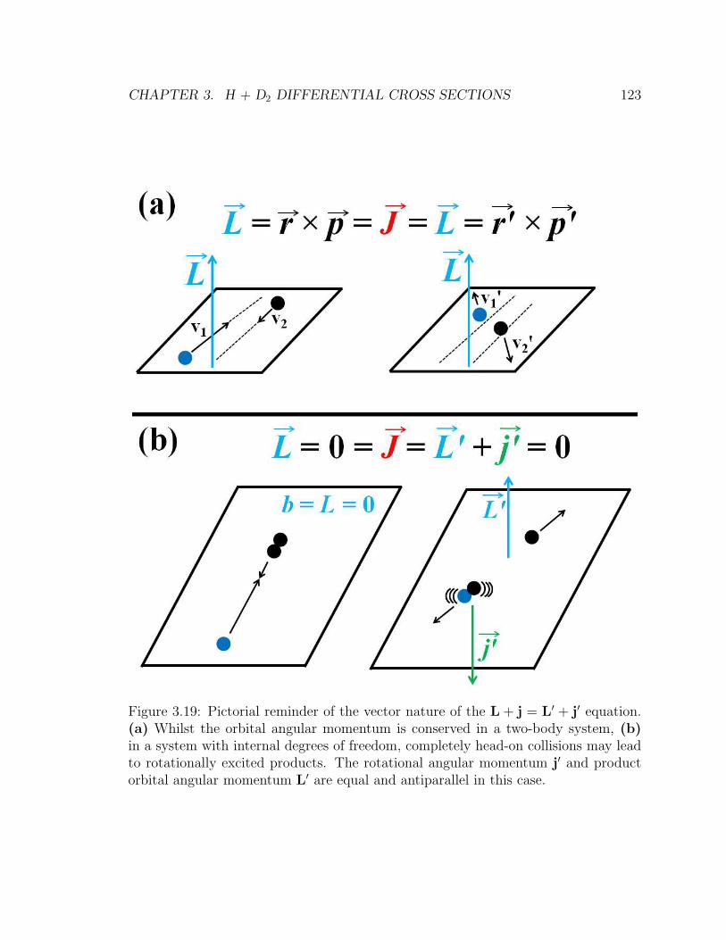
CHAPTER 3. H + D2 DIFFERENTIAL CROSS SECTIONS 123
Figure 3.19: Pictorial reminder of the vector nature of the L + j = L′ + j′ equation.(a) Whilst the orbital angular momentum is conserved in a two-body system, (b)in a system with internal degrees of freedom, completely head-on collisions may leadto rotationally excited products. The rotational angular momentum j′ and productorbital angular momentum L′ are equal and antiparallel in this case.
CHAPTER 3. H + D2 DIFFERENTIAL CROSS SECTIONS 124
rotationally excited HD products. It does not mean that low impact-parameter tra-
jectories cannot in principle lead to high j′ HD states; they can, albeit with a lower
probability than high b collisions. In summary, the guiding principles (i) and (ii) are
useful for building our understanding of the H + H2 scattering dynamics. It should
be kept in mind, however, that the total angular momentum conservation law is a
vector equation, and should be used as such.

Chapter 4
Geometric Phase in H + HD → H
+ HD
4.1 Geometric Phase and I
I have a very good recollection of how and when I found out about the geometric phase
for the first time. Days after I joined the H + H2 project in the Zarelab in January of
2009, I walked into the lab and asked Noah Goldberg and Nate Bartlett about the ex-
perimental progress. Jokingly Noah replied, ’Well, while you were away we measured
the geometric phase effect in H + H2’. I had no idea what geometric phase was, and
felt very ignorant not being able to reply to this comment. I started reading about
classical and quantum mechanical parallel vector transport, conical intersections, hy-
perspherical coordinates, topologically undeformable paths in N−dimensional space,
and even though I understood almost none of it, I realized what geometric phase
meant for the reaction dynamics community in general, and the H + H2 afficionados
in particular - this was THE ultimate H + H2 experiment. Even though it would take
me another three years to properly understand the geometric phase and its effects in
HER, I knew right away that I wanted to do the ultimate experiment. Although we
have come close to observing a signature of geometric phase in the H + H2 reaction,
we ran out of experimental resolution, or, more precisely, experimental time... The
quest continues.
125

CHAPTER 4. GEOMETRIC PHASE IN H + HD → H + HD 126
4.2 What is Geometric Phase?
A good way to start the geometric phase tale, from here on abbreviated as GP, is to
take a pencil, a piece of flat paper, and a basketball. A pencil will play a role of a
vector. Draw a circle on a flat piece of paper, and any closed path on a sphere. Next,
transport the pencil around the two closed paths on a piece of paper and around
the basketball. The results of this thirty-second experiment are shown in Fig. 4.1.
Even though the pencil ends up in the same position on a two- and three-dimensional
journey, there is one key difference: the pencil on a sphere does not point in the same
direction that it started with. The subtended angle α is the simplest example of a
geometric phase.
Although, the actual discussion of GP in molecular systems is more complicated,
the above example is remarkably informative. For example, it is evident that the GP
will depend on the dimensionality of a problem, and the connection is made with
molecular systems where the potential energy is often a function of 3N − 6 degrees
of freedom, in other words it is multi dimensional. The actual value of α in Fig. 4.1
depends on the path taken by the pencil. For a perfect sphere,
α =A
r2(4.1)
where A is the area enclosed by the closed path, and r is the radius of a sphere.1 For
a particular path shown in Fig. 4.1b, the closed path encompasses 1/8 of the sphere’s
surface. Because the sphere’s surface is 4πr2, this translates into an enclosed area of
A = πr2/2, and Eq. 4.1 tells us that α = π/2, as drawn in Fig. 4.1. The illustrated
ideas of topology are borne out in the molecular world.
Physicists were once again ahead of chemists in the field of GP effects. The most
1For an oddly-shaped object, the angle α is given by
α =
∫
RdA
where R is the local curvature. (For a sphere R = 1/r2, and one recovers Eq. 4.1.)

CHAPTER 4. GEOMETRIC PHASE IN H + HD → H + HD 127
Figure 4.1: Schematic showing the simplest example of a geometric phase. (a) Clas-sical parallel vector transport along a closed loop on a curved manifold results in anon-zero angle α, whereas (b) an analogous procedure in a flat space yields α ≡ 0.

CHAPTER 4. GEOMETRIC PHASE IN H + HD → H + HD 128
widely known Aharonov-Bohm (AB) effect first emerged from thought experiments
that involved electrons going around a closed loop, and then interfering. Aharonov
and Bohm noted that if a solenoid is put inside the loop, the electron interference pat-
tern is altered [110]. The concept of a solenoid inside a closed loop entails a non-zero
magnetic field inside the solenoid, but zero fields outside it. This is the reason why the
statement by Aharonov and Bohm that the electron interference can be affected by
the insertion of a solenoid, seemed so puzzling at first: how can particles be affected
in any measurable way in the absence of fields, and, consequently, forces? The answer
comes from the heart of quantum mechanics. The argument is rather complex, but
the main qualitative details are straightforward. The classical Hamiltonian for an
electron in an electromagnetic field is given by [111]
H = eφ+ (p− eA)2/2me (4.2)
where p is the particle’s momentum, and A and φ are the so-called vector and scalar
potentials, respectively. (Quantum Hamiltonian is obtained by replacing classical
momentum and energy by their appropriate quantum mechanical operators.) The
vector and scalar potentials can be related to classical electric, E, and magnetic, B,
fields via
E = −1
c
∂A
∂t−∇φ (4.3)
B = ∇×A (4.4)
Classically, for example, the equation of motion for an electron in an electromagnetic
field can be written in terms of electric and magnetic fields alone (for c≫ v),
mdv
dt= eE+
e
cv ×B (4.5)
where v is the velocity of a particle. Quantum mechanically, ’equation of motion’,
or wavefunction, is obtained by solving the time-dependent Schrodinger’s equation.
The origin of the geometric phase comes from a closer consideration of Eqs. 4.3 and
4.4. For certain A and φ potentials, the E and B are uniquely determined. For a

CHAPTER 4. GEOMETRIC PHASE IN H + HD → H + HD 129
given set of E and B, however, there exists a family of A′ and φ′, where
A′ = A+∇f(r, t) (4.6)
φ′ = φ− ∂f(r, t)
∂t(4.7)
with f(r, t) as a scalar function. From Eqs. 4.3 and 4.4 it follows that E and B fields
corresponding to particular A and φ potentials, are not altered upon A → A′, and
φ → φ′ transformation.2 This is, of course, the famous gauge transformation [112].
Classical electrodynamics is manifestly gauge invariant, i.e. the equations of motion
remain unchanged upon the class of transformations shown in Eqs. 4.6 and 4.7.3
Quantum electrodynamics however is also gauge invariant, although in a less obvious
manner than the classical counterpart [113, 114]. Thus, it remained unclear, at least
prior to Aharonov and Bohm’s paper [110], how the interference of two electron beams
going around a closed loop can be affected by the insertion of a solenoid. Given the
above, we can show that (i) for A = ∇f(r, t), B = 0, i.e. particles experience no
force, and (ii) crucially, the wavefunction corresponding to a quantum mechanical
analog of classical Hamiltonian in Eq. 4.2, is not gauge invariant. One can show this
by considering time-dependent Schrodinger’s equation,
ih∂
∂tΨ = HΨ (4.8)
with H = eφ + (p − eA)2/2me, and H ′ = eφ′ + (p − eA′)2/2me, where A′ and φ′
are given in Eqs. 4.6 and 4.7. By inserting the two Hamiltonians in Eq. 4.8 and
doing the algebra, one finds that the two wavefunctions corresponding to H and H ′
are related by
Ψ(r, t)′ = exp(
ie
hf(r, t)
)
Ψ(r, t) (4.9)
2Using the ∇× (∇f(r, t)) = 0 identity.3The easiest, but not rigorous, way to see this is to look at Eq. 4.5 - the theory must be gauge
invariant, because vector and scalar potentials do not appear in Eq. 4.5!

CHAPTER 4. GEOMETRIC PHASE IN H + HD → H + HD 130
Figure 4.2: Illustration of the Aharonov-Bohm (AB) effect, that predicts a changein the interference pattern between two electron packets (a) without and (b) with asolenoid present. Even though the magnetic field B is zero outside solenoid, and elec-trons experience no forces whilst going around the current-carrying wire, the presenceof a ∇f(r, t) term in the vector potential does influence the electron’s wavefunction,which is not gauge invariant.
Consider what happens when an electron follows a particular path 1 in Fig. 4.2b. In
this region, A = ∇f(r, t) and B = 0. Wavefunction now acquires a total phase of
Φ1 =e
h
∫
path 1
A · dr (4.10)
For electron following path 2,
Φ2 =e
h
∫
path 2
A · dr (4.11)

CHAPTER 4. GEOMETRIC PHASE IN H + HD → H + HD 131
The phase difference, ∆Φ = Φ1 − Φ2 is
∆Φ =e
h
∮
A · dr = e
h
∫
S
B · dS (4.12)
where Stokes theorem was used to obtain the second equality, using the fact that
∇ × A = B. The second integral in Eq. 4.12 is the magnetic flux through area S
enclosed by path 1 and path 2 in Fig. 4.2. Thus, the electron interference pattern in
the absence of a solenoid will be different from the one in the presence of a current-
carrying wire! Mathematically,
Ino solenoid = |Ψ1 +Ψ2|2 (4.13)
Isolenoid = |Ψ1 + exp(
ie
h∆Φ
)
Ψ2|2 (4.14)
where ∆Φ is given by Eq. 4.12 and is clearly path dependent. These are the bare
bones of the AB effect. The mathematics however is simple enough for an ’uninitiated
dynamicist’ to follow through.
There are of course many more GP manifestations. Rotations by 360 is a good
example. While ’rotation of 2π of the entire universe in unobservable’ [115], rotating
part of the system may have measurable GP effects. Several types of geometric phase
have been discovered prior to 1984; that year Berry showed that these seemingly un-
related effects can all be derived by considering an adiabatic trasport of a quantum
system around a closed path [116]. Geometric phase and Berry’s phase since then
are used almost interchangeably. A collection of various types of geometric phase
observed and proposed can be found in Geometric Phases in Physics [117].
Common thought experiments performed by physicists involved electrons, as op-
posed to molecules. The investigation of GP effects in molecular systems was left
to chemists. Herzberg (undeniably a chemist) and Longuet-Higgins are often cred-
ited as being pioneers in the study of molecular GP effects. In a brief communication
they considered a system of three 2S atoms [118]. Three ground state hydrogen atoms

CHAPTER 4. GEOMETRIC PHASE IN H + HD → H + HD 132
exhibit a conical intersection at all equilateral triangle (D3h) geometries. To see this,
consider the orbital correlation diagram in Fig. 4.3. It is clear from the drawing that
when the three atoms find themselves in a configuration of an equilateral triangle,
the energies of formerly non-bonding and antibonding molecular orbitals become de-
generate. This degeneracy has been referred to as a conical intersection (CI). It is a
result of intersection of ground and first excited electronic states of H3, both of the
same symmetry 2A′.4 The seam of a conical intersection in H3 is a line. In other
words, conical intersection occurs for equilateral triangle configuration of three hy-
drogen atoms, but the ’area’ of an equilateral triangle may vary. The world of conical
intersections is a rich one, but we shall not go into any more detail here, suffice it to
say that the CI in H3 is a real one and cannot be removed by applying a higher order
perturbation theory, for example [119–121].
Although von Neumann and Wigner [123], as well as Teller [126] have shown that
potential energy surfaces of the same symmetry may cross in polyatomic molecules,
it was Herzberg and Longuet-Higgins who noticed that the electronic wavefunction
changes sign, when the nuclear coordinates are transported (2π rotation) around the
CI. In essence, if the two electronic wavefunctions corresponding to the ground and
electronically excited states are known, e.g. φ1 and φ2, then, following a ’classic’
quantum mechanical rule of ’take linear combinations when things become degener-
ate’, the two wavefunctions in the vicinity of the conical intersection will be a linear
combination of the two orthogonal wavefunctions φ1 and φ2, i.e.
ψ = c1φ1 + c2φ2 (4.15)
4Intersection of potential energy surfaces of the same symmetry is yet another window into thehistory of physics! Such states cannot intersect in the case of a diatomic molecule [122]. It has beensuggested that in molecular systems with more than one vibrational degree of freedom, surfaces ofthe same system may intersect [123, 124], but this has been debated even up to 1970s [125]. Thedebate appears to be settled now: potential energy surfaces of polyatomic molecules of the samesymmetry may intersect.

CHAPTER 4. GEOMETRIC PHASE IN H + HD → H + HD 133
Figure 4.3: Electronic level correlation diagram for the H3 system as a function of thebend angle α. At all equilateral triangle geometries the H3 configuration has doublydegenerate electronic state.
CHAPTER 4. GEOMETRIC PHASE IN H + HD → H + HD 134
Solving a 2 × 2 secular determinant one obtains the two energies corresponding to
ψ1 and ψ2,5 exactly as was done by Teller [126]. Herzberg and Longuet-Higgins went
further, and computed the c1 and c2 coefficients [118]
ψ1(θ) = sin(θ/2)φ1 − cos(θ/2)φ2 (4.16)
ψ2(θ) = − sin(θ/2)φ1 + cos(θ/2)φ2 (4.17)
where θ is the angle that defines movement around the conical intersection. (The
ψ dependence on nuclear and electronic coordinates has been suppressed. In fact,
angle θ has implicit dependence on nuclear coordinates.) The surprising result is that
upon a 2π rotation, i.e. when the system returns to where it started, both electronic
wavefunctions change sign!6
ψ1(θ + 2π) = −ψ1(θ) (4.18)
ψ2(θ + 2π) = −ψ2(θ) (4.19)
The sign change is purely due to the presence of a conical intersection. The two
orthogonal wavefunctions φ1 and φ2 are ’mixed’ by the conical intersection. Herzberg
and Longuet-Higgins’ paper [118] would have made an even greater contribution had
the authors pointed out the fact that, in a molecular system, the total wavefunction
must remain single-valued. To a very good Born-Oppenheimer approximation, the
total molecular wavefunction can be written as a product of electronic, nuclear, and
nuclear spin wavefunctions,7
Ψtotal(θ) = ψelec(θ)χnuc(θ)ξI (4.20)
5ψ1 and ψ2 are wavefunctions corresponding to the top and bottom sheaths of the potentialenergy surface in the vicinity of a conical intersection.
6Using the fact that sin(θ + π) = − sin(θ), and cos(θ + π) = − cos(θ).7At first, it may seem contradictory to invoke the Born-Oppenheimer approximation in an obvious
presence of electronic degeneracy, i.e. when the Born-Oppenheimer assumption breaks down. Theapproximation of Eq. 4.20, however, is to do with the fact that the nuclear dynamics takes placesolely on the lower potential energy sheet.

CHAPTER 4. GEOMETRIC PHASE IN H + HD → H + HD 135
Thus, if ψelec(θ + 2π) = −ψelec(θ), then in order to have Ψtotal(θ + 2π) = Ψtotal(θ),
one has
χnuc(θ + 2π) = −χnuc(θ) (4.21)
This is an important formula for anyone doing experiments with atoms and molecules,
as there is a possibility of observing the nuclear wavefunction sign change experimen-
tally!8 An experimentalist therefore asks, ’How does the nuclear wavefunction sign
change in Eq. 4.21 manifest itself, and how can it be measured?’.
4.3 GP in H + H2
Discussion of the AB effect in Sec. 2.1 contains a key ingredient to observing the
GP effects in the H + H2 reaction: the sign change of electron’s wavefunction in
the presence of a solenoid can be seen via the interference term, Fig. 4.2b. This is
also true for the H + H2 system: the nuclear wavefunction sign change, Eq. 4.21,
may be observed via an interference. More precisely, trajectories, or wavefunctions,
that encircle the conical intersection will interfere with those that do not encircle
the conical intersection. To understand these effects better, one needs to ’visualize’
the dynamics of H + H2 scattering. A very classical picture in shown in Fig. 4.4:
a pathway wherein a hydrogen atom strikes a deuterium molecule to make an HD
product in a direct manner, will interfere with a pathway in which H atom goes
around the conical intersection, reacts with D2 molecule, and HD product recoils
away. Unfortunately, this is only a qualitative way of thinking about the H + H2
scattering. Better and, sadly, much more mathematically involved ways, have been
invented to describe molecular processes. We shall discuss briefly the hyperspherical
method, wherein conical intersection encirclement can be visualized more easily.
8Indeed, the nuclear wavefunction sign change resembles the AB effect, vide supra; consequently,the geometric phase effect in molecular systems has been ingeniously called Molecular Aharonov-Bohm (MAB) effect [127].

CHAPTER 4. GEOMETRIC PHASE IN H + HD → H + HD 136
Figure 4.4: Cartoon illustrating the interference between two pathways: a direct one,wherein the incoming hydrogen atom ’reacts’ with D2 molecule in a direct manner,and a looping pathway, wherein the H atom comes close to the deuterium molecule,then goes around the conical intersection (marked ’x’ in the figure), and then ’reacts’with the D2 molecule. Note that the interference will be noticeable only if the twopathways scatter HD products into the same angular space, as shown in the cartoon.

CHAPTER 4. GEOMETRIC PHASE IN H + HD → H + HD 137
Figure 4.5: Jacobi coordinates for a A + BC collision.
4.3.1 Hyperspherical Coordinates
A mathematical description of reactive scattering like H + D2 → HD + D is challeng-
ing, because different coordinates must be used for reactants and products. Although
these problems have been largely overcome, the visualization of these highly dimen-
sional graphs is difficult. Kuppermann pioneered the use of so-called hyperspherical
coordinates to ’show’ reactant and product potential energy contours for a reaction
like H + D2 → HD + D [128]. For a general A + BC reaction, the three internal
degrees of freedom can be conveniently taken as vectors representing the diatomic
separation in BC, the separation between A and the BC center of mass, and the an-
gle between these two vectors, see Fig. 4.5. The set of variables is known as Jacobi

CHAPTER 4. GEOMETRIC PHASE IN H + HD → H + HD 138
coordinates. Hyperspherical coordinates are defined as [128]
ρ =√S2 + s2 (4.22)
ϑ = 2 tan−1(s/S) (4.23)
where S = aR and s = r/a, and a =√
a(1−mA/M)µ
, where M = mA + mB + mC is
the total mass of a system, and µ =√
mAmBmC/M is the three-body reduced mass.
Next, a Cartesian mapping of Eqs. 4.22 and 4.23 is obtained through [128]
x = ρ sinϑ cos γ (4.24)
y = ρ sinϑ sin γ (4.25)
z = ρ cosϑ (4.26)
Visualization of a A + BC reaction is facilitated through xy, xz, and yz plots [129].
Often one plot is sufficiently informative, at least for visualization of the conical
intersection in the case of H + H2. Althorpe used the xz plots [130] via
u =√x2 + z2 (4.27)
α = tan−1(z/x) (4.28)
A typical plot for H + H2 reaction is shown in Fig. 4.6. The three distinct reaction
channels are evident. In this figure, the outermost circle represents all linear H3
geometries. The transition states are found halfway between any two entrance/exit
channels. All points closer to the center correspond to bent H3 configurations. The
center of the diagram, in the case of H + H2, represents the conical intersection.
In other words, movement of a point in the hyperspherical coordinate diagram (Fig.
4.6) represents progressive change from one nuclear configuration to another. We are
now ready to discuss the conical intersection encirclement in the H + H2 reaction.
There are two ways this can be done: dynamic and symmetric encirclement, which
are discussed individually.

CHAPTER
4.
GEOMETRIC
PHASEIN
H+
HD→
H+
HD
139Figure 4.6: Hyperspherical coordinate diagram for the H + H2 scattering. Each hydrogen atom is treated as beingdistinguishable. For a highly symmetric H3 system, the conical intersection is located in the center of a ’circle’, and thethree β angles are equal.

CHAPTER 4. GEOMETRIC PHASE IN H + HD → H + HD 140
4.3.2 GP1: Dynamic Encirclement
Let us consider the H + H2(v = 0, j = 0) → H2(v′, j′ − odd) + H reaction. The
distinguishability of the three H atoms is evident from the hyperspherical diagram
shown in Fig. 4.7. Note that the H2(v′, j′ − odd) products can only come from reac-
tive scattering, as inelastic collisions can only lead to H2(v′, j′ − even) products. To
get the correct experimental observables, the total wavefunction must be antisym-
metrized with respect to exchange of any two fermionic hydrogen atoms [131]. For a
dynamic encirclement, however, one can neglect one of the H + H2 channels, and only
concentrate on two of them, e.g. H1 + H2H3 and H2 + H1H3, as indicated by solid
and dashed arrows in Fig. 4.7. Two pathways are shown: a direct pathway, with an
associated scattering amplitude fd, and a looping pathway, fl. As first pointed out by
Mead and Truhlar [132], and later worked out in detail by Althorpe and co-workers
[133], the DCS is proportional to9
dσ
dΩ
(NGP )
= |fd + fl|2 (4.29)
dσ
dΩ
(GP )
= |fd − fl|2 (4.30)
where NGP and GP stand for calculations that ignore and include the geometric
phase, respectively. As advertised, the geometric phase effects can be seen in an
interference experiment. In this case, the interference is between direct and looping
pathways of the H + H2 reaction. Notice that analogous conclusions also hold for
the H + D2 → HD(v′, j′) + D reaction, where the reactants and products need not
be identical in order to exhibit interference between direct and looping pathways,
Fig. 4.7. From a ’chemical’ point of view, direct and looping mechanisms are of very
different nature: looping pathway undergoes two transition states, whereas the direct
mechanism has only one transition state. This is where the power of hyperspherical
diagrams comes forward in helping one see the number of transition states involved,
9This is, of course, the end result of an involved calculation. This is in a way similar to ourdiscussion of the AB effect: after some mathematics, the end result, Eqs. 4.13 and 4.14, is verysimilar to Eqs. 4.29 and 4.30.

CHAPTER
4.
GEOMETRIC
PHASEIN
H+
HD→
H+
HD
141Figure 4.7: Hyperspherical coordinate diagram for the H + H2 reaction at Ecoll > 4 eV. Red lines (solid and broken)show a direct reactive scattering, blue lines (solid and broken) show a looping reactive scattering. Inelastic scattering,and analogous reactive/inelastic pathways originating from the two other H + H2 channels are not shown to avoid clutter.Angle φ is the encirclement angle.

CHAPTER 4. GEOMETRIC PHASE IN H + HD → H + HD 142
see Figs. 4.6 and 4.7. In order to see a considerable interference between fd and fl,
these two terms must be comparable in magnitude. Early calculations by Kupper-
mann and co-workers have shown significant NGP anf GP differences for H + H2
reaction and its isotopologues. Significant GP and NGP differences were predicted
in the rotational state distributions for the D + H2 → HD(v′, j′) + D reaction [134],
seemingly solving the problem of a disagreement between experiment and theory that
did not include the geometric phase [135]. Pronounced NGP and GP differences were
also predicted in the DCS for H + D2 → HD(v′, j′) + D reaction [136–138]. The work
of Kendrick [139, 140] and Althorpe and his co-workers [133, 141–145], have defini-
tively established that geometric phase effects are negligible in H + D2 → HD(v′, j′)
+ D, or H + H2(v = 0, j = 0)→ H2(v′, j′− odd) + H reactions for Ecoll < 4 eV. This
agrees with our ’chemical’ intuition: H + D2 trajectories with 2 transition states (fl)
are less likely than collisions going over 1 transition state. Indeed, at Ecoll = 2.3 eV,
only 2 · 10−4 % of all trajectories pass over 2 transition states. At Ecoll = 4.3 eV, on
the other hand, the fraction of fl rises to about 1/3 [146]. Thus, one way to measure
GP effects in the H + D2 → HD(v′, j′) + D reaction is by increasing the collision
energy to about 4 eV.
Achieving Ecoll = 4 eV experimentally is not trivial. In the current set-up, H atoms
are generated via the photolysis of HBr and HI diatomics. The shortest wavelength
that can be easily obtained is λ = 199 nm. This corresponds to Ecoll = 2.5 eV if HI
is employed. Shorter wavelengths can be generated by high-harmonic generation in
noble gases, however this method suffers from very low conversion efficiencies. Al-
ternatively, one can use a fluorine laser with λ = 157 nm; this would correspond to
Ecoll = 3.85 eV. We think this is the most promising way of observing GP effects in
the H + H2 reaction.
There is also another way of generating very fast hydrogen atoms. One could imagine
using high laser intensities to achieve a two-photon photodissociation of HBr or HI,
as opposed to the usual one-photon approach. I have spent a lot of time working on
two-photon dissociation of HBr. To make a very long story short, I have managed to

CHAPTER 4. GEOMETRIC PHASE IN H + HD → H + HD 143
observe a signal corresponding to H atoms from a two-photon photodissociation of
HBr, but the number density of these hyper fast H atoms proved to be too low to be
useful in the H + D2 reaction. I did a [2+1] H atom REMPI at λprobe = 243.068 nm,
and set λphoto = 286.5 nm. The ratio of H atoms corresponding to λphoto = 143 nm,
i.e. two-photon dissociation of HI, to H atoms coming from a one-photon dissociation
of HI at λ = 286.5 nm, was between 1:100 and 1:1000. (Large background due to HI
photolysis at 243 nm prevented an accurate measurement.) Wittig and co-workers
have observed a similar H atom signal due to a two-photon photodissociation of HI
at λphoto = 266 nm [147]. It appears that the ratio of ’two-photon’ H atoms to ’one-
photon’ H atoms is about 1:240, which is consistent with current findings. It seems
therefore that the most viable option of producing fast hydrogen atoms, with the
current experimental set-up, is to use λphoto = 157 nm by employing a fluorine laser.
4.3.3 GP2: Symmetric Encirclement
Another manifestation of the geometric phase in the H + H2 reaction is through
interference of reactive and inelastic scattering. Consider the H + HD → HD(v′, j′)
+ H reaction. The hyperspherical diagram is shown in Fig. 4.8. Notice that the
looping pathways are intentionally not shown, because at Ecoll < 4 eV they make a
negligible contribution to the reaction rate. The interference comes from the fact that
the two H atoms are indistinguishable. Thus, the inelastic H1 + H2D → H2D + H1
scattering will interfere with the reactive H2 + H1D → H2D + H1 scattering (solid
lines in Fig. 4.8). Analogous argument applies to the H2 + H1D channel (dotted lines
in Fig. 4.8). Unlike the dynamic encirclement, where the effect of geometric phase
must be taken into account either by introducing a vector potential in the Hamiltonian
for the H + HD→ HD + H scattering, or by replacing a double-valued real electronic
wavefunction by a single-valued complex electronic wavefunction, the GP and NGP
differences for reactive and inelastic scattering interference as measured in the DCS
can be expressed by simply changing the sign of the reactive scattering amplitude fR
[148]. As was shown by Bill Miller, the DCS for a A + AB → AB + A chemical

CHAPTER
4.
GEOMETRIC
PHASEIN
H+
HD→
H+
HD
144Figure 4.8: Hyperspherical coordinate diagram for the H + HD reaction at Ecoll < 4 eV. At low collision energies loopingpathways are negligible. Conical intersection is encircled symmetrically, and the GP manifests itself through the interferenceterm between reactive pathway (fR, red lines), and inelastic pathway (fNR, blue lines).

CHAPTER 4. GEOMETRIC PHASE IN H + HD → H + HD 145
reaction is given by [149]
dσ
dΩ=
1
2(1 + λ)|fR + fNR|2 +
1
2(1− λ)|fR − fNR|2 (4.31)
where λ = (−1)2s/(2s+ 1), and s is the nuclear spin of atom A. For hydrogen atom,
s = 1/2, so λ = −1/2. Thus, ignoring the geometric phase effect, the differential
cross section for the H + HD → HD + H reaction is given by
dσ
dΩ
(NGP )
= |fR|2 + |fNR|2 +1
2|f ∗
NRfR + f ∗RfNR| (4.32)
The GP effect can be incorporated by changing the fR sign in Eq. 4.31, This yields,
dσ
dΩ
(GP )
= |fR|2 + |fNR|2 −1
2|f ∗
NRfR + f ∗RfNR| (4.33)
As it turns out, the magnitude of fR and fNR for most HD(v′, j′) states studied are
comparable. It would seem therefore that the gates to GP are open! Unfortunately,
the resulting oscillatory term, fRf∗NR + f ∗
RfNR, exhibits very fine oscillations, often
less than 10. In addition, experiments wherein the detected species is the same as
the molecular beam species, often have a large background and very poor S/N ratios.
In spite of all this, an attempt to ’scale mount GP’ has been taken!
4.4 DCS for H + HD → HD(v′, j′) + H
Before starting the hunt for GP effects in the H + HD reaction, DCS for several
HD(v′, j′) product states have been recorded to establish the fact that the experi-
mental signal is indeed a sum of reactive and inelastic scattering in the H + HD →HD + H reaction. Note that HD does not exist in ortho-para modifications, unlike its
H2 and D2 cousins. Thus, inelastic H + HD(v, j−odd(even))→ HD(v′, j′−even(odd))+ H transitions are allowed.10 Unlike all other theoretical DCS in this work, H +
10Supersonic expansion yielded 33 % HD(v = 0, j = 0), 37 % HD(v = 0, j = 1), and 20 %HD(v = 0, j = 2). The rest of the population is in j > 2 states. These states however were nottaken into account when performing QM calculations.

CHAPTER 4. GEOMETRIC PHASE IN H + HD → H + HD 146
HD reaction has been treated by time-independent QM (TI-QM) as carried out by
Bouakline and Althorpe. The results have undergone an identical blurring proce-
dure to the one for the H + D2 reaction. A total of five states have been studied:
HD(v′ = 1, j′ = 8), HD(v′ = 1, j′ = 12), and HD(v′ = 1, j′ = 13) at Ecoll = 1.86
eV, HD(v′ = 2, j′ = 3) at Ecoll = 1.46 eV, and HD(v′ = 2, j′ = 5) at Ecoll = 1.44
eV. The first three states have been studied under two-laser conditions, i.e. a dedi-
cated photolysis and a probe laser, whereas the latter two product states have been
interrogated under one-laser conditions. (For a more detailed description of one- and
two-laser experimental conditions see Sec. 2.5.)
An example of raw and processed experimental speed distribution for HD(v′ = 2, j′ =
3) product state is shown in Fig. 4.9. As mentioned earlier, detection of HD(v′, j′)
reaction products when the molecular beam is composed of more than 90% per-
cent of HD, leads to a marked increase in background. Non-resonant ionization of
HD(v = 0, j′ = 0, 1, 2) reactant leads to a peak centered at ∼ 1300 m/s, clearly visi-
ble in Fig. 4.9a. All five states studied were chosen such that the reactive HD(v′, j′)
signal, or the Photoloc speed range, did not overlap with this large HD peak. Notice
also that the HD(v′ = 2, j′ = 3) signal is small outside the Photoloc speed range (as
indicate by the vertical bars in Fig. 4.9), giving us confidence in our method. The
corrected HD(v′ = 2, j′ = 3) laboratory speed distribution is obtained by subtracting
the ’Offline scan’ signal from the ’Online scan’ signal, shown in in Fig. 4.9b. Finally,
the corrected signal is converted into a DCS, and these are shown in Fig. 4.10.
A visual examination of Fig. 4.10 makes it obvious that the experimental measure-
ment is a sum of reactive and inelastic H + HD → HD + H scattering. There are,
of course, two types of ’sums’: an incoherent and a coherent one. The latter is given
in Eqs. 4.32 and 4.33. If, however, the interference term is small, the experimental
signal is going to be mainly due to
dσ
dΩ
(incoh)
= |fR|2 + |fNR|2 (4.34)

CHAPTER 4. GEOMETRIC PHASE IN H + HD → H + HD 147
Figure 4.9: (a) Raw and (b) processed experimentally measured HD(v′ = 2, j′ = 3)laboratory speed distribution.

CHAPTER
4.
GEOMETRIC
PHASEIN
H+
HD→
H+
HD
148
Figure 4.10: DCS for HD(v′ = 1, j′ = 8) product at Ecoll = 1.86 eV. Red dots have the same meaning as in Fig. 3.8. Allcurves are TI-QM calculations: blue curve is for a reactive H + HD→ HD + H scattering, green curve for inelastic process,and black curve in panel (a) is an incoherent sum of reactive and inelastic pathways. Panel (d) is a coherent sum of fRand fNR: black and light blue curves are GP and NGP curves, respectively.

CHAPTER
4.
GEOMETRIC
PHASEIN
H+
HD→
H+
HD
149
Figure 4.10 (continued): DCS for HD(v′ = 1, j′ = 12) product at Ecoll = 1.86 eV.

CHAPTER
4.
GEOMETRIC
PHASEIN
H+
HD→
H+
HD
150
Figure 4.10 (continued): DCS for HD(v′ = 1, j′ = 13) product at Ecoll = 1.86 eV.

CHAPTER
4.
GEOMETRIC
PHASEIN
H+
HD→
H+
HD
151
Figure 4.10 (continued): DCS for HD(v′ = 2, j′ = 3) product at Ecoll = 1.46 eV.
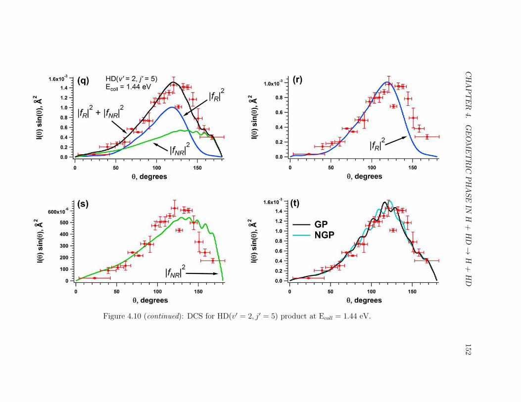
CHAPTER
4.
GEOMETRIC
PHASEIN
H+
HD→
H+
HD
152
Figure 4.10 (continued): DCS for HD(v′ = 2, j′ = 5) product at Ecoll = 1.44 eV.

CHAPTER 4. GEOMETRIC PHASE IN H + HD → H + HD 153
We call Eq. 4.34 an ’incoherent’ sum of reactive and inelastic scattering, blue and
green curves in Fig. 4.10. In other words, experimental signal fits an incoherent sum
|fR|2 + |fNR|2 much better than either |fR|2 or |fNR|2 alone. Finally, Figs. 4.10d,
4.10h, 4.10l, 4.10p, and 4.10t show an experimental fit to a coherent sum of reactive
and inelastic scattering. In this case, the GP effect is to change the relative sign
between the reactive and inelastic scattering amplitudes, resulting in two different
theoretical fits, dσdΩ
(NGP )and dσ
dΩ
(GP ), Eqs. 4.32 and 4.33, respectively.
To make the discussion of an experimental fit to theoretical coherent and incoherent
sums of reactive and inelastic scattering, we have carried out a least-squares analysis.
Because the experiment measures relative, and not absolute cross sections, one is free
to multiply the experimental DCS by a constant F to best fit theoretical calculations.
In other words,
S =i=N∑
i=1
(I(θi)theo − F · I(θi)exp)2 (4.35)
one must solve the ∂S∂F
= 0 equation to obtain Fbest.11 The use of Fbest in Eq. 4.35
yields residual sum of squares (RSS),
RSS =i=N∑
i=1
(I(θi)theo − Fbest · I(θi)exp)2 (4.36)
Upon a normalization of Eq. 4.36, one obtains the familiar R2 parameter
R2 ≡ 1−∑i=N
i=1 (I(θi)theo − Fbest · I(θi)exp)2
∑i=Ni=1 Fbest · I(θi)exp
(4.37)
where R2 = 1 indicates a perfect fit. The resulting R2 values for experimental fits to
a theoretical calculation of reactive, inelastic, and an incoherent sum of the two scat-
tering channels, are shown in Table 4.1. In all cases, the |fR|2 + |fNR|2 fit is superior
to either |fR|2 or |fR|2 fit. Thus, experimental signal is indeed a sum of reactive and
11The sum in Eq. 4.35 runs up to N , where N is the number experimental points, or bins, in aDCS.

CHAPTER 4. GEOMETRIC PHASE IN H + HD → H + HD 154
Table 4.1: R2 values for experimental fits to |fR|2+|fNR|2, |fR|2, and |fNR|2 theoreticalcalculations.
HD(v′, j′) R2
|fR|2 + |fNR|2 |fR|2 |fNR|2v′ = 1, j′ = 8 0.96 0.86 0.81v′ = 1, j′ = 12 0.89 0.76 0.54v′ = 1, j′ = 13 0.76 0.43 0.37v′ = 2, j′ = 3 0.97 0.91 0.88v′ = 2, j′ = 5 0.97 0.89 0.93
inelastic scattering in the H + HD → HD + H reaction.
It is worth pointing out an increased disagreement between experiment and theory
(for an incoherent sum of reactive and inelastic scattering) for HD(v′ = 1, j′ = 12)
and HD(v′ = 1, j′ = 13) product states, Figs. 4.10e and 4.10i. In a way the results
are ’encouraging’, because the observations are consistent with a disagreement seen
in the DCSs for HD(v′, high j′) products of the H + D2 reaction, discussed in Sec.
3.5. It appears that the solution of the ’disagreement puzzle’ for the H + D2 →HD(v′, high j′) + D may also solve the disagreement between theory and experiment
for HD(v′ = 1, j′ = 12, 13) products of the H + HD reaction.
We now turn our attention to a superposition of reactive and inelastic scattering
amplitudes, Eqs. 4.32 and 4.33. By looking at Figs. 4.10d, 4.10h, 4.10l, 4.10p,
and 4.10t it is clear that differences between GP and NGP calculations are very
small indeed. In addition, some states exhibit imperceptibly small differences, e.g.
HD(v′ = 1, j′ = 8) state, Fig. 4.10d, whilst others show somewhat more pronounced
differences, e.g. HD(v′ = 2, j′ = 5) product, Fig. 4.10t. A considerable amount of
time was spent browsing through over 300 theoretical DCSs, looking for cases that
exhibit the largest GP and NGP differences; the DCS for HD(v′ = 2, j′ = 5) product

CHAPTER 4. GEOMETRIC PHASE IN H + HD → H + HD 155
at Ecoll = 1.44 eV proved to be an example with one of the most pronounced differ-
ences between GP and NGP calculations. There were certain DCSs that exhibited
even larger GP/NGP differences than the HD(v′ = 2, j′ = 5) product at Ecoll = 1.44
eV; unfortunately, such HD(v′, j′) states had a very low reaction cross section, be-
yond our experimental capabilities. An example is shown in Fig. 4.11: GP and
NGP differences in the DCS for HD(v′ = 3, j′ = 4) product state at Ecoll = 1.37 eV
(Fig. 4.11a) are larger than the oscillations seen for the HD(v′ = 2, j′ = 5) reaction
product at a collision energy of 1.44 eV (Fig. 4.11b), however the cross section for
the former HD state is beyond our experimental ’patience’: the lowest cross section
measured in the current study (and perhaps in the Zarelab over its entire history) was
for HD(v′ = 4, j′ = 6) at Ecoll = 1.97 eV (Fig. 3.8e), with a count rate of 100 HD+
ions an hour. The cross section for HD(v′ = 3, j′ = 4) state is almost a thousand
times smaller - it would therefore take about 4000 days to measure a differential cross
section for this product!
The blurring of theoretical results due to a spread in the experimental collision en-
ergy, and a finite HD reactant rotational state distribution, washes out the GP and
NGP differences even more so than for the H + D2 → HD(v′, j′) + D reaction. Av-
eraging over HD(v = 0, j = 0, 1, 2) reactant states is particularly severe, as shown in
Fig. 4.12. This is due to an interesting fact that DCSs for a reactive scattering, i.e.
Ha + HbD(v, j = 0, 1, 2) → HaD(v′, j′) + Hb are rather similar, whereas DCSs for
inelastic Ha + HbD(v, j = 0, 2)→ HbD(v′, j′) + Ha collision are out of phase with the
DCSs for the Ha + HbD(v, j = 1) → HbD(v′, j′) + Ha process (Fig. 4.13). The origin
of this behavior is currently not completely understood, although a similar behavior
has been observed by Brouard and co-workers, in their study of inelastic Ar + NO
collisions, wherein parity-changing and parity-conserving collisions are out of phase
with each other [150–152].
Nevertheless, even after a considerable amount of blurring, the GP and NGP differ-
ences in the DCS for HD(v′ = 2, j′ = 5) product at Ecoll = 1.44 eV are still visible, Fig.
4.10t. About 9500 ions were used in constructing the DCS for HD(v′ = 2, j′ = 5)

CHAPTER 4. GEOMETRIC PHASE IN H + HD → H + HD 156
Figure 4.11: DCSs for (a) HD(v′ = 3, j′ = 4) and (b) HD(v′ = 2, j′ = 5) reactionproducts. Although HD(v′ = 3, j′ = 4) product shows more pronounced GP andNGP differences, the reaction cross section is prohibitively small.
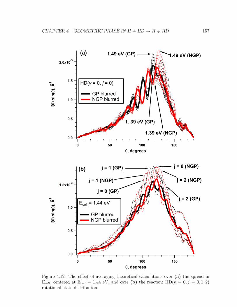
CHAPTER 4. GEOMETRIC PHASE IN H + HD → H + HD 157
Figure 4.12: The effect of averaging theoretical calculations over (a) the spread inEcoll, centered at Ecoll = 1.44 eV, and over (b) the reactant HD(v = 0, j = 0, 1, 2)rotational state distribution.

CHAPTER 4. GEOMETRIC PHASE IN H + HD → H + HD 158
Figure 4.13: DCSs for (a) Ha + HbD(v = 0, j = 0, 1, 2) → HaD(v′ = 2, j′ = 3) + Hb
reactive scattering, and (b) Ha + HbD(v = 0, j = 0, 1, 2)→ HbD(v′ = 2, j′ = 3) + Ha
inelastic scattering. The inelastic DCSs show a tremendous dependence on the initialrotational state of HD reactant.

CHAPTER 4. GEOMETRIC PHASE IN H + HD → H + HD 159
product. As can be seen from Fig. 4.10t, the agreement between theory and ex-
periment is good, however the ordinate error bars are large, and the experimental
points show a significant scatter - a classic example of low ’precision and accuracy’.
To reduce a random error by a factor of 2, four times as many ions are needed to
construct the DCS. Accuracy should also improve two-fold. A heroic effort was there-
fore undertaken to collect ’more’ ions in order to improve accuracy and precision.
Over a course of thirty days, 44446 ions were collected, and the resulting DCS for
HD(v′ = 2, j′ = 5) product is shown in Fig. 4.14. What a beauty! Even a quick glance
at Figs. 4.10t and 4.14 is enough to convince one that the ordinate error bars, as
well as the overall experimental accuracy have improved! Unfortunately, differences
between the experiment vs. GP and experiment vs. NGP fits are statistically (and
visually!) insignificant. Statistical analysis confirms this. Differential cross section
for the HD(v′ = 2, j′ = 5) product at a collision energy of 1.44 eV ( Fig. 4.14) is the
closest we have come to uncovering the GP effect in the H3 system.

CHAPTER
4.
GEOMETRIC
PHASEIN
H+
HD→
H+
HD
160
Figure 4.14: DCS for the HD(v′ = 2, j′ = 5) product at Ecoll = 1.44 eV. Red and green dots represent the best experimentalfit to NGP and GP theoretical calculations, respectively. The two experimental fits are barely distinguishable, suggestingthat the superiority of an experimental fit to either GP or NGP curve is insignificant.

Chapter 5
H + H2: Not Over Yet!
The definition of a complete understanding of a chemical reaction is not a clear-cut
one. When can we claim we truly understand HER? A quantitative agreement be-
tween theory and experiment is certainly a necessary ingredient, but, I believe, not a
sufficient one. One of the underlying principles of chemistry is to predict. This is one
of the reasons chemistry undergraduates get so lost in an organic chemistry course:
how is it possible to memorize thousands of seemingly different chemical reactions?
The answer is that there are only a few fundamental reaction mechanisms in organic
chemistry, and these few mechanisms, if properly understood, may be applied to a
multitude of ’different’ chemical reactions. If, however, we cannot build a model of
a chemical reaction, then predicting the outcome of related chemical transformations
is impossible. Angular distributions of the H + H2 reaction is a good example of
this. The proposed model for the correlation between the most probable scattering
angle and the rotational quantum number j′ of the diatomic product is now a more
complete one, because we understand that in addition to the negative j′ − θ corre-
lation, there exists also a positive j′ − θ correlation. In this sense, the current work
has been a success. On the other hand, the glaring disagreement between theory and
experiment, particularly for HD(v′, high j′) product states, remains an outstanding
issue. From this point of view, we clearly do not have a complete understanding of
the H + H2 chemical reaction.
161

CHAPTER 5. H + H2: NOT OVER YET! 162
One of the ’holy grails’ of the H + H2 reaction is the role played by the geometric
phase. Alas, we were not able to experimentally resolve minute differences between
theoretical calculations with and without the geometric phase. As mentioned earlier,
the best bet to experimentally observe the presence (or absence!) of the geometric
phase is by doing a high collision energy H + D2 → HD(v′, j′) + D experiment. Such
an experiment would be an important milestone in the history of hydrogen exchange
reaction.
To inch closer toward a complete understanding of the H + H2 reaction, one must
perform an ’ideal’ experiment, i.e.
H + H2(v, j,mj)→ H2(v′, j′,mj′) + H (5.1)
A substantial progress has been recently made on the ’reactant side’ of Eq. 5.1. A
molecular variant of the adiabatic rapid passage has been developed, with nearly
100% of H2(v = 0, j = 0,mj = 0) population being pumped into the H2(v′ = 1, j′ =
0,mj′ = 0) level [153, 154]. With a clever ionization scheme of H2 one could also
resolve individual product mj′ levels [155].
These are but two problems yet to be solved. We do not know however, how many sur-
prises the H + H2 reaction has in store for us! The discovery of backward-scattered
rotationally excited HD(v′ = 4, j′) products has been precisely such a surprise. It
would be interesting to see, for example, the differential cross sections for the H +
D2 → HD(v′ = 5, j′) + D reaction. One would think that scattering becomes even
more isotropic than the DCSs for HD(v′ = 4, j′) products. Only experiments will
tell! Finally, there are several trends in the H + H2 reaction still not completely ex-
plained. Theoretical calculations suggest that the excitation function (integral cross
section (ICS) as a function of collision energy) for reactive and inelastic H + HD →HD + H scattering exhibit very different shape/behavior, as shown in Fig. 5.1. The
most striking difference between reactive and inelastic scattering is that the integral
cross section for inelastically-scattered HD seems to keep increasing with increasing
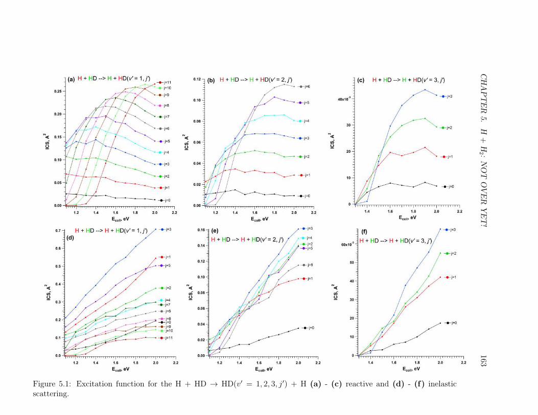
CHAPTER
5.
H+
H2 :
NOT
OVER
YET!
163
Figure 5.1: Excitation function for the H + HD → HD(v′ = 1, 2, 3, j′) + H (a) - (c) reactive and (d) - (f) inelasticscattering.
CHAPTER 5. H + H2: NOT OVER YET! 164
collision energy (at least within the collision energy range reported herein), whereas
reactively-scattered HD products’ ICS shows a marked dependence on j′: rotation-
ally cold HD(v′, j′) products’ integral cross section decreases with increasing collision
energy, at least for HD(v′ = 1, j′) vibrational manifold, whilst the ICS for rotation-
ally excited HD diatomics increases with increasing Ecoll, and then levels off/drops.
Surely a model is needed to explain this most interesting behavior! A novice reaction
dynamicist should seize the opportunity!

Appendix A
GP in H + HD → HD + H
A.1 Symmetric Encirclement of CI
In a way, the dynamic encirclement of a conical intersection in the H + H2 reaction
is easier to visualize than the symmetric case.1 For example, when the conical inter-
section is encircled dynamically, the geometric phase effect manifests itself without
any reference to identical nuclei. In other words, a reaction H + DT → HD + T at
Ecoll > 4 eV would show non-trivial GP effects, even though all nuclei are distinguish-
able. The dynamic encirclement can be seen ’visually’ by examining Fig. 3.7, where
direct and looping pathways clearly encircle the conical intersection. The differential
cross sections for the H + DT → HD(v′, j′) + T reaction are given by
dσ
dΩ
(NGP )
= |fd + fl|2 (A.1)
dσ
dΩ
(GP )
= |fd − fl|2 (A.2)
where the geometric phase effect is to change the sign of the looping scattering am-
plitude, fl, in Eq. A.2.
1As mentioned in Chapter 4, although the visualization of the dynamic CI encirclement is easier,the mathematical accommodation of GP effects is far more involved for the dynamic encirclementthan the symmetric case.
165

APPENDIX A. GP IN H + HD → HD + H 166
’Visualizing’ the symmetric encirclement of a CI in the H + H2 system is a little
less straightforward. We begin with Fig. A.1, where we show how the symmetrized
wavefunctions are obtained from the unsymmetrized ones. The hyperspherical dia-
gram for the symmetrized system makes the encirclement of a conical intersection
explicit. The D + H2 reaction channel is literally the key link here. As was shown
in Chapter 4, the differential cross section for the H + HD → HD + H reaction (a
reaction of the type A + AB → AB + A), forgetting for a second any GP effects, is
given bydσ
dΩ=
1
4|fR + fNR|2 +
3
4|fR − fNR|2 (A.3)
where fR and fNR are reactive and inelastic scattering amplitudes, respectively. If
desired, Eq. A.3 can be recast
dσ
dΩ= |fR|2 + |fNR|2 +
1
2|f ∗
RfNR + f ∗NRfR| (A.4)
Because the total symmetrized wavefunction (symmetrically) encircles the conical in-
tersection in the H + HD → HD+ H reaction (Fig. A.1), the question we have to
answer is, ’How is the differential cross section in Eqs. A.3 and A.4 affected by the
geometric phase?’. Mead has correctly suggested that, provided the dynamic encir-
clement is negligible, the only GP effect is the sign change in front of the fR in Eq.
A.3. We are interested in how to show, or derive, this sign change.
We begin with the so-called double cover space. It is convenient for the following
reason. When the electronic wavefunction completes one full (2π) revolution around
the conical intersection, it changes sign, i.e.
ψelec(φ+ 2π) = −ψelec(φ) (A.5)
How would this look like in the regular 0 → 2π hyperspherical coordinate diagram
(Fig. A.2c)? Let us start with the H1 + H2D channel. If we arbitrarily assign a ’+’
sign to ψelec(φ = 0), then, according to Eq. A.5, ψelec(φ = 2π) = −ψelec(φ = 0). This
implies that ψelec(φ = 2π/3) = −ψelec(φ = 0), ψelec(φ = 4π/3) = ψelec(φ = 0), and so

APPENDIX
A.GPIN
H+
HD→
HD
+H
167
Figure A.1: Graphical illustration of a symmetric conical intersection encirclement for the H + HD → HD + Hreaction. The conical intersection is encircled due to a proper total wavefunction symmetrization.

APPENDIX A. GP IN H + HD → HD + H 168
on, so that ψelec(φ = 4π) = ψelec(φ = 0). In a so-called 0 → 2π space each channel
will have a double-valued electronic wavefunction (Fig. A.2c). It is convenient to
map the 0→ 2π space onto an (unphysical) 0→ 4π space, where ψelec(φ) associated
with each channel is manifestly single-valued (Fig. A.2b and A.2d). As will be seen
momentarily, the use of 0→ 4π space simplifies the sign change analysis considerably.
Moreover, the (physical) 0 → 2π space can be recovered from the 0 → 4π space by
cutting a 2π slice from the latter.
The guiding principle in determining the GP effects in the DCS for the H + HD
→ HD + H reaction, Eqs. A.3 and A.4, is that the total molecular wavefunction for
the DH2 system,
Ψtotal(φ) = ψelec(φ)χnuc(φ)ξI (A.6)
must be antisymmetric under the exchange of two fermionic H atoms. Molecular
hydrogen has 3 symmetric, and 1 antisymmetric nuclear spin states, corresponding
to ortho-H2 and para-H2, respectively. The task is then to investigate the sign of the
nuclear wavefunction for each H2 species, i.e. ortho-H2 and para-H2, without and with
the geometric phase. As can be seen from Fig. A.2a and A.2b, the NGP condition is
that the ψelec(φ+ 2π) = ψelec(φ), so that the electronic wavefunction is single-valued
even in the 0→ 2π space (Fig. A.2a).
Let us draw a properly symmetrized hyperspherical coordinate diagram in the 0→ 4π
space for ortho-H2 and para-H2 species, with and without the geometric phase effect.
This is shown in Fig. A.3: panels a, b, c, d correspond to NGP para-H2, NGP
ortho-H2, GP para-H2, and GP ortho-H2 conditions, respectively. In all cases we
shall start our analysis in the D + H2 channel on the top left, because at large D and
H2 separations the H2 electronic wavefunction is symmetric under the exchange of
two H atoms (1Σ+g state), so that the nuclear wavefunction χnuc must be symmetric
for para-H2, and antisymmetric for ortho-H2, so that in both cases the total molec-
ular wavefunction in Eq. A.6 is antisymmetric under the permutation of two H atoms.
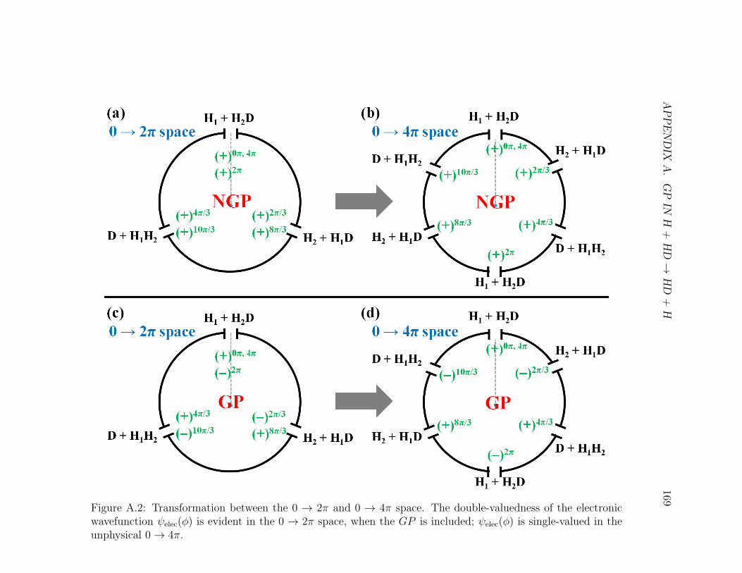
APPENDIX
A.GPIN
H+
HD→
HD
+H
169
Figure A.2: Transformation between the 0 → 2π and 0 → 4π space. The double-valuedness of the electronicwavefunction ψelec(φ) is evident in the 0 → 2π space, when the GP is included; ψelec(φ) is single-valued in theunphysical 0→ 4π.

APPENDIX A. GP IN H + HD → HD + H 170
The D + H2 products may come from two neighboring channels: H1 + H2D and
H2 + H1D. If we look at the top left D + H2 channel, then the two contributing H +
HD channels are denoted by solid red and dashed blue lines. The nuclear wavefunc-
tion will be a linear combination of ’solid red’ and ’dashed blue’ scattering amplitudes,
i.e.
χnuc =1√2(ϕred ± ϕblue) (A.7)
The two scattering amplitudes ϕred and ϕblue represent two physical processes, namely
H1 + H2D → H1H2 + D, and H2 + H1D → H1H2 + D, respectively. It follows
therefore that the permutation of the two H atoms simply interchanges the two H +
HD channels, i.e.
Pϕred = ϕblue (A.8)
Pϕblue = ϕred (A.9)
This leads us to conclude that there are two linear combinations of Eq. A.7: a
symmetric and an antisymmetric one under the exchange of two hydrogen atoms,
χsymmnuc =
1√2(ϕred + ϕblue) (A.10)
χantinuc =
1√2(ϕred − ϕblue) (A.11)
where χsymmnuc is the symmetric nuclear wavefunction associated with para-H2, whereas
χantinuc corresponds to ortho-H2.
2
We are now well equipped to tackle the problem. Let us start with the D + H2
channel in the top left corner of the hyperspherical diagram of Fig. A.3a. Because
2The symmetry of χnuc follows from the fact that
Pχsymmnuc = χsymm
nuc
Pχantinuc = −χanti
nuc
The above statements can be verified by using Eqs. A.8 and A.9.

APPENDIX
A.GPIN
H+
HD→
HD
+H
171
Figure A.3: Diagrammatic illustration of the sign derivation for the nuclear wavefunction χnuc(φ). The first sixsigns follow from a straightforward symmetry argument (see text for details).

APPENDIX A. GP IN H + HD → HD + H 172
para-H2 has an antisymmetric nuclear spin wavefunction, and the electronic wavefunc-
tion of the D + H2 channel is also symmetric, vide supra, it follows that the nuclear
wavefunction χnuc must be symmetric, to leave Eq. A.6 antisymmetric. A symmetric
nuclear wavefunction χsymmnuc , Eq. A.10, is a sum of ϕred and ϕblue. We therefore copy
the signs of ϕred and ϕblue into the Fig. A.3a. This is the origin of the two ’+’ signs
next to solid red and dashed blue lines in the top left D + H2 channel (Fig. A.3a).
Next, we copy these signs (’+’, in this case) for the neighboring H1 + H2D and H2
+ H1D channels, by following solid red and dashed blue lines, because it is the same
adiabatic wavefunction. We repeat the procedure of following solid red and dashed
blue lines into the other two neighboring channels, for the same adiabatic reason. We
now have six signs assigned in Fig. A.3a. These six signs can be copied directly into
Fig. A.3c, i.e. para-H2 for the GP case, because so far we have done nothing where
geometric phase could have an effect. Finally, we tackle ortho-H2 case (NGP and
GP ). In this case the nuclear wavefunction must be antisymmetric, Eq. A.11, because
electronic wavefunction in the D + H2 channel is symmetric under the exchange of
two H atoms, and the nuclear spin wavefunction for ortho-H2 is symmetric upon the
permutation of two H atoms. In other words, we copy the ’+’ sign in front of ϕred, and
the ’−’ sign in front of ϕblue (Eq. A.11) into the top left D + H2 channel of Fig. A.3b.
Each panel of Fig. A.3 has now six signs completed. How do we get the remaining six?
The trick is to rotate each hyperspherical diagram in Fig. A.3 (0→ 4π space) by 2π,
and copy the ’missing’ signs. Let us first do this for panels (a) and (b), i.e. the NGP
case. By definition, if we ignore the GP effects, then ψelec(φ+ 2π) = ψelec(φ). Thus,
upon a 2π rotation of Figs. A.3a and A.3b, we are ’told’ that the missing sign of a
dashed red line in the H1 + H2D channel is the same as the sign of a solid red line in
the H1 + H2D channel. In other words, we simple copy the signs in the case of NGP
panels in Fig. A.3. The diagrams with a complete set of signs are shown in Fig. A.4.
Next, we turn out attention to the GP case. Because ψelec(φ + 2π) = −ψelec(φ), we
must not copy the nuclear wavefunction sign upon a 2π rotation, but instead copy
the opposite sign, i.e. +→ − and − → +. The ’grand total’ is shown in Fig. A.4.

APPENDIX
A.GPIN
H+
HD→
HD
+H
173
Figure A.4: Diagrammatic illustration of the sign derivation for the nuclear wavefunction χnuc(φ). The remainingsix signs are derived through a 2π rotation that changes all nuclear wavefunction signs in the case of GP , andleaves them unchanged under NGP conditions.

APPENDIX A. GP IN H + HD → HD + H 174
Finally, let us compare Fig. A.4a with Fig. A.4c, and Fig. A.4b with Fig. A.4d. In
other words, let us see how experimental observables are affected by the geometric
phase for the H + HD → HD + HD reaction. It is enough to inspect any one par-
ticular channel in Fig. A.4, e.g. top H1 + H2D channel in Fig. A.4a and A.4c. As
indicated by solid red and solid blue arrows in the H1 + H2D channel, the ’HD’ signal
is a coherent sum of inelastic scattering, fNR (solid red line), and reactive scattering,
fR (solid blue line). The signs next to each arrow tell us that under the NGP con-
ditions, the signal is proportional to |fR + fNR|2 (Fig. A.4a), whereas the inclusion
of GP yields | − fR + fNR|2. In other words, the GP changes the sign of a reactive
term, as advertised! Identical conclusions are reached for any H + HD channel.3 The
correct formula for experimentally measured differential cross sections is given by Eq.
A.3. The NGP anf GP DCSs are
dσ
dΩ
(NGP )
=1
4|fR + fNR|2 +
3
4|fR − fNR|2 (A.12)
dσ
dΩ
(GP )
=1
4| − fR + fNR|2 +
3
4| − fR − fNR|2 (A.13)
which both simplify to Eqs. 4.32 and 4.33.
3On the other hand, there are no experimentally observable GP effects for the D + H2 channel.We can consider the bottom right D + H2 channel in Fig. A.4a and A.4c. The NGP and GP resultsare |fR + f ′R|2, and | − fR − f ′R|2, respectively, which are, of course, identical up to an overall phasefactor that cannot be measured experimentally. Indeed, this is not surprising because unlike the H+ HD → HD + H reaction wherein reactive and inelastic pathways contribute to the reaction, onlyreactive scattering is relevant in the H + HD → H2 + D reaction, hence there is no interference,and no ’place’ for GP effects to appear.

Bibliography
[1] R. D. Levine and R. B. Bernstein, Molecular Reaction Dynamics and Chemical
Reactivity (Oxford University Press, New York, 1987).
[2] D. M. Dennison, ”A Note on the Specific Heat of the Hydrogen Molecule”, Proc.
Roy. Soc. 115, 483 (1927).
[3] Adalbert Farkas, Orthohydrogen, Parahydrogen and Heavy Hydrogen (Cambridge
University Press, Cambridge, 1935).
[4] A. Farkas and L. Farkas, ”Experiments on Heavy Hydrogen. V - The Elemen-
tary Reactions of Light and Heavy Hydrogen. The Thermal Conversion of Ortho-
Deuterium and the Interaction of Hydrogen and Deuterium”, Proc. Roy. Soc. 152,
124 (1935).
[5] A. Farkas, ”Kinetik Der Thermischen Umwandlung von Parawasserrstoff” [”Ki-
netics of Thermal para-Hydrogen Conversion”], Z. Elektrochem. 36, 782 (1930).
[6] R. B. Woodward and R. Hoffmann, The Conservation of Orbital Symmetry (Verlag
Chemie, Weinheim, 1970).
[7] R. Hoffmann, ”Transition State for the Hydrogen-Iodine and the Hydrogen Ex-
change Reactions”, J. Chem. Phys. 49, 3739 (1968).
[8] J. S. Wright, ”Allowed and Forbidden Reaction Paths for the H2 + D2 Exchange
Reaction”, Can. J. Chem. 53, 549 (1975).
[9] S. Glasstone, K. J. Laidler and H. Eyring, The Theory of Rate Processes,
(McGraw-Hill Book Company, New York, 1941).
175
BIBLIOGRAPHY 176
[10] O. W. Richardson, Molecular Hydrogen and Its Spectrum, (Yale University Press,
New Haven, 1934).
[11] W. Heitler and F. London, ”Wechselwirkung neutraler Atome und homoopolare
Bindung nach der Quantenmechanik” [”Exchange Interaction Between Atoms and
Homopolar Bonding According to Quantum Mechanics”], Z. Phys. 44, 455 (1927).
[12] Y. Sugiura, ”Uber die Eigenschaften des Wasserstoffmolekuls” [Properties of
Ground State Hydrogen Molecules”], Z. Phys. 45, 484 (1927).
[13] K. P. Huber and G. Herzberg, Molecular Spectra and Molecular Structure IV.
Constants of Diatomic Molecules, (Van Nostrand Reinhold Company, New York,
1979).
[14] J. Liu, E. J. Salumbides, U. Hollenstein, J. C. J. Koelemeij, K. S .E. Eikema, W.
Ubachs and F. Merkt, ”Determination of the Ionization and Dissociation Energies
of the Hydrogen Molecule”, J. Chem. Phys. 130, 174306 (2009).
[15] G. A. Gallup, Valence Bond Theory, (Ed. D. L. Cooper, Elsevier, Amsterdam,
2002).
[16] F. London, ”Quantenmechanische Deutung des Vorgangs der Aktivierung”
[”Quantum Mechanical Interpretation of Activation Steps”], Z. Elektrochem. 35,
552 (1929).
[17] L. S. Kassel, The Kinetics of Homogeneous Gas Reactions, (Elsevier, New York,
1935).
[18] E. Wigner, ”The Transition State Method”, Trans. Faraday Soc. 34, 29 (1938).
[19] K. T. Tang, J. P. Toennies and C. L. Yiu, ”The Generalized Heitler-London
Theory for Interatomic Interaction and Surface Integral Method for Exchange
Energy”, Int. Rev. Phys. Chem. 17, 363 (1998).
[20] W. Hu and G. C. Schatz ”Theories of Reactive Scattering”, J. Chem. Phys. 125,
132301 (2006).

BIBLIOGRAPHY 177
[21] H. Eyring and M. Polanyi, ”Uber einfache Gasreaktionen” [On Simple Gas Re-
actions], Z. Phys. Chem. Ab. B 12, 279 (1931).
[22] S. Sato, ”A New Method of Drawing the Potential Energy Surface”, Bull. Chem.
Soc. Japan 28, 450 (1955).
[23] D. G. Truhlar and R. E. Wyatt, ”H + H2: Potential-Energy Surfaces and Elastic
and Inelastic Scattering”, Adv. Chem. Phys. 36, 141 (1977).
[24] L. D. Landau and E. M. Lifshitz, Course of Theoretical Physics. Volume 1:
Mechanics, (Pergamon Press, Reading, 1960).
[25] H. Goldstein, Classical Mechanics, (Addison-Wesley, Boston, 1965).
[26] L. J. Bain and M. Engelhardt, Introduction to Probability and Mathematical
Statistics, (Duxbury Press, Boston, 1987).
[27] N. E. Henriksen and F. Y. Hansen, Theories of Molecular Reaction Dynamics:
The Microscopic Foundation of Chemical Kinetics, (Oxford University Press, Ox-
ford, 2008).
[28] D. R. Herschbach, ”Reactive Collisions in Crossed Molecular Beams”, University
of California, Lawrence Radiation Laboratory, Berkeley, United States Depart-
ment of Energy, (1962).
[29] Y. T. Lee, ”Crossed Molecular Beam Studies and Dynamics of Decomposition of
Chemically Activated Radicals”, University of Chicago, United States Department
of Energy, (1973).
[30] N. E. Shafer, A. J. Orr-Ewing, W. R. Simpson, H. Xu and R. N. Zare, ”State-
to-State Differential Cross Sections from Photoinitiated Bulb Reactions”, Chem.
Phys. Lett. 212, 155 (1993).
[31] S. J. Greaves, R. A. Rose and A. J. Orr-Ewing, ”Velocity Map Imaging of the
Dynamics of Bimolecular Chemical Reactions”, Phys. Chem. Chem. Phys. 12,
9129 (2010).

BIBLIOGRAPHY 178
[32] N. E. Shafer, H. Xu, R. P. Tuckett, M. Springer and R. N. Zare, ”Direct Measure-
ment of the Three-Dimensional Product Velocity Distribution from Photoinitiated
Bulb reactions”, J. Phys. Chem. 98, 3369 (1994).
[33] R. N. Zare and D. R. Herschbach, ”Doppler Line Shape of Atomic Fluorescence
Excited by Molecular Photodissociation”, Proc. IEEE 51, 173 (1963).
[34] R. N. Zare, ”My Life with LIF: A Personal Account of Developing Laser-Induced
Fluorescence”, Annu. Rev. Anal. Chem. 5, 1 (2012).
[35] J. J. Valentini and D. P. Gerrity ”State-to-State Dynamics of the Hydrogen
Exchange Reaction”, Int. J. Chem. Kin. 18, 937 (1986).
[36] E. Habart, C. M. Walmsley, L. Verstraete, S. Cazaux, R. Maiolino, P. Cox, F.
Boulanger and G. P. des Forets, ”Molecular Hydrogen”, Space Sci. Rev. 119, 71
(2005).
[37] S.-M. Hu, H. Pan, C.-F. Cheng, Y. R. Sun, X.-F. Li, J. Wang, A. Campargue
and A.-W. Liu, ”The v = 3 ← 0 S(0) − S(3) Electric Quadrupole Transitions of
H2 Near 0.8 µm”, Astrophys. J. 749, 76 (2012).
[38] E. E. Marinero, C. T. Rettner and R. N. Zare, ”Quantum-State-Specific Detec-
tion of Molecular Hydrogen by Three-Photon Ionization”, Phys. Rev. Lett. 48,
1323 (1982).
[39] K.-D. Rinnen, M. A. Buntine, D. A. V. Kliner, R. N. Zare and W. M. Huo,
”Quantitative Determination of H2, HD, and D2 Internal-State Distributions by
(2+1) Resonance-Enhanced Multiphoton Ionization”, J. Chem. Phys. 95, 214
(1991).
[40] H. Lefebvre-Brion and R. W. Field, The Spectra and Dynamics of Diatomic
Molecules, (Elsevier, Amsterdam, 2004).
[41] P. Lambropoulos, ”Topics on Multiphoton Processes in Atoms”, Adv. At. Mol.
Phys. 12, 87 (1976).

BIBLIOGRAPHY 179
[42] J. D. Buck, D. C. Robie, A. P. Hickman, D. J. Bamford and W. K. Bischel,
”Two-Photon Excitation and Excited-State Absorption Cross Sections for H2
E,F 1Σg(v = 6): Measurements and Calculations”, Phys. Rev. A 39, 3932 (1989).
[43] W. K. Bischel, J. Bokor, D. J. Kligler and C. K. Rhodes, ”Nonlinear Optical Pro-
cesses in Atoms and Molecules Using Rare-Gas Halide Lasers”, IEEE J. Quantum.
Elect. 15, 380 (1979).
[44] A. H. Kung, R. Trickl, N. A. Gershenfeld and Y. T. Lee, ”State-Selective Detec-
tion of H2 by 1+1 REMPI via the C 1Πu(v′ = 0, J ′) States”, Chem. Phys. Lett.
144, 427 (1988).
[45] D. R. Miller, Atomic and Molecular Beam Methods, Volume 1, Ed. G. Scoles,
(Oxford University Press, New York, 1988).
[46] J. B. Nee, M. Suto and L. C. Lee, ”Quantitative Spectroscopy Study of HBr in
the 105−235 nm Region”, J. Chem. Phys. 85, 4919 (1986).
[47] E. E. Marinero, C. T. Rettner and R. N. Zare, ”Excitation of H2 Using Contin-
uously Tunable Coherent XUV Radiation ( 97.3−102.3 nm)”, Chem. Phys. Lett.
95, 486 (1983).
[48] C. R. Scheper, W. J. Buma, C. A. de Lange and W. J. van der Zande, ”Photoion-
ization and Photodissociation Dynamics of H2 After (3+1) Resonance-Enhanced
Multiphoton Ionization via the B 1Σ+u State”, J. Chem. Phys. 109, 8319 (1998).
[49] D. Normand, C. Cornaggia and J. Morellec, ”Six-Photon Ionization of H2 via
the E,F 1Σ+g , vE = 0 level. Absorption of Photons in the Ionization Continuum”,
J. Phys. B: At. Mol. Phys. 19, 2881 (1986).
[50] M. Penno, A. Holzwarth and K.-M. Weitzel, ”State Selective Predissociation of
Hydrogen Bromide Ions (HBr+) via the 2Σ+ ←2 Πi(i = 1/2, 3/2) Transition”, J.
Phys. Chem. A 102, 1927 (1998).

BIBLIOGRAPHY 180
[51] K. Koszinowski, N. T. Goldberg, A. E. Pomerantz and R. N. Zare, ”Construction
and Calibration of an Instrument for Three-Dimensional Ion Imaging”, J. Chem.
Phys. 125, 133503 (2006).
[52] S. R. Langford, P. M. Regan, A. J. Orr-Ewing and M. N. R. Ashfold, ”On the UV
Photodissociation Dynamics of Hydrogen Iodide”, Chem. Phys. 231, 245 (1998).
[53] S. C. Althorpe, F. Fernandez-Alonso, B. D. Bean, J. D. Ayers, A. E. Pomerantz,
R. N. Zare and E. Wrede, ”Observation and Interpretation of a Time-Delayed
Mechanism in the Hydrogen Exchange Reaction”, Nature 416, 67 (2002).
[54] S. A. Harich, D. Dai, C. C. Wang, X. Yang, S. D. Chao and R. T. Skodje,
”Forward Scattering Due to Slow-Down of the Intermediate in the H + HD→ D
+ H2 Reaction”, Nature 419, 281 (2002).
[55] J. D. Ayers, A. E. Pomerantz, F. Fernandez-Alonso, F. Ausfelder, B. D. Bean and
R. N. Zare, ”Measurements of the Cross Section for H + D2 → HD(v′ = 3, j′ = 0)
+ D as a Function of Angle and Energy”, J. Chem. Phys. 119, 4662 (2003).
[56] N. T. Goldberg, J. Zhang, D. J. Miller and R. N. Zare, ”Corroboration of Theory
for H + D2 → HD(v′ = 3, j′ = 0) + D Reactive Scattering Dynamics”, J. Phys.
Chem. A 112, 9266 (2008).
[57] S. J. Greaves, D. Murdock and E. Wrede, ”A Quasiclassical Trajectory Study
of the Time-Delayed Forward Scattering in the Hydrogen Exchange Reaction”, J.
Chem. Phys. 128, 164307 (2008).
[58] X. Shan and J. N. L. Connor, ”Application of Heisenberg’s S Matrix Program to
the Angular Scattering of the H + D2(vi = 0, ji = 0)→ HD(vf = 3, jf = 0) + D
Reaction: Piecewise S Matrix Elements Using Linear, Quadratic, Step-Function,
and Top-Hat Parametrizations”, J. Phys. Chem. A 116, 11414 (2012).
[59] N. C.-M. Bartlett, J. Jankunas, T. Goswami, R. N. Zare, F. Bouakline and S. C.
Althorpe, ”Differential Cross Sections for H + D2 → HD(v′ = 2, j′ = 0, 3, 6, 9) +

BIBLIOGRAPHY 181
D at Center-of-Mass Collision Energies of 1.25, 1.61, and 1.97 eV”, Phys. Chem.
Chem. Phys. 13, 8175 (2011).
[60] D. R. Herschbach, ”Reactive Scattering in Molecular Beams”, Adv. Chem. Phys.
10, 319 (1966).
[61] M. Godfrey and M. Karplus, ”Theoretical Investigation of Reactive Collisions in
Molecular Beams: K + Br2”, J. Chem. Phys. 49, 3602 (1968).
[62] S. Datz and E. H. Taylor, ”Atom-Molecule Reaction of Hydrogen Studied by
Molecular Beams”, J. Chem. Phys. 39, 1896 (1963).
[63] J. Geddes, H. F. Krause and W. L. Fite, ”Results on the Reaction D + H2 →HD + H Using Modulated Crossed Beams”, J. Chem. Phys. 52, 3296 (1970).
[64] P. Brumer and M. Karplus, ”Differential Cross Sections for D + H2: A Compar-
ison with Experiment”, J. Chem. Phys. 54, 4955 (1961).
[65] J. Aldegunde, P. G. Jambrina, V. Saez-Rabanos, M. P. de Miranda and F. J.
Aoiz, ”Quantum Mechanical Mechanisms of Inelastic and Reactive H + D2(v =
0, j = 2) Collisions”, Phys. Chem. Chem. Phys. 12, 13626 (2010).
[66] F. Fernandez-Alonso, B. D. Bean and R. N. Zare, ”Differential Cross Sections
for H + D2 → HD(v′ = 2, J ′ = 0, 3, 5) + D at 1.55 eV”, J. Chem. Phys. 111,
2490 (1999).
[67] L. Schnieder, K. Seekamp-Rahn, E. Wrede and K. H. Welge, ”Experimental
Determination of Quantum State Resolved Differential Cross Sections for the Hy-
drogen Exchange Reaction H + D2 → HD + D”, J. Chem. Phys. 107, 6175
(1997).
[68] E. Wrede, L. Schnieder, K. H. Welge, F. J. Aoiz, L. Banares, J. F. Castillo, B.
Martinez-Haya and V. J. Herrero, ”The Dynamics of the Hydrogen Exchange Re-
action at 2.20 eV Collision Energy: Comparison of Experimental and Theoretical
Differential Cross Sections”, J. Chem. Phys. 110, 9971 (1999).

BIBLIOGRAPHY 182
[69] F. Fernandez-Alonso, B. D. Bean and R. N. Zare, ”Measurement of the HD(v′ =
2, J ′ = 3) Product Differential Cross Section for the H + D2 Exchange Reaction at
1.55 ± 0.05 eV Using the Photoloc Technique”, J. Chem. Phys. 111, 1022 (1999).
[70] F. Fernandez-Alonso, B. D. Bean, R. N. Zare, F. J. Aoiz, J. Banares and J. F.
Castillo, ”Forward Scattering in the H + D2 → HD + D Reaction: Comparison
Between Experiment and Theoretical Predictions”, J. Chem. Phys. 115, 4534
(2001).
[71] B. J. Huebert and R. M. Martin, ”Gas-Phase Far-Ultraviolet Absorption Spec-
trum of Hydrogen Bromide and Hydrogen Iodide”, J. Phys. Chem. 72, 3046
(1968).
[72] S. C. Althorpe, ”QuantumWavepacket Method for State-to-State Reactive Cross
Sections”, J. Phys. Chem. 114, 1601 (2001).
[73] F. Bouakline, personal communication, June 2013.
[74] K. Koszinowski, N. T. Goldberg, J. Zhang, R. N. Zare, F. Bouakline and S. C.
Althorpe, ”Differential Cross Section for the H + D2 → HD(v′ = 1, j′ = 2, 6, 10)
+ D Reaction as a Function of Collision Energy ”, J. Phys. Chem. 127, 124315
(2007).
[75] W. R. Simpson, A. J. Orr-Ewing and R. N. Zare, ”State-to-State Differential
Cross Sections for the Reaction Cl(2P3/2) + CH4(ν3 = 1, J = 1)→ HCl(v′ = 1, J ′)
+CH3”, Chem. Phys. Lett. 212, 163 (1993).
[76] H. A. Bechtel, J. P. Camden, D. J. Ankeny Brown and R. N. Zare, ”Comparing
the Dynamical Effects of Symmetric and Antisymmetric Stretch Excitation of
Methane in the Cl + CH4 Reaction”, J. Chem. Phys. 120, 5096 (2004).
[77] Z. H. Kim, H. A. Bechtel, J. P. Camden and R. N. Zare, ”Effect of Bending and
Torsional Mode Excitation on the Reaction Cl + CH4 → HCl + CH3”, J. Chem.
Phys. 122, 084303 (2005).
BIBLIOGRAPHY 183
[78] R. A. Rose, S. J. Greaves and A. J. Orr-Ewing, ”Velocity Map Imaging the
Dynamics of the Reactions of Cl Atoms with Neopentane and Tetramethylsilane”,
J. Chem. Phys. 132, 244312 (2010).
[79] F. Fernandez-Alonso, B. D. Bean and R. N. Zare, ”Differential Cross Sections
for H + D2 → HD(v′ = 1, J ′ = 1, 5, 8) at 1.7 eV ”, J. Chem. Phys. 111, 1035
(1999).
[80] B. D. Bean, J. D. Ayers F. Fernandez-Alonso and R. N. Zare, ”State-Resolved
Differential and Integral Cross Sections for the Reaction H + D2 → HD(v′ =
3, j′ = 0−7) + D at 1.64 eV Collision Energy”, J. Chem. Phys. 116, 6634 (2002).
[81] C. F. Goodeve and A. W. C. Taylor, ”The Continuous Absorption Spectrum of
Hydrogen Bromide”, Proc. Roy. Soc. A 152, 221 (1935).
[82] J. R. Bates, J. O. Halford and L. C. Anderson, ”A Comparison of Some Physical
Properties of Hydrogen and Deuterium Bromides”, J. Chem. Phys. 3, 531 (1935).
[83] N. Bjerre, R. Kachru and H. Helm, ”Three-Photon Double-Resonance Spec-
troscopy of Autoionizing Rydberg States in H2”, Phys. Rev. A 31, 1206 (1984).
[84] J. H. M. Bonnie, J. W. J. Verschuur, H. J. Hopman and H. B. van Linden van
den Heuvell, ”Photoelectron Spectroscopy on Resonantly Enhanced Multiphoton
Dissociative Ionization of Hydrogen Molecules”, Chem. Phys. Lett. 130, 43 (1986).
[85] J. D. Buck, D. H. Parker and D. W. Chandler, ”Proton Production in One- and
Two-Color Laser Ionization and Dissociation of Molecular Hydrogen”, J. Phys.
Chem. 92, 3701 (1988).
[86] C. J. Latimer, J. Geddes, M. A. MacDonald, N. Kouchi nad K. F. Dunn,
”The Photodissociative Ionization of Hydrogen and Deuterium in the VUV via Π
States”, J. Phys. B: At. Mol. Opt. Phys. 29, 6113 (1996).
[87] A. I. Boothroyd, W. J. Keogh, P. G. Martin and M. R. Peterson, ”An Improved
H3 Potential Energy Surface”, J. Chem. Phys. 95, 4343 (1991).

BIBLIOGRAPHY 184
[88] A. I. Boothroyd, W. J. Keogh, P. G. Martin and M. R. Peterson, ”A Refined H3
Potential Energy Surface”, J. Chem. Phys. 104, 7139 (1996).
[89] S. C. Althorpe, personal communication, May 2013.
[90] V. Aquilanti and S. Cavalli, ”Hyperspherical Analysis of Kinetic Paths for Ele-
mentary Chemical Reactions and Their Angular Momentum Dependence”, Chem.
Phys. Lett. 141, 309 (1987).
[91] G. Polya, How to Solve It, 2nd Ed. (Doubleday Anchor Books, Garden City, New
York, 1957).
[92] J. Aldegunde, D. Herraez-Aguilar, P. G. Jambrina, F. J. Aoiz, J. Jankunas and
R. N. Zare, ”H + D2 Reaction Dynamics in the Limit of Low Product Recoil
Energy”, J. Phys. Chem. Lett. 3, 2959 (2012).
[93] P. G. Jambrina, J. Aldegunde, J. F. Castillo, F. J. Aoiz and V. S. Rabanos,
”Vibrationally Inelastic Collisions of H + D2: A Comparison of Quantum Me-
chanical, Quasiclassical, and Experimental Results”, J. Chem. Phys. 130, 031102
(2009).
[94] R. T. Skodje and X. Yang, ”The Observation of Quantum Bottleneck States”,
Int. Rev. Phys. Chem. 23, 253 (2004).
[95] R. T. Skodje, ”Resonances in Bimolecular Chemical Reactions”, Adv. Quant.
Chem. 63, 119 (2012).
[96] D. C. Chatfield, R. S. Friedman, D. G. Truhlar and D. W. Schwenke, ”Quantum-
Dynamical Characterization of Reactive Transition States”, Faraday Discuss.
Chem. Soc. 91, 289 (1991).
[97] J. V. Michael, ”Rate Constants for the Reaction H + D2 → HD + D, Over the
Temperature range, 721 - 2061 K, by the Flash Photolysis-Shock Technique”, J.
Chem. Phys. 92, 3394 (1990).
BIBLIOGRAPHY 185
[98] D. Dai, C. C. Wang, S. A. Harich, X. Wang, X. Yang, S. D. Chao and R. T.
Skodje, ”Interference of Quantized Transition-State Pathways in the H + D2 →D + HD Chemical Reaction”, Science 300, 1730 (2003).
[99] F. Fernandez-Alonso and R. N. Zare, ”Scattering Resonances in the Simplest
Chemical Reaction”, Annu. Rev. Phys. Chem. 53, 67 (2000).
[100] M. Gustafsson and R. T. Skodje, ”The State-to-State Model for Direct Chemical
Reactions: Application to D + H2 → HD + H”, J. Chem. Phys. 124, 144311
(2006).
[101] M. Gustafsson and R. T. Skodje, ”Probing Stereodynamics in Reactive Colli-
sions Using Helicity Filtering”, Chem. Phys. Lett. 434, 20 (2007).
[102] G. C. Schatz and A. Kuppermann, ”Quantum Mechanical Reactive Scattering
for Three-Dimensional Atom Plus Diatom Systems. II. Accurate Cross Section for
H + H2”, J. Chem. Phys. 65, 4668 (1976).
[103] J. Zhang, D. Dai, C. C. Wang, S. A. Harich, X. Wang, X. Yang, M. Gustafsson
and R. T. Skodje, ”State to State Dynamics of the D + H2 → HD + H Reaction:
Control of Transition-State Pathways via Reagent Orientation”, Phys. Rev. Lett.
96, 093201 (2006).
[104] M. Gustafsson, R. T. Skodje, J. Zhang, D. Dai, S. A Harich, X. Wang and
X. Yang, ”Observing the Stereodynamics of Chemical Reactions Using Randomly
Oriented Molecular Beams”, J. Chem. Phys. 124, 241105 (2006).
[105] S. J. Greaves, D. Murdock, E. Wrede and S. C. Althorpe, ”New, Unexpected,
and Dominant Mechanisms in the Hydrogen Exchange Reaction”, J. Chem. Phys.
128, 164306 (2008).
[106] Z. Sun, personal communication, April 2013.
[107] Z. Xu, B. Koplitz and C. Wittig, ”Velocity-Aligned Doppler Spectroscopy”, J.
Chem. Phys. 90, 2692 (1989).

BIBLIOGRAPHY 186
[108] E. Wrede and L. Schnieder, ”On the Appearance of Resonances in the Reactive
Scattering: An Experimental Study of the H + D2 → HD + D Reaction at
Collision Energies Near 1.29 eV”, J. Chem. Phys. 107, 786 (1997).
[109] S. D. Chao, S. A. Harich, D. X. Dai, C. C. Wang, X. Yang and R. T. Skodje,
”A Fully State- and Angle-Resolved Study of the H + HD → D + H2 Reaction:
Comparison of a Molecular Beam Experiment to ab initio Quantum Reaction
Dynamics”, J. Chem. Phys. 117, 8341 (2002).
[110] Y. Aharonov and D. Bohm, ”Significance of Electromagnetic Potentials in the
Quantum Theory”, Phys. Rev. 115, 485 (1959).
[111] W. Heitler, The Quantum Theory of Radiation, 2nd Ed. (Oxford University
Press, Oxford, 1944).
[112] L. D. Landau and E. M. Lifshitz, Course of Theoretical Physics Volume 2: The
Classical Theory of Fields, 4th Ed. (Elsevier, Oxford, 1975).
[113] L. D. Landau and E. M. Lifshitz, Course of Theoretical Physics Volume 4:
Quantum Electrodynamics, 2nd Ed. (Elsevier, Oxford, 1982).
[114] P. A. M. Dirac, ”Gauge-Invariant Formulation of Quantum Electrodynamics”,
Can. J. Phys. 33, 650 (1955).
[115] Y. Aharonov and L. Susskind, ”Observability of the Sign Change of Spinors
Under 2π Rotations”, Phys. Rev. 155, 1428 (1967).
[116] M. V. Berry, ”Quantal Phase Factors Accompanying Adiabatic Changes”, Proc.
R. Soc. London A 392, 45 (1984).
[117] Ed. A. Shapere and F. Wilczek, Geometric Phases in Physics, (World Scientific,
Singapore, 1989).
[118] G. Herzberg and H. C. Longuet-Higgins, ”Intersection of Potential Energy Sur-
faces in Polyatomic Molecules”, Discuss. Faraday Soc. 35, 77 (1963).

BIBLIOGRAPHY 187
[119] D. R. Yarkony, ”Diabolical Conical Intersections”, Rev. Mod. Phys. 68, 985
(1996).
[120] C. A. Mead, ”The Geometric Phase in Molecular Systems”, Rev. Mod. Phys.
64, 51 (1992).
[121] Eds. W. Domcke, D. Yarkony and H. Koppel, Conical Intersections. Electronic
Structure, Dynamics and Spectroscopy, (World Scientific, Singapore, 2004).
[122] L. D. Landau and E. M. Lifshitz, Course of Theoretical Physics Volume 3:
Quantum Mechanics (Non-Relativistic Theory), 3rd Ed. (Elsevier, Singapore,
1965), p302.
[123] J. von Neumann and E. Wigner, ”Uber das Verhalten von Eigenwerten bei Adi-
abatischen Prozessen” [”On the Bahevior of Eigenvalues in Adiabatic Processes”],
Phys. Z. 30, 467 (1929).
[124] H. A. Jahn and E. Teller, ”Stability of Polyatomic Molecules in Degenerate
Electronic States”, Proc. R. Soc. A 161, 220 (1937).
[125] K. R. Naqvi, ”On the Non-Crossing Rule for Potential Energy Surfaces of Poly-
atomic Molecules”, Chem. Phys. Lett. 15, 634 (1972).
[126] E. Teller, ”The Crossing of Potential Surfaces”, J. Phys. Chem. 41, 109 (1937).
[127] C. A. Mead, ”The Molecular Aharonov-Bohm Effect in Bound States”, Chem.
Phys. 49, 23 (1980).
[128] A. Kuppermann, ”A Useful Mapping of Triatomic Potential Energy Surfaces”,
Chem. Phys. Lett. 32, 374 (1975).
[129] B. R. Johnson, ”On Hyperspherical Coordinates and Mapping the Internal Con-
figurations of a Three Body System”, J. Chem. Phys. 73, 5051 (1980).
[130] J. C. Juanes-Marcos and S. C. Althorpe, ”On the Role of the Conical Intersec-
tion in H + H2 Reactive Scattering”, Chem. Phys. Lett. 381, 743 (2003).

BIBLIOGRAPHY 188
[131] L. I. Schiff, Quantum Mechanics, 2nd Ed. (McGraw-Hill Book Company, New
York, 1955).
[132] C. A. Mead and D. G. Truhlar, ”On the Determination of Born-Oppenheimer
Nuclear Motion Wave Functions Including Complications due to Conical Intersec-
tions and Identical Nuclei”, J. Chem. Phys. 70, 2284 (1978).
[133] S. C. Althorpe, J. C. Juanes-Marcos and E. Wrede, ”The Influence of the Geo-
metric Phase on Reaction Dynamics”, Adv. Chem. Phys. 138, 1 (2008).
[134] A. Kuppermann and Y.-S. M. Wu, ”The Geometric Phase Effect Shows up in
Chemical Reactions”, Chem. Phys. Lett. 205, 577 (1993).
[135] D. A. V. Kliner, D. E. Adelman and R. N. Zare, ”Comparison of Experimental
and Theoretical Integral Cross Sections for D + H2(v = 1, j = 1)→ HD(v′ = 1, j′)
+ H”, J. Chem. Phys. 95, 1648 (1991).
[136] Y.-S. M. Wu and A. Kuppermann, ”The Importance of the Geometric Phase
Effect for the H + D2 → HD + D Reaction”, Chem. Phys. Lett. 235, 105 (1995).
[137] A. Kuppermann and Y.-S. M. Wu, ”The Quantitative Prediction and Lifetime
of a Pronounced Reactive Scattering Resonance”, Chem. Phys. Lett. 241, 229
(1995).
[138] A. Kuppermann and Y.-S. M. Wu, ”Sensitivity of the Geometric Phase Effect
to Resonances, the Potential Energy Surface, the Partial Wave Sum, and the
Energy”, Chem. Phys. Lett. 349, 537 (2001).
[139] B. K. Kendrick, ”Geometric Phase Effects in the H + D2 → HD + D Reaction”,
J. Chem. Phys. 112, 5679 (2000).
[140] B. K. Kendrick, ”Geometric Phase Effects in Chemical Reaction Dynamics and
Molecular Spectra”, J. Phys. Chem. A 107, 6739 (2003).
[141] J. C. Juanes-Marcos and S. C. Althorpe, ”Geometric Phase Effects in the H
+ H2 Reaction: Quantum Wave-Packet Calculations of Integral and Differential
Cross Sections”, J. Chem. Phys. 122, 204324 (2005).

BIBLIOGRAPHY 189
[142] S. C. Althorpe, ”General Explanation of Geometric Phase Effects in Reactive
Systems: Unwinding the Nuclear Wave Function Using Simple Topology”, J.
Chem. Phys. 124, 084105 (2006).
[143] J. C. Juanes-Marcos, S. C. Althorpe and E. Wrede, ”Effect of the Geometric
Phase on the Dynamics of the Hydrogen-Exchange Reaction”, J. Chem. Phys.
126, 044317 (2007).
[144] S. C. Althorpe, T. Stecher and F. Bouakline, ”Effect of the Geometric Phase on
Nuclear Dynamics at a Conical Intersection: Extension of a Recent Topological
Approach from One to Two Coupled Surfaces”, J. Chem. Phys. 129, 214117
(2008).
[145] F. Bouakline, B. Lepetit, S. C. Althorpe and A. Kuppermann, ”Influence of the
Geometric Phase and Non-Adiabatic Couplings on the Dynamics of the H + H2
Molecular System”, Springer Series Chem. 97, 201 (2009).
[146] F. Bouakline, S. C. Althorpe, P. Larregaray and L. Bonnet, ”Strong Geometric-
Phase Effects in the Hydrogen-Exchange Reaction at High Collision Energies: II.
Quasiclassical Trajectory Analysis”, Mol. Phys. 108, 969 (2010).
[147] J. Zhang, M. Dulligan, J. Segall, Y. Wen and C. Wittig, ”Ultraviolet Photo-
chemistry and Photophysics of Weakly-Bound (HI)2 Clusters via High-n Rydberg
Time-of-Flight Spectroscopy”, J. Phys. Chem. 99, 13680 (1995).
[148] C. A. Mead, ”Superposition of Reactive and Nonreactive Scattering Amplitudes
in the Presence of a Conical Intersection”, J. Chem. Phys. 72, 3839 (1980).
[149] J. D. Doll, T. F. George and W. H. Miller, ”Complex-Valued Classical Trajec-
tories for Reactive Tunneling in Three-Dimensional Collisions of H and H2”, J.
Chem. Phys. 58, 1343 (1973).
[150] C. J. Eyles, M. Brouard, C.-H. Yang, J. Klos, F. J. Aoiz, A. Gijsbertsen, A. E.
Wiskerke and S. Stolte, ”Interference Structures in the Differential Cross-Section
for Inelastic Scattering of NO by Ar”, Nature Chem. 3, 597 (2011).

BIBLIOGRAPHY 190
[151] C. J. Eyles, M. Brouard, H. Chadwick, F. J. Aoiz, J. Klos, A. Gijsbertsen,
X. Zhang and S. Stolte, ”The Effect of Parity Conservation on the Spin-orbit
Conserving and Spin-Orbit Changing Differential Cross Sections for the Inelastic
Scattering of NO(X) by Ar”, Phys. Chem. Chem. Phys. 14, 5420 (2012).
[152] C. W. McCurdy and W. H. Miller, ”Interference Effects in Rotational State Dis-
tributions: Propensity and Inverse Propensity”, J. Chem. Phys. 67, 463 (1977).
[153] N. Mukherjee, W. Dong, J. A. Harrison and R. N. Zare, ”Transfer of More Than
Half the Population to a Selected Rovibrational State of H2 by Stark-Induced
Adiabatic Raman Passage”, J. Chem. Phys. 138, 051101 (2013).
[154] W. Dong, N. Mukherjee and R. N. Zare, ”Optical Preparation of H2 Rovi-
brational Levels with Almost Complete Population Transfer”, J. Chem. Phys.
(submitted).
[155] F. Fernandez-Alonso, B. D. Bean, J. D. Ayers, A. E. Pomerantz and R. N.
Zare, ”New Scheme for Measuring the Angular Momentum Spatial Anisotropy of
Vibrationally Excited H2 via the I1Πg State”, Z. Phys. Chem. 214, 1167 (2000).

Justin Jankunas
I certify that I have read this dissertation and that, in my opinion, it
is fully adequate in scope and quality as a dissertation for the degree
of Doctor of Philosophy.
(Richard N Zare) Principal Adviser
I certify that I have read this dissertation and that, in my opinion, it
is fully adequate in scope and quality as a dissertation for the degree
of Doctor of Philosophy.
(Robert Pecora)
I certify that I have read this dissertation and that, in my opinion, it
is fully adequate in scope and quality as a dissertation for the degree
of Doctor of Philosophy.
(Todd J Martinez)
Approved for the University Committee on Graduate Studies