Simulating Realistic-Looking Sediment Ripple Fields

444 IEEE JOURNAL OF OCEANIC ENGINEERING, VOL. 34, NO. 4, OCTOBER 2009

Peer-Reviewed Technical Communication

Simulating Realistic-Looking Sediment Ripple FieldsDajun Tang, Frank S. Henyey, Brian T. Hefner, and Peter A. Traykovski

Abstract—Sandy sediment ripples impact sonar performance incoastal waters through Bragg scattering. Observations from datasuggest that sandy ripple elevation relative to the mean seafloor as afunction of the horizontal coordinates is not Gaussian distributed;specifically, peak amplitude fading over space associated with arandom Gaussian process is largely absent. Such a non-Gaussiannature has implications for modeling acoustic scattering from, andpenetration into, sediments. An algorithm is developed to generateripple fields with a given power spectrum; these fields have non-Gaussian statistics and are visually consistent with data. Higherorder statistics of these ripple fields and their implications to sonardetection are discussed.

Index Terms—Acoustics, penetration, ripple statistics, sand,scattering, sediments.

I. INTRODUCTION

S ANDY ripple fields are common in coastal waters. Theirpresence can either increase sound penetration into sedi-

ments, thereby improving detection of buried targets, or add un-wanted noise by scattering sound back into the water column.Therefore, an understanding of the interaction between acousticenergy and ripple fields is a necessity from the viewpoint of im-proving sonar performance in coastal waters. Of particular im-portance is the spatial distribution of ripple elevations that willinfluence the uncertainty of sonar predictions. The ripple ele-vation is the -coordinate (vertical coordinate) of the interface,viewed as a random process in two horizontal coordinates (and ). In this paper, we consider the ripple elevation as a sta-tionary, anisotropic process.

For acoustic detection of buried targets, the effective targetcross section is proportional to the fourth power of the rippleamplitude due to two-way passage across the rippled surface[1]; for low-frequency backscatter, the added noise level fromripple scattering is proportional to the second power of rippleamplitude [2].

Manuscript received January 14, 2008; revised November 19, 2008 andMarch 05, 2009; accepted May 07, 2009. First published October 30, 2009;current version published November 25, 2009. This work was supported by theU.S. Office of Naval Research.

Associate Editor: M. D. Richardson.D. Tang, F. S. Henyey, and B. T. Hefner are with the Applied Physics Labo-

ratory, University of Washington, Seattle, WA 98105 USA (e-mail: [email protected]).

Peter A. Traykovski is with the Woods Hole Oceanographic Institution,Woods Hole, MA 02543 USA.

Color versions of one or more of the figures in this paper are available onlineat http://ieeexplore.ieee.org.

Digital Object Identifier 10.1109/JOE.2009.2025905

While the sediment transport literature contains many paperson waveformed ripple geometry (see [3] for a recent literaturereview), almost all of these studies have focused on a few param-eters to describe the ripple fields such as amplitude, wavelength,steepness, and asymmetry. Some of the more recent work hasused spectral descriptions of the ripple fields [4], [5]. Therehave been few measurements of ripple elevation in the field andthese have generally been limited to small patches covering afew wavelengths [6], [7]. In terms of the three-dimensionalityof the ripple field this has largely been described qualitativelywith terms such as “irregular” [8] or “hummocky” [9], etc. Afew examples of more quantitative descriptions such as powerspectra [6], [7] and distributions of amplitudes [7] can be foundin the acoustics literature. The statistical descriptions of ripplefields are related to the physical processes that form the ripples.For instance, Allen [10] and Tanner [11] have shown that rip-ples generated by mean currents tend to have strong horizontalasymmetry (i.e., pitched forward as defined by Tanner’s rippleasymmetry index) and have fairly broad power spectrum in thewave number space as smaller ripples are formed between thelarger wavelength ripples. In combined flows, the amount ofasymmetry is thought to be related to the relative influence ofwaves versus mean currents (see [12] for an excellent pictorialrepresentation of this). We do not address issues related to rip-ples of this kind here.

For the purposes of this paper, the analysis is restricted towaveformed ripples in medium-to-coarse sands preserved undermoderate energy conditions. We will also restrict analysis toripples that have had enough time to either be in equilibriumwith forcing or ripples that were preserved in an equilibriumstate [5]. These tend to be long-crested orbital scale ripples thatare ubiquitous on sandy continental shelves. Countless sidescanand mulitbeam surveys have imaged these ripples (including[13]–[16], [5], and [18]). Because the ripple fields are gener-ated under complex dynamic conditions and demonstrate a widevariety of forms, it is profitable to describe the ripple fields sta-tistically. Of particular interest are the ripple power spectrumand the single-point statistics of the ripple amplitude, as wellas higher order statistics of the ripple field. If only small rippleamplitude is concerned, the first-order perturbation theory is ap-plicable. In that case, the power spectrum is the quantity thatuniquely determines the spatially averaged, scattered intensity(as a function of scattering angle) of acoustic waves [1]. How-ever, the scattered field envelope statistics (as opposed to the av-erage intensity) depend on higher order ripple statistics such asthose described here. Furthermore, if scattering is strong enoughto void the first-order perturbation approximation, then the av-

0364-9059/$26.00 © 2009 IEEE

TANG et al.: SIMULATING REALISTIC-LOOKING SEDIMENT RIPPLE FIELDS 445

Fig. 1. Sidescan imagery taken with a 900-kHz Marine Sonic Technology, Ltd. (White Marsh, VA) sonar mounted on a REMUS-100 AUV set to fly 3 m abovethe seabed in 50-m water depth off the coast of western Florida (near Fort Walton Beach). The sidescan imagery of the 1.2-m wavelength ripples is consistent witha ripple surface that has a non-Gaussian elevation distribution.

erage intensity cannot be predicted without knowledge of higherorder statistics, and non-Gaussian behavior will have an impact.If a ripple field were a Gaussian random process, its elevationprobability density function (pdf) would be Gaussian. In con-trast, if the ripple field is more sinusoidal, its elevation pdf wouldbe close to an arcsine. Microtopography data [5], [7] show thatripples have very uniform heights, thus leading to approximatearcsine distributions. Because sediment transport is localized toregions near the crest, these ripples have also been documentedto have significant elevation distribution skewness due to theirbroad flat troughs and narrow peaked crests [12]. More com-plex ripple morphologies can occur under higher wave energyconditions, or during transitions between forcing events. Thesetransitional waveformed ripples tend to have broad spectra andmore Gaussian-like pdfs. Thus, natural ripples can have direc-tional spectra that range from highly directional to isotropic andboth broad and narrow wave number bandwidth. The elevationdistributions can range from Gaussian to arcsine. We do not ad-dress ripples formed under transitional wave conditions here.

Based on high-frequency synthetic aperture sonar images,Piper et al. [17] estimated the ripple power spectrum. From theirlimited measurements [17, Fig. 10], we derived a reasonablepreliminary model of the sediment ripple field with a narrow-band, shifted Gaussian power spectrum in the following form:

(1)

where and is the dominant ripple wave-length, and the dominant ripple wave number is chosen to be inthe -direction. The parameter is the root mean square (rms)height of the ripple field. In the equation, and are stan-dard deviations of the spectrum in the - and -directions, re-spectively. The standard deviations determine the wave numberbandwidth of the spectrum: the larger the standard deviation, thenarrower the spatial correlation is for the ripple field.

The ripple fields measured by Piper et al. [17, Fig. 9] showthat the ripple elevation distribution is non-Gaussian. Morespecifically, the ripples have very consistent and uniform peakamplitudes over a large area. If the ripple elevation as a randomprocess were Gaussian distributed, the peak amplitude wouldhave deep fades where the peak amplitude is close to zero in aregion of the size on the order of the inverse bandwidth. Thesedeep fades are compensated by areas of large peak amplitudes

much greater than the rms amplitude. These kinds of bumps andfades are necessary to fulfill the Gaussian pdf. However, datashow no appreciable deviation of the amplitude magnitude fromits rms value. More recent data collected by Traykovski [5]using a sidescan sonar mounted on an autonomous underwatervehicle (AUV) during the 2004 Sediment Acoustics Experi-ment (SAX04; see Fig. 1) illustrate this behavior, implying thatripple elevations are not Gaussian distributed.

Because the dynamics of ripple field formation and evolutionremain under investigation [5], [18], successful simulation ofrealistic-looking ripple fields is important for modeling soundpenetration into sediment for target detection applications. De-spite aeolian and riverine sand ripple images having a similarnon-Gaussian look, the only quantitative data we chose to ex-amine are from shallow-water, wave-generated ripples.

To simulate sound penetration into, and scattering from, arippled bottom, it is often necessary to have realizations of theripple field as an input to acoustics scattering and penetrationmodels. Therefore, algorithms to generate ripple fields with pre-determined statistical properties are needed.

The goal of this paper is to offer a random model of ripplefields based on a given power spectrum, which produces ripplefield realizations that are visually similar to images of ripplefield data. The statistics of these ripple fields are presented andtheir non-Gaussian nature is documented. The effects of theseripples on sonar performance are also discussed. The purposeof this model is to provide a means by which one can anticipatestatistical properties of real-world ripples.

II. SIMULATIONS

Both previously cited ripple field data sets, one by Piperet al. (see [17, Fig. 9]) and the other by Traykovski (see Fig. 1),show that the ripples do not have the spatial variation of am-plitude related to a Gaussian process. We begin by consideringa Gaussian process with a given power spectrum, then showthat both Gaussian and non-Gaussian wave fields may have thesame spectrum, while the higher order statistics are different.We start the simulations assuming that the elevation distributionhas zero skewness, so all third moments are chosen to vanish.Later we show how skewness can be incorporated into thesimulations.

Fig. 2 shows a surface that is a realization of a 2-D Gaussianprocess based on the given power spectrum in (1). We refer tosuch a surface as a Gaussian surface. The parameters used forthis example are 50 cm, 0.1 cm , and 1


Fig. 2. Gaussian ripple with spectrum given in (1). Gray scale in centimetersfor ripple elevation.

Fig. 3. Non-Gaussian ripple from model through iteration. It has the samepower spectrum as that in Fig. 2.

cm, typical for ripple fields found in shallow water around 20 min depth. The figure shows that the “ripple” height varies fromlocation to location; at some places, the “ripples” become subtleto indistinct (fade). The fading at some locations of ripple peakamplitude is characteristic of a Gaussian process.

Our goal is to generate a ripple field that has the spectrumgiven by (1), but which does not exhibit fading (Fig. 2). Anintroductory example to the model presented later is a surface(Fig. 3) that we refer to as a non-Gaussian surface. This surfacewas generated using the Gaussian surface shown in Fig. 2 andthe following iteration process.

1) The surface was normalized by dividing it at each pointby the envelope at that point. The envelope of a surfaceis defined as the magnitude of the analytic signal alongeach trace in the direction of the dominant ripple wavenumber (in this case, the -direction in Fig. 2). This step

involves a 1-D Hilbert transform in the -direction withthe -direction treated as a running parameter.

2) The Fourier coefficients of the surface were scaled to makethe spectrum equal to the original spectrum in magnitudewithout changing their phase. From this adjusted spectrum,a new surface was generated.

The above steps were iterated until the difference between thenew surface and the one in the previous iteration step was negli-gible. Specifically, Fig. 2 is obtained after ten iterations, wherethe integrated difference square of the amplitude between theninth and tenth iterations is less than 0.1% when normalized tothe amplitude square of the ninth iteration.

Our model for ripple fields is then formalized as follows.For the given power spectrum, the surface is invariant under atwo-step operation, but otherwise random. The first step is toequalize the ripple height in the spatial domain. The second stepis to normalize the spectrum so that the generated surface has thesame spectrum as the original surface. The random nature of themodel stems from the fact that we initiate the model by gener-ating a random surface such as the one in Fig. 2. We can expressthe model as follows.Step 1) Equalize the ripple height of the input surface

(2)

where

(3)

and is the Hilbert transform.Step 2) Adjust the spectrum to get the output ripple surface

(4)

where is the ripple power spectrum in (1) andand are Fourier forward and inverse trans-

forms.The model is then . The method of constructing re-alizations is, as illustrated in the previous example, to start withthe surface of a Gaussian process such as that in Fig. 2 and it-erate the two steps until convergence is obtained. Although thefinal step is to adjust the spectrum, the ripple heights remainnearly equalized.

III. DISCUSSION

Here we present some of the statistical properties of the rip-ples generated using the algorithm given in the previous sectionand discuss the implications to acoustics of such non-Gaussianripple fields. We will start the discussion on single-point statis-tics of these ripple fields, i.e., their pdfs. Fig. 4 shows the el-evation pdfs of the Gaussian surface (Fig. 2) and of the non-Gaussian surface (Fig. 3). As expected, the pdf for the Gaussiansurface is Gaussian distributed. However, the pdf for the non-Gaussian ripple is very different from a Gaussian distribution,and is instead similar to the arcsine distribution. The arcsine dis-tribution is the elevation distribution of a sine wave with randomphase [19]. The cumulative distribution functions (cdfs) of theripple surfaces are compared to those of theoretical Gaussian


Fig. 4. The pdf through histogram for the Gaussian surface (solid) in Fig. 2 andthe non-Gaussian surface (dashed) in Fig. 3.

and arcsine cumulative distributions in Fig. 5. We find that thenon-Gaussian ripple field generated from the iteration algorithmhas a cdf indeed close to that of the arcsine, except for rare ele-vation values with magnitude greater than cm. Next, we cal-culate the kurtosis of the non-Gaussian ripples. For a Gaussianrandom process, its kurtosis is 3. The mean excess coefficient isdefined as (kurtosis-3) and for a Gaussian random process, thisvalue is zero. Hence, the mean excess coefficient is a measure ofthe deviation of a process from a Gaussian process. In our case,the mean excess coefficient is estimated from real-izations of the ripple surface to be , where 0.01is the standard error defined as . The mean excess co-efficient for the arcsine distribution is . For any randomprocesses, the most negative value for any pdf is . Our calcu-lation shows that the non-Gaussian ripple surface has an excesscoefficient closer to that of an arcsine distribution than that of aGaussian distribution. A Gaussian-distributed ripple field as inFig. 2 has greater peak amplitude fluctuations than that of thenon-Gaussian ripples generated from the model. Here, we com-pare the square of the envelope of the input Gaussian field tothe output non-Gaussian ripple field by depicting the level rela-tive to the mean square of the envelope (Figs. 6 and 7). Clearly,the value of the square of the non-Gaussian ripple envelope hasmuch less spatial variation compared to that of the Gaussianripple. Only at the phase defects (where a ripple crest ends) ofFig. 3 is there a small region of reduced level. This difference isfurther elucidated in Fig. 8, where the pdfs of the values of thesquared envelope for the two kinds of surfaces are given. Thepdf for the Gaussian case is the exponential distribution, wherethe smallest amplitudes are most probable, but larger amplitudesare widely distributed. The pdf for the case of the non-Gaussianripples, however, is much more narrowly distributed. The widthof the peak is related to the bandwidth of the ripple surface.

This type of ripple elevation distribution has implications toacoustic penetration into the sediments. When a beam of soundimpinges onto rippled sediments, the ripples serve as a Bragggrating that enhances sound penetration. The first-order Braggforwarded-scattered field is proportional to the envelope of the

Fig. 5. Comparison of cdfs for surfaces: dotted curve is Gaussian, dashed curveis arcsine, and solid curve is non-Gaussian.

Fig. 6. Envelope squared for a Gaussian surface. The legend bar: decibels rel-ative to its mean envelope squared.

surface, to a good approximation [1]. Therefore, we expect thatthe transmitted acoustic field from non-Gaussian ripples wouldhave less spatial variations than that from Gaussian-distributedripples. This means a more uniform penetrated field into thesediment can be expected.

Now, consider acoustic backscatter into the water. If the foot-print of incident sound is greater than the inverse bandwidth ofthe ripple field, incoherent reverberation will result. An inter-esting issue is the envelope statistics of the backscattered sound.If the backscatter is used for detection purposes, different enve-lope statistics will result in different false-alarm rates [20]. Thenon-Gaussian nature of the ripple field will certainly have animpact on work in that area.

Finally, because the non-Gaussian ripple field has less spatialvariability, it also will be easier to invert for the ripple heightsusing high-frequency acoustic backscatter [21], where the inver-sion is based on local curvature of the ripples.


Fig. 7. Envelope squared for a non-Gaussian surface. The legend bar: decibelsrelative to its mean envelope squared.

Fig. 8. The pdfs of the square of the envelope for simulated Gaussian (solid)and non-Gaussian surfaces (dashed). The pdf for the Gaussian case shows theexponential distribution that peaks at zero and has a long tail. The pdf for thenon-Gaussian case is much more concentrated.

In freshly formed ripple fields, the ripple elevation distribu-tion is often skewed. Fig. 9 is an example of the acousticallyimaged ripple surface provided by Traykovski [5], where thereis an asymmetry between the peaks and the troughs. A skewedripple field will also have an unsymmetrically distributed ele-vation pdf. Here skewness is incorporated into the simulationscheme with a simple step using a single parameter. Letdefine a simulated non-Gaussian surface with zero skewnessusing the model described previously. A surface with skewnessis obtained by

(5)

Fig. 9. Ripple surfaces from [5, Fig. 3]. The top panel shows the 2-D surfaceand the lower panel a single trace of the surface (trace at � � �). The skewnessis observable where the peaks are sharper while the troughs are rounded.

Fig. 10. Ripple with skewness. The parameters used are � � �� , and �� . Gray scale in centimeters for ripple elevation.

Fig. 11. A segment of a slice of the ripple field in Fig. 10.

where is a tuning parameter and and are adjusted tomake the mean of equal to zero and the variance equal to thatof . Figs. 10 and 11 show the result of applying (5) to the ripplesurface in Fig. 3. The troughs in this figure are wider than those


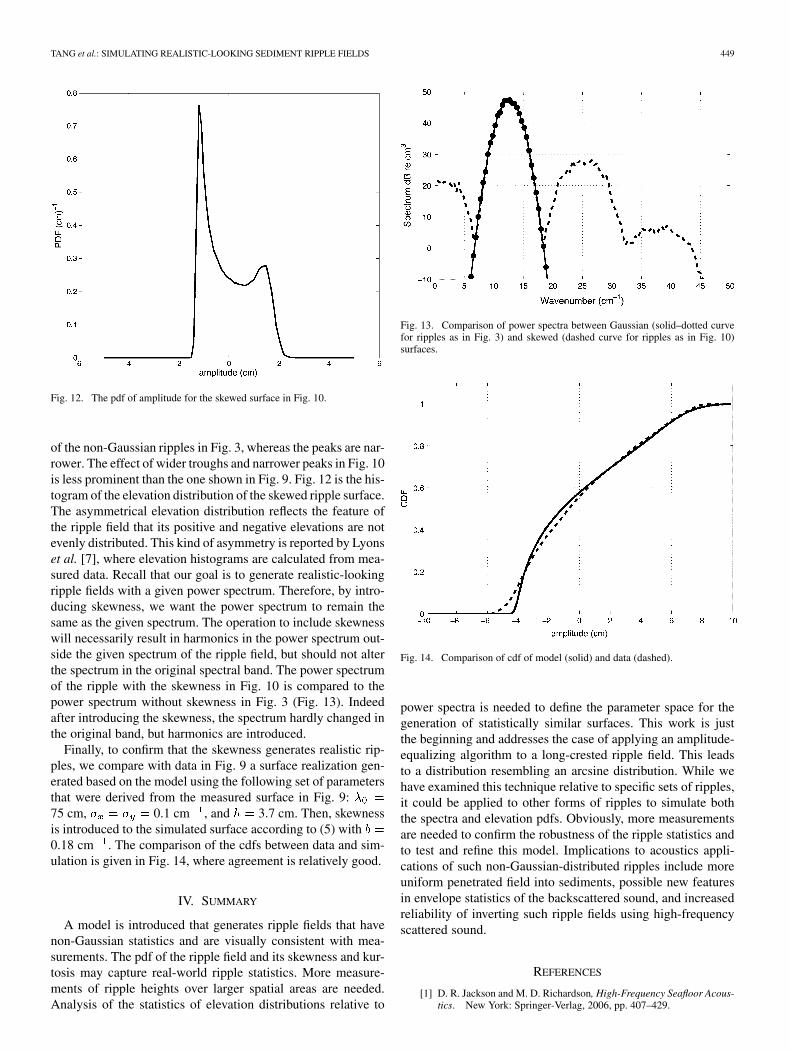
Fig. 12. The pdf of amplitude for the skewed surface in Fig. 10.

of the non-Gaussian ripples in Fig. 3, whereas the peaks are nar-rower. The effect of wider troughs and narrower peaks in Fig. 10is less prominent than the one shown in Fig. 9. Fig. 12 is the his-togram of the elevation distribution of the skewed ripple surface.The asymmetrical elevation distribution reflects the feature ofthe ripple field that its positive and negative elevations are notevenly distributed. This kind of asymmetry is reported by Lyonset al. [7], where elevation histograms are calculated from mea-sured data. Recall that our goal is to generate realistic-lookingripple fields with a given power spectrum. Therefore, by intro-ducing skewness, we want the power spectrum to remain thesame as the given spectrum. The operation to include skewnesswill necessarily result in harmonics in the power spectrum out-side the given spectrum of the ripple field, but should not alterthe spectrum in the original spectral band. The power spectrumof the ripple with the skewness in Fig. 10 is compared to thepower spectrum without skewness in Fig. 3 (Fig. 13). Indeedafter introducing the skewness, the spectrum hardly changed inthe original band, but harmonics are introduced.

Finally, to confirm that the skewness generates realistic rip-ples, we compare with data in Fig. 9 a surface realization gen-erated based on the model using the following set of parametersthat were derived from the measured surface in Fig. 9:75 cm, 0.1 cm , and 3.7 cm. Then, skewnessis introduced to the simulated surface according to (5) with0.18 cm . The comparison of the cdfs between data and sim-ulation is given in Fig. 14, where agreement is relatively good.

IV. SUMMARY

A model is introduced that generates ripple fields that havenon-Gaussian statistics and are visually consistent with mea-surements. The pdf of the ripple field and its skewness and kur-tosis may capture real-world ripple statistics. More measure-ments of ripple heights over larger spatial areas are needed.Analysis of the statistics of elevation distributions relative to

Fig. 13. Comparison of power spectra between Gaussian (solid–dotted curvefor ripples as in Fig. 3) and skewed (dashed curve for ripples as in Fig. 10)surfaces.

Fig. 14. Comparison of cdf of model (solid) and data (dashed).

power spectra is needed to define the parameter space for thegeneration of statistically similar surfaces. This work is justthe beginning and addresses the case of applying an amplitude-equalizing algorithm to a long-crested ripple field. This leadsto a distribution resembling an arcsine distribution. While wehave examined this technique relative to specific sets of ripples,it could be applied to other forms of ripples to simulate boththe spectra and elevation pdfs. Obviously, more measurementsare needed to confirm the robustness of the ripple statistics andto test and refine this model. Implications to acoustics appli-cations of such non-Gaussian-distributed ripples include moreuniform penetrated field into sediments, possible new featuresin envelope statistics of the backscattered sound, and increasedreliability of inverting such ripple fields using high-frequencyscattered sound.

REFERENCES

[1] D. R. Jackson and M. D. Richardson, High-Frequency Seafloor Acous-tics. New York: Springer-Verlag, 2006, pp. 407–429.


[2] M. D. Richardson, K. B. Briggs, K. L. Williams, D. Tang, D. R.Jackson, and E. I. Thorsos, “The effects of seafloor roughness onacoustic scattering: Manipulative experiments,” in Boundary Influ-ences in High Frequency, Shallow Water Acoustics, N. G. Pace and P.Blondel, Eds. Bath, U.K.: Univ. Bath Press, pp. 109–116.

[3] J. S. Doucette and T. O’Donoghue, “Sand ripples in irregular andchanging wave conditions: A review of laboratory and field studies,”Rep. EC MAST Project MAS3-CT97-0086 Sandpit, 2003 [Online].Available: http://sandpit.wldelft.nl/reportpage/right/SandpitLiteratur-eReviewVanDerWerf.pdf

[4] J. P. Davis, D. J. Walker, M. Townsend, and I. R. Young, “Waveformedsediment ripples: Transient analysis of ripple spectral development,” J.Geophys. Res., vol. 109, 2004, DOI:10.1029/2004JC002307, C07020.

[5] P. Traykovski, “Observations of wave orbital scale ripples and anonequilibrium time-dependent model,” J. Geophys. Res. Oceans, vol.112, 2007, DOI: 10.1029/20065C003811, C06026.

[6] K. B. Briggs, D. Tang, and K. L. Williams, “Characterization of inter-face roughness of rippled sand off Fort Walton Beach, Florida,” IEEEJ. Ocean. Eng., vol. 29, no. 4, pp. 505–514, Oct. 2004.

[7] A. P. Lyons, W. L. J. Fox, T. Hasiotis, and E. Pouliquen, “Character-ization of the two-dimensional roughness of wave-rippled sea floorsusing digital photogrammetry,” IEEE J. Ocean. Eng., vol. 27, no. 3,pp. 515–524, Jul. 2002.

[8] A. M. Crawford and A. E. Hay, “Wave orbital velocity skewness andlinear transition ripple migration; comparison with weakly nonlineartheory,” J. Geophys. Res., vol. 108, no. C3, pp. 36-1–36-6, 2003, DOI:10.1029/2001JC001254.

[9] M. Z. Li and C. L. Amos, “Sheet flow and large wave ripples undercombined waves and currents: Field observations, model predictionsand effects on boundary layer dynamics,” Continental Shelf Res., vol.19, no. 5, pp. 637–663, 1999.

[10] J. R. L. Allen, “Sedimentary structures, their character and physicalbasis,” in Developments in Sedimentology. Amsterdam, The Nether-lands: Elsevier, 1982, p. 593, 30A.

[11] W. F. Tanner, “Ripple mark indices and their uses,” Sedimentology, vol.9, pp. 89–104, 1967.

[12] S. Dumas, R. W. C. Arnott, and J. B. Southard, “Experiments on oscil-latory-flow and combined-flow bed forms: Implications for interpretingparts of the shallow-marine sedimentary record,” J. Sedimentary Res.,vol. 75, no. 3, pp. 501–513, 2005.

[13] F. Ardhuin, T. G. Drake, and T. H. C. Herbers, “Observationsof wave-generated vortex ripples on the North Carolina conti-nental shelf,” J. Geophys. Res., vol. 107, no. C10, p. 3143, 2002,DOI:10.1029/2001JC000986.

[14] L. A. Mayer, R. Raymond, G. Glang, M. D. Richardson, P. Traykovski,and A. C. Trembanis, “High-resolution mapping of mines and ripplesat the Martha’s Vineyard coastal observatory,” IEEE J. Ocean. Eng.,vol. 32, no. 1, pp. 133–149, Jan. 2007.

[15] A. C. Trembanis, L. D. Wright, C. T. Friedrichs, M. O. Green, andT. Hume, “The effects of spatially complex inner shelf roughness onboundary layer turbulence and current and wave friction: Tairua em-bayment, New Zealand,” Continental Shelf Res., vol. 24, no. 13–14,pp. 1549–1571, 2004.

[16] E. R. Thieler, O. H. Pilkey, W. J. Cleary, and W. C. Schwab,“Modern sedimentation on the shoreface and inner continental shelf atWrightsville Beach, North Carolina, USA,” J. Sedimentary Res., vol.71, no. 6, pp. 958–970, 2001.

[17] J. E. Piper, K. W. Commander, E. I. Thorsos, and K. L. Williams,“Detection of buried targets using a synthetic aperture sonar,” IEEEJ. Ocean. Eng., vol. 27, no. 3, pp. 495–504, Jul. 2002.

[18] P. Traykovski, A. E. Hay, J. D. Irish, and J. F. Lynch, “Geometry, mi-gration and evolution of wave orbital ripples at LEO-15,” J. Geophys.Res., vol. 104, pp. 1505–1524, 1999.

[19] R. M. Norton, “Arc-sine distribution,” in Encyclopedia of StatisticalSciences. New York: Wiley, 1982, vol. 1, p. 1224.

[20] D. A. Abraham and A. P. Lyons, “Reverberation envelope statisticsand their dependence on sonar bandwidth and scatterer size,” IEEE J.Ocean. Eng., vol. 29, no. 1, pp. 126–137, Jan. 2004.

[21] D. Tang, K. L. Williams, and E. I. Thorsos, “Utilizing high-frequencyacoustic backscatter to estimate bottom sand ripple parameters,” IEEEJ. Ocean. Eng., vol. 34, no. 4, pp. 431–443, Oct. 2009.

Dajun Tang received the B.S. degree from theUniversity of Science and Technology, Hefei, China,in 1981, the M.S. degree from the Institute ofAcoustics, Beijing, China, in 1985, and the Ph.D.degree in oceanographic engineering from the JointProgram of Massachusetts Institute of Technology,Cambridge and the Woods Hole OceanographicInstitution, Woods Hole, MA, in 1991.

From 1991 to 1996, first he was an Assistant Sci-entist and then an Associate Scientists at Woods HoleOceanographic Institution. In 1996, he moved to the

Applied Physics Laboratory, University of Washington, Seattle, where currentlyhe is a Senior Oceanographer. His research encompasses acoustics in shallowwater, emphasizing impacts on acoustics by the sea bottom and water columnvariability.

Frank S. Henyey received the Ph.D. degree in theo-retical physics from the California Institute of Tech-nology, Pasadena, in 1967.

He held postdoctoral and faculty positions at theUniversity of Michigan, and research positions atthe La Jolla Institute and Areté Associates. Since1991, he has been a Principal Physicist at the OceanPhysics Department, Applied Physics Laboratory,University of Washington, Seattle. He has interestsin ocean acoustics and small-scale ocean hydrody-namics. In both fields, his interest centers on internal

waves. His work is mostly theoretical, but he has participated in sea-goingexperiments.

Dr. Henyey is a member of the American Physical Society and the AmericanGeophysical Union, and a Fellow of the Acoustical Society of America.

Brian T. Hefner received the B.S. degree in physicsfrom Bard College, Annandale-On-Hudson, NY, in1994 and the M.S. and Ph.D. degrees in physics fromWashington State University, Pullman, in 1996 and2000, respectively.

From 2000 to 2001, he was a Postdoctoral Scholarat Crocker Nuclear Laboratory, University of Cal-ifornia, Davis, where he studied light scatteringfrom airborne dust using light detection and ranging(LIDAR). In 2001, he moved to the Applied PhysicsLaboratory, University of Washington, Seattle,

where he is currently a Physicist in the Ocean Acoustics Department. Hisprimary research interests include acoustic interaction with the sea bottom,characterization of sediment interface roughness, and propagation and scat-tering in ocean sediments.

Dr. Hefner is a member of the Acoustical Society of America.

Peter A. Traykovski received the B.S.E. degreein mechanical engineering from Duke University,Durham, NC, in 1988 and the M.S./Engineers degreeand the Ph.D. degree in applied ocean sciences andengineering from the Massachusetts Institute ofTechnology/Woods Hole Oceanographic InstitutionJoint Program, Cambridge/Woods Hole, in 1994 and1998, respectively.

Currently, he is an Associate Scientist at the Ap-plied Ocean Physics and Engineering Department,Woods Hole Oceanographic Institution. His main

research interests are sediment transport dynamics on the continental shelf andestuaries and developing instrumentation to measure these processes.

Dr. Traykovski is a member of the American Geophysical Union.

Simulating Realistic-Looking Sediment Ripple Fields

Documents

Transcript of Simulating Realistic-Looking Sediment Ripple Fields