SIMULATING RADIATIVE FEEDBACK AND THE FORMATION ...
307
SIMULATING RADIATIVE FEEDBACK AND THE FORMATION OF MASSIVE STARS
-
Upload
khangminh22 -
Category
Documents
-
view
4 -
download
0
Transcript of SIMULATING RADIATIVE FEEDBACK AND THE FORMATION ...

SIMULATING RADIATIVE FEEDBACK AND THE FORMATION OF
MASSIVE STARS

SIMULATING RADIATIVE FEEDBACK AND THE
FORMATION OF MASSIVE STARS
By
MIKHAIL KLASSEN, B.Sc., M.Sc.
A Thesis
Submitted to the School of Graduate Studies
in Partial Fulfillment of the Requirements
for the Degree of
Doctor of Philosophy
McMaster University
c© Mikhail Klassen, July 2016

DOCTOR OF PHILOSOPHY (2016) McMaster University
(Physics and Astronomy) Hamilton, Ontario
TITLE: Simulating Radiative Feedback and the Formation of Massive Stars
AUTHOR: Mikhail Klassen, B.Sc. (Columbia University), M.Sc. (McMaster
University)
SUPERVISOR: Professor Ralph E. Pudritz
NUMBER OF PAGES: xxv, 281
ii

Abstract
This thesis is a study of massive star formation: the environments in which
they form and the effect that their radiation feedback has on their environ-
ments. We present high-performance supercomputer simulations of massive
star formation inside molecular cloud clumps and cores. First, we present a
novel radiative transfer code that hybridizes two previous approaches to ra-
diative transfer (raytracing and flux-limited diffusion) and implements it in
a Cartesian grid-based code with adaptive mesh refinement, representing the
first of such implementations. This hybrid radiative transfer code allows for
more accurate calculations of the radiation pressure and irradiated gas tem-
perature that are the hallmark of massive star formation and which threaten
to limit the mass which stars can ultimately obtain. Next, we apply this hy-
brid radiative transfer code in simulations of massive protostellar cores. We
simulate their gravitational collapse and the formation of a massive protostar
surrounded by a Keplerian accretion disk. These disks become gravitationally
unstable, increasing the accretion rate onto the star, but do not fragment to
form additional stars. We demonstrate that massive stars accrete material
predominantly through their circumstellar disks, and via radiation pressure
drive large outflow bubbles that appear stable to classic fluid instabilities. Fi-
nally, we present simulations of the larger context of star formation: turbulent,
magnetised, filamentary cloud clumps. We study the magnetic field geometry
and accretion flows. We find that in clouds where the turbulent and magnetic
energies are approximately equal, the gravitational energy must dominate the
kinetic energy for there to be a coherent magnetic field structure. Star clus-
ter formation takes place inside the primary filament and the photoionisation
feedback from a single massive star drives the creation of a bubble of hot,
ionised gas that ultimately engulfs the star cluster and destroys the filament.
iii


To Sheila.

Acknowledgments
Stars may form in the vacuum of space, but the same cannot be said
of a dissertation. Many people were involved in this enterprise and it could
not have come together but for a combination of circumstances and the help
of some special individuals.
I would first of all like to thank my supervisor, Ralph Pudritz, for
guiding this project, for trusting in my abilities, for connecting me with the
right individuals who would be very influential in my research, and for his keen
eye towards the big picture. The results of this thesis had a long gestation
period. A new radiative transfer code needed to be developed and thoroughly
tested. This took much longer than planned, following the old programming
maxim that however much time one thinks one needs to debug a code, it will
probably take at least twice that long. Ralph Pudritz was patient with me
during the years it took to develop and debug the radiative transfer code we
put into flash.
I would also like to express my gratitude for the rest of my supervisory
committee, which included Christine Wilson and James Wadsley. They’ve
been supportive of my work and have always given good recommendations
and guidance.
In the development of this code, Rolf Kuiper was instrumental. The
code we implemented in flash is based on a similar code that Rolf wrote for
pluto. It was not a matter of copying and pasting, however. The method
needed to be re-implemented using the code architecture of flash, its inherent
diffusion solver, various modules that I needed to port from version 2 to version
4 of flash, including the raytracer and protostellar evolution module from my
M.Sc. thesis. And then nothing worked for the longest time. Patiently, Rolf
and my collaborators helped me through each impasse until a working code
had come together.
To these collaborators I owe much thanks: Thomas Peters, for his
knowledge of and assistance with the hybrid-characteristics raytracer; Robi
vi

Banerjee, for insightful comments on the project at many stages; Lars Bunte-
meyer, for his suggestions and comments on the manuscript of Chapter 2; and
Helen Kirk, for her diligent help collaborating on the filaments project.
The research for this thesis involved a fair amount of travel, and in the
places I stayed, many have made me feel welcome, volunteering their time to
help me with my research. In Hamburg, this was Robi Banerjee. In Heidelberg,
I had help at various times from Ralf Klessen and Rolf Kuiper, as well as Sarah
Ragan and Paul Clark. Among my German friends, thanks also to Daniel
Seifried, Philipp Girichidis, and Christian Baczynski. In Chicago, during my
visits to the FLASH Center, I was helped a great deal by Klaus Weide, with
additional help from Anshu Dubey, Dongwook Lee, and Petros Tzeferacos. I
also benefited from my interactions with Donald Lamb, Carlo Graziani, and
Milad Fatenejad. And though we never met in person, Manos Chatzopoulos
helped me with a modified version of an unsplit hydro solver.
In May of 2014, I was accepted to participate as an affiliate the work-
shop and program “Gravity’s Loyal Opposition: The Physics of Star Forma-
tion Feedback” at the Kavli Institute for Theoretical Physics (KITP) at the
University of Santa Barbara. My participation in the program allowed for
many useful conversations that furthered my code development process and
research. I am grateful for input from Romain Teyssier, Christoph Federrath,
Benoıt Commercon, and Norm Murray.
Some interractions can’t take place in person, but must happen over
e-mail. I’m grateful to Stella Offner and Mark Krumholz, who answered my
research questions over e-mail even before they knew me. It was nice to later
share a beer with Mark at Protostars & Planets VI in Heidelberg, and a glass
of viognier in Santa Barbara with Stella during the KITP program. I’m also
grateful to Thierry Sousbie, who agreed to share with me a pre-release version
of the DisPerSE code so that Helen Kirk, Samantha Pillsworth, and I could
use to launch our study of filaments in molecular cloud simulations.
Closer to home, my colleagues at McMaster University have been tremen-
dous to work with and alongside. I am grateful to them for our many con-
verations, for their help, and for their friendship. These are, especially, Rory
Woods, Rachel Ward-Maxwell, Alyssa Cobb, Alex Cridland, Jeremy Webb,
Rob Cockcroft, Tara Parkin, Max Schirm, Kaz Sliwa, Samantha Benincasa,
vii
Matthew Alessi, Aaron Maxwell, Ben Keller, Kevin Sooley, Matthew Mc-
Creadie, Nick Miladinovic, Leo van Nierop, Ben Jackel, Gabriel Devenyi, Eliz-
abeth Tasker, Helen Kirk, Rene Heller, and Samantha Pillsworth. I am also
grateful to the department secretaries, for their tireless work in helping things
run smoothly: Tina Stewart, Rosemary McNeice, Mara Esposto, and Cheryl
Johnston; and to Hua Wu, the department systems administrator, who can
magically discern hard disk failures before they actually happen and stage the
appropriate intervention.
Outside of the department, a group of friends in Hamilton kept me sane
when I needed to speak to someone who wasn’t a scientist: to Tessa Klettl
and Nicole Nı Rıordain, thank you for your friendship; also to my close circle
of Seth Enriquez, Owen Pikkert, and Danielle Wong, I owe a great debt of
friendship.
After moving to Calgary during the last year of my Ph.D. I was often
in need of a place to stay during my regular visits back to Hamilton. Several
wonderful people stepped forward and offered me a place to stay during those
times and they need to be thanked here. Firstly, thank you to Mandy Tam and
Brian Chan, who opened their home in Burlington to me on many occassions.
I also stayed with Joel and Sara Klinck, Rory Woods, Gwendolyn and Aaron
Springford, Josh Chu, and Preston Steinke. You all opened your home to me
at one time or another, and I am hugely grateful.
I am thankful to my longsuffering parents, Adolfo and Elly Klassen,
who encouraged me to persist in this Ph.D. and have supported my education
from the beginning. Much of this work I owe to their love. An to my mother-
and father-in-law, Rosa Lai and Peter Liu: thank you for your encouragement,
your faith in me, and the ways in which you have always been willing to help.
Finally, I would be adrift without my wife, Sheila, to whom I have
dedicated this thesis. You are my keel and compass. Thank you for sharing
in this journey.

“The worthwhile problems are the ones you can really solve or help
solve, the ones you can really contribute something to. A problem is
grand in science if it lies before us unsolved and we see some way for
us to make some headway into it.”
Richard Feynman (1918–1988)
ix


Table of Contents
Abstract iii
Acknowledgments vi
List of Figures xiv
List of Tables xxv
Chapter 1
Introduction 1
1.1 Observations of massive stars . . . . . . . . . . . . . . . . . . 51.2 Theory of massive star formation . . . . . . . . . . . . . . . . 211.3 Radiative feedback . . . . . . . . . . . . . . . . . . . . . . . . 271.4 Thesis outline and major contributions . . . . . . . . . . . . . 37
1.4.1 Chapter descriptions . . . . . . . . . . . . . . . . . . . 42
Chapter 2
A General Hybrid Radiation Transport Scheme for Star For-
mation on an Adaptive Grid 47
2.1 Introduction . . . . . . . . . . . . . . . . . . . . . . . . . . . . 472.2 Theory . . . . . . . . . . . . . . . . . . . . . . . . . . . . . . . 512.3 Numerical methodology . . . . . . . . . . . . . . . . . . . . . 53
2.3.1 FLASH . . . . . . . . . . . . . . . . . . . . . . . . . . 532.3.2 Radiation hydrodynamics . . . . . . . . . . . . . . . . 552.3.3 Flux-limited diffusion . . . . . . . . . . . . . . . . . . . 572.3.4 Stellar irradiation . . . . . . . . . . . . . . . . . . . . . 612.3.5 Opacities . . . . . . . . . . . . . . . . . . . . . . . . . 642.3.6 Radiation pressure . . . . . . . . . . . . . . . . . . . . 66
xi

2.3.7 Summary of the hybrid radiation hydrodynamics method 672.4 Tests of thermal radiation diffusion . . . . . . . . . . . . . . . 68
2.4.1 Thermal radiative equilibration . . . . . . . . . . . . . 682.4.2 1D radiative shock tests . . . . . . . . . . . . . . . . . 69
2.5 Irradiation of a static disk . . . . . . . . . . . . . . . . . . . . 742.5.1 Radiation pressure on a static, flared disk . . . . . . . 81
2.6 Tests involving multiple sources . . . . . . . . . . . . . . . . . 832.6.1 Two proximal sources in a homogeneous medium . . . 832.6.2 Two sources irradiating a dense core of material . . . . 87
2.7 Discussion and Summary . . . . . . . . . . . . . . . . . . . . . 922.8 Appendix to Chapter 2: 3T radiation hydrodynamics . . . . . 95
Chapter 3
Simulating the Formation of Massive Protostars: I. Radia-
tive Feedback and Accretion Disks 98
3.1 Introduction . . . . . . . . . . . . . . . . . . . . . . . . . . . . 983.2 Physical and numerical model . . . . . . . . . . . . . . . . . . 104
3.2.1 Radiation transfer . . . . . . . . . . . . . . . . . . . . 1043.2.2 Further developments of the hybrid radiation transfer code1093.2.3 Temperature iteration . . . . . . . . . . . . . . . . . . 1133.2.4 FLASH . . . . . . . . . . . . . . . . . . . . . . . . . . 1143.2.5 Pre-main sequence evolution and sink particles . . . . . 1153.2.6 Opacity and dust model . . . . . . . . . . . . . . . . . 1173.2.7 Radiation pressure . . . . . . . . . . . . . . . . . . . . 119
3.3 Numerical simulations . . . . . . . . . . . . . . . . . . . . . . 1213.3.1 Sink particles . . . . . . . . . . . . . . . . . . . . . . . 1223.3.2 Resolution . . . . . . . . . . . . . . . . . . . . . . . . . 1243.3.3 Turbulence . . . . . . . . . . . . . . . . . . . . . . . . 1243.3.4 Summary . . . . . . . . . . . . . . . . . . . . . . . . . 125
3.4 Results . . . . . . . . . . . . . . . . . . . . . . . . . . . . . . . 1263.4.1 General description: different phases of massive star for-
mation . . . . . . . . . . . . . . . . . . . . . . . . . . . 1263.4.2 Disk formation and evolution . . . . . . . . . . . . . . 1343.4.3 Disk fragmentation . . . . . . . . . . . . . . . . . . . . 1383.4.4 Radiatively-driven bubbles . . . . . . . . . . . . . . . . 1443.4.5 Accretion flows and outflows . . . . . . . . . . . . . . . 152
3.5 Discussion . . . . . . . . . . . . . . . . . . . . . . . . . . . . . 1553.6 Conclusion . . . . . . . . . . . . . . . . . . . . . . . . . . . . . 162
Chapter 4
Filamentary Flow and Magnetic Geometry in Evolving Cluster-
Forming Molecular Cloud Clumps 167
xii

4.1 Introduction . . . . . . . . . . . . . . . . . . . . . . . . . . . . 1674.2 Numerical methods . . . . . . . . . . . . . . . . . . . . . . . . 175
4.2.1 Numerical simulations . . . . . . . . . . . . . . . . . . 1764.2.2 Initial conditions . . . . . . . . . . . . . . . . . . . . . 1774.2.3 Filament-finding . . . . . . . . . . . . . . . . . . . . . 181
4.3 Filament and B-field alignments: early cloud evolution . . . . 1884.3.1 Large-scale magnetic field orientation . . . . . . . . . . 1924.3.2 Magnetic fields in 2D . . . . . . . . . . . . . . . . . . . 1954.3.3 Velocity fields in 2D . . . . . . . . . . . . . . . . . . . 2044.3.4 Magnetic field orientation relative to filaments in 3D . 2064.3.5 Virial parameter and mass-to-flux ratio . . . . . . . . . 214
4.4 Star formation and the effect of radiative feedback . . . . . . . 2164.5 Discussion . . . . . . . . . . . . . . . . . . . . . . . . . . . . . 223
4.5.1 Magnetic fields, filament formation, and dynamics . . . 2244.5.2 Effects on massive star formation . . . . . . . . . . . . 226
4.6 Conclusions . . . . . . . . . . . . . . . . . . . . . . . . . . . . 227
Chapter 5
Conclusion 233
5.1 Summary of results . . . . . . . . . . . . . . . . . . . . . . . . 2355.1.1 Chapter 2: A General Hybrid Radiation Transport Scheme
for Star Formation on an Adaptive Grid . . . . . . . . 2365.1.2 Chapter 3: Simulating the Formation of Massive Proto-
stars: I. Radiative Feedback and Accretion Disks . . . 2375.1.3 Chapter 4: Filamentary Flow and Magnetic Geometry
in Evolving Cluster-Forming Molecular Cloud Clumps . 2385.2 Outlook . . . . . . . . . . . . . . . . . . . . . . . . . . . . . . 240
Bibliography 281
xiii

List of Figures
1.1 Image of the filamentary infrared dark cloud (IRDC) G035.39-00.33. Figure reproduced with permission from Jimenez-Serra,Caselli, Fontani, Tan, Henshaw, Kainulainen, and Hernandez,MNRAS, Volume 439, Issue 2, p.1996–2013, 2014 (Figure 1).White contours show the integrated intensity of the 13CO J=2→1line emission. These have been superimposed on a mass surfacedensity map from Kainulainen and Tan [2013] (in colour, withan angular resolution of 2”). White contour levels correspondto 33, 40, 50, 60, 70, 80, and 90% of the peak integrated inten-sity (40 K km s−1). High-mass cores are indicated with crossesand are taken from Butler and Tan [2012]. Black open circlesand black open triangles indicate 8 µm and 24 µm sources de-tected with Spitzer, respectively. Marker sizes are scaled bysource flux intensity. Finally, the yellow and light-blue filleddiamonds indicate the low-mas cores and IR-quiet high-masscores, respectively, found by Nguyen Luong et al. [2011] withthe Herschel Space Observatory. . . . . . . . . . . . . . . . . . 7
1.2 Images of a part of the Orion Molecular Cloud, NGC 2024/NGC2023. Reproduced with permission from Megeath, Gutermuth,Muzerolle, Kryukova, Flaherty, Hora, Allen, Hartmann, Myers,Pipher, Stauffer, Young, and Fazio, AJ, Volume 144, Issue 6,p.192, 2012 (Figure 13). The left image is a mosaic of theNGC 2024/NGC 2023 field with 4.5µm emission coloured inblue, 5.8µm in green, and 24µm in red. The right image shows4.5µm emission with the positions of dusty YSOs superimposed.Young stars with disks are indicated by green diamonds andprotostars with red asterisks. The green outline indicates thesurveyed field. . . . . . . . . . . . . . . . . . . . . . . . . . . . 10
xiv

1.3 An image of the Polaris flare. Reproduced with permissionfrom Andre, Di Francesco, Ward-Thompson, Inutsuka, Pudritz,and Pineda, Protostars and Planets VI, University of ArizonaPress, Tucson, p.27-51, 2014 (Figure 1). The left panel showsa 250 µm dust continuum map taken with Herschel/SPIRE.The right panel shows the corresponding column density map,with contrast added by performing a curvelet transform. TheDisPerSE filament-finding algorithm [Sousbie, 2011] was thenapplied, and found filaments traced in light blue. Assuming atypical filament width of 0.1 pc [Arzoumanian et al., 2011], thecolour density map indicates the mass per unit length along thefilaments (color scale shown on the right edge of the figure). . 12
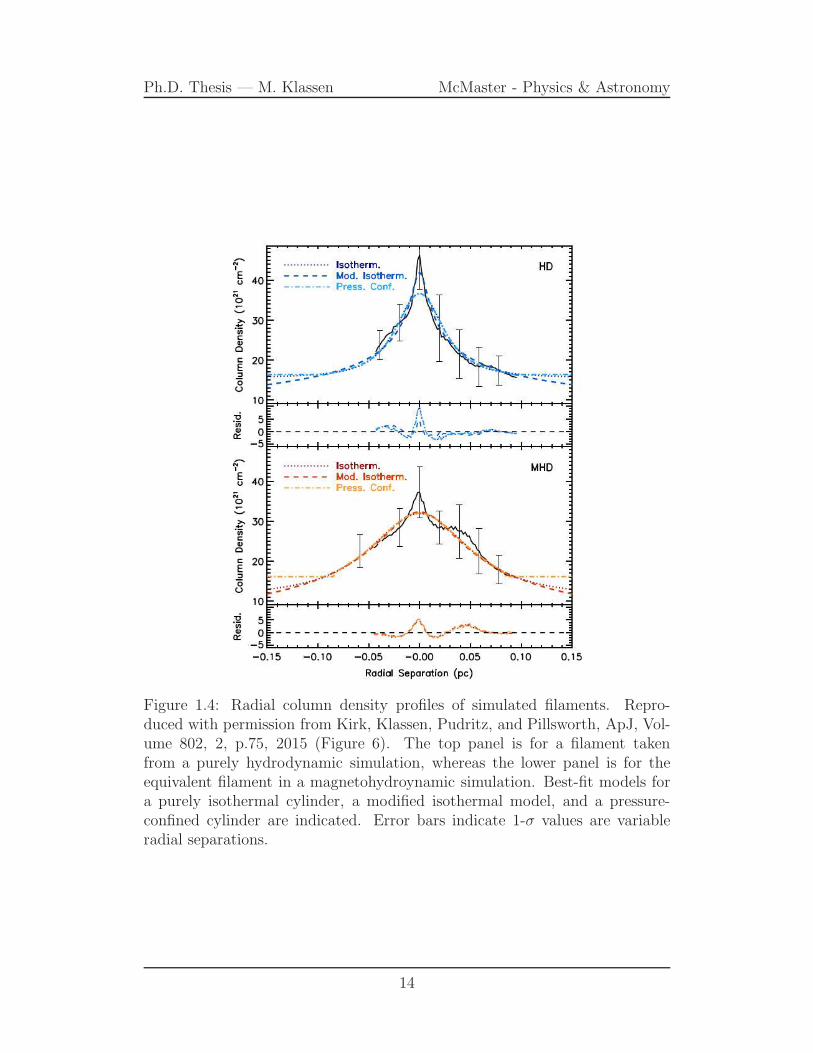
1.4 Radial column density profiles of simulated filaments. Repro-duced with permission from Kirk, Klassen, Pudritz, and Pillsworth,ApJ, Volume 802, 2, p.75, 2015 (Figure 6). The top panel is for afilament taken from a purely hydrodynamic simulation, whereasthe lower panel is for the equivalent filament in a magnetohy-droynamic simulation. Best-fit models for a purely isothermalcylinder, a modified isothermal model, and a pressure-confinedcylinder are indicated. Error bars indicate 1-σ values are vari-able radial separations. . . . . . . . . . . . . . . . . . . . . . . 14
1.5 Column density maps and histograms of relative orientation(HRO) for parts of the Taurus and Ophiucus molecular clouds.Reproduced with permission from Planck Collaboration XXXV[2016], A&A, 586 (Figure 3). c© ESO. Left panels show the col-umn density maps with magnetic pseudo-vectors overlaid. Theorientation of these was inferred using the 353 GHz polariza-tion data from the Planck satellite. The right panels show theHRO, where the relative orientation is between the magneticpseudo-vectors and the gradient of the column density in theleft panels. The density gradient is a proxy for the filamen-tary structure in the column density maps. Hence, the HROgives an indication of the relative orientation of magnetic fieldsand filaments. Three histograms are produced corresponding tothe lowest, an intermediate, and the highest NH density ranges(black, blue, and red, respectively). Where the histograms peaknear 0, it is understood that magnetic fields are aligned withfilamentary structure, whereas when the histograms show rel-atively high counts near ±90, it is understood that magneticfields are oriented perpendicular to filamentary structure. . . . 17
xv

1.6 Snapshots of a simulation of high-mass star formation. FromKrumholz, Klein, McKee, Offner, and Cunningham [2009], Sci-ence, Volume 323, 5915, pp.754–757, 2009 (Figure 1). Reprintedwith permission from AAAS. State of the simulation is indi-cated at (A) 17,500 years, (B) 25,000 years, (C) 34,000 years,(D) 41,700 years, and (E) 55,900 years. Left panels show a(3000 AU)2 face-on view of column density, whereas the rightpanels show an edge-on volume density slice. Colours are scaledlogarithmically from 100 to 102.5 g cm−2 on the left and 10−18
to 10−14 g cm−3 on the right (black at the minimum and red atthe maximum). Stars are indicated with plus signs. . . . . . . 33
2.1 Frequency-averaged opacity (in units of cm2 per gram gas) asa function of temperature for a 1% mixture of interstellar dustgrains with gas, based on the model by Draine and Lee [1984]. 65
2.2 Results from matter-radiation coupling tests. The initial radia-tion energy density is Er = 1012 ergs/cm3. The matter internalenergy density is initially out of thermal equilibrium with theradiation field. Crosses indicate simulation values at every timestep, while the solid line is the analytical solution, assuminga constant Er. Initial matter energy densities are e = 1010
ergs/cm3 (upper set) and e = 102 ergs/cm3 (lower set). . . . . 692.3 Temperature profile for a subcritical radiative shock with a gas
velocity of v = 6 km/s at time t = 5.80× 10⁴ s. Red and greenlines indicates matter and radiation temperatures, respectively.Circles along matter temperature indicate the grid resolution. 71
2.4 Temperature profile for a supercritical radiative shock with agas velocity of v = 20 km/s at time t = 5.08× 10³ s. Lines andcircles represent the same as in previous figure. . . . . . . . . . 72
2.5 Density profile of the Pascucci et al. [2004] irradiated disk setup.Contours show lines of constant density. The radiation sourceis located at the bottom-left corner of the computational domain. 76
2.6 Temperature profile of the Pascucci et al. [2004] irradiated disksetup. Contours show lines of constant density. The gas isheated by a radiation source in the bottom-left corner of thecomputational domain. Note that the temperature has beenscaled logarithmically. . . . . . . . . . . . . . . . . . . . . . . 77
2.7 Specific irradiation profile of the Pascucci et al. [2004] irradiateddisk setup, which shows the stellar radiation energy absorbedper gram of material. Contours show lines of constant opticaldepth, as computed by a raytrace through the material withfrequency-averaged opacities. . . . . . . . . . . . . . . . . . . . 78
xvi
2.8 Comparison of the midplane temperature profiles in simula-tions of the hybrid radiation feedback scheme in the Pascucciet al. [2004] benchmark test in the high-density simulation (ρ0 =8.321 × 10⁻¹⁸): The implementation in flash vs. makemakeby Kuiper et al. [2010a]. Solid lines belong to simulations us-ing the makemake code, completed using a spherical polargeometry, while dashed lines indicate simulations done usingthe scheme described in this paper using the flash code. Thenumber associated with each flash run indicates the maximumrefinement level. Vertical gray lines in the figure indicate thegrid resolution (in AU) for each of the flash runs. . . . . . . 80
2.9 Radiation force density through the midplane of the disk. Thesolid line indicates the radiation force density for the flash cal-culation, resulting from the total flux (direct stellar and ther-mal). The dotted line indicates the radiation force density dueonly to the stellar component of the radiation field. We com-pare the flash results to a 2T gray calculation in makemake
(dashed line). The lower panel indicates the relative differencebetween the total flux radiation force density in flash versusmakemake. . . . . . . . . . . . . . . . . . . . . . . . . . . . . 82
2.10 Gas temperature after equilibrating with the radiation fielddriven by two stellar sources (T = 5800 K). Vertical dashedline indicates the symmetry axis along which the temperaturein figure 2.11 is measured. The black contour marks a gas tem-perature of T = 35K. . . . . . . . . . . . . . . . . . . . . . . . 84
2.11 Gas temperature along dashed line from Figure 2.10, the locusof points equidistant from both radiation sources. The upperpanel shows the gas temperature from our simulation (solid)compared to the Monte Carlo result (dashed). The lower panelshows the relative difference in temperature as a percentage. . 86
2.12 Specific irradiation by two sources in an otherwise homogeneousmedium at ρ = 10−20 g/cm3, but for a central density concentra-tion indicated by the black circle, where the density is ρ = 10−17
g/cm3. The two sources are stellar sources with effective tem-peratures of 8000K. The flash block AMR structure is alsoshown, with each block containing 83 cells. . . . . . . . . . . . 88
2.13 Same as in figure 2.12, but instead showing the gas temperature. 892.14 Radiation energy density with the thermal radiation flux Fr =
−D∇Er overplotted as a vector field. The gradients in the radi-ation energy density are steepest near the spherical overdensityin the centre, on the side facing the two sources. . . . . . . . . 90
xvii
2.15 The temperature difference (in percent) in the raytrace casecompared to the hybrid radiation transfer case. . . . . . . . . 91
3.1 Temperature profile of a 1D subcritical radiating shock with agas velocity of v = 6 km/s at a time t = 5.8 × 10⁴ s. The redsolid line and green dashed line indicate the matter and radi-ation temperatures, respectively. Gray horizontal dashed lineswere added to indicate the semi-analytic estimates for the tem-perature in the preshock, shock, and postshock regions. Statedtemperatures are the semi-analytic estimates for the various re-gions surrounding a subcritical shock. . . . . . . . . . . . . . 113
3.2 Dust opacity correction to account for dust sublimation in re-gions of high gas temperature. Here we show the correction asa function of gas temperature for two different gas densities,ρ = 10−21 and 10−10 g/cm3. The vertical lines indicate thesublimation temperatures Tevap for the given gas densities. Theapproach is identical to Kuiper et al. [2010a]. . . . . . . . . . . 119
3.3 A series of panels from our 100M⊙ simulation showing the timeevolution of the disk in face-on and edge-on views. The timesare indicated in the upper left corner of each row. The leftcolumn shows the projected gas density of the disk within a(3000 AU)2 region. The colors indicating column densities arescaled from Σ = 1 g/cm2 to 102.5 g/cm2. The right column isa slice of the volume density taken to show the edge-on view ofthe protostellar disk. The window is (3000 AU)2 and the colorsare scaled from ρ = 10−18 g/cm3 to 10−14 g/cm3. The mass ofthe star in each pair of panels is indicated in the top-left of thesecond panel of each row. . . . . . . . . . . . . . . . . . . . . . 127
3.4 The time-evolution of the sink particle formed in each of thethree simulations (30, 100, and 200 M⊙ initial core mass). Thesink particle represents the accreting protostar and its internalevolution is governed by a protostellar model. The top-left panelshows its mass. The top-right panel indicates the accretionrates onto the sink particles. The effective surfance temperatureof the protostar is estimated by a protostellar model and isindicated in the bottom-left panel. The star radiates both dueto the high accretion rate and its own intrinsic luminosity dueto nuclear burning. The total luminosity of the sink is the sumof these two, and each sink particle’s total luminosity is shownin the bottom-right panel. . . . . . . . . . . . . . . . . . . . . 130
xviii
3.5 The accretion rate plotted as a function of stellar mass for eachof our three main simulations. The line thickness scales in orderof ascending initial mass for the protostellar core. . . . . . . . 133
3.6 The Toomre Q parameter, which quantifies the gravitationalstability of disks. Values of Q < 1 are unstable to gravitationalfragmentation and are colored in red. Stable regions are coloredblue. Here we see the disk in our 100 M⊙ simulation becomingmarginally unstable. The period of time immediately after thismarks a strong increase in the accretion rate of material ontothe star. The mass of the star is indicated in the top-left. . . . 134
3.7 Sequence of snapshots from the 200 M⊙ simulation showingface-on volume density slices (top row) and the local ToomreQ parameter (bottom row) in a (3000 AU)2 region centered onthe location of the sink particle. Scale bars have been addedto show the volume density (in g/cm2) and the value of theQ parameter (see Equation 3.28). Values of Q < 1 indicatedisk instability. Velocity streamlines have been added to thevolume density slice. The mass of the star is indicated in thebottom-left of each panel in the bottom row. . . . . . . . . . . 135
3.8 The evolution of our three simulations, with initial core massesindicated above each frame. These show the simultaneous growthof the star and disk masses in each simulation. . . . . . . . . . 136
3.9 An analysis of the local stability of the entire protostellar diskfrom the 100 M⊙ simulation. The rows show the state of thesimulation at the stated times, which are identical to the onesshown in Figure 3.3. The left column shows the column densityof the disk. The center column shows the β stability parameterfor the entire disk. The right column shows the β stability pa-rameter again, but with Toomre-stable regions (Q > 1) maskedout. Colored in red, therefore, are only those regions that areboth Toomre-unstable and β-unstable. These are expected tobe gravitationally unstable. The white contour in the panelsof the middle and right columns indicate those regions wherethe density exceeds the threshold for sink particle formation,ρthresh = 1.4× 10⁻¹⁴ g/cm3. . . . . . . . . . . . . . . . . . . . 139
3.10 The evolution as a function of time of the total luminosity (solidline) of the star formed in each of our three main simulations.In each case it is compared to the star’s Eddington luminos-ity (dashed line), the threshold where radiation forces exceedgravitational forces. In the 100M⊙ and 200M⊙ simulations,the star’s luminosity becomes super-Eddington. It is in thesesimulations that radiatively-driven bubbles are observed. . . . 145
xix

3.11 Volume density slice of a (400 AU)2 region through our 200M⊙ simulation, showing an edge-on view of the circumstellardisk. The slice is centered on the sink particle, representing a39.8 M⊙ star. flash’s block structure is shown in the grid,with each block containing 83 cells. Overplotted are contoursshowing dust fraction. Nearest the star, the dust is completelysublimated. Contours show dust sublimation correction factorsof 0.2, 0.5, and 0.8. . . . . . . . . . . . . . . . . . . . . . . . . 146
3.12 Acceleration vectors showing the net acceleration (in units ofcm/s−2) of the gas due to radiative forces and gravity (both thegravity of the star and the gas). Vectors are overplotted on abackground indicating volume density slice of an approximately(6000 AU)2 region through our 200 M⊙ simulation after about21.8 kyr of evolution, showing an edge-on view of the circum-stellar disk and radiatively-driven bubble. The slice is centeredon the sink particle, representing a 43.5 M⊙ star. . . . . . . . 148
3.13 Edge-on volume density slices, centered on the sink particle,showing in a (5000 AU)2 region the evolution of a radiatively-driven bubble in our 200 M⊙ simulation. Shown are six snap-shots at different points in the simulation with the times indi-cated. Velocity vectors have been overplotted. Volume densitieshave been scaled from ρ = 10−17 g/cm3 to 10−13 g/cm3. Themass of the star is indicated in the top-left of each panel. . . . 149
3.14 Azimuthal accretion and outflow profile at two different timesduring the 100M⊙ simulation within a 1000 AU radius cen-tered on the sink particle. In each of these we measure theazimuthally-averaged radial velocity of the gas relative to thestar. This gives a picture of how much gas is moving towardsor away from the star as a function of the polar angle. The firstpanel shows the simulation after the formation of a flared pro-tostellar disk. The disk is even and hasn’t yet gone unstable.The second frame shows the state of the simulation after thestar has gone super-Eddington and a radiatively-driven bubblehas formed. Gas is accelerated to around 10 km/s away fromthe star in the regions above (20–70) and below (110–160)the disk. . . . . . . . . . . . . . . . . . . . . . . . . . . . . . . 153
xx

4.1 3D plot of gas density from the MHD1200 simulation at 250,000years of evolution. Green isosurfaces indicate gas at densitiesof n = 3.1 × 103 cm−3 (ρ = 1.1 × 10⁻²⁰ g/cm3). Red linesindicate filament skeleton selected by DisPerSE . Black linesare magnetic field lines at 8 randomly selected locations withinthe volume. . . . . . . . . . . . . . . . . . . . . . . . . . . . . 189
4.2 2D column density maps along each of the coordinate axes withprojections of the filament skeleton overplotted. Data is sameas in Figure 4.1 . . . . . . . . . . . . . . . . . . . . . . . . . . 191
4.3 B-field streamline evolution over the course of 325 kyr in ourMHD1200 simulation. The green density contour is as in Figure4.1. Box depicts entire simulation volume with L = 3.89 pc ona side. Turbulence and rotation largely account for the changesin local magnetic field orientation. . . . . . . . . . . . . . . . . 192
4.4 Left: Column density maps along the y-axis of our MHD1200 sim-ulation at 250 kyr of evolution with density-weighted projectedmagnetic field orientation overplotted in red arrows. Middle:
The autocorrelation of the previous column density map, whichhighlight self-similar structure. Contours highlight levels from1% to 10% of peak correlation values. The diagonal bar rep-resents cloud orientation and is the best fit line through thepixels contained within the outermost contour, weighted by thebase-10 logarithm of the autocorrelation values. Magnetic fieldlines based on the values measured for the left panel are over-plotted. Right: The histogram of magnetic field orientationsbased on the values measured for the left panel, normalized sothat the total area is 1. The orientations are measured rela-tive to “north”. The blue histogram shows the low-density gas,while red indicates only the orientations of high-density gas.The vertical grey lines indicate the angle of the best fit line tothe large-scale structure (solid right line), and the angle offsetby 90 (dashed left line). . . . . . . . . . . . . . . . . . . . . . 194
4.5 The same as in Figure 4.4, except using MHD500 at 150 kyrof evolution. Because of the higher average gas density, wedraw contours in the middle panel from 0.1% to 10% of peakcorrelation values. The best-fit line is still calculated based onthe outermost contour. The data is taken at approximately thesame number of freefall times as in the MHD1200 simulation. . 195
xxi

4.6 A zoom-in of the MHD1200 cloud, in the same region as thatshown in Figure 4.4 (left panel), centred on the highest-densitygas and framing a (1.5 pc)2 region. Column density is shownin colour with density-weighted projected velocity vectors over-plotted, which emphasizes the motion of the higher-density gas.The initial Alfven Mach number is 0.99, and the initial virialparameter is αvir = 0.56, i.e. the cloud is highly bound andundergoing gravitational collapse. . . . . . . . . . . . . . . . . 197
4.7 A zoom-in of the MHD500 cloud, in the same region as thatshown in Figure 4.5 (left panel), centred on the highest-densitygas and framing a (1.5 pc)2 region. Column density is shownin colour with density-weighted projected velocity vectors over-plotted, which emphasizes the motion of the higher-density gas.The initial Alfven Mach number is 0.92, slightly lower than theMHD1200 case in Figure 4.6. However, the initial virial parame-ter is αvir = 0.95, i.e. the turbulent kinetic energy is roughly inequilibrium with the gravitational binding energy. . . . . . . . 198
4.8 Left: Volume density slice through the molecular cloud of ourMHD1200 simulation after 250 kyr of evolution with arrows in-dicating the velocity field. The colours cover a range in volumedensities from n = 100 cm−3 to n = 106 cm−3. Photoionizationfeedback from a cluster of stars (not shown) has begun formingan Hii region at the side of the main trunk filament. Right: Lo-cal Alfven Mach number with arrows indicating the magneticfield. The colours are scaled logarithmically from MA = 10−1
(blue) to MA = 101 (red). White regions have values for theAlfven Mach number of MA ≈ 1, indicating that the turbulentenergy is balancing the magnetic energy. Sub-Alfvenic regions(MA < 1) have stronger magnetic fields. . . . . . . . . . . . . 200
4.9 The same as in Figure 4.8, except for the MHD500 simulation.As the simulation volume is smaller, the panels have been madeproportionally smaller, while still centering on the densest partof the simulation. The snapshot of the simulation is taken after150 kyr of evolution, which is earlier than in MHD1200, but atthe same number of freefall times to permit better comparison. 200
xxii

4.10 Left: Density projection along the y-axis of our MHD1200 simu-lation at 250 kyr of evolution with density-weighted projectedvelocity field overplotted in red arrows. Middle: The autocor-relation of the previous column density project, which high-light self-similar structure. Contours highlight levels from 1%to 10% of peak correlation values. The shaded diagonal barrepresents cloud orientation as previously calculated for Figure4.4. Velocity streamlines based on the values measured for theleft panel are overplotted. Right: The histogram of the veloc-ity field orientations based on the values measured for the leftpanel, normalized so that the total area is 1. The orientationsare measured relative to “north”. The blue histogram shows thelow-density gas distribution, while red indicates only the orien-tations of high-density gas. The vertical grey lines indicate theangle of the best fit line to the large-scale structure (solid rightline), and the angle offset by 90 (dashed left line). . . . . . . 204
4.11 The same as in Figure 4.10, except using MHD500 at 150 kyrof evolution. Because of the higher average gas density, wedraw contours in the middle panel from 0.1% to 10% of peakcorrelation values. The best-fit line is still calculated based onthe outermost contour. The data is taken at approximately thesame number of freefall times as in the MHD1200 simulation. . 205
4.12 Sequence of histograms from the MHD1200 simulation. The areaunder each curve has been normalized to 1. By tracing alongthe filaments in 3D through the simulated volume, we producehistograms of the relative orientation of the magnetic field andthe filament. In each panel, we compare the relative orientationmeasured in the data (blue) with the histogram that would haveresulted if the magnetic field had been randomly oriented (red).In addition to a standard step-shaped histogram, a kernel den-sity estimate (KDE), with a Gaussian kernel, has been run overthe data and is shown via the smooth curves, providing a con-tinuous analog to the discretely-binned histogram data. Shadedareas indicate either an exceess relative to random (blue) or adeficit (red). Each row of panels gives the state of the simulationat the indicated time. Columns restrict the relative orientationdata to the indicated density regims, as measured locally alongthe filament spine. The last column applies no density selection. 208
4.13 The same as in Figure 4.12, except for our MHD500 simulation. 212
xxiii

4.14 The evolution of the virial parameter and the mass-to-flux ratioof our two simulations. These parameters remain fairly steadythroughout the MHD1200 simulation, but the MHD500 becomesmagnetically critical during gravitational collapse. The addedmagnetic support causes some of the gas in the outer regions torebound, adding kinetic energy. . . . . . . . . . . . . . . . . . 214
4.15 The evolution of the sink particles formed in the MHD1200 simu-lation. 7 particles are formed near the center of the simulationvolume inside the main trunk filament and make up a tight clus-ter. These accrete mass, the largest of which reaches nearly 16M⊙. . . . . . . . . . . . . . . . . . . . . . . . . . . . . . . . . 217
4.16 Evolution of the most massive star formed as part of the MHD1200simulation, which reaches a maximum mass of 16 M⊙. The top-left panel shows the history of the mass of the sink particle rep-resenting this star. The top-right panel shows the evolution ofthe accretion rate in units of M⊙/yr. The bottom-left panel isthe history of the effective (surface) temperature, as computedby our protostellar model. The bottom-right panel shows theintrinsic luminosity and the accretion luminosity of the star. . 218
4.17 The same as in Figure 4.4, except for the final state of theMHD1200 simulation at 325 kyr of evolution. Photoionizationfeedback from a massive star of ∼ 16M⊙ has created an ex-panding Hii region. . . . . . . . . . . . . . . . . . . . . . . . . 220
4.18 Volume density slices through the center of the MHD1200 sim-ulation volume showing an expanding Hii region as a result ofionizing feedback from the cluster of stars. A single massive starof nearly 16 M⊙ dominates all the others and has a luminosityof nearly 23,000 L⊙. This drives a bubble of hot (10,000 K)ionized gas, forming a blister on the side of the main trunk fila-ment. The left panel shows the state of this bubble after 250 kyrof evolution, while the right panel shows the state of the bubbleafter 325 kyr, near the very end of the simulation. Overplottedon each are magnetic field vectors based on the magnetic fieldorientation in the plane of the slice. . . . . . . . . . . . . . . . 220
4.19 A slice through the simulation volume of the MHD1200 simula-tion at 325 kyr showing the line-of-sight magnetic field strengtharound the Hii region driven by the cluster of stars in the lower-left corner of the image. Magnetic field vectors are overplottedgiving the plane-of-sky magnetic field orientation. . . . . . . . 222
xxiv

List of Tables
2.1 Simulations of the irradiated disk setup. . . . . . . . . . . . . 75
3.1 Protostellar core collapse simulation parameters . . . . . . . . 125
4.1 Simulation parameters . . . . . . . . . . . . . . . . . . . . . . 175
xxv

Ph.D. Thesis — M. Klassen McMaster - Physics & Astronomy
Chapter 1
Introduction
As far as the physical universe is concerned, stars are engines of creation. The
process of their formation takes cold molecular gas—mostly hydrogen—and
through the action of gravity confines it to a core. The collapse of this core
down to extreme conditions of density and temperature occurs when gravity
finally overcomes all other forms of pressure support (turbulence, thermal,
magnetic, and radiative). This allows for the onset of nuclear fusion reactions
that herald stellar birth. The fusion of light elements into heavier ones releases
the energy that heats the gas to provide the pressure to hold it up against its
own weight and causes it to radiate. Successive cycles of stellar birth and
death, some in the form of supernovae, enriched the universe with heavy ele-
ments and provided all the raw materials for planets, asteroids, and ultimately
life. It is not an exaggeration to say, then, that stars and understanding how
they form are extremely important.
In the catalogue of stars existing in our present universe, massive stars
are a rare and special breed, yet they exert an influence on their environments
that is greatly disproportionate to their number. They supply most of the
1

Ph.D. Thesis — M. Klassen McMaster - Physics & Astronomy
heavy elements and ultraviolet radiation found in galaxies. They typically
end their short lives as supernova explosions, and during their existence exert
powerful forces on the interstellar medium (ISM)—consisting of gas (ionized,
atomic, and molecular) and dust—in which they are embedded. Their prodi-
gious luminosities drive stellar winds, outflows, and bubbles of ionized gas
called Hii regions. Finally, by their supernovae, they might also be important
sources of mixing and turbulent energy within galaxies.
Massive stars are generally defined as having masses M∗ > 8M⊙, and
luminosities above L∗ > 103L⊙ [Cesaroni, 2008]. After their main sequence
evolution, massive stars end their lives as supernovae. They are born from ex-
tremely dense cores and effectively begin their lives as hydrogen-burning stars
on the main sequence [Palla and Stahler, 1993] without any pre-main-sequence
evolution. This is in contrast to lower-mass stars, that are born on a well-
defined “birthline” on the Hertzsprung-Russell (H-R) diagram [Stahler, 1983],
which is defined by the onset of deuterium fusion—the first possible nuclear
fuel. They then undergo gravitational contraction until their stellar interiors
become hot and dense enough for the fusion of hydrogen. The timescale for
this collapse is known as the Kelvin-Helmholz time. Protostars may still be
accreting new material at rates of about 10−5–10−4 M⊙/yr and undergoing
changes in stellar structure. By contrast, massive stars are accreting at rates
in excess of 10−3 M⊙/yr and begin fusing hydrogen almost immediately, even
while in the mass accretion phase.
For stars this luminous, the formation scenario becomes problematic.
Massive stars drive radiative feedback mechanisms that are not available to
low-mass stars—radiation pressure and photoionization [Larson and Starrfield,
1971a]. Wolfire and Cassinelli [1987] predicted accretion rates of M ∼ 10−3
2

Ph.D. Thesis — M. Klassen McMaster - Physics & Astronomy
M⊙/yr in order to overcome radiation pressure. Some early spherical collapse
(i.e. 1D) calculations sought to determine an upper mass limit for stars, given
that there ought to be a critical luminosity capable of halting the accretion
flow. The Eddington Luminosity, given by
Ledd =4πGM∗c
κ, (1.1)
characterizes this limit, where G is Newton’s constant, M∗ the mass of the
star, c the speed of light, and κ the specific opacity of the gas (and its dust
content) in units of cm2/g. Depending on the choice of dust model, this
resulted in “upper mass limits” for stars in the range of 20–40 M⊙ [Larson
and Starrfield, 1971b, Kahn, 1974, Yorke and Krugel, 1977]. This is, of course,
in direct contradiction to observations of stars with masses in excess of 100
M⊙ [Crowther et al., 2010, Doran et al., 2013]. This is another indication that
massive star formation must differ from low-mass star formation.
The vast majority of stars are formed in clusters embedded in molecular
clouds [Lada and Lada, 2003]. Giant molecular clouds (GMCs) are observed to
be inhomogeneous across a wide range of scales [Williams et al., 2000], which
is understood to be the result of supersonic turbulence in either magnetized or
unmagnetized clouds [Vazquez-Semadeni et al., 2000, Mac Low and Klessen,
2004, Elmegreen and Scalo, 2004, Scalo and Elmegreen, 2004]. Supersonic
turbulence also results in the formation of filaments, which both observations
and numerical simulations have conclusively shown to be the sites of star
formation [Andre et al., 2014, Mac Low and Klessen, 2004]. If the mass per
unit length of a filament exceeds a critical value, it will undergo gravitational
fragmentation into bound objects that will collapse to form either a single star
3

Ph.D. Thesis — M. Klassen McMaster - Physics & Astronomy
or a small multiple system.
Massive stars are rare: they constitute the tail end of the mass spec-
trum, occurring at a frequency only 10% that of stars in the mass range of
1–2 M⊙. Their environments are more extreme: deeply embedded and highly
obscured by dust, it has taken the latest generation of instruments (Herschel
and ALMA) to properly image these environments and study their proper-
ties. The observations now tend to favour monolithic collapse model with disk
accretion. Models of coalescence, proposed to circumvent the problem of radi-
ation pressure barriers, are no longer necessary, although coalescence may still
occur in a rarity of exceptional circumstance such as ultradense protoclusters.
Radiative forces on dust grains are not dynamically important when
modeling low-mass stars, hence numerical simulations may employ simpler
models for radiative transport. These radiative forces were long thought to
limit monolithic collapse models to stars of. 40M⊙ until sufficiently advanced
three-dimensional simulations demonstrated that higher masses were possible.
Our understanding of massive stars today is being greatly advanced
by the advent of next-generation telescopes and observatories, such as ALMA,
and as well as state-of-the-art numerical simulations that carefully incorporate
radiative feedback effects into the hydro- and magnetohydrodynamics of star
formation. The work described in this thesis develops a new radiative transfer
technique for numerical simulations (Chapter 2), allowing us to perform highly
accurate simulations of massive star formation (Chapter 3). We demonstrate
how accretion through a circumstellar disk is sufficient to explain the origins
of massive stars, despite their having super-Eddington luminosities. The for-
mation of radiatively-driven polar outflow bubbles acts to relieve the pressure
on incoming material so that accretion can continue.
4
Ph.D. Thesis — M. Klassen McMaster - Physics & Astronomy
We then connect up to the scales of massive cluster formation by pre-
senting numerical simulations of turbulent, magnetized cloud clumps (Chapter
4). Here we address the full filamentary nature of molecular clouds that re-
sults from the presence of supersonic turbulence. We investigate how the
coevolution of magnetic fields, turbulence, and radiative feedback (specifically
ionization) from a massive star affects the filamentary geometry of molecular
clouds. In cluster-forming clumps, magnetohydrodynamic and turbulence pro-
cesses are often in balance, leaving gravity to play a strong role in establishing
filamentary flow and magnetic field orientation in forming clusters. Feedback
from massive stars can also disrupt filaments, halting accretion and disordering
the magnetic field.
In this introduction, we will review the paradigm of star formation pre-
sented by current observational evidence and outline the theory of massive star
formation. This thesis is comprised of three related journal articles, making
up Chapters 2–4. We include a summary of each and some explanatory notes
on their context within the field and within this thesis.
1.1 Observations of massive stars
Most stars form inside GMCs [McKee and Ostriker, 2007b], the largest struc-
tures inside of galaxies, which have physical scales of ∼ 20–100 pc and masses
between 104 and 106M⊙. Volume-averaged densities inside GMCs are about
50–100 cm−3, which is very low, but molecular gas within clouds is highly
inhomogeneous. The temperatures inside GMCs of the Milky Way typically
range from 10–15 K [Sanders et al., 1993], which gives a sound speed of 0.2
km/s. The velocity dispersion, based on molecular line widths, is measured
5

Ph.D. Thesis — M. Klassen McMaster - Physics & Astronomy
to be about 2–3 km/s, indicating the present of highly supersonic turbulence
with turbulent Mach numbers of M = u/cs . 50 [Mac Low and Klessen,
2004], where u is the gas velocity and cs is the sound speed. GMCs sometimes
contain substructures (“clumps”) with masses between a few 100 M⊙ and a
few 1000 M⊙, sizes of up to a few pc, and mean densities of between 103
and 105 cm−3. Within these, peak densities can easily exceed 106 cm−3. The
dense clumps (0.25–0.5 pc) can be identified in (sub)mm continuum emission
and molecular line tracers and it is inside the dense clumps that massive star
formation is taking place [Beltran et al., 2006, Beuther et al., 2007].
Among these, infrared dark clouds (IRDCs) are the likely precursor
environments for massive star formation. IRDCs are dense molecular clouds
seen in extinction against the bright mid-infrared background of the galaxy.
An example is given in Figure 1.1 from Jimenez-Serra et al. [2014], where the
filamentary IRDC G035.39-00.33 is pictured. The IR-quiet high-mass cores
found using the Herschel Space Observatory are indicated with ligh-blue filled
diamonds. IRDCs are cold (T < 20 K), highly turbulent (1–3 km/s) and
exhibit considerable velocity structure, with variations of 1–2 km/s over the
cloud [Pillai et al., 2006]. They are large (1–10 pc in diameter) compared to
dense molecular cloud clores (∼ 0.1 pc), with gas at densities of ∼ 106 cm−3
[Carey et al., 2000]. They range in mass from 120 to 16000 M⊙ and contain at
least one compact core of size D . 0.5pc, with most IRDCs showing multiple
cores [Rathborne et al., 2006]. Given the spectrum of core masses inside IRDCs
and assuming that most cores will form one star, then most of these will be
OB stars.
This formation process is divided into four stages by [Beuther et al.,
2007]:
6

Ph.D. Thesis — M. Klassen McMaster - Physics & Astronomy
Figure 1.1: Image of the filamentary infrared dark cloud (IRDC) G035.39-00.33. Figure reproduced with permission from Jimenez-Serra, Caselli,Fontani, Tan, Henshaw, Kainulainen, and Hernandez, MNRAS, Volume 439,Issue 2, p.1996–2013, 2014 (Figure 1). White contours show the integratedintensity of the 13CO J=2→1 line emission. These have been superimposedon a mass surface density map from Kainulainen and Tan [2013] (in colour,with an angular resolution of 2”). White contour levels correspond to 33,40, 50, 60, 70, 80, and 90% of the peak integrated intensity (40 K km s−1).High-mass cores are indicated with crosses and are taken from Butler and Tan[2012]. Black open circles and black open triangles indicate 8 µm and 24 µmsources detected with Spitzer, respectively. Marker sizes are scaled by sourceflux intensity. Finally, the yellow and light-blue filled diamonds indicate thelow-mas cores and IR-quiet high-mass cores, respectively, found by NguyenLuong et al. [2011] with the Herschel Space Observatory.
7
Ph.D. Thesis — M. Klassen McMaster - Physics & Astronomy
1. High-mass starless cores (HMSCs)
2. High-mass cores harboring accreting low/intermediate-mass protostar(s)
destined to become a high-mass star(s)
3. High-mass protostellar objects (HMPOs)
4. Final stars
HMSCs are difficult to detect, but several candidates have been ob-
served [Sridharan et al., 2005, Olmi et al., 2010]. HMSCs are identified as
single-component blackbodies with T ∼ 17 K. More evolved candidates be-
gin to show a mid-infrared excess [Beuther et al., 2010a], suggestive of the
presence of a deeply-embedded protostar. Observations of HMSCs and the
transition scenario to HMPOs would support the monolithic collapse hypoth-
esis as the mechanism for forming massive stars. Competing theories such as
stellar mergers or the competitive accretion scenario (in which more evolved
low- or intermediate-mass stars compete for the gas in a reservoir, accreting
via Bondi-Hoyle accretion) predict the absence of HMSCs [McKee and Os-
triker, 2007b]. Such observations are extremely rare, but Motte et al. [2007]
and Beuther et al. [2015a] identify high-mass starless clumps that will likely
collapse to form several massive stars.
Observations by the Herschel Space Observatory [Pilbratt et al., 2010] of
star-forming regions identify filaments containing high-mass protostellar cores,
some of which are associated with Hii regions [Hill et al., 2011]. The Herschel
results favour a star formation scenario in which networks of filaments, followed
by the formation of protostellar cores within dense filaments, are the precursors
for stars [Andre et al., 2014].
8

Ph.D. Thesis — M. Klassen McMaster - Physics & Astronomy
Filament formation is not completely understood, although turbulence
(as well as gravity and magnetic fields) likely play important roles [Hennebelle,
2013]. In particular, the interaction of shocks from supersonic turbulence
results in large-scale density enhancements that can take the form of filaments
[Ballesteros-Paredes et al., 2007, Pudritz and Kevlahan, 2013].
Prominent filamentary structure is observed in both CO and dust maps
for two nearby star-forming clouds: Orion A, with L ∼ 10 pc, [Bally et al.,
1987, Chini et al., 1997, Johnstone and Bally, 1999] and Taurus, with L ∼ 1
pc, [Abergel et al., 1994, Mizuno et al., 1995, Hartmann, 2002, Nutter et al.,
2008, Goldsmith et al., 2008]. As already mentioned, infrared dark clouds
also possess filamentary morphology. Myers [2009] noted how filaments would
sometimes form hubs in which stellar clusters were observed.
In Figure 1.2 we show a part of the Orion Molecular Cloud complex,
in particular the NGC 2024/NGC 2023 field and the Horsehead nebula, re-
produced with permission from Megeath et al. [2012]. The image shows the
clustered nature of star formation, as captured by the Spitzer Space Telescope.
Young stars with disks are indicated by the green diamonds, while the red
asterisks indicate protostars. The bright central feature is NGC 2024, an Hii
region. The smaller reflection nebula approximately 20′ to the south is NGC
2023.
The intersections of some of the densest filaments are associated with
massive star formation [Schneider et al., 2012, Peretto et al., 2013]. One of
the findings of the Herschel mission was the ubiquity of filamentary structure
throughout the cold interstellar medium (ISM) [Andre et al., 2010, Men’shchikov
et al., 2010, Molinari et al., 2010, Henning et al., 2010, Motte et al., 2010].
Figure 1.3 shows the Polaris flare imaged using Herschel, reproduced
9

Ph.D. Thesis — M. Klassen McMaster - Physics & Astronomy
Figure 1.2: Images of a part of the Orion Molecular Cloud, NGC 2024/NGC2023. Reproduced with permission from Megeath, Gutermuth, Muzerolle,Kryukova, Flaherty, Hora, Allen, Hartmann, Myers, Pipher, Stauffer, Young,and Fazio, AJ, Volume 144, Issue 6, p.192, 2012 (Figure 13). The left image isa mosaic of the NGC 2024/NGC 2023 field with 4.5µm emission coloured inblue, 5.8µm in green, and 24µm in red. The right image shows 4.5µm emissionwith the positions of dusty YSOs superimposed. Young stars with disks areindicated by green diamonds and protostars with red asterisks. The greenoutline indicates the surveyed field.
10

Ph.D. Thesis — M. Klassen McMaster - Physics & Astronomy
here with permission from Andre et al. [2014]. The left panel, a 250 µm dust
continuum map, exhibits much filamentary structure. Filaments have lengths
of ∼ 1 pc or more (see scale bar in right panel of Figure 1.3). To extract a
map or skeleton of the network of filaments from the image, a curvelet trans-
form [Starck et al., 2003a,b] was first taken, which highlights the filamentary
structure. Following this, the DisPerSE algorithm [Sousbie, 2011, Sousbie
et al., 2011] is applied. A technical description of the algorithm is included
in Chapter 4, but the resulting map is shown in the right panel of Figure 1.3.
This has aided observers, such as Arzoumanian et al. [2011], to characterize
filament properties.
In their arrangement, filaments are long (l ∼ 1–10 pc) and often lie
co-linear with their host clouds [Andre et al., 2014], suggesting a common for-
mation mechanism such as supersonic turbulence or magnetic fields [Li et al.,
2013]. Some clouds appear to contain populations of sub-filaments [Arzou-
manian et al., 2011, Russeil et al., 2013] and these can sometimes appear
as coherent structures in position-position-velocity (PPV) maps [Hacar and
Tafalla, 2011]. Since astronomers cannot directly measure the line-of-sight
spatial dimension, seeing only a 2D projection, PPV maps are a way of gain-
ing information about the third dimension from the line-of-sight velocity. This
can be very useful if 3D structures have coherent velocities.
Their radial density profiles are well fit by Plummer-like functions [Ar-
zoumanian et al., 2011]:
ρp(r) =ρc
[1 + (r/Rflat)2]p/2
, (1.2)
11

Ph.D. Thesis — M. Klassen McMaster - Physics & Astronomy
Figure 1.3: An image of the Polaris flare. Reproduced with permission fromAndre, Di Francesco, Ward-Thompson, Inutsuka, Pudritz, and Pineda, Pro-tostars and Planets VI, University of Arizona Press, Tucson, p.27-51, 2014(Figure 1). The left panel shows a 250 µm dust continuum map taken withHerschel/SPIRE. The right panel shows the corresponding column densitymap, with contrast added by performing a curvelet transform. The Dis-
PerSE filament-finding algorithm [Sousbie, 2011] was then applied, and foundfilaments traced in light blue. Assuming a typical filament width of 0.1 pc [Ar-zoumanian et al., 2011], the colour density map indicates the mass per unitlength along the filaments (color scale shown on the right edge of the figure).
which is equivalent to column density profile of
Σp(r) = ApρcRflat
[1 + (r/Rflat)2]p−1
2
, (1.3)
where ρc is the central density of the filament, Rflat is the radius of the flat
inner region, p ≈ 2 is the power-law index at radii r ≫ Rflat, and Ap is a
constant of order unity that includes the effect of inclination relative to the
plane of the sky. The fact that the power-law index p is approximately 2
and not 4, as would be the case for an isothermal cylinder [Ostriker, 1964],
12

Ph.D. Thesis — M. Klassen McMaster - Physics & Astronomy
suggests that filaments are not isothermal, but rather better fit by polytropic
equations of state, P ∝ ργ with γ . 1. The temperature profile then goes
as T ∝ ργ−1. The observed temperature structure in filaments does indeed
deviate from isothermal [Palmeirim et al., 2013]. Federrath [2016] claims that
the p = 2 scaling of the filament density profile results naturally from the
collision of two planar shocks that form a filament at their intersection.
In a survey of nearby Gould Belt clouds, the filaments appear to have
a characteristic width of d = 2 × Rflat ∼ 0.1 pc. This filament width appears
universal, even being reproduced in numerical simulations, such as the ones
we performed in Kirk, Klassen, Pudritz, and Pillsworth [2015]. We analyzed
filament properties in column density maps from hydrodynamic and magneto-
hydrodynamic simulations. The filaments studied in simulation had physical
properties remarkably similar to observations.
Figure 1.4 is reproduced from that paper and shows filament profiles
of an equivalent filament taken from a purely hydrodynamic and a mangneto-
hydrodynamic simulation. The simulated observations are of a radial column
density profile, which is then fit with three different models of idealized cylin-
drical filaments: the isothermal case presented first in Ostriker [1964], where
gravity is balanced by thermal pressure; a modified isothermal case, which is
sometimes referred to as a“Plummer-like” profile [Equation 1.3]; and a third
model, based on Fischera and Martin [2012], which includes the effects of ex-
ternal confining pressure. These three model profiles are overplotted on our
radial column density measurements, and residuals are shown beneath each
case (HD or MHD).
We noted that magnetic fields can result in wider, “puffier” filaments,
although Seifried and Walch [2015] find that if the magnetic fields are arranged
13
Ph.D. Thesis — M. Klassen McMaster - Physics & Astronomy
Figure 1.4: Radial column density profiles of simulated filaments. Repro-duced with permission from Kirk, Klassen, Pudritz, and Pillsworth, ApJ, Vol-ume 802, 2, p.75, 2015 (Figure 6). The top panel is for a filament takenfrom a purely hydrodynamic simulation, whereas the lower panel is for theequivalent filament in a magnetohydroynamic simulation. Best-fit models fora purely isothermal cylinder, a modified isothermal model, and a pressure-confined cylinder are indicated. Error bars indicate 1-σ values are variableradial separations.
14

Ph.D. Thesis — M. Klassen McMaster - Physics & Astronomy
perpendicular to the filaments, filaments may be slightly narrower than 0.1 pc.
The mechanism responsible for the near-universally measured 0.1 pc width is
still not understood, although recent theoretical work claims that it is a natu-
ral consequence of the physical properties of magnetized, turbulent molecular
clouds [Federrath, 2016]. What is significant is that our simulated filaments
resemble observed filaments in their characteristics. We study these in Chap-
ter 4, including the interplay of magnetic fields and accretion flows, as well as
the destructive effects of photoionization feedback from massive star clusters.
Among the other results of Kirk, Klassen, Pudritz, and Pillsworth
[2015], we also found that magnetic fields result in filaments that are less
centrally peaked, and less prone to fragmentation. Our simulated filaments
exhibited complex structure reminiscent of the filament bundles observed in
Hacar et al. [2013]. Complex 3D substructure is also observed in other simu-
lations, such as those by Smith et al. [2014] and Moeckel and Burkert [2015].
The question of magnetic field orientation is of importance to star for-
mation studies because magnetic fields support protostellar cores against grav-
itational collapse by opposing gravity and have dynamically important effects
in molecular clouds. Observations of magnetic field structure on GMC scales
shows that molecular clouds are threaded with large-scale magnetic fields [Li
et al., 2013] that roughly preserve their overall orientation. Filaments are seen
as oriented largely perpendicular or parallel to magnetic fields.
In Figure 1.5, reproduced with permission from Planck Collaboration
XXXV [2016], we show the magnetic structure around parts of the Taurus and
Ophiucus molecular clouds, as mapped by the Planck satellite using 353 GHz
dust polarization observations. The resolution is insufficient to map individual
cores, but captures the large-scale magnetic field structure of giant molecular
15

Ph.D. Thesis — M. Klassen McMaster - Physics & Astronomy
clouds. The left panels show the column density and magnetic pseudo-vectors
indicating the orientation of the magnetic field are overplotted. A technique
called the Histogram of Relative Orientations [Diego Soler et al., 2013] is used
to generate the right panels in Figure 1.5. To generate these, the relative
angle between the magnetic field pseudo-vector and the gradient in the column
density is measured. The gradients in column density serve as a proxy for
filamentary structure, and so can be used to generate histograms of the relative
orientation of magnetic fields and filaments. We showcase a different technique
that we developed in Chapter 4 using the filament spines directly as mapped
out using DisPerSE in 3D simulated molecular cloud clumps,
Magnetic field orientation is measured using optical or infrared polariza-
tion measurements. Non-spherical dust grains align their long axis perpendic-
ular to the ambient magnetic field [Hoang and Lazarian, 2008]. Light at optical
wavelengths from background stars is absorbed by the dust grains, resulting
in the starlight being linearly polarized in the direction of the magnetic field.
Meanwhile, the dust emits radiation in infrared frequencies, but which appear
linearly polarized perpendicular to the magnetic field [Hildebrand et al., 1984,
Novak et al., 1997, Vaillancourt, 2007, Davis and Greenstein, 1951, Hildebrand,
1988, Heiles and Haverkorn, 2012].
Polarization measurements, such as in Taurus [see, e.g. Palmeirim et al.,
2013, Figure 3] show an alignment perpendicular to the dense filaments. Small
filaments, sometimes called “striations” appear to feed into larger filaments
and show alignment parallel to these magnetic field orientations. Numerical
simulations by Diego Soler et al. [2013] suggest that there exists for molecular
clouds a threshold density below which parallel alignment is favoured and
above which the relative orientation is more perpendicular.
16

Ph.D. Thesis — M. Klassen McMaster - Physics & Astronomy
Figure 1.5: Column density maps and histograms of relative orientation (HRO)for parts of the Taurus and Ophiucus molecular clouds. Reproduced withpermission from Planck Collaboration XXXV [2016], A&A, 586 (Figure 3).c© ESO. Left panels show the column density maps with magnetic pseudo-vectors overlaid. The orientation of these was inferred using the 353 GHzpolarization data from the Planck satellite. The right panels show the HRO,where the relative orientation is between the magnetic pseudo-vectors and thegradient of the column density in the left panels. The density gradient isa proxy for the filamentary structure in the column density maps. Hence,the HRO gives an indication of the relative orientation of magnetic fields andfilaments. Three histograms are produced corresponding to the lowest, anintermediate, and the highest NH density ranges (black, blue, and red, respec-tively). Where the histograms peak near 0, it is understood that magneticfields are aligned with filamentary structure, whereas when the histogramsshow relatively high counts near ±90, it is understood that magnetic fieldsare oriented perpendicular to filamentary structure.
17

Ph.D. Thesis — M. Klassen McMaster - Physics & Astronomy
This scenario favours a magnetic origin for dense filaments. The ISM is
weakly ionized by cosmic rays and the interstellar radiation field. Dust, which
makes up about 1% of the mass of the ISM, also contributes free electrons that
have been photoejected. This means that the ISM responds dynamically to
the presence of magnetic fields. Motion along parallel field lines is unhindered,
but gas moving across field lines or along a gradient in magnetic field strength
encounters a magnetic pressure. B-fields can thus channel gas along what
appear as striations and onto high-gravity filaments [see Li et al., 2013, Figure
3]. The relative orientation of magnetic fields and filaments is sensitive also
the relative energies of magnetic fields and turbulence, characterized by the
Alfven Mach number, given by
MA = (β/2)1/2M =σ
vA, (1.4)
where β = 8πρσ2/〈B2〉 = 2σ2/v2A is the plasma beta, which describes the
ratio of thermal pressure to magnetic pressure. σ and vA = B/√4πρ are the
1D velocity dispersion and the Alfven speed, respectively. The latter is the
characteristic speed of a magnetohydrodynamic wave. M is the thermal Mach
number.
If sub-Alfvenic (MA < 1) turbulent pressure is high enough, turbu-
lent pressure extends gas parallel along magnetic fields and filaments appear
elongated in the direction of the magnetic field [Li et al., 2013]. If not, grav-
ity contracts material along magnetic field lines to form a filament with a
perpendicular orientation.
If the turbulence is super-Alfvenic (MA > 1), then magnetic fields are
not dynamically important, then turbulence can compress gas in any direc-
18

Ph.D. Thesis — M. Klassen McMaster - Physics & Astronomy
tion to form filaments regardless of the large-scale orientation of intercloud
magnetic fields.
In a study of 27 Zeeman measurements towards molecular clouds, Crutcher
[1999] was able to characterize their magnetic properties and found them to
have Alfven Mach numbers ranging from MA = 0.3 to MA = 2.7, although
for some clouds, only a lower bound was obtained. Most had Alfven Mach
numbers close to unity.
Core formation along filaments is also influenced by the magnetic field
geometry. Seifried and Walch [2015] performed numerical simulations of a
large (l ∼ 1 pc) filament with magnetic fields oriented parallel or perpendic-
ular. When the field was oriented perpendicular to the filament, stellar cores
were formed with an even distribution along the filament. With a parallel
orientation, cores were seen first forming at the ends of the filament.
Filaments can be characterized by their line masses, Mline, also known
as the mass per unit length. For an isothermal cylinder (Equation 1.2 with
p = 4), there exists a critical line mass for which the gravitational force per
unit mass is balanced by thermal pressure,
Mline,crit ≡∫ ∞
0
2πρ4(r)rdr =2c2sG
, (1.5)
where cs is the isothermal sound speed. Filaments with line masses above
this critical value should be unstable to gravitationl collapse unless they are
supported by other mechanisms, such as non-thermal gas motions or magnetic
fields. Beuther et al. [2015b] present an extreme filament embedded within an
IRDC that is supported by turbulent gas motions. If its radial support came
only from thermal pressure, it would have a critical line mass of 25M⊙/pc.
19

Ph.D. Thesis — M. Klassen McMaster - Physics & Astronomy
The measured line mass is closer to 1000 M⊙/pc, but the filament has only
fragmented into 12 approximately equally-spaced cores. If turbulent gas mo-
tions are included, the critical line mass becomes 525 M⊙/pc, which is more
than 20 times higher and much more consistent with the fragmentation pat-
tern observed. The turbulent contribution to the critical line mass was derived
in Fiege and Pudritz [2000] and shown to be relevant in Kirk et al. [2015]. We
reproduce some radial column density profiles in Figure 1.4. Filaments such
as these are prime candidates for massive star formation.
Dense cores embedded within filamentary networks inside molecular
clouds have become the new paradigm of star formation [Andre et al., 2014],
reinforced by observational evidence across a wide array of instruments and a
wide range of scales. The transition from dense cores to massive stars is char-
acterized by Zinnecker and Yorke [2007] as going from cold dense massive cores
(CDMC) to hot dense massive cores (HDMC) to disk-accreting main-sequence
star (DAMS), to final main-sequence star (FIMS). The transition from cold
(starless) core to hot core results from the formation of an intermediate-mass
protostar that can heat up the core. H2O and later methanol maser emission
traces collimated jets and outflows, which appear as soon as protostellar disks
begin to form through gravitational collapse of magnetized clouds [Banerjee
and Pudritz, 2006, Pudritz et al., 2007b, Seifried et al., 2012b]. The star
becomes increasingly luminous (more from hydrogen burning than disk ac-
cretion) and begins to photoionize the gas around it and photoevaporate the
accretion disk. At this point, gravitationally-confined hypercompact Hii re-
gions are observed via hydrogen recombination lines. The disk is dissipated
and what remains is a “final” main-sequence star driving an expanding Hii
region.
20
Ph.D. Thesis — M. Klassen McMaster - Physics & Astronomy
There is no agreed-upon upper mass limit for stars. Figer [2005] claims
an upper limit of 150 M⊙ from observations of the Arches cluster, and on
account of its total absence of stars with initial masses greater that 130 M⊙,
despite the fact that for a cluster of its size, typical mass function would predict
that Arches should have 18 such stars. Later work, however, showed a strong
sensitivity of the derived stellar masses to the choice of extinction law [Habibi
et al., 2013]. The relative difference in derived stellar mass for two different
extinctions laws could be as great as 30%. Crowther et al. [2010] performed
spectroscopic analyses of two stellar clusters, NGC3603 and R136, the latter of
which is part of 30 Doradus. Both NGC3603 and R136 are extremely compact
stellar clusters and contain some of the most massive stars detected to date.
Crowther et al. [2010] estimate that three systems in NGC3063 have initial
masses of 105–170 M⊙, while four stars in R136 have masses in the range
of 165–320 M⊙. It is important to note that these masses are sensitive to
the choice of stellar evolution model, age estimates, and estimates of mass
loss due to stellar wind. Nevertheless, it appears that stars with masses above
150M⊙ are possible and have been observed. How they were able to accrete so
much matter despite their extreme luminosities is one of the central questions
addressed in this thesis. Its solution motivated the creation of our new hybrid
AMR radiative transfer code (described in Chapter 2) and its implementation
for massive star formation in Chapter 3.
1.2 Theory of massive star formation
Statements about the gravitational stability of a molecular cloud usually begin
with the virial theorem, which, stated one helpful way, is [McKee and Zweibel,
21

Ph.D. Thesis — M. Klassen McMaster - Physics & Astronomy
1992, McKee and Ostriker, 2007b]:
1
2I = 2 (T − TS) + B +W − 1
2
∫
S
(
ρvr2)
· dS. (1.6)
In the first term, I, comes from the moment of inertia of the molecular cloud.
If the shape of the cloud remains the same, then it tells us whether the cloud
is expanding or contracting. T is the total kinetic plus thermal energy of the
cloud and TS is the confining surface pressure on the cloud, which includes both
thermal and ram pressure. B is the difference in magnetic pressure between
the inside and outside of the molecular cloud. If the magnetic field across the
surface takes on a uniform value B0, then
B =1
8π
∫
V
(
B2 − B20
)
dV. (1.7)
W is the gravitational energy of the cloud, usually expressed simply as the
binding energy in the case of no external gravitational fields. The final term
in Equation 1.6 represents the rate of change of momentum flux across the
cloud surface. If v = 0 at the surface S, then no gas is crossing the surface of
the cloud and this term is zero.
If the magnetic and surface forces are negligible (B ≈ TS ≈ 0), and the
cloud is in virial equilibrium (I = 0), then we have
2T = −W. (1.8)
This is the simplest possible statement of the virial theorem and the one from
22

Ph.D. Thesis — M. Klassen McMaster - Physics & Astronomy
which we define the virial parameter, αvir,
αvir =2T|W| . (1.9)
A cloud in virial balance has αvir ≈ 1. A cloud undergoing gravitational
collapse will have αvir < 1. In Chapter 4 we simulate two molecular cloud
clumps, one with αvir ≈ 1 and another with αvir ≈ 0.6, and show that the
difference can influence the geometry of the magnetic field as the simulation
evolves. The strongly bound cloud drags magnetic fields inwards as it collapses
gravitationally. This effect is much less strong in the marginally bound cloud.
Using Equation 1.8, we can define a simple expression of the length
and mass scales required for gravitational stability. For a uniform sphere of
isothermal gas with radius R and mass M , we have
T =3
2NkBT, (1.10)
where N = M/(µmH) is the number of molecules of mean molecular weight
µmH . kB is Boltmann’s constant and T is the temperature. The gravitational
binding energy is W = −aGM2/R, where a is a constant of order unity that
depends on the internal structure of the spherical cloud. For a homogeneous
cloud of uniform mass density ρ, a = 3/5. This allows us to write the simplified
virial thereom as
3Mc2s =3
5
GM2
R, (1.11)
where we have substitued in the isothermal sound speed c2s = kBT/(µmH).
After a little rearranging, we can write the critical radius for gravitational
23

Ph.D. Thesis — M. Klassen McMaster - Physics & Astronomy
stability,
RJ =
√
15c2s4πGρ
, (1.12)
where we have added a subscript J to denote its connection with the Jeans
length. A more rigorous stability analysis following Jeans [1902], yields almost
exactly the same result. The critical wavenumber at which perturbations grow
to non-linear amplitudes and undergo gravitational collapse is:
kJ =
√
4πGρ
c2s, (1.13)
for which the corresponding wavelength, λJ , is the Jeans length,
λJ =2π
kJ=
√
πc2sGρ
=
√
πkBT
GµmHρ. (1.14)
This naturally defines a mass scale, MJ = ρλ3J , the Jeans mass, and it is the
critical mass above which a sphere of uniform density ρ will undergo gravita-
tional collapse. The corresponding timescale for collapse is called the freefall
time and is given by
tff =
√
3π
32Gρ. (1.15)
Magnetic fields can provide support against gravitational collapse and
are present throughout the ISM. Starting from the simplified statement of the
magnetic field energy in Equation 1.7, the magnetic terms can be approximated
1
8π
∫
V
(
B2 − B20
)
dV ≈ 1
6
(
B2R3 − B20R
30
)
(1.16)
This assumes the molecular cloud of radius R is inside a much larger virial
volume of radius R0. The flux passing through through the cloud, ΦB = πBR2,
24

Ph.D. Thesis — M. Klassen McMaster - Physics & Astronomy
must necessarily pass through the virial surface as well, hence ΦB = πB0R20,
allowing us to write
1
6
(
B2R3 − B20R
30
)
=1
6π2
(
Φ2B
R− Φ2
B
R0
)
≈ 1
6π
Φ2B
R, (1.17)
where, in the last step, we can used R ≪ R0 to drop the 1/R0 term. Setting
B = |W| allows us to write a magnetic critical mass,
MΦ =
√
5
2
ΦB
3πG1/2. (1.18)
Molecular clouds or cores with masses M < MΦ remain magnetically sup-
ported against collapse, though processes such as ambipolar diffusion can
reduce the flux ΦB threading the cloud or core and allowing it to collapse.
Following McKee and Ostriker [2007b], we write the critical mass as
MΦ ≡ cΦΦB
G1/2, (1.19)
where all other factors have been gathered into the coefficient cΦ. For the
idealized case that we followed above, cΦ =√
5/2/(3π) ≈ 0.168. More exact
numerical calculations including the pressure of the intercloud medium by
Mouschovias and Spitzer [1976] find cΦ = 0.126.
For simulations of magnetized molecular cloud cores, it is important
to characterize the core’s mass-to-flux ratio, usually stated normalized to the
critical value,
µ ≡ Mcore
Φcore/
(
MΦ
Φ
)
crit
=Mcore∫
BzdA/cΦ√G. (1.20)
Observed values for the mass-to-flux ratio in high-mass star-forming cores
25

Ph.D. Thesis — M. Klassen McMaster - Physics & Astronomy
are typically only slightly supercritical, with µ . 5 [Falgarone et al., 2008,
Girart et al., 2009, Beuther et al., 2010b]. This indicates that magnetic fields
are dynamically important in high-mass star formation and may provide a
significant amount of support against gravity. This implies that cores will
reach much higher masses before they eventually collapse to form stars.
A typical massive core might contain ∼ 100M⊙ of molecular gas and
have a radius of ∼ 0.1 pc [Reid and Wilson, 2005, Sridharan et al., 2005,
Beuther et al., 2005]. This gives it a mean density of ρ ∼ 10−18 g/cm3, or
n ∼ 106 cm−3. The freefall time of such a core is tff = 5 × 10⁴ years. For a
core to form within 105 years, we require accretion rates of M = Mcore/tff ∼
10−3M⊙/yr. Accretion rates this high are never observed or expected in low-
mass star formation regions. It is also much higher than the value expected
from the thermal sound speed, c3s/G ∼ 10−6M⊙/yr and can only be met in
conditions with strong turbulence, since it is the turbulent velocity dispersion,
not the sound speed, that is relevant [Myers and Fuller, 1992, McLaughlin and
Pudritz, 1997, McKee and Tan, 2003].
Another characteristic feature of high-mass protostars is their short
Kelvin-Helmholtz times. This timescale,
tKH ∼ GM2
RL, (1.21)
where M , R, and L are the mass, radius, and luminosity of the protostar,
respectively, describes the conversion of gravitational energy to radiation be-
fore the protostar has reached equilibrium. This precedes the onset of nuclear
burning. Typical Kelvin-Helmholtz times for high-mass protostars will be a
few 104 years, which is shorter than the typical formation time of ∼ 105 years.
26

Ph.D. Thesis — M. Klassen McMaster - Physics & Astronomy
These short Kelvin-Helmholtz times, relative to freefall times, imply
that massive stars effectively begin their lives on the main sequence, burning
hydrogen long before they’ve finished accreting. Their higher effective surface
temperatures also mean that they will begin ionizing the surrounding gas even
while they are still forming.
Magnetic fields and radiative feedback act together in disks, with mag-
netic fields serving to extract angular momentum from disks, potentially ac-
celerating the accretion process [Commercon et al., 2010], resulting in an in-
creased accretion luminosity. Magnetic braking of accretion disks is by itself
far too efficient a process, preventing the formation of a Keplerian disk, but
this “magnetic breaking catastrophe” is averted by the presence of even small
amounts of turbulence [Seifried et al., 2012a].
In summary, massive stars are quite unlike low-mass stars. Their envi-
ronments are characterized by much higher mean gas densities, they accrete
at much higher rates, begin burning hydrogen almost immediately, and influ-
ence their surrounds through powerful feedback mechanisms that include pho-
toionization, radiation pressure, and—later, during main sequence evolution—
stellar winds. In the next section, we introduce the radiative feedback mech-
anisms most relevant to this thesis.
1.3 Radiative feedback
Stars influence their environments through their radiation feedback effects.
One of the most important feedback mechanisms for the study of stellar popu-
lations and the star formation efficiency of molecular clouds is radiative heat-
ing. By raising the temperature of the gas, gravitational fragmentation is
27

Ph.D. Thesis — M. Klassen McMaster - Physics & Astronomy
suppressed by increasing the Jeans mass, which scales as MJ ∼ T32 (see Equa-
tion 1.14). This process is relevant even for low-mass stars, which through
the heating of their protostellar cores suppress disk fragmentation and the
formation of brown dwarfs [Offner et al., 2009].
Stars heat their environments primarily through the interaction of ra-
diation and dust. Dust grains make up about 1% of the ISM by mass and
absorb stellar radiation preferentially at UV and optical, heating up in the
process. They re-emit this energy at longer, infrared wavelengths. This repro-
cessing occurs very close to the stars themselves. Collisions between gas and
dust ensure that they are in thermal equilibrium. It is usually safe to assume
that within molecular clouds, Tgas = Tdust.
In the diffuse ISM the gas can be hotter than the dust, while in the
envelopes of protostars, dust temperatures can exceed gas temperatures [Tie-
lens, 2005]. At densities above n & 104.5 cm−3, dust-gas coupling is so strong
that dust is the dominant coolant and regulates the temperatures. At lower
densities, molecular or atomic species are more important coolants [Goldsmith,
2001, Glover and Clark, 2012]. In simulations of star formation involving dif-
fusive schemes of radiative transfer, local thermodynamic equilibrium between
dust and gas species is usually assumed [Turner and Stone, 2001, Krumholz
et al., 2007b, Commercon et al., 2011b].
Dense molecular cloud clumps are often sufficiently optically thick that
even the radiation field is in thermal equilibrium with the dust, i.e. Trad ≈
Tdust = Tgas. Within circumstellar disks, the gas/dust temperature follows the
thermal radiation temperature closely, except at the inner boundary nearest
the star, where the direct radiation flux is high.
When modeling radiative feedback in molecular clouds using numerical
28

Ph.D. Thesis — M. Klassen McMaster - Physics & Astronomy
simulations, various simplifications must be made because solving the full set
of radiative transfer equations, including scattering, absorption, and emission,
along with the full set of (magneto)hydrodynamics equations is computation-
ally infeasible on today’s supercomputers. In the optically thick environments
in which stars form, radiation diffuses through gas much like heat, and hence
it obeys Fick’s diffusion law: F = −c∇E/(3κρ), where F is the flux, E is
the radiation energy density and κ is the specific opacity of the dust. This
can be applied in either the “grey” atmosphere approach, where F , E, and κ
are integrated over all frequencies, or via a multi-group approach that splits
the radiation field into discrete energy bins and the relevant quantities are
integrated over the frequencies within each bin.
A problem arises, however, if the cloud becomes optically thin. In
these regions, κρ becomes sufficiently small that the flux F can exceed cE,
violating Special Relativity. To circumvent this problem, a “flux-limiter” was
introduced [Alme and Wilson, 1973, Levermore and Pomraning, 1981], so that
the diffusion law became
F = −λc
κρ∇E, (1.22)
where λ is the flux-limiter, a dimensionless function of E and κρ that in the
optically thick limit, λ → 1/3, and in the optically thin limit, λ → κρE/|∇E|.
Between these two limits, λ is a smoothly-varying function. The result is that
in the optically thick limit, Fick’s Law is preserved, and in the optically thin
limit, the magnitude of the flux does not exceed cE.
Many different functional forms for the flux limiter are possible, and
depend on assumptions about the angular distribution of the specific intensity
of the radiation [Turner and Stone, 2001]. One of the most popular flux limiters
29

Ph.D. Thesis — M. Klassen McMaster - Physics & Astronomy
is the one by Levermore and Pomraning [1981],
λ =2 +R
6 + 3R +R2, (1.23)
where
R =|∇E|κρE
. (1.24)
The flux-limited diffusion (FLD) approximation opened a wide frontier
of star formation research via numerical simulations of molecular clouds and
cores, first in 2D [Yorke and Bodenheimer, 1999, Yorke and Sonnhalter, 2002],
and then 3D [Whitehouse and Bate, 2006, Krumholz et al., 2007a]. Modern
approaches to flux-limited diffusion use increasing sophistication, such as the
hybridization with raytracers that we present in this thesis. Other next gen-
eration FLD codes are including multifrequency effects [Kuiper et al., 2010b,
Flock et al., 2013] and ionization [Norman et al., 2015]. Other methods for
modeling radiative feedback in molecular clouds include characteristics-based
raytracing with accelerated Λ-iteration [Buntemeyer et al., 2015], a scheme
that passes a collection of parallel rays through the simulation volume across
a distribution of angles, determines the flux local to each cell, and then it-
eratively computes the equilibrium temperature. Another approach is time-
dependent Monte Carlo radiative transfer [Harries, 2011, 2015], which follows
packets of rays through many scattering, emission, and absorption events—
very accurate, but computationally expensive.
FLD, still the most popular approach, can by itself never be a complete
solution to the radiative transfer problem. Each parcel of gas will see some
energy also from the direct ray from the star. The medium in question is highly
30

Ph.D. Thesis — M. Klassen McMaster - Physics & Astronomy
anisotropic—filled with filaments, voids, and radiative cavities—so the direct
ray will often convey most of the energy. Thus by hybridizing a raytracing
approach with a diffusion approach, one achieves the best of both worlds:
high accuracy, especially nearest the star, and high efficiency, especially in the
optically thick regions.
While the suppression of gas fragmentation through radiative heating
is an important feedback effect, it is not unique to massive stars, nor is it one
that challenges our understanding of how massive stars form. In fact, radiative
heating is partly responsible for massive stars. A dense 100 M⊙ core of radius
0.1 pc at a temperature of 20 K contains ∼ 80 Jeans masses and yet collapses
to form only a single massive star, as we show in Chapter 3 of this thesis.
Radiative heating plays an extremely important role in the origin of massive
stars.
What does challenge the formation of massive stars is radiation pres-
sure, a feedback mechanism that is not dynamically important for low-mass
stars. Radiation pressure has been recognized as an important problem in
massive star formation since at least the 1970s [Larson and Starrfield, 1971b,
Kahn, 1974]. The most massive stars known, with masses of 100–150 M⊙, are
internally supported against gravity by radiation pressure on electrons. Yet
the cross-section for Thompson scattering is an order of magnitude smaller
than the cross-section for absorption by dusty gas. How then can a star,
which is already near its Eddington limit for stellar structure, accrete dusty
gas from its environment, for which it exceeds the Eddington limit by an order
of magnitude? Radiation pressure becomes as strong as gravity for stars of
roughly 20 M⊙.
The resolution to this dilemma lies in the non-sphericity of the ac-
31

Ph.D. Thesis — M. Klassen McMaster - Physics & Astronomy
cretion process. If accretion proceeds through a disk, the radiation field be-
comes highly anisotropic, with the short-wavelength radiation, which most
contributes to radiative acceleration, being concentrated in the polar direc-
tion. The radiative force density is proportional to opacity κ of the gas, which
in turn is a function of the frequency of the radiation.
In the plane of the disk, short-wavelength radiation is strongly ab-
sorbed within the inner regions of the disk. The long-wavelength radiation,
least responsible for radiative acceleration, is more or less isotropic [Yorke and
Sonnhalter, 2002]. This is known as the “flashlight effect” [Yorke and Boden-
heimer, 1999] and applies even in “grey amospheres”. In our simulations, the
direct radiation component is assumed to have a spectrum corresponding the
effective temperature of the star, and the (grey) opacity is calculated based
on this temperature. In pure FLD simulations, the disk has a higher radi-
ation energy density than the polar regions, which results in an anisotropic
flux of radiation into the polar regions. Nevertheless, hybrid radiation codes
would see an enhancement of the flashlight effect, and the effect is even more
pronounced in multifrequency codes [Yorke and Sonnhalter, 2002]. The colli-
mation of the radiation field along the polar axis provides pressure relief on
the material in the disk, which may then continue accreting. Two-dimensional
(axisymmetric) multifrequency simulations by Yorke and Sonnhalter [2002] of
the collapse of a 120 M⊙ core formed a star with a final mass of M ≈ 43M⊙.
In three-dimensional simulations, there does not appear to be a fundamental
mass limit [Krumholz et al., 2009, Kuiper et al., 2011b].
Is disk accretion sufficient to account for observations of stars with
masses greater than 20M⊙, or are there other mechanisms by which a star
can accrete material? Krumholz et al. [2005a, 2007a, 2009] performed numer-
32
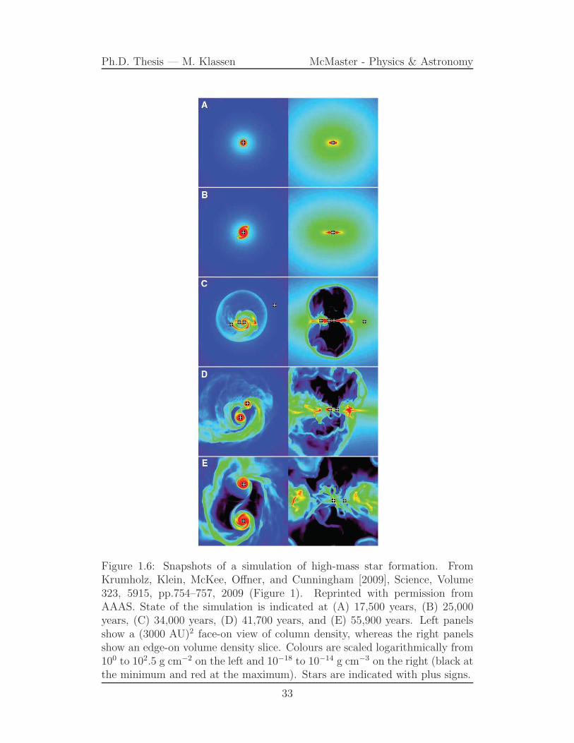
Ph.D. Thesis — M. Klassen McMaster - Physics & Astronomy
Figure 1.6: Snapshots of a simulation of high-mass star formation. FromKrumholz, Klein, McKee, Offner, and Cunningham [2009], Science, Volume323, 5915, pp.754–757, 2009 (Figure 1). Reprinted with permission fromAAAS. State of the simulation is indicated at (A) 17,500 years, (B) 25,000years, (C) 34,000 years, (D) 41,700 years, and (E) 55,900 years. Left panelsshow a (3000 AU)2 face-on view of column density, whereas the right panelsshow an edge-on volume density slice. Colours are scaled logarithmically from100 to 102.5 g cm−2 on the left and 10−18 to 10−14 g cm−3 on the right (black atthe minimum and red at the maximum). Stars are indicated with plus signs.
33

Ph.D. Thesis — M. Klassen McMaster - Physics & Astronomy
ical simulations of the collapse of a massive protostellar core with radiation
feedback, handled via a grey FLD method.
In Figure 1.6, we reproduce with permission a figure from Krumholz
et al. [2009] showing the state of a numerical simulation of massive star for-
mation at different times. The left column of panels shows the face-on column
density of the simulation, while the right column of panels shows edge-on vol-
ume density slices. Each views a 3000 × 3000 AU area. Stars are indicated
using plus signs. In contrast to simulations we performed with our hybrid
radiative transfer method (described in Chapter 2), the results of which are
detailed in Chapter 3, we only form a single star within the time simulated.
As the simulation evolves, Krumholz et al. [2009] observe the formation
radiatively-driven outflow bubbles. Along the edges of the outflow bubble, a
fluid instability was observed that resembled the classical Rayleigh-Taylor in-
stability, in which a heavy fluid is supported by a lighter fluid. In this picture,
dense fingers of material sunk back down onto the star and circumstellar ac-
cretion disk. They argued in analogy to the classical case that radiation was
the lighter fluid supporting the dense molecular gas above it, and this resulted
in the instability. This “radiative Rayleigh-Taylor” instability has been re-
produced in more controlled simulations [Jacquet and Krumholz, 2011], but
still only using FLD. As we have pointed out however, FLD is not a complete
solution for radiative transfer, and its problems were noted in subsequent work.
Kuiper et al. [2012] performed similar calculations, but involving a “hy-
brid” radiative transfer method that decomposed the radiation field into a
direct, stellar component and a diffuse, thermal component. The stellar radi-
ation field was handled via raytracing method, while the diffuse radiation was
handled using an FLD solver. Simulations comparing the FLD-only case to the
34

Ph.D. Thesis — M. Klassen McMaster - Physics & Astronomy
hybrid case showed Rayleigh-Taylor instabilities were suppressed in the hybrid
case. Kuiper et al. [2012] showed that the FLD approximation underestimates
the radiative forces acting on the cavity shells because direct irradiation from
the star is neglected. In the FLD approach, stellar radiation is assumed to be
deposited within a few grid cells around the source. A raytracer can measure
the optical depth along different angles and estimate the local absorption and
momentum deposition accurately. It also carries the temperature information
about the stellar surface, even in the grey case, resulting in a two-temperature
approach to radiative transfer. As this energy is absorbed by the dust, it is
thermalized and the dust is warmed. Ray tracers also cause optically thick
blobs of gas to cast shadows, something that FLD is inherently incapable of
(see, e.g. Figure 2.12 in Chapter 2).
The hybrid radiative transfer scheme described in Kuiper et al. [2010b]
still suffered from several weaknesses. It was implemented on a spherical grid,
which automatically fixes the source immovably at the centre. The “sink”
source measured gas passing through an inner grid radius as accretion. The
resolution of the grid decreased logarithmically with radius and was non-
adaptive. The advantage of this geometry was that the raytrace operation
was essentially one-dimensional, making it computationally inexpensive and
allowing for efficient multi-frequency radiative transfer.
In order to settle the matter of whether radiative Rayleigh-Taylor in-
stabilities were an accretion mechanism for massive protostars, the hybrid
radiative transfer technique needed to be implemented on a general Cartesian
grid with adaptive mesh refinement (AMR). Building this code is one of the
main technical achievements of the thesis and was published in Klassen et al.
[2014], included as Chapter 2 in this thesis. We showed that even in this more
35

Ph.D. Thesis — M. Klassen McMaster - Physics & Astronomy
general geometry, with moveable sink particles coupled to a protostellar evolu-
tion code, the formation of radiative Rayleigh-Taylor instabilities is suppressed
(Chapter 3). Disk accretion alone is sufficient for forming massive stars. An-
other key result that stems from our new methods is that our accretion disks
do not fragment into other stars—which contradicts the results of the pure
FLD code papers [see, e.g. Krumholz et al., 2009].
Finally, we turn to ionizing radiation as an important feedback mech-
anism for massive stars. Hydrogen molecules dissociate at photon energies
above 11 eV and hydrogen atoms are ionized at photon energies above 13.6
eV. When the rate of photoionization exceeds the recombination rate, gas be-
comes a hot (10,000 K), ionized plasma known as an Hii region. Hii regions
are associated with OB stars (M > 8M⊙) and begin to form even while the
protostar is still embedded within its natal envelope.
Hii regions do not become significant feedback mechanisms until fairly
late in protostellar evolution [Klessen et al., 2011] because high rates of ac-
cretion causes protostellar radii to swell to ∼ 100R⊙ [Hosokawa and Omukai,
2009], resuling in low surface temperatures. High accretion rates also result
in high outflow rates [Tan and McKee, 2003], which confines Hii region to the
dense collimated outflows and shields much of the accreting material (in the
disk) from radiative feedback, preventing early disk evaporation. Once the Hii
regions become large enough to exceed their protostellar envelopes, they can
quickly become a dominant feedback mechanism [Keto, 2007, Klessen et al.,
2011] by driving shocks and potentially unbinding the molecular cloud.
Although we did not finish implementing ionization feedback in our
hybrid radiative transfer code in time for this thesis, we do include simulations
done with solely a characteristics-based raytracer coupled to an equilibrium
36

Ph.D. Thesis — M. Klassen McMaster - Physics & Astronomy
ionization code for calculating radiative heating, cooling, and photoionization
in filamentary, magnetized, and turbulent molecular clouds (see Chapter 4).
1.4 Thesis outline and major contributions
This introduction presents the observational evidence and current paradigm of
star formation in order to frame the contributions made by this PhD candidate.
The work has focussed around numerical simulations of massive star formation
and their environments, both at the clump scale (few pc) where clusters form,
and at the core scale (< 1 pc), where individual or low-multiple star systems
form. To this end we have taken the flash magnetohydrodynamics code and
done substantial new development.
My contributions were based on my development of a new hybrid ra-
diative method developed within an adaptive mesh refinement code (flash).
This required substantial modifications to the flash v.4.0 FLD code [Fryxell
et al., 2000a, Dubey et al., 2009]. This version had been expanded for the study
of high-energy density physics, such as the ignition of laser-confined plasmas
for controlled fusion experiments. The code was not designed with cold, dusty
molecular gas in mind. I needed to equilibrate the ion and electron species to
create a “neutral” medium to serve as my molecular gas, which would have the
correct mean molecular weight. This equilibration strategy was originally pub-
lished in the Appendix to Klassen et al. [2014]. The various shock and energy
exchange tests I performed were also detailed in that paper, which is included
as Chapter 2 of this thesis. On the development of this hybrid radiation code,
we collaborated with Rolf Kuiper, who implemented a similar scheme in the
pluto astrophysics code and provided technical assistance as we wrote and
37
Ph.D. Thesis — M. Klassen McMaster - Physics & Astronomy
tested the scheme in flash. Additional technical assistance came from the
flash Center at the University of Chicago, especially from Klaus Weide and
Manos Chatzopoulos, who assisted with making some necessary modifications
to the equation of state (EOS) unit and hydrodynamics unit to accommodate
the new radiative transfer scheme.
Following this, in order to implement the hybrid radiative transfer
scheme of Kuiper et al. [2010b], we needed to make use of a raytracer in
flash . The included laser energy deposition code was too cumbersome and
inappropriate for our purposes. We decided instead to port a characteristics-
based raytracer that we had used in version 2.5 of flash that had originally
been implemented by Rijkhorst et al. [2006b], then improved upon by Pe-
ters et al. [2010a] and with which I had considerable experience work through
my published M.Sc. papers: (1) Klassen, Pudritz, and Peters [2012b] and
(2) Klassen, Peters, and Pudritz [2012a]. Porting this code to version 4.0 of
flash was a process that took months because of the substantial changes in
code architecture between versions 2.5 and 3.0 of flash .
Next the raytracer needed to be coupled with the FLD code. Taking the
discretized, coupled equations of the gas internal energy and radiation diffu-
sion, and with temperature linearization approach borrowed from Commercon
et al. [2011b], I was able to write the new emission and absorption coeffi-
cients in the coupling term and modify these in the flash radiative transfer
routines. I had to replace the explicit temperature update that flash was
making with an iterative Newton-Raphson temperature update method. This
required several additional months of testing to debug and implement an ap-
propriate method for handling the temperature update. In particular, many of
the problems did not become apparent until working on the paper for Chapter
38

Ph.D. Thesis — M. Klassen McMaster - Physics & Astronomy
3 of this thesis, because we had previously only applied our radiative transfer
technique in static test problems or dynamic tests with short timesteps. Sim-
ulating protostellar cores with all of the relevant physics (e.g. hydrodynamics)
turned on was a much more demanding problem that necessitated more code
development and testing. After 2 years of development and the eventual pub-
lication of our code paper [Klassen, Kuiper, Pudritz, Peters, Banerjee, and
Buntemeyer, 2014, ApJ, 797], we were ready to perform star formation calcu-
lations.
I set up a protostellar model based on the initial conditions of both
Krumholz et al. [2009] and Kuiper et al. [2010a]. I simulated the collapse
of three protostellar cores at masses of 30, 100, and 200 M⊙ and then per-
formed extensive analyses of the resulting data, looking at the mass evolution,
disk stability, accretion history, outflow formation, and bubble morphology.
The results were published as Klassen, Pudritz, Kuiper, Peters, and Banerjee
[2016b, ApJ, 823], and are included in this thesis as Chapter 3. We found that
disk accretion is sufficient to explain the formation of massive stars, with the
need for other mechanisms, such as radiative Rayleigh-Taylor instabilities of
the outflow bubble walls. Our accretion disks become Toomre-unstable, which
increases the accretion rate onto the central star, but do not fragment within
the time simulated to form companion stars.
All the while I was also engaged in research on the larger context of
massive star formation by simulating magnetized, turbulent molecular cloud
clumps of around 500, 1000, and 2000 M⊙. These are the environments in
which massive stellar clusters are formed and we wanted to take a closer look
at the filamentary structure of these environments and their interplay with
the larger magnetic field structure. To this end, I set up MHD simulations
39

Ph.D. Thesis — M. Klassen McMaster - Physics & Astronomy
including supersonic turbulence, with average mass-to-flux ratios akin to what
has been observed. We compared the filamentary structure of these to similar
simulations I ran without magnetic fields and published the results as part in
Kirk, Klassen, Pudritz, and Pillsworth [2015].
To study the relation of magnetic fields to filaments in clouds, I con-
tacted Thierry Sousbie, the author of the DisPerSE code, which has been
successfully applied in the analysis of Herschel data for the study of filamen-
tary structure. DisPerSE can analyze both 2D images and 3D simulation
data and produce a filament skeleton. The technique the DisPerSE uses
has been described in Sousbie [2011] and Sousbie et al. [2011]. I included a
summary of it in the methods section of Chapter 4. Sousbie supplied me with
a pre-release version of DisPerSE and we used it to analyze column density
projections of simulation data in Kirk, Klassen, Pudritz, and Pillsworth [2015],
a paper to which I contributed the numerical simulations, as well as part of the
analysis and writing. We next began developing our 3D analysis capabilities
for a study of magnetic field structure in relation to filaments.
A primary goal of Chapter 4 is to trace the role of magnetic fields on
star formation within filaments. No study to our knowledge has yet achieved
this by following a filament along in a 3D data cube. We believe that this
is the first study to achieve this by applying DisPerSE . DisPerSE was
incompatible with HDF5 files, which is the default way that flash stores its
AMR grid data. Helen Kirk initially had done some work remapping this
data onto a uniform grid in the FITS file format, but found that DisPerSE
frequently ran out of memory when trying to analyze this data. I was able
to get this approach to work using tools from the yt toolkit to remap flash
AMR data to a downsampled uniform grid. This was able to fit within memory
40

Ph.D. Thesis — M. Klassen McMaster - Physics & Astronomy
and DisPerSE produced useable filament skeletons.
The analysis tools I wrote for handling flash data and DisPerSE
spanned hundreds of lines of code and dozens of subroutines. When I ran out of
desktop computing power and memory, I portedDisPerSE to Amazon’s cloud
computing hardware, where I could leverage scaleable computing hardware on
demand with root-level privileges.
The results of our analysis of simulated magnetised turbulent cloud
clumps is part of a paper submitted to Monthly Notices of the Royal Astro-
nomical Society and revised in response to the referee report [see Klassen, Pu-
dritz, and Kirk, 2016a, arXiv:1605.08835]. We simulated clouds with roughly
equal magnetic and turbulent energies (“trans-Alfvenic” clouds) and studied
the magnetic field geometry, the filamentary structure, and accretion flows.
We found that in such clouds, the virial parameter plays an important role.
Highly bound clouds, due to gravitational infall dragging magnetic field lines
inward, show more coherent large-scale magnetic field structure. For clouds in
virial balance, the magnetic field is chaotic and disorderly, except within the
largest, primary filament (the main “trunk”), where the magnetic field lines
have been shock-compressed to lie parallel with the long axis of the filament.
This paper is reproduced in this thesis as Chapter 4.
One simulation included ionizing feedback from a cluster of stars. Star
formation takes place within the main filament. A cluster forms, but is dom-
inated by a single massive star that reaches about 16 M⊙. It drives an Hii
region that ultimately engulfs the cluster and begins destroying the filament.
This makes the connection then, with the work from Chapter 3, where we
examined the radiative feedback effects of a massive isolated star in a simpli-
fied environment. This star provides sufficient ionizing flux that an Hii region
41

Ph.D. Thesis — M. Klassen McMaster - Physics & Astronomy
forms and begins disrupting the main trunk filament of the cloud clump. Along
the edges of the Hii region, swept-up material forms a shell and the magnetic
fields lines are seen threading parallel to the shell, showing that photoioniza-
tion feedback modifies the magnetic field geometry.
1.4.1 Chapter descriptions
The chapters of this thesis are presented as electronic copies of journal articles
either in print, recently submitted, or in preparation to submit. The case for
each one has been indicated in the list below. In lieu of prefacing each chapter
with a separate introduction, we include a brief statement on the research’s
context within the thesis. For each one, I have been the primary contributor
(first author), and the author list of each one has been included. Instead of the
abstract of each journal article, I have written a short description that better
shows the cohesion of the three papers within this thesis.
• Chapter 2: A General Hybrid Radiation Transport Scheme for Star
Formation on an Adaptive Grid
Authors: Mikhail Klassen, Rolf Kuiper, Ralph Pudritz, Thomas Pe-
ters, Robi Banerjee, Lars Buntemeyer
Published: The Astrophysical Journal, Volume 797, Issue 1 (December,
2014)
Description: We present the implementation of a general hybrid radia-
tive transport scheme in flash and the general theory. We perform
numerical tests of the accuracy of the method. This represents the first
time that this type of complete radiative transfer method has been imple-
mented in a general, Cartesian, adaptive mesh refinement (AMR) code
42

Ph.D. Thesis — M. Klassen McMaster - Physics & Astronomy
(flash in this case). It opens up a wide range of important problems for
detailed study, including the evolution of protoplanetary disks, radiative
feedback from a cluster a massive stars in turbulent, magnetized envi-
ronments, and the formation of clusters inside giant molecular clouds.
Contributions: Mikhail Klassen implemented the radiative transfer
scheme in flash with support from Rolf Kuiper, who had implemented
a similar scheme in the PLUTO code. Mikhail the ran the tests de-
scribed in the paper and analysed the results. Rolf supplied benchmark
data. Ralph Pudritz, Thomas Peters, Robi Banerjee, and Lars Bun-
temeyer assisted in debugging, advised on test selection, and supplied
comments to the paper. The main text of the paper was written by
Mikhail Klassen.
• Chapter 3: Simulating the Formation of Massive Protostars: I. Radia-
tive Feedback and Accretion Disks
Authors: Mikhail Klassen, Ralph Pudritz, Rolf Pudritz, Thomas Pe-
ters, Robi Banerjee
Published: The Astrophysical Journal, Volume 823, Issue 1 (May, 2016)
Description: We describe a series of improvements to the hybrid radiative
transfer scheme and simulate the collapse of massive protostellar cores.
We show each core collapses gravitationally to form a single massive star
with all further fragmentation suppressed. We study the formation and
evolution of a circumstellar accretion disk. We analyze the disk stability
and conclude that while gravitationally unstable, which resulted in the
formation of large spiral waves, these spiral waves are still stable against
43

Ph.D. Thesis — M. Klassen McMaster - Physics & Astronomy
fragmentation. Radiatively-driven bubbles form, but show no signs of ra-
diative Rayleigh-Taylor instabilities. This is the first time that a general
3D framework with a complete treatment of radiation has been applied
to this critical problem. The lack of disk fragmentation has major impli-
cations for trying to understand how O stars manage to typically reside
in binary systems.
Contributions: Mikhail Klassen implemented the necessary code changes
and improvements in flash needed to run dynamic star formation sim-
ulations with hybrid radiation feedback. Members of the flash Center
at the University of Chicago supplied a new hydro solver and various
other modification that helped stabilize the code. Mikhail then ran the
simulations and performed the data analysis, as well as wrote the main
text of the paper. Comments, suggestions, and theoretical insights on
disk stability were supplied by the co-authors.
• Chapter 4: Filamentary Flow and Magnetic Geometry in Evolving
Cluster-Forming Molecular Cloud Clumps
Authors: Mikhail Klassen, Ralph Pudritz, Helen Kirk
Submitted: Revised in response to referee comments and resubmitted to
Monthly Notices of the Royal Astronomical Society (May 2016)
Description: We perform one of the first-ever applications of 3D fil-
ament extraction using the DisPerSE algorithm on numerical simula-
tions of massive star-forming molecular cloud clumps—the environments
in which protostellar cores are formed. Supersonic turbulence gives rise
to a network of filaments, as observed in molecular clouds. We initialize
44
Ph.D. Thesis — M. Klassen McMaster - Physics & Astronomy
our simulations with realistic magnetic fields and then follow the evolu-
tion of the magnetic field geometry. We measure the relative orientation
of filaments and magnetic fields. Our cloud clumps are trans-Alfvenic,
meaning that the ratio of magnetic energy to turbulent energy is ap-
proximately unity. In these clouds, we found that the magnetic geom-
etry is sensitive to the virial parameter. Highly bound clouds show a
more coherent magnetic field geometry, with fields tending to align more
parallel to filaments and accretion flows tending to drag magnetic field
lines inward. This gave the appearance of field lines oriented perpen-
dicular to the main “trunk” filament of our molecular cloud clump. In
our marginally bound cloud, the magnetic fields tended to be oriented
more perpendicular to filaments in 3D. Photoionisation feedback from
massive stars disrupts the filamentary birth environment and modifies
the magnetic field geometry in the vicinity of the star cluster. It also
cuts off accretion flows and sets the mass of the stars within the cluster.
Contributions: Mikhail Klassen ran the simulations for this paper
with input on setup design and parameter selection from Ralph Pudritz
and Helen Kirk. Various analysis routines were supplied by Helen Kirk.
Mikhail wrote many additional analysis scripts and performed the data
analysis of the simulation results. The main text of the paper was writ-
ten by Mikhail with improvements, recommendations, and corrections
supplied by Ralph Pudritz and Helen Kirk.
Due to the nature of “sandwich” theses, there is necessarily some over-
lap between the chapters written as scientific journal articles. There may be
some moderate overlap in the content of the introductions of Chapters 2 and
45

Ph.D. Thesis — M. Klassen McMaster - Physics & Astronomy
3, as well as in the numerical methods sections. With Chapter 4, sections
describing the flash astrophysics code may overlap with similar sections in
Chapters 2 and 3, but these are minimal. I note that the work of Chapter 4 is
built upon another publication during my Ph.D. work—Kirk, Klassen, Pudritz
& Pillsworth (2015, The Astrophysics Journal, 802) for which I performed the
numerical simulations and contributed to the analysis of the data.
Finally, in Chapter 5 we summarize our conclusions and how they fit
within the current state of star formation research. We present an outlook to
the future of the research field and the simulations that naturally follow from
the advances presented within this thesis.
46

Ph.D. Thesis — M. Klassen McMaster - Physics & Astronomy
Chapter 2
A General Hybrid Radiation
Transport Scheme for Star
Formation on an Adaptive Grid
2.1 Introduction
The last several years have seen increasingly sophisticated radiation feedback
models implemented in a wide variety of codes to simulate an ever wider array
of physical problems. The importance of radiation feedback in the problem of
star formation cannot be overstated. It is an essential process in the regulation
of star formation rates and efficiencies on galactic scales, the resulting effects
on the structure and evolution of galaxies [Agertz et al., 2013], the formation
of star clusters and possible regulation of the IMF [Mac Low and Klessen,
2004, McKee and Ostriker, 2007b], the formation of massive stars [Beuther
et al., 2007, Krumholz et al., 2007a, Kuiper et al., 2010b, 2011a, Kuiper and
Yorke, 2013a,b], and the heating and chemistry of protoplanetary disks and
47
Ph.D. Thesis — M. Klassen McMaster - Physics & Astronomy
implications for planet formation [Aikawa and Herbst, 1999, Fogel et al., 2011].
Radiation feedback’s relevance for star formation has long been under-
stood. The depletion time for a molecular cloud tdep = Mgas/M is 1–3 orders
of magnitude longer than the cloud’s freefall time tff ∼ 1/√Gρ [Krumholz and
Tan, 2007, Evans et al., 2009], yet simulations that do not include any feed-
back mechanisms routinely see unrealistically high star formation efficiencies,
with tdep ∼ tff .
We focus here on radiation feedback, which has been repeatedly demon-
strated in simulations as an effective means of suppressing star formation, even
radiation from low-mass stars [Offner et al., 2009]. While magnetic fields have
been suggested as a mechanism for slowing gravitational collapse, Crutcher
[2012] shows that many molecular clouds are 2–3 times supercritical to gravi-
tational collapse. Magnetic fields have the effect of suppressing star formation
[Tilley and Pudritz, 2007, Price and Bate, 2009], and a careful treatment of
them must be done in any accurate star formation simulation, but it is one
of several critical processes in play. Other stellar feedback mechanisms have
also been studied, including winds, outflows [Kuiper et al., 2014, Peters et al.,
2014], ionization [Peters et al., 2010a], radiation pressure, and supernovae, but
many of these are at least in part tied to the stellar radiation [Murray et al.,
2010].
We focus on the problem of thermal and momentum radiation feedback
and the challenge of implementing highly accurate radiation hydrodynamics
into a grid code for general simulations of star formation, leaving ionization ef-
fects to future work. Radiation hydrodynamics (RHD) methods have been im-
plemented into several grid codes, e.g. zeus [Turner and Stone, 2001], athena
[Skinner and Ostriker, 2013], orion [Krumholz et al., 2007b], ramses [Com-
48
Ph.D. Thesis — M. Klassen McMaster - Physics & Astronomy
mercon et al., 2011b, Rosdahl et al., 2013], and pluto [Mignone et al., 2007b]
by Kuiper et al. [2010a], Flock et al. [2013], Kolb et al. [2013].
Most implementations of radiation hydrodynamics have been limited
to the gray flux-limited diffusion (FLD) approximation, in which the radiation
flux is proportional to the gradient of the radiation energy, ∇Er. In this limit,
it is usually assumed that the radiation and matter internal energies are tightly
coupled, with the radiation and gas temperatures being equal. Further, the
energy from stellar sources is deposited within some kernel centred on the
radiation sources.
The problem with this approach is that the geometry of the environ-
ment surrounding stellar sources of radiation is rarely spherically symmetrical.
Stars create outflow cavities and Hii regions that are optically thin to radia-
tion. Meanwhile, protostars accrete material through a rotating disk structure
that is usually highly optically thick. Outflow cavities provide an outlet for
the radiation flux—the so-called “flashlight effect” described in Yorke and
Sonnhalter [2002], Krumholz et al. [2005b], and Kuiper et al. [2014, submit-
ted]. Protostellar jets are on the scale of 100–1000 AU or even parsec scales
for massive protostars, and Hii regions can easily approach the parsec scale as
well.
Above all, the birth environments of stars contain supersonic turbu-
lence, which gives rise to filaments that allow stellar radiation a path of easy
egress into the optically thin cavities between filaments while remaining op-
tically thick along the direction of the filament. Typical implementations of
FLD schemes will fail to take into account this high degree of asymmetry when
depositing stellar radiation energy. This may miss important effects.
A particularly important problem in this regard is the formation of
49

Ph.D. Thesis — M. Klassen McMaster - Physics & Astronomy
a massive star and its associated accretion disk. The intense radiation field
from the forming star heats and ionizes the infalling envelope but does far
less damage to the highly optically thick accretion disk through which most
of gas, destined for the star, flows. Disk accretion therefore becomes the chief
mechanism by which massive stars continue to accrete material despite their
high luminosity [Kuiper et al., 2010b]. The accretion disk creates an environ-
ment with sharp transition regions between optically thick and optically thin,
where traditional FLD codes are most inaccurate [Kuiper and Klessen, 2013].
To address this high degree of asymmetry, Kuiper et al. [2010a] implemented
a radiation transfer scheme in pluto that combined a 1D multifrequency ray-
trace with a gray FLD code. The method was implemented for spherical polar
grids, which meant that the raytrace needed only be carried out in the radial
direction.
As an example application of this, Kuiper et al. [2012] studied the
stability of radiation-pressure-dominated cavities around massive protostars.
Radiatively-driven outflows have the potential to remove a significant amount
of mass from the stellar environment that would otherwise be accreted by the
protostar. Several mechanisms have been proposed for how a massive protostar
could accrete material beyond its Eddington limit. Krumholz et al. [2009]
proposed a “radiative Rayleigh-Taylor instability” in which the radiatively-
driven shell becomes unstable and material is able resume gravitational infall.
But Kuiper et al. [2012] argued that a gray FLD-only radiative transfer scheme
underestimates the radiative forces acting on the shell.
We now generalize the method to 3D Cartesian grids with adaptive
mesh refinement (AMR) and implement a hybrid raytrace/FLD method in
the flash astrophysics code. This method extends to multiple sources and
50
Ph.D. Thesis — M. Klassen McMaster - Physics & Astronomy
does not rely on any special geometry, allowing for the treatment of more
general problems such as star cluster formation. Moreover, for the FLD solver
step, we implement a two-temperature (2T) radiation transport scheme; that
is, we do not force the radiation temperature and matter temperature to be
equal everywhere. We discuss the general theory of this approach in section
2.2; the equations to be solved and the numerical methods for flash in section
2.3; the tests of our radiation transport scheme in sections 2.4, 2.5, and 2.6;
and our final thoughts and discussion in section 2.7.
2.2 Theory
The general idea to split the radiation field into a direct component and a
diffuse or scattered component is an old one [see, e.g., Wolfire and Cassinelli,
1986, Murray et al., 1994, Edgar and Clarke, 2003]. The direct component
dominates in the optically thin regions, such as in the outflow cavities created
by massive stars, or in Hii regions, where the temperature of the radiation
field is that of the stellar photosphere. Within a few optical depths, inside the
optically thick regions, the radiation field becomes dominated by the diffuse,
thermal component of the radiation field. The main advantage of splitting
the radiation field in this way is accuracy [Murray et al., 1994]. Raytracing
is a solution to the radiative transfer problem, whereas FLD is a convenient
approximation for the sake of computation. In the optically thin regions such
as those noted above, a direct raytrace ignoring scattering is an excellent
way of accurately calculating the radiation field, whereas the gray FLD is
accurate inside optically thick regions where the temperature of the radiation
is equilibrated to the matter temperature. In complex morphologies, with
51

Ph.D. Thesis — M. Klassen McMaster - Physics & Astronomy
interspersed regions of varying optical depth, FLD is not at all accurate.
This general splitting approach is equivalent to extracting the first ab-
sorption event from the FLD solver and allowing the radiation flux to be
calculated by a raytracing scheme instead, with all re-emission and secondary
absorption handled by the FLD solver. This improves the accuracy in precisely
the region where the FLD approximation is worst, namely in regions directly
irradiated by discrete radiation sources such as stars.
A hybrid radiation transport scheme splits the flux term,
F = F∗ + Fth, (2.1)
into a direct (stellar) component F∗ and a thermal radiation component Fth.
FLD implementations treat only the transport of a single radiation flux pro-
portional to the gradient in the radiation energy Er,
Fth ∝ −∇Er. (2.2)
Hybrid schemes decompose the radiation field, transporting the direct com-
ponent via a raytracer (see 2.3.4) and the indirect component via a diffusion
equation. The radiation transport equation, integrated over all solid angle,
with the operator-split hydrodynamic terms removed, is
∂tEr +∇ · Fr = κPρ (4πB − cEr) , (2.3)
with Er is the radiation energy density, Fr the flux of the radiation energy, σP
the Planck opacity, B = B(T ) the Planck function, and c the speed of light.
In a split scheme the direct component ∇ ·F∗ is calculated everywhere
52
Ph.D. Thesis — M. Klassen McMaster - Physics & Astronomy
for all sources. We describe how this is done in section 2.3.4. How the thermal
component is handled is the subject of section 2.3.3.
In order to address problems of multiple star formation, as well as the
formation of star clusters, a more general approach is needed. Specifically, we
generalize the hybrid radiation transfer approach to Cartesian grids with AMR.
These kinds of codes already have the ability to follow the gravitational collapse
of multiple regions within a simulation, and have excellent implementations of
turbulent and MHD processes. They also enable further study of radiatively-
driven shells and outflows with adaptive resolution.
The scope of the current paper is the implementation of the general
hybrid radiation transfer scheme in an AMR grid code, and tests of its accu-
racy. As noted in the introduction, there are many important applications of
our code which we will take up in subsequent papers, including the formation
of a massive star in a turbulent, magnetized, collapsing medium, ionization
feedback, and the formation of star clusters.
2.3 Numerical methodology
2.3.1 FLASH
We use the publicly available flash high-performance general application
physics code, currently in its 4th major version [Fryxell et al., 2000a, Dubey
et al., 2009]. The code is modular, and has physics capabilities that now in-
clude 2T radiation hydrodynamics (our contribution), magnetohydrodynam-
ics, multi-group flux-limited diffusion, self-gravity, and a variety of options for
the equation of state.
53

Ph.D. Thesis — M. Klassen McMaster - Physics & Astronomy
The code has been expanded to include sink particles, originally imple-
mented in version 2.5 [Federrath et al., 2010a], and then later ported to version
4.0 [Safranek-Shrader et al., 2012]. Multigroup flux-limited diffusion for ra-
diation hydrodynamics was added in version 4.0 for the study of high-energy
density physics (HEDP), such as radiative shocks and laser energy deposition
experiments. Despite these original motivations, the code is general and can
be applied to astrophysical scenarios.
A time-independent raytracer with hybrid characteristics was added
in version 2.5 by Rijkhorst et al. [2006a] and then modified for the study
of collapse calculations by Peters et al. [2010a]. The raytracer was used to
calculate photoelectric heating and photoionization rates, as well as heating
by optically thin non-ionizing radiation, to study Hii regions and ionization
feedback in molecular clouds [Peters et al., 2010a,d,c, 2011, 2012, Klassen
et al., 2012b]. However, this approach is not suitable to propagate non-ionizing
radiation in optically thick clouds.
We ported this raytracer into the present version of the flash code in
order to calculate the irradiation of gas and dust by point sources within the
domain and solve the radiation hydrodynamic equations.
flash solves the fluid equations on an Eulerian mesh with adaptive
mesh refinement (AMR) using the piecewise parabolic method [Colella and
Woodward, 1984]. The method is well-suited for dealing with shocks. The dif-
fusion equation is solved implicitly via the generalized minimal residual (GM-
RES) method. The refinement criterion used by flash is an error estimator
based on Lohner [1987], which is a modified second derivative normalized by
the average of the gradient over one computational cell. It has the advantage
of being dimensionless and local, so one has the flexibility to choose the grid
54

Ph.D. Thesis — M. Klassen McMaster - Physics & Astronomy
variable upon which to refine.
In this paper we describe the implementation of a hybrid radiation
transfer scheme, involving raytracing coupled to a flux-limited diffusion (FLD)
solver. The raytracer finds the flux each cell receives from all point sources
(e.g. stars) in the simulation while the FLD solver evolves the diffuse radiation
field. The combined radiation field is used to update the matter temperature.
In the sections below we recapitulate the basic theory and how these
equations are implemented in flash .
2.3.2 Radiation hydrodynamics
If the radiation fields are assumed to have a blackbody spectrum, then in
the absence of magnetic and gravitational fields, and assuming local ther-
modynamic equilibrium (LTE), the frequency- and angle-integrated radiation
hydrodynamic equations in the comoving frame are [Turner and Stone, 2001,
Mihalas and Mihalas, 1984]
DρDt
+ ρ∇ · v = 0 (2.4)
ρDv
Dt= −∇p+ 1
cκPρFr (2.5)
ρ DDt
(
eρ
)
+ p∇ · v = −κPρ(4πB − cEr) (2.6)
ρ DDt
(
Er
ρ
)
+∇ · Fr +∇v : P = κPρ(4πB − cEr) (2.7)
where D/Dt ≡ ∂/∂t + v · ∇ is the convective derivative. The fluid variables
ρ, e, v, and p are the matter density, internal energy density, fluid velocity,
and scalar pressure, respectively, while Er,Fr, and P are the total frequency-
integrated radiation energy, flux, and pressure, respectively. Equations 2.4
55
Ph.D. Thesis — M. Klassen McMaster - Physics & Astronomy
and 2.5 express the conservation of mass and momentum, respectively, where
the radiation applies a force proportional to κPρFr/c, where κP is the Planck
mean opacitiy defined in equation 2.9 below.
The hydrodynamic equations must also be closed via an equation of
state. We use a gamma-law equation of state for simple ideal gases. The gas
pressure P , density ρ, internal energy ǫ, and gas temperature T are related by
the equations,
P = (γ − 1)ρǫ =NakBµ
ρT, (2.8)
with adiabatic index γ = 5/3. Na is Avogadro’s number, kB is the Boltzmann
constant, and µ is the mean molecular weight.
The coupling between internal and radiation energy is expressed by
equations 2.6 and 2.7. Coupling comes through the emission and absorption
of radiation energy. The assumption of LTE lets us write the source function
as the Planck function, B, so that matter emits thermal radiation proportional
to the rate,
4πκPρB(T ) ≡ κPρcaT4,
where κP is the Planck mean opacity,
κP =
∫∞
0dνκνBν(T )
B(T ), (2.9)
with
Bν(T ) =2hν3/c2
ehν/kBT − 1. (2.10)
Meanwhile, matter is absorbing radiation out of the thermal field at a
rate κPρcEr. Energy lost by the radiation field is gained by the matter and
vice versa. We will use the flux-limited diffusion approximation to relate the
56

Ph.D. Thesis — M. Klassen McMaster - Physics & Astronomy
radiation flux Fr to the radiation energy Er.
In practice, many grid codes implement the flux-limited diffusion ap-
proximation [Turner and Stone, 2001, Krumholz et al., 2007b, Commercon
et al., 2011b], which relates the radiation flux Fr to the radiation energy Er.
In the FLD approximation, the radiation and matter components may be
thought of as two fluids, each with their own equation of state, internal en-
ergy, temperature, and pressure. The matter component may be further split
into ion and electron components, which exchange energy via collisions. This
is three-temperature, or “3T” approach is used in the modeling of laboratory
plasmas. The flash code was extended in version 4 to include 3T radiation
hydrodynamics [Lamb et al., 2010, Fatenejad et al., 2012, Kumar et al., 2011].
Energy exchange under the 3T model is included for reference in Section 2.8.
In astrophysics, we are more concerned with modeling the gas/dust mixture
of the ISM, with the gas sometimes ionized. By setting a unified matter tem-
perature in flash , with Tion = Tele ≡ Tgas/dust, we return to a 2T model, with
only matter and radiation temperatures varying and exchanging energy.
Radiation only behaves like a fluid when it is tightly coupled to matter,
which occurs only in very optically thick regions. Hybrid radiation schemes
more accurately transport the radiation energy through the computational
domain.
2.3.3 Flux-limited diffusion
Under the flux-limited diffusion approximation [Levermore and Pomraning,
1981, Bodenheimer et al., 1990], the flux of radiation is proportional to the
57

Ph.D. Thesis — M. Klassen McMaster - Physics & Astronomy
gradient in the radiation energy density,
Fr = −D∇Er, (2.11)
where
D =λc
κRρ(2.12)
is the diffusion coefficient. κR is the Rosseland mean opacity and λ is the flux
limiter that bridges the radiation diffusion rate between the optically thin and
optically thick regimes. In the extreme optically thick limit, λ → 1/3, which
is the diffusion limit. In the extreme optically thin limit, the flux of radiation
becomes Fr = cEr, the free-streaming limit.
We use the Levermore and Pomraning [1981] flux limiter, one of the
most commonly used,
λ =2 +R
6 + 3R +R2, (2.13)
with
R =|∇Er|κRρEr
. (2.14)
Other flux limiter are possible, such as Minerbo [1978], another popular choice.
Different flux limiters result from different assumptions about the angular
distribution of the specific intensity [Turner and Stone, 2001].
flash solves the radiation diffusion equation 2.7 using a general im-
plicit diffusion solver. Using the method of operator splitting, terms such as
advection and hydrodynamic work are handled by the code’s hydro solver.
The radiation diffusion solver then updates the radiation energy equation by
58

Ph.D. Thesis — M. Klassen McMaster - Physics & Astronomy
solving
∂Er
∂t+∇ ·
(
λc
κRρ∇Er
)
= κPρc(
aT 4 − Er
)
(2.15)
where T is the gas temperature.
To solve this equation, we use the method of the generalized minimum
residual (GMRES) by Saad and Schultz [1986]. It is included in flash via the
hypre library [Falgout and Yang, 2002]. The GMRES method is the same one
employed by Kuiper et al. [2010a] in their hybrid radiation-transport scheme.
It belongs to the class of Krylov subspace methods for iteratively solving sys-
tems of linear equations of the form Ax = b, where the matrix A is large
and must be inverted. Matrix inversion is, in general, a very computation-
ally expensive operation, but because A is also a sparse matrix, methods exist
for rapidly computing an approximate inverse with relatively high accuracy,
outperforming methods such as conjugate gradient (CG) and successive over-
relaxation (SOR). The hypre library that flash uses is a collection of sparse
matrix solvers for massively parallel computers.
A difference in matter and radiation temperatures in equation 2.15 re-
sults in an energy “excess” on the right-hand side. We must update the mat-
ter temperature due to the action of the combined radiation fields. Restating
equations 2.6 and 2.7, with operator-split hydrodynamic terms removed, and
a stellar radiation source term added, we have
∂tρǫ = −κPρc(
aRT4 − Er
)
−∇ · F∗ (2.16)
∂tEr +∇ · Fr = +κPρc(
aRT4 − Er
)
(2.17)
59

Ph.D. Thesis — M. Klassen McMaster - Physics & Astronomy
Discretizing equation 2.16 and 2.17, we have
ρcV Tn+1−ρcV Tn
∆t= −κn
Pρc(
aR(
T n+1)4 −En+1
r
)
−∇ · F∗, (2.18)
and
En+1r −En
r
∆t−∇ ·
(
Dn∇En+1r
)
= +κρc(
aR(
T n+1)4 − En+1
r
)
(2.19)
recalling that the specific internal energy ǫ = cV T , with cV being the specific
heat capacity of the matter. Variables with superscript indices n and n + 1
take their values from before and after the implicit update, respectively. It is
important to remember that the opacity κP is temperature-dependent. The
source term for stellar radiation takes the form ∇ · F∗ and represents the
amount of stellar radiation energy absorbed at a given location in the grid
from all sources.
The presence of the nonlinear term (T n+1)4 makes it difficult to solve
for the temperature in 2.18. Assuming that the change in temperature is small,
Commercon et al. [2011b] linearizes this term,
(
T n+1)4
= (T n)4(
1 +T n+1 − T n
T n
)4
≈ 4 (T n)3 T n+1 − 3 (T n)4 . (2.20)
This allows for equation 2.20 to be substituted into equation 2.18 and
for us to write an expression for the updated temperature,
T n+1 =3aRα (T n)4 + ρcV T
n + αEn+1r −∆t∇ · F∗
ρcV + 4aRα (T n)3, (2.21)
60

Ph.D. Thesis — M. Klassen McMaster - Physics & Astronomy
where we have used α ≡ κnPρc∆t.
The irradiation term, ∇·F∗, is supplied by the raytracer. Its calculation
is the subject of section 2.3.4.
The raytrace is performed first in order to calculate ∇ · F∗. By sub-
stituting equation 2.21 into 2.19 via the approximation of equation 2.20, and
making appropriate simplifications, the FLD equation becomes
En+1r − En
r
∆t−∇ ·
(
Dn∇En+1r
)
+
κρc
[
ρcV Tn
ρcV T n + 4αaR (T n)4
]
En+1r
= κρcaR (T n)4[
ρcV Tn − 4∆t∇ · F∗
ρcV T n + 4αaR (T n)4
]
, (2.22)
where we have gathered implicit terms on the left-hand side and explicit terms
on the right-hand side.
We solve equation 2.22 via the diffusion solver to calculate the updated
radiation energy density and temperature, then update the gas/dust temper-
ature via 2.21. This completes the radiation transfer update for the current
timestep.
2.3.4 Stellar irradiation
When the effects of scattering and emission are ignored, the equation for the
specific intensity of radiation from a point source along a ray assumes a very
simple form,
I(r) = I0e−τ(r), (2.23)
61

Ph.D. Thesis — M. Klassen McMaster - Physics & Astronomy
where I0 is the specific intensity of the source and τ(r) is the optical depth
from the source up to r:
τ(r) =
∫ r
R∗
κP (T∗)ρ(r′) dr′ (2.24)
The opacity κP is a function of temperature and the optical depth is calcu-
lated using the temperature of the radiation source, e.g. the effective temper-
ature of a star. ρ is the usual gas density. Rays are traced from individual
cells in the computational grid back to the point sources (usually stars) via a
characteristics-based method described in Rijkhorst et al. [2006a].
In characteristics-based raytracing, there are two approaches to com-
puting the column density toward sources, each with its own advantages and
disadvantages. Long characteristics involves tracing rays from the source to
each cell in the computational domain. This method is very accurate, but
involves many redundant calculations of the column density through cells in-
tersected by similar rays near the source. Short characteristics tries to mitigate
the redundant calculations by tracing rays only across the length of each grid
cell in the direction of the source, then interpolating upwind toward the source
to calculate the total column density. The disadvantage of this approach is
that the upwind values need to be known ahead of time, which imposes an
order on the calculations and makes scaling the code to many processors very
problematic. Some amount of numerical diffusivity is also introduced in this
approach on account of interpolating column densities at each cell.
As a compromise between these two methods, Rijkhorst et al. [2006a]
developed a method they called hybrid characteristics that minimizes the num-
ber of redundant calculations and can be parallelized. The local contributions
62
Ph.D. Thesis — M. Klassen McMaster - Physics & Astronomy
to the column density are computed for each block of n×n×n cells. Then the
values on the block faces are computed and communicated to all processors.
Finally, the total column density at each cell is computed by adding the local
and interpolated face values.
Peters et al. [2010a] have improved the method to allow collapse simu-
lations with arbitrary many refinement levels and sources of radiation. They
added the propagation of (optically thin) non-ionizing radiation and coupled
the respective heating terms to a prescription of molecular and dust cooling
[Banerjee et al., 2006]. Furthermore, they have linked the radiation module to
sink particles [Federrath et al., 2010a] as sources of radiation and implemented
a simple prestellar model to determine the value of the stellar and accretion
luminosities. In our current implementation, we no longer use a separate cool-
ing function because the thermal evolution is already implicit in the coupled
equations of internal and radiation energy, as described in section 2.3.3.
The stellar flux a distance r is given by
F∗(r) = F∗(R∗)
(
R∗
r
)2
exp (−τ(r)) , (2.25)
where R∗ is the stellar radius, and F∗(R∗) is the flux at the stellar surface,
given by
F∗(R∗) = σT 4∗ . (2.26)
T∗ is the effective temperature of the stellar surface and σ is the Stefan-
Boltzmann constant.
At this time, our raytracing is purely gray; we use the Draine and
Lee [1984] dust model and compute the temperature-dependent frequency-
63

Ph.D. Thesis — M. Klassen McMaster - Physics & Astronomy
averaged opacities, assuming a 1% dust-to-gas ratio. Multifrequency raytrac-
ing is relatively straightforward to implement, but the computational costs
increase linearly with the number of frequency bins. We leave the implemen-
tation of multifrequency effects to a future paper.
Using the stellar flux computed at each cell, we estimate an “irradia-
tion” term, i.e. the amount of stellar flux absorbed by a given cell,
∇ · F∗(r) ≈ −(1− eτlocal)
∆rF∗(r), (2.27)
where τlocal is the “local” contribution to the optical depth through the cell,
i.e.
τlocal ≈ κP (T∗)ρ∆r, (2.28)
and ∆r is the distance traced by the ray through a grid cell. For numerical
stability, when τlocal is very small, e.g. 10−5, we estimate the irradiation by
Taylor-expanding the exponential,
∇ · F∗(r) ≈ −κPρF∗(r), (2.29)
which is the optically thin limit.
2.3.5 Opacities
The primary source of opacity in the interstellar medium is dust grains. We
use the tabulated optical properties of graphite and silicate dust grains from
Draine and Lee [1984]. They evaluate absorption cross-sections for particles
with sizes between 0.003 and 1.0 microns at wavelengths between 300 A and
1000 microns. These tabulated dust properties are widely used both in simu-
64

Ph.D. Thesis — M. Klassen McMaster - Physics & Astronomy
100 101 102 103 104
Temperature (K)
10−4
10−3
10−2
10−1
100
101
102
103κ
(cm
2/g
)
Planck Mean Opacity
Rosseland Mean Opacity
Figure 2.1: Frequency-averaged opacity (in units of cm2 per gram gas) as afunction of temperature for a 1% mixture of interstellar dust grains with gas,based on the model by Draine and Lee [1984].
lations [e.g. Pascucci et al., 2004, Offner et al., 2009, Flock et al., 2013] and in
observational work [e.g. Nielbock et al., 2012].
We assume a dust to gas ratio of 1% and integrate the dust opacity
over a wavelength range of 1 A–1000 microns. This is done as a function of
temperature, resulting in “gray” (frequency-averaged) temperature-dependent
Planck and Rosseland mean opacity tables. Figure 2.1 shows, e.g., the opacity
κ over a range of temperatures from 0.1 K to 2000 K. We see that these
opacities cover many orders of magnitude.
65
Ph.D. Thesis — M. Klassen McMaster - Physics & Astronomy
2.3.6 Radiation pressure
Both the direct radiation field and the diffuse radiation field contribute to the
radiation pressure. In the case of the diffuse (thermal) radiation field, flash
makes the Eddington approximation,
Prad =1
3Er =
aT 4rad
3, (2.30)
where Er is the radiation energy density and Trad is the corresponding temper-
ature. Additional momentum is added to the gas from the direct component
of the radiation field. We take the stellar fluxes computed by the raytracer
(Equation 2.25). These exert a body force
frad = ρκP (T∗)F∗
c= −∇ · F∗
c, (2.31)
where frad is the force density and F∗ is the direct stellar radiation flux. The
temperature of the direct radiation field is that of the source, T∗ = Teff , the
effective stellar surface temperature.
From equation 2.31 we see that the radiation force density is propor-
tional to the absorbed radiation energy computed by the raytracer, i.e. the
force felt by the gas and dust in a local region is proportional to its absorbed
stellar radiation energy.
We do not expect our radiation force to change much if it were to be
computed with a multifrequency raytracer. The radiation force is propor-
tional to the absorbed flux. In the multifrequency case, infrared radiation can
penetrate further into the gas, but also carries less energy. Most of the higher
frequencies are all absorbed in the same (few) grid cells. Tests by Kuiper et al.
66

Ph.D. Thesis — M. Klassen McMaster - Physics & Astronomy
[2010a] also showed very little deviation between the gray and multifrequency
cases.
2.3.7 Summary of the hybrid radiation hydrodynamics
method
In summary, we treat radiation hydrodynamics by complementing the fluid
dynamics equations to include the effects of radiation (equations 2.4 through
2.7. We have decomposed the radiation field into a direct stellar component
and an indirect diffuse component. The method of raytracing is used to cal-
culate the direct stellar radiation field. The method of flux-limited diffusion
is used to transport radiation in the diffuse radiation field.
Matter and radiation are coupled by emission and absorption processes,
while stars represent sources of radiation energy. This relationship is given in
equations 2.16 and 2.17.
We have discretized and linearized equation 2.16 and 2.17 to derive an
expression for evolving the matter temperature, given absorption and emission
of radiation, the presence of a thermal radiation field, and the flux from discrete
stellar sources. This is expressed in equations 2.21 and 2.22.
The next sections describe tests of the radiation transport routines and
the reliability of our method.
67

Ph.D. Thesis — M. Klassen McMaster - Physics & Astronomy
2.4 Tests of thermal radiation diffusion
2.4.1 Thermal radiative equilibration
To test the accuracy of the matter/radiation coupling, we set up a unit sim-
ulation volume with a uniform gas density of ρ = 10−7 g/cm3 initially out of
equilibrium with the radiation field [Turner and Stone, 2001]. If the radia-
tion energy dominates the total energy, then any radiation energy absorbed or
emitted is relatively small and the radiation field can be said to be unchanging.
The matter energy evolves according to equation 2.16, but without the source
term, i.e.
∂e
∂t= χc
(
Er − aRT4)
, (2.32)
where e = ρǫ is the volumetric matter energy density, and χ = κPρ = 4×10⁻⁸
cm−1 is the absorption coefficient.
We set the radiation energy density Er = 1012 ergs/cm3, as in Turner
and Stone [2001]. We solve equation 2.32 assuming a constant Er and plot the
results in Figure 2.2 as the solid black lines. The initial matter energy density
is e = 1010 ergs/cm3 in the case where the gas cools to equilibrium. In the gas
warming case, the initial matter energy density is e = 102 ergs/cm3.
The gas is assumed to be an ideal gas with γ = 5/3 and a mean mass
per particle of µ = 0.6.
Figure 2.2 shows the results of numerical simulations with FLASH.
The simulation has an adaptive timestep initially set to ∆t = 10−14 s. The
maximum timestep size for this simulation was set to ∆t = 10−8 s. The
total energy in the simulation volume is conserved to better than 1% over the
68

Ph.D. Thesis — M. Klassen McMaster - Physics & Astronomy
10−15 10−14 10−13 10−12 10−11 10−10 10−9 10−8 10−7 10−6 10−5
Time (s)
102
103
104
105
106
107
108
109
1010E
nerg
y(e
rg/c
m3)
Figure 2.2: Results from matter-radiation coupling tests. The initial radiationenergy density is Er = 1012 ergs/cm3. The matter internal energy density isinitially out of thermal equilibrium with the radiation field. Crosses indicatesimulation values at every time step, while the solid line is the analyticalsolution, assuming a constant Er. Initial matter energy densities are e = 1010
ergs/cm3 (upper set) and e = 102 ergs/cm3 (lower set).
duration of the simulation.
2.4.2 1D radiative shock tests
The treatment of radiative shocks is an important benchmark in many ra-
diative transfer codes [Hayes and Norman, 2003, Whitehouse and Bate, 2006,
Gonzalez et al., 2007, Kuiper et al., 2010a, Commercon et al., 2011b]. We
follow the setup described in Ensman [1994] of a streaming fluid impinging
on a wall, represented by a reflective boundary condition. The fluid is com-
69
Ph.D. Thesis — M. Klassen McMaster - Physics & Astronomy
pressed and a shock wave travels in the upstream direction. The hot fluid
radiates thermally, and the radiation field preheats the incoming fluid. By
varying the speed of the incoming fluid, sub- or supercritical shocks can be
formed. Criticality occurs when there is sufficient upstream radiation flux that
the preshock temperature is equal to the postshock temperature. The fluid
velocity at which this occurs is called the critical velocity. Numerical simula-
tions can be compared to analytic arguments by Mihalas and Mihalas [1984]
for the gas temperature in various parts of the shock to check how well these
shock features are being reproduced by the code.
The initial conditions are as follows: an ideal fluid (γ = 5/3) has a
uniform mass density of ρ0 = 7.78 × 10⁻¹⁰ g/cm3, a mean molecular weight
µ = 1, and is at a uniform temperature of T0 = 10 K. The domain size is
L = 7× 1010 cm.
For the subcritical shock, the fluid moves to the left with a speed v = 6
km/s. For the supercritical shock, v = 20 km/s. The fluid is given a uniform
absorption coefficient of σ = 3.1× 10⁻¹⁰ cm−1.
Upon compression of the gas at the leftmost boundary, the postshock
temperature T2 increases and a radiative flux of order σBT42 is produced, where
σB is the Stefan-Boltzmann constant. This radiation penetrates upstream to
preheat the gas ahead of the shock front to a temperature T−. This preheating
can be clearly seen in Figure 2.3. The shock is considered subcritical so long
as T− < T2.
If the speed of the incoming gas v is increased, there is greater pre-
heating and the preshock temperature approaches the postshock temperature,
T− ∼ T2. These temperatures are equal for a critical shock. If the incoming
gas speed is increased still further, the temperature of the preshock gas re-
70
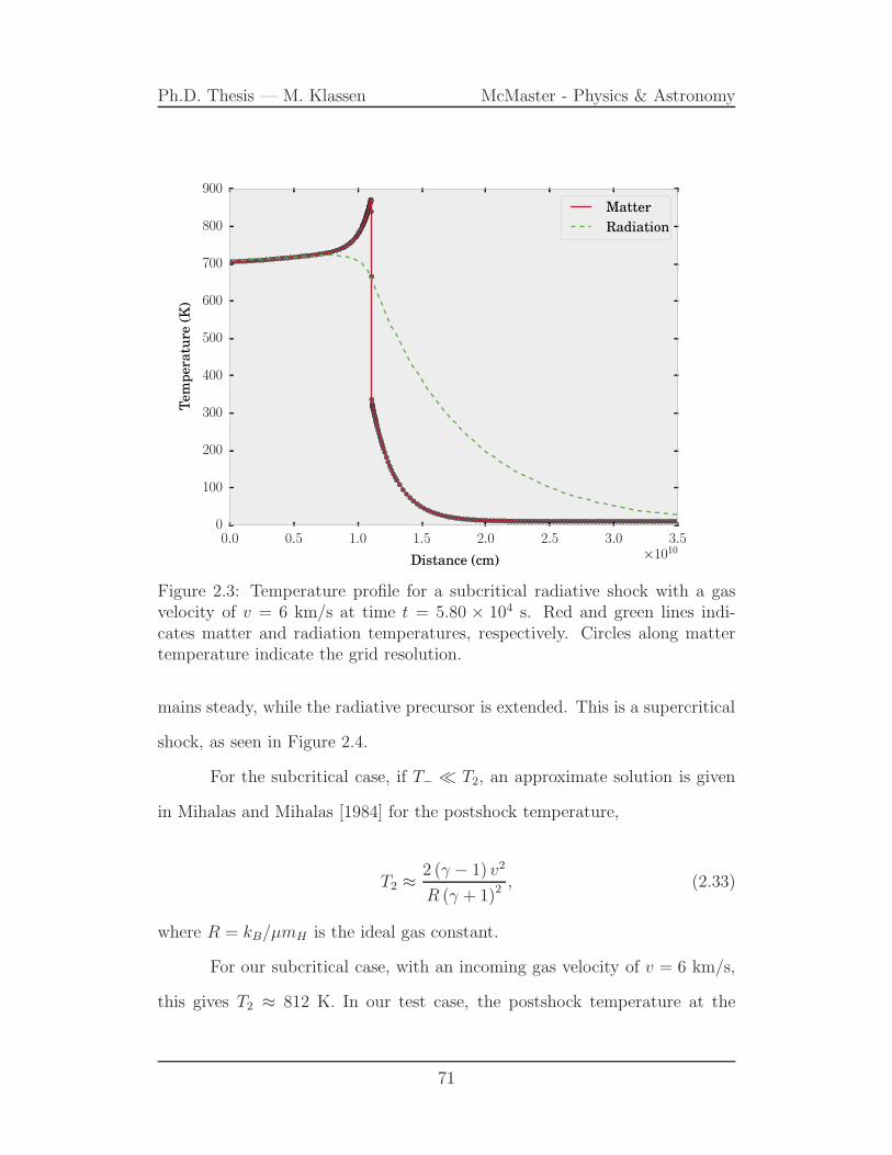
Ph.D. Thesis — M. Klassen McMaster - Physics & Astronomy
0.0 0.5 1.0 1.5 2.0 2.5 3.0 3.5
Distance (cm) ×1010
0
100
200
300
400
500
600
700
800
900T
em
pera
ture
(K)
Matter
Radiation
Figure 2.3: Temperature profile for a subcritical radiative shock with a gasvelocity of v = 6 km/s at time t = 5.80 × 10⁴ s. Red and green lines indi-cates matter and radiation temperatures, respectively. Circles along mattertemperature indicate the grid resolution.
mains steady, while the radiative precursor is extended. This is a supercritical
shock, as seen in Figure 2.4.
For the subcritical case, if T− ≪ T2, an approximate solution is given
in Mihalas and Mihalas [1984] for the postshock temperature,
T2 ≈2 (γ − 1) v2
R (γ + 1)2, (2.33)
where R = kB/µmH is the ideal gas constant.
For our subcritical case, with an incoming gas velocity of v = 6 km/s,
this gives T2 ≈ 812 K. In our test case, the postshock temperature at the
71
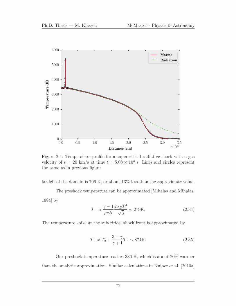
Ph.D. Thesis — M. Klassen McMaster - Physics & Astronomy
0.0 0.5 1.0 1.5 2.0 2.5 3.0 3.5
Distance (cm) ×1010
0
1000
2000
3000
4000
5000
6000T
em
pera
ture
(K)
Matter
Radiation
Figure 2.4: Temperature profile for a supercritical radiative shock with a gasvelocity of v = 20 km/s at time t = 5.08 × 10³ s. Lines and circles representthe same as in previous figure.
far-left of the domain is 706 K, or about 13% less than the approximate value.
The preshock temperature can be approximated [Mihalas and Mihalas,
1984] by
T− ≈ γ − 1
ρvR
2σBT42√
3∼ 279K. (2.34)
The temperature spike at the subcritical shock front is approximated by
T+ ≈ T2 +3− γ
γ + 1T− ∼ 874K. (2.35)
Our preshock temperature reaches 336 K, which is about 20% warmer
than the analytic approximation. Similar calculations in Kuiper et al. [2010a]
72
Ph.D. Thesis — M. Klassen McMaster - Physics & Astronomy
did not reproduce any preheating due to the 1-T approach in FLD. Our nu-
merical shock temperature T+ ≈ 871 K agrees to within better than 1%.
In the supercritical case, the radiation spike has collapsed to a thickness
of less than about a photon mean free path. The temperature of the spike is
T+ ≈ 5420 K, whereas the analytic approximation [Mihalas and Mihalas, 1984]
gives
T+ ≈ (3− γ)T2 ∼ 4612K, (2.36)
with which our numerical calculations agree to within 18%. Comparing to
other FLD implementations on AMR grids, Commercon et al. [2011b] matches
the analytic estimates of the subcritical postshock temperature a little closer
(to within 2%). Our scheme captures the preshock heating that the 1-T scheme
described in Kuiper et al. [2010a] could not (makemake has since been made
into a 2-T scheme), but not as closely as Commercon et al. [2011b], which
captures it to within 1%. The subcritical shock temperature we capture com-
parably well to Commercon et al. [2011b]. While flash has a different re-
finement criterion from the one used in Commercon et al. [2011b], this is not
likely the cause of the differences. More likely is the different choice of flux
limiter (Levermore and Pomraning [1981] vs Minerbo [1978]), which, because
of different assumptions about the angular dependence of the radiation field
in a particular problem, can yield slightly different solutions, with the greatest
differences seen in regions of intermediate to low optical depth [Turner and
Stone, 2001]. It is not obvious which flux limiter is best for a given problem,
but we have opted for one shared by Kuiper et al. [2010a].
73
Ph.D. Thesis — M. Klassen McMaster - Physics & Astronomy
2.5 Irradiation of a static disk
A radiation test of general astrophysical interest is that of a star embedded
in a circumstellar disk. The disk itself is optically thick and is surrounded
by an optically thin envelope. The setup we use follows Pascucci et al. [2004]
and includes a sun-like star surrounded by a flared circumstellar disk similar
to those considered by Chiang and Goldreich [1997, 1999] for T Tauri stars.
The density structure features steep gradients in the inner disk, which can be
challenging for radiative transfer codes, making this an excellent test.
We compare the temperature profile of the disk midplane in our simula-
tion with one calculated using the radiative transfer module called makemake
implemented in pluto [Mignone et al., 2007a] by Kuiper et al. [2010a]. In the
comparable setup (τ550nm ∼ 100), the difference between the simulated temper-
atures and Monte Carlo calculation was . 16%. However, in the Pascucci et al.
[2004] benchmark paper, the temperature variation between different Monte
Carlo codes including isotropic scattering is of the same order (. 15%).
The setup of the flared disk is as follows:
ρ(r, z) = ρ0rdrexp
(
−π
4
(
z
h(r)
)2)
, (2.37)
where
h(r) = zd
(
r
rd
)1.125
, (2.38)
and
rd =rmax
2= 500 AU (2.39)
74
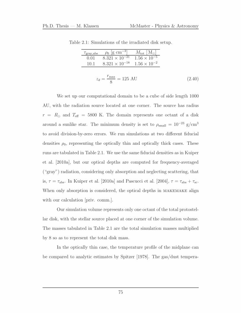
Ph.D. Thesis — M. Klassen McMaster - Physics & Astronomy
Table 2.1: Simulations of the irradiated disk setup.
τgray,abs ρ0 [g cm−3] Mtot [M⊙]0.01 8.321× 10⁻²¹ 1.56× 10⁻⁵
10.1 8.321× 10⁻¹⁸ 1.56× 10⁻²
zd =rmax
8= 125 AU (2.40)
We set up our computational domain to be a cube of side length 1000
AU, with the radiation source located at one corner. The source has radius
r = R⊙ and Teff = 5800 K. The domain represents one octant of a disk
around a sunlike star. The minimum density is set to ρsmall = 10−23 g/cm3
to avoid division-by-zero errors. We run simulations at two different fiducial
densities ρ0, representing the optically thin and optically thick cases. These
runs are tabulated in Table 2.1. We use the same fiducial densities as in Kuiper
et al. [2010a], but our optical depths are computed for frequency-averaged
(“gray”) radiation, considering only absorption and neglecting scattering, that
is, τ = τabs. In Kuiper et al. [2010a] and Pascucci et al. [2004], τ = τabs + τsc.
When only absorption is considered, the optical depths in makemake align
with our calculation [priv. comm.].
Our simulation volume represents only one octant of the total protostel-
lar disk, with the stellar source placed at one corner of the simulation volume.
The masses tabulated in Table 2.1 are the total simulation masses multiplied
by 8 so as to represent the total disk mass.
In the optically thin case, the temperature profile of the midplane can
be compared to analytic estimates by Spitzer [1978]. The gas/dust tempera-
75

Ph.D. Thesis — M. Klassen McMaster - Physics & Astronomy
0.0 0.2 0.4 0.6 0.8 1.0Radial Distance (AU) ×103
0.0
0.2
0.4
0.6
0.8
1.0V
ert
ical
Dis
tan
ce(A
U)
×103
-17.0
-17.5
-18.0
-18.5
-19.0
10−23
10−22
10−21
10−20
10−19
10−18
10−17
10−16
Den
sity
(g/c
m3)
Figure 2.5: Density profile of the Pascucci et al. [2004] irradiated disk setup.Contours show lines of constant density. The radiation source is located atthe bottom-left corner of the computational domain.
ture far from the central star (r ≫ R∗) is given by
T (r) =
(
Rmin
2r
)2
4+β
Tmin, (2.41)
where β is the index of the dust absorption coefficient. For Draine and Lee
[1984] silicates, β = 2.0508 in the long wavelength regime [Kuiper and Klessen,
2013]. Tmin is the temperature at the inner edge of the disk Rmin = 1 AU.
76
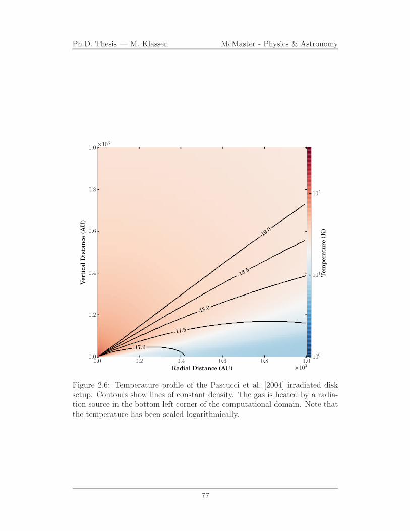
Ph.D. Thesis — M. Klassen McMaster - Physics & Astronomy
0.0 0.2 0.4 0.6 0.8 1.0Radial Distance (AU) ×103
0.0
0.2
0.4
0.6
0.8
1.0
Vert
ical
Dis
tan
ce(A
U)
×103
-17.0
-17.5
-18.0
-18.5
-19.0
100
101
102
Tem
pera
ture
(K)
Figure 2.6: Temperature profile of the Pascucci et al. [2004] irradiated disksetup. Contours show lines of constant density. The gas is heated by a radia-tion source in the bottom-left corner of the computational domain. Note thatthe temperature has been scaled logarithmically.
77
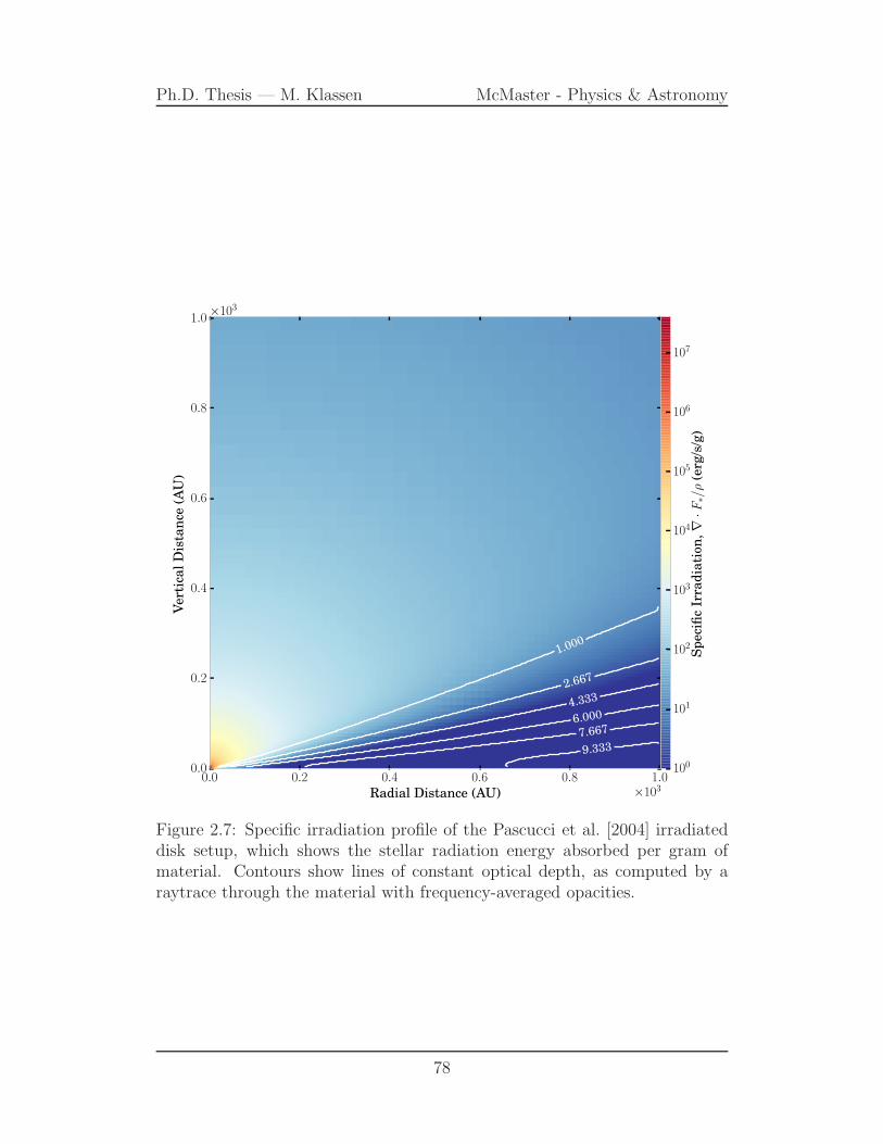
Ph.D. Thesis — M. Klassen McMaster - Physics & Astronomy
0.0 0.2 0.4 0.6 0.8 1.0Radial Distance (AU) ×103
0.0
0.2
0.4
0.6
0.8
1.0
Vert
ical
Dis
tan
ce(A
U)
×103
1.000
2.667
4.333
6.000
7.667
9.333
100
101
102
103
104
105
106
107
Sp
eci
fic
Irra
dia
tion
,∇
·F∗/ρ
(erg
/s/g
)
Figure 2.7: Specific irradiation profile of the Pascucci et al. [2004] irradiateddisk setup, which shows the stellar radiation energy absorbed per gram ofmaterial. Contours show lines of constant optical depth, as computed by araytrace through the material with frequency-averaged opacities.
78

Ph.D. Thesis — M. Klassen McMaster - Physics & Astronomy
In the optically thin regime, diffusion effects are negligible and the
radiation field is dominated by the direct component. At radii greater than
about 4 AU, our scheme reproduces the Spitzer [1978] estimate to within 10%,
and for radii greater than 10 AU, better than 5%.
Figure 2.5 shows the density structure of the protostellar disk in a
vertical slice in the optically thick case, with the radiation source positioned
at the origin in the bottom-left corner. Contours mark lines of equal density
and are labeled by the powers of ten of density.
The flared disk shields some of the stellar radiation. We run the sim-
ulation until the temperature of gas reaches an equilibrium state. Without
hydrodynamics enabled, the gas can only absorb or radiate energy. We run
the simulation for 1012 seconds and show the equilibrium temperature in Fig-
ure 2.6.
To show the shielding properties of the disk and the energy being ab-
sorbed by the gaseous medium surrounding the star, we show the specific
irradiation in Figure 2.7, that is, the stellar (direct) radiation energy being
absorbed per gram of material. We therefore show lines of equal optical depth
τ , as calculated during the raytrace.
We compare the temperatures through the midplane of the disk against
the same calculation completed with the makemake code by Kuiper et al.
[2010a]. Their simulation was done in a spherical polar geometry, which,
although not adaptively refined, naturally has more resolution in the polar
angular component at small radii, and therefore the scale height of the disk is
extremely well resolved.
Figure 2.8 shows the radial temperature profile through the midplane of
the disk for the case with fiducial density ρ0 = 8.321×10¹⁸ g/cm3. Three flash
79

Ph.D. Thesis — M. Klassen McMaster - Physics & Astronomy
10−1 100 101 102 103
Radial Distance (AU)
100
101
102
103
104T
em
pera
ture
(K)
7.8 AU2 AU
0.24 AU
0.12 AU
MAKEMAKE multifrequency
MAKEMAKE gray
FLASH gray 5
FLASH gray 7
FLASH gray 10
FLASH gray 11
Figure 2.8: Comparison of the midplane temperature profiles in simulations ofthe hybrid radiation feedback scheme in the Pascucci et al. [2004] benchmarktest in the high-density simulation (ρ0 = 8.321× 10⁻¹⁸): The implementationin flash vs. makemake by Kuiper et al. [2010a]. Solid lines belong to simula-tions using the makemake code, completed using a spherical polar geometry,while dashed lines indicate simulations done using the scheme described inthis paper using the flash code. The number associated with each flash
run indicates the maximum refinement level. Vertical gray lines in the figureindicate the grid resolution (in AU) for each of the flash runs.
runs are compared to two makemake simulations. The flash simulations use
the hybrid scheme as described in this paper, with both gray raytracer and gray
FLD solver. These we compare against gray and multifrequency simulations
by Kuiper et al. [2010a].
Because the flash simulations were completed in a Cartesian AMR
geometry, we indicate the maximum refinement level in the figure legend. We
compare maximum levels 5, 7, 10, and 11. At 10 levels of refinment, the
80

Ph.D. Thesis — M. Klassen McMaster - Physics & Astronomy
smallest grid size is 0.24 AU; at 11 levels, it is 0.12 AU. For this simulation
to match the results obtained using makemake, it is necessary to resolve
the scale height (Eq. 2.38) of the disk at its inner edge (≈ 0.1 AU), which we
effectively do with 11 levels of refinement, although convergence is already seen
with 10 levels of refinment. When the scale height is resolved, the midplane
temperature profile converges to the gray radiation result of Kuiper et al.
[2010a]. Lower resolution runs show a temperature excess.
2.5.1 Radiation pressure on a static, flared disk
We compute the radiation force density for the stellar radiation component
through the midplane of our disk as in Equation 2.31. A similar test was done
by Kuiper et al. [2010a], although their cut was not done through the midplane
but along a polar angle of θ ≈ 27. flash computes an isotropic radiation
pressure via the Eddington approximation (Equation 2.30), so we estimate the
thermal radiation force density via
frad,thermal = −dpraddx
. (2.42)
We use the makemake code (revised to be a 2-T solver) to perform
the same calculation through the midplane (θ ≈ 0) and compare to flash.
The results are shown in Figure 2.9. Most of the radiation pressure is due to
the direct, stellar component, with the diffuse, reprocessed field adding only
a tiny contribution that is more apparent far from the source. The outer
boundary is treated as optically thin outflow in makemake. In flash, we set
the “vacuum” outer boundary condition, dF/dx = −2F .
In the inner 40 AU, the two codes match to within about 20%, despite
81

Ph.D. Thesis — M. Klassen McMaster - Physics & Astronomy
100 101 102 10310−6
10−5
10−4
10−3
10−2
10−1
100
101
102
Ra
dia
tion
forc
ed
en
sity
(10−20
dyn
/cm
3) FLASH gray (total flux)
FLASH gray (stellar flux)
MAKEMAKE gray
100 101 102 103
Radial Distance (AU)
−100
−75
−50
−25
0
25
50
75
100
Rela
tive
Dif
fere
nce
(%)
Figure 2.9: Radiation force density through the midplane of the disk. The solidline indicates the radiation force density for the flash calculation, resultingfrom the total flux (direct stellar and thermal). The dotted line indicates theradiation force density due only to the stellar component of the radiation field.We compare the flash results to a 2T gray calculation in makemake (dashedline). The lower panel indicates the relative difference between the total fluxradiation force density in flash versus makemake.
82
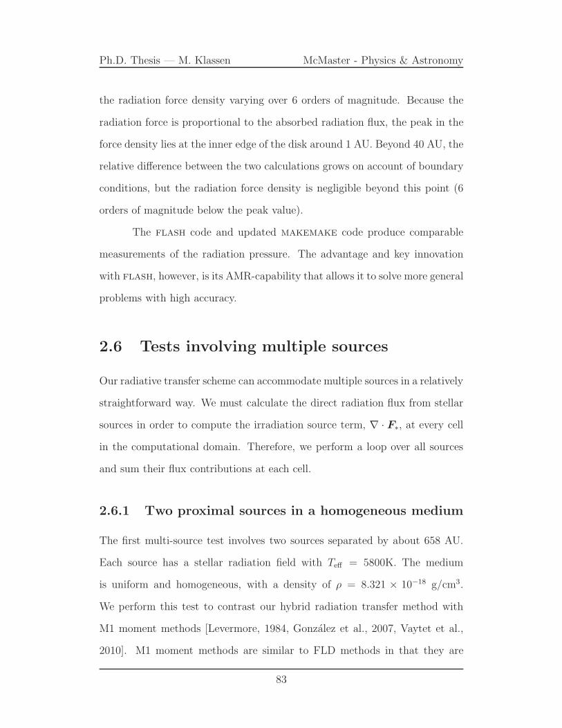
Ph.D. Thesis — M. Klassen McMaster - Physics & Astronomy
the radiation force density varying over 6 orders of magnitude. Because the
radiation force is proportional to the absorbed radiation flux, the peak in the
force density lies at the inner edge of the disk around 1 AU. Beyond 40 AU, the
relative difference between the two calculations grows on account of boundary
conditions, but the radiation force density is negligible beyond this point (6
orders of magnitude below the peak value).
The flash code and updated makemake code produce comparable
measurements of the radiation pressure. The advantage and key innovation
with flash, however, is its AMR-capability that allows it to solve more general
problems with high accuracy.
2.6 Tests involving multiple sources
Our radiative transfer scheme can accommodate multiple sources in a relatively
straightforward way. We must calculate the direct radiation flux from stellar
sources in order to compute the irradiation source term, ∇ · F∗, at every cell
in the computational domain. Therefore, we perform a loop over all sources
and sum their flux contributions at each cell.
2.6.1 Two proximal sources in a homogeneous medium
The first multi-source test involves two sources separated by about 658 AU.
Each source has a stellar radiation field with Teff = 5800K. The medium
is uniform and homogeneous, with a density of ρ = 8.321 × 10⁻¹⁸ g/cm3.
We perform this test to contrast our hybrid radiation transfer method with
M1 moment methods [Levermore, 1984, Gonzalez et al., 2007, Vaytet et al.,
2010]. M1 moment methods are similar to FLD methods in that they are
83

Ph.D. Thesis — M. Klassen McMaster - Physics & Astronomy
0.0 0.5 1.0 1.5 2.0Position (AU) ×103
0.0
0.5
1.0
1.5
2.0
Posi
tion
(AU
)
×103
0
25
50
75
100
125
150
175
200
225
250
Tem
pera
ture
(K)
Figure 2.10: Gas temperature after equilibrating with the radiation field drivenby two stellar sources (T = 5800 K). Vertical dashed line indicates the sym-metry axis along which the temperature in figure 2.11 is measured. The blackcontour marks a gas temperature of T = 35K.
84

Ph.D. Thesis — M. Klassen McMaster - Physics & Astronomy
both based on taking angular moments of the radiative transfer equation.
FLD takes only the zeroth-order moment, and the conservation equations are
closed using a diffusion relation based on the gradient of the radiation energy.
M1 methods take the first moment of the radiative transfer equation, and
the closure of the conservation equations takes a form that preserves the bulk
directionality of photon flows. Problems arise, however, when multiple sources
are present. With two sources, photons flow in opposing directions, canceling
the opposing components of their flow and introducing spurious flows in the
direction perpendicular to the line between the two sources [Rosdahl et al.,
2013]. Raytracers do not suffer from this artifact because the irradiation at
each grid location is calculated along sightlines to each of the sources present
in the simulation.
Figure 2.10 shows the simulation setup as well as the temperature of
the gas after it has been allowed to equilibrate with the radiation field. We
measure the temperature of the gas along the vertical dashed line and plot the
result in Figure 2.11.
Figure 2.11 shows the temperature along the dashed line from Figure
2.10, the locus of points equidistant from both radiation sources. Here we
compare the simulated temperatures of our hybrid scheme in flash against
a Monte Carlo calculation performed with RADMC-3D1 [Dullemond, 2012].
The Monte Carlo calculation was done with 109 photons using the “modified
random walk” method with scattering neglected, on an uneven grid (101x1x101
cells for the x× y × z dimensions) using the same Draine and Lee [1984] dust
model as in the rest of this paper.
The flash temperatures differ from the Monte Carlo results by less
1http://www.ita.uni-heidelberg.de/ dullemond/software/radmc-3d/
85

Ph.D. Thesis — M. Klassen McMaster - Physics & Astronomy
−1000 −500 0 500 100015
20
25
30
35
40T
em
pera
ture
(K)
Simulation
Monte Carlo
−1000 −500 0 500 1000Position (AU)
−6
−4
−2
0
2
4
6
Rela
tive
Dif
fere
nce
(%)
Figure 2.11: Gas temperature along dashed line from Figure 2.10, the locus ofpoints equidistant from both radiation sources. The upper panel shows the gastemperature from our simulation (solid) compared to the Monte Carlo result(dashed). The lower panel shows the relative difference in temperature as apercentage.
than 5%, with flash calculating slightly warmer temperatures directly be-
tween the sources and slightly cooler temperatures at the edges of the simu-
lation volume. These small differences are most likely due to multifrequency
effects.
Monte Carlo calculations are considered the benchmark for accuracy,
but are extremely computationally intensive and cannot, in general, be used
in dynamic calculations. Simulations of star formation cannot be addressed
with full Monte Carlo methods using present-day machines and reasonable
time constraints. Moreover, they are highly nontrivial to parallelize. In these
86

Ph.D. Thesis — M. Klassen McMaster - Physics & Astronomy
cases, approximate schemes such as flux-limited diffusion must be used.
2.6.2 Two sources irradiating a dense core of material
We next create a test setup inspired by Rijkhorst et al. [2006a], where a central
concentration was irradiated by two sources. Since FLD methods are based on
local gradients in the radiation energy, they cannot properly treat shadowing.
In this test we place a dense clump of material at the center of our simulation
volume and irradiate it from two angles, creating a shadowed region. We
compute the irradiation and equilibrium temperatures.
Our setup contains a mix of optically thin and optically thick regions,
creating strong gradients in the radiation energy density. We compare the
equilibrium temperatures computed by the hybrid scheme to the temperature
computed without diffusion.
The two radiation sources have a temperature Teff = 8000 K and are
situated in a low-density (ρ = 10−20 g/cm−3) medium to the side and below
a central density concentration (ρ = 10−17 g/cm−3) with radius Rc = 4 ×
1015 cm ≈ 267 AU. The side length of the simulation box is about 2000 AU.
Hydrodynamics are disabled.
Figure 2.12 shows the simulation setup and the specific irradiation of
the gas in a slice through the midplane of the simulation volume. The overlaid
grid shows the flash AMR block structure, with each block containing 83 cells
and refining on gradients in density, radiation energy, and matter temperature
using the flash error estimator described in Section 2.3.1. The simulation was
run with a maximum 8 levels of refinement, achieving a maximum resolution of
1.96 AU. The black circle in the centre marks the central density concentration.
87
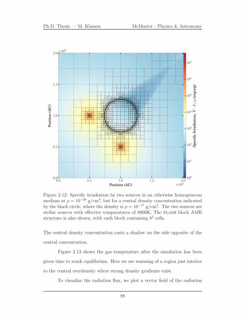
Ph.D. Thesis — M. Klassen McMaster - Physics & Astronomy
0.0 0.5 1.0 1.5 2.0Position (AU) ×103
0.0
0.5
1.0
1.5
2.0P
osi
tion
(AU
)×103
100
101
102
103
104
105
106
107
Sp
eci
fic
Irra
dia
tion
,∇
·F∗/ρ
(erg
/s/g
)Figure 2.12: Specific irradiation by two sources in an otherwise homogeneousmedium at ρ = 10−20 g/cm3, but for a central density concentration indicatedby the black circle, where the density is ρ = 10−17 g/cm3. The two sources arestellar sources with effective temperatures of 8000K. The flash block AMRstructure is also shown, with each block containing 83 cells.
The central density concentration casts a shadow on the side opposite of the
central concentration.
Figure 2.13 shows the gas temperature after the simulation has been
given time to reach equilibrium. Here we see warming of a region just interior
to the central overdensity where strong density gradients exist.
To visualize the radiation flux, we plot a vector field of the radiation
88
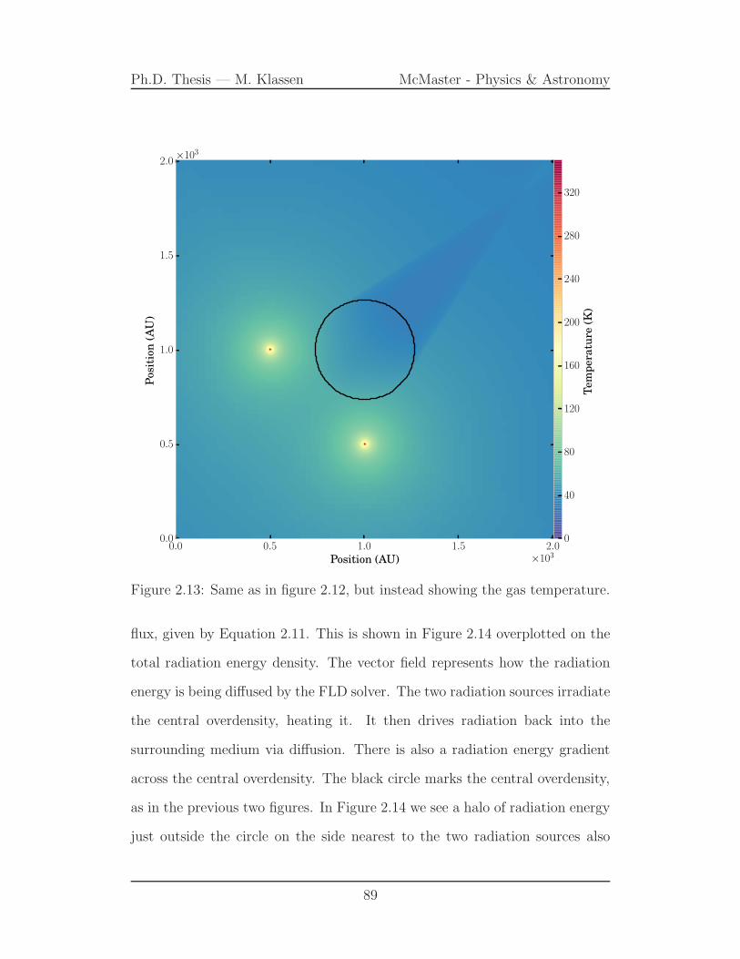
Ph.D. Thesis — M. Klassen McMaster - Physics & Astronomy
0.0 0.5 1.0 1.5 2.0Position (AU) ×103
0.0
0.5
1.0
1.5
2.0P
osi
tion
(AU
)×103
0
40
80
120
160
200
240
280
320
Tem
pera
ture
(K)
Figure 2.13: Same as in figure 2.12, but instead showing the gas temperature.
flux, given by Equation 2.11. This is shown in Figure 2.14 overplotted on the
total radiation energy density. The vector field represents how the radiation
energy is being diffused by the FLD solver. The two radiation sources irradiate
the central overdensity, heating it. It then drives radiation back into the
surrounding medium via diffusion. There is also a radiation energy gradient
across the central overdensity. The black circle marks the central overdensity,
as in the previous two figures. In Figure 2.14 we see a halo of radiation energy
just outside the circle on the side nearest to the two radiation sources also
89

Ph.D. Thesis — M. Klassen McMaster - Physics & Astronomy
0.0 0.5 1.0 1.5 2.0Position (AU) ×103
0.0
0.5
1.0
1.5
2.0P
osi
tion
(AU
)×103
1.2
1.8
2.4
3.0
3.6
4.2
4.8
5.4
6.0
Erad
(erg
/cm
3)
×10−11
Figure 2.14: Radiation energy density with the thermal radiation flux Fr =−D∇Er overplotted as a vector field. The gradients in the radiation energydensity are steepest near the spherical overdensity in the centre, on the sidefacing the two sources.
resulting from the diffusion of radiation.
We now compare this to the zero-diffusion case by performing the same
calculation with the diffusion term set to zero. The gas equilibrates with the
radiation field imposed by the sources, but this energy is not allowed to diffuse.
Figure 2.15 shows the difference in the resultant equilibrium temperature as a
percentage of the relative difference. The result is that the central overdensity
90

Ph.D. Thesis — M. Klassen McMaster - Physics & Astronomy
0 500 1000 1500 2000Position (AU)
0
500
1000
1500
2000P
osi
tion
(AU
)
−45
−30
−15
0
15
30
45
(Traytrace−Thybrid)/Thybrid(%
)
Figure 2.15: The temperature difference (in percent) in the raytrace case com-pared to the hybrid radiation transfer case.
is approximately 50% hotter. It cannot cool by diffusing its radiation energy
into the surrounding medium.
Because the re-emission terms are often left out of raytracing-methods
for the sake of simplicity and computational cost, they are unsuitable and inac-
curate in simulations containing optically thick material, although re-emission
is often treated using a cooling function to extract the energy. In optically
thick envelopes surrounding young stellar objects, radiation is reprocessed as
the envelope of gas absorbs and re-emits the radiation in the infrared.
91

Ph.D. Thesis — M. Klassen McMaster - Physics & Astronomy
2.7 Discussion and Summary
We have described the implementation of a hybrid radiation transfer scheme
in a 3D Cartesian AMR framework. To the best of our knowledge, this is the
first such implementation. Our hybrid scheme splits the radiation field into a
direct (stellar) component and a diffuse (thermal) component. A specialized
raytracer is used to solve for the direct flux, the absorption of which by dusty,
molecular gas constitutes an energy source term that heats the dust. The dust
emits radiation thermally, and the thermal radiation field is evolved via flux-
limited diffusion. The gas is assumed in thermal equilibrium with the dust,
whose temperature is evolved according to both direct and indirect radiation
fields.
Radiation feedback from massive stars takes manifold forms: heating
of dust grains, which are coupled to the gas; radiation pressure; ionizing radia-
tion, leading to the formation of Hii regions; jets and stellar winds; and finally
supernovae. We have implemented the first two, with future work intent on
implementing ionizing radiation. Various authors have drawn attention to the
potential for ionizing radiation to disrupt molecular clouds [Matzner, 2002,
Krumholz et al., 2006, Walch et al., 2012], at least in low-mass clouds, while
in larger clouds, star formation may be fed through accretion along filaments,
with ionizing radiation feeding into the low-density voids between filaments
Dale et al. [2012]. The effect of ionizing radiation, through heating of the gas
and suppression of fragmentation, also leads to higher Jeans masses and more
massive stars [Peters et al., 2010c].
As a mechanism for disrupting giant molecular clouds, Murray et al.
[2010] argue that radiation pressure from starlight interacting with dust grains
92

Ph.D. Thesis — M. Klassen McMaster - Physics & Astronomy
plays a dominant role, at least in the case of the most massive clusters inside
GMCs.
In implementing our radiative transfer scheme, the addition of the ray-
tracer helps overcome some of the main limitation of a purely FLD approach.
The primary limitation of the FLD approach is the assumption that the flux
always travels in the direction down the radiation energy gradient. This as-
sumption is reasonable in purely optically thick regions, but breaks down in
regions where radiation sources ought to be casting shadows.
Furthermore, some FLD implementations assume that the radiation
field is everywhere in thermal equilibrium with the gas. This is not always
true, especially radiatively critical shocks. We have relaxed this assumption
and allowed the radiation temperature and the gas temperature to differ from
each other.
The primary advance over the hybrid implementation of Kuiper et al.
[2010a] is the generalization to 3D Cartesian AMR from the specialized geom-
etry of a spherical polar grid. Spherical coordinates are ideal for studying the
radiation field from a single, central source. By their nature, spherical grids
have higher effective resolution closer to the center, precisely where it is most
needed simulations of accretion disks around massive stars. In our test prob-
lem of a static, irradiated disk [Pascucci et al., 2004], we required 11 levels of
refinement before we could resolve the scale height of the disk near the inner
boundary.
However, when generalizing to multiple point sources of radiation, Carte-
sian geometry becomes a natural choice. This enables us to approach a much
larger array of problems. flash is a highly scalable MHD code with driven
turbulence, sink particles and protostellar evolution. The addition of our hy-
93

Ph.D. Thesis — M. Klassen McMaster - Physics & Astronomy
brid radiation transfer unit greatly complements flash ’s abilities.
One of the most general problems this enables us to study is the effect
of radiative heating and momentum feedback around massive, accreting proto-
stars. These objects reside deep within dense envelopes and accrete material
through a disk. Whether disk accretion is the only mechanism, or whether
raditiave Rayleigh-Taylor instabilities are another viable mechanism has not
yet been fully settled. High resolution simulations, resolving in particular the
regions of intermediate optical depth using adaptive mesh refinment, and in-
cluding the effects of turbulence and MHD ought to be able to resolve the
remaining controversies.
We have also connected the hybrid radiation scheme to sink particles,
which we will use to model the formation of protostars in larger-scale simu-
lations of molecular cloud clumps. The protostellar properties such as stellar
radius and luminosity are evolved using a subgrid model [Klassen et al., 2012b]
that directly feeds into the radiation transfer subroutines. The sum of flash’s
capabilities now enable the study of clustered star formation in turbulent, fil-
amentary, and magnetized environments.
The code also presents opportunities for further development. The
raytracer, as implemented by Rijkhorst et al. [2006a] and Peters et al. [2010a],
contained ionization feedback, which we will soon implement in our hybrid
radiation framework. Multifrequency effects will also be included in future
versions of the code.
94

Ph.D. Thesis — M. Klassen McMaster - Physics & Astronomy
2.8 Appendix to Chapter 2: 3T radiation hy-
drodynamics
flash is a code that is supported by a team of developers at the DOE-
supported Alliances Center for Astrophysical Thermonuclear Flashes (ASCI)
at the University of Chicago2. Recent development has added significant ca-
pabilities for plasma and high-energy-density physics. These included a “3T”
radiation hydrodynamics solver [Lamb et al., 2010, Fatenejad et al., 2012,
Kumar et al., 2011] that evolves an ion fluid, and electron fluid, and a ra-
diation “fluid”. 3T implies that each fluid has its own temperature, with
Tele 6= Tion 6= Trad.
These three fluids are coupled in the following way:
∂t(ρeion) +∇ · (ρeionv) + Pion∇ · v = (2.43)
ρcv,ionτei
(Tele − Tion)
∂t(ρeele) +∇ · (ρeelev) + Pele∇ · v = (2.44)
ρcv,eleτei
(Tion − Tele)−∇ · qele +Qabs −Qemis
∂t(ρerad) +∇ · (ρeradv) + Prad∇ · v = (2.45)
∇ · qrad −Qabs +Qemis
The ion and electron components exchange energy via Coulomb colli-
sions. The electron and radiation components exchange energy through ab-
sorption and emission processes. In our case, Qabs = κPρcEr and Qemis =
κPρcaT4, where a is the radiation constant. The ∇ · qele and ∇ · qrad terms
2http://flash.uchicago.edu/
95
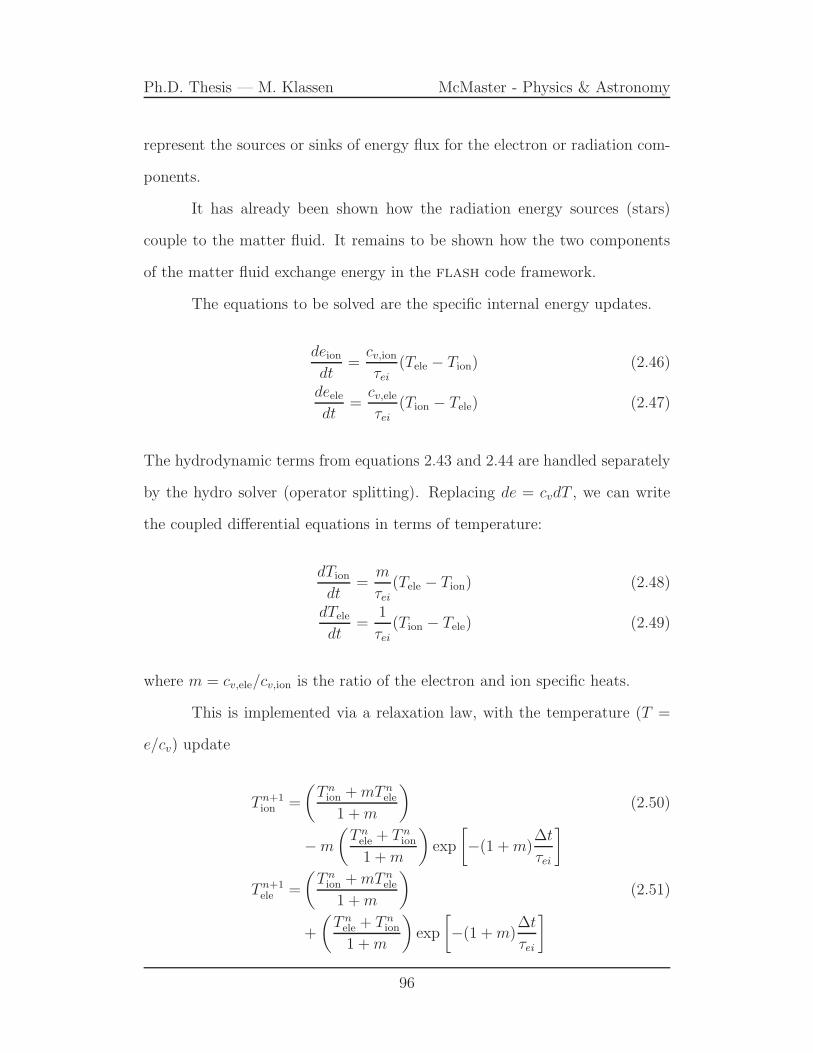
Ph.D. Thesis — M. Klassen McMaster - Physics & Astronomy
represent the sources or sinks of energy flux for the electron or radiation com-
ponents.
It has already been shown how the radiation energy sources (stars)
couple to the matter fluid. It remains to be shown how the two components
of the matter fluid exchange energy in the flash code framework.
The equations to be solved are the specific internal energy updates.
deiondt
=cv,ionτei
(Tele − Tion) (2.46)
deeledt
=cv,eleτei
(Tion − Tele) (2.47)
The hydrodynamic terms from equations 2.43 and 2.44 are handled separately
by the hydro solver (operator splitting). Replacing de = cvdT , we can write
the coupled differential equations in terms of temperature:
dTion
dt=
m
τei(Tele − Tion) (2.48)
dTele
dt=
1
τei(Tion − Tele) (2.49)
where m = cv,ele/cv,ion is the ratio of the electron and ion specific heats.
This is implemented via a relaxation law, with the temperature (T =
e/cv) update
T n+1ion =
(
T nion +mT n
ele
1 +m
)
(2.50)
−m
(
T nele + T n
ion
1 +m
)
exp
[
−(1 +m)∆t
τei
]
T n+1ele =
(
T nion +mT n
ele
1 +m
)
(2.51)
+
(
T nele + T n
ion
1 +m
)
exp
[
−(1 +m)∆t
τei
]
96

Ph.D. Thesis — M. Klassen McMaster - Physics & Astronomy
The equilibration time, τei, is given by,
τei =3k
3/2B
8√2πe4
(mionTele +meleTion)3/2
(melemion)1/2z2nion ln Λei, (2.52)
where e is the electron charge, mion and mele are the ion and electron masses,
respectively, z is the mean ionization level, nion is the ion number density, and
lnΛei is the Coulomb logarithm.
With these updated temperatures, the internal energies are updated:
en+1ele = enele + cnv,ele(T
n+1ele − T n
ele) (2.53)
en+1ion = enion + cnv,ion(T
n+1ion − T n
ion) (2.54)
97

Ph.D. Thesis — M. Klassen McMaster - Physics & Astronomy
Chapter 3
Simulating the Formation of
Massive Protostars: I. Radiative
Feedback and Accretion Disks
3.1 Introduction
The formation of high-mass stars (M & 8 M⊙) has been a subject of intense
study and considerable controversy for several decades. Despite being slight
in abundance, with only 2 or 3 high-mass stars for every 100, they exert
enormous influence on the galaxies and host clusters in which they reside
[Zinnecker and Yorke, 2007]. Their extreme nature demands attention because
the mechanisms of their formation are not immediately obvious. A defining
feature of massive stars is that the timescale for their gravitational contraction,
the Kelvin-Helmholtz time, is shorter than the timescale for accretion. This
implies that the star begins nuclear burning before it has finished accreting
to its final mass. During this phase, powerful feedback mechanisms due to
98

Ph.D. Thesis — M. Klassen McMaster - Physics & Astronomy
radiation pressure and photoionization [Larson and Starrfield, 1971b] become
important—mechanisms that are either absent or insignificant for low-mass
star formation.
Observations exist for stars in excess of 150M⊙ [Crowther et al., 2010].
The 30 Doradus region inside the Large Magellanic Cloud contains at least
10 stars with initial masses in excess of 100 M⊙ [Doran et al., 2013]. There
is no consensus on the precise upper mass limit for stars, although it may lie
somewhere within 150–300 M⊙ [Figer, 2005, Crowther et al., 2010]. Assuming
that such masses can be reached by accretion, then we must ask whether the
accretion proceeds through a circumstellar disk alone, or additionally through
other mechanisms. In addition, a large body of theoretical and numerical work
shows that it is essential to adopt a three-dimensional treatment that includes
a careful implementation of the radiation field. Many different theoretical and
observational approaches have been undertaken to address this.
Massive stars are expected to reach the main sequence while still deeply
embedded in molecular envelopes [Stahler et al., 2000]. This makes observ-
ing high-mass protostars and their circumstellar disks challenging, although a
growing number of candidates have been detected in recent years. Beltran and
de Wit [2015] summarize the observations of accretion disks around luminous
young stellar objects (YSOs). Where observations of circumstellar disks are
available, their rotation rates appear consistent with Keplerian velocities. For
massive protostars (M∗ = 8–30 M⊙), accretion disks generally range in size
from a few hundred AU to a few thousand AU. These sizes are consistent with
the disks formed in simulations presented in this paper.
Observations with the Atacama Large Millimeter/submillimeter Array
(ALMA) are also revealing the properties of disks around massive protostars.
99

Ph.D. Thesis — M. Klassen McMaster - Physics & Astronomy
Very recent observations highlighted the discovery of a Keplerian-like disk
around a forming O-type star, AFGL 4176 [Johnston et al., 2015]. Model fits
to line and continuum emission are consistent with a 25 M⊙ star surrounded
by 12 M⊙ disk with a radius of 2000 AU. The velocity structure, as traced
by CH3CN, is consistent with Keplerian rotation. These observations are in
excellent agreement with the results of our simulations of a 100 M⊙ protostellar
core.
Early 1D calculations sought to estimate the upper mass limit for stars,
given that the accretion flow onto a star should be halted at some critical lumi-
nosity. The Eddington Limit describes this maximal luminosity and depends
on the ratio of radiative to gravitational forces, including the specific opacity
of the gas and dust. Since the luminosity scales with the mass of the star
more strongly than gravity, there should exist a natural upper mass limit for
stars in the spherically-averaged case. Studies such as Larson and Starrfield
[1971b], Kahn [1974], Yorke and Krugel [1977] found upper mass limits around
20–40 M⊙, although such calculations are always sensitive to the choice of dust
model. The interstellar medium is about 1% dust by mass. Stellar radiation
impinges on dust particles, imparting momentum. This momentum is trans-
ferred to the gas via drag forces. In 1D, a sufficiently luminous star (roughly
20 M⊙ or more) should be able to arrest and even reverse the accretion flow
via radiation pressure alone, thus setting an upper mass limit for the star.
How one chooses to model the dust opacity will affect the upper mass limit
that results from these kinds of 1D calculations.
These theoretical 1D mass limits have been confirmed by simulations
[Yorke and Krugel, 1977, Kuiper et al., 2010a]. Kahn [1974] suggested that
the envelope of material around the protostar would likely fragment, lead-
100
Ph.D. Thesis — M. Klassen McMaster - Physics & Astronomy
ing to anisotropic accretion. The importance of geometry was later shown
[Nakano, 1989] and circumstellar disks highlighted as an accretion channel.
These disks form easily in the presence of rotation. Yorke and Sonnhalter
[2002] studied slowly-rotating nonmagnetic cores in 2D simulations that as-
sumed axial symmetry. Their simulations modeled the collapse of high-mass
cores and included frequency-dependent radiation feedback handled via flux-
limited diffusion (FLD). The effect of the disk is to channel radiation into the
polar directions, a phenomenon known as the “flashlight effect” [Yorke and
Bodenheimer, 1999]. This radiation is also most responsible for radiative ac-
celerations. Even so, Yorke and Sonnhalter [2002] still only formed stars with
masses . 43M⊙.
Radiatively-driven outflows are expected to form in the vicinity of mas-
sive stars. Krumholz et al. [2009], using a frequency-averaged flux-limited dif-
fusion approach to radiative transfer, proposed that as the stars become more
luminous, rather than blowing away all the gas enveloping the cavity, radia-
tion would pierce through the cavity wall. Meanwhile, dense fingers of material
would rain back down onto the massive protostar. This “radiative Rayleigh-
Taylor” instability is analogous to the classical Rayleigh-Taylor instability, but
with radiation taking the place of the lighter fluid. These instabilities may al-
low the star to continue accreting material. Jacquet and Krumholz [2011]
showed that these instabilities can arise under the right circumstances even
around Hii regions.
This mechanism, however, may not be necessary to explain how massive
stars achieve their prodigious masses. Kuiper et al. [2010a] demonstrated that
with a much more accurate treatment of the radiation field, including both
FLD as well as ray-tracing of energy directly from the star, disk accretion alone
101

Ph.D. Thesis — M. Klassen McMaster - Physics & Astronomy
was sufficient to achieve stellar masses larger than any previously achieved in
a simulation.
The question becomes whether a classically two-dimensional fluid in-
stability holds in a 3D environment, and whether it is appropriate to model the
stellar radiation field as a fluid. Kuiper et al. [2010b] decomposed the radiation
field into a direct component and a diffuse component. The diffuse component,
which consisted entirely of thermal radiation re-emitted by dust, was handled
by an FLD solver. Meanwhile, the direct component consisted of the stellar
radiation and was treated by a multifrequency raytracer. In simulations using
this “hybrid” technique for radiation transfer, the radiative Rayleigh-Taylor
instability was absent [Kuiper et al., 2012]. Kuiper et al. [2010a] found that it
was necessary to model and to resolve the dust sublimation front around the
accreting protostar. With dust sublimation, matter becomes transparent to
radiation in the extreme vicinity of the protostar. Rather than being blown
away, it can now be accreted by the protostar.
These and subsequent simulations have shown that stars in excess of
100M⊙ may form by disk accretion without the need for new fluid instabilities
[Kuiper et al., 2010a, 2011a, 2012]. However, these simulation also have their
limitations. They were performed on grids with a spherical geometry and a
sink cell fixed at the center. The advantage of this geometry is that it allowed
for extremely high resolution near to the source. The radial grid resolution
increases logarithmically towards the center. Kuiper et al. [2010a] was able to
resolve down to 1 AU in the vicinity of the star. Raytracing is also easy to
implement in this geometry as rays travel only along the radial dimension. The
disadvantage of this setup is that it only handles a single immovable source,
fixed at the center. Fragmentation of the pre-stellar core was neglected, and the
102

Ph.D. Thesis — M. Klassen McMaster - Physics & Astronomy
source cannot drift even as the disk becomes gravitationally unstable. While
the resolution at small radii is very good, large-scale structure (particularly at
large radii) are poorly resolved. These would be better handled in an adaptive
mesh framework.
The combined limitations of this body of work motivated our imple-
mentation of hybrid radiation transport on an adaptive, 3D Cartesian grid in
flash [Chapter 2], first for the study of massive stars and their outflow cavi-
ties, then more general problems of star formation in clusters. In Klassen et al.
[2014] we demonstrated the accuracy of our method in solving the radiative
transfer problem with a battery of benchmark tests, most of which were static.
In this paper, we apply our method to the dynamical problem of following the
gravitational collapse of a molecular cloud core to form a massive protostar.
We also describe improvements and some necessary modifications that were
made to the code in order for us to simulate massive star formation.
We performed three different computationally-intense simulations of
protostellar cores collapsing gravitationally. These cores were of three differ-
ent initial masses, 30 M⊙, 100 M⊙, and 200 M⊙, respectively. Their initial
conditions emulated earlier studies of massive star formation, but that had
different radiatively feedback techniques or different grid geometries. In our
case, we formed only a single massive star in each simulation, with final masses
of 5.48M⊙, 28.8M⊙, and 43.7M⊙. The simulations were run for 81.4 kyr (0.85
tff), 41.6 kyr (0.79 tff), and 21.9 kyr (0.59 tff), respectively. The formation of
a massive protostar was accompanied by the formation of an accretion disk
that grew in mass until becoming unstable, triggering a factor of 2–10 increase
in the accretion rate, but which did not undergo further fragmentation into
mutlpile stars. The strong radiative feedback from the massive protostars did
103

Ph.D. Thesis — M. Klassen McMaster - Physics & Astronomy
not halt accretion, which continued through the disk, but launched radiatively-
driven bubbles in the 100M⊙ and 200M⊙ simulations, in which the stars had
super-Eddington luminosities.
Below we describe the setup of these simulations and their results in
detail. Section 3.2 provides the background to the physical and numerical
models we employ. Section 3.3 details the simulation setup. The results of
these simulations are discussed in Section 3.4, while some nuances, caveats,
as well as the direction of future simulations are discussed in Section 3.5. We
summarize our results in Section 3.6.
3.2 Physical and numerical model
3.2.1 Radiation transfer
The details of our radiative transfer method are covered in Klassen et al. [2014],
but we summarize the basics of the method here. The code was further devel-
oped to handle dynamical star formation calculations. These improvements
are described in sections 3.2.2 and 3.2.3. The radiation field is decomposed
into a direct, stellar component and a diffuse, thermal component [Wolfire and
Cassinelli, 1986, Murray et al., 1994, Edgar and Clarke, 2003, Kuiper et al.,
2010b], for which we can apply different methods that are better suited to
each type of radiation:
F = F∗ + Fr (3.1)
The direct radiation flux from a protostar F∗(r) measured a distance r
104

Ph.D. Thesis — M. Klassen McMaster - Physics & Astronomy
from the star is given by
F∗(r) = F∗(R∗)
(
R∗
r
)2
exp (−τ(r)) , (3.2)
where F∗(R∗) = σT 4eff is the flux at the stellar surface R∗, where σ is the
Stefan-Boltzmann constant and Teff the effective surface temperature of the
protostar. The stellar flux is attenuated both geometrically with distance
from the source, and by intervening material that is scattering or absorbing
starlight. The latter effect is captured by the exponential term in Eq. 3.2,
where
τ(r) =
∫ r
R∗
κ(T∗, r′)ρ(r′)dr′ (3.3)
is the optical depth.
Raytracing is a method that is well-suited for treating the direct radi-
ation field, determining for each grid cell the flux of photons arriving directly
from the photosphere of any stars within the simulation. A raytracer making
use of the fast voxel traversal algorithm [Amanatides et al., 1987] is used to
calculate optical depths to every cell in the computational domain, from which
we calculate the local stellar flux. This flux depends on the integrated optical
depth along the ray. The amount of stellar radiation absorbed by a grid cell
depends on the local opacity,
∇ · F∗(r) ≈ −1− e−κP (T∗)ρ∆r
∆rF∗(r) (3.4)
where κ is the specific opacity and ρ is the matter density.
This absorbed energy enters the coupled energy equations as a source
105

Ph.D. Thesis — M. Klassen McMaster - Physics & Astronomy
term:
∂(ρǫ)
∂t= −κPρc
(
aRT4 − Er
)
−∇ · F∗ (3.5)
∂Er
∂t+∇ · Fr = +κPρc
(
aRT4 −Er
)
(3.6)
Here Er is the radiation energy, κP is the Planck opacity, and aR is the
radiation constant. The temperature in Equation 3.5 is solved for implicitly
(see Section 3.2.3), which is used in equation 3.6. Equation 3.6, in turn, is
solved implicitly using the flux-limited diffusion approximation [Levermore
and Pomraning, 1981],
Fr = −(
λc
κRρ
)
∇Er, (3.7)
where κR is the Rosseland mean opacity, c is the speed of light, and λ is
the flux-limiter. Different choices for the flux limiter have been made in the
literature, and are based on slightly different assumptions about the angular
distribution of the specific intensity of the radiation field. The flux limiter
always takes on values between 0 and 13[Levermore and Pomraning, 1981,
Turner and Stone, 2001].
We use the Levermore and Pomraning [1981] flux limiter, one of the
most commonly used,
λ =2 +R
6 + 3R +R2, (3.8)
with
R =|∇Er|κRρEr
. (3.9)
Another popular choice of flux limiter is the one by Minerbo [1978].
The advantage of FLD methods is their speed and relative accuracy in
106

Ph.D. Thesis — M. Klassen McMaster - Physics & Astronomy
regions of high optical depth. And while massive stars form in very dense en-
velopes of molecular gas [Sridharan et al., 2002, Hill et al., 2005, Klein et al.,
2005, Beltran et al., 2006], within the dust sublimation front, or inside the
radiatively-driven outflow cavities that form around massive stars, the radi-
ation field is highly anisotropic. The FLD approximation, however, assumes
that flux is in the direction antiparallel to the gradient of the radiation energy
Er. FLD methods can become less accurate in regions transitioning from op-
tically thin to optically thick, or in regions with highly anisotropic radiation
fields.
The addition of stellar sources of radiation in FLD-only radiation trans-
fer codes is often handled via an isotropic source term that considers the lu-
minosity of the star:
∂Er
∂t+∇ ·
(
λc
κRρ∇Er
)
= κPρc(
aT 4 −Er
)
+∑
n
LnW (x− xn) (3.10)
The coupling of radiation energy from the stars to the gas is mediated by a
weighting function centered on the stellar locations and appears as a source
term in the radiation energy diffusion equation. The weighting function W ,
which might be a spherical Gaussian function, mediates the radiation energy
contributed by a sink particle n, located at xn, which has a luminosity Ln.
The luminosity may be computed via a model for protostellar evolution or an
estimate based on a zero-age main sequence (ZAMS) star, but if the weighting
function is symmetric, then the radiation is still administered isotropically.
Unfortunately, these regions, if circumstellar disks are present or assumed, are
often the grid cells where the radiation field can be very anisotropic.
Using solely a raytracer has major disadvantages as well. For compu-
107

Ph.D. Thesis — M. Klassen McMaster - Physics & Astronomy
tational efficiency, scattering and non-stellar source terms are often neglected,
which implies that this method is accurate only in optically thin regions where
the radiation field is dominated by stellar sources. In reality, the presence of
optically thick regions means radiation is absorbed, re-emitted at lower en-
ergy, or scattered by particles. This occurs especially in the envelopes around
massive protostars, where the gas and radiation become tightly coupled. For
reasons of technical complexity or computational cost, raytracers have typi-
cally been avoided for dynamical star formation calculations, though Monte
Carlo raytracers are sometimes used in post-hoc analysis of data. In numerical
simulations, diffusion codes are popular, which perform well under conditions
of tight matter-radiation coupling. That said, Buntemeyer et al. [2015] re-
implemented a characteristics-based raytracer in flash to calculate the mean
radiation intensity at each cell using the Accelerated Lambda Iteration (ALI)
approach [see Trujillo Bueno and Fabiani Bendicho, 1995], allowing for dy-
namical star formation simulations without a major loss of accuracy.
Monte Carlo raytracers are another species of raytracer worth men-
tioning because of their popularity and accuracy. These follow the path of
many photon packets and solve the full radiative transfer problem including
many generations of photon absorption, re-emission, and scattering. With
enough simulated photons, highly accurate estimations of temperature may
be made. However, these methods are so computationally expensive that they
are not typically implemented in dynamical calculations. There are excep-
tions, however. Dynamical simulations with Monte Carlo radiative transfer
were performed by Harries et al. [2014], Harries [2015].
By decomposing the radiation field into a direct component and a dif-
fuse component, and computing the first via a raytracer and the second via
108
Ph.D. Thesis — M. Klassen McMaster - Physics & Astronomy
the diffusion approximation, the worst flaws of each method are minimized.
It is not that different radiative transfer methods are active in different parts
of the grid. Rather, at each location in the grid, the raytracer is computing
the incident stellar flux, though it may be extremely attenuated far from any
sources. Meanwhile, the FLD solver is also operating on the entire grid to dif-
fuse the thermal radiation, with the incident stellar flux appearing as a source
term. This is how the two methods are linked. As a result, we compute a more
accurate equilibrium gas temperature and radiative force. The flashlight effect
is enhanced and circumstellar disks more effectively shield incoming material
from stellar radiation.
The validity of this hybrid radiative transfer approach and its applica-
tion to various problems of star formation has been demonstrated by Kuiper
et al. [2010b, 2012], Kuiper and Klessen [2013], Klassen et al. [2014] and the
method has been implemented in other adaptive mesh codes [Ramsey and
Dullemond, 2015].
3.2.2 Further developments of the hybrid radiation trans-
fer code
Since the publication of Klassen et al. [2014], we have been applying our code
to gravitational collapse calculations. One drawback of the previous imple-
mentation was that our hydrodynamics solver was not taking into account
any dynamical effects resulting from gradients in the radiation field. The only
direct consequence of the diffuse thermal radiation field was the addition of
an isotropic radiation pressure, Prad = Er/3, to the total pressure.
We have now switched our hydro solver from a split method to the
109

Ph.D. Thesis — M. Klassen McMaster - Physics & Astronomy
unsplit hydro solver included in flash, with modifications for handling radi-
ation in the flux-limited diffusion approximation that follow the equations of
Krumholz et al. [2007b], which are similar to the implementation described in
Zhang et al. [2011]. Our simulations were done with a pre-release version of
this modified unsplit hydro solver. It has since been released as part of flash
version 4.3. Diffuse thermal radiation no longer contributes an isotropic ra-
diation pressure to the total pressure. Instead, the gradient of the radiation
energy density and the flux limiter are considered in the momentum equation
(see Equation 3.12 below).
Directionally split solvers sequentially consider rows of cells in 1D and
solve the Riemann problem at cell boundaries. The x, y, and z dimensions are
solved in turn. Unsplit solvers consider a larger kernel of cells and can include
more cross-terms in the solving of the hydrodynamic equations. Unsplit solvers
are better at minimizing grid artifacts and preserving flow symmetries.
The relevant set of radiation hydrodynamic equations follows the mixed-
frame formulation of Krumholz et al. [2007b], keeping terms up to O(v/c) and
dropping terms insignificant in the streaming, static diffusion, and dynamic
diffusion limits. Mixed-frame implies that the radiation quantities are written
in the lab frame, but fluid quantities, in particular the fluid opacities, are writ-
ten in the comoving frame. The approach begins with writing the radiation
hydrodynamics equations in the lab frame, applying the flux-limited diffusion
approximation in the comoving frame, and then transforming back into the
lab frame and retaining terms to order v/c. The mixed-frame approach is
advantageous because it conserves total energy and is well-suited for AMR
codes. For a detailed derivation, see Krumholz et al. [2007b].
In practice, it is not exclusively the domain of the hydro solver to oper-
110

Ph.D. Thesis — M. Klassen McMaster - Physics & Astronomy
ate on the set of equations below. Rather, like most similar astrophysics codes,
flash employs operator-splitting for handling diffusion and source terms. The
most important feature of the solver modifications mentioned above consists
in making the hydro solver “flux-limiter aware”, rather than restricting the
effect of flux limiting to the diffusion solver.
flash solves the following equations for the mass, momentum, internal
energy of the gas and radiation field energy density:
∂ρ∂t
+∇ · (ρv) = 0 (3.11)
∂(ρv)∂t
+∇ · (ρvv) +∇p+ λ∇Er =κP
cF∗ − ρ∇Φ (3.12)
∂(ρe)∂t
+∇ · (ρev + Pv) = −κP ρc (aRT4 −Er)
+λ(
2κP
κR− 1)
v · ∇Er −∇ · F∗ (3.13)
∂Er
∂t−∇ ·
(
cλκRρ
∇Er
)
= −∇ ·(
3−f2Erv
)
+κPρc (aRT4 − Er)− λ
(
2κP
κR− 1)
v · ∇Er (3.14)
In the above equations, ρ, v, p, e, and T are the gas density, velocity,
pressure, specific internal energy, and temperature, while Er, λ, c, and aR
are the radiation energy density, the flux limiter, the speed of light, and the
radiation constant. Φ is the gravitational potential. κP and κR are the Planck
and Rosseland mean opacities. f denotes the Eddington factor,
f = λ + λ2R2. (3.15)
In the optically-thick limit, the flux limiter λ and the Eddington factor
f both approach 1/3, whereas in the optically-thin limit these approach 0 and
1, respectively.
111

Ph.D. Thesis — M. Klassen McMaster - Physics & Astronomy
This set of equations becomes equivalent to the one solved in Klassen
et al. [2014] under the following simplifications: first, replace all ocurrences of
λ and f , except in the diffusive term of (3.14), by the value appropriate for
the diffusion limit, 1/3; second, omit the Lorentz transformation terms.
The Appendix of Klassen et al. [2014] also no longer applies, since
we have since switched to a two-temperature model. flash ’s original flux-
limited diffusion solver was designed to handle separate electron and ion matter
species, and the Appendix to Klassen et al. [2014] described how equilibrate
their temperatures. We have done away with this distinction and deal only
with a single matter species (molecular gas).
We tested the flux-limiter-aware hydro solver on a classic benchmark
for the combined effects of radiation and fluid motion, the 1-D critical radi-
ation shock test. In this setup, gas flows at a given speed to the left and
strikes a wall, which we implement as a reflecting boundary condition. This
creates a shock that travels upstream. The compressed gas is heated and ra-
diates energy upstream. The radiation field is coupled to the gas, and so the
incoming material is preheated before encountering the shock. Semi-analytic
estimates by Mihalas and Mihalas [1984] allow for the comparison of measured
temperatures.
The test is described in greater detail in Klassen et al. [2014]. We use
a ratio of specific heats γ = 5/3 and a mean molecular weight µ = 0.5. In
Klassen et al. [2014], we obtained adequate results with our radiation code on
this benchmark, but our preshock temperature for the subcritical case were
overshooting the semi-analytic value considerably (by ∼ 20%).
Figure 3.1 gives the revised calculation using the current version of
hydrodynamics and radiation modules. The postshock temperature of T2 =
112

Ph.D. Thesis — M. Klassen McMaster - Physics & Astronomy
0.0 0.5 1.0 1.5 2.0 2.5 3.0 3.5
Distance (cm) ×1010
0
100
200
300
400
500
600
700
800
Te
mp
era
ture
(K)
Post-Shock: 727K
Shock: 782K
Pre-Shock: 111K
Matter
Radiation
Figure 3.1: Temperature profile of a 1D subcritical radiating shock with a gasvelocity of v = 6 km/s at a time t = 5.8× 10⁴ s. The red solid line and greendashed line indicate the matter and radiation temperatures, respectively. Grayhorizontal dashed lines were added to indicate the semi-analytic estimates forthe temperature in the preshock, shock, and postshock regions. Stated tem-peratures are the semi-analytic estimates for the various regions surroundinga subcritical shock.
717 K agrees to within 2% of the semi-analytic estimate. The temperature
(T+ = 792 K) inside the shock agrees with the analytic value of 782 K to
within 2%. Finally, the preshock temperature, where our code previously had
the most difficulty matching semi-analytic estimates, is T− = 125 K, compared
to an expected value of 111 K—a difference of 13%.
In simulations of supercritical shocks, the revised code showed no major
improvements over the results of Klassen et al. [2014].
3.2.3 Temperature iteration
In Klassen et al. [2014], equation 21, we expressed the implicit temperature
update as
T n+1 =3aRα (T n)4 + ρcV T
n + αEn+1r −∆t∇ · F∗
ρcV + 4aRα (T n)3, (3.16)
113
Ph.D. Thesis — M. Klassen McMaster - Physics & Astronomy
where we have used α ≡ κnPρc∆t. The approach follows Commercon et al.
[2011b] and involves a discretization of the coupled energy evolution equations,
followed by a linearization of the temperature term, (T n+1)4. We have now
added a Newton-Raphson iteration to the temperature update (Eq. 3.16),
which was not previously necessary because all of the benchmark tests in
Klassen et al. [2014] involved either very short timesteps or were static irra-
diation tests. In a star formation simulation, the time steps are much longer,
and the temperature in a cell could change by a significant amount (more than
10%) in a single time step. The emission term scales as T 4 and the opacities
are also temperature-dependent. When the equations of internal and radiation
energy transport were discretized, we retained the opacity κ from the previous
time index n because κ = κ(T (n)) is a function of temperature T and the
updated temperature T (n+1) had yet to be determined. Provided the tempera-
ture does not change dramatically, this approach is acceptable, but in our later
dynamical calculations involving star formation, longer timesteps and strong
irradiation from the massive protostar meant that Equation (3.16) needed to
be applied via a Newton-Raphson iteration. We thus modified the code to
cycle the temperature update until the changes fell within safe tolerances: a
minimum of 3 iterations, a minimum relative error of 10−5, and a minimum
absolute error of 1 K.
3.2.4 FLASH
We have implemented the above radiative transfer method in the publicly avail-
able general-purpose magnetohydrodynamics code flash [Fryxell et al., 2000a,
Dubey et al., 2009], now in its fourth major version. flash solves the equations
114

Ph.D. Thesis — M. Klassen McMaster - Physics & Astronomy
of (magneto)hydrodynamics using the high-order piecewise-parabolic method
of Colella and Woodward [1984] on an Eulerian grid with adaptive mesh re-
finement (AMR) by way of the PARAMESH library [MacNeice et al., 2000].
Flux-limited diffusion is handled via a general implicit diffusion solver using
a generalized minimum residual (GMRES) method [Saad and Schultz, 1986]
that is part of the HYPRE libraries [Falgout and Yang, 2002] for parallel
computation.
3.2.5 Pre-main sequence evolution and sink particles
flash has a modular code framework and can thus be easily extended with
new solvers and physics units. It has been modified to handle Lagrangian
sink particles for representing stars [Federrath et al., 2010a] or star clusters
[Howard et al., 2014]. These particles exist within code grid and interact with
the gas in the grid via mutual gravitation. A sink particle represents a region
in space that is undergoing gravitational collapse. They were first implemented
in grid codes because it was computationally infeasible to continue resolving
the gravitational collapse of gas down to stellar densities. Instead, regions of
runaway collapse are identified and sink particles created in their place. We
understand that at the center of a sink particle resides a protostar that accretes
from the gas reservoir around it—any gas above a threshold density is added
to the mass of the particle (see details in section 3.3.1).
The pre-main sequence evolution of a protostar involves changes in
stellar structure that result in changes in radius, effective surface temperature,
and luminosity. For massive stars, they continue to grow and accrete material
even after they have reached the main sequence. When modeling the radiative
115

Ph.D. Thesis — M. Klassen McMaster - Physics & Astronomy
feedback of stars, it is important to capture all of these transitions. The
amount of radiation injected into the simulation depends heavily on how the
stellar properties are modeled.
Klassen et al. [2012b] explored the pre-main-sequence evolution of pro-
tostars and a protostellar model was implemented in flash based on the
one-zone model described in Offner et al. [2009]. The star is modeled as a
polytrope, and the stellar properties (mass, radius, luminosity, effective sur-
face temperature) are evolved self-consistently as the star accretes material.
The model was designed with high accretion in mind and is robust even when
accretion rates are highly variable or episodic. We demonstrated in Klassen
et al. [2012b] that one-zone protostellar evolution models can handle high and
extremely variable accretion rates. We compared our results to Hosokawa and
Omukai [2009], who had a more sophisticated treatment of the stellar structure
evolution for massive protostars with high accretion rates and showed accept-
able agreement (but see Haemmerle and Peters, 2016 for a critical assessment
of high-mass pre-main-sequence evolution models). Krumholz et al. [2009] also
use protostellar evolution model. While not perfect, these models represent
a more accurate treatment of the protostellar evolution, especially the stellar
radius and surface temperature, than the traditional approach of fitting to a
ZAMS model. These stellar properties are of great importance when calcu-
lating radiative feedback. The evolution of the sink particles formed in our
simulations is described in section 3.4.1.
In each simulation, we witnessed the sink particle form at the center of
the simulation volume. Given the comparable disk and stellar masses during
the early evolution of the system, when the disk did become gravitationally
unstable, the sink particle was perturbed from its location at the center of the
116

Ph.D. Thesis — M. Klassen McMaster - Physics & Astronomy
simulation volume. The total displacement over the course of the simulation
was less than 1000 AU in each simulation, almost all of which was in the plane
of the disk. The higher the mass of the initial protostellar core, the less the
sink particle moved.
3.2.6 Opacity and dust model
For radiative transfer calculations, we must consider the properties of inter-
stellar dust. In the typical interstellar medium, the dust-to-gas ratio is about
1% by mass. We use the opacity tables of Draine and Lee [1984] that compute
the optical properties of interstellar dust composed of graphite and silicates.
These opacities we average over frequency to compute temperature-dependent
dust opacities. In Figure 2.1 of Chapter 2 we showed the matter temperature-
dependent Rosseland and Planck mean dust opacities. The former is appro-
priate for treating radiation in the diffusion approximation, whereas we use
the latter when calculating the absorption or emission of radiation by dust.
We use the same opacities in this paper.
We assume Tgas = Tdust = Tmatter, which is appropriate for most sim-
ulations of massive star formation, and which most FLD simulations assume.
We distinguish between matter and radiation (Tr = (Er/aR)0.25) temperatures,
which exchange energy via emission and absorption. A third temperature that
we calculate is the surface effective temperature of the star, which is used to
calculate the direct radiative flux from the star.
The opacities are calculated for temperatures ranging between 0.1 K to
20000 K. However, in regions of hot gas, especially surrounding the protostar,
it is necessary to consider dust sublimation, which modifies the opacity. We
117

Ph.D. Thesis — M. Klassen McMaster - Physics & Astronomy
account for this in the form of a correction factor to the opacity, κ(x) =
ǫ (ρ, Tgas)κ(T ). To estimate the temperature at which dust begins sublimating,
we use the formula by Isella and Natta [2005],
Tevap = gρβ, (3.17)
where g = 2000K, β = 0.0195, and ρ is the gas density. This formula is based
on a power-law approximation to the dust properties as determined by Pollack
et al. [1994]. The correction factor we use is a smoothly-varying function of
density and gas temperature, as in Kuiper et al. [2010a]:
ǫ(ρ, T ) = 0.5− 1
π
(
T (x)− Tevap(x)
100
)
(3.18)
Figure 3.2 shows the form of this function for two different gas densities,
one high and one low. The vertical lines in the figure show the sublimation
temperature Tevap for the two different densities, computed via equation 3.17
and used in equation 3.18 to scale the dust opacity. Dust sublimation plays
a crucial role in the inner regions of the disk nearest to the star. It both
allows material to continue accreting and radiation an escape channel into the
lower-density polar regions around the protostar.
One minor artifact of this method is that if gas temperatures drop,
dust spontaneously reforms. More sophisticated dust treatments, including
dust formation times or gas mixing, are theoretically possible, but would not
substantively change the results of our simulation. The only regions affected
by dust sublimation are the grid cells immediately surrounding the star, where
the gas is sufficiently hot.
118
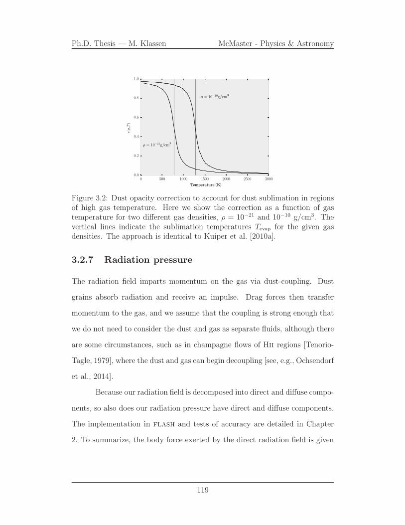
Ph.D. Thesis — M. Klassen McMaster - Physics & Astronomy
0 500 1000 1500 2000 2500 3000
Temperature (K)
0.0
0.2
0.4
0.6
0.8
1.0
ǫ(ρ,T)
ρ = 10−21g/cm3
ρ = 10−10g/cm3
Figure 3.2: Dust opacity correction to account for dust sublimation in regionsof high gas temperature. Here we show the correction as a function of gastemperature for two different gas densities, ρ = 10−21 and 10−10 g/cm3. Thevertical lines indicate the sublimation temperatures Tevap for the given gasdensities. The approach is identical to Kuiper et al. [2010a].
3.2.7 Radiation pressure
The radiation field imparts momentum on the gas via dust-coupling. Dust
grains absorb radiation and receive an impulse. Drag forces then transfer
momentum to the gas, and we assume that the coupling is strong enough that
we do not need to consider the dust and gas as separate fluids, although there
are some circumstances, such as in champagne flows of Hii regions [Tenorio-
Tagle, 1979], where the dust and gas can begin decoupling [see, e.g., Ochsendorf
et al., 2014].
Because our radiation field is decomposed into direct and diffuse compo-
nents, so also does our radiation pressure have direct and diffuse components.
The implementation in flash and tests of accuracy are detailed in Chapter
2. To summarize, the body force exerted by the direct radiation field is given
119

Ph.D. Thesis — M. Klassen McMaster - Physics & Astronomy
by Equation 2.31 from Chapter 2,
frad = ρκP (T∗)F∗
c= −∇ · F∗
c, (3.19)
where T∗ is the temperature of the photosphere, which is the characteristic
temperature of the direct radiation field. We see that the force is proportional
to the absorbed radiation energy in a grid cell. The stellar flux, also, depends
on the optical depth (see Equation 3.2). In the gray radiation approximation,
the optical depth is integrated using the stellar surface temperature for the
opacity calculation (see Equation 3.3). This is because interstellar dust has
a strong frequency dependence and most of the energy and momentum is
carried by the high-frequency radiation. The result is that most of the energy
and momentum from the direct radiation is deposited in an area close to the
star. However, as the dust sublimates and an optically thin cavity begins to
form, more of the direct radiation is able to escape into the polar direction.
For the diffuse (thermal) radiation field, the updated hydrodynamics
solver incorporates the effects of radiation on the momentum of the gas.
While we currently use a frequency-averaged opacity model, we do not
expect there to be large deviations in radiation pressure when compared to
a multifrequency approach. The reason for this is that while low frequency
radiation can penetrate further into the gas, it also carries much less energy
compared to the higher-frequency components.
120
Ph.D. Thesis — M. Klassen McMaster - Physics & Astronomy
3.3 Numerical simulations
Our goal was to emulate the initial conditions of the simulations of Krumholz
et al. [2009] and Kuiper et al. [2010a, 2011a] to determine what effect our
improved numerical and physical treatment has on the massive star formation
problem. Each paper sought to address the question of how massive stars
continued to accrete despite their enormous luminosities. As noted in the
introduction, the main difference between their methods was the type of ra-
diative transfer code used, with the former using an FLD-based scheme on a
Cartesian AMR grid in orion and the latter using a hybrid raytrace/FLD
scheme implemented in pluto on a fixed, spherical grid. Krumholz et al.
[2009] showed simulations in which a radiative Rayleigh-Taylor instability fed
material back onto the star and disk, whereas Kuiper et al. [2012] argued that
dust sublimation and a more accurate treatment of the radiation field in prox-
imity to the star allows for a stable radiatively-driven cavity to form around
the star, and for material to continue accreting through the disk. In the latter
radiation scheme, since the stellar radiation is first carried by a raytracer, it
is the optical depth along each ray that determines the star’s impact. Pure
FLD schemes use a kernel centered on the star to mediate the radiative energy
injection, typically isotropically. In both cases, it was found that radiation
pressure did not imply an upper mass limit for star formation.
As in the mentioned papers, the volume we simulate has a side length
of 0.4 pc, with an central core of radius 0.1 pc residing inside. The core is
initially cold (T0 = 20K) and the molecular gas and dust has a matter density
121

Ph.D. Thesis — M. Klassen McMaster - Physics & Astronomy
profile that follows a power-law,
ρ(r) ∝ r−p, (3.20)
with p = 1.5. The density is scaled by a multiplicative constant to give the
desired total core mass (30, 100, or 200 M⊙). To avoid a cusp, a quadratic
smoothing function over the central 6 cells smooths out the singularity.
The core is initially in solid-body rotation. We choose an angular ro-
tation rate to match that used in Kuiper et al. [2010a], Ω0 = 5 × 10⁻¹³ s−1.
Krumholz et al. [2009] set their rotation so that the ratio of rotational kinetic
energy to gravitational binding energy,
βrot =12IΩ2
Ugrav=
( 3−p
5−p)McoreR2Ω2/3
( 3−p
5−2p)GM2core/R
=(
5−2p5−p
)
R3Ω2
3GMcore, (3.21)
is 2% for a core with a power-law profile with index p. Our rotational en-
ergy ratios are higher (see Table 3.1). Higher rotation rates result in larger
accretion disks, which should be more prone to fragmentation at larger radii.
The rotation rates of disks eventually settle into Keplerian motion around the
central star.
3.3.1 Sink particles
Our simulations are initialized without any stars present, but sink particles
are allowed to form naturally according to their formation criteria [Federrath
et al., 2010a] and act as the ray source location in the raytracing code. Sink
particles interact with the gas via mutual gravitation and are not held fixed at
122

Ph.D. Thesis — M. Klassen McMaster - Physics & Astronomy
the center of the simulation volume, a key difference between our simulation
and those of Kuiper et al. [2010a], wherein the source was held fixed at the
center of the spherical grid and represented by a sink cell. Material crossing
the inner grid boundary at rmin = 10 AU was considered accreted onto the
star. In Krumholz et al. [2009] the sink particles were allowed to form in
regions that were Jeans-unstable and undergoing gravitational collapse (as in
our case), according to the sink particle algorithm in orion [Krumholz et al.,
2004].
In order to form a star, gas must be Jeans unstable. The Truelove et al.
[1997] criterion states that the Jeans length must be resolved by at least four
grid cells, this imposes a natural density threshold for sink particle formation.
If the sink radius, rsink, is equal to the Jean’s length, λJ = (πc2s/(Gρ))1/2, then
the threshold density becomes
ρthresh =πc2s
4Gr2sink, (3.22)
where the factor of 4 in the denominator comes from the Truelove criterion
and the sink radius is defined by the grid scale, rsink = 2.5∆x. Given our grid
resolution of ∆x ≈ 10 AU, this results in a threshold density of ρ ∼ 10−14
g/cm3 for all of the simulations described in this paper.
The sink particles in Krumholz et al. [2009] followed an implementation
described in Krumholz et al. [2004], with the threshold density and Jeans
criterion determining sink particle creation. The sink particle algorithm of
Federrath et al. [2010a] that we use is stricter, checking also for convergent
flow, a gravitational potential minimum, and a negative total energy (Egrav +
Eth + Ekin < 0) within a control volume.
123

Ph.D. Thesis — M. Klassen McMaster - Physics & Astronomy
3.3.2 Resolution
In order to resolve the dust sublimation region around the accreting star, we
operate with 11 levels of refinement on our Cartesian grid, resulting in a grid
resolution of ∆xcell = L/2lmax+2 = 10.07 AU. Krumholz et al. [2009] used a
similar resolution in their simulations.
For our refinement criterion we choose to resolve the Jeans length with
8 grid cells, that is
λJ =
√
15kBT
4πGµρ≥ 8∆xcell, (3.23)
where kB is Boltzmann’s constant, T is temperature, G is Newton’s constant,
µ = 2.33 is the mean molecular weight in our simulation, and ρ is the gas
density.
Additionally, any block containing the sink particle is refined to the
highest level.
3.3.3 Turbulence
Star-forming environments inside molecular clouds are turbulent [Larson, 1981,
Evans, 1999], and turbulence plays a crucial role in regulating star forma-
tion [Mac Low and Klessen, 2004, McKee and Ostriker, 2007b, Federrath and
Klessen, 2012]. However, in this paper we are studying the role of radiation
feedback in massive star formation, revisiting important simulations in the
scientific literature, but without some of the previous limitations. It is essen-
tial, then, that other complexities, such as the inclusion of initial turbulence
and magnetic fields, be left out until the ‘basic case’ has been treated and
fully studied. In forthcoming papers, we aim to study star formation in more
realistic environments featuring turbulence and magnetic fields.
124

Ph.D. Thesis — M. Klassen McMaster - Physics & Astronomy
Table 3.1: Protostellar core collapse simulation parameters
Physical simulation parameters
Parameter M30 M100 M200
Cloud radius [pc] R0 0.1 0.1 0.1Power law index p 1.5 1.5 1.5Total cloud mass [M⊙] Mtot 30 100 200Number of Jeans masses NJ 13.03 79.33 224.37Peak (initial) mass density [g/cm3] ρc 2.58× 10⁻¹⁵ 8.84× 10⁻¹⁵ 1.77× 10⁻¹⁴
Peak (initial) number density [cm−3] nc 6.62× 10⁸ 2.27× 10⁹ 4.54× 10⁹
Initial temperature [K] T 20 20 20Mean freefall time [kyr] tff 95.8 52.4 37.0Sound crossing time (core) [Myr] tsc 0.569 0.569 0.569Rigid rotation angular frequency [s−1] Ωrot 5.0× 10⁻¹³ 5.0× 10⁻¹³ 5.0× 10⁻¹³
Rotational energy ratio βrot 35.1 % 10.5 % 5.3 %
Numerical simulation parameters
Simulation box size [pc] Lbox 0.40 0.40 0.40Smallest cell size [AU] ∆x 10.071 10.071 10.071
Simulation outcomes
Final simulation time [kyr] tfinal 81.4 41.6 21.9Number of sink particles formed nsinks 1 1 1Final sink mass [M⊙] 5.48 28.84 43.65
3.3.4 Summary
We performed a total of three supercomputer simulations, varying the ini-
tial core mass across these. We selected initial cores with masses of 30M⊙,
100M⊙, and 200M⊙. We kept all other parameters consistent between these
simulations, including initial temperature, rotation rate, resolution, etc.
The initial conditions and final sink particle properties are summarized
in Table 3.1. In addition to the simulations listed, we performed supplementary
simulations of the 30 M⊙ and 100 M⊙ protostellar core setups at lower rotation
rates so that βrot = 2% (see Equation 3.21). These lower rotation results did
not change our conclusions.
125
Ph.D. Thesis — M. Klassen McMaster - Physics & Astronomy
3.4 Results
In this section we discuss the results from the three simulations described in
the section above and summarized in Table 3.1.
3.4.1 General description: different phases of massive
star formation
The evolution of the protostellar core proceeds through approximately four
stages: (1) collapse, (2) disk formation, (3) disk instability, and (4) radiation
feedback. The gas is initially spherically symmetric in all our simulations
and begins to contract gravitationally. Before long, a Jeans instability at the
center of the volume results in the creation of a sink particle representing the
gravitational collapse to stellar densities. The sink particle begins accreting
material from the surrounding gas.
Figure 3.3 shows snapshots taken from our 100 M⊙ simulation at ap-
proximately 15, 25, 35, and 40 kyr of evolution, as indicated. The left column
shows the density projected along the z-axis, giving a face-on view of the pro-
tostellar disk. Each frame is centered on the location of the sink particle. The
column densities in the first column are scaled from Σ = 100 g/cm2 to 102.5
g/cm2. The column on the right shows the edge-on view, also centered on
the sink particle, where a slice has been taken and volume densities within
the slice plotted. The color of the indicated volume densities are scaled from
ρ = 10−18 g/cm3 to 10−14 g/cm2.
In this figure, each row shows the state of the simulation at the indi-
cated time, zoomed in to a (3000 AU)2 region around the sink particle. At
15 kyr (first row), the core has undergone gravitational collapse and a small
126

Ph.D. Thesis — M. Klassen McMaster - Physics & Astronomy
15 kyr M∗ = 6.12 M⊙
25 kyr M∗ = 10.9 M⊙
35 kyr M∗ = 24.3 M⊙
40 kyr M∗ = 27.8 M⊙
0.0 0.8 1.6 2.4 −18 −17 −16 −15 −14
log10 Σ (g/cm2) log10 ρ (g/cm3)
Figure 3.3: A series of panels from our 100M⊙ simulation showing the timeevolution of the disk in face-on and edge-on views. The times are indicatedin the upper left corner of each row. The left column shows the projected gasdensity of the disk within a (3000 AU)2 region. The colors indicating columndensities are scaled from Σ = 1 g/cm2 to 102.5 g/cm2. The right column is aslice of the volume density taken to show the edge-on view of the protostellardisk. The window is (3000 AU)2 and the colors are scaled from ρ = 10−18
g/cm3 to 10−14 g/cm3. The mass of the star in each pair of panels is indicatedin the top-left of the second panel of each row.
127
Ph.D. Thesis — M. Klassen McMaster - Physics & Astronomy
protostellar disk has formed around the sink particle. In the second row, at 25
kyr, the disk is just beginning to undergo a gravitational instability. We see the
formation of ripples at the edges of the disk, as well as a ring of dense material
in the outer region of the disk. After a further 10 kyr of evolution, this disk
shows clear spiral density waves (third row, Figure 3.3) and two radiatively-
driven bubbles, one on either side of the accretion disk. The final row of Figure
3.3 shows the end state of the simulation. The radiatively-driven bubble below
the disk has continued to expand and is now more than 2000 AU across, while
dense material flowing above the ray origin has momentarily quenched the di-
rect radiation field above the disk and caused the bubble to disappear. In the
face-on view, dramatic spiral density waves still swirl around the protostar,
which continues to accrete material at a high rate (M ∼ 10−3M⊙/yr).
When we compare this sequence of stages in each simulation, they all
tell a similar story. In the 30 M⊙ core simulation, the star does not become
quite luminous enough to drive bubble formation, but we still witness disk
instability and the formation spiral waves. In the 200 M⊙ core simulation,
the formation of star and disk proceed through the same stages, except the
star is even more massive (reaching almost 44 M⊙) and so luminous that large
outflow bubbles are formed on both sides of the disk and continue to grow
until the end of the simulation.
We run each simulation until the timestep becomes too short to be
practical. A strict upper limit on the simulation timestep is set by the gas
velocities and the resolution. A highly luminous star will launch powerful
outflows. These gas motions must be resolved. We observe velocities exceeding
107 cm/s. With a grid resolution of ∼ 1014 cm, this gives an upper limit to
the timestep of ∆tsim ≤ 107 seconds, which is shorter than a year.
128
Ph.D. Thesis — M. Klassen McMaster - Physics & Astronomy
At the time when we halted our simulations, each simulation had pro-
duced only a single sink particle. For an initial core mass of 30M⊙, the re-
sulting sink attained a final mass of 5.48M⊙ after 81.4 kyr of evolution. The
simulation that began with a core mass of 100M⊙ produced a star of 28.84M⊙,
whereas our 200M⊙ simulation produced a star of 43.65M⊙.
The freefall time for a sphere of uniform density ρ is given by
tff =
√
3π
32Gρ, (3.24)
where G is Newton’s constant. It represents the characteristic timescale for
gravitational collapse. We estimate the freefall for our protostellar cores using
the mean density. More massive cores have shorter freefall times, resulting in
higher accretion rates onto the protostar. The simulations ran for 0.85, 0.79,
and 0.59 freefall times for each of the initial 30 M⊙, 100 M⊙, and 200 M⊙
core simulations, respectively.
We show the sink particle evolution in Figure 3.4 as a function of time.
In the upper left panel we show the mass histories of the star formed in each
simulation. One interesting feature of these is that each possesses a ‘knee’,
where the rate of accretion shifts from one steady value to another relatively
steady value. The knee appears to occur simultaneously with the disk insta-
bility, and we explore this below.
The accretion rate is shown in the upper right panel for Figure 3.4 and
shows the same transition to higher accretion rates. This occurs between 0.35
and 0.55 freefall times. The accretion rate increases by a factor of about 2–10,
while also become more variable. We attribute both the increase in accretion
rate and its increased variability to a transition in the accretion disk, which
129

Ph.D. Thesis — M. Klassen McMaster - Physics & Astronomy
0 10 20 30 40 50 60 70 80 900
5
10
15
20
25
30
35
40
45
Mass
(M⊙
)
0 10 20 30 40 50 60 70 80 9010−7
10−6
10−5
10−4
10−3
10−2
10−1
100
Accre
tion
Rate
(M⊙
/yr)
0 10 20 30 40 50 60 70 80 90
Time (kyr)
0
5000
10000
15000
20000
25000
30000
35000
Surf
ace
Tem
pera
ture
(K)
0 10 20 30 40 50 60 70 80 90
Time (kyr)
10−11
10−9
10−7
10−5
10−3
10−1
101
103
105
107
Lum
inosity
(L⊙
)
30 M⊙
100 M⊙
200 M⊙
Figure 3.4: The time-evolution of the sink particle formed in each of the threesimulations (30, 100, and 200 M⊙ initial core mass). The sink particle repre-sents the accreting protostar and its internal evolution is governed by a proto-stellar model. The top-left panel shows its mass. The top-right panel indicatesthe accretion rates onto the sink particles. The effective surfance temperatureof the protostar is estimated by a protostellar model and is indicated in thebottom-left panel. The star radiates both due to the high accretion rate andits own intrinsic luminosity due to nuclear burning. The total luminosity ofthe sink is the sum of these two, and each sink particle’s total luminosity isshown in the bottom-right panel.
130

Ph.D. Thesis — M. Klassen McMaster - Physics & Astronomy
we discuss in detail below in section 3.4.2.
The bottom two panels of Figure 3.4 show the effective surface temper-
ature (left) and luminosity (right) of the star, respectively. The temperature
is given by a protostellar model that we introduced into the flash code in
Klassen et al. [2012b] and is based on a one-zone model described in Offner
et al. [2009]. The drop in temperature observed in the 100 M⊙ and 200 M⊙
runs is on account of a swelling of the stellar radius at a time when the ac-
creting protostar undergoes a change in its internal structure, switching from
a convective to a radiative structure. The much larger stellar radius is initally
cooler. The luminosity shown in the bottom right panel of Figure 3.4 shows
the combined stellar luminosity and accretion luminosity, Lacc ∝ GM∗M∗/R∗.
This impact of protostellar evolution on the radiative feedback is in general
agreement with earlier models of high-mass core collapse using 1D stellar evolu-
tion modeling (Kuiper and Yorke, 2013b, but compare Haemmerle and Peters,
2016).
We note that in each of our three main simulations, only a single sink
particle is formed. This is in contrast to the similar calculation by Krumholz
et al. [2009], which formed a binary companion with an orbital semi-major axis
of 1280 AU. The secondary was about 1000 AU away from the central star,
which is similar to the radius of the circumstellar accretion disks we form.
In Figure 3.5 we plot the evolution of the mass accretion rate as a func-
tion of the stellar mass for the sink particle in each of our three simulations.
We apply a moving average filter of 1000 datapoints to smooth out the accre-
tion rate, which is highly variable, especially at late times. We were unable
to evolve the simulation to the point were accretion shuts down onto the sink
particle. The figure is similar to Figure 11 in Kuiper et al. [2010a], but which
131

Ph.D. Thesis — M. Klassen McMaster - Physics & Astronomy
featured simulation with axial and midplane symmetries. The 2D axisymmet-
ric geometry of those simulations allowed for much longer runtimes. At late
times accretion is seen to shut down, on account of both gas reservoir depletion
and radiative feedback. We were unable to run our 3D non-axisymmetric sim-
ulations for the same duration, and so in Figure 3.5 we do not yet see strong
evidence of a shutdown in accretion and the gas reservoir is still far from fully
depleted.
In the corresponding 3D simulation of Kuiper et al. [2011a], the accre-
tion disk also shows the formation of spiral arms and highly variable accretion
rates, but no disk fragmentation. But the simulation could only be performed
up to 12 kyr of evolution, hence, further evolution of the circumstellar disk,
including binary formation, remains uncovered.
Before disk instability sets in, the accretion rate onto the star is gov-
erned more by spherically symmetric collapse of the initial core. Girichidis
et al. [2011a] examined the collapse of a singular isothermal sphere [Shu, 1977]
and the scaling of accretion rate with the number of Jeans masses NJ present
in initial the protostellar core. We therefore compare the maximal accretion
rate before disk instability sets in to the number of Jeans masses, and find
that there is a linear relationship between accretion and NJ . The Jeans mass
is given by
MJ =π5/2
6
c3sG3/2ρ1/2
, (3.25)
where cs is the isothermal sound speed and ρ is the mean density of the spher-
ical protostellar core. Thus, the number of Jeans masses present is
NJ =Mcore
MJ(3.26)
132

Ph.D. Thesis — M. Klassen McMaster - Physics & Astronomy
0 5 10 15 20 25 30 35 40 45
M∗ (M⊙)
10−6
10−5
10−4
10−3
10−2
10−1
M∗
(M⊙
/yr)
30 M⊙
100 M⊙
200 M⊙
Figure 3.5: The accretion rate plotted as a function of stellar mass for eachof our three main simulations. The line thickness scales in order of ascendinginitial mass for the protostellar core.
The linear scaling in accretion rate followed
M∗ = 9.638× 10⁻⁶NJ M⊙ yr−1. (3.27)
The 30, 100, 200 M⊙ simulations contained 13.0, 79.3, and 224.4 Jeans
masses, respectively, assuming isothermal 20 K gas. An approximately linear
scaling is consistent with the theoretical results of Girichidis et al. [2011a],
although they were following the self-similar collapse of a singular isothermal
sphere [Shu, 1977] with power-law profiles ρ ∝ r−2.
133
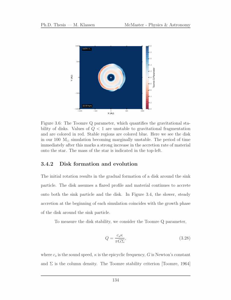
Ph.D. Thesis — M. Klassen McMaster - Physics & Astronomy
−1000 −500 0 500 1000
X (AU)
−1000
−500
0
500
1000
Y(A
U)
22.50 kyrs
9.874 M⊙
0.0
0.2
0.4
0.6
0.8
1.0
1.2
1.4
1.6
1.8
2.0
Toom
reQ
Para
mete
r
Figure 3.6: The Toomre Q parameter, which quantifies the gravitational sta-bility of disks. Values of Q < 1 are unstable to gravitational fragmentationand are colored in red. Stable regions are colored blue. Here we see the diskin our 100 M⊙ simulation becoming marginally unstable. The period of timeimmediately after this marks a strong increase in the accretion rate of materialonto the star. The mass of the star is indicated in the top-left.
3.4.2 Disk formation and evolution
The initial rotation results in the gradual formation of a disk around the sink
particle. The disk assumes a flared profile and material continues to accrete
onto both the sink particle and the disk. In Figure 3.4, the slower, steady
accretion at the beginning of each simulation coincides with the growth phase
of the disk around the sink particle.
To measure the disk stability, we consider the Toomre Q parameter,
Q =csκ
πGΣ, (3.28)
where cs is the sound speed, κ is the epicyclic frequency, G is Newton’s constant
and Σ is the column density. The Toomre stability criterion [Toomre, 1964]
134

Ph.D. Thesis — M. Klassen McMaster - Physics & Astronomy
100 au
14.26 kyr
20.44 M⊙
18.06 kyr
28.69 M⊙
21.31 kyr
42.68 M⊙
10-18 10-17 10-16 10-15 10-14 10-13 10-12
0.0 0.2 0.4 0.6 0.8 1.0 1.2 1.4 1.6 1.8 2.0
Volume Density Slice with Velocity Streamlines
Local Toomre Q
Figure 3.7: Sequence of snapshots from the 200 M⊙ simulation showing face-on volume density slices (top row) and the local Toomre Q parameter (bottomrow) in a (3000 AU)2 region centered on the location of the sink particle. Scalebars have been added to show the volume density (in g/cm2) and the value ofthe Q parameter (see Equation 3.28). Values of Q < 1 indicate disk instability.Velocity streamlines have been added to the volume density slice. The massof the star is indicated in the bottom-left of each panel in the bottom row.
135
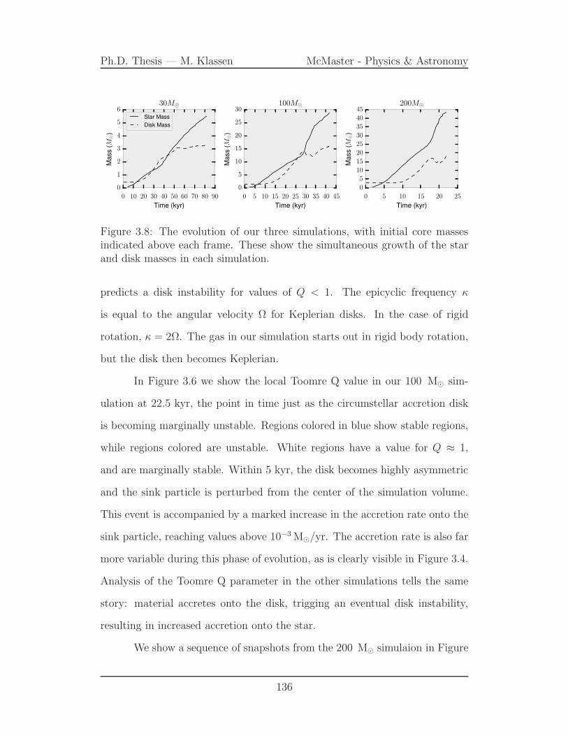
Ph.D. Thesis — M. Klassen McMaster - Physics & Astronomy
0 10 20 30 40 50 60 70 80 90
Time (kyr)
0
1
2
3
4
5
6M
ass
(M⊙
)30M⊙
Star Mass
Disk Mass
0 5 10 15 20 25 30 35 40 45
Time (kyr)
0
5
10
15
20
25
30
Mass
(M⊙
)
100M⊙
0 5 10 15 20 25
Time (kyr)
0
5
10
15
20
25
30
35
40
45
Mass
(M⊙
)
200M⊙
Figure 3.8: The evolution of our three simulations, with initial core massesindicated above each frame. These show the simultaneous growth of the starand disk masses in each simulation.
predicts a disk instability for values of Q < 1. The epicyclic frequency κ
is equal to the angular velocity Ω for Keplerian disks. In the case of rigid
rotation, κ = 2Ω. The gas in our simulation starts out in rigid body rotation,
but the disk then becomes Keplerian.
In Figure 3.6 we show the local Toomre Q value in our 100 M⊙ sim-
ulation at 22.5 kyr, the point in time just as the circumstellar accretion disk
is becoming marginally unstable. Regions colored in blue show stable regions,
while regions colored are unstable. White regions have a value for Q ≈ 1,
and are marginally stable. Within 5 kyr, the disk becomes highly asymmetric
and the sink particle is perturbed from the center of the simulation volume.
This event is accompanied by a marked increase in the accretion rate onto the
sink particle, reaching values above 10−3M⊙/yr. The accretion rate is also far
more variable during this phase of evolution, as is clearly visible in Figure 3.4.
Analysis of the Toomre Q parameter in the other simulations tells the same
story: material accretes onto the disk, trigging an eventual disk instability,
resulting in increased accretion onto the star.
We show a sequence of snapshots from the 200 M⊙ simulaion in Figure
136
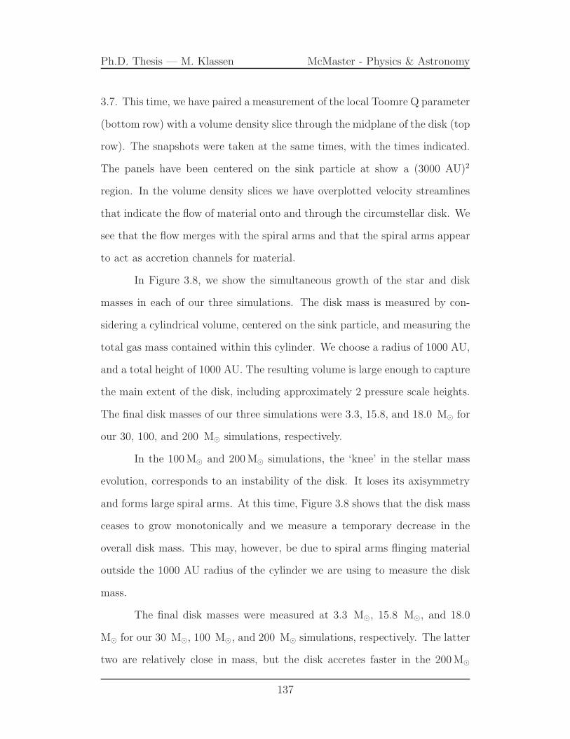
Ph.D. Thesis — M. Klassen McMaster - Physics & Astronomy
3.7. This time, we have paired a measurement of the local Toomre Q parameter
(bottom row) with a volume density slice through the midplane of the disk (top
row). The snapshots were taken at the same times, with the times indicated.
The panels have been centered on the sink particle at show a (3000 AU)2
region. In the volume density slices we have overplotted velocity streamlines
that indicate the flow of material onto and through the circumstellar disk. We
see that the flow merges with the spiral arms and that the spiral arms appear
to act as accretion channels for material.
In Figure 3.8, we show the simultaneous growth of the star and disk
masses in each of our three simulations. The disk mass is measured by con-
sidering a cylindrical volume, centered on the sink particle, and measuring the
total gas mass contained within this cylinder. We choose a radius of 1000 AU,
and a total height of 1000 AU. The resulting volume is large enough to capture
the main extent of the disk, including approximately 2 pressure scale heights.
The final disk masses of our three simulations were 3.3, 15.8, and 18.0 M⊙ for
our 30, 100, and 200 M⊙ simulations, respectively.
In the 100M⊙ and 200M⊙ simulations, the ‘knee’ in the stellar mass
evolution, corresponds to an instability of the disk. It loses its axisymmetry
and forms large spiral arms. At this time, Figure 3.8 shows that the disk mass
ceases to grow monotonically and we measure a temporary decrease in the
overall disk mass. This may, however, be due to spiral arms flinging material
outside the 1000 AU radius of the cylinder we are using to measure the disk
mass.
The final disk masses were measured at 3.3 M⊙, 15.8 M⊙, and 18.0
M⊙ for our 30 M⊙, 100 M⊙, and 200 M⊙ simulations, respectively. The latter
two are relatively close in mass, but the disk accretes faster in the 200M⊙
137
Ph.D. Thesis — M. Klassen McMaster - Physics & Astronomy
case. It also has the highest time-averaged star mass to disk mass ratio (1.96).
The 30 M⊙ simulation had the lowest time-averaged star-to-disk mass ratio
(1.07), with the 100 M⊙ falling in between with 1.45.
3.4.3 Disk fragmentation
Contrary to a very similar calculation performed by Krumholz et al. [2009],
we do not form a binary star as the disk goes unstable, or any additional
sink particles. Despite the instability of the disk, fragmentation is not seen.
This is a significant result given that spectroscopic surveys show a high binary
fraction among massive stars. Chini et al. [2012] performed a high-resolution
radial velocity spectroscopic survey of massive stars within the Milky Way
galaxies that included about 250 O-type stars and 540 B-type stars. Their
results indicated that over 82% of stars with masses above 16 M⊙ form close
binaries. This fraction drops precipitously for lower-mass stars.
How many stars are expected to form per protostellar core? Goodwin
and Kroupa [2005] argue from dynamical constraints and observations that
protostellar cores should produce only 2 or 3 stars. This contrasts with some
numerical simulations, in which the protostellar core fragments into a greater
number of stars, as in Goodwin et al. [2004] or the simulations of Krumholz
et al. [2009]. It also contrasts with our simulations, which show a massive disk
that does not fragment into more stars.
We examine several approaches to the question of fragmentation. First,
we follow the analysis of Rogers and Wadsley [2012], who studied the frag-
mentation of protostellar disks and derived a Hill criterion for the spiral arms
[although, see Takahashi et al., 2016]. These are the sites most likely to begin
138
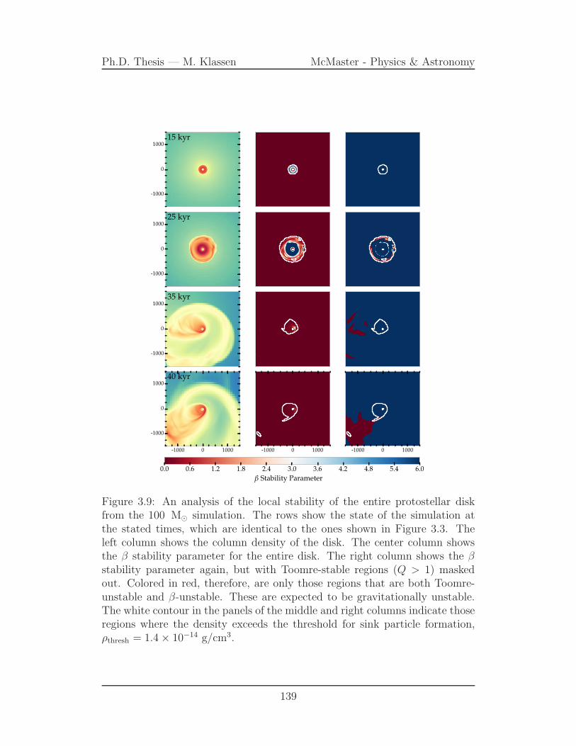
Ph.D. Thesis — M. Klassen McMaster - Physics & Astronomy
-1000
0
100015 kyr
-1000
0
100025 kyr
-1000
0
100035 kyr
-1000 0 1000
-1000
0
100040 kyr
-1000 0 1000 -1000 0 1000
0.0 0.6 1.2 1.8 2.4 3.0 3.6 4.2 4.8 5.4 6.0
β Stability Parameter
Figure 3.9: An analysis of the local stability of the entire protostellar diskfrom the 100 M⊙ simulation. The rows show the state of the simulation atthe stated times, which are identical to the ones shown in Figure 3.3. Theleft column shows the column density of the disk. The center column showsthe β stability parameter for the entire disk. The right column shows the βstability parameter again, but with Toomre-stable regions (Q > 1) maskedout. Colored in red, therefore, are only those regions that are both Toomre-unstable and β-unstable. These are expected to be gravitationally unstable.The white contour in the panels of the middle and right columns indicate thoseregions where the density exceeds the threshold for sink particle formation,ρthresh = 1.4× 10⁻¹⁴ g/cm3.
139

Ph.D. Thesis — M. Klassen McMaster - Physics & Astronomy
fragmenting. They discovered that if the width of these spiral arms is less
than twice the Hill radius, then fragmentation of the spiral arms is expected
because the self-gravity of that spiral arm segment dominates the tidal forces
from the star (manifested as rotational shear).
To quantify this, we look at the Hill radius, as defined in Rogers and
Wadsley [2012],
HHill =
[
GΣl2
3Ω2
]1/3
, (3.29)
where G is Newton’s constant, Σ is the column density of the spiral arms
segment, l is the width (thickness) of the spiral arm, Ω is the angular velocity,
assuming a Keplerian disk. Here Σl2 is a measure of the mass contained within
the Hill sphere.
The Hill criterion for stability against fragmentation is
l
2HHill
> 1. (3.30)
Rogers and Wadsley [2012] demonstrate the validity of this criterion
through hydrodynamic simulations of protostellar disks, finding gravitational
fragmentation occurring when l/(2HHill) < 1. We test whether the spiral arms
present in our own calculation are indeed stable by looking at snapshots from
our simulations at an evolved state. We then took a cross-section of the spiral
arm where column densities were greatest and measured the mass along the
cross section and the angular rotation rate. In each case the spiral arms were
100 AU wide, and the masses through a section of the spiral arms at the cross
section were 0.033 M⊙, 0.15 M⊙, and 0.29 M⊙ for the 30, 100, and 200 M⊙
simulations, respectively. Meanwhile, the rotation rates at these locations were
140

Ph.D. Thesis — M. Klassen McMaster - Physics & Astronomy
Ω = 3 × 10⁻¹⁰, 6 × 10⁻¹⁰, and 6 × 10⁻¹⁰, respectively. Finally, this resulted
in Hill criterion values of l/(2HHill) = 2.95, 2.82, 2.26, respectively, consistent
with the lack of fragmentation observed in our simulations.
This analysis nevertheless focuses on the role of shear stabilization in
spiral arms. We now turn to the role of cooling and disk fragmentation across
the entire disk. Gammie [2001] and Johnson and Gammie [2003] investigated
nonlinear gravitational instability in numerical models of thin, Keplerian disks.
By considering the cooling time τc and the angular rotation rate Ω, a stability
parameter can be defined,
β = τcΩ, (3.31)
which must be greater than some critical value in order for the disk to remain
gravitationally stable. Gas with short cooling times relative to the orbital
period is expected to cool rapidly—opening the way to fragmentation if the
gas is also sufficiently self-gravitating. The critical value for β is established
via numerical simulations, but depends critically on which heating and cooling
mechanisms are present in the simulation. The cooling time can be defined as
the internal energy of the gas, divided by its cooling rate. For optically thick
disks, Johnson and Gammie [2003] found fragmentation occurs for values of
β = 〈τc〉Ω ∼ 1, where 〈τc〉 is the disk-averaged cooling time. It is important to
note that the β-criterion for stability does not replace the Toomre Q stability
criterion, but rather complements it. That is, a disk must be both Toomre-
unstable and have a Gammie β less than some critical value for fragmentation
to occur.
We choose to look at the local cooling rate. Since we possess informa-
tion about the rate of radiative flux loss from the disk, we define the cooling
141

Ph.D. Thesis — M. Klassen McMaster - Physics & Astronomy
time as
τc =E
〈|Frad,z|〉, (3.32)
where E is the column internal energy integrated through the disk. Meanwhile,
〈|Frad,z|〉 is the mean radiative flux in the vertical direction (away from the
disk). Our cooling time, therefore, is a direct function of the mean density,
temperature, and opacity of a vertical column through the circumstellar disk.
Since we know the rotation rate at each point, we then calculate a local β =
τcΩ.
In Figure 3.9 we compare side-by-side the column density and disk
stability for the circumstellar disk in our 100 M⊙ simulation, taking snapshots
from the simulation at the same times as in Figure 3.3. As in that earlier figure,
we show the column density in the left column. The middle column shows the
value for β throughout the disk. We see that the cooling time is short relative
to the orbital period and the disk should be prone to rapid cooling. Recall
that Johnson and Gammie [2003] found that fragmentation occurs for values
of β ∼ 1.
However, if we consider only those regions which are also Toomre-
unstable, as we do in the right column of Figure 3.9, we see that most parts of
the disk remain stable. In generating the panels for this column, we created an
image mask, i.e. we filter the pixels based on value of the Toomre Q parameter
at that location and then draw the β parameter. Regions where Q > 1 are
colored uniformly in blue; these regions are stable regardless of the value of β.
Additionally, we draw a white contour in the panels of the middle and right
columns to indicate those regions where the density exceeds the threshold for
sink particle formation, ρthresh = 1.4× 10⁻¹⁴ g/cm3.
142

Ph.D. Thesis — M. Klassen McMaster - Physics & Astronomy
For our 100M⊙ simulation, the threshold density for sink particles is
ρthresh = 1.4 × 10⁻¹⁴ g/cm3. We draw a white contour in Figure 3.9 to indi-
cate those regions within a disk slice possessing densities greather than this
threshold value.
Taken together, the disk is largely stable across much of its extent.
Nevertheless, Figure 3.9 shows the disk is not completely stable everywhere,
at least predicted by linear stability analysis. This can be seen especially in the
final set of panels at 40 kyr. There appears an island of high density gas that is
both Toomre-unstable and β-unstable at about 1200 AU separation from the
central star. This is a candidate region for collapse. Given more time it could
indeed collapse to form a single wide binary companion to the central star. As
pointed out in Takahashi et al. [2016], fragmentation is a nonlinear outcome
of gravitational instability and highly dependent on initial conditions. They
demonstrate that the only necesssary condition for the formation of spiral
arms is that Q < 1, and the only necessary condition for the fragmentation of
these arms is Q < 0.6. Taken together with our stricter sink particle criteria, as
described in Section 3.3.1, this accounts for the lack of secondary fragmentation
over the timescales simulated.
The gravitational collapse that formed the first star in our simulation,
and the strong radiative accelerations produced by the intense luminosity of
that massive star, conspire with the Courant condition to strongly limit the
timestep size of our simulation. The timestep is now so small that the simu-
lation has now effectively stalled.
143

Ph.D. Thesis — M. Klassen McMaster - Physics & Astronomy
3.4.4 Radiatively-driven bubbles
In the vicinity of a massive star, the radiative force can exceed the force of its
gravitational attraction, resulting in radiatively-driven winds or bubbles, and
possibly halting any further accretion. Radiation pressure is also one of the
main mechansism for the disruption of giant molecular clouds (GMCs) and the
cumulative radiation pressure from star clusters may drive large-scale galactic
outflows [Murray et al., 2010, 2011].
The Eddington luminosity describes the force balance between radia-
tion and gravity:
Ledd =4πGM∗c
κ, (3.33)
where κ denotes the opacity of the absorbing medium. We estimate the direct
radiation pressure using temperature-dependent gray opacity [see Figure 2.1
in Chapter 2] for the dust. The body force on the dust grains is given by
frad = ρκP (Teff)F∗
c, (3.34)
where κP = κP (Teff) is the Planck mean opacity, Teff is the effective tempera-
ture of the star, estimated by protostellar model, and F∗ is the stellar flux.
In Figure 3.10, we show the evolution of the stellar radiative flux in each
of our three simulations. It is plotted here as a function time and compared,
in each case, to the star’s Eddington luminosity. We see that only in the
100M⊙ and 200M⊙ simulations does the star become bright enough to exceed
the Eddington limit. The excess radiation pressure in these two more massive
simulations results in the formation of radiatively-driven outflow bubbles that
expand away from the star above and below the accretion disk, sweeping up a
144
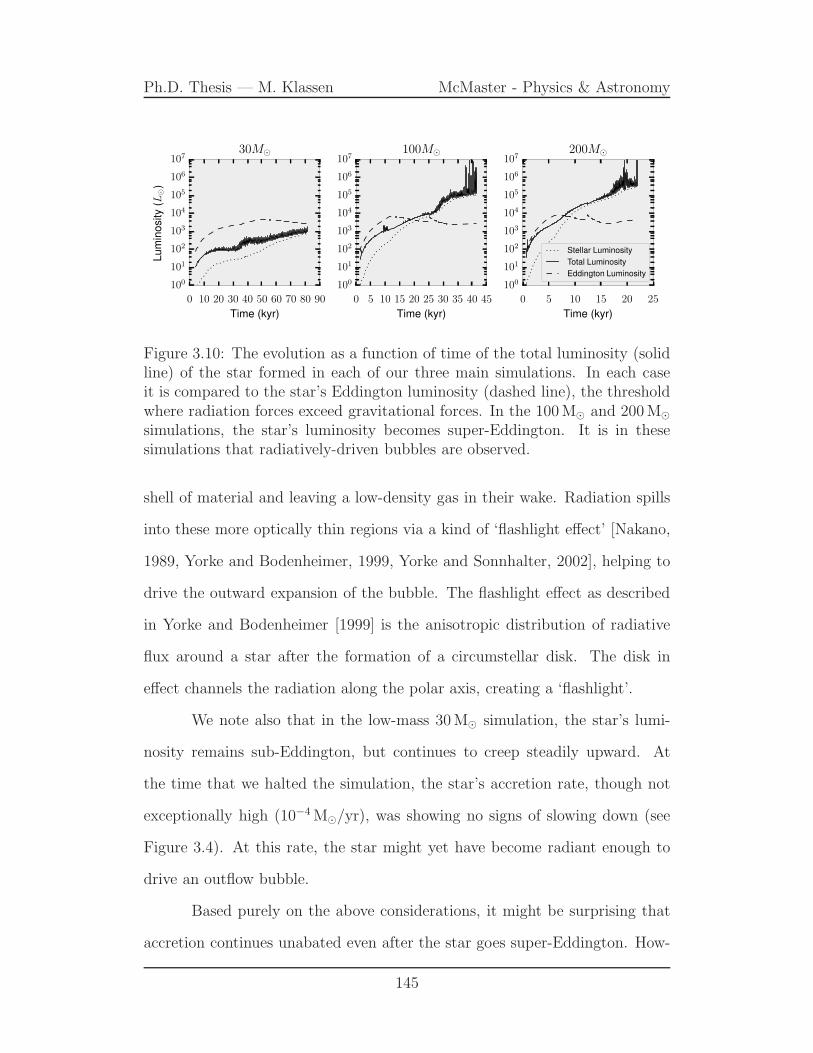
Ph.D. Thesis — M. Klassen McMaster - Physics & Astronomy
0 10 20 30 40 50 60 70 80 90
Time (kyr)
100
101
102
103
104
105
106
107Lum
inosity
(L⊙
)30M⊙
0 5 10 15 20 25 30 35 40 45
Time (kyr)
100
101
102
103
104
105
106
107100M⊙
0 5 10 15 20 25
Time (kyr)
100
101
102
103
104
105
106
107200M⊙
Stellar Luminosity
Total Luminosity
Eddington Luminosity
Figure 3.10: The evolution as a function of time of the total luminosity (solidline) of the star formed in each of our three main simulations. In each caseit is compared to the star’s Eddington luminosity (dashed line), the thresholdwhere radiation forces exceed gravitational forces. In the 100M⊙ and 200M⊙
simulations, the star’s luminosity becomes super-Eddington. It is in thesesimulations that radiatively-driven bubbles are observed.
shell of material and leaving a low-density gas in their wake. Radiation spills
into these more optically thin regions via a kind of ‘flashlight effect’ [Nakano,
1989, Yorke and Bodenheimer, 1999, Yorke and Sonnhalter, 2002], helping to
drive the outward expansion of the bubble. The flashlight effect as described
in Yorke and Bodenheimer [1999] is the anisotropic distribution of radiative
flux around a star after the formation of a circumstellar disk. The disk in
effect channels the radiation along the polar axis, creating a ‘flashlight’.
We note also that in the low-mass 30M⊙ simulation, the star’s lumi-
nosity remains sub-Eddington, but continues to creep steadily upward. At
the time that we halted the simulation, the star’s accretion rate, though not
exceptionally high (10−4M⊙/yr), was showing no signs of slowing down (see
Figure 3.4). At this rate, the star might yet have become radiant enough to
drive an outflow bubble.
Based purely on the above considerations, it might be surprising that
accretion continues unabated even after the star goes super-Eddington. How-
145

Ph.D. Thesis — M. Klassen McMaster - Physics & Astronomy
−200 −150 −100 −50 0 50 100 150 200y (AU)
−200
−150
−100
−50
0
50
100
150
200
z(A
U)
20.122 kyr
M∗ = 39.8 M⊙
0.2 0
.50.5
0.8
10 au
10−17
10−16
10−15
10−14
10−13
Density(
g
cm3
)
Figure 3.11: Volume density slice of a (400 AU)2 region through our 200M⊙ simulation, showing an edge-on view of the circumstellar disk. The sliceis centered on the sink particle, representing a 39.8 M⊙ star. flash’s blockstructure is shown in the grid, with each block containing 83 cells. Overplottedare contours showing dust fraction. Nearest the star, the dust is completelysublimated. Contours show dust sublimation correction factors of 0.2, 0.5, and0.8.
ever, the above estimation of the Eddington luminosity did not account for
dust sublimation, which occurs at the inner edge of the disk. In our simula-
tions, the dust sublimation was approximated by Eqs. (3.17) and (3.18), and
this results in a low opacity in regions where the gas has been heated to high
temperature. Radiative forces can no longer couple to the gas via the dust,
and the gas continues to move inward and accrete onto the star. In Kuiper
et al. [2010a], Kuiper and Yorke [2013a] it was shown that the inclusion of the
dust sublimation front was a requirement for continued accretion via the pro-
tostellar disk and enhanced the anisotropy of the radiation field, contributing
to the flashlight effect. Our resolution (10 AU) is not quite as high as those
(1.27 AU radially at the inner edge of the disk) in Kuiper et al. [2010a], but
146

Ph.D. Thesis — M. Klassen McMaster - Physics & Astronomy
we also show continued disk accretion and a strong flashlight effect.
Figure 3.11 shows the dust sublimation front at a snapshot in time from
our most massive (200 M⊙) core simulation, after about 20 kyr of evolution.
We plot an edge-on volume density slice intersecting the sink particle and
circumstellar disk and showing a region 400 AU wide on a side. The flash
block-grid structure is overplotted for reference. Each block contains 83 cells.
The sink particle, representing a 39.8M⊙ star, is located at the center of
the frame and is in the process of driving a radiative bubble. The star has
grown to almost 20% of the initial mass of the protostellar core. Figure 3.11
shows contours of dust fraction overplotted. A value of 0.0 implies total dust
destruction and a value of 1.0 implies no sublimation. We show contours at
values of 0.2, 0.5, and 0.8. Dust sublimation regions are also optically thin,
and Figure 3.11 shows clearly how radiation is channeled in the polar direction.
In the classical Rayleigh-Taylor instability, a heavy fluid cannot be
stably supported by a light fluid. In Figure 3.12, we plot the net acceleration
based on the radiative and gravitational forces present. The data is taken from
our 200 M⊙ simulation, after 21.8 kyr of evolution. The radiative acceleration
includes both the direct and the diffuse radiation field, while the gravitational
acceleration include the attractions of both the star and the self-gravity of the
gas. The figure shows the volume density of the gas in a slice centered on
the sink particle so that an edge-on view of the disk is shown. Overplotted
are the acceleration vectors with magnitude coded in the color. The direct
radiation field exerts very powerful accelerations immediately surrounding the
star. This energy is absorbed and reprocessed so that the diffuse radiation
field dominates the radiative accelerations in shadowed regions, the disk, and
far away from the star.
147

Ph.D. Thesis — M. Klassen McMaster - Physics & Astronomy
Figure 3.12: Acceleration vectors showing the net acceleration (in units ofcm/s−2) of the gas due to radiative forces and gravity (both the gravity ofthe star and the gas). Vectors are overplotted on a background indicatingvolume density slice of an approximately (6000 AU)2 region through our 200M⊙ simulation after about 21.8 kyr of evolution, showing an edge-on view ofthe circumstellar disk and radiatively-driven bubble. The slice is centered onthe sink particle, representing a 43.5 M⊙ star.
The star has reached a mass of 43.5 M⊙ and has driven a radiative
bubble above and below the disk. While along the edge of the lower bubble
wall, there is a null surface in the acceleration—the radiative and gravitational
forces roughly cancel, though momentum is likely still causing the bubble to
expand. On the upper edge, however, we see that a net outward acceleration
extends well beyond the bubble wall, ensuring that the bubble will continue
to expand outward. It also means that the classic condition for the Rayleigh-
Taylor instability (that of a heavy fluid supported by a light fluid) is not
met. The acceleration vector is outwards, so that the “lighter” fluid (FLD
approximates the radiation field as a fluid) sits atop the heaver fluid of the
bubble wall. This is another reason why our bubbles appear roughly uniform
148

Ph.D. Thesis — M. Klassen McMaster - Physics & Astronomy
17.429 kyr
M∗ = 26.2 M⊙
18.696 kyr
M∗ = 32 M⊙
19.171 kyr
M∗ = 35.5 M⊙
19.884 kyr
M∗ = 38.4 M⊙
20.122 kyr
M∗ = 39.8 M⊙
21.310 kyr
M∗ = 42.7 M⊙
1000 AU
Figure 3.13: Edge-on volume density slices, centered on the sink particle,showing in a (5000 AU)2 region the evolution of a radiatively-driven bubblein our 200 M⊙ simulation. Shown are six snapshots at different points in thesimulation with the times indicated. Velocity vectors have been overplotted.Volume densities have been scaled from ρ = 10−17 g/cm3 to 10−13 g/cm3. Themass of the star is indicated in the top-left of each panel.
and show no signs of the Rayleigh-Taylor instability. We checked the bubble
in the 100 M⊙ simulation and there, too, there was net outward acceleration.
We therefore conclude that Rayleigh-Taylor instabilities are absent in these
early phases, which are instead dominated by net outward acceleration driven
by the radiation field.
In Krumholz et al. [2009], the Rayleigh-Taylor instability that was ob-
served in their simulations served to feed material back onto the disk and the
star. If the disk can be fed continually, either from the outer regions of the
simulation, or from material escaping the polar outflow, then the star should
be able to continue accreting, provided the thermal radiation pressure within
149
Ph.D. Thesis — M. Klassen McMaster - Physics & Astronomy
the disk itself is not so strong as to reverse the accretion flow. In contrast,
Kuiper et al. [2012] modeled the high-mass pre-stellar core collapse comparing
two different schemes for radiative feedback, namely the hybrid scheme used
also in this investigation and the FLD-only scheme used in Krumholz et al.
[2009]; as a result, only simulations using the FLD approximation yield a ra-
diative Rayleigh-Taylor instability, simulations with the hybrid scheme show
stable outflows for stars in the super-Eddington regime. Kuiper et al. [2010a]
showed that the anisotropy of the radiation field prevents the thermal radia-
tion from ever becoming strong enough to halt disk accretion. It then becomes
a question as to whether the disk can be continually fed.
Figure 3.13 clearly shows that collapsing gas is deflected along the walls
of the bubble, and flows onto the disk. Here we look at the gas density and
velocities in a series of slices from our 200M⊙ simulation. We centered in-
dividual slices on the position of the sink particle and took an edge-on view
of a (5000 AU)2 region. The slice intersects the circumstellar accretion disk
and shows a radiatively-driven bubble forming. The second-to-last panel was
taken at the same time as Figure 3.11, which is also near the end of our simu-
lation. The star’s luminosity is super-Eddington in each of the panels shown
(compare Figure 3.10) and the outflow bubbles develop uniformly, both above
and below the disk, and grow to be over 2000 AU in diameter. Interior to
these bubbles is evidence of smaller bubbles, expanding in successive waves
and finally bursting their walls.
We overplot velocity vectors to show the gas motion. Interior to the
radiatively-driven bubbles, the gas is being driven away from the star asym-
metrically. The direct radiation field from the star is highly sensitive to the
gas distribution: it is strongly attenuated in the disk plane, whereas the polar
150

Ph.D. Thesis — M. Klassen McMaster - Physics & Astronomy
direction is more optically thin. The result is rarified gas being accelerated to
high velocity along the polar axis. The highest measured velocity can be over
60 km/s. There is no evidence of Rayleigh-Taylor instability.
Outside of the radiatively-driven bubble, we see gas continuing to fall
gravitationally towards the star. This motion is deflected at the bubble wall
and we observe gas moving along the bubble walls and onto the accretion disk.
Material simply flows along the bubble wall and in this way continues to sup-
ply the protostellar disk with matter. We note that the details may depend on
opacity effects: while our work uses gray atmospheres, long-wavelength radia-
tion was seen to accelerate matter outside the cavity walls in multifrequency
simulations by Kuiper et al. [2010a, 2011a, 2012].
The motion of the star relative to its massive, asymmetric disk results
in the star becoming periodically buried in disk material. This has the result
of temporarily reducing the direct irradiation of the polar cavities. It is also
the likely reason for the formation of successive shells of outward-moving ma-
terial visible in Figure 3.13. It also contributes to the sometimes asymmetric
appearance of the radiatively-driven bubbles, as seen in Figure 3.3 for the 100
M⊙ simulation.
Given the symmetric nature of the initial conditions of the simulation,
one might expect the formation of radiatively-driven bubbles with North-South
symmetry. The Cartesian grid structure easily introduces small numerical per-
turbations that break axial symmetry and trigger gravitational instability and
spiral wave formation, but these do not explain the breaking of plane sym-
metry. Pringle [1996] showed analytically that even initially flat disks with
a central radiation source are subject to a warping instability caused by ra-
diative torques. Also, small numerical perturbations can also be introduced
151

Ph.D. Thesis — M. Klassen McMaster - Physics & Astronomy
by the diffusion solver that iterates over grid cells until specific global conver-
gence criteria are met. If the solution is converged, then the current iteration
ceases without needing to visit the remaining grid cells. This then breaks
North-South symmetry. Eventually, differential shadowing in each hemisphere
by material spilling onto the star then results in the asymmetric bubbles as
seen in our simulation.
3.4.5 Accretion flows and outflows
Finally, we analyzed the accretion flows in our simulation at various times.
To do this, we found it very helpful to create a type of graph profiling the
material moving towards or away from our sink particle as a function of the
polar angle as measured from the ‘north’ vector at the location of the star.
We used yt’s profiling tools to examine the radial velocity at the lo-
cation of the sink particle, being careful to subtract the sink particle’s own
motion from the gas velocity. We then produced an azimuthally-averaged gas
velocity profile as a function of polar angle.
We show two examples of this in Figure 3.14, where we look at gas
motions around the star formed in our 100M⊙ simulation. The first panel
shows the state of the simulation after 20.28 kyr. The star’s mass is about
8.9M⊙. The panel has two inset frames, one showing a representation of gas
density, the other the magnitude of the gas velocity, both within an edge-on
slice centered on the star. Colorbars have been omitted for the inset frames
so as not to overly complicate the figure. We profile the gas motions within
a spherical volume, centered on the sink particle, with a radius of 1000 AU.
The inset frames show a slice through this volume, i.e. their width of 2000 AU
152

Ph.D. Thesis — M. Klassen McMaster - Physics & Astronomy
0 20 40 60 80 100 120 140 160 180Polar Angle φ
−30
−20
−10
0
10
20
30
40
50
60
Radia
lV
elo
city
(km
/s) Time: 20.28 kyr
10−7
10−6
10−5
10−4
10−3
10−2
CellMass(M
⊙)
Density Speed
(a) t = 20.28 kyr, M∗ = 8.88M⊙
0 20 40 60 80 100 120 140 160 180Polar Angle φ
−30
−20
−10
0
10
20
30
40
50
60
Radia
lV
elo
city
(km
/s) Time: 32.96 kyr
10−7
10−6
10−5
10−4
10−3
10−2
CellMass(M
⊙)
Density Speed
(b) t = 32.96 kyr, M∗ = 21.73M⊙
Figure 3.14: Azimuthal accretion and outflow profile at two different timesduring the 100M⊙ simulation within a 1000 AU radius centered on the sinkparticle. In each of these we measure the azimuthally-averaged radial velocityof the gas relative to the star. This gives a picture of how much gas is movingtowards or away from the star as a function of the polar angle. The first panelshows the simulation after the formation of a flared protostellar disk. The diskis even and hasn’t yet gone unstable. The second frame shows the state of thesimulation after the star has gone super-Eddington and a radiatively-drivenbubble has formed. Gas is accelerated to around 10 km/s away from the starin the regions above (20–70) and below (110–160) the disk.
matches the diameter of the profiling volume.
The main panel has been colored like a two-dimensional histograph,
where the color indicates the amount of gas (in units of solar masses) mea-
sured at a particular radial velocity and along a particular polar angle, while
averaging along the azimuthal angle. In the left panel of Figure 3.14, we see
steady inward gas motion across virtually all angles. This can be seen in
the horizontal line at vr = −4 km/s. Some of the fastest inward gas motion
happens along angles ±30 from the rotation axis. This is seen in the gas
components with radial velocities from vr = −10 to −20 km/s.
At a polar angle of ∼ 90 (the plane of the protostellar disk) we see
a dense gas component with a radial velocity of vr ∼ 0 km/s. This is the
153

Ph.D. Thesis — M. Klassen McMaster - Physics & Astronomy
gas that is within the accretion disk and is orbiting the star in the plane of
the disk. We observe that this radially stationary component is spread over a
range of angles, from about 75 to about 105.
Within the disk plane is another velocity component that indicates gas
moving inward. At φ = 90 ± 5 is some of the highest density gas, moving
with a velocity of about vr = −4 km/s. This we understand to be disk
accretion. At this time in our 100M⊙ simulation, the star’s accretion rate is
M ≈ 3× 10⁻⁴M⊙/yr.
In the second panel of Figure 3.14, the 100M⊙ simulation is shown at a
later time, at almost 33 kyr of evolution. The star has grown to about 21.7M⊙.
The disk has already gone Toomre-unstable and is no longer axisymmetric.
Gas orbiting the star inside the accretion disk moves in elliptical orbits and
the measured accretion rates onto the particle are much higher (M ≈ 1–
2× 10⁻³M⊙/yr).
The inset frames show the density and gas velocity magnitude in a slice
as before. The density slice shows a swept-up shell of material that is being
radially driven by the star. It also shows the highly asymmetric accretion disk.
The radiatively-driven wind shows up in the angles of 20–70, which is the
region above the protostellar disk, and 110–160, the region below the disk.
Some of these outflows reach 12 km/s.
What is also interesting about this panel is that the inward gas motion
at all polar angles has accelerated. This is evidenced by the horizontal line at
vr = −6 km/s. This is gas outside the radiatively-driven bubble undergoing
gravitational infall. Within the plane of the disk, φ = 90 ± 10, an enor-
mous amount of gas is seen moving radially inward, mostly with relatively
low velocities between 0 km/s and −6 km/s, but some with radial velocities
154
Ph.D. Thesis — M. Klassen McMaster - Physics & Astronomy
approaching −20 km/s. This is accretion flow in the disk. There is also a
gas component that has a positive radial velocity within this spread of polar
angles with some gas even reaching 8–10 km/s. We expect that the star’s
own motion relative to some component of the gas would produce a positive
radial velocity. As the fairly massive disk becomes gravitationally unstable, it
also becomes asymmetric. Given that at this stage the disk and stellar masses
are still comparable (see Figure 3.8), gravitational interactions between star
and disk will displace the star from the center. However, we measure the sink
particle speed as only about 1 km/s in the frame of the simulation volume.
More likely, some gas orbiting the star in an eccentric elliptical orbit reaches
a high radial velocity.
Seifried et al. [2015] ran simulations of comparable mass (100 M⊙)
protostellar cores without radiation feedback and found that in both cases,
provided that there at least some initial turbulence present, accretion onto the
star proceeded along a relatively small number of filamentary channels. Figure
3.7 suggests that spiral arms arising from disk instability may aid in focusing
accretion along them. This occurs despite not having any initial turbulence in
our simulation. Figure 3.14 also suggests that most accretion happens in the
plane of the disk.
3.5 Discussion
The purpose of this paper is to use our powerful new hybrid radiative feedback
technique introduced in Klassen et al. [2014] to understand massive star for-
mation: (1) how do they accrete so much material, (2) what is the role of the
disk, (3) does their radiation feedback shut down accretion, and (4) what is
155

Ph.D. Thesis — M. Klassen McMaster - Physics & Astronomy
the nature of the radiatively-driven bubbles formed by massive stars once they
become super-Eddington. All of these questions depend on having a highly
accurate radiative feedback method.
Our hybrid radiative transfer scheme is based on a similar one that
Kuiper et al. [2010b] implemented in spherical geometry, also for the study of
accretion onto massive stars and their radiative feedback. Our main advance
over this scheme is its implementation in a Cartesian geometry with adaptive
mesh refinement and its generalization to multiple source terms (stars). We
believe that the adoption of hybrid radiative transfer schemes will become more
common and it has already been implemented in at least one other AMR code
[Ramsey and Dullemond, 2015].
After implementing this method in flash , we revisited a problem cen-
tral to the study of massive stars, but where previous treatments had either
left out a treatment of the direct radiation field or were performed in a con-
strained geometry. The problem focussed on a scaled-up protostellar core with
a power-law density profile in slow rigid body rotation. While idealized, it has
all the necessary parts to show the role that radiation plays and the relative
importance of the disk.
Despite the absence of any initial turbulence, gravitational instabilities
within the protostellar accretion disk eventually destroy the symmetry of the
gas distribution. Our analysis of the local Toomre Q parameter for the disk
shows how gravitational instability is inevitable as the disk becomes more
massive. In each of our three main simulations, the disk went gravitationally
unstable in the same way, leading to the formation of spiral arms and an
increase in the accretion rate by a factor of 2–10.
Had the simulations included initial turbulence, fragmentation might
156

Ph.D. Thesis — M. Klassen McMaster - Physics & Astronomy
have presented. Observations of giant molecular clouds show supersonic turbu-
lence down to length scales l > λs = 0.05 pc [Ballesteros-Paredes et al., 2007],
where λs is the sonic scale below which gas motions are subsonic. While super-
sonic turbulence is essential for providing the density enhancements that result
in clumps and cores within GMCs, below the sonic scale subsonic turbulence
is less important than thermal pressure in resisting self-gravity and does not
contribute to further fragmentation [Padoan, 1995, Vazquez-Semadeni et al.,
2003]. High-mass protostellar objects show line widths in NH3 of about 2.0
km/s [Sridharan et al., 2002], and molecular cores associated with ultracom-
pact Hii regions show linewidths of 3.1 km/s [Churchwell et al., 1990]. Tur-
bulence is thus associated with high-mass protostellar cores.
Turbulence will likely have an effect on the morphology of radiatively-
driven outflow bubble. In our simulations, these bubbles showed a smooth,
round morphology, likely because they were expanding into a medium without
any local density enhancements. Had the medium been turbulent, the expand-
ing bubble would have engulfed the filaments. Future simulations will explore
the relationship to turbulence and radiatively-driven bubbles.
The formation of massive stars is an interplay between gravity and radi-
ation, though with MHD and turbulence playing comparably important roles.
For practical reasons, the gray atmosphere (frequency-averaged) approxima-
tion is still often used in numerical simulations of radiative feedback, although
this is slowly changing as codes become more sophisticated and supercomput-
ers faster. Presently our code uses the gray approximation for both the direct
radiation transfer (ray-tracer) and diffusion (FLD). Compared to frequency-
dependent approaches, gray radiative transfer will underestimate the optical
depth of UV radiation and overestimate the optical depth of infrared radia-
157
Ph.D. Thesis — M. Klassen McMaster - Physics & Astronomy
tion. UV radiation will be absorbed closer to the star and infrared radiation
will penetrate deeper into the disk, resulting in warmer midplane temperatures
[Kuiper and Klessen, 2013].
With magnetic fields, hydromagnetic outflows occur very early [see
Banerjee and Pudritz, 2007, simulations of a hydromagnetic disk wind]. This
occurs long before a massive protostellar core even appears. Thus, in the MHD
case, the first outflow channel is not created by a radiatively-driven bubble,
but by the MHD outflow. This significantly affects bubble evolution in the
early phases, and providing an even lower impediment to outflow as studied
in Kuiper et al. [2015] using a sub-grid module for early protostellar outflows.
At the same time, magnetic fields are known to suppress disk formation and
keep them sub-Keplerian [Seifried et al., 2011a, 2012b].
Our simulations do not show the formation of any Rayleigh-Taylor type
instabilities in the wall of the radiatively-driven bubble. The bubble continues
expanding with the shell sweeping up material and deflecting the gravitational
infall of new material. Figure 3.13 shows that material flows along the bubble
walls and thus find its way into the accretion disk. Simulations of massive star
formation including frequency-dependent irradiation feedback [Kuiper et al.,
2010a, 2011a, 2012] show that the mass on top of the cavity wall can already
be accelerated into an outflow by the long-wavelength radiation of the stellar
spectrum. As the bubble expands, its shell is pushed into regions of lower reso-
lution. We therefore rule out radiative Rayleigh-Taylor instability contributing
to disk accretion or direct accretion onto the star.
As a caveat on our simulation, our grid refinement was set using a
Jeans length criterion, which resulted in high-density regions being highly
refined, and saving the computational cost elsewhere. This, however, meant
158

Ph.D. Thesis — M. Klassen McMaster - Physics & Astronomy
that as radiatively-driven bubbles expanded, they were not always resolved
at the highest level. It is conceivable that the lower resolution suppressed
the formation of Rayleigh-Taylor instabilities in the bubble wall. Krumholz
et al. [2009] also had no refinement criteria that focussed explicitly on bubble
walls, although they do refine any grid cell where the gradient in the radiation
energy density exceeds a 15% relative value. We are investigating approaches
to selectively enhancing the resolution of the bubble wall. Nevertheless, given
the fact that the net gas acceleration at the bubble wall is often outward or
null, and that momentum appears to be carrying on the expansion even when
acceleration is null, we conclude that radiative Rayleigh-Taylor instabilities do
not form in the types of environments simulated in this paper.
While radiation pressure may play the dominant role in regulating star
formation by disrupting GMCs [Murray et al., 2010], other important feed-
back mechanisms are also present and have been left out of the simulations
presented in this paper. The other main ways that massive stars disrupt their
environments is through the formation of Hii regions and jets.
Hii regions are formed around protostars when the flux of UV photons
from the star becomes great enough that a bubble of ionized hydrogen forms.
These expanding regions of hot (104 K), ionized gas are formed around massive
stars. Their impact has been studied in various numerical simulations [Peters
et al., 2010a, Dale et al., 2014, Walch et al., 2015], which show that they do
not halt accretion onto massive stars, but may act together with stellar winds
to reduce the final star formation efficiency. We chose to study radiatively-
driven outflows in isolation, but have simulated ionizing feedback in the past
[Klassen et al., 2012b,a]. Ionizing radiation has not yet been fully tested in
the most recent version of the flash code, but forthcoming simulations will
159

Ph.D. Thesis — M. Klassen McMaster - Physics & Astronomy
include ionization feedback and we anticipate that the added thermal pressure
would accelerate bubble expansion, though leakage would occur in turbulent
environments. The extremely high accretion rates would initially confine any
Hii region to the star’s immediate vicinity. As optically thin voids form inside
the radiatively-driven bubbles, the extreme UV radiation from the massive
star would ionize this gas. In our simulations, the sloshing of the high mass
disk around the star, as well as the high accretion rates mean that the ionizing
radiation is still relatively trapped and the circumstellar disk is not at risk of
being photoevaporated (and thus limiting the final mass of the star).
Newly formed protostars and their protostellar disks launch powerful
jets and outflows that can carry a significant amount of mass and momentum.
Observations show that even low-mass stars launch jets [Dunham et al., 2014].
The launching mechanism for these jets is magnetic in nature [Blandford and
Payne, 1982, Pudritz and Norman, 1983, Lynden-Bell, 2003, Banerjee and Pu-
dritz, 2006, Pudritz et al., 2007a], but can be difficult to resolve in simulations
of GMC evolution. Subgrid feedback models have been developed that show
that jets can reduce the average star mass by a factor of ∼ 3 [Federrath et al.,
2014]. The removal of stellar material limits the efficiency of star formation
and influences the initial mass function, with Hii regions inflated by radiation
pressure predominating in clusters of massive protostars [Fall et al., 2010].
The launching of jets is fundamentally a magnetic phenomenon and
magnetic fields alter the star formation process in important ways that we have
not captured in this paper. Magnetic fields suppress star formation through
added magnetic pressure support and radiation-magnetohydrodynamic simu-
lations show that magnetic braking of protostellar disks increases radial infall
and the accretion luminosity [Commercon et al., 2011a]. The addition of even
160

Ph.D. Thesis — M. Klassen McMaster - Physics & Astronomy
subsonic turbulence, however, greatly reduces the magnetic braking efficiency
[Seifried et al., 2015].
Our results give an interesting twist to the idea that the accretion of
massive stars may be limited by the formation of secondary stars in their
gravitationally unstable accretion flows, the so-called fragmentation-induced
starvation scenario [Peters et al., 2010a,d,c, 2011]. These models naturally
explain that massive stars tend to form in clusters [Peters et al., 2010a], the
observed clustering and number statistics of ultracompact H II regions [Peters
et al., 2010d] as well as characteristic properties of poorly collimated high-
mass outflows [Peters et al., 2014]. This work is based on larger-scale models
compared to our present simulations, with a simulation box of several pc size,
a 1000 M⊙ initial core, and 98 AU grid resolution. Most importantly, the as-
sumed initial condition is optically thin in the infrared, and the highly optically
thick accretion flow around high-mass stars is beyond their resolution limit.
Therefore, the radiative heating in these simulations could be treated using
raytracing, which gave comparable results to a more accurate Monte Carlo
computation [Peters et al., 2010c]. Peters et al. [2011] speculated that the
gravitational fragmentation seen in their radiation-magnetohydrodynamical
simulations might continue down to smaller scales, based on the observation
that massive stars form with accretion rates of the order 10−3M⊙/yr, which
requires non-Keplerian disks. Our present simulations show that this is indeed
the case. However, this gravitational instability does apparently not lead to the
formation of companion stars on the smallest scales, so that fragmentation-
induced starvation only occurs on scales larger than the disk scale. Future
simulations run from different initial conditions will shed further light on this
issue.
161
Ph.D. Thesis — M. Klassen McMaster - Physics & Astronomy
3.6 Conclusion
Numerical simulations of star formation is a truly rich field with many out-
standing challenges. Attempting to capture all of the relevant physical pro-
cesses and assess their relative importance is an ongoing process, and here we
simulate some of the most important physical mechanisms that come into play
to affect massive star formation.
We have made important strides in improving existing radiation feed-
back codes and implementing them in a magnetohydrodynamics code with
adaptive mesh refinement, building on the work done by many other authors
and collaborators. Klassen et al. [2014] introduced our hybrid radiative feed-
back method, blending together the accuracy of a raytracer with the efficiency
of a flux-limited diffusion method, as in Kuiper et al. [2010b] but in a more
general 3D Cartesian geometry.
In this paper we have made a major new advance in the study of massive
star formation by using this new tool. By simulating protostellar cores of dif-
ferent masses (30M⊙, 100M⊙, 200M⊙), we showed that even stars with masses
over 40M⊙ may continue to accrete despite their high luminosity. Through
radiation pressure they succeed in driving expanding bubbles that sweep up
material and possibly channel gas over their shells back onto the disk. Over
the time periods and at the resolution limits we tested, these shells do not
show any signs of breaking apart or becoming unstable, but this may still
change with the introduction of turbulence and greater resolution in future
simulations.
The results presented in this paper are in excellent agreement with
recent observations of massive, embedded protostars [Beltran and de Wit,
162

Ph.D. Thesis — M. Klassen McMaster - Physics & Astronomy
2015, Johnston et al., 2015], which show the presence of Keplerian accretion
disks of similar radius and mass to what we measure in our simulations. In
particular, ALMA observations of AFGL 4176 by Johnston et al. [2015], which
show a 25 M⊙ forming O7-type star surrounded by a 12 M⊙ Keplerian-like
disk, strongly resemble the results of our 100 M⊙ simulation.
Protostellar disks grow rapidly and become Toomre unstable. These
instabilities do not result in further star formation, but instead form spiral
arms and an assymetric disk that channels material onto the star at rates 2–
10 times faster than before. The disk mass begins to level out at around this
same time while the stellar mass continues to grow.
We now summarize the results of our investigation as follows:
• Each of our three simulated massive protostellar cores produced only a
single star, despite a Toomre analysis showing their circumstellar disks
to be unstable.
• After 81.4 kyr of evolution, our 30M⊙ simulation showed a star with a
mass of 5.48M⊙, while our 100M⊙ simulation formed a 28.84M⊙ mass
star and our 200M⊙ simulation formed a 43.65M⊙ star. The latter
two were about 30 and 100 times super-Eddington in their luminosity,
respectively, and drove powerful winds occassionally achieving speeds of
greater than 50 km/s.
• Despite becoming locally Toomre Q unstable and forming spiral arms,
the accretion disks do not fragment gravitationally to form more stars,
at least for the duration of our simulations. We use the Hill criterion
analysis of Rogers and Wadsley [2012] to show that these spiral arms
are still stable against fragmentation. We also find that the combined
163
Ph.D. Thesis — M. Klassen McMaster - Physics & Astronomy
Gammie [2001] and Toomre conditions for fragmentation predict frag-
mentation of the disk to potentially form a binary companion at ∼ 1200
AU radius, but this has not (at least, yet) occurred.
• Accretion onto massive protostars occurs very efficiently through a pro-
tostellar disk, despite an extremely high flux of photons. Towards the
ends of our simulations, accretion rates were about 5 × 10⁻⁵M⊙/yr,
6×10⁻⁴M⊙/yr, and 1.5×10⁻³M⊙/yr for the 30, 100, and 200M⊙ simu-
lations, respectively. These showed no signs of slowing down significantly
and we speculate that our stars could have gone on to accrete a signifi-
cant fraction of the total core mass.
• Optically-thick circumstellar disks are responsible for the flashlight ef-
fect, i.e. the channeling of flux along the polar axis and into the polar
cavities. Dust sublimation reduces the optical depth, but also allows
radiation to more easily escape into the polar cavities.
• After the stars luminosities exceeded the Eddington limit, they drove ra-
diative bubbles, sometimes in successive shells that could appear pierced
by stellar winds.
• Material was observed flowing along the outer shell of these bubbles back
onto the circumstellar disk, but the outer shell itself did not show signs
of a Rayleigh-Taylor instability. Net gas acceleration at the bubble wall
is outward or close to zero. We conclude that radiative Rayleigh-Taylor
instabilities do not form in the types of environments simulated in this
paper.
Future simulations will explore the effects of turbulence, ionizing feed-
164

Ph.D. Thesis — M. Klassen McMaster - Physics & Astronomy
back, and magnetic fields, each of which contributes to the star formation
efficiency and cloud lifetime in important ways. Although our model is ideal-
ized, it allows us to investigate several key processes in great detail that would
have been difficult to tease apart if more physics had been included in our
model. The way forward will be to look at each in turn.
Acknowledgments
We thank the referee for providing a very useful report that helped improve
the paper. The development of this hybrid radiation transfer code benefited
from helpful discussions with Romain Teyssier, Christoph Federrath, Klaus
Weide, and Petros Tzeferacos, and from two visits by M.K. to the flash
Center at the University of Chicago. We also thank Henrik Beuther, Thomas
Henning, and Ralf Klessen for interesting discussions about observations and
theory. Manos Chatzopoulos supplied the modified unsplit hydrodynamics
solver that improved the accuracy of our simulations. M.K. acknowledges fi-
nancial support from the National Sciences and Engineering Research Council
(NSERC) of Canada through a Postgraduate Scholarship. R.E.P. is supported
by an NSERC Discovery Grant. R.K. acknowledges financial support by the
Emmy-Noether-Program of the German Research Foundation (DFG) under
grant no. KU 2849/3-1. T.P. acknowledges support from the DFG Prior-
ity Program 1573 Physics of the Interstellar Medium. The flash code was
in part developed by the DOE-supported Alliances Center for Astrophysical
Thermonuclear Flashes (ASCI) at the University of Chicago1. This work was
made possible by the facilities of the Shared Hierarchical Academic Research
1http://flash.uchicago.edu/
165

Ph.D. Thesis — M. Klassen McMaster - Physics & Astronomy
Computing Network (SHARCNET: www.sharcnet.ca), SciNet at the Univer-
sity of Toronto, and Compute/Calcul Canada.
We are grateful to KITP, Santa Barbara, for supporting M.K. as an
affiliate (for 3 weeks), R.E.P. as an invited participant (for 2.5 months), and
R.K. as an invited participant (1 week) in the program “Gravity’s Loyal Oppo-
sition: The Physics of Star Formation Feedback,” where some of this research
was supported by the National Science Foundation under Grant No. NSF
PHY11-25915. R.E.P. also thanks the MPIA and the Institut fur Theoretis-
che Astrophysik (ITA) in the Zentrum fur Astronomie Heidelberg for support
during his sabbatical leave (2015/16) during the final stages of this project.
Much of the analysis and data visualization was performed using the
yt toolkit2 by Turk et al. [2011].
2http://yt-project.org
166
Ph.D. Thesis — M. Klassen McMaster - Physics & Astronomy
Chapter 4
Filamentary Flow and Magnetic
Geometry in Evolving
Cluster-Forming Molecular Cloud
Clumps
4.1 Introduction
Observations of nearby molecular clouds obtained with the Herschel Space
Observatory [Pilbratt et al., 2010] have shown them to be highly filamentary,
with filaments being the clear sites for star formation [Andre et al., 2010,
Konyves et al., 2010, Henning et al., 2010, Men’shchikov et al., 2010, Hill
et al., 2011, Polychroni et al., 2013, Andre et al., 2014] and the intersections
of filaments the sites of clustered and massive star formation [Schneider et al.,
2012, Peretto et al., 2013]. Myers [2009] also showed that star clusters form
within “hubs”, with multiple parsec-length filaments radiating from them like
167

Ph.D. Thesis — M. Klassen McMaster - Physics & Astronomy
spokes. Star formation on a galactic scale is very inefficient, and so efforts to
understand it have focussed on the physics of molecular clouds, which are now
being imaged with unprecedented resolution. Older observations see gradients
along the long axis of a filament [e.g. Bally et al., 1987, Schneider et al., 2010],
while a few new observations, such as from CLASSy [Storm et al., 2014], are
high enough resolution to see velocity gradients across filaments [Fernandez-
Lopez et al., 2014].
Beuther et al. [2015b] recently imaged a massive filamentary infrared
dark cloud (IRDC 18223), observed in 3.2mm continuum and in molecular
line data. This massive filament has a line mass of about 1000 M⊙/pc. Along
its length, 12 massive cores have formed with approximately even spacing.
This extremely high line mass and fragmentation pattern requires additional
support, either in the form of supersonic turbulence or magnetic fields. Line
data suggests a kinematic origin of this filament, suggesting that large-scale
flows or rotation might have played a role.
The relevance of magnetic fields to the star formation process is already
well established [McKee and Ostriker, 2007b, Crutcher, 2012, Li et al., 2014],
but direct measurement of magnetic fields remains difficult. One of the best-
studied regions of star formation is the Taurus molecular cloud. Molecular
line observations of 12CO show striations aligned with the local magnetic field
[Heyer et al., 2008] as traced by background starlight polarization. This obser-
vation is also confirmed by Palmeirim et al. [2013], who suggest that material
may be accretion along these striations and onto the larger B211 filament.
Planck Collaboration XXXIII [2016] also confirm that magnetic fields effect
filament formation, based on observations of polarized dust emission in the
Taurus and Musca clouds.
168

Ph.D. Thesis — M. Klassen McMaster - Physics & Astronomy
Optical, infrared, and submillimetre polarisation measurements, de-
pending on the gas density, remain the best way of mapping the plane-of-sky
magnetic field orientation. Optical properties are seen in absorption, whereas
regions of higher extinction are best probed in the infrared. Non-spherical
dust grains to align their long axis perpendicular to the ambient magnetic field
[Lazarian, 2007, Hoang and Lazarian, 2008]. Starlight in the optical regime
linearly polarized parellel to the long axis of the grains is absorbed, while the
grains themselves emit infrared radiation. Thus, infrared light is polarized per-
pendicular to the magnetic field [Hildebrand et al., 1984, Novak et al., 1997,
Vaillancourt, 2007], while optical light is polarized parallel to the magnetic
field [Davis and Greenstein, 1951, Hildebrand, 1988, Heiles and Haverkorn,
2012]. Polarization of submillimetre radiation is produced by thermal dust
emission by aligned grains and is also oriented perpendicular to the magnetic
field [Alves et al., 2014]. This allows for the measurement of magnetic field
orientations.
The orientation of magnetic fields relative to the filaments in star-
forming regions is of dynamical importance. One of the proposed mechanisms
for the interaction between magnetic fields and filaments is that magnetic fields
could channel material along the field line orientation, allowing filaments to
form by gravitational contraction [Nakamura and Li, 2008]. Low density fila-
ments or striations should be oriented parallel to magnetic fields, channeling
material onto the larger filaments [cf. Cho and Vishniac, 2000, Cho and Lazar-
ian, 2002, Vestuto et al., 2003, Li et al., 2008].
On galactic scales, the recent publication of the Planck polarization
data [Planck Collaboration XXXV, 2016] shows that galactic magnetic fields
have a strong tendency to be parallel to diffuse filamentary clouds with column
169

Ph.D. Thesis — M. Klassen McMaster - Physics & Astronomy
densities below NH ≈ 1021.7 cm−2, and perpendicular to dense filaments of
higher column density.
Li et al. [2013] examined the orientation of the filamentary giant molec-
ular clouds of the Gould Belt (NH ∼ 2 × 10²¹–2 × 1022 cm−2) relative to the
magnetic fields of the intercloud medium (ICM) and found a bimodal dis-
tribution. Most clouds are oriented either perpendicular or parallel to ICM
B-fields, with offsets typically less than 20 degrees. This strongly suggests the
dynamical importance of magnetic fields in the formation of filaments. The
physical scales observed in Li et al. [2013] were generally a few parsecs to a
few tens of parsecs, up to an order of magnitude larger than our clump-scale
simulations. The alignment of the large-scale magnetic field with the large-
scale structure of the cloud was studied, showing a bimodal distribution with
peaks near parallel and perpendicular relative orientation.
Given that the magnetic field energy dominates the gravity and thermal
energy in the diffuse ISM, these results clearly point to the fact in diffuse gas,
magnetic fields directs infall along them, resulting in the creation of dense,
self-gravitating filaments oriented perpendicular to the field on impact. Field
aligned flow of the more diffuse ISM arising from galactic scale, Parker insta-
bilities can readily create the dense molecular filaments as it falls back towards
the galactic plane [Gomez de Castro and Pudritz, 1992].
Magnetic fields may also play a role in the stability of filaments. Virial
analysis by Fiege and Pudritz [2000] showed that, depending on orientation,
magnetic fields may work to stabilize filaments against gravitational collapse
or have the opposite effect. Toroidal fields assist gravity in squeezing filaments,
while the poloidal fields threading filaments offer a magnetic pressure support
against gravity.
170

Ph.D. Thesis — M. Klassen McMaster - Physics & Astronomy
Our research has focused on comparing numerical simulations of mag-
netized molecular cloud clumps to observations, with the aim of better un-
derstanding the co-evolution of the magnetic fields, filamentary structure, and
star formation. We have examined scales on the order of a few parsec, far
smaller than the Gould Belt clouds examined in Li et al. [2013], but on the
same physical scales as the Serpens South cloud [e.g. Sugitani et al., 2011,
Kirk et al., 2013] and the Taurus B211 filament [Palmeirim et al., 2013].
In Kirk, Klassen, Pudritz, and Pillsworth [2015] [henceforth simply
Kirk et al., 2015], we examined the structure of magnetized and unmagnetized
filaments via numerical simulations, showing that simulated filaments have
properties consistent with observed filaments, specifically the radial column
density profiles, with similar shapes and extents to those observed. Magnetic
fields can offer pressure support to filaments, and were observed to be some-
what “puffier” than their unmagnetized counterparts. Turbulence was also
observed to play a critical role in supporting the filament against collapse,
consistent with the observations by Beuther et al. [2015b] of the massive, tur-
bulent filament. This paper is the follow-on and extension of the investigations
into simulated filaments begun in Kirk et al. [2015].
Magnetohydrodynamic (MHD) simulations provide an experimental
laboratory for studying the evolution of the turbulent ISM within a magnetic
field. Diego Soler et al. [2013] examined the relative orientations of density
gradients and magnetic fields in 3D MHD simulations with decaying turbu-
lence. Isodensity contours serve to trace filaments in this technique. Here
too, filaments were seen to lie parallel to magnetic field lines at low densities,
but switch to perpendicular in high density regions. This effect was more
pronounced in simulations with high magnetisation.
171
Ph.D. Thesis — M. Klassen McMaster - Physics & Astronomy
Characterizing the relative energies of turbulence and magnetic fields
is the turbulent Alfven Mach number,
MA = (β/2)1/2M =σ
vA, (4.1)
where β = 8πρσ2/〈B2〉 = 2σ2/v2A is the plasma beta, which describes the
ratio of thermal pressure to magnetic pressure. σ and vA = B/√4πρ are
the 1D velocity dispersion and the Alfven speed, respectively. The latter is
the characteristic speed of a transverse magnetohydrodynamic wave. Because
we are dealing with supersonic turbulence, if makes more sense to use the
velocity dispersion, rather than the sound speed to characterize the gas motion.
M = v/cs is the thermal Mach number of the turbulence, where v is the gas
speed. If the turbulence is sub-Alfvnic (MA < 1) and turbulent pressure is
high enough, the filament appears elongated in the direction of the magnetic
field. If not, gravity draws material along B-fields to form a filament with a
perpendicular orientation. If the turbulence is super-Alfvenic (MA > 1), then
magnetic fields are not dynamically important and turbulence can compress
gas in any direction to form filaments regardless of the large-scale orientation
of intercloud magnetic fields. Molecular clouds are observed to possess Alfven
Mach numbers of order unity [Crutcher, 1999] and this is where we situate our
own simulations.
Falceta-Goncalves et al. [2008] performed MHD simulations with vary-
ing degrees of turbulence. They examined sub-Alfvenic (MA = 0.7) and
super-Alfvenic (MA = 2.0) cases. Field lines were ordered in the sub-Alfvenic
case, but observed to be random in the super-Alfvenic case. They did not
examine a transitional case near MA ∼ 1. These cases are highly relevant be-
172

Ph.D. Thesis — M. Klassen McMaster - Physics & Astronomy
cause many molecular clouds are observed to have Alfven Mach number close
to unity [Crutcher, 1999]. In this paper, we investigate these trans-Alfvenic
cases.
We perform numerical simulations of rotating, magnetised, turbulent
molecular cloud clumps. The large-scale modes of the supersonic turbulence
create a primary filamentary structure, which we term the “trunk”. The sim-
ulations also show many secondary filamentary structures consisting of more
diffuse gas, some of these appearing as off-shoots from the main trunk. Our
two simulations have similar initial conditions, but differ primarily in two
aspects: total mass and virial parameter. The latter of these, the virial pa-
rameter, measures the boundedness of the cloud clump and turns out to be
crucial in understanding the magnetic field structure. The more massive of
the two simulations is highly bound, and gravitational infall of material drags
magnetic fields into coherent large-scale patterns. Meanwhile, the cloud in
virial balance, i.e. where the kinetic energy balances the gravitational binding
energy, shows no such large-scale ordering of the magnetic field. The super-
sonic and trans-Alfvenic turbulence has enough energy to create disorder in
the magnetic field geometry.
On the very largest scales, i.e. the scale of entire simulated volume
(∼ 2–4 pc), we find that the molecular cloud clump does show some weak
alignment patterns similar to observations on somewhat larger scales in Li et al.
[2013], i.e. that gas above a certain density shows a weak bimodal distribution
tending towards either parallel or perpendicular alignment with the overall
structure of the molecular cloud, although the Gould Belt clouds studied in Li
et al. [2013] are physically larger (10s-of-parsecs), but of comparable density
(NH ∼ 5× 1021 cm−2). This effect is most prominent in the more massive and
173

Ph.D. Thesis — M. Klassen McMaster - Physics & Astronomy
more gravitationally bound simulation.
We then apply a filament-finding algorithm and measure the B-field
orientation local to the filaments in 3D, as well as other variables of interest,
such as density or velocity. This allows a view of what is happening along
the filaments. Supersonic turbulence, as usual, rapidly creates a network of
filaments and voids and because of its trans-Alvfenic nature, the ordered ini-
tial (vertical) field is gradually disordered with time. In the strongly bound
cloud model, we see magnetic fields aligning with the filamentary structure,
especially at higher gas densities. Inside the virialized cloud, by contrast, the
magnetic field is more randomly aligned relative to the filamentary structure.
In the massive, highly bound (subvirial) scenario, the velocity field in the dens-
est gas is both collapsing onto the filament as well as flowing along the main
(cluster forming) filament, the latter flow dragging the magnetic field with it
into parallel alignment.
Finally, feedback from massive stars resulting in the formation of Hii re-
gions creates blisters inside these molecular cloud clumps. In the more massive
(subvirial) of our two simulations, we include star formation and the effects of
photoionizing radiative feedback. A cluster of 7 stars is formed along the main
trunk filament. One star grows to reach 16M⊙ and its luminosity comes to
dominate all the rest. It forms an Hii region that eventually engulfs the entire
cluster and begins to eat away at the filament. We observe that the expanding
Hii region sweep up a shell of gas that appears threaded with magnetic field
lines.
In the following sections we first describe our numerical methods (Sec-
tion 4.2), lay out our results for filamentary and magnetic structure during
early cloud evolution (Section 4.3), analyze the effects of radiative feedback
174

Ph.D. Thesis — M. Klassen McMaster - Physics & Astronomy
Table 4.1: Simulation parameters
Physical simulation parametersParameter MHD500 MHD1200
cloud radius [pc] R0 1.00 1.94total cloud mass [M⊙] Mtot 502.6 1209.2mean mass density [g/cm3] ρ 4.26e-21 1.39e-21mean number density [cm−3] n 1188.98 388.841mean initial column density [g/cm−2] Σ 0.0262 0.0167mean initial column (number) density [cm−2] 7.33× 10²¹ 4.66× 10²¹
mean molecular weight µ 2.14 2.14initial temperature [K] T 10.0 10.0sound speed [km/s] cs 0.19 0.191D velocity dispersion [km/s] σ1D 0.64 0.55rms Mach number MRMS 6.0 6.0mean Mach number M 4.36 3.71mean freefall time [Myr] tff 1.02 1.78sound crossing time [Myr] tsc 10.4 20.2turbulent crossing time [Myr] ttc 1.73 3.36magnetic field flux density [µG] Φ 28.5 15.0Alfven speed [km/s] vA 1.23 1.13Alfven Mach number MA 0.92 0.99mass-to-flux ratio λ 2.33 2.82virial parameter αvir 0.95 0.56angular rotation frequency [s−1] Ωrot 1.114× 10⁻¹⁴ 1.114 × 10⁻¹⁴
rotational energy fraction βrot 1.0 % 3.2 %critical thermal line mass [M⊙/pc] Mcrit
line30.1 35.4
critical turbulent line mass [M⊙/pc] Mcritline
190.5 138.5
Numerical simulation parameters
simulation box size [pc] Lbox 2.0 3.89smallest cell size [AU] ∆x 50.35 391.68
Simulation outcomes
final simulation time [kyr] tfinal 161.3 kyr 326.4
during later cloud evolution (Section 4.4), and then discuss our results (Section
4.5).
4.2 Numerical methods
We explore the relationship between the structure of molecular gas inside
cloud clumps and the presence of magnetic fields through numerical simulation.
MHD simulations, initialized with a turbulent velocity field, allow us to explore
the three-dimensional structure of turbulence and filaments. Projections can
then be made of this three-dimensional data to produce column density maps
175

Ph.D. Thesis — M. Klassen McMaster - Physics & Astronomy
for closer comparison to astronomical observations.
Through the application of structure-mapping algorithms, we can ex-
tract the (2D or 3D) filamentary networks evident in the simulation data (from
column or volume density). Once the filamentary structure is mapped, we can
compare local magnetic field orientation to study how orientation might be
related filament characteristics.
The analysis of Herschel results has seen the widespread application
of image analysis algorithms for filament detection. These include the getfil-
aments algorithm by Men’shchikov [2013] and DisPerSE 1 [Sousbie, 2011,
Sousbie et al., 2011].
We opted to useDisPerSE , which maps out the topological features in
an image or datacube, such as peaks, voids, or filaments. It has the advantage
of being applicable also to 3D data cubes built from our simulation data.
Previously, DisPerSE had seen wide use for analysis of Herschel observations
[e.g. Arzoumanian et al., 2011, Peretto et al., 2012, Hennemann et al., 2012,
Schneider et al., 2012], but we used it in a new way—on 3D star formation
simulation data for examining the 3D structure of molecular gas filaments.
This is in contrast to analyzing filaments solely in projection and is one of the
first times this has been done in 3D for studies of filaments inside molecular
clouds [see Smith et al., 2014, for another example].
4.2.1 Numerical simulations
We perform numerical magnetohydrodynamic simulations using the flash
AMR code [Fryxell et al., 2000b] in its version 2.5. It makes use of the
paramesh library to solve the fluid equations on an adaptive Eulerian grid
1http://www2.iap.fr/users/sousbie/
176

Ph.D. Thesis — M. Klassen McMaster - Physics & Astronomy
[Olson et al., 1999, MacNeice et al., 2000]. The code has been expanded to in-
clude Lagrangian sink particles [Banerjee et al., 2009, Federrath et al., 2010b],
radiative heating and ionization feedback [Rijkhorst et al., 2006b, Peters et al.,
2010b], and self-consistent protostellar evolution [Klassen et al., 2012b].
4.2.2 Initial conditions
We performed numerical simulations, which we label MHD500 and MHD1200, of
two molecular clouds at different scales, one (MHD500) more compact and close
to virial equilibrium (αvir = 0.95), with approximately 500M⊙ of material in
a volume of side length 2.0 pc, and the second (MHD1200) containing about
1200M⊙ of material in a volume of side length 3.89 pc and considerably more
subvirial (αvir = 0.56). These molecular clouds have column densities similar
to those observed for Gould Belt clouds. The column density of the MHD500
cloud has an average value of NH = 7.33 × 1021 cm−2 and a peak value of
NH = 3.4 × 1023 cm−2 at the start of the simulation. The MHD1200 cloud has
an average column density of NH = 4.66 × 1021 cm−2 and a peak value of
NH = 2.13× 1023 cm−2 at the start of the simulation. Comparing to Figure 7
from Li et al. [2013], we see that the average value of the column densities and
the magnetic fields correspond to Gould Belt clouds, while the peak column
densities correspond to cloud cores.
The initial conditions are very similar to those we performed for Kirk
et al. [2015] and the MHD500 simulation is the same in both papers. Pre-
viously, we examined filaments properties, comparing purely hydrodynamic
simulations with MHD simulations. In this paper, we focus on magnetized
molecular cloud clumps, and include a simulation (MHD1200) that has star for-
177

Ph.D. Thesis — M. Klassen McMaster - Physics & Astronomy
mation and photoionizing feedback in order to study the effect this form of
radiative feedback has on filamentary structure and the magnetic field orien-
tation. In Kirk et al. [2015] we did not include radiative feedback as part of
our study.
Molecular clouds are observed to have non-thermal linewidths attributed
supersonic turbulence [Larson, 1981, 2003]. We initialize our simulations with
a turbulent velocity field that is a mixture of compressive and solenoidal modes
with a Burgers spectrum, Ek ∝ k−2 [Federrath et al., 2008, Girichidis et al.,
2011b]. Kolmogorov turbulence (Ek ∝ k−5/3) would be expected for incom-
pressible fluids. The largest modes in our simulations have characteristic size
scales on the order of box width (3.89 pc and 2 pc, for our MHD1200 and MHD500
simulations, respectively). See also Larson [1981], Boldyrev [2002], Heyer and
Brunt [2004]. The turbulent velocities represent only an initial condition,
and are allowed to decay. We do not continuously drive turbulence during
the simulation, which would be an artificial injection of energy. We use the
same turbulent initial velocity field for both simulations so that the structures
arising from the turbulence will be similar. The root-mean-square (RMS) ve-
locity and Mach number of each simulation is the same, and we initialized the
simulations with root-mean-square velocities equal to 6 times the isothermal
sound speed, but the mass-weighted average Mach number between our two
simulations differs (see Table 4.1).
Observations of dense molecular cloud cores forming high-mass stars
show column density profiles consistent with power laws [Pirogov, 2009]. Hence,
we initialize our simulations with density profiles of the form ρ(r) ∝ r−3/2. We
simulated two different initial conditions, looking at a high mass case (1200
M⊙) and a low mass case (500M⊙). The low-mass simulation was run without
178

Ph.D. Thesis — M. Klassen McMaster - Physics & Astronomy
any radiative feedback, whereas in our high-mass simulation we allowed stars
to influence their environments via ionizing feedback.
Observations of molecular cloud cores with sizes in the range of 0.3–2.1
pc and masses up to several thousand M⊙ show velocity gradients consistent
with a ratio of rotational to gravitational energy, βrot . 7% [Pirogov et al.,
2003]. Numerical simulations of molecular clouds are sometimes initialized in
rigid body rotation a low βrot [e.g. Peters et al., 2010c].
Our molecular cloud clumps are initialized in slow rigid body rotation
about the z-axis. The rotation rate is set to Ω = 1.114 × 10⁻¹⁴ s−1 in both
cases, which corresponds to a ratio of rotational kinetic to gravitational bind-
ing energy, βrot of 1% in the MHD500 simulation and 3.2% in the MHD1200
simulation.
We quantify magnetic field strengths via a mass-to-flux ratio, normal-
ized against a critical mass-to-flux ratio:
λ =M/Φ
(M/Φ)crit(4.2)
Crutcher et al. [2010] finds molecular clouds to typically have magnetic
field strengths such that λ ∼ 2–3, so we initialize our simulations with the
values in this range. The mass-to-flux ratio quantifies the dynamical impor-
tance of the magnetic field relative to gravity. The critical mass-to-flux ratio
(λcrit ∼ 0.13/√G) is the value needed for gravitational energy to be balanced
by the magnetic energy [Mouschovias and Spitzer, 1976]. For massive star
forming regions, λ . 5 [Falgarone et al., 2008, Girart et al., 2009, Beuther
et al., 2010b].
The magnetic field is initially uniform at aligned parallel to the z-axis.
179

Ph.D. Thesis — M. Klassen McMaster - Physics & Astronomy
Using equation 4.1, we calculate the RMS Alfven Mach number of
each simulation, an important measure into whether the magnetic fields will
dominate the turbulence. The MHD500 cloud has an RMS Alfven Mach num-
ber of 0.92, while the MHD1200 cloud has an RMS Alfven Mach number of
0.99, i.e. both clouds have Alfven Mach number very close to unity and are
essentially trans-Alfvenic, meaning they are in the regime where turbulence
threatens to destroy any orderly magnetic field structure the cloud may have
inherited from the inter-cluster medium (ICM). This regime is of interest be-
cause most clouds have Alfven Mach numbers close to unity Crutcher [1999].
Finally, we compare the kinetic energy to the gravitational energy by
calculating the virial parameter [Bertoldi and McKee, 1992] for each of our
clouds. The virial parameter,
αvir =2T|W| ≈
5σ2R
GM, (4.3)
measures the boundedness of the clouds. Most clouds have virial parameters
of αvir = 0.5–5 [see Figure 6, Rosolowsky, 2007] and a cloud with αvir < 1 is
expected to collapse gravitationally, while clouds with αvir ≈ 1 are marginally
stable against collapse. In Equation 4.3, R is the radius of the cloud, G is New-
ton’s constant, M is the mass of the cloud, and σ is the velocity dispersion,
usually measured from line width observations. We find the one-dimensional
velocity dispersion by taking the mass-weighted average velocity in our simu-
lation,
σ =
(
∫
ρ(r)|v(r)|2dV3∫
ρ(r)dV
)1/2
, (4.4)
where the number 3 in the denominator is the geometrical factor accounting
180
Ph.D. Thesis — M. Klassen McMaster - Physics & Astronomy
for the number of dimensions. The virial parameter of the MHD500 simulation
is 0.95, i.e. marginally bound, while the MHD1200 is substantially sub-virial at
αvir = 0.56.
We provide a summary of our simulation parameters in Table 4.1.
4.2.3 Filament-finding
Filamentary structure results from collisions between supersonic shocks [re-
view; Mac Low and Klessen, 2004, Schneider et al., 2011, Pudritz and Kevla-
han, 2013]. Once the simulations are sufficiently evolved, filamentary structure
is well developed. This always preceeds any star formation within the cloud
clump. We took the evolved simulation output for our filaments analysis.
Identifying filamentary structure is challenging, and a variety of tech-
niques have been developed for this task. One of the most straightforward
approaches is based on structure-characterisation. Hennebelle [2013] set char-
acteristic density thresholds for molecular clumps. Filaments represented elon-
gated clumps. In Planck Collaboration XXXII [2016], a Hessian matrix is de-
fined for every pixel of the dust intensity map. By solving for the eigenvalues
of this matrix, the local curvature is defined and filamentary structure can be
extracted. The authors then construct a mask based on the intensity contrast
relative to the background dust map, curvature, and the signal-to-noise of the
polarization fraction. This selects the most significant ridge-like structures in
the all-sky Planck map.
In Planck Collaboration XXXIII [2016], the Musca, and Taurus B211
and L1506 filaments are analyzed. Their physical scales are 2–10 pc and were
resolved with 4.′6 angular resolution, which corresponds to a scale of 0.3 pc and
181

Ph.D. Thesis — M. Klassen McMaster - Physics & Astronomy
0.2 pc and the distances of Musca (200 pc) and Taurus (140 pc) respectively.
This is much larger than our simulated grid resolution (∆x ≈ 50 AU and 400
AU, for our MHD500 and MHD1200 simulations, respectively). These filaments in
Musca and Taurus appear clearly in the dust intensity and polarization maps.
DisPerSE is applied to identify the filament ridges. Magnetic fields are seen
to be ordered with low dispersion of the polarization angle around filaments,
suggesting the dynamical importance of magnetic fields.
Another approach is the “histogram of relative orientations” (HRO)
developed by Diego Soler et al. [2013], which is based on a computer vision
algorithm called the Histogram of Oriented Gradients. Gradients in either the
volume density or column density are used to indicate filaments, as filaments
must lie perpendicular to the gradient vector. The relative angle between the
gradient and the magnetic field orientation may then be used as a proxy for
the relative orientation of magnetic fields and filaments. If the magnetic field
is parallel to the density gradient, it thus lies perpendicular to the filament.
Applying this technique to magnetohydrodynamic simulations, they
showed how there exists a threshold density above which the relative orienta-
tion switches from parallel to perpendicular. This threshold density was de-
pendent on the magnetic field. The technique was also applied by the Planck
Collaboration for the analysis of Gould Belt clouds using the polarization of
thermal dust emission observed by the Planck satellite at 353 GHz [Planck
Collaboration XXXV, 2016]. Gradients were measured in the column density
maps and compared to the magnetic orientation inferred from polarimetry.
They also found that magnetic fields went from having mostly parallel or no
alignment at low density, to mostly perpendicular alignment at high density.
The Planck Collaboration is the current state-of-the-art in mapping the
182
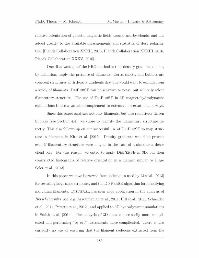
Ph.D. Thesis — M. Klassen McMaster - Physics & Astronomy
relative orientation of galactic magnetic fields around nearby clouds, and has
added greatly to the available measurements and statistics of dust polarisa-
tion [Planck Collaboration XXXII, 2016, Planck Collaboration XXXIII, 2016,
Planck Collaboration XXXV, 2016].
One disadvantage of the HRO method is that density gradients do not,
by definition, imply the presence of filaments. Cores, sheets, and bubbles are
coherent structures with density gradients that one would want to exclude from
a study of filaments. DisPerSE can be sensitive to noise, but will only select
filamentary structure. The use of DisPerSE in 3D magnetohydrodynamic
calculations is also a valuable complement to extensive observational surveys.
Since this paper analyzes not only filaments, but also radiatively driven
bubbles (see Section 4.4), we chose to identify the filamentary structure di-
rectly. This also follows up on our successful use of DisPerSE to map struc-
ture in filaments in Kirk et al. [2015]. Density gradients would be present
even if filamentary structure were not, as in the case of a sheet or a dense
cloud core. For this reason, we opted to apply DisPerSE in 3D, but then
constructed histograms of relative orientation in a manner similar to Diego
Soler et al. [2013].
In this paper we have borrowed from techniques used by Li et al. [2013]
for revealing large scale structure, and theDisPerSE algorithm for identifying
individual filaments. DisPerSE has seen wide application in the analysis of
Herschel results [see, e.g. Arzoumanian et al., 2011, Hill et al., 2011, Schneider
et al., 2011, Peretto et al., 2012], and applied to 3D hydrodynamic simulations
in Smith et al. [2014]. The analysis of 3D data is necessarily more compli-
cated and performing “by-eye” assessments more complicated. There is also
currently no way of ensuring that the filament skeletons extracted from the
183

Ph.D. Thesis — M. Klassen McMaster - Physics & Astronomy
simulation grid at discrete points in the time map to the same structures in
3D. These filaments are constantly moving, shifting, and evolving. They might
merge or dissipate or become disrupted by stellar feedback.
While the filament skeletons extracted by DisPerSE are sensitive to
the input parameters (lower persistence or noise thresholds tend to identify
more striations), these structures are real topoligical features in the volumet-
ric density maps. The properties of simulated filaments were compared to
observed filaments in our earlier study [Kirk et al., 2015] and found to be in
agreement.
flash uses an adaptive mesh composed of blocks containing 8× 8× 8
cells. The grid is refined as needed to resolve the gravitational collapse. flash
writes simulation plot files at specified intervals containing information about
the state of the simulation and the values of grid variables. These represent
global state of the simulation at a discrete point in time and are the primary
output that we analyze. We refer to plot files often throughout this text.
Hierarchical grid structure is preserved in these plot files using the
HDF5 file format. We used yt [Turk et al., 2011], a general-purpose data
analysis tool for computational astrophysics, to load the flash output data
and resample it to a uniform grid. Memory constraints meant that we mapped
the density information to a 256 × 256 × 256 uniform grid and wrote the
output to a FITS file, a format compatible with DisPerSE . The remapping
to a uniform grid results in the loss of some information at the highest gas
densities but preserves the large-scale structure throughout the simulation
volume. The remapping is necessary because DisPerSE does not currently
support hierarchical grid structures. At a 2563 sampling, the grid resolution
is 1611 AU (0.00781 pc) for our MHD500 simulation and 3134 AU (0.01519 pc)
184

Ph.D. Thesis — M. Klassen McMaster - Physics & Astronomy
for our MHD1200 simulation.
It is on these remapped FITS files that DisPerSE operates, first to
generate the Morse-Smale complex, then to extract the filament skeleton. The
Morse-Smale complex is computed by finding all the critical points (where
∇ρ(x, y, z) = 0). The maxima define a set of descending manifolds (the re-
gions where all integral lines traveling along the gradients share the same max-
imum), while the minima define a dual set of ascending manifolds (the integral
lines all share the same minimum). The intersection of these two manifolds
defines a new set that is called the Morse-Smale complex. The simulation
volume is partitioned into a natural tesselation of cells. The line segments
connecting maxima and passing through saddle points are a natural way to
define filaments. In cosmological studies, connecting dark matter haloes in the
way allows for mapping of the cosmic web [Sousbie et al., 2011]. In molecu-
lar clouds, we use it to trace filaments. For visualization and analysis, we can
use these filament skeletons together with the original un-resampled HDF out-
put files from FLASH to retrieve other variables of interest along their extent
(e.g. magnetic field information).
We apply this process to several plot files from each simulation. The
calculation of the Morse-Smale complex is particularly computationally in-
tensive. To handle this, we used Amazon’s Elastic Compute Cloud (EC2),
especially their c3.8xlarge-type compute-optimized instances which provide
32 virtual CPUs and 60 GiBs of attached memory on demand. DisPerSE
can then be run in parallel across these cores.
In order to avoid tracing filaments in the noise of the data, and in
order to select only the most prominent filaments, DisPerSE measures the
“persistence” of topological structures. Local maxima and minima form pairs
185

Ph.D. Thesis — M. Klassen McMaster - Physics & Astronomy
of critical points. The absolute difference in value between these two is the
persistence. A persistence cut removes pairs below a given threshold, but the
topology of structures consisting of high-persistence points remains. By se-
lecting the appropriate persistence threshold, we can avoid tracing filaments
within the noise. “Noise” in our simulations would actually be small-scale den-
sity perturbations resulting from the high-wavenumber part of the turbulent
power spectrum. These might appear as striations, lumps, or voids.
Another challenge when it comes to visualizing this data in 3D was
that filaments span a large dynamic range in density. Because we simulated
molecular cloud cores with a power-law density distribution, as are typically
observed, and superimposed a supersonic velocity field on top of this, 3D plots
of the filamentary structure require the selection of isosurfaces at particular
densities. A volume rendering approach using raytracing requires a particu-
lar transfer function designed to highlight gas at particular densities. When
the filament changes density along its length it can be difficult to plot the
morphology using standard techniques.
To give an observer’s picture, we take the output from these evolved
simulations and project the density along each of the coordinate axes to pro-
duce column density maps from different perspectives. We then project the
3D filamentary skeletons onto these column density maps. Often there is clear
alignment between the filament maps and the column density maps. Other
times, the filamentary structure found in 3D is not obviously visible in 2D
projection.
To produce a plane-of-sky magnetic field map, we perform a density-
weighted projection along the same coordinate axes. We project the compo-
nents of the magnetic field that lie perpendicular to the axis of projection.
186

Ph.D. Thesis — M. Klassen McMaster - Physics & Astronomy
This gives us, at every location in our map, the integrated local magnetic field
orientation. By weighting the magnetic field projection by density, we favour
contributions to the magnetic field orientations local to filaments in the line of
sight. Also, any observations of light polarization by dust would be weighted
by dust density, which traces the gas density.
To measure the orientation of the magnetic field relative to the filament,
we trace the filament skeletons and interpolate Bx, By, and Bz to find the
local magnetic field orientation at the filament spine. We then measure the
angle formed by the unit vectors of filament orientation and magnetic field
orientation.
An important measure of the dynamical importance of a filament seg-
ment is the mass-per-unit-length, sometimes called the dynamical mass or line
mass of a filament. An equilibrium analysis can be used to define a critical
value for stability, as was done in Ostriker [1964] who showed that for an
isothermal cylinder, the mass per unit length is
mcrit =2c2sG
=2kBT
µmHG, (4.5)
where cs is the sound speed, G is Newton’s constant, kB is Boltzmann’s con-
stant, T is the temperature, µ is the mean molecular weight, and mH is the
mass of the hydrogen atom [see also Inutsuka and Miyama, 1997, Fiege and
Pudritz, 2000]. More generally, the total velocity dispersion should be used,
since filaments are the products of supersonic motions and therefore may have
nonthermal support, i.e. mcrit = 2σ2/G [Fiege and Pudritz, 2000].
Line masses in excess of this critical value will undergo gravitational col-
lapse and fragmentation to form protostars, with the most massive stars likely
187

Ph.D. Thesis — M. Klassen McMaster - Physics & Astronomy
to be formed at the intersection of filaments [Schneider et al., 2012, Peretto
et al., 2013]. When using column density maps with traced filaments, one way
of estimating the local mass-per-unit-length along filaments is to multiply the
column density value by the characteristic filament width. Arzoumanian et al.
[2011] characterized the filaments in Herschel observations of IC 5146 as hav-
ing a median width of 0.10±0.03 pc. By estimating filament line masses in the
column density projections from our simulation data, and pairing it with fila-
ment maps and magnetic field information, we can investigate whether relative
orientation might be a function of the underlying line masses.
4.3 Filament and B-field alignments: early cloud
evolution
We simulated molecular cloud clumps of various initial masses with an ini-
tially spherically symmetric density profile, upon which a supersonic velocity
distribution was imposed. Supersonic turbulence gave the gas a filamentary
structure across many scales in density. In this section, we examine cloud and
magnetic field properties during the first 250 kyr of cloud evolution before
radiative feedback becomes important.
In Figure 4.1, we take a representative plotfile from the MHD1200 simula-
tion, after just over 250 kyr of evolution. We ranDisPerSE with a persistence
threshold of 10−17 g/cm3, which selects some of the major-trunk filaments
within the volume. Gas below a density of 10−22 g/cm3 is excluded from con-
sideration. The persistence threshold was adjusted manually until only major
filaments were being selected. Small-scale turbulence can cause DisPerSE to
188

Ph.D. Thesis — M. Klassen McMaster - Physics & Astronomy
Figure 4.1: 3D plot of gas density from the MHD1200 simulation at 250,000years of evolution. Green isosurfaces indicate gas at densities of n = 3.1× 10³
cm−3 (ρ = 1.1 × 10⁻²⁰ g/cm3). Red lines indicate filament skeleton selectedby DisPerSE . Black lines are magnetic field lines at 8 randomly selectedlocations within the volume.
189

Ph.D. Thesis — M. Klassen McMaster - Physics & Astronomy
identify many potentially spurious short-length filaments that we did not wish
to include in our analysis. A higher persistence threshold removes these from
consideration.
Figure 4.1 highlights in green the n = 3.1 × 103 cm−3 (ρ = 1.1 ×
10−20 g/cm3) isosurface. The box enclosing the rendering depicts the entire
simulation volume, with a side length of 3.89 pc.
Traced in red are the main filaments as DisPerSE identifies them,
satisfying the selection criteria described above. They align with some of the
obvious filamentary structure visible in the rendering.
To visualize what is happening with the magnetic field, we draw mag-
netic field lines that trace the orientation of the magnetic field from 8 ran-
domly sampled locations. Recall that the magnetic field is initially aligned
with the z-axis of the simulation volume. Over 250 kyr, the structure of the
magnetic field has evolved in response somewhat to the slow rigid body ro-
tation of the gas about the z-axis, but much more to the turbulent velocity
field. The Alfven Mach number quantifies the relative energies of the turbu-
lence and magnetic fields. Our simulated clouds have Alfven Mach numbers
of approximately unity, indicating an approximate equipartition in energies.
By contrast the energy in rotation is only a few percent of the gravitational
binding energy, which is greater even than the kinetic energy in the MHD1200
simulation. Figure 4.1 shows large deflections in the magnetic field from the
initial orientation.
While Figure 4.1 illustrates the structure of the magnetic field and fil-
aments, we use projections to confirm whether structures seen in projection
align with the filamentary structure that is traced in 3D. Studies of the fila-
mentary nature of molecular clouds rely on some proxy of the column density
190

Ph.D. Thesis — M. Klassen McMaster - Physics & Astronomy
0.0 0.5 1.0 1.5 2.0 2.5 3.0 3.5
0.0
0.5
1.0
1.5
2.0
2.5
3.0
3.5
X-Axis Projection
0.0 0.5 1.0 1.5 2.0 2.5 3.0 3.5
0.0
0.5
1.0
1.5
2.0
2.5
3.0
3.5
Y-Axis Projection
0.0 0.5 1.0 1.5 2.0 2.5 3.0 3.5
0.0
0.5
1.0
1.5
2.0
2.5
3.0
3.5
Z-Axis Projection
21.3
21.6
21.9
22.2
22.5
22.8
23.1
23.4
Log10N
H(c
m−2)
Figure 4.2: 2D column density maps along each of the coordinate axes withprojections of the filament skeleton overplotted. Data is same as in Figure 4.1
(dust emission or integrated line intensity over some range of velocities). Den-
sity is seen in projection and hence may be hiding important structure inside
the third dimension. Efforts to extract information about the 3D structure
of molecular gas often make use spectral velocity data, with examples from
simulations [e.g. Ward et al., 2012] and observations [Hacar and Tafalla, 2011,
Hacar et al., 2013]. In the latter case it was found that filaments often have
coherent velocity structures, with subsonic velocity dispersions, and marginal
stability. In Kirk et al. [2015] we also noted evidence of this kind of fine
structure in numerical simulations.
In Figure 4.2 we take the same data as in Figure 4.1, but in order to
verify that apparent structures in projection match the structures found by
DisPerSE in 3D we also project the filament skeleton into each of the three
coordinate axes and plot them side-by-side. Column densities range from
about 0.01 g/cm2 to about 1.0 g/cm2, while the mean initial column density
of the simulation was 0.02 g/cm2. The black lines in Figure 4.2 indicate the
projected filaments. We see that most of the major structures are captured
by this technique. This confirms that at least some of the observed major
structures in the column density plots are not just the result of projection ef-
191

Ph.D. Thesis — M. Klassen McMaster - Physics & Astronomy
Figure 4.3: B-field streamline evolution over the course of 325 kyr in ourMHD1200 simulation. The green density contour is as in Figure 4.1. Boxdepicts entire simulation volume with L = 3.89 pc on a side. Turbulence androtation largely account for the changes in local magnetic field orientation.
fects, but correspond to true filamentary structures in 3D. Smith et al. [2014]
also found correspondence when comparing 2D and 3D DisPerSE-mapped
filaments from simulations, except that filaments seen in column density pro-
jection did not belong to a single structure, but were made up of a network of
sub-filaments reminiscent of those observed by Hacar et al. [2013].
4.3.1 Large-scale magnetic field orientation
The initial condition for our simulations is a molecular cloud core embedded
in a uniform magnetic field. The field lines are initially oriented parallel to
the z-axis. In ideal MHD, the fluid is assumed to be perfectly conducting, and
so the magnetic field moves with the fluid. The ideal MHD limit is a good
192

Ph.D. Thesis — M. Klassen McMaster - Physics & Astronomy
approximation for the interstellar medium (ISM), with non-ideal effects such
as ambipolar diffusion or Ohmic dissipation only becoming relevant at the
scales of protostellar disks, and even in simulations of these they have often
been ignored.
Hence, in Figure 4.1, in which the magnetic field lines show significant
deformation, the structure of the magnetic field is the result of gas motions:
the initial solid body rotation of the molecular cloud clump, the turbulent
velocity field, and the slow gravitational collapse. These motions will drag
field lines.
We show the evolution of this field line dragging through the series of
panels in Figure 4.3 in which we have plotted the magnetic field lines at 6
different snapshots in time, with the density isocontour of ρ = 1.1 × 10⁻²⁰
g/cm3 (n = 3.1 × 103 cm−3) highlighted, as in Figure 4.1. The first panel
shows the state of the simulation at 8 kyr. The magnetic field lines are almost
perfectly parallel with the z-axis, which was the initial condition. In the
next panel, at 100 kyr, their state reflects some field line dragging due to the
turbulent velocity field and solid body rotation. The deformation becomes
more and more extreme from one panel to the next, with the last panel at 325
kyr reflecting very little of the original structure of the magnetic field.
Molecular clouds are observed to have large-scale velocity gradients
across them, which some have interpreted as rotation, although this is con-
tentious [Phillips, 1999]. We have initialized our simulations with an initial
solid body rotation of Ω = 1.114× 10⁻¹⁴ s−1, giving them an orbital timescale
of torbit = 2.8 Myr, which is longer than the freefall time of each simulation,
but on the same order of magnitude. It is also of the same order of magni-
tude as the turbulent crossing time (see Table 4.1). Nevertheless, the ratio
193

Ph.D. Thesis — M. Klassen McMaster - Physics & Astronomy
Figure 4.4: Left: Column density maps along the y-axis of our MHD1200 simu-lation at 250 kyr of evolution with density-weighted projected magnetic fieldorientation overplotted in red arrows. Middle: The autocorrelation of the pre-vious column density map, which highlight self-similar structure. Contourshighlight levels from 1% to 10% of peak correlation values. The diagonal barrepresents cloud orientation and is the best fit line through the pixels con-tained within the outermost contour, weighted by the base-10 logarithm ofthe autocorrelation values. Magnetic field lines based on the values measuredfor the left panel are overplotted. Right: The histogram of magnetic fieldorientations based on the values measured for the left panel, normalized sothat the total area is 1. The orientations are measured relative to “north”.The blue histogram shows the low-density gas, while red indicates only theorientations of high-density gas. The vertical grey lines indicate the angle ofthe best fit line to the large-scale structure (solid right line), and the angleoffset by 90 (dashed left line).
of rotational kinetic energy to gravitational energy, parameterized by βrot, is
still only about 1–3%. Turbulence and gravity are expected to have a much
greater influence over the dynamics and the geometry of the magnetic field.
Over time, strong turbulence will randomize the orientation of an initially co-
herent magnetic field. In highly super-Alfvenic clouds, turbulence dominates
the magnetic energy, the magnetic geometry is random [Falceta-Goncalves
et al., 2008].
194

Ph.D. Thesis — M. Klassen McMaster - Physics & Astronomy
Figure 4.5: The same as in Figure 4.4, except using MHD500 at 150 kyr ofevolution. Because of the higher average gas density, we draw contours inthe middle panel from 0.1% to 10% of peak correlation values. The best-fitline is still calculated based on the outermost contour. The data is taken atapproximately the same number of freefall times as in the MHD1200 simulation.
4.3.2 Magnetic fields in 2D
In Li et al. [2013], the authors took observations of molecular clouds in the
Gould Belt with physical sizes of a few to a few tens of pc. Many of these
clouds have large-scale elongated structure. The authors were interested in the
magnetic field orientation relative to orientation of the large-scale structure of
the cloud. Plotting these clouds in galactic coordinates (see their Figures 1
and 2), they then took the autocorrelation of the extinction maps. The auto-
correlation map is produced by taking a copy of the image and displacing it in
x and y coordinates, and at each such displacement calculating the sum of the
product of the overlapping pixels. The map of this highlights any self-similar
structure. Any elongated structures feature prominently in the autocorrela-
tion maps. Li et al. [2013] then contoured various levels in the autocorrelation
maps and took the best-fit linear regression to the pixel positions in the con-
tours, giving the long-axis orientation of the molecular cloud. The angle of this
could then be compared to the angles of magnetic field measurements derived
195

Ph.D. Thesis — M. Klassen McMaster - Physics & Astronomy
from polarimetry data.
Motivated by the Li et al. [2013] approach, we perform a similar anal-
ysis on our simulation data. In Figure 4.4 we show data from our MHD1200
simulation at 250 kyr of evolution, while in Figure 4.5 we show data from
our MHD500 simulation after 150 kyr of evolution. Although taken at different
times, the data are at the same number of freefall times in each simulation
(tff ≈ 0.14). The freefall time,
tff =
√
3π
32Gρ, (4.6)
is a natural measure of the gravitational timescale of the simulation. The first
panel from the left shows the map of projected mean density. This is very
similar to a column density projection, except that each sample in the integral
is itself weighted by density. We opted for this approach because it brings
dense structures into stronger relief and produces clearer autocorrelation maps.
We then overplot the magnetic field vectors in red. The magnetic field values
are density-weighted averages computed by integrating through the simulation
volume along the same projection axis. Unlike polarimetric observations, we
can measure the magnetic field everywhere.
The middle panel of Figure 4.4 shows the autocorrelation of the “col-
umn density” plot from the left panel after downsampling to a 200x200 pixel
greyscale image. The largest modes in the initial turbulent velocity field create
a main filament “trunk” that is home to some of the highest-density gas in
the simulation. In performing an autocorrelation of the column density map,
the large-scale structure is also the most similar, and features prominently in
the autocorrelation map. We contour several levels, from 1% (the outermost
196
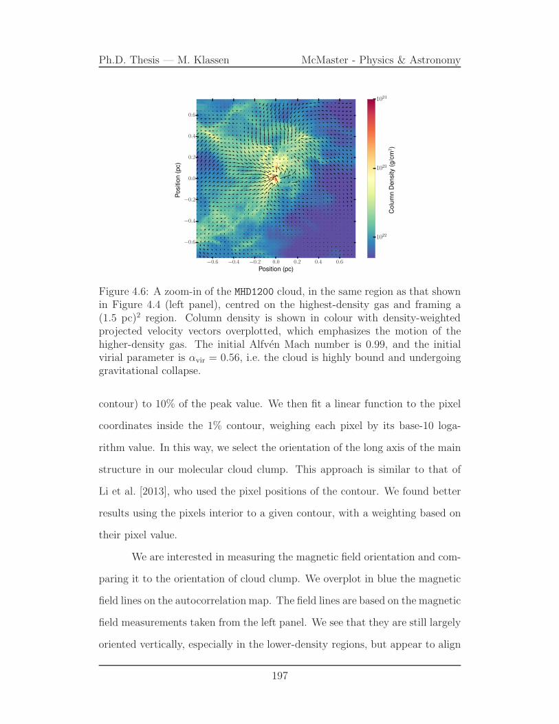
Ph.D. Thesis — M. Klassen McMaster - Physics & Astronomy
−0.6 −0.4 −0.2 0.0 0.2 0.4 0.6
Position (pc)
−0.6
−0.4
−0.2
0.0
0.2
0.4
0.6
Positio
n(p
c)
1022
1023
1024
Colu
mn
Density
(g/c
m2)
Figure 4.6: A zoom-in of the MHD1200 cloud, in the same region as that shownin Figure 4.4 (left panel), centred on the highest-density gas and framing a(1.5 pc)2 region. Column density is shown in colour with density-weightedprojected velocity vectors overplotted, which emphasizes the motion of thehigher-density gas. The initial Alfven Mach number is 0.99, and the initialvirial parameter is αvir = 0.56, i.e. the cloud is highly bound and undergoinggravitational collapse.
contour) to 10% of the peak value. We then fit a linear function to the pixel
coordinates inside the 1% contour, weighing each pixel by its base-10 loga-
rithm value. In this way, we select the orientation of the long axis of the main
structure in our molecular cloud clump. This approach is similar to that of
Li et al. [2013], who used the pixel positions of the contour. We found better
results using the pixels interior to a given contour, with a weighting based on
their pixel value.
We are interested in measuring the magnetic field orientation and com-
paring it to the orientation of cloud clump. We overplot in blue the magnetic
field lines on the autocorrelation map. The field lines are based on the magnetic
field measurements taken from the left panel. We see that they are still largely
oriented vertically, especially in the lower-density regions, but appear to align
197
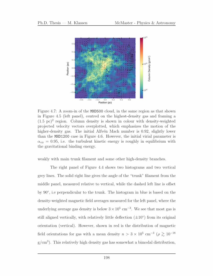
Ph.D. Thesis — M. Klassen McMaster - Physics & Astronomy
−0.6 −0.4 −0.2 0.0 0.2 0.4 0.6
Position (pc)
−0.6
−0.4
−0.2
0.0
0.2
0.4
0.6
Positio
n(p
c)
1022
1023
1024
Colu
mn
Density
(g/c
m2)
Figure 4.7: A zoom-in of the MHD500 cloud, in the same region as that shownin Figure 4.5 (left panel), centred on the highest-density gas and framing a(1.5 pc)2 region. Column density is shown in colour with density-weightedprojected velocity vectors overplotted, which emphasizes the motion of thehigher-density gas. The initial Alfven Mach number is 0.92, slightly lowerthan the MHD1200 case in Figure 4.6. However, the initial virial parameter isαvir = 0.95, i.e. the turbulent kinetic energy is roughly in equilibrium withthe gravitational binding energy.
weakly with main trunk filament and some other high-density branches.
The right panel of Figure 4.4 shows two histograms and two vertical
grey lines. The solid right line gives the angle of the “trunk” filament from the
middle panel, measured relative to vertical, while the dashed left line is offset
by 90, i.e perpendicular to the trunk. The histogram in blue is based on the
density-weighted magnetic field averages measured for the left panel, where the
underlying average gas density is below 3×105 cm−3. We see that most gas is
still aligned vertically, with relatively little deflection (±10) from its original
orientation (vertical). However, shown in red is the distribution of magnetic
field orientations for gas with a mean density n > 3 × 105 cm−3 (ρ & 10−18
g/cm3). This relatively high density gas has somewhat a bimodal distribution,
198

Ph.D. Thesis — M. Klassen McMaster - Physics & Astronomy
showing preferred alignment with the main filament trunk (the right peak
in the distribution). The smaller left peak in the distribution is towards a
perpendicular alignment with the filament (the left vertical grey line), but
not exactly perpendicular. Accretion flow onto the main trunk filament has
dragged magnetic field lines along with it such that they are deflected towards
the filament. This accretion flow is responsible for this second (left) peak in
the bimodal distribution.
We now compare this to Figure 4.5 (the virialized cloud simulation),
which applies the same analysis to the MHD500 simulation. The analysis is done
in the same way, except that for the autocorrelation map contours we plot
evenly-spaced levels between 0.1% and 10% of the peak value. The MHD500,
being the tighter, more compact cloud with a higher overal gas density relative
to the MHD1200 simulation, is actually less bound.
The measurements for Figure 4.5 are taken at the same number of
freefall times as compared to the MHD1200 simulation to allow for a fair com-
parison.
The higher overall gas densities in MHD500meant a more strongly peaked
central value in the autocorrelation map. For this reason, we contoured down
to 0.1% of the peak value in the middle panel of Figure 4.5 to trace more of
the overall structure.
The magnetic field orientations appear much more chaotic in Figure
4.5, despite the sound speed and RMS Mach number of the turbulence being
the same in both simulations. The initial Alfven Mach numbers are also virtu-
ally identical, suggesting that the magnetic field structure should be similarly
ordered or disordered. This is, however, not the case. The difference is entirely
on account of the relative boundedness of each cloud.
199

Ph.D. Thesis — M. Klassen McMaster - Physics & Astronomy
−0.5 0.0 0.5
Position (pc)
−0.5
0.0
0.5
Po
sitio
n(p
c)
Density
−0.5 0.0 0.5
Position (pc)
−0.5
0.0
0.5
Alfven Mach Number
2.0
2.4
2.8
3.2
3.6
4.0
4.4
4.8
5.2
5.6
6.0
log10n/(cm
−3)
−1.0
−0.8
−0.6
−0.4
−0.2
0.0
0.2
0.4
0.6
0.8
1.0
log10M
A
Figure 4.8: Left: Volume density slice through the molecular cloud of ourMHD1200 simulation after 250 kyr of evolution with arrows indicating the ve-locity field. The colours cover a range in volume densities from n = 100 cm−3
to n = 106 cm−3. Photoionization feedback from a cluster of stars (not shown)has begun forming an Hii region at the side of the main trunk filament. Right:Local Alfven Mach number with arrows indicating the magnetic field. Thecolours are scaled logarithmically from MA = 10−1 (blue) to MA = 101 (red).White regions have values for the Alfven Mach number of MA ≈ 1, indicat-ing that the turbulent energy is balancing the magnetic energy. Sub-Alfvenicregions (MA < 1) have stronger magnetic fields.
−0.4 −0.2 0.0 0.2 0.4
Position (pc)
−0.4
−0.2
0.0
0.2
0.4
Po
sitio
n(p
c)
Density
−0.4 −0.2 0.0 0.2 0.4
Position (pc)
−0.4
−0.2
0.0
0.2
0.4
Alfven Mach Number
2.0
2.4
2.8
3.2
3.6
4.0
4.4
4.8
5.2
5.6
6.0
log10n/(cm
−3)
−1.0
−0.8
−0.6
−0.4
−0.2
0.0
0.2
0.4
0.6
0.8
1.0
log10M
A
Figure 4.9: The same as in Figure 4.8, except for the MHD500 simulation. Asthe simulation volume is smaller, the panels have been made proportionallysmaller, while still centering on the densest part of the simulation. The snap-shot of the simulation is taken after 150 kyr of evolution, which is earlierthan in MHD1200, but at the same number of freefall times to permit bettercomparison.
200
Ph.D. Thesis — M. Klassen McMaster - Physics & Astronomy
The virialized cloud in MHD500 shows no strong preferred ordering of the
magnetic field in 2D, as is seen in the right panel of Figure 4.5. Figure 4.5 also
shows less obvious large-scale structure, as evinced by the autocorrelation map,
which appears much more square when compared to Figure 4.4. This is on
account of MHD500 being in virial equilibrium. MHD1200, being the more bound
cloud, has undergone strong gravitational collapse onto the central filamentary
structure, which appears very prominently in the autocorrelation map. The
gravitational collapse has dragged the magnetic field structure with it, which
accounts for the more regular structure seen in Figure 4.4 compared to Figure
4.5.
The lower-density gas (n ≤ 3 × 105 cm−3) forms an approximately
Gaussian distribution in angle relative to “North”, centered at 0. This dis-
tribution is shown in blue in the right panel of Figure 4.5. The higher-density
gas (n ≤ 3 × 105 cm−3), shown in red, is spread over many angles, but, if
anything, tends to be oriented more perpendicular to the main trunk filament,
an angle indicated by the left vertical gray line.
Comparing our simulations, we note this pattern: similar to Diego Soler
et al. [2013], Planck Collaboration XXXV [2016], the low-density case tends
towards parallel orientation and the high-density case towards perpendicular
orientation, but in our case we are comparing gas at similar densities from two
different simulations with different average densities.
In Figure 4.6 we show the column density projection of the same region
as in the left panel of Figure 4.4 of the MHD1200 simulation. We then overplot
the density-weighted average velocity vectors to show the average flows onto
the main filament. We see a pattern of flow both along the long axis of the
main trunk filament and accretion onto the filament radially. The flow appears
201

Ph.D. Thesis — M. Klassen McMaster - Physics & Astronomy
to converge onto the central, densest region. Compare this to Figure 4.7, which
is the equivalent but for the MHD500 simulation, displaying the same region as
in the left panel of Figure 4.5. The density-weighted average velocity shows
a pattern of randomly-oriented flows. The difference, again, can be entirely
attributed to the degree of boundedness in each case, with MHD1200 undergoing
strong gravitational collapse and MHD500 exhibiting a relative balance of kinetic
and gravitational energies.
To examine the relationship between magnetic field ordering and the
Alfven Mach number more closely, we plot volume density slices through the
center of our simulations showing the gas structure and compare these to slices
of the local Alfven Mach number. We also compare the velocity and magnetic
field structure. We show these in Figures 4.8 and 4.9 for the MHD1200 (strongly
bound) and MHD500 (virialized) models, respectively.
These two figures were taken at the same number of freefall times,
tff ≈ 0.14, which corresponds to about 250 kyr in the MHD1200 simulation and
150 kyr in the MHD500 simulation. In Figure 4.8, we see that the velocity
field is channeling mass both onto the main trunk filament and along it. This
resembles the mass flows measured for the cluster-forming region in the Serpens
South molecular cloud studied in Kirk et al. [2013]. Material appears to be
flowing along the long axis of our main trunk filament, feeding a tight cluster
of stars that is driving the Hii region already visible in the left panel of Figure
4.8. There is also material flowing onto the main filament radially, and this
radial accretion appears stronger than the flows along the filament’s long axis,
as it was in Kirk et al. [2013]. The right panel of Figure 4.8 shows the local
Alfven Mach number. More sub-Alfvenic regions possess stronger magnetic
fields and slower accretion flows. The magnetic field is depicted with arrows
202

Ph.D. Thesis — M. Klassen McMaster - Physics & Astronomy
in the right panel, showing how the magnetic field has been concentrated into
the main trunk filament so that it lies parallel with the filament long axis.
In Figure 4.9 we see the result of trans-Alfvenic turbulence in virial
balance with the gravitational forces in the MHD500 simulation. Recall that
both simulations were initialized with the same turbulent velocity field, similar
mass-to-flux ratios, and the same radial density profile. The MHD500 simulation
is actually at higher average density—a more compact setup. However, after
150 kyr of evolution, the magnetic field has become disordered and the local
Alfven Mach number is a patchwork of ripples, alternating islands of sub-
and super-Alfvenic regions, encircled with magnetic fields that do not possess
very much coherent large-scale structure. There is some similarity with the
MHD1200 simulation, however: the field is generally aligned within the main
filament, lying parallel to the long axis.
The consensus so far is that turbulence plays a major role in trans-
Alfvenic molecular clouds. In the trans-Alfvenic regime, neither turbulence
nor magnetic fields have the clear upper hand. Unlike the sub-Alfvenic regime,
which dominates in the diffuse ISM and where magnetic fields clearly channel
flows, filaments are more the result of turbulence and not of slow accretion
flow along dominant field lines. The large-scale turbulent modes give rise to
the primary filaments—the trunk—via shock compression, and magnetic field
lines are dragged along with the gas, pushed together so that they lie together
within the main filaments, parallel to their axes. In super-Alfvenic clouds,
magnetic fields are not dynamically important. Falceta-Goncalves et al. [2008]
explored cases of numerical simulations with Alfven Mach numbers of 0.7 and
2.0, but did not explore the space around MA = 1, a dynamically interesting
transition region.
203

Ph.D. Thesis — M. Klassen McMaster - Physics & Astronomy
Figure 4.10: Left: Density projection along the y-axis of our MHD1200 simu-lation at 250 kyr of evolution with density-weighted projected velocity fieldoverplotted in red arrows. Middle: The autocorrelation of the previous col-umn density project, which highlight self-similar structure. Contours highlightlevels from 1% to 10% of peak correlation values. The shaded diagonal barrepresents cloud orientation as previously calculated for Figure 4.4. Velocitystreamlines based on the values measured for the left panel are overplotted.Right: The histogram of the velocity field orientations based on the valuesmeasured for the left panel, normalized so that the total area is 1. The ori-entations are measured relative to “north”. The blue histogram shows thelow-density gas distribution, while red indicates only the orientations of high-density gas. The vertical grey lines indicate the angle of the best fit line tothe large-scale structure (solid right line), and the angle offset by 90 (dashedleft line).
In our case, wherein turbulence and magnetic forces are nearly in bal-
ance, we show that the discriminating factor is likely whether gravity dom-
inates over the other energies. The MHD1200 simulation was substantially
sub-virial (αvir = 0.56), whereas magnetic fields were chaotic in the virially-
balanced case of MHD500.
4.3.3 Velocity fields in 2D
In Figures 4.10 and 4.11, we show the large-scale velocity patterns in projection
for the MHD1200 and MHD500 simulations, respectively. In each of these figures,
204

Ph.D. Thesis — M. Klassen McMaster - Physics & Astronomy
Figure 4.11: The same as in Figure 4.10, except using MHD500 at 150 kyr ofevolution. Because of the higher average gas density, we draw contours inthe middle panel from 0.1% to 10% of peak correlation values. The best-fitline is still calculated based on the outermost contour. The data is taken atapproximately the same number of freefall times as in the MHD1200 simulation.
the left panel shows the mean projected gas density in blue. Overplotted are
velocity vectors computed by taking the density-averaged mean velocity along
the line of sight. The white contour is the threshold density used in the right
panel to separate “low” and “high” density gas.
The middle panels compute the autocorrelation of the mean gas density,
just as we had done previously for Figures 4.4 and 4.5. The only difference
in this case is that the overplotted streamlines reflect the velocity structure
instead of the magnetic field structure.
Finally, the right panels in Figures 4.10 and 4.11 show the histograms
of the velocity field orientation angles, relative to “north” (the z-axis), based
on the angles in every pixel of the left panel. The data is divided into “low-
density” and “high-density” pixels, based on the mean gas density along the
line of sight, with ρ = 10−18 g/cm3 (n = 2.8×105 cm−3) as the threshold. The
high-density regions are contoured in the left panel of each figure, and show a
dense core region in each case.
205

Ph.D. Thesis — M. Klassen McMaster - Physics & Astronomy
The velocity angle histogram in Figure 4.10 shows a bimodal distribu-
tion for the low-density gas in blue for the MHD1200 simulation. These do not
perfectly align with the parallel and perpendicular main trunk filament angles
(the right and left vertical grey lines, respectively), but do follow a general
pattern: most of the low-density gas is flowing onto main trunk filament at
an angle roughly perpendicular to it, with a smaller fraction of the gas also
flowing along the main filament.
The high-density core region shows a high degree of flow along the main
filament with another significant portion coming in laterally. This is shown by
the red histogram.
In the MHD500 simulation, the histogram of gas velocities shows a differ-
ent picture. The low-density gas is randomly oriented. There are no preferred
accretion channels and gas appears to flow in all directions. This is in strong
contrast to the high-density gas of the inner core region (shown in red), which
shows extremely strong flow along the main trunk filament, and roughly per-
pendicular to it. This region is likely undergoing gravitational collapse and
the main filament appears to set up accretion pathways, either along and per-
pendicular to it, to supply this central region with gas.
4.3.4 Magnetic field orientation relative to filaments in
3D
What is happening to the relative orientation of the filaments and the magnetic
field lines at the level local to the filaments? Using the filamentary structure
extracted from the 3D data cubes by DisPerSE , we analyze the filament
spines by visiting the vertices and locally measuring the tangent vector, the
206

Ph.D. Thesis — M. Klassen McMaster - Physics & Astronomy
magnetic field vector, and other physical variables such as the mass density.
This procedure allows us to construct histograms of the relative orientation of
the magnetic field and the filament orientation.
We take the relative angle θ of the filament tangent vector and mag-
netic field vector. Some authors measure cos θ or cos(2θ), but trigonometric
projection can cause histograms to suggest a strong trend toward cos θ = ±1.
(Imagine a unit circle evenly sampled in the angular dimension. A histogram
of the cosine of these angles will collect more samples in the bins nearest
cos θ = ±1 unless the bin width is carefully modified as a function of θ.) To
avoid these problems, we produce histograms in relative angle only.
We are also careful to compare to the case of random orientation. Be-
cause of the two angular degrees of freedom in three-dimensional space, a
histogram of relative orientation will have a higher proportion of vectors with
angles closer to perpendicular than parallel. Any true tendency in nature to-
wards a parallel or perpendicular orientation of filaments relative to magnetic
fields should therefore be measured relative to the case of random alignment.
For our MHD1200 simulation, for the series of time points under consider-
ation, which were selected to be spaced roughly evenly throughout the simula-
tion, we partition the data into three density groups: “low” (n/cm−3 < 5000),
“medium” (5000 < n/cm−3 < 50000), and “high” (n/cm−3 > 50000). These
are the first three columns shown in Figure 4.12. The final column gives the
histogram for all data, making no density cuts. In this figure, the rows rep-
resent the time evolution of these histograms of relative 3D orientation. The
times at which these histograms were taken are indicated the top-left corner
of the first panel in each row.
In each panel, two histograms are shown. In blue is the distribution
207

Ph.D. Thesis — M. Klassen McMaster - Physics & Astronomy
0 15 30 45 60 75 900.000
0.005
0.010
0.015
0.020
0.025
0.030
0.035
0.040100 kyr
n < 5000
0 15 30 45 60 75 90
5000 < n < 50000
0 15 30 45 60 75 90
n > 50000
0 15 30 45 60 75 90
All
Actual
Random
0 15 30 45 60 75 900.000
0.005
0.010
0.015
0.020
0.025
0.030
0.035
0.040175 kyr
0 15 30 45 60 75 90 0 15 30 45 60 75 90 0 15 30 45 60 75 90
0 15 30 45 60 75 900.000
0.005
0.010
0.015
0.020
0.025
0.030250 kyr
0 15 30 45 60 75 90 0 15 30 45 60 75 90 0 15 30 45 60 75 90
0 15 30 45 60 75 900.000
0.005
0.010
0.015
0.020
0.025
0.030325 kyr
0 15 30 45 60 75 90 0 15 30 45 60 75 90 0 15 30 45 60 75 90
Relative Angle (deg)
Figure 4.12: Sequence of histograms from the MHD1200 simulation. The areaunder each curve has been normalized to 1. By tracing along the filamentsin 3D through the simulated volume, we produce histograms of the relativeorientation of the magnetic field and the filament. In each panel, we comparethe relative orientation measured in the data (blue) with the histogram thatwould have resulted if the magnetic field had been randomly oriented (red).In addition to a standard step-shaped histogram, a kernel density estimate(KDE), with a Gaussian kernel, has been run over the data and is shownvia the smooth curves, providing a continuous analog to the discretely-binnedhistogram data. Shaded areas indicate either an exceess relative to random(blue) or a deficit (red). Each row of panels gives the state of the simulationat the indicated time. Columns restrict the relative orientation data to theindicated density regims, as measured locally along the filament spine. Thelast column applies no density selection.
208

Ph.D. Thesis — M. Klassen McMaster - Physics & Astronomy
of relative angles presented by our data—the “Actual” case. We compare
the measured relative angles to the case of random orientation, shown in red
and labeled “Random”. In this case, the local magnetic field is assigned a
random orientation in 3D space and the relative orientation to the filament
is measured. The sample size for the “Random” case therefore matches the
“Actual” case.
In addition to performing the standard step-shaped histogram with 12
bins over 90 of angle, we apply a kernel density estimate (KDE) using Gaus-
sian kernels. KDEs are a continuous analog to the traditional histogram with
its discrete number of bins. Figures 4.12 and 4.13 show both representations.
Additionally, we shade any “excess” (blue) or “deficit” (red) relative to the
“Random”.
In studying Figure 4.12, the MHD1200 simulation, a few trends appear.
Although containing more mass overall, the volume of the MHD1200 is also
much larger, causing the mean gas density in the MHD1200 simulation to be
about one third the value in the MHD500 simulation. We see that in the “All”-
density column there is a deficit in the distribution of relative angles around
90. This pattern shows up in many of the panels where the data has been
further segmented based on underlying mass density.
In the low-density column, where we measure relative angles at fila-
ments segments situated in gas at densities n < 5000 cm−3, there is neither
a trend towards parallel nor perpendicular orientation. Instead, there is an
excess relative to random at angles between 30 and 75. This low-density
regime represents the outer regions of our simulation volume. The magnetic
fields lines, initially coherent and oriented parallel to the z-axis, have been
dragged inward during the molecular cloud clump’s gravitational collapse. In
209
Ph.D. Thesis — M. Klassen McMaster - Physics & Astronomy
the outer regions of the simulation volume, this inward dragging may account
for the observed excess at “middle” angles.
At relatively early times, after 100 kyr of evolution (first row of Figure
4.12), most of the gas is still at low density. It has not had time to collapse
to higher density, i.e. into the main trunk filament. In the low-density gas
histogram, the peak is measured around 45 relative orientation between fila-
ments and B-field. This may be on account of the main filament trunk having
this approximately this orientation, which may just be starting to form as a
result of the largest turbulent modes. At this time, there is very little gas with
densities above 5000 cm−3.
As the simulation progresses, we observe increased power at near-
parallel orientations. See, especially, the “intermediate” and “high”-density
panels at 250 kyr of evolution, with corresponding deficits at near-perpendicular
orientations. An interesting thing happens between 250 kyr and 325 kyr. Be-
tween these times, star formation has occurred in this simulation, and radiative
feedback has injected energy into the molecular cloud clump. The measured
relative orientations between the magnetic field and the filamentary structure
in 3D is much closer to random than in any of the other panels. We attribute
this to the energy injected through radiative feedback from high-mass stars,
an effect we discuss further in section 4.4. Radiative feedback is already un-
derway by 250 kyr, but by 325 kyr has largely disrupted the main filament
trunk. The radiative feedback is in the form of ionizing radiation from a tight
cluster of massive stars that lead to the formation of an expanding Hii region.
At 175 and 250 kyr, we see a feature indicating alignment of the fila-
mentary structure and the magnetic field. It is seen in the medium and high
density panels, and also appears more modestly in the “all data” panel on
210
Ph.D. Thesis — M. Klassen McMaster - Physics & Astronomy
the right. As the simulation progress, this feature is apparently washed out,
because the alignment isn’t seen in the last row. Again, this is on account of
radiative feedback from star formation.
It is important to note that DisPerSE was run on each simulation
plotfile separately, and the filamentary structure extracted from each will be
different. The persistence and noise thresholds were held the same for the sake
of consistently, but the simulation evolves over time and central regions become
denser due to gravitational infall. Therefore the skeletons that DisPerSE
extracts from the set of plot files, though they come from the same simulation,
may not necessarily strongly resemble each other. This is in contrast to what
was done in Kirk et al. [2015], wherein the filament skeletons were found in
2D column density projections and the skeletons kept consistent between time
slices using by-hand adjustments as necessary. Owing to the considerably
higher complexity of doing this with 3D skeletons and having sparser time
sampling, we did not attempt to map out the exact same filaments at each
time slice.
Nevertheless, the filament skeletons extracted from one column density
projection to the next were largely similar, and Kirk et al. [2015] demon-
strated that the properties of our flash-simulated filaments matched those of
filaments observed in nature.
In Figure 4.13 we show the same analysis performed on our MHD500
simulation. MHD1200 and MHD500 both have the same angular rotation rate,
similar ratios of rotational kinetic energy to gravitational energy, the same
initial temperature and RMS Mach number turbulence. We initialized both
from the same turbulent velocity field, hence they would have developed similar
initial structure. The difference is that MHD500 is tighter and more compact,
211

Ph.D. Thesis — M. Klassen McMaster - Physics & Astronomy
0 15 30 45 60 75 900.000
0.005
0.010
0.015
0.020
0.025
0.030
0.035
0.04075.6 kyr
n < 5000
0 15 30 45 60 75 90
5000 < n < 50000
0 15 30 45 60 75 90
n < 50000
0 15 30 45 60 75 90
All
Actual
Random
0 15 30 45 60 75 900.000
0.005
0.010
0.015
0.020
0.025
0.030
0.035
0.040100 kyr
0 15 30 45 60 75 90 0 15 30 45 60 75 90 0 15 30 45 60 75 90
0 15 30 45 60 75 900.000
0.005
0.010
0.015
0.020
0.025
0.030125 kyr
0 15 30 45 60 75 90 0 15 30 45 60 75 90 0 15 30 45 60 75 90
0 15 30 45 60 75 900.000
0.005
0.010
0.015
0.020
0.025
0.030150 kyr
0 15 30 45 60 75 90 0 15 30 45 60 75 90 0 15 30 45 60 75 90
Relative Angle (deg)
Figure 4.13: The same as in Figure 4.12, except for our MHD500 simulation.
212
Ph.D. Thesis — M. Klassen McMaster - Physics & Astronomy
with a higher average gas density (n500 ≈ 1200 vs n1200 ≈ 390 cm−3).
At early times it is difficult to discern any pattern in the relative ori-
entations. Most of the gas has not yet collapsed to very high density, and the
orientations appear relatively close to random distributed.
This changes as the simulation evolves. In the panels at 100 kyr and 125
kyr, the data shows a tendency towards a perpendicular relative orientation.
This is visible even in the low-density panels where n < 5000 cm−3. At late
times (150 kyr, final row), however, this trend is less clear. The high-density
(n > 50000 cm−3) at 150 kyr appears either to have reversed the trend, or
else the orientations have simply become closer to random. In Figure 4.14, we
showed how at 150 kyr the MHD500 simulation becomes magnetically critical,
meaning that the magnetic flux is sufficient to support against further gravita-
tional collapse. We also showed how the virial parameter, which measures the
ratio of kinetic to graviational energy increases sharply toward 150 kyr. We
interpret this as gravitational energy being converted to kinetic energy during
gravitational collapse, in particular as the cloud clump becomes magnetically
critical.
Whereas in the MHD1200 simulation we saw kinetic energy being injected
in the form of radiative feedback from massive stars, in the MHD500 simulation,
in which we did not simulate star formation, gravitational energy is converted
to kinetic energy, with similar results: the relative orientation of the magnetic
field to the filamentary structure becomes closer to random with the injection
of kinetic energy.
213
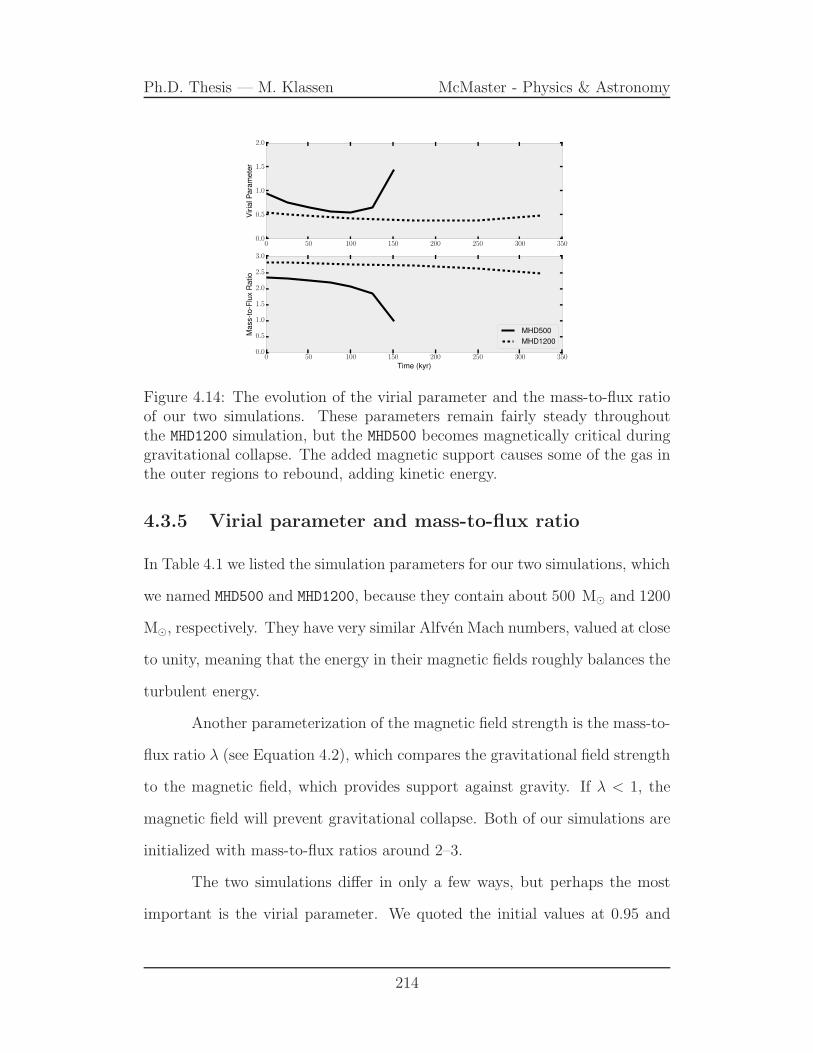
Ph.D. Thesis — M. Klassen McMaster - Physics & Astronomy
0 50 100 150 200 250 300 3500.0
0.5
1.0
1.5
2.0
Vir
ialP
ara
mete
r
0 50 100 150 200 250 300 350Time (kyr)
0.0
0.5
1.0
1.5
2.0
2.5
3.0M
ass-t
o-F
lux
Ratio
MHD500
MHD1200
Figure 4.14: The evolution of the virial parameter and the mass-to-flux ratioof our two simulations. These parameters remain fairly steady throughoutthe MHD1200 simulation, but the MHD500 becomes magnetically critical duringgravitational collapse. The added magnetic support causes some of the gas inthe outer regions to rebound, adding kinetic energy.
4.3.5 Virial parameter and mass-to-flux ratio
In Table 4.1 we listed the simulation parameters for our two simulations, which
we named MHD500 and MHD1200, because they contain about 500 M⊙ and 1200
M⊙, respectively. They have very similar Alfven Mach numbers, valued at close
to unity, meaning that the energy in their magnetic fields roughly balances the
turbulent energy.
Another parameterization of the magnetic field strength is the mass-to-
flux ratio λ (see Equation 4.2), which compares the gravitational field strength
to the magnetic field, which provides support against gravity. If λ < 1, the
magnetic field will prevent gravitational collapse. Both of our simulations are
initialized with mass-to-flux ratios around 2–3.
The two simulations differ in only a few ways, but perhaps the most
important is the virial parameter. We quoted the initial values at 0.95 and
214

Ph.D. Thesis — M. Klassen McMaster - Physics & Astronomy
0.56 for the MHD500 and MHD1200, respectively. The virial parameter gives the
ratio of kinetic energy to gravitational energy (see Equation 4.3).
We plot the evolution of both the virial parameter and the mass-to-flux
ratio in Figure 4.14. The MHD1200 simulation begins substantially sub-virial,
meaning that as an unmagnetized cloud clump, it would be highly bound and
undergo gravitational collapse. Since its mass-to-flux ratio is also supercritical,
it does indeed undergo gravitational collapse.
The value of the virial parameter remains relatively level throughout
the simulation, decreasing slightly over time as the cloud collapses, but then
beginning to increase against around 250 kyr, the time at which massive star
formation has resulted in kinetic energy being injected into the simulation via
radiative feedback. The mass-to-flux ratio decreases monotonically throughout
the simulation as a result of magnetic field lines being dragged slowly inward,
following the gravitational collapse.
The MHD500 simulation behaves rather differently. The simulation evolves
quickly, and the virial parameter goes from marginally bound (0.95) to 0.55
after 100 kyr, following which it increases dramatically to 1.43 after 150 kyr.
This trend is attributable to what is happening with the mass-to-flux ratio.
The simulation begins slightly more magnetized than the MHD1200 simulation.
Magnetic field lines are dragged inward following the gravitational collapse of
the gas (which is, on average, 3 times denser than that of the MHD1200 sim-
ulation). The MHD500 simulation becomes magnetically critical after 150 kyr,
meaning that magnetic support is able to prevent further collapse. Gravita-
tional energy gets converted to kinetic energy as the collapse is halted. This
increase in kinetic energy is reflected in the virial parameter.
215

Ph.D. Thesis — M. Klassen McMaster - Physics & Astronomy
4.4 Star formation and the effect of radiative
feedback
How does radiative feedback from a forming massive star (which we find in
the MHD1200 simulation) affect the filamentary structure of the cloud? In
particular, can it destroy or alter the filamentary accretion flow so as to shut
down accretion onto the massive star?
To answer these questions, we ran our MHD1200 simulation including ra-
diative feedback from star formation. We use a characteristics-based raytracer
coupled to a simplified version of the DORIC radiative cooling, heating, and
ionization package [Frank and Mellema, 1994, Mellema and Lundqvist, 2002,
Rijkhorst et al., 2006b] implemented in FLASH for the study of star formation
and Hii regions [Peters et al., 2010b].
The MHD1200 forms a cluster of massive stars near the center of the
simulation volume, directly within the main trunk filament. Schneider et al.
[2012], Peretto et al. [2013] observe that the intersections of filaments are the
sites of clustered and massive star formation. The main trunk filament in our
simulation shows various smaller branches connecting with it. The cluster of
massive protostars that forms in our simulation eventually becomes luminous
enough to begin ionizing the gas around it and form a Hii region with the
appearance of a blister on the side of main trunk filament, similar to the
Cocoon nebula in IC 5416 [Arzoumanian et al., 2011], although the Cocoon
nebula is an Hii region powered by only a single B star.
The formation of the Hii region ultimately begins to disrupt and de-
stroy the main filament, creating an expanding cavity of hot (104 K) gas and
injecting a lot of kinetic energy. The Hii region, driven mainly by a single
216

Ph.D. Thesis — M. Klassen McMaster - Physics & Astronomy
0 50 100 150 200 250 300
Time (kyrs)
0
2
4
6
8
10
12
14
16
Mass
(M⊙
)
Figure 4.15: The evolution of the sink particles formed in the MHD1200 simu-lation. 7 particles are formed near the center of the simulation volume insidethe main trunk filament and make up a tight cluster. These accrete mass, thelargest of which reaches nearly 16 M⊙.
massive star that grows to 16M⊙, comes to envelope the entire star cluster
and shuts off accretion onto every star.
Figure 4.15 shows the mass evolution of the stars formed in the MHD1200
simulation. A total of 7 stars are formed, although only one of them becomes
a massive star, achieving about 16 M⊙. Of the others, one reaches 3M⊙, while
the others remain below 2M⊙. The luminosity of the massive star dominates
all the others, achieving a total luminosity of Ltot = 22942L⊙. This star
powers the formation of the Hii region. The 10,000 K gas within this region
supplies the thermal pressure needed to drive the outward expansion of the
bubble and form the blister that eventually begins to disrupt the main filament.
A star with a mass of 16 M⊙, in a cluster of 7 stars with a total mass of 26.16
M⊙ is at the high end—but still observed—range for embedded star clusters
[Weidner et al., 2010].
We take a closer look at the evolution of the most massive star in Figure
217

Ph.D. Thesis — M. Klassen McMaster - Physics & Astronomy
0 50 100 150 200 250 300 3500
2
4
6
8
10
12
14
16
18
Mass
(M⊙
)
0 50 100 150 200 250 300 35010−9
10−8
10−7
10−6
10−5
10−4
10−3
Accre
tion
Rate
(M⊙
/yr)
0 50 100 150 200 250 300 350
Time (kyr)
0
5000
10000
15000
20000
25000
30000
35000
Surf
ace
Tem
pera
ture
(K)
0 50 100 150 200 250 300 350
Time (kyr)
10−1
100
101
102
103
104
105
Lum
inosity
(L⊙
)
Lint
Lacc
Figure 4.16: Evolution of the most massive star formed as part of the MHD1200simulation, which reaches a maximum mass of 16 M⊙. The top-left panelshows the history of the mass of the sink particle representing this star. Thetop-right panel shows the evolution of the accretion rate in units of M⊙/yr.The bottom-left panel is the history of the effective (surface) temperature,as computed by our protostellar model. The bottom-right panel shows theintrinsic luminosity and the accretion luminosity of the star.
4.16, which plots the evolution of several of its properties. The top-left panel
shows the mass evolution as in Figure 4.15, but only for the most massive star.
After about 250 kyr of evolution, the mass of the star begins to plateau as it
envelopes itself in the Hii region of its own making. Less gas reaches the star
and its accretion is shut off. We see this play out in the top-right panel of
the figure, which shows the accretion rate reaching a maximum of around 1–2
×10−4 M⊙/yr, but then beginning to drop off. After 275 kyr, the accretion
rate has shut off completely and the star ceases to grow. In this panel, we
218

Ph.D. Thesis — M. Klassen McMaster - Physics & Astronomy
have applied a small amount of smoothing via a moving average filter.
In the bottom-left panel of Figure 4.16 we plot the evolution of the
effective (surface) temperature of the star. This is computed via a protostellar
evolution model that we first implemented in flash in Klassen et al. [2012b]
and used in the study of Hii region variability in Klassen et al. [2012a]. In
particular, the notch seen in the surface temperature near 150 kyr is due to
a change in protostellar structure as the star’s radius swells and the surface
cools temporarily. From 150 to 225 kyr, the surface temperature increases
dramatically, which results in a high flux of ionizing photons. The Hii region
starts to form during this time as the massive star begins to ionize the gas in
its vicinity.
The bottom-right panel of Figure 4.16 shows the evolution of star’s
intrinsic luminosity (from nuclear burning or Kelvin-Helmholtz contraction
during the earliest phases) and the accretion luminosity. Initially, accretion
is the dominant luminosity, but is overtaken by the star’s intrinsic luminosity
after about 125 kyr of evolution, when the star is between 4 and 6 M⊙. We
see that the accretion luminosity shuts off completely around 275 kyr.
We repeat the column density autocorrelation analysis in Figure 4.17,
this time for the terminal plotfile at 325 kyr of evolution. We zoom in on the
inner (1.2 pc)2 of the simulation. The effects of the forming Hii region are
seen in the column density plot as a blister on the side of the main filament.
Photoionizing feedback injects a large amount of kinetic energy—the gas inside
the Hii region is 104 K. The orientation of the magnetic field vectors for the
high-density gas (n > 2.8 × 105 cm−3) is almost random, being spread out
fairly evenly across all angles.
The consequences for the magnetic field in a slice through the centre of
219

Ph.D. Thesis — M. Klassen McMaster - Physics & Astronomy
Figure 4.17: The same as in Figure 4.4, except for the final state of the MHD1200simulation at 325 kyr of evolution. Photoionization feedback from a massivestar of ∼ 16M⊙ has created an expanding Hii region.
−0.4 −0.2 0.0 0.2 0.4
Position (pc)
−0.4
−0.2
0.0
0.2
0.4
Positio
n(p
c)
250 kyr
−0.4 −0.2 0.0 0.2 0.4
Position (pc)
−0.4
−0.2
0.0
0.2
0.4
325 kyr
2.0
2.4
2.8
3.2
3.6
4.0
4.4
4.8
5.2
5.6
6.0
Log10
Density
(cm
−3)
Figure 4.18: Volume density slices through the center of the MHD1200 simula-tion volume showing an expanding Hii region as a result of ionizing feedbackfrom the cluster of stars. A single massive star of nearly 16 M⊙ dominatesall the others and has a luminosity of nearly 23,000 L⊙. This drives a bubbleof hot (10,000 K) ionized gas, forming a blister on the side of the main trunkfilament. The left panel shows the state of this bubble after 250 kyr of evolu-tion, while the right panel shows the state of the bubble after 325 kyr, nearthe very end of the simulation. Overplotted on each are magnetic field vectorsbased on the magnetic field orientation in the plane of the slice.
220
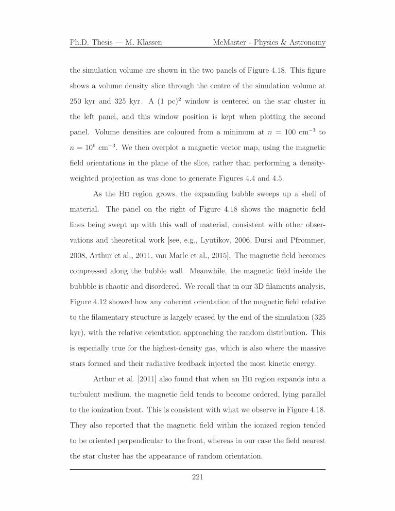
Ph.D. Thesis — M. Klassen McMaster - Physics & Astronomy
the simulation volume are shown in the two panels of Figure 4.18. This figure
shows a volume density slice through the centre of the simulation volume at
250 kyr and 325 kyr. A (1 pc)2 window is centered on the star cluster in
the left panel, and this window position is kept when plotting the second
panel. Volume densities are coloured from a minimum at n = 100 cm−3 to
n = 106 cm−3. We then overplot a magnetic vector map, using the magnetic
field orientations in the plane of the slice, rather than performing a density-
weighted projection as was done to generate Figures 4.4 and 4.5.
As the Hii region grows, the expanding bubble sweeps up a shell of
material. The panel on the right of Figure 4.18 shows the magnetic field
lines being swept up with this wall of material, consistent with other obser-
vations and theoretical work [see, e.g., Lyutikov, 2006, Dursi and Pfrommer,
2008, Arthur et al., 2011, van Marle et al., 2015]. The magnetic field becomes
compressed along the bubble wall. Meanwhile, the magnetic field inside the
bubbble is chaotic and disordered. We recall that in our 3D filaments analysis,
Figure 4.12 showed how any coherent orientation of the magnetic field relative
to the filamentary structure is largely erased by the end of the simulation (325
kyr), with the relative orientation approaching the random distribution. This
is especially true for the highest-density gas, which is also where the massive
stars formed and their radiative feedback injected the most kinetic energy.
Arthur et al. [2011] also found that when an Hii region expands into a
turbulent medium, the magnetic field tends to become ordered, lying parallel
to the ionization front. This is consistent with what we observe in Figure 4.18.
They also reported that the magnetic field within the ionized region tended
to be oriented perpendicular to the front, whereas in our case the field nearest
the star cluster has the appearance of random orientation.
221

Ph.D. Thesis — M. Klassen McMaster - Physics & Astronomy
Figure 4.19: A slice through the simulation volume of the MHD1200 simulationat 325 kyr showing the line-of-sight magnetic field strength around the Hiiregion driven by the cluster of stars in the lower-left corner of the image.Magnetic field vectors are overplotted giving the plane-of-sky magnetic fieldorientation.
The Rosette Nebula within the Monoceros molecular cloud is an exam-
ple of an observed region with ongoing massive star formation that provided
an opportunity to study the effect of an expanding Hii region within a mag-
netized environment. Planck Collaboration XXXIV [2016] were able to fit an
analytical model to this Hii region using Planck 353 GHz dust polarisation
data that was able to reproduce the observed rotation measure data. An en-
hancement of the line-of-sight magnetic field by about a factor of 4 was seen
inside shell swept up by the Hii region.
Results from the Planck mission offer opportunities to compare numer-
ical simulations and high-resolution observations. We plotted the line-of-sight
magnetic field strength from our MHD1200 simulation at 325 kyr, when the Hii
region is already evolved. We show this in Figure 4.19. The plot centres on an
222

Ph.D. Thesis — M. Klassen McMaster - Physics & Astronomy
area similar to that shown in the right panel of Figure 4.18. We again overplot
the plane-of-sky magnetic field vectors. The enhancement of the line-of-sight
magnetic field strength in the shell of the expanding Hii region is roughly a
factor of 4–10, depending on which part of the shell is probed. The magnetic
field strength inside the Hii region varies over 1–20 µG, similar to the ambient
field strength in our simulation and in agreement with the ambient field esti-
mates in Planck Collaboration XXXIV [2016], though the studied Hii region
in Rosette is much larger (R ∼ 20 pc) than our simulated volume (L ∼ 4 pc).
Massive stars are a possible mechanism for driving turbulence in molec-
ular clouds. They also complicate the picture of how magnetic fields ought to
be orientated around filamentary clouds, randomizing it in some places, while
possibly sweeping together field lines within expanding shells of material. We
can expect sites of active star formation, especially massive star formation, to
disturb the order of the magnetic field inherited from the intercloud medium.
4.5 Discussion
In Kirk et al. [2015], we analyzed the properties of filaments resulting from
hydrodynamic and magnetohydrodynamic simulations, finding that magnetic
fields resulted in “puffier” filaments that were less prone to gravitational frag-
mentation. The filamentary structure was extracted from column density pro-
jections, but no analysis was done on the relative orientation of the magnetic
field and the filament. This was taken up by other authors [Seifried and Walch,
2015], who analyzed linear initial filament configurations and showed that per-
pendicular magnetic fields can result in filaments thinner than the proposed
univeral filament width of 0.1 pc [Arzoumanian et al., 2011]. Different field
223

Ph.D. Thesis — M. Klassen McMaster - Physics & Astronomy
configurations and turbulence will result in different fragmentation patterns.
One of the key differences between our simulations and those of Seifried
and Walch [2015] is the origin of the filaments. Seifried and Walch [2015] start
with a single filament as an initial condition, whereas we form a network of
filaments in a molecular cloud clump. In our simulations, filaments are the
result of supersonic turbulence. In Seifried and Walch [2015], turbulence is
present, but affects the fragmentation pattern of the gas; it is not responsible
for the filament’s structure.
4.5.1 Magnetic fields, filament formation, and dynamics
What is the case in nature? Do flows of gas along the magnetic fields of
the intercloud medium result in filament-shaped clouds, or does supersonic
turbulence help define both the filamentary structure and the magnetic field
structure? Various scenarios for filament formation have been studied. In the
supersonic turbulence scenario, colliding shocks create a network of filaments
where dense gas can stagnate [e.g. Hartmann et al., 2001, Padoan et al., 2001,
Arzoumanian et al., 2011]. These colliding shocks may be driven by stellar
feedback, supernovae, or other sources of turbulence. Our own use of a random
initial supersonic velocity field with a turbulent power spectrum is motivated
by this scenario. The relative orientation of magnetic fields in this scenario
will depend on the relative strengths of gravity, turbulence, and the magnetic
field, as we have shown in this paper. For trans-Alfvenic turbulence, gas
compression can happen both perpendicular or parallel to magnetic fields.
A related scenario is colliding flows or cloud-cloud collisions [see, e.g.
Redfield and Linsky, 2008, Banerjee et al., 2009, Inoue and Fukui, 2013]. In
224
Ph.D. Thesis — M. Klassen McMaster - Physics & Astronomy
the local ISM, cloud-cloud collisions may be responsible for the observed fila-
mentary morphology [Redfield and Linsky, 2008]. In cloud-cloud collisions, the
magnetic fields may thread the massive, filamentary cloud cores perpendicu-
lar to the filaments [Inoue and Fukui, 2013]. Compression of Warm Neutral
Medium (WNM) flows (possibly through turbulence) can trigger the conden-
sation of cold gas structures, even filaments with magnetic field alignment as
the shear of the turbulent flow stretches gas condensations into sheets and fil-
aments [Audit and Hennebelle, 2005, Inoue and Inutsuka, 2009, Heitsch et al.,
2009, Saury et al., 2014]. The ubiquity of filaments may thus be explained as
generic turbulence sheers gas condensations into filaments, and magnetic fields
may help keep these as coherent structures [Hennebelle, 2013]. The alignment
reported in Planck Collaboration XXXII [2016] between matter structures in
the diffuse ISM and magnetic fields could be a signature of the Cold Neutral
Medium (CNM) filaments through turbulence.
Another mechanism for forming filamentary molecular clouds is B-
field channeled gravitational contraction [e.g. Nakamura and Li, 2008]. Here
Lorentz forces imply that gas motion along magnetic fields is unhindered,
whereas gas moving perpendicular to field lines encouters a magnetic pres-
sure. This means that gravity can channel gas along field lines, fragmenting
the cloud into filaments that perendicular to the B-field, but parallel to each
other.
In a related scenario, anisotropic sub-Alfvenic turbulence has the effect
of spreading gas preferentially along magnetic fields. In this case, filaments ap-
pear parallel to magnetic field lines. These latter two scenarios are considered
for Gould Belt clouds by [Li et al., 2013].
Which of these scenarios is true likely depends on the local environment:
225
Ph.D. Thesis — M. Klassen McMaster - Physics & Astronomy
the relative strengths of turbulence and magnetic fields, the physical scales
under consideration, the enclosed mass and boundedness of the region, the
isotropy of the turbulence, and the star formation history of the region.
4.5.2 Effects on massive star formation
In Chapter 3, we simulated the evolution of an isolated, massive protostellar
core using a new hybrid radiative transfer code introduced in Chapter 2. In a
core with a radius of 0.1 pc and an initial mass of 100M⊙, we were able to form
a star of 16 M⊙ mass in around 30 kyr, which is much faster than what we see
in this chapter’s simulations. This star then proceeded to grow to almost 30
M⊙ in another 10 kyr. The accretion rates in this chapter are also an order of
magnitude lower than in the isolated protostellar core simulation. What limits
the accretion onto massive stars in the filamentary molecular cloud clump
scenario? For one, turbulence may slow accretion by reconfiguring the gas
reservoir into a network of filaments. Stars form along supercritical filaments,
and initially have only these from which to draw mass. Accretion flows onto
and along these filaments must then supply new material in order for the
stars to continue growing. Magnetic fields, depending on their configuration,
limit or enable these accretion flows, and provide additional support against
gravitational collapse.
We use sink particles to represent stars as a practical necessity [Krumholz
et al., 2004]. The size of the sink particle is ultimately set by the grid—it needs
to have a radius of at least 2 grid cells in order to resolve the Jeans length with
at least 4 cells [the Truelove criterion, Truelove et al., 1997]. The sink particle
radius in our MHD1200 simulation was set to Rsink = 1.758× 1016 cm, which is
226

Ph.D. Thesis — M. Klassen McMaster - Physics & Astronomy
1175 AU, or 3 grid cells. At this radius, the sink particle completely encloses
the protostellar disk, through which much of the accretion takes place [Kuiper
et al., 2011a]. Beuther et al. [2009] concluded from a study of 12 protostellar
disk candidates, that the disks were fed from infalling outer envelopes and
their radii were less than 1000 AU.
Ultimately, the mechanism that shut off accretion in the MHD1200 sim-
ulation was photoionization feedback. We did not include ionizing radiation in
Chapter 3, which studied protostellar core collapse and disk accretion. Here,
photoionization is cutting off the gas supplied by filamentary flow, strongly
limiting the gas reservoir for the star cluster.
4.6 Conclusions
We performed realistic simulations of the evolution of turbulent, magnetized
molecular clouds of various mean densities and Alfven Mach numbers close
to unity. To each we applied the same turbulent velocity field, with an RMS
Mach number of 6 in both cases. The mass-to-flux ratio was between 2 and 3,
consistent with observations. We measured the virial parameter of each simu-
lated cloud. The MHD500 simulation was initialized in virial balance, whereas
the MHD1200 simulation had an initial virial parameter of 0.56, meaning that
the gravitational binding energy substantially exceeded the kinetic energy.
The largest filaments formed in our simulation were on the order of
1–2 pc in size, i.e. the size of our simulated region, and in each simulation
we identified the primary structure, which we refer to as the main “trunk”
filament using autocorrelation maps of the column density projection. We then
measured the distribution of magnetic field vectors relative to the orientation
227

Ph.D. Thesis — M. Klassen McMaster - Physics & Astronomy
of this primary filament.
We then applied the DisPerSE algorithm to extract the 3D filamen-
tary structure from these simulations. We trace along the filaments and mea-
sure the orientation of the filament and local physical variables, such as density
and the magnetic field.
In summary, we make two major conclusions:
1. The gravitational binding of a cloud has a profound effect on relative
orientation of B-fields and dense filaments. For strongly bound clouds,
we see the magnetic fields aligned with filaments in accretion flows along
filaments. For trans-Alfvenic molecular clouds, coherent magnetic field
structure depends on coherent velocity field structure. The filaments
within them are largely the result of supersonic turbulence, not of slow
accretion flows along magnetic field lines. Most clouds are observed to
have Alfven Mach numbers near unity. Simulations tend to focus on
cases where the clouds are clearly sub-Alfvenic or super-Alfvenic, but
we must also examine transition cases. There is no reason to expect
magnetic fields to have large-scale coherent structure in these cases, but
in clouds undergoing strong gravitational collapse, as in our MHD1200
simulation, which has a virial parameter of αvir = 0.56, accretion flows
onto the main filament result in a bimodal distribution of magnetic field
orientation. Within the main filament, fields are aligned parallel to the
long axis. Outside the main filament, magnetic fields show some align-
ment perpendicular to the main filament. The velocity field shows strong
accretion flows radially toward the main filament.
We compared the MHD1200 and MHD500 simulations at the same number
228

Ph.D. Thesis — M. Klassen McMaster - Physics & Astronomy
of freefall times. The MHD1200 showed a preference for parallel alignment
of the magnetic field relative to the main trunk filament, with accretion
flows radially onto the filament and along the filament axis towards the
location of the star cluster. The MHD500, which had a higher average
mass density, showed a much more chaotic magnetic field, but with a
trend towards a more perpendicular alignment.
2. Radiation feedback from massive star formation disrupts the structure
of both filaments and magnetic fields. We looked at the effect of star
formation and stellar radiative feedback in the MHD1200 simulation. Here
we form a cluster of 7 massive stars, the most massive of which is about
16 M⊙ and has a luminosity of almost 23,000 L⊙. The other stars in the
cluster have masses of about 3M⊙ or below. The massive star dominates
the others and drives the formation of an Hii region that appears as a
blister on the side of the main trunk filament and expands outwards. This
expanding bubble sweeps up a shell of gas and compresses the magnetic
field. The magnetic field lines are seen to roughly trace the outline of
the expanding shell. Within the bubble and in some parts outside the
shell, the magnetic fields are chaotically orientated. Ultimately, the Hii
region destroys the main trunk filament, cutting off the accretion flow
onto the massive star.
Additionally, we find that:
• Highly bound clouds have a less random ordering of their magnetic fields
than weakly bound clouds. Our MHD500 simulation was more sub-Alfvenic
(MA = 0.92) than our MHD1200 simulation (MA = 0.99), yet it had the
more disordered magnetic field structure. We attribute this to the cloud
229

Ph.D. Thesis — M. Klassen McMaster - Physics & Astronomy
being in virial balance (αvir = 0.95) as opposed to the very bound case of
αvir = 0.56 for the MHD1200 simulation. The kinetic energy of the cloud
(including both thermal and non-thermal motions) was on par with both
the magnetic field energy and the gravitational binding energy.
• At small-scale sub-parsec length filaments, the relative magnetic field
structure is very complex. The filamentary and magnetic field struc-
ture are influenced by the supersonic, turbulent velocity field, and the
globally rotating molecular cloud clump also drags magnetic field lines
into the plane of rotation. Over the course of the simulation, and within
much less than a freefall time, the distribution of magnetic field orienta-
tions spreads out from an initially uniform field aligned with the z-axis
to a broad range of angular values.
The MHD500 simulation was more compact and had a higher average
mass density. There did not appear a strong preference for aligning
its filaments either parallel or perpendicular to the magnetic field as
the simulation evolved. At late times and at lower density, some of
the filaments did appear aligned perpenidcular to the magnetic field,
although this was not a strong trend.
In this trans-Alfvenic regime, where magnetic energy balances turbu-
lent kinetic energy, gravity’s contribution to the energy budget is a determining
factor in understanding how material is channeled onto filaments and the ge-
ometry of the magnetic field. We have studied an under-represented part of
the parameter space and highlighted the importance of the virial parameter to
be considered in tandem with the Alfven Mach number. Filament-aligned flow
helps feed star clusters forming in dense regions within massive filaments, and
230

Ph.D. Thesis — M. Klassen McMaster - Physics & Astronomy
their radiative feedback, especially via photoionization, may set the lifetimes
of molecular cloud clumps. Magnetic fields certainly act to channel diffuse
gas onto the main filament trunk and must finally be overcome by gravity if
filamentary flow onto a forming cluster is to occur.
Acknowledgments
We thank an anonymous referee for a very useful report that helped to improve
our manuscript. We also thank Henrik Beuther, Jouni Kainulainen, Thomas
Henning, and Ralf Klessen for stimulating discussions. We would also like
to thank Thierry Sousbie for having shared a pre-release version of the Dis-
PerSE code with us. M.K. acknowledges financial support from the Natural
Sciences and Engineering Research Council (NSERC) of Canada. R.E.P. is
supported by an NSERC Discovery Grant. R.E.P. also thanks the Institut fur
Theoretische Astrophysik and the Max Planck Institut fur Astronomie at Hei-
delberg for support during his sabbatical leave during the final stages of this
work. H.K. was supported by a Banting Fellowship during the early stages
of this project. R.E.P. thanks the MPIA and the Institut fur Theoretische
Astrophysik (ITA) of the Zentrum fur Astronomie Heidelberg for support of
his sabbatical leave (2015/16) when this project was completed.
The flash code was in part developed by the DOE-supported Alliances
Center for Astrophysical Thermonuclear Flashes (ASCI) at the University of
Chicago. This work was made possible by the facilities of the Shared Hierarchi-
cal Academic Research Computing Network (SHARCNET: www.sharcnet.ca)
and Compute/Calcul Canada.
Much of the analysis and data visualization was performed using the
231

Ph.D. Thesis — M. Klassen McMaster - Physics & Astronomy
yt toolkit2 by Turk et al. [2011].
2http://yt-project.org
232

Ph.D. Thesis — M. Klassen McMaster - Physics & Astronomy
Chapter 5
Conclusion
Massive star formation is unlike low-mass star formation because of the im-
portance of radiative feedback during their formation. In many other respects
however, their formation has many similarities with the formation of low-mass
stars including the importance of core collapse, disk formation, and the launch
of powerful MHD jets and outflows in the very earliest stages of their forma-
tion. Understanding massive star formation has required diligent effort on the
part of observers and theorists employing large surveys and high resolution
observations as well as complex numerical simulations.
Early 3D simulations were stymied by the fact that ever more grid
resolution was required to follow the dynamics of gravitational collapse to
form stars. Even with adaptive grids, this resulted in simulations that could
proceed no further than the formation of the first hydrostatic core, at which
point the simulation timestep was so short, any further simulation was no
longer practical.
The introduction of sink particles partially resolved this problem by
drastically simplifying the computation of the evolution of sufficiently dense
233

Ph.D. Thesis — M. Klassen McMaster - Physics & Astronomy
gas during the collapse process. Jeans-unstable regions could be represented
by a particle that exchanged energy and momentum with the grid, and subgrid
physics such as protostellar evolution could be modelled efficiently—research
I was able to contribute to [Klassen et al., 2012b,a].
Radiation feedback has been implemented via flux-limited diffusion
(FLD) approaches in various grid codes, including RAMSES [Commercon
et al., 2011b], CASTRO [Zhang et al., 2011], and PLUTO [Kolb et al., 2013].
This resulted in many simulations of clustered massive star formation that
quantified their radiative heating and pressure, and sought quantify the im-
pact that initial conditions had on star formation. These included magnetized
and unmagnetized cases, and investigations into the impact of turbulence.
The next step was to improve upon the limitation of FLD approaches
to radiative transfer. FLD methods generally lose accuracy in regions transi-
tioning between optically thin and optically thick, especially if the medium is
anisotropic or heterogeneous. FLD cannot handle shadows well, and under-
estimates the radiation pressure in radiatively-driven cavities such as massive
stars are expected to produce.
To address these issue, hybrid approaches were considered that split
the radiation field into direct and diffuse components, with different radia-
tive transfer methods applied to each. The combination of raytracers and
diffusion solvers addresses the above problems, combining the best aspects of
each method, while still being an efficient way to solve the radiative transfer
problem.
Increasingly high resolution simulations of individual protostellar cores
have sought to understand how radiative feedback and magnetic fields act
to launch jets, outflows, and drive Hii regions and bubbles. The flashlight
234
Ph.D. Thesis — M. Klassen McMaster - Physics & Astronomy
effect was identified as a mechanism for relieving radiative forces on the inner
edges of accretion disks by allowing radiation to escape along polar channels.
Simulations by Kuiper et al. [2010b,a, 2011a], introduced a more accurate
treatment of the radiation field and showed that radiatively-driven bubbles
were stable features of massive star formation and solidified the disk accretion
mechanism as the only required means of assembling massive stars. Our own
simulations built on this by demonstrating its validity in a 3D rather than
axisymmetric geometry with moving sink particles and adaptive grids.
We produced the first ever implementation of such a hybrid radiative
transfer scheme in an adaptive Cartesian grid code, which enables a wide range
of interesting star formation problems for study. Our first major application
of the technique was in the formation of massive stars from high-mass rotating
cores, and, among other results summarized below, we showed how radiative
feedback suppresses fragmentation and drives a stable outflow bubble, and how
disk accretion is sufficient to form massive stars despite their high luminosities.
In the arena of molecular cloud clumps, we have contributed to the
understanding of the role that magnetic fields play in filamentary structure
[Kirk, Klassen, Pudritz, and Pillsworth, 2015], pioneered new techniques for
the study of filamentary structure in 3D AMR simulations and studied the roles
that turbulence and gravity play in influencing the magnetic field geometry.
5.1 Summary of results
We now summarize the key conclusions of each chapter of this thesis, high-
lighting the technical achievements and scientific impact of our results.
235

Ph.D. Thesis — M. Klassen McMaster - Physics & Astronomy
5.1.1 Chapter 2: A General Hybrid Radiation Trans-
port Scheme for Star Formation on an Adaptive
Grid
• We presented the first implementation of a hybrid radiative transfer
scheme on an adaptive mesh with a Cartesian grid, opening up many
important problems in star formation for study. Proper radiative trans-
fer is crucial for calculating the correct gas temperature in simulations
of molecular clouds. Heating from stars suppresses gas fragmentation
and the formation of many low-mass stars. Calculating the correct gas
temperature, therefore, has direct implications for the resulting stellar
populations, accretion rates onto stars, and the stability of circumstellar
disks.
• Our hybrid radiative transfer code also calculates the direct radiation
pressure from stars. This is important in driving outflow bubbles (as
we showed in Chapter 3) and is a major radiatve feedback mechanism.
The radiation pressure from massive clusters plays a dominant role in
disrupting and unbinding molecular clouds [Murray et al., 2010].
• In implementing this radiative transfer code in FLASH, we have enabled
the study of protostellar disks, and clustered star formation in turbulent,
magnetised, filamentary environments. Because flash has a modular
code framework, our radiative transfer method sits well alongside other
physics modules. In the coming months and years, we will add ionizing
feedback and multifrequency radiative transfer, which will expand its
capabilities even further.
236

Ph.D. Thesis — M. Klassen McMaster - Physics & Astronomy
5.1.2 Chapter 3: Simulating the Formation of Massive
Protostars: I. Radiative Feedback and Accretion
Disks
• We applied our hybrid radiative transfer code to the problem of massive
protostellar cores. In three simulations, with initial masses of 30, 100,
and 200 M⊙, we formed in each only a single star, with final masses of
5.48, 28.84, and 43.65 M⊙, respectively. The luminosities of the latter
two were 30 and 100 times super-Eddington, respectively, driving massive
radiative outflow bubbles and winds achieving speeds in excess of 50
km/s.
• The circumstellar disks accreted material from the surrounding envelope
of gas. The cores began in rigid body rotation, but the rotation rates
of the disks became Keplerian. These disks were observed to become
Toomre unstable and formed large spiral arms, yet did not fragment
into further stars. We used a Hill analysis to show that the spiral arms
are still stable against fragmentation.
• At the onset of gravitational instability and the formation of spiral arms,
the accretion rates onto the stars increased dramatically, as much as a
factor of 2–10, with the most massive simulation seeing the greatest
increase in accretion.
• The accretion disks do not fragment to form a binary or higher-order
star system, at least during the course of our simulations. This despite
being Toomre-unstable. A Hill analysis showed that the spiral arms
were stable. When applying a combined Gammie [2001] and Toomre
237
Ph.D. Thesis — M. Klassen McMaster - Physics & Astronomy
analysis, we found a disk region at ∼ 1200 AU distance from the main
star predicted to be unstable, but it had not (as of yet) collapsed to form
a star.
• Radiative pressure from the stars as they went super-Eddington drove
radiative outflow bubbles, sometimes in successive shells. These did not
show signs of radiative Rayleigh-Taylor instabilities, as other authors
have observed in pure FLD simulations. Material was observed to flow
along the outer shell wall of these bubbles and back onto the circumstellar
disk, feeding them.
• Optically thick disks are responsible for the “flashlight effect”, i.e. the
channeling of radiative flux into the direction of the polar axis. This
serves as a pressure release valve for radiation.
• Disk accretion alone is entirely sufficient to explain how massive stars
continue to accrete material despite their great luminosities. At the
time we terminated our simulations, accretion showed no signs of slowing
down significantly and the stars could have gone on to accrete a large
fraction of the total core mass.
5.1.3 Chapter 4: Filamentary Flow and Magnetic Ge-
ometry in Evolving Cluster-Forming Molecular Cloud
Clumps
• We expanded our view to the cluster-forming environments of turbulent,
magnetised, filamentary molecular cloud clumps and simulate the forma-
tion of a network of filaments in clouds with trans-Alfvenic turbulence,
238

Ph.D. Thesis — M. Klassen McMaster - Physics & Astronomy
i.e. where the magnetic field energy is approximately balanced by the
kinetic energy of the turbulence. The Alfven Mach number, MA, char-
acterizes this balance and most molecular clouds are observed to have
MA ∼ 1.
• We studied the relationship between the magnetic field geometry, fila-
mentary structure, and accretion flows onto and along filaments. We find
that boundedness of the molecular cloud, parameterized by the virial pa-
rameter αvir, has a huge effect on the large-scale magnetic field geometry.
Highly bound clouds show large gravitational infall in the form of accre-
tion flows radially onto the primary filament, or “trunk”, seen in our
simulations. Magnetic fields are dragged along with the flow and this
forms large-scale coherent magnetic field structure.
In our simulation of a highly-bound massive molecular cloud clump
(αvir = 0.56), the magnetic fields are oriented parallel within the main
filament, but mostly perpendicular to it outside of it. The velocity field
shows strong flows radially towards the main filament. For the filaments
mapped in 3D, magnetic fields tended to be oriented more parallel to
filaments. This trend was erased by radiative feedback from a stellar
cluster.
In our simulation of a molecular cloud clump in virial balance (αvir =
0.95), the velocity field was largely random. Large-scale gravitational
infall was not visible. Within the main trunk filament, the magnetic
field was still seen to align parallel to the long axis, but outside the main
filament it appeared more chaotic. For the filaments mapped in 3D,
magnetic fields tended to be oriented more perpendicular to filaments.
239

Ph.D. Thesis — M. Klassen McMaster - Physics & Astronomy
• Stars form inside the densest regions of the most massive filaments. Our
more massive molecular cloud clump simulation included star formation
and radiative feedback in the form of photoionisation. We observed the
formation of a cluster of a 7 stars, one of which reaches about 16M⊙, an
O star. Its luminosity is about 23,000 L⊙. This massive star drives the
formation of an Hii region that eventually engulfs the entire cluster. It
begins to disrupt and destroy the main trunk filament in which it formed.
Inside the shell wall of the expanding Hii region, we see the compression
of magnetic field lines that appear to wrap the bubble. This feedback
mechanism cuts off the star cluster from accreting new material and
limits the masses of the stars in the cluster.
5.2 Outlook
Observations with ALMA are opening a new frontier in star formation re-
search. The spatial resolution of this instrument at 350 microns is ∼ 0.01
arcsec, or 50 AU at 5 kpc. This resolution allows for the mapping of molec-
ular clouds in dust continuum to see where fragmentation is occuring. For
the first time, astronomers are resolving the disks around massive protostars
[Beltran and de Wit, 2015, Johnston et al., 2015] and measuring their kine-
matics. These papers are just starting to be published, confirming many of the
things we simulated and described in this thesis, such as turbulent, filamen-
tary molecular clumps as the sites of potentially high-mass cluster formation
[Rathborne et al., 2015], filament fragmentation into cores [Sanchez-Monge
et al., 2014, Beltran et al., 2014], massive star formation mediated by Keple-
rian accretion disks [Beltran et al., 2014]; and informing future work, such as
240

Ph.D. Thesis — M. Klassen McMaster - Physics & Astronomy
the study of magnetised, turbulent, high-mass cores [Tan et al., 2013]. The
Atacama Pathfinder Experiment (APEX) is a modified ALMA prototype an-
tenna operating at submm wavelengths capable of polarimetry. Alves et al.
[2014] were able to produce submm polarisation maps of a starless core using
APEX. This type of polarimetry is still scarce, but we antipicate that future
observations will allow for the study of magnetic field structure within star-
forming cores. We also anticipate that ALMA observations will reveal isolated
massive stars forming within high-mass dense cores.
The Herschel Space Observatory has been crucial for revealing at high
resolution the filamentary structure of molecular clouds [Andre et al., 2010]and
the properties of high-mass prestellar cores [Motte et al., 2010]. The next gen-
eration of infrared telescope will be the James Webb Space Telescope (JWST),
scheduled for launch in 2018. Operating in the mid-infrared, it will be the
successor to the Hubble Space Telescope and the Spitzer Space Telescope and
have unprecedented, background-limited sensitivity. It will allow for the study
of deeply embedded massive protostars and star-forming regions such as R136
in 30 Doradus or the Arches cluster.
From a numerical point of view, I expect we will see a wider deployment
of hybrid radiative transfer codes like our own. It was recently implemented
in the AZEuS code by Ramsey and Dullemond [2015]. There are also vari-
ous natural extensions to this radiative transfer technique that will make the
code more efficient. The current raytracer is limited by memory, since every
processor must have access to a representation of the entire grid, not just the
decomposed part of the domain. As a memory-saving technique, the raytracer
was constructed such that rays are always traced from block corners instead
of cell corners. Blocks in flash are typically 8x8x8 cells. This results in some
241

Ph.D. Thesis — M. Klassen McMaster - Physics & Astronomy
loss of resolution in the true ray source position. Adaptive raytracers such as
FERVENT [Baczynski et al., 2015], reduce the number of rays necessary to cover
the domain by adaptively splitting rays as they traverse the grid. Coupled to a
chemistry code for calculating the ionization fraction, FERVENT can be used to
simulate feedback from Hii regions—a highly important feedback mechanism,
especially when studying star formation in the larger cluster environments,
where Hii regions can potentially unbind molecular clouds. FERVENT will be
implemented as the new raytrace and ionization method in flash.
Another natural extension of current radiative transfer techniques is to
add multifrequency capability. When using hybrid radiative transfer schemes
such as ours, this is more relevant for the raytracer, since it carries the direct
stellar radiation and has a high UV component. Grey atmosphere approaches
underestimate the optical depth of UV radiation, while doing the opposite for
IR radiation, which can penetrate much deeper into disks, but carries much
less momentum. flash already has multigroup FLD, but we did not have
time to explore its use in this thesis. Multifrequency raytracing should be a
development goal for our research group, but not before the implementation
of ionization feedback, which should be the easier problem to solve and more
relevant for simulations of star cluster formation, building on [Howard et al.,
2014].
After simulating the gravitational collapse of a rotating protostellar
core with hybrid radiative feedback, as was done for this thesis, our forthcom-
ing simulations will include turbulence, as protostellar cores are known to be
turbulent [Caselli and Myers, 1995, McLaughlin and Pudritz, 1997, McKee and
Tan, 2003]. The effect of the including turbulence as part of our simulation
initial conditions might be to induce the already gravitationally unstable disk
242

Ph.D. Thesis — M. Klassen McMaster - Physics & Astronomy
to fragment into one or two more protostars, resulting in a binary or low-order
multiple star system. It will also be interesting to study the morphology of
the radiatively-driven outflow bubble in a turbulent environment. Future sim-
ulations will also look at larger molecular cloud regions to study the effect of
radiative feebdack simulated with our hybrid method.
Time also did not permit for the study of magnetized protostellar cores.
How will magnetic fields affect the accretion history of the protostar? As the
magnetic fields are wound up by rotation and a toroidal component developes
during the disk formation stage, a magnetohydrodynamic jet forms. How will
outflow bubbles driven by radiative pressure interact with the jet? An indica-
tion of the effects of turbulence and magnetic fields can be seen in the 100 M⊙
collapse simulations of [Seifried et al., 2014], which did not include radiative
feedback. Here the disk is built up by accretion from multiple filaments in a
fairly disorganized magnetic geometry. Hydromagnetic outflows are launched
which will precede the radiative bubbles. We anticipate that this will have
important effects on the evolution of the radiative bubbles [Seifried et al.,
2012b]. And of course, how will these results compare with the future ALMA
observations of massive cores?
Taking a step back to consider the larger star forming environment,
it will be interesting to see simulations of cluster formation within turbulent,
filamentary environments. Will Hii regions from evolving massive stars unbind
molecular clouds? What are the consequences for estimates of molecular cloud
lifetimes and star formation efficiency within molecular clouds? Will these
simulations be able to inform galactic models of star formation feedback, which
critically affect galactic evolution?
One smaller scales, the code development advanced in this thesis opens
243

Ph.D. Thesis - Mikhail Klassen McMaster - Physics and Astronomy
up important research possibilities within the study of disks and planet for-
mation. The thermal and kinematic structure of simulated disks influence
chemistry models and models of planet formation. flash admits the possi-
bility of implementing chemistry codes for time-dependent chemical evolution
within protostellar disks. Our code provides a detailed treatment of how disks
are heated by their central protostars as the disk is assembled. This has im-
portant implications for suppressing gravitational instabilities that may lead
to planet formation, at least in the inner parts of those disks [Rogers and
Wadsley, 2012].
Massive star formation is at the nexus of much in astrophysics. There
are still many open research questions. Simulations such as ours have opened
up new avenues to explore and brought new problems within reach. New obser-
vations come at the heels of simulations and vice versa. Our understanding of
star formation is better than ever, but with new facilities yielding up exciting
results and other new facilities planned or proposed, there will undoubtedly
be surprises.
244

Bibliography
A. Abergel, F. Boulanger, A. Mizuno, and Y. Fukui. Comparative analysisof the far-infrared and (13)CO (J = 0-1) emissions of the Taurus complex.ApJL, 423:L59–L62, March 1994. doi: 10.1086/187235.
O. Agertz, A. V. Kravtsov, S. N. Leitner, and N. Y. Gnedin. Toward aComplete Accounting of Energy and Momentum from Stellar Feedback inGalaxy Formation Simulations. ApJ, 770:25, June 2013. doi: 10.1088/0004-637X/770/1/25.
Y. Aikawa and E. Herbst. Molecular evolution in protoplanetary disks. Two-dimensional distributions and column densities of gaseous molecules. A&A,351:233–246, Nov 1999.
M. L. Alme and J. R. Wilson. X-Ray Emission from a Neutron Star AccretingMaterial. ApJ, 186:1015–1026, Dec 1973. doi: 10.1086/152566.
A. S. Almgren, V. E. Beckner, J. B. Bell, M. S. Day, L. H. Howell, C. C. Jog-gerst, M. J. Lijewski, A. Nonaka, M. Singer, and M. Zingale. CASTRO: ANew Compressible Astrophysical Solver. I. Hydrodynamics and Self-gravity.ApJ, 715:1221–1238, June 2010. doi: 10.1088/0004-637X/715/2/1221.
F. O. Alves, P. Frau, J. M. Girart, G. A. P. Franco, F. P. Santos, and H. Wiese-meyer. On the radiation driven alignment of dust grains: Detection ofthe polarization hole in a starless core. A&A, 569:L1, Sept 2014. doi:10.1051/0004-6361/201424678.
J. Amanatides, A. Woo, et al. A fast voxel traversal algorithm for ray tracing.In Proceedings of EUROGRAPHICS, volume 87, pages 3–10, 1987.
P. Andre, A. Men’shchikov, S. Bontemps, V. Konyves, F. Motte, N. Schnei-der, P. Didelon, V. Minier, P. Saraceno, D. Ward-Thompson, J. di Francesco,G.White, S. Molinari, L. Testi, A. Abergel, M. Griffin, T. Henning, P. Royer,
Ph.D. Thesis - Mikhail Klassen McMaster - Physics and Astronomy
B. Merın, R. Vavrek, M. Attard, D. Arzoumanian, C. D. Wilson, P. Ade,H. Aussel, J.-P. Baluteau, M. Benedettini, J.-P. Bernard, J. A. D. L. Blom-maert, L. Cambresy, P. Cox, A. di Giorgio, P. Hargrave, M. Hennemann,M. Huang, J. Kirk, O. Krause, R. Launhardt, S. Leeks, J. Le Pennec, J. Z.Li, P. G. Martin, A. Maury, G. Olofsson, A. Omont, N. Peretto, S. Pezzuto,T. Prusti, H. Roussel, D. Russeil, M. Sauvage, B. Sibthorpe, A. Sicilia-Aguilar, L. Spinoglio, C. Waelkens, A. Woodcraft, and A. Zavagno. Fromfilamentary clouds to prestellar cores to the stellar IMF: Initial highlightsfrom the Herschel Gould Belt Survey. A&A, 518:L102, July 2010. doi:10.1051/0004-6361/201014666.
P. Andre, J. Di Francesco, D. Ward-Thompson, S.-I. Inutsuka, R. E. Pudritz,and J. E. Pineda. From Filamentary Networks to Dense Cores in MolecularClouds: Toward a New Paradigm for Star Formation. Protostars and Planets
VI, pages 27–51, 2014. doi: 10.2458/azu uapress 9780816531240-ch002.
S. J. Arthur, W. J. Henney, G. Mellema, F. de Colle, and E. Vazquez-Semadeni. Radiation-magnetohydrodynamic simulations of H II regionsand their associated PDRs in turbulent molecular clouds. MNRAS, 414:1747–1768, June 2011. doi: 10.1111/j.1365-2966.2011.18507.x.
D. Arzoumanian, P. Andre, P. Didelon, V. Konyves, N. Schneider,A. Men’shchikov, T. Sousbie, A. Zavagno, S. Bontemps, J. di Francesco,M. Griffin, M. Hennemann, T. Hill, J. Kirk, P. Martin, V. Minier, S. Moli-nari, F. Motte, N. Peretto, S. Pezzuto, L. Spinoglio, D. Ward-Thompson,G. White, and C. D. Wilson. Characterizing interstellar filaments withHerschel in IC 5146. A&A, 529:L6+, May 2011. doi: 10.1051/0004-6361/201116596.
E. Audit and P. Hennebelle. Thermal condensation in a turbulent atomichydrogen flow. A&A, 433:1–13, Apr 2005. doi: 10.1051/0004-6361:20041474.
C. Baczynski, S. C. O. Glover, and R. S. Klessen. Fervent: chemistry-coupled,ionizing and non-ionizing radiative feedback in hydrodynamical simulations.MNRAS, 454:380–411, Nov 2015. doi: 10.1093/mnras/stv1906.
J. Ballesteros-Paredes, R. S. Klessen, M.-M. Mac Low, and E. Vazquez-Semadeni. Molecular Cloud Turbulence and Star Formation. Protostars
and Planets V, pages 63–80, 2007.
J. Bally, W. D. Lanber, A. A. Stark, and R. W. Wilson. Filamentary struc-ture in the Orion molecular cloud. ApJL, 312:L45–L49, Jan 1987. doi:10.1086/184817.
246

Ph.D. Thesis - Mikhail Klassen McMaster - Physics and Astronomy
R. Banerjee and R. E. Pudritz. Outflows and Jets from Collapsing MagnetizedCloud Cores. ApJ, 641:949–960, Apr 2006. doi: 10.1086/500496.
R. Banerjee and R. E. Pudritz. Massive Star Formation via High AccretionRates and Early Disk-driven Outflows. ApJ, 660:479–488, May 2007. doi:10.1086/512010.
R. Banerjee, R. E. Pudritz, and L. Holmes. The formation and evolution ofprotostellar discs; three-dimensional adaptive mesh refinement hydrosimu-lations of collapsing, rotating Bonnor-Ebert spheres. MNRAS, 355:248–272,Nov 2004. doi: 10.1111/j.1365-2966.2004.08316.x.
R. Banerjee, R. E. Pudritz, and D. W. Anderson. Supersonic turbulence,filamentary accretion and the rapid assembly of massive stars and discs.MNRAS, 373:1091–1106, Dec 2006. doi: 10.1111/j.1365-2966.2006.11089.x.
R. Banerjee, E. Vazquez-Semadeni, P. Hennebelle, and R. S. Klessen.Clump morphology and evolution in MHD simulations of molecular cloudformation. MNRAS, 398:1082–1092, Sept 2009. doi: 10.1111/j.1365-2966.2009.15115.x.
M. R. Bate. The importance of radiative feedback for the stellar initialmass function. MNRAS, 392:1363–1380, Feb 2009. doi: 10.1111/j.1365-2966.2008.14165.x.
M. T. Beltran and W. J. de Wit. Accretion disks in luminous young stellarobjects. ArXiv e-prints, Sept 2015.
M. T. Beltran, J. Brand, R. Cesaroni, F. Fontani, S. Pezzuto, L. Testi, andS. Molinari. Search for massive protostar candidates in the southern hemi-sphere. II. Dust continuum emission. A&A, 447:221–233, Feb 2006. doi:10.1051/0004-6361:20053999.
M. T. Beltran, A. Sanchez-Monge, R. Cesaroni, M. S. N. Kumar, D. Galli,C. M. Walmsley, S. Etoka, R. S. Furuya, L. Moscadelli, T. Stanke, F. F. S.van der Tak, S. Vig, K.-S. Wang, H. Zinnecker, D. Elia, and E. Schisano.Filamentary structure and Keplerian rotation in the high-mass star-formingregion G35.03+0.35 imaged with ALMA. A&A, 571:A52, Nov 2014. doi:10.1051/0004-6361/201424031.
M. J. Berger and P. Colella. Local adaptive mesh refinement for shock hy-drodynamics. Journal of Computational Physics, 82:64–84, May 1989. doi:10.1016/0021-9991(89)90035-1.
F. Bertoldi and C. F. McKee. Pressure-confined clumps in magnetized molec-ular clouds. ApJ, 395:140–157, Aug 1992. doi: 10.1086/171638.
247

Ph.D. Thesis - Mikhail Klassen McMaster - Physics and Astronomy
H. Beuther, T. K. Sridharan, and M. Saito. Caught in the Act: The On-set of Massive Star Formation. ApJL, 634:L185–L188, Dec 2005. doi:10.1086/498867.
H. Beuther, E. B. Churchwell, C. F. McKee, and J. C. Tan. The Formation ofMassive Stars. Protostars and Planets V, pages 165–180, 2007.
H. Beuther, A. J. Walsh, and S. N. Longmore. Hot High-Mass Accre-tion Disk Candidates. ApJS, 184:366–386, Oct 2009. doi: 10.1088/0067-0049/184/2/366.
H. Beuther, T. Henning, H. Linz, O. Krause, M. Nielbock, and J. Steinacker.From high-mass starless cores to high-mass protostellar objects. A&A, 518:L78, July 2010a. doi: 10.1051/0004-6361/201014532.
H. Beuther, W. H. T. Vlemmings, R. Rao, and F. F. S. van der Tak. MagneticField Structure in a High-mass Outflow/Disk System. ApJL, 724:L113–L117, Nov 2010b. doi: 10.1088/2041-8205/724/1/L113.
H. Beuther, T. Henning, H. Linz, S. Feng, S. E. Ragan, R. J. Smith, S. Bihr,T. Sakai, and R. Kuiper. Hierarchical fragmentation and collapse signa-tures in a high-mass starless region. A&A, 581:A119, Sept 2015a. doi:10.1051/0004-6361/201526759.
H. Beuther, S. E. Ragan, K. Johnston, T. Henning, A. Hacar, and J. T.Kainulainen. Filament fragmentation in high-mass star formation. A&A,584:A67, Dec 2015b. doi: 10.1051/0004-6361/201527108.
R. D. Blandford and D. G. Payne. Hydromagnetic flows from accretion discsand the production of radio jets. MNRAS, 199:883–903, June 1982.
P. Bodenheimer, H. W. Yorke, M. Rozyczka, and J. E. Tohline. The for-mation phase of the solar nebula. ApJ, 355:651–660, June 1990. doi:10.1086/168798.
S. Boldyrev. Kolmogorov-Burgers Model for Star-forming Turbulence. ApJ,569:841–845, Apr 2002. doi: 10.1086/339403.
B. P. Bowler, W. H. Waller, S. T. Megeath, B. M. Patten, and M. Tamura.An Infrared Census of Star Formation in the Horsehead Nebula. AJ, 137:3685–3699, March 2009. doi: 10.1088/0004-6256/137/3/3685.
L. Buntemeyer, R. Banerjee, T. Peters, M. Klassen, and R. E. Pudritz. Ra-diation Hydrodynamics using Characteristics on Adaptive Decomposed Do-mains for Massively Parallel Star Formation Simulations. ArXiv e-prints,Jan 2015.
248

Ph.D. Thesis - Mikhail Klassen McMaster - Physics and Astronomy
J. R. Burke and D. J. Hollenbach. The gas-grain interaction in the interstellarmedium - Thermal accommodation and trapping. ApJ, 265:223–234, Feb1983. doi: 10.1086/160667.
M. J. Butler and J. C. Tan. Mid-infrared Extinction Mapping of Infrared DarkClouds. II. The Structure of Massive Starless Cores and Clumps. ApJ, 754:5, July 2012. doi: 10.1088/0004-637X/754/1/5.
S. J. Carey, P. A. Feldman, R. O. Redman, M. P. Egan, J. M. MacLeod,and S. D. Price. Submillimeter Observations of Midcourse Space Experi-ment Galactic Infrared-Dark Clouds. ApJL, 543:L157–L161, Nov 2000. doi:10.1086/317270.
P. Caselli and P. C. Myers. The Line Width–Size Relation in Massive CloudCores. ApJ, 446:665, June 1995. doi: 10.1086/175825.
R. Cesaroni. High-mass star forming regions: An ALMA view. Ap&SS, 313:23–28, Jan 2008. doi: 10.1007/s10509-007-9596-3.
N. L. Chapman, P. F. Goldsmith, J. L. Pineda, D. P. Clemens, D. Li, andM. Krco. The Magnetic Field in Taurus Probed by Infrared Polarization.ApJ, 741:21, Nov 2011. doi: 10.1088/0004-637X/741/1/21.
E. I. Chiang and P. Goldreich. Spectral Energy Distributions of T Tauri Starswith Passive Circumstellar Disks. ApJ, 490:368–376, Nov 1997.
E. I. Chiang and P. Goldreich. Spectral Energy Distributions of Passive TTauri Disks: Inclination. ApJ, 519:279–284, July 1999. doi: 10.1086/307351.
R. Chini, B. Reipurth, D. Ward-Thompson, J. Bally, L.-A. Nyman, A. Sievers,and Y. Billawala. Dust Filaments and Star Formation in OMC-2 and OMC-3. ApJL, 474:L135–L138, Jan 1997. doi: 10.1086/310436.
R. Chini, V. H. Hoffmeister, A. Nasseri, O. Stahl, and H. Zinnecker. A spec-troscopic survey on the multiplicity of high-mass stars. MNRAS, 424:1925–1929, Aug 2012. doi: 10.1111/j.1365-2966.2012.21317.x.
J. Cho and A. Lazarian. Compressible Sub-Alfvenic MHD Turbulence inLow- β Plasmas. Physical Review Letters, 88(24):245001, June 2002. doi:10.1103/PhysRevLett.88.245001.
J. Cho and E. T. Vishniac. The Anisotropy of Magnetohydrodynamic AlfvenicTurbulence. ApJ, 539:273–282, Aug 2000. doi: 10.1086/309213.
E. Churchwell, C. M. Walmsley, and R. Cesaroni. A survey of ammonia andwater vapor emission from ultracompact HII regions. A&ASS, 83:119–144,Apr 1990.
249

Ph.D. Thesis - Mikhail Klassen McMaster - Physics and Astronomy
P. Colella and P. R. Woodward. The Piecewise Parabolic Method (PPM) forGas-Dynamical Simulations. Journal of Computational Physics, 54:174–201,Sept 1984. doi: 10.1016/0021-9991(84)90143-8.
B. Commercon, P. Hennebelle, E. Audit, G. Chabrier, and R. Teyssier. Pro-tostellar collapse: radiative and magnetic feedbacks on small-scale fragmen-tation. A&A, 510:L3+, Feb 2010. doi: 10.1051/0004-6361/200913597.
B. Commercon, P. Hennebelle, and T. Henning. Collapse of Massive Magne-tized Dense Cores Using Radiation Magnetohydrodynamics: Early Frag-mentation Inhibition. ApJL, 742:L9, Nov 2011a. doi: 10.1088/2041-8205/742/1/L9.
B. Commercon, R. Teyssier, E. Audit, P. Hennebelle, and G. Chabrier. Ra-diation hydrodynamics with adaptive mesh refinement and application toprestellar core collapse. I. Methods. A&A, 529:A35, May 2011b. doi:10.1051/0004-6361/201015880.
P. A. Crowther, O. Schnurr, R. Hirschi, N. Yusof, R. J. Parker, S. P. Goodwin,and H. A. Kassim. The R136 star cluster hosts several stars whose individualmasses greatly exceed the accepted 150M⊙ stellar mass limit. MNRAS, 408:731–751, Oct 2010. doi: 10.1111/j.1365-2966.2010.17167.x.
R. M. Crutcher. Magnetic Fields in Molecular Clouds: Observations ConfrontTheory. ApJ, 520:706–713, Aug 1999. doi: 10.1086/307483.
R. M. Crutcher. Magnetic Fields in Molecular Clouds. ARA&A, 50:29–63,Sept 2012. doi: 10.1146/annurev-astro-081811-125514.
R. M. Crutcher, B. Wandelt, C. Heiles, E. Falgarone, and T. H. Troland.Magnetic Fields in Interstellar Clouds from Zeeman Observations: Inferenceof Total Field Strengths by Bayesian Analysis. ApJ, 725:466–479, Dec 2010.doi: 10.1088/0004-637X/725/1/466.
T. Csengeri, J. S. Urquhart, F. Schuller, F. Motte, S. Bontemps, F. Wyrowski,K. M. Menten, L. Bronfman, H. Beuther, T. Henning, L. Testi, A. Zavagno,and M. Walmsley. The ATLASGAL survey: a catalog of dust condensa-tions in the Galactic plane. A&A, 565:A75, May 2014. doi: 10.1051/0004-6361/201322434.
A. J. Cunningham, R. I. Klein, M. R. Krumholz, and C. F. McKee. Radiation-hydrodynamic Simulations of Massive Star Formation with Protostellar Out-flows. ApJ, 740:107, Oct 2011. doi: 10.1088/0004-637X/740/2/107.
250

Ph.D. Thesis - Mikhail Klassen McMaster - Physics and Astronomy
J. E. Dale, B. Ercolano, and I. A. Bonnell. Ionizing feedback from massive starsin massive clusters - II. Disruption of bound clusters by photoionization.MNRAS, 424:377–392, July 2012. doi: 10.1111/j.1365-2966.2012.21205.x.
J. E. Dale, J. Ngoumou, B. Ercolano, and I. A. Bonnell. Before the firstsupernova: combined effects of H II regions and winds on molecular clouds.MNRAS, 442:694–712, July 2014. doi: 10.1093/mnras/stu816.
G. D’Angelo and P. Bodenheimer. Three-dimensional Radiation-hydrodynamics Calculations of the Envelopes of Young Planets Embed-ded in Protoplanetary Disks. ApJ, 778:77, Nov 2013. doi: 10.1088/0004-637X/778/1/77.
L. Davis, Jr. and J. L. Greenstein. The Polarization of Starlight by AlignedDust Grains. ApJ, 114:206, Sept 1951. doi: 10.1086/145464.
J. Diego Soler, P. Hennebelle, P. G. Martin, M.-A. Miville-Deschenes, C. BarthNetterfield, and L. M. Fissel. An Imprint of Molecular Cloud Magnetizationin the Morphology of the Dust Polarized Emission. ArXiv e-prints, March2013.
E. I. Doran, P. A. Crowther, A. de Koter, C. J. Evans, C. McEvoy, N. R. Wal-born, N. Bastian, J. M. Bestenlehner, G. Grafener, A. Herrero, K. Kohler,J. Maız Apellaniz, F. Najarro, J. Puls, H. Sana, F. R. N. Schneider, W. D.Taylor, J. T. van Loon, and J. S. Vink. The VLT-FLAMES Tarantula Sur-vey. XI. A census of the hot luminous stars and their feedback in 30 Doradus.A&A, 558:A134, Oct 2013. doi: 10.1051/0004-6361/201321824.
B. T. Draine and H. M. Lee. Optical properties of interstellar graphite andsilicate grains. ApJ, 285:89–108, Oct 1984. doi: 10.1086/162480.
A. Dubey, R. Fisher, C. Graziani, G. C. Jordan, IV, D. Q. Lamb, L. B.Reid, P. Rich, D. Sheeler, D. Townsley, and K. Weide. Challenges of Ex-treme Computing using the FLASH code. In N. V. Pogorelov, E. Audit, &G. P. Zank, editor, Numerical Modeling of Space Plasma Flows, volume 385of Astronomical Society of the Pacific Conference Series, pages 145–+, Apr2008.
A. Dubey, K. Antypas, M. K. Ganapathy, L. B. Reid, K. Riley,D. Sheeler, A. Siegel, and K. Weide. Extensible component-based ar-chitecture for flash, a massively parallel, multiphysics simulation code.Parallel Computing, 35(10–1):512–522, 2009. ISSN 0167-8191. doi:http://dx.doi.org/10.1016/j.parco.2009.08.001.
C. P. Dullemond. RADMC-3D: A multi-purpose radiative transfer tool, Feb2012. Astrophysics Source Code Library.
251
Ph.D. Thesis - Mikhail Klassen McMaster - Physics and Astronomy
C. P. Dullemond and C. Dominik. The effect of dust settling on the appearanceof protoplanetary disks. A&A, 421:1075–1086, July 2004. doi: 10.1051/0004-6361:20040284.
C. P. Dullemond and R. Turolla. An efficient algorithm for two-dimensionalradiative transfer in axisymmetric circumstellar envelopes and disks. A&A,360:1187–1202, Aug 2000.
M. M. Dunham, H. G. Arce, D. Mardones, J.-E. Lee, B. C. Matthews, A. M.Stutz, and J. P. Williams. Molecular Outflows Driven by Low-mass Pro-tostars. I. Correcting for Underestimates When Measuring Outflow Massesand Dynamical Properties. ApJ, 783:29, March 2014. doi: 10.1088/0004-637X/783/1/29.
L. J. Dursi and C. Pfrommer. Draping of Cluster Magnetic Fields over Bulletsand Bubbles-Morphology and Dynamic Effects. ApJ, 677:993–1018, Apr2008. doi: 10.1086/529371.
R. Edgar and C. Clarke. A new algorithm for radiative feedback and itsapplication to the formation of massive stars. MNRAS, 338:962–972, Feb2003. doi: 10.1046/j.1365-8711.2003.06139.x.
B. G. Elmegreen and J. Scalo. Interstellar Turbulence I: Observationsand Processes. ARA&A, 42:211–273, Sept 2004. doi: 10.1146/an-nurev.astro.41.011802.094859.
L. Ensman. Test problems for radiation and radiation-hydrodynamics codes.ApJ, 424:275–291, March 1994. doi: 10.1086/173889.
N. J. Evans, II. Physical Conditions in Regions of Star Formation. ARA&A,37:311–362, 1999. doi: 10.1146/annurev.astro.37.1.311.
N. J. Evans, II, M. M. Dunham, J. K. Jørgensen, M. L. Enoch, B. Merın, E. F.van Dishoeck, J. M. Alcala, P. C. Myers, K. R. Stapelfeldt, T. L. Huard,L. E. Allen, P. M. Harvey, T. van Kempen, G. A. Blake, D. W. Koerner,L. G. Mundy, D. L. Padgett, and A. I. Sargent. The Spitzer c2d LegacyResults: Star-Formation Rates and Efficiencies; Evolution and Lifetimes.ApJS, 181:321, Apr 2009. doi: 10.1088/0067-0049/181/2/321.
D. Falceta-Goncalves, A. Lazarian, and G. Kowal. Studies of Regular andRandom Magnetic Fields in the ISM: Statistics of Polarization Vectors andthe Chandrasekhar-Fermi Technique. ApJ, 679:537–551, May 2008. doi:10.1086/587479.
252
Ph.D. Thesis - Mikhail Klassen McMaster - Physics and Astronomy
E. Falgarone, T. H. Troland, R. M. Crutcher, and G. Paubert. CN Zeemanmeasurements in star formation regions. A&A, 487:247–252, Aug 2008. doi:10.1051/0004-6361:200809577.
RobertD. Falgout and UlrikeMeier Yang. hypre: A library of high performancepreconditioners. In PeterM.A. Sloot, AlfonsG. Hoekstra, C.J.Kenneth Tan,and JackJ. Dongarra, editors, Computational Science – ICCS 2002, volume2331 of Lecture Notes in Computer Science, pages 632–641. Springer BerlinHeidelberg, 2002. ISBN 978-3-540-43594-5. doi: 10.1007/3-540-47789-6 66.URL http://dx.doi.org/10.1007/3-540-47789-6 66.
S. M. Fall, M. R. Krumholz, and C. D. Matzner. Stellar Feedback in MolecularClouds and its Influence on the Mass Function of Young Star Clusters. ApJL,710:L142–L146, Feb 2010. doi: 10.1088/2041-8205/710/2/L142.
M. Fatenejad, J. Bachan, S. Couch, C. Daley, A. Dubey, N. Flocke,C. Graziani, D. Lamb, D. Lee, A. Scopatz, P. Tzeferacos, and K. Weide.Improvements to the FLASH code for Simulating HEDP Experiments. InAPS Meeting Abstracts, page 8081P, Oct 2012.
C. Federrath. On the universality of interstellar filaments: theory meetssimulations and observations. MNRAS, 457:375–388, March 2016. doi:10.1093/mnras/stv2880.
C. Federrath and R. S. Klessen. The Star Formation Rate of Turbulent Mag-netized Clouds: Comparing Theory, Simulations, and Observations. ApJ,761:156, Dec 2012. doi: 10.1088/0004-637X/761/2/156.
C. Federrath, R. S. Klessen, and W. Schmidt. The Density Probability Distri-bution in Compressible Isothermal Turbulence: Solenoidal versus Compres-sive Forcing. ApJL, 688:L79–L82, Dec 2008. doi: 10.1086/595280.
C. Federrath, R. Banerjee, P. C. Clark, and R. S. Klessen. Modeling Collapseand Accretion in Turbulent Gas Clouds: Implementation and Comparisonof Sink Particles in AMR and SPH. ApJ, 713:269–290, Apr 2010a. doi:10.1088/0004-637X/713/1/269.
C. Federrath, R. Banerjee, P. C. Clark, and R. S. Klessen. Modeling Collapseand Accretion in Turbulent Gas Clouds: Implementation and Comparisonof Sink Particles in AMR and SPH. ApJ, 713:269–290, Apr 2010b. doi:10.1088/0004-637X/713/1/269.
C. Federrath, R. Banerjee, D. Seifried, P. C. Clark, and R. S. Klessen. Im-plementing and comparing sink particles in AMR and SPH. In J. Alves,
253
Ph.D. Thesis - Mikhail Klassen McMaster - Physics and Astronomy
B. G. Elmegreen, J. M. Girart, & V. Trimble, editor, IAU Sympo-
sium, volume 270 of IAU Symposium, pages 425–428, Apr 2011. doi:10.1017/S1743921311000755.
C. Federrath, M. Schron, R. Banerjee, and R. S. Klessen. Modeling Jet andOutflow Feedback during Star Cluster Formation. ApJ, 790:128, Aug 2014.doi: 10.1088/0004-637X/790/2/128.
M. Fernandez-Lopez, H. G. Arce, L. Looney, L. G. Mundy, S. Storm, P. J.Teuben, K. Lee, D. Segura-Cox, A. Isella, J. J. Tobin, E. Rosolowsky,A. Plunkett, W. Kwon, J. Kauffmann, E. Ostriker, K. Tassis, Y. L. Shirley,and M. Pound. CARMA Large Area Star Formation Survey: ObservationalAnalysis of Filaments in the Serpens South Molecular Cloud. ApJL, 790:L19, Aug 2014. doi: 10.1088/2041-8205/790/2/L19.
J. D. Fiege and R. E. Pudritz. Helical fields and filamentary molecular clouds- I. MNRAS, 311:85–104, Jan 2000. doi: 10.1046/j.1365-8711.2000.03066.x.
D. F. Figer. An upper limit to the masses of stars. Nature, 434:192–194, March2005. doi: 10.1038/nature03293.
J. Fischera and P. G. Martin. Physical properties of interstellar filaments.A&A, 542:A77, June 2012. doi: 10.1051/0004-6361/201218961.
M. Flock, S. Fromang, M. Gonzalez, and B. Commercon. Radiation magne-tohydrodynamics in global simulations of protoplanetary discs. A&A, 560:A43, Dec 2013. doi: 10.1051/0004-6361/201322451.
J. K. J. Fogel, T. J. Bethell, E. A. Bergin, N. Calvet, and D. Semenov. Chem-istry of a Protoplanetary Disk with Grain Settling and Lyα Radiation. ApJ,726:29, Jan 2011. doi: 10.1088/0004-637X/726/1/29.
A. Frank and G. Mellema. A radiation-gasdynamical method for numericalsimulations of ionized nebulae: Radiation-gasdynamics of PNe I. A&A, 289:937–945, Sept 1994.
B. Fryxell, K. Olson, P. Ricker, F. X. Timmes, M. Zingale, D. Q. Lamb,P. MacNeice, R. Rosner, J. W. Truran, and H. Tufo. FLASH: An Adap-tive Mesh Hydrodynamics Code for Modeling Astrophysical ThermonuclearFlashes. ApJS, 131:273–334, Nov 2000a. doi: 10.1086/317361.
B. Fryxell, K. Olson, P. Ricker, F. X. Timmes, M. Zingale, D. Q. Lamb,P. MacNeice, R. Rosner, J. W. Truran, and H. Tufo. FLASH: An Adap-tive Mesh Hydrodynamics Code for Modeling Astrophysical ThermonuclearFlashes. ApJS, 131:273–334, Nov 2000b. doi: 10.1086/317361.
254

Ph.D. Thesis - Mikhail Klassen McMaster - Physics and Astronomy
G. Fuller, N. Peretto, A. Traficante, A. Avison, J. Pineda, S. Molinari, andM. Lackington. Filaments and Massive Clumps: Probing The Initial Con-ditions for Massive Star Formation. IAU General Assembly, 22:57928, Aug2015.
C. F. Gammie. Nonlinear Outcome of Gravitational Instability in Cooling,Gaseous Disks. ApJ, 553:174–183, May 2001. doi: 10.1086/320631.
J. M. Girart, M. T. Beltran, Q. Zhang, R. Rao, and R. Estalella. MagneticFields in the Formation of Massive Stars. Science, 324:1408–, June 2009.doi: 10.1126/science.1171807.
P. Girichidis, C. Federrath, R. Banerjee, and R. S. Klessen. Importanceof the initial conditions for star formation - I. Cloud evolution and mor-phology. MNRAS, 413:2741–2759, June 2011a. doi: 10.1111/j.1365-2966.2011.18348.x.
P. Girichidis, C. Federrath, R. Banerjee, and R. S. Klessen. Importanceof the initial conditions for star formation - I. Cloud evolution and mor-phology. MNRAS, 413:2741–2759, June 2011b. doi: 10.1111/j.1365-2966.2011.18348.x.
S. C. O. Glover and P. C. Clark. Is molecular gas necessary for star formation?MNRAS, 421:9–19, March 2012. doi: 10.1111/j.1365-2966.2011.19648.x.
P. F. Goldsmith. Molecular Depletion and Thermal Balance in Dark CloudCores. ApJ, 557:736–746, Aug 2001. doi: 10.1086/322255.
P. F. Goldsmith, M. Heyer, G. Narayanan, R. Snell, D. Li, and C. Brunt.Large-Scale Structure of the Molecular Gas in Taurus Revealed by HighLinear Dynamic Range Spectral Line Mapping. ApJ, 680:428–445, June2008. doi: 10.1086/587166.
A. Gomez de Castro and R. E. Pudritz. Global aspects of dynamics and starformation in Taurus. ApJ, 395:501–515, Aug 1992. doi: 10.1086/171671.
M. Gonzalez, E. Audit, and P. Huynh. HERACLES: a three-dimensionalradiation hydrodynamics code. A&A, 464:429–435, March 2007. doi:10.1051/0004-6361:20065486.
A. A. Goodman, P. J. Benson, G. A. Fuller, and P. C. Myers. Dense coresin dark clouds. VIII - Velocity gradients. ApJ, 406:528–547, Apr 1993. doi:10.1086/172465.
S. P. Goodwin and P. Kroupa. Limits on the primordial stellar multiplicity.A&A, 439:565–569, Aug 2005. doi: 10.1051/0004-6361:20052654.
255

Ph.D. Thesis - Mikhail Klassen McMaster - Physics and Astronomy
S. P. Goodwin, A. P. Whitworth, and D. Ward-Thompson. Simulating starformation in molecular cloud cores. I. The influence of low levels of turbu-lence on fragmentation and multiplicity. A&A, 414:633–650, Feb 2004. doi:10.1051/0004-6361:20031594.
M. Habibi, A. Stolte, W. Brandner, B. Hußmann, and K. Motohara. TheArches cluster out to its tidal radius: dynamical mass segregation and theeffect of the extinction law on the stellar mass function. A&A, 556:A26,Aug 2013. doi: 10.1051/0004-6361/201220556.
A. Hacar and M. Tafalla. Dense core formation by fragmentation of velocity-coherent filaments in L1517. A&A, 533:A34, Sept 2011. doi: 10.1051/0004-6361/201117039.
A. Hacar, M. Tafalla, J. Kauffmann, and A. Kovacs. Cores, filaments, and bun-dles: hierarchical core formation in the L1495/B213 Taurus region. A&A,554:A55, June 2013. doi: 10.1051/0004-6361/201220090.
L. Haemmerle and T. Peters. Impact of initial models and variable accretionrates on the pre-main-sequence evolution of massive and intermediate-massstars and the early evolution of H II regions. MNRAS, March 2016. doi:10.1093/mnras/stw517.
T. J. Harries. An algorithm for Monte Carlo time-dependent radiation transfer.MNRAS, 416:1500–1508, Sept 2011. doi: 10.1111/j.1365-2966.2011.19147.x.
T. J. Harries. Radiation-hydrodynamical simulations of massive star formationusing Monte Carlo radiative transfer - I. Algorithms and numerical methods.MNRAS, 448:3156–3166, Apr 2015. doi: 10.1093/mnras/stv158.
T. J. Harries, T. J. Haworth, and D. M. Acreman. Radiation Hydrodynam-ics Simulations of Massive Star Formation Using Monte Carlo RadiationTransfer. Astrophysics and Space Science Proceedings, 36:395, 2014. doi:10.1007/978-3-319-03041-8 77.
L. Hartmann. Flows, Fragmentation, and Star Formation. I. Low-Mass Starsin Taurus. ApJ, 578:914–924, Oct 2002. doi: 10.1086/342657.
L. Hartmann, J. Ballesteros-Paredes, and E. A. Bergin. Rapid Formation ofMolecular Clouds and Stars in the Solar Neighborhood. ApJ, 562:852–868,Dec 2001. doi: 10.1086/323863.
J. F. Hawley. Non-linear evolution of a non-axisymmetric disc instability.MNRAS, 225:677–694, Apr 1987.
256
Ph.D. Thesis - Mikhail Klassen McMaster - Physics and Astronomy
J. C. Hayes and M. L. Norman. Beyond Flux-limited Diffusion: Parallel Algo-rithms for Multidimensional Radiation Hydrodynamics. ApJS, 147:197–220,July 2003. doi: 10.1086/374658.
C. Heiles and M. Haverkorn. Magnetic Fields in the Multiphase InterstellarMedium. Space Sci. Rev., 166:293–305, May 2012. doi: 10.1007/s11214-012-9866-4.
C. Heiles, A. A. Goodman, C. F. McKee, and E. G. Zweibel. Magnetic fieldsin star-forming regions - Observations. In E. H. Levy & J. I. Lunine, editor,Protostars and Planets III, pages 279–326, 1993.
F. Heitsch, J. M. Stone, and L. W. Hartmann. Effects of Magnetic FieldStrength and Orientation on Molecular Cloud Formation. ApJ, 695:248–258, Apr 2009. doi: 10.1088/0004-637X/695/1/248.
P. Hennebelle. On the origin of non-self-gravitating filaments in the ISM.A&A, 556:A153, Aug 2013. doi: 10.1051/0004-6361/201321292.
M. Hennemann, F. Motte, N. Schneider, P. Didelon, T. Hill, D. Arzoumanian,S. Bontemps, T. Csengeri, P. Andre, V. Konyves, F. Louvet, A. Marston,A. Men’shchikov, V. Minier, Q. Nguyen Luong, P. Palmeirim, N. Peretto,M. Sauvage, A. Zavagno, L. D. Anderson, J.-P. Bernard, J. Di Francesco,D. Elia, J. Z. Li, P. G. Martin, S. Molinari, S. Pezzuto, D. Russeil, K. L. J.Rygl, E. Schisano, L. Spinoglio, T. Sousbie, D. Ward-Thompson, and G. J.White. The spine of the swan: a Herschel study of the DR21 ridge andfilaments in Cygnus X. A&A, 543:L3, July 2012. doi: 10.1051/0004-6361/201219429.
T. Henning, H. Linz, O. Krause, S. Ragan, H. Beuther, R. Launhardt, M. Niel-bock, and T. Vasyunina. The seeds of star formation in the filamen-tary infrared-dark cloud G011.11-0.12. A&A, 518:L95, July 2010. doi:10.1051/0004-6361/201014635.
M. Heyer, H. Gong, E. Ostriker, and C. Brunt. Magnetically Aligned VelocityAnisotropy in the Taurus Molecular Cloud. ApJ, 680:420–427, June 2008.doi: 10.1086/587510.
M. H. Heyer and C. M. Brunt. The Universality of Turbulence in GalacticMolecular Clouds. ApJL, 615:L45–L48, Nov 2004. doi: 10.1086/425978.
R. H. Hildebrand. Magnetic alignment of grains. Astrophysical Letters and
Communications, 26:263–275, 1988.
257

Ph.D. Thesis - Mikhail Klassen McMaster - Physics and Astronomy
R. H. Hildebrand, M. Dragovan, and G. Novak. Detection of submillimeterpolarization in the Orion nebula. ApJL, 284:L51–L54, Sept 1984. doi:10.1086/184351.
T. Hill, M. G. Burton, V. Minier, M. A. Thompson, A. J. Walsh, M. Hunt-Cunningham, and G. Garay. Millimetre continuum observations of southernmassive star formation regions - I. SIMBA observations of cold cores. MN-
RAS, 363:405–451, Oct 2005. doi: 10.1111/j.1365-2966.2005.09347.x.
T. Hill, F. Motte, P. Didelon, S. Bontemps, V. Minier, M. Hennemann,N. Schneider, P. Andre, A. Men’shchikov, L. D. Anderson, D. Arzouma-nian, J.-P. Bernard, J. di Francesco, D. Elia, T. Giannini, M. J. Griffin,V. Konyves, J. Kirk, A. P. Marston, P. G. Martin, S. Molinari, Q. NguyenLuong, N. Peretto, S. Pezzuto, H. Roussel, M. Sauvage, T. Sousbie, L. Testi,D. Ward-Thompson, G. J. White, C. D. Wilson, and A. Zavagno. Fila-ments and ridges in Vela C revealed by Herschel: from low-mass to high-mass star-forming sites. A&A, 533:A94, Sept 2011. doi: 10.1051/0004-6361/201117315.
T. Hoang and A. Lazarian. Radiative torque alignment: essential phys-ical processes. MNRAS, 388:117–143, July 2008. doi: 10.1111/j.1365-2966.2008.13249.x.
T. Hosokawa and K. Omukai. Evolution of Massive Protostars with HighAccretion Rates. ApJ, 691:823–846, Jan 2009. doi: 10.1088/0004-637X/691/1/823.
C. S. Howard, R. E. Pudritz, and W. E. Harris. Cluster formation in molecularclouds - I. Stellar populations, star formation rates and ionizing radiation.MNRAS, 438:1305–1317, Feb 2014. doi: 10.1093/mnras/stt2275.
T. Inoue and Y. Fukui. Formation of Massive Molecular Cloud Cores byCloud-Cloud Collision. ApJL, 774:L31, Sept 2013. doi: 10.1088/2041-8205/774/2/L31.
T. Inoue and S.-i. Inutsuka. Two-Fluid Magnetohydrodynamics Simulations ofConverging H I Flows in the Interstellar Medium. II. Are Molecular CloudsGenerated Directly from a Warm Neutral Medium? ApJ, 704:161–169, Oct2009. doi: 10.1088/0004-637X/704/1/161.
S.-i. Inutsuka and S. M. Miyama. A Production Mechanism for Clusters ofDense Cores. ApJ, 480:681–693, May 1997.
A. Isella and A. Natta. The shape of the inner rim in proto-planetary disks.A&A, 438:899–907, Aug 2005. doi: 10.1051/0004-6361:20052773.
258

Ph.D. Thesis - Mikhail Klassen McMaster - Physics and Astronomy
E. Jacquet and M. R. Krumholz. Radiative Rayleigh-Taylor Instabilities. ApJ,730:116, Apr 2011. doi: 10.1088/0004-637X/730/2/116.
J. H. Jeans. The Stability of a Spherical Nebula. Philosophical Trans-
actions of the Royal Society of London Series A, 199:1–53, 1902. doi:10.1098/rsta.1902.0012.
J. Jijina and F. C. Adams. Infall Collapse Solutions in the Inner Limit: Radi-ation Pressure and Its Effects on Star Formation. ApJ, 462:874, May 1996.doi: 10.1086/177201.
I. Jimenez-Serra, P. Caselli, F. Fontani, J. C. Tan, J. D. Henshaw, J. Kain-ulainen, and A. K. Hernandez. Gas kinematics and excitation in the fil-amentary IRDC G035.39-00.33. MNRAS, 439:1996–2013, Apr 2014. doi:10.1093/mnras/stu078.
B. M. Johnson and C. F. Gammie. Nonlinear Outcome of Gravitational In-stability in Disks with Realistic Cooling. ApJ, 597:131–141, Nov 2003. doi:10.1086/378392.
K. G. Johnston, T. P. Robitaille, H. Beuther, H. Linz, P. Boley, R. Kuiper,E. Keto, M. G. Hoare, and R. van Boekel. A Keplerian-like disk around theforming O-type star AFGL 4176. ArXiv e-prints, Sept 2015.
D. Johnstone and J. Bally. JCMT/SCUBA Submillimeter Wavelength Imagingof the Integral-shaped Filament in Orion. ApJL, 510:L49–L53, Jan 1999.doi: 10.1086/311792.
F. D. Kahn. Cocoons around early-type stars. A&A, 37:149–162, Dec 1974.
J. Kainulainen and J. C. Tan. High-dynamic-range extinction mapping ofinfrared dark clouds. Dependence of density variance with sonic Mach num-ber in molecular clouds. A&A, 549:A53, Jan 2013. doi: 10.1051/0004-6361/201219526.
E. Keto. The Formation of Massive Stars: Accretion, Disks, and the Devel-opment of Hypercompact H II Regions. ApJ, 666:976–981, Sept 2007. doi:10.1086/520320.
H. Kirk, P. C. Myers, T. L. Bourke, R. A. Gutermuth, A. Hedden, and G. W.Wilson. Filamentary Accretion Flows in the Embedded Serpens South Pro-tocluster. ApJ, 766:115, Apr 2013. doi: 10.1088/0004-637X/766/2/115.
H. Kirk, M. Klassen, R. Pudritz, and S. Pillsworth. The Role of Turbulenceand Magnetic Fields in Simulated Filamentary Structure. ApJ, 802:75, Apr2015. doi: 10.1088/0004-637X/802/2/75.
259
Ph.D. Thesis - Mikhail Klassen McMaster - Physics and Astronomy
M. Klassen, T. Peters, and R. E. Pudritz. H II Region Variability and Pre-main-sequence Evolution. ApJ, 758:137, Oct 2012a. doi: 10.1088/0004-637X/758/2/137.
M. Klassen, R. E. Pudritz, and T. Peters. Simulating protostellar evolutionand radiative feedback in the cluster environment. MNRAS, 421:2861–2871,Apr 2012b. doi: 10.1111/j.1365-2966.2012.20523.x.
M. Klassen, R. Kuiper, R. E. Pudritz, T. Peters, R. Banerjee, and L. Bunte-meyer. A General Hybrid Radiation Transport Scheme for Star FormationSimulations on an Adaptive Grid. ApJ, 797:4, Dec 2014. doi: 10.1088/0004-637X/797/1/4.
M. Klassen, R. E. Pudritz, and H. Kirk. Filamentary flow and magneticgeometry in evolving cluster-forming molecular cloud clumps. ArXiv e-
prints, May 2016a.
M. Klassen, R. E. Pudritz, R. Kuiper, T. Peters, and R. Banerjee. Simulatingthe Formation of Massive Protostars. I. Radiative Feedback and AccretionDisks. ApJ, 823:28, May 2016b. doi: 10.3847/0004-637X/823/1/28.
R. Klein, B. Posselt, K. Schreyer, J. Forbrich, and T. Henning. A MillimeterContinuum Survey for Massive Protoclusters in the Outer Galaxy. ApJS,161:361–393, Dec 2005. doi: 10.1086/496962.
R. S. Klessen, M. R. Krumholz, and F. Heitsch. Numerical Star-FormationStudies - A Status Report. Advanced Science Letters, 4:258–285, Feb 2011.doi: 10.1166/asl.2011.1207.
S. M. Kolb, M. Stute, W. Kley, and A. Mignone. Radiation hydrodynamics in-tegrated in the PLUTO code. A&A, 559:A80, Nov 2013. doi: 10.1051/0004-6361/201321499.
V. Konyves, P. Andre, A. Men’shchikov, N. Schneider, D. Arzoumanian,S. Bontemps, M. Attard, F. Motte, P. Didelon, A. Maury, A. Abergel,B. Ali, J.-P. Baluteau, J.-P. Bernard, L. Cambresy, P. Cox, J. di Francesco,A. M. di Giorgio, M. J. Griffin, P. Hargrave, M. Huang, J. Kirk, J. Z.Li, P. Martin, V. Minier, S. Molinari, G. Olofsson, S. Pezzuto, D. Russeil,H. Roussel, P. Saraceno, M. Sauvage, B. Sibthorpe, L. Spinoglio, L. Testi,D. Ward-Thompson, G. White, C. D. Wilson, A. Woodcraft, and A. Zav-agno. The Aquila prestellar core population revealed by Herschel. A&A,518:L106, July 2010. doi: 10.1051/0004-6361/201014689.
K. M. Kratter and C. D. Matzner. Fragmentation of massive protostellar discs.MNRAS, 373:1563–1576, Dec 2006. doi: 10.1111/j.1365-2966.2006.11103.x.
260

Ph.D. Thesis - Mikhail Klassen McMaster - Physics and Astronomy
K. M. Kratter, C. D. Matzner, and M. R. Krumholz. Global Models for theEvolution of Embedded, Accreting Protostellar Disks. ApJ, 681:375–390,July 2008. doi: 10.1086/587543.
M. R. Krumholz and J. C. Tan. Slow Star Formation in Dense Gas: Evidenceand Implications. ApJ, 654:304–315, Jan 2007. doi: 10.1086/509101.
M. R. Krumholz, C. F. McKee, and R. I. Klein. Embedding LagrangianSink Particles in Eulerian Grids. ApJ, 611:399–412, Aug 2004. doi:10.1086/421935.
M. R. Krumholz, R. I. Klein, and C. F. McKee. Radiation Pressure in MassiveStar Formation. In Protostars and Planets V Posters, page 8271, 2005a.
M. R. Krumholz, C. F. McKee, and R. I. Klein. How Protostellar Out-flows Help Massive Stars Form. ApJL, 618:L33–L36, Jan 2005b. doi:10.1086/427555.
M. R. Krumholz, C. D. Matzner, and C. F. McKee. The Global Evolutionof Giant Molecular Clouds. I. Model Formulation and Quasi-EquilibriumBehavior. ApJ, 653:361–382, Dec 2006. doi: 10.1086/508679.
M. R. Krumholz, R. I. Klein, and C. F. McKee. Radiation-HydrodynamicSimulations of Collapse and Fragmentation in Massive Protostellar Cores.ApJ, 656:959–979, Feb 2007a. doi: 10.1086/510664.
M. R. Krumholz, R. I. Klein, C. F. McKee, and J. Bolstad. Equations and Al-gorithms for Mixed-frame Flux-limited Diffusion Radiation Hydrodynamics.ApJ, 667:626–643, Sept 2007b. doi: 10.1086/520791.
M. R. Krumholz, R. I. Klein, C. F. McKee, S. S. R. Offner, and A. J. Cun-ningham. The Formation of Massive Star Systems by Accretion. Science,323:754–, Feb 2009. doi: 10.1126/science.1165857.
R. Kuiper and R. S. Klessen. The reliability of approximate radiation trans-port methods for irradiated disk studies. A&A, 555:A7, July 2013. doi:10.1051/0004-6361/201321404.
R. Kuiper and H. W. Yorke. On the Effects of Optically Thick Gas (Disks)around Massive Stars. ApJ, 763:104, Feb 2013a. doi: 10.1088/0004-637X/763/2/104.
R. Kuiper and H. W. Yorke. On the Simultaneous Evolution of Massive Pro-tostars and Their Host Cores. ApJ, 772:61, July 2013b. doi: 10.1088/0004-637X/772/1/61.
261

Ph.D. Thesis - Mikhail Klassen McMaster - Physics and Astronomy
R. Kuiper, H. Klahr, H. Beuther, and T. Henning. Circumventing the Radia-tion Pressure Barrier in the Formation of Massive Stars via Disk Accretion.ApJ, 722:1556–1576, Oct 2010a. doi: 10.1088/0004-637X/722/2/1556.
R. Kuiper, H. Klahr, C. Dullemond, W. Kley, and T. Henning. Fast andaccurate frequency-dependent radiation transport for hydrodynamics sim-ulations in massive star formation. A&A, 511:A81, Feb 2010b. doi:10.1051/0004-6361/200912355.
R. Kuiper, H. Klahr, H. Beuther, and T. Henning. Three-dimensional Simu-lation of Massive Star Formation in the Disk Accretion Scenario. ApJ, 732:20, May 2011a. doi: 10.1088/0004-637X/732/1/20.
R. Kuiper, H. Klahr, H. Beuther, and T. Henning. Radiation pressure feedbackin the formation of massive stars. Bulletin de la Societe Royale des Sciences
de Liege, 80:211–216, Jan 2011b.
R. Kuiper, H. Klahr, H. Beuther, and T. Henning. On the stability of radiation-pressure-dominated cavities. A&A, 537:A122, Jan 2012. doi: 10.1051/0004-6361/201117808.
R. Kuiper, H. Yorke, and N. J. Turner. Protostellar outflows and radiativefeedback from massive stars. submitted to ApJ, 2014.
R. Kuiper, H. W. Yorke, and N. J. Turner. Protostellar Outflows and RadiativeFeedback from Massive Stars. ApJ, 800:86, Feb 2015. doi: 10.1088/0004-637X/800/2/86.
S. Kumar, J. Bachan, S. Couch, C. Daley, A. Dubey, M. Fatenejad, N. Flocke,C. Graziani, D. Q. Lamb, D. Lee, and K. Weide. Improvements to the HighEnergy Density Physics Capabilities in FLASH. In APS Meeting Abstracts,page 9131P, Nov 2011.
C. J. Lada and E. A. Lada. Embedded Clusters in Molecular Clouds. ARA&A,41:57–115, 2003. doi: 10.1146/annurev.astro.41.011802.094844.
D. Q. Lamb, S. M. Couch, A. Dubey, S. Gopal, C. Graziani, D. Lee, K. Weide,and G. Xia. Making FLASH an Open Code for the Academic High-EnergyDensity Physics Community. In APS Meeting Abstracts, page 8010, Nov2010.
A. Laor and B. T. Draine. Spectroscopic constraints on the properties of dustin active galactic nuclei. ApJ, 402:441–468, Jan 1993. doi: 10.1086/172149.
R. B. Larson. Turbulence and star formation in molecular clouds. MNRAS,194:809–826, March 1981.
262

Ph.D. Thesis - Mikhail Klassen McMaster - Physics and Astronomy
R. B. Larson. The physics of star formation. Reports on Progress in Physics,66:1651–1697, Oct 2003. doi: 10.1088/0034-4885/66/10/R03.
R. B. Larson and S. Starrfield. On the formation of massive stars and theupper limit of stellar masses. A&A, 13:190–197, July 1971a.
R. B. Larson and S. Starrfield. On the formation of massive stars and theupper limit of stellar masses. A&A, 13:190–197, July 1971b.
A. Lazarian. Tracing magnetic fields with aligned grains. J. Quant. Spec. Ra-
diat. Transf., 106:225–256, July 2007. doi: 10.1016/j.jqsrt.2007.01.038.
A. Leonardis, H. Bischof, and A. Pinz. Computer Vision - ECCV 2006: 9th
European Conference on Computer Vision, Graz, Austria, May 7-13, 2006
: Proceedings. Computer Vision– ECCV 2006: 9th European Conference onComputer Vision, Graz, Austria, May 7-13, 2006 : Proceedings. Springer,2006. ISBN 9783540338321.
C. D. Levermore. Relating Eddington factors to flux limiters.J. Quant. Spec. Radiat. Transf., 31:149–160, Feb 1984. doi: 10.1016/0022-4073(84)90112-2.
C. D. Levermore and G. C. Pomraning. A flux-limited diffusion theory. ApJ,248:321–334, Aug 1981. doi: 10.1086/159157.
H.-b. Li, M. Fang, T. Henning, and J. Kainulainen. The link between magneticfields and filamentary clouds: bimodal cloud orientations in the Gould Belt.MNRAS, 436:3707–3719, Dec 2013. doi: 10.1093/mnras/stt1849.
H.-B. Li, A. Goodman, T. K. Sridharan, M. Houde, Z.-Y. Li, G. Novak,and K. S. Tang. The Link Between Magnetic Fields and Cloud/StarFormation. Protostars and Planets VI, pages 101–123, 2014. doi:10.2458/azu uapress 9780816531240-ch005.
P. S. Li, C. F. McKee, R. I. Klein, and R. T. Fisher. Sub-Alfvenic Non-ideal MHD Turbulence Simulations with Ambipolar Diffusion. I. TurbulenceStatistics. ApJ, 684:380–394, Sept 2008. doi: 10.1086/589874.
R. Lohner. An adaptive finite element scheme for transient problems in CFD.Computer Methods in Applied Mechanics and Engineering, 61:323–338, Apr1987. doi: 10.1016/0045-7825(87)90098-3.
D. Lynden-Bell. On why discs generate magnetic towers and collimate jets.MNRAS, 341:1360–1372, June 2003. doi: 10.1046/j.1365-8711.2003.06506.x.
263
Ph.D. Thesis - Mikhail Klassen McMaster - Physics and Astronomy
M. Lyutikov. Magnetic draping of merging cores and radio bubbles in clus-ters of galaxies. MNRAS, 373:73–78, Nov 2006. doi: 10.1111/j.1365-2966.2006.10835.x.
M.-M. Mac Low and R. S. Klessen. Control of star formation by super-sonic turbulence. Reviews of Modern Physics, 76:125–194, Jan 2004. doi:10.1103/RevModPhys.76.125.
P. MacNeice, K. M. Olson, C. Mobarry, R. de Fainchtein, and C. Packer.PARAMESH: A parallel adaptive mesh refinement community toolkit. Com-
puter Physics Communications, 126:330–354, Apr 2000. doi: 10.1016/S0010-4655(99)00501-9.
B. C. Matthews, J. D. Fiege, and G. Moriarty-Schieven. MagneticFields in Star-forming Molecular Clouds. III. Submillimeter Polarimetry ofIntermediate-Mass Cores and Filaments in Orion B. ApJ, 569:304–321, Apr2002. doi: 10.1086/339318.
T. G. Matthews, P. A. R. Ade, F. E. Angile, S. J. Benton, E. L. Chapin,N. L. Chapman, M. J. Devlin, L. M. Fissel, Y. Fukui, N. N. Gandilo, J. O.Gundersen, P. C. Hargrave, J. Klein, A. L. Korotkov, L. Moncelsi, T. K.Mroczkowski, C. B. Netterfield, G. Novak, D. Nutter, L. Olmi, E. Pascale,F. Poidevin, G. Savini, D. Scott, J. A. Shariff, J. D. Soler, K. Tachihara,N. E. Thomas, M. D. P. Truch, C. E. Tucker, G. S. Tucker, and D. Ward-Thompson. Lupus I Observations from the 2010 Flight of the Balloon-borneLarge Aperture Submillimeter Telescope for Polarimetry. ApJ, 784:116, Apr2014. doi: 10.1088/0004-637X/784/2/116.
C. D. Matzner. On the Role of Massive Stars in the Support and Destruction ofGiant Molecular Clouds. ApJ, 566:302–314, Feb 2002. doi: 10.1086/338030.
C. D. Matzner and R. Krasnopolsky. Radiative bubbles blown by slowstellar winds. MNRAS, 386:903–908, May 2008. doi: 10.1111/j.1365-2966.2008.13056.x.
C. D. Matzner and C. F. McKee. Bipolar Molecular Outflows Driven byHydromagnetic Protostellar Winds. ApJL, 526:L109–L112, Dec 1999. doi:10.1086/312376.
C. F. McKee and E. C. Ostriker. Theory of Star Formation. ARA&A, 45:565–687, Sept 2007a. doi: 10.1146/annurev.astro.45.051806.110602.
C. F. McKee and E. C. Ostriker. Theory of Star Formation. ARA&A, 45:565–687, Sept 2007b. doi: 10.1146/annurev.astro.45.051806.110602.
264

Ph.D. Thesis - Mikhail Klassen McMaster - Physics and Astronomy
C. F. McKee and J. C. Tan. The Formation of Massive Stars from TurbulentCores. ApJ, 585:850–871, March 2003. doi: 10.1086/346149.
C. F. McKee and E. G. Zweibel. On the virial theorem for turbulent molecularclouds. ApJ, 399:551–562, Nov 1992. doi: 10.1086/171946.
C. F. McKee, E. G. Zweibel, A. A. Goodman, and C. Heiles. Magnetic Fieldsin Star-Forming Regions - Theory. In E. H. Levy & J. I. Lunine, editor,Protostars and Planets III, pages 327–+, 1993.
D. E. McLaughlin and R. E. Pudritz. Gravitational Collapse and Star For-mation in Logotropic and Nonisothermal Spheres. ApJ, 476:750–765, Feb1997.
S. T. Megeath, R. Gutermuth, J. Muzerolle, E. Kryukova, K. Flaherty, J. L.Hora, L. E. Allen, L. Hartmann, P. C. Myers, J. L. Pipher, J. Stauffer, E. T.Young, and G. G. Fazio. The Spitzer Space Telescope Survey of the OrionA and B Molecular Clouds. I. A Census of Dusty Young Stellar Objectsand a Study of Their Mid-infrared Variability. AJ, 144:192, Dec 2012. doi:10.1088/0004-6256/144/6/192.
G. Mellema and P. Lundqvist. Stellar wind bubbles around WR and [WR]stars. A&A, 394:901–909, Nov 2002. doi: 10.1051/0004-6361:20021164.
A. Men’shchikov. A multi-scale filament extraction method: getfilaments.A&A, 560:A63, Dec 2013. doi: 10.1051/0004-6361/201321885.
A. Men’shchikov, P. Andre, P. Didelon, V. Konyves, N. Schneider, F. Motte,S. Bontemps, D. Arzoumanian, M. Attard, A. Abergel, J.-P. Baluteau,J.-P. Bernard, L. Cambresy, P. Cox, J. di Francesco, A. M. di Giorgio,M. Griffin, P. Hargrave, M. Huang, J. Kirk, J. Z. Li, P. Martin, V. Minier,M.-A. Miville-Deschenes, S. Molinari, G. Olofsson, S. Pezzuto, H. Roussel,D. Russeil, P. Saraceno, M. Sauvage, B. Sibthorpe, L. Spinoglio, L. Testi,D. Ward-Thompson, G. White, C. D. Wilson, A. Woodcraft, and A. Zav-agno. Filamentary structures and compact objects in the Aquila and Polarisclouds observed by Herschel. A&A, 518:L103, July 2010. doi: 10.1051/0004-6361/201014668.
A. Mignone, G. Bodo, S. Massaglia, T. Matsakos, O. Tesileanu, C. Zanni, andA. Ferrari. PLUTO: A Numerical Code for Computational Astrophysics.ApJS, 170:228–242, May 2007a. doi: 10.1086/513316.
A. Mignone, G. Bodo, S. Massaglia, T. Matsakos, O. Tesileanu, C. Zanni, andA. Ferrari. PLUTO: A Numerical Code for Computational Astrophysics.ApJS, 170:228–242, May 2007b. doi: 10.1086/513316.
265

Ph.D. Thesis - Mikhail Klassen McMaster - Physics and Astronomy
D. Mihalas and B. W. Mihalas. Foundations of radiation hydrodynamics. Ox-ford University Press, 1984.
G. N. Minerbo. Maximum entropy Eddington factors. J. Quant. Spec. Ra-
diat. Transf., 20:541–545, 1978. doi: 10.1016/0022-4073(78)90024-9.
M.-A. Miville-Deschenes, P. G. Martin, A. Abergel, J.-P. Bernard,F. Boulanger, G. Lagache, L. D. Anderson, P. Andre, H. Arab, J.-P. Ba-luteau, K. Blagrave, S. Bontemps, M. Cohen, M. Compiegne, P. Cox, E. Dar-tois, G. Davis, R. Emery, T. Fulton, C. Gry, E. Habart, M. Huang, C. Joblin,S. C. Jones, J. Kirk, T. Lim, S. Madden, G. Makiwa, A. Menshchikov,S. Molinari, H. Moseley, F. Motte, D. A. Naylor, K. Okumura, D. PinheiroGoncalves, E. Polehampton, J. A. Rodon, D. Russeil, P. Saraceno, N. Schnei-der, S. Sidher, L. Spencer, B. Swinyard, D. Ward-Thompson, G. J. White,and A. Zavagno. Herschel-SPIRE observations of the Polaris flare: Struc-ture of the diffuse interstellar medium at the sub-parsec scale. A&A, 518:L104, July 2010. doi: 10.1051/0004-6361/201014678.
A. Mizuno, T. Onishi, Y. Yonekura, T. Nagahama, H. Ogawa, and Y. Fukui.Overall distribution of dense molecular gas and star formation in thethe Taurus cloud complex. ApJL, 445:L161–L165, June 1995. doi:10.1086/187914.
N. Moeckel and A. Burkert. The Formation of Filamentary Bundles in Tur-bulent Molecular Clouds. ApJ, 807:67, July 2015. doi: 10.1088/0004-637X/807/1/67.
S. Molinari, B. Swinyard, J. Bally, M. Barlow, J.-P. Bernard, P. Martin,T. Moore, A. Noriega-Crespo, R. Plume, L. Testi, A. Zavagno, A. Abergel,B. Ali, L. Anderson, P. Andre, J.-P. Baluteau, C. Battersby, M. T. Beltran,M. Benedettini, N. Billot, J. Blommaert, S. Bontemps, F. Boulanger,J. Brand, C. Brunt, M. Burton, L. Calzoletti, S. Carey, P. Caselli, R. Cesa-roni, J. Cernicharo, S. Chakrabarti, A. Chrysostomou, M. Cohen, M. Com-piegne, P. de Bernardis, G. de Gasperis, A. M. di Giorgio, D. Elia, F. Faus-tini, N. Flagey, Y. Fukui, G. A. Fuller, K. Ganga, P. Garcia-Lario, J. Glenn,P. F. Goldsmith, M. Griffin, M. Hoare, M. Huang, D. Ikhenaode, C. Joblin,G. Joncas, M. Juvela, J. M. Kirk, G. Lagache, J. Z. Li, T. L. Lim, S. D. Lord,M. Marengo, D. J. Marshall, S. Masi, F. Massi, M. Matsuura, V. Minier,M.-A. Miville-Deschenes, L. A. Montier, L. Morgan, F. Motte, J. C. Mot-tram, T. G. Muller, P. Natoli, J. Neves, L. Olmi, R. Paladini, D. Paradis,H. Parsons, N. Peretto, M. Pestalozzi, S. Pezzuto, F. Piacentini, L. Pi-azzo, D. Polychroni, M. Pomares, C. C. Popescu, W. T. Reach, I. Ris-torcelli, J.-F. Robitaille, T. Robitaille, J. A. Rodon, A. Roy, P. Royer,D. Russeil, P. Saraceno, M. Sauvage, P. Schilke, E. Schisano, N. Schneider,
266

Ph.D. Thesis - Mikhail Klassen McMaster - Physics and Astronomy
F. Schuller, B. Schulz, B. Sibthorpe, H. A. Smith, M. D. Smith, L. Spinoglio,D. Stamatellos, F. Strafella, G. S. Stringfellow, E. Sturm, R. Taylor, M. A.Thompson, A. Traficante, R. J. Tuffs, G. Umana, L. Valenziano, R. Vavrek,M. Veneziani, S. Viti, C. Waelkens, D. Ward-Thompson, G. White, L. A.Wilcock, F. Wyrowski, H. W. Yorke, and Q. Zhang. Clouds, filaments, andprotostars: The Herschel Hi-GAL Milky Way. A&A, 518:L100, July 2010.doi: 10.1051/0004-6361/201014659.
F. Motte, S. Bontemps, P. Schilke, N. Schneider, K. M. Menten, andD. Broguiere. The earliest phases of high-mass star formation: a 3 squaredegree millimeter continuum mapping of Cygnus X. A&A, 476:1243–1260,Dec 2007. doi: 10.1051/0004-6361:20077843.
F. Motte, A. Zavagno, S. Bontemps, N. Schneider, M. Hennemann, J. diFrancesco, P. Andre, P. Saraceno, M. Griffin, A. Marston, D. Ward-Thompson, G. White, V. Minier, A. Men’shchikov, T. Hill, A. Abergel,L. D. Anderson, H. Aussel, Z. Balog, J.-P. Baluteau, J.-P. Bernard, P. Cox,T. Csengeri, L. Deharveng, P. Didelon, A.-M. di Giorgio, P. Hargrave,M. Huang, J. Kirk, S. Leeks, J. Z. Li, P. Martin, S. Molinari, Q. Nguyen-Luong, G. Olofsson, P. Persi, N. Peretto, S. Pezzuto, H. Roussel, D. Russeil,S. Sadavoy, M. Sauvage, B. Sibthorpe, L. Spinoglio, L. Testi, D. Teyssier,R. Vavrek, C. D. Wilson, and A. Woodcraft. Initial highlights of the HOBYSkey program, the Herschel imaging survey of OB young stellar objects. A&A,518:L77, July 2010. doi: 10.1051/0004-6361/201014690.
T. C. Mouschovias and L. Spitzer, Jr. Note on the collapse of magnetic inter-stellar clouds. ApJ, 210:326, Dec 1976. doi: 10.1086/154835.
N. Murray, E. Quataert, and T. A. Thompson. The Disruption of Giant Molec-ular Clouds by Radiation Pressure & the Efficiency of Star Formation inGalaxies. ApJ, 709:191–209, Jan 2010. doi: 10.1088/0004-637X/709/1/191.
N. Murray, B. Menard, and T. A. Thompson. Radiation Pressure from MassiveStar Clusters as a Launching Mechanism for Super-galactic Winds. ApJ,735:66, July 2011. doi: 10.1088/0004-637X/735/1/66.
S. D. Murray, J. I. Castor, R. I. Klein, and C. F. McKee. Accretion diskcoronae in high-luminosity systems. ApJ, 435:631–646, Nov 1994. doi:10.1086/174842.
P. C. Myers. Filamentary Structure of Star-forming Complexes. ApJ, 700:1609–1625, Aug 2009. doi: 10.1088/0004-637X/700/2/1609.
P. C. Myers and G. A. Fuller. Density structure and star formation in densecores with thermal and nonthermal motions. ApJ, 396:631–642, Sept 1992.doi: 10.1086/171744.
267

Ph.D. Thesis - Mikhail Klassen McMaster - Physics and Astronomy
P. C. Myers and A. A. Goodman. Evidence for magnetic and virial equilibriumin molecular clouds. ApJL, 326:L27–L30, March 1988. doi: 10.1086/185116.
Z. Nagy, T. Megeath, W. J. Fischer, J. Tobin, A. M. Stutz, B. Ali, T. Wilson,C. Poteet, T. Stanke, J. Di Francesco, and J. Booker. Measuring rotation inprotostellar envelopes: ALMA Observations of Edge-On Orion Protostars.IAU General Assembly, 22:54106, Aug 2015.
F. Nakamura and Z.-Y. Li. Magnetically Regulated Star Formation in ThreeDimensions: The Case of the Taurus Molecular Cloud Complex. ApJ, 687:354–375, Nov 2008. doi: 10.1086/591641.
T. Nakano. Conditions for the formation of massive stars through nonsphericalaccretion. ApJ, 345:464–471, Oct 1989. doi: 10.1086/167919.
T. Nakano, T. Hasegawa, and C. Norman. The Mass of a Star Formed in aCloud Core: Theory and Its Application to the Orion A Cloud. ApJ, 450:183, Sept 1995. doi: 10.1086/176130.
Q. Nguyen Luong, F. Motte, M. Hennemann, T. Hill, K. L. J. Rygl, N. Schnei-der, S. Bontemps, A. Men’shchikov, P. Andre, N. Peretto, L. D. Anderson,D. Arzoumanian, L. Deharveng, P. Didelon, J. di Francesco, M. J. Griffin,J. M. Kirk, V. Konyves, P. G. Martin, A. Maury, V. Minier, S. Molinari,M. Pestalozzi, S. Pezzuto, M. Reid, H. Roussel, M. Sauvage, F. Schuller,L. Testi, D. Ward-Thompson, G. J. White, and A. Zavagno. The Her-schel view of massive star formation in G035.39-00.33: dense and cold fila-ment of W48 undergoing a mini-starburst. A&A, 535:A76, Nov 2011. doi:10.1051/0004-6361/201117831.
M. Nielbock, R. Launhardt, J. Steinacker, A. M. Stutz, Z. Balog, H. Beuther,J. Bouwman, T. Henning, P. Hily-Blant, J. Kainulainen, O. Krause, H. Linz,N. Lippok, S. Ragan, C. Risacher, and A. Schmiedeke. The Earliest Phasesof Star formation (EPoS) observed with Herschel: the dust temperature anddensity distributions of B68. A&A, 547:A11, Nov 2012. doi: 10.1051/0004-6361/201219139.
M. L. Norman, D. R. Reynolds, G. C. So, R. P. Harkness, and J. H. Wise.Fully Coupled Simulation of Cosmic Reionization. I. Numerical Methodsand Tests. ApJS, 216:16, Jan 2015. doi: 10.1088/0067-0049/216/1/16.
G. Novak, J. L. Dotson, C. D. Dowell, P. F. Goldsmith, R. H. Hildebrand,S. R. Platt, and D. A. Schleuning. Polarized Far-Infrared Emission fromthe Core and Envelope of the Sagittarius B2 Molecular Cloud. ApJ, 487:320–327, Sept 1997.
268

Ph.D. Thesis - Mikhail Klassen McMaster - Physics and Astronomy
D. Nutter, J. M. Kirk, D. Stamatellos, and D. Ward-Thompson. SCUBA andSpitzer observations of the Taurus molecular cloud - pulling the bull’s tail.MNRAS, 384:755–763, Feb 2008. doi: 10.1111/j.1365-2966.2007.12750.x.
B. B. Ochsendorf, S. Verdolini, N. L. J. Cox, O. Berne, L. Kaper, andA. G. G. M. Tielens. Radiation-pressure-driven dust waves inside burst-ing interstellar bubbles. A&A, 566:A75, June 2014. doi: 10.1051/0004-6361/201423545.
S. S. R. Offner, R. I. Klein, C. F. McKee, and M. R. Krumholz. The Effectsof Radiative Transfer on Low-Mass Star Formation. ApJ, 703:131–149, Sept2009. doi: 10.1088/0004-637X/703/1/131.
L. Olmi, E. D. Araya, E. L. Chapin, A. Gibb, P. Hofner, P. G. Martin, andC. M. Poventud. High Angular Resolution Observations of Four CandidateBLAST High-mass Starless Cores. ApJ, 715:1132–1142, June 2010. doi:10.1088/0004-637X/715/2/1132.
K. M. Olson, P. MacNeice, B. Fryxell, P. Ricker, F. X. Timmes, and M. Zin-gale. PARAMESH: A Parallel, Adaptive Mesh Refinement Toolkit and Per-formance Oof the ASCI/FLASH code. In American Astronomical Society
Meeting Abstracts, volume 31 of Bulletin of the American Astronomical So-
ciety, pages 1430–+, Dec 1999.
E. C. Ostriker, J. M. Stone, and C. F. Gammie. Density, Velocity, and Mag-netic Field Structure in Turbulent Molecular Cloud Models. ApJ, 546:980–1005, Jan 2001. doi: 10.1086/318290.
J. Ostriker. The Equilibrium of Polytropic and Isothermal Cylinders. ApJ,140:1056, Oct 1964. doi: 10.1086/148005.
P. Padoan. Supersonic turbulent flows and the fragmentation of a cold medium.MNRAS, 277:377–388, Nov 1995.
P. Padoan and A. Nordlund. The Stellar Initial Mass Function from TurbulentFragmentation. ApJ, 576:870–879, Sept 2002. doi: 10.1086/341790.
P. Padoan, M. Juvela, A. A. Goodman, and A. Nordlund. The TurbulentShock Origin of Proto-Stellar Cores. ApJ, 553:227–234, May 2001. doi:10.1086/320636.
F. Palla and S. W. Stahler. The Pre-Main-Sequence Evolution of Intermediate-Mass Stars. ApJ, 418:414, Nov 1993. doi: 10.1086/173402.
269

Ph.D. Thesis - Mikhail Klassen McMaster - Physics and Astronomy
P. Palmeirim, P. Andre, J. Kirk, D. Ward-Thompson, D. Arzoumanian,V. Konyves, P. Didelon, N. Schneider, M. Benedettini, S. Bontemps, J. DiFrancesco, D. Elia, M. Griffin, M. Hennemann, T. Hill, P. G. Martin,A. Men’shchikov, S. Molinari, F. Motte, Q. Nguyen Luong, D. Nutter,N. Peretto, S. Pezzuto, A. Roy, K. L. J. Rygl, L. Spinoglio, and G. L.White. Herschel view of the Taurus B211/3 filament and striations: evi-dence of filamentary growth? A&A, 550:A38, Feb 2013. doi: 10.1051/0004-6361/201220500.
J. C. B. Papaloizou and J. E. Pringle. The dynamical stability of differentiallyrotating discs with constant specific angular momentum. MNRAS, 208:721–750, June 1984.
I. Pascucci, S. Wolf, J. Steinacker, C. P. Dullemond, T. Henning, G. Niccolini,P. Woitke, and B. Lopez. The 2D continuum radiative transfer problem.Benchmark results for disk configurations. A&A, 417:793–805, Apr 2004.doi: 10.1051/0004-6361:20040017.
B. Paxton. EZ to Evolve ZAMS Stars: A Program Derived from Eggle-ton’s Stellar Evolution Code. PASP, 116:699–701, July 2004. doi:10.1086/422345.
N. Peretto, P. Andre, V. Konyves, N. Schneider, D. Arzoumanian,P. Palmeirim, P. Didelon, M. Attard, J. P. Bernard, J. Di Francesco, D. Elia,M. Hennemann, T. Hill, J. Kirk, A. Men’shchikov, F. Motte, Q. Nguyen Lu-ong, H. Roussel, T. Sousbie, L. Testi, D. Ward-Thompson, G. J. White, andA. Zavagno. The Pipe Nebula as seen with Herschel: formation of filamen-tary structures by large-scale compression? A&A, 541:A63, May 2012. doi:10.1051/0004-6361/201118663.
N. Peretto, G. A. Fuller, A. Duarte-Cabral, A. Avison, P. Hennebelle, J. E.Pineda, P. Andre, S. Bontemps, F. Motte, N. Schneider, and S. Moli-nari. Global collapse of molecular clouds as a formation mechanism forthe most massive stars. A&A, 555:A112, July 2013. doi: 10.1051/0004-6361/201321318.
T. Peters, R. Banerjee, R. S. Klessen, M.-M. Mac Low, R. Galvan-Madrid,and E. R. Keto. H II Regions: Witnesses to Massive Star Formation. ApJ,711:1017–1028, March 2010a. doi: 10.1088/0004-637X/711/2/1017.
T. Peters, R. Banerjee, R. S. Klessen, M.-M. Mac Low, R. Galvan-Madrid,and E. R. Keto. H II Regions: Witnesses to Massive Star Formation. ApJ,711:1017–1028, March 2010b. doi: 10.1088/0004-637X/711/2/1017.
270
Ph.D. Thesis - Mikhail Klassen McMaster - Physics and Astronomy
T. Peters, R. S. Klessen, M.-M. Mac Low, and R. Banerjee. Limiting Accretiononto Massive Stars by Fragmentation-induced Starvation. ApJ, 725:134–145,Dec 2010c. doi: 10.1088/0004-637X/725/1/134.
T. Peters, M.-M. Mac Low, R. Banerjee, R. S. Klessen, and C. P. Dullemond.Understanding Spatial and Spectral Morphologies of Ultracompact H II Re-gions. ApJ, 719:831–843, Aug 2010d. doi: 10.1088/0004-637X/719/1/831.
T. Peters, R. Banerjee, R. S. Klessen, and M.-M. Mac Low. The Interplay ofMagnetic Fields, Fragmentation, and Ionization Feedback in High-mass StarFormation. ApJ, 729:72, March 2011. doi: 10.1088/0004-637X/729/1/72.
T. Peters, P. D. Klaassen, M.-M. Mac Low, R. S. Klessen, and R. Banerjee. AreMolecular Outflows around High-mass Stars Driven by Ionization Feedback?ApJ, 760:91, Nov 2012. doi: 10.1088/0004-637X/760/1/91.
T. Peters, P. D. Klaassen, M.-M. Mac Low, M. Schron, C. Federrath, M. D.Smith, and R. S. Klessen. Collective Outflow from a Small Multiple StellarSystem. ApJ, 788:14, June 2014. doi: 10.1088/0004-637X/788/1/14.
J. P. Phillips. Rotation in molecular clouds. A&ASS, 134:241–254, Jan 1999.doi: 10.1051/aas:1999137.
G. L. Pilbratt, J. R. Riedinger, T. Passvogel, G. Crone, D. Doyle, U. Gageur,A. M. Heras, C. Jewell, L. Metcalfe, S. Ott, and M. Schmidt. Herschel SpaceObservatory. An ESA facility for far-infrared and submillimetre astronomy.A&A, 518:L1, July 2010. doi: 10.1051/0004-6361/201014759.
T. Pillai, F. Wyrowski, S. J. Carey, and K. M. Menten. Ammonia in in-frared dark clouds. A&A, 450:569–583, May 2006. doi: 10.1051/0004-6361:20054128.
J. E. Pineda, A. A. Goodman, H. G. Arce, P. Caselli, J. B. Foster, P. C.Myers, and E. W. Rosolowsky. Direct Observation of a Sharp Transitionto Coherence in Dense Cores. ApJL, 712:L116–L121, March 2010. doi:10.1088/2041-8205/712/1/L116.
L. Pirogov, I. Zinchenko, P. Caselli, L. E. B. Johansson, and P. C. Myers.N2H
+(1-0) survey of massive molecular cloud cores. A&A, 405:639–654,July 2003. doi: 10.1051/0004-6361:20030659.
L. E. Pirogov. Density profiles in molecular cloud cores associated with high-mass star-forming regions. Astronomy Reports, 53:1127–1135, Dec 2009.doi: 10.1134/S1063772909120051.
271

Ph.D. Thesis - Mikhail Klassen McMaster - Physics and Astronomy
Planck Collaboration XIX. Planck intermediate results. XIX. An overview ofthe polarized thermal emission from Galactic dust. A&A, 576:A104, Apr2015. doi: 10.1051/0004-6361/201424082.
Planck Collaboration XXXII. Planck intermediate results. XXXII. The relativeorientation between the magnetic field and structures traced by interstellardust. A&A, 586:A135, Feb 2016. doi: 10.1051/0004-6361/201425044.
Planck Collaboration XXXIII. Planck intermediate results. XXXIII. Signatureof the magnetic field geometry of interstellar filaments in dust polarizationmaps. A&A, 586:A136, Feb 2016. doi: 10.1051/0004-6361/201425305.
Planck Collaboration XXXIV. Planck intermediate results. XXXIV. The mag-netic field structure in the Rosette Nebula. A&A, 586:A137, Feb 2016. doi:10.1051/0004-6361/201525616.
Planck Collaboration XXXV. Planck intermediate results. XXXV. Probingthe role of the magnetic field in the formation of structure in molecularclouds. A&A, 586:A138, Feb 2016. doi: 10.1051/0004-6361/201525896.
J. B. Pollack, D. Hollenbach, S. Beckwith, D. P. Simonelli, T. Roush, andW. Fong. Composition and radiative properties of grains in molecular cloudsand accretion disks. ApJ, 421:615–639, Feb 1994. doi: 10.1086/173677.
D. Polychroni, E. Schisano, D. Elia, A. Roy, S. Molinari, P. Martin, P. Andre,D. Turrini, K. L. J. Rygl, J. Di Francesco, M. Benedettini, G. Busquet,A. M. di Giorgio, M. Pestalozzi, S. Pezzuto, D. Arzoumanian, S. Bontemps,M. Hennemann, T. Hill, V. Konyves, A. Men’shchikov, F. Motte, Q. Nguyen-Luong, N. Peretto, N. Schneider, and G. White. Two Mass Distributionsin the L 1641 Molecular Clouds: The Herschel Connection of Dense Coresand Filaments in Orion A. ApJL, 777:L33, Nov 2013. doi: 10.1088/2041-8205/777/2/L33.
D. J. Price and M. R. Bate. Inefficient star formation: the combined effectsof magnetic fields and radiative feedback. MNRAS, 398:33–46, Sept 2009.doi: 10.1111/j.1365-2966.2009.14969.x.
J. E. Pringle. Self-induced warping of accretion discs. MNRAS, 281:357–361,July 1996. doi: 10.1093/mnras/281.1.357.
R. Pudritz. The formation of star clusters - 3D simulations of hydrodynamicturbulence in self-gravitating gas. In CfA Colloquium Lecture Series Talk,March 2004.
272

Ph.D. Thesis - Mikhail Klassen McMaster - Physics and Astronomy
R. E. Pudritz and N. K.-R. Kevlahan. Shock interactions, turbulenceand the origin of the stellar mass spectrum. Philosophical Transactions
of the Royal Society of London Series A, 371:20248, Oct 2013. doi:10.1098/rsta.2012.0248.
R. E. Pudritz and C. A. Norman. Centrifugally driven winds from contractingmolecular disks. ApJ, 274:677–697, Nov 1983. doi: 10.1086/161481.
R. E. Pudritz, R. Ouyed, C. Fendt, and A. Brandenburg. Disk Winds, Jets,and Outflows: Theoretical and Computational Foundations. Protostars andPlanets V, pages 277–294, 2007a.
R. E. Pudritz, R. Ouyed, C. Fendt, and A. Brandenburg. Disk Winds, Jets,and Outflows: Theoretical and Computational Foundations. Protostars andPlanets V, pages 277–294, 2007b.
R. R. Rafikov. The local axisymmetric instability criterion in a thin, ro-tating, multicomponent disc. MNRAS, 323:445–452, May 2001. doi:10.1046/j.1365-8711.2001.04201.x.
J. P. Ramsey and C. P. Dullemond. Radiation hydrodynamics including irra-diation and adaptive mesh refinement with AZEuS. I. Methods. A&A, 574:A81, Feb 2015. doi: 10.1051/0004-6361/201424954.
J. M. Rathborne, J. M. Jackson, and R. Simon. Infrared Dark Clouds: Pre-cursors to Star Clusters. ApJ, 641:389–405, Apr 2006. doi: 10.1086/500423.
J. M. Rathborne, S. N. Longmore, J. M. Jackson, J. F. Alves, J. Bally, N. Bas-tian, Y. Contreras, J. B. Foster, G. Garay, J. M. D. Kruijssen, L. Testi, andA. J. Walsh. A Cluster in the Making: ALMA Reveals the Initial Con-ditions for High-mass Cluster Formation. ApJ, 802:125, Apr 2015. doi:10.1088/0004-637X/802/2/125.
S. Redfield and J. L. Linsky. The Structure of the Local Interstellar Medium.IV. Dynamics, Morphology, Physical Properties, and Implications of Cloud-Cloud Interactions. ApJ, 673:283–314, Jan 2008. doi: 10.1086/524002.
M. A. Reid and C. D. Wilson. High-Mass Star Formation. I. The Mass Dis-tribution of Submillimeter Clumps in NGC 7538. ApJ, 625:891–905, June2005. doi: 10.1086/429790.
E.-J. Rijkhorst, T. Plewa, A. Dubey, and G. Mellema. Hybrid characteristics:3D radiative transfer for parallel adaptive mesh refinement hydrodynamics.A&A, 452:907–920, June 2006a. doi: 10.1051/0004-6361:20053401.
273

Ph.D. Thesis - Mikhail Klassen McMaster - Physics and Astronomy
E.-J. Rijkhorst, T. Plewa, A. Dubey, and G. Mellema. Hybrid characteristics:3D radiative transfer for parallel adaptive mesh refinement hydrodynamics.A&A, 452:907–920, June 2006b. doi: 10.1051/0004-6361:20053401.
T. P. Robitaille. HYPERION: an open-source parallelized three-dimensionaldust continuum radiative transfer code. A&A, 536:A79, Dec 2011. doi:10.1051/0004-6361/201117150.
P. D. Rogers and J. Wadsley. The importance of photosphere cooling in simu-lations of gravitational instability in the inner regions of protostellar discs.MNRAS, 414:913–929, June 2011. doi: 10.1111/j.1365-2966.2011.18523.x.
P. D. Rogers and J. Wadsley. The fragmentation of protostellar discs: theHill criterion for spiral arms. MNRAS, 423:1896–1908, June 2012. doi:10.1111/j.1365-2966.2012.21014.x.
J. Rosdahl, J. Blaizot, D. Aubert, T. Stranex, and R. Teyssier. RAMSES-RT: radiation hydrodynamics in the cosmological context. MNRAS, 436:2188–2231, Dec 2013. doi: 10.1093/mnras/stt1722.
E. Rosolowsky. Giant Molecular Clouds in M31. I. Molecular Cloud Properties.ApJ, 654:240–251, Jan 2007. doi: 10.1086/509249.
D. Russeil, N. Schneider, L. D. Anderson, A. Zavagno, S. Molinari, P. Persi,S. Bontemps, F. Motte, V. Ossenkopf, P. Andre, D. Arzoumanian, J.-P.Bernard, L. Deharveng, P. Didelon, J. Di Francesco, D. Elia, M. Hennemann,T. Hill, V. Konyves, J. Z. Li, P. G. Martin, Q. Nguyen Luong, N. Peretto,S. Pezzuto, D. Polychroni, H. Roussel, K. L. J. Rygl, L. Spinoglio, L. Testi,J. Tige, R. Vavrek, D. Ward-Thompson, and G. White. The Herschel viewof the massive star-forming region NGC 6334. A&A, 554:A42, June 2013.doi: 10.1051/0004-6361/201219971.
Youcef Saad and Martin H Schultz. Gmres: A generalized minimal resid-ual algorithm for solving nonsymmetric linear systems. SIAM J. Sci. Stat.
Comput., 7(3):856–869, July 1986. ISSN 0196-5204. doi: 10.1137/0907058.
C. Safranek-Shrader, M. Agarwal, C. Federrath, A. Dubey, M. Milosavl-jevic, and V. Bromm. Star formation in the first galaxies - I. Collapsedelayed by Lyman-Werner radiation. MNRAS, 426:1159–1177, Oct 2012.doi: 10.1111/j.1365-2966.2012.21852.x.
V. S. Safronov. On the gravitational instability in flattened systems with axialsymmetry and non-uniform rotation. Annales d’Astrophysique, 23:979, Feb1960.
274

Ph.D. Thesis - Mikhail Klassen McMaster - Physics and Astronomy
A. Sanchez-Monge, M. T. Beltran, R. Cesaroni, S. Etoka, D. Galli, M. S. N.Kumar, L. Moscadelli, T. Stanke, F. F. S. van der Tak, S. Vig, C. M.Walmsley, K.-S. Wang, H. Zinnecker, D. Elia, S. Molinari, and E. Schisano.A necklace of dense cores in the high-mass star forming region G35.20-0.74N: ALMA observations. A&A, 569:A11, Sept 2014. doi: 10.1051/0004-6361/201424032.
D. B. Sanders, N. Z. Scoville, R. P. J. Tilanus, Z. Wang, and S. Zhou. Amulti-transition CO and 13CO survey of the Galactic Plane. In S. S. Holtand F. Verter, editors, Back to the Galaxy, volume 278 of American Institute
of Physics Conference Series, pages 311–314, 1993. doi: 10.1063/1.43993.
E. Saury, M.-A. Miville-Deschenes, P. Hennebelle, E. Audit, and W. Schmidt.The structure of the thermally bistable and turbulent atomic gas in thelocal interstellar medium. A&A, 567:A16, July 2014. doi: 10.1051/0004-6361/201321113.
J. Scalo and B. G. Elmegreen. Interstellar Turbulence II: Implicationsand Effects. ARA&A, 42:275–316, Sept 2004. doi: 10.1146/an-nurev.astro.42.120403.143327.
N. Schneider, T. Csengeri, S. Bontemps, F. Motte, R. Simon, P. Hennebelle,C. Federrath, and R. Klessen. Dynamic star formation in the massive DR21filament. A&A, 520:A49, Sept 2010. doi: 10.1051/0004-6361/201014481.
N. Schneider, S. Bontemps, R. Simon, V. Ossenkopf, C. Federrath, R. S.Klessen, F. Motte, P. Andre, J. Stutzki, and C. Brunt. The link betweenmolecular cloud structure and turbulence. A&A, 529:A1+, May 2011. doi:10.1051/0004-6361/200913884.
N. Schneider, T. Csengeri, M. Hennemann, F. Motte, P. Didelon, C. Feder-rath, S. Bontemps, J. Di Francesco, D. Arzoumanian, V. Minier, P. Andre,T. Hill, A. Zavagno, Q. Nguyen-Luong, M. Attard, J.-P. Bernard, D. Elia,C. Fallscheer, M. Griffin, J. Kirk, R. Klessen, V. Konyves, P. Martin,A. Men’shchikov, P. Palmeirim, N. Peretto, M. Pestalozzi, D. Russeil, S. Sa-davoy, T. Sousbie, L. Testi, P. Tremblin, D. Ward-Thompson, and G. White.Cluster-formation in the Rosette molecular cloud at the junctions of fila-ments. A&A, 540:L11, Apr 2012. doi: 10.1051/0004-6361/201118566.
D. Seifried and S. Walch. The impact of turbulence and magnetic field orien-tation on star-forming filaments. MNRAS, 452:2410–2422, Sept 2015. doi:10.1093/mnras/stv1458.
D. Seifried, R. Banerjee, R. S. Klessen, D. Duffin, and R. E. Pudritz. Magneticfields during the early stages of massive star formation - I. Accretion and
275

Ph.D. Thesis - Mikhail Klassen McMaster - Physics and Astronomy
disc evolution. MNRAS, 417:1054–1073, Oct 2011a. doi: 10.1111/j.1365-2966.2011.19320.x.
D. Seifried, R. Banerjee, R. S. Klessen, D. Duffin, and R. E. Pudritz. Magneticfields during the early stages of massive star formation - I. Accretion anddisc evolution. MNRAS, 417:1054–1073, Oct 2011b. doi: 10.1111/j.1365-2966.2011.19320.x.
D. Seifried, R. Banerjee, R. E. Pudritz, and R. S. Klessen. Disc formation inturbulent massive cores: circumventing the magnetic braking catastrophe.MNRAS, 423:L40–L44, June 2012a. doi: 10.1111/j.1745-3933.2012.01253.x.
D. Seifried, R. E. Pudritz, R. Banerjee, D. Duffin, and R. S. Klessen. Magneticfields during the early stages of massive star formation - II. A generalizedoutflow criterion. MNRAS, 422:347–366, May 2012b. doi: 10.1111/j.1365-2966.2012.20610.x.
D. Seifried, R. Banerjee, R. E. Pudritz, and R. S. Klessen. Disc Formation inTurbulent Cloud Cores: Circumventing the Magnetic Braking Catastrophe.Astrophysics and Space Science Proceedings, 36:75, 2014. doi: 10.1007/978-3-319-03041-8 13.
D. Seifried, R. Banerjee, R. E. Pudritz, and R. S. Klessen. Accretion andmagnetic field morphology around Class 0 stage protostellar discs. MNRAS,446:2776–2788, Jan 2015. doi: 10.1093/mnras/stu2282.
F. H. Shu. Self-similar collapse of isothermal spheres and star formation. ApJ,214:488–497, June 1977. doi: 10.1086/155274.
F. H. Shu, S. Lizano, and F. C. Adams. Star formation in molecular cloudcores. In M. Peimbert and J. Jugaku, editors, Star Forming Regions, volume115 of IAU Symposium, pages 417–433, 1987.
M. A. Skinner and E. C. Ostriker. A Two-moment Radiation HydrodynamicsModule in Athena Using a Time-explicit Godunov Method. ApJS, 206:21,June 2013. doi: 10.1088/0067-0049/206/2/21.
R. J. Smith, S. C. O. Glover, and R. S. Klessen. On the nature of star-formingfilaments - I. Filament morphologies. MNRAS, 445:2900–2917, Dec 2014.doi: 10.1093/mnras/stu1915.
T. Sousbie. The persistent cosmic web and its filamentary structure - I. Theoryand implementation. MNRAS, 414:350–383, June 2011. doi: 10.1111/j.1365-2966.2011.18394.x.
276
Ph.D. Thesis - Mikhail Klassen McMaster - Physics and Astronomy
T. Sousbie, C. Pichon, and H. Kawahara. The persistent cosmic web and itsfilamentary structure - II. Illustrations. MNRAS, 414:384–403, June 2011.doi: 10.1111/j.1365-2966.2011.18395.x.
L. Spitzer. Physical processes in the interstellar medium. Wiley, 1978. ISBN9780471293354.
T. K. Sridharan, H. Beuther, P. Schilke, K. M. Menten, and F. Wyrowski.High-Mass Protostellar Candidates. I. The Sample and Initial Results. ApJ,566:931–944, Feb 2002. doi: 10.1086/338332.
T. K. Sridharan, H. Beuther, M. Saito, F. Wyrowski, and P. Schilke. High-Mass Starless Cores. ApJL, 634:L57–L60, Nov 2005. doi: 10.1086/498644.
S. W. Stahler. The birthline for low-mass stars. ApJ, 274:822–829, Nov 1983.doi: 10.1086/161495.
S. W. Stahler, F. Palla, and P. T. P. Ho. The Formation of Massive Stars.Protostars and Planets IV, pages 327–352, May 2000.
J. L. Starck, D. L. Donoho, and E. J. Candes. Astronomical image repre-sentation by the curvelet transform. A&A, 398:785–800, Feb 2003a. doi:10.1051/0004-6361:20021571.
J.-L. Starck, F. Murtagh, E. J. Candes, and D. L. Donoho. Gray and color im-age contrast enhancement by the curvelet transform. IEEE Transactions on
Image Processing, 12:706–717, June 2003b. doi: 10.1109/TIP.2003.813140.
J. Stil, N. Wityk, R. Ouyed, and A. R. Taylor. Three-dimensional Simula-tions of Magnetized Superbubbles: New Insights into the Importance ofMHD Effects on Observed Quantities. ApJ, 701:330–347, Aug 2009. doi:10.1088/0004-637X/701/1/330.
S. Storm, L. G. Mundy, M. Fernandez-Lopez, K. I. Lee, L. W. Looney,P. Teuben, E. Rosolowsky, H. G. Arce, E. C. Ostriker, D. M. Segura-Cox,M. W. Pound, D. M. Salter, N. H. Volgenau, Y. L. Shirley, C.-Y. Chen,H. Gong, A. L. Plunkett, J. J. Tobin, W. Kwon, A. Isella, J. Kauffmann,K. Tassis, R. M. Crutcher, C. F. Gammie, and L. Testi. CARMA LargeArea Star Formation Survey: Project Overview with Analysis of Dense GasStructure and Kinematics in Barnard 1. ApJ, 794:165, Oct 2014. doi:10.1088/0004-637X/794/2/165.
K. Sugitani, F. Nakamura, M. Watanabe, M. Tamura, S. Nishiyama, T. Na-gayama, R. Kandori, T. Nagata, S. Sato, R. A. Gutermuth, G. W. Wilson,and R. Kawabe. Near-infrared-imaging Polarimetry Toward Serpens South:
277
Ph.D. Thesis - Mikhail Klassen McMaster - Physics and Astronomy
Revealing the Importance of the Magnetic Field. ApJ, 734:63, June 2011.doi: 10.1088/0004-637X/734/1/63.
S. Z. Takahashi, Y. Tsukamoto, and S.-i. Inutsuka. A revised condition for self-gravitational fragmentation of protoplanetary disks. ArXiv e-prints, March2016.
J. C. Tan and C. F. McKee. Outflow-Confined HII Regions and the Formationof Massive Stars by Accretion. ArXiv Astrophysics e-prints, Sept 2003.
J. C. Tan, S. Kong, M. J. Butler, P. Caselli, and F. Fontani. The Dynam-ics of Massive Starless Cores with ALMA. ApJ, 779:96, Dec 2013. doi:10.1088/0004-637X/779/2/96.
G. Tenorio-Tagle. The gas dynamics of H II regions. I - The champagne model.A&A, 71:59–65, Jan 1979.
A. G. G. M. Tielens. The Physics and Chemistry of the Interstellar Medium.Aug 2005.
D. A. Tilley and R. E. Pudritz. The formation of star clusters - II. 3D simu-lations of magnetohydrodynamic turbulence in molecular clouds. MNRAS,382:73–94, Nov 2007. doi: 10.1111/j.1365-2966.2007.12371.x.
K. Tomisaka. Collapse-Driven Outflow in Star-Forming Molecular Cores.ApJL, 502:L163–L167, Aug 1998. doi: 10.1086/311504.
A. Toomre. On the gravitational stability of a disk of stars. ApJ, 139:1217–1238, May 1964. doi: 10.1086/147861.
C. A. Tout, O. R. Pols, P. P. Eggleton, and Z. Han. Zero-age main-seqenceradii and luminosities as analytic functions of mass and metallicity. MNRAS,281:257–262, July 1996.
J. K. Truelove, R. I. Klein, C. F. McKee, J. H. Holliman, II, L. H. Howell,and J. A. Greenough. The Jeans Condition: A New Constraint on SpatialResolution in Simulations of Isothermal Self-gravitational Hydrodynamics.ApJL, 489:L179–L183, Nov 1997. doi: 10.1086/310975.
J. K. Truelove, R. I. Klein, C. F. McKee, J. H. Holliman, II, L. H. Howell,J. A. Greenough, and D. T. Woods. Self-gravitational Hydrodynamics withThree-dimensional Adaptive Mesh Refinement: Methodology and Applica-tions to Molecular Cloud Collapse and Fragmentation. ApJ, 495:821–852,March 1998. doi: 10.1086/305329.
278

Ph.D. Thesis - Mikhail Klassen McMaster - Physics and Astronomy
J. Trujillo Bueno and P. Fabiani Bendicho. A Novel Iterative Scheme for theVery Fast and Accurate Solution of Non-LTE Radiative Transfer Problems.ApJ, 455:646, Dec 1995. doi: 10.1086/176612.
M. J. Turk, B. D. Smith, J. S. Oishi, S. Skory, S. W. Skillman, T. Abel,and M. L. Norman. yt: A Multi-code Analysis Toolkit for AstrophysicalSimulation Data. ApJS, 192:9, Jan 2011. doi: 10.1088/0067-0049/192/1/9.
N. J. Turner and J. M. Stone. A Module for Radiation Hydrodynamic Cal-culations with ZEUS-2D Using Flux-limited Diffusion. ApJS, 135:95–107,July 2001. doi: 10.1086/321779.
J. E. Vaillancourt. Polarized Emission from Interstellar Dust. In M.-A. Miville-Deschenes and F. Boulanger, editors, EAS Publications Series, volume 23of EAS Publications Series, pages 147–164, 2007. doi: 10.1051/eas:2007010.
A. J. van Marle, Z. Meliani, and A. Marcowith. Shape and evolution of wind-blown bubbles of massive stars: on the effect of the interstellar magneticfield. ArXiv e-prints, Sept 2015.
N. Vaytet, E. Audit, and B. Dubroca. A Numerical Model for MultigroupRadiation Hydrodynamics. In N. V. Pogorelov, E. Audit, and G. P. Zank,editors, Numerical Modeling of Space Plasma Flows, Astronum-2009, vol-ume 429 of Astronomical Society of the Pacific Conference Series, page 160,Sept 2010.
E. Vazquez-Semadeni, E. C. Ostriker, T. Passot, C. F. Gammie, and J. M.Stone. Compressible MHD Turbulence: Implications for Molecular Cloudand Star Formation. Protostars and Planets IV, page 3, May 2000.
E. Vazquez-Semadeni, J. Ballesteros-Paredes, and R. S. Klessen. A HolisticScenario of Turbulent Molecular Cloud Evolution and Control of the StarFormation Efficiency: First Tests. ApJL, 585:L131–L134, March 2003. doi:10.1086/374325.
J. G. Vestuto, E. C. Ostriker, and J. M. Stone. Spectral Properties of Com-pressible Magnetohydrodynamic Turbulence from Numerical Simulations.ApJ, 590:858–873, June 2003. doi: 10.1086/375021.
S. Walch, A. P. Whitworth, T. G. Bisbas, D. A. Hubber, and R. Wunsch.Comparing simulations of ionization triggered star formation and observa-tions in RCW 120. MNRAS, 452:2794–2803, Sept 2015. doi: 10.1093/mn-ras/stv1427.
279
Ph.D. Thesis - Mikhail Klassen McMaster - Physics and Astronomy
S. K. Walch, A. P. Whitworth, T. Bisbas, R. Wunsch, and D. Hubber. Dis-persal of molecular clouds by ionizing radiation. MNRAS, 427:625–636, Nov2012. doi: 10.1111/j.1365-2966.2012.21767.x.
R. L. Ward, J. Wadsley, A. Sills, and N. Petitclerc. Connecting the Dots: Ana-lyzing Synthetic Observations of Star-forming Clumps in Molecular Clouds.ApJ, 756:119, Sept 2012. doi: 10.1088/0004-637X/756/2/119.
D. Ward-Thompson, J. M. Kirk, P. Andre, P. Saraceno, P. Didelon,V. Konyves, N. Schneider, A. Abergel, J.-P. Baluteau, J.-P. Bernard, S. Bon-temps, L. Cambresy, P. Cox, J. di Francesco, A. M. di Giorgio, M. Griffin,P. Hargrave, M. Huang, J. Z. Li, P. Martin, A. Men’shchikov, V. Minier,S. Molinari, F. Motte, G. Olofsson, S. Pezzuto, D. Russeil, M. Sauvage,B. Sibthorpe, L. Spinoglio, L. Testi, G. White, C. Wilson, A. Woodcraft,and A. Zavagno. A Herschel study of the properties of starless cores in thePolaris Flare dark cloud region using PACS and SPIRE. A&A, 518:L92,July 2010. doi: 10.1051/0004-6361/201014618.
C. Weidner and P. Kroupa. Evidence for a fundamental stellar upper masslimit from clustered star formation. MNRAS, 348:187–191, Feb 2004. doi:10.1111/j.1365-2966.2004.07340.x.
C. Weidner, P. Kroupa, and I. A. D. Bonnell. The relation between the most-massive star and its parental star cluster mass. MNRAS, 401:275–293, Jan2010. doi: 10.1111/j.1365-2966.2009.15633.x.
S. C. Whitehouse and M. R. Bate. The thermodynamics of collapsingmolecular cloud cores using smoothed particle hydrodynamics with ra-diative transfer. MNRAS, 367:32–38, March 2006. doi: 10.1111/j.1365-2966.2005.09950.x.
J. P. Williams, L. Blitz, and C. F. McKee. The Structure and Evolutionof Molecular Clouds: from Clumps to Cores to the IMF. Protostars and
Planets IV, page 97, May 2000.
M. G. Wolfire and J. P. Cassinelli. The temperature structure in accretion flowsonto massive protostars. ApJ, 310:207–221, Nov 1986. doi: 10.1086/164676.
M. G. Wolfire and J. P. Cassinelli. Conditions for the formation of massivestars. ApJ, 319:850–867, Aug 1987. doi: 10.1086/165503.
H. W. Yorke and P. Bodenheimer. The Formation of Protostellar Disks. III.The Influence of Gravitationally Induced Angular Momentum Transporton Disk Structure and Appearance. ApJ, 525:330–342, Nov 1999. doi:10.1086/307867.
280

Ph.D. Thesis - Mikhail Klassen McMaster - Physics and Astronomy
H. W. Yorke and E. Krugel. The dynamical evolution of massive protostellarclouds. A&A, 54:183–194, Jan 1977.
H. W. Yorke and C. Sonnhalter. On the Formation of Massive Stars. ApJ,569:846–862, Apr 2002. doi: 10.1086/339264.
W. Zhang, L. Howell, A. Almgren, A. Burrows, and J. Bell. CASTRO: ANew Compressible Astrophysical Solver. II. Gray Radiation Hydrodynamics.ApJS, 196:20, Oct 2011. doi: 10.1088/0067-0049/196/2/20.
W. Zhang, L. Howell, A. Almgren, A. Burrows, J. Dolence, and J. Bell. CAS-TRO: A New Compressible Astrophysical Solver. III. Multigroup RadiationHydrodynamics. ApJS, 204:7, Jan 2013. doi: 10.1088/0067-0049/204/1/7.
H. Zinnecker and H. W. Yorke. Toward Understanding Massive StarFormation. ARA&A, 45:481–563, Sept 2007. doi: 10.1146/an-nurev.astro.44.051905.092549.
B. Zuckerman and N. J. Evans, II. Models of massive molecular clouds. ApJL,192:L149–L152, Sept 1974. doi: 10.1086/181613.
281