RADIATIVE HEAT TRANSFER

WITH QUASI-MONTE CARLO METHODS�

A. Kersch1 W. Moroko�2

A. Schuster1

1Siemens AG, Corporate Research and Development

ZFE BT ACM 31, 8000 Munich 83, Germany

2Institute for Mathematics and its Applications

University of Minnesota

Minneapolis, MN 55455

Abstract

Monte Carlo simulation is often used to solve radiative transfer problems where

complex physical phenomena and geometries must be handled. Slow convergence

is a well known disadvantage of such methods. In this paper we demonstrate

that a signi�cant improvement in computation time can be achieved by using

Quasi-Monte Carlo methods to simulate Rapid Thermal Processing, which is an

important technique for the production of semiconductor wafers, as well as many

other industrial processes. Several factors are considered including surface ab-

sorptivity, position of wafer surface to heat source, and choice of quasi-random

sequence. A comparison of the fractional and discrete absorption methods is also

made. Results show accelerated convergence and improved accuracy of QMC over

the standard Monte Carlo approach, and indicate when the fractional and discrete

absorption methods should be used to obtain optimal results.

�This research was supported in part by the Institute for Mathematics and its Applications with

funds provided by the National Science Foundation.

1

1 Introduction

The Quasi-Monte Carlo method, described in detail in section 1.3, involves using de-

terministic, quasi-random sequences in place of random numbers in a Monte Carlo cal-

culation. This method has been applied to the radiative transfer problem of radiation

passing through an absorbing slab in [8] and [9]. In this paper we consider a related

problem where the radiation is scattered and absorbed only on a surface, the interior

of a reactor. In section 1.1 such a reactor is brie y described. Then a mathemati-

cal formulation of the problem as an integral equation with a series solution is given.

The second half of the paper is devoted to the results of numerical experiments on this

problem. First the experimental technique is described, then the results are analyzed.

Finally we summarize the results and present conclusions on the optimal application ofQuasi-Monte Carlo to this problem.

1.1 Radiative Heat Transfer Reactors

In the manufacturing of semiconductor products, Rapid Thermal Processing is of in-creasing importance. A typical application is to use thermal radiation to heat a siliconwafer placed inside a reactor. The control of the temperature distribution of the waferin such processing equipment is of prime importance. Since the in situ control of thetemperature is a partially unsolved problem, the simulation of the physical mechanisms

determining the temperature cycles can provide important information for the optimiza-tion of such processes. One of the problems which can be solved by such a simulationis high accuracy modeling of the radiative heat transfer from the heater to the wafer.Figure 1 shows the draft of the cylinder symmetric projection of a typical single waferreactor.

This reactor was the basis for the calculations described in section 2. Because of the

cylinder symmetry, the surface elements shown in the �gure actually represent annuli.

The heater, labeled surface 0, had an inner radius of 5.5 cm and an outer radius of 6.0cm. When a point source heating element was used, it was placed at a radius of 5.75cm. The annulus of the wafer labeled surface 1 was placed directly above the heater

and had an area of 18.06 cm2. Surface 2, on the back side of the wafer, had an inner

radius of 2.5 cm and an outer radius of 3.0 cm, corresponding to an area of 8.64 cm2.

The radiative heat exchange in such a reactor is a function of the geometry of theproblem, the spectral absorptivity, re ectivity and transmissivity of the surfaces, there ection law of the radiation from the surfaces, and �nally on the temperature dis-

tribution on all surfaces. A mathematical formulation of this problem is given next,

including an indication of when Monte Carlo methods are the appropriate means ofsolution.

2

sym

met

ry a

xis

heating zone

wafer

surface 2

surface 1

surface 0

w

w*

n(x)n(X)

x

X(x,w)

Figure 1: Geometry of the reactor and position of speci�c surface elements.

3

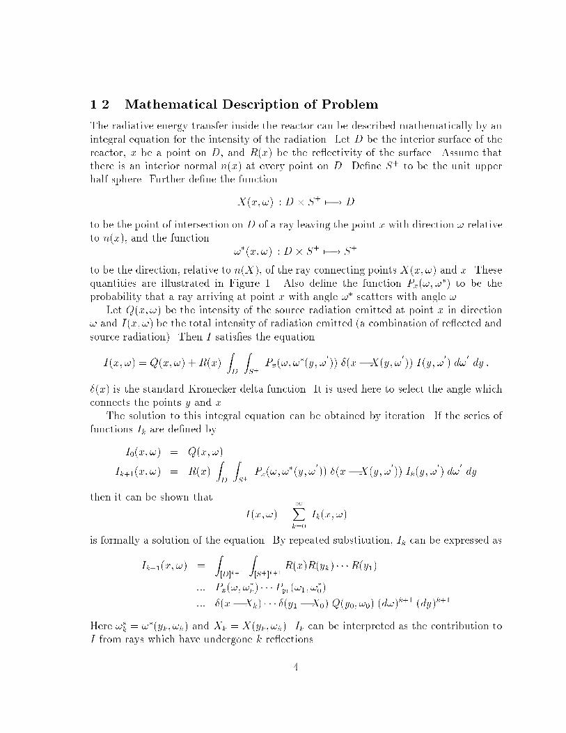
1.2 Mathematical Description of Problem

The radiative energy transfer inside the reactor can be described mathematically by an

integral equation for the intensity of the radiation. Let D be the interior surface of the

reactor, x be a point on D, and R(x) be the re ectivity of the surface. Assume that

there is an interior normal n(x) at every point on D. De�ne S+ to be the unit upper

half sphere. Further de�ne the function

X(x; !) : D � S+ 7�! D

to be the point of intersection on D of a ray leaving the point x with direction ! relative

to n(x), and the function

!�(x; !) : D � S+ 7�! S+

to be the direction, relative to n(X), of the ray connecting points X(x; !) and x. Thesequantities are illustrated in Figure 1. Also de�ne the function Px(!; !

�) to be theprobability that a ray arriving at point x with angle !� scatters with angle !.

Let Q(x; !) be the intensity of the source radiation emitted at point x in direction! and I(x; !) be the total intensity of radiation emitted (a combination of re ected and

source radiation). Then I satis�es the equation

I(x; !) = Q(x; !) +R(x)ZD

ZS+

Px(!; !�(y; !

0

)) �(x�X(y; !0

)) I(y; !0

) d!0

dy :

�(x) is the standard Kronecker delta function. It is used here to select the angle whichconnects the points y and x.

The solution to this integral equation can be obtained by iteration. If the series of

functions Ik are de�ned by

I0(x; !) = Q(x; !)

Ik+1(x; !) = R(x)ZD

ZS+

Px(!; !�(y; !

0

)) �(x�X(y; !0

)) Ik(y; !0

) d!0

dy

then it can be shown that

I(x; !) =1Xk=0

Ik(x; !)

is formally a solution of the equation. By repeated substitution, Ik can be expressed as

Ik+1(x; !) =Z[D]k+1

Z[S+]k+1

R(x)R(yk) � � �R(y1)

::: Px(!; !�

k) � � �Py1 (!1; !�

0)

::: �(x�Xk) � � � �(y1 �X0) Q(y0; !0) (d!)k+1 (dy)k+1

Here !�k = !�(yk; !k) and Xk = X(yk; !k). Ik can be interpreted as the contribution toI from rays which have undergone k re ections.

4

Generally, the quantity of interest is EA(x), the total radiative energy absorbed at a

point on the surface. Up to this point we have been working with the emitted radiation.

The two quantities are related as follows. It is assumed that all radiation arriving at a

point is either absorbed with absorptivity A(x) or re ected with re ectivity R(x). This

requires that A(x) = 1�R(x). The total energy re ected, ER, can be expressed as

ER(x) =ZS+

(I(x; !)�Q(x; !)) d! :

This can also be expressed as

ER(x) = R(x) ET (x)

where ET is the total energy arriving at x. Similarly the total absorbed energy can bewritten

EA(x) = A(x) ET (x) :

Then by solving and substituting in for ET , we have that

EA =A(x)

R(x)

ZS+

(I(x; !)�Q(x; !)) d! :

From the series representation of I it follows that

EA(x) =1Xk=1

Ek(x)

where

Ek(x) =Z[D]k

Z[S+]k+1

A(x)R(yk�1) � � �R(y1)

::: Px(!; !�

k�1) � � �Py1(!1; !�

0)

::: �(x�Xk�1) � � � �(y1 �X0) Q(y0; !0) (d!)k+1 (dy)k

There are two special cases of surface re ection which are of particular interest,di�use and specular. In the di�use case, the probability of scattering into a given angleis independent of the incoming angle. The function P is Px(!; !

�) = n(x) �!. The deltafunctions select out those k-step paths which can connect the starting point y0 and the

end point x. If D does not bound a convex region, not every set of k points on D can beconnected by a path that lies inside D. This is related to the visibility of various parts

of the reactor, a quantity which depends only on geometry and which can be calculatedseparately from the energy transfer computation. This is the basis for the view factor

method, an e�ective, non-Monte Carlo method for computing radiative transfer in the

di�use case.

5

The second case, specular re ection, is described by setting P equal to a delta

function

Px(!; !�) = � [! � !� + 2 (n(x) � !�) n(x)] :

Under the assumption of specular re ection, the above formula for Ek can be consider-

ably simpli�ed by noting that the ray paths are completely determined by the starting

point y0; !0. If the function X̂k(y0; !0) is de�ned as the position of a ray starting at

(y0; !0) at the kth re ection, then Ek can be written

Ek(x) =ZD

ZS+

A(x) R̂k�1(y0; !0)�(x� X̂k(y0; !0)) Q(y0; !0) d!0 dy0 :

Here R̂k�1 is the product of the k � 1 re ectivities encountered along the path of theray. Although this is now a low dimensional integral, because of the discontinuity of theintegrand, only in the simplest case when the integral reduces to one dimension will a

grid based quadrature method outperform the standard Monte Carlo approach. ThusMonte Carlo is generally used to compute the specular re ection case, which we studyin this paper.

At this point it should be mentioned that the radiation intensitiesQ, I and E, as wellas the re ectivityR and absorptivity A are functions of the frequency � of the radiation.

Typically the direction and frequency dependencies will be separated by writing

Q(x; !; �) = �(x; !) Q0(x; �)

where � is a directional distribution (e.g. Lambert's Law �(x; !) = n(x) � !), and Q0 isthe frequency distribution. Often Q0 is taken to be Plank's black body distribution attemperature T (x)

Q0(x; �) =c1�

3

ec2�=T (x) � 1:

Here c1 and c2 are constants. The inclusion of this frequency dependence simply involves

adding an additional integration to the formula for Ek over the frequency range [0;1].

The problem described above can be considered a fractional absorptivity problem.That is, every ray loses a certain percent of its energy (the absorptivity) at each re ec-

tion. This requires that the ray be re ected an in�nite number of times. Of course in acomputation involving ray tracing, it is necessary to terminate the path of a ray once it

has lost a given percent of its energy. This corresponds to use only a �nite number ofterms in the above in�nite series. When this method is used, it is only necessary to use

Monte Carlo to choose the initial position, energy and direction of the ray. The path

of the ray is �xed according to the laws of specular re ection, and at each re ection,

the amount of energy absorbed is simply the absorptivity times the amount of energy

remaining. One potential disadvantage to this method is that each ray must be tracedthrough a full set of re ections, which may prove computationally expensive.

6

There is another formulation of this problem of radiative heat transfer in which

many rays undergo fewer re ections than in the fractional absorption method, so that

the average computation time per ray is smaller. In this alternative approach, the

entire energy of the ray is absorbed with probability equal to the absorptivity and the

ray tracing is terminated. We call this method the discrete absorptivity problem. A

mathematical formulation can be obtained by employing the identity

R =Z 1

0�(R � z)dz

where �(z) is the Heavyside function:

�(z) =

(1 ; z � 00 ; z < 0

:

This identity can be used in the above formula for Ek to obtain

Ek(x) =Z1

0

ZD

ZS+

ZIk

�(A(x; �)� zk)k�1Yi=1

�(Ri � zi)

�(x� X̂k(y0; !0)) Q(y0; !0; �) (dz)k d!0 dy0 d�

Here Ri is the re ectivity encountered in the ith re ection. The dimension and variance

(and therefore Monte Carlo error) of this integrand are considerably larger than thecorresponding quantities for the fractional absorption method. Thus, a greater numberof rays will be required to achieve the same accuracy. This is weighted by the fact thatrays may be computed faster using the discrete method. The two approaches have beencompared experimentally for a variety of cases, and the results are given below.

Finally, it should be noted that for a typical reactor, the source term has supportonly on a portion of D, such as the heating element labeled surface 0 in Figure 1. Also,while we are interested in the absorbed energy distribution at every point on the wafer, it

is only practical to divide the wafer into small elements, such as those shown in Figure 1,and compute the energy absorbed by each one. In general, if Di is a sub-region of D,

the question at hand is how much energy is transferred from the source to Di. Thisvalue can be expressed as Z

Di

EA(x) dx :

In the experiments of section 2, we calculate this for the surface elements described inFigure 1. When formulated in this way, the both the fractional and discrete problems

lend themselves to Monte Carlo simulations fairly easily. The inclusion of the e�ects

described above, as well as other possible factors is relatively straight forward. A precisedescription of how these methods were implemented is given in section 2.

7

1.3 Quasi-Monte Carlo Methods

To evaluate a d-dimensional integral, the standard Monte Carlo method uses indepen-

dent, uniformly distributed random numbers on the d-dimensional unit cube Id as the

source of integration nodes. In the simplest case, if fzig is such a sequence of random

points in Id, then the integral of the function f(x1; � � � ; xd) over Id is approximated by

the average of f evaluated at the points zi. The error,

� =ZIdf(x) dx�

1

N

NXi=1

f(zi) ;

satis�es the relationship involving the expectation E(�) of a random variable

E(�2) =�2(f)

N

where �2(f) is the variance of f de�ned by

�2(f) =ZIdf2(x) dx�

�ZIdf(x) dx

�2:

This shows the familiar convergence rate of N�1=2 associated with random methods.The key property of the random sequence which is used here is its uniformity, so that

any contiguous subsequence is well spread throughout the cube. This idea has lead tothe suggestion that using other sequences which are more uniformly distributed than arandom sequence may produce better results. Such sequences are called quasi-randomor low discrepancy sequences.

Initially it may appear that a grid would provide optimal uniformity. However, gridssu�er from several di�culties. First, the number of points required to create even a

course mesh is exponentially large in dimension. Moreover, not all dimensions are ofequal importance in particle simulation problems. Generally the majority of the energy

transfer will occur in the �rst collisions. Thus in a 6 dimensional problem, even if a

million rays are used, the �rst collision will be described by only 10 di�erent values ofthe variable. Another di�culty is that grids have rather high discrepancy, a quantity

which measures the uniformity of a set of points. This is de�ned and discussed below.Finally, the standard method for increasing accuracy of a grid is to halve the mesh size,

which requires adding 2d times the current number of points. It is desirable to be able

to increase the number of points used without adding such an extremely large number.It is unclear how to place additional points on a grid to maintain uniformity unless the

mesh is halved, though.The solution to this problem is to use in�nite sequences of points such that for every

N , the �rst N terms of the sequence are in some sense optimally distributed throughout

the cube. In order to quantify this, the discrepancy of a set of N points in de�ned as

8

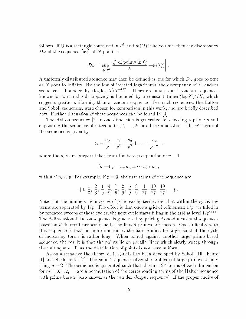
follows. If Q is a rectangle contained in Id, and m(Q) is its volume, then the discrepancy

DN of the sequence fxig of N points is

DN = supQ2Id

�����# of points in Q

N�m(Q)

����� :A uniformly distributed sequence may then be de�ned as one for which DN goes to zero

as N goes to in�nity. By the law of iterated logarithms, the discrepancy of a random

sequence is bounded by (log logN)N�1=2. There are many quasi-random sequences

known for which the discrepancy is bounded by a constant times (logN)d=N , which

suggests greater uniformity than a random sequence. Two such sequences, the Halton

and Sobol' sequences, were chosen for comparison in this work, and are brie y describednow. Further discussion of these sequences can be found in [3]

The Halton sequence [2] in one dimension is generated by choosing a prime p andexpanding the sequence of integers 0; 1; 2; . . . ; N into base p notation. The nth term of

the sequence is given by

zn =a0

p+a1

p2+a2

p3+ � � �+

am

pm+1;

where the ai's are integers taken from the base p expansion of n� 1

[n� 1]p = amam�1 � � � a2a1a0 ;

with 0 � ai < p. For example, if p = 3, the �rst terms of the sequence are

f0;1

3;2

3;1

9;4

9;7

9;2

9;5

9;8

9;1

27;10

27;19

27; . . .g :

Note that the numbers lie in cycles of p increasing terms, and that within the cycle, theterms are separated by 1=p. The e�ect is that once a grid of re�nement 1=pm is �lled inby repeated sweeps of these cycles, the next cycle starts �lling in the grid at level 1=pm+1.

The d-dimensional Halton sequence is generated by pairing d one-dimensional sequences

based on d di�erent primes; usually the �rst d primes are chosen. One di�culty withthis sequence is that in high dimensions, the base p must be large, so that the cycle

of increasing terms is rather long. When paired against another large prime basedsequence, the result is that the points lie on parallel lines which slowly sweep through

the unit square. Thus the distribution of points is not very uniform.

As an alternative the theory of (t,s)-nets has been developed by Sobol' [10], Faure[1] and Niederreiter [7]. The Sobol' sequence solves the problem of large primes by onlyusing p = 2. The sequence is generated such that the �rst 2m terms of each dimension

for m = 0; 1; 2; . . . are a permutation of the corresponding terms of the Halton sequence

with prime base 2 (also known as the van der Corput sequence). If the proper choice of

9

permutations is used, the resulting d-dimensional sequence can be shown to have good

uniformity properties. However, as dimension increases, more permutations must be

used, and the possibility increases that a bad pairing may exist between two dimensions

leading to a highly non-uniform distribution in that plane.

In his book [6], Niederreiter summarizes the properties and theory of these sequences.

The key point is that their discrepancy satis�es the relationship

DN � cd(logN)d

N+O

(logN)d�1

N

!;

where cd, di�erent for each sequence, is constant in N , but depends on d. This is an

optimal upper bound in the sense that for any in�nite sequence, there exist an in�nitenumber of N such that

DN � c(logN)d

N

for some constant c. These bounds suggest that at least for large N , the quasi-randomsequences described above will be considerably more uniform than a random sequence.

As discussed in [3] and [4], there is a rather large gap between the theoretical boundson discrepancy and integration error and what can be observed in practical computa-tions. There is no theory which accurately predicts integration error for a given inte-grand. However, computational experiments have established various trends in behav-ior. For many problems, quasi-Monte Carlo methods signi�cantly outperform randomsequences in the range of practical N . The convergence rate is generally between N�:5

and N�1. There is a tendency, however, for the improvement over random to diminishas the dimension of the problem increases. Computations of discrepancy indicate thatthere is a transition point in N which grows exponentially with dimension such thatbefore this point, the discrepancy of quasi-random sequences is the same as for randomsequences. Also, integrands which have step function like behavior, such as charac-

teristic functions of sets, tend to show less improvement with quasi-random sequencesthan continuous integrands. The best way to predict performance for a speci�c type of

problem is to analyze the results for a test problem, as is done below.

2 Results

While the idea of quasi-Monte Carlo is almost as old as the Monte Carlo approach

itself, these methods have rarely been used in real world engineering problems. Thismay be attributed to the fact that many Monte Carlo problems are high dimensional,and quasi-random sequences tend to lose their advantage as dimension increases [4].

Another di�culty is that for many simulations (particularly non-linear ones) great care

must be taken to avoid problems arising from the fact that the quasi-random numbers are

10

not independent [5]. Due to their relative simplicity and robustness, standard random

Monte Carlo methods have remained dominant.

As the following results show, however, a considerable advantage can be won by ap-

plying quasi-random sequences to an appropriate problem. In this case, computational

experiments were performed on the radiative heat transfer problem for the cylinder

symmetric reactor described above. Several parameters were tested to determine which

simulations might bene�t the most from the quasi-random approach. Comparisons were

made between the discrete and fractional absorption methods, among several absorptivi-

ties, among di�erent surfaces elements on the wafer, between point and surfaces sources,

and among the Halton, Sobol' and pseudo-random sequences. To limit the number of

parameters studied, the absorptivity was assumed independent of frequency.

2.1 Experimental Technique

The typical experiment consisted of emitting N rays from a surface or point sourcelocated at surface 0. The point source is actually a circle under cylinder symmetry. For

the surface source, the rays were distributed sequentially by increasing radius on a onedimensional grid so the distribution on the corresponding annulus would be uniform.The initial direction was sampled using Lambert's Law, which means that the zenithangle was sampled from a cosine distribution, while the azimuthal angle was sampledfrom a uniform distribution on [0; 2�]. The sampling was done using one point from a

multi-dimensional quasi- or pseudo-random sequence, such that two angles were assignedseparate dimensions. A third dimension was used to sample the initial energy of the rayfrom a modi�ed version of Plank's black body distribution. The fractional method thenconsisted of tracing the ray path through the reactor according to the laws of specularre ection, such that at each re ection a certain percentage of the ray's energy, givenby the absorptivity at that point, was transferred to the surface element in question.

The tracing continued until the ray had lost a �xed percentage of its initial energy.

The discrete method varied from the fractional method only in that at each re ection,either no energy was absorbed and the ray continued on, or the entire initial energywas absorbed and the ray tracing was terminated. In both cases, the �nal answer was

computed as the percentage of the energy which left the source that was absorbed by

the target element.The ultimate goal of the experiments was to determine the accuracy as a function

of computation time. This is discussed in more detail below. The �rst step towardsthis goal was to compute error size as a function of N , the number of rays emitted

from the source. The approach taken here was to compute the \expected" convergence

rate and error size by performing the calculation 30 times for each value of N usingdi�erent, \independent" subsequences of the sequences in question. The error was then

averaged to give a better estimate of what the expected error using N rays would be.This calculation was then repeated using a larger value of N , again using di�erent

11

subsequences. In this way, errors at di�erent values of N are also independent, which

allows for an unbiased description of the convergence rate. The values of N tested were

chosen to be evenly spaced on a logarithmic scale, so that convergence of the type N�

could more easily be studied.

The terms expectation and independence are only strictly de�ned for a sequence

of random variables. Performing the experiments described above with such a random

sequence would show converge at a rate of N�:5 and an error size determined by the

variance of the integrand. The results for the pseudo-random sequence do indeed show

a convergence rate of approximately 1=pN . The same method of computing expected

error is then extended to the quasi-random sequences as a means of comparison. It

should be noted that this kind of convergence study using averaging and independent

Ns requires considerably more computation time than a straight forward simulationusing a �xed number of rays.

An additional di�culty in this convergence study was that the exact solution for theenergy transfer was not known. Thus it was necessary to estimate the exact answer fromthe Monte Carlo calculation and use this to measure the error at each value of N . Theestimate for the exact answer was obtained by �rst averaging the 30 results obtained foreach of the last four values of N , then taking a weighted average of these four values.

Under the assumption of a Gaussian error distribution, it can be shown that this givesan optimal estimate to the true answer.

As stated above, the real quantity of interest is computation time to reach a speci�ederror tolerance. This is of particular importance in comparing the fractional and discretemethods. The discrete method requires fewer re ections, but at the cost of being ahigher dimensional integral. Thus N might be larger in the discrete case, but the time

to compute each ray path would be smaller than in the fractional case. The experimentsjust described address only the question of convergence with N . The problem is thatcomputation time depends on the coding of the programs and sequences and is verymachine dependent. To avoid issues of optimal coding, which would in any case only beaccurate for a speci�ed machine, we devised the following means of comparison for the

fractional and discrete methods.The computation consists roughly in computing an average of nr random numbers

in a time nrtr and performing an average of m ray tracing steps in a time mtt. Thusthe total computing time is T = N(nrtr +mtt). We observed that most of the time is

spent on ray tracing. Because our geometry is not very complex, the most realistic case

will be a situation very close to the limit, in which all computation time is spent on

tracing. Then a comparison T f=T d of the computation time with fractional and discrete

method will only depend on the ratio mf=md of the number mf of ray traces with thefractional method to the average number md of ray traces with the discrete method.

It is simple to realize that md = 1=A, but mf depends on the desired accuracy of the

calculation. If we require that a ray be traced using the fractional method until the ratio

12

of its �nal energy to its initial energy is less than � (in our case � = 10�4), we have

mf = [log(�)= log(1�A)]+ 1. With our energy limit and A = 0:4 we get T f=T d = 7:61.

This gives the scale to allow the comparison of the computation time of the fractional

and discrete method.

Three absorptivities were tested, A = 0:1; 0:4 and 0:7. The associated number

of re ections mf necessary using the fractional method to achieve the accuracy � =

10�4 were 88, 19 and 8 respectively. In order to compare the fractional method across

absorptivity, a reference time T � was chosen as the time required to compute 105 rays

with A = 0:1 using the fractional method. Under the assumption that ray tracing

dominates the computation time, 88=19 = 4:63 times as many rays could be calculated

for A = 0:4 in the same T �, and 88=8 = 11 times as many rays for A = 0:7. A similar

scaling is used to determine the number of rays which can be computed in T � for thedi�erent absorptivities using the discrete method.

2.2 Experimental Results

For the sake of brevity, results are presented here for only one quasi-random sequence,Halton. The Sobol' sequence was also tested, but the results were generally the same

as for Halton; on the occasions where there was a di�erence, Halton appeared slightlybetter. Also, all calculations described here were performed using a point source for theradiation. Experiments were also done using a surface source; however, as there is nosigni�cant di�erence in the results of the two approaches, only the point source resultsare given here.

The �rst set of calculations is illustrated in Figure 2 and Table 1. This �gure shows

the expected relative error �(N) as a function of the number of emitted rays N for theHalton sequence and a pseudo-random sequence using the fractional absorption methodwith a constant surface absorptivity of 0.4. Results are given for surface 1 on the wafer(see Figure 1), which is directly visible to the source, and for surface 2, on the back sideof the wafer. The plotted points are the calculated errors for various N (averaged over

30 runs), while the lines are a least squares �t of the data to the functional form

�(N) = c N� :

This is the correct form for the expected error using a random sequence, in which case

c is the standard deviation of the integrand and � is �1=2. As plotted on a log scale,the error appears as a line with slope �.

Figure 2 illustrates a clear advantage of using a quasi-random sequence over a pseudo-

random sequence in the calculation, both in error size and in convergence rate (i.e., �).

The error in calculating the energy transfer to surface 1 with N = 100000 is over a factor

1In our actual calculation this limit was between 6.23 and 6.81 for the di�erent number generators.

Hence we were pretty close to the assumed limit.

13

102

103

104

105

106

107

10-4

10-3

10-2

10-1

100

NUMBER OF RAYS

RE

LA

TIV

E

ER

RO

R

SURFACE 1

RANDOM

HALTON

102

103

104

105

106

107

10-4

10-3

10-2

10-1

100

NUMBER OF RAYS

RE

LA

TIV

E

ER

RO

R

SURFACE 2

RANDOM

HALTON

Figure 2: Comparison of random and quasi-random sequences using the fractional ab-

sorption method with absorptivity = 0.4.

Surface Abs. Convergence Error at Improvement Error at Improvement� : N� N = 105 Factor Time T � Factor

1 0.1 -.64 .0027 2.3 .0027 2.30.4 -.70 .0033 3.4 .0012 4.6

0.7 -.70 .0042 3.7 .0008 6.0mix -.66 .0036 2.8 .0017 3.3

2 0.1 -.64 .0049 2.7 .0049 2.70.4 -.65 .0099 2.4 .0036 3.0

0.7 -.65 .0152 2.4 .0032 3.4

mix -.65 .0097 2.3 .0047 2.7

Table 1: Convergence results for fractional absorptivity method using the Halton se-

quence.

14

of three smaller if the Halton sequence is used than if a random sequence is used. This

�gure also shows that the accuracy of the calculation depends on the region of the wafer

in question. The error in computing the energy transfer to surface 2 is considerably

higher than for surface 1. This is related to the fact that a ray must undergo at least

one re ection before reaching surface 2, as opposed to the possibility of direct energy

transfer from the source to surface 1. This leads to a higher variance in the rays hitting

surface 2, and thus larger error. A second consequence is that the improvement gained

by using a quasi-random sequence is somewhat less pronounced. Table 1 summarizes

the results of the calculations using the fractional absorptivity method for several values

of absorptivity, as well as for a mixed absorptivity case in which the walls are highly

re ective (A = 0:1), while the wafer is highly absorbing (A = 0:7). The mixed case is

more typical of an actual reactor. The table gives the convergence rate in terms of �, theexpected error for the Halton sequence for N = 100000, and the ratio of the expected

random error to the Halton error. The expected error after computing for time T �

(de�ned above) is also given as well as the improvement factor of Halton over randomfor this case. This table shows that a signi�cant advantage is gained by using the Haltonsequence in all cases. Again, the advantage is more prominent for the directly visiblesurface 1.

Figure 3 and Table 2 provide a similar comparison of the Halton and pseudo-randomsequences for the discrete absorption method. As mentioned above, the integrand beingevaluated in this method has a larger variance than the integrand associated with thefractional absorption method, and therefore considerably more rays are need to obtainthe same degree of accuracy. However, the computation time required per ray in thediscrete case is on average much less. In Figure 3 the values of N were chosen so as to

have the same computation time as in Figure 2, based on the scaling argument givenin section 2.1. The dimension of the integral is also much larger, as each re ectioncorresponds to a separate dimension. Depending on absorptivity, as many as 40 ormore dimensions could be required, compared with the three dimensional integrandof the fractional method (in which the ray path is completely determined by its initial

direction). As discussed previously, quasi-random sequences tend to lose their advantageover random sequences as the dimension of the integral increases. This is tempered by

the fact that the higher dimensions play a less signi�cant role in the calculation. Forexample, with an absorptivity of 0.4, 99 per cent of all rays have been absorbed after

nine re ections. Nevertheless, this dimensional e�ect on the quasi-random approach can

be seen in Figure 3 and Table 2. The factor of improvement for Halton over random isnoticeably smaller than for the fractional case, although signi�cant gains are still madeby using Halton. Again, there is a considerable di�erence in the accuracy for surfaces

1 and 2, most notably in the case of high absorptivity. In this case most rays do not

survive the �rst re ection, so that many fewer rays eventually make it to surface 2 than

surface 1.

15

103

104

105

106

107

10-4

10-3

10-2

10-1

100

NUMBER OF RAYS

RE

LA

TIV

E

ER

RO

R

SURFACE 1

RANDOM

HALTON

103

104

105

106

107

10-4

10-3

10-2

10-1

100

NUMBER OF RAYS

RE

LA

TIV

E

ER

RO

R

SURFACE 2

RANDOM

HALTON

Figure 3: Comparison of random and quasi-random sequences using the discrete ab-

sorption method with absorptivity = 0.4.

Surface Abs. Convergence Error at N Improvement Error at Improvement� : N� = 8:8 � 105 Factor Time T � Factor

1 0.1 -.54 .0061 1.2 .0061 1.20.4 -.65 .0030 2.4 .0012 2.9

0.7 -.66 .0020 3.6 .0006 5.1

mix -.59 .0020 2.2 .0011 2.5

2 0.1 -.54 .0141 1.2 .0141 1.20.4 -.57 .0141 1.6 .0064 1.8

0.7 -.57 .0213 1.3 .0071 1.5

mix -.57 .0063 2.0 .0036 2.2

Table 2: Convergence results for discrete absorptivity method using the Halton sequence.

16

Surface Abs. Random Error QMC Error

Discrete/Fract. Discrete/Fract.

1 0.1 1.70 2.23

0.4 0.75 1.06

0.7 0.45 0.71mix 0.49 0.65

2 0.1 2.17 2.850.4 0.64 1.76

0.7 0.96 2.20mix 0.49 0.78

Table 3: Comparison of error for discrete absorptivity method to error for fractionalabsorptivity method for random and Halton sequences at T �.

Table 3 summarizes a comparison of the fractional and discrete methods for both a

random sequence and the Halton sequence. For the various surfaces and absorptivitiesthe ratio of the expected error using the discrete method to the expected error usingthe fractional method is shown. In the random case, both methods have the same con-vergence rate, so this ratio of errors depends only on the variance of the two integrands(computed from the least squares �t of the experimental data) and the computational

time scaling factor described above. Thus this value is independent of the computationtime, or equivalently, of N . However, since the two quasi-Monte Carlo cases do notconverge at the same rate, the associated error ratio depends on the computation time.The results are given for time T �.

At low absorptivities, the fractional method is clearly superior for both random

and quasi-random, as well as for both surfaces. As the numbers for the random caseindicate, the variance of the discrete method integrand is considerably larger than that

of the fractional method. There is a further penalty for the discrete method in the quasi-

random case coming from the use of a higher dimensional sequence. As the absorptivityincrease, the variance di�erence becomes small enough to favor the discrete method inthe random case. This trend can also be seen for quasi-random for surface 1, although

the low dimensional advantage of the fractional method moderates the gains seen for the

discrete method using the random sequence. Surface 2, however, shows rather di�erentbehavior, strongly favoring the fractional method for all but the mixed case. This can

be explained by noting that when the absorptivity is large, many fewer particles evermake it to the back of the wafer in the discrete case. The \e�ective" N is then much

smaller, so that the quasi-random advantage is considerably less. Figure 4 illustrates

17

102

103

104

105

106

10-3

10-2

10-1

100

SCALED TIME

RE

LA

TIV

E

ER

RO

R

SURFACE 1

FRACTIONAL

DISCRETE

102

103

104

105

106

10-3

10-2

10-1

100

SCALED TIME

RE

LA

TIV

E

ER

RO

R

SURFACE 2

DISCRETE

FRACTIONAL

Figure 4: Comparison of fractional and discrete absorption methods using the Haltonsequence with absorptivity = 0.7.

this by plotting the relative error for the two methods using the Halton sequence forabsorptivity 0.7. Results for both surface 1 and surface 2 are shown. The abscissa is

computation time in arbitrary units, which allows a comparison of the two methods.The scaling was chosen so that one time unit corresponds to the average time need tocompute the path of one ray using the fractional method. On this scale T � = 105. Inthe range of a practical computation, for surface 1 the advantage of the discrete methodover the fractional method starts at about a factor of two, but steadily decreases as

the accuracy increases. On the other hand, for surface 2 the fractional method has anincreasing advantage over the discrete approach as the computation time increases.

The results for the mixed absorptivity case are shown in Figure 5. The success of thediscrete method for both surfaces may be explained as follows. The wafer acts as a sink

for the rays, absorbing 70 per cent of the rays which strike it. The walls simply re ect

most rays. Thus a large percentage of the rays emitted contribute to the statistics of the

wafer, both front and back, so that both methods show a comparable improvement over

the random case. The relatively low variance of the discrete method in this situationthen tilts the balance in favor of discrete over fractional. However, as the graphs show,

the advantage of the discrete method again decreases with increasing accuracy. Thisis a result of the superior convergence rate of the fractional method associated with it

being a low dimensional integral. In general, the choice of method may then dependon geometry, the regions of the reactor which are of most interest, and the minimum

accuracy required.

To round out the computations, we will brie y describe several other results obtained.A third surface element taken at the edge of the wafer was also observed. The size of

18

102

103

104

105

106

10-3

10-2

10-1

100

SCALED TIME

RE

LA

TIV

E

ER

RO

R

SURFACE 1

FRACTIONAL

DISCRETE

102

103

104

105

106

10-3

10-2

10-1

100

SCALED TIME

RE

LA

TIV

E

ER

RO

R

SURFACE 2

FRACTIONAL

DISCRETE

Figure 5: Comparison of fractional and discrete absorption methods using the Haltonsequence with absorptivity = 0.1 on reactor walls and absorptivity = 0.7 on wafer.

this element was 2.36 cm2, which was much smaller than the other surface elements.Although this element had visibility relative to the heat source similar to that of surface

1, the error was almost an order of magnitude larger, and the performance of the Haltonsequence was identical or only slightly better than the pseudo-random sequence. Thiscan be attributed to the di�erence in size of the elements. Many fewer rays strikethe smaller surface, leading to an e�ectively smaller N . Thus for the smaller surface,over the range of N considered, the calculation was still in the range where random

and quasi-random are close, similar to what appears in the above graphs at small N .Moreover, the variance of the integrand being evaluated by the simulation is related tothe surface size such that the smaller the surface, the higher the variance, and thereforeerror. This is not surprising, as the use of small surface elements leads to a greater

amount of information about the temperature distribution on wafer. To obtain this

more re�ned temperature distribution to the same degree of accuracy of course requires

more work (larger N).

Another case considered was that of di�use re ection at the walls instead of spec-ular. Frequently such cases are often handled by non-Monte Carlo methods. However,

as di�use re ection is easily implemented in a Monte Carlo code, and the results arepotentially of interest, a calculation with di�use re ection for absorptivity 0.4 was car-

ried out. The results using fractional absorption show a signi�cant improvement forHalton over pseudo-random for surface 1 similar to the results of Figure 2. However,

for surface 2, there results are the same for Halton and random. The di�erence between

the performance for surface 1 and 2 can again be explained in terms of visibility. Muchof the energy transferred to surface 1 comes from rays which have not undergone a

19

re ection. In contrast, to reach surface 2 requires at least one re ection. Each re ec-

tion increases the dimension of the problem by two (two numbers are needed to sample

the new direction). Thus the integrand for surface 2 has a much stronger dependence

on the higher dimensions, which leads to a weaker performance by the quasi-random

sequence. It should be noted, however, that in no case tested did a pseudo-random

sequence outperform the quasi-random sequence.

3 Conclusions

For the simulation of heat transfer reactors and other related radiative transfer problems,

the results of this paper indicate that quasi-Monte Carlo methods can be e�ectivelyimplemented. The error associated with using a quasi-random sequence is always at least

as small as in the standard random Monte Carlo approach, and frequently a signi�cantreduction in error can be obtained, up to a factor of 6 in some cases within the range ofrealistic computations. Because these calculations tend to be dominated by time spentin the ray tracing algorithm, there is no additional computational cost associated withgeneration of the quasi-random sequence over the pseudo-random sequence. Moreover,the quasi-random sequence may simply be substituted in for the random sequence in

existing codes, so that virtually no extra work is required to obtain the quasi-MonteCarlo advantage.

The advantage of quasi-random over random appears to increase as the absorptivityof the reactor increases, for �xed computation time. At lower absorptivities the fractionalabsorption method is superior to the discrete method. However, as absorptivity increases

the discrete method gives better accuracy for surfaces directly visible to the heat source.For the case of highly re ective walls and a highly absorbing wafer, the discrete methodwas superior for all surfaces, but the advantage over the fractional method decreasedwith increasing accuracy due to the faster convergence of the fractional method.

The choice of quasi-random sequence (in this case Halton or Sobol') appeared to have

little impact on the results. There was also little di�erence between using a point sourceor a surface source for the radiation. This additional element of robustness makes quasi-

Monte Carlo methods attractive for use in a wide range of radiative transport problems.

20

References

[1] Henri Faure, Discr�epance de suites associ�ees �a un syst�eme de num�eration (en di-

mension s), Acta Arithmetica 41, 337-351, 1982.

[2] J.H. Halton, On the e�ciency of certain quasi-random sequences of points in eval-

uating multi-dimensional integrals, Numer. Math. 2, 84-90, 1960.

[3] W.J. Moroko� and R.E. Ca isch, Quasi-random sequences and discrepancy, SIAM

Sci. Comp. (to appear).

[4] W.J. Moroko� and R.E. Ca isch, Quasi-Monte Carlo Integration, submitted to J.

Comp. Phys. (1991).

[5] W.J. Moroko� and R.E. Ca isch, A quasi-Monte Carlo approach to particle simu-

lation of the heat equation, SIAM Num. Anal. (to appear).

[6] H. Niederreiter,Random number generation and quasi-Monte Carlo methods, SIAM

Regional Conference Series in Applied Mathematics, CBMS-NSF 63, 1992.

[7] H. Niederreiter, Quasi-Monte Carlo methods for multidimensional numerical inte-gration, Numerical Integration III, International Series of Numerical Math. 85, H.

Brass and G. H�ammerlin eds., Birkh�auser Verlag, Basel, 1988.

[8] D.M. O'Brien, Accelerated quasi-Monte Carlo integration of the radiative transfer

equation, J. Quant. Spectrosc. Radiat. Transfer 48, no. 1, 41 - 59, 1992.

[9] P.K. Sarkar and M.A. Prasad, A comparative study of pseudo and quasi randomsequences for the solution of integral equations, J. Comp. Phys. 68, 66 - 88, 1987.

[10] I.M. Sobol', The distribution of points in a cube and the approximate evaluation ofintegrals, U.S.S.R. Computational Math. and Math. Phys. 7, no. 4, 86-112, 1967.

21