Nearly degenerate neutrinos, supersymmetry and radiative corrections
33
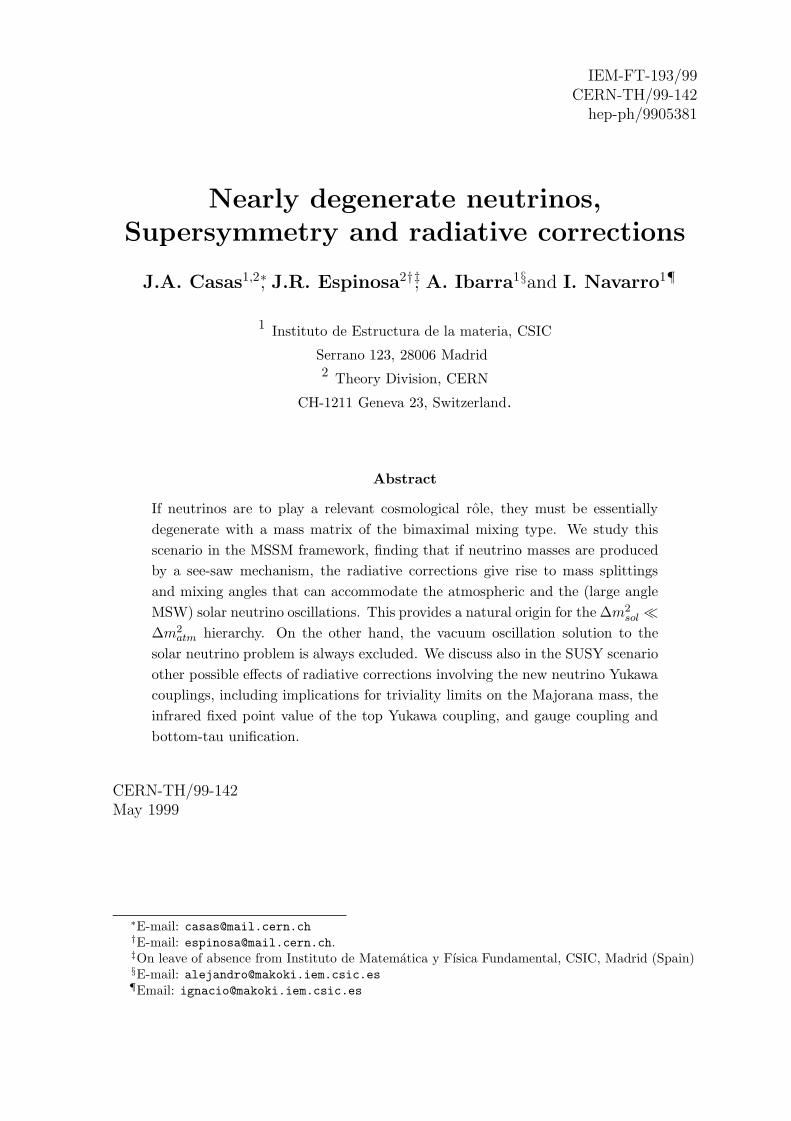
Nearly degenerate neutrinos, Supersymmetry and radiative corrections J.A. Casas 1,2 * , J.R. Espinosa 2 †‡ , A. Ibarra 1 § and I. Navarro 1 ¶ 1 Instituto de Estructura de la materia, CSIC Serrano 123, 28006 Madrid 2 Theory Division, CERN CH-1211 Geneva 23, Switzerland. Abstract If neutrinos are to play a relevant cosmological rˆ ole, they must be essentially degenerate with a mass matrix of the bimaximal mixing type. We study this scenario in the MSSM framework, finding that if neutrino masses are produced by a see-saw mechanism, the radiative corrections give rise to mass splittings and mixing angles that can accommodate the atmospheric and the (large angle MSW) solar neutrino oscillations. This provides a natural origin for the Δm 2 sol Δm 2 atm hierarchy. On the other hand, the vacuum oscillation solution to the solar neutrino problem is always excluded. We discuss also in the SUSY scenario other possible effects of radiative corrections involving the new neutrino Yukawa couplings, including implications for triviality limits on the Majorana mass, the infrared fixed point value of the top Yukawa coupling, and gauge coupling and bottom-tau unification. CERN-TH/99-142 May 1999 IEM-FT-193/99 CERN-TH/99-142 hep-ph/9905381 * E-mail: [email protected] † E-mail: [email protected]. ‡ On leave of absence from Instituto de Matem´atica y F´ ısica Fundamental, CSIC, Madrid (Spain) § E-mail: [email protected] ¶ Email: [email protected]
Transcript of Nearly degenerate neutrinos, supersymmetry and radiative corrections
Nearly degenerate neutrinos,Supersymmetry and radiative corrections
J.A. Casas1,2∗, J.R. Espinosa2†‡, A. Ibarra1§and I. Navarro1¶
1 Instituto de Estructura de la materia, CSIC
Serrano 123, 28006 Madrid2 Theory Division, CERN
CH-1211 Geneva 23, Switzerland.
Abstract
If neutrinos are to play a relevant cosmological role, they must be essentiallydegenerate with a mass matrix of the bimaximal mixing type. We study thisscenario in the MSSM framework, finding that if neutrino masses are producedby a see-saw mechanism, the radiative corrections give rise to mass splittingsand mixing angles that can accommodate the atmospheric and the (large angleMSW) solar neutrino oscillations. This provides a natural origin for the ∆m2
sol �∆m2
atm hierarchy. On the other hand, the vacuum oscillation solution to thesolar neutrino problem is always excluded. We discuss also in the SUSY scenarioother possible effects of radiative corrections involving the new neutrino Yukawacouplings, including implications for triviality limits on the Majorana mass, theinfrared fixed point value of the top Yukawa coupling, and gauge coupling andbottom-tau unification.
CERN-TH/99-142May 1999
IEM-FT-193/99CERN-TH/99-142
hep-ph/9905381
∗E-mail: [email protected]†E-mail: [email protected].‡On leave of absence from Instituto de Matematica y Fısica Fundamental, CSIC, Madrid (Spain)§E-mail: [email protected]¶Email: [email protected]

1 Introduction
If neutrinos are to play a relevant cosmological role, their masses should be O(eV).
In that case, since atmospheric and solar neutrino anomalies [1] indicate that mass-
squared splittings are at most 10−2 eV2, neutrinos must be almost degenerate [2]-[5]. On
the other hand, supersymmetry (SUSY) is a key ingredient in most of the extensions
of the Standard Model (SM) which are candidate for a more fundamental theory.
In this paper we will analyze, within the supersymmetric framework, under which
circumstances the “observed” mass splittings between quasi-degenerate neutrinos arise
naturally (or not), as a radiative effect, in agreement with all the available experimental
data.
This problem has been also addressed in a recent paper by Ellis and Lola [6], in
which they treat the neutrino mass matrix, Mν , as an effective operator, emerging at
some scale, Λ, with the bimaximal mixing form. Then the renormalization group (RG)
analysis shows that the splittings and mixings at low energy are not in agreement with
observations. Here we take a more general point of view. Besides exploring the effective
operator scenario, we focus our attention in the (well motivated) case in which this
operator is produced by a see-saw mechanism2. This introduces crucial differences in
the analysis. In particular, the form of Mν is modified by a first stage of RG running of
the neutrino Dirac-Yukawa matrix and the right-handed neutrino mass matrix from the
high energy scale (say Mp or MGUT ) to Λ, which is identified with the Majorana mass
scale. As we will see, this modification allows in many cases to reconcile the scenario
with experiment, providing also a natural origin for the “observed” solar-atmospheric
hierarchy of splittings, ∆m2sol � ∆m2
at.
In a recent paper [9], we performed a similar analysis in the SM framework (in
which the only particles added to the SM are three right-handed neutrinos), also with
positive results. There are similarities and differences between the SUSY and the SM
cases. First, SUSY introduces additional unknowns in the scenario, particularly the
supersymmetric mass spectrum. In the analysis, the only role of this spectrum is to
give the threshold scale(s) below which the effective theory is just the SM. In this sense,
the combination of (negative) experimental data and naturalness requires MSUSY ∼ 1
2An alternative possibility to generate small non-zero neutrino masses in the MSSM involves R-parity breaking [7]. See Ref. [8] for a discussion on the interplay between the two possibilities.
1

TeV. Of course, there may be appreciable differences between the masses of various
supersymmetric particles (squarks, gluino, charginos, etc.). Still, the variation in the
results of the RG analysis are not important. Hence, we will take a unique thresh-
old at MSUSY = 1 TeV throughout the paper. Let us mention here that, apart from
three right-handed neutrinos, we will assume a minimal spectrum of particles; in other
words we will work within the minimal supersymmetric standard model (MSSM). Sec-
ond (and more important), in the supersymmetric regime, the charged-lepton Yukawa
couplings are multiplied by a factor 1/ cosβ with respect to their SM value. These
couplings (together with the neutrino Yukawa couplings) play a major role in the ra-
diative modification of the form of Mν. Thus, the results are going to present a strong
dependence on tan β (we recall that tanβ is defined as the ratio of the expectation
values of the two supersymmetric Higgs doublets, tanβ ≡ 〈H02 〉/〈H0
1〉). Finally, the
renormalization group equations (RGEs) themselves are different in the SUSY and in
the SM cases. The difference is not just quantitative (i.e. differences in the size of the
various coefficients), but also qualitative. In particular, the modification of the Mν
texture due to the contribution from the charged-lepton Yukawa couplings has oppo-
site signs in the two cases (while the contribution from the neutrino Yukawa couplings
themselves remains with the same sign).
Let us briefly review the current relevant experimental constraints on neutrino
masses and mixing angles (a more detailed account is given in ref. [9]). Observations
of atmospheric neutrinos are well described by νµ − ντ oscillations driven by a mass
splitting and a mixing angle in the range [10]
5× 10⁻⁴ eV2 < ∆m2at < 10−2 eV2 ,
sin2 2θat > 0.82 . (1)
Concerning the solar neutrino problem, as has been shown in ref. [2] the small angle
MSW solution is unplausible in a scenario of nearly degenerate neutrinos, so we are
left with the large angle MSW (LAMSW) and the vacuum oscillation (VO) solutions,
which require mass splittings and mixing angles in the following ranges
LAMSW solution:
10−5 eV2 < ∆m2sol < 2× 10⁻⁴ eV2,
0.5 < sin2 2θsol < 1. (2)
2
VO solution:
5× 10⁻¹¹ eV2 < ∆m2sol < 1.1× 10⁻¹⁰ eV2,
sin2 2θsol > 0.67 . (3)
From the previous equations, it is apparent the hierarchy of mass splittings between
the different species of neutrinos, ∆m2sol � ∆m2
at, which should be reproduced by any
natural explanation of those splittings. Let us also remark that it is not clear at the
moment the value of the upper bound on sin2 2θsol [see eq.(2)]. As we will see, an
upper limit like sin2 2θsol < 0.99 or even greater, may disallow the scenario examined
in this paper. For the moment, we will not consider any upper bound on sin2 2θsol (see
ref.[9] for a more detailed discussion). On the other hand, according to the most recent
combined analysis of SK + CHOOZ data (last paper of ref. [10]) the third independent
angle, say φ (the one mixing the electron with the most split mass eigenstate), is
constrained to have low values, sin2 2φ < 0.36 (0.64) at 90% (99%) C.L.
Other relevant experimental information concerns the non-observation of neutrino-
less double β-decay, which requires the ee element of the Mν matrix to be bounded
as [11]
Mee < B = 0.2 eV. (4)
In addition, Tritium β-decay experiments indicate mνi< 2.5 eV for any mass eigenstate
with a significant νe component [12]. Finally, concerning the cosmological relevance of
neutrinos, we will take∑
mνi= 6 eV as a typical possibility and we will explain how
the results vary when this value is changed.
Let us introduce now some notation. In the SUSY framework the effective mass term
for the three light (left-handed) neutrinos in the flavour basis is given by a term in the
superpotential
Weff =1
2νTMνν . (5)
The mass matrix, Mν , is diagonalized in the usual way, i.e. Mν = V ∗D V †, where
D = diag(m1eiφ, m2e
iφ′, m3) and V is a unitary ‘CKM’ matrix, relating flavour to mass
eigenstates νe
νµ
ντ
=
c2c3 c2s3 s2e−iδ
−c1s3 − s1s2c3eiδ c1c3 − s1s2s3e
iδ s1c2
s1s3 − c1s2c3eiδ −s1c3 − c1s2s3e
iδ c1c2
ν1
ν2
ν3
. (6)
3
Here si and ci denote sin θi and cos θi, respectively. In the following we will label the
mass eigenvectors νi as m2ν1
< m2ν2
and |∆m212| < |∆m2
23|, where ∆m2ij ≡ m2
j −m2i (m2
ν3
is thus the most split eigenvalue). In this notation, constraint (4) reads
Mee ≡ |mν1 c22c
23e
iφ + mν2 c22s
23e
iφ′+ mν3 s2
2 ei2δ| < B . (7)
As it has been put forward by Georgi and Glashow in ref. [2], a scenario of nearly
degenerate neutrinos should be close to a bimaximal mixing, which constrains the
texture of the mass matrix Mν to be essentially [2,3]
Mb = mν
0
1√2
1√2
1√2
1
2−1
21√2
−1
2
1
2
, (8)
where mν gives an overall mass scale. Mb can be diagonalized by a V matrix
Vb =
−1√2
1√2
0
1
2
1
2
−1√2
1
2
1
2
1√2
, (9)
leading to exactly degenerate neutrinos, D = mν diag(−1, 1, 1), and θ2 = 0, sin2 2θ3 =
sin2 2θ1 = 1.
It is quite conceivable that Mν = Mb could be generated at some high scale by
interactions obeying appropriate continuous or discrete symmetries [13]. However, in
order to be realistic, Mν at low energy should be slightly different from Mb to account
for the mass splittings given in eqs.(1–3). We will explore whether the appropriate
splittings (and mixing angles) can be generated or not through radiative corrections;
more precisely, through the running of the RGEs from the high scale down to low
energy. As discussed in ref.[9], the output of this analysis can be of three types:
i) All the mass splittings and mixing angles obtained from the RG running are in
agreement with all experimental limits and constraints.
ii) Some (or all) mass splittings are much larger than the acceptable ranges.
iii) Some (or all) mass splittings are smaller than the acceptable ranges, and the rest
is within.
4

Case (i) is fine, while case (ii) is disastrous. Case (iii) is not fine, but it admits
the possibility that other (not specified) effects could be responsible for the splittings.
Concerning the mixing angles, it has been stressed in refs. [6,9] that due to the two
degenerate eigenvalues of Mb, Vb is not uniquely defined. Hence, once the ambiguity
is removed thanks to the small splittings coming from the RG running, the mixing
angles may be very different from the desired ones. If such cases correspond to the
previous (iii) possibility, they could still be rescued since the modifications on Mν (of
non-specified origin) needed to reproduce the correct mass splittings will also change
dramatically the mixing angles.
In section 2, we examine the general case in which the neutrino masses arise from an
effective operator, remnant from new physics entering at a scale Λ. In this framework,
we assume a bimaximal-mixing mass structure at the scale Λ as an initial condition
and do not consider possible perturbations of that initial condition coming from the
new physics entering at Λ. If tan β is small the LAMSW scenario in this case is of the
undecidable type [possibility (iii) above], but for tan β above a certain value which we
compute, it is excluded (the VO solution is excluded for any tanβ).
In section 3 we consider in detail a particularly well motivated example for the new
physics beyond the scale Λ introduced before: the see-saw scenario. We include here
the high energy effects of the new degrees of freedom above the scale Λ (identified now
with the mass scale of the right-handed neutrinos). We find regions of parameter space
where the neutrino spectrum and mixing angles fall naturally in the pattern required
to explain solar (LAMSW solution) and atmospheric neutrino anomalies, which we find
remarkable. We complement the numerical results, presented in section 4, with compact
analytical formulas which give a good description of them, and allow to understand
the pattern of mass splittings and mixing angles obtained. We also present plausible
textures for the neutrino Yukawa couplings leading to a good fit of the oscillation data.
Section 5, still in the see-saw framework, discusses several possible implications of
the effect of large neutrino couplings on: triviality limits on the Majorana mass; the
infrared fixed point value of the top Yukawa coupling, with consequences for the lower
limit on tanβ and the value of the Higgs mass; and gauge coupling and bottom-tau
unification. Finally we draw some conclusions.
5
2 Mν as an effective operator
In this section we will simply assume that the effective mass matrix for the left-handed
neutrinos, Mν , is generated at some high energy scale, Λ, by some unspecified mech-
anism. Assuming that below Λ the effective theory is the MSSM with unbroken
R−parity, the lowest dimension operator in the superpotential producing a mass of
this kind is [14]
Weff =1
4κνT νH0
2H02 , (10)
where κ is a matricial coupling and H02 is the neutral component of the Y = +1/2
Higgs field (the one coupled to the u−quarks). Obviously, Mν = 12κ〈H0
2 〉2. Between Λ
and MSUSY , the effective coupling κ runs with the scale with a RGE [14]
16π2dκ
dt= κ
[−6
5g2
1 − 6g22 + 6Y 2
t
]+[κY†
eYe + (Y†eYe)
T κ]
, (11)
where t = log µ, and g2, g1, Yt,Ye are the SU(2)×U(1)Y gauge couplings, the (MSSM)
top Yukawa coupling and the (MSSM) matrix of Yukawa couplings for the charged
leptons respectively. Between MSUSY and MZ κ runs with the SM RGE [14]
16π2dκ
dt=[−3g2
2 + 2λ + 6Yt2+ 2TrY†
eYe
]κ− 1
2
[κY†
eYe + (Y†eYe)
T κ]
, (12)
where λ is the SM quartic Higgs coupling and Yt, Ye correspond to the SM Yukawa
couplings [the matching at MSUSY is Yt(MSUSY ) = sin β Yt(MSUSY ), Ye(MSUSY ) =
cos β Ye(MSUSY )].
In a scenario of almost degenerate neutrinos, the simplest assumption for the initial
form of the matricial coupling, κ(Λ) is just the bimaximal mixing texture of eq.(8),
and this was also the assumption made in refs.[6,9]. In consequence,
Mν(Λ) =1
2κ(Λ)〈H0
2〉2 =1
2κ(Λ) sin2 βv2 = Mb , (13)
where v2 = 〈H01 〉2 + 〈H0
2〉2 = (175 GeV)2. The last terms in eqs.(11, 12), i.e. those
depending on Y†eYe, are generation-dependent and will modify the Mν texture, thus
generating mass splittings and changing the mixing angles. It is easy to see [6,9] that,
in first approximation, the splittings ∆m2ij ≡ m2
j −m2i have the form
∆m212 = −1
2∆m2
13 = −1
3∆m2
23 ' −m2νε > 0. (14)
6
where, neglecting for a while all the charged lepton Yukawa couplings but Yτ , and
working in the approximation of constant RGE β functions, ε is given by
ε =Yτ
2
32π2
[− 2
cos2 βlog
Λ
MSUSY
+ logMSUSY
µ0
]. (15)
Thus, the SUSY and the SM corrections have opposite signs. If (Λ/MSUSY )2/ cos2 β >
MSUSY /µ0, as it is the usual case, ε has negative sign and the most split eigenvalue
is the smallest one [thus the convention of labels used in eq.(14)]. Notice also that
the pure SM case is recovered setting MSUSY = Λ. As in the SM case, the previous
spectrum is not realistic, i.e. the splittings are barely able to reproduce simultaneously
the ∆m2sol and ∆m2
at splittings given in eqs.(1–3). Actually, the size of the splittings
is larger than in the pure SM case (due to the coefficients of the RGEs and, especially,
to the dependence on cos β). This makes the scenario potentially more difficult than
the SM one (see the discussion in the Introduction).
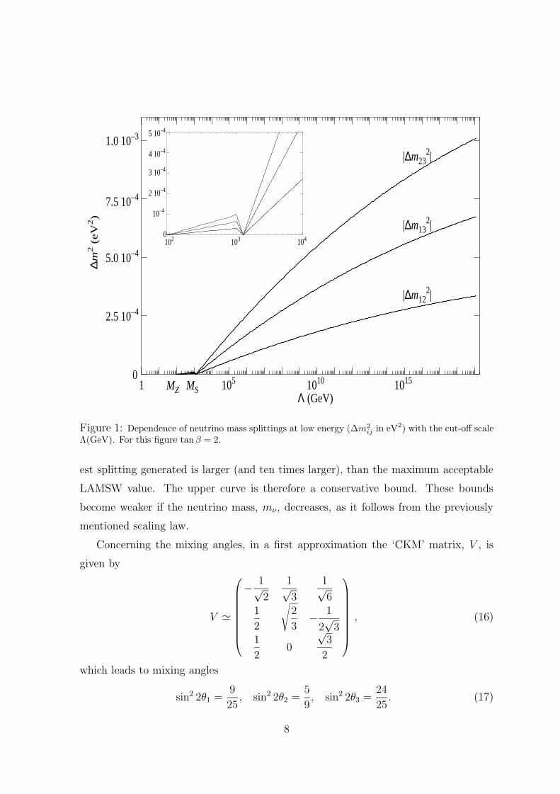
Fig.1 shows the complete numerical evaluation of the RGEs for mν = 2 eV and
tan β = 2, which corroborates the structure of eqs.(14, 15). The splittings are always
much larger than those required for the VO solution to the solar neutrino problem,
∆m2sol ∼ 10−10 eV2. Therefore, the effect of the RGEs for this scenario is disastrous
in the sense discussed in the Introduction for the possibility (ii). In consequence, as
for the pure SM case, the VO solution to the solar neutrino problem is excluded3. For
the LAMSW solution to the solar neutrino problem, things are a bit different. The
smallest mass splitting is always within (or not far larger than) the LAMSW range,
which indicates that we are in the situation (iii) explained in the Introduction (not
satisfactory, but it may be rescued by extra physics). When mν is varied the results
change with the scaling law ∆m2ij ∝ m2
ν .
The dependence of the splittings on tanβ is quite strong. Fig.2 shows this de-
pendence for Λ = 1010 GeV. Even for moderate values of tan β the smallest splitting
is much larger than the LAMSW range, thus spoiling that solution. Therefore, for a
given value of Λ and mν , the viability of the supersymmetric scenario of nearly degen-
erate neutrinos puts an upper bound on tanβ. A reasonable estimate for this upper
bound is given in Fig.3, which shows the value of tanβ (vs. Λ) for which the small-
3Notice from the figure and from eq.(15) that there is a value of Λ (close to MSUSY ) for which thesplittings vanish, but of course the fine-tuning required for Λ to be close enough to that point, so thatthe splittings are within the VO range, is enormous.
7
1 105 1010 1015MZ MSΛ (GeV)
∆m
2 (
eV
2)
0
2.5 10–4
5.0 10–4
7.5 10–4
1.0 10–3
|∆m232|
|∆m132|
|∆m122|
102 103 1040
10–4
2 10–4
3 10–4
4 10–4
5 10–4
Figure 1: Dependence of neutrino mass splittings at low energy (∆m2ij in eV2) with the cut-off scale
Λ(GeV). For this figure tanβ = 2.
est splitting generated is larger (and ten times larger), than the maximum acceptable
LAMSW value. The upper curve is therefore a conservative bound. These bounds
become weaker if the neutrino mass, mν , decreases, as it follows from the previously
mentioned scaling law.
Concerning the mixing angles, in a first approximation the ‘CKM’ matrix, V , is
given by
V '
− 1√2
1√3
1√6
1
2
√2
3− 1
2√
31
20
√3
2
, (16)
which leads to mixing angles
sin2 2θ1 =9
25, sin2 2θ2 =
5
9, sin2 2θ3 =
24
25. (17)
8

1 2 3 4 5 6 7 8 9 10tan β
0
0.002
0.004
0.006
0.008
0.01
0.012∆
m2 (
eV
2)
|∆m122|
|∆m132|
|∆m232|
Figure 2: Dependence of neutrino mass splittings at low energy (∆m2ij in eV2) with tanβ, for
Λ = 1010GeV.
These values are far away from the bimaximal mixing ones. In consequence, they are
not acceptable, stressing the fact that the simplified scenario discussed in this section
does not work. However, as explained in the Introduction, if extra effects are able to
modify the form of Mν in order to produce the correct splittings, this modification
will also change drastically the mixing angles, hopefully in a positive direction. This
leads us to the see-saw scenario, which is analyzed in the next section.
3 Mν from the see-saw mechanism
The simplest example of the kind of new physics appearing at a scale Λ which can
generate an effective mass term for the low-energy neutrinos we observe is the so-called
see-saw mechanism [15]. Its supersymmetric version has superpotential
W = WMSSM − 1
2νc
RMνcR + νc
RYνL ·H2, (18)
9

1 105 1010 10150
2
4
6
8
10
12
MSΛ (GeV)
tan β
∆m122=2 10–4 eV2
∆m122=2 10–3 eV2
Figure 3: Upper limit on tanβ, as a function of Λ, beyond which the smallest neutrino mass splittingis larger (lower curve), or ten times larger (upper curve), than the maximum acceptable LAMSW value.
where WMSSM is the superpotential of the MSSM. The extra terms involve three ad-
ditional neutrino chiral fields (one per generation; indices are suppressed) not charged
under the SM group: να,R (α = e, µ, τ). Yν is the matrix of neutrino Yukawa cou-
plings and H2 is the hypercharge +1/2 Higgs doublet. Now, the Dirac mass matrix is
mD = Yνv sin β. Finally, M is a 3 × 3 Majorana mass matrix which does not break
the SM gauge symmetry. It is natural to assume that the overall scale of M, which we
will denote by M , is much larger than the electroweak scale or any soft mass. Below
M the theory is governed by an effective superpotential
Weff = WMSSM +1
2(YνL ·H2)
TM−1(YνL ·H2), (19)
obtained by integrating out the heavy neutrino fields in (18). From this effective
superpotential, the Lagrangian contains a mass term for the left-handed neutrinos:
δL = −1
2νTMνν + h.c., (20)
10

with
Mν = mDTM−1mD = Yν
TM−1Yν〈H02 〉2, (21)
suppressed with respect to the typical fermion masses by the inverse power of the large
scale M .
The approximate degeneracy of neutrino masses in this framework follows from the
initial condition for the neutrino mass matrix at the Planck scale: Mν(Mp) = Mb,
which would lead to exactly degenerate neutrino masses. We do not address in this
paper the possible origin of this very symmetric form. As explained in [9], to explore
the simplest (and most natural) textures of Yν and M leading to this initial condition
it is enough to consider the case in which the Majorana mass matrix is
M = M
−1 0 00 1 00 0 1
, (22)
and all the structure is in the Yukawa matrix, which reads
Yν = YνBV Tb . (23)
Here Yν is the overall magnitude of Yν and B is a combination of two ‘boosts’
B =
cosh a 0 sinh a0 1 0
sinh a 0 cosh a
cosh b sinh b 0
sinh b cosh b 00 0 1
, (24)
with two free parameters a, b. Having all the structure in the Majorana matrix and
Yν ∝ I3 is equivalent to the case a = b = 0. We will present our results, for fixed
values of M and tanβ, in the (a, b) plane demanding |a|, |b| ≤ 1.5. If |a| or |b| are
larger than 1.5 the matrix elements of Yν are fine-tuned at least in a 10% [9].
The neutrino masses, exactly degenerate at tree-level by assumption, will receive
generation dependent radiative corrections which will lift that degeneracy, eventually
reproducing the pattern of mass splittings necessary to interpret the experimental in-
dications. The bulk of these radiative corrections is logarithmic and easy to compute
by standard renormalization group techniques: one starts at Mp with (22) and (23) as
boundary conditions and integrates down in energy the relevant RGEs in a supersym-
metric theory which is the MSSM with three right-handed neutrino chiral fields and
the superpotential (18). At the scale M the νR,α are decoupled and below this scale
11

the running is performed exactly as in the previous section, except that now we have
precise boundary conditions for the couplings and masses at M .
From Mp to M the evolution of the relevant matrices is governed by the following
renormalization group equations [16]:
dYν
dt= − 1
16π2Yν
[(3g2
2 +3
5g2
1 − T2
)I3 −
(3Yν
†Yν + Y†eYe
)], (25)
dYe
dt= − 1
16π2Ye
[(3g2
2 +9
5g2
1 − T1
)I3 −
(Yν
†Yν + 3Y†eYe
)], (26)
where
T1 = Tr(3Y†DYD + Y†
eYe), T2 = Tr(3Y†UYU + Y†
νYν), (27)
and
dMdt
=1
8π2
[M(YνYν
†)T + YνYν†M
], (28)
(not yet given in the literature). Here g2 and g1 are the SU(2)L and U(1)Y gauge
coupling constants, and YU,D,e are the Yukawa matrices for up quarks, down quarks
and charged leptons.
At M , νR decouple, and Ye must be diagonalized to redefine the flavour basis of
leptons [note that the last term in (26) produces non-diagonal contributions to Ye]
affecting the form of the Yν matrix. Then the effective mass matrix for the light
neutrinos is Mν ' YνTM−1Yν〈H0
2 〉2.From M to MZ , the effective mass matrix Mν is run down in energy exactly as
described in section 2.
The renormalization group equations are integrated with the following boundary
conditions: M and Yν are chosen at Mp so as to satisfy
Mν(Mp) = Mb, (29)
with the overall magnitude of Yν fixed, for a given value of the Majorana mass M , by
the requirement mν ∼ O(eV). We will take mν = 2 eV as a guiding example. The
boundary conditions for the other Yukawa couplings are also fixed at the low energy
side to give the observed fermion masses. The free parameters are therefore M, tanβ, a
and b.
12
3.1 Analytical integration of the RGEs
It is simple and very illuminating to integrate analytically the renormalization group
equations (11,25,26,28) in the approximation of constant right hand side. In this ap-
proximation (which works very well for our analysis), the effective neutrino mass matrix
at low-energy is simply Mb plus some small perturbation. The overall mass scale is
fixed to be of order 2 eV, so we need only to pay attention to the non-universal terms
in the RGEs, which will be responsible for the mass splittings. Neglecting the Ye, Yµ
Yukawa couplings, we get the following analytical expressions (the labelling of mass
eigenvalues below may not always correspond to the conventional order m2ν1
< m2ν2
,
|∆m212| < |∆m2
23|):mν1 ' mν [−1 + (2c2
ac2b − 1)εν − 2ετ ] ,
mν2,3 ' mν
[1 + 3ετ − c2
ac2bεν ±
{[ετ + (c2
ac2b − c2a)εν ]
2+[s2asbεν − 2
√2ετ
]2}1/2](30)
where ca = cosh a, s2a = sinh 2a, etc. These expressions are identical to the ones
derived in [9] for the SM case, except for the numerical values of ετ and εν , which are
now given by:
ετ =Y 2
τ
128π2
[−2 log
Mp
MSUSY
+ cos2 β logMSUSY
MZ
], (31)
εν =Y 2
ν
8π2log
Mp
M. (32)
The Yukawa couplings in these expressions should be chosen at an appropriate inter-
mediate scale but the simple formulas (31,32) are good enough for our purpose. Note
also that Yν and Yτ have an implicit dependence on tanβ and, furthermore Yν depends
strongly on M (due to the requirement mν ∼ 2 eV).
There are important differences with respect to the SM case presented in [9]: 1)
ετ is insensitive to the Majorana threshold, its sign is negative (it was positive in the
SM) and it grows in magnitude for increasing tan β; 2) εν is twice larger than in the
SM and decreases slightly when tanβ increases.
In the case a = b = 0, the mass splittings are independent of εν and similar to those
found in section 2, that is, not satisfactory (remember that this case is equivalent
to having all the structure in M, while Yν is proportional to the identity and thus
universal).
13
For a given M , there is a critical value of tanβ below (above) which |ετ | is smaller
(larger) than εν . This critical value of tanβ increases with M . When εν � |ετ |, we can
further expand the neutrino masses in powers of ετ/εν finding
mν1 ' mν [−1 + (2c2ac
2b − 1)εν − 2ετ ] ,
mν2 ' mν
[1− (2c2
ac2b − 1)εν +
(2− 1− c2a − 2
√2s2asb
c2ac
2b − 1
)ετ
],
mν3 ' mν
[1− εν +
(4 +
1− c2a − 2√
2s2asb
c2ac
2b − 1
)ετ
].
(33)
Here we clearly see that the small mass splitting (solar) is controlled by the small
parameter ετ , proportional to the squared Yukawa couplings of the charged leptons,
while εν (proportional to the square of the larger Yukawa coupling Yν) is responsible for
the larger mass difference (atmospheric). Moreover, the two neutrino eigenstates closest
in mass (mν1 , mν2) have masses of opposite sign, which is exactly what is required to
fulfill the neutrinoless double β-decay condition, eq.(7). In the SM case, for values of
M between 109 and 1012 GeV, ετ and εν have the right orders of magnitude to account
for ∆m2sol, ∆m2
at [9]. In the supersymmetric scenario it is still the case that εν gives the
correct atmospheric mass splitting, but for mν = 2 eV ετ gives typically a ∆m2sol one
order of magnitude too high (recall here that by lowering mν this splitting becomes
smaller following the approximate law ∆m2 ∝ m2ν). This means that in this case
only in particular regions of the (a, b) plane, in which some mild cancellation is taking
place, we will obtain the right mass splitting to solve the solar neutrino problem. This
cancellation does occur in regions around the lines a = 0 and 2√
2 sinh b = − tanh a for
which, in the approximation (33), m2ν1
= m2ν2
. In those regions then, we have a natural
explanation for the ∆m2sol mass splitting while ∆m2
at requires only a mild fine-tuning
of parameters.
If εν � |ετ |, then a different expansion shows that there is no natural hierarchy
of mass splittings, which tend to be of the same order. In these cases, a stronger
fine-tuning is required to get small enough ∆m2sol and the regions in parameter space
where this occurs shrink, again around 1− c2a − 2√
2s2asb = 0. However, ∆m2at is still
naturally of the right order of magnitude.
Turning to the mixing angles, it is easy to see that the eigenvectors of the perturbed
14
Mν matrix are of the form
V ′1 = V1, V ′
2 =1√
α2 + β2(αV2 + βV3), V ′
3 =1√
α2 + β2(−βV2 + αV3), (34)
where Vi are the eigenstates corresponding to the bimaximal mixing matrix, Vb [see
eq.(9)]
V1 =
−1√2
1
21
2
, V2 =
1√2
1
21
2
, V3 =
0−1√
21√2
. (35)
In the approximation |ετ | � εν , the parameters α, β are given by
α = casb +O(ετ/εν), β = sa +O(ετ/εν). (36)
The V ′i vectors define the new ‘CKM’ matrix V ′ from which the mixing angles are
extracted. In the case of interest, the spectrum of neutrinos consists of two lightest
states (mν1,2) very close in mass and a heavier one mν3 . The relative ordering in mass
of mν1,2 is not fixed and this affects the relative order of V ′1 and V ′
2 in the V ′ matrix.
This has an effect on the sign of cos 2θ3, which is important for the MSW condition
cos 2θ3 > 0 (written using the conventional order m2ν1
< m2ν2
). This will be satisfied as
long as V1 corresponds to the lightest mass eigenvalue. In other words, this condition
requires that the negative mass eigenvalue, see eqs.(30, 33), corresponds to the lightest
neutrino. On the other hand, the relative ordering of the two lightest neutrinos does
not change the values of sin2 2θi.
In this approximation, if just one of the two (a, b) parameters is vanishing, then
V ′ = Vb, i.e. exactly the bimaximal mixing case. Also, whenever ca, cb are sizeable
(i.e. away from a = b = 0), |α| � |β|, and thus we are close to the bimaximal case.
Therefore, it is not surprising that in most of the parameter space this will be in fact
the case. This is remarkable, because it gives a natural origin for the bimaximal mixing,
which was not guaranteed a priori due to the ambiguity in the diagonalization of the
initial Mν(Mp) = Mb matrix, as was explained in the Introduction.
The only free parameter in the V ′ matrix is the ratio α/β and one obtains the
relations:
sin2 2θ1 =(2r − 1)2
(2r + 1)2, sin2 2θ2 = 1− r2
(1 + r)2, sin2 2θ3 = 1− 1
(1 + 2r)2, (37)
15

0.00 0.25 0.50 0.75 1.000.00
0.25
0.50
0.75
1.00
Sin 2θ23
Sin 2
θ i2
Sin 22
Sin 2
1θ
2 θ 2
0.90 0.92 0.94 0.96 0.980.0
0.2
0.4
0.6
0.8
1.0
Sin 2θ23
Sin 2
θ i2
Sin 22
Sin 2
1θ
2θ2
1.00
Figure 4: Upper plot: Neutrino mixing angles, sin2 2θ1 and sin2 2θ2, vs. sin2 2θ3 in the near degen-erate scenario. Lower plot: Zoom of the 0.9 ≤ sin2 2θ3 ≤ 1 region.
where r ≡ α2/β2. It is instructive to invert the last relation, find r in terms of sin2 2θ3,
and then substitute back in the two previous relations.
Figures 4a,b present sin2 2θ1,2 as functions of sin2 2θ3 obtained in this way. For
clarity, figure 4b focuses on the region of sin2 2θ3 close to 1, which is the interesting one.
We can impose the experimental limits on these angles directly in this figure. We see
that the limit sin2 2θ2 < 0.64 (dashed line) translates into a lower limit sin2 2θ3>∼ 0.94
(the region to the left of the dashed line is forbidden). In a similar way, sin2 2θ1 > 0.82
(dotted lines) requires either sin2 2θ3 < 0.09 (but this solution gives sin2 2θ2 > 0.64 and
is not acceptable) or sin2 2θ3>∼ 0.9978 (the region to the right of the dotted line in figure
4b is allowed). Note that if we impose the stringent condition sin2 2θ3 < 0.99, derived
16

-1.5 -1 -0.5 0 0.5 1 1.5-1.5
-1
-0.5
0
0.5
1
1.5
b
a
-1.5 -1 -0.5 0 0.5 1 1.5-1.5
-1
-0.5
0
0.5
1
1.5
b
a
Figure 5: Left plot: contours of ∆m212/eV2 in the (b, a) plane from less than 10−5 (black area),
through 6×10⁻⁵ (lines) to more than 2×10⁻⁴ (grey). Right plot: same for ∆m223/eV2, from 5×10⁻⁴
(black) to 10−2 (grey). The Majorana mass is 1010 GeV and tan β = 2.
from some fits to solar data as discussed in the Introduction, then no viable solution
would exist. Without such condition we find that this framework can accomodate the
angles required by the data with
sin2 2θ1 ≥ 0.82, sin2 2θ2 ≤ 0.17, sin2 2θ3 ≥ 0.9978. (38)
Since, in first approximation, the perturbed Mν will have eigenvectors of the form
(34), this result and the previous discussion are also valid for the SM case [9] and any
model starting with Mν = Mb. Actually, the results shown in eq.(37) and Fig. 4 may
be considered as predictions of such a kind of scenarios.
In the next section we show that there are regions in parameter space where both
the mass splittings and the mixing angles have the right values to explain the solar and
atmospheric neutrino data.
17
-1.5 -1 -0.5 0 0.5 1 1.5-1.5
-1
-0.5
0
0.5
1
1.5
b
a
-1.5 -1 -0.5 0 0.5 1 1.5-1.5
-1
-0.5
0
0.5
1
1.5
b
a
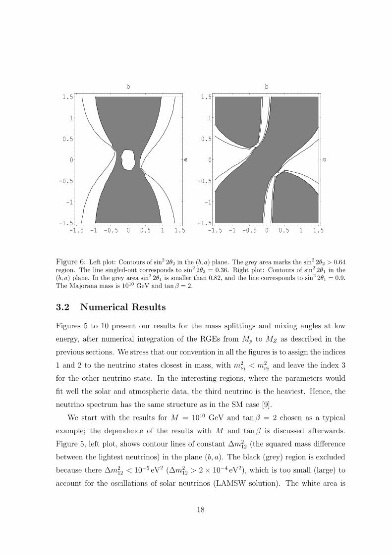
Figure 6: Left plot: Contours of sin2 2θ2 in the (b, a) plane. The grey area marks the sin2 2θ2 > 0.64region. The line singled-out corresponds to sin2 2θ2 = 0.36. Right plot: Contours of sin2 2θ1 in the(b, a) plane. In the grey area sin2 2θ1 is smaller than 0.82, and the line corresponds to sin2 2θ1 = 0.9.The Majorana mass is 1010 GeV and tan β = 2.
3.2 Numerical Results
Figures 5 to 10 present our results for the mass splittings and mixing angles at low
energy, after numerical integration of the RGEs from Mp to MZ as described in the
previous sections. We stress that our convention in all the figures is to assign the indices
1 and 2 to the neutrino states closest in mass, with m2ν1
< m2ν2
and leave the index 3
for the other neutrino state. In the interesting regions, where the parameters would
fit well the solar and atmospheric data, the third neutrino is the heaviest. Hence, the
neutrino spectrum has the same structure as in the SM case [9].
We start with the results for M = 1010 GeV and tan β = 2 chosen as a typical
example; the dependence of the results with M and tanβ is discussed afterwards.
Figure 5, left plot, shows contour lines of constant ∆m212 (the squared mass difference
between the lightest neutrinos) in the plane (b, a). The black (grey) region is excluded
because there ∆m212 < 10−5 eV2 (∆m2
12 > 2 × 10⁻⁴ eV2), which is too small (large) to
account for the oscillations of solar neutrinos (LAMSW solution). The white area is
18

thus the allowed region. The line in it corresponds to ∆m212 = 6 × 10⁻⁵ eV2. Note
how the allowed area is not too large and extends around the parametric line 1− c2a−2√
2s2asb = 0, as explained in the previous section.
Figure 5, right plot, gives contour lines of constant ∆m223. The black (grey) region
is excluded because there ∆m223 < 5 × 10⁻⁴ eV2 (∆m2
23 > 10−2 eV2), which is too
small (large) to account for the oscillations of atmospheric neutrinos. Again, the white
area is allowed. The small black areas correspond in fact to the “undecidable” case
discussed in the Introduction: they might be rescued by unspecified extra effects. We
do not present a plot for ∆m213 because it can always be inferred from ∆m2
23 and ∆m212.
Moreover, in the interesting case, ∆m212 � ∆m2
23, one has ∆m213 ' ∆m2
23.
The intersection of the white areas in both plots is non-zero and would give the
allowed area concerning mass splittings. It is always the case that the area surrounding
the origin is excluded. There, the mass differences are always of the same order, and
follow the same pattern discussed in section 2 (∆m223 = 2∆m2
12). In any case we
conclude that, away from the origin, there is a non-zero region of parameter space
where ∆m223 � ∆m2
12, in accordance with the values required to explain the solar and
atmospheric neutrino anomalies simultaneously.
For mixing angles, figure 6, left plot, gives contours of constant sin2 2θ2 (one of the
mixing angles relevant for atmospheric neutrino oscillations). The grey (white) area
has sin2 2θ2 larger (smaller) than 0.64 and is disfavored (favored) by the data (SK +
CHOOZ) at 99% C.L. according to the most recent analysis (last paper of ref. [10]).
The line singled-out corresponds to sin2 2θ2 = 0.36 (maximum allowed value at 90%
C.L. according to the same reference). Figure 6, right plot, shows contours of constant
sin2 2θ1 (the other mixing angle relevant for atmospheric neutrinos). The grey (white)
area corresponds to sin2 2θ1 smaller (larger) than 0.82, and is thus disallowed (allowed).
The additional line included has sin2 2θ1 = 0.9.
Finally, figure 7, left plot, presents contours of constant sin2 2θ3 which is relevant for
oscillations of solar neutrinos. The grey (white) region has sin2 2θ3 larger (smaller) than
0.99. If one is willing to interpret the existing data as implying an upper bound of 0.99
on sin2 2θ3, then the grey region would be excluded. The plotted curves give sin2 2θ3 =
0.95. Figure 7, right plot, shows the region of the parameter space accomplishing the
resonance condition (cos 2θ3 > 0), which is required for an efficient MSW solution of
the solar anomaly (see however the first paper of ref. [10] for caveats on this issue).
19

-1.5 -1 -0.5 0 0.5 1 1.5-1.5
-1
-0.5
0
0.5
1
1.5
b
a
-1.5 -1 -0.5 0 0.5 1 1.5-1.5
-1
-0.5
0
0.5
1
1.5
b
a
Figure 7: Left plot: Same as figure 6 for sin2 2θ3. The grey area corresponds to values above 0.99.The curves give sin2 2θ3 = 0.95. Right plot: The grey area corresponds to cos 2θ3 < 0
The region of parameter space where all constraints on mixing angles and mass
splittings are satisfied is given by the intersection of all white areas in figures 5, 6 and
7 (right plot). If sin2 2θ3 < 0.99 is imposed, then that intersection region, including
now figure 7 (left plot), is empty and no allowed region remains. It should be noticed
that this fact does not come from an incompatibility between the previous constraint
and the sin2 2θ3 > 0.99 obtained from neutrinoless double β-decay limits, eq. (7), in
the θ2 = 0 approximation. If this were the case, it could be easily solved by decreasing
the overall size of the neutrino masses, mν , in eq.(7), and this is not the case. Indeed,
eq.(7) is satisfied in nearly all the parameter space. Even where sin2 2θ3 < 0.99, this is
still true thanks to the contribution of θ2. What actually forbids the whole parameter
space if sin2 2θ3 < 0.99 is imposed is the incompatibility between acceptable θ1, θ2
and θ3 angles to fit simultaneously all the neutrino oscillation data, as can be seen
from the figures and in agreement with the discussion of the previous subsection, see
eq.(38). This fact remains when mν is decreased. In fact, the effect of decreasing mν is
essentially an amplification of the figures shown here, which comes from the fact that
for a given Majorana mass, the neutrino Yukawa couplings become smaller (the effect
20
-1.5 -1 -0.5 0 0.5 1 1.5-1.5
-1
-0.5
0
0.5
1
1.5
b
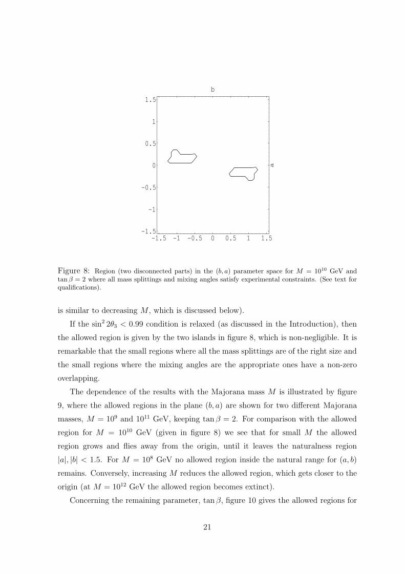
aFigure 8: Region (two disconnected parts) in the (b, a) parameter space for M = 1010 GeV andtan β = 2 where all mass splittings and mixing angles satisfy experimental constraints. (See text forqualifications).
is similar to decreasing M , which is discussed below).
If the sin2 2θ3 < 0.99 condition is relaxed (as discussed in the Introduction), then
the allowed region is given by the two islands in figure 8, which is non-negligible. It is
remarkable that the small regions where all the mass splittings are of the right size and
the small regions where the mixing angles are the appropriate ones have a non-zero
overlapping.
The dependence of the results with the Majorana mass M is illustrated by figure
9, where the allowed regions in the plane (b, a) are shown for two different Majorana
masses, M = 109 and 1011 GeV, keeping tan β = 2. For comparison with the allowed
region for M = 1010 GeV (given in figure 8) we see that for small M the allowed
region grows and flies away from the origin, until it leaves the naturalness region
|a|, |b| < 1.5. For M = 108 GeV no allowed region inside the natural range for (a, b)
remains. Conversely, increasing M reduces the allowed region, which gets closer to the
origin (at M = 1012 GeV the allowed region becomes extinct).
Concerning the remaining parameter, tanβ, figure 10 gives the allowed regions for
21

-1.5 -1 -0.5 0 0.5 1 1.5-1.5
-1
-0.5
0
0.5
1
1.5
b
a
-1.5 -1 -0.5 0 0.5 1 1.5-1.5
-1
-0.5
0
0.5
1
1.5
b
a
Figure 9:Same as figure 8 for tan β = 2 and different values of the Majorana mass. Left plot: M = 109 GeV;Right plot: 1011 GeV.
M = 1010 GeV and four different values of tan β: 1.75, 3, 4 and 6.5, as indicated.
The minimum in tan β is dictated by the requirement of perturbativity of all couplings
up to the Planck scale, banning the presence of a Landau pole below it, as discussed
in section 5. The allowed region gets smaller and smaller when tanβ increases. As
explained in the previous section, |ετ | grows with tanβ making harder and harder a
cancellation that gives the correct ∆m2sol and mixing angles. Eventually, for tan β >∼ 6.5
the allowed region disappears (for M = 1011 GeV that value is tan β >∼ 3.5).
Finally, let us stress that, if the sin2 2θ3 < 0.99 condition is imposed, the whole
parameter space becomes disallowed for any value of M and tan β. We also find that,
whenever there is a hierarchy in the mass splittings, the two lightest eigenvalues have
opposite signs. This is just what is needed to have a cancellation occurring in the
neutrinoless double β-decay constraint (7). This constraint is satisfied in almost the
whole parameter space for any M .
22

-1.5 -1 -0.5 0 0.5 1 1.5-1.5
-1
-0.5
0
0.5
1
1.5
b
a
-1.5 -1 -0.5 0 0.5 1 1.5-1.5
-1
-0.5
0
0.5
1
1.5
b
a
-1.5 -1 -0.5 0 0.5 1 1.5-1.5
-1
-0.5
0
0.5
1
1.5
b
a
-1.5 -1 -0.5 0 0.5 1 1.5-1.5
-1
-0.5
0
0.5
1
1.5
b
a
Figure 10:Same as figure 8 for M = 1010 GeV and different values of tan β. Upper left: tanβ = 1.75. Upperright: 3. Lower left: 4. Lower right: 6.5.
23
4 Examples of acceptable ansatze
It is possible to find examples of matrices Yν(Mp) which both fall inside the allowed
areas presented in the previous section and are natural (perhaps pointing to a possible
underlying symmetry).
An example, already presented in [9], which still survives in the supersymmetric
case (for M ∼ 1010 GeV and tanβ ∼ 2) is
Yν(Mp) = Yν
− 1
2√
21 1
1
2√
21 1
0 − 1√2
1√2
. (39)
It corresponds to a = 0 and b = sinh−1(3/4) ' 0.69. The mass splittings are
∆m212 ' 1× 10⁻⁴ eV2, ∆m2
13 ' 2× 10⁻³ eV2, ∆m223 ' 2× 10⁻³ eV2, (40)
and the mixing angles
sin2 2θ2 = 0.082, sin2 2θ1 = 0.9163, sin2 2θ3 = 0.99954, (41)
with cos 2θ3 at the border of the resonance condition for the MSW mechanism.
Another examples of working ansatze can be obtained. For instance, the following
ansatz (corresponding to a = − cosh−1(√
5/2) ' −0.48, b = log(√
10/2) ' 1.15 )
Yν(Mp) = Yν
−1
4
3√2
√2
1
2√
5
√5
2
√5
21
4√
5−√
5
20
, (42)
works correctly for M ∼ 109 GeV and tan β ∼ 2, giving
∆m212 ' 1× 10⁻⁴ eV2, ∆m2
13 ' 9× 10⁻⁴ eV2, ∆m223 ' 8× 10⁻⁴ eV2, (43)
and the mixing angles
sin2 2θ2 = 0.02, sin2 2θ1 = 0.979, sin2 2θ3 = 0.99997, (44)
with cos 2θ3 > 0. It could be interesting to explore possible symmetries that may be
responsible for the form of these ansatze and to analyze their implications for future
long-baseline experiments [18].
24
5 Other relevant implications of neutrino-induced
radiative corrections
The previous sections focussed on the possibility of reproducing the “observed” neu-
trino mass splittings from supersymmetric radiative corrections. In particular we ana-
lyzed the case of nearly degenerate neutrinos, which is closely related to the bimaximal
mixing scenario.
In this section, still working in a see-saw framework, we take a different point of
view and analyze the physical impact of neutrino-induced radiative corrections. The
results of this section are quite generic. They are not associated to the bimaximal
mixing scenario, not even to a scenario of degenerate neutrinos, but we will take this
case as a representative example to illustrate the phenomena. Some of the following
effects have already been mentioned along the paper, but here they are studied in
greater detail.
The first topic concerns the appearance of Landau poles associated to the neutrinos
and the corresponding implications. It is easy to check from eq.(25) that the neutrino
Yukawa couplings, Yν , have a supersymmetric RGE quite similar to the top Yukawa
coupling. It is therefore not surprising that they can develop Landau poles at high
energy in a similar way. Obviously, the larger the right-handed neutrino Majorana
mass, M , and the larger the low energy neutrino masses, mν , the larger the neutrino
Yukawa couplings, thus lowering the scale at which the Landau pole appears. Con-
sequently, if, in order to preserve perturbation theory (and the nice supersymmetric
gauge coupling unification), we demand that the Landau pole does not appear below
Mp (or the preferred high-energy scale), this puts upper bounds on M and mν (see
ref.[17] for the analogue in the SM framework).
To analyze this effect, we will use the simplest textures of Yν and M, leading to
a bimaximal mass matrix, namely Yν = YνI3 and M(Mp) ∝ Mb [M has exactly
the form given in eq.(8) but with overall scale M instead of mν ]. Recall that this is
equivalent to the case a = b = 0 in the analysis of textures performed in section 3.
Obviously, for a, b 6= 0 the neutrino Yukawa couplings are larger and the corresponding
bounds stronger. Hence, we are analyzing here the most conservative case
To extract the bounds, we set the Landau pole of Yν at Mp (i.e. Yν(Mp) � 1)
and evaluate the corresponding low energy value of mν , through the renormalization
25

1013 1014 1015
M (GeV)
0
1
2
3
mνIR
(eV
)
tan β = 2
tan β = 10
Figure 11: Upper bound on the neutrino mass, mIRν , vs. the Majorana mass M for two different
values of tan β.
group equations of Yν (between Mp and M) and κ (below M), for a certain value of the
Majorana mass M . This “infrared fixed point” value, say mIRν , represents an upper
bound for the neutrino mass. The dependence of mIRν on M is illustrated in Fig. 11
for two different values of tanβ (the value of M in the plot is to be understood as
evaluated at the M−scale itself). Alternatively, for a particular value of the neutrino
mass, mν , we can extract from the figure the upper bound on the Majorana mass.
We note that the bounds are quite strong. For quite moderate values of the neutrino
masses, they conflict with the possibility of a Majorana mass of O(MGUT ).
A different issue concerns the appearance of limits on tanβ. In section 2, it was shown
that the scenario of nearly degenerate neutrinos is in conflict with large values of tanβ,
the reason being that the radiative corrections to the mass splittings become much
larger than the observed ones. The bounds were shown in Fig.3, for mν = 2 eV. For
26
1010 1011 1012 1013
M (GeV)
1.4
1.45
1.5
1.55
tan β
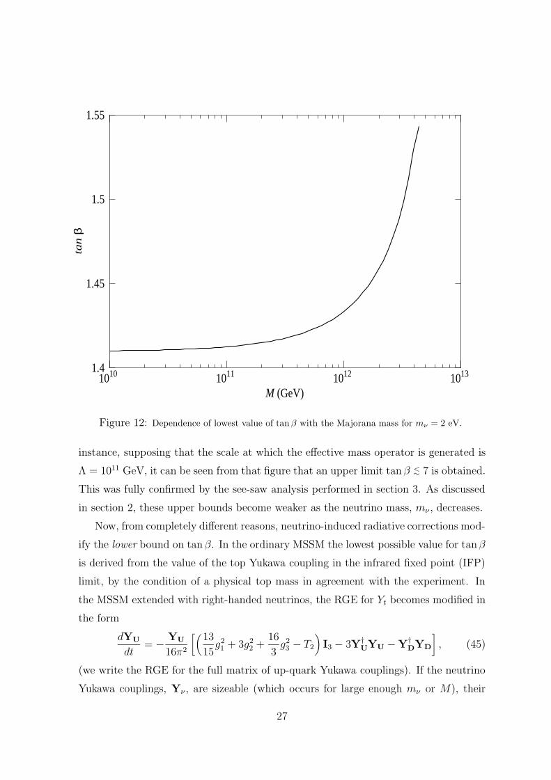
Figure 12: Dependence of lowest value of tanβ with the Majorana mass for mν = 2 eV.
instance, supposing that the scale at which the effective mass operator is generated is
Λ = 1011 GeV, it can be seen from that figure that an upper limit tanβ <∼ 7 is obtained.
This was fully confirmed by the see-saw analysis performed in section 3. As discussed
in section 2, these upper bounds become weaker as the neutrino mass, mν , decreases.
Now, from completely different reasons, neutrino-induced radiative corrections mod-
ify the lower bound on tanβ. In the ordinary MSSM the lowest possible value for tanβ
is derived from the value of the top Yukawa coupling in the infrared fixed point (IFP)
limit, by the condition of a physical top mass in agreement with the experiment. In
the MSSM extended with right-handed neutrinos, the RGE for Yt becomes modified in
the form
dYU
dt= − YU
16π2
[(13
15g21 + 3g2
2 +16
3g2
3 − T2
)I3 − 3Y†
UYU −Y†DYD
], (45)
(we write the RGE for the full matrix of up-quark Yukawa couplings). If the neutrino
Yukawa couplings, Yν , are sizeable (which occurs for large enough mν or M), their
27

contribution tends to lower the value of Yt further. In consequence, Yt(mtop) decreases
and the corresponding tan β increases. Fig. 12 shows the new lower bound on tanβ
for the typical case mν = 2 eV. Again, a diagonal structure for the neutrino Yukawa
matrix, Yν = YνI3, has been assumed for simplicity. It is important to realize that we
cannot raise the value of Yν arbitrarily, since then Yν develops a Landau pole below
Mp, as has been discussed in the previous subsection. This is the reason why the curve
shown stops abruptly. As can be seen from the figure (evaluated at the 1-loop level),
the change on tanβ is very modest, but it may give rise to an increment on the Higgs
mass of about 3 GeV, which should be taken into account for precision calculations.
From a more qualitative point of view, we would like to mention two important im-
plications of the presence of massive neutrinos for the supersymmetric perturbative
unification.
First, supersymmetric gauge coupling unification is considered as a brilliant success
of the MSSM, since the two-loop running of the SU(3)×SU(2)×U(1) gauge couplings
unifies with great precision at MGUT ∼ 2 × 10¹⁶ GeV. The unification, although re-
markable, is not perfect. It is usual to invoke unknown (GUT or superstring) threshold
effects in order to explain the discrepance. Since neutrino Yukawa couplings, Yν, give
a 2-loop contribution to the g1 and g2 gauge couplings (see e.g. [19]), for large enough
Yν (which means large mν and/or M) this may be useful for a complete satisfactory
unification.
Second, the Yν couplings have a 1-loop contribution to the charged lepton Yukawa
couplings, Ye, see eq.(26). Again, for large Yν, this produces significant variations for
Ye at low energy, affecting the perturbative bottom-tau unification. This subject has
been already addressed in the literature [20]. Due to the form of eq.(26), working in
the flavour basis for the charged leptons, the mass eigenvalues meireceive a correction
from Yν that, at first order, goes like ∆νm2ei∼ R m2
ei[Y†
νYν ]ii, where R is negative
and flavour-independent. Thus, at this order, the neutrino contribution to the mb/mτ
ratio goes always in the same sense for any Yν texture. For the (problematic) first two
families this means in particular that neutrinos are not useful to rescue the analogous
second generation (ms/mµ) ratio, since the correction goes in the wrong direction, but
they might be useful for the md/me ratio. In any case, non-trivial Yν textures will
have a significant impact on the supersymmetric mb/mτ unification scenarios.
28

6 Conclusions
We have studied the possibility that neutrinos masses have O(eV ), in order to be
cosmologically relevant. In that case they must be nearly degenerate, as required by
the oscillation interpretation of atmospheric and solar data. An important question is
whether radiative corrections have the right size to account for the small mass splittings
required or are generically too large for the scenario to be considered natural. We
addressed this problem in the context of the SM (plus three right-handed neutrinos) in
a previous publication [9] and, in this paper, we have extended this thorough analysis
to the supersymmetric case.
The size of the mass splittings that we find is always much larger than required
by the vacuum oscillation solution to the solar neutrino problem, solution which is
therefore excluded in this scenario.
When the origin of the non-zero neutrino masses is the see-saw mechanism (we
concentrate our study in this appealing case) we find non-negligible regions in param-
eter space where the mass splittings are consistent with the large angle MSW solution,
providing a natural origin for the ∆m2sol � ∆m2
atm hierarchy. These regions correspond
to Majorana masses around 1010 GeV and small tan β ∼ 2. Concerning the mixing
angles, they are remarkably stable and close to the bimaximal mixing form (something
that is not guaranteed a priory, due to an ambiguity in the diagonalization of the initial
matrix).
We have understood analytically the origin of these remarkable features, giving
explicit expressions for the mass splittings and the mixing angles. In particular, we
give simple analytical relations between the mixing angles, which are also valid for any
model starting with a bimaximal mixing form for the neutrinos. In addition, we have
presented particularly simple see-saw ansatze consistent with all atmospheric and solar
neutrino observations.
Let us remark that the viability of the scenario is very sensitive to a possible up-
per bound on sin2 2θ3 (the angle responsible for the solar neutrino oscillations). An
upper bound such as sin2 2θ3 < 0.99 would disallow completely the scenario of nearly
degenerate neutrinos due to the incompatibility between acceptable mixing angles to
fit simultaneously all the neutrino oscillation data. This incompatibility is also easily
understood from the analytical relations between the mixing angles, and thus is applies
29

also for the SM case and more generic models.
Finally we have described in some detail several implications of the existence of
(possibly large) neutrino Yukawa couplings. This includes the effects on: the trivial-
ity limits on the see-saw Majorana mass, the infrared fixed-point of the top yukawa
coupling, and the gauge and bottom-tau unification.
Acknowledgements
This research was supported in part by the CICYT (contract AEN95-0195) and the
European Union (contract CHRX-CT92-0004) (JAC). A.I. and I.N. thank the CERN
Theory Division for hospitality.
References
[1] Y. Fukuda et al., Super-Kamiokande Collaboration, Phys. Lett. B433 (1998)
9; Phys. Rev. Lett. 81 (1998) 1562; S. Hatakeyama et al., Kamiokande Collabora-
tion, Phys. Rev. Lett. 81 (1998) 2016; M. Ambrosio et al., MACRO Collaboration,
Phys. Lett. B434 (1998) 451.
[2] H. Georgi and S.L. Glashow, [hep-ph/9808293].
[3] F. Vissani, [hep-ph/9708483]; V. Barger, S. Pakvasa, T.J. Weiler and K. Whisnant,
Phys. Lett. B437 (1998) 107.
[4] C. Giunti, Phys. Rev. D59:077301 (1999).
[5] C.D. Carone and M. Sher, Phys. Lett. B420 (1998) 83; A.S. Joshipura,
Z. Phys. C64 (1994) 31; A. Ioannisian and J.W.F. Valle, Phys. Lett. B332 (1994)
93; D. Caldwell and R.N. Mohapatra, Phys. Rev. D48 (1993) 3259; G.K. Leon-
taris, S. Lola, C. Scheich and J.D. Vergados, Phys. Rev. D53 (1996) 6381; S. Lola
and J.D. Vergados, Prog. Part. Nucl. Phys. 40 (98) 71; B.C. Allanach, [hep-
ph/9806294]; A.J. Baltz, A.S. Goldhaber and M. Goldhaber, Phys. Rev. Lett. 81
(1998) 5730; R.N. Mohapatra and S. Nussinov, Phys. Lett. B441 (1998) 299 and
[hep-ph/9809415]; C. Jarlskog, M. Matsuda and S. Skadhauge, [hep-ph/9812282];
Y. Nomura and T. Yanagida, Phys. Rev. D59:017303 (1999); S.K. Kang
and C.S. Kim, Phys. Rev. D59:091302 (1999); S. Davidson and S. King,
30

Phys. Lett. B445 (1998) 191; H. Fritzsch and Z. Xing, Phys. Lett. B440 (1998)
313 and [hep-ph/9903499]; M. Tanimoto, Phys. Rev. D59:017304 (1998); N.
Haba, Phys. Rev. D59:035011 (1999); Yue-Liang Wu, [hep-ph/9901245]; E. Ma,
[hep-ph/9812344] and [hep-ph/9902465]; E.M. Lipmanov, [hep-ph/9901316];
T. Ohlsson and H. Snellman, [hep-ph/9903252]; A.H. Guth, L. Randall and
M. Serna, [hep-ph/9903464]; G.C. Branco, M.N. Rebelo and J.I. Silva-Marcos,
Phys. Rev. Lett 82 (1999) 683; Y.-L. Wu., [hep-ph/990522].
[6] J. Ellis and S. Lola, [hep-ph/9904279].
[7] C.S. Aulakh and R.N. Mohapatra, Phys. Lett. B119 (1982) 136; Phys. Lett. B121
(1982) 147; L.J. Hall and M. Suzuki, Nucl. Phys. B231 (1984) 419.
[8] C.S. Aulakh, A. Melfo, A. Rasin and G. Senjanovic, [hep-ph/9902409].
[9] J.A. Casas, J.R. Espinosa, A. Ibarra and I. Navarro, [hep-ph/9904395].
[10] R. Barbieri et al., JHEP 9812 (1998) 017; G.L. Fogli, E. Lisi, A. Marrone and
G. Scioscia, Phys. Rev. D59:033001 (1999), [hep-ph/9904465].
[11] L. Baudis et al., Heidelberg-Moscow exp., [hep-ex/9902014].
[12] V. Lobashev, Pontecorvo Prize lecture at the JINR, Dubna, January 1999; A.I. Be-
lesev et al., Phys. Lett. B350 (1995) 263.
[13] Y. L. Wu, [hep-ph/9810491], [hep-ph/9901245] and [hep-ph/9901320]; C. Wet-
terich, [hep-ph/9812426]; R. Barbieri, L.J. Hall, G.L. Kane, and G.G. Ross, [hep-
ph/9901228]; M. Tanimoto, T. Watari, T. Yanagida, [hep-ph/9904338].
[14] K. Babu, C. N. Leung and J. Pantaleone, Phys. Lett. B319 (1993) 191.
[15] M. Gell-Mann, P. Ramond and R. Slansky, proceedings of the Supergravity Stony
Brook Workshop, New York, 1979, eds. P. Van Nieuwenhuizen and D. Freedman
(North-Holland, Amsterdam); T. Yanagida, proceedings of the Workshop on Uni-
fied Theories and Baryon Number in the Universe, Tsukuba, Japan 1979 (edited
by A. Sawada and A. Sugamoto, KEK Report No. 79-18, Tsukuba); R. Mohapatra
and G. Senjanovic, Phys. Rev. Lett. 44 (1980) 912, Phys. Rev. D23 (1981) 165.
[16] N. Haba, N. Okamura and M. Sugiura, [hep-ph/9810471], [hep-ph/9904292]
31
[17] J.A. Casas, V. Di Clemente, A. Ibarra and M. Quiros, [hep-ph/9904295].
[18] A. De Rujula, M.B.Gavela and P. Hernandez, [hep-ph/9811390].
[19] Yu.F. Pirogov, O. V. Zenin, [hep-ph/9808396].
[20] F. Vissani and A. Yu. Smirnov, Phys. Lett. B341 (1994) 173; A. Brignole, H.
Murayama and R. Rattazzi, Phys. Lett. B335 (1994) 345; G. K. Leontaris, S.
Lola, G. G. Ross, Nucl. Phys. B454 (1995) 25; M. Bando and K. Yoshioka,
Phys. Lett. B444 (1998) 373.
32