Degenerate Bose Gases: Tuning Interactions & Geometry

Degenerate BoseGases: Tuning Interactions &

Geometry

Alexander Lloyd GauntTrinity College, October 2014

A dissertation submitted for thedegree of Doctor of Philosophy

Cavendish Laboratory

Declaration

I declare that this thesis is my own work and is not substan-tially the same as any that I have submitted or am currentlysubmitting for a degree, diploma or any other qualificationat any other university. No part of this thesis has alreadybeen or is being concurrently submitted for any such de-gree, diploma or any other qualification. This thesis doesnot exceed the word limit of sixty thousand words, includingtables, footnotes, bibliography and appendices, set out bythe Faculty of Physics and Chemistry.

2014 Alex Gaunt

Cavendish LaboratoryUniversity of CambridgeJ J Thomson AvenueCambridge CB3 0HEUK

ii

Abstract

This thesis describes experiments carried out on a dilute cloud of Bosonic atomscooled to quantum degeneracy. It is divided into two parts: Part I describes ex-periments in which we tune the inter-particle interactions to explore the system’sdynamics in both weakly and strongly interacting limits. Part II describes noveloptical trapping geometries for cold atomic gases, with an emphasis on the first everrealisation of an atomic Bose-Einstein condensate in a uniform potential.

Part I employs a method in which inter-particle interactions in a nanokelvin gas of39K atoms are tuned via a Feshbach resonance. Using this technique we explorethe non-equilibrium dynamics of a weakly interacting Bose-condensed gas in adissipative system. The highlight of this study is the observation of a “superheated”Bose-Einstein condensate persisting at temperatures up to 1.5 times higher thanthe equilibrium critical temperature. In a second study, we investigate the oppositeregime of maximal interaction strength (the “unitary” regime). Here we experimentallydemonstrate scaling laws governing the dynamics of clouds undergoing atom lossand heating by multi-particle collisions.

In Part II, we demonstrate holographic techniques for shaping laser beams to producenew atom trap geometries. We concentrate on the theoretically important andexperimentally novel uniform geometry and review our first experiments performedin this system. In equilibrium we study both the thermodynamics of a homogeneous87Rb gas held in our novel trap and perform spectroscopic measurements of itsground-state. In a dynamical study we investigate the coherence properties of aBose-Einstein condensate formed after a rapid thermal quench of a homogeneousgas. We observe Kibble-Zurek dynamics following this quench, and are able makethe first measurement of the dynamical critical exponent for the 3D Bose-Einsteincondensation transition using our homogeneous system.

iii

Acknowledgements

“Writing is difficult: only some people are good at it.” This diplomatic phrase positedby a wise man rings in my ears as I struggle to eloquently pen my heartfelt gratitudeto the people who have supported me over the last three years. My Ph.D. has taughtme that where the pen can stutter, the keyboard can triumph. Therefore I will attemptto forego the unfamiliar world of vocabulary, sentence structure and punctuation bydistilling my gratitude into a more manageable Excel bar chart.

Fig. 0.1 shows the average flux of emails that I received from contemporaneous labmembers normalised to a reference flux from my wife, Beth. This bar chart providesa good starting point for objectively dividing my acknowledgements among the keycharacters who helped me with the work presented in this thesis1.

Fig. 0.1.: Normalised email flux from lab members. We count the total number of emails receivedfrom each lab member and divide by the overlap time with my Ph.D. For reference, theresulting fluxes are normalised to that from my wife, Beth.

Zoran’s unerring dedication and enthusiasm irrefutably shines out of Fig. 0.1. As mysupervisor, his active influence and impact on every aspect of the lab’s progress isexemplified by the only score greater than unity. An analysis of the length and depthof the emails is beyond the scope of this thesis, but I am certain that Zoran would

1In my analysis of this data I will mitigate any potential offense by mentioning systematic errorsarising from the use of email volume as a metric for gratitude.

v

again claim victory in these statistics. There is nothing more reassuring for a Ph.D.student than knowing that your supervisor is always available with deeply insightfulcomments on the experiments. Furthermore, Zoran has gone out of his way tosupport the progress of my career and I am truly grateful to Zoran for everythingthat he has done to help me over the years.

The next highest bars in Fig. 0.1 are the postdocs, Rob Smith and Nir Navon, whowere directly involved in the experiments presented in this thesis. Rob’s contributionis vastly under-represented in Fig. 0.1. As a man of quiet brilliance, he exemplifiesthe systematic problem with the email metric. His uncanny ability to understandeverything and make anything work, has been pivotal to every success in this thesis.Nir has injected great enthusiasm and “rock and roll” into the lab. As one of the mostbadass physicists in the group, he played an essential role in the uniform-systemexperiments, and was a key antagonist in the on-going dialogue concerning thequality of my software, PIDs, and general persona.

I have been proud to be part of a motley band of Ph.D. students alongside RichardFletcher, Tobias Schmidutz and Igor Gotlibovych. Rich formed part of the originalDream Team and many happy nights were spent watching cartoons as we super-heated some BECs. A lot of thanks have to go to Tobias and Igor (as a strong butsilent type, Igor’s contribution is again underestimated by the email tally). Theirmonths of hard work (including an unfortunate incident involving my laser and adrill) meant that I could hit the ground running in Part II of this thesis. Thanks alsogo to the former members of the lab, Naaman Tammuz, Robbie Campbell, StuartMoulder and Scott Beattie who built the machine used in Part I of this thesis.

Aziza Suleymanzade and Martin Robert-de-Saint-Vincent have been busy workingon experiments which are not covered in this thesis, but their presence has completedthe daily life that I have enjoyed in the group. Regardless of experimental allocation,all group members (including the Ghost) are bonded by TheQuiz, and it has been apleasure to MC TheQuiz for such an enthusiastic bunch of budding historians.

Finally, even though “working from home doesn’t count”, I have been supportedoutside the lab by my parents, Mary and Stephen, my siblings, Jo and Steph andmy wife Beth. Beth’s contribution to this work is difficult to overstate. Withouther concern for my well-being, I would have rapidly devolved into a cave-dwellingcreature surviving solely on Cherryade and prawn cocktail crisps. Her unerringoptimism that I will one day share her delight in a picturesque sunset or a brightrainbow and her contagious enthusiasm for life infinitely brighten up my life outsidethe lab. I am truly grateful to her for being my companion through everything.

Contents

Outline 1

I Tuneable Interactions 5

1 Introduction 71.1 Tuneable s-wave scattering . . . . . . . . . . . . . . . . . . . . . . . 71.2 Producing 39K condensates . . . . . . . . . . . . . . . . . . . . . . . 111.3 Extreme interactions . . . . . . . . . . . . . . . . . . . . . . . . . . . 12

2 A Superheated Bose-condensed Gas 152.1 Qualitative picture . . . . . . . . . . . . . . . . . . . . . . . . . . . . 162.2 Experimental procedure . . . . . . . . . . . . . . . . . . . . . . . . . 202.3 Experimentally measuring chemical potentials . . . . . . . . . . . . . 212.4 Observation of a superheated state . . . . . . . . . . . . . . . . . . . 282.5 Dynamical model of superheating . . . . . . . . . . . . . . . . . . . . 312.6 Limits of superheating . . . . . . . . . . . . . . . . . . . . . . . . . . 362.7 Conclusion . . . . . . . . . . . . . . . . . . . . . . . . . . . . . . . . 38

3 Stability of a Unitary Bose Gas 393.1 Can a unitary bose gas be stable at degeneracy? . . . . . . . . . . . 413.2 Scaling Law 1: NT β = const. . . . . . . . . . . . . . . . . . . . . . . 433.3 Scaling Law 2: L3 ∝ 1/T 2 at unitarity . . . . . . . . . . . . . . . . . . 503.4 Extraction of the rate parameter ζ . . . . . . . . . . . . . . . . . . . . 513.5 Conclusion . . . . . . . . . . . . . . . . . . . . . . . . . . . . . . . . 53

II Trap Geometry 55

4 Introduction 574.1 Atom-light interactions . . . . . . . . . . . . . . . . . . . . . . . . . . 584.2 Outline . . . . . . . . . . . . . . . . . . . . . . . . . . . . . . . . . . . 63

5 Robust Digital Holography for Ultracold Atom Trapping 655.1 Digital holography . . . . . . . . . . . . . . . . . . . . . . . . . . . . 665.2 Vector-holography . . . . . . . . . . . . . . . . . . . . . . . . . . . . 685.3 Raster-holography . . . . . . . . . . . . . . . . . . . . . . . . . . . . 725.4 Conclusion . . . . . . . . . . . . . . . . . . . . . . . . . . . . . . . . 75

vii

6 Bose-Einstein Condensation of Atoms in a Uniform Potential 776.1 Building an optical box . . . . . . . . . . . . . . . . . . . . . . . . . . 786.2 First realisation with atoms . . . . . . . . . . . . . . . . . . . . . . . 866.3 Conclusion . . . . . . . . . . . . . . . . . . . . . . . . . . . . . . . . 96

7 Observing Equilibrium Properties of a Homogeneous Bose Gas 977.1 Thermodynamic experiments . . . . . . . . . . . . . . . . . . . . . . 977.2 Ground state measurements . . . . . . . . . . . . . . . . . . . . . . 1057.3 Conclusion . . . . . . . . . . . . . . . . . . . . . . . . . . . . . . . . 115

8 Critical Dynamics of Spontaneous Symmetry Breaking in a Homoge-neous Bose gas 1178.1 Domain size in Kibble-Zurek theory . . . . . . . . . . . . . . . . . . . 1188.2 Quantitative measurement of domain sizes . . . . . . . . . . . . . . 1228.3 Direct observation of Kibble-Zurek freeze-out . . . . . . . . . . . . . 1318.4 Kibble-Zurek scaling and universal critical exponents . . . . . . . . . 1368.5 Conclusion . . . . . . . . . . . . . . . . . . . . . . . . . . . . . . . . 138

9 Conclusions and Outlook 1399.1 Thermodynamics with tuneable interactions . . . . . . . . . . . . . . 1399.2 Kibble-Zurek with tuneable interactions . . . . . . . . . . . . . . . . . 1409.3 Interferometry . . . . . . . . . . . . . . . . . . . . . . . . . . . . . . . 140

Appendices 145

A Experimental Sequence Overview 147A.1 Rubidium-87 D2 Lines . . . . . . . . . . . . . . . . . . . . . . . . . . 147

B Raster Holography 151B.1 MRAF: Mixed-region amplitude freedom . . . . . . . . . . . . . . . . 151B.2 Optical vortices . . . . . . . . . . . . . . . . . . . . . . . . . . . . . . 152B.3 Experimental realisation with laser light . . . . . . . . . . . . . . . . 154B.4 Fourier vs Helmholtz . . . . . . . . . . . . . . . . . . . . . . . . . . . 155

C Graphics Card Acceleration of Computations for Ultracold Atom Ex-periments 159C.1 Image processing: AnalysisGpUI . . . . . . . . . . . . . . . . . . . . 160C.2 Physical simulation: EvolveGPuE . . . . . . . . . . . . . . . . . . . . 162

D Numerical Simulation of Kibble-Zurek Dynamics 167D.1 Dynamical evolution of ξ . . . . . . . . . . . . . . . . . . . . . . . . . 167D.2 Simulation results . . . . . . . . . . . . . . . . . . . . . . . . . . . . . 169

Bibliography 173

Outline

Single atoms are well understood quantum objects. However, when a macroscopicnumber of interacting atoms come together, an exact treatment of the ensemble canbecome impossible. The fundamental difficulty with many-body quantum mechan-ics stems from the exponential scaling of the system’s Hilbert space with particlenumber2. Some analytical and computational methods such as the mean-field ap-proximation or Monte-Carlo techniques allow us to probe weakly interacting systems.However, strongly interacting many-body systems are at the heart of many of themost fascinating and least understood phenomena in modern physics, ranging fromhigh temperature superconductivity and superfluidity to exotic forms of magnetism.Moreover, we are often interested in dynamical effects in out-of-equilibrium systems,which can again be difficult to describe exactly with theory.

One fruitful approach to understand many-body quantum systems is to use experi-mental rather than theoretical simulations, as envisioned by Feynmann in 1982 [1,2].This is the route persued here, where we use an experimental simulator basedon an ultracold atomic gas cloud. A "quantum simulator" is simply a very cleanquantum system which is easily accessed and tuned in the laboratory. The dynamicand static properties of our simulator are defined by a many-body Hamiltonian overwhich we have excellent control. By observing the behaviour of our simulation aswe tune the parameters of the Hamiltonian, we can probe the many-body physics ofour system, and any other quantum system described by the same Hamiltonian.

At the core of our experimental simulator is a dilute gas of ultracold Bosonic atoms.In Einstein’s textbook picture of a 3D Bose gas (discussed in detail in chapter 7),this system undergoes a phase transition to form a Bose-Einstein condensate (BEC)at the critical point nλ3

T ≈ 2.612, where n is the atom density and λT is the thermal

2The intractability of macroscopic quantum systems is best exemplified by trying to write down anexact description of a state, even before we start to tackle any evolution. Whereas in the classicalcase, recording the 3D position and velocity of N particles requires only 6N real numbers, to write thestate vector for a quantum system containing N distinguishable particles occupyingM levels in anarbitrary superposition requiresMN complex numbers. Computationally, if we have 1 GB of computerRAM, this means we can store a classical state containing N ∼ 107 particles, but only the state ofN ≈ 26 particles in the simplestM = 2 level system.

1

wavelength3. Below the critical temperature, the characteristic wavepacket size, λT ,is larger than the interparticle spacing, n−1/3, meaning quantum effects dominateand our simulator probes many body quantum mechanics.

In general, the anatomy of a many-body Hamiltonian, H, to be simulated in ourexperimens is as follows:

H = HKin︸︷︷︸Kinetic

energy

+ HInt︸︷︷︸Interaction

energy

+ HPot︸︷︷︸Potential

energy

. (0.1)

An essential property of a useful quantum simulator is the ability to implement customHamiltonians, H in the lab. Dilute atomic gases fulfil this requirement because theresponse of the individual atoms to electromagnetic fields is well understood. Thisallows us to use a toolbox of magnetic and optical techniques to synthesise tailoredHamiltonians, and for a dilute Bose gas, any of the three terms in Eq. 0.1 can beexperimentally tuned4. This thesis describes techniques for tuning the last two termsin Eq. 0.1: the interaction term, HInt, and the potential term, HPot. We then explorethe phenomenon of Bose-Einstein condensation in the unconventional Hamiltoniansthat we produce. The thesis is divided into two parts, each of which concentrateson tuning one term, as summarised below.

Interactions Potential Geometry Species

Part I Tuneable Traditional harmonic 39K

Part II Fixed Uniform 87Rb

Outlook Tuneable Uniform 39K

Tab. 0.1.: Summary of the emphasis throughout the thesis. A different machine is used for each partwith specialisations to handle new interaction regimes or geometries. In the outlook section,we briefly comment on the prospect of a new machine which combines these researchstrands.

Part I: HInt - Tuneable interactions

Since the presence of inter-particle interactions poses many theoretical difficultiesin many body quantum physics, it is extremely useful to experimentally tune theinteractions and empirically explore the resulting physics. The ability to tune inter-particle interactions in ultracold gases is unparalleled in other systems, and the firsthalf of this thesis will be dedicated to exploring Bose gases in the two extremes of

3The ideal value 2.612 is modified slightly in finite-size and interacting systems [3,4]4The kinetic energy term is not strictly tuneable, however using synthetic gauge fields [5–7], or by

trapping the atoms in a lattice, we can modify the dispersion relation of our Bose gas.

2

interaction strength: In chapter 2, we will explore a very weakly interacting system,and demonstrate a novel non-equilibrium state of a “superheated Bose condensedgas". In chapter 3, we study the opposite limit where the interaction strength is themaximum allowed by quantum mechanics. This strong coupling limit is particularlyinteresting because the behaviour of the system ceases to depend on the nature ofthe interactions and universal behaviour emerges.

Part II: HPot - Flexible geometries

Perhaps the most intuitive term to change in the Hamiltonian is HPot. The geometryof the potential energy landscape can play a key role in the physics displayed bya system. By sculpting appropriate potentials for our atoms, we can create racetracks for superfluids [8–10], lattices to model solid-state materials [11–13], andmany other interesting geometries. In chapter 5, we present two very versatileoptical methods for creating custom atom traps, and demonstrate experimentalrealisation of high-quality, intricate trapping potentials using these techniques.The development of this optical toolbox inspired us to create one of the mostlong-sought, and theoretically simplest, potentials: a homogeneous box potential.This potential is abundant in theoretical work because it often offers the simplestunderstanding of many-body phenomena, and is appropriate for describing severalnaturally occuring many-body systems. However, this potential is difficult toachieve in experiments with atomic gases. In chapter 6, we overcome thesedifficulties and present the first realisation of an atomic BEC in a three-dimensionalhomogeneous potential, and in chapters 7 and 8 we outline the first equilibrium anddynamical results from the fruitful research paths that our uniform trap has opened up.

3

The following publications are derived from work presented in this thesis:

Part I

Chapter 2 A Superheated Bose-condensed GasA. L. Gaunt∗, R. J. Fletcher∗, R. P. Smith and Z. Hadzibabic

Nature Phys. 9, 271-274 (2013).

Chapter 3 Stability of a Unitary Bose GasR. J. Fletcher, A. L. Gaunt, N. Navon, R. P. Smith and Z. Hadzibabic

Phys. Rev. Lett. 111, 125303 (2013).

Part II

Chapter 5 Robust Digital Holography For Ultracold Atom TrappingA. L. Gaunt and Z. Hadzibabic

Sci. Rep. 2, 721 (2012).

Chapter 6 Bose-Einstein Condensation of Atoms in a Uniform PotentialA. L. Gaunt, T. F. Schmidutz, I. Gotlibovych, R. P. Smith, and Z. Hadzibabic

Phys. Rev. Lett. 110, 200406 (2013).

Chapter 7 Quantum Joule-Thomson Effect in a Saturated Homogeneous BoseGasT. F. Schmidutz, I. Gotlibovych, A. L. Gaunt, R. P. Smith, N. Navon and Z.Hadzibabic

Phys. Rev. Lett. 112, 040403 (2014).

Chapter 7 Observing properties of an interacting homogeneous Bose-Einsteincondensate: Heisenberg-limited momentum spread, interaction energy,and free-expansion dynamicsI. Gotlibovych, T. F. Schmidutz, A. L. Gaunt, N. Navon, R. P. Smith, and Z.Hadzibabic

Phys. Rev. A 89, 061604(R) (2014).

Chapter 8 Critical Dynamics of Spontaneous Symmetry Breaking in a Homoge-neous Bose gasN. Navon∗, A. L. Gaunt∗, R. P. Smith, and Z. Hadzibabic

Science (in press) (2015).

4

Part I

Tuneable Interactions

1Introduction

Ultracold atoms, and in particular BECs of atoms, give us a unique opportunity toexperimentally access many-body physics in different limits of inter-partical interac-tion strength. The ability to continuously tune the interaction strength makes coldatom systems both insightful simulators of less accessible quantum systems, andalso interesting quantum systems in their own right.

Chapters 2 and 3 will separately detail our experiments exploring two oppositeregimes of very weak and very strong interactions. Throughout these chapterswe attempt to highlight novel physical phenomena without reviewing an unduevolume of background theory. In particular, an understanding of standard methodsof laser and evaporative cooling [14] is not required to understand the results inthese chapters (the novel stages of the experiments start after a degenerate cloudhas been prepared). Therefore we have attempted to limit the discussion of thecooling stage of the experiment into section 1.2 and Fig. 1.2. An short pictorialsynopsis of the basic steps for laser cooling can also be found in Appendix A.

Aside from the cooling process, another textbook concept, which underpins the novelaspects of these experiments, is the phenomenon of Feshbach resonances. Thisphenomenon provides the mechanism by which we tune the inter-atomic interactions.Since this is of central importance in our work, we devote a short section below tooutlining the basic theory of inter-atomic interactions and Feshbach resonances.

1.1 Tuneable s-wave scattering

In order to understand Feshbach resonances, we must first clarify exactly what wemean by "inter-atomic interactions". Below, we briefly describe how the potentiallycomplex process of one atom scattering off another can be entirely characterised bya single parameter known as the s-wave scattering length, a. We then move on todescribe how a Feshbach resonance can be used to tune a.

1.1.1 s-wave scattering

One could set about the daunting task of writing down a very detailed microscopicmodel for the the Van derWaals interaction between neutral bosonic atoms. However,

7

we often work in the dilute regimewhere the typical length scale, rint, of the interactionpotential is much smaller than the other length scales in the gas (namely the meandistance between atoms, n−1/3, and the thermal wavelength, λT ). This meansthat the microscopic properties of the interaction potentials are largely irrelevantfor describing physical phenomena in an ensemble. In this section, we outline thestandard formalism which coarse-grains these microscopic details into a singleparameter [3,15,16].

The first step of this formalism is to solve the Schrödinger equation, (∇2 + k2)ψ =2mrV (r)

~2 ψ, in relative coordinates, r, for the wavefunction ψ describing the relativemotion of two colliding particles with energy E and reduced mass mr in a generalinteraction potential, V (note that we have defined k =

√2mrE/~2). Using the

Green’s function for the Helmholtz operator (∇2 + k2), and applying the first orderBorn approximation, the solution is as follows1:

ψ(r) ≈ φk(r)︸︷︷︸incident

+eikr

r

f(k)︷︸︸︷[− mr

2π~2

∫e−ikr·r

′V (r′)φk(r′) d3r′

]︸︷︷︸

scattered

, (1.1)

where φk = eik·r is the particles’ wavefunction before the scattering event andr = r/|r|. We can now make the following simplifications:

• The angular momentum of a pair of atoms colliding with impact parameter Ris hR/λdB where λdB is the deBroglie wavelength associated with the relativemotion. In a thermal ensemble at temperature T , we write λdB ∼ λT , whereλT is the thermal wavelength of the atoms. At degeneracy, λT ∼ n−1/3, andfor the colliding particles to interact, we require R < rint. Since we assumerint n−1/3, we conclude that hR/λdB h, and thus that the collidingpair’s angular momentum is small [14]. This means that the amplitude of thescattered spherical wave must be a function, f(k), with no angular dependence.This limit is known as the s-wave scattering limit, with higher order angularterms only significant for clouds at kBT > ~2/2mr2

int ∼ kB × 100µK.

For k → 0, we can expand 1/f(k) = −1/a+ bk +O(k2), with suitable coeffi-cients a and b. In the simplest case (|ka| 1), we take f(k) = −a, therebyreducing the entire scattering problem to the single parameter, a, known as the

1To see this qualitatively, note that the Schrödinger equation is identical to the optical Helmholtzequation with a source term ∝ V ψ. By analogy with Huygens’ wavelets and Fraunhofer diffraction,we quote that the far-field solution to this Schrödinger equation is a spherical wave with amplitudeproportional to the Fourier transform of this source term. Since the source term explicitly contains ψitself, we use the first order Born approximation, ψ ≈ φk to obtain Eq. 1.1.

8 Chapter 1 Introduction

“s-wave scattering length". We will return to the second term in this expansionin chapter 3.

• Eq. 1.1 states that the amplitude of the scattered wave is proportional to theFourier transform of V . Since rint is the smallest length scale in the scatteringproblem, V has a very broad Fourier spectrum, which can be treated asa constant for experimentally relevant k. Therefore, regardless of the truemicroscopic details of V , we obtain good results using a delta-function pseudo-potential V (r) = V0δ(r).

Using these simplifications in Eq. 1.1, we find:

V0 =4π~2a

m, (1.2)

where we have usedmr = m/2 for atoms of massm. Importantly, in this expression,both the sign and magnitude of the scattering potential have been parameterised interms of a single number, a.

1.1.2 Feshbach resonances

Experimental tuning of a is achieved by the phenomenon of Feshbach resonances[17]. Feshbach resonances arise from spin-dependent terms in the interactionpotential which couple different spin states during elastic scattering. The details ofthis mechanism are provided below.

When two alkali atoms are brought close together, their atomic orbitals overlap andstart to form a molecular orbital. If the (fermionic) electrons in the atom are in asymmetric spin-triplet state, this molecular orbital must be spatially antisymmetric,and the converse is true for electrons in antisymmetric spin-singlet states. Sincethe spatially symmetric and antisymmetric orbitals experience different degreesof attraction to the nuclei, their energies are different. This means that there is aspin-dependent exchange term χ(r)S1 ·S2 in the scattering Hamiltonian, which splitsthe energy depending on the alignment of the electron spins S1 and S2 (χ capturesthe dependence of this term on inter-atomic separation). The total Hamiltonian, H,for the two atoms can then be written:

H = H1hf,Z +H2

hf,Z + χ(r)S1 · S2 +HVdW(r), (1.3)

1.1 Tuneable s-wave scattering 9

Fig. 1.1.: Using a Feshbach resonance to tune the s-wave scattering length. (a) Interaction potentialfor two states of definite F at large separation. The red curve shows the incident "open"channel, and the blue curve is the "closed" channel containing a bound state (horizontalline). Using a magnetic field, B, we can tune the bound state above or below the freeparticle energy (since the different F states have a differential magnetic moment, δµ). (b)The bound state energy (blue) with respect to the free particle energy (red) as a function ofB at fixed particle separation. The dotted lines show the energy ignoring coupling betweenthese states, and the solid lines show the coupled states. (c) Second-order perturbationtheory for the full scattering event gives a resonance in the scattering length when the boundstate energy equals the free particle energy. We illustrate the parameters of this resonancefor 39K atoms in the |F,mF 〉 = |1, 1〉 state.

whereH ihf,Z are the hyperfine and Zeeman terms for the ith atom, andHVdW contains

any spin-independent parts of the Van der Waals interaction. For large separations,χ is small and the spin coupling is a perturbation on the separate eigenstates of thehyperfine terms. For small separations, χ dominates, and the hyperfine terms areperturbations to the singlet and triplet eigenstates.

Now suppose we have a collision between two atoms which are both in the hyperfinestate |F,mF 〉 at large separation. The S1 · S2 term is not diagonal in the hyperfinebasis, and therefore, can couple different hyperfine states and cause transitionsbetween them. The symmetry of the Hamiltonian means that the total projectionof the angular momentum on a quantisation axis is conserved, but F can changeduring a scattering event. At low temperatures (kBT the hyperfine splitting),spontaneous increases in F are energetically forbidden. This means that there maybe a "closed" channel of higher F which the atoms cannot make a real transitionto.

The closed channel may contain one or more bound states (Fig. 1.1(a)), and even ifa real transition to these states is energetically forbidden, a virtual transition can bemade during a scattering event. This is a second order process (transition in to andthen back out of the bound state), and we diagrammatically illustrate the resulting


energy shift in Fig. 1.1(b). We can include this energy shift as an effective change,δa, in the scattering pseudo-potential parameterised by a. Analytically, we write themagnitude of the shift using the familiar second order perturbation theory "energydenominator" to obtain [3,18,19]:

δa ∝ 1

E − Ebs, (1.4)

where E is the incident energy and Ebs is the energy of the virtual bound state.Since the incident and virtual states have different magnetic moments (they havedifferent F ), the (linear) Zeeman effect allows us to write the energy denominator interms of an external magnetic field B:

δa(B) = − ∆

B −B∞, (1.5)

where B∞ is the resonant magnetic field and ∆ is called the width of the resonance2.We plot this form in Fig. 1.1(c) where it is clear that the scattering length can betuned to any value by varying an external B.

1.2 Producing 39K condensates

To harness the mechanism in the previous section, we need to work with a specieswhich has a suitably broad Feshbach resonance at an experimentally accessiblemagnetic field strength. 39K fits these criteria and is the species which we will usethroughout the first part of this thesis. Unfortunately, despite all of its attractiveproperties, 39K is comparatively difficult to cool to degeneracy. The methods toovercome this problem are now standard in our lab [24–26], and we describe themonly briefly here.

The difficulties with cooling 39K are:

1. Standard sub-Doppler laser cooling techniques are ineffective for 39K (due tothe poorly resolved hyperfine structure in the excited electronic state). Thismakes the starting conditions for evaporative cooling unfavourable.

2. Evaporative cooling relies on the inter-atomic interactions to continuously re-equilibrate the gas to lower temperatures as we remove the highest energy

2In our experiment, we use 39K atoms in the |F,mF 〉 = |1, 1〉 state. In this case, ∆ = 52 G, andB∞ = 402.5 G [20–23]

1.2 Producing 39K condensates 11

atoms. Alongside the Feshbach shift, δa(B), each atomic species has abackground scattering length, abg such that a = abg + δa(B). Unfortunately,abg = −29 a0 for 39K [23] (where a0 is the Bohr radius). This means thatpotassium is a very weakly interacting gas atB = 0, which makes conventionalevaporative cooling in low-field magnetic traps inefficient. Moreover, even ifa BEC could be achieved by standard low field evaporation, the negativescattering length means it would be unstable against collapse [3,27–29].

A combination of these two facts makes 39K comparatively hard to cool to degeneracy.While these problems can in principle be overcome, and both sub-Doppler cooling ofK and direct evaporation of this species to degeneracy have recently been reported[30–32] (see also chapter 9), we take a different approach, originally inspired by [20].We use an easy-to-cool gas of 87Rb to sympathetically cool 39K down to a point(∼ 5µK) where we can effectively trap it in a standard optical dipole trap. In thedipole trap, we can exploit the Feshbach resonance to tune a to a large positivevalue (135 a0). We finally achieve condensation by standard evaporative cooling atthis high scattering length. The stages of this cooling are schematically outlinedin Fig. 1.2. Further details of the apparatus can be found in the PhD theses ofRobert Campbell [25], Naaman Tammuz [26] and Stuart Moulder [33], who, alongwith post-doctoral researchers Scott Beattie and Robert Smith, are credited with theconstruction of most of the setup. Since all the novel experiments described in thefollowing two chapters start after the cooling process has been completed, we willnot include technical details of the inherited apparatus here and instead direct thereader towards the builders’ theses for description beyond the schematic presentedin 1.2.

1.3 Extreme interactions

The two experiments discussed in the first part of this thesis concentrate the extremesof a very weakly interacting and very strongly interacting gas:

In chapter 2 we will tune the interactions to sufficiently small values to observe a gasfar from equilibrium. By stalling the transfer of atoms between the condensate andits thermal surroundings, we will prevent the decay of the BEC even as the systemrises above the critical temperature. We refer to this BEC stranded above the criticaltemperature as a "superheated" BEC.

In chapter 3, we tune the interactions to the opposite regime, where the gas isas stongly interacting as quantum mechanics allows. In this so-called "unitary"limit, we can probe universal physics which is hard to describe theoretically. In thislimit, collisions involving more than two particles become more frequent and can


1. Magneto-optical trap loaded

from background vapour of K and

Rb.

2. Optical molasses followed by

pumping to magnetically

trappable |F,mF=|2,2 state for

both species.

3. Physical transport

of atoms to lower

pressure chamber in

a magnetic

quadrupole trap.

6.8 GHz

4. Microwave evaporation of Rb

in a Quadrupole-Ioffe

configuration (QUIC) trap using

microwaves to induce |2,2→|1,1 transitions. K is

sympathetically cooled by elastic

collisions with Rb.

469 MHz

5. Transfer to an optical dipole

trap. Remaining Rb atoms are

removed with a resonant light

pulse. Transfer K to |1,1 by

Landau-Zener sweep of

magnetic field while applying RF

radiation.

6. Tune K scattering length to

135a0 and evaporatively cool in

optical trap by reducing optical

power.

0

15

15

17

82

84

90

Tim

e/s

108

105

1mK

100nK

200nK

T (l

og)

N(l

og)

Magnetic trap

Optical trap

Magneto-optical trap

RF/Microwave radiation

K atoms

Rb atoms

Optical radiation

100μK

10μK

1μK

107

106

105

104

Evaporative cooling/Science chamber

Laser cooling chamber

1 m

Fig. 1.2.: Summary of our experimental sequence for cooling 39K [24–26]. At the top we show aschematic of the experimental apparatus, containing two vacuum chambers (we omit allelectromagnetic coils and optics for clarity). Cartoons of the trapping potential for eachcooling stage are drawn below the part of the apparatus where the stage takes place. Thebars on the right show the approximate atom number and temperature (log scales) at theend of each step.

1.3 Extreme interactions 13

destabilise the cloud. We observe the dynamics of a cloud where this few-bodyphysics dominates, and by characterising this dynamics (particularly concentratingon three-body physics), we address the question of whether a degenerate unitaryBose cloud can ever be stable.


2A Superheated Bose-condensedGas

Without any inter-particle interactions, individual particles in a closed system travelindefinitely on a fixed trajectory. Only by introducing interactions can particles re-distribute their energy and change their dynamics, ultimately tending towards anequilibrium steady state. Interactions therefore play a key role in attaining and main-taining thermodynamic equilibrium, and systems can be stranded out of equilibriumif interactions are turned off or modified.

In this chapter we will study the non-equilibrium dynamics of a BEC of very weaklyinteracting 39K atoms. The most striking phenomenon we will observe in this regimeis the persistence of a condensate stranded in a system far out of equilibrium ata temperature approximately 1.5 times higher than the equilibrium BEC transitiontemperature. We can draw parallels between this novel superheated state andtraditional superheated systems such as very pure water heated to over 100°C. In asample of superheated water, the particle motion is microscopically characteristicof a temperature over 100°C, whereas macroscopically, the system is not in thethermodynamically stable phase. This is directly analogous to what we observe inour superheated Bose-condensed gas.

An important difference is that whereas superheated water is an example of a stalledfirst-order transition, our Bose gas is superheated relative to the second-order BECtransition. First order transitions can be easily stalled by rendering the systemincapable of overcoming the activation energy for the transition (in pure water weremove all nucleation sites for the formation of steam bubbles). Meanwhile, secondorder transitions have no activation energy, and instead, we exploit a dynamicalmethod for making our novel superheated state. Specifically, our experimentalsystem is dissipative (technical heating and atom loss gradually deplete the cloud),and by tuning the inter-particle interaction strength, we render the system incapableof keeping up with the rate of dissipation, and we allow the system to diverge awayfrom equilibrium.

This chapter is organised as follows: In the first section, we will clarify the processeswhich move atoms and energy around our system, and describe a simple qualitativepicture of our dissipative system. We then move on to present the experimentalprocedure for realisation of the superheated state in section 2.2, and the quantitative

15

techniques for analysing the experimental data in section 2.3. We show experimentalresults comparing the dynamics of a superheated state to an equilibrium system in2.4. Finally, we build a quantitative model for the non-equilibrium dynamics of oursuperheated state in section 2.5, and test it by predicting the limits of superheatingseen in the experiment.

2.1 Qualitative picture

Fig. 2.1.: The two fluid model for ourBose gas. The components of this modelwill be explained individually in sections2.1.1 - 2.1.4 and figures 2.2 - 2.5.

Fig. 2.2.: Division of the system into de-generate and non-degenerate subsys-tems. We treat each subsystem as in-dividually in equilibrium and study non-equilibrium effects arising from imbal-ance between the subsystems.

To construct a simple picture in which superheat-ing may occur, we consider a “two-fluid" modelof our partially condensed Bose gas held in atrap (Fig. 2.1). In this model, we have two equi-librium subsystems - the thermal bath and thecondensate. We consider the dissipation of eachof these subsystems and the mechanisms foratom and energy transfer between them in thefollowing sections.

2.1.1 Equilibrium subsystems

In the two-fluid model, we conceptually divide ourdegenerate cloud into (1) the condensate and (2)its surrounding thermal cloud. In the Bogoliubovpicture, we crudely imagine this division to be atthe transition from the linear phonon spectrum tothe free particle spectrum. In real space the con-densate appears as a dense object embedded inthe thermal cloud. We schematically representthe two subsystems in Fig. 2.2.

Empirically (see section 2.4.3 for more justifi-cation), we find that these subsystems can beindividually described by equilibrium properties(excluding |a| < 1 a0), and it is the balance be-tween these two systemswhich can be driven outof equilibrium (even at much larger interactionstrengths 1 a0). Specifically, there are twokey aspects to the equilibrium between thesesubsystems:

16 Chapter 2 A Superheated Bose-condensed Gas

1. Thermal equilibrium: In thermal equilibrium, the temperature, T ′, describingthe thermal cloud is the same as the temperature, T0, describing the excitationsof the condensate. We explain in section 2.1.4 that in almost all cases that westudy (more precisely, for |a| > 1 a0), thermal equilibrium holds. this means wealways consider a state with a single well defined temperature, T ′ = T0 ≡ T .

2. Phase equilibrium: In phase equilibrium, the chemical potential, µ′, describingthe thermal cloud is the same as the chemical potential, µ0, describing thecondensate. In particular, phase equilibrium forbids there to be a condensatepresent if the number of atoms in the system, N , is less than a critical number,Nc, or equivalently if T is greater than a critical temperature, Tc(N). This formof equilibrium will be violated in our superheated system.

2.1.2 Dissipation

Fig. 2.3.: Dissipation in our system(namely technical heating and atom loss)causes the chemical potentials of the twosubsystems to become unbalanced at arate dictated by the per particle loss ratesΓ′ and Γ0. An additional imbalancing ofµ′ < µ0 due to heating of the cloud by thelaser beams is also taken into account inour calculations.

Fig. 2.4.: Elastic scattering between thesubsystems proceeds at a rate κ to try tocontinuously re-equilibrate the chemicalpotentials in response to dissipation.

At the start of the experiment, the two subsys-tems are in global equilibrium. However, dissipa-tion plays a key role in their subsequent evolution.Dissipation in our experiment is primarily causedby scattering of atoms with photons from thelaser beams used to trap the cloud. This drivesboth particle loss and heating on a characteristictimescale of 35 s in our system (see Eq. 2.25).

By continuously changing the atom number andtemperature of the two subsystems at differentrates, dissipation causes their chemical poten-tials to diverge away from the phase equilibriumcondition µ′ = µ0. In the absence of any furtherprocesses, µ′ always falls faster than µ0 (seeEq. 2.19). This imbalance breaks phase equi-librium unless an additional process acts to con-tinuously re-equilibrate the chemical potentials(see below).

2.1.3 Atom transfer - Elastic scattering

If the two subsystems interact, they will exchangeatoms with the aim of equilibrating their chemicalpotentials. This exchange proceeds by elastic

2.1 Qualitative picture 17

s-wave scattering between atoms, with the dissipation-induced imbalance µ′ < µ0

tending to drive a net flow of atoms out of the BEC into the thermal cloud.

The rate, κ, at which atoms are transferred depends on the strength of inter-atomicinteractions, parameterised by a. Indeed, we will see in Eq. 2.24 that κ ∝ a2.

For sufficiently large a, re-equilibration by elastic scattering will be faster than thedissipation rate. In this large-a case, we will simply observe quasi-static equilibriumdecay of the cloud and the condensate will vanish when the atom number falls belowthe equilibrium critical number Nc. However, in a very weakly interacting system,elastic scattering cannot keep up with the dissipation and a non-equilibrium statewill form (for reference, the characteristic time scale for elastic scattering at a = 5 a0

is 16 s in our experiment). In this non equilibrium state, atoms are stranded in thecondensed state, and the phase transition to a purely thermal state is dynamicallyinhibited even as the atom number falls below the equilibrium critcal number Nc (orequivalently the temperature rises above Tc). We then refer to the state in whichatoms are still stranded in the condensate as a “superheated Bose-condensedgas".

2.1.4 Energy transfer - Landau damping

Fig. 2.5.: Landau damping maintainsthermal equilibrium between the two sub-systems for all interaction strengths (ex-cluding |a| 1 a0).

The final process we consider in the two-fluidpicture is concerned with thermal equilibrium: Ifwe take a thermos flask of cold water and putit in a room full of steam at over 100°C, thenwe have successfully stranded the water out ofphase equilibrium with the steam by reducing theinteractions between the two phases. However,this is not an interesting superheated systembecause microscopic inspection of the particlesreveals that the water in the flask is still below itsboiling point. Crucially, this analogy tells us thatit is not only the absence of phase equilibrium,but also the presence thermal equilibrium whichdefines a superheated state.

In our Bose-condensed gas, we define the temperature of the thermal cloud fromthe occupation of free particle energy levels, and we define the temperature of theBEC from the occupations of collective modes (i.e. phonons). Consider artificiallyamplifying one phonon mode in a condensate originally at thermal equilibrium withits surrounding thermal cloud. Through mean-field interactions, this condensatephonon modifies the thermal cloud density distribution, and in turn, the mean-field


Fig. 2.6.: Comparision of the characteristic rates of relevant processes in our system for typical initialconditions. In this plot we adjust the elastic scattering rate based on the assumption that∼ 3 collisions are required to achieve equilibrium [36–38]. This very simple picture takenat the start of the cloud’s evolution predicts phase equilibrium for a > 6a0. As the systemevolves, the atom number and temperature change, which changes the elastic scatting rateand extends the range of a in which we can observe non-equilibrium behaviour. In order tocapture these effects, we need the fully dynamical model in section 2.5.

effect of this modified thermal cloud alters the spectrum of the condensate. Theultimate result of this “back-action" on the condensate is that the original phonon isdamped back to equilibrium. The rate at which this damping occurs depends onthe interaction strength, a. A more complete description of this process (known asLandau damping) can be found in [3, 34,35]. By analytically modelling this back-action in a homogeneous system1, one arrives at the following phonon dampingrate2:

τL(ωp) =8

3π3/2

n1/20 λ2

T

ωp

1

|a|1/2, (2.1)

where τL(ωp) is the Landau damping time for a phonon at frequency ωp, n0 is thecondensate density and λT is the thermal wavelength at the equilibrium tempera-ture.

We insert our empirical peak density, n0 ≈ 5× 1014 cm−3, into the homogeneousgas result in Eq. 2.1 to estimate the thermal equilibration time scale in our trappedsystem3. The lowest frequency phonon mode in our trapped system is ωp =

√2ωho

[3] where ωho ≈ 2π × 71 Hz is the trap frequency of our isotropic harmonic trap. At

1Note that here we are resorting to homogeneous system results to avoid the complications of theinhomogeneous trapping potential. Exactly these sorts of simplifications motivate the work to producean experimental uniform system in chapter 6.

2Here we assume that the kinetic energy of the thermal cloud is greater than the interaction energyof the condensate, which is appropriate for our experiments.

3Handled in this way, the homogeneous expression should give an upper bound on τL for ourharmonically trapped gas [35].

2.1 Qualitative picture 19

typical experimental temperatures of ∼ 180 nK, this gives a Landau damping timeof τL < 1 s even for a as low as 1 a0.

Since Landau damping occurs on a timescale (< 1 s) much faster than the dissipation(≈ 35 s), we can be confident that our gas is almost always in thermal equilibrium.Only for a → 0, where the Landau damping time diverges, is the assumption ofthermal equilibrium unjustified (exactly at a = 0 we have a situation similar to thethermos flask analogy). Therefore, throughout this investigation, we assume thermalequilibrium T0 = T ′ ≡ T , and anticipate that this assumption will only fail to capturethe correct behaviour for |a| < 1 a0.

We stress that the key point in our experiments is that 1/τL ∝√a, while κ ∝ a2. It is

this difference in scaling with a that allows us to find a large parameter space wherethe two subsystems are in thermal equilibrium, but not in phase equilibrium (see Fig.2.6).

2.1.5 Summary

We have described how the inter-particle interaction strength sets the rate at whichour system can respond to being driven out of phase equilibrium by dissipation.For sufficiently strong interactions, particle transfer between the BEC and thermalcloud proceeds quickly enough to keep the system in global equilibrium. Underthese conditions, the BEC disappears when the system crosses the equilibriumcritical point. However, in a weakly interacting gas, particles are stranded in theBEC, meaning we can observe a BEC at a temperature higher than the equilibriumcritical temperature - i.e. we see a superheated state.

2.2 Experimental procedure

To put our discussion on a concrete footing, it is helpful to immediately introduce theexperimental procedure which is illustrated in Fig. 2.7(a).

The experiment starts after cooling the atoms to degeneracy at T ≈ 160 nK (seesection 1.2). We stop the evaporative cooling by raising the dipole trap depth to 2 µK,and wait at a = 135 a0 for 2 s to ensure the cloud has reached global equilibrium.Then we use a Feshbach resonance (see section 1.1.2) to tune the interactions byramping an external uniform magnetic field over 50ms to create a weakly interactingsystem. Finally we wait for a hold time, t, to allow the system to evolve under theinfluence of dissipation.


Fig. 2.7.: Experimental sequence. (a) We prepare a BEC and then reduce a over a period of 50msto study the cloud as it evolves at low a. (b) Schematic illustration of µ0 (red) and µ′(blue) in an equilibrium system (large a). µ0 and µ′ are locked together until µ′ = µc ≈ 0and the BEC disappears. (c) Schematic illustration of the chemical potentials when a isinsufficient to maintain phase equilibrium. We define the superheated regime as the regionwith µ′ < µeq < µc but µ0 > µc.

To probe the properties of the gas created in this procedure, we reduce the interactionstrength all the way to 2.2 a0 (i.e. essentially non-interacting) and release the cloudfrom the trap, allowing it to expand ballistically for a time-of-flight (ToF) of tToF =

18 ms. After this time, an atom with momentum p is at r ≈ ptToF/m (ignoring thesmall initial size of the cloud). Therefore, when we image the cloud using absorptionimaging [25,26,39,40], we obtain it’s momentum distribution.

By repeating this whole sequence for different hold times, t, we can measure themomentum distribution as a function of time in the presence of dissipation. In thenext section, we will see how the momentum distributions can be converted intothe chemical potentials µ′ and µ0 which we use to track the superheating of oursystem.

2.3 Experimentally measuring chemical potentials

We already indicated that the balance between chemical potentials µ′ and µ0 isof central importance in defining whether a system is in phase equilibrium. In thelanguage of chemical potentials, the arguments of our qualitative picture run asfollows: For large interaction strengths4, we expect µ′ = µ0 always, and a BECexists whenever µ′ > µc where µc is the critical chemical potential (see section2.3.2). For "small" interaction strengths, we will show in Eq. 2.19 that dissipationcauses µ′ to diverge away from µ0. Eventually µ′ < µeq < µc while µ0 > µc (whereµeq is the chemical potential that a cloud of the observed total atom number and

4We empirically find that (approximately) a > 50 a0 is sufficiently large in our system to observepredominantly equilibrium effects (see Fig. 2.13).

2.3 Experimentally measuring chemical potentials 21

energy would have in phase equilibrium). These inequalities define the superheatedregime, and this behaviour is schematically illustrated in Fig. 2.7.

Since we cannot assume that our partially condensed gas is in global equilibrium,extraction of µ and µ0 from the absorption images that we record is not immediatelysimple. We proceed by considering that regardless of whether a system is inequilibrium or not, two extensive variables are always well defined: the total atomnumber, N = N ′ +N0, and the total cloud energy, E. We will first explain how weextract these two extensive variables from the absorption images in the followingsection, and then in section 2.3.2 we take the next step of calculating µ and µ0 fromN and E.

2.3.1 Extraction of N and E

We use absorption imaging to probe our atom clouds. The light absorbed from animaging beam of intensity I propagating in the z direction through an atom cloudcan be linked to the cloud of density n(r), using the Beer-Lambert law:

dI

dz= −n(r)σ(I)I, (2.2)

where the cross section σ is given on resonance by the Optical-Bloch equations[14]:

σ = σ01

1 + I/Isat. (2.3)

Here Isat is the saturation intensity for the imaging transition and5 σ0 = 3λ2/2π

where λ is the wavelength of the resonant imaging light. Integrating 2.2 gives:

− log

(I

I0

)+I − I0

IS= σ0

∫ndz, (2.4)

where I0 is the initial intensity of the beam before entering the cloud, which wemeasure by taking an additional image with no atoms present. For our low intensitybeam (I < IS), to good approximation, we can keep only the logarithmic term onthe left-hand-side of Eq. 2.4 (in section 6.2 we will keep both terms).

5σ0 can deviate from this theoretical value due to (among other factors) components of incorrectpolarisation in the imaging light. To eliminate these uncertainties we calibrate the value of σ0 bymeasuring the critical atom number for a cloud at a = 62a0 and comparing to the theoretical valueassuming that the cloud is in equilibrium at this value of a [41,42].


0

1 0 0

2 0 0

0 2 0 4 0 6 00 2 0 4 0 6 00

1 0 02 0 03 0 0

E k/Nk

B (nK)

N (10

3 )

t i m e ( s )

8 3 a 0 5 a 0

t i m e ( s )

Fig. 2.8.: Raw measurement of N and Ek after tuning a0 as in Fig 2.7 (single experimental run perpoint; scatter indicates random error scale). These series at 83 a0 and 5 a0 are put throughthe analysis in section 2.3.2 to extract T eq and µ′ in Fig. 2.9. To calculate µeq and thetheoretical curves in Fig. 2.13, we parameterise N and Ek/N using the polynomial fitsshown by solid lines.

With this link between n and I, the extensive variables N and E can be calculatedfrom the image as follows:

N =

∫nd3r =

1

σ0

∫log

(I0

I

)dxdy (2.5)

E ≈ 2Ek = m

∫r2nd3r

t2ToF

=3πm

σ0t2ToF

∫ρ3 log

(I0

I

)dρ, (2.6)

where m is the mass of a 39K atom and ρ is the radial coordinate in the 2D cameraimage centred on the cloud. Note that we have assumed spherical symmetry andignored the interaction energy in the expression for E (we assess its contribution tobe < 1% for a < 100 a0). Furthermore, we have assumed that the total energy, E, issimply twice the kinetic energy, Ek (the mean kinetic and potential energy are equalin a non-interacting harmonic oscillator). Any initial size effects from the finite in-trapsize can be accounted for by rescaling the energy by a factor ωhot

2ToF/(1 + ωhot

2ToF),

which effectively un-does the effect of convolving the momentum distribution withthe in-trap cloud size (assuming gaussian-like cloud profiles).

Example plots of N and Ek/N curves during experimental sequences for cloudsevolving with strong (83a0) and weak (5a0) interactions are shown in Fig. 2.8. Thesecurves can be converted into chemical potentials and temperatures (see Fig. 2.9)by the operations summarised in the next section.


2.3.2 Calculation of chemical potentials

The process to obtain µ′ and µ0, from the extensive variables,N and E, is not simpleand requires several numerical steps. Below we outline the basic procedure (whichcould be omitted on first reading) and in section 2.3.3 we use some of the resultspresented here to provide a satisfactory answer to the question of why dissipationshould necessarily tend to drive particles in the direction from the BEC to the thermalcloud. We leave a full dynamical calculation of the rate of this particle flow untilsection 2.5.

We start the task of relating µ′ to N ′ and E by integrating the Bose distribution for anon interacting gas to obatin theoretical form for the density, n′, of the excited statesunder the semi-classical approximation [3]:

n′(r, µ′, T ) =

∫d3p

(2π~)3

1

exp[

1kBT

(p2

2m + 12mω

2hor

2 − µ′))]− 1

=1

λ3T

g3/2

[exp

(−mω2

hor2

2kBT+

µ′

kBT

)], (2.7)

where gα(z) is the polylogarithm function. This allows us to calculate the theoreticalforms for N ′ and Ek as functions of µ′ and T :

N ′(µ′, T ) =

∫n(r, µ′, T ) d3r =

N0c

ζ(3)g3

(eµ′/kBT

)(2.8)

Ek(µ′, T )

N ′(µ′, T )=

1

N ′

∫1

2mωhor

2n(r, µ′, T )/, d3r =3

2kBT

g4

(eµ′/kBT

)g3

(eµ′/kBT

) (2.9)

where N0c = ζ(3)

(kBT~ωho

)3is the critical atom number, and ζ(α) = gα(1) is the

Riemann zeta function. These non-interacting expressions are modified in a finite-sized interacting system by two corrections:

• Finite-size corrections: The maximum value of N ′ = N0c in Eq. 2.8 occurs at

µ = 0. However, the semi-classical description does not capture the quantummechanical zero-point energy ε0 = 3~ωho/2 of a trapped system. When weinclude this in the Bose factor, we find that the maximum (i.e. critical) valueof N ′ is actually reached when µ rises to µ = µ0

c ≡ ε0. The correction to the


critical number, N0c in a trapped system can then be calculated by expanding

N ′(µ0c , T ) = N ′(0, T ) + µ0

c∂µ′N′:

N0c = N0

c

(1 +

ζ(2)

ζ(3)

µ0c

kBT

)(2.10)

• Interaction shift: Mean-field interactions shift the critical chemical potential ina harmonic trap to µc = µ0

c + 4ζ(3/2)a/λT , and the resulting shift in the criticalnumber has been measured (including beyond mean-field terms) as [41,42]:

Nc = N0c

(1− 3.426

a

λT+ 42

(a

λT

)2)−3

(2.11)

These corrections transform Eq. 2.8 and 2.9 into:

N ′(µ′, T ) =Nc

ζ(3)g3

[exp

(µ′ − µckBT

)],

Ek(µ′, T )

N ′(µ′, T )=

3

2kBT

g4

[exp

(µ′−µckBT

)]g3

[exp

(µ′−µckBT

)](2.12)

Finally, the key step in this procedure is to numerically invert this pair of equations:

N ′(µ′, T )

E(µ′, T )

invert−−−→

µ′(N ′, E)

T (N ′, E)

. (2.13)

Since these expressions for µ′ and T are in terms of N ′ rather than the measuredN , there are two routes to proceed:

1. In the column densities retrieved from the absorption images, the BEC standsout as a sharp peak at low momentum on top of the broader thermal distribution(see Fig. 2.11(a)). We can remove the thermal cloud by fitting and subtractingthe theoretical thermal profile:

∫n′(r, µ′, T ) dz =

√2πkBT

mω2g2

[exp

(µ′

kBT− mω2ρ2

2kBT

)](2.14)


leaving only the residual BEC atoms,N0, to be counted. We can then calculateN ′ = N −N0 to find µ′(N,N0, E) and T (N,N0, E).

To establish whether the system is in phase equilibrium, we also need toknow µ0. To find µ0, we use a modified Thomas-Fermi law for the condensatesubsystem, which interpolates between µ0 = µ0

c = 3~ωho/2 for N0 = 0 and theinfinite particle Thomas-Fermi limit [43]:

µ0 − µc =~ωho

2

[15N0a

aho+ 35/2

]2/5

− 3~ωho

2, (2.15)

where aho is the harmonic oscillator length.

So, by this route, we measure N,N0, E and calculate µ′, µ0, T.

2. An alternative route would be to ask how the measured N atoms would bedistributed if the system was in global equilibrium (µ′ = µ0 ≡ µeq) at energy E.In this case, we know from [44,45] that the harmonically trapped gas has anequilibrium equation of state6:

N ′

Nc≈ 1 +

ζ(2)

ζ(3)

µ′

kBT(2.16)

More precisely, in our calculations we include the next order term ∝ (µeq)2 ∼N

4/50 , found experimentally in [45] as:

N ′ = Nc + S0(N0)2/5 + S2(N0)4/5, (2.17)

where S0 and S2 depend on a and T , and we used Eq. 2.15 to link µ′ andN0. Using N0 = N −N ′, Eq. 2.17 becomes an implicit equation for N ′(N,T ).Inserting this into Eq. 2.13 allows us to calculate µeq, T eq from N,E viaN ′eq, N eq

0 .

Empirically, we find T eq ≈ T (i.e. T (N ′eq, E) ≈ T (N ′, E)) for all the exper-imental sequences we measure (because the condensate atom number isalways small). This allows us to drop the notation T eq and simply refer to thetemperature of the cloud as T .

6The derivation of Eq. 2.16 is outlined in section 7.1.1


By comparing the ‘true’ chemical potentials (calculated via route 1) with their equilib-rium counterparts (calculated via route 2), we are able to see which range of a is welldescribed by the equilibrium theory and which range of a shows large deviationsfrom it.

2.3.3 Direction of the particle flow

Having introduced the basic expressions for calculating chemical potentials, it isworth returning to the question raised in section 2.1.2 and 2.1.3 of why the dominantmotion of atoms in response to dissipation is out of rather than into the BEC.

Imagine a system which is infinitesimally displaced from equilibrium (µ′ ≈ µ0). Inthe absence of elastic processes, we can write:

µ′/µ′ = −α′Γ′

µ0/µ0 = −α0Γ0

where

Γ′ = −N ′/N

Γ0 = −N0/N0

. (2.18)

We can calculate α0 ≈ 2/5 (from Eq. 2.15), and α′ ≈ (1−Nc/N′)−1 (from Eq. 2.16).

Therefore, without any elastic effects, the instantaneous ratio of the rates of decayof µ′ and µ0 when the system starts to depart from equilibrium is:

µ0/µ0

µ′/µ′=

2

5

(1− Nc

N ′

)︸︷︷︸

<1

Γ0

Γ′︸︷︷︸≈1

. (2.19)

Assuming three-body effects do not dominate (see Eq. 2.26 and chapter 3), energyinselective inelastic processes should give a ratio of Γ0/Γ

′ ∼ 1, and since we startwith an equilibrium condensate (N ′ > Nc), the right-hand side of Eq. 2.19 is alwayssmaller than 1, meaing µ’ always falls faster than µ0’. Atoms will tend to flow downthis dynamically growing chemical potential gradient by elastic processes in thedirection from the BEC to the thermals.

Now that we have shown that elastic processes necessarily deplete our BEC in thepresence of energy-inselective dissipation, we are justified in our notion that limitingthe elastic scattering rate will preserve the condensate in a superheated state.


Fig. 2.9.: Equilibrium vs. non-equilibrium BEC decay. (a) At a = 83 a0 the cloud is always in quasi-static equilibrium. The measured N0 is in excellent agreement with the predicted Neq

0 , andvanishes when T eq = Tc; the three separately calculated chemical potentials, µ0, µ′ andµeq, all agree with each other. The dotted green line marks the equilibrium critical time,tc, and the dashed red lines show the experimental bounds on the time t when the BECactually vanishes. (b) At 5 a0, the BEC persists in the superheated regime (T eq > Tc) fort− tc ≈ 40 s. Note that we are careful to start both the 83 a0 and 5 a0 series with the sameinitial conditions. The raw data for N0 are shown with one experimental run per point, andthe extracted values of T and µ′ are shown with three experimental runs per point; errorbars indicate the uncertainty in the mean.

2.4 Observation of a superheated state

The previous sections take us from absorption images to chemical potentials for thetwo subsystems. In this section, we present experimental trajectories of µ0 and µ′

for the examples of an equilibrium decay at 83 a0 and a non-equilibrium decay at5 a0. After analysing this data within the two-fluid model, we then verify the validityof this model a posteriori in section 2.4.3.

2.4.1 Equilibrium decay vs. superheating

Using the methods of sections 2.2 and 2.3.2, Fig. 2.9 shows the trajectories ofN0, T , µ′ and µ0 as we hold the gas at fixed a (this figure can be compared withthe predictions of Fig. 2.7). By contrasting data taken at a "high" scattering length(a = 83 a0) and at a "low" scattering length (a = 5 a0) we can compare the cases ofequilibrium and non-equilibrium decay, which are discussed separately below.


0 10 20 300

10

20

N0 (1

03 )

time (s)

Fig. 2.10.: Quenching the superheated Bose-condensed gas. Solid symbols show the evolution of N0

at a = 3a0 (single experimental run per point), the green solid line shows Neq0 , and orange

shading indicates the superheated regime. Open symbols show the rapid decay of theBEC after it is strongly coupled to the thermal bath by an interaction quench to a = 62a0 attime tq. We show two experimental series in which tq = 20 s (black) and 30 s (red).

Equilibrium: a = 83 a0

At a = 83 a0 (Fig. 2.9(a)) we find excellent agreement between the measured N0

and the predicted N eq0 . The BEC vanishes exactly at the equilibrium “critical time",

tc (dotted green line), at which T = Tc. Furthermore, the separately calculated µ0,µ′ and µeq all coincide exactly as predicted for a system in global equilibrium.

Superheated: a = 5 a0

At a = 5 a0 (Fig. 2.9(b)) we observe strikingly different behaviour. The BEC nowsurvives much longer than it would in true equilibrium; t − tc ≈ 40 s. We alsosee that µ0 and µ′ diverge from each other for t > tc, so the system is movingaway from the global phase equilibrium rather than towards it. The non-equilibriumbehaviour is thus not just a transient effect. Explicitly, since T > Tc for t > tc whileN0 > 0, we have direct evidence that our non-equilibrium state is a superheatedBose-condensed gas.

2.4.2 Quenching the superheated state

We can further confirm our observation of a superheated state by suddenly rein-troducing strong interactions into the system. In Fig. 2.10, we show the effect ofquenching the interaction strength from 3 a0 to 62 a0. The quench is performed within∼ 10 ms, and for the experimental sequences shown, we either perform the quenchat hold times t = 20 s or 30 s.

When we suddenly increase in the elastic scattering rate, we are giving the atomswhich were stranded in the BEC a mechanism (elastic scattering) to rapidly flow

2.4 Observation of a superheated state 29

Fig. 2.11.: Thermal distribution in a gas out of global phase equilibrium. (a) Absorption image of theof a BEC in a system at 5 a0 in the superheated regime after 18 ms ToF. Inset: the sameimage azimuthally averaged. The red peak shows the condensed part of the cloud, withthe thermal part in blue. The dotted blue line shows the expected profile for the criticalnumber of atoms at the temperature of our superheated cloud. (b) From the profile in(a), we can extract (1) the radial velocity distribution (red), (2) the theoretical distributioncorresponding to the measured N , E and calculated T eq (green), and (3) the temperaturefrom a fit, T f , (blue). Even though the gas is not in true equilibrium, the distribution stilllooks thermal and T f and T eq agree to within a few percent. Inset: Comparison of T f(blue) and T eq (green) for the whole 5 a0 series (error bars analogous to Fig 2.9). Thesolid black line shows the equilibrium Tc(N). Note that T f (blue) and T eq agree within afew percent and both differ singificantly from equilibrium.

down the chemical potential gradient into the thermal cloud, leading to rapid decayof the BEC in < 1 s. This is the second-order transition analogy to sprinkling gritinto a sample of superheated water: the water suddenly boils when the grit surfaceprovides a nucleation site with lower activation energy.

2.4.3 Verification of the two-fluid model

Throughout the data analysis above, we employed a key feature of our two-fluidmodel: the assumption that the thermal and BEC subsystems are individually inequilibrium. This is essential because out of equilibrium temperature and chemicalpotential are potentially ill-defined concepts. In this section, we give evidence whichsupports this assumption.

In our experiment, we only measure extensive variables, and then calculate intensivevariables from these. If the thermal subsystem is individually in equilibrium, thenwe should recover the same intensive variables (e.g. temperature) by fitting thecloud with a suitable polylogarithm function (Eq. 2.14). In Fig. 2.11(b) we show theradial velocity distribution (n(r)r/tToF) of a cloud deep in the superheated regime(a = 5 a0, t = 45 s). Overlaid on this figure are two curves:


• A fitted profile (Eq. 2.7) with temperature T f as one of the free parameters(blue).

• The distribution expected based on the temperature, T eq, derived from thetotal kinetic energy of the cloud (Eq. 2.13) (green).

We find that the data is fitted almost perfectly by the equilibrium distribution char-acterised by T eq, and the fit for T f gives only very slightly different shape. In Fig.2.11(c), we compare the calculated T eq with the fitted T f for the whole 5 a0 series;T f always agrees with T eq to within 10%. This indicates that the themal cloud isitself thermal equilibrium. The very fast rate for Landau damping calculated in 2.1.4ensures the condensate excitations are also separately in thermal equilibrium (fora > 1 a0), as required for our two-fluid picture.

2.5 Dynamical model of superheating

So far we have only observed the superheating effect at a = 5a0. To add quantitativeunderstanding, we now explore how the superheating phenomenon varies across arange of interaction strengths, a. In this section, we first re-cast the two-fluid modelin a quantitative framework, and then demonstrate that our quantitative picturecaptures the main features of the experimental dynamics for almost all values ofa.

The non-equilibrium evolution ofN0 in the two-fluidmodel is governed by the followingequation which combines the dissipative and elastic terms from Fig. 2.3 and 2.4:

N0 = −κ− Γ0N0. (2.20)

By evaluating the rates of both the elastic (κ) and dissipative (Γ0) processes in thecloud, we can integrate this expression to extract a predicted trajectory for N0(t).The forms for κ and Γ0 are described in the following sections:

2.5.1 2-body elastic term, κ

First consider the process in which two thermal atoms collide to form one condensateand one thermal atom. The rate at which this process occurs is calculated in [46].Here we will give a simple outline which explains the physical origin of each of theterms.

2.5 Dynamical model of superheating 31

The semi-classical s-wave collision rate, nσv sets the time scale for elastic scatter-ing:

nσv =8m(kBT )2

π~3a2. (2.21)

Here n ∼ λ−3T is the atom density of our degenerate gas, σ = 8πa2 is the s-wave

scattering cross section for indistinguishable bosons7 and v ∼√

8kBT/πm is themean velocity of the atoms in the gas.

Alongside this characteristic rate, we need a factor to account for the availability ofcollision partners and final states. The rate at which atoms in thermal states withenergies ε1 and ε2 can collide is proportional to the number of atoms, f(ε1) andf(ε2), in those states. Indeed, the full collision integral describing the availability ofstates for this process is:

κ ∝∫dε1dε2dε3 f(ε1)f(ε2)(1+f(ε3))(1+N0)∆(ε1, ε2, ε3),

(2.22)

where the explicit factors of 1 represent spontaneous collision and their accompany-ing occupation factors represent stimulated collisions. ∆(ε1, ε2, ε3) represents a setof delta functions which ensure energy and momentum conservation. For simplicity,rather than evaluate this collision integral, we will extract the main functional form ofthe most dominant term: The condensate is macroscopically occupied, so we retainonly the stimulated part of (1 +N0)→ N0, and the thermal cloud levels have smalloccupation factors so we retain only the spontaneous part8 of (1 + f(ε3))→ 1.The

collision integral then becomes N0

∫dε1dε2 f(ε1)f(ε2) ∼ N0e

(µ′−µc)+(µ′−µc)kBT , where

for simplicity we use a Boltzmann form for f , and we deliberately leave the exponentungathered for later comparison.

Combining Eq. 2.21 and 2.22, we find the total scattering rate into the condensateis:

κin ∝ γelN0eµ′−µckBT , (2.23)

7For distinguishable bosons, the s-wave scattering cross section is 4πa2. The extra factor of 2 inthe indistinguishable case arises from symmetrisation.

8By ignoring f(ε3), we are taking the lowest order term in eµ′kBT . Higher order terms have little

role once the system becomes superheated (µ′ 0)


where we define γel = nσve(µ′−µc)kBT .

By a similar argument, we can write the collision integral of the reverse process

(scattering out of the condensate) as ∼ N0e(µ0−µc)+(µ′−µc)

kBT . The total rate for twobody processes then becomes:

κ = AγelN0

(eµ0−µckBT − e

µ′−µckBT

), (2.24)

where A is a theoretically uncertain prefactor in the range 1− 10 [43].

Eq. 2.24 sets the rate at which system can re-equilibrate after being driven out ofequilibrium. This rate is to be compared with the dissipation term in the next sectionto establish whether superheating will take place.

2.5.2 Dissipation term

The dominant source of dissipation in our system is spontaneous scattering of atomswith photons in the trapping beam (a “one-body" process). Additional dissipationcomes from the finite probability of three atoms simultaneously colliding, with theresult that all three atoms ultimately leave the trap. This three-body process becomesmore dominant as the interaction strength increases, and will be discussed morewhen we consider strongly interacting systems in chapter 3. Below we give sufficientdetails to calculate the rates, Γ

(1)0 and Γ

(3)0 , of the one- and three-body processes

respectively to recover the full dissipation rate Γ0 = Γ(1)0 + Γ

(3)0

One-body

Our optical trap is made from two crossed 1.2W laser beams with waists of 140µm.The laser light is at λ = 1070 nm, which is far red-detuned from the potassiumλ0 = 767 nm D2 transition in an effort to minimise the photon-atom scattering ratewhile maintaining a deep dipole trap. In this far-detuned limit, the scattering rate isgiven by [15,47]:

Γ(1)0 =

3πc2

2~ω30

(ω

ω0

)3( Γ

ω0 − ω+

Γ

ω0 + ω

)2

ICDT ≈1

35s−1, (2.25)

where Γ = 2π × 6 MHz is the linewidth of the transition, and ICDT is the intensityof the crossed dipole trap experienced by the atoms. Since the thermal radius at200 nK (≈ 14µm) is much smaller than the beam waist (140µm) we use the peakintensity of the beams to obtain the 35 s time scale in Eq. 2.25.


Three-body

The probability of finding three atoms in the same unit volume scales as the cube ofthe atomic density. Accounting for all of the thermal-thermal-condensate, thermal-condensate-condensate and condensate-condensate-condensate collisions, theper-particle three-body loss rate from the condensate is [48]:

Γ(3)0 =

L3(a)

6

(〈n2

0〉+ 6〈n0n′〉+ 6〈n′2〉

). (2.26)

The behaviour of the rate coefficient, L3, for a strongly interacting system is thesubject of considerable study in chapter 3. In this section we use the empiricalresults of [23] for a weakly interacting gas. For the average densities, 〈n〉, we usethe following

〈n′〉: In the term 〈n′2〉 =∫n3(r) d3r/

∫n(r) d3r, we use the expression for n′(r) in

Eq. 2.7. In the term 〈n′0n′〉 we use the local value of the thermal density at thetrap centre, n′(0), (where the three-body rate is highest):

〈n0〉: We use a functional form which smoothly interpolates9 between the non-interacting Gaussian ground state, 〈n0〉GS (applicable for N0a/aho 1) andthe interacting Thomas-Fermi result, 〈n0〉TF (applicable for N0a/aho 1):

〈n0〉 =〈n0〉GS(

1 +[〈n0〉GS

〈n0〉TF

]5/3)3/5

, 〈n20〉 =

〈n20〉GS(

1 +[〈n2

0〉GS

〈n20〉TF

]5/6)6/5

, (2.27)

where:

〈n0〉GS = N0

(2πa2

ho

)−3/2

〈n20〉GS = N2

0

(3π2a4

ho

)−3/2

〈n0〉TF = 15√

2π7

(15N0aaho

)−3/5〈n0〉GS

〈n20〉TF = 675

√π

56

(15N0aaho

)−6/5〈n2

0〉GS

(2.28)

2.5.3 Integration of non-equilibrium dynamics

Now that we have all the required rates in Eqs. 2.24, 2.25 and 2.26, we can integratethe trajectory of N0 in Eq. 2.20. The method for this integration is as follows:

9The results do not strongly depend on the exact form of the interpolation between these limits.


0 2 0 4 0 6 00

1 0

2 0 m e a s u r e d N 0 c a l c u l a t e d N 0 N e q

0

N 0 (103 )

t i m e ( s )

Fig. 2.12.: Non-equilibrium N0 dynamics. We plot the calculated N0(t) (dashed red line) together withthe measured N0 (red points; single experimental run per point) for the same 5 a0 dataseries as in Fig. 2.9. For comparison, we also show the calculated Neq

0 (t) (solid greenline).

1. Take the starting measurements of N(t = 0), E(t = 0), N0(t = 0) and evaluateµ′(t = 0) as described in section 2.3.2.

2. Using this initial value for µ′, evaluate κ in Eq. 2.24 (since the theoretical valueof A is unknown, we repeat this whole integration scheme for several valuesin the range 1-10, which appear in Fig. 2.13).

3. With this initial κ, take an Euler step to N0(t = δt), where δt is the time intervalbetween the experimental measurements on the decay curves.

4. Using the measured N(t = δt), E(t = δt) and this calculated N0(t = δt),calculate µ′(t = δt) and iterate back to step 2 to produce entire N0 and µ′

decay curves.

The success of our model in reproducing the observed condensate decay at 5 a0

(using A=3) is shown in Fig. 2.12.

Since we only included 2-body effects which are stimulated by the macroscopiccondensate, the theoretical solutions of Eq. 2.20 can only asymptote to N0 = 0, andwe can never predict the N0 = 0 point. A more physical cut-off is to define that thecondensate has disappeared when N0 falls below the thermal occupation of thefirst excited state, i.e. N cut

0 ≈ 3kBT~ωho

. This cut-off allows us to calculate the time t atwhich the condensate vanishes.


In the following section, we test the quantitative model derived here by investigatingthe extremes of the superheating as a function of a.

2.6 Limits of superheating

It is natural to ask how far the system can be heated above the critical temperatureand how long this non-equilibrium state can live for. These limits of our superheatedstate are treated in the sections below where we will see that our dymaical modelcaptures the basic behaviour very well.

2.6.1 Maximum temperature

In Fig. 2.13(a) we plot the highest temperature at which we still observe a BEC,T ≡ T (t = t) scaled to the equilibrium critical temperature Tc corresponding tothe observed N(t = t). For a → 0, the BEC survives up to T ≈ 1.47Tc. This isanalogous to observing superheated water at 275 °C.

We also show the calculated T /Tc derived from our quantitative model. The red lineshows the results for A = 3 and the shaded area corresponds to A = 1− 10. Ourmodel captures the data well, with A = 3 agreeing everywhere except exactly ata = 0. We already anticipated that the model would not be accurate at a = 0 becauseLandau damping vanishes in this limit, so the assumption of thermal equilibrium isno longer valid. Furthermore, our simple model does not include interactions beyonds-wave scattering (e.g. weak dipolar interactions [49]) which become relevant fora→ 0. The effect of these residual interactions is to drive T /Tc below the predictedvalue, as observed.

2.6.2 Maximum lifetime

In Fig. 2.13(b), we reconstruct the temporal phase diagram of our non-equilibriumgas. Here, a horizontal cut though the graph corresponds to a time series such asthat shown in Fig. 2.9. For each a, we plot the measured t (red points) and theequilibrium tc (green points) together with spline fits to the data. The width of theorange region corresponds to the time that the BEC survives in the superheatedregime. For a ≈ 0, this region spans a whole minute. In addition, in the inset, weplot the calculated phase diagram with A = 3 for comparison with the data. Again,the main features are captured well for a 6= 0.


Fig. 2.13.: Limits of superheating. (a) The highest temperature at which we observe a BEC, T , scaledto the equilibrium Tc. Close to a = 0 the BEC survives up to ≈ 1.47Tc. The red line showsthe results of our numerical calculations, with the shaded area indicating the theoreticaluncertainty (A = 1− 10). Experimental error bars are statistical. The point at 62a0 is fixedto unity by the absolute atom number calibration [41,42]. (b) Temporal phase diagram.For each value of a we plot the equilibrium tc (green points) and the time t at which theBEC actually vanishes (red points). The t errors correspond to dashed lines in Fig. 2.9and the uncertainty in tc is indicated by the scatter of points. Solid curves are spline fits tothe data. For a ≈ 0 the BEC survives in the superheated regime for a whole minute. Inset:numerically calculated phase diagram, with t data overlaid.

2.6.3 Independence on the initial conditions

We have now presented the main results of this work: observation of a long livednon-equilibrium BEC above the equilibrium critical temperature. However, beforeconcluding this chapter, we highlight a fortuitous universality in our results.

Non-equilibrium phenomena are usually strongly dependent on the initial conditions.For the data presented here, we were careful to always start withN0(t = 0) ≈ 2×104

atoms by holding the cloud at a = 135 a0 to allow the atom number to decay (inquasi-static equilibrium) to reach this constant starting point. However, empirically,we find that t is essentially constant, within experimental error bars, for initial N0 inthe range (1−5)×104. Our quantitative model captures this unexpected universalitywell, and for a > 0, we attribute this effect to the three body term Γ

(3)0 . Γ

(3)0 grows with

N0, and therefore it has a “self-stabilizing" effect, rapidly depleting large condensatesto bring them in line with the behaviour of smaller condensates on timescales muchshorter than t.

For a < 0, we attribute the universality to the “Bosenova" phenomenon [3,27–29],where attractive interactions violently collapse the cloud to a dense point accompa-nied by rapid atom loss (see Fig. 2.14(a)). By studying the balance of kinetic, poten-tial and interaction energy it can be shown that the collapse continues until the con-densate atom number falls below a critical number Nnova ≈ 0.57aho/|a| [3,27] (seeFig. 2.14(b)). This rapid Bosenova collapses all initial conditions with N0 > Nnova toN0 = Nnova.

2.6 Limits of superheating 37

Fig. 2.14.: Observation of Bosenovae for a < 0. (a) We record violent collapse and revival (red points)of N0 during the early times in of a series at a = −5a0 (single experimental run per point).N0 eventually stabilises at N0 ≈ Nnova (blue dotted line) and then decays slowly. (b) Theobserved Nnova agrees well with the theoretical prediction Nnova ≈ 0.57aho/|a|. Horizontalerror bars are associated with the uncertainty in the Feshbach resonance position andvertical error bars indicate the error in Nnova from the extrapolation of data for t > 5 s backto t = 0. (see black line in (a)).

2.7 Conclusion

In this chapter, we explored and understood the dynamics of a weakly interactingBose gas. The highlight of our investigation was the observation of a novel state:a superheated Bose-condensed gas. We demonstrated that this phenomenonarises because the phase transition from a BEC to a normal gas can be dynamicallyinhibited by the slow atom transfer out of the BEC at low interaction strengths. Thestate is long lived, lasting up to one minute, and reaches temperatures up to 1.47

times the critical temperature. We mapped out a non-equilibrium phase diagramfor this system, and successfully reproduced our measurements using a numericalmodel based on a two-fluid picture of a partially condensed gas. The successof our calculations supports a conceptually simple way to think about dynamicalnon-equilibrium effects near a second order transition.


3Stability of a Unitary Bose Gas

The previous chapter concentrated on the dynamics of an extremely weakly inter-acting Bose gas. Now, we use our ability to tune a to arbitrarily large values toinvestigate the opposite limit where interactions are as strong as quantummechanicsallows: the so-called “unitary" regime. This regime is experimentally particularlyexciting because the strongly interacting gas is difficult to understand analytically.Many condensed matter phenomena (most famously high temperature supercon-ductivity) exist only in strongly correlated systems. While this physics has beenstudied extensively in unitary Fermi gases over the past decade (see e.g. [50] andreferences within), work is only now starting on the unitary regime in a Bosonic gas.The reason for the lack of experimental work on unitary Bose gases is that dissipa-tive three- or more-particle collisions (which are forbidden by the Pauli principle inFermionic gases) can rapidly destabilise a strongly interacting cloud of Bosons. It isthus an open question to what extent and in what regimes a unitary Bose gas haswell defined equilibrium properties. Here we experimentally study a thermal unitarygas of 39K bosons, and address the viability of bringing this gas to degeneracy atunitary.

In the unitary limit, a diverges to infinity. Recall that we defined a in section 1.1.1from the expansion of the s-wave scattering amplitude, 1/f(k) = −1/a+ bk+O(k2).A full treatment of the scattering problem with a regularized δ function pseudo-potential [16,51] shows that |b| = 1. This means that in the unitary regime (ka 1),the scattering amplitude takes the value |f(k)| ≈ 1/k; i.e. the scattering length iseffectively replaced by 1/k.

Extending this argument to a thermal gas of many atoms, we say that if a is greaterthan the thermal wavelength, λT , then we should replace awith λT . For a condensate,the natural length scale cutoff which replaces a is the interparticle spacing. Thishighlights the universality of the physics in the unitary regime: Once a has droppedout of the problem, the details of the very strong inter-atomic interactions cease toplay any direct role in the phenomena we observe, and the two-body interactions areinstead characterised by parameters of the gas which are not species-specific.

For Bosons, a particularly important phenomenon arising in this very strongly in-teracting regime is the dominance of multi-particle collisions. Outside unitarity, wecan model low energy collisions as colliding billiard balls of radius a. The probability

39

Fig. 3.1.: Final states available to three interacting particles. For a < 0, three particles can form anEfimov trimer which rapidly decays to a deep dimer and a high energy third atom. For a > 0,two particles can form a shallow dimer with the third carrying away a large share of theexcess binding energy. Note that the shallow dimer forms from s-wave interactions whichare characterised by the length scale a and the energy scale ~2/ma2, which is linear onthese axes.

of a third atom being present in the volume ∼ a3 surrounding the colliding pairgrows strongly with a (∝ na3) until a is replaced with λT at unitarity. The increasedlikelihood of the presence of a third particle dramatically influences the physicsof the collision: At a simple level, conservation of energy and momentum allowsmany different final states if the conserved quantities can be divided between threeparticles (e.g. the atoms can leave as three free atoms or as an atom and a dimer).At a more complicated level, the particles can form a 3-particle bound state, knownas an Efimov trimer under suitable conditions (see Fig. 3.1) [23,52–64].

We will see that the net effect of a three-body collision on the atom cloud involvesboth particle-loss and heating. In this chapter we will study the dynamics of non-condensed Bose gases in and around the unitary regime where we expect thesethree- (or more generally, few-) body effects to dominate. Wewill focus on the generalscaling laws relating the three-body particle-loss and heating rates to temperature,scattering length and atom number. The dynamics that we uncover can be used tospeculate on the stability of a unitary gas at different phase space densities.

The chapter is organised as follows: in section 3.1, we summarise the theory whichaddresses whether a degenerate unitary bose gas can be studied in equilibrium. Inthis theory, a single species-specific parameter, ζ, determines whether equilibrium,can be reached at a given phase space density. We measure this parameter for our39K system by experimentally recovering two general scaling laws in sections 3.2and 3.3. The conclusions in section 3.5 show that our measured value of ζ makes

40 Chapter 3 Stability of a Unitary Bose Gas

39K a promising species for further studies of many-body physics in a unitary Bosegas.

3.1 Can a unitary bose gas be stable at degeneracy?

In the previous chapter, we assessed the dynamics of a weakly interacting gas bycomparing the rate of elastic (two-body) processes with the (one-body) dissipationrate. The same logic can be applied in the opposite limit of strong interactions, but inthis limit dissipation is dominated by three-body processes. Below we examine thebalance of the two- and three- body scattering rates to quantitatively address whetherrapid three-body loss can destabilise a cloud approaching the critical point.

Three-body loss rate

For a non-condensed cloud (N ′ = N ) we already defined the three-body losscoefficent, L3, in Eq. 2.26 such that:

Γ(3) = −NN

= L3〈n2〉. (3.1)

In this chapter, we will be primarily interested in measring values of L3 and its scalingwith a and temperature, T . Theoretically, close to a Feshbach resonance, but stillaway from unitarity, L3 can be shown to scale as ∼ ~a4/m [65,66]. At unitarity wereplace a → λT to reach the asymptotic form L3 ∼ ~λ4

T /m ∝ 1/T 2. We will verifythis scaling law in section 3.3.

Additionally, species-specific Efimov physics gives a dimensionless prefactor asfollows [67]:

L3 = ζ9√

3~m

λ4T , (3.2)

(where we have ignored additional weak log-periodic modulation arising from theEfimov spectrum [23,54,62]). The non-universal constant ζ ≤ 1 [67–70] will play animportant role in the stability calculations below. Physically, ζ describes the fractionof three particle interactions which result in atom loss. A fraction 1− ζ of three bodycollisions form a transient trimer which decays back into free atoms which remain inthe trapped gas1.

1ζ can be written ζ = 1 − e−4η where η is known as the Efimov width parameter. η is definedsuch that the lifetime of a deeply bouind effimov trimer is ∼ ~/ηET , where ET is the trimer stateenergy [71,72].

3.1 Can a unitary bose gas be stable at degeneracy? 41

Two body scattering rate

To asses the stability of a unitary gas, we compare Γ(3) to the the two-body elasticscattering rate, γel = nσv. We are careful to define v as the relative velocity of twothermal particles, 4

√kBT/πm, and σ = 8πλ2

T at unitarity. The ratio of the two- andthree-body rates is then locally:

γel

Γ(3)=

16√

2

9ζ√

3

1

nλ3T

. (3.3)

Equilibrium criterion

For a system near the ideal-gas critical point2 nλ3T ≈ 2.612, and the ratio of two-

to three- body rates is γel/Γ(3) ≈ 0.56/ζ. This means that for the case ζ = 1, a

critical gas cannot exist in equilibrium, and if we wish to study the universal stronglycorrelated physics in a unitary degenerate gas, we need to search for a specieswhich has a non-universal parameter ζ 1. Until we have verified ζ 1, we workwith thermal clouds (nλ3

T 1) for which the equlibrium criterion is satisfied.

Experimental scheme

The experimental difficulty in finding ζ lies in the fact that three-body effects causeboth atom number decay and heating. Since temperature varies with time, Eq. 3.1cannot be analytically integrated3 (temperature enters via 〈n2〉, and L3 at unitarity).One solution offered in [67] is to hold the atoms in a shallow trap such that anyheating leads to evaporation which keeps the temperature constant. By modelingthis evaporation and assuming L3 ∝ 1/T 2, the value ζ ≈ 0.9 was measured for7Li. Here, we aim to extract ζ for 39K, and we will use a method which allows us toexperimentally verify (rather than assume) L3 ∝ 1/T 2 along the way. The schemefor our approach is summarised as follows:

1. Scaling Law 1: We first eliminate T from the problem by empirically observinga simple scaling law, NT β ≈ const. in a three-body decay process, and weexperimentally determine the parameter β.

2. Scaling Law 2: Using scaling law 1, Eq. 3.2 reduces to an integrable formN = −ANν , with a combination of the experimental exponents β and ν

revealing L3 ∝ 1/T 2 at unitarity.

2Note that it is not known whether a phase space density of 2.612 is the condition for criticaliyat unitarity. We just use this weak-interaction result as a scale where interesting effects may start tooccur.

3We need to integrate Eq. 3.1 because numerical differentiation of an experimental decay curveof atom number with respect to time leads to large uncertainties in ζ.


3. ζ Extraction: Using the values of A and ν obtained by fitting data to theintegrated form of N = −ANν , we can calculate ζ.

We now consider each of these steps in the following sections.

3.2 Scaling Law 1: NT β = const.

The first scaling law can be considered to be purely empirical for our purposes,but we will attempt to provide some theoretical justification for the values of β weobserve in different regimes. We begin by outlining the experimental sequence,and then move on to display results supporting this scaling law. To emphasise theempirical nature of this law, we only suggest theoretical justification for the observedvalues of β after presenting the experimental results.

3.2.1 Experimental sequence

The experimental procedure is similar to the sequence in chapter 2, but here weramp interactions up rather than down, and watch the system’s evolution at the highinteraction strength. More precisely, the sequence is:

1. Using the apparatus described in [24], we cool a cloud of 39K in the |F,mF 〉 =

|1, 1〉 state with the interaction strength tuned to 135 a0. We stop the evaporativecooling when the cloud is still not condensed and then ramp up the trap depthto U ≈ kB × 30µK to prevent any further evaporation. We choose the point atwhich we stop the evaporation such that we achieve a temperature T ≈ 1µK

(λT ≈ 5000a0) after the ramp up. At the final trap depth, the trap has anisotropic trapping frequency of ωho = 2π × 185 Hz.

2. We then tune a to the desired value using the Feshbach resonance centredat 402.5 G. The external magnetic field which achieves this turns on in 10 ms.At this point, we have N ≈ 105 atoms. Note that these parameters given ≈ 3× 1012 cm−3, so nλ3

T < 0.1, and we can guarantee equilibrium even forζ = 1.

3. We let the cloud evolve at the chosen interaction strength for a variable holdtime, t, of up to 4 s.

4. We simultaneously switch off both the trap and the Feshbach field (within∼ 100µs)4 and image the cloud after 5ms ToF.

4Note that we must switch off the Feshbach field quickly, especially when starting at a < 0, toprevent atoms adiabatically following the molecular branch as a changes (see Fig. 1.1(b)). Such

3.2 Scaling Law 1: NT β = const. 43

3.2.2 Experimental verification of the scaling law

We have taken 19 data series, each at a fixed a, which span the range −12 <

λT /a < 12. Fig. 3.2(a) shows an example the particle loss and heating during thesesequences. Specifically, we show results for a resonantly interacting (λT /a = 0)series in this figure. Note that we restrict our measurements to T < 2µK U/kB

to ensure that evaporative losses and cooling are always negligible.

In the inset of Fig. 3.2(b), we give an example series at λT /a = −5.3 and 8.5 whichillustrate that the variation of log(N) with log(T ) is well captured by a straight line.This linear relationship is true for all our measurement series, which indicates thevalidity of scaling law 1. We extract the constant slope, β = −d[log(N)]/d[log(T )],for all our series and plot this as a function of λT /a in Fig. 3.2(b). Note that in theunitary region (|λT /a| < 1) all the measured values of β are the same to within theexperimental errors. This is characteristic of the universal (a-independent) behaviourof a unitary gas.

Having observed evidence for the empirically driven scaling law 1, we now intro-duce some theoretical concepts to help to explain the numerical values of β in Fig.3.2(b).

3.2.3 Theoretical estimates of β

Throughout our discussion, it is important to note that in our final analysis the exactvalues of β are not essential for extracting ζ: only the existance of scaling law 1 isrequired. A very basic understanding of why three body loss should cause heatingcomes from the fact that three body processes preferentially occur in the densestcentral part of the trap. Since the potential energy is lowest here, this atom loss leadsto heating through what could be considered as the opposite process to evaporativecooling.

Quantitatively, the rate at which the potential energy, U , of the cloud varies as atomsare lost is:

U =

∫ [1

2mω2

h.o.r2

]n(r) d3r = −L3

∫ [1

2mω2

h.o.r2

]n3 d3r. (3.4)

Using a Gaussian model for the non-degenerate density, n ∝ exp(mω2hor

2/2kBT ),gives U/N = 1

2kBT . The mean kinetic energy per atom is 32kBT , so the rate of

adiabatic following is undesirable becase any molecules which form would not be resonant with theimaging light, and therefore the atom number would appear reduced.


Fig. 3.2.: Particle loss and heating in a strongly interacting Bose gas. (a) The time evolution of theatom number and temperature of a resonantly interacting gas (λT /a = 0) held in a deepoptical trap. Each point is an average of 5 measurements and error bars show statisticalerrors. Solid red lines are fits based on Eq. 3.10 and scaling law 1. (b) Heating exponentβ, as defined in scaling law 1. The red dashed line is a result of non-unitary three-bodytheory, while the red star indicates the predicted value of 1.8 at unitarity [67]. Open symbolsindicate the region where four-body decay is significant (see text and Fig. 3.4). Note thatλT ≈ 5×103a0 and horizontal error bars reflect its variation during a measurement sequenceat a fixed a. Vertical error bars show fitting uncertainties. Inset: Log-log plots of N vs. T(scaled to their values at t = 0) for the data series at λT /a ≈ −5.3 (open) and 8.5 (solid).


change of the total energy, E = 3NkBT , of the cloud is E/N = 2kBT . This givesthe following scaling law:

3NkBT + 3NkBT

N= 2kBT =⇒ NT 3 = const. (λT /a 0). (3.5)

This very simple model predicts the form of the scaling law we observe, and predictsβ = 3. However, referring to Fig. 3.2(b), we see that it does not correctly capturethe experimental data which shows wide variations of β with λT /a. We consider themodifications to this simple theory for λT /a 0, λT /a 0 and λT /a → 0 casesseparately below.

β for λT/a 0

From Fig. 3.1, the closest three-body state to free atoms for a > 0 is the shallowmolecular dimer state, with the third atom gaining most of the released bindingenergy. The fate of the molecule and third atom can be summarised as follows (seeFig. 3.3):

• Third Atom: When the dimer forms, it releases binding energy ε which canbe calculated from the length scale a of the shallow dimer: ε = ~2/ma2. Fora/λT > 1, we ignore the initial kinetic energy of the atoms, meaning thatenergy and momentum conservation dictate the energy of the third atom afterthe three-body collision to be 2

3ε. For a > 300 a0 (i.e. λT /a < 17), this energyis less than our trap depth (≈ kB × 30µK) and the atom will remain in the trap.Therefore the cloud is heated by an energy contribution 2

3ε per collision event.

Fig. 3.3.: The fate of thee atoms colliding with a > 0. (a) Approach of three atoms within a distance a.(b) Two atoms form a shallow dimer and the third atom (3) flies away with 2/3 of the dimerbinding energy (insufficient to knock the atom out of the trap). (c) A fourth atom (4) collideswith the dimer allowing it to relax to a deeply bound state. The fourth atom picks up ∼ 2/3of the deep dimer binding energy and is ejected from the trap, along with the deep dimer.


• Shallow dimer: The shallow dimer will collide with a fourth atom to decay intoa deeply bound state and leave the trap. The fourth atom gains most of thedeep binding energy which is sufficient to eject it from the trap.

The net result of this process is to modify our calculation in Eq. 3.5. Whereas inEq. 3.5, we stated that that three atoms each originally carry average energy 2kBT ,and all this energy is lost when the atoms leave, we have now argued that atom 3 inFig. 3.3 remains in the trap with energy 2

3ε. Therefore, the total energy of the cloudis reduced by [3(2kBT )− 2

3ε] in each three body event. Using ε = ~2/ma2, we canwrite:

E

N= kBT

[2− 1

9π

(λTa

)2]

=⇒ 3NkBdT

dN= −kBT

[1 +

1

9π

(λTa

)2](3.6)

Strictly speaking, we should integrate Eq. 3.6 as before to extract the law governingthe decay. However, the dependence of λT on T complicates this integration. Wenote that our experimental decay curves cover at most a factor of 2 in temperaturerange (1− 2µK). For a modest λT /a = 5, as T increases by a factor of 2, the factor[1 + 1/9π(λT /a)2] only falls to 80% of its original value. We therefore treat λT /a asa constant in this integration to obtain β = 3/[1 + 1/9π(λT /a)2].

We find that this approximate form for β is a good match for the data in the range5 < λT /a < 10. For λT /a < 5, the data bends away from this crude predictionbecause the unitarity effects discussed in the next section start to play a role.

β for λT /a→ 0 (unitarity)

Considerable theoretical work was carried out in [67], leading to the predictionβ = 1.8 at unitarity. This value arises from two contributions

• As before, preferential removal of atoms from the lowest potential energyregions of the trap gives U/N = 1

2kBT .

• At unitariy, three body effects also preferentially remove low kinetic energyparticles. The scattering length, a, is capped by the deBroglie wavelength, λdB

of the atoms, meaning that at unitarity high kinetic energy atoms experience alower effective interaction strength than low kinetic energy atoms. Thus thereis a higher loss rate for low kinetic energy atoms, and it can be shown that thetotal effective rate of loss of kineitc energy is Ekin/N = 5

6kBT [67].


Combining these contributions gives E/N = 56kBT which can be integrated as in

Eq. 3.5 to give β = 95 . Experimentally, we find β = 1.94± 0.09 on resonance, which

is close to the unitary prediction.

β for λT/a 0

Referring to Fig. 3.1, the closest three-body state to free atoms for a < 0 is anEfimov trimer state. This state is very short lived, rapidly decaying into an un-trappeddeeply bound dimer with the third atom gaining most of the released binding energyand also escaping the trap [73]. On its own, this loss mechanism should lead toβ = 3 as predicted above, but in Fig. 3.2(b), we see that the experimental value ofβ does not rise to meet this expected value.

One possible reason for this difference is the presence of four-body processes ata < 0. Studies using 133Cs have previously observed four-body loss features in thea < 0 region [58], and indirect evidence of four-body decay in a 39K gas at a < 0

was seen in [23] (but not in [64], where the initial cloud density was significantlylower). We find evidence of four-body processes by analysing the dynamics of theparticle loss in the following way:

In the presence of dominant three- and four-body processes, the atom numbershould evolve according to:

N = −L3〈n2〉N − L4〈n3〉N, (3.7)

WhereL3 andL4 are the three- and four-body rate coefficients respectively, which, farfrom unitarity, depend only on a. We numerically evolve Eq. 3.7 for each data seriesat constant a, using the measured values of T (t) to evaluate 〈ni〉 for a calculatedN(t) in a Gaussian model. We then fit the constants L3 and L4 to our experimentaldecays. This allows us to evaluate the relevance of each term. The results aresummarised in table 3.1, and illustrated in Fig. 3.4. We compare the cases of a < 0

and, a > 0 below:

For a = −850a0, only the decay model which includes both three- and four-bodydecay captures the data well (χ2 ≈ 1), and a pure four- (three-)body decay in whichL3 (L4) is fixed to 0 does not. This means that both the three- and four- body termsare relevant. We find a similar conclusion for all our data with −2000 < a/a0 < −400.Furthermore by comparing the fitted values of L3 and L4 in the ratio L4n/L3, wefind that L4 is relevant for densities > 1012 cm−3 (note that this criterion on densityreconciles the observations of [23,64] in which the experiments were carried out atdifferent densities).


a/a0 L3 L4 χ2

-850

free free 1free 0 70 free 4

+700

free free 1free 0 10 free 2

Tab. 3.1.: Evidence of four-body decay for a < 0. We try to fit our data at a = −850a0 and +700a0

using the numerically evolved form of Eq. 3.7. We allow either or both of L3 and L4 to befree parameters or fixed to zero, and measure the goodness-of-fit metric, χ2.

1 0 - 3 12 0

6 0

1 0 0

1 0 - 2 18 0

1 6 0

a = 7 0 0 a 0

t ( s )

3 b o d y 4 b o d y 3 + 4 b o d y

N (10

3 )

a = - 8 5 0 a 0

N (10

3 )

t ( s )

Fig. 3.4.: Three- vs four-body decay for a < 0 (away from unitarity). The decay of N at a = −850a0 isfitted to a model including both three- and four-body losses (green solid line), as well asto pure three- and pure four-body models (red dashed and black dot-dashed line, respec-tively). Inset: For comparison, at a = 700a0, the solid green and the dashed red lines areindistinguishable, showing that four-body decay does not play a detectable role.


For a = +700a0, we find that the model which includes three- and four-body decaygives essentially the same fit as a pure three-body decay (within our 10% fittingerrors on L3), with χ2 ≈ 1 in both cases. A pure four-body decay does not capturethe data well (χ2 ≈ 2). This excludes L4 as a relevant fitting parameter for a > 0,meaning the decay is three-body dominated. Using a similar procedure, we alsochecked that we do not detect any five-body decay for either a < 0 or a > 0.

Since we are ultimately interested in the ζ parameter for three-body processes,we exclude the four-body region (a/λT 0) from the remainder of the analysis.Having now experimentally established scaling law 1 between N and T , and havingunderstood the limits of β, we may now proceed to the second scaling law in thenext section.

3.3 Scaling Law 2: L3 ∝ 1/T 2 at unitarity

Armed with the experimental result NT β = const, we eliminate the varying tem-perature from the differential equation in Eq. 3.1. Using a Gaussian model for thethermal cloud gives

〈n2〉 = N2

(mω2

ho

2π√

3kBT

)3

, (3.8)

and we parameterise the scaling of L3 with temperature as L3 ∝ T−α. Combiningthese parametrisations in Eq. 3.1, we can write N ∝ −N3T−3−α. Now invokingscaling law 1, this becomes:

N = −ANν , (3.9)

where we introduced ν = 3 + 3+αβ , and A is constant. Away from unitarity, we

expect L3 to be temperature independent (depending only on a), while at unitarity,we expect L3 ∝ 1/T 2. Explicitly, the onset of this unitary scaling can be detected bya change of ν from 3 + 3/β to 3 + 5/β.

Eq. 3.9 can be integrated to give:

N(t) =[A(ν − 1)t+N(0)1−ν]1/(1−ν)

. (3.10)


0 5 1 0

0 . 1 0

0 . 1 5

0 . 2 0

0 . 2 5

1 / ν

λ / a

Fig. 3.5.: Particle-loss exponent ν, as defined in Eq. 3.9. The red dashed line shows the nonunitarytheory, ν = 3 + 3/β, assuming nonunitary theoretical β values. The red star shows theunitary prediction, ν = 3 + 5/β, corresponding to L3 ∝ 1/T 2 and the measured β. Errorbars are analogous to those in Fig. 3.2(b).

We fit the atom decay to this form with A and ν as free parameters. An example fitis shown for the resonant (λT /a = 0) series in Fig. 3.2(a) together with a fit to T (t)

found by combining the fitted N(t) and the fitted β in scaling law 1.

Fig. 3.5 shows the values of ν for all our three-body dominated decays. Thedashed line in this figure corresponds to the non-unitary theory, ν = 3 + 3/β usingthe theoretical values of β from section 3.2.3. Again, we see surprisingly goodagreement in the range 5 < λT /a < 10. For λT /a < 5, we see the data startto diverge away from the non-unitary theory, and instead approach the predictionν = 3 + 5/β (using the measured value of β on resonance). From the measuredvalue of ν on resonance, we obtain α = 1.7± 0.3 (i.e. L3 ∼ 1/T 1.7±0.3), which is inagreement with the expected 1/T 2 scaling.

The remaining fit parameter, A, will be discussed in the next section, where we useits value to extract ζ.

3.4 Extraction of the rate parameter ζ

Comparing the definition of A to the definition of L3 in Eq. 3.1, we obtain:

L3(t) = 3√

3

(2πkBT (t)

mωh.o.

)N(t)ν−3A. (3.11)

3.4 Extraction of the rate parameter ζ 51

- 2 0 2 4 6 8012

4

6

0 11 0 - 2 4

1 0 - 2 3

(L 3 / LM 3)-1/

4

λ / a

L 3 (cm6 s-1 )

1 0 0 0 a 0 / a

Fig. 3.6.: Three-body loss coefficient. Main panel: (L3/LM3 )−1/4 (see text) at T = 1.1µK. The

horizontal green line marks the theoretical upper bound on L3, while the red dashed lineis a guide to the eye showing the L3 ∝ a4 nonunitary scaling. At unitarity, L3/L

M3 ∝ 0.27.

Inset: L3 at 1.1µK (open symbols) and 1.7µK (solid symbols). The expected ratio betweenthe two unitary plateaux is indicated by the green vertical bar.

Inserting all of our raw data, N(t) and T (t), with the fitted parameters, ν and A, intothis expression, allows us to reconstruct L3(a, T ). In Fig. 3.6 we show L3 at a fixedT = 1.1µK, scaled to the theoretical upper bound, LM3 (T ), obtained by setting ζ = 1

in Eq. 3.2. Plotting (L3/LM3 )−1/4 vs. λT /a clearly reveals two key effects. Firstly,

for λT /a > 3, we see the non-unitary scaling L3 ∝ a4. Secondly, we observe thesaturation of L3 for |λT /a| < 1 to an a-independent value ≈ 0.27LM3 (i.e. ζ ≈ 0.27).This saturation is characteristic of the universal behaviour at unitarity, and we havechecked that the ratio of the saturated values at different temperatures is in line withexpected 1/T 2 scaling (see Fig. 3.6 inset).

We refine our estimate of ζ by fixing ν = 3 + 5/β and re-analysing the threedata series taken closest to the resonance, (|λT /a| < 0.6). By this method, weobtain ζ = 0.29 ± 0.035, with a systematic uncertainty (due to absolute atom-number calibration) of about 30%. This value of ζ (approximately three times smallerthan the theoretical maximum) makes 39K a promising candidate for many-bodyphysics in a unitary Bose gas because the ratio of two- to three-body rates becomesγel/Γ

(3) ≈ 5/nλ3T . There are still open questions regarding magnitude of phase

space densities at which exotic states first form at unitarity, and the exact numberof collisions required to recover equilibrium at unitarity. These questions make itdifficult to give precise statements about whether this balance of two- and three-body rates is sufficient to achieve a stable degenerate 39K gas in unitarity. However,

5Recalling the definition of the Efimov width parameter, η, as ζ = 1 − e−4η, we deduce η =0.09± 0.04.


we can say that a gas of 39K atoms can be used to probe phase space densitiesthree times higher than 7Li (ζ = 0.9) while remaining in equilibrium at unitarity.

3.5 Conclusion

In this chapter, we have characterised the stability of a 39K gas at and near unitarity.We experimentally verified two general scaling laws characterising particle lossand heating in the unitary regime, namely NT β = const. and L3 ∝ 1/T 2. Usingthese laws we were able to measure the species-specific three-body loss parameter,ζ. We find a value ζ = 0.29 ± 0.03 for 39K, meaning the three body rate in thisspecies is roughly 3 times smaller than the theoretical maximum. This could allow adegenerate unitary 39K to be observed in (quasi)equilibrium.

Note that since this work was carried out, a study of a degenerate unitary 85Rb gaswas reported in [74]. 85Rb has a 10G wide Feshbach resonance at 155.05G [75],and a value of ζ ≈ 0.21 [63] (similar to our observed ζ). This gives us furtherencouragement that our 39K system will be useful for future studies into the universalphysics at unitarity. However, the work in [74] highlights a further problem withstudying unitary systems: the absolute time-scales in a unitary gas are extremelyshort. For example, three body loss limits the lifetime of the gas in [74] to ≈ 600µs.Such rapid decays pose many technical challenges, the most notable being thedifficulty of ramping the Feshbach magnetic field to the resonance in a time muchshorter than the cloud lifetime.

3.5 Conclusion 53

Part II

Trap Geometry

4Introduction

All of the experiments in the first part of this thesis were carried out in parabolictraps. In these experiments considerable effort is put into controling the frequency,polarisation, intensity, and alignment of the many laser beams which manipulate andprobe an atom cloud. However, little attempt is made to sculpt a laser beam’s profilebeyond the simple Gaussian mode which comes straight out of a commercial source.When used for optical trapping, these Gaussian modes produce a parabolic potentialto first order. While a parabolic trap may be the easiest optical geometry to produce,it is not always the most revealing trap shape in which to study many-body quantummechanics. New trap geometries can produce different forms for the density ofstates, different dispersion relations [13], different transport properties [76,77], and(of relevance to chapter 3) different three-body loss rates. This can lead to interestingphysics being either highlighted or obscured by the experimental trap geometry.

In this part of the thesis, we will use an optical technique described in chapter 5for sculpting complex atom traps beyond simple parabolae. In chapters 6, 7 and8 we will concentrate on one particular novel geometry - the uniform trap - andwe will present the first work which experimentally probes a truly homogeneousBose gas. Many quantum theories, including Einstein’s original BEC proposal, arephrased in terms of homogeneous systems, but until now it has been experimentallychallenging to produce the sharp walls needed to box off a uniform region of spacein which to trap an atom cloud. Our uniform box trap opens many future researchpaths, and here, we will present two contrasting routes:

Chapter 7 Equilibrium studies of condensation and the ground state in a uniform potential

Chapter 8 Dynamical studies of the BEC phase transition in a uniform potential

Additional ideas for future research directions in our uniform system are presentedin chapter 9.

Since optical methods are crucial for realising and probing our flexible trap geome-tries, we will use this chapter to briefly review the theory of atom-light interactionbefore embarking on any experimental details.

57

4.1 Atom-light interactions

A full treatment of atom-light interactions can become very complicated, so we willwork under a careful set of assumptions which allow us to develop a useful intuitionwithout undue theoretical labour. These assumptions are enumerated explicitlybelow in the context of a laser beam of frequency ω driving an atomic transitionbetween a ground state |g〉 and excited state |e〉 separated by energy ~ω0 (see Fig.4.1(a)).

1. Semi-classical approximation: In our treatment we will quantise the atom’senergy, but we will treat the laser radiation as a classical electric field E =

E0 cos (ωt). Qualitatively, this is justified by the large occupation of the lasermode.

2. Dipole approximation: Since the atom is smaller than the wavelength of incidentradiation (a0 λ), we ignore the spatial variation of the electric field and treatthe microscopic theory as a local picture with spatial variation inserted by handat the end.

3. Rotating wave approximation: We assume that the laser is tuned sufficientlyclose to resonance such that the detuning δ = ω − ω0 is much smaller thanthe laser frequency. Specifically, the rotating wave approximation requires|δ| ω + ω0

4. No scattering limit: From Eq. 2.25, we see that after applying the rotating wavecondition, the rate at which an atom incoherently scatters incident photons isproportional to (Γ/δ)2, where Γ is the linewidth of the atomic transition. Here,we will work in the limit Γ δ such that we can ignore these spontaneousscattering events.

Using these assumptions, we can build a framework for describing the behaviour ofatoms in off resonant laser light. In particular, in section 4.1.1, we will describe thecoherent single photon process which will be used for constructing the potentials andin section 4.1.2, we will discuss two photon processes used to probe the propertiesof the trapped atom clouds.

4.1.1 1-Photon: The AC Stark effect

The AC Stark effect is a phenomenon in which an optical field creates either atrapping or anti-trapping potential for the atoms. The techniques described in thefollowing chapters all rely on this effect to link the optical intensity to the depth of


the potential experienced by the atoms. Once this link is established, the task ofproducing potentials of complex geometry is reduced to the task of sculpting opticalfields. The derivation below explicitly reveals the link between intensity and potential,and is included in detail for comparison with the two-photon theory in section 4.1.2.

The arrangement we use to describe the AC stark effect is illustrated in Fig. 4.1(a),consisting of a single laser illuminating a two-level atom. Under the semi-classical ap-proximation, the laser introduces a term −d ·E into the two-level atomic Hamiltonian,where d = qr is the electric dipole operator for the atom. In a simple hydrogen-likeatom q is the electron charge and r is the position operator for the electron. Forbasis states with definite parity the diagonal matrix elements of d are zero, and wecan write:

H = ~ω0 |e〉〈e| −[d ·E0 cos (ωt) |e〉〈g|+ h.c.

](4.1)

The Schrödinger equation for the time evolution of the two-level atom wavefunction|ψ〉 = cg |g〉+ ce |e〉 in H is then:

i~

cgce

= ~

0 Ω cos (ωt)

Ω cos (ωt) ω0

cgce

, (4.2)

where Ω = −〈g| d · E0 |e〉 /~ is the Rabi frequency for the interaction. Now wemake the unitary transformation (cg, ce)

T = (cg, eiωtce)

T and apply the rotating waveapproximation to remove rapidly oscillating terms1:

id

dt

cgce

=1

2

0 Ω

Ω −2δ

cgce

=⇒ Heff =~2

0 Ω

Ω −2δ

, (4.3)

1Strictly speaking, we should first perform the transformation (˜cg, ˜ce)T = (cg, e

iω0tce)T which

produces terms oscillating at frequency δ and ω + ω0. At this point we can use the rotating waveapproximation to drop the ω + ω0 terms before applying a second unitary transformation (cg, ce)

T =(˜cg, e

iδt ˜ce)T. For clarity, we combine the unitary transformations into a single operation in the main text

and appeal to the intuitive interpretation of the rotating wave approximation as a removal of "rapidlyoscillating terms". This produces the same results.

4.1 Atom-light interactions 59

Diagonalising the effective Hamiltonian, Heff in Eq. 4.3 reveals a new ground stateenergy,

U =~Ω2

4δ∝ I

δ, (4.4)

Where we have taken the limit of large detuning: δ Ω and I ∝ Ω2 is the intensityof the laser. This shift of the ground state provides an effective potential for theatoms due to the interaction with the light. Equation 4.4 provides all our qualitativeunderstanding of the optical trapping potential, U :

• The depth of the potential is directly proportional to the local intensity of thelight field.

• The sign of the potential depends on the detuning, δ. Red-detuned light(i.e. ω < ω0) produces attactive potentials, and blue detuned light (ω > ω0)produces repulsive potentials.

Although Eq. 4.4 is conceptually useful, we often do not work in the |δ| ω0 regimerequired for the rotating wave approximation. Instead, we use large detuningsin order to minimise technical heating due photon scattering (see Eq. 2.25). Amore careful derivation of the optical potential, which is valid for large detunings,gives [15,47]:

U = −3πc2

2ω30

(Γ

ω0 − ω+

Γ

ω0 + ω

)I, (4.5)

where c is the speed of light and Γ is the linewidth of the transition. This expressionretains all the qualitative properties of Eq. 4.4 discussed above, the key result beingthat the potential experienced by the atoms is proportional to the local intensity ofthe light. Since the intuition that U ∝ I is sufficient to understand that we can directlysculpt a potential landscape for atoms by shaping the optical field, we can now moveon from our 1-photon discussion to start describing 2-photon processes.

4.1.2 2-Photon: Stimulated Raman scattering

In chapters 7 and 8, we will use a technique known as Bragg spectroscopy to probeatom clouds produced in our novel trap geometries. At the heart of this technique isa 2-photon process in which the atom absorbs a photon from one laser beam andthen emits into a second beam (Raman scattering). Since the theory of this processfollows along similar lines to the 1-photon AC Stark effect already described, we


Fig. 4.1.: Illustration of atom-light interactions discussed in this chapter. (a) Level diagrams illustratingthe AC stark effect. States are labelled with |atomic state, photon number〉, and ~ is omittedfor clarity. (a.i.) The bare states illuminated by laser light of frequency ω. (a.ii.) Performinga unitary transformation gives the dressed state picture described by Heff in Eq. 4.3. Thedashed lines illustrate the effect of the off-diagonal coupling terms in Heff on the eigenstatesof the diagonal part. (a.iii.) Transforming the coupled states back to the bare state picturereveals a shift U to the ground state energy, which we treat as an external potential. (b)Illustration of stimulated Raman two-photon scattering. (b.i.) The level diagram for a threestate atom absorbing frequency ω1 and emitting at ω2. (b.ii.) Solution for the occipationof the ground (blue) and excited state (red) as a function of time according to Eq. 4.12 fordifferent detunings, δ.

will derive the basic expressions for the behaviour of an atom in the presence oftwo laser beams here and then later expand upon theory for application in Braggspectroscopy in section 7.2.1.

Consider the arrangement shown in Fig 4.1(bi.) where two lasers with frequenciesω1 (laser 1) and ω2 (laser 2) illuminate a three-level system, |g〉 , |i〉 , |e〉 withenergy levels 0, ~ωi, ~ωe respectively, (0 < ωe ωi). We assume that the energylevels are sufficiently resolved to allow us to treat the transition |g〉 → |i〉 (driven bylaser 1) separately from |i〉 → |e〉 (driven by laser 2). Under this arrangement, theHamiltonian for the atom in the laser fields is:

H = ~ωi |i〉〈i|+ ~ωe |e〉〈e| −[d ·E1

0 cos (w1t) |i〉〈g|+ d ·E20 cos (w2t) |i〉〈e|+ h.c.

],

(4.6)

4.1 Atom-light interactions 61

where En0 is the electric field envelope produced by laser n (n ∈ 1, 2). As in

the discussion of the AC Stark effect, we immediately write the time evolution ofthe atomic wavefunction |ψ〉 = cg |g〉 + ci |i〉 + ce |e〉 accoring to the Schrödingerequation:

i~

cg

ci

ce

= ~

0 Ω1 cos (w1t) 0

Ω1 cos (w1t) ωi Ω2 cos (w2t)

0 Ω2 cos (w2t) ωe

cg

ci

ce

, (4.7)

where Ωn = −〈g| d ·En0 |e〉 /~ is the Rabi frequency for the transition driven by laser

n. Now using the unitary transformation (cg, ci, ce)T =

(cg, e

iω1tci, ei(ω1−ω2)tce

)T,and applying the rotating wave approximation, Eq. 4.7 becomes:

id

dt

cg

ci

ce

=1

2

0 Ω1 0

Ω1 −2∆ Ω2

0 Ω2 −2δ

cg

ci

ce

, (4.8)

where ∆ = ω1 − ωi and δ = (ω1 − ω2)− ωe. In the case ∆ Ωn, δ Eq. 4.8 predictsthat ci will oscillate much faster than the amplitudes of the other states, implying thatdci/dt will average to zero over timescales in which the other amplitudes change.This allows us to perform a so-called "adiabatic elimination" [78] of the intermediatestate, |i〉:

ci =Ω1

2∆cg +

Ω2

2∆ce =⇒ i

d

dt

cgce

=

Ω21

4∆Ω1Ω24∆

Ω1Ω24∆

Ω22

4∆ − δ

cgce

. (4.9)

The terms Ω2n/4∆ in the diagonal elements of the matrix above arise from the AC

Stark shift of the atom’s energy levels. Therefore, we define a new detuning, δ′,taken with respect to these shifted levels:

δ′ = δ − Ω22

4∆+

Ω21

4∆=⇒ i

cgce

=

Ω21

4∆Ω1Ω24∆

Ω1Ω24∆

Ω21

4∆ − δ′

cgce

(4.10)


Solving the coupled differential equations in Eq. 4.10 gives:

cg(t)ce(t)

=

cos(

12Ωefft

)+ i δ′

Ωeffsin(

12Ωefft

)−i ΩR

Ωeffsin(

12Ωefft

)−i ΩR

Ωeffsin(

12Ωefft

)cos(

12Ωefft

)− i δ′

Ωeffsin(

12Ωefft

)cg(0)

ce(0)

,

(4.11)

where ΩR = Ω1Ω2/2∆, Ωeff =√

Ω2R + δ′2 and we have ignored any overall phase

factors. This solution is illustrated in Fig. 4.1(bii.) for different values of δ′/ΩR wherewe see that the two laser beams drive Rabi oscillations between the states |e〉 and|g〉 at frequency Ωeff . A particularly important case is the evolution of the excitedstate population after starting with all the atoms in the ground state:

|ce(t)|2 =Ω2R

Ω2eff

sin2

(1

2Ωefft

)(4.12)

This expression, along with Eq. 4.11 will be used as the starting point for buildingour theory of Bragg spectroscopy in chapters 7 and 8.

4.2 Outline

The remaining chapters of this thesis are based on a holographic trap shapingtechnique to produce light fields with arbitrary custom profiles (chapter 5). Usingthe AC Stark effect described in this chapter, we can translate these light fields intotuneable potential geometries of our atom clouds. With recent developments inprojector technology (e.g. digital mirror devices and liquid-crystal-on-silicon spatiallight modulators), there has been an increased interest in atom traps of complexgeometry [12, 76, 77, 79], and our methods provide a very versatile and robustapproach.

We will concentrate on a uniform trap geometry and produce the first homogeneoustrapped gases (chapter 6). Within this novel geometry, we will study the equilibriumproperties of thermal clouds, partially condensed clouds and pure BECs (chapter 7).Using the 2-photon theory presented here, we will also study the dynamics of thehomogeneous 3D BEC phase transition (chapter 8). Since six different experimentswill be discussed in the remaining chapters, we provide a graphical roadmap in Fig.4.2 of the topics covered to show the links between the experiments. Throughoutthese studies, we will highlight the (often dramatic) difference between the behaviourof our homogeneous gas and more conventional harmonically trapped clouds.

4.2 Outline 63

Fig. 4.2.: A graphical roadmap for the chapters in this part of the thesis. Colours indicate the contentof each chapter and the bounding boxes indicate thematically linked subjects


5Robust Digital Holography forUltracold Atom Trapping

Whereas theoreticians are free to write down any form for the potential term, HPot, intheir Hamiltonian and explore the resulting physics, experimentalists usually requiresignificant investment in new optical and magnetic equipment to construct a newpotential geometry. The physics of a quantum gas depends on the connectivity,dimensionality, symmetries and exact form of the geometry in which it is trapped,and considerable work has been put into trapping gases in novel chambers [79–81],channels [9, 76, 77] and lattices [11–13]. One versatile experimental approachis to use configurable arrays of wires or magnetic videotape [82–85] to producenovel magnetic trapping geometries on so-called “atom chips". However, it is oftenundesirable to use a purely magnetic trap, since these deny the use some of thetechniques which make cold atoms an appealing system to study in the first place (astrong external magentic trapping potential makes tuning interactions via a Feshbachresonance or manipulating atoms’ hyperfine states more complicated). Instead, weideally need a purely optical method for sculpting the potential geometry.

In this chapter, we describe and experimentally demonstrate two algorithms forproducing optical traps which can have arbitrary 2D profiles. These two algorithmsserve two complementary roles in cold atom experiments, and we can understandtheir differences by comparison with vector- and raster-graphics in computer science(see Fig 5.1):

• Vector-Holography: Here we first build a toolbox of analytic holograms whichsculpt laser beams into simple geometrical profiles in the far field e.g. a ring-shaped beam, or a line-shaped beam. We then find a way to combine thesesimple shapes to construct our final desired trap shape. This method is veryefficient, with almost all the input laser power appearing in the desired trap,but it is only possible to produce relatively simple trap shapes. This is similarto the memory-efficient manner in which simple graphics are stored in vectorformat on a computer.

• Raster-Holography: Here we use a numerical method to directly find thehologram which produces our desired trap shape in the far field. This methodis (by construction) not as efficient as vector-holography, but we can producevery intricate trap shapes with details down to the diffraction limit. This is

65

Fig. 5.1.: Holographic analogues of vector- and raster-graphics. In a vector-graphics program, we aregiven a set of basic shapes, and we can arrange them in a complex image (top left). Thebottom left row shows a simulation of a complex light fields prepared by a vector-hologram.In contrast, raster-graphics are typically used for storing more complex images, such asthe one in the top right, at the expense of memory efficiency. The bottom right imageshows a real experimental light field prepared by our optical raster method (the image isapproximately 1mm across).

similar to the memory-inefficient manner in which complex graphics can bestored in a rastered format with pixel-level detail on a computer.

Once a light field has been sculpted by either of these holographic techniques, wecan directly associate the optical geometry with a potential landscape using Eq.4.4.

After defining what we mean by "holography" in section 5.1, we will devote onesection to each of the two holographic techniques outlined above. We will placegreater emphasis on vector-holography since this technique will be used in laterchapters. Technical details of the raster holography method will be relagated toAppendix B with simple proof-of-principle experiments with atoms in raster hologramsbeing outlined in section 5.3.

5.1 Digital holography

Holography was originally demonstrated as a means to record both the phase andamplitude of light scattered from an object in order to later reconstruct this light fieldwhen the object is absent [86]. Digital holography has now evolved to encompassmore than this object reconstruction technique, and refers to any process whichuses a computer to reconstruct a desired light field by altering the light’s phaseand/or amplitude in a single control plane.

66 Chapter 5 Robust Digital Holography for Ultracold Atom Trapping

Fig. 5.2.: Apparatus for producing holograms using an SLM. The SLM imprints a phase on the incidentGaussian laser beam, and the far field diffraction pattern of this imprinted beam is broughtto z = 2f by the lens.

In this chapter, we will use a phase-only spatial light modulator1 (SLM) to imprint aphase pattern, φ(r⊥), on an incident Gaussian laser beam with the aim of producinga desired custom trapping pattern in the far-field diffraction plane (r⊥ spans theplane perpendicular to the propagation direction). We choose an SLM which onlyaffects the laser’s phase and does not modify the amplitude of the incident lightbecause we want to produce deep atom traps with lasers of reasonable power (i.e.we do not want to block out any of the incident light by amplitude moduation). Sinceour phase-only method is vulnerable to any phase aberrations in our system, wekeep the apparatus accompanying the SLM in this chapter very simple: A singlelens of focal length f acts to bring the far-field diffraction pattern from infinity to thetrapping plane at z = 2f (see Fig. 5.2).

The techniques presented in this chapter rely on a good understanding of the transferfunction which maps the imprinted light field in the SLM plane to the resultingdiffraction pattern in the trapping plane. Fraunhofer diffraction theory states thatthis mapping is approximately a Fourier transform [87]. This approximation willsuffice for most of our work, however, in Appendix B.4 we will find that full numericalsimulation of the Helmholtz equation describing the light propagation can lead tobetter experimental results.

Note that we can only imprint the phase φ onto a single 2D plane in the light field.Since we can only control one plane of light, we can only make traps which havean arbitrary 2D profile, and we rely on the beam propagation to extrude this patternin the third direction. Simulations and experiment suggest that the 2D profile wecreate is preserved up to at least one Rayleigh length on either side of the focus(see Fig. 5.3).

1Part number: Hamamatsu X10468-04

5.1 Digital holography 67

Fig. 5.3.: A simulation (left) and experimental images (right) of light fields within δz < 2zR of the focalplane (z-axis not to scale, zR ≈ 1 mm is the Rayleigh range of our apparatus). Using thesetechniques we qualitatively determine that the trap shape persists for ∼ zR either side ofthe focal plane before degrading significantly.

The first form of holography that we will consider here is vector-holography, which,despite its simplicity, has great practical use and will form the basis for the work inchapter 6.

5.2 Vector-holography

A typical vector-graphics program on a computer provides a toolbox of simple shapesand a method to arrange these shapes on a canvas. In this section we build opticalanalogues to these features which will allow us to produce and combine severalsimple atom traps.

5.2.1 Toolbox of shapes

We do not intend to give an exhaustive list of primitive shapes constructed in lightfields. Instead, we will only illustrate the phase patterns for the shapes which wewill use to produce the uniform potential in chapter 6. Alongside the trivial case of a“dot", the important shapes are the “line" and the “circle". In table 5.1 we give thedetails of the analytical holograms for these shapes together with the theoreticaland experimental diffraction patterns that they produce. These holograms form theprimitive building blocks for our more complex atom traps (note that the face in Fig.5.1 is built from these primitive shapes).

5.2.2 Arranging shapes

Once we can make the basic shapes, we need a method to move the shapes aroundon our optical canvas and a method to place more than one shape on the canvasusing a single hologram. This is the “arrange" stage depicted in Fig. 5.1. We handlethe tasks of moving and compositing shapes separately in the sections below:


Tab. 5.1.: Example primitive beam shapes for use in vector-holography. Here we only mention thoseshapes which will be useful in chapter 6. In particular, we note that there are many waysto produce a circular beam, and we will discuss the relative merits of two methods whichwe refer to as the "Axicon beam" and the "Pseudo-Laguerre-Gauss (Pseudo-LG) beam" inchapter 6.

5.2 Vector-holography 69

Moving shapes

Appealing to a familiar property of Fourer transforms, adding a phase gradient inthe SLM plane will shift the position of the diffraction pattern in the trapping plane.Explicity, we can follow through the Fraunhofer theory to obtain the following result(we illustrate the effect of the gradient on an example φ = `θ):

φ→ φ− 2πv · r⊥Shifts the pattern corresponding

to φ by λfv in the trapping plane

We can also move the shapes in and out of the focal plane by adding a quadraticradial phase pattern (analogous to a lens):

φ→ φ+kr2⊥

2F

Shifts the focal point of the pattern

by δz = f2/F

Compositing shapes

Using the shifts above, we can now place a single shape anywhere on the trappingplane, but often we will want to produce a trap which contains several shapes (e.g.the face hologram in Fig. 5.1 consists of five individual component shapes). Supposewe want to produce a trap containing two shapes corresponding to holograms φ1

and φ2. For any individual hologram, φi, the light field at the SLM is given by Geiφiwhere G is the incident Gaussian beam amplitude. The addition rule for Fouriertransforms then says that a light field G

(eiφ1 + eiφ2

)will produce the desired two-

shape diffraction pattern. However, since in general∣∣eiφ1 + eiφ2

∣∣ 6= 1, our phase-onlySLM cannot prepare the required light field since it cannot modulate the amplitude.

Instead, to composit several shapes in the diffraction pattern from a single phase-onlyhologram, we must appeal to another property of Fourier transforms: the concept of“phase-dominance" [88–90]. This concept is illustrated using an example in Fig 5.4,where we see that the phase part of a Fourier transformed function seems to have aqualitatively greater impact on the modulus of the transform than the amplitude part.There are counter examples to this phenomenon [91,92], but phase-dominance hasproved to be a very useful experimental tool in all the discussions below.


Fig. 5.4.: The phenomenon of phase-dominance in Fourier transforms. The green panels representfunction amplitudes, and the gray panels give their corresponding phase. If we Fouriertransform the two pictures in (a), we obtain the spectra in (b). Now we take the phaseof one of these spectra and the amplitude of the other and combine these into a hybridfunction, (c). Inverse Fourier transforming this hybrid function gives (d), the amplitude ofwhich closely resembles the picture from which we took the transform’s phase information.This phenomenon has counter examples, but it is very useful in almost all experimentalcases.

Fig. 5.5.: Ghost and alias traps. We make a hologram with three composited shapes: a single circledisplaced upwards and two short lines displaced to the left (this trapping pattern will becomevery relevant in chapter 6). Panel (a) shows a computer simulation of the trapping intensityproduced by this hologram on an intensity scale 0→ 1. Inspecting the trapping plane ona scale 0 → 0.02 in (b) reveals faint ghost traps which were generated by discarding theamplitude of the hologram sum in Eq. 5.1. (c) Inspecting the simulated trapping plane on alarger scale reveals an array of aliases of the trapping pattern which are artefacts of thefinite-sized pixels on the SLM screen.

5.2 Vector-holography 71

If we simply discard the troublesome amplitude part of G(eiφ1 + eiφ2

), and just

apply the phase: φ1+2 = arg(eiφ1 + eiφ2

), then phase-dominance says that the

(allowed) light field Geiφ1+2 almost invariably propagates to produce a diffractionpattern containing the both of the desired shapes (see e.g. Fig. 5.5(a)) [93–95].

In general, to composite n holograms, we use the expression:

φΣ = arg

(n∑

m=1

αmeiφm+iχm

), (5.1)

where αm is a set of parameters used to empirically tune the intensity of theindividual shapes, and χm is a set of random numbers between [0, 2π] whichreduce cross-talk between patterns [93] (see next section).

5.2.3 Ghost traps

A side effect of discarding the amplitude in our compositing step is the generationof faint “ghost traps". These are spurious shapes which resemble the desired trapbut are severely distorted and misplaced on the canvas (see Fig. 5.5(b)). The peakintensity of the brightest ghost traps is typically < 2% of the peak intensity of thedesired trap.

In addition to these ghost traps which arise from our compositing technique, theFourier components of the discrete square pixels on the SLM cause both the desiredand ghost traps to be aliased across the trapping plane (see Fig. 5.5(c)). This divertslight away from the desired trap, but even with the combined losses of ghost trapsand aliasing, we still retain ≈ 80% of the incident power in the desired trap. Thishigh efficiency, combined with the method’s simplicity, make this the most suitabletechnique to produce the homogeneous optical box discussed in detail in the nextchapter.

5.3 Raster-holography

The major limitation of the vector-holography method described above is that wecannot make a trap in which shapes overlap. Since all the shapes are derived fromthe same laser, they are all coherent and generally produce interference patterns ifoverlapped (see Fig. 5.6). To make complex traps with overlapping geometries, weneed to devise an alternative algorithm.


Fig. 5.6.: Limitations of the vector-holography method. Suppose we want a trap which consists ofan overlapping circle and line (a). Since the two patterns are coherent, they interfere whenthey overlap and we simulate the resulting pattern in (b). We need to use the raster methodin section 5.3 for any complex pattern with overlapping geometries.

Figure 5.7(a) summarises the problem that we are trying to solve: we want to findthe phase pattern which when applied to our Gaussian input beam produces thedesired trapping intensity in the trapping plane. Since the potential depends onlyon the intensity of the light, we place no constraint on the phase in the trappingplane. This gives us sufficient degrees of freedom to use a numerical method toself consistently solve for the phase in both the SLM and trapping planes subject tothe amplitude constraints in each plane. Many numerical methods have been usedto approach this problem, ranging from steepest-decent optimisation [96–98] togenetic algorithms [99]. We choose the iterative Gerechberg-Saxton algorithm [100](illustrated in Fig. 5.7(b)) because it is very computationally efficient, and is easilyexecuted on a fast graphics processing unit.

It is well documented that the convergence of the naïve Gerchberg-Saxton algorithmis highly erratic because the amplitude constraints in each plane are non-convex

Fig. 5.7.: The Gerchberg-Saxton algorithm. (a) A cartoon of the constraints and the variables to besolved for. The modulus of the light field is fixed in the SLM plane, and we wish to solve forthe phase hologram which produces the correct modulus with no constraints on the phasein the trapping plane. (b) Diagrammatic representation of the iterative Gerchberg-Saxtonalgorithm.

5.3 Raster-holography 73

Fig. 5.8.: Motivation for an improved algorithm. We try to make a light field in the shape shown onthe far left (this shape is also used in [103]). Real experimental light fields produced usingdifferent algorithms are recorded on the right. A naïve implementation of the Gerchberg-Saxton algorithm fails to converge to the desired pattern. MRAF improves on this by onlyasking for convergence inside regions C and D. In the original MRAF paper, the canvasregion, C was shrunk to a tight fit around D, which is experimentally impractical. Wedeveloped an improved algorithm, OMRAF, which allows C to be expanded to approach theNyquist limit.

[101,102]. For this reason, Pasienski and DeMarco modified the algorithm to theso-called MRAF algorithm [103–106], and we have made further improvements inAppendix B to create the OMRAF algorithm. Fig. 5.8 shows the evolution of the trapquality between these algorithm upgrades.

Using OMRAF we have generated complex optical patterns in laser light with only∼ 7% root mean square deviation from the target potential. Furthermore, since ourphase-only method essentially "steers" light into the desired pattern, and does notblock out any of the incident light, we manage to direct approximately 20−30% of theincident laser power into the final trapping potential (the remaining light is scatteredoutside region C shown in Fig. 5.8). This is considerably higher than the efficiencyof more traditional amplitude-modulation techniques (e.g. digital projectors) whichwould be less than 1% efficient for the target pattern shown in Fig. 5.8.

While our OMRAF algorithm, has the potential to produce more complex trap ge-ometries than can be achieved with only vector-holography, it has not yet been putto use in an extended project. However by adapting and repurposing the apparatusdescribed in Stuart Moulder’s PhD thesis [33], we have produced some preliminary87Rb atom clouds trapped in simple OMRAF traps (see Fig. 5.9). These very basictrials serve to show that this moderately sophisticated holographic technique hasgenuine promise for trapping real atom clouds in flexible geometries. Note that thequality of the traps shown in Fig. 5.9 is at present primarily limited by our currentoptical setup, which was originally designed to create small ring-traps for study ofsuperfluid flow [9,33]. Re-purposing this apparatus without modification meant thata typical BEC only covers ∼ 10× 10 pixels of the trapping plane, so we can currentlyonly trap atoms in simple shapes.


Fig. 5.9.: Preliminary trials trapping 87Rb BECs using OMRAF traps in the apparatus describedin [33].The top row shows the target potentials, and the bottom row shows a BEC of atomstrapped in 805nm laser light shaped into these potentials (blue to red indicates opticaldensity of 0 to 3). The apparatus in [33] was not explicitly designed for testing OMRAF, andthe geometry of this apparatus is such that the atom cloud covers only ∼ 10× 10 pixels inthe trapping plane.

5.4 Conclusion

The two holographic methods in this chapter have opened an entirely new researchpath with an unprecedented control over the trap geometry. In the following chapters,we will concentrate on one particular geometry - the uniform trap - where ourvector holographic method proves to be a very versatile technique for trapping andcondensing real clouds of atoms.

5.4 Conclusion 75

6Bose-Einstein Condensation ofAtoms in a Uniform Potential

In an undergraduate quantummechanics course, the first system that students tackleis the uniform, square well. Later, as an introduction to the BEC transition, studentsstudy quantum statistics in an infinite uniform gas of Bosons. Even for difficultconcepts in this thesis, such as Landau damping rates in chapter 2, we have quotedthe simplest uniform system results. It seems that whenever we want to understandcomplex phenomena, it is often best to approach them in a uniform environmentwhere there are no additional length scales to complicate the problem.

With its simple and fundamental description, the uniform system has a very specialplace in theoretical physics. However, experimentally, it is very difficult to achieve athree-dimensional homogeneous potential for cold atoms. Most existing experimentsinstead use simple optical or magnetic apparatus to produce parabolic traps. Whilethe apparatus for parabolic traps may be simple, the many-body physics we wishto study can be complicated by the inhomogeneous trapping potential, and thefundamental phenomena at play can become obscured by trapping artifacts [41,45,107–109].

Various methods have been developed to overcome the problems with inhomoge-neous traps and to extract uniform-system properties from a harmonically trappedsample [42,110–117]. These methods generally rely on the local density approx-imation (LDA) [42, 110–115] or selective probing of a small central portion of thecloud [42,116,117]. In some cases, this can work extremely well, particularly if asingle experimental run in a harmonic system can be mapped onto many uniform-system runs with different (local) particle densities. However, some experimentalsignatures are still difficult to separate from relics of the trap geometry, and somesignals simply cannot be recovered using the LDA. In particular, the LDA breaksdown close to phase transitions where the correlation length diverges (see chapter8). In these situations it is of central importance to construct a genuinely uniformatom trap.

Motivated by this, we will describe the preparation and observation of the first atomicBEC in a truly uniform potential. We start in section 6.1 by designing a holographicmethod based on the techniques in the previous chapter to create a uniformly dark3D optical box with steep repulsive walls. Atoms are loaded into this trap using a

77

single-chamber apparatus described in detail elsewhere [118], and schematicallyillustrated in Fig. 6.1 and Appendix A. This machine was originally constructedby Igor Gotlibovych and Tobias Schmidutz to create harmonically trapped BECsof 87Rb atoms in a hybrid magnetic and optical trap (introduced in [6]). A morecomplete description of the apparatus can be found in the PhD theses of Igor andTobias [39, 40]. We adapt this apparatus to transfer atoms out of this harmonictrap into to the novel uniform trap as described in section 6.2. Since this is thefirst realisation of a homogeneous atomic Bose gas, we will spend most of thischapter explaning and benchmarking the technical details of the uniform trap. Inparticular, we will verify the uniformity of our trap (section 6.2.2) and verify that wecan condense in our trap (section 6.2.3). Chapters 7 and 8 will give more details ofthe physics that we have explored using this apparatus. These experiments revealphenomena which could not have been observed in a more conventional harmonictrap.

6.1 Building an optical box

We will use the simpler vector-holography method from chapter 5 to produce theuniform trap which is used throughout the remaining sections of this thesis. Ourchosen trapping arrangement must fulfill the following criteria:

• 3D: In chapter 5, we concentrated on 2D optical traps, and assumed thatthese 2D profiles are typically extruded in the third direction by ∼ 1 Rayleighlength before significant distortion. In section 6.1.2, we will describe themodifications to the holography apparatus which allow us to properly handlethe third direction and produce a 3D region of uniform potential.

• Dark traps. We can either trap the atoms in a uniformly dark region surroundedby steep, blue-detuned (repulsive1) walls, or in a uniformly bright, red-detuned(attractive) region. On the bench we can produce dark regions uniform to< 1%

of the total trap depth (see Fig. 6.4(e)), or bright regions uniform to within 6%of the total trap depth (see Fig. B.3). We therefore strongly favour a methodwhich creates a uniformly dark region surrounded by sharp, high, repulsive(blue detuned) walls.

Below we briefly describe the historic progression of the technique which satisfiesboth of these criteria.

78 Chapter 6 Bose-Einstein Condensation of Atoms in a Uniform Potential

1. Magneto-optical trap loaded

from background vapour of Rb.

2. Optical molasses followed by

pumping to magnetically

trappable |F,mF=|2,2 state.

3. Transfer atoms into

quadrupole magnetic trap

4. RF evaporation in the

magnetic trap using a sweep of

RF frequency to induce

transitions to anti-trapped mF

states.

5. Decompress magnetic trap to

just below gravity compensation

and allow atoms to fall into

optical trap. Then perform optical

evaporation to BEC.

0

15

15

15

17

30

Tim

e/s

109

0

200μK

100nK

T (l

og)

N(l

in)

Magnetic trap

Optical trap

Magneto-optical trap

RF radiation

Rb atoms

Optical radiation

~10 MHz

g

105

10μK

1μK

Single chamber

0.25m

Fig. 6.1.: Summary of the experimental sequence for cooling 87Rb in a simple single-chamber ap-paratus [118] inspired by the hybrid optical/magnetic trapping technique in [6]. We showa schematic of the experimental apparatus at the top (we omit all electromagnetic coilsand optics for clarity), and underneath we show cartoons of the trapping potentials whichthe atoms experience. The bars on the right show the approximate atom number andtemperature (log scale) at the end of each step.

6.1 Building an optical box 79

Fig. 6.2.: Possible methods for producing dark optical traps in 532nm (green) light. (a) and (b)show co-propagating beam methods: Using an appropriate hologram, we can (a) createco-propagating coherent Gaussian beams of different waists, or (b) radially offset the focusof a beam in the axially symmetric manner shown. These both produce the dark trapsindicated by white shading. However, the trap in (a) is parabolic in the propagation direction,and the walls of the trap in (b) are very diffuse which wastes most of the input power. Instead,we will use a crossed-beam method illustrated in (c). The original proposal was to use twocrossed tubes of differing diameter to create a dark arena at their intersection as shownhere. This was later modified to a geometry in which a tube of light is capped by two sheetbeams (see Fig. 6.3).

6.1.1 The evolution of our box

To minimise the number of optics which can introduce aberrations into our laserbeam, and for ease of alignment, we want to make the trap using only one SLM.Furthermore, ideally, we would create our dark 3D optical box using only one opticalaxis. This can be achieved usingmethods which we refer to as "co-propagating beammethods" (see Fig. 6.2(a) and (b)). Unfortunately, these methods either produceparabolic dark traps [119] or are extremely inefficient in their use of light [120,121](see Fig. 6.2), meaning we are forced to use a second optical axis to make a 3Dtrap.

Originally we planned to generate two "tube" beams using a single SLM and thenintersect these tubes at right-angles to trap atoms in the central cavity (see Fig.6.2(c)). If the tube walls are sufficiently sharp, then the enclosed region will beuniformly dark. Much of the preliminary optical work was carried out based on thistwo-tube geometry, and the first realisation of a uniform Bose-condensed gas wasachieved using this arrangement. However, as work progressed with atoms, theoriginal choice of optical geometry evolved to optimise the atomic cloud shape (seesection 6.1.3). The final geometry used is constructed with the followng beams:

1δ > 0 in 4.4 gives a repulsive potential


Tube beam Along one optical axis we shine a "pseudo-LG" beam (see table 5.1) with acircular profile to form a steep-walled tube.

Capping beam The tube is capped at both ends by sheets of light formed from the extrusionof the "line" beam in table 5.1 and propagating perpendicular to the tube.

This capped tube forms a uniformly dark "optical tin-can" in which to trap atoms (seeFig. 6.3(b)). Since all the experimental images from the preliminary optical trials arebased on the two-tube approach, we include simulated images of the final geometryalongside the experimental images in Fig. 6.3.

In either the two-tube or final geometry, the beams along both optical axes areshaped using a single SLM as described below.

6.1.2 Beam-shaping apparatus

The central principle behind our apparatus is to use a single vector-hologram onthe SLM to generate a plane (referred to as "focal plane A") which contains twospatially separated sets of optical geometry: one set for the tube beam and one forthe capping beam (see Fig. 6.3(a)). We then use a sharp-edged mirror coveringhalf of focal plane A to split the capping beam away from the tube beam. The simpleoptical components shown in Fig. 6.3 steer and refocus the two beams until theyintersect at right angles to form the optical box in focal region B which coincideswith the atoms in the vacuum chamber.

Approximate positions of the relay lenses are given in Fig. 6.3. However as we haveseen in section 5.2.2, a particularly elegant feature of the SLM is that each beamcan be independently digitally focused by adding a lens-like parabolic phase term offocal length Fm to each component hologram:

φΣ = arg

n∑

m=1

αm exp

φm + 2πvm · r⊥︸︷︷︸position

−kr2⊥

2Fm︸︷︷︸focus

, (6.1)

where we have used the notation of Eq. 5.1. This precise digital control means thatwe can empirically correct for small errors in the relay lens positions (the SLM pixelsize sets a lower bound Fm > 400 mm, which gives us several mm tolerance on thelens positions).


Fig. 6.3.: The optical apparatus used to sculpt and cross the trapping beams. We show approximatedistances and focal lengths in mm. A single hologram on the SLM creates the spatiallyseparated optical geometry for both the tube and capping beams in the focal plane A. Aknife-edge mirror is used to steer the capping beam perpendicular to the tube beam. (a)We show both an experimental image of plane A for the original two-tube geometry, and asimulation of the final geometry, indicating the position of the splitting mirror in white. Simpleoptics image the patterns in focal plane A into focal region B. (b) By moving a CCD throughregion B (without the vacuum chamber in place), we can map out the 3D equipotentialsurface of the two-tube trap and identify the trapping volume. We also present a cartoonof the final trapping geometry with the area occupied by the atoms highlighted in red. Thediffraction limited spot size in region B is 3µm radius, and the Rayleigh length is 54µm.


6.1.3 The final geometry

Both the tube and the capping beams were revised after observing their performancewhen trapping atoms. Below we highlight the major design choices and reasons forthe final geometry:

Tube beam: Axicon vs. pseudo-LG

In table 5.1 we saw two different holograms for producing circular (tubular) beams:a spiral phase winding, φ = `θ produces a "pseudo-Laguerre-Gauss" (pseudo-LG) beam2 parameterised by integer `, and a radial phase gradient, φ = kR

f r⊥,produces an "axicon" beam3. The analyical form for the diffraction pattern of theseholograms in the focal plane can be found by appropriate Fourier transforms. Forthese calculations we imagine illuminating the hologram with a Gaussian beam,E0(r⊥, z = 0) ∝ w0

w exp(− r2⊥w2

), of waist w (note that we have defined w0 = λf

πw asthe diffraction limited spot size in the Fourier plane). The results of the transformsare as follows:

Pseudo-LG ELG(r⊥, z = 2f) ∝r⊥w0

exp

(−r2⊥

2w20

)[I `−1

2

(r2⊥

2w20

)− I `+1

2

(r2⊥

2w20

)]exp (i`θ)

Axicon Eax(r⊥, z = 2f) ∝∫ ∞

0e− (ρ−iR)2

w20 J0

(2ρr⊥w2

0

)ρdρ

where Jn(z) is a Bessel function, and In(z) is a modified Bessel functions of thefirst kind. We also consider a hybrid beam, produced by the phase pattern φ =kRf r⊥ + àxθ, which we refer to as the "spiral-axicon". In the limit R/w0 0.5 àx, aspiral-axicon beam still resembles an axicon beam, but, unlike a pure axicon beam,a spiral-axicon is truly dark at r⊥ = 0, which satisfies our desire for a strictly darktrap.

Spiral-axicon Espax(r⊥, z = 2f) ∝ exp (iàxθ)

∫ ∞0

e− (ρ−iR)2

w20 Jàx

(2ρr⊥w2

0

)ρdρ

2The origin of this name is the Laguerre-Gauss solution to the cylindrically symmetric paraxialHelmholtz equation describing laser beam propagation. Pure Laguerre-Gauss laser modes areindexed by integers ` and p where ` determines the azimuthal phase winding number of the beam, andp determines the number of radial nodes [122]. Since we imprint a phase winding onto a Gaussianbeam, we obtain a beam which is a superposition of several pmodes all with the same `. The dominantmode is p = 0, but since our beam is not a pure Laguerre-Gauss mode, we refer to it as a pseudo-LGbeam.

3The origin of this name is the refractive optical element, known as an axicon. An axicon is aglass cone which can be modelled as a thin optical element which imprints a radial phase gradientonto an incident beam.


Fig. 6.4.: A theoretical comparison between the ` = 12 pseudo-LG beam and the R = 6w0, `ax = 3spiral-axicon beam. (a) The profiles of the two beams in the direction of propagation andin the focal plane. Here zR is the Rayleigh length. (b) Analysis of the wall thickness andsteepness for a fixed peak radius. The pseudo-LG beam (red shading) has much broaderwalls than the spiral-axicon (blue shading), and therefore requires more laser power toachieve the same trap depth. For reference, we show a diffraction limited spot (gray shading)and an r10 power law fit (blue line) to the pseudo-LG for η = 10. (c) Comparison of the fittedsteepness, rn for different η. (d) Experimental focal plane of an ` = 12 pseudo-LG beamwith a zoom showing the level of noise in the bottom of the trap. The circular fringes aroundthe main peak come from a circular aperture that we impose on the hologram to eliminatethe Fourier components of the square edge of the SLM screen (see Fig. 6.6). (e) A plot ofthe potential along the dashed line in (d) showing < 1% noise on the trap floor.

Fig. 6.4 shows a comparison between pseudo-LG and spiral-axicon beams, with` and R set appropriately to achieve the trap dimensions we will use later. Thereare three main beam properties to consider when comparing these two methods ofgenerating tubes. These are considered separately below:

1. Wall steepness: A perfectly uniform trap would have infinitely steep walls. Thiscan never be achieved for any real optical system with a finite diffraction limit.To assess how close our beams come to the ideal case, we fit the analyticintensity patterns with a radial power law |E|2 ∝ rn⊥. As n→∞, we approachthe ideal uniform case, and for n→ 2 we have the traditional case of a parabolictrap. Fig. 6.4(c) compares the fitted power n(η) for spiral-axicon and pseudo-LG beams with radii 6w0. Note that η is a parameter which describes how farup the sides of the wall we explore with the fit. If the peak depth of the trap(i.e. the height of the walls) is Upeak = ηkBT where T is the temperature ofthe trapped cloud then we are only concerned with fitting the region exploredby the bulk of the atoms, i.e. up to ∼ Upeak/η. We find that for η 1, both


beams are very much steeper than parabolic, but the spiral-axicon beam issteeper for all η.

2. Efficiency: Both beams produce rings of light of finite thickness. If the ringis too thick then we will not have enough laser power to reach high η traps.Numerically examining the beam profiles reveals that the radius of a pseudo-LG beam is rLG

⊥ ≈ 0.5 `w0, and from a parabolic expansion around this radiusof peak intensity, we obtain the ring thickness as δr⊥ ≈ 0.35 `w0. For a spiral-axicon, these values are rax

⊥ ≈ R and δr ≈ 1.66w0. Therefore, the ratio of thetrap depths created by the two beams is: Uax

peak/ULGpeak ≈ 0.4R/w0. Since we

will be working at R ≈ 6w0, the spiral-axicon will produce deeper traps for agiven total laser power.

3. 3D profile: Using the Helmholtz propagator in Eq. B.2 we can simulate thepropagation of the shaped beams near z = 2f . We find that the pseudo-LGbeam produces the expected tube of roughly constant radius over a Rayleighlength, zR, on either side of the focus. However, the radius of the axicon tubemonotonically falls with z near the focus (see Fig. 6.4(a)). This varying radiusdoes not threaten the uniformity of our trap, but the loss of symmetry doesmake analysing our images more difficult and is an unnecessarily complicationto the otherwise simple message of our atom cloud images (see Fig. 6.5(a)).

In summary, the spiral-axicon wins points 1 and 2: the beam is steeper and moreefficient than the pseudo-LG beam However, for clarity of presentation, we chooseto make our trap using a pseudo-LG tube beam which has a more favorable 3Dstructure (point 3). In the final experiment, we use an ` = 12 beam, which gives atube of diameter `ω0 ≈ 35µm (w0 ≈ 3µm).

Capping beam: Tube vs sheets

To cap the tube, we can either use a second, larger diameter tube or two line beams.Both of these arrangements are shown in Fig. 6.3.

Experimentally, we find that if we try to perform evaporative cooling in the two-tube arrangement, then atoms which evaporate radially out of the inner tube getstuck in the larger outer tube (see Fig. 6.5(a),(b)). Since evaporating atoms needto completely escape the trap, this confinement in the capping tube may affectevaporation and distorts the images we take. Therefore we choose to use two linebeams to cap the tube. This geometry is achieved by compositing two F = 7.5 m

cylindrical lens patterns, φ = −ky2

2F , with different horizontally displacing phasegradients. This produces two sheet beams 54µm tall and 3µm wide separatedhorizontally by an easily adjustable 70µm (see Fig. 6.3(a)).


Fig. 6.5.: Evolution of the final trap geometry. The main trap is the dense, red region in the centre ofeach image, and we have ramped down the trap depth to spill atoms which map out thepath of the laser beams. The white lines show the inferred points of peak light intensity. (a)and (b) show that the cloud shape formed with a spiral-axicon tube beam is distorted by theconverging beam walls, and a pseudo-LG tube beam does not show any distortion. In (a)and (b), some radially evaporating atoms escape from the tube beam but are still trappedin the larger diameter capping beam. Since our picture integrates atom density along thecapping beam propagation direction, these externally trapped atoms will distort our images.To avoid this, we choose to cap the beam with two sheets of light. The final geometry isshown in (c).

The final hologram to produce the tube and two linear capping beams is shown in Fig.6.6. Note that this hologram includes the empirically selected phase gradients andlens terms which correct for the imperfect placement of the relay optics. Simulationsof the pattern produced by this hologram in Focal plane A are shown in Fig. 5.5 and6.3(a).

6.2 First realisation with atoms

Having established the optical technique for producing a uniform trap, we nowdescribe the results of the experiment using this apparatus to create the first(quasi)homogeneous atomic BEC. We briefly describe the loading procedure, andthen verify that we have succeded in our aim of (a) producing a uniform cloud and(b) condensing that cloud.


Fig. 6.6.: The phase hologram used to produce both the tube and capping beam geometry. To preventdistortion by the Fourier components of the sharp corners of the SLM screen, we only applythe phase ramps, 2πvm · r⊥, inside the circular region which is the same radius as theincident beam waist and centered on the incident beam.

6.2.1 Loading procedure

Using the apparatus described in [118], we cool a gas of 87Rb atoms in a harmonichybrid magneto-optical trap until the cloud is small enough to fit inside our cylindricaluniform box trap. At this point, the cloud of ∼ 7× 105 atoms is partially condensedat a temperature T = 120 nK. To transfer these atoms into our uniform trap, weramp on the 532 nm laser as illustrated in Fig. 6.7 to create the uniform opticalbox surrounding the harmonically trapped cloud. Out of the 1 W of power from thegreen laser source, 700 mW reach the atoms, achieving a maximum trap depth ofUpeak = kB×2µK. Once the green laser is on we ramp down the harmonic trappingbeam.

At this point we need to counter the effect of gravity, which if left uncompensated willturn our uniform trap into a linear trap with potential U = mgz. We use a magneticfield gradient of 15.276 G/cm produced by the combination of a quadrupole field anda uniform bias field to cancel gravity at the 10−4 level. The transfer into the uniformbox is completed once the harmonic trap has fully turned off and the anti-gravityfield is fully on.

Approximately 80% of the atoms originally in the harmonic trap are successfullytransferred into the uniform trap, but the transfer is not adiabatic. After the transfer,the temperature of the gas is 130 nK. Under these conditions, the cloud is no longercondensed. Nevertheless, it is sufficiently degenerate to show the effects of Bosestatistics. In the next section, we use this non-condensed gas to verify the uniformityof the trap. We will then progress to the task of condensing in the uniform trap insection 6.2.3.

6.2 First realisation with atoms 87

Fig. 6.7.: Experimental apparatus for preparing a uniform BEC. (a) A schematic of the optical andmagnetic components of the trap showing the 532 nm green (uniform) and 1070 nm red(harmonic) lasers and the quadrupole (Q) and bias (B) coils. The location of the atoms isshown by the central red cylinder, and the laser detunings are shown (not to scale) on acartoon of the 87Rb D2 lines. (b) The experimental sequence used to create and probethe uniform BEC. The uniform box trap is loaded from a harmonic trap, and a magneticfield gradient cancels gravity. Images from Figs. 6.8 and 6.10 are shown (not to scale) toindicate when in the sequence these pictures are taken.


Fig. 6.8.: Preparing a quasiuniform Bose gas. (a) The atoms are loaded into the box trap afterprecooling in a harmonic trap. (b) In situ images of the cloud just before (left) and after(right) loading into the box and corresponding line-density profiles along x (bottom plots)and z (side plots) directions. The line densities along x (z) are obtained by integrating theimages along z (x). The blue dashed lines in the left panel are fits to the thermal componentof the harmonically trapped gas. The green dashed lines in the right panel are fits based onthe expected profiles for a uniform-density gas. The rounding off of these profiles is due tothe imaging resolution, which is taken into account in the fits.

6.2.2 Non-condensed atoms in a uniform potential

The non-condensed cloud produced immediately after transfer into the uniformtrap can be investigated either in situ or after release from the trap to gather bothqualitative and quantitative evidence for the uniformity of our optical box. These twocases are considered below:

In situ images – Qualitative uniformity

We take images of the optically dense clouds immediately before and after thetransfer using a 500 ns exposure of intense laser light with saturation parameterI/IS = 150. These high intensity images are analysed using the full form of Eq.2.4 [113,114,123] to give the optical density, OD = σ0

∫ndz profiles shown in Fig.

6.8. The contrast between the shape of the atom cloud in a harmonic trap and ourtrap is our first qualitative evidence that the novel trap is indeed uniform.

For each image, we show the line-density profiles, n, obtained by integrating theimage along either x (across) or z (down). For a perfectly cylindrical volume oflength L and radius R uniformly filled with atoms, the profiles in these two directionswould be:

n(x) =

∫ODdy ∝ TH

(xL

)~ PSF (6.2)


n(z) =

∫ODdx ∝

√1−

( zR

)2~ PSF, (6.3)

where TH(x) is a top hat function which is unity for −1/2 < x < 1/2 and zeroelsewhere, and ~PSF indicates convolution with the imaging point spread function(which we take to be a Gaussian of waist 5µm). The green dashed lines in Fig.6.8(b) are fits to the data using the functions above. These fits describe the datawell, and give L = 63 ± 2µm and R = 15 ± 1µm, which are consistent with thecalculated separation of the green walls based on the hologram in Fig 6.6, reducedby the diffraction-limited wall thickness.

Time-of-flight images – Quantitative uniformity

We now turn to a more quantitative study of the uniformity of our gas, which weaccess via the momentum distribution of trapped thermal clouds. To measure themomentum distribution, we release the non-condensed cloud from the uniform trapand image it after 50 ms ballistic expansion in ToF (see in section 2.2). For a thermalcloud, this gives an image of the momentum distribution of the atoms convolvedwith the (relatively large) initial density distribution in the box4.

For a quantum gas, the momentum distribution of a cloud contains the fingerprint ofthe uniformity of the trap from which that cloud was released. To quantitatively extractthis fingerprint, we parameterise our trap by considering it to be an effective isotropic5

potential of the form U0rn. Under this assumption6, the momentum distribution is:

f(p) =

∫d3r

1

exp(

1kBT

[p2

2m + U0rn − µ])− 1

=4π

n

U0

kBTΓ

(3

n

)g3/n

(e

1kBT

(µ− p2

2m

)). (6.4)

4Note that we ignore the interaction effects for these non-condensed clouds. The interactionenergy per particle is ∼ kB × 10 nK which is much less than the cloud temperature (refer forward toFig. 7.5)

5The anisotropy of the potential does not affect the scalings discussed here: for an anisotropictrap of the form

∑i Uir

ni , the parameter α (defined after Eq. 6.5) becomes α = 1 +∑i 1/ni, and the

remainder of the subsequent analysis is unchanged.6Note that we have also used the semi-classical approximation (replacing a sum over eigenstates

with an integral over momenta). We used this approximation for harmonic traps in Part I of this thesis.In the context of a uniform box-trap is exact in the case of an infinite box size. Performing a numericalcomparison between an exact eigenstate summation and the semi-classical momentum integral for afinite box [39] shows that semi-classical approximation reproduces the momentum state occupationsto within 1% relative error for experimentally relevant parameters.


Note that the trap parameter n has a strong influence on the form of the momentumdistribution (as n increases, g3/n(e−x

2) becomes more sharply peaked). Using the

fact that an atom with momentum p will travel a distance x′ = pt/m in time t, wecan calculate the line-density profile for the cloud (ignoring the initial size of the box)as:

nToF(z) =

∫f(p =

xm

t

)dydx

=

√m

2t2kBT

(T

θα

)α+1/2

gα

(e

1kBT

(µ−mz

2

2t2

)), (6.5)

where α = 1 + 3/n and the constant θα absorbs various factors such as the imagingmagnification and cross section. To account for the initial size of the uniform box,we convolve nToF with the in situ profile from Eq. 6.3.

The limiting cases of a parabolic trap (n = 2) and a truly uniform trap (n → ∞)correspond to α = 5/2 and α = 1 respectively. In Fig. 6.9(a), we attempt to fit ourToF images with these two limiting cases, using θα, µ and T as free parameters. Theg1 function fits nToF very well, with the reduced χ2 ≈ 1. The g5/2 fit is comparativelypoor: χ2 ≈ 7 and the systematic patterns in the fitting residuals ∆n = nToF − nfit

clearly show that this is fundamentally a wrong functional form. Qualitatively, themeasuredmomentum distribution is more "peaky" than that of a harmonically trappeddegenerate gas (this arises because the density of states in a uniform box allows agreater occupation of low energy states than in a harmonic trap).

As shown in the inset of Fig. 6.9(a), the measured n can be fitted well using α in therange 1− 1.7, whereas higher values can be clearly excluded. Note, however, thatθα was one of our free parameters in these fits. Allowing this theoretical constant tovary gives the fitting function an unphysical freedom and overestimates the rangeof suitable α values. Crucially, only for the correct α is the best-fit value of θα atemperature-independent constant. Below we use this fact to accurately determinethe leading-order correction to the flatness of our trapping potential.

Cooling in the uniform trap – Precise evaluation of flatness

Above, we have looked at qualitative evidence from in-situ density profiles andsimple quantitative evidence from ToF images which suggest that our box is uniformto within α < 1.7 (i.e. a power law certainly steeper than r4). However, we havenoted that we used too many degrees of freedom in these simple fits, and we canextract a better estimate of the true uniformity by finding the value of α for which thefit parameter θα (theoretically constant for fixed α) does not vary with temperature.


Fig. 6.9.: Momentum distribution in a (quasi)uniform degenerate Bose gas. (a) ToF profile n(z) of anoncondensed cloud (red) and gα fits to the data, with α = 1 (green) and 5/2 (blue). Wealso show the fitting residuals ∆n. Inset: fitting χ2 versus α. (b) Flatness of the box potential:the condition S = d[log(θ)]/d[log(T )] = 0 (see text) gives α = 1.23± 0.03, correspondingto an effective r13±2 potential.

This process is outlined below to reveal that the trap is in fact uniform up to a leadingorder correction of the form ∼ r13.

To vary the temperature of the cloud, we cool the atoms by forced evaporation (i.e.we reduce the green laser intensity to lower the trap walls and let high energy atomsescape). Since θα varies with the the total depth of the trap (i.e. with U0), we alwaysrecompress the trap back to a depth of 2µK to keep θα theoretically constant, beforereleasing the atoms to take ToF images7.

The drift of the fitted θα with the corresponding temperature, T , is shown for dif-ferent values of α in Fig. 6.9(b) (each point represents a single experimentalrun). We empirically observe that this drift is described well by a constant slopeSα = d [log (θα)] /d [log (T )], and we see that Sα varies monotonically8 with α. Fromthe no-drift condition, Sα = 0, we get α = 1.23± 0.03, and therefore conclude thatthe leading-order correction to the flatness of our box is captured by an effectiver13±2 power law.

7At sufficiently low temperatures, a condensate may form in the trap which will appear as a sharppeak at low momentum in the centre of our ToF image. Since we do not want to address the additionalcomplication of the condensate until the next section, we exclude the central 180µm region of thecloud (i.e. a region larger than all the BECs observed below) from the fits in this section.

8Physically, if the α used for fitting is too high, as the gas cools the actual momentum distributionnarrows faster than gα. The fit then increasingly underestimates T and compensates by decreasingθα. Conversely, if α is too low, the fitted θα increases as the gas is cooled. The fitted temperaturesalso show the expected systematic drifts.


In reality, our trap is anisotropic: from Fig. 6.4(c), we theoretically expect our potentialto resemble ULG

0 r′10⊥ + U cap

0 x′nx for η ≈ 10, where nx is the steepness parameterof the capping beams which we numerically find to be nx 10. These valuespredict α ≈ 1.2, which corresponds to an effective r15 power law, consistent with theexperimental observation.

Although our careful analysis has enabled us to distinguish an r13 power law fromthe ideal case, we will see in section 7.1 that this distinction is minor for mostthermodynamic and many-body studies.

6.2.3 A BEC of atoms in a uniform potential

Having verified the uniformity of our trap, we now turn our attention to observingevidence that a phase transition to a condensed state occurs when we evaporativelycool the cloud using the full experimental sequence in Fig. 6.7. Below, we discusstwo pieces of evidence which indicate that a phase transition does indeed occurwhen we cool.

Evidence for BEC – Aspect ratio inversion in time-of-flight

The most immediate evidence for a BEC in our uniform box comes from the sharpincrease in occupation of low momentum states after evaporative cooling. Weobserve these states as a dense central peak when we release the cloud for 50msToF. This macroscopic occupation is obvious in momentum space (ToF) pictures,but importantly, it cannot be seen in situ. Such behaviour is expected for a uniformsystem, where the condensate is delocalised across the entire trap volume, andcannot be easily discerned from the homogeneous thermal atoms in situ. Thisphenomenon of condensation in momentum space but not in real space is shown inFig. 6.10(b), where it is contrasted with the harmonic case which shows obvioussigns of condensation in both spaces.

In ToF images from our homogeneous trap, the thermal cloud expands with anisotropic velocity distribution, while the BEC peak undegoes an aspect ratio inversionfrom the wide, short trap to a narrow, tall ToF peak. This inversion is characteristicof a condensed state9.


Fig. 6.10.: Condensation in real space and/or momentum space. (a) Harmonic trap. We showabsorption images taken after 50ms of ToF (main panels) and in situ (inset panels, with thesame colour scale as in Fig. 6.8). The top panels show cuts through the in situ distributions(green points) together with fits to the thermal wings (red line). The condensate is revealedin the colder cloud as a sharp peak rising above the thermal cloud in both real space andmomentum space, with the aspect ratio of the BEC inverting during ToF. (b) Uniform trap.Cooling is achieved by lowering the trapping laser power P . Again, we show images after50 ms of ToF and in situ (insets). The bottom panels show cuts through the momentumdistributions recorded in ToF. In contrast to the case of a harmonic trap, no dramatic effectsof cooling are observed in situ. However, BEC is clearly seen in the anisotropic expansion.

Fig. 6.11.: Matter-wave interference with a (quasi)uniform BEC. (a) In situ image of a two-trap con-figuration, together with a sketch of the green-light arrangement used to create it. (b)Interference pattern observed after 100 ms of ToF expansion. (c) Numerical simulation ofthe expected interference pattern.


Evidence for coherence – Interference

A BEC is a phase-coherent object, and we prove the presence of coherence byobserving interference fringes when we overlap our BEC with another coherentmatter-wave. This is very easily achieved in our apparatus as follows:

The versatility of our vector-hologram method allows us to digitally insert a thirdcapping wall further down the tube beam. This traps a small satellite cloud nextto the large uniform cloud (see Fig. 6.11(a)).We can fill both of these dark trapswith atoms and then simultaneously evaporate in the green light to produce twospatially separated condensates. Since the satellite trap is very small, the roundingof the potential by the diffraction limit means that it is not uniform. Nevertheless, thesatellite BEC is a coherent object which we can use to interferometrically probe thecoherence of the larger, uniform BEC.

We produce a quasi-pure BEC in both traps (T < 30 nK), and then release theatoms, allowing the two clouds to overlap in ToF. After 100 ms ToF, we observe theinterference fringes seen in Fig. 6.11(b). The contrast of these fringes is up to≈ 50%, limited by our imaging resolution and the fact that the satellite BEC containsconsiderably fewer atoms than the uniform BEC. This contrast, and the shape of thefringes are reproduced in a numerical simulation of the Gross-Pitaevskii equation(see Appendix C) shown in Fig. 6.11(c).

Note that the fringes become narrower from right to left in Fig. 6.11. This can bequalitatively understood by considering that the uniform BEC expands very slowlyin the x direction, meaning that we can just consider the expansion of the satelliteBEC, which expands rapidly in all directions. When we take an image after timetToF of time-of-flight, the momentum component, ~kx, originating in the satellitewill have moved a distance δx = ~kxtToF/m. This gives a parabolic variation ofphase kδx ≈ (m/~tToF)δx2 for the components of the satellite BEC in the x direction.When this interferes with the uniform BEC (which is essentially not expanding alongx), we obtain fringes with parabolic spacing.

Observation of interference is firm evidence that the cloud in our trap is a coherentcondensate. We will return to the opportunities that this versatile interferometrictechnique offers for future experiments in section 9.3.

9The inversion can be caused either by the anisotropic momentum distribution of an anisotropicspatial wavefunction or by interactions which tend to expand the cloud fastest in the most constrainedtrapping direction where the interaction force −V0∇n is largest. In our case, interaction effectsdominate the BEC expansion because the interaction energy of the our BEC with 105 atoms is∼ kB × 1 nK, which is much greater than the kinetic energy of the box ground state (approximatelykB × 10−2 nK).


6.3 Conclusion

In this chapter, we have discussed the first realisation of an atomic BEC in a uniformpotential. So far, we have simply outlined the novel apparatus, illustrated the profilesof thermal clouds in our trap, and verified that we can produce BECs by evaporativecooling. Furthermore, we have benchmarked the uniformity of our trap by measuringthe leading order correction from a flat potential to be a steep power law ∼ r13.This new system has great potential for new experiments where parabolic trappinggeometries complicate or entirely mask many fundamental many-body phemonenawhich we wish to investigate. In the next chapter, we will summarise a series ofexperiments which probe the equilibrium properties of Bose gases in our uniformtrap both near and far below the critical BEC transition temperature. Throughoutthese experiments, we will contrast our homogeneous gas results with the moretraditional harmonic trap experiments.


7Observing Equilibrium Propertiesof a Homogeneous Bose Gas

While benchmarking our novel trap we immediately saw considerable contrastbetween the behaviour of our homogeneous gas and that of a harmonically trappedsample. Most notably, in the previous chapter we observed that the momentumdistribution of a degenerate homogeneous gas is "more sharply peaked" at anygiven temperature and chemical potential, and we saw that condensation occurs inmomentum space only. In this chapter we will continue to highlight the equilibriumproperties of a gas trapped in our novel system and contrast these with the behaviourof gases in more conventional harmonic traps.

Our discussion will be split into two parts (see Fig. 4.2): Section 7.1 will concentrateon the equilibrium thermodynamics of a thermal or partially condensed homoge-neous Bose gas, while 7.2 will specifically study the equilibrium properties of theground state BEC. Since we designed our homogeneous gas as an idealised system,the experiments discussed in this chapter can all be described accurately by textbooktheories, and they will not not highlight many unexpected surprises (except perhapssection 7.1.3). This allows us to progress rapidly through many topics with the aimof with creating a solid foundation on which to build more complex experiments later(see chapter 8).

7.1 Thermodynamic experiments

The thermodynamic studies that we present here will concentrate on a central con-cept in BEC theory: Einstein’s textbook picture of condensation as a purely statisticalphase transition. Using our new trap, we are able to give the best experimental ob-servation of the statistically-driven phenomenon of excited-state saturation (section7.1.1), and we uncover experimental evidence for a novel cooling effect driven byquantum statistics - the quantum Joule-Thomson effect - which was theoreticallypredicted more than 70 years ago [124] (section 7.1.3). Both of these effects werepreviously obscured by the inhomogeneity of parabolic traps.

97

7.1.1 Saturation of a Bose gas

We will begin our discussion with a theoretical summary of Einstein’s picture of anon-interacting Bose gas in a potential U(r), and present our experimental supportfor this picture in later subsections. Einstein said that the density of atoms in theexcited states is given by:

n′(r) =

∫d3p

2π~1

exp(

1kBT

[p2

2m + U(r)− µ])− 1

=⇒ n′(r)λ3T = g3/2

(e[µ−U(r)]/kBT

), (7.1)

where gα(z) is the polylogarithm function, and the remaining symbols are the stan-dard notation of the semi-classical approximation.

Inspecting Eq. 7.1, we find that the excited state density (in a infinite1, non interactinggas) cannot rise above ncλ3

T = ζ(3/2) = 2.612. This sets a strict limit on the excitedstate populations at a given temperature, which occurs for the case µ→ min[U(r)].Once the excited states are saturated in this way, any additional atoms must pileup in the ground state, leaving the excited state population constant at constanttemperature (see Fig. 7.1(a)). This is capping of the thermal population is Einstein’ssaturation picture.

The trapping geometry can modify this picture in the following way: The criticaldensity, nc is first achieved at the point(s) satisfying U(r) = min[U(r)], and addingfurther atoms will cause a condensate to form at these points. The mean fieldinteraction between the thermal cloud and the newly-formed dense condensatemodifies the effective potential experienced by the thermal atoms. Hartree-Focktheory gives the modification as [3] (see also footnote 8).

Veff(r) = U(r) + 2V0[n′(r) + n0(r)], (7.2)

1Here we ignore the zero-point energy of the trap which shifts the critical value of µ in traps with afinite atom number [3]

98 Chapter 7 Observing Equilibrium Properties of a Homogeneous Bose Gas

where n0 is the condensate density and V0(> 0) is the interaction pseudo-potentialstrength defined in Eq. 1.2. Ignoring the dilute thermal-thermal interaction term, andinserting the Thomas-Fermi solution n0(r) = [µ− U(r)]/V0 gives:

Veff = |U(r)− µ|+ µ. (7.3)

Now we make the contrast between the harmonic and uniform cases:

Harmonic case

If U(r) = 12mω

2hor

2, then Eq. 7.3 describes a “Mexican hat" potential (see Fig.7.1(b)). Crucially as the condenate appears (i.e. as µ changes sign) the locus ofpoints U(r) = min[Veff(r)] changes from a single point (µ < 0) to a 3D shell of points(µ > 0). Therefore, the growing condensate effectively pushes the critical regioninto a larger volume, and hence more thermal atoms must be added to maintainthe critical density nc. Due to the geometry of the trap, as the condensate grows,the critical region is pushed further out of the trap and by the volumetric argumentpresented above, more and more thermal atoms are required to support the growingcondensate. The growth of the thermal occupation as the condensate grows meanswe cannot say that the excited states are saturated on a global scale2. The trapgeometry has played a key role in this non-saturation argument [45].

For completeness, we briefly quantify this this non-saturation to first order by mod-elling the thermal atoms as entirely excluded from the region r < RTF occupied bythe condensate [25,26]. Under this assumption, integrating 7.1 gives:

N ′λ3T = 4π

∫ ∞RTF

g3/2

(e[µ− 1

2mωhor

2]/kBT)r2 dr (7.4)

where R2TF = 2µ/mω2

ho is the Thomas-Fermi radius of the condensate. Making thesubstitution R2 = r2 − R2

TF and expanding r to first order3 in RTF/R allows us toevaluate this integral as:

N ′

N0c

≈ 1 + 2.02~ωho

kBT

(N0a

aho

)2/5

, (7.5)

2Note that the excited states are locally saturated3The main contribution to the integral comes from r ≈

√2kT/mωho, so this expansion is valid in

the regime kT µ.

7.1 Thermodynamic experiments 99

Fig. 7.1.: Saturation of the thermal component. (a) Einstein’s textbook picture of saturation in a uniformBose-gas at fixed temperature. Once the total atom number, N passes a temperaturedependent critical number, Nc, the excited state population, N ′ saturates and all additionalatoms appear in the condensate. (b) Mean-field repulsion of thermal atoms from the densecondensate. We present cartoons of the effective potential (solid line) experienced bythermal atoms in the presence of a condensate. The black dotted lines are the potentialshapes in the absence of a condensate. The orange dotted lines mark the radial extentof the condensate in the harmonic case and the condensate spans the box in the uniformcase. (c) In the box trap, a partially condensed gas follows the ideal prediction, N0 = Nc,whereas in the harmonic trap the thermal component is strongly non-saturated. Each pointrepresents the average of approximately six experimental runs with error bars indicatingthe uncertainty on the mean. The dashed red line shows the theoretical prediction for theharmonic trap. (For the harmonic-trap data T ≈ 110 nK and Nc ≈ 65× 103.)

where we have used the Thomas-Fermi result µ = 152/5

2

(Naaho

)2/5~ωho [3], aho is

the harmonic oscillator length, and N c0 is the non-interacting critical atom number

(compare this result with Eq. 2.16). This completes our demonstration that thecombination of geometrical and interaction effects cause N ′ to increases with N0

for a < 0 in a harmonic trap.

Uniform case

In contrast to the harmonic case, there is no geometrical change to a uniformpotential as µ varies in Eq. 7.3. The presence of a condensate only causes a globalshift in Veff (see Fig. 7.1(b)). This means that there is no geometrical argumentfor non-saturation in a homogeneous bose gas. A full treatment of an interactinghomogeneous gas, should strictly replace p2/2m in the Bose factor in Eq. 7.1 withthe full Bogoluibov dispersion relation ε(p) = [(p2/2m+ V0n0)2 − (V0n0)2]1/2. Thisleads to the thermal phase-space density actually dropping below ncλ

3 once theBEC forms in a uniform system [125–127]. For our parameters this effect is small,and we do not hope to measure it in our experiment [39,125–127]. Therefore, wehope to observe a saturated gas even at finite interaction strengths in our system.

We experimentally test this saturation of a homogeneous gas as follows: By vary-ing the number of atoms initially captured in the magneto-optical trap from thebackground gas (see Fig. 6.1), we can change the number of atoms loaded intothe uniform trap. We then evaporate to empirically chosen points such that we


achieve clouds at a constant temperature of 45 ± 1 nK with different condensedfractions N0/N . The thermal atom number is counted by fitting the gα form to a ToFimage, excluding the condensate peak, and we then count N0 by and integratingthe residual of this fit at low momenta. We find, in stark contrast to the harmoniccase, that N ′ does not increase as N0 increases (i.e. the dashed blue line in Fig.7.1(c) is horizontal to within our experimental errorbars), indicating that our gas isglobally saturated. This is the best demonstration of Einstein’s picture of excitedstate saturation to date.

Two further thermodynamic experiments arise from this saturation property. Theseare briefly outlined below:

7.1.2 The critical condition

By varying the final depth of the evaporation in the uniform trap during the sequencein Fig. 6.7, we simultaneously vary the temperature and condensed fraction of thefinal cloud. We can extract a critical point by plottingN ′ andN0 vs. T in Fig. 7.2, andlooking at the conditions at which the condensate first appears. For the experimentalsequence shown, we find the critical point to be when N ′ ≈ 5 × 105 atoms, andTc = 92 ± 3 nK. From the measured box volume, we get a consistent theoreticalvalue for a critical temperature, T 0

c = 98± 10 nK. This calculation includes a smallnumerically caluclated finite-size shift and an interaction shift of T 0

c [128–130], ofabout 6% and 1%, respectively on top of the ideal gas result nλ3

T = ζ(3/2). The error

Fig. 7.2.: The number of condensed (N0) and thermal (N ′) atoms versus T . The critical temperatureTc = 92 ± 3 nK is in agreement with the prediction for a uniform Bose gas. Below Tc, apower-law fit (solid red line) givesN0 ∝ T 1.73±0.06.(single experimental run per point; scatterindicates random error scale)


on the theoretical value includes the 10% uncertainty in our absolute atom-numbercalibration (calibrated by measuring Tc in a harmonic trap [41]).

Now we harness the saturation of our gas to verify Einstein’s prediction Nc ∝ λ−3T in

Eq. 7.1. Cooling beyond the critical point gives a gas with N0 > 0 and N ′ = Nc (i.e.saturation). We measure N ′ and T as we cool and fit our experimental data belowTc to obtain Nc ∝ T 1.73±0.06. The measured exponent of 1.73± 0.06 is close to theperfectly uniform behaviour of 3/2, and agrees very well with the predicted powerlaw in an r13 potential (for a trap of fixed α, we expect4 Nc ∝ Tα+1/2, so our powerlaw is consistent with our value of α ≈ 1.23).

7.1.3 The quantum Joule-Thomson effect

So far, we have presented studies which give the best experimental evidence for thewell known phenomenon of saturation at ncλ3

T = ζ(3/2). While working on theseexperiments, we uncovered a more surprising effect: when a condensed cloud isheld in the imperfect vacuum of our apparatus, it spontaneously cools down.

This phenomenon again boils down to the saturation of the gas: If we remove anatom from the thermal cloud in a partially condensed sample, then, instantaneously,N ′ < Nc. This inequality is not allowed for a saturated gas with N0 > 0, and so thebalance N ′ = Nc must be restored by transferring an atom from the condensate tothe thermal cloud. This transfer alone does not conserve energy (the condensateatom is gaining energy), and must be accompanied by a redistribution of the existingthermal atoms into a lower energy state (see Fig. 7.3). In summary, this means thatif we hold a saturated cloud and remove particles in an energy-independent way,then the cloud temperature will decrease. In our imperfect vacuum, it is collisionswith the background gas which removes atoms from our sample.

We can phrase this process as the quantum analogue of the classical Joule-Thomsonrarefaction of a gas. The Joule-Thomson effect (which is used in industrial refrigera-tors) describes the change in temperature of an interacting classical gas when itundergoes isoenthalpic rarefaction: (∂T/∂P )H . In an ideal classical gas, the en-thalpy, H, depends only on T , and thus (∂T/∂P )H = 0. Therefore, classically, onlyinteracting gases can show any change in temperature in an isoenthalpic process.On the other hand, a quantum Bose gas will show Joule-Thomson cooling as a purelyquantum-statistical effect even in the absence of interactions (see below) [124]. Wetherefore refer to the process in which (∂T/∂P )H 6= 0 in a system without interac-tions as the quantum Joule-Thomson effect. This quantum-mechanical cooling effectwas predicted more than 70 years ago [124], and it is only with the experimental

4This scaling can be obtained by integrating Eq. 6.5 over z


Fig. 7.3.: A cartoon of the quantum Joule-Thomson effect (a) Isoenthalpic rarefaction. In a classicalJoule-Thomson process the system volume is increased, whereas in our experiment, theatom number is reduced. For an ideal gas, both processes conserve specific enthalpyand are thermodynamically equivalent. (b) Microscopic origin of JT cooling in a saturatedquantum gas. Removal of a thermal atom requires a zero-energy particle to come out ofthe BEC in order to maintain N0 = Nc, while energy conservation requires redistribution ofatoms between energy levels. Cooling is seen in the change of the relative populations ofthe excited states (in this cartoon we neglect the fact that Nc also slowly decreases).

advantages of our uniform system that it has been finally experimentally observed(see also [131] for the fermionic case).

Predicted cooling trajectory

For a non-interacting equilibrium Bose gas, the process of atom loss by backgroundgas collisions is isoenthalpic by the following argument: Within the ideal-gas approx-imation, the pressure is P = 2

3 E/V [3], where E is the total energy of the system.The enthalpy is then H = 5

3 E. Since the collisions with the background gas are notenergy selective, the average energy per particle, E/N , remains constant, so thespecific enthalpy, h = H/N , is conserved.

We can calculate the temperature change as atoms are lost in this isoenthalpicprocess by starting with the expression for the energy of a partially condensed idealBose gas: E = (α + 1/2) ζ(α+3/2)

ζ(α+1/2)NckBT [3], and substituting in Nc = Tα+1/2, toobtain:

E

N∝ Tα+3/2

N=⇒

(∂T

∂N

)h

=1

α+ 3/2

T

N

=⇒ T

Ti=

(N

Ni

)1/(α+3/2)

. (7.6)


Fig. 7.4.: The quantum Joule Thomson effect in a partially condensed and a thermal, weakly degen-erate Bose gas. Each point represents the average of approximately five experimental runswith error bars indicating the uncertainty on the mean. The dashed and solid blue line arepredictions based on α = 1 (Eq. 7.6) and a more realistic α ∼ 1.2 for our trap, respectively.The dotted red line is a numerical calculation (see text).

This provides a theoretical prediction for the cooling phenomenon that we observe.

Experimental results

Fig. 7.4 shows the cooling trajectory for an experiment in which we hold a partiallycondensed cloud at initial temperature Ti = 45 nK in a uniform trap with a vacuumlifetime5 of τ ≈ 10 s. The cooling as N varies in this plot from Ni = 1.7Nc(Ti) to0.3Nc(Ti) is well captured by Eq. 7.6.

Classically, the Joule-Thomson effect is often phrased in terms of a coefficientµJT = (∂T/∂P )h. For our quantum system, we write:

µJT =

(∂T

∂N

)h

(∂N

∂P

)h

=3

2VN

E

(∂T

∂N

)h

=⇒ µJT =2

5

λ3T

ζ (5/2) kB. (7.7)

5Note that due to the low particle density (< 5× 1012 cm−3) the three body recombination rate isnegligible [48], and throughout the decay, the elastic scattering rate remains sufficiently high for thegas to re-equilibrate on a timescale ≤ 2 s τ [36]. This ensures that we do not form a superheatedstate.


where we have taken the perfectly uniform case (α = 1). At our lowest temperature,µJT ≈ 4× 109 K/bar, which is 10-11 orders of magnitude larger than typical valuesobserved in classical gases [132].

The effect we observe is purely quantum mechanical (µJT → 0 as ~→ 0) and drivenby Bose statistics (not by interactions6). Note that this physics is masked in thecase of a harmonic trap because (a) the gas is not saturated for any experimentallyaccessible interaction strengths, and (b) the increased densities at the centre ofthe trap lead to greater three-body effects which heat the cloud faster than theJoule-Thomson effect cools it (see the equlibrium decay curves in chapter 2).

We do not expect this dramatic cooling to occur in a non saturated cloud sincethe qualitative understanding we gave relies on the clamping N ′ = Nc. A minorcomplication to this picture is that for a degenerate but not condensed cloud, we doexpect some cooling effect from energy-unselective atom loss. This arises from thefact that the ratio ξ ≡ E/[(α+ 1/2)NkBT ] decreases from 1 to ζ(α+3/2)

ζ(α+1/2) (≈ 0.514 forα = 1) between the classical limit and the critical point. As background collisionsreduce N , the gas becomes less degenerate, and ξ grows. Hence, if E/N is keptconstant T must slightly decrease. The dotted red line in Fig. 7.4 shows a numericalcalculation of this effect for a thermal cloud with Ni = 0.6Nc(Ti) [124], and again,this fits the data very well.

7.2 Ground state measurements

We now shift our attention away from the the thermodynamics of thermal and par-tially condensed homogeneous gases to concentrate on the BEC itself. In orderto investigate this low energy state, we will introduce the technique of Bragg spec-troscopy. Bragg spectroscopy is a valuable tool for accessing precise informationon the momentum distribution of our trapped gas. This will allow us to perform morecomplex studies such as the dynamical study in chapter 8. Before embarking onthese dynamical studies, we will invest time in this section to discuss and benchmarkour Bragg spectroscopy apparatus in a simple equilibrium context. We start withthe theory of Bragg spectroscopy (section 7.2.1), and then briefly illustrate this withexperimental applications in static equilibrium (section 7.2.2 and 7.2.3).

6The total drop in temperature of 22 nK cannot be explained by the < 4 nK change in interactionenergy (calculated from the upper bound 8π~2a

mNi−NV

). In fact the interaction energy change actuallypredicts a small increase in temperature.

7.2 Ground state measurements 105

7.2.1 Bragg spectroscopy

Throughout our thermodynamic studies, we were able to extract quantitative infor-mation from ToF profiles of partially condensed gases. This is because the kineticenergy of the excited states in a cloud near the critical temperature is much higherthan the interaction energy (see fig: 7.5), meaning the time-of-flight dynamics isdominated by the kinetic energy. Therefore, after an experimentally achieveabletime-of-flight we can obtain a reasonable measure of the excited-state momentumdistribution of the partially condensed gas.

Fig. 7.5.: Typical energy scales for the experiments in this chapter. For thermal and partially condensedclouds, ToF expansion is governed by the atoms’ kinetic energy (when we cross Tc, wehave ∼ 5× 105 atoms). For a pure BEC of ∼ 105 atoms, the interaction energy dominates.

However, if we have a pure BEC, the interaction energy dominates the time-of-flightdynamics, so we cannot directly image the momentum distribution of a BEC in aninteracting system. Instead, interactions drive the BEC to adopt a characteristicdiamond shape in ToF for which we have no analytical form. So-far we only under-stand this shape in numerical simulations (see Fig. 7.6), and through the qualitativeargument that that the expansion occurs fastest where the contours of |∇n0| haveleast curvature.

The difficulty in extracting the momentum distribution can be overcome using Braggspectroscopy [133–139]. The essence of the technique is to pick out and spatiallyseparate the atoms in a particular momentum state from the bulk cloud, allowing usto count the occupation of that individual momentum state. By addressing differentmomenta in turn, we can reconstruct the complete in-situ momentum distributionof the cloud. For a pure condensate, this will give the ground state momentumwave-function, |ψ(p)|2.

Below we will describe how this momentum selection can theoretically be achievedusing two light beams, and later we will outline the apparatus required for Braggspectroscopy.

The theory of Bragg spectroscopy

Since a photon’s energy/momentum ratio is much larger than that of a non-relativisticatom, single photon interactions produce "near vertical" transitions on an energy-


Fig. 7.6.: ToF expansion of a gas from a uniform box. (a) Experimental images of a freely expandinggas taken 0, 25 and 50 ms after release from the box (delineated in orange). Since thecloud becomes more dilute as it expands, we adjust the colour scale as shown by themultiplicatative factor in the top left of each panel. (b) A simulation based on the Gross-Pitaevskii equation including realistic interactions for 1.5 × 105 atoms (see Appendix C)matches the experiment well. (c) Simulation of a non-interacting gas under the sameconditions as (b). This illustrates that the ground state expansion in our experiment isdominated by interaction effects.

momentum diagram (see Fig. 7.7(a)). However, combining two laser beams withwavevectors k1 and k2 = k1 + ∆k, we can arrange "near horizontal" transitionswhich impart momentum ~∆k to the atom (the atom absorbs a photon from the firstbeam and emits into the second). Importantly, energy and momentum conservationensure that for fixed k1 and k2 there is only one class of momentum states (a singleplane in momentum space7) which is resonant with this two photon transition. In thisway, a two photon transition can be used to precisely select atoms in a particularmomentum class and kick them out of the bulk cloud.

Two photon transitions have been discussed in section 4.1.2 in the context of Ramanscattering in a system with three discrete levels. For the present application, thewavefunction of the condensate can be written in a continuous momentum basis (i.e.plane waves) which can all be coupled by the two lasers. To develop an intuition forthe effect of the two laser beams on the occupations of this continuum, we artificiallyselect one particular momentum state |p〉 and its corresponding state |p + ~∆k〉and imagine applying our Raman theory to only these states. In our experiments,|p〉 and |p + ~∆k〉 are in the F = 2 internal state, and the intermediate state, |i〉, inthe Raman process will be played by states in the F ′ = 3 hyperfine level (see Fig.7.7(a)).

7The resonant plane is given by p ·∆k = 2πm(f − fr − fint) using symbols defined in Eq. 7.8


Fig. 7.7.: Theoretical picture for Bragg spectroscopy. (a) The laser arrangement for transferringmomentum ~∆k. (b) A non-interacting 1D numerical (Gross-Pitaevskii) simulation illustratingthe real and momentum space effect of a resonant Bragg pulse with Ω/2π = 8 Hz, t = 35 mson a top-hat wavefunction of width L. After tToF = 140 ms ToF (bottom panels) diffractedcloud (red) is at position vrtToF. In momentum space, the Bragg pulse has transfered a verynarrow band of momenta out of the the states P (blue shading) to the states P + ~∆k(red shading). Thus, by counting the diffracted atoms as we address different momentawith the Bragg pulse, we obtain the momentum distribution to a momentum resolution of∼ ∆fRes. (c) A (3D) experimental image corresponding to the (1D) simulation in (b).

As shown in Fig. 4.1(bii.), the detuning δ is a key parameter defining the Rabioscillations between the coupled states (note that we will use two lasers with equalintensities such that δ′ = δ in the notation of Eq. 4.10). From Fig. 7.7(a), we canwrite δ as:

δ = ∆ω +1

~

(p2

2m+ E0

int

)− 1

~

((p + ~∆k)2

2m+ E∆

int

)= 2π(f − fr − fint − fp), (7.8)

where:

• f is the frequency difference between the two laser beams: 2πf = (ω1 − ω2)

• fr is the recoil energy Er = ~2|∆k|2/2m expressed in frequency units:fr = Er/h


• fint = (E∆int −E0

int)/h is the difference in per-particle interaction energy for thetwo momentum states expressed in frequency units

• fp is the atomic momentum expressed in Bragg frequency units: 2πfp =

∆k · p/m

Inserting Eq. 7.8 into Eq. 4.12 gives the population of state |p + ~∆k〉 after illumi-nating state |p〉 with light for time t as:

|cp+~∆k(t)|2 = |cp(0)|2(

ΩRt

2

)2

sinc2

(t

2

√Ω2R + 4π2(f − fr − fint − fp)2

)︸︷︷︸

"Resolution kernel", Res(f − fp)

. (7.9)

This describes Rabi oscillations in time in our artificial 3-level system. When wereturn to the continuous momentum picture, we can interpret this result by dividingthe continuum into two relevant sets of states:

• States P, which are significantly occupied by atoms in the trap (for a pureBEC, we expect this set to extend ∼ ~/L either side of zero momentum, whereL is the trap length).

• States P + ~∆k, which are the displacement of P by ~∆k in momentumspace.

For ∆k 1/L, these two sets can be treated as entirely separate (i.e. orthogonal)(see Fig. 7.7(b)), and we further posit that we can treat two photon interactions withthe continuum of momentum states as a set of independent Raman interactionsbetween each state in P exclusively with its corresponding state in P + ~∆k.Under these assumptions, the total occupation of the states P + ~∆k after aBragg pulse of time t is:

NP+~∆k(f) =

(ΩRt

2

)2 ∫P|ψ(p)|2 Res (f − fp) d3p, (7.10)

where, in the continuum limit, we have identified |cp(0)|2 with the initial momentumwavefunction, |ψ(p)|2. By symmetry, we can separate ψ(p) =

√Nϕ(pr, pθ)φ(px)

where pr, pθ and px are momentum space cylindical polar coordinates aligned withthe symmetries of our cylindrical trap, ϕ and φ are both normalised to unity, and


N is the total atom number. If we align ∆k parallel to the px axis, we can write thebragg-diffracted fraction as the convolution:

NP+~∆k(f)

N=

(ΩRt

2

)2 ∫|φ(px)|2Res (f −∆kpx/m) dpx. (7.11)

Therefore, plotting the diffracted fraction as a function of the relative laser detuning,f , we obtain the momentum wave-function, |φ(px)|2, at a resolution set by theconvolution kernel, Res(f). Res(f) is a function centered at f = fc = fr + fint witha zero-zero width, ∆fRes, of:

∆fRes =1

π

√(2π

t

)2

− Ω2R. (7.12)

For maximummomentum space resolution, we want Res(f)→ δ(f) (i.e. ∆fRes → 0).Therefore we minimize ΩR and maximise t while empirically ensuring that (i) wemaintain a measurable diffracted fraction and (ii) the bragg pulse remains shorterthan any characteristic time for the free evolution of φ(px) (this is particularly relevantfor the ToF measurements in section 7.2.3).

The diffracted atoms move at velocity vr ≈ ~∆k/m, which is much faster thanthe ground state BEC expansion velocity by virtue of the arranged ∆k 1/L.Therefore, after sufficient ToF, the diffracted atoms appear as a cloud separatedfrom the non-diffracted atoms. This allows us to simply count NP+~∆k(f) and N(see Fig. 7.7(c)), and by changing the relative frequency f of the two lasers, weachieve our initial goal of mapping out |φ(px)|2 via Eq. 7.11.

Apparatus for Bragg spectroscopy

We now put the theory outlined above on a more concrete footing by outlining theapparatus used to realise Bragg spectroscopy in our experiment.

We use two 3 mm diameter, intensity stabilized [40] laser beams of approximately780 nm which are ∼ 6.6 GHz blue-detuned from the |F = 2〉 → |F ′ = 3〉 transition.The frequencies of these beams are further shifted one by −80 MHz and the otherby (−80 + f) MHz using AOMs. They are then steered with mirrors to intersect atthe atoms at a total angle of 30° (see Fig. 7.8). This arrangement gives vr ≈ 3 mm/sand fr ≈ 1 kHz.

Unless otherwise stated, we will apply the Bragg pulse in situ and allow the diffractedatoms to escape by lowering the walls of the uniform trap below the recoil energy,


Fig. 7.8.: Apparatus for Bragg spectroscopy. (a) The arrangement of the bragg beams (red) illuminat-ing the uniform trap. The detunings of the lasers are shown (not to scale) on a cartoon of the87Rb D2 line. (b) A trapped atom with initial momentum p absorbs recoil momentum ~∆kaligned with x-axis. The trap wall height (green) is lower than the energy of the recoilingatoms. The Bragg beams and interference lattice are not drawn to scale; in reality thebeams are much larger than the box and the lattice spacing is much smaller.

Er, while still trapping the BEC (see Fig. 7.8(b)). Atoms diffracted out of the trapare then easily counted. Since the trapped BEC momentum distribution does notevolve with time (ignoring the Bragg perturbation), we can apply long Bragg pulses(t = 35 ms) with a low Rabi-frequency (ΩR = 8 Hz) to minimize ∆fRes. In dynamicalexperiments (e.g. probing |φ(px)| in ToF) we will reduce the length of the Braggpulse and increase ΩR to improve the time resolution of our measurements whilesacrificing spectral resolution.

The experimental results using this apparatus to probe an equilibrium BEC areoutlined in the next sections.

7.2.2 Ground-state wavefunction & The Heisenberg limit

We will start our experimental discussion with a simple example of a momentumspectrum recorded for an in situ homogeneous BEC in a trap of length L = 30±1 µmand radius R ≈ 16 µm (see Fig. 7.9(a)). Depending on the interaction strength,there are two limits for the shape of this ground state wavefunction, summarisedin table 7.1. Referring to Fig. 7.5, we expect our BEC to be deeply in the Thomas-Fermi regime. This is supported experimentally by both in situ images which revealthe top-hat profile of the trapped condensate, and by the Bragg spectrum whichclosely fits the sinc2 profile, |φTF(px)|, defined in table 7.1 convolved with Res(f).As expected for a fully coherent BEC spanning the uniform box-trap, we find that


Non-interacting Thomas-Fermi

Real Space φ0(x) = cos(πxL

)TH

(xL

)φTF(x) = TH

(xL

)Momentum Space |φ0(px)|2 =

4L

π3

(cos(πfpL/vr)

1− (2fpL/vr)2

)2

|φTF(px)|2 =L

2πsinc2

(πfpL

vr

)FWHM W 0 ≈ 1.19

vrL

WTF ≈ 0.89vrL

Tab. 7.1.: Key results for the real and momentum space wave functions in the non-interacting andThomas-Fermi limits. TH(z) is a top hat function equal to unity for −1/2 < z < 1/2 andzero elsewhere. FWHM indicates the full-width-at-half-maximum for the absolute-squaredmomentum space wave functions.

the full-width-at-half-maximum (FWHM),W = 100± 3 Hz, is independent of N andclosely matches the expected width (after convolution with Res(f)) of 93 Hz. Notethat since Res(f) is centered at fc ≈ 1 kHz, we plot the spectrum against Braggbeam detuning relative to fc.

In Fig. 7.9(b), we plot the FWHM of the Bragg spectra measured for different boxsizes, L (we use the SLM techniques in chapter 5 to move the walls of the opticalbox). This reveals the expected Heisenberg 1/L scaling of the momentum width forthe range of boxes studied.

Fig. 7.9.: Heisenberg-limited momentum spread in a uniform interacting BEC. (a) Main panel: Braggspectrum of a trapped BEC of length L = 30 µm. The solid red line shows the theoreticalHeisenberg-limited spectrum |φTF(px)|2 and the dashed blue line shows the theoreticalspectrum after convolution with the Bragg resolution kernel, Res(f). Left inset: L is de-termined by fitting the in-trap BEC density profile, accounting for the imaging resolution.Right inset: FWHM of the spectrum,W , versus the atom number, N , for the same L. Thefilled square corresponds to the data in the main panel, withW = (100± 3) Hz. The solidred line shows WTF = 0.89vr/L = 87 Hz and the dashed blue line shows the FWHMafter convolution: WTF = 93 Hz. The dotted blue line shows W 0 = 123 Hz, expectedfor a noninteracting BEC. (b) W versus inverse box length, 1/L, showing the expectedHeisenberg scaling. Solid red, dashed blue, and dotted blue lines showWTF, WTF, andW 0 respectively.(All error bars represent 1σ fitting uncertainty onW ).


7.2.3 Ground state interaction energy

So far, we have only looked at the widths of the Bragg spectrum. However, infor-mation can also be extracted from the position fc = fr + fint of the spectral peak.Since the peak position depends on fint, we can use shifts in the peak position tomonitor variations in the ground state interaction energy. From exchange symmetry,the interaction energy between atoms in distinguishable states is twice that of atomsin the same state8. Therefore we can evaluate the shift fint as:

hfint =E∆int − E0

int

=(2V0n0 + 2V0n′)− (V0n0 + 2V0n

′)

=V0n0, (7.13)

where V0 is the interaction parameter defined in Eq. 1.2, n0 is the density of atoms inthe BEC, and n′ is the thermal atom density. We rewite this expression as fint = αN

where N is the total atom number, and

α =N0

N

2~amπR2L

. (7.14)

We can estimate the condensed fraction N0/N by numerically simulating the ex-pected diffracted fraction for a pure condensate at f = fc (see Appendix C) andcomparing this to the experimental value (∼ 15%) measured in Fig. 7.9(a). Thismethod gives N0/N = 0.8± 0.1, which is also supported by "BEC filtering" experi-ments [40,140] (the uncertainty indicates variation between experimental runs). Thisallows us to calculate the theoretical value for α as α = (24± 2)× 10−5 Hz/atom.

Experimental Results

To experimentally measure the slope α = dfint/dN we can vary the final value of Nby changing the time during which we catch atoms from the background gas at thestart of an experimental run (i.e. the duration of the magneto-optical trap step in Fig.6.1). Plotting measured values of fint as a function of N gives an empirical valueα = (20± 1)× 10−5 Hz/atom (see Fig. 7.10(a)). This is slightly below the theoretical

8Briefly, this ’Bosonic factor of 2’ can be derived in the two-particle case by comparing theexpectation of the interaction potential V0δ(r1 − r2) for atoms in identical states |φ1(r1)〉 |φ1(r2)〉 anddifferent states 2−1/2[|φ1(r1)〉 |φ2(r2)〉+ |φ1(r2)〉 |φ2(r1)〉]. In the latter case, exchange terms of theform 〈φ1(r1)| 〈φ2(r2)|V0δ(r1− r2) |φ2(r1)〉 |φ1(r2)〉 contribute a total additional energy V0/V where Vis the box volume. It is simple to extend this to the n0-particle case to explain extra interaction energyV0n0.


Fig. 7.10.: Bragg spectrum shifts and widths as functions of N and ToF. (a) We plot fc versus Nfor Bragg pulses applied in situ (solid squares) and after 50 ms of ToF (open diamonds)for L = 30 µm. Dashed line: fc ≈ fr ≈ 975 Hz, solid line: fc = fr + αN , with α ≈20× 10−5 Hz/atom. (b) Evolution of fc during ToF. The solid square corresponds to the in-trap data from Fig. 3. The horizontal error bars indicate our temporal resolution, limited bythe Bragg-pulse duration, and vertical error bars indicate fitting uncertainties. (c) Spectralwidth for the ToF data presented in panel (a). The solid line shows a numerical simulationbased on the Gross-Pitaevskii equation. (d) Spectral width during ToF for the data in panel(b). In (b) and (d), the solid lines show numerical simulations based on the GP equationfor N = 1.25× 105 atoms.

value due to the ≈ 15% depletion of the condensate atom number during the Braggpulse9.

To obtain the baseline (i.e. limN→0 fc) in Fig. 7.10(a), we perform a differentexperiment where we release the cloud in ToF before applying the Bragg pulse.Fig. 7.10(b) shows that the interaction energy (as measured by fc) drops as thecloud becomes more dilute in ToF10. This allows us to assume that after 50 ms ToF,the interaction energy is negligible. Experimentally, we observe this effect in theindependence of fc on N after 50 ms ToF in Fig. 7.10(a). These measurments giveus an accurate measurement of the recoil energy fr = fc(N = 0) ≈ 975 Hz, and abaseline for the in situ measurements.

9We can repeat the measurement with a reduced ΩR and extrapolate to the vanishing diffracted-fraction limit to obtain an improved estimate α = (23± 1)× 10−5 Hz/atom [40].

10Note that since the BEC momentum distribution evolves with time in ToF, we must apply shorterpulses (t = 10 ms) with a higher Rabi-frequency (ΩR = 28 Hz) to "instantaneously" measure themomentum. We thus sacrifice specrtal resolution to gain temporal resolution in the data in Figs 7.10(b)and (d).


For completeness, we finally show the FWHM, W, of the Bragg spectrum as afunction of N after 50 ms ToF and as a function of ToF for N = 1.25× 105 atoms inFigs 7.10(c) and (d) respectively. These again show the conversion of interactionenergy to kinetic energy (i.e. broadening of the momentum distribuition) in ToF, withthe size of the effect increasing with N . Furthermore, they demonstrate the excellentagreement of our experimental system with simple GP simulations11 (see AppendixC).

Before leaving this topic, it is worth briefly contrasting our results with those obtainedfor a harmonically trapped system [141,142]. The most striking difference is thatin an inhomogeneous cloud, fint is a function of position, and therefore the Braggspectrum is broadened by the spread of fint in the cloud. This makes interpretingBragg spectra of inhomogeneous systems more difficult than the homogeneouscase: the true momentum distribution is only recovered by processing out theinteraction broadening. Hence we claim that the measurements presented in thesesections have been the clearest demonstration of Heisenberg scaling in cold atomicgases. Furthermore, we have seen that without any post-processing we have beenable to resolve interaction energies with an astonishing precision of ≈ h × 2Hz

(corresponding to a temperature scale of 100pK).

7.3 Conclusion

This section has provided a brief review of the first experiments carried out with ahomogeneous atomic Bose gas. We have discussed both the equilibrium thermody-namics of thermal and partially condensed gases, and also the quantum mechanicalproperties of the ground state in equilibrium. These experiments have alreadyshown that the uniform system has great potential for new experiments whereparabolic trapping geometries complicate or entirely mask fundamental many-bodyphemonena which we wish to investigate. In the next chapter, we will perform amore sophisticated experiment which again requires our uniform system, and alsoemploys the technique of Bragg diffraction introduced here.

11note that we include a residual 1.5Hz harmonic trapping potential in the simulations to model thecurvature of the imperfect gravity compensating magnetic field

7.3 Conclusion 115

8Critical Dynamics of SpontaneousSymmetry Breaking in aHomogeneous Bose gas

Prehistoric cultures long perfected the art of cooling metals across the liquid-solidphase transition. Crucially, they found that it is not only the transition itself but alsothe approach to the transition (via different quenching, tempering and annealingprotocols) which is important for defining the mechanical properties of the final solid.Nowadays, we interpret these metallic properties in terms of the grain structure ofthe material (i.e. the size of the domains of common crystallographic axes), andwe know that the dynamics of the nucleation and growth of grains during a specificcooling trajectory dictates the properties of the resulting solid phase.

This metallurgic example concerns a first order phase transition, but we have alreadyseen that dynamics are also important for determining the properties of systemsnear second order transitions. For example, in chapter 2, we saw that a superheatedstate can be dynamically generated when the phase equilibrium point moves fromthe ordered to disordered state at a rate faster than the system can follow. In thischapter, we consider crossing the BEC transition in the opposite direction: we willdrive a homogeneous Bose gas below the critical temperature at a finite rate andexplore the coherence properties of the resulting BEC. Importantly, we will observethat the growth of correlations is stalled by the systems diverging response timenear the critical point. This leads to the formation of finite sized domains of phasecoherence in the condensate, with each domain choosing a different value for thesymmetry breaking phase of the BEC order parameter. Note that unlike the metallicgrains formed in the thermal quench of a metal, we expect the domain boundariesin a quenched BEC to be a smooth region in which the phase interpolates fromone area (domain) of approximately constant phase to another area (domain) ofapproximately constant phase. We will measure the size of these domains using anadaptation of the spectroscopic techniques introduced in the previous chapter.

The chapter is organised as follows: In section 8.1 we describe the theory of domainformation in quench-cooled homogeneous BECs, then in section 8.2 we present anexperimental method for accurately extracting the size of these domains. We willcompare the experimentally measured domain sizes to the theoretical predictions in

117

8.3 and 8.4, ultimately allowing us to extract the first measurement of the dynamicalcritical exponent for the universality class of the homogeneous 3D BEC transition.

8.1 Domain size in Kibble-Zurek theory

The key result in this chapter will be experimental verification of a link between therate at which we cool a homogeneous Bose gas through the BEC transition and thesize of the domains of phase coherence in the resulting condensate. Theoretically,a simple framework for predicting this link is provided by the Kibble-Zurek (KZ)mechanism [143, 144]. Signatures of this theory have already been studied in arange of experimental systems, including liquid crystals [145], liquid helium [146,147],superconductors [148–150], atomic BECs [151–156], multiferroics [157] and trappedions [158–160]. We will briefly discuss the KZ theory below before presenting ourexperimental results on homogeneous BECs.

When performing a thermal quench through the transition we define the "distance"to the critical point as the reduced temperature ε = (T − Tc)/Tc. A fundamentalcharacteristic of second order transitions is that as ε → 0 several macroscopicobservables diverge as scale-invariant power laws in ε. Since short-range physicsbecomes largely irrelevant near the critical point (due to long-range fluctuationsof the order parameter) all second-order transitions can be classified into a smallnumber of universality classes depending on their generic features such as sym-metries, dimensionallity and range of interactions [161,162]. All transitions within auniversality class display the same critical exponents for the power-law divergences.In particular, we will be interested in the critical behaviour of two quantities:

• The asymptotic divergence of the correlation length, ξ, as ε approaches 0:

ξ ∼

X+ε

−ν ε > 0 (disordered)

X−ε−ν ε < 0 (ordered)

, (8.1)

where the exponent ν and the ratio of the critical amplitudes X+/X− areuniversal quantities within a universality class.

• The characteristic rate at which correlations can build up in our system. Thisrate is given by the inverse of the relaxation time, τ , which by the dynamical

118 Chapter 8 Critical Dynamics of Spontaneous Symmetry Breaking

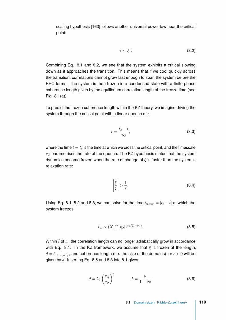
scaling hypothesis [163] follows another universal power law near the criticalpoint:

τ ∼ ξz. (8.2)

Combining Eq. 8.1 and 8.2, we see that the system exhibits a critical slowingdown as it approaches the transition. This means that if we cool quickly acrossthe transition, correlations cannot grow fast enough to span the system before theBEC forms. The system is then frozen in a condensed state with a finite phasecoherence length given by the equilibrium correlation length at the freeze time (seeFig. 8.1(a)).

To predict the frozen coherence length within the KZ theory, we imagine driving thesystem through the critical point with a linear quench of ε:

ε =tc − tτQ

, (8.3)

where the time t = tc is the time at which we cross the critical point, and the timescaleτQ parametrises the rate of the quench. The KZ hypothesis states that the systemdynamics become frozen when the rate of change of ξ is faster than the system’srelaxation rate:

∣∣∣∣∣ ξξ∣∣∣∣∣ > 1

τ. (8.4)

Using Eq. 8.1, 8.2 and 8.3, we can solve for the time tfreeze = |tc − t| at which thesystem freezes:

t± ∼ (X1/ν± |τQ|)νz/(1+νz). (8.5)

Within t of tc, the correlation length can no longer adiabatically grow in accordancewith Eq. 8.1. In the KZ framework, we assume that ξ is frozen at the length,d = ξ|t=tc−t+ , and coherence length (i.e. the size of the domains) for ε < 0 will begiven by d. Inserting Eq. 8.5 and 8.3 into 8.1 gives:

d = λ0

(τQτ0

)bb =

ν

1 + νz, (8.6)

8.1 Domain size in Kibble-Zurek theory 119

Fig. 8.1.: Domain formation during spontaneous symmetry breaking in a homogeneous Bose gas. (a)Red circles depict thermal atoms and blue areas coherent domains, in which the U(1) gaugesymmetry is spontaneously broken. The black arrows indicate the independently chosencondensate phase at different points in space, and dashed lines delineate domains overwhich the phase is approximately constant. The average size d of the domains formed atthe critical point depends on the cooling rate. Further cooling can increase the population ofeach domain before the domain boundaries evolve. (b) Cartoons illustrating the calculationof the Kibble-Zurek scaling law. The system is frozen in the blue shaded region where|ξ/ξ| > 1/τ . The lower panel shows the equilibrium value of ξ (orange), and the KibbleZurek hypothesis states that ξ stalls at the value ∼ d (blue dashed line) when the system isfrozen

where we have explicitly inserted dimensionful constants λ0 and τ0, which dependon the microsopic details of a particular system. In our system λ0 is expected to beset by the thermal wavelength at the critical point, and τ0 by the elastic scatteringtime τel [152,164]; for our experimental parameters, λc ≈ 0.7 µm, and a classicalestimate gives τel ≈ 30 ms.

Fig. 8.1(b) graphically summarises the steps in the derivation of Eq. 8.6. In essence,we have shown that due to the phenomenon of critical slowing down, crossingthe BEC transition at a finite rate causes domains of predictable size to form withindependent choices of the symmetry-breaking order parameter1 (i.e. the BECphase).

Our ultimate aim is to quantitatively measure the power-law d ∼ τ bQ for the homoge-neous 3D BEC transition. This transition resides in the same universality class as the3D XY model and the lambda transition of liquid 4He, for which the critical exponentscan be calculated in a mean-field (i.e. Ginzburg-Landau) theory [163, 166], or ina beyond mean-field dynamical critical model, known as the F Model [163]. Therelevant exponents in these theories are summarized in table 8.1.

1Note that at the domain boundaries, rare long lived topological defects can also form [165], theirnature and density depending on the physical system. We will not explicity consider these defects inour discussion.


Mean Field Beyond Mean Field

z 2 3/2

ν 1/2 2/3

X+/X− 0 ∼0.3

b 1/4 1/3

Tab. 8.1.: Crtical exponents and amplitude ratios for time-dependent-Ginzburg-Landaumean field (MF)[163,166] and beyond MF [163] models. The beyond MF critical exponents are calculatedaccording to the so-called F Model, and the amplitude ratio is calculated numerically [167].

We hope to measure these critical exponents in later sections, however it is usefulto first discuss the qualitative evidence for domain formation and introduce the basicexperimental parameters. This will be the task for the next section.

8.1.1 Qualitative evidence for domain formation

Experimentally, we will use our uniform box trap to study the Kibble-Zurek theory.Using individual ToF images it is remarkably simple to observe the qualitativemessage of Fig. 8.1(a) - i.e. the faster the temperature quench, the smaller thedomains. The procedure for this qualitative study is outlined below:

We prepare a homogeneous Bose gas by loading 3 × 105 87Rb atoms into ourcylindrical optical-box trap with length L ≈ 26 µm along the horizontal x-axis, andradius R ≈ 17 µm. Initially T ≈ 170 nK, corresponding to T/Tc ≈ 2. We thenevaporatively cool the gas by lowering the trap depth linearly from ∼ 2 µK to ∼ 30 nKin time tQ. We cross Tc ≈ 70 nK with 2× 105 atoms, and at the end of the coolingwe have 105 atoms at T . 10 nK (T/Tc . 0.2).

Fig. 8.2.: Phase inhomogeneities in a deeply degenerate gas are revealed in time-of-flight expansionas density inhomogeneities. (a) The gas is cooled in 1 s from T ≈ 170 nK, throughTc ≈ 70 nK, to . 10 nK. Each realization of the experiment results in a different pattern, andaveraging over many images results in a smooth featureless distribution. (b) Preparing aT . 10 nK gas more slowly (over 5 s) results in an essentially pure BEC with a spatiallyuniform phase.

8.1 Domain size in Kibble-Zurek theory 121

When we release this condensate from the trap, any phase inhomogeneities arerevealed in ToF expansion as density inhomogeneities [153,168]. In Fig. 8.2, wecompare the ToF profiles for a gas cooled to T Tc "quickly" (tQ ≈ 1 s) and "slowly"(tQ & 5 s). Gases cooled quickly reveal density modulations in ToF indicative ofthe presence of small domains in situ. In contrast, in our finite-sized box, slowcooling can produce an essentially pure and fully coherent (single-domain) BECwhich develops the characteristic diamond shape in ToF (c.f. Fig. 7.6). This contrastsupports the qualitative picture illustrated in Fig. 8.1(a).

8.2 Quantitative measurement of domain sizes

We now study the KZ mechanism more quantitatively. Specifically, we will developan experimental technique for measuring the size, d, of the domains in our quench-cooled clouds.

To measure the size of the domains, imagine a pure condensate described inthe classical field approximation2 by the complex wavefunction ψ(r), and considerinspecting this wavefunction at two points separated by r′. If |r′| < d then the twopoints may lie in the same domain, so there will be a correlation between the phasesof ψ(r) and ψ(r + r′). Conversely if |r′| > d, we expect little correlation betweenthe phases. These phase correlations which decay over the length-scale d can becaptured by the spatially averaged two point first order correlation function, definedas

C1(r′) =

∫〈ψ(r)∗ψ(r− r′)〉 d3r√∫

〈|ψ(r)|2〉 d3r∫〈|ψ(r− r′)|2〉 d3r

=1

N

∫〈ψ(r)∗ψ(r− r′)〉 d3r, (8.7)

where 〈...〉 denotes averaging over different domain configurations of ψ, and ψ isnormalised to

∫d3r |ψ|2 = N .

In our experiment, ψ is only non-zero inside our uniform cylindrical box trap. Thisartificially introduces the length scales of the finite-sized box, L and R, into theproblem which complicates the extraction of d from the decay of C1. Below, weoutline a technical derivation of how the finite sized box affects the measurement ofd. While we attempt to be as formally correct as possible at each step, it is only thefinal result in Eq. 8.13 which is important for the later sections. This final result is

2Note that we could treat the Bose gas using the field operators Ψ(r) and inspect the spatiallyaveraged first order correlation function proportional to

∫d3r 〈Ψ(r)†Ψ(r − r′)〉. However for large

occupation of the BEC, it is simpler to approximate Ψ(r) as a complex function ψ(r) (i.e. ignore thefield operator commutator).


relatively intuitive when one considers the limits of d→ L and d L, and simpleexperimets reproduce these intiuitve limits (see Fig. 8.6).

8.2.1 Infinite system correlations from a finite-sized experiment

We begin by constructing a function ψ∞(r) defined in a homogeneous system ofvolume V∞ →∞ with a constant modulus

√N/πR2L and a phase Θ(r):

ψ∞ =

√N

πR2Lexp [iΘ(r)] . (8.8)

The function Θ is chosen such that ψ∞ everywhere has the same characteristicphase correlations as ψ. This means that we can obtain ψ from ψ∞ by "maskingout" all points not inside the cylindrical trap:

ψ(r) = Cyl(r)ψ∞(r) (8.9)

Fig. 8.3.: The relationship between ψ∞ and ψ. We imagine cutting a finite sized cylinder out of aninfinite system ψ∞ to obtain ψ. The infinite system has characteristic domain size d (phasedomains are illustrated in different colours).

where Cyl(r) is a unity inside the cylindrical trap and zero elsewhere. Inserting Eq.8.9 into 8.7 gives:

C1(r′) =1

N

∫V∞

Cyl(r)Cyl(r− r′)〈ψ∗∞(r)ψ∞(r− r′)〉 d3r, (8.10)

By symmetry, since ψ∞ describes an infinite homogeneous system, we can replace〈ψ∗∞(r)ψ∞(r + r′)〉 with it’s spatial average:

〈ψ∗∞(r)ψ∞(r− r′)〉 =1

V∞

∫V∞

〈ψ∗∞(s)ψ∞(s− r′)〉 d3s. (8.11)

8.2 Quantitative measurement of domain sizes 123

Now, noting from Eq. 8.8 that∫V∞

d3s |ψ∞(s)|2 = NV∞/πR2L, we can insert Eq.

8.11 into Eq. 8.10 to obtain:

C1(r′) =1

πR2L

∫V∞〈ψ∗∞(s)ψ∞(s− r′)〉 d3s√∫

V∞〈|ψ∞(s)|2〉 d3s

∫V∞〈|ψ∞(s− r′)|2〉 d3s︸︷︷︸

C∞1 (r′)

∫V∞

Cyl(r)Cyl(r−r′) d3r,

(8.12)

Where we have identified the central term as the infinite system correlation functionC∞1 (r). For the case r′ = xx (where x is a unit vector along the axis of the cylin-drical trap) we can calculate the geometric overlap integral in Eq. 8.12 under theassumption of a perfectly uniform trap with no healing length. This gives the finalresult:

C1(xx) = C∞1 (xx)×(

1− x

L

). (8.13)

I.e. if we measure C1 (as described in the next section), then we will be measuringthe infinite system correlation function, C∞1 (which contains the length-scale d)modulated by a linear geometric envelope arising from the finite trap size.

8.2.2 Homodyne interference for measuring domain size

So far we have said that the length scale d which we want to measure is encoded inthe decay of C∞1 , and we have shown that C∞1 can be deduced from C1. Now wemust find a way to experimentally measure C1 itself.

Inserting the Fourier transform of ψ(r) into Eq. 8.7 immediately gives C1 as theFourier transform of the momentum distribution of the BEC. Therefore, it is temptingto refer to our momentum-space measurements chapter 7 and say that we cansimply Fourier transform a Bragg spectrum to obtain C1. However, for very fastquenches (τQ ∼ τ0), we expect d ∼ λc, corresponding to a Bragg spectrum spreadoverW ∼ 3 kHz. Such a wide spectrum requires the Bragg pulse to have a large ΩRt

in order to diffract a measureable fraction of atoms. From Eq. 7.12, this generallyleads to broadening of the Bragg spetrum for experimentally achievable valuesof t. This broadening begins to significantly affect the spectrum as d grows (i.e.W shrinks), and it was found to be difficult to find a suitable protocol which couldmeasure both large (∼ 30 µm) and small (∼ 0.7 µm) domains. For this reason, wedevise an alternative experimental approach based on homodyne interference.


The approach is inspired by [142], and is based on three steps:

"Copy" Create a "copy" of ψ(r) ψ(r), ψ(r)

Arrange Displace one copy by xx ψ(r), ψ(r− xx)

Interfere Create a superposition of the displaced copies ψ(r) + ψ(r− xx)

If we count the number of atoms in the homodyne interference pattern arising in thefinal step, we recover C1(xx):

∫|ψ(r) + ψ(r + xx)|2 d3r = 2N 1 + Re [C1(xx)] . (8.14)

In the next subsections, we will describe how the steps above can be achieved usingtwo separated Bragg pulses.

Step 1: "Copy"

After releasing the cloud from the trap, suppose we apply a very short, powerfulpulse of Bragg light with ΩR/2π ≈ 700 Hz and t = 0.1 ms. With these parameters,the Bragg resolution kernel in Eq. 7.9 becomes very broad with ∆fres ≈ 20 kHz.Even for correlations of size λc, the Bragg spectrum of the atomic cloud is 3 kHz 20 kHz wide. Therefore, the resolution kernel can be treated as flat, and allmomenta in the cloud experience the same population transfer in time t.

Since the Bragg process is now effectively momentum-independent, we can treatthe system as a two level system with the lower level, |P〉, representing the bandof states in the stationary cloud and a higher level |P + ~∆k〉 representing thediffracted atoms. In this basis, we write the initial state as ψ(r) |P〉 ≡ (ψ(r) , 0)T,which we represent pictorially as follows:


Now we can set the frequency difference between the Bragg lasers as f = fc ≈1 kHz such that δ = 0 in Eq. 4.11. The Bragg pulse then couples the |P〉 and|P + ~∆k〉 states according to the matrix

B(ΩR) =

(cos(θ2

)−i sin

(θ2

)−i sin

(θ2

)cos(θ2

) ) , (8.15)

where for our parameters, θ = ΩRt ≈ π/7. Therefore, after the first Bragg pulse, wehave the state:

B(ΩR)

(ψ(r)

0

)=

(cos(θ2

)ψ(r)

−i sin(θ2

)ψ(r)

)(8.16)

Thus we have "copied" the wavefunction ψ(r) into the state(s) |P + ~∆k〉.

Step 2: Arrange

If we turn off the Bragg beams and wait for time tA, then the diffracted cloud in themoving states |P + ~∆k〉 moves by vrtA. We represent the action of this waitusing the matrix:

A(tA) =

(1 0

0 TtA

)(8.17)

where T is the translation operator defined by Ttf(x) = f(x− vrt). After the wait,tA, we have the state

A(tA)B(ΩR)

(ψ(r)

0

)=

(cos(θ2

)ψ(r)

−i sin(θ2

)ψ(r− vrtA)

), (8.18)


And thus we have achieved the aim of displacing one of the copies.

Step 3: Interfere

Finally, we interfere the displaced copies by applying a second Bragg pulse identicalto and in phase with the first pulse. This gives the final state:

B(ΩR)A(tA)B(ΩR)

(ψ(r)

0

)=

(cos2

(θ2

)ψ(r)− sin2

(θ2

)ψ(r− vrtA)

−i sin(θ2

)cos(θ2

)[ψ(r) + ψ(r− vrtA)]

), (8.19)

In the region where the copies overlap, the final density of atoms in the |P + ~∆k〉state depends on the relative phase of the overlapping domains in the two copies. Ifwe wait a further time-of-flight of tToF = 140 ms (i.e. apply A(tToF)) we obtain theinterference term ∝ [ψ(s) + ψ(s− vrtA)] in state |P + ~∆k〉 spatially separatedby vrtToF from the stationary cloud in state |P〉. Therefore, we can count thefraction of atoms in this diffracted cloud, and using Eq. 8.14 and 8.13, we obtain:

N|P+~∆k〉

N=

1

2

1 +

(1− x

L

)Re [C∞1 (xx)]

sin2(θ), (8.20)

where xx = vrtA. Eq. 8.20 is the key result of this section, stating that we canmeasure theC∞1 correlation function (encoding the length scale d) by simply countingthe fraction of atoms diffracted by our homodyne interferometric scheme. We willuse this technique in our quantitative studies in sections 8.3 and 8.4, however, firstwe will outline one final technical point in the section below.


Fig. 8.4.: Level diagram for the -1 Bragg diffraction order (red). The lasers are tuned such that astationary atom is resonant with the +1 order transition (shown in gray). This results in alarge detuning, δ, for the -1 order.

Aside: Bragg diffraction orders

Note that so far we have only considered transitions from P to P + ~∆k (the so-called +1 order). Using the same laser beams but swapping the roles of absorbtionand stimulated emission, it is possible to couple P to P− ~∆k (the −1 order).Since the lasers are resonant with the +1 transition, the −1 transition is detuned byδ/2π = 2fc (see Fig. 8.4). To find the population of the −1 order, we can repeat theanalysis above with δ 6= 0 using the full matrix B(ΩR, δ) from Eq. 4.11 and includingthe free evolution of the states3 in A(ΩR, δ). This gives the diffracted fraction in the−1 order as:

N|P−~∆k〉

N=

2Ω2R

δ2

1 + cos

[δ

(t+

x

vr

)](1− x

L

)C∞1 (xx)

sin2

(δt

2

)(8.21)

where we have assumed√

Ω2R + δ2 ≈ |δ| and that C∞1 is a real function (which

is true for any system with an even momentum distribution). We can draw twoconclusions from Eq. 8.21:

3It is important to note that when the lasers are off (ΩR = 0) during the wait time tA, B(ΩR = 0, δ)does not reduce to the idenitity for δ 6= 0. Therefore, in the rotating frame, we must include theevolution of the states at relative frequency δ during the "arrange" step:

A(tA, δ) =

exp(iδtAt

2

)0

0 exp(−iδtA

2

)︸︷︷︸

B(ΩR=0,δ)|t→tA

(1 0

0 TtA

).


Fig. 8.5.: Relevant Bragg diffraction orders. The arrows show the cumulative population transferbetween the orders with the lines of decreasing thickness indicating relative populationsO(1), O[(ΩRt)

2], and O[(ΩRt)4] respectively. Note that the homodyne interference circuit

(highlighted in blue) is only affected to O[(ΩRt)4] by the presence of other Bragg orders.

The ToF image shows the result of an experimental run from section 8.3 in which we coolthe gas in tQ = 0.8 s, apply Bragg pulses separated by tA = 0.4 ms, and then wait 140 msToF.

• The population in the −1 order cloud oscillates with tA = x/vr at frequency δ.

• The population in the −1 order is as significant as the +1 order (ignoringosillations). This can be seen by taking the envelope of the osillations ofN|P−~∆k〉/N , and expanding sin(θ) for small angles, givingN|P±~∆k〉/N ∼(ΩRt)

2. Qualitatively, the symmetry in the amplitude of the ±1 orders is a resultof the broad Bragg resolution kernel 2π ×∆fres 2δ.

The significance of the −1 order brings into question the validity of our treatment ofP and P + ~∆k as a closed two-level system coupled by B. However, followingthe schematic diagram in Fig. 8.5, we see that the −1 order only modifies ourexpression in Eq. 8.20 by terms O(Ω4

Rt4), provided that we count all the −1, 0 and

+1 orders in N . Since (ΩRt)2 ≈ 0.2 1, we ignore all these higher order terms

(4-photon processes and depletion of the zero-order cloud) and work to just firstorder with Eq. 8.20.

This concludes our technical discussion of the derivation and validity of Eq. 8.20which is key to the experimental work discussed in the remainder of this chapter.

8.2.3 Experimental measurement of C1

In this section, we introduce the various forms for C1 which we observe in theexperiment using our homodyne interference scheme. Fig. 8.6 shows C1(xx)


Fig. 8.6.: Correlation function C1(x) = (1− x/L)C∞1 (x) measured in equilibrium (blue) and after aquench (red) for, respectively, two different T/Tc values and two different quench times(four experimental runs per point; error bars indicate standard deviation in mean). Inset: 1Dcalculation of G1 for a fragmented BEC containing D = 10 (red) and 20 (light red) domainsof random sizes and phases. The solid lines correspond to C∞1 = exp(−xD/L)

functions measured in equilibrium (blue) and after a quench (red), and we comparethree experimental cases:

Pure BEC In an essentially pure equilibrium BEC (prepared slowly, as for Fig. 8.2(b)),C∞1 (xx) = 1 and C1(xx) is simply given by the linear overlap function 1− x/L(dark blue line).

Partial BEC Cooling slowly in equilibrium, but stopping at T/Tc ≈ 0.7, gives a C1 with afast initial decay, corresponding to the significant thermal fraction. Importantly,the coherence still spans the whole system, with the slope of the long-rangedpart of C1 giving the condensed fraction (light blue line is a guide to the eye).

Quenched clouds By comparison, the C1 functions for quenched clouds have no equilibriuminterpretation. For the curves shown, T/Tc ≈ 0.2, corresponding to a phasespace density > 25, and yet coherence extends over only a small fraction of L.Furthermore, in Fig. 8.6, we immediately see agreement with the qualitativepicture that faster quenches lead to C1 functions with a shorter decay length.

The data for the quenched clouds are fitted well by C∞1 ∝ exp(−x/`) (red lines),which provides a simple and robust way to extract the coherence length. Thisexponential form is further supported by a 1D calculation shown in the inset ofFig. 8.6. Here we generate a wavefunction with a fixed number of domains D,randomly positioning the domain walls and assigning each domain a random phase.Averaging over many realizations, we obtain C∞1 (x) that is fitted very well by anexponential with ` = L/D = d. (In our 3D experiments the total number of domainsis ∼ D3 and C1(x) is effectively averaged over ∼ D2 1D distributions.).


Since the exponential fit gives us direct access to ` = d, we can now move on to afully quantitative study of the KZ theory.

8.3 Direct observation of Kibble-Zurek freeze-out

We are hoping to observe the scaling of d with τQ, but as we will see, in ourexperiment we also directly observe the freeze-out phenomenon central to the KZhypothesis. For the KZ scaling law of Eq. 8.6, a crucial assumption is that ξ isessentially frozen within t± of tc. While intuitively appealing, this assumption is inprinciple only approximate, and the dynamics of the system coarsening (i.e., mergingof the domains) at times t > tc is still a subject of theoretical work [169].

In our experiment we use two different quench protocols outlined in Fig. 8.7. Westart by describing the first quench protocol, QP1, where we vary only the total timetQ over which we ramp down the trap depth.

8.3.1 Quench protocol 1: Basic KZ scaling and its breakdown

In QP1 we restrict tQ to values between 0.2 s and 3.5 s, for which we observe thatthe cooling curves are self-similar4. We find that we always cross Tc = (70± 10) nKat time

tc = (0.72± 0.05) tQ, (8.22)

and always have the same atom number (within ±20%) at the end of cooling. Theself-similarity of the measured cooling trajectories and the essentially constantevaporation efficiency indicate that for this range of tQ values the system is alwayssufficiently thermalised for the temperature (as determined from the thermal wingsin ToF) to be well defined during the quench5. Furthermore, from the definition of ε,we can linearise the cooling trajectory near tc and calculate τQ from the derivativeas follows:

dε

dt

∣∣∣∣t≈tc

= − 1

τQ, (8.23)

4Note that we empirically find that for tQ < 0.2 s the evaporation is less efficient and the coolingtrajectories are no longer self-similar

5Near Tc the mean free path for classical elastic collisions is about four times larger than the sizeof the box. Hence, while the evaporation takes place at the box walls, we can also safely assume thatT is uniform across the sample.

8.3 Direct observation of Kibble-Zurek freeze-out 131

Fig. 8.7.: Quench protocols. (a) In QP1, the laser power is ramped down linearly over time tQ toreduce the trap depth. In QP2 the laser power is ramped faster (at a slope characteristic oftQ = 0.2 s) after tk & tc. (b) The self-similar QP1 cooling trajectories are shown in blue fortotal cooling time tQ = 0.2 s (upper panel) and 3.2 s (lower panel) (four experimental runsper point; error bars indicate standard deviation in mean). We use polynomial fits to thedata (such as shown by the solid lines) to deduce tc and τQ. QP2 is shown in the lowerpanel by the orange points, with the kink at tk = 0.85 tQ.

and due to the self similarity, we find that to good approximation6

τQ ∝ tQ. (8.24)

It is worth briefly commenting on this result in light of the non-linearity of the coolingtrajectories in Fig. 8.7:

The definition of τQ for a non-linear quench

The KZ theory is built upon the assumption of a linear quench for which the derivativein Eq. 8.23 is constant and τQ is unambiguously defined. Experimentally, we donot perform linear temperature quenches and for a quench which is not truly linear,there is some uncertainty over exactly where the derivative should be evaluated(hence we write t ≈ tc in Eq. 8.23). According to the KZ hypothesis, the domainsize is determined by the system properties at the freeze-out point. Therefore, it ismost reasonable to define τQ from the derivative at the point, tc − t+, given by thesolution to the (non-linearised) equation |ξ/ξ| = 1/τ .

In Appendix D, we use a simple numerical model for our non-linear quench toinvestigate whether evaluating τQ from the slope at the freeze time rather than atthe critical time affects the simple proportionality in 8.24 (see Fig. 8.8). The modelconfirms two important results:

6When the derivative is evaluated at exactly at t = tc, we find a constant of proportionalityτQ = (0.41± 0.02) tQ.


Fig. 8.8.: Technical details of our non-linear quench trajectory. We parameterise the self-similar shapeof the QP1 cooling curves by the quadratic curve shown in blue. In a numerical model inAppendix D we calculate the freeze-out conditions (blue shaded region) and illustrate thetQ = 1 s case above (assuming F-Model critical exponents). To link this non-linear curve tothe linearised KZ theory, we can define τQ as the inverse slope of ε(t) evaluated at eithert = tc (gray) or t = tc − t (red). See text for a discussion of these two scenarios.

• The KZ scaling law for the domain size at the critical point is only recovedexactly if we use τQ defined by the slope of the quench trajectory at tc − t+.

• There is a small non-linearity between the τQ evaluated from the slope at thefreeze time and at the critical time. A numerical power-law fit in both the MFand F Model for characteristc parameters in our experiment gives τQ|t=tc−t+ ≈1.1(τQ|t=tc)0.94, i.e. τQ|t=tc−t+ ∝ t

0.94Q . This non-linearity means that we must

be careful when replacing τQ with tQ when evaluating any exponents.

In summary, the numerical analysis tells us that if we were to ignore all complicationsarising from our non-linear quench and evaluate the derivative in Eq. 8.24 at t = tc,then we would recover a value of the exponent b which is 6% smaller than thetrue value. Since this correction is small (considerably smaller than the differencebetween the values of b in the MF and the F-Model), we will proceed with theassumption of a linear quench (i.e. that the proportionality in Eq. 8.24 always holds).Only once we have experimentally evaluated the exponent b under this assumptionwill we attempt to account for any corrections arising from the non-linearity of ourcooling curve.

With this assumption in mind, we now inspect the size of the domains formed at theend of a QP1 quench:

QP1 Results

In Fig. 8.9(a) we plot `(= d) vs. tQ(∝ τQ), for experiments using QP1. For tQ ≤ 1 swe observe a slow power-law growth of ` with tQ, in good agreement with the


Fig. 8.9.: Kibble-Zurek scaling and the freeze-out hypothesis. (a) Coherence length ` as a functionof tQ. Blue points correspond to QP1, error bars indicate fitting errors on `. The shadedblue area shows power-law fits with 1/4 < b < 1/3 to the data with tQ ≤ tbr

Q = 1 s. Thehorizontal dotted line indicates our instrumental resolution (arising from the finite Braggpulse time). (b) Coherence length ` measured following QP2, as a function of tk/tQ, fortQ = 3.2 s (orange), 0.7 s (green), and 0.3 s (purple) (four experimental runs per point; errorbars indicate standard deviation in mean). The shaded areas correspond to the essentiallyconstant ` (and its uncertainty) in the freeze-out period tk− tc < t. (For tQ < tbr

Q the systemnever unfreezes). The (average) ` values within these plateaux are shown in their respectivecolours as diamonds in panel (b).

expected KZ scaling. However, for tQ > tbrQ ≈ 1 s this scaling breaks down and `

grows faster, quickly approaching the system size.

For quenches longer than tbrQ , we suggest that the breakdown of the KZ scaling is

due to the system unfreezing and healing significantly during the quench and beforeit is observed. We note from Eq. 8.22 that the time between crossing Tc and the endof cooling is tQ − tc ≈ 0.28 tQ ∝ tQ, while the KZ freeze-out time is t− ∝ tνz/(1+νz)

Q

(assuming Eq. 8.24). Due to the different scaling of these two times with tQ, it isalways possible to perform slow enough quenches such that tQ − tc exceeds t− forνz > 0 (see Fig. 8.10). Solving for the intersection t− ≈ 0.28 tbr

Q in Fig. 8.10, weobtain an estimate of the absolute value of t− without a priori knowledge of τ0 orλ0.

t− ≈ 0.28 tbrQ

(tQ

tbrQ

)νz/(1+νz)

. (8.25)

Since νz = 1 holds at both the mean field and F Model level, we can say that forboth models t− ≈ 0.28

√tQtbr

Q . In the next section we will have an opportunity todirectly measure t− for comparison with this expression.


Fig. 8.10.: Proposed mechanism for the breakdown of the KZ scaling in Fig. 8.9(b). We plot tQ − tcand t− as a function of tQ and suggest that beyond the intersection point, tbr

Q (orangeshaded region), the system unfreezes and begins to heal during the QP1 quench. Toexplore this region we must used QP2.

8.3.2 Quench Protocol 2: Directly observing the KZ freeze-out

Our second quench protocol consists of two steps as shown in Fig. 8.7. This protocolallows us to directly observe the freezing of the system and to fully understand thebreakdown of the scaling law at tbr

Q in the QP1 results. Once this breakdown isunderstood, we can also use QP2 measurements to extend the range of tQ overwhich we can fit a power law. Using this extended range we will experimentallydistingush the MF and F Model critical exponents.

In QP2 we initially follow the QP1 trajectory for a given tQ, but then at a variable"kink" time tk & tc we accelerate the cooling. The last part of the trajectory alwayscorresponds to the final portion of our fastest, 0.2 s cooling trajectory. This way,even for tQ > tbr

Q we can complete the cooling and measure C1 before the systemhas time to unfreeze.

In Fig. 8.9(b), the orange points show the QP2 measurements of ` for tQ = 3.2 sand various values of the kink position tk/tQ. These data reveal two remarkablefacts:

• For a broad range of tk values, ` is indeed constant (within errors), and thewidth of this plateau agrees with our estimate from Eq. 8.25, t− ≈ 0.5 s fortQ = 3.2 s, indicated by the horizontal arrow.

• The value of ` within the plateaued region falls in line with the KZ scaling lawin Fig. 8.9(a).

We also show analogous QP2 measurements for tQ = 0.7 s (green) and 0.3 s(purple); in these cases tQ < tbr

Q , so t− is longer than tQ − tc, the system never


0.1 0.4 1.6

2.0

1.0

ΤQ HsL

HΜm

L

Fig. 8.11.: Critical exponents of the interacting BEC transition. Orange circles and diamonds show` values obtained using QP2, as in Fig. 8.9(b); the diamonds show the same three datapoints as in Fig. 8.9(a). Blue circles show the same QP1 data with tQ ≤ 1 s as in Fig. 8.9(a).The horizontal error bars indicate the systematic uncertainty in τQ based on evaluationof −(ε)−1 over the range t = tc − t+ → tc. We obtain b = 0.33±0.02 sys.

±0.03 stat. (solid line), inagreement with the F model prediction b ≈ 1/3, corresponding to ν ≈ 2/3 and z = 3/2,and excluding the mean-field value b = 1/4.

unfreezes, and thus the acceleration of the cooling has no effect on `. Theseplateaux provide direct support for the KZ freeze-out hypothesis.

8.4 Kibble-Zurek scaling and universal criticalexponents

To accurately determine the KZ exponent b, we have made extensive measurementsfollowing QP2, extracting ` from the plateaued regions of width min[t−, tQ − tc], asin Fig. 8.9(b). In Fig. 8.11 we combine these data with the QP1 measurementsfor tQ ≤ tbr

Q , and plot ` versus τQ. To construct this plot we must return to theproblem raised in section 8.3 of exactly where on the non-linear cooling trajectorywe should evaluate τQ = −(ε)−1. There are two routes to proceed which we dealwith separately below:

Evaluate τQ at tc

The simplest analysis which ignores the non-linearity of the cooling trajectory isto accept the proportionality τQ ∝ tQ and find b as the slope of a plot of log(`) vs.log(tQ). This gives b = 0.31± 0.03, which is in agreement with the F Model (b = 1/3)and excludes the MF prediction (b = 1/4). Furthermore, note that this approachgives a lower bound on the value of b, and the numerical simulation in Appendix Dsuggests that we should include a 6% systematic correction to this value (becauseτQ ∝ t0.94

Q ). Applying this correction (which is smaller than the statistical error on


b) hints at a value b = 0.33 which is in even better agreement with the F Modelprediction.

Evaluate τQ at tc − t+

The study above gave considerable support to the beyond mean-field F Modelexponents, however rather than accessing b directly, it only provided a tight lowerbound to b and relied on numerical simulations to indicate the true value of b. Ideally,we would not rely on any simulations, but instead estimate t+ directly from theexperiment, and evaluate τQ at tc − t+. Measuring t+ is experimentally challenging,however we proceed with the following assumptions:

• First we assume from Eq. 8.5 that t+/t− = (X+/X−)z/(1+νz) ≈ 0.4, where weassume F Model results for ν, z and X+/X− in the hope of self-consistentlymeasuring b.

• Next we assume that the value of t− = 0.28√tQtbr

Q suggested in section 8.3.1is a good estimate of t− from which we can evaluate t+ = 0.4 t−.

These assumptions are difficult to justify rigorously. In particular, the second as-sumption requires that the microscopic time and length scales τ0 and λ0 do notchange when a BEC is present. Nevertheless, we can follow this protocol withtbrQ = 1 s to achieve an estimate b = 0.35± 0.03. This is again consistent with the FModel, and gives us a way to assess the systematic error in our value of b.

One could even combine the values of b for the two methods above to give b =

0.33±0.02 sys.±0.03 stat.. It is reassuring to note that the systematic variation on b as we analyse

the data in different ways is not larger than the statistical uncertainty on any givenanalysis, and is also significantly smaller than the difference between the F Modeland MF theory.

8.4.1 Dynamical critical exponent, z

Having observed excellent agreement with the KZ theory, we now discuss the im-plications of our measurements for the critical exponents of the interacting BECphase transition, which is in the same universality class as the λ-transition of 4He.While ν ≈ 0.67 has been measured in both liquid helium (see [170]) and atomicgases [171], the dynamical exponent z has, to our knowledge, never been measuredbefore (see [163,172]). Using the well-established ν = 0.67 and Eq. 8.6, we obtainz = 1.5±0.2 sys.

±0.3 stat.. In contrast, MF theory does not provide a self-consistent interpre-tation of our results, since fixing ν = 1/2 yields an inconsistent z = 1.0±0.2 sys.

±0.3 stat..Interestingly, if we instead fix νz = 1, which holds at both MF and F-model level,

8.4 Kibble-Zurek scaling and universal critical exponents 137

from Eq. 8.6 we obtain a slightly more precise z = 1.5±0.1 sys.±0.1 stat. and also recover

ν = 0.67±0.04 sys.±0.06 stat..

8.5 Conclusion

This chapter has presented an experiment which is the culmination of all the workin the second half of this thesis. We developed a versatile trapping technique inchapter 5, applied this to make a uniform system in chapter 6, introduced braggspectroscopy to benchmark the equilibrium ground state properties in chapter 7,and now finally applied this in a dynamical study of the KZ freeze-out mechanismand measurement of the dynamical critical exponent for our universality class.

Note that our uniform trapping potential was essential for the clean observation ofthe KZ mechanism presented here. In an inhomogeneous potential U(r), the criticaltemperature is a function of position. This means that ε is position dependent and aswe decrease T , the critical point ε(x, t) = 0 is reached at different points at differenttimes. Condensation happens first at the point(s) r0 = arg min[U(r)], and then a"transition front" radiates out from this(these) point(s) at speed:

vF =

∣∣∣∣ ∂ε/∂t∂ε/∂x

∣∣∣∣ (8.26)

Independent phase domains will only form if this front travels faster than the speed vsat which the choice of symmetry breaking phase can be communicated7. Whereas ina uniform system, vF diverges (because ∂ε/∂x = 0 - i.e. the entire system becomescritical at once), in an inhomogeneous system, we need to take the competitionbetween vF and vs into account. This means that we cannot directly observe theKZ freeze-out (only local regions of the system are frozen at any time), and the(local) size of the domains and is generally not given by any simple power law.Instead, a harmonically trapped system is described the so-called inhomogeneousKZ theory [165], which is only able to predict approximate scaling laws with b ≥ 1

holding near r0. Hence, our uniform system was essential for the observation of thefundamental mechanism and consequences of KZ theory that we have describedhere.

7Intuitively, vs can be bounded by the velocity scale vs < ξ/τ given by the local frozen quantitiesξ and τ


9Conclusions and Outlook

The experiments in Part I and Part II of this thesis were carried out on two separatemachines. The first machine is able to tune inter-atomic interactions and allowed usto study dynamical effects of superheating and three-body loss in regimes of veryweak and very strong interactions respectively. The second machine is specialisedfor producing novel optical geometries, and specifically we created the worlds firstatomic Bose gas in a uniform potential. The chapters presented here reviewed aseries of equilibrium and dynamical experiments performed so-far in this uniformtrap.

In the future, we plan to combine the two key features of both machines in a third ma-chine which will allow us to tune interactions and geometry on the same experiment.Work has already started on this machine, and several proof-of-principle experimentshave been carried out on our existing machines to lay the ground-work for when thethird machine is fully operational. The uniform system in chapter 6 offers such arich range of experimental paths that our investigations in the immediate future willconcentrate on this simple geometry rather than expanding to more elaborate trapshapes. There are four experiments which we envisage for the near future, whichare described in the sections below. The first two are extensions to chapters 7 and8, and the last two involve small additions to our uniform trap geometry.

9.1 Thermodynamics with tuneable interactions

The first proposed experiment continues our strand of thermodynamic experimentsfrom chapter 7. In particular, we first wish to investigate the effect of interactions onthe the critical temperature (Tc) for condensation.

In a harmonically trapped gas, Tc is shifted relative to the ideal gas value by amean-field effect arising from the inhomogeneity of the trap. It was recently possibleto also measure a more interesting Tc-shift arising from interaction-driven criticalcorrelations on top of this much larger mean-field shift [41] (see Eq. 2.11). Furtheraccurate measurement is not possible in a harmonic trap because the large mean-field effect dominates over any interesting physics. In a homogeneous gas, thereis no mean-field Tc-shift, and any Tc-shifts due to critical correlations become thehighest order effects [173]. This means that experiments on our uniform system

139

will give us an immediate handle on the fundamental critical phenomena drivingthe beyond-mean field Tc shift, which has been the focus of theoretical debates formany years (see [26] for a historical summary).

9.2 Kibble-Zurek with tuneable interactions

In chapter 8, we observed behaviour of a thermally quenched Bose gas consistentwith the beyond mean-field critical exponents of the F Model. The reason for thefailure of mean-field is that fluctuations in the order parameter become as large asthe value of order parameter near the critical point. It is possible to derive a criterion(the so-called Ginzburg criterion) for the point at which critical fluctuations causethe breakdown of mean-field theory as [171]:

ξ > ξG =λ2c√

128π2a(9.1)

where a is the s-wave scattering length. In our experiment in chapter 8, ξG ≈ 0.8,and since the freeze-out values of ` are consistently higher than this value, ourobservation of beyond mean-field exponents is consistent with the Ginzburg criterion.When we tune the interaction strength, a, in our new machine we will be able toincrease ξG and repeat our Kibble-Zurek measurements in this weakly interactinggas to try to measure mean-field exponents in a regime where ξ < ξG.

Another interesting future study could focus on the dynamics of domain coarseningafter unfreezing on the ordered side, or on the variance and distribution of domainsizes formed after the quench.

9.3 Interferometry

In Fig. 6.11 we saw how simple it is to apply our digital holographic methods tocreate trapped-atom interferometers. Atom interferometers can be used to detectany external stimulus (e.g. a magnetic field gradient) which causes the phase of oneof the interfering clouds to evolve at a different rate to the other. Interfering two BECsin uniform traps offers the following fundamental advantages over interferometersconstructed using locally harmonic potentials:

1. Our trap is dark, and therefore there is no dephasing between the trappedcondensates arising from a differential AC Stark effect caused by small trapasymmetries.

140 Chapter 9 Conclusions and Outlook

Fig. 9.1.: Trapped atom interferometry using our uniform system (preliminary). (a) In situ image ofa single condensate split into two halves using the three-wall potential illustrated in thegreen profile. (b) Typical ToF images showing interference fringes when the condensateshave been held in their separate halves for 1, 20 and 500ms. We mark the locations of thefringe peaks after 1ms hold time with vertical lines. We obtain the same pattern with highprobability after 20ms hold time, but the fringe phase is randomised after 500ms. (c) Wequantitatively extract the phase and amplitude of the fringes using a fit (red dotted line) toa cut through the fringes in the x direction (blue line). (d) Interferometric measurement ofdecoherence time. We hold the gas in the split trap for 1, 20 or 500ms and then observethe interference in ToF. Repeating this many times, we can extract the distribution of thephase, φ, and amplitude, A, of the fringes and plot them on a polar plot. We find that forhold times greater than ∼ 100ms, the phase is fully randomised.

2. The peak atom density in uniform traps is low compared to a cloud of the samenumber of atoms in locally harmonic traps. This allows us to put enough atomsin our uniform interferometer to achieve a good signal-to-noise ratio, whilemaintaining a low density such that dephasing from differential mean-fieldshifts significantly reduced. Mean-field dephasing can be further reduced byturning off interatomic interactions.

Dephasing from the AC Stark shift and the mean-field shift can severely limit theintegration time of traditional trapped-atom interferometers [174,175]. To indicatethe advantages of our homogeneous arrangement, we carried out the followingproof-of-principle experiment:

We create a uniform BEC with a small central wall running up the middle of the trap(see Fig 9.1(a)). Initially, this wall is sufficiently low with respect to the chemicalpotential of the BEC to allow a single, connected BEC to form in the entire trap.We then ramp up the green laser power to raise the wall, and split the BEC in two.

9.3 Interferometry 141

Fig. 9.2.: Transport phenomena in an ultracold Bose gas (preliminary). (a) A cartoon of the opticalgeometry for creating a narrow channel for investigation of quantum transport properties.The central green wall is split to create a channel which can be as narrow as the diffractionlimit. The atoms are shown in red, and for clarity, we suppress the appearance of the tubebeam. (b) An experimental image using the apparatus of chapter 6 to load atoms into thispotential.

Since the two BECs were formed from a single common ancestor, they are initiallyphase-locked with each other. Therefore if we immediately release the green trap,we should always observe the same fringe pattern when they interfere. We candetect any dephasing of the two condensates after a hold time t as a randomisationof the fringe pattern in repeated realisations at the same hold time. Figure 9.1(d)shows the distribution of phases and amplitudes of the interference fringe patternafter t = 1, 20 or 500 ms. We can see that the dephasing time is at least 20 ms in ourapparatus, and further experiments gave evidence that the dephasing time is longerthan ∼ 100 ms. This is similar to state-of-the-art trapped atom interferometers usingsqueezed states or non-interacting gases which achieve dephasing times of a fewhundred milliseconds [49,174].

9.3.1 Transport and thermomechanical phenomena

There has been a recent growth in interest in transport [76,77,176–178] and ther-momechanical [179,180] effects in ultracold gases. We note that our holographicmethods make it very simple to construct a geometry in which two uniform reservoirsare connected by a thin channel (see Fig. 9.2). Using a magnetic field gradient, wecan load all the atoms into one reservoir, and then watch the atoms diffuse throughthe channel when we turn off the gradient. For our bosonic gas, we should see twodifferent transport effects: the thermal atoms should move ballistically through thechannel, while the BEC should show superfluid properties. We suggest that it maybe possible to tune the parameters of the channel (e.g. by changing the channelwidth or inserting a tunnelling barrier) such that the superflow is much faster than theballistic themal diffusion. This will allow us to create a "superleak" which only allows

142 Chapter 9 Conclusions and Outlook

superfluid through. We will use this to explore thermomechanical effects in our Bosegas [179–181] similar to those observed in superfluid helium experiments [182].

Other transport effects could be observed by shaking our optical box (e.g. usingan oscillating magnetic field graident) and observing the superfluid response usingbragg spectroscopy.

9.3 Interferometry 143

Appendices

145

AExperimental Sequence Overview

During this thesis, we have not dwelt on the preparatory stages of laser- andevaporative-cooling required to reach condensation. Instead, we have concen-trated on experiments performed when the cloud is already near degeneracy ordeeply condensed. It is somewhat humbling to note that all the techniques andexperiments presented in this thesis take place only in the final few moments of along experimental sequence. The bulk of the sequence was built up by previousstudents and is summarised in their theses: [25,26,33] (Part I machine) and [39,40](Part II machine). For specific details of the early experimental procedure, the readeris directed towards these theses. Here we will just provide a brief overview of thekey concepts of the simpler Part II machine in a manageable two-page cartoon. It ishoped that this overview will be a useful first roadmap for any future students taskedwith extending upon this work.

A.1 Rubidium-87 D2 Lines

Throughout the cartoons on the following pages, we will illustrate the relevant lasertransitions on a skeleton of the 87Rb D2 line. For clarity, labels are omitted from thisskeleton, and a labelled level spectrum is included in Fig. A.1 for reference.

Fig. A.1.: Hyperfine structure of the 87Rb D2 lines. Data (reported in MHz) reproduced from [183].

147

`

Lase

rC

oo

ling

:Captu

ring

and

coolin

ga

87 R

bato

ms

from

aback

gro

und

vapour.

1.M

ag

neto

-op

tica

l-tr

ap

:A

com

bin

atio

no

fci

rcula

rly

po

larize

dla

ser

beam

salo

ng

each

coo

rdin

ate

direct

ion

and

aq

uad

rup

ole

mag

netic

field

pro

vid

ea

po

sitio

n-

and

velo

city

-dep

end

ent

trap

pin

gfo

rce.

Inp

ract

ice,

we

use

lase

rsδ

0=

25M

Hz

detu

ned

fro

mth

eF=

2→F’

=3

transi

tio

n,b

ut

the

princi

ple

isb

est

und

ers

too

db

yco

nsi

dering

a

syst

em

with

asi

mp

ler

F=0

→F’

=1

transi

tio

n.The

detu

nin

go

fth

ela

ser

light

fro

mth

is

transi

tio

nhas

thre

eco

ntr

ibutio

ns:

1.The

static

detu

nin

g,δ

0,o

fth

ela

ser

fro

mth

eze

ro-f

ield

F=0

→F’

=1

transi

tio

n.

2.

The

Do

pp

ler-

shift,

k∙v,

due

toth

eato

ms’

velo

city

.

3.

The

Zeem

an-s

hift,

gFm

FμBB/ħ,o

fth

em

F=+

1,0,-

1hyp

erf

ine

leve

ls.

The

dia

gra

ms

belo

will

ust

rate

the

detu

nin

go

fth

ela

sers

(red

)fr

om

the

ato

mic

leve

ls

(bla

ck)

for

ast

atio

nary

and

mo

ving

ato

m:

For

ast

ationary

ato

mat

x>

0,th

e|0

,0

→|1

,-1

(σ- )

transi

tio

nis

clo

sest

tore

sonance

.

We

can

arr

ang

ea

rest

oring

forc

eby

cho

osi

ng

circ

ula

rly

po

larize

dlig

ht

such

that

pho

tons

are

pre

fere

ntially

scatt

ere

dfr

om

the

beam

pro

pag

ating

inth

e–x

direct

ion.

This

rest

oring

forc

ep

rovi

des

ap

osi

tio

n-d

ep

end

ent

trap

pin

gp

ote

ntial.

For

ato

ms

movi

ng

the

+x

direct

ion,th

eb

eam

pro

pag

ating

inth

e–x

direct

ion

isb

lue-

shifte

dto

ward

sre

sonance

.This

pro

duce

sa

velo

city

-dep

end

ent

dam

pin

gfo

rce

whic

h

coo

lsth

etr

ap

ped

ato

mic

clo

ud

.

1. M

ag

neto

-op

tica

l-tr

ap

2. O

ptica

l Mo

lass

es

Mag

netic

Trap

pin

g: C

onfin

ing t

he

ato

ms

in a

str

ong q

uadru

pole

magnet

ic f

ield

whic

h s

plit

s th

e hyp

erfin

e le

vels

rea

dy

for

radio

-fre

quen

cy e

vapora

tion.

1. O

ptica

l pu

mp

ing

: Puts

ato

ms

in t

he m

ag

netica

lly t

rap

pab

le |2,2

state

by

drivi

ng

the σ

+|F

= 2

,mF

→ |F’

= 2

,mF+

1tr

ansi

tio

n u

sing

circu

larly

po

larize

d lig

ht

pro

pag

ating

alo

ng

a q

uantiza

tio

n a

xis

defined

by

a s

ing

le c

oil.

Ato

ms

pum

ped

into

the e

xcited

sta

tes

spo

nta

neo

usl

y d

eca

y b

ack

to

the g

round

sta

tes

to b

e p

um

ped

ag

ain

until t

he p

op

ula

tio

n b

uild

s up

in t

he d

ark

|F

= 2

,mF

= 2

state

. A

ny

ato

ms

whic

h

deca

y in

to t

he F

= 1

manifo

ld a

re r

e-p

um

ped

back

into

the c

yclin

g t

ransi

tio

n b

y re

-

pum

p lase

rs r

eso

nant

with |F

= 1

→ |F’

= 2.

2. M

ag

netic

trap

pin

g: T

he lo

w-f

ield

-seeki

ng

|2,2

state

is

confined

by

a s

tro

ng

quad

rup

ole

fie

ld.

3. O

ptica

l Pu

mp

ing

4. M

ag

netic

Trap

7G

/cm

mF =

-1 0

+1

F =

0

F =

1

Energy

BB

x

x=

0

v

BB

x=

0

5 G

With

ap

pro

priate

lyp

ola

rize

db

eam

sin

all

6

direct

ions,

the

ato

ms

are

trap

ped

and

coo

led

ina

3D

.

When

coo

ling

on

the

F=2

→F’

=3

transi

tio

n,

spo

nta

neo

us

em

issi

on

toth

eF=

1g

round

state

is

po

ssib

levi

ahig

her

ord

er

transi

tio

ns.

Ato

ms

inth

e

F=1

leve

lare

bro

ug

ht

back

into

F=2

usi

ng

re-p

um

p

light

reso

nant

with

the

F=1

→F’

=2

transi

tio

n.

2.

Op

tica

lM

ola

sses:

The

quadru

po

lefield

istu

rned

off

and

the

clo

ud

isallo

wed

toco

ol

inth

epre

sence

of

only

the

velo

city

-dep

end

ent

dam

pin

gfo

rce.

Witho

ut

the

mag

netic

field

,ad

ditio

nal,

‘sub

-Do

pp

ler’

coo

ling

mech

anis

ms

(Sis

yphus

coo

ling

)ca

n

sig

nific

antly

red

uce

the

tem

pera

ture

of

the

clo

ud

.

25M

Hz

68M

Hz

20m

m

100 G

/cm

Lase

r co

olin

g li

mits:

1. D

op

ple

r co

olin

g li

mit:S

po

nta

neo

us

em

issi

on a

t a r

ate

giv

en b

y th

e inve

rse

exc

ited

sta

te lin

ew

idth

, Γ-1

, heats

at

a

rate

(ħk)

2/(

2m

Γ). B

ala

nci

ng

this

with t

he

lase

r co

olin

g d

am

pin

g r

ate

(-F

∙v~

v∙v

)

giv

es

an e

quili

brium

tem

pera

ture

of

k BT=ħ

Γ/2 (~

150μ

K f

or

87R

b).

2. R

eco

il lim

it:A

bso

rptio

n/e

mis

sio

n o

f

pho

tons

only

aff

ect

s th

e a

tom

’s

mo

mentu

m in u

nits

of ħk.

This

dis

cretisa

tio

n g

ives

a ‘re

coil

limit’ fo

r

lase

r co

olin

g k

BT=(ħk)

2/(

2m

)(~

200nK

for

87R

b).

Eva

po

rative

co

olin

g is

use

d in late

r

step

s to

beat

the r

eco

il lim

it

`

Rad

io-F

req

uency

Eva

po

ratio

n:

Rem

ovi

ng t

he

hig

hes

t en

ergy

ato

ms

to

allo

w t

he

rem

ain

ing a

tom

s to

re-

ther

malis

e at

a low

er t

emper

atu

re.

Zeem

an s

plit

ting

of

the F

=2 m

anifo

ld in

the q

uad

rup

ole

fie

ld a

llow

s us

to a

dd

ress

ato

ms

in d

iffe

rent

reg

ions

of

the t

rap

by

tunin

g t

he fre

quency

of ra

dio

-wave

rad

iatio

n flo

od

ing

the a

pp

ara

tus.

By

targ

eting

the h

ighest

energ

y ato

ms

(at

larg

e r

ad

ius

fro

m t

he m

ag

netic

zero

) and

transf

err

ing

them

fro

m t

he t

rap

ped

|2,2

state

into

un-t

rap

ped

sta

tes,

we a

llow

the

rem

ain

ing

ato

ms

to r

e-t

herm

alis

e a

t a

low

er

tem

pera

ture

. This

is illu

stra

ted

schem

atica

lly b

elo

w:

Sw

eep

ing

the r

ad

iatio

n fro

m 1

5 →

5 M

Hz

in 2

s, co

ols

the c

loud

to

90 μ

K.

Hyb

rid

-tra

p &

Op

tica

l Eva

po

ratio

n:

Majo

rana s

pin

-flip

s o

ccur

at

the

quad

rup

ole

mag

netic

zero

where

the

ato

m’s

sp

in (

pre

cess

ing

at

a v

anis

hin

g

Larm

or

freq

uency

) ca

nno

t ad

iab

atica

lly

follo

w t

he c

hang

e in m

ag

netic

field

direct

ion. These

flip

s eje

ct lo

w e

nerg

y

ato

ms

dw

elli

ng

near

the m

ag

netic

zero

.

To

co

ol b

elo

w t

he μ

K leve

l, w

e t

ransf

er

the a

tom

s in

to a

sin

gle

-beam

(harm

onic

)

op

tica

l d

ipo

le t

rap

(O

DT)

far

red

-detu

ned

(1070nm

) fr

om

all

reso

nance

s and

po

sitio

ned

60

μm

(1

op

tica

l w

ais

t) b

elo

w

the m

ag

netic

zero

. R

ed

uci

ng

the

quad

rup

ole

fie

ld ‘p

ours

’ th

e a

tom

s in

to

the O

DT:

Un

ifo

rm-t

rap

Tra

nsf

er a

tom

s in

to a

nd c

onden

se in n

ove

l tra

p g

eom

etry

Trapped

atom density

Energy5. R

ad

io-f

req

uency

Eva

po

ratio

n6. H

ybrid

-tra

p &

Op

tica

l

Eva

po

ratio

n

100 G

/cm

5W

15-5

MH

z r

ad

iatio

n

|2,2

|2,1

|2,0

|2,-

1

|2,-

2

Low

er

tem

pera

ture

aft

er

therm

alis

atio

n

Pro

file

befo

re

therm

alis

atio

n

Ato

ms

transf

err

ed

to

un-t

rap

ped

sta

tes

x=

0

x

BB

In t

he O

DT, th

e a

tom

s are

co

nfined

alo

ng

the b

eam

by

the r

esi

dual 7

.4 G

/cm

quad

rup

ole

fie

ld. O

ff a

xis

this

fie

ld

pro

vid

es

an a

pp

roxi

mate

ly h

arm

onic

po

tential w

ith t

rap

pin

g f

req

uency

30H

z.

Op

tica

l Evap

ora

tio

n:T

he O

DT is

ram

ped

do

wn f

rom

5W

exp

onentially

ove

r 7s.

This

eva

po

rative

ly c

oo

ls t

he g

as,

ach

ievi

ng

cond

ensa

tio

n a

t 0.1

6W

(2

μK t

rap

dep

th,

90H

z ra

dia

l fre

quency

)

z

Mag

netic,

op

tica

l +

gra

vita

tio

nal p

ote

ntial

tim

e

7. U

nifo

rm t

rap

load

ing

8. U

nifo

rm tra

p e

vap

ora

tio

n

9. B

rag

g s

pect

rosc

op

y &

Tim

e-o

f-

Flig

ht

10. A

bso

rptio

n Im

ag

ing

Tra

p lo

ad

ing

:532 n

m s

hap

ed

unifo

rm

trap

beam

s are

ram

ped

on a

s th

e O

DT is

ram

ped

do

wn. To

rele

ase

ato

ms

into

the

bo

x. A

unifo

rm b

ias

field

is a

dd

ed

to

the

quad

rup

ole

fie

ld t

o c

reate

a u

nifo

rm a

nti-

gra

vity

mag

netic

field

gra

die

nt

15.2

76 G

/cm

.

Op

tica

l evap

ora

tio

n: T

he g

reen la

ser

po

wer

is

ram

ped

do

wn e

xpo

nentially

ove

r 2s

to

ach

ieve

co

nd

ensa

tio

nSee c

hap

ter

6

Qu

ery

clo

ud

pro

pert

ies

via

mo

mentu

m d

istr

ibutio

n

Either

by

Bra

gg-s

pec

trosc

opy

(pure

BEC

)

or

tim

e-of-

flight

(anti-g

ravi

ty f

ield

lef

t

on)

See c

hap

ter

7

Ab

sorp

tio

n Im

ag

ing

Circu

larly

po

larize

d lig

ht

drive

s th

e σ

+

|2, 2

→|3

, 3

transi

tio

n in

the p

rese

nce

of

a 5

G g

uid

e f

ield

. A

cam

era

cap

ture

s

the s

had

ow

in t

he p

rofile

of

the a

tom

s

as

they

ab

sorb

pho

tons.

17.5

G

15.2

76 G

/cm

5 G

BRaster Holography

In Fig 5.7(b), we saw the Gerchberg-Saxton algorithm for generating raster holo-grams. The Gerchberg-Saxton algorithm calculates a phase hologram by linkingthe known moduli in the SLM and trapping planes through simulation of the lightpropagation back and fourth between these planes. After each propagation, wemanually impose the modulus constraints while leaving the phase to converge on therequired solution. The convergence of this algorithm is problematic (see Fig. 5.8),and in this section, we describe improvements to this computational method, buildingon the work of Pasienski and DeMarco [103]. In addition, we present experimentalresults which indicate that the traps produced by our method are of sufficient qualityto integrate into cold atom experiments.

B.1 MRAF: Mixed-region amplitude freedom

To combat the fact that the Gerchberg-Saxton algorithm generally fails to convergecorrectly, Pasienski and DeMarco devised the MRAF algorithm. The idea of MRAFis to enhance convergence of the Gerchberg-Saxton algorithm in one region ofthe trapping plane by giving up control of the remaining regions [103–106]. Moreprecisely, MRAF defines a "drawing" D in the trapping plane containing all the pointsin which the desired potential is non-zero, and an additional "canvas" region, C,of zero potential around the drawing (see Fig. 5.8). The modulus constraint isthen manually imposed only inside C and D at each iterative step, thus reducingthe number of constraints the algorithm aims to satisfy. It is hoped that with theadditional freedom of amplitude outside C the algorithm will correctly converge ontothe desired diffraction pattern inside C and D. Meanwhile, a complex pattern offringes and speckles develop in the unconstrained region outside C,

In the original MRAF paper, region C is limited to a tight border around D (witha typical width of ≈ 1% of the trapping region length scales). Although C is afeatureless region of zero potential, it is an integral part of the trap since it definesthe zero to which all the pixels in D are referenced. For practical purposes, sucha small canvas can be a severe limitation because the fringes and speckles in theunconstrained region could greatly complicate the process of loading atoms intothe desired region, D. Therefore, our method aims to expand C to approach itstheoretical limit, which is set by Nyquist’s theorem to be 25% of the area of the

151

simulated trapping plane1. In this large canvas regime, MRAF suffers the samefate as the Gerchberg-Saxton algorithm: convergence stagnates to produce poorsolutions even after many iterations.

B.2 Optical vortices

The reason for the failure of the MRAF algorithm in the extended canvas regime isthe formation of large populations of optical vortices during the early iterations (ap-proximately 1 vortex for every 10 pixels in Fig. B.2). Optical vortices are topologicalfeatures of the light field corresponding to a phase winding around a point of zerointensity. Large vortex populations are problematic because individual vortices aredifficult to eliminate in subsequent iterations of the algorithm. Unwinding a vortexrequires global disruption of the hologram, which cannot be achieved in late itera-tions of Gerchberg-Saxton-type algorithms which monotonically reduce the meansquare deviation from the target [184,185]. Therefore any erroneous vortices are“frozen in” early on, and the algorithm gets stuck in a local optimum correspondingto a particular vortex distribution.

B.2.1 Offset-MRAF

One possibility for handling vortices is by pairwise creation and annihilation, whichrequires only local operations; computational algorithms which encourage suchpairwise operations are given in [186]. However, here we consider a much simplersolution. Our method simply offsets the trapping pattern inside C and D by a uniformintensity, |∆|2, to remove all points of zero light intensity. This redefines the zeroof the potential but does not change the physics of the trap. The aim is to ensurethe phase of all points inside C and D is well defined for all iterations. If a pointof zero intensity is generated, then the phase becomes ambiguous, and we riskforming a vortex in later iterations (see Fig. B.1). To ensure |∆|2 is sufficiently largeto prevent vortex formation, we perform a single iteration of the algorithm and countthe number of vortices produced. This first iteration starts from a parabolic phasehologram which defocuses the light into a vortex-free patch of characteristic sizeset by C. We then gradually increase |∆|2 until a single iteration from this startingpoint does not introduce any vortices. We call this method of introducing an offsetto prevent vortex formation the “offset-MRAF" (OMRAF) algorithm.

1The Nyquist argument proceeds as follows: AnN×N SLM plane can be fast-Fourier-transformedto an N × N trapping plane with a diffraction limited spot size of exactly 1 pixel. The Nyquist limitstates that the diffraction limit should be reduced to half a pixel (the smallest feature in the trap is 1pixel). This can be achieved by padding the computer-simulated SLM plane with zeros to increase itssize to 2N × 2N . This means that only 25% of the simulated SLM plane is covered by the physicalSLM, so we can at best control only 25% of the trapping plane.

152 Chapter B Raster Holography

Fig. B.1.: Choosing the optimal offset intensity. (a) Clarification of the role of the offset as a meansto eliminate vorticies and points of zero intensity which could develop into vortices. (b)The method for picking the optimal offset, ∆, measured in units of the peak amplitude inthe target pattern. We perform a single iteration of the algorithm, for different offsets, toproduce patterns such as those shown in the insets. We then choose the lowest value of ∆(indicated by the dashed line) which gives no vortices within C or D in this first iteration. (c)Improvement in the trap reconstruction associated with the offset.)

Fig. B.2.: Computational results for traps with a well defined zero potential background. We presentreconstructions of the test trap with MRAF and OMRAF methods. We also show detailsof the local reconstruction error (bottom insets) and the local phase (right insets). In thephase plots (obtained after 30 iterations) we use black to white to represent 0 to 2π and reddots to mark vortex cores.

B.2 Optical vortices 153

For maximum light-usage efficiency, we want to minimise the proportion of theincident light which is steered into the featureless background, i.e. choose theminimal |∆| which gives satisfactory results. We find that for all the patterns wetested a suitable offset was |∆| ∼ 10−15% of the maximum amplitude in the trappingplane (i.e. |∆|2 ∼ 1% of the maximum intensity). A computational simulation of thetrapping potential produced using the OMRAF algorithm is shown in Fig. B.2. Ourmethod reduces the number of vortices seen in C after 30 iterations by a factor of∼ 20

compared to MRAF in the large-canvas limit. This allows excellent convergence ofthe algorithm, leaving only 4% RMS error between the desired trap and the OMRAFresult after 30 iterations and 1% RMS after 1000.

B.2.2 Efficiency

One compromise associated with the OMRAF method is a reduction in the efficiencyof light use. We define efficiency as the ratio of the integral of the trap intensityabove the background offset to the total integral across the trapping plane. Includingthe non-zero ∆ causes a drop in efficiency by a factor of approximately 2 relative toMRAF, from 43% to 24%, for the trap shape shown in Fig. B.2. Nevertheless, ourmethod remains more efficient than intensity-masking methods such as [187], whichreport 3% efficiency for simple patterns. We calculate that for more complex patternssuch as our test trap shape, intensity masking would be less than 1% efficient.

B.3 Experimental realisation with laser light

We test our OMRAF algorithm experimentally by producing light patterns using 532nm laser light in the arrangement shown in Fig. 5.2. Throughout this section, weuse the following techniques to improve the quality of our final traps:

• We use the standard SLM-based Shack-Hartmann algorithm [188] to correctfor the low spatial frequency phase aberrations in the optical system andcharacterise our input laser beam.

• We use an active feedback algorithm [8] to optimise the final experimentalpatterns. This feedback routine is essential to remove the “sinc envelope”caused by the pixellation of the SLM, which would otherwise globally modulatethe intensity pattern.

• Finally, in practice, we find that when we try to produce experimental patternswith C covering the maximum theoretically permitted area (25% of the trappingplane), we cannot achieve patterns with less than 20% RMS fluctuations. This


is significantly improved in the results presented below by reducing C to coveronly 10% of the trapping plane.

Unfortunately, even with these precautions, we are not immediately able to generatetraps with the low RMS errors predicted by our simulations. Below we suggest afurther improvement which leads to traps of sufficient quality to consider integrationinto cold atom experiments.

B.4 Fourier vs Helmholtz

In the previous section, we presented computational results generated under theparaxial approximation in which the propagator mapping the light in the SLM planeto the trapping plane is given by a scaled Fourier transform. Using this approachin our experiments with an f = 200 mm lens, we are able to produce a trappingpattern with RMS error of ≈ 11% (see Fig. B.3). As highlighted in Fig. B.3(b), themost prominent form of error is semi-regular fringing. We suggest that the source ofthis error is the inadequacy of the paraxial approximation, and we use a numericalHelmholtz solver to test this hypothesis.

The Helmholtz equation for light propagation in free space gives that the Fouriertransform of a light field,E(x; z), is modified by a phase factor Θ(ξ; z) as it propagatesin the +z direction [87]:

F [E(r; 0); ξ] = F [E(r; z); ξ] expikz√

1− (λξ)2

︸︷︷︸Θ(ξ;z)

, (B.1)

where F [g(r); ξ] denotes the Fourier transform (FT) of g, making the Fourier variablepairing r ↔ ξ explicit, and k = 2π/λ denotes the wave vector of the light. Theroutine for propagation of E0 via the apparatus in Fig. 5.2 can then be conceptuallydecomposed into 3 stages:

“Propagate FT from SLM to lens" ψ1(ξ) = F [E0(r); ξ] Θ (ξ; f)

“Apply Lens in Fourier space" ψ2(η) =[ψ1 ~ L

](η)

“Propagate FT to trapping plane" ψ3(η) = ψ2(η)Θ(η; f)

Then: PHelmholtz [E0(r); R] = F−1 [ψ3(η); R] , (B.2)

B.4 Fourier vs Helmholtz 155

Fig. B.3.: Experimental results with 532nm laser light. (a) Experimental patterns based on fourdifferent computational methods (for display we crop the trapping plane around region C).We observe low quality traps with the MRAF algorithm, and we are unable to improvethem by adjusting the propagator (indeed, in this high RMS error regime, the additionalcomplexity of the Helmholtz propagator can be detrimental). However, incorporating aHelmholtz propagator into our OMRAF algorithm allows us to produce the test patternwith only 7% RMS error. (b) Illustrates the need for a beyond-paraxial propagator. Theleft panel shows an experimental pattern based on OMRAF calculation under the paraxialapproximation. The right panel shows that similar fringing is reproduced when the sameparaxial kinoform is fed into a Helmholtz propagator to simulate the experiment. (c) To testthe universality of our method, we also show experimental OMRAF patterns cropped to theboundary of C for a uniform square trap and an annular BEC stirrer [8,103].

where PHelmholtz represents the overall Helmholtz propagator, ~ represents convo-lution, and L represents the FT of the phase pattern imprinted by the lens, which,after aberration correction, we assume to be:

L(ξ) ≈ F

[exp

(ikr2

2f

); ξ

]. (B.3)

To show that the Helmholtz propagator is required, we use the OMRAF algorithmunder the Fourier approximation to produce a “Fourier-generated” kinoform, andthen input this kinoform into our numerical Helmholtz propagator to simulate theexperimental apparatus. This indeed produces the fringing pattern similar to thatobserved experimentally, which gives us confidence to continue with the Helmholtzmethod (Fig. B.3(b)). We thus replace all instances of the Fourier propagator in theOMRAF algorithm with a Helmholtz propagator. In this way, we are able to eliminatethe erroneous fringing, and reduce the RMS error of the experimental pattern to7%. As shown in Fig. B.3, we can produce other trap shapes with similar fidelity.Thus, even for traps with sharp edges and an extended canvas region, we achieveRMS variation comparable to the 4% fluctuations previously seen only for simple


smooth traps with negligible canvas [8]. In [189], it has already been shown that 5%RMS errors are sufficiently low for superfluid circuit and atomtronic applications. Wetherefore believe that our methods show great promise for future applications.

B.4 Fourier vs Helmholtz 157

CGraphics Card Acceleration ofComputations for Ultracold AtomExperiments

Computers play a central role in almost every aspect of a cold atom experiment. Inparticular, there are two large computational jobs:

• Data Analysis: The amount of data produced by the experimental machines isintractable without a concerted computational effort

• Physical Simulations: Often even "simple" calculations (e.g. determination ofthe ToF profile after release from a uniform trap in Fig. 7.6) must be performednumerically.

These applications generally require a large number of relatively simple operationsto be perfomed on a large data set. Such tasks are ideally suited to a graphical-processing-unit (GPU), which can be visualised as a large team of very basicprocessors which all operate concurrently on separate parts of the data set (seeFig. C.1). In the sections below we will give one example from each two categoriesabove in which the use of a GPU has had a significant impact.

Fig. C.1.: Comparison of a computer’s central-processing-unit (CPU) and graphical-processing-unit(GPU). The CPU can be visualised as running a heavy-duty thread sequentially through thedata to be processed, whereas a GPU uses multiple light-weight threads running in parallelon different parts of the data.

.

159

C.1 Image processing: AnalysisGpUI

A typical project may require upwards of 105 experimental runs from the first planningstages to the final publication. This corresponds to approximately 1TB of raw datain the form of camera images which need to be processed. Image processing is notonly required in the final stages of data analysis: more often, image processing mustbe performed instantaneoustly while the machine is running such that an opticalcomponent or machine setting can be adjusted with near real-time feeback. For thisreason, we harness massively parallel GPU for rapid processing of experimentalimages. In particular, we usually want to fit a theoretical model to the atomic profilein the images in order to extract atom numbers and temperatures. This requiresan efficient technique for non-linear least-squares fitting, as discussed in the nextsection.

GPU Levenberg-Marquardt least squares fitting

A GPU based Levenberg-Marquardt non-linear least-squares solver library1 waswritten and embedded in a user friendly interface2 shown in Fig. C.2 (note that thesoftware name, AnalysisGpUI, is a play on the acronyms GPU and GUI (graphical-user-interface)). The Levenberg-Marquardt algorithm finds the parameter set β for amodel function fi(β) which minimizes the sum of the square deviation from data yiover all points, i: arg minβ(

∑i |yi − fi(β)|2). This algorithm proceeds by iteratively

solving for an improved parameter set β′ = β + δ given by:

[JTJ + λ diag(JTJ)

]δ = JT[y − f(β)] (C.1)

where Jij = ∂fi/∂βj , diag(M) indicates the square matrix constructed from thediagonal of M, and λ is a tuning parameter which is decreased when the computerdetects it is approaching convergence. Solving Eq. C.1 is not computationally de-manding (the dimension of the matricies is equal to the number of fitting parametersin the set β). However, constructing the objects (particularly JTJ) in this expressionfrom the experimental images can require a very large number (∼ 1010) of very basicfloating point operations per image. This is were we can profit from the parallel GPUarchitecture.

1Written in CUDA/C++2Written in C#/OpenGL

160 Chapter C Graphics Card Acceleration of Computations for Ultracold Atom Experiments

Fig. C.2.: AnalysisGpUI user interface..

C.1 Image processing: AnalysisGpUI 161

Fig. C.3.: Performance analysis of our GPU algorithm. (a) Image processing time as a function ofimage size. The 0.1 s GPU initialisation time per image makes it slower than the CPU forvery small tasks, but (b) the GPU is up to ×16 faster than the CPU for large tasks in ourtest rig.

.

GPU performance

In Fig. C.3, we compare the performance of our GPU implementation with thesame code running on a CPU (we also compare the speed to a previous-generationMATLAB-based fitting software [26]). The hardware used for this comparision was:

Memory Bandwidth Peak giga-FLOPS

CPU (Intel Core 2 Duo T9400) 3.2 GB/s 20GPU (NVIDIA GeForce 9600M GT) 25.6 GB/s 120

As expected, the GPU performs much better than the CPU for large problem sizes,with a speedup of up to 16×. Since performing this benchmark test, we haveupgraded to an NVIDIA GTX 550Ti card which provides up to 64× speedup, andthe fitting process is now primarily limited by the process of loading the image filefrom the network.

C.2 Physical simulation: EvolveGPuE

Throughout this thesis, there have been several occasions when we have had toresort to numerical simulations to make a quantitative comparision with experiments(see e.g. Fig. 7.6 and 7.10). Here we will briefly outline how these simple simulationsof pure condensates can be quickly performed on a graphics card.


We consider a condensate described by the classical field ψ(x, t) in the Gross-Pitaevskii equation (GPE):

i~∂ψ

∂t=

[− ~2

2m∇2︸︷︷︸

HKin

+ U(r, t) + V0|ψ|2︸︷︷︸H1

]ψ (C.2)

The formal solution to this equation is [190]:

ψ(r, t+ ∆t) = exp

(− i∆t

~(HKin + H1)

)ψ(r, 0)

= exp

(− i∆t

2~H1

)︸︷︷︸

X

exp

(− i∆t

~HKin

)︸︷︷︸

K

exp

(− i∆t

2~H1

)︸︷︷︸

X

ψ(r, t) +O(∆t3)

(C.3)

Where in the last line we will drop commutators scaled by∼ ∆t3 and higher. Since Xis diagonal in position space (Xf(x) = X(x)f(x)) and K is diagonal in momentumspace (Kf(p) = K(p)f(p)), we can perform appropriate (scaled) Fourier transformsto write Eq. C.3 in a form which can be calculated on a computer:

ψ(x, t+ ∆t) = X(x)×F−1 [K(p)×F [X(x)×ψ(x, t)]] , (C.4)

where F denotes an appropriately scaled Fourier transform to map from position tomomentum space.

Note that if we choose an imaginary value for ∆t, Eq. C.3 decribes the decayof all excited components of ψ in imaginary time, and ψ(r, t) asymptotes to theground state of the system. Therefore, to simulate the time-of-flight dynamics ofan equilibrium system, we start with any ψ(x, 0) which has finite overlap with theground state and propagate in-trap in imaginary time until the system converges onthe ground state. Then we release the trap and propagate in real time.

The GPE on a GPU

We simulate the GPE with arbitrary U(r, t) using our program EvolveGPuE (a play onthe acronyms GPU and GPE) to perform the parallelisable operations highlighted inblue in Eq. C.4 on the GPU. Since we are often interested in watching the dynamicalevolution of our system (e.g. in ToF or as a response to a change of trap geometry),EvolveGPuE, is purpose-built to display ψ(r, t) immediately as it is calculated (see

C.2 Physical simulation: EvolveGPuE 163

Fig. C.4: An example dynam-ical simulation. A cylindri-cal obstacle is dragged at ≈1 mm/s through an anisotropicharmonically trapped cloud withtrapping frequencies of approxi-mately 60,14 and 9 Hz in the threecoordinate directions. The cloudcontains 5 × 105 87Rb atoms.Snapshots of the cloud are il-lustrated every 15 ms showingthe development of quantized vor-tices (seen as tubes of zero den-sity) in the wake of the object.This simulation is carried out ona 256× 256× 256 grid, and witha time discretisation of ∆t =0.04 ms, we obtain a simulationspeed of 1.4 seconds per 1 ms ofevolution.


e.g. Fig. C.4). Since an NVIDA GTX 680 graphics card takes ∼ 0.06 s to calculatethe update t → t + ∆t on a spatial grid of 256 × 256 × 256 points, the frame rateof the calculation is fast enough to play as a continuous movie as the calculationproceeds, and the user can interact with this movie by changing the camera angle toinspect the 3D cloud as it evolves (see real-time videos at [191,192]). To ensure thatthe dynamically updating display does not significantly slow down the calculation,the calculation is done directly in part of the GPU’s memory already belonging tothe OpenGL display pipeline. This minimises the movement of the large array ofnumbers representing ψ in memory.

Note that a CPU based calculation is > 10 times slower than our GPU calculation,and the overhead of transferring this data to the GPU for display makes it impracticalto run a continuous movie of the CPU calculation in real time. The main limitationof our GPU solution is the limited graphical memory resources available. Highend consumer graphics cards have up to 4 GB of RAM which (once the memoryoverheads of the fast-Fourier transform routine are subtracted) allows us to workwith grid dimensions up to 4853 (in this limit ψ ∼ 1 GB).

Volumetric display of ψ

The calculation of ψ is performed in 3D, but the results must be displayed on the2D screen. This is achieved by sampling the volume occupied by ψ on ≈ 200

equally spaced planes perpendicular to the viewing direction. The value of |ψ|2 isinterpolated onto these planes and translated into a colour and transparency (denserregions being more opaque). The semi-transparent stack of planes is then renderedonto the screen one by one with the colours blending according to the transparencyof the added plane. This gives the illusion of a semi-transparent cloud in 3D space(see Fig. C.5).

C.2 Physical simulation: EvolveGPuE 165

Fig. C.5.: Volumetric rendering of ψ. (a) The volume occupied by ψ is sampled by many equallyspaced semi-transparent planes perpendicular to viewing direction (green - only 10 planes are shown).These planes are rendered one by one to the screen with the final pixel values being the accumulatedcolour and transparency. (b) When 200 planes are used, we see the illusion of a 3D cloud. The cloudshown here is the same as in Fig. 7.6 (50 ms ToF).

.


DNumerical Simulation ofKibble-Zurek Dynamics

Kibble-Zurek theory is deliberately very simple and very general, making only broadclaims about the exponents of the power laws governing the frozen properties ofa system as its dynamics slows near the critical point. To give definite numericalvalues to the microscopic length- and time-scales λ0 and τ0 is certainly not in thespirit of the original formulation, and to claim that the KZ theory should captureanything but the most basic properties of the dynamical evolution of ξ near thecritical point is incorrect.

Nevertheless, in this appendix, we will break these conventions and try to directlycompare the KZ predictions to a simple numerical model of the system’s dynamicsnear the critical point. Our motivation for performing this study is to assess theextent to which the non-linear form of our temperature quench, illustrated in Fig.8.7, affects our interpretation of the experiment in chapter 8 where we evaluateparameters based on a linear KZ theory.

Since this section is an abuse of the intended purpose of KZ theory, there will bemany questions which arise during the formulation of our dynamic model. Thesequestions are highlighted in blue below, and it must be remembered that our answersto these questions are sensible but not rigorously justified. Although the assumptionsare uncontrolled, we include the full details of our model here because it reproducesthe KZ predictions remarkably well.

D.1 Dynamical evolution of ξ

We are fundamentally interested in the size of phase coherent domains in our BEC,but critical phenomena are all phrased in terms of the correlation length ξ. Therefore,our first question is:

Question 1: How does the correlation length on the approach to thecritical point relate to the size of the BEC domains on the ordered side?

We simply assume ξ(tc) = d, and thus to evaluate d we must simulate the evolutionof ξ up to the critical point. This evolution is governed by the relaxation timescale,

167

τ , however there is some question over the exact form of the dynamical equationlinking ξ and τ :

Question 2: What is the functional form linking ξ/ξ and τ?

Here we assume a simple form inspired by the nomenclature "relaxation time".

ξ = −ξ − ξeq

τ(D.1)

where ξeq = λ0X|ε|−ν and X = X+ for ε > 0 and X = X− for ε < 0. In equilibrium,the dynamical scaling hypothesis says that we can write down a "dispersion relation"between τ eq and ξeq

τ eq = τ0(ξeq/λ0)z ∝ |ε|−νz (D.2)

Note that we were careful to include the critical amplitude ratio,X±, in the expressionfor ξ, but we leave it as an open question whether there is such a ratio for τ :

Question 3: Is there a critical amplitude ratio associated with τ?

When the system is far from equilibrium, it is not obvious that τ = τ eq. Instead, it ispossible that τ is given by an extension of the dispersion relation to non-equilibriumscenarios:

τdyn = τ0(ξ/λ0)z (D.3)

These two possible definitions of τ lead us to another question:

Question 4: Is the relaxation dynamics governed by the distance tothe critical point (i.e. by τ = τ eq) or by the instantaneous ξ and thenon-equilibrium dispersion relation (i.e. by τ = τdyn)?

We answer this question by noting that inserting the (finite) τdyn into Eq. D.1 leadsto ξ/ξ →∞ at the critial point, which is not in the spirit of a "critical slowing down".Therefore, we believe that the choice τ = τ eq is more realistic. For interest we alsoshow calcuations with and τ = τdyn in Fig. D.1.

The full numerical model for a quench with a quadratic non-linearity matching ourexperimental cooling trajectory (see Fig. 8.8) is written explicitly below. For the

168 Chapter D Numerical Simulation of Kibble-Zurek Dynamics

Fig. D.1.: Numerical simulations for the dynamics during a non-linear quench self similar to theexample shown in Fig. 8.8. We show separate simulations for tQ = 0.2 s, 1 s and 3.2 s. The orangeline shows ξeq and the blue line shows the dynamically evaluated ξ based on τ eq (for interest, we alsoshow ξ evaluated base on τdyn in gray). The vertical blue dashed line indicates tc and the horizontalline marks ξ(tc). The frozen region is shaded blue. Note that ξeq(tc − t+) = ξ(tc) as expected fromKZ theory.

purposes of illustration, we run the simulation with the F Model critical parameters.We have checked that inserting general ν and z leads to consistent results.

Cooling trajectory ε = − t−tcτ0Q

(1− γ t−tctQ

)tc = 0.72 tQ τ0

Q = 0.41 tQ γ = 0.7

Dynamical equations ξ = −(ξ − ξeq)/τ eq ξeq = λ0X|ε|−ν τ eq = τ0(ξeq/λ0)z

Freeze-out∣∣∣ ξeq(t±)

ξeq(t±)

∣∣∣ = 1τeq(t±)

d = ξ(tc)

Critical Exponents ν = 2/3 z = 3/2 X+ = 1 X+/X− = 0.3

Microscopics λ0 = 0.7 µm τ0 = 30 ms

D.2 Simulation results

The simulation produces a number of reassuring conclusions for our non-linearcooling curve which are briefly enumerated below:

• The model with no free parameters captures the size d of the domains mea-sured in the experiment remarkably well (see Fig. D.2)

• The model correctly predicts tbr ≈ 1 s (see Fig. D.1)

• ξeq(tc−t+) is very close to the dynamical value ξ(tc), which numerically justifiesthe KZ hypothesis that the system’s correlation length as it crosses the criticalpoint is equal to the equilibrium correlation length at the freeze-out time.

D.2 Simulation results 169

Fig. D.2.: The effect of calculating τQ at tc − t+. When we run the simulation and plot ξ(tc) vs. τQevaluated at tc, we obtain the gray line which is (i) not perfectly linear and (ii) gives a KZ exponent of0.94ν/(1 + νz). If we instead evaluate τQ at tc − t+, we obtain the blue line, which is (i) linear and (ii)gives b = ν/(1 + νz). To compare the absolute values of ξ(tc) we plot the experimentaly measureddomain sizes as grey points. These points are shown "un-processed" (i.e. with τQ evaluated at tc) forcomparison with the grey line. Note that here we used τ0 = τel = 30 ms and λ0 = λc = 70 µm, whichwere independently estimated. The fact that the absolute values of the experimentally measured `are close to our prediction with no free parameters is remarkable because there could be severalnumerical factors of order 1 which we have omitted.

• For a linear quench (γ = 0) we recover b = ν/(1 + νz) to three digit precision

• For γ = 0.7 (corresponding to our experiment) we only recover b = ν/(1 + νz)

when we evaluate τQ at tc − t+. Evaluating τQ at tc gives a strict lower boundon b.

• A power law fit to τQ|tc−t+ vs. tQ gives τQ|tc−t+ ∝ t0.94Q indicating that analysing

the data with τQ|tc ∝ tQ gives an underestimate of b by 6% (see Fig. D.2).

One surprising prediction from our simulation is the observation that ξ continuouslyevolves during the "frozen" period. This is in contradiction with a literal interpretationof the KZ freezing hypothesis, and also in contradiction with the plateau observedin the experimentally measured value of d after tc (see Fig. 8.9). We suggestthat this contradiction could be due to the fact that the experiment measures thephase coherence length and not the correlation length. Although we assume thatthe coherence length is set by the correlation length at the critical point it does notnecessarily evolve in the same way as the correlation length. This can be particularlyseen in the long-time limit where the coherence length will increase as the systemunfreezes and cools further, while the correlation length of the fluctuations willreduce. Since the evolution of the coherence length is not captured by our model, itis surprising that the experimental breakdown time tbr = 1 s is still approximatelyconsistent with the quench time for which tc+ t− = tQ in our simulation. The fact that

170 Chapter D Numerical Simulation of Kibble-Zurek Dynamics

the simulation correctly predicts tbr gives us some reassurance that t− calculatedfrom Eq. 8.25 is a relevant unfreezing time for the KZ theory.

In conclusion, although there are still many open questions, this simulation producesresults which are reassuringly similar to the experimental values. Most importantly, itjustifies our analysis of the data when extracting critical exponents in chapter 8.

D.2 Simulation results 171

Bibliography

[1] Feynman RP. Simulating physics with computers. Int J Theor Phys 21,467–488 (1982).

[2] Bloch I, Dalibard J, Nascimbène S. Quantum simulations with ultracoldquantum gases. Nature Phys 8, 267–276 (2012).

[3] Pethick CJ, Smith H. Bose-Einstein condensation in dilute gases (CambridgeUniversity Press, 2002).

[4] Smith RP, Hadzibabic Z. Effects of interactions on Bose-Einstein condensationof an atomic gas. In: Bramati A, Modugno M, editors, Physics of QuantumFluids (Springer Berlin Heidelberg, 2013), volume 177 of Springer Series inSolid-State Sciences. pp. 341-359.

[5] Lin YJ, Compton R, Perry A, Phillips W, Porto J, et al. Bose-Einstein conden-sate in a uniform light-induced vector potential. Phys Rev Lett 102, 130401(2009).

[6] Lin YJ, Compton RL, Jimenez-Garcia K, Porto JV, Spielman IB. Syntheticmagnetic fields for ultracold neutral atoms. Nature 462, 628–632 (2009).

[7] Lin YJ, Compton RL, Jiménez-García K, Phillips WD, Porto JV, et al. Asynthetic electric force acting on neutral atoms. Nature Phys 7, 531–534(2011).

[8] Bruce GD, Mayoh J, Smirne G, Torralbo-Campo L, Cassettari D. Smooth,holographically generated ring trap for the investigation of superfluidity inultracold atoms. Phys Scripta T143, 8 (2010).

[9] Moulder S, Beattie S, Smith RP, Tammuz N, Hadzibabic Z. Quantized su-percurrent decay in an annular Bose-Einstein condensate. Phys Rev A 86,013629 (2012).

173

[10] Beattie S, Moulder S, Fletcher RJ, Hadzibabic Z. Persistent currents in spinorcondensates. Phys Rev Lett 110, 025301 (2013).

[11] Bloch I. Ultracold quantum gases in optical lattices. Nature Phys 1, 23–30(2005).

[12] Bakr WS, Peng A, Tai ME, Ma R, Simon J, et al. Probing the superfluid–to–Mott insulator transition at the single-atom level. Science 329, 547–550(2010).

[13] Uehlinger T, Jotzu G, Messer M, Greif D, Hofstetter W, et al. Artificial graphenewith tunable interactions. arXiv:13084401 (2013).

[14] Foot C. Atomic physics (Oxford University Press, 2008).

[15] Landau L, Lifshitz E. Quantum Mechanics (Elsevier, 2007), 3 edition.

[16] Dalibard J. Collisional dynamics of ultra-cold atomic gases. In: Proceedingsof the International School of Physics-Enrico Fermi. volume 321 (1999).

[17] Inouye S, Andrews M, Stenger J, Miesner HJ, Stamper-Kurn D, et al. Obser-vation of Feshbach resonances in a Bose–Einstein condensate. Nature 392,151–154 (1998).

[18] Köhler T, Góral K, Julienne PS. Production of cold molecules via magneticallytunable Feshbach resonances. Rev Mod Phys 78, 1311 (2006).

[19] Chin C, Grimm R, Julienne P, Tiesinga E. Feshbach resonances in ultracoldgases. Rev Mod Phys 82, 1225 (2010).

[20] Roati G, Zaccanti M, D’Errico C, Catani J, Modugno M, et al. 39K Bose-Einsteincondensate with tunable interactions. Phys Rev Lett 99, 010403 (2007).

[21] De Sarlo L, Maioli P, Barontini G, Catani J, Minardi F, et al. Collisionalproperties of sympathetically cooled 39K. Phys Rev A 75, 022715 (2007).

[22] D’Errico C, Zaccanti M, Fattori M, Roati G, Inguscio M, et al. Feshbachresonances in ultracold 39K. New J Phys 9, 223 (2007).

[23] Zaccanti M, Deissler B, D’Errico C, Fattori M, Jona-Lasinio M, et al. Obser-vation of an Efimov spectrum in an atomic system. Nature Phys 5, 586–591(2009).

174 Bibliography

[24] Campbell RL, Smith RP, Tammuz N, Beattie S, Moulder S, et al. Efficientproduction of large 39K Bose-Einstein condensates. Phys Rev A 82, 063611(2010).

[25] Campbell RL. Thermodynamic Properties of a Bose Gas with TuneableInteractions. Ph.D. thesis, University of Cambridge (2011).

[26] Tammuz N. Thermodynamics of Ultracold 39K Atomic Bose Gases WithTuneable Interactions. Ph.D. thesis, University of Cambridge (2011).

[27] Ruprecht P, Holland M, Burnett K, Edwards M. Time-dependent solution of thenonlinear Schrödinger equation for Bose-condensed trapped neutral atoms.Phys Rev A 51, 4704 (1995).

[28] Gerton JM, Strekalov D, Prodan I, Hulet RG. Direct observation of growth andcollapse of a Bose–Einstein condensate with attractive interactions. Nature408, 692–695 (2000).

[29] Donley EA, Claussen NR, Cornish SL, Roberts JL, Cornell EA, et al. Dynamicsof collapsing and exploding Bose–Einstein condensates. Nature 412, 295–299(2001).

[30] Landini M, Roy S, CarcagníL, Trypogeorgos D, Fattori M, et al. Sub-dopplerlaser cooling of potassium atoms. Phys Rev A 84, 043432 (2011).

[31] Landini M, Roy S, Roati G, Simoni A, Inguscio M, et al. Direct evaporativecooling of 39K atoms to bose-einstein condensation. Phys Rev A 86, 033421(2012).

[32] Salomon G, Fouché L, Wang P, Aspect A, Bouyer P, et al. Gray molassescooling of 39K to a high phase-space density. arXiv:13104014 (2013).

[33] Moulder S. Persistent Currents in Bose-Einstein Condensates. Ph.D. thesis,University of Cambridge (2013).

[34] Griffin A, Nikuni T, Zaremba E. Bose-condensed gases at finite temperatures(Cambridge University Press, 2009).

[35] Fedichev P, Shlyapnikov G, Walraven J. Damping of low-energy excitationsof a trapped Bose-Einstein condensate at finite temperatures. Phys Rev Lett80, 2269 (1998).

[36] Monroe CR, Cornell EA, Sackett CA, Myatt CJ, Wieman CE. Measurementof Cs-Cs elastic scattering at T = 30µK. Phys Rev Lett 70, 414–417 (1993).

Bibliography 175

[37] DeMarco B, Bohn JL, Burke JP, Holland M, Jin DS. Measurement of p-wavethreshold law using evaporatively cooled fermionic atoms. Phys Rev Lett 82,4208–4211 (1999).

[38] Smith RP, Beattie S, Moulder S, Campbell RL, Hadzibabic Z. Condensationdynamics in a quantum-quenched Bose gas. Phys Rev Lett 109, 105301(2012).

[39] Gotlibovych I. Degenerate Bose Gases in a Uniform Potential. Ph.D. thesis,University of Cambridge (2011).

[40] Schmidutz T. In preparation. Ph.D. thesis, University of Cambridge (2011).

[41] Smith RP, Campbell RL, Tammuz N, Hadzibabic Z. Effects of interactions onthe critical temperature of a trapped Bose gas. Phys Rev Lett 106, 250403(2011).

[42] Smith RP, Tammuz N, Campbell RL, Holzmann M, Hadzibabic Z. Condensedfraction of an atomic Bose gas induced by critical correlations. Phys Rev Lett107, 190403 (2011).

[43] Gardiner C, Lee M, Ballagh R, Davis M, Zoller P. Quantum kinetic theory ofcondensate growth: Comparison of experiment and theory. Phys Rev Lett 81,5266 (1998).

[44] Dalfovo F, Giorgini S, Pitaevskii LP, Stringari S. Theory of Bose-Einsteincondensation in trapped gases. Rev Mod Phys 71, 463–512 (1999).

[45] Tammuz N, Smith RP, Campbell RL, Beattie S, Moulder S, et al. Can a Bosegas be saturated? Phys Rev Lett 106, 230401 (2011).

[46] Gardiner C, Zoller P, Ballagh R, Davis M. Kinetics of Bose-Einstein conden-sation in a trap. Phys Rev Lett 79, 1793 (1997).

[47] Bransden BH, Joachain CCJ. Physics of atoms and molecules (PearsonEducation India, 2003).

[48] Söding J, Guéry-Odelin D, Desbiolles P, Chevy F, Inamori H, et al. Three-bodydecay of a rubidium Bose–Einstein condensate. Appl Phys B 69, 257–261(1999).

[49] Fattori M, Roati G, Deissler B, D’errico C, Zaccanti M, et al. Magnetic dipolarinteraction in a Bose-Einstein condensate atomic interferometer. Phys RevLett 101, 190405 (2008).

176 Bibliography

[50] Taylor E, Randeria M. BCS-BEC crossover and the unitary fermi gas. AnnuRev Cond Mat Phys 5 (2013).

[51] Huang K. Statistical mechanics (Wiley, 1987).

[52] Braaten E, Hammer HW, Kusunoki M. Efimov states in a Bose-Einsteincondensate near a Feshbach resonance. Phys Rev Lett 90, 170402 (2003).

[53] Kraemer T, Mark M, Waldburger P, Danzl J, Chin C, et al. Evidence for Efimovquantum states in an ultracold gas of caesium atoms. Nature 440, 315–318(2006).

[54] Braaten E, Hammer HW. Efimov physics in cold atoms. Ann Phys 322,120–163 (2007).

[55] Hammer HW, Platter L. Universal properties of the four-body system withlarge scattering length. Eur Phys J A 32, 113–120 (2007).

[56] Braaten E, Hammer HW, Kang D, Platter L. Three-body recombination ofidentical bosons with a large positive scattering length at nonzero temperature.Phys Rev A 78, 043605 (2008).

[57] Massignan P, Stoof HT. Efimov states near a Feshbach resonance. Phys RevA 78, 030701 (2008).

[58] Ferlaino F, Knoop S, Berninger M, Harm W, D’Incao JP, et al. Evidence foruniversal four-body states tied to an Efimov trimer. Phys Rev Lett 102, 140401(2009).

[59] Gross N, Shotan Z, Kokkelmans S, Khaykovich L. Observation of universalityin ultracold 7Li three-body recombination. Phys Rev Lett 103, 163202 (2009).

[60] von Stecher J, D’Incao JP, Greene CH. Signatures of universal four-bodyphenomena and their relation to the Efimov effect. Nature Phys 5, 417–421(2009).

[61] Pollack SE, Dries D, Hulet RG. Universality in three-and four-body boundstates of ultracold atoms. Science 326, 1683–1685 (2009).

[62] Ferlaino F, Zenesini A, Berninger M, Huang B, Nägerl HC, et al. Efimovresonances in ultracold quantum gases. Few-Body Syst 51, 113–133 (2011).

[63] Wild R, Makotyn P, Pino J, Cornell E, Jin D. Measurements of Tan’s contactin an atomic Bose-Einstein condensate. Phys Rev Lett 108, 145305 (2012).

Bibliography 177

[64] Roy S, Landini M, Trenkwalder A, Semeghini G, Spagnolli G, et al. Testof the universality of the three-body Efimov parameter at narrow Feshbachresonances. Phys Rev Lett 111, 053202 (2013).

[65] Fedichev PO, Reynolds MW, Shlyapnikov GV. Three-body recombinationof ultracold atoms to a weakly bound s level. Phys Rev Lett 77, 2921–2924(1996).

[66] Weber T, Herbig J, Mark M, Nägerl HC, Grimm R. Three-body recombinationat large scattering lengths in an ultracold atomic gas. Phys Rev Lett 91,123201 (2003).

[67] Rem B, Grier A, Ferrier-Barbut I, Eismann U, Langen T, et al. Lifetime of theBose gas with resonant interactions. Phys Rev Lett 110, 163202 (2013).

[68] Greene CH, Esry B, Suno H. A revised formula for 3-body recombination thatcannot exceed the unitarity limit. Nucl Phys A 737, 119–124 (2004).

[69] D’Incao JP, Suno H, Esry BD. Limits on universality in ultracold three-bosonrecombination. Phys Rev Lett 93, 123201 (2004).

[70] Mehta N, Rittenhouse ST, D’Incao J, Von Stecher J, Greene CH. Generaltheoretical description of n-body recombination. Phys Rev Lett 103, 153201(2009).

[71] Braaten E, Hammer HW. Universality in few-body systems with large scatteringlength. Phys Rep 428, 259–390 (2006).

[72] Gross N, Shotan Z, Kokkelmans S, Khaykovich L. Nuclear-spin-independentshort-range three-body physics in ultracold atoms. Phys Rev Lett 105, 103203(2010).

[73] Jonsell S. Efimov states for systems with negative scattering lengths. EurophysLett 76, 8 (2006).

[74] Makotyn P, Klauss CE, Goldberger DL, Cornell E, Jin DS, et al. Universaldynamics of a degenerate unitary Bose gas. arXiv:13083696 (2013).

[75] Claussen N, Kokkelmans S, Thompson S, Donley E, Hodby E, et al. Very-high-precision bound-state spectroscopy near a 85Rb Feshbach resonance.Phys Rev A 67, 060701 (2003).

178 Bibliography

[76] Brantut JP, Meineke J, Stadler D, Krinner S, Esslinger T. Conduction ofultracold fermions through a mesoscopic channel. Science 337, 1069–1071(2012).

[77] Lee JG, McIlvain BJ, Lobb C, Hill III W. Analogs of basic electronic circuitelements in a free-space atom chip. Sci Rep 3 (2013).

[78] Han R, Khoon Ng H, Englert BG. Raman transitions without adiabatic elimi-nation: A simple and accurate treatment. J Mod Optic 60, 255–265 (2013).

[79] Bruce GD, Bromley SL, Smirne G, Torralbo-Campo L, Cassettari D. Holo-graphic power-law traps for the efficient production of Bose-Einstein conden-sates. Phys Rev A 84, 053410 (2011).

[80] Gaunt AL, Schmidutz TF, Gotlibovych I, Smith RP, Hadzibabic Z. Bose-einsteincondensation of atoms in a uniform potential. Physical Review Letters 110,200406 (2013).

[81] Meyrath T, Schreck F, Hanssen J, Chuu CS, Raizen M. Bose-einstein con-densate in a box. Physical Review A 71, 041604 (2005).

[82] Hinds EA, Hughes IG. Magnetic atom optics: mirrors, guides, traps, and chipsfor atoms. J Phys D Appl Phys 32, R119 (1999).

[83] Reichel J, Hänsel W, Hänsch TW. Atomic micromanipulation with magneticsurface traps. Phys Rev Lett 83, 3398–3401 (1999).

[84] Retter JA. Cold Atom Microtraps above a Videotape Surface. Ph.D. thesis,University of Sussex (2002).

[85] Fortágh J, Zimmermann C. Magnetic microtraps for ultracold atoms. RevMod Phys 79, 235–289 (2007).

[86] Gabor D. A new microscopic principle. Nature 161, 777–778 (1948).

[87] Ersoy OK. Diffraction, Fourier Optics and Imaging. Wiley Series in Pure andApplied Optics (Wiley, 2007), 414 pp.

[88] Kozma A, Kelly DL. Spatial filtering for detection of signals submerged innoise. Appl Optics 4, 387–392 (1965).

[89] Huang T, Burnett J, Deczky A. The importance of phase in image processingfilters. IEEE T Acoust Speech 23, 529–542 (1975).

Bibliography 179

[90] Oppenheim AV, Lim JS. The importance of phase in signals. P IEEE 69,529–541 (1981).

[91] Tadmor Y, Tolhurst D. Both the phase and the amplitude spectrum maydetermine the appearance of natural images. Vision Res 33, 141–145 (1993).

[92] Millane R, Hsiao W. On apparent counterexamples to phase dominance. JOpt Soc Am A 20, 753–756 (2003).

[93] Liesener J, Reicherter M, Haist T, Tiziani H. Multi-functional optical tweezersusing computer-generated holograms. Opt Commun 185, 77–82 (2000).

[94] Di Leonardo R, Ianni F, Ruocco G, et al. Computer generation of optimalholograms for optical trap arrays. Opt Express 15, 1913–1922 (2007).

[95] Spalding GC, Courtial J, Di Leonardo R. Holographic optical tweezers. In:DL A, editor, Structured Light and Its Applications (Academic Press, 2008).pp. 139–168.

[96] Seldowitz MA, Allebach JP, Sweeney DW. Synthesis of digital holograms bydirect binary search. Appl Optics 26, 2788–2798 (1987).

[97] Boyer V, Chandrashekar C, Foot C, Laczik Z. Dynamic optical trap generationusing FLC SLMs for the manipulation of cold atoms. J Mod Optic 51, 2235–2240 (2004).

[98] Boyer V, Godun RM, Smirne G, Cassettari D, Chandrashekar CM, et al.Dynamic manipulation of Bose-Einstein condensates with a spatial light mod-ulator. Phys Rev A 73, 031402 (2006).

[99] Zhou G, Chen Y, Wang Z, Song H. Genetic local search algorithm for opti-mization design of diffractive optical elements. Appl Optics 38, 4281–4290(1999).

[100] Gerchberg BRW, Saxton WO. A practical algorithm for the determination ofphase from image and diffraction plane pictures. Optik 35, 237–246 (1972).

[101] Levi A, Stark H. Image restoration by the method of generalized projectionswith application to restoration from magnitude. J Opt Soc Am A 1, 932–943(1984).

[102] Bauschke HH, Combettes PL, Luke DR. Phase retrieval, error reductionalgorithm, and Fienup variants: a view from convex optimization. J Opt SocAm A 19, 1334–1345 (2002).

180 Bibliography

[103] Pasienski M, DeMarco B. A high-accuracy algorithm for designing arbitraryholographic atom traps. Opt Express 16, 2176–2190 (2008).

[104] Wyrowski F. Diffractive optical elements: iterative calculation of quantized,blazed phase structures. J Opt Soc Am A 7, 961 (1990).

[105] Akahori H. Spectrum leveling by an iterative algorithm with a dummy area forsynthesizing the kinoform. Appl Optics 25, 802–811 (1986).

[106] Aagedal H, Schmid M, Beth T, Teiwes S, Wyrowski F. Theory of specklesin diffractive optics and its application to beam shaping. J Mod Optic 43,1409–1421 (1996).

[107] Raman C, Köhl M, Onofrio R, Durfee DS, Kuklewicz CE, et al. Evidencefor a critical velocity in a Bose-Einstein condensed gas. Phys Rev Lett 83,2502–2505 (1999).

[108] Perali A, Palestini F, Pieri P, Strinati GC, Stewart JT, et al. Evolution of thenormal state of a strongly interacting Fermi gas from a pseudogap phase to amolecular Bose gas. Phys Rev Lett 106, 060402 (2011).

[109] Nascimbène S, Navon N, Pilati S, Chevy F, Giorgini S, et al. Fermi-liquidbehavior of the normal phase of a strongly interacting gas of cold atoms. PhysRev Lett 106, 215303 (2011).

[110] Ho TL, Zhou Q. Obtaining the phase diagram and thermodynamic quantitiesof bulk systems from the densities of trapped gases. Nature Phys 6, 131–134(2010).

[111] Nascimbène S, Navon N, Jiang K, Chevy F, Salomon C. Exploring the ther-modynamics of a universal Fermi gas. Nature 463, 1057–1060 (2010).

[112] Navon N, Nascimbène S, Chevy F, Salomon C. The equation of state of alow-temperature Fermi gas with tunable interactions. Science 328, 729–732(2010).

[113] Hung CL, Zhang X, Gemelke N, Chin C. Observation of scale invariance anduniversality in two-dimensional Bose gases. Nature 470, 236–239 (2011).

[114] Yefsah T, Desbuquois R, Chomaz L, Günter KJ, Dalibard J. Exploring thethermodynamics of a two-dimensional Bose gas. Phys Rev Lett 107, 130401(2011).

Bibliography 181

[115] Ku MJ, Sommer AT, Cheuk LW, Zwierlein MW. Revealing the superfluidlambda transition in the universal thermodynamics of a unitary Fermi gas.Science 335, 563–567 (2012).

[116] Drake TE, Sagi Y, Paudel R, Stewart JT, Gaebler JP, et al. Direct observationof the Fermi surface in an ultracold atomic gas. Phys Rev A 86, 031601(2012).

[117] Sagi Y, Drake TE, Paudel R, Jin DS. Measurement of the homogeneouscontact of a unitary Fermi gas. Phys Rev Lett 109, 220402 (2012).

[118] Gotlibovych I, Schmidutz TF, Moulder S, Campbell RL, Tammuz N, et al. Acompact single-chamber apparatus for Bose-Einstein condensation of 87Rb.arXiv:12124108 (2012).

[119] Isenhower L, Williams W, Dally A, Saffman M. Atom trapping in an interfero-metrically generated bottle beam trap. Opt Lett 34, 1159–1161 (2009).

[120] Cacciapuoti L, De Angelis M, Pierattini G, Tino G. Single-beam optical bottlefor cold atoms using a conical lens. Eur Phys J D 14, 373–376 (2001).

[121] Wei MD, Shiao WL, Lin YT. Adjustable generation of bottle and hollow beamsusing an axicon. Opt Commun 248, 7–14 (2005).

[122] Pampaloni F, Enderlein J. Gaussian, Hermite-Gaussian, and Laguerre-Gaussian beams: A primer. arXiv:0410021 (2004).

[123] Reinaudi G, Lahaye T, Wang Z, Guéry-Odelin D. Strong saturation absorptionimaging of dense clouds of ultracold atoms. Opt lett 32, 3143–3145 (2007).

[124] Kothari D, Srivasava B. Joule-Thomson effect and quantum statistics. Nature140, 970–971 (1937).

[125] Goldman VV, Silvera IF. Atomic-hydrogen in an inhomogeneous magnetic-field-density profile and Bose-Einstein condensation. Phys Rev B 24, 2870–2873 (1981).

[126] Huse DA, Siggia ED. The density distribution of a weakly interacting Bosegas in an external potential. J Low Temp Phys 46, 137–149 (1982).

[127] Minguzzi A, Tosi M. Linear density response in the random-phase approxima-tion for confined Bose vapours at finite temperature. J Phys-Condens Mat 9,10211 (1997).

182 Bibliography

[128] Grossmann S, Holthaus M. Bose-Einstein condensation in a cavity. Z Phys BCon Mat 97, 319–326 (1995).

[129] Arnold P, Moore G. BEC transition temperature of a dilute homogeneousimperfect Bose gas. Phys Rev Lett 87, 120401 (2001).

[130] Kashurnikov V, Prokof’ev N, Svistunov B. Critical temperature shift in weaklyinteracting Bose gas. Phys Rev Lett 87, 120402 (2001).

[131] Timmermans E. Degenerate Fermion gas heating by hole creation. Phys RevLett 87, 240403 (2001).

[132] Roebuck J, Osterberg H. The Joule-Thomson effect in helium. Phys Rev 43,60 (1933).

[133] Kozuma M, Deng L, Hagley E, Wen J, Lutwak R, et al. Coherent splittingof Bose-Einstein condensed atoms with optically induced Bragg diffraction.Phys Rev Lett 82, 871 (1999).

[134] Steinhauer J, Ozeri R, Katz N, Davidson N. Excitation spectrum of a Bose-Einstein condensate. Phys Rev Lett 88, 120407 (2002).

[135] Richard S, Gerbier F, Thywissen JH, Hugbart M, Bouyer P, et al. Momentumspectroscopy of 1d phase fluctuations in bose-einstein condensates. PhysRev Lett 91, 010405 (2003).

[136] Ozeri R, Katz N, Steinhauer J, Davidson N. Colloquium: Bulk Bogoliubovexcitations in a Bose-Einstein condensate. Rev Mod Phys 77, 187–205(2005).

[137] Papp SB, Pino JM, Wild RJ, Ronen S, Wieman CE, et al. Bragg spectroscopyof a strongly interacting 85Rb Bose-Einstein condensate. Phys Rev Lett 101,135301 (2008).

[138] Ernst PT, Götze S, Krauser JS, Pyka K, LühmannDS, et al. Probing superfluidsin optical lattices by momentum-resolved Bragg spectroscopy. Nature Phys 6,56–61 (2009).

[139] Lingham MG, Fenech K, Hoinka S, Vale CJ. Local observation of pair con-densation in a fermi gas at unitarity. Phys Rev Lett 112, 100404 (2014).

[140] Gerbier F, Thywissen JH, Richard S, Hugbart M, Bouyer P, et al. Experi-mental study of the thermodynamics of an interacting trapped Bose-Einsteincondensed gas. Phys Rev A 70, 013607 (2004).

Bibliography 183

[141] Stenger J, Inouye S, Chikkatur AP, Stamper-Kurn D, Pritchard D, et al. Braggspectroscopy of a Bose-Einstein condensate. Phys Rev Lett 82, 4569 (1999).

[142] Hagley E, Deng L, Kozuma M, Trippenbach M, Band Y, et al. Measurementof the coherence of a Bose-Einstein condensate. Phys Rev Lett 83, 3112(1999).

[143] Kibble TW. Topology of cosmic domains and strings. J Phys A-Math Gen 9,1387 (1976).

[144] Zurek WH. Cosmological experiments in superfluid helium? Nature 317,505–508 (1985).

[145] Chuang I, Durrer R, Turok N, Yurke B. Cosmology in the laboratory: Defectdynamics in liquid crystals. Science 251, 1336–1342 (1991).

[146] Bäuerle C, Bunkov YM, Fisher S, Godfrin H, Pickett G. Laboratory simulationof cosmic string formation in the early Universe using superfluid 3He. Nature382, 332–334 (1996).

[147] Ruutu V, Eltsov V, Gill A, Kibble T, Krusius M, et al. Vortex formation in neutron-irradiated superfluid 3He as an analogue of cosmological defect formation.Nature 382, 334–336 (1996).

[148] Carmi R, Polturak E. Search for spontaneous nucleation of magnetic fluxduring rapid cooling of YBa2Cu3O7-δ films through tc. Phys Rev B 60, 7595(1999).

[149] Carmi R, Polturak E, Koren G. Observation of spontaneous flux generation ina multi-Josephson-junction loop. Phys Rev Lett 84, 4966 (2000).

[150] Monaco R, Mygind J, Rivers R. Zurek-Kibble domain structures: the dynamicsof spontaneous vortex formation in annular Josephson tunnel junctions. PhysRev Lett 89, 080603 (2002).

[151] Sadler LE, Higbie JM, Leslie SR, Vengalattore M, Stamper-Kurn DM. Sponta-neous symmetry breaking in a quenched ferromagnetic spinor Bose-Einsteincondensate. Nature 443, 312-315 (2006).

[152] Weiler CN, Neely TW, Scherer DR, Bradley AS, Davis MJ, et al. Spontaneousvortices in the formation of Bose-Einstein condensates. Nature 455, 948-951(2008).

184 Bibliography

[153] Chen D, White M, Borries C, DeMarco B. Quantum quench of an atomic Mottinsulator. Phys Rev Lett 106, 235304 (2011).

[154] Lamporesi G, Donadello S, Serafini S, Dalfovo F, Ferrari G. Spontaneouscreation of Kibble-Zurek solitons in a Bose-Einstein condensate. Nature Phys9, 656-660 (2013).

[155] Braun S, Friesdorf M, Hodgman S, Schreiber M, Ronzheimer J, et al.Emergence of coherence and the dynamics of quantum phase transitions.arXiv:14037199 (2014).

[156] Corman L, Chomaz L, Bienaimé T, Desbuquois R, Weintenberg C, et al.Quench-induced supercurrents in an annular two-dimensional Bose gas.arXiv:14064073 (2014).

[157] Chae S, Lee N, Horibe Y, Tanimura M, Mori S, et al. Direct observation of theproliferation of ferroelectric loop domains and vortex-antivortex pairs. PhysRev Lett 108, 167603 (2012).

[158] Ulm S, Roßnagel J, Jacob G, Degünther C, Dawkins S, et al. Observation ofthe Kibble-Zurek scaling law for defect formation in ion crystals. Nat commun4, 2290 (2013).

[159] Pyka K, Keller J, Partner H, Nigmatullin R, Burgermeister T, et al. Topologicaldefect formation and spontaneous symmetry breaking in ion Coulomb crystals.Nat Commun 4, 2291 (2013).

[160] Ejtemaee S, Haljan P. Spontaneous nucleation and dynamics of kink defectsin zigzag arrays of trapped ions. Phys Rev A 87, 051401 (2013).

[161] Kardar M. Statistical physics of fields (Cambridge University Press, 2007).

[162] Altland A, Simons BD. Condensed matter field theory (Cambridge UniversityPress, 2010).

[163] Hohenberg PC, Halperin BI. Theory of dynamic critical phenomena. Rev ModPhys 49, 435–479 (1977).

[164] Anglin JR, Zurek WH. Vortices in the wake of rapid Bose–Einstein condensa-tion". Phys Rev Lett 83, 1707 (1999).

[165] del Campo A, Zurek WH. Universality of phase transition dynamics: Topologi-cal defects from symmetry breaking. Int J Mod Phys A 29 (2014).

Bibliography 185

[166] Täuber UC. Critical dynamics: a field theory approach to equilibrium andnon-equilibrium scaling behavior (Cambridge University Press, 2014).

[167] Cucchieri A, Engels J, Holtmann S, Mendes T, Schulze T. Universal amplituderatios from numerical studies of the three-dimensional o(2) model. Journal ofPhysics A: Mathematical and General 35, 6517 (2002).

[168] Dettmer S, Hellweg D, Ryyty P, Arlt JJ, Ertmer W, et al. Observation of phasefluctuations in elongated Bose–Einstein condensates. Phys Rev Lett 87,160406 (2001).

[169] Biroli G, Cugliandolo LF, Sicilia A. Kibble-Zurek mechanism and infinitely slowannealing through critical points. Phys Rev E 81, 050101 (2010).

[170] Pogorelov A, Suslov I. On the critical exponents for the λ transition in liquidhelium. JETP Letters 86, 39–45 (2007).

[171] Donner T, Ritter S, Bourdel T, Ottl A, Köhl M, et al. Critical behavior of atrapped interacting Bose gas. Science 315, 1556-1558 (2007).

[172] Folk R, Moser G. Critical dynamics: a field-theoretical approach. J Phys A39, R207 (2006).

[173] Zobay O, Metikas G, Kleinert H. Nonperturbative effects on Tc of interactingbose gases in power-law traps. Phys Rev A 71, 043614 (2005).

[174] Jo GB, Shin Y, Will S, Pasquini T, Saba M, et al. Long phase coherence timeand number squeezing of two bose-einstein condensates on an atom chip.Phys Rev lett 98, 030407 (2007).

[175] Grond J, Hohenester U, Mazets I, Schmiedmayer J. Atom interferometry withtrapped bose–einstein condensates: impact of atom–atom interactions. NewJ Phys 12, 065036 (2010).

[176] Stadler D, Krinner S, Meineke J, Brantut JP, Esslinger T. Observing the drop ofresistance in the flow of a superfluid fermi gas. Nature 491, 736–739 (2012).

[177] Brantut JP, Grenier C, Meineke J, Stadler D, Krinner S, et al. A thermoelectricheat engine with ultracold atoms. arXiv:13065754 (2013).

[178] Krinner S, Stadler D, Meineke J, Brantut JP, Esslinger T. Superfluidity withdisorder in a thin film of quantum gas. Phys Rev Lett 110, 100601 (2013).

186 Bibliography

[179] Karpiuk T, Gremaud B, Miniatura C, Gajda M. Superfluid fountain effect in aBose-Einstein condensate. Phys Rev A 86, 033619 (2012).

[180] Papoular D, Ferrari G, Pitaevskii L, Stringari S. Increasing quantum degener-acy by heating a superfluid. Phys Rev Lett 109, 084501 (2012).

[181] Marques G, Bagnato V, Muniz S, Spehler D. Mechanocaloric and thermo-mechanical effects in Bose-Einstein-condensed systems. Phys Rev A 69,053808 (2004).

[182] Allen J, Jones H. New phenomena connected with heat flow in helium II.Nature 141, 243-244 (1938).

[183] Steck DA. Rubidium 87 D line data (2001) http://george.ph.utexas.edu/˜dsteck/alkalidata/rubidium87numbers. pdf .

[184] Fienup JR. Phase retrieval algorithms: a comparison. Appl Opt 21, 2758–2769 (1982).

[185] Wyrowski F, Bryngdahl O. Iterative Fourier-transform algorithm applied tocomputer holography. J Opt Soc Am A 5, 1058–1065 (1988).

[186] Senthilkumaran P, Wyrowski F, Schimmel H. Vortex stagnation problem initerative Fourier transform algorithms. Opt Laser Eng 43, 43–56 (2004).

[187] Scherer DR, Weiler CN, Neely TW, Anderson BP. Vortex formation by mergingof multiple trapped Bose-Einstein condensates. Phys Rev Lett 98, 110402(2007).

[188] Bowman RW, Wright AJ, Padgett MJ. An SLM-based Shack-Hartmann wave-front sensor for aberration correction in optical tweezers. J Opt 12, 124004(2010).

[189] Wright K, Blakestad R, Lobb C, Phillips W, Campbell G. Driving phase slips ina superfluid atom circuit with a rotating weak link. Phys Rev Lett 110, 025302(2013).

[190] Feit M, Fleck Jr J, Steiger A. Solution of the schrödinger equation by a spectralmethod. J Comput Phys 47, 412–433 (1982).

[191] Gaunt AL. Laser spoon through a condensate (2013) https://www.youtube.com/watch?v=37IZq_uUBI8 .

Bibliography 187

[192] Gaunt AL. Double well tunnelling (2013) https://www.youtube.com/watch?v=9EKguw1bqhk .

188 Bibliography

Bibliography 189

Degenerate Bose Gases: Tuning Interactions & Geometry

Documents

Transcript of Degenerate Bose Gases: Tuning Interactions & Geometry