arX

iv:c

ond-

mat

/010

2416

v1 [

cond

-mat

.sof

t] 2

2 Fe

b 20

01

Effective s- and p-Wave Contact Interactions

in Trapped Degenerate Fermi Gases

R. Roth∗ and H. Feldmeier†

Gesellschaft fur Schwerionenforschung (GSI), Planckstr. 1, 64291 Darmstadt, Germany

(Dated: January 16, 2014)

The structure and stability of dilute degenerate Fermi gases trapped in an external potentialis discussed with special emphasis on the influence of s- and p-wave interactions. In a firststep an Effective Contact Interaction for all partial waves is derived, which reproduces theenergy spectrum of the full potential within a mean-field model space. Using the s- and p-wave part the energy density of the multi-component Fermi gas is calculated in Thomas-Fermiapproximation. On this basis the stability of the one- and two-component Fermi gas againstmean-field induced collapse is investigated. Explicit stability conditions in terms of density andtotal particle number are given. For the single-component system attractive p-wave interactionslimit the density of the gas. In the two-component case a subtle competition of s- and p-waveinteractions occurs and gives rise to a rich variety of phenomena. A repulsive p-wave part,for example, can stabilize a two-component system that would otherwise collapse due to anattractive s-wave interaction. It is concluded that the p-wave interaction may have importantinfluence on the structure of degenerate Fermi gases and should not be discarded from theoutset.

PACS numbers: 03.75.Fi, 32.80.Pj, 34.20.Cf

I. INTRODUCTION

The achievement of Bose-Einstein condensation intrapped dilute gases of bosonic atoms [1] triggered awide spread interest in the field of ultracold atomic gases.Meanwhile these systems appear as a unique lab for thestudy of all kinds of fundamental quantum phenomena.

After a series of excellent experiments on bosonic sys-tems the question arises, whether a dilute gas of fermionicatoms can also be cooled to temperatures where quan-tum effects dominate. In 1999 the group of DeborahJin managed to cool a sample of typically 106 fermionic40K atoms to temperatures significantly below the Fermienergy of the system [2]; in recent experiments theyachieved a temperature corresponding to one fifth of theFermi energy [3]. In this temperature regime the systemcan be described as a degenerate Fermi gas, where themajority of the atoms successively fills the lowest avail-able one-body states according to the Pauli principle.

One of the goals of the investigations on dilute and ul-tracold Fermi gases is the observation of Cooper pairingand the transition to a superfluid state. The transitiontemperature depends on the density and on the strengthof the attractive interaction that is necessary for the for-mation of Cooper pairs [4, 5]. In order to increase thetransition temperature one may increase the density or

∗Electronic address: r.roth@gsi.de;

URL: http://theory.gsi.de/~trap/†Electronic address: h.feldmeier@gsi.de

the interaction strength, where the latter seems to bemore promising. An atomic species favored for the exper-imental observation of a BCS transition is 6Li due to itslarge s-wave scattering length of a0 ≈ −2160aB [6]. Butalso 40K, which shows a rather small natural scatteringlength, is a possible candidate for Cooper pair formation[3], because a simultaneous s- and p-wave Feshbach reso-nance is predicted [7], which allows tuning of the s- andp-wave scattering lengths over a very wide range.

A serious constraint on the way towards a superfluidFermi gas is the mechanical stability of the progenitor,i.e., the normal degenerate Fermi gas. As was experi-mentally demonstrated for the bosonic 85Rb system [8],an attractive interaction between the atoms leads to amean-field instability of the trapped gas if the densityexceeds a critical value. A similar collapse is expected infermionic systems with attractive interactions. In con-trast to the bosonic systems p-wave interactions con-tribute in a Fermi gas and may have strong influenceon the stability of the system [9].

In the following we address the question of the stabil-ity of degenerate one- and two-component Fermi gasesin presence of s- and p-wave interactions within a simpleand transparent model. In Section II we derive an Effec-tive Contact Interaction (ECI) for all partial waves thatis suited for a mean-field treatment of the many-bodyproblem. Using the s- and p-wave part of this interac-tion we construct in Section III the energy functional ofa trapped multi-component Fermi gas in Thomas-Fermiapproximation. From that the ground state density pro-file can be determined by functional variation. In Sec-tion IV we discuss the structure and stability of single-

2

component Fermi gases, where only the p-wave interac-tion contributes according to the Pauli principle. Sec-tion V deals with two-component Fermi gases where s-and p-wave interactions are present and lead to a subtledependence of the stability on the two scattering lengths.

II. EFFECTIVE CONTACT INTERACTION

A. Concept

The approximate solution of the many-body prob-lem in a restricted low-momentum sub-space of the fullHilbert space faces a fundamental problem: Many realis-tic two-body interactions — like van-der-Waals-type in-teractions between atoms or the interactions between twonucleons in an atomic nucleus — exhibit a strong short-range repulsion. This repulsion generates particularshort-range correlations in the many-body state, whichcannot be described within a low-momentum model-space [10]. Therefore short-range correlations inhibit theuse of a realistic two-body interactions in the frameworkof a naive mean-field model. One way to overcome thisproblem is to replace the original interaction by a suit-able effective interaction. How this effective interactionhas to be constructed from the original potential dependson the properties of the actual physical system under in-vestigation.

Cold and very dilute quantum gases allow an effectiveinteraction of simple structure. The typical wave lengthof the relative motion of two particles is always large com-pared to the range of the interaction. Therefore the par-ticles experience only an “averaged” two-body potentialand do not probe the detailed radial dependence. More-over the gases are in a metastable not self-bound statethat is kept together by the external trapping potential.Thus the bound states of the two-body potential are notpopulated and have only indirect influence. We makeuse of these facts and replace the original potential by acontact interaction. The strength of the contact terms isrelated to the properties of the original potential.

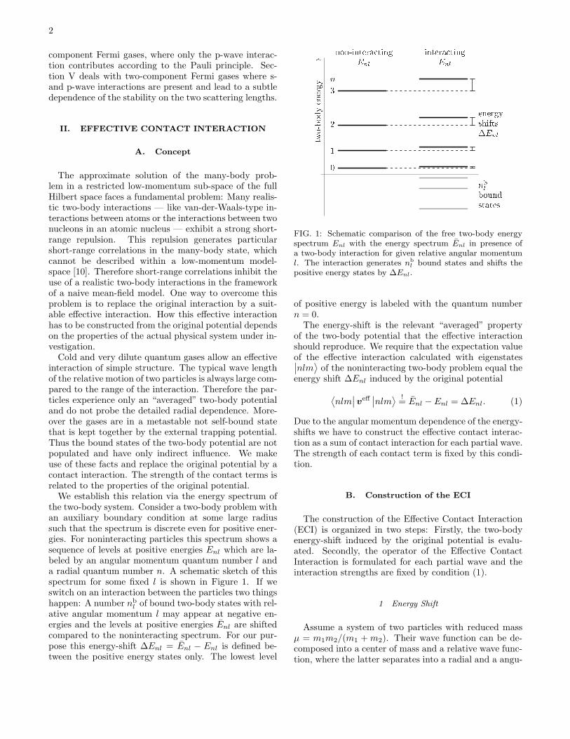
We establish this relation via the energy spectrum ofthe two-body system. Consider a two-body problem withan auxiliary boundary condition at some large radiussuch that the spectrum is discrete even for positive ener-gies. For noninteracting particles this spectrum shows asequence of levels at positive energies Enl which are la-beled by an angular momentum quantum number l anda radial quantum number n. A schematic sketch of thisspectrum for some fixed l is shown in Figure 1. If weswitch on an interaction between the particles two thingshappen: A number nb

l of bound two-body states with rel-ative angular momentum l may appear at negative en-ergies and the levels at positive energies Enl are shiftedcompared to the noninteracting spectrum. For our pur-pose this energy-shift ∆Enl = Enl − Enl is defined be-tween the positive energy states only. The lowest level

t

w

o

-

b

o

d

y

e

n

e

r

g

y

!

non-intera ting

E

nl

intera ting

E

nl

energy

shifts

E

nl

n

b

l

bound

states

n

3

2

1

0

FIG. 1: Schematic comparison of the free two-body energyspectrum Enl with the energy spectrum Enl in presence ofa two-body interaction for given relative angular momentuml. The interaction generates nb

l bound states and shifts thepositive energy states by ∆Enl.

of positive energy is labeled with the quantum numbern = 0.

The energy-shift is the relevant “averaged” propertyof the two-body potential that the effective interactionshould reproduce. We require that the expectation valueof the effective interaction calculated with eigenstates∣

∣nlm⟩

of the noninteracting two-body problem equal theenergy shift ∆Enl induced by the original potential

⟨

nlm∣

∣veff∣

∣nlm⟩ !

= Enl − Enl = ∆Enl. (1)

Due to the angular momentum dependence of the energy-shifts we have to construct the effective contact interac-tion as a sum of contact interaction for each partial wave.The strength of each contact term is fixed by this condi-tion.

B. Construction of the ECI

The construction of the Effective Contact Interaction(ECI) is organized in two steps: Firstly, the two-bodyenergy-shift induced by the original potential is evalu-ated. Secondly, the operator of the Effective ContactInteraction is formulated for each partial wave and theinteraction strengths are fixed by condition (1).

1 Energy Shift

Assume a system of two particles with reduced massµ = m1m2/(m1 + m2). Their wave function can be de-composed into a center of mass and a relative wave func-tion, where the latter separates into a radial and a angu-

3

lar component because of rotational symmetry

⟨

~r∣

∣nlm⟩

= Rnl(r)Ylm(Ω). (2)

The radial wave functions Rnl(r) of the noninteractingtwo-body system are solutions of the Schrodinger equa-tion

[

− 1

r

∂2

∂r2r +

l(l + 1)

r2− 2µEnl

]

Rnl(r) = 0 (3)

(we use units with ~ = 1). We require the radial wavefunction to vanish at some arbitrary but large radius Λ

Rnl(Λ)!= 0. (4)

This auxiliary boundary condition leads to a discrete en-ergy spectrum, which is needed to enumerate the energylevels and to evaluate the energy shift.

In the noninteracting case the solution of the radialSchrodinger equation (3) is given by a spherical Besselfunction jl(x)

Rnl(r) = Anl jl(qnlr), (5)

where qnl denotes the relative momentum of the two par-ticles and Anl a normalization constant. The discretemomenta qnl are determined by the boundary condition(4) and thus are related the to the zeros of the Besselfunction. Since the radius Λ can be chosen arbitrarylarge it is sufficient to use the asymptotic expansions ofthe spherical Bessel and Neumann functions

jl(x)x≫l=

1

xsin

(

x − πl/2)

,

nl(x)x≫l= − 1

xcos

(

x − πl/2)

.

(6)

Evaluating the boundary condition (4) with the asymp-totic form of the Bessel function we obtain for the possi-ble relative momenta

qnlΛ = π(n + l/2). (7)

Accordingly the two-body energy spectrum in the nonin-teracting case is given by

Enl =1

2µq2nl =

π2

2µΛ2(n + l/2)2. (8)

The normalization constant can be determined explicitly

A−2nl =

∫ Λ

0

dr r2j2l (qnlr) =

Λ3

2j2l+1(qnlΛ). (9)

Inserting the asymptotic form of the Bessel function wefinally get

A−2nl

qnlΛ≫l=

Λ

2q2nl

. (10)

In presence of a two-body potential v(r) of finite rangeλ the solution Rnl(r) of Schrodinger equation

[

− 1

r

∂2

∂r2r +

l(l + 1)

r2+ 2µ

[

v(r) − Enl

]

]

Rnl(r) = 0

(11)

outside the range of the potential (r > λ) is given by asuperposition of spherical Bessel and Neumann functions

Rnl(r) = Anl

[

jl(qnlr) − tan ηl(qnl) nl(qnlr)]

, (12)

where ηl(q) denotes the phase shift of the potential forthe l-th partial wave. The bar distinguishes quantitiesin presence of the interaction from those in the nonin-teracting case. Imposing the boundary condition (4) weget the following implicit equation for the momenta qnl

in the interacting case

jl(qnlΛ)

nl(qnlΛ)= tan ηl(qnl). (13)

Expressing the Bessel and Neumann functions by theirasymptotic expansion (6) this reduces to

− tan(qnlΛ − πl/2) = tan ηl(qnl). (14)

In order to associate the energy levels with same quantumnumber n in the interacting and noninteracting case asdescribed above, the lowest positive-energy state shouldbe labeled with the quantum number n = 0. To achievethis for a potential with nb

l bound two-body states withangular momentum quantum number l we add the phaseπ(n + nb

l ) to the argument on the r.h.s., i.e., the boundstates contribute according to Levinson’s theorem. Themomenta qnl in presence of the interaction are thus de-termined by the equation

qnlΛ = −ηl(qnl) + π(n + nbl + l/2). (15)

The momentum shift ∆qnl induced by the interactionis obtained by subtracting the momenta of the noninter-acting system (7) from equation (15)

∆qnlΛ = (qnl − qnl)Λ

= −[ηl(qnl) − πnbl ] = −ηl(qnl).

(16)

Here ηl(q) = ηl(q)− πnbl denotes the phase shift reduced

by the contribution of the bound states. In a final stepwe expand the phase shifts around the momenta qnl ofthe noninteracting system

ηl(qnl) = ηl(qnl) + η′l(qnl)∆qnl + · · · . (17)

Already the term linear in ∆qnl can be neglected in goodapproximation because the momentum shift is of the or-der 1/Λ according to equation (16). Thus we retain thefollowing simple expression for the momentum shift

∆qnlΛ = −ηl(qnl). (18)

4

The shift of the energy levels of the interacting two-body system compared to the noninteracting spectrumis connected with the momentum shift by

∆Enl

Enl= 2

∆qnl

qnl+

(

∆qnl

qnl

)2

. (19)

The term quadratic in the momentum shift can be ne-glected because ∆qnl/qnl is small. The final expressionfor the energy shift reads

∆Enl

Enl= − 2

Λ

ηl(qnl)

qnl. (20)

The proportionality between energy shift and phase shiftsis well known [11] and was used in different applicationsbefore.

2 ECI in Scattering Length Approximation

In a second step we construct an operator form of theEffective Contact Interaction that obeys condition (1).For the application to ultracold dilute quantum gases thegeneral form (20) of the energy shift ∆Enl can be simpli-fied considerably. The relative momenta in these systemsare extremely low, i.e., typical relative wave lengths arelarge compared to the range of the interaction. This al-lows an expansion of the phase shifts ηl(q) in a powerseries in relative momentum. In lowest order approxima-tion (q al ≪ 1) the phase shifts of the l-th partial wavecan be expressed in terms of the corresponding scatteringlength al [20]

ηl(q)

q2l+1≈ tan ηl(q)

q2l+1≈ − (2l + 1)

[(2l + 1)!!]2a2l+1

l . (21)

The energy shift in this scattering length approximationis given by

∆Enl

Enl=

2

Λ

(2l + 1)

[(2l + 1)!!]2q2lnl a2l+1

l . (22)

Based on this form we can construct a simple operator forthe ECI. For applications where the approximation (21)is not sufficient higher order terms of the power seriescan be included successively. We will come back to thispoint in the following section.

According to the dependence of the energy shifts onthe angular momentum quantum number l the operatorof the effective interaction veff is formulated as a sum ofindependent operators veff

l for each partial wave

veff =∞∑

l=0

Πl veffl Πl, (23)

where Πl denotes the projection operator on the sub-space spanned by states of relative angular momentuml. We want to use a contact interaction for each par-tial wave. This requires nonlocal interaction operators

beyond l = 0, i.e., derivative couplings. The simplestansatz for the operator of the effective contact interac-tion for the l-th partial wave is

veffl = (~q · r)l gl δ

(3)(~r) (r · ~q)l

=

∫

d3r∣

∣~r⟩

∂ l

∂rlgl δ

(3)(~r)

∂ l

∂rl

⟨

~r∣

∣ .(24)

Here ~q = 12 (~p1 − ~p2) denotes the operator of the rela-

tive momentum of two particles, r = ~r/r the unit vec-tor along the relative coordinate and δ(3)(~r) = 1

4πr2 δ(r)the radial component of the 3-dimensional delta function.The arrows above the derivatives indicate to which sidethey act.

The interaction strength gl is a constant that containsthe relevant information on the original two-body poten-tial. The connection is provided by condition (1) via theshift of the energy levels with respect to the free spec-trum. To evaluate (1) we calculate the expectation valueof the contact interaction (24) for the l-th partial wavetaken with the noninteracting two-body states

∣

∣nlm⟩

⟨

nlm∣

∣veffl

∣

∣nlm⟩

= gl

∫

d3r δ(3)(~r)∣

∣

∣

∂l

∂rlRnl(r)Ylm(Ω)

∣

∣

∣

2

=gl

4π

∣

∣

∣

∂l

∂rlRnl(r)

∣

∣

∣

2

r=0

=gl

4π

[

l!

(2l + 1)!!

]2

A2nl q2l

nl,

(25)

where we used the expansion of the radial wave-functionaround the origin

Rnl(r) = Anl(qnlr)

l

(2l + 1)!!

[

1 − (qnlr)2

2(2l + 3)+ · · ·

]

. (26)

Equating the expectation value (25) with the energyshift results in the following equation for the interactionstrengths

gl = 4π

[

(2l + 1)!!

l!

]2

A−2nl

∆Enl

q2lnl

(27)

Inserting the normalization constant (10) and the energyshift in scattering length formulation (22) gives the finalexpression for the interaction strengths

gl =4π

2µ

(2l + 1)

(l!)2a2l+1

l . (28)

Together with equation (24) this defines the scatteringlength formulation of the Effective Contact Interaction.Notice that these expressions do not depend on the aux-iliary boundary condition (4), which was introduced toobtain a discrete energy spectrum.

For l = 1 sometimes a gradient operator with respectto the relative coordinate is used instead of the radial

5

derivative (24). This alternative ansatz reads

veff1 = ~q g1 δ(3)(~r) ~q

=

∫

d3r∣

∣~r⟩

∇ g1 δ(3)(~r)

∇⟨

~r∣

∣ .(29)

It should be noted that the p-wave interaction strengthg1 in the gradient formulation is related to the interactionstrength (28) by

g1 = g1/3. (30)

3 Beyond Scattering Length Approximation

The operator of the Effective Contact Interactioncan be generalized systematically beyond the scatteringlength approximation shown in the preceding section. Aformal scheme emerges from the expansion of the phaseshifts in a power series in q

ηl(q)

q2l+1=

∞∑

ν=0

1

ν!c(ν)l q2ν . (31)

The momentum independent lowest order term of thisexpansion matches the scattering length approximation.From equation (21) the connection between the coeffi-

cient c(0)l and the the scattering length al becomes obvi-

ous

c(0)l = − (2l + 1)

[(2l + 1)!!]2a2l+1

l . (32)

The coefficient c(1)l of the quadratic term of the expansion

is connected to the so called effective range or effectivevolume of the potential. We will discuss this contributionin more detail later. By inserting the expansion (31) intothe general formula (20) for the energy shifts we obtain

∆Enl

Enl= − 2

Λ

∞∑

ν=0

1

ν!c(ν)l q2l+2ν

nl . (33)

Following the basic concept of the ECI these energyshifts have to be generated by the operator of the ECIaccording to condition (1). To include the momentumdependence of the energy shifts we have to generalizethe ansatz for the ECI operator compared to the sim-ple momentum-independent scattering-length formula-tion (24). The further calculation will show that

veffl =

∞∑

ν=0

1

2g(ν)l

[

(~q · r)l δ(3)(~r) (r · ~q)l+2ν

+ (~q · r)l+2ν δ(3)(~r) (r · ~q)l]

(34)

is a proper ansatz for the effective interaction operator forthe l-th partial wave. Besides the more complex nonlocal

structure a set of interaction strengths g(ν)l (ν = 0, 1, . . . )

for each partial wave is included. They are related to

the coefficients c(ν)l and thus correspond to the different

powers of the momentum in equation (33). To employcondition (1) we calculate the expectation value of veff

lwith noninteracting two-body states

∣

∣nlm⟩

⟨

nlm∣

∣ veffl

∣

∣nlm⟩

=1

4π

∞∑

ν=0

g(ν)l

[ ∂l

∂rlRnl(r)

]

r=0

[ ∂l+2ν

∂rl+2νRnl(r)

]

r=0

=A2

nl

4π

∞∑

ν=0

g(ν)l

l!

(2l + 1)!!

(−1)ν(l + 2ν)!

2νν!(2l + 2ν + 1)!!q2l+2νnl ,

(35)

where the full expansion of the noninteracting radial wavefunction (5) around r = 0 was used [12]

Rnl(r) = Anl

∞∑

µ=0

(−1)µ

2µµ!(2l + 2µ + 1)!!(qnlr)

l+2µ. (36)

By inserting the expansion of the energy shifts (33) andthe expectation value into condition (1) and comparingthe coefficients for the different powers of the momentumqnl we obtain

g(ν)l = (−1)ν+1 4π

2µ

2ν(2l + 1)!!(2l + 2ν + 1)!!

l!(l + 2ν)!c(ν)l . (37)

Thus the interaction strengths g(ν)l of the general oper-

ator form of the ECI (34) are proportional to the coeffi-

cients c(ν)l of the expansion of the phase shifts (31). The

equations (34) and (37) define the most general form ofthe Effective Contact Interaction.

For the application to dilute degenerate Fermi gases wewill use the ECI up to quadratic terms in the momentum,i.e., we include the scattering length term of the s- and p-wave part as well as the s-wave effective range correction.At this point we have to discuss the connection betweenthe quadratic term of the expansion (31) and the usualeffective range theory. For the s-wave phase-shifts theeffective range expansion reads

q cot η0(q) ≈ − 1

a0+

1

2r0 q2, (38)

where r0 is the effective range of the potential. If weconvert this into an expression for η0(q)/q and expand inq we obtain

η0(q)

q= −a0 − b0 q2 + · · · (39)

with an effective volume b0 that depends on the scatter-ing length a0 and the effective range r0

b0 = 12a2

0r0 − 13a3

0. (40)

Rather than using this relation we will adjust b0 in orderto get the best representation of the phase shift η0(q)/qwith the truncated expansion (39).

6

Finally, inserting c(1)0 = −b0 into equation (37) gives

an expression for the interaction strength of the s-waveeffective range term

g(1)0 = −12π

2µb0. (41)

C. Example: Square-Well Potential

To illustrate the concept of the Effective Contact In-teraction we use the simple toy-problem of two particlesinteracting by an attractive square-well potential of ra-dius λ and depth −V0.

First we look at typical wave functions to which theidea of the ECI applies. The major condition is that thetypical wavelength of the relative motion is large com-pared to the range of the interaction. This is ensuredby choosing the radius λ of the square-well much smallerthan the radius Λ associated with the boundary condition(4); in the following we use λ = 0.01Λ. Figure 2 showsthe radial wave function of the lowest l = 0 state withpositive energy for different potential depths V0. Out-side the potential the structure of the wave functions isvery similar for the different interaction strengths. Onlythe wavelength is changed slightly due to the differentmatching to the wave function in the interior (see in-sert of Figure 2). This change of the relative momentumtranslates immediately into an energy shift. From thatpicture the connection between energy shifts and phaseshifts is evident.

A second point becomes clear from this simple exam-ple: The detailed structure of the radial dependence ofthe potential or the number of bound states is irrelevantfor the energy shift, only the phase shifts ηl(q) matter.The insert in Figure 2 shows that the wave functions be-have very different within the range λ due to the differentpotential depths. Moreover the potentials have a differ-ent number of bound states, e.g., the thick solid curve isassociated with a potential with one bound state but zerophase shift. Hence the behavior outside the potential isidentical to the noninteracting case (thin solid curve) andthe energy shift is zero.

Next we investigate the dependence of the l = 0 en-ergy shifts on the strength of the attractive potential.Figure 3 shows the relative energy shift ∆Eexact/E ver-sus λ

√V0, where the radius λ = 0.01Λ of the square-well

potential is kept fixed and the depth V0 is increased. Acharacteristic pattern appears: In the vicinity of interac-tion strengths where the potential gains another boundstate the relative energy shift assumes large positive andnegative values. Large positive energy shifts occur forpotentials that have a very weakly bound state, nega-tive energy shifts for those that have an almost boundstate. In between these interaction strengths extendedplateaus of nearly constant energy shift appear. Withinthe plateaus the energy shift is independent of the radialquantum number n of the level or the relative momen-tum. This is a special property of the s-wave channel;

for higher partial waves the relative energy shift (22) isproportional to q2l. Only at the edges of the plateaus aslight dependence on the relative momentum shows up(see Figure 3).

This structure is closely related to the behavior of thes-wave scattering length. The l = 0 energy shift inducedby the ECI in scattering length approximation (22) isproportional to the scattering length a0. For the square-well potential we get

∆En0

En0= 2

a0

Λwith

a0

λ= 1 − tan(λ

√V0)

λ√

V0

. (42)

This ECI energy shift is right on top of the solid curvein Figure 3, i.e., it agrees very well with the exact energyshift for the lowest positive energy state. Even for highermomenta the agreement is very good provided that themagnitude of the scattering length is not too large. Sig-nificant deviations occur only if momentum and scatter-ing length are large.

To obtain a quantitative measure of for the applica-bility of the ECI in scattering length approximation weinvestigate the relative deviation (E − Eexact)/E of theECI energy levels compared to the exact ones for thesquare-well potential. We expect that the agreement getsworse if either the relative momentum or if the scatter-ing length is large. Therefore, Figure 4 shows the relativeenergy deviation for l = 0 and l = 1 states as functionof the product of momentum and scattering length, q al,which was assumed to be small in order to introduce thescattering length (21). The different curves correspondto different values of the momentum qnl and were ob-tained by varying the depth of the square-well potentialand thus the scattering length.

As expected the deviation increases with increasingvalue of q al. Nevertheless, the deviation of the energycalculated with the ECI in scattering length approxima-tion is below 1% up to rather large values of q al . 1.If we tolerate a maximum deviation of 5% then thescattering length formulation can be used up to valuesq al . 1.5.

It should be noted that the relative deviation of thegeneral form (20) of the ECI in the parameter range dis-cussed above is below 10−4. Thus all approximationsmade to obtain equation (20) are valid on a high level ofaccuracy. The restrictions on the validity of the scatter-ing length formulation (22) originate for the replacementof the phase shifts by the scattering length alone, whichis no inherent part of th ECI concept. If the simple scat-tering length formulation is not sufficient for a specialapplication one can go beyond that.

For example, the inclusion of effective volume correc-tions (see eq. (39)) improves the agreement with theexact energy shifts. In this way we can reduce the maxi-mum deviation to only 1% up to q a0 . 1.5.

7

0 0.1 0.2 0.3 0.4 0.5 0.6 0.7 0.8 0.9 1

r [

0 0.01 0.02

0

0.25

-0.05

0

0.05

r

R

00

(r)

FIG. 2: Radial wave functions rR00(r) of the lowest l = 0 positive energy state for different potential depths V0 of the square-well potential. The interaction strengths are λ

√V0 = 0 (thin solid), 4.49 (solid), 4.85 (dashed), and 9.5 (dotted). The radius

of the well is λ = 0.01Λ and marked by the gray area. The insert shows a magnification of the region around the origin.

0 2 4 6 8 10

p

V

0

-0.15

-0.1

-0.05

0

0.05

0.1

E

exa t

n0

E

n0

FIG. 3: Relative energy-shift ∆Eexact

n0 /En0 obtained from theexact l = 0 solutions plotted versus the strength λ

√V0 of the

square-well potential. The solid line gives the energy shiftfor the lowest (n = 1), the dashed line for the 10th, and thedotted line for 20th state of the positive energy spectrum.The dots mark the interaction strengths used in Figure 2.

D. ECI versus Pseudopotential

The idea to simulate the effect of a complicated finite-range two-body potential by a simple s-wave contact in-teraction dates back to E. Fermi [13] and was used by sev-eral authors [14] in various physical contexts. K. Huangand C.N. Yang [15, 16] generalized this idea and con-structed the so called pseudopotential that acts in allpartial waves.

The aim of the pseudopotential is (a) to generate thephase shifts of the original potential by a boundary con-dition at r = 0 and (b) to reformulate this by an addi-tional inhomogenous term in the Schrodinger equation ofthe two-body scattering problem. This additional term isinterpreted as the pseudopotential, which can be phrased

0 1 2

q a

0

0 1 2

q a

1

0

0.02

0.04

0.06

0.08

E

E

exa t

E

l = 0 l = 1

FIG. 4: Relative deviation of the two-body energy calculatedwith the ECI in scattering length approximation from theexact energy as function of qal for l = 0 (left) and l = 1states (right). The curves were obtained for interactions withthree bound states by varying the strength λ

√V0 and looking

at the energy shifts for different relative momenta qnlΛ ≈ 20(solid), 40 (dashed), and 80 (dotted).

in the following operator form [17]

vpseudol =

∫

d3r∣

∣~r⟩ 1

rlgpseudo

l δ(3)(~r)

∂ 2l+1

∂r2l+1rl+1

⟨

~r∣

∣

(43)

with an interaction strength

gpseudol =

4π

2µ

(l + 1)

(2l + 1)!a2l+1

l (44)

for the l-th partial wave. For this discussion we restrictourselves to the scattering length approximation of thephase shifts. Due to the fact that the radial derivativeacts only to the right hand side the operator of the pseu-

8

dopotential (43) is not hermitian. This is in contradictionto the basic concept of effective interactions.

A more severe weakness shows up when we evaluatethe energy shifts induced by the pseudopotential. As dis-cussed in section II A the expectation value of a propereffective interaction with eigenstates

∣

∣nlm⟩

of the nonin-teracting two-body system should be equal to the energyshift induced by the original potential. For the pseudopo-tential (43) we obtain an energy shift

∆Epseudonl

Enl=

1

Enl

⟨

nlm∣

∣vpseudol

∣

∣nlm⟩

=2

Λ

(l + 1)

[(2l + 1)!!]2q2lnla

2l+1l .

(45)

This has to be compared with the full energy shift inscattering length approximation (22) which is by con-struction reproduced by the ECI. Obviously the energyshift induced by the pseudopotential for states with l > 0is by a factor (l+1)/(2l+1) smaller the the energy shift ofthe original potential. Thus the pseudopotential under-estimates the effect of the two-body interactions beyonds-wave when used in a mean-field framework. For thewidely used s-wave part the energy shifts of the pseu-dopotential agree with the energy shifts of the originalpotential.

We conclude that the nonhermitian pseudopotential isnot a proper effective interaction for a mean-field descrip-tion of a dilute quantum gases that goes beyond s-waveinteractions.

III. ENERGY FUNCTIONAL OF A TRAPPED

MULTI-COMPONENT FERMI GAS

A. Fundamentals

In the following we investigate the ground state prop-erties of a dilute Fermi gas composed of Ξ distinguishablecomponents that is trapped in an external potential U(~x)at temperature T = 0 K. In present experiments [2] oneor two components are used, which belong to the sameatomic species but are distinguished by different projec-tions MF of the total angular momentum F onto thedirection of an external magnetic field. We distinguishthe different components by a formal quantum numberξ = 1, . . . , Ξ. For simplicity we use the same mass m ofthe atoms for all components.

We treat the many-body problem in the frameworkof density functional theory and construct an energyfunctional of the inhomogenous multi-component Fermigas within a proper approximation. The ground statedensity-distribution of the many-body system is then de-termined by functional minimization of the energy.

The large particle numbers of the order N ∼ 106 allowthe rather simple Thomas-Fermi approximation for theenergy functional. It is assumed that the energy densityof the inhomogenous system is described locally by the

energy density of the corresponding homogenous system,and higher-order terms which include gradients of thedensity are small. To check the quality of the Thomas-Fermi approximation we calculated the next order gradi-ent corrections for a trapped noninteracting Fermi gas.For N = 100 particles the relative contribution of thegradient correction to the total energy is of the order of10−2; for typical particle numbers of N = 106 it drops to10−5 [17].

As starting point for the Thomas-Fermi approximationwe calculate the energy density of the homogenous inter-acting multi-component Fermi gas in mean-field approx-imation. The basic restriction of the mean-field pictureis that two- and many-body correlations induced by theinteraction are not contained in the many-body state.Nevertheless they can be implemented implicitly by us-ing a proper effective interaction that is tailored for themodel-space available. In the previous section we con-structed the Effective Contact Interaction especially forthe mean-field description of dilute not self-bound quan-tum gases.

A central topic of the following studies is the role ofthe interaction on the structure and stability of trappeddegenerate Fermi gases. Our special interest concerns thep-wave part of the interaction, which contributes even atT = 0K — in contrast to bosonic systems. It will turn outthat the p-wave terms can be of substantial importancefor the ground state properties of fermionic systems andshould not be neglected from the outset.

We write the Hamilton operator of the system as a sumof the external trapping potential U and an internal partHint

H = U + Hint. (46)

The internal part contains the kinetic energy and the Ef-fective Contact Interaction as discussed in section II. Weinclude the s-wave and p-wave terms of the ECI in scat-tering length formulation as well as the s-wave effectiverange correction. With equations (24), (28), (34), and(41) the internal Hamiltonian reads

Hint =1

2m

∑

i

~p2i

+4π

ma0

∑

i, j>i

δ(3)(~rij) (47)

− 12π

mb0

∑

i, j>i

1

2

[

δ(3)(~rij)(rij ·~qij)2 + h.a.

]

+12π

ma31

∑

i, j>i

(~qij ·rij) δ(3)(~rij) (rij ·~qij).

The summations over the particle indices i and j rangefrom 1 to the total number of particles. The properties ofthe two-body interaction are parameterized by the s- andp-wave scattering lengths a0 and a1, respectively, and bythe s-wave effective volume b0. In general the interactionparameters depend on the component quantum numbers

9

ξ of the interacting particles. In order to discuss thebasic phenomena we restrict ourselves to equal interac-tion parameters for all components. The generalizationto scattering length matrices that account for the depen-dence on the component indices of the two interactingparticles is straightforward.

Experimentally each component may experience a dif-ferent trapping potential Uξ(~x). For magnetic traps thisis due to the different magnetic momenta of the com-ponents, which leads to a relative shift of the trappingpotentials for the components. Thus the operator of theexternal potential has the following form

U =∑

i

∑

ξ

Uξ(~xi)Πξ,i (48)

where Πξ is a projection operator onto states with thecomponent quantum number ξ.

Many of the results shown in the next sections do notdepend on the actual shape of the trapping potential. Ifthe shape enters explicitly we assume a deformed har-monic oscillator potential

U(~x) =mω2

2

(

λ21x

21 + λ2

2x22 + λ2

3x23

)

=1

2mℓ4

(

λ21x

21 + λ2

2x22 + λ2

3x23

)

,

(49)

where ω = 3√

ω1ω2ω3 is the mean oscillator frequency

and ℓ = (mω)−1/2 the corresponding mean oscillatorlength, i.e., the mean width of the Gaussian single-particle ground state of the harmonic oscillator poten-tial. The deformation is parameterized by the ratiosλi = ωi/ω, which fulfill the condition λ1λ2λ3 = 1.

B. Energy Density in Thomas-Fermi

Approximation

The calculation of the energy density functional of theinhomogenous interacting Fermi gas is performed in twosteps: First we calculate the energy density of the corre-sponding homogenous system in mean-field approxima-tion. In the second step this is translated into an en-ergy density of the inhomogenous system by means ofthe Thomas-Fermi approximation.

The ground state of a many-fermion system in mean-field approximation is given by an antisymmetrized prod-uct of one-body states

∣

∣i⟩

. In the case of a homogenoussystem the one-body states are eigenstate of the momen-

tum operator with eigenvalues ~ki. In addition they arecharacterized by the component quantum number ξ

∣

∣i⟩

=∣

∣~ki

⟩

⊗∣

∣ξi

⟩

. (50)

Assuming a box of volume V with periodic boundaryconditions the spatial part of the one-body states is givenby

⟨

~x∣

∣~ki

⟩

=1√V

exp(

i~ki ·~x)

. (51)

The energy density of the homogenous system is givenby the expectation value of the internal part of the Hamil-ton operator (47)

Ehom =⟨

Hint

⟩

/V. (52)

The calculation of the expectation values of the severalparts of the Hamiltonian is straightforward [17]. As afunction of the Fermi momenta κξ of the different com-ponents the energy density reads

Ehom(κ1, . . . , κΞ)

=1

20π2m

∑

ξ

κ5ξ

+a0

9π3m

∑

ξ, ξ′>ξ

κ3ξκ

3ξ′ (53)

+a31

30π3m

∑

ξ

κ8ξ

+a31 + b0

60π3m

∑

ξ, ξ′>ξ

[κ3ξκ

5ξ′ + κ5

ξκ3ξ′ ].

The summations run over all components ξ = 1, . . . , Ξ.To avoid fractional exponents we use Fermi momenta κξ

rather than densities ρξ = κ3ξ/(6π2).

The basic assumption of the Thomas-Fermi (or local-density) approximation is that the energy density of theinhomogenous Fermi gas is locally given by the energydensity of the corresponding homogenous system. Thusthe energy density of the inhomogenous system is con-structed from (53) by replacing κξ with local Fermi mo-

menta κξ(~x). In addition the contribution of the externaltrapping potential has to be included. This results in thefollowing expression for the energy density of the trappedinteracting multi-component Fermi gas

E [κ1, . . . , κΞ](~x)

=1

6π2

∑

ξ

Uξ(~x) κ3ξ(~x)

+1

20π2m

∑

ξ

κ5ξ(~x)

+a0

9π3m

∑

ξ, ξ′>ξ

κ3ξ(~x)κ3

ξ′(~x) (54)

+a31

30π3m

∑

ξ

κ8ξ(~x)

+a31 + b0

60π3m

∑

ξ, ξ′>ξ

[κ3ξ(~x)κ5

ξ′(~x) + κ5ξ(~x)κ3

ξ′(~x)].

The local Fermi momentum is related to the density ofparticles of the component ξ by

ρξ(~x) =1

6π2κ3

ξ(~x). (55)

10

Accordingly the number of particles of component ξ isgiven by

Nξ =

∫

d3x ρξ(~x) =1

6π2

∫

d3x κ3ξ(~x). (56)

As discussed in section II C we can reproduce the two-body energy spectrum with an accuracy of about 5% upto alq ≈ 1.5. If we take this as a limit for the root meansquare of the relative momentum 〈q2〉1/2 = 0.53 κ in themany-body system, we can apply our many-body modelup to alκ ≈ 3.

C. Functional Variation and the Extremum

Condition

The ground state density of a system is found by min-imizing the energy functional

E[κ1, . . . , κΞ] =

∫

d3x E [κ1, . . . , κΞ](~x). (57)

for given particle numbers Nξ. This constraint is im-plemented with help of a set of Lagrange multipliers µξ,which are the chemical potentials of the different compo-nents. The Legendre transformed functional

F [κ1, . . . , κΞ]

= E[κ1, . . . , κΞ] −∑

ξ

µξNξ

=

∫

d3x E [κ1, . . . , κΞ](~x) −∑

ξ

µξ

6π2κ3

ξ(~x)

=

∫

d3x F [κ1, . . . , κΞ](~x),

(58)

has to be minimized by functional variation. A necessarybut not sufficient condition for a set of local Fermi mo-menta κ1(~x), . . . , κΞ(~x) to minimize the transformedenergy functional F [κ1, . . . , κΞ] is stationarity, i.e., thatthe first variation of F [κ1, . . . , κΞ] with respect to allκξ(~x) vanishes

δ

δκξF [κ1, . . . , κξ] = 0 for all ξ. (59)

This extremum condition is fulfilled if the derivative ofthe integrand F [κ1, . . . , κΞ](~x) with respect to all localFermi momenta vanishes at each point ~x

∂

∂κξ(~x)F [κ1, . . . , κΞ](~x) = 0 for all ~x, ξ. (60)

Inserting expression (54) for the energy density and eval-uating the derivative results in the extremum condition

m[µξ − Uξ(~x)]

=1

2κ2

ξ(~x) +2a0

3π

∑

ξ′ 6=ξ

κ3ξ′(~x) +

8a31

15πκ5

ξ(~x)

+a31 + b0

30π

∑

ξ′ 6=ξ

[3 κ5ξ′(~x) + 5 κ2

ξ(~x)κ3ξ′(~x)]

(61)

for all ~x and each ξ. This is a coupled set ofΞ polynomial equations for the local Fermi momentaκ1(~x), . . . , κΞ(~x) at some given point ~x. Note that thetrivial solutions κξ(~x) = 0 were separated already. Anyreal solution of the extremum condition (61) correspondsto a stationary point of the energy functional. In generalone has to check explicitly whether they correspond toa minimum of the energy functional or whether they aremaxima or saddle points.

All following investigations on the structure and sta-bility of degenerate Fermi gases and on the influence ofs- and p-wave interactions are based on the extremumcondition (61). Many physical conclusions can be drawnfrom its algebraic structure already. We will discuss thesequestions in detail for the one- and two-component Fermigas in section IV and V, respectively.

IV. SINGLE-COMPONENT FERMI GAS

As a first application of the formalism developed in thepreceding section we study the properties of a degeneratesingle-component Fermi gas.

A. Effect of the p-Wave Interaction

The energy density of the interacting multi-componentFermi gas (54) reduces for the single-component systemto the form

E [κ](~x) =1

6π2U(~x)κ3(~x) +

1

20π2mκ5(~x)

+a31

30π3mκ8(~x),

(62)

where κ(~x) is the local Fermi momentum. The first termis the contribution of the trapping potential U(~x), thesecond term is the kinetic energy, and the third termdescribes the contribution of the p-wave interaction witha p-wave scattering length a1. As mentioned earlier thes-wave part of the interaction does not contribute in asystem of identical fermions due to the Pauli principle.Therefore the p-wave part is the leading interaction termand there is no reason to neglect it from the outset.

A first hint on the effects of the p-wave interaction aregiven by the density distributions for different values ofthe p-wave scattering length. The density distributionis obtained by solution of the extremum condition (61),which takes the simple form

m[µ − U(~x)] = f1[κ(~x)] (63)

with f1(κ) =1

2κ2 +

8a31

15πκ5.

This 5th order polynomial equation for the local Fermimomentum κ(~x) is solved numerically for each point ~x.The chemical potential µ is adjusted such that particlenumber (56) assumes the desired value.

11

0 5 10 15 20 25

x [`

0

50

100

150

(x)

[`

3

FIG. 5: Density profile ρ(x) of a single-component Fermigas of N = 106 particles trapped in a spherical symmetricparabolic trap with oscillator length ℓ. The solid curve showsthe noninteracting gas a1/ℓ = 0. Dotted curves correspond torepulsive p-wave interactions with a1/ℓ = 0.03, 0.06, and 0.1(from top to bottom). The dashed curves show attractive p-wave interactions with a1/ℓ = −0.03, −0.04 and −0.044 (topto bottom), respectively.

Figure 5 shows the resulting radial density profilesρ(x) = κ3(x)/(6π2) for a single-component gas of N =106 particles in a spherical trap with oscillator length ℓfor different p-wave scattering lengths a1. The oscillatorlength defines the fundamental length scale of the prob-lem and the parameter that determines the strength ofthe interaction is the ratio of the p-wave scattering lengthand oscillator length, a1/ℓ. To increase the magnitude ofthis ratio experimentally one can either increase the mag-nitude of the scattering length or decrease the oscillatorlength.

For a repulsive p-wave interaction, i.e., a1/ℓ > 0, of in-creasing strength (dotted curves) the density distributionflattens and expands radially compared to the noninter-acting system (solid line). For a ratio a1/ℓ = 0.1 the cen-tral density has dropped to one half of the density of thenoninteracting gas. With a typical experimental oscilla-tor length of ℓ = 1µm this ratio corresponds to a ratherlarge scattering length of a1 ≈ 2000aB, which neverthe-less may be within the range of experimental parameters[7]. For a tightly confining trap with ℓ = 0.1µm a moder-ate scattering length of a1 ≈ 200aB is required to obtainthe same ratio.

For an attractive p-wave interaction, a1/ℓ < 0, thecentral density increases significantly with increasing in-teraction strength. If the central density exceeds a cer-tain value, i.e., if |a1/ℓ| exceeds a critical value, then theextremum condition (63) has no real solution any more.Physically this corresponds to a collapse of the dilute gascaused by the attractive mean-field that is generated bythe p-wave interaction. We will discuss this question indetail in the following sections.

The dependence of the density distribution on thep-wave scattering length as depicted in Figure 5 al-ready demonstrates that the p-wave interaction may havestrong influence on the properties of degenerate Fermigases.

B. Mean-Field Instability: A Variational Picture

To illustrate the origin and mechanism of the collapseof the metastable state of the trapped Fermi gas we utilizea simple variational picture. Assume a single-componentFermi gas of N particles in a spherical symmetric oscil-lator potential. The local Fermi momentum of the inter-acting system is parameterized by the analytic expressionfor the local Fermi momentum of the noninteracting sys-tem

κ(~x) =2(6N)1/3

Xt

√

1 −( x

Xt

)2

for x ≤ Xt, (64)

where the classical turning point Xt is treated as varia-tional parameter. By inserting this parameterization intothe energy density (62) and integrating we obtain a closedexpression for the energy as function of the parameter Xt

E(Xt) = CuNX2

t

ℓ4+ Ct

N5/3

X2t

+ C1N8/3 a3

1

X5t

, (65)

with constant coefficients

Cu =3

16m, Ct =

3(9/2)1/3

2m, C1 =

86(4/3)1/3

1925π2m. (66)

Again the first term corresponds to the external poten-tials, the second to the kinetic energy, and the third termto the p-wave interaction.

Figure 6 shows the dependence of the total energy (65)on the parameter Xt for a system of N = 106 particleswith different p-wave scattering lengths. For attractivep-wave interactions, i.e., negative scattering length a1,the contribution of the interaction in (65) is negative.Due to its X−5

t dependence this interaction contributionleads to a rapid drop of the energy for systems of de-creasing spatial extension and thus increasing density.At very high densities (small Xt) one formally ends upwith states of negative energy, i.e., bound states. Oneshould however keep in mind that the assumptions madefor the construction of the Effective Contact Interactionare not valid in this high density regime any more.

The not self-bound metastable state appears as localminimum at positive energies and low densities providedthe p-wave attraction is sufficiently weak; the thick solidcurve in Figure 6 shows an example. If the strengthof the attractive p-wave interaction increases then thelocal minimum flattens and devolves to a saddle point(dashed curve). From this particular interaction strengthon the metastable low-density state does not exist any-more, only the true ground state of the system remains,which is usually a crystal. The system collapses if the

12

5 10 15 20 25 30

X

t

[`

0.5

1

1.5

E(X

t

)

[E

0

FIG. 6: Variational energy (65) of a trapped single-componentFermi gas with N = 106 as function of the parameter Xt.The curves show the noninteracting gas (thin solid), a1/ℓ =−0.035 (solid), a1/ℓ = −0.051 (dashed), and a1/ℓ = −0.065(dotted). The energies are given in units of the ground stateenergy E0 of the noninteracting gas.

barrier caused by the positive kinetic and the attractivemean-field energy vanishes. Since the mean-field attrac-tion grows with increasing density the system is unstableand collapses towards a high-density configuration.

C. Mean-Field Instability: Stability Conditions

Based on the extremum condition (63) we derive a setof analytic stability conditions that relate the maximumdensity of a metastable system with the p-wave scatteringlength. Part of this was already discussed in [9].

The mean-field instability of the system occurs at val-ues of the chemical potential µ and the scattering lengtha1, where the extremum condition (63) does not havea real solution any more. This is shown in a pictorialway in Figure 7 where the the right hand side f1(κ) ofthe extremum condition is plotted as function of κ fordifferent a1/ℓ. The solution of the extremum conditionat some specific point ~x is given by the value of κ atwhich the respective curve reaches the value m[µ−U(~x)].In the minimum of the trapping potential (we assumeU(~x) = 0 in the minimum) the solution is given by thepoint where f1(κ) reaches the value mµ. By movingtowards the outer regions of the trap m[µ − U(~x)] de-creases and one scans f1(κ) down along ordinate untilone reaches m[µ − U(~x)] = 0, i.e., the classical turningpoint.

For repulsive p-wave interactions (dotted curve) ther.h.s. of (63) is a monotonic growing function and so-lutions exist for arbitrary values of m[µ − U(~x)]. If thescattering length a1 is negative (dashed curve) then f1(κ)exhibits a maximum at a Fermi momentum κmax and

0 10 20 30 40

[`

1

0

100

200

300

f

1

()

[`

2

m

(

max

;m

max

)

FIG. 7: Right hand side f1(κ) of the extremum condition(63) as function of the Fermi momentum for a noninteractingsinge-component gas (solid), with repulsive p-wave interactiona1/ℓ = 0.04 (dotted), and with attractive p-wave interactiona1/ℓ = −0.04 (dashed). The horizontal lines mark the respec-tive values of the chemical potentials for N = 106 particles.

chemical potential µmax

κmax = −3√

3π

2a1, µmax =

3(3π)3/2

40ma21

. (67)

For values of the chemical potential µ > µmax no solutionof the extremum condition exists, i.e., there is no meta-stable low-density state. Equivalently only solutions withlocal Fermi momenta below κmax correspond to minimaof the energy functional; those above κmax (gray segmentof the dashed curve) correspond to maxima of the energy.Thus we get a limiting condition for the local Fermi mo-mentum of the metastable state

−a1κ(~x) ≤3√

3π

2(68)

or in terms of the density

−a31ρ(~x) ≤ 1

16π. (69)

This is one form of the stability condition for the single-component Fermi gas. We note that this condition iscompletely independent of the trap geometry. As soon asthe stability condition is violated somewhere in the trap,in general in the minimum of the trapping potential, thesystem will become unstable.

For practical purposes we formulate a stability condi-tion in terms of the particle number N . The maximumparticle number Nmax of the metastable degenerate Fermigas is directly connected to the maximum chemical po-tential µmax. This relation is established numerically bysolving the extremum condition for the maximum chemi-cal potential µmax and integrating over the resulting den-sity distribution to obtain the corresponding maximum

13

particle number (56). This is done for several scatteringlength a1 assuming a deformed oscillator potential (49)with mean oscillator length ℓ. Finally a parametrizedform of the stability condition is fitted to this data. Theparameterization is motivated by the noninteracting gas,where the maximum local Fermi momentum is propor-tional to 6

√N/ℓ. Inserting this into the stability condi-

tion (68) leads to the form

C(

6√

Na1

ℓ

)

≤ 1 , C = −2.246. (70)

The parameter C is fitted to the numerical results, whichare reproduced with a deviation far below 1%. Note thatthis condition is independent of the deformation of theharmonic oscillator trap [17].

For an interaction strength of a1/ℓ = −0.01 whichcorresponds to a scattering length a1 ≈ −200aB for atrap with ℓ = 1µm the maximum particle number isNmax = 7.8 × 109. This seems to be out of the rangeof present experiments. Nevertheless if we increase thestrength of the p-wave attraction to a1/ℓ = −0.1 thenthe maximum particle number drops to Nmax = 7800.Experimentally this could be achieved by utilizing a p-wave Feshbach resonance to increase the p-wave scatter-ing length to a1 ≈ −2000aB as proposed by J. Bohn [7]for the 40K system.

V. TWO-COMPONENT FERMI GAS

As second application we consider the degenerate two-component Fermi gas.

A. Interplay between s- and p-Wave Interaction

The general energy density of a trapped multi-component Fermi gas in Thomas-Fermi approximation(54) takes for the two-component system the followingform

E [κ1, κ2](~x) =1

6π2

[

U1(~x)κ31(~x) + U2(~x)κ3

2(~x)]

+1

20π2m

[

κ51(~x) + κ5

2(~x)]

+a0

9π3mκ3

1(~x)κ32(~x) (71)

+a31

30π3m

[

κ81(~x) + κ8

2(~x)]

+a31 + b0

60π3m

[

κ31(~x)κ5

2(~x) + κ51(~x)κ3

2(~x)]

,

where κ1(~x) and κ2(~x) denote the local Fermi momenta ofthe two components. In contrast to the single-componentsystem, both, s- and p-wave terms of the Effective Con-tact Interaction contribute. The s-wave interaction actsonly between particles of different species and generates acontribution proportional to the product of the densities

of both components in the energy density (71). The p-wave term acts between particles of different componentsas well as between particles of the same species. For rea-sons of simplicity we assume the same p-wave scatteringlength a1 for these different interactions.

Including the constraint of given particle numbers N1

and N2 of the two components with help of the chemi-cal potentials µ1 and µ2 (see section III C) leads to thetransformed energy density

F [κ1, κ2](~x) = E [κ1, κ2](~x)

− µ1

6π2κ3

1(~x) − µ2

6π2κ3

2(~x).(72)

Functional variation of the transformed energy functionalleads to the extremum condition. For the two-componentsystem the general form (61) reduces to a coupled set oftwo polynomial equations

m[µ1 − U1(~x)] =1

2κ2

1(~x) +2a0

3πκ3

2(~x) +8a3

1

15πκ5

1(~x)

+a31 + b0

30π

[

3κ52(~x) + 5κ2

1(~x)κ32(~x)

]

,

(73)

where the second equation is generated by the exchangeκ1(~x) ↔ κ2(~x) and [µ1 − U1(~x)] → [µ2 − U2(~x)]. Trivialsolutions with κ1(~x) = 0 and κ2(~x) = 0, resp., are alreadyseparated in this expression.

These coupled equations have a great variety of solu-tions. In order to show the generic phenomena of thetwo-component system without too many parameters werestrict ourselves to equal numbers of particles in bothcomponents N = N1 = N2 as well as trapping po-tentials that differ only by an additive constant, thusµ − U(~x) = µ1 − U1(~x) = µ2 − U2(~x).

We will concentrate the further studies on the stabil-ity of the degenerate two-component Fermi gas againstmean-field collapse. For this phenomenon solutions withidentical local Fermi momenta for both components,κ(~x) = κ1(~x) = κ2(~x), are relevant. Under this assump-tion the extremum condition reduces to a single equation

m[µ − U(~x)] = f2[κ(~x)] (74)

with f2(κ) =1

2κ2 +

2a0

3πκ3 +

4a31

5πκ5.

For simplicity we introduce a modified p-wave scatteringlength [21]

a31 = a3

1 + b0/3, (75)

which contains the s-wave effective volume parameter.In the following we will discuss the properties of the two-component Fermi gas as function of the s-wave and themodified p-wave scattering length.

For other phenomena, like the separation of thetwo components due to repulsive interactions, differentclasses of solutions become important. We will discussthese in a forthcoming publication.

14

B. Mean-Field Instability: Stability Conditions

The stability of the two-component Fermi gas underthe influence of s- and p-wave interactions can be inves-tigated with tools similar to the single-component case.Here the solutions with identical Fermi momenta for bothcomponents are of interest.

Similar to the single-component case the right handside f2(κ) of the extremum condition (74) may exhibit amaximum if the s-wave or the p-wave scattering lengthis negative. Thus the density and particle number ofthe metastable low-density state may be limited. For adetailed analysis one has to look at all possible combi-nations of signs of the s- and p-wave scattering lengthsseparately:

a0 ≥ 0, a1 ≥ 0 : For a purely repulsive interaction f2(κ)is a monotonic growing function and no mean-fieldinduced collapse occurs.

a0 < 0, a1 ≤ 0 : For purely attractive interactions f2(κ)shows a maximum; thus the density of the meta-stable low-density state is limited.

a0 ≥ 0, a1 < 0 : The negative contribution of the p-waveinteraction dominates f2(κ) at high densities andgenerates a maximum, i.e., the mean-field inducedcollapse can occur even if the s-wave interaction isrepulsive.

a0 < 0, a1 > 0 : It depends on the relative strength ofthe s- and p-wave interaction whether the r.h.s. ofthe extremum condition has a local maximum orgrows monotonically.

Especially the stability in the last case depends on a sub-tle competition between s- and p-wave interaction. More-over it shows some completely new phenomena, whichwill be discussed in the following section.

For those cases where f2(κ) has a maximum the valueof the local Fermi momentum κmax at the maximum isgiven by the equation

−a0κmax − 2[a1κmax]3 =

π

2. (76)

Again κmax is an upper limit for the local Fermi mo-menta, which can occur for a metastable low-densitystate of the two-component gas. Thus we can formulatethe stability condition

−a0κ(~x) − 2[a1κ(~x)]3 ≤ π

2(77)

or equivalently in terms of the density

−[6π2 a30ρ(~x)]1/3 − 12π2 a3

1ρ(~x) ≤ π

2. (78)

If these stability conditions are violated than no metasta-ble low-density state exists for the two-component Fermigas. For a pure s-wave interaction (a1 = 0) the stability

-0.12 -0.08 -0.04 0 0.04 0.08

a

0

=`

-0.1

-0.08

-0.06

-0.04

-0.02

0

0.02

~a

1

=`

3

4

5

6

7

11

log

10

N

max

FIG. 8: Contour plot of the logarithm of the maximum par-ticle number, log

10Nmax, as function of the s- and p-wave

scattering lengths for a two-component Fermi gas in a har-monic oscillator potential with mean oscillator length ℓ. Se-lected contours are labeled with the corresponding value oflog

10Nmax. In the white area at positive p-wave scattering

length no collapse can occur, i.e., the maximum particle num-ber is infinity.

TABLE I: Parameters of the fitted stability condition (79) forthe two-component Fermi gas for different interaction types.

interaction type C0 C1 C01 na0 ≤ 0, a1 ≤ 0 -1.835 -2.570 0.656 1a0 ≥ 0, a1 < 0 -1.378 -2.570 1.360 1a0 < 0, a1 ≥ 0 -1.835 -1.940 2.246 3

condition (77) reduces to the form −a0κ(~x) ≤ π/2, whichwas obtained earlier by M. Houbiers et. al. [4]. Com-pared to this simple form the inclusion of the p-waveinteraction reveals several new effects.

Before we discuss the structure of (77) we formulatean equivalent stability condition in terms of the numberof particles N = N1 = N2 of each component. For givenvalues of the two scattering lengths the maximum localFermi momentum and the maximum chemical potentialis calculated. From the solution of the extremum condi-tion (74) for these parameters the corresponding maxi-mum particle number is determined. This numerical datais fitted by a suitable parameterization of the stabilitycondition in terms of the particle number and the twoscattering lengths a0/ℓ and a1/ℓ

C0

(

6√

Na0

ℓ

)

+ C31

(

6√

Na1

ℓ

)3

+ Cn+101

(

6√

Na0

ℓ

)(

6√

Na1

ℓ

)n

≤ 1.

(79)

This parameterization is constructed in analogy to thesingle-component case (70); the additional cross-term isnecessary to achieve a similar accuracy with typical devi-ations below 1%. The parameters C0, C1, and C01 have

15

to be fitted for each combination of signs of the two scat-tering length separately. The value of n is not included inthe fitting procedure but chosen by hand. The resultingvalues are summarized in Table I.

Figure 8 illustrates the dependence of the maximumparticle number resulting from this stability conditionon the s- and p-wave scattering lengths. The contourplot shows the logarithm of the maximum particle num-ber for each component as function of a0/ℓ and a1/ℓ.The first gross observation is that attractive s- and p-wave interactions with similar scattering lengths set sim-ilar restrictions to the stability of the two-componentFermi gas. For example, a pure s-wave interaction witha0/ℓ = −0.05 leads to a maximum particle number ofNmax ≈ 1.7 × 106. In comparison a pure p-wave interac-tion with same scattering length a1/ℓ = −0.05 causesa collapse at even lower particle numbers of Nmax ≈2.2 × 105.

If both interaction parts are attractive they cooper-ate and cause an instability at lower particle numbers ordensities.

If the interaction is attractive in one partial wave andrepulsive in the other than the repulsive part leads toa stabilization, i.e., it increases the maximum particlenumber. Here a significant difference between s- and p-wave interactions arises: The stabilization caused by arepulsive s-wave interaction is rather weak. Compared toa pure p-wave interaction with a1/ℓ = −0.05 the presenceof a s-wave repulsion of the same magnitude a0/ℓ = 0.05increases the maximum particle number only from 2.2 ×105 to 8.9 × 105. In the opposite case of an attractives-wave interaction a p-wave repulsion of same magnitudewill always lead to an absolute stabilization, i.e., there isno collapse for arbitrary large particle number despite ofthe s-wave attraction. We will study these special effectsin detail in the following section.

These results clearly demonstrate that it is necessaryto include the p-wave interaction if the scattering lengtha1 is roughly in the same order of magnitude as the s-wave scattering length. Even if the ratio of the scatteringlengths, a1/a0, is approximately 0.3 dramatic effects likethe p-wave stabilization, which is discussed in the nextsection, can occur. As can be seen from Figure 8 the p-wave interaction may be neglected only if the ratio a1/a0

is smaller than 0.1.

C. Mean-Field Instability: p-Wave Stabilization

Several new phenomena occur due to the competitionbetween an attractive s-wave (a0 < 0) and a repulsivep-wave interaction (a1 > 0). To understand the originof these phenomena, which are a unique property of thistype of interactions, we investigate the right hand sidef2(κ) of the extremum condition (74). Figure 9 depictsthe dependence of f2(κ) on the local Fermi momentumfor a s-wave scattering length a0/ℓ = −0.05 and three

0 20 40 60 80 100

[`

1

0

100

200

300

f

2

()

[`

2

(

max

;m

max

)

Q

Qs

(

min

;m

min

)

?

I

FIG. 9: Right hand side f2(κ) of the extremum condition(74) as function of the Fermi momentum for attractive s-waveinteraction with a0/ℓ = −0.05 and a repulsive p-wave inter-action with a1/ℓ = 0.014 (dotted curve), 0.015 (solid), and0.016 (dashed). The gray segments of the curves correspondto maxima of the energy density.

slightly different positive p-wave scattering lengths in therange a0/ℓ = 0.014 . . .0.016.

Due to the dominant κ5-dependence any repulsive p-wave interaction causes f2(κ) to grow fast for large Fermimomenta. Thus the maximum is only local and does notdetermine necessarily the maximum Fermi momentum orchemical potential as in the cases with attractive or van-ishing p-wave interaction. If the p-wave repulsion is suf-ficiently strong the local maximum vanishes completelyand f2(κ) is a monotonically growing function. Then asolution of the extremum condition exists for any den-sity, chemical potential or particle number. An exampleis shown by the dashed curve in Figure 9. It can be seenfrom equation (74) that the local maximum disappears ifthe ratio of the two scattering lengths fulfills the condi-tion

a1

|a0|≥ 2

3π2/3≈ 0.311. (80)

If this condition is fulfilled the p-wave repulsion causesan absolute stabilization of the system against s-wave in-duced collapse. In this case the total mean-field contri-bution of the interactions is always repulsive and growsmonotonically with density.

Notice that the p-wave scattering length necessary forthis stabilization is only approx. 1/3 of the modulus ofthe s-wave scattering length. Obviously the p-wave in-teraction may have drastic influence on the stability evenif it is significantly weaker than the s-wave interaction interms of scattering lengths.

For weaker p-wave repulsions f2(κ) still shows a localmaximum and in addition a (local) minimum at largerFermi momenta. Examples are shown by the solid anddotted curves in Figure 9. In this case the extremum con-

16

0 20 40 60 80

[`

1

140

160

180

200

220

240

f

2

()

[`

2

(

min

;m

min

)

(

max

; m

max

)

m

trans

(a)

(b)

( )

0 5 10 15 20

x [`

0

20

40

60

(x)

[`

1

(a)

(b) ( )

FIG. 10: Upper plot: f2(κ) of the extremum condition (74)as function of the Fermi momentum for an interaction witha0/ℓ = −0.05 and a1/ℓ = 0.015. Lower plot: Distributionof local Fermi momenta κ(x) for a spherical trap of oscillatorlength ℓ for the three different chemical potentials marked inthe upper panel. Solid curves show the equilibrium profiles,dotted curves show metastable configurations.

dition has two separate branches that correspond to lo-cal minima of the energy density, which are separated bybranch of local maxima (gray segments). The branch atlower Fermi momenta corresponds to the usual family oflow-density solutions that were obtained with other typesof interactions too. It ends up at the local maximumwith κmax given by (76) and mµmax = f2(κmax). Thesolution branch at higher Fermi momenta gives rise toa new family of high-density solutions, which are uniquefor this type of interaction. It is bounded from below bythe local minimum (κmin, µmin) and raises up to arbitraryFermi momenta and chemical potentials.

For values of [µ−U(~x)] between µmin and µmax the ex-tremum condition has two solutions κlow and κhigh withf2(κlow) = f2(κhigh), see Figure 10. In equilibrium theone with lower free energy density (72) is realized. Wedefine a chemical potential µtrans at which the free energy

densities of both branches are equal; the value of µtrans

can be determined numerically. Since we expect the so-lution κ(~x) to correspond to a minimum of the energyfunctional at each point ~x, for [µ − U(~x)] < µtrans thelow-density branch gives the equilibrium solution and for[µ − U(~x)] > µtrans the high-density branch does. Thisgives rise to a Maxwell construction for the r.h.s. of theextremum condition (74) as illustrated in the upper plotof Figure 10. The dotted parts of the lower and up-per branch in Figure 10 correspond to local minima andmay occur as metastable states that eventually undergo atransition to the energetically lower equilibrium solution.

The structure of the density distribution depends cru-cially on the value of the chemical potential µ, i.e., theparticle number. The upper plot of Figure 10 shows ther.h.s. of the extremum condition (74) for an interac-tion with a0/ℓ = −0.05 and a1/ℓ = 0.015. The dashedhorizontal lines mark three different chemical potentials.The lower plot shows the radial dependencies of the lo-cal Fermi momenta κ(x) = (6π2ρ(x))1/3 for these threechemical potentials assuming a spherical trap with oscil-lator length ℓ. For chemical potentials µ < µtrans — case(a) — the equilibrium solution is completely on the low-density branch and we obtain the usual smooth densityprofile. If µ > µtrans — case (b) and (c) — then the equi-librium solution in the center of the trap is given by thehigh-density branch, while the solution for the outer re-gions of the trap is given by the low-density branch. Thusthe equilibrium density profile shows a jump in densityby typically one order of magnitude as one approachesthe center of the trap. The location of the discontinuityis always given by the equation [µ−U(~x)] = µtrans whichreflects the mechanical equilibrium between the low andthe high-density phase, i.e., the equality of the pressuresp = −F [κ](~x) at the boundary between the two phases.

If the chemical potential is still below µmax — case(b) — then a solution with a smooth low-density profileall over the trap may exist as metastable state. Due todensity fluctuations this state may undergo a transitionto the energetically preferred equilibrium state, whichincludes the high-density phase.

The physical origin of the high-density phase is quiteintuitive: The usual stability is determined by a compe-tition between kinetic energy, which favors low densities,and attractive mean-field, which prefers higher densities.If the attractive mean-field becomes too strong, than thekinetic energy is not able to stabilize the system any-more and the mean-field collapse occurs. In case of thehigh-density phase the attractive mean-field generatedby the s-wave interaction has already overcome the sta-bilizing effect of the kinetic energy. Nevertheless the col-lapse is prevented by the repulsive p-wave contributionwhich grows for higher densities faster than the s-waveattraction and inhibits a further increase of density. Wecall this new phenomenon p-wave stabilized high-density

phase — in contrast to the low-density phase stabilizedby the kinetic energy, which is still present in the periph-eral regions of the trap.

17

The situation discussed so far assumes a repulsive p-wave interaction that is slightly to weak to cause theabsolute stabilization according to (80). If the p-wavestrength is decreased further, then the values of µmin,µmax, and µtrans also decrease. If the ratio of the p-waveand s-wave scattering lengths drops below the limit

a1

|a0|<

3

√

160

729π2≈ 0.281 (81)

then the chemical potential of the minimum is negative,µmin < 0. An example is shown by the dotted curve inFigure 9. For even weaker p-wave interactions with

a1

|a0|< 0.274 (82)

µ can be negative. That means that the high-density so-lution forms a self-bound state independent of the trap-ping potential. Therefore as soon as the maximum chem-ical potential µmax is exceeded the gas collapses into aself-bound high-density state which is independent of thetrap.

We summarize the variety of structures that appear forinteractions with attractive s-wave (a0 < 0) and repulsivep-wave part (a1 > 0) in the following list

0.311 < a1/|a0|: the p-wave repulsion stabilizes the sys-tem for arbitrary densities and particle numberswith a smooth low-density profile. For ratios ofthe scattering lengths near the limit a smooth butsignificant increase of the central density occurs.

0.274 < a1/|a0| < 0.311: For chemical potentials belowµmax or particle numbers below the correspondingmaximum particle number (79) the usual low den-sity solution exists. Above these values the p-wavestabilized high-density phase appears, i.e., the den-sity in the central region of the trap is increased bytypically one order of magnitude compared to thelow-density profile in the outer regions.

a1/|a0| < 0.274: Below µmax or Nmax a stable solutionwith the regular low-density profile exists. Abovethe system collapses; the high-density phase is notstable anymore.

This subtle dependence on the ratio of the scatteringlengths is illustrated in Figure 8. The white region for“strong” repulsive p-wave interactions shows the domainof absolute stabilization. The solid line corresponds tothe condition (80) for absolute stabilization, the dashedline to condition (82) for the stability of the high-densityphase. The small area between those lines representsthe parameter region where the p-wave stabilized high-density phase exists if the maximum particle number isexceeded.

To conclude this section we perform a Gedankenex-

periment : Assume a two-component Fermi gas of N =N1 = N2 = 60000 particles in each component trapped

0 2 4 6 8 10

x [`

0

100

200

300

400

500

600

(x)

[`

3

FIG. 11: Evolution of the density profile of a two-componentsystem of N = N1 = N2 = 60000 particles with p-wave scat-tering length a1/ℓ = 0.03 according to the Gedankenexperi-ment described in the text. The s-wave scattering length istuned in the range a0/ℓ = −0.095 (solid), −0.1 (dash-dotted),−0.101 (dashed), and −0.102 (dotted).

in a spherical oscillator potential with ℓ = 1µm. Maythe interaction be composed of a repulsive p-wave partwith a1/ℓ = 0.03 and an attractive s-wave compo-nent which can be tuned within a small range a0/ℓ =−0.095, . . . ,−0.102, e.g., by using a Feshbach resonance.Figure 11 shows the evolution of the density profile of theFermi gas if the strength of the attractive s-wave inter-action is increased slowly such that density fluctuationsare negligible. For a0/ℓ = −0.095 (solid curve) and −0.1(dash-dotted) we observe a smooth low density profile,where the central density increases slightly with increas-ing s-wave attraction. A dramatic change happens if theattraction is increased to a0/ℓ = −0.101 (dashed). Forthis interaction strength the particle number of the sys-tem is already above the maximum particle number givenby (79) and the high-density phase appears and occupiesa rather large volume. Further increase of the s-waveattraction (dotted) causes a growth of the high-densityphase. If the limit a0/ℓ = −0.11 is reached than part ofthe high-density component is self-bound and the systemis expected to collapse.

VI. SUMMARY AND CONCLUSIONS

We formulated a simple and transparent model to de-scribe the structure and stability of degenerate multi-

18

component Fermi gases trapped in an external potential.In a first step we derived an Effective Contact Interaction(ECI) for all partial waves that reproduces the exact two-body energy spectrum when used in a mean-field modelspace. Including the s- and p-wave parts of the ECIwe constructed the energy density of the inhomogenousFermi gas in a mean-field calculation using the Thomas-Fermi approximation. By functional minimization of theenergy we obtained a set of coupled polynomial equa-tions for the ground state density profile of the system.We showed that the combination of s- and p-wave inter-actions leads to a rich variety of phenomena in trappeddegenerate Fermi gases.

In the single-component system the p-wave part is theleading interaction term since s-wave scatterings are pro-hibited by the Pauli principle. Attractive p-wave interac-tions cause a mean-field instability of the one-componentgas if a certain maximum density is exceeded. We de-rived explicit stability conditions in terms of the densityor particle number and the p-wave scattering length.

The interplay between s- and p-wave interactions leadsto several new effects in the two-component Fermi gas.We discussed the dependence of the mean-field instabilityon the s- and p-wave scattering lengths and derived alsofor this case closed stability conditions. It turns out thatattractive s-wave as well as attractive p-wave interactionscan cause a mean-field collapse. In addition a repulsiveinteraction part leads to stabilization, i.e., an increase ofthe maximum possible density of the Fermi gas.

Interactions with attractive s-wave and repulsive p-wave parts show several special properties. If the p-wavescattering length exceeds about 1/3 of the modulus ofthe s-wave scattering length the s-wave attraction is fullycompensated and no mean-field collapse occurs anymoreat high densities. In the transition region towards thisabsolute stabilization a distinct high-density phase mayappear in the center of the trap, which is stabilized bythe p-wave repulsion alone.

We conclude that the p-wave interaction may have animportant influence on the structure and stability of di-lute degenerate Fermi gases. Considering the simulta-neous s- and p-wave Feshbach resonances predicted forthe 40K system [7] it can be foreseen that large valuesof p-wave scattering length will be available experimen-tally. In a two-component 40K gas this Feshbach reso-nance would allow to probe nearly the whole stabilitymap shown in Figure 8 by modifying the magnetic field.Alternatively, tightly confining optical traps [18] generatelarge values of the ratio of scattering length and oscillatorlength, al/ℓ, such that instabilities occur at much lowerdensities and particle numbers (Nmax ∝ ℓ6; see equations(70) and (79)).

Concerning the envisioned observation of Cooper pair-ing in trapped dilute Fermi gases two-component sys-tems with strong attractive s-wave interactions are fa-vored [3, 19]. Here the mean-field instability limits thedensity of the normal Fermi gas. With a suitably cho-sen repulsive p-wave interaction one could use the effect

of absolute stabilization, which we discussed, to allowhigher densities of the normal Fermi gas and thus in-crease the transition temperature to a superfluid state[4].

REFERENCES

[1] M. Anderson, J. Ensher, M. Matthews, C. Wieman,and E. Cornell, Science 269, 198 (1995).

[2] B. DeMarco and D. S. Jin, Science 285, 1703 (1999).[3] B. DeMarco, S. B. Papp, and D. S. Jin, Pauli block-

ing of collisions in a quantum degenerate atomic

fermi gas (2001), cond-mat/0101445.[4] M. Houbiers, R. Ferwerda, H. T. C. Stoof, W. I.

McAlexander, C. A. Sackett, and R. G. Hulet, Phys.Rev. A 56, 4864 (1997), and references therein.

[5] H. T. C. Stoof and M. Houbiers, in Proceedings of

the International School of Physics - Enrico Fermi,edited by M. Inguscio, S. Stringari, and C. E. Wie-man (IOS Press, 1999), p. 537.

[6] E. R. I. Abraham, W. I. MacAlexander, J. M. Ger-ton, R. G. Hulet, R. Cote, and A. Dalgarno, Phys.Rev. A 55, R3299 (1997).

[7] J. Bohn, Phys. Rev. A 61, 053409 (2000).[8] S. Cornish, N. Claussen, J. Roberts, E. Cornell, and

C. Wiemann, Phys. Rev. Lett. 85, 1795 (2000).[9] R. Roth and H. Feldmeier, J. Phys. B 33, 787 (2000).

[10] H. Feldmeier, T. Neff, R. Roth, and J. Schnack,Nucl. Phys. A632, 61 (1998).

[11] K. Gottfried, Quantum Mechanics – Volume I: Fun-

damentals (Benjamin/Cummings Publishing Inc.,1966).

[12] M. Abramowitz and I. A. Stegun, Handbook of Math-

ematical Functions (Dover Publications, Inc., NewYork, 1972).

[13] E. Fermi, Ricerca Sci. 7, 13 (1936).[14] J. Blatt and V. Weisskopf, Theoretical Nuclear

Physics (Springer-Verlag, New York, 1979).[15] K. Huang and C. Yang, Phys. Rev. 105, 767 (1957).[16] K. Huang, Statistical Mechanics (John Wiley &

Sons, New York, 1963).[17] R. Roth, Ph.D. thesis, Technische Universitat

Darmstadt (2000), URL http://theory.gsi.de/~rroth/phd/.

[18] L. Viverit, S. Giorgini, L. Pitaevskii, andS. Stringari, Phys. Rev. A 63, 033603 (2001).

[19] K. M. O’Hara, M. E. Gehm, S. R. Granade, S. Bali,and J. E. Thomas, Phys. Rev. Lett. 85, 2092 (2000).

[20] Some authors [7] use a different definition of the p-wave scattering length without the l-dependent pref-actors. We use this general form (see [15]) where thescattering length for a hard sphere equals the sphereradius for all l.

[21] This can be generalized to include different p-wavescattering lengths for the different combinations ofthe two species: a3

1 = 13 (a3

1[11] + a31[22] + a3

1[12] + b0).