J. Fluid Mech. (2010), vol. 661, pp. 32–44. c© Cambridge University Press 2010

doi:10.1017/S0022112010003034

Solutions of barotropic trapped wavesaround seamounts

LUIS ZAVALA SANSON†Department of Physical Oceanography, CICESE, Carretera Ensenada-Tijuana 3918,

22860 Ensenada, Baja California, Mexico

(Received 26 November 2009; revised 5 June 2010; accepted 5 June 2010;

first published online 8 September 2010)

In this paper, solutions of free, barotropic waves around axisymmetric seamountsare derived. Even though this type of oscillation has been studied before, we revisitthis problem for two main reasons: (i) the linear, barotropic, shallow-water equationswith a rigid lid are now solved with no further approximations, in contrast withprevious studies; (ii) the solutions are applied to a wide family of seamounts withprofiles proportional to exp(rs), with r being the radial distance from the centre ofthe mountain and s any positive real number. (Most previous works are restrictedto the special case s = 2.) The resulting dispersion relation possesses a remarkablesimplicity that reveals a number of wave characteristics, for instance, the discretewave frequencies and the angular phase speed of the waves around the seamount areeasily derived as a function of the seamount shape. By varying the shape parameterone can study trapped waves around flat-topped seamounts or guyots (s > 2) or sharp,cone-shaped topographies (s < 2).

Key words: shallow water flows, topographic effects, waves in rotating fluids

1. IntroductionSeamounts are abundant topographic features over the ocean floor. Nowadays

there is a global estimate of more than 200 000 probable seamounts within a heightrange of 0.1 and 6.7 km (Hillier & Watts 2007), and this number will continue toincrease as new methods and techniques of geological exploration progress. (The sameauthors estimate that 60 % of seamounts higher than 1 km are yet undiscovered.) Theevolution of oceanic flows above and around isolated seamounts and ridges hasbeen the subject of intensive research during the past decades. As a result, severalphysical mechanisms have been reported for different flow regimes: free barotropicwaves (Rhines 1969), trapped waves with stratification and friction effects (Brink1989), forced waves associated with tides (Huthnance 1974), trapped waves aroundnon-axisymmetric seamounts (Chapman 1989), the generation of vortices (Huppert& Bryan 1976), the evolution of nonlinear vortices above seamounts (Nycander &Lacasce 2004), among many other studies where both theoretical and numericaloceanic models have been applied. A concise review of the most relevant dynamicalprocesses over seamounts is presented in Beckman & Mohn (2002). It must alsobe mentioned that part of the scientific and economic interest in understandingthe circulation above these topographic features is their relation with the large

† Email address for correspondence: lzavala@cicese.mx

Barotropic waves around seamounts 33

plankton and fish abundances frequently observed above them, as widely reviewed byGenin (2004). Thus, there is strong evidence that the seamount biology is profoundlyinfluenced by hydrodynamical processes, as pointed out by Beckman & Mohn (2002).

In this paper, we revisit the basic problem of barotropic, free waves aroundaxisymmetric seamounts from the theoretical point of view. An approximate analyticalsolution for these waves was found by Rhines (1969) 40 years ago for a particulartype of topography, in which the fluid depth increases proportionally to exp(r2) fromthe summit of the mountain (r being the radial distance from the centre). Thatstudy showed the trapping of waves around seamounts, and that these perturbationsrotate in the clockwise direction (in the Northern Hemisphere). These results havebeen examined under different conditions in subsequent studies. In particular, Brink(1989) numerically calculated the free modes of trapped waves around seamounts ina stratified ocean, and also devoted some attention to the barotropic case. A relevantconclusion is that waves with low azimuthal and radial wavenumbers are morelikely to survive in the ocean due to resonance effects associated with tides, whilsthigher wavenumber modes are damped by bottom friction. The detailed numericalsimulations of Haidvogel et al. (1993) supported these results.

There are three main reasons for coming back to the problem of trapped wavesaround seamounts: (i) here, we derive new, exact analytical solutions of the barotropicproblem; (ii) the solutions include a wide class of topographies, from seamounts witha very narrow summit to flat-topped seamounts or guyots; and (iii) the procedureis fairly simple and therefore widens the possibilities for attacking more complexproblems on topographic waves. The existence of complete solutions reveals the exactdispersion relation of these waves with no numerical approximations. This expressionshows the dependence of the wave frequency on the shape of the seamount and theangular phase speed of the waves around the topographic feature, among some otherwave characteristics.

Thus, a fundamental point examined here is the shape of the mountain. For instance,several tall seamounts are characterized by a flat plateau on the summit extendinga few tens of kilometres, and a pronounced steepness. Well-known structures of thistype are the Great Meteor Seamount in the Atlantic Ocean (e.g. Beckman & Mohn2002) and the Fieberling Guyot in the Pacific Ocean (see, e.g., Haidvogel et al. 1993).In contrast, some other seamounts have a sharp, cone-shaped summit. The solutionsobtained here are a family of barotropic waves over seamounts with depth profileincreasing as exp(rs), with s being a positive real number. We first examine the caseof a seamount profile with s = 2, considered in several other studies. Afterwards,the behaviour of trapped waves over flat-topped guyots (s > 2) or sharp-peak (s < 2)mountains is analysed.

The rest of this paper is organized as follows. The family of topographic wavesolutions in the presence of an axisymmetric seamount is derived in § 2. In § 3some examples are presented for different seamount profiles (different values of theparameter s). The discussion is presented in § 4.

2. SolutionsUsing polar coordinates, the linear shallow-water equations for a homogeneous

fluid layer in a rotating system are

ut − f v = −gηr, (2.1)

vt + f u = −g

rηθ , (2.2)

34 L. Zavala Sanson

1

r(rhu)r +

1

r(hv )θ = 0, (2.3)

where subindices denote partial derivatives, u and v are the velocity components inthe radial and azimuthal directions, respectively, η is the free-surface deformation, h isthe fluid-layer depth, f is the Coriolis parameter (assumed constant) and g is gravity.Note that the rigid-lid approximation has been applied in the continuity equation:the fluid depth, h(r, θ), is considered time-independent. Hereafter, we consider thefluid depth associated with an axisymmetric seamount h(r). From continuity, thevelocity components can be defined in terms of the derivatives of a transport functionψ(r, θ, t) as

u =1

hrψθ, v = −1

hψr. (2.4)

The vorticity equation is derived by subtracting the appropriate derivatives of themomentum equations, which yields[

1

r(rv )r − 1

ruθ

]t

+ f

[1

r(ru)r +

1

rvθ

]= 0. (2.5)

This expression states that changes of relative vorticity (first term) are associatedwith horizontal divergence or convergence of the flow (second term) as fluid columnsexperience changes of depth. Substituting the divergence obtained from the continuityequation and the expressions for the velocity components (see (2.4)) gives the followingequation for the transport function:

ψrrt +

(1

r− hr

h

)ψrt +

1

r2ψθθt +

f

r

hr

hψθ = 0. (2.6)

Wave solutions are proposed to be of the form

ψ(r, θ, t) = h(r)1/2φ(r) exp[i(ωt + nθ)], (2.7)

where the azimuthal wavenumber n is a positive integer and ω is the wave frequency.This yields an equation for the radial function:

φrr +1

rφr +

[(1

2

hr

h

)r

−(

1

2

hr

h

)2

+1

2r

hr

h− n2

r2+

f n

ωr

hr

h

]φ = 0. (2.8)

Note that the complete radial part of solutions (2.7), h1/2φ, is the only one for whichthe surviving factor of the first derivative of φ is 1/r in (2.8), as noted by Rhines(1969) (in the context of continental shelf waves, see also Gill 1982, p. 409). Rhines(1969) derived an equivalent expression for an axisymmetric seamount with profileh ∝ exp(r2). In addition, he neglected the second term in the square bracket in orderto obtain solutions in terms of Bessel functions. A different approach is followed here.First, the depth profile and its first derivative have the following form:

h(r) = h0 exp(λr)s ⇒ hr

h= sλ(λr)s−1, (2.9)

where h0 is the minimum depth at the summit, λ−1 is the horizontal length scale ofthe seamount and the parameter s measures the shape of the mountain: for small s,the mountain is very steep near the summit and less steep far from it; in contrast, forlarge s the summit is nearly flat whilst the topography is rather abrupt for a distancelarger than λ−1. Secondly, the full equation is considered with no approximations,

Barotropic waves around seamounts 35

which yields

φrr +1

rφr +

[(s2

2+

fns

ω

)λsrs−2 − s2λ2s

4r2s−2 − n2

r2

]φ = 0. (2.10)

Now the following change of variable is applied:

ρ = (λr)s , χ(ρ) = φ(r), (2.11)

which yields the equation for the new dependent variable

ρχρρ + χρ +

(1

2+

f n

sω− ρ

4− n2

s2ρ

)χ = 0. (2.12)

This expression is exactly the self-adjoint form of the associated Laguerre equation(Arfken 1970, p. 620):

ρχρρ + χρ +

(2p + k + 1

2− ρ

4− k2

4ρ

)χ = 0, (2.13)

with solutions in terms of the associated Laguerre polynomials Lkp(ρ),

χ(ρ) = exp(−ρ/2)ρk/2Lkp(ρ), (2.14)

where k > −1 is a real number and p � 0 is an integer. By comparing the terms insidebrackets in (2.12) and (2.13), we note that these indices are given by

k =2n

s, (2.15)

p =n

s

(f

ω− 1

). (2.16)

These definitions provide some important properties of the waves around theseamount:

(i) The dispersion relation of the waves is derived from the expression for p:

ω

f=

n

sp + n. (2.17)

Hence, the frequency depends on integers n � 1, p � 0 and the real number s > 0.(ii) The angular phase speed around the seamount is

cn,p(s) =ω

n=

f

sp + n, (2.18)

which shows that waves rotate around the mountain with angular speeds dependinginversely on s, n and p.

(iii) If p is zero then ω = f , resulting in a family of inertial motions (for differentvalues of n and s). Besides, the fastest oscillation around the seamount is (n, p) = (1, 0),which rotates around the mountain in one inertial period, c1,0(s) = f , regardless of theshape of the mountain. However, previous studies indicate that trapped waves aroundseamounts are subinertial; so this analytical result should be taken with caution, aspointed out in § 4.

In order to find the complete solutions, we first note that the dimensional form ofthe radial function is

φ(r) = A exp(−λsrs/2)(λsrs)k/2Lkp(λsrs), (2.19)

36 L. Zavala Sanson

where A is an arbitrary constant with appropriate units. When substituted in (2.7),the full solution for the transport function is

ψ(r, θ, t) = ψ0(λr)nL2n/s

p (λsrs) exp[i(ωt + nθ)], (2.20)

where ψ0 = Ah1/20 is the arbitrary amplitude.

The horizontal velocity components are calculated by means of expression (2.4)and by taking the real parts:

u = −ψ0nλ

h0

exp(−λsrs)(λr)n−1L2n/sp (λsrs) sin(ωt + nθ), (2.21)

v = −ψ0λ

h0

exp(−λsrs)(λr)n−1

×[(sp + 2n)L2n/s−1

p (λsrs) − nL2n/sp (λsrs)

]cos(ωt + nθ), (2.22)

where the r-derivative of the transport function is calculated by using a suitablerecurrence relation of the associated Laguerre polynomials (see the Appendix). Finally,the relative vorticity field is calculated by using appropriate recurrence relations forthe polynomials again:

ζ = −ψ0λ2

h0

exp(−λsrs)(λr)n−2

×[snλsrsL2n/s

p (λsrs) − (sp + 2n)2L2n/s−1p (λsrs)

+ (sp + 2n)(sp + s)L2n/s−1p+1 (λsrs)

]cos(ωt + nθ). (2.23)

The polynomials are written in a form such that the corresponding indices are withinthe range of permitted values (see the Appendix for further details).

Another important point to notice is that the transport function (2.20) increasesindefinitely for large r . This is a consequence of using the depth profile proportionalto exp(rs), which also diverges. However, the velocity components and the vorticityfield are proportional to exp(−rs) and therefore these fields converge for large r .From the oceanographical point of view, the physical validity of the solutions is thenrestricted to some finite distance proportional to the length scale of the mountain,λ−1. This is further discussed in § 4.

3. ExamplesIn order to describe the structure and evolution of the waves, three representative

cases of seamounts of the form (2.9) are presented in this section: with s = 1, 2and 6. The corresponding profiles are shown in figure 1. Hereafter, in all cases theminimum depth (at the origin) is h0 = 500 m and the length scale of the mountain isλ−1 = 20 km. A Coriolis parameter of 10−4 s−1 is considered, which gives an inertialperiod of T ≈ 0.72 days. Finally, recall that the wave solutions have an arbitraryamplitude determined by ψ0, which, for simplicity, is taken as unity.

3.1. Typical seamount profile (s = 2)

The seamount with shape parameter s = 2 was considered by Rhines (1969) andhas been used in several other studies (e.g. Brink 1989). In order to appreciate theazimuthal structure of waves over this feature, figure 2 shows the vorticity and velocityfields at time t = 0 of three waves with n= 1, 2, 3 and setting p =1. The vorticity fieldis composed of 2n cells with alternate signs around the seamount. Thus, for instance,

Barotropic waves around seamounts 37

0

–0.2

–0.4

–0.6

–0.8

–1.0

h (k

m)

–1.2

–1.4

–1.6

–1.8

–2.0–30 –20 –10 10 20 300

r (km)

s = 1

s = 2

s = 6

Figure 1. Depth profiles over seamounts of the form h = h0 exp(λsrs): s = 1 (dashed line),s = 2 (solid line) and s =6 (dashed–dotted line). Topographic parameters are h0 = 500 m andλ−1 = 20 km.

(n, p) = (1, 1)

(a)

(d) (e) ( f )

(b) (c)

(n, p) = (2, 1) (n, p) = (3, 1)

Figure 2. Azimuthal structure of topographic waves over a seamount with s =2. (a–c)Relative vorticity contours for waves with azimuthal wavenumber n= 1, 2 and 3. In allcases p = 1. Continuous (dashed) contours indicate positive (negative) vorticity values ofarbitrary magnitude. The contour interval is one-tenth of the maximum value. The seamountis indicated by a grey circle with radius λ−1 = 20 km. (d–f ) Horizontal velocity vectors for thesame waves. The magnitude of the vectors is arbitrary.

38 L. Zavala Sanson

(n, p) = (1, 0)

(a)

(d) (e) ( f )

(b) (c)

0 20 40

r (km) r (km) r (km)60 0 20 40 60 0 20 40 60

(n, p) = (1, 1) (n, p) = (1, 2)

ω

Figure 3. Radial structure of topographic waves over a seamount with s =2. (a–c) Relativevorticity contours for waves with radial wavenumber p = 0, 1 and 2. In all cases n= 1. Contoursand grey circle as in previous figure. (d–f ) Radial vorticity profiles of the same waves. Theprofiles begin at the origin and continue along the (eastward) horizontal direction. Vorticityvalues on the vertical axis are arbitrary.

the case n= 1 shows a dipolar structure, which has been described in previous studies(Beckman & Mohn 2002). Note that these cells are arranged along the circumferencewith radius λ−1 (indicated with a black line). Accordingly, the velocity field shows anequivalent distribution of counter-rotating cells.

Figure 3 shows the radial structure of three cases with p = 0, 1, 2 and setting n= 1.Recall that index p is allowed to be zero. As mentioned above, the correspondingazimuthal distributions for n= 1 are dipolar modes, as shown by the correspondingvorticity fields. The radial structure is presented in figure 3(d–f ), where radial profilesof the vorticity field are plotted. These profiles show an oscillatory behaviour withdecreasing amplitude for large radial distances. Note that index p indicates the numberof radial zero crossings of the vorticity. For p = 0, there are no zero crossings: theprofile reaches a maximum and asymptotically approaches zero for large r . Forp = 1, there is one zero crossing, after which the profile asymptotically approacheszero. Equivalently, for p = 2, there are two zero crossings. Thus, index p is a naturalmeasure of the radial structure or, in other words, the radial wavenumber. It is alsoworth noticing that the amplitude of the profile rapidly decreases with r .

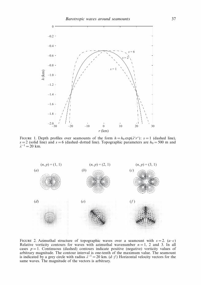
The dispersion relation for this seamount, ω/f = n/(2p + n), is plotted in figure 4for different values of n and p. This plot is made in a way similar to figure 3 ofBrink (1989): waves exist only at discrete points, and dashed lines are drawn just forclarity. Waves with radial wavenumbers equal to or larger than 1 (p = 1, 2, . . .) showa subinertial frequency that increases with azimuthal wavenumber n; in fact, for verylarge n their frequency asymptotically approaches f . Another important point toconsider is that waves with radial number p equal to zero correspond to oscillationswith inertial frequency for any azimuthal mode n (horizontal line).

The topographic waves progress around the seamount in an anticyclonic direction.This behaviour has been described by Rhines (1969) and many others in subsequentstudies. By using expression (2.18) the angular phase speed is cn,p(2) = f/(2p+n). Forinstance, for waves in figure 2 the angular phase speeds are c1,1(2) = f/3, c2,1(2) = f/4

Barotropic waves around seamounts 39

1.0

0.8

p = 0

p = 1

p = 2

p = 3

p = 4

0.6

ω/f

0.4

0.2

0 1 2 3n

4 5 6

Figure 4. Dispersion relation for waves over a seamount with s = 2 (using f = 10−4 s−1).Valid frequencies are indicated with stars; dashed lines are used for clarity and for comparisonwith figure 3 from Brink (1989).

and c3,1(2) = f/5, i.e. waves with more azimuthal modes progress more slowly (for agiven p). Analogously, waves with larger radial wavenumbers p are slower as well(for a given n).

3.2. Flat-topped seamounts or guyots (s > 2)

As mentioned § 1, several tall seamounts are characterized by a flat plateau on thesummit. Structures of this kind are well represented by the exponential profile withthe shape parameter s > 2. Here, some examples for s = 6 are presented. Note infigure 1 the pronounced flatness of the summit for this case.

Figure 5(a–c) shows the vorticity field of waves (n, p) = (1, 1), (3, 1) and (6, 1).Of course, the azimuthal structure of the waves is similar to the cases shown inthe previous subsection: an arrangement of 2n counter-rotating cells around theseamount. However, the vorticity cells are strongly confined along the periphery ofthe circle with radius λ−1: the strength of the waves is nearly zero close to the centreof the seamount and also at large radial distances. The low values over the almost-flat summit are expected since there are weak divergence effects in this region. Theconfinement of the waves over a narrow region of the guyot periphery is remarkablefor the first wave with n= 1: note the strong deformation of its dipolar structure ina new-moon fashion in order to be confined within an annular region of radius λ−1.

The rapid decay for large r , on the other hand, is one of the characteristics of theanalytical solutions due to the term exp(−λsrs) in the vorticity and velocity fields. Forthis reason, the structure of waves with larger radial wavenumber p is very similar tothe ones presented here, since the amplitudes of successive radial oscillations rapidlydecay for large radial distances (as shown in the radial profiles in figure 3).

40 L. Zavala Sanson

(n, p) = (1, 1) (n, p) = (3, 1)

(a)

(d)

(e) ( f )

(b) (c)

(n, p) = (6, 1)

Figure 5. Relative vorticity contours of topographic waves. (a–c) Over a flat-topped seamountwith s = 6. (d–f ) Over a sharp peak seamount with s = 1. Contours and grey circle as in figure 2.

The dispersion relation in this example is ω/f = n/(6p + n), and therefore thesewaves have a lower frequency compared with those over the less steep seamountpresented in the previous subsection. Besides, the corresponding angular speeds,cn,p(6) = f/(6p + n), are slower as well: c1,1(6) = f/7, c3,1(6) = f/9 and c6,1(6) = f/12(except for p = 0).

3.3. Sharp, conical seamounts (s < 2)

The case of a cone-shaped mountain with s = 1 is also shown in figure 1. Figure 5(d–f ) presents the corresponding vorticity fields for the same waves (n, p) = (1, 1),(3, 1) and (6, 1). There are strong differences between these cases: the dipolar structureof the first wave is strongly confined within the region around the tip of the seamount.In contrast, the waves with larger azimuthal numbers n are more intense far from thesummit and present a triangular configuration of the vorticity cells.

It is also worth noticing that the waves over this sharp seamount have radicallydifferent character compared with previous cases over the guyot, as can be seen infigure 5(a–c). Another important difference with guyots is that these waves have agreater angular phase speed, cn,p(1) = f/(p+n), compared with those over seamountswith larger s. For these examples, c1,1(1) = f/2, c3,1(1) = f/4 and c6,1(1) = f/7.

Sharp seamounts present a minor restriction on the permitted values of the shapeparameter only for the wave with n= 1. Although the mathematical solutions of thevelocity fields are valid over the entire domain, the vorticity field diverges at r = 0when n=1 and s < 1. This can be shown explicitly by calculating the vorticity fieldand finding that it is proportional to rn+s−2. Thus, for n= 1 it is required that s � 1in order to have a finite vorticity value over the summit. For n � 2 this restriction fors does not exist.

4. DiscussionExact solutions of barotropic, linear, rigid-lid topographic waves around

axisymmetric seamounts have been derived. Even though this type of oscillation hasbeen studied since some time ago, complete analytical expressions for the barotropic

Barotropic waves around seamounts 41

1.0

0.8

0.6

0.4

0.2

0

1.0p = 2p = 1

0.8

0.6

0.4

0.2

02 4s s

n = 5

n = 5n = 4n = 3

n = 2

n = 1

n = 4n = 3

n = 2

n = 1

6 2 4 6

ω/f

Figure 6. Wave frequency as a function of the shape parameter s for different sets of waves.

case have not been reported, as far as the author knows. One of the earlier andmore complete works is that of Rhines (1969), who found approximate solutionsin terms of Bessel functions over a topography with depth profile proportional toexp(r2). (Rhines’ paper also considers the coupling of such solutions with an externalfield dominated by Rossby waves, while in this paper our attention is restrictedonly to regions over the seamount.) In this study, we report complete solutions of(2.8) in terms of associated Laguerre polynomials, and applied to an infinite set ofaxisymmetric seamounts with profile proportional to exp(rs), with s being a realpositive number. Thus, besides the fact that no further approximations are made,the present solutions describe topographic waves over seamounts with very differentshapes determined by the parameter s. These topographic features can be flat-toppedseamounts for large s (which are frequently observed in the ocean) or sharp peaksfor low s (see figure 1).

A number of characteristics of the waves can be noticed from the derived solutions:(a) The main spatial distribution of the waves is essentially given by the azimuthal

wavenumber n: the waves are characterized by 2n cells of alternating relative vorticityaround the summit, and which rotate around the seamount in an anticyclonicdirection. Thus, waves with n= 1 are formed by a dipolar structure, n= 2 by aquadrupole, etc. The radial wavenumber is directly associated with index p, whichgives the number of zero crossings of the vorticity radial profiles.

(b) The exact dispersion relation has a remarkable simplicity given by expression(2.17). This relation shows the dependence of the wave frequencies on the parameter s,i.e. on the shape of the mountain, as well as on the azimuthal and radial wavenumbersn and p, respectively. For p � 1 the wave frequency increases with n, as shown infigure 4. This behaviour was shown in the nearly barotropic numerical solutions ofBrink (1989), who numerically solved the structure of seamount-trapped waves withs = 2 (see his figure 3). The frequency of all waves asymptotically tends to f forvery large n (fixing p and s). In addition, waves over seamounts with very small s

(very sharp peaks) also tend towards the inertial frequency. On the other hand, wavefrequencies approach zero for very large p or s. Figure 6 shows the frequency in termsof the shape parameter for different waves.

42 L. Zavala Sanson

(c) The angular phase speed of waves around the seamount is given by (2.18).This speed approaches zero for large s, p or n. On the contrary, the fastest motionaround the seamount, regardless of the shape parameter, is when (n, p) = (1, 0),which completes one turn around the seamount in one inertial period (c1,0(s) = f ).It is also possible to observe that, for a given pair (n, p), topographic waves overguyots (s > 2) tend to have an angular speed slower than waves trapped arounda sharp seamount (s < 2). In general, the dispersive character of the waves isevident.

(d) Over guyots (s > 2), the waves are strongly concentrated within an annularregion with radius of the order of the topography horizontal scale, λ−1. Wave motionsover the summit are nearly zero since flow divergence is very weak over the almost flattop. As mentioned in § 1, this seamount shape is commonly found in the ocean, andtherefore the concentration of the wave motion at a distance λ−1 from the summit isone of the cases that might have a direct application to oceanographical situations. Incontrast, for sharp seamounts (s < 2) the waves are strongly concentrated around thepeak only when n= 1, whilst the vorticity cells have a triangular, spatially extendedshape for larger n. There are two remarks of caution about the present model. First,inertial oscillations are obtained for the gravest radial wavenumber p = 0 and arbitraryazimuthal wavenumber n, which has not been considered in previous works ontopographic trapped waves. In general, other studies deal with subinertial frequencies.Inertial oscillations correspond to the motion of fluid columns unconstrained bypressure forces, but subject to the influence of topographic spatial variations. Thiscan be demonstrated by showing that the solutions (2.21) and (2.22) with ω = f

satisfy the unforced governing equations (2.1)–(2.3) (setting the right-hand sides tozero). This is not very difficult to calculate since the associated Laguerre polynomialsare L

2n/s

0 = L2n/s−10 = 1. The vorticity equation (2.5) and the original equation for the

transport function (2.6) are also satisfied. In addition, the group velocity aroundthe seamount is zero for inertial motions: using the dispersion relation (2.17) yields∂ω/∂n= f sp/(sp + n)2 = 0 for p = 0; so these oscillations do not transport energy.Actually, they should not be regarded as waves, but as inertial motions in the absenceof pressure forces and governed by the presence of the topography. Therefore, inprinciple, inertial solutions should not be excluded, although their physical meaningmust be considered carefully.

Another important point is that the transport function (2.20) diverges for larger . This is a consequence of using the depth profile proportional to exp(λsrs), whichobviously also diverges. Therefore, the solutions of ψ are physically unrealistic farfrom the seamount. In order to avoid this problem, other authors solve the flow overthe seamount and then match the solution with an external flow over a flat-bottomambient ocean. That was the procedure followed by Rhines (1969), who obtainedapproximate solutions of the radial part of ψ (see (2.8) in § 2). In the present case,in contrast, it has been preferred to obtain exact solutions over the seamount withno further approximations, though it implies paying the price of a transport functionincreasing indefinitely for r � λ−1. More importantly, the velocity components and therelative vorticity are well-behaved functions on top and around the mountain: theypossess values that are physically realistic over these regions, and do not diverge forlarge distances because they are proportional to exp(−λsrs), which rapidly decays forlarge r . This is evident from figures 2 and 3, for instance, which show that the mainstructure of the waves is restricted or trapped around the seamount. As a conclusion,the solutions are physically valid within a range of a few times the length scale of themountain λ−1.

Barotropic waves around seamounts 43

A more precise estimation of this range in the oceanographical context can bedetermined by considering that the solutions are valid up to a radial distance D, atwhich the depth field reaches about 4000 m. Using a 200 m depth at the summit, sucha distance is D = (ln 20)1/sλ−1 ≈ 31/sλ−1. Thus, an appropriate criterion depends onthe steepness of the seamount. Furthermore, since the velocity and relative vorticityfields have strongly decayed beyond D (due to the term exp(−λsrs)), it is reasonableto consider that the solutions are still valid for about three or four times λ−1.This criterion suggests a practical restriction for some solutions over a cone-shapedseamount, since the oscillations are not clearly confined or trapped within a shortdistance from the top, as in case (6, 1) shown in figure 5(f ).

Future work will focus on comparing the characteristics of the present wavesolutions (e.g. frequencies and angular phase speeds) with seamount-trapped wavesdescribed in other observational and numerical studies. According to some authors(e.g. Brink 1989; Chapman 1989; Beckmann & Mohn 2002), predominant waves inoceanographical situations are those with low azimuthal and radial wavenumbers,since frictional effects or bottom roughness would damp higher modes. Thus, theexpected manifestation of oceanic waves would be a dipolar structure rotatinganticyclonically around a seamount. On the other hand, additional efforts inlaboratory experiments are in progress in order to elucidate the nonlinear behaviourof barotropic flows over seamounts, and the signal of linear oscillations; the resultswill be published elsewhere.

The author gratefully acknowledges the comments of J. L. Ochoa on the earliestversion of this paper, and the fruitful remarks made by one of the anonymous refereesduring the revision process.

Appendix. Recurrence relations for polynomial solutionsThe azimuthal velocity component v and the relative vorticity ζ contain one and

two r-derivatives of the transport function, respectively, and hence derivatives ofthe associated Laguerre polynomials. In order to calculate these fields, the followingrecurrence relation for derivatives of the polynomials is used (Abramowitz & Stegun1972):

ρ[Lk

p(ρ)]ρ

= pLkp(ρ) − (p + k)Lk

p−1(ρ), (A 1)

which gives

v = −ψ0λ

h0

exp(−λsrs)(λr)n−1

×[(sp + n)L2n/s

p (λsrs) − (sp + 2n)L2n/s

p−1(λsrs)

]cos(ωt + nθ), (A 2)

ζ = −ψ0λ2

h0

exp(−λsrs)(λr)n−2

×{[(sp + n)(sp + n − sλsrs) − n2]L2n/s

p (λsrs)

− [(sp + 2n)(2(sp + n) − s(1 + λsrs)] L2n/s

p−1(λsrs)

+ (sp + 2n)(sp + 2n − s)L2n/s

p−2(λsrs)

}cos(ωt + nθ). (A 3)

Note that polynomials with subindices p − 1 and p − 2 appear, which apparentlyrestricts the value of p to be equal to or larger than 2. In order to remove this

44 L. Zavala Sanson

limitation, the following recurrence relations are used:

Lkp−1(ρ) = Lk

p(ρ) − (p + k)Lk−1p (ρ), (A 4)

Lkp−2(ρ) = Lk

p(ρ) − 2Lk−1p (ρ) + Lk−2

p (ρ). (A 5)

For the second expression, it is necessary to use an additional relation for Lk−2p (in

order to avoid restrictions on k):

(p + k − 1)Lk−2p (ρ) = (p + 1)Lk−1

p+1(ρ) − (p + 1 − ρ)Lk−1p (ρ). (A 6)

The resulting v and ζ fields are given by (2.22) and (2.23). Using appropriate recurrencerelations, one can find an infinite way of expressing the solutions. Here we chose thosegiving the simplest forms.

REFERENCES

Abramowitz, M. & Stegun, I. A. 1972 Handbook of Mathematical Functions. National Bureau ofStandards.

Arfken, G. 1970 Mathematical Methods for Physicists. Academic.

Beckmann, A. & Mohn, C. 2002 The upper ocean circulation at Great Meteor Seamount. Part II:Retention potential of the seamount-induced circulation. Ocean Dyn. 52, 194–204.

Brink, K. H. 1989 The effect of stratification on seamount-trapped waves. Deep-Sea Res. 36,825–844.

Chapman, D. C. 1989 Enhanced subinertial diurnal tides over isolated topographic features. Deep-Sea Res. 36, 815–824.

Genin, A. 2004 Bio-physical coupling in the formation of zooplankton and fish aggregations overabrupt topographies. J. Mar. Syst. 50, 3–20.

Gill, A. E. 1982 Atmosphere-Ocean Dynamics. Academic.

Haidvogel, D. B., Beckmann, A., Chapman, D. C. & Lin, R. Q. 1993 Numerical simulation offlow around a tall isolated seamount. Part II: Resonant generation of trapped waves. J. Phys.Oceanogr. 23, 2373–2391.

Hillier, J. K. & Watts, A. B. 2007 Global distribution of seamounts from ship-track bathymetrydata. Geophys. Res. Lett. 34, L13304.

Huppert, H. E. & Bryan, K. 1976 Topographically generated eddies. Deep-Sea Res. 23, 655–679.

Huthnance, J. M. 1974 On the diurnal tide currents over Rockall Bank. Deep-Sea Res. 21, 23–35.

Nycander, J. & Lacasce, J. H. 2004 Stable and unstable vortices attached to seamounts. J. FluidMech. 507, 71–94.

Rhines, P. B. 1969 Slow oscillations in an ocean of varying depth. Part 2. Islands and seamounts.J. Fluid Mech. 37, 191–205.