Submitted to Swansea University in fulfilment of the requirements

for the Degree of Doctor of Philosophy

September 2017

Observation of the 1S-2S Transition in Trapped Antihydrogen

Author

Steven Jones

Supervisor

Dr Stefan Eriksson

i

Thesis summary

Our current understanding of physics suggests that matter and antimatter should be

created and destroyed in equal amounts, but this seems inconsistent with the

observation that our universe consists almost entirely of matter. Comparisons between

matter and antimatter could reveal new physics which explains why the universe has

formed with this apparent imbalance. The 1S-2S transition of hydrogen has been

measured with incredible precision, and a similarly precise measurement of the 1S-2S

transition of antihydrogen would constitute one of the best comparisons between

matter and antimatter.

The ALPHA collaboration have been producing and trapping antihydrogen since

2010. This thesis presents an overview of the apparatus and techniques and examines

the theoretical aspects of antihydrogen spectroscopy. Generating sufficient optical

intensity at 243 nm to excite the 1S-2S transition in a reasonable amount of time

requires an enhancement cavity. The development of this enhancement cavity and the

setup of the ultra-stable 243 nm laser source form the main focus of this thesis.

The thesis concludes by reporting the first observation of the 1S-2S transition in

trapped antihydrogen, which can be interpreted as a comparison between matter and

antimatter at the 200 parts-per-trillion level. This result was aided by a significantly

improved trapping rate of 10.5 ± 0.6 detected trapped antihydrogen atoms per

production cycle, and the stacking of multiple production cycles without ramping

down the magnetic trap to accumulate more than 70 simultaneously trapped

antihydrogen atoms.

ii

iii

DECLARATION

This work has not previously been accepted in substance for any degree and is not

being concurrently submitted in candidature for any degree.

Signed ...................................................................... (candidate)

Date ........................................................................

STATEMENT 1

This thesis is the result of my own investigations, except where otherwise stated.

Where correction services have been used, the extent and nature of the correction is

clearly marked in a footnote(s).

Other sources are acknowledged by footnotes giving explicit references. A

bibliography is appended.

Signed ..................................................................... (candidate)

Date ........................................................................

STATEMENT 2

I hereby give consent for my thesis, if accepted, to be available for photocopying

and for inter-library loan, and for the title and summary to be made available to outside

organisations.

Signed ..................................................................... (candidate)

Date ........................................................................

iv

v

Table of Contents

i. Acknowledgements ...................................................................................... ix

ii. List of Figures .............................................................................................. xi

iii. List of Tables .............................................................................................. xxi

1 Introduction ................................................................................................... 1

1.1 The baryon asymmetry problem ............................................................ 1

1.2 Physics with low energy antiprotons ..................................................... 2

1.2.1 The AD and ELENA .......................................................................... 2

1.2.2 Measurement of the antiproton-proton magnetic moment ratio ......... 4

1.2.3 Measurement of the antiproton-electron mass ratio ........................... 4

1.2.4 Antihydrogen formation ..................................................................... 4

1.3 Physics with antihydrogen ..................................................................... 6

1.3.1 Magnetically trapping antihydrogen................................................... 6

1.3.2 Tests of the weak equivalence principle ............................................. 7

1.3.3 Measuring the charge neutrality of antihydrogen ............................... 7

1.3.4 Microwave spectroscopy of antihydrogen ......................................... 8

1.3.5 Laser spectroscopy of antihydrogen ................................................... 9

2 Antihydrogen production in the ALPHA apparatus .................................... 11

2.1 The apparatus ....................................................................................... 11

2.1.1 Penning traps .................................................................................... 12

2.1.2 Catching trap .................................................................................... 14

2.1.3 Positron accumulator ........................................................................ 15

2.1.4 Atom trap .......................................................................................... 17

2.1.5 Sequencing and data acquisition ...................................................... 18

2.2 Tools and diagnostics ........................................................................... 18

2.2.1 Sticks ................................................................................................ 18

2.2.2 Electron gun ..................................................................................... 19

2.2.3 Faraday cup ...................................................................................... 19

2.2.4 Multichannel plate ............................................................................ 19

2.2.5 Flappers ............................................................................................ 20

2.2.6 Scintillator panels ............................................................................. 21

2.2.7 Silicon vertex detector ...................................................................... 22

2.2.8 Temperature diagnostics ................................................................... 23

vi

2.2.9 Magnetometry ................................................................................... 24

2.3 Antihydrogen formation and trapping .................................................. 26

2.3.1 Autoresonant mixing ........................................................................ 26

2.3.2 Slow merge mixing ........................................................................... 27

2.3.3 Antihydrogen accumulation ............................................................. 28

2.4 Antihydrogen detection ........................................................................ 29

3 Antihydrogen spectroscopy considerations ................................................. 31

3.1 The hydrogen atom ............................................................................... 32

3.1.1 Historical observations ..................................................................... 33

3.1.2 The Bohr model ................................................................................ 33

3.1.3 Fine structure .................................................................................... 34

3.1.4 The Lamb shift.................................................................................. 35

3.1.5 Hyperfine structure ........................................................................... 36

3.1.6 The Zeeman Effect ........................................................................... 37

3.1.7 Diamagnetic shift .............................................................................. 38

3.1.8 Antihydrogen 1S-2S frequencies ...................................................... 38

3.2 Systematic shifts and broadenings ....................................................... 39

3.2.1 Residual Zeeman Effect .................................................................... 40

3.2.2 Stark effect ........................................................................................ 41

3.2.3 Transit time broadening .................................................................... 41

3.2.4 2S lifetime reduction ........................................................................ 42

3.3 Simulated transition rates ..................................................................... 43

3.4 Detection schemes ................................................................................ 44

3.4.1 Ly-α detection ................................................................................... 44

3.4.2 Annihilation - disappearance mode .................................................. 45

3.4.3 Annihilation - appearance mode ....................................................... 45

4 The 1S-2S Enhancement Cavity .................................................................. 47

4.1 Enhancement cavity theory .................................................................. 48

4.1.1 Resonance ......................................................................................... 49

4.1.2 Transverse mode matching ............................................................... 51

4.1.3 Cavity locking techniques ................................................................ 54

4.1.4 Cavity power..................................................................................... 56

4.2 Athermal mirror cell development ....................................................... 57

vii

4.2.1 Design and Prototyping .................................................................... 58

4.2.2 Mirror cell assembly ......................................................................... 60

4.2.3 Optical deformation measurements .................................................. 62

4.2.4 Improved interferometry .................................................................. 70

4.3 Internal cavity mechanical design ........................................................ 74

4.4 External cavity mechanical design ....................................................... 80

4.5 Optical design....................................................................................... 83

4.6 Performance ......................................................................................... 85

4.6.1 Loss versus reflectivity ..................................................................... 87

4.6.2 Laser induced damage ...................................................................... 88

4.6.3 Spatial mode matching ..................................................................... 90

4.7 Mirror degradation and recovery ......................................................... 92

5 The 1S-2S Laser System ............................................................................. 93

5.1 243 nm light generation ....................................................................... 93

5.2 Frequency control and metrology ........................................................ 96

5.2.1 Reference cavity ............................................................................... 96

5.2.2 Frequency comb ............................................................................... 98

5.2.3 Frequency shifter .............................................................................. 99

5.3 Beam transport ................................................................................... 101

5.3.1 Optical components ........................................................................ 102

5.3.2 Losses ............................................................................................. 103

5.3.3 Alignment ....................................................................................... 105

5.3.4 Active beam stabilisation ............................................................... 106

6 Experimental results .................................................................................. 107

6.1 Experimental protocol ........................................................................ 107

6.1.1 2014 ................................................................................................ 107

6.1.2 2015 ................................................................................................ 108

6.1.3 2016 ................................................................................................ 109

6.2 Results and analysis ........................................................................... 111

6.2.1 2014 ................................................................................................ 111

6.2.2 2015 ................................................................................................ 111

6.2.3 2016 ................................................................................................ 112

6.3 Conclusion ......................................................................................... 115

viii

7 Conclusions and Outlook........................................................................... 117

References .......................................................................................................... 119

ix

i. Acknowledgements

Firstly, I would like to thank my supervisor Dr. Stefan Eriksson, for his dedication

and guidance. I would also like to thank Prof. Niels Madsen and Prof. Jeffrey Hangst

for their support throughout, as well as the rest of the senior researchers at ALPHA

for sharing their knowledge and expertise with me. ALPHA is a collaboration in

which the work and opinions of a student are treated with the same respect as a

senior researcher, and I could not have asked for a better environment to work in.

Thanks to all of my fellow students and post-docs within the ALPHA collaboration,

who have truly become my family away from home. In particular, I would like to

thank Chris, Graham, and Bruno, who have all experienced the joys and frustrations

from round-the-clock work on the 243 nm laser.

I would like to acknowledge and thank Swansea University and the Engineering and

Physical Sciences Research Council (EPSRC) for funding my PhD scholarship,

which has been the most amazing opportunity.

Thanks to the friends I’ve made through the CERN board games club, past and

present, who are too many to name. Also, a special thank you to my parents for their

continuous love and support, even when I decided to move to Geneva.

And finally, I would like to thank Melina, for sharing the adventure with me.

x

xi

ii. List of Figures

Figure 1.1: A schematic of the AD hall experiments in the 2017 run configuration.

The ATRAP zone is on a platform above the surrounding experiments. ELENA and

GBAR are still in the commissioning phase. The GBAR zone includes a shielded linear

accelerator for positron production. Image adapted from [6]. ..................................... 3

Figure 1.2: A Breit-Rabi diagram showing the Zeeman splitting of the

(anti)hydrogen ground state. The ALPHA collaboration injected resonant microwaves

(shown by the black arrows) into the 1 T magnetic trap, and observed a spin flip of the

positron (single arrow) which caused the atoms to seek a high magnetic field and

annihilate on the walls of the trap. Image from [25]. ................................................... 8

Figure 2.1: An overview of the ALPHA beamline. Antiprotons are captured in the

3 T field of the CT and cooled using electrons loaded from the CT stick. Meanwhile,

positrons are accumulated in a 3-stage Surko-type accumulator. After initial

preparations, both species antiprotons and positrons are transferred into the AT for

antihydrogen production and trapping. Small solenoids are positioned along the

beamline to aid the transfer of particles. The distance between the CT and AT is

approximately 3 m...................................................................................................... 11

Figure 2.2: A simple Penning-Malmberg trap constructed from three stacked

cylindrical electrodes. ................................................................................................ 13

Figure 2.3: The motion of a single particle in a Penning trap is described by a

combination of the magnetron (green), cyclotron (black), and axial motion (red). The

image is adapted from [28]. ....................................................................................... 13

Figure 2.4: A sketch of the catching trap electrode stack. The trap has a length of

396 mm and an inner diameter of 29.6 mm. The two high voltage electrodes are shown

in blue and the segmented electrodes used for plasma compression are shown in

yellow. An external solenoid provides a 3 T field to complete the Penning trap. The

antiproton beam enters from the left of the image. .................................................... 14

Figure 2.5: a) After an initial stage of rotating wall compression, the antiprotons

(left) and the electrons (right) are centrifugally separated [30]. b) Kicking out 90% of

xii

the electrons allows the antiprotons to be compressed further. c) Finally, the remaining

electrons are kicked out and the antiprotons are ready for transfer. The two species

map to different locations on the MCP due to a small misalignment between the

electrode stack and the magnetic field. ...................................................................... 15

Figure 2.6: A schematic of the positron accumulator. Positrons are emitted from a

5 Kelvin 22Na source (blue) and accumulated in a three stage Penning-Malmberg trap

(orange). The accumulator is equipped with a small vertical translator containing a

phosphor screen (red) for imaging the positrons and a grounded pass-through tube.

The image is adapted from [33]. ................................................................................ 16

Figure 2.7: The high energy positrons are cooled by interacting with a nitrogen

buffer gas within the electrodes. The accumulator is differentially pumped such that

the cooling interactions are strongest in the first stage (right hand side of graph) and

the lifetime is prolonged in the third stage (left hand side of graph). The image is

adapted from [33]. ...................................................................................................... 16

Figure 2.8: A schematic of the nested Penning-Malmberg and Ioffe-Pritchard traps

within the ALPHA-2 atom trap. The antiprotons are transferred in from the left hand

side and the positrons are transferred in from the right hand side of the image. The

electrodes are in the UHV space, whereas the magnets are in direct contact with liquid

helium. An outer vacuum chamber and a layer of super-insulation reduce the heat load

on the cryostat. Not shown is an external 1T solenoid............................................... 17

Figure 2.9: The locations of the scintillator panels are highlighted on the CT (left)

and AT (right). The scintillators are positioned in pairs either side of the solenoids.

Portable scintillator pairs are positioned next to the diagnostic sticks when additional

information about the annihilation position is needed. .............................................. 21

Figure 2.10: An example reconstruction of an antiproton annihilation (left) and a

cosmic ray event (right). The blue diamond indicates the position of the reconstructed

annihilation event, the red dots the positions of the detected hits, and the inner circle

shows the radius of the Penning trap electrodes. Image adapted from [39]. .............. 22

Figure 2.11: A plot of the detection efficiency against the accepted background rate

for the MVA analysis. For reference, the performance of the standard online analysis

xiii

is circled in red. The data displayed is from around 670 mixing cycles and 82 hours of

cosmic data from 2014. The Y-axis error bars are negligible. ................................... 23

Figure 2.12: An example of an ECR line shape recorded during the 2016 beam

period. The trace shows the quadrupole vibrational mode frequency of an electron

plasma when excited by microwave pulses of increasing frequency. ........................ 25

Figure 2.13: In the autoresonant scheme (left), the antiprotons are excited into the

positrons by a chirped frequency. In the slow merge scheme (right), the initial wells

(solid line) are reduced until the two species spill into each other (dashed line)....... 27

Figure 2.14: The number of trapped atoms increases linearly with each successive

mixing cycle. The error bars show the 𝑁 counting statistics alone. The detection

efficiency is 73.0±0.4%.............................................................................................. 29

Figure 3.1: The energy levels of the hydrogen atom are illustrated as the accuracy

of models which describe them improves. The horizontal axis shows the quantum

numbers which describe the energy levels, and are introduced in the text. The vertical

axis shows the energy of the levels, but the scale is illustrative only. ....................... 32

Figure 3.2: Feynman diagrams showing the most significant contributions to the

Lamb shift [50]. .......................................................................................................... 36

Figure 3.3: The calculated Breit-Rabi diagrams of the 1S (bottom) and 2S (top)

states of antihydrogen. The blue lines show the low-field seeking trappable states and

the red lines show the high-field seeking untrappable states. Image from [60]. ........ 39

Figure 3.4: A plot of three possible magnetic field configurations. The black

markers labelled A-E show the approximate sizes and locations of the mirror coils.

Image from [52]. ........................................................................................................ 40

Figure 3.5: A simulation of the interaction between the antihydrogen atoms within

the flattened trap yields the excitation rate and the linewidth of the summed c-c and d-

d transitions. The inset shows the time dependence of the excitation period. Image

from [60]. ................................................................................................................... 44

Figure 3.6: A close-up image of an antiproton annihilation on an MCP which has

left identifiable tracks. The surrounding bright spots are also due to antiproton

annihilations. .............................................................................................................. 46

xiv

Figure 4.1: A two-mirror Fabry-Pérot cavity ....................................................... 48

Figure 4.2: A plot of the beam waist (top) and the wavefront radius of curvature

(bottom) for a Gaussian beam with 𝑤0 = 0.2 𝑚𝑚, 𝜆 = 243 𝑛𝑚, and 𝑧0 = 0.517 m

over a 6 m propagation length. ................................................................................... 52

Figure 4.3: The stability of different cavity configurations as defined by their g

factors (g1,g2). Only the configurations under the blue shaded region are stable. Image

by [63]. ....................................................................................................................... 53

Figure 4.4: Hermite-Gaussian (top) and Laguerre-Gaussian (bottom) modes. Image

from [64] .................................................................................................................... 54

Figure 4.5: The ‘x’ shows the lock points for the side of peak lock (left) and the

amplitude modulation error signal (right). The frequency scale is the same for both

plots. ........................................................................................................................... 55

Figure 4.6: The frequency/phase modulation adds sidebands to the beam, which

are visible in the transmitted signal (left). The capture range of the PDH error signal

extends to the sidebands, yet maintains a sharp slope to lock to (right). The ‘x’ indicates

the lock point. ............................................................................................................. 56

Figure 4.7: An athermal mirror cell consisting of an optic (green) bonded within a

metal ring (grey) using an epoxy (orange). Autodesk Inventor model. ..................... 57

Figure 4.8: A close up view of the cell making jig, showing the locations where the

ring and optic sit (Autodesk Inventor drawing). ........................................................ 61

Figure 4.9: The optic and ring are placed onto the jig. The ring is clamped via two

slash-cut needles and the optic is clamped via a Teflon spacer whilst the epoxy cures

(Autodesk Inventor model). ....................................................................................... 61

Figure 4.10: The mirror cell is epoxied to a stainless steel adapter piece using the

same epoxy and curing process as the cell manufacture. The adapter piece threads into

a copper heat sink which is cooled to 20 K by the inner stage of a coldhead. The heat

sink is equipped with a Cernox temperature sensor and a heater element. Connected to

the outer stage of the coldhead is a copper radiation shield, which has a Ø 12 mm hole

for optical access. ....................................................................................................... 63

xv

Figure 4.11: The coldhead cools from room temperature to 20 K in just under 3

hours, which is similar to the cooldown rate of the ALPHA apparatus. .................... 63

Figure 4.12: A 767 nm single mode laser is coupled into a fibre and output onto an

optical bench. The light is collimated at Ø 10 mm and split into two beams using a 50-

50 beam splitter. One beam is reflected from the mirror cell under test, whilst the other

is reflected from a flat reference mirror. The vacuum window and the beam splitter

have THORLABS –B NIR anti-reflection coatings to prevent multiple images. The

test and reference mirrors are both THORLABS PF05-03 mirror blanks, which have a

ground back surface to prevent multiple reflections. Recombining the beams creates

an interference pattern which is imaged on a screen. A webcam placed behind the

screen saves the image for analysis. ........................................................................... 64

Figure 4.13: An example of two interference patterns generated by the

interferometer. The image on the left has no tilt between the two mirrors, whereas the

image on the right has a tilt of 6 waves. The edge of the images corresponds to the

edge of the Ø10 mm laser beam. ................................................................................ 65

Figure 4.14: The image on the left shows the interference pattern with the dark

fringes traced, and the image on the right shows a reconstruction of the surface using

Zernike polynomials................................................................................................... 66

Figure 4.15: An initial measurement of the 0.5 mm H77 titanium cell. The chamber

is at room temperature and under a vacuum of 1× 10 − 6 mbar. .............................. 68

Figure 4.16: A measurement of the surface of the 0.5 mm H77 titanium cell when

cooled to 20 K for the first time. The mirror appears to have bulged outwards by >1100

nm. The surface looked similar for the subsequent two cooldowns. The vacuum

reaches 1× 10 − 8 mbar when the coldhead is at 20 K. ............................................ 68

Figure 4.17: A measurement of the surface of the 0.5 mm H77 titanium cell at room

temperature and still under vacuum after 3 thermal cycles. There appears to be a

residual deformation of around 400 nm. .................................................................... 68

Figure 4.18: An initial measurement of the 0.5 mm T7109 titanium cell. The

chamber is at room temperature and under a vacuum of 1× 10 − 6 mbar. ............... 69

xvi

Figure 4.19: A measurement of the surface of the 0.5 mm T7109 titanium cell when

cooled to 20 K. There is no obvious deformation within the precision of the

interferometer. ............................................................................................................ 69

Figure 4.20: A measurement of the surface of the 0.5 mm T7109 titanium cell at

room temperature and still under vacuum after thermally cycling. There is no obvious

change from the initial surface. .................................................................................. 69

Figure 4.21: In this improved interferometer setup, a stabilised 532 nm laser is

coupled into a single mode fibre and output onto an optical bench which is directly

mounted to the cryostat. Not shown are a 400 V piezo driver and a laptop equipped

with a NI-DAQ module for controlling the piezo and acquiring images from the

camera. The optics are coated for visible light and the vacuum window is wedged to

prevent interference patterns from the window surfaces being imaged. The setup is

designed to be as compact and lightweight as possible to avoid coupling vibrations

into the cryostat. ......................................................................................................... 71

Figure 4.22: The deformation of a mirror blank in a 0.5 mm athermal cell cooled

to 20 K. ....................................................................................................................... 72

Figure 4.23: The residual deformation of a mirror blank after being thermally

cycled between room temperature and 20 K. ............................................................. 72

Figure 4.24: A plot of the radial gap size of an athermal cell vs the cooldown

deformation of the central Ø 12 mm of the optic. A positive deformation indicates a

bulging of the mirror surface. In each case, the deformation was almost purely a

defocussing of the mirror. For small deformations the error is approximately the

resolution of the interferometer, whereas for larger deformations, the error is

dominated by knowledge of the beam size and image edge. Inset is the result of the

DeLuzio stress calculation based on equation 4.30, which is in rough agreement with

the trend and the zero-crossing point. ........................................................................ 74

Figure 4.25: From left to right: The upstream triangle, the upstream end of the

magnet form, the downstream end of the magnet form, and the downstream triangle.

Both triangles contain two slots for mounting a mirror assembly, but are shown with

only one mirror assembly installed. ........................................................................... 75

xvii

Figure 4.26: The mirror cell, piezo (yellow with grey electrodes), and downstream

adapter piece mounted within the alignment jig. A similar jig is used to ensure the

alignment of the upstream assembly. ......................................................................... 76

Figure 4.27: The upstream and downstream mirror adapter pieces. .................... 76

Figure 4.28: The downstream adapter pieces still mounted into the triangle (left)

and one of the piezo assemblies (right). The piezos were attached to the adapter pieces

by placing beads of epoxy around the outer diameter, but the piezo also seems to have

bonded close to the inner diameter. Piezo material can be seen still bonded to the

adapter pieces. ............................................................................................................ 77

Figure 4.29: The modified downstream adapter................................................... 77

Figure 4.30: As the triangle was inserted, one of the support rods (highlighted)

came into contact with the piezo assembly and sheared it off. A kapton bumper was

installed to protect the piezo against knocks during installation, but this had also been

sheared and epoxy had been scraped off the piezo, implying that the damage was done

when holding tension was applied to the back of the triangle. .................................. 78

Figure 4.31: A 13 mm PI Ceramic’s PAHH+0050 piezo was cooled down to 20 K

on a coldhead. The travel was measured interferometrically as the piezo warmed up.

.................................................................................................................................... 79

Figure 4.32: A Bode plot of the piezo electrical response at 7 K. The black curve

shows the magnitude and the blue curve shows the phase of the response relative to

the drive signal. .......................................................................................................... 79

Figure 4.33: A photograph of the assembled mirror flange. The flange adapter

contains holes to allow the space in the bellows behind it to be pumped, but it is an

acknowledged pumping restriction. The mirror, piezo, and adapter are bonded using

EPOTEK T7109 epoxy. ............................................................................................. 80

Figure 4.34: The mirror is mounted on a piezo between two bellows. The window

is clamped in place, allowing the mirror flange to be titled using a modified

commercial mirror mount. ......................................................................................... 81

xviii

Figure 4.35: An Autodesk Inventor rendering (left) and photograph (right) of the

structure designed to clamp the external cavity assembly to the beamline. The vacuum

window is not shown. ................................................................................................. 82

Figure 4.36: The highlighted nuts on the M4 threaded rods were loosened or

tightened to adjust the alignment of the cavity mirror. .............................................. 82

Figure 4.37: A histogram of the cavity length fluctuation in nm over 100 s, as

measured by a wave meter when the laser was locked to the external cavity. ........... 83

Figure 4.38: In a confocal cavity, transverse modes (red) are frequency degenerate

as all path lengths are equal. As the cavity is made longer or shorter, the transverse

modes will separate. ................................................................................................... 84

Figure 4.39: A photograph of the 2015 upstream window mounted on the bench.

A large diameter 243 nm beam was sent through and the transmission was measured

using a CCD camera. The laser induced damage can already be seen by the dark spot

within the blue fluorescence. ...................................................................................... 89

Figure 4.40: A small burn spot is present on the AR coating of the upstream mirror.

.................................................................................................................................... 90

Figure 4.41: The PDH error signal (upper) and the transmitted intensity (lower) as

the piezo is scanned linearly over 50 V to cover a full free spectral range of the cavity.

.................................................................................................................................... 91

Figure 4.42: A saturated image of the transmitted beam when the cavity has been

locked on resonance for 1 s (left) and 30 s (right). .................................................... 91

Figure 5.1: A schematic of the optical elements in the 1S-2S spectroscopy setup.

The red, cyan, and navy blue lines show the propagation of the 972, 486, and 243 nm

light respectively. Some steering mirrors have been removed for simplicity. ........... 94

Figure 5.2: The internal layout of the Toptica TA-FHG pro laser, which generates

the high power 243 nm light for antihydrogen spectroscopy. Image modified from [61].

.................................................................................................................................... 95

Figure 5.3: A flow chart of the frequency control setup. ..................................... 96

Figure 5.4: The set point of the PDH lock to the reference cavity was adjusted at

100 s intervals to ± 1 FWHM of the measured noise of the locked cavity, the frequency

xix

of the laser is measured using the frequency comb. The difference between the blue

and red points gives 2 x the FWHM of the laser linewidth, assuming the dominant

source of broadening of the linewidth is the quality of the lock. ............................... 97

Figure 5.5: A schematic diagram of a v-2v frequency comb. The repetition rate

(vrep) is referenced to a microwave clock, and the offset of the zeroth line (v0) can be

determined by measuring the beat note between the frequency-doubled red end of the

comb and the blue end................................................................................................ 98

Figure 5.6: An AOM in double-pass configuration is used to shift the 972 nm light

to the reference cavity frequency (not to scale). The black curve illustrates the gain

profile of the AOM, which must be accounted for when normalising the output power.

.................................................................................................................................. 100

Figure 5.7: A non-overlapping Allen deviation measurement of the fractional

uncertainty of the comb locked to the OCXO (black dots) and the light sent to the

reference cavity (red dots). The turning point at 20 s corresponds to a fractional

uncertainty of 2.45 × 10 − 13, or equivalently, 75 Hz at 972 nm. ......................... 101

Figure 5.8: The fluorescence observed from a 243 nm beam passing through a

standard UV grade fused silica substrate changes from pale blue to bright red after

several hours of exposure, and the transmission through the substrate falls. .......... 102

Figure 5.9: The black trace at the top of the graph shows the control voltage applied

to a piezo used to scan the length of the cavity over a full spectral range. The blue trace

shows the temporal mode structure of a cavity which is enclosed by a tube and the red

trace shows the mode structure of a cavity which is stirred by the laboratory air

conditioning. ............................................................................................................ 104

Figure 6.1: A plot of the declining mixing triggers (proportional to antihydrogen

production) when the 243 nm cavity is locked for two trapping series with 1 W

circulating power (black squares) and 0.65 W of circulating power (red circles). The

first few points of the 0.65 W series are low as the laser experiment has begun whilst

some trap surfaces are still cooling down. ............................................................... 113

Figure 6.2: Evolution of the trapping data for the on resonance, off resonance, and

no laser runs. The error bars represent the counting statistics (𝑁) alone. ................ 114

xx

xxi

iii. List of Tables

Table 3.1: Spectroscopic notation. ....................................................................... 34

Table 3.2: A summary of the shifts and broadenings which contribute >1 kHz

towards the total 1S-2S transition frequency ............................................................. 42

Table 4.1: A comparison of the properties of EPO-TEK H77 and EPO-TEK T7109

epoxies. Data from the H77 [70] and T7109 [71] datasheets. It is important to note that

the CTE data for the epoxies was only available down to 228K and must be

extrapolated down to 7K. ........................................................................................... 59

Table 4.2: A calculation of optimal radial bond thicknesses using the Bayar and

DeLuzio equations for four potential mirror cells...................................................... 60

Table 4.3: A summary of the deformation of a 0.5 mm T7109 titanium athermal

mirror cell when cooled from room temperature to 20 K, for different batches of the

same epoxy. ................................................................................................................ 73

Table 4.4: The enhancement cavity design parameters. ....................................... 85

Table 4.5: A summary of the cavity performance. Values marked with (*) were not

well characterised as contributing effects were not discovered until later. The measured

coupling is the ratio of injected to reflected light, and hence is a function of both the

impedance mismatch and spatial mode matching. ..................................................... 87

Table 4.6: Measurements of the mirrors delivered to ALPHA. The “HR” mirror

was specified for maximum reflectivity. The measured transmission is an average over

several mirrors from each batch in new condition, including substrate losses. The

variance between mirrors is approximately ± 5%. ..................................................... 88

Table 5.1: Power losses at 243 nm as measured at the end of the 2016 run. The

components are listed in the order they are seen by the beam, with the exception of the

transport mirrors which are interspersed among the other components. ................. 105

Table 6.1: A summary of the experimental protocol employed in 2014, 2015 and

2016. ......................................................................................................................... 111

xxii

Table 6.2: The annihilation events detected during the shutdown of the neutral trap.

The magnet system is intentionally quenched to de-energise the neutral trap in <30 ms,

so there is no significant detector background. The error of the rate is from the 𝑁

counting statistics alone. .......................................................................................... 111

Table 6.3: The annihilation events detected during the 1.5 s ramp down of the

neutral trap magnets. The error of the rate is the standard deviation about the mean of

the number of detected events. ................................................................................. 112

Table 6.4: The number of events detected upon ramping down the trap after 2 x

300 s of laser exposure on resonance, laser exposure off resonance, or a wait without

any laser exposure. The uncertainty is from the counting statistics(𝑁) alone. ........ 114

Table 6.5: Detector efficiency of the different protocols ................................... 115

Table 6.6: The number of events detected during the 300 s hold periods. The

uncertainty is from counting statistics (𝑁) alone. .................................................... 115

1

(1.1)

)

1 Introduction

1.1 The baryon asymmetry problem

As predicted by the Standard Model of particle physics, and indeed as observed in

high energy particle accelerators, particles and antiparticles are always created in pairs.

Particles and antiparticles have opposite electrical charge and opposite baryon/lepton

numbers, but are otherwise indistinguishable. However, when they recombine, they

annihilate and release a blast of energy given by Einstein’s famous equation;

𝐸 = 𝑚𝑐2.

One of the greatest open questions in physics today is the ‘Baryon Asymmetry’

problem. As the early universe cooled to the point where there was no longer enough

energy to create particle-antiparticle pairs, one would expect the existing pairs to

recombine and annihilate, leaving a universe devoid of both particles and antiparticles

today. However, it seems a small fraction of these early universe particles survived to

create the universe as we know it today. If matter and antimatter were originally

created in equal amounts, then the question is simply “where is the antimatter?” The

search for antimatter in astrophysics is ongoing, but no experiment to date has detected

any signal, such as the distinctive 511 keV gamma rays emitted from electron-positron

annihilations, which would be indicative of a significant quantity of antimatter in the

observable universe [1]. Instead, physicists must consider a different hypothesis: “Is

there a difference between matter and antimatter that has caused this imbalance, and

can we measure it experimentally?”

A surprise result came in the form of a violation of charge conjugation and parity

transformation (CP) symmetry, one of the fundamental symmetries of the Standard

Model of Particle Physics. CP violation was first observed indirectly in 1964, when

neutral kaons were observed to transform into their antiparticles and vice-versa with

differing rates [2], and later measured explicitly by both the NA48 experiment [3] at

CERN, and the KTeV experiment [4] at Fermilab. This CP violation is due to the

existence of the Top and Bottom quarks in the Standard Model, and is explained by

2

the Kobayashi–Maskawa model [5]. However, it is generally agreed that this amount

of CP violation is not sufficient to explain the matter-antimatter imbalance alone.

The most fundamental symmetry of the Standard Model is charge conjugation,

parity transformation, and time reversal (CPT) symmetry. Direct evidence for CPT

violation can be searched for by comparing the quantum energy spectra of atoms with

their antiatom counterparts. The search for CPT violation has led to the construction

of the Antiproton Decelerator (AD) at CERN, and the creation and trapping of

antihydrogen atoms for comparison with hydrogen, the simplest and best understood

(both experimentally and theoretically) atom to date.

1.2 Physics with low energy antiprotons

Antiprotons are formed at CERN by firing a beam of protons from the Proton

Synchrotron (PS) into a metal target. The proton beam has sufficient kinetic energy to

create many secondary particles, including proton-antiproton pairs. As protons and

antiprotons have opposite electrical charge, the antiprotons can be separated and

steered away by strong magnetic fields.

Prior to the construction of the AD, antiprotons were produced and accumulated at

the Antiproton Accumulation Complex (AAC). As well as serving high energy physics

experiments at CERN, the AAC also supplied antiprotons to the Low Energy

Antiproton Ring (LEAR) which explored the possibilities of making antihydrogen and

capturing antiprotons within Penning traps – a type of charged particle trap which we

will discuss in further detail in chapter 2.

1.2.1 The AD and ELENA

Constructed in 2000, the AD is capable of decelerating the injected antiproton

beam down to 5.3 MeV. A combination of stochastic cooling and electron cooling are

used to cool and increase the density of the antiprotons, and a short (~100 ns) bunch

of around 3x107 antiprotons can be delivered to the experiments within the AD hall

every ~2 minutes.

3

The ELENA (Extra-Low ENergy Antiproton) ring is a synchrotron with a

circumference of just 30 m, and is reaching the final stages of commissioning. This

decelerator is designed to reduce the energy of the AD beam to just 100 keV, and

promises to increase the number of antiprotons which can be trapped by the

experiments within the AD hall by a factor of between 10 and 100 [6]. Figure 1.1

shows an overview of the AD hall, with the location of the ELENA ring and the

experimental zones highlighted.

Figure 1.1: A schematic of the AD hall experiments in the 2017 run configuration. The ATRAP zone is on a

platform above the surrounding experiments. ELENA and GBAR are still in the commissioning phase. The GBAR

zone includes a shielded linear accelerator for positron production. Image adapted from [6].

4

1.2.2 Measurement of the antiproton-proton magnetic moment ratio

Both the ATRAP (Antihydrogen TRAP) and BASE (Baryon-Antibaryon

Symmetry Experiment) collaborations have experiments dedicated to measuring the

ratio between the proton and antiproton magnetic moment in a Penning trap. In 2013,

ATRAP reported a measurement with a precision of 4.4 parts-per-million [7]. The

BASE collaboration reported a 6-fold improvement in this measurement in 2016, with

an uncertainty of just 0.8 parts-per-million, as well as outlining a new trapping

technique which, when implemented in their next generation apparatus, could enable

a measurement precision with an uncertainty at the level of a few parts-per-billion [8].

By using an isolated reservoir trap, BASE have also demonstrated the ability to hold a

few tens of antiprotons for more than 1 year without any losses [9].

1.2.3 Measurement of the antiproton-electron mass ratio

The ASACUSA (Atomic Spectroscopy And Collisions Using Slow Antiprotons)

collaboration measures the antiproton to electron mass ratio by ionising a helium atom

and replacing the lost electron with an antiproton. Probing two-photon transitions in

antiprotonic helium with high powered pulsed lasers has allowed the team to resolve

the antiproton to electron mass ratio to better than 5 parts-per-billion [10].

1.2.4 Antihydrogen formation

Antihydrogen was first produced at the Low Energy Antiproton Ring at CERN in

1995 [11], and later at Fermilab [12]. Antiprotons were shot through a xenon gas target

with a small chance to produce electron-positron pairs, and velocity matched positrons

would bind with the antiprotons in the beam to form antihydrogen. However, these

relativistic atoms were much too energetic to be suitable for detailed study. With the

subsequent construction of the AD, a new generation of experiments were able to

capture and cool antiprotons in Penning traps with the aim of producing much colder

antihydrogen.

5

By mixing these antiprotons in a carefully controlled way with positrons

accumulated in a Surko-type accumulator, cold antihydrogen was produced in 2002

by the ATHENA (AnTiHydrogEN Apparatus) [13], and ATRAP [14] collaborations.

The dominant formation method at low temperatures is thought to be a three-body

process, where two positrons scatter in close proximity to an antiproton. One positron

carries away the excess energy of the other positron, which binds with the antiproton

to form antihydrogen. However, these antihydrogen atoms would still annihilate on

the walls of the Penning trap shortly after production, leaving little time for precision

measurements. Confining the antihydrogen atoms in a magnetic trap was the next step

for the ATRAP collaboration, along with ALPHA (Antihydrogen Laser PHysics

Apparatus), a collaboration which succeeded ATHENA.

The ASACUSA collaboration aim to produce a beam of ground state antihydrogen

atoms for measurements free from any significant magnetic field perturbations, and

reported the first antihydrogen beam in 2014 [15]. ASACUSA uses a similar technique

to ALPHA and ATRAP for antihydrogen synthesis, but does so in a cusp trap

consisting of an anti-Helmholtz coil for beam formation.

The AEGIS (Antihydrogen Experiment: Gravity, Interferometry, Spectrometry)

collaboration’s approach to antihydrogen formation begins by shooting a beam of

positrons at a micro structured target, on which some of the positrons bind with an

electron to form positronium atoms. Positronium can be formed in two different states

depending on the spin orientations of the positron and electron, and these states have

individual lifetimes of 0.125 and 142 ns [16] before self-annihilating. However, the

lifetime can be prolonged by using lasers to excite the positronium to a high Rydberg

state. Theory suggests that Rydberg positronium should give more efficient production

of antihydrogen atoms [17], and could result in colder antihydrogen than what is

produced with the methods employed by ALPHA, ATRAP, and ASACUSA, as it

allows the antihydrogen atom to form at the temperature of the antiproton.

GBAR (Gravitational Behaviour of Antihydrogen at Rest) is the newest

collaboration in the AD hall, and is scheduled to be the first collaboration to use the

beam from ELENA. By further cooling the ELENA beam and sending it through a

6

very dense region of positronium, the collaboration plans to produce positive

antihydrogen ions, which can be trapped and sympathetically cooled using laser cooled

beryllium ions in a Paul trap. The conventional positron sources and accumulation

techniques used by the other collaborations do not produce nearly enough positrons to

achieve the required density of positronium for creating positive antihydrogen ions, so

the team is installing a small linear accelerator for positron production which has been

developed off-site.

1.3 Physics with antihydrogen

High precision comparisons between hydrogen and antihydrogen provide a

sensitive test of CPT symmetry. As well as measurements of both optical and

microwave spectroscopy transitions, there are other tests of CPT which can be

examined, such as the charge neutrality of the atom. Another area of interest is the

weak equivalence principle (a statement of the equality of gravitational and inertial

mass), which can be tested by measuring the influence of gravity on antihydrogen

atoms in free fall.

1.3.1 Magnetically trapping antihydrogen

Although antihydrogen is electrically neutral, the spin orientations of the

antiproton and the positron form a dipole which causes the atom to seek a magnetic

maximum or minimum. Both ALPHA and ATRAP developed magnetic minimum

traps, where antihydrogen atoms that were cold enough would be confined radially by

a cylindrical multipole magnet and prevented from escaping at the ends by short

solenoids known as mirror coils. In November 2010 the ALPHA collaboration

reported the first trapped atoms of antihydrogen [18], with ATRAP reporting similar

success in 2012 [19]. By the end of 2011, the ALPHA collaboration had detected more

than 300 trapped antihydrogen atoms, with as many as three trapped simultaneously

and for up to 1000 seconds [20].

7

1.3.2 Tests of the weak equivalence principle

ALPHA’s approach to testing the weak equivalence principle is to compare the

ratio of the atoms which annihilated on the top and bottom halves of their trap. Any

significant difference observed could be used to infer the gravitational mass of

antihydrogen, and an analysis of the initial data was performed [21]. However, the

geometry and systematic uncertainties of the ALPHA apparatus make it relatively

insensitive to gravitational variations and unable to place any meaningful bounds

without much colder antihydrogen. However, the technique was shown to be a viable

method for a future specifically designed experiment, and work on a new apparatus

has already begun. ALPHA-g is a vertically orientated version of the ALPHA

apparatus, which is designed to look for the escape of antihydrogen atoms at either the

top or bottom of the trap as the confining magnetic fields are slowly ramped down.

AEGIS’s approach to testing the weak equivalence principle is to produce a

horizontally travelling beam of cold antihydrogen atoms that will be sent through a

moiré deflectometer, which will measure the drop of atoms of different velocities with

respect to an optical interference pattern.

Finally, the GBAR collaboration’s trapped and cooled antihydrogen ions will be

photo-ionised, and the now neutral antihydrogen will be in free-fall within their

detector.

1.3.3 Measuring the charge neutrality of antihydrogen

Similar to how the gravitational measurement was conducted, the ALPHA

collaboration searched for a left/right bias in the annihilation locations within their trap

as it was shut down under the influence of a strong electrostatic gradient. This

technique was used to place an experimental limit on the charge of antihydrogen in

2014 [22]. This bound was improved by a factor of 20 in 2015 when stochastic

acceleration [23] was applied to the trapped antihydrogen atoms in an attempt to kick

them out of the trap, determining the charge of antihydrogen to equal zero to 0.71

parts-per-billion (one standard deviation) [24].

8

1.3.4 Microwave spectroscopy of antihydrogen

The Zeeman Effect causes a splitting of the energy levels of atoms under the

influence of a magnetic field. Figure 1.2 is the Breit-Rabi diagram which shows the

hyperfine splitting of the ground state of hydrogen.

In 2012, the ALPHA collaboration observed the first resonant quantum transitions

in antihydrogen [25] by exciting the ground state hyperfine splitting transitions in a 1T

magnetic field. When tuned on resonance, the microwaves caused the spin state of the

positron to flip from a low-field seeking state to a high-field seeking state, and the

atoms would travel towards and annihilate on the walls of the trap.

ASACUSA plan to improve on this measurement by using a beam of antihydrogen

atoms to measure the ground state hyperfine splitting in a region free of strong

magnetic gradients in the near future.

Figure 1.2: A Breit-Rabi diagram showing the Zeeman splitting of the (anti)hydrogen ground state. The ALPHA

collaboration injected resonant microwaves (shown by the black arrows) into the 1 T magnetic trap, and observed

a spin flip of the positron (single arrow) which caused the atoms to seek a high magnetic field and annihilate on the

walls of the trap. Image from [25].

9

1.3.5 Laser spectroscopy of antihydrogen

Laser spectroscopy of antihydrogen was one of the key motivations for the

construction of the AD [26], and it marks the next step towards studying antihydrogen

in detail. Spectroscopic measurements of hydrogen have inspired many of the quantum

and field theory developments we have today, and the hydrogen atom is still a major

source of study for many ongoing experiments.

With a natural linewidth of only 1.3 Hz, the 1S-2S transition in atomic hydrogen

provides one of the most sensitive measurements of several fundamental physical

constants, and the high level of experimental precision possible pushes for more

precise calculations of QED and field theories. As such, a comparison between the 1S-

2S transition in hydrogen and antihydrogen would constitute an extremely sensitive

test of CPT symmetry. The precise measurement of the antihydrogen 1S-2S transition

frequency is one of the primary goals of the ALPHA collaboration.

Also of interest is the 121.5 nm Lyman-α transition between the 1S and 2P states.

Whilst the transition is relatively broad, it could potentially be used to laser cool

antihydrogen, which would push the precision of other measurements. Both the

ALPHA and ATRAP collaborations are developing lasers towards this effort.

10

11

2 Antihydrogen production in the ALPHA apparatus

2.1 The apparatus

The ALPHA apparatus (upgraded from ALPHA-1 to ALPHA-2 in 2012) consists

of a catching trap (CT) for capturing and cooling antiprotons from the AD beam, a

positron accumulator for collecting and cooling positrons emitted from a 22Na source,

and an atom trap (AT) for precision manipulation of the antiproton and positron

plasmas and the formation and trapping of antihydrogen. In addition, two vertical

translators, or “sticks”, are used to position instruments for loading electrons into the

traps and diagnosing particles ejected from the traps. The ALPHA beamline is shown

in Figure 2.1.

The storage time of antiparticles is directly related to the quality of the vacuum, as

the antiparticles will annihilate with background gas particles. To achieve an ultra-

high vacuum (UHV), the individual sections of the beamline must be baked to between

80 and 120 °C whilst being pumped by turbo molecular pumps, before being closed

off to the outside world and pumped by a combination of ion pumps and titanium

sublimation pumps. The room temperature sections of the beamline typically achieve

Figure 2.1: An overview of the ALPHA beamline. Antiprotons are captured in the 3 T field of the CT and

cooled using electrons loaded from the CT stick. Meanwhile, positrons are accumulated in a 3-stage Surko-type

accumulator. After initial preparations, both species antiprotons and positrons are transferred into the AT for

antihydrogen production and trapping. Small solenoids are positioned along the beamline to aid the transfer of

particles. The distance between the CT and AT is approximately 3 m.

12

a vacuum below 10-9 mbar, whilst the cryogenic CT and AT can achieve a vacuum

below 10-12 mbar, yielding antiproton lifetimes longer than 10,000 s.

The ALPHA-2 upgrade allows optical access to the AT via four paths which cross

the central trap axis at an angle of 2.3° (shown in Figure 2.8), for the introduction of

121 and 243 nm light for antihydrogen spectroscopy. Precision mounting structures at

the ends of the magnet form enable the installation of two 90 cm Fabry-Pérot cavities

in the UHV, cryogenic region, which we will discuss in detail in chapter 4. The access

windows at the ends of the vacuum chamber are within the laser enclosures shown in

Figure 2.1 and are separated by 2.7 m.

In the context of the ALPHA apparatus, the terms “upstream” and “downstream”

are used throughout to relate the apparatus to the direction which the antiproton beam

enters. The most upstream point of the beamline is the catching trap degrader, and the

most downstream point is the positron source. 243 nm light is injected into the

enhancement cavity at the upstream end of the AT. Where applicable, images are

orientated so that the antiproton beam enters from the left side.

2.1.1 Penning traps

The CT, AT, and positron accumulator all contain a variant of a Penning trap.

Penning traps are composed of a set of at least three electrodes within a homogenous

axial magnetic field, such as the central region of a solenoid. The magnetic field

confines charged particles radially, and a static electric potential provided by the

electrodes confines oppositely charged particles axially. In an ideal trap, the electrodes

are either hyperbolically shaped, or have hyperbolic end-caps to produce a perfectly

quadratic electric field. However, simpler electrode structures such as the stacked

cylinders of Figure 2.2 still form functional traps. These so-called Penning-Malmberg

traps are used by ALPHA as the shaped electrode design would take up more radial

space and reduce the depth of the magnetic trap, whilst the end-cap design would make

it much more technically challenging to load particles into the trap.

13

(2.1)

The movement of charged particles within a Penning trap is described by the

Lorentz force;

𝐹 = 𝑞(𝑬 + 𝐯 × 𝑩) ,

where q is the charge of the particle, 𝐯 is its velocity, and 𝑬 and 𝑩 are the electric and

magnetic fields respectively. In a perfect Penning trap, the axial motion is decoupled

from the radial motion and undergoes simple harmonic motion within the confining

electric potential. The radial motion consists of a high frequency solution known as

the (modified) cyclotron frequency, and a slower drift around the trap axis known as

the magnetron frequency. Note that the emission of cyclotron radiation is the dominant

source of cooling for electron and positron plasmas in a strong magnetic field.

Removing energy from the magnetron motion (e.g. by collisions with background gas)

causes the orbit to increase, and is the dominant source of loss from a trap which is not

operated under UHV conditions. The radiative loss associated with the magnetron

frequency is low enough that the motion is otherwise stable for many years [27]. Figure

2.3 shows the combined motion within a Penning trap. [28]

Figure 2.2: A simple Penning-Malmberg trap constructed from three stacked cylindrical electrodes.

Figure 2.3: The motion of a single particle in a Penning trap is described by a combination of the magnetron

(green), cyclotron (black), and axial motion (red). The image is adapted from [28].

14

2.1.2 Catching trap

The CT is a cryogenic Penning-Malmberg trap consisting of an electrode stack

within a 3 T external solenoid field. The electrodes are overlapping, but electrically

isolated from each other using ruby balls, and the outer diameter of the electrode stack

is wrapped in Kapton to isolate it from the surrounding cryostat. The 5.3 MeV

antiproton beam from the AD is extracted and steered into the ALPHA zone using a

series of dipole magnets, and focussed onto a layered Al/Be foil degrader at the nose

of the catching trap using a pair of quadrupole magnets. The degrader also separates

the ALPHA beamline vacuum from the vacuum of the AD. A small fraction of the

beam passing through the degrader has a low enough energy to be trapped between

two specialised 5 kV electrodes labelled HVA and HVB in Figure 2.4. HVB is

energised in advance, and a fast amplifier triggered at the arrival of the beam energises

HVA to close the trap. The trapped antiprotons are then sympathetically cooled by

collisions with electrons pre-loaded into the trap from the CT stick, and transferred

into a six-segmented electrode (RW1).

A high frequency sinusoidal electric field with a phase difference of 60° between

neighbouring electrode segments is used to apply a torque to the combined antiproton-

electron plasma to compress it using a technique known as ‘rotating wall’ compression

[29]. This technique also heats the plasma, so electrons are required throughout to

sympathetically cool the antiprotons. Lowering one side of the confining potential in

the Penning trap for 75 ns allows the lighter electrons to escape, whilst retaining the

majority of the heavier antiprotons. After several stages of rotating wall compression

and electron removal, a pure antiproton plasma containing between 105 and 106

Figure 2.4: A sketch of the catching trap electrode stack. The trap has a length of 396 mm and an inner

diameter of 29.6 mm. The two high voltage electrodes are shown in blue and the segmented electrodes used for

plasma compression are shown in yellow. An external solenoid provides a 3 T field to complete the Penning

trap. The antiproton beam enters from the left of the image.

15

particles with a temperature of a few hundred Kelvin is ready to be transferred across

to the AT. Figure 2.5 shows images of the antiproton and electron plasmas at various

stages of the preparation cycle, generated by ejecting the plasma towards a

multichannel plate (MCP) mounted on the catching trap stick (which we will discuss

in more detail in section 2.2.4). Multiple shots from the AD can be stacked to capture

additional antiprotons. [30]

2.1.3 Positron accumulator

Positrons are emitted via β+ decay from a 22Na source mounted to a coldhead

(shown in blue in Figure 2.6). The source is cooled to 5 K, and a solid Ne moderator

film is grown over the surface as gas which is allowed into the chamber condenses.

This reduces the emission energy of the positron to around 50 eV meaning the can

readily be formed into a beam. The positrons are guided into a Surko-type accumulator

[31], which employs a nitrogen buffer gas cooling technique to slow down and trap

the positrons within a three stage Penning-Malmberg trap [32]. The accumulator is

differentially pumped from both ends so that the hotter positrons in the first stage have

more interaction with the nitrogen gas than the cooler positrons in the third stage (see

Figure 2.7). A six-segment rotating wall electrode in the third stage is used to compress

the positron cloud. [33]

Figure 2.5: a) After an initial stage of rotating wall compression, the antiprotons (left) and the electrons

(right) are centrifugally separated [30]. b) Kicking out 90% of the electrons allows the antiprotons to be

compressed further. c) Finally, the remaining electrons are kicked out and the antiprotons are ready for transfer.

The two species map to different locations on the MCP due to a small misalignment between the electrode stack

and the magnetic field.

16

After 150 s, the accumulator reaches a saturation point with around 50 million

trapped positrons. The rotating wall compression is run continuously, so at this point

the accumulator can be thought of as an on-demand positron reservoir. Before ejecting

the positrons towards the atom trap, the nitrogen buffer gas is pumped out to reach a

vacuum of 10-8 mBar. The positrons are transferred through a 100 mm long tube with

a narrow pumping restriction, and a 1.2 T solenoid which covers the length of the tube

is pulsed to prevent the positrons annihilating on the wall. CsI diode detectors are

placed in various locations around the apparatus to identify and quantify positron

losses by detecting the 511 keV gamma rays emitted by electron-positron annihilation.

Figure 2.6: A schematic of the positron accumulator. Positrons are emitted from a 5 Kelvin 22Na source (blue)

and accumulated in a three stage Penning-Malmberg trap (orange). The accumulator is equipped with a small

vertical translator containing a phosphor screen (red) for imaging the positrons and a grounded pass-through

tube. The image is adapted from [33].

Figure 2.7: The high energy positrons are cooled by interacting with a nitrogen buffer gas within the

electrodes. The accumulator is differentially pumped such that the cooling interactions are strongest in the first

stage (right hand side of graph) and the lifetime is prolonged in the third stage (left hand side of graph). The

image is adapted from [33].

17

2.1.4 Atom trap

The AT (shown in Figure 2.8) consists of a Penning-Malmberg electrostatic trap

nested within a Ioffe-Pritchard magnetic minimum trap. Not pictured is the 1 T

external solenoid, which provides the magnetic field for the Penning-Malmberg trap.

The magnetic trap is composed of a superconducting octupole magnet for radial

confinement, and a set of short solenoids known as mirror coils (labelled A-E in Figure

2.8) for axial confinement. The five mirrors allow for a flatter central field, as well as

the realisation of more complex well shapes compared to the original ALPHA

apparatus which only had mirrors in locations A and E. The design trap depth is 1.16

T [34], which corresponds to a peak trappable antihydrogen temperature of 0.78 K. In

practice, the octupole only runs at 70% of the design current, reducing the well depth

to 0.54 K.

The Penning-Malmberg trap is separated into three independently controllable

regions nicknamed the re-catching, mixing, and positron traps. The re-catching trap

functions to catch and further cool the antiprotons transferred over from the CT.

Electrons loaded from the AT stick are used to sympathetically cool the antiproton

plasma in a second round of rotating wall compression and cooling, and the end result

is a dense plasma with a temperature of 70 K. The positron trap is a mirror of the re-

Figure 2.8: A schematic of the nested Penning-Malmberg and Ioffe-Pritchard traps within the ALPHA-2 atom

trap. The antiprotons are transferred in from the left hand side and the positrons are transferred in from the right

hand side of the image. The electrodes are in the UHV space, whereas the magnets are in direct contact with liquid

helium. An outer vacuum chamber and a layer of super-insulation reduce the heat load on the cryostat. Not shown

is an external 1T solenoid.

18

catching trap, and is used to catch and compress the positrons from the accumulator.

Both of these traps have a six-segment electrode for rotating wall compression, and a

booster solenoid which locally raises the magnetic field to 3 T for more effective

cyclotron cooling of leptons. The mixing trap electrodes are much thinner to allow

antihydrogen atoms to approach closer to the octupole, maximising the neutral trap

depth. The antiprotons and positrons are brought almost simultaneously into the centre

of the mixing trap to adjacent electrostatic wells. The wells are reduced slightly to

evaporatively cool the antiprotons to 50 K and the positrons to below 20 K [35], and

the two species of particle are now ready to be mixed to form cold, trappable

antihydrogen.

2.1.5 Sequencing and data acquisition

A set of FPGA-based sequencers are used to maintain the timing and

reproducibility of experiments. The sequencers are equipped with National

Instruments (NI) PXI-6733 cards to control the Penning trap voltages and an NI PXI-

7811R card for communicating with external hardware using TTL logic. A frontend

created using NI LabVIEW allows an experimental sequence to be written by

generating a set of ‘states’. A state can include a voltage change of the Penning trap

electrodes or a trigger to/from an external device. The sequencers maintain the timing

of states to within 500 ps, and will respond to external triggers with a timing jitter of

approximately 100 ns. This allows for complex operations to be performed

simultaneously and with a high level of reproducibility.

2.2 Tools and diagnostics

2.2.1 Sticks

Two vertical translators, or ‘sticks’ (locations shown in Figure 2.1), are used to

position various pieces of essential hardware onto the ALPHA beamline. The CT stick

carries an electron gun and an MCP which face the CT, and a Faraday cup which faces

19

the AT, whilst the AT stick carries an electron gun and an MCP, both of which face

the AT. Both sticks also carry a pass-through electrode for particle transfer. The sticks

are driven by stepper motors, and use a laser range-finder to consistently position the

instruments on the beamline.

2.2.2 Electron gun

Electrons are essential for sympathetically cooling antiprotons via their short

cooling time in a strong magnetic field (0.4 s at 3 T) by the emission of cyclotron

radiation. The electron guns consist of a thermionically emitting barium oxide filament

and an accelerating plate. The resulting electron beam is guided into the Penning-

Malmberg traps by the axial magnetic fields generated by several transfer magnets.

2.2.3 Faraday cup

A Faraday cup is a simple piece of conducting material with a known capacitance.

Electrons and positrons dumped to a Faraday cup will generate a voltage, which can

be converted to the amount of charge collected, and thus the number of particles. Using

an SRS SR560 amplifier, a resolution of around 2 × 105 particles can be achieved. A

Faraday cup is mounted to the CT stick and faces towards the AT, whilst the CT

degrader functions as a Faraday cup for diagnostics from the CT.

2.2.4 Multichannel plate

The MCP devices used on the catching trap and atom trap sticks are manufactured

by PHOTONIS, and consist of a single layer MCP, a P45 phosphor screen, and a 45°

mirror for reflecting the light from the phosphor. Plasmas trapped in the Penning-

Malmberg traps can be imaged by manipulating the trapping potentials to eject them

towards an MCP. The front surface of the MCP can be biased with either a positive

voltage to accelerate electrons and antiprotons towards it, or negative voltage to

accelerate positrons towards it.

20

Particles hitting the channels produce a shower of electrons, with a gain of between

104 and 106 depending on the bias voltage across the plate. The bias voltage is typically

between 400 and 900 V, and is chosen to avoid saturation. The electron shower is then

accelerated towards the phosphor screen by a 4 kV potential difference, and the spatial

distribution of the plasma can be reconstructed by imaging the phosphor screen using

a CCD camera looking through a vacuum viewport [36].

The MCP can be used to calibrate the number of leptons by measuring the charge

drawn away from the front surface. However, calibrating the number of antiprotons is

more difficult as they will annihilate upon impact with the MCP, and the products of

the annihilation can trigger electron emission in other channels, drawing away more

charge than a proton collision would. Instead, scintillator panels (which we will discuss

in section 2.2.6) are placed close to the MCP to count the antiproton annihilation

events.

2.2.5 Flappers

The atom trap contains two beamline shutters, or ‘flappers’, which are heat sunk in

their respective ends of the AT cryostat. When closed, these prevent black body

radiation from the room temperature parts of the beamline entering the trap. The

flappers use a small coil to open and close within the field from the external 1 T

solenoid. Note that the flappers were not used in this work, as they are still in the final

stages of testing, and it was deemed too risky to run them during the antiproton beam

periods because the atom trap would have to be aired up if one was to get stuck in the

closed position.

21

2.2.6 Scintillator panels

To detect antiproton annihilations, scintillator panels are placed in key locations

around the ALPHA apparatus. As particles pass through a scintillating material, the

material emits a small amount of light which can be detected by a photo multiplier

tube (PMT). The panels are paired and read out in coincidence to reduce the dark noise

of the PMTs, and pairs positioned on both sides of the catching trap and atom trap

(shown in Figure 2.9) can further improve the signal to noise ratio by using

coincidence to reject cosmic events. The scintillators are useful for measuring the

antiproton lifetime, as well as counting the number of annihilations when the

antiproton plasma is dumped to a solid surface.

Figure 2.9: The locations of the scintillator panels are highlighted on the CT (left) and AT (right). The scintillators

are positioned in pairs either side of the solenoids. Portable scintillator pairs are positioned next to the diagnostic sticks

when additional information about the annihilation position is needed.

Catching trap

Atom trap

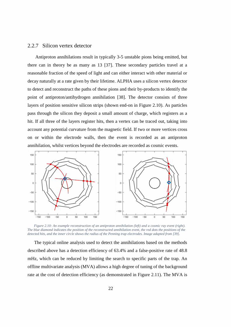
22

2.2.7 Silicon vertex detector

Antiproton annihilations result in typically 3-5 unstable pions being emitted, but

there can in theory be as many as 13 [37]. These secondary particles travel at a

reasonable fraction of the speed of light and can either interact with other material or

decay naturally at a rate given by their lifetime. ALPHA uses a silicon vertex detector

to detect and reconstruct the paths of these pions and their by-products to identify the

point of antiproton/antihydrogen annihilation [38]. The detector consists of three

layers of position sensitive silicon strips (shown end-on in Figure 2.10). As particles

pass through the silicon they deposit a small amount of charge, which registers as a

hit. If all three of the layers register hits, then a vertex can be traced out, taking into

account any potential curvature from the magnetic field. If two or more vertices cross

on or within the electrode walls, then the event is recorded as an antiproton

annihilation, whilst vertices beyond the electrodes are recorded as cosmic events. [39]

The typical online analysis used to detect the annihilations based on the methods

described above has a detection efficiency of 63.4% and a false-positive rate of 48.8

mHz, which can be reduced by limiting the search to specific parts of the trap. An

offline multivariate analysis (MVA) allows a high degree of tuning of the background

rate at the cost of detection efficiency (as demonstrated in Figure 2.11). The MVA is

Figure 2.10: An example reconstruction of an antiproton annihilation (left) and a cosmic ray event (right).

The blue diamond indicates the position of the reconstructed annihilation event, the red dots the positions of the

detected hits, and the inner circle shows the radius of the Penning trap electrodes. Image adapted from [39].

23

trained on annihilation events during the mixing process, and cosmic runs where no

antiprotons or positrons were present in the apparatus.

2.2.8 Temperature diagnostics

We have discussed the temperature of the plasmas held within the Penning traps

without yet quantifying how they were measured. The temperature of a plasma can be

diagnosed by directly sampling the energy distribution. This is done by measuring the

charge that escapes when one side of the confining potential well is lowered and the

particles are extracted to the MCP front. Although antiprotons can also be extracted to

the MCP, as we discussed earlier a better signal can be attained by detecting the

annihilations using the scintillator panels instead.

For a plasma in equilibrium, it has been demonstrated [40] that the number of

particles (𝑁) with charge (𝑞) that escape the trap is approximately related to the change

in the confining potential (𝑉𝑐) by

Figure 2.11: A plot of the detection efficiency against the accepted background rate for the MVA analysis. For

reference, the performance of the standard online analysis is circled in red. The data displayed is from around 670

mixing cycles and 82 hours of cosmic data from 2014. The Y-axis error bars are negligible.

24

(2.2)

(2.3)

𝜕ln (𝑁)

𝜕𝑉𝑐≈ −

|𝑞|

𝑘𝐵𝑇 ,

where 𝑘𝐵 is the Boltzmann constant and T is the plasma temperature. The equation is

approximate for two reasons: Firstly, the approximation is only valid for the very first,

highest energy particles to escape from the potential well, as the change in space charge

of the remaining particles is neglected. Secondly, the manipulation of the potentials

required to extract the plasmas necessarily change the shape of the well, causing the

plasma to lengthen and adiabatically cool. The expected influence of these two factors

can be numerically calculated and used to correct the measured plasma temperature.

By incorporating these corrections, it has been demonstrated that the temperature of

the plasma can be determined to within 20% [34]. However, this method has never

been calibrated by ALPHA in an absolute sense.

2.2.9 Magnetometry

The magnetic field of the CT, AT, and positron accumulator are continuously

monitored using Hall probes. However, for experiments such as the 1S-2S transition

measurement, a more precise measurement is needed in the AT. This can be achieved

by measuring the electron cyclotron resonance (ECR), which is the circular movement

of an electron in a static and uniform magnetic field due to the Lorentz force. The

frequency of this motion (𝑓𝐸𝐶𝑅) is related to the magnetic field 𝐵 by the equation

𝑓𝐸𝐶𝑅 =𝑒𝐵

𝑚 ,

where 𝑒 is the charge and 𝑚 is the mass of the electron.

25

An electron plasma containing around 40 million particles with a diameter of 1.5

– 3 mm is loaded into a single electrode. Microwave pulses are then injected into the

trap via a waveguide situated behind the downstream flapper, and the electric fields

associated with these pulses heat the electron plasma when the frequency of the

microwave radiation matches the electron cyclotron frequency [34]. Typical

measurements inject a microwave pulse only every 15 seconds to allow the plasma to

cool to its equilibrium temperature between each pulse. The temperature change can

be inferred by monitoring the vibrational modes of the plasma. The quadrupole

vibrational mode of the plasma is excited by applying high frequency Gaussian noise

to a neighbouring electrode (typically centred around 25 MHz), and the response of

the plasma is measured on the confining electrode through a high pass filter. This

frequency increases in a manner which is approximately linearly proportional to the

temperature of the plasma [41]. Figure 2.12 shows a trace of an ECR line shape which

was taken during the 2016 run. The peak of the line shape is resolvable to around 10

MHz, which corresponds to a magnetic field accuracy of ± 0.5 mT. The technique is

detailed in [42].

Figure 2.12: An example of an ECR line shape recorded during the 2016 beam period. The trace shows the

quadrupole vibrational mode frequency of an electron plasma when excited by microwave pulses of increasing

frequency.

26

2.3 Antihydrogen formation and trapping

The formation of antihydrogen by mixing antiprotons and positrons has been

relatively routine since the early ATHENA and ATRAP experiments, but the

formation of antihydrogen with a low enough kinetic energy to be confined by the

magnetic trap is a much more difficult endeavour. Antihydrogen is thought to be

created by a three-body recombination process where a ‘spectator’ positron carries

away the excess energy of the ‘active’ positron – antiproton pair [43]. It is therefore

beneficial to have the positron plasma as cold and dense as possible during the mixing

process to maximise the three-body recombination cross section. In this section, we

will discuss two different methods that have been employed to make cold, trappable

antihydrogen, as well as a technique for bringing additional antiprotons and positrons

into the trap for further antihydrogen production and antihydrogen accumulation. The

silicon vertex detector has been (and remains) an essential tool for analysing and

tuning the antihydrogen production techniques.

2.3.1 Autoresonant mixing

Autoresonance is an effect which has been observed in a variety of non-linear

oscillators, including plasma modes [44]. When a swept frequency drive is applied to

a non-linear oscillator whose frequency varies with its amplitude, the response can

become phase-locked to the drive [45]. This technique can be applied to the antiproton

plasma to gradually excite it into the positron plasma whilst being largely independent

of the initial conditions of the positrons and antiprotons [34]. The antiproton bounce

frequencies are typically too low for the autoresonant drive to have a direct effect on

the positrons, however, the positrons are observed to heat from 20 K to around 50 K

after antiproton injection is finished. Increasing the number of antiprotons would

increase the positron heating, and result in a lower trapping rate. Autoresonant

excitation was used up until the 2016 beam period and yielded a peak trapping rate of

2 atoms per trial and a maximum of 4 atoms detected within the trap simultaneously

(using the standard online analysis method with a detection efficiency of 63.4%).

27

2.3.2 Slow merge mixing

During the 2016 run, an older mixing technique was revisited which lead to a

trapping rate of 10.5±0.6 atoms per trial using an MVA analysis tuned to give a

efficiency of 73.0±0.4%. In this scheme, the positron and antiproton electrostatic wells

are slowly merged over 1 s, effectively allowing the two species to flow into each

other. The positron plasma evaporatively cools to below 20 K during the merge, and

increasing the antiproton number doesn’t have the same adverse heating effect as it

did during autoresonant mixing. This technique is potentially more sensitive to the

initial plasma conditions, but the use of evaporative cooling during the earlier rotating

wall compression stages allowed the plasmas to be prepared with a high degree of

consistency [46]. A fraction of the positron plasma is retained after the mixing step for

temperature diagnostics and sanity checks. Figure 2.13 shows a comparison of the

autoresonant and slow merge mixing techniques.

Figure 2.13: In the autoresonant scheme (left), the antiprotons are excited into the positrons by a chirped

frequency. In the slow merge scheme (right), the initial wells (solid line) are reduced until the two species spill into

each other (dashed line).

28

2.3.3 Antihydrogen accumulation

In 2016, the possibility of bringing additional batches of antiprotons and positrons

into the neutral trap without first ramping down the trap magnets to repeat the mixing

process and accumulate, or “stack”, additional antihydrogen atoms was investigated.

The octupole field distorts the solenoid field of the Penning-Malmberg trap, which will

guide particles towards the walls. The critical radius at which particles will be lost in

this circumstance has been calculated [47] to be approximately 4.5 mm, which is

significantly larger than the sub-mm radii of the electron, positron and antiproton

plasmas typically used in ALPHA. Electrons used to cool the antiprotons are normally

loaded directly into the re-catching trap from an electron gun on the AT stick.

However, as this loading beam must pass through the mixing trap, it has the potential

to ionise the trapped antihydrogen atoms. To reduce the likelihood of this, the electrons

are instead loaded into the positron trap before being quickly shuffled by electrostatic

potentials through the mixing trap and into the re-catching trap.

Preliminary trials, mixing between one and five successive stacks of positrons and

antiprotons, showed that the number of antihydrogen atoms within the trap increased

linearly with each successive mixing cycle (see Figure 2.14). The linear relationship

suggests that no antihydrogen atoms are lost during the transfer of plasmas through the

magnetic trap. Each stack of antihydrogen takes approximately 4 minutes to produce,

meaning that the first stack has been trapped for as long as 16 minutes. The five stack

experiment was only performed once and yielded a record 54 detected atoms, implying

that around 74 atoms were trapped simultaneously when accounting for the detection

efficiency of 73.0±0.4%. It was not possible to investigate higher numbers of stacks at

29

this time due to temperature considerations of the octupole magnet power supply

circuit.

2.4 Antihydrogen detection

There are not currently any non-destructive methods of detecting trapped

antihydrogen, so we must instead turn off the trap and look for the annihilation of any

atoms which were trapped. This can either be done by intentionally triggering the

quench response of the magnets, or by ramping down the power supplies as fast as

possible without triggering the quench response.

Triggering the quench response will shut down the magnets with a 1/e time

constant of 9.5 ms [34]. To avoid damaging the magnets or generating excess heat in

the cryostat, the current is extracted through a series of external resistors which are

connected by an insulated-gate bipolar transistor (IGBT) when the control system

Figure 2.14: The number of trapped atoms increases linearly with each successive mixing cycle. The error bars

show the 𝑁 counting statistics alone. The detection efficiency is 73.0±0.4%.

30

detects a voltage across the magnets [34]. The quench response can be manually

triggered, giving the 9.5 ms shutdown that is fast enough that there are essentially no

false-positive events due to the cosmic background, and MVA protocols with detection

efficiencies of 80% or higher can be safely used. The disadvantage of this technique is

that eddy currents induced in the electrodes by the quenching magnets cause them to

heat up, requiring a 15 minute wait before they reach thermal equilibrium with the

cryostat and the experiment can be repeated.

Ramping down the magnets without triggering a quench can be achieved in 1.5 s,

with negligible electrode heating. This lengthens the search time for annihilation

events and increases the false positive signal accordingly. However, the rate of false

positives is still less than 0.1 per ramp down, so with a sufficiently high trapping rate,

the fast ramp down technique allows us to perform experiments with a higher duty

cycle without introducing significant background.

To be certain that the annihilation events we detect are from antihydrogen and not

just low energy antiprotons left over from mixing and trapped between the mirror coils,

we pulse an electric potential across the mixing trap electrodes to kick out any charged

particles. Furthermore, a sloped electrostatic potential is held during the shutdown of

the trap to deflect any antiprotons to one side. The direction of the potential is

alternated between trapping runs so that a comparison can be made. The lack of a

correlation between the annihilation positions and the direction of the sloped potential

not only rules out mirror-trapped antiprotons, but allowed an initial limit to be placed

on the charge of antihydrogen [22].

31

3 Antihydrogen spectroscopy considerations

The 1S-2S transition in hydrogen is electric dipole forbidden, and as a consequence

it cannot be driven by a single 121.5 nm photon. Instead, we must excite the transition

with two photons at 243 nm. If the atom absorbs two counter-propagating photons,

then the Doppler shift which arises due to the atom’s motion with respect to the laser

beam cancels to first order. This technique is known as two-photon Doppler-free

spectroscopy, and is instrumental in overcoming thermal linewidth broadening without

having to cool the atoms down to millikelvin temperatures.

The 1S-2S transition frequency has been measured in a cold sample of

magnetically trapped hydrogen with a precision of 2 × 10−12 by the MIT group [48],

and in a cold atomic beam with a precision of 4.2 × 10−15 by the Hänsch group [49].

Both experiments used counter-propagating beams of 243 nm light for Doppler-free

spectroscopy, with the MIT group using a single mirror to retro-reflect a tightly

focussed 4 mW beam and the Hänsch group using a Fabry-Pérot enhancement cavity

to generate 300 mW of circulating power.

To achieve such high precision, the Hänsch group generates 243 nm light from a

frequency quadrupled 972 nm laser, which is locked to an ultra-stable reference cavity

and related to the SI second using a frequency comb and portable caesium fountain

clock. The ALPHA laser setup described in chapter 5 is closely modelled upon this

system. A velocity selection technique is used to overcome the second order Doppler

shift, and the experiment is repeated with different optical intensities to allow

correction of the AC Stark shift. Both hydrogen experiments used a sample of between

1010 and 1012 atoms per trial, and detect the 1S-2S transition by mixing together the

2S and 2P states using an electric field and detecting the Ly-α photon emitted from the

resulting 2P-1S decay.

In ideal circumstances antihydrogen would be subject to the exact same

experiments as hydrogen, without relying on theoretical models, and avoiding

systematics. However, the large magnetic fields required to synthesise and trap

antihydrogen, the limited number of antihydrogen atoms produced per trial, and the

32

necessary geometry of the ALPHA apparatus make such a comparison impossible.

Instead, we must design our experimental procedures relying on the single particle

sensitivity of the silicon vertex detector and MCP, and utilise the high accuracy at

which modern theories can predict the behaviour of hydrogen to predict the energy

levels of antihydrogen in the ALPHA magnetic field configurations for comparison.

Several assumptions have to be made, and the handling of these will be detailed in this

chapter.

3.1 The hydrogen atom

In this section we will look at how the model of the hydrogen atom has evolved

over the last two centuries to the level where we can use it to accurately predict the

energy levels of antihydrogen in a magnetic field (assuming CPT theory holds), and

how this evolution was inspired by experimental discoveries. The derivation of these

models is beyond the scope of this thesis, so we will simply examine the results.

Examples of the derivations can be found elsewhere [50] [51] [52] [53], which are the

sources of the equations presented. SI units are used throughout.

Figure 3.1: The energy levels of the hydrogen atom are illustrated as the accuracy of models which describe

them improves. The horizontal axis shows the quantum numbers which describe the energy levels, and are

introduced in the text. The vertical axis shows the energy of the levels, but the scale is illustrative only.

33

(3.1)

(3.2)

(3.3)

3.1.1 Historical observations

Dark lines in the solar spectrum were first recorded in 1802 by William Hyde

Wollaston [54], and in 1814 were independently discovered by Fraunhofer, who

systematically characterised the wavelength of over 570 such lines [55]. Around 45

years later, Kirchoff and Bunsen noticed that several of the lines observed by

Fraunhofer coincided with bright lines emitted by heating chemical elements [56]. It

was correctly deduced that the dark lines were created by the absorption of light by

chemical elements in the solar atmosphere.

Although physicists could now observe emission and absorption lines, there was

not yet a mathematical model for predicting where they should appear. Based on the

visible spectra of hydrogen, Balmer developed an empirical equation in 1885 for

predicting where these lines appear

𝜆 = 𝐵 (𝑛2

𝑛2 − 22) ,

where λ is the wavelength of the line, B is the continuum point with a value of

364.50682 nm, and n is an integer > 2.

This equation was generalised for all hydrogen series by Rydberg in 1888 as

1

𝜆𝑣𝑎𝑐= 𝑅(

1

𝑛12 −

1

𝑛22) ,

where R is the Rydberg constant and 𝑛1 < 𝑛2 . It identifies the Balmer series as a

special case where 𝑛1 = 2, and successfully predicts the spectra of other series such as

the Lyman series (𝑛1 = 1) in the UV and the Paschen (𝑛1 = 3) series in the IR.

3.1.2 The Bohr model

The physical explanation of the Rydberg formula was not understood until 1913,

when the Bohr model of the atom was introduced. This model explained the spectra as

the spacing between quantised energy levels, with the energies of the levels given by:

𝐸𝑛 = − 𝑍2

(𝑘𝑒𝑒2)2𝑚𝑒

2ħ2𝑛2 ,

34

(3.4)

where 𝑚𝑒𝑐2 is the rest mass energy of the electron, 𝑘𝑒𝑒

2

ħ𝑐≡ 𝛼 is the fine structure

constant, and Z is the atomic number of the atom (although the equation is only

accurate for hydrogen-like systems). The energy levels are denoted by the quantum

number n, which is an integer greater than zero.

We have so far assumed that the electron orbits around a stationary nucleus, which

in the case of hydrogen is a single proton. As the proton has a finite mass M, the

electron and proton will both orbit the centre of mass of the system. In the rest frame

of the proton, the electron will appear to have a reduced mass m, which is given by the

relationship

𝑚 =𝑚𝑒𝑀

𝑚𝑒 + 𝑀 .

3.1.3 Fine structure

As quantum mechanics developed, the Schrodinger equation introduced an

additional quantization of the orbital angular momentum of the electron, with a

corresponding quantum number l where 0 ≤ 𝑙 < 𝑛, although states with the same 𝑛

but different l still appear degenerate. At this point, it is convenient to introduce

spectroscopic notation.

l 0 1 2 3

Spectroscopic notation S P D F

Table 3.1: Spectroscopic notation.

Energy levels can be identified by the principal quantum number n and a letter

which corresponds to the orbital angular momentum l. The first four letters of

spectroscopic notation stand for sharp, primary, diffuse and fundamental (for historical

reasons), and continue alphabetically afterwards. For example, the ground state of the

hydrogen atom is denoted as “1S”.

Importantly, photons also carry one unit of angular momentum. This means that

transitions between energy levels involving a single photon must obey the selection

35

(3.5)

rule ∆𝑙 = ±1, which is why the single photon transition between the 1S and 2S levels

(∆𝑙 = 0) of hydrogen is forbidden.

In addition to orbital angular momentum, the electron has an intrinsic angular

momentum called “spin” corresponding to its magnetic moment. The quantum number

s is associated with the spin, and for the electron 𝑠 =1

2. As the two are necessarily

coupled, the total angular momentum can be described by the quantum number j,

where 𝑗 = |𝑙 − 𝑠|, |𝑙 − 𝑠| + 1…0… 𝑙 + 𝑠 − 1, 𝑙 + 𝑠. The value of j is depicted in

spectroscopic notation by a subscript below the orbital angular momentum letter. For

example, the ground state of hydrogen can be denoted as “1S1/2”.

The Schrödinger equation neglects the relativistic effects of the electron, and whilst

these can be included, it is easier to present the results of the Dirac equation, which is

an attempt to unify the theories of quantum mechanics and special relativity:

𝐸𝑛,𝑗 = 𝑚𝑐2

[

1 +𝑍2𝛼2

(𝑛 − (𝑗 +12) + √(𝑗 +

12)

2

− 𝑍2𝛼2)

2

] −

12

.

This result correctly predicts the splitting of energy levels i.e. the 2P1/2 and 2P3/2 states,

but note that the 2S1/2 and 2P1/2 states still appear degenerate.

3.1.4 The Lamb shift

The lamb shift is a splitting of the 2S1/2 and 2P1/2 states, first measured in the

microwave spectrum of atomic hydrogen by the Lamb-Retherford experiment in 1947

[57]. The discovery of the Lamb shift led to the development of renormalisation theory

and quantum electrodynamics (QED). The 1057 MHz frequency difference between

the two states is primarily due to the vacuum polarisation effect (-27 MHz), the

electron mass renormalisation effect (+1017 MHz), and the anomalous magnetic

36

(3.7)

(3.8)

(3.6)

moment of the electron (+68 MHz), which are a result of the Feynman diagrams shown

in Figure 3.2.

The energy shifts at the one-loop level for hydrogen are given for 𝑙 = 0 by

∆𝐸𝐿𝑎𝑚𝑏 = 𝛼5 𝑚𝑐21

4𝑛3{𝑘(𝑛, 0)},

and for 𝑙 ≠ 0 by

∆𝐸𝐿𝑎𝑚𝑏 = 𝛼5 𝑚𝑐21

4𝑛3{𝑘(𝑛, 𝑙) ±

1

𝜋 (𝑗 +12) (𝑙 +

12)

},

where 𝑗 = 𝑙 ±1

2. 𝑘(𝑛, 0) is a numerical factor which varies slightly with n from 12.7

to 13.2, and 𝑘(𝑛, 𝑙) is a much smaller numerical factor (<0.05) which again varies

slightly with n and l. The Lamb shift mostly affects the S states, as these are the only

states which the electron can be found at the nucleus.

3.1.5 Hyperfine structure

The theories we have considered so far have only considered quantisations of the

electron, but the proton also has a spin of 𝑠 =1

2. This leads to an additional quantum

number f which has the possible values of 𝑓 = 𝑗 +1

2, 𝑗 −

1

2. The result of this is the

splitting of each energy level into two, depending on the orientation of the electron

and proton magnetic dipoles. The hyperfine energy shift for 𝑙 = 0 states is given by

∆𝐸𝐻𝐹𝑆 = 𝑚

𝑀𝛼4 𝑚𝑐2

4𝜇𝑝

3𝑛3[𝑓(𝑓 + 1) −

3

2],

e

e e

e

e

e

p

p

p

p

p

p

e

e

acuum polarisation Electron mass renormalisation Anomalous magnetic moment

Figure 3.2: Feynman diagrams showing the most significant contributions to the Lamb shift [50].

37

(3.9)

(3.10)

(3.11)

where M is the proton mass and 𝜇𝑝 is the proton magnetic moment. The ground state

hyperfine splitting of hydrogen, i.e. ∆𝐸𝐻𝐹𝑆(𝑓 = 1) − ∆𝐸𝐻𝐹𝑆(𝑓 = 0), has been

measured with a relative uncertainty of 6 × 10−13 [58]. For 𝑙 ≠ 0, the hyperfine

energy shift is given by

∆𝐸𝐻𝐹𝑆 = 𝑚

𝑀𝛼4 𝑚𝑐2

𝜇𝑝

2𝑛3

±1

(𝑓 + 12)(𝑙 + 1

2) ,

where 𝑓 = 𝑗 ±1

2.

3.1.6 The Zeeman Effect

So far we have only discussed atoms in a field-free environment. Each hyperfine

state has a 2𝑓 + 1 degeneracy associated with the quantum number 𝑚𝑓, which is the

projection of the total angular momentum onto the z-axis and can take the values 𝑚𝑓 =

−𝑓,−𝑓 + 1…0…𝑓 − 1, 𝑓. The Zeeman effect is the breaking of this degeneracy due

to the atoms interaction with a static magnetic field. For a moderate magnetic field B,

the Zeeman splitting can be calculated with respect to the hyperfine centroid using the

Breit-Rabi equation:

∆𝐸𝑛,𝑓=𝑗±

12,𝑚𝑓

= −∆𝐸𝐻𝐹𝑆

4− 𝜇𝑃𝑚𝑓𝐵 ±

∆𝐸𝐻𝐹𝑆

2√1 + 2𝑚𝑓𝑥 + 𝑥2,

𝑥 ≡𝐵(𝜇𝑒(𝑛) + 𝜇𝑃)

∆𝐸𝐻𝐹𝑆.

In the case where 𝑚𝑓 = −1, the square root contains an exact square and the positive

solution is taken. Note that due to interactions with the nucleus, the magnetic moment

of the electron 𝜇𝑒(𝑛) depends upon principle quantum number n, and for the 𝑙 = 0

states is given by the relationship

𝜇𝑒(𝑛) = 𝜇𝑒 (1 −𝛼2

3𝑛2) .

In spectroscopic notation, the hyperfine structure is commonly notated as a

subscript after the angular momentum indicator, so for the hydrogen ground state

would be 1Sa, 1Sb, 1Sc, and 1Sd, in order of increasing energy (see Figure 3.3).

38

(3.12)

(3.13)

(3.14)

3.1.7 Diamagnetic shift

An electron in an S state will circulate in an applied magnetic field (recall cyclotron

motion from section 2.1.1), producing its own magnetic field which opposes the

applied field. This field effectively shields the proton and causes the transition

frequencies to shift upwards. This is known as the diamagnetic shift, and is given for

the 1S and 2S states by

∆𝐸𝑑𝑖𝑎(1𝑆) =𝑒2𝑎0

2

4𝑚𝐵2, ∆𝐸𝑑𝑖𝑎(2𝑆) =

7𝑒2𝑎02

2𝑚𝐵2,

where 𝑎0 is the Bohr radius.

3.1.8 Antihydrogen 1S-2S frequencies

The hydrogen 1S-2S transition frequency and the hyperfine splitting of both the 1S

and 2S states have been measured with a precision meeting or exceeding what QED is

able to predict [49] [58] [59]. As such, we only need to solve the Breit-Rabi and

diamagnetic equations to calculate the Zeeman shift of the transition frequencies in the

~1 T magnetic field of the ALPHA apparatus. Only the c (𝑓 = 1,𝑚𝑓 = 0) and d (𝑓 =

1,𝑚𝑓 = 1) hyperfine states are trappable in a magnetic minimum trap, and the energy

differences are given with an accuracy at the few kHz level by

𝑣1𝑆𝑑→2𝑆𝑑= 𝑣1𝑆→2𝑆 +

1

ℎ((∆𝐸𝑛=2,𝑓=1,𝑚𝑓=1 − ∆𝐸𝑛=1,𝑓=1,𝑚𝑓=1) +

13𝑒2𝑎02

4𝑚𝐵2),

𝑣1𝑆𝑐→2𝑆𝑐= 𝑣1𝑆→2𝑆 +

1

ℎ((∆𝐸𝑛=2,𝑓=1,𝑚𝑓=0 − ∆𝐸𝑛=1,𝑓=1,𝑚𝑓=0) +

13𝑒2𝑎02

4𝑚𝐵2),

where 𝑣1𝑆→2𝑆 is the hyperfine centroid frequency [49] and h is the Planck constant.

Frequency units are used instead of energy units to avoid accumulating factors of h.

Figure 3.3 is a Breit-Rabi diagram of the 1S and 2S states, with arrows indicating the

relevant transitions. Note that these are the total frequencies, and hence need to be

halved for two-photon excitation. [60].

39

At the measured magnetic minimum of 1.0168 T in the flattened trap configuration

of 2016, the calculated transition frequencies are

𝑣1𝑆𝑑→2𝑆𝑑= 2 466 061 103 064 kHz ,

𝑣1𝑆𝑐→2𝑆𝑐= 2 466 061 707 104 kHz .

There are of course additional systematic shifts imposed by the experimental

conditions, which we will discuss in the next section.

3.2 Systematic shifts and broadenings

The transition frequencies will be subject to a number of systematic shifts and

broadenings which must also be considered. As before, the values quoted correspond

to the total 1S-2S transition frequency, and should be halved when compared to the

243 nm laser frequency which drives the transitions.

Figure 3.3: The calculated Breit-Rabi diagrams of the 1S (bottom) and 2S (top) states of antihydrogen. The

blue lines show the low-field seeking trappable states and the red lines show the high-field seeking untrappable

states. Image from [60].

40

3.2.1 Residual Zeeman Effect

The Zeeman shifts of the 1S and 2S states almost cancel, but there is still a small

dependence on the magnetic field which we call the residual Zeeman effect. Around

the 1 T magnetic field of the trap, this scales as 9.6 Hz/mT for the d-d transition and

190 Hz/mT for the c-c transition. Whilst this shift is calculated in equation 3.10,

magnetic field deviations will make a small contribution to the transition frequency

uncertainty. The precision of the ECR technique discussed in section 2.2.9 therefore

represents an uncertainty of ± 347 Hz and ± 6446 Hz for the d-d and c-c transitions

respectively.

The shape of the magnetic field means that the line shape will be asymmetric, as

the atom won’t always cross through the laser beam at the magnetic minimum. The

magnetic trap is described in chapter 2 and consists of an octupole for radial

confinement and five mirror coils for axial confinement. The mirror coils can be

operated with current running in either direction, allowing the shape of the trap to be

carefully tuned. Figure 3.4 shows three possible configurations of the magnetic field.

Figure 3.4: A plot of three possible magnetic field configurations. The black markers labelled A-E show the

approximate sizes and locations of the mirror coils. Image from [52].

41

The original ALPHA field is shown in blue, and comprises of just the octupole and the

end mirror coils. The line shape asymmetry can be reduced by running reverse current

through, or ‘bucking’, mirrors B, C, and D to flatten the field and increase the volume

of the magnetic minimum region as shown in red. By running sufficient reverse current

through mirror E, the field generated will cancel out the field of the external solenoid

to create a zero field region (not shown) which is still within the coverage region of

the silicon vertex detector (we will discuss why this could be useful soon). As a result

the volume of the trap is reduced, as shown by the green dashed line.

3.2.2 Stark effect

The Stark effect is the shifting and splitting of energy levels with the application

of an external electric field, due to the pulling of the nucleus and electrons in opposite

directions. There exists both a DC and an AC Stark effect, and the two can be treated

separately.

The DC Stark effect is responsible for broadening the transition due to the range of

electric fields the atoms will experience from their ~90 m/s movement within the

magnetic trap, as well as any potentials applied to the Penning trap electrodes. For the

1S-2S transition, the magnitude of the effect has been calculated [52] to be around 300

Hz, which is below the current accuracy requirements.

An AC stark shift occurs due to the oscillating electric field of the laser. For the

target intensities within the ALPHA enhancement cavity, the shift in the middle of the

beam was calculated [52] to be approximately 10 kHz. The shift is typically

compensated for by measuring the line shape at several different circulating powers

and extrapolating to zero power.

3.2.3 Transit time broadening

Heisenberg’s uncertainty principle tells us that there is a fundamental limit to the

accuracy at which complimentary observables can be measured. In our case, the

42

(3.15)

complimentary observables are the time at which the transition to the 2S state occurs,

and the energy of the 2S state (i.e. the transition frequency).

As the waist of the enhancement cavity is relatively small (𝜔0 = 196 μm), and the

atom travels through it relatively quickly (v ~90 m/s), the transit time is quite short.

Therefore, there is a fundamental limit placed on the accuracy at which we can

determine the 1S-2S transition frequency. The full-width half-maximum (FWHM) of

this broadening [52] at 121 nm is given by the Fourier transform

∆𝑣𝑡𝑟𝑎𝑛𝑠𝑖𝑡 = √ln (2)v

𝜋𝜔0≈ 120 kHz .

This is the most significant source of broadening for the current 1S-2S experiment,

and must be addressed if we wish to improve the precision of the measurement. Transit

time broadening can be reduced by either enlarging the beam waist, or by cooling the

atoms such that their transverse velocity is lowered.

3.2.4 2S lifetime reduction

The natural linewidth of the 1S-2S transition is inversely proportional to the

lifetime of the 2S state. As such, any effect that acts to reduce the lifetime of the 2S

state will accordingly broaden the transition linewidth. For 2 W of circulating power

within the enhancement cavity, the main source of lifetime reduction was calculated

[52] to be ionisation from the 2S state by a third 243 nm photon, which contributes

approximately 8 kHz to the transition linewidth.

Table 3.2 gives a summary of the shifts and broadenings of 1 kHz or more towards

the total 1S-2S transition frequency, using the parameters we have discussed above.

Effect Contribution

Residual Zeeman ± 0.35 kHz (d-d) error

± 6.45 kHz (c-c) error

AC Stark 0-10 kHz shift

Transit time 120 kHz FWHM broadening

2S lifetime reduction 8 kHz FWHM broadening

Table 3.2: A summary of the shifts and broadenings which contribute >1 kHz towards the total 1S-2S transition

frequency

43

3.3 Simulated transition rates

A simulation1 by C. Rasmussen and F. Robicheaux was used to predict the

transition rate and the loss mechanism for the atoms within the magnetic minimum

trap. The simulation models the movement of the atoms within the trap as they interact

with the laser. Once excited to the 2S state, the atoms can either decay back to the 1S

state via two-photon emission, become ionised via a third 243 nm photon, or mix with

the 2P states via the electric fields generated by the atom’s movement through the

magnetic field. The 2P state can decay to either a trappable 1S hyperfine state where

243 nm excitation can occur once again, or to an untrappable hyperfine state and

annihilate on the trap walls. The simulation is described in detail in [52].

Figure 3.5 shows a plot of the relative fraction of antihydrogen atoms against the

detuning of the 243 nm laser frequency using the simulation described above for the

summed c-c and d-d transitions in the flattened magnetic trap configuration. The beam

circulating within the enhancement cavity is assumed to have a waist of 200 μm and a

power of 1 W. The laser linewidth is assumed to be 10 kHz. As discussed in section

3.2.1, the transition profile is asymmetric due to the shape of the magnetic field. Note

from the inset figure that the time required to reach an excitation fraction of 0.5 is of

the order of 100’s of seconds.

1 At the time of writing, Figure 3.5 differs from the figure shown in source [60] due to a factor of

two error in the simulation of the linewidth. The corrected simulation is presented here, and a

corrigendum to the original paper is being prepared.

44

3.4 Detection schemes

3.4.1 Ly-α detection

The hydrogen 1S-2S experiments discussed earlier used a sample size of more than

1010 atoms, whereas ALPHA is currently limited to just a few trapped antihydrogen

atoms at a time. Although the 121 nm Ly-α photons emitted by the decay from the 2P

state can be detected with high efficiency using PMT’s, the few photons emitted by

the antihydrogen atoms are unlikely to register above the dark noise of the detectors

over excitation times of 100’s of seconds. Furthermore, the nested Penning-Malmberg

Figure 3.5: A simulation of the interaction between the antihydrogen atoms within the flattened trap yields the

excitation rate and the linewidth of the summed c-c and d-d transitions. The inset shows the time dependence of the

excitation period. Image from [60].

45

and Ioffe-Pritchard traps within the ALPHA apparatus and the essential cryogenic

hardware severely restricts the solid angle (~10-5) available for placing detectors,

ruling out Ly-α detection as a viable method.

3.4.2 Annihilation - disappearance mode

Both the spin-flip and ionisation mechanisms reduce the number of atoms in the

trap, so one can compare the apparent trapping rate between trial runs with different

laser frequencies by simply counting the atoms left when the trap is shut down. As the

trap can be shut down quickly, the cosmic background rate is almost negligible. This

method requires the trapping rate to be roughly constant between consecutive runs,

and that the excitation rate is sufficiently high or that there is sufficient data to be able

to distinguish the laser runs from a control test. As this is the standard method of

antihydrogen detection for ALPHA, no new techniques need to be developed.

3.4.3 Annihilation - appearance mode

After laser excitation to the 2S state, the dominant source of loss from the trap is

ionisation by a third 243 nm photon. If the cold antiproton left behind could be detected

with high sensitivity and low noise it would complement the disappearance

measurement, and could significantly improve the efficiency of the experiment if the

excitation rate is low.

The silicon vertex detector records events not only during the trap shut down, but

throughout the long laser exposure periods too. As described in section 2.2.7, the MVA

protocol can be tuned to maximise the signal to noise ratio for a given background rate.

The background rate can be significantly reduced by only looking at the data during

specific time periods (as was done for the microwave ground state hyperfine splitting

experiment [25]), and can be further reduced by setting a region of interest within the

trap. A weak electrostatic potential can be formed within the mixing trap to hold the

antiprotons resulting from laser ionisation, and they can be ejected axially at well-

defined times. If mirror E is bucked as we discussed in section 3.2.1, the antiprotons

46

should follow the magnetic field lines to the wall and annihilate under mirror E. As

these annihilations will have both a predictable time and location, the detector

background can be almost zero.

The MCP is also capable of imaging single antiprotons [36], although the

efficiency is unknown and difficult to estimate due to the large spread in energy

deposited. On rare occasion, the secondary particles from the annihilation on the multi-

channel plate can pass through neighbouring channels, triggering electrons to be

emitted here as well, and leaving identifiable tracks (example: Figure 3.6). Similar to

the process described before, the antiprotons resulting from laser ionisation could be

captured in an electrostatic potential and ejected towards the MCP at regular intervals.

There is a caveat to these two techniques, which is that the antiproton plasmas

trapped in an electrostatic potential which spans the entire mixing trap have been

observed to become quickly unstable, with all particles lost after a few seconds.

However, if the trapping and excitation rates are high enough, the annihilation of these

lost antiprotons could be detectable over the background noise regardless.

Figure 3.6: A close-up image of an antiproton annihilation on an MCP which has left identifiable tracks. The

surrounding bright spots are also due to antiproton annihilations.

47

4 The 1S-2S Enhancement Cavity

Commercial laser systems are only able to produce around 100 mW [61] of

continuous wave power at 243 nm, so an enhancement cavity is required to build up a

higher intensity within the ALPHA apparatus. A Fabry-Pérot cavity consists of two

(or more) mirrors, within which constructive interference amplifies the optical

intensity when the cavity length is tuned to resonance. Photons propagate in both

directions, forming a standing wave within the cavity. Cavities within which photons

only propagate in one direction also exist, and are known as ring or travelling wave

cavities. The Fabry-Pérot configuration is more beneficial for spectroscopy, as the

atoms within the cavity which absorb two counter-propagating photons will not

experience a Doppler shift (to 1st order).

Two different Fabry-Pérot cavity geometries have been trialled within the ALPHA

apparatus - an internal cavity, using mirrors mounted within the cryogenic region, and

an external cavity, with mirrors mounted just inside the vacuum viewports at the ends

of the apparatus. Whilst the external cavity is simpler to construct, at 2.7 m it is triple

the length of the internal cavity and more susceptible to environmental noise. The

internal cavity is a rigid, pre-aligned cavity whose only degree of freedom is length.

However, as the mirrors are installed in the cryogenic, UHV region of the apparatus,

they must fulfil strict criteria. The mirrors must not break or deform when the

experiment is baked at 80 °C and cooled down to 7 K, and must maintain their

alignment and not need servicing during the ~5 month antiproton beam period. The

mirror mounts must not be made from or include any magnetic or superconducting

material, as this can influence the shape of the magnetic field and potentially be

damaged when the trap magnets are ramped. The mounts must also be made using

only very low outgassing materials, so as not to degrade the lifetime of the trapped

antiprotons, positrons, and antihydrogen by contaminating the vacuum. Finally, the

mounts must fit within the few cm of space between the particle beam line and the

inner diameter of the vacuum chamber. The tight space constraints severely limit the

use of flexure mounts and of any kind of active alignment, and attempts to simply

48

(4.1)

(4.2)

(4.3)

epoxy the mirrors to a solid mount resulted in them breaking due to the mismatched

coefficients of thermal contraction.

In this chapter we will examine how light behaves in a simple Fabry-Pérot cavity,

before looking at the development of an athermal mirror cell which solves the

aforementioned problems and enables the use of an internal cavity. We will also look

at the design of the external cavity, and compare the performance of the two designs.

4.1 Enhancement cavity theory

Let us consider the interaction between a laser beam of wavelength λ and a Fabry-

Pérot cavity consisting of two mirrors separated by distance d. The mirrors have a field

amplitude reflection coefficient r and a transmission coefficient t, and the incident light

has field amplitude 𝐸0.

We can write the field amplitude transmitted through the first mirror (or ‘input

coupler’) simply as

𝐸 = 𝑡1𝐸0 .

After one complete round trip within the cavity the light will have an amplitude

𝐸 = 𝑡1𝐸0𝑟1𝑟2𝑒𝑖4𝜋𝑑/𝜆 ,

where the exponent contains the accumulated phase shift. After 𝑁 complete round trips

within the cavity without interference, the resultant field amplitude of the light will be

𝐸 = 𝑡1𝐸0(𝑟2𝑟2)𝑁𝑒𝑖4𝜋𝑑𝑁/𝜆 .

If the incident light is continuous, then the circulating field inside the cavity can be

written as a sum of the waves which have made 0, 1, 2, …𝑁 round trips,

Figure 4.1: A two-mirror Fabry-Pérot cavity

49

(4.4)

(4.5)

(4.6)

(4.7)

(4.8)

(4.9)

𝐸𝑐𝑖𝑟𝑐 = 𝑡1𝐸0 ∑(𝑟1𝑟2)𝑁𝑒𝑖4𝜋𝑑𝑁/𝜆

∞

𝑁=0

=𝑡1

(1 − 𝑟1𝑟2𝑒𝑖4𝜋𝑑/𝜆)𝐸0 .

The reflected field includes contributions from both the incident field reflected directly

from the input coupler and the field transmitted through the input coupler from the

cavity:

𝐸𝑟 = [−𝑟1∗ +

𝑟2𝑡12𝑒𝑖4𝜋𝑑/𝜆

(1 − 𝑟1𝑟2𝑒𝑖4𝜋𝑑/𝜆)

] 𝐸0 .

To calculate the enhancement factor of the cavity, it is more practical to convert

into units of power. The mirrors have a power reflectivity 𝑅 ≡ |𝑟|2 and transmission

𝑇 ≡ |𝑡|2. Note that the mirrors are not perfect and will also have a loss L associated

with them, which can be due to absorption within the mirror coating or surface

imperfections scattering the incident light. Conservation of energy dictates that the

sum of these parameters must equal 1, i.e.

𝑅 + 𝑇 + 𝐿 = 1 .

We can write the power circulating within the cavity as

𝑃𝑐𝑖𝑟𝑐 = |𝐸𝑐𝑖𝑟𝑐|2 =

𝑇1

|1 − √𝑅1𝑅2𝑒𝑖4𝜋𝑑 𝜆⁄ |2 𝑃0 .

The reflected power is given by

𝑃𝑟 = |𝐸𝑟|2 =

|−1 + (1 +𝑇1

𝑅1)√𝑅1𝑅2𝑒

𝑖4𝜋𝑑 𝜆⁄ |2

|1 − √𝑅1𝑅2𝑒𝑖4𝜋𝑑 𝜆⁄ |2 𝑅1𝑃0 ,

and the power transmitted through the cavity is simply

𝑃𝑡 = 𝑇2𝑃𝑐𝑖𝑟𝑐 .

4.1.1 Resonance

When the cavity length is a half-integer (𝑛/2) number of wavelengths of the laser,

the exponent 𝑒𝑖4𝜋𝑑 𝜆⁄ = 𝑒𝑖2𝜋𝑛 = 1. This is the resonant condition of the cavity, where

the circulating power is at a maximum and the reflected power is at a minimum. We

50

(4.10)

(4.11)

(4.12)

(4.13)

can define the enhancement factor b as the ratio between the circulating power on

resonance and the input power, i.e.

𝑏 =𝑃𝑐𝑖𝑟𝑐

𝑃0=

𝑇1

(1 − √𝑅1𝑅2)2 .

For certain mirror configurations, the reflected power becomes zero when the cavity

is on resonance. This condition is known as ‘impedance matched’, and is given to first

order by

𝑇1 = 𝑇2 + 𝐿1 + 𝐿2 .

The spacing between resonances is known as the free spectral range (FSR). A free

spectral range can be spanned either by scanning the cavity length by 𝜆/2 or by

changing the laser frequency by 𝑐 2𝑑⁄ , where c is the speed of light. The linewidth of

the cavity is defined as the FWHM of a resonance, and for high reflectivity mirrors (R

> 0.9) has an approximately Lorentzian profile. Like the free spectral range, it can be

expressed in terms of both the cavity length and the laser frequency. The cavity length

interpretation is important as it gives us an idea of how accurately we need to control

the length of the cavity to keep it on resonance, and the laser frequency interpretation

is important as if the laser linewidth is greater than the cavity linewidth, it will be an

additional source of loss.

The ratio between the free spectral range and the linewidth gives us a parameter

called the finesse F. For high reflectivity mirrors (R > 0.9), the finesse is well

approximated by

𝐹 ≡FSR

Linewidth≈

𝜋(𝑅1𝑅2)14

1 − √𝑅1𝑅2

.

Note that the finesse depends only upon the mirror reflectivity and not the cavity length

or laser frequency. The enhancement factor can be expressed in terms of the finesse as

𝑏 ≈ 𝑇1 (𝐹

𝜋)2

,

which is convenient as it can be difficult to accurately measure mirror reflectivity when

it approaches 1, whereas the finesse is relatively straightforward to measure.

51

(4.14)

(4.15)

(4.16)

(4.17)

4.1.2 Transverse mode matching

So far we have only discussed the longitudinal properties of the cavity, but we must

of course consider the transverse properties of the cavity as well. Gaussian beams can

be characterised by the beam waist at the focal point 𝑤0, and the laser wavelength 𝜆.

The beam radius along the direction of propagation (𝑧) is given by [62]

𝑤(𝑧) = 𝑤0√1 + (𝑧

𝑧0)

2

,

and the radius of curvature ℛ of the wavefront is given by [62]

ℛ(𝑧) = 𝑧 [1 + (𝑧0

𝑧)2

] .

The wavefront curvature decreases from infinity at 𝑧 = 0 to a minimum at 𝑧 = 𝑧0

before increasing linearly for large 𝑧. 𝑧0 is known as the ‘Rayleigh range’, and is

related to the beam waist by [62]

𝑧0 =𝜋𝑤0

2

𝜆 .

Let’s consider a Gaussian beam with 𝑤0 = 0.2 mm located at 𝑧 = 0, 𝜆 = 243 nm,

and 𝑧𝑜 = 0.517 m as illustrated in Figure 4.2. A cavity with this beam profile could be

formed by placing mirrors at any 𝑧 where the radius of curvature of the mirror matches

the radius of curvature of the wavefront. Note that the waist does not necessarily have

to be within the cavity, as a cavity could be formed using a convex and concave mirror

on the same side of the waist. However, if we place a pair of concave mirrors with ℛ1

and ℛ2 either side of the waist at 𝑧1 and 𝑧2, we can equate ℛ1 = ℛ(𝑧1) and −ℛ2 =

ℛ(𝑧2), where the negative radius of curvature of mirror 2 is because the mirror is

facing the opposite direction. Writing out equation 4.15 explicitly,

ℛ1 = 𝑧1 +𝑧0

2

𝑧1 , −ℛ2 = 𝑧2 +

𝑧02

𝑧2 ,

52

(4.18)

(4.19)

(4.20)

(4.21)

and using our earlier definition of the cavity length,

𝑑 = 𝑧2 − 𝑧1 ,

this gives us a set of equations which we can solve for 𝑧1, 𝑧2, and 𝑧0:

𝑧1 =−𝑑(ℛ2 + 𝑑)

ℛ2 + ℛ1 + 2𝑑 , 𝑧2 = 𝑧1 + 𝑑 ,

𝑧02 =

−𝑑(ℛ1 + 𝑑)(𝑅2 + 𝑑)(ℛ2 + ℛ1 + 𝑑)

(ℛ2 + ℛ1 + 2𝑑)2 .

Since we have a method for calculating 𝑧0 and the location of the waist, everything

about the cavity can be determined. The size of the beam waist can be calculated by

re-arranging equation 4.16 to give 𝑤𝑜 = √𝜆𝑧𝑜

𝜋, and the beam size at the mirrors can be

calculated using equation 4.14. For the beam to be confined by the cavity, 𝑧0 must be

real, and hence 𝑧02 in equation 4.20 must be positive. It can be shown that the condition

𝑧02 > 0 is equivalent to

0 ≤ (1 −𝑑

ℛ1) (1 −

𝑑

ℛ2) ≤ 1.

Figure 4.2: A plot of the beam waist (top) and the wavefront radius of curvature (bottom) for a Gaussian beam

with 𝑤0 = 0.2 𝑚𝑚, 𝜆 = 243 𝑛𝑚, and 𝑧0 = 0.517 m over a 6 m propagation length.

53

(4.22)

(4.23)

(4.24)

This condition is known as the confinement condition, and is commonly expressed in

terms of two 𝑔 factors;

𝑔𝑖 = 1 −𝑑

ℛ𝑖 , 𝑖 = 1, 2 .

Figure 4.3 shows the stable region (blue) where the confinement condition is satisfied

for various cavity geometries. Points along the dashed red line represent symmetrical

resonators, i.e. where 𝑔1 = 𝑔2. [63]

For a perfectly aligned and mode matched cavity, the only resonant spatial mode

will be the fundamental Gaussian mode, sometimes labelled as the TEM00 mode. The

peak intensity 𝐼0 of such a beam is related to the optical power 𝑃 by [62]

𝐼0 =2𝑃

𝜋𝑤02 ,

and the relative intensity at any point within the beam is given by [62]

𝐼(𝑥, 𝑦, 𝑧)

𝐼0= (

𝑤0

𝑤(𝑧))2

𝑒−2(𝑥2+𝑦2)

𝑤2(𝑧) .

However, a cavity can often support many different spatial modes, and these will have

a different intensity profile. Hermite-Gaussian modes typically result from a

Figure 4.3: The stability of different cavity configurations as defined by their g factors (g1,g2). Only the

configurations under the blue shaded region are stable. Image by [63].

54

misaligned or distorted input beam, and Laguerre-Gaussian modes typically arise from

a mismatch between the laser and cavity beam waists (see Figure 4.4 for examples),

but these depend greatly on the cavity geometry. In general it is desirable to eliminate

these higher order modes, so we will not examine their spatial profile in more detail.

[64]

4.1.3 Cavity locking techniques

For many applications, it is desirable to lock the cavity on resonance. This can

either be done by locking the cavity length to a laser or by locking the laser frequency

to the cavity. The former is useful for building up the intensity of the laser beam for

spectroscopy or non-linear processes such as frequency doubling, whilst the latter is

useful for stabilising a laser by locking it to an ultra-stable cavity with an extremely

narrow linewidth. Both applications require an error signal which has a zero crossing

point to be generated. A servo loop can then control an actuator (such as a piezo behind

a cavity mirror, or the temperature of the laser) to actively minimise the error signal.

The most basic form of lock is a side-of-peak lock. In this case, the error signal is

simply the transmission signal of the cavity with a DC offset subtracted. This locking

technique is not capable of locking to the top of a resonance however, as the error

signal here would be unipolar and the servo would not know in which direction to

Figure 4.4: Hermite-Gaussian (top) and Laguerre-Gaussian (bottom) modes. Image from [64]

55

actuate. The lock is extremely susceptible to amplitude noise, including DC sources

such as changes in the ambient background light.

A large improvement can be realised by applying a small modulation to the cavity

length at a frequency higher than any expected noise sources (typically > 10 kHz). The

difference signal derived from electronically mixing the drive modulation and the

modulation present in the cavity transmission is proportional to the phase difference

between the two signals (more precisely, it is the derivative of the peak), and has a

zero crossing point at the peak of the resonance. This error signals allows the cavity to

be locked at the top of the resonance and is relatively insensitive to sources of noise.

This technique is known as an ‘amplitude modulation’ (AM) lock, or ‘dither’ lock.

A further improvement can be gained by modulating the frequency of the laser

instead. With the Pound-Drever-Hall (PDH) locking technique [65], sidebands are

added to the laser frequency by either directly modulating the laser frequency or

passing the beam through an external electro-optic modulator (EOM). The sidebands

are typically many MHz away from the carrier frequency and can span a significant

fraction of the cavity free spectral range. As the sidebands are outside of the cavity

linewidth they will not be resonant at the same time as the carrier frequency and instead

get reflected. By electronically mixing the modulation frequency with the beat

frequency between the reflected sidebands and carrier, an error signal with a sharp zero

crossing point similar to the amplitude modulation technique can be generated.

Figure 4.5: The ‘x’ shows the lock points for the side of peak lock (left) and the amplitude modulation error

signal (right). The frequency scale is the same for both plots.

56

(4.25)

(4.26)

However, the error signal now extends all the way out to the sidebands, greatly

increasing the capture range of the lock.

4.1.4 Cavity power

We can write the average circulating power within the cavity as

𝑃𝑎𝑣𝑔 = 𝑏𝛾𝑄𝑙𝑜𝑐𝑘𝑃0 .

In this equation, we have introduced a spatial mode matching constant 𝛾, which we

define as the ratio of the fundamental mode to all other modes coupled into the cavity.

𝑄𝑙𝑜𝑐𝑘 is a fraction representing the quality of the lock.

As the PDH scheme uses only the reflected light to lock the cavity, this allows a

power meter to be placed after the output coupler to accurately measure the transmitted

power. If the transmission of the output coupler is well known, the average circulating

power can be calculated by rearranging equation 4.9 to get

𝑃𝑎𝑣𝑔 =𝑃𝑡

𝑇2 .

Figure 4.6: The frequency/phase modulation adds sidebands to the beam, which are visible in the transmitted

signal (left). The capture range of the PDH error signal extends to the sidebands, yet maintains a sharp slope to

lock to (right). The ‘x’ indicates the lock point.

57

(4.27)

(4.28)

(4.29)

4.2 Athermal mirror cell development

An athermal mirror cell consists of an optic bonded inside a metal ring using an

epoxy, where the materials and dimensions have been chosen such that there is zero

stress applied to the optic at all temperatures within a given range. For this to be true,

the coefficient of thermal expansion (CTE) of the ring 𝑎𝑟 must be greater than the CTE

of the optic 𝑎𝑜, and the CTE of the epoxy bond 𝑎𝑏 must be greater than the CTE of

both the cell and the optic. Equivalently;

𝑎𝑏 > 𝑎𝑟 > 𝑎𝑜 .

This condition alone is not sufficient, so the cell must then be fine-tuned by varying

the thickness of the epoxy bond. There exist several published methods for calculating

the optimal thickness ℎ of the epoxy bond for an optic of diameter 𝑑𝑜 [66]. The

simplest of these is the Bayar equation [67];

ℎ𝐵𝑎𝑦𝑎𝑟 =𝑑𝑜(𝑎𝑐 − 𝑎0)

2(𝑎𝑏 − 𝑎𝑟) .

However, this equation neglects the Poisson’s ratio of the epoxy bond 𝜎𝑏, which is the

ratio of the transverse contraction to longitudinal expansion of a material when it is

stretched or compressed. A more complete description of the bond (including 𝜎𝑏) is

given by the DeLuzio equation;

ℎ𝐷𝑒𝐿𝑢𝑧𝑖𝑜 =𝑑𝑜

2

1 − 𝜎𝑏

1 + 𝜎𝑏

𝑎𝑟 − 𝑎𝑜

(𝑎𝑏 − 𝑎𝑜) −(7 − 6𝜎𝑏)(𝑎𝑟 − 𝑎𝑜)

4(1 + 𝜎𝑏)

.

Figure 4.7: An athermal mirror cell consisting of an optic (green) bonded within a metal ring (grey) using an

epoxy (orange). Autodesk Inventor model.

58

(4.30)

DeLuzio also provides an equation [66] for calculating the radial stress applied to the

optic 𝑆𝑜.𝑟 for a given bond thickness;

𝑆𝑜.𝑟 =𝐸𝑏∆𝑇

4(1 − 2𝜎𝑏)(1 + 𝜎𝑏)

[

[

−1

ln(

𝑑𝑜

2+ ℎ

𝑑𝑜

2

)

+ (10 − 8𝜎𝑏)(𝑑𝑜

2+ ℎ)

2

(𝑑𝑜

2+ ℎ)

2

− (𝑑𝑜

2)

2

]

(𝑎𝑟 − 𝑎𝑜) + 4(1 + 𝜎𝑏)(𝑎𝑜 − 𝑎𝑏)

]

,

where 𝐸𝑏 is the modulus of elasticity of the bond and ∆𝑇 is the change in temperature

experienced.

4.2.1 Design and Prototyping

One of the key difficulties with athermal mirror cells is forming the bond. Some

groups have had success by engineering the metal ring with epoxy injection holes [68]

[69]. However, a finite element modelling study by Kihm et al. [69] shows that the

epoxy in the injection holes can adversely influence the mirror surface. A series of

tests were performed to prototype simpler methods using an M6 bolt head to represent

the optic and an M8 washer to represent the metal ring. EPO-TEK’s H77 epoxy was

used for the initial trials as it is NASA certified as a low outgassing material [70]. Two

different approaches were investigated:

First, the bolt head and washer were firmly clamped to an aluminium base coated

in PTFE tape, and the gap between them was flooded with epoxy. Whilst this technique

reliably bonded the bolt head to the washer, the epoxy had a tendency to seep beneath

the components. The PTFE tape would also be weakly bonded to the epoxy and had to

be scraped off, which is unsuitable for use in a UHV system.

Second, the bolt head and washer were gently clamped to a clean aluminium base,

and a bead of epoxy was used to bridge the gap, held in place by surface tension.

Initially, the air trapped behind the epoxy would bubble up causing the bond to fail.

This was solved by adding small vents in the aluminium base under the gap. A single

vent caused the epoxy bond to be slightly deeper on one side, whereas with 4 vents (a

cross cut into the aluminium as shown in Figure 4.8), the epoxy bond formed

uniformly.

59

The second approach was chosen as it would preserve the back surface of the

mirror. However, this meant that the epoxy had to be viscous enough to span the gap

between the mirror and the ring, so a more viscous epoxy with the same low-

outgassing certification was sought after and identified. Table 4.1 compares the

properties of EPO-TEK H77 with EPO-TEK T7109. In addition to the higher viscosity,

T7109 also has a higher elasticity and a greater CTE.

EPO-TEK

Epoxy

CTE (average

m/m per K)

Storage modulus (Pa)

(α elasticity-1)

Viscosity (cPs

@ 20 rpm)

Poisson

ratio

H77 3.30 × 10−8 6.55 × 109 6,000-12,000 0.3 – 0.35

T7109 4.60 × 10−8 1.78 × 109 14,000-20,000 0.3 – 0.35

Table 4.1: A comparison of the properties of EPO-TEK H77 and EPO-TEK T7109 epoxies. Data from the H77

[70] and T7109 [71] datasheets. It is important to note that the CTE data for the epoxies was only available down

to 228K and must be extrapolated down to 7K.

The H77 epoxy was measured to be able to reliably span a radial gap of 0.5 mm or

less, whereas the more viscous T7109 epoxy could reliably span a gap of 1 mm.

Leaving the uncured epoxy to sit for several hours would increase the viscosity at room

temperature, but when heated in an oven to cure, the epoxy would return to its less

viscous state and the bond would fail.

Table 4.2 shows the calculated optimum gap sizes for cells made using H77 and

T7109 epoxy with both titanium and steel rings, using data from [72]. Based on the

epoxies’ ability to span gaps, the combination of a titanium ring with T7109 epoxy

appeared to be most favourable. Note that the optic is necessarily fused silica as it must

have high transmission of 243 nm light. Tungsten was ultimately ruled out as a ring

material as although it would allow for a cell with a smaller gap, it is difficult to

machine.

60

Ring Epoxy ℎ𝐵𝑎𝑦𝑎𝑟 (mm) ℎ𝐷𝑒𝐿𝑢𝑧𝑖𝑜 (mm)

Titanium H77 1.24 0.62

Titanium T7109 0.84 0.42

Steel H77 2.13 1.07

Steel T7109 1.40 0.71

Table 4.2: A calculation of optimal radial bond thicknesses using the Bayar and DeLuzio equations for four

potential mirror cells.

A trial cell was made, using a THORLABS WG40530 UV fused silica window

(Øouter = 12.7 mm) and a steel M12 washer (Øinner = 13.0 mm) and cooled down to 20

K on a coldhead. Even though the 0.15 mm radial gap was almost an order of

magnitude smaller than the value calculated by equation 4.12, the optic did not break,

thus proving the viability of the technique. Three athermal cells were produced and

tested in parallel to have a working design ready for the 2014 antiproton beam period:

1) 0.5 mm radial gap H77 titanium cell – slightly smaller than the predicted ideal

gap but encouraged by the prototype results

2) 0.5 mm radial gap T7109 titanium cell – close to the predicted ideal gap

3) 1.0 mm radial gap T7109 titanium cell – the larger gap is inspired by the

dimensions used in [69], where the elasticity of the epoxy is claimed to prevent

deformations of the mirror surface

The optic chosen for these test cells was the THORLABS PF05-03 fused silica mirror

blank, as only the top surface is polished, allowing interferometric measurements of

the deformation to be made without suffering from secondary reflections.

4.2.2 Mirror cell assembly

To ensure that the optic was well centred within the ring, and that the top surface

of the optic was parallel with the bottom surface of the ring, an alignment jig was

made. The jig (shown in Figure 4.8) features a central cup which supports the optic,

and a ring holder which maintains the centring of the ring. The mirror cup is raised 0.5

61

mm above the bottom of the ring holder to prevent the optic coming into contact with

the surface the cell is finally attached to. Crossed channels are cut into the jig to prevent

pressure building up underneath the epoxy when heated, and the central 8 mm is bored

out to prevent the back surface of the optic becoming scratched. Figure 4.9 shows the

optic and the cell placed on the jig, which are then clamped down before the epoxy is

applied.

Two slash-cut needles (shown in red) are used to firmly clamp the ring in place, whilst

pressure is applied to the optic from above through a Teflon spacer. A third slash-cut

needle is used to pick up a 1 mm bead of epoxy and apply it to the gap. The epoxy

must not be forced into the gap, but should instead be applied carefully to the top of

Figure 4.8: A close up view of the cell making jig, showing the locations where the ring and optic sit

(Autodesk Inventor drawing).

Figure 4.9: The optic and ring are placed onto the jig. The ring is clamped via two slash-cut needles

and the optic is clamped via a Teflon spacer whilst the epoxy cures (Autodesk Inventor model).

62

the gap, where it will naturally sink in slightly until it becomes suspended by surface

tension. Beads of epoxy are placed all the way around the optic to form a continuous

bond. The assembly is then placed into an oven to cure in a 2 step sequence. It is first

heated at 40°C for 30 minutes to remove air bubbles from the epoxy, and then heated

at 150°C for 1 hour to cure the epoxy. After cooling back to room temperature, the cell

is removed from the jig and is ready for use.

4.2.3 Optical deformation measurements

To achieve a high finesse cavity, it is essential that the mirrors do not significantly

deform. An interferometer was constructed to measure the deformation with a target

precision of around 100 nm peak to peak (see Figure 4.12 for the optical layout). The

mirror cells are epoxied to an adapter piece of the same material and dimensions as

used within the ALPHA apparatus, and mounted to a coldhead. The coldhead consists

of 20 K inner stage with a copper heat sink, temperature sensor, and heater element,

as well as an outer stage which hosts a radiation shield. The mirror adapter can be

mounted directly to the inner stage heat sink, as shown in Figure 4.10. The coldhead

is mounted in a vacuum chamber which sits on vibration dampening feet next to the

interferometer optical table. Two clamping arms connect the vacuum chamber to the

optical table to minimise the measurement noise. The chamber is pumped out using a

turbomolecular pump, but during measurements and cooldowns this is valved off and

shut down, and the vacuum is maintained by an ion pump. The chamber has a window

to allow optical access, and achieves a vacuum of 1× 10−6 mbar at room temperature

and 1× 10−8 mbar when cold. The cooldown rate is shown in Figure 4.11.

.

63

Figure 4.10: The mirror cell is epoxied to a stainless steel adapter piece using the same epoxy and curing

process as the cell manufacture. The adapter piece threads into a copper heat sink which is cooled to 20 K by the

inner stage of a coldhead. The heat sink is equipped with a Cernox temperature sensor and a heater element.

Connected to the outer stage of the coldhead is a copper radiation shield, which has a Ø 12 mm hole for optical

access.

Figure 4.11: The coldhead cools from room temperature to 20 K in just under 3 hours, which is similar

to the cooldown rate of the ALPHA apparatus.

64

The image produced by the interferometer is a function on the phase difference

between the waves travelling in each arm. For a perfectly aligned interferometer with

perfect optics, the image will merely show the Gaussian profile of the laser beam

multiplied by the phase difference between the arms. Any deformations of the mirror

cell will distort the reflected wavefront and be imaged as lighter or darker regions in

the interference pattern, which can be thought of like contours. However, in this

configuration it would be difficult to quantitatively measure the flatness of the test

surface, and impossible to determine the axial direction of any deformation. Instead,

the reference mirror can be titled in a known direction to cause fringes to appear in the

interference pattern. If the tilt angle is greater than the expected deformation, then it is

possible to reconstruct the direction and magnitude of the deformation.

Figure 4.12: A 767 nm single mode laser is coupled into a fibre and output onto an optical bench. The light is

collimated at Ø 10 mm and split into two beams using a 50-50 beam splitter. One beam is reflected from the mirror

cell under test, whilst the other is reflected from a flat reference mirror. The vacuum window and the beam splitter

have THORLABS –B NIR anti-reflection coatings to prevent multiple images. The test and reference mirrors are

both THORLABS PF05-03 mirror blanks, which have a ground back surface to prevent multiple reflections.

Recombining the beams creates an interference pattern which is imaged on a screen. A webcam placed behind the

screen saves the image for analysis.

65

A commonly used unit in interferometry is “waves”. One wave is the optical path

length corresponding to the 360° phase difference between two successive interference

fringes, and is proportional to the laser wavelength λ. In the example shown in Figure

4.13, a tilt of 6 waves would allow the characterisation of wavefront deformations up

to 6λ = 4602 nm (which corresponds to surface deformations of 2301 nm). By

measuring the distances between successive fringes, as well as the curvature of the

fringes, it is possible to reconstruct the surface of the optic. Whilst introducing further

tilt would increase the measurement range, it would reduce the resolution of the

measurement as the fringes would be more difficult to trace.

An open source software package called OpenFringe [73] was used to trace the

dark fringes and reconstruct the mirror surface in the form of Zernike coefficients (see

Figure 4.14). Zernike polynomials are a set of mathematical functions that represent

typical modes of deformation of a disk, and are commonly used in the optics industry.

However, the extreme edges of the Zernike fits are generally considered unreliable, so

when discussing the mirror deformation, we will only consider the central 95% of the

Zernike fit.

Figure 4.13: An example of two interference patterns generated by the interferometer. The image on the

left has no tilt between the two mirrors, whereas the image on the right has a tilt of 6 waves. The edge of the

images corresponds to the edge of the Ø10 mm laser beam.

66

The 0.5 mm H77 titanium cell was installed in the cryostat and a measurement of

the initial surface was made (Figure 4.15). The surface appears flat to within ± 100 nm

which is in agreement with the 63 nm pp quoted flatness of the test and reference

mirror blanks, but when cooled down to 20 K, the test mirror bulges outwards by more

than 1100 nm (Figure 4.16) – recall that the image is only of the central 10 mm of the

Ø12.7 mm substrate. By looking at the Zernike terms, we can identify that this

deformation is almost purely a change in focal length of the mirror. This would change

the beam waist within the cavity slightly, but could be fully compensated for by

changing the mode matching externally. The cell was thermally cycled 3 times, with

the surface measured at each room temperature and 20 K point. The defocus at 20 K

appeared consistently during each cycle, but by the end of the third thermal cycle, the

mirror appeared to have acquired a residual deformation of around 400 nm (Figure

4.17) at room temperature. The cell was removed from the cryostat for a visual

inspection, but no damage could be identified.

The 0.5 mm T7109 titanium cell was subjected to the same tests. However, it is

worth noting that the alignment of the interferometer optics and the imaging system

were improved after the H77 cell tests, which may explain why this cell appears

initially flatter. Figure 4.18 shows the reconstructed surface upon installation of the

cell, Figure 4.19 shows the mirror surface when cooled to 20 K, and Figure 4.20 looks

for residual deformation when the mirror cell is back at room temperature after

thermally cycling. Within the precision of the interferometer (± ~100 nm), there was

Figure 4.14: The image on the left shows the interference pattern with the dark fringes traced, and the image

on the right shows a reconstruction of the surface using Zernike polynomials.

67

no sign of any deformation of the mirror surface during the thermal cycles. The cell

was cycled a total of 5 times without showing any deformation, before it was removed

and inspected for damage. After a final check to confirm that the mirror surface was

unchanged between atmospheric pressure and vacuum, the cell design was approved

to make the 2014 internal cavity mirrors.

The 1.0 mm gap T7109 titanium cell was also tested and showed initial promise,

but the cell was discovered to have fractures around the bond line upon removal and

inspection. It appears that under compression, the optic bulges but does not break.

However, under tension, the optic fractures around the bond line.

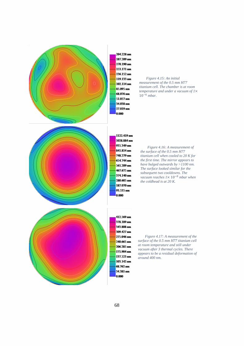
68

Figure 4.15: An initial

measurement of the 0.5 mm H77

titanium cell. The chamber is at room

temperature and under a vacuum of 1×10−6 mbar.

Figure 4.16: A measurement of

the surface of the 0.5 mm H77

titanium cell when cooled to 20 K for

the first time. The mirror appears to

have bulged outwards by >1100 nm.

The surface looked similar for the

subsequent two cooldowns. The

vacuum reaches 1× 10−8 mbar when

the coldhead is at 20 K.

looked similar for the

× 10−8

Figure 4.17: A measurement of the

surface of the 0.5 mm H77 titanium cell

at room temperature and still under

vacuum after 3 thermal cycles. There

appears to be a residual deformation of

around 400 nm.

69

Figure 4.18: An initial measurement of

the 0.5 mm T7109 titanium cell. The

chamber is at room temperature and under

a vacuum of 1× 10−6 mbar.

Figure 4.19: A measurement of the

surface of the 0.5 mm T7109 titanium cell

when cooled to 20 K. There is no obvious

deformation within the precision of the

interferometer.

Figure 4.20: A measurement of the

surface of the 0.5 mm T7109 titanium cell

at room temperature and still under

vacuum after thermally cycling. There is

no obvious change from the initial

surface.

70

4.2.4 Improved interferometry

After the initial success of the athermal mirror cell tests at Swansea University, and

with no damage observed after multiple cooldowns of the 2014 internal cavity mirrors

within the ALPHA apparatus, the test cryostat was shipped to CERN and an improved

interferometer was developed. To remove the fluctuations between the laser table and

the cryostat, a small optics bench was mounted directly to the cryostat. The 767 nm

laser was replaced with a shorter wavelength 633 nm HeNe laser, and later a 532 nm

laser (THORLABS CPS532-C2). To achieve single mode operation of the 532 nm

laser, a simple temperature control circuit was implemented consisting of

thermocouple and heater coil attached to the laser, and a NI USB-6001 module running

a PID controller. The imaging was improved by replacing the screen and instead

directly imaging on a CMOS camera chip. A 640x480 pixel webcam chip was initially

used, but was later replaced by a 1280x1024 pixel (THORLABS DCC1545M) camera.

An apodising filter (THORLABS NDY10B) was placed in front of the camera to

convert the Gaussian wavefront into a square wavefront to increase the gain at the edge

of the image whilst avoiding saturation in the middle. The reference mirror is mounted

on a piezo to scan the length of the reference arm. The optics setup is shown in Figure

4.21.

In addition to controlling the laser, the NI USB-6001 module is used to control the

piezo. After aligning the interference pattern with no tilt on to the camera, the piezo is

scanned over several wavelengths and a video is acquired. As each pixel of the camera

will record a sine wave, a fit can be used to extract the phase at the pixel. By plotting

the phase differences between pixels, a 2D phase map of the wavefront and thus the

mirror surface can be generated without relying on fringe tracing. A LabVIEW

implementation of the Goldstein algorithm [74] is used to unwrap the phase (remove

the discontinuities between 359° and 0°) and reconstruct the mirror surface. In this

form, it is easy to remove tilt from the image and surface maps can be accurately

71

averaged or subtracted to compare the initial and final surface shape without being

limited by the quality of the reference mirror surface. Figure 4.22 and Figure 4.23 show

the deformation of a mirror cell measured using this technique at 20 K and the residual

deformation once the cell has returned to room temperature. The ring-like features in

Figure 4.23 are due to diffraction in the test arm from the coldhead radiation shield

aperture, and the striped feature is an unwanted interference pattern from other optics

in the path. These effects currently limit the interferometer resolution to around 25 nm.

Figure 4.21: In this improved interferometer setup, a stabilised 532 nm laser is coupled into a single mode

fibre and output onto an optical bench which is directly mounted to the cryostat. Not shown are a 400 V piezo

driver and a laptop equipped with a NI-DAQ module for controlling the piezo and acquiring images from the

camera. The optics are coated for visible light and the vacuum window is wedged to prevent interference patterns

from the window surfaces being imaged. The setup is designed to be as compact and lightweight as possible to

avoid coupling vibrations into the cryostat.

72

Figure 4.22: The deformation of a mirror blank in a 0.5 mm athermal cell cooled to 20 K.

Figure 4.23: The residual deformation of a mirror blank after being thermally cycled between room

temperature and 20 K.

73

A new batch of epoxy was ordered for manufacturing the athermal mirror cells of

the 2015 cavity, which would replace the input mirrors from 2014. However, tests

revealed that the 0.5 mm gap size that performed well in 2014 caused the mirrors to

fracture in every case. An additional batch of epoxy was ordered and for the same gap

size of 0.5 mm mirror cell design, the optic deformed by 100 nm inwards. There is a

clear difference between otherwise identical cells made using different batches of

epoxy, as summarised in Table 4.3.

EPOTEK T7109 batch Optic deformation in 0.5 mm cell (nm)

2014 0 ± 100

2015 batch 1 Mirror fractures

2015 batch 2 50 ± 25

2016 -100 ± 25

2017 -130 ± 25

Table 4.3: A summary of the deformation of a 0.5 mm T7109 titanium athermal mirror cell when cooled from room

temperature to 20 K, for different batches of the same epoxy.

A measurement campaign starting in 2015 and continuing in 2016 was undertaken

to measure the deformation of cells with a range of radial gaps from 0.1 mm to 0.9

mm. The expiration date of the epoxy (1 year from manufacture) meant that the < 0.5

mm cells were made with the second 2015 epoxy batch, whereas the > 0.5 mm cells

were made using the 2016 batch of epoxy. The results are shown in Figure 4.24.

It is thought that the mirror surface bulges due to the stress applied when the radial

gap is too small, and dips due to the tension applied when the radial gap is too big. No

mirrors were observed to break during this measurement run so the cause of failure is

still uncertain. However, the original measurements in Swansea where the 0.5 mm cell

survived but the 1.0 mm cell broke imply that the fused silica substrate fails when

placed under sufficient tension.

74

4.3 Internal cavity mechanical design

The internal cavity mirrors are situated symmetrically around the magnetic

minimum trap and are separated by 90 cm. At the ends of the magnet form (shown in

Figure 2.8) are a pair of structures with three precision mounted ball bearings.

Triangular mirror mounts are located against the ball bearings to ensure precise and

reproducible alignment (see Figure 4.25). The top leg of each triangle has a spherical

surface, the left leg has a slotted surface, and the right leg has a flat surface. The

upstream (with respect to the antiproton beam) triangle is held in place using a set of

three bolts which contact the back of each leg. By tightening them down in the

sequence top, left, right, the triangle can be reproducibly located. The bolts are made

Figure 4.24: A plot of the radial gap size of an athermal cell vs the cooldown deformation of the central Ø 12

mm of the optic. A positive deformation indicates a bulging of the mirror surface. In each case, the deformation

was almost purely a defocussing of the mirror. For small deformations the error is approximately the resolution

of the interferometer, whereas for larger deformations, the error is dominated by knowledge of the beam size and

image edge. Inset is the result of the DeLuzio stress calculation based on equation 4.30, which is in rough

agreement with the trend and the zero-crossing point.

75

from titanium, and the magnet form and triangle are made from steel, meaning the

triangle will always be held tightly in place during thermal contraction due to the

smaller coefficient of thermal expansion of titanium. The downstream triangle is

threaded onto a set of guide rods (visible in Figure 4.30), and beryllium-copper springs

located behind the triangle apply force to keep the legs in contact with the ball

bearings. The triangles contain angled slots for mounting the cavity mirrors at a 2.3°

angle with respect to the trap axis. They contain two additional paths for laser access,

as well as a central aperture for particles to be loaded into the trap.

Both cavity mirrors are bonded into an athermal mirror cell. The upstream mirror

cell is epoxied directly to a stainless steel adapter piece using a thin bead of epoxy

applied to the edge of the mated surfaces. The downstream mirror is epoxied atop a

piezo, which is then epoxied to a shorter adapter piece. Both epoxy joints are cured

simultaneously. The precise alignment required between the adapter pieces and the

mirrors is achieved by making the bonds within a precision alignment jig as shown in

Figure 4.26. The adapter piece is clamped from the bottom with a stainless steel base

and the mirror is clamped from the top with a thin sheet of Teflon plastic. The bolt

holes on the back of the jig are used to secure a thermocouple needed for monitoring

the temperature of the epoxy during the curing process.

Figure 4.25: From left to right: The upstream triangle, the upstream end of the magnet form, the downstream

end of the magnet form, and the downstream triangle. Both triangles contain two slots for mounting a mirror

assembly, but are shown with only one mirror assembly installed.

76

The adapter pieces (shown in Figure 4.27) have a clear aperture with a diameter Ø = 8

mm, so the mirror assemblies must be aligned with a precision of approximately 4

mrad.

For the 2014 run, a 633 nm cavity for laser-safe diagnostics and a 243 nm cavity

for 1S-2S spectroscopy were installed. Both of the downstream mirrors were well

aligned, but the upstream 243 nm mirror was slightly misaligned. To solve this, the

mirror assembly was rotated until the misalignment direction was parallel to the axis

between the top and left legs of the triangle, and the right (flat) leg was shimmed by

placing several layers of aluminium foil beneath it (at the cost of misaligning the 633

nm cavity). This successfully aligned the 243 nm cavity, but a jig was manufactured

to test the alignment of future cavity pieces before installation, by measuring the

deflection of a laser beam as the mirror assembly was rotated in the jig.

Whilst the adapter pieces shown in Figure 4.27 worked well in 2014, after baking

and cooling the apparatus in 2015, the downstream mirror (which had remained

untouched since the 2014 run) had become misaligned. It was this failure which lead

Figure 4.26: The mirror cell, piezo (yellow with grey electrodes), and downstream adapter piece mounted

within the alignment jig. A similar jig is used to ensure the alignment of the upstream assembly.

Figure 4.27: The upstream and downstream mirror adapter pieces.

77

to the creation of an external cavity, as it was deemed too high risk to remove the

Penning trap to access the mirror at the time. Upon removing the downstream triangle

at the end of the 2015 beam period, both piezos were discovered to have broken away

from their adapter pieces (see Figure 4.28).

Although epoxy had only been applied to the outer diameter of the piezo, there was

material bonded close to the inner diameter. It would appear that epoxy had either

seeped beneath the piezo to form the bond, or the piezo itself had melted during the

curing process. A piezo sandwiched between two metal plates was baked in an oven

mimicking the curing process to test the second hypothesis, but no bond was formed.

The problem was solved by simply removing material from the adapter piece to mimic

the dimensions of the successful cell-piezo joint, as shown in Figure 4.29.

For the 2016 run, the downstream Penning trap insertion structure was redesigned

to make servicing the cavity possible without removing the Penning traps. During the

installation with this new structure, it was realised that 4 rods which ran through the

Figure 4.29: The modified downstream adapter.

Figure 4.28: The downstream adapter pieces still mounted into the triangle (left) and one of the piezo

assemblies (right). The piezos were attached to the adapter pieces by placing beads of epoxy around the outer

diameter, but the piezo also seems to have bonded close to the inner diameter. Piezo material can be seen still

bonded to the adapter pieces.

78

triangle to support the trap were coming into contact with the piezos (see Figure 4.30),

which could also have caused the shearing of the piezos in 2015. The insertion

structure was further modified to remove the rods which were coming into contact with

the piezos.

The experiment was cooled down for the 2016 run with two 243 nm cavities

installed. However, one of these cavities was trialling a new method of shimming the

alignment of the adapter pieces by placing small washers between them and the

triangle bolt holes. This trial cavity failed to maintain its alignment, and the piezo was

found to have again sheared off the adapter piece on the downstream end due to

thermal gradients newly introduced by the shims. The standard cavity maintained its

alignment throughout the beam period.

The piezo used is a cryogenic, UHV compatible version of the PI Ceramic

PAHH+0050 with a height of 13 mm, giving a nominal 10 nm/V travel at room

temperature. The travel was measured at 20 K to be 2.5 nm/V (see Figure 4.31), which

is sufficient to scan the 121.5 nm free spectral range of the cavity, given the voltage

limitation of 140 V set by the internal circuitry. The frequency response of the piezo-

Figure 4.30: As the triangle was inserted, one of the support rods (highlighted) came into contact with the

piezo assembly and sheared it off. A kapton bumper was installed to protect the piezo against knocks during

installation, but this had also been sheared and epoxy had been scraped off the piezo, implying that the damage

was done when holding tension was applied to the back of the triangle.

79

mirror assembly was measured using a network analyser whilst it was at 7 K within

the ALPHA apparatus, and no resonances were observed below 10 kHz (see Figure

4.32).

Figure 4.32: A Bode plot of the piezo electrical response at 7 K. The black curve shows the

magnitude and the blue curve shows the phase of the response relative to the drive signal.

Figure 4.31: A 13 mm PI Ceramic’s PAHH+0050 piezo was cooled down to 20 K on a

coldhead. The travel was measured interferometrically as the piezo warmed up.

80

4.4 External cavity mechanical design

When the internal cavity failed during the 2015 beam period, an external cavity

was quickly designed and constructed. As the cavity would now be much longer, lower

reflectivity mirrors were chosen to compensate for the corresponding decrease of the

linewidth and the additional noise which would be coupled into the cavity - both of

which could make maintaining peak build-up more difficult.

Identical mirror assemblies were installed on both sides of the apparatus. The

cavity mirror is epoxied to a piezo, which itself is epoxied to a small steel adapter

piece. This adapter piece is then attached to the mirror flange, which sits between two

bellows. The front bellows is bolted to the window flange of the apparatus and the rear

bellows is secured to the optical table using a fixed clamp. A modified commercial

mirror mount is attached to an additional flange clamp near the middle of the assembly,

and is used to align the mirror. A copper support rod attached to the mirror flange

guides the cabling from the piezo past the mirror to a feedthrough on another window

port of the apparatus (see Figure 4.33 and Figure 4.34).

Figure 4.33: A photograph of the assembled mirror flange. The flange adapter contains holes to

allow the space in the bellows behind it to be pumped, but it is an acknowledged pumping restriction.

The mirror, piezo, and adapter are bonded using EPOTEK T7109 epoxy.

81

However, there were two major problems with this design: Firstly, the bellows

were much stiffer than anticipated, and the springs in the mirror mount were not strong

enough for it to be able to apply any force on the mirror flange. Secondly, the

vibrations and slow drifts of the optical tables would cause the cavity to become

misaligned after minutes, and be impossible to lock. These problems were solved by

removing the connection to the optical table and instead securing the end bellows to

the beamline as shown in Figure 4.35. M4 threaded rods were used to connect the two

flange clamps, and create a basic but effective alignment mechanism (see Figure 4.36).

Even with the improved mounting structure, locking the cavity was still

challenging. By locking the laser to the cavity, the FWHM of the length fluctuation

was measured to be around 400 nm over 100 s (see Figure 4.37). For comparison, the

length fluctuation of the internal cavity was around 10 nm. By driving one piezo with

a slow but quiet amplifier to correct the large fluctuations, and driving the other piezo

with a carefully filtered fast driver, the cavity was successfully locked with > 90%

efficiency.

Figure 4.34: The mirror is mounted on a piezo between two bellows. The window is clamped in place, allowing

the mirror flange to be titled using a modified commercial mirror mount.

82

Figure 4.35: An Autodesk Inventor rendering (left) and photograph (right) of the structure designed to clamp

the external cavity assembly to the beamline. The vacuum window is not shown.

Figure 4.36: The highlighted nuts on the M4 threaded rods were

loosened or tightened to adjust the alignment of the cavity mirror.

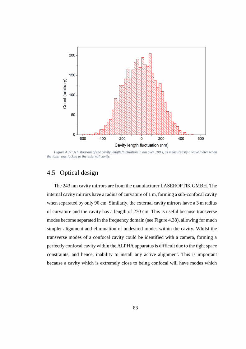
83

4.5 Optical design

The 243 nm cavity mirrors are from the manufacturer LASEROPTIK GMBH. The

internal cavity mirrors have a radius of curvature of 1 m, forming a sub-confocal cavity

when separated by only 90 cm. Similarly, the external cavity mirrors have a 3 m radius

of curvature and the cavity has a length of 270 cm. This is useful because transverse

modes become separated in the frequency domain (see Figure 4.38), allowing for much

simpler alignment and elimination of undesired modes within the cavity. Whilst the

transverse modes of a confocal cavity could be identified with a camera, forming a

perfectly confocal cavity within the ALPHA apparatus is difficult due to the tight space

constraints, and hence, inability to install any active alignment. This is important

because a cavity which is extremely close to being confocal will have modes which

Figure 4.37: A histogram of the cavity length fluctuation in nm over 100 s, as measured by a wave meter when

the laser was locked to the external cavity.

84

are not fully frequency degenerate and interfere with the fundamental mode, reducing

the effectiveness of many locking schemes (e.g. PDH).

In 2014, two identical 0.995 reflectivity mirrors were used to form the internal

cavity, giving a design finesse of 627. However, it was discovered that these mirrors

had a transmission of only 0.00043, and as such, a maximum enhancement factor of

only 17 was predicted. With 50 mW of laser power, even in perfect conditions the

cavity would have been unable to produce more than 850 mW of circulating power.

The input coupler was replaced for the 2015 antiproton beam period, but the failure

of the piezo joint meant that an external cavity was installed and operated instead. This

cavity used two 0.985 reflectivity mirrors with a transmission of ~0.015. Lower

reflectivity mirrors were chosen as it was believed locking the external cavity would

be significantly more difficult due to mechanical noise. These mirrors were predicted

to form a cavity with a finesse of 208 and an enhancement factor of 65, so with 50 mW

of laser power, a maximum circulating power of 3.25 W was attainable. Accounting

for mode matching and lock quality considerations, we aimed for a circulating power

of 2 W.

In 2016, the piezo joint problem was solved, and an internal cavity consisting of

an input coupler with a reflectivity of 0.99 and transmission of 0.0075 and a 2014

output coupler (𝑅 = 0.995) was installed. This cavity was designed to have a finesse

of 417 and an enhancement factor of 132, meaning that with 50 mW of incident laser

Figure 4.38: In a confocal cavity, transverse modes (red) are frequency degenerate as all path lengths are

equal. As the cavity is made longer or shorter, the transverse modes will separate.

85

power, a maximum circulating power of 6.6 W would be achievable (again, with the

aim to run the cavity at 2 W). The design parameters are summarised in Table 4.4.

2014 2015 2016

Configuration Internal External Internal

Length 90 cm 270 cm 90 cm

Mirror reflectivity Input: 0.995

Output: 0.995

Input: 0.985

Output: 0.985

Input: 0.990

Output: 0.995

Mirror transmission Input: 0.00043

Output: 0.00043

Input: 0.015

Output: 0.015

Input: 0.0075

Output: 0.00043

Design Finesse 627 208 417

Enhancement factor 17 65 132

𝑤0 0.196 mm 0.340 mm 0.196 mm

Table 4.4: The enhancement cavity design parameters.

4.6 Performance

2014 marked the first successful cooldown of an internal cavity and injection of

243 nm light into the apparatus. The finesse was measured to be 717 ± 80, and there

was no evidence of mirror degradation throughout the year. An error signal was

produced using the amplitude modulation technique, but the lock quality was very poor

at just 15% of the peak power. The low transmission of the input coupler meant that

less than 3% of the laser power was coupled into the cavity, and the maximum

circulating power was < 0.13 W. 𝑃0 was measured to be 50 mW before the vacuum

window, but the actual power reaching the cavity was likely to be lower than this due

to laser induced damage of the window which was not discovered until 2015.

2015 saw the use of an external cavity with a high level of environmental noise.

Although making a finesse measurement with a cavity fluctuating by several free

spectral ranges was difficult, comparing the cavity linewidth with the sideband spacing

imposed by the electro-optic modulator placed the finesse at 125 ± 15, which was

significantly lower than expected. The laser power reaching the cavity was reduced by

a factor of 2 due to degradation of the vacuum windows, which were not made of a

86

sufficiently good UV grade fused silica. Combined with the reduced finesse, this

ultimately limited the circulating power to 0.45 ± 0.05 W. The average circulating

power as calculated from the transmitted power method (equation 4.26) agrees well

with both the measured finesse and the average circulating intensity as calculated using

the enhancement factor method (equation 4.25), if the reflectivity of both mirrors has

fallen to 0.972.

In 2016 an internal cavity was installed, and the vacuum windows were replaced

with an improved grade of UV fused silica glass. The measured finesse of the cavity

was initially around 400, but degraded to around 200 after the apparatus was baked.

During subsequent bake-outs, the finesse fell further to 110. The finesse was recovered

to 230 by running the cavity in an oxygen rich environment (which we will discuss in

section 4.7), and the laser power was increased to 140 mW by replacing a damaged

frequency doubling stage. However, even with this increased power, only 45 mW was

estimated to reach the enhancement cavity due to additional losses along the beam

path. The average circulating power as calculated using the transmitted power method

can again be made to agree with the measured finesse and the average circulating

power as calculated using the enhancement factor method if the input coupler

reflectivity has fallen to 0.975. Table 4.5 summarises these measurements.

87

2014 2015 2016

Configuration Internal (90 cm) External (270 cm) Internal (90 cm)

Estimated 𝑃0 < 50 mW* 25 ± 5 mW 45 mW

Measured finesse 717 ± 80 125 ± 17 230 ± 20

Measured coupling 0.03 0.65 0.7

Enhancement factor 17 19 33

Lock type AM PDH PDH

Measured 𝑄𝑙𝑜𝑐𝑘 0.15 0.9 0.75

Measured 𝑃𝑡 Not measured 7 ±1 mW 0.45 ± 0.03 mW

Estimated 𝑃𝑎𝑣𝑔 < 0.13 W* 0.45 ± 0.05 W 1.05 ± 0.1 W

Estimated 𝐼0 < 215 W/cm2* 250 ± 25 W/cm2 1740 ± 165 W/cm2

Table 4.5: A summary of the cavity performance. Values marked with (*) were not well characterised as

contributing effects were not discovered until later. The measured coupling is the ratio of injected to reflected light,

and hence is a function of both the impedance mismatch and spatial mode matching.

4.6.1 Loss versus reflectivity

The 2014 mirrors were observed to have a higher than expected loss (compared to

typical visible-light cavity mirrors), which meant that relatively little light could be

coupled into the cavity. To compensate for this in subsequent years, the reflectivity of

the input coupler was lowered and the mirror was annealed by heating it after the

coating process.

Table 4.6 shows the measured reflectivity and transmission of the mirrors received

from LASEROPTIK. Lowering the reflectivity seems to additionally reduce the loss.

Annealing the mirrors is also beneficial. This observation implies that choice of mirror

reflectivity is already reasonably well optimised. The transmission measurements were

made with a 243 nm beam at a 0° angle of incidence by placing a calibrated diode

power meter before and after the mirrors.

88

Batch Specified

reflectivity

Measured

transmission Loss (1-R-T)

2014 non-annealed 0.995 0.00043 0.00457

2015 non-annealed 0.985 0.0135 0.0015

0.99 0.074 0.0026

2015 annealed 0.985 0.015 0

0.99 0.0075 0.0025

2017 annealed

0.985 0.015 0

0.99 0.0077 0.0023

“HR” 0.00033 -

Table 4.6: Measurements of the mirrors delivered to ALPHA. The “HR” mirror was specified for maximum

reflectivity. The measured transmission is an average over several mirrors from each batch in new condition,

including substrate losses. The variance between mirrors is approximately ± 5%.

4.6.2 Laser induced damage

After the 2015 run with the external cavity, a loss of power of 50% in the upstream

window and 20% in the downstream window was discovered. There were likely to be

similar losses in the 2014 upstream window. The source of these losses was UV

induced degradation of the glass. Figure 4.39 shows a large 243 nm beam passing

through the 2015 upstream window. The damaged section is clearly visible, as it

fluoresces less.

89

The UV degradation occurred because the windows were made from a standard

grade of fused silica glass. Several UV-compatible grades of fused silica are available,

of which Corning 7980 KrF has the best transmission at 243 nm, coupled with good

resistance to laser induced damage [75]. Although the 2016 windows were

manufactured from this glass, the transmission had dropped by 30% where the beam

had been passing through when they were measured at the end of the year.

In addition to the damage to the window, a small burnt spot was discovered on the

antireflection coating of the 2016 input coupler (shown in Figure 4.40). Transmission

through this part of the mirror was 30% lower than the transmission through other parts

of the mirror. No damage was observed on the high reflectivity side of the mirror, or

on either side of the output coupler.

Figure 4.39: A photograph of the 2015 upstream window mounted on the bench. A large diameter 243 nm

beam was sent through and the transmission was measured using a CCD camera. The laser induced damage can

already be seen by the dark spot within the blue fluorescence.

90

4.6.3 Spatial mode matching

The spatial mode matching was generally good for both the internal and external

cavities. Figure 4.41 shows the mode structure of the 2016 cavity as the piezo is

scanned to cover a free spectral range, which is typical of all three years. The upper

trace shows the demodulated PDH signal, and the lower trace shows the intensity

transmitted through the cavity. A small number of transverse modes are present, with

a summed intensity of less than 10% the intensity of the fundamental mode. The PDH

signal is skewed slightly due to the presence of a nearby transverse mode.

The transmitted beam is split so that one half is focussed onto a photodiode and the

other half is imaged on a paper screen by a webcam. The webcam is used to aid

alignment and confirm that the cavity is operating at the fundamental mode, although

the image saturates when the cavity is locked. After locking the cavity for more than

10 seconds, higher order transverse modes begin to be excited (as shown in Figure

4.42). This is thought to be due to thermal lensing in the path between the laser lab and

the apparatus, which we will discuss in more detail in chapter 5. The amplitude of

these higher order modes was later measured to be 4% of the fundamental mode using

a non-saturated beam profiler.

Figure 4.40: A small burn spot is present on the AR coating of the upstream mirror.

91

Figure 4.41: The PDH error signal (upper) and the transmitted intensity (lower) as the piezo is

scanned linearly over 50 V to cover a full free spectral range of the cavity.

Figure 4.42: A saturated image of the transmitted beam when the cavity has been locked on resonance

for 1 s (left) and 30 s (right).

92

4.7 Mirror degradation and recovery

Both the external cavity in 2015 and the internal cavity in 2016 suffered from a

reduction in finesse. A study by Gangloff et al. in 2015 [76] found that high finesse

cavities which used oxide based mirror coatings suffered from vacuum degradation,

due to oxygen depletion on the surface. They typically observed finesse losses of

factors of 3 or more, and the loss was not proportional to the light intensity. The loss

rate was significantly higher at elevated temperatures however, which agrees well with

the observation of the finesse falling after baking the ALPHA apparatus, but not during

the experimental runs at 7 K.

A technique for regenerating the mirrors using a pure oxygen environment is also

presented in the paper. The regeneration is supposedly enhanced by higher

temperatures and higher pressures, and greatly accelerated by shining UV light on the

mirrors. In an attempt to regenerate the 2016 cavity mirrors, the apparatus was filled

with synthetic air consisting of 75 mBar of nitrogen and 25 mBar of oxygen. The

temperature was increased to 80°C and the cavity was locked for 2 hours. After

pumping out the gas and cooling down to 7 K, the finesse was measured to have

improved by a factor of 2 from 110 ± 10 to 230 ± 20.

The paper also found that a 1 nm final coating of SiO2 could significantly reduce

the rate of degradation, and a 100 nm layer could prevent it completely. It is important

to note that the 𝑅 = 0.995 mirrors used in the 2014 internal cavity did have a final

SiO2 coating and were not observed to degrade, whereas both mirrors of the 2015

external cavity and the upstream mirror of the 2016 cavity lacked the final SiO2 layer,

and were observed to degrade.

93

5 The 1S-2S Laser System

The antihydrogen 1S-2S laser system is based on the setup used by Hänsch et al.

[49] for hydrogen spectroscopy. At the heart of the setup is a Toptica TA-FHG pro

laser, which can produce up to 200 mW of 243 nm light. The laser is locked to a

reference cavity for stability, and related to atomic time using a GPS-disciplined

frequency comb. The 243 nm beam is delivered along a 7 m actively stabilised path to

the enhancement cavity, which is locked to the laser frequency using the PDH

technique. Figure 5.1 shows a schematic of the setup.

5.1 243 nm light generation

A commercial Toptica TA-FHG pro laser (shown in Figure 5.2) generates high

intensity 243 nm light by twice frequency doubling a tuneable 972 nm DL pro

extended cavity diode laser. The standard DL pro consists of a diode in a Littrow

configuration cavity which boasts a free running linewidth of 100 kHz [61]. The laser

frequency can be tuned by changing the temperature of the diode (coarse), changing

the angle of the extended cavity diffraction grating (coarse), or changing the diode

current (fine). The DL pro has a mode hop free tuning range of >20 GHz [61], meaning

the frequency can be tuned without suddenly jumping a free spectral range to a

different cavity mode with higher gain. Our custom DL pro has a longer cavity to

reduce the free running linewidth and reach sub-Hz performance when locked to an

ultra-stable reference [77], but the mode hop free tuning range is reduced to around

1.5 GHz. This is still sufficiently large that the laser can be ramped between the c-c

and d-d transition frequencies without mode hopping.

A tapered amplifier (TA) driven at 4 A boosts the 972 nm intensity from 50 mW

to 2.5 W. Optical isolators are placed after the DL pro and TA to prevent feedback. A

single EOM placed after the TA adds 5 MHz sidebands to the light, which are used to

actively stabilise the length of two frequency doubling cavities via the PDH locking

94

Fig

ure 5

.1: A

schem

atic o

f the o

ptica

l elemen

ts in th

e 1S

-2S sp

ectrosco

py setu

p. T

he red

, cyan

, and

na

vy blu

e lines sh

ow

the

pro

pa

ga

tion

of th

e 97

2, 4

86, a

nd 2

43 n

m lig

ht resp

ectively. So

me steerin

g m

irrors h

ave b

een rem

oved

for sim

plicity.

95

technique [65]. The second harmonic generation (SHG) cavity produces 1.2 W of 486

nm light and the fourth harmonic generation (FHG) cavity can produce as much as 200

mW of 243 nm light (when new). In practice, the FHG cavity output is reduced to 140

mW or lower to obtain a high quality beam and reduce damage to the crystal and output

optics. To minimise the impact of damage to the FHG optics, the beam is periodically

walked within the cavity to an undamaged spot. The entire FHG cavity was replaced

in 2016 once it was no longer possible to tune the output power to above 100 mW.

Meanwhile, the SHG cavity output power has dropped by less than 10% in 3 years of

operation. The sidebands from the internal EOM are not present at any detectable level

in the 243 nm beam. Using a THORLABS BC106N-UV beam profiler, the 243 nm

Figure 5.2: The internal layout of the Toptica TA-FHG pro laser, which generates the high power 243 nm

light for antihydrogen spectroscopy. Image modified from [61].

96

beam was measured to have a beam waist (1/e2 radius) of 228 µm at a distance of 1.28

m from the laser face, and an M2 value close to 1.

5.2 Frequency control and metrology

The 972 nm laser light is shifted to the reference cavity frequency using an acousto-

optic modulator (AOM) in double-pass configuration. The frequency of the reference

cavity is continuously monitored by a frequency comb and fed into a frequency

controller. This is a LabVIEW program which calculates the 1S-2S transition

frequencies (equations 3.13 and 3.14) using the latest measurement of the magnetic

field within the apparatus, subtracts the reference cavity frequency, and corrects the

AOM frequency accordingly at a rate of 1 Hz. Two state selection bits allow triggering

of the frequency controller to ramp the AOM between the c-c and d-d transitions, and

select if the laser frequency is exactly set to the calculated resonance, or offset by a

pre-programmed value.

5.2.1 Reference cavity

The laser is locked to a high finesse reference cavity made with an ultra-low

coefficient of thermal expansion (ULE) glass. The cavity was manufactured by Menlo

Systems and is based on the ORS 1500. The cavity is suspended within a temperature

controlled vacuum chamber, which itself is located within an acoustically dampened

enclosure, and sits upon an active vibration control module (Accurion Vario series).

Figure 5.3: A flow chart of the frequency control setup.

97

The 972 nm light is brought by fibre onto a bench mounted to the vacuum chamber,

which holds an EOM and mode matching optics, as well as polarisation optics and a

detector for generating the PDH error signal. The cavity has a linear drift (due to length

contraction) of 53 mHz/s, which is typical for ULE glass as it shrinks due to a

recrystallization process [78]. To lock the laser to the reference cavity, a Toptica

Digilock 110 module is used to servo the high frequency noise by acting on the diode

current, and the larger amplitude, low frequency shifts (e.g. when the AOM is being

ramped) by acting on the internal grating of the DL pro.

The short term linewidth of the laser can be estimated by making the assumption

that the frequency fluctuations of the locked laser are the dominant source of the

linewidth broadening and not the frequency fluctuations of the cavity. By shifting the

set point of the lock by ± 1 FWHM of the measured noise of the PDH error signal (DC-

40 MHz sensitivity), a frequency difference of 1.0 kHz was measured by the frequency

comb, giving the laser a FWHM linewidth of 500 Hz at 972 nm and, in a worst-case

extrapolation through the frequency doubling cavities, 2.0 kHz at 243 nm. The

measurement data is shown in Figure 5.4.

Figure 5.4: The set point of the PDH lock to the reference cavity was adjusted at 100 s intervals

to ± 1 FWHM of the measured noise of the locked cavity, the frequency of the laser is measured using

the frequency comb. The difference between the blue and red points gives 2 x the FWHM of the laser

linewidth, assuming the dominant source of broadening of the linewidth is the quality of the lock.

98

(5.1)

(5.2)

5.2.2 Frequency comb

A frequency comb (Menlo Systems FC1500-250-WG) is used to monitor the

frequency of the reference cavity and relate it to the SI second. The comb is generated

by a femtosecond laser, which is mode-locked using the Kerr-lensing effect. The laser

has a repetition rate of 250 MHz, and inherits the stability of a GPS-disciplined oven

controlled quartz oscillator (OCXO) (K+K Messtechnik GPS6) via a phase-locked

loop. As the comb spectrum spans a complete octave, the comb can be characterised

completely. Figure 5.5 shows how the nth line of the comb is frequency doubled and

beat against the 2nth line to determine the offset frequency of the zeroth line 𝑣0, i.e.

𝑣0 = 2𝑣𝑛 − 𝑣2𝑛 .

The frequency of a CW laser 𝑣𝑐𝑤 beat against the nth comb line is therefore given

by:

𝑣𝑐𝑤 = 𝑛. 𝑣𝑟𝑒𝑝 ± 𝑣0 ± 𝑣𝑏𝑒𝑎𝑡 ,

where 𝑣𝑏𝑒𝑎𝑡 is the beat frequency between the CW laser and the nearest comb line.

The sign of 𝑣𝑏𝑒𝑎𝑡 and 𝑣0 can be determined by varying 𝑣𝑟𝑒𝑝 and 𝑣0 respectively and

observing whether 𝑣𝑏𝑒𝑎𝑡 increases or decreases. For example, if increasing 𝑣𝑟𝑒𝑝 causes

𝑣𝑏𝑒𝑎𝑡 to decrease, then we know that the laser 𝑣𝑐𝑤 is above the nearest comb line (as

shown in Figure 5.5) and 𝑣𝑏𝑒𝑎𝑡 is positive. Next, if we increase 𝑣0 and see 𝑣𝑏𝑒𝑎𝑡

Figure 5.5: A schematic diagram of a v-2v frequency comb. The repetition rate (vrep) is referenced to a

microwave clock, and the offset of the zeroth line (v0) can be determined by measuring the beat note between the

frequency-doubled red end of the comb and the blue end.

99

(5.3)

(5.4)

decrease again we know that 𝑣0 must also be positive (as shown in Figure 5.5), as it

shifts the comb to higher frequencies.

The comb line n, can then be determined trivially if it is possible to measure 𝑣𝑐𝑤

to a precision of 𝑣𝑟𝑒𝑝

2 or better using a wavemeter, by choosing the closest integer value

which satisfies equation 5.2. If a wavemeter is not available, then the measurement can

be repeated for a significantly different 𝑣𝑟𝑒𝑝, and a search can be made for a pair of

integer numbers which satisfy equation 5.2 for both values of 𝑣𝑟𝑒𝑝. Because 𝑣𝑐𝑤 is

constant,

𝑛1. 𝑣𝑟𝑒𝑝1 + 𝑣01 + 𝑣𝑏𝑒𝑎𝑡1 + ∆𝑣𝑐𝑤1 = 𝑛2. 𝑣𝑟𝑒𝑝2 + 𝑣02 + 𝑣𝑏𝑒𝑎𝑡2 + ∆𝑣𝑐𝑤2 ,

where ∆𝑣𝑐𝑤 is the measurement uncertainty of 𝑣𝑐𝑤. Letting 𝑚 = 𝑛2 − 𝑛1 and solving

for 𝑛1,

𝑛1 =𝑚. 𝑣𝑟𝑒𝑝2 + 𝑣02 + 𝑣𝑏𝑒𝑎𝑡2 − 𝑣𝑟𝑒𝑝2 + 𝑣02 + 𝑣𝑏𝑒𝑎𝑡2

𝑣𝑟𝑒𝑝1 − 𝑣𝑟𝑒𝑝2±

√∆𝑣𝑐𝑤12 + ∆𝑣𝑐𝑤2

2

𝑣𝑟𝑒𝑝1 − 𝑣𝑟𝑒𝑝2 .

The change in 𝑣𝑟𝑒𝑝 must be large enough that the last term (the measurement

uncertainty) does not contribute much. With the further condition that 𝑛1 and 𝑛2 are

both integers, 𝑛1 and 𝑣𝑐𝑤 can be determined by searching for two frequency solutions

which correspond to integer values of 𝑛1 and 𝑛2 within the estimated uncertainty.

The frequency comb is equipped with 20 MHz pi-type counters for accurately

measuring 𝑣0 and 𝑣𝑏𝑒𝑎𝑡, which are read out every second. However, as the 972 nm

laser is beat against the frequency doubled component of a comb centred at 1550 nm,

𝑣0 effectively doubles to 40 MHz and a HighFinesse WS-U wavemeter with 2 MHz

precision [79] can be used to identify not only n, but the sign of 𝑣0 and 𝑣𝑏𝑒𝑎𝑡 uniquely.

The technique using two significantly different repetition rates is reserved to

periodically confirm the correct operation of the wavemeter.

5.2.3 Frequency shifter

An AOM with a centre frequency of 250 MHz placed between the laser and the

reference cavity (shown in Figure 5.1) shifts the 972 nm light from the 1S-2S transition

100

to the closest resonance of the reference cavity. As we wish to probe both the c-c and

d-d transitions in a single trapping sequence, the AOM is configured to be able to ramp

the 76 MHz spacing without unlocking the laser. Figure 5.6 shows the frequency

offsets, along with the gain profile of the AOM. In the double-pass configuration, the

AOM has a bandwidth (FWHM) of 100 MHz. The gain profile is programmed into the

frequency controller to make the frequency shift invisible to the reference cavity,

although the absolute power delivered to the reference cavity is not yet actively

controlled. A Keysight 81160A synthesiser [80] was selected to drive the AOM as it

boasts glitch free and drop-out free operation when shifting frequencies, and has µHz

precision when referenced to the OCXO.

The frequency control program communicates with the experimental sequencer via

2 input bits and 1 output bit. The first input bit sets the frequency to that of the c-c or

d-d transition, and the second input bit chooses if the frequency is on resonance or off

resonance by a pre-programmed amount. The output bit functions as a ‘laser ready’

signal, to inform the opening and closing of the shutter.

Figure 5.6: An AOM in double-pass configuration is used to shift the 972 nm light to the reference

cavity frequency (not to scale). The black curve illustrates the gain profile of the AOM, which must be

accounted for when normalising the output power.

101

When the AOM is not ramping between different transitions, the control program

updates the AOM frequency to compensate for fluctuations of the reference cavity

with respect to the comb. The fluctuations are averaged over 20 seconds, which is the

turning point of the Allan deviation as shown in Figure 5.7. At this timescale, the 53

mHz/s drift of the cavity is negligible. The Allan deviation (which is the square root

of the Allan variance) is a standard measure of frequency stability over time [81]. For

example, the Allan deviation of 2.45 × 10−13 at a gate time of 20 s (as in Figure 5.7)

corresponds to a frequency instability between any two sets of 20 s measurements with

a root-mean-square (RMS) fractional uncertainty of 2.45 × 10−13, or 75 Hz at the 972

nm laser frequency.

5.3 Beam transport

The 243 nm light must propagate along a 7 m path from the controlled atmosphere

of the laser lab through an enclosed periscope onto the laser table attached to the nose

of the ALPHA cryostat, before being coupled into the enhancement cavity. Power is

lost along the path due to absorption within the optical elements and the air itself.

Figure 5.7: A non-overlapping Allen deviation measurement of the fractional uncertainty of the

comb locked to the OCXO (black dots) and the light sent to the reference cavity (red dots). The turning

point at 20 s corresponds to a fractional uncertainty of 2.45 × 10−13, or equivalently, 75 Hz at 972

nm.

102

5.3.1 Optical components

The transport mirrors are from manufacturer LASEROPTIK and have a reflectivity

of 99% for both s and p polarisations at angles of 45° or less. The telescope lenses are

from the same manufacturer, but during 2016 were upgraded to Corning 7980 KrF

glass after we observed that standard UV-grade fused silica would start fluorescing

bright red (see Figure 5.8) after several hours of exposure to a 𝐼0 = 130 W/cm2 beam,

and the transmission would drop. The cavity mode matching is done inside the laser

lab using a Galilean telescope, before the beam is sent to the apparatus. As the laser

lab is kept at a higher pressure than the experimental zone in which the apparatus sits

to discourage dust from entering, a window is required between the two ends of the

periscope to prevent loss of pressure. The window is 2” in diameter, 10 mm thick, and

is also made from Corning 7980 KrF glass.

A QUBIG EOM placed close to the laser adds 6.25 MHz sidebands to the beam for

use in a PDH locking scheme. A λ/2 plate before the EOM rotates the polarisation to

match the axis of the birefringent crystal, and the EOM sits on a 6-axis alignment

mount to correct misalignments and minimise the parasitic amplitude modulation.

Typically, a polarising beam splitter and λ/4 wave plate are used to extract the reflected

Figure 5.8: The fluorescence observed from a 243 nm beam passing through a standard UV grade fused silica

substrate changes from pale blue to bright red after several hours of exposure, and the transmission through the

substrate falls.

103

beam from an enhancement cavity, but due to the high losses in beam splitters

available at 243 nm and the high beam power available, a simpler approach was

adopted. The reflected beam is picked off through the back of one of the steering

mirrors and focussed onto a THORLABS APD120A2 avalanche photodetector. The

50 – 100 µW transmitted beam is still intense enough to saturate the detector, so an

additional filter must be used. The reflected signal is demodulated to produce the PDH

error signal with a signal to noise ratio of about 100 (see Figure 4.41), which is sent to

a Toptica Digilock 110 PID controller to lock the cavity. A THORLABS PDA10A

detector looks at the beam transmitted through the cavity, but this must also be

attenuated as the detector quickly degrades when more than 100 µW is incident. This

is done by placing a 243 nm transport mirror in the beam path at an angle greater than

45°, and tuning the angle until it acts as a 90-10 beam splitter. The higher intensity

reflected beam is directed at a screen and imaged by a camera to monitor the transverse

mode structure of the output beam.

5.3.2 Losses

In addition to the losses within the optical elements, the beam intensity also suffers

in air. In a still air environment such as the 5m long transport tubing between the laser

lab and the experimental zone, losses as high as 50% can accumulate over minutes.

There are several hypotheses about the cause of this, including ozone creation (which

strongly absorbs at 243 nm) and dust/moisture becoming trapped in the beam. A study

was made using an enhancement cavity on the optical bench to investigate the effects

of stirring the air.

An enhancement cavity was set up on an optical table using the same mirrors as

the internal cavity (𝑅1 = 0.99, 𝑅2 = 0.995), separated by 90 cm. The cavity was

excited with 50 mW of 243 nm light and a piezo mounted behind the output coupler

was used to scan the length of the cavity over several FSR. A THORLABS PDA10A

detector placed behind the cavity was used to measure the intensity of the light

transmitted through the output coupler. It was observed that when the cavity length is

expanding (i.e. when a negative voltage gradient is applied to the piezo), the

104

transmission peaks are higher and have a flat period where the circulating power is

held constant (see the red trace in Figure 5.9). This suggests that there is some thermal

process which maintains the optical path length of the cavity for a given threshold

intensity of 243 nm light. Placing an 85 cm long, 2 cm diameter tube between the two

cavity mirrors prevents the air being stirred by the air conditioning and causes the

transmitted light intensity to drop by approximately a factor of 2, in addition to

lowering the threshold for the thermal effect (see the blue trace in Figure 5.9).

Upon discovering this effect, the transport tubing was modified so that nitrogen

gas could be flowed through it and into the zone laser box to stir the air. This improved

the power transmitted through the periscope from 65 mW to 90 mW. Of the 140 mW

output from the laser in 2016, losses in the EOM and mode matching lenses meant that

only 110 mW reached the periscope. It is likely that another 10 mW can be gained by

implementing a similar system for stirring the air in the shorter transport tubing on the

laser lab side. Thermal lensing is observed in the beam path, as evidenced by the time

Figure 5.9: The black trace at the top of the graph shows the control voltage applied to a piezo used

to scan the length of the cavity over a full spectral range. The blue trace shows the temporal mode

structure of a cavity which is enclosed by a tube and the red trace shows the mode structure of a cavity

which is stirred by the laboratory air conditioning.

105

dependent mode structure of the enhancement cavity (shown earlier in Figure 4.42).

Table 5.1 summarises the losses as measured at the end of the 2016 run.

Component Loss (%) at end of 2016 run

Transport mirrors (x13) ~1% each

EOM 15%

Convex lens 5%

Concave lens 3%

Laser lab periscope ~10%

Laser lab window ~0%

Apparatus periscope 40% without N2 stirring

~10 % with N2 stirring

Apparatus window 30%

Cavity input mirror 30%

Table 5.1: Power losses at 243 nm as measured at the end of the 2016 run. The components are listed in the

order they are seen by the beam, with the exception of the transport mirrors which are interspersed among the

other components.

5.3.3 Alignment

The 243 nm path is first pre-aligned using a class-II green laser pointer

(THORLABS CPS532-C2), which is coupled in through a dichroic mirror just before

the periscope. The common path mirrors have a secondary 532 nm coating with a

reflectivity of about 80%. The primary aim of this guide laser was to have a safe way

to align the 243 nm beam into the experimental zone, but it became a useful tool for

diagnosing and aligning the enhancement cavity. Each surface of the enhancement

cavity mirrors reflects ~5% of the 532 nm light, and the reflections are uniquely

identifiable. By co-aligning the 532 nm beam with the reflections from the curved

surfaces of the two cavity mirrors, the 243 nm beam can be injected very close to the

cavity axis for trivial alignment. Additionally, by co-aligning the reflections of the

curved and flat surface of each mirror and comparing them to the cavity axis, the

misalignment of each mirror can be determined and the cavity axis can be completely

characterised with respect to the mirrors.

106

5.3.4 Active beam stabilisation

Without active stabilisation, the passive beam pointing stability contributes a 50%

reduction to the average power coupled into the cavity, and frequent realignment is

needed. Two position sensitive detectors (ON-TRAK Photonics 2L20SP) are

positioned on the optical table attached to the nose of the cryostat, and paired with

piezo actuated mirrors (one on the same table and one in the laser lab) to lock the

position and angle of the beam and correct any pointing errors. The detectors view the

50 – 100 µW pick-off through the back of the high-reflectivity transport mirrors, which

is sufficient for identifying the position of the beam. A homemade FPGA based PID

controller locks the beam with an accuracy of 20 mV, which corresponds to 20 µm on

each detector. With the lock engaged, there is no visible noise contribution to the cavity

due to beam pointing, and minor adjustments to the alignment are only required every

few hours. In addition, the control system allows the user to align the beam remotely

when access to the zone is not possible.

107

6 Experimental results

In 2014, a first attempt at observing the 1S-2S transition in antihydrogen was

conducted with a newly arrived 243 nm laser and the first iteration of a cryogenic

enhancement cavity. The reference cavity and frequency comb had not yet arrived, so

the laser frequency control was limited by the 2 MHz precision of the wavemeter,

which measures the SHG 486 nm light (recall from chapter 3 the linewidth of the

transition is expected to be approximately 60 kHz at 243 nm). The frequency comb

and ultra-stable reference cavity arrived in 2015, and the next two years were dedicated

to making a serious measurement of the 1S-2S transition. Whilst in 2015 the cavity

intensity was insufficient to detect the transition, the 1.05 W of circulating power and

greatly improved trapping rate in 2016 made for a viable experiment.

6.1 Experimental protocol

6.1.1 2014

In 2014, the experiment searched for a reduction in the apparent trapping rate when

the laser was tuned to the d-d transition (“on resonance”), compared to when it was

detuned by 50 MHz (at 243 nm) below the transition (“off resonance”). On and off

resonance runs were interspersed, and apart from the laser frequency, were otherwise

identical. The magnetic trap was flattened by bucking (running current in reverse)

mirror coils B-D to increase the length of the minimum field region. The experimental

protocol was as follows:

1) Antihydrogen is formed using the autoresonance technique, and a 1 s wait

ensures that any trapped atoms have sufficient time to decay to the ground

state.

2) A shutter between the laser lab and the apparatus opens, to allow the 243

nm light to enter the apparatus.

3) The enhancement cavity is locked for 300 s.

108

4) The shutter is closed, and electric fields are pulsed to remove any charged

particles (particularly antiprotons) from the trap.

5) The trap is shut down by triggering the quench response for the

superconducting magnets, and the silicon detector counts the number of

annihilation events.

6.1.2 2015

As the circulating power within the external cavity in 2015 was estimated to be

below the threshold where a difference in the trapping rate would be discernible, the

experiment was reconfigured to try to detect laser ionised antihydrogen atoms with a

very low background. Instead of using the full magnetic trap, a shorter trap was formed

using only mirror coils A-D. Mirror E was bucked to cancel out the field of the external

1 T solenoid and create a zero-field region within the detector. A weak potential well

was formed in the mixing trap with the aim to capture the antiproton from the ionised

atom. The gradient of the electrostatic potential was limited to prevent mixing of the

2S and 2P states. As the lifetime of single antiprotons in a long well is thought to be

short, the well was dumped towards the zero field region every second. The silicon

detector then counted the annihilations localised to beneath mirror coil E within a 9

ms window either side of the dump. Instead of quenching the magnets, the trap was

shut down by ramping down the magnets over a period of 1.5 s. This induces much

lower currents in the Penning trap electrodes when compared with quenching the

magnets, resulting in less heating and therefore a higher overall duty cycle of the

experiment, as well as allaying fears that quenching the magnets could cause electrical

shorts between the electrodes.

As in 2014, on and off resonance runs were interspersed, but the off resonance shift

was reduced to 200 kHz (at 243 nm) below the transitions and both the c-c and d-d

transitions were targeted. Towards the end of the season, a ‘no laser’ run was added to

investigate the effect of the laser on the trapping rate. For example; the laser light could

cause additional outgassing from the cryogenic surfaces and reduce the antihydrogen

lifetime. This run had identical timing to the on and off resonance runs, but the laser

109

shutter never opened. To maximise data taking in the on and off resonance runs, the

no laser runs were not run as frequently as their laser counterparts. The experimental

protocol was as follows:

1) Antihydrogen is formed using the autoresonance technique, and a 1 s wait

ensures that any trapped atoms have sufficient time to decay to the ground

state.

2) Electric fields are pulsed to remove any charged particles from the trap,

before a weak electrostatic well is formed to trap any laser ionised

antihydrogen atoms (antiprotons).

3) With the laser tuned to the d-d transition, the shutter between the laser lab

and the apparatus is opened.

4) The cavity is locked for 250 s, and the contents of the electrostatic well are

dumped towards the zero field region every second.

5) The shutter closes, and the laser frequency is ramped to the c-c transition

in 10 s. The shutter reopens once the correct frequency is reached and the

laser is stable.

6) The cavity is locked for an additional 250 s, and the contents of the

electrostatic well continue to be dumped towards the field free region every

second.

7) The shutter closes, and electric fields are pulsed to remove any remaining

charged particles from the trap.

8) The magnets are ramped down over 1.5 s, and the silicon detector counts

the number of annihilation events.

6.1.3 2016

In 2016, a greatly improved trapping rate and a higher circulating power within the

enhancement cavity made for a much more feasible experiment. The trap magnets

were run in the same flattened field configuration as in 2014, but the trap was shut

down using the 1.5 s ramp down technique used in 2015. On resonance, off resonance

(-200 kHz at 243 nm), and no laser runs were strictly interspersed to reduce the

110

sensitivity of the experiment to trapping rate fluctuations, with the repeating sequence:

on resonance, off resonance, no laser, off resonance, on resonance, no laser. Whilst the

main aim of the experiment was to identify a difference between the apparent trapping

rate of on vs off resonance runs, a shallow electrostatic well was formed in the Penning

trap to try to collect any ionised antihydrogen atoms (antiprotons). At the end of each

300 s laser exposure period, the contents of the trap were ejected towards the MCP to

image any trapped antiprotons, although it was considered unlikely that the antiprotons

would remain trapped within the long well. The experimental protocol was as follows:

1) Antihydrogen is formed in two successive mixing cycles using the slow

merge technique, and a 1 s wait ensures that any trapped atoms have

sufficient time to decay to the ground state.

2) Electric fields are pulsed to remove any charged particles from the trap,

before a weak electrostatic well is formed to contain any laser ionised

antihydrogen atoms (antiprotons).

3) With the laser tuned to the d-d transition, the shutter between the laser lab

and the apparatus is opened.

4) The cavity is locked for 300 s.

5) The shutter closes, and the laser frequency is ramped to the c-c transition

in 10 s. Whilst the shutter is closed, the contents of the electrostatic well

are ejected towards the MCP. The shutter reopens once the correct

frequency is reached and the laser is stable.

6) The cavity is locked for an additional 300 s

7) The shutter closes, and the contents of the electrostatic well are again

ejected towards the MCP.

8) The magnets are ramped down over 1.5 s, and the silicon detector counts

the number of annihilation events.

Table 6.1 gives a summary of the experimental protocol employed across the three

years.

111

2014 2015 2016

Laser exposure 300 s (d-d only) 2 x 250 s 2 x 300 s

Detection window 30 ms 1.5 s 1.5 s

Mixing technique Autoresonance Autoresonance Slow merge

Antihydrogen stacks 1 1 2

Table 6.1: A summary of the experimental protocol employed in 2014, 2015 and 2016.

6.2 Results and analysis

6.2.1 2014

Due to the low circulating power within the enhancement cavity, and the lack of

precise frequency metrology in 2014, only a single shift worth of trapped atoms were

dedicated to 1S-2S transition measurements. As expected from simulations, there was

no significant difference detected between the on and off resonance trapping rates.

Type Trials Detected events Rate

On resonance 5 6 1.2 ± 0.73

Off resonance 4 6 1.5 ± 0.96

Table 6.2: The annihilation events detected during the shutdown of the neutral trap. The magnet system is

intentionally quenched to de-energise the neutral trap in <30 ms, so there is no significant detector background.

The error of the rate is from the 𝑁 counting statistics alone.

6.2.2 2015

With around 0.45 W of circulating power within the external cavity of 2015,

simulation predicted that there would be no discernible difference between the on and

off resonance trials in the disappearance data. Whilst this is apparent in the data shown

in Table 6.3, what is surprising is that the no laser runs actually have a significantly

lower rate than the off resonance runs. This is due to the fact that the no laser runs

were introduced late into the experiment and were not able to accurately capture the

trapping rate. The higher number of on resonance trials compared to off resonance

trials is an artefact of the way the shifts were run; each 8 hour beam period allowed for

112

approximately 8 pairs of on and off resonance runs, but always started with an on

resonance run – an additional bias which needed to be addressed in 2016.

Table 6.3: The annihilation events detected during the 1.5 s ramp down of the neutral trap magnets. The error

of the rate is the standard deviation about the mean of the number of detected events.

Annihilation events were searched for within the zero-field region and within 9 ms

either side of the dumps but none were found, suggesting that this appearance mode

detection technique may not work. The search was widened to include the entire trap,

but the results were still consistent with background.

6.2.3 2016

In 2016, it was quickly discovered that exciting the cavity with 243 nm light

reduces the antihydrogen production and trapping rates over time. This is most evident

in the mixing triggers (a number which is proportional to the number of antihydrogen

atoms produced) as shown in Figure 6.1, which plots the cumulative laser exposure

against the mixing triggers for two trapping series with different laser powers. The

effect is also visible in Figure 6.2, which plots the number of detected annihilation

events against the trial number for the published trapping data. From this plot it is

already clear that there is a significant difference between the on and off resonance

runs, whilst the good agreement between the off resonance and no laser runs suggest

that the laser does not adversely influence the antihydrogen lifetime. The full set of

data is shown in Table 6.4. No evidence of antiproton annihilations was seen on the

MCP images of the dumps at the end of each 300 s hold.

Type Trials Detected

events

Expected

background

Rate

On resonance 42 27 3 0.64 ± 0.12

Off resonance 39 24 2.8 0.62 ± 0.13

No laser 12 4 0.9 0.33 ± 0.17

113

Figure 6.1: A plot of the declining mixing triggers (proportional to antihydrogen production) when the 243

nm cavity is locked for two trapping series with 1 W circulating power (black squares) and 0.65 W of circulating

power (red circles). The first few points of the 0.65 W series are low as the laser experiment has begun whilst some

trap surfaces are still cooling down.

114

Type Trials Detected

events

Expected

background

Uncertainty

Off resonance 11 159 0.7 13

On resonance 11 67 0.7 8.2

No laser 11 142 0.7 12

Table 6.4: The number of events detected upon ramping down the trap after 2 x 300 s of laser exposure on

resonance, laser exposure off resonance, or a wait without any laser exposure. The uncertainty is from the counting

statistics( 𝑁) alone.

The silicon vertex detector is not only active during the ramp down of the trap

magnets, but is continuously triggered throughout the measurement cycle. The 2 x 300

s laser exposure periods can be analysed with a different MVA routine which reduces

the cosmic background rate to 0.0043 ± 0.0003 Hz (at the cost of reducing the overall

reconstruction efficiency to 0.376 ± 0.002) [60], to try to detect the spin-flipped or

laser ionised atoms which aren’t surviving in the trap long enough to be imaged by the

Figure 6.2: Evolution of the trapping data for the on resonance, off resonance, and no laser runs. The error

bars represent the counting statistics ( 𝑁) alone.

115

MCP. A significantly higher number of detected events were observed during the on

resonance runs, compared to the off resonance and no laser runs which are both

consistent with the expected background. The distribution of detected events was

approximately equal between the c-c and d-d transitions.

Pass-cut

(2014 & 2015)

Disappearance

MVA (2016)

Appearance

MVA (2016)

Reconstruction

efficiency

0.634 0.688 ± 0.002 0.376 ± 0.002

Cosmic false-positive

rate (Hz)

0.042 0.042 0.0043 ± 0.0003

Table 6.5: Detector efficiency of the different protocols

Type Detected

events

Expected

background

Uncertainty

d-d off resonance 15 14.2 3.9

d-d on resonance 39 14.2 6.2

No laser, 1st 300 s 22 14.2 4.7

c-c off resonance 12 14.2 3.5

c-c on resonance 40 14.2 6.3

No laser, 2nd 300 s 8 14.2 2.8

d-d + c-c off resonance 27 28.4 5.2

d-d + c-c on resonance 79 28.4 8.9

No laser (sum) 30 28.4 5.5

Table 6.6: The number of events detected during the 300 s hold periods. The uncertainty is from counting

statistics ( 𝑁) alone.

6.3 Conclusion

Examining the results of the 2016 1S-2S experiment, we find a very significant

difference in the number of detected annihilations between the on resonance and off

resonance trials (C-test [82], probability of result being due to statistical fluctuations

of 4.2 × 10−10) when the magnetic trap is shut down after the laser exposure. From

116

these results, we conclude that 58 ± 6% of the trapped antihydrogen atoms have been

removed from the trap via resonant 1S-2S excitation, followed by either a spin-flip or

ionisation event. This fraction is in good agreement with the simulations presented in

chapter 3, which predict a loss of 47% for a circulating power of 1 W within the

enhancement cavity. The off resonance and no laser trials are in good agreement,

suggesting that the laser has had no adverse effect on the antihydrogen lifetime.

Looking for annihilations during the 300 s long hold times with an MVA protocol

optimised to reduce the rate of false-positives from the cosmic background, we again

see a clear statistical difference (C-test [82], probability of result being due to statistical

fluctuations of 2.2 × 10−7) between the on and off resonance runs. We also see that

atoms are excited at both the c-c and d-d (on resonance) transition frequencies, with

an approximately equal distribution. The signal observed during the off resonance and

no laser trials is consistent with the cosmic background rate alone.

Taking into account the relative efficiency of the two MVA protocols, we see that

the number of atoms lost from the trap (92

0.688= 134 ± 11.9) is in good agreement

with the number of annihilations detected during the two 300 s laser exposure periods

(52

0.376= 138 ± 23.7) when the laser frequency is tuned on resonance.

117

7 Conclusions and Outlook

The first resonant excitation of an optical transition within an anti-atom has been

observed. If the spectrum of antihydrogen is assumed to be similar to that of hydrogen

(i.e. there are no exotic asymmetries in the spectrum of antihydrogen), then the 400

kHz (at 121 nm) resolution of this measurement can be interpreted as a test of CPT

theory at a precision of 200 parts-per-trillion. However, a stronger statement of CPT

invariance requires a detailed measurement of the transition line shape, which is one

of the main goals of the ALPHA collaboration during the 2017 antiproton beam period.

The sensitivity of this initial measurement is approximately 2 × 10−18 Ge in terms of

the absolute energy scale, which approaches the precision of the CPT test in the neutral

kaon system of approximately 5 × 10−19 Ge [3].

The next step is to extend the techniques used to observe the transition to make a

measurement of the full 1S-2S line shape. The laser-induced degradation of the

antihydrogen production and trapping rates imposes a significant time constraint, as it

requires a full thermal cycle of the apparatus to recover from. Whilst it may be possible

to mitigate this effect by reducing the amount of scattered light from the cavity mirrors

which reaches the electrodes, the recently developed antihydrogen accumulation

technique enables many more antihydrogen atoms to be simultaneously interrogated

by the laser, reducing the overall laser exposure, and allowing several frequencies to

be measured per thermal cycle. The signal to noise ratio already demonstrated shows

that it is possible to distinguish the c-c and d-d transitions individually, and this could

be further improved by ejecting one of the states using resonant microwaves.

Measuring the line shape with a precision of 40 kHz (at 121 nm) is a reasonable goal

for the 2017 antiproton beam period, and requires no further modifications to the

apparatus. Such a measurement would improve upon the precision of our current

measurement by a factor of 10, and constitute a test of CPT theorem at the 20 part-per-

trillion level. In terms of the absolute energy scale, this CPT test would have a

precision of 2 × 10−19 Ge , surpassing that of the neutral kaon system. Going beyond

this precision will most likely require overcoming the transit time broadening, which

118

can be achieved by either laser cooling the trapped antihydrogen atoms or by

increasing the waist size of the 243 nm enhancement cavity. Both of these options are

the subject of ongoing investigation within ALPHA.

In addition to providing a sensitive test of CPT theory, the ability to excite

antihydrogen to the 2S state opens up the opportunity to explore further physics such

as the ‘anti-Rydberg constant’, the ‘anti-Lamb shift’, and the antiproton charge radius

by measuring additional optical transitions in antihydrogen.

119

References

[1] L. Canetti, M. Drewes and M. Shaposhnikov, “Matter and Antimatter in

the Universe,” New Journal of Physics, vol. 14, 2012.

[2] J. H. Christenson, J. W. Cronin, . L. Fitch and R. Turlay, “Evidence for

the 2π Decay of the K Meson,” Physical Review Letters, vol. 13, no. 138,

1964.

[3] NA31 and NA48 Collaborations, “A precision measurement of direct CP

violation in the decay of neutral kaons into two pions,” Physical Letters B,

vol. 544, no. 1-2, 2002.

[4] A. Alavi-Harati et al. (KTe Collaboration), “Measurements of direct CP

violation, CPT symmetry, and other parameters in the neutral kaon system,”

Physical Review D, vol. 67, no. 1, 2003.

[5] M. Kobayashi and M. Toshihide, “CP-Violation in the Renormalizable

Theory of Weak Interaction,” Progress of Theoretical Physics, vol. 49, no.

2, 1973.

[6] CERN, “ELENA Project,” [Online]. Available:

https://espace.cern.ch/elena-project/sitepages/home.aspx. [Accessed 16 02

2017].

[7] J. DiSciacca et al. (ATRAP Collaboration), “One-Particle Measurement

of the Antiproton Magnetic Moment,” Physical Review Letters, vol. 110,

2013.

[8] H. Nagahama et al. (BASE Collaboration), “Sixfold improved single

particle measurement of the magnetic moment of the antiproton,” Nature

Communications, 2017.

[9] CERN, “The BASE antiprotons celebrate their first birthday,” CERN

press release, [Online]. Available:

https://home.cern/about/updates/2016/12/base-antiprotons-celebrate-their-

first-birthday.

[10] M. Hori et al. (ASACUSA Collaboration), “Two-photon laser

spectroscopy of antiprotonic helium and the antiproton-to-electron mass

ratio,” Nature, no. 475, pp. 454-488, 2011.

[11] D. H. Freedman, Antiatoms: Here Today..., Discover magazine, 1997.

[12] G. Blanford, D. Christian, K. Gollwitzer, M. Mandelkern, C. Munger, J.

Schultz and G. Zioulas, “Observation of Atomic Antihydrogen,” Physical

Review Letters, vol. 80, no. 14, 1997.

[13] M. Amoretti et al. (ATHENA Collaboration), “Production and detection

of cold antihydrogen atoms,” Nature, vol. 419, pp. 456-459, 2002.

120

[14] G. Gabrielse et al. (ATRAP Collaboration), “Driven Production of Cold

Antihydrogen and the First Measured Distribution of Antihydrogen States,”

Physical Review Letters, vol. 89, no. 23, 2002.

[15] N. Kuroda et al. (ASACUSA Collaboration), “A source of antihydrogen

for in-flight hyperfine spectroscopy,” Nature Communications, vol. 5, 2014.

[16] T. Namba, “Precise measurement of positronium,” Prog Theor Exp Phys,

no. 1, 2012.

[17] A. S. Kadyrov, C. M. Rawlins, A. T. Stelbovics, I. Bray and M. Charlton,

“Antihydrogen Formation via Antiproton Scattering with Excited

Positronium,” Physical Review Letters, vol. 114, no. 18, pp. 183-201, 2015.

[18] G. B. Andresen et al. (ALPHA Collaboration), “Trapped antihydrogen,”

Nature, vol. 468, pp. 673-676, 2010.

[19] G. Gabrielse et al. (ATRAP Collaboration), “Trapped Antihydrogen in

its Ground State,” Physical Review Letters, vol. 108, p. 113002, 2012.

[20] G. B. Andresen et al. (ALPHA Collaboration), “Confinement of

antihydrogen for 1,000 seconds,” Nature Physics, vol. 7, pp. 558-564, 2011.

[21] C. Amole et al. (ALPHA Collaboration), “Description and first

application of a new technique to measure the gravitational mass of

antihydrogen,” Nature Communucations, vol. 4, p. 1785, 2013.

[22] C. Amole et al. (ALPHA Collaboration), “An experimental limit on the

charge of antihydrogen,” Nature communications, vol. 5, p. 3955, 2014.

[23] M. Baquero-Ruiz, A. E. Charman, J. Fajans, A. Little, A. Povilus, F.

Robicheaux, J. S. Wurtele and A. I. Zhmoginov, “Using stochastic

acceleration to place experimental limits on the charge of antihydrogen,”

New Journal of Physics, vol. 16, 2014.

[24] M. Ahmadi et al. (ALPHA Collaboration), “An improved limit on the

charge of antihydrogen from stochastic acceleration,” Nature, vol. 529, pp.

373-376, 2016.

[25] C. Amole et al. (ALPHA Collaboration), “Resonant quantum transitions

in trapped antihydrogen atoms,” Nature, vol. 483, pp. 439-443, 2012.

[26] S. Maury, “The antiproton decelerator: AD,” Hyperfine Interactions, vol.

109, pp. 43-52, 1997.

[27] G. Gabrielse, “Particle Motions in a Penning Trap,” [Online]. Available:

http://gabrielse.physics.harvard.edu/gabrielse/papers/1990/1990_tjoelker/ch

apter_2.pdf. [Accessed 03 05 2017].

[28] Physik Uni Mainz, “The Penning Trap,” [Online]. Available:

http://wswww.physik.uni-mainz.de/werth/g_fak/penning.htm.

[29] G. B. Andresen et al. (ALPHA Collaboration), “Compression of

Antiproton Clouds for Antihydrogen Trapping,” Phys. Rev.Lett., vol. 100,

no. 20, 2008.

121

[30] G. B. Andresen et al. (ALPHA Collaboration), “Centrifugal Separation

and Equilibration Dynamics in an Electron-Antiproton Plasma,” Phys. Rev.

Lett, vol. 106, no. 14, 2011.

[31] T. J. Murphy and C. M. Surko, “Positron trapping in an electrostatic well

by inelastic collisions with nitrogen molecules,” Physical Review A, vol. 46,

pp. 5696-5705, 1992.

[32] D. P. van der Werf, L. V. Jørgensen, T. L. Watson, M. Charlton, M. J. T.

Collier, M. Doser and R. Funakoshi, “The ATHENA positron accumulator,”

Applied Surface Science, vol. 194, pp. 312-316, 2002.

[33] ALPHA, “Alpha Experiment,” [Online]. Available:

http://alpha.web.cern.ch. [Accessed 24 04 2017].

[34] C. Amole et al. (ALPHA Collaboration), “The ALPHA antihydrogen

trapping apparatus,” Nuclear Intsruments and Methods in Physics Research,

vol. 735, pp. 319-340, 2014.

[35] G. B. Andresen et al. (ALPHA Collaboration), “Evaporative Cooling of

Antiprotons to Cryogenic Temperatures,” Physical Review Letters, vol. 105,

2010.

[36] G. B. Andresen et al. (ALPHA Collaboration), “Antiproton, positron, and

electron imaging with a microchannel plate/phosphor detector,” Review of

Scientific Instruments, vol. 80, 2009.

[37] E. Klempt, C. Batty and J.-M. Richard, “The antinucleon–nucleon

interaction at low energy: Annihilation dynamics,” Physics Reports, vol.

413, pp. 197-317.

[38] G. B. Andresen et al. (ALPHA Collaboration), “The ALPHA – detector:

Module Production and Assembly,” Journal of Instrumentation, vol. 7, 2012.

[39] C. Amole et al. (ALPHA Collaboration), “Silicon vertex detector

upgrade in the ALPHA experiment,” Nuclear Instruments and Methods in

Physics Research Section A, vol. 732, pp. 134-136, 2013.

[40] D. L. Eggleston, B. R. Driscoll, A. W. Hyatt and J. H. Malmberg,

“Parallel energy analyzer for pure electron plasma devices,” Physics of

Fluids B: Plasma Physics, vol. 4, no. 10, 1992.

[41] M. D. Tinkle, G. G. Greaves, C. M. Surko, R. L. Spencer and G. W.

Mason, “Low-order modes as diagnostics of speroidal non-neutral plasmas,”

Physical Review Letters, vol. 72, no. 3, 1994.

[42] C. Amole et al. (ALPHA Collaboration), “In situ electromagnetic field

diagnostics with an electron plasma in a Penning–Malmberg trap,” New

Journal of Physics, vol. 16, 2014.

[43] S. Roy, S. Gosh Deb and C. Sinha, “Formation of antihydrogen in three-

body antiproton-positron collisions,” Physical Review A, vol. 76, 2008.

122

[44] J. Fajans and L. Friedland, “Autoresonant (nonstationary) excitations of

pendulums, Plutinos, plasmas, and other nonlinear oscillators,” American

Journal of Physics, vol. 69, no. 10, 2001.

[45] W. Bertsche, J. Fajans and L. Friedland, “Direct Excitation of High-

Amplitude Chirped Bucket-BGK Modes,” Physical Review Letters, vol. 91,

no. 26, 2003.

[46] C. Carruth et al. (ALPHA Collaboration), “Evaporative cooling in the

strong drive regime to produce stable plasmas for antihydrogen production,”

Manuscript in preparation.

[47] J. Fajans, N. Madsen and F. Robicheaux, “Critical loss radius in a

Penning trap subject to multipole fields,” Physics of Plasmas, vol. 15, no. 3,

2008.

[48] C. L. Cesar, “Trapping and Spectroscopy of Hydrogen,” Hyperfine

Interactions, vol. 109, pp. 293-304, 1997.

[49] C. G. Parthey, A. Matveev, J. Alnis, B. Bernhardt, A. Beyer, R.

Holzwarth, A. Maistrou, R. Pohl, K. Predehl, T. Udem, T. Wilken, N.

Kolachevsky, M. Abgrall, D. Rovera, C. Saloman, P. Laurent and T. W.

Hänsch, “Improved Measurement of the Hydrogen 1S-2S Transition

Frequency,” Physical Review Letters, vol. 107, no. 20, 2011.

[50] R. C. Telfer, “Everything You Always Wanted to Know About the

Hydrogen Atom (But Were Afraid to Ask),” Johns Hopkins University,

1996.

[51] R. P. Feynman, R. B. Leighton and M. Sands, The Feynman Lectures on

Physics, Reading, Massachusetts: Addison-Wesley, 1965.

[52] C. Rasmussen, “Tests Of Fundamental Symmetries With Trapped

Antihydrogen (PhD thesis),” Aarhus University, 2016.

[53] H. A. Bethe and E. E. Salpeter, Quantum Mechanics of One- and Two-

Electron Atoms, Springer Berlin Heidelberg, 1957.

[54] M. C. Usselman, Encyclopedia Britannica, retrieved 2013.

[55] J.B.Hearnshaw, The analysis of starlight, Cambridge: Cambridge

University Press, 1986.

[56] G. Kirchhoff, “Ueber die Fraunhofer'schen Linien,” Annalen der Physik,

vol. 185, no. 1, pp. 148-150, 1860.

[57] W. E. Lamb and R. C. Retherford, “Fine structure of the Hydrogen Atom

by a Microwave Method,” Physical Review, vol. 72, no. 3, pp. 241-243,

1947.

[58] A. Dupays, A. Beswick, B. Lepetit and C. Rizzo, “Proton Zemach radius

from measurements of the hyperfine splitting of hydrogen and muonic

hydrogen,” Physical Reveiw A, 2003.

123

[59] N. Kolachevsky, A. Matveev, J. Alnis, C. G. Parthey, S. G. Karshenboim

and T. W. Hänsch, “Measurement of the 2S Hyperfine Interval in Atomic

Hydrogen,” Physical Review Letters, vol. 102, no. 21, 2009.

[60] M. Ahmadi et al. (ALPHA Collaboration), “Observation of the 1S–2S

transition in trapped antihydrogen,” Nature, vol. 541, pp. 506-510, 2016.

[61] Toptica, “TA-FHG pro,” [Online]. Available:

http://www.toptica.com/products/tunable-diode-lasers/frequency-

converted-lasers/ta-fhg-pro/. [Accessed 5 January 2017].

[62] B. E. A. Saleh and M. C. Teich, Fundamentals of Photonics, Wiley, 2007.

[63] F. Dominec, “Optical cavity,” [Online]. Available:

https://commons.wikimedia.org/w/index.php?curid=3017470. [Accessed 21

04 2017].

[64] Sasada Lab, “Light possessing orbital angular momenta,” Keio

University, [Online]. Available:

http://www.phys.keio.ac.jp/guidance/labs/sasada/research/orbangmom-

en.html. [Accessed 15 05 2017].

[65] R. Drever, J. L. Hall, F. V. Kowalski, J. Hough, G. M. Ford, A. J. Munley

and H. Ward, “Laser phase and frequency stabilization using an optical

resonator,” Applied Physics B: Lasers and Optics 31, pp. 97-105, 1983.

[66] J. J. Herbert, “Techniques for Deriving Optimal Bondlines for Athermal

Bonded Mounts,” Proc. SPIE, vol. 6288, 2006.

[67] M. Bayar, “Lens barrel optomechanical principles,” Optical Engineering,

vol. 20, no. 2, 1981.

[68] D. Vukobratovich, K. A. Fetterhoff, J. R. Myers, P. D. Wheelwright and

G. R. Cunnington, “Bonded mounts for small cryogenic optics,” SPIE

Proceedings, vol. 4131, no. 228, 2000.

[69] H. Kihm, H. S. Yang, I. K. Moon and Y. W. Lee, “Athermal Elastomeric

Lens Mount for Space Optics,” Journal of the Optical Society of Korea, vol.

13, pp. 201-205, 2009.

[70] EPOTEK, “H77 Datasheet,” April 2010. [Online].

[71] EPO-TEK, “T7109 datasheet,” April 2010. [Online].

[72] R. J. Corruccini and J. J. Gniewek, “Thermal Expansion of Technical

Solids at Low Temperatures,” National Bureau of Standards, Washington,

1961.

[73] D. Eason, “OpenFringe,” 28 04 2016. [Online]. Available:

https://sourceforge.net/projects/openfringe/.

[74] R. M. Goldstein, H. A. Zebker and C. L. Werner, “Satellite radar

interferometry: Two-dimensional phase unwrapping,” Radio Science, vol.

23, no. 4, pp. 713-720, 23 1988.

[75] Corning Incorporated, “HPFS Fused Silica KrF Grade,” 2008.

124

[76] D. Gangloff, M. Shi, T. Wu, A. Bylinskii, B. Braverman, M. Gutierraz,

R. Nichols, J. Li, K. Aicholz, M. Cetina, L. Karpa, B. Jelenkovic, I. Chuang

and . uletic, “Preventing and Reversing acuum-Induced Optical Losses

in High-Finesse Tantalum( ) Oxide Mirror Coatings,” Optical Express, vol.

23, no. 14, pp. 18014-18028, 2015.

[77] Y. N. Zhao, “Sub-Hertz frequency stabilization of a commercial diode

laser,” Optics Communications, vol. 283, no. 23, pp. 4696-4700, 2010.

[78] M. Lessing, “Menlo Systems’ Optical Reference System (ORS): Design

and Performance,” 2016.

[79] HighFinesse, “HighFinesse Wavelength Meter,” [Online]. Available:

http://www.highfinesse.com/en/wavelengthmeter. [Accessed 03 07 2017].

[80] Keysight Technologies, “81160A Pulse Function Arbitrary Noise

Generator,” [Online]. Available: http://www.keysight.com/en/pd-1946612-

pn-81160A/pulse-function-arbitrary-noise-generator. [Accessed 12 08

2017].

[81] D. W. Allan, “Allan ariance,” [Online]. Available:

http://www.allanstime.com/AllanVariance/index.html. [Accessed 05

January 2017].

[82] J. Przyborowski and H. Wilenski, “Homogeneity of results in testing

samples from Poisson series: with an application to testing clover seed for

dodder,” Biometrika, vol. 31, pp. 313-323, 1940.