from Random Matrix Theory to Trapped Fermions - arXiv
232
Préparée à l’École Normale Supérieure Stochastic and Quantum Dynamics of Repulsive Particles : from Random Matrix Theory to Trapped Fermions Soutenue par Tristan Gautié Le 4 novembre 2021 École doctorale n o 564 Physique en Île-de-France Spécialité Physique Théorique Composition du jury : Cécile Monthus CEA Présidente du jury Pierpaolo Vivo King’s College Rapporteur Malte Henkel Université de Lorraine Rapporteur Reda Chhaibi Université Paul Sabatier Examinateur Pierre Le Doussal École Normale Supérieure Directeur de thèse Jean-Philippe Bouchaud CFM Co-directeur Satya N. Majumdar Université Paris-Saclay Co-directeur
-
Upload
khangminh22 -
Category
Documents
-
view
0 -
download
0
Transcript of from Random Matrix Theory to Trapped Fermions - arXiv

Préparée à l’École Normale Supérieure
Stochastic and Quantum Dynamics of Repulsive Particles :from Random Matrix Theory to Trapped Fermions
Soutenue par
Tristan GautiéLe 4 novembre 2021
École doctorale no564
Physique en Île-de-France
SpécialitéPhysique Théorique
Composition du jury :
Cécile MonthusCEA Présidente du jury
Pierpaolo VivoKing’s College Rapporteur
Malte HenkelUniversité de Lorraine Rapporteur
Reda ChhaibiUniversité Paul Sabatier Examinateur
Pierre Le DoussalÉcole Normale Supérieure Directeur de thèse
Jean-Philippe BouchaudCFM Co-directeur
Satya N. MajumdarUniversité Paris-Saclay Co-directeur
arX
iv:2
111.
0573
7v1
[m
ath-
ph]
10
Nov
202
1


Une civilisation sans la science,ce serait aussi absurde qu’unpoisson sans bicyclette.
Pierre Desproges 1939-1988

ii

Remerciements
Aux derniers instants de rédaction de ce manuscrit qui clôt trois ans de doctorat, jesouhaite adresser mes remerciements les plus sincères à toutes celles et tous ceux quim’ont aidé à accomplir ce long travail de thèse, par leur conduite attentive, leur collabo-ration active ou simplement leur présence amicale.
Ainsi, je tiens tout d’abord à remercier ceux qui m’ont permis d’entreprendre ce voyageen physique statistique, à commencer par mon directeur de thèse, Pierre Le Doussal. J’aibeaucoup appris à ses côtés au cours des trois dernières années, entre investigations cal-culatoires et rédaction d’articles, des couloirs de l’Ecole Normale aux centres de physiquethéorique de Santa Barbara. Les longues séances de travail avec Pierre, lorsque le rythmes’accélérait en fin de projet, ont toujours été des moments d’intense activité et de bellesdécouvertes.Merci ensuite à mes co-directeurs, Jean-Philippe Bouchaud et Satya Majumdar, pour leuraccompagnement dans ce parcours de recherche, leurs idées lumineuses et leurs conseilsbienveillants. J’ai eu beaucoup de plaisir à collaborer avec eux.Je souhaite également remercier mes co-auteurs avec qui le travail a toujours été très stim-ulant et plaisant: Naftali Smith, Grégory Schehr, ainsi que Tony Jin et toute l’équipe.Merci aussi à Pierre Mergny pour les nombreuses discussions intéressantes que nous avonspartagées.Je remercie chaleureusement le personnel de l’ENS et de l’école doctorale, qui m’ont sou-vent aidé face à d’insolubles problèmes administratifs. Je pense en particulier à LauraBaron-Ledez, Jean-François Allemand, Sandrine Patacchini, Christine Chambon, OlgaHodges et Wissam Chaalal.
Les couloirs bigarrés de l’ENS n’auraient pas été un lieu aussi convivial sans la présencede tous ceux que j’ai eu la chance d’y cotoyer. En particulier, celui dont j’ai suivi la traceces dernières années mérite une place spéciale dans ces remerciements: Alexandre Kra-jenbrink, mon "grand-frère" de thèse, n’a pas fini de m’impressionner par ses mille projetset ses bons tuyaux habituels. Les pauses-déjeuner et les bières dans le jardin ont toujoursété de bons moments en compagnie de Clément Le Priol et Gabriel Gouraud, qui complè-tent cette belle "fratrie" de thèse, ainsi qu’avec Clément Roussel, Victor Chardès, MeriemBensouda, Augustin Lafay, Hugo Bartolomei, Vassilis Papadopoulos et Manuel Diaz. J’aiégalement une pensée pour ceux que j’ai régulièrement croisés avec plaisir: Alexis Brès,Thibaud Richard, Arnaud Fanthomme, Benjamin Aubin, José Moran, Dongsheng Ge,Ludwig Hruza, Elena Bellomi, Maria Ruiz, Marko Medenjak, Stéphane d’Ascoli, MichaëlPereira... Merci enfin à toute l’équipe pour la riche aventure de Physique Pour Tous.
J’ai eu la chance, au cours de cette thèse, de participer à de nombreuses conférencespassionnantes de Bangalore à Cargèse, dont je tiens à remercier les organisateurs. Je
iii
iv Remerciements
salue toutes les personnes formidables que j’y ai rencontrées, et particulièrement YuanMiao, Federico Balducci, Cecilia De Fazio, Federica Montana, Sara Murciano, AlessandroGalvani, Octavio Pomponio et Federico Morelli chez les italiens; Victor Dagard, YashVardhan Chopra, Jyoti Sharma, Pawandeep Kaur, Mamta Yadav et Ankit Singh chez lesindiens et Thibaud Maimbourg chez les corses. Merci également au professeur Takeuchipour la visite de son laboratoire tokyoïte.
Ces trois années n’auraient pas eu la même saveur sans la présence constante de nom-breux amis que je remercie du fond du coeur. Brice et Bruno, qui ne sont jamais bien loinpour mon plus grand bonheur; Lionel, Alice, tous les potos et nos séjours épiques à Tré-gastel ou Cotignac; Louis, Jean-Baptiste et tous les brillants idiots; Gustave, Robin et lessquasheurs; Andrei et les toulousains; Clara, Thibault, Benoît, Colin et Marie, Alilou...La liste est bien longue et continue encore; vous avez tous été très importants dans cetteaventure, rythmée par les obsessions littéraires auvergnates, les formal dinners artisanauxet les campagnes de recrutement de l’Hôtel-Spa du Trois Bis. Mes pensées vont aussi versPaul, qui nous a quittés.
Cette thèse est l’aboutissement d’un long et exaltant parcours académique. J’aiune pensée reconnaissante pour les professeurs de sciences, mais aussi de langues etd’humanités, qui m’ont souvent passionné de Charcot à Cambridge, en passant par SaintDominique, Sainte Geneviève et Polytechnique.
Merci à Sophie et Christophe, mes parents, et à Joséphine, ma soeur, pour leurprésence et leur soutien depuis toujours, ainsi qu’à Jean, Gisèle et Marie-Ange, sansoublier Jean Oger, mes grands-parents à qui je dédie cette thèse.
Enfin, je tiens à exprimer ma tendre reconnaissance à Joanne, pour tout et surtoutpour avoir transformé cette année de confinements en exils flamboyants et cet été derédaction en doux rêve breton.

v

Contents
Remerciements iii
Introduction ix
Publications related to this thesis xi
Index of notations and abbreviations xii
I Introduction to random matrix theory and eigenvalue processes 1
I.1 Random matrices . . . . . . . . . . . . . . . . . . . . . . . . . . . . . . 1I.1.1 Historical context and applications . . . . . . . . . . . . . . . . . . 2I.1.2 Main random matrix ensembles . . . . . . . . . . . . . . . . . . . . 6
I.2 Eigenvalue statistics and fermion systems . . . . . . . . . . . . . . . . 21I.2.1 Global statistics: typical densities . . . . . . . . . . . . . . . . . . . 22I.2.2 Local statistics: determinantal processes and fermion systems . . . 29I.2.3 Extreme value statistics . . . . . . . . . . . . . . . . . . . . . . . . 44
I.3 Free probability for large matrices . . . . . . . . . . . . . . . . . . . . . 46I.3.1 Definition and properties of freeness . . . . . . . . . . . . . . . . . 47I.3.2 Sum of free random matrices . . . . . . . . . . . . . . . . . . . . . 51I.3.3 Product of free random matrices . . . . . . . . . . . . . . . . . . . 54
II Non-crossing walkers and vicious boundary problems 57
II.1 Non-crossing walkers and dynamical random matrix theory . . . . . . 58II.1.1 The Dyson Brownian motion . . . . . . . . . . . . . . . . . . . . . 58II.1.2 Non-crossing walkers . . . . . . . . . . . . . . . . . . . . . . . . . . 69
II.2 Vicious boundary . . . . . . . . . . . . . . . . . . . . . . . . . . . . . . 79II.2.1 Single Brownian motion under a moving boundary . . . . . . . . . 79II.2.2 Non-crossing walkers under a square-root boundary . . . . . . . . . 84II.2.3 Application: Dyson Brownian motion . . . . . . . . . . . . . . . . 97
II.3 Gaussian ensemble interpolation and partial non-crossing condition . . 101II.3.1 Solution . . . . . . . . . . . . . . . . . . . . . . . . . . . . . . . . . 102II.3.2 Links with the Pandey-Mehta matrix ensemble . . . . . . . . . . . 104
vi
CONTENTS vii
III Stochastic matrix evolutions 107
III.1 Matrix Kesten recursion . . . . . . . . . . . . . . . . . . . . . . . . . . 108III.1.1 The Kesten recursion . . . . . . . . . . . . . . . . . . . . . . . . . . 108III.1.2 Matrix Kesten evolution in continuous time . . . . . . . . . . . . . 113III.1.3 Discrete recursion in the large matrix-size limit . . . . . . . . . . . 125
III.2 Other matrix evolutions . . . . . . . . . . . . . . . . . . . . . . . . . . 130III.2.1 Itô and Stratonovich stochastic prescriptions . . . . . . . . . . . . 130III.2.2 Processes related to the matrix Kesten evolution . . . . . . . . . . 132III.2.3 Generalized processes . . . . . . . . . . . . . . . . . . . . . . . . . 135
III.3 A Hamilton-Jacobi point of view . . . . . . . . . . . . . . . . . . . . . 139
IV Scalar and matrix bridge processes 143
IV.1 Scalar Brownian bridge . . . . . . . . . . . . . . . . . . . . . . . . . . . 144IV.1.1 Definition and properties . . . . . . . . . . . . . . . . . . . . . . . 144IV.1.2 Moving boundary: the Ferrari-Spohn distribution . . . . . . . . . . 149
IV.2 Generalized Ferrari-Spohn distribution for non-crossing bridges . . . . 151IV.2.1 Generalized Ferrari-Spohn distribution . . . . . . . . . . . . . . . . 151IV.2.2 Density of particles above the boundary . . . . . . . . . . . . . . . 158IV.2.3 Links with area-tilted excursions . . . . . . . . . . . . . . . . . . . 161
IV.3 The HCIZ integral and the Dyson Brownian bridge . . . . . . . . . . . 162IV.3.1 The HCIZ integral . . . . . . . . . . . . . . . . . . . . . . . . . . . 162IV.3.2 Large deviations of extreme eigenvalues in some RMT ensembles . 167IV.3.3 Schrödinger bridges and optimal transport . . . . . . . . . . . . . . 168
Conclusion 171
Appendices 175A Normalization for β-ensembles . . . . . . . . . . . . . . . . . . . . 177B Special functions . . . . . . . . . . . . . . . . . . . . . . . . . . . . 178C Vandermonde determinant limit . . . . . . . . . . . . . . . . . . . . 180D An integral computation . . . . . . . . . . . . . . . . . . . . . . . . 181E Details on generalized processes . . . . . . . . . . . . . . . . . . . . 182
Bibliography 187


Introduction
Walking down the streets of a city with a curious eye, you may glimpse the traces of ahidden universal principle. Whether glancing at parked cars along a street, perched birdson a power line or time intervals between bus arrivals at a station, you might discoversystems which elements tend to be separated by a fair distance, as if repelling one another.The respective causes for this repulsion, in systems of such different natures, are necessar-ily unfit for comparison. However, comparing their ensuing statistics unveils a remarkableconnection: in these systems, the distribution of spacings between particles follows theone of eigenvalues in random matrix theory [1–3]. Further from these everyday-life ex-amples, the universality of random matrices extends deep into physics and mathematics,making appearances in many different contexts [4].
In recent years, the quest to exhibit such random-matrix-related universal behavioursin physical systems has driven many efforts in statistical physics. In this thesis, wefocus in particular on three kinds of systems. First, eigenvalues of random matricesthemselves, which exhibit repulsion as a consequence of the geometry of random matrixensembles. Secondly, independent random walks and stochastic processes conditioned notto cross each other, which are a toy model for interface systems and for which repulsionis a consequence of their conditional definition. Lastly, fermions in a trapping potentialwhere repulsion is a consequence of Pauli’s exclusion principle. These systems sharemany connections which fundamentally rely on their common repulsion property, suchthat they can be described in the same mathematical framework, relying on determinantsand Pfaffians. At the static level, these connections emerge, for some models, as similarjoint distributions for the eigenvalues of random Hermitian matrices, the altitude of thenon-crossing walkers at a given time, and the fermions’ positions. At the dynamicallevel, richer connections appear between eigenvalue processes of matrices with a stochasticperturbation, non-crossing processes and time-evolving fermions.
The goal of the present thesis is to introduce the above-mentioned systems, to presenttheir deep connections with one another and to develop the results obtained during thecourse of the doctoral studies for some problems surrounding this theme. In addition tothis exposition, an effort is made to draw perspectives on related issues. In this purpose,the last section of each chapter is devoted to an outlook from the chapter’s theme.
The outline of the thesis is as follows.The first chapter is an introduction to random matrix theory and eigenvalue processes.
After brushing the historical evolution of the theory, and detailing the numerous appli-cations it has encountered in physics, mathematics, telecommunication theory or finance,we present its main concepts and tools. As such, we define the main ensembles of random
ix

x Introduction
matrices and describe the crucial results concerning the global and local statistics of theireigenvalues. Herein, the link of some ensembles with quantum systems of non-interactingfermions is underlined. Finally, we give a presentation of free probability, a branch ofnon-commutative probability which grants powerful tools when applied to large randommatrices.
The second chapter discusses non-crossing walkers, i.e. independent random walksconditioned not to cross each other. As detailed in this chapter, they share profoundconnections with stochastic matrix processes such as the Dyson Brownian motion, andwith the eigenvalue distributions of Gaussian ensembles. The persistence properties ofnon-crossing walkers are treated in the context of a moving vicious boundary. Detailedresults are given for this problem, in relation to a quantum fermionic system. Finally, per-spectives are drawn on the connection between non-crossing random walkers and randommatrices, through the imposition of a partial non-crossing condition.
After this study of non-crossing scalar processes, we turn to stochastic matrix processesin the third chapter. We introduce in particular a process inspired from the Kesten randomrecursion, the matrix Kesten recursion, for which we exhibit both continuous-time anddiscrete-time results. In the continuous setting, we highlight the new link it allows to drawbetween the inverse-Wishart ensemble of random matrix theory and fermions trapped inthe Morse potential. In the discrete setting, we describe the results given by the tools offree probability. Further from the matrix Kesten process, we discuss processes related to itand generalizations of it. Finally, we present a Hamilton-Jacobi perspective on stochasticmatrix evolutions, following recent literature.
Lastly, the fourth chapter combines the study of both scalar and matrix processes, byfocusing on the particular case of bridge processes, where a final condition is fixed. Aftera presentation of the scalar Brownian bridge, we develop results obtained on non-crossingbridge processes in presence of a semi-circle moving boundary, which yield a generalizationof the Ferrari-Spohn problem for a single walker. As an opening, we discuss the DysonBrownian bridge process in relation to the Harish-Chandra-Itzykson-Zuber integral andits connection to the large deviations of extreme eigenvalues in some random matrixensembles.
Publications related to this thesis
(1) T. Gautié, P. Le Doussal, S. N. Majumdar & G. Schehr, Non-crossing BrownianPaths and Dyson Brownian Motion Under a Moving Boundary.Journal of Statistical Physics 177(5), 752–805, (2019).arXiv:1905.08378.
(2) T. Gautié, J.-P. Bouchaud & P. Le Doussal, Matrix Kesten recursion, inverse-Wishart ensemble and fermions in a Morse potential.Journal of Physics A: Mathematical and Theoretical 54(25) 255201, (2021).arXiv:2101.08082.
(3) T. Gautié & N. R. Smith, Constrained non-crossing Brownian motions, fermionsand the Ferrari-Spohn distribution.Journal of Statistical Mechanics: Theory and Experiment 033212, (2021).arXiv:2011.12995.
(4) T. Jin, T. Gautié, A. Krajenbrink, P. Ruggiero & T. Yoshimura, Interplay betweentransport and quantum coherences in free fermionic systems.Journal of Physics A: Mathematical and Theoretical 54(40) 404001, (2021).arXiv:2103.13371.
xi

Index of notations and abbreviations
RMT Random Matrix TheoryGOE, GUE, GSE Gaussian Orthogonal, Unitary, Symplectic EnsembleLOE, LUE, LSE Laguerre Orthogonal, Unitary, Symplectic EnsembleCOE, CUE, CSE Circular Orthogonal, Unitary, Symplectic EnsembleDBM Dyson Brownian motionDPP Determinantal point processTW Tracy-WidomHCIZ Harish-Chandra-Itzykson-ZuberFS Ferrari-SpohnESD Empirical spectral distributionH Self-adjoint matrixU Unitary matrixX Generic matrix1 Identity matrixβ Dyson indexg Stieltjes transformR R-transformS S-transformTr Tracedet DeterminantPf Pfaffian
PDF Probability distribution functionJPDF Joint probability distribution functionCDF Cumulative distribution functioni.i.d. Independent and identically distributedFP Fokker-PlanckSDE Stochastic differential equationE ExpectationP ProbabilityP( | ) Conditional probabilityP Probability densityP ( | ) Conditional probability densityρ Average densityS Survival probability
xii

xiii
|k〉 Single-particle quantum stateH Single-particle Hamiltonianφk Single-particle wavefunctionεk Single-particle energy level∣∣∣~k⟩ Many-body quantum stateH Many-body HamiltonianΨ~k
Many-body wavefunctionε~k Many-body energy levelG( | ) Quantum propagator
i Imaginary unitlog Logarithm to base eWN Weyl chamber for the Symmetric group SNr.h.s. , l.h.s. Right, left hand side[a, b] , ]a, b[ Real interval with bounds included, excluded
Ai Airy function of the first kindαk Zeros of the Airy functionJα Bessel function of order α


Chapter IIntroduction to random matrix theoryand eigenvalue processes
The theory of random matrices has attracted immense interest in mathematics and inphysics in the last hundred years, especially through the statistics of their eigenvalues.From the definition of rather mundane objects, matrices with random coefficients, randommatrix theory unveils fascinating behaviours in the statistics of many different observ-ables. Decades of scientific publications have investigated the properties of eigenvaluesand other singular values, eigenvectors, condition numbers, determinants and other poly-nomials, integrals and linear statistics in a swarm of different matrix models. Thesestudies require tools from an impressive collection of mathematical fields : probabilityand linear algebra of course, but also complex analysis, partial differential equations,quantum theory, combinatorics, group theory and even number theory.
In the first chapter of this thesis, we will give a broad and pedagogical introduction tothe theory of random matrices, its tools and most important properties. We will brush thetheory’s history, from the first theoretical endeavours to the most recent applications, anddetail the statistical properties of random eigenvalues as well as their natural extensionto stochastic processes, and the more exotic aspects of free probability. This chapterpresents the theoretical foundations upon which the contents of the thesis are built in thefollowing chapters.
The first section I.1 will present the historical development and fields of applicationof random matrix theory, along with its most significant random ensembles. The secondsection I.2 will give a short description of the many interesting statistical properties ofeigenvalue ensembles in random matrix theory, with a detailed explanation of their linkswith fermionic quantum systems. Finally, section I.3 will introduce the theory of freeprobability, a framework that proves very useful in the study of large random matriceswhere it generalizes the notion of independence to non-commutative random variables.
I.1 Random matricesMatrices are ubiquitous mathematical objects as a building block of linear algebra andnatural representatives of linear applications. It is therefore not surprising that randommatrices, matrices whose entries are random variables, should appear as useful tools in a
1
2 Chapter I. Introduction to RMT and eigenvalue processes
large variety of settings and have been studied by experts in different fields. The historyof random matrix theory (RMT ) reflects this through the variety of its contributions:mathematicians have studied it for the abstract beauty of its constructions and connec-tion to other fields of mathematics, physicists for its natural implications in quantumtheory, condensed matter physics and statistical physics, statisticians for its usefulnessin multivariate statistics and signal processing, computer scientists for its applicability innumerical linear algebra and network modelling, etc.
In the first subsection, we will give a brief overview of the history and applicationsof RMT. In subsection I.1.2, we will present the main constructions of the theory, therandom ensembles of the Gaussian and Wishart class.
I.1.1 Historical context and applicationsa) History of random matrix theory
The first hints of random matrices date back to the beginning of the XXth century, whenJohn Wishart introduced approaching notions in his studies of multivariate statistics in1928 [5]. Two decades later, Eugene Wigner achieved the first feats of the theory inthe context of nuclear physics [6]. At the time, experimental physicists had collectedlarge amounts of data about the excitation spectra of heavy nuclei, and were seekingmodels explaining the positions of the observed resonances. A detailed explanation ofthe interactions between many nucleons unfortunately seemed out of reach, making itimpossible to approximate the Hamiltonian of this quantum system reliably. Obtainingthe energy levels, the eigenvalues of the Hamiltonian, by meticulous modelling from firstprinciples was thus hopeless. The system of interest, the nucleus of a given heavy atom,is deterministic but highly complex, such that its configuration of energy levels is difficultto predict.
Eugene Wigner’s ingenious solution was to trade complexity for randomness: he at-tempted to model the unknown Hamiltonian matrix by a random sample from a matrixdistribution respecting the adequate symmetries of the system, i.e. real symmetric for atime-reversal symmetric quantum system. Amazingly, even though it cannot predict theexact details of the spectrum, this ansatz effectively reproduces universal properties suchas the local statistics in the energy level observations [7]. Note that this constitutes aleap forward in the theory of statistical physics: in the usual statistical setting, a givensystem, with its associated Hamiltonian or set of dynamical rules, can occupy a numberof states according to a probability distribution, such that the randomness concerns thestate that the system occupies. The energy of the system is then, for example, a randomobservable that an observer wishes to characterize. In contrast, Wigner’s proposal con-sists in acknowledging ignorance on the system itself, and its Hamiltonian, such that theset of accessible states itself is a random observable.
The main statistical feature of Wigner’s random matrix ensembles that was foundto match the nuclear spectra observations is the repulsion of eigenvalues: diagonalizinga typical sample of a random matrix ensemble produces a set of eigenvalues that havelow probability of being found close to each other. This feature was famously unearthedas Wigner’s surmise [8], his conjecture for the distribution of level spacing in nuclearspectra, i.e. the distance separating two consecutive resonances. The surmise consisted

I.1 Random matrices 3
in the following probability density p(s):
p(s) = a s e−bs2 (I.1)
where a and b are parameters which we leave unspecified for now. This consecutive-neighbour separation distribution p is indeed approximately verified for real symmetricrandom matrices [9] and for a class of nuclei [7]. We plot this distribution in Fig I.1, alongwith the spacing distribution of a set of a large number of i.i.d. random variables, consti-tuting a Poisson point process, which can easily found to be the exponential distributionpiid(s):
piid(s) = λ e−λs . (I.2)It is evident in this figure that a small distance between eigenvalues of a random matrixbears much lower probability than a similar spacing in the system of independent variables.This central feature of RMT, eigenvalue repulsion, will be the focus of many of ourdiscussions in the next sections.
0.5 1.0 1.5 2.0
0.2
0.4
0.6
0.8
1.0
Fig. I.1 Wigner’s surmise: plot of the spacing distributions p and piid, withparameters fixed such that both distributions have unit mean.
Eugene Wigner also studied the global statistics of the first simple ensembles [10].Consider for example a real symmetric N × N matrix with the entries of its upper-triangular part distributed independently from the same distribution, with variance σ2
Nand finite higher moments. Wigner found that, when N becomes large, the eigenvaluesare systematically found on the interval [−2σ, 2σ], and are distributed according to thedensity that bears his name today:
Wigner’s semicircle ρSC(x) =√
4σ2 − x2
2πσ2 . (I.3)
After the first successes of RMT in the description of physical reality, the study ofrandom matrices was undertaken in full mathematical rigour by Freeman Dyson in the1960’s [11]. He developed the classification of random matrix ensembles according to theirsymmetry properties, the threefold way which structures the theory [12]. He therebyformalized Wigner’s ideas by constructing ensembles with the three possible symmetryclasses for a quantum system’s Hamiltonian. Indeed, a system’s Hamiltonian should beeither:

4 Chapter I. Introduction to RMT and eigenvalue processes
• complex Hermitian, if time-reversal symmetry is broken, in the presence of a mag-netic field for example ;
• real symmetric, if the system is time-reversal and spin-rotation symmetric ;
• quaternionic self-adjoint, if the system is time-reversal symmetric with broken spin-rotation symmetry, in the presence of spin-orbit coupling for example.
This threefold way is known as the Wigner-Dyson classification. Dyson’s achievementwas to define, in a unified framework, random ensembles with coefficients belonging to allthree number systems: real, complex and quaternionic numbers. The presentation of themain ensembles according to this hierarchy will be the focus of section I.1.2.
Another major contribution by Freeman Dyson was the introduction of a dynamicaltheory of random matrices, by his interest in the evolution of eigenvalues under stochasticperturbation of the matrix [13]. In this effort, he constructed the Dyson Brownian motion,under which eigenvalues experience stochastic diffusion coupled with repulsion from oneanother, as expected from the eigenvalue repulsion presented above. Furthermore, thismodel was used to build notable connections with the world of integrable systems, whichwas an important stimulation for subsequent research on these themes. We will presentthe Dyson Brownian motion in detail, including this connection to an integrable system,in relation to non-crossing walkers in chapter II.
Fig. I.2 John Wishart, Eugene Wigner and Freeman Dyson.
After the achievements of these pioneers, whose photographs are shown in Fig. I.2 asa tribute, RMT has been developed in many research directions, both in purely mathe-matical studies and in applied settings. The study of eigenvalue statistics has been led torefine the knowledge of local and global properties, in the limit of large matrix size and inthe finite size setting. Extremal eigenvalue statistics in particular has led to many impor-tant discoveries, along with the study of eigenvectors. The extension of results obtainedinitially in the Gaussian setting to more general distributions, uncovering the universalityproperties of RMT, is among the most notable developments. The study of matrices witha source, elliptic ensembles and many other models should also be mentioned in the his-tory of RMT, as well as the onset of free probability which will be presented in section I.3.The theory has found many applications, of which we detail a few in the next paragraph.
For a more detailed introduction to the historical developments of RMT, giving duecredit to many scientists that we could not mention here, we point to the review articles[14,15] and the books [16–18].

I.1 Random matrices 5
b) Applications
Apart from the nuclear physics cradle from which it emerged, RMT is deeply connectedto many branches of physics, mathematics and has been successfully applied outside ofthese sciences in telecommunications, finance and even recently in machine learning.
Staying for now in the physics realm, the field of disordered mesoscopic systems hasimmensely gained from the developments of RMT. Indeed, the diffusion of waves in ran-dom media as well as the conductance of quantum particles in disordered conductorsrely on the description of a random scattering matrix. The mesoscopic properties of thesystem, such as transport or localization of electrons through a conductor, or time delayof wave propagation, are thus guided by the random matrix statistics observed under acertain symmetry class suitable for the condensed matter system [19]. In a related note,the extension of the notion of chaos to quantum systems has been built with regards toRMT: the repulsion feature observed in RMT is a signature of chaos in quantum systems,such as the quantum Sinai’s billiard [20]. Random matrices have been fruitfully employedin the study of fundamental interactions as well, in the context of large-N limit of gaugetheories [21], quantum chromodynamics (QCD) [22], as well as two-dimensional Liou-ville and Jackiw-Teitelboim (JT ) models of quantum gravity [23, 24]. Furthermore, thestudy of black holes reveals connections to RMT, through the Sachdev-Ye-Kitaev (SYK )model [25].
Classical statistical physics also has deep links with RMT. In the study of disorderedspin systems, or spin glasses, the interaction between pairs of spins is modelled by arandom matrix. The subtle emergent behaviour of the system thus ensues from randommatrix properties [26]. This extends to similar models of interacting agents in ecology[27] and economy [28–30]. In addition, the directed polymer model, a toy model ofdisordered systems that has been at the core of modern studies in the field, was found todisplay the same law for the polymer’s lowest energy as the maximal eigenvalue in somerandom matrix ensembles, the Tracy-Widom distribution [31]. The connections furtherextend to the whole class of Kardar-Parisi-Zhang (KPZ ) growth models, that share thesame universality class as the directed polymer’s interface [32–36]. In recent studies, theGeneralized Gibbs Ensembles (GGE) of certain integrable models were related to thecircular ensembles of RMT [37,38].
In the mathematical realm, RMT connects to fields as far-reaching as combinatoricsand number theory. In combinatorics for example, the Ulam problem is the study of thelongest increasing subsequence (LIS) in a random permutation of N integers. For largeN , the cardinality of the LIS fluctuates around its typical value, with a law related againto the Tracy-Widom distribution [31, 39]. Startlingly, connections between RMT andnumber theory have deployed since the day Freeman Dyson and number theorist HughMontgomery realized, by chance, that the statistical properties of the objects each of themwas studying were very similar: spacing distribution of large hermitian matrix eigenvalueson one part, and spacing distribution of the imaginary part of consecutive non-trivial zerosof Riemann’s ζ function on the axis 1
2 + iR on the other part. This unexpected connectionof RMT with a deterministic but intricate point distribution structure is reminiscent ofthe nuclear spectra comparisons that gave birth to the theory. After the first realization,numerical verifications and further studies have extended this connection to other L-functions and have aroused enthusiasm for a potential RMT track to the proof of the

6 Chapter I. Introduction to RMT and eigenvalue processes
Riemann hypothesis, not yet successful unfortunately [40,41].Outside of physics and pure mathematics as well, random matrices have found diverse
applications. As a probabilistic theory, RMT teaches one what a noise matrix resembles.A natural application of these insights in a practical setting is the separation of the sig-nal from the pure noise in an empirical matrix or its spectrum. In this respect, randommatrix statistics are a useful tool in fields where noisy matrices appear, when one mightbe interested to reconstruct the original signal. This concerns of course a large varietyof areas. For example, as soon as one has data samples for a collection of variables andseeks to understand their correlation properties, one is interested in the structure of thetrue underlying correlation matrix: approximating it by the empirical noisy correlationmatrix requires RMT-inspired techniques to separate signal from noise. Interestingly,these questions have inspired theoretical modelling, which has given some rigorous an-swers. Practical matrix statistical studies have been developed, to name some areas ofapplication, in the analysis of financial data [42] or in the biostatistics of single-cell RNAsequencing [43,44]. Other original applications were mentioned in the introduction of thethesis as the repulsion properties in parked cars along a street pavement [1], perched birdsalong a power line [2] and in the time intervals between bus arrivals in the Mexican cityof Cuernavaca [3]. In two dimensions, random matrix signatures were also found in theterritorial behaviour of birds of prey [45].
In certain fields, the use of RMT is becoming inescapable because of technologicaldevelopment. In the field of wireless communications, for example, where infrastructuresemploy multiple antennas to communicate with multiple users, information theory ispushed in the Multiple Input - Multiple Output (MIMO) era. In the simplest linearmodel, the transmission is characterized by a channel matrix, which determines the levelof optimal signal transmission. The modern requirements of efficient bandwidth use arean incentive to develop the theory with the tools of RMT, adapted to this regime, in orderto obtain the best possible performance [46].
Finally, recent studies suggest that RMT is the adequate theoretical framework forthe study of the large-dimensional statistical problems at the heart of machine learning.Interestingly, it seems that usual machine learning techniques such as the kernel method,which relies on the construction of a kernel matrix in order to extract features from thedata, are limited by the wrong low-dimensional intuitions they were built on. Indeed,studies of the model have shown that kernel methods can be improved by using non-intuitive kernel functions, after they were suggested by RMT analysis of the model. Thiscurrent direction of research provides hope that random matrices could be useful to shinelight on some mysterious aspects of machine learning techniques which yet resist theoret-ical understanding [47]. For a broader scope on machine learning techniques, see [48–53],and [54,55] for ethical considerations surrounding this field.
In addition to the specific references given for each of these topics, we point to [18]for an exhaustive review of the random matrix theory applications.
I.1.2 Main random matrix ensemblesWe turn to a technical description of random matrix theory and describe in this sectionthe main ensembles of RMT.
An ensemble is defined by a set of matrices along with a probability measure supported

I.1 Random matrices 7
on this set. In this thesis, we will mostly consider square matrices with real spectrum.Following the Wigner-Dyson classification presented in the historical section, this leavesthree possibilities identified by the Dyson index β: real symmetric matrices (β = 1),complex Hermitian matrices (β = 2), or quaternionic self-adjoint matrices (β = 4).
We present the main classes of ensembles following this framework, starting with theGaussian ensembles which are most central. We will then turn to the Wishart ensembles,before presenting briefly other important ensembles of the theory.
a) Gaussian ensembles
The first ensembles that were introduced in RMT are the Gaussian ensembles. As ex-plained above, there are three Gaussian ensembles:
• the Gaussian Orthogonal Ensemble (GOE), defined on the set of real symmetricsquare matrices (β = 1),
• the Gaussian Unitary Ensemble (GUE), defined on the set of complex Hermitiansquare matrices (β = 2),
• and the Gaussian Symplectic Ensemble (GSE), defined on the set of quaternionicself-adjoint square matrices (β = 4).
The Gaussian ensembles are central because they respect two restrictive constraints:Firstly, in these ensembles, the entries of the random matrix are independent randomvariables, apart from the obvious symmetry constraints. An ensemble respecting thisproperty is called a Wigner ensemble. This condition makes for easy numerical simula-tions, as it is then straightforward to sample coefficients independently to obtain a validmatrix sample. Following this condition, a random matrix has no structure at the levelof its entries.Secondly, the probability measures of these ensembles are invariant with respect to achange of basis, meaning that a joint rotation of its set of eigenvectors leaves the prob-abilistic weight of a matrix unchanged. This will be formally detailed in the followingparagraphs. Following this condition, a random matrix has no structure at the level ofits eigenvectors.
A standard result of RMT, the Porter-Rosenzweig theorem [7], states that the Gaus-sian ensembles are the only ones that respect the two conditions simultaneously. As aconsequence, the Gaussian ensembles have been excellent candidates for structure-lessrandom matrices since the birth of the theory in nuclear physics.
a) 1. Gaussian Orthogonal Ensemble
Definition The Gaussian Orthogonal Ensemble is defined on the set of real sym-metric N × N matrices H = HT , where HT is the transpose of H. Denoting Hij theentries of H, we thus have Hij = Hji for any (i, j) pair.
By the Wigner ensemble property, the N(N+1)2 entries of the upper triangular part
of the matrix are independent random variables. The GOE is defined by specifying the

8 Chapter I. Introduction to RMT and eigenvalue processes
entry distributions as:
Hij ∼ N (0, σ2ij) with σij =
√2σ if i = j
σ else (I.4)
with σ > 0 a fixed parameter. All entries are thus centered Gaussian variables, withvariance 2σ2 for the diagonal entries and variance σ2 for the off-diagonal entries. Anequivalent formulation of this definition is to introduce a N × N matrix X with N2
i.i.d. Gaussian entries N (0, 1) and to let
H = σX + XT
√2
. (I.5)
As a consequence of this definition, the GOE is characterized by the following matrixprobability distribution function (PDF):
P(H) =∏i
(1√
4πσ2e−
H2ii
4σ2
) ∏i<j
(1√
2πσ2e−
H2ij
2σ2
)(I.6)
with respect to the N(N+1)2 -dimensional Lebesgue measure:
dH =∏i6j
dHij . (I.7)
In order to let the invariance properties of the ensemble appear, note that the asym-metry between diagonal and off-diagonal variances allows us to write the matrix PDFas
P(H) = C1 e− 1
4σ2 TrH2(I.8)
where the normalization constant is
C1 = 12N2 (2σ2π)
N(N+1)4
. (I.9)
For a real symmetric matrix H, which is diagonalizable in an orthonormal basis, a rotationof the eigenbasis is implemented through conjugation by an element of the orthogonalgroup O(N) as H → OHO−1 where O is an orthogonal matrix, i.e. OT = O−1. It isvisible in Eq. (I.8) that the matrix PDF P is invariant under this transformation:
P(OHO−1) = P(H) for any orthogonal matrix O . (I.10)
Since the Lebesgue measure itself is invariant as well, the probability measure of the GOEis invariant under orthogonal rotations. The ensemble takes its name from this property.
JPDF of eigenvalues A real symmetric matrix H is diagonalizable as H = OΛO−1,with Λ = diag(λ1, · · · , λN ) the diagonal eigenvalue matrix and O the orthogonal eigen-vector matrix.
The joint probability distribution function (JPDF) of eigenvalues of the GOE ensemblecan be obtained as a marginal of the matrix distribution, integrating over the distribution

I.1 Random matrices 9
of O which, from the invariance property, is the flat Haar distribution. The Jacobian ofthe transformation from H to the eigenvalue-eigenvector set Λ,O is shown in the nextparagraph to be
J(Λ) = |∆(λ1, · · · , λN )| (I.11)where ∆ is the Vandermonde determinant
∆(x1, · · · , xN ) = det16i,j6N
(xi−1j
)=
∣∣∣∣∣∣∣∣∣∣∣
1 1 · · · 1x1 x2 · · · xNx2
1 x22 · · · x2
N
· · · · · · · · · · · ·xN−1
1 xN−12 · · · xN−1
N
∣∣∣∣∣∣∣∣∣∣∣=
∏16i<j6N
(xj − xi) .
(I.12)Since this Jacobian factor is independent of the eigenvectors, integrating them out istrivial and the JPDF of eigenvalues is readily found as:
P (~λ) = CN1
∣∣∣∆(~λ)∣∣∣ e− 1
4σ2∑N
i=1 λ2i (I.13)
where ~λ denotes the N -dimensional vector of eigenvalues (λ1, · · · , λN ), and with a nor-malization factor CN1 given by
CN1 = 2−N (2σ2)−N(N+1)
4
N∏j=1
Γ(
1 + j
2
)−1(I.14)
such that∫RN P (~λ) d~λ = 1.
Jacobian proof Let us prove that the Vandermonde determinant is indeed theJacobian of the transformation H = OΛOT → Λ,O. Recalling that OT = O−1,differentiating H yields:
dH = dO ΛOT + O dΛ OT + OΛ dOT = dO ΛOT + O dΛ OT −OΛOTdO OT (I.15)
Introducing dH = OTdH O in order to study the variations in the eigenbasis, and notingthat the final Jacobian is unchanged by substituting H for H, we have
dH = dΩ Λ−Λ dΩ + dΛ (I.16)
where dΩ = OTdO is an anti-symmetric matrix which encodes the variations of O. Notethat it is natural that the variations of orthogonal matrices should appear in the form ofanti-symmetric matrices, as it is the set which forms the Lie algebra of O(N). For theentry of index (i, j), the variations read dHij = dΩij(λj−λi)+dλiδij such that we obtainthe following derivatives:
∂Hij
∂λk= δijδik ; ∂Hij
∂Ωk`= δikδj` (λj − λi) . (I.17)
The Jacobian matrix is defined as the matrix which displays as its coefficients the deriva-tives of each entry of H with respect to each variable λk or Ωkl. By rearranging rows ofthis large matrix, the absolute value of its determinant, i.e. the Jacobian of the transfor-mation, can be seen to be J(Λ) =
∣∣∣∆(~λ)∣∣∣.

10 Chapter I. Introduction to RMT and eigenvalue processes
a) 2. Gaussian Unitary Ensemble
Definition The Gaussian Unitary Ensemble is defined on the set of complex Her-mitian N × N matrices H = H†, where H† is the Hermitian conjugate of H, such thatHij = Hji for any (i, j) pair.
By the Wigner ensemble property, the N real diagonal entries and the N(N−1)2 complex
entries of the upper triangular part are independent random variables. The GUE is definedby specifying their distributions as:
• real centered Gaussian variables of variance σ2, for the diagonal entries ;
• complex centered Gaussian variables of variance σ2, for the off-diagonal entries,meaning that their real and imaginary parts are independent centered Gaussianvariables of variance σ2
2 .An equivalent formulation of this definition is to introduce two independent N ×N ma-trices X and X, both with N2 i.i.d. real Gaussian entries N (0, 1), and to let
H = σX + XT
2 + iσ X− XT
2 (I.18)
where i is the imaginary unit.As a consequence of this definition, the GUE is characterized by the following matrix
probability distribution function:
P(H) =∏i
(1√
2πσ2e−
H2ii
2σ2
) ∏i<j
1πσ2 e
− |Hij|2
σ2
(I.19)
with respect to the N2-dimensional Lebesgue measure dH = ∏i dHii
∏i<j
dReHij dImHij .
In the same fashion as the GOE case, the matrix PDF can be written in the followingsimple way:
P(H) = C2 e− 1
2σ2 TrH2(I.20)
where the normalization constant is
C2 = 1σN2(2πN )N2
. (I.21)
As claimed, this ensemble is invariant under eigenbasis rotations. A complex Her-mitian matrix H is diagonalizable in an orthonormal basis, such that a rotation of theeigenbasis is implemented through conjugation by an element of the unitary group U(N)as H → UHU−1 where U is a unitary matrix, i.e. U† = U−1. It is visible in Eq. (I.20)that the matrix PDF P is invariant under this transformation:
P(UHU−1) = P(H) for any unitary matrix U . (I.22)
Since the Lebesgue measure itself is invariant, the probability measure of the GUE isinvariant under unitary rotations, as indicated by the ensemble’s name once again.

I.1 Random matrices 11
JPDF of eigenvalues A complex Hermitian matrix H is diagonalizable as H =UΛU−1, with Λ = diag(λ1, · · · , λN ) the real diagonal eigenvalue matrix and U theunitary eigenvector matrix. In the complex setting, the Jacobian in the transformationfrom H to the eigenvalue-eigenvector set Λ,U can be shown to be
J(Λ) = |∆(λ1, · · · , λN )|2 . (I.23)
The JPDF of eigenvalues ensues:
P (~λ) = CN2
∣∣∣∆(~λ)∣∣∣2 e− 1
2σ2∑N
i=1 λ2i (I.24)
with a normalization factor given by
CN2 = σ−N2(2π)−
N2
N∏j=1
Γ(1 + j)−1 (I.25)
such that∫RN P (~λ) d~λ = 1.
a) 3. Gaussian Symplectic Ensemble
Definition The Gaussian Symplectic Ensemble is defined on the set of quaternionicself-adjoint N × N matrices H = H?, where H? is the quaternionic adjoint of H. Werecall that a quaternion h ∈ H can be written as
h = xr + ixi + jxj + k xk with (xr, xi, xj , xk) ∈ R4 (I.26)
where (1, i, j, k) is the canonical basis of H, and that its conjugate is h = xr−ixi−jxj−k xksuch that its squared norm is |h|2 = hh = ∑
α x2α. The quaternionic adjoint transformation
of the matrix is the combination of matrix transposition and quaternionic conjugationof the entries. By the representation of quaternions as 2 × 2 matrices, with a basistraditionally given by the identity and the three Pauli matrices, an equivalent definitionof the GSE relies on the set of complex Hermitian self-dual 2N × 2N matrices.
A quaternionic self-adjoint matrix H is diagonalizable as H = SΛS−1, with Λ thediagonal matrix of real eigenvalues and with S a symplectic matrix, i.e. a quaternionicmatrix such that S? = S−1. In the complex 2N ×2N representation, the eigenvalues eachhave a multiplicity of 2, such that the spectrum is identical to the quaternionic setting.
The GSE is defined by specifying the distribution of entries of H as:• real centered Gaussian variables of variance σ2
2 on the diagonal ;
• quaternionic centered Gaussian variables of variance σ2, out of the diagonal, mean-ing that the scalars (xr, xi, xj , xk) are four independent real centered Gaussian vari-ables of variance σ2
4 .An equivalent formulation of this definition is to introduce four independent N × Nmatrices X and X(k), each with N2 i.i.d. real Gaussian entries N (0, 1), and to let
H = σX + XT
2√
2+
3∑k=1
i(k)σX(k) − X(k),T
2√
2(I.27)

12 Chapter I. Introduction to RMT and eigenvalue processes
where we denote (i(1), i(2), i(3)) = (i, j, k). The matrix PDF of the GSE, with respect tothe (2N2 −N)-dimensional Lebesgue measure, is:
P(H) = C4 e− 1σ2 TrH2
(I.28)
with a normalization constant equal to
C4 = 1
2N2 (σ2π/2) 2N2−N2
. (I.29)
This distribution is invariant under the action of the symplectic group Sp(N), giving itsname to the ensemble, through conjugation by their quaternionic representatives S? =S−1:
P(SHS−1) = P(H) for any symplectic matrix S . (I.30)
JPDF of eigenvalues The Jacobian in the transformation from H = SΛS−1 tothe eigenvalue-eigenvector set Λ,S can be shown to be
J(Λ) = |∆(λ1, · · · , λN )|4 . (I.31)
The JPDF of eigenvalues ensues:
P (~λ) = CN4
∣∣∣∆(~λ)∣∣∣4 e− 1
σ2∑N
i=1 λ2i (I.32)
with a normalization factor such that∫RN P (~λ) d~λ = 1, given by
CN4 =(σ2
2
)− 2N2−N2 (
π
2
)−N2 N∏j=1
Γ(1 + 2j)−1 . (I.33)
a) 4. β-ensembles and eigenvalue repulsion
A unifying framework Using the Dyson index β = 1, 2, 4 in the three cases pre-sented above respectively, the Gaussian ensembles are unified in a common framework.Indeed, the matrix PDF of each of them is given by:
P(H) = Cβ e− β
4σ2 TrH2(I.34)
with a normalization constant
Cβ =
(β
2σ2
)N2 (1+β
2 (N−1))
(2π)N2 πβ2N(N−1)
2
. (I.35)
Similarly, their eigenvalue JPDF reads in all three cases:
P (~λ) = CNβ
∣∣∣∆(~λ)∣∣∣β e− β
4σ2∑N
i=1 λ2j (I.36)

I.1 Random matrices 13
with a normalization constant which guarantees that∫RN P (~λ) d~λ = 1:
CNβ =
(β
2σ2
)N2 (1+β
2 (N−1))
(2π)N2
N∏j=1
Γ(1 + β
2
)Γ(1 + β
2 j) . (I.37)
Within this framework, the Dyson index encodes the number of real degrees of freedomin an off-diagonal entry of the matrix: β = 1 for a real variable; β = 2 for complexvariables with independent real and imaginary parts ; β = 4 for quaternions with fourindependent scalar coefficients. Note that, in contrast, the diagonal entries are real in allthree cases. This interpretation as a number of degrees of freedom suggests that it has animpact on the randomness of the off-diagonal coefficients’ squared norm: in each case, theexpectation of the squared norm is σ2, but the fluctuations around this expected valuedecrease when the number β of independent contributions grows, as illustrated by theCentral Limit Theorem (CLT ). This hints that β acts as a kind of inverse-temperature,as will be verified in section I.2.
In order to widen the scope, it is possible to define a random N -point process on RNaccording to the JPDF of Eq. (I.36) for any value β > 0, without restricting to the threevalues β = 1, 2, 4 obtained from the random matrix construction. These general processesare called β-ensembles [56]. Constructions by Dumitriu and Edelman have interestinglyshown, in return, that it is possible to find tridiagonal matrix models with a JPDF ofeigenvalues matching Eq. (I.36) for general β > 0, at the cost of losing the invarianceproperties [57].
Note that the β-ensemble framework can be further generalized by considering ahigher-degree polynomial or even a general function V , such that the JPDF is givenby
P (~λ) = CNβ,V
∣∣∣∆(~λ)∣∣∣β e−β∑N
i=1 V (λi) (I.38)
The particular β-ensemble of Eq. (I.36) is called the β-Hermite ensemble, for reasonsthat will also become clear in section I.2. In the cases β = 1, 2, 4 and for regular-enoughfunctions V , it is also possible to define a corresponding invariant matrix ensemble as
P(H) = Cβ,V e−TrV (H) (I.39)
For details on the normalization constants of the invariant β-ensembles and the connectionbetween the matrix PDF and the eigenvalue JPDF normalizations, see App. A. For details,on the Γ function, see App. B.
Eigenvalue repulsion Having laid down the technical foundations for the pivotalGaussian ensembles of RMT, we can now return to an important property presented inthe historical section: the repulsion of random matrix eigenvalues.
This repulsion is visible in the eigenvalue JPDF of the Gaussian ensembles in Eq. (I.36).The eigenvalues are distributed as Gaussian variables, with an additional term that in-duces a repulsive interaction. Indeed, the probabilistic weight of configurations where two

14 Chapter I. Introduction to RMT and eigenvalue processes
eigenvalues are close-by is killed by the interaction Vandermonde term∣∣∣∆(~λ)∣∣∣β =
∏i<j
|λj − λi|β (I.40)
which is equal to zero for a configuration with a pair of equal eigenvalues. We recall thatthis Vandermonde term stems from the Jacobian factor of the transformation from thematrix to the eigenvalue-eigenvector decomposition, which is a geometrical measure ofconfiguration volume stretching along this change of variables. For a choice of ~λ with twoclose-by eigenvalues, on the order of ε, a small Jacobian, on the order of εβ, indicatesa vanishing corresponding volume in matrix space. In other words, there are very fewmatrices with eigenvalues at distance ε.
This may be counter-intuitive at first, as fixing an eigenvalue to the value of anotherone seems to be only fixing one real degree of freedom on the system. But in reality, morethan one degree of freedom is lost. Consider for instance a real symmetric matrix H, witheigenvalues ~λ and corresponding set of eigenspaces (Eλ)
λ∈~λ.In the generic setting where all eigenvalues are different, the N eigenspaces all havedimension 1 and are characterized by one eigenvector in SN−1 = ~x ∈ RN | ‖x‖ = 1.The number of real degrees of freedom in the choice of the orthonormal eigenbasis isN(N−1)
2 : the first eigenvector ~e1 ∈ SN−1 is characterized by N − 1 angles; after thischoice, ~e2 must be chosen orthogonal to ~e1, such that its choice bears N − 2 degrees offreedom; and successively until ~eN which is fixed by the choice of the N − 1 previousvectors. The total number of degrees of freedom is thus N(N−1)
2 , which is consistent withthe representation of the eigenbasis as an orthogonal matrix O and with the fact thatadding the N degrees of freedom of ~λ should recover the total N(N+1)
2 degrees of freedomof the real symmetric matrix H.Consider now the case where two eigenvalues are equal, for example λN−1 = λN . Thefirst N − 2 eigenvectors are chosen as above, and bear N(N−1)
2 − 1 degrees of freedom.The final eigenspace, corresponding to the multiplicity-two eigenvalue, is 2-dimensional.From the orthogonality constraints, it is fixed uniquely by the choice of the previous N−2dimensions, such that the number of degrees of freedom in the choice of the eigenbasis isN(N−1)
2 − 1. As a consequence, the codimension of matrices with two equal eigenvalues inthe space of real symmetric matrices is 2: one from the eigenvalue condition and one fromthe eigenbasis construction. This is one more than what the intuition first suggests, whichexplains geometrically why the Vandermonde Jacobian kills configurations with close-byeigenvalues in the GOE.As suggested by the β exponent which amplifies the effect of the Jacobian, the eigenvector-related degree of freedom loss is higher in the GUE and GSE. Indeed, a similar countas above shows that the (real) codimension of the space of matrices with two equaleigenvalues is [58]:
• 3 in the case of complex Hermitian matrices (β = 2), with 2 from the eigenbasisconstruction ;
• 5 in the case of quaternionic self-adjoint matrices (β = 4), with 4 from the eigenbasisconstruction.
This gives another interpretation to the exponent β: it is a measure of the geometricdepletion of matrix space when restricting to configurations with close-by eigenvalues,

I.1 Random matrices 15
which is stronger for greater β.We can now give a generalization of the surmise which was conjectured for real sym-
metric matrices by Wigner, as presented in the historical section. Let us define thesuccessive spacings Si and the unit-mean relative spacings si as
Si = λi+1 − λi ; si = SiE[Si]
. (I.41)
A more general Wigner’s surmise statement is that the distribution obeyed by the relativespacings si in samples of the Gaussian ensembles is very well approximated (and equal inthe N = 2 case) by the PDF
pβ(s) = aβ sβ e−bβs
2 (I.42)
with β = 1, 2, 4 according to the Gaussian ensemble considered. The coefficients (aβ, bβ),fixed by the unit-mean and normalization conditions, are given below in Table I.1 forcompleteness [59].
β aβ bβ
1 π
2π
4
2 32π2
4π
4 262144729π3
649π
Table I.1: Coefficients aβ and bβ in the general Wigner’s surmise distribution Eq. (I.42).
The three PDF of the general Wigner’s surmise are plotted in Fig. I.3. In the regionof small s, as can be seen in the inset plot, these PDF behave as sβ. As expected from theabove discussion on the influence of β, this shows that the repulsion is stronger for a highervalue of β, such that the probabilistic weight of low spacings is killed more effectively. Ona larger scale, it appears that the width of the distribution diminishes with an increasingβ, in line with the inverse-temperature interpretation mentioned above.
This closes the discussion of the generalized Wigner’s surmise, which illustrates eigen-value repulsion in the three Gaussian ensembles. Further statistical properties of theeigenvalues will be presented in section I.2.
b) Wishart and inverse-Wishart ensembles
The next important ensembles that we present are the Wishart ensembles, which are ofparticular interest in the context of statistical applications. We will then turn to thecorresponding matrix-inverse ensembles.
b) 1. Wishart ensembles

16 Chapter I. Introduction to RMT and eigenvalue processes
0.1 0.3 0.5
0.1
0.3
0.5
0.5 1.0 1.5 2.0
0.2
0.4
0.6
0.8
1.0
1.2
Fig. I.3 Plot of the three Wigner’s surmise distributions pβ for β = 1, 2, 4, withan inset showing a close-up on the region s ∈ [0, 1
2 ].
Definition According to the Wigner-Dyson classification laid out in the Gaussiancase, the Wishart ensembles also come in a trio of real symmetric (β = 1), complex Her-mitian (β = 2) and quaternionic self-adjoint (β = 4) invariant ensembles, such that wepresent them all at once for simplicity. Because of their connection to Laguerre poly-nomials, see section I.2, the Wishart ensembles are also called the Laguerre OrthogonalEnsemble (LOE), the Laguerre Unitary Ensemble (LUE) and the Laguerre SymplecticEnsemble (LSE) respectively.
Let X be a rectangular T × N matrix where all entries are i.i.d. real, complex orquaternion centered Gaussian random variables of variance σ2. Denoting X† the adjointof X in the three cases, the Wishart ensembles are composed of the N ×N matrices
W = X†X (I.43)
with the probability measure inherited from that of X. By construction, W† = W suchthat W is self-adjoint in the three cases, and has real spectrum. Furthermore, it can benoted that x†Wx > 0 for any vector x, such that W is a positive semidefinite matrix,with non-negative eigenvalues.
As explained in the historical section, this ensemble was studied in theoretical statisticsin the real setting by John Wishart and others, before the actual birth of RMT [5,60,61].Their interest in this model lies in the fact that W has a pivotal statistical interpretation:it is related to the empirical covariance matrix of N variables, for which T samplesare stored in the corresponding column of X. Indeed, with this interpretation of X =(Xi(t))16t6T,16i6N as the data collected on N centered real random variables from T

I.1 Random matrices 17
trials, the empirical covariance between two variables is 1 :
〈XiXj〉emp. = 1T
T∑t=1
Xi(t)Xj(t) = 1T
Wij . (I.44)
When the different trials t ∈ [1. . T ] are independent from each other, 1T W is an unbi-
ased estimator of the real covariance matrix (〈XiXj〉)16i,j6N , meaning that E[
1T Wij
]=
〈XiXj〉. Because of this property, the empirical covariance matrix is a useful tool in manysituations to gain information about the structure of the data. In financial applicationsfor example, the variablesXi(t) can represent stock price variations observed at T instantsin time. Finding hints about the correlations between price changes, i.e. reconstructingthe correlation matrix, can be very useful to optimize a portfolio or to build hedgingstrategies [62–66].
In the zero-signal case where the random variables (Xi)16i6N are i.i.d. and Gaussian,the empirical covariance matrix is a sample of the Wishart ensemble. Understanding theproperties of this model can then help build statistical tools for practical applications.Furthermore, the statistical technique of principal component analysis (PCA) gives astrong incentive to specifically study the eigenvalues of this model. This widely usedtechnique aims at compressing the data to retain only its most significant features: itconsists in finding the high-variance linear combinations of the variables Xi, which canbe shown to be encoded in the eigenvectors corresponding to the highest eigenvalues ofthe empirical covariance matrix. In the ideal i.i.d. Gaussian case, such properties aregoverned by the statistics of eigenvalues in the Wishart ensemble, which can thus givedeep insights on more general applications of the PCA technique. For more details aboutPCA, we point to the introductory note [67].
Matrix PDF We present now the matrix PDF of the Wishart ensembles, withrespect to the adequate Lebesgue measures. Omitting a normalization constant, thematrix distribution of X, as defined above Eq. (I.43), is
P(X) ∝ e−β
2σ2 TrX†X . (I.45)
The Jacobian of the transformation X → W = X†X can be shown to be equal todet(W)
β2 (T−N+1)−1 such that the matrix PDF of the Wishart ensembles is:
P(W) = Kβ det(W)β2 (T−N+1)−1 e−
β
2σ2 TrW (I.46)
where the normalization constant Kβ is
Kβ =(β
2σ2
)β2NT π−
β2N(N−1)
2∏Nj=1 Γ
(β2 (T −N + j)
) . (I.47)
1Note that we have restricted the scope to centered variables. In the more generalcase where the variable means are unknown, the unbiased empirical covariances are given by〈XiXj〉emp. = 1
T−1∑T
t=1(Xi(t)−Xi)(Xj(t)−Xj) with the empirical averages Xi = 1T
∑T
t=1 Xi(t), suchthat the structure of Eq. (I.43) remains after centering the data.

18 Chapter I. Introduction to RMT and eigenvalue processes
Note in the matrix PDF of Eq. (I.46) that the Wishart ensembles are invariant un-der orthogonal, unitary and symplectic conjugation respectively, in the same way as theGaussian ensembles.
JPDF of eigenvalues From the invariance properties, the eigenvalue JPDF is de-rived from the matrix PDF as in the Gaussian case and yields:
P (~λ) = KNβ
∣∣∣∆(~λ)∣∣∣β N∏
i=1λβ2 (T−N+1)−1i e−
β
2σ2∑N
i=1 λi (I.48)
where the normalization constant KNβ , which ensures
∫R+N P (~λ) d~λ = 1, is:
KNβ =
(β
2σ2
)β2NT N∏
j=1
Γ(1 + β
2
)Γ(1 + β
2 j)
Γ(β2 (T −N + j)
) . (I.49)
The eigenvalues of the Wishart ensembles are distributed as Gamma random variables
X ∼ Γ(k, θ) PX(x) = 1Γ(k)θk x
k−1 e−xθ 1R+(x) with
k = β
2 (T −N + 1)θ = 2σ2
β
(I.50)with an additional Vandermonde term that induces repulsion among the eigenvalues. Thisprocess is called the Laguerre β-ensemble, and is generalizable to arbitrary β > 0 and tonon-integers N and T , as long as T > N − 1 which guarantees normalizability. This βensemble is the particular case of Eq. (I.38) with
V (λ) = 12σ2λ−
(12(T −N + 1)− 1
β
)log λ . (I.51)
As in the Gaussian case, tridiagonal matrix models respecting the Wishart eigenvalueJPDF have been constructed for non-standard values of β [57].
b) 2. Inverse-Wishart ensembles
Definition The inverse-Wishart ensembles are the three ensembles defined by thematrices W= W−1 (I.52)
where W belongs to the corresponding Wishart ensemble. Taking into account the Ja-cobian of the W → W−1 transform, equal to det(W)−β(N−1)−2, we obtain the inverse-Wishart matrix probability density function as
P ( W) = Kβ det( W)−β2 (T+N−1)−1 e−
β
2σ2 Tr
W−1
(I.53)
with the normalization constant given in Eq. (I.47).

I.1 Random matrices 19
JPDF of eigenvalues The corresponding joint eigenvalue distribution is
P (~λ) = KNβ
∣∣∣∆(~λ)∣∣∣β N∏
i=1λ−β2 (T+N−1)−1i e
− β
2σ2∑N
i=11λi (I.54)
with the normalization constant given in Eq. (I.49), such that it is the particular case ofEq. (I.38) with
V (λ) = 12σ2
1λ
+(1
2(T +N − 1) + 1β
)log λ . (I.55)
c) Other ensembles
In this last subsection, we briefly mention other interesting ensembles of RMT.
c) 1. Jacobi ensembles The Gaussian and Wishart ensembles are natural matrixgeneralizations of the Gaussian and Gamma laws of real random variables, as seen above.Interestingly, a similar generalization exists for the Beta distribution: the Jacobi ensem-bles. The Beta distribution is the law of a real random variable X ∈ [0, 1] sampled fromtwo Gamma random variables Y1 and Y2 as
X = Y1Y1 + Y2
= 11 + Y −1
1 Y2with Y1,2 ∼ Γ(c1,2, 1) (I.56)
and it has the PDFPX(x) = Γ (c1 + c2)
Γ (c1) Γ (c2)xc1−1(1− x)c2−1 (I.57)
which is normalized per the Beta function, see App. B.In a parallel construction, the Jacobi ensembles consist of N ×N self-adjoint matrices
J with eigenvalues in [0, 1] sampled from two Wishart matrices B1 and B2 as:
J = (1 + B1/21 B−1
2 B1/21 )−1 (I.58)
where B1,2 = X†1,2X1,2 with X1,2 a rectangular matrix of size T1,2×N with all entries i.i.d.Gaussian; and where 1 is the identity matrix. With Zβ and ZNβ fixed by normalization,we give the matrix PDF of this ensemble:
P(J) = Zβ det Jβ(T1−N+1)/2−1 det(1− J)β(T2−N+1)/2−1 (I.59)
and the corresponding eigenvalue JPDF:
P (~λ) = ZNβ
∣∣∣∆( ~λ)∣∣∣β N∏
i=1λβ(T1−N+1)/2−1i
N∏i=1
(1− λi)β(T2−N+1)/2−1 (I.60)
such that the Jacobi β-ensemble is the particular case of Eq. (I.38) with
V (λ) = −A1 log λ−A2 log(1− λ) ; A1,2 = 12(T1,2 −N + 1)− 1
β. (I.61)

20 Chapter I. Introduction to RMT and eigenvalue processes
Ensemble Support Eigenvalue JPDF : P (~λ) ∝
Gaussian R∣∣∣∆(~λ)
∣∣∣β ∏Ni=1 e−
β
4σ2 λ2i
Wishart R+∣∣∣∆(~λ)
∣∣∣β ∏Ni=1 λ
β(T−N+1)2 −1
i e−β
2σ2 λi
inverse-Wishart R+∣∣∣∆(~λ)
∣∣∣β ∏Ni=1 λ
−β(T+N−1)2 −1
i e− β
2σ2λi
Jacobi [0, 1]∣∣∣∆(~λ)
∣∣∣β ∏Ni=1 λ
β2 (T1−N+1)−1i (1− λi)
β2 (T2−N+1)−1
Table I.2: Main random matrix ensembles
See [65,68] for the value of the Jacobi ensemble normalization constants Zβ and ZNβ .We summarize in Table I.2 the four β-ensembles presented in the previous pages, with
the support of the matrix spectrum in these ensembles and their eigenvalue JPDF.Finally, another ensemble with an interesting matrix construction is the Cauchy en-
semble obtained with V (λ) = (N−12 + 1
β ) log(1 + λ2) [69]. Note that the general JPDF
Eq. (I.38) allows one to generalize any real distribution, but that this does not necessarilycome with a matrix interpretation.
c) 2. Ensembles with complex spectrum Relaxing the restriction to ensembles ofself-adjoint matrices with real spectrum, it is possible to consider more general ensembleswith complex-valued eigenvalues.
Circular ensembles The ensembles of orthogonal matrices in O(N), unitary ma-trices in U(N) and symplectic matrices in Sp(N), distributed according to the uniformHaar measure of the corresponding group, are called the circular ensembles. More pre-cisely, they are the Circular Orthogonal Ensemble (COE), the Circular Unitary Ensemble(CUE) and the Circular Symplectic Ensemble (CSE) respectively.
The eigenvalues of these matrices lie on U = z ∈ C | |z| = 1, the unit circle ofthe complex plane, such that the set of eigenvalues can be denoted as (eiθk)16k6N withθ ∈ [0, 2π]N . With the Dyson index β distinguishing the three cases as usual, the JPDFof the real θ variables is:
P (~θ) = QNβ∏i<j
∣∣∣eiθi − eiθj∣∣∣β (I.62)
with QNβ fixed by normalization.
Ginibre ensembles By relaxing the symmetry constraints of the three Gaussianensembles, one obtains ensembles of real, complex and quaternionic matrices where theN2 entries are i.i.d. centered Gaussian random variables of variance σ2: this defines the

I.2 Eigenvalue statistics and fermion systems 21
Ginibre ensembles [70], denoted GinOE,GinUE and GinSE. We will not detail here theJPDF of the complex eigenvalues, however note the interesting property that, after arescaling of the matrix by 1
σ√N, the eigenvalues of a Ginibre matrix tend, in the large-
N limit, to spread uniformly on D = z ∈ C | |z| 6 1, the unit disc of the complexplane [71]. Note however that the situation is subtle at large but finite N : in the GinOE,a positive fraction of the complex eigenvalues is then found on the real axis [72].
Elliptic ensembles In the Gaussian ensembles, two symmetrical entries of the ma-trix are conjugate (or equal in the real case): Hji = Hij . In the Ginibre ensembles,they are completely independent. The elliptic ensembles are an interpolation of thesetwo extreme cases by considering real, complex and quaternionic matrices where entriesare centered σ2-variance Gaussian random variables verifying E
[HjiHji
]= τσ2, with
τ ∈ [0, 1].For τ = 1, the covariance of the Gaussian random variables (Hij ,Hji) saturates their
shared variance such that Hji = Hij and the Gaussian ensembles are recovered. Forτ = 0, these Gaussian random variables are independent such that the Ginibre ensemblesare recovered.
For intermediate values of τ , the properties of the eigenvalues interpolate betweenthose of the real spectrum of the Gaussian ensembles and those of the complex Ginibrespectrum. In particular after a rescaling by 1√
N, the eigenvalues spread, in the large-N
limit, on an ellipse in the complex plane, with an eccentricity parameter expressed interms of τ [65, 73].
What is more, the range of τ can be further extended to [−1, 1]. Indeed for τ = −1,Hji = −Hij such that H is anti-symmetric, anti-Hermitian, anti self-adjoint for β = 1, 2, 4respectively, and the spectrum is then supported on the imaginary axis of the complexplane. For −1 < τ < 0, the properties of the eigenvalues of the elliptic ensembles interpo-late between those of this imaginary spectrum and those of the complex Ginibre spectrum.
Besides this brief overview, many other interesting ensembles and matrix models havebeen defined and studied. For complementary elements to the presentation of randommatrix theory given in this section, we point to the books [16, 18, 58, 65, 68, 74] andthe theses [75–77]. In the next section, we detail further statistical properties of theeigenvalues in random matrix ensembles.
I.2 Eigenvalue statistics and fermion systemsAs discussed and illustrated in the previous section, eigenvalues of random matrices in-teract repulsively, such that configurations with small spacings occur infrequently. In ad-dition to the behaviour of nearest-neighbour spacings, we will see in this section that it ispossible to investigate many other statistical properties of the eigenvalues in β-ensembles.
In the first subsection, we will discuss the typical densities observed as the matrix sizebecomes large, investigating the global statistics of eigenvalues. In subsection I.2.2, we willturn to the local statistics and detail connections to fermion systems and determinantal

22 Chapter I. Introduction to RMT and eigenvalue processes
point processes. In the last subsection I.2.3, we will discuss the behaviour of the maximaleigenvalue, i.e. the extreme value statistics of the system.
I.2.1 Global statistics: typical densitiesConsider the general β-ensemble defined in Eq. (I.38), in which N eigenvalues are confinedby a potential V while repelling each other. How do these two influences balance out inthe system when N becomes large ? What does a typical configuration resemble ? Weaddress these questions for the main ensembles, by first giving a physical interpretationto the system.
a) Coulomb gas interpretationThe JPDF of eigenvalues in a β-ensemble given by Eq. (I.38) can be rewritten directly inthe following way:
P (~λ) = 1Zβ,V
e−βH(~λ) (I.63)
where
H(~λ) =N∑i=1
V (λi)−∑i<j
log |λj − λi| . (I.64)
In this form, the probabilistic system directly gains a statistical physics interpreta-tion: the eigenvalues ~λ are the positions of particles on a line, governed by the classicalHamiltonian H, such that they are placed in an external potential V and repel each otherlogarithmically. Since the logarithm is the Green’s function of the Laplacian operator intwo dimensions, this interaction is the repulsion of charged particles in two-dimensionalspace and this system is called a Coulomb gas.
In this statistical physics perspective, the Dyson index is equal to the inverse of thesystem’s temperature β = 1
T , as hinted by observations in the previous section. Finally,the normalization constant appears now as the inverse of the partition function of thesystem Zβ,V .
The question of global statistics becomes the following: in the external potential V ,how does a plasma of same-charge particles arrange itself in space in order to reachequilibrium ? More precisely, when the number of particles become large, an interestingobservable is the average density of particles defined as
ρ(λ) = 1N
N∑i=1
E [δ(λ− λi)] . (I.65)
This is the marginal distribution for one eigenvalue, such that it is normalized and canalso be written
ρ(λ) =∫RN−1
P (λ, λ2, · · · , λN )N∏i=2
dλi . (I.66)
In the large-N limit, the average density of β-ensembles, which is also the equilibriumconfiguration of the Coulomb gas, converges to a certain typical density which depends onthe external potential. We will present this typical density in the Gaussian case where the

I.2 Eigenvalue statistics and fermion systems 23
potential is V (λ) = λ2
4σ2 and in the Wishart case where the potential is V (λ) = Aλ+B log λwith constants given in Eq. (I.51).
b) Wigner’s semicircleAs mentioned in the historical section, Eugene Wigner was the first to study the Gaus-sian ensembles and their global statistics. He exhibited the typical density in which theeigenvalues of these ensembles arrange at large N , which now bears his name: Wigner’ssemicircle [10]. In this section, we discuss the global statistics of the Gaussian ensemblesand subsequently fix the harmonic potential
V (λ) = λ2
4σ2 . (I.67)
b) 1. Density convergence Because of the repulsion, the typical lengthscale ` onwhich the eigenvalues spread out must grow with N . To find this rate of expansion,notice that the two terms in Eq. (I.64) must scale identically with N in the typicalconfiguration, in order to respect the equilibrium between confinement in the quadraticpotential V (λ) = λ2
4σ2 and logarithmic repulsion. The potential term scales as N`2, whilethe interaction term scales as N2, such that the typical support of the density must growas ` =
√N . The typical density is observed after a rescaling by this factor; in the following
we denote µ the variable in rescaled space.Let H be a N ×N matrix from one of the three Gaussian ensembles and let ρ√N be
the average density of the rescaled matrix M = H√N. Then:
ρ√N(µ) = 1N
N∑i=1
E[δ
(µ− λi√
N
)]−−−−→N→∞
ρSC(µ) (I.68)
in the weak sense of distribution convergence, where ρSC is Wigner’s semicircle distribution
ρSC(µ) =√
4σ2 − µ2
2πσ2 (I.69)
This distribution is supported on [−2σ, 2σ] and plotted in Fig. I.4 with the quadraticpotential of the Gaussian ensembles.
Strikingly, this convergence result on the density of M = H√N
extends to the empiricaldensity: if one replaces in Eq. (I.68) the average density of the rescaled matrix by itsempirical spectral distribution (ESD) ρemp defined as
ρemp(µ) = 1N
N∑i=1
δ(µ− λi√N
) , (I.70)
then the convergence to Wigner’s semicircle is true in the almost-sure sense. This showsa general feature of random matrices: the eigenvalues of a large matrix self-average to theequilibrium configuration.
In the next paragraphs, we outline a few trails of proof, in order to show how theeigenvalues of the Gaussian ensembles arrange themselves in the semicircle distribution,first by a matrix analysis, then by using the Coulomb gas interpretation presented in theprevious section.

24 Chapter I. Introduction to RMT and eigenvalue processes
-2 -1 0 1 2
0.1
0.2
0.3
0.4
0.5
Fig. I.4 Wigner’s semicircle and quadratic potential of the Gaussian ensembles,for σ = 1.
b) 2. Resolvent derivation The first trail we take to the semicircle is by a directanalysis of the matrix structure, restricting to the real case for simplicity. A useful toolis the resolvent matrix GM(z) obtained from the rescaled GOE matrix M and dependingon a complex parameter z. Its normalized trace g(z) is called the Stieltjes transform,or also simply resolvent. Denoting the eigenvalues of M as µi = λi√
N, both objects are
defined as:GM(z) = (z1−M)−1 (I.71)
and
g(z) = 1N
Tr GM(z) = 1N
N∑i=1
1z − µi
=∫ ∞−∞
ρemp(µ)z − µ
dµ . (I.72)
We see that the Stieltjes transform g is defined directly from the empirical density ρemp.Conversely, it is also possible to extract ρemp from the knowledge of g close to the realaxis, from the Sokhotski–Plemelj formula [78,79]:
ρemp(µ) = 1π
limη→0+
Im g(µ− iη) . (I.73)
A trail to the semicircle is then to first obtain the large-N limit of the Stieltjes trans-form of M. Applying Schur’s complement formula 2 to A = z1 −M = GM(z)−1 withA11 its top-left element and A22 the (N − 1)× (N − 1) submatrix of A with the first rowand column removed gives directly:
1GM(z)11
= A11 −N∑
k,l=2A1k (A22)−1
kl Al1 (I.74)
Taking the expectation on the r.h.s. over the variables of the first line and column A1k =Ak1 = −M1k, we obtain: EM1k
[A1k (A22)−1
kl Al1]
= σ2
N (A22)−1kk δkl such that the sum
2Let A an invertible matrix, divided in four blocks: A = ((A11, A12), (A21, A22)) and A−1 = G =((G11, G12), (G21, G22)). The upper-left block of G is given by Schur’s complement formula [65] as:G−1
11 = A11 −A12 (A22)−1 A21.

I.2 Eigenvalue statistics and fermion systems 25
converges to the Stieltjes transform of the (N − 1) × (N − 1) submatrix of M with firstline and column removed, which is proportional to g in the large-N limit:
EM1i
N∑k,l=2
A1k (A22)−1kl Al1
= σ2
NTr[(A22)−1
]−−−−→N→∞
σ2g(z) (I.75)
With GM(z)11 having the same distribution as all other diagonal entries by rotationalinvariance, we have E [GM(z)11] = 1
NE [Tr GM(z)] → g(z). In the large-N limit wherefluctuations are small, the expectation of (I.74) then gives the following self-consistentequation for the Stieltjes transform g:
1g(z) = z − σ2g(z) (I.76)
The Stieltjes transform of a large GOE matrix is then the complex function:
g(z) = z −√z2 − 4σ2
2σ2 (I.77)
where the branch is chosen such that g(z) ' 1z as z →∞. From this solution, we obtain
by the Sokhotski–Plemelj formula Eq. (I.73) the semicircle density ρSC of Eq. (I.69).
b) 3. Coulomb gas derivations We briefly brush two other trails to the semicircle,from the perspective of the Coulomb gas physics. Interestingly, these methods applydirectly for all three Gaussian ensembles, since β appears only as the inverse-temperatureof the Coulomb gas.
Equilibrium configuration One possibility is to investigate the equilibrium con-figuration of the Coulomb gas at fixed N , in order to deduce the equilibrium density atlarge N . The equilibrium configuration is found by differentiating the Hamiltonian H ofEq. (I.64) with respect to the particle positions:
∂H∂λi
= 0 such that λi = 2σ2∑j 6=i
1λi − λj
. (I.78)
This can be used, as in [65], to constrain the (rescaled) Stieltjes transform g defined inEq. (I.72) such that
zg(z)− 1 = σ2g(z)2 + σ2 g′(z)N
. (I.79)
In the large-N limit, we obtain the same equation as Eq. (I.77), which leads again to thesemicircle distribution.
Saddle-point optimization Instead of studying the minimum-energy configura-tion of the Coulomb gas, another approach is to consider directly the N → ∞ limit andintroduce an arbitrary density ω corresponding to a certain distribution of the rescaledeigenvalues µi. The HamiltonianH can be used to assign an exponential functional weightto this density ω, with an additional sub-dominant entropy term
∫ω logω which accounts

26 Chapter I. Introduction to RMT and eigenvalue processes
for the likelihood of this density with respect to the underlying discrete configurations,as:
P (ω) = Z−1 exp(− βN2
[∫R
dxω(x) x2
4σ2 −12
∫R2
dx dy ω(x)ω(y) log |x− y|]
−N∫R
dxω(x) logω(x)) (I.80)
The goal is then to find the equilibrium density ω∗, which maximizes this functionalweight. Applying a saddle-point method, one obtains unsurprisingly:
ω∗(µ) = ρSC(µ) =√
4σ2 − µ2
2πσ2 . (I.81)
See [75] for more details on these Coulomb gas techniques.
c) Marčenko-Pastur distribution
c) 1. Wishart density convergence The similar study of the global arrangementof eigenvalues in the Wishart ensembles yields the Marčenko-Pastur distribution as thetypical eigenvalue density [80]. More precisely, this convergence holds in the large-sizelimit, when the dimensions of the intermediate T × N matrix X in the definition of aWishart matrix W = X†X, see Eq. (I.43), both tend to +∞ with fixed ratio
q = N
T. (I.82)
The normalizability conditions of the Wishart ensembles impose 0 6 q 6 1, otherwise therank of the matrix implies that a macroscopic fraction of eigenvalues are equal to zero.Recall that the potential corresponding to the Wishart ensembles is
V (λ) = Aλ−B log λ (I.83)
with constants given in Eq. (I.51).Let us denote ` the lengthscale over which N eigenvalues spread under the coupled
actions of potential confinement and pairwise repulsion. Notice that the interaction termin Eq. (I.64) is of order N2, as in the Gaussian case, while the confinement term is now oforder N`. The typical support of the density must then grow as ` = N , and the typicaldensity is observed after an order-N rescaling. Specifically, we will rescale the matrix bya factor T in the following.
Let ρT be the average density of the rescaled matrix WT . In the limit of large N and
T with q = NT fixed, we have
ρT (µ) = 1N
N∑i=1
E[δ
(µ− λi
T
)]q=N
T−−−−−−→N,T→+∞
ρMP(µ) (I.84)
where ρMP is the Marčenko-Pastur distribution of parameter q
ρMP(µ) =√
4qσ2 µ− (µ+ σ2(q − 1))2
2qπσ2 µ(I.85)

I.2 Eigenvalue statistics and fermion systems 27
which is supported on[µMP− , µMP
+
]=[σ2(1−√q)2 , σ2(1 +√q)2
]. (I.86)
1 2 3 4
0.5
1.0
1.5
Fig. I.5 Plots of the Marčenko-Pastur distribution, with parameters σ = 1 andq ∈ 1
8 ,14 ,
12 , 1.
Note that one can also re-write this conveniently as
ρMP(µ) =
√(µMP
+ − µ)(µ− µMP− )
2qπσ2 µ. (I.87)
As in the Gaussian case, this convergence also holds almost-surely for the empirical densityof the rescaled Wishart matrix.
The Marčenko-Pastur distribution is plotted in Fig. I.5 for several values of 0 6 q 6 1.For the critical case q = 1, the density is supported on [0, 4σ2] and diverges at zero, asany q > 1 would lead to a macroscopic fraction of eigenvalues being strictly equal tozero. Furthermore, for q = 1, the Wishart density has an interesting connection withthe Gaussian setting: changing variables to ν = √µ, the transformed Marčenko-Pasturdistribution is
ρQC(ν) =√
4σ2 − ν2
2πσ2 ν ∈ [0, 2σ] . (I.88)
This is Wigner’s semicircle (I.69) restricted to R+, such that it is called the quarter-circledistribution.
c) 2. Inverse-Wishart density convergence For the inverse-Wishart ensemble,the limit density is directly obtained by a change of variables from the previous results.Firstly, in the large (N,T ) limit with q = N
T fixed, the inverse-Wishart matrix W= W−1
should be scaled-up by a factor T , from the asymptotics of the Wishart ensemble. Wewill also introduce a factor (1− q) in order to obtain a unit-mean distribution.

28 Chapter I. Introduction to RMT and eigenvalue processes
Let ρ(1−q)T and ρemp(1−q)T be the average and empirical spectral distributions of the
rescaled matrix (1− q)T × W. By the previous results, both these distributions converge,in the large (N,T ) limit with q = N
T fixed, to the inverse Marčenko-Pastur distribution
ρIMP(µ) =(1− q)
√(µIMP
+ − µ) (µ− µIMP
−)
2qπσ2 µ2 (I.89)
supported on
[µIMP− , µIMP
+ ] =[
1− qµMP
+,
1− qµMP−
]. (I.90)
0 1 2 3 4
0.5
1.0
1.5
Fig. I.6 Plots of the Inverse Marčenko-Pastur distribution, with parametersσ = 1 and q ∈ 1
8 ,14 ,
12 , 1− 10−2.
Introducing
κ = 1− q2q (I.91)
such that q = 12κ+1 , the inverse Marčenko-Pastur distribution can be re-written
ρIMP(µ) = κ
√(µIMP
+ − µ) (µ− µIMP
−)
πσ2 µ2 (I.92)
with µIMP± = 1
κσ2(κ+ 1±
√2κ+ 1
).
The inverse-Marčenko-Pastur distribution is plotted in Fig. I.6 for several values of0 6 q < 1. Close to q = 1, the divergence of the Marčenko-Pastur distribution at zeroinduces a diverging mean for the inverse eigenvalues, such that the unit-mean inverse-Marčenko-Pastur distribution ρIMP is not defined in the critical case q = 1.

I.2 Eigenvalue statistics and fermion systems 29
I.2.2 Local statistics: determinantal processes and fermion sys-tems
In the previous section, we have detailed the global statistics that are observed at large Nin the distribution of eigenvalues, on the full scale of the spectrum. At this global scale,we have described the typical density of eigenvalues. The previous study does not howevershed light on the system’s behaviour at a scale where individual eigenvalues reappear, byzooming in on a small region of the typical density. This issue is that of the local statisticsof the eigenvalues, which we turn to in this section.
The study is simpler in the case of unitary ensembles (β = 2) because the deter-minantal structure allows the use of orthogonal polynomials, as we explain in the firstparagraph. This structure is also the key element in the important bridges that existbetween eigenvalue ensembles and fermion systems, which will be a central element ofthe next chapters of this thesis. Finally, we explain how a different structure, relying onPfaffian calculus, appears in the orthogonal and symplectic cases (β = 1, 4).
a) Eigenvalues of unitary ensembles (β = 2)In this section, we restrict to the unitary ensembles characterized by the Dyson indexβ = 2. In order to study the local statistics, we will need to investigate the propertieshidden in the JPDF Eq. (I.38). The special case β = 2 allows to transform this JPDFadvantageously in order to introduce orthogonal polynomials and exhibit a determinantalprocess.
a) 1. Orthogonal polynomials
JPDF transformation For a general potential V , we consider the correspondingunitary ensemble with eigenvalue JPDF
P (~λ) = CN2,V
∣∣∣∆(~λ)∣∣∣2 e−2
∑N
i=1 V (λi) . (I.93)
An interesting remark is that for any family (Rk)16k6N of monic polynomials suchthat degRk = k − 1, the Vandermonde determinant is equal, by standard operations onrows, to
∆(~λ) = det16i,j6N
(λj−1i
)= det
16i,j6N(Rj(λi)) . (I.94)
Recall that a polynomial is called monic when the coefficient of the highest power is one.Inserting arbitrary positive constants (hk)16k6N for future needs, this becomes:
∆(~λ) =N∏k=1
√hk det
16i,j6N
(1√hjRj(λi)
)(I.95)
The squared Vandermonde term is then
∣∣∣∆(~λ)∣∣∣2 =
N∏k=1
hk
[det
16i,j6N
(1√hjRj(λi)
)]2
=N∏k=1
hk (det R)2 (I.96)

30 Chapter I. Introduction to RMT and eigenvalue processes
where R is the matrix defined by Rij = 1√hjRj(λi). Since (det R)2 = det R. det R =
det R.det RT = det RRT , we obtain
∣∣∣∆(~λ)∣∣∣2 =
N∏k=1
hk det RRT =N∏k=1
hk det16i,j6N
(N∑k=1
1hkRk(λi)Rk(λj)
)(I.97)
where each eigenvalue appears in one row and one column of the matrix RRT . Theeigenvalue JPDF of Eq. (I.93) can thus be written in a new form as:
P (~λ) = CN2,V
N∏k=1
hk det16i,j6N
(N∑k=1
1hkRk(λi)Rk(λj)
)e−2
∑N
i=1 V (λi) (I.98)
or in the compact form
P (~λ) = CN2,V
N∏k=1
hk det16i,j6N
(e−V (λi)−V (λj)
N∑k=1
1hkRk(λi)Rk(λj)
)(I.99)
An interesting choice for the family of polynomials, which is arbitrary as of now, isthe family of orthogonal polynomials with respect to the weight function ω(λ) = e−2V (λ).
Definition Let us consider a general non-negative weight function ω, which weassume either to have sufficiently fast decay at ±∞, or to vanish outside of a boundedsupport. There exists a unique set of monic polynomials (Rk)16k6N which respects theorthogonality conditions ∫
Rω(x)Ri(x)Rj(x)dx = 0 if i 6= j (I.100)
and are such that degRk = k − 1 for all k. This set can be constructed sequentiallythrough the Gram-Schmidt orthogonalisation procedure, which gives a direct proof of theprevious statement [81]. From this set of polynomials are defined the following quantities
hk =∫Rω(x)Rk(x)2dx > 0 . (I.101)
Application We suppose now that the polynomials Rk in Eq. (I.99) are the monicorthogonal polynomials with respect to ω(λ) = e−2V (λ), and that the constants hk aresuch that ∫
Re−2V (λ) Ri(λ)Rj(λ) dλ = hi δi,j . (I.102)
This assumption gives a helpful tool to manipulate the JPDF, and in particular to applysuccessive integrations. In this regard, let us further introduce a useful algebraic toolcalled the continuous Cauchy-Binet (or Andréief’s) formula [82, 83]:
∫RN
det16i,j6N
[fi (xj)] det16i,j6N
[gi (xj)]N∏i=1
dµ (xi) = N ! det16i,j6N
[∫Rfi(x)gj(x)dµ(x)
](I.103)
I.2 Eigenvalue statistics and fermion systems 31
where (fi, gi)i are two sets of functions and dµ is a measure supported on R.As an example of a computation made possible by the orthogonality constraint on the
polynomial family, let us study the following integral
IN =∫RN
N∏k=1
dλk∣∣∣∆(~λ)
∣∣∣2 e−2∑N
i=1 V (λi) (I.104)
which determines the normalization constant. Rewriting the Vandermonde term, we haveby a direct application of the continuous Cauchy-Binet formula:
IN =∫RN
N∏k=1
(hkdλk)(
det16i,j6N
[Ri(λj)√
hi
])2e−2
∑N
i=1 V (λi) (I.105)
= N !N∏k=1
hk det16i,j6N
[∫R
dλRi(λ)Rj(λ)√hihj
e−2V (λ)]
(I.106)
= N !N∏k=1
hk det16i,j6N
δi,j (I.107)
IN = N !N∏k=1
hk (I.108)
As a consequence of this computation, we deduce the normalization constant
CN2,V =(N !
N∏k=1
hk
)−1
(I.109)
such that, with this choice of orthogonal polynomials and related constants hk, Eq. (I.99)can be written in a compact form where the prefactor becomes very simple:
P (~λ) = 1N ! det
16i,j6N
(e−V (λi)−V (λj)
N∑k=1
1hkRk(λi)Rk(λj)
)(I.110)
In a more general setting, let us consider a function f and compute the average ofthe product ∏k(1 + f(λk)). This general computation will allow to obtain interestingquantities such as the m-particle marginal PDF for all 0 6 m 6 N . Up to a constant,E [∏k (1 + f(λk))] is given by the integral:
If =∫RN
N∏k=1
dλk∣∣∣∆(~λ)
∣∣∣2 e−2∑N
i=1 V (λi)N∏k=1
(1 + f(λk)) . (I.111)
Fixing f = 0 recovers directly the previous computation. In the general case, a similarcomputation as above yields:
If = N ! (N∏k=1
hk) det16i,j6N
(δi,j +
∫R
dλRi(λ)Rj(λ)√hihj
e−2V (λ)f(λ)). (I.112)
32 Chapter I. Introduction to RMT and eigenvalue processes
Since for an arbitrary N ×N matrix C, we have the determinant expansion
det(1 + C) = 1 +N∑m=1
1m!
N∑i1,...,im=1
det16r,s6m
(Ciris) (I.113)
we obtain:
If = N ! (N∏k=1
hk)
1 +N∑m=1
1m!
N∑i1,...,im=1
det16r,s6m
(ψir,is)
(I.114)
where ψi,j =∫R dλRi(λ)Rj(λ)√
hihje−2V (λ)f(λ). By a reverse application of the continuous
Cauchy-Binet formula (I.103) for the m×m determinant:
det16r,s6m
(ψir,is) = 1m!
∫Rm
(det
16r,s6m
Rir(λs)√hir
)2 m∏k=1
e−2V (λk)f(λk)dλk (I.115)
= 1m!
∫Rm
det16r,s6m
(m∑k=1
Rik(λr)Rik(λs)hik
)m∏k=1
e−2V (λk)f(λk)dλk .
We have by symmetry
1m!
N∑i1,...,im=1
det16r,s6m
(m∑k=1
Rik(λr)Rik(λs)hik
)=
N∑i1,...,im=1
det16r,s6m
(Rir(λr)Rir(λs)
hir
)
= det16r,s6m
(N∑i=1
Ri(λr)Ri(λs)hi
)(I.116)
such thatN∑
i1,...,im=1det
16r,s6m(ψir,is) =
∫Rm
det16r,s6m
(N∑i=1
Ri(λr)Ri(λs)hi
)m∏k=1
dλke−2V (λk)f(λk) (I.117)
and we finally obtain If for a general function f as
If = N !(N∏k=1
hk)(
1 +N∑m=1
1m!
∫Rm
det16r,s6m
(N∑i=1
Ri(λr)Ri(λs)hi
)m∏k=1
dλke−2V (λk)f(λk)).
(I.118)These computations are very general for now, but can be applied as follows in orderto obtain the m-particle marginal PDF P (λ1, · · · , λm) =
∫RN−m P (~λ)∏N
k=m+1 dλk. In-deed, functionally differentiating If in Eq. (I.111) m times with respect to f , at points(λ1, · · · , λm), and then setting f = 0 yields:
Im(λ1, · · · , λm) = N !(N −m)!
∫RN−m
N∏k=m+1
dλk∣∣∣∆(~λ)
∣∣∣2 e−2∑N
i=1 V (λi) (I.119)
which is related to the m-particle marginal density through
P (λ1, · · · , λm) = CN2,V(N −m)!
N ! Im(λ1, · · · , λm) . (I.120)

I.2 Eigenvalue statistics and fermion systems 33
Applying the same operation on Eq. (I.118), we obtain directly:
Im(λ1, · · · , λm) = N !(N∏k=1
hk) det16r,s6m
(N∑i=1
Ri(λr)Ri(λs)hi
)e−2
m∑k=1
V (λk)(I.121)
and we are finally able to conclude that the m-particle marginal density is given by
P (λ1, · · · , λm) = (N −m)!N ! det
16i,j6m
(e−V (λi)−V (λj)
N∑k=1
1hkRk(λi)Rk(λj)
)(I.122)
Thanks to the introduction of orthogonal polynomials, we have obtained in this formulathe marginal densities for all number of particlesm 6 N in a very elegant form as am×mdeterminant, which is a generalization of the case m = N given as a N ×N determinantin the full JPDF of Eq. (I.110). It is truly noteworthy that the marginal densities shouldkeep the same structure after successive integrations, and we insist that the key elementin this result are the orthogonal conditions imposed on the polynomials Rk.
In the next section, we will introduce the mathematical framework which defines sucha structure: the theory of determinantal point processes. However, we give before thatsome details on the classical orthogonal polynomials, obtained with respect to usual weightfunctions.
Hermite, Laguerre and Jacobi Some families of orthogonal polynomials whichprove useful in RMT are presented below.
The Hermite polynomials (Hk)k>0 are the monic orthogonal polynomials with respectto the Gaussian weight function supported on R:
ω(x) = e−x22 . (I.123)
They obey∫RHi(x)Hj(x)e−x
22 dx = i!
√2π δi,j . Note that ω(x) = e−2V (x) with V (x) = x2
4such that the Hermite polynomials are useful in the Gaussian ensembles, with a possiblerescaling if a factor σ2 is introduced as in the previous sections. This explains theiralternate name of β-Hermite ensembles. The first six Hermite polynomials (Hk)06k65 areplotted in Fig. I.7.
The Laguerre polynomials (L(α)k )k>0 are the orthogonal polynomials with respect to
the weight function supported on R+:
ω(x) = xαe−x . (I.124)
They are usually defined such that the coefficient of their highest-degree monomial is(−1)kk! and they are thus not monic, in contrast with the assumption of the previous pages.
From the form of the weight function, the Laguerre polynomials are directly useful in theWishart ensembles, which are also called β-Laguerre ensembles as a consequence.
Finally, we also mention the Jacobi polynomials (P (α,β)k )k>0 which are the orthogonal
polynomials with respect to the weight function supported on [−1, 1]:
ω(x) = (1− x)α(1 + x)β . (I.125)

34 Chapter I. Introduction to RMT and eigenvalue processes
-4 -2 2 4
-20
-10
10
20
Fig. I.7 Plot of the first six Hermite polynomials Hk.
The variable x can be translated and rescaled to make the support match with the interval[0, 1], such that the polynomials P (α,β)
k appear in the study of the Jacobi ensembles, whichdirectly take their name from this polynomial family.
We point to the book [81] for more details on the classical families of orthogonalpolynomials and their properties.
a) 2. Determinantal point processes The special structure exhibited in Eq. (I.110)and Eq. (I.122) for the JPDF and marginal densities of the eigenvalue process in the uni-tary ensembles is characteristic of a determinantal point process (DPP). We give thedefinition and main properties of these objects and show how this framework can beapplied to study the local statistics of the system.
Definition and properties A point process is a probability measure on all pointconfigurations x1, x2, · · · = X on the real line, and the special case where the cardinalityof the set of points card(X ) is almost-surely equal to N is called an N -point process. Itis then characterized by its JPDF P (x1, · · · , xN ) which is invariant under permutations.
A determinantal point process is an N -point process with JPDF and marginal densitiesgiven, for every 0 6 m 6 N , by
P (x1, · · · , xm) = (N −m)!N ! det
16i,j6m(K(xi, xj)) (I.126)
where the function K is called the correlation kernel of the DPP. K is crucial in thisdefinition as it contains all the information about the system, such that all quantitiesof interest can be expressed in term of it. Note that the kernel is not unique as theconjugation with any positive function h gives an equivalent kernel
K(x, y) = h(x)K(x, y)h(y)−1 (I.127)
which is easily seen to describe the same DPP. Finally, it should be noted that this kernelK naturally defines an integral operator on L2(R) acting as Kf (t) =
∫RK(t, s)f(s)ds.

I.2 Eigenvalue statistics and fermion systems 35
This definition of the DPP can be extended to general point processes, where thenumber of points is not necessarily fixed with probability 1, by using correlation func-tions instead of marginal densities such that the prefactor, with the particular integerN , disappears in Eq. (I.126). We will however only consider N -point processes in thefollowing.
We now state a useful theorem [84], which gives the conditions for a kernel functionto be suitable for the definition of a corresponding determinantal point process. For akernel K respecting the following three conditions
• trace-class property : TrK =∫RK(x, x)dx = N < +∞ ;
• positivity : det16i,j6N
K (xi, xj) > 0 for every ~x ∈ RN ;
• reproducing property : K(x, y) =∫RK(x, s)K(s, y)ds for every x, y ∈ R ;
then P (~x) = 1N ! det
16i,j6NK (xi, xj) is a probability measure on RN , invariant under per-
mutations, which defines a DPP with kernel K. Note that the reproducing propertyimplies that the spectrum of K is bounded above by one. Interestingly, replacing repro-ducibility by spectrum-boundedness in the conditions preserves the result, see [84]. Asa consequence, the last two conditions can be replaced by the mere requirement that alleigenvalues of K belong to [0, 1].
Let us review some properties of DPP. An interesting element on a point process is thestatistics of the number of particles `B = card(X ∩ B) found in a given compact subsetB, say for simplicity an interval of R. This is usually called the full counting statistics(FCS) in the physics literature. The key observable in the study of the random variable`B is the generating function of its probability distribution:
FB(z) = E[z`B
]. (I.128)
Taylor expanding this expression close to z = 1 gives:
FB(z) = 1 +∞∑k=1
(z − 1)k E(`Bk
)(I.129)
where E(`Bk
)is the expected number of k-element groups which can be formed, with the
constraint that they all belong to B. It is thus equal to the number of possible k-elementgroups multiplied by the probability that the chosen elements all belong to B:
E(`Bk
)=(N
k
)∫Bk
k∏i=1
dxiP (x1, · · · , xk) = 1k!
∫Bk
k∏i=1
dxi det16i,j6k
K(xi, xj) (I.130)
such that:
FB(z) = 1 +∞∑k=1
(z − 1)kk!
∫Bk
k∏i=1
dxi det16i,j6k
K(xi, xj) . (I.131)
This quantity is called the Fredholm determinant of the trace-class integral operator K,with prefactor (z − 1), restricted to the subset B [68] and it is denoted:
FB(z) = det(
1 + (z − 1)K|B)
(I.132)
36 Chapter I. Introduction to RMT and eigenvalue processes
where 1 is the identity operator. This generating function encodes the full probabilitydistribution of `B. As a special case, the probability that no particle is found in B iscalled the gap probability and can be expressed directly as
P(`B = 0) = FB(0) = det(
1− K|B). (I.133)
For more details about DPP and proofs of some statements made above, we point tothe pedagogical presentation [85] and to the more complete articles [84,86–88]. DPP havefound a large number of applications in physics and combinatorics, but also in computerscience and machine learning where their repulsive feature proves useful to ensure thediversity of data samples picked from a dataset. This diverse sampling can be used, forexample, to ensure high-quality search results by avoiding redundant answers that wouldbe close to each other in a representative space [89].
Application This presentation has shown that the eigenvalue process in a unitaryensemble of RMT (β = 2) with potential V is indeed a determinantal point process, fromthe structure of the JPDF and subsequent marginal densities in Eq. (I.122), with a kernelgiven by:
K(x, y) = e−V (x)−V (y)N∑k=1
1hkRk(x)Rk(y) (I.134)
where (Rk)k>0 is the orthogonal monic polynomial family with respect to ω(·) = e−2V (·)
and with corresponding hk =∫RRk(x)2e−2V (x)dx.
Assuming that we had not already derived the decisive set of marginal densities inEq. (I.122), we can verify that this kernel indeed verifies the three conditions given bythe suitability theorem of the previous section:
• the trace of the operator K is
TrK =∫RK(x, x)dx =
∫Re−2V (x)
N∑k=1
1hkRk(x)2dx =
N∑k=1
hkhk
= N < +∞ (I.135)
such that the trace-class condition is verified ;
• the N ×N determinant of the kernel on an arbitrary vector ~x ∈ RN is :
det16i,j6N
K (xi, xj) = (det R)2e−2∑N
i=1 V (xi) > 0 (I.136)
where R is the matrix introduced in Eq. (I.96), such that the positivity conditionis verified ;
• and finally for arbitrary x, y ∈ R:∫RK(x, s)K(s, y)ds =
∑16k,l6N
e−V (x)−V (y)Rk(x)Rl(y)hkhl
∫RRk(s)Rl(s)e−2V (s)ds
=∑
16k,l6N
e−V (x)−V (y)Rk(x)Rl(y)hkhl
hkδk,l = K(x, y) (I.137)

I.2 Eigenvalue statistics and fermion systems 37
such that the reproducing property is verified.
Any statistical property of eigenvalues that one might be interested in can be expressedin terms of this kernel K. As announced at the beginning of this section, we are interestedin particular in the local statistics of the system. However, let us first make a small detourback to the eigenvalue density, studied in the previous section I.2.1. The determinantalstructure gives a direct expression for the average density ρ(λ) defined in Eq. (I.65), whichcoincides with the 1-particle marginal, as:
ρ(λ) = 1NK(λ, λ) = e−2V (λ)
N
N∑k=1
Rk(λ)2
hk=RN (λ)R′N+1(λ)−R′N (λ)RN+1(λ)
NhN e2V (λ) (I.138)
where the last equation is obtained by the Christoffel-Darboux formula, which applies toall families of orthogonal polynomials [81]. The prime indicates derivation with respectto the polynomial’s argument.
The convergence of the eigenvalue density of the GUE towards Wigner’s semicirclestated in Eq. (I.68) can thus be reformulated as the convergence of
ρ√N (λ) =√Nρ(√Nλ) =
HN (√Nλ)H ′N+1(
√Nλ)−H ′N (
√Nλ)HN+1(
√Nλ)
√NhN eNλ
2/2(I.139)
towards ρSC(λ) when N grows to infinity, with V (λ) = λ2
4 and Hk the Hermite polyno-mials, where we have fixed σ = 1 here. As a consequence, this is now a simple exerciseof Hermite polynomial asymptotics. A similar statement can be made in the LUE withthe Laguerre polynomials and the Marčenko-Pastur distribution about the convergenceof Eq. (I.84).
Finally, we turn to the precise matter of the local statistics of the unitary ensembles,equipped with the powerful determinantal tools.
Universal local statistics The issue of the local statistics consists in determiningthe behaviour of the system at a small scale compared to the lengthscale given by thesupport of the typical density. In the unitary ensembles, the statistics of the eigenvalueprocess are characterized by the kernel K. As a consequence, investigating the propertieson a small scale of the spectrum requires to determine what the kernel becomes when wezoom in to this microscopic scale. The asymptotic kernel will then bear all the informationon the rescaled system, opening the road to the local statistics.
Strikingly, only a few asymptotic kernels are found as the limit of the rescaling proce-dure of K, whatever the choice of the potential V . Which class the result falls in dependson which region of the spectrum we investigate. There are two choices: either we zoomin on some place in the interior of the typical spectrum, the bulk, or we zoom in on aboundary of the typical spectrum, the edge, where there are far fewer eigenvalues andthe behaviour is different. In the latter option, two cases arise: either the potential hasa finite slope at the edge such that the edge is soft, or the potential rises abruptly andimposes a hard constraint on the system, such that the edge is hard. We present theasymptotic kernel in these three cases.

38 Chapter I. Introduction to RMT and eigenvalue processes
• In the bulk, the limit kernel obtained in the microscopic scale, where the meandistance between eigenvalues is 1, is the sine kernel [11]
Ksine(x, y) = sin π(x− y)π(x− y) . (I.140)
As an illustration in the GUE with σ = 1, this means that the following convergenceis observed, when choosing a point x0 ∈]− 2, 2[ in the bulk of ρSC:
1√NρSC(x0)
K
(√Nx0 + x√
NρSC(x0),√Nx0 + y√
NρSC(x0)
)−−−−→N→∞
Ksine(x, y)
(I.141)as we focus around
√Nx0 on the scale of the typical distance between two eigen-
values, which is 1√NρSC(x0) . Indeed, we can see that the number of particles found
in an interval of order√N around x0 is of order NρSC(x0).
Note that the sine kernel is invariant under translation (x, y) → (x + d, y + d) asexpected from the bulk behaviour.
• At a soft edge, the limit kernel in the microscopic scale is the Airy kernel [90]
KAiry(x, y) = Ai(x)Ai′(y)−Ai′(x)Ai(y)x− y
(I.142)
where Ai is the Airy function, see App. B. In the GUE with σ = 1, the followingconvergence is observed at the soft edge 2
√N :
1N
16K
(2√N + x
N16, 2√N + y
N16
)−−−−→N→∞
KAiry(x, y) (I.143)
with a point density of the order of N 16 around the edge. This scaling can be ob-
tained from the square-root behaviour of ρSC close to the edge, such that the numberof particles found in [(2−t)
√N, 2√N ] for small t > 0 is of order N
∫ t0√udu = Nt3/2.
One should impose t = N−2/3 to observe a number of particles of order 1, implying alengthscale of order N−1/6. As expected, the edge density N1/6 is thus much smallerthan the bulk density of order
√N . For a general potential V , this lengthscale is
related to the slope of the potential at the edge.
• At a hard edge, the limit kernel in the microscopic scale is the Bessel kernel [91]
KBesselα (x, y) =
√yJ ′α(√y)Jα(
√x)−
√xJ ′α(
√x)Jα(√y)
2(x− y) (I.144)
where Jα is the Bessel function of order α, see App. B. Common examples of hardedge situations are the lower edge in the Laguerre-Wishart unitary ensemble whichis supported on R+, or the two edges of the Jacobi unitary ensemble supported on[0, 1].For example in the LUE with σ = 1, the hard-edge appears when the left edge isequal to zero such that the boundary of the support imposes a hard constraint on

I.2 Eigenvalue statistics and fermion systems 39
the spectrum. As seen in Eq. (I.86) and illustrated in Fig. I.5, this happens forq = 1, such that T = N + α, with α a constant. The large-N kernel convergencecan then be stated as
14NK
(x
4N ,y
4N
)−−−−→N→∞
KBesselα (x, y) (I.145)
with the natural order-N scaling coinciding with the typical density scaling, seeEq. (I.84).Note that the Airy and Bessel kernels are not invariant under translation (x, y) →(x+ d, y + d) as expected from the edge behaviour.
These kernels are universal in the sense that they characterize the microscopic limitof the process regardless of the particular shape of the potential V . For details on theextension of universality in local statistics of RMT, we point to [92].
Other kernels do arise in special situations, of which we give an example. In the above,we have assumed implicitly that the support of the spectrum is an interval, as suggestedby the Gaussian and Wishart ensembles; if we however allow potentials such that thesupport is a reunion of intervals, a different behaviour appears when two disconnectedintervals reunite. The asymptotic kernel at the cusp point, the point in the bulk wherethe density vanishes, is the Pearcey kernel [93].
b) Connections with fermion systems
In the previous section, we have detailed the determinantal structure of the unitary en-sembles and the resulting local statistics. Before turning to the different structure arisingin the orthogonal and symplectic ensembles, let us make a digression and note in this sec-tion the important connections of the eigenvalues in the unitary ensembles with quantumsystems of fermions.
b) 1. The physics of cold fermions Consider a system of N spin-less fermionsin one-dimensional space, trapped by a potential Vf and denote by (xi, pi)16i6N theirpositions and impulsions. We will restrict to the study of non-interacting fermions, forwhich the quantum Hamiltonian of the system is
H =N∑i=1
Hi =N∑i=1
H(xi, pi) where H(xi, pi) = p2
2m + Vf(x) . (I.146)
The one-particle Hamiltonian H is characterized by the set of its eigenstates (|k〉)k>0defined by
H |k〉 = εk |k〉 (I.147)
where εk is the corresponding eigenvalue or energy. In position space, the correspondingwavefunctions φk(x) = 〈x|k〉 are eigenfunctions of the position space Hamiltonian, suchthat (
− ~2
2m∂2
∂x2 + Vf(x))φk(x) = εkφk(x) . (I.148)
40 Chapter I. Introduction to RMT and eigenvalue processes
In the following, we will simplify the conventions by fixing m = ~ = 1. The wavefunctionsform an orthonormal basis of the quantum system’s Hilbert space as∫
Rdxφk(x)φl(x) = δk,l (I.149)
where the Hermitian inner product is used. From quantum principles, the position of afermion occupying the state |k〉 is a random variable distributed according to the PDF
P (x) = |φk(x)|2 . (I.150)
For N fermions in the N -particle eigenstate∣∣∣~k⟩ = |k1, · · · , kN 〉, the energy of the
system is directly obtained from Eq. (I.146) as E~k = ∑Ni=1 εki and the N -particle wave-
function is the Slater determinant
Ψ~k(~x) = 1√
N !det
16i,j6Nφki(xj) . (I.151)
The N -particle position JPDF is given by its squared modulus as
P (~x) = 1N !
∣∣∣∣ det16i,j6N
φki(xj)∣∣∣∣2 . (I.152)
The Pauli exclusion principle states that no two fermions should occupy the same state,i.e. ki 6= kj for all (i, j), and is enforced by the Slater determinant which associates atrivial wavefunction to a forbidden state. The admissible set of eigenstates is thus
ΩN = ~k ∈ NN | k1 < k2 < · · · < kN (I.153)and the ground-state of the system is ~0 = |0, · · · , N − 1〉, such that the position JPDF isgiven at zero temperature by:
P (~x) = 1N !
∣∣∣∣ det16i,j6N
φi−1(xj)∣∣∣∣2 = 1
N ! det16i,j6N
Kf(xi, xj) (I.154)
with the kernel
Kf(xi, xj) =N−1∑k=0
φk(x)φk(y) . (I.155)
The position statistics of zero temperature fermions on the line is then a DPP with kernelKf , which can be shown to respect the three conditions of trace-class, positivity andreproducibility. It is now obvious that the statistics of fermions should be related toRMT, as we detail in the next section.
As a side note, we mention that the determinantal structure is lost for a system of Nfermions at positive temperature, where all states
∣∣∣~k⟩ appear with probability e−βE~k asper the canonical ensemble description, with β the inverse-temperature. However, whendescribing the system in the grand canonical ensemble, where the number of particles isfree to fluctuate, the determinantal structure reappears with a kernel depending on allsingle-particle states with a prefactor given by the Fermi-Dirac statistics.
For more details on the theory of quantum mechanics in general and fermion systems inparticular, see [94–97]. For reviews of experimental realizations in the field of cold fermionsystems, see [98–100]. In particular, the recent development of quantum microscopes forFermi gases gives a practical motivation for the theoretical investigations into the spatialcorrelations of these systems [101]. In a wider scope, cold boson systems are also a subjectof intense experimental activity [102,103].
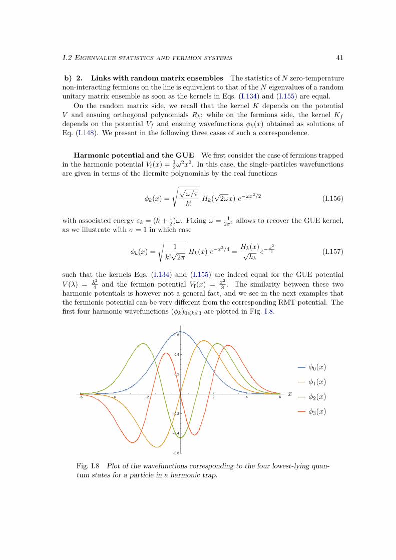
I.2 Eigenvalue statistics and fermion systems 41
b) 2. Links with randommatrix ensembles The statistics ofN zero-temperaturenon-interacting fermions on the line is equivalent to that of the N eigenvalues of a randomunitary matrix ensemble as soon as the kernels in Eqs. (I.134) and (I.155) are equal.
On the random matrix side, we recall that the kernel K depends on the potentialV and ensuing orthogonal polynomials Rk; while on the fermions side, the kernel Kf
depends on the potential Vf and ensuing wavefunctions φk(x) obtained as solutions ofEq. (I.148). We present in the following three cases of such a correspondence.
Harmonic potential and the GUE We first consider the case of fermions trappedin the harmonic potential Vf(x) = 1
2ω2x2. In this case, the single-particles wavefunctions
are given in terms of the Hermite polynomials by the real functions
φk(x) =
√√ω/π
k! Hk(√
2ωx) e−ωx2/2 (I.156)
with associated energy εk = (k + 12)ω. Fixing ω = 1
2σ2 allows to recover the GUE kernel,as we illustrate with σ = 1 in which case
φk(x) =√
1k!√
2πHk(x) e−x2/4 = Hk(x)√
hke−
x24 (I.157)
such that the kernels Eqs. (I.134) and (I.155) are indeed equal for the GUE potentialV (λ) = λ2
4 and the fermion potential Vf(x) = x2
8 . The similarity between these twoharmonic potentials is however not a general fact, and we see in the next examples thatthe fermionic potential can be very different from the corresponding RMT potential. Thefirst four harmonic wavefunctions (φk)06k63 are plotted in Fig. I.8.
-6 -4 -2 2 4 6
-0.6
-0.4
-0.2
0.2
0.4
0.6
Fig. I.8 Plot of the wavefunctions corresponding to the four lowest-lying quan-tum states for a particle in a harmonic trap.

42 Chapter I. Introduction to RMT and eigenvalue processes
Potential Vf(x) = Ax2+B/x2 and the LUE The second correspondence we discussconcerns fermions restricted to x > 0, in the potential
Vf(x) = b2
2 x2 + α(α− 1)
2x2 (I.158)
where we follow [104] for the convenient parametrization with b > 0, α > 1. The wave-functions φk(x) can be expressed in terms of the Laguerre polynomials as
φk(x) = ck L(α− 1
2 )k
(bx2)xαe−
b2x
2 (I.159)
with corresponding energy εk = b(2k + α+ 1
2
). Changing variables to yi = x2
i , thekernel for the process of the y variables can be shown to match that of the LUE, wherethe eigenvalues are restricted to be in R+ with however a potential V which is verydifferent of Vf , see Eq. (I.51).
Hard box potential and the JUE Finally, fermions confined in a hard-box, suchthat Vf(x) = 0 on [−1, 1] and Vf(x) =∞ if x /∈ [−1, 1], can be related to the eigenvaluesof the JUE. Indeed, changing variables to ui = 1
2(1 + sin(πxi
2)) ∈ [0, 1], the process
of the u variables has the same statistics as the eigenvalues of the Jacobi Ensemble withpotential V given in Eq. (I.61) where the two Jacobi parameters are fixed as A1 = A2 = 1
4 .Furthermore, the JUE with arbitrary parameters can similarly be obtained as a variablechange of a fermion system with potential Vf(x) = A
sin(x/2)2 + Bcos(x/2)2 .
For a review of these connections between RMT and fermions on the real line, anddetails on the results mentioned above, we point to [68,104].
As presented above, there are a small number of known exact mappings betweenfermion systems and RMT ensembles. In the course of the research projects related tothis thesis and presented in publication (2), we were led to exhibit a previously unknownconnection between the inverse-Wishart ensemble and fermions in the renowned Morsepotential Vf(x) ∝ (1− e−ax)2, as will be explained in chapter III.
Higher dimensions Complex spectra of non-Hermitian random matrices can alsobe mapped to certain two-dimensional systems of spinless fermions in rotation [70,96], toone-dimensional fermions with spin [105] and to two-dimensional one-component plasma(2DOCP) [106,107].
Fermions can also be studied in higher dimensions, in contrast with eigenvalues ofRMT. Investigations in higher-dimensional fermion systems show that they exhibit similarkind of universal local statistics as seen in the d = 1 case presented in the previous sectionfor the equivalent RMT systems [108, 109]. In this general d > 1 setting, investigationshave also concerned the full counting statistics and gap probabilities of the non-interactingfermions [110,111].
c) Eigenvalues of orthogonal and symplectic ensembles (β = 1, 4)
The previous sections have dealt in length with the unitary ensembles (β = 2), where thesquared Vandermonde determinant induces the powerful determinantal structure of the
I.2 Eigenvalue statistics and fermion systems 43
eigenvalue JPDF, and allows a mapping to fermion systems. In this section, we turn tothe remaining orthogonal (β = 1) and symplectic (β = 4) ensembles, and present brieflyhow a parallel structure intervenes.
c) 1. Pfaffian point processes This structure requires the definition of the Pfaffianof a 2N × 2N anti-symmetric matrix A, which is a polynomial of degree N in the matrixentries such that
(PfA)2 = det A . (I.160)
It is formally defined as a sum on the (2N)! permutations of [1. . 2N ], denoted (i) withsign σ(i), as
PfA = 12NN !
∑(i)σ(i)
N∏k=1
Ai2k−1,i2k . (I.161)
In parallel with the construction of the determinantal point process, we define a Pfaf-fian point process (PPP) as the probability measure on the configurations of N points onthe real line, given by the JPDF and marginal densities given for 0 6 m 6 N by
P (x1, · · · , xm) = (N −m)!N ! Pf
16i,j6NK(xi, xj) (I.162)
where the kernel K is now a 2× 2 matrix
K(x, y) =(K11(x, y) K12(x, y)K21(x, y) K22(x, y)
). (I.163)
For the 2N × 2N matrix entering the Pfaffian to be anti-symmetric, the kernel is con-strained to verifyK12(x, y) = −K21(y, x), with anti-symmetric diagonal entriesKii(x, y) =−Kii(y, x), i = 1, 2.
A PPP can be viewed as a generalization of a DPP. Indeed, in the particular casewhere the diagonal parts of the kernel vanish, such that K11 = K22 = 0, the Pfaffianappearing in Eq. (I.162) reads
Pf16i,j6N
K(xi, xj) = det16i,j6N
K12(xi, xj) (I.164)
and the point process is in fact a DPP with kernel K12.
c) 2. Orthogonal and symplectic ensembles The eigenvalue processes of or-thogonal and symplectic ensembles, i.e. β-ensembles with β = 1 and 4, can be shown tobe Pfaffian point processes. The corresponding 2×2 matrix anti-symmetric kernel can beconstructed from the family of skew-orthogonal polynomials associated with the potentialV and corresponding weight function ω(·) = e−βV (·).
We will not detail the construction in this thesis, but instead point to [112] for theexact mapping of the eigenvalue JPDF in a Pfaffian form, to [113] for the application to theGOE and GSE particular cases and to [16,68] for extensive details on the skew-symmetricconstructions.
Remarkably, the universal local statistics observed in the unitary case extend to thePPP structure of the orthogonal and symplectic cases. On the microscopic scale, the

44 Chapter I. Introduction to RMT and eigenvalue processes
bulk, soft edge and hard edge statistics are then respectively described by the sine, Airyand Bessel 2 × 2 matrix kernels [92], which are different in the β = 1 and β = 4 cases,and are of course different from the scalar kernels presented in the β = 2 case.
I.2.3 Extreme value statisticsIn this section, we present another aspect of random matrix eigenvalues: the statistics ofthe extreme values of the spectrum. These properties have raised much interest in RMT,and many efforts have been made until recent years to refine the knowledge on this aspectof the eigenvalue statistics.
The interest in the properties of the maximal eigenvalue of a random matrix spectrumcan be explained by the fact that they are non-standard with respect to usual indepen-dent probability theory. Indeed, for a set of i.i.d. random variables, the distribution ofthe maximal value follows either the Gumbel, Fréchet or Weibull law according to thecharacteristics of the initial distribution’s tail [114]. The maximum of a random matrixspectrum, where the eigenvalues form a set of strongly-correlated variables, does not fitin this classification.
a) Tracy-Widom distributionCraig Tracy and Harold Widom were the first to study the statistics of the maximaleigenvalue of the main RMT ensembles [90, 115]. They exhibited the distribution of themaximal eigenvalue λmax of Gaussian ensembles around its typical value, which is nowcalled the Tracy-Widom (TW ) distribution. This distribution depends on the index βand describes the fluctuations of λmax on the microscopic scale around the typical edge ofthe spectrum. The cumulative distribution function (CDF) of the TW-β law is usuallydenoted Fβ.
Let us state the precise result for the Gaussian β ensemble with σ = 1. We saw insection I.2.2 that the eigenvalue density around the edge 2
√N is of order N1/6, such
that the typical lengthscale is then N−1/6. The maximal eigenvalue then follows the TWdistribution, in the large-N limit, after a corresponding rescaling as
λmax − 2√N
N−16
∼ χ (I.165)
where χ is a TW-distributed random variable, such that P[χ 6 x] = Fβ(x).The probability P[χ 6 x] is the probability that the rescaled process has no particles
above the position x. In the case β = 2, the local Airy kernel DPP structure at the softedge allows to write this gap probability on [x,+∞[ in the Fredholm determinant formof Eq. (I.133) such that:
F2(x) = P[χ 6 x] = det(
1− KAiry∣∣∣[x,+∞[
). (I.166)
In the cases β = 1 and 4, the PPP structure implies an expression of F1,4 as FredholmPfaffians, which are an extension of Pfaffians to skew-symmetric operators similarly asthe Fredholm version of the determinant. The TW distribution has been further extendedto general β > 0 in the study of the stochastic Airy operator [116].

I.2 Eigenvalue statistics and fermion systems 45
The PDF F ′β(x) of the TW distribution is plotted for the three values of β in Fig. I.9,where their asymmetry is apparent. Indeed, the two tails of the distribution are notequivalent and obey the following asymptotics:
F ′β(x) '
e−β24 |x|
3as x→ −∞ ,
e−2β3 x
32 as x→ +∞ .
(I.167)
The left tail vanishes much faster than the right tail, as expected from the fact that alarge maximum value only requires to have an unexpected position for one eigenvalue,while a low maximum value requires to push a large number of eigenvalues to the left. Formore technical precisions about the TW distribution, and in particular its connections tothe Painlevé II nonlinear differential equation, see [16,75,117].
-4 -3 -2 -1 1 2
0.1
0.2
0.3
0.4
0.5
Fig. I.9 The Tracy-Widom PDF F ′β(x) for β = 1, 2, 4.
The universality of the Airy kernel on the local scale at a soft edge implies the univer-sality of the Tracy-Widom distribution which therefore appears in many random matrixensembles. Furthermore, this distribution appears outside of RMT in a wide range ofproblems such as the directed polymer model and other growth processes [33] or thecombinatorics of longest increasing subsequences [31]. It has also been observed in exper-iments on nematic liquid crystal behaviour [118] and coupled lasers [119]. An explanationfor the universal emergence of the Tracy-Widom distribution in many different contextshas been suggested through the mechanism of a third-order phase transition [120].
b) Large deviations
Beyond the typical fluctuations of the maximal eigenvalue around the edge of the spec-trum, the rare events obey a large deviation principle [121]. These rare events can beeither an extremely high or an extremely low value of λmax, such that the distance ofλmax with the expected edge is of the order of the global scale of the spectrum.

46 Chapter I. Introduction to RMT and eigenvalue processes
For example, in the Gaussian β ensembles, the large deviation tails behave asymptot-ically in the large-N limit as
∂x P[λmax 6
√Nx
]'
exp(−βN2 Φ−(x)
)for x < 2
exp (−βN Φ+(x)) for x > 2(I.168)
where the large deviations functions Φ− and Φ+ were obtained for general values of βin [122–124]. Once again, the asymmetry between the left and right tail is visible inthe different exponent appearing in the prefactor. In physical terms, pulling a singleparticle of the Coulomb gas to a high value costs an energy of order N , while pushingthe whole gas of particles such that all the particles stay to the left of a low barrier costsan energy of order N2. The difference between these two tails has similarities with theGross-Witten-Wadia phase transition of lattice QCD [120].
The large deviations of the extreme eigenvalues of some RMT ensembles are furtherdiscussed in relation to the HCIZ integral in chapter IV. On this topic of recent activityand for studies of other ensembles, one may also consult [75,120,125].
I.3 Free probability for large matricesIn this last section of the introduction chapter, we give a presentation of the theory of freeprobability. This young branch of probability theory was founded at the beginning of the1980’s by Dan-Virgil Voiculescu who studied Von Neumann operator algebras, and wasin particular led to investigate properties of random objects in these non-commutativealgebras. He thereupon defined the property of freeness for non-commutative randomvariables [126] and found a major field of application of this notion in the study of largerandom matrices [127, 128]. The constructions and methods of free probability are nowan essential part of the standard toolbox of random matrix theory.
In the context of random matrices, a first idea of free probability can be given asfollows. In general, the knowledge of the eigenvalues of two matrices is not sufficientto deduce the spectrum of the matrix sum, unless the matrices commute and are thendiagonalizable in the same basis. Free probability introduces a condition under which thespectrum of the sum can be obtained from the two initial spectra. This freeness conditionmust then imply that eigenvectors are immaterial, and we will see that the condition isindeed respected for large matrices whose eigenbases are randomly rotated with respectto each other.
In addition to its ties with random matrices, free probability is connected to thebeautiful combinatorics of non-crossing partitions and to many other fields such as rep-resentation theory of large groups, quantum groups, statistical inference and quantuminformation theory [129].
In the first subsection, we define the notion of freeness and give an overview of thecombinatorial structure of the theory. In subsection I.3.2, we detail the properties of thesum of free random matrices and the relevant tool of this issue, the R-transform. Insubsection I.3.3, we detail the properties of the product of free random matrices and therelevant tool of this issue, the S-transform. For more comprehensive presentations of freeprobability, we refer the reader to [46,64,65,129–133].

I.3 Free probability for large matrices 47
I.3.1 Definition and properties of freenessWe define the notion of freeness for random matrices, which applies in the large-sizelimit. We will see that this notion leads naturally to the definition of free cumulants, inan elegant connection to the combinatorics of non-crossing partitions.
a) Asymptotic freenessThe random variables that we ought to consider are sequences of HermitianN×N matricesMN which converge to a well-defined infinite-size random matrix M. Note that for thelimit to be well-defined, the matrix sequence must be normalized such the asymptoticspectrum is compactly supported. The limit M is then characterized by its eigenvaluedensity ρemp = ρ, which is equal to the average density by the self-averaging propertyof large matrices. In full rigour, the limit of the sequence belongs to a non-commutativeoperator algebra, to which the free probability results can be formally applied, but wewill informally consider that we are handling a large random matrix M in the following.
A useful observable is then the expected renormalized trace as:
φ(M) = limN→∞
1N
E [Tr MN ] =∫Rλ ρ(λ) dλ . (I.169)
Note that φ is linear and verifies φ(1) = 1. This allows to define the kth asymptoticmoment as
mk = φ(Mk) =∫Rλkρ(λ)dλ . (I.170)
With these conventions in place, we can define the notion of asymptotic freeness.
a) 1. Definition The random matrices A and B are asymptotically free if for all `and for all polynomials pi and qi (1 6 i 6 `) such that φ(pi(A)) = φ(qi(B)) = 0, we have:
φ
(p1(A)q1(B) · · · p`(A)q`(B)
)= 0 (I.171)
Of course this definition extends to several matrices, such that A1, · · · ,Am are asymp-totically free if φ
(p1(Aj1)p2(Aj2) · · · p`(Aj`)
)= 0 whenever φ(pi(Aji)) = 0 for all i, and
all consecutive indices are different: ji 6= ji+1. Note that this is a statement on the limitmatrices, hence the asymptotic nature of the notion in the RMT setting.
The construction is intended to be a non-commutative version of independence. In-deed, if we consider m distinct asymptotically free matrices (Ai)16i6m, the freeness prop-erty implies for example that for any polynomials (pi)16i6m:
φ
(p1(A1) · · · pm(Am)
)= φ
(p1(A1)
)· · ·φ
(pm(Am)
)(I.172)
which is reminiscent of the expectation factorization of independent scalar random vari-ables (Xi)16i6m:
E[p1(X1) · · · pm(Xm)
]= E
[p1(X1)
]· · ·E
[pm(Xm)
]. (I.173)
48 Chapter I. Introduction to RMT and eigenvalue processes
However in the commutative case, if two variables are the same Xi = Xj , they can beregrouped before the factorization as:
E[XYXY
]= E
[X2] E[Y 2] . (I.174)
For free matrices A and B on the other hand, non-commutativity changes things drasti-cally when a matrix appears several times in the product. For example, by introducingcentered polynomials such as A − φ(A) and by successive applications of Eq. (I.171), afew lines of algebra yield
φ
(ABAB
)= φ(A)2φ(B2) + φ(B)2φ(A2)− φ(A)2φ(B)2 . (I.175)
We note that φ(ABAB), in addition to featuring three terms when the usual scalarversion only gives one, does not even display the term φ(A2)φ(B2) that would be expectedfrom the scalar setting. As a non-commutative version of independence, freeness has manydifferences from the usual version, which we will detail after giving a few results on theconditions for random matrices to be asymptotically free.
a) 2. Sufficient conditions An important question is the following: when do twolarge random matrices constitute pair of free variables, in the asymptotic sense ? In thefollowing lines, we give interesting results on this issue.
• Any random matrix and the identity 1 are asymptotically free.
• If two matrices are asymptotically free and they commute, then one of them is amultiple of 1. Such a scalar matrix is also called constant, from the point of viewof the eigenvalue distribution.
• A random matrix which is free with itself is constant.
• X11 and X21, where X1 and X2 are two independent scalar random variables withnon-zero variance, are not asymptotically free.
• Independent standard Gaussian matrices are asymptotically free.
Finally, the most important result for the application of free probability to RMT is thefollowing theorem:
If A and B are random matrices (with compactly supported asymptotic ESD)and if U is a (Haar-distributed) random unitary matrix, then UAU† and Bare asymptotically free.
This result shows the importance of free probability theory in random matrix theory:any two matrices that are randomly rotated with respect to each other are asymptoticallyfree. In the large size limit, they can be treated as free random variables. For more precisestatements and proofs of results cited above, we point to [46,65,129].

I.3 Free probability for large matrices 49
b) Non-crossing partitions and free cumulants
As defined above, freeness is a rule that allows the computation of mixed moments of Aand B at all orders, given the moments of A and the moments of B. The application ofthis rule quickly becomes cumbersome and it is useful to introduce a tool called the freecumulant. Its construction relies on the combinatorics of non-crossing partitions.
b) 1. Non-crossing partitions A partition ω = V1, · · · , Vk of the set Sn =1, · · · , n, where the blocks Vi are non-empty subsets of Sn with no shared element suchthat ∪ki=1Vi = Sn, is called non-crossing if there are no four elements 1 6 p1 < q1 < p2 <q2 6 n such that:
p1, p2 ∈ Vi , q1, q2 ∈ Vj with i 6= j. (I.176)
A partition where this occurs is said to be crossing. In the following, we denote Pn asthe set of all partitions of the set Sn, and PNC
n as the subset of Pn consisting of thenon-crossing partitions.
As an illustration, the non-crossing partition 1, 3, 2, 4, 5 and the crossingpartition 1, 3, 2, 4, 5 of S5 are represented in Fig. I.10, where elements in the sameblock are connected by a line, such that a partition is crossing if and only if two linesintersect.
1 2 3 4 5 1 2 3 4 5
Fig. I.10 Two partitions of S5 = 1, 2, 3, 4, 5.
The number of non-crossing partitions of Sn is the n-th Catalan number Cn:
Cn = card(PNCn
)= 1n+ 1
(2nn
). (I.177)
Interestingly, Cn is also the number of non-crossing pair partitions of S2n, i.e. elementsof PNC
2n consisting of n pairings of elements. Denoting PNC(2)2n their ensemble, Cn =
card(PNC(2)
2n
). Elements of PNC(2)
2n can be seen as Dyck words of length 2n, i.e. wordsthat can be written using pairs of left and right parentheses without closing an unopenedparenthesis. For example C3 = 5 as seen in Fig. I.11, because there are 5 ways to order3 pairs of parentheses.
()()() ()(()) (())() ((())) (()())
Fig. I.11 Five orderings of three pairs of parentheses.

50 Chapter I. Introduction to RMT and eigenvalue processes
b) 2. Standard cumulants Before introducing free cumulants, we briefly recall thestandard construction of cumulants kn of a scalar random variable X, in relation withits moments Mn = E[Xn]. The cumulants are defined as the coefficients of the followingseries:
logE[etX
]=∑n>1
kntn
n! (I.178)
and they are related to the moments through
Mn =∑ω∈Pn
k∏i=1
k`i =∑ω∈Pn
k`1 · · · k`k . (I.179)
where we denote ω = V1, · · · , Vk ∈ Pn a partition and `i = card(Vi) the cardinalities ofits blocks.
As their name suggests, the main interest of these cumulants is that they behavewell under the addition of two independent random variables. For any two independentrandom variables X and Y and for all integers n, with kn(·) the nth cumulant function :
kn(X + Y ) = kn(X) + kn(Y ) (I.180)
which is easily proven as:∑n>1
kn(X+Y ) tn
n! = logE[et(X+Y )
]= log
(E[et(X)
]E[et(Y )
])=∑n>1
(kn(X) + kn(Y )) tn
n! .
(I.181)
b) 3. Free cumulants In the non-commutative realm also, it is possible to definefree cumulants which behave well under the addition of free random matrices. For arandom matrix M with a given sequence of moments mn = φ(Mn), the sequence of freecumulants κn is defined recursively such that
mn =∑
ω∈PNCn
k∏i=1
κ`i =∑
ω∈PNCn
κ`1 · · ·κ`k (I.182)
where the sum is taken on non-crossing partitions only, in contrast with the standardcase. Denoting κn(M) the nth cumulant of a random matrix M, it is a theorem that forany two free random matrices A and B and for all integers n:
κn(A + B) = κn(A) + κn(B) . (I.183)
This property translates the information carried by the property of freeness, i.e. thatalternating and centered mixed moments vanish, in a very simple form with free cu-mulants. A proof of this theorem requires the additional definition of mixed cumulantsκn(A,B,C, ...), which can be shown to vanish for free matrices. The quantity κn(A + B)can then be written as a sum on all possible mixed cumulants of A and B, where onlyκn(A) and κn(B) survive.
For a proof of Eq. (I.183), showing how the structure of non-crossing partitions usedin the definition of free cumulants provides a useful tool to simplify the analysis of freevariables addition, we point to [65,130,131,133].

I.3 Free probability for large matrices 51
In Table I.3, we give the first expressions of moments in terms of cumulants both inthe standard and free cases, obtained from Eq. (I.179) and Eq. (I.182). We note thatthe first three terms are identical, as all partitions of Sn are non-crossing for n 6 3. Forn = 4, the difference is the removal of the unique crossing partition 1, 32, 4 suchthat the coefficient of κ2
2 is 2 instead of 3.
n Mn mn
1 k1 κ1
2 k2 + k21 κ2 + κ2
1
3 k3 + 3k2k1 + k31 κ3 + 3κ2κ1 + κ3
1
4 k4 + 4k3k1 + 3k22 + 6k2k
21 + k4
1 κ4 + 4κ3κ1 + 2κ22 + 6κ2κ
21 + κ4
1
5 k5 + 5k4k1 + 10k3k2 + 10k3k21 +
15k22k1 + 10k2k
31 + k5
1
κ5 + 5κ4κ1 + 5κ3κ2 + 10κ3κ21 +
10κ22κ1 + 10κ2κ
31 + κ5
1
Table I.3: Five first moments expressed in terms of cumulants, in standard and free cases.
I.3.2 Sum of free random matricesIn the previous section, we have seen that freeness provides a free-cumulant additionformula Eq. (I.183). We now turn to a practical use of this property, to solve the problemmentioned at the beginning of the section: from the knowledge of the spectra of two freerandom matrices A and B, how can we characterize the spectrum of A+B ? This problemof free addition of random variables was first studied in [134] and the tools introducedtherein are now commonly used in RMT.
a) The R-transform
The interesting property on free cumulants will be transformed on an addition property forthe generating function of these free cumulants, the R-transform, defined in the following.
Recall the definition of the Stieltjes transform g of our large matrix M in terms ofthe density ρ in Eq. (I.72), and note that it admits a large-z series expansion where thecoefficients are the moments mn:
g(z) = 1z
+∑n>1
mn
zn+1 . (I.184)
Denoting [a, b] the support of the density ρ on the real line, g is defined on C \ [a, b]. Itsfunctional inverse is called the B (or Blue) transform:
B(g(z)) = z , ∀z ∈ C \ [a, b] (I.185)

52 Chapter I. Introduction to RMT and eigenvalue processes
and the R (or Red) transform is defined from it as:
R(ω) = B(ω)− 1ω. (I.186)
Both functions are defined on C∗.It can be shown that the R-transform is precisely the free cumulant generating func-
tion, such that it admits the following Taylor expansion as ω → 0:
R(ω) =∑n>1
κn ωn−1 (I.187)
where the coefficients are the free cumulants of M. This is proven by analyzing thefunctional relation of R with the generating function of the moments g(1
z ), in regards tothe combinatorial definition Eq. (I.182), see [65,131,133].
The addition property of free cumulants directly yields:
RA+B(ω) = RA(ω) +RB(ω) (I.188)
for two random matrices A and B. This relation characterizes exactly the asymptoticspectrum of the sum A+B from the knowledge of the spectra of A and B: the knowledgeof RA+B indeed allows to recover the Stieltjes transform, which in turn characterizes theeigenvalue distribution exactly.
b) Wigner’s semicircle and the free central limit theoremWe give in the following paragraph an example of R transform for the large-size limitof the Gaussian ensembles, characterized by Wigner’s semicircle eigenvalue density, aspresented in section I.2.1.
b) 1. The free cumulants of Wigner’s semicircle For M a rescaled Gaussianmatrix (with either β = 1, 2 or 4) of large size, the eigenvalue density is characterizedby Wigner’s semicircle density ρSC supported on [−2σ, 2σ], see Eq. (I.69). The Stieltjestransform of this distribution can be computed as Eq. (I.77), which is inverted as B(ω) =σ2ω + 1
ω such that the R-transform is linear in ω:
R(ω) = σ2ω . (I.189)
The free cumulants of the semicircle distribution are directly read as:κ1 = m1 = 0κ2 = σ2
κn = 0 for n > 3 .(I.190)
The first cumulant is zero, as every odd moment of M, because the distribution is centered.The semicircle distribution is further characterized by the fact that all cumulants of orderlarger than 2 vanish. This can be understood from the study of the moments, which canbe computed in terms of the Catalan numbers as:
mn =∫RλnρSC(λ)dλ =
0 for n odd;σn Cn/2 for n even. (I.191)

I.3 Free probability for large matrices 53
With the interpretation of Catalan numbers as the number of non-crossing pair partitions,we have:
mn = σn Cn/2 =∑PNC(2)n
(σ2)n/2 =∑PNC(2)n
κn/22 (I.192)
such that only one kind of term is non-zero in the sum relating mn to free cumulants(I.182), corresponding to the non-crossing partitions where all blocks have two elements.All other partitions have vanishing contributions such that κn = 0 for all n > 3.
These vanishing free cumulants give rise to a linear R-transform which has an inter-esting consequence. If A and B have semicircle distributions with variance σ2 and theyare free, then their sum verifies RA+B(ω) = RA(ω) +RB(ω) = 2σ2ω such that A + Bhas semicircle distribution of variance 2σ2. Up to a rescaling, the semicircle distributionis stable under free addition.
The semicircle distribution thus plays, in the free world, the role of the Gaussiandistribution which is stable under the addition of independent scalar variables. In thesame way, the Gaussian distribution is characterized by vanishing standard cumulantskn = 0 for n > 3, as a corollary of Wick’s theorem. This plays a crucial role in the CLT,which can thus be extended to the non-commutative case [135], along with the law oflarge numbers [136].
The correspondence between the properties of the Gaussian distribution in standardtheory and those of the semicircle distribution in the free setting is an example of theBercovici-Pata bijection, which associates to any standard distribution of finite cumulants(kn)n>1 a free random variable with the same sequence of free cumulants κn = kn [137].
b) 2. Free Law of Large Numbers The sum of L free identically distributedrandom matrices (Mk)16k6L, of mean φ(Mk) = m and finite other moments, normalizedby L converges to a constant with the same mean:
1L
L∑k=1
Mk −−−−→L→∞
mI (I.193)
as proven by noticing that the additive free cumulants converge to
κn(L∑k=1
Mk
L) = L
Lnκn −→
κ1 = m if n = 10 if n > 2 (I.194)
such that 1L
∑Lk=1 Mk converges to a variable with all free cumulants equal to zero except
the first one, which is a constant matrix mI.
b) 3. Free Central Limit Theorem The sum of L free identically distributedcentered random matrices (Mk)16k6L, of variance φ(M2
k) = κ2 and finite other moments,normalized by
√L converges to a semicircle-distributed random matrix M∞ with the
same variance κ2:
1√L
L∑k=1
Mk −−−−→L→∞
M∞ ∼ Semicircle(κ2) (I.195)
54 Chapter I. Introduction to RMT and eigenvalue processes
as proven by noticing that the additive free cumulants converge to
κn(L∑k=1
Mk√L
) = L
Ln/2κn −→
0 if n = 1κ2 if n = 20 if n > 3
(I.196)
such that 1√L
∑Lk=1 Mk converges to a variable with second cumulant κ2 and all others
equal to zero, which follows a semicircle distribution with parameter κ2.It should be noted that the condition in these two theorems is that all variables Mk are
collectively free, not just pairwise free. The same warning is in order in the commutativesetting.
I.3.3 Product of free random matricesAs we have seen in the previous section, it is possible to retrieve the spectrum of thefree sum A + B from the spectra of A and B. We now turn to the same question forthe free product: it is possible to retrieve the spectrum of A.B from the spectra of thefree random matrices A and B ? In the context of self-adjoint random matrices, the freeproduct must be defined as
√A B
√A, in order to ensure that the ensuing spectrum is
real. As for the free addition, the free product was first studied by Voiculescu [138].We introduce additional entire functions in order to study the spectrum of the free
product. The T -transform is defined from the Stieltjes transform as:
T (z) = z g(z)− 1 =∫R
u ρ(u)z − u
du =∑n>1
mn
zn. (I.197)
Denoting T −1 the functional inverse of the T -transform, the S-transform is defined forω ∈ C as:
S(ω) = ω + 1ωT −1(ω) . (I.198)
The S-transform is formally related to the R-transform as:
S(ω) = 1R(ωS(ω)) R(ω) = 1
S(ωR(ω)) (I.199)
and, from the series expansion of the T -transform, it can be shown that the followingexpansion, in terms of the moments and free cumulants of the distribution, holds for smallω:
S(ω) = 1m1
+ ω
m31
(m2
1 −m2)
+ ω2
m51
(2m2
2 −m2m21 −m3m1
)+O
(ω3)
(I.200)
= 1κ1− κ2κ3
1ω + 2κ2
2 − κ1κ3κ5
1ω2 +O
(ω3). (I.201)
This shows that the S-transform of a centered distribution, with m1 = κ1 = 0, is ill-defined. It can however be defined by introducing a translation to break the symmetry,see Table I.4 for the semicircle distribution.

I.3 Free probability for large matrices 55
The interest of this transform appears in the following theorem. For two free self-adjoint matrices A and B, the S-transform of the self-adjoint product
√A B
√A verifies
the following factorization property:
S√AB√
A(ω) = SA(ω)× SB(ω) (I.202)
For proofs of this theorem and presentations of the combinatorial structures relatedto the free product, we point to [65, 131, 133]. Note that the scalar equivalent of theS-transform is the Mellin transformMX(s) = E[Xs−1] of a random variable X, which ismultiplicative for the product of independent variables.
To conclude this introduction to free probability, we give in Table I.4 the Stieltjes, Rand S transforms for the main RMT ensembles’ asymptotic distributions [64], i.e. thesemicircle, Marčenko-Pastur and inverse Marčenko-Pastur distributions defined respec-tively in Eqs. (I.69), (I.85) and (I.92). For the sake of well-posedness, the S-transform ofthe semicircle distribution is in fact that of the µ-translated distribution, with µ > 0. Forµ < 0, the branch should be chosen with minus sign in front of the square-root to ensureregular behaviour as ω → 0.
Distribution g(z) R(ω) S(ω)
Semicircle z −√z2 − 4σ2
2σ2 σ2ω−µ+
√µ2 + 4σ2ω
2σ2ω
MarčenkoPastur
z + σ2(q − 1)−√z − µMP
−
√z − µMP
+
2qσ2 z
11σ2 − qω
1σ2
11 + qω
InverseMarčenkoPastur
z(κ+ 1)− κσ2 − κ
√z − µIMP
−
√z − µIMP
+
z2
κ−√κ(κ− 2
σ2ω)
ωσ2(
1− ω
2κ
)
Table I.4: Stieltjes, R and S transforms of the main asymptotic distributions.
This ends our presentation of random matrix theory, eigenvalue statistics on the globaland local scales, and free probability tools related to the study of large random matricesand their asymptotic spectrum.


Chapter II
Non-crossing walkers and vicious bound-ary problems
As presented in chapter I, the theory of random matrices has spawned from its appli-cations in nuclear physics, where eigenvalue repulsion matched heavy nuclei energy levelstatistics, and has developed through the study of properties implied by this fundamen-tal repulsive feature. This gives a direct motivation to study other systems displayingrepulsive interactions and investigate the links they may share with random matrices.An example of such a system is the simple exclusion process (SEP), exactly solvablein its symmetric and asymmetric versions [139, 140], where particles are free to performa random walk on Z under the restriction that no two particles may occupy the samesite. Remarkably, the current fluctuations of the totally asymmetric SEP is related to theTracy-Widom distribution [141]. Another example of spatial exclusion is given by randomdomino tilings of the Aztec diamond domain, where the spatial configurations of dominosare highly constrained and where determinantal processes appear as in RMT [142]. Fi-nally, other systems which display repulsion are models of interfaces, where a portion ofspace is divided into different regions separated by interfaces which should then remaindistinct. An example of these is the multi-layer polynuclear growth model (PNG) whichdescribes multiple layer growth on a substrate in a super-saturated vapor, and is linkedto Pfaffian processes and random matrices [33,143].
In this chapter, we turn to the simplest model of random one-dimensional interfaces:non-crossing walkers. In this system of N Brownian motions on the line, repulsion isprovided by conditioning the paths not to cross each other. The resulting conditionedprocess gives a simple model for horizontal interfaces splitting the plane in N + 1 layers,and it is also naturally a model of repulsive stochastic particles in one-dimension. Assuch, it is intimately related to the Dyson Brownian motion (DBM ), the diffusion ofeigenvalues obtained in the dynamic extension of RMT to stochastic processes, whereeigenvalues diffuse randomly while repelling each other. These two systems are presentedin detail in this chapter.
The focus of publication (1) was to study the properties of these systems under amoving vicious boundary. Considering that the system is "killed" if a particle touches theboundary, the main properties of interest concern the decay of the survival probabilityS(t), the probability that the system is not killed before time t. As will be illustrated
57
58 Chapter II. Non-crossing walkers and boundary problems
in this chapter, the most interesting case is that of the critical square-root boundaryg(t) = W
√t, which grows at the same speed as the stochastic expansion of the walkers.
It was found in this case that the survival probability decays as S(t) ∼ t−β(N,W ), wherethe exponent β(N,W ) was found to be the ground-state energy of a particular system ofnon-interacting fermions and studied in a variety of different scaling limits. Furthermore,the joint distribution of particles under the boundary at large time was also studied.
The first section will present the dynamic extension of RMT which gives rise tostochastic evolution of eigenvalues and derive the DBM stochastic differential equationas well as the connections of the model to fermion systems. We will then present thesystem of non-crossing walkers in the context of random interfaces, and detail its linkswith the DBM. The second section II.2 will present the results of publication (1) and theresolution of the square-root boundary problem for non-crossing walkers and the DBM,after detailing the simpler one-particle case. Finally, section II.3 will give an additionalperspective into the connections between non-crossing walkers and RMT by constructingan interpolating GβE measure through a partial non-crossing condition.
II.1 Non-crossing walkers and the dynamical exten-sion of random matrix theory
In this section, we complete the presentation of RMT of chapter I by the discussion ofits dynamical extension. Following the first steps made by Freeman Dyson [13, 144], thetheory of random matrices can indeed be extended to stochastic processes where a matrixevolves dynamically in time. In this context, the most important construction is theDyson Brownian motion, which we present thoroughly here, before presenting the systemof non-crossing walkers and the links shared by these two systems of diffusing particles.
In the first subsection, we define the DBM and present its dynamical connections tofermions in the Calogero-Moser Hamiltonian. In subsection II.1.2, we define the systemof non-crossing walkers and detail its links with the DBM.
II.1.1 The Dyson Brownian motiona) Definition and properties
Let us recall, as a preamble, the definition of the one-dimensional Brownian motion (Bt)t>0as the unique stochastic process on R which verifies the following properties:
• B0 = 0 ;
• Bt is almost-surely continuous ;
• all increments are independent ;
• and an increment Bt+T −Bt is distributed as N (0, T ).The Brownian motion has become a central construction in mathematics and physics afterits insightful introduction by Albert Einstein in the context of small particle suspensionsin liquids [145, 146]. The myriad of its applications [147] include statistical physics and

II.1 Non-crossing walkers and dynamical RMT 59
studies on non-equilibrium dynamics [148–151], biological physics and soft matter sci-ence [152–154], solid state fracture analysis [155, 156], interstellar medium research andastrophysics [157] and the surge in financial modelling of the second part of the last cen-tury [63]. For a presentation of stochastic calculus, discussions of the Brownian motionand of its detailed properties, we point to [158–161].
The Brownian motion is a diffusion process on the line which is distributed as astandard Gaussian random variable at time 1, i.e. B1 ∼ N (0, 1). The Dyson Brownianmotion is the stochastic process obtained by promoting all independent real Gaussianvariables appearing in the Gaussian ensembles (β = 1, 2 or 4) to standard Brownianmotions. It is thus a first step in a dynamical extension of RMT, where random matricesare promoted to stochastic processes [162].
a) 1. Definition Let us define the Dyson Brownian motion Hβt in the three usual
cases, and denote it the DBM-β. We introduce Xt a real matrix with N2 independentstandard Brownian motions as its entries, and X(k)
t independent versions of Xt. Withthese notations, the DBM-1 is the real symmetric matrix process:
H1t = Xt + XT
t√2
; (II.1)
the DBM-2 is the complex Hermitian matrix process:
H2t = Xt + XT
t
2 + i Xt − XTt
2 ; (II.2)
and the DBM-4 is the following self-adjoint quaternionic matrix process, denoting thecanonical basis of quaternions (1, i(1), i(2), i(3)):
H4t = Xt + XT
t
2√
2+
3∑k=1
i(k) X(k)t − X(k),T
t
2√
2. (II.3)
In all three cases, the construction ensures that Hβ1 , the evaluation of the process at
time t = 1, is distributed as a GβE matrix with parameter σ = 1, as can be seen fromEqs. (I.5), (I.18) and (I.27). For general time t, Hβ
t is distributed as a GβE matrix withparameter σ =
√t.
The DBM is formally a Brownian motion in the space of self-adjoint matrices: it hascontinuous paths and independent increments distributed according to the correspondingGaussian ensemble, with variance given by the time increment. As in the scalar case whereDonsker’s invariance principle implies the convergence of a random walk with i.i.d. cen-tered finite-variance steps to the Brownian motion, the DBM can be interpreted as thecontinuous limit of a large sum of independent infinitesimal matrix increments [65]. In amore abstract scope, Brownian motions on general Lie groups have been widely studiedin mathematics [163,164].

60 Chapter II. Non-crossing walkers and boundary problems
a) 2. Langevin equation for the eigenvalues By extension, the Dyson Brownianmotion also refers to the stochastic process of the N real eigenvalues (λi,t)16i6N of Hβ
t . Inthis section, we derive the stochastic differential equation (SDE), or Langevin equation,obeyed by this RN -valued process, for β = 1, 2 or 4.
Perturbation theory Let us consider a fixed time t. From the addition propertiesof the Brownian motion, the evolution of the DBM between t and infinitesimally largertime t+ dt is distributed as
∆∆dt = Hβt+dt −Hβ
t ∼√
dt Hβ1 (II.4)
with H an independent version of the DBM. The infinitesimal matrix ∆∆dt is thus dis-tributed as
√dt times a unit-variance GβE matrix ∆∆, and we write ∆∆dt =
√dt∆∆.
In order to deduce the eigenvalue SDE, we are interested in the infinitesimal evolutionof the eigenvalues of Hβ
t under the addition of this infinitesimal matrix increment ∆∆dt.This amounts to develop a perturbation theory for eigenvalues, which is well-know in thecontext of quantum mechanics where it is used to determine the evolution of energy levelsunder slight modification of the Hamiltonian [94]. In reference, we develop the argumentwith notations inspired from this setting.
Let us denote (|vi,t〉)16i6N the set of orthonormal eigenvectors of the matrix Hβt ,
corresponding respectively to eigenvalue λi,t. The perturbed eigenvalues and eigenvectorscan be written in an expansion on the infinitesimal factor ε =
√dt:
λi,t+dt = λi,t + ελ(1)i + ε2λ
(2)i · · · (II.5)
and|vi,t+dt〉 = |vi,t〉+ ε |vi〉(1) + ε2 |vi〉(2) · · · (II.6)
with the orthonormality constraint 〈vi,t+dt|vj,t+dt〉 = δi,j . The expansion coefficients λ(k)i
and |vi〉(k) are found recursively on k by enforcing the eigenvalue equation
Hβt+dt |vi,t+dt〉 =
(Hβt + ε∆∆
)|vi,t+dt〉 = λi,t+dt |vi,t+dt〉 (II.7)
such that the perturbed eigenvalues and eigenvectors are given at first orders by [94]:
λi,t+dt = λi,t + ε 〈vi,t|∆∆ |vi,t〉+ ε2 ∑16j6Nj 6=i
|〈vj,t|∆∆ |vi,t〉|2
λi,t − λj,t+O(ε3) (II.8)
and|vi,t+dt〉 = |vi,t〉+ ε
∑16j6Nj 6=i
〈vj,t|∆∆ |vi,t〉λi,t − λj,t
|vj,t〉+O(ε2) . (II.9)
From the distribution of ∆∆ as a unit-variance rotation-invariant Gaussian matrix, wehave on one hand that 〈vi,t|∆∆ |vi,t〉 ∼ N (0, 2
β ) and on the other that |〈vi,t|∆∆ |vj,t〉|2 − 1has mean zero, such that Eq. (II.8) yields, in the ε→ 0 limit:
λi,t+dt ' λi,t + ε
√2βXi + ε2 ∑
16j6Nj 6=i
1λi,t − λj,t
(II.10)

II.1 Non-crossing walkers and dynamical RMT 61
where Xi ∼ N (0, 1). Introducing N independent standard Brownian motions (Bi,t)16i6Nand replacing ε =
√dt, this yields the N stochastic differential equations for the eigen-
values of the Dyson Brownian motion as:
dλi,t =√
2β
dBi,t +∑
16j6Nj 6=i
1λi,t − λj,t
dt (II.11)
For details on the convergence of the perturbation result to this SDE, in particular forthe rigorous treatment of the (|∆∆ij |2 − 1) term, see [58]. This SDE is also often found inthe literature in the time-rescaled form, with t→ β
2 t, as
dλi,t = dBi,t + β
2∑j 6=i
1λi,t − λj,t
dt . (II.12)
Itô’s formula Another derivation of the SDE (II.11) can be obtained by a formalapplication of Itô’s formula [158]. Indeed, the DBM matrix processes in Eqs. (II.1),(II.2) and (II.3) are defined from the joint process of the β N2 independent Brownianmotions in the X matrices. The eigenvalues λi,t are a function of the entries of Hβ
t , andthus of these independent Brownian motions, such that Itô’s formula can be applied toobtain their stochastic evolution, which recovers (II.11). We point to [65] for the detailedcomputation in the β = 1 case.
Properties The evolution equation of eigenvalues given by Eq. (II.11) combines twoingredients. On the one hand, the eigenvalues diffuse according to independent Brownianmotions, following the stochastic diffusion of the matrix entries. On the other hand, theyrepel each other through the drift term, as expected from the statistics of eigenvalues instatic RMT presented in the first chapter.
Note that this drift term is similar to the one of the Bessel process (Rt)t>0 whichdescribes the norm of the D-dimensional Brownian motion Rt =
∥∥∥ ~Bt∥∥∥D
and obeys thefollowing SDE [165]
dRt = dBt + D − 12
1Rt
dt . (II.13)
By the recurrence properties of the Brownian motion, Rt is repelled away from the originand stays almost-surely strictly positive as soon as D > 2.
The process (λi,t)t>0 can be seen as a generalization on RN of the Bessel process,restricted to stay in the Weyl chamber WN defined as
WN = ~λ ∈ RN | λ1 > λ2 > · · · > λN . (II.14)
We also introduce the notation W∗N for the interior of the Weyl chamber, where theinequalities are strict. For both the DBM and the Bessel processes, the repulsive driftterm is the inverse-distance to the forbidden boundary. From the properties of the Besselprocess, the boundary is almost-surely never touched when the prefactor of this drift termis at least 1
2 , such that the prefactor β2 in the time-rescaled DBM SDE (II.12) ensures
that eigenvalues of the DBM never meet each other in the three cases β = 1, 2, 4 [58,166].

62 Chapter II. Non-crossing walkers and boundary problems
For a more practical point of view, consider a situation where two diffusing DBMeigenvalues λi > λj get very close to each other at some time t. The difference of theirstochastic evolutions (II.12) yields the SDE for the difference λi − λj as d(λi − λj) '√
2dBt + βλi−λj dt or after a time-rescaling t→ t/2:
d(λi − λj) ' dBt + β
21
λi − λjdt . (II.15)
After this time-rescaling, the difference of two close-by DBM eigenvalues is distributedas the (β + 1)-dimensional Bessel process, such that indeed two eigenvalues of the DBMalmost-surely never collide as soon as β > 1. For more details on the DBM as a mul-tivariate extension of the Bessel process, see [167] where connections are also presentedbetween the Schramm-Loewner Evolution (SLE) [168–170] and the Bessel flow.
The dynamical extension of RMT given by the Dyson Brownian motion can also beseen, at the eigenvalue level, as a dynamical extension of the Coulomb gas frameworkof Eq. (I.63), as particles experience stochastic diffusion in addition to repulsion andgenerate configuration samples of the Coulomb gas. We recover in Eq. (II.11) the inverse-temperature interpretation of β since the coefficient of dBt is expected, in the Coulombgas with stochastic diffusion, to be proportional to the square-root temperature by theStokes-Einstein law [171].
a) 3. Stieltjes transform evolution As seen in the first chapter, the Stieltjestransform g defined in Eq. (I.72) is a useful tool to characterize the spectrum of a randommatrix, especially in the large-N setting, in parallel with other transforms defined fromit as seen in section I.3. In this paragraph, we derive the evolution of g under the DBMmatrix diffusion.
More precisely, we define the time-dependent Stieltjes transform of the rescaled DBMprocess Hβ
t = 1√N
Hβt as
g(z, t) = 1N
N∑i=1
1z − λi,t/
√N
(II.16)
where the√N scaling factor is the one that appeared naturally in the Stieltjes transform
study of the Gaussian ensembles in section I.2.1.
Itô’s formula The Stieltjes transform g(z, t) is a function of the time-evolving eigen-values λi,t and verifies:
∂g
∂λi,t= 1N√N
1(z − λi,t/
√N)2
(II.17)
and∂2g
∂λ2i,t
= 2N2
1(z − λi,t/
√N)3
. (II.18)

II.1 Non-crossing walkers and dynamical RMT 63
A direct application of Itô’s formula then gives the evolution of g(z, t) as:
dg(z, t) =N∑i=1
∂g
∂λi,tdλi,t + 1
2
N∑i=1
∂2g
∂λ2i,t
2β
dt (II.19)
= 1N
√2βN
∑i
dBi
(z − λi√N
)2+ dtN√N
∑i 6=j
1(λi − λj)(z − λi√
N)2
+ 2dtβN2
∑i
1(z − λi√
N)3
where we have dropped time indices for simplicity. A usual computation is then to rewritethe second term as:
dtN√N
∑i 6=j
1(λi − λj)(z − λi√
N)2
= 12
dtN√N
∑i 6=j
[ 1(λi − λj)(z − λi√
N)2
+ 1(λj − λi)(z − λj√
N)2
]
= dt2N2
∑i 6=j
2z − λi+λj√N
(z − λi√N
)2(z − λj√N
)2(II.20)
= dtN2
∑i 6=j
1(z − λi√
N)2(z − λj√
N)
(II.21)
= dtN2
∑i,j
1(z − λi√
N)2(z − λj√
N)− dtN2
∑i
1(z − λi√
N)3.(II.22)
The first term in this sum can be recognized to be equal to −g∂g∂zdt and the second oneto −1
2N∂2g∂z2 , such that the SDE satisfied by the Stieltjes transform combines as:
dg(z, t) = 1N
√2βN
∑i
dBi
(z − λi√N
)2− g
∂g
∂zdt+ ( 2
β− 1) dt
2N∂2g
∂z2 . (II.23)
At large N , the self-averaging Stieltjes transform evolves according to the differentialequation obtained by taking the expectation of this SDE. Dropping the sub-dominant ∂2g
∂z2
term, the partial differential equation (PDE) obeyed by the large-N Stieltjes transformis then the inviscid complex Burger’s equation [172,173]:
∂g(z, t)∂t
= −g(z, t)∂g(z, t)∂z
(II.24)
This PDE is renowned in its real form, because it occurs as a conservation equationin many fields such as fluid mechanics, nonlinear acoustics, gas dynamics and trafficflow [174, 175]. It can exhibit shocks in this inviscid form [176], if it is not dampenedby the dissipative diffusion term ∂2g
∂z2 which was dropped in the large-N limit step of ourcomputation. See [177,178] for recent results on the dispersive Burgers equation.
The appearance of this equation in random matrix theory was first obtained in [179],suggesting that shocks in hydrodynamical conservation equations can explain some prop-erties of random matrices. This link was further investigated in [180–183].

64 Chapter II. Non-crossing walkers and boundary problems
Solution by the method of characteristics This equation can be solved by themethod of complex characteristics, which involves an ingenious change of variables andallows to reduce the non-linear PDE to an ordinary differential equation. We point to [173]for the specificities of the complex version of this technique. Denoting g0(z) = g(z, 0) theinitial condition of the PDE, the solution is found as the solution of [65,172,173]:
g(z, t) = g0
(z − t g(z, t)
). (II.25)
With the initial value of our Dyson Brownian motion being the zero matrix, the initialcondition is g0(t) = 1
z such that the solution for g is found as
g(z, t) = z −√z2 − 4t2t (II.26)
where the branch is chosen such that the boundary condition g(z, t) ∼|z|→∞
1z is verified. As
expected from the fixed-time distribution of the DBM as a Gaussian matrix, this large-N result is the Stieltjes transform associated to Wigner’s semicircle in Eq. (I.77), withσ =√t .
b) From Fokker-Planck to Schrödinger
As a stochastic process on RN , the DBM describes the diffusion of N repulsive particles onthe line. An interesting property of such a stochastic system, as shown for a single-particlesystem in the next paragraph, is that it can be mapped to a quantum system. In thesecond paragraph, we will apply this general framework to the Dyson Brownian motionand detail its well-known mapping with the Calogero-Moser system. This property of theDBM is thus an opportunity for us to describe in this section the dynamical mapping thatcan hold between the Fokker-Planck equation of a stochastic system to the Schrödingerequation of a quantum system.
b) 1. Single particle Let us consider a single-particle stochastic system in a po-tential V , such that the position of the particle xt evolves according to the SDE:
dxt =√
2D dBt − V ′(xt) dt . (II.27)
Here the coefficient of the Brownian term is expressed in terms of a constant diffusioncoefficient D.
Evolution mapping The associated Fokker-Planck (FP) equation driving the evo-lution of the position PDF P (x, t) [158,159,184] is:
∂P (x, t)∂t
= ∂2
∂x2
(DP (x, t)
)+ ∂
∂x
(V ′(x)P (x, t)
)= −HFP P (x, t) (II.28)
where this equation defines the Fokker-Planck operator HFP . This evolution equationcharacterizes in particular the steady-state solution P∞, observed for large times, as thesolution of
0 = ∂
∂x
(D∂P∞(x)∂x
+ V ′(x)P∞(x)). (II.29)

II.1 Non-crossing walkers and dynamical RMT 65
It can be shown in this setting that the solution has zero flux such that 0 = D ∂P∞(x)∂x +
V ′(x)P∞(x) and the solution is found as
P∞(x) = A e−V (x)D (II.30)
where A is a normalization constant. Introducing the auxiliary function
φ(x, t) = P (x, t)√P∞(x)
, (II.31)
the evolution equation of φ is given by the following PDE
∂φ(x, t)∂t
= D∂2φ(x, t)∂x2 −
(V ′(x)2
4D − V ′′(x)2
)φ(x, t) . (II.32)
By a change of perspective, the initial diffusion dynamics are now characterized by thefollowing Schrödinger equation, in imaginary time, describing the evolution of a quantumwavefunction φ as
∂φ
∂t= −Hφ (II.33)
with the Hamiltonian given by
H = −D ∂2
∂x2 + Vf(x) where Vf(x) =(V ′(x)2
4D − V ′′(x)2
). (II.34)
Formally, the previous computations show that the Fokker-Planck operator and the quan-tum Hamiltonian are related as:
HFP = P∞12 H P∞
− 12 (II.35)
Notice the formal similarity of this mapping with Doob’s h-transform of probability theory[185].
Propagator mapping The mapping of evolution operators can be used to expressthe stochastic transition probabilities in terms of the quantum propagator
G(x, t | x0, 0) = 〈x| e−tH |x0〉 (II.36)
which evolves according to ∂tG = −HG and verifies the initial condition G(x, 0 | x0, 0) =δ(x − x0). Indeed, let us introduce in parallel the stochastic propagator defined as theprobability density of the particle’s position, conditioned on a known initial position x0at time 0, and denoted P (x, t | x0, 0). This stochastic propagator evolves according to∂tP = −HFPP and also verifies P (x, 0 | x0, 0) = δ(x − x0). By the connection, givenin Eq. (II.31), between these two solutions of their respective evolution equation, thepropagators are proportional up to a factor
√P∞(x) with a constant fixed by the initial
condition such that:
P (x, t | x0, 0) =√P∞(x)P∞(x0) G(x, t | x0, 0) . (II.37)

66 Chapter II. Non-crossing walkers and boundary problems
This relation can also be seen formally by injecting the operator relation Eq. (II.35) intothe propagator definition Eq. (II.36).
As a consequence, all properties of the single-particle stochastic system defined bySDE (II.27) can be obtained from solving the quantum problem with Hamiltonian H inEq. (II.34). This fact will prove useful in the rest of this chapter, as this mapping was akey element in publication (1). More generally, these computations hint that stochasticand quantum systems share deep links. For a presentation of these links far beyond thissimple mapping and with a focus on discrete-space Markov chains, see [186,187].
b) 2. Calogero-Moser: application to the Dyson Brownian motion The linkbetween the diffusion of a stochastic particle in a potential V and the quantum mechanicsof a single-particle quantum system in a related potential Vf can be extended to many-body systems as the Dyson Brownian motion, which is the focus of the current section.In this paragraph, we apply the mapping presented above to this N -particle system.
Let us first note that the trapping potential, which is a key element in the mappingas it ensures the existence of a steady-state, is not present in the DBM SDE Eq. (II.11).As a consequence, the particles expand indefinitely, as illustrated in the large-N limit inEq. (II.26). Adding a potential V can be done by modifying the set of SDEs to
dλi,t =√
2β
dBi,t − V ′(λi,t)dt+∑
16j6Nj 6=i
1λi,t − λj,t
dt . (II.38)
The steady-state distribution of this stochastic N -particle system, which can be derivedsimilarly as in the single-particle case, is the probability measure of the β-ensemble withpotential V defined in Eq. (I.38):
P∞(~λ) = CNβ,V
∣∣∣∆(~λ)∣∣∣β e−β∑N
i=1 V (λi) . (II.39)
As an illustration, the one-particle case, where the Vandermonde term disappears, matcheswith the steady state solution of Eq. (II.30), after injecting D → 1
β .
Evolution mapping The multivariate Fokker-Planck equation associated with thisSDE sequence is
∂P (~λ, t)∂t
=N∑i=1
∂
∂λi
(1β
∂P (~λ, t)∂λi
−Fi(~λ)P (~λ, t))
= −HFP P (~λ, t) (II.40)
where HFP is the associated Fokker-Planck operator, and where the force acting on theith particle is
Fi(~λ) =∑
16j6Nj 6=i
1λi − λj
− V ′(λi) . (II.41)
As in the previous paragraph, we introduce
φ(~λ, t) = P (~λ, t)√P∞(~λ)
. (II.42)

II.1 Non-crossing walkers and dynamical RMT 67
Note that the derivative of the square-root steady-state distribution with respect to aneigenvalue is
∂λi
√P∞(~λ) = β
2√P∞Fi (II.43)
such that the evolution of φ is obtained as
∂φ(~λ, t)∂t
=N∑i=1
(1β
∂2φ(~λ, t)∂λ2
i
−(β
4F2i + 1
2∂Fi∂λi
)φ(~λ, t)
)(II.44)
where we omit the dependence on ~λ in the forces Fi(~λ). We see that we recover aSchrödinger-like evolution, in imaginary time, where the potential felt by a particle, i.e.the prefactor of φ, can be expanded as:
β
4F2i + 1
2∂Fi∂λi
= β
4∑j 6=ik 6=i
1(λi − λj)(λi − λk)
− 12∑j 6=i
1(λi − λj)2
−βV′(λi)2
∑j 6=i
1λi − λj
+ β
4V′(λi)2 − 1
2V′′(λi)
(II.45)
where the first two terms are proportional since ∑i 6=j 6=k1
(λi−λj)(λi−λk) = 0 by symmetry,such that:β
4F2i + 1
2∂Fi∂λi
= β − 24
∑j 6=i
1(λi − λj)2−
βV ′(λi)2
∑j 6=i
1λi − λj
+β
4V′(λi)2−1
2V′′(λi) . (II.46)
This potential exhibits a one-particle contribution β4V′(λi)2 − 1
2V′′(λi) reminiscent of
Eq. (II.34) and two interaction terms, one of which depends on the RMT potential V .Until this point, we have kept full generality in this potential V . In order to get rid
of the potential-dependent interaction term, we now make the usual assumption [65, 68]that we are considering the quadratic potential V (λ) = λ2
4 , such that the large-timedistribution of the particles is that of the GβE with σ = 1. In this case indeed, theevolution of φ is the Schrödinger equation
∂φ(~λ, t)∂t
= −H φ(~λ, t) (II.47)
with the N -particle Hamiltonian H given by
H = − 1β
N∑i=1
∂2
∂λ2i
+ Vf(~λ) (II.48)
where the N -particle potential Vf is given by
Vf(~λ) =N∑i=1
(β
4F2i + 1
2∂Fi∂λi
)(II.49)
= β
16
N∑i=1
λ2i + β − 2
4∑
16i,j6Ni 6=j
1(λi − λj)2 −
N
4 −βN(N − 1)
16 . (II.50)
68 Chapter II. Non-crossing walkers and boundary problems
Under this mapping, the DBM has been connected to an N -particle quantum system withquadratic confinement for each particle as β
16λ2i , and inverse-square interaction between
each pair of particles as β−24
1(λi−λj)2 . This is the Calogero-Moser Hamiltonian, first in-
troduced by Francesco Calogero in 1971 [188], which is integrable both classically andquantum-mechanicallly [189,190]. The special inverse-square interaction term indeed en-dows the system with an integrable structure that makes it fully-solvable, as in the caseof the Sutherland-type 1/ sinh2 term and, on the circle, the 1/ sin2 term. More generally,the name Calogero-Sutherland is given to a large class of quantum many-body systemsrelated to root systems of classical reflection groups [191]. For a presentation of integrablesystems, we point to [192–196].
The formal operator mapping, unveiled above, between the DBM FP operator HFPand the Calogero-Moser Hamiltonian H reads
HFP = P∞12 H P∞
− 12 (II.51)
Boundary conditions and fermions In addition to this evolution-operator con-nection, the boundary conditions of the system are fixed by the fact that the DBMparticles have probability zero of crossing, as explained earlier from the Bessel process.This implies that, as soon as λi = λj for i 6= j, P (~λ, t) = 0 =⇒ φ(~λ, t) = 0. Assumingthat the eigenvalues are ordered in the initial condition, the stochastic system is thenconstrained inside the Weyl chamber WN defined in Eq. (II.14). Since the wavefunctionφ(~λ, t) is zero on the boundary of WN , the system can be naturally specified to havefermionic symmetry, such that the mapping yields a system of N fermions in the Hamil-tonian H. As a consequence, the mapping relates the large-time position statistics of Nfermions in H to the GβE eigenvalue JPDF P∞(~λ) as
∣∣∣φ(~λ, t→∞)∣∣∣2 =
P (~λ, t→∞)√P∞(~λ)
2
= P∞(~λ) . (II.52)
In this imaginary-time Schrödinger setting, the large-time wavefunction φ(~λ, t→∞) is theground-state of the system, as contribution from all other states are killed exponentiallyfast in time.
In the case β = 2 where the interaction term of Vf(~λ) vanishes, we recover the con-nection laid out in section I.2.2 b) between eigenvalues of the GUE and zero-temperaturenon-interacting fermions in the potential Vf(x) = x2
8 .In the cases β = 1, 4 where the interaction term remains, the above results grant a
connection between the statistics of the GOE and GSE eigenvalues and those of zero-temperature inverse-square interacting fermions in a quadratic potential.
Ornstein-Uhlenbeck matrix diffusion As an aside, note that in the special caseof the Harmonic RMT potential V (λ) = λ2
4 chosen here to simplify the quantum potential,the SDEs (II.38) that were introduced artificially at the beginning of the section can in factbe obtained elegantly from the matrix setting. Indeed, this is done simply by replacing theindependent Brownian motions in the X matrices of the DBM definition in Eqs. (II.1-II.2-II.3) by independent identically distributed Ornstein-Uhlenbeck (OU ) processes [158], i.e.

II.1 Non-crossing walkers and dynamical RMT 69
processes obeying the following SDE
dxt = dBt −xt2 dt . (II.53)
In this case, the linear drift implies that the perturbative computations go through, underthe replacement ∆∆→ ∆∆− ε
2Hβt in Eq. (II.8), and indeed yield Eq. (II.38). Besides, we note
that this Ornstein-Uhlenbeck version was the original model introduced by Freeman Dyson[13,144], with the aim of dynamically generating samples of the Gaussian ensembles. Fora generalization of interacting Ornstein-Uhlenbeck walkers with coloured Gaussian noise,entering the realm of active matter, see [197].
As suggested by the links of Wishart and Jacobi ensembles with fermion systems men-tioned in section I.2.2 b), stochastic matrix models also exist for these models and granta connection to a Calogero-Moser Hamiltonian with adequate potential. For the Wishartensemble for example, the stochastic extension is obtained by upgrading all independentGaussian entries of the matrix X in Eq. (I.43) to independent Brownian motions. A sim-ilar parameter-dependent ensemble construction exists for circular ensembles as well [68].
However this cannot be fully generalized. From the constraints imposed by Eq. (II.46),a non-interacting system of fermions for β = 2 can only be achieved for certain RMTpotentials V .
II.1.2 Non-crossing walkersIn the previous subsection, we have completed our introduction to random matrix theoryby the presentation of its dynamical extension to stochastic matrix processes such asthe Dyson Brownian motion. As laid out above, this extension naturally brings therepulsive feature of eigenvalues in RMT into N -particle stochastic systems. This is adirect motivation to study in parallel another model of repulsive diffusive particles, whichwe present in this section.
Non-crossing walkers are a system of N standard one-dimensional random walks thatare conditioned not to cross each other, as illustrated in Fig. II.1. The non-crossing con-dition acts as an interaction between otherwise independent random processes. We willmostly consider in the following that space is continuous and that the processes are stan-dard Brownian motions. The model of non-crossing (or non-intersecting, or non-colliding)walkers is also called (surviving) vicious walkers: considering a reaction-diffusion systemof N independent random walkers who kill each other upon crossing, such that theyare dangerously vicious indeed, the full-survival configurations are exactly those of non-crossing walkers, and bear the same probabilistic weight when conditioning on the survivalof the full vicious system.
This system has been widely studied because it is a toy model for an interactingsystem, which can be physically relevant in the modelling of random interfaces, and wherefirst-passage properties play a direct role in the behaviour of the system [75, 198, 199].As we will further detail in this subsection, the non-crossing condition gives birth toa determinantal probabilistic structure which allows to solve it completely and grantsconnections with random matrix theory and the Dyson Brownian motion.

70 Chapter II. Non-crossing walkers and boundary problems
Fig. II.1 A configuration of N = 10 non-crossing paths, for random walkersdiffusing in one-dimensional space (x) over time (t).
a) A model of random interfaces
The first model of one-dimensional non-crossing polymers was introduced in 1968 byPierre-Gilles de Gennes, as a toy model for lipid-water interfaces [200]. He studied acollection of thin, long, flexible chains in two dimensions. The chains being in thermalequilibrium under a strong unidirectional stretching force, each one can be modelled by aone-dimensional Brownian motion. In order to introduce a steric constraint, he excludedconfigurations where different chains intersect each other, such that his model is exactly asystem of non-crossing walkers. In the philosophy of the stochastic-to-quantum mappingpresented in the previous subsection, he solved the system by a path integral methodfor a fermionic system. This theoretical work was a first important step in the theory oflipid-water lamellar interfaces where lines of lipids separate thick sheets of water, althoughphysically relevant elements such as rigidity and long-range interactions are absent fromthe toy model.
Two decades later, non-crossing walkers were studied in a large variety of settings byMichael Fisher, who coined the name of "vicious" walkers . He studied many properties ofthe walkers in presence or not of an absorbing wall, and applied these results to physicalmodels of random interfaces. For example in a two-dimensional multiphase liquid, thefull wetting of two phases by an intermediate one leads to two non-intersecting linearinterfaces as seen in Fig. II.2, which can be modelled efficiently by non-crossing walkers. Amultiple-non-crossing-line problem arises in the interfaces between commensurate phasesof adsorbed atoms on an underlying two-dimensional substrate lattice, as seen in Fig. II.3.Further, the applications proposed by Fisher extend to domain walls in magnetic systemssuch as the Ising model, the denaturation transition of a biopolymer molecule such as
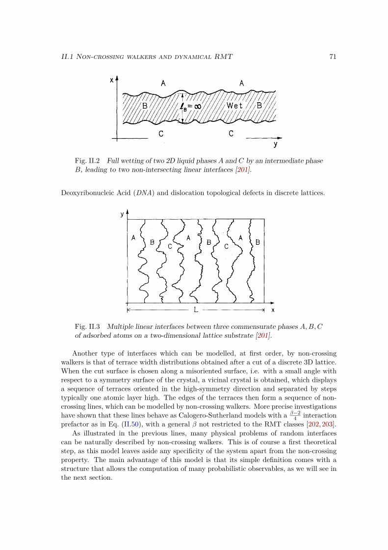
II.1 Non-crossing walkers and dynamical RMT 71
Fig. II.2 Full wetting of two 2D liquid phases A and C by an intermediate phaseB, leading to two non-intersecting linear interfaces [201].
Deoxyribonucleic Acid (DNA) and dislocation topological defects in discrete lattices.
Fig. II.3 Multiple linear interfaces between three commensurate phases A,B,Cof adsorbed atoms on a two-dimensional lattice substrate [201].
Another type of interfaces which can be modelled, at first order, by non-crossingwalkers is that of terrace width distributions obtained after a cut of a discrete 3D lattice.When the cut surface is chosen along a misoriented surface, i.e. with a small angle withrespect to a symmetry surface of the crystal, a vicinal crystal is obtained, which displaysa sequence of terraces oriented in the high-symmetry direction and separated by stepstypically one atomic layer high. The edges of the terraces then form a sequence of non-crossing lines, which can be modelled by non-crossing walkers. More precise investigationshave shown that these lines behave as Calogero-Sutherland models with a β−2
4 interactionprefactor as in Eq. (II.50), with a general β not restricted to the RMT classes [202,203].
As illustrated in the previous lines, many physical problems of random interfacescan be naturally described by non-crossing walkers. This is of course a first theoreticalstep, as this model leaves aside any specificity of the system apart from the non-crossingproperty. The main advantage of this model is that its simple definition comes with astructure that allows the computation of many probabilistic observables, as we will see inthe next section.

72 Chapter II. Non-crossing walkers and boundary problems
Before proceeding, let us note that another track of research on the physics of elasticinterfaces concerns avalanches that occur in a random environment when a force is gradu-ally applied to the interface [204–206]. For a presentation of the experimental, numericaland theoretical aspects of this field, see [207].
b) Non-crossing statistics
b) 1. Determinantal structure In order to derive analytical results on the statis-tics of non-crossing Brownian motions, a pivotal tool is the determinantal structure thatappears naturally in the joint probabilistic weight of non-crossing independent paths. Thiswas first realized by Samuel Karlin and James McGregor [208] such that the correspondingresult is now called the Karlin-McGregor theorem.
Karlin-McGregor To state this theorem, let us consider a continuous Markovprocess on the line, with transition probability density from x to y in time t given byP (y, t | x, 0). This is the PDF corresponding to the event where, starting from a knowninitial position x, the process is found at y after a time interval of t. Note that the stan-dard Brownian motion respects the above conditions, with P (y, t | x, 0) being the PDFof a variance-t Gaussian random variable as
P (y, t | x, 0) = 1√2πt
e−(y−x)2
2t . (II.54)
Let us further introduce (~x, ~y) ∈ (W∗N )2 respectively composed of N ordered distinctpositions on the real line.
The Karlin-McGregor theorem [208–210] states that for N independent processes dis-tributed as the one introduced above, the joint probability density for the N particles togo, without crossing each other, from ~x to ~y in time t is
PNC(~y, t | ~x, 0) = det16i,j6N
P (yi, t | xj , 0) (II.55)
See Fig. II.4 for an illustration of the walkers started from initial positions ~x and endingat positions ~y at time t, evolving along a non-crossing configuration.
This result is elegantly proven as we now describe, following [208]. Let us denote theN processes (Bi,τ )16i6N
06τ6tand assume that they verify Bi,0 = xi. For a permutation (k) of
[1. . N ], let us denote A(k) the event
A(k) = Bi,t = yki , ∀i ∈ [1. . N ] (II.56)
and ANC(k) the event where the non-crossing condition between 0 and t is added to theprevious definition
ANC(k) = A(k)⋂Bi,τ 6= Bj,τ , ∀i 6= j,∀τ ∈ [0, t] . (II.57)
The proof consists in showing the following equality:∑(k)
σ(k)P(A(k)
)=∑(k)
σ(k)P(ANC(k)
). (II.58)

II.1 Non-crossing walkers and dynamical RMT 73
Fig. II.4 Non-intersecting paths started from initial positions ~x and ending atpositions ~y at time t.
where P designates the probability density of these singular events, which is defined withrespect to the N -dimensional Lebesgue measure.
Assuming that this equality holds, the only admissible non-crossing contribution onthe r.h.s is the one where (k) is the identity permutation (id). For a continuous-pathprocess on the line, the particles must indeed have the same order at initial and finalconditions in order to be non-crossing, and the r.h.s of Eq. (II.58) is then simply equalto P
(ANC(id)
)= PNC(~y, t | ~x, 0). As a consequence of independence, we then have the
Karlin-McGregor formula:
PNC(~y, t | ~x, 0) =∑(k)
σ(k)N∏i=1
P (yki , t | xi, 0) = det16i,j6N
P (yj , t | xi, 0) . (II.59)
Finally, let us explain why Eq. (II.58) holds. In order to do this, let us fix (k) andchoose a specific crossing configuration of A(k). We denote τC the first crossing time ofthe configuration, such that τC is the smallest time where two particles i and j are suchthat Bi,τC = Bj,τC .
Denoting (k′) the same permutation with simply i and j inverted such that k′i = kjand k′j = ki, a configuration of A(k′) is naturally defined from our initial configurationas being exactly the same for τ < τC and the same up to i ↔ j inversion for τ > τC .From i.i.d. and Markov properties, the two configurations constructed above have thesame probabilistic weight.
The configuration transformation described above, and illustrated in Fig. II.5, is easilyseen to be an involution. As a consequence, any configuration of A(k) has a uniquecounterpart, which belongs to A(k′) where (k′) is such that σ(k′) = −σ(k). This ensuresby symmetry that all crossing configurations vanish from the l.h.s of Eq. (II.58) such thatthe equality holds.

74 Chapter II. Non-crossing walkers and boundary problems
⇐⇒
Fig. II.5 Schematics of the crossing configuration involution employed in theproof of the Karlin-McGregor theorem. Under this transformation, the first twocrossing particles i and j are inverted after their first crossing time τC . Theconfiguration on the right is crossing as well, since the positions of the particlescoincide at τC .
The general Karlin-McGregor theorem Eq. (II.58) holds in a higher-dimensional metricspace, where the r.h.s. cannot be reduced to the identity permutation as in the one-dimensional case. Another special case is obtained when placing the process on the circle,such that the r.h.s. is restricted to cyclic permutations.
Lindström-Gessel-Viennot In the setting of discrete combinatorics, the determi-nantal structure underpinning the enumeration of non-crossing paths on a general latticewas obtained by Bert Lindström [211] and developed by Ira Gessel and Xavier GérardViennot [212, 213]. In this context, the counterpart to the Karlin-McGregor theorem iscalled the Lindström-Gessel-Viennot theorem. For a process on a finite metric space,the combinatorial and probabilistic results are exactly equivalent. The continuous-spaceKarlin-McGregor result can thus be seen as an infinitesimal limit of the Lindström-Gessel-Viennot result.
The discrete result is most useful in applications to combinatorics of semi-standardYoung tableaux [214,215], as well as in random tilings and dimer models [39,142].
b) 2. Connections with random matrix theory The determinantal structurelaid out above will allow us to present the well-known links between non-crossing walkersand RMT: we will first detail the static links with the Gaussian ensembles before turningto the dynamical links with the DBM.
Links with Gaussian ensembles The links between non-crossing walkers andGaussian ensembles, first obtained from the mapping of discrete random walks to random
II.1 Non-crossing walkers and dynamical RMT 75
permutations [39,142,216,217], rest on the determinantal probabilistic structure grantedby the Karlin-McGregor theorem.
Let us consider N independent standard Brownian motions (Bi,t). The followingresults hold:
• Conditioning the walkers to be non-crossing on ]0, t], the joint positiondistribution at time t is given by the GOE eigenvalue JPDF with param-eter σ =
√t/2.
• Conditioning the walkers to be non-crossing on ]0,+∞[, the joint posi-tion distribution at time t is given by the GUE eigenvalue JPDF withparameter σ =
√t.
Note that, being standard Brownian motions, the processes are all started from 0, which issingular with respect to the non-crossing condition. However, the distributions describedabove can be shown to make sense in the conditional sense, as will be clear in the following.
Let us prove the GOE statement first for a given time t, by choosing the initialpositions as Bi,0 = xi = ε t zi with fixed ordered ~z ∈ WN . This regularization allows usto use the Karlin-McGregor formula before taking the ε → 0 limit. Let us introduce anotation for the event that particles are observed to be non-crossing on a certain intervalas
NC[a,b] = Bi,τ 6= Bj,τ , ∀τ ∈ [a, b],∀i 6= j . (II.60)With this notation, the JPDF of positions at time t, knowing the initial condition ~x andconditioned on the non-crossing property on ]0, t], is:
P(~y, t | ~x, 0,NC]0,t]
)=
det16i,j6N
P (xi, yj , t)∫RN d~z det
16i,j6NP (xi, zj , t)
. (II.61)
The numerator of this expression can be expressed in our Brownian setting as
det16i,j6N
P (xi, yj , t) = det16i,j6N
(1√2πt
e−(yj−xi)
2
2t
)= 1
(2πt)N2e−∑N
i=1x2i
+y2i
2t det16i,j6N
eyixjt
(II.62)where the determinant is det
16i,j6Neyixjt = det
16i,j6Neεyizj . As proven in App. C, the following
equivalent holds in the ε→ 0 limit:
det16i,j6N
eεyizj ' εN(N−1)
2∆(~z)∏N−1i=1 i!
∆(~y) . (II.63)
Removing all constants not depending on the positions ~y and removing εN(N−1)
2 factorsappearing both on the numerator and denominator of Eq. (II.61), the conditional JPDFis then, in the small-ε limit, proportional to:
P(~y, t | ~0, 0,NC]0,t]
)∝ |∆(~y)| e−
12t∑N
i=1 y2i (II.64)
In this equation, an absolute value has been harmlessly added as the ~y positions arenecessarily ordered from the non-crossing condition and the ordered initialization. As

76 Chapter II. Non-crossing walkers and boundary problems
claimed, this is the eigenvalue JPDF of the GOE with σ =√t/2, see Eq. (I.13). The
fact that it converges to a well-defined JPDF further proves well-posedness of the singularconditionment.
For the proof of the GUE case, we regularize the initial condition in the same fashion asabove. Consider that in order to condition the walkers to remain non-crossing on ]0,+∞[,we can consider first that this condition is verified until large time T where we can furtherassume that the walkers come back to their initial positions xi = εtzi. This artificialassumption is harmless, as the T →∞ limit will dissipate any influence of this constrainton the JPDF at fixed time t, and we leave the corresponding term P
(~x, T | ~x, 0,NC[0,T ]
)away in the next lines. The conditioned JPDF can then be decomposed, by the Markovproperty, into two parts:
P(~y, t | ~x, 0, ~x, T,NC[0,T ]
)∝ P
(~y, t | ~x, 0,NC[0,t]
)P(~x, T | ~y, t,NC[t,T ]
). (II.65)
The first term is directly given by the previous GOE computations leading to Eq. (II.64).The second term can be reduced to the same form by time-reversibility of the Brownianmotion as:
P(~0, T | ~y, t,NC[t,T ]
)= P
(~y, T − t | ~0, 0,NC[0,T−t]
)∝ ∆(~y) e
− 12(T−t)
N∑i=1
y2i
−−−−→T→∞
∆(~y) .(II.66)
In the (ε→ 0, T →∞) limit, the distribution at time t is then
P (~y, t | ~0, 0,NC]0,∞[) ∝ |∆(~y)|2 e−12t∑N
i=1 y2i (II.67)
which is, as claimed, the JPDF of the GUE with σ =√t, see Eq. (I.24).
Links with the Dyson Brownian motion We turn to the dynamical links of non-crossing walkers with the DBM, where we are interested in the law of the process instead ofits mere fixed-time distributions. In this scope, a central result is as follows [65,166,218] :
The law of N Brownian motions conditioned to never intersect is equal to thatof the DBM-2.
When conditioning to avoid crossings on ]0,+∞[, we have seen in the previous para-graph that fixed-time distributions of non-crossing walkers started from ~0 are equal tothat of the DBM with β = 2. The result cited above states that the two processes are infact identical.
In order to prove this result, let us first relate the propagator of the β = 2 DysonBrownian motion
PDBM (~y, t2 | ~x, t1) (II.68)with the one of vicious Brownian motions
P (~y, t2,NC[t1,t2] | ~x, t1) . (II.69)
Note that this propagator is the probability that the Brownian motions go from positions~x to ~y in time t2 − t1 and do not cross in the meantime. This can be directly expressed

II.1 Non-crossing walkers and dynamical RMT 77
by the Karlin-McGregor formula as a determinant of the one-particle propagators as inEq. (II.55). The Fokker-Planck equations respected by these one-particle propagators∂tP = 1
2∂2yP imply directly that
∂P (~y, t2,NC[t1,t2] | ~x, t1)∂t2
= 12
N∑i=1
∂2P (~y, t2,NC[t1,t2] | ~x, t1)∂y2
i
. (II.70)
In other words, vicious walkers respect the diffusion equation of independent Brownianmotions, as they should, with null boundary condition at the boundary of the Weylchamber.
Recalling the quantum mapping of the DBM in section II.1.1 b), we see that thisequation (II.70) is the same as the evolution of the auxiliary function in Eq. (II.44), inthe case of the DBM-2, with β = 2 and V = 0 where only the diffusion term remains.This correspondence allows us to express the vicious walker propagator as:
P (~y, t2,NC[t1,t2] | ~x, t1) = ∆(~x)∆(~y) PDBM (~y, t2 | ~x, t1) (II.71)
where the numerator ∆(~x) is needed to ensure that the initial conditions P (~y, t,NC[t,t] |~x, t) = PDBM (~y, t | ~x, t) = ∏N
i=1 δ(yi − xi) are verified.Finally, we relate this to our pursued process of Brownian motions conditioned to
never intersect. The propagator of this process is
P (~y, t2, | ~x, t1,NC[0,∞[) . (II.72)
This joint probability distribution function can be transformed by modifying the condi-tions and splitting the probabilities from Markov property as
P (~y, t2, | ~x, t1,NC[0,∞[) =P (~y, t2,NC[t1,t2],NC[t2,∞[ | ~x, t1)
P (NC[t1,∞[ | ~x, t1) (II.73)
=P (NC[t2,∞[ | ~y, t2)P (NC[t1,∞[ | ~x, t1)P (~y, t2,NC[t1,t2] | ~x, t1) (II.74)
We have transformed the propagator into the vicious walkers’ propagator with a prefactor.This prefactor presents ill-defined probabilities, but note that one could regularize with alarge time T →∞ such that the limit of the fraction is well-defined. By summing on allpossible configurations at the regularizing endtime T and through manipulations on theconditions, this limit can be obtained from Eq. (II.66) as
P (NC[t2,∞[ | ~y, t2)P (NC[t1,∞[ | ~x, t1) = ∆(~y)
∆(~x) (II.75)
such thatP (~y, t2, | ~x, t1,NC[0,∞[) = ∆(~y)
∆(~x) P (~y, t2,NC[t1,t2] | ~x, t1) . (II.76)
We can finally conclude that walkers conditioned to never intersect for t ∈ R+ and theDBM-2 are identical processes since their propagators are equal:
P (~y, t2, | ~x, t1,NC[0,∞[) = PDBM (~y, t2 | ~x, t1) (II.77)

78 Chapter II. Non-crossing walkers and boundary problems
Other links The analytical connections of non-crossing walkers extend beyond thefundamental examples given above. In the presence of a repulsive substrate, they areconnected to the Wishart ensembles of RMT [219]. Connections with the Gaussian andWishart ensembles have also been unveiled from the extremal properties of non-crossingwalkers [220–222]. On a larger scope, the reunion probabilities of non-crossing walkershave been mapped to the partition function of two-dimensional Yang-Mills theory on thesphere [223]. Finally, the applications of the model, further from the physical modellingof random interfaces, extend to computer science [224].
b) 3. Survival probability decay and first-passage As detailed above, non-crossing Brownian motions have deep links with random matrix theory. However, manyquestions of interest go beyond these situations where walkers are assumed to have nec-essarily survived. For example, a problem that has been widely studied [201, 225, 226] isthat of the decay of the survival probability.
The survival probability, at time t, of vicious walkers started at a given initial position~x, is obtained by summing the non-crossing probability on all possible endpoints as
S(t | ~x, 0) =∫RN
d~z P (~z, t,NC[0,t] | ~x, 0) . (II.78)
The quantity S(t | ~x, 0) depends on the details of the initial condition ~x but its large-time behaviour is universal. In this large-time limit, S(t) decays algebraically, i.e. as apower-law, according to
S(t) ' t−N(N−1)
4 (II.79)
where the exponent is known as the Fisher exponent [201, 214, 225]. We will prove thisstatement in a larger scope in the next section. Indeed, it will be a by-product of moregeneral computations related to the boundary problems.
Many peripheral results have been obtained on this topic. Survival probability com-putations have been extended to vicious walkers in a potential [227], and vicious walkersdivided in families such that family members are harmless with each other [228]. Otherinteresting aspects include the distribution of positions in certain situations such as theflat-to-flat boundary conditions [183] or with a vicious boundary, see next section, andextremal statistics of vicious walkers [218,229–233], see [114] for a review.
The survival probability for non-crossing walkers is a typical first-passage property ofthe multiple Brownian motion system. Indeed, it relies on a variable reaching a specificvalue for the first time, here the distance between two walkers reaching zero. The first-passage properties of a stochastic system are also called persistence properties, as theydescribe the statistics of remaining away from the given bound. For example, viciouswalkers persist in surviving as long as they remain away from each other, which happenswith vanishing probability S(t).
First-passage problems have been widely studied, see [234] for a mathematical re-view, and have found many applications in engineering and in physics, where persistenceproperties have attracted a lot of interest in the context of non-equilibrium statisticalmechanics of spatially extended systems, both theoretically and experimentally [199]. We

II.2 Vicious boundary 79
point to [198] for a pedagogical introduction to first-passage probabilities and relatedprocesses.
In many systems, such as stochastic diffusion in finite or semi-infinite domains, on theline or in higher dimensions, with spherical symmetry or in wedges [198], first-passageprobabilities decay algebraically as does the survival probability of vicious walkers inEq. (II.79). As a consequence many physical models where first-passage plays a role, fromcoarsening dynamics to fluctuating interfaces or polymer chains, present an algebraically-decaying persistence probability, in accordance with experiments [199]. The exponent ofthe algebraic decay, or persistence exponent, thus bears high theoretical and experimentalinterest, and will be the focus of next section in the setting of boundary problems.
II.2 Vicious boundaryIn this section, we turn to the study of vicious boundary problems for one-dimensionalwalkers, where a deterministic time-dependent moving boundary kills any walker thatreaches it. Such a vicious boundary can be seen in a pictorial way as a moving cliff[198], off which an unlucky walker will fall if he steps too far. For a unique Brownianmotion, this is a well-known problem in probability theory [185,235–237] and a lynchpinof first-passage processes [198, 238, 239]. Another broadly-studied problem is the cagemodel with two absorbing time-dependent boundaries [238, 240–242]. In statistics, thisversion is furthermore related to the Kolmogorov-Smirnov (KS) distribution test [243,244]: quantifying the survival probability in an expanding cage can be used to improvethe sensitivity of the KS test in the tails [245].
The Brownian motion diffusing below an absorbing moving boundary displays analgebraically decaying survival probability for a large range of boundary shapes. Aspresented in the first subsection II.2.1, the behaviour of the system depends on the speedof the moving boundary g(t) compared with the standard deviation of the Brownianmotion growing as
√t. In particular, it will be shown that the critical case is obtained
for a square-root boundary g(t) = W√t.
In publication (1), I studied an extension of this classical problem to non-crossingwalkers and investigated the survival probability exponent decay of vicious walkers undera square-root vicious boundary g(t) = W
√t, as presented in subsection II.2.2. From the
mapping presented in the previous section, these results can be applied to the DysonBrownian motion as developed in subsection II.2.3.
II.2.1 Single Brownian motion under a moving boundaryWe consider in this subsection a single Brownian motion (Bt)t>0, started from positionx, under a deterministic moving boundary g(t). We present the properties of the survivalprobability
S(t | x, 0) = P (Bτ < g(τ) , ∀τ ∈ [0, t] | B0 = x) (II.80)
and in particular the exponent of its algebraic decay, in different cases.

80 Chapter II. Non-crossing walkers and boundary problems
a) Fixed boundary: method of images
In the case of a fixed boundary g(t) = g, the symmetry of the problem grants us with anelegant solution through the method of images.
a) 1. Electrostatic image This method is well-known in the context of electro-statics [246]. Consider a point charge q facing a perfect planar conductor with fixedelectrostatic potential Φ = 0. What is the potential field in the half-space domain, fromthis charge distribution and boundary condition ?
The method of images consists in switching to an equivalent problem, where theplanar conductor is replaced by a mere point charge −q, located symmetrically from theinitial charge with respect to the conductor’s boundary, see Fig. II.6. This problem isequivalent at the level of the potential since it respects the same Poisson (or Maxwell-Gauss) equation in the half-space domain, and since the boundary condition Φ = 0 stillstands by symmetry. The electrostatic problem is greatly simplified by this change ofpoint of view: the equivalent formulation allows to conclude directly that, in the half-space, the potential is given by Φ = Φq + Φ−q where (Φq,Φ−q) are the potential fieldsgenerated by the two charges.
Fig. II.6 Electrostatic equivalence of the problem with a charge facing a perfectconductor (left) and the image-problem with two opposite charges (right) [246].
a) 2. Stochastic image As in the electrostatic situation, symmetry can be used inthe first-passage problem of a Brownian motion under a fixed boundary, in a stochasticmethod of images which relies on a similar equivalence. Let us introduce the followingnotation for the event where the Brownian motion remains below the boundary:
B[a,b] = Bτ < g(τ) , ∀τ ∈ [a, b] (II.81)
where the boundary is fixed in this section as g(τ) = g. The PDF for the walker, diffusingunder the vicious boundary, to be found at position y at time t after starting from initialposition x, is
P(y, t,B[0,t] | x, 0
)(II.82)

II.2 Vicious boundary 81
and verifies the diffusion evolution in the free half-space ]−∞, g[
∂ P(y, t,B[0,t] | x, 0
)∂t
= 12∂2 P
(y, t,B[0,t] | x, 0
)∂y2 (II.83)
with boundary conditionP(g, t,B[0,t] | x, 0
)= 0 . (II.84)
The method of images consists in removing the boundary, and considering two stan-dard Brownian motions started at the symmetrical positions x and 2g−x, with propagatorgiven in Eq. (II.54). The difference of their propagators Pdiff(y, t) = P (y, t | x, 0)−P (y, t |2g − x, 0) verifies by linearity
∂ Pdiff(y, t)∂t
= 12∂2 Pdiff(y, t)
∂y2 (II.85)
and Pdiff(g, t) = 0 by symmetry. It is thus the solution of the boundary problem:
P(y, t,B[0,t] | x, 0
)= 1√
2πt
(e−
(y−x)22t − e−
(y+x−2g)22t
)(II.86)
This solution can be explained intuitively through the reflection symmetry of theBrownian motion’s law. Consider an arbitrary path starting from initial position x attime 0 and ending at a given position y below the barrier at time t. If the path crossesthe boundary and τC is the first crossing time, a path can be constructed between 2g− xand x, by reflecting (Bτ )06τ6τC with respect to the g axis. Every crossing configurationfrom x to y then has an analogue configuration from 2g − x to y, of same probabilisticweight by reflection symmetry [158–160]. The non-crossing propagator is then given bythe difference (II.86). The construction is illustrated in Fig. II.7.
The Brownian motion considered here is driftless, but the method of images presentedabove can in fact be extended to the case of a boundary moving linearly in time, as toencompass the drifting Brownian motion with fixed boundary as well [198].
a) 3. Survival probability decay The survival probability can be obtained directlyfrom the analytic solution presented above, as
S(t | x, 0) =∫ g
−∞P(y, t,B[0,t] | x, 0
)= erf
(g − x√
2t
)(II.87)
where erf is the error function of the Gaussian distribution, defined by
erf(z) = 2√π
∫ z
0e−u
2du . (II.88)
From the asymptotics erf(ε) ' 2√πε for ε→ 0 [247], we have at large time:
S(t | x, 0) ' (g − x)√
2πt∝ t−
12 (II.89)

82 Chapter II. Non-crossing walkers and boundary problems
Fig. II.7 Crossing configuration from x to y (blue) and equivalent configurationfrom (2g − x) to y (orange before crossing time τC and blue afterwards). Bothconfigurations bear the same probabilistic weight by reflection symmetry of theBrownian motion.
We have recovered here the well-known power-law decay with exponent 12 of the survival
probability for a standard Brownian under a fixed absorbing boundary. See [198] for anin-depth presentation of the previous computations and other analogies between first-passage properties and electrostatics.
Note that the decay exponent found here is identical to the one of two vicious walkersin Eq. (II.79) with N = 2. Indeed, the difference of two independent Brownian motions isequal in law to
√2 times a Brownian motion. The system of two vicious walkers is then
equivalent to a single Brownian motion above a fixed boundary at 0.
b) Slow boundary: universal exponentLet us now consider a moving boundary, such that g(t) recovers its time-dependence. Letus further restrict it to having slow enough growth at infinity compared to the standarddeviation of the Brownian motion, which grows as
√t. Then, the decay exponent of the
survival probability is the same as the above result for a fixed barrier. The exponent 12 is
thus universal for slow boundaries:
Sslow(t) ∝ t−1/2 . (II.90)
More precisely, Uchiyama showed in [248] that this exponent holds for g continuousand either concave or convex, respecting the following condition∫ ∞
1|g(τ)| τ−3/2 dτ <∞ . (II.91)
This covers in particular all power-law barriers slower than√t:
g(t) = Wtα with α <12 , (II.92)

II.2 Vicious boundary 83
such that the boundary motion is asymptotically irrelevant in these cases, and the large-time behaviour is identical to the fixed-boundary case.
Although the exact solution for an arbitrary slow boundary cannot be derived by theimage method presented above, the large-time behaviour can be heuristically obtainedby a quasi-static (or adiabatic) approximation. Since the boundary is slow, the PDF isexpected to be linear on a region of scale
√t close to the boundary. Further away, the
particle is expected to diffuse independently of the boundary. Matching these two regionsyields the square-root decay of the total surviving probability, in the slow-boundary case[198].
c) Fast boundary
For a fast boundary, compared with the√t expansion rate, the behaviour is also very
simple.For a fast boundary with positive velocity, receding away from the walker, the survival
probability does not decay but instead converges to a non-zero limit, asS>fast(t)→ S∞ > 0 (II.93)
where S∞ can be calculated explicitly in some cases [240].For a fast boundary with negative velocity, approaching the walker as g(t) = −Atα
with α > 12 , the survival probability vanishes faster than any power law as [198]
S<fast(t) ∝ e−A t2α−1
. (II.94)
d) Critical square-root boundaryAs seen in the previous paragraphs, the algebraic decay of the survival probability is verysimple if the boundary is either slow or fast. The interesting case, at the level of the decayexponent, thus concerns the critical square-root boundary
g(t) = W√t . (II.95)
In this case, the survival probability is characterized by a non-universal decay exponentβ(W ) which depends on the boundary prefactor W , such that [198,235,238,242,248]
SW (t) ∝ t−β(W ) (II.96)
The survival exponent β(W ) can be computed for a general value of W as the smallestroot of the following equation
D2β(W )(−W ) = 0 (II.97)where Dν(x) is the parabolic cylinder function of index ν, see App. B. This exponent hasthe following asymptotics [247]
β(W ) −→
12 as W → 0 ;
0 as W → +∞ ;+∞ as W → −∞ .
(II.98)
We see that these asymptotics match the behaviour of the slow and fast boundariesdescribed above.

84 Chapter II. Non-crossing walkers and boundary problems
II.2.2 Non-crossing walkers under a square-root boundaryIn the previous sections, we have described the decay of the survival probability of viciouswalkers, see Eq. (II.79), and the decay of the survival probability of a single Brownianmotion under a moving boundary, see Eq. (II.96). It is thus natural to extend and reunitethese problems, and study the properties of N non-crossing walkers under a square-rootboundary, shown in the single-particle case to be the critical setting of interest. Thiswas done in publication (1), the results of which we present here. This study gives exactresults on a system of interacting particles in the presence of a time-dependent externalpotential, which is a central generic problem in non-equilibrium statistical physics, bothfor classical and quantum systems.
In the following, the moving boundary is g(t) = W√t as in Eq. (II.95). The N walkers
are independent Brownian motions (Bi,t)16i6N06t
. The main object of interest will be thesurvival probability between times t0 and t, defined as
S(t | ~x, t0) = P(NC[t0,t] , B[t0,t] | ~Bt0 = ~x
)(II.99)
where NC[t0,t] is the event that the N walkers do not touch each other as in Eq. (II.60),B[t0,t] is the event that none of the walkers touches the boundary g as in Eq. (II.81),and where the initial condition is fixed at starting time t0 by the N positions ~x. Aconfiguration of non-crossing walkers under a square-root boundary is illustrated in Fig.II.8.
Fig. II.8 Configuration of N = 6 Brownian motions which remain non-crossingamong each other and with the square-root boundary, between times t0 and t.
The starting time t0 > 0 introduced above is useful to regularize the survival proba-bility: for t0 → 0, the probability that N Brownian motions started from the same pointdo not cross vanishes. The same can be said about their crossing of the boundary asg(0) = 0. As in the single-particle case, the choice of initial positions ~x is not significantin the large-time limit.

II.2 Vicious boundary 85
As can be expected from the previous sections, the main result presented in thefollowing is that the survival probability of this system behaves for large time as
S(t | ~x, t0) ∝ t−β(N,W ) (II.100)
where the exponent β(N,W ), which depends on the prefactor of the square-root boundaryand on the number of walkers, is the ground-state energy of a quantum system as shownbelow.
a) Mapping to fermions in a quadratic potential
The stochastic system described above can be mapped to a quantum system of fermionsin a quadratic potential, after a first mapping to Ornstein-Uhlenbeck processes called theLamperti mapping.
a) 1. Lamperti mapping The Lamperti mapping states that a standard Brownianmotion Bt and an Ornstein-Uhlenbeck process MT with restoring coefficient 1
2 are relatedby the following correspondence
Mlog(t) ∼law
Bt√t. (II.101)
Indeed, applying Itô’s formula on the process
MT = e−T2 BeT (II.102)
yields
dMT = −e−T2
2 BeT dT + e−T2 dBeT = −MT
2 dT + dBT (II.103)
such that (MT )06T is an OU process with restoring coefficient 12 . The mapping is named
in reference to the fact that it is a special case of Lamperti’s transformations for scale-invariant self-similar stochastic processes applied to the Brownian Motion [249,250]. Thismapping is also sometimes called Doob’s transform [236], since it is given by the applica-tion of Doob’s transformation theorem [185] to the OU process.
The interest of this transformation is that it maps our system of non-crossing Brownianmotions under a square-root barrier g(t) = W
√t to a system of non-crossing Ornstein-
Uhlenbeck processes under a fixed barrier atW . Indeed, the processesMi,T , obtained as inEq. (II.102) from the Brownian motions Bi,t, remain below a fixed barrier atW if and onlyif the Bi,t remain below g(t). This trick was used by Breiman in [235] to study a similarproblem for a single particle, and in later works in the physics literature [199,227,239,251].Furthermore, the processes Mi,T are non-crossing if and only if the initial processes Bi,tare. The survival probabilities of both systems are thus equal.
More precisely, let us relate the propagators of the two systems. The propagator ofthe vicious walkers killed by the boundary is
P(~y, t,NC[t0,t],B[t0,t] | ~x, t0
)(II.104)

86 Chapter II. Non-crossing walkers and boundary problems
which, we recall, is the probability density for N walkers to go from ~x to ~y and survive.We denote
POU(~Y , T,NC[T0,T ],B[T0,T ] | ~X, T0
)(II.105)
the propagator of N vicious OU processes independently obeying SDE (II.103), wherethe notations are similar as above with the boundary now fixed at W . By the Lampertimapping, the propagators are related as
P(~y, t,NC[t0,t],B[t0,t] | ~x, t0
)d~y = POU
(~Y , T,NC[T0,T ],B[T0,T ] | ~X, T0
)d~Y (II.106)
wheret = eT t0 = eT0
~Y = ~y√t
~X = ~x√t0.
(II.107)
a) 2. Quantum mapping In the spirit of section II.1.1 b), the stochastic systemof N vicious OU processes can be mapped to a many-body quantum system of non-interacting fermions.
Single-particle mapping The OU process obeying SDE (II.103), i.e. Eq. (II.27)with V (x) = x2
4 and D = 12 , is mapped by Eq. (II.35) to a quantum system with Hamil-
tonianH = −1
2∂2
∂X2 + 18X
2 − 14 . (II.108)
The wavefunctions φk(X) of this quadratic potential are given in Eq. (I.157). Taking intoaccount the −1
4 translation, the corresponding energy levels are εk = k2 .
Hard wall An additional element of our system of vicious OU walkers is the pres-ence of the wall, which imposes that the position PDF vanishes at position W . In aquantum system, an equivalent boundary condition is imposed by an infinite potentialin the forbidden region. For a single particle, the presence of the boundary thus simplychanges the above quantum Hamiltonian to
HW =
−12∂2
∂X2 + 18X
2 − 14 for X < W ,
+∞ for X >W .
(II.109)
Let us denote (φWk , εWk )k>0 the normalized wavefunctions and corresponding energy levelsof this Hamiltonian, such that the dependence on the position of the hard wall is madeexplicit.
Multiple walkers Finally, as illustrated by the DBM in section II.1.1 b), the non-crossing property of a vicious stochastic system directly leads, in the stochastic to quan-tum mapping, to the fermionic symmetry of a many-body quantum system. As a conse-quence, the vicious OU processes under an absorbing boundary at W are mapped to a

II.2 Vicious boundary 87
system of N non-interacting fermions in the Hamiltonian
H =N∑i=1
HWi (II.110)
where HWi is obtained by replacing X → Xi in Eq. (II.109).
The N -particle mapping can be proven at propagator level as we detail now. Thepropagator of the vicious OU walkers below the boundary, defined in Eq. (II.105), is equalby the Karlin-McGregor theorem to the determinant of the one-particle OU propagatorsunder the boundary as
POU(~Y , T,NC[T0,T ],B[T0,T ] | ~X, T0
)= det
16i,j6NPOU
(Yj , T,B[T0,T ] | Xi, T0
). (II.111)
The single-particle propagator mapping of Eq. (II.37) yields
POU(~Y , T,NC[T0,T ],B[T0,T ] | ~X, T0
)= e− 1
4
N∑i=1
(Y 2i −X
2i )
det16i,j6N
G(Yi, T |Xj , T0) (II.112)
whereG is the quantum propagator of the quantum system with Hamiltonian HW , definedby
G(Y, T | X,T0) = 〈Y | e−(T−T0)HW |X〉 =∑k>0
φWk (Y )φWk∗(X)e−εWk (T−T0) . (II.113)
By the discrete Cauchy-Binet formula, the determinant is given by
det16i,j6N
G(Yi, T |Xj , T0) = 1N !
∑k1,··· ,kN>0
det16i,j6N
φWki (Yj) det16i,j6N
φWki∗(Xj)e
−(T−T0)N∑=1εWk`
(II.114)where the r.h.s. is related to the quantum propagatorGN (~Y , T | ~X, T0) ofN non-interactingfermions with Hamiltonian H defined in Eq. (II.110). Indeed, the N -particle wavefunc-tion ΨW
~k( ~X) are given by a Slater determinant, see Eq. (I.151), and the corresponding
energy level is εW~k =N∑=1εWk` . With a symmetry factor N ! from the order constraint in the
admissible set of eigenstates ΩN defined in Eq. (I.153), we have:
1N ! det
16i,j6NG(Yi, T |Xj , T0) =
∑~k∈ΩN
ΨW~k
(~Y ) ΨW~k
∗( ~X) e−(T−T0) εW~k = GN (~Y , T | ~X, T0) .
(II.115)The N -particle stochastic and quantum propagators are finally related as
POU(~Y , T,NC[T0,T ],B[T0,T ] | ~X, T0
)= N ! e
− 14
N∑i=1
(Y 2i −X
2i )GN (~Y , T | ~X, T0) . (II.116)
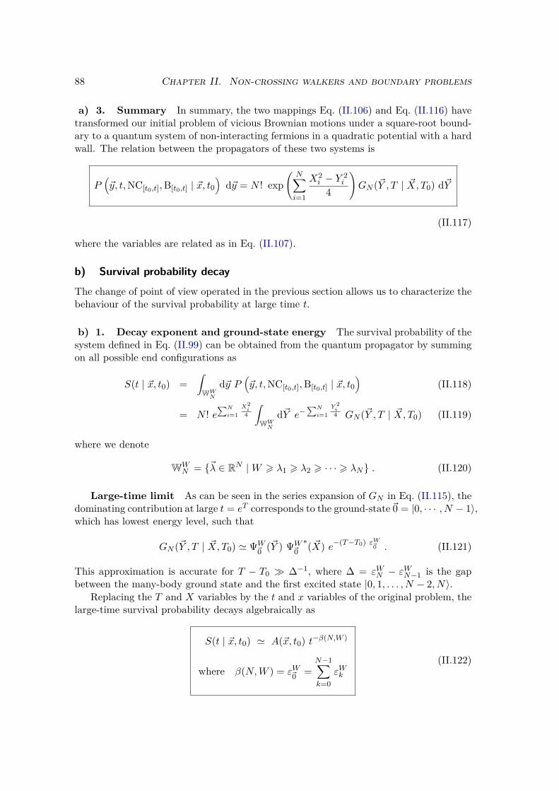
88 Chapter II. Non-crossing walkers and boundary problems
a) 3. Summary In summary, the two mappings Eq. (II.106) and Eq. (II.116) havetransformed our initial problem of vicious Brownian motions under a square-root bound-ary to a quantum system of non-interacting fermions in a quadratic potential with a hardwall. The relation between the propagators of these two systems is
P(~y, t,NC[t0,t],B[t0,t] | ~x, t0
)d~y = N ! exp
(N∑i=1
X2i − Y 2
i
4
)GN (~Y , T | ~X, T0) d~Y
(II.117)
where the variables are related as in Eq. (II.107).
b) Survival probability decay
The change of point of view operated in the previous section allows us to characterize thebehaviour of the survival probability at large time t.
b) 1. Decay exponent and ground-state energy The survival probability of thesystem defined in Eq. (II.99) can be obtained from the quantum propagator by summingon all possible end configurations as
S(t | ~x, t0) =∫WWN
d~y P(~y, t,NC[t0,t],B[t0,t] | ~x, t0
)(II.118)
= N ! e∑N
i=1X2i
4
∫WWN
d~Y e−∑N
i=1Y 2i4 GN (~Y , T | ~X, T0) (II.119)
where we denote
WWN = ~λ ∈ RN |W > λ1 > λ2 > · · · > λN . (II.120)
Large-time limit As can be seen in the series expansion of GN in Eq. (II.115), thedominating contribution at large t = eT corresponds to the ground-state~0 = |0, · · · , N − 1〉,which has lowest energy level, such that
GN (~Y , T | ~X, T0) ' ΨW~0 (~Y ) ΨW
~0∗( ~X) e−(T−T0) εW
~0 . (II.121)
This approximation is accurate for T − T0 ∆−1, where ∆ = εWN − εWN−1 is the gapbetween the many-body ground state and the first excited state |0, 1, . . . , N − 2, N〉.
Replacing the T and X variables by the t and x variables of the original problem, thelarge-time survival probability decays algebraically as
S(t | ~x, t0) ' A(~x, t0) t−β(N,W )
where β(N,W ) = εW~0 =N−1∑k=0
εWk
(II.122)

II.2 Vicious boundary 89
and with
A(~x, t0) = N ! e∑N
i=1x2i
4t0 ΨW~0∗( ~x√
t0) t
εW~0
0
∫WWN
d~Y e−∑N
i=1Y 2i4 ΨW
~0 (~Y ) . (II.123)
As announced earlier, the survival probability of our problem decays as a power-law, witha decay exponent characterized as the ground-state energy of a system of non-interactingfermions with Hamiltonian H of Eq. (II.110).
Simple cases The exponent β(N,W ) can be obtained straightforwardly in a fewspecial cases.
• In the limit W → +∞:HW tends to H, the simple harmonic oscillator hamiltonian without a wall, whichhas energy levels ε∞k = εk = k
2 , such that
limW→+∞
β(N,W ) =N−1∑k=0
k
2 = N(N − 1)4 . (II.124)
This proves the Fisher exponent announced in Eq. (II.79), which characterizes thedecay of the survival probability for vicious walkers without a boundary.
• If W = 0:With respect to the previous case, the hard wall imposes a cancellation of thewavefunction at W = 0, such that the wavefunctions are simply the odd wave-functions of the harmonic oscillator. The ground-state energy is then obtained bypopulating the first N odd levels of the free harmonic oscillator:
β(N,W = 0) =N−1∑k=0
2k + 12 = N2
2 . (II.125)
This exponent characterizes the survival probability’s decay for vicious walkers un-der a fixed boundary, recovering the results of [215,252].
• In the limit W → −∞:The wall is very far to the left of the center at a potential energy V (W ) = W 2
8 .Expanding X = W + X for small X < 0 the potential energy is V (X) = W 2
8 +W4 X + O(W 0). The energy levels are therefore equal to those of a particle in alinear potential with a slope W
4 and confined on the negative axis. These single-particle energy levels are given by
εWk = W 2
8 − 125/3αk+1|W |2/3 (II.126)
where αm is the mth zero of the Airy function, see App. B. Hence we find thefollowing asymptotics for β(N,W ) for fixed N and W → −∞
β(N,W ) ' NW 2
8 −AN |W |2/3 , AN = 125/3
N∑m=1
αm . (II.127)

90 Chapter II. Non-crossing walkers and boundary problems
This limit is treated at length in chapter IV, in the context of non-crossing bridges.We simply remark that the eigenfunctions are Airy functions centered at Xk =αk+1(2/W )1/3 which is much smaller than |W | for fixed k and W → −∞. As aconsequence, one can indeed neglect the term ∝ X2 = O(1) in the potential andthe linear potential approximation becomes exact.
General W For a general value of the wall’s position W , the single-particle energylevels εWk can be expressed as follows. The spectrum of the single particle HamiltonianHW is obtained by solving the eigenvalue equation with a Dirichlet boundary conditionat X = W
HWφ = εφ ⇐⇒
∂2φ∂X2 + (2ε+ 1
2 −14X
2)φ = 0 for X < W
φ(W ) = 0 , φ(−∞) = 0 .(II.128)
The solution of the differential equation, which vanishes as X → −∞, is the paraboliccylinder function
φ(X) = C D2ε(−X) (II.129)
with C a normalization constant. The boundary condition atW quantizes the eigenvaluesε = εWk according to the equation
D2ε(−W ) = 0 . (II.130)
The energy levels (εWk )k>0 are thus given by the ordered sequence of solutions of thisequation. The corresponding wavefunctions are
φWk (X) = CkD2εWk
(−X) . (II.131)
As an illustration, D2ε(−W ) is plotted as a function of ε in Fig. II.9, for a given valueof W = 6. The first 11 zeros can be seen, and the amplitude of the oscillations quicklyincreases. We note that the first seven levels are very close to what would be expected fora harmonic oscillator (0, 1
2 , 1,32 , 2,
52 , 3), but that the following levels start deviating from
the k2 levels, as the effect of the hard wall becomes more important for large ε.For general W , the decay exponent β(N,W ) is given in Eq. (II.122) as the sum of the
first N solutions of Eq. (II.130). We recover from this result the exponent β(W ) for thespecial case N = 1, as announced in Eq. (II.97).
The decay exponent β(N,W ) can be profitably studied in some limiting cases, furtherfrom the simple situations described in the previous section. In the following, we describefirstly the perturbative analysis that can be developed for W ∼ 0, and secondly thesemi-classical scaling obtained for large N with W = O(
√N).
b) 2. Perturbative expansion for the slow boundary For a slow boundary|W | 1, i.e. when the hard wall is close to the minimum of the harmonic trap, we cancalculate the energy levels εWk and the exponent β(N,W ) perturbatively.
When W = 0 precisely, the spectrum is composed of the odd eigenstates of the freeharmonic oscillator with wavefunctions φ2k+1(x) and energies ε0
k = ε2k+1 = (2k+1)2 , as
explained in Eq. (II.125).

II.2 Vicious boundary 91
1 2 3 4 5
-150
-100
-50
50
100
150
Fig. II.9 Plot of the function D2ε(−W ) versus ε for W = 6. Note the firstcancellation close to ε = 0.
For |W | 1, let us change variables to Y = X −W ∈] −∞, 0], such that the hardwall is at the origin in the new frame. In the Y -coordinate the Hamiltonian becomes
H ′ = −12∂2
∂Y 2 + 18(Y +W )2 − 1
4 = HW=0 +W∆H + 18W
2 , (II.132)
with ∆H = 14Y . The energy levels of the perturbed hamiltonian H ′ can be obtained by
perturbation theory [94] as explained in Eq. (II.8). The energy level εWk is thus given, upto second order in W , by:
εWk − εW=0k = ∆Ek = ∆E(1)
k W + ∆E(2)k W 2 + 1
8W2 +O(W 3) (II.133)
with ∆E(1)
k = 〈2k + 1|∆H |2k + 1〉
∆E(2)k =
∑k′>0,k′ 6=k
∣∣∣〈2k′ + 1|∆H |2k + 1〉∣∣∣2
ε2k+1 − ε2k′+1
(II.134)
where (|2k + 1〉)k>0 denote the odd levels of the free harmonic oscillator, however normal-ized to unity over the half-space R−. Computing the matrix elements on the half-space,see (1), one obtains explicitly
∆E(1)k = − 1√
2π22k(2k+1)!k!2
∆E(2)k = (2k+1)!
π 22k+1 (k!)2∑
k′>0,k′ 6=k
1k−k′
(2k′+1)!22k′ (k′!)2
1(4(k−k′)2−1)2
(II.135)
One can show that the intricate expression for ∆E(2)k has a simple limit
limk→∞
∆E(2)k = 1
π2 −18 = −0.0236788 . . . (II.136)

92 Chapter II. Non-crossing walkers and boundary problems
The decay exponent β(N,W ) =N−1∑k=0
εWk is then obtained, in the small-W limit withfixed N , as
β(N,W ) = N2
2 −W√
23√π
122N
N(2N + 1)!(N !)2 +W 2
(N−1∑k=0
∆E(2)2k+1 + N
8
)+O(W 3) . (II.137)
Note that we recover the limit result of Eq. (II.125). Specialising this formula to the caseN = 1, we obtain
β(N = 1,W ) = 12 −
W√2π
+ 1− log 2π
W 2 +O(W 3) (II.138)
which is in agreement with the first order result β(1,W ) = 12 −
W√2π + O(W 2) obtained
in [238]. Note that the constant coefficient 12 is the universal exponent discussed in length
in section II.2.1. Details on the Taylor coefficients for general N are given in (1).
b) 3. Semi-classical scaling We consider now the limit when N and |W | = O(√N)
are simultaneously large. In this regime, the quantum system can be analyzed in a semi-classical approximation, which is asymptotically exact.
In this large-N limit, the key quantity is the density ρ(ε) of single-particle energylevels of the system with Hamiltonian HW in Eq. (II.109). Formally, it is defined by
ρ(ε) =∑k>0
δ(ε− εWk ) . (II.139)
Denoting εF the highest occupied level in the N -particle ground-state (or Fermi energy),we have
N =∫ εF
0dε ρ(ε) . (II.140)
The decay exponent β(N,W ) is the ground-state energy, given by
β(N,W ) =∫ εF
0dε ε ρ(ε) . (II.141)
Hence β(N,W ) is obtained from the knowledge of the level density ρ, by eliminating εFfrom these two equations (II.140) and (II.141).
The density of states can be approximated semi-classically in the large-N limit [94,253–255]. Under the semi-classical approximation, εk, the kth energy level of a quan-tum particle under potential V , satisfies the Bohr-Sommerfeld quantization condition∫X2X1
p(X)dX = kπ with the classical momentum p(X) =√
2(εWk − V (X)) and whereX1 < X2 are the turning points of the classical trajectories.
In our problem, the potential can be approximated to V (X) ' X2
8 since the in-tegrals are dominated by large values of X ∼
√N and we have X1 = −
√8ε and
X2 = min(√
8ε,W ), as illustrated in Fig. II.10. For the kth level, this leads to thecondition ∫ min(
√8εWk,W )
−√
8εWk
√2(εWk −
X2
8
)dX = kπ . (II.142)
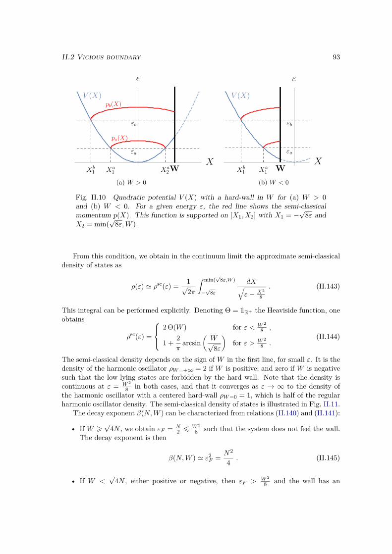
II.2 Vicious boundary 93
(a) W > 0 (b) W < 0
Fig. II.10 Quadratic potential V (X) with a hard-wall in W for (a) W > 0and (b) W < 0. For a given energy ε, the red line shows the semi-classicalmomentum p(X). This function is supported on [X1, X2] with X1 = −
√8ε and
X2 = min(√
8ε,W ).
From this condition, we obtain in the continuum limit the approximate semi-classicaldensity of states as
ρ(ε) ' ρsc(ε) = 1√2π
∫ min(√
8ε,W )
−√
8ε
dX√ε− X2
8
. (II.143)
This integral can be performed explicitly. Denoting Θ = 1R+ the Heaviside function, oneobtains
ρsc(ε) =
2 Θ(W ) for ε < W 2
8 ,
1 + 2π
arcsin(W√8ε
)for ε > W 2
8 .(II.144)
The semi-classical density depends on the sign of W in the first line, for small ε. It is thedensity of the harmonic oscillator ρW=+∞ = 2 if W is positive; and zero if W is negativesuch that the low-lying states are forbidden by the hard wall. Note that the density iscontinuous at ε = W 2
8 in both cases, and that it converges as ε → ∞ to the density ofthe harmonic oscillator with a centered hard-wall ρW=0 = 1, which is half of the regularharmonic oscillator density. The semi-classical density of states is illustrated in Fig. II.11.
The decay exponent β(N,W ) can be characterized from relations (II.140) and (II.141):
• If W >√
4N , we obtain εF = N2 6 W 2
8 such that the system does not feel the wall.The decay exponent is then
β(N,W ) ' ε2F = N2
4 . (II.145)
• If W <√
4N , either positive or negative, then εF > W 2
8 and the wall has an

94 Chapter II. Non-crossing walkers and boundary problems
1 2 3 4 5 6
0.5
1.0
1.5
2.0
Fig. II.11 Plot of the semi-classical density of states ρscW (ε) versus the energy
ε in units of W 2
8 , in both cases W > 0 and W < 0. For large ε, both branchesconverge to ρW=0 = 1.
influence on the system. One then obtains the following system
N = W√
8εF −W 2
4π +2εF arcsin
(W
2√
2εF
)π
+ εF ,
β(N,W ) ' NεF2 − W
96π(8εF −W 2
) 32 .
(II.146)
In conclusion, the decay exponent β(N,W ) takes the following scaling form in the limit(N,W )→ +∞ with y = W√
4N fixed:
β(N,W ) ' N2
4 b(
W√4N
)(II.147)
with the scaling function b is given by b(y) = 1 for y > 1 ,
b(y) = y2(
1u2 − 2
3πy2 (1−u2)3/2
u3
)for y < 1 ,
(II.148)
where in the second line u = W√8εF∈ [−1, 1] is obtained in terms of y by solving
1y2 = 1
2u2 +√
1− u2
πu+ arcsin(u)
πu2 . (II.149)
The semi-classical scaling function b is plotted numerically in Fig. II.12, along with itsasymptote 2y2 + 3
53√2(3π)2/3y2/3 for large negative argument. Details on the asymptotics
of b(y) as y → 1−, y → 0 and y → −∞ can be found in (1). In particular, there is a 52
th
order non-analyticity at y = 1, where the wall starts to be felt by the system.In the last sections, we have shown how the knowledge of the decay exponent can be
refined in the cases of slow barrier and large-N limit with W = O(√N). Other limits can
also be investigated from the asymptotics of roots of parabolic cylinder functions, as thelarge-N limit for fixed W , see (1).
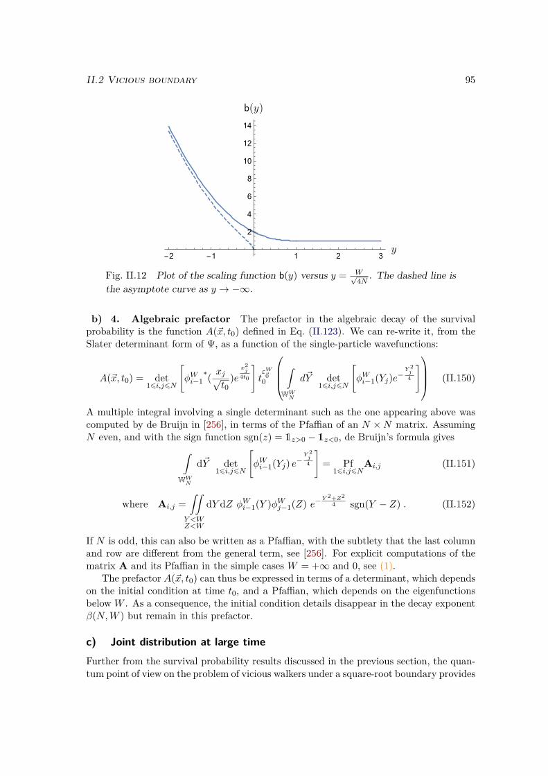
II.2 Vicious boundary 95
-2 -1 1 2 3
2
4
6
8
10
12
14
Fig. II.12 Plot of the scaling function b(y) versus y = W√4N . The dashed line is
the asymptote curve as y → −∞.
b) 4. Algebraic prefactor The prefactor in the algebraic decay of the survivalprobability is the function A(~x, t0) defined in Eq. (II.123). We can re-write it, from theSlater determinant form of Ψ, as a function of the single-particle wavefunctions:
A(~x, t0) = det16i,j6N
[φWi−1
∗( xj√t0
)ex2j
4t0
]tεW~0
0
∫WWN
d~Y det16i,j6N
[φWi−1(Yj)e−
Y 2j4
] (II.150)
A multiple integral involving a single determinant such as the one appearing above wascomputed by de Bruijn in [256], in terms of the Pfaffian of an N ×N matrix. AssumingN even, and with the sign function sgn(z) = 1z>0 − 1z<0, de Bruijn’s formula gives∫
WWN
d~Y det16i,j6N
[φWi−1(Yj) e−
Y 2j4
]= Pf
16i,j6NAi,j (II.151)
where Ai,j =∫∫
Y <WZ<W
dY dZ φWi−1(Y )φWj−1(Z) e−Y 2+Z2
4 sgn(Y − Z) . (II.152)
If N is odd, this can also be written as a Pfaffian, with the subtlety that the last columnand row are different from the general term, see [256]. For explicit computations of thematrix A and its Pfaffian in the simple cases W = +∞ and 0, see (1).
The prefactor A(~x, t0) can thus be expressed in terms of a determinant, which dependson the initial condition at time t0, and a Pfaffian, which depends on the eigenfunctionsbelow W . As a consequence, the initial condition details disappear in the decay exponentβ(N,W ) but remain in this prefactor.
c) Joint distribution at large timeFurther from the survival probability results discussed in the previous section, the quan-tum point of view on the problem of vicious walkers under a square-root boundary provides

96 Chapter II. Non-crossing walkers and boundary problems
the joint distribution of the surviving walkers, at large time.
c) 1. Arbitrary W At large time, from approximation (II.121), the stochastic prop-agator is obtained from the quantum propagator in Eq. (II.117) such that
P(~y, t,NC[t0,t],B[t0,t] | ~x, t0
)' N ! t
εW~0
0
tεW~0
+N2
ΨW~0 ( ~y√
t) ΨW
~0∗( ~x√
t0) e∑N
i=1x2i
4t0−y2i
4t (II.153)
where the additional factor of tN/2 arises from the Jacobian of the transformation fromYi to yi/
√t. With the expression of the single-particle wavefunctions for general W in
Eq. (II.131), this propagator can be expressed formally in terms of parabolic cylinderfunctions as
P(~y, t,NC[t0,t],B[t0,t] | ~x, t0
)' C
tN2
(t0t
)β(N,W )det
16i,j6ND2εWi−1
(− yj√t) det
16i,j6ND2εWi−1
∗(− xj√t0
) e∑N
i=1x2i
4t0−y2i
4t
(II.154)
with C = ∏Ni=0C
2k from the normalization constants defined in Eq. (II.131). As a conse-
quence, keeping only terms that depend on ~y, the joint distribution of surviving walkersat time t is given by
P(~y, t | NC[t0,t],B[t0,t], ~x, t0
)= K e−
14t∑N
i=1 y2i det
16i,j6ND2εWi−1
(− yj√t) . (II.155)
The normalization constant K is the ratio of the terms in Eq. (II.154) that do not dependon ~y over the survival probability S (t | ~x, t0), and decays as t−N2 such that the jointdistribution is normalized.
The JPDF of surviving vicious walkers in Eq. (II.155) can be evaluated in the caseswhere the wavefunctions are simple.
c) 2. W → +∞ In this case, the wavefunctions are simply those of the harmonicoscillator, see Eq. (I.157), such that the JPDF is
P(~y, t | NC[t0,t],B[t0,t], ~x, t0
)∝ e−
14t∑N
i=1 y2i det
16i,j6N
(Hi−1(− yj√
t)e−
y2j
4t
)(II.156)
∝ |∆(~y)| e−12t∑N
i=1 y2i . (II.157)
In the boundary-less settingW → +∞, we recover the GOE eigenvalue JPDF as discussedin section II.1.2 b) and proven in Eq. (II.64).
c) 3. W = 0 In this case, the wavefunctions are the odd ones of the harmonicoscillator, such that the JPDF is
P(~y, t | NC[t0,t],B[t0,t], ~x, t0
)∝ e−
14t∑N
i=1 y2i det
16i,j6N
(H2i−1(− yj√
t)e−
y2j
4t
)(II.158)

II.2 Vicious boundary 97
and can be shown, see (1), to be proportional to
P(~y, t | NC[t0,t],B[t0,t], ~x, t0
)∝
N∏i=1|yi|
∣∣∣∣∆(−→y2)∣∣∣∣ e− 1
2t∑N
i=1 y2i (II.159)
where ∣∣∣∣∆(−→y2)∣∣∣∣ =
∏16i<j6N
(y2j − y2
i
). (II.160)
Note that this JPDF (II.159) is identical to the one for the eigenvalues λi of the LOE,see Eq. (I.48), with the correspondence λi = y2
i and by fixing T = N + 1. In the large-Nlimit, this yields q = 1 such that the limit density in the bulk is given by the quarter-circledistribution (I.88), with σ =
√t. Similar results were obtained in [252], where vicious
walkers were studied under a fixed wall.
II.2.3 Application: Dyson Brownian motion under an absorbingboundary
As discussed at the beginning of this chapter, non-crossing walkers share deep links withthe Dyson Brownian motion of index β = 2. The results presented above for the behaviourof non-crossing walkers under a moving boundary can, as a consequence, be applied tothe DBM-2 under the same boundary g(t) = W
√t.
The process of interest is now (λi,t)16i6N,t>0, the eigenvalues of H2t in Eq. (II.2). Since
the DBM eigenvalues almost-surely never touch, the only source of danger for the walkersis the vicious moving boundary. We denote the survival probability of this system as
SDBM (t | ~x, t0) = PDBM(B[t0,t] | ~λt0 = ~x
)(II.161)
where the notations are similar to those of the previous sections.
a) Square-root boundaryRecall the mapping between the propagators of vicious walkers and the DBM-2 in Eq. (II.71).One can show that this propagator relation holds in the presence of a moving boundaryas well, see Appendix F of (1), such that
PDBM (~y, t,B[t0,t] | ~x, t0) = ∆(~y)∆(~x) P (~y, t,NC[t0,t],B[t0,t] | ~x, t0) . (II.162)
The large-time expression of the non-crossing propagator in Eq. (II.154) directly gives thelarge-time expression of the DBM propagator under the boundary. This can be used tocharacterize the decay of the survival probability SDBM (t | ~x, t0) defined in Eq. (II.161),since
SDBM (t | ~x, t0) =∫WW
√t
N
d~y PDBM (~y, t,B[t0,t] | ~x, t0) . (II.163)
One finds from the results of the previous section that the large-time decay of the DBM-2survival probability is
SDBM (t | ~x, t0) ∝ t−β(N,W )+N(N−1)4 (II.164)

98 Chapter II. Non-crossing walkers and boundary problems
The decay exponent
βDBM (N,W ) = β(N,W )− N(N − 1)4 (II.165)
is expressed from β(N,W ), the exponent studied in the previous section and defined inEq. (II.122), by removing the Fisher exponent (II.124). We note that the large-W limitis βDBM (N,W ) W→+∞−−−−−→ 0 such that the survival probability does not decay in this limit,as expected.
The expression of the large-time propagator is useful to characterize the joint distri-bution of surviving DBM particles under the boundary, as was done for vicious walkers inthe previous section. In the largeW -limit, one recovers easily the usual GUE distributionfor the DBM-2 without a barrier. In the next section, we dwell on the more interestingcase W = 0.
b) Fixed boundary
b) 1. Biorthogonal ensemble In the special case W = 0, i.e. with fixed boundaryat 0, the DBM propagator at large time is obtained from the computations of the previoussection as
PDBM (~y, t,B[t0,t] | ~x, t0) ' C e− 1
2t
N∑i=1
y2i ∏
16i6N|yi|
∏16i<j6N
(yj − yi) (y2j − y2
i )
×∏
16i6N|xi|
∏16i<j6N
|xj + xi| t−N(N+ 12 )
(II.166)
with C the constant appearing in Eq. (II.154).As a consequence, the JPDF of surviving particles is given by
PDBM (~λ, t | B[t0,t], ~x, t0) = K e− 1
2t
N∑i=1
λ2i ∏
16i6Nλi
∏16i<j6N
(λj − λi) (λ2j − λ2
i ) (II.167)
withK a normalization constant. The process is restricted to (R−)N by the boundary, butwe choose for simplicity to reflect the process in the following and consider ~λ ∈ (R+)N , i.e.DBM-2 eigenvalues over the fixed boundary. We have accordingly removed the absolutevalues in Eq. (II.167).
In order to shed light on this process, we change variables to zi = λ2i /2t, with corre-
sponding JPDF
PbiorthL(~z) = K ′ e−∑N
i=1 zi∏
16i<j6N
(z
12j − z
12i
)(zj − zi) , (II.168)
supported on (R+)N . Joint distributions of the type of PbiorthL are known to belong to theso-called biorthogonal ensembles [257–259], which are a generalization of the orthogonalensembles, i.e. β-ensembles with β = 2 solvable in terms of orthogonal polynomials aspresented in chapter I, with different exponents in the two Vandermonde terms.
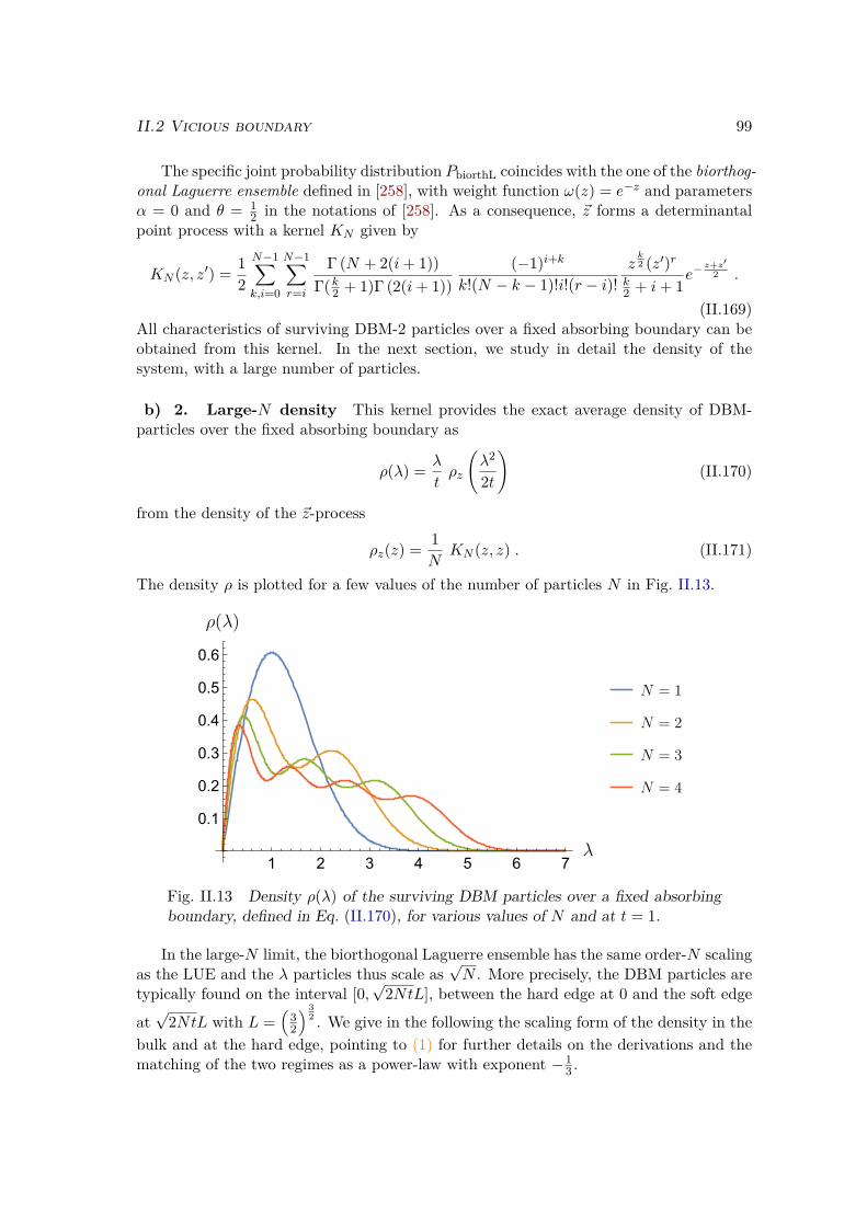
II.2 Vicious boundary 99
The specific joint probability distribution PbiorthL coincides with the one of the biorthog-onal Laguerre ensemble defined in [258], with weight function ω(z) = e−z and parametersα = 0 and θ = 1
2 in the notations of [258]. As a consequence, ~z forms a determinantalpoint process with a kernel KN given by
KN (z, z′) = 12
N−1∑k,i=0
N−1∑r=i
Γ (N + 2(i+ 1))Γ(k2 + 1)Γ (2(i+ 1))
(−1)i+kk!(N − k − 1)!i!(r − i)!
zk2 (z′)r
k2 + i+ 1
e−z+z′
2 .
(II.169)All characteristics of surviving DBM-2 particles over a fixed absorbing boundary can beobtained from this kernel. In the next section, we study in detail the density of thesystem, with a large number of particles.
b) 2. Large-N density This kernel provides the exact average density of DBM-particles over the fixed absorbing boundary as
ρ(λ) = λ
tρz
(λ2
2t
)(II.170)
from the density of the ~z-process
ρz(z) = 1N
KN (z, z) . (II.171)
The density ρ is plotted for a few values of the number of particles N in Fig. II.13.
1 2 3 4 5 6 7
0.1
0.2
0.3
0.4
0.5
0.6
Fig. II.13 Density ρ(λ) of the surviving DBM particles over a fixed absorbingboundary, defined in Eq. (II.170), for various values of N and at t = 1.
In the large-N limit, the biorthogonal Laguerre ensemble has the same order-N scalingas the LUE and the λ particles thus scale as
√N . More precisely, the DBM particles are
typically found on the interval [0,√
2NtL], between the hard edge at 0 and the soft edge
at√
2NtL with L =(
32
) 32 . We give in the following the scaling form of the density in the
bulk and at the hard edge, pointing to (1) for further details on the derivations and thematching of the two regimes as a power-law with exponent −1
3 .

100 Chapter II. Non-crossing walkers and boundary problems
In the bulk At large N , with λ = O(√
2Nt), the average density in the bulk takesthe following scaling form:
ρ(λ) = 1√2Nt
rbulk
( 1√2Nt
λ
)(II.172)
where the scaling function rbulk has a finite support [0, L] with L =(
32
) 32 , and such that∫√2NtL
0 ρ(λ)dλ = 1. The scaling function can be computed by a Coulomb gas method,see (1) and [75,260,261], as
rbulk(λ) = 12π√
2
g−(λ)− g+(λ) + 3
√1− λ2
L2
(g−(λ) + g+(λ)
) (II.173)
with
g±(λ) =
Lλ±
√L2
λ2 − 1
1/3
. (II.174)
The bulk density scaling function rbulk for the DBM-2 over an absorbing boundary isplotted in Fig. II.14.
0.5 1.0 1.5 2.00.0
0.5
1.0
1.5
Fig. II.14 Large-N bulk density of the surviving DBM particles over an absorb-ing boundary at 0, given by the scaling function rbulk in Eq. (II.173).
At the hard edge Close to the hard edge, the density can be obtained from thelimiting kernel of the biorthogonal Laguerre ensemble [258]. In contrast with the LUEbehaviour discussed in Eq. (I.145), the limiting ~z-process is obtained after rescaling byN2, such that the hard-edge regime concerns the DBM particles at scale λ ∼
√2tN .
At this scale such that λ ∼√
2t/N , the density is given by
ρ(λ) = 1√2t
redge
(N√2t
λ
)(II.175)

II.2 Gaussian ensemble interpolation and non-crossing condition 101
where redge(x) = 2x ρedge,z(x2) depends on the density of the rescaled ~z-process, expressedin the z = z/N2 variables as
ρedge,z(z) = Kedge(z, z) (II.176)
with the hard-edge limiting kernel [258]
Kedge(z, z′) =∞∑
j,k=0
(−1)kzkk!Γ (2(1 + k))
(−1)j(z′)j2
j!Γ(1 + j2)
12(1 + k) + j
. (II.177)
The scaling function redge and the hard-edge density ρedge,z of the rescaled ~z are plottedin Fig. II.15. Note that the scaling form Eq. (II.175) ensures that a fraction O( 1
N ) ofparticles are found close to the hard edge, as can be expected.
5 10 15 20
0.1
0.2
0.3
0.4
0.5
5 10 15 20
0.1
0.2
0.3
0.4
Fig. II.15 Left: Plot of the scaling function ρedge,z(z). Right: Plot of the scalingfunction redge(x) = 2x ρedge,z(x2) which describes the hard edge scaling limit ofρ(λ) for λ ∼
√2t/N . At this scale, individual particles appear as oscillations in
redge, which cannot be seen in ρedge,z due to the overall decay.
II.3 Gaussian ensemble interpolation and partial non-crossing condition
As a conclusion to this chapter, we present an interesting perspective on the links betweennon-crossing walkers and random matrix theory. Recall that, as proven in section II.1.2 b),the JPDF of non-crossing walkers at time t is given by that of the GOE or the GUE ifthe non-crossing condition is imposed on [0, t] or [0,∞[ respectively. A natural questionis then the following:
What is the position JPDF at time t of N independent Brownian motionsconditioned to remain non-crossing on [0, T ], with t 6 T 6∞ ?
This distribution should of course interpolate between the GOE and GUE eigenvaluedistributions. Can it then be reduced to a β-ensemble with β ∈ [1, 2] ?

102 Chapter II. Non-crossing walkers and boundary problems
We compute the interpolating JPDF in the first section, and show that the latterquestion can be answered negatively. Instead of a β-ensemble, we show in the secondsection that the distribution is that of the eigenvalues in the interpolating Pandey-Mehtarandom matrix ensemble [262]. As a consequence, the position distribution of non-crossingwalkers retains a random matrix interpretation in the intermediate case t < T <∞.
This problem and its solution constituted a project of this thesis, before it was realizedthat this was already known in the literature, as it had been studied by Katori andTanemura in [263–266].
II.3.1 SolutionLet (Bi,t)16i6N,06t be N independent Brownian motions, started at initial position ~x ∈WN at 0. With T > t, the distribution of interest is
P (~y, t | NC[0,T ], ~x, 0) . (II.178)
Rewriting this conditional distribution and by Markov property, this is equal to
P (~y, t | NC[0,T ], ~x, 0) =P (~y, t,NC[0,T ] | ~x, 0)P(NC[0,T ] | ~x, 0) (II.179)
= P (~y, t,NC[0,t] | ~x, 0)P(NC[t,T ] | ~y, t)P(NC[0,T ] | ~x, 0) (II.180)
The first term can be written as a determinant by Karlin-McGregor theorem, and con-verges to Eq. (II.64) in the ~x → ~0 limit. Both the terms in the fraction are computedas
P(NC[0,τ ] | ~x, 0) =∫WN
d~z P (~z, τ,NC[0,τ ] | ~x, 0) (II.181)
=∫WN
d~z det16i,j6N
P (zi, τ | xj , 0) (II.182)
By de Bruijn’s formula [256], assuming N is even for simplicity as in Eq. (II.152), this is:
P(NC[0,τ ] | ~x, 0) = Pf16i,j6N
I(xi, xj , τ) (II.183)
where I(xi, xj , τ) =∫∫
R2P (z1, τ | xi, 0) P (z2, τ | xj , 0) sgn(z1 − z2) dz1dz2 . (II.184)
It is shown in App. D that, in the Brownian setting with Gaussian propagator (II.54),this integral is
I(xi, xj , τ) = erf(xj − xi
2√τ
)(II.185)
where the error function erf is defined in Eq. (II.88).The JPDF of positions at time t with the intermediate condition can be written in
terms of the single-particle propagator as
P (~y, t | NC[0,T ], ~x, 0) = det16i,j6N
P (yi, t | xj , 0)Pf
16i,j6NI(yi, yj , T − t)
Pf16i,j6N
I(xi, xj , T ) (II.186)
II.3 Gaussian ensemble interpolation and non-crossing condition 103
such that finally, in our Brownian setting:
P (~y, t | NC[0,T ], ~x, 0) = 1(2πt)N2
det16i,j6N
e−(yj−xi)
2
2t
Pf16i,j6N
erf(yj−yi
2√T−t
)Pf
16i,j6Nerf(xj−xi2√T
) (II.187)
Note that the Pfaffian terms are well-defined since they concern antisymmetric matricesfrom the odd symetry of the erf function.
In order to obtain the solution for standard Brownian motions, let us now consider thelimit ~x→ ~0, for example as ~x = ε t ~z with fixed ~z and vanishing ε. From the computationsof App. C, the determinant term is equivalent, as ε→ 0, to
det16i,j6N
e−(yj−xi)
2
2t ' εN(N−1)
2∆ (~z)∏N−1i=1 i!
∆ (~y) e−12t∑N
i=1 y2i . (II.188)
The Pfaffian term, see App. D, behaves as
Pf16i,j6N
erf(ε
t
2√T
(zj − zi))' A ε
N(N−1)2
(t√T
)N(N−1)2
∆(~z) (II.189)
with a constant A. The sought position density of non-crossing standard Brownian mo-tions, under partial non-crossing condition is finally
P (~y, t | NC[0,T ],~0, 0) = K ∆(~y) e−12t∑N
i=1 y2i Pf
16i,j6Nerf(yj − yi
2√T − t
)(II.190)
Some remarks can be made on this distribution result. First and foremost, it can beseen to converge to the GOE and GUE measures in the limit cases T → t and T → ∞respectively, as expected. Indeed, the limits of the Pfaffian term are
Pf16i,j6N
erf(yj − yi
2√T − t
)T→t−−−→ Pf
16i,j6Nsgn(yj − yi) =
∏16i<j6N
sgn(yj − yi) = 1 (II.191)
such that P (~y, t | NC[0,t],~0, 0) then coincides with the JPDF of GOE eigenvalues, see [256]for the sign Pfaffian formula ; and
Pf16i,j6N
erf(yj − yi
2√T − t
)T→∞∼ T−
N(N−1)4 ∆(~y) (II.192)
such that P (~y, t | NC[0,∞[,~0, 0) then coincides with the JPDF of GUE eigenvalues, wherethis line holds from Eq. (II.189).
The interpolation is thus operated by the Pfaffian term which depends on ~y as ∆(~y)0
for T → t and as ∆(~y)1 for T → ∞. However, it cannot be reduced to ∆(~y)α withα ∈]0, 1[ for intermediate T , as seen from the analytical expression. As a consequence,the interpolation uncovered here between the GOE and the GUE measures is differentfrom the one given by the Hermite β-ensemble of Eq. (I.36) with 1 < β < 2. We see in thenext section that it coincides in fact with the eigenvalue measure of the Pandey-Mehtamatrix ensemble.

104 Chapter II. Non-crossing walkers and boundary problems
II.3.2 Links with the Pandey-Mehta matrix ensemblePandey and Mehta have defined in [262] the random matrix ensemble defined by matrices
H = γ√1 + α2
√1− α2
2 HGOE + αHGUE
(II.193)
where HGOE and HGUE are samples of the GOE and GUE with parameter 1, α ∈ [0, 1]is an interpolation parameter and γ > 0 is a normalization parameter. The interest ofthis construction is that it provides a rotation-invariant ensemble of Hermitian matrices,interpolating between the GOE, as α → 0, and the GUE, as α → 1. It is of particularinterest in the context of quantum chaos [267], where it allows to study the transition fromthe time-reversal symmetric Hamiltonian HGOE to the unrestricted Hamiltonian HGUE.
As for the Gaussian ensembles presented in chapter I, it is possible to obtain theeigenvalue distribution by integrating out the eigenvector-related variables. This is donein a slightly more technical way in this case, involving the Harish-Chandra-Itzykson-Zuber(HCIZ ) integral. We give the final result for the eigenvalue JPDF [262]:
P (~λ) = K e− 1+α2
2γ2∑N
i=1 λ2i
∣∣∣∆(~λ)∣∣∣ Pf
16i,j6Nerf
√1− α4
4α2γ2 (λj − λi)
(II.194)
It can be seen directly that this matches our JPDF (II.190) under the replacementt = γ2
1 + α2 ,
T = γ2
1− α4 .
(II.195)
The limits match naturally as T → t⇔ α→ 0 and T →∞⇔ α→ 1. The ratio of T andt is thus in direct correspondence with α as
T
t= 1
1− α2 ∈ R+ . (II.196)
The models are thus equivalent, such that non-crossing walkers observed at t whileconditioned to be non-crossing on [0, T ] can be interpreted as the eigenvalues of (arguably)the simplest interpolating matrix model (II.193). This completes our presentation of thelinks between non-crossing walkers and random matrix theory, in a generalization of theresults presented at the beginning of the chapter.
As explained above, the results presented here were a rediscovery of findings by Katori,Tanemura and co-workers. In [263], they identified and solved the problem studied here,and also noticed the connection with the Pandey-Mehta interpolating ensemble. Furtherfrom the single-time distribution, they also studied multi-dimensional marginals in [266],before the law of the full process in [264, 265]. In these latter works, they identified arandom matrix equivalent for the full process, as a natural generalization of the staticcase explained above, whose entries are sums of Brownian motions (providing the GOEingredient) and Brownian bridges (providing the GUE ingredient).

II.3 Gaussian ensemble interpolation and non-crossing condition 105
Finally, we note that a different interpolation between GOE and GUE statistics wasobserved in the soft edge region in [268]. This interpolation is provided by the transitionbetween flat and curved regions in the TASEP model of the KPZ universality class, whichare respectively related to the β = 1 and β = 2 Gaussian edge statistics through the Airy1and Airy2 processes.


Chapter IIIStochastic matrix evolutions
The stochastic evolutions of random matrices, and their eigenvalue processes, are a dy-namical extension of the static theory of random matrix ensembles. They are deeplyconnected to fermion systems and non-crossing walkers, as illustrated at length in thecontext of the Dyson Brownian motion, in chapter II. This Gaussian matrix diffusion isindeed in correspondence with fermions in the Calogero-Moser Hamiltonian, as proven insection II.1.1 b), and its connections with non-crossing walkers are established in sectionII.1.2. The DBM occupies a central space because it is arguably the simplest stochasticmatrix process: it is structure-less as an extension of the Gaussian ensembles, and itsstochastic evolution is driftless, Markovian and stationary.
Besides this pillar of stochastic matrix evolutions, there exist many noteworthy pro-cesses. Firstly, there similarly exist stochastic matrix extensions for the Wishart, Ja-cobi and circular ensembles [68, 269]. Secondly, generalized Dyson Brownian motionsin an arbitrary potential are useful in the study of line ensembles and growth mod-els [18, 87, 270, 271]. Modified additive processes with alternate free addition, as in theDBM, and co-diagonalizable addition, such that eigenvalues evolve independently, havebeen designed in order to provide asymptotically a rotation-invariant interpolating β-ensemble for the Gaussian and Wishart classes [180, 272]. Multiplicative versions ofthe DBM have also been constructed and investigated [273–275], with a particular in-terest in the corresponding Lyapunov exponents which drive the behaviour of chaoticsystems [276–278]. Significantly, other stochastic matrix models have been introducedfor their physical significance in the problems of wave-diffusion in random media andquantum transport in disordered wires [19, 76, 279, 280]. In these problems of quasi-1Dwave scattering, the Dorokhov-Mello-Pereyra-Kumar approach (DMPK ) introduced inthe 1980’s [281, 282] consists in studying the random evolution of the scattering matrixalong the disordered multichannel wave-conductor. This field of study has thus providedinterest in the study of different stochastic matrix models [283–285], especially in the last20 years after it was realized that multichannel disordered wires were a convenient frame-work to study topological phase transitions in quasi-1D systems [286, 287]. In discretespace-time, Chalker-Coddington type of matrix models on graphs are useful for the studyof localization in two dimensions [288], or in lattice QCD [289].
In this chapter, we turn to other models of stochastic evolution for a random matrixprocess. Mainly, we present the process defined and studied in publication (2), the matrixKesten recursion. This model is a matricial realization of the renowned stochastic recur-
107

108 Chapter III. Stochastic matrix evolutions
sion equation introduced by Harry Kesten in the 1970’s [290, 291] which asymptoticallyexhibits a heavy tail distribution. The interest for a matrix version of the Kesten recur-sion is then to study this heavy-tail mechanism in a multivariate setting. As we presentbelow, the matrix Kesten recursion converges, in the continuum limit of this recursion, tothe distribution of the inverse-Wishart ensemble. The full dynamics can be solved by amapping to fermions in a Morse potential, which are non-interacting for β = 2. At finiteN , the distribution of eigenvalues exhibits heavy tails, generalizing Kesten’s results in thescalar case. These results display a correspondence between the inverse-Wishart ensembleand fermions in a Morse potential, and thus add the Morse potential to the list of poten-tials in one dimension, presented in chapter II, for which the quantum correlations can becomputed using their connection to random matrices. For the discrete matrix recursion,the problem can be studied using free probability in the large-N limit, and translated ina recursion equation for the S and Stieltjes transforms of the process.
In section III.1, we present the original Kesten recursion and its matricial extensionstudied in publication (2), both in the continuous- and discrete-time setting. In sectionIII.2, we present briefly other interesting matrix evolutions. In section III.3, we presentan interesting perspective on stochastic matrix evolutions, from the recent work of Grela,Nowak and Tarnowski [292].
III.1 Matrix Kesten recursion
III.1.1 The Kesten recursionThe Kesten recursion is an example of the fascinating phenomenon of dynamical gen-eration of random variables with heavy power-law tails. Such power-law distributionsoccur in problems such as diffusion in random media [293, 294], directed polymers inrandom environment [295], growing networks [296] and Anderson localization in an ex-ternal field [297–299]. Power-laws are also essential in avalanches of driven elastic sys-tems [207, 300] and in self-organized critical systems such as sandpiles [301]. Finally,they are ubiquitous in economics and finance [302–304] and in social systems [305–308],see [309] for a recent joint exposition.
After defining the Kesten recursion and giving the first details on its power-law be-haviour, we explain in the following some application fields in which the Kesten recursionappears explicitly, and finally present some useful technical properties.
a) Definition
Let (Zn, ξn)n>0 be two sequences of scalar random variables, where the ξn are i.i.d. posi-tive. The Kesten recursion is defined by the following system of equations:
Z0 = 0Zn = ξn (1 + Zn−1)
(III.1)

III.1 Matrix Kesten recursion 109
The solution of this recursion is formally:
Zn =n−1∑j=0
ξn · · · ξn−j =n−1∑j=0
n∏k=n−j
ξk . (III.2)
Harry Kesten studied the limit as n→∞ of such recursions in [290,291,310], showingthat the behaviour of the model depends on the sign of E[log ξ]. The sum in Eq. (III.2)may either grow unboundedly with n if E[log ξ] > 0, or converge to a positive randomvariable, denoted Z∞, if E[log ξ] < 0.
Kesten further showed that in the latter case, the tail of the distribution of Z∞ exhibitsa power-law behaviour with exponent 1 + ν, such that for z 1
P∞(z) ∝ 1z1+ν (III.3)
where P∞ is the PDF of Z∞. The power-law index ν is characterized by the distributionof ξ as
E [ξν ] = 1 . (III.4)
This condition can be understood as follows. From the definition (III.1) one must havethe equality in law Z∞
law= ξ(1 +Z∞), where ξ and Z∞ are taken as independent randomvariables in the r.h.s. Denoting Pξ the PDF of ξ, we see that the PDF PZ∞ of Z∞ mustthen obey the integral equation
P∞(z) =∫
dz′P∞(z′)∫
dxPξ(x)δ(z − x(1 + z′)) =∫ dx
xPξ(x)P∞( z
x− 1) . (III.5)
If one assumes that P∞(z) ∼ z−(1+ν) at large z, the relation (III.4) follows.
b) Applications
As presented above, the Kesten recursion is a simple random recursion which elegantlyleads to power-law tail distributions. It appears explicitly in a variety of problems, whichexhibit a power-law behaviour as a consequence. We present below a selection of three ofthese settings.
b) 1. Random walk in a random environment The Kesten recursion has a closeconnection to the problem of a random walk in a random environment (RWRE) [311–314].The RWRE is a random walk where the hopping probabilities are random variables, andthus constitute a random environment. Let us explain how the Kesten recursion occursfrom RWRE in one dimension, following an argument by Solomon [311].
We denote by αn = Pn,n+1 and βn = Pn,n−1 = 1−αn the random hopping probabilitiesfrom site n of the random walk on Z, as illustrated in Fig. III.1. Let these randomvariables be sampled once and fixed, such that they are a source of quenched disorder forthe system. With µn the mean first-passage time from site n to site n + 1 for a randomwalk in this environment, we have:
µn = αn + βn (1 + µn−1 + µn) . (III.6)

110 Chapter III. Stochastic matrix evolutions
n− 2 n− 1 n n+ 1 n+ 2
αnβn
Fig. III.1 One-dimensional random walk in a random environment, where thetransition probabilities from site n, αn and βn = 1− αn, are random variables.
Indeed, the first-passage time is 1 with probability αn, if the first step from site n is takento the right; or (1 + µn−1 + µn) in average with probability βn, if the first step is takento the left.
Defining ξn = βnαn
and Zn = 12 (µn − 1), we obtain directly the Kesten recursion (III.1)
Zn = ξn(1 + Zn−1) (III.7)
with the initialization Z0 = 0 if we choose α0 = 1 such that the random walk is constrainedto the positive sites. The mean first-passage time µn from site n to site n + 1 is thusdistributed as the Kesten random variable of Eq. (III.2). The quantity −E[log ξ] thusrepresents the effective bias of the environment: if it is positive, the random walkertypically moves to the right, and µ∞ is a finite random variable. Its distribution thenhas a power-law tail, such that it is not rare that µn should reach very large values for atypical random environment.
b) 2. Directed polymers in random media and wealth condensation TheKesten recursion also appears in a simplified model of directed polymers in random media[295], where the polymer lives on a complete graph [304]. The time evolution of thepartition function of polymers ending on site a = 1, · · · , N at time n is given by:
zan+1 = ηan
((1− ε)zan + ε
N
N∑b=1
zbn
), (III.8)
where N is the total number of sites and ε the hopping rate of the polymer. On thecomplete graph, the Laplacian takes a mean-field form that allows one to simplify theanalysis considerably. Introducing zn = ∑
b zbn/N , one can indeed show that for large N ,
the rescaled partition function Zan := (1− ε)zan/εzn obeys a Kesten recursion:
Zan+1 = ξan(1 + Zan), (III.9)
with ξn = (1−ε)ηnE[η] , see [304]. In this work, the polymer is a model of capital distribu-
tion in a population, explaining in a simplified economy the appearance of a power-lawcondensation for the wealth.
b) 3. Investment problem In [315], Dufresne exhibited the Kesten recursion inan investment management problem, seeking the asset statistics of an investor after hehas saved consistently for many years. Consider that a savings account is credited witha unit currency at the beginning of every year. Denoting Rn the random rate of returnduring the nth year, let us define the random variable ξn = 1 + Rn. The accumulated

III.1 Matrix Kesten recursion 111
value Sn is then given as a function of that of the previous year Sn−1 through the Kestenrecursion:
Sn = ξn(1 + Sn−1) . (III.10)This shows that the statistics of the investor’s assets follows a power-law distribution aftermany years, such that it exhibits large variability.
Beyond these examples, the Kesten recursion has applications in the physics of therandom-field Ising chain problem, as well as in biosciences and other fields [316].
c) Properties
c) 1. Continuous version A continuous version of the scalar recursion was stud-ied in physics, as a Langevin equation describing the diffusion of a particle in a one-dimensional white noise Gaussian random field [294], and in mathematics [315, 317]. Inthis continuous setting, the exact limit distribution can be obtained as we present in thefollowing, while only the power-law behaviour is accessible in the discrete case, apart fromspecial cases [318].
Vanishing time increment A path to a meaningful continuous version is to con-sider the Kesten variable multiplied by a vanishing time interval, as
Ut = Zn= tdt
dt (III.11)
where dt is the infinitesimal time step. Note that for a given integer n, the variableZn in Eq. (III.2) has the same distribution, by permuting the ξk variables according to(0, 1, · · ·, n)→ (n, · · ·, 1, 0), as
Znlaw=
n−1∑j=0
j∏k=0
ξk . (III.12)
Writing the random variable ξ in exponential form as ξn = eηn , the reordered equivalentform (III.12) gives the following convergence for the process U at time t = ndt :
Utlaw=
n−1∑j=0
e
j∑k=0
ηkdt dt→0−→
∫ t
0eAsds (III.13)
where the process As is the continuous limit of the random walkj∑
k=0ηk. This process is
well-defined provided the i.i.d. η random variables scale as:
η = γdt+ α√
dtX with X ∼ N (0, 1) , (III.14)
such that As is a drifted Brownian motion
As = γs+ αBs . (III.15)
The parameters depend on the distribution of ξ asγ = E[log ξ]dt ;
α2 = Var(log ξ)dt .
(III.16)

112 Chapter III. Stochastic matrix evolutions
The infinite-time limit of the U variable can then finally be written as
U∞law=∫ ∞
0eγt+αBtdt . (III.17)
This last equation characterizes the law of U∞, in terms of the distribution of the widelystudied Brownian exponential functional on the r.h.s., see [319] for a review, as wellas [320,321].
Large-time distribution In order to exhibit the large-time distribution of the pro-cess Ut, let us derive its stochastic evolution from the Kesten recursion obeyed by Zn.Exponentiating the scaling form (III.14), and denoting m = γ + α2
2 and σ = α√2 , the ξ
variables are given by
ξ = 1 +mdt+ σ√
2dtX with X ∼ N (0, 1) (III.18)
Injecting this in the Kesten recursion (III.1) yields the following SDE for the process Ut
dUt = (1 +m Ut) dt+√
2σUtdBt (Itô) (III.19)
Since the prefactor of the Brownian term dBt depends on the process Ut itself, a choice ofprescription must be made and this SDE is understood in the sense of Itô. We postponethe detailed discussion of this issue to section III.2.1. The Fokker-Planck equation for theassociated PDF P (x, t) is
∂P (x, t)∂t
= σ2 ∂2
∂x2
(x2P (x, t)
)− ∂
∂x((1 +mx)P (x, t)) . (III.20)
When γ < 0, that is to saym < σ2 , (III.21)
the PDF converges to a stationary limit and U∞ then follows an inverse-gamma lawdistributed as
P∞(x) = σ−2+2 mσ2
Γ(1− m
σ2
) x−2+ mσ2 e−
1σ2x . (III.22)
In other words, the inverse of U∞ follows the gamma law
U−1∞ ∼ Γ
(1− m
σ2 , σ2). (III.23)
Note that this result confirms, in the continuous limit, the power-law behaviour of Eq. (III.3)with the heavy tail exponent 1 + ν = 2− m
σ2 .
c) 2. Vector recursion The vector case for the discrete recursion (III.1) was alsostudied by Kesten [290], promoting Zn to d-dimensional vectors and ξn to d× d matrices.Under suitable hypothesis, there also exists ν such that for any unit d-dimensional vectorx the following limit exists and is nonzero:
0 < limt→∞
tν P(xT . Z∞ > t
)<∞ . (III.24)
In this case however, ν is not characterized by a simple moment equation, in contrast toEq. (III.4) in the scalar case.

III.1 Matrix Kesten recursion 113
III.1.2 Matrix Kesten evolution in continuous timeThe focus of publication (2) was the introduction of a matrix realization of the Kestenrecursion. In the present section, we define this matrix model and present the propertiesof its continuous limit, which can be solved exactly by a remarkable connection with thequantum mechanics of fermions in a Morse potential.
a) A matricial version of the Kesten recursion
a) 1. Definition For N ∈ N∗, let us consider (ξn)n>0 a sequence of i.i.d. symmetricpositive semidefinite N × N matrices. We define the Kesten recursion for a sequence ofsymmetric positive semidefinite N ×N matrices (Zn)n>0 in a manifestly self-adjoint wayas:
Zn+1 =√ε1 + Zn ξn
√ε1 + Zn (III.25)
The regularizing real parameter ε > 0 will be given a value of order 1 in the discretesetting, and taken to 0 in the continuous limit. The symmetric positive semidefinite prop-erty of the sequence ξ implies by recursion the same property for the sequence (Zn)n>0,as we denote for each n by
√ε1 + Zn the principal square-root of ε1+Zn. The properties
of ξn and Zn can be summed up by stating that they are symmetric matrices with onlynonnegative eigenvalues.
In parallel, we also consider a model where all matrices are Hermitian positive semidef-inite. We will define as usual a Dyson index β = 1 in the real symmetric case, and β = 2in the complex Hermitian case. Note that the study could be generalized to the caseβ = 4, but we restrict to the first two cases.
a) 2. Continuous limit
Matrix evolution Let us derive the continuous limit of the matrix Kesten recursion(III.25). Remembering the picture laid out in the previous section for the scalar case, seethe scaling (III.14), we choose the following structure for the matrices ξn
ξn = exp(γε1 + σ
√εHn
)(III.26)
where ε is the parameter introduced in Eq. (III.25) and where H is a unit-variance GOEor GUE matrix. Note that this ensures positive definiteness of ξ. A small-ε expansion ofthe matrix exponential definition for ξn gives to order ε:
ξn = (1 +mε)1 + σ√εHn (III.27)
where parameters m = γ + 12σ
2(N + δβ=1) and σ respectively tune the mean and thenoise in ξn. Indeed, for the sake of the continuum limit, we can replace ε(Hn)2 by itsexpectation ε1(N +δβ=1), where the Kronecker delta appears as correlations are differentin the β = 1, 2 cases.
With this choice for the i.i.d. sequence ξ and expanding the square-root matrix, theevolution of Z reads at order ε:
Zn+1 = Zn + εI +mεZn + σ√ε√
ZnHn
√Zn +O(ε3/2) (III.28)
114 Chapter III. Stochastic matrix evolutions
In the ε→ 0 limit, we define a continuous time matrix process Vt, where the time variableis t = nε, simply as
Vt = Zt/ε . (III.29)
We have avoided here the scaling between the discrete and continuous processes, whichappeared in the scalar case, from the insertion of ε in the definition of the recursion.From the recursion (III.28), we obtain the time evolution for Vt as the following Itômatrix SDE, where Ht is the DBM:
dVt = (1 +mVt) dt+ σ√
VtdHt
√Vt (III.30)
Similarly as in the scalar case, the multiplicative noise imposes the choice of a prescriptionfor this SDE, which is understood here in the sense of Itô, see section III.2.1. TakingN = 1 in the real case β = 1 recovers exactly the continuous Kesten evolution (III.19) asexpected, because the diagonal terms in the DBM-1 are
√2 times a standard Brownian
motion.
Joint eigenvalue evolution The stochastic evolution (III.30) is rotation-invariant,as conjugation by a unitary matrix, as V → UVU−1, preserves the SDE. As a conse-quence, the eigenvectors of Vt are uniformly distributed on the unit sphere as soon as theyare in the initial condition, for example with V0 = 0. The model can then be cruciallyreduced to the study of the eigenvalues.
Let us denote λi,t16i6N , the set of positive eigenvalues of Vt. Their evolution can bederived by perturbation theory, as presented for the DBM in section II.1. This procedureyields, see publication (2):
dλi,t = (1 +mλi,t) dt+ σ2 ∑16j6Nj 6=i
λi,tλj,tλi,t − λj,t
dt+√
2βσλidBi,t (III.31)
where the (Bi,t)16i6N are N independent standard Brownian motions. This evolutioncan be compared with that of the DBM in Eq. (II.11): the evolution of the eigenvaluesis similarly obtained with no a priori knowledge of the evolution of the eigenvectors,and display a repulsive interaction term. However a difference is that, because of themultiplicative noise, the repulsion depends also multiplicatively on the eigenvalues.
From this stochastic evolution, one can obtain the evolution of the eigenvalue JPDFP (~λ, t). The Fokker-Planck equation associated with the eigenvalue evolution of the Itôprocess Vt is:
∂P (~λ, t)∂t
= σ2
β
N∑i=1
∂2
∂λ2i
(λ2iP (~λ, t)
)−
N∑i=1
∂
∂λi
1 +mλi + σ2 ∑
16j6Nj 6=i
λiλjλi − λj
P (~λ, t)
(III.32)
where the initial condition is specified by the eigenvalues of V0.

III.1 Matrix Kesten recursion 115
Stationary solution The stationary solution P∞ of this diffusion can be found asa zero-flux solution as
0 = ∂
∂λi
( 1β
(σλi)2 P∞
)−
1 +mλi + σ2 ∑16j6Nj 6=i
λiλjλi − λj
P∞ . (III.33)
This equation is found to be solved by the inverse-Wishart eigenvalue distribution (I.54)with parameters
T = N − 2mσ2 + 2
β − 1
σW = σ√2
(III.34)
where we rename σW the parameter in (I.54) in order to avoid ambiguities; such that thestationary JPDF is
P∞(~λ) = KNβ
∣∣∣∆(~λ)∣∣∣β N∏
i=1λβ(mσ2−N+1
)−2
i e− β
σ2∑N
i=11λi (III.35)
We note that for N = 1 the Vandermonde factor is absent and setting β = 1 one recoversexactly the inverse gamma law of Eq. (III.22).
The eigenvector-basis rotation invariance then allows to conclude that the inverse-Wishart matrix distribution (I.53) is a stationary distribution for this model. Note thatthe normalizability condition translates here to
m <σ2
β(III.36)
which coincides, as expected for N = 1 and β = 1, with the scalar-case condition (III.21).For more details on the marginal density for the largest eigenvalue and its matching withthe scalar case, see (2).
b) Quantum Morse-Sutherland mappingFurther from the large-time solution, the full finite-time dynamics can be solved exactlyby a quantum mapping to fermions in a Morse potential, in the spirit of section II.1.1 b).
b) 1. Stochastic-to-quantum connection To elicit this mapping we first performa change of variables by defining
xi,t = log λi,t . (III.37)
From Itô rules, the stochastic evolution of the x variables has additive noise following:
dxi,t = Fidt+√
2βσdBi,t Fi = e−xi,t +m− σ2
β+ σ2 ∑
16j6Nj 6=i
1exi,t−xj,t − 1 , (III.38)
where Fi is the force felt by particle xi. The initial condition is fixed as xi,t=0 = x0 alarge negative constant, for all i.
116 Chapter III. Stochastic matrix evolutions
Operator mapping Let us denote P (~x, t) the PDF of the x-process. In the follow-ing, P indicates a distribution function on the x variables. Denoting consequently P∞the distribution obtained from Eq. (III.35) through the change of variables (III.37), wehave
P∞(~x) = e∑N
i=1 xi P∞(exp ~x) . (III.39)The time-dependent PDF P (~x, t) verifies the following Fokker-Planck equation
∂P
∂t=
N∑i=1
(σ2
β
∂2P
∂x2i
− ∂
∂xi(FiP )
)= −HFP P (III.40)
where we have introduced the generator HFP of this diffusion. The auxiliary function
ψ(~x, t) = P (~x, t)√P∞(~x)
(III.41)
is then a solution of the following imaginary-time Schrödinger equation, which we rewriteby introducing the operator H and the constant E0:
∂ψ
∂t=
N∑i=1
(σ2
β
∂2ψ
∂x2i
−(βF2i
4σ2 + 12∂Fi∂xi
)ψ
)= −σ
2
β(H − E0)ψ . (III.42)
The quantum Hamiltonian H is
H =N∑i=1
− ∂2
∂x2i
+ VM(xi) +∑
16j6Nj 6=i
Vint(xi, xj)
(III.43)
with a one-particle potential of the Morse form VM(x) = Ae−2x − Be−x [322] and withSutherland sinh−2 interaction potential Vint [192]:
VM(xi) = β2 e−2xi
4σ4 −β
σ2
(β
2 (N − 1− m
σ2 ) + 1)e−xi
Vint(xi, xj) = β(β − 2)16
1
sinh(xi−xj
2
)2
(III.44)
Notice the translation by the constant E0 and the rescaling by σ2/β in Eq. (III.42), suchthat the stochastic-to-quantum operator mapping can be formally written as
σ2
β(H − E0) = P∞
− 12 HFP P∞
12 . (III.45)
The lowest Fokker-Planck eigenvalue is equal to 0, the eigenvalue of the stationary state,such that the constant E0 is in fact the ground-state energy of H, and is given by
E0 = −N (βm− σ2)2
4σ4 + N(N − 1)4
(β2
σ2m− ββ + 2
2
)−N(N − 1)(N − 2)β
2
12 . (III.46)

III.1 Matrix Kesten recursion 117
Fermionic symmetry As in the DBM case, it can be shown that the non-crossingstatistics of the x-process implies the fermionic symmetry of the quantum system, see (2).As a consequence, we are led to the study of N fermions in the Hamiltonian H.
In summary, we have detailed in the previous lines a connection of the eigenvalue pro-cess of the continuous Kesten evolution (III.30), through the change of variables (III.37),with a system of fermions with Hamiltonian H in Eq. (III.43). For both β = 1, 2, thisgives at large time a direct connection between the inverse-Wishart matrix ensemble inEq. (III.35) and the ground-state of this many-body Morse-Sutherland quantum system.This result is thus an addition to the literature of random matrix theory, through the lensof its connections to many-body quantum systems [16,68,96,104,109,323]. As presentedbelow, a specificity of the present case is that the Morse potential can only accomodatea finite number of fermions in its quantized bound states.
b) 2. The single-particle Morse potential We present in this paragraph theproperties of the Morse potential
VM(x) = g2(e−2(x−x0) − 2e−(x−x0)
)(III.47)
which appears as the external potential in Eq. (III.44). This potential is well-known inthe literature as it is a convenient model for the potential energy of a diatomic molecule.Indeed, it is fully tractable as we detail in the following, and has the expected properties ofan interatomic interaction: it displays a minimum VM(x0) = −g2 at position x0, divergesexponentially fast for x → −∞ and tends to zero for x → +∞. See Fig. III.2 for a plotof the Morse potential. In the Kesten setting, the parameters of the potential are fixedper Eq. (III.44) as g = β
2 (N − mσ2 − 1) + 1 ;
e−x0 = σ2(N − mσ2 − 1 + 2
β ) .(III.48)
Notice that the parameters depend explicitly on the matrix size N , which has importantconsequences.
Let us review the properties of a single quantum particle in Hamiltonian VM [322,324]. The spectrum of this Hamiltonian is composed of two branches: a finite branch ofdiscrete bound states with negative eigenenergies, and a continuum of positive-eigenenergydiffusion states.
Let us denote K = g − 12 . The discrete states, indexed by k > 0, exist under the
conditionk < K (III.49)
such that the maximum number of fermions that can be stacked in the discrete spectrumof the Morse potential is the largest integer m such that m < K + 1, denoted as the floorof an infinitesimally smaller value Nmax = b(K + 1)−c. For 0 6 k < K, the bound stateshave energy level and corresponding eigenfunction
εk = − (K − k)2 ; (III.50)
ψk(x) = Nk
(2ge−(x−x0)
)g−k− 12 e−ge
−(x−x0)L
(2g−2k−1)k
(2ge−(x−x0)
). (III.51)

118 Chapter III. Stochastic matrix evolutions
The eigenfunction is expressed in terms of the Laguerre polynomials L(α)k , see chapter I,
with
Nk =√k!(2g − 2k − 1)
Γ(2g − k) (III.52)
a normalization constant. The admissible bound states described above are plotted inFig. III.2 along with the Morse potential.
-60
-40
-20
20
-4 -2 2 4
Fig. III.2 The Morse potential VM(x) in Eq. (III.47) is plotted in the blue line,with parameters g = 8 and x0 ' −2.079 which corresponds for example toN = 5, σ = 1 and m = −3 in the β = 2 Kesten model. The eight admissiblebound-state eigenfunctions ψk are plotted at altitude εk, in coloured lines.
In addition to this discrete spectrum of bound states, there is a continuum of positiveenergy eigenstates ε = p2 > 0. The associated eigenfunctions are of the form
ψp(x) ∼ ex−x0
2 Wg,ip(2ge−(x−x0)
)(III.53)
in terms of the Whittaker Wk,µ function, see App. B, such that ψp is a real functiondecreasing fast for x < 0 and oscillating for x > 0.
In the following section, we turn back to the N -particle case and study the many-bodyfermionic system with Hamiltonian H in Eq. (III.43), with a restriction to β = 2.
c) Full solution for the non-interacting case β = 2The single-particle results of the previous paragraph can be directly applied to the caseβ = 2. Indeed, since the interaction potential Vint vanishes, the particles are simply Nnon-interacting fermions in the Morse potential.

III.1 Matrix Kesten recursion 119
c) 1. Ground state of the non-interacting case In the present case β = 2, theparameters of the Morse potential are g = N − m
σ2 and e−x0 = σ2(N − m
σ2
)such that the
energy levels and corresponding eigenfunctions of the Morse potential are
εk = −(N − m
σ2 − k −12
)2; (III.54)
ψk(x) = Nk
( 2σ2 e
−x)N− m
σ2−k−12e−
1σ2 e−xL
(2N− 2mσ2 −2k−1)
k
( 2σ2 e
−x). (III.55)
Ground-state wavefunction and energy The ground-state wavefunction of theN -fermion model is expressed as a Slater determinant with corresponding energy ε~0:
Ψ~0(~x) = 1√N !
det16i,j6N
(ψi−1(xj)) , (III.56)
ε~0 =N−1∑k=0
εk . (III.57)
Two things can be verified algebraically: the coincidence of the ground-state energy ε~0with the constant E0 in Eq. (III.46); and the coincidence of the fermionic JPDF withthe large-time stochastic distribution as
∣∣Ψ~0(~x)∣∣2 = P∞(~x). Furthermore, as mentioned
above, the Morse potential has a finite number of bound states Nmax = b(K + 1)−c. Inorder for the ground-state of N fermions to be well-defined, the condition N 6 Nmaxmust hold, i.e.
m <σ2
2 (III.58)
which coincides perfectly with the stochastic normalizability condition (III.36) in thepresent case β = 2.
Finally, we define the Fermi energy εF as the last occupied level
εF = εN−1 = −(1
2 −m
σ2
)2. (III.59)
We note that it is independent of the number of particles, such that the potential withgrowing depth, given from g in Eq. (III.48), is filled by a growing number of N particlesup to a fixed energy level εF . This is not true any more if σ depends on N , as we discussbelow.
Determinantal structure of the ground state The fermionic setting suggests adeterminantal rewriting of the stationary solution:
P∞(~x) = 1N ! det
16i,j6NKM(xi, xj) (III.60)
where the kernel KM, which respects the trace-class, positivity and reproducibility prop-erties, is given formally by the weighted sum of the first N Morse eigenfunctions as
KM(x, y) = (2/σ2)2(N− mσ2−
12 )N−1∑k=0
σ4kN2k
4k e−(x+y)(N− mσ2−k−
12 )e−
1σ2 (e−x+e−y)
L(2N− 2m
σ2 −2k−1)k
( 2σ2 e
−x)L
(2N− 2mσ2 −2k−1)
k
( 2σ2 e
−y).
(III.61)

120 Chapter III. Stochastic matrix evolutions
All statistical properties of the fermion positions in the ground state are characterized bythis kernel, such as their average density
P (x) = 1NKM(x, x) . (III.62)
This coincides with the infinite-time average density of the β = 2 Kesten-matrix eigen-values λi as P (λ) = 1
λ P (log λ). We recall from chapter I that a similar kernel can beobtained on the inverse-Wishart side from the orthogonal polynomial method for β = 2.
c) 2. Large-N behaviour For large N , the density P (x) of the Fermi gas in theMorse potential without interactions can be well described by approximations in the bulkregion and close to the edges. The results are presented briefly in the following. Wepoint to (2) for the full computations concerning the Morse potential in Eq. (III.47) witharbitrary parameters g and x0, and their application to the Kesten setting.
Density in the bulk When N is large, the density is well described in the bulk bya semi-classical approximation for the density of a Fermi gas, also called the local densityapproximation (LDA) [325]. The bulk density approximation is supported on [x−, x+]and given by:
Pbulk(x) = 1σ2πN
√(e−x − e−x+)(e−x− − e−x) (III.63)
where the positions of the edges x± are
x± = x0 − log(
1∓√
11− m
Nσ2
√2− 1
1− mNσ2
)(III.64)
expressed in relation to the bottom of the Morse potential at position x0 = − log(σ2(N − m
σ2 )).
We can rewrite this density from a random matrix point of view. Let us recall T =N − 2m
σ2 the inverse-Wishart parameter obtained for the large time distribution of theKesten model, from Eq. (III.34) in the present case β = 2. Introducing the rescaled 1/λvariable
Λ = 1T
2σ2 e−x (III.65)
the previous asymptotic density becomes, under the change of variables:
Pbulk(x)dx =√
(Λ− Λ−)(Λ+ − Λ)2qπΛ dΛ = ρMP(Λ)dΛ
with Λ± = 1T
2σ2 e
−x∓(III.66)
where ρMP is the Marčenko-Pastur distribution (I.87) with parametersq = N
T= N
N − 2mσ2
;
σW = 1 .(III.67)
Here, we have renamed the Wishart variance σW as in Eq. (III.34).

III.1 Matrix Kesten recursion 121
We recover in this asymptotic Marčenko-Pastur result the fact that the Λi ∝ 1/λiare distributed according to the eigenvalues of the Wishart ensemble, since the λi aredistributed as the eigenvalues of the inverse-Wishart ensemble. The parameters q andσW = 1, coincide as expected with the parameters obtained from the inverse-Wishartcorrespondence Eq. (III.34) after the rescaling implemented in the definition (III.65).
In addition to giving a RMT perspective on the Fermi gas asymptotic result at large-N , this obtention of the Marčenko-Pastur distribution indicates that the system displaystwo different regimes depending on parameter σ:
• Either σ scales as 1/√N such that
σ ' σ√N
(III.68)
with σ constant, such thatq = 1
1− 2mσ2
< 1 (III.69)
where m is necessarily negative per condition (III.58). In this case, asymptotics ofthe Wishart ensemble presented in chapter I show that there are two soft edges atthe boundaries of the support, where the statistics are described by the universalAiry kernel.The Fermi gas and the Kesten eigenvalues are then, in turn, distributed betweentwo soft edges at fixed positions. This can be understood intuitively as follows: atlarge N , the depth of the trapping potential grows as −g2 ∼ N2. In this regime, theFermi energy in Eq. (III.59) grows at the same speed εF ∼ N2, and the fermionsthus remain confined between two soft edges.
• Or σ remains constant of order 1, such that asymptotically
q = 1 . (III.70)
In this case, the lower edge of the Wishart ensemble at 0 is a hard edge, wherethe statistics are described by the universal Bessel kernel. The Fermi gas and theKesten eigenvalues then lose their right edge and extend infinitely to the right forN = +∞.In this case, the Fermi energy remains of order 1, εF = O(1), see Eq. (III.59). Thedepth of the potential however still grows as −g2 ∼ N2, such that the support ofthe density extends very far to the right, as explained above.
The difference between these two regimes is illustrated in Fig. III.3. In the following, wepresent the edge densities for both cases.
Density at the edges with σ ∼ σ/√N With vanishing σ at speed 1/
√N , the
edges of the Fermi gas converge to the fixed positions
x± = − log(σ2 −m∓ σ2
√1− 2m
σ2
). (III.71)
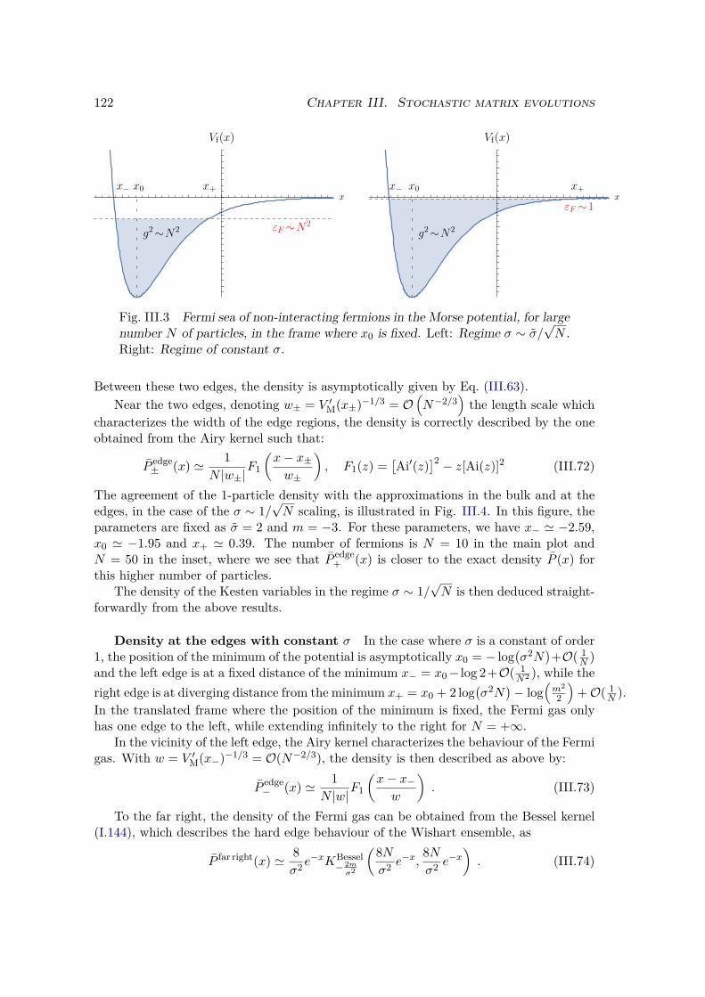
122 Chapter III. Stochastic matrix evolutions
Fig. III.3 Fermi sea of non-interacting fermions in the Morse potential, for largenumber N of particles, in the frame where x0 is fixed. Left: Regime σ ∼ σ/
√N .
Right: Regime of constant σ.
Between these two edges, the density is asymptotically given by Eq. (III.63).Near the two edges, denoting w± = V ′M(x±)−1/3 = O
(N−2/3
)the length scale which
characterizes the width of the edge regions, the density is correctly described by the oneobtained from the Airy kernel such that:
P edge± (x) ' 1
N |w±|F1
(x− x±w±
), F1(z) =
[Ai′(z)
]2 − z[Ai(z)]2 (III.72)
The agreement of the 1-particle density with the approximations in the bulk and at theedges, in the case of the σ ∼ 1/
√N scaling, is illustrated in Fig. III.4. In this figure, the
parameters are fixed as σ = 2 and m = −3. For these parameters, we have x− ' −2.59,x0 ' −1.95 and x+ ' 0.39. The number of fermions is N = 10 in the main plot andN = 50 in the inset, where we see that P edge
+ (x) is closer to the exact density P (x) forthis higher number of particles.
The density of the Kesten variables in the regime σ ∼ 1/√N is then deduced straight-
forwardly from the above results.
Density at the edges with constant σ In the case where σ is a constant of order1, the position of the minimum of the potential is asymptotically x0 = − log
(σ2N
)+O( 1
N )and the left edge is at a fixed distance of the minimum x− = x0− log 2+O( 1
N2 ), while theright edge is at diverging distance from the minimum x+ = x0 + 2 log
(σ2N
)− log
(m2
2
)+O( 1
N ).In the translated frame where the position of the minimum is fixed, the Fermi gas onlyhas one edge to the left, while extending infinitely to the right for N = +∞.
In the vicinity of the left edge, the Airy kernel characterizes the behaviour of the Fermigas. With w = V ′M(x−)−1/3 = O(N−2/3), the density is then described as above by:
P edge− (x) ' 1
N |w|F1
(x− x−w
). (III.73)
To the far right, the density of the Fermi gas can be obtained from the Bessel kernel(I.144), which describes the hard edge behaviour of the Wishart ensemble, as
P far right(x) ' 8σ2 e
−xKBessel− 2mσ2
(8Nσ2 e
−x,8Nσ2 e
−x). (III.74)

III.1 Matrix Kesten recursion 123
-3 -2 -1 1 2 3
0.1
0.2
0.3
0.4
0.5
-0.1 0.1 0.3 0.50
0.04
0.08
0.12
Fig. III.4 Scaling σ ∼ 1/√N : Plot of the exact average density P (x) (III.62)
for N = 10 particles (solid blue line). The bulk density Pbulk(x) (III.63) is thedashed gray line, and the Airy-kernel edge densities P edge
± (x) (III.72) are thedashed red lines. The inset shows the region near the right edge for N = 50.
This can be written as a function of the distance between x and the diverging edgex+ ' log
(2Nσ2
m2
), with the expression of the Bessel kernel at the singular point in terms
of Bessel functions:
P far right(x) = 2σ2 e
−x(J− 2m
σ2
(2|m|σ2 e−
x−x+2
)2
− J− 2mσ2 +1
(2|m|σ2 e−
x−x+2
)J− 2m
σ2 −1
(2|m|σ2 e−
x−x+2
)).
(III.75)
The agreement of the 1-particle density with the approximations in the bulk and at theedges, in the case of constant σ, is illustrated in Fig. III.5. In this figure, the parametersare fixed as σ = 2 and m = −3. The main plot is drawn for N = 10 fermions, withx− ' −4.45, x0 ' −3.76 and x+ ' 2.26. The inset has N = 50, where x+ ' 3.81. We seethat the exact density is very closely approximated by P far right(x) in that region.
The density of the Kesten variables in the regime of constant σ is then deducedstraightforwardly from the above results. For more details on the tail of the distributionof the rightmost eigenvalue from asymptotics of the solution of the Painlevé III equation,see (2).
c) 3. Finite-time solution Further from the large-time stationary distributiondetailed in the previous sections through the ground state of the related Fermi gas, onecan solve analytically the full dynamics of the Kesten eigenvalue process in the presentcase β = 2. In this section, we give the analytical expression for the PDF P (~λ, t) atarbitrary finite time.

124 Chapter III. Stochastic matrix evolutions
-4 -2 2 4
0.05
0.10
0.15
0.20
0.25
0.30
0.35
0 1 2 3 4 5
0.01
0.02
0.03
Fig. III.5 Constant σ : Plot of the average density P (x) (III.62) for N = 10particles (solid blue line), with the approximations in the bulk Pbulk(x) (III.63)(dashed gray line), at the left edge P edge
− (x) (III.73) (red dashed line) and on thefar right P far right(x) near x+ ∼ logN (III.75) (orange dashed line). The insetshows this latter region for N = 50.
Taking into account the bound states and the continuous branch of the spectrum, theEuclidean propagator, or Green’s function in imaginary time, of a one-particle system inthe Morse potential (III.47) can be expressed in terms of the Whittaker W function as:
G(y, t | x, 0) =b(g− 1
2 )−c∑k=0
ψk(x)ψk(y)e−(g−k− 12 )2t
+∫ +∞
0
dp2gπ2 p sinh(2πp)
∣∣∣∣Γ(ip− g + 12)∣∣∣∣2 ex+y
2 −x0
Wg,ip(2ge−(x−x0)) Wg,ip(2ge−(y−x0)) e−p2t .
(III.76)
From completeness of the eigenbasis, this propagator satisfiesG(y, 0 | x, 0) = δ(x−y). Thepropagator of the N -particle system of non-interacting fermions in the Morse potential isthen simply:
G(~y, t | ~x, 0) = 〈~y| e−tH |~x〉 = det16i,j6N
G(yi, t | xj , 0) (III.77)
which satisfies G(~y, 0 | ~x, 0) = δ(~x−~y). From this quantum result, the finite time solutionof the transformed Kesten stochastic diffusion in the x = log(λ) variables (III.38) can be

III.1 Matrix Kesten recursion 125
obtained as:
P (~x, t) = 〈~x| e−tHFP |~x0〉 =(P∞(~x)P∞(~x0)
) 12
G(~x, t | ~x0, 0) eE0t, P (~x, 0) = δ(~x− ~x0)
(III.78)
Upon changing back to the λ = ex variables, these computations yield an analyticalformula for the finite-time solution of the Kesten eigenvalue diffusion as:
P (~λ, t) = P (~x = log~λ, t)N∏i=1
1λi. (III.79)
d) Interacting case β = 1We have treated the non-interacting case β = 2 in detail, and will only mention brieflythe properties of the interacting case β = 1. In this case, the Kesten process can givemany informations about the ground-state statistics of the interacting fermions. Note thatthese statistics cannot be easily found from first principles as a mere Slater determinant,in contrast with the non-interacting case.
In the case β = 1, the large-time stationary solution for the Kesten eigenvalue pro-cess was also obtained in Eq. (III.35). The ground-state wavefunction of the interactingfermion system is directly obtained from this result as
∣∣Ψ~0(~x)∣∣ =
√P∞(~x) (III.80)
where P∞ is expressed in terms of P∞ in Eq. (III.39), and where the sign of the wave-function can be deduced from fermionic symmetry. The ground-state energy is also foundfrom the above studies, as it is given by the constant E0 in Eq. (III.46) with β = 1.
Furthermore, the large-N behaviour of the system can also be obtained from theinverse-Wishart statistics of the Orthogonal class β = 1. For the case σ = O(1), the leftedge is now described, upon the same change of variable, by the universality of the GOEsoft edge. The fermions on the far right, corresponding to the largest eigenvalues of thecontinuous matrix Kesten recurrence, are now described, upon this change of variable, bythe β = 1 Bessel Pfaffian point process, characterized by the universal Bessel 2×2 matrixkernel mentioned in section I.2.2.
The finite-time solution of the diffusion requires the knowledge of the whole spectrumof Morse-Sutherland fermions, beyond the ground state discussed in the previous lines,addressed in the literature of integrable systems [326].
III.1.3 Discrete recursion in the large matrix-size limitIn analogous fashion with the scalar setting, the matrix Kesten recursion defined inEq. (III.25) is fully solvable in its continuous version (III.30). We have detailed thissolution through a mapping to Morse-Sutherland fermions in the previous section, witha particular emphasis on the non-interacting case β = 2.
126 Chapter III. Stochastic matrix evolutions
In this section, we turn back to the discrete setting, where ε remains of order 1in (III.25). Similarly as in the scalar setting, the discrete version is not easily solved.However, the powerful toolbox of free probability presented in section I.3 gives a way tohandle this problem in the limit of large matrix-size N → ∞, to which we turn in thefollowing. We note that the Dyson index β does not have the same significance in thissection as in the previous one, since, in the free case, all the information is contained inthe eigenvalue density: results apply to both β = 1, 2 cases.
a) Free product approachFree probability tools can help characterize the behaviour of the Kesten matrix Zn if thelarge matrices ε1 + Zn and ξn are free such that the Kesten recursion
Zn+1 =√ε1 + Zn ξn
√ε1 + Zn (III.81)
gives Zn+1 as their free product. The S-transform of the Z matrices is then a useful tool,as we discuss in the following.
a) 1. S-transform recursion Let us make two assumptions on the distribution ofthe large i.i.d. random matrices ξn ∼ ξ:
• it is invariant under eigenbasis-rotation ;
• the spectrum of ξ is compactly supported in the large-N limit.
We have under the first assumption, as explained in section I.3, that ε1 + Zn and ξn areasymptotically free, in the large-N limit, for arbitrary index n. Zn+1 is their free product,such that by the factorization property (I.202):
SZn+1 = Sξ × Sε1+Zn (III.82)
This relation characterizes the spectral distribution of Zn+1, through the transform SZn+1 ,in terms of the spectral distribution of Zn, through the transform Sε1+Zn . This functioncan be expressed in terms of the S-transform of Zn itself, see (2), yielding the followingrecursion equation on the functional sequence (SZn)n>0, for all ω:
Sξ(ω)SZn+1(ω) = 1
SZn
(ω(1− ε SZn+1 (ω)
Sξ(ω) )) + ε (III.83)
Stationary self-consistent equation At large-n, the S-transform, denoted S∞,of the stationary spectral distribution solves the following self-consistent equation, for allω:
Sξ(ω)S∞(ω) = 1
S∞(ω(1− ε S∞(ω)
Sξ(ω) )) + ε . (III.84)
In the previous lines, we have presented the relation which characterizes the evolutionof the spectral distribution of Zn for an arbitrary ξ-distribution, in (III.83). At late times,

III.1 Matrix Kesten recursion 127
this characterizes the stationary spectral distribution of Z∞ in Eq. (III.84). Note thatthese two equations are functional relations, holding for all ω, which are not easily solvedfor an arbitrary choice of the noise matrix distribution. In the continuous limit however,these discrete relations can be shown to match the results of section III.1.2, as we showbelow. Further, they give access to some information in a perturbative manner, as wediscuss next.
a) 2. Continuous limit We recall the suitable form for the random matrix ξ inEq. (III.27), in the continuous-time ε→ 0 limit, as:
ξn = (1 +mε)1 + σ√εHn (III.85)
where H is a unit-variance GOE or GUE matrix. The large-N spectral density is thesame for both versions of H, such that there is no difference in the infinite-N resultsbetween the β = 1 and β = 2 cases. The
√N -scaling in the convergence of a Gaussian
matrix spectral density to Wigner’s semicircle in Eq. (I.68), imposes that
σ = σ√N
(III.86)
with σ fixed, in order for ξ to have a compactly supported asymptotic spectrum. Werecognize here the large-N situation of the previous section: this is the regime where thespectrum remains bounded, while on the other σ = O(1) implies a blowup of the support.From the continuous setting, recall also that m < 0. The spectral distribution of ξ isfixed, by Eq. (III.85), as a translated semicircle distribution, such that by Table I.4:
Sξ(ω) = −1−mε+√
(1 +mε)2 + 4σ2εω
2σ2εω. (III.87)
In the small-ε limit, it is then natural to introduce the following expansion for thefunction of interest:
SZn(ω) = S(0)Zn (ω) + εS(1)
Zn (ω) + ε2S(2)Zn (ω) + · · · (III.88)
At first order in ε, the recursion (III.83) implies
SZn+1(ω)− SZn(ω) = −εSZn(ω)(m+ σ2ω + SZn(ω) + ωS ′Zn(ω)
). (III.89)
In the continuous ε → 0 limit, the S-transform S(ω, t) of the continuous matrix processVt thus obeys the following PDE
∂
∂tS(ω, t) = −S(ω, t)
(m+ σ2ω + S(ω, t) + ω
∂
∂ωS(ω, t)
)(III.90)
Stationary distribution The stationary solution of this evolution is
S∞(ω) = −m− σ2
2 ω = |m|(
1− σ2
2|m|ω). (III.91)

128 Chapter III. Stochastic matrix evolutions
This is the S-transform of the large-time Vt process, which is thus distributed as
V∞ ∼
W (III.92)
where Wfollows an inverse Marčenko-Pastur distribution, see Table I.4, with parametersκ = −m
σ2 ;
σW =√|m| .
(III.93)
As in the previous section, we add an index W to the standard deviation parameter ofthe IMP distribution, to avoid ambiguities.
As expected, this distribution matches the large-N stationary results of the previoussection in the regime σ ∼ 1/
√N , where q was obtained in Eq. (III.69). Indeed, the
q and κ inverse Marčenko-Pastur parameters are related as q = 12κ+1 , see Eq. (I.91).
Furthermore, the variance can also be shown to agree with Eq. (III.67) asymptotically.This shows a perfect matching between the stationary solution in the continuous limit forthe present discrete-time/large-N setting ; and the one obtained in the large-N limit forthe continuous-time/finite-N setting in Eq. (III.35).
Exact solution The PDE (III.90) can be solved analytically through a hodographtransform [327]. The convergence of S(ω, t) to S∞(ω) can further be investigated bylinearizing the evolution equation of ∆S(ω, t) = S(ω, t) − S∞(ω). For details on boththese approaches, see (2).
a) 3. Non-vanishing ε The introduction of the ε-expansion (III.88) allows to reachfurther than the continuous-time stationary distribution. At large-time with non-zero ε,the stationary distribution of Z∞ can be characterized by perturbative corrections to itsspectral density, moments, and distribution edges. We point to (2) for the results of thisperturbative analysis.
In addition, the first moments can be obtained for arbitrary finite ε from a small-ωexpansion. As an example, the first moment of Z∞ can be obtained as
φ(Z∞) = −mε+ 1m
−−−→ε→0
1|m|
(III.94)
where the continuous-time limit coincides with Eq. (III.93).
b) Evolution of other functions
In the previous section, we have presented how the Kesten matrix diffusion can be studiedfrom the point of view of the S-transform, under mild assumptions in the large-matrix-size limit. Crucially, this results in the discrete (III.83) and continuous (III.90) evolutionequations. The study can be generalized to other functions of the Kesten eigenvalueprocess in the continuous setting, as we present now.

III.1 Matrix Kesten recursion 129
b) 1. Stieltjes transform The Stieltjes transform of the Kesten matrix, with eigen-values (λi,t)16i6N , is
g(z, t) = 1N
N∑i=1
1z − λi,t
. (III.95)
As presented in chapter I, this function coincides with its expectation in the infinite Nlimit, by the self-averaging property. The time-evolution of g(z, t) can be obtained fromthe eigenvalue SDE (III.31), by an application of Itô’s formula. Removing the noise term,which vanishes for infinite N , the evolution of g is governed by the following PDE:
∂
∂tg(z, t) = ∂
∂z
(−g + (σ2 −m)zg− 1
2 σ2(zg)2
). (III.96)
This evolution can be deduced from Eq. (III.90), as expected but not directly obvious.The stationary solution is easily seen to be the following inverse Marčenko-Pastur Stieltjestransform
g∞(z) =z(κ+ 1)− κ
σ2W− κ
√z − µIMP
−
√z − µIMP
+
z2 (III.97)
with σ2W = |m|, κ = −m
σ2 and µIMP± = 1
κσ2W
(κ+ 1±
√2κ+ 1
), in keeping with the
previous results and Table I.4.
b) 2. Expected characteristic polynomial Another function of the eigenvalueswhich displays an interesting evolution equation is the expected characteristic polynomialΠ(z, t) defined as
Π(z, t) = E[N∏i=1
(z − λi,t)]. (III.98)
This function was studied for the DBM and diffusing Wishart process in [179,328,329].Let us fix a finite matrix-size N , with Dyson index equal indifferently to β = 1 or 2.
The evolution of Π(z, t) can be found in closed form from the eigenvalue SDE (III.31) asthe following PDE
∂
∂tΠ(z, t) = N
(m− σ2(N − 1)
2
)Π(z, t)
+(z(σ2(N − 1)−m)− 1
) ∂
∂zΠ(z, t)− σ2
2 z2 ∂
2
∂z2 Π(z, t) .(III.99)
Remarkably, the dynamics of Π(z, t) can be related to the Morse potential VM(x) inEq. (III.47). Indeed one can perform a change of functions as
Π(z = ex, t) = f(x) ψ(x, t) (III.100)
withf(x) = e(N− 1
2−mσ2 )x e
1σ2 e−x. (III.101)
One finds that ψ(x, t) evolves according to minus the Schrödinger Hamiltonian in theMorse potential as
∂
∂tψ = σ2
2
(− ∂2
∂x2 + VM(x)− εN)ψ (III.102)

130 Chapter III. Stochastic matrix evolutions
where VM(x) is obtained by setting β = 2 in Eq. (III.44) and εN = −(
12 + m
σ2
)2is the
(N + 1)th energy level in this potential, see Eq. (III.54).Because the initial condition for Π(z, t = 0) is a polynomial in z of degree N , the
initial wavefunction ψ(x, t = 0) belongs to the subspace spanned by the N + 1 lowestlevels of the Morse potential. Since the time evolution is reversed, it converges to thehighest energy accessible. As a consequence, Π(z, t) converges to the following degree-Npolynomial
limt→+∞
Π(z, t) = aN zN L−1− 2m
σ2N ( 2
σ2z) (III.103)
which is obtained from ψN+1 in Eq. (III.55), with a constant aN . As expected, thisfunction can be verified to be a stationary solution for the PDE (III.99).
We remark that the previous analysis holds at finite N in both cases β = 1, 2 because∏Ni=1(z − λi,t) is linear in each eigenvalue. Taking the expectation on Itô’s formula for
the evolution of this product then removes any β-dependent terms inherited from dλi,t inSDE (III.31).
III.2 Other matrix evolutionsAfter having detailed the matrix Kesten process in the previous section, we turn hereto other interesting processes: processes already studied in the literature that bear closesimilarities to the Kesten process on the one hand, and generalized classes of processesinspired by it on the other hand.
Beforehand, we give a brief mention of the difference between the Itô and Stratonovichprescriptions, which will be useful in the rest of the section. In the previous sections andchapters, every SDE was considered to be in the Itô sense. We now present the differentStratonovich prescription, and authorize Stratonovich SDEs in the next sections.
III.2.1 Itô and Stratonovich stochastic prescriptionsAs mentioned after Eq. (III.19), a stochastic differential equation where the Brownianterm’s prefactor depends on the diffusing process itself must be specified with a prescrip-tion, and understood in the sense of either Itô or Stratonovich.
a) Scalar prescriptions
Let us consider a scalar stochastic process (Xt)t>0 obeying the SDE
dXt = f(Xt)dt+ g(Xt)dBt . (III.104)
The two prescriptions are obtained by understanding the evolution as the continuous limitof two different discrete schemes. These two schemes, presented in the following, differby the choice of the exact value to choose for the variable Xt in the noise term g(Xt)dBt.

III.2 Other matrix evolutions 131
a) 1. Itô prescription The Itô convention assigns to Eq. (III.104) the limit of thefollowing discrete scheme:
Xn+1 −Xn = f(Xn) + g(Xn)dBn+1 (III.105)where dBn+1 is a Gaussian random variable sampled independently from the value of Xn.As a consequence, in the continuum, the prefactor g(Xt) is independent of the Brownianincrement dBt, such that
E [g(Xt)dBt] = 0 . (III.106)This prescription leads to the following Fokker-Planck equation for the PDF P (x, t)
of the X-process, employed in the previous sections:∂
∂tP (x, t) = 1
2∂2
∂2x
(g(x)2P (x, t)
)− ∂
∂x(f(x)P (x, t)) . (III.107)
a) 2. Stratonovich prescription The Stratonovich convention assigns to Eq. (III.104)the limit of the following discrete scheme:
Xn+1 −Xn = f(Xn) + g
(Xn +Xn+1
2
)dBn+1 . (III.108)
Instead of being defined from the previous value Xn, the Brownian term’s prefactor isdefined from the half-sum of the values before and after the jump. In the continuum, theprefactor g(Xt) is not independent of dBt any more, such that
E [g(Xt)dBt] = E[1
2g(Xt)g′(Xt)]. (III.109)
This prescription leads to a different Fokker-Planck equation:∂
∂tP (x, t) = 1
2∂
∂x
(g(x) ∂
∂x(g(x)P (x, t))
)− ∂
∂x(f(x)P (x, t)) . (III.110)
a) 3. Itô-Stratonovich Drift As can be seen from the comparison of the FP equa-tions (III.107) and (III.110), these prescriptions are finally equivalent up to a drift term∆IS given by
∆IS = 12 g g
′ . (III.111)
Considering two versions of the SDE (III.104), one in Itô prescription with drift functionfI and the other in Stratonovich prescription with drift function fS, this means that bothSDEs describe the same process if:
fI = fS + ∆IS . (III.112)Note that the drift term can also be obtained from the SDE (III.104) as the continuous
limit of the difference of the two discrete schemes as:
∆IS dt = g
(Xt+dt +Xt
2
)dBt+dt − g(Xt)dBt+dt (III.113)
= g
(Xt + Xt+dt −Xt
2
)dBt+dt − g(Xt)dBt+dt (III.114)
=g
(Xt + 1
2
(f(Xt)dt+ g
(Xt+dt +Xt
2
)dBt+dt
))dBt+dt
−g(Xt)dBt+dt
(III.115)

132 Chapter III. Stochastic matrix evolutions
Expanding in a Taylor expansion at order dB2 ∼ dt, this is as expected
∆IS dt = 12g(Xt)g′(Xt) dt . (III.116)
We point to [330] for more details on these stochastic prescriptions, and their differentbehaviour under variable change. See [331] for an experimental display of the importanceof the prescription choice in physical models of randomness.
b) Matrix prescriptionsThe same prescriptions can be defined for the stochastic evolution of a matrix process.If the noise term’s prefactor depends on the matrix process itself, the SDE should beendowed with a prescription.
Similarly as in the scalar case, the matrix Itô and Stratonovitch prescriptions denotethe limits of the two discrete schemes presented above, where the value of the prefactor’svariable is taken before the jump in the former case, and as the half-sum of the valuesbefore and after the jump in the latter case.
As in the scalar case, both prescriptions are identical up to a drift term which is nowa matrix denoted
∆∆IS . (III.117)This drift is conveniently computed, for an actual process, by similar computations to theones leading to Eq. (III.116).
In the rest of this chapter, the prescription used is specified in parenthesis for eachSDE.
III.2.2 Processes related to the matrix Kesten evolutionSome models studied in the literature present some similarities, but also some differences,with the Kesten matrix process presented in this chapter. These models were studied byRider and Valkó on the one hand, and by Grabsch and Texier on the other hand. Wediscuss the precise relation between these models in the following.
a) Model studied by Rider and ValkóRider and Valkó define in [332] the following geometric N ×N drifted matrix Brownianmotion M:
dMt =(1
2 − µ)
Mtdt+ MtdXt, M0 = 1 (Itô) (III.118)
where the elements of the Brownian matrix Xt areN2 independent real Brownian motions,in contrast with the Hermitian symmetry of the Dyson Brownian motion. We recall thatthey are related as in Eq. (II.1).
Since Mt is not symmetric, the authors study the law of MtMTt . To this aim, they
define the process Qt = M−1−t
(∫∞−t MsMT
s ds)
M−T−t for negative time t, and show that it
obeys the Itô SDE:
dQt = ((1 + TrQt)1 + (1− 2µ)Qt) dt+ QtdXt + dXTt Qt (Itô) . (III.119)

III.2 Other matrix evolutions 133
The stationary distribution of this SDE, i.e. the law of Q0 =∫∞
0 MsMTs ds, is proved to
be the following inverse-Wishart distribution:
γ−12µ (Q) ∝ det(Q)−µ−1−N−1
2 e−12 TrQ−1
. (III.120)
The motivation of this construction is to provide an extension to the matrix realm ofthe Dufresne identity which gives the distribution of the exponential Brownian functional(III.17) as an inverse-gamma law.
b) Models studied by Grabsch and Texier
b) 1. Multichannel random-mass Dirac equation In [333], Grabsch and Texierstudy topological phase transitions occurring in a multichannel random wire modelled bya random-mass Dirac equation. As explained in the chapter introduction, multichanneldisordered wires are naturally studied through stochastic matrix evolutions. In [333]specifically, a Riccati matrix Zt is introduced, which obeys the SDE:
dZt =(−Z2
t + k21− µGZt − µZtG)
dt+ σβ(ZtdHt + dHtZt) (Stratonovich)(III.121)
where both symmetry cases β = 1, 2 are considered, such that the matrix Z is realsymmetric for β = 1 and complex Hermitian for β = 2. Ht is a Hermitian matrixBrownian motion with correlations given by G, which coincides with the DBM in thecase where G = I provided one sets σβ =
√β/2. We keep here the evolution variable as
t, but the evolution parameter, in the original setting, is in fact a position x along thelongitudinal direction of the disordered wire, see [333]. Notice finally that this stochasticequation is given with the Stratonovitch prescription.
Using the Fokker-Planck operator acting on the entries of the matrix Z, Grabschand Texier demonstrate that the matrix diffusion for Z admits the following stationarydistribution for σβ =
√β/2:
f(Z) ∝ det(Z)−µ−1−βN−12 e−
12 TrG−1(Z+k2Z−1) . (III.122)
Let us restrict to the special case G = 1. After the change of variables Z, k2 → εZ, εthe SDE becomes in the ε→ 0 limit:
dZt = (1− 2µZt) dt+ σβ(ZtdHt + dHtZt) (Stratonovich) (III.123)
which admits as a consequence the following stationary distribution, restoring the param-eter σβ for future comparisons:
f(Z) ∝ det(Z)− β
2σ2β
µ−1−βN−12
e− β
4σ2β
TrZ−1
. (III.124)
b) 2. Wigner-Smith time delay In a recent work [334], Grabsch and Texier en-countered the SDE (III.123) in a different problem: the evolution of the (symmetrized)Wigner-Smith time delay matrix Q of a multi-channel disordered wire, where the size L ofthe disordered region plays the role of the time parameter in the SDE. More precisely, thescattering process is defined by a Schrödinger equation with random potential coupling

134 Chapter III. Stochastic matrix evolutions
the N channels. Their work generalizes a problem which is known to coincide in the caseN = 1 with the Brownian exponential functional (III.17). In the general N case, theyshow that the symmetrized Wigner-Smith matrix Q can be written as:
Qt = Xt
(∫ t
0dsX−1
s
(X†s)−1
)X†t (III.125)
where Xt follows the following Stratonovitch flow:
dXt = (−µ+ σβ dHt)Xt (Stratonovich) (III.126)
such that Qt satisfies the SDE (III.123) where Zt is replaced by Qt. They rewrite (III.125)by defining Λ†s = XtX−1
t−s, which satisfies dΛs = (−µ + σβdHs)Λs in Stratonovitchprescription, where dHs = dHt−s. Upon reordering s→ t− s in (III.125), they obtain:
Qtlaw=∫ t
0Λ†sΛs ds . (III.127)
As a result they show that both Qt and the r.h.s. of Eq. (III.127) are distributed as(III.124) in the limit of large time.
As pointed out by Grabsch and Texier, this is very close to the results of Rider andValkó in the real case (β = 1) as can be seen by comparing the stationary distributions(III.120) and (III.124) with σβ =
√β/2. Fixing β = 1, the two SDEs (III.119) and
(III.123) differ by a drift term (Q + 1TrQ)dt. This is shown below to be exactly the drift∆∆IS to be removed to the Itô SDE (III.119) with noise term Q dX+dXT Q to transform itinto a Stratonovich SDE. The only difference of the two SDEs is the absence of structurein the noise matrix dXt used by Rider and Valkó. Grabsch and Texier show in [334] thatthis is transparent at the level of the distribution. Indeed, the non-symmetric structurecan be dealt with by gauging out the non-Hermitian part of dXt in a way that leaves thelaw of
∫∞0 MsMT
s ds unaltered. In conclusion, the models introduced by both groups arefinally identical for β = 1.
Since the expression of Q as a matrix Brownian functional and the stationary distribu-tion for SDE (III.123) were both established also in the complex Hermitian case (β = 2)by Grabsch and Texier, their work is in fact an extension of the matrix Dufresne identityto the complex case.
b) 3. Drift computation We compute the Itô-Stratonovich drift ∆∆IS correspondingto the noise structure
dQ = Q dX + dXT Q (III.128)where we recall that Xt is the matrix process whose entries are N2 independent Brownianmotions. As explained in section III.2.1, this drift can be obtained as the continuous limitof the Stratonovich and Itô discrete schemes, at order dX2:
∆∆IS dt =Qt + Qt+dt
2 dXt+dt + dXTt+dt
Qt + Qt+dt2
−(QtdXt+dt + dXT
t+dtQt
) (III.129)
= 12dQtdXt+dt + 1
2dXTt+dtdQt (III.130)
' 12(QtdX2
t+dt + dXTt+dt
2Qt) + dXTt+dtQtdXt+dt . (III.131)

III.2 Other matrix evolutions 135
In the continuous limit, the drift is given as a consequence in terms of the matrix processQ and with X a matrix filled with N2 independent standard Gaussian random variables:
∆∆IS = E[1
2(Q X2 + XT 2 Q) + XT Q X]. (III.132)
The correlations between entries of the matrix X verify
E [XijXkl] = δikδjl (III.133)
which yields∆∆IS = Q + 1 Tr(Q) . (III.134)
As explained above, this is the difference between the Stratonovich SDE of Grabsch-Texier and the Itô SDE of Rider-Való, such that their models are identical. This processis closely related to the Kesten evolution presented in the previous sections.
c) Connections with the Kesten evolution
The Kesten evolution is naturally related to the Brownian exponential functional, asshown in the scalar case in Eq. (III.17). The matrix model was however not definedfrom this point of view, but instead from the recursion (III.25). We showed that, in thecontinuous limit, this recursion yields the SDE (III.30)
dVt = (1 +mVt) dt+ σ√
VtdHt
√Vt (Itô) . (III.135)
This is close to the diffusion of Rider-Valkó and Grabsch-Texier, as the drift terms areessentially the same, but there is a crucial difference in the noise term, which is
√VdH
√V
instead of VdH + dHV.Remarkably, although these two matrix processes are different, the eigenvalue pro-
cesses are actually identical provided one compares Eq. (III.135) in Itô prescription andEq. (III.123) in Stratonovitch prescription, with some correspondence between the pa-rameters. This is shown in (2) through the study of the joint evolution of the eigenvaluesin the Grabsch-Texier model, which was not done in [333,334]. We can identify the eigen-values of Vt and those of Zt if we set σβ = σ
2 and µ = −m2 + σ2
4 (N + 2 − β). Insertingthese values in the stationary distribution (III.124) reproduces exactly our result (III.35)for β = 1, 2.
The evolution processes of the eigenvectors, however, have no obvious reason to berelated. Since the stationary matrix measure is isotropic in both cases, the two modelsconverge to the identical inverse-Wishart distribution.
III.2.3 Generalized processesAfter having presented in details the Kesten matrix stochastic evolution (III.30) as well asthe related processes (III.119) and (III.123), we now give results on other processes con-structed in the idea of generalizing and widening the scope of the previous sections. Somedetails on the computations leading to these results are given in App. E. For simplicity,we restrict to the real symmetric β = 1 case in the following.

136 Chapter III. Stochastic matrix evolutions
a) Generalized Kesten processThe Kesten process (III.30) can be generalized by adding drift terms depending on anypower of Vt, as
dVt =
mVt +∑k 6=1
pkVkt
dt+ σ√
VtdHt
√Vt (Itô) . (III.136)
We suppose, here and for the following models, that the coefficient pkmax of the highest-power term is negative as to ensure the convergence of the process. The coefficient of thelinear term ∝ Vt is kept aside as it drives the power-law behaviour of the stationary solu-tion, as we will see below. The perturbative analysis of the eigenvalue process (λi,t)16i6Nyields the Itô SDE
dλi,t = (mλi,t +∑k 6=1
pkλki,t)dt+ σ2∑
j 6=i
λi,tλj,tλi,t − λj,t
dt+√
2σλi,tdBi,t (III.137)
which is a generalization of (III.31) in the presence of additional drift terms. The sta-tionary JPDF of the eigenvalue process can be found to be
P∞(~λ) ∝∣∣∣∆(~λ)
∣∣∣ N∏i=1
λmσ2−(N+1)i e
1σ2
∑16i6Nk 6=1
pkk−1λ
k−1i
. (III.138)
This is an interesting generalization of the Kesten process, since the freedom gainedin the drift terms allow to define the drift function as any sufficiently regular function fwhich admits a Taylor expansion around 0. The stationary solution of the model thendepends on the Taylor coefficients as seen above, with the power-law exponent driven bythe coefficient of the linear term.
b) Generalized Grabsch-Texier-Rider-Valkó processA similar generalization, with arbitrary-power drift terms, can be defined for the processes(III.119) and (III.123). As explained in the previous section, these models are equivalentupon Itô-Stratonovich drift translation, up to the difference of symmetry in the noiseterms. We deal with the two possible cases in the following, with dXt and dHt respectivelya structure-less and a symmetric noise term.
b) 1. With asymmetric noise We can define a similar generalized model as(III.136), where the noise term is the one of (III.119), i.e. VdX + dXTVt, as:
dVt =
mVt +∑k 6=1
pkVkt
dt+ σVtdXt + dXT
t Vt√2
(Stratonovich) . (III.139)
The noise term is renormalized for ease of comparison with the previous generalized model.The evolution of eigenvalues can be obtained from perturbative analysis, with the
warning that the SDE should be taken to the Itô prescription before applying the com-putations described above Eq. (II.8). In this case, the drift term to be taken into account

III.2 Other matrix evolutions 137
is the one computed in the previous section, up to a rescaling:
∆∆IS = 12Vt + Tr(Vt)
2 1 . (III.140)
Taking SDE (III.139) to Itô prescription and applying the perturbation theory frameworkyields the following Itô SDE for the eigenvalues
dλi,t =
(m+ σ2N + 12
)λi,t +
∑k 6=1
pkλki,t
dt+ σ2∑j 6=i
λi,tλj,tλi,t − λj,t
dt+√
2σλi,tdBi,t .
(III.141)The stationary solution for the JPDF of eigenvalues is then
P∞(~λ) ∝∣∣∣∆(~λ)
∣∣∣ N∏i=1
λmσ2−
N+12
i e
1σ2
∑16i6Nk 6=1
pkk−1λ
k−1i
. (III.142)
As in the simple case where pk = 0 if k 6= 0 discussed in III.2.2, the models with noiseterms given by
√VdH
√V and VdX+dXTVt are closely related, at the level of the eigen-
value evolution and stationary distribution. Notice indeed the proximity of Eq. (III.142)with the stationary solution of the generalized Kesten process in Eq. (III.138).
The reason for this connection is a subtle interplay between the form of the noise andthe prescription used, such that terms of the Stratonovitch-Itô drift combine with theperturbative eigenvalue drift to recover the same eigenvalue flow. Under the perturbationcomputations, both noise terms indeed lead to different interaction terms which finallymatch after taking into account the drift ∆∆IS. These manipulations are detailed in App. E.
b) 2. With symmetric noise A similar model can be defined with symmetric noiseas
dVt =
mVt +∑k 6=1
pkVkt
dt+ σVtdHt + dHt Vt√
2(Stratonovich) (III.143)
which can be shown, in a similar fashion as above, to have eigenvalues evolving as the ItôSDE
dλi,t =
(m+ σ2(N + 1))λi,t +∑k 6=1
pkλki,t
dt+ 2σ2∑j 6=i
λi,tλj,tλi,t − λj,t
dt+ 2σλi,tdBi,t
(III.144)with stationary solution given by
P∞(~λ) ∝∣∣∣∆(~λ)
∣∣∣ N∏i=1
λm
2σ2−N+1
2i e
12σ2
∑16i6Nk 6=1
pkk−1λ
k−1i
. (III.145)
In this case, the correlations of the symmetric noise yield a different drift term
∆∆IS = (1 + N
2 )Vt + Tr(Vt)2 1 . (III.146)

138 Chapter III. Stochastic matrix evolutions
Note that this case, which is different on the structure of the noise matrix, recovers avery similar eigenvalue evolution, related to the previous case by a simple rescaling ofthe parameter σ. This simple relation is similar to the one discussed below Eq. (III.127)about the connection between the symmetric noise of the Grabsch-Texier model and thestructure-less noise of the Rider-Valkó model.
c) Square-root multiplicative noiseBeyond adding arbitrary drift terms, the models studied in this chapter can be furthergeneralized by changing the power to which the process appears in the noise term. Ineach of the previous models, this power was 1, meaning that rescaling the process Vt bya scalar z leads to a rescaling of the noise term by z.
Many models can be defined with other exponents in the noise term prefactor, butnot so many can be easily solved in order to find the stationary solution, if we restrictto simple Vk drift terms. A first model where a solution can be found is the following,where the process appears with exponent 1
2 in the prefactor of the noise term:
dVt = (m1 +∑k 6=0
pkVkt )dt+ σ
√VtdXt + dXT
t
√Vt√
2(Itô) (III.147)
Note that, in this case, we put aside the term with power k = 0. The perturbative analysisyields the following joint eigenvalue Itô SDE
dλi,t = (m+∑k 6=0
pkλki,t)dt+ σ2
2∑j 6=i
λi,t + λj,tλi,t − λj,t
dt+ σ√
2λi,tdBi,t (III.148)
which admits the following stationary solution
P∞(~λ) ∝∣∣∣∆(~λ)
∣∣∣ N∏i=1
λmσ2−
N+12
i e
1σ2
∑16i6Nk 6=0
pkkλki
. (III.149)
The term leading the power-law behaviour is the prefactor of the identity matrix drift,while the others appear in the exponential term. In spite of the different power of themultiplicative noise, the solution is remarkably close to the models presented above.
d) Squared multiplicative noiseWe present another model where a stationary solution can be found, with overall squaredweight in the prefactor of the noise term. In this case, the model is defined with theStratonovich prescription, because the drift ∆∆IS allows to simplify the interaction termin the eigenvalue evolution, and to finally solve for the stationary solution.
The model in question is defined as
dVt = (mV3t +
∑k 6=3
pkVkt )dt+ σVtdHtVt (Stratonovich) . (III.150)
Note that, in this case, we put aside the term with power k = 3. Taking this SDE to theItô prescription by taking into account the drift
∆∆IS = V3t + Tr(Vt) V2
t , (III.151)

III.3 A Hamilton-Jacobi point of view 139
the eigenvalue process is found, by perturbative analysis, to follow the Itô SDE
dλi,t =
(m+ 2σ2)λ3i,t +
∑k 6=3
pkλki,t
dt+σ2λ2i,t
∑j 6=i
λi,tλj,tλi,t − λj,t
dt+√
2σλ2i,tdBi,t . (III.152)
The stationary eigenvalue JPDF is then
P∞(~λ) ∝∣∣∣∆(~λ)
∣∣∣ N∏i=1
λmσ2−(N+1)i e
1σ2
∑16i6Nk 6=3
pkk−3λ
k−3i
(III.153)
where the term leading the power-law behaviour corresponds to k = 3, such that it wasset aside in the model definition. Once again, the solution is remarkably close to that ofthe other models presented above.
III.3 A Hamilton-Jacobi point of viewAs a conclusion to this chapter, we present an interesting perspective on stochastic matrixevolutions, proposed recently by Grela, Nowak and Tarnowski in [292]. In this work, theauthors give an original formulation for the evolution of a large randommatrix. As laid outextensively in this chapter, this study can be done by focusing on the stochastic evolutionof the entries and eigenvalues, or on evolution equations for the standard transforms suchas Burger’s equation (II.24) for the Stieltjes transform of the DBM. Instead, the authorsof [292] build an eikonal formulation, i.e. a Hamilton-Jacobi framework for random matrixevolutions.
From the self-averaging property of RMT, the description of the evolution of a largerandom matrix relies on the deterministic evolution of its spectral density. The corner-stone of the problem is then the trajectory of the spectral density, or equivalently of therelated transforms, along the evolution of the time variable.
The proposition of [292] is to take the focus away from the trajectory of the matrix,in order to gain a different point of view on the system’s dynamics. Their effort can beunderstood in analogy with the wavefront description of light propagation, which grantsone with an encompassing point of view, as opposed to the light-ray trajectory description.Another powerful analogy is the one that can be drawn with a mechanical system. One caneither describe the intricacies of a mechanical system’s trajectory, integrating the evolutionequation under the influence of different actions. Or one can take a step back and optfor a Hamilton-Jacobi formalism, describing the system itself through its Hamiltonianoperator. This latter Hamilton-Jacobi framework is the one developed in [292] in thescope of large matrix random evolutions.
To this aim, the authors of [292] propose to consider a canonical pair of complexvariables (q, p), corresponding respectively to (z, g), the complex variable which appearsas the argument of the Stieltjes transform g(z) and the value of the transform itself. Thecorrespondence is thus
(z, g) ⇔ (q, p) . (III.154)In contrast with the trajectory description, where the pseudo-position z and pseudo-moment g(z, t) are deeply intertwined along the time evolution, these variables are to be

140 Chapter III. Stochastic matrix evolutions
considered completely independent in the Hamilton-Jacobi formalism. In this formalism,the evolution of the variables is driven by the pair of Hamilton equations
∂q
∂t= ∂H
∂p;
∂p
∂t= −∂H
∂q.
(III.155)
As an illustration of the matrix Hamilton-Jacobi formalism, let us consider the DBMwith large matrix-size N , which corresponds to successive addition of infinitesimal Gaus-sian matrices. As recalled above, the evolution of the spectral density is convenientlydescribed in terms of the Stieltjes transform g as
∂
∂tg(z, t) + g(z, t) ∂
∂zg(z, t) = 0 . (III.156)
Using the method of complex characteristics, the trajectory is found from the initialcondition g0 as the solution of Eq. (II.25), i.e.
g(z, t) = g0
(z − t g(z, t)
). (III.157)
We recall that the trivial initial solution g0(z) = 1z yields the expanding semi-circle
distribution, see Eq. (II.26), as expected for the DBM. It can be seen that the DBMevolution described in Eq. (III.157) corresponds to
∂
∂tz = g
∂
∂tg = 0
(III.158)
such that the DBM evolution is represented, in this point of view, by the free Hamiltonian
HDBM = p2
2 . (III.159)
The simplest matrix diffusion, the Dyson Brownian motion where infinitesimal gaussianmatrices are successively added, is represented in this framework by the Hamiltonianof an isolated mechanical particle, which travels ballistically in the complex plane, withconstant velocity from a given initial position.
The authors build the formalism by characterizing the Hamiltonian for all Hermitianadditive processes. With R the R-transform of the infinitesimal increment, they showthat the Hamiltonian of the corresponding diffusion is
Hadditive =∫ p
0R(ω)dω . (III.160)
One can then verify that Eq. (III.159) is indeed the particular case where the incrementhas unit-variance semicircle distribution such that R(ω) = ω, see Table I.4.
In addition to the Hermitian case, they construct a generalized resolvent functionand corresponding Hamiltonian for non-Hermitian and non-normal additive problems.

III.3 A Hamilton-Jacobi point of view 141
Moreover, their formalism is not restricted to the additive case and can accomodateprocesses such as the Ornstein-Uhlenbeck process with restoring coefficient k, for whichthe Hamiltonian is also a function of the pseudo-position z as
HOU = 12p
2 + k(1− qp) . (III.161)
In this scope, it is interesting to note that the formalism can be applied to the Kestenprocess studied in this chapter. One finds by inspection that, in the Hamilton-Jacobi pointof view, the large-N Kesten evolution characterized by (III.90) and (III.96) is endowedwith the following Hamiltonian:
HKesten = p−(σ2 −m
)qp+ σ2
2 q2p2 . (III.162)


Chapter IVScalar and matrix bridge processes
A bridge process is a stochastic process defined on a time interval [0, T ] and conditioned toend in a certain configuration at final time T . For a (continuous) scalar or matrix bridge,the final value of the process is thus fixed, such that the process converges to this valueas t → T . In the previous chapters, we have presented a range of stochastic processes,with a focus on non-intersecting scalar processes in chapter II, and matricial processes inchapter III. In this chapter, we study both these constructions concurrently, as we turnto the special properties of the bridge versions of scalar and matrix stochastic processes.
In the scalar realm, the Brownian bridge is the bridge version of the standard Brownianmotion. Both processes share subtle links and can be mapped onto each other in severalways. Remarkably, although the bridge process is conditioned on an event in the future,a differential description can be constructed, such that the condition appears as a drift ina SDE. These properties will be detailed below. Most importantly, the survival propertiesof a bridge above a semicircle boundary have been studied in [335]. This work unveiledthe renowned Ferrari-Spohn distribution for the position of the bridge above the barrierat mid-time, expressed in terms of Airy functions. The motivation for this problem isto understand crudely the behaviour of the top trajectory in a multi-layer PNG model[33, 143], or equivalently the top walker in a group of non-intersecting Brownian bridges.Indeed, because of conditioning, the expected trajectory of the upper walker is a semicircle,such that a unique bridge conditioned to remain above this moving boundary is a toymodel for the upper walker. If the correct scaling is recovered in this toy model, the fulldistributions however differ, and the Ferrari-Spohn (FS) distribution is observed insteadof the Tracy-Widom distribution [336], presented in the scope of random matrix extremeeigenvalues in chapter I. The object of publication (3) was to study a multiple-walkerversion of the toy model described above, and thus to investigate the generalization ofthe Ferrari-Spohn distribution observed for N non-crossing bridges above a semicircleboundary.
In the matrix realm, bridges have a special significance as they appear in the asymp-totics of the HCIZ integral, and in the large deviations of some models of random matrixtheory. The chapter will be closed on this interesting perspective.
In section IV.1, we present the properties of the simplest scalar bridge process, theBrownian bridge, and detail its properties and links with the standard Brownian motion.In section IV.2, we present the extension to N non-crossing walkers of the renownedFerrari-Spohn distribution, and detail the connection with fermions in a linear potential.
143
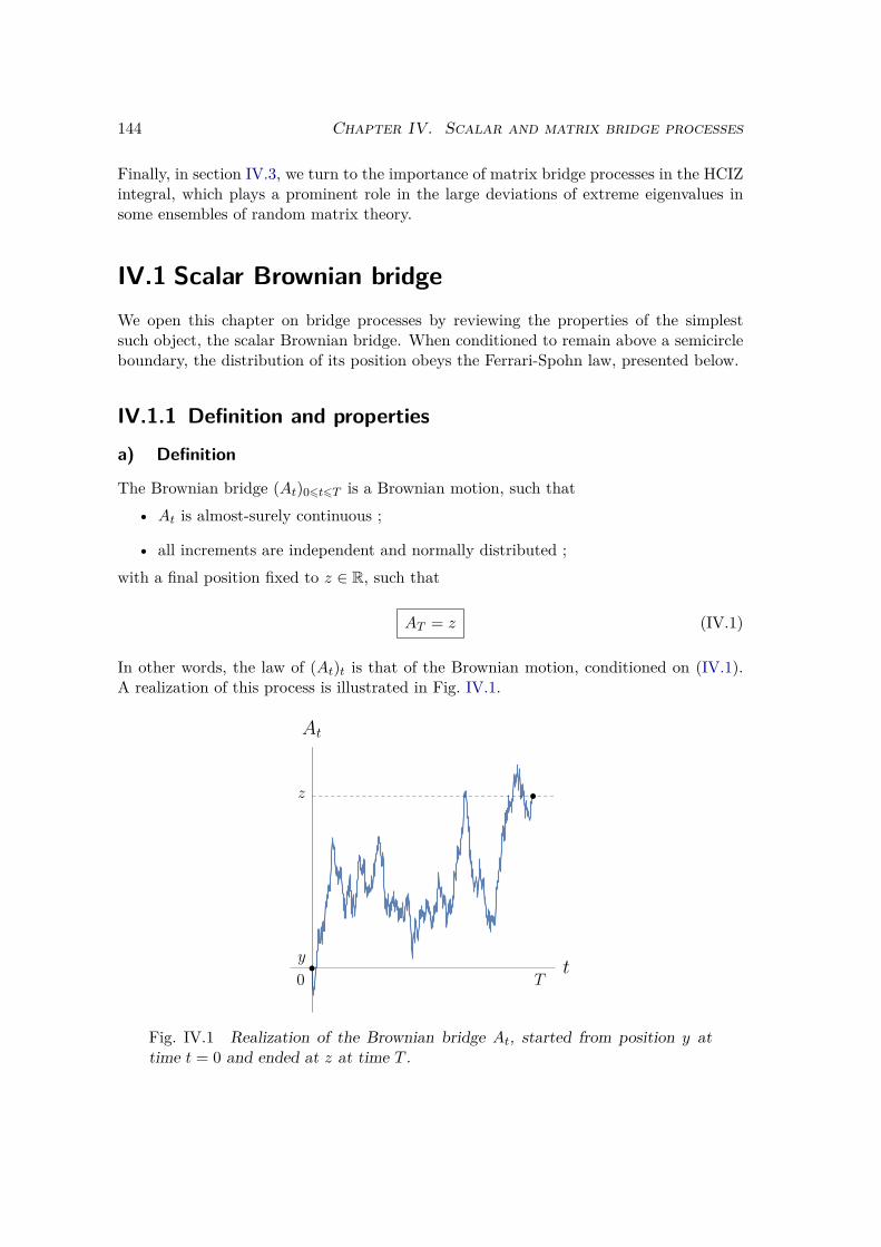
144 Chapter IV. Scalar and matrix bridge processes
Finally, in section IV.3, we turn to the importance of matrix bridge processes in the HCIZintegral, which plays a prominent role in the large deviations of extreme eigenvalues insome ensembles of random matrix theory.
IV.1 Scalar Brownian bridgeWe open this chapter on bridge processes by reviewing the properties of the simplestsuch object, the scalar Brownian bridge. When conditioned to remain above a semicircleboundary, the distribution of its position obeys the Ferrari-Spohn law, presented below.
IV.1.1 Definition and properties
a) Definition
The Brownian bridge (At)06t6T is a Brownian motion, such that• At is almost-surely continuous ;
• all increments are independent and normally distributed ;with a final position fixed to z ∈ R, such that
AT = z (IV.1)
In other words, the law of (At)t is that of the Brownian motion, conditioned on (IV.1).A realization of this process is illustrated in Fig. IV.1.
Fig. IV.1 Realization of the Brownian bridge At, started from position y attime t = 0 and ended at z at time T .

IV.1 Scalar Brownian bridge 145
b) Properties
We give a few properties of the Brownian bridge, which can be obtained easily from itsdefinition [160]. We consider that the process is started from an arbitrary initial positiony.
The single-time distribution of the process at time t, i.e. the distribution of the randomvariable At, can be obtained in conditional form from the Markov property of Brownianmotion, as
P (x, t) = P (x, t | y, 0)P (z, T | x, t)P (z, T | y, 0) (IV.2)
with the propagator given in Eq. (II.54). This yields
P (x, t) = 1√2π t(T−t)T
e−(x−y)2
2t e− (z−x)2
2(T−t) e(z−y)2
2T (IV.3)
= 1√2π t(T−t)T
e− T
2t(T−t)
(x− y(T−t)+zt
T
)2
. (IV.4)
As a consequence, At is distributed as a Gaussian random variable with expectation
E [At] = y(T − t) + zt
T= y + t
T(z − y) , (IV.5)
and varianceE[(At − E [At])2
]= t(T − t)
T. (IV.6)
Let us denote the standard deviation
s(t) =
√t(T − t)
T. (IV.7)
The expectation and variance are illustrated for many realizations of the process inFig. IV.2. In this plot, the linear expectation is the black dashed line, and the red dashedlines are one standard variation above and below the expectation, i.e. E[At]± s(t).
More generally for two instants t1 < t2, the covariance of the process (At)06t6T is
E [(At1 − E [At1 ]) (At2 − E [At2 ])] = t1(T − t2)T
. (IV.8)
c) Mappings to the standard Brownian motion
The Brownian bridge can be constructed from a realization of the Brownian motion(Bt)t>0 as we detail now. Two cases can occur: either one considers that the realizationis already known, or one considers that the details of this realization are still unknownand cannot be used in the construction. Without loss of generality, we consider in thefollowing that the process is started from y = 0.

146 Chapter IV. Scalar and matrix bridge processes
Fig. IV.2 Realization of N = 20 independent Brownian bridges Ai,t startedfrom a at time t = 0 and ended at b at time T . The black dashed line indicatesE[At] and the red dashed lines indicate E[At]± s(t), see Eqs. (IV.5) and (IV.7).
c) 1. With knowledge of the Brownian endpoint Let us consider that a real-ization (Bt)t>0 of the Brownian motion is fixed, such that, in particular, its value BT attime T is known. One can construct a statistically correct realization of the Brownianbridge (At)06t6T ended at z by defining [160]
At = Bt + t
T(z −BT ) . (IV.9)
We immediately have AT = z with probability 1, as expected.
c) 2. Without knowledge of the Brownian endpoint The previous trick how-ever fails if one considers that a special value BT of the Brownian realization is out ofreach. Another representation of the Brownian bridge from the Brownian motion, whichescapes this drawback and does not require future information about the Brownian motiontrajectory, is as follows.
General bridge endpoint From the Brownian motion (Bt)t>0, the Brownian bridge(At)06t6T ending at AT = z can be constructed as [161]
At = T − tT
B TtT−t
+ t
Tz . (IV.10)
One can verify that this Gaussian process respects the expectation and covariance of theBrownian bridge presented in the previous subsection, such that it is indeed equal in lawto a Brownian bridge started from 0 and ended at z at time T .
Symmetric bridge Let us consider the particular case where z = y = 0, such thatthe bridge is returned to its initial position at the ending time T . The expectation of the

IV.1 Scalar Brownian bridge 147
bridge is then E[At] = 0 for any t, and the mapping is simply a rescaling of the standardBrownian motion in both space and time directions, as
At = T − tT
B TtT−t
. (IV.11)
It is remarkable that the standard deviation s(t) in Eq. (IV.7) is then recovered, underthe same mapping, from the square-root standard deviation of the Brownian motion as
s(t) = T − tT
√Tt
T − t=
√t(T − t)
T. (IV.12)
The equivalence of the standard Brownian motion and the symmetric Brownian bridgethrough mapping (IV.11) is illustrated in Fig. IV.3, along with the equivalence of theirrespective standard deviations under the same mapping. Notice in particular that everycrossing of the Brownian trajectory Bt with ±
√t corresponds to a crossing of the bridge
trajectory At with ±s(t), at the relevant time t = TtT+t under the mapping. More crossings
can be observed on the bridge side, since t ∈ [0, T ] in this case corresponds to t ∈ [0,+∞[in the Brownian case, which outflanks the plot range.
1 2 3 4
-2
-1
1
2
⇐⇒0.2 0.4 0.6 0.8 1.0
-1.0
-0.5
0.5
1.0
Fig. IV.3 Left: Realization of the standard Brownian motion (Bt)t>0. Right:Brownian bridge realization (At)06t6T=1 obtained from the Brownian realizationthrough Eq. (IV.11). The running time parameter in the mapping is indicatedas the end of the dark blue colour in both plots. The standard deviations of eachprocess, which coincide under the mapping, are plotted in the black lines.
d) Conditional drift : stochastic differential equation for a bridge
The bridge process is conditioned on its endpoint AT , such that an intuitive descriptionof (At)06t6T requires information about the future as in Eq. (IV.9). The second mappingof the Brownian bridge to the standard Brownian motion, presented in the previous lines,however suggests that a description which does not break temporal locality is possible.

148 Chapter IV. Scalar and matrix bridge processes
We can indeed write a time-local SDE for the evolution of At, by applying Itô’s formulato Eq. (IV.10):
dAt =(−At − t
T z
T − t+ z
T
)dt+ T − t
TdB Tt
T−t= z −At
T − tdt+ dBt . (IV.13)
The Brownian bridge diffuses as a Brownian motion, with a linear force attracting ittowards its endpoint z with a prefactor 1/(T − t) which increases with t and divergesas t → T . We emphasize that Eq. (IV.13) is a time-local differential equation for theevolution of the process.
This can be seen as a particular case of a broader problem of obtaining a Langevinequation for a conditioned process, and an application of Doob’s h-transform theory. Letus consider an unconstrained stochastic process obeying a given SDE and constrain thisprocess such that we add a condition on an event concerning the future. Let us denoteQ(x, t) the probability under which the unconstrained process respects this very condition.For example, in the case of the bridge, Q(x, t) is the probability that the unconstrainedBrownian motion ends in z at time T , i.e.
Q(x, t) = P (z, T | x, t) = 1√2π(T − t)
e− (x−z)2
2(T−t) . (IV.14)
It can be shown, see [337], that the constrained process respects the same SDE as theunconstrained process, with an additional drift term given by
∂
∂xlogQ(x, t) . (IV.15)
This conditional drift enforces the condition through infinitesimal time evolution. Asexpected in the particular bridge case, it can be verified from Eq. (IV.14) that(
∂
∂xlogQ(x, t)
)∣∣∣∣x=At
= z −AtT − t
. (IV.16)
We finally remark that this conditional drift gives a proof of the well-known coincidenceof the three-dimensional Bessel process, evolving according to Eq. (II.13) in the specialcase D = 3, with the Brownian motion conditioned to never reach the origin [338]. Indeedfor large time t, the survival probability S(t | x, 0) of a Brownian motion above a fixedvicious boundary at g = 0 is asymptotically, per Eq. (II.89):
S(t | x, 0) ' x√
2πt
(IV.17)
such that (∂
∂xlogS(t | x, 0)
)∣∣∣∣x=Rt
= 1Rt
(IV.18)
which recovers the drift in SDE (II.13) with D = 3. A comparison with Eq. (II.15)explains, with the framework of this paragraph, why the DBM-2 coincides with the processof independent Brownian motions conditioned to never intersect, as explained in detail insection II.1.2 b).

IV.1 Scalar Brownian bridge 149
IV.1.2 Moving boundary: the Ferrari-Spohn distributionIn [335], Ferrari and Spohn considered a Brownian bridge (At)06t6T started and endedat 0, and conditioned to stay above a semicircle wall defined with W > 0 as
g(t) = W
√t(T − t)
T. (IV.19)
They studied the typical fluctuations of the distance x = AT2− g
(T2
)between the Brow-
nian particle and the wall, which we specialize in this presentation to the mid-time T2 .
Dropping the dependence on T , we denote the corresponding Brownian probability den-sity for the mid-time distance x as
R(x,W ) = P
(x+ g
(T
2
),T
2 | B[0,T ], 0, 0, 0, T). (IV.20)
This PDF gives the probabilistic weight associated with finding the Brownian motionat x + g
(T2
)at time T
2 knowing that it is started and ended at 0, and remains abovethe boundary for t ∈ [0, T ]. Abiding by the notations of chapter II, B[0,T ] is the eventwhere the particle remains away from the boundary g, and we add brackets when severalposition-time pairs appear on the same line, in order to avoid ambiguities. The bridgeunder consideration in this problem is illustrated in Fig. IV.4.
Fig. IV.4 Brownian bridge conditioned to remain above a semicircle boundaryg(t) and found at distance x of the wall at the mid-time T
2 .
In the large-W limit, Ferrari and Spohn found that the typical fluctuations of themid-time distance are described by a universal distribution given in terms of the squareof the Airy function Ai. Under the assumption W 1 on this dimensionless parameter,

150 Chapter IV. Scalar and matrix bridge processes
the distribution (IV.20) is the Ferrari-Spohn distribution:
R(x,W ) ' PFS(x) = (4W )1/3√TAi′(α1)2
Ai(α1 + (4W )1/3
√T
x
)2
Θ(x) (IV.21)
The constant α1 = −2.33811 . . . is the smallest zero, in absolute value, of the Airy functionsuch that PFS(x) → 0 as x → 0, as expected. As introduced earlier in this thesis, Θ isthe Heaviside function such that PFS is supported on R+, on which it is normalized. Thisdistribution is plotted in Fig. IV.5, in the case where 4W and T are both fixed to unity.
1 2 3 4 5
0.1
0.2
0.3
0.4
0.5
0.6
Fig. IV.5 Plot of the Ferrari-Spohn distribution PFS in Eq. (IV.21), for T =4W = 1.
The limit holds when the distance reached by the wall, g (T/2) ∼ W√T , is much
larger than the typical diffusion length ∼√T , such that the wall pushes the particles into
a rare-event regime. The characteristic scale of fluctuations of the distance between thebridge’s position and the wall is then given, in terms of T , by the prefactor in Eq. (IV.21)as
√T
W 1/3 .The exact setting of [335] is W =
√T such that the semi-circle is not deformed, and
the problem is studied in the large-T limit. The position fluctuations are then observedon scale T 1/3, given by the characteristic scale
√T
W 1/3 upon fixing W =√T .
More generally, the results of [335] allow for a general point of observation furtherfrom the mid-point T
2 , and a range of parabolic boundaries further from the semicirclepresented here. In each case, the Ferrari-Spohn distribution holds, with a prefactor of thevariable fixed by
` =(−2 g′′(tobs)
)1/3 (IV.22)
where g′′(tobs) is the second derivative of the boundary g at the point of observation tobs.One sees that, for the semicircle boundary in Eq. (IV.19), this gives indeed:
` = (4W )1/3√T
. (IV.23)
IV.2 Generalized Ferrari-Spohn distribution for non-crossing bridges 151
Finally, the results of [335] extend to a description of the temporal evolution on a timescale T 2/3.
Further from the typical regime described by the Ferrari-Spohn distribution, largedeviations in this problem and its extensions were studied in [339, 340]. In addition,the Ferrari-Spohn distribution has also been encountered in other settings. It has beenobtained for the position of a Brownian excursion conditioned to have very small totalarea [341], where we recall that a Brownian excursion is a Brownian bridge started andended at the origin, and conditioned to remain strictly positive in the meantime. The FSdistribution has also been encountered in models of two-dimensional Brownian motionconditioned on non-absorption by a stationary wall and pushed into a large-deviationregime through further constraints [342,343].
IV.2 Generalized Ferrari-Spohn distribution for multi-ple non-crossing bridges
In publication (3), a generalization of the Ferrari-Spohn model was considered for NBrownian bridges conditioned not to cross each other. In a direct extension of the single-particle case presented in the previous paragraph, the statistics of the positions at mid-time were investigated, for N non-crossing bridges ( ~At)06t6T started and ended at ~0 andconditioned to avoid the semicircle wall g(t) in Eq. (IV.19). The statistical quantity ofinterest is thus the following joint distribution, denoted R(~x,W ) and expressed in termsof the set of distances to the wall ~x at mid-time as
R(~x,W ) = P
(~x+ g
(T
2
),T
2 | B[0,T ],NC[0,T ], ~0, 0, ~0, T). (IV.24)
As in chapter II, NC[0,T ] denotes the event where the walkers remain non-crossing, andB[0,T ] the one where the lowest particle remains above the boundary. Note that R(~x,W )also depends on T but this dependence is not made explicit for simplicity. The situationis illustrated in Fig. IV.6, where the distance xk = Ak,T2
− g(T2
)of the kth particle with
the wall at mid-time is highlighted.In the limit of large W , the distribution (IV.24) is found to converge to a multi-
particle generalization of the Ferrari-Spohn distribution PFS in Eq. (IV.21), as we detailbelow. The resulting distribution displays a determinantal structure, such that it is indirect equivalence with the position statistics of a fermionic system. More precisely, thecorresponding system is subject to a linear potential above a hard wall. This mappingallows one to undertake a large-N analysis of the system. Finally, we mention below linkswith other systems such as area-tilted random walks.
IV.2.1 Generalized Ferrari-Spohn distributionThe problem defined above can be solved by a transformation into a problem concerninga collection of non-crossing Brownian motions over a barrier with a square-root profile,such that results from (1) presented in chapter II apply directly. In order to do this,the mapping (IV.11) between Brownian motions with a square-root barrier and Brownian

152 Chapter IV. Scalar and matrix bridge processes
Fig. IV.6 Non-crossing Brownian bridges conditioned to remain above a semi-circle boundary g(t) and found at distances ~x of the wall at the mid-time T
2 .
bridges with a semicircle barrier is employed. The problem needs to be slightly modifiedin the first place, as presented in the next lines.
a) Problem redefinition
a) 1. Boundary condition regularization We begin by regularizing the initialand final conditions, in order to escape the singularity caused by the null probabilityof the conditioning event B[0,T ],NC[0,T ], ~0, 0, ~0, T. This singular conditioning isnot problematic in the definition (IV.24) but will be in the next operations on the jointdistribution, such that the regularization is necessary.
The initial and final positions of the N Brownian bridges ~At are thus taken as a fixedset of positions ~s, such that 0 < s1 < · · · < sN . Furthermore, the results from chapter IIimpose a starting time that is not exactly zero, therefore we introduce a time t0 at whichthe bridges are started, and the final position is now observed at T − t0 by symmetry.The initial and final conditions are thus given by:
~At0 = ~AT−t0 = ~s. (IV.25)
With these precise conditions, the joint density is redefined as
R(~x,W ) = P
(~x+ g
(T
2
),T
2 | B[t0,T−t0],NC[t0,T−t0], ~s, t0, ~s, T − t0). (IV.26)
The joint limit (t0 → 0, ~s→ ~0) will be taken in the last step to recover Eq. (IV.24).
a) 2. Conditional manipulations After this regularization, the distributionR(~x,W )can be reshaped in order to obtain quantities upon which the results of chapter II maybe applied. This is done by massaging the conditional density, as follows.

IV.2 Generalized Ferrari-Spohn distribution for non-crossing bridges 153
We begin the by writing the conditional density R (~x,W ) as
R (~x,W ) =P(~x+ g
(T2
), T2
, ~s, T − t0,B[t0,T−t0],NC[t0,T−t0] | ~s, t0
)P(~s, T − t0,B[t0,T−t0],NC[t0,T−t0] | ~s, t0
) . (IV.27)
By Markov’s property, the numerator can be cut in two terms, which are equal by sym-metry, such that
R (~x,W ) =P(~x+ g
(T2
), T2
,B[t0,T2 ],NC[t0,T2 ] | ~s, t0
)2
P(~s, T − t0,B[t0,T−t0],NC[t0,T−t0] | ~s, t0
) . (IV.28)
We now introduce back a conditioning on the final position in order to recover bridgeprocesses, modifying the numerator term as
P
(~x+ g
(T
2
),T
2
,B[t0,T2 ],NC[t0,T2 ] | ~s, t0
)(IV.29)
=P(~x+ g
(T2
), T2
,B[t0,T2 ],NC[t0,T2 ], ~0, T | ~s, t0
)P(~0, T | ~x+ g
(T2
), T2
) (IV.30)
=P(
~x+ g
(T
2
),T
2
,B[t0,T2 ],NC[t0,T2 ] | ~s, t0, ~0, T
) P(~0, T | ~s, t0
)P(~0, T | ~x+ g
(T2
), T2
) .(IV.31)
Injecting this relation in (IV.28) yields the following reshaped expression for R(~x,W ):
R (~x,W ) =P(~x+ g
(T2
), T2
,B[t0,T2 ],NC[t0,T2 ] | ~s, t0, ~0, T
)2
P(~s, T − t0,B[t0,T−t0],NC[t0,T−t0] | ~s, t0
) P(~0, T | ~s, t0
)2
P(~0, T | ~x+ g
(T2
), T2
)2 .
(IV.32)The interest of this calculation is to express the desired JPDF in terms of a survival
probability density concerning N Brownian bridges over a semicircle boundary. Moreprecisely the term Q(~x,W ) defined by
Q(~x,W ) = P
(~x+ g
(T
2
),T
2
,B[t0,T2 ],NC[t0,T2 ] | ~s, t0, ~0, T
)(IV.33)
is the probability density that N Brownian bridges on [0, T ] started and ended from ~0and known to be in ~s at t0, are found at positions ~x + g(T2 ) at mid-time, and that theystay non-crossing and above the semicircle barrier on [t0, T2 ]. We now turn to the studyof Q(~x,W ), as the other terms in Eq. (IV.32) depend trivially on the positions ~x.
b) Brownian motions over a square-root boundaryAs seen in the previous paragraph, the problem has been transformed into the studyof Q(~x,W ), which concerns symmetric bridges on [0, T ] over a semicircle boundary on[t0, T2 ]. This object can be transformed into quantities presented in chapter II. Indeed,
154 Chapter IV. Scalar and matrix bridge processes
Eq. (IV.11) gives a mapping of the present Brownian bridges over a semicircle boundarytowards standard Brownian motions over a square-root boundary.
By inverting this change of variables, each Brownian bridge Ai,t defined for t ∈ [0, T ]and conditioned to end back at 0 at t = T , is mapped to a standard Brownian motionBi,u with a time variable u = Tt
T−t ∈ [0,∞[ as
Ai,tt → u= Tt
T−t−−−−−−−−−−→ Bi,u = T + u
TA TuT+u
. (IV.34)
The semicircle barrier g(t) is mapped under this transformation to the square root barrierh(u) = W
√u:
g(t) = W
√t
T(T − t) −−−−−−−→ h(u) = W
√u . (IV.35)
Under this transformation, the initial condition ~At0 = ~s is mapped to
~Bu0 = T + u0T
~s where u0 = Tt0T − t0
. (IV.36)
We are particularly interested in the mid-time t = T2 , where the following relations hold:
t = T
2 =⇒
u = T ,
Ai,T2= 1
2 Bi,T ,
g(T2 ) = 12 h(T ) = W
√T
2 .
(IV.37)
As can be seen easily, this mapping preserves the non-crossing properties among walk-ers and with the boundary: the ~B-paths and the boundary h do not cross on [u0, T ] if andonly if the ~A-paths and boundary g do not cross on [t0, T2 ]. As a consequence, Q(~x,W )can be expressed in terms of the following probability density for the (Bi,u) process, wherewe denote Bh the event where the square-root boundary h is not touched by the walkersin order to avoid ambiguities with the previous lines:
Q(~x,W ) = 2NP(2~x+ h(T ), T ,Bh
[u0,T ],NC[u0,T ] |T + u0T
~s, u0
)(IV.38)
This quantity is precisely given in Eq. (II.117) by the computations on Brownianmotions over a square-root boundary presented in chapter II, with the slight modificationthat the walkers are above the boundary in this section. Let us denote (φk, εk)k>0 thesequence of 1-particle eigenfunctions and eigenenergies of the 1-particle Hamiltonian Hdefined as in Eq. (II.109) with reversed inequalities. In particular
φk(X) = CkD2εk(X) (IV.39)
is defined on [W,+∞[, with a modified sign from Eq. (II.131). The JPDF Q(~x,W ) can

IV.2 Generalized Ferrari-Spohn distribution for non-crossing bridges 155
then be expressed analytically as
Q(~x,W ) = 2NTN/2
e− 1
4
N∑k=1
[(W+ 2xk√
T
)2− T
(T−t0)t0s2k
]
×∑~k∈ΩN
[det
16i,j6Nφki
(W + 2 xj√
T
)det
16i,j6Nφ∗ki
(√T
(T − t0)t0sj
)(T − t0t0
)−ε~k ](IV.40)
where the initial conditions are expressed in terms of t0. We recall that ΩN is defined inEq. (I.153) and that the multiple-fermion energies are given by
ε~k =N∑i=1
εki . (IV.41)
c) Limit resultsBefore stating the results, we remove the regularization of the boundary condition, andthen turn to the large-W limit.
c) 1. Initial condition limit t0, ~s → 0,~0 A non-zero initial condition wasnecessary for the conditional manipulations and the use of the results of chapter II. Wemay remove it by scaling ~s with t0 as follows:
~s = g (t0) ~S = W
√t0T
(T − t0) ~S, (IV.42)
where ~S satisfies 1 < S1 < · · · < SN , and taking the limit t0 → 0 with ~S held constant.The dominant contribution in (IV.40) then corresponds to the ground state such that
Q(~x,W ) ' 2NTN/2
e−
N∑k=1
[1T
(W√T
2 +xk)2−W2S2
k4
]det
16i,j6Nφi−1
(W + 2 xj√
T
)det
16i,j6Nφ∗i−1 (WSj)
(T
t0
)−ε~0.
(IV.43)
We note that the eigenfunctions φi are defined on [W,+∞[ such that det16i,j6N
φ∗i−1 (WSj)is a well-defined constant.
The JPDF of interest, R(~x,W ), is obtained in Eq. (IV.32) from the expression ofQ(~x,W ). Evaluating the simple propagator terms which cancel the exponential term, wehave in the limit t0 → 0:
R (~x,W ) '
(2T
)N ( t0T
)2ε~0 ( det16i,j6N
φ∗i−1 (WSj))2e
12
N∑k=1
W 2S2k
P(~s, T − t0,B[t0,T−t0],NC[t0,T−t0] | ~s, t0
) [det
16i,j6Nφi−1
(W + 2 xj√
T
)]2.
(IV.44)

156 Chapter IV. Scalar and matrix bridge processes
We can directly read, from this equivalent expression, the limiting joint distribution func-tion of the positions of the bridges above the semicircle boundary by discarding the termswhich do not depend on variables ~x. We conclude that, at t0 = 0 and for arbitrary W ,the JPDF R(~x,W ) defined in Eq. (IV.24) is given by
R(~x,W ) = C
[det
16i,j6Nφi−1
(W + 2 xj√
T
) ]2(IV.45)
where we recall that the expression of the eigenfunctions φ of the Schrödinger operatorwith a quadratic potential and a hard wall at W is given in Eq. (IV.39). We point to(3) for additional details on the convergence, for the value of the prefactor C and for theconclusions which can be drawn on the vanishing speed of the denominator of Eq. (IV.45).
c) 2. Large-W limit In order to achieve a generalization of the Ferrari-Spohndistribution, we finally specialize this expression to the large-W case, where the wallpushes the particles in a large-deviation regime.
In the large-W limit, the Hamiltonian of the underlying fermionic system H is nearlylinear, neglecting a (X −W )2 term, as
H '
−12∂2
∂X2 + 18W
2 + 14(X −W )− 1
4 for X > W ,
+∞ for X 6W .
(IV.46)
As detailed in (3), the eigenfunctions φk and eigenvalues εk can then be shown to be givenin terms of the Airy function by the following expressions
φk(X) = Dk,W Ai(αk+1 +
(W
2
)1/3(X −W )
)εk = −αk+1
2 (W2 )2/3 + 18W
2 − 14
(IV.47)
where (αk)k>1 is the sequence of zeros of the Airy function. The normalization constantDk,W is such that
∫∞W φ2
k(X)dX = 1. It is found from the integral∫∞αk
Ai(x)2dx = Ai′(αk)2,see App. B, as
Dk,W = (W/2) 16∣∣Ai′(αk+1)∣∣ . (IV.48)
Let us give some details about the validity of the approximations made above. Ne-glecting the quadratic term in the potential as we did in Eq. (IV.46) requires ∆X =X −W W . On the other hand, the eigenfunctions of Eq. (IV.47) are spread over aspatial scale ∆X ∼ W−1/3. We therefore find that the requirement is simply W 1, asassumed in the large-W regime. Recalling that the wall’s position is given by Eq. (IV.19),this requirement simply means that the distance reached by the wall, g (T/2) ∼ W
√T ,
is much larger than the typical diffusion length ∼√T , such that the wall pushes the
particles into a large-deviation regime.In the large W regime, the limiting distribution for the distance of the bridges with
the wall is obtained by injecting the eigenfunctions (IV.47) in (IV.45). We can then give

IV.2 Generalized Ferrari-Spohn distribution for non-crossing bridges 157
the final result of our analysis, which gives R(~x,W ) as the following generalization of theFerrri-Spohn distribution:
R(~x,W ) = CN,W
[det
16i,j6NAi(αi + (4W )1/3
√T
xj
)]2
(IV.49)
The normalization constant, such that∫R+N R(~x,W ) d~x = 1, is given by
CN,W = (4W )N3N ! T N
2∏Nk=1 Ai′(αk)2
. (IV.50)
This distribution can be seen to coincide with Eq. (IV.21) in the single-bridge case N = 1.
d) General observation timeThe goal of the previous computations was to extend the mid-time result given in Eq. (IV.21)for a single bridge, but we emphasize that the manipulations can be extended to any ob-servation time t ∈]0, T [, further from the special case t = T
2 detailed above.Crucially, for a general observation time t, the term Q(~x,W )2 in the expression of
R(~x,W ) is replaced by the product of two different terms
P(~x+ g (t) , t ,B[t0,t],NC[t0,t] | ~s, t0, ~0, T
)× P
(~x+ g (T − t) , T − t ,B[t0,T−t],NC[t0,T−t] | ~s, t0, ~0, T
).
(IV.51)
The mapping to Brownian motions over a square-root boundary can be applied to boththese terms separately. The procedure goes through and yields the following result
Rt(~x,W ) = C
[det
16i,j6Nφi−1
(W + xj
√T
t(T − t)
) ]2
(IV.52)
which gives back Eq. (IV.45) for t = T2 . The large-W limit then yields the general-
observation-time generalization of the Ferrari-Spohn distribution
Rt(~x,W ) = C
[det
16i,j6NAi(αi +
(W
2
) 13√
T
t(T − t) xj)]2
(IV.53)
Similarly as in the single-bridge case, the prefactor of the x variable is given by thesecond derivative of the boundary at the time of observation as
` =(−2 g′′(t)
)1/3 =(W
2
) 13√
T
t(T − t) . (IV.54)
This suggests that the N -particle setting extends to general concave boundary shapes,although we are limited to the semi-circle boundary with the method employed in thisderivation.
In the generalized Ferrari-Spohn problem, the distribution of positions can thus bederived for a general observation time, as shown in this section. Notice that the situationis different in other non-crossing bridge problems where analytical solutions can only befound for particular times, as in [183].
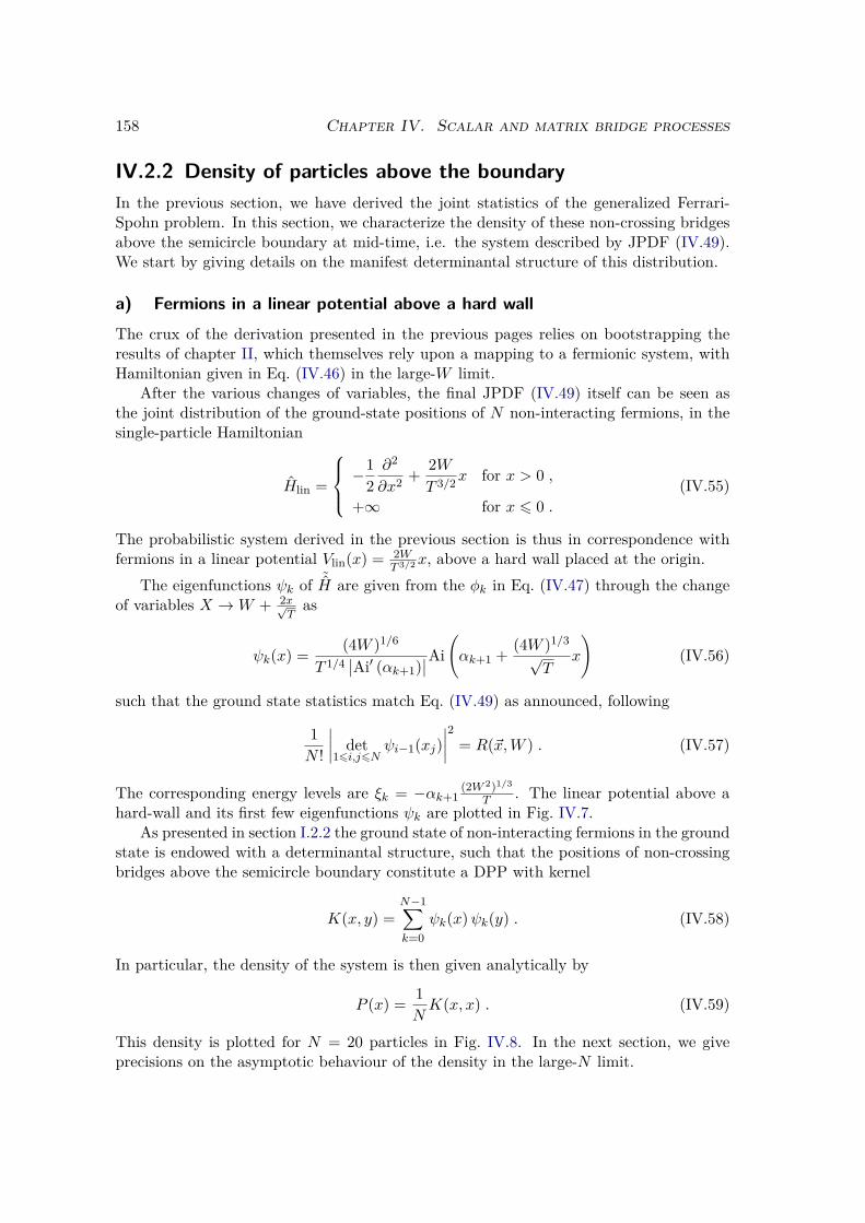
158 Chapter IV. Scalar and matrix bridge processes
IV.2.2 Density of particles above the boundaryIn the previous section, we have derived the joint statistics of the generalized Ferrari-Spohn problem. In this section, we characterize the density of these non-crossing bridgesabove the semicircle boundary at mid-time, i.e. the system described by JPDF (IV.49).We start by giving details on the manifest determinantal structure of this distribution.
a) Fermions in a linear potential above a hard wallThe crux of the derivation presented in the previous pages relies on bootstrapping theresults of chapter II, which themselves rely upon a mapping to a fermionic system, withHamiltonian given in Eq. (IV.46) in the large-W limit.
After the various changes of variables, the final JPDF (IV.49) itself can be seen asthe joint distribution of the ground-state positions of N non-interacting fermions, in thesingle-particle Hamiltonian
Hlin =
−12∂2
∂x2 + 2WT 3/2x for x > 0 ,
+∞ for x 6 0 .(IV.55)
The probabilistic system derived in the previous section is thus in correspondence withfermions in a linear potential Vlin(x) = 2W
T 3/2x, above a hard wall placed at the origin.The eigenfunctions ψk of ˜
H are given from the φk in Eq. (IV.47) through the changeof variables X →W + 2x√
Tas
ψk(x) = (4W )1/6
T 1/4∣∣Ai′ (αk+1)
∣∣Ai(αk+1 + (4W )1/3
√T
x
)(IV.56)
such that the ground state statistics match Eq. (IV.49) as announced, following
1N !
∣∣∣∣ det16i,j6N
ψi−1(xj)∣∣∣∣2 = R(~x,W ) . (IV.57)
The corresponding energy levels are ξk = −αk+1(2W 2)1/3
T . The linear potential above ahard-wall and its first few eigenfunctions ψk are plotted in Fig. IV.7.
As presented in section I.2.2 the ground state of non-interacting fermions in the groundstate is endowed with a determinantal structure, such that the positions of non-crossingbridges above the semicircle boundary constitute a DPP with kernel
K(x, y) =N−1∑k=0
ψk(x)ψk(y) . (IV.58)
In particular, the density of the system is then given analytically by
P (x) = 1NK(x, x) . (IV.59)
This density is plotted for N = 20 particles in Fig. IV.8. In the next section, we giveprecisions on the asymptotic behaviour of the density in the large-N limit.

IV.2 Generalized Ferrari-Spohn distribution for non-crossing bridges 159
2 4 6 8 10
Fig. IV.7 Plot of the linear potential Vlin(x) above a hard-wall at the originwith T = 4W = 1 (black line). The first seven eigenfunctions (ψk)06k66 areplotted at the corresponding energy level ξk (coloured lines). Notice that |ψ0|2recovers the PDF plotted in Fig. IV.5.
b) Large-N behaviour
In the limit where the number of Brownian bridges is very large, the behaviour of thedensity (IV.59) can be obtained from the universal properties of noninteracting fermions,related to the universal properties of RMT presented in chapter I. The fermion system ofinterest here presents three different regimes in the bulk, at the soft edge around the topparticle and close to the hard edge. We present briefly the exposition of (3).
b) 1. In the bulk In the bulk regime, the density is well described by the LDA [325],which yields the following approximation
P bulk (x) =√
2πN
√(3πWN)2/3
21/3T− 2WT 3/2x , x ∈ [0, xedge] (IV.60)
where
xedge = (3πN)2/3 T 1/2
24/3W 1/3 . (IV.61)
The effective Fermi energy of the fermion system is given by
µ = (3πWN)2/3
21/3T. (IV.62)
More precisely, the bulk statistics of the particles on a scale(NP bulk(x)
)−1are de-
scribed by the sine kernel Ksine (I.140).

160 Chapter IV. Scalar and matrix bridge processes
b) 2. At the soft edge Near the soft edge at position xedge, the statistics aredescribed by the Airy kernel KAiry (I.142). The width of the edge regime is
wN = [2Vlin(xedge)]−1/3 =√T
(4W )1/3 . (IV.63)
The density is then correctly described by
P edge(x) ' 1NwN
F1
(x− xedgewN
), F1 (z) =
[Ai′ (z)
]2 − z [Ai (z)]2 (IV.64)
as discussed in Eq. (III.72).As a result of the Airy statistics in the soft edge region, the fluctuations of the position
of the highest particle, i.e. the one furthest from the wall, can be characterized as seenin chapter I. This position can be written as xN = xedge + wNχ where χ converges, forlarge N , to the GUE Tracy-Widom distribution (I.166).
As explained in the chapter introduction, a motivation for the Ferrari-Spohn model[335] is to study a single bridge above a sea of non-crossing bridges, whose expectedenvelope is the semicircular boundary. The semicircle toy model then yields the Ferrari-Spohn distribution instead of the Tracy-Widom distribution. As shown above, the studyof (3) sheds light on the intermediate regime between these two distributions, as theFerrari-Spohn distribution is obtained for N = 1 and the Tracy-Widom distribution isrecovered for N 1. For intermediate values of N , the distribution of the top particlecan be obtained as a marginal of (IV.49).
b) 3. At the hard edge Close to the hard-edge, the kernel converges to the hard-wall kernel
KHb (x, y) = sin (x− y)π (x− y) −
sin (x+ y)π (x+ y) (IV.65)
as1kN
K
(x
kN,y
kN
)−−−−→N→∞
KHb (x, y) (IV.66)
where the scaling is fixed by
kN = πNP bulk(0) =√
2µ = (6πWN)1/3√T
. (IV.67)
KHb is the universal kernel obtained for fermions close to a hard-wall [96,104,109,344].It can be seen to hold in particular for the hard-box fermionic potential, through therelation to the JUE mentioned in chapter I. Note that KHb is related to the Bessel kernelKBesselα (I.144) with parameter α = 1
2 as
KHb (x, y) = 2√xy KBessel1/2
(x2, y2
). (IV.68)
All statistics close to the hard-wall, such as the PDF of the position of the particleclosest to the wall, can be expressed in terms of the kernel KHb (IV.65). The density nearthe wall is obtained in the limit y → x as
P hard(x) ' kNNFHb (kN x) , FHb(z) = 1
π
[1− sin (2z)
2z
]. (IV.69)

IV.2 Generalized Ferrari-Spohn distribution for non-crossing bridges 161
The exact density P (x) of the Fermi gas, given in Eq. (IV.59), is plotted in Fig. IV.8 forN = 20 particles, along with the approximations P bulk(x) in the bulk, given in Eq. (IV.60),P edge(x) at the soft edge, given in Eq. (IV.64), and P hard(x) at the hard edge, given inEq. (IV.69). As in previous figures, the parameters are fixed as T = 4W = 1.
This concludes our presentation of the properties of non-crossing bridges above asemicircular boundary, in the limit where the boundary pushes the particles in a large-deviation regime, following (3). Fig. IV.8 shows the density of this ensemble of non-crossing particles above the boundary, in direct extension of the single-particle Ferrari-Spohn setting illustrated in Fig. IV.5.
0 5 10 15 20 250.00
0.02
0.04
0.06
0.08
0.0 0.5 1.0 1.5 2.00.00
0.02
0.04
0.06
0.08
Fig. IV.8 Plot of the exact average density P (x) for N = 20 particles, in theblue line. The bulk density P bulk(x) is the dashed gray line, the soft edge densityP edge(x) is the dashed red line and the hard-edge density P hard(x) is the dashedorange line. The inset shows the region near the hard edge.
IV.2.3 Links with area-tilted excursionsLet us consider a single Brownian excursion (Xt)06t6T . The fluctuations of the area∫ T
0 Xt dt covered by this process are described by the Airy distribution, which also appliesto the maximal height of a fluctuating interface of Edwards-Wilkinson or KPZ type [345].As mentioned earlier, when conditioning this Brownian excursion to cover only a verysmall area, the fluctuations of its position at a given time are described by the Ferrari-Spohn distribution. We point in particular to Appendix C of [341] for a detailed derivationof the connection between the Brownian excursion and the Ferrari-Spohn model, in a pathintegral formalism.
Accordingly, it is natural to expect the results presented in the previous pages tobe valid for N non-crossing Brownian excursions Xi,t conditioned on the sum of areas
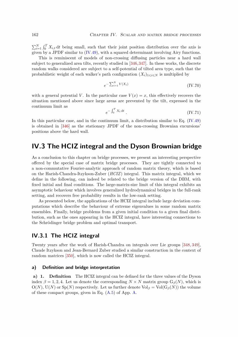
162 Chapter IV. Scalar and matrix bridge processes
∑Ni=1
∫ T0 Xi,t dt being small, such that their joint position distribution over the axis is
given by a JPDF similar to (IV.49), with a squared determinant involving Airy functions.This is reminiscent of models of non-crossing diffusing particles near a hard wall
subject to generalized area tilts, recently studied in [346,347]. In these works, the discreterandom walks considered are subject to a self-potential of tilted area type, such that theprobabilistic weight of each walker’s path configuration (Xi)16i6N is multiplied by
e−∑N
i=1 V (Xi) (IV.70)
with a general potential V . In the particular case V (x) = x, this effectively recovers thesituation mentioned above since large areas are prevented by the tilt, expressed in thecontinuum limit as
e−∫ T
0 Xt dt . (IV.71)
In this particular case, and in the continuum limit, a distribution similar to Eq. (IV.49)is obtained in [346] as the stationary JPDF of the non-crossing Brownian excursions’positions above the hard wall.
IV.3 The HCIZ integral and the Dyson Brownian bridgeAs a conclusion to this chapter on bridge processes, we present an interesting perspectiveoffered by the special case of matrix bridge processes. They are tightly connected toa non-commutative Fourier-analytic approach of random matrix theory, which is basedon the Harish-Chandra-Itzykson-Zuber (HCIZ ) integral. This matrix integral, which wedefine in the following, can indeed be related to the bridge version of the DBM, withfixed initial and final conditions. The large-matrix-size limit of this integral exhibits anasymptotic behaviour which involves generalized hydrodynamical bridges in the full-ranksetting, and recovers free probability results in the low-rank setting.
As presented below, the applications of the HCIZ integral include large deviation com-putations which describe the behaviour of extreme eigenvalues in some random matrixensembles. Finally, bridge problems from a given initial condition to a given final distri-bution, such as the ones appearing in the HCIZ integral, have interesting connections tothe Schrödinger bridge problem and optimal transport.
IV.3.1 The HCIZ integralTwenty years after the work of Harish-Chandra on integrals over Lie groups [348, 349],Claude Itzykson and Jean-Bernard Zuber studied a similar construction in the context ofrandom matrices [350], which is now called the HCIZ integral.
a) Definition and bridge interpretation
a) 1. Definition The HCIZ integral can be defined for the three values of the Dysonindex β = 1, 2, 4. Let us denote the corresponding N ×N matrix group Gβ(N), which isO(N), U(N) or Sp(N) respectively. Let us further denote Volβ = Vol(Gβ(N)) the volumeof these compact groups, given in Eq. (A.5) of App. A.
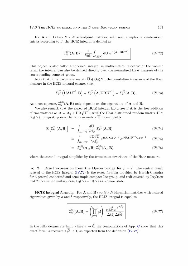
IV.3 The HCIZ integral and the Dyson Brownian bridge 163
For A and B two N × N self-adjoint matrices, with real, complex or quaternionicentries according to β, the HCIZ integral is defined as
I(β)N (A,B) = 1
Volβ
∫Gβ(N)
dU eTr(AUBU−1) (IV.72)
This object is also called a spherical integral in mathematics. Because of the volumeterm, the integral can also be defined directly over the normalized Haar measure of thecorresponding compact group.
Note that, for an arbitrary matrix U ∈ Gβ(N), the translation invariance of the Haarmeasure in the HCIZ integral ensures that
I(β)N
(UAU−1
,B)
= I(β)N
(A,UBU−1) = I(β)
N (A,B) . (IV.73)
As a consequence, I(β)N (A,B) only depends on the eigenvalues of A and B.
We also remark that the expected HCIZ integral factorizes if A is the free additionof two matrices as A = A1 + UA2U
−1, with the Haar-distributed random matrix U ∈Gβ(N). Integrating over the random matrix U indeed yields
E[I(β)N (A,B)
]=
∫Gβ(N)
dUVolβ
I(β)N (A,B) (IV.74)
=∫
Gβ(N)2
dUdUVol2β
eTrA1UBU−1eTrUA2U−1UBU−1 (IV.75)
= I(β)N (A1,B) I(β)
N (A2,B) (IV.76)
where the second integral simplifies by the translation invariance of the Haar measure.
a) 2. Exact expression from the Dyson bridge for β = 2 The central resultrelated to the HCIZ integral (IV.72) is the exact formula provided by Harish-Chandrafor a general connected and semisimple compact Lie group, and rediscovered by Itzyksonand Zuber in the unitary case G2(N) = U(N) as we now state.
HCIZ integral formula For A and B two N×N Hermitian matrices with orderedeigenvalues given by ~a and ~b respectively, the HCIZ integral is equal to
I(2)N (A,B) =
N−1∏p=1
p!
det16i,j6N
eaibj
∆(~a) ∆(~b)(IV.77)
In the fully degenerate limit where ~a → ~0, the computations of App. C show that thisexact formula recovers I(2)
N → 1, as expected from the definition (IV.72).

164 Chapter IV. Scalar and matrix bridge processes
Dyson bridge proof This formula can be proved in an insightful way by turningto a bridge interpretation, as we detail now. A slight remodelling of the β = 2 HCIZintegral of A and B gives
C2 I(2)N (A,B) e−
Tr(A2+B2)2 = C2
Volβ
∫U(N)
dU e−12 Tr(A−UBU−1)2
, (IV.78)
where we have included C2, the constant defined in Eq. (I.21) with σ = 1.Let us now recall that H2
1, the DBM with Dyson index β = 2 at time t = 1 defined inEq. (II.2), is distributed as the σ = 1 GUE matrix distribution (I.20). As a consequence,the r.h.s. of Eq. (IV.78) is the exact probabilistic weight for the DBM-2 started at H2
0 = Ato end, at time t = 1, in any rotation UBU−1 of the matrix B. We deduce
C2 I(2)N (A,B) e−
Tr(A2+B2)2 = E
[1H2
1=UBU−1 | H20 = A
](IV.79)
where the conditional expectation is taken over both the value H21 of the DBM at t = 1
and a normalized-Haar-measure distributed random matrix U.At the eigenvalue level, this expectation is the probabilistic weight of the N -particle
DBM-2 bridge configurations starting at ~a and ending at ~b, between t = 0 and t = 1,after taking into account the Jacobian term ∆(~b)2 and the proportionality factor N ! ΞN2given in Eq. (A.8), both needed to recover the (ordered) eigenvalue distribution fromthe matrix distribution. We furthermore recall per chapter II that the DBM-2 eigenvalueprocess is identical to the process of never-crossing Brownian motions. The expectation inEq. (IV.79) can then be written simply in terms of the following Brownian joint probabilitydensity
C2 I(2)N (A,B) e−
Tr(A2+B2)2 = 1
N ! ΞN2 ∆(~b)2P(~b, 1 | ~a, 0,NC[0,∞[
). (IV.80)
The application of relation (II.76) and of the Karlin-McGregor theorem (II.55) gives
P(~b, 1 | ~a, 0,NC[0,∞[
)= ∆(~b)
∆(~a) det16i,j6N
P (bi, 1 | aj , 0) (IV.81)
in terms of the single-particle Brownian propagator, such that
C2 I(2)N (A,B) e−
Tr(A2+B2)2 = 1
N ! ΞN2√
2πNdet
16i,j6Ne−
(ai−bj)2
2
∆(~a) ∆(~b)(IV.82)
= e− 1
2
N∑i=1
(a2i+b
2i )
N ! ΞN2√
2πNdet
16i,j6Neaibj
∆(~a) ∆(~b). (IV.83)
Simplifying the squared terms finally recovers the celebrated HCIZ integral formula (IV.77).This derivation shows that the HCIZ integral is fundamentally related to a probabilis-
tic weight concerning a DBM bridge, with bounds given in terms of the two arguments Aand B of I(2)
N (A,B). The Dyson bridge matrix process is, as a consequence, connected

IV.3 The HCIZ integral and the Dyson Brownian bridge 165
to many aspects of RMT through the HCIZ integral, as we develop below. Note thatthe Dyson bridge connection can be extended to the β = 1, 4 cases. However, we havenot included them in the derivation above, because the absence of a simple expressionfor the DBM propagator for β 6= 2 prevents one from obtaining an expression similar toEq. (IV.77). We recall that this is directly linked to the presence of interactions in thecorresponding Calogero-Moser Hamiltonian’s potential (II.50) when β 6= 2.
For more details on the above definition of the HCIZ integral and for algebraic proofsof the integral formula, see [65,351–353].
b) Large-N limitWe present briefly the asymptotics of the HCIZ integral in the large-N limit, which canbe investigated in the general full-rank setting, where A and B both have many non-zero eigenvalues, and in the particular low-rank setting, where one of them has mosteigenvalues equal to zero.
b) 1. Full-rank setting The large-N asymptotics of the HCIZ integral were firstobtained by Matytsin in the unitary case [354], before being derived in full mathematicalrigour [355] and extended to the orthogonal case [356]. These asymptotics can be usefulin many applications, such as matrix models where the HCIZ integral (IV.72) appears asa consequence of interaction, and thus controls the large-N behaviour of the system andthe asymptotic spectral distributions [350].
Let us state the asymptotic result in the β = 2 case. Assuming that the eigenvaluesof A and B scale as
√N such that the occupation densities of ~a/
√N and ~b/
√N are
described in the limit by two distribution functions ρa and ρb, we have
I(2)N (A,B) ' eN
2F(ρa,ρb) (IV.84)
The leading term grows exponentially at speed N2 with a rate function F related to theaction corresponding to the Euler system
∂ρ
∂t+ ∂(ρv)
∂x= 0 ,
∂v
∂t+ v
∂v
∂x− π2ρ
∂ρ
∂x= 0 (IV.85)
describing the one-dimensional evolution of a fluid with density ρ(x, t) and velocity v(x, t),with boundary conditions fixed by
ρ(x, t = 0) = ρa(x) , ρ(x, t = 1) = ρb(x) . (IV.86)
The leading term in the large-N limit of I(2)N (A,B) is thus related to a hydrodynamical
bridge problem, and is characterized by the dynamics of a fluid evolving as (IV.85) fromthe eigenvalues of A/
√N at initial time to those of B/
√N at final time. This hydro-
dynamical bridge is reminiscent of the Dyson bridge, explained in the previous sectionto be at the center of the HCIZ construction. Remarkably, it was shown in [357] thatthis hydrodynamical description can be obtained directly from the finite-N Dyson bridgesetting, through an instanton approach to the large deviations of the DBM bridge.
Finally, in order to stress the connections with the Dyson bridge, we remark thatthe complex field f(x, t) = v(x, t) + iπρ(x, t) evolves, per Eq. (IV.85), as the complex

166 Chapter IV. Scalar and matrix bridge processes
Burgers equation which characterizes the Stieltjes transform evolution for the DBM, seeEq. (II.24), as
∂f(x, t)∂t
+ f(x, t)∂f(x, t)∂x
= 0 . (IV.87)
For more details on the hydrodynamical system and its complex Burgers version, see[173,175,354].
b) 2. Low-rank setting The analysis is simpler in the case where one of the ma-trices has low rank, or even rank one as we turn to now. The result was obtained inthe context of spin glasses in [358] for β = 1, 2, and derived in full mathematical rigourin [359]. In this regime, the HCIZ integral is tightly related to the partition function ofthe spherical Sherrington-Kirkpatrick model [360,361].
With x be a unit N -dimensional vector, we consider that the second argument of theHCIZ integral is
B = Ntxx† (IV.88)
such that its eigenvalues are ~b = Nt, 0, · · · , 0. The corresponding HCIZ integral thendepends on the eigenvalues ~a of A and on the parameter t, such that we denote it
I(β)~a (t) = I(β)
N (A, Ntxx†) . (IV.89)
For small enough t, the large-N behaviour of the rank-one HCIZ integral is found to growexponentially at speed N , according to
I(β)~a (t) ' e
N∫ t
0 RA(
2βu)
du (IV.90)
where RA is the R-transform of A, defined in Eq. (I.186). For higher values of t, aphase transition is encountered at a given t∗ and the rate function is different thereafter,see [359]. Notice the difference of the N scaling in this low-rank setting with the N2
scaling which characterizes the full-rank asymptotics in Eq. (IV.84).The appearance of RA in the large-N HCIZ integral of A and a rank-one matrix
shows that the HCIZ construction has profound ties to free probability. These ties canbe illustrated by applying Eq. (IV.76) to the current setting. Indeed, taking ~c to be theeigenvalues of the free sum of two matrices A and B, we have in the self-averaging large-Nlimit
I(β)~c (t) = I(β)
~a (t)× I(β)~b
(t) . (IV.91)
Therefore, the HCIZ integral is, in the large-N limit, the exponential of a function whichis additive under the free sum. Recalling Eq. (I.188), it is therefore not surprising that theR-transform should appear in the asymptotics of the log of the rank-one HCIZ integral.
Finally, we remark that the nature of I(β)~a (t) as a function of the random matrix A
and the external parameter t which is multiplicative under the asymptotically free summakes it a natural matrix counterpart of the characteristic function for a scalar randomvariable X, defined as E[eitX ]. This illustrates Harish-Chandra’s initial motivation, whenintroducing the HCIZ integral, to develop a non-commutative Fourier analysis on Liealgebras [362]; we point to [359] for a discussion on the validity of upgrading the parametert to a complex number.

IV.3 The HCIZ integral and the Dyson Brownian bridge 167
For more details on the relation of the HCIZ construction with free probability, deriva-tions of Eq. (IV.90), replica computations surrounding the HCIZ integral and results in thesetting where the rank is small compared to N but higher than one, we point to [65,353].Interestingly, a multiplicative version of the HCIZ integral can be constructed, see [363],which displays a rank-one large-N behaviour similar to Eq. (IV.90) with the S-transformtaking the place of the R-transform.
IV.3.2 Large deviations of extreme eigenvalues in some RMTensembles
The HCIZ integral has applications in many areas of physics and mathematics. It appearsnaturally in harmonic analysis, representation theory and symplectic geometry, as well asin the combinatorics of Hurwitz number, see [352]. In physics, the HCIZ integral appearsnaturally in matrix models presenting interactions: it was initially studied in relation toQCD and map enumeration [350, 354, 364], but it also appears in spin glass models [65]and in quantum ergodic transport [365,366].
Remarkably, the HCIZ integral also plays a central role in the large deviations of someRMT ensembles which have an external source [367], as noticed in the formal derivationof the full-rank large-N asymptotics [355]. In order to probe the largest eigenvalue’sright-tail large deviations in some ensembles, the idea has recently emerged in [368] totilt the matrix distribution by the rank-one HCIZ integral. As explained in [369], thisprocedure amounts to tilt the law of the matrix in a random direction, in order to pushthe top eigenvalue in a large-deviation regime. This yields large-deviation results whichare, as a consequence, directly expressed in terms of the rank-one asymptotics presentedin the previous section. Because of the phase transition mentioned below Eq. (IV.90), theensuing rate functions can be intricate. Consequently, we will not present them in fulldetail here, but instead mention results that were recently obtained with this technique,for some ensembles of RMT.
Let A and B be two large deterministic Hermitian matrices, and U a unitary Haar-distributed matrix. In [370], large-deviation results were obtained for the largest eigen-value of
A + UBU−1 . (IV.92)
With A a large deterministic matrix as above, and H a Wigner matrix (GOE or GUEfor example), the large-deviation principle for the largest eigenvalue of
A + H (IV.93)
was established in [371]. Notice the difference with the previous model, as the eigenvaluesof H are not fixed here, unlike those of B in Eq. (IV.92).
For H a GOE or GUE matrix and x a fixed vector, the largest eigenvalue of the spikedmodel
θ xx† + H (IV.94)
was described in the large-deviation regime in [372]. The transition in the behaviour ofthe largest eigenvalue of this rank-one perturbation of a Gaussian matrix was famouslydescribed by Baik-Ben Arous-Péché (BBP) in [373]; the investigation of [372] thus explores

168 Chapter IV. Scalar and matrix bridge processes
the large-deviation regime beyond the BBP mechanism. We remark that the results arealso generalized to the Wishart ensemble.
In a distinctly more accessible derivation, the generalized Wishart ensemble was stud-ied in [374]. The model in question is
X† Γ X (IV.95)
defined as in Eq. (I.43) with an arbitrary covariance matrix Γ. Specifically, the topeigenvalue’s large deviations were described. Remarkably, the rate function is shown inthis case to take a very simple form as the integral of the difference of the two admissiblebranches of the Stieltjes transform, see Eq. (3) of [374].
We insist that the rank-one HCIZ tilt technique, used to obtain the largest eigenvaluelarge-deviation regime in these ensembles, limits all the above results to the right tail.Indeed, the tilt pushes one eigenvalue in a rare configuration, but is incapable of pushinga large portion of eigenvalues away from their typical position, which is required to reacha left-tail large-deviation event. As a consequence, the development of a measure-tilt bythe full-rank HCIZ integral is necessary in the left-tail setting. This is illustrated in [369]where large deviations are obtained for the empirical eigenvalue distribution for the modeldefined in Eq. (IV.92) through such a full-rank tilt, further from the largest-eigenvaluestudy of [370]. Notice in this regard that the respective scaling behaviours of the low-rankand full-rank cases coincide exactly with the Coulomb-gas energy cost of pulling a singleparticle (∝ N) or pushing a large portion (∝ N2), as discussed in subsection I.2.3.
IV.3.3 Schrödinger bridges and optimal transportIn subsection IV.3.1, we have shown how the HCIZ integral is intimately connected to thetransportation of particles from a given distribution at time t = 0 to another one at timet = 1. In a wider scope and relaxing interactions between particles, this is reminiscent ofa bridge problem introduced by Erwin Schrödinger in the 1930’s. This problem has deepconnections to the theory of optimal transport, on which we close the perspectives laidout in this section.
a) Schrödinger bridge problem
In [375, 376], Schrödinger introduced the following thought experiment concerning thestatistical physics of hot gas particles. The problem is to find the most likely trajectorytaken by a cloud of N independent Brownian particles, started according to a distributionρ0 at t = 0 and known to have ended in an arbitrary distribution ρ1 at t = 1, potentiallyvery different from the distribution expected from the convolution of ρ0 with the Brownianpropagator over a unit-time evolution.
This maximum-entropy problem can be recast and solved in the modern frameworkof stochastic processes and large deviations, but recall that these did not yet exist at thetime. The remarkable aspect of this problem lies in the analogy that can be drawn withthe laws of quantum mechanics. Indeed, the solution ρ(x, t), describing the most probabledistribution of the particles at intermediate time t ∈ [0, 1], can be written as a product
ρ(x, t) = ψ(x, t) ψ(x, t) (IV.96)

IV.3 The HCIZ integral and the Dyson Brownian bridge 169
where ψ is the forward solution of the stochastic evolution from the initial conditionρ0, and ψ is the backward solution from the final condition ρ1. This is evocative ofthe quantum framework where the probability distribution is the modulus square of thewavefunction, see Eq. (I.150), and where the conjugate of the wavefunction is a solutionof the time-reversed Schrödinger equation.
We point to the survey [377] for more details on the solution of the bridge problem andits quantum analogy. For financial applications of the Schrödinger bridge construction,see [378]. As mentioned in these works, the Schrödinger bridge solution can be shown torespect a SDE with drift term similar to (IV.15), as expected from the explanations ofsubsection IV.3.1.
b) Optimal transportBeyond quantum mechanics, the ties of this problem extend to the Monge-Kantorovichtheory of optimal transport. This field focuses on the study of the optimization problemof finding the transport map, from an initial mass distribution to a final mass distribution,that minimizes a quadratic cost-function. This problem induces the Wasserstein distancebetween probability distributions and is solved, in some practical applications, by animplementation of Sinkhorn’s algorithm, which relies on the observation that the doubly-stochastic matrix defining the transport map can be obtained as the result of alternativelynormalizing the rows and columns of a matrix.
The Schrödinger bridge problem is an entropy regularization of optimal transport,adding a noise ingredient to the particles’ trajectories in a blurry approximation of theMonge-Kantorovich problem. Conversely, optimal transport can be viewed as a zero-temperature limit of Schrödinger bridges. Interestingly, Sinkhorn’s algorithm is itself aspecial case of a numerical scheme developed in the study of Schrödinger bridges. For athorough review of these profuse connections from the point of view of stochastic control,see [379].
We point to [380] for a recent exposition of optimal transport and some results onits entropy regularization in the unbalanced case where the initial and final distributionshave different mass.

Conclusion
In this manuscript, we have given a joint presentation of random matrix theory, non-crossing walkers and trapped fermions, highlighting the remarkable connections sharedby these systems. After a broad introduction to RMT, we focused on non-crossing scalarprocesses before turning to stochastic matrix processes, underlining in both cases theirlinks to quantum fermionic systems. Finally, we turned to a joint treatment of scalar andmatrix models through the particular case of their bridge processes. In each chapter, wetook care to address perspectives offered by these themes, detailing further questions andconnections to other fields.
The results presented in the realm of this thesis can be summarized as follows.Moving boundary problems were studied for non-crossing walkers, in the critical square-root boundary case. The exponent driving the decay of the survival probability wasrelated to the ground-state energy of a system of non-interacting fermions in a harmonicpotential with a hard-wall, and studied in various limits. The distribution of walkersabove the boundary was also studied, and extensions of these results were given for theDyson Brownian motion with a boundary.Links between non-crossing walkers and the Gaussian ensembles were expanded, recover-ing results known in the literature, in a notable connection between partially non-crossingwalkers and the Pandey-Mehta interpolating random matrix ensemble.Stochastic matrix processes were introduced and studied, with a particular interest inthe matrix Kesten recursion, a matrix model inspired from the Kesten random recur-sion. In the continuous-time limit, a mapping was established between this model andtime-evolving fermions in the Morse potential with Sutherland sinh−2 interactions. Atlarge time, this mapping yields a new connection between the inverse-Wishart ensembleof random matrices and the ground-state of this fermionic system. Further, we introducedgeneralized models and solved for their stationary distributions.A generalization of the Ferrari-Spohn problem was considered for multiple non-crossingbridges above a semi-circle distribution. The joint distribution of the bridge positionsabove the boundary was obtained in a direct determinantal expansion of the renownedFerrari-Spohn distribution, and studied in relation with a fermionic system in a linearpotential with a hard wall.
In the scope of the links between random matrices and quantum systems, our presen-tation could have been extended in several directions.Such connections were recently observed in second-quantization fermionic systems. Inparticular, the transport properties of the XX spin chain, equivalent to a system of free
171

172 Conclusion
fermions on the Z lattice through a Jordan-Wigner transformation, were studied in aquench protocol with an initially filled Z− half-space and empty Z+ half-space. We pointfor instance to [381] for the obtention of the magnetization profile. The local statisticsof this fermionic system at the edge of the front, propagating from Z− into Z+, wereexpressed in terms of the Airy kernel, and were thus related to the edge spectrum of GUEmatrices, in [382]. On the global scale, a richer connection was established with the Besselkernel of RMT through a remarkable determinant expression in [383], allowing the obten-tion of large deviations for the current from the large-deviation literature on the Wishartensemble, see [77]. In publication (4), we studied a generalization of this problem wherethe filled half-space in the initial condition presents non-trivial quantum correlations, incontrast with the uncorrelated initial condition chosen in the works previously cited. Inthis scope, an extension of the determinant expression of [383] was obtained. This cor-related quench for the free fermions on the lattice showed, for this particular example,that the effect of correlations was to slow down the transport. This observation was thendetailed in a general framework for the continuous case, and discussed in the interactingcase.In addition to fermions on the lattice as detailed above, RMT also has connections withmodels of Majorana fermions relevant to topological superconductors, as recent researchindicates [384,385]. A complete review of these themes is beyond the scope of the presentmanuscript.
Finally, we hope that the results and the many connections outlined in this thesis willinstil enthusiasm for future research in the field. In this respect, we give in the followinga few tracks which are worthy of investigation.In the same fashion as the matrix generalization of a random recursion undertaken in thiswork, developing matrix extensions for other disordered systems would be of great inter-est. An example, in the spirit of [386–388], would be to investigate a matrix extension ofthe KPZ equation and the directed polymer model, and to examine the universality classassociated to such models. The study of the Kesten recursion was intended as a first stepin this direction.Beyond the few known cases, many connections between one-dimensional trapped fermionsystems and random matrix theory ensembles certainly remain to be discovered. Theirunveiling would be valuable for the application of random matrix tools to a broader rangeof fermion systems, and for a deeper understanding of these links. Furthermore, the studyof cold trapped fermions presents, on its own, a collection of interesting open questionsin higher-dimensional, non-zero-temperature or interacting cases.As presented in the last chapter, the large-N asymptotics of the HCIZ integral, for whichonly some special cases are well understood, remain a promising research track. The rich-ness of the HCIZ theory is hinted by its connections to integrable systems, fluid dynamicsand large deviations of random matrix models, such that other links can certainly beexpected.Lastly, improving our understanding of the depth of random matrix universality, and itsubiquitous appearances both in the physical and mathematical realms, is a long-termambition which promises many new interesting discoveries.

173


Appendices
175


177
A Normalization for β-ensembles
We give a few details about the normalization constants appearing in the matrix PDFand eigenvalue JPDF of the β-ensembles, and especially the connection between the twonormalization constants. As presented in chapter I, these density functions with respectto the appropriate Lebesgue measures can be written as
P(H) = Cβ,V e−TrV (H) (A.1)
P (~λ) = CNβ,V
∣∣∣∆(~λ)∣∣∣βe−∑N
i=1 V (λi) (A.2)
where the normalization constants are such that∫Ωβ
P(H) dH =∫RN
P (~λ) d~λ = 1 . (A.3)
The matrix integral is done on the space Ωβ of real symmetric, complex Hermitian orquaternionic self-dual matrices, for β = 1, 2, 4 respectively. Note that the JPDF of eigen-values is sometimes defined only on the Weyl chamber WN = ~λ ∈ RN | λ1 > · · ·>λNsuch that the normalization constant CNβ,V then differs by a factor N !.
Let us introduce the three compact groups defining the symmetries of these threeensembles as
Gβ(N) =
O(N) if β = 1 ,U(N) if β = 2 ,Sp(N) if β = 4 .
(A.4)
The volume of these compact groups is given by [389]:
Vol(Gβ(N)) =∫
Gβ(N)dU = 2Nπ
β2N(N+1)
2∏Nk=1 Γ
(β2k) . (A.5)
Let us also recall the surface Aβ of a unit-sphere in β dimensions, i.e. the volume ofmodulus-one numbers in R,C or H, is:
Aβ = 2πβ2
Γ(β2 )=
2 if β = 1 ,2π if β = 2 ,2π2 if β = 4 .
(A.6)
Note that this coincides, as expected, with the volume of the symmetry groups for N = 1,as Aβ = Vol(Gβ(1)).
The connection between normalization constants can be obtained as follows. Theeigenvalue JPDF is obtained by integrating out the eigenvectors, which the density doesnot depend on, and the normalization CNβ,V is thus equal to Cβ,V times the volume ofGβ(N). However, symmetry factors should be taken into account: multiplying an eigen-vector by a modulus-one number in R,C or H does not change the matrix, such that thereis an overcount factor Aβ for each eigenvector ; and jointly permuting the N eigenvalue-eigenvector pairs does not change the matrix either, such that there is also an overcountfactor N !. This gives
CNβ,V = Vol(Gβ(N))N ! (Aβ)N Cβ,V (A.7)

178
where the proportionality factor can be expressed precisely as
ΞNβ = Vol(Gβ(N))N ! (Aβ)N = π
β2N(N−1)
2
N∏j=1
Γ(1 + β2 )
Γ(1 + β2 j)
. (A.8)
The specific values of these normalization constants for the main ensembles are ob-tained via Selberg integrals [16, 68] and are given in the main text.
B Special functions
We define the special functions appearing in the thesis, and give their main properties[390].
Gamma
For complex argument such that Re(z) > 0, the Gamma function Γ is defined as
Γ(z) =∫ +∞
0tz−1e−tdt (B.1)
such that it is the Mellin transform of z → e−z. It verifies
Γ(z + 1) = zΓ(z) (B.2)
and Γ(1) = 1 such that, for n ∈ N
Γ(n+ 1) = n! . (B.3)
Beta
For complex arguments (x, y) such that Re(x) > 0 and Re(y) > 0, the Beta function B isdefined as
B(x, y) =∫ 1
0tx−1(1− t)y−1dt . (B.4)
It is symmetric under the exchange x↔ y and is naturally related to the Gamma functionas
B(x, y) = Γ(x)Γ(y)Γ(x+ y) . (B.5)
Airy
The Airy function of the first kind Ai is defined as the solution of the differential equation
Ai′′(x) = xAi(x) (B.6)
with the boundary conditionlimx→∞
Ai(x) = 0 . (B.7)

179
For real arguments, it has the following integral representation
Ai(x) = 1π
∫ ∞0
cos(t3
3 + xt
)dt . (B.8)
The Airy function can be extended to the complex plane. For complex arguments, it hasthe following integral representation
Ai(z) = 12πi
∫ ∞eiπ/3
∞e−iπ/3exp
(13 t
3 − zt)
dt . (B.9)
By integrating Ai2 =(Ai′′/x
)2 on [αk,+∞[ with αk a zero of the Airy function as Ai(αk) =0, we obtain the following integral∫ ∞
αk
Ai(x)2 dx = Ai′(αk)2 . (B.10)
More generally, the following equalities hold:∫ ∞y
Ai(x)2 dx = Ai′(y)2 − yAi(y)2 (B.11)∫ ∞y
xAi(x)2 dx = 13(yAi′(y)2 − y2Ai(y)2 −Ai(y)Ai′(y)
)(B.12)∫ ∞
yAi′(x)2 dx = 1
3(y2Ai(y)2 − yAi′(y)2 − 2 Ai(y)Ai′(y)
)(B.13)∫ ∞
yx2Ai(x)2 dx = 1
5(y2Ai′(y)2 − y3Ai(y)2 − 2yAi(y)Ai′(y) + Ai(y)2
)(B.14)∫ ∞
yxAi′(x)2 dx = 1
5
(y3Ai(y)2 − y2Ai′(y)2 − 3yAi(y) Ai′(y) + 3
2Ai(y)2)
(B.15)
The first zeros of the Airy function are given in Table B.1.
k 1 2 3 4 5
αk −2.33811 . . . −4.08795 . . . −5.52056 . . . −6.78671 . . . −7.94413 . . .
Table B.1: First five zeros of the Airy function.
BesselThe Bessel function of the first kind of order α, denoted Jα, is defined as the solution ofthe differential equation
x2J ′′α(x) + xJ ′α(x) + (x2 − α2)Jα(x) = 0 (B.16)
with the boundary condition that limx→0
Jα(x) is finite. This defines an analytic functionz → Jα(z) on the complex plane, except for a branch point at z = 0 when α /∈ N. Forα = n ∈ N, it has the following integral representation
Jn(z) = 1π
∫ π
0cos (z sin θ − nθ) dθ = i−n
π
∫ π
0eiz cos θ cos(nθ)dθ . (B.17)

180
It also has a contour integral representation
Jn(z) =∮|x|=1
dx2iπx e
z2 (x− 1
x) (−x)n . (B.18)
Parabolic cylinderThe parabolic cylinder function Dν is the solution of the differential equation
D′′ν(x) + (ν + 12 −
x2
4 )Dν(x) = 0 (B.19)
with the boundary conditionlimx→∞
Dν(x)xν e−
x24
= 1 . (B.20)
For ν = n ∈ N, the parabolic cylinder functions reduce to
Dn(x) = e−x24 Hn(x) (B.21)
in terms of the Hermite polynomial defined above Eq. (I.123). For general ν ∈ R, Dν
admits the integral representation
Dν(x) = e− 14x
2
Γ (−ν)
∫ ∞0
t−ν−1e−12 t
2−xtdt . (B.22)
Whittaker WThe Whittaker Wk,µ function is the solution of Whittaker’s equation
W ′′k,µ(x) +(−1
4 + k
x+ 1/4− µ2
x2
)Wk,µ(x) = 0 (B.23)
with the boundary conditionlimx→∞
Wk,µ(x)xk e−
x2
= 1 . (B.24)
The Whittaker function is related to the parabolic cylinder function as
Dν(x) =W 1
4 + ν2 ,±
14
(x2
2
)√x 2− 1
4−ν2
. (B.25)
C Vandermonde determinant limit
In this appendix, we prove the following limit
limε→0
ε−N(N−1)
2
N−1∏i=1
i! det16i,j6N
eε xi yj = ∆(~x) ∆(~y) (C.1)

181
Keeping the first N terms in the exponential expansion ex = ∑k>0
xk
k! , the determinantof interest can be expressed as
det16i,j6N
eε xi yj ' det16i,j6N
(N−1∑k=0
(εxiyj)kk!
). (C.2)
This can be rewritten by a matrix product as
det16i,j6N
eε xi yj '
∣∣∣∣∣∣∣1 x1 · · · xN−1
11 · · · · · · · · ·1 xN · · · xN−1
N
∣∣∣∣∣∣∣×∣∣∣∣∣∣∣∣∣∣
1 1 1(εy1) · · · (εyN )· · · · · · · · ·
(εy1)N−1
(N−1)! · · · (εyN )N−1
(N−1)!
∣∣∣∣∣∣∣∣∣∣(C.3)
which gives the result when bringing the constants out of the rightmost determinant, as
det16i,j6N
eε xi yj ' εN(N−1)
2∏N−1i=1 i!
∆ (~x) ∆ (~y) (C.4)
such that the limit (C.1) holds.
D An integral computation
We prove in this appendix that the integral
I(xi, xj , τ) =∫∫
R2P (z1, τ | xi, 0) P (z2, τ | xj , 0) sgn(z1 − z2) dz1dz2 (D.1)
defined in section II.3, is equal to
I(xi, xj , τ) = erf(xj − xi
2√τ
)(D.2)
From the expression of the Brownian propagator (II.54), the integral is
I(xi, xj , τ) = 12πτ
∫R2e−
(z1−xi)2+(z2−xj)2
2τ sgn(z1 − z2) dz1dz2 . (D.3)
It can be computed as follows
I(xi, xj , τ) = 12πτ
∫R
dz1 e− (z1−xi)
22τ
∫R
dz2 e−
(z2−xj)2
2τ sgn(z1 − z2) (D.4)
where ∫R
dz2 e−
(z2−xj)2
2τ sgn(z1 − z2) =∫ z1
−∞dz2 e
−(z2−xj)2
2τ −∫ ∞z1
dz2 e−
(z2−xj)2
2τ (D.5)
=√
2τ(∫ ∞−z1−xj√
2τ
du e−u2 −∫ ∞z1−xj√
2τ
du e−u2)
(D.6)
= 2√
2τ∫ z1−xj√
2τ
0du e−u2 (D.7)
=√
2πτ erf(z1 − xj√
2τ
)(D.8)

182
in terms of the erf function defined in Eq. (II.88). As a consequence, we have
I(xi, xj , τ) = 1√2πτ
∫R
dz1 e− (z1−xi)
22τ erf
(z1 − xj√
2τ
). (D.9)
By virtue of the following erf integration formula [390]
∫ ∞−∞
e−b2(x−c)2 erf(a(x− d))dx =
√π
berf(ab(c− d)√a2 + b2
)(D.10)
we have the desired result
I(xi, xj , τ) = erf(xj − xi
2√τ
). (D.11)
E Details on generalized processes
In this appendix, we give a few details on the results of subsection III.2.3 where someprocesses inspired by the matrix Kesten recursion are introduced and discussed.
a) Generalized Kesten process
The stationary solution of the Generalized Kesten process (III.136) can be found as thesolution P∞ of the following multivariate stationary Fokker-Planck equation
0 = −N∑i=1
∂
∂λi
mλi +∑k 6=1
pkλki + σ2∑
j 6=i
λiλjλi − λj
P∞(~λ)
+ σ2N∑i=1
∂2
∂λ2i
(λ2iP∞(~λ)
)
=N∑i=1
∂
∂λi
−mλi +
∑k 6=1
pkλki + σ2∑
j 6=i
λiλjλi − λj
P∞(~λ) + σ2 ∂
∂λi(λ2iP∞(~λ))
(E.1)
As given in Eq. (III.138), one finds the following stationary JPDF
P∞(~λ) ∝∣∣∣∆(~λ)
∣∣∣ N∏i=1
λmσ2−(N+1)i e
1σ2
∑16i6Nk 6=1
pkk−1λ
k−1i
. (E.2)
b) Generalized Grabsch-Texier-Rider-Valkó process
b) 1. Perturbative evolution As detailed in the main text, the perturbative evolu-tion of eigenvalues in models (III.139) and (III.143) is obtained by first taking the matrixSDE to the Itô prescription. This is done by adding σ2 times the drift ∆∆IS, respectivelygiven in Eq. (III.140) and Eq. (III.146).

183
Asymmetric noise The first model, with asymmetric noise, is then equivalent tothe following Itô matrix SDE
dVt =
(m+ σ2
2
)Vt +
∑k 6=1
pkVkt + σ2
2 Tr(Vt)1
dt+ σVtdXt + dXT
t Vt√2
(Itô) .
(E.3)Leaving the trivial drift terms aside and following the perturbative framework describedbelow Eq. (II.4), the evolution of the eigenvalues ~λt induced by the noise term follows
dλi,t =√
2σλi,tdBi,t + σ2
2∑j 6=i
λ2i,t + λ2
j,t
λi,t − λj,tdt . (E.4)
Adding the drift terms of Eq. (E.3), that were overlooked in the above equation, thenyields the eigenvalue evolution given in SDE (III.141) as
dλi,t =
(m+ σ2N + 12
)λi,t +
∑k 6=1
pkλki,t
dt+σ2∑j 6=i
λi,tλj,tλi,t − λj,t
dt+√
2σλi,tdBi,t . (E.5)
Symmetric noise By the explanations given above, the second model, with sym-metric noise, is equivalent to the following Itô matrix SDE
dVt =
(m+ σ2(1 + N
2 ))
Vt +∑k 6=1
pkVkt + σ2
2 Tr(Vt)1
dt+σVtdHt + dHt Vt√2
(Itô) .
(E.6)Leaving the trivial drift terms aside, the evolution of the eigenvalues ~λt is different in thissymmetric case, and follows
dλi,t = 2σλi,tdBi,t + σ2
2∑j 6=i
(λi,t + λj,t)2
λi,t − λj,tdt . (E.7)
Adding the drift terms of Eq. (E.6), that were overlooked in the above equation, yieldsthe eigenvalue evolution given in SDE (III.144) as
dλi,t =
(m+ σ2(N + 1))λi,t +∑k 6=1
pkλki,t
dt+2σ2∑j 6=i
λi,tλj,tλi,t − λj,t
dt+2σλi,tdBi,t . (E.8)
b) 2. Stationary solutions The stationary distribution (III.142) is found as thesolution of the stationary Fokker-Planck equation
0 =N∑i=1
∂
∂λi
−(m+ σ2N + 1
2
)λi +
∑k 6=1
pkλki + σ2∑
j 6=i
λiλjλi − λj
P∞(~λ) + σ2 ∂
∂λiλ2iP∞(~λ)
(E.9)
and (III.145) is found simply by rescaling σ →√
2σ.

184
c) Square-root multiplicative noiseIn the study of model (III.147), the derivation of the eigenvalue evolution is very similar tothe one of the asymmetric model above. Leaving drift terms aside, the eigenvalue SDE isobtained from Eq. (E.4) under replacement λ→
√λ in all terms except the denominator
∝ 1λi−λj which is inherent to perturbation theory. It thus reads
dλi,t =√
2λi,tσdBi,t + σ2
2∑j 6=i
λi,t + λj,tλi,t − λj,t
dt . (E.10)
Adding drift terms, we recover the full SDE (III.148), as
dλi,t =
m+∑k 6=0
pkλki,t
dt+ σ2
2∑j 6=i
λi,t + λj,tλi,t − λj,t
dt+ σ√
2λi,tdBi,t . (E.11)
The stationary solution (III.149) is then obtained from the stationary Fokker-Planckequation
0 =N∑i=1
∂
∂λi
−m+
∑k 6=0
pkλki,t + σ2
2∑j 6=i
λi,t + λj,tλi,t − λj,t
P∞(~λ) + σ2 ∂
∂λiλiP∞(~λ)
. (E.12)
d) Squared multiplicative noiseThe model (III.150) is equivalent, by addition of σ2 times the drift (III.151), to the Itômatrix SDE
dVt =
(m+ σ2)V3t +
∑k 6=3
pkVkt + σ2Tr(Vt)V2
t
dt+ σVtdHtVt (Itô) . (E.13)
The perturbation evolution of the eigenvalues under this noise term is obtained, leavingdrift terms aside, as
dλi,t =√
2σλ2i,tdBi,t + σ2∑
j 6=i
λ2i,tλ
2j,t
λi,t − λj,tdt . (E.14)
Adding the drift terms recovers the full eigenvalue SDE given in Eq. (III.152) as
dλi,t =
(m+ 2σ2)λ3i,t +
∑k 6=3
pkλki,t
dt+ σ2λ2i,t
∑j 6=i
λi,tλj,tλi,t − λj,t
dt+√
2σλ2i,tdBi,t . (E.15)
The stationary solution (III.153) is finally obtained as the solution of the following sta-tionary Fokker-Planck equation
0 =N∑i=1
∂
∂λi
−(m+ 2σ2)λ3
i +∑k 6=3
pkλki + σ2λ2
i
∑j 6=i
λiλjλi − λj
P∞(~λ) + σ2 ∂
∂λiλ4iP∞(~λ)
.
(E.16)

185


Bibliography
[1] A. Abul-Magd; “Modelling gap-size distribution of parked cars using random-matrix theory”; Physica A: Statistical Mechanics and its Applications 368, pp.536–540 (2006). physics/0510136. ix, 6
[2] P. Šeba; “Parking and the visual perception of space”; Journal of Statistical Me-chanics: Theory and Experiment 2009, p. L10002 (2009). 0907.1914. ix, 6
[3] M. Krbálek & P. Šeba; “The statistical properties of the city transport in Cuer-navaca (Mexico) and random matrix ensembles”; Journal of Physics A: Mathemat-ical and General 33, p. L229 (2000). nlin/0001015. ix, 6
[4] P. Deift; “Universality for mathematical and physical systems”; (2006). math-ph/0603038. ix
[5] J. Wishart; “The generalised product moment distribution in samples from aNormal Multivariate population”; Biometrika 20A, pp. 32–52 (1928). 2, 16
[6] E. P. Wigner; “On the statistical distribution of the widths and spacings of nu-clear resonance levels”; Mathematical Proceedings of the Cambridge PhilosophicalSociety 47, pp. 790–798 (1951). 2
[7] C. E. Porter & N. Rosenzweig; “Statistical properties of atomic and nuclearspectra”; Ann. Acad. Sci. Fennicae. Ser. A VI 44 (1960). 2, 3, 7
[8] E. P. Wigner; “Statistical properties of real symmetric matrices with many dimen-sions”; Princeton University (1957). 2
[9] M. L. Mehta; “On the statistical properties of the level-spacings in nuclear spectra”;Nuclear Physics 18, pp. 395–419 (1960). 3
[10] E. P. Wigner; “On the Distribution of the Roots of Certain Symmetric Matrices”;The Annals of Mathematics 67, p. 325 (1958). 3, 23
[11] F. J. Dyson; “Statistical Theory of the Energy Levels of Complex Systems. I, IIand III”; Journal of Mathematical Physics 3, pp. 140–175 (1962). 3, 38
[12] F. J. Dyson; “The Threefold Way. Algebraic Structure of Symmetry Groups andEnsembles in Quantum Mechanics”; Journal of Mathematical Physics 3, pp. 1199–1215 (1962). 3
[13] F. J. Dyson; “A Brownian-motion model for the eigenvalues of a random matrix”;Journal of Mathematical Physics 3, pp. 1191–1198 (1962). 4, 58, 69
187

188 BIBLIOGRAPHY
[14] T. Guhr, A. Müller-Groeling & H. A. Weidenmüller; “Random-matrix the-ories in quantum physics: Common concepts”; Physics Report 299, pp. 189–425(1998). cond-mat/9707301. 4
[15] P. J. Forrester, N. C. Snaith & J. J. Verbaarschot; “Developments in randommatrix theory”; Journal of Physics A: Mathematical and General 36, p. R1 (2003).cond-mat/0303207. 4
[16] M. L. Mehta; Random Matrices (Elsevier) (2004). 4, 21, 43, 45, 117, 178
[17] C. E. Porter; Statistical theories of spectra: fluctuations (Academic Press) (1965).4
[18] G. Akemann, J. Baik & P. Di Francesco; The Oxford handbook of randommatrix theory (Oxford University Press) (2011). 4, 6, 21, 107
[19] C. W. Beenakker; “Random-matrix theory of quantum transport”; Reviews ofModern Physics 69, pp. 731–808 (1997). cond-mat/9612179. 5, 107
[20] O. Bohigas, M. J. Giannoni & C. Schmit; “Characterization of chaotic quantumspectra and universality of level fluctuation Laws”; Physical Review Letters 52(1984). 5
[21] E. Brézin, C. Itzykson, G. Parisi & J.-B. Zuber; “Planar diagrams”; in “TheLarge N Expansion In Quantum Field Theory And Statistical Physics” ; pp. 567–583(World Scientific) (1993). 5
[22] J. J. Verbaarschot & T. Wettig; “Random matrix theory and chiral symmetryin QCD”; Annual Review of Nuclear and Particle Science 50, pp. 343–410 (2000).hep-ph/0003017. 5
[23] P. D. Francesco, P. Ginsparg & J. Zinn-Justin; “2D gravity and random ma-trices”; Physics Reports 254, pp. 1–133 (1995). hep-th/9306153. 5
[24] D. Stanford & E. Witten; “JT Gravity and the Ensembles of Random MatrixTheory”; Advances in Theoretical and Mathematical Physics 24, pp. 1475–1680(2020). 1907.03363. 5
[25] J. S. Cotler, G. Gur-Ari, M. Hanada, J. Polchinski, P. Saad, S. H. Shenker,D. Stanford, A. Streicher & M. Tezuka; “Black holes and random matrices”;Journal of High Energy Physics 2017, p. 118 (2017). 1611.04650. 5
[26] A. Auffinger, G. Ben Arous & J. Černý; “Random matrices and complexity ofspin glasses”; Communications on Pure and Applied Mathematics 66, pp. 165–201(2013). 1003.1129. 5
[27] R. May; “Will a Large Complex System be Stable ?” Nature 238, pp. 413–414(1972). 5
[28] J. Moran & J.-P. Bouchaud; “May’s instability in large economies”; PhysicalReview E 100, p. 032307 (2019). 1901.09629. 5

BIBLIOGRAPHY 189
[29] J. Moran; Statistical physics and anomalous macroeconomic fluctuations ; Ph.D.thesis; EHESS (2020). 5
[30] F. G. Morelli, M. Benzaquen, M. Tarzia & J.-P. Bouchaud; “Confidence col-lapse in a multihousehold, self-reflexive DSGE model”; Proceedings of the NationalAcademy of Sciences 117, pp. 9244–9249 (2020). 1907.07425. 5
[31] S. N. Majumdar; “Random matrices, the ulam problem, directed polymers &growth models, and sequence matching”; in “Les Houches Summer School Proceed-ings” , volume 85 ; pp. 179–216 (Elsevier) (2007). cond-mat/0701193. 5, 45
[32] T. Halpin-Healy & Y. C. Zhang; “Kinetic roughening phenomena, stochasticgrowth, directed polymers and all that. Aspects of multidisciplinary statistical me-chanics”; Physics Reports 254, pp. 215–414 (1995). 5
[33] M. Prähofer & H. Spohn; “Universal distributions for growth processes in 1+1 di-mensions and random matrices”; Physical Review Letters 84, pp. 4882–4885 (2000).5, 45, 57, 143
[34] A. Krajenbrink; Beyond the typical fluctuations : a journey to the large deviationsin the Kardar-Parisi-Zhang growth model ; Ph.D. thesis; PSL (2019). 5
[35] T. Gueudré; Stochastic growth models: universality and fragility ; Ph.D. thesis;PSL (2016). 5
[36] A. Krajenbrink & P. Le Doussal; “Exact short-time height distribution in theone-dimensional Kardar-Parisi-Zhang equation with Brownian initial condition”;Physical Review E 96, p. 020102 (2017). 5
[37] T. Grava & G. Mazzuca; “Generalized Gibbs ensemble of the Ablowitz-Ladik lat-tice, Circular β-ensemble and double confluent Heun equation”; (2021). 2107.02303.5
[38] H. Spohn; “Hydrodynamic Equations for the Ablowitz-Ladik Discretization of theNonlinear Schrödinger Equation”; (2021). 2107.04866. 5
[39] K. Johansson; “Discrete orthogonal polynomial ensembles and the Plancherel mea-sure”; Annals of Mathematics 153, pp. 259–296 (2001). math/9906120. 5, 74, 75
[40] J. P. Keating; “Randommatrices and number theory”; in “Applications of RandomMatrices in Physics” , edited by É. Brézin, V. Kazakov, D. Serban, P. Wieg-mann & A. Zabrodin (Springer) (2006). 6
[41] P. Biane; “La fonction zêta de Riemann et les probabilités”; in “La fonction zêta”pp. 165–193 (Ecole polytechnique) (2003). 6
[42] J.-P. Bouchaud & M. Potters; “Financial applications of random matrix theory:a short review”; in “The Oxford Handbook of Random Matrix Theory” ; pp. 823–850 (Oxford University Press) (2011). 0910.1205. 6

190 BIBLIOGRAPHY
[43] F. Luo, Y. Yang, J. Zhong, H. Gao, L. Khan, D. K. Thompson & J. Zhou;“Constructing gene co-expression networks and predicting functions of unknowngenes by random matrix theory”; BMC Bioinformatics 8 (2007). 6
[44] B. Landa, T. T. C. K. Zhang & Y. Kluger; “Biwhitening Reveals the Rank of aCount Matrix”; (2021). 2103.13840. 6
[45] G. Akemann, M. Baake, N. Chakarov, O. Krüger, A. Mielke, M. Ottens-mann & R. Werdehausen; “Territorial behaviour of buzzards versus random ma-trix spacing distributions”; Journal of Theoretical Biology 509, p. 110475 (2021).2003.09204. 6
[46] A. M. Tulino & S. Verdú; Random Matrix Theory and Wireless Communications(Now Publishers Inc) (2004). 6, 46, 48
[47] R. Couillet & Z. Liao; Random Matrix Theory for Machine Learning (2021). 6
[48] T. Hastie, R. Tibshirani & J. Friedman; The Elements of Statistical Learning:Data Mining, Inference, and Prediction (Springer) (2009). 6
[49] R. Cadène; Deep Multimodal Learning for Vision and Language Processing ; Ph.D.thesis; Sorbonne Université (2020). 6
[50] M. Ernoult; Rethinking biologically inspired learning algorithms towards bettercredit assignment for on-chip learning ; Ph.D. thesis; Université Paris-Saclay (2020).6
[51] B. Aubin; Mean-field methods and algorithmic perspectives for high-dimensionalmachine learning ; Ph.D. thesis; Université Paris-Saclay (2020). 6
[52] C. Roussel, S. Cocco & R. Monasson; “Barriers and Dynamical Paths in Al-ternating Gibbs Sampling of Restricted Boltzmann Machines”; (2021). 2107.06013.6
[53] V. Billaut, M. de Rochemonteix &M. Thibault; “ColorUNet: A convolutionalclassification approach to colorization”; (2018). 1811.03120. 6
[54] M. D. Dubber, F. Pasquale & S. Das; The Oxford Handbook of Ethics of AI ;Oxford handbooks (Oxford University Press) (2020). 6
[55] J. Kirkham; “La régulation des armes létales autonomes, un état des lieux desnégociations onusiennes”; Revue Nationale de Défense (2018). 6
[56] P. Forrester; “Beta ensembles”; in “The Oxford Handbook of Random MatrixTheory” ; pp. 414–432 (Oxford University Press) (2011). 13
[57] I. Dumitriu & A. Edelman; “Matrix models for beta ensembles”; Journal ofMathematical Physics 43, pp. 5830–5847 (2002). math-ph/0206043. 13, 18
[58] T. Tao; Topics in Random Matrix Theory; volume 123 (American MathematicalSociety) (2012). 14, 21, 61
BIBLIOGRAPHY 191
[59] A. Y. Abul-Magd & M. H. Simbel; “Wigner surmise for high-order level spacingdistributions of chaotic systems”; Physical Review E - Statistical Physics, Plasmas,Fluids, and Related Interdisciplinary Topics 60, pp. 5371–5374 (1999). 15
[60] P. L. Hsu; “On the distribution of roots of certain determinantal equations”; Annalsof Eugenics 9, pp. 250–258 (1939). 16
[61] L. Hua; Harmonic Analysis of Functions of Several Complex Variables in the Clas-sical Domains; translatio edition (American Mathematical Society) (1963). 16
[62] J.-P. Bouchaud & M. Potters; Theory of Financial Risk and Derivative Pricing(Cambridge University Press) (2003). 17
[63] C. Walter; Le modèle de marche au hasard en finance (Economica) (2013). 17,59
[64] J. Bun, J.-P. Bouchaud & M. Potters; “Cleaning large correlation matrices:Tools from Random Matrix Theory”; Physics Reports 666, pp. 1–109 (2017).1610.08104. 17, 46, 55
[65] M. Potters & J.-P. Bouchaud; A First Course in Random Matrix Theory (Cam-bridge University Press) (2020). 17, 20, 21, 24, 25, 46, 48, 50, 52, 55, 59, 61, 64,67, 76, 165, 167
[66] J. Bun; “Cleaning correlation matrices”; Risk Magazine (2016). 17
[67] J. Shlens; “A Tutorial on Principal Component Analysis”; (2014). 1404.1100. 17
[68] P. J. Forrester; Log-Gases and Random Matrices (Princeton university press)(2010). 20, 21, 35, 42, 43, 67, 69, 107, 117, 178
[69] Z. Burda, R. A. Janik, J. Jurkiewicz, M. A. Nowak, G. Papp & I. Zahed;“Free random Lévy matrices”; Physical Review E - Statistical Physics, Plasmas,Fluids, and Related Interdisciplinary Topics 65, p. 021106 (2002). 20
[70] J. Ginibre; “Statistical ensembles of complex, quaternion, and real matrices”; Jour-nal of Mathematical Physics 6, pp. 440–449 (1965). 21, 42
[71] C. Bordenave & D. Chafai; “Around the circular law”; Probability Surveys 9,pp. 1–89 (2012). 1109.3343. 21
[72] J. Baik & T. Bothner; “The largest real eigenvalue in the real Ginibre ensembleand its relation to the Zakharov-Shabat system”; Annals of Applied Probability 30,pp. 460–501 (2020). 21
[73] B. A. Khoruzhenko & H.-J. Sommers; “Non-Hermitian Ensembles”; in “TheOxford Handbook of Random Matrix Theory” (Oxford University Press) (2011).0911.5645. 21
[74] G. Livan, M. Novaes & P. Vivo; Introduction to Random Matrices - Theory andPractice (Springer) (2018); 1712.07903. 21
192 BIBLIOGRAPHY
[75] C. Nadal; Matrices aléatoires et leurs applications a la physique statistique etphysique quantique ; Ph.D. thesis; Université Paris-Sud (2011). 21, 26, 45, 46,69, 100
[76] A. Grabsch; Théorie des matrices aléatoires en physique statistique: théorie quan-tique de la diffusion et systèmes désordonnés ; Ph.D. thesis; Université Paris-Sud(2018). 21, 107
[77] R. Marino; Number statistics in random matrices and applications to quantumsystems ; Ph.D. thesis (2015). 21, 172
[78] J. Plemelj; “Ein ergänzungssatz zur cauchyschen integraldarstellung analytischerfunktionen, randwerte betreffend”; Monatshefte für Mathematik und Physik 19,pp. 205–210 (1908). 24
[79] N. I. Muskhelishvili & J. R. M. Radok; Singular integral equations: boundaryproblems of function theory and their application to mathematical physics (Springer)(2008). 24
[80] V. A. Marčenko & L. A. Pastur; “Distribution of eigenvalues for some sets ofrandom matrices”; Mathematics of the USSR-Sbornik 1, pp. 457–483 (1967). 26
[81] B. G. S. Doman; The Classical Orthogonal Polynomials (World Scientific) (2015).30, 34, 37
[82] C. Andréief; “Note sur une relation les intégrales définies des produits des fonc-tions”; Mém. de la Soc. Sci. Bordeaux 2, pp. 1–14 (1883). 30
[83] P. J. Forrester; “Meet Andréief, Bordeaux 1886, and Andreev, Kharkov 1882-83”;(2018). 1806.10411. 30
[84] A. Soshnikov; “Determinantal random point fields”; Russian Mathematical Sur-veys 55, pp. 923–975 (2000). math/0002099. 35, 36
[85] M. Girotti; “Determinantal point processes and random matrix theory in a nut-shell – parts I & II –”; (2015). 36
[86] J. B. Hough, M. Krishnapur, Y. Peres & B. Virág; “Determinantal Processesand Independence”; Probability Surveys 3, pp. 206–229 (2006). 36
[87] K. Johansson; “Random matrices and determinantal processes”; in “Les HouchesSummer School Proceedings” , volume 83 ; pp. 1–56 (2006). math-ph/0510038. 36,107
[88] A. Borodin; “Determinantal Point Processes”; (2016). 0911.1153. 36
[89] A. Kulesza & B. Taskar; “Determinantal point processes for machine learning”;Foundations and Trends in Machine Learning 5, pp. 123–286 (2012). 1207.6083. 36
[90] C. A. Tracy & H. Widom; “Level-spacing distributions and the Airy kernel”; Com-munications in Mathematical Physics 159, pp. 151–174 (1994). hep-th/9211141. 38,44

BIBLIOGRAPHY 193
[91] C. A. Tracy & H. Widom; “Level spacing distributions and the Bessel ker-nel”; Communications in Mathematical Physics 161, pp. 289–309 (1994). hep-th/9304063. 38
[92] A. B. J. Kuijlaars; “Universality”; Lecture Notes in Mathematics 1877, pp. 87–110 (2007). 1103.5922. 39, 44
[93] E. Brézin & S. Hikami; “Universal singularity at the closure of a gap in a ran-dom matrix theory”; Physical Review E - Statistical Physics, Plasmas, Fluids, andRelated Interdisciplinary Topics 57, p. 4140 (1998). 39
[94] J.-L. Basdevant & J. Dalibard; Mécanique Quantique (Ecole polytechnique)(2002). 40, 60, 91, 92
[95] S. Giorgini, L. P. Pitaevskii & S. Stringari; “Theory of ultracold atomic Fermigases”; Reviews of Modern Physics 80, p. 1215 (2008). 40
[96] B. Lacroix-A-Chez-Toine; Extreme value statistics of strongly correlated sys-tems: fermions, random matrices and random walks ; Ph.D. thesis; UniversitéParis-Saclay (2019). 1906.09200. 40, 42, 117, 160
[97] D. S. Dean, P. Le Doussal, S. N. Majumdar & G. Schehr; “Noninteractingfermions at finite temperature in a d-dimensional trap: Universal correlations”;Physical Review A 94, p. 063622 (2016). 2008.01045. 40
[98] W. Ketterle &M. W. Zwierlein; “Making, probing and understanding ultracoldFermi gases”; Rivista del Nuovo Cimento 31, pp. 247–422 (2008). 0801.2500. 40
[99] S. Nascimbène, N. Navon, K. J. Jiang, F. Chevy & C. Salomon; “Exploringthe thermodynamics of a universal Fermi gas”; Nature 463, pp. 1057–1060 (2010).0911.0747. 40
[100] I. Bloch, J. Dalibard & W. Zwerger; “Many-body physics with ultracoldgases”; Reviews of Modern Physics 80, pp. 885–964 (2008). 0704.3011. 40
[101] R. Anderson, V. Venu, P. Xu, G. Edge, D. Jervis, D. McKay, R. Day,S. Trotzky & J. Thywissen; “Implementation of a Quantum Gas Microscopefor Fermions”; in “APS Division of Atomic, Molecular and Optical Physics MeetingAbstracts” p. Q1.133 (2016). 40
[102] B. Bakkali-Hassani, C. Maury, Y. Q. Zou, É. L. Cerf, R. Saint-Jalm,P. C. M. Castilho, S. Nascimbene, J. Dalibard & J. Beugnon; “Realizationof a Townes soliton in a two-component planar Bose gas”; (2021). 2103.01605. 40
[103] R. Saint-Jalm, P. C. Castilho, Le Cerf, B. Bakkali-Hassani, J. L.Ville, S. Nascimbene, J. Beugnon & J. Dalibard; “Dynamical Symmetryand Breathers in a Two-Dimensional Bose Gas”; Physical Review X 9 (2019).1903.04528. 40

194 BIBLIOGRAPHY
[104] D. S. Dean, P. Le Doussal, S. N. Majumdar & G. Schehr; “Noninteractingfermions in a trap and random matrix theory”; Journal of Physics A: Mathematicaland Theoretical 52, p. 144006 (2019). 1810.12583. 42, 117, 160
[105] S. T. Chui & P. A. Lee; “Equivalence of a one-dimensional Fermion model and thetwo-dimensional Coulomb gas”; Physical Review Letters 35, pp. 315–318 (1975).42
[106] A. Alastuey & B. Jancovici; “On the classical two-dimensional one-componentCoulomb plasma”; Journal de Physique 42, pp. 1–12 (1981). 42
[107] P. J. Forrester; “Exact results for two-dimensional Coulomb systems”; PhysicsReport 301, pp. 235–270 (1998). 42
[108] D. S. Dean, P. Le Doussal, S. N. Majumdar & G. Schehr; “Universal ground-state properties of free fermions in a d-dimensional trap”; EPL 112, pp. 60001–60002 (2015). 1505.01543. 42
[109] B. Lacroix-A-Chez-Toine, P. Le Doussal, S. N. Majumdar & G. Schehr;“Non-interacting fermions in hard-edge potentials”; Journal of Statistical Mechan-ics: Theory and Experiment 2018, p. 123103 (2018). 1806.07481. 42, 117, 160
[110] G. Gouraud, P. L. Doussal & G. Schehr; “Hole probability for noninteractingfermions in a d-dimensional trap”; (2021). 2104.08574. 42
[111] N. R. Smith, P. Le Doussal, S. N. Majumdar & G. Schehr; “Counting statisticsfor noninteracting fermions in a d -dimensional potential”; Physical Review E 103,p. L030105 (2021). 2008.01045. 42
[112] A. Soshnikov; “Janossy Densities. II. Pfaffian Ensembles”; Journal of StatisticalPhysics 113, pp. 611–622 (2003). math-ph/0301003. 43
[113] P. L. Ferrari; “Random matrices and determinantal processes”; Note di Matem-atica e Fisica, CERFIM 12, pp. 67–83 (2003). 43
[114] S. N. Majumdar, A. Pal & G. Schehr; “Extreme value statistics of correlatedrandom variables: A pedagogical review”; Physics Reports 840, pp. 1–32 (2020).1910.10667. 44, 78
[115] C. A. Tracy & H. Widom; “On orthogonal and symplectic matrix ensem-bles”; Communications in Mathematical Physics 177, pp. 727–754 (1996). solv-int/9509007. 44
[116] J. A. Ramírez, B. Rider & B. Virág; “Beta ensembles, stochastic Airy spectrum,and a diffusion”; Journal of the American Mathematical Society 24, pp. 919–944(2011). math/0607331. 44
[117] A. Krajenbrink; “From Painlevé to Zakharov-Shabat and beyond: Fredholm de-terminants and integro-differential hierarchies”; Journal of Physics A: Mathematicaland Theoretical 54 (2021). 2008.01509. 45
BIBLIOGRAPHY 195
[118] K. A. Takeuchi, M. Sano, T. Sasamoto & H. Spohn; “Growing interfaces un-cover universal fluctuations behind scale invariance”; Scientific Reports 1, p. 34(2011). 45
[119] M. Fridman, R. Pugatch, M. Nixon, A. A. Friesem & N. Davidson; “Mea-suring maximal eigenvalue distribution of Wishart random matrices with coupledlasers”; Physical Review E - Statistical, Nonlinear, and Soft Matter Physics 85, p.020101 (2012). 45
[120] S. N. Majumdar & G. Schehr; “Top eigenvalue of a random matrix: Large devi-ations and third order phase transition”; Journal of Statistical Mechanics: Theoryand Experiment 2014, p. P01012 (2014). 1311.0580. 45, 46
[121] H. Touchette; “The large deviation approach to statistical mechanics”; (2009).0804.0327. 45
[122] D. S. Dean & S. N. Majumdar; “Large deviations of extreme eigenvalues of ran-dom matrices”; Physical Review Letters 97, p. 160201 (2006). cond-mat/0609651.46
[123] D. S. Dean & S. N. Majumdar; “Extreme value statistics of eigenvalues of Gaus-sian random matrices”; Physical Review E - Statistical, Nonlinear, and Soft MatterPhysics 77, p. 041108 (2008). 0801.1730. 46
[124] S. N. Majumdar & M. Vergassola; “Large deviations of the maximum eigen-value for Wishart and Gaussian random matrices”; Physical Review Letters 102,p. 060601 (2009). 46
[125] G. Borot, B. Eynard, S. N. Majumdar & C. Nadal; “Large deviations of themaximal eigenvalue of random matrices”; Journal of Statistical Mechanics: Theoryand Experiment 2011, p. 11024 (2011). 46
[126] D. Voiculescu; “Symmetries of some reduced free product C*-algebras”; in “Oper-ator algebras and their connections with topology and ergodic theory” ; pp. 556–588(Springer) (1985). 46
[127] D. Voiculescu; “Limit laws for Random matrices and free products”; Invent. math104, pp. 201–220 (1991). 46
[128] D. Voiculescu; “Free Probability Theory: Random Matrices and von NeumannAlgebras”; in “Proceedings of the International Congress of Mathematicians” ; pp.227–242 (Birkhäuser Basel) (1995). 46
[129] J. A. Mingo & R. Speicher; Free Probability and Random Matrices (Springer)(2010). 46, 48
[130] R. Speicher; “Free Probability Theory and Random Matrices”; in “AsymptoticCombinatorics with Applications to Mathematical Physics” ; pp. 53–73 (Springer)(2003). 46, 50

196 BIBLIOGRAPHY
[131] R. Speicher; “Free probability and non-crossing partitions”; SéminaireLotharingien de Combinatoire 39, pp. B39c–38 (1997). 46, 50, 52, 55
[132] J. Novak & M. LaCroix; “Three lectures on free probability”; (2012). 1205.2097.46
[133] A. Nica & R. Speicher; Lectures on the Combinatorics of Free Probability; volume335 (Cambridge University Press) (2006). 46, 50, 52, 55
[134] D. Voiculescu; “Addition of certain non-commuting random variables”; Journalof functional analysis 66, pp. 323–346 (1986). 51
[135] V. Pata; “The central limit theorem for free additive convolution”; Journal ofFunctional Analysis 140, pp. 359–380 (1996). 53
[136] H. Bercovici & V. Pata; “The law of large numbers for free identically distributedrandom variables”; Annals of Probability 24, pp. 453–465 (1996). 53
[137] H. Bercovici & V. Pata; “Classical versus free domains of attraction”; Mathe-matical Research Letters 2, pp. 791–795 (1995). 53
[138] D. Voiculescu; “Multiplication of certain non-commuting random variables”;Journal of Operator Theory pp. 223–235 (1987). 54
[139] G. M. Schütz; “Conditioned stochastic particle systems and integrable quantumSpin systems”; in “From Particle Systems to Partial Differential Equations II” ; pp.371–393 (Springer) (2015). 1410.0184. 57
[140] O. Golinelli & K. Mallick; “The asymmetric simple exclusion process: Anintegrable model for non-equilibrium statistical mechanics”; Journal of Physics A:Mathematical and General 39, pp. 12679–12705 (2006). cond-mat/0611701. 57
[141] K. Johansson; “Shape fluctuations and random matrices”; Communications inMathematical Physics 209, pp. 437–476 (2000). math/9903134. 57
[142] K. Johansson; “Non-intersecting paths, random tilings and random matrices”;Probability Theory and Related Fields 123, pp. 225–280 (2002). math/0011250.57, 74, 75
[143] P. L. Ferrari; “Polynuclear growth on a flat substrate and edge scaling of GOEeigenvalues”; Communications in Mathematical Physics 252, pp. 77–109 (2004).57, 143
[144] F. Dyson; “On the Brownian-motion model for the eigenvalues of a random ma-trix”; Il Nuovo Cimento Series 10 38, pp. 1047–1053 (1965). 58, 69
[145] A. Einstein; “On the motion of small particles suspended in liquids at rest requiredby the molecular-kinetic theory of heat”; Annalen der physik 17, p. 208 (1905). 58
[146] J. Renn; “Einstein’s invention of Brownian motion”; Ann. Phys. (Leipzig) 14, pp.23–37 (2005). 58

BIBLIOGRAPHY 197
[147] B. Duplantier; “Le mouvement brownien,“divers et ondoyant””; séminairePoincaré 1, pp. 155–212 (2005). 58
[148] R. Kubo; “Brownian motion and nonequilibrium statistical mechanics”; Science233, pp. 330–334 (1986). 59
[149] S. N. Majumdar; “Brownian functionals in physics and computer science”; in“The Legacy of Albert Einstein: A Collection of Essays in Celebration of the Yearof Physics” , volume 89 ; pp. 93–129 (World Scientific) (2006). cond-mat/0510064.59
[150] F. Ferretti, V. Chardès, T. Mora, A. M. Walczak & I. Giardina; “A Renor-malization Group Approach to Connect Discrete- and Continuous-Time Descrip-tions of Gaussian Processes”; (2021). 2101.06482. 59
[151] A. Krajenbrink, B. Lacroix-A-Chez-Toine & P. Le Doussal; “Distributionof Brownian coincidences”; Journal of Statistical Physics 177, pp. 119–150 (2019).59
[152] E. Frey & K. Kroy; “Brownian motion: A paradigm of soft matter and biologicalphysics”; (2005). cond-mat/0502602. 59
[153] G. Ronteix, S. Jain, C. Angely, M. Cazaux, R. Khazen, P. Bousso & C. N.Baroud; “A Multiscale Immuno-Oncology on-Chip System (MIOCS) establishesthat collective T cell behaviors govern tumor regression”; bioRxiv (2021). 59
[154] G. Gerber, M. Bensouda, D. Weitz & P. Coussot; “Self-Limited Accumulationof Colloids in Porous Media”; Physical Review Letters 123, p. 158005 (2019). 59
[155] E. Bouchaud; “Complex Microstructures Analysis: Fracture Surfaces as an Ex-ample”; Solid State Phenomena 35-36, pp. 353–368 (1993). 59
[156] A. Finel, Y. Le Bouar, B. Dabas, B. Appolaire, Y. Yamada & T. Mohri;“Sharp Phase Field Method”; Physical Review Letters 121, p. 025501 (2018).1803.06238. 59
[157] B. Regaldo-Saint Blancard, F. Levrier, E. Allys, E. Bellomi &F. Boulanger; “Statistical description of dust polarized emission from the dif-fuse interstellar medium: A RWST approach”; Astronomy and Astrophysics 642,p. A217 (2020). 2007.08242. 59
[158] D. Applebaum; Lévy Processes and Stochastic Calculus (Cambridge UniversityPress) (2009). 59, 61, 64, 68, 81
[159] S. R. S. Varadhan; Stochastic Processes (Courant Institute of Mathematical Sci-ences) (2007). 59, 64, 81
[160] R. Mansuy & M. Yor; Aspects of Brownian Motion (Springer) (2008). 59, 81,145, 146

198 BIBLIOGRAPHY
[161] D. Revuz & M. Yor; Continuous Martingales and Brownian Motion; grundlehreedition (Springer) (1995). 59, 146
[162] L. Erdos & H.-T. Yau; “A dynamical approach to random matrix theory”; CourantLecture Notes in Mathematics 28 (2017). 59
[163] K. Itô; “Brownian motions in a Lie group”; Proceedings of the Japan Academy,Series A, Mathematical Sciences 26, pp. 4–10 (1950). 59
[164] R. Chhaibi; Littelmann path model for geometric crystals, Whittaker functionson Lie groups and Brownian motion ; Ph.D. thesis; Université Paris VI (2013).1302.0902. 59
[165] G. F. Lawler; “Notes on the Bessel Process”; (2019). 61
[166] D. J. Grabiner; “Brownian motion in a Weyl chamber, non-colliding particles,and random matrices”; Annales de l’institut Henri Poincare (B) Probability andStatistics 35, pp. 177–204 (1999). math/9708207. 61, 76
[167] M. Katori; Bessel Processes, Schramm–Loewner Evolution, and the Dyson Model(Springer) (2016). 62
[168] J. Cardy; “SLE for Theoretical Physicists”; (2005). 62
[169] M. Bauer & D. Bernard; “2D growth processes: SLE and Loewner chains”;Physics Reports 432, pp. 115–221 (2006). math-ph/0602049. 62
[170] G. Baverez; “On the log-regularity of SLE-4”; (2020). 2004.09462. 62
[171] C. Cruickshank; “The Stokes-Einstein law for diffusion in solution”; Proceedingsof the Royal Society of London. Series A, Containing Papers of a Mathematical andPhysical Character 106, pp. 724–749 (1924). 62
[172] A. D. Polyanin & V. F. Zaitsev; Handbook of Nonlinear Partial DifferentialEquations: Exact Solutions, Methods, and Problems (Chapman and Hall/CRC)(2003). 63, 64
[173] G. Menon; “The complex burgers equation, the hciz integral and the calogero-moser system”; (2017). 63, 64, 166
[174] M. P. Bonkile, A. Awasthi, C. Lakshmi, V. Mukundan & V. S. Aswin; “Asystematic literature review of Burgers’ equation with recent advances”; Pramana- Journal of Physics 90, p. 69 (2018). 63
[175] G. Menon; “Lesser known miracles of Burgers equation”; Acta Mathematica Sci-entia 32, pp. 281–294 (2012). 63, 166
[176] Y. G. Sinai; “Statistics of shocks in solutions of inviscid Burgers equation”; Com-munications in Mathematical Physics 148, pp. 601–621 (1992). 63
[177] A. R. Said; “On the Cauchy problem of dispersive Burgers type equations”; (2021).2103.03588. 63

BIBLIOGRAPHY 199
[178] A. R. Said; “Regularity results on the flow maps of periodic dispersive Burgers typeequations and the Gravity-Capillary equations”; (2021). 2103.03576. 63
[179] J. P. Blaizot & M. A. Nowak; “Universal shocks in random matrix theory”;Physical Review E - Statistical, Nonlinear, and Soft Matter Physics 82, p. 051115(2010). 0902.2223. 63, 129
[180] R. Allez, J.-P. Bouchaud & A. Guionnet; “Invariant beta ensembles and thegauss-Wigner crossover”; Physical Review Letters 109, p. 094102 (2012). 1205.3598.63, 107
[181] J.-P. Blaizot, J. Grela, M. A. Nowak & P. Warchoł; “Diffusion in the space ofcomplex Hermitian matrices-microscopic properties of the averaged characteristicpolynomial and the averaged inverse characteristic polynomial”; Acta Phys. Pol. B46, p. 1801 (2015). 1405.5244. 63
[182] A. Krajenbrink, P. Le Doussal & N. O’Connell; “Tilted elastic lines withcolumnar and point disorder, non-Hermitian quantum mechanics, and spiked ran-dom matrices: Pinning and localization”; Physical Review E 103, p. 042120 (2021).2009.11284. 63
[183] J. Grela, S. N. Majumdar & G. Schehr; “Non-intersecting Brownian bridges inthe flat-to-flat geometry”; (2021). 2103.02545. 63, 78, 157
[184] H. Risken; “Fokker-Planck Equation”; in “The Fokker-Planck Equation” ; pp. 63–95 (Springer) (1996). 64
[185] J L Doob; “Heuristic Approach to Kolmogorov Smirnov Theorems”; Ann. Math.Statist. 20, pp. 393–403 (1949). 65, 79, 85
[186] J. C. Baez & J. Biamonte; “Quantum Techniques for Stochastic Mechanics”;(2012). 1209.3632. 66
[187] F. Guerra & L. M. Morato; “Quantization of dynamical systems and stochasticcontrol theory”; Physical Review D 27, pp. 1774–1786 (1983). 66
[188] F. Calogero; “Solution of the one-dimensional N-body problems with quadraticand/or inversely quadratic pair potentials”; Journal of Mathematical Physics 12,pp. 419–436 (1971). 68
[189] A. P. Polychronakos; “The physics and mathematics of Calogero particles”;Journal of Physics A: Mathematical and General 39, pp. 12793–12845 (2006). hep-th/0607033. 68
[190] E. Corrigan & R. Sasaki; “Quantum versus classical integrability in Calogero-Moser systems”; Journal of Physics A: Mathematical and General 35, pp. 7017–7061(2002). 68
[191] M. A. Olshanetsky & A. M. Perelomov; “Quantum integrable systems relatedto lie algebras”; (1983). 68
200 BIBLIOGRAPHY
[192] B. Sutherland; Beautiful Models (World Scientific) (2004). 68, 116
[193] O. Babelon, D. Bernard & M. Talon; Introduction to Classical Integrable Sys-tems (Cambridge University Press) (2003). 68
[194] A. B. Shabat, V. E. Adler, V. G. Marikhin & V. V. Sokolov; “Encyclopediaof integrable systems”; LD Landau Institute for Theoretical Physics 303 (2010).68
[195] J. M. Maillet, G. Niccoli & L. Vignoli; “Separation of variables bases forintegrable glM|N and Hubbard models”; SciPost Physics 9 (2020). 68
[196] A. Lafay, A. M. Gainutdinov & J. L. Jacobsen; “Uq (sln) web models and Znspin interfaces”; Journal of Statistical Mechanics: Theory and Experiment 2021,p. 053104 (2021). 68
[197] D. Martin, J. O’Byrne, M. E. Cates, É. Fodor, C. Nardini, J. Tailleur &F. Van Wijland; “Statistical mechanics of active Ornstein-Uhlenbeck particles”;Physical Review E 103, p. 032607 (2021). 2008.12972. 69
[198] S. Redner; A Guide to First-Passage Processes (Cambridge University Press)(2001). 69, 79, 81, 82, 83
[199] A. J. Bray, S. N. Majumdar & G. Schehr; “Persistence and first-passage prop-erties in nonequilibrium systems”; Advances in Physics 62, pp. 225–361 (2013).1304.1195. 69, 78, 79, 85
[200] P. G. De Gennes; “Soluble model for fibrous structures with steric constraints”;The Journal of Chemical Physics 48, pp. 2257–2259 (1968). 70
[201] M. E. Fisher; “Walks, walls, wetting, and melting”; Journal of Statistical Physics34, pp. 667–729 (1984). 71, 78
[202] T. L. Einstein; “Applications of Ideas from Random Matrix Theory to Step Distri-butions on "Misoriented" Surfaces”; Annales Henri Poincare 4, pp. 811–824 (2003).cond-mat/0306347. 71
[203] H. L. Richards & T. L. Einstein; “Beyond the Wigner distribution: Schrödingerequations and terrace width distributions”; Physical Review E - Statistical, Nonlin-ear, and Soft Matter Physics 72, p. 016124 (2005). cond-mat/0008089. 71
[204] C. Le Priol, J. Chopin, P. Le Doussal, L. Ponson & A. Rosso; “UniversalScaling of the Velocity Field in Crack Front Propagation”; Physical Review Letters124, p. 065501 (2020). 1909.09075. 72
[205] C. Le Priol, P. Le Doussal & A. Rosso; “Spatial Clustering of DepinningAvalanches in Presence of Long-Range Interactions”; Physical Review Letters 126,p. 025702 (2021). 72
[206] P. Le Doussal & K. J. Wiese; “Avalanche dynamics of elastic interfaces”; PhysicalReview E - Statistical, Nonlinear, and Soft Matter Physics 88, p. 022106 (2013).72

BIBLIOGRAPHY 201
[207] C. Le Priol; Long-range interactions in the avalanches of elastic interfaces ; Ph.D.thesis; PSL (2020). 2103.07701. 72, 108
[208] S. Karlin & J. Mc Gregor; “Coincidence probabilities”; Pacific Journal of Math-ematics 9, pp. 1141–1164 (1959). 72
[209] S. Karlin; “Coincident probabilities and applications in combinatorics”; Journalof Applied Probability 25, pp. 185–200 (1988). 72
[210] W. Böhm & S. G. Mohanty; “On the Karlin-McGregor theorem and applications”;Annals of Applied Probability 7, pp. 314–325 (1997). 72
[211] B. Lindström; “On the vector representations of induced matroids”; Bulletin ofthe London Mathematical Society 5, pp. 85–90 (1973). 74
[212] I. Gessel & G. Viennot; “Binomial determinants, paths, and hook length formu-lae”; Advances in Mathematics 58, pp. 300–321 (1985). 74
[213] I. Gessel & X. Viennot; “Determinants, Paths, and Plane Partitions”; (1989).74
[214] A. J. Guttmann, A. L. Owczarek & X. G. Viennot; “Vicious walkers and youngtableaux I: Without walls”; Journal of Physics A: Mathematical and General 31,pp. 8123–8135 (1998). 74, 78
[215] C. Krattenthaler, A. J. Guttmann & X. G. Viennot; “Vicious Walkers,Friendly Walkers, and Young Tableaux. II. With a wall”; Journal of Physics A:Mathematical and General 33, p. 8835 (2000). 74, 89
[216] J. Baik & E. M. Rains; “Symmetrized Random Permutations”; in “RandomMatrix Models and Their Applications” (Cambridge University Press) (1999).math/9910019. 75
[217] P. J. Forrester; “Random walks and random permutations”; Journal of PhysicsA: Mathematical and General 34, pp. 417–423 (2001). math/9907037. 75
[218] J. Rambeau & G. Schehr; “Distribution of the time at which N vicious walkersreach their maximal height”; Physical Review E - Statistical, Nonlinear, and SoftMatter Physics 83, p. 061146 (2011). 1102.1640. 76, 78
[219] C. Nadal & S. N. Majumdar; “Nonintersecting Brownian interfaces and Wishartrandom matrices”; Physical Review E - Statistical, Nonlinear, and Soft MatterPhysics 79, p. 061117 (2009). 0903.1494. 78
[220] G. B. Nguyen & D. Remenik; “Extreme statistics of non-intersecting Brownianpaths”; Electronic Journal of Probability 22, pp. 1–40 (2017). 1611.10294. 78
[221] G. B. Nguyen & D. Remenik; “Non-intersecting Brownian bridges and the La-guerre Orthogonal Ensemble”; Annales de l’institut Henri Poincare (B) Probabilityand Statistics 53, pp. 2005–2029 (2017). 1505.01708. 78
202 BIBLIOGRAPHY
[222] N. Kobayashi, M. Izumi & M. Katori; “Maximum distributions of bridges ofnoncolliding Brownian paths”; Physical Review E - Statistical, Nonlinear, and SoftMatter Physics 78, p. 051102 (2008). 78
[223] P. J. Forrester, S. N. Majumdar & G. Schehr; “Non-intersecting Brownianwalkers and Yang-Mills theory on the sphere”; Nuclear Physics B 844, pp. 500–526(2011). 1009.2362. 78
[224] N. Bonichon & M. Mosbah; “Watermelon uniform random generation with appli-cations”; in “Theoretical Computer Science” , volume 307 ; pp. 241–256 (Elsevier)(2003). 78
[225] D. A. Huse & M. E. Fisher; “Commensurate melting, domain walls, and disloca-tions”; Physical Review B 29, pp. 239–270 (1984). 78
[226] J. W. Essam & A. J. Guttmann; “Vicious walkers and directed polymer networksin general dimensions”; Physical Review E 52, pp. 5849–5862 (1995). 78
[227] A. J. Bray & K. Winkler; “Vicious walkers in a potential”; Journal of Physics A:Mathematical and General 37, pp. 5493–5501 (2004). cond-mat/0403220. 78, 85
[228] J. Cardy & M. Katori; “Families of vicious walkers”; Journal of Physics A: Math-ematical and General 36, pp. 609–629 (2003). cond-mat/0208228. 78
[229] G. Schehr, S. N. Majumdar, A. Comtet & J. Randon-Furling; “Exact distri-bution of the maximal height of p vicious walkers”; Physical Review Letters 101,p. 150601 (2008). 78
[230] G. Schehr; “Extremes of N vicious walkers for large N : application to the di-rected polymer and KPZ interfaces”; Journal of Statistical Physics 149, pp. 385–410(2012). 1203.1658. 78
[231] G. Schehr, S. N. Majumdar, A. Comtet & P. J. Forrester; “Reunion Proba-bility of N Vicious Walkers: Typical and Large Fluctuations for Large N”; Journalof Statistical Physics 150, pp. 491–530 (2013). 78
[232] J. Rambeau & G. Schehr; “Extremal statistics of curved growing interfaces in1+1 dimensions”; EPL 91, p. 60006 (2010). 1004.0141. 78
[233] A. Borodin, P. L. Ferrari, M. Prähofer, T. Sasamoto & J. Warren; “Maxi-mum of dyson brownian motion and non-colliding systems with a boundary”; Elec-tronic Communications in Probability 14, pp. 486–494 (2009). 78
[234] F. Aurzada & T. Simon; “Persistence probabilities and exponents”; Lecture Notesin Mathematics 2149, pp. 183–224 (2015). 78
[235] L. Breiman; “First exit times from a square root boundary.” Proc. 5th BerkeleySympos. Math. Statist. Probab 2, pp. 9–16 (1967). 79, 83, 85
[236] P. Salminen; “On the first hitting time and the last exit time for a Brownianmotion to/from a moving boundary”; Advances in Applied Probability 20, pp.411–426 (1988). 79, 85
BIBLIOGRAPHY 203
[237] F. Aurzada & T. Kramm; “First Exit of Brownian Motion from a One-sidedMoving Boundary”; in “High Dimensional Probability VI” ; pp. 213–217 (Springer)(2013). 1203.4691. 79
[238] P. L. Krapivsky & S. Redner; “Life and death in an expanding cage and atthe edge of a receding cliff”; American Journal of Physics 64, pp. 546–552 (1996).cond-mat/9502041. 79, 83, 92
[239] S. N. Majumdar; “Persistence in nonequilibrium systems”; Current Science 77,pp. 370–375 (1999). cond-mat/9907407. 79, 85
[240] A. A. Novikov; “On estimates and the asymptotic behavior of nonexit probabilitiesof a wiener process to a moving boundary”; Mathematics of the USSR - Sbornik38, pp. 495–505 (1981). 79, 83
[241] A. J. Bray & R. Smith; “Survival of a diffusing particle in an expanding cage”;Journal of Physics A: Mathematical and Theoretical 40, p. 10965 (2007). 0705.0501.79
[242] L. Turban; “Anisotropic critical phenomena in parabolic geometries: The directedself-avoiding walk”; Journal of Physics A: Mathematical and General 25, p. L127(1992). cond-mat/0106627. 79, 83
[243] A. Kolmogorov; “On the empirical determination of a distribution function”;Giorn. Inst. Ital. Attuari 4 (1933). 79
[244] N. V. Smirnov; “Sur la distribution de w2”; Comptes Rendus (Paris) 202, pp.449–452 (1936). 79
[245] R. Chicheportiche & J.-P. Bouchaud; “Weighted Kolmogorov-Smirnov test: Ac-counting for the tails”; Physical Review E - Statistical, Nonlinear, and Soft MatterPhysics 86, p. 041115 (2012). 1207.7308. 79
[246] J. D. Jackson; Classical Electrodynamics (John Wiley & Sons) (1999). 80
[247] M. Abramowitz & I. A. Stegun; Handbook of mathematical functions (DoverPublications) (1964). 81, 83
[248] K. Uchiyama; “Brownian first exit from and sojourn over one sided moving bound-ary and application”; Zeitschrift für Wahrscheinlichkeitstheorie und Verwandte Ge-biete 54, pp. 75–116 (1980). 82, 83
[249] J. Lamperti; “Semi-Stable Markov Processes . I”; Probab. Theory Rel. 22, pp.205–225 (1972). 85
[250] P. Borgnat, P. O. Amblard & P. Flandrin; “Scale invariances and Lampertitransformations for stochastic processes”; Journal of Physics A: Mathematical andGeneral 38, pp. 2081–2101 (2005). 85
[251] S. N. Majumdar, C. Sire, A. J. Bray & S. J. Cornell; “Nontrivial exponentfor simple diffusion”; Physical Review Letters 77, pp. 2867–2870 (1996). cond-mat/9605084. 85

204 BIBLIOGRAPHY
[252] M. Katori, H. Tanemura, T. Nagao & N. Komatsuda; “Vicious walks with awall, noncolliding meanders, and chiral and Bogoliubov–de Gennes random matri-ces”; Physical Review E - Statistical Physics, Plasmas, Fluids, and Related Inter-disciplinary Topics 68, p. 16 (2003). cond-mat/0303573. 89, 97
[253] A. Voros; “Semi-classical approximations”; Annales de l’Institut Henri PoincaréA 24 (1976). 92
[254] S. Abe & S. Naka; “On the Bohr-Sommerfeld Quantization in the PseudoclassicalSystems”; Progress of Theoretical Physics 72, pp. 881–883 (1984). 92
[255] M. Eckerta; “How Sommerfeld extended Bohr’s model of the atom (1913-1916)”;European Physical Journal H 39, pp. 141–156 (2014). 92
[256] N. G. De Bruijn; “On some multiple integrals involving determinants”; J. IndianMath. Soc 19, pp. 133–151 (1955). 95, 102, 103
[257] K. A. Muttalib; “Random matrix models with additional interactions”; Journalof Physics A: Mathematical and General 28, p. L159 (1995). 98
[258] A. Borodin; “Biorthogonal ensembles”; Nuclear Physics B 536, pp. 704–732(1998). 98, 99, 100, 101
[259] Y. Dolivet & M. Tierz; “Chern-Simons matrix models and Stieltjes-Wigert poly-nomials”; Journal of Mathematical Physics 48, p. 23507 (2007). hep-th/0609167.98
[260] G. Borot & C. Nadal; “Purity distribution for generalized random Bures mixedstates”; Journal of Physics A: Mathematical and Theoretical 45, p. 075209 (2012).1110.3838. 100
[261] T. Claeys & S. Romano; “Biorthogonal ensembles with two-particle interactions”;Nonlinearity 27, p. 2419 (2014). 100
[262] M. L. Mehta & A. Pandey; “Gaussian ensembles of random Hermitian matricesintermediate between orthogonal and unitary ones”; Communications in Mathemat-ical Physics 87, pp. 449–468 (1983). 102, 104
[263] M. Katori & H. Tanemura; “Scaling limit of vicious walks and two-matrixmodel”; Physical Review E - Statistical Physics, Plasmas, Fluids, and Related In-terdisciplinary Topics 66, p. 011105 (2002). 102, 104
[264] M. Katori & H. Tanemura; “Functional central limit theorems for vicious walk-ers”; Stochastics and Stochastic Reports 75, pp. 369–390 (2003). math/0203286.102, 104
[265] M. Katori & H. Tanemura; “Noncolliding brownian motions and Harish-Chandra formula”; Electronic Communications in Probability 8, pp. 112–121(2003). math/0306386. 102, 104
BIBLIOGRAPHY 205
[266] T. Nagao, M. Katori & H. Tanemura; “Dynamical correlations among viciousrandom walkers”; Physics Letters, Section A: General, Atomic and Solid StatePhysics 307, pp. 29–35 (2003). 102, 104
[267] F. Haake; Quantum Signatures of Chaos; Springer Series in Synergetics (Springer)(2000). 104
[268] A. Borodin, P. L. Ferrari & T. Sasamoto; “Transition between Airy1 andAiry2 processes and TASEP fluctuations”; Communications on Pure and AppliedMathematics 61, pp. 1603–1629 (2008). math-ph/0703023. 105
[269] B. Collins, A. Dahlqvist & T. Kemp; “The spectral edge of unitary Brownianmotion”; Probability Theory and Related Fields 170, pp. 49–93 (2017). 107
[270] H. Spohn; “Exact solutions for KPZ-type growth processes, random matrices, andequilibrium shapes of crystals”; Physica A: Statistical Mechanics and its Applica-tions 369, pp. 71–99 (2006). cond-mat/0512011. 107
[271] T. Sasamoto; “Fluctuations of the one-dimensional asymmetric exclusion processusing random matrix techniques”; Journal of Statistical Mechanics: Theory andExperiment 2007, p. P07007 (2007). 107
[272] R. Allez, J.-P. Bouchaud, S. N. Majumdar & P. Vivo; “Invariant β-Wishartensembles, crossover densities and asymptotic corrections to the Marčenko-Pasturlaw”; Journal of Physics A: Mathematical and Theoretical 46, p. 015001 (2013).1209.6171. 107
[273] B. C. Hall & T. Kemp; “Brown measure support and the free multiplicative Brow-nian motion”; Advances in Mathematics 355, p. 106771 (2019). 107
[274] B. K. Driver, B. C. Hall & T. Kemp; “The Brown measure of the free multi-plicative Brownian motion”; (2019). 1903.11015. 107
[275] P. Biane; “Free brownian motion, free stochastic calculus and random matrice, infree probability theory”; Fields Inst. Commun. 12, pp. 1–19 (1997). 107
[276] G. Akemann, Z. Burda & M. Kieburg; “From integrable to chaotic systems:Universal local statistics of Lyapunov exponents”; EPL 126, p. 40001 (2019). 107
[277] C. Monthus; “Large deviations of the Lyapunov exponent in 2D matrix Langevindynamics with applications to one-dimensional Anderson localization models”;Journal of Statistical Mechanics: Theory and Experiment 2021, p. 033303 (2021).2010.14994. 107
[278] D. T. Son; Lyapunov Exponents for Random Dynamical Systems ; Ph.D. thesis;University of Dresden (2009). 107
[279] C. Texier; “Wigner time delay and related concepts: Application to transport incoherent conductors”; Physica E: Low-dimensional Systems and Nanostructures 82,pp. 16–33 (2016). 107

206 BIBLIOGRAPHY
[280] D. Delande & C. Texier; “Waves in disordered media and localisation phenom-ena”; Cours de l’Université Paris-Saclay (2015). 107
[281] P. A. Mello, P. Pereyra & N. Kumar; “Macroscopic approach to multichanneldisordered conductors”; Annals of Physics 181, pp. 290–317 (1988). 107
[282] O. N. Dorokhov; “Solvable model of multichannel localization”; Physical ReviewB 37, p. 10526 (1988). 107
[283] P. W. Brouwer, A. Furusaki & C. Mudry; “Universality of delocalization inunconventional dirty superconducting wires with broken spin-rotation symmetry”;Physical Review B 67, p. 014530 (2003). 107
[284] P. W. Brouwer, C. Mudry, B. D. Simons & A. Altland; “Delocalization inCoupled One-Dimensional Chains”; Physical Review Letters 81, p. 862 (1998). 107
[285] P. W. Brouwer, A. Furusaki, I. A. Gruzberg & C. Mudry; “Localization andDelocalization in Dirty Superconducting Wires”; Physical Review Letters 85, p.1064 (2000). 107
[286] A. Y. Kitaev; “Unpaired Majorana fermions in quantum wires”; Physics-Uspekhi44, p. 131 (2001). 107
[287] Y. Oreg, G. Refael & F. von Oppen; “Helical Liquids and Majorana BoundStates in Quantum Wires”; Physical Review Letters 105, p. 177002 (2010). 107
[288] J. Cardy; “Quantum network models and classical localization problems”; Inter-national Journal of Modern Physics B 24, pp. 1989–2014 (2010). 1004.3198. 107
[289] R. Gopakumar & D. J. Gross; “Mastering the master field”; Nuclear Physics B451, pp. 379–415 (1995). 107
[290] H. Kesten; “Random difference equations and Renewal theory for products ofrandom matrices”; Acta Mathematica 131, pp. 207–248 (1973). 108, 109, 112
[291] H. Kesten, M. V. Kozlov & F. Spitzer; “A limit law for random walk in arandom environment”; Compositio Math 30, pp. 145–168 (1975). 108, 109
[292] J. Grela, M. A. Nowak & W. Tarnowski; “Eikonal formulation of large dynam-ical random matrix models”; (2020). 2010.01690. 108, 139
[293] J.-P. Bouchaud & A. Georges; “Anomalous diffusion in disordered media”;Physics Reports 195, pp. 127–293 (1990). 108
[294] J.-P. Bouchaud, A. Comtet, A. Georges & P. Le Doussal; “Classical diffusionof a particle in a one-dimensional random force field”; Annals of Physics 201, pp.285–341 (1990). 108, 111
[295] B. Derrida & H. Spohn; “Polymers on disordered trees, spin glasses, and travelingwaves”; Journal of Statistical Physics 51, pp. 817–840 (1988). 108, 110

BIBLIOGRAPHY 207
[296] S. N. Dorogovtsev & J. F. F. Mendes; Evolution of networks: From biologicalnets to the Internet and WWW (Oxford University Press) (2013). 108
[297] C. C. de Bellaistre, C. Trefzger, A. Aspect, A. Georges & L. Sanchez-Palencia; “Expansion of a quantum wave packet in a one-dimensional disorderedpotential in the presence of a uniform bias force”; Physical Review A 97, p. 013613(2018). 108
[298] F. Delyon, B. Simon & B. Souillard; “From Power-Localized to Extended Statesin a Class of One-Dimensional Disordered Systems”; Physical Review Letters 52,p. 2187 (1984). 108
[299] V. N. Prigodin; “One-dimensional disordered system in an electric field”; Zh. Eksp.Teor. Fiz. 79,2338-2355 79, pp. 2338–2355 (1980). 108
[300] B. Alessandro, C. Beatrice, G. Bertotti & A. Montorsi; “Domain-wall dy-namics and Barkhausen effect in metallic ferromagnetic materials. I. Theory”; Jour-nal of Applied Physics 68, p. 2901 (1998). 108
[301] P. Bak, C. Tang & K. Wiesenfeld; “Self-organized criticality: An explanationof the 1/f noise”; Physical Review Letters 59, p. 381 (1987). 108
[302] J.-P. Bouchaud; “Power laws in economics and finance: some ideas from physics”;Quantitative Finance 1, p. 105 (2001). 108
[303] X. Gabaix; “Power Laws in Economics and Finance”; Annual Review of Economics1, pp. 255–294 (2009). 108
[304] J.-P. Bouchaud & M. Mézard; “Wealth condensation in a simple model of econ-omy”; Physica A: Statistical Mechanics and its Applications 282, pp. 536–545(2000). cond-mat/0002374. 108, 110
[305] X. Gabaix; “Zipf’s Law for Cities: An Explanation”; The Quarterly Journal ofEconomics 114, pp. 739–767 (1999). 108
[306] V. Verbavatz & M. Barthelemy; “The growth equation of cities”; Nature 587,pp. 397–401 (2020). 108
[307] R. L. Axtell; “Zipf Distribution of U.S. Firm Sizes”; Science 293, pp. 1818–1820(2001). 108
[308] A. Robichet & P. Nierat; “Consequences of logistics sprawl: Order or chaos? - thecase of a parcel service company in Paris metropolitan area”; Journal of TransportGeography 90, p. 102900 (2021). 108
[309] J.-P. Bouchaud; “De la physique statistique aux sciences sociales : les défis de lapluridisciplinarité”; (Chaire d’innovation technologique Liliane Bettencourt - Col-lège de France); 2020-2021. 108
[310] H. Kesten & F. Spitzer; “Convergence in distribution of products of randommatrices”; Zeitschrift für Wahrscheinlichkeitstheorie und Verwandte Gebiete 67,pp. 363–386 (1984). 109

208 BIBLIOGRAPHY
[311] F. Solomon; “Random walks in a random environment”; Annals of Probability 3,pp. 1–31 (1975). 109
[312] H. Kesten; “The limit distribution of Sinai’s random walk in random environment”;Physica A: Statistical Mechanics and its Applications 138, pp. 299–309 (1986). 109
[313] Y. G. Sinai; “The Limiting Behavior of a One-Dimensional Random Walk in aRandomMedium”; Theory of Probability & Its Applications 27, pp. 256–268 (1983).109
[314] P. Le Doussal, C. Monthus & D. S. Fisher; “Random walkers in one-dimensional random environments: Exact renormalization group analysis”; PhysicalReview E - Statistical Physics, Plasmas, Fluids, and Related Interdisciplinary Top-ics 59, pp. 4795–4840 (1999). 109
[315] D. Dufresne; “The distribution of a perpetuity, with applications to risk theoryand pension funding”; Scandinavian Actuarial Journal 1990, pp. 39–79 (1990). 110,111
[316] L. Cavalli-Sforza & M. W. Feldman; “Models for cultural inheritance I. Groupmean and within group variation”; Theoretical Population Biology 4, pp. 42–55(1973). 111
[317] D. Dufresne; “The integral of geometric Brownian motion”; Advances in AppliedProbability 33, pp. 223–241 (2001). 111
[318] C. de Calan, J. M. Luck, T. M. Nieuwenhuizen & D. Petritis; “On thedistribution of a random variable occurring in 1D disordered systems”; Journal ofPhysics A: Mathematical and General 18, pp. 501–523 (1985). 111
[319] M. Yor; Exponential Functionals of Brownian Motion and Related Processes(Springer) (2001). 112
[320] C. Monthus & A. Comtet; “On the flux distribution in a one dimensional disor-dered system”; Journal de Physique I 4, pp. 635–653 (1994). 112
[321] A. Comtet, C. Monthus &M. Yor; “Exponential functionals of Brownian motionand disordered systems”; Journal of Applied Probability 35, pp. 255–271 (1998).112
[322] P. M. Morse; “Diatomic Molecules According to the Wave Mechanics. II. Vibra-tional Levels”; Physical Review 34, pp. 57–64 (1929). 116, 117
[323] F. D. Cunden, F. Mezzadri & N. O’Connell; “Free Fermions and the ClassicalCompact Groups”; Journal of Statistical Physics 171, pp. 768–801 (2018). 117
[324] S.-H. Dong; Factorization method in quantum mechanics (Springer) (2007). 117
[325] Y. Castin; “Proceedings of the International School of Physics Enrico Fermi”;(2007). 120, 159

BIBLIOGRAPHY 209
[326] V. I. Inozemtsev; “Exactly solvable model of interacting electrons confined by theMorse potential”; Physica Scripta 53, pp. 516–520 (1996). 125
[327] A. M. Siddiqui, P. N. Kaloni & O. P. Chandna; “Hodograph transformationmethods in non-Newtonian fluids”; Journal of Engineering Mathematics 19, pp.203–216 (1985). 128
[328] J. P. Blaizot, M. A. Nowak & P. Warchoł; “Universal shocks in the Wishartrandom-matrix ensemble. II. Nontrivial initial conditions”; Physical Review E -Statistical, Nonlinear, and Soft Matter Physics 89, p. 042130 (2014). 129
[329] J. P. Blaizot, M. A. Nowak & P. Warchoł; “Universal shocks in the Wishartrandom-matrix ensemble”; Physical Review E - Statistical, Nonlinear, and SoftMatter Physics 87, p. 052134 (2013). 1211.0029. 129
[330] N. G. van Kampen; “Itô versus Stratonovich”; Journal of Statistical Physics 24,pp. 175–187 (1981). 132
[331] G. Pesce, A. McDaniel, S. Hottovy, J. Wehr & G. Volpe; “Stratonovich-to-Itô transition in noisy systems with multiplicative feedback”; Nature Communica-tions 4, p. 2733 (2013). 132
[332] B. Rider & B. Valkó; “Matrix dufresne identities”; International MathematicsResearch Notices 2016, pp. 174–218 (2016). 1409.1954. 132
[333] A. Grabsch & C. Texier; “Topological phase transitions in the 1D multichannelDirac equation with random mass and a random matrix model”; EPL 116, p. 17004(2016). 1506.05322. 133, 135
[334] A. Grabsch & C. Texier; “Wigner–Smith matrix, exponential functional of thematrix Brownian motion and matrix Dufresne identity”; Journal of Physics A:Mathematical and Theoretical 53, p. 425003 (2020). 2002.12077. 133, 134, 135
[335] P. L. Ferrari & H. Spohn; “Constrained Brownian motion: Fluctuations awayfrom circular and parabolic barriers”; Annals of Probability 33, pp. 1302–1325(2005). math/0308242. 143, 149, 150, 151, 160
[336] H. Widom; “On Asymptotics for the Airy Process”; Journal of Statistical Physics115 (2004). 143
[337] S. N. Majumdar & H. Orland; “Effective Langevin equations for constrainedstochastic processes”; Journal of Statistical Mechanics: Theory and Experiment2015, p. P06039 (2015). 1503.02639. 148
[338] J. W. Pitman; “One-dimensional Brownian motion and the three-dimensionalBessel process”; Advances in Applied Probability 7, pp. 511–526 (1975). 148
[339] N. R. Smith & B. Meerson; “Geometrical optics of constrained Brownian excur-sion: From the KPZ scaling to dynamical phase transitions”; Journal of StatisticalMechanics: Theory and Experiment 2019, p. 023205 (2019). 1811.01565. 151

210 BIBLIOGRAPHY
[340] B. Meerson; “Large fluctuations of the area under a constrained Brownian excur-sion”; Journal of Statistical Mechanics: Theory and Experiment 2019, p. 013210(2019). 1811.03345. 151
[341] T. Agranov, P. Zilber, N. R. Smith, T. Admon, Y. Roichman & B. Meer-son; “Airy distribution: Experiment, large deviations, and additional statistics”;Physical Review Research 2, p. 013174 (2020). 1908.08354. 151, 161
[342] S. Nechaev, K. Polovnikov, S. Shlosman, A. Valov & A. Vladimirov;“Anomalous one-dimensional fluctuations of a simple two-dimensional random walkin a large-deviation regime”; Physical Review E 99, p. 012110 (2019). 151
[343] A. Vladimirov, S. Shlosman & S. Nechaev; “Brownian flights over a circle”;Physical Review E 102, p. 012124 (2020). 151
[344] B. Lacroix-A-Chez-Toine, P. Le Doussal, S. N. Majumdar & G. Schehr;“Statistics of fermions in a d-dimensional box near a hard wall”; EPL 120, p. 10006(2017). 1706.03598. 160
[345] S. N. Majumdar & A. Comtet; “Airy distribution function: from the area undera Brownian excursion to the maximal height of fluctuating interfaces”; Journal ofStatistical Physics 119, pp. 777–826 (2005). 161
[346] D. Ioffe, Y. Velenik & V. Wachtel; “Dyson Ferrari–Spohn diffusions and or-dered walks under area tilts”; Probability Theory and Related Fields 170, pp. 11–47(2018). 162
[347] P. Caputo, D. Ioffe & V. Wachtel; “Confinement of brownian polymers un-der geometric area tilts”; Electronic Journal of Probability 24, pp. 1–21 (2019).1809.03209. 162
[348] Harish-Chandra; “Invariant differential operators on a semisimple Lie Algebra”;Proceedings of the National Academy of Sciences of the United States of America42, p. 252 (1956). 162
[349] Harish-Chandra; “Differential Operators on a Semisimple Lie Algebra”; Ameri-can Journal of Mathematics 79, p. 87 (1957). 162
[350] C. Itzykson & J. B. Zuber; “The planar approximation. II”; Journal of Mathe-matical Physics 21, pp. 411–421 (1979). 162, 165, 167
[351] J.-B. Zuber; “Introduction to random matrices”; in “Lectures at ICTS, Bangalore”(2012). 165
[352] C. McSwiggen; “The Harish-Chandra integral”; (2018). 1806.11155. 165, 167
[353] P. Mergny & M. Potters; “Rank one HCIZ at high temperature: interpolatingbetween classical and free convolutions”; (2021). 2101.01810. 165, 167
[354] A. Matytsin; “On the large-N limit of the Itzykson-Zuber integral”; NuclearPhysics, Section B 411, pp. 805–820 (1994). hep-th/9306077. 165, 166, 167

BIBLIOGRAPHY 211
[355] A. Guionnet & O. Zeitouni; “Large deviations asymptotics for spherical inte-grals”; Journal of Functional Analysis 188, pp. 461–515 (2002). 165, 167
[356] J.-B. Zuber; “The large-N limit of matrix integrals over the orthogonal group”;Journal of Physics A: Mathematical and Theoretical 41, p. 382001 (2008). 165
[357] J. Bun, J. P. Bouchaud, S. N. Majumdar & M. Potters; “Instanton approachto large N Harish-Chandra-Itzykson-Zuber integrals”; Physical Review Letters 113,p. 070201 (2014). 1403.7763. 165
[358] E. Marinari, G. Parisi & F. Ritort; “Replica field theory for deterministicmodels. II. A non-random spin glass with glassy behaviour”; Journal of PhysicsA: Mathematical and General 27, p. 7647 (1994). 166
[359] A. Guionnet & M. Maïda; “A Fourier view on the R-transform and relatedasymptotics of spherical integrals”; Journal of Functional Analysis 222, pp. 435–490(2005). 166
[360] J. M. Kosterlitz, D. J. Thouless & R. C. Jones; “Spherical model of a spin-glass”; Physical Review Letters 36, p. 1217 (1976). 166
[361] J. Baik & J. O. Lee; “Fluctuations of the free energy of the spherical Sherrington–Kirkpatrick model”; Journal of Statistical Physics 165, pp. 185–224 (2016). 166
[362] Harish-Chandra; “Fourier Transforms on a Semisimple Lie Algebra I”; AmericanJournal of Mathematics 79, p. 193 (1957). 166
[363] P. Mergny &M. Potters; “Asymptotic behavior of the multiplicative counterpartof the Harish-Chandra integral and the S-transform”; (2020). 2007.09421. 167
[364] A. Zvonkin; “Matrix integrals and map enumeration: An accessible introduction”;Mathematical and Computer Modelling 26, pp. 281–304 (1997). 167
[365] M. Bauer, D. Bernard & T. Jin; “Universal fluctuations around typicality forquantum ergodic systems”; Physical Review E 101, p. 012115 (2020). 167
[366] Y. V. Fyodorov & B. A. Khoruzhenko; “Systematic Analytical Approach toCorrelation Functions of Resonances in Quantum Chaotic Scattering”; PhysicalReview Letters 83, p. 65 (1999). 167
[367] E. Brézin & S. Hikami; Random Matrix Theory with an External Source (Springer)(2016). 167
[368] A. Guionnet & J. Husson; “Large deviations for the largest eigenvalue ofRademacher matrices”; The Annals of Probability 48, pp. 1436–1465 (2020). 167
[369] S. Belinschi, A. Guionnet & J. Huang; “Large Deviation Principles via SphericalIntegrals”; (2020). 2004.07117. 167, 168
[370] A. Guionnet & M. Maïda; “Large deviations for the largest eigenvalue of the sumof two random matrices”; Electronic Journal of Probability 25, pp. 1–24 (2020).1810.02538. 167, 168

212 BIBLIOGRAPHY
[371] B. McKenna; “Large deviations for extreme eigenvalues of deformed Wigner ran-dom matrices”; Electronic Journal of Probability 26, pp. 1–37 (2021). 1910.13566.167
[372] G. Biroli & A. Guionnet; “Large deviations for the largest eigenvalues and eigen-vectors of spiked Gaussian random matrices”; Electronic Communications in Prob-ability 25, pp. 1–13 (2020). 1904.01820. 167
[373] J. Baik, G. Ben Arous & S. Péché; “Phase transition of the largest eigenvaluefor nonnull complex sample covariance matrices”; The Annals of Probability 33,pp. 1643–1697 (2005). 167
[374] A. Maillard; “Large deviations of extreme eigenvalues of generalized sample co-variance matrices”; EPL 133, p. 20005 (2021). 2008.09496. 168
[375] E. Schrödinger; “Über die umkehrung der naturgesetze”; SitzungsberichtePreuss. Akad. Wiss. Berlin. Phys. Math. 144, pp. 144–153 (1931). 168
[376] E. Schrödinger; “Sur la théorie relativiste de l’électron et l’interprétation de lamécanique quantique”; Ann. Inst. Henri Poincaré 2, pp. 269–319 (1932). 168
[377] C. Léonard; “A survey of the Schrödinger problem and some of its connectionswith optimal transport”; Discrete and Continuous Dynamical Systems- Series A 34,pp. 1533–1574 (2014). 1308.0215. 169
[378] P. Henry-Labordère; “From (Martingale) Schrödinger bridges to a new class ofstochastic volatility models”; (2019). 1904.04554. 169
[379] Y. Chen, T. T. Georgiou & M. Pavon; “Stochastic Control Liaisons: RichardSinkhorn Meets Gaspard Monge on a Schrödinger Bridge”; SIAM Review 63, pp.249–313 (2021). 169
[380] T. Séjourné, J. Feydy, F.-X. Vialard, A. Trouvé & G. Peyré; “SinkhornDivergences for Unbalanced Optimal Transport”; (2019). 1910.12958. 169
[381] T. Antal, Z. Rácz, A. Rákos & G. M. Schütz; “Transport in the XX chainat zero temperature: Emergence of flat magnetization profiles”; Physical Review E59, p. 4912 (1999). cond-mat/9812237. 172
[382] V. Eisler & Z. Rácz; “Full counting statistics in a propagating quantum front andrandom matrix spectra”; Physical Review Letters 110, p. 060602 (2013). 1211.2321.172
[383] H. Moriya, R. Nagao & T. Sasamoto; “Exact large deviation function of spincurrent for the one dimensional XX spin chain with domain wall initial condition”;Journal of Statistical Mechanics: Theory and Experiment 2019, p. 063105 (2019).1901.07228. 172
[384] C. W. J. Beenakker; “Random-matrix theory of Majorana fermions and topo-logical superconductors”; Rev. Mod. Phys. 87, pp. 1037–1066 (2015). 1407.2131.172

BIBLIOGRAPHY 213
[385] A. Grabsch, Y. Cheipesh & C. W. J. Beenakker; “Pfaffian Formula for FermionParity Fluctuations in a Superconductor and Application to Majorana Fusion De-tection”; Annalen der Physik 531, p. 1900129 (2019). 1903.11498. 172
[386] M. Kardar & A. Zee; “Matrix generalizations of some dynamic field theories”;Nuclear Physics B 464, pp. 449–462 (1996). 172
[387] N. O’Connell; “Directed polymers and the quantum Toda lattice”; The Annalsof Probability 40, pp. 437–458 (2012). 172
[388] N. O’Connell; “Interacting diffusions on positive definite matrices”; ProbabilityTheory and Related Fields 180, p. 679–726 (2021). 172
[389] L. Zhang; “Volumes of Orthogonal Groups and Unitary Groups”; (2015).1509.00537. 177
[390] “NIST Digital Library of Mathematical Functions”; (dlmf.nist.gov). 178, 182


MOTS CLÉS
Matrices aléatoires, marches aléatoires non-croisantes, fermions piégés, mouvement Brownien de Dyson, probabilitéslibres, systèmes désordonnés.
RÉSUMÉ
Cette thèse de physique statistique a pour objet l’étude de trois types de systèmes présentant une interaction répulsive:valeurs propres de matrices aléatoires, marches aléatoires conditionnées à ne pas se croiser et fermions piégés. Cesmodèles présentent de nombreux liens, qui peuvent être établis non seulement au niveau de leur version statique,mais aussi au niveau de leur version dynamique. Nous en proposons une analyse combinée, en exploitant les outilsprobabilistes des matrices aléatoires et des processus stochastiques ainsi que les outils de la mécanique quantique,dans le but de résoudre certains problèmes originaux. Outre la présentation détaillée du domaine et le compte-rendu desrésultats obtenus durant le doctorat, les différents thèmes abordés dans les chapitres de la thèse permettent d’évoquerdes perspectives sur des problèmes connexes.
Ainsi, le premier chapitre est une introduction à la théorie des matrices aléatoires; nous détaillons son évolution his-torique et ses nombreuses applications, et présentons en détail les concepts, constructions et résultats essentiels qui s’yrapportent. Le deuxième chapitre porte sur les marches aléatoires scalaires non-croisantes; nous décrivons leurs liensprofonds avec les processus de valeurs propres de matrices aléatoires et exposons les résultats obtenus dans le cadre deproblèmes de barrière. Dans le troisième chapitre, qui aborde les processus stochastiques matriciels, nous introduisonsen particulier un modèle inspiré par la récurrence aléatoire de Kesten, et mettons en lumière le lien nouveau qu’il permetd’établir entre l’ensemble de Wishart inverse et les fermions soumis au potentiel de Morse. Enfin le quatrième chapitre,centré sur le cas particulier des processus de ponts, permet de traiter conjointement les modèles scalaires et matriciels;nous y présentons une généralisation du problème de Ferrari-Spohn pour des ponts scalaires non-croisants, et, en guised’ouverture, les connexions des ponts matriciels avec d’autres aspects des matrices aléatoires.
ABSTRACT
This statistical physics thesis focuses on the study of three kinds of systems which display repulsive interactions:eigenvalues of random matrices, non-crossing random walks and trapped fermions. These systems share many links,which can be exhibited not only at the level of their static version, but also at the level of their dynamical version. Wepresent a combined analysis of these systems, employing tools of random matrix theory and stochastic calculus as wellas tools of quantum mechanics, in order to solve some original problems. Further from the detailed presentation of thefield and the report of the results obtained during the PhD, the different themes exposed in the chapters of the thesisallow for perspectives on related issues.
As such, the first chapter is an introduction to random matrix theory; we detail its historical evolution and numerousapplications, and present its essential concepts, constructions and results. The second chapter discusses non-crossingrandom walks; we describe the deep links they share with random matrix eigenvalue processes and showcase theresults obtained in the scope of boundary problems. In the third chapter, which focuses on stochastic matrix processes,we introduce in particular a process inspired from the Kesten random recursion, and highlight the new link it allows todraw between the inverse-Wishart ensemble and fermions trapped in the Morse potential. Lastly, the fourth chapter,centred on the particular case of bridge processes, allows for a joint treatment of scalar and matrix models; therein, wedevelop a generalization of the Ferrari-Spohn problem for non-crossing scalar bridges and, as an opening, we exhibit theconnections of matrix bridges with other aspects of random matrices.
KEYWORDS
Random matrices, non-crossing random walks, trapped fermions, Dyson Brownian motion, free probability, disorderedsystems.