Ultrafast Dynamics of Strongly Correlated Fermions— Nonequilibrium Green Functions and SelfenergyApproximations

N. Schlünzen, S. Hermanns, M. Scharnke, and M. BonitzInstitut für Theoretische Physik und Astrophysik, Christian-Albrechts-Universität zuKiel, D-24098 Kiel, Germany

Abstract. This article presents an overview on recent progress in the theory ofnonequilibrium Green functions (NEGF). We discuss applications of NEGF simulationsto describe the femtosecond dynamics of various finite fermionic systems followingan excitation out of equilibrium. This includes the expansion dynamics of ultracoldatoms in optical lattices following a confinement quench and the excitation of stronglycorrelated electrons in a solid by the impact of a charged particle. NEGF, presently, arethe only ab-initio quantum approach that is able to study the dynamics of correlationsfor long times in two and three dimensions. However, until recently, NEGF simulationshave mostly been performed with rather simple selfenergy approximations such as thesecond-order Born approximation (SOA). While they correctly capture the qualitativetrends of the relaxation towards equilibrium, the reliability and accuracy of these NEGFsimulations has remained open, for a long time.

Here we report on recent tests of NEGF simulations for finite lattice systemsagainst exact-diagonalization and density-matrix-renormalization-group benchmarkdata. The results confirm the high accuracy and predictive capability of NEGFsimulations—provided selfenergies are used that go beyond the SOA and adequatelyinclude strong correlation and dynamical-screening effects. With an extended arsenalof selfenergies that can be used effectively, the NEGF approach has the potential ofbecoming a powerful simulation tool with broad areas of new applications includingstrongly correlated solids and ultracold atoms. The present review aims at makingsuch applications possible. To this end we present a selfcontained introduction to thetheory of NEGF and give an overview on recent numerical applications to computethe ultrafast relaxation dynamics of correlated fermions. In the second part we givea detailed introduction to selfenergies beyond the SOA. Important examples are thethird-order approximation, the GW approximation, the T -matrix approximation andthe fluctuating-exchange approximation. We give a comprehensive summary of theexplicit selfenergy expressions for a variety of systems of practical relevance, startingfrom the most general expressions and the Feynman diagrams, and including also the

Ultrafast dynamics of strongly correlated fermions 2

important cases of diagonal basis sets, the Hubbard model and the differences occuringfor bosons and fermions. With these details, and information on the computationaleffort and scaling with the basis size and propagation duration, an easy use of theseapproximations in numerical applications is made possible.

Submitted to: J. Phys.: Condens. Matter

CONTENTS 3

Contents

1 Introduction 51.1 Strong correlations in quantum systems . . . . . . . . . . . . . . . . . . . 51.2 Nonequilibrium correlation dynamics following rapid external excitation. 61.3 Theoretical approaches to computing nonequilibrium dynamics in

correlated quantum systems. . . . . . . . . . . . . . . . . . . . . . . . . . 71.4 Nonequilibrium Green Functions (NEGF) . . . . . . . . . . . . . . . . . 71.5 Outline of this review . . . . . . . . . . . . . . . . . . . . . . . . . . . . . 9

2 Basics of nonequilibrium Green functions 92.1 Dynamics of indistinguishable quantum particles in second quantization . 102.2 Choice of the one-particle basis . . . . . . . . . . . . . . . . . . . . . . . 142.3 The Hubbard model . . . . . . . . . . . . . . . . . . . . . . . . . . . . . 162.4 Time-dependence of observables and the Schwinger–Keldysh time-contour 192.5 Nonequilibrium Green functions and their equations of motion . . . . . . 212.6 Definition of the selfenergy . . . . . . . . . . . . . . . . . . . . . . . . . . 252.7 Keldysh–Kadanoff–Baym equations (KBE) . . . . . . . . . . . . . . . . . 262.8 Basic equations for deriving selfenergy approximations . . . . . . . . . . 292.9 Summary of selfenergy approximations . . . . . . . . . . . . . . . . . . . 332.10 The generalized Kadanoff–Baym Ansatz . . . . . . . . . . . . . . . . . . 352.11 Interacting initial state . . . . . . . . . . . . . . . . . . . . . . . . . . . . 37

2.11.1 Extension of the contour to finite temperatures . . . . . . . . . . 372.11.2 Adiabatic switch-on of interactions . . . . . . . . . . . . . . . . . 40

3 Applications: Numerical results for fermionic lattice systems 413.1 Algorithm for the solution of the Keldysh–Kadanoff–Baym equations (KBE) 413.2 Important time-dependent observables . . . . . . . . . . . . . . . . . . . 433.3 Numerical results for the correlated ground state . . . . . . . . . . . . . 46

3.3.1 Results for the ground-state energy. . . . . . . . . . . . . . . . . 463.3.2 Results for the spectral function in the ground state. . . . . . . . 49

3.4 Time evolution following an external excitation . . . . . . . . . . . . . . 533.4.1 Time evolution following a confinement quench. . . . . . . . . . . 543.4.2 Time evolution starting from a charge-density-wave state. . . . . . 593.4.3 Time evolution following a charged-particle impact. . . . . . . . . 61

CONTENTS 4

3.4.4 Time evolution following a short enhancement (“kick”) of thesingle-particle potential . . . . . . . . . . . . . . . . . . . . . . . . 65

3.4.5 Time evolution following a strong rapid quench of the onsite potential. 673.5 Discussion of the numerical results and outlook . . . . . . . . . . . . . . 71

4 Selfenergy approximations I: Perturbation expansions 744.1 First-order terms. Hartree and Fock selfenergies . . . . . . . . . . . . . . 754.2 Second-order terms. Second-Born approximation (SOA) . . . . . . . . . . 784.3 Third-order selfenergy (TOA) . . . . . . . . . . . . . . . . . . . . . . . . 854.4 Selfenergies of orders higher than three. . . . . . . . . . . . . . . . . . . . 105

5 Selfenergy approximations II: Diagram resummation. GW , T matrix,FLEX 1065.1 Mean field. Hartree and Fock approximations for G(2) . . . . . . . . . . . 1085.2 Polarization bubble resummation. GW approximation . . . . . . . . . . 1105.3 Strong coupling. T -matrix approximation. Particle–particle and particle–

hole T matrices . . . . . . . . . . . . . . . . . . . . . . . . . . . . . . . . 1205.4 Particle–hole T -matrix approximation . . . . . . . . . . . . . . . . . . . 1375.5 Fluctuating-exchange approximation (FLEX) . . . . . . . . . . . . . . . 148

6 Discussion and outlook 149

Appendices 155

A Derivations in full notation 155A.1 Second-order selfenergy contributions . . . . . . . . . . . . . . . . . . . . 155

A.1.1 Direct second-order selfenergy . . . . . . . . . . . . . . . . . . . . 155A.1.2 Exchange–correlation second-order selfenergy . . . . . . . . . . . . 156

A.2 Third-order selfenergy contributions . . . . . . . . . . . . . . . . . . . . . 157A.2.1 Third-order term: Σ(3),{3;0,2},0

ij . . . . . . . . . . . . . . . . . . . . 157A.2.2 Third-order term: Σ(3),{3;1,1},0

ij . . . . . . . . . . . . . . . . . . . . 158A.2.3 Third-order term: Σ(3),2,1

ij . . . . . . . . . . . . . . . . . . . . . . . 159A.2.4 Third-order term: Σ(3),1,{2;1,1}

ij . . . . . . . . . . . . . . . . . . . . 160A.2.5 Second-order vertex terms . . . . . . . . . . . . . . . . . . . . . . 161A.2.6 Third-order terms: Σ(3),1,2

ij . . . . . . . . . . . . . . . . . . . . . . 163A.3 Resummation approaches: GW approximation . . . . . . . . . . . . . . 165

CONTENTS 5

A.4 Resummation approaches: T matrix . . . . . . . . . . . . . . . . . . . . 167

B Non-selfconsistent second-order selfenergy contributions 172B.1 General basis . . . . . . . . . . . . . . . . . . . . . . . . . . . . . . . . . 172B.2 Diagonal basis . . . . . . . . . . . . . . . . . . . . . . . . . . . . . . . . . 174B.3 Hubbard basis . . . . . . . . . . . . . . . . . . . . . . . . . . . . . . . . . 176B.4 Spin-0 bosons/spin-1/2 fermions . . . . . . . . . . . . . . . . . . . . . . . 180

1. Introduction

Strong correlation effects, arising when the interaction energy of a many-particle systemexceeds the single-particle energy, are ubiquitous in nature and laboratory systems.Examples are the interior of dwarf stars or giant planets, the quark–gluon plasma, e.g.Refs. [1, 2] or electrons in strongly correlated materials, e.g. Ref. [3]. In classical systemsstrong correlations exist e.g. in electrolytes [4], in ultracold plasmas [5, 6], or in complexplasmas where they lead to fluid-like or crystalline behavior of charge particles, foran overview see Ref. [7]. Even though there exist many similarities in the static anddynamic properties between classical and quantum systems [8], the latter have a numberof peculiarities and require dedicated theoretical approaches. Therefore, in the presentarticle, we will concentrate only on quantum systems.

1.1. Strong correlations in quantum systems

In recent years strong correlations in quantum systems have come into the focus ina variety of fields. The first example are dense plasmas as they exist in the interiorof giant planets, dwarf stars or neutron stars. Similar conditions are also generatedin the laboratory by compression of matter by means of shock waves, ion beams orhigh-intensity lasers [9, 10]. This typically leads to situations where the electrons arequantum degenerate whereas the heavy particles exhibit only weak quantum behavior.This peculiar state of highly excited nonideal matter has been termed “warm densematter” or high-energy density matter, e.g. Ref. [11]. The range of electron densitieswhere correlation effects are important is characterized by values of the Bruecknerparameter exceeding unity, i.e. rs = r/aB>1, where r denotes the mean interparticledistance and aB the Bohr radius. In warm dense matter in thermodynamic equilibrium,temperatures are in the range of 0.1 . Θ = T

TF. 10 (with the Fermi temperature TF)

CONTENTS 6

which means that electrons are highly excited and ground-state approaches fail. Here,the method of choice are first-principle approaches such as path-integral Monte Carlosimulations [12–14], for a recent overview, see Ref. [15].

The second example are condensed-matter systems where strong electroniccorrelations are of high importance in many materials, e.g. Refs. [3, 16]. Examples aretransition metals and their oxids, rare-earth metals or cuprate superconductors. Herethe standard mean-field description fails and correlated approaches such as dynamicalmean-field theory [16] or Hubbard-type model Hamiltonians, e.g. [17] are being used.

The third example of strong correlation effects are ultracold fermionic and bosonicatoms. In particular ultracold atoms in optical lattices have allowed one to studycorrelation effects experimentally with unprecedented accuracy, e.g. Ref. [18]. Moreover,with the advent of atomic microscopes even single-site spatial resolution has beenachieved [19–21].

1.2. Nonequilibrium correlation dynamics following rapid external excitation.

There is a large a variety of excitation scenarios that drive a many-body system rapidlyout of equilibrium. This includes excitation by laser pulses—from the infrared, over theoptical and ultraviolet to the x-ray range. Time-resolved optical diagnostics (pump–probespectroscopy) has evolved as a powerful experimental tool to probe the time evolutionof atoms, molecules and materials that has been covered in many textbooks. Anothermethod that provides spatially localized excitations is the impact of charged particlesthat may lead to surface modifications, heating or excitations of the electronic degrees offreedom, e.g. Refs. [22–24]. For correlated atoms in optical lattices, additional excitationschemes have been developed. This includes rapid changes of confinement potentials(confinement quench) [25, 26], rapid changes of the pair interaction (interaction quench)via Feshbach resonance [27] or periodic modulation of the lattice depth (lattice-modulationspectroscopy), e.g. Refs. [28–30].

All these methods have seen a rapid development in recent years and allow foraccurate diagnostic of the time evolution of many-body systems. This, on the otherhand, requires extensive theory developments in order to achieve detailed comparisonswith and explanation of experimental observations.

CONTENTS 7

1.3. Theoretical approaches to computing nonequilibrium dynamics in correlatedquantum systems.

The theoretical approaches that have been applied most extensively in the fieldof correlated lattice systems are exact diagonalization (CI) [31–33], density-matrixrenormalization group (DMRG) methods [34–36], diagrammatic Monte Carlo [37–39],real-time quantum Monte Carlo (RTQMC) [40, 41], reduced-density-matrix approaches[42–44], and time-dependent density-functional theory (TDDFT) [45–49]. However, eachof these methods has fundamental problems and limitations. CI faces an exponentialincrease of the CPU time with the system size and applies only for small systems.RTQMC can only treat short evolution times due to the dynamic fermion sign problem.DMRG is accurate at strong coupling but has difficulties at moderate and weak couplingand is, moreover, restricted to 1D systems, e.g. Refs. [50]. Finally, TDDFT has nodimensional restrictions, but it is not able to accurately treat electronic correlations in asystematic way. Besides, the simulations usually involve the adiabatic approximationwhich neglects memory effects and may make the results unreliable. Presently, there areintense activities underway to improve each of these approaches.

1.4. Nonequilibrium Green Functions (NEGF)

There exists an independent approach to the dynamics of correlated systems thatoriginates in quantum-field theory. It is based on nonequilbirium Green functions (NEGF)that were introduced by Keldysh [51] and Baym and Kadanoff [52]. This approach hasbeen extremely successful and extensively applied in many fields of physics, includingsemiconductor optics [53–56], semiconductor quantum transport [57–60], nuclear physics[61–63], laser plasmas [64, 65], high-energy physics [66–68], and small atoms and molecules[69–71]. For text-book discussions, see Refs. [53, 54, 72–74].

NEGF have only recently been applied to finite correlated lattice systems out ofequilibrium [49, 73, 75, 76]. This method is not suffering from most of the limitationsof the other approaches and has achieved remarkable results. Benchmarks against CIsimulations for small systems, cold atom experiments [26] and DMRG data [50] haveshown impressive accuracy of the approach for many observables, for details see Sec. 3.Of course there is a price to pay: NEGF methods are complicated and computationallyvery expensive. A recent overview on the NEGF results for the dynamics of fermioniclattice systems can be found in Ref. [77], and a recent overview on different NEGF

CONTENTS 8

applications is given in Ref. [78].At this point it is useful to have a look at the conceptual basis of nonequilbrium

Green functions. This approach is internally consistent. It obeys conservation lawsand the dynamics are time-reversible [79]. NEGF simulations depend on a single inputquantity—the selfenergy Σ (this is analogous to DFT which depends only on the accuracyof the exchange–correlation potential). Would Σ be known exactly, the NEGF methodwould be exact. In practice, of course, aside from a few model cases, the exact Σ is notknown and one has to resort to approximations. In the majority of applications to closedcorrelated many-body systems (neglecting the coupling to phonons or other bosonicdegrees of freedom) just two approximations are used: the Hartree–Fock selfenergy andthe second-order Born approximation that incorporates correlations to lowest order.These approximations are well studied and their numerical application can be consideredroutine.

At the same time, the excellent quantitative agreement with benchmark data thatwas mentioned above could only be achieved by applying more complex selfenergyapproximations that adequateley take into account both, the coupling strength andthe filling (density) of the system. However, even though a number of improvedapproximations such as the T -matrix selfenergy, that describes strong coupling and bound-state formation, or the GW approximation, that describes dynamical screening, areknown for half a century, their application is often still very challenging. Unfortunately,in most publications the presentation of these approximations is rather sketchy, andoften does not include all details about the spin degrees of freedom or general basisrepresentations. Moreover, there is a high need for additional approximations, forinstance, selfenergies that couple dynamical screening and strong coupling (includingthe FLEX approximation) or perturbation results that go beyond the second-Bornapproximation that have occasionally been used in the literature, but usually not undernonequilibrium conditions.

Thus, limited availability of a broad class of selfenergy approximations, includingtheir representations for commonly used situations, can be considered a major bottleneckfor further progress in nonequilibrium Green functions and their applications to manyfields of many-body physics. It is a goal of the present review, to fill this gap.

CONTENTS 9

1.5. Outline of this review

This article is organized as follows. In Section 2 we present a brief but selfcontainedintroduction into the concepts of nonequilibrium Green functions including the equationsof motion for the NEGF—the Keldysh–Kadanoff–Baym equations. This is followed by anintroduction to the Hubbard model for strongly correlated systems and the transformationof the NEGF into a Hubbard basis. We then introduce the selfenergy Σ and the twomain approaches for deriving approximations for Σ: the first is based on an expansion interms of the bare pair interaction whereas the second uses the screened interaction, as thebasic ingredient (Hedin’s equations). We then present an overview of the main selfenergyapproximations that follow from those two schemes. This is followed, in Sec. 3, by asummary of representative numerical applications to the dynamics of strongly correlatedfermions under various excitation conditions which illustrate the performance of thedifferent approximations for Σ. In the second part of the review that contains sections 4and 5 we return to the governing equations for the selfenergy where the former (latter)is devoted to the expansion in terms of unscreened (screened) pair potentials. In each ofthe two sections the relevant approximations for Σ will be presented first in a generalform which is then specified to various practically relevant representations including theHubbard basis. Finally, a summary and outlook is presented in Sec. 6.

2. Basics of nonequilibrium Green functions

This section gives an overview about the theoretical foundations of the NEGF methodand focuses on the interconnection between and classification of common approximationschemes. As far as we are aware, it provides the first comprehensive overview of therelevant equations in a fully general basis representationii. From this, the common casesof a diagonal basis such as the coordinate basis and the Hubbard basis for fermions andbosons are deduced. Alongside the development of the theory, the numerical scalingof the different approximation techniques will be detailed to enable a suitable choicewith respect to the achievable simulation duration and basis size. In Section 2.1, therepresentation of states of indistinguishable quantum particles such as electrons in theso-called Fock space is discussed. The underlying notion of the second quantizationallows for a suitable description of the dynamics for these particles in terms of canonical

iiFor the particle–particle T -matrix approximation, a thorough derivation for a general basis set waspresented in [77].

CONTENTS 10

operators which perform the creation and annihilation in a chosen basis comprisedof single-particle orbitals. Section 2.2 explores several possible sets of basis functionsand their numerical suitability for different classes of systems. As a special case, thedescription of bosons and fermions in the basis set of the Hubbard model [80] is described.

For general time-dependent problems, it turns out to be advantageous to work on acomplex time-contour (Schwinger–Keldysh contour), that is introduced in Section 2.4.The central quantity on the time-contour—the single-particle Green function—whichgives access to all single-particle observables, the single-particle spectrum and sometwo-particle quantities, is defined in Section 2.5. The equations of motion for theGreen functions are a set of integro-differential equations, which are mutually coupled,constituting a hierarchy between Green functions of different particle number, the Martin–Schwinger hierarchy (MSH). A suitable reformulation of the MSH has been given in [81],where a set of five contour quantities is introduced, which also obey coupled equations ofmotion, the solutions of which yield the same Green function as the solution of the MSH.The representations of these equations in a general basis set are given in Section 2.8. Sincethe exact solution of either set of equations is numerically impossible for most realisticsystems, approximation techniques have to be employed. The approaches presented inthis work are based on the common building block of the so-called selfenergy the purposeof which is to capture all relevant many-body effects. How it can be approximatelydetermined using both perturbative and non-perturbative methods is detailed at the endof this section.

2.1. Dynamics of indistinguishable quantum particles in second quantization

The physical properties of all quantum particles are determined by their nature asexcitations of an underlying field. These fields are quantized, i.e., they can onlyaccommodate an integral number of elementary excitations, which are identified withthe quantum particles. If only a single particle is excited, its state can be described by awavefunction

∣∣∣Ψ⟩ defined on a single-particle Hilbert space H over the field of complexnumbers C, which is assumed to be of finite dimensioniii. For excitations of more thanone particle, the indistinguishability of quantum particles has to be taken into accountproperly. Experimentally, it has been found that quantum particles either carry bosonicor fermionic statistics, i.e., obey either the Fermi–Dirac [82, 83] or the Bose–Einstein [84]

iiiIn practice, this does not constitute a restriction, since the Hilbert space is either already of finitedimension or has to be approximated as such anyway to make a numerical treatment possible.

CONTENTS 11

distribution. The group of fermions, which all have half-integer spin, contains the quarksand leptons, such as the electron, whereas phonons, W - and Z gauge-particles, gluonsand the recently experimentally verified Higgs particle are bosons. Particles that arecomposed of elementary fermions or bosons can be of either bosoniciv (e.g. mesons,pions, kaons, excitons, biexcitons) or fermionic (baryons [68], nucleons, trions etc.) type,depending on the number of fermions involved. In the theoretical description, the spinstatistics amounts to the many-body wavefunction being totally symmetric, for bosons,or totally anti-symmetric, for fermions with respect to interchange of two particles. Howthese statistics are conveniently built into the description of the many-body system, isdetailed in the following.

To be able to treat states of varying particle number on an equal footing, it isconvenient to define the so-called Fock space FHσ induced by the single-particle Hilbertspace H as the (completion of the) direct sum of (anti-)symmetrized n-fold tensorproducts of H,

FHσ =∞⊕n=0

SσH⊗n = C⊕H⊕ Sσ(H⊗H)⊕ . . . , (1)

with

H⊗n =n times︷ ︸︸ ︷

H⊗H⊗ · · · ⊗ H for all n ∈ N0 . (2)

The operator Sσ symmetrizes or anti-symmetrizes tensors for bosonic (σ = +) or fermionic(σ = −) particles. To define its action, it is suitable to fix a single-particle orbital basisof H,

Bsp ={∣∣∣bi⟩, i ∈ I} , (3)

for an index set I of cardinality dimH. With this, for every n ∈ N0 and basis elements∣∣∣b1

⟩, . . . ,

∣∣∣bn⟩ ∈ Bsp, the action of Sσ on the standard tensor product is given by

S+

(∣∣∣b1

⟩⊗ . . .⊗

∣∣∣bn⟩) (4)

= 1√n!

∑s∈Sym

n

∣∣∣bs(1)

⟩⊗ . . .⊗

∣∣∣bs(n)

⟩=:∣∣∣b1

⟩◦ . . . ◦

∣∣∣bn⟩ivNote that the Bose character is only approximate, and deviations may appear on short length

scales on the order of the interparticle distance.

CONTENTS 12

and

S−

(∣∣∣b1

⟩⊗ . . .⊗

∣∣∣bn⟩) (5)

= 1√n!

∑s∈Sym

n

sign(s)∣∣∣bs(1)

⟩⊗ . . .⊗

∣∣∣bs(n)

⟩=:∣∣∣b1

⟩∧ . . . ∧

∣∣∣bn⟩ ,for bosons and fermions, respectively. Note that it is sufficient to define the(anti-)symmetrization operator only for basis elements, since it is linear. For example, ageneral fermionic anti-symmetrized state

∣∣∣Ψ−2 ⟩ on the 2-fold tensor product H⊗H is ofthe form ∣∣∣Ψ−2 ⟩ =

∑i<j∈I

cij

∣∣∣bi⟩ ∧ ∣∣∣bj⟩ for∣∣∣bi⟩, ∣∣∣bj⟩ ∈ Bsp , (6)

for cij ∈ C. Here, the antisymmetric tensor product∣∣∣bi⟩ ∧ ∣∣∣bj⟩ is given in terms of the

standard tensor product as∣∣∣bi⟩ ∧ ∣∣∣bj⟩ = 12(∣∣∣bi⟩⊗ ∣∣∣bj⟩+

(−1)∣∣∣bj⟩⊗ ∣∣∣bi⟩) . (7)

Note that∣∣∣bi⟩∧ ∣∣∣bi⟩ = 0, which reflects that, due to the Pauli exclusion principle, no two

fermions can occupy the same state. With this, a general state in the Fock space FHσ , aFock state

∣∣∣Ψσ⟩, which is a superposition of states with a different number of particles,

can be written as∣∣∣Ψσ⟩

= c0|0〉 ⊕∑i∈I

ci

∣∣∣bi⟩⊕ ∑i≤j∈I

cij

∣∣∣bi⟩⊗σ ∣∣∣bj⟩⊕ . . . , (8)

for c0, ci, cij ∈ C, where the short-hand notation

⊗σ =

◦ for bosons ,

∧ for fermions ,(9)

has been introduced. The first state, |0〉, is the vacuum state, which is the state of zerophysical particles and of the lowest possible energy, Evac—in the context of this article,Evac = 0 is assumedv.

With the concept of Fock states that are suitable to describe systems with a varyingparticle number, it is most natural to define operators that create

(c†[∣∣∣bi⟩] =: c†i

)or

remove(c[∣∣∣bi⟩] =: ci

)a particle in a given single-particle orbital

∣∣∣bi⟩. To characterizetheir action, it is sufficient to define the action on all (anti-)symmetrized n-particle

vIn quantum chromodynamics and quantum electrodynamics, the lowest energy state may not havezero energy and allow for quantum fluctuations [85].

CONTENTS 13

subspaces of FHσ defined in a fashion similar to Eq. (2),

H⊗σn =n times︷ ︸︸ ︷

H⊗σ H⊗σ . . .H , (10)

as

c†i

∈H⊗σn︷ ︸︸ ︷(∣∣∣b1

⟩⊗σ . . .⊗σ

∣∣∣bn⟩) =

∈H⊗n+1︷ ︸︸ ︷∣∣∣bi⟩⊗σ ∣∣∣b1

⟩⊗σ . . .⊗σ

∣∣∣bn⟩and

ci

∈H⊗σn︷ ︸︸ ︷(∣∣∣b1

⟩⊗σ . . .⊗σ

∣∣∣bn⟩) (11)

=

∈H⊗n−1︷ ︸︸ ︷∑k∈I

(−σ)k⟨bi

∣∣∣bk⟩∣∣∣b1

⟩⊗σ . . .������⊗σ

∣∣∣bk⟩⊗σ . . .⊗σ ∣∣∣bn⟩ .With these equations, the (anti-)commutator between the creation operators andannihilation operators as well as between one creation and one annihilation operator forfermions (bosons) is easily worked out,[

c†i , c†j

]±

= 0 ,[ci , cj

]±

= 0 ,[ci , c

†j

]±

= 〈i|j〉 . (12)

Note that we used a general description that allows for a non-orthogonal set, {|i〉}, ofsingle-particle basis states. In the special case of an orthonormal basis, 〈i|j〉 = δi,j, andone recovers, in the final expression δi,j which is familiar from many text books.

The creation and annihilation operators form a basis for all operators acting on thespace FHσ . For instance, general single-particle and two-particle operators O(1), O(2) aregiven as linear superpositionsvi

O(1) =

∑mn

o(1)mnc

†mcn , (13)

O(2) =

∑mnpq

o(2)mnpq c

†mc†ncpcq , (14)

where the matrix elements are

o(1)mn =

⟨bm∣∣∣o(1)

∣∣∣bn⟩ , o(2)mnpq =

⟨bmbn

∣∣∣o(2)∣∣∣bpbq⟩ . (15)

As a special case, the Hamiltonian, which carries the specific geometries of the studiedsystems as well as any external (time-dependent) potentials and forces driving the

viFrom now on, if not stated otherwise, all sums run over the complete basis set.

CONTENTS 14

dynamics transforms to

H(t)

=∑mn

hmnc†mcn︸ ︷︷ ︸

H0

+ 12∑mnpq

wmnpq c†mc†ncq cp︸ ︷︷ ︸

W

+∑mn

fmn

(t)c†mcn︸ ︷︷ ︸

F (t)

, (16)

containing the single-particle part H0, the interaction W and the time-dependent single-particle excitation part F

(t). Since all quantities discussed in this section are formulated

in terms of the single-particle basis Bsp (cf. Eq. (3)), its suitable choice is vital for thenumerical implementation to achieve the best possible performance. A strategy for theselection of a set of basis functions is detailed in the next section.

2.2. Choice of the one-particle basis

Selecting a single-particle basis (cf. Eq. (3)) constitutes the first step in the process ofthe theoretical modeling of a system. With the basis, elements

∣∣∣Ψ⟩ of the single-particleHilbert space H can be expanded as∣∣∣Ψ⟩ =

∑i∈I

bi

∣∣∣bi⟩ , (17)

where I is an index set of cardinality dimH. For Hilbert spaces of infinite dimension, Ihas to be substituted by a finite set I ′ to make a numerical treatment possible, whichrenders Eq. (17) only approximately valid. For the formulation of the Hamiltonian,according to Eq. (16), the matrix elements hkm, wklmn, fkm

(t)have to be specified. Once

they are given in the natural basis of the studied system, they can be transformed intoanother single-particle basis Csp =

{∣∣∣cj⟩, j ∈ J} by

hCkm =dimH∑r=1

dimH∑s=1

b∗rkhBrsbsm , (18)

with the expansion of the new basis functions∣∣∣ci⟩ in terms of the old

∣∣∣bi⟩ given as

⟨ci

∣∣∣ =dimH∑r=1

b∗ri

⟨br

∣∣∣ , (19)

∣∣∣ci⟩ =dimH∑s=1

∣∣∣bs⟩bsi , (20)

with the transformation matrix elements

bsi =⟨bs

∣∣∣ci⟩ , b∗ri =⟨br

∣∣∣ci⟩∗ . (21)

CONTENTS 15

With these transformations, the basis can be chosen to suit the numerical needs. To thisend, two criteria can be formulated which characterize how well numerically tractablea set of basis functions is. First, it should consist of as few basis functions as possibleto achieve the accuracy demanded, i.e., it describes single-particle orbitals that are asclose as possible to the true orbitals occupied by the particles. To work out the othercriterion, one notices that, according to Eq. (16), the interaction—a central quantityin any exact treatment as well as the selfenergy approximations discussed later in thisarticle—is represented by a fourth-order tensor wklmn in a general basis. This structureis numerically prohibitive since it involves at least a scaling of O

(N4

b

), where Nb is the

dimension of the basis set. Fortunately, the interaction tensor can be brought into adiagonal representation, where it is characterized by a second-order tensor, i.e., is of thestructure

wklmn = δknδlmwkl . (22)

In practice, this diagonalization can be achieved by choosing a quadrature rule for theintegrals involved in the computation of the interaction matrix elements (cf. Eq. (15))and construction of a (finite-element) discrete variable representation upon it [73, 86,87]. For details, the reader is referred to Ref. [70, 88], where various aspects of differentchoices of quadratures and their implementation are discussed. Accordingly, the secondcriterion is that the basis functions are chosen such that the interaction matrix elementsare (approximately) diagonal in the sense of Eq. (22). Unfortunately, both criteria areoften “orthogonal” to each other, and the user has to choose between them. Whilephysically motivated basis sets achieve a good representation with only a small numberof basis functions, they entail a dense fourth-order tensorial structure of the interactionmatrix elements. In contrast, discrete-variable-representation basis sets provide thelatter in diagonal form, but the basis functions are “general purpose” and the worserepresentation of physical states requires their number to be comparably large. As a ruleof thumb, it can be stated that, for small systems, which require only few basis functions,physical basis sets are preferable while, for large systems, for instance in the descriptionof photoemission experiments on atoms, molecules or solide [87, 89, 90], a grid-basedapproach is often favorable. In both cases, a close look at the structure of the equationsat hand provides a more thorough basis for the decision. As an example, looking ahead toEqs. (189) and (191) vs. Eqs. (176) and (183), the index structure of the selfenergy—thecentral quantity in Green function based calculations—for example, in the important

CONTENTS 16

second-order Born (2B) approximation, looks like (omitting time arguments and scalarfactors)

Σ(2),diagonalij ∼

∑np

GinwipGnpGpjwnj ±∑pr

GijwipGrpGprwrj , (23)

Σ(2)ij ∼

∑mnpqrs

GmnwipqmGspGqr

(wnrjs ± wrnjs

), (24)

in a diagonal basis vs. general basis representation. At first glance, the diagonal caseof Eq. (23) suggests a scaling of O

(N4

b

)stemming from the two external indices i, j

and the summation over the two internal indices, whereas in the case of full interaction,according to Eq. (24), the summation over six internal indices (m,n, p, q, r, s) promptsa scaling of O

(N8

b

), which would strongly favor the former over the latter. A quick

reordering, though, lets one rewrite Eqs. (23) and (24) as

Σ(2),diagonalij ∼

∑n

Ginwnj∑p

wipGnpGpj ±Gij

∑p

wip∑r

GprGrpwrj , (25)

Σ(2)ij ∼

∑mpq

wipqm∑s

Gsp

∑r

Gqr

∑n

Gmn

(wnrjs ± wrnjs

). (26)

This elucidates that, for diagonal interaction, Σ(2),diagonalij indeed scales as O

(N4

b

)+

O(N3

b

)= O

(N4

b

), whereas, Σ(2)

ij scales as O(N5

b

)+O

(N5

b

)+O

(N5

b

)+O

(N5

b

)= O

(N5

b

),

in contrastvii. Thus, the preferable basis choice strongly depends on the respective basissizes needed.

2.3. The Hubbard model

Since it plays an important role underlying the applications in Sec. 3, the special caseof the Hubbard basis and the associated Hubbard model is briefly discussed here. TheHubbard model has been introduced by John Hubbard, a British physicist, in 1963 [80]to describe the physics—especially the transition between conducting and insulatingbehavior—of electrons in narrow energy bands of solid-state systems such as transition-metal oxides. At the heart of the Hubbard model is the observation that, in narrow d-and f -bands, the electrons are mostly located at the nuclei—where they interact—andonly rarely move between different positions on the lattice. Therefore, Hubbard proposedto describe these systems in terms of “sites” between which the electrons “hop” with agiven amplitude J . At each site, which, in the model, contains one orbital for spin-up andone orbital for spin-down orientation, the electrons experience a repulsion by electrons in

viiAs one notices, the ordering of the terms in Eqs. (25) and (26) is not unique but there exists noordering which results in a better scaling.

CONTENTS 17

the other orbital of strength U . Accordingly, the Hubbard model can be described by thegeneric Hamiltonian, cf. Eq. (16), with matrix elements (written in the representation interms of spin-orbitals |iα〉, with site i and spin α),

hiαjβ = − Jδ〈ij〉δαβ − µδijδαβ c†iαciα , (27)

wiαjβkγlδ = Uδilδαδδjkδβγδij , (28)

fiαjβ

(t)

= δijδαβfiα

(t), (29)

where δ〈ij〉 = 1, exactly if the sites i, j are nearest neighbors. The term

− µδijδαβ c†iαciα (30)

describes the chemical energy induced by a chemical potential µ. The time-dependentexcitation matrices fiαjβ

(t)for all processes considered in this work are both, on-site(

δij

)and spin-conserving

(δαβ

). Inserting Eqs. (27), (28) and (29) into the general form

of Eq. (16), one arrives at

H(t)

= −J∑mεnζ

δ〈mn〉δεζ c†mεcnζ + U

2∑

mεnζpηqθ

δmqδεθδnpδζηδmnc†mεc†nζ cpη cqθ

+∑mεnζ

δmnδεζfmεnζ

(t)c†mεcnζ − µ

∑mε

c†mεcmε (31)

= −J∑〈m,n〉

∑ε

c†mεcnε + U

2∑m

∑εζ

c†mεc†mζ cmζ cmε

+∑mε

fmε

(t)c†mεcmε − µ

∑mε

c†mεcmε .

The following results differ for the cases of fermions and bosons, respectively, so weprovide both cases separately. With the canonical anti-commutation relations, cf. Eq. (12),for bosons, the interaction term can be rewritten as

WHubbardbosons = U

2∑m

∑εζ

c†mεc†mζ cmζ cmε = U

2∑m

∑εζ

c†mεc†mζ cmεcmζ

= U

2∑m

∑εζ

c†mεcmεc†mζ cmζ −

U

2∑m

∑ε

c†mεcmε

=: U2∑m

∑εζ

nmεnmζ −U

2∑m

∑ε

nmε

= U

2∑m

∑ε6=ζ

nmεnmζ + U

2∑m

∑ε

nmε

(nmε − 1

). (32)

The special case of spin-0 bosons results in the Bose–Hubbard interaction,

WHubbardbosons,0 = U

2∑m

nm

(nm − 1

), (33)

CONTENTS 18

and the corresponding Bose–Hubbard Hamiltonian (without time-dependent excitation),

HBose–Hubbardspin-0 = − J

∑〈m,n〉

c†mcn + U

2∑m

nm

(nm − 1

)− µ

∑m

nm . (34)

Next consider fermions. Now, due to the Pauli exclusion principle, Eq. (28) can berewritten as

wiαjβkγlδ = Uδilδαδδjkδβγδij δαβ , (35)

with δαβ = 1− δαβ. Consequently, the interaction part W of the Hamiltonian becomes

WHubbardfermions = U

2∑m

∑ε6=ζ

c†mεc†mζ cmζ cmε = −U2

∑m

∑ε6=ζ

c†mεc†mζ cmεcmζ

= U

2∑m

∑ε6=ζ

c†mεcmεc†mζ cmζ = U

2∑m

∑ε6=ζ

nmεnmζ . (36)

For the special case of spin-12 fermions, this expression simplifies to

WHubbardfermions,1/2 = U

2∑m

(nm↑nm↓ + nm↓nm↑

)= U

∑m

nm↑nm↓ (37)

and the (Fermi–)Hubbard Hamiltonian (again without time-dependent excitation) isgiven by

HFermi–Hubbardspin-1/2 = −J

∑〈m,n〉

∑ε∈{↑,↓}

c†mεcnε + U∑m

nm↑nm↓ − µ∑m

(nm↑ + nm↓

).

One notices that the Hubbard interaction wiαjβkγlδ is highly diagonal, which is veryadvantageous for the numerical treatment—a property which has contributed greatlyto the recurring popularity of the Hubbard model in computational physics in the lastdecade, e.g. Refs. [26, 49, 76, 91–94]. Accordingly, for the example of the second-orderselfenergy that was presented above in Eq. (23) and which will be treated in full detailin Sec. 4, the expression in the Hubbard basis reads, cf. Eq. (198),

Σ(2),2,0,Hubbard,f,1/2i↓(↑)j↓(↑)

(z1, z2

)(38)

= ±(i~)2Gi↓(↑)j↓(↑)

(z1, z2

)U(z1

)Gi↑(↓)j↑(↓)

(z1, z2

)Gj↑(↓)i↑(↓)

(z2, z1

)U(z2

).

This expression only scales as O(N2

b

), since it involves no matrix multiplications,

compared to the scaling for a general basis, with O(N5

b

), and of O

(N4

b

), in a diagonal

basis. Here, the arguments z1,2 denote times that are situated on the Schwinger–Keldyshcontour that naturally emerges in nonequilibrium quantum statistics and which weintroduce next.

CONTENTS 19

t

t0

t0

z1

t1

z2

t2

C−

C+

Figure 1. Schwinger–Keldysh contour C. The forward-branch C− extends from theinitial time t0 to the current time t, bends and leads back to t0 along the backwardC+-branch. Note that the projections of the contour times z1 < z2 on the real axisobey the inverse relationship t1 > t2.

2.4. Time-dependence of observables and the Schwinger–Keldysh time-contour

The purpose of the formalism of second quantization, introduced in the last section, is toprovide a suitable framework for the description of quantum many-particle systems, inparticular, for time-dependent processes. Here, one is mostly interested in the expectationvalues of operators of the form of Eqs. (13) and (14), at any given time t. With the time-dependent many-particle wavefunction,

∣∣∣Ψ(t)⟩, i.e. the solution of the time-dependentSchrödinger equation, the expectation value can be computed as

O(t)

=⟨

Ψ(t)∣∣∣∣O(t)∣∣∣∣Ψ(t)⟩ (39)

=⟨

Ψ0

∣∣∣∣∣Ta{exp

(1i~

∫ t0

tdt H

(t))}

O(t)Tc

{exp

(− 1i~

∫ t0

tdt H

(t))}∣∣∣∣∣Ψ0

⟩,

where the operators Tc(Ta)are the (anti)-chronological time-ordering superoperators,

which rearrange the operators acted on such that the latest (earliest) times are movedto the left-hand side to account for (anti-)causality. A more concise formulation canbe achieved by introducing an oriented contour C which starts from t0, extends to theturning point t and then reaches back to t0,

C =(t0, t

)︸ ︷︷ ︸C−

⊕(t, t0

)︸ ︷︷ ︸C+

, (40)

with a forward branch C− and a backward branch C+, depicted in Fig. 1. Henceforth, ageneral time on the contour C will be denoted as z and z± to refer to a time lying onone of the branches. Accordingly, an operator O can be extended to the contour, having

CONTENTS 20

possibly different values on both branches,

O(z)

=

O−

(z)

if z ∈ C−

O+

(z)

if z ∈ C+. (41)

With this definition, one can define a contour time-ordering superoperator TC whichmoves operators at later contour times ahead of operators at earlier contour times. As aconsequence, its action agrees with that of Tc, for all times z− ∈ C

−, and with that ofTa, for all times z+ ∈ C

+. Furthermore, time integrals are extended in a natural way tothe contour by defining

∫ z2

z1

dz O(z)

:=

∫ t2

t1

dt O−(t)

if z1, z2 ∈ C−

∫ t

t1

dt O−(t)

+∫ t2

tdt O+

(t)

if z1 ∈ C−, z2 ∈ C

+

∫ t2

t1

dt O+

(t)

if z1, z2 ∈ C+

,

assuming z1 is later than z2. Using the contour integral, one can reformulate Eq. (39)for operators which have the same value on both branches, i.e., O− = O+ =: O±, as

O(t)

=⟨

Ψ0

∣∣∣∣∣TC{exp

(1i~

∫C+

dz H(z))O±

(t)exp

(1i~

∫C−

dz H(z))}∣∣∣∣∣Ψ0

⟩, (42)

which, taking into account the action TC, can be further simplified to

O(t)

=⟨

Ψ0

∣∣∣∣∣TC{exp

(1i~

∫Cdz H

(z))O±

(t)}∣∣∣∣∣Ψ0

⟩. (43)

On both branches, the contour Hamiltonian H(z)is set equal to its definition in Eq. (16)

for the corresponding real-time argument.An undesirable feature of the introduced contour is that it seemingly depends on

the value of t. This can be remedied by extending the contour to t →∞, which leavesall expressions, in particular Eq. (43), invariant, since the additional two integral partscancel. The corresponding contour is depicted in Fig. 2. Finally, one notices that Eq. (43)is also true for all contour times z ,

O(z)

=⟨

Ψ0

∣∣∣∣∣TC{exp

(1i~

∫Cdz H

(z))O(z)}∣∣∣∣∣Ψ0

⟩. (44)

The contour C was introduced by L. Keldysh in 1964 [51] who showed that, with

CONTENTS 21

t

t0

t0

∞

z1

t1

z2

t2

C−

C+

Figure 2. Schwinger–Keldysh contour C extended to ∞. The forward-branch C−spans from the initial time t0 to ∞, bends and leads back to t0 along the backwardC+-branch.

this modified time axis all expressions of ground state and thermodynamic Greenfunctions, including Feynman’s diagram technique, are naturally transferred to arbitrarynonequilibrium situations. The historical context of the development of this method ofreal-type (Keldysh) Green functions has been reviewed by Keldysh himself, for detailssee Ref. [95].

2.5. Nonequilibrium Green functions and their equations of motion

To compute time-dependent operator expectation values, there are two immediate choicesat hand, following Eq. (39): one can either solve the first or the second line. The firstoption requires the solution of the equation of motion for the time-dependent wavefunction∣∣∣Ψ(t)⟩, which is the Schrödinger equation. This is the road taken by wavefunction-based methods like full configuration interaction [96, 97], multiconfigurational time-dependent Hartree–Fock [88, 98, 99], generalized active-space configuration interaction [90,100], exact diagonalization [91], coupled-cluster methods [101] and density-matrixrenormalization group based approaches [102–107].

The other way is to follow the second line and to work with the (known) initialwavefunction

∣∣∣Ψ0

⟩viii and develop an equation of motion for the term

TC

{exp

(1i~

∫Cdz H

(z))O(z)}

, (45)

according to Eqs. (43) and (44), respectively. Approaches relying on this method are,among others, time-dependent Hartree–Fock [108], reduced-density-matrix theory [42,109], density-functional theory [49, 110–112], dynamical mean-field theory (DMFT) [113–116] and the method of Green functions [26, 70, 71, 76, 77, 92, 94, 117–125], whichis the topic of this article. In principle, both approaches are equivalent and yield theviiiIt will be shown in Section 2.11 that, actually, the knowledge of the ideal, i.e., non-interacting,

initial state is sufficient.

CONTENTS 22

same results. The main difference is the set of available approximation techniques and,foremost, the numerical scaling behavior with respect to the maximal simulation time,particle number, basis size and interaction strength. The wavefunction-based methods,in general, can cope with huge basis sets with a number of basis functions, dependingon the system at hand, ranging from thousands to millions and interaction strengthsfrom weak to strong coupling. Additionally, they offer a linear scaling of the numericaleffort with the simulation time. The trade-off is the exponential scaling of the numericaleffort with the particle number rendering the simulation of systems with more than afew particles impossible [90, 100].

In contrast, the second group of methods, which relies on the equation of motionfor the creation and annihilation operators, are not limited by the particle number. Thescaling with the basis size is worse compared to the other group but still polynomialand the scaling with the total simulation time is at least quadratic for methods goingbeyond Hartree–Fock (which has a linear scaling). Apart from DMFT, which is also goodfor very strong interactions but can simulate only short time-spans, all methods of thesecond group, including Green functions, are mostly suited for small interaction strengths.In the following, the theory behind the Green functions method will be summarized.For a more in-detail derivation, see, e.g., Refs. [72, 73]. In the following section, thedefinition of the Green functions, their equations of motion and the determination oftime-dependent observables from them will be discussed.

The direct computation of the time-dependent values of operators according toEq. (44) involves the evaluation of the time-ordered exponential, which is impracticalapart from very small basis sizes due to the dimensionality of the Hamiltonian. Onestrategy to bypass the direct evaluation of the exponential is to introduce the contourHeisenberg picture, which will be described in the following. Similar as for standardtime, one can define the time-evolution operator U

(z1, z2

)on the contour,

U(z1, z2

)=

TC

{exp

(1i~

∫Cdz H

(z))}

if z1 later than z2 ,

TaC

{exp

(1i~

∫Cdz H

(z))}

if z1 earlier than z2 ,

(46)

where, in the second line, the anti-chronological time-ordering operator T aC has been

introduced, which places operators with later contour times to the right. The contour

CONTENTS 23

time-evolution operator has the usual properties, i.e, fulfills

i~ ddz1

U(z1, z0

)= H

(z1

)U(z1, z0

), (47)

i~ ddz1

U(z0, z1

)= −U

(z0, z1

)H(z1

). (48)

With this, Eq. (44) can be cast into the form

O(z1

)=⟨

Ψ0

∣∣∣∣U(z0+ , z0−)U(z0− , z1

)O(z1

)U(z1, z0−

)∣∣∣∣Ψ0

⟩, (49)

where z0− and z0+ represent the start (end) of the contour. Eq. (49) suggests to introducethe contour Heisenberg picture

OH

(z1

):= U

(z0− , z1

)O(z1

)U(z1, z0−

), (50)

with the equation of motion

i~ ddz1

OH

(z1

)=[OH

(z1

), HH

(z1

) ]−

+ ∂z1OH

(z1

). (51)

Using the commutator relations, cf. Eq. (12), the contour equations of motion for thecanonical creation and annihilation operators for systems described by the Hamiltonianin Eq. (16) are readily found,

i~ ddz1

ci

(z1

)=∑n

(hin

(z1

)+ fin

(z1

))cn

(z1

)(52)

+∑npq

winpq

(z1

)c†n

(z1

)cp

(z1

)cq

(z1

),

−i~ ddz1

c†i

(z1

)=∑m

c†m

(z1

)(hmi

(z1

)+ fmi

(z1

))(53)

+∑mnp

c†m

(z1

)c†n

(z1

)cp

(z1

)wmnpi

(z1

),

where

c(z1

):= cH

(z1

), c†

(z1

):= c†H

(z1

). (54)

These equations can be used to derive equations for operator correlators, such as alreadyencountered in Eq. (44). For N operators, they are of the form

k(z1 . . . zN

)= TC

{O1

(z1

). . . ON

(zN

)}. (55)

Remembering that any operator can be expressed in terms of the canonical operators,a special role is played by the correlators of these operators. From Eqs. (13) and (14),it is evident that especially those with the same number of creation and annihilation

CONTENTS 24

operators are of interest, since they give direct access to observables. Thus it is useful todefine the correlator of N annihilation and creation operators,

G(N)i1...iN j1...jN

(z1 . . . zN , z

′1 . . . z

′N

)(56)

:= 1(i~)N TC{ci1(z1

). . . ciN

(zN

)c†j1

(z′1

). . . c†jN

(z′N

)},

with 2N contour time arguments. Using some contour calculus, not repeated here (fordetails see Refs. [72, 77]), and the contour Heisenberg equations, one can derive theirequations of motion, which couple the N -particle correlator to the (N − 1) and (N + 1)particle correlators,

∑l

[i~ d

dzkδikl − hikl

(zk

)]G

(N)i1...l...iN j1...jN

(z1 . . . zN , z

′1 . . . z

′N

)(57)

= ±i~∑lmn

∫Cdz wiklmn

(zk, z

)G

(N+1)i1...m...iNn j1...jNm

(z1 . . . zN , z , z

′1 . . . z

′N , z

)+∑p

(±)k+p

δikjpδC

(zk, z

′p

)G

(N−1)i1...�ik...iN j1...�jp...jN

(z1 . . .�

�zk . . . zN , z′1 . . . �

�z′p . . . z′N

),

∑l

G(N)i1...iN j1...l...jN

(z1 . . . zN , z

′1 . . . z

′N

)−i~ ←d

dz′kδljk − hljk

(z′k

) (58)

= ±i~∑lmn

∫Cdz G(N+1)

i1...iNn j1...l...jNm

(z1 . . . zN , z , z

′1 . . . z

′N , z

)wlmjkn

(z , z′k

)+∑p

(±)k+p

δipjkδC

(zp, z

′k

)G

(N−1)i1...�ip...iN j1...��jk...jN

(z1 . . . �

�zp . . . zN , z′1 . . .�

�z′k . . . z′N

).

The expectation value of the operator G(N) in the initial state Ψ0 yields the N -particleGreen function G(N),

G(N) =

⟨Ψ0

∣∣∣∣G(N)∣∣∣∣Ψ0

⟩. (59)

Note that in Eqs. (57) and (58), the bare interaction is written as a two-time quantity—ageneralization that would become important e.g. in the context of retarded and advancedrelativistic potentials. However, in this work, the bare interaction is always consideredsingle-time-dependent, i.e.,

wijkl

(z1, z2

)= δC

(z1, z2

)wijkl

(z1

). (60)

Nevertheless, the two-time structure of w is often used for the illustration via Feynman

CONTENTS 25

diagrams (see Section 2.8).The equations of motion for the Green functions are directly generated from the equationsfor the underlying operators by taking the expectation value, which corresponds toreplacing all correlator operators in Eqs. (57) and (58) by the respective Green functions,

G(N)−→ G

(N). (61)

These mutually coupled equations form a hierarchy, the Martin–Schwinger hierarchy [126].The solution of the full hierarchy gives access to all observables of the studied systemand, by virtue of the connections to the (N − 1)-particle and (N + 1)-particle spaces,also spectral information is available. Thus, as a subset, the solution of the hierarchyincorporates the solution of the N -particle Schrödinger equation. Unfortunately and asexpected, the effort for the full solution of the hierarchy also scales exponentially with theparticle number. For the one-particle Green function G(1), which will be simply called theGreen function G in the following, the equations of motion, the Keldysh–Kadanoff–Baymequations (KBE), read

∑l

[i~ d

dz1δil − hil

(z1

)]Glj

(z1, z2

)(62)

= δC

(z1, z2

)δij ± i~

∑lmn

wilnm

(z1

)G

(2)mnjl

(z1, z1, z2, z1+

),

∑l

Gil

(z1, z2

)−i~ ←d

dz2δlj − hlj

(z2

) (63)

= δC

(z1, z2

)δij ± i~

∑lmn

G(2)inlm

(z1, z2− , z2, z2

)wlmnj

(z2

).

Note that the short-hand notation z± := z ± ε (ε → +0) has been introduced here

to facilitate the correct ordering of the operators under TC. One notices that eventhe determination of the one-particle Green functions requires the solution of all otherhierarchy equations as well, due to the coupling to the two-particle Green function(which, in turn couples to the three-particle Green function, and so on).

2.6. Definition of the selfenergy

To decouple the Martin–Schwinger hierarchy, approximations are necessary. Thisrequires to find a functional relation of G(n) in terms of G(n−1) that is based on physicalconsiderations about the dominant processes. Alternatively, one can apply perturbationtheory in terms of the particle interaction. If the knowledge of the single-particle Green

CONTENTS 26

function is sufficient for the physical problem at hand, it is suitable to introduce theso-called single-particle selfenergy Σ, which allows one to (formally) decouple the time-evolution of the Green function from those of the (N > 1)-particle Green functions andobtain a closed equation for the one-particle Green function. The selfenergy is implicitlydefined as

± i~∑lmn

wilnm

(z1

)G

(2)mnjl

(z1, z1, z2, z1+

)=:∑l

∫z3

Σil

(z1, z3

)Glj

(z3, z2

), (64)

± i~∑lmn

G(2)inlm

(z1, z2− , z2, z2

)wlmnj

(z1

)=:∑l

∫z3

Gil

(z1, z3

)Σlj

(z3, z2

). (65)

With this, Eqs. (62) and (63) transform into∑l

[i~ d

dz1δil − hil

(z1

)]Glj

(z1, z2

)(66)

= δC

(z1, z2

)δij +

∑l

∫z3

Σil

(z1, z3

)Glj

(z3, z2

),

∑l

Gil

(z1, z2

)−i~ ←d

dz2δlj − hlj

(z2

) (67)

= δC

(z1, z2

)δij +

∑l

∫z3

Gil

(z1, z3

)Σlj

(z3, z2

).

These equations contain the two main quantities in Green functions theory, bothdepending on two contour times z1, z2: the (single-particle) selfenergy Σ

(z1, z2

)(which

is a functional of G) and the (single-particle) Green function G(z1, z2

)itself. Before

turning to the self-consistent determination of Σ[G]in Sec. 2.8, and several approximation

strategies thereof in Sec. 4, a mapping technique for single-particle contour quantitiesonto real-time quantities is detailed in Section 2.7.

2.7. Keldysh–Kadanoff–Baym equations (KBE)

For the actual computation of expressions containing integrals and products of contourquantities, a mapping to ordinary real-time quantities has to be used. A suitabletechnique has been provided by Langreth and Wilkins [127]. Since, in this work, onlysingle-particle correlators like the (single-particle) Green function and selfenergy are ofconcern, the following technique will only deal with terms of the form [cf. Eq. (55)],

k(z1, z2

)=⟨

Ψ0

∣∣∣∣TC{O1

(z1

)O2

(z2

)}∣∣∣∣Ψ0

⟩, (68)

CONTENTS 27

with the restriction that the operators have to obey

O− = O+ , (69)

i.e., they have the same values for contour arguments on the upper and lower branch.The appearance of the contour-ordering operator TC in Eq. (68) suggest to split k into

k(z1, z2

)(70)

= δC

(z1, z2

)kδ(z1

)+ ΘC

(z1, z2

)k>(z1, z2

)+ ΘC

(z2, z1

)k<(z1, z2

),

with

k>(z1, z2

)=⟨

Ψ0

∣∣∣∣O1

(z1

)O2

(z2

)∣∣∣∣Ψ0

⟩, (71)

k<(z1, z2

)= ±

⟨Ψ0

∣∣∣∣O2

(z2

)O1

(z1

)∣∣∣∣Ψ0

⟩, (72)

where the ± stands for bosonic/fermionic operators. Both functions, less and greater,obey

k≷(z1+ , z2

)= k≷

(z1− , z2

), (73)

k≷(z1, z2+

)= k≷

(z1, z2−

).

Therefore, only two linearly independent quantities remain and it is thus natural todefine the so-called real-time less and greater Keldysh components

k>(t1, t2

):= k

(t1+ , t2−

)= k>

(t1+ , t2−

), (74)

k<(t1, t2

):= k

(t1− , t2+

)= k<

(t1− , t2+

)(75)

and the δ-component

kδ(t1

):= k

(t1− , t1−

)= k

(t1+ , t1+

)(76)

= kδ(t1+ , t1+

)= kδ

(t1− , t1−

),

where t1/2± are the projections on the backward/forward branch of the contour, and therelations are depicted in Fig. 3. For convenience, two more (redundant) components, theretarded and advanced component, can be defined as

kR(t1, t2

)= δ

(t1, t2

)kδ(t1

)+ Θ

(t1, t2

)[k>(t1, t2

)− k<

(t1, t2

)], (77)

kA(t1, t2

)= δ

(t1, t2

)kδ(t1

)+ Θ

(t2, t1

)[k<(t1, t2

)− k>

(t1, t2

)]. (78)

With these components, the real-time expressions for two common concatenations ofKeldysh functions, i.e., functions satisfying Eqs. (70) and (73), the convolution and the

CONTENTS 28

t

t0

t0G<G>

z1 z2C+

C−

Figure 3. Subordinated Green functions on C with the forward branch C− and thebackward branch C+. The positions of the two time arguments of G

(z1, z2

)for the

≷-components, which can lie an both parts of the contour, are depicted.

product, can be worked out. For the convolution

c(z1, z2

)=∫Cdz3 a

(z1, z3

)b(z3, z2

), (79)

one has

c≷(t1, t2

)=∫ t1

t0

dt3 aR(t1, t3

)b≷(t3, t2

)+∫ t2

t0

dt3 a≷(t1, t3

)bA(t3, t2

)(80)

and

cR(t1, t2

)=∫ t1

t2

dt3 aR(t1, t3

)bR(t3, t2

), (81)

cA(t1, t2

)=∫ t2

t1

dt3 aA(t1, t3

)bA(t3, t2

). (82)

For the product of type

c(z1, z2

)= a

(z1, z2

)b(z2, z1

), (83)

with aδ = 0 = bδ, one arrives at

c≷(t1, t2

)= a≷

(t1, t2

)b≶(t2, t1

)(84)

and

cR/A

(t1, t2

)= a

R/A(t1, t2

)b<(t2, t1

)+ a<

(t1, t2

)bA/R

(t2, t1

)= a

R/A(t1, t2

)b>(t2, t1

)+ a>

(t1, t2

)bA/R

(t2, t1

), (85)

while for the product of type

c(z1, z2

)= a

(z1, z2

)b(z1, z2

), (86)

with aδ = 0 = bδ, one has

c≷(t1, t2

)= a≷

(t1, t2

)b≷(t1, t2

)(87)

CONTENTS 29

and

cR/A

(t1, t2

)= a

R/A(t1, t2

)b<(t1, t2

)+ a>

(t1, t2

)bR/A

(t1, t2

)= a

R/A(t1, t2

)b>(t1, t2

)+ a<

(t1, t2

)bR/A

(t1, t2

). (88)

With these definitions, the KBE in component representation read∑l

[i~ d

dt1δil − hil

(t1

)]G≷lj

(t1, t2

)(89)

=∑l

∫ t1

t0

dt3 ΣRil(t1, t3

)G≷lj

(t, t′

)+∫ t2

t0

dt3 Σ≷il

(t1, t3

)GAlj

(t, t′

)

=∑l

∫ t1

t0

dt3(Σ>il

(t1, t3

)− Σ<

il

(t1, t3

))G≷lj

(t, t′

)

+∑l

∫ t2

t0

dt3 Σ≷il

(t1, t3

)(G<lj

(t, t′

)−G>

lj

(t, t′

))and

∑l

G≷il

(t1, t2

)−i~ ←ddt2

δlj − hlj(t2

) (90)

=∑l

∫ t1

t0

dt3GRil

(t1, t3

)Σ≷lj

(t3, t2

)+∫ t2

t0

dt3G≷il

(t1, t3

)ΣAlj(t3, t2

)

=∑l

∫ t1

t0

dt3(G>il

(t1, t3

)−G<

il

(t1, t3

))Σ≷lj

(t3, t2

)

+∑l

∫ t2

t0

dt3G≷il

(t1, t3

)(Σ<lj

(t3, t2

)− Σ>

lj

(t3, t2

)).

Note the missing δC in the ≷-components of Eqs. (89) and (90) compared to Eqs. (66)and (67), which, as it is a time-diagonal function, only enters the retarded and advancedcomponents.

2.8. Basic equations for deriving selfenergy approximations

In this brief section, a coupled set of equations of motions for five dynamical quantities,two of which are the Green function and the selfenergy, is summarized. It has been firstpresented by Lars Hedin in 1965 [81] in association with the GW method, which willbe discussed in more detail in Section 5. If solved exactly, the set of Hedin’s equationsyields the same G as the solution of the Martin–Schwinger hierarchyix and provides

ixAlthough, to the knowledge of the authors, no strict proof exists that shows the equivalence of thesolutions for G of Hedin’s equation versus that from the Martin–Schwinger hierarchy, both approachesagree for all practically relevant approximations.

CONTENTS 30

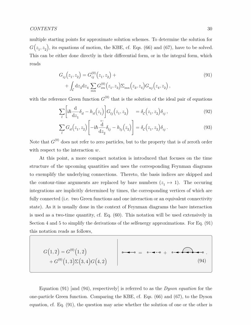
multiple starting points for approximate solution schemes. To determine the solution forG(z1, z2

), its equations of motion, the KBE, cf. Eqs. (66) and (67), have to be solved.

This can be either done directly in their differential form, or in the integral form, whichreads

Gij

(z1, z2

)= G

(0)ij

(z1, z2

)+ (91)

+∫Cdz3dz4

∑mn

G(0)im

(z1, z3

)Σmn

(z3, z4

)Gnj

(z4, z2

),

with the reference Green function G(0) that is the solution of the ideal pair of equations∑l

[i~ d

dz1δil − hil

(z1

)]Glj

(z1, z2

)= δC

(z1, z2

)δij , (92)

∑l

Gil

(z1, z2

)−i~ ←d

dz2δlj − hlj

(z2

) = δC

(z1, z2

)δij . (93)

Note that G(0) does not refer to zero particles, but to the property that is of zeroth orderwith respect to the interaction w.

At this point, a more compact notation is introduced that focuses on the timestructure of the upcoming quantities and uses the corresponding Feynman diagramsto exemplify the underlying connections. Thereto, the basis indices are skipped andthe contour-time arguments are replaced by bare numbers (z1 7→ 1). The occuringintegrations are implicitly determined by times, the corresponding vertices of which arefully connected (i.e. two Green functions and one interaction or an equivalent connectivitystate). As it is usually done in the context of Feynman diagrams the bare interactionis used as a two-time quantity, cf. Eq. (60). This notation will be used extensively inSection 4 and 5 to simplify the derivations of the selfenergy approximations. For Eq. (91)this notation reads as follows,

G(1, 2

)= G

(0)(1, 2)+G

(0)(1, 3)Σ(3, 4)G(4, 2)= + .

(94)

Equation (91) [and (94), respectively] is referred to as the Dyson equation for theone-particle Green function. Comparing the KBE, cf. Eqs. (66) and (67), to the Dysonequation, cf. Eq. (91), the question may arise whether the solution of one or the other is

CONTENTS 31

numerically more favorable. Realizing that the determination of G(0) via Eqs. (92) and(93) is of O

(N2

b

)and O

(N2

t

), whereas the solution of the full G via Eq. (91) involves

two separable time integrations and matrix multiplications, it is of order O(N3

b

)and

O(N3

t

), which is the same scaling as the solution of the KBE, although the prefactors are

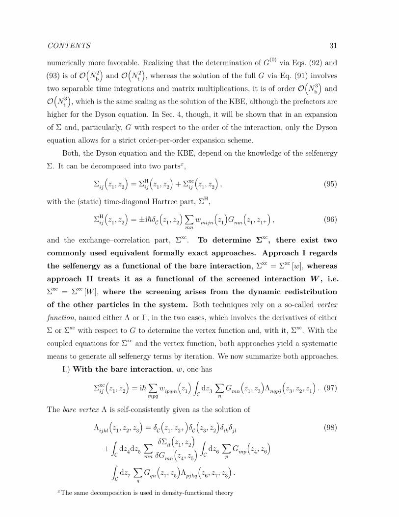
higher for the Dyson equation. In Sec. 4, though, it will be shown that in an expansionof Σ and, particularly, G with respect to the order of the interaction, only the Dysonequation allows for a strict order-per-order expansion scheme.

Both, the Dyson equation and the KBE, depend on the knowledge of the selfenergyΣ. It can be decomposed into two partsx,

Σij

(z1, z2

)= ΣH

ij

(z1, z2

)+ Σxc

ij

(z1, z2

), (95)

with the (static) time-diagonal Hartree part, ΣH,

ΣHij

(z1, z2

)= ±i~δC

(z1, z2

)∑mn

wmijn

(z1

)Gnm

(z1, z1+

), (96)

and the exchange–correlation part, Σxc. To determine Σxc, there exist twocommonly used equivalent formally exact approaches. Approach I regardsthe selfenergy as a functional of the bare interaction, Σxc = Σxc [w], whereasapproach II treats it as a functional of the screened interaction W , i.e.Σxc = Σxc [W ], where the screening arises from the dynamic redistributionof the other particles in the system. Both techniques rely on a so-called vertexfunction, named either Λ or Γ, in the two cases, which involves the derivatives of eitherΣ or Σxc with respect to G to determine the vertex function and, with it, Σxc. With thecoupled equations for Σxc and the vertex function, both approaches yield a systematicmeans to generate all selfenergy terms by iteration. We now summarize both approaches.

I.) With the bare interaction, w, one has

Σxcij

(z1, z2

)= i~

∑mpq

wipqm

(z1

) ∫Cdz3

∑n

Gmn

(z1, z3

)Λnqpj

(z3, z2, z1

). (97)

The bare vertex Λ is self-consistently given as the solution of

Λijkl

(z1, z2, z3

)= δC

(z1, z2+

)δC

(z3, z2

)δikδjl (98)

+∫Cdz4dz5

∑mn

δΣil

(z1, z2

)δGmn

(z4, z5

) ∫Cdz6

∑p

Gmp

(z4, z6

)∫Cdz7

∑q

Gqn

(z7, z5

)Λpjkq

(z6, z7, z3

).

xThe same decomposition is used in density-functional theory

CONTENTS 32

In the compact notation this set of equations becomes,

Σ(1, 2

)= ±i~δ

(1, 2

)w(1, 3

)G(3, 3+

)+ i~w

(1, 3

)G(1, 4

)Λ(4, 2, 3

)

Λ(1, 2, 3

)= δ

(1, 2+

)δ(3, 2

)+δΣ(1, 2

)δG(4, 5

)G(4, 6)G(7, 5)Λ(6, 7, 3)

= ±i~ + i~ ,

(99)

= + .

(100)

II. Using the screened interaction, W , as a basis for the expansion, the exchange–correlation selfenergy reads, cf. Eq. (97),

Σxcij

(z1, z2

)= i~

∫Cdz3

∑mpq

Wipqm

(z1, z3

)× (101)

∫Cdz4

∑n

Gmn

(z1, z4

)Γnqpj

(z4, z2, z3

),

where W obeys

Wijkl

(z1, z2

)= W bare

ijkl

(z1, z2

)+W ns

ijkl

(z1, z2

), (102)

with the bare interaction

W bareijkl

(z1, z2

)= δC

(z1, z2

)wijkl

(z1

), (103)

and the non-singular (ns) induced part

W nsijkl

(z1, z2

)=∑mn

wimnl

(z1

) ∫Cdz3

∑pq

Pnqpm

(z1, z3

)Wpjkq

(z3, z2

). (104)

The occurring polarizability P is given by

Pijkl

(z1, z2

)= ±i~

∫Cdz3

∑m

Gim

(z1, z3

)× (105)∫

Cdz4

∑n

Gnl

(z4, z1

)Γmjkn

(z3, z4, z2

).

CONTENTS 33

The screened vertex function Γ—which Σxc and P depend on—is governed by

Γijkl(z1, z2, z3

)= δC

(z1, z2+

)δC

(z3, z2

)δikδjl + (106)

+∫Cdz4dz5

∑mn

δΣxcil

(z1, z2

)δGmn

(z4, z5

) ∫Cdz6

∑p

Gmp

(z4, z6

)∫Cdz7

∑q

Gqn

(z7, z5

)Γpjkq

(z6, z7, z3

).

To summarize, Hedin’s equations are repeated in the compact notation,

Σ(1, 2

)= ±i~δ

(1, 2

)w(1, 3

)G(3, 3+

)+ i~W

(1, 3

)G(1, 4

)Γ(4, 2, 3

)

W(1, 2

)= w

(1, 2

)+ w

(1, 3

)P(3, 4

)W(4, 2

)

P(1, 2

)= ±i~G

(1, 3

)G(4, 1

)Γ(3, 4, 2

)

Γ(1, 2, 3

)= δ

(1, 2+

)δ(3, 2

)+δΣxc

(1, 2

)δG(4, 5

) G(4, 6)G(7, 5)Γ(6, 7, 3)

= ±i~ + i~xc

,

(107)

= + ,

(108)

= ±i~ xc ,

(109)

xc = + xcxc .

(110)

2.9. Summary of selfenergy approximations

We now list the selfenergies that will be discussed in this paper and briefly summarizetheir respective strengths and weaknesses. For approach I.) that starts with the bareinteraction, Eq. (97), we will consider:

– The particle–particle T -matrix approximation (TPP)The TPP selfenergy sums up the diagrams of the Born series. This process iscomputationally expensive, which, therefore, restricts the applicability range ofthe approximation to systems of moderate basis size. The TPP is a moderate- to

CONTENTS 34

strong-coupling approximaton, that becomes exact in the limit of low (large) density.It, thus, performes best away from half-filling.

– The particle–hole T -matrix approximation (TPH)The TPH selfenergy sums up a series of particle–hole diagrams, which is ofcomparable numercial complexity as the TPP. It is specifically designed to describesystems around half-filling, i.e., where the particle and hole densities are close toeach other. For these cases, it provides accurate results for moderate to stronginteraction strengths. For the application to electronic Hubbard systems, the TPHwill later be called electron–hole T -matrix approximation (TEH).

For approach II.) that starts with the screened interaction, Eq. (101), we willconsider:

– The Hartree–Fock (HF) approximationThe HF selfenergy results from a perturbative expansion up to first order in theinteraction. It is equivalent to a description on the mean-field level. Due to itssimplicity, it is numerically easy to use and applicable to large systems and longsimulation times. However, it only gives accurate results in the weak-couplingregime.

– The second-order (Born) approximation (SOA)The SOA selfenergy consists of all diagrams up to second order in the interaction. Itprovides the easiest way to include correlation effects in a NEGF calculation. Dueto its basic structure, the combination with the GKBA (see Section 2.10) leads to afavorable numerical scaling, which opens its applicability to a wide range of systems.The SOA gives accurate result for weak to moderate coupling strengths.

– The third-order approximation (TOA)The TOA selfenergy combines all possible selfenergy contributions up to third orderin the interaction. It is much more involved than the SOA rendering the simulationsnumerically costly. Thus, the applicability range of the TOA is restricted to problemswith a moderate basis size. In return, the TOA remains accurate even in the regimeof moderate to strong coupling.

– The GW approximation (GWA)The GW selfenergy provides the easiest way to decribe dynamical-screening effectsby summing up the polarization-bubble diagram series. The resummation processis computationally demanding which narrows the class of the systems that can be

CONTENTS 35

Abbreviation Selfenergy

HF Hartree–Fock approximation: Σ = ΣH + ΣF Sec. 4.1

SOA Second-order approximation: Σ = Σ(2) Sec. 4.2

TOA Third-order approximation: Σ = Σ(3) Sec. 4.3

GWA GW approximation : Σ = ΣGW Sec. 5.2

TPP Particle–particle T -matrix approximation : Σ = ΣTpp

Sec. 5.3

TPH Particle–hole T -matrix approximation : Σ = ΣTph

Sec. 5.3

FLEX Fluctuating-exchange approximation: Σ = ΣFLEX Sec. 5.5

Table 1. Main selfenergy approximations, abbreviations and section where theapproximation is being introduced and discussed.

treated, although there are some scaling advantages for problems that require ageneral (i.e. with non-diagonal interaction matrix) basis set. The GWA can beconsidered a moderate- to strong-coupling approximation, which is particularlyaccurate around half filling, where the contributions of particles and holes coincide.

Finally, a combination of some of the above results leads to:

– The fluctuating-exchange approximation (FLEX)The FLEX selfenergy merges the diagram series of the TPP, the TPH and the GWA.It, therefore, has the highest computational demands of the presented selfenergyapproximations. By combining the advantages of its ingredients, it is applicable forall filling factors and up to strong interaction strengths.

An overview of the selfenergies and the abbreviations that are being used is givenin Table 1. The detailed derivation of these expressions will be given later in Section 4and 5. A thorough comparison of the respective performance of the presented selfenergyapproximations is given in Section 3.

2.10. The generalized Kadanoff–Baym Ansatz

To compute the time-dependent single-particle Green functions, either the KBE,cf. Eqs. (66) and (67), or the Dyson equation, cf. Eq. (91) have to be solved, which bothscale cubically with respect to the time duration. An approximate way to transformthe scaling to a quadratic one, has been proposed by Lipavský et al. and was named

CONTENTS 36

generalized Kadanoff–Baym ansatz (GKBA), for details about the derivation see Ref. [128]by Lipavský et al. and Refs. [121, 123, 124, 129]. The approximation starts from anexact reformulation of the Dyson equation, the less-component of which reads

G<ij

(t1, t2

)= − i~

∑k

GRik

(t1, t2

)G<kj

(t2, t2

)(111)

+∫ t1

t2

dt3∫ t2

t0

dt4∑kl

GRik

(t1, t3

)Σ<kl

(t3, t4

)GAlj

(t4, t2

)

+∫ t1

t2

dt3∫ t2

t0

dt4∑kl

GRik

(t1, t3

)ΣRkl

(t3, t4

)G<lj

(t4, t2

)+ i~G<

ik

(t1, t1

)GAkj

(t1, t2

)−∫ t1

t0

dt3∫ t2

t1

dt4∑kl

GRik

(t1, t3

)Σ<kl

(t3, t4

)GAlj

(t4, t2

)

−∫ t1

t0

dt3∫ t2

t1

dt4∑kl

G<ik

(t1, t3

)ΣAkl

(t3, t4

)GAlj

(t4, t2

),

and analogously for the greater component. The GKBA approximates these terms byonly retaining the non-integral contributions, which can be considered a simultaneousperturbative expansion of G with respect to Σ and to the spectral structure conveyed bythe off-diagonal elements of both quantities. It reads,

G≷ij

(t1, t2

)= −i~

∑k

{GRik

(t1, t2

)G≷kj

(t2, t2

)+G≷

ik

(t1, t1

)GAkj

(t1, t2

)}(112)

=∑k

Aik

(t1, t2

) {Θ(t1, t2

)G≷kj

(t2, t2

)+ Θ

(t2, t1

)G≷kj

(t1, t1

)},

where, in the second line, the spectral function

Aij

(t1, t2

)= i~

{G>ij

(t1, t2

)−G<

ij

(t1, t2

)}, (113)

has been introduced. The approximated ≷-components are used in the right-handsides of the KBE which, thereby, need to be propagated only along the time diagonal.To achieve the overall reduction to a quadratic scaling, though, the GKBA has to beaccompanied by a second-order selfenergy and another approximation concerning theretarded and advanced components, which, unapproximated, obey equations of similarcomplexity as the original KBE, i.e., with cubic scaling. In this work, the propagators,and with that the spectral function, will be approximated on the HF level. Anotherpossibility, employed in Ref. [130], is to use approximate correlated propagators. TheGKBA has several important benefits: It preserves the causal structure of the KBE and it

CONTENTS 37

conserves important constants of motion, whenever the chosen selfenergy approximationdoes [94]. Further, it cures certain damping-induced artifacts for small systems [76, 118],an example of which will be further explored in Section 3.4. For a recent discussion, seeRef. [24].

2.11. Interacting initial state

To compute the time-evolution of the single-particle Green function according to Eqs. (66)and (67), the initial state represented by G

(t0, t0

)has to be calculated. It is determined

by the environment of the system. If the system is isolated, i.e., is described by a purestate, G

(t0, t0

)is the fully interacting initial state. For a system embedded into a bath

with which it exchanges particles or energy, the initial state is strongly influenced bythe equilibrium between degrees of freedom of the system and the bath. Under theassumption that the interaction between both is weak and dominantly uncorrelated asuitable ensemble, for instance the canonical or grand-canonical ensemble, determinesthe occupation of the energy levels in the initial state of the system. For both cases ofsystems, whether connected to a bath or isolated, there exist several methodologies togenerate the interacting initial state, some of which will be detailed in the next sectionsincluding the method of adiabatic switch-on of the interaction in Section 2.11.2, which isused throughout this work.

2.11.1. Extension of the contour to finite temperatures One possibility to include thedescription of the interacting initial state, in equilibrium with a bath or isolated, is toaugment the original contour, comprised of a forward and a backward branch C+, C−, bya “vertical” branch CM of complex time arguments ranging along the imaginary axis fromz0 to z0− i~β. Here β is the inverse temperature of the bath [or equal to∞ for an isolatedsystem at zero temperature]. The reasoning behind this can be understood by consideringthe following observations for quantum systems in contact with an environment. Thesimplest way to treat the interaction of the system with the environment is statistically,i.e. by assigning bath-induced weights wn (i.e., probabilities, with 0 ≤ wn ≤ 1 and∑nwn = 1) of finding the system in one of its eigenstates |n〉. With this, the ensemble

average of an observable O(t0

)in such a mixed state is defined as

O(t0

)=∑n

wn

⟨n

∣∣∣∣O(t0)∣∣∣∣n⟩ . (114)

CONTENTS 38

Note that Eq. (114) is a natural generalization of a pure state∣∣∣n⟩ =

∣∣∣Ψk

⟩, to which it

reduces if wn = δk,n. With Eq. (114), the statistical density-matrix operator ρ can bedefinedxi,

ρ =∑n

wn

∣∣∣n⟩⟨n∣∣∣ , (115)

with which Eq. (114) can be rewritten as

O(t0

)= Tr

[ρO

(t0

)]. (116)

The trace Tr is to be understood as acting on the full Fock space FHσ . For thegrand-canonical ensemble (GCE), which describes a system which exchanges energy(characterized by inverse temperature β) and particles (characterized by the chemicalpotential µ) with its environment, the density-matrix operator ρ reads

ρ =exp

(−βHM

)ZGCE , (117)

with the corresponding Hamiltonian, HM = H − µN , and the partition functionZGCE = Tr

[exp

(−βHM

)]. For the GCE, Eq. (116) becomes

O(t0

)=

Tr[exp

(−βHM

)O(t0

)]ZGCE . (118)

With this result, Eq. (44) can be specialized to

O(z)

=Tr[exp

(−βHM

)TC

{exp

(1i~

∫Cdz3 H

(z3

)O(z))}]

Tr[exp

(−βHM

)] . (119)

Using

TC

{exp

(1i~

∫Cdz3 H

(z3

))}= 1 , (120)

and introducing the vertical part of the contour CM running from z0 to z0 − i~β withthe identity

exp(−βHM

)= exp

(−

i~

∫CM

dz3 HM

), (121)

xiThe concept of the density operator was introduced by Landau and von Neumann. For a generalnonequilibrium approach, see Ref. [131].

CONTENTS 39

t

t0

t0

∞

z1

t1

z2

t2

t0 − i~β

C−

C+

Figure 4. Schwinger–Keldysh contour C extended to the imaginary axis. The forward-branch C− spans from the initial time t0 to ∞, bends and leads back to t0 along thebackward C+-branch. Then it continues along the imaginary branch CM to t0 − i~β,where β is the inverse temperature.

we arrive at

O(z)

= (122)

Tr[exp

(− i

~

∫CM

dz3 HM

)TC

{exp

(− i

~

∫Cdz3 H

(z3

))O(z)}]

Tr[exp

(− i

~

∫CM

dz3 HM

)TC

{exp

(− i

~

∫Cdz3 H

(z3

))}] .

From this structure, the contour extension idea can be directly derived. If one defines

H∣∣∣CM ≡ HM, O

∣∣∣CM ≡ O

(t0

)(123)

and redefines the contour C as

C = C−⊕C+⊕ CM , (124)

so that every point on the vertical track is defined as “later” than all points on theforward and backward branches, Eq. (122) can be recast as

O(z)

=Tr[TC

{exp

(− i

~

∫Cdz3 H

(z3

))O(z)}]

Tr[TC

{exp

(− i

~

∫Cdz3 H

(z3

))}] . (125)

The corresponding contour is depicted in Fig. 4. With this, definition (125) correctlyreproduces the time-dependent expectation values in accordance with Eq. (44) forz ∈ C−⊕ C+ and the ensemble average for z ∈ CM, agreeing with Eq. (118). Note thoughthat this treatment of the system–bath interaction is only valid for times smaller thanits relaxation time as the bath only directly influences the initial state and not any

CONTENTS 40

time-dependent excitations during the propagation [72].

2.11.2. Adiabatic switch-on of interactions If one is mainly interested in the evolution ofisolated systems described by a pure state, a suitable procedure is the generation of thenon-interacting state of the system, which is known for most systems and a subsequentsufficiently slow ramp-up of the interaction strength from zero to the desired value.Provided the Gell-Mann–Low theorem holds [132], which assures the existence of somelimites, and the non-interacting ground state is non-degenerate, it follows that the stateof the system after switch-on of the interaction is an eigenstate of the fully interactingHamiltonian. It remains to be checked—e.g., by comparison with other methods—that itis the ground state. Under the adiabatic-switching protocol, the Hamiltonian of Eq. (16)is replaced by

HAS(

t)

=∑mn

hmnc†mcn︸ ︷︷ ︸

H0

+ 12f

AS(t) ∑mnpq

wmnpq c†mc†ncpcq︸ ︷︷ ︸

WAS(t)

(126)

+∑mn

fmn

(t)c†mcn︸ ︷︷ ︸

F (t)

,

where the monotonically increasing switching function fAS : R −→ [0, 1] satisfies

limt→−∞

fAS(t)

= 0 , fAS(t)

= 1 , for t ≥ t0 . (127)

To achieve a high fidelity of the final state the switch-on process has to be performedslow enough and as smooth as possible. Here, the use of the function [133]

fτ,tHAS

(t)

= exp

− AτtH

t1/(2tH

)exp Bτ

tH

t1/(2tH

)− 1

,

Bτ

tH= tHτ ln 2 −

12 , Aτ

tH= ln 2

2 exp(

2Bτ

tH

), (128)

is superior compared to an approach based on a Fermi function, since it provides a verysmall relative change for values near the beginning and the end of the switch-on process.The free parameters τ and tH, the halftime, control the steepness and the duration ofthe switch-on. Using the adiabatic-switching methodology, the time-contour attains theform depicted in Fig. 5.

A third option to include initial correlation is via an additional collision integralor selfenergy term [24, 131, 134, 135]. For completeness, we also mention that similar

CONTENTS 41

t

−∞

−∞∞

z1

t1

z2

t2

C+

C−

Figure 5. Schwinger–Keldysh contour CAS with adiabatic switch-on of the interactions.The starting and end point is now −∞.

problems arise by use of the GKBA [131].

3. Applications: Numerical results for fermionic lattice systems

This section discusses some applications of the approximation strategies detailed inthe previous section. All simulations described in this section have been performedfor spin-1/2 fermions in the Hubbard model, cf. Section 2.3, for zero temperature.After providing an overview of the algorithm for the numerical solution of the KBE inSection 3.1, results for the correlated ground state of Hubbard nano-clusters are presentedin Section 3.3. The ground-state energy and spectral function are used as benchmarksto compare the performance of the selfenergy approximations listed in 2.9 for differentfilling factors and interaction strengths. Subsequently, in Section 3.4, the behavior of theapproximation strategies in the simulation of the time-dependent response of Hubbardclusters to external excitations is studied. A special focus lies on excitations that stronglydrive the system out of equilibrium. There, the occurrence of a particular weakness ofselfconsistent approaches, the so-called correlation-induced damping [118], is analyzedfor all approximations and it is demonstrated how it can be overcome to a large extentby application of the GKBA, in Section 3.4.

3.1. Algorithm for the solution of the Keldysh–Kadanoff–Baym equations (KBE)

This section gives an overview of the algorithm to calculate the solution of the KBE,cf. Eqs. (89) and (90), for spin-1/2 fermions. Both equations need to be equipped withthe initial value G≷

(t0, t0

), which are the Green functions of the—in general, correlated—

initial state. These Green functions are, in turn, generated from the ones of the idealground state, G(0),≷, via the adiabatic-switching method described in Section 2.11.2. The≷-components of the ideal Green function directly follow from the ideal one-particle

CONTENTS 42

density matrix n(0) via the relations

G(0),<ij = − 1

i~n

(0)ji , (129)

G(0),>ij = 1

i~

(δij − n

(0)ji

), (130)

where the second follows from the more general relation for an arbitrary time t,

G>ij

(t, t)

= 1i~δij +G<

ij

(t, t). (131)

Since, here, only zero-temperature applications are considered, the ideal fermionic densitymatrix can be found by diagonalization of the single-particle part of the Hamiltonian,H

0, cf. Eq. (16). The density matrix nH0

in the eigenbasis of H0 is diagonal and, for Nparticles, reads (sorted by the eigenvalues, starting from the smallest one)

nH

0

ij = δij

1 , if i ≤ N

0 , else. (132)

After transformation into the Hubbard basis, this yields the ideal density matrix n(0)ji

and, via Eqs. (129) and (130), the components of the ideal Green function. Using G(0),≷ij

as initial values, following Eq. (126), the KBE are propagated along both time-directionssimultaneously switching on the interaction with the switching function, cf. Eq. (128),i.e., the solutions of

∑l

[i~ d

dt1δil − hil

(t1

)]G≷lj

(t1, t2

)(133)

=∑l

∫ t1

ts

dt3[Σ>il

(t1, t3

)− Σ<

il

(t1, t3

)]G≷lj

(t, t′

)

+∑l

∫ t2

ts

dt3 Σ≷il

(t1, t3

)[G<lj

(t, t′

)−G>

lj

(t, t′

)],

and∑l

G≷il

(t1, t2

)−i~ ←ddt2

δlj − hlj(t2

) (134)

=∑l

∫ t1

ts

dt3[G>il

(t1, t3

)−G<

il

(t1, t3

)]Σ≷lj

(t3, t2

)

+∑l

∫ t2

ts

dt3G≷il

(t1, t3

)[Σ<lj

(t3, t2

)− Σ>

lj

(t3, t2

)],

for all values t1, t2 ∈[ts, t0

], are computed, where ts is the starting time of the adiabatic

switching. The interaction matrix in the selfenergy terms for the chosen approximation,

CONTENTS 43

on the right-hand sides are replaced by [cf. Section 4 and 5]

wijkl −→ fτ,tHAS

(t)wijkl , (135)

where the switching parameters tH and τ are chosen such that the resulting state isconverged with respect to the relevant observables. In practice, values of τ = 19.0 J−1

and tH = 25.0 J−1 have been found sufficient for all calculations. After the switching iscompleted, the system is in the correlated ground statexii described by G≷

(t0, t0

). The

information about the correlations in the system is encoded in the values of the Greenfunctions for all time-points during the switching. That is why all integrals occurring inthe solution of the KBE for physically relevant times have to extend along the wholetime-plane including the adiabatic-switching part, i.e., Eqs. (133) and (134) have tobe used also for t1, t2 > t0. It has to be noted that any time-dependent excitation ofthe system has to occur after the switching is finished and that the values of G withat least one argument in the switching region cannot be used for the determination ofobservables, as detailed in Section 3.2.

For the numerical solution of the KBE, standard approaches for the solution ofordinary differential equations (ODEs), such as Runge–Kutta methods [136], can beemployed upon appropriately discretizing the two-time plane. Further, an integrationroutine for the right-hand sides of Eqs. (133) and (134) is required. Here, the approachdetailed in Ref. [77] has been employed for all calculations. The accuracy of thesimulations can be monitored by verifying the conservation laws, in particular of thedensity and total energy [137] and time-reversibility [79]. As a general note, the use ofhigher-order methods for the solution of the ODEs and the integrals, i.e., methods wherethe error scales with a high power of the time step such that time steps of the order of10−2 to 10−1 are possible, is especially advisable to achieve performance and accuracy,since the right-hand sides of the KBE are numerically very expensive.

3.2. Important time-dependent observables

This section briefly describes how important physical observables can be obtained fromthe time-dependent Green functions and additionally from the right-hand sides of theKBE, cf. Eqs. (133) and (134), the so-called collision integrals. As detailed in theEq. (129), the less-component of the Green function of the interacting ground state isxiiAs already pointed out in Section 2.11.2, it has to be checked externally, e.g., by comparison with

other methods, that the final state of the adiabatic switching is indeed the ground state.

CONTENTS 44

directly linked to the density matrix. This relation also holds true for the time-dependentdensity matrix nij

(t), which describes the single-particle response of the system subject

to a time-dependent excitation, reading

G<ij

(t, t)

= − 1i~nji

(t). (136)

Apart from the time-dependent occupations of the Hubbard sites, which are given bythe diagonal elements of the time-dependent density matrix, the latter also permits thecalculation of several energy contributions:

– the kinetic energy,

Ekin

(t)

= Re(∑mn

hmnnnm

(t))

, (137)

– the energy induced by a time-dependent excitation fmn(t),

Eex

(t)

= Re(∑mn

fmn

(t)nnm

(t))

. (138)

– the mean interaction energy is also available, but it requires the full two-time Greenfunctions,

Eint

(t)

= − i~2∑kl

∫ t

t0

dt[Σ>kl

(t, t)− Σ<

kl

(t, t)]G<lk

(t, t)

+∑kl

∫ t

t0

dtΣ<kl

(t, t)[G<lk

(t, t)−G>

lk

(t, t)]

(139)

= − i~2∑kl

∫ t

t0

dt{

Σ>kl

(t, t)G<lk

(t, t)− Σ<

kl

(t, t)G>lk

(t, t)}

.

This expression originates from the trace over the right-hand side of Eq. (89)—thecollision integral. The possibility to compute the interaction energy (a two-particlequantity) from a single-particle function is a unique feature of the Green functionsapproach (in contrast, in reduced-density-operator theory this requires the two-particledensity operator [131]).

The availability of information off the time diagonal in the one-particle NEGF ofthe Green function allows, furthermore, to gain insight into the (N + 1)- and (N − 1)particle spaces by means of the single-particle spectral function, already encountered inEq. (113). If an N -particle system is prepared in the ground state

∣∣∣Ψ(N)0

⟩with energy

E(N)0 (or any other N -particle energy eigenstate), e.g., via adiabatic switching, and

afterwards propagated without additional excitations, the greater/less-components of

CONTENTS 45

the two-time Green functions obey

G<ji

(t1, t2

)= ∓i~

∑m

Qm(j)Q∗m(i)exp(

1i~

(E

(N−1)m − E(N)

0

)(t2 − t1

)),(140)

G>ji

(t1, t2

)= i~

∑m

Pm(j)P ∗m(i)exp(

1i~

(E

(N+1)m − E(N)

0

)(t1 − t2

)), (141)

where the amplitudes Qm(i), Pm(i) are defined as

Pm(i) =⟨Ψ(N)

0

∣∣∣ci∣∣∣Ψ(N+1)m

⟩, (142)

Qm(i) =⟨Ψ(N−1)m

∣∣∣ci∣∣∣Ψ(N)0

⟩. (143)

They are the overlap matrix elements of the (N − 1)- and (N + 1)-particle states ofenergy Em with the state which originates from removing/adding one particle in thei-th basis state from/to the N -particle state. By Fourier transforming and via theknowledge of E(N)

0 , the (N − 1)- and (N + 1)-particle energies can be determined fromthe propagation of the two-time Green function of the N -particle system. In otherwords, the correlation function G< contains information about the occupied states of theN -particle system and the transition energies to the N − 1-particle system. In contrast,G> contains information about the unoccupied states (“holes”) of the N -particle systemand the transition energies to the N + 1-particle system when one of the unoccupiedstates is being filled.

The combination of both functions directly yields the spectral function,

Aji(t1, t2) = i~{G>ji

(t1, t2

)−G<

ji

(t1, t2

)}. (144)

Aside from the two-particle energy, cf. Eq. (139), the single-particle Green functiongives also access to another two-particle quantity—the local two-particle density. Indeed,via the collision integral, the time-dependent double-occupations, n(2)

i

(t)

= 〈ni↑(t)ni↓(t)〉,i.e., the probability that one electron with spin up and another with spin downsimultaneously occupy the same spatial orbital on a Hubbard site “i”, can be computedas

n(2)i

(t)

= 12U

∑l

∫ t

t0

dt{

Σ>il

(t, t)G<li

(t, t)− Σ<

il

(t, t)G>li

(t, t)}

, (145)

which becomes obvious when taking into account the relation between the selfenergyand the two-particle Green function, cf. Eqs. (64) and (65). Further, the two-particlelocal density correlation (pair-correlation function) can be computed by subtracting theuncorrelated (mean-field) expression of the two-particle density which (for the Hubbard

CONTENTS 46

model) is nothing but the product of two single-particle densities,

δn(2)i (t) = n

(2)i (t)− ni↑(t)ni↓(t) . (146)

This quantity is identical to zero if the system is uncorrelated and thus directlymeasures effects beyond Hartree–Fock. A quantity that also measures the space-resolvedcorrelations in a many-body system is the local entanglement entropy [26],

Si(t) = − 2(ni2 − n

(2)i

)log2

(ni2 − n

(2)i

)− n(2)

i log2 n(2)i

−(1− ni + n

(2)i

)log2

(1− ni + n

(2)i

). (147)

We now turn to a survey of recent computational results that were obtained by(part of) the authors. Our focus is on comparison of differtent selfenergy approximationsand on tests of their accuracy.

3.3. Numerical results for the correlated ground state

In this section, numerical results for the interacting ground-state energies are presented.As an example, we consider a 6-site Hubbard model for which exact results can beobtained. Our main interest is to test the performance of the different selfenergyapproximation schemes introduced in Section 4 and 5 with respect to filling level n(i.e. density) and interaction strength, U/J , of the system, by comparison with exactcalculations.

Following the adiabatic-switching algorithm of Section 2.11.2, the system is initiallyprepared in the non-interacting ground state for N↑ = N↓ = 1, 2, 3 particles, i.e., fillinglevels n = 1/6, n = 1/3 and n = 0.5. Using the switching function (128) with parametersτ = 19.0 J−1 and tH = 25.0 J−1, ensuing, the interaction U is ramped up to the finalvalues U = 0.1, 0.5, 1.0 and 2.0. In Table 1, we list the selfenergy approximations thatare being used and compared.

3.3.1. Results for the ground-state energy. We begin with a detailed analysis of theground-state energy to understand the quality of the different selfenergy approximation,in dependence on the coupling strength and the filling. Starting with U = 0.1, which isvery close to an ideal system, the results for N↑ = N↓ = 1, 2, 3 are listed in the secondcolumns of Tables (2), (3) and (4), respectively.

For all three filling factors, the Hartree results differ from the exact results in the

CONTENTS 47

Σ U/J = 0.1 U/J = 0.5 U/J = 1.0 U/J = 2.0

H −0.533604 −0.44956 −0.34718 −0.14939

TPP -0.534067 −0.45981 −0.38291 −0.26319

Exact −0.534073 -0.46065 -0.38810 -0.28820

TOA -0.534075 -0.46048 −0.38545 -0.26738

FLEX −0.534076 -0.46129 −0.39685 −0.36059

SOA −0.534084 −0.46164 -0.39472 -0.32514

GWA −0.534084 −0.46181 −0.39723 −0.35068

TEH −0.534093 −0.46293 −0.40535 −0.39065

Table 2. Ground-state energies, Egs/J , for Ns = 6 sites and 1/6 filling, i.e.N↑ = N↓ = 1, for different couplings and for different selfenergy approximations.Approximations are ordered by Egs for the smallest U . In each column, the two resultsthat are closest to the exact one are typed bold.

Σ U/J = 0.1 U/J = 0.5 U/J = 1.0 U/J = 2.0

H −2.642487 −2.35948 −2.00967 −1.31891

TPP −2.643354 −2.37963 −2.08369 −1.57367

Exact −2.643367 −2.38107 −2.09367 −1.63342

TOA −2.643367 −2.38093 −2.09182 −1.61455

FLEX −2.643368 −2.38174 −2.10424 −1.61455

SOA −2.643376 −2.38208 −2.10058 −1.67092

GWA −2.643376 −2.38226 −2.10357 −1.71303

TEH −2.643390 −2.38400 −2.11746 −1.80334

Table 3. Ground-state energies, Egs/J , for Ns = 6 sites and 1/3 filling, i.e.N↑ = N↓ = 2, for different couplings and for different selfenergy approximations.Approximations are ordered by Egs for the smallest U . In each column, the two resultsthat are closest to the exact one are typed bold.

third decimal place, while all methods beyond Hartree agree up to the fourth decimalplace. This can be explained by the fact that the Hartree approximation is only correctup to the first order in the interaction strength, while all other methods agree up tothe second order in the interaction with each other and the exact solution. For bothsmaller-than-half-filling factors, the results of the non-Hartree methods behave similarly.

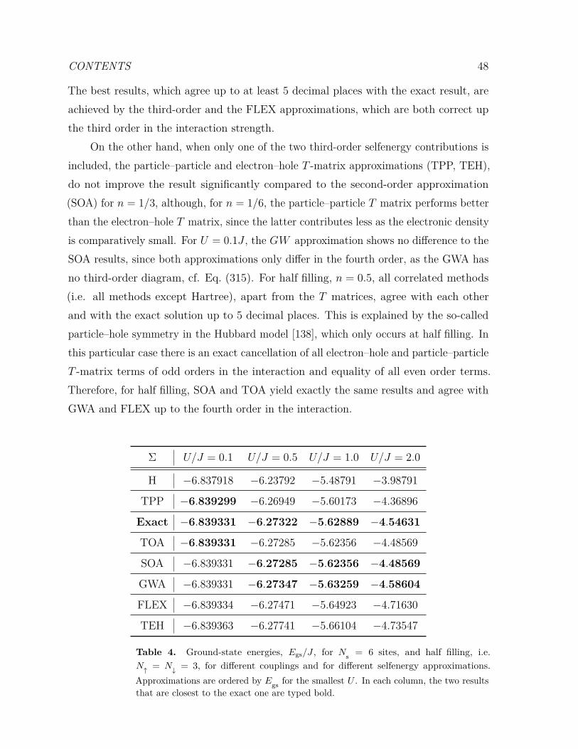
CONTENTS 48

The best results, which agree up to at least 5 decimal places with the exact result, areachieved by the third-order and the FLEX approximations, which are both correct upthe third order in the interaction strength.

On the other hand, when only one of the two third-order selfenergy contributions isincluded, the particle–particle and electron–hole T -matrix approximations (TPP, TEH),do not improve the result significantly compared to the second-order approximation(SOA) for n = 1/3, although, for n = 1/6, the particle–particle T matrix performs betterthan the electron–hole T matrix, since the latter contributes less as the electronic densityis comparatively small. For U = 0.1J , the GW approximation shows no difference to theSOA results, since both approximations only differ in the fourth order, as the GWA hasno third-order diagram, cf. Eq. (315). For half filling, n = 0.5, all correlated methods(i.e. all methods except Hartree), apart from the T matrices, agree with each otherand with the exact solution up to 5 decimal places. This is explained by the so-calledparticle–hole symmetry in the Hubbard model [138], which only occurs at half filling. Inthis particular case there is an exact cancellation of all electron–hole and particle–particleT -matrix terms of odd orders in the interaction and equality of all even order terms.Therefore, for half filling, SOA and TOA yield exactly the same results and agree withGWA and FLEX up to the fourth order in the interaction.

Σ U/J = 0.1 U/J = 0.5 U/J = 1.0 U/J = 2.0

H −6.837918 −6.23792 −5.48791 −3.98791

TPP −6.839299 −6.26949 −5.60173 −4.36896

Exact −6.839331 −6.27322 −5.62889 −4.54631

TOA −6.839331 −6.27285 −5.62356 −4.48569

SOA −6.839331 −6.27285 −5.62356 −4.48569

GWA −6.839331 −6.27347 −5.63259 −4.58604

FLEX −6.839334 −6.27471 −5.64923 −4.71630

TEH −6.839363 −6.27741 −5.66104 −4.73547

Table 4. Ground-state energies, Egs/J , for Ns = 6 sites, and half filling, i.e.N↑ = N↓ = 3, for different couplings and for different selfenergy approximations.Approximations are ordered by Egs for the smallest U . In each column, the two resultsthat are closest to the exact one are typed bold.

CONTENTS 49

For the increased but still small interaction strength U = 0.5J , the results forN↑ = N↓ = 1, 2, 3 (n = 1/6, 1/3, 0.5) are shown in the third columns of Tables (2), (3)and (4), respectively. Here, the Hartree results differ from the exact result already inthe second decimal place. In contrast, all correlated methods agree with the exact resultin the second decimal place. Compared to the U = 0.1J results, only the TOA remainsclose to the exact solution whereas all other methods show more pronounced deviations.For n = 1/6, FLEX and TPP yield comparably good results. Further, TEH is worsecompared to its particle–particle counterpart, and GWA is worse than the SOA. Forn = 1/3, FLEX becomes better than TPP, showing the increasing importance of thethird-order electron–hole contribution. For half filling, the GWA result is the closest tothe exact solution, closely followed by the equal results of the SOA and TOA. This givesa first hint that, at U = 0.5J , the fourth- and possibly higher-order terms gain influence,although among the approximations containing fourth-order and higher terms, only theGWA gives improved energies compared to second-/third-order perturbative results.

For the higher interaction strengths U/J = 1.0 and U/J = 2.0, the resultsare shown in the fourth and fifth columns of Tables (2), (3) and (4), respectively.Compared to the results for U = 0.5J , the relative order of the performance of thedifferent selfenergy approximations remains the same, but the absolute differences tothe exact results increase. Summarizing the results for the ground-state energies, it isevident that, away from half filling, the TOA outperforms all other perturbative andnon-perturbative selfenergy approximations, at least in the covered range of couplingparameters U/J = 0.1 . . . 2.0. For half filling, on the other hand, the best results areobtained from the GW approximation.

3.3.2. Results for the spectral function in the ground state. Let us now consider anotherimportant quantity of the correlated ground state, which goes beyond the descriptionof the lowest energy level: the single-particle spectral function, that was introducedin Section 3.2. For an N -particle system, it shows the transition energies into the(N − 1)-particle as well as the (N + 1)-particle system, i.e., the single-particle removaland addition energies. The removal energies are carried by the off-timediagonal values ofG<, while the addition energies are similarly encoded in G>. They can be made visible bytransforming into relative and center-of-mass time and, afterwards, Fourier transformingwith respect to the relative time. Comparing with Eqs. (140) and (141), one expectspeaks at the energy levels of (N ± 1)-particle systems shifted by the ground-state energy

CONTENTS 50

−1 0 1 2 3 4 5 6

frequency ω [J ]

0.00

0.01

0.02

0.03

0.04

0.05A

(ω)

[arb

.u

.]TOA

SOA

TPP

TEH

GWA

FLEX

HF

Exact

Exact

Figure 6. 6-site Hubbard cluster with U = 1 at one-sixth filling. Spectralfunction generated from different selfenergy approximations: brown full line: third-order approximation (TOA), crimson dashed line: second-order approximation(SOA), green dashed line: particle–particle T matrix (TPP), yellow dashed line:electron–hole T matrix (TEH), blue dashed line: GW approximation (GWA),purple semi-dashed line: fluctuating-exchange approximation (FLEX), gray fullline: Hartree–Fock approximation (HF). For comparison: Exact excitation spectraof the systems with N↑ = 1, N↓ = 0 (blue) and N↑ = 2, N↓ = 1 (red). Thespectra are shifted such that E = 0 lies in the center between the highest removalenergy and the lowest addition energy.

of the N -particle system.For the six-site Hubbard system of interaction strength U = 1J , the performance of

the different selfenergy approximations is studied for the three filling factors n = 1/6, 1/3and 1/2. The results are compared with exact excitation spectra of the relevant (N ± 1)-particle systems, which in turn are generated by excitation with a δ-kick and subsequentFourier transform of the time-dependent density evolution.

For n = 1/6, the results are shown in Fig. 6. The frequency axis of the spectrum isshifted such that all removal energies, corresponding to G<, have negative values whilethe addition energies, corresponding to G>, have positive energies. Since the spectrumof the (N − 1)-particle system only contains one spin-up or spin-down particlexiii ithas no interaction effects and, thus, is ideal. This corresponds to the less-part of thexiiiAs the fermionic Hubbard Hamiltonian contains no terms which are different for up or down

spin-orientation, a system with N spin-up and M spin-down particles behaves like the system with Mspin-up particles and N spin-down particles.

CONTENTS 51

spectrum having only one spectral line which matches the exact result (blue line) for everyapproximation including Hartree(–Fock). Analyzing the greater part of the spectrumwhich belongs to the system with two particles of one spin-direction and one particle ofthe other, one can separate two sets of spectral lines. The three spectral lines belongingto the lowest addition energies are in exact agreement throughout all approximationsincluding Hartree and, thus, indicate mostly uncorrelated states. The position of thepeak for the next higher addition energy begins to differ between the approximations.The best agreement with the exact solution is reached by the GWA followed by SOA,TEH and HF. The positions for TPP and FLEX are slightly shifted to lower energies.For TOA, the peak position cannot be easily distinguished with the shown spectralresolution, but the knee-structure within the left slope of the peak for the next higherenergy suggests that the accuracy is comparable to that of the other approximations.Unlike any other tested approximation, though, the TOA is able to show the energylevel just above ω = 3. The next-higher energy level at ω ≈ 3.3 is best captured by theFLEX approximation followed by TPP, which slightly shifts to lower energies. The SOA,GWA and the TEH show this peak shifted to higher energies. For the TOA, it remainsquestionable if the peak at ω ≈ 3.8 is to be attributed to exact energy level at ω ≈ 3.3or if it shows the energy level at ω ≈ 3.9. The level just above ω = 4 is only shown bythe TPP and FLEX approximations, which indicates that these states embody a highdegree of correlation. Summing up the findings for one-sixth filling, the best overallresults are achieved by the TPP and FLEX approximation, with the latter performingslightly better. In addition, the TOA shows energy levels which are not captured by anyother approximation.

For n = 0.33, the results are shown in Fig. 7. Two removal energy levels with alarge amplitude and one with a small amplitude are visible. It is noteworthy that theremoval energies of the one-third filled Hubbard cluster connect to, i.e., that of two andone particle of both spin-directions, respectively, is the same the addition energies ofthe one-sixth filled cluster connect to. Comparing with the right part of Fig. 6, oneimmediately recognizes that the shown energy levels are not the same. For n = 1/3, thedestination energy levels are levels 1, 2 and 6, while, for n = 1/6, the levels 1, 3, 6 andhigher levels are reached. Thus, the combined information of both fillings can be usedto gain insight into the energy spectrum of the intermediate system that differs by oneparticle to both. Concerning the quality of the approximations for the removal energylevels, all approximation agree with each other and with the exact solution, indicating

CONTENTS 52

−3 −2 −1 0 1 2 3 4 5

frequency ω [J ]

0.00

0.01

0.02

0.03

0.04

0.05A

(ω)

[arb

.u

.]TOA

SOA

TPP

TEH

GWA

FLEX

HF

Exact

Exact

Figure 7. 6-site Hubbard cluster with U = 1 at one-third filling. Spectralfunction generated from different selfenergy approximations: brown full line: third-order approximation (TOA), crimson dashed line: second-order approximation(SOA), green dashed line: particle–particle T matrix (TPP), yellow dashed line:electron–hole T matrix (TEH), blue dashed line: GW approximation (GWA),purple semi-dashed line: fluctuating-exchange approximation (FLEX), gray fullline: Hartree–Fock approximation (HF). For comparison: Excitation spectra ofthe systems with N↑ = 2, N↓ = 1 (blue) and N↑ = 3, N↓ = 2 (red). The spectraare shifted such that E = 0 lies in the center between the highest removal energyand the lowest addition energy.

that the states belonging to the removal energies are mainly uncorrelated. For theaddition energies, the same is true for the first two levels. Starting from just aboveω = 2, there are many close-lying energy levels in the range up to ω ≈ 4, which rendersan attribution to the different approximations difficult. In general, confirming the trendfound for n = 1/6, the FLEX approximation yields results which very well agree withthe exact energy levels, while the TOA reveals correct energy levels not found with theother approximations.

Turning to the results for half filling, shown in Fig. 8, one immediately recognizestwo peculiarities of this setup. First, the removal and addition part of the spectrum issymmetric with respect to E = 0. This is, again, due to the occurrence of particle–holesymmetry [138]. Second, comparing the quality of the different approximations, one candiscern only minor differences at energy levels farther away from E = 0, which are mostpronounced for the FLEX approximation. As a special note, the good performance of

CONTENTS 53

−4 −3 −2 −1 0 1 2 3 4

frequency ω [J ]

0.000

0.005

0.010

0.015

0.020

0.025

0.030

0.035

0.040A

(ω)

[arb

.u

.]TOA

SOA

TPP

TEH

GWA

FLEX

HF

Exact

Exact

Figure 8. 6-site Hubbard cluster with U = J at half filling. Spectral functiongenerated from different selfenergy approximations: brown full line: third-orderapproximation (TOA), crimson dashed line: second-order approximation (SOA),green dashed line: particle–particle T matrix (TPP), yellow dashed line: electron–hole T matrix (TEH), blue dashed line: GW approximation (GWA), purplesemi-dashed line: fluctuating-exchange approximation (FLEX), gray full line:Hartree–Fock approximation (HF). For comparison: Excitation spectra of thesystems with N↑ = 3, N↓ = 2 (blue) and N↑ = 4, N↓ = 3 (red). The spectra areshifted such that E = 0 lies in the center between the highest removal energy andthe lowest addition energy.

the Hartree approximation for the spectral function indicates that the use of the GKBAwith Hartree propagators is justified for half filling and explains the excellent resultsthat could be achieved [76, 124, 139].

Summarizing the ability of NEGF methods to describe the spectral function ofHubbard clusters, one can state that the overall agreement for small to medium interactionstrength is good and especially via combination of different approximation methods aswell as probing from both systems with adjacent number of particles, one can gain alarge part of the spectral information.

3.4. Time evolution following an external excitation

After analyzing simulation results for the correlated ground state and the quality ofdifferent selfenergy approximations, we now turn to time-dependent simulations. Therebythe ground-state data serve as the initial condition of the system prior to the excitation.

CONTENTS 54

The dynamics of the system which is driven out of equilibrium by an external excitationare studied numerically using the correlated selfenergy approximations that were describedin Section 4 and 5. Thereby we focus on separate dynamics studies following differenttypes of excitations.

Again, the motivation here is to analyze the accuracy of different approximationsby performing tests against benchmark data. These include exact-diagonalization (CI)calculations that are possible for small systems; examples are given in Secs. 3.4.4 and 3.4.5.For larger systems, comparisons with time-dependent density-matrix renormalizationgroup (DMRG) simulations can be performed, [cf. Secs. 3.4.1, 3.4.2] which, however, arerestricted to one-dimensional systems, due to the present limitations of DMRG. Finally,comparisons can be made to experiments with ultracold atoms, cf. Sec. 3.4.1.

3.4.1. Time evolution following a confinement quench. A rather simple excitation ofa finite system is to start with a spatially localized configuration that is achieved by astrong confinement potential and then to rapidly remove the confinement at some timet = 0. This resembles classical diffusion experiments where a localized particle densityexpands into vacuum. Such a configuration of a quantum system is straightforwardlyrealized with ultracold atoms in a trap or an optical lattice. An example of a rapidexpansion of cold fermionic atoms was presented by Schneider et al. in Ref. [140].

With the NEGF approach it is fairly straightforward to simulate such an expansionscenario of atoms on an optical lattice because the latter accurately reproduces theHubbard Hamiltonian (27) with onsite interaction. In the present experiment a two-dimensional geometry was used. Before presenting NEGF results for this setup we focuson benchmark calculations where comparison with DMRG simulations were performed.In Ref. [50], expansion simulations for N = 34 fermions in a one-dimensional configurationhave been carried out. Initially, the 17 central sites were doubly occupied whereas theouter sites were empty, cf. the bottom row (left column) of Fig. 9. The expansiondynamics are quite interesting and differ significantly from the classical case due to therectangular shape of the initial density profile. Furthermore, the expansion of fermionsis constrained by the Pauli principle, i.e., the innermost particles cannot move until thefermions at the edge have (partially) emptied their sites.

In Figure 9 three sets of simulations are presented. The full lines are time-dependentDMRG results, cf. Ref. [50] for details. In addition, the authors show NEGF resultswith particle–particle T -matrix selfenergies (here TMA) in order to accurately simulate

CONTENTS 55

10 20 30 40 50 60 70site s

0

1

0

1

0

1

dens

ity

n s

tJ = 0

tJ = 2

tJ = 4

tJ = 6

tJ = 8

tJ = 10

(a)

TMA HF-GKBA + TMA DMRG

10 20 30 40 50 60 70site s

0

0.5

0

0.5

0

0.5

doub

leoc

cupa

ncy

d s

(b)

tJ = 0

tJ = 2

tJ = 4

tJ = 6

tJ = 8

tJ = 10

0

1

0

1

0

1

0

0.5

0

0.5

0

0.5

Figure 9. Symmetric 1D sudden expansion of a Hubbard chain of N = 34 fermionsat U = J . Time evolution of (a) density ns and (b) double occupancy ds for six times(from bottom to top): tJ = 0, 2, 4, 6, 8, 10. Solid lines: DMRG, long dashes: TMA(two-time NEGF with T -matrix selfenergy), dashed lines: T matrix with HF-GKBA.From Ref. [50].

strong-correlation effects. One set of results is from a full two-time simulation (TMA,green dashes), the other one, from a single-time approximation using the GKBA withHartree–Fock propagators (HF-GKBA+TMA, yellow dots). In the present simulationsthe coupling was moderate, U/J = 1 and, not surprisingly, the agreement of the NEGFresults for the density profile with DMRG is excellent. An interesting observation isthat the two-time simulations show a faster dynamics than the one-time approximation(HF-GKBA).

A more sensitive quantity than the density is the local doublon number, Eq. (145),which is plotted in the right column of Fig. 9. Here the agreement with the DMRGdata is similar. While the two-time result for ds(t) shows stronger deviations than

CONTENTS 56

the single-particle density, the HF-GKBA exhibits the same high accuracy for bothquantities. A very interesting observation is that the exact (DMRG) result is enclosedby the two-time and GKBA results. This behavior was confirmed for a broad range ofcoupling parameters, selfenergy approximations and in many other setups as well, e.g.Ref. [50]. This has important implications for the use of NEGF simulations for morecomplex systems where independent benchmark data are not available.

Returning to the physics of the expansion of fermions—one of the most interestingquestions is how the expansion speed depends on the interaction strength U/J (i.e., onthe correlations in the system). A particularly interesting theoretical prediction was[91] that fermions that are in doubly occupied lattice sites (“doublons”) should expandslower compared to singly occupied sites (“singlons”) giving rise to a spatial separationof the two components (“quantum distillation”). A first test can be made by comparingthe two columns of Fig. 9. There, indeed, the doublon expansion is slightly slower thanthat of the total density, in particular, for the initial time frames (cf. the lowest threerows). Here, however, the interaction is comparably weak and the effect is small.

Such a peculiar separated expansion of doublons and singlons was, in fact, observedexperimentally for strongly correlated fermionic atoms in Ref. [140]. They demonstratedthat, when the system is initially in a fully doubly occupied configuration, after removalof the confinement, doublons remain dominantly in the trap center. Moreover, theexpansion speed of this central part (“core”) decreases when the coupling strength U/Jincreases. The experimental results for the “core expansion velocity” Cexp are reproducedin Fig. 10 by the full black line. Interestingly, Cexp even becomes negative what meansthat the “core shrinks”. Furthermore, the result is exactly the same for attractive andrepulsive interaction (negative and positive U , respectively), what is an exact propertyof the Hubbard model.

Figure 10 also contains results from a semiclassical kinetic simulation in relaxation-time approximation (grey dashed curve [140]) which reproduces the overall trend butexhibits very strong deviations, for most values of U . It is, therefore, of high interestto apply the NEGF approach to this problem since, due to the 2D geometry, DMRGsimulations are not possible. Such NEGF simulations were developed by three of thepresent authors and published in Ref. [26]. To correctly describe strong-coupling effects,the second-Born approximation cannot be applied. Instead, T -matrix selfenergies wereused. An advantage in these simulations is that the initial state is uncorrelated (it is anHartree–Fock state), so no adiabatic switching needs to be done. This is particularly

CONTENTS 57

−4 −2 0 2 4U

−1.0

−0.5

0.0

0.5

1.0

1.5

2.0

2.5

3.0C

exp

7Er

8Er

10Er

12Er

fitTMARTA

Figure 10. Asymptotic core (half width at half maximum of the density) expansionvelocity Cexp. Plus signs: experimental results for different lattice depths in unitsof the recoil energy Er; gray dashed line: relaxation-time approximation model ofRef. [140]; red circles: two-time NEGF results with T -matrix selfenergies, the errorbars denote the statistical uncertainty due to the extrapolation with respect to timeand particle number (see text). The black line is a fit through the experimentalpoints to guide the eye. From Ref. [26].

important since the simulations have to be sufficiently long to reach the regime wherethe expansion velocity approaches a constant value (“hydrodynamic stage”).

The present NEGF simulations with particle–particle T -matrix selfenergies werecarried out for a broad range of particle numbers, up to aboutN = 100 particles. It turnedout that the expansion velocity shows a simple scaling with N , so an extrapolation tothe thermodynamics limit, N →∞ (the experiments used several hundred thousands ofatoms) was possible. At the same time, the statistical error of the extrapolation providesa measure of the numerical uncertainty of the macroscopic results [77]. These resultsare also included in Fig. 10 by the red dots and the associated error bars. Obviously,the agreement with the experiment, over the whole range of coupling parameters, isimpressive. These have been the first and so far the only quantum-dynamics simulationsthat allow for a direct comparison with cold-atom experiments in two dimensions.Moreover, in Ref. [26] results for three-dimensional lattice configurations were presentedand the dependence of the expansion velocity on the dimensionality was analyzed.

The time-dependent NEGF simulations provide extensive additional information on

CONTENTS 58

N = 74

√n s

N = 74

√2·n↑↓ s

N = 74

√S s

N = 74

√15·δ

n↑↓ s

N = 2√

n s

t=0 t=1 t=2 t=3

N = 26

√n s

0.0

0.2

0.4

0.6

0.8

1.0

1.2

1.4

Figure 11. Site-resolved expansion dynamics in a 2D 19× 19 Hubbardlattice at U/J = 4 for four times (in units of J−1). Top three rows: squareroot of density ns for N = 2, N = 26, and N = 74, respectively. Rows4–6: square root of double occupation, local entanglement entropy Ss,Eq. (147), and the pair-correlation function δn↑↓s = δn

(2)s , Eq. (146). From

Ref. [26].

the expansion dynamics. From the nonequilibrium Green functions it is straightforwardto obtain full space (site)-resolved information. An example is shown in Fig. 11 wherethe time evolution of various quantities with single-site resolution is presented [26]. Thisincludes the density (first three rows), the doublon density [row 4, Eq. (145)], the doubloncorrelation function, [Eq. (146)] and the entanglement entropy, [Eq. (147)]. The lattertwo quantities are of particular interest, as they allow to separate the effect of the buildup

CONTENTS 59

of correlations in the system: as mentioned above, the initial state is uncorrelated, andwith removal of the confinement correlations start to from at the cluster edge and thenspread in and outward. These simulation results can be directly compared to experimentswith ultracold atoms where single-site resolution has been achieved with quantum-gasmicroscopes [19–21]. More details on the present simulations can be found in Ref. [77].

Concluding this section, we note that the present NEGF simulations with T -matrix selfenergies are rather costly and require large computer resources. In particular,simulations for large U become increasingly difficult which explains the choice of themaximum U -values displayed in Fig. 10. To reach large coupling values, improvedcomputational approaches and, possibly, further improved selfenergy approximations,have to be developed.

3.4.2. Time evolution starting from a charge-density-wave state. Next, we focus onthe time evolution of correlated electrons after a confinement quench starting from adifferent initial state than before. In Ref. [50] the authors considered a state of alternatingdoubly occupied and empty sites which will be called “charge-density-wave state” (CDW).After removal of the confinement density can spread to the originally empty sites. Tocompare with benchmark data from DMRG simulations the simulations are limited to1D geometry. In Ref. [50] extensive NEGF–DMRG comparisons have been carried out.Here we show some typical results, cf. Fig. 12.

The first question to answer for the NEGF simulations is again the proper choice ofthe selfenergy. Since, again, correlation effects and, in particular, large values of U/Jare of interest, the second-Born approximation is not appropriate. The particle–particleT matrix that showed impressive results in the diffusion setup of Sec. 3.4.1 is not expectedto work well here. The reason is that the T -matrix selfenergy treats interaction effectsaccurately on the two-particle level but neglects three-particle effects. It is, therefore,expected to be adequate for low densities. In application to Hubbard systems, thiscorresponds to low (or, due to particle–hole symmetry, high) filling factors. In thediffusion setup, the filling factor is low, except for the initial dynamics in the core region.

In contrast, in the present CDW setup the entire system is initially at half fillingand remains at half filling. There, the particle–particle T matrix is inaccurate. At halffilling we found in Sec. 3.3 that the third-order approximation (TOA) provides muchmore accurate data for the ground-state energy. It is, therefore, expected that also thedynamics will be treated more accurately within TOA selfenergies. Consequently, this

CONTENTS 60

selfenergy is being used, in addition to applying the HF-GKBA. The results are shown inFig. 12 for two values of the coupling strength and 5 different chain lengths, in the rangeof L = 6 and L = 36. Note that we do not show the dynamics of the densities—there theagreement is excellent—but we focus on the more sensitive double occupations, Eq. (145),summed over the entire cluster.

0 1 2 3 4 5time tJ

0.3

0.4

0.5

0.6

0.7

0.8

0.9

doub

leoc

cupa

tion

∑ sd

s(t)

(a)U = J

L = 6

L = 12

L = 20

L = 24

L = 36

HF-GKBA + TOA DMRG

0 1 2 3 4 5time tJ

(b)U = 4J

Figure 12. Charge-density wave excitation (the initial state conists of alternatingdoubly occupied and empty lattice sites): Time evolution of the total doubleoccupation, cf. Eq. (145) for two coupling strengths and 5 different systemssizes, L = 6, . . . 36. Comparison of DMRG (full lines) and NEGF with third-orderselfenergies within the single-time HF-GKBA scheme. From Ref. [50].

For moderate coupling, U/J = 1, left column, the NEGF results are practicallyindistinguishable from the DMRG data. Only for the smallest system and for long times,small deviations are visible. For the case of larger coupling U/J = 4 significantly largerdeviations are observed. While the overall trends, such as the mean value of the totaldouble occupation, d(t), is well reproduced for the initial time interval, the oscillationsof d(t) occur with a slightly modified frequency, and the amplitude of the HF-GKBAresults is substantially larger than in the DMRG data. Also, the “density revival” seenin small systems at weak coupling (bottom curve of left column) which seems to bepresent also at larger coupling (bottom right DMRG curve) seems to be amplified bythe HF-GKBA. Most interestingly, the agreement of the NEGF data with the DMRGsystematically improves with increasing system size. For more details, the reader is

CONTENTS 61

−4

−2

0

2

4

−4 −2 0 2 4

y(a

0)

x (a0)

1 2

3

4

L=24

L=54

a0

UT〈i j〉

Figure 13. Sketch of the lattice structure of circularhoneycomb clusters with L = 24 (black) and L = 54 sites (blue).The green point indicates the position where the projectile hitsthe lattice plain. From Ref. [23]

referred to Ref. [50].

3.4.3. Time evolution following a charged-particle impact. Let us now consider a verydifferent type of excitation that is caused by the impact of an energetic projectile in acorrelated Hubbard cluster. The interaction of the projectile with the electrons of thecluster is particularly strong for a charged particle. This type of excitation differs fromthe quenches above by its strongly localized character: typically only the few nearestneighbors of the impact point will be strongly affected. Depending on the velocity ofthe projectile, the interaction is also localized in time where the interaction duration iscontrolled by the initial velocity of the projectile.

The associated energy loss of the projectile (“stopping power”) has been studiedexperimentally and theoretically for many years, for an overview see e.g. Ref. [141], andbroad purpose numerical simulation tools (e.g. SRIM) were developed, e.g. Ref. [142].These models are based on extensive averages and experimental input. Moreover, theyassume that the solid can be treated as following the excitation adiabatically. Morerecently, time-dependent simulations have provided very detailed information on thecomplex physical processes. This mostly concerns time-dependent DFT simulations,e.g. Refs. [143, 144]. At the same time, TD-DFT does not allow one to reliablydescribe electronic correlation effects and the dynamics of correlations. Therefore, NEGFsimulations are of high interest.

Time-dependent NEGF simulations of ion stopping were first presented by Balzer etal. in Ref. [23]. Here we summarize a few representative results. To investigate electroniccorrelation effects one can apply an NEGF–Ehrenfest approach where the dynamics of

CONTENTS 62

the projectile are treated classically. The corresponding electronic Hamiltonian is givenby

He =− J∑〈i,j〉,σ

c†iσcjσ + U∑i

(ni↑ −

12

)(ni↓ −

12

)

− Zpe2

4πε0∑i,σ

c†iσciσ

|~rp(t)− ~Ri|+

∑〈i,j〉,σ

Wij(t)c†iσcjσ , (148)

which, in addition to the standard Hubbard Hamiltonian, now includes the Coulombinteraction between a Zp-fold charged ion and all electrons of the target. The trajectoryof the projectile, ~rp(t), is obtained by solving Newton’s equation where the force isgiven by the total force from the interaction with all electrons. By solving the coupledKeldysh–Kadanoff–Baym equations for the electrons and Newton’s equation for theprojectile one obtains the time-dependent energy exchange between the ion and theelectrons. The energy loss of the projectile follows from the asymptotic values for longtimes after and before the impact,

Se[Ekin] = mp

r2p(t→ −∞)

2 −mp

r2p(t→ +∞)

2 . (149)

Before starting the time-dependent simulations, again, the initial state has to begenerated. Here two approximations are considered: (A) the initial state is a Hartree–Fock state and (B) the initial state is correlated and generated by adiabatic switching.From a computational stand point, (A) is advantageous, whereas (B) is more accuratebut requires a substantially increased total computation duration.

The dependence of the energy loss on the initial kinetic energy, Ekin, of the projectileis plotted in Fig. 14 and show the characteristic single-peak behavior. For very fastprojectiles, the interaction duration vanishes, and so does the energy exchange. Onthe other hand, for very slow projectiles, the initial kinetic energy is small. Therefore,obviously, a maximum exists, for an optimal choice of Ekin. For the present honeycombclusters (see Fig. 13) this peak is in the range of 10keV.

Since no spatial homogeneity is assumed, the energy loss can be compared in finiteclusters of different size. In Fig. 14 Balzer et al. [23] compare the energy loss of a protonof the same energy in two clusters [cf. the sketch in Fig. 13] of size L = 54 (top figure)and L = 24 (bottom figure). Clearly, the energy loss increases with cluster size becausemore electrons are being excited by the projectile.

CONTENTS 63

0

5

10

15

20

0.1 1 10 100 1000

S e/e

V

Ekin/(keV/u)

b) L=54 U/J=0U/J=2U/J=4Hartree

2B (local)2B (full)3rd order

TM

(A)

∝ ln(vz)

0

5

10

15

20

0.1 1 10 100 1000

S e/e

V

Ekin/(keV/u)

L=54, U/J=4 Hartree2B (local): (A)

GKBA: (A)GKBA: (B)

0

5

10

15

20

0.1 1 10 100 1000

S e/e

V

Ekin/(keV/u)

c) L=24

a)

b)

U/J=0U/J=2U/J=4Hartree

2B (local): (A)2B (local)

2B (full)3rd order

TM

(B)

Figure 14. Energy loss Se, Eq. (149), for protons passing through the honeycombclusters of Fig. 13 of size L = 54 [panels (a) and (b)] and L = 24 [panel (c)]. Inall panels, the value of the onsite interaction U/J is encoded in the line style, thesymbols correspond to NEGF results, and the black lines indicate the results of theHartree approximation. The shortcuts stand for 2B (3rd order): second-order Born(third-order) approximation, TM: particle–particle T matrix, local: local approximationof the selfenergy, Σij → Σiiδij . From Ref. [23].

CONTENTS 64

Next, the role of interaction effects in the substrate on the stopping power isanalyzed. This can be achieved by comparing mean-field (Hartree) simulations withdifferent coupling parameters U/J as well as Hartree simulations to correlated NEGFresults. Obviously, one should expect that interaction effects will be of minor importanceat large projecticle energies because, in this case, kinetic energy exceeds interactionenergy. This is indeed observed in all simulations shown in Fig. 14. At energies exceeding200keV the differences between different approximations quickly vanish. In contrast,for lower impact energies and, in particular, for energies below the peak energy, strongdeviations are observed. The general trend is that, with increasing U/J the stoppingpower decreases, regardless of the chosen selfenergy approximation. A comparison ofHartree and correlated simulations reveals that correlations, at large energies, tend tomake the system “more rigid” what reduces the stopping power. Interestingly, at lowimpact energies, Ekin . 3keV the situation changes and correlation effects lead to anincrease of the stopping power. The explanation is that the fast and strong impact ofthe projectile excites a large number of electronic transitions in the system, includingdouble excitations that are missing in a mean-field approach, see also Sec. 3.4.4.

Let us now discuss the influence of different selfenergy approximations. Figure 14contains a large variety of approximations. Note, however, that these calculations arequite expensive and become increasingly more difficult when the impact energy decreasesbecause then the required simulation duration grows. Therefore, most results wereobtained for large impact energies where the differences between different approximationsare small. In Ref. [23] the authors performed simulations using second-order Born (2B),third-order and particle–particle T -matrix (TM) selfenergies. The differences are smallwith the T matrix yielding the largest stopping power. Comparing two-time simulationsand single-time simulations within the HF-GKBA (top two frames of Fig. 14), the GKBAleads to a slight reduction of the stopping power. However, this comparison has onlybeen done for a few cases, and more simulations are required to obtain a systematicpicture. Also, the effect of initial correlations has not yet been fully clarified.

More recently, a special correlation effect has been investigated: the formation oflocal electronic double occupations, Eq. (145), due to the ion impact [145]. There it wasshown that, at low projectile energies, electrons may be efficiently excited across theHubbard gap (e.g. at half filling) which gives rise to an enhancement of the stoppingpower. This effect has been explored in more detail in Refs. [24, 146].

To summarize this section: NEGF simulations coupled to an Ehrenfest description

CONTENTS 65

of a classical ion have been shown to be a powerful tool to model the energy transferbetween a projectile and correlated target. They allow for a fully time-resolved analysisand deep insight into the electronic transitions that can be triggered by the ion impact.At the same time, these simulations are very expensive at low impact energies and furtheroptimization is needed. Interesting future questions include the quantum treatmentof the projectile and of the electronic excitations in the ion as well as possible chargetransfer processes between projectile and substrate [146, 147].

3.4.4. Time evolution following a short enhancement (“kick”) of the single-particlepotential We now consider another excitation scenario where an external single-particlepotential is turned on for a very short time only,

fi(t) = fi0 δ(t− t0). (150)

Such a very short excitation, is spectrally (energetically) broad which means that a broadrange of energetic transitions will be excited. Following the time-dependent dynamics B(t)of a suitable observable one can easily reconstruct the spectral information contained init, via Fourier transformation. It turns out that this is a very efficient way to obtain high-quality spectral information, provided the propagation can be extended to sufficientlylong times, to avoid windowing effects in the Fourier transform. If, furthermore, theexcitation is weak, i.e. linear response applies, then one accurately probes the propertiesof the unperturbed system, e.g. the ground state or the equilibrium properties.

This approach was first used in NEGF simulations by Kwong et al. to compute theoptical absorption of a semiconductor [148]. There, the frequency-resolved absorptioncoefficient was obtained, after applying a short optical laser pulse, from Fouriertransforming the interband polarization P (t), for details, see Ref. [131]. Similarly,it was shown that one can obtain the dynamical structure factor and dielectric functionof a correlated system (e.g. electron gas or plasma) by applying a short monochromaticelectric field with wavenumber q, i.e. in Eq. (150) we replace fi → U0 cos (qr), thatexcites a density modulation δn(r, t) of wavelength 2π/q which yields the linear dynamicdensity-response function χ(q, ω) [149]. As a consequence one obtains results for thedynamic dielectric function and for the dynamic structure factor that selfconsistentlyinclude correlation effects thereby obeying the relevant sum rules.

After successful applications to macroscopic systems this method was also usedfor finite systems. Van Leeuwen et al. computed the optical absorption of atoms by

CONTENTS 66

Fourier transforming the time-dependent dipole transition signal [69]. The method canalso be applied to compute, via time-dependent NEGF simulations, the spectrum ofelectronic excitations of finite correlated systems. Balzer et al. considered a four electronmodel quantum well and showed the second-order Born selfenergies yield accurate resultsfor the electronic double excitations [120]. Similar results were obtained by Säkinen etal. [150].

Here we illustrate this approach for a small Hubbard cluster of 8 sites and couplingstrength U/J = 0.1. In the simulations of Hermanns et al. [76] the excitation was local onone site, i.e. in Eq. (150) the excitation amplitude was fi0 → fijαβ = w0δi,1δijδα,β, whereα and β denote the spin projections. Choosing a very small amplitude, w0 = 0.01J , thesystem remained well inside the linear-response regime. Performing a very long simulationof duration T = 1000J−1 provided an accurate excitation spectrum. The selfenergy wasused on the second-order Born level, which is adequate for the present weak-couplingcase. To achieve the desired long simulation duration a single-time simulation (with theHartree–Fock GKBA) was carried out. The result is shown in Fig. 15 where the NEGFresult is compared to an exact-diagonalization calculation. Obviously, the agreementis excellent. The NEGF simulations accurately reproduce the exact spectrum over abroad range of energies and practically capture all peaks. This agreement extends overan impressive seven orders of magnitude (note the logarithmic scale). Small deviationsare visible for increasing frequency where peak shapes exhibit slight deviations. Thiscalculation also allows to clearly single out correlation effects and explore the limitationsof the mean-field result (cf. the blue curves labeled HF). While HF well captures thelow-frequency peaks, it entirely misses peaks occuring above ω ∼ 3.8J . But also at lowerenergy, many peaks are missing, e.g. at ω/J ≈ 2.7, 3.2 and 3.6 that are associated todouble excitations.

This result confirms the power of this approach and the capability of NEGFsimulations to obtain accurate ground-state (or equilibrium) spectra via time propagation.These results can, of course, be directly compared to independent pure ground-state (orequilibrium) simulations, e.g. within the framework of the Bethe–Salpeter equation forthe Matsubara Green function. The comparison of the two approaches reveals that [149]time-dependent NEGF simulations with a selfenergy Σ correspond to Bethe–Salpeterresults with a two-particle kernel KBSE = δΣ/δG. For text-book discussions, see Refs. [72,131].

CONTENTS 67

0 1 2 3 4 5

frequency ω [J ]

10−9

10−7

10−5

10−3

10−1

spec

tru

m[a

rb.

u.]

2B-GKBA

Exact

HF

Figure 15. Spectral function of an 8-site Hubbard cluster at U/J = 0.1 computed viaFourier transform after a single-particle potential kick, Eq. (150). NEGF simulationswith second-order Born selfenergies (Hartree–Fock-GKBA) are compared to Hartree andexact diagonalization results. From Ref. [76]

3.4.5. Time evolution following a strong rapid quench of the onsite potential. We nowturn to the final example of time-dependent excitation that is very different from theprevious cases. This section investigates the dynamics of small Hubbard clusters thatare driven out of equilibrium by a very strong sudden quench of the on-site potential ofthe form

fij

(t)

= Θ(t, t0

)δijδi1w0 , (151)

where throughout this section the value w0 = 5J is used. Thus at t = 0 site i = 1 is verystrongly excited by a constant potential. This excitation, initially, drives a depletion ofthis site which is followed by a subsequent oscillation of the electronic density throughoutthe system. Such strong excitations of this form [Eq. (151)] of very small Hubbardclusters were studied in detail by Verdozzi and co-workers [117, 118] using selfconsistenttwo-time solutions of the KBE. They made a surprising observation: in contrast to theexact solution (which is easily found for these small systems), the NEGF dynamics ofthe density oscillations are strongly damped. The authors of these papers explainedthis artifact by the selfconsistency of the solution of the Dyson equation (or the KBE)which contains selfenergy contribution to arbitrary orders (powers). This leads to aseries of peaks in the spectral function that are not present in the exact result. Theyalso observed that the effect is particularly strong for small clusters.

In the following we illustrate this effect for a few examples. In particular, weare interested in 1) how this damping behavior depends on the chosen selfenergyapproximation, 2) on the filling and 3) how results from the HF-GKBA behave. To thisend we focus on very small systems containing just two electrons on two and four sites,corresponding to half and quarter filling, respectively. The case of a half-filled Hubbard

CONTENTS 68

dimer, with an interaction of U = J and excitation strength of w0 = 5.0J , is shown inFig. 16 [76]. There, three of us analyzed the time-evolution of the density on the first(excited) site, comparing the exact result to selfconsistent two-time NEGF simulationsand also single-time GKBA calculations with HF propagators. As expected, the exact

0 2 4 6 8 10

time t [J−1]

0.2

0.4

0.6

0.8

1.0

dens

ity

onsi

tei=

1

GKBA+T Exact Full T

Figure 16. Half-filled Hubbard dimer for U = J . Density evolution on the first sitefollowing a sudden switch-on of the onsite potential [Eq. (151)] of strength w0 = 5.0Jon site i = 1. Black line with dots: exact results; green dashed line: two-time NEGFresult, and red full line: HF-GKBA. Top figure: NEGF and GKBA with second-orderBorn selfenergy (Full 2B). Bottom figure: NEGF and GKBA with T -matrix selfenergy(Full T). From Ref. [76].

solution exhibits undamped oscillations of the density because electrons periodicallymove between the two sites after an initial depletion of the first site. Consider now

CONTENTS 69

the result of fully selfconsistent solutions of the KBE with second-order selfenergy (topfigure). Here, reasonably good agreement with the exact solution is only observed for thefirst 1.5 oscillation periods. For later times the oscillation period becomes smaller andthe oscillations quickly damp, reaching an artificial steady state that is not present in theexact result. It is now of interest to reduce the level of selfconsistency for which differentapproximations can be considered [151]. Here we followed a different and more systematicstrategy: we applied the Hartree–Fock-GKBA propagators as described in Sec. 2.10.The results for the case of second-order Born selfenergies are also included in the toppart of Fig. 16. Evidently, application of the HF-GKBA indeed “cures” the artificialdamping and qualitatively agrees with the exact solution. The quantitative agreement,though, can only be considered satisfactory for the first five oscillation periods up to 6inverse hopping amplitudes. While the exact oscillation period is roughly reproduced,the GKBA exhibits several phase changes that are not present in the exact dynamics.

To further improve the agreement with the exact results we then combined the HF-GKBA with a higher-order non-perturbative selfenergy. Results for the particle–particleT -matrix approximation, both, for two-time solutions and in combinations with theHF-GKBA, are shown in the bottom part of Fig. 16. In this case, the GKBA achievesvery good agreement with the exact result. The first four periods are reproduced veryaccurately, wheres for later times a slight dephasing is observed. In contrast, the fulltwo-time solution of the KBE with the particle–particle T matrix is quickly damped,as in the case of the second-order Born approximation (Full 2B, SOA, top figure). Atthe same time, the T -matrix result is better than the second-Born approximation whichis explained by the moderate coupling strength. Based on these results we concludethat the HF-GKBA, if used with the proper selfenergy, provides an excellent method tosolve the problem of artificial damping of two-time simulations in the case of very strongexcitation.

We now turn to the case of a four-site fermionic Hubbard model with one quarterfilling, and an interaction strength of U = 1.5J . The excitation is the same as before.For this setup, Friesen et. al. [151] reported the particle–particle T matrix to show verygood agreement with the exact solution, while the GW approximation performed muchworse. Here, the same setup is re-examined using all selfenergy approximations that wereintroduced in Section 4 and 5. We observe that the selfenergies can be categorized intothree groups based on the amount of artificial damping they exhibit. The three moststrongly damped methods, which quickly start to deviate from the exact result are the

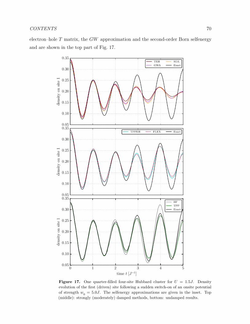
CONTENTS 70

electron–hole T matrix, the GW approximation and the second-order Born selfenergyand are shown in the top part of Fig. 17.

0 1 2 3 4 5

time t [J−1]

0.05

0.10

0.15

0.20

0.25

0.30

0.35

den

sity

onsi

te1

HF

TPP

Exact

Figure 17. One quarter-filled four-site Hubbard cluster for U = 1.5J . Densityevolution of the first (driven) site following a sudden switch-on of an onsite potentialof strength w0 = 5.0J . The selfenergy approximations are given in the inset. Top(middle): strongly (moderately) damped methods, bottom: undamped results.

CONTENTS 71

For all three methods, the damping sets in after the second oscillation period, and theamplitude quickly drops to roughly one third of the exact amplitude. For the fluctuating-exchange approximation (FLEX) and the similarly constructed approximation combiningonly the electron–hole and the particle–particle T matrix (TPPEH), the results areshown in the middle part of Fig. 17. Here, one notices only a slight damping, and theoverall agreement with the exact result is significantly improved, compared to the firstgroup of selfenergies approximations. The third group of methods that don’t exhibitconceivable damping, in the present situation, are the particle–particle T matrix and, byconstruction, the uncorrelated Hartree(–Fock) approximation. The corresponding resultsare shown in the bottom part of Fig. 17. Both methods are in good agreement with theexact result, but the quality of the T -matrix approximation is much better than that ofthe uncorrelated Hartree approximation. The superior quality of the particle–particleT matrix, in the present case, is of course arising from the low density in the systemas was noted also in the previous sections. For higher density the situation changes.Most importantly, we conclude that the artificial damping in strongly excited finitesystems is not a generic feature of all two-time simulations but is observed for selfenergyapproximations that most strongly deviate from the exact Hamiltonian. In addition, wehave seen before that the artificial damping is removed almost completely by invokingthe GKBA with Hartree–Fock propagators.

3.5. Discussion of the numerical results and outlook

We conclude the overview of numerical solutions of the KBE in equilibrium andnonequilibrium with a brief summary of the main findings and an outlook. In Sec. 3.3it has been shown that, for the interacting ground state, the order-by-order expansionwith respect to the interaction strength yields good results, already with the second-order approximation (SOA). The results significantly improve further when also thethird-order terms are into account (TOA). On the other hand, the non-perturbativeexpansions, such as the particle–particle and particle–hole T -matrix approximationsand the GW approximation, as well as combinations of several non-perturbativeapproximations, do, in general, not reach the same accuracy. Concerning the single-particle spectrum, both, perturbative and non-perturbative methods, yield good resultsand especially with the combination of the results for all available methods, most of thespectral information can be computed.

For time-dependent processes involving strong excitations, the GKBA has been

CONTENTS 72

found to be a valuable tool to mitigate correlation-induced damping. Combined withthe particle–particle T matrix, which has shown to produce excellent results in fullcalculations for lower filling factors, it yields a density evolution which is close to theexact solution. With the great variety of available selfenergy approximations, covered inSection 4 and 5 both, with and without application of the GKBA, a powerful toolsetis available to study systems of arbitrary dimension and large particle numbers, wherecurrently no exact methods are available.

In section 3.4 we considered the dynamics of small- and intermediate-size Hubbardclusters in response to various kinds of excitations ranging from short to long and weakto strong. Where comparisons with benchmark data were available NEGF calculationshave obtained very good agreement, provided the proper selfenergy approximationhas been chosen. This means that Σ has to be chosen such that is matches both thecoupling strength and filling (density). While, at weak coupling, the second-order Bornapproximation is adequate, at moderate coupling, U & J , this approximation showssignificant deviations and there is even no guarantee that it captures the dominant trends.Therefore, it is crucial to have a sufficiently large arsenal of selfenergy approximationsavailable that can be used in a flexible manner. Thus, we can conclude that NEGFsimulations have, indeed, reached a level of accuracy where reliable predictions can bemade. For an efficient use of the proper selfenergies, it is crucial to have explicit resultsfor each approximation available that can be rapidly implemented. This will be discussedin great detail in the next sections.

Before doing this we note that time-dependent NEGF simulations have seen adramatic surge in activity in many areas. Even though the most accurate and best testedresults were obtained for lattice models, as discussed above, there exist many furtherapplications that are outside the scope of this article but should be briefly mentioned,together with a few relevant references. Indeed, second-order Born simulations werereported for electrons in quantum dots [152, 153], the laser excitation of small atomsand molecules [69–71]. Interestingly, second-order Born calculations were shown to beapplicable also to the photoionization of larger atoms such as krypton [154] and to wellreproduce two-electron processes such as Auger ionization [155]. Other finite systemsthe relaxation dynamics of which were recently studied include graphene-type clusterssuch as graphene nanoribbons [156]. Correlation effects of particular interest here are,e.g., carrier multiplication effects.

While in the applications listed above the electronic system was typically treated

CONTENTS 73

as isolated, in many cases the coupling to the environment (bath) has to be included.Examples are transport problems. Since the bath is typically much larger than thephysical system of interest with time scales often well separated from those of the system,suitable procedures to eliminate the bath degrees of freedom are of high interest. Animportant example is transport through nanoscale systems where it is often advantageousto eliminate the effect of the leads. Here a highly efficient solution within the NEGFscheme is provided by an embedding approach [157], for a text-book discussion seeRef. [72]. This approach has been extended to the photoionization of atoms [154] andcharge transfer processes between atoms and a solid surface [24, 147].

Due to the success of these NEGF simulations we expect that the number andscope of applications will continue to increase over the next years. Further progressrequires new developments in several directions. One is certainly the use of improvedmore realistic models. Here we mention the idea to combine NEGF simulations with anab initio basis set that is provided by a Kohn–Sham simulation. This concept is realized,e.g., within the Yambo code of Marini et al., e.g. Refs. [158, 159]. A major problem forthese approaches is the large basis size which leads to very large requirements of CPUtime and computer memory.

One approach that allows to mitigate these problems, at least partially, is thegeneralized Kadanoff–Baym ansatz (GKBA) that was introduced in Sec. 5.2. We haveseen throughout the present section that the GKBA, combined with Hartree–Fockpropagators, indeed provides the expected major savings of resource. Moreover, in manycases it yields excellent results that may be not worse than the full two-time simulation,e.g. Ref. [76]. This, however, does not mean that two-time simulations become obsolete.In contrast, as we have seen from the comparison to DMRG results in Secs. 3.4.1 and3.4.2, in many cases, the exact result is enclosed between two-time and single-time NEGFresults. Thus, both types of simulations should be developed in parallel.

Future developments in this field should also aim at improving the GKBA simulations.Part of the problems of the GKBA will be overcome if, instead of Hartree–Fockpropagators, correlated propagators are being used. Here, we mention recent promisingproposals of Refs. [24, 160]. Furthermore, it will also be important to include correlatedinitial states into GKBA simulations and to develop efficient schemes that reduce theassociated computational overhead, e.g. Refs. [24, 161–163].

Finally, all of the NEGF applications discussed above crucially depend on theavailability of a large arsenal of selfenergy approximations and their optimization for

CONTENTS 74

special basis sets. In the remainder of this paper, we present a detailed overview ofpractical formulas that are ready to use in NEGF simulations.

4. Selfenergy approximations I: Perturbation expansions

To study time-dependent observables of the system of interest by solving the Keldysh–Kadanoff–Baym equations, one has to know the less and greater components of thetwo-time Green function, G≶

(t1, t2

). These components can be generated from the

solution of the contour Dyson equation, which is the first equation of Hedin’s equations,cf. Eq. (91). Its main ingredient is the selfenergy Σ. It is of great importance, both,from a physical point of view—since it incorporates all different classes of inter-particleeffects and processes—as well as from the computational view—since a large portionof the numerical resources is consumed for its determination. Σ is the solution of thesecond Hedin equation, Eq. (95), which, in turn, is dependent on the third to fifth Hedinequation, Eqs. (102), (105) and (106), and, in turn, also on the Dyson equation viathe Green function entering it. Since the selfenergy, by iteration of Hedin’s equations,consists of an infinite number of terms, a strategy has to be used to reach a goodapproximation with only a small finite subset. The two most common approaches aredetailed in the following. The first applies a perturbative approach with respect tothe interaction strength, i.e., with respect to the powers of the potential w, whereasthe second uses a resummation idea. The resummation involves (infinitely many)diagrams in all orders of the interaction strength belonging to certain topological classes,namely the particle–particle, the particle–hole T -matrix approximation (TPP, TEH),the GW approximation (GWA), or a combination of all of them or some subsets. Thepresent Section 4 deals with the expansion in orders of the interaction strength where wesystematically study selfenergies of first, second and third order. After this, in Section 5,the resummation approaches, are introduced and discussed for all relevant special cases.In these two sections we introduce all selfenergies that were applied in the calculationsof Section 3.

In the remainder of this section we focus on the expansion of the selfenergy withrespect to the number of interaction factors w involved. This means that the n-th orderapproximation contains only terms with no more than n interactions. This procedurehas two sources of reasoning behind it. First, for small interaction strength (in units ofthe single-particle energy), higher-order processes with more interaction factors usually

CONTENTS 75

have small amplitudes. Second, even for larger coupling strength, higher-order terms alsocontain several Green functions corresponding to the correlated creation and annihilationof several particles. The strength of these correlations is not directly coupled to theinteraction strength and, therefore, a lower-order approximation may give good resultseven for stronger interactions.

Regarding the treatment of the Green functions occuring in the expansion ofthe selfenergy, two different approaches are common. In the self-consistent approach,one starts from the non-interacting Green function G(0) and computes the selfenergyaccording to Eq. (95), within the chosen approximation. Then, the Dyson equation isevaluated, taking G = G

(0) on the right-hand side. With the resulting G, the selfenergyis reevaluated. This procedure is continued iteratively until convergence is reached. Incontrast, the free-particle approach—expands G with respect to the number of occurrencesof the interaction, as it is done with the other quantities in Hedin’s equations. That way,it is ensured that the n-th order approximation contains no terms of higher order, whichis in contrast to the self-consistent approach (through the iteration procedure terms ofall orders are produced). Nonetheless, these terms are valid terms of order higher thann, so it cannot be answered beforehand which method is superior.

In the remainder of this section, both these approaches will be analyzed in detailby considering selfenergies up to the third order in the interaction, i.e. Hartree–Fock(HF), second-order Born approximation (SOA) and third-order approximation (TOA).These approximations will be systematically deduced from Hedin’s equation first, for ageneral basis. After this, each result will be specified to two important cases: a basiswhere the interaction is diagonal (“diagonal basis”) and the Hubbard basis. For all threebasis representations we present the quantities first on the Keldysh contour and then wederive the greater/less and retarded/advanced components. In addition, we separatelypresent the results for bosons and fermions. In cases when there are differences fordifferent spin projections, the different cases will be specified separately. In addition tothe formulas we present the graphical representation in terms of Feynman diagrams thatwill be introduced in Fig. 18.

4.1. First-order terms. Hartree and Fock selfenergies

To determine the first-order contributions to Σ, one starts from the second Hedinequation, Eq. (95). The first term, the Hartree term ΣH, is of first order, since it contains

CONTENTS 76

one w. It was already given in Eq. (96) and is repeated here for consistency,

ΣHij

(z1, z2

)= ±i~δC

(z1, z2

)∑mn

wmijn

(z1

)Gnm

(z1, z1+

). (152)

Since this expression contains a contour delta function, δC, the only non-vanishingKeldysh component is

ΣH,δij

(t1

)= ΣH

ij

(z1, z1

)= (153)

= ± i~∑mn

wmijn

(z1

)Gnm

(z1, z1+

)= ±i~

∑mn

wmijn

(t1

)G<nm

(t1, t1

).

The second first-order term belongs to Σxc, cf. Eq. (95), and is generated by the first-orderterm W

(1) of Eq. (102),

W(1)ijkl

(z1, z2

)= W bare

ijkl

(z1, z2

)= δC

(z1, z2

)wijkl

(z1

), (154)

and the zeroth order vertex Γ(0), cf. Eq. (106),

Γ(0)ijkl

(z1, z2, z3

)= δC

(z1, z2+

)δC

(z3, z2

)δikδjl . (155)

This yields the Fock term, ΣF, which is of time-diagonal structure as the Hartree termand is given by

ΣFij

(z1, z2

)= Σxc

ij

(W

(1) ≡ W bare,Γ(0)) = (156)

= i~δC(z1, z2

)∑mn

winjm

(z1

)Gmn

(z1, z1+

).

The δ-component (prefactor of the delta function) is given by

ΣF,δij

(t1

)= ΣF

ij

(z1, z1

)=∑mn

winjm

(t1

)G<mn

(t1, t1

). (157)

Because there is no further term stemming from W(0) and Γ(1), since W (0) ≡ 0, the final

result for the first-order selfenergy Σ(1) is given by

Σ(1) = ΣH + ΣF , (158)

which both are time-diagonal. For the non-selfconsistent treatment, the Green functionsappearing in ΣH and ΣF are taken as free Green functions, i.e., G −→ G

(0). Otherwise,all expressions remain the same. There are no additional terms containing higher-orderGreen functions in first order.

CONTENTS 77

i, z1 j, z1+i, z1

mm, z1z1+

Figure 18. First-order diagrams in the diagonal basis.Left: Fock diagram, ΣF,diagonal. Right: Hartree diagram,ΣH,diagonal. Both diagrams are time-diagonal.

Diagonal basis. In a basis where the interactions are diagonal, wijkl = δilδjkwij, thefirst-order terms read

ΣH,diagonalij

(z1, z2

)= ±i~δC

(z1, z2

)δij∑m

wmi

(z1

)Gmm

(z1, z1+

), (159)

ΣF,diagonalij

(z1, z2

)= i~δC

(z1, z2

)wij

(z1

)Gij

(z1, z1+

), (160)

with the δ-components

ΣH,diagonal,δij

(t1

)= ±i~δij

∑m

wmi

(t1

)G<mm

(t1, t1

), (161)

ΣF,diagonal,δij

(t1

)= i~wij

(t1

)G<ij

(t1, t1

). (162)

Feynman diagrams. The structure of the selfenergy contributions can be suitablyvisualized by using Feynman diagrams [164]. In this diagrammatic representation, Greenfunctions are depicted as solid lines with an arrow pointing from the second argument tothe first argument (since the creation operator in G has the second argument and theannihilation operator has the first argument). The interaction is represented by a wigglyline which has two endpoints (in the diagonal basis). Employing the Feynman diagramtechnique, the two first-order contributions to the selfenergy are depicted in Fig. 18.

Hubbard basis. For the Hubbard basis, introduced in Section 2.3, the first-orderselfenergy terms can be directly worked out. Here we separately consider the cases ofbosons and fermions (superscripts b and f, respectively), cf. Eqs. (28) and (35). Forbosons we obtain

ΣH,biαjα

(z1, z2

)= i~δC

(z1, z2

)δij∑ε

U(z1

)Giεiε

(z1, z1+

), (163)

ΣF,biαjα

(z1, z2

)= i~δC

(z1, z2

)δijU

(z1

)Giαiα

(z1, z1+

), (164)

CONTENTS 78

with the δ-components

ΣH,b,δiαjα

(t1

)= i~δij

∑ε

U(t1

)G<iεiε

(t1, t1

), (165)

ΣF,b,δiαjα

(t1

)= i~δijU

(t1

)G<iαiα

(t1, t1

). (166)

On the other hand, for fermions one obtains the following Hartree terms

ΣH,fiαjα

(z1, z2

)= − i~δC

(z1, z2

)δij∑ε6=α

U(z1

)Giεiε

(z1, z1+

), (167)

ΣH,f,δiαjα

(t1

)= − i~δij

∑ε6=α

U(t1

)G<iεiε

(t1, t1

), (168)

whereas the fermionic Fock terms vanish exactly in the Hubbard basis, ΣF,fiαjα

(z1, z2

)≡

ΣF,f,δiαjα

(t1

)≡ 0.

We also consider the important special cases of spin-0 bosons and spin-1/2 fermions,respectively (the spin is indicated by an additional superscript). For spin-0 bosons theterms attain the form

ΣH,b,0ij

(z1

)= i~δC

(z1, z2

)δijU

(z1

)Gii

(z1, z1+

),

ΣF,b,0ij

(z1

)= i~δC

(z1, z2

)δijU

(z1

)Gii

(z1, z1+

),

ΣH,b,0,δij

(t1

)= i~δijU

(t1

)G<ii

(t1, t1

),

ΣF,b,0,δij

(t1

)= i~δijU

(t1

)G<ii

(t1, t1

),

whereas for spin-1/2 fermions the results are

ΣH,f,1/2i↑j↑

(z1

)= − i~δC

(z1, z2

)δijU

(z1

)Gi↓i↓

(z1, z1+

),

ΣH,f,1/2i↓j↓

(z1

)= − i~δC

(z1, z2

)δijU

(z1

)Gi↑i↑

(z1, z1+

),

ΣH,f,1/2,δi↑j↑

(t1

)= − i~δijU

(t1

)G<i↓i↓

(t1, t1

),

ΣH,f,1/2,δi↓j↓

(t1

)= − i~δijU

(t1

)G<i↑i↑

(t1, t1

),

where the fermionic Fock terms are again zero. The corresponding diagrams for spin-0bosons and spin-1/2 fermions are shown in Figs. 19 and 20, respectively.

4.2. Second-order terms. Second-Born approximation (SOA)

We now return to Eqs. (95) and (101), and investigate the selfconsistent second-ordercontribution,

Σ(2) = Σxc,(2). (169)

CONTENTS 79

i, z1 i, z1+i, z1

ii, z1z1+

Figure 19. First-order diagrams inHubbard basis forspin-0 bosons. Left:Fock diagram, ΣF,b,0.Right: Hartree dia-gram, ΣH,b,0. Notethat both diagrams co-incide for the Hubbardbasis.

.i ↓ (↑), z1

i ↑ (↓)i ↑ (↓), z1z1+

Figure 20. First-order (Hartree) dia-gram in Hubbard basisfor spin-1/2 fermions,ΣH,f,1/2.

The second-order terms of Σxc,(2) can only be of either one of two forms

Σ(2),2,0 = Σxc,(2)(W

(2),Γ(0))

, Σ(2),1,1 = Σxc,(2)(W

(1),Γ(1))

, (170)

where the superscripts refer to the orders of W and Γ. The first term involves W (2), thestructure of which is determined from Eq. (102),

W(2) = W ns

(P

(0),W

(1)), (171)

where the zeroth order polarization is

P(0) = P

(Γ(0))

, (172)

which is explicitly given byxiv

P(0)(1, 2) = ±i~G

(1, 3

)G(4, 1

)δ(3, 4+

)δ(2, 4

)= ±i~G

(1, 2

)G(2, 1

)7→ ±i~ xc

∣∣∣∣∣∣xc 7→

= ±i~ . (173)

Inserting this result into Eq. (171) and, employing Eq. (104), one arrives atxivFor the purpose of better understanding, the following derivations are given in the simplified

notation, as introduced in Section 2.8. The way to the first second-order selfenergy term in the fullnotation is presented in Appendix A.1.1.

CONTENTS 80

W(2)(1, 2) = w

(1, 3

)P

(0)(3, 4)W

(1)(4, 2)= ±i~w

(1, 3

)G(3, 4

)G(4, 3

)w(4, 2

)7→

∣∣∣∣∣∣ 7→±i~

7→

= ±i~ . (174)

With this, Σ(2),2,0 can be calculated as, [cf. Eq. (101)],

Σ(2),2,0(1, 2)= i~W (2)(1, 3)G(1, 4)

Γ(0)(4, 2, 3)= ±

(i~)2w(1, 3

)G(3, 4

)G(4, 3

)w(4, 2

)G(1, 2

)

xc 7→ i~xc

∣∣∣∣∣∣ 7→±i~xc 7→

= ± (i~)2 , (175)

or, in the full extended notation,

Σ(2),2,0ij

(z1, z2

)= ±

(i~)2∑

mn

Gmn

(z1, z2

)∑st

Gst

(z1, z2

)× (176)

×∑r

wirsm

(z1

)∑u

wtnju

(z2

)Gur

(z2, z1

).

The other second-order selfenergy term, Σ(2),1,1, requires the first-order term of thevertex Γ, the structure of which is

Γ(1) = Γ(δΣxc,(1)

/δG,Γ(0)), (177)

and involves the functional derivative of Σxc,(1) with respect to G,

δΣxc,(1)(1, 2)δG(5, 6

) =δΣxc,(1),F(1, 2)δG(5, 6

) . (178)

Employing Eq. (156), one findsxv

xvFor the full-notation derivation, see Appendix A.1.2.

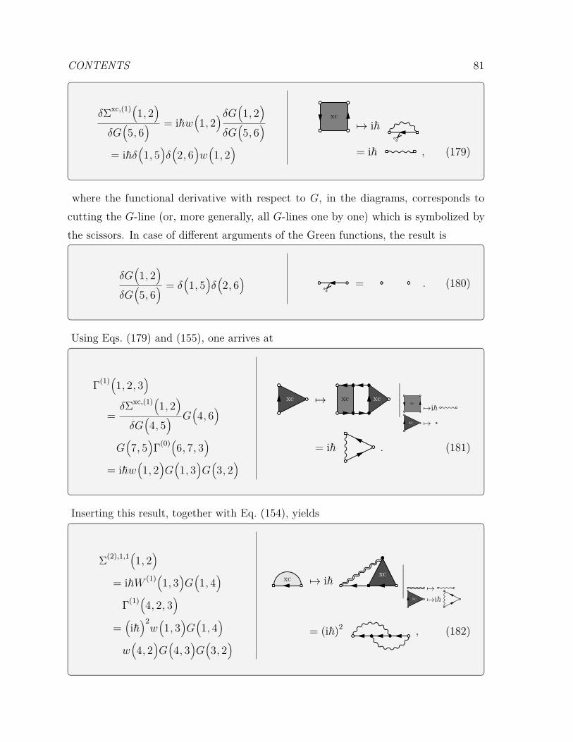
CONTENTS 81

δΣxc,(1)(1, 2)δG(5, 6

) = i~w(1, 2

)δG(1, 2)δG(5, 6

)= i~δ

(1, 5

)δ(2, 6

)w(1, 2

)xc

7→ i~�

= i~ , (179)

where the functional derivative with respect to G, in the diagrams, corresponds tocutting the G-line (or, more generally, all G-lines one by one) which is symbolized bythe scissors. In case of different arguments of the Green functions, the result is

δG(1, 2

)δG(5, 6

) = δ(1, 5

)δ(2, 6

)�

= . (180)

Using Eqs. (179) and (155), one arrives at

Γ(1)(1, 2, 3)=δΣxc,(1)(1, 2)δG(4, 5

) G(4, 6

)G(7, 5

)Γ(0)(6, 7, 3)

= i~w(1, 2

)G(1, 3

)G(3, 2

)

xc 7→ xcxc

∣∣∣∣∣∣ xc7→i~

xc 7→

= i~ . (181)

Inserting this result, together with Eq. (154), yields

Σ(2),1,1(1, 2)= i~W (1)(1, 3)G(1, 4)

Γ(1)(4, 2, 3)=(i~)2w(1, 3

)G(1, 4

)w(4, 2

)G(4, 3

)G(3, 2

)

xc 7→ i~xc

∣∣∣∣∣∣ 7→xc 7→i~

= (i~)2 , (182)

CONTENTS 82

or, in the full notation,

Σ(2),1,1ij

(z1, z2

)=(i~)2 ∑

mpq

wipqm

(z1

)∑n

Gmn

(z1, z2

)× (183)

×∑rs

wnsjr

(z2

)Grp

(z2, z1

)Gqs

(z1, z2

).

This is the final result that is still written on the Keldysh contour, i.e. is an equationfor Keldysh matrices. The corresponding matrix elements (greater, less, retarded andadvanced components) of the selfconsistent second-order selfenergy contributions Σ(2),2,0

ij

and Σ(2),1,1ij are straightforwardly extracted, applying the Langreth rules:

Σ(2),2,0,≷ij

(t1, t2

)= ±

(i~)2∑

mn

G≷mn

(t1, t2

)∑st

G≷st

(t1, t2

)× (184)

×∑r

wirsm

(t1

)∑u

wtnju

(t2

)G≶ur

(t2, t1

),

Σ(2),1,1,≷ij

(t1, t2

)=(i~)2 ∑

mpq

wipqm

(t1

)∑n

G≷mn

(t1, t2

)× (185)

×∑rs

wnsjr

(t2

)G≶rp

(t2, t1

)G≷qs

(t1, t2

).

All the above results where for the selfconsistent approach where all expressionscontain full Green functions. As we noted in the beginning of this section, alternativelyone can perform a non-selfconsistent treatment, where all Green functions arereplaced by non-interacting functions. In that case, the possible second-order classes are

Σ(2),(2),2,0,0 = Σxc,(2)(W

(2), G

(0),Γ(0)) ≡ Σ(2),2,0(

G → G(0))

, (186)

Σ(2),(2),1,0,1 = Σxc,(2)(W

(1), G

(0),Γ(1)) ≡ Σ(2),1,1(

G → G(0)) (187)

and

Σ(2),{H,0},1 = ΣH,0(G

(1)), Σ(2),{F,0},1 = ΣF,0

(G

(1)). (188)

A detailed list of these contributions, including all Keldysh matrix components for allconsidered basis sets, is given in Appendix B.

CONTENTS 83

i, z1n, z2

p, z1j, z2 i, z1 j, z2

s, z1 t, z2

Figure 21. Selfconsistent second-order diagrams in thediagonal basis. Left: Exchange diagram Σ(2),1,1,diagonal.Right: Direct diagram, Σ(2),2,0,diagonal.

Diagonal basis. For a basis where the interaction is diagonal, wijkl = δilδjkwij, theselfconsistent second-order selfenergy terms, [cf. Eqs. (176) and (183)], simplify to

Σ(2),2,0,diagonalij

(z1, z2

)= (189)

= ±(i~)2Gij

(z1, z2

)∑s

wis

(z1

)∑t

Gst

(z1, z2

)Gts

(z2, z1

)wtj

(z2

),

Σ(2),1,1,diagonalij

(z1, z2

)= (190)

=(i~)2∑

p

wip

(z1

)∑n

Gin

(z1, z2

)wnj

(z2

)Gnp

(z2, z1

)Gpj

(z1, z2

),

with the corresponding Keldysh matrix components

Σ(2),2,0,diagonal,≷ij

(t1, t2

)= (191)

= ±(i~)2G≷ij

(t1, t2

)∑s

wis

(t1

)∑t

G≷st

(t1, t2

)G≶ts

(t2, t1

)wtj

(t2

),

Σ(2),1,1,diagonal,≷ij

(t1, t2

)= (192)

=(i~)2∑

p

wip

(t1

)∑n

G≷in

(t1, t2

)wnj

(t2

)G≶np

(t2, t1

)G≷pj

(t1, t2

).

The Feynman diagrams for these expressions are shown in Fig. 21.

Hubbard basis. For the Hubbard basis, we give the selfconsistent second-orderselfenergy contributions first for bosons

Σ(2),2,0,Hubbard,biαjα

(z1, z2

)= (193)

=(i~)2Giαjα

(z1, z2

)U(z1

)∑ε

Giεjε

(z1, z2

)Gjεiε

(z2, z1

)U(z2

),

Σ(2),1,1,Hubbard,biαjα

(z1, z2

)= (194)

=(i~)2U(z1

)Giαjα

(z1, z2

)U(z2

)Gjαiα

(z2, z1

)Giαjα

(z1, z2

).

CONTENTS 84

Similarly, we obtain for fermions:

Σ(2),2,0,Hubbard,fiαjα

(z1, z2

)= (195)

= −(i~)2Giαjα

(z1, z2

)U(z1

)∑ε6=α

Giεjε

(z1, z2

)Gjεiε

(z2, z1

)U(z2

),

whereas the second expression vanishes, Σ(2),1,1,Hubbard,fiαjα

(z1, z2

)≡ 0 .

The corresponding greater/less Keldysh matrix components read, for bosons,

Σ(2),2,0,Hubbard,b,≷iαjα

(t1, t2

)=

=(i~)2G≷iαjα

(t1, t2

)U(t1

)∑ε

G≷iεjε

(t1, t2

)G≶jεiε

(t2, t1

)U(t2

),

Σ(2),1,1,Hubbard,b,≷iαjα

(t1, t2

)=

=(i~)2U(t1

)G≷iαjα

(t1, t2

)U(t2

)G≶jαiα

(t2, t1

)G≷iαjα

(t1, t2

).

Analogously, we have, for fermions,

Σ(2),2,0,Hubbard,f,≷iαjα

(t1, t2

)=

= −(i~)2G≷iαjα

(t1, t2

)U(t1

)∑ε6=α

G≷iεjε

(t1, t2

)G≶jεiε

(t2, t1

)U(t2

)

and, as before, Σ(2),1,1,Hubbard,f,≷iαjα

(t1, t2

)≡ 0 .

We again consider the special cases of spin-0 bosons and spin-1/2 fermions,respectively. For spin-0 bosons, the selfconsistent second-order contributions are givenby

Σ(2),2,0,Hubbard,b,0ij

(z1, z2

)= (196)

=(i~)2Gij

(z1, z2

)U(z1

)Gij

(z1, z2

)Gji

(z2, z1

)U(z2

),

Σ(2),1,1,Hubbard,b,0ij

(z1, z2

)= (197)

=(i~)2U(z1

)Gij

(z1, z2

)U(z2

)Gji

(z2, z1

)Gij

(z1, z2

).

Similarly, for spin-1/2 fermions we obtain

Σ(2),2,0,Hubbard,f,1/2i↓(↑)j↓(↑)

(z1, z2

)= (198)

= −(i~)2Gi↓(↑)j↓(↑)

(z1, z2

)U(z1

)Gi↑(↓)j↑(↓)

(z1, z2

)Gj↑(↓)i↑(↓)

(z2, z1

)U(z2

).

The Feynman diagrams of the self-consistent second-order selfenergy contributions forspin-0 bosons and spin-1/2 fermions are depicted in Figs. 22 and 23, respectively.

Consider again the corresponding greater and less Keldysh matrix components. For

CONTENTS 85

i, z1j, z2

i, z1j, z2 i, z1 j, z2

i, z1 j, z2

Figure 22. Selfconsistent second-order diagrams forspin-0 bosons in the Hubbard basis. Left: Exchangediagram Σ(2),1,1,Hubbard,b,0. Right: Direct diagram,Σ(2),2,0,Hubbard,b,0. Note that both diagrams coincide for theHubbard basis.

i ↓ (↑), z1 j ↓ (↑), z2

i ↑ (↓), z1 j ↑ (↓), z2Figure 23.Selfconsistent second-order diagram forspin-1/2 fermions inthe Hubbard basis,Σ(2),2,0,Hubbard,f,1/2.

spin-0 bosons, we have

Σ(2),2,0,Hubbard,b,0,≷ij

(t1, t2

)=(i~)2G≷ij

(t1, t2

)U(t1

)G≷ij

(t1, t2

)G≶ji

(t2, t1

)U(t2

),

Σ(2),1,1,Hubbard,b,0,≷ij

(t1, t2

)=

=(i~)2U(t1

)G≷ij

(t1, t2

)U(t2

)G≶ji

(t2, t1

)G≷ij

(t1, t2

).

In similar manner, we find the correlation components for spin-1/2 fermions:

Σ(2),2,0,Hubbard,f,1/2,≷i↓(↑)j↓(↑)

(t1, t2

)=

= −(i~)2G≷i↓(↑)j↓(↑)

(t1, t2

)U(t1

)G≷i↑(↓)j↑(↓)

(t1, t2

)G≶j↑(↓)i↑(↓)

(t2, t1

)U(t2

),

whereas the second contribution vanishes, as before.

4.3. Third-order selfenergy (TOA)

After discussing the frequently used first- and second-order contributions, we now turnto the selfenergy approximations that are of third order in the interaction. We haveseen in the results section 3 that, in many cases, the third order provides surprisinglyaccurate results. On the other hand, this approximation has not been discussed in theliterature before. Therefore, we discuss the third-order approximation and its differentvariants in detail below.

The structure of the selfconsistent third-order contributions to the selfenergy can

CONTENTS 86

again be deduced from Eq. (101). There is a total of three terms that contribute to thethird-order selfenergy

Σ(3),3,0 = Σxc(W

(3),Γ(0))

, (199)

Σ(3),2,1 = Σxc(W

(2),Γ(1))

, (200)

Σ(3),1,2 = Σxc(W

(1),Γ(2))

. (201)

For the first class, in turn, there exist two contributions to W (3):

W(3),0,2 = W ns

(P

(0),W

(2)), W

(3),1,1 = W ns(P

(1),W

(1)). (202)

Using Eq. (104), together with Eq. (174), one findsxvi

W(3),0,2(1, 2)

= w(1, 3

)P

(0)(3, 4)W

(2)(4, 2)=(i~)2w(1, 3

)G(3, 4

)G(4, 3

)w(4, 5

)G(5, 6

)G(6, 5

)w(6, 2

)7→

∣∣∣∣∣∣ 7→±i~

7→±i~

= (i~)2 . (203)

Combining this with Eq. (155), the first term of the first third-order selfenergy class,Σ(3),3,0, becomes

Σ(3),{3;0,2},0(1, 2)= i~W (3),0,2(1, 3)G(1, 4)

Γ(0)(4, 2, 3)=(i~)3G(1, 2

)w(1, 3

)G(3, 4

)G(4, 3

)w(4, 5

)G(5, 6

)G(6, 5

)w(6, 2

)

7→ i~xc

∣∣∣∣∣∣ 7→(i~)2·

xc 7→

= (i~)3 , (204)

xviThe corresponding equations in the full notation are given in Appendix A.2.1.

CONTENTS 87

or, in the full notation,

Σ(3),{3;0,2},0ij

(z1, z2

)= (205)

=(i~)3∑

mn

Gmn

(z1, z2

)∑rs

wirsm

(z1

) ∫Cdz3

∑tu

Gst

(z1, z3

)Gur

(z3, z1

)×

×∑vw

wtvwu

(z3

)∑xy

Gwx

(z3, z2

)Gyv

(z2, z3

)wxnjy

(z2

).

For the second class of the interaction,W (3),1,1, contributing to Eq. (199), the first-ordercontribution to the polarization is needed, which is given byxvii[cf. Eqs. (105) and (181)],

P(1)(1, 2)

= ±i~G(1, 3

)G(4, 1

)Γ(1)(3, 4, 2)

= ±(i~)2G(1, 3

)G(4, 1

)w(3, 4

)G(3, 2

)G(2, 4

)7→ ±i~ xc

∣∣∣∣∣∣xc 7→i~

= ± (i~)2 . (206)

Inserting this result back, one finds, using Eq. (104),

W(3),1,1(1, 2)= w

(1, 3

)P

(1)(3, 4)W (1)(4, 2)= ±

(i~)2w(1, 3

)G(3, 5

)G(6, 3

)w(5, 6

)G(5, 4

)G(4, 6

)w(4, 2

)7→

∣∣∣∣∣∣ 7→7→±(i~)2

= ± (i~)2 . (207)

With these results, the second term of the class Σ(3),3,0 is found, using Eqs. (101) and(155),xviiThe corresponding equations in the full notation are given in Appendix A.2.2.

CONTENTS 88

Σ(3),{3;1,1},0(1, 2)= i~W (3),1,1(1, 3)G(1, 4)

Γ(0)(4, 2, 3)= ±

(i~)3w(1, 3

)G(3, 5

)G(6, 3

)w(5, 6

)G(5, 4

)G(4, 6

)w(4, 2

)G(1, 2

)

7→ i~xc

∣∣∣∣∣∣ 7→±(i~)2·

xc 7→

= ± (i~)3 , (208)

or, in the full notation,

Σ(3),{3;1,1},0ij

(z1, z2

)= (209)

= ±(i~)3∑

mn

Gmn

(z1, z2

)∑rs

wirsm

(z1

) ∫Cdz3

∑t

Gst

(z1, z3

)∑u

Gur

(z3, z1

)×∑vw

wtwuv

(z3

)∑xy

Gvx

(z3, z2

)Gyw

(z2, z3

)wxnjy

(z2

).

We continue with the second class, Σ(3),2,1, which is straightforwardly worked outxviiibycombining Eqs. (174) and (181),

Σ(3),2,1(1, 2) = i~W (2)(1, 3)G(1, 4

)Γ(1)(4, 2, 3)

= ±(i~)3w(1, 5

)G(5, 6

)G(6, 5

)w(6, 3

)G(1, 4

)w(4, 2

)G(4, 3

)G(3, 2

)7→ i~

xc∣∣∣∣∣∣ 7→±i~

xc 7→i~

= ± (i~)3 , (210)

or, in the full notation,

Σ(3),2,1ij

(z1, z2

)= (211)

= ±(i~)3 ∫

Cdz3

∑mrs

wirsm

(z1

)∑tu

Gst

(z1, z3

)Gur

(z3, z1

)∑pq

wtpqu

(z3

)×

×∑n

Gmn

(z1, z2

)∑vw

wnwjv

(z2

)Gvp

(z2, z3

)Gqw

(z3, z2

).

xviiiThe corresponding equations in the full notation are given in Appendix A.2.3.

CONTENTS 89

For the third class Σ(3),1,2, the second-order contributions to the vertex, Γ(2), have to becomputed. There are two structural classes to consider:

Γ(2),1,1 = Γ(δΣxc,(1)

/δG,Γ(1)), (212)

Γ(2),2,0 = Γ(δΣxc,(2)

/δG,Γ(0)). (213)

For the class Γ(2),1,1, there exists a single contributionxixwhich is found by employingEqs. (179) and (181),

Γ(2),1,1(1, 2, 3) =δΣxc,(1)(1, 2)δG(4, 5

)G(4, 6

)G(7, 5

)Γ(1)(6, 7, 3)

=(i~)2w(1, 2

)G(1, 6

)G(7, 2

)w(6, 7

)G(6, 3

)G(3, 7

)

xc 7→ xcxc

∣∣∣∣∣∣ xc7→i~

xc 7→i~

= (i~)2 . (214)

This enables the computation of Σ(3),1,{2;1,1} with Eqs. (101) and (154),

Σ(3),1,{2;1,1}(1, 2) = i~W (1)(1, 3)G(1, 4

)Γ(2),1,1(4, 2, 3)

=(i~)3w(1, 3

)G(1, 4

)w(4, 2

)G(4, 5

)G(6, 2

)w(5, 6

)G(5, 3

)G(3, 6

)7→ i~

xc∣∣∣∣∣∣ 7→i~

xc 7→(i~)2

= (i~)3 , (215)

i.e., in the full notation,

Σ(3),1,{2;1,1}ij

(z1, z2

)= (216)

=(i~)3 ∑

mpq

wipqm

(z1

)∑n

Gmn

(z1, z2

)∑rs

wnsjr

(z2

) ∫Cdz3

∑t

Grt

(z2, z3

)×

×∑u

Gus

(z3, z2

)∑vw

wtwuv

(z3

)Gvp

(z3, z1

)Gqw

(z1, z3

).

The vertex class Γ(2),2,0 has six members stemming from the derivatives with respectto each of the three Green functions in both second-order contributions to Σ(2), cf.xixThe corresponding equations in the full notation are given in Appendix A.2.4.

CONTENTS 90

Eqs. (176) and (183),

Γ(2),{2;2,0},0 = Γ(δΣ(2),2,0

/δG,Γ(0)), (217)

Γ(2),{2;1,1},0 = Γ(δΣ(2),1,1

/δG,Γ(0)). (218)

For the first terms, one findsxx

Γ(2),{2;2,0},0(1, 2, 3) =δΣ(2),2,0(1, 2)δG(4, 5

)G(4, 6

)G(7, 5

)Γ(0)(6, 7, 3)

=δΣ(2),2,0(1, 2)δG(4, 5

) G(4, 3

)G(3, 5

)

xc 7→ xcxc

∣∣∣∣∣∣xc 7→

= xc . (219)

Inserting Eq. (176), the occurring derivative evaluates to

δΣ(2),2,0(1, 2)δG(4, 5

) = ±(i~)2 δ

(w(1, 6

)G(6, 7

)G(7, 6

)w(7, 2

)G(1, 2

))δG(4, 5

)= ±

(i~)2δ(1, 4

)δ(2, 5

)w(1, 6

)G(6, 7

)G(7, 6

)w(7, 2

)±(i~)2w(1, 4

)G(5, 4

)w(5, 2

)G(1, 2

)±(i~)2w(1, 5

)G(5, 4

)w(4, 2

)G(1, 2

)

xc7→ ± (i~)2

�

± (i~)2

�

± (i~)2 �

= ± (i~)2 ± (i~)2 ± (i~)2 . (220)

With that, the resulting vertex splits up into three parts labeled “A”, “B” and “C”:xxThe corresponding equations in the full notation are given in Appendix A.2.5.

CONTENTS 91

Γ(2),{2;2,0},0,A(1, 2, 3)=δΣ(2),2,0,A(1, 2)

δG(4, 5

) G(4, 3

)G(3, 5

)= ±

(i~)2w(1, 6

)G(6, 7

)G(7, 6

)w(7, 2

)G(1, 3

)G(3, 2

)

xc 7→ xc

∣∣∣∣∣∣ xc7→±(i~)2

= ± (i~)2 , (221)

Γ(2),{2;2,0},0,B(1, 2, 3)=δΣ(2),2,0,B(1, 2)

δG(4, 5

) G(4, 3

)G(3, 5

)= ±

(i~)2w(1, 4

)G(5, 4

)w(5, 2

)G(1, 2

)G(4, 3

)G(3, 5

)

xc 7→ xc

∣∣∣∣∣∣ xc7→±(i~)2

= ± (i~)2 , (222)

Γ(2),{2;2,0},0,C(1, 2, 3)=δΣ(2),2,0,C(1, 2)

δG(4, 5

) G(4, 3

)G(3, 5

)= ±

(i~)2w(1, 5

)G(5, 4

)w(4, 2

)G(1, 2

)G(4, 3

)G(3, 5

)

xc 7→ xc

∣∣∣∣∣∣ xc7→±(i~)2

= ± (i~)2 . (223)

Similarly, one finds

Γ(2),{2;1,1},0(1, 2, 3) =

δΣ(2),1,1(1, 2)δG(4, 5

) G(4, 3

)G(3, 5

) xc 7→ xc . (224)

CONTENTS 92

Inserting Eq. (183), the occurring derivative evaluates to

δΣ(2),1,1(1, 2)δG(4, 5

) =(i~)2 δ

(w(1, 6

)G(1, 7

)w(7, 2

)G(7, 6

)G(6, 2

))δG(4, 5

)=(i~)2δ(1, 4

)w(1, 6

)w(5, 2

)G(5, 6

)G(6, 2

)+(i~)2w(1, 5

)G(1, 4

)w(4, 2

)G(5, 2

)+(i~)2δ(2, 5

)w(1, 4

)G(1, 7

)w(7, 2

)G(7, 4

)

xc7→ (i~)2

�+ (i~)2

�

+ (i~)2�

= (i~)2 + (i~)2 + (i~)2 . (225)

Again, three vertex contributions A, B and C are generated:

Γ(2),{2;1,1},0,A(1, 2, 3)=δΣ(2),1,1,A(1, 2)

δG(4, 5

) G(4, 3

)G(3, 5

)=(i~)2w(1, 6

)w(5, 2

)G(5, 6

)G(6, 2

)G(1, 3

)G(3, 5

)

xc 7→ xc

∣∣∣∣∣∣ xc7→(i~)2

= (i~)2 , (226)

Γ(2),{2;1,1},0,B(1, 2, 3)=δΣ(2),1,1,B(1, 2)

δG(4, 5

) G(4, 3

)G(3, 5

)=(i~)2w(1, 5

)G(1, 4

)w(4, 2

)G(5, 2

)G(4, 3

)G(3, 5

)

xc 7→ xc

∣∣∣∣∣∣ xc7→(i~)2

= (i~)2 , (227)

CONTENTS 93

Γ(2),{2;1,1},0,C(1, 2, 3)=δΣ(2),1,1,C(1, 2)

δG(4, 5

) G(4, 3

)G(3, 5

)=(i~)2w(1, 4

)G(1, 7

)w(7, 2

)G(7, 4

)G(4, 3

)G(3, 2

)

xc 7→ xc

∣∣∣∣∣∣ xc7→(i~)2

= (i~)2 . (228)

With this result, the corresponding selfenergy termsxxican be computed by combiningEqs. (101) and (154) with Eqs. (221-228),

Σ(3),1,{2;{2;2,0},0,A}(1, 2) = i~W (1)(1, 3)G(1, 4

)Γ(2),{2;2,0},0,A(4, 2, 3)

= ±(i~)3w(1, 3

)G(1, 4

)w(4, 6

)G(6, 7

)G(7, 6

)w(7, 2

)G(4, 3

)G(3, 2

)7→ i~

xc∣∣∣∣∣∣ 7→i~

xc 7→±(i~)2

= ± (i~)3 , (229)

Σ(3),1,{2;{2;2,0},0,B}(1, 2) = i~W (1)(1, 3)G(1, 4

)Γ(2),{2;2,0},0,B(4, 2, 3)

= ±(i~)3w(1, 3

)G(1, 4

)w(4, 5

)G(6, 5

)w(6, 2

)G(4, 2

)G(5, 3

)G(3, 6

)7→ i~

xc∣∣∣∣∣∣ 7→i~

xc 7→±(i~)2

= ± (i~)3 , (230)

xxiThe corresponding equations in the full notation are given in Appendix A.2.6.

CONTENTS 94

Σ(3),1,{2;{2;2,0},0,C}(1, 2) = i~W (1)(1, 3)G(1, 4

)Γ(2),{2;2,0},0,C(4, 2, 3)

= ±(i~)3w(1, 3

)G(1, 4

)w(4, 6

)G(6, 5

)w(5, 2

)G(4, 2

)G(5, 3

)G(3, 6

)7→ i~

xc∣∣∣∣∣∣ 7→i~

xc 7→±(i~)2

= ± (i~)3 , (231)

Σ(3),1,{2;{2;1,1},0,A}(1, 2) = i~W (1)(1, 3)G(1, 4

)Γ(2),{2;1,1},0,A(4, 2, 3)

=(i~)3w(1, 3

)G(1, 4

)w(4, 6

)w(5, 2

)G(5, 6

)G(6, 2

)G(4, 3

)G(3, 5

)7→ i~

xc∣∣∣∣∣∣ 7→i~

xc 7→±(i~)2

= ± (i~)3 ,

(232)

Σ(3),1,{2;{2;1,1},0,B}(1, 2) = i~W (1)(1, 3)G(1, 4

)Γ(2),{2;1,1},0,B(4, 2, 3)

=(i~)3w(1, 3

)G(1, 4

)w(4, 6

)G(4, 5

)w(5, 2

)G(6, 2

)G(5, 3

)G(3, 6

)7→ i~

xc∣∣∣∣∣∣ 7→i~

xc 7→±(i~)2

= ± (i~)3 ,

(233)

CONTENTS 95

Σ(3),1,{2;{2;1,1},0,C}(1, 2) = i~W (1)(1, 3)G(1, 4

)Γ(2),{2;1,1},0,C(4, 2, 3)

=(i~)3w(1, 3

)G(1, 4

)w(4, 5

)G(4, 6

)w(6, 2

)G(6, 5

)G(5, 3

)G(3, 2

)7→ i~

xc∣∣∣∣∣∣ 7→i~

xc 7→±(i~)2

= ± (i~)3 .

(234)

In the full notation, these contributions read,

Σ(3),1,{2;{2;2,0},0,A}ij

(z1, z2

)= ±

(i~)3 ∑

mpq

wipqm

(z1

)× (235)

×∫Cdz4

∑n

Gmn

(z1, z4

) ∑rsuv

Guv

(z4, z2

)∑t

wntur

(z4

)×

×∑w

wvsjw

(z2

)Gwt

(z2, z4

)Grp

(z4, z1

)Gqs

(z1, z2

),

Σ(3),1,{2;{2;2,0},0,B}ij

(z1, z2

)= (236)

= ±(i~)3 ∑

mpq

wipqm

(z1

) ∫Cdz4

∑n

Gmn

(z1, z4

)∑rs

∑tu

Gtu

(z4, z2

)×

×∑v

wnvrt

(z4

)∑w

wsujw

(z2

)Gwv

(z2, z4

)Grp

(z4, z1

)Gqs

(z1, z2

),

Σ(3),1,{2;{2;2,0},0,C}ij

(z1, z2

)= (237)

= ±(i~)3 ∑

mpq

wipqm

(z1

) ∫Cdz4

∑n

Gmn

(z1, z4

)∑rs

∑tu

Gtu

(z4, z2

)×

×∑vw

Gvw

(z4, z2

)wnsvt

(z4

)wwujr

(z2

)Grp

(z2, z1

)Gqs

(z1, z4

),

Σ(3),1,{2;{2;1,1},0,A}ij

(z1, z2

)= (238)

=(i~)3 ∑

mpq

wipqm

(z1

) ∫Cdz4

∑n

Gmn

(z1, z4

)∑rs

∑tu

wntur

(z4

)×

×∑vw

wswjv

(z2

)Gvt

(z2, z4

)Guw

(z4, z2

)Grp

(z4, z1

)Gqs

(z1, z2

),

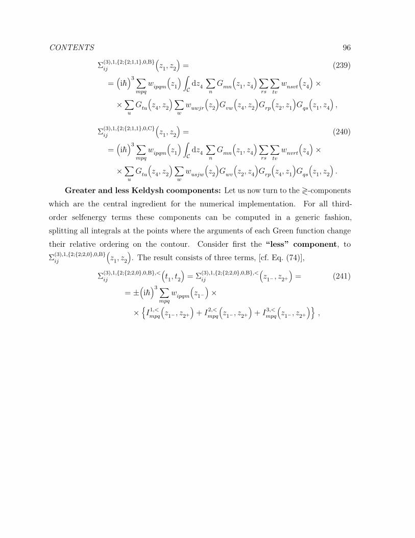
CONTENTS 96

Σ(3),1,{2;{2;1,1},0,B}ij

(z1, z2

)= (239)

=(i~)3 ∑

mpq

wipqm

(z1

) ∫Cdz4

∑n

Gmn

(z1, z4

)∑rs

∑tv

wnsvt

(z4

)×

×∑u

Gtu

(z4, z2

)∑w

wuwjr

(z2

)Gvw

(z4, z2

)Grp

(z2, z1

)Gqs

(z1, z4

),

Σ(3),1,{2;{2;1,1},0,C}ij

(z1, z2

)= (240)

=(i~)3 ∑

mpq

wipqm

(z1

) ∫Cdz4

∑n

Gmn

(z1, z4

)∑rs

∑tv

wnvrt

(z4

)×

×∑u

Gtu

(z4, z2

)∑w

wusjw

(z2

)Gwv

(z2, z4

)Grp

(z4, z1

)Gqs

(z1, z2

).

Greater and less Keldysh coomponents: Let us now turn to the ≷-componentswhich are the central ingredient for the numerical implementation. For all third-order selfenergy terms these components can be computed in a generic fashion,splitting all integrals at the points where the arguments of each Green function changetheir relative ordering on the contour. Consider first the “less” component, toΣ(3),1,{2;{2;2,0},0,B}ij

(z1, z2

). The result consists of three terms, [cf. Eq. (74)],

Σ(3),1,{2;{2;2,0},0,B},<ij

(t1, t2

)= Σ(3),1,{2;{2;2,0},0,B},<

ij

(z1− , z2+

)= (241)

= ±(i~)3 ∑

mpq

wipqm

(z1−

)×

×{I1,<mpq

(z1− , z2+

)+ I2,<

mpq

(z1− , z2+

)+ I3,<

mpq

(z1− , z2+

)},

CONTENTS 97

with the three terms given by

I1,<mpq

(z1− , z2+

)=∫ z

1−

z0−

dz4

∑n

G>mn

(z1− , z4

)× (242)

×∑rs

∑tu

G<tu

(z4, z2+

)∑v

wnvrt

(z4

)×

×∑w

wsujw

(z2+

)G>wv

(z2+ , z4

)G<rp

(z4, z1−

)G<qs

(z1− , z2+

),

I2,<mpq

(z1− , z2+

)=∫ z

2+

z1−

dz4

∑n

G<mn

(z1− , z4

)× (243)

×∑rs

∑tu

G<tu

(z4, z2+

)∑v

wnvrt

(z4

)×

×∑w

wsujw

(z2+

)G>wv

(z2+ , z4

)G>rp

(z4, z1−

)G<qs

(z1− , z2+

),

I3,<mpq

(z1− , z2+

)=∫ z

0+

z2+

dz4

∑n

G<mn

(z1− , z4

)(244)

∑rs

∑tu

G>tu

(z4, z2+

)∑v

wnvrt

(z4

)∑w

wsujw

(z2+

)G<wv

(z2+ , z4

)G>rp

(z4, z1−

)G<qs

(z1− , z2+

).

We now transform these expression to real-time integrals:

Σ(3),1,{2;{2;2,0},0,B},<ij

(t1, t2

)= ±

(i~)3 ∑

mpq

wipqm

(t1

)× (245)

×{I1,<mpq

(t1, t2

)+ I2,<

mpq

(t1, t2

)+ I3,<

mpq

(t1, t2

)},

CONTENTS 98

with the corresponding results for the three contributions

I1,<mpq

(t1, t2

)=∫ t1

t0

dt4∑n

G>mn

(t1, t4

)× (246)

×∑rs

∑tu

G<tu

(t4, t2

)∑v

wnvrt

(t4

)×

×∑w

wsujw

(t2

)G>wv

(t2, t4

)G<rp

(t4, t1

)G<qs

(t1, t2

),

I2,<mpq

(t1, t2

)=∫ t2

t1

dt4∑n

G<mn

(t1, t4

)× (247)

×∑rs

∑tu

G<tu

(t4, t2

)∑v

wnvrt

(t4

)×

×∑w

wsujw

(t2

)G>wv

(t2, t4

)G>rp

(t4, t1

)G<qs

(t1, t2

),

I3,<mpq

(t1, t2

)=∫ t0

t2

dt4∑n

G<mn

(t1, t4

)× (248)

×∑rs

∑tu

G>tu

(t4, t2

)∑v

wnvrt

(t4

)×

×∑w

wsujw

(t2

)G<wv

(t2, t4

)G>rp

(t4, t1

)G<qs

(t1, t2

).

For the greater component, we find analogously

Σ(3),1,{2;{2;2,0},0,B},>ij

(t1, t2

)= Σ(3),1,{2;{2;2,0},0,B},>

ij

(z1+ , z2−

)= (249)

= ±(i~)3 ∑

mpq

wipqm

(z1+

)×

×{I1,>mpq

(z1+ , z2−

)+ I2,>

mpq

(z1+ , z2−

)+ I3,>

mpq

(z1+ , z2−

)},

CONTENTS 99

which, again, consists of three terms:

I1,>mpq

(z1+ , z2−

)=∫ z

2−

z0−

dz4

∑n

G>mn

(z1+ , z4

)× (250)

×∑rs

∑tu

G<tu

(z4, z2−

)∑v

wnvrt

(z4

)×

×∑w

wsujw

(z2−

)G>wv

(z2− , z4

)G<rp

(z4, z1+

)G>qs

(z1+ , z2−

),

I2,>mpq

(z1+ , z2−

)=∫ z

1+

z2−

dz4

∑n

G>mn

(z1+ , z4

)× (251)

×∑rs

∑tu

G>tu

(z4, z2−

)∑v

wnvrt

(z4

)×

×∑w

wsujw

(z2−

)G<wv

(z2− , z4

)G<rp

(z4, z1+

)G>qs

(z1+ , z2−

),

I3,>mpq

(z1+ , z2−

)=∫ z

0+

z1+

dz4

∑n

G<mn

(z1+ , z4

)× (252)

×∑rs

∑tu

G>tu

(z4, z2−

)∑v

wnvrt

(z4

)×

×∑w

wsujw

(z2−

)G<wv

(z2− , z4

)G>rp

(z4, z1+

)G>qs

(z1+ , z2−

).

Transforming, again, to real-time integrals, we obtain

Σ(3),1,{2;{2;2,0},0,B},>ij

(t1, t2

)= ±

(i~)3 ∑

mpq

wipqm

(t1

)× (253)

×{I1,>mpq

(t1, t2

)+ I2,>

mpq

(t1, t2

)+ I3,>

mpq

(t1, t2

)},

CONTENTS 100

with the three contributions becoming

I1,>mpq

(t1, t2

)=∫ t2

t0

dt4∑n

G>mn

(t1, t4

)× (254)

×∑rs

∑tu

G<tu

(t4, t2

)∑v

wnvrt

(t4

)×

×∑w

wsujw

(t2

)G>wv

(t2, t4

)G<rp

(t4, t1

)G>qs

(t1, t2

),

I2,>mpq

(t1, t2

)=∫ t1

t2

dt4∑n

G>mn

(t1, t4

)× (255)

×∑rs

∑tu

G>tu

(t4, t2

)∑v

wnvrt

(t4

)×

×∑w

wsujw

(t2

)G<wv

(t2, t4

)G<rp

(t4, t1

)G>qs

(t1, t2

),

I3,>mpq

(t1, t2

)=∫ t0

t1

dt4∑n

G<mn

(t1, t4

)× (256)

×∑rs

∑tu

G>tu

(t4, t2

)∑v

wnvrt

(t4

)×

×∑w

wsujw

(t2

)G<wv

(t2, t4

)G>rp

(t4, t1

)G>qs

(t1, t2

).

Non-selfconsistent expansion: We now briefly discuss how the above resultschange in the case that all expressions are expanded in terms of noninteracting Greenfunctions. The additional non-selfconsistent diagrams are of either of the structures

Σ(3)(G −→ G

(0)), (10 terms)

Σ(2)(G

(0) −→ G(0)Σ(1)

G(0))

, (6 · 2 = 12 terms)

ΣH/ΣF(G

(0) −→ G(0)Σ(2)

G(0))

, (2 · 6 = 12 terms)

ΣH/ΣF(G

(0) −→ G(0)Σ(1)

G(0)Σ(1)

G(0))

, (2 · 2 · 2 = 8 terms)

This makes a total of 42 non-selfconsistent third-order terms.

Diagonal basis. In a diagonal basis, the selfconsistent third-order selfenergycontributions become

Σ(3),{3;0,2},0,diagij

(z1, z2

)= (257)

=(i~)3Gij

(z1, z2

)∑r

wir

(z1

) ∫Cdz3

∑t

Grt

(z1, z3

)Gtr

(z3, z1

)×

×∑v

wtv

(z3

)∑x

Gvx

(z3, z2

)Gxv

(z2, z3

)wxj

(z2

),

CONTENTS 101

Σ(3),{3;1,1},0,diagij

(z1, z2

)= (258)

= ±(i~)3Gij

(z1, z2

)∑r

wir

(z1

) ∫Cdz3

∑t

Grt

(z1, z3

)∑u

Gur

(z3, z1

)×

× wtu(z3

)∑x

Gtx

(z3, z2

)Gxu

(z2, z3

)wxj

(z2

),

Σ(3),2,1,diagij

(z1, z2

)= (259)

= ±(i~)3 ∫

Cdz3

∑r

wir

(z1

)∑t

Grt

(z1, z3

)Gtr

(z3, z1

)∑p

wtp

(z3

)×

×∑n

Gin

(z1, z2

)wnj

(z2

)Gnp

(z2, z3

)Gpj

(z3, z2

),

Σ(3),1,{2;1,1},diagij

(z1, z2

)= (260)

=(i~)3∑

p

wip

(z1

)∑n

Gin

(z1, z2

)wnj

(z2

) ∫Cdz3

∑t

Gnt

(z2, z3

)×

×∑u

Guj

(z3, z2

)wtu

(z3

)Gtp

(z3, z1

)Gpu

(z1, z3

),

Now we again provide the three contributions labeled “A, B, C”, respectively:

Σ(3),1,{2;{2;2,0},0,A},diagij

(z1, z2

)= (261)

= ±(i~)3∑

p

wip

(z1

) ∫Cdz4

∑n

Gin

(z1, z4

)∑tv

Gtv

(z4, z2

)×

× wnt(z4

)wvj

(z2

)Gvt

(z2, z4

)Gnp

(z4, z1

)Gpj

(z1, z2

),

Σ(3),1,{2;{2;2,0},0,B},diagij

(z1, z2

)= (262)

= ±(i~)3∑

p

wip

(z1

) ∫Cdz4

∑n

Gin

(z1, z4

)∑rs

Gnj

(z4, z2

)×

× wnr(z4

)wsj

(z2

)Gsr

(z2, z4

)Grp

(z4, z1

)Gps

(z1, z2

),

Σ(3),1,{2;{2;2,0},0,C},diagij

(z1, z2

)= (263)

= ±(i~)3∑

p

wip

(z1

) ∫Cdz4

∑n

Gin

(z1, z4

)∑rs

Gnj

(z4, z2

)×

×Gsr

(z4, z2

)wns

(z4

)wrj

(z2

)Grp

(z2, z1

)Gps

(z1, z4

)and, similarly, for the second class of selfenergy contributions:

Σ(3),1,{2;{2;1,1},0,A},diagij

(z1, z2

)= (264)

=(i~)3∑

p

wip

(z1

) ∫Cdz4

∑n

Gin

(z1, z4

)∑st

wnt

(z4

)×

× wsj(z2

)Gst

(z2, z4

)Gtj

(z4, z2

)Gnp

(z4, z1

)Gps

(z1, z2

),

CONTENTS 102

Σ(3),1,{2;{2;1,1},0,B},diagij

(z1, z2

)= (265)

=(i~)3∑

p

wip

(z1

) ∫Cdz4

∑n

Gin

(z1, z4

)∑rs

wns

(z4

)×

×Gnr

(z4, z2

)wrj

(z2

)Gsj

(z4, z2

)Grp

(z2, z1

)Gps

(z1, z4

),

Σ(3),1,{2;{2;1,1},0,C},diagij

(z1, z2

)= (266)

=(i~)3∑

p

wip

(z1

) ∫Cdz4

∑n

Gin

(z1, z4

)∑r

wnr

(z4

)×

×∑u

Gnu

(z4, z2

)wuj

(z2

)Gur

(z2, z4

)Grp

(z4, z1

)Gpj

(z1, z2

).

The corresponding Keldysh matrix components as well as the non-selfconsistentselfenergy contributions can be worked out in analogy to those in the non-diagonal basis.The diagrams of the selfconsistent third-order selfenergy contributions in a diagonalbasis are shown in Fig. 24.

Hubbard basis. Spin-0 bosons. For the Hubbard basis we separately considerspin-0 bosons and spin-1/2 fermions. For the case of spin-0 bosons, the third-orderselfenergy contributions separate into two classes. The first is given by

Σ(3),{3;0,2},0,b,0ij

(z1, z2

)= Σ(3),{3;1,1},0,b,0

ij

(z1, z2

)= (267)

= Σ(3),2,1,b,0ij

(z1, z2

)= Σ(3),1,{2;1,1},b,0

ij

(z1, z2

)=

= Σ(3),1,{2;{2;2,0},0,A},b,0ij

(z1, z2

)= Σ(3),1,{2;{2;2,0},0,B},b,0

ij

(z1, z2

)=

= Σ(3),1,{2;{2;1,1},0,A},b,0ij

(z1, z2

)= Σ(3),1,{2;{2;1,1},0,C},b,0

ij

(z1, z2

)=

=(i~)3Gij

(z1, z2

)U(z1

) ∫Cdz3

∑t

Git

(z1, z3

)Gti

(z3, z1

)×

× U(z3

)Gtj

(z3, z2

)Gjt

(z2, z3

)U(z2

),

and the second is given by

Σ(3),1,{2;{2;2,0},0,C},b,0ij

(z1, z2

)= Σ(3),1,{2;{2;1,1},0,B},b,0

ij

(z1, z2

)= (268)

=(i~)3U(z1

) ∫Cdz4

∑n

Gin

(z1, z4

)Gnj

(z4, z2

)×

×Gnj

(z4, z2

)U(z4

)U(z2

)Gji

(z2, z1

)Gin

(z1, z4

).

The corresponding diagrams are shown in Fig. 25.Let us now turn to the Hubbard result For spin-1/2 fermions. In this case only the

terms with the superscripts “B” and “C” exist which are denoted by Σ(3),1,{2;{2;2,0},0,B},f,1/2

CONTENTS 103

i, z1 j, z2

r, z1

t, z3 v, z3

x, z2

i, z1 j, z2

r, z1t, z3

u, z3x, z2

i, z1n, z2

p, z3j, z2

r, z1 t, z3

i, z1n, z2 t, z3

p, z1

u, z3j, z2

i, z1n, z4

p, z1j, z2

t, z4 v, z2

i, z1n, z4

j, z2

p, z1r, z4

s, z2

i, z1n, z4

j, z2

p, z1s, z4

r, z2

i, z1n, z4

p, z1 s, z2

t, z4j, z2

i, z1n, z4

r, z2 p, z1

s, z4j, z2 i, z1

n, z4

u, z2

r, z4 p, z1j, z2

Figure 24. Third-order diagrams in diagonal basis from left to right.First row: Σ(3),{3;0,2},0,diag, Σ(3),{3;1,1},0,diag Second row: Σ(3),2,1,diag,Σ(3),1,{2;1,1},diag Third row: Σ(3),1,{2;{2;2,0},0,A},diag, Σ(3),1,{2;{2;2,0},0,B},diag

Fourth row: Σ(3),1,{2;{2;2,0},0,C},diag, Σ(3),1,{2;{2;1,1},0,A},diag Fifth row:Σ(3),1,{2;{2;1,1},0,B},diag, Σ(3),1,{2;{2;1,1},0,C},diag.

CONTENTS 104

i, z1n, z3

j, z2

i, z1n, z3

j, z2

i, z1n, z4

j, z2

i, z1n, z4

j, z2

Figure 25. Third-order diagrams in the Hub-bard basis for spin-0 bosons. Left: First equiv-alence class of Σ(3),{3;0,2},0,diag, Σ(3),{3;1,1},0,diag,Σ(3),2,1,diag,Σ(3),1,{2;1,1},diag, Σ(3),1,{2;{2;2,0},0,A},diag,Σ(3),1,{2;{2;2,0},0,B},diag, Σ(3),1,{2;{2;1,1},0,A},diag andΣ(3),1,{2;{2;1,1},0,C},diag. Right: Second equivalence classof Σ(3),1,{2;2,0,C},diag and Σ(3),1,{2;1,1,B},diag.

and Σ(3),1,{2;{2;2,0},0,C},f,1/2, respectively. The “B”-terms are given by

Σ(3),1,{2;{2;2,0},0,B},f,1/2i↑j↑

(z1, z2

)= (269)

= −(i~)3U(z1

) ∫Cdz4

∑n

Gi↑n↑

(z1, z4

)Gn↑j↑

(z4, z2

)×

× U(z4

)U(z2

)Gj↓n↓

(z2, z4

)Gn↓i↓

(z4, z1

)Gi↓j↓

(z1, z2

),

Σ(3),1,{2;{2;2,0},0,B},f,1/2i↓j↓

(z1, z2

)= (270)

= −(i~)3U(z1

) ∫Cdz4

∑n

Gi↓n↓

(z1, z4

)Gn↓j↓

(z4, z2

)×

× U(z4

)U(z2

)Gj↑n↑

(z2, z4

)Gn↑i↑

(z4, z1

)Gi↑j↑

(z1, z2

),

and, for the “C”-terms, we find

Σ(3),1,{2;{2;2,0},0,C},f,1/2i↑j↑

(z1, z2

)= (271)

= −(i~)3U(z1

) ∫Cdz4

∑n

Gi↑n↑

(z1, z4

)Gn↑j↑

(z4, z2

)×

× U(z4

)U(z2

)Gn↓j↓

(z4, z2

)Gi↓n↓

(z1, z4

)Gj↓i↓

(z2, z1

),

Σ(3),1,{2;{2;2,0},0,C},f,1/2i↓j↓

(z1, z2

)= (272)

= −(i~)3U(z1

) ∫Cdz4

∑n

Gi↓n↓

(z1, z4

)Gn↓j↓

(z4, z2

)×

× U(z4

)U(z2

)Gn↑j↑

(z2, z4

)Gi↑n↑

(z4, z1

)Gj↑i↑

(z1, z2

),

whereas the “A” terms vanish, as well as all other contributions in third order. Thecorresponding Feynman diagrams are shown in Fig. 26.

CONTENTS 105

i ↓ (↑), z1n ↓ (↑), z3

j ↓ (↑), z2

i ↑ (↓), z1n ↑ (↓), z3

j ↑ (↓), z2

i ↓ (↑), z1n ↓ (↑), z4

j ↓ (↑), z2

i ↑ (↓), z1n ↑ (↓), z4

j ↑ (↓), z2

Figure 26. Third-order diagrams in Hubbard basis for spin-1/2 fermions. Left:Σ(3),1,{2;{2;2,0},0,B},f,1/2. Right: Σ(3),1,{2;{2;2,0},0,C},f,1/2.

4.4. Selfenergies of orders higher than three.

All terms of orders higher than three can be generated similarly as was demonstratedabove for the lower orders. So we only outline the main steps. As before, one computesall possible permutations of the quantities involved in Hedin’s equations that lead to thedesired total order. An approach that is suitable for a systematic recursive algorithm,starts by eliminating the polarizability from Hedin’s equations, yielding, for the selfenergyand the screened potential [cf. Eq. (95) to Eq. (106)],

Σij

(z1, z2

)= ΣH

ij

(z1, z2

)+ i~

∫Cdz3

∑mpq

Wipqm

(z1, z3

)× (273)

×∫Cdz4

∑n

Gmn

(z1, z4

)Γnqpj

(z4, z2, z3

),

Wijkl

(z1, z2

)= δC

(z1, z2

)wijkl

(z1

)± (274)

± i~∑mn

wimnl

(z1

) ∫Cdz3

∑pq

∫Cdz4

∑r

Gnr

(z1, z4

)×

×∫Cdz5

∑s

Gsm

(z5, z1

)Γrqps

(z4, z5, z3

)Wpjkq

(z3, z2

)and, for the vertex function,

Γijkl(z1, z2, z3

)= δC

(z1, z2+

)δC

(z3, z2

)δikδjl + (275)

+∫Cdz4dz5

∑mn

δΣxcil

(z1, z2

)δGmn

(z4, z5

) ∫Cdz6

∑p

Gmp

(z4, z6

)×

×∫Cdz7

∑q

Gqn

(z7, z5

)Γpjkq

(z6, z7, z3

).

With this set of three coupled equations, the following recursive algorithm can be appliedto calculate the N -th order selfenergy contributions:

(i) Initialize Σ(1) = ΣH, cf. Eq. (273),

CONTENTS 106

(ii) Initialize W (1) = w, cf. Eq. (274),

(iii) Initialize Γ = Γ(0), cf. Eq. (275),

(iv) Loop over n = 1 . . . N :

(a) If n > 1: Loop over all orders m = 1 . . . (n− 1):– Loop over all selfenergy contributions Σ(m) of order m:

– Loop over all vertex contributions Γ(n−1−m) of order n − 1−m:– Calculate the new vertex contribution Γ(n−1) of order m+n−1−m =n − 1, from Σ(m) and Γ(n−1−m), via Eq. (275),

(b) If n > 1: Loop over all orders m = 1 . . . (n− 1):– Loop over all contributions to the screened interaction W (m) of order m:

– Loop over all vertex contributions Γ(n−1−m) of order n − 1−m:– Calculate the new contribution to the screened interaction W (n) of

order 1+m+n−1−m = n, from w,W (m) and Γ(n−1−m), via Eq. (274)(c) Loop over all orders m = 1 . . . n:

– Loop over all contributions to the screened interaction W (m) of order m:– Loop over all vertex contributions Γ(n−m) of order n −m:– Calculate the new selfenergy contribution Σ(n) fromW

(m) and Γ(n−m)

of order m+ n −m = n via Eq. (273)

A similar algorithm yielding the diagrams with respect to the bare interaction, w, can bededuced, replacing the full vertex Γ by the bare vertex Λ, cf. Eqs. (97) and (98). Further,the generation of the non-selfconsistent diagrams is straightforward by inclusion of theDyson equation and, additionally, taking into account the order of the Green functionsin the respective equations.

With this we conclude the discussion of the perturbative approaches to the selfenergy.

5. Selfenergy approximations II: Diagram resummation. GW , T matrix,FLEX

In this section we discuss an alternative to the perturbative expansion of the selfenergyin terms of the interaction strength that was presented in Section 4. The perturbationexpansion is expected to become questionable or, at least, inefficient with increasinginteraction strength. This was confirmed in the Sec. 3 where we demonstrated thata number of non-perturbative approaches, such as the GW approximation, the T -matrix approximation or the FLEX approach are significantly more accurate, in many

CONTENTS 107

cases.Thus, when perturbation expansions fail, a more appropriate approach consists in

diagram resummation techniques that sum an entire infinite perturbation series and whichis in the focus of the present section. The underlying idea is to take into considerationone or several classes of terms with a recursive structure which occur in all orders of theinteraction, based on physical intuition about their importance. In fact such resummationapproaches have a long history. For example the T -matrix approximation has beensuccessfully applied in scattering theory and in nuclear physics. On the other hand, theconcept of dynamical screening (GW approximation) has been employed for electrolytesand plasmas. The major advance provided by Green functions theory is the extension ofthe concept to arbitrary nonequilibrium situations.

GW approximation. Starting from the notion of the screened interaction, W ,the simplest choice is the GW approximation [81] which centers around treating Wexactly according to Eq. (102) while taking the screened vertex Γ only in zeroth-orderapproximation. This leads to the familiar concept of dynamical screening and plasmondynamics which is of particular importance for long-range Coulomb interaction in denseplasmas [131] or molecules. The resulting structure of the selfenergy approximation isdiscussed in the ensuing Section 5.2.

T -matrix approximation. In contrast to GW , the T -matrix approximation,treats the interaction only at the level of the bare interaction, but focuses insteadon a good representation of the bare vertex functions Λ. This approximation sumsthe entire Born series and is, thus expected to be more accurate than the second-Born approximation, at strong coupling. The T -matrix approximation exists in twoflavors—the particle–particle T -matrix approximation (TPP) and the particle–holeT -matrix approximation (TPH).

Combination of strong coupling and dynamical screening. Furthermore,several other approaches have been introduced that mix screened and bareinteraction [165]. An example for this group is the second-order screened-exchange(SOSEX) approximation [101, 165, 166], which takes the second-order exchange diagram,cf. Eq. (183), and replaces one of the bare interactions w by the screened interactionW . Doing that, the total complexity is still of O

(N3

t

), since the determination of the

selfenergy, the computation of the screened interaction according to Eq. (104) and thesolution of the KBE, [cf. Eqs. (66) and (67)], all scale as O

(N3

t

).

Another possible way is to combine several existing approximations. Thereby one

CONTENTS 108

has to correct for possible double counting. This strategy is pursued in the so-calledfluctuating-exchange (FLEX) approximation which adds the diagrams of thirdand higher order of the GW approximation and both T matrices to the second-orderdiagrams, which are taken only once. The FLEX approximation which will be detailedin Section 5.5 can be seen as a the starting term of the more sophisticated plaquettheory [167–173], where one uses coupled equations for the vertex functions in theparticle–particle and particle–hole channels.

Before discussing in detail the GW approximation, the T -matrix approximation andthe FLEX approximation, in Sections 5.2, 5.3 and 5.5, respectively, we investigate insome detail the two-particle Green function G(2). We start by introducing the Hartreeand the Fock approximation for G(2) in Section 5.1, since they will be used later.

5.1. Mean field. Hartree and Fock approximations for G(2)

In the following, the two simplest approximations for the two-particle Green function aredefined which will are the starting point for simplifying the expressions occuring in theresummation approaches. Those are the Hartree Green function, G(2),H, and the FockGreen function, G(2),F.

G(2),H corresponds to the approximation that two particles are uncorrelated. Then

the two-particle Green function G(2) is approximated as

G(2)ijkl

(z1, z2, z3, z4

)≡ G

(2),Hijkl

(z1, z2, z3, z4

):= Gik

(z1, z3

)Gjl

(z2, z4

). (276)

This approximation applies to classical and quantum many-particle systems alike. Incontrast, an additional approximation that exists only in the case of quantum systemsand reflects the indistinguishability of quantum particles (exchange effects of bosons orfermions) is the Fock approximations which, is denoted as G(2),F and reads

G(2)ijkl

(z1, z2, z3, z4

)≡ G

(2),Fijkl

(z1, z2, z3, z4

):= ±Gil

(z1, z4

)Gjk

(z2, z3

).(277)

For better illustration both two-particle quantities are repeated in the compactnotation:

CONTENTS 109

G(2)(1, 2, 3, 4) ≈ G

(2),H(1, 2, 3, 4):= G

(1, 3

)G(2, 4

)

G(2)(1, 2, 3, 4) ≈ G

(2),F(1, 2, 3, 4):= ±G

(1, 4

)G(2, 3

)

7→ , (278)

7→ . (279)

Following the above considerations, in a quantum system the mean-field approximationfor G(2) is the sum of the Hartree and Fock contributions.

In the resummation expansions presented in this section, both quantities play acentral role. However, in most cases, we will only need simpler two-time versions ofthe two-particle functions, GH and GF, respectively These expressions follow by settingequal two pairs of time-arguments and adding a dimensionality factor i~. This leads to(we skip the superscript “(2)” since it is clear that a function with four basis indicesrefers to a two-particle Green function)

GHijkl

(z1, z2

):= i~G(2),H

ijkl

(z1, z1, z2, z2

)≡ i~Gik

(z1, z2

)Gjl

(z1, z2

), (280)

whereas, for the Fock approximation, one has

GFijkl

(z1, z2

)= i~G(2),F

ijkl

(z1, z2, z1, z2

)≡ ±i~Gil

(z1, z2

)Gjk

(z2, z1

). (281)

We now provide the Keldysh matrix components of Eqs. (280) and (281). For theHartree function, we have the following greater/less and advanced/retarded components:

GH,≷ijkl

(t1, t2

)= i~G≷

ik

(t1, t2

)G≷jl

(t1, t2

),

GH,A/Rijkl

(t1, t2

)= ∓i~Θ[±(t2 − t1)]

[G>ik

(t1, t2

)G>jl

(t1, t2

)−G<

ik

(t1, t2

)G<jl

(t1, t2

)],

Similarly, for the Fock two-particle function follows

GF,≷ijkl

(t1, t2

)= ±i~G≷

il

(t1, t2

)G≶jk

(t2, t1

),

GF,A/Rijkl

(t1, t2

)= ∓i~Θ[±(t2 − t1)]

[G>il

(t1, t2

)G<jk

(t2, t1

)−G<

il

(t1, t2

)G>jk

(t2, t1

)],

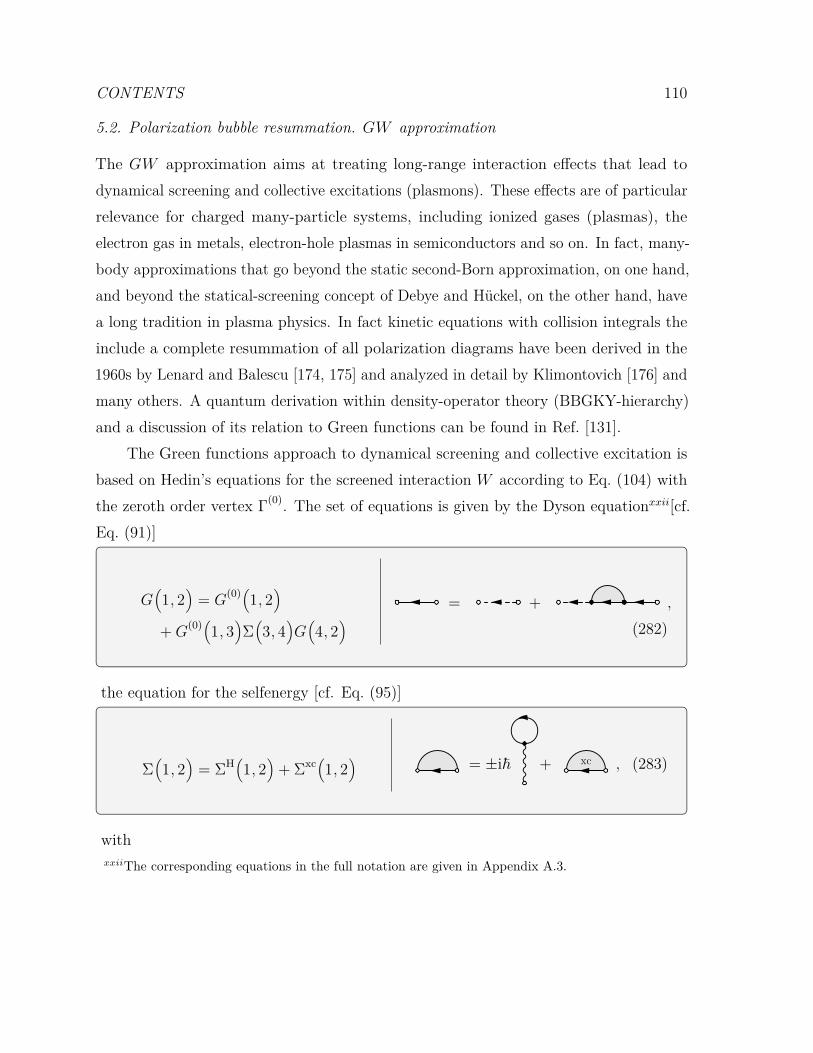
CONTENTS 110

5.2. Polarization bubble resummation. GW approximation

The GW approximation aims at treating long-range interaction effects that lead todynamical screening and collective excitations (plasmons). These effects are of particularrelevance for charged many-particle systems, including ionized gases (plasmas), theelectron gas in metals, electron-hole plasmas in semiconductors and so on. In fact, many-body approximations that go beyond the static second-Born approximation, on one hand,and beyond the statical-screening concept of Debye and Hückel, on the other hand, havea long tradition in plasma physics. In fact kinetic equations with collision integrals theinclude a complete resummation of all polarization diagrams have been derived in the1960s by Lenard and Balescu [174, 175] and analyzed in detail by Klimontovich [176] andmany others. A quantum derivation within density-operator theory (BBGKY-hierarchy)and a discussion of its relation to Green functions can be found in Ref. [131].

The Green functions approach to dynamical screening and collective excitation isbased on Hedin’s equations for the screened interaction W according to Eq. (104) withthe zeroth order vertex Γ(0). The set of equations is given by the Dyson equationxxii[cf.Eq. (91)]

G(1, 2

)= G

(0)(1, 2)+G

(0)(1, 3)Σ(3, 4)G(4, 2)= + ,

(282)

the equation for the selfenergy [cf. Eq. (95)]

Σ(1, 2

)= ΣH

(1, 2

)+ Σxc

(1, 2

) = ±i~ + xc , (283)

withxxiiThe corresponding equations in the full notation are given in Appendix A.3.

CONTENTS 111

Σxc(1, 2

)= i~W

(1, 3

)G(1, 4

)Γ(0)(4, 2, 3)

= i~W(1, 2

)G(1, 2

)xc 7→ i~

xc∣∣∣∣∣∣

xc 7→

= i~ , (284)

the zeroth-order polarizability [cf. Eq. (173)]

P(0)(1, 2) = ±i~G

(1, 3

)G(4, 1

)Γ(0)(3, 4, 2)

= ±i~G(1, 2

)G(2, 1

)7→ ±i~ xc

∣∣∣∣∣∣xc 7→

= ±i~ , (285)

and the screened interaction [cf. Eqs. (102) and (104)]

W(1, 2

)= w

(1, 2

)+ w

(1, 3

)P

(0)(3, 4)W (4, 2

)= w

(1, 2

)± i~w

(1, 3

)G(3, 4

)G(4, 3

)W(4, 2

)

7→

+

∣∣∣∣∣∣7→±i~

= ± i~ .

(286)

To solve this set of equations, one has to determine the selfconsistent solution ofEq. (286). Due to the time-diagonal structure (i.e. due to the time delta function) of thebare interaction [cf. Eq. (60)] the computational solution of Eq. (286) in the displayedform becomes ill-defined. Therefore, it is advantageous to eliminate the singular bareinteraction by defining the “non-singular” part of the interaction (or the induced potentialwhich will be labeled with the superscript “ns”)

CONTENTS 112

W ns(1, 2

):= W

(1, 2

)−W bare

(1, 2

)= W

(1, 2

)− w

(1, 2

) ns = − (287)

Using this and, by comparison with Eq. (156), one arrives at

ΣGW(1, 2

)= ΣH

(1, 2

)+ i~W

(1, 2

)G(1, 2

)= ΣH

(1, 2

)+ i~w

(1, 2

)G(1, 2

)+ i~W ns

(1, 2

)G(1, 2

)=: ΣH

(1, 2

)+ ΣF

(1, 2

)+ ΣGW,corr

(1, 2

)

7→ ±i~ + i~

∣∣∣∣∣∣= + ns

= ±i~ + i~ + i~ns

. (288)

Thus the full selfenergy in the GW approximation contains, in addition to the Hartree–Fock selfenergy, a correlation contribution which is denoted ΣGW,corr and which will bein the focus of the subsequent analysis.

For the non-singular part of the screened interaction, we have

W ns(1, 2

)= ±i~w

(1, 3

)G(3, 4

)G(4, 3

)w(4, 2

)± i~w

(1, 3

)G(3, 4

)G(4, 3

)W ns

(4, 2

)ns =± i~

± i~ ns.

(289)

Returning to the full notation and the single-time interaction one can use the

CONTENTS 113

definition of GF in Eq. (281) to simplify Eq. (289) to

W nsijkl

(z1, z2

)= ΦGW

ijkl

(z1, z2

)+∑mn

wimnl

(z1

) ∫Cdz3

∑pq

GFnqmp

(z1, z3

)W nspjkq

(z3, z2

),

(290)

ΦGWijkl

(z1, z2

)=:∑mn

wimnl

(z1

)∑pq

GFnqmp

(z1, z2

)wpjkq

(z2

), (291)

where we introduced the short notation Φ for the second-Born contribution to thescreened potential.

Finally, we provide the correlation components of Eq. (288)

ΣGW,corr,≷ij

(t1, t2

)= i~

∑mp

W ns,≷ipjm

(t1, t2

)G≷mp

(t1, t2

), (292)

which require knowledge of the correlation components of the non-singular screenedpotential Eq. (290), that are given by

W ns,≷ijkl

(t1, t2

)= ΦGW,≷

ijkl

(t1, t2

)+∑mn

wimnl

(t1

)∑pq

(293)(∫ t1

t0

dt3GF,Rnqmp

(t1, t3

)W ns,≷pjkq

(t3, t2

)+∫ t2

t0

dt3GF,≷nqmp

(t1, t3

)W ns,Apjkq

(t3, t2

)),

as well as of the advanced/retarded components,

Wns,A/Rijkl

(t1, t2

)= ΦGW,A/R

ijkl

(t1, t2

)+ (294)

+∑mn

wimnl

(t1

) ∫ t2/1

t1/2

dt3∑pq

GF,A/Rnqmp

(t1, t3

)W

ns,A/Rpjkq

(t3, t2

).

In the integration limits, in the notation t1/2, the first (second) subscript refers to theadvanced (retarded) function.

Diagonal basis. In a diagonal basis set, Eq. (290) simplifies to

W ns,diagijkl

(z1, z2

)= δilδjkΦ

GW,diagijji

(z1, z2

)+ (295)

+ δil∑m

wim

(z1

) ∫Cdz3

∑pq

GFmpmq

(z1, z3

)W ns,diagpjkq

(z3, z2

).

ΦGW,diagijji

(z1, z2

)=:∑m

wim

(z1

)∑p

GFmpmp

(z1, z2

)wpj

(z2

), (296)

CONTENTS 114

i, z1

mm, z1z1+

i, z1 j, z1+ i, z1 j, z2

s, z1 t, z2

i, z1 j, z2

r, z1

t, z3 v, z3

x, z2

Figure 27. The first four terms of the GW selfenergy, including Hartree andFock terms, in a diagonal basis.

where we again used the function Φ, Eq. (291). By iteration, it becomes evident thatW ns,diag and ΦGW,diag

ijji are always of the form

W ns,diagijkl

(z1, z2

)= δilδjkW

ns,diagijji

(z1, z2

)=: δilδjkW

ns,diagij

(z1, z2

), (297)

ΦGW,diagijkl

(z1, z2

)= δilδjkΦ

GW,diagijji

(z1, z2

)=: δilδjkΦ

GW,diagij

(z1, z2

). (298)

With this, for a diagonal basis, Eq. (290) attains the form

W ns,diagij

(z1, z2

)= ΦGW,diag

ij

(z1, z2

)+ (299)

+∑m

wim

(z1

) ∫Cdz3

∑p

GFmpmp

(z1, z3

)W ns,diagpj

(z3, z2

).

The correlation part of the selfenergy, Eq. (288), reads

ΣGW,corr,diagij

(z1, z2

)= + i~W ns,diag

ij

(z1, z2

)Gij

(z1, z2

). (300)

The first four terms of the GW selfenergy (mean field plus correlation selfenergy) areshown diagrammatically in Fig. 27. The sum continues to infinite order (infinite numberof polarization bubbles).

The relevant components of the Keldysh matrix read [cf. Eqs. (293) and (294)],

W ns,diag,≷ij

(t1, t2

)= ΦGW,diag,≷

ij

(t1, t2

)+∑mp

wim

(t1

)(301)

(∫ t1

t0

dt3GF,Rmpmp

(t1, t3

)W ns,diag,≷pj

(t3, t2

)+

+∫ t2

t0

dt3GF,≷mpmp

(t1, t3

)W ns,diag,Apj

(t3, t2

)),

Wns,diag,A/Rij

(t1, t2

)= ΦGW,diag,A/R

ij

(t1, t2

)+ (302)

+∑mp

wim

(t1

) ∫ t2/1

t1/2

dt3GF,A/Rmpmp

(t1, t3

)W

ns,diag,A/Rpj

(t3, t2

),

CONTENTS 115

and [cf. Eq. (292)],

ΣGW,corr,diag,≷ij

(t1, t2

)= i~W ns,diag,≷

ij

(t1, t2

)G≷ij

(t1, t2

). (303)

Hubbard basis. In the Hubbard basis, cf. Section 2.3, the GW approximation sim-plifies considerably. We start by presenting the equations for bosons:

W ns,biαjβ

(z1, z2

)= ΦGW,b

ij

(z1, z2

)+ U

(z1

) ∫Cdz3

∑pε

GFiεpεiεpε

(z1, z3

)W ns,bpεjβ

(z3, z2

), (304)

ΦGW,bij

(z1, z2

)=: U

(z1

)∑ε

GFiεjεiεjε

(z1, z2

)U(z2

), (305)

and the correlation selfenergy on the Keldysh contour is

ΣGW,corr,biαjα

(z1, z2

)= i~W ns,b

iαjα

(z1, z2

)Giαjα

(z1, z2

). (306)

The Keldysh matrix components of the screened potential in the Hubbard basis become

W ns,b,≷iαjβ

(t1, t2

)= ΦGW,b,≷

ij

(t1, t2

)+

+ U(t1

) ∫ t1

t0

dt3∑pε

GF,Riεpεiεpε

(t1, t3

)W ns,b,≷pεjβ

(t3, t2

)+

+ U(t1

) ∫ t2

t0

dt3∑pε

GF,≷iεpεiεpε

(t1, t3

)W ns,b,Apεjβ

(t3, t2

),

Wns,b,A/Riαjβ

(t1, t2

)= ΦGW,b,A/R

ij

(t1, t2

)+

+ U(t1

) ∫ t2/1

t1/2

dt3∑pε

GF,A/Riεpεiεpε

(t1, t3

)W

ns,b,A/Rpεjβ

(t3, t2

),

and the greater/less components of the correlation selfenergy (306) are

ΣGW,corr,b,≷iαjα

(t1, t2

)= i~W ns,b,≷

iαjα

(t1, t2

)G≷iαjα

(t1, t2

). (307)

For the special case of spin-0 bosons, the screened potential on the Keldysh contourhas the form

W ns,b,0ij

(z1, z2

)= ΦGW,b,0

ij

(z1, z2

)+ U

(z1

) ∫Cdz3

∑p

GFipip

(z1, z3

)W ns,b,0pj

(z3, z2

),

ΦGW,b,0ij

(z1, z2

)=: U

(z1

)GFijij

(z1, z2

)U(z2

), (308)

and the correlation selfenergy in GW approximation becomes

ΣGW,corr,b,0ij

(z1, z2

)= i~W ns,b,0

ij

(z1, z2

)Gij

(z1, z2

).

CONTENTS 116

i, z1

ii, z1z1+

i, z1 i, z1+ i, z1 j, z2

i, z1 j, z2

i, z1 j, z2

i, z1

t, z3 t, z3

j, z2

Figure 28. The first four terms of the GW selfenergy (Hartree, Fock andcorrelation part) in the Hubbard basis for spin-0 bosons.

The greater, less and advanced/retarded matrix components become

W ns,b,0,≷ij

(t1, t2

)= ΦGW,b,0,≷

ij

(t1, t2

)+

+ U(t1

) ∫ t1

t0

dt3∑p

GF,Ripip

(t1, t3

)W ns,b,0,≷pj

(t3, t2

)+

+ U(t1

) ∫ t2

t0

dt3∑p

GF,≷ipip

(t1, t3

)W ns,b,0,Apj

(t3, t2

),

Wns,b,0,A/Rij

(t1, t2

)= ΦGW,b,0,A/R

ij

(t1, t2

)+

+ U(t1

) ∫ t2/1

t1/2

dt3∑p

GF,A/Ripip

(t1, t3

)W

ns,b,0,A/Rpj

(t3, t2

)and, for the greater/less components of the correlation selfenergy, we have

ΣGW,corr,b,0,≷ij

(t1, t2

)= i~W ns,b,0,≷

ij

(t1, t2

)G≷ij

(t1, t2

).

The diagrammatic representation of the leading terms for spin-0 bosons in the Hubbardbasis is shown in Fig. 28.

Let us now turn to fermions. In that case the equations on the Keldysh contourattain the form

W ns,fiαjβ

(z1, z2

)= ΦGW,f

ijαβ

(z1, z2

)+ (309)

+ U(z1

) ∫Cdz3

∑p

∑ε 6=α

GFiεpεiεpε

(z1, z3

)W ns,fpεjβ

(z3, z2

)ΦGW,fijαβ

(z1, z2

)=:

∑ε6={α,β}

U(z1

)GFiεjεiεjε

(z1, z2

)U(z2

), (310)

whereas the correlation part of the selfenergy becomes

ΣGW,corr,fiαjα

(z1, z2

)= i~W ns,f

iαjα

(z1, z2

)Giαjα

(z1, z2

).

CONTENTS 117

The Keldysh matrix components of the screened potential are now

W ns,f,≷iαjβ

(t1, t2

)= ΦGW,f,≷

ijαβ

(t1, t2

)+

+ U(t1

) ∫ t1

t0

dt3∑p

∑ε6=α

GF,Riεpεiεpε

(t1, t3

)W ns,f,≷pεjβ

(t3, t2

)+

+ U(t1

) ∫ t2

t0

dt3∑p

∑ε6=α

GF,≷iεpεiεpε

(t1, t3

)W ns,f,Apεjβ

(t3, t2

),

Wns,f,A/Riαjβ

(t1, t2

)= ΦGW,f,A/R

ijαβ

(t1, t2

)+

+ U(t1

) ∫ t2/1

t1/2

dt3∑p

∑ε6=α

GF,A/Riεpεiεpε

(t1, t3

)W

ns,f,A/Rpεjβ

(t3, t2

).

The GW selfenergy has now the following correlation components

ΣGW,corr,f,≷iαjα

(t1, t2

)= i~W ns,f,≷

iαjα

(t1, t2

)G≷iαjα

(t1, t2

).

For the special case of spin-12-fermions, the equations for the screened interaction

require some care. Since the particles can have two spin projections, there are fourdifferent screened potentials each obeying its own equation which, in turn, are coupled.To underline these details we use different colors for the four potentials:

Wns,f,1/2i↑j↑

(z1, z2

)= ΦGW,f,1/2

ij↑

(z1, z2

)+ U

(z1

) ∫Cdz3

∑m

GFi↓m↓i↓m↓

(z1, z3

)W

ns,f,1/2m↓j↑

(z3, z2

),

ΦGW,f,1/2ij↑

(z1, z2

)=: U

(z1

)GFi↓j↓i↓j↓

(z1, z2

)U(z2

),

Wns,f,1/2i↓j↑

(z1, z2

)= U

(z1

) ∫Cdz3

∑m

GFi↑m↑i↑m↑

(z1, z3

)W

ns,f,1/2m↑j↑

(z3, z2

), (311)

Wns,f,1/2i↓j↓

(z1, z2

)= ΦGW,f,1/2

ij↓

(z1, z2

)+ U

(z1

) ∫Cdz3

∑m

GFi↑m↑i↑m↑

(z1, z3

)W

ns,f,1/2m↑j↓

(z3, z2

),

ΦGW,f,1/2ij↓

(z1, z2

)=: U

(z1

)GFi↑j↑i↑j↑

(z1, z2

)U(z2

),

Wns,f,1/2i↑j↓

(z1, z2

)= U

(z1

) ∫Cdz3

∑m

GFi↓m↓i↓m↓

(z1, z3

)W

ns,f,1/2m↓j↓

(z3, z2

). (312)

Interestingly, the equations for the screened potentials with different spin combinations,Eqs. (311) and (312), do not contain a contribution from the bare interaction.

The correlation selfenergies of fermions with spin up and down read, respectively,

ΣGW,corr,f,1/2i↑j↑

(z1, z2

)= i~W ns,f,1/2

i↑j↑

(z1, z2

)Gi↑j↑

(z1, z2

), (313)

ΣGW,corr,f,1/2i↓j↓

(z1, z2

)= i~W ns,f,1/2

i↓j↓

(z1, z2

)Gi↓j↓

(z1, z2

). (314)

The diagrammatic representation of the leading terms for spin-1/2 fermions in the

CONTENTS 118

i ↓ (↑), z1

i ↑ (↓)i ↑ (↓), z1z1+

i ↓ (↑), z1 j ↓ (↑), z2

i ↑ (↓), z1 j ↑ (↓), z2

i ↓ (↑), z1 j ↓ (↑), z2

i ↑ (↓), z1

p ↑ (↓), z3 p ↓ (↑), z3 q ↓ (↑), z4 q ↑ (↓), z4

j ↑ (↓), z2

Figure 29. The first three terms of the GW selfenergy (mean field plus correlationterm) in the Hubbard basis for spin-1/2 fermions. Note that the Fock term equalszero.

Hubbard basis is shown in Fig. 29. One recognizes a special structure of these equations for

spin-12 -fermions. The selfenergy

(ΣGW,f,1/2i↑j↑ / ΣGW,f,1/2

i↓j↓

), which couples only contributions

of the same spin, also directly depends only on the same-spin parts of the screened

interaction(W

ns,f,1/2i↑j↑ Gi↑j↑ / W

ns,f,1/2i↓j↓ Gi↓j↓

), cf. Eqs. (313) and (314). The same-spin

screened interaction, in turn, depends on the screened interaction with different spin

orientations(W

ns,f,1/2m↓j↑ / W ns,f,1/2

m↑j↓

), which itself couples back to the same-spin part.

Finally, we present the respective greater/less and retarded/advanced Keldyshcomponents of the screened potential for all four spin combinations:

Wns,f,1/2,≷i↑j↑

(t1, t2

)= ΦGW,f,1/2,≷

ij↑

(t1, t2

)+

+ U(t1

) ∫ t1

t0

dt3∑m

GF,Ri↓m↓i↓m↓

(t1, t3

)W

ns,f,1/2,≷m↓j↑

(t3, t2

)+

+ U(t1

) ∫ t2

t0

dt3∑m

GF,≷i↓m↓i↓m↓

(t1, t3

)W

ns,f,1/2,Am↓j↑

(t3, t2

),

Wns,f,1/2,A/Ri↑j↑

(t1, t2

)= ΦGW,f,1/2,A/R

ij↑

(t1, t2

)+

+ U(t1

) ∫ t2/1

t1/2

dt3∑m

GF,A/Ri↓m↓i↓m↓

(t1, t3

)W

ns,f,1/2,A/Rm↓j↑

(t3, t2

),

CONTENTS 119

Wns,f,1/2,≷i↓j↑

(t1, t2

)= U

(t1

) ∫ t1

t0

dt3∑m

GF,Ri↑m↑i↑m↑

(t1, t3

)W

ns,f,1/2,≷m↑j↑

(t3, t2

)+

+ U(t1

) ∫ t2

t0

dt3∑m

GF,≷i↑m↑i↑m↑

(t1, t3

)W

ns,f,1/2,Am↑j↑

(t3, t2

),

Wns,f,1/2,A/Ri↓j↑

(t1, t2

)= U

(t1

) ∫ t2/1

t1/2

dt3∑m

GF,A/Ri↑m↑i↑m↑

(t1, t3

)W

ns,f,1/2,A/Rm↑j↑

(t3, t2

),

Wns,f,1/2,≷i↓j↓

(t1, t2

)= ΦGW,f,1/2,≷

ij↓

(t1, t2

)+

+ U(t1

) ∫ t1

t0

dt3∑m

GF,Ri↑m↑i↑m↑

(t1, t3

)W

ns,f,1/2,≷m↑j↓

(t3, t2

)+

+ U(t1

) ∫ t2

t0

dt3∑m

GF,≷i↑m↑i↑m↑

(t1, t3

)W

ns,f,1/2,Am↑j↓

(t3, t2

),

Wns,f,1/2,A/Ri↓j↓

(t1, t2

)= ΦGW,f,1/2,A/R

ij↓

(t1, t2

)+

+ U(t1

) ∫ t2/1

t1/2

dt3∑m

GF,A/Ri↑m↑i↑m↑

(t1, t3

)W

ns,f,1/2,A/Rm↑j↓

(t3, t2

),

Wns,f,1/2,≷i↑j↓

(t1, t2

)= U

(t1

) ∫ t1

t0

dt3∑m

GF,Ri↓m↓i↓m↓

(t1, t3

)W

ns,f,1/2,≷m↓j↓

(t3, t2

)+

+ U(t1

) ∫ t2

t0

dt3∑m

GF,≷i↓m↓i↓m↓

(t1, t3

)W

ns,f,1/2,Am↓j↓

(t3, t2

)

Wns,f,1/2,A/Ri↑j↓

(t1, t2

)= U1

∫ t2/1

t1/2

dt3∑m

GF,A/Ri↓m↓i↓m↓

(t1, t3

)W

ns,f,1/2,A/Rm↓j↓

(t3, t2

).

The correlation components of the selfenergy read

ΣGW,corr,f,≷i↑j↑

(t1, t2

)= i~W ns,f,≷

i↑j↑

(t1, t2

)G≷i↑j↑

(t1, t2

), (315)

ΣGW,corr,f,≷i↓j↓

(t1, t2

)= i~W ns,f,≷

i↓j↓

(t1, t2

)G≷i↓j↓

(t1, t2

). (316)

With this we conclude the discussion of the GW approximation. As mentionedbefore the strength of this approximation is the account of long-range screening effects andcollective excitations (plasmons) which is of particular relevance for systems with Coulombinteraction. As we have seen in Sec. 3, the GW approximation has an impressivelyhigh accuracy, in many cases. At the same time, the GW approximation does not takeinto account strong-coupling effects since it includes only terms of second order in the(screened) interaction. Effects of multiple scattering are, thus, missing.

The inclusion of these effects for the case of a static pair interaction is the goal ofthe T -matrix approximation that is studied in Sec. 5.3. On the other hand, to account

CONTENTS 120

for multiple scattering and dynamical screening simultaneously, is the goal of the FLEXscheme that is discussed in Sec. 5.5.

5.3. Strong coupling. T -matrix approximation. Particle–particle and particle–holeT matrices

The goal of the T -matrix approximation is to capture effects of multiple scattering that areimportant in strongly coupled systems, but are missing in the second-Born approximation.The solution is to sum all higher-order Born terms up what leads to an effective interaction.In contrast to the GW approximation, the T -matrix approximation takes only the bareinteraction, w, into account (at least in its standard versions), neglecting dynamicalscreening, and aims, instead, at a good approximation of the bare vertex function Λ.The goal here is to accurately capture multiple scattering effects. Thus, its constitutiveequations are the Dyson equationxxiii

G(1, 2

)= G

(0)(1, 2)+G

(0)(1, 3)Σ(3, 4)G(4, 2)= + ,

(317)

the equation for the selfenergy, cf. Eqs. (95) and (97),

Σ(1, 2

)= ΣH

(1, 2

)+ Σxc

(1, 2

) = ±i~ + xc , (318)

with the exchange–correlation selfenergy (all contributions beyond Hartree) given by

Σxc(1, 2

)= i~w

(1, 3

)G(1, 4

)Λ(4, 2, 3

) xc = i~ . (319)

The bare vertex Λ is self-consistently given as the solution of the integral equationxxiiiThe corresponding equations in the full notation are given in Appendix A.4.

CONTENTS 121

Λ(1, 2, 3

)= δ

(1, 2+

)δ(3, 2

)+δΣ(1, 2

)δG(4, 5

)G(4, 6)G(7, 5)Λ(6, 7, 3)= + .

(320)

If these equations are iterated ad infinitum, all selfenergy terms will begenerated. To break the circular dependence between Eqs. (319) and (320), the T -matrix approximation starts by taking the bare vertex on the right-hand side of Eq. (320)only in zeroth order, transforming it into

Λcl(1, 2, 3

)= δ

(1, 2+

)δ(3, 2

)+δΣcl

(1, 2

)δG(4, 5

) G(4, 6)G(7, 5)Λ(0)(6, 7, 3)= δ

(1, 2+

)δ(3, 2

)+δΣcl

(1, 2

)δG(4, 5

) G(4, 3)G(3, 5)

7→ +

∣∣∣∣∣∣7→

= + . (321)

This closure of the equation for Λ allows to systematically generate results for theselfenergy which we will denote by the superscript “cl”. Using this result in Eq. (318),we obtain [cf. Eq. (156)]

CONTENTS 122

Σcl(1, 2

)= ΣH

(1, 2

)+ i~w

(1, 3

)G(1, 4

)Λcl(4, 2, 3

)= ΣH

(1, 2

)+ ΣF

(1, 2

)+ i~w

(1, 3

)G(1, 4

)δΣcl(4, 2

)δG(5, 6

)G(5, 3

)G(3, 6

)

7→ ±i~

+ i~

∣∣∣∣∣∣7→ +

= ±i~ + i~

+ i~ . (322)

To solve for δΣcl/δG, we differentiate the whole equation with respect to G:

CONTENTS 123

δΣcl(1, 2

)δG(7, 8

) = ±i~δ(1, 2

)δ(7, 8

)w(1, 7

)+ i~δ

(1, 7

)δ(2, 8

)w(1, 2

)

+ i~δ(1, 7

)w(1, 3

)δΣcl(8, 2

)δG(5, 6

) G(5, 3)G(3, 6)

+ i~w(1, 8

)G(1, 4

)δΣcl(4, 2

)δG(7, 6

) G(8, 6)

+ i~w(1, 7

)G(1, 4

)δΣcl(4, 2

)δG(5, 8

) G(5, 7)

+ i~w(1, 3

)G(1, 4

) δΣcl(4, 2

)δG(5, 6

)δG(7, 8

)G(5, 3)G(3, 6)

7→ ±i~

�

+ i~�

+ i~�

+ i~�

+ i~

�

+ i~ �

= ±i~ + i~ + i~

+ i~ + i~ + i~ � . (323)

This equation is still very complicated. Therefore, to make further progress, we transformEq. (323) into a closed equation for δΣcl

δGby neglecting the term δΣcl(4,2)

δG(5,6)δG(7,8) . The firstiteration yields the second-order terms

CONTENTS 124

δΣcl,(2)(1, 2)δG(7, 8

) ≈ i~δ(1, 7

)w(1, 3

)δΣcl,(1)(8, 2)δG(5, 6

) G(5, 3

)G(3, 6

)

+ i~w(1, 8

)G(1, 4

)δΣcl,(1)(4, 2)δG(7, 6

) G(8, 6

)

+ i~w(1, 7

)G(1, 4

)δΣcl,(1)(4, 2)δG(5, 8

) G(5, 7

)= ±

(i~)2δ(1, 7

)δ(8, 2

)w(1, 3

)w(2, 5

)G(5, 3

)G(3, 5

)+(i~)2δ(1, 7

)w(1, 3

)w(8, 2

)G(8, 3

)G(3, 2

)±(i~)2w(1, 8

)G(1, 2

)w(2, 7

)G(8, 7

)+(i~)2w(1, 8

)G(1, 7

)w(7, 2

)G(8, 2

)±(i~)2w(1, 7

)G(1, 2

)w(2, 8

)G(8, 7

)+(i~)2δ(2, 8

)w(1, 7

)G(1, 4

)w(4, 2

)G(4, 7

)

≈ i~

∣∣∣∣∣∣7→±i~ +i~

+ i~

∣∣∣∣∣∣7→±i~ +i~

+ i~

∣∣∣∣∣∣7→±i~ +i~

= ± (i~)2 + (i~)2 ± (i~)2

+ (i~)2 ± (i~)2 + (i~)2 , (324)

recovering Eqs. (220) and (225) from the derivation of the third-order selfenergy guided

CONTENTS 125

by Hedin’s equations. Note that, for the first iteration, δΣcl(4,2)δG(5,6)δG(7,8) is exactly equal to

zero, thus Eq. (324) is also exact up to second order in w.Considering Eq. (323), in the following, each of the three leading higher-order terms

will be treated separately, starting off its particular diagrammatic series. Looking backat Eqs. (323) and (324), it is convenient to choose a common starting point for all series,leading to the same first- and second-order selfenergy contributions,

Σcl,(1)(1, 2) = ΣH(1, 2

)+ ΣF

(1, 2

)Σcl,(2)(1, 2)

= i~w(1, 3

)G(1, 4

)δΣcl,(1)(4, 2)δG(5, 6

)G(5, 3

)G(3, 6

)= ±

(i~)2w(1, 3

)G(1, 2

)w(2, 5

)G(5, 3

)G(3, 5

)+(i~)2w(1, 3

)G(1, 4

)w(4, 2

)G(4, 3

)G(3, 2

)

7→ ±i~ + i~ (325)

7→ +i~

∣∣∣∣∣∣7→±i~ +i~

= ± (i~)2 + (i~)2 ,

(326)

which agree with the exact first and second-order terms, already encountered in Eqs. (158),(176) and (183).

The first diagram series (A) is generated by decoupling the first higher-ordercontribution of the derivation of the selfenergy in Eq. (323), leading to

δΣcl,A(1, 2

)δG(7, 8

)= ±i~δ

(1, 2

)δ(7, 8

)w(1, 7

)+ i~δ

(1, 7

)δ(2, 8

)w(1, 2

)+ i~δ

(1, 7

)w(1, 3

)δΣcl,A(8, 2

)δG(5, 6

)G(5, 3

)G(3, 6

)

7→ ±i~ + i~

+ i~ . (327)

CONTENTS 126

The corresponding third-order selfenergy terms of series A follow by insertion of therespective second-order derivative terms in Eq. (324) as

Σcl,A(3)(1, 2)= i~w

(1, 3

)G(1, 4

)δΣcl,A(2)(4, 2)δG(5, 6

)G(5, 3

)G(3, 6

)= ±

(i~)3w(1, 3

)G(1, 4

)w(4, 5

)w(2, 6

)G(6, 5

)G(5, 6

)G(4, 3

)G(3, 2

)+(i~)3w(1, 3

)G(1, 4

)w(4, 5

)w(6, 2

)G(6, 5

)G(5, 2

)G(4, 3

)G(3, 6

)

7→ i~

∣∣∣∣∣∣ 7→±(i~)2

+(i~)2

= ± (i~)3

+ (i~)3 . (328)

At this point it is convenient to go back to the full notation and, particularly, thesingle-time interaction, to estimate the numerical effort of computationally solving thefirst diagrammatic series. By introducing the kernel K in the following way,

KAijkl

(z1, z2, z3, z4

):= ±

δΣcl,Aik

(z1, z3

)δGlj

(z4, z2

) , (329)

we arrive at a closed equation for KAijkl

(z1, z2, z3, z4

),

KAijkl

(z1, z2, z3, z4

)= ±i~δC

(z1, z3

)δC

(z1, z4

)δC

(z1+ , z2

)w±ijkl

(z1

)+ (330)

+ i~δC(z1, z4

)∑pq

wipql

(z1

)×

×∫Cdz5dz6

∑rs

KAjskr

(z2, z6, z3, z5

)Grp

(z5, z1

)Gqs

(z1, z6

),

where we introduced the (anti-)symmetrized interaction, w±ijkl(z1

):= wijkl

(z1

)±wjikl

(z1

).

Iterating this equation, starting from

KA,(1)ijkl

(z1, z2, z3, z4

)= ±i~δC

(z1, z3

)δC

(z1, z4

)δC

(z1+ , z2

)w±ijkl

(z1

),

CONTENTS 127

we have, for the second iteration,

KA,(2)ijkl

(z1, z2, z3, z4

)= i~δC

(z1, z4

)∑pq

wipql

(z1

)×

×∫Cdz5dz6

∑rs

KA,(1)jskr

(z2, z6, z3, z5

)Grp

(z5, z1

)Gqs

(z1, z6

)= ±

(i~)2δC

(z1, z4

)δC

(z2, z3

)∑pq

wipql

(z1

)∑rs

w±jskr

(z2

)Grp

(z2, z1

)Gqs

(z1, z2

),

Similarly, we obtain the third and fourth iterations,

KA,(3)ijkl

(z1, z2, z3, z4

)= i~δC

(z1, z4

)∑pq

wipql

(z1

)×

×∫Cdz5dz6

∑rs

KA,(2)jskr

(z2, z6, z3, z5

)Grp

(z5, z1

)Gqs

(z1, z6

)= ±i~δC

(z1, z4

)∑pq

wipql

(z1

)∑rs

KA,(2)jskr

(z2, z3, z3, z2

)Grp

(z2, z1

)Gqs

(z1, z3

),

KA,(4)ijkl

(z1, z2, z3, z4

)= i~δC

(z1, z4

)∑pq

wipql

(z1

)×

∫Cdz5dz6

∑rs

KA,(3)jskr

(z2, z6, z3, z5

)Grp

(z5, z1

)Gqs

(z1, z6

)= i~δC

(z1, z4

)∑pq

wipql

(z1

) ∫Cdz6

∑rs

KA,(3)jskr

(z2, z6, z3, z2

)Grp

(z2, z1

)Gqs

(z1, z6

),

and a similar structure for the higher orders. It is noteworthy that the computationof the fourth- and higher-order iterations are of complexity O

(N4

t

), since, due to the

appearance of the delta function, δC(z1, z4

),

KA,(N)ijkl

(z1, z2, z3, z4

)= δC

(z1, z4

)K

A,(N)ijkl

(z1, z2, z3, z1

), (331)

and the right-hand side contains one integral over an intermediate time, which typicallylimits the applicability of this approximation to very short time scales. Therefore, seriesA is usually omitted in efficient quantum-many-body frameworks.

The second approximation (B) is generated by the second higher-ordercontribution of δΣcl

δGin Eq. (323), leading to

CONTENTS 128

δΣcl,B(1, 2

)δG(7, 8

)= ±i~δ

(1, 2

)δ(7, 8

)w(1, 7

)+ i~δ

(1, 7

)δ(2, 8

)w(1, 2

)+ i~w

(1, 8

)G(1, 4

)δΣcl,B(4, 2

)δG(7, 6

) G(8, 6

)7→ ±i~ + i~

+ i~ . (332)

Using the respective second-order derivative terms in Eq. (324) one obtains the third-order selfenergy contributions of series B,

Σcl,B(3)(1, 2)= i~w

(1, 3

)G(1, 4

)δΣcl,B(2)(4, 2)δG(5, 6

)G(5, 3

)G(3, 6

)= ±

(i~)3w(1, 3

)G(1, 4

)w(4, 6

)G(4, 2

)w(2, 5

)G(6, 5

)G(5, 3

)G(3, 6

)+(i~)3w(1, 3

)G(1, 4

)w(4, 6

)G(4, 5

)w(5, 2

)G(6, 2

)G(5, 3

)G(3, 6

)

7→ i~

∣∣∣∣∣∣ 7→±(i~)2

+(i~)2

= ± (i~)3

+ (i~)3 . (333)

In the full notation with the single-time interaction we again introduce a kernel K forthe series B:

KBijkl

(z1, z2, z3, z4

):= ±

δΣcl,Bik

(z1, z3

)δGlj

(z4, z2

) , (334)

which obeys the equation of motion

KBijkl

(z1, z2, z3, z4

)= ±i~δC

(z1, z3

)δC

(z1, z4

)δC

(z1+ , z2

)w±ijkl

(z1

)+

+ i~δC(z1, z2

)∑mq

wijqm

(z1

) ∫Cdz5

∑n

Gmn

(z1, z5

)×

∫Cdz6

∑s

KBnskl

(z5, z6, z3, z4

)Gqs

(z1, z6

).

CONTENTS 129

Iterating, starting again from the first iteration,

KB,(1)ijkl

(z1, z2, z3, z4

)= ±i~δC

(z1, z3

)δC

(z1, z4

)δC

(z1+ , z2

)w±ijkl

(z1

),

we find, for the second iteration,

KB,(2)ijkl

(z1, z2, z3, z4

)= i~δC

(z1, z2

)∑mq

wijqm

(z1

) ∫Cdz5

∑n

Gmn

(z1, z5

)×

×∫Cdz6

∑s

KB,(1)nskl

(z5, z6, z3, z4

)Gqs

(z1, z6

)= (335)

= i~δC(z1, z2

)δC

(z3, z4

)∑mq

wijqm

(z1

)∑n

Gmn

(z1, z3

)∑s

KB,(1)nskl

(z3, z3, z3, z3

)Gqs

(z1, z3

)

and, for the third iteration,

KB,(3)ijkl

(z1, z2, z3, z4

)= i~δC

(z1, z2

)∑mq

wijqm

(z1

) ∫Cdz5

∑n

Gmn

(z1, z5

)×

∫Cdz6

∑s

KB,(2)nskl

(z5, z6, z3, z4

)Gqs

(z1, z6

)= (336)

= i~δC(z1, z2

)δC

(z3, z4

)∑mq

wijqm

(z1

) ∫Cdz5

∑n

Gmn

(z1, z5

)×

∑s

KB,(2)nskl

(z5, z5, z3, z3

)Gqs

(z1, z5

).

In similar manner higher orders are derived. The structure of this approximation is suchthat the computation of all terms scales as O

(N3

t

)since, due to the two delta functions,

we have, for each iteration order (N),

KB,(N)ijkl

(z1, z2, z3, z4

)= δC

(z1, z2

)δC

(z3, z4

)K

B,(N)ijkl

(z1, z2

),

and one integration on the right-hand side. With this, one finds [cf. Eq. (336)],

KBijkl

(z1, z3

)= δC

(z1, z3

)K

B,(1)ijkl

(z1, z1

)+ (337)

+∑mq

wijqm

(z1

) ∫Cdz5

∑ns

GHmqns

(z1, z5

)KBnskl

(z5, z3

),

where Eq. (280) has been used, in the last line. To simplify the following expressionsfurther, it is useful to eliminate the contributions with the delta function by introducingthe non-singular kernel (superscript “ns”)xxiv [cf. Eqs. (337) and (335)], according to

KB,nsijkl

(z1, z2

):= KB

ijkl

(z1, z2

)− δC

(z1, z2

)K

B,(1)ijkl

(z1, z1

)= (338)

= KBijkl

(z1, z2

)∓ i~δC

(z1, z2

)w±ijkl

(z1

).

xxivthis follows the procedure applied for the GWA, Sec. 5.2

CONTENTS 130

It obeys its own equation where no singular terms appear anymore [cf. Eq. (337)],

KB,nsijkl

(z1, z2

)=∑mq

wijqm

(z1

) ∫Cdz5

∑ns

GHmqns

(z1, z5

)×

×{KB,nsnskl

(z5, z2

)± i~δC

(z5, z2

)w±nskl

(z2

)}=± i~

∑mq

wijqm

(z1

)∑ns

GHmqns

(z1, z2

)w±nskl

(z2

)+∑mq

wijqm

(z1

) ∫Cdz5

∑ns

GHmqns

(z1, z5

)KB,nsnskl

(z5, z2

). (339)

The corresponding selfenergy reads, [cf. Eq. (322)],

Σcl,Bij

(z1, z2

)= ΣH

ij

(z1, z2

)+ ΣF

ij

(z1, z2

)+ Σcl,corr,B

ij

(z1, z2

)(340)

Σcl,corr,Bij

(z1, z2

)=: ±i~

∑mpq

wipqm

(z1

) ∫Cdz3

∑n

Gmn

(z1, z3

)× (341)

∫Cdz4dz5

∑rs

KBnsjr

(z3, z5, z2, z4

)Grp

(z4, z1

)Gqs

(z1, z5

),

where we defined the correlation part of the selfenergy via the additional superscript“corr”. Inserting the expression for KB, we find

Σcl,corr,Bij

(z1, z2

)= ±i~

∑mpq

wipqm

(z1

) ∫Cdz3

∑n

Gmn

(z1, z3

)×

×∑rs

Gqs

(z1, z3

)KBnsjr

(z3, z2

)Grp

(z2, z1

),

which, by insertion of Eq. (338), transforms to

Σcl,corr,Bij

(z1, z2

)= ±

∑mpq

wipqm

(z1

) ∫Cdz3

∑nrs

GHmqns

(z1, z3

)×

×{KB,nsnsjr

(z3, z2

)± i~δC

(z3, z2

)w±nsjr

(z2

)}Grp

(z2, z1

).

After restructuring, one has

Σcl,corr,Bij

(z1, z2

)= ±

(±i~

∑mpq

wipqm

(z1

)∑nrs

GHmqns

(z1, z3

)w±nsjr

(z2

)+

+∑mpq

wipqm

(z1

) ∫Cdz3

∑nrs

GHmqns

(z1, z3

)KB,nsnsjr

(z3, z2

))Grp

(z2, z1

).

Looking at Eq. (339), it is obvious that the right-hand side already contains the firstiteration of the recursion equation, so we simply have

Σcl,corr,Bij

(z1, z2

)= ±

∑pr

KB,nsipjr

(z1, z2

)Grp

(z2, z1

). (342)

CONTENTS 131

With the definition

i~T ppijkl

(z1, z2

):= ±KB,ns

ijkl

(z1, z2

), (343)

the coupled solution of, Eqs. (339) and (342) becomes,

T ppijkl

(z1, z2

)= Φpp

ijkl

(z1, z2

)+∑mq

wijqm

(z1

)∑ns

∫Cdz5G

Hmqns

(z1, z5

)T ppnskl

(z5, z2

), (344)

Φppijkl

(z1, z2

)=:∑mq

wijqm

(z1

)∑ns

GHmqns

(z1, z2

)w±nskl

(z2

), (345)

where we introduced an abbreviation for the first term that contains the second-Bornapproximation [as we did before for the GW approximation].

Thus, according to Eq. (342), the correlation part of the selfenergy in the so-called(particle–particle) T -matrix approximation is given by

Σppij

(z1, z2

):= ΣTpp,corr

ij

(z1, z2

)= i~

∑pr

T ppipjr

(z1, z2

)Grp

(z2, z1

). (346)

The T matrix relates to a similar quantity in scattering theory, which is called transfermatrix there. It describes an interacting scattering state of a system selfconsistentlyin terms of a free state of two particles which undergo multiple (in general, infinitelymany) scattering events with each other, which can be resummed into the transfer matrixacting on the two particles. Looking at Eqs. (344) and (346), the same interpretation ispossible, since GH describes a particle pair, and their scattering is governed by T pp.

The Keldysh correlation components of the particle–particle T matrix read

T pp,≷ijkl

(t1, t2

)= Φpp,≷

ijkl

(t1, t2

)+∑mq

wijqm

(t1

)∑ns

× (347)(∫ t1

t0

dt5GH,Rmqns

(t1, t5

)T pp,≷nskl

(t5, t2

)+∫ t2

t0

dt5GH,≷mqns

(t1, t5

)T pp,Anskl

(t5, t2

)),

where Φpp,≷ is the ≷-component of Φpp that is obtained from Eq. (345) by replacingGH → GH,≷. Analogously, we have for the advanced/retarded Keldysh component and

Tpp,A/Rijkl

(t1, t2

)= Φpp,A/R

ijkl

(t1, t2

)+∑mq

wijqm

(t1

)∑ns

∫ t2/1

t1/2

dt5GH,A/Rmqns

(t1, t5

)T

pp,A/Rnskl

(t5, t2

),

where Φpp,A/R again follows from Φpp by replacing GH → GH,A/R, and in the notation

t1/2 the first (second) subscript refers to the advanced (retarded) function. For the

CONTENTS 132

i, z1 j, z1+i, z1

mm, z1z1+

i, z1n, z2

p, z1j, z2

i, z1 j, z2

s, z1 t, z2

i, z1n, z4

r, z2 p, z1

s, z4j, z2 i, z1

n, z4j, z2

p, z1s, z4

r, z2

Figure 30. Leading terms of the particle–particle T -matrix selfenergy, Σpp,diag

(including first-order terms), in a diagonal basis.

correlation components of the particle–particle T -matrix selfenergy (346), we have

Σpp,≷ij

(t1, t2

)= i~

∑pr

T pp,≷ipjr

(t1, t2

)G≶rp

(t2, t1

).

Particle–particle T matrix in a diagonal basis. In a basis with diagonalinteraction, wijkl = δilδjkwij, Eq. (344) attains the form

T pp,diagijkl

(z1, z2

)=: Φpp,diag

ijkl

(z1, z2

)+ (348)

+ wij

(z1

)∑ns

∫Cdz5G

Hijns

(z1, z5

)T pp,diagnskl

(z5, z2

),

where the diagonal basis version of Eq. (345) is

Φpp,diagijkl

(z1, z2

)= wij

(z1

) {GHijlk

(z1, z2

)±GH

ijkl

(z1, z2

)}wlk

(z2

). (349)

The correlation part of the selfenergy, corresponding to Eq. (346), reads

Σpp,diagij

(z1, z2

)= i~

∑pr

T pp,diagipjr

(z1, z2

)Grp

(z2, z1

). (350)

The leading contributions to the selfenergy for a diagonal basis are shown in Fig. 30.The respective Keldysh matrix components are

CONTENTS 133

T pp,diag,≷ijkl

(t1, t2

)= Φpp,diag,≷

ijkl

(t1, t2

)+ (351)

+ wij

(t1

)(∫ t1

t0

dt5∑ns

GH,Rijns

(t1, t5

)T pp,diag,≷nskl

(t5, t2

)+

+∫ t2

t0

dt5GH,≷ijns

(t1, t5

)T pp,diag,Anskl

(t5, t2

)),

Tpp,diag,A/Rijkl

(t1, t2

)= Φpp,diag,A/R

ijkl

(t1, t2

)+ (352)

+ wij

(t1

)∑ns

∫ t2/1

t1/2

dt5GH,A/Rijns

(t1, t5

)T

pp,diag,A/Rnskl

(t5, t2

)and, finally, the diagonal version of the correlation selfenergy (346) becomes

Σpp,diag,≷ij

(t1, t2

)=∑pr

T pp,diag,≷ipjr

(t1, t2

)G≶rp

(t2, t1

).

Particle–particle T matrix in the Hubbard basis. In the Hubbard basis theexpressions for the T matrix simplify further. We start from the case of bosons. In thebosonic Hubbard basis, the particle–particle T matrix reads

T pp,biαjβkαlβ

(z1, z2

)= δijδklΦ

pp,biαiβkαkβ

(z1, z2

)+ (353)

+ δijU(z1

)∑ns

∫Cdz5G

Hiαiβnαsβ

(z1, z5

)T pp,bnαsβkαlβ

(z5, z2

),

where the bosonic Hubbard version of the function Φpp is given by

Φpp,biαiβkαkβ

(z1, z2

)=: 2U

(z1

)GHiαiβkαkβ

(z1, z2

)U(z2

). (354)

For the correlation part of the selfenergy, we now have

Σpp,biαjα

(z1, z2

)= i~

∑pr

∑ε

T pp,biαpεjαrε

(z1, z2

)Grεpε

(z2, z1

).

From these equations it is evident that the equality

Φpp,biαjβkαlβ

(z1, z2

)= δijδklΦ

pp,biαiβkαkβ

(z1, z2

)=: δijδklΦ

pp,bikαβ

(z1, z2

), (355)

implies T pp,biαjβkαlβ

(z1, z2

)=: δijδklT

pp,bikαβ

(z1, z2

), which is verified by iteration. Regarding

the notation, one has to bear in mind that T pp,bikαβ and GH

ikαβ := GHiαiβkαkβ are quantities

of all four spin-space orbitals∣∣∣iα⟩, ∣∣∣iβ⟩, ∣∣∣kα⟩, ∣∣∣kβ⟩. With this, the equations become

T pp,bikαβ

(z1, z2

)= Φpp,b

ikαβ

(z1, z2

)+ U

(z1

)∑n

∫Cdz5G

Hinαβ

(z1, z5

)T pp,bnkαβ

(z5, z2

),

CONTENTS 134

and the correlation selfenergy is

Σpp,biαjα

(z1, z2

)= i~

∑ε

T pp,bijαε

(z1, z2

)Gjεiε

(z2, z1

).

The Keldysh greater/less matrix components of the selfenergy and the T matrix read

Σpp,b,≷iαjα

(t1, t2

)= i~

∑ε

T pp,b,≷ijαε

(t1, t2

)G≶jεiε

(t2, t1

),

T pp,b,≷ikαβ

(t1, t2

)= Φpp,b,≷

ikαβ

(t1, t2

)+ U

(t1

)∑n

(356)(∫ t1

t0

dt5GH,Rinαβ

(t1, t5

)T pp,≷nkαβ

(t5, t2

)+∫ t2

t0

dt5GH,≷inαβ

(t1, t5

)T pp,Ankαβ

(t5, t2

)),

whereas the advanced/retarded component is given by

Tpp,b,A/Rikαβ

(t1, t2

)= Φpp,b,A/R

ikαβ

(t1, t2

)+ (357)

+ U(t1

)∑n

∫ t1/2

t1/2

dt5GH,A/Rinαβ

(t1, t5

)T

pp,A/Rnkαβ

(t5, t2

).

In the special case of spin-0 bosons, there is no spin index, and we have

T pp,b,0ik

(z1, z2

)= Φpp,b,0

ik

(z1, z2

)+ U

(z1

)∑n

∫Cdz5G

Hin

(z1, z5

)T pp,b,0nk

(z5, z2

),

and the correlation part of the selfenergy reduces to

Σpp,b,0ij

(z1, z2

)= i~T pp,b,0

ij

(z1, z2

)Gji

(z2, z1

). (358)

The greater/less components of the correlation selfenergy are

Σpp,b,0,≷ij

(t1, t2

)= i~T pp,b,0,≷

ij

(t1, t2

)G≶ji

(t2, t1

), (359)

with the Keldysh components of the T matrix given by

T pp,b,0,≷ik

(t1, t2

)= Φpp,b,0,≷

ik

(t1, t2

)+ U

(t1

)∑n

(360)

×(∫ t1

t0

dt5GH,Rin

(t1, t5

)T pp,b,0,≷nk

(t5, t2

)+∫ t2

t0

dt5GH,≷in

(t1, t5

)T pp,b,0,Ank

(t5, t2

)),

Tpp,b,0,A/Rik

(t1, t2

)= Φpp,b,0,A/R

ik

(t1, t2

)+ (361)

+ U(t1

)∑n

∫ t2/1

t1/2

dt5GH,A/Rin

(t1, t5

)T

pp,b,0,A/Rnk

(t5, t2

).

The corresponding diagrams are shown in Fig. 31.Fermions. Let us now consider the results for the T -matrix approximation for the

CONTENTS 135

i, z1

ii, z1z1+

i, z1 j, z2

i, z1 j, z2

i, z1n, z4

j, z2

i, z1n, z4

j, z2

Figure 31. Leading terms of Σpp,b,0 (including first-order terms) in the Hubbard basis for spin-0 bosons.Each term carries a factor of two.

fermionic Hubbard model. The correlation part of the selfenergyxxv is

Σpp,fiαjα

(z1, z2

)= ih

∑pr

∑ε

T pp,fiαpεjαrε

(z1, z2

)Grεpε

(z2, z1

),

and the equation of motion for the T matrix reads

T pp,fiαjβkαlβ

(z1, z2

)= U

(z1

)δijδklδαβ × (362){

GHiαiβkβkα

(z1, z2

)δαβ −G

Hiαiβkαkβ

(z1, z2

)δααδββ

}U(z2

)+

+ U(z1

)δαβδij

∑ns

∫Cdz5G

Hiαiβnαsβ

(z1, z5

)T pp,fnαsβkαlβ

(z5, z2

).

After cancellations, the equation becomes

T pp,fiαjβkαlβ

(z1, z2

)= δαβδijδklΦ

pp,fiikkαβ

(z1, z2

)+ (363)

+ U(z1

)δαβδij

∑ns

∫Cdz5G

Hiαiβnαsβ

(z1, z5

)T pp,fnαsβkαlβ

(z5, z2

),

Φpp,fiikkαβ

(z1, z2

)=: −U

(z1

)GHiαiβkαkβ

(z1, z2

)U(z2

), (364)

where we again introduced the function Φpp. Similar as for bosons, by iteration startingwith

Φpp,fiαjβkαlβ

(z1, z2

)= δαβδijδklΦ

pp,fiikkαβ

(z1, z2

)=: δαβδijδklΦ

pp,fikα6=β

(z1, z2

),

xxvThe total selfenergy contains the Hartree selfenergy. There is no Fock term.

CONTENTS 136

the particle–particle T matrix is also of the structure

T pp,fiαjβkαlβ

(z1, z2

):= δαβδijδklT

pp,fiikkαβ

(z1, z2

)=: δijδklδαβT

pp,fikα6=β

(z1, z2

).

The resulting equations for the T matrix and the correlation selfenergy read

T pp,fikα6=β

(z1, z2

)= Φpp,f

ikα6=β

(z1, z2

)+ (365)

+ U(z1

)∑n

∫Cdz5G

Hinα 6=β

(z1, z5

)T pp,fnkα6=β

(z5, z2

),

Σpp,fiαjα

(z1, z2

)= i~

∑ε6=α

T pp,fijα6=ε

(z1, z2

)Gjεiε

(z2, z1

). (366)

The greater/less components of the selfenergy are given by

Σpp,f,≷iαjα

(t1, t2

)= i~

∑ε6=α

T pp,f,≷ijα6=ε

(t1, t2

)G≶jεiε

(t2, t1

),

whereas the Keldysh components of the T matrix are

T pp,f,≷ikα6=β

(t1, t2

)= Φpp,f,≷

ikα6=β

(t1, t2

)+ (367)

U(t1

)∑n

(∫ t1

t0

dt5GH,Rinα 6=β

(t1, t5

)T pp,f,≷nkα6=β

(t5, t2

)+

+∫ t2

t0

dt5GH,≷inα 6=β

(t1, t5

)T pp,f,Ankα6=β

(t5, t2

)),

and

Tpp,f,A/Rikα6=β

(t1, t2

)= Φpp,f,A/R

ikα6=β

(t1, t2

)+ U

(t1

)∑n

∫ t2/1

t1/2

dt5GH,A/Rinα 6=β

(t1, t5

)T

pp,f,A/Rnkα6=β

(t5, t2

).

In the special case of spin-12 fermions, we have

Φpp,f,1/2ikα6=β

(z1, z2

)=: Φpp,f,1/2

ik

(z1, z2

),

GHikα6=β

(z1, z2

)=: GH

ik

(z1, z2

),

and, consequently, T pp,f,1/2ikα6=β

(z1, z2

)=: T pp,f,1/2

ik

(z1, z2

), holds. With this, one arrives at

Tpp,f,1/2ik

(z1, z2

)= Φpp,f,1/2

ik

(z1, z2

)+ (368)

+ U(z1

)∑n

∫Cdz5G

Hin

(z1, z5

)T

pp,f,1/2nk

(z5, z2

),

and obtains for the spin up and spin down selfenergies

Σpp,f,1/2i↑j↑

(z1, z2

)= i~T pp,f,1/2

ij

(z1, z2

)Gj↓i↓

(z2, z1

),

Σpp,f,1/2i↓j↓

(z1, z2

)= i~T pp,f,1/2

ij

(z1, z2

)Gj↑i↑

(z2, z1

).

CONTENTS 137

i ↓ (↑), z1

i ↑ (↓)i ↑ (↓), z1z1+

i ↓ (↑), z1 j ↓ (↑), z2

i ↑ (↓), z1 j ↑ (↓), z2

i ↓ (↑), z1n ↓ (↑), z4

j ↓ (↑), z2

i ↑ (↓), z1n ↑ (↓), z4

j ↑ (↓), z2

Figure 32. Leading terms of Σpp,f,1/2 (including first-order terms)in the Hubbard basis for spin-1/2 fermions.

The greater/less components of the selfenergy are given by

Σpp,f,1/2,≷i↑j↑

(t1, t2

)= i~T pp,f,1/2,≷

ij

(t1, t2

)G≶j↓i↓

(t2, t1

),

Σpp,f,1/2,≷i↓j↓

(t1, t2

)= i~T pp,f,1/2,≷

ij

(t1, t2

)G≶j↑i↑

(t2, t1

),

and the corresponding greater/less Keldysh components of the T matrix are

Tpp,f,1/2,≷ik

(t1, t2

)= Φpp,f,1/2,≷

ik

(t1, t2

)+ (369)

+ U(t1

)∑n

∫ t1

t0

dt5GH,Rin

(t1, t5

)T

pp,f,1/2,≷nk

(t5, t2

)+

+ U(t1

)∑n

∫ t2

t0

dt5GH,≷in

(t1, t5

)T

pp,f,1/2,Ank

(t5, t2

),

whereas the advanced and retarded components become

Tpp,f,1/2,A/Rik

(t1, t2

)= Φpp,f,1/2,A/R

ik

(t1, t2

)(370)

+ U(t1

)∑n

∫ t2/1

t1/2

dt5GH,A/Rin

(t1, t5

)T

pp,f,1/2,A/Rnk

(t5, t2

).

Finally, the corresponding Feynman diagrams are shown in Fig. 32.

5.4. Particle–hole T -matrix approximation

Returning to Eq. (323) and taking the third approximation (C), we have

CONTENTS 138

δΣcl,C(1, 2

)δG(7, 8

)= ±i~δ

(1, 2

)δ(7, 8

)w(1, 7

)+ i~δ

(1, 7

)δ(2, 8

)w(1, 2

)+ i~w

(1, 7

)G(1, 4

)δΣcl,C(4, 2

)δG(5, 8

) G(5, 7

)7→ ±i~ + i~

+ i~ . (371)

The corresponding third-order selfenergy terms follow as [cf. Eq. (324)]

Σcl,C(3)(1, 2)= i~w

(1, 3

)G(1, 4

)δΣcl,C(2)(4, 2)δG(5, 6

)G(5, 3

)G(3, 6

)= ±

(i~)3w(1, 3

)G(1, 4

)G(4, 2

)w(4, 5

)w(2, 6

)G(6, 5

)G(5, 3

)G(3, 6

)+(i~)3w(1, 3

)G(1, 4

)w(4, 5

)G(4, 6

)w(6, 2

)G(6, 5

)G(5, 3

)G(3, 2

)

7→ i~

∣∣∣∣∣∣ 7→±(i~)2

+(i~)2

= ± (i~)3

+ (i~)3 . (372)

The Kernel of series C is again introduced in the full notation with the single-timeinteraction,

KCijkl

(z1, z2, z3, z4

):= ±

δΣcl,Cik

(z1, z3

)δGlj

(z4, z2

) ,

and obeys the equation

KCijkl

(z1, z2, z3, z4

)= ±i~δC

(z1, z3

)δC

(z1, z4

)δC

(z1+ , z2

)w±ijkl

(z1

)+ i~δC

(z1, z4

)∑mp

wiplm

(z1

) ∫Cdz5

∑n

Gmn

(z1, z5

)×

×∫Cdz6

∑r

KCnjkr

(z5, z2, z3, z6

)Grp

(z6, z1

).

CONTENTS 139

Iterating as before, starting with

KC,(1)ijkl

(z1, z2, z3, z4

)= ±i~δC

(z1, z3

)δC

(z1, z4

)δC

(z1+ , z2

)w±ijkl

(z1

), (373)

we arrive at

KC,(2)ijkl

(z1, z2, z3, z4

)= i~δC

(z1, z4

)∑mp

wiplm

(z1

) ∫Cdz5

∑n

Gmn

(z1, z5

)×

∫Cdz6

∑r

KC,(1)njkr

(z5, z2, z3, z6

)Grp

(z6, z1

). (374)

Use of the δ-structure of KC,(1), leads to

KC,(2)ijkl

(z1, z2, z3, z4

)= i~δC

(z1, z4

)δC

(z2, z3

)∑mp

wiplm

(z1

)∑n

Gmn

(z1, z2

)×∑r

KC,(1)njkr

(z2, z2, z2, z2

)Grp

(z2, z1

), (375)

KC,(3)ijkl

(z1, z2, z3, z4

)= i~δC

(z1, z4

)∑mp

wiplm

(z1

) ∫Cdz5

∑n

Gmn

(z1, z5

)×∫Cdz6

∑r

KC,(2)njkr

(z5, z2, z3, z6

)Grp

(z6, z1

)(376)

= i~δC(z1, z4

)δC

(z2, z3

)∑mp

wiplm

(z1

) ∫Cdz5

∑n

Gmn

(z1, z5

)×∑r

KC,(2)njkr

(z5, z2, z2, z5

)Grp

(z5, z1

).

The structure again remains the same for higher orders, so that this approximation lieswithin O

(N3

t

)due to

KC,(N)ijkl

(z1, z2, z3, z4

)=: δC

(z1, z4

)δC

(z2, z3

)K

C,(N)ijkl

(z1, z2

),

and one integration on the right-hand side. With this, we arrive at [cf. Eq. (373)]

KCijkl

(z1, z2

)= δC

(z1, z2

)K

C,(1)ijkl

(z1, z1

)+ i~

∑mp

wiplm

(z1

)×∫Cdz5

∑n

Gmn

(z1, z5

)∑r

KCnjkr

(z5, z2

)Grp

(z5, z1

). (377)

To simplify, we again go over to a non-singular kernel

KC,nsijkl

(z1, z2

):= KC

ijkl

(z1, z2

)− δC

(z1, z2

)K

C,(1)ijkl

(z1, z1

)= KC

ijkl

(z1, z2

)∓ i~δC

(z1, z2

)w±ijkl

(z1

). (378)

CONTENTS 140

This quantity obeys the equation [cf. Eq. (376)]

KC,nsijkl

(z1, z2

)= i~

∑mp

wiplm

(z1

) ∫Cdz5

∑n

Gmn

(z1, z5

)∑r

Grp

(z5, z1

)×{KC,nsnjkr

(z5, z2

)± i~δC

(z5, z2

)w±njkr

(z2

)}. (379)

Restructuring, this implies

KC,nsijkl

(z1, z2

)=±

(i~)2∑

mp

wiplm

(z1

)∑n

Gmn

(z1, z2

)∑r

Grp

(z2, z1

)w±njkr

(z2

)+ i~

∑mp

wiplm

(z1

) ∫Cdz5

∑n

Gmn

(z1, z5

)∑r

Grp

(z5, z1

)KC,nsnjkr

(z5, z2

)

and, finally,

KC,nsijkl

(z1, z2

)=i~

∑mp

wiplm

(z1

)∑nr

GFmrpn

(z1, z2

)w±njkr

(z2

)(380)

±∑mp

wiplm

(z1

) ∫Cdz5

∑nr

GFmrpn

(z1, z5

)KC,nsnjkr

(z5, z2

),

where in the last line, Eq. (281) has been used.With this, the correlation selfenergy readsxxvi, [cf. Eq. (322)]

Σcl,corr,Cij

(z1, z2

)= ±i~

∑mpq

wipqm

(z1

) ∫Cdz3

∑n

Gmn

(z1, z3

)×

∫Cdz4dz5

∑rs

KCnsjr

(z3, z5, z2, z4

)Grp

(z4, z1

)Gqs

(z1, z5

).

Using Eq. (378), we arrive at

Σcl,corr,Cij

(z1, z2

)= ±i~

∑mpqs

wipqm

(z1

)Gqs

(z1, z2

)∑nr

∫Cdz3Gmn

(z1, z3

)Grp

(z3, z1

)×{KC,nsnsjr

(z3, z2

)± i~δC

(z3, z2

)w±nsjr

(z2

)}.

xxvithe total selfenergy contains, in addition the mean-field terms ΣHij

(z1, z2

)+ ΣF

ij

(z1, z2

)

CONTENTS 141

Evaluating this expression further, we find

Σcl,corr,Cij

(z1, z2

)= ±

∑qs

Gqs

(z1, z2

)×

×(i~∑pm

wipqm

(z1

)∑rn

GFmrpn

(z1, z2

)w±nsjr

(z2

)±

±∑pm

wipqm

(z1

) ∫Cdz3

∑rn

GFmrpn

(z1, z3

)KC,nsnsjr

(z3, z2

)).

As for the particle–particle T matrix, the right-hand side already contains the firstiteration of Eq. (380) and, thus, we can simplify

Σcl,corr,Cij

(z1, z2

)= ±

∑qs

Gqs

(z1, z2

)KC,nsisjq

(z1, z2

).

Defining i~T phijkl

(z1, z2

):= ±KC,ns

ijkl

(z1, z2

), and solving Eqs. (380) and (381), we have

T phijkl

(z1, z2

)= Φph

ijkl

(z1, z2

)±

±∑mp

wiplm

(z1

) ∫Cdz5

∑nr

GFmrpn

(z1, z5

)T phnjkr

(z5, z2

), (381)

Φphijkl

(z1, z2

)= ±

∑mp

wiplm

(z1

)∑nr

GFmrpn

(z1, z2

)w±njkr

(z2

), (382)

where we again defined the proper function Φph corresponding to the first iteration(second-Born approximation).

With these definitions, we obtain the correlation selfenergy

Σphij

(z1, z2

):= ΣTph,corr

ij

(z1, z2

)= i~

∑qs

Gqs

(z1, z2

)T phisjq

(z1, z2

),

which is the so-called particle–hole T -matrix approximationxxvii (TPH). In contrast tothe particle–particle T matrix, which describes the recurrent scattering of a pair ofparticles, the particle–hole T matrix describes the (multiple) scattering of a particle–holepair. The Keldysh components of the particle–hole T matrix read

T ph,≷ijkl

(t1, t2

)= Φph,≷

ijkl

(t1, t2

)±∑mp

wiplm

(t1

)∑nr

(383)(∫ t1

t0

dt5GF,Rmrpn

(t1, t5

)T ph,≷njkr

(t5, t2

)+∫ t2

t0

dt5GF,≷mrpn

(t1, t5

)T ph,Anjkr

(t5, t2

)),

xxviiIn the context of the Fermi–Hubbard model for electrons, the particle–hole T matrix will later becalled electron–hole T matrix (TEH).

CONTENTS 142

and

Tph,A/Rijkl

(t1, t2

)= Φph,A/R

ijkl

(t1, t2

)± (384)

±∑mp

wiplm

(t1

)∑nr

∫ t2/1

t1/2

dt5GH,A/Rmrpn

(t1, t5

)T

ph,A/Rnjkr

(t5, t2

).

For the greater/less components of the selfenergy, we have

Σph,≷ij

(t1, t2

)=∑qs

G≷qs

(t1, t2

)T ph,≷isjq

(t1, t2

).

Particle–hole T matrix in a diagonal basis. For diagonal basis sets withwijkl = δilδjkwij, Eqs. (381) and (383) become

T ph,diagijkl

(z1, z2

)= Φph,diag

ijkl

(z1, z2

)± wil

(z1

) ∫Cdz5

∑nr

GFirln

(z1, z5

)T ph,diagnjkr

(z5, z2

),

Φph,diagijkl

(z1, z2

)=: ±wil

(z1

){δjk

∑n

GFinln

(z1, z2

)wnj

(z2

)±GF

ijlk

(z1, z2

)wjk

(z2

)},

where we defined the diagonal version of the particle–hole function Φph. Then theselfenergy in the diagonal basis becomes

Σph,diagij

(z1, z2

)= i~

∑qs

Gqs

(z1, z2

)T ph,diagisjq

(z1, z2

).

The greater/less Keldysh components are

T ph,diag,≷ijkl

(t1, t2

)= Φph,diag,≷

ijkl

(t1, t2

)± wil

(t1

)∑nr

(385)

×

∫ t1

t0

dt5GF,Rirln

(t1, t5

)T ph,diag,≷njkr

(t5, t2

)+∫ t2

t0

dt5GF,≷irln

(t1, t5

)T ph,diag,Anjkr

(t5, t2

) ,whereas, for the advanced/retarded T matrices we obtain

Tph,diag,A/Rijkl

(t1, t2

)= Φph,diag,A/R

ijkl

(t1, t2

)± (386)

± wil(t1

)∑nr

∫ t2/1

t1/2

dt5GF,A/Rirln

(t1, t5

)T

ph,diag,A/Rnjkr

(t5, t2

).

For the greater/less components of the selfenergy, we have

Σph,diag,≷ij

(t1, t2

)= i~

∑qs

G≷qs

(t1, t2

)T ph,diag,≷isjq

(t1, t2

). (387)

The diagrammatic representation of the first terms of the particle–hole T matrix is givenin Fig. 33.

CONTENTS 143

i, z1

mm, z1z1+

i, z1 j, z1+

i, z1 j, z2

s, z1 t, z2

i, z1n, z2

p, z1j, z2

i, z1n, z4

j, z2

p, z1r, z4

s, z2

i, z1n, z4

u, z2

r, z4 p, z1j, z2

Figure 33. The first six terms of the particle–hole T -matrix selfenergy (including first-order terms) in a diagonal basis.

Particle–hole T matrix in the Hubbard basis. For the bosonic Hubbard basis,the particle–hole T matrix reads

T ph,biαjβkαlβ

(z1, z2

)= δilδjkU

(z1

) {δαβG

Fiαjαiαjα

(z1, z2

)+GF

iαjβiβjα

(z1, z2

)}U(z2

)+

+ δilU(z1

) ∫Cdz5

∑nr

GFiαrβiβnα

(z1, z5

)T ph,bnαjβkαrβ

(z5, z2

).

Introducing the function Φph, as before, this expression becomes

T ph,biαjβkαlβ

(z1, z2

)=: δilδjkΦ

ph,biαjβiαjβ

(z1, z2

)+

+ δilU(z1

) ∫Cdz5

∑nr

GFiαrβiβnα

(z1, z5

)T ph,bnαjβkαrβ

(z5, z2

).

By iteration, starting from

Φph,biαjβkαlβ

(z1, z2

)= δilδjkΦ

ph,biαjβjαiβ

(z1, z2

)=: δilδjkΦ

ph,bijαβ

(z1, z2

),

CONTENTS 144

it is evident that the particle–hole T matrix is also of the structure

T ph,biαjβkαlβ

(z1, z2

)=: δilδjkT

ph,bijαβ

(z1, z2

).

Thus the governing equation for the T matrix becomes

T ph,bijαβ

(z1, z2

)= Φph,b

ijαβ

(z1, z2

)+ (388)

+ U(z1

) ∫Cdz5

∑n

GFiαnβiβnα

(z1, z5

)T ph,bnjαβ

(z5, z2

),

and the resulting correlation selfenergy reads

Σph,biαjα

(z1, z2

)= i~

∑ε

Giεjε

(z1, z2

)T phijαε

(z1, z2

). (389)

The greater/less components of the correlation selfenergy are given by

Σph,b,≷iαjα

(t1, t2

)= i~

∑ε

G≷iεjε

(t1, t2

)T ph,≷ijαε

(t1, t2

), (390)

with the greater/less components of the T matrix:

T ph,b,≷ijαβ

(t1, t2

)= Φph,b,≷

ijαβ

(t1, t2

)+ (391)

+ U(t1

)(∫ t1

t0

dt5∑n

GF,Riαnβiβnα

(t1, t5

)T ph,b,≷njαβ

(t5, t2

)+

+∫ t2

t0

dt5∑n

GF,≷iαnβiβnα

(t1, t5

)T ph,b,Anjαβ

(t5, t2

)),

and the advanced/retarded components,

Tph,b,A/Rijαβ

(t1, t2

)= Φph,b,A/R

ijαβ

(t1, t2

)(392)

+ U(t1

) ∫ t2/1

t1/2

dt5∑n

GF,A/Riαnβiβnα

(t1, t5

)T

ph,b,A/Rnjαβ

(t5, t2

).

For spin-0 bosons, the equations simplify to

T ph,b,0ij

(z1, z2

)= Φph,b,0

ij

(z1, z2

)+ U

(z1

) ∫Cdz5

∑n

GFinin

(z1, z5

)T ph,b,0nj

(z5, z2

)

and the correlation selfenergy is

Σph,b,0ij

(z1, z2

)= i~Gij

(z1, z2

)T ph,b,0ij

(z1, z2

), (393)

with the greater/less components

Σph,b,0,≷ij

(t1, t2

)= i~G≷

ij

(t1, t2

)T ph,b,0,≷ij

(t1, t2

). (394)

CONTENTS 145

i, z1 i, z1+i, z1

ii, z1z1+

i, z1 j, z2

i, z1 j, z2

i, z1n, z3

j, z2

i, z1n, z3

j, z2

Figure 34. Leading terms of Σph,b,0 (including first-orderterms) in the Hubbard basis for spin-0 bosons. Each termcarries a factor of two.

The greater/less components of the T matrix that enter this expression are given by

T ph,b,0,≷ij

(t1, t2

)=Φph,b,0,≷

ij

(t1, t2

)+ U

(t1

)(∫ t1

t0

dt5∑n

GF,Rinin

(t1, t5

)T ph,b,0,≷nj

(t5, t2

)

+∫ t2

t0

dt5∑n

GF,≷inin

(t1, t5

)T ph,b,0,Anj

(t5, t2

)), (395)

and the advanced/retarded components are

Tph,b,0,A/Rij

(t1, t2

)= Φph,b,0,A/R

ij

(t1, t2

)(396)

+ U(t1

) ∫ t2/1

t1/2

dt5∑n

GF,A/Rinin

(t1, t5

)T

ph,b,0,A/Rnj

(t5, t2

).

The leading terms of the corresponding diagrams are shown in Fig. 34.For fermionic particles and holes, the particle–hole T matrix satisfies

T ph,fiαjβkαlβ

(z1, z2

)= δilδjkδαβU

(z1

)× (397)

×{−δαβG

Fiαjαiαjα

(z1, z2

)+GF

iαjβiβjα

(z1, z2

)}U(z2

)− δilδαβU

(z1

) ∫Cdz5

∑nr

GFiαrβiβnα

(z1, z5

)T ph,fnαjβkαrβ

(z5, z2

).

CONTENTS 146

Evaluating the terms, we have

T ph,fiαjβkαlβ

(z1, z2

)= δilδjkδαβU

(z1

)GFiαjβiβjα

(z1, z2

)U(z2

)−

− δilδαβU(z1

) ∫Cdz5

∑nr

GFiαrβiβnα

(z1, z5

)T ph,fnαjβkαrβ

(z5, z2

),

which, with the introduction of the function Φph, becomes

T ph,fiαjβkαlβ

(z1, z2

)=: δilδjkδαβΦph,f

iαjβiαjβ

(z1, z2

)(398)

− δilδαβU(z1

) ∫Cdz5

∑nr

GFiαrβiβnα

(z1, z5

)T ph,fnαjβkαrβ

(z5, z2

).

Again by iteration, starting from Φph,fiαjβkαlβ

(z1, z2

)=: δilδjkδαβΦph,f

ijα6=β

(z1, z2

), it follows

T ph,fiαjβkαlβ

(z1, z2

)=: δilδjkδαβT

ph,fijα6=β

(z1, z2

). With this, Eq. (398) simplifies to

T ph,fijα6=β

(z1, z2

)= Φph,f

ijα6=β

(z1, z2

)(399)

− U(z1

) ∫Cdz5

∑n

GFiαnβiβnα

(z1, z5

)T ph,fnjα6=β

(z5, z2

).

The corresponding correlation selfenergy becomesxxviii

Σph,fiαjα

(z1, z2

)= i~

∑ε6=α

Giεjε

(z1, z2

)T ph,fijα6=ε

(z1, z2

). (400)

The Keldysh components of the T matrix read

T ph,f,≷ijα6=β

(t1, t2

)= Φph,f,≷

ijα6=β

(t1, t2

)(401)

− U(t1

)(∫ t1

t0

dt5∑n

GF,Riαnβiβnα

(t1, t5

)T ph,f,≷njα6=β

(t5, t2

)+

+∫ t2

t0

dt5∑n

GF,≷iαnβiβnα

(t1, t5

)T ph,f,Anjα6=β

(t5, t2

)),

Tph,f,A/Rijα6=β

(t1, t2

)= Φph,f,A/R

ijα6=β

(t1, t2

)(402)

− U(t1

) ∫ t2/1

t1/2

dt5∑n

GF,A/Riαnβiβnα

(t1, t5

)T

ph,f,A/Rnjα6=β

(t5, t2

).

For the correlation selfenergy, the greater/less components read

Σph,f,≷iαjα

(t1, t2

)= i~

∑ε6=α

G≷iεjε

(t1, t2

)T ph,f,≷ijα6=ε

(t1, t2

).

For spin-12 fermions, we now switch to the name electron–hole T matrix (TEH), since

xxviiithe total selfenergy contains, in addition, the Hartree selfenergy, ΣH,fiαjα

(z1, z2

)

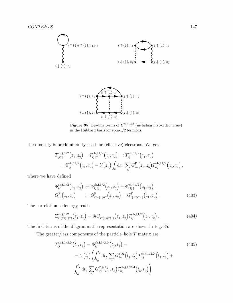
CONTENTS 147

i ↓ (↑), z1

i ↑ (↓)i ↑ (↓), z1z1+

i ↓ (↑), z1 j ↓ (↑), z2

i ↑ (↓), z1 j ↑ (↓), z2

i ↓ (↑), z1n ↓ (↑), z3

j ↓ (↑), z2

i ↑ (↓), z1n ↑ (↓), z3

j ↑ (↓), z2

Figure 35. Leading terms of Σeh,f,1/2 (including first-order terms)in the Hubbard basis for spin-1/2 fermions.

the quantity is predominantly used for (effective) electrons. We get

Teh,f,1/2ij↑↓

(z1, z2

)= T

eh,f,1/2ij↓↑

(z1, z2

)=: T eh,f,1/2

ij

(z1, z2

)= Φeh,f,1/2

ij

(z1, z2

)− U

(z1

) ∫Cdz5

∑n

GFin

(z1, z5

)T

eh,f,1/2nj

(z5, z2

),

where we have defined

Φeh,f,1/2ij

(z1, z2

):= Φeh,f,1/2

ij↑↓

(z1, z2

)= Φeh,f,1/2

ij↓↑

(z1, z2

),

GFin

(z1, z2

):= GF

i↑n↓i↓n↑

(z1, z2

)= GF

i↓n↑i↑n↓

(z1, z2

). (403)

The correlation selfenergy reads

Σeh,f,1/2i↓(↑)j↓(↑)

(z1, z2

)= i~Gi↑(↓)j↑(↓)

(z1, z2

)T

eh,f,1/2ij

(z1, z2

). (404)

The first terms of the diagrammatic representation are shown in Fig. 35.The greater/less components of the particle–hole T matrix are

Teh,f,1/2,≷ij

(t1, t2

)= Φeh,f,1/2,≷

ij

(t1, t2

)− (405)

− U(t1

)(∫ t1

t0

dt5∑n

GF,Rin

(t1, t5

)T

eh,f,1/2,≷nj

(t5, t2

)+

∫ t2

t0

dt5∑n

GF,≷in

(t1, t5

)T

eh,f,1/2,Anj

(t5, t2

)),

CONTENTS 148

and the advanced/retarded components become

Teh,f,1/2,A/Rij

(t1, t2

)= Φeh,f,1/2,A/R

ij

(t1, t2

)− (406)

− U(t1

) ∫ t2/1

t1/2

dt5∑n

GF,A/Rin

(t1, t5

)T

eh,f,1/2,A/Rnj

(t5, t2

).

The greater/less components of the correlation selfenergy read

Σeh,f,1/2,≷i↓(↑)j↓(↑)

(t1, t2

)= i~G≷

i↑(↓)j↑(↓)

(t1, t2

)T

eh,f,1/2,≷ij

(t1, t2

).

With this we conclude the discussion of the T -matrix approximation. Afterconsidering separately the standard approximations—the particle–particle and particle–hole T matrix, we briefly mention the limitations and possible extensions. The presentapproximations were based on the static pair interaction. While we took into accountmultiple scattering processes to all orders, on the other hand, dynamical-screening effects(as described by the GW approximation in Sec. 5.2), have been neglected completely. Anapproximate combination of dynamical-screening and strong-coupling effects is, therefore,considered in the next section.

5.5. Fluctuating-exchange approximation (FLEX)

The idea to combine strong-coupling and dynamical-screening effects goes back severaldecades. A discussion in the frame of Green functions is summarized in Ref. [177]. Analternative approach has been presented within density-operator theory. The solutionfor the pair-correlation operator that includes both, ladder and polarization terms leadsto the screened-ladder approximation, e.g. Ref. [131]. However, implementing theseapproximations for nonequilibrium situations is presently not computationally feasible.Therefore, it is reasonable to employ a simpler approach where contributions of bothapproximations are taken into account approximately. This idea was first realized forclassical plasmas by Gould and DeWitt [178]. They had the idea to simultaneouslyinclude strong-coupling and dynamical-screening effects in a kinetic equation by simplyadding the Boltzmann (B) and Lenard–Balescu (LB) collision integrals,

IGDW = IB + ILB − IL , (407)

where the Boltzmann collision integral includes the entire Born series and Lenard–Balescuthe entire ring-diagram sum [174, 175]. In the Green functions language the formercorresponds to the T -matrix approximation and the latter to GW . Subtraction of the

CONTENTS 149

Landau integral, IL, is necessary to avoid double counting of terms. The Landau integralcorresponds to the static second-Born approximation (collision integrals of second orderin the pair potential) which are contained (as the lowest iteration orders) in both, theT matrix and the dynamically screened potential, see Ref. [179] for a recent discussionand further references.

Extension of this idea to quantum systems directly leads to the fluctuating-exchangeapproximation (FLEX). The idea behind FLEX is to construct an approximation thatincludes both flavors of the T matrix as well as the GW approximation thereby neglectingcross-terms that mix the three different approximations. To avoid double counting,the common to all three second-order terms are subtracted twice in the correlationcontribution. Thereby, the resulting FLEX selfenergy becomes

ΣFLEX = ΣH + ΣF + ΣFLEX,corr .

ΣFLEX,corr = ΣGW,corr + Σpp + Σeh − 2Σ(2). (408)

where Eq. (408) directly corresponds to the Gould–DeWitt approach, Eq. (407).This scheme can be applied in an arbitrary basis representation. The diagrammaticrepresentation of the leading terms for a diagonal basis, and for spin-0 bosons as wellas spin-1/2 fermions in the Hubbard basis are shown in Figs. 36 and 37 and Fig. 38,respectively.

We have implemented this scheme for a fermionic Hubbard basis and found excellentperformance. Numerical results for the ground-state properties and for nonequilibriumdynamics were presented in Sec. 3 and confirm that this is a powerful and highly accurateapproximation.

6. Discussion and outlook

Summary of numerical results. In this article, an overview of recent progress inthe dynamics of correlated fermions out of equilibrium has been given. The theoreticalframework in the focus was nonequilibrium (real-time) Green functions that wereintroduced 55 years ago by Keldysh, in the Soviet Union, and Baym and Kadanoff,in the U.S. For more than two decades the method of NEGF was primarily a tool tosystematically derive Boltzmann-type quantum-kinetic equations and improvementsthereof. Only after the work of Danielewicz two decades later [180] it became a practicaloption to use the NEGF technique for numerical simulations. However, the computational

CONTENTS 150

i, z1 j, z1+i, z1

mm, z1z1+

i, z1n, z2

p, z1j, z2

i, z1 j, z2

s, z1 t, z2

i, z1n, z4

r, z2 p, z1

s, z4j, z2 i, z1

n, z4j, z2

p, z1s, z4

r, z2

i, z1n, z4

j, z2

p, z1r, z4

s, z2

i, z1 j, z2

r, z1

t, z3 v, z3

x, z2

i, z1n, z4

u, z2

r, z4 p, z1j, z2

Figure 36. Leading terms of ΣFLEX,diag in a diagonal basis.

i, z1

ii, z1z1+

i, z1 j, z2

i, z1 j, z2

i, z1n, z4

j, z2

i, z1n, z4

j, z2

i, z1n, z3

j, z2

i, z1n, z3

j, z2

Figure 37. Leading terms of ΣFLEX,b,0 in the Hubbard basisfor spin-0 bosons.

CONTENTS 151

i ↓ (↑), z1

i ↑ (↓)i ↑ (↓), z1z1+

i ↓ (↑), z1 j ↓ (↑), z2

i ↑ (↓), z1 j ↑ (↓), z2

i ↓ (↑), z1n ↓ (↑), z4

j ↓ (↑), z2

i ↑ (↓), z1n ↑ (↓), z4

j ↑ (↓), z2

i ↓ (↑), z1n ↓ (↑), z3

j ↓ (↑), z2

i ↑ (↓), z1n ↑ (↓), z3

j ↑ (↓), z2

Figure 38. Leading terms of ΣFLEX,f,1/2 in the Hubbard basis forspin-1/2 fermions.

effort that exceeds that of other many-body approaches by far, remained a major obstacle.The next step forward occured in the second half of the 1990s where important effectsin semiconductor optics and transport, in nuclear matter and laser plasmas could beexplained for the first time by using NEGF methods, for details see the text books [53,54, 131, 181]. Not only were new approximations derived but also the number of groupsthat attempted numerical solutions increased rapidly.

The next spike of activity came 10 years later when NEGF methods were firstapplied to finite spatially inhomogenous systems including electrons in atoms, moleculesor quantum dots [70, 72, 182]. NEGF simulations with second-order Born selfenergies(SOA) were able to reproduce the qualitative features of the excitation and ionizationdynamics of optically excited few-electron systems. Another new application concernedfinite Hubbard-type lattice models [76, 117, 118]. The simplicity of the basis allowed, forthe first time, to systematically study strongly correlated systems in nonequilibrim withselfenergies beyond the simple second-Born approximation. This has allowed for NEGFapplications in the fields of strongly correlated solids and cold atoms [26, 77, 145].

Still it remained unclear what level of accuracy NEGF simulations can provide andwhether they are an approach that is competitive with other many-body methods. Thisquestion was answered in a series of papers where small Hubbard clusters were treatedwith NEGF simulations that could be compared to exact-diagonalization calculations [76,151]. Recently the first systematic test of various selfenergy approximations was reportedby two of the present authors by comparing to DMRG benchmark simulations for 1D

CONTENTS 152

Hubbard systems [50]. The result was that, indeed, NEGF simulations are a highlyaccurate tool if, in each case, the proper selfenergy approximation is being used. Thechoice is dictated, primarily, by the coupling strength and the particle density (fillingfactor). With that NEGF simulations have reached the level of a predictive tool wherethe main observables can be accurately computed—with an error not exceeding theorder of 10 . . . 20%. This allows extensions of the system size, system geometry and thesimulation duration to situations that are out of the reach of alternative methods suchas CI, DMRG or real-time quantum Monte Carlo.

Thus, NEGF simulations have the potential of becoming a broadly used tool inmany fields of physics including atomic and molecular physics, condensed-matter physics,nuclear matter, warm dense matter and cold atomic and molecular gases. This requiresnot only codes that efficiently solve the Keldysh–Kadanoff–Baym equations but alsoa quick, easy and reliable use of the entire arsenal of selfenergy approximations. Thepresent article attempted to pave the way for such applications focusing on the lattertask.

To this end, we gave a short selfcontained introduction to the theory of NEGF inSec. 2 and an overview on recent numerical results for the dynamics of finite Hubbardsystems in Sec. 3. There a variety of selfenergy approximations was used that included,in addition to the commonly used Hartree–Fock and second-order Born approximation(SOA), also the third-order approximation (TOA), the particle–particle and particle–holeT matrices (TPP, TPH), the GW and the FLEX approximations, and their accuracywas investigated. The first tests concerned the interacting ground-state properties, inparticular, the ground-state energy and the spectral function of small Hubbard clusters ofvarying coupling strength and filling. The best results were obtained for the perturbativeapproaches, i.e., the second-order and especially the third-order approximations, thelatter being applied for the first time to the Hubbard model, in this article. For smalland medium fillings, the TOA ground-state energies were, by far, the most accurate, andthe TOA outperformed all previously applied approximations. For half filling, though,the TOA exactly agrees with the SOA due to particle–hole symmetry and, consequently,yields no improvement over it.

We then analyzed the spectral properties of small Hubbard clusters by computingthe single-particle spectral function via the solution of the full two-time KBE. Here,the best results were achieved with the FLEX approximation, for all filling factors.Additionally, the TOA shows single-particle energy transitions which are not contained

CONTENTS 153

in any other approximation. Thus, by taking into account the full set of approximationmethods, most of the relevant energy levels of the systems differing by one particle fromthe analyzed system can be determined.

Finally, the performance of the different selfenergies in various time-dependent setups,was investigated. We showed results for the time evolution following a confinement quenchthat was motivated by recent experiments with fermionic atoms. The NEGF resultsusing the particle–particle T -matrix selfenergy agreed very well with the experiment.The second setup used a one-dimensional charge-density-wave state as initial state. Here,by comparison with DMRG simulations the best results were obtained for third-orderselfenergies. The third setup were finite graphene-type honeycomb clusters that wereexposed to the impact of energetic ions. Here we compared, among others, second-orderBorn selfenergies and HF-GKBA simulations. The fourth type of excitation was a rapidweak change of the lattice potential. The subsequent (linear-response) dynamics allowedto compute the spectral function of the system.

Finally, we considered a strong excitation of the system where the lattice potentialof one site was changed. Here previous studies have indicated problems in the dynamicsof the NEGF, in particular, a strongly damped behavior that is absent in exact-diagonalization calculations [118]. This behavior was found to vary strongly for differentselfenergy approximations. We also compared two-time and single-time simulationswithin the HF-GKBA. The latter almost completely removed the damping.

Summary of Selfenergy approximations. In the second part of this review, adetailed overview of approximation strategies for the single-particle selfenergy withinthe framework of nonequilibrium Green functions has been presented. Here we followedtwo strategies. The first is a perturbative approach with respect to the interactionstrength that, i.a., gives rise to the Born series. After reproducing the familiar andbroadly used second-order Born approximation we derived the third-order selfenergy(TOA). This approximation contains all terms that are of third order in the interactionstrength including, in particular, the relevant ladder-type and polarization diagrams.This important new approximation was derived for all relevant system types, startingfrom a general basis representation. Additionally, for the special cases of a basis, inwhich the interaction is diagonal, as well as for the fermionic and bosonic Hubbard basiswith a scalar interaction, the corresponding selfenergy terms with Keldysh componentshave been derived.

CONTENTS 154

The second strategy was a non-perturbative approach where the selfenergies arederived using resummations of infinite partial series. Here our starting point was the set ofHedin’s equations from which we derived the GW approximation. The closely related setof integral equations for the bare interaction and vertex led us to the particle–particle andthe particle–hole T matrix. In each case we presented all details of the formulas that areneeded for an efficient numerical implementation. As before, the results were summarizedfor general basis sets, for the case of a diagonal potential and for the Hubbard basis.The presentation was concluded by a discussion of the fluctuating-exchange (FLEX)approximation that involves the combination of the terms from both T matrices andGW .

Outlook. With the set of selfenergies that were introduced in this review a powerfularsenal of approximations is available. In addition to two-time results that are obtainedfrom the full Keldysh–Kadanoff–Baym equations, also the single-time version is available.Here the basis is the Hartree–Fock-GKBA that, in many cases was found to becomplementary to the KBE. The HF-GKBA removes the artificial damping for two-timesimulations but does not yield spectral information. It has been successfully combinedwith most of the selfenergies discussed in this paper, which confirmes the attractiveproperties of this approximation. Moreover, comparisons with DMRG benchmark dataindicated that the exact result is typically enclosed between KBE and HF-GKBA. Thismeans that, if both simulations are performed independently, accurate predictions arepossible even in the absence of benchmark data.

An important further development will consist in combining the GKBA withpropagators beyond Hartree–Fock, i.e. correlated propagators [24]. This is expectedto improve the spectral content of single-time simulations and bringing the GKBAsimulations closer to the exact result.

The presently available selfenergies have been found to work well for arbitrary fillingparameters and weakly to moderately correlated Fermi systems, within the Hubbardmodel this corresponds to U/J . 8. For larger couplings the present implementationfailed to converge. Here it will be important to attempt modified implementations toextend the range of accessible coupling strengths. In addition, it is of high interest toderive higher-order selfenergy approximations, along the lines outlined in this article.For example, for half filling, the implementation of the fourth-order terms, followingthe algorithm presented in Section 4.4, could achieve significant improvements, as was

155

done successfully for homogeneous systems by Gebhard et. al. in Ref. [138]. Oneimportant obstacle to the application of the fourth-order terms, though, is the numericaldownside of a quartic scaling with the propagation time, which will probably limit theapplicability to small system sizes and short propagation times. If achievable, though, itopens the way to many new approximation strategies and resummations starting fromthe fourth-order terms similar to the (third-order-starting) T matrices. Furthermore,the equations for the screened interaction W , cf. Eq. (104), and the polarizability P , cf.Eq. (105), can be solved exactly in fourth order for a given approximation of the vertexfunction.

AppendicesA. Derivations in full notation

A.1. Second-order selfenergy contributions

A.1.1. Direct second-order selfenergyThe first second-order selfenergy term involves W (2), which structurally is given by, cf.Eq. (102),

W(2) = W ns

(P

(0),W

(1)). (409)

The structure of the zeroth-order term of the polarization is

P(0) = P

(Γ(0))

. (410)

Thus, it is given by

P(0)ijkl

(z1, z2

)= ±i~

∫Cdz3

∑m

Gim

(z1, z3

)(411)∫

Cdz4

∑n

Gnl

(z4, z1

)δC

(z3, z4+

)δC

(z2, z4

)δmkδjn

= ±i~Gik

(z1, z2

)Gjl

(z2, z1

).

Inserting this result into Eq. (409), one arrives at

W(2)ijkl

(z1, z2

)=∑mn

wimnl

(z1

)(412)∫

Cdz3

∑pq

(±i~Gnp

(z1, z3

)Gqm

(z3, z1

))δC

(z3, z2

)wpjkq

(z3

)

156

and, employing Eq. (104), finally, one has

W(2)ijkl

(z1, z2

)(413)

= ±i~∑mn

wimnl

(z1

)∑pq

Gnp

(z1, z2

)Gqm

(z2, z1

)wpjkq

(z2

).

With this, Σ(2),2,0 can be calculated as, cf. Eq. (101),

Σ(2),2,0ij

(z1, z2

)(414)

= i~∫Cdz3

∑mpq

(±i~

∑rs

wirsm

(z1

)∑tu

Gst

(z1, z3

)Gur

(z3, z1

)wtpqu

(z3

))∫Cdz4

∑n

Gmn

(z1, z4

)δC

(z4, z2+

)δC

(z3, z2

)δnpδqj .

Evaluating the terms, one arrives at

Σ(2),2,0ij

(z1, z2

)(415)

= ±(i~)2∑

mn

Gmn

(z1, z2

)∑st

Gst

(z1, z2

)∑r

wirsm

(z1

)∑u

wtnju

(z2

)Gur

(z2, z1

).

A.1.2. Exchange–correlation second-order selfenergyThe other second-order selfenergy term, Σ(2),1,1

ij , requires the first-order term of the vertexΓ, the structure of which is

Γ(1) = Γ(δΣxc,(1)

/δG,Γ(0)). (416)

This term involves the functional derivative of Σxc,(1) with respect to G. One has

δΣxc,(1)ij

(z1, z2

)δGrs

(z5, z6

) =δΣxc,(1),F

ij

(z1, z2

)δGrs

(z5, z6

) . (417)

Employing Eq. (156), one finds

δΣxc,(1)ij

(z1, z2

)δGrs

(z5, z6

) = i~δC(z1, z2

)∑mn

winjm

(z1

)δGmn

(z1, z1+

)δGrs

(z5, z6

) (418)

= i~δC(z1, z2

)δC

(z1, z5

)δC

(z1, z6

)wisjr

(z1

),

whereδGij

(z1, z2

)δGmn

(z5, z6

) = δC

(z1, z5

)δC

(z2, z6

)δimδjn (419)

157

has been applied. With this,

Γ(1)ijkl

(z1, z2, z3

)(420)

=∫Cdz4dz5

∑mn

δΣxc,(1)il

(z1, z2

)δGmn

(z4, z5

) ∫Cdz6

∑p

Gmp

(z4, z6

)∫Cdz7

∑q

Gqn

(z7, z5

)Γ(0)pjkq

(z6, z7, z3

).

Using Eq. (418), one has

Γ(1)ijkl

(z1, z2, z3

)(421)

= i~δC(z1, z2

)∑mn

winlm

(z1

) ∫Cdz6

∑p

Gmp

(z1, z6

)∫Cdz7

∑q

Gqn

(z7, z1

)Γ(0)pjkq

(z6, z7, z3

).

With Eq. (155), finally,

Γ(1)ijkl

(z1, z2, z3

)(422)

= i~δC(z1, z2

)∑mn

winlm

(z1

)Gmk

(z1, z3

)Gjn

(z3, z1

)ensues. Inserting this result yields

Σ(2),1,1ij

(z1, z2

)(423)

= i~∫Cdz3

∑mpq

W(1)ipqm

(z1, z3

) ∫Cdz4

∑n

Gmn

(z1, z4

)Γ(1)nqpj

(z4, z2, z3

).

Employing Eqs. (154) and (422), one arrives at

Σ(2),1,1ij

(z1, z2

)(424)

= i~∑mpq

wipqm

(z1

) ∫Cdz4

∑n

Gmn

(z1, z4

)Γ(1)nqpj

(z4, z2, z1

)=(i~)2 ∑

mpq

wipqm

(z1

)∑n

Gmn

(z1, z2

)∑rs

wnsjr

(z2

)Grp

(z2, z1

)Gqs

(z1, z2

).

A.2. Third-order selfenergy contributions

A.2.1. Third-order term: Σ(3),{3;0,2},0ij

Using Eq. (104), one finds

W(3),0,2ijkl

(z1, z2

)(425)

=∑mn

wimnl

(z1

) ∫Cdz3

∑pq

(±i~Gnp

(z1, z3

)Gqm

(z3, z1

))W

(2)pjkq

(z3, z2

).

158

Employing Eq. (412) yields

W(3),0,2ijkl

(z1, z2

)(426)

=∑mn

wimnl

(z1

) ∫Cdz3

∑pq

(±i~Gnp

(z1, z3

)Gqm

(z3, z1

))(±i~

∑rs

wprsq

(z3

)∑tu

Gst

(z3, z2

)Gur

(z2, z3

)wtjku

(z2

)).

Evalutating and reordering, one has

W(3),0,2ijkl

(z1, z2

)(427)

=(i~)2∑

mn

wimnl

(z1

) ∫Cdz3

∑pq

Gnp

(z1, z3

)Gqm

(z3, z1

)∑rs

wprsq

(z3

)∑tu

Gst

(z3, z2

)Gur

(z2, z3

)wtjku

(z2

).

With this, the first term of the first third-order selfenergy class, Σ(3),3,0, becomes

Σ(3),{3;0,2},0ij

(z1, z2

)(428)

= i~∫Cdz3

∑mpq

W(3),0,2ipqm

(z1, z3

) ∫Cdz4

∑n

Gmn

(z1, z4

)Γ(0)nqpj

(z4, z2, z3

).

Using Eq. (155), one has

Σ(3),{3;0,2},0ij

(z1, z2

)(429)

=(i~)3∑

mn

Gmn

(z1, z2

)∑rs

wirsm

(z1

) ∫Cdz3

∑tu

Gst

(z1, z3

)Gur

(z3, z1

)∑vw

wtvwu

(z3

)∑xy

Gwx

(z3, z2

)Gyv

(z2, z3

)wxnjy

(z2

).

A.2.2. Third-order term: Σ(3),{3;1,1},0ij

For the second class of the interaction, W (3),1,1, the first-order contribution to thepolarizability is needed, which is given by, cf. Eqs. (105) and (422),

P(1)ijkl

(z1, z2

)= Pijkl

(z1, z2

)(Γ(1)) (430)

= ±i~∫Cdz3

∑m

Gim

(z1, z3

) ∫Cdz4

∑n

Gnl

(z4, z1

)Γ(1)mjkn

(z3, z4, z2

).

159

Employing Eq. (422), one arrives at

P(1)ijkl

(z1, z2

)(431)

= ±(i~)2 ∫

Cdz3

∑m

Gim

(z1, z3

)∑n

Gnl

(z3, z1

)∑pq

wmqnp

(z3

)Gpk

(z3, z2

)Gjq

(z2, z3

).

Inserting this result back, one finds, using Eq. (104),

W(3),1,1ijkl

(z1, z2

)=∑mn

wimnl

(z1

) ∫Cdz3

∑pq

P(1)nqpm

(z1, z3

)W

(1)pjkq

(z3, z2

)

=∑mn

wimnl

(z1

) ∫Cdz3

∑pq

(±(i~)2 ∫

Cdz4

∑r

Gnr

(z1, z4

)∑s

Gsm

(z4, z1

)∑tu

wrust

(z4

)Gtp

(z4, z3

)Gqu

(z3, z4

))δC

(z3, z2

)wpjkq

(z2

). (432)

After reordering, one has

W(3),1,1ijkl

(z1, z2

)(433)

= ±(i~)2∑

mn

wimnl

(z1

) ∫Cdz3

∑r

Gnr

(z1, z3

)∑s

Gsm

(z3, z1

)∑tu

wrust

(z3

)∑pq

Gtp

(z3, z2

)Gqu

(z2, z3

)wpjkq

(z2

).

With these results, the second term of the class Σ(3),3,0 is found, using Eq. (101),

Σ(3),{3;1,1},0ij

(z1, z2

)(434)

= i~∫Cdz3

∑mpq

W(3),1,1ipqm

(z1, z3

) ∫Cdz4

∑n

Gmn

(z1, z4

)Γ(0)nqpj

(z4, z2, z3

).

Using Eq. (155), one finds

Σ(3),{3;1,1},0ij

(z1, z2

)(435)

= ±(i~)3∑

mn

Gmn

(z1, z2

)∑rs

wirsm

(z1

) ∫Cdz3

∑t

Gst

(z1, z3

)∑u

Gur

(z3, z1

)∑vw

wtwuv

(z3

)∑xy

Gvx

(z3, z2

)Gyw

(z2, z3

)wxnjy

(z2

).

A.2.3. Third-order term: Σ(3),2,1ij

Continuing with the second class Σ(3),2,1, it is directly worked out by combining Eqs. (412)

160

and (422),

Σ(3),2,1ij

(z1, z2

)= i~

∫Cdz3

∑mpq

W(2)ipqm

(z1, z3

)(436)

∫Cdz4

∑n

Gmn

(z1, z4

)Γ(1)nqpj

(z4, z2, z3

).

Inserting Eq. (422) yields

Σ(3),2,1ij

(z1, z2

)(437)

= ±(i~)3 ∫

Cdz3

∑mrs

wirsm

(z1

)∑tu

Gst

(z1, z3

)Gur

(z3, z1

)∑pq

wtpqu

(z3

)∑n

Gmn

(z1, z2

)∑vw

wnwjv

(z2

)Gvp

(z2, z3

)Gqw

(z3, z2

).

A.2.4. Third-order term: Σ(3),1,{2;1,1}ij

For the single contribution to the class Γ(2),1,1, one finds, employing Eqs. (418) and (422),

Γ(2),1,1ijkl

(z1, z2, z3

)=∫Cdz4dz5

∑mn

δΣxc,(1)il

(z1, z2

)δGmn

(z4, z5

) ∫Cdz6

∑p

Gmp

(z4, z6

)∫Cdz7

∑q

Gqn

(z7, z5

)Γ(1)pjkq

(z6, z7, z3

). (438)

Evaluating the derivative yields

Γ(2),1,1ijkl

(z1, z2, z3

)(439)

= i~δC(z1, z2

)∑mn

winlm

(z1

) ∫Cdz6

∑p

Gmp

(z1, z6

)∫Cdz7

∑q

Gqn

(z7, z1

)Γ(1)pjkq

(z6, z7, z3

).

Employing Eq. (422), one finds

Γ(2),1,1ijkl

(z1, z2, z3

)(440)

=(i~)2δC

(z1, z2

)∑mn

winlm

(z1

) ∫Cdz6

∑p

Gmp

(z1, z6

)∑q

Gqn

(z6, z1

)∑rs

wpsqr

(z6

)Grk

(z6, z3

)Gjs

(z3, z6

).

161

This enables the computation of Σ(3),1,{2;1,1} with Eqs. (101) and (154),

Σ(3),1,{2;1,1}ij

(z1, z2

)(441)

= i~∫Cdz3

∑mpq

W(1)ipqm

(z1, z3

) ∫Cdz4

∑n

Gmn

(z1, z4

)Γ(2),1,1nqpj

(z4, z2, z3

)= i~

∑mpq

wipqm

(z1

) ∫Cdz4

∑n

Gmn

(z1, z4

)Γ(2),1,1nqpj

(z4, z2, z1

).

Using Eq. (440), one arrives at

Σ(3),1,{2;1,1}ij

(z1, z2

)(442)

=(i~)3 ∑

mpq

wipqm

(z1

)∑n

Gmn

(z1, z2

)∑rs

wnsjr

(z2

) ∫Cdz3

∑t

Grt

(z2, z3

)∑u

Gus

(z3, z2

)∑vw

wtwuv

(z3

)Gvp

(z3, z1

)Gqw

(z1, z3

).

A.2.5. Second-order vertex termsFor the first terms, one finds

Γ(2),{2;2,0},0ijkl

(z1, z2, z3

)=∫Cdz4dz5

∑mn

δΣ(2),2,0il

(z1, z2

)δGmn

(z4, z5

) ∫Cdz6

∑p

Gmp

(z4, z6

)∫Cdz7

∑q

Gqn

(z7, z5

)Γ(0)pjkq

(z6, z7, z3

)(443)

=∫Cdz4dz5

∑mn

δΣ(2),2,0il

(z1, z2

)δGmn

(z4, z5

) Gmk

(z4, z3

)Gjn

(z3, z5

).

Inserting Eq. (415), the term attains the form

Γ(2),{2;2,0},0ijkl

(z1, z2, z3

)= ±

(i~)2 ∫

Cdz4dz5 (444)

∑mn

δ

(∑pqGpq

(z1, z2

)∑stGst

(z1, z2

)∑rwirsp

(z1

)∑uwtqlu

(z2

)Gur

(z2, z1

))δGmn

(z4, z5

)Gmk

(z4, z3

)Gjn

(z3, z5

).

Evaluating the derivative, one has

Γ(2),{2;2,0},0ijkl

(z1, z2, z3

)= Γ(2),{2;2,0},0,A

ijkl

(z1, z2, z3

)(445)

+ Γ(2),{2;2,0},0,Bijkl

(z1, z2, z3

)+ Γ(2),{2;2,0},0,C

ijkl

(z1, z2, z3

),

162

with

Γ(2),{2;2,0},0,Aijkl

(z1, z2, z3

)(446)

= ±(i~)2∑

mn

∑st

Gst

(z1, z2

)∑r

wirsm

(z1

)∑u

wtnlu

(z2

)Gur

(z2, z1

)Gmk

(z1, z3

)Gjn

(z3, z2

)and

Γ(2),{2;2,0},0,Bijkl

(z1, z2, z3

)(447)

±(i~)2∑

mn

∑pq

Gpq

(z1, z2

)∑r

wirmp

(z1

)∑u

wnqlu

(z2

)Gur

(z2, z1

)Gmk

(z1, z3

)Gjn

(z3, z2

)as well as

Γ(2),{2;2,0},0,Cijkl

(z1, z2, z3

)(448)

±(i~)2∑

mn

∑pq

Gpq

(z1, z2

)∑st

Gst

(z1, z2

)winsp

(z1

)wtqlm

(z2

)Gmk

(z2, z3

)Gjn

(z3, z1

).

Similarly, one finds

Γ(2),{2;1,1},0ijkl

(z1, z2, z3

)=∫Cdz4dz5

∑mn

δΣ(2),1,1il

(z1, z2

)δGmn

(z4, z5

) ∫Cdz6

∑p

Gmp

(z4, z6

)∫Cdz7

∑q

Gqn

(z7, z5

)Γ(0)pjkq

(z6, z7, z3

). (449)

Inserting Eq. (424) yields

Γ(2),{2;1,1},0ijkl

(z1, z2, z3

)=(i~)2 ∫

Cdz4dz5 (450)

∑mn

δ

(∑prswirsp

(z1

)∑qGpq

(z1, z2

)∑tuwqult

(z2

)Gtr

(z2, z1

)Gsu

(z1, z2

))δGmn

(z4, z5

)Gmk

(z4, z3

)Gjn

(z3, z5

),

which, after evaluation of the derivative, yields

Γ(2),{2;1,1},0ijkl

(z1, z2, z3

)= Γ(2),{2;1,1},0,A

ijkl

(z1, z2, z3

)(451)

+ Γ(2),{2;1,1},0,Bijkl

(z1, z2, z3

)+ Γ(2),{2;1,1},0,C

ijkl

(z1, z2, z3

),

163

with

Γ(2),{2;1,1},0,Aijkl

(z1, z2, z3

)(452)

=(i~)2∑

mn

∑rs

wirsm

(z1

)∑tu

wnult

(z2

)Gtr

(z2, z1

)Gsu

(z1, z2

)Gmk

(z1, z3

)Gjn

(z3, z2

)and

Γ(2),{2;1,1},0,Bijkl

(z1, z2, z3

)(453)

+(i~)2∑

mn

∑ps

winsp

(z1

)∑q

Gpq

(z1, z2

)∑u

wqulm

(z2

)Gsu

(z1, z2

)Gmk

(z2, z3

)Gjn

(z3, z1

)as well as

Γ(2),{2;1,1},0,Cijkl

(z1, z2, z3

)(454)

+(i~)2∑

mn

∑pr

wirmp

(z1

)∑q

Gpq

(z1, z2

)∑t

wqnlt

(z2

)Gtr

(z2, z1

)Gmk

(z1, z3

)Gjn

(z3, z2

).

A.2.6. Third-order terms: Σ(3),1,2ij

With this result, the corresponding selfenergy terms can be computed,

Σ(3),1,{2;{2;2,0},0,A}ij

(z1, z2

)(455)

= i~∫Cdz3

∑mpq

W(1)ipqm

(z1, z3

) ∫Cdz4

∑n

Gmn

(z1, z4

)Γ(2),{2;2,0},0,Anqpj

(z4, z2, z3

)= i~

∑mpq

wipqm

(z1

) ∫Cdz4

∑n

Gmn

(z1, z4

)Γ(2),{2;2,0},0,Anqpj

(z4, z2, z1

).

Inserting Eq. (446), one arrives at

Σ(3),1,{2;{2;2,0},0,A}ij

(z1, z2

)= ±

(i~)3 ∑

mpq

wipqm

(z1

)(456)

∫Cdz4

∑n

Gmn

(z1, z4

) ∑rsuv

Guv

(z4, z2

)∑t

wntur

(z4

)∑w

wvsjw

(z2

)Gwt

(z2, z4

)Grp

(z4, z1

)Gqs

(z1, z2

).

For the second term, one has

Σ(3),1,{2;{2;2,0},0,B}ij

(z1, z2

)(457)

= i~∑mpq

wipqm

(z1

) ∫Cdz4

∑n

Gmn

(z1, z4

)Γ(2),{2;2,0},0,Bnqpj

(z4, z2, z1

).

164

Using Eq. (447) yields

Σ(3),1,{2;{2;2,0},0,B}ij

(z1, z2

)(458)

= ±(i~)3 ∑

mpq

wipqm

(z1

) ∫Cdz4

∑n

Gmn

(z1, z4

)∑rs

∑tu

Gtu

(z4, z2

)∑v

wnvrt

(z4

)∑w

wsujw

(z2

)Gwv

(z2, z4

)Grp

(z4, z1

)Gqs

(z1, z2

).

The third term is given by

Σ(3),1,{2;{2;2,0},0,C}ij

(z1, z2

)(459)

= i~∑mpq

wipqm

(z1

) ∫Cdz4

∑n

Gmn

(z1, z4

)Γ(2),{2;2,0},0,Cnqpj

(z4, z2, z1

).

With Eq. (448), one finds

Σ(3),1,{2;{2;2,0},0,C}ij

(z1, z2

)(460)

= ±(i~)3 ∑

mpq

wipqm

(z1

) ∫Cdz4

∑n

Gmn

(z1, z4

)∑rs

∑tu

Gtu

(z4, z2

)∑vw

Gvw

(z4, z2

)wnsvt

(z4

)wwujr

(z2

)Grp

(z2, z1

)Gqs

(z1, z4

).

For the other class, one has

Σ(3),1,{2;{2;1,1},0,A}ij

(z1, z2

)(461)

= i~∫Cdz3

∑mpq

W(1)ipqm

(z1, z3

) ∫Cdz4

∑n

Gmn

(z1, z4

)Γ(2),{2;1,1},0,Anqpj

(z4, z2, z3

)= i~

∑mpq

wipqm

(z1

) ∫Cdz4

∑n

Gmn

(z1, z4

)Γ(2),1,1,Anqpj

(z4, z2, z1

).

Inserting Eq. (452) yields

Σ(3),1,{2;{2;1,1},0,A}ij

(z1, z2

)(462)

=(i~)3 ∑

mpq

wipqm

(z1

) ∫Cdz4

∑n

Gmn

(z1, z4

)∑rs

∑tu

wntur

(z4

)∑vw

wswjv

(z2

)Gvt

(z2, z4

)Guw

(z4, z2

)Grp

(z4, z1

)Gqs

(z1, z2

).

Similarly, the second term reads

Σ(3),1,{2;{2;1,1},0,B}ij

(z1, z2

)(463)

= i~∑mpq

wipqm

(z1

) ∫Cdz4

∑n

Gmn

(z1, z4

)Γ(2),{2;1,1},0,Bnqpj

(z4, z2, z1

).

165

With Eq. (453), one has

Σ(3),1,{2;{2;1,1},0,B}ij

(z1, z2

)(464)

=(i~)3 ∑

mpq

wipqm

(z1

) ∫Cdz4

∑n

Gmn

(z1, z4

)∑rs

∑tv

wnsvt

(z4

)∑u

Gtu

(z4, z2

)∑w

wuwjr

(z2

)Gvw

(z4, z2

)Grp

(z2, z1

)Gqs

(z1, z4

).

For the third term, one finds

Σ(3),1,{2;{2;1,1},0,C}ij

(z1, z2

)(465)

= i~∑mpq

wipqm

(z1

) ∫Cdz4

∑n

Gmn

(z1, z4

)Γ(2),{2;1,1},0,Cnqpj

(z4, z2, z1

).

Employing Eq. (454), one arrives at

Σ(3),1,{2;{2;1,1},0,C}ij

(z1, z2

)(466)

=(i~)3 ∑

mpq

wipqm

(z1

) ∫Cdz4

∑n

Gmn

(z1, z4

)∑rs

∑tv

wnvrt

(z4

)∑u

Gtu

(z4, z2

)∑w

wusjw

(z2

)Gwv

(z2, z4

)Grp

(z4, z1

)Gqs

(z1, z2

).

A.3. Resummation approaches: GW approximation

The GW approximation solves Hedin’s equation for the screened interactionW accordingto Eq. (104) with the zeroth-order vertex Γ(0). The set of equations is given by theDyson equation, cf. Eq. (91),

Gij

(z1, z2

)= G

(0)ij

(z1, z2

)(467)

+∫Cdz3dz4

∑mn

G(0)im

(z1, z3

)Σmn

(z3, z4

)Gnj

(z4, z2

),

the equation for the selfenergy [cf. Eq. (95)]

Σij

(z1, z2

)= ΣH

ij

(z1, z2

)+ Σxc

ij

(z1, z2

), (468)

with

Σxcij

(z1, z2

)= i~

∫Cdz3

∑mpq

Wipqm

(z1, z3

)(469)

∫Cdz4

∑n

Gmn

(z1, z4

)Γ(0)nqpj

(z4, z2, z3

)= i~

∑mp

Wipjm

(z1, z2

)Gmp

(z1, z2

),

166

the zeroth-order polarizability, cf. Eq. (411),

Pijkl

(z1, z2

)= P

(0)ijkl

(z1, z2

)= ±i~Gik

(z1, z2

)Gjl

(z2, z1

), (470)

the zeroth-order vertex, cf. Eq. (155),

Γijkl(z1, z2, z3

)= Γ(0)

ijkl

(z1, z2, z3

)= δC

(z1, z2+

)δC

(z3, z2

)δikδjl (471)

and the screened interaction [cf. Eqs. (102) and (104)]

Wijkl

(z1, z2

)= δC

(z1, z2

)wijkl

(z1

)+W ns

ijkl

(z1, z2

), (472)

with

W nsijkl

(z1, z2

)(473)

=∑mn

wimnl

(z1

) ∫Cdz3

∑pq

P(0)nqpm

(z1, z3

)Wpjkq

(z3, z2

)= ±i~

∑mn

wimnl

(z1

) ∫Cdz3

∑pq

Gnp

(z1, z3

)Gqm

(z3, z1

)Wpjkq

(z3, z2

).

To solve this set of equations, one has to determine the selfconsistent solution of Eq. (472).Thereto, it is more suitable to eliminate the singular bare interaction by using

W nsijkl

(z1, z2

)= Wijkl

(z1, z2

)−W bare

ijkl

(z1, z2

)(474)

= Wijkl

(z1, z2

)− δC

(z1, z2

)wijkl

(z1

).

The selfenergy [cf. Eqs. (468) and (469)] in terms of W ns is then given by

ΣGWij

(z1, z2

)= ΣH

ij

(z1, z2

)+ i~

∑mp

Wipjm

(z1, z2

)Gmp

(z1, z2

)= ΣH

ij

(z1, z2

)+ i~

∑mp

wipjm

(z1

)Gmp

(z1, z1+

)δC

(z1, z2

)+ i~

∑mp

W nsipjm

(z1, z2

)Gmp

(z1, z2

). (475)

Using Eq. (156), the expression simplifies to

ΣGWij

(z1, z2

)(476)

= ΣHij

(z1, z2

)+ ΣF

ij

(z1, z2

)+ i~

∑mp

W nsipjm

(z1, z2

)Gmp

(z1, z2

)=: ΣH

ij

(z1, z2

)+ ΣF

ij

(z1, z2

)+ ΣGW,corr

ij

(z1, z2

).

167

For the screened interaction, one has

W nsijkl

(z1, z2

)(477)

= ±i~∑mn

wimnl

(z1

)∑pq

Gnp

(z1, z2

)Gqm

(z2, z1

)wpjkq

(z2

)± i~

∑mn

wimnl

(z1

) ∫Cdz3

∑pq

Gnp

(z1, z3

)Gqm

(z3, z1

)W nspjkq

(z3, z2

).

A.4. Resummation approaches: T matrix

In contrast to the GW approximation, the T matrix is an approximation, which takesonly the bare interaction w into account and aims instead at a good approximation ofthe bare vertex function Λ. Thus, its constitutive equations are the Dyson equation,

Gij

(z1, z2

)= (478)

G(0)ij

(z1, z2

)+∫Cdz3dz4

∑mn

G(0)im

(z1, z3

)Σmn

(z3, z4

)Gnj

(z4, z2

),

the equation for the selfenergy, cf. Eqs. (95) and (97),

Σij

(z1, z2

)= ΣH

ij

(z1, z2

)+ Σxc

ij

(z1, z2

), (479)

with

Σxcij

(z1, z2

)(480)

= i~∑mpq

wipqm

(z1

) ∫Cdz3

∑n

Gmn

(z1, z3

)Λnqpj

(z3, z2, z1

).

The bare vertex Λ is self-consistently given as the solution of

Λijkl

(z1, z2, z3

)= δC

(z1, z2+

)δC

(z3, z2

)δikδjl (481)

+∫Cdz4dz5

∑mn

δΣil

(z1, z2

)δGmn

(z4, z5

) ∫Cdz6

∑p

Gmp

(z4, z6

)∫Cdz7

∑q

Gqn

(z7, z5

)Λpjkq

(z6, z7, z3

).

If these equations are iterated ad infinitum, all selfenergy terms will begenerated. To break the circular dependence between Eqs. (480) and (481), the T -matrix approximation starts by taking the bare vertex on the right-hand side of Eq. (481)only in zeroth order,

Λ(0)ijkl

(z1, z2, z3

)= δC

(z1, z2+

)δC

(z3, z2

)δikδjl , (482)

168

transforming it into

Λclijkl

(z1, z2, z3

)= δC

(z1, z2+

)δC

(z3, z2

)δikδjl (483)

+∫Cdz4dz5

∑mn

δΣclil

(z1, z2

)δGmn

(z4, z5

)Gmk

(z4, z3

)Gjn

(z3, z5

).

To arrive at a closed equation, this result is used in Eq. (479), yielding

Σclij

(z1, z2

)= ΣH

ij

(z1, z2

)+ Σxc

ij

(z1, z2

)(484)

= ΣHij

(z1, z2

)+ i~

∑mpq

wipqm

(z1

) ∫Cdz3

∑n

Gmn

(z1, z3

)Λclnqpj

(z3, z2, z1

).

Inserting Eq. (483), one has

Σclij

(z1, z2

)= ±i~δC

(z1, z2

)∑mn

wmijn

(z1

)Gnm

(z1, z1+

)(485)

+ i~∑mn

winjm

(z1

)Gmn

(z1, z1+

)δC

(z1, z2

)+ i~

∑mpq

wipqm

(z1

) ∫Cdz3

∑n

Gmn

(z1, z3

)∫Cdz4dz5

∑rs

δΣclnj

(z3, z2

)δGrs

(z4, z5

)Grp

(z4, z1

)Gqs

(z1, z5

).

This term can be restructured to yield

Σclij

(z1, z2

)(486)

= i~δC(z1, z2

)∑mn

Gmn

(z1, z1+

)w±injm

(z1

)+ i~

∑mpq

wipqm

(z1

) ∫Cdz3

∑n

Gmn

(z1, z3

)∫Cdz4dz5

∑rs

δΣclnj

(z3, z2

)δGrs

(z4, z5

)Grp

(z4, z1

)Gqs

(z1, z5

),

with the (anti-)symmetrized potential w±ijkl(z1

):= wijkl

(z1

)±wjikl

(z1

). Using Eq. (156)

again, one finds

Σclij

(z1, z2

)(487)

= ΣHij

(z1, z2

)+ ΣF

ij

(z1, z2

)+ i~

∑mpq

wipqm

(z1

) ∫Cdz3

∑n

Gmn

(z1, z3

)∫Cdz4dz5

∑rs

δΣclnj

(z3, z2

)δGrs

(z4, z5

)Grp

(z4, z1

)Gqs

(z1, z5

).

169

Taking the derivative with respect to G, one arrives at

δΣclij

(z1, z2

)δGtu

(z6, z7

) = i~δC(z1, z2

)δC

(z1, z6

)δC

(z1+ , z7

)w±iujt

(z1

)δΣcl,A

ij

(z1, z2

)δGtu

(z6, z7

) +δΣcl,B

ij

(z1, z2

)δGtu

(z6, z7

)+δΣcl,C

ij

(z1, z2

)δGtu

(z6, z7

) +δΣcl,D

ij

(z1, z2

)δGtu

(z6, z7

) , (488)

withδΣcl,A

ij

(z1, z2

)δGtu

(z6, z7

) (489)

= i~δC(z1, z6

)∑pq

wipqt

(z1

)∫Cdz4dz5

∑rs

δΣcluj

(z7, z2

)δGrs

(z4, z5

)Grp

(z4, z1

)Gqs

(z1, z5

),

δΣcl,Bij

(z1, z2

)δGtu

(z6, z7

) (490)

= i~δC(z1, z7

)∑mq

wiuqm

(z1

) ∫Cdz3

∑n

Gmn

(z1, z3

)∫Cdz5

∑s

δΣclnj

(z3, z2

)δGts

(z6, z5

)Gqs

(z1, z5

)and

δΣcl,Cij

(z1, z2

)δGtu

(z6, z7

) (491)

= i~δC(z1, z6

)∑mp

wiptm

(z1

) ∫Cdz3

∑n

Gmn

(z1, z3

)∫Cdz4

∑r

δΣclnj

(z3, z2

)δGru

(z4, z7

)Grp

(z4, z1

),

170

as well asδΣcl,D

ij

(z1, z2

)δGtu

(z6, z7

) (492)

= i~∑mpq

wipqm

(z1

) ∫Cdz3

∑n

Gmn

(z1, z3

)∫Cdz4dz5

∑rs

δΣclnj

(z3, z2

)δGrs

(z4, z5

)δGtu

(z6, z7

)Grp

(z4, z1

)Gqs

(z1, z5

).

NeglectingδΣcl

nj(z3,z2)δG

rs(z4,z5)δGtu(z6,z7)as an approximation, Eq. (488) becomes a closed equation

for δΣcl

δG. The first iteration yields the second-order terms

δΣcl,(2)ij

(z1, z2

)δGtu

(z6, z7

) ≈ δΣcl,(2),Aij

(z1, z2

)δGtu

(z6, z7

) (493)

+δΣcl,(2),B

ij

(z1, z2

)δGtu

(z6, z7

) +δΣcl,(2),C

ij

(z1, z2

)δGtu

(z6, z7

) ,

withδΣcl,(2),A

ij

(z1, z2

)δGtu

(z6, z7

) (494)

=(i~)2δC

(z1, z6

)δC

(z2, z7

)∑pq

wipqt

(z1

)∑rs

w±usjr

(z2

)Grp

(z2, z1

)Gqs

(z1, z2

)and

δΣcl,(2),Bij

(z1, z2

)δGtu

(z6, z7

) (495)

=(i~)2δC

(z1, z7

)δC

(z2, z6

)∑mq

wiuqm

(z1

)∑n

Gmn

(z1, z2

)∑s

w±nsjt

(z2

)Gqs

(z1, z2

)as well as

δΣcl,(2),Cij

(z1, z2

)δGtu

(z6, z7

) (496)

=(i~)2δC

(z1, z6

)δC

(z2, z7

)∑mp

wiptm

(z1

)∑n

Gmn

(z1, z2

)∑r

w±nujr

(z2

)Grp

(z2, z1

).

171

Note that, for the first iteration,δΣcl,D

ij (z1,z2)δG

tu(z6,z7)is exactly equal to zero, thus Eq. (493) is

also exact up to second order in w. In the following, each of the three terms will beconsidered separately. To start with, one recognizes that all three terms yield the samefirst and second-order contributions to the selfenergy, which read

Σcl,(1)ij

(z1, z2

)= ΣH

ij

(z1, z2

)+ ΣF

ij

(z1, z2

)(497)

Σcl,(2)ij

(z1, z2

)=(i~)2 ∑

mpq

wipqm

(z1

)∑n

Gmn

(z1, z2

)(498)

∑rs

w±nsjr

(z2

)Grp

(z2, z1

)Gqs

(z1, z2

)and agree with the exact first and second-order terms, already encountered in Eqs. (158),(415) and (424). The third-order contributions to Σcl from the second-order terms inEq. (493) are given by

Σcl,(3),Aij

(z1, z2

)= i~

∑mpq

wipqm

(z1

) ∫Cdz3

∑n

Gmn

(z1, z3

)(499)

∫Cdz4dz5

∑rs

δΣcl,(2),Anj

(z3, z2

)δGrs

(z4, z5

) Grp

(z4, z1

)Gqs

(z1, z5

).

Inserting the second-order term yields

Σcl,(3),Aij

(z1, z2

)=(i~)3 ∑

mpq

wipqm

(z1

) ∫Cdz3

∑n

Gmn

(z1, z3

)(500)

∑rs

∑tu

wntur

(z3

)∑vw

w±swjv

(z2

)Gvt

(z2, z3

)Guw

(z3, z2

)Grp

(z3, z1

)Gqs

(z1, z2

).

For the second third-order selfenergy term, one has

Σcl,(3),Bij

(z1, z2

)= i~

∑mpq

wipqm

(z1

) ∫Cdz3

∑n

Gmn

(z1, z3

)(501)

∫Cdz4dz5

∑rs

δΣcl,(2),Bnj

(z3, z2

)δGrs

(z4, z5

) Grp

(z4, z1

)Gqs

(z1, z5

).

which evaluates to

Σcl,(3),Bij

(z1, z2

)=(i~)3 ∑

mpq

wipqm

(z1

) ∫Cdz3

∑n

Gmn

(z1, z3

)(502)

∑rs

∑tu

wnsut

(z3

)∑v

Gtv

(z3, z2

)∑w

w±vwjr

(z2

)Guw

(z3, z2

)Grp

(z2, z1

)Gqs

(z1, z3

).

172

The third term reads

Σcl,(3),Cij

(z1, z2

)= i~

∑mpq

wipqm

(z1

) ∫Cdz3

∑n

Gmn

(z1, z3

)(503)

∫Cdz4dz5

∑rs

δΣcl,(2),Cnj

(z3, z2

)δGrs

(z4, z5

) Grp

(z4, z1

)Gqs

(z1, z5

).

(504)

Using the second-order result, one arrives at

Σcl,(3),Cij

(z1, z2

)= i~

∑mpq

wipqm

(z1

) ∫Cdz3

∑n

Gmn

(z1, z3

)(505)

∑rs

∑tu

wnurt

(z3

)∑v

Gtv

(z3, z2

)∑w

w±vsjw

(z2

)Gwu

(z2, z3

)Grp

(z3, z1

)Gqs

(z1, z2

).

B. Non-selfconsistent second-order selfenergy contributions

B.1. General basis

The first two classes are just the same as in the selfconsistent approximation, cf. Eqs. (176)and (183), with the replacement G → G

(0). Likewise, their components follow directlyfrom Eqs. (184) and (185). For the third and fourth class, one needs the contributionsto G(1), which are

G(1),{H,0},0ij

(z1, z2

)(506)

=∫Cdz3dz4

∑mn

G(0)im

(z1, z3

)ΣH,0mn

(z3, z4

)G

(0)nj

(z4, z2

)= ±i~

∫Cdz3

∑mn

G(0)im

(z1, z3

)∑pq

wpmnq

(z3

)G

(0)qp

(z3, z3+

)G

(0)nj

(z3, z2

)and

G(1),{F,0},0ij

(z1, z2

)(507)

=∫Cdz3dz4

∑mn

G(0)im

(z1, z3

)ΣF,0mn

(z3, z4

)G

(0)nj

(z4, z2

)= i~

∫Cdz3

∑mn

G(0)im

(z1, z3

)∑pq

wmqnp

(z3

)G

(0)pq

(z3, z3+

)G

(0)nj

(z3, z2

).

173

With these results, the additional non-selfconsistent contributions are

Σ(2),{H,0},{1,{H,0},0}ij

(z1, z2

)= ±i~δC

(z1, z2

)∑mn

wmijn

(z1

)G

(1),{H,0},0nm

(z1, z1+

)=(i~)2δC

(z1, z2

)∑mn

wmijn

(z1

)(508)∫

Cdz3

∑pq

G(0)np

(z1, z3

)∑rs

wrpqs

(z3

)G

(0)sr

(z3, z3+

)G

(0)qm

(z3, z1+

),

as well as

Σ(2),{H,0},{1,{F,0},0}ij

(z1, z2

)= ±i~δC

(z1, z2

)∑mn

wmijn

(z1

)G

(1),{F,0},0nm

(z1, z1+

)= ±

(i~)2δC

(z1, z2

)∑mn

wmijn

(z1

)(509)∫

Cdz3

∑pq

G(0)np

(z1, z3

)∑rs

wpsqr

(z3

)G

(0)rs

(z3, z3+

)G

(0)qm

(z3, z1+

)and

Σ(2),{F,0},{1,{H,0},0}ij

(z1, z2

)= i~δC

(z1, z2

)∑mn

winjm

(z1

)G

(1),{H,0},0mn

(z1, z1+

)= ±

(i~)2δC

(z1, z2

)∑mn

wnimj

(z1

)(510)∫

Cdz3

∑pq

G(0)mp

(z1, z3

)∑rs

wrpqs

(z3

)G

(0)sr

(z3, z3+

)G

(0)qn

(z3, z1+

),

as well as

Σ(2),{F,0},{1,{F,0},0}ij

(z1, z2

)= i~δC

(z1, z2

)∑mn

winjm

(z1

)G

(1),{F,0},0mn

(z1, z1+

)=(i~)2δC

(z1, z2

)∑mn

wnimj

(z1

)(511)∫

Cdz3

∑pq

G(0)mp

(z1, z3

)∑rs

wpsqr

(z3

)G

(0)rs

(z3, z3+

)G

(0)qn

(z3, z1+

).

The corresponding components are all time-diagonal and read

Σ(2),{H,0},{1,{H,0},0},δij

(t1

)(512)

=(i~)2∑

mn

wmijn

(t1

)(∫ t1

t0

dt3∑pq

G(0),>np

(t1, t3

)∑rs

wrpqs

(t3

)G

(0),<sr

(t3, t3

)G

(0),<qm

(t3, t1

)

+∫ t0

t1

dt3∑pq

G(0),<np

(t1, t3

)∑rs

wrpqs

(t3

)G

(0),<sr

(t3, t3

)G

(0),>qm

(t3, t1

))

174

and

Σ(2),{H,0},{1,{F,0},0},δij

(t1

)(513)

= ±(i~)2∑

mn

wmijn

(t1

)(∫ t1

t0

dt3∑pq

G(0),>np

(t1, t3

)∑rs

wpsqr

(t3

)G

(0),<rs

(t3, t3

)G

(0),<qm

(t3, t1

)

+∫ t0

t1

dt3∑pq

G(0),<np

(t1, t3

)∑rs

wpsqr

(t3

)G

(0),<rs

(t3, t3

)G

(0),>qm

(t3, t1

)),

as well as

Σ(2),{F,0},{1,{H,0},0},δij

(t1

)(514)

= ±(i~)2∑

mn

wnimj

(t1

)(∫ t1

t0

dt3∑pq

G(0),>mp

(t1, t3

)∑rs

wrpqs

(t3

)G

(0),<sr

(t3, t3

)G

(0),<qn

(t3, t1

)

+∫ t0

t1

dt3∑pq

G(0),<mp

(t1, t3

)∑rs

wrpqs

(t3

)G

(0),<sr

(t3, t3

)G

(0),>qn

(t3, t1

))

and

Σ(2),{F,0},{1,{F,0},0},δij

(t1

)(515)

=(i~)2∑

mn

wnimj

(t1

)(∫ t1

t0

dt3∑pq

G(0),>mp

(t1, t3

)∑rs

wpsqr

(t3

)G

(0),<rs

(t3, t3

)G

(0),<qn

(t3, t1

)

+∫ t0

t1

dt3∑pq

G(0),<mp

(t1, t3

)∑rs

wpsqr

(t3

)G

(0),<rs

(t3, t3

)G

(0),>qn

(t3, t1

)).

B.2. Diagonal basis

For wijkl = δilδjkwij , the non-selfconsistent selfenergy terms attain the form, cf. Eqs. (189)and (191),

Σ(2),(2),2,0,0,diagonalij

(z1, z2

)(516)

≡ Σ(2),2,0,diagonalij

(z1, z2

)(G → G

(0))and

Σ(2),(2),1,0,1,diagonalij

(z1, z2

)(517)

≡ Σ(2),1,1,diagonalij

(z1, z2

)(G → G

(0)),

175

as well as

Σ(2),{H,0},{1,{H,0},0},diagonalij

(z1, z2

)(518)

=(i~)2δC

(z1, z2

)δij∑m

wmi

(z1

)∫Cdz3

∑p

G(0)mp

(z1, z3

)G

(0)pm

(z3, z1+

)∑r

wrp

(z3

)G

(0)rr

(z3, z3+

)and

Σ(2),{H,0},{1,{F,0},0},diagonalij

(z1, z2

)(519)

= ±(i~)2δC

(z1, z2

)δij∑m

wmi

(z1

)∫Cdz3

∑p

G(0)mp

(z1, z3

)∑q

wpq

(z3

)G

(0)pq

(z3, z3+

)G

(0)qm

(z3, z1+

).

Further,

Σ(2),{F,0},{1,{H,0},0},diagonalij

(z1, z2

)(520)

= ±(i~)2δC

(z1, z2

)wij

(z1

)∫Cdz3

∑p

G(0)ip

(z1, z3

)∑r

wrp

(z3

)G

(0)rr

(z3, z3+

)G

(0)pj

(z3, z1+

)and

Σ(2),{F,0},{1,{F,0},0},diagonalij

(z1, z2

)(521)

=(i~)2δC

(z1, z2

)wij

(z1

)∫Cdz3

∑p

G(0)ip

(z1, z3

)∑q

wpq

(z3

)G

(0)pq

(z3, z3+

)G

(0)qj

(z3, z1+

).

The components read [cf. Eqs. (191) and (192)]

Σ(2),(2),2,0,0,diagonal,≷ij

(t1, t2

)≡ Σ(2),2,0,diagonal,≷

ij

(t1, t2

)(G → G

(0)), (522)

Σ(2),(2),1,0,1,diagonal,≷ij

(t1, t2

)≡ Σ(2),1,1,diagonal,≷

ij

(t1, t2

)(G → G

(0)), (523)

as well as [cf. Eq. (512) to Eq. (516)]

Σ(2),{H,0},{1,{H,0},0},diagonal,δij

(t1

)(524)

=(i~)2δij∑m

wmi

(t1

)(∫ t1

t0

dt3∑p

G(0),>mp

(t1, t3

)∑r

wrp

(t3

)G

(0),<rr

(t3, t3

)G

(0),<pm

(t3, t1

)

+∫ t0

t1

dt3∑p

G(0),<mp

(t1, t3

)∑r

wrp

(t3

)G

(0),<rr

(t3, t3

)G

(0),>pm

(t3, t1

))

176

and

Σ(2),{H,0},{1,{F,0},0},δij

(t1

)(525)

= ±(i~)2δij∑m

wmi

(t1

)(∫ t1

t0

dt3G(0),>mr

(t1, t3

)∑rs

wrs

(t3

)G

(0),<rs

(t3, t3

)G

(0),<sm

(t3, t1

)

+∫ t0

t1

dt3G(0),<mr

(t1, t3

)∑rs

wrs

(t3

)G

(0),<rs

(t3, t3

)G

(0),>sm

(t3, t1

)).

Further,

Σ(2),{F,0},{1,{H,0},0},diagonal,δij

(t1, t2

)(526)

= ±(i~)2wji

(t1

)(∫ t1

t0

dt3∑p

G(0),>ip

(t1, t3

)∑rs

wrp

(t3

)G

(0),<rr

(t3, t3

)G

(0),<pj

(t3, t1

)

+∫ t0

t1

dt3∑p

G(0),<ip

(t1, t3

)∑rs

wrp

(t3

)G

(0),<rr

(t3, t3

)G

(0),>pj

(t3, t1

))

and

Σ(2),{F,0},{1,{F,0},0},δij

(t1

)(527)

=(i~)2∑

n

wji

(t1

)(∫ t1

t0

dt3G(0),<ir

(t1, t3

)∑rs

wrs

(t3

)G

(0),<rs

(t3, t3

)G

(0),>sj

(t3, t1

)

+∫ t0

t1

dt3G(0),>ir

(t1, t3

)∑rs

wrs

(t3

)G

(0),<rs

(t3, t3

)G

(0),<sj

(t3, t1

)).

B.3. Hubbard basis

In the Hubbard basis, the non-selfconsistent contributions attain the form

Σ(2),(2),2,0,0,Hubbard,biαjα

(z1, z2

)(528)

≡ Σ(2),2,0,Hubbard,biαjα

(z1, z2

)(G → G

(0))and

Σ(2),(2),1,0,1,Hubbard,biαjα

(z1, z2

)(529)

≡ Σ(2),1,1,Hubbard,biαjα

(z1, z2

)(G → G

(0)),

177

as well as

Σ(2),{H,0},{1,{H,0},0},Hubbard,biαjα

(z1, z2

)(530)

=(i~)2δC

(z1, z2

)δij∑ε

U(z1

)∫Cdz3

∑p

G(0)iεpε

(z1, z3

)G

(0)pεiε

(z3, z1+

)∑ζ

U(z3

)G

(0)pζpζ

(z3, z3+

)and

Σ(2),{H,0},{1,{F,0},0},Hubbard,biαjα

(z1, z2

)(531)

=(i~)2δC

(z1, z2

)δij∑ε

U(z1

)∫Cdz3

∑p

G(0)iεpε

(z1, z3

)U(z3

)G

(0)pεpε

(z3, z3+

)G

(0)pεiε

(z3, z1+

).

Further,

Σ(2),{F,0},{1,{H,0},0},Hubbard,biαjα

(z1, z2

)(532)

=(i~)2δC

(z1, z2

)δijU

(z1

)∫Cdz3

∑p

G(0)iαpα

(z1, z3

)U(z3

)∑ε

G(0)pεpε

(z3, z3+

)G

(0)pαiα

(z3, z1+

)and

Σ(2),{F,0},{1,{F,0},0},Hubbard,biαjα

(z1, z2

)(533)

=(i~)2δC

(z1, z2

)δijU

(z1

)∫Cdz3

∑p

G(0)iαpα

(z1, z3

)U(z1

)G

(0)pαpα

(z1, z1+

)G

(0)pαiα

(z3, z1+

),

for bosons, and

Σ(2),(2),2,0,0,Hubbard,fiαjα

(z1, z2

)(534)

≡ Σ(2),2,0,Hubbard,fiαjα

(z1, z2

)(G → G

(0))and

Σ(2),(2),1,0,1,Hubbard,fiαjα

(z1, z2

)(535)

≡ Σ(2),1,1,Hubbard,fiαjα

(z1, z2

)(G → G

(0)),

178

as well as

Σ(2),{H,0},{1,{H,0},0},Hubbard,fiαjα

(z1, z2

)(536)

=(i~)2δC

(z1, z2

)δij∑ε 6=α

U(z1

)∫Cdz3

∑p

G(0)iεpε

(z1, z3

)G

(0)pεiε

(z3, z1+

)∑ζ 6=ε

U(z3

)G

(0)pζpζ

(z3, z3+

),

Σ(2),{H,0},{1,{F,0},0},Hubbard,fiαjα

(z1, z2

)≡ 0 (537)

and

Σ(2),{F,0},{1,{H,0},0},Hubbard,fiαjα

(z1, z2

)≡ 0 , (538)

Σ(2),{F,0},{1,{F,0},0},Hubbard,fiαjα

(z1, z2

)≡ 0 , (539)

for fermions. The components read

Σ(2),(2),2,0,0,Hubbard,b,≷iαjα

(t1, t2

)(540)

≡ Σ(2),2,0,Hubbard,b,≷iαjα

(t1, t2

)(G → G

(0)),

Σ(2),(2),1,0,1,Hubbard,b,≷iαjα

(t1, t2

)(541)

≡ Σ(2),1,1,Hubbard,b,≷iαjα

(t1, t2

)(G → G

(0)),

Σ(2),(2),2,0,0,Hubbard,f,≷iαjα

(t1, t2

)(542)

≡ Σ(2),2,0,Hubbard,f,≷iαjα

(t1, t2

)(G → G

(0)),

Σ(2),(2),1,0,1,Hubbard,f,≷iαjα

(t1, t2

)(543)

≡ Σ(2),1,1,Hubbard,f,≷iαjα

(t1, t2

)(G → G

(0)),

as well as

Σ(2),{H,0},{1,{H,0},0},Hubbard,b,δiαjα

(t1, t2

)(544)

=(i~)2δij∑ε

U(t1

)(∫ t1

t0

dt3∑p

G(0),>iεpε

(t1, t3

)G

(0),<pεiε

(t3, t1

)∑ζ

U(t3

)G

(0),<pζpζ

(t3, t3

)

+∫ t0

t1

dt3∑p

G(0),<iεpε

(t1, t3

)G

(0),>pεiε

(t3, t1

)∑ζ

U(t3

)G

(0),<pζpζ

(t3, t3

))

179

and

Σ(2),{H,0},{1,{F,0},0},Hubbard,b,δiαjα

(t1, t2

)(545)

=(i~)2δij∑ε

U(t1

)(∫ t1

t0

dt3∑p

G(0),>iεpε

(t1, t3

)U(t3

)G

(0),<pεpε

(t3, t3

)G

(0),<pεiα

(t3, t1

)

+∫ t0

t1

dt3∑p

G(0),<iεpε

(t1, t3

)U(t3

)G

(0),<pεpε

(t3, t3

)G

(0),>pεiε

(t3, t1

)).

Further,

Σ(2),{F,0},{1,{H,0},0},Hubbard,b,δiαjα

(t1, t2

)(546)

=(i~)2δijU

(z1

)(∫ t1

t0

dt3∑p

G(0),>iαpα

(t1, t3

)U(t3

)∑ε

G(0),<pεpε

(t3, t3

)G

(0),<pαiα

(t3, t1

)

+∫ t0

t1

dt3∑p

G(0),<iαpα

(t1, t3

)U(t3

)∑ε

G(0),<pεpε

(t3, t3

)G

(0),>pαiα

(t3, t1

))

and

Σ(2),{F,0},{1,{F,0},0},Hubbard,b,δiαjα

(t1, t2

)(547)

=(i~)2δijU

(t1

)(∫ t1

t0

dt3∑p

G(0),>iαpα

(t1, t3

)U(t3

)G

(0),<pαpα

(t3, t3

)G

(0),<pαiα

(t3, t1

)

+∫ t0

t1

dt3∑p

G(0),<iαpα

(t1, t3

)U(t3

)G

(0),<pαpα

(t3, t3

)G

(0),>pαiα

(t3, t1

))

and

Σ(2),{H,0},{1,{H,0},0},Hubbard,f,δiαjα

(t1, t2

)(548)

=(i~)2δij∑ε6=α

U(t1

)(∫ t1

t0

dt3∑p

G(0),>iεpε

(t1, t3

)G

(0),<pεiε

(t3, t1

)∑ζ 6=ε

U(t3

)G

(0),<pζpζ

(t3, t3

)

+∫ t0

t1

dt3∑p

G(0),<iεpε

(t1, t3

)G

(0),>pεiε

(t3, t1

)∑ζ 6=ε

U(t3

)G

(0),<pζpζ

(t3, t3

)).

180

B.4. Spin-0 bosons/spin-1/2 fermions

For the specific bosonic and fermionic cases, one has

Σ(2),(2),2,0,0,Hubbard,b,0ij

(z1, z2

)(549)

≡ Σ(2),2,0,Hubbard,b,0ij

(z1, z2

)(G → G

(0))and

Σ(2),(2),1,0,1,Hubbard,b,0ij

(z1, z2

)(550)

≡ Σ(2),1,1,Hubbard,b,0ij

(z1, z2

)(G → G

(0)),

as well as

Σ(2),{H,0},{1,{H,0},0},Hubbard,b,0ij

(z1, z2

)(551)

= Σ(2),{H,0},{1,{F,0},0},Hubbard,b,0ij

(z1, z2

)= Σ(2),{F,0},{1,{H,0},0},Hubbard,b,0

ij

(z1, z2

)= Σ(2),{F,0},{1,{F,0},0},Hubbard,b,0

ij

(z1, z2

)=(i~)2δC

(z1, z2

)δijU

(z1

)∫Cdz3

∑p

G(0)ip

(z1, z3

)G

(0)pi

(z3, z1+

)U(z3

)G

(0)pp

(z3, z3+

),

for spin-0 bosons, and

Σ(2),(2),2,0,0,Hubbard,f,1/2iαjα

(z1, z2

)(552)

≡ Σ(2),2,0,Hubbard,f,1/2iαjα

(z1, z2

)(G → G

(0))and

Σ(2),(2),1,0,1,Hubbard,f,1/2iαjα

(z1, z2

)(553)

≡ Σ(2),1,1,Hubbard,f,1/2iαjα

(z1, z2

)(G → G

(0)),

as well as

Σ(2),{H,0},{1,{H,0},0},Hubbard,f,1/2i↑j↑

(z1, z2

)(554)

=(i~)2δC

(z1, z2

)δijU

(z1

)∫Cdz3

∑p

G(0)i↓p↓

(z1, z3

)G

(0)p↓i↓

(z3, z1+

)U(z3

)G

(0)p↑p↑

(z3, z3+

)

181

and

Σ(2),{H,0},{1,{H,0},0},Hubbard,f,1/2i↓j↓

(z1, z2

)(555)

=(i~)2δC

(z1, z2

)δijU

(z1

)∫Cdz3

∑p

G(0)i↑p↑

(z1, z3

)G

(0)p↑i↑

(z3, z1+

)U(z3

)G

(0)p↓p↓

(z3, z3+

),

for spin-1/2 fermions. The corresponding components read

Σ(2),(2),2,0,0,Hubbard,b,0,≷ij

(t1, t2

)(556)

≡ Σ(2),2,0,Hubbard,b,0,≷ij

(t1, t2

)(G → G

(0)),

Σ(2),(2),1,0,1,Hubbard,b,0,≷ij

(t1, t2

)(557)

≡ Σ(2),1,1,Hubbard,b,0,≷ij

(t1, t2

)(G → G

(0)),

Σ(2),(2),2,0,0,Hubbard,f,1/2,≷iαjα

(t1, t2

)(558)

≡ Σ(2),2,0,Hubbard,f,1/2,≷iαjα

(t1, t2

)(G → G

(0)),

Σ(2),(2),1,0,1,Hubbard,f,1/2,≷iαjα

(t1, t2

)(559)

≡ Σ(2),1,1,Hubbard,f,1/2,≷iαjα

(t1, t2

)(G → G

(0)),

as well as

Σ(2),{H,0},{1,{H,0},0},Hubbard,b,0,δij

(t1, t2

)(560)

= Σ(2),{H,0},{1,{F,0},0},Hubbard,b,0,δij

(t1, t2

)= Σ(2),{F,0},{1,{H,0},0},Hubbard,b,0,δ

ij

(t1, t2

)= Σ(2),{F,0},{1,{F,0},0},Hubbard,b,0,δ

ij

(t1, t2

)=(i~)2δijU

(t1

)(∫ t1

t0

dt3∑p

G(0),>ip

(t1, t3

)G

(0),<pi

(t3, t1

)U(t3

)G

(0),<pp

(t3, t3

)

+∫ t0

t1

dt3∑p

G(0),<ip

(t1, t3

)G

(0),>pi

(t3, t1

)U(t3

)G

(0),<pp

(t3, t3

)),

REFERENCES 182

for spin-0 bosons, and

Σ(2),{H,0},{1,{H,0},0},Hubbard,f,1/2,δi↑j↑

(t1, t2

)(561)

=(i~)2δijU

(t1

)(∫ t1

t0

dt3∑p

G(0),>i↓p↓

(t1, t3

)G

(0),<p↓i↓

(t3, t1

)U(t3

)G

(0),<p↑p↑

(t3, t3

)

+∫ t0

t1

dt3∑p

G(0),<i↓p↓

(t1, t3

)G

(0),>p↓i↓

(t3, t1

)U(t3

)G

(0),<p↑p↑

(t3, t3

)),

as well as

Σ(2),{H,0},{1,{H,0},0},Hubbard,f,1/2,δi↓j↓

(t1, t2

)(562)

=(i~)2δijU

(t1

)(∫ t1

t0

dt3∑p

G(0),>i↑p↑

(t1, t3

)G

(0),<p↑i↑

(t3, t1

)U(t3

)G

(0),<p↓p↓

(t3, t3

)

+∫ t0

t1

dt3∑p

G(0),<i↑p↑

(t1, t3

)G

(0),>p↑i↑

(t3, t1

)U(t3

)G

(0),<p↓p↓

(t3, t3

)),

for spin-1/2 fermions.

References

[1] B. Müller and J. L. Nagle, “Results from the relativistic heavy ion collider,” Annu.Rev. Nucl. Part. Sci. 56, 93 (2006).

[2] V. Filinov, M. Bonitz, Y. Ivanov, V. Skokov, P. Levashov, and V. Fortov, “Equationof State of Strongly Coupled Quark–Gluon Plasma – Path Integral Monte CarloResults,” Contrib. Plasma Phys. 49, 536 (2009).

[3] G. Kotliar and D. Vollhardt, “Strongly correlated materials: insights fromdynamical mean-field theory,” Phys. Today 57, 53 (2004).

[4] H. Falkenhagen, Theorie der Elektrolyte (S. Hirzel Verlag, Leipzig, 1971).

[5] D. J. Wineland, J. Bergquist, W. M. Itano, J. Bollinger, and C. Manney, “Atomic-ion Coulomb clusters in an ion trap,” Phys. Rev. Lett. 59, 2935 (1987).

[6] M. Drewsen, I. Jensen, J. Lindballe, N. Nissen, R. Martinussen, A. Mortensen, P.Staanum, and D. Voigt, “Ion Coulomb crystals: a tool for studying ion processes,”Int. J. Mass Spectrom. 229, 83 (2003).

REFERENCES 183

[7] M. Bonitz, C. Henning, and D. Block, “Complex plasmas: a laboratory for strongcorrelations,” Rep. Prog. Phys. 73, 066501 (2010).

[8] M. Bonitz, P. Ludwig, H. Baumgartner, C. Henning, A. Filinov, D. Block, O. Arp,A. Piel, S. Käding, Y. Ivanov, A. Melzer, H. Fehske, and V. Filinov, “Classicaland quantum Coulomb crystals,” Phys. Plasmas 15, 055704 (2008).

[9] M. R. Gomez, S. A. Slutz, A. B. Sefkow, D. B. Sinars, K. D. Hahn, S. B. Hansen,E. C. Harding, P. F. Knapp, P. F. Schmit, C. A. Jennings, T. J. Awe, M. Geissel,D. C. Rovang, G. A. Chandler, G. W. Cooper, M. E. Cuneo, A. J. Harvey-Thompson, M. C. Herrmann, M. H. Hess, O. Johns, D. C. Lamppa, M. R. Martin,R. D. McBride, K. J. Peterson, J. L. Porter, G. K. Robertson, G. A. Rochau, C. L.Ruiz, M. E. Savage, I. C. Smith, W. A. Stygar, and R. A. Vesey, “ExperimentalDemonstration of Fusion-Relevant Conditions in Magnetized Liner Inertial Fusion,”Phys. Rev. Lett. 113, 155003 (2014).

[10] O. A. Hurricane, D. A. Callahan, D. T. Casey, E. L. Dewald, T. R. Dittrich, T.Döppner, S. Haan, D. E. Hinkel, L. F. Berzak Hopkins, O. Jones, A. L. Kritcher,S. Le Pape, T. Ma, A. G. MacPhee, J. L. Milovich, J. Moody, A. Pak, H.-S.Park, P. K. Patel, J. E. Ralph, H. F. Robey, J. S. Ross, J. D. Salmonson, B. K.Spears, P. T. Springer, R. Tommasini, F. Albert, L. R. Benedetti, R. Bionta,E. Bond, D. K. Bradley, J. Caggiano, P. M. Celliers, C. Cerjan, J. A. Church,R. Dylla-Spears, D. Edgell, M. J. Edwards, D. Fittinghoff, M. A. Barrios Garcia,A. Hamza, R. Hatarik, H. Herrmann, M. Hohenberger, D. Hoover, J. L. Kline,G. Kyrala, B. Kozioziemski, G. Grim, J. E. Field, J. Frenje, N. Izumi, M. GatuJohnson, S. F. Khan, J. Knauer, T. Kohut, O. Landen, F. Merrill, P. Michel,A. Moore, S. R. Nagel, A. Nikroo, T. Parham, R. R. Rygg, D. Sayre, M. Schneider,D. Shaughnessy, D. Strozzi, R. P. J. Town, D. Turnbull, P. Volegov, A. Wan,K. Widmann, C. Wilde, and C. Yeamans, “Inertially confined fusion plasmasdominated by alpha-particle self-heating,” Nat. Phys. 12, 800 (2016).

[11] S. H. Glenzer, L. B. Fletcher, E. Galtier, B. Nagler, R. Alonso-Mori, B. Barbrel,S. B. Brown, D. A. Chapman, Z. Chen, C. B. Curry, F. Fiuza, E. Gamboa, M.Gauthier, D. O. Gericke, A. Gleason, S. Goede, E. Granados, P. Heimann, J.Kim, D. Kraus, M. J. MacDonald, A. J. Mackinnon, R. Mishra, A. Ravasio, C.Roedel, P. Sperling, W. Schumaker, Y. Y. Tsui, J. Vorberger, U Zastrau, A. Fry,

REFERENCES 184

W. E. White, J. B. Hasting, and H. J. Lee, “Matter under extreme conditionsexperiments at the Linac Coherent Light Source,” J. Phys. B 49, 092001 (2016).

[12] E. W. Brown, J. L. DuBois, M. Holzmann, and D. M. Ceperley, “Exchange-correlation energy for the three-dimensional homogeneous electron gas at arbitrarytemperature,” Phys. Rev. B 88, 081102 (2013).

[13] V. S. Filinov, V. E. Fortov, M. Bonitz, and Z. Moldabekov, “Fermionic path-integral Monte Carlo results for the uniform electron gas at finite temperature,”Phys. Rev. E 91, 033108 (2015).

[14] T. Schoof, S. Groth, J. Vorberger, and M. Bonitz, “Ab Initio thermodynamicresults for the degenerate electron gas at finite temperature,” Phys. Rev. Lett.115, 130402 (2015).

[15] T. Dornheim, S. Groth, and M. Bonitz, “The uniform electron gas at warm densematter conditions,” Phys. Rep. 744, 1 (2018).

[16] G. Kotliar, S. Y. Savrasov, K. Haule, V. S. Oudovenko, O. Parcollet, and C. A.Marianetti, “Electronic structure calculations with dynamical mean-field theory,”Rev. Mod. Phys. 78, 865 (2006).

[17] F. H. Essler, H. Frahm, F. Göhmann, A. Klümper, and V. E. Korepin, Theone-dimensional Hubbard model (Cambridge University Press, 2005).

[18] I. Bloch, in Quantum Information and Coherence, edited by E. Andersson andP. Öhberg, Scott. Grad. Ser. (Springer International Publishing, 2014), pp. 31–63.

[19] L. W. Cheuk, M. A. Nichols, M. Okan, T. Gersdorf, V. V. Ramasesh, W. S.Bakr, T. Lompe, and M. W. Zwierlein, “Quantum-Gas Microscope for FermionicAtoms,” Phys. Rev. Lett. 114 (2015).

[20] M. F. Parsons, F. Huber, A. Mazurenko, C. S. Chiu, W. Setiawan, K. Wooley-Brown, S. Blatt, and M. Greiner, “Site-Resolved Imaging of Fermionic Li 6 in anOptical Lattice,” Phys. Rev. Lett. 114 (2015).

[21] E. Haller, J. Hudson, A. Kelly, D. A. Cotta, B. Peaudecerf, G. D. Bruce, andS. Kuhr, “Single-atom imaging of fermions in a quantum-gas microscope,” Nat.Phys. 11, 738 (2015).

[22] E. Gruber, R. A. Wilhelm, R. Pétuya, V. Smejkal, R. Kozubek, A. Hierzenberger,B. C. Bayer, I. Aldazabal, A. K. Kazansky, F. Libisch, et al., “Ultrafast electronicresponse of graphene to a strong and localized electric field,” Nat. Commun. 7,13948 (2016).

REFERENCES 185

[23] K. Balzer, N. Schlünzen, and M. Bonitz, “Stopping dynamics of ions passingthrough correlated honeycomb clusters,” Phys. Rev. B 94, 245118 (2016).

[24] M. Bonitz, K. Balzer, N. Schlünzen, M. Rasmussen, and J.-P. Joost, “Ion impactinduced ultrafast electron dynamics in correlated materials and finite grapheneclusters,” Phys. Status Solidi B, accepted for publication (2018).

[25] U. Schneider, L. Hackermüller, J. P. Ronzheimer, S. Will, S. Braun, T. Best,I. Bloch, E. Demler, S. Mandt, D. Rasch, and A. Rosch, “Fermionic transportand out-of-equilibrium dynamics in a homogeneous Hubbard model with ultracoldatoms,” Nat. Phys. 8, 213 (2012).

[26] N. Schlünzen, S. Hermanns, M. Bonitz, and C. Verdozzi, “Dynamics of stronglycorrelated fermions:Ab initio results for two and three dimensions,” Phys. Rev. B93, 035107 (2016).

[27] M. Schecter and A. Kamenev, “Forming doublons by a quantum quench,” Phys.Rev. A 85, 043623 (2012).

[28] D. Greif, L. Tarruell, T. Uehlinger, R. Jördens, and T. Esslinger, “Probing nearest-neighbor correlations of ultracold fermions in an optical lattice,” Phys. Rev. Lett.106, 145302 (2011).

[29] A. Tokuno, E. Demler, and T. Giamarchi, “Doublon production rate in modulatedoptical lattices,” Phys. Rev. A 85, 053601 (2012).

[30] A. Dirks, K. Mikelsons, H. Krishnamurthy, and J. Freericks, “Theoreticaldescription of coherent doublon creation via lattice modulation spectroscopy,”Phys. Rev. A 89, 021602 (2014).

[31] R. M. Noack and S. R. Manmana, “Diagonalization- and numerical renormalization-group-based methods for interacting quantum systems,” AIP Conf. Proc. 789, 93(2005).

[32] M. Rigol, V. Dunjko, and M. Olshanii, “Thermalization and its mechanism forgeneric isolated quantum systems,” Nature 452, 854 (2008).

[33] P. Prelovšek and J. Bonča, “Ground state and finite temperature Lanczosmethods,” Springer Ser. Solid-State Sci. 176, 1 (2013).

[34] G. Vidal, “Efficient simulation of one-dimensional quantum many-body systems,”Phys. Rev. Lett. 93, 040502 (2004).

REFERENCES 186

[35] A. J. Daley, C. Kollath, U. Schollwöck, and G. Vidal, “Time-dependent density-matrix renormalization-group using adaptive effective Hilbert spaces,” J. Stat.Mech.: Theory Exp. 2004, P04005 (2004).

[36] S. R. White and A. E. Feiguin, “Real-time evolution using the density matrixrenormalization group,” Phys. Rev. Lett. 93, 076401 (2004).

[37] N. V. Prokof’ev and B. V. Svistunov, “Polaron problem by diagrammatic quantumMonte Carlo,” Phys. Rev. Lett. 81, 2514 (1998).

[38] P. Werner, T. Oka, and A. J. Millis, “Diagrammatic Monte Carlo simulation ofnonequilibrium systems,” Phys. Rev. B 79, 035320 (2009).

[39] E. Kozik, K. V. Houcke, E. Gull, L. Pollet, N. Prokof’ev, B. Svistunov, and M.Troyer, “Diagrammatic Monte Carlo for correlated fermions,” EPL (Europhys.Lett.) 90, 10004 (2010).

[40] A. N. Rubtsov, V. V. Savkin, and A. I. Lichtenstein, “Continuous-time quantumMonte Carlo method for fermions,” Phys. Rev. B 72, 035122 (2005).

[41] E. Gull, A. J. Millis, A. I. Lichtenstein, A. N. Rubtsov, M. Troyer, and P. Werner,“Continuous-time Monte Carlo methods for quantum impurity models,” Rev. Mod.Phys. 83, 349 (2011).

[42] A. Akbari, M. J. Hashemi, A. Rubio, R. M. Nieminen, and R. van Leeuwen,“Challenges in truncating the hierarchy of time-dependent reduced density matricesequations,” Phys. Rev. B 85, 235121 (2012).

[43] D. Lacroix, S. Hermanns, C. M. Hinz, and M. Bonitz, “Ultrafast dynamics of finiteHubbard clusters: A stochastic mean-field approach,” Phys. Rev. B 90, 125112(2014).

[44] S. Krönke and P. Schmelcher, “Born-Bogoliubov-Green-Kirkwood-Yvon hierarchyfor ultracold bosonic systems,” Phys. Rev. A 98, 013629 (2018).

[45] E. Runge and E. K. U. Gross, “Density-functional theory for time-dependentsystems,” Phys. Rev. Lett. 52, 997 (1984).

[46] M. Marques and E. Gross, “Time-dependent density functional theory,” Annu.Rev. Phys. Chem. 55, 427 (2004).

[47] G. Onida, L. Reining, and A. Rubio, “Electronic excitations: density-functionalversus many-body Green’s-function approaches,” Rev. Mod. Phys. 74, 601 (2002).

REFERENCES 187

[48] R. van Leeuwen, “Key concepts in time-dependent density-functional theory,” Int.J. Mod. Phys. B 15, 1969 (2001).

[49] C. Verdozzi, D. Karlsson, M. Puig von Friesen, C.-O. Almbladh, and U. von Barth,“Some open questions in TDDFT: Clues from lattice models and Kadanoff–Baymdynamics,” Chem. Phys., Open problems and new solutions in time dependentdensity functional theory 391, 37 (2011).

[50] N. Schlünzen, J.-P. Joost, F. Heidrich-Meisner, and M. Bonitz, “Nonequilibriumdynamics in the one-dimensional Fermi-Hubbard model: Comparison of thenonequilibrium Green-functions approach and the density matrix renormalizationgroup method,” Phys. Rev. B 95, 165139 (2017).

[51] L. Keldysh, “Diagram technique for nonequilibrium processes,” Soviet Phys. JETP20, (Zh. Eksp. Teor. Fiz. 47, 1515 (1964)), 1018 (1965).

[52] L. Kadanoff and G. Baym, Quantum statistical mechanics (Benjamin, New York,1962).

[53] W. Schäfer and M. Wegener, Semiconductor optics and transport phenomena(Springer, Berlin, Heidelberg, 2002).

[54] H. Haug and A.-P. Jauho, Quantum kinetics in transport and optics ofsemiconductors (Springer, Berlin, Heidelberg, 2008).

[55] J. Seebeck, T. R. Nielsen, P. Gartner, and F. Jahnke, “Polarons in semiconductorquantum dots and their role in the quantum kinetics of carrier relaxation,” Phys.Rev. B 71, 125327 (2005).

[56] M. Lorke, T. R. Nielsen, J. Seebeck, P. Gartner, and F. Jahnke, “Quantum kineticeffects in the optical absorption of semiconductor quantum-dot systems,” J. Phys.:Conf. Ser. 35, 182 (2006).

[57] J. Rammer and H. Smith, “Quantum field-theoretical methods in transport theoryof metals,” Rev. Mod. Phys 58, 323 (1986).

[58] Y. Meir and N. S. Wingreen, “Landauer formula for the current through aninteracting electron region,” Phys. Rev. Lett 68, 2512 (1992).

[59] A. P. Jauho, N. S. Wingreen, and Y. Meir, “Time-dependent transport ininteracting and noninteracting resonant-tunneling systems,” Phys. Rev. B 50,5528 (1994).

[60] G. Stefanucci and C. O. Almbladh, “Time-dependent partition-free approach inresonant tunneling systems,” Phys. Rev. B 69, 195318 (2004).

REFERENCES 188

[61] H. S. Köhler, “Memory and correlation effects in nuclear collisions,” Phys. Rev. C51, 3232 (1995).

[62] H. S. Köhler, “Beyond the quasi-particle picture in nuclear matter calculationsusing Green’s function techniques,” J. Phys.: Conf. Ser. 35, 384 (2006).

[63] A. Rios, B. Barker, M. Buchler, and P. Danielewicz, “Towards a nonequilibriumGreen’s function description of nuclear reactions: One-dimensional mean-fielddynamics,” Ann. Phys. 326, 1274 (2011).

[64] D. Kremp, T. Bornath, M. Bonitz, and M. Schlanges, “Quantum kinetic theoryof plasmas in strong laser fields,” Phys. Rev. E 60, 4725 (1999).

[65] M. Bonitz, T. Bornath, D. Kremp, M. Schlanges, and W. D. Kraeft, “Quantumkinetic theory for laser plasmas. dynamical screening in strong fields,” Contrib.Plasma Phys. 39, 329 (1999).

[66] M. Garny and M. M. Müller, “Kadanoff-Baym equations with non-Gaussian initialconditions: The equilibrium limit,” Phys. Rev. D 80, 085011 (2009).

[67] M. Herranen, K. Kainulainen, and P. M. Rahkila, “Coherent quasiparticleapproximation (cqpa) and nonlocal coherence,” J. Phys.: Conf. Ser. 220, 012007(2010).

[68] M. Garny, A. Kartavtsev, and A. Hohenegger, “Leptogenesis from first principlesin the resonant regime,” Ann. Phys. 328, 26 (2013).

[69] A. Stan, N. E. Dahlen, and Robert van Leeuwen, “Time propagation of theKadanoff–Baym equations for inhomogeneous systems,” J. Chem. Phys. 130,224101 (2009).

[70] K. Balzer, S. Bauch, and M. Bonitz, “Efficient grid-based method in nonequilibriumGreen’s function calculations: Application to model atoms and molecules,” Phys.Rev. A 81, 022510 (2010).

[71] K. Balzer, S. Bauch, and M. Bonitz, “Time-dependent second-order Borncalculations for model atoms and molecules in strong laser fields,” Phys. Rev. A82, 033427 (2010).

[72] G. Stefanucci and R. van Leeuwen, Nonequilibrium many-body theory of quantumsystems (Cambridge University Press, Cambridge, 2013).

[73] K. Balzer and M. Bonitz, Nonequilibrium Green’s functions approach toinhomogeneous systems, Lect. Notes Phys. 867 (Springer, Berlin, Heidelberg,2013).

REFERENCES 189

[74] A. Kamenev, Field theory of non-equilibrium systems (Cambridge University Press,Cambridge, 2011).

[75] R. van Leeuwen, R. Tuovinen, and M. Bonitz, “Progress in Nonequilibrium Green’sFunctions V (PNGF V),” J. Phys.: Conf. Ser. 427, 011001 (2013).

[76] S. Hermanns, N. Schlünzen, and M. Bonitz, “Hubbard nanoclusters far fromequilibrium,” Phys. Rev. B 90, 125111 (2014).

[77] N. Schlünzen and M. Bonitz, “Nonequilibrium Green Functions Approach toStrongly Correlated Fermions in Lattice Systems,” Contrib. Plasma Phys. 56, 5(2016).

[78] M. R. Hirsbrunner, T. M. Philip, B. Basa, Y. Kim, M. J. Park, and M. J. Gilbert,“A review of modeling interacting transient phenomena with non-equilibriumGreen functions,” Rep. Prog. Phys. (2019).

[79] M. Scharnke, N. Schlünzen, and M. Bonitz, “Time reversal invariance of quantumkinetic equations: Nonequilibrium Green functions formalism,” J. Math. Phys. 58,061903 (2017).

[80] J. Hubbard, “Electron Correlations in Narrow Energy Bands,” Proc. R. Soc.London, Ser. A 276, 238 (1963).

[81] L. Hedin, “New Method for Calculating the One-Particle Green’s Function withApplication to the Electron-Gas Problem,” Phys. Rev. 139, A796 (1965).

[82] E. Fermi, “Sulla quantizzazione del gas perfetto monoatomico,” Rend. Lincei 3,145 (1926).

[83] P. A. M. Dirac, “On the Theory of Quantum Mechanics,” Proc. R. Soc. London,Ser. A 112, 661 (1926).

[84] Bose, “Plancks Gesetz und Lichtquantenhypothese,” Z. Phys. 26, 178 (1924).

[85] T. Y. Cao, Conceptual Foundations of Quantum Field Theory (CambridgeUniversity Press, Mar. 25, 2004).

[86] K. Balzer, S. Bauch, and M. Bonitz, “Finite elements and the discrete variablerepresentation in nonequilibrium Green’s function calculations. Atomic andmolecular models,” J. Phys.: Conf. Ser. 220, 012020 (2010).

[87] H. R. Larsson, S. Bauch, L. K. Sörensen, and M. Bonitz, “Correlation effects instrong-field ionization of heteronuclear diatomic molecules,” Phys. Rev. A 93,013426 (2016).

REFERENCES 190

[88] D. Hochstuhl, C. M. Hinz, and M. Bonitz, “Time-dependent multiconfigurationmethods for the numerical simulation of photoionization processes of many-electronatoms,” Eur. Phys. J. Spec. Top. 223, 177 (2014).

[89] M. Eckstein and M. Kollar, “Measuring correlated electron dynamics with time-resolved photoemission spectroscopy,” Phys. Rev. B 78, 245113 (2008).

[90] S. Bauch, L. K. Sörensen, and L. B. Madsen, “Time-dependent generalized-active-space configuration-interaction approach to photoionization dynamics of atomsand molecules,” Phys. Rev. A 90, 062508 (2014).

[91] F. Heidrich-Meisner, S. R. Manmana, M. Rigol, A. Muramatsu, A. E. Feiguin, andE. Dagotto, “Quantum distillation: Dynamical generation of low-entropy statesof strongly correlated fermions in an optical lattice,” Phys. Rev. A 80, 041603(2009).

[92] K. Balzer and M. Eckstein, “Auxiliary Hamiltonian representation of thenonequilibrium Dyson equation,” Phys. Rev. B 89, 035148 (2014).

[93] S. Mandt, “Damping of Bloch oscillations: Variational solutions of the Boltzmannequation beyond linear response,” Phys. Rev. A 90, 053624 (2014).

[94] M. Bonitz, S. Hermanns, and K. Balzer, “Dynamics of Hubbard Nano-ClustersFollowing Strong Excitation,” Contrib. Plasma Phys. 53, 778 (2013).

[95] M. Bonitz, A. Jauho, M. Sadovskii, and S. Tikhodeev, “In memoriam LeonidKeldysh,” Phys. Status Solidi B, accepted for publication (2018).

[96] S. Bauch, K. Balzer, and M. Bonitz, “Electronic correlations in double ionizationof atoms in pump-probe experiments,” EPL (Europhys. Lett.) 91, 53001 (2010).

[97] S. Bauch and M. Bonitz, “Theoretical description of field-assisted postcollisioninteraction in Auger decay of atoms,” Phys. Rev. A 85, 053416 (2012).

[98] D. Hochstuhl, S. Bauch, and M. Bonitz, “Multiconfigurational time-dependentHartree-Fock calculations for photoionization of one-dimensional Helium,” J. Phys.:Conf. Ser. 220, 012019 (2010).

[99] D. Hochstuhl and M. Bonitz, “Two-photon ionization of helium studied with themulticonfigurational time-dependent Hartree–Fock method,” J. Chem. Phys. 134,084106 (2011).

[100] D. Hochstuhl and M. Bonitz, “Time-dependent restricted-active-spaceconfiguration-interaction method for the photoionization of many-electron atoms,”Phys. Rev. A 86, 053424 (2012).

REFERENCES 191

[101] D. L. Freeman, “Coupled-cluster expansion applied to the electron gas: Inclusionof ring and exchange effects,” Phys. Rev. B 15, 5512 (1977).

[102] S. R. White, “Density matrix formulation for quantum renormalization groups,”Phys. Rev. Lett. 69, 2863 (1992).

[103] R. Rausch and M. Potthoff, “Multiplons in the two-hole excitation spectra of theone-dimensional Hubbard model,” New J. Phys. 18, 023033 (2016).

[104] L. Riegger, G. Orso, and F. Heidrich-Meisner, “Interaction quantum quenches inthe one-dimensional Fermi-Hubbard model with spin imbalance,” Phys. Rev. A91, 043623 (2015).

[105] M. Okumura, H. Onishi, S. Yamada, and M. Machida, “Dynamics of attractivelyinteracting fermi atoms in one-dimensional optical lattices: non-equilibriumsimulations of fermion superfluidity,” Physica C, Proceedings of the 9thInternational Conference on Materials and Mechanisms of Superconductivity470, S949 (2010).

[106] S. Langer, M. J. A. Schuetz, I. P. McCulloch, U. Schollwöck, and F. Heidrich-Meisner, “Expansion velocity of a one-dimensional, two-component Fermi gasduring the sudden expansion in the ballistic regime,” Phys. Rev. A 85, 043618(2012).

[107] S. Keßler, I. P. McCulloch, and F. Marquardt, “Creation and dynamics of remotespin-entangled pairs in the expansion of strongly correlated fermions in an opticallattice,” New J. Phys. 15, 053043 (2013).

[108] B. Zhang, J. Yuan, and Z. Zhao, “DMTDHF A full dimensional time-dependentHartree–Fock program for diatomic molecules in strong laser fields,” Comput.Phys. Commun. 194, 84 (2015).

[109] F. Lackner, I. Březinová, T. Sato, K. L. Ishikawa, and J. Burgdörfer, “Propagatingtwo-particle reduced density matrices without wave functions,” Phys. Rev. A 91,023412 (2015).

[110] E. Boström, A. Mikkelsen, and C. Verdozzi, “Time-resolved spectroscopy atsurfaces and adsorbate dynamics: Insights from a model-system approach,” Phys.Rev. B 93, 195416 (2016).

REFERENCES 192

[111] M. Hopjan, D. Karlsson, S. Ydman, C. Verdozzi, and C.-O. Almbladh, “MergingFeatures from Green’s Functions and Time Dependent Density Functional Theory:A Route to the Description of Correlated Materials out of Equilibrium?” Phys.Rev. Lett. 116, 236402 (2016).

[112] D. Karlsson, A. Privitera, and C. Verdozzi, “Time-Dependent Density-FunctionalTheory Meets Dynamical Mean-Field Theory: Real-Time Dynamics for the 3DHubbard Model,” Phys. Rev. Lett. 106, 116401 (2011).

[113] K. Byczuk and D. Vollhardt, “Correlated bosons on a lattice: Dynamical mean-field theory for Bose-Einstein condensed and normal phases,” Phys. Rev. B 77,235106 (2008).

[114] M. Eckstein, A. Hackl, S. Kehrein, M. Kollar, M. Moeckel, P. Werner, and F. Wolf,“New theoretical approaches for correlated systems in nonequilibrium,” Eur. Phys.J. Spec. Top. 180, 217 (2009).

[115] S. Biermann, “Dynamical screening effects in correlated electron materials—aprogress report on combined many-body perturbation and dynamical mean fieldtheory: ‘GW + DMFT’,” J. Phys.: Condens. Matter 26, 173202 (2014).

[116] T. Ayral, S. Biermann, and P. Werner, “Screening and nonlocal correlations inthe extended Hubbard model from self-consistent combined GW and dynamicalmean field theory,” Phys. Rev. B 87, 125149 (2013).

[117] M. P. von Friesen, C. Verdozzi, and C.-O. Almbladh, Kadanoff-Baym equationsand approximate double occupancy in a Hubbard dimer, arXiv e-print 1009.2917(Sept. 15, 2010).

[118] M. P. von Friesen, C. Verdozzi, and C.-O. Almbladh, “Successes and Failuresof Kadanoff-Baym Dynamics in Hubbard Nanoclusters,” Phys. Rev. Lett. 103,176404 (2009).

[119] G. Lani, P. Romaniello, and L. Reining, “Approximations for many-body Green’sfunctions: insights from the fundamental equations,” New J. Phys. 14, 013056(2012).

[120] K. Balzer, S. Hermanns, and M. Bonitz, “Electronic double excitations in quantumwells: solving the two-time Kadanoff-Baym equations,” EPL (Europhys. Lett.) 98,67002 (2012).

REFERENCES 193

[121] K. Balzer, S. Hermanns, and M. Bonitz, “The generalized Kadanoff-Baym ansatz.Computing nonlinear response properties of finite systems,” J. Phys.: Conf. Ser.427, 012006 (2013).

[122] K. Balzer, F. A. Wolf, I. P. McCulloch, P. Werner, and M. Eckstein, “NonthermalMelting of Neel Order in the Hubbard Model,” Phys. Rev. X 5, 031039 (2015).

[123] S. Hermanns, K. Balzer, and M. Bonitz, “The non-equilibrium Green functionapproach to inhomogeneous quantum many-body systems using the generalizedKadanoff–Baym ansatz,” Phys. Scr. 2012, 014036 (2012).

[124] S. Hermanns, K. Balzer, and M. Bonitz, “Few-particle quantum dy-namics–comparing nonequilibrium Green functions with the generalizedKadanoff–Baym ansatz to density operator theory,” J. Phys.: Conf. Ser. 427,012008 (2013).

[125] D. Sangalli and A. Marini, “Complete collisions approximation to the Kadanoff-Baym equation: a first-principles implementation,” J. Phys.: Conf. Ser. 609, 12006(2015).

[126] P. C. Martin and J. Schwinger, “Theory of Many-Particle Systems. I,” Phys. Rev.115, 1342 (1959).

[127] D. C. Langreth, in Linear and Nonlinear Electron Transport in Solids, edited byJ. T. Devreese and V. E. van Doren, NATO Advanced Study Institutes Series 17(Springer US, 1976), pp. 3–32.

[128] P. Lipavský, V. Špička, and B. Velický, “Generalized Kadanoff-Baym ansatz forderiving quantum transport equations,” Phys. Rev. B 34, 6933 (1986).

[129] V. Špička, B. Velický, and A. Kalvová, “Long and short time quantum dynamics:I. Between Green’s functions and transport equations,” Physica E 29, 154 (2005).

[130] E. Perfetto, A.-M. Uimonen, R. van Leeuwen, and G. Stefanucci, “First-principles nonequilibrium Green’s-function approach to transient photoabsorption:Application to atoms,” Phys. Rev. A 92, 033419 (2015).

[131] M. Bonitz, Quantum Kinetic Theory, 2nd ed., Teubner-Texte zur Physik (Springer,2016).

[132] M. Gell-Mann and F. Low, “Bound States in Quantum Field Theory,” Phys. Rev.84, 350 (1951).

[133] M. Watanabe and W. Reinhardt, “Direct dynamical calculation of entropy andfree energy by adiabatic switching,” Phys. Rev. Lett. 65, 3301 (1990).

REFERENCES 194

[134] D. Semkat, D. Kremp, and M. Bonitz, “Kadanoff-Baym equations with initialcorrelations,” Phys. Rev. E 59, 1557 (1999).

[135] D. Semkat, D. Kremp, and M. Bonitz, “Kadanoff–Baym equations and non-Markovian Boltzmann equation in generalized T-matrix approximation,” J. Math.Phys. 41, 7458 (2000).

[136] J. C. Butcher, in Numerical Methods for Ordinary Differential Equations (JohnWiley & Sons, Ltd, 2008).

[137] N. Schlünzen, J.-P. Joost, and M. Bonitz, “Comment on “On the unphysicalsolutions of the Kadanoff-Baym equations in linear response: Correlation-inducedhomogeneous density-distribution and attractors”,” Phys. Rev. B 96, 117101(2017).

[138] F. Gebhard, E. Jeckelmann, S. Mahlert, S. Nishimoto, and R. M. Noack, “Fourth-order perturbation theory for the half-filled Hubbard model in infinite dimensions,”Eur. Phys. J. B 36, 491 (2003).

[139] S. Latini, E. Perfetto, A.-M. Uimonen, R. van Leeuwen, and G. Stefanucci, “Chargedynamics in molecular junctions: Nonequilibrium Green’s function approach madefast,” Phys. Rev. B 89, 075306 (2014).

[140] V. Schneider, T. Strunskus, M. Elbahri, and F. Faupel, “Light-inducedconductance switching in azobenzene based near-percolated single wall carbonnanotube/polymer composites,” Carbon 90, 94 (2015).

[141] P. Sigmund, Particle penetration and radiation effects (Springer, 2006).

[142] J. F. Ziegler, J. P. Biersack, and U. Littmark, The stopping and range of ions insolids (Pergamon Press, New York, 1996).

[143] S. Zhao, W. Kang, J. Xue, X. Zhang, and P. Zhang, “Comparison of electronicenergy loss in graphene and BN sheet by means of time-dependent densityfunctional theory,” J. Phys. Condens. Matter 27, 025401 (2015).

[144] A. Ojanperä, A. V. Krasheninnikov, and M. Puska, “Electronic stopping powerfrom first-principles calculations with account for core electron excitations andprojectile ionization,” Phys. Rev. B 89, 035120 (2014).

[145] K. Balzer, M. R. Rasmussen, N. Schlünzen, J.-P. Joost, and M. Bonitz, “Doublonformation by ions impacting a strongly correlated finite lattice system,” Phys.Rev. Lett. 121, 267602 (2018).

REFERENCES 195

[146] N. Schlünzen, K. Balzer, M. Bonitz, L. Deuchler, and E. Pehlke, “Time-dependentsimulation of ion stopping: charge transfer and electronic excitations,” Contrib.Plasma Phys., accepted for publication (2019).

[147] M. Bonitz, A. Filinov, J. W. Abraham, K. Balzer, H. Kaehlert, E. Pehlke, F. X.Bronold, M. Pamperin, M. Becker, D. Loffhagen, and H. Fehske, “Towardsan integrated modeling of the plasma-solid interface,” Front. Chem. Sci. Eng.,accepted for publication (2019).

[148] N. H. Kwong, M. Bonitz, R. Binder, and H. S. Köhler, “Semiconductor Kadanoff-Baym equation results for optically excited electron–hole plasmas in quantumwells,” Phys. Status Solidi B 206, 197 (1998).

[149] N.-H. Kwong and M. Bonitz, “Real-time Kadanoff-Baym approach to plasmaoscillations in a correlated electron gas,” Phys. Rev. Lett. 84, 1768 (2000).

[150] N. Säkkinen, Y. Peng, H. Appel, and R. van Leeuwen, “Many-body Green’sfunction theory for electron-phonon interactions: the Kadanoff-Baym approach tospectral properties of the Holstein dimer,” J. Chem. Phys. 143, 234102 (2015).

[151] M. von Friesen, C. Verdozzi, and C.-O. Almbladh, “Kadanoff-Baym dynamicsof Hubbard clusters: Performance of many-body schemes, correlation-induceddamping and multiple steady and quasi-steady states,” Phys. Rev. B 82, 155108(2010).

[152] K. Balzer, M. Bonitz, R. van Leeuwen, A. Stan, and N. E. Dahlen, “NonequilibriumGreen’s function approach to strongly correlated few-electron quantum dots,”Phys. Rev. B 79, 245306 (2009).

[153] K. Balzer and M. Bonitz, “Nonequilibrium properties of strongly correlatedartificial atoms—a Green’s functions approach,” J. Phys. A: Math. Theor. 42,214020 (2009).

[154] E. Perfetto, A.-M. Uimonen, R. van Leeuwen, and G. Stefanucci, “Time-resolvedphotoabsorption in finite systems: a first-principles negf approach,” J. Phys.: Conf.Ser. 696, 012004 (2016).

[155] F. Covito, E. Perfetto, A. Rubio, and G. Stefanucci, “Real-time dynamics of Augerwave packets and decays in ultrafast charge migration processes,” Phys. Rev. A97, 061401 (2018).

REFERENCES 196

[156] J.-P. Joost, N. Schlünzen, and M. Bonitz, “Femtosecond electron dynamics ingraphene nanoribbons – a nonequilibrium Green functions approach within anextended Hubbard model,” Phys. Status Solidi B 0, 1800498 (2019).

[157] P. Myöhänen, A. Stan, G. Stefanucci, and R. van Leeuwen, “Kadanoff-Baymapproach to quantum transport through interacting nanoscale systems: From thetransient to the steady-state regime,” Phys. Rev. B 80, 115107 (2009).

[158] A. Marini, NEGF with Kohn-Sham orbitals, Yambo-code: www.yambo-code.org.

[159] A. Marini, C. Hogan, M. Grüning, and D. Varsano, “Yambo: an ab initio tool forexcited state calculations,” Comput. Phys. Commun. 180, 1392 (2009).

[160] M. Hopjan and C. Verdozzi, “Initial correlated states for the generalized Kadanoff–Baym Ansatz without adiabatic switching-on of interactions in closed systems,”Eur. Phys. J. Spec. Top., 1 (2019).

[161] D. Karlsson, R. van Leeuwen, E. Perfetto, and G. Stefanucci, “The generalizedKadanoff-Baym ansatz with initial correlations,” Phys. Rev. B 98, 115148 (2018).

[162] M. Hopjan, “Theoretical developments for the real-time description and controlof nanoscale systems,” PhD thesis (Lund University, 2018).

[163] D. Semkat, D. Kremp, and M. Bonitz, “Generalized T-matrix approximation inquantum kinetic equations,” Contrib. Plasma Phys. 42, 31 (2002).

[164] R. P. Feynman, “The Theory of Positrons,” Phys. Rev. 76, 749 (1949).

[165] P. Romaniello, F. Bechstedt, and L. Reining, “Beyond the GW approximation:Combining correlation channels,” Phys. Rev. B 85, 155131 (2012).

[166] A. Grüneis, M. Marsman, J. Harl, L. Schimka, and G. Kresse, “Making the randomphase approximation to electronic correlation accurate,” J. Chem. Phys. 131,154115 (2009).

[167] N. E. Bickers, D. J. Scalapino, and S. R. White, “Conserving Approximations forStrongly Correlated Electron Systems: Bethe-Salpeter Equation and Dynamicsfor the Two-Dimensional Hubbard Model,” Phys. Rev. Lett. 62, 961 (1989).

[168] N. E. Bickers and D. J. Scalapino, “Conserving approximations for stronglyfluctuating electron systems. I. Formalism and calculational approach,” Ann. Phys.193, 206 (1989).

REFERENCES 197

[169] N. E. Bickers and S. R. White, “Conserving approximations for strongly fluctuatingelectron systems. II. Numerical results and parquet extension,” Phys. Rev. B 43,8044 (1991).

[170] R. van Leeuwen, N. E. Dahlen, and A. Stan, “Total energies from variationalfunctionals of the Green function and the renormalized four-point vertex,” Phys.Rev. B 74, 195105 (2006).

[171] S. Babu and G. E. Brown, “Quasiparticle interaction in liquid 3He,” Ann. Phys.78, 1 (1973).

[172] C. D. Dominicis and P. C. Martin, “Stationary Entropy Principle andRenormalization in Normal and Superfluid Systems. I. Algebraic Formulation,” J.Math. Phys. 5, 14 (1964).

[173] C. D. Dominicis and P. C. Martin, “Stationary Entropy Principle andRenormalization in Normal and Superfluid Systems. II. DiagrammaticFormulation,” J. Math. Phys. 5, 31 (1964).

[174] A. Lenard, “On Bogoliubov’s kinetic equation for a spatially homogeneous plasma,”Ann. Phys. 10, 390 (1960).

[175] R. Balescu, “Irreversible processes in ionized gases,” Phys. Fluids 3, 52 (1960).

[176] Y. Klimontovich, Kinetic Theory of Nonideal Gases and Nonideal Plasmas(Pergamon, 1982).

[177] W. Kraeft, D. Kremp, W. Ebeling, and G. Röpke, Quantum statistics of chargedparticle systems (Akademieverlag, Berlin, 1986).

[178] H. A. Gould and H. E. DeWitt, “Convergent kinetic equation for a classicalplasma,” Phys. Rev. 155, 68 (1967).

[179] H. D. Whitley, A. Alastuey, J. Gaffney, R. Cauble, W. Kraeft, and M. Bonitz, “Atribute to pioneers of strongly coupled plasmas: hugh e. dewitt, bernard jancovici,and forrest j. rogers,” Contrib. Plasma Phys. 55, 102 (2015).

[180] P. Danielewicz, “Quantum theory of nonequilibrium processes ii. application tonuclear collisions,” Ann. Phys. 152, 305 (1984).

[181] D. Kremp, M. Schlanges, and W. Kraeft, Quantum statistics of nonideal plasmas(Springer, Berlin, Heidelberg, 2005).

REFERENCES 198

[182] N. E. Dahlen and R. van Leeuwen, “Solving the Kadanoff-Baym Equations forInhomogeneous Systems: Application to Atoms and Molecules,” Phys. Rev. Lett.98, 153004 (2007).