Effective Dynamics of Interacting Fermions from Semiclassical

Theory to the Random Phase Approximation

Niels Benedikter

Universita degli Studi di Milano, Dipartimento di Matematica, Via Cesare Saldini 50, 20133 Milano, Italy

March 30, 2022

Abstract

I review results concerning the derivation of effective equations for the dynamics ofinteracting Fermi gases in a high–density regime of mean–field type. Three levels ofeffective theories, increasing in precision, can be distinguished: the semiclassical theorygiven by the Vlasov equation, the mean–field theory given by the Hartree–Fock equation,and the description of the dominant effects of non–trivial entanglement by the randomphase approximation. Particular attention is given to the discussion of admissible initialdata, and I present an example of a realistic quantum quench that can be approximatedby Hartree–Fock dynamics.

Contents

1 Interacting Fermi Gases at High Density 1

2 The Semiclassical Theory: Vlasov Equation 4

3 The Mean–Field Theory: Hartree–Fock Equation 63.1 Initial Data: Non–Interacting Fermions in a Harmonic Trap . . . . . . . . . . 8

4 Quantum Correlations: Random Phase Approximation 10

1 Interacting Fermi Gases at High Density

Interacting fermions make up much of our world, from metals and semiconductors to neutronstars. Their quantum mechanical description is very complicated because a system of N par-ticles is described by vectors in the (antisymmetrized) N–fold tensor product of L2(R3). Asthe particle number N is usually huge (easily of the order of 1023), the Schrodinger equationbecomes quickly inaccessible by numerical methods. Effective evolution equations provide asolution: in certain idealized physical regimes they allow an efficient approximation in termsof simpler theories, where “simpler” means of lower numerical complexity or even explic-itly solvable. In this review I present different effective descriptions of the time evolutionproviding increasing precision of approximation.

In this section I introduce the starting point of the quantum mechanical investigation,i. e., the fundamental description in terms of the Schrodinger equation. Moreover I discuss thehigh–density physical regime modelled as a coupled mean–field and semiclassical scaling limit.

1

arX

iv:2

203.

1125

5v2

[m

ath-

ph]

29

Mar

202

2

In the further sections I review, in order of increasing precision of approximation, recentresults in the derivation of effective evolution equations. I proceed from the semiclassicalapproximation (the Vlasov equation) over the mean–field approximation (the Hartree–Fockequation) to the random phase approximation (formulated as bosonization).

Schrodinger Equation The quantum mechanical description is given by the Hamiltonian

H := −N∑i=1

∆xi + λ∑

1≤i<j≤NV (xi − xj) , λ ∈ R , (1.1)

acting as a self–adjoint operator on L2(R3)⊗N ' L2(R3N ), or more precisely, since we con-sider fermions, on its antisymmetric subspace; i. e., on functions ψ ∈ L2(R3N ) satisfying

ψ(x1, x2, . . . , xN ) = sgn(σ)ψ(xσ(1), xσ(2), . . . , xσ(N)) for σ ∈ SN . (1.2)

This subspace will be denoted L2a(R3N ). The Hamiltonian generates the dynamics of the

system according to the Schrodinger equation: given initial data ψ0 ∈ L2a(R3N ), the evolution

is given by the solution to

idψ

dt(t) = Hψ(t) , ψ(0) = ψ0 . (1.3)

If the initial data ψ0 is antisymmetric, so is the solution ψ(t) at all times t ∈ R.In this review I discuss the approximation of solutions to (1.3) by simpler initial value

problems. This of course depends on the choice of initial data, and I will dedicate particularattention to the discussion of the physically most important classes of initial data.

Mean–Field and Semiclassical Scaling Regime The Hamiltonian (1.1) describes anextremely wide variety of physical systems, depending on the parameters such as the choiceof the interaction potential V , of the sign and size of the coupling constant λ, the density, andthe initial data. No approximation can describe all regimes; therefore we impose a specificchoice of the parameters. The simplest case are mean–field type scaling regimes: a largenumber (N →∞) of particles in a fixed volume (whose size is defined by restricting R3 to adomain such as a box with periodic boundary conditions (the torus) or assuming the initialdata to be up to small tails compactly supported), with the interaction strength λ assumedto be so small that the many small contributions of particle collisions sum to an effectiveexternal potential (the so–called mean field). The effective potential itself depends on thewave function ψ, making the effective description non–linear.

Let us derive the precise choice of parameters. For this argument we restrict attention tothe torus, i. e., H acting on L2(T3N ), where T3 := R3/2πZ3. The simplest imaginable wavefunction in the antisymmetric subspace is a Slater determinant of plane waves

ψ(x1, x2, . . . xN ) := (N !)−1/2 det(fj(xi)) , with fj(x) := (2π)−3/2eikj ·x for x ∈ T3 . (1.4)

If BF := k ∈ Z3 : |k| ≤ kF for some kF > 0, and N := |BF|, then the Slater determi-nant formed by the plane waves kj ∈ BF is the unique minimizer of the non–interacting

Hamiltonian H = −∑N

i=1 ∆xi . The kinetic energy is then, since kF ∼ N1/3, of the order

〈ψ,Hψ〉 =∑k∈BF

|k|2 ∼ N5/3 .

2

Now let us bring the interaction back into the game. How small should λ be? To havea system in which neither the kinetic energy nor the interaction (as a sum over all pairstypically of order N2) dominates the behavior, we choose

λ := N−1/3 .

Since typical momenta (those close to the “surface” of the Fermi ball BF, and thus the mostsusceptible to the interaction) are of order |k| ∼ kF ∼ N1/3, also the typical velocities ofthese particles are of order N1/3, while the length of the system is 2π. So it is not a severerestriction to look only at short times of order N−1/3; rescaling the time variable accordingly,the Schrodinger equation (1.3) becomes

iN1/3 dψ

dt(t) =

N∑i=1

−∆xi +N−1/3∑

1≤i<j≤NV (xi − xj)

ψ(t) .

Introducing the parameter~ := N−1/3

and multiplying the whole equation by ~2, we find a form reminiscent of a naive mean–field scaling limit (having coupling constant 1/N) and a semiclassical scaling limit (effectivePlanck constant ~→ 0):

i~dψ

dt(t) =

N∑i=1

−~2∆xi +1

N

∑1≤i<j≤N

V (xi − xj)

ψ(t) . (1.5)

One expects that the broad idea of the argument is equally applicable, but of course notexplicit, for fermions initially placed in a confining potential in R3 instead of on the torus.Therefore (1.5) will be the form of the Schrodinger equation I discuss in all of the presentreview. The scaling presented here was introduced by [NS81, Spo81].

Reduced Density Matrices Associated to ψ ∈ L2a(R3N ) there is the density matrix

|ψ〉〈ψ|, i. e., in Dirac bra–ket notation the projection operator on the subspace spanned byψ. Given a N–particle observable A, i. e., a self–adjoint operator A acting in L2

a(R3N ), itsexpectation value may be computed by

〈ψ,Aψ〉 = trN(|ψ〉〈ψ|A

),

the trace being over L2a(R3N ). Easier to observe are the averages over all particles of a one–

particle observable. That is, if a is a self–adjoint operator acting in L2(R3), and we write ajfor the operator a acting on the j–th of N particles (i. e., aj = I⊗ · · · ⊗ a⊗ I⊗ · · · ⊗ I), theexpectation value

1

N

N∑j=1

〈ψ, ajψ〉 = 〈ψ, a1ψ〉 = tr1

((trN−1|ψ〉〈ψ|

)a)

;

for the first equality we used the antisymmetry (1.2), and trN−1 is the partial trace overN − 1 particles (i. e., over N − 1 tensor factors). The quantity

N trN−1|ψ〉〈ψ| =: γ(1)ψ

3

(note the normalization factor N ; in many conventions this is chosen to be 1 instead) is calledthe one–particle reduced density matrix of ψ; it is an operator acting in the one–particle spaceL2(R3). In the analysis of many–body quantum problems, the reduced density matrices are

often the most natural quantities to study, as the next two sections will confirm. Since γ(1)ψ

is a self–adjoint trace class operator, it has a spectral decomposition

γ(1)ψ =

∑j∈N

λj |ϕj〉〈ϕj | , ϕj ∈ L2(R3) , λj ∈ R .

This may be used to define the integral kernel of the one–particle reduced density matrix andin particular its “diagonal” (the latter physically corresponding to the density of particlesexpected at position x ∈ R3)

γ(1)ψ (x;x′) :=

∑j∈N

λjϕj(x)ϕj(x′) , γ(1)ψ (x;x) :=

∑j∈N

λj |ϕj(x)|2 .

Assuming that the many–body state is a Slater determinant

ψ(x1, x2, . . . xN ) = (N !)−1/2 det(ϕj(xi)) with arbitrary ϕj ∈ L2(R3) ,

the many–body state and the one–particle reduced density matrix are in one–to–one cor-respondence (up to multiplication by a phase). In fact, the one–particle reduced densitymatrix of a Slater determinant is a rank–N projection operator on L2(R3), i. e.,

γ(1)ψ =

N∑j=1

|ϕj〉〈ϕj | . (1.6)

Conversely, given a rank–N projection operator, we can compute its spectral decomposition(1.6) to find the orbitals ϕj ; using the orbitals one can write down the corresponding Slaterdeterminant.

2 The Semiclassical Theory: Vlasov Equation

The first level of approximation is provided by semiclassical theory. While the state of thequantum system is described by a vector ψ ∈ L2

a(R3N ), a classical system is described by aparticle density f : R3×R3 → [0,∞) on phase space. This is, f(x, p) describes the fraction ofparticles which are at position x ∈ R3 and have momentum p ∈ R3; as a probability density,f should satisfy f(x, p) ≥ 0 and

∫R3×R3 f(x, p)dxdp = 1.

Vlasov Equation The expected classical evolution equation for f is the Vlasov equation

∂f

∂t(t) + 2p · ∇xf(t) = −F (f(t)) · ∇vf(t) , (2.1)

where the mean–field force F is given by F (f(t)) := −∇(V ∗ρf(t)), the position space particledensity appearing here being ρf(t)(x) :=

∫f(t, x, p)dp.

Wigner Function The key idea of the semiclassical approximation is to associate a func-tion Wψ : R3 × R3 → R to a vector ψ ∈ L2

a(R3N ). One then assumes ψ to be a solutionof the time–dependent Schrodinger equation (1.5) and considers the evolution of Wψ in thesemiclassical limit of Planck constant ~→ 0. A common choice is the Wigner function

Wψ(x, p) :=1

(2π)3

∫e−ip·y/~ γ

(1)ψ

(x+

y

2;x− y

2

)dy . (2.2)

4

Also in the Wigner function we consider ~ = N−1/3. The Wigner function satisfies allthe properties of a probability density on phase space, except that it usually has negativeparts [SC83, BW95]. The relation between the one–particle density matrix and the Wignerfunction is inverted by the Weyl quantization:

γ(1)ψ (x; y) = N

∫Wψ

(x+ y

2, p)eip·(x−y)/~dp . (2.3)

The Vlasov equation as an approximation to the fermionic many–body dynamics is jus-tified by the following theorem.

Theorem 2.1 (Vlasov Dynamics, combining Theorem 3.1 below and [BPSS16, Theorem 2.4]).Assume that V ∈ L1(R3) and

∫|V (p)|(1 + |p|3)dp < ∞. Let ωN be a sequence of rank–N

projection operators on L2(R3), and assume there exists C > 0 such that for all i ∈ 1, 2, 3the sequence satisfies

‖[xi, ωN ]‖tr ≤ CN~ , ‖[pi, ωN ]‖tr ≤ CN~ , (2.4)

where xi is the position operator and pi = −i~∇i the momentum operator. Let ψ0 be theSlater determinant corresponding to ωN . Assume that there exists C > 0 such that

‖Wψ0‖W 1,1 :=∑|β|≤1

∫|∇βWψ0(x, p)|dxdp ≤ C . (2.5)

Let γ(1)(t) be the one–particle reduced density matrix associated to the solution of the Schrodingerequation, ψ(t) := e−iHt/~ψ0. Let f(t) be the solution of the Vlasov equation with initial dataf(0) := Wψ0, and ωVlasov(t) the Weyl quantization of f(t).

Then there exists C, c1, c2 > 0 such that

|tr ei(α·x+β·p)(γ(1)(t)− ωVlasov(t)

)| ≤ CN~(1 + |α|+ |β|) exp(c2 exp(c1|t|)) (2.6)

for all α, β ∈ R3 and all t ∈ R.

Remarks. (i) Note that ‖γ(1)(t)‖tr = ‖ωVlasov(t)‖tr = N ; the bound (2.6) is non–trivial,showing that their difference (at least when tested with the observable ei(α·x+β·p), xbeing the position operator and p the momentum operator) is by ~ = N−1/3 smaller.

(ii) There are two lines of proof for the derivation of the Vlasov equation. One maydirectly take the step from the many–body quantum theory to the Vlasov equation[NS81, Spo81], or one first derives (as discussed in the next section) the time–dependentHartree–Fock equation (3.3) with bounds uniform in ~ before taking the limit ~→ 0 ofthe solution of the Hartree–Fock equation [BPSS16] (with weaker error estimate also[APPP11]).

(iii) For the latter step, from the Hartree–Fock to the Vlasov equation as ~ → 0, moresingular interaction potentials may be treated when considering mixed states as initialdata [Saf20a, Saf20b, Saf21, LS21, CLS22]. In that case one has only 0 ≤ ωN ≤ 1 butnot ωN = ω2

N .

(iv) Alternatively, convergence of Hartree–Fock solutions to Vlasov solutions with singularinteraction potential has also been proved in [LP93, MM93] (without exchange term)and [GIMS98] (for the full Hartree–Fock equation), however only as weak convergence.Explicit bounds using the semiclassical Wasserstein pseudo–distance where later ob-tained by [Laf19, Laf21].

(v) In [PP09, AKN13b, AKN13a] expansions of the solution of the Hartree–Fock equationin powers of ~, with leading order given by the Vlasov equation, have been derived.

5

Initial Data The construction of initial data satisfying all the assumptions is non–trivial.One may [BPSS16] use coherent states (Gaussian wave packets with momentum roughlylocalized around p ∈ R3 and position roughly localized around r ∈ R3) of the form

fr,p(x) := ~−3/2e−ip·x/~e−(x−r)2/2δ2

(2πδ2)3/4, x ∈ R3 , δ > 0 ,

to define with some probability density M ∈W 1,1(R3×R3) the sequence of density matrices

ωN (x; y) =

∫M(r, p)fr,p(x)fr,p(y) .

One easily sees that by this construction we satisfy (2.4) and (2.5). However, in general, ωNwill not be a rank–N projection but one may expect that this form can (with some non–trivial effort) approximate some examples of sequences of rank–N projections. A rigorousverification of the W 1,1–condition for, e. g., fermions in a trapping potential, would requiretools from semiclassical analysis.

3 The Mean–Field Theory: Hartree–Fock Equation

The second, more precise, level of approximation is provided by a quantum theory of mean–field type. Unlike the semiclassical theory, this theory is described in terms of a quantumstate, i. .e., vector in the many–body Hilbert space. The key simplification is that only asubmanifold of states with the minimum amount of correlations compatible with the anti-symmetry requirement of indistinguishable fermions is considered. Unlike the many–bodySchrodinger equation, the effective evolution equation in this submanifold (the Hartree–Fockequation) is non–linear, with the many–body interaction having been replaced by an effectiveexternal potential generated by averaging over the position of all other particles.

Hartree–Fock Theory The key idea of Hartree–Fock theory is to restrict the quantummany–body problem from L2

a(R3N ) to the submanifold given by Slater determinants

ψ(x1, x2, . . . xN ) = (N !)−1/2 det(ϕj(xi)) , with ϕj ∈ L2(R3) . (3.1)

The choice of the orbitals ϕj is to be optimized in Hartree–Fock theory. (The restrictioncompared to the full space L2

a(R3N ) consists of not permitting linear combinations of Slaterdeterminants.) The time–dependent Schrodinger equation for the evolution of ψ can belocally projected onto the tangent space of this submanifold (illustrated in Fig. 1); this givesrise to the system of time–dependent Hartree–Fock equations for the evolution of the orbitals:

i~dϕj(t)

dt= −~2∆ϕj(t) +

1

N

N∑i=1

(V ∗ |ϕi(t)|2

)ϕj(t)−

1

N

N∑i=1

(V ∗ (ϕj(t)ϕi(t)

)ϕi(t)) . (3.2)

Since Slater determinants are in one–to–one correspondence with their one–particle reduceddensity matrices, it is natural to write the time–dependent Hartree–Fock equation (3.2)directly in terms of a one–particle density matrix ωN (t) :=

∑Nj=1|ϕj(t)〉〈ϕj(t)|:

i~dωN (t)

dt= [−~2∆ + (V ∗ ρ(t))−X(t), ωN (t)] , (3.3)

where ρ(t)(x) := ωN (t)(x;x) , X(t)(x;x′) := V (x− x′)ωN (t)(x;x′) .

The term V ∗ ρ(t), a multiplication operator, is called the direct term. The so–called ex-change term X(t) is understood with X(t)(x;x′) as the integral kernel of an operator. TheHartree–Fock equation in terms of a one–particle density matrix may also be derived via areformulation of the Dirac–Frenkel principle for the reduced density matrix [BSS18].

6

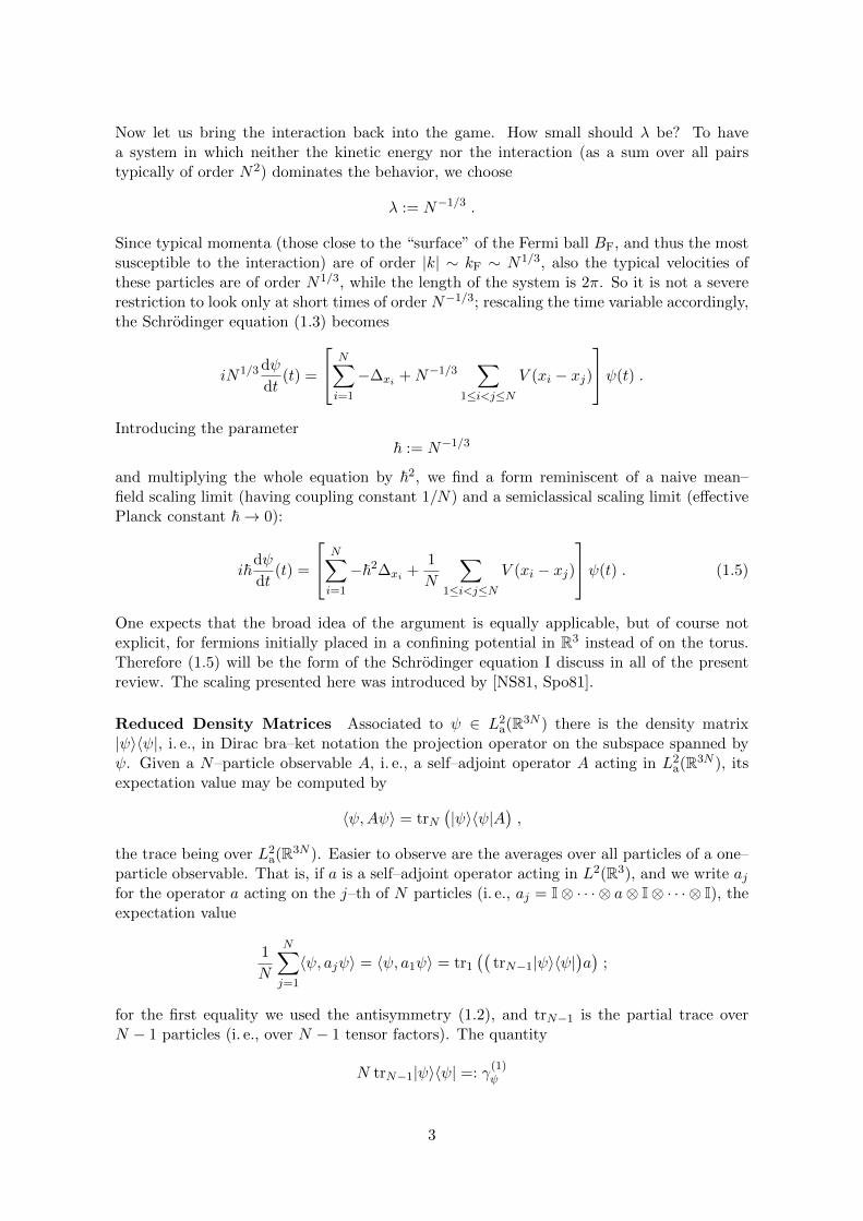
1iHψ

TψMP (ψ)1

iHψψ

M

Figure 1: Dirac–Frenkel principle: Consider the Schrodinger equation in a Hilbert spaceH and let M ⊂ H be a submanifold. Let ψ ∈ M. At any “time step”, 1

iHψ of (1.3) isorthogonally projected to the tangent space TψM, yielding an evolution inM. Figure following

[Lub08, BSS18].

Quantum Quench The typical experimental situation is a quantum quench: a low–energystate (or even the ground state) of fermions in a confining potential is prepared, then byswitching the interaction between particles (e. g., via a Feshbach resonance) or by switchingthe confining external potential, the previously prepared state becomes excited with respectto the switched Hamiltonian, thus exhibiting non–trivial dynamics. This dynamics is thenobserved. The following theorem proves that such a quench can be described by the time–dependent Hartree–Fock equation. To illustrate the idea we only give the simplest case, inwhich the initial data is exactly a Slater determinant (one may generalize to initial datacontaining a small number of particles excited over the Slater determinant).

Theorem 3.1 (Hartree–Fock Dynamics, [BPS14c, BPS14a]). Let V ∈ L1(R3) and∫

dp(1 +

|p|)2|V (p)| < ∞. Let ωN be a sequence of rank–N projection operators on L2(R3), andassume there exists C > 0 such that for all i ∈ 1, 2, 3 the sequence satisfies

‖[xi, ωN ]‖tr ≤ CN~ , ‖[pi, ωN ]‖tr ≤ CN~ . (3.4)

Let ψ0 be the Slater determinant corresponding to ωN . Let γ(1)(t) be the one–particle reduceddensity matrix associated to the solution of the Schrodinger equation ψ(t) := e−iHt/~ψ0. Ifω(t) is the solution of the Hartree–Fock equation (3.3) with initial data ωN , then

‖γ(1)(t)− ω(t)‖tr ≤ CN1/6 exp(c2 exp(c1|t|)) for all t ∈ R . (3.5)

Remarks. (i) Note that ‖γ(1)(t)‖tr = ‖ω(t)‖tr = N ; their difference is by N−5/6 smaller.

(ii) The exchange term X(t) in (3.3) may be dropped without changing the error boundof (3.5), see [BPS14c, Appendix A].

(iii) A similar theorem can be proven with relativistic kinetic energy√−~2∆ +m2 of mas-

sive particles, m > 0, replacing −∆ [BPS14b].

(iv) A similar theorem has first been proven by [EESY04], under assumption of analyticinteraction potential, and with error term controllable for short times.

(v) Singular V have been considered in [PRSS17, Saf18], however only for translationinvariant initial data, which is stationary under the Hartree–Fock evolution.

7

(vi) The Hartree–Fock equation has also been derived for initial data given by a mixedstate [BJP+16]. This has been generalized to singular interaction potentials, includingthe Coulomb potential and the gravitational attraction, at least up to small times, in[CLS21]. Mixed initial states are particularly important in view of the discussion ofadmissible initial data concerning the derivation of the Vlasov equation in Section 2.

(vii) The derivation of Hartree–Fock equations has also been considered in scaling limitswhere the interaction is weaker [BGGM03, BGGM04, FK11, PP16, BBP+16].

3.1 Initial Data: Non–Interacting Fermions in a Harmonic Trap

In Theorem 3.1 a key role is played by the assumption that the one–particle reduced densitymatrix of the initial Slater determinant satisfies the semiclassical commutator bounds (3.4).The only example given by [BPS14c] was the initial data constituted by the ground state ofnon–interacting fermions on a torus, i. e., a Slater determinant of planes waves (1.4) whosemomenta form a complete Fermi ball BF = k ∈ Z3 : |k| ≤ kF for some kF > 0. In[FM20] it was shown that non–interacting fermions in general confining potentials exhibitthe semiclassical structure, the proof using methods of semiclassical analysis. Instead inthe following we verify (3.4) by an explicit computation for non–interacting fermions in aharmonic trap.

We consider the Hamiltonian h, acting on L2(R3), describing a single particle in a three–dimensional anisotropic harmonic oscillator potential

h =3∑i=1

(p2i + ω2

i x2i

), with ωi > 0 for i ∈ 1, 2, 3 . (3.6)

We introduce standard creation and annihilation operators by

ai :=

√ωi2~

(xi +

i

ωipi

), a∗i :=

√ωi2~

(xi −

i

ωipi

). (3.7)

Then the Hamiltonian h becomes diagonal, and we can read off its spectrum:

h = ~3∑i=1

2ωi

(a∗i ai +

1

2

), σ(h) =

~

3∑i=1

2ωi

(ni +

1

2

): ni ∈ N

.

Now consider N non–interacting fermions in a harmonic external potential, i. e., as anoperator acting in L2

a(R3N ) we consider the Hamiltonian

H =N∑j=1

hj .

(In the language of second quantization this is the operator dΓ(h) on the N–particle subspaceof the fermionic Fock space F over L2(R3).) The ground state of H is the antisymmetrizedtensor product of the N lowest energy levels of the one–body Hamiltonian h, i. e., the eigen-functions associated with the ni up to a certain nmax

i form a Slater determinant. To occupythe eigenfunctions from all three oscillators up to the same energy, assuming without loss ofgenerality ω1 ≤ ω2 ≤ ω3, we take E > 0 and set

nmax1 := N1/3E , nmax

2 := N1/3Eω1

ω2, nmax

3 := N1/3Eω1

ω3. (3.8)

8

(To be precise we should round to integer values.) The one–particle reduced density matrixof the corresponding Slater determinant is

ωN =

nmax1 ,nmax

2 ,nmax3∑

n1,n2,n3=0

|n1, n2, n3〉〈n1, n2, n3| . (3.9)

(Here we have introduced the occupation number representation and Dirac bra–ket notation,i. e., |n1, n2, n3〉〈n1, n2, n3| denotes the projection on the tensor product of an eigenfunctionto eigenvalue n1, an eigenfunction to n2, and an eigenfunction to n3, this triple tensor productforming a wave function in the one–particle space L2(R3).)

According to the following theorem, non–interacting fermions in a harmonic confinementsatisfy the semiclassical commutator bounds used to derive the Hartree–Fock dynamics.

Theorem 3.2 (Semiclassical Structure of Non–Interacting Fermions in a Harmonic Trap).There is a C > 0 such that for all i ∈ 1, 2, 3 the one–particle density matrix (3.9) satisfies

‖[xi, ωN ]‖tr ≤ CN~ and ‖[pi, ωN ]‖tr ≤ CN~ . (3.10)

Proof. We prove the first bound, without loss of generality, for i = 1. Relation (3.7) is easilyinverted to obtain x1 =

√~/(2ω1) (a1 + a∗1). We compute the commutator

[x1, ωN ] =

√~

2ω1

nmax1∑

n1=0

[a∗1 + a1, |n1〉〈n1|

]⊗

nmax2∑

n2=0

|n2〉〈n2| ⊗nmax3∑

n3=0

|n3〉〈n3| .

By the usual creation operator rules

a∗1|n1〉〈n1| − |n1〉〈n1|a∗1 + a1|n1〉〈n1| − |n1〉〈n1|a1

=√n+ 1|n1 + 1〉〈n1| − |n1〉〈n1 − 1|

√n1 + |n1 − 1〉〈n1|

√n1 − |n1〉〈n1 + 1|

√n1 + 1 .

Paying attention to the summation indices (recall that a1|0〉 = 0) we find

nmax1∑

n1=0

√n1 + 1|n1 + 1〉〈n1| − |n1〉〈n1 + 1|

√n1 + 1

+

nmax1∑

n1=1

|n1 − 1〉〈n1|√n1 − |n1〉〈n1 − 1|

√n1

=√nmax

1 + 1(|nmax

1 + 1〉〈nmax1 | − |nmax

1 〉〈nmax1 + 1|

).

Squaring yields

|[x1, ωN ]|2

= (nmax1 + 1)

(|nmax

1 〉〈nmax1 + 1| − |nmax

1 + 1〉〈nmax1 |

)(|nmax

1 + 1〉〈nmax1 | − |nmax

1 〉〈nmax1 + 1|

)⊗ ~

2ω1

nmax2∑

n2=0

nmax2∑

n2=0

|n2〉 〈n2|n2〉︸ ︷︷ ︸δn2,n2

〈n2| ⊗nmax3∑

n3=0

nmax3∑

n3=0

|n3〉 〈n3|n3〉︸ ︷︷ ︸δn3,n3

〈n3| .

The square root is easy to calculate since the second and third component of the tensorproduct are already diagonal and the first one also becomes diagonal when we evaluate the

9

scalar products, leading to

√|[x1, ωN ]|2 =

√~

2ω1

√nmax

1 + 1(|nmax

1 〉〈nmax1 |+ |nmax

1 + 1〉〈nmax1 + 1|

)⊗

nmax2∑

n2=0

|n2〉〈n2| ⊗nmax3∑

n3=0

|n3〉〈n3| .

Finally taking the trace we obtain the claimed bound

‖[x1, ωN ]‖tr =

√~

2ω1

√nmax

1 + 1 2nmax2 nmax

3 = const×N2/3√N1/3E + 1

√~ ≤ CN~ .

The same holds for the momentum operator because the Hermite functions |n〉 are eigen-vectors of the Fourier transform with the eigenvalues being complex phases, which cancelout from the density matrix; this argument uses that the Fourier transform takes the dif-ferential operator p1 into the multiplication operator x1 and by unitarity leaves the tracenorm invariant. (Alternatively one can do the calculation analogous to the above also forthe momentum operator.)

This shows that the experimentally most important quantum quench can be described byTheorem 3.1: non–interacting fermions are cooled in a harmonic trap and then the interactionis switched on and the harmonic confinement switched off.

Remark. For the mean–field scaling limit to be non–trivial, the volume should be fixed andthe density proportional to total particle number N . For (3.9) one easily computes

trx21ωN =

~2ω1

nmax1∑

n1=0

nmax2∑

n2=0

nmax3∑

n3=0

〈n1, n2, n3|(a1 + a∗1)2|n1, n2, n3〉

=~

2ω1

nmax1∑

n1=0

nmax2∑

n2=0

nmax3∑

n3=0

〈n1, n2, n3|2a∗1a1 + 1|n1, n2, n3〉

=~

2ω1

nmaxi∑

n1=0

(2n1 + 1)(nmax2 + 1)(nmax

3 + 1) =~

2ω1(nmax

1 + 1)2(nmax2 + 1)(nmax

3 + 1) .

With N = trωN = (nmax1 + 1)(nmax

2 + 1)(nmax3 + 1) we find the spatial extension

√〈x2

1〉 =

√trx2

1ωNtrωN

=

√~

2ω1(nmax

1 + 1) =

√E

2ω1+O(N−1/3) = O(1) as N →∞ .

So we have indeed N particles in a fixed volume, the density thus being of order N asrequired.

4 Quantum Correlations: Random Phase Approximation

The random phase approximation (RPA) has originally been introduced by [BP53] for com-puting the ground state energy to the next order of precision beyond the Hartree–Fockvariational approximation. The RPA was later shown to correspond to a formal partial re-summation of the perturbative expansion in powers of the interaction [GB57]. A further,morally equivalent formulation of the RPA was developed treating pair excitations as ap-proximately bosonic particles with a diagonalizable Hamiltonian. This latter “bosonization”

10

approach is the only that has found a rigorous justification so far, namely for the groundstate energy in [HPR20, CHN21, BNP+20, BNP+21b, BPSS21]. In the following I discussa recent result showing that the bosonization formulation of the RPA also has a dynamicalcounterpart, which is valid as a refinement of Hartree–Fock theory to describe the evolutionof collective pair excitations over the Fermi ball of plane waves. The discussion in this sectiontherefore applies only to the case of fermions on the torus T3.

Fock Space Representation To explain the approximate collective bosonization ap-proach developed in [BNP+20], the method of second quantization is necessary. In secondquantization the N–particle space L2

a(T3N ) is embedded in the fermionic Fock space, i. e.,the direct sum over all possible particle numbers n,

F := C⊕∞⊕n=1

L2a(T3n) .

More explicitly, a vector ψN ∈ L2a(T3N ) is identified with a sequence (0, 0, . . . , 0, ψN , 0, . . .) ∈

F . The advantage of Fock space is that one can use creation and annihilation operators.These are operators on Fock space satisfying the canonical anticommutator relations (CAR)

ap, a∗q := apa∗q + a∗qap = δp,q , ap, aq = 0 = a∗q , a∗p , for all momenta p, q ∈ Z3 .

We skip the well–known definition of these operators (see, e. g., [Sol14]); the convenience ofthese operators lies exactly in the fact that we only need to know their anticommutators,the fact that applying arbitrary numbers of creation operators a∗ to the vacuum vectorΩ = (1, 0, 0, . . .) ∈ F one obtains a basis of Fock space F , and the fact that Ω lies in thenull space of all annihilation operators a. The starting point for all further steps is that theHamiltonian H is just the restriction to the N–particle sector of the Fock space Hamiltonian

H := ~2∑k∈Z3

|p|2a∗pap +1

2N

∑k,q,p∈Z3

V (k)a∗p+ka∗q−kaqap .

Particle–Hole Transformation In the first step, a particle–hole transformation is usedto separate the fixed Fermi ball of plane waves from its excitations. The particle–holetransformation is a unitary map R : F → F , defined by its properties

R∗a∗pR :=

ap for p ∈ BF

a∗p for p ∈ BcF := Z3 \BF

, RΩ := ψBF,

the latter vector being the Slater determinant constructed from the plane waves in BF, asin (1.4). Using this rule for conjugation with R and the CAR to arrange the result innormal–order (creation operators a∗ to the left of annihilation operators a) one obtains

R∗HR = EHF + H0 +QB + E .

The first summand EHF = 〈ψBF, HψBF

〉 is a real number and can be identified as theHartree–Fock energy. The term

H0 :=∑k∈Z3

e(k)a∗kak , e(k) := ~2∣∣|k|2 − k2

F

∣∣ , (4.1)

11

is the kinetic energy of pair excitations (removing one momentum mode from inside theFermi ball by applying an annihilation operator and adding a particle outside the Fermi ballby applying a creation operator). The term

QB :=1

N

∑k∈Γnor

V (k)(b∗(k)b(k) + b∗(−k)b(−k) + b∗(k)b∗(−k) + b(−k)b(k)

)(4.2)

is the part of the interaction that can be written purely in terms of particle–hole excitations“delocalized” over the entire Fermi ball, i. e., the linear combinations

b∗(k) :=∑

p∈BcF,h∈BF

δp−h,ka∗pa∗h . (4.3)

The purpose of introducing a separation of the support of V into two parts, supp V =Γnor ∪ (−Γnor), defined by

Γnor := k ∈ Z3 ∩ supp V : k3 > 0 or (k3 = 0 and k2 > 0) or (k2 = k3 = 0 and k1 > 0) ,

is that the pair creation operators appear only once in the summand, not both for k and −k(which will permit us to approximate them as independent bosonic modes later).

All further contributions to the Hamiltonian, i. e., everything that is not part of H0 orcannot be written using the b∗– and b–operators, are collected in E and can be proven toconstitute only small error terms, at least when acting on states with few excitations.

At this point the main observation is that QB is quadratic when expressed through theb∗– and b–operators; moreover, being (sums of) pairs of anticommuting operators, the b∗

among them commute, i. e.,

[b∗(k), b∗(l)] := b∗(k)b∗(l)− b∗(l)b∗(k) = 0 ,

i. e., these operators commute just like bosonic operators. Moreover, the vacuum Ω is in thenull space of all the b–operators, just like a vacuum vector in Fock space. One may thereforeconjecture that the b–operators realize a representation of the canonical commutator relations(CCR), which describe bosonic particles in a symmetric Fock space. Recall that true bosonicoperators bk and b∗l would satisfy the exact CCR

[b∗k, b∗l ] = 0 = [bk, bl] , [bk, b

∗l ] = δk,l . (4.4)

That this cannot be quite true is easily noted: whereas by antisymmetry one can nevercreate more than two fermions in the same state (one has (a∗k)

2 = 0, the Pauli exclusionprinciple), for bosons arbitrary powers of b∗k never vanish. Since the concrete b∗(k) of (4.3)are constructed from fermionic operators, they will at high powers eventually vanish andthus violate this bosonic property. But as long as we consider states with few excitations,(4.4) may constitute a valid approximation for the commutator relations of the constructedoperators. This will in fact be quantified by (4.7) below.

For the moment, let us focus on another difficulty: the operator H0 is not given in termsof b∗– and b–operators. To obtain an exactly solvable quantum theory, we need to express notonly QB but also H0 as a quadratic expression in terms of approximately bosonic operators.This will be achieved by the patch decomposition we introduce next.

12

Patch Decomposition of the Fermi Surface It turns out that a formula for H0 that isquadratic in the b∗– and b–operators can be found if the dispersion relation e(k) (as definedin (4.1)) is linearized first. For this purpose, note that the main term QB of the interactioncontains only pair operators in which k ∈ supp V ; so assuming V to have compact supportwe may restrict to pair operators (4.3) in which both momenta, p ∈ Bc

F and h ∈ BF, because

of the requirement p − h = k with k ∈ supp V , belong to a shell of width diam(supp V )around the Fermi surface k ∈ R3 : |k| = kF. One half of this shell may then be sliced intopatches Bα (with indices α = 1, . . . ,M/2) and this slicing reflected by the origin to the otherhalf, as indicated in Fig. 2. The total number of patches will be chosen as M := Nα withα ∈ (0, 2/3) (further requirements of the proof narrow down this interval). These patchesare separated by corridors of width strictly larger than 2 diam supp V ; moreover they do notdegenerate as N →∞ in the sense that their circumference will always be of order N1/3/

√M

while they cover an area of size N2/3/M on the Fermi sphere. For every patch Bα we choosea vector ωα with |ωα| = kF near the patch center.

The main idea is now to localize the pair creation operators to these patches, defining

b∗α(k) :=1

nα(k)

∑p∈BcF∩Bαh∈BF∩Bα

δp−h,ka∗pa∗h , (4.5)

where we introduced the normalization constant nα(k) such that ‖b∗α(k)Ω‖ = 1. Here wenotice a small problem: only if k points outward the Fermi ball (from a hole momentumh ∈ BF to a particle momentum p ∈ Bc

F) this sum will be non–zero. If k points radiallyinward or outward but under a very flat angle to the tangent plane, the sum may be emptyor contain very few (h, p)–pairs. We therefore impose a cut–off on the set of α such that wekeep only those with

k · ωα|ωα|

≥ N−δ (4.6)

(the choice of δ > 0 may be optimized). One finds

nα(k) =

[ ∑p∈BcF∩Bαh∈BF∩Bα

δp−h,k

]1/2

≈

√4πk2

F

M

∣∣∣∣k · ωα|ωα|∣∣∣∣ .

We can now prove that these operators are almost bosonic, in the sense that

[b∗α(k), b∗β(l)] = [bα(k), bβ(l)] = 0 , [bα(k), b∗β(l)] = δα,β (δk,l + Eα(k, l)) (4.7)

where the error term of the last commutator can be estimated, e. g., by bounds such as‖Eα(k, l)ψ‖ ≤ 2nα(k)−1nα(l)−1‖Nψ‖ for all ψ ∈ F . Thanks to the introduction of thecut–off and the assumption M N2/3 we have nα(k)→∞ as N →∞.

As we have seen, for at least half of the values of α, the operators b∗α(k) vanish. Tosimplify notation we introduce

c∗α(k) :=

b∗α(k) for α such that k · ωα/|ωα| ≥ N−δ ,b∗α(−k) for α such that k · ωα/|ωα| ≤ −N−δ .

(In the following we will use I+k := α : k · ωα/|ωα| ≥ N−δ ⊂ 1, 2, . . . ,M and Ik :=

I+k ∪ I

+−k, implicitly depending on the choice of δ.)

13

1

lU

Figure 2: The shell around the Fermi surface is decomposed into M = Nα patches, withα > 0 to be optimized. Patches on the southern half are obtained through reflection atthe origin. (From [BNP+20] under CC BY 4.0 license, http://creativecommons.org/

licenses/by/4.0/, with ωα added.)

Now turning back to the kinetic energy, one may linearize the dispersion relation asclaimed around the patch centers ωα: in fact (without loss of generality for α ∈ I+

k )

[H0, c∗α(k)] =

[∑i∈Z3

e(i)a∗i ai,1

nα(k)

∑p∈BcF∩Bαh∈BF∩Bα

δp−h,ka∗pa∗h

]

=1

nα(k)

∑p∈BcF∩Bαh∈BF∩Bα

δp−h,k (e(p)− e(h)) a∗pa∗h ≈ 2~2kFk ·

ωα|ωα|

c∗α(k) .

The same commutator is obtained replacing H0 in this formula by

DB := 2~2kF

∑k∈Γnor

∑α∈Ik

∣∣∣∣k · ωα|ωα|∣∣∣∣ c∗α(k)cα(k) .

If vectors of the form∏mj=1 c

∗αj (kj)Ω, m ∈ N, constituted a basis of the fermionic Fock space,

this would imply an identity between the operators H0 and DB. In [BNP+21b, BPSS21] mucheffort is dedicated to justifying this at least as an approximation of vectors close to the groundstate. As far as the approximation of the time evolution presented below is concerned, thiswill be much less of a problem since we only consider initial data created by the applicationof the pair creation operators c∗α(k).

Approximately Bosonic Effective Hamiltonian We may now combine what we learnedabout the dominant interaction term QB and the kinetic energy to state the bosonic the-ory providing us with the effective evolution of particle–hole pair excitations. Summing theapproximate kinetic energy DB and the dominant interaction terms QB, and decomposing

b∗(k) ≈∑α∈I+k

nα(k)c∗α(k) ,

we find the approximation (with κ := (3/4π)1/3)

Hcorr = R∗HNR− EpwN ≈

∑k∈Γnor

2~κ|k|heff(k) (4.8)

14

with the effective Hamiltonian

heff(k) :=∑

α,β∈Ik

[(D(k) +W (k)

)α,βc∗α(k)cβ(k) +

1

2W (k)α,β

(c∗α(k)c∗β(k) + h.c.

)](4.9)

where D(k), W (k), and W (k) are real symmetric matrices

D(k)α,β := δα,β|k · ωα|/(|k||ωα|) , ∀α, β ∈ Ik ,

W (k)α,β :=V (k)

2~κN |k|×nα(k)nβ(k) if α, β ∈ I+

k or α, β ∈ I+−k

0 otherwise ,

W (k)α,β :=V (k)

2~κN |k|×

0 if α, β ∈ I+k or α, β ∈ I+

−knα(k)nβ(k) otherwise .

(4.10)

The rigorous justification of this (approximately) bosonic Hamiltonian as an approximationto the microscopic fermionic Schrodinger equation is provided by Theorem 4.1 below. Tostate it we need to discuss the solution (i. e., Fock space diagonalization) of the effectiveHamiltonian first.

Diagonalization If c∗α(k) were exactly bosonic creation operators, then the quadraticHamiltonian heff(k) could be diagonalized by a Bogoliubov transformation (a linear au-tomorphism of the CCR algebra) of the form [BNP+20, Appendix A.1]

T := eB , B :=∑k∈Γnor

1

2

∑α,β∈Ik

K(k)α,βc∗α(k)c∗β(k)− h.c. (4.11)

where

K(k) := log|S(k)ᵀ| = 1

2log(S(k)S(k)ᵀ

),

S(k) := (D(k) +W (k)− W (k))1/2E(k)−1/2 ,

E(k) :=[(D(k) +W (k)− W (k)

)1/2(D(k) +W (k) + W (k))

(D(k) +W (k)− W (k)

)1/2]1/2.

Since our pair operators do not quite satisfy the commutator relations of the CCR algebra,T turns out to be only approximately a Bogoliubov transformation:

T ∗cγ(k)T ≈∑α∈Ik

cosh(K(k))α,γcα(k) +∑α∈Ik

sinh(K(k))α,γc∗α(k) .

With the indicated choice of K(k), the “off–diagonal” terms in the quadratic Hamiltonian(i. e., those of the form c∗c∗ and cc) are approximately cancelled by conjugation with theunitary T (see the proof of [BNP+21b, Lemma 10.1]), so that

T ∗HcorrT ≈ ERPAN +

∑k∈Γnor

2~κ|k|∑

α,β∈Ik

K(k)α,βc∗α(k)cβ(k) (4.12)

with the Hermitian matrix

K(k) = cosh(K(k))(D(k) +W (k)) cosh(K(k)) + sinh(K(k))(D(k) +W (k)) sinh(K(k))

+ cosh(K(k))W (k) sinh(K(k)) + sinh(K(k))W (k) cosh(K(k)) (4.13)

15

and the RPA prediction for the ground state energy correction

ERPAN =

∑k∈Γnor

~κ|k| tr(E(k)−D(k)−W (k)) ∈ R . (4.14)

Thus heff(k) can be understood as the approximately bosonic second quantization of theoperator K(k) on the one–boson space `2(Ik) ' C|Ik|. If the effective Hamiltonians atdifferent momenta k were independent, we could simply sum over k ∈ Γnor and find that theexcitation spectrum consists of sums of eigenvalues of 2~κ|k|E(k) (see [Ben21]).

Particle–Hole Pairs: Initial Data and Bosonic Dynamics The theorem will describethe evolution of collective particle–hole excitations of the Fermi ball. We consider the many–body Schrodinger equation with the initial data

ψ := RTξ ∈ L2a(R3N ) , ξ :=

1

Zmc∗(ϕ1) · · · c∗(ϕm)Ω , (4.15)

wherec∗(ϕi) =

∑k∈Γnor

∑α∈Ik

c∗α(k)(ϕi(k))α (4.16)

with a number m ∈ N of one–boson states

ϕ1, . . . , ϕm ∈⊕k∈Γnor

`2(Ik) , ‖ϕi‖2 :=∑k∈Γnor

∑α∈Ik

|(ϕi(k))α|2 = 1 . (4.17)

We do not require orthogonality of the functions ϕi: since they describe approximatelybosonic excitations, they may all occupy the same one–boson state ϕ1. The normalizationconstant Zm is chosen such that ‖ξ‖ = 1. We will approximate the evolution of such initialdata using the effective evolution

ξ(t) :=1

Zmc∗(ϕ1(t)) · · · c∗(ϕm(t))Ω , t ∈ R , (4.18)

where, with K(k) defined in (4.12),

ϕm(t) := e−iHBt/~ϕm , HB :=⊕k∈Γnor

2~κ|k|K(k) . (4.19)

The state ξ(t) can be viewed as an approximate m–boson state, where every ϕi evolvesindependently according to the one–boson Hamiltonian HB. We can now state the theorem.

Theorem 4.1 (RPA Dynamics, [BNP+21a]). Assume that V : Z3 → R is compactly sup-ported, non–negative, and V (k) = V (−k) for all k ∈ Z3. Let kF > 0, N := |k ∈ Z3 : |k| ≤kF|, and ~ := κk−1

F = N−1/3 + O(N−2/3) with κ = (3/4π)13 . Moreover assume that the

number m of pair excitations satisfies m3(2m− 1)!! N δ, where δ is given by (4.6). Thenthere exists a Cm,V > 0 such that for any t ∈ R we have

‖e−iHt/~RTξ − e−i(EpwN +ERPA

N )t/~RTξ(t)‖ (4.20)

≤ C(m+ 1)2√

(2m− 1)!!(N−

δ2 +M−

12 +M

32N−

13

+δ +M14N−

16

)|t| . (4.21)

Remarks. (i) The states RTξ and RTξ(t) are N–particle states. In particular the actionof the second quantized H agrees with the action of H on these states. This followssince the pair operators c∗α(k) create equal numbers of particles p ∈ Bc

F and holesh ∈ BF. More precisely, with N p :=

∑p∈BcF

a∗pap and N h :=∑

h∈BFa∗hah one has

(N p −N h)Tξ = 0, which implies

NRTξ = R(R∗NR)Tξ = R(N p −N h +N)Tξ = RNTξ = NRTξ .

16

(ii) In [BNP+21a] we specialized to the number of patches M := N4δ and the cut–offparameter δ := 2/45 (entering in (4.6)). The present form is more general since it alsodescribes the evolution of initial data given with non–optimal choice of M and δ. (Butof course the theorem is only of interest when the error estimate is 1.)

(iii) We avoided some trivial contributions to the error by keeping ERPAN instead of replacing

it by a (more explicit) integral formula as in [BNP+21a].

(iv) The theorem not only provides a stronger approximation than Theorem 3.1 by em-ploying Fock space norm instead of the trace norm of a reduced density matrix, butalso has a better time dependence of the error.

(v) The mentioned improvement comes at a cost: the theorem is only applicable to initialdata given in terms of pair excitations over the Fermi ball. According to [BNP+21b,Appendix A], the Fermi ball constitutes the minimizer (due to the scaling limit, ingeneral only a stationary point) of the Hartree–Fock variational problem (i. e., mini-mization of 〈ψ,Hψ〉 over Slater determinants ψ on the torus) and is thus stationary forthe time–dependent Hartree–Fock equation (3.3). The theorem does not apply, e. g., tothe harmonically confined Fermi gas, where we reach only the Hartree–Fock precisionof the previous section.

(vi) Only the pair excitations have a non–trivial evolution, the Fermi ball remains station-ary. The spectrum of pair excitations has been discussed in [Ben21, CHN21].

(vii) Different bosonization concepts appear in the analysis of low–density Fermi gases[FGHP21], spin systems [CG12, CGS15, Ben17, NS21], and one–dimensional fermionicsystems [ML65, LLMM17a, LLMM17b].

Concluding Remarks I have described three levels of approximation for the dynamicsof the fermionic many–body problem at high densities. While providing increasingly preciseresults (from approximation of the Wigner transform to approximation of reduced densitymatrices in trace norm to a Fock space norm approximation) we have also seen the role ofthe initial conditions, such as regularity of the Wigner transform when deriving the Vlasovequation, semiclassical commutator bounds for the validity of Hartree–Fock theory, and theinitial data consisting of pair excitations over a stationary Fermi ball for the RPA. Moreoverwe have seen that the generalization of these assumptions still provides a number of importantquestions on which further progress would be desirable.

Acknowledgements

The author has been supported by the Gruppo Nazionale per la Fisica Matematica (GNFM)of the Istituto Nazionale di Alta Matematica “Francesco Severi” (INdAM) in Italy. Theauthor has no conflicts to disclose.

References

[AKN13a] Laurent Amour, Mohamed Khodja, and Jean Nourrigat. The classical limit ofthe Heisenberg and time-dependent Hartree–Fock equations: The Wick symbolof the solution. Mathematical Research Letters, 20(1):119–139, January 2013.

17

[AKN13b] Laurent Amour, Mohamed Khodja, and Jean Nourrigat. The semiclassical limitof the time dependent Hartree–Fock equation: The Weyl symbol of the solution.Analysis & PDE, 6(7):1649–1674, December 2013.

[APPP11] Agissilaos Athanassoulis, Thierry Paul, Federica Pezzotti, and Mario Pulvirenti.Strong semiclassical approximation of Wigner functions for the Hartree dynam-ics. Rendiconti Lincei - Matematica e Applicazioni, 22(4):525–552, December2011.

[BBP+16] Volker Bach, Sebastien Breteaux, Soren Petrat, Peter Pickl, and Tim Tzaneteas.Kinetic Energy Estimates for the Accuracy of the Time-Dependent Hartree-Fock Approximation with Coulomb Interaction. Journal de MathematiquesPures et Appliquees, 105(1):1–30, January 2016.

[Ben17] Niels Benedikter. Interaction Corrections to Spin-Wave Theory in the Large-SLimit of the Quantum Heisenberg Ferromagnet. Mathematical Physics, Analysisand Geometry, 20(2):5, June 2017.

[Ben21] Niels Benedikter. Bosonic collective excitations in Fermi gases. Reviews inMathematical Physics, 33(1):2060009, 2021.

[BGGM03] Claude Bardos, Francois Golse, Alex D. Gottlieb, and Norbert J. Mauser. Meanfield dynamics of fermions and the time-dependent Hartree–Fock equation.Journal de Mathematiques Pures et Appliquees, 82(6):665–683, June 2003.

[BGGM04] Claude Bardos, Francois Golse, Alex D. Gottlieb, and Norbert J. Mauser. Ac-curacy of the Time-Dependent Hartree–Fock Approximation for UncorrelatedInitial States. Journal of Statistical Physics, 115(3/4):1037–1055, May 2004.

[BJP+16] Niels Benedikter, Vojkan Jaksic, Marcello Porta, Chiara Saffirio, and BenjaminSchlein. Mean-Field Evolution of Fermionic Mixed States. Communications onPure and Applied Mathematics, 69(12):2250–2303, December 2016.

[BNP+20] Niels Benedikter, Phan Thanh Nam, Marcello Porta, Benjamin Schlein, andRobert Seiringer. Optimal Upper Bound for the Correlation Energy of a FermiGas in the Mean-Field Regime. Communications in Mathematical Physics,374(3):2097–2150, March 2020.

[BNP+21a] Niels Benedikter, Phan Thanh Nam, Marcello Porta, Benjamin Schlein,and Robert Seiringer. Bosonization of Fermionic Many-Body Dynamics.arXiv:2103.08224 [math-ph], to appear in Annales Henri Poincare, March 2021.

[BNP+21b] Niels Benedikter, Phan Thanh Nam, Marcello Porta, Benjamin Schlein, andRobert Seiringer. Correlation energy of a weakly interacting Fermi gas. Inven-tiones mathematicae, 225(3):885–979, September 2021.

[BP53] David Bohm and David Pines. A Collective Description of Electron Interac-tions: III. Coulomb Interactions in a Degenerate Electron Gas. Physical Review,92(3):609–625, November 1953.

[BPS14a] Niels Benedikter, Marcello Porta, and Benjamin Schlein. Hartree-Fock dynam-ics for weakly interacting fermions. In Mathematical Results in Quantum Me-chanics (Proceedings of the QMath12 Conference). World Scientific PublishingCompany, 2014.

18

[BPS14b] Niels Benedikter, Marcello Porta, and Benjamin Schlein. Mean-field dynam-ics of fermions with relativistic dispersion. Journal of Mathematical Physics,55(2):021901, February 2014.

[BPS14c] Niels Benedikter, Marcello Porta, and Benjamin Schlein. Mean–Field Evolutionof Fermionic Systems. Communications in Mathematical Physics, 331(3):1087–1131, November 2014.

[BPSS16] Niels Benedikter, Marcello Porta, Chiara Saffirio, and Benjamin Schlein. Fromthe Hartree Dynamics to the Vlasov Equation. Archive for Rational Mechanicsand Analysis, 221(1):273–334, July 2016.

[BPSS21] Niels Benedikter, Marcello Porta, Benjamin Schlein, and Robert Seiringer. Cor-relation Energy of a Weakly Interacting Fermi Gas with Large Interaction Po-tential. arXiv:2106.13185 [cond-mat, physics:math-ph], June 2021.

[BSS18] Niels Benedikter, Jeremy Sok, and Jan Philip Solovej. The Dirac–Frenkel Prin-ciple for Reduced Density Matrices, and the Bogoliubov–de Gennes Equations.Annales Henri Poincare, 19(4):1167–1214, April 2018.

[BW95] T. Brocker and R. F. Werner. Mixed states with positive Wigner functions.Journal of Mathematical Physics, 36(1):62–75, January 1995.

[CG12] M. Correggi and A. Giuliani. The Free Energy of the Quantum HeisenbergFerromagnet at Large Spin. Journal of Statistical Physics, 149(2):234–245,October 2012.

[CGS15] Michele Correggi, Alessandro Giuliani, and Robert Seiringer. Validity of theSpin-Wave Approximation for the Free Energy of the Heisenberg Ferromagnet.Communications in Mathematical Physics, 339(1):279–307, October 2015.

[CHN21] Martin Ravn Christiansen, Christian Hainzl, and Phan Thanh Nam. TheRandom Phase Approximation for Interacting Fermi Gases in the Mean-FieldRegime. arXiv:2106.11161 [cond-mat, physics:math-ph], June 2021.

[CLS21] Jacky J. Chong, Laurent Lafleche, and Chiara Saffirio. From many-body quan-tum dynamics to the Hartree–Fock and Vlasov equations with singular poten-tials. arXiv:2103.10946 [math-ph], May 2021.

[CLS22] Jacky J. Chong, Laurent Lafleche, and Chiara Saffirio. On the $L2$ rate of con-vergence in the limit from Hartree to Vlasov$\unicodex2013$Poisson equa-tion. arXiv:2203.11485 [math-ph, physics:quant-ph], March 2022.

[EESY04] Alexander Elgart, Laszlo Erdos, Benjamin Schlein, and Horng-Tzer Yau. Non-linear Hartree equation as the mean field limit of weakly coupled fermions. Jour-nal de Mathematiques Pures et Appliquees, 83(10):1241–1273, October 2004.

[FGHP21] Marco Falconi, Emanuela L. Giacomelli, Christian Hainzl, and MarcelloPorta. The dilute Fermi gas via Bogoliubov theory. Annales Henri Poincare,22(7):2283–2353, July 2021.

[FK11] Jurg Frohlich and Antti Knowles. A Microscopic Derivation of the Time-Dependent Hartree-Fock Equation with Coulomb Two-Body Interaction. Jour-nal of Statistical Physics, 145(1):23, September 2011.

19

[FM20] Søren Fournais and Søren Mikkelsen. An optimal semiclassical bound on com-mutators of spectral projections with position and momentum operators. Let-ters in Mathematical Physics, 110(12):3343–3373, December 2020.

[GB57] Murray Gell-Mann and Keith A. Brueckner. Correlation Energy of an ElectronGas at High Density. Physical Review, 106(2):364–368, April 1957.

[GIMS98] Ingenuin Gasser, Reinhard Illner, Peter A. Markowich, and Christian Schmeiser.Semiclassical, $t\rightarrow \infty $ asymptotics and dispersive effects forHartree-Fock systems. ESAIM: Mathematical Modelling and Numerical Analy-sis - Modelisation Mathematique et Analyse Numerique, 32(6):699–713, 1998.

[HPR20] Christian Hainzl, Marcello Porta, and Felix Rexze. On the Correlation Energyof Interacting Fermionic Systems in the Mean-Field Regime. Communicationsin Mathematical Physics, 374(2):485–524, March 2020.

[Laf19] Laurent Lafleche. Propagation of Moments and Semiclassical Limit fromHartree to Vlasov Equation. Journal of Statistical Physics, 177(1):20–60, Oc-tober 2019.

[Laf21] Laurent Lafleche. Global semiclassical limit from Hartree to Vlasov equation forconcentrated initial data. Annales de l’Institut Henri Poincare C, 38(6):1739–1762, December 2021.

[LLMM17a] Edwin Langmann, Joel L. Lebowitz, Vieri Mastropietro, and Per Moosavi.Steady States and Universal Conductance in a Quenched Luttinger Model.Communications in Mathematical Physics, 349(2):551–582, January 2017.

[LLMM17b] Edwin Langmann, Joel L. Lebowitz, Vieri Mastropietro, and Per Moosavi. Timeevolution of the Luttinger model with nonuniform temperature profile. PhysicalReview B, 95(23):235142, June 2017.

[LP93] Pierre-Louis Lions and Thierry Paul. Sur les mesures de Wigner. RevistaMatematica Iberoamericana, 9(3):553–618, 1993.

[LS21] Laurent Lafleche and Chiara Saffirio. Strong semiclassical limit from Hartreeand Hartree-Fock to Vlasov-Poisson equation. arXiv:2003.02926 [math-ph,physics:quant-ph], February 2021.

[Lub08] Christian Lubich. From Quantum to Classical Molecular Dynamics: ReducedModels and Numerical Analysis. Zurich Lectures in Advanced Mathematics.European Mathematical Society, Zurich, Switzerland, 2008.

[ML65] Daniel C. Mattis and Elliott H. Lieb. Exact Solution of a Many-Fermion Systemand Its Associated Boson Field. Journal of Mathematical Physics, 6(2):304–312,February 1965.

[MM93] Peter A. Markowich and Norbert J. Mauser. The classical limit of a self-consistent quantum-vlasov equation in 3d. Mathematical Models and Methodsin Applied Sciences, 03(01):109–124, February 1993.

[NS81] Heide Narnhofer and Geoffrey L. Sewell. Vlasov hydrodynamics of a quan-tum mechanical model. Communications in Mathematical Physics, 79(1):9–24,March 1981.

20

[NS21] Marcin Napiorkowski and Robert Seiringer. Free energy asymptotics of thequantum Heisenberg spin chain. Letters in Mathematical Physics, 111(2):31,March 2021.

[PP09] Federica Pezzotti and Mario Pulvirenti. Mean-Field Limit and SemiclassicalExpansion of a Quantum Particle System. Annales Henri Poincare, 10(1):145–187, March 2009.

[PP16] Soren Petrat and Peter Pickl. A New Method and a New Scaling for DerivingFermionic Mean-Field Dynamics. Mathematical Physics, Analysis and Geome-try, 19(1):3, February 2016.

[PRSS17] Marcello Porta, Simone Rademacher, Chiara Saffirio, and Benjamin Schlein.Mean Field Evolution of Fermions with Coulomb Interaction. Journal of Sta-tistical Physics, 166(6):1345–1364, March 2017.

[Saf18] Chiara Saffirio. Mean-Field Evolution of Fermions with Singular Interaction.In Daniela Cadamuro, Maximilian Duell, Wojciech Dybalski, and Sergio Si-monella, editors, Macroscopic Limits of Quantum Systems, volume 270, pages81–99. Springer International Publishing, Cham, 2018.

[Saf20a] Chiara Saffirio. From the Hartree Equation to the Vlasov–Poisson System:Strong Convergence for a Class of Mixed States. SIAM Journal on MathematicalAnalysis, 52(6):5533–5553, January 2020.

[Saf20b] Chiara Saffirio. Semiclassical Limit to the Vlasov Equation with Inverse PowerLaw Potentials. Communications in Mathematical Physics, 373(2):571–619,January 2020.

[Saf21] Chiara Saffirio. From the Hartree to the Vlasov Dynamics: Conditional StrongConvergence. In Cedric Bernardin, Francois Golse, Patrıcia Goncalves, ValeriaRicci, and Ana Jacinta Soares, editors, From Particle Systems to Partial Dif-ferential Equations, Springer Proceedings in Mathematics & Statistics, pages335–354, Cham, 2021. Springer International Publishing.

[SC83] Francisco Soto and Pierre Claverie. When is the Wigner function of multidimen-sional systems nonnegative? Journal of Mathematical Physics, 24(1):97–100,January 1983.

[Sol14] Jan Philip Solovej. Many Body Quantum Mechanics. Lecture Notes ErwinSchrodinger Institute Vienna, March 2014.

[Spo81] Herbert Spohn. On the Vlasov hierarchy. Mathematical Methods in the AppliedSciences, 3(1):445–455, 1981.

21