Macroscopic quantum phenomena in strongly interacting ...
285
HAL Id: tel-00197118 https://tel.archives-ouvertes.fr/tel-00197118 Submitted on 14 Dec 2007 HAL is a multi-disciplinary open access archive for the deposit and dissemination of sci- entific research documents, whether they are pub- lished or not. The documents may come from teaching and research institutions in France or abroad, or from public or private research centers. L’archive ouverte pluridisciplinaire HAL, est destinée au dépôt et à la diffusion de documents scientifiques de niveau recherche, publiés ou non, émanant des établissements d’enseignement et de recherche français ou étrangers, des laboratoires publics ou privés. Macroscopic quantum phenomena in strongly interacting fermionic systems Jérôme Rech To cite this version: Jérôme Rech. Macroscopic quantum phenomena in strongly interacting fermionic systems. Condensed Matter [cond-mat]. Université Paris Sud - Paris XI; Rutgers University, 2006. English. tel-00197118
-
Upload
khangminh22 -
Category
Documents
-
view
4 -
download
0
Transcript of Macroscopic quantum phenomena in strongly interacting ...

HAL Id: tel-00197118https://tel.archives-ouvertes.fr/tel-00197118
Submitted on 14 Dec 2007
HAL is a multi-disciplinary open accessarchive for the deposit and dissemination of sci-entific research documents, whether they are pub-lished or not. The documents may come fromteaching and research institutions in France orabroad, or from public or private research centers.
L’archive ouverte pluridisciplinaire HAL, estdestinée au dépôt et à la diffusion de documentsscientifiques de niveau recherche, publiés ou non,émanant des établissements d’enseignement et derecherche français ou étrangers, des laboratoirespublics ou privés.
Macroscopic quantum phenomena in stronglyinteracting fermionic systems
Jérôme Rech
To cite this version:Jérôme Rech. Macroscopic quantum phenomena in strongly interacting fermionic systems. CondensedMatter [cond-mat]. Université Paris Sud - Paris XI; Rutgers University, 2006. English. tel-00197118

C.E.A. / D.S.M.
Service de Physique Theorique
These de doctorat de l’universite Paris XI
Specialite : Physique theorique
presentee par :
Jerome RECH
pour obtenir le grade de Docteur de l’Universite Paris XI
Sujet de la these :
Phenomenes quantiquesmacroscopiques dans les systemes
d’electrons fortement correles
soutenue le 19 Juin 2006 devant le jury compose de :
Mme LHUILLIER Claire PresidenteMelle PEPIN Catherine Co-DirectriceM. COLEMAN Piers Co-DirecteurM. JOLICOEUR Thierry RapporteurM. PUJOL Pierre RapporteurM. KOTLIAR Gabriel ExaminateurM. GLASHAUSSER Charles Invite


MACROSCOPIC QUANTUM PHENOMENA
IN STRONGLY INTERACTING FERMIONIC
SYSTEMS
BY JEROME RECH
A dissertation submitted to the
Graduate School – New Brunswick
Rutgers, The State University of New Jersey
in partial fulfillment of the requirements
for the degree of
Doctor of Philosophy
Graduate Program in Physics and Astronomy
Written under the direction of
Doctor Catherine Pepin and
Professor Piers Coleman
and approved by
Prof. Piers Coleman
Prof. Charles Glashausser
Prof. Gabriel Kotliar
Dr. Catherine Pepin
New Brunswick, New Jersey
June, 2006


A ma famille. . .

Remerciements
“-How did you find America?
-Turned left at Greenland”
John Lennon, repondant a un journaliste.
Cette these a ete le resultat d’une experience - a ma connaissance une despremieres en la matiere - puisqu’elle a ete effectuee au sein de deux structuresseparees de plus de 6000 km, tout en etant reconnues par les “autorites locales” desdeux pays.
Je tiens tout d’abord a remercier le Service de Physique theorique du CEA etle departement de physique de l’universite de Rutgers ainsi que leurs directeursrespectifs Henri Orland et Charles Glashausser pour m’avoir accueilli dans leursdepartements.
Je remercie ensuite chaleureusement Catherine Pepin et Piers Coleman d’avoiraccepte chacun d’encadrer un demi-etudiant avec les problemes d’indisponibilitetemporaire que cela impliquait. Bien sur, j’ai beaucoup appris de nos nombreusesdiscussions, de leur vaste culture scientifique et de leur encadrement si different etpourtant complementaire. Ils ont toujours ete tres patients et disponibles pour mesquestions, avec le dynamisme qui les caracterise tous deux. Mais au dela de l’aspectpurement scientifique, ce fut aussi une experience humaine des plus agreables. Mercidonc a Catherine pour son inebranlable sourire, ses theories sur la derniere perfor-mance de l’equipe de France et ses nombreux problemes informatiques qu’il m’afallu resoudre. Merci a Piers pour son humour so british, son rire tonitruant, sonenthousiasme sans faille et les petites histoires de physique et de physiciens qu’il seplait a conter reguli‘erement.
Je souhaite aussi remercier Olivier Parcollet qui au fil de nos collaborations afini, un peu malgre lui, par jouer le role de “troisieme directeur de these”. En plus deme convertir au numerique en m’initiant au C++ et au Python, Olivier a toujoursete disponible, offrant une oreille attentive a mes questions numeriques, physiqueset mathematiques. J’ai enormement appris a son contact.
Je me sens tout aussi redevable envers mes autres collaborateurs. Tout d’abordAndrey Chubukov pour m’avoir, entre autres choses, initie a l’art du calcul de dia-grammes. Puis Indranil Paul, qui a ete un ami avant d’etre un collaborateur. Enfin
7

Eran Lebanon et Gergely Zarand, dont l’expertise de l’effet Kondo m’a ete d’ungrand secours.
Je tiens evidemment a remercier Thierry Jolicoeur et Pierre Pujol d’avoir acceptela lourde (et un peu ingrate aussi) tache de rapporter mon manuscrit. Je realise lacharge de travail supplementaire que cela represente. Je remercie egalement GabiKotliar et Charles Glashausser d’avoir franchi le quart du globe pour participer amon jury de these et m’eviter de fait la difficulte supplementaire d’organiser unesoutenance en video-conference. Merci aussi a Claire Lhuillier d’avoir preside cejury en reussissant a concilier les styles francais et americains.
Merci a Corinne Donzaud, Alexandre Dazzi, Catherine Even, les enseignants etpreparateurs que j’ai pu cotoyer durant mes enseignements a l’Universite Paris-SudXI. Ils ont su rendre ces trois annees de monitorat particulierement enrichissantes,grace a leur attention, leurs conseils et leur competence.
C’est aussi l’occasion pour moi de montrer ma reconnaissance envers ceux quim’ont guide dans les annees precedant cette these. Merci a Roger Morin pourm’avoir fait decouvrir le vaste monde de la matiere condensee. Merci a Pierre Pujolpour m’avoir donne le gout pour la physique theorique, pour ses conseils avises aucommencement de cette these et pour ne pas m’avoir tenu rigueur du choix que j’aifini par faire.
Que ce soit a Rutgers ou au SPhT, venir travailler au labo a toujours ete unplaisir, et je pourrais en remercier l’ensemble de l’annuaire: merci pour l’ambianceagreable, la bonne humeur, les discussions scientifiques ou non en salle cafe, . . .
Merci a tout le personnel administratif de Saclay et Rutgers (Sylvie et Kathy entete) pour m’avoir simplifie la tache, et aide dans les differentes demarches admin-istratives qui ont emaillees ces deux mi-theses.
J’en viens maintenant aux remerciements plus personnels que, par pudeur, jeferai tres courts. Merci a mes “co-buros”, Gerhard, Nicolas, Cristian et Clement,pour supporter mes interruptions intempestives, et pour leur indulgence vis-avis demon humour. Merci a mes compagnons de galere de part et d’autre de l’Atlantique:Tristan, Cyrille, Pierre, Alexey, Nicolas, Yann, Stephane, Cedric, Loıck, Constantin,Emmanuel, Pankaj, Nicci, Craig, Leeann, Masud, Sergey, Marcello, Edouard, Fatiha,Nayana, Ruslan, Mariana, Tonia, Lorenzo, Benjamin, Max, Ivan, Banu. Merci aDave pour m’avoir si bien americanise. Merci a tous mes amis de Marseille, Greno-ble, Lyon, Paris, Strasbourg, Stuttgart, Pekin, New Brunswick, Santa Barbara etailleurs, pour avoir ete a mes cotes de pres ou de loin.
Par dessus tout, merci a mes parents et a ma soeur. Il m’est difficile de resumeren quelques mots tout ce qu’ils m’ont toujours apporte, et a quel point je leur suisredevable, pour leur soutien, leur amour et tout le reste. . .
8

Contents
Introduction 151 From critical opalescence to quantum criticality . . . . . . . . . . . . 152 Stirring up a quantum cocktail . . . . . . . . . . . . . . . . . . . . . . 173 Quantum criticality observed . . . . . . . . . . . . . . . . . . . . . . . 184 Unsolved puzzles . . . . . . . . . . . . . . . . . . . . . . . . . . . . . 195 Outline . . . . . . . . . . . . . . . . . . . . . . . . . . . . . . . . . . . 20
I Instability of a Ferromagnetic Quantum Critical Point 23
1 Introduction and motivations 251.1 Quantum critical theory of itinerant ferromagnets . . . . . . . . . . . 25
1.1.1 Mean-field theory and Stoner criterion . . . . . . . . . . . . . 261.1.2 Hertz-Millis-Moriya effective theory (HMM) . . . . . . . . . . 27
1.2 Experiments . . . . . . . . . . . . . . . . . . . . . . . . . . . . . . . . 311.2.1 Successes . . . . . . . . . . . . . . . . . . . . . . . . . . . . . 311.2.2 Departures from HMM results . . . . . . . . . . . . . . . . . . 321.2.3 The puzzling case of MnSi . . . . . . . . . . . . . . . . . . . . 35
1.3 Non-analytic static spin susceptibility . . . . . . . . . . . . . . . . . . 351.3.1 Long-range correlations . . . . . . . . . . . . . . . . . . . . . . 351.3.2 Effect on the quantum critical regime . . . . . . . . . . . . . . 37
2 Eliashberg theory of the spin-fermion model 392.1 Spin-fermion model . . . . . . . . . . . . . . . . . . . . . . . . . . . . 40
2.1.1 Low-energy model . . . . . . . . . . . . . . . . . . . . . . . . 402.1.2 Forward scattering model . . . . . . . . . . . . . . . . . . . . 41
2.2 Direct perturbative results . . . . . . . . . . . . . . . . . . . . . . . . 432.2.1 Bosonic polarization . . . . . . . . . . . . . . . . . . . . . . . 442.2.2 One-loop fermionic self-energy . . . . . . . . . . . . . . . . . . 44

2.2.3 Two-loop fermionic self-energy . . . . . . . . . . . . . . . . . . 462.2.4 Conclusion . . . . . . . . . . . . . . . . . . . . . . . . . . . . . 47
2.3 Eliashberg theory . . . . . . . . . . . . . . . . . . . . . . . . . . . . . 482.3.1 Self-consistent solution . . . . . . . . . . . . . . . . . . . . . . 482.3.2 A few comments . . . . . . . . . . . . . . . . . . . . . . . . . 50
2.4 Validity of the approach . . . . . . . . . . . . . . . . . . . . . . . . . 542.4.1 Vertex corrections . . . . . . . . . . . . . . . . . . . . . . . . . 552.4.2 Self-energy corrections . . . . . . . . . . . . . . . . . . . . . . 602.4.3 Summary . . . . . . . . . . . . . . . . . . . . . . . . . . . . . 64
3 Static spin susceptibility 653.1 Revisiting the Hertz-Millis-Moriya theory . . . . . . . . . . . . . . . . 66
3.1.1 φ4 term . . . . . . . . . . . . . . . . . . . . . . . . . . . . . . 663.1.2 φ3 term . . . . . . . . . . . . . . . . . . . . . . . . . . . . . . 68
3.2 Static spin susceptibility . . . . . . . . . . . . . . . . . . . . . . . . . 693.2.1 Away from the QCP . . . . . . . . . . . . . . . . . . . . . . . 713.2.2 At criticality . . . . . . . . . . . . . . . . . . . . . . . . . . . . 73
3.3 Related results . . . . . . . . . . . . . . . . . . . . . . . . . . . . . . 763.3.1 Finite temperature result . . . . . . . . . . . . . . . . . . . . . 763.3.2 Three-loop fermionic self-energy . . . . . . . . . . . . . . . . . 783.3.3 Conclusion . . . . . . . . . . . . . . . . . . . . . . . . . . . . . 79
3.4 Non-SU(2) symmetric case . . . . . . . . . . . . . . . . . . . . . . . . 803.4.1 Discussion . . . . . . . . . . . . . . . . . . . . . . . . . . . . . 803.4.2 Ising case . . . . . . . . . . . . . . . . . . . . . . . . . . . . . 803.4.3 Charge channel . . . . . . . . . . . . . . . . . . . . . . . . . . 813.4.4 Physical arguments . . . . . . . . . . . . . . . . . . . . . . . . 81
4 Conclusions and perspectives 83
Publication 1 85
Publication 2 91
Appendices 93
A Bosonic self-energy 95
B Fermionic self-energy 97B.1 One-loop . . . . . . . . . . . . . . . . . . . . . . . . . . . . . . . . . . 97
B.1.1 At the Fermi level . . . . . . . . . . . . . . . . . . . . . . . . . 97B.1.2 Momentum dependence . . . . . . . . . . . . . . . . . . . . . 99
B.2 Two-loop . . . . . . . . . . . . . . . . . . . . . . . . . . . . . . . . . 101
10

B.3 Three loop . . . . . . . . . . . . . . . . . . . . . . . . . . . . . . . . . 103
C Vertex corrections 105C.1 q = Ω = 0 . . . . . . . . . . . . . . . . . . . . . . . . . . . . . . . . . 105C.2 q = 0, Ω finite . . . . . . . . . . . . . . . . . . . . . . . . . . . . . . . 106C.3 q finite, Ω = 0 . . . . . . . . . . . . . . . . . . . . . . . . . . . . . . . 107C.4 q,Ω finite . . . . . . . . . . . . . . . . . . . . . . . . . . . . . . . . . 108C.5 4-leg vertex . . . . . . . . . . . . . . . . . . . . . . . . . . . . . . . . 110
D Static spin susceptibility 113D.1 Diagrams . . . . . . . . . . . . . . . . . . . . . . . . . . . . . . . . . 113
D.1.1 First diagram . . . . . . . . . . . . . . . . . . . . . . . . . . . 114D.1.2 Second diagram . . . . . . . . . . . . . . . . . . . . . . . . . . 114
D.2 Away from the QCP . . . . . . . . . . . . . . . . . . . . . . . . . . . 115D.3 At criticality . . . . . . . . . . . . . . . . . . . . . . . . . . . . . . . . 117D.4 The other two diagrams . . . . . . . . . . . . . . . . . . . . . . . . . 120
E Two-loop renormalization of the charge susceptibility 123
F Mass-shell singularity 125
II Bosonic approach to quantum impurity models 127
5 Introduction and motivations 1295.1 Kondo and Anderson models: a brief review . . . . . . . . . . . . . . 130
5.1.1 History of the Kondo effect . . . . . . . . . . . . . . . . . . . 1305.1.2 Anderson model . . . . . . . . . . . . . . . . . . . . . . . . . . 1325.1.3 Experimental and theoretical relevance: the revival . . . . . . 133
5.2 Quantum dots . . . . . . . . . . . . . . . . . . . . . . . . . . . . . . . 1355.2.1 Charge quantization . . . . . . . . . . . . . . . . . . . . . . . 1355.2.2 Coulomb blockade . . . . . . . . . . . . . . . . . . . . . . . . 1365.2.3 Kondo physics in quantum dots . . . . . . . . . . . . . . . . . 137
5.3 Heavy fermions and the Kondo lattice . . . . . . . . . . . . . . . . . 1395.3.1 Kondo lattice . . . . . . . . . . . . . . . . . . . . . . . . . . . 1395.3.2 Heavy fermion: a prototypical Kondo lattice . . . . . . . . . . 141
6 Single impurity multichannel Kondo model 1456.1 Background . . . . . . . . . . . . . . . . . . . . . . . . . . . . . . . . 146
6.1.1 Generalized Kondo model . . . . . . . . . . . . . . . . . . . . 146
11
6.1.2 Strong coupling limit . . . . . . . . . . . . . . . . . . . . . . . 1486.1.3 Saddle-point equations . . . . . . . . . . . . . . . . . . . . . . 151
6.2 Known results . . . . . . . . . . . . . . . . . . . . . . . . . . . . . . . 1566.2.1 High temperature regime . . . . . . . . . . . . . . . . . . . . . 1576.2.2 Overscreened case: p0 < γ (OS) . . . . . . . . . . . . . . . . . 1586.2.3 Underscreened case: p0 > γ (US) . . . . . . . . . . . . . . . . 161
6.3 Exactly screened case: p0 = γ (ES) . . . . . . . . . . . . . . . . . . . 1656.3.1 General belief and counter-arguments . . . . . . . . . . . . . . 1656.3.2 Spectral functions . . . . . . . . . . . . . . . . . . . . . . . . . 1666.3.3 Entropy and specific heat . . . . . . . . . . . . . . . . . . . . 1696.3.4 Susceptibility and Wilson ratio . . . . . . . . . . . . . . . . . 1716.3.5 Scales . . . . . . . . . . . . . . . . . . . . . . . . . . . . . . . 172
6.4 Conclusion . . . . . . . . . . . . . . . . . . . . . . . . . . . . . . . . . 172
7 Two-impurity multichannel Kondo model 1757.1 Large-N equations . . . . . . . . . . . . . . . . . . . . . . . . . . . . 176
7.1.1 The model . . . . . . . . . . . . . . . . . . . . . . . . . . . . . 1767.1.2 Saddle-point equations . . . . . . . . . . . . . . . . . . . . . . 1777.1.3 General remarks . . . . . . . . . . . . . . . . . . . . . . . . . 181
7.2 Phase diagram and quantum critical point . . . . . . . . . . . . . . . 1827.2.1 Tools for exploring the phase diagram . . . . . . . . . . . . . . 1837.2.2 Renormalized Fermi liquid region (I) . . . . . . . . . . . . . . 1847.2.3 Magnetically correlated region (II) . . . . . . . . . . . . . . . 1867.2.4 Quantum critical region (III) . . . . . . . . . . . . . . . . . . 187
7.3 Discussion . . . . . . . . . . . . . . . . . . . . . . . . . . . . . . . . . 1897.3.1 Jones-Varma critical point . . . . . . . . . . . . . . . . . . . . 1897.3.2 Low-temperature physics close to the QCP . . . . . . . . . . . 1907.3.3 Stability of the critical point . . . . . . . . . . . . . . . . . . . 192
7.4 Conclusion . . . . . . . . . . . . . . . . . . . . . . . . . . . . . . . . . 193
8 Conserving approximation for the single impurity model 1958.1 Model and set of equations . . . . . . . . . . . . . . . . . . . . . . . . 196
8.1.1 Infinite U Anderson model . . . . . . . . . . . . . . . . . . . . 1968.1.2 Conserving approximation . . . . . . . . . . . . . . . . . . . . 197
8.2 Thermodynamics and transport properties . . . . . . . . . . . . . . . 1998.2.1 Existence of a gap . . . . . . . . . . . . . . . . . . . . . . . . 1998.2.2 Thermodynamics and identities . . . . . . . . . . . . . . . . . 2008.2.3 Transport properties . . . . . . . . . . . . . . . . . . . . . . . 204
8.3 The N → 2 limit . . . . . . . . . . . . . . . . . . . . . . . . . . . . . 2068.3.1 Spectral functions . . . . . . . . . . . . . . . . . . . . . . . . . 2068.3.2 Low-energy analysis . . . . . . . . . . . . . . . . . . . . . . . 207
8.4 What is still missing? . . . . . . . . . . . . . . . . . . . . . . . . . . . 208
12

8.4.1 Uncontrolled ways of fixing the method . . . . . . . . . . . . . 2088.4.2 Box representation and matrix models . . . . . . . . . . . . . 208
8.5 Conclusion . . . . . . . . . . . . . . . . . . . . . . . . . . . . . . . . . 209
9 Kondo lattice models: preliminary results 2119.1 Kondo lattice model . . . . . . . . . . . . . . . . . . . . . . . . . . . 212
9.1.1 Model and saddle-point equations . . . . . . . . . . . . . . . . 2129.1.2 Luttinger sum rule . . . . . . . . . . . . . . . . . . . . . . . . 214
9.2 Kondo-Heisenberg lattice model . . . . . . . . . . . . . . . . . . . . . 2159.2.1 Model and saddle-point equations . . . . . . . . . . . . . . . . 2159.2.2 Uncontrolled local approximation . . . . . . . . . . . . . . . . 217
9.3 Conclusion . . . . . . . . . . . . . . . . . . . . . . . . . . . . . . . . . 2209.3.1 Looking for a gap . . . . . . . . . . . . . . . . . . . . . . . . . 2209.3.2 Kondo hedgehog . . . . . . . . . . . . . . . . . . . . . . . . . 2209.3.3 Dynamical mean-field theory . . . . . . . . . . . . . . . . . . . 220
Publication 3 221
Publication 4 237
Publication 5 243
Appendices 249
A Generalized Luttinger-Ward scheme: free energy and entropy 251A.1 Free energy . . . . . . . . . . . . . . . . . . . . . . . . . . . . . . . . 251A.2 Entropy . . . . . . . . . . . . . . . . . . . . . . . . . . . . . . . . . . 254
B Local vs. impurity susceptibility 257B.1 Local susceptibility . . . . . . . . . . . . . . . . . . . . . . . . . . . . 257B.2 Impurity susceptibility . . . . . . . . . . . . . . . . . . . . . . . . . . 258
B.2.1 χ2 . . . . . . . . . . . . . . . . . . . . . . . . . . . . . . . . . 259B.2.2 χ3 . . . . . . . . . . . . . . . . . . . . . . . . . . . . . . . . . 259B.2.3 χ4 . . . . . . . . . . . . . . . . . . . . . . . . . . . . . . . . . 260B.2.4 χimp . . . . . . . . . . . . . . . . . . . . . . . . . . . . . . . . 260
B.3 Zero-temperature limit . . . . . . . . . . . . . . . . . . . . . . . . . . 260
C Fermi liquid identities 263C.1 Scattering phase shift . . . . . . . . . . . . . . . . . . . . . . . . . . . 263C.2 Specific heat . . . . . . . . . . . . . . . . . . . . . . . . . . . . . . . . 264C.3 Susceptibilities . . . . . . . . . . . . . . . . . . . . . . . . . . . . . . 265
C.3.1 Charge susceptibility . . . . . . . . . . . . . . . . . . . . . . . 265C.3.2 Spin susceptibility . . . . . . . . . . . . . . . . . . . . . . . . 265
13

C.3.3 Channel susceptibility . . . . . . . . . . . . . . . . . . . . . . 266C.4 Results . . . . . . . . . . . . . . . . . . . . . . . . . . . . . . . . . . . 266
D QCP in the two-impurity model: low-energy analysis 267D.1 Ansatz . . . . . . . . . . . . . . . . . . . . . . . . . . . . . . . . . . . 267D.2 Derivation . . . . . . . . . . . . . . . . . . . . . . . . . . . . . . . . . 268
D.2.1 Bosonic parameters . . . . . . . . . . . . . . . . . . . . . . . . 268D.2.2 Fermionic parameters . . . . . . . . . . . . . . . . . . . . . . . 269D.2.3 Analysis of the self-consistent equations . . . . . . . . . . . . . 270
D.3 General remarks . . . . . . . . . . . . . . . . . . . . . . . . . . . . . . 270D.3.1 Causality . . . . . . . . . . . . . . . . . . . . . . . . . . . . . 270D.3.2 Spectral asymmetry . . . . . . . . . . . . . . . . . . . . . . . . 271
Conclusion 273
Bibliography 275
14

Introduction
From the crystallization of water into snowflakes, the alignment of electron spins ina ferromagnet, the emergence of superconductivity in a cooled metal, to the veryformation of the large scale structure of the universe, all involve phase transitions.These phase transitions can be either dramatic - first order - or smooth - secondorder.
Understanding the so-called “critical behavior” occuring at a second order phasetransition, has been a great challenge and more than a century has gone by fromthe first discoveries until a consistent picture emerged. The theoretical tools andconcepts developed in the meantime now belong to the central paradigms of modernphysics.
When the temperature at which a phase transition occurs is suppressed to nearabsolute zero, quantum effects become important and the new puzzling behavior thatdevelops around this “quantum critical point” is still very far from being completelyresolved.
1 From critical opalescence to quantum criticality
A typical material consist of many elementary particles or degrees of freedom. Thefundamental microscopic laws that capture the physics of such systems are known:we have to solve a Schrodinger equation for an ensemble of about 1023 atoms. This,however, is like trying to understand the layout of a city by examining it one brickat a time.
Instead, new ways of thinking are required, ones that can describe the behaviorof complex collections of atoms. Statistical physics, by arguing that although theindividual motions are complex the collective properties acquire qualitatively newforms of simplicity, does exactly that. Collective behavior is also important at theunstable interface between two stable states: the critical point.
The notion of a critical phenomenon traces back to 1869, when Andrews [1]discovered a very special point in the phase diagram of carbon dioxide: at 31C andunder 73 atm, the properties of the liquid and the vapor become indistinguishable.Andrews called this point a “critical point”, and the associated strong scattering oflight displayed by the system close to this point, the critical opalescence. At thecritical point, the system undergoes a transition from one state to another – a phase
15

transition – in a quest to minimize its free energy. Close to this critical point, thematerial is in maximum confusion, fluctuating between the two competing phases.
Seventy years later, pioneering work by Lev Landau [2] proposed that the de-velopment of phases in a material can be described by the emergence of an “orderparameter”, a quantity which describes the state of order as it develops at eachpoint in the material. In this picture, the critical state of the system, close to a sec-ond order phase transition, corresponds to the development of thermal fluctuations(responsible for the “confusion” of the system at criticality) over successively largerregions: the associated length scale ξ diverges at the critical point. In the meantime,the typical time scale τ that determines the relaxation of the order parameter alsodiverges at criticality, verifying:
τ ∼ ξz (1)
where z is the dynamical exponent.
Ordered Disordered Orderstate state parameterGas Liquid Density difference
Ferromagnet Paramagnet MagnetizationFerroelectric Paraelectric Polarization
Nematic liquid Isotropic Directorcrystal liquid
T
R
ordered
disordered
a) b)
Figure 1: a) Typical phase diagram of a classical continuous phase transition. Theline separating the ordered and disordered states is a line of critical points. b) Afew examples of order parameters and their associated phase transition.
Later on, it was realized that in the vicinity of the critical point, the physicalproperties of the system could be described by a handful of numbers: the criticalexponents. The critical exponent z defined above is one of them.
It turns out that the same set of these exponents allows to describe phase tran-sitions with totally different microscopic origins. This feature led to the concept ofuniversality: the details of the microscopic laws governing the behavior of atoms inthe material are no longer important in specifying its physical properties.
In the mid-seventies, when the study of phase transitions was undergoing arenaissance triggered by the development of Wilson’s renormalization group, JohnHertz [3] asked the following question: what happens to a metal undergoing a phasetransition whose critical temperature is tuned down to absolute zero?
16

2 Stirring up a quantum cocktail
What is so special about a zero-temperature phase transition? First of all, if thetemperature is fixed at absolute zero, one needs another control parameter to drivethe system through the critical point: the change of state now results from modifyingpressure, magnetic field, or even chemical composition.
Moreover, at zero temperature, the thermal fluctuations that drive the transitionno longer exist. In this situation, the phase transition is triggered by quantumfluctuations: due to the uncertainty principle, a particle cannot be at rest at zerotemperature (since then both its position and velocity would be fixed), so that allparticles are in the state of quantum agitation. This “zero point motion” plays thesame role as the random thermal motion of the classical phase transitions: when itbecomes too wild, it can melt the long-range order.
Hertz showed in his original work that the key new feature of the quantumphase transition is an effective increase of the number of dimensions, associated toquantum mechanics. While a statistical description of a classical system is basedon an average over all possible spatial configurations of the particles, weighted bythe Boltzmann factor1 e−E/(kBT ), a probabilistic description of a quantum systemrelies on averaging all the ways in which a particle moves in time weighted by aSchrodinger factor e−iHt/~. Due to the close resemblance of these two weightingfactors, a single combined description of a quantum statistical system is possible.Therefore a quantum phase transition looks like a classical one, except that theconfigurations now vary in “imaginary time” in addition to varying in space. Theimaginary time now appears as an extra dimension, or more accurately as z extradimensions, where z is the dynamical critical exponent defined in Eq. (1). Theeffective dimensionality deff of the model increases compared to the spatial dimensiond according to:
deff = d+ z (2)
One might legitimately wonder why the appearance of such new dimensions donot invalidate previous classical thermodynamic results. It turns out that at finitetemperature, there always exist a region close to the critical point, where the thermalfluctuations are much more important than the quantum ones. It follows that, in thevicinity of a finite temperature critical point, the phase transition can be describedwithin the framework of classical statistical mechanics. This naturally does notmean that quantum mechanics plays no role in this case as it might determine thevery existence of the order parameter. This only points out that the behavior ofthis order parameter, close to the finite temperature critical point, is controlled byclassical thermal fluctuations.
Hertz’s idea of a quantum critical point may seem like a rather esoteric theoreticalobservation. After all, the zero temperature is impossible to access experimentally,
1where E is the energy of the configuration
17

so that quantum critical points look more like mathematical oddities rather thanobservable physical phenomena.
It took several years after Hertz’s work to realize that the quantum critical pointgoverns the physics of a whole region of the phase diagram: the quantum criticalregime. Moving away from the quantum critical point by increasing the temperature,one enters a region of the phase diagram where there is no scale to the excitationsother than temperature itself (which restricts the extent of the “imaginary time”dimension): the system “looks” critical, as the quantum fluctuations are still verystrong. As a consequence, the properties of the system in this region of the phasediagram are qualitatively transformed in a fashion that is closely related to thephysics behind the quantum phase transition.
Antiferromagnet Heavy fermion metalQuantum criticalmatter
AN
e–
e–
D
T
RQCP
quantumcritical
a) b)QCP
Figure 2: a) Typical phase diagram of a phase transition whose critical temperaturehas been tuned to zero, leading to a quantum critical point, and the correspondingquantum critical region. b) Picturesque view of droplets of nascent order developingat quantum criticality. Inside the droplet, the intense fluctuations radically modifythe motion of the electrons (from [4]).
3 Quantum criticality observed
Indeed, the quantum critical region, through its unusual properties, has been ex-tensively observed experimentally. The best studied examples involve magnetism inmetals. Gold-doped CeCu6 was among the first ones [5].
When pressure is applied to this compound, the transition towards an anti-ferromagnetic ordering (associated to the cerium atoms acting as local magneticmoments) is tuned to occur at zero temperature. In the quantum critical region,experimentalists found an almost linear resistivity (unseen in both phases surround-ing the quantum critical region) extending way above the quantum critical point,
18

on almost a decade in temperature. Since then, more than fifty other compounds,built on the same recipe of localized moments buried inside a non-magnetic bulk,have been discovered. We even have an apparent case of a line of quantum criticalityinstead of a single point.
But the observation of quantum criticality is not limited to these magnetic mate-rials. Quantum critical behavior has been reported, e.g., in organic material wherethe change of pressure or chemical doping leads to quantum critical fluctuations ofthe electric charge. Quantum criticality has even been observed in a surprisinglysimple metal: chromium.
Hertz’s original idea of a zero-temperature phase transition was once regardedas an intellectual curiosity. It has now become a rapidly growing field of condensed-matter physics.
0.3
0.1
0.0
0.2
0 1 2B (T)
T(K
)
YbRh2Si2B || c
T(K
)
B(T)a) b)
Figure 3: a) Temperature-magnetic field phase diagram of YbRh2Si2. Blue regionsindicate normal metallic behavior. Orange regions correspond to the quantum criti-cal regime (from [6]). b) Resistivity as a function of temperature for the compoundCeCu5.9Au0.1. Solid lines indicate a linear (B = 0) and a quadratic fit (B 6= 0) (from[5]).
4 Unsolved puzzles
Some of the strange properties reported experimentally in the quantum critical re-gion echo the predictions of Hertz (and subsequent extensions of his original theory).But this conventional wisdom is flouted in several aspects, and Hertz thirty-year-oldtheory cannot account for present experiments. The discrepancy ranges from an
19

incorrect order of the transition (like itinerant ferromagnetic systems that turn outto order magnetically through a first-order transition where a continuous one waspredicted) to a profound inadequacy in the physical properties of the quantum crit-ical regime (like the antiferromagnetic transition of Ce and Yb-based compounds,the so-called “heavy fermion” materials).
A series of compounds, which a priori do not seem so different from the onesmatching perfectly Hertz predictions, created the controversy. Some physicists be-lieve that Hertz theory can be saved, and that provided one can derive a new exten-sion that could take proper account of the complexity of the material, new experi-ments can be explained based on Hertz framework of quantum critical phenomena.However, none of these attempts have been convincing enough, and the “ultimateextension” of Hertz theory remains to be found.
Others argue that the discrepancy between the canonical theory and the recentexperimental results comes from a failure of Hertz’s original approximations. Thisfailure can be attributed to an incomplete account of the realities of the materials(like, say, disorder), or to an unjustified assumption in the mathematical derivation.This is the point of view we develop in the first part of the present text, where weshow that independently of its failures to explain experimental results, Hertz theoryis bound to break down in the special case of a ferromagnetic quantum critical point.
Finally, a third possibility considers that a new starting point is needed for aproper examination of the fluctuations: a new framework for quantum phase tran-sitions is required. If it were the case, such a new development would be quiteremarkable, as the current conventional picture relies on two cornerstones of mod-ern physics, namely the theory of classical critical phenomena and the quantummechanics. In the second part of this work, we develop a new approach towards theunderstanding of the quantum critical behavior of heavy fermion materials. Moti-vated by the failures of Hertz theory to account for the recent experimental resultsfor these compounds, we seek new insights from an unexplored route towards crit-icality. Such new elements may help in devising a new mean field theory for thequantum critical point in these systems.
5 Outline
The present dissertation is divided up into two parts.In the first part, we study the stability of the ferromagnetic critical point in close
relation with Hertz theory.Chapter 1 is an introduction to the ideas and assumptions behind Hertz canoni-
cal theory of quantum critical phenomena. After reviewing some of the experimentalsuccesses of the latter, we focus on the main failures and the possible explanationsadvanced to account for them.
Chapter 2 presents the phenomenological model used as a starting point ofour analysis. After a short treatment based on a perturbative expansion, we show
20

what the crucial elements are for deriving a controllable scheme that could describethe quantum critical behavior of itinerant ferromagnets. We then move on to thisderivation, and later verify that the various approximations made in the beginningare indeed justified.
Chapter 3 contains our main results. It presents the computation of the staticspin susceptibility and shows that a non-analytic contribution arises, leading toa breakdown of the continuous transition towards ferromagnetism below a givenenergy scale. This same result is recast within the framework of Hertz theory. Wefurther argue that the breakdown is a peculiarity of the ferromagnetic case and doesnot seem to appear in closely related models.
Chapter 4 recalls the main conclusions of this first part and presents the futurework towards a better understanding of the ferromagnetic quantum critical point.
Some of the results of this first part have been published in a short letter (Pub-lication 1) but most of the present work is unpublished at the moment and will giverise to a longer publication, still in preparation (Publication 2). For this reason, wechoose to present all technical details either in the main text or in the appendices.
In the second part, we study a large-N approach of quantum impurity modelsbased on a bosonic representation of the localized spin.
Chapter 5 is an introduction to the Kondo and Anderson models, and to theirmodern applications to the physics of quantum dots and heavy fermion materials.
Chapter 6 recalls the main results of the bosonic large-N approach to thedescription of the overscreened and underscreened Kondo impurity. We then provethat contrarily to the common wisdom, the same method can be used to describethe exactly screened case as well.
Chapter 7 presents an extension of the previous bosonic large-N approach tothe case of two coupled impurities. Our results suggest that the approach is notonly capable of handling magnetic correlations but also to describe the physics ofthe quantum critical point. They are in line with previous results for this system.The results of Chapters 6 and 7 have been grouped in Publication 4.
Chapter 8 seeks a generalized procedure that could cure some of the failures ofthe original large-N method. We show that although this promising new approachdo lead to a better description of the exactly screened single impurity, it does notaccount for the full physics of the Fermi liquid state. These results led to Publication5.
Chapter 9 concerns an extension of the large-N bosonic approach to the Kondolattice model. Some of these results, along with technical derivations of an extendedLuttinger-Ward description of this model, are presented in Publication 3.
21

Chapter 1
Ferro-QCP:Hertz-Millis-Moriya theory
Chapter 2
Spin-fermionand Eliashberg
theory
Chapter 3
Instability of
a ferro-QCP
Chapter 4
Conclusions
Chapter 5
Kondo effect:from the impurity
to the lattice
Chapter 6
One-impuritymultichannelKondo model
Chapter 8
Conservingapprox. for a
single impurity
Chapter 7
Two-impuritymultichannelKondo model
Chapter 9
Kondo lattice:
first results
Par
t I:
In
stab
ilit
y o
f a
ferr
o-Q
CP
Part II: B
oso
nic ap
pro
ach fo
r Ko
nd
o
Introduction
Quantum criticality
Conclusion
Figure 4: Layout of the thesis
22

Part I
Instability of a FerromagneticQuantum Critical Point
23


CHAPTER 1
Introduction and motivations
Contents
1.1 Quantum critical theory of itinerant ferromagnets . . . 25
1.1.1 Mean-field theory and Stoner criterion . . . . . . . . . . . 26
1.1.2 Hertz-Millis-Moriya effective theory (HMM) . . . . . . . . 27
1.2 Experiments . . . . . . . . . . . . . . . . . . . . . . . . . . 31
1.2.1 Successes . . . . . . . . . . . . . . . . . . . . . . . . . . . 31
1.2.2 Departures from HMM results . . . . . . . . . . . . . . . 32
1.2.3 The puzzling case of MnSi . . . . . . . . . . . . . . . . . . 35
1.3 Non-analytic static spin susceptibility . . . . . . . . . . . 35
1.3.1 Long-range correlations . . . . . . . . . . . . . . . . . . . 35
1.3.2 Effect on the quantum critical regime . . . . . . . . . . . 37
In this chapter, we review the canonical quantum critical theory for the itiner-ant electronic systems, the so-called Hertz-Millis-Moriya theory (HMM). We thenpresent some of the experimental puzzles related to the ferromagnetic quantum crit-ical point in these systems as well as some recent analytical studies questioning thevalidity of the HMM theory.
1.1 Quantum critical theory of itinerant ferromagnets
The simplest model of a metal is the non-interacting Fermi gas. In such a system,however, there is an equal number of electrons occupying either spin states in the
25

Introduction and motivations
conducting band and there are no interesting magnetic effects to be found. Intro-ducing an interaction between the electrons leads to strong correlations, ultimatelygiving rise to instabilities into new ordered electronic phases, including magneticones.
To be more concrete, we consider a lattice model with repulsion between theelectrons, such as the Hubbard model [7], whose Hamiltonian writes:
H =∑
k
∑
σ=↑,↓(ǫk − µ)c
†
kσckσ + U∑
i
ni↑ni↓ (1.1)
where we consider the system at low density (to stay far away from the Mott tran-sition at half-filling). This model Hamiltonian is characterized by a competitionbetween the kinetic term and the Coulomb interaction U , and as such is a goodcandidate for displaying a quantum phase transition between a Fermi liquid (wherethe kinetic term dominates) and a magnetically ordered state (where the repulsionis dominant).
The Coulomb repulsion term can be written in terms of the charge and spindensity variables:
U∑
i
ni↑ni↓ =U
4
∑
i
(ni↑ + ni↓)2 − U
4
∑
i
(ni↑ − ni↓)2 (1.2)
where (ni↑ − ni↓)/2 = φzi is the magnetization, and Ni = ni↑ + ni↓ the total numberof electrons at site i.
1.1.1 Mean-field theory and Stoner criterion
Let’s assume that there exists a net magnetization Mz = 〈φzi 〉 and ask under whatcondition this is energetically favorable compared to the unmagnetized state.
Treating this model in a mean-field way, each electron sees an effective magneticfield Beff = 2UMz due to the magnetization of its fellow electrons, as well as arenormalization of the chemical potential:
−U (φzi )2 −→
MFU(−2Mzφ
zi +M2
z ) (1.3a)
U
4N2i −→
MF
U
4
(2〈N〉Ni − 〈N〉2
)(1.3b)
The variational energy of the ground-state then writes:
Evar(Mz) = 〈Heff〉= Ekin(Mz)−MzBeff + UM2
z (1.4)
where Ekin(Mz) =∑
k,σ(ǫk − µ)〈c†kσckσ〉, and µ is the renormalized chemical poten-tial.
26

1.1. Quantum critical theory of itinerant ferromagnets
As we are interested in the onset of ferromagnetism, the spontaneous magneti-zation Mz can be assumed to be small, so that one can treat the electron gas in thelinear response regime. Introducing the Pauli susceptibility χ0 of the non-interactingFermi gas in zero magnetic field, one has:
Ekin(Mz) = Ekin(0) +M2
z
2χ0(1.5)
It follows that an instability towards the development of a spontaneous magne-tization occurs when:
2Uχ0 = 1 (1.6)
which is known as the Stoner criterion [8] for the onset of ferromagnetism in metals.
1.1.2 Hertz-Millis-Moriya effective theory (HMM)
Now that we know from this simple mean-field approach that a quantum criticalpoint is expected as a function of the Coulomb interaction U , we turn to a morecareful analysis of the behavior of the system as one approaches this QCP from theparamagnetic side.
Derivation
The derivation of the effective theory was first carried out by Beal-Monod andHertz [9, 10, 3]. Starting from the Hubbard model, Eq. (1.2), and performing aHubbard-Stratonovich decomposition on the interacting term in the spin channel,the partition function reads:
Z = Z0
∫
D[c, φ]exp
[
−∫ β
0
dτ(
φzi (τ)φzi (τ)−
√Uφzi (τ)c
†
iα(τ)σzαβciβ(τ)
)]
(1.7)
where we chiefly focused on the spin fluctuations and disregarded the charge ones,assuming they are unimportant close to the ferromagnetic QCP.
Integrating the fermionic degrees of freedom out of the partition function, oneobtains a purely bosonic effective theory in terms of the order-parameter field φ(x, τ),given by the Landau-Ginzburg-Wilson (LGW) free energy functional:
Φ[φ] =
∫ β
0
dτ
∫ β
0
dτ ′[
φi(τ)φi(τ)δ(τ − τ ′)− Tr(
1−√UφiG
ij0 (τ − τ ′)
)]
=∑
ωn,q
(1− Uχ0(q, iωn))φ(q, iωn)φ(−q,−iωn)
+T∑
ωi,qi
u(1, 2, 3, 4)φ(q1, iω1)φ(q2, iω2)φ(q3, iω3)φ(q4, iω4)
×δ(q1 + q2 + q3 + q4)δ(ω1 + ω2 + ω3 + ω4) + . . . (1.8)
27
Introduction and motivations
where we expanded in the last expression up to fourth power in φ, and used thenotation G0 for the conduction electron Green’s functions at U = 0.
The bare dynamical susceptibility χ0(q, iωn) is given by a Lindhard expansionaround q = ω = 0 close to the ferromagnetic phase transition:
χ0(q, ωn) = χ0 − bq2
k2F
+ a|ωn|vF q
(1.9)
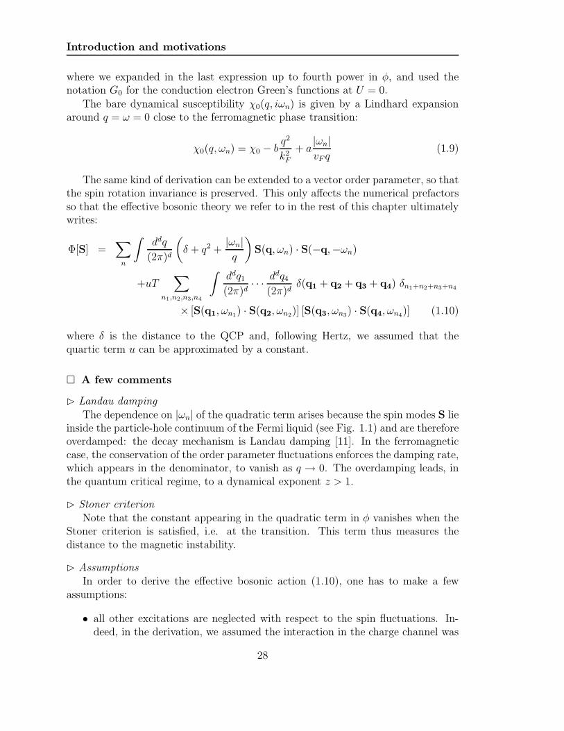
The same kind of derivation can be extended to a vector order parameter, so thatthe spin rotation invariance is preserved. This only affects the numerical prefactorsso that the effective bosonic theory we refer to in the rest of this chapter ultimatelywrites:
Φ[S] =∑
n
∫ddq
(2π)d
(
δ + q2 +|ωn|q
)
S(q, ωn) · S(−q,−ωn)
+uT∑
n1,n2,n3,n4
∫ddq1(2π)d
· · · ddq4
(2π)dδ(q1 + q2 + q3 + q4) δn1+n2+n3+n4
× [S(q1, ωn1) · S(q2, ωn2)] [S(q3, ωn3) · S(q4, ωn4)] (1.10)
where δ is the distance to the QCP and, following Hertz, we assumed that thequartic term u can be approximated by a constant.
A few comments
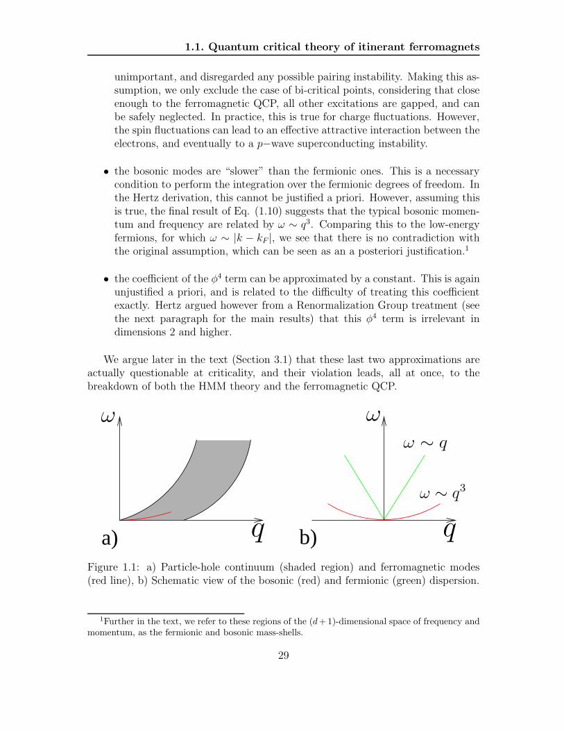
⊲ Landau dampingThe dependence on |ωn| of the quadratic term arises because the spin modes S lie
inside the particle-hole continuum of the Fermi liquid (see Fig. 1.1) and are thereforeoverdamped: the decay mechanism is Landau damping [11]. In the ferromagneticcase, the conservation of the order parameter fluctuations enforces the damping rate,which appears in the denominator, to vanish as q → 0. The overdamping leads, inthe quantum critical regime, to a dynamical exponent z > 1.
⊲ Stoner criterionNote that the constant appearing in the quadratic term in φ vanishes when the
Stoner criterion is satisfied, i.e. at the transition. This term thus measures thedistance to the magnetic instability.
⊲ AssumptionsIn order to derive the effective bosonic action (1.10), one has to make a few
assumptions:
• all other excitations are neglected with respect to the spin fluctuations. In-deed, in the derivation, we assumed the interaction in the charge channel was
28
1.1. Quantum critical theory of itinerant ferromagnets
unimportant, and disregarded any possible pairing instability. Making this as-sumption, we only exclude the case of bi-critical points, considering that closeenough to the ferromagnetic QCP, all other excitations are gapped, and canbe safely neglected. In practice, this is true for charge fluctuations. However,the spin fluctuations can lead to an effective attractive interaction between theelectrons, and eventually to a p−wave superconducting instability.
• the bosonic modes are “slower” than the fermionic ones. This is a necessarycondition to perform the integration over the fermionic degrees of freedom. Inthe Hertz derivation, this cannot be justified a priori. However, assuming thisis true, the final result of Eq. (1.10) suggests that the typical bosonic momen-tum and frequency are related by ω ∼ q3. Comparing this to the low-energyfermions, for which ω ∼ |k − kF |, we see that there is no contradiction withthe original assumption, which can be seen as an a posteriori justification.1
• the coefficient of the φ4 term can be approximated by a constant. This is againunjustified a priori, and is related to the difficulty of treating this coefficientexactly. Hertz argued however from a Renormalization Group treatment (seethe next paragraph for the main results) that this φ4 term is irrelevant indimensions 2 and higher.
We argue later in the text (Section 3.1) that these last two approximations areactually questionable at criticality, and their violation leads, all at once, to thebreakdown of both the HMM theory and the ferromagnetic QCP.
ω ω
q q
ω ∼ q3
ω ∼ q
a) b)Figure 1.1: a) Particle-hole continuum (shaded region) and ferromagnetic modes(red line), b) Schematic view of the bosonic (red) and fermionic (green) dispersion.
1Further in the text, we refer to these regions of the (d+1)-dimensional space of frequency andmomentum, as the fermionic and bosonic mass-shells.
29

Introduction and motivations
Millis and Moriya additions
In order to obtain a quantitative description, Moriya and Kawabata developed amore sophisticated theory, the so-called self-consistent theory of spin fluctuations[12]. This theory is very successful in describing magnetic materials with strongspin fluctuations outside the quantum critical region. As for the quantum criticalregime of itinerant ferromagnets, this leads to identical results to those of Hertztheory [13].
Later, Millis [14] revisited the theory developed by Hertz. He considered anadditional scaling equation for the temperature, which allowed him to correct someof Hertz’ results concerning the crossover behavior at finite temperature.
For these reasons, the quantum critical theory, associated to the effective action(1.10), is known as the Hertz-Millis-Moriya theory.
Results
We now present the main results of the HMM theory for the ferromagnetic QCP.From the effective action (1.10), Hertz applied a Renormalization Group (RG)
treatment. Eliminating the outer-shell defined as:e−l < q < 1e−zl < ω < 1
(1.11)
where z is the dynamical exponent and l an infinitesimal scaling factor, one can leavethe quadratic and the quartic terms of the effective action unchanged by rescaling q,ω and S, and imposing scaling conditions on the parameters δ and u. The rescalingof frequency and momentum requires that z = 3 in order for the q2 term to scalelike the Landau damping.
Incorporating the contribution of the outer-shell beyond the simple rescaling,this leads to the following:
dδ
dl= 2δ + 2uf(T, δ) (1.12a)
du
dl= (4− (d+ z)) u− 4u2g(T, δ) (1.12b)
dT
dl= zT (1.12c)
where f and g are complicated integrals depending on T and δ. The last equation,missed by Hertz, was proved by Millis to be important for the finite temperaturecrossover regime.
The set of equations (1.12) already suggests the existence of an unstable Gaussianfixed point at T = u = δ = 0. Moreover, close to this critical point, the interactionu is irrelevant if d+ z > 4 (i.e. if d > d+
c = 1) , and one then expects the exponentsto be those of the Gaussian model.
30

1.2. Experiments
Solving the set of RG equations, one can extract the behavior in temperatureof several physical properties in the quantum critical regime for a 3-dimensionalsystem:
Specific heat: Cv ∼ T log
(T0
T
)
(1.13a)
Resistivity: ρ(T ) ∼ T 5/3 (1.13b)
Susceptibility: χ(T ) ∼ χ0 − χ1T4/3 (1.13c)
Critical temperature: Tc(δ) ∼ |δ − δc|3/4 (1.13d)
1.2 Experiments
Magnetic quantum phase transitions are among the most studied ones experimen-tally. In this section, we present some experimental results concerning the quantumcritical regime of some itinerant ferromagnetic compounds.
1.2.1 Successes
The behavior of many physical properties in the quantum critical regime of itiner-ant ferromagnets, as predicted by the Hertz-Millis-Moriya theory, was observed inseveral compounds.
NixPd1−x
Pd is a strongly enhanced Pauli paramagnet, close to ferromagnetic order. It has longbeen known [15] that roughly 2.5% of nickel ions doped into palladium induce sucha ferromagnetic order. Below 10% of doping, the induced structural and magneticdisorder is rather small and is believed to play only a minor role.
Nicklas and collaborators [16] studied samples of NixPd1−x for doping concen-trations 0 ≤ x ≤ 1. They observed the following:
• close to x = 0.1, a clear change of slope appears in the logTc vs. log(x − xc)plot, revealing a (x−xc)3/4 behavior at low doping (see Fig. 1.2). They couldextract from these data that the critical concentration xc = 0.026± 0.002,
• at x = 0.026, the resistivity follows a T 5/3 dependence for more than twodecades in temperature (see Fig. 1.2). The exponent changes quickly as onedeparts form xc either way, signaling that the quantum critical behavior islimited to a narrow region around the critical doping,
• the heat capacity linear coefficient Cv/T increases logarithmically towards lowtemperature for a range of doping 0.022 ≤ x ≤ 0.028 (see Fig. 1.3),
All these results match the predictions of the HMM theory for the quantumcritical regime.
31

Introduction and motivations
a) b)
Figure 1.2: NixPd1−x, data from [16]: a) Curie temperature Tc as a function of x−xc.The dashed line indicates (x − xc)1/2 and the doted line (x − xc)3/4; b) Resistivityas a function of temperature for three concentrations: in the paramagnet x = 0.01,in the ferromagnet x = 0.05, and at the critical doping xc = 0.026. The solid linesstand for ρ = ρ0 + AT n.
Zr1−xNbxZn2
Although it is made of non-magnetic constituents, ZrZn2 is a ferromagnetic com-pound at low temperature. The Curie temperature at which the ferromagneticordering develops can be reduced towards zero by applying pressure (see next para-graph) or doping with niobium.
Sokolov and collaborators [17] studied the phase diagram of Nb-doped ZrZn2,for concentrations 0 ≤ x ≤ 0.14. They observed that upon doping, the criticaltemperature of the ferromagnetic transition continuously drops like a power-law:Tc(x) ∼ (x−xc)3/4 (see Fig. 1.3). The critical concentration where the extrapolatedcritical temperature terminates is estimated to be xc = 0.083± 0.002.
They could also measure the susceptibility close to this critical doping, in theparamagnetic region. The temperature dependent part of the susceptibility behavesas 1/χ∗ = (χ−1 − χ−1
0 ) = aT 4/3 (see Fig. 1.3) close to the QCP. The temperatureT ∗(x) below which this power-law behavior develops is maximum for x = xc anddrops as one departs from it, ultimately vanishing at x = 0.15.
The quantum critical behavior documented by Sokolov et al. is in excellentagreement with the theoretical predictions of the HMM theory.
1.2.2 Departures from HMM results
Nevertheless, experimental studies have revealed notable differences from the stan-dard second order behavior predicted by Hertz, Millis and Moriya.
32

1.2. Experiments
1200
800
400
0
1/aχ∗
12008004000T
4/3 (K
4/3)
x=0.08
x=0.09
x=0.12
x=0.14
104
105
106
1/χ∗
(µB/f
.u.)-1
10T
4/3 (K
4/3)
1 102
x=0.06
x=0.03
50
40
30
20
10
00.080.060.040.020.0
Nb concentration x
0.2
0.1
0.00
m0(
0) (
µ B/f.u
.)
40200TC (K)
α=1.04
α=1.0
(b)
Tc
a) b) c)
Figure 1.3: NixPd1−x, data from [16]: a) Specific heat vs. log T for three concentra-tions. The quadratic temperature dependence has been subtracted from these data,and the prefactor δ of the logarithmic term is shown in the inset. Zr1−xNbxZn2, data
from [17]: b) Variation of the Curie temperature Tc (white dots) and T4/3c (black
dots) as a function of the Nb concentration. The solid lines are fits to Tc ∝ (x− xc)and T
4/3c ∝ (x− xc); c) The inverse susceptibility 1/χ∗ = (χ−1 − χ−1
0 ) for x ≥ xc isproportional to T 4/3 (solid line) for T ≤ T ∗.
Superconductivity
The first departure from the HMM results concerns the development of a super-conducting instability. This is actually expected as in order to derive the effectivebosonic action, we made the assumption that all excitations but the spin fluctuationscould be neglected. As a result, it would be quite surprising that the HMM the-ory predicts the existence of a superconducting phase without including a possibleinstability towards that state from the very beginning.
A superconducting instability has been reported at very low temperature inseveral compounds, among which ZrZn2 [18], UGe2 [19] and URhGe [20] (see Fig.1.4).
The existence of such a superconducting state generated a lot of interest as itseems to develop only inside the ferromagnetically ordered phase, and might haveties with the magnetic quantum critical point. We choose not to detail here thevarious aspects of the controversy these results initiated, since we will not discussin this work the properties of the ordered state.
First order transition
The second and most interesting departure from the standard results of the HMMtheory stands in the order of the transition towards the ferromagnetic state. Hertz,Millis and Moriya predicted a second order transition all the way down to the quan-tum critical point. However, a first order transition at low temperature has been
33
Introduction and motivations
observed in almost all the itinerant materials investigated to date2.
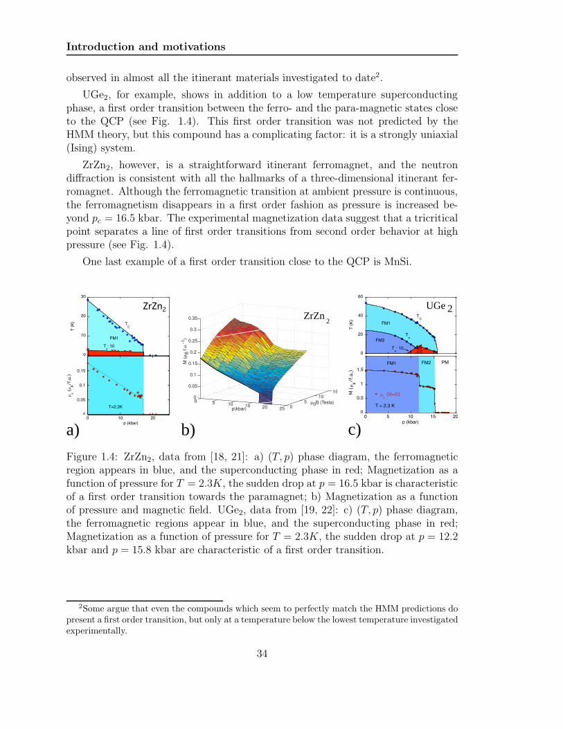
UGe2, for example, shows in addition to a low temperature superconductingphase, a first order transition between the ferro- and the para-magnetic states closeto the QCP (see Fig. 1.4). This first order transition was not predicted by theHMM theory, but this compound has a complicating factor: it is a strongly uniaxial(Ising) system.
ZrZn2, however, is a straightforward itinerant ferromagnet, and the neutrondiffraction is consistent with all the hallmarks of a three-dimensional itinerant fer-romagnet. Although the ferromagnetic transition at ambient pressure is continuous,the ferromagnetism disappears in a first order fashion as pressure is increased be-yond pc = 16.5 kbar. The experimental magnetization data suggest that a tricriticalpoint separates a line of first order transitions from second order behavior at highpressure (see Fig. 1.4).
One last example of a first order transition close to the QCP is MnSi.
ZrZn2
0
10
20
30
T (
K)
TC
Ts
* 10
FM1
0
0.05
0.1
0.15
µs (µ
B/f.
u.)
T=2.3K
0 10 20
p (kbar)
0 5 10 15 20 25 05
1015
0
0.05
0.1
0.15
0.2
0.25
0.3
0.35
µ0B (Tesla)
p(kbar)
M (
µB
f.u
.-1
)
0
0.5
1
1.5
µs (H=0)M
(µ
B/f.
u.)
T = 2.3 K
FM1 FM2 PM
0
20
40
60
T (
K)
FM1
FM2
TC
Tx
Ts* 10
0 5 10 15 20p (kbar)
a) b) c)
ZrZn2
UGe 2
Figure 1.4: ZrZn2, data from [18, 21]: a) (T, p) phase diagram, the ferromagneticregion appears in blue, and the superconducting phase in red; Magnetization as afunction of pressure for T = 2.3K, the sudden drop at p = 16.5 kbar is characteristicof a first order transition towards the paramagnet; b) Magnetization as a functionof pressure and magnetic field. UGe2, data from [19, 22]: c) (T, p) phase diagram,the ferromagnetic regions appear in blue, and the superconducting phase in red;Magnetization as a function of pressure for T = 2.3K, the sudden drop at p = 12.2kbar and p = 15.8 kbar are characteristic of a first order transition.
2Some argue that even the compounds which seem to perfectly match the HMM predictions dopresent a first order transition, but only at a temperature below the lowest temperature investigatedexperimentally.
34

1.3. Non-analytic static spin susceptibility
1.2.3 The puzzling case of MnSi
For completeness, we present here some of the results associated to MnSi, which wasone of the first itinerant magnet where a first order transition was discovered [23].It turns out that the behavior of this compound deviates from the HMM picture inseveral aspects beyond the simple order of the transition [24, 25].
MnSi is a very well-known system, perhaps the most extensively studied itinerantelectron magnet apart from iron, cobalt, nickel and chromium. At ambient pressure,the ground-state below the magnetic ordering temperature Tc = 29.5K is a three-dimensional weakly spin-polarized Fermi-liquid state. As the pressure in increased,the critical temperature continuously approaches zero. The order of the transition,however, changes from second order at ambient pressure to first order below p∗ = 12kbar.
The ordered state of MnSi is not a simple ferromagnet: the crystalline structurelacks an inversion symmetry, and weak spin-orbit interactions (of a Dzyaloshinsky-Moriya form) destabilizes the uniform ferromagnetic order and introduces a helicalmodulation. Further spin-orbit interactions lock the direction of the spiral in thedirection Q = 〈111〉.
The most surprising features of MnSi come from the region of the phase diagramabove the critical pressure pc where the transition temperature vanishes. This regionof the phase diagram seems to be the cleanest example of an extended non-Fermiliquid (NFL) state in a three-dimensional metal: the bulk properties of MnSi suggestthat sizable quasi-static magnetic moments survive far into the NFL phase. Thesemoments are organized in an unusual pattern with partial long-range order. Theresistivity displays a power-law behavior ρ ∼ T 1.5, characteristic of the NFL state, upto the highest pressure achieved experimentally, i.e. extending at low temperaturefar away from the QCP (see Fig. 1.5).
MnSi seems to question not only the results of the HMM theory, but the wholequantum criticality paradigm, and remains an understood puzzle to date.
1.3 Non-analytic static spin susceptibility
1.3.1 Long-range correlations
It is well known that in fluids, that is in interacting many-body systems, thereare long-range correlations between the particles. For example, in classical fluidsin thermal equilibrium, there are dynamical long-range correlations in time thatmanifest themselves as long-time tails. However long-range spatial correlations inclassical systems in equilibrium are impossible due to the fluctuation-dissipationtheorem.
In quantum statistical mechanics, though, statics and dynamics are coupled andneed to be considered together, allowing long-range spatial correlations to develop.
35

Introduction and motivations
0
10
20
30
0 10 20 30
TC
T0
T (
K)
p (kbar)
pc
p*
NFL
a) b)
Figure 1.5: a) Temperature vs. pressure phase diagram of MnSi. The insets qualita-tively show the location and key features of elastic magnetic scattering intensity inreciprocal space. At high pressure, the neutron scattering signal disappears abovea temperature T0 represented by a dotted line. b) Schematic phase diagram withapplied magnetic field in the third direction. The non-Fermi liquid behavior seemsto extend to the region of finite magnetic field.
In return, this leads to non-analyticities in the limit of small momentum.Following this idea, Belitz, Kirkpatrick and Vojta (BKV) [26] studied the long-
wavelength properties of the spin-density correlation function (i.e. the spin suscep-tibility) of a Fermi liquid using a perturbative expansion in the interaction.
The existence of non-analytic corrections to the Fermi liquid theory has a long-standing history and it has been predicted that such non-analyticities occur in thespecific heat coefficient [27] but was thought not to affect the spin and charge sus-ceptibilities.
BKV proved that in a three-dimensional Fermi liquid, away from criticality, theleading long-wavelength dependence of the static susceptibility reads, up to second-order in perturbation theory:
χ3D(q)
χ3D(0)= 1 + c3
|q|2k2F
log
( |q|2kF
)
+O(|q|2) (1.14)
where c3 is a negative prefactor.Later on, Chubukov and Maslov confirmed that a non-analytic dependence of
the static spin susceptibility survives below d = 3 [28, 29], becoming:
χ2D(q)
χ2D(0)= 1 + c2
|q|kF
+O(|q|2) (1.15)
in two dimensions, where c2 is again a negative prefactor.
36
1.3. Non-analytic static spin susceptibility
Both groups of authors argued that these non-analytic corrections to the Fermi-liquid theory originate from the singularities in the dynamic particle-hole responsefunction.
Following these results, Belitz and collaborators argued that the LGW functional,derived in the HMM approach, was formally ill-defined as the spin susceptibility en-ters the quadratic term in φ. The non-analyticities in the static susceptibility wouldthen prevent a continuous quantum phase transition towards the ferromagnetic or-der. The authors argued that such a mechanism could explain the failures of theHMM approach, and the appearance of a first order ferromagnetic transition closeto the QCP.
1.3.2 Effect on the quantum critical regime
It is a priori unclear, however, whether the results of Belitz et al. can be extendedto the quantum critical regime. We emphasize that these results have been derivedin a generic Fermi liquid, away from criticality.
Approaching the quantum critical point, one expects the effective four-fermioninteraction to be strongly renormalized (which is consistent with a divergence ofthe effective mass at criticality). This would lead to a breakdown of the simpleperturbative expansion performed by Belitz et al. Moreover, experimentally, theFermi liquid behavior does not seem to survive as one approaches the QCP [30, 31]which may invalidate the results derived perturbatively for a Fermi liquid.
The first main motivation of our work is to clarify this issue and check whetherthe non-analytic behavior predicted in the Fermi liquid phase survives as one ap-proaches the QCP (perhaps under a somewhat different form) or is washed out inthe quantum critical regime.
In the next chapters, we re-analyze the problem of the quantum critical regime ofitinerant ferromagnets. We build a controllable expansion close to the QCP, withoutintegrating out the low-energy fermions, and analyze in details the stability of theferromagnetic quantum critical point.
As one can see from (1.14) and (1.15), the effect of long-range correlations ismore dramatic as the dimensionality is lowered. For that reason, we focus in all thiswork on the case of a two-dimensional system, close to criticality.
37

Introduction and motivations
38

CHAPTER 2
Eliashberg theory of thespin-fermion model
Contents
2.1 Spin-fermion model . . . . . . . . . . . . . . . . . . . . . . 40
2.1.1 Low-energy model . . . . . . . . . . . . . . . . . . . . . . 40
2.1.2 Forward scattering model . . . . . . . . . . . . . . . . . . 41
2.2 Direct perturbative results . . . . . . . . . . . . . . . . . . 43
2.2.1 Bosonic polarization . . . . . . . . . . . . . . . . . . . . . 44
2.2.2 One-loop fermionic self-energy . . . . . . . . . . . . . . . 44
2.2.3 Two-loop fermionic self-energy . . . . . . . . . . . . . . . 46
2.2.4 Conclusion . . . . . . . . . . . . . . . . . . . . . . . . . . 47
2.3 Eliashberg theory . . . . . . . . . . . . . . . . . . . . . . . 48
2.3.1 Self-consistent solution . . . . . . . . . . . . . . . . . . . . 48
2.3.2 A few comments . . . . . . . . . . . . . . . . . . . . . . . 50
2.4 Validity of the approach . . . . . . . . . . . . . . . . . . . 54
2.4.1 Vertex corrections . . . . . . . . . . . . . . . . . . . . . . 55
2.4.2 Self-energy corrections . . . . . . . . . . . . . . . . . . . . 60
2.4.3 Summary . . . . . . . . . . . . . . . . . . . . . . . . . . . 64
39

Eliashberg theory of the spin-fermion model
In this chapter, we describe the starting model for our study of the ferromagneticquantum critical point. After a direct perturbative treatment which justifies the needto include the curvature, we carry out a self-consistent approximate treatment (alsoknown as “Eliahberg theory”) and check a posteriori that the assumptions made forthese computations are indeed justified.
2.1 Spin-fermion model
We argued in the previous chapter that integrating the fermions out of the partitionfunction was a questionable way of studying the quantum critical regime, becauseof the possible non-analyticities that are missed in such a procedure.
Therefore, our starting point for the study of the ferromagnetic quantum criti-cal point is a model describing low-energy fermions interacting with Landau over-damped collective bosonic excitations. These excitations are spin-fluctuations andbecome gapless at the quantum critical point.
2.1.1 Low-energy model
The general strategy to derive such a low-energy model is to start with a modeldescribing the fermion-fermion interaction, and assume that there is only one low-energy collective degree of freedom near the QCP. This assumption is basically thesame as one of the HMM assumptions: the idea is to exclude all excitations butthe ferromagnetic spin fluctuations we are interested in. One then has to decouplethe four-fermion interaction term using the critical bosonic field as an Hubbard-Stratonovich field, and integrate out of the partition function all high-energy degreesof freedom, with energies between the fermionic bandwidth W and some cutoffΛ [32].
If this procedure was performed completely we would obtain a full Renormaliza-tion Group treatment of the problem. Unfortunately, there is no controllable schemeto perform this procedure. It is widely believed, though that although the propaga-tors of the remaining low-energy modes possess some memory of the physics at highenergies, the integration of high-energy fermions does not give rise to anomalousdimensions for the bare fermionic and bosonic propagators in the low-energy model.
In practical terms, this assumption implies that the bare propagator of the rel-evant collective mode is an analytic function of momentum and frequency, and thefermionic propagator has the Fermi liquid form:
G(k, ω) =Z0
iω − ǫk, (2.1)
where Z0 < 1 is a constant, and ǫk is the renormalized band dispersion.Near the Fermi surface,
ǫk = vFk⊥ +k2‖
2mB. (2.2)
40

2.1. Spin-fermion model
Here k is the momentum deviation from kF, the parallel and perpendicular com-ponents are with respect to the direction along the Fermi surface at kF, mB is theband mass, the Fermi velocity vF = kF/m, and for a circular Fermi surface one hasm = mB.
Following this scheme, the original model of fermions interacting with themselvescan be recast into an effective low-energy fermion-boson model. In the context ofthe magnetic QCP, this model is known as the “spin-fermion model” and was firstsuggested by Chubukov and collaborators [32].
Close to the ferromagnetic quantum critical point, the low-energy degrees offreedom are:
• fermions, whose propagator is given by Eq. (2.1);
• long-wavelength collective spin excitations whose propagator (in this case, thespin susceptibility) is analytic near q = Ω = 0, and is given by:
χs,0(q,Ω) =χ0
ξ−2 + q2 + AΩ2 +O(q4,Ω4). (2.3)
In this last expression, A is a constant, and ξ is the correlation length of themagnetic spin fluctuations, which diverges at the QCP. We prove, further in thischapter, that the quadratic term in frequency does not play any role in our anal-ysis. Indeed, one can argue that the interaction of these collective bosonic modeswith fermions close to the Fermi surface generates a Landau damping of the spinfluctuations, as we demonstrate in the next section. As a consequence, we neglectfrom now on the Ω2 term in the spin susceptibility, and approximate the above barepropagator by the static one χs,0(q).
The model can then be described by the following Hamiltonian:
Hsf =∑
k,α
ǫkc†k,αck,α +
∑
q
χ−1s,0(q)SqS−q + g
∑
k,q,α,β
c†k,ασαβck+q,β · Sq. (2.4)
where Sq are vector bosonic variables, and g is the effective fermion-boson interac-tion. For convenience, we incorporated the fermionic residue Z0 into g.
We emphasize that the above spin-fermion model cannot be derived in a trueRG-like procedure, and has to be considered as a phenomenological model whichcaptures the essential physics of the problem.
2.1.2 Forward scattering model
To illustrate how this effective Hamiltonian can, in principle, be derived from themicroscopic model of interacting conduction electrons, we consider a model in which
41
Eliashberg theory of the spin-fermion model
the electrons interact with a short range four-fermion interaction U(q) and assumethat only the forward scattering is relevant (U(0) = U):
H =∑
k,α
ǫkc†k,αck,α +
1
2
∑
q
U∑
k,k′,α,β
c†k,αck+q,αc†k′βck′−q,β, (2.5)
In this situation, the interaction is renormalized independently in the spin andin the charge channels [33]. Using the identity for the Pauli matrices:
σαβ · σγδ = −δαβδγδ + 2δαδδβγ (2.6)
one can demonstrate [33] that in each of the channels, the Random Phase Ap-proximation (RPA) summation is exact, and the fully renormalized four-fermioninteraction Ufull
αβ,γε(q) is given by:
Ufullαβ,γε(q) = U
[
δαγδβε
(1
2+ Gρ
)
+ σαγσβε
(1
2+ Gσ
)]
, (2.7)
where σαβ are Pauli matrices, and
Gρ ≡1
2
1
1− UΠ (q); Gσ ≡ −
1
2
1
1 + UΠ (q), (2.8)
with Π(q) = −m2π
(1 − a2(q/kF )2) is the fermionic bubble made out of high-energyfermions, and a > 0.
For positive values of U satisfying mU/2π ≈ 1, the interaction in the spin channelis much larger than the one in the charge channel. Neglecting then the interactionin the charge channel, we can simplify the Hamiltonian (2.5):
H =∑
k,α
ǫkc†k,αck,α +
1
2
∑
q
Ueff (q)∑
k,k′,α,β,γ,δ
c†k,ασαβck+q,β · c†k′γσγδck′−q,δ. (2.9)
where Ueff(q) = (1/2)U2Π(q)/(1 + UΠ(q)). Performing a Hubbard-Stratonovichdecomposition in the three fields Sq, one recasts (2.9) into Eq. (2.4) with:
g = U a2
χ0 = 2k2
F
Ua2
g = g2χ0 = (U/2)k2F
ξ−2 =k2
F
a2
(2πmU− 1)
(2.10)
The QCP is reached when mU/2π = 1, i.e., ξ−2 = 0. This coincides with the Stonercriterion for a ferromagnetic instability [8].
We emphasize that the bosonic propagator in Eq. (2.3) does not contain theLandau damping term. This is because we only integrated out the high-energy
42
2.2. Direct perturbative results
a)q,Ω
b)k, ω
c)k, ω
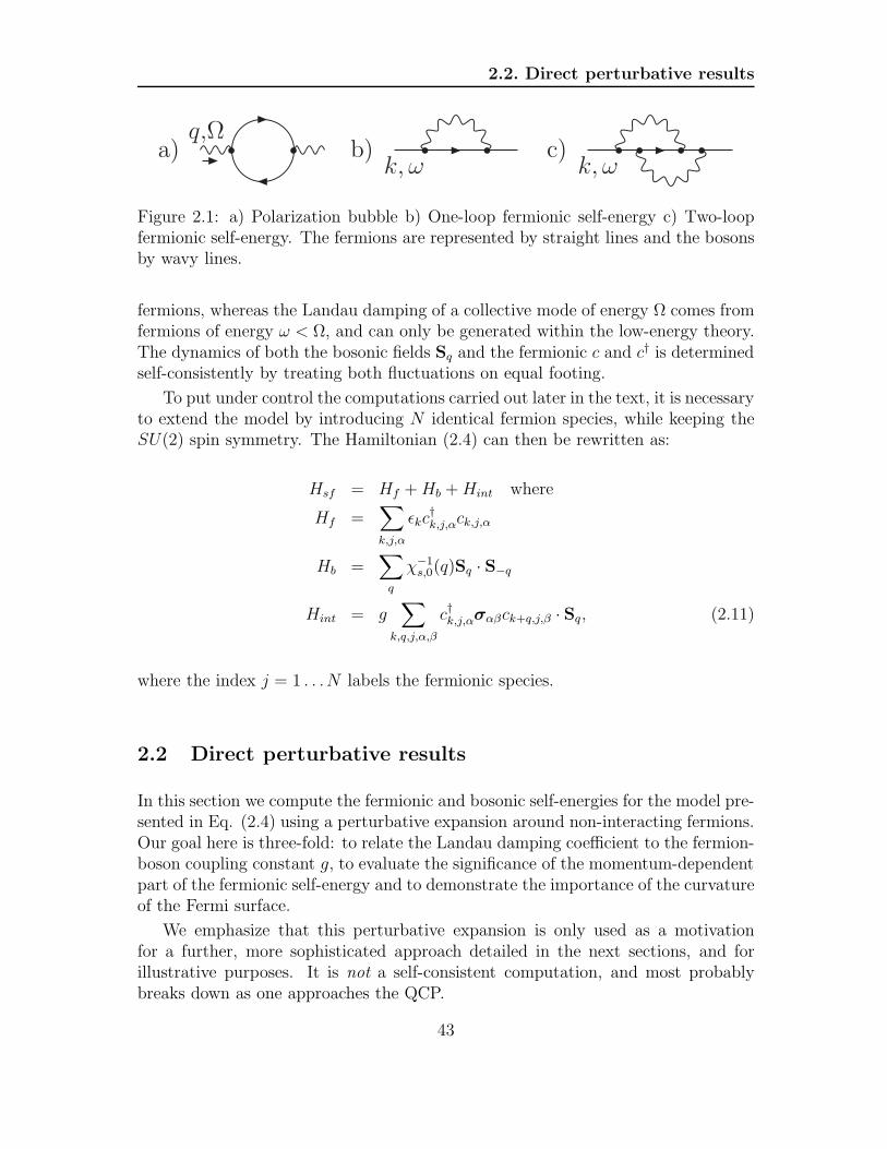
Figure 2.1: a) Polarization bubble b) One-loop fermionic self-energy c) Two-loopfermionic self-energy. The fermions are represented by straight lines and the bosonsby wavy lines.
fermions, whereas the Landau damping of a collective mode of energy Ω comes fromfermions of energy ω < Ω, and can only be generated within the low-energy theory.The dynamics of both the bosonic fields Sq and the fermionic c and c† is determinedself-consistently by treating both fluctuations on equal footing.
To put under control the computations carried out later in the text, it is necessaryto extend the model by introducing N identical fermion species, while keeping theSU(2) spin symmetry. The Hamiltonian (2.4) can then be rewritten as:
Hsf = Hf +Hb +Hint where
Hf =∑
k,j,α
ǫkc†k,j,αck,j,α
Hb =∑
q
χ−1s,0(q)Sq · S−q
Hint = g∑
k,q,j,α,β
c†k,j,ασαβck+q,j,β · Sq, (2.11)
where the index j = 1 . . .N labels the fermionic species.
2.2 Direct perturbative results
In this section we compute the fermionic and bosonic self-energies for the model pre-sented in Eq. (2.4) using a perturbative expansion around non-interacting fermions.Our goal here is three-fold: to relate the Landau damping coefficient to the fermion-boson coupling constant g, to evaluate the significance of the momentum-dependentpart of the fermionic self-energy and to demonstrate the importance of the curvatureof the Fermi surface.
We emphasize that this perturbative expansion is only used as a motivationfor a further, more sophisticated approach detailed in the next sections, and forillustrative purposes. It is not a self-consistent computation, and most probablybreaks down as one approaches the QCP.
43

Eliashberg theory of the spin-fermion model
2.2.1 Bosonic polarization
The full bosonic propagator depends on the self-energy Π(q,Ω) according to:
χs(q,Ω) =χ0
ξ−2 + q2 + Π(q,Ω). (2.12)
At the lowest order in the spin-fermion interaction, the bosonic self-energy isgiven by the first diagram in Fig. 2.1, and reads:
Π(q,Ω) = 2Ng
∫d2k dω
(2π)3G(k, ω) G(k + q, ω + Ω). (2.13)
The curvature of the fermionic dispersion does not affect much the result ofthis computation as it only leads to small corrections in q/mBvF . Neglecting thequadratic term in the fermionic propagators, we introduce the angle θ defined asǫk+q = ǫk + vF q cos θ and perform the integration over ǫk, which gives us:
Π(q,Ω) = iNgm
2π2
∫ +∞
−∞dω (θ(ω + Ω)− θ(ω))
∫ 2π
0
dθ1
iΩ− vF q cos θ
=Nmg
π
|Ω|√
(vF q)2 + Ω2. (2.14)
At the QCP, the bosonic mass-shell corresponds to the region of momentum andfrequency space for which the terms in the inverse propagator are of the same order,i.e. near a mass shell q and Ω satisfies Π(q,Ω) ∼ q2. It follows that, at the QCP, nearthe bosonic mass shell, vF q/Ω ∼ vF (mgv2
F/Ω2)1/3 ≫ 1 at small enough frequency,
so that vF q is the largest term in the denominator of Π(q,Ω). The expression of thebosonic self-energy then reduces to:
Π(q,Ω) = γ|Ω|q, (2.15)
where γ =Nmg
πvF.
We see that the lowest order bosonic self-energy recovers the form of the Landaudamping presented in Chapter 1, with a prefactor depending on the fermion-bosoncoupling constant.
As explained earlier, this term is larger than a regular O(Ω2) term, and fullydetermines the dynamics of the collective bosonic mode.
2.2.2 One-loop fermionic self-energy
We now turn to the fermionic self-energy, right at the QCP, where ξ−1 = 0. To thelowest order in the interaction, the fermionic self-energy contains one bosonic line,
44

2.2. Direct perturbative results
as represented in Fig.2.1.b, and its analytic form writes:
Σfree1 (k, ω) = 3ig2
∫d2q dΩ
(2π)3G0(k + q, ω + Ω)χ(q,Ω). (2.16)
The superscript “free” implies that we use the free fermionic G0(k, ω) in the integralfor the self-energy.
In a direct perturbation theory in g, one would have to use the bare form of thebosonic propagator, Eq. (2.3), which leads to Σ(ω) ∝ logω. However, this result isuseless, as we already know that the Landau damping term completely overshadowsa regular frequency dependence in (2.3). It makes more sense then to estimate theperturbative self-energy using the full bosonic propagator Eq. (2.12). This is not afully self-consistent procedure, but we use it here to estimate the functional form ofthe self-energy at various orders in perturbation around free fermions.
It is instructive to distinguish between Σ(kF, ω) = Σ(ω) and Σ(k, 0) = Σ(k).Indeed, there is an asymmetry in the behavior of the fermionic self-energy dependingon whether one computes it at zero frequency or at zero momentum departure fromthe Fermi surface. This feature is one of the key elements of the self-consistenttreatment presented in the next section.
Frequency dependence
Substituting the renormalized bosonic propagator with the Landau damping terminto (2.16), the frequency-dependent self-energy reads:
Σfree1 (ω) =
3ig
(2π)3
∫
dΩ qdq dθ1
q2 + γ |Ω|q
1
i(ω + Ω)− vF q cos θ. (2.17)
Here θ is the angle between kF and q, and we linearized the fermionic dispersion.Evaluating the integral over the angle, and using that the typical internal bosonicmomentum q ∼ Ω1/3 is much larger than Ω ∼ ω, we obtain:
Σfree1 (ω) =
3g
2π2vF
∫ ω
0
dΩ
∫dq q
q3 + γ|Ω|= ω
1/30 ω2/3, (2.18)
where
ω0 =3√
3g3
8π3v3Fγ
=3√
3g2
8π2Nmv2F
. (2.19)
This result has been first obtained in Ref. [34, 35] when treating the interactionof low-energy fermions with singular gauge fields. It suggests that in D = 2, theinteraction between bare fermions and critical bosons leads to a breakdown of theFermi-liquid behavior: at low energies, the ω2/3 term in (2.18) is larger than thebare ω in the fermionic propagator. This obviously makes one wonder if higherorder insertions lead to even more singular contributions.
45

Eliashberg theory of the spin-fermion model
Momentum dependence
Before looking at higher-order self-energy corrections, we compute the one-loopmomentum-dependent self-energy Σ(k), given by:
Σfree1 (k) =
3ig
(2π)3
∫
dΩ qdq dθ1
q2 + γ |Ω|q
1
iΩ− ǫk − vF q cos θ
=3g
(2π)2ǫk
∫dΩ dq
q2 + γ |Ω|q
q|Ω|(Ω2 + (vF q)2)3/2
. (2.20)
One can make sure that the integral is infrared-convergent, i.e. Σfree(ǫk) ∝ ǫk, withan interaction dependent prefactor, which also depends on the upper cutoff of thetheory, Λ.
This suggests that the momentum dependent part of the fermionic self-energy,unlike the frequency-dependent part derived earlier, is regular at the QCP and onlyleads to a finite mass renormalization.
2.2.3 Two-loop fermionic self-energy
As the one-loop frequency-dependent self-energy seems to dominate over the bare ωterm of the fermionic propagator, one could wonder whether higher-order insertionslead to even more singular contributions.
To investigate this issue, we next calculate the contribution to the fermionic self-energy Σ(ω) from diagrams at the two-loop level, and focus, for illustrative purposes,on the diagram presented in Fig. 2.1.c, which writes:
Σfree2 (ω) ∼ g2
∫
dω1d2q1
∫
dω2d2q2 G(kF + q1, ω + ω1) G(kF + q2, ω + ω2)
× G(kF + q1 + q2, ω + ω1 + ω2) χs(q1, ω1) χs(q2, ω2),(2.21)
where we use the full bosonic propagator, the free fermionic one, and we restrictourselves to the frequency dependence of this contribution to the self-energy.
We first compute this integral expanding the dispersion of the internal fermionsto linear order, since the quadratic term was not significant in the computationof the one-loop bosonic and fermionic self-energy. Choosing the x axis along theexternal k = kF and integrating over qx1 and qx2 , we are left with:
Σfree2 (ω) ∼ g2
v2Fω
∫ ω
0
dω1dq1y
q21y + γ|ω1|
q1y
∫ ω
ω−ω1
dω2dq2y
q22y + γ|ω2|
q2y
∼ ω2/30 ω1/3. (2.22)
where ω0 is defined in (2.19).
46
2.2. Direct perturbative results
At low-energy, this two-loop self-energy diverges faster than the one-loop self-energy obtained in (2.18). Estimating higher-order diagrams, we find that they forma series in powers of (ω0/ω)1/3, such that the perturbative expansion around freefermions breaks down at ω ∼ ω0.
This result is in line with the one obtained by Lawler et al. [36], in the context of aQCP in the charge channel using a two-dimensional bosonization scheme. The scaleω0 is related by ω0 = vF/x0 to the spatial scale at which the equal time fermionicGreen’s function G(x), obtained from bosonization, begins decaying exponentially
(G(x) ∝ e−(x/x0)1/3).
However, the divergence of the perturbation theory can be cured once the cur-vature of the fermionic dispersion is included, as we now show. We re-evaluate thetwo-loop self-energy (2.21), using now the full fermionic dispersion, Eq. (2.2), with-out neglecting the quadratic term. After integrating over the momentum componentqx1 and qx2 , one has:
Σfree2 (ω) ∼ g2
v2F
∫ ω
0
dω1dq1y
q21y + γ|ω1|
q1y
∫ ω
ω−ω1
dω2dq2y
q22y + γ|ω2|
q2y
1
iω − q1yq2y
mB
∼ m2B g
2
γ2v2F
ω log2 ω. (2.23)
When the curvature of the fermionic dispersion is included, we see that thetwo-loop self-energy turns out to be small compared to its one-loop counterpart,at low energy. In a separate study [37], Chubukov and Khveshchenko reconsideredthe bosonization procedure in the presence of the curvature and obtained the sameresults as in (2.23).
2.2.4 Conclusion
As a conclusion, this first crude approach suggests that both the fermionic andthe bosonic self-energies are important at the QCP. The bosonic self-energy setsthe dynamics of the bosons, while the fermionic self-energy is non-analytic andparametrically larger than the bare ω term at low energy, which implies a breakdownof the Fermi-liquid behavior at criticality.
We argued that only the frequency-dependent part of the self-energy matters, themomentum-dependent one only leads to a regular renormalization of the effectivemass.
We also found that the curvature of the Fermi surface actually plays a veryimportant role in regularizing the perturbative expansion, which was missed byprevious studies in comparable low-energy models.
However, the full account of these effects cannot be obtained from this simpleanalysis. For example, we did not account here for the mutual effects of the self-energies onto each other. One has to develop a controllable way to treat the bosonicand fermionic self-energies on equal footing, in a self-consistent fashion.
47

Eliashberg theory of the spin-fermion model
Since we found that only the frequency-dependent Σ(ω) is relevant, a way toproceed is to verify whether an Eliashberg-like theory, similar to the one developedin the context of phonon superconductivity[38], may be such a controllable approx-imation.
2.3 Eliashberg theory
The Eliashberg procedure allows to compute the fermionic self-energy Σ(ω) and thebosonic polarization Π(q,Ω), by solving the self-consistent set of coupled Dyson’sequations, neglecting all contributions coming from the vertex corrections and themomentum-dependent fermionic self-energy.
2.3.1 Self-consistent solution
Specifically the Eliashberg theory follows three steps:
• neglect both the vertex corrections and the momentum dependent part of thefermionic self-energy, i.e. approximate:
Σ(k, ωn) = Σ(ωn)
gTot = g + ∆g = g (2.24)
• construct the set of self-consistent Dyson’s equations:
G−1(k, ωn) = iωn − vF (k − kF ) + iΣ(ωn)
χs(q,Ωm) =χ0
ξ−2 + q2 + Π(q,Ωm), (2.25)
with the following fermionic and bosonic self-energies:
iΣ(ωn) =k, ωn
χ−10 Π(q,Ωm) =
q,νm(2.26)
The fermionic Green’s functions in (2.26) are full (they are represented dia-grammatically by a straight line) and χs(q,Ωm) is the full bosonic propagator(represented by a wavy line).
• check a posteriori that the neglected terms ∆g and Σ(k), are all parametricallysmall.
48

2.3. Eliashberg theory
The evaluation of the momentum integral for the fermionic self-energy in theEliashberg theory requires care. Since fermions are faster than bosons, the leadingcontribution to Σ(ω) is obtained if one integrates over the momentum componenttransverse to the Fermi surface only in the fermionic propagator and sets this com-ponent to zero in the bosonic propagator (this implies that the momentum integralis factorized).
One can show that the corrections that arise from keeping the transverse com-ponent of momentum in the bosonic propagator are small to the same parameteras ∆g/g and should therefore be neglected, as keeping them would be beyond theaccuracy of the theory.
The evaluation of the bosonic and fermionic self-energies within the Eliashbergtheory is presented in Appendices A and B. We list here the main results.
Away from the QCP
At large but finite correlation length ξ and for a bosonic momentum and frequencysatisfying vF q ≫ Σ(Ω) we obtain:
Π(q,Ω) = γ|Ω|q
, and
Σ(ω) = λωF (γωξ3) ,
(2.27)
where F (x ≪ 1) = 1 + O(x), and F (x ≫ 1) = 2√3x−1/3. The parameter γ is the
same as for free fermions,
γ =Nmg
πvF, (2.28)
and λ is the dimensionless coupling
λ =3g
4πvF ξ−1g = g2χ0 (2.29)
At finite ξ−1 and vanishing ω, the self-energy has a Fermi liquid form:
Σ(ω) = λω. (2.30)
The Fermi liquid theory is stable in this case, and the low-energy quasiparticleshave a finite effective mass:
m∗ = m(1 + λ). (2.31)
The effective mass diverges proportionally to ξ in the vicinity of the QCP.
49

Eliashberg theory of the spin-fermion model
At criticality
At ω ≫ (γξ3)−1, however, the system is in the quantum-critical regime. Herethe Fermi liquid theory breaks down in the sense that the quasiparticles dampingbecomes comparable to its energy. We have:
Σ(ω) = ω1/30 |ω|2/3sign(ω), (2.32)
where ω0 = 3√
3g2/(8π2Nmv2F ) is the same as in (2.19).
At the QCP, ξ−1 = 0, the region of Fermi-liquid behavior collapses in frequencyspace, and the ω2/3 dependence of the self-energy extends down to the lowest fre-quencies. The expression for Σ(ω) is valid for all frequencies below the cutoff Λ.
However, only frequencies ω ≤ ω0 are actually relevant for the quantum criticalregime, as at higher frequencies the system behaves as a nearly ideal Fermi gas.
2.3.2 A few comments
General remarks
One has to make a few remarks concerning the Eliashberg solution obtained at theQCP:
⊲ Curvature
Note that the curvature of the fermionic dispersion is unimportant here forboth self-energies, and only accounts for small corrections containing higherpowers of frequencies.
⊲ Direct perturbative expansion
Comparing (2.27) and (2.32) with (2.15) and (2.18), we see that the self-energies in the Eliashberg theory coincide with the one-loop perturbative re-sults around free fermions that we carried out in the previous section. Thisarises from the fact that the full fermionic propagator appears in both self-energies only via the fermionic density of states (DOS):
N(ω) =i
π
∫
dǫk1
ω + Σ(ω)− ǫk. (2.33)
This DOS reduces to N(ω) = Sign(ω), independently on the self-energy: itremains the same as for free fermions.
⊲ Bosonic momentum and frequency
Note that Eq. (2.27) for the bosonic self-energy is only valid as long as theinterplay between the external momentum and frequency is such that vF q ≫Σ(Ω). When this is verified, the Landau damping term no longer depends on
50

2.3. Eliashberg theory
the fermionic self-energy, which explains why we recover the same expressionfor the self-consistent treatment and the direct perturbative expansion. In theopposite limit, the vertex corrections cannot be neglected as we argue in thenext section.
Mass-shells
A lot of the computations we carry out in the further sections are estimated based onthe typical bosonic and fermionic momenta and frequencies. Indeed, from inspect-ing the propagators, one can isolate a region of the three-dimensional momentum-frequency space where they are maximum. It follows that the quantities we computeare dominated by these regions of the phase space.
We thus distinguish two “mass shells”, defined respectively as:
• the fermionic one is given by G(k, ω)−1 ≃ 0, i.e. at the fermionic mass-shell,one has:
|k− kF| ∼ω + Σ(ω)
vF(2.34)
• the bosonic mass-shell, on the other hand, is given by:
|q| ∼ (γ|Ω|)1/3 (2.35)
In the computations carried out in the next sections, we argue that the resultstrongly depends on the typical internal bosonic momentum and frequency. Depend-ing whether one, two, or none of the components of this internal bosonic momentumvibrate on the bosonic mass-shell, we end up with very different results.
Factors of N
We argue in the next section that the extension of the model to N fermionic flavorsis essential for the validity of the current approach. However, it can be readily seenfrom (2.27) and (2.32) that both self-energies contain factors of N through theirprefactors.
In a “conventional” large-N approach, one would have to rescale the effectiveinteraction g prior to taking the infinite N limit. In this situation, the bosonicpolarization is of order O(1) but the fermionic one vanishes like 1/N so that thelarge-N limit describes free fermions and overdamped bosons. However, we sawthat the frequency dependence of the fermionic self-energy suggests that it mightdominate over the bare propagator for N finite. It is thus reasonable to analyze theeffects of this frequency-dependent self-energy.
Following this reasoning, we argue that our approach is not an infinite N limit,but rather an asymptotic expansion, where we keep N finite but consider it is largeenough to allow us to neglect higher-powers of N .
51

Eliashberg theory of the spin-fermion model
For further analysis of the corrections to the Eliashberg theory, it is then conve-nient to rescale N out of the formulas for Σ(ω) and for Π(q,Ω). This can be doneby rescaling m, mB and kF leaving vF intact:
m→ m/N mB → mB/N kF → kF/N. (2.36)
We emphasize that the fermionic self-energy Σ ∝ ω2/3 and the Landau dampingterm in the bosonic propagator do not contain N after rescaling. They are includedinto the new “zero-order” theory about which we then expand using 1/N as a smallparameter. This theory includes:
χ(q,Ω) =χ0
ξ−2 + q2 + γ|Ω|/qG(k, ω) =
1
i(ω + Σ(ω))− ǫk.
(2.37)
We can reformulate the Eliashberg theory by introducing the following effectiveLagrangian describing the fermion-boson interaction:
L = LF + LB + Lint ,with
LB =T∑
q,n
Sq,nχ−1(q,Ωn)S−q,−n,
LF =T∑
k,n,α,j
c†k,j,n,αG−1(k, ωn)ck,j,n,α,
Lint =gT 2∑
n,m,k,q
Sq,mc†k,j,nασαβck−q,j,n−m,β, (2.38)
where n,m number Matsubara frequencies, α, β are spin indices, j is a flavor index,and G and χ are given by (2.37). The upper limit of the frequency summation isthe cutoff Λ.
We emphasize that there is no double counting in the bosonic propagator (2.37a).The integration of high-energy fermions, above the cutoff Λ leads to the momentumdependence of the static bosonic propagator, whereas the interaction at frequenciesbelow Λ gives rise to the Landau damping, without affecting the static part.
To summarize, the Eliashberg-type theory at the QCP contains a non-analyticfermionic self-energy which scales as ω2/3 and breaks down the Fermi liquid descrip-tion of fermions. At the same time, the bosonic propagator is regular – the onlyeffect of the interaction with low-energy fermions is the appearance of a Landaudamping.
We emphasize that the fully renormalized bosonic susceptibility does not neces-sarily coincide with the one in (2.37) and may, in particular, acquire an anomalousdimension [39]. However, this can only be due to infra-red divergent corrections tothe Eliashberg theory, which are fully captured by the effective low-energy model ofEq. (2.38). An anomalous dimension was proved to emerge at the antiferromagneticQCP in d = 2 [32, 39], but not in our case.
52

2.3. Eliashberg theory
Expression Definition Eq.
vF Fermi velocity (2.2)
m bare quasiparticle mass, m = kF/vF (2.2)
m∗ effective (renormalized) quasiparticle mass (2.31)
mB band mass, determines the curvature of theFermi surface
(2.2)
g spin-fermion coupling constant (2.4)
ξ ferromagnetic correlation length (2.3)
χ0ξ2 value of the spin susceptibility at q = 0 (2.3)
N number of fermionic flavors
g=g2χ0 effective four-fermion interaction (2.29)
γ=NmgπvF
Landau damping coefficient (2.28)
λ= 3gξ4πvF
dimensionless coupling constant, it mea-sures the mass enhancement: λ = m∗
m− 1
(2.29)
ω0=3√
3g3
8π3γv3F∼ g2
EFfrequency up to which Σ(ω) dominatesover ω in the fermionic propagator
(2.32)
ωMax=√
γv3F ∼√gEF frequency up to which the fermionic and
the bosonic mass-shells are well separated(2.42)
α= g2
γv3F∼ g
EFsmall parameter measuring the slownessof the bosonic modes compared to thefermionic ones; the same small parameterjustifies the low-energy description
(2.39)
β=mB
mNsmall parameter related to the curvatureof the fermionic dispersion
(2.53)
Table 2.1: List of the various parameters used in the text, their expression beforethe rescaling in N , and the reference equation where it is defined in the text.
53

Eliashberg theory of the spin-fermion model
2.4 Validity of the approach
The essential part of the Eliashberg procedure is an a posteriori verification that theneglected terms in the self-energies are small. Quite generally, the validity of thisprocedure is based on the idea that the fermions are fast excitations compared tothe bosons, and hence the fermionic and bosonic mass shells are well separated inenergy.
When scattering off physical mass-shell bosons, the fermions are forced to vibrateon the bosonic mass shell, which is far away from their own. The electronic spectralfunction near the bosonic mass-shell is then small and this reduces the self-energythat arises from true fermion-boson scattering. In the case of the electron-phononinteraction, this is known as the Migdal theorem, and ensures that the correctionsto the electron-phonon vertex are small.
The computation of the fermionic self-energy Σ(ω) gives us an idea of whatthe typical intermediate momenta and frequencies are in the problem. One canmake sure that at criticality the typical fermionic momenta k − kF are of orderΣ(ω)/vF = ω
1/30 ω2/3/vF . On the other hand, the typical bosonic momenta q⊥ along
the direction of kF (i.e. transverse to the Fermi surface) are of the same order as thetypical fermionic momenta, while the momenta q‖ transverse to kF (i.e. along the
Fermi surface) are of order (γω)1/3 ≫ ω1/30 ω2/3/vF . We see that for a given frequency
ω, the typical |q| =√
q2⊥ + q2
‖ are much larger than k − kF , i.e. the effective boson
velocity is much smaller than vF . One then expects that the extension of Migdaltheorem to our model holds.
The ratio of the typical fermionic k − kF and bosonic |q| at the same frequencyω is (ω0ω/γv
2F )1/3. At ω ∼ ω0, this ratio then becomes, after rescaling in N :
α =
(ω2
0
γv3F
)1/3
∼ g
EF, (2.39)
and the slowness of the bosonic mode is then ensured in the quantum critical regimeprovided that α≪ 1. This condition coincides, in our case, with the condition thatthe interaction should be smaller than the bandwidth. This is a necessary conditionfor the effective low-energy model to be valid, for if it is not satisfied, one cannotdistinguish between contributions coming from low and from high energies.
However, the smallness of α is not sufficient. In the integral for the fermionicself-energy, only one component of the bosonic momentum, q‖, is much larger thank − kF , the other one is comparable: q⊥ ∼ k − kF . One needs to check whether thecorrections to the Eliashberg theory scale as the ratio of k − kF to the modulus of|q| or one of its components.
To address these issues, we explicitly compute the vertex corrections and thefermionic self-energy at the two-loop level.
54
2.4. Validity of the approach
2.4.1 Vertex corrections
We consider the vertex corrections due to the insertion of one bosonic propaga-tor (three-leg vertex) and two bosonic propagators (four-leg vertex). The behaviorof these vertex corrections strongly depends on the interplay between the internaland external momenta and frequencies. We present the results below and discusstechnical details of the calculations in Appendix C.
In the case of the three-leg vertex, the result strongly depends on the interplaybetween external as well as internal momentum and frequency. We thus distinguishbetween three cases.
Three-leg vertex with zero external momentum and frequency
We begin with the simplest 3-leg vertex, with strictly zero incoming frequency Ω andmomentum q. The one-loop vertex renormalization diagram contains one bosonicline and is presented in Fig. 2.2a. In analytic form, it writes:
∆g
g
∣∣∣∣q=Ω=0
∼ g2
∫
dωd2p G(kF, ω)2 χ(p, ω)
∼ g
∫dωd2pγ|ω|p
+ p2
1(
iΣ(ω)− vFpx − p2y2mB
)2 , (2.40)
where we defined Σ(ω) = ω+ Σ(ω) and we have chosen kF along the x axis, so thatpx = p⊥ and py = p‖.
Since the poles coming from the fermionic Green’s functions are in the same halfplane, the integral over qx is only non-zero because of the branch cut in the bosonicpropagator. At the branch cut px ∼ py, so that we can safely drop the quadraticterm in the fermionic propagators. Introducing polar coordinates, and integratingsuccessively over the angle between kF and p, then over the modulus p, we obtain:
∆g
g
∣∣∣∣q=Ω=0
∼ g
γv3F
∫ ωMax
0
dωΣ(ω)
ω, (2.41)
where ωMax is the frequency up to which bosons are slow modes compared tofermions, i.e. up to which Σ(ω)/vF ≪ (γω)1/3. This frequency exceeds ω0, soto find it we have to use Σ(ω) ≈ ω. We then obtain:
ωMax ∼√
γv3F . (2.42)
which reduces to ωMax ∼√gEF after the rescaling in N . Note that for small values
of α, ωMax ≫ ω0, and the maximum frequency up to which the bosons can be treatedas slow modes well exceeds the upper limit of the quantum-critical behavior.
55

Eliashberg theory of the spin-fermion model
Substituting Σ and ωMax into (2.41), we obtain
∆g
g
∣∣∣∣q=Ω=0
∼ √α (2.43)
This correction to the vertex can then be neglected provided that α is small.
Three-leg vertex with finite external momentum
We now turn to the three-leg vertex with zero external frequency but a finite bosonicmomentum q. The one-loop renormalization is given in Fig.2.2, and its analytic formwrites:
∆g
g
∣∣∣∣q,Ω=0
∼ g2
∫
dωd2p G(kF + p + q, ω)G(kF + p, ω)χ(p, ω)
∼ g
∫dωd2pγ|ω|p
+ p2
1
iΣ(ω)− vFpx − p2y2mB
× 1
iΣ(ω)− vF qx − vFpx − p2y2mB− qypy
mB
, (2.44)
where px is the projection of p along kF.As before, the integral over px can be reduced to the contribution from only the
branch cut in the bosonic propagator. At the branch cut, px ∼ py, hence we canneglect the quadratic term in the fermionic Green’s function, which then allows usto integrate over py. Expanding in qx, and subtracting the constant term at zeromomentum calculated in (2.41), we obtain:
∆g
g
∣∣∣∣q,Ω=0
− ∆g
g
∣∣∣∣q=Ω=0
∼ iqxkF
∫
|vF qx|
dω
|ω| log[iΣ(ω)]
∼ qxkF
log |qx|, (2.45)
When not only the bosonic momentum q is finite but also the external fermionicmomentum is away from kF , the q log q dependence of the static vertex correctionsurvives, but the argument of the logarithm is the maximum of the bosonic q andfermionic k − kF (we directed both along x).
In general, the typical value of qx is much smaller than kF , hence the momentumdependent part of this vertex correction is small. However, we argue in the nextchapter that because of the logarithmic term in (2.45), the insertion of this vertexcorrection into the static susceptibility gives rise to a non-analytic term.
We also emphasize that although the calculations of ∆gg
∣∣∣q=Ω=0
and ∆gg
∣∣∣q,Ω=0
look
similar, the characteristic bosonic momenta are different for the two cases. At
56

2.4. Validity of the approach
q = Ω = 0, the typical bosonic momenta in (2.40) are of order (γω)1/3, i.e. near thebosonic mass shell. On the other hand, the typical bosonic momenta in (2.44) areof order Σ(ω)/vF , i.e. near the fermionic mass shell. This is why only one of thesetwo vertex corrections is small in α, as this parameter measures the slowness of thebosonic modes compared to the fermionic ones.
Generic three-leg vertex
We next consider the same vertex with small but finite external momentum q andfrequency Ω. This diagram, presented in Fig. 2.2b, reads:
∆g
g
∣∣∣∣q,Ω
∼ g2
∫
dωd2p G(kF + p + q, ω + Ω)G(kF + p, ω) χ(p, ω)
∼ g
∫dωd2pγ|ω|p
+ p2
1
iΣ(ω)− vFpx − p2y2mB
× 1
iΣ(ω + Ω)− vF qx − vFpx − p2y2mB− qypy
mB
, (2.46)
where we have chosen kF along the x axis, so that qx = q⊥ and qy = q‖.Integrating over px first, one obtains two contributions: one arising from the
poles in the fermionic Green’s functions (which now can be in different half-planessince Ω is finite), and the other from the branch cut in the bosonic propagator. Thelatter leads to the same result as (2.41), up to small corrections due to the finitenessof the external q and Ω.
Focusing on the other contribution, one has:
∆g
g
∣∣∣∣q,Ω
∼ ig
vF
∫ Ω
0
dω
∫
dpy|py|
γ|ω|+ |py|31
iΣ(Ω− ω) + iΣ(ω)− vF qx − qypy
mB
, (2.47)
where the simplification of the frequency integral comes from the pole structure inpx.
This generic correction to the vertex strongly depends on the interplay betweenthe external qx, qy, and Ω.
When q and Ω are both finite,
∆g
g
∣∣∣∣q,Ω
∼ F(vF q
Σ(Ω)
)
, (2.48)
where
F(x) =
∫ 1
0
dz
z1/3
1
(1− z)2/3 + z2/3 + ix(2.49)
has the following asymptotic behavior:F(x≪ 1) = O(1)F(x≫ 1) = O
(1x
) (2.50)
57

Eliashberg theory of the spin-fermion model
If the typical external momentum q is on the bosonic mass shell, then q ∼ (γΩ)1/3,and one has:
∆g
g
∣∣∣∣q,Ω
∼ Σ(Ω)
vF qx∼ √α
(Ω
ωMax
)1/3
. (2.51)
This is obviously small in α.It turns out that the behavior of the vertex correction is more complex and the
result for ∆g/g strongly depends on the direction of q compared to the direction ofkF .
This directional dependence is important for our purposes as we saw in previouscomputations that in the fermionic self-energy, only the y component of the internalbosonic momentum is near the bosonic mass shell and scales as (γΩ)1/3, while thex component of the bosonic momentum is much smaller and is actually of the orderof Σ(ω)/vF , i.e. is near the fermionic mass shell.
Let’s take a more careful look at this vertex correction, depending on the direc-tion of q.
For the case where qx ∼ Σ(Ω)/vF and qy ∼ (γΩ)1/3, one would argue from (2.51)that the vertex correction now becomes of order O(1) and is no longer parametri-cally small. However, the computation that lead to (2.51) cannot be extended tothe strongly anisotropic case as for external qx ∼ Σ(Ω)/vF and qy ∼ (γΩ)1/3, thecurvature of the fermionic dispersion becomes relevant and changes the result.
The full dependence on qx and qy is rather complex and we restrict ourselvesto the case when the importance of the curvature ensures that 1
NmB
m≪ 1. In this
situation, q2y/mB ∼ (vF qx)/β ≫ vF qx, so that the quadratic term in the fermionic
propagator dominates.Performing the integration, we then find that:
∆g
g
∣∣∣∣q,Ω
∼ β2
(γΩ
q3y
)2/3
log2
[
β(γΩ)1/3
qy
]
∼ β2 log2 β, (2.52)
where
β =1
N
mB
m≪ 1. (2.53)
It follows that even when only one component of the bosonic momentum is nearthe bosonic mass shell, the vertex correction is small if β is small. This is the secondcondition for the Eliashberg theory to be controllable at criticality.
The smallness of β can be ensured by either extending the theory to large valuesof N , or by considering a very strong curvature of the Fermi surface which impliesthat mB ≪ m. Even though the latter can hardly be satisfied for realistic Fermisurfaces, we emphasize that the curvature of the dispersion plays a crucial role inthe theory, for even in the case of N ≫ 1, the vertex correction is of order O(1)without this very curvature.
58

2.4. Validity of the approach
a)0, 0
kF, 0
b)Q, 0
kF, 0
c)Q,Ω
kF, 0
Figure 2.2: Three-leg vertices: a) zero external momentum and frequency b) finitemomentum c) generic vertex.
Pairing vertex
By contrast to the previous vertices we studied, the pairing vertex in the Cooperchannel is not sensitive to the curvature of the Fermi surface. This leads to a vertexof order O(1) even in the large-N limit and the pairing problem then has to becarried out exactly within the Eliashberg theory.
This vertex renormalization is presented in Fig. 2.3 and its analytic form is givenby:
∆g
g
∣∣∣∣Cooper
∼ g2
∫
dωd2q χ(q, ω) G(kF + q, ω)G(−kF − q,−ω − Ω)
∼ g
∫dωd2qγ|ω|q
+ q2
1
iΣ(ω)− vF qx − q2y2mB
1
−iΣ(ω + Ω)− vF qx − q2y2mB
.
Integrating over qx, restricting ourselves to the contribution from the fermionicpoles (the one from the branch cut can be proved to be smaller), we find that thequadratic terms cancel out, leaving us with:
∆g
g
∣∣∣∣Cooper
∼ g
vF
∫ D
|Ω|
dω
Σ(ω + Ω) + Σ(ω)
∫ ∞
0
dqy qyγω + q3
y
. (2.54)
Performing the remaining integral, the prefactor simplifies and we obtain:
∆g
g
∣∣∣∣Cooper
∼ g
γ1/3ω1/30 vF
log
∣∣∣∣
Ω
D
∣∣∣∣
∼ log
∣∣∣∣
Ω
D
∣∣∣∣, (2.55)
where we assumed that we were in the quantum critical regime, i.e. |Ω| < ω0.We emphasize that the prefactor of the log in (2.55) is O(1), even when one
takes into account the curvature of the fermionic dispersion. The result of Eq.(2.55) confirms previous studies [40] advocating that the system at a ferromagneticQCP can lead to a superconducting instability.
59

Eliashberg theory of the spin-fermion model
Four-leg vertex
We consider now higher-order corrections to the vertex through the example of afour-leg vertex correction with two crossed bosonic lines, also called a Cooperoninsertion. Analytically, the expression for this renormalized vertex, presented dia-grammatically in Fig. 2.3, writes:
Γ2(q,Ω) ∼ g2
∫
dωd2p χs
(Ω + ω
2,p + q
2
)
χs
(Ω− ω
2,q− p
2
)
×G(
Ω + ω
2,kF +
p + q
2
)
G
(Ω− ω
2,kF +
q− p
2
)
(2.56)
After integrating over px (projection of p along kF), and ω, we are left with:
Γ2(q,Ω) ∼ g2
vF
Ω
|qy|3∫
dz
√(
z2 + q2
q2y
)2
− 4z2
2iΣ(
Ω2
)− vF qx − q2y
4m(1 + z2)
× 1(
z2 + 2z + q2
q2y
)3/2
+ γ|Ω||qy|3
1(
z2 − 2z + q2
q2y
)3/2
− γ|Ω||qy|3
, (2.57)
where we have changed py into z = py/|qy|.This renormalized 4-leg vertex Γ2(q,Ω) has to be compared with the bare four-
leg vertex, whose analytic form is given by the bosonic propagator multiplied byg2:
Γ1(q,Ω) ∼ g
q2 + γ|Ω|q
. (2.58)
In the case of a typical external momentum qx ∼ qy ∼ (γΩ)1/3, the ratio Γ2/Γ1 isof order α. For a typical qx ∼ Σ(ω)/vF and qy ∼ (γω)1/3, we obtain, to logarithmicaccuracy:
Γ2
Γ1∼ β ≪ 1. (2.59)
This last result again critically depends on the curvature of the Fermi sur-face: neglecting the quadratic terms in the fermionic propagators, one would obtainΓ2/Γ1 = O(1). We see that likewise to the three-loop vertices, the smallness of thecrossed vertex Γ2(q,Ω) requires both α and β to be small.
2.4.2 Self-energy corrections
The second element one has to check in order to validate the Eliashberg procedureconcerns the momentum-dependent self-energy. After verifying on the practicalexample of the two-loop self-energy, that the vertex correction analyzed above areindeed small, we turn to the computation of the momentum-dependent self-energyand the density of states.
60

2.4. Validity of the approach
a)0,−Ω
kF, 0
b)
kF, 0kF + q,Ω
kF, 0 kF + q,Ω
Figure 2.3: a) Cooper pairing vertex b) Four-leg vertex
Corrections to the self-energy at the two-loop level
We found in our analysis of the vertex corrections that the result depends on theinterplay between the typical momentum and frequency. In our estimates, we consid-ered two regions of external q and Ω, namely qx ∼ qy ∼ (γΩ)1/3 and qx ∼ Σ(ω)/vF ,qy ∼ (γΩ)1/3. In both cases, we found that the vertex corrections are small.
We verify here that the two-loop self-energy, obtained by inserting vertex cor-rections into the one-loop self-energy diagram, is also small.
The two-loop self-energy diagram is presented in Fig. 2.1. We have:
Σ2(ω) ∼ g2
∫
dω1d2q1
∫
dω2d2q2 χ(q1, ω1) χ(q2, ω2) G(kF + q1, ω + ω1)
×G(kF + q2, ω + ω2) G(kF + q1 + q2, ω + ω1 + ω2)
∼ g2
∫
dω1d2q1
∫
dω2d2q2
q1γ|ω1|+ q3
1
q2γ|ω2|+ q3
2
× 1
iΣ(ω + ω1)− vF q1x1
iΣ(ω + ω2)− vF q2x − q22y
2mB
× 1
iΣ(ω + ω1 + ω2)− vF q1x − vF q2x − q21y
2m− q22y
2mB
, (2.60)
where we recall Σ(ω) = ω + Σ(ω).
Integrating successively over q1x and q2x, and rescaling the remaining momentumcomponents by introducing x = q1y/(γ|ω1|)1/3 and y = q2y/(γ|ω2|)1/3, we obtain:
Σ2(ω) ∼ mB g2
v2F
∫ ω
0
dω2
∫ ω
ω−ω2
dω11
(γ2ω1ω2)2/3
∫ ∞
−∞
dxdy
xy + iζ
|xy|(1 + |x|3) (1 + |y|3)
(2.61)
where ζ = mBΣ(ω+ω1)+Σ(ω+ω2)−Σ(ω+ω1+ω2)
(γ2ω1ω2)1/3 .
As the typical frequencies ω1 and ω2 are of order ω, the typical value of ζ isof order β ≪ 1. Expanding then in (2.61) to first order in ζ and performing the
61

Eliashberg theory of the spin-fermion model
remaining integrals, we obtain in the quantum-critical regime:
Σ2(ω) ∼ mg2
v2F
∫ ω
0
dω2
∫ ω
ω−ω2
dω1ζ log2 ζ
(γ2ω1ω2)2/3
∼ Σ(ω) β2 log2 β, (2.62)
where Σ(ω) = Σ1(ω) = ω1/30 ω2/3 is the self-energy in the Eliashberg theory.
This result agrees with the one obtained in [30], and shows that Σ2(ω) ∼ Σ1(ω)×∆gg
∣∣∣q,Ω
where ∆gg
∣∣∣q,Ω
is given by (2.52). This last result implies that the typical
internal q and Ω for the Eliashberg self-energy and for Σ2(ω) are the same.It is also instructive to compare these two-loop results, obtained as an expansion
around the Eliashberg solution, to the perturbative expansion around free fermions.In the latter, we found in Eq. (2.23) that Σ2(ω) ∼ ω log2 ω whereas in the former
we have Σ2(ω) ∝ β(ω1/30 ω2/3) log2 β, Eq. (2.62). The free-fermion result can be
reproduced if we neglect the self-energy in (2.61). We see that the expansion aroundfree fermions does not reproduce the correct frequency dependence of Σ2(ω). Thisobviously implies that if one expands around free fermions, there exist higher-orderterms associated with insertions of the self-energy Σ(ω) into the internal fermioniclines, which may overshadow the two-loop result around free fermions. Accordingly,near the QCP, the expansion around free fermions does not converge, even if thecurvature of the fermionic dispersion is included. On the other hand, the expansionaround the Eliashberg solution is regular and holds in powers of the small parametersα and β.
Momentum dependence of the self-energy and the density of states
Along with the vertex corrections, we also neglected the momentum dependence ofthe fermionic self-energy in order to proceed with the Eliashberg scheme. We nowverify whether the momentum dependent part of the self-energy Σ(k, ω = 0) = Σ(k)remains small when evaluated with the full fermionic propagator. The k dependentself-energy is given by:
Σ(k, 0) = 3ig2
∫d2q dΩ
(2π)3G(k + q,Ω)χ(q,Ω)
=3ig
(2π)3
∫dΩd2q
iΣ(Ω)− ǫk+qq
γ|Ω|+ q3. (2.63)
Defining the angular variable θ as ǫk+q = ǫk + vF q cos θ, integrating over it, andexpanding to linear order in ǫk we obtain:
Σ(k, 0) = −3iǫk ×g
2π2
∫ ∞
0
dΩ Σ(Ω)
∫q2dq
(q3 + (γ|Ω|))(
(vF q)2 + Σ(Ω)2)3/2
. (2.64)
62

2.4. Validity of the approach
A simple experimentation with the integrals shows that the integration overmomentum is confined to q ∼ Σ(Ω)/vF , while the frequency integral is confined toΩ < ωMax, where ωMax, defined in (2.42), is the scale where (γΩ)1/3 = Σ(Ω)/vF . Thecomputation of Σ(k) is given in the Appendix B, and the result is
Σ(k, 0) = −iǫk ×3× 1.3308
2√
2π3/2
√α = −iǫk 0.253
√α (2.65)
Plugging this back into the fermionic propagator, we then obtain that Σ(k, 0) givesrise to a small, regular correction to the quasiparticle mass ǫk − iΣ(k, 0) = ǫ∗k =v∗F (k − kF ), where
v∗F = vF(1− 0.253
√α). (2.66)
Like the vertex correction at zero external bosonic momentum and frequency,this small correction is of order O(
√α) and comes from frequencies of order ωMax.
The momentum dependent self-energy, unlike the frequency dependent part, gen-erally gives rise to corrections to the fermionic density of states (DOS)
N(ω) ∼ −∫dǫkπ
ImG(ǫk, ω). (2.67)
Assuming that Σ(k) is small and expanding in it in the fermionic propagator,we obtain, in real frequencies
N(ω)
N0∼ 1− Im
(
Σ(k)
ǫk
∣∣∣∣ǫk=iΣ(−iω)
)
, (2.68)
where N0 is the density of states of free fermions.Substituting (2.65) into (2.68), we find that the density of states just shifts by a
constant. It follows that in order to extract the frequency dependence of the densityof states, one has to evaluate the momentum-dependent self-energy to the next orderin ǫk and on the mass shell, where ǫk = iΣ(ω).
The evaluation of the self-energy near a mass shell generally requires extra cau-tion as the self-energy may possess mass-shell singularities [33]. We, however, havechecked in Appendix F that in our case the self-energy does not possess any mass-shell singularity, and the self-energy remains finite on the mass shell.
The calculation of the self-energy to order ǫ2k is displayed in the Appendix B,and the result is
Σ(k, ω) = iǫk ×0.45
8πα|Σ(ω)| log
ω1
|ω| (2.69)
on the mass-shell.Substituting this self-energy into the expression for the DOS and converting to
real frequencies, we find at small ω
N(ω) ∼ N0
(
1−(ω
ω1
)2/3
log2 ωMax
ω
)
, (2.70)
63

Eliashberg theory of the spin-fermion model
where we explicitly defined
ω1 =128π5/2
0.453/2 33/4
g
α2. (2.71)
2.4.3 Summary
We have shown in this section that there are two conditions for the validity of theEliashberg theory that one can recast as the smallness of two parameters:
α ∼ g2
γv3F
∼ g
EF≪ 1 β ∼ mg
γvF∼ mB
Nm≪ 1. (2.72)
The first condition is quite generic for a low-energy theory since it requires thatthe fermion-fermion interaction mediated by the exchange of a boson should besmaller than the Fermi energy. Otherwise, the physics is not restricted to the vicinityof the Fermi surface anymore. The parameter α plays the same role as the Migdalparameter for the electron-phonon interaction: it sets the condition that fermionsare fast excitations compared to bosons. In the scattering processes that are small inα, fermions are forced by the interaction to vibrate at frequencies near the bosonicmass shell. They are then far from their own resonance and thus have a smallspectral weight.
However, the condition α ≪ 1 is not sufficient to construct a fully controllableperturbative expansion around the non-Fermi liquid state at the QCP. In spatiallyisotropic systems there exist vertex corrections for which the external momentumhas a component on the fermionic mass-shell. These corrections don’t contain α.However, these corrections are sensitive to the curvature of the Fermi surface, andare small if β is small which can be achieved either by imposing mB ≪ m or byextending the theory to a large number N of fermionic flavors.
In evaluating the renormalization of the static vertex, we silently assumed that√α≪ β, i.e., g/EF < (mB/m)2/N . At very large N , this is no longer valid, but in
this situation our estimates show that the static vertex is even smaller than√α.
Finally, the pairing vertex in the Cooper channel stays of order O(1), signalingthe possibility of a pairing instability close to the quantum critical point. Nev-ertheless, we assume, based on explicit calculations worked out in [40], that thequantum critical behavior extends in the parameter space to a region where thesuperconductivity is not present.
64

CHAPTER 3
Static spin susceptibility
Contents
3.1 Revisiting the Hertz-Millis-Moriya theory . . . . . . . . 66
3.1.1 φ4 term . . . . . . . . . . . . . . . . . . . . . . . . . . . . 66
3.1.2 φ3 term . . . . . . . . . . . . . . . . . . . . . . . . . . . . 68
3.2 Static spin susceptibility . . . . . . . . . . . . . . . . . . . 69
3.2.1 Away from the QCP . . . . . . . . . . . . . . . . . . . . . 71
3.2.2 At criticality . . . . . . . . . . . . . . . . . . . . . . . . . 73
3.3 Related results . . . . . . . . . . . . . . . . . . . . . . . . . 76
3.3.1 Finite temperature result . . . . . . . . . . . . . . . . . . 76
3.3.2 Three-loop fermionic self-energy . . . . . . . . . . . . . . 78
3.3.3 Conclusion . . . . . . . . . . . . . . . . . . . . . . . . . . 79
3.4 Non-SU(2) symmetric case . . . . . . . . . . . . . . . . . . 80
3.4.1 Discussion . . . . . . . . . . . . . . . . . . . . . . . . . . . 80
3.4.2 Ising case . . . . . . . . . . . . . . . . . . . . . . . . . . . 80
3.4.3 Charge channel . . . . . . . . . . . . . . . . . . . . . . . . 81
3.4.4 Physical arguments . . . . . . . . . . . . . . . . . . . . . . 81
In this chapter, we revisit the Hertz-Millis-Moriya φ4 theory using the solution ofour Eliashberg scheme at criticality. We then turn to the computation of the staticspin susceptibility, following the remarks of Belitz and collaborators: now that we
65
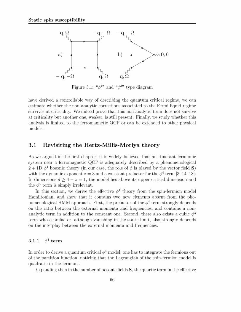
Static spin susceptibility
a)
− q,−Ω
q,Ω −q,−Ω
q,Ω
b)
q,Ω
−q,−Ω
0, 0
Figure 3.1: “φ4” and “φ3” type diagram
have derived a controllable way of describing the quantum critical regime, we canestimate whether the non-analytic corrections associated to the Fermi liquid regimesurvives at criticality. We indeed prove that this non-analytic term does not surviveat criticality but another one, weaker, is still present. Finally, we study whether thisanalysis is limited to the ferromagnetic QCP or can be extended to other physicalmodels.
3.1 Revisiting the Hertz-Millis-Moriya theory
As we argued in the first chapter, it is widely believed that an itinerant fermionicsystem near a ferromagnetic QCP is adequately described by a phenomenological2 + 1D φ4 bosonic theory (in our case, the role of φ is played by the vector field S)with the dynamic exponent z = 3 and a constant prefactor for the φ4 term [3, 14, 13].In dimensions d ≥ 4− z = 1, the model lies above its upper critical dimension andthe φ4 term is simply irrelevant.
In this section, we derive the effective φ4 theory from the spin-fermion modelHamiltonian, and show that it contains two new elements absent from the phe-nomenological HMM approach. First, the prefactor of the φ4 term strongly dependson the ratio between the external momenta and frequencies, and contains a non-analytic term in addition to the constant one. Second, there also exists a cubic φ3
term whose prefactor, although vanishing in the static limit, also strongly dependson the interplay between the external momenta and frequencies.
3.1.1 φ4 term
In order to derive a quantum critical φ4 model, one has to integrate the fermions outof the partition function, noticing that the Lagrangian of the spin-fermion model isquadratic in the fermions.
Expanding then in the number of bosonic fields S, the quartic term in the effective
66

3.1. Revisiting the Hertz-Millis-Moriya theory
action reads:
∫d2qd2pd2p′ dΩdνdν′
(2π)9A(p,p′,q, ν, ν′,Ω)
[Sp+q/2 · Sq/2−p Sp′−q/2 · S−p′−q/2
+ Sp+q/2 · S−p′−q/2 Sq/2−p · Sp′−q/2 − Sp+q/2 · Sp′−q/2 S−q/2−p′ · Sq/2−p]
(3.1)
where p, p′, q are bosonic momenta, and ν, ν′,Ω are bosonic frequencies.
Our goal here is to prove that the prefactor A is not a regular function of mo-menta and frequencies. To simplify the presentation, we choose to study only thedependence of A on q and Ω and set p,p′, ν, ν′ to zero (see Fig 3.1).
The analytic form of this prefactor then writes:
A(q,Ω) ∼ Ng4
∫
dω
∫
d2k G(k, ω)2 G(k + q, ω + Ω)2. (3.2)
Defining θ as the angle between k and q, and performing the integration overǫk, and the angular variable, we find:
A(q,Ω) ∼ mg4
ω0Ω
∫ 1
0
dy
[(vF qΣ(Ω)
)2
− 2(y2/3 + (1− y)2/3
)2]
[(vF qΣ(Ω)
)2
+ (y2/3 + (1− y)2/3)2
]5/2, (3.3)
where we performed the rescaling in N , defined y = ω/Ω, and neglected at thisstage a regular part that comes from large values of ǫk and for which the curvatureis relevant.
We see that A(q,Ω) depends on the interplay between the momentum and fre-quency. We can identify two regimes
• If |q| ∼ (γ|Ω|)1/3, i.e. if the bosonic momenta are near the bosonic mass shell,the self-energy in the denominator can be neglected. The frequency factors inthe numerator and the denominator then cancel out, and we obtain:
A(Ω) ∼ mg4
γv3F
∼ m
χ20
α , (3.4)
We see that A can be safely replaced by a constant O(α). This is consistentwith the previous works of Hertz, Millis and Moriya. The agreement is notsurprising as the relation q ∼ (γ|Ω|)1/3 is assumed in the power countingbased on the fact that the dynamic exponent z = 3. Note that the condition|q| ∼ (γ|Ω|)1/3 only specifies the magnitude of q, one of its components (e.g.,qx) can be much smaller.
67

Static spin susceptibility
• If q ∼ Σ(ω) ∼ ω1/30 Ω2/3vF (at ω < ω0), i.e. when a boson resonates near a
fermionic mass shell, the scaling arguments of the z = 3 theory are no longerapplicable. We have in this regime:
A(q,Ω) ∼ mg4
ω0Ω∼ m
χ20
EFΩ. (3.5)
In this case, A(Ω) is a singular function of frequency, and cannot be replacedby a constant.
We see therefore that the prefactor of the φ4 term is actually singular outsidethe scaling regime of a z = 3 theory.
3.1.2 φ3 term
In the similar spirit, one can construct a cubic term in the bosonic fields.
∫d2qd2pdΩdν
(2π)9B(p,q, ν,Ω) Sp · (Sq−p/2 × S−q−p/2), (3.6)
where the prefactor B is a convolution of three fermionic Green’s functions as pre-sented in Fig.3.1, and is given by:
B(q,p,Ω, ν) ∼ Ng3
∫
dω d2k G(k− p, ω − ν)G(
k− p
2− q, ω − ν
2− Ω
)
G(k, ω)
Proceeding as for the quartic term, we set for simplicity p = 0, ν = 0, andintegrate over ǫk and the angular variable, leading to:
B(q,Ω) ∼ mg3
ω2/30 Ω1/3
∫ 1
0
dy
(y2/3 + (1− y)2/3
)
[(vF qΣ(Ω)
)2
+ (y2/3 + (1− y)2/3)2
]3/2, (3.7)
where we again introduced the rescaled frequency y = ω/Ω, and performed therescaling in N .
We can again identify two regimes.
• In the z = 3 regime where q ∼ (γΩ)1/3, one can expand for large vF qΣ(Ω)
, whichleads to:
B(q,Ω) ∼ mg
χ0α
(Ω
ωMax
)2/3
, (3.8)
where ωMax is given by (2.42). This term is small in the quantum criticalregime where Ω < ω0 ∼ ωMaxα
3/2, and can be safely neglected.
68

3.2. Static spin susceptibility
• For q ∼ Σ(Ω), the remaining integral is of order O(1) and the result writes:
B(q,Ω) ∼ mg
χ0
1√α
(ωMax
Ω
)1/3
, (3.9)
which is large and cannot be neglected.
We demonstrate in the next section how the singular behavior of the φ3 and φ4
terms lead to a non-analytic contribution to the static spin susceptibility.
3.2 Static spin susceptibility
We found that the Eliashberg theory for fermions interacting with gapless long-wavelength bosons is stable and controlled by two small parameters. We verifiedthis by calculating the fermionic self-energy in a two-loop expansion around theEliashberg solution
One may wonder whether the same conclusions hold for the bosonic self-energyas well. In particular, what are the corrections to the static susceptibility χs(q, 0)?
For a ferromagnetic SU(2) QCP, for which the massless bosons are spin fluctu-ations, we show in this section that the corrections to the static spin susceptibilityare non-analytic: they scale like q3/2, and do not contain any prefactor except fora proper power of kF . Such terms obviously overshadow the regular q2 of the baresusceptibility at small enough momenta.
The physics behind the q3/2 term in χ(q, 0) at a ferromagnetic QCP is, by itself,not directly related to criticality: far away from the QCP, the spin susceptibilityalso contains negative, non-analytic |q| term as we argued in the first chapter. Thisterm gradually evolves as the correlation length ξ increases, and transforms into theq3/2 term at the QCP. Both these non-analyticities, at and away from the QCP,emerge because the boson-mediated interaction between fermions contain a long-range dynamic component, generated from the Landau damping.
We now estimate the effect of these singularities on physical quantities. Boththe φ3 and φ4 terms in the effective action give rise to corrections to the φ2 term,i.e. to the spin susceptibility. These corrections are obtained diagrammatically bycontracting the external legs of the φ3 and φ4 terms, as shown in Fig. 3.2.
The contributions from the φ4 terms have been considered in Publication 1. Thecontributions from cubic terms were missed, and were first considered in [41] in theanalysis of the spin susceptibility in the paramagnetic phase, away from a QCP.
Using the bosonic Dyson’s equation:
χ(q, 0) =χ0
ξ−2 + q2 + Π(q, 0)(3.10)
we define the static polarization bubble at this order by Π = Π1(q, 0) + Π2(q, 0) +Π3(q, 0)+Π4(q, 0), where the individual contributions are presented in Fig. 3.2, and
69

Static spin susceptibility
write:
Π1(q, 0) =ΓS1Ng
2
(2π)6χ0
∫
d2kdωd2ldΩ χs(l,Ω) G(ω, k) G(ω + Ω, k + l)
×G(ω + Ω, k + q + l) G(ω, k + q) (3.11a)
Π2(q, 0) =ΓS2Ng
2
(2π)6χ0
∫
d2kdωd2ldΩ χs(l,Ω) G(ω, k)2 G(ω + Ω, k + l)
×G(ω, k + q) (3.11b)
Π3(q, 0) =ΓS3N
2g3
(2π)9χ20
∫
d2kdωd2k′dω′dldΩ χs(l,Ω) χs(q + l,Ω) G(ω, k)
×G(ω + Ω, k + l + q) G(ω′, k′) G(ω′ + Ω, k′ + l + q)
×G(ω, k + q) G(ω′, k′ + q) (3.11c)
Π4(q, 0) =ΓS4N
2g3
(2π)9χ20
∫
d2kdωd2k′dω′dldΩ χs(l,Ω) χs(l,Ω) G(ω, k)
×G(ω, k + q) G(ω + Ω, k + l + q) G(ω′, k′)
×G(ω′ + Ω, k′ + l) G(ω′ + Ω, k′ + l + q) (3.11d)
The factors of N come from the fermionic loops and the numerical prefactorsfrom the following spin summations:
ΓS1 =∑
α,β,γ,δ
σZαβσβγσZγδσδα = −2 (3.12a)
ΓS2 =∑
α,β,γ,δ
σZαβσβγ · σγδσZδα = 6 (3.12b)
ΓS3 =∑
α,β,γ,δ,ǫ,ζ
σZαβ (σβγ · σδǫ) (σγα · σζδ)σZǫζ = 8 (3.12c)
ΓS4 =∑
α,β,γ,δ,ǫ,ζ
σZαβ (σβγ · σǫδ) (σγα · σδζ)σZζǫ = −8 (3.12d)
These four diagrams are related by pairs. To verify this, it is useful to expandthe products of Green’s functions according to:
G(ω1, k1)G(ω2, k2) =G(ω1, k1)−G(ω2, k2)
G−1(ω2, k2)−G−1(ω1, k1). (3.13)
Applying this to Π2(q, 0), we find that it splits into two parts. In one part, thepoles in ǫk are located in the same half-plane, leading to a vanishing contribution.The remaining term in Π2(q, 0) is related to Π1(q, 0) in such a way that:
Π1(q, 0) = −2Γ1
Γ2Π2(q, 0). (3.14)
(see Appendix D for details).
70

3.2. Static spin susceptibility
a)q, 0
b)q, 0
c)q, 0
d)q, 0
Figure 3.2: Corrections to the polarization bubble from diagrams with one and twoextra bosonic lines
Similarly, Π3(q, 0) and Π4(q, 0) are related as
Π3(q, 0) = −Γ3
Γ4Π4(q, 0). (3.15)
Collecting all four contributions and using the relations between prefactors, weobtain:
Π(q, 0) = ΠA(q, 0) + ΠB(q, 0) , (3.16)
ΠA(q, 0) = Π1(q, 0) + 2Π2(q, 0)
= 16Ng2
(2π)6
∫
d2Kdωd2ldΩ χs(l,Ω)G(ω, k)2G(ω + Ω, k + l)G(ω, k + q)
ΠB(q, 0) = Π3(q, 0) + Π4(q, 0)
= 16N2g3
(2π)9χ20
∫
d2kdωd2k′dω′dldΩ χs(l,Ω) χs(q + l,Ω) G(ω, k)
×G(ω, k + q) G(ω + Ω, k + l + q) G(ω′, k′ + q)
×G(ω′, k′) G(ω′ + Ω, k′ + l + q) (3.17)
3.2.1 Away from the QCP
Away from criticality, the correlation length ξ is finite, and at low frequency, thesystem is in the Fermi-liquid regime. The fermionic self-energy is given by Σ(ω) =λω, Eq. (2.30).
The spin susceptibility in this regime has been analyzed in [42, 43, 29, 44, 45,46, 41]. It was shown there that to the lowest order in the interaction, ΠB(q, 0) =ΠA(q, 0), i.e., Π(q, 0) = 2ΠA(q, 0). Beyond leading order, ΠB(q, 0) and ΠA(q, 0)are not equivalent but are of the same sign and of comparable magnitude. For
71

Static spin susceptibility
simplicity, we assume that the relation ΠB(q, 0) = ΠA(q, 0) holds in the whole Fermiliquid regime. We will see below that even at the QCP, ΠB(q, 0) and ΠA(q, 0) arequite similar (at criticality ΠB(q, 0) ≃ 1.3ΠA(q, 0)).
Introducing cos θ = k·l|k||l| and cos θ′ = k·q
|k||q| , and successively integrating over |k|,ω and θ′, (3.16) can be rewritten as:
Π(q, 0) =8g|q|
π3(1 + λ)vF
∫ ∞
0
dz
∫ π2
0
dφ
∫ π
0
dθ1
1γξ2
+ tanφ
× cos φ sinφ
(i sinφ− cos θ cosφ)2
z√
1 + z2(sin φ+ i cosφ cos θ)2(3.18)
where we defined γ = γvF
1+λ, and introduced the new variables z and φ, which satisfy
z cos φ = lq
and z sinφ = (1+λ)ΩvF q
.
The universal part of Π(q, 0) can be isolated by subtracting from it the constantpart Π(0, 0). The integral over z then becomes convergent. Integrating successivelyover z, φ and θ, we obtain:
δΠ(q, 0) = Π(q, 0)− Π(0, 0) = − 4
π2
g
vF (1 + λ)|q| H
(1 + λ
γξ2
)
, (3.19)
where H(0) = 13, and H(x ≫ 1) ≃ 2/(3x2). We do recover the non-analytic |q|
correction to the static spin susceptibility in D = 2, as obtained in earlier studies[26, 29, 42, 43, 44].
Note that Eq. (3.21) does not contradict the Fermi liquid relation:
χs(q → 0, ω = 0) ∝ (1 + F1,s)
(1 + F0,a)(3.20)
where F1,s and F0,a are Landau parameters. The Fermi liquid theory only impliesthat the static spin susceptibility saturates to a constant value as q → 0, but doesnot impose any formal constraint on the q−dependence of χs(q, ω).
As one gets closer to the QCP, λ = 3g/(4πvSξ−1) diverges and the prefactor of
the |q| term vanishes as:
δΠ(q, 0) = −16
9πξ−1|q|. (3.21)
This is not surprising since the Fermi liquid regime extends on a region of thephase diagram that shrinks and ultimately vanishes as one approaches the QCP.
Now, two different scenarios are possible:
• the divergence of ξ at the QCP completely eliminates the non-analyticity andthe expansion of Π(q, 0) begins as q2, like the bare spin susceptibility,
• the self-energy Σ(ω) ∝ ω2/3 at the QCP still leads to a non-analytic termΠ(q, 0) ∝ |q|δ, with 1 < δ < 2, which dominates over the bare q2 term.
We show in the next subsection that the second scenario is realized, and at the QCP,one has Π(q, 0) ∝ |q|3/2.
72

3.2. Static spin susceptibility
3.2.2 At criticality
At the QCP, we have to take into account two new elements: the bosonic propagatoris massless (ξ−1 = 0) and the fermionic self-energy is no longer Fermi-liquid-like, itis given by (2.32).
The full calculation of ΠA(q, 0) and ΠB(q, 0) is presented in Appendix D. Wejust outline here the main steps of the computation and show where the q3/2 termcomes from.
Consider first ΠA(q, 0). Using (3.16) as a starting point, and substituting thefull form of the spin susceptibility1, Eq. (A.8), we then expand ǫk+l and ǫk+q, andintegrate successively over ly (projection of l perpendicular to kF) and ǫk, leadingto:
ΠA(q, 0) = i16mg2
(2π)5
∫ 2π
0
dθ
∫ +∞
−∞dlx
∫ +∞
−∞dΩ
∫ 0
−Ω
dω(γ|Ω|)−1/3
(iΣ(ω + Ω)− iΣ(ω)− vF lx)2
h
(√
l2x + c2Σ2(Ω)
(γ|Ω|)1/3
)
1
iΣ(ω + Ω)− iΣ(ω)− vF lx + vF q cos θ, (3.22)
where c ≃ 1.19878 (see A.6), and h(x) is the bosonic propagator integrated over themomentum component ly. The asymptotic behavior of h(x) is given by:
h(x≫ 1) = πx
h(x≪ 1) = 4π3√
3+ (log 2− 1)x2 − x2 logx2
2
(3.23)
Since the integrand in (3.22) has poles in lx located in the same half-plane, theonly non-vanishing contributions to Π comes from the non-analyticities in h(x).
There are two non-analyticities in h(x). The first one comes from the 1/x be-havior at large x, which extends to x ∼ 1. This is a conventional non-analyticityassociated with bosons vibrating near their own mass shell, since at x ∼ 1, lx ∼ ly ∼(γ|Ω|)1/3.
Subtracting the non-universal Π(a)A (0, 0), expanding in q in (3.22) and substitut-
ing lx ∼ (γ|Ω|)1/3, we find for this contribution to Π:
δΠ(a)A ∝ q2 mg2
v3Fγ
5/3
∫ ΩMax
0
dΩ
Ω2/3
∝ √αq2, (3.24)
where ΩMax ∼√
γv3F .
We see that the integration over the momentum range relevant to the z = 3scaling regime yields a regular q2 contribution to the static susceptibility. Not only
1To account for a possible contribution from bosonic momentum near the fermionic mass-shell, we have computed in Appendix A, the one-loop bosonic polarization in the regime wherevF q ∼ Σ(ω). This is the expression we use here.
73

Static spin susceptibility
this contribution is regular in q, but it is also small in α. This result is similar tothe one we obtained in (2.41) for the static vertex at a vanishing momentum.
However, Eq. (3.23) shows that h(x) has a non-analytic x2 log x term alreadyat small x, i.e. far from the bosonic mass shell: the branch cut associated with thelogarithmic term emerges at vF lx ∼ Σ(ω). The typical value of ly in the integral thatleads to this x2 log x term is also of the same order, although larger in the logarithmicsense. This implies that this second non-analyticity comes from a process in whichthe bosons are vibrating near a fermionic mass shell and far from their own.
Furthermore, this logarithmic term in (3.23) comes exclusively from the Landaudamping term in the bosonic propagator – the q2 term in χ(l,Ω) can be safelyomitted. Indeed, one has:
∫ Λ
−Λ
dly1γ|Ω|√l2x+l2y
= f(Λ)− l2x log l2x2γΩ
. (3.25)
Figure 3.3: Integration contour: the hatched region stands for a branch cut, and thecross for a pole.
Substituting the logarithmic term from (3.23) into (3.22), we subtract the non-
universal constant term Π(b)A (0, 0), which makes the integral over lx convergent. In-
troducing z = lx/(cΣ(Ω)), one can perform the integral over z over the contour of
74

3.2. Static spin susceptibility
Fig. 3.3, which leads to the following contribution to Π:
Π(b)A (q, 0)− Π
(b)A (0, 0) =
4Nmg2
c2π4γvFq2
∫ π/2
0
dθ
∫ +∞
1
dy
∫ +∞
0
dω
Σ(Ω)2
∫ 1
0
dwcos2 θ
[c−1 ((1− w)2/3 + w2/3) + y]3
1− y2
[y + c−1 ((1− w)2/3 + w2/3)]2+(vF q cos θcΣ(Ω)
)2 , (3.26)
where we defined w = ω/Ω. Introducing the new variables t =(
cΣ(Ω)vF q cos θ
)3/2
and
v = t[y + c−1
((1− w)2/3 + w2/3
)], it becomes possible to separate the integrals,
leading to the following final result:
Π(b)A (q, 0)−Π
(b)A (0, 0) = −0.8377q3/2 Nmg2
π4γv3/2F ω
1/20
= −0.1053√
kF q3/2. (3.27)
We emphasize that this dependence comes from bosonic modes vibrating at thefermionic mass-shell. This explains why the result of (3.27) is not small in α, asthis small parameter measures the softness of the mass-shell bosons compared tothe mass-shell fermions.
The integrals for ΠB(q, 0) cannot be exactly evaluated analytically, but an ap-proximate calculation, detailed in Appendix D, yields:
Π(b)B (q, 0)−Π
(b)B (0, 0) = −0.14q3/2√pF , (3.28)
such that the total contribution of all four diagrams reads:
Π(q, 0)− Π(0, 0) = −0.25 q3/2√
kF . (3.29)
We see that Π(q, 0) is still non-analytic in q and the prefactor is negative. Atsmall q, the negative q3/2 term well exceeds the regular q2 term in the static spinsusceptibility, which reads at criticality:
χs(q, 0) =χ0
q2 − 0.25 q3/2√kF
(3.30)
This implies that the static spin susceptibility is negative at small momenta, i.e. aferromagnetic QCP is unstable. We discuss the consequences of this instability in theconcluding chapter. The momentum qmin below which χs is negative is determinedby:
χ−1s (qmin) ∝ q2
min − 0.25q3/2min
√
kF = 0, (3.31)
75

Static spin susceptibility
which gives qmin = 0.06kF .Parametrically, qmin is of order kF , which is the largest momentum scale in our
problem. Strictly speaking, this suggests that the whole quantum-critical theoryfor the ferromagnetic case is not valid, since the quantum critical behavior extendsup to energies of order ω0, i.e. up to momenta of order q ≤ ω0/vF ∼ α2kF ≪kF . Numerically, however, qmin is much smaller than kF . This implies that forreasonable values of α, there exists an intermediate momentum and energy rangeqmin < q < ω0/vF where the system is in the quantum-critical regime, but the staticspin susceptibility is still positive.
The q3/2 non-analyticity can also be viewed as emerging from the momentumdependence of the static vertex analyzed in the previous chapter. Using Eq. (2.45),one can rewrite:
Π(q, 0) ∼ Ng
∫
d2kdω1
iΣ(ω)− ǫk
∆gg
∣∣∣q,Ω=0
iΣ(ω)− ǫk+q(3.32)
Performing the contour integration over ǫk, and changing variables into y = ǫk/Σωand t =
√ω0ω/(vF q)
3/2, we obtain:
Π(q, 0) ∼√
kF q3/2 (3.33)
We note in this regard that the non-analytic momentum dependence of the fermion-boson static vertex also comes from bosons vibrating near the fermionic mass shell,i.e. it emerges due to the same physics as we outlined above.
3.3 Related results
3.3.1 Finite temperature result
We can also prove that the non-analyticity appears in the temperature-dependentuniform static susceptibility χs(T ). We show below that χ−1
s (T ) ∝ T | logT |, againwith a negative prefactor.
In this section, we show that the static uniform susceptibility is negative atfinite temperature above a ferromagnetic QCP. To demonstrate this, we computethe static uniform ΠA(q = 0, ω = 0, T ) = ΠA(T ), assuming that ξ−1 = 0. Thecontribution from ΠB(T ) is of the same sign and comparable in magnitude. Wehave
ΠA(0, T ) = 16iNmg2
(2π)3T∑
p 6=0
Ωp
∫
d2q1
q2 + γ|Ωp|q
1(
iΣ(Ωp)− vF qx − q2y2m
)3 . (3.34)
Since the poles in qx from the fermionic Green’s functions are all in the samehalf-plane, one expects that qTyp
x ∼ (γΩ)1/3 and thus dominates over the q2y term,
76

3.3. Related results
which in turn can be neglected in the fermionic Green’s functions. It then becomespossible to perform the integral over qy, which gives
ΠA(0, T ) = 2iNmg2
π3γv3F
T∑
p 6=0
Ωp
|Ωp|
∫ (γΩp)1/3
0
dqxq2x log |qx|
(iΣ(Ωp)− vF qx)3(3.35)
Integrating over the half-space where there is no triple pole, we find that the integralis determined by the branch cut in log |qx|. Evaluating the integral we obtain
∫dqxq
2x log |qx|
(iΣ(Ωp)− vF qx)3= Sign(Ωp)
iπ
v3F
log
(
EF
|Σ(Ωp)|
)
. (3.36)
Thus
ΠA(0, T ) =2N
3
mg2
π2γv3F
T∑
p 6=0
logEF|Ωp|
(3.37)
To perform the summation over p, we notice that when the summand does notdepend on p
T
Λ/T∑
−Λ/T
A = 2AΛ , (3.38)
is independent on T . Then the same sum but without the term at p = 0 will be2AΛ−AT . Using this, we obtain with logarithmic accuracy
T∑
p 6=0
logEF|Ωp|
= −T logEFT
+ ... (3.39)
where dots stand for O(T ) terms. Substituting this into (3.37), we obtain the finalresult:
ΠA(0, T ) = −2k2F
3π2αT
EFlog
(EFT
)
. (3.40)
Although small, because of the prefactor in α, this term dominates at low tem-perature over any regular T 2 term. The sign of this T logEF/T term is oppositeto the sign of a conventional correction to the HMM theory, which comes from aconstant part of the prefactor of the φ4 term. In the HMM theory the temperaturedependence of the spin susceptibility is bT
d+z−2z , where b > 0, which in d = 2 leads
to a linear in T contribution with positive prefactor. The negative sign of the non-analytic temperature correction in (3.40) implies that the static spin susceptibilityis negative right above the QCP. This is another indication that the ferromagneticQCP is unstable.
77

Static spin susceptibility
kF , ω
Figure 3.4: Three-loop contribution to the fermionic self-energy
3.3.2 Three-loop fermionic self-energy
Finally, we show how one can detect the instability of a ferromagnetic QCP from ananalysis of higher order self-energy diagrams. This analysis is complimentary to thecalculations that we have already done in the previous subsections. We show thatupon inserting the contributions from the diagrams presented in Fig. 3.2 into thefermionic self-energy, we obtain series of singular corrections in powers of ωmin/ω,where (γωmin)
1/3 = qmin, and qmin is the scale at which the static susceptibility χs(q)becomes negative, Eq. (3.31).
To illustrate this, we consider one of the three-loop diagrams, represented in Fig.3.4. In the case of a spin interaction, we obtained a finite result after collecting thevarious diagrams, so we restrict ourselves here with just one of these contributions.The analytic form of the diagram in Fig. 3.4 writes:
Σ3(ω) ∼ g
∫
dω1d2q1
C(q1, ω1)
iΣ(ω − ω1)− vF q1x − q21y
2m
(
1
q21 + γ|ω1|
q1
)2
, (3.41)
where C(q1, ω1) is the dynamic fermionic bubble given by:
C(q1, ω1) ∼ Ng2
∫
d2kdΩ
∫
d2q2dω21
q22 + γ|ω2|
q2
1
iΣ(Ω) − ǫk1
iΣ(Ω− ω1)− ǫk+q1
× 1
iΣ(Ω + ω1 + ω2)− ǫk+q1+q21
iΣ(Ω + ω2)− ǫk+q2. (3.42)
Approximating C(q1, ω1) by its singular static part q3/21
√kF and substituting
into (3.4) we obtain:
Σ3(ω) ∼ g√
kF
∫
dω1d2q1
(q1
q31 + γ|ω1|
)2q3/21
iΣ(ω − ω1)− vF q1x − q21y
2m
. (3.43)
A simple analysis of this expression shows that the dominant contribution toΣ3(ω) comes from q1x ∼ q1y ∼ (γω2)
1/3 since the integral over q1x is determined bythe branch cut in the bosonic propagator. One can then safely drop the quadratic
78

3.3. Related results
term in the fermionic propagator and integrate over the angle θ between kF and q1.This leads to:
Σ3(ω) ∼ g√
kF
∫ ω
0
dω1
∫
dq1q9/21
(q31 + γω1)
1√
(vF q1)2 + Σ(ω)2
∼ g√kF
vF√γ
∫ ω
0
dω1√ω1
. (3.44)
Collecting the prefactors, we find:
Σ3(ω) ∼ (gω)1/2 . (3.45)
We see that the non-analyticity in the static spin susceptibility feeds back intothe fermionic self-energy leading to a contribution from the three loop self-energywhose frequency dependence is more singular than the ω2/3 dependence that weobtained assuming that the static susceptibility is regular. Comparing these twocontributions, we see that they become comparable at a frequency:
ω1/30 ω
2/3min ∼
√gωmin =⇒ ωmin ∼
q3min
γ∼ E2
F
g. (3.46)
where qmin is given by (3.31). Parametrically, qmin is not small since qmin ∼ kF , andωmin ∼ EF/α is larger than EF . However, qmin ∼ 0.06kF is small numerically sothat ωmin is four orders of magnitude smaller than EF/α.
3.3.3 Conclusion
To summarize, we found that the Eliashberg theory for an SU(2) symmetric ferro-magnetic QCP has to be extended to include extra singular terms into both the spinsusceptibility and the fermionic self-energy. These terms originate from the “anti-Migdal” processes in which slow bosons are vibrating near the fermionic mass shell.Physically, these extra processes originate from the dynamic long-range interactionbetween fermions, which is still present at the QCP despite the fact that fermionsare no longer good quasiparticles.
We demonstrated that these extra non-analytic terms can be understood in theframework of HMM φ4 theory of quantum criticality. We showed that the prefactorfor the φ4 term is non-analytic and depends on the interplay between momentumand frequency. The non-analytic bosonic self-energy is the feedback from the non-analytic φ4 term to the quadratic φ2 term.
We found that these extra terms in the Eliashberg theory make a ferromagneticQCP unstable below a certain momentum/energy scale. We detected the instabilityby analyzing the momentum and temperature dependence of the spin susceptibility,and also the fermionic self-energy at the three-loop order.
79
Static spin susceptibility
3.4 Non-SU(2) symmetric case
3.4.1 Discussion
The low-energy model used to describe the ferromagnetic quantum critical point isactually quite similar to other models. The problem of fermions interacting withbosonic collective modes with a propagator similar to the one we considered, is quitegeneral, and one can wonder to what extent our analysis for a ferromagnetic casecan be extended to these systems.
Indeed, even though it arises from very different underlying microscopic models,one can use an effective Hamiltonian comparable to the spin-fermion one in otherproblems, namely:
• fermions interacting with singular gauge fields (as studied in [34, 35, 30]);
• a quantum critical point in the charge channel;
• a quantum critical point towards a nematic-type ordering [47, 36, 48, 49, 50];
• a ferromagnetic QCP with Ising symmetry;
The essential difference between these cases and the ferromagnetic one lies inthe symmetry of the order parameter. In an SU(2) spin-symmetric ferromagneticcase, the order parameter (magnetization) is a three-dimensional vector, while inthe other cases, it is a scalar.
The Eliashberg theory, and the analysis of its validity at the two-loop level canbe carried out equally for systems with vector and with scalar order parameter: theonly unessential difference is in the numerical prefactors. On the other hand, theevaluation of the corrections to the static susceptibility leads to different results forscalar and vector order parameters, as we now demonstrate.
3.4.2 Ising case
Consider first the situation of a magnetically-mediated interaction, where we changethe spin symmetry of the bosons from SU(2) to Ising. The Ising case was argued tobe relevant for metamagnetic quantum critical points [51].
The use of Ising spins doesn’t change the expression for the Green’s functions butreplaces the Pauli matrix σ at the fermion-boson vertex by σz. As a consequence,the computations performed for the SU(2) case still hold, but the interplay betweendifferent diagrams changes because of a change in the numerical prefactors. Inparticular, instead of Eq. (3.12) we now have:
ΓIsing1 = ΓIsing
2 = 2,
ΓIsing3 = ΓIsing
4 = 0. (3.47)
80

3.4. Non-SU(2) symmetric case
Under these circumstances, the non-analytic contributions from the diagrams inFig. 3.2 cancel each other out. As a result, the static spin susceptibility remainsanalytic and scales as χ−1(q) ∝ q2 with a positive prefactor at the QCP.
This result can be extended to the case of a nematic instability, following thesame arguments.
3.4.3 Charge channel
For a charge vertex, one has to replace the Pauli matrices present at the vertex byKronecker symbols δαβ. We then have:
ΓCharge1 = ΓCharge
2 =∑
α,β,γ,δ
δαβδβγδγδδδα = 2,
ΓCharge3 = ΓCharge
4 =∑
α,β,γ,δ,ǫ,ζ
δαβδβγδδǫδγαδζδδǫζ = 4.
Substituting these ΓCharge into the expressions for Π, we find that the diagramsΠ1 and Π2, as well as Π3 and Π4 cancel each other out. This leaves only a regularq2 term in the static charge susceptibility.
3.4.4 Physical arguments
The cancellation of the non-analytic terms in the charge susceptibility is not a directconsequence of the conservation laws. These laws impose constraints on the behaviorof the susceptibilities in the opposite limit q = 0, ω 6= 0 (χc(q = 0, ω) vanishes as auniform perturbation cannot affect a time independent, conserved quantity).
Instead, the absence of the non-analytic terms in the charge channel is relatedto the fact that this susceptibility measures the response of the system to a changein the chemical potential. We showed that the origin of the singular behavior of thestatic spin susceptibility lies in the Landau damping term in the bosonic propagator(see (3.25), (3.29) ). The Landau damping does not depend in a singular way on kF(i.e. on the density of electrons), and therefore there is no singular response of thesystem to a change in the chemical potential.
Conversely, the effect of a magnetic field on the Landau damping is singular. Fora fermionic bubble with opposite spin projections of the two fermions, one has, inthe presence of a small magnetic field H :
Π± ∼|Ω|
√
(Ω + 2iµBH)2 + (vF l)2(3.48)
instead of the usual Π± ∼ |Ω|/√
Ω2 + (vF l)2.
81

Static spin susceptibility
As a consequence, taking the second derivative of Π± over H and setting H = 0later, one obtains, for vF l ≫ Ω, the following non-analytic term:
d2Π±dH2
∼ µBv3F
Ω
l3. (3.49)
This non-analyticity ultimately gives rise to the q3/2 term in the static spinsusceptibility [46, 41]. For an Ising ferromagnet, this effect does not exist as thereare no bubbles with opposite spin projections in the theory.
The above reasoning shows that the non-analyticity appears in the spin responsebut not in the charge one. To further verify this argument, we computed the sublead-ing, three-loop diagrams for the charge susceptibility and found that the non-analyticcontributions from individual diagrams all cancel out. We present the calculationsin Appendix E.
The same argument holds for the self-energy at the three-loop and higher orders.The singular ω1/2 term obtained in Eq. (3.45) appears in individual diagrams, butin the case of a QCP in the charge channel (or an Ising QCP in the spin channel)the total singular contribution cancel out.
82

CHAPTER 4
Conclusions and perspectives
We have constructed a fully controllable quantum critical theory describing theinteraction of fermions with gapless long-wavelength collective bosonic modes. Ourapproach, similar but not identical to the Eliashberg theory for the electron-phononinteraction, allows us to perform detailed calculations of the fermionic self-energyand the vertex corrections at the QCP.
We constructed a controllable expansion at the QCP as follows: we first createda new, non Fermi-liquid “zero-order” theory by solving a set of coupled equations forthe fermionic and the bosonic propagators, neglecting the vertex corrections as wellas the momentum dependence of the fermionic self-energy, and then analyzed theresidual interaction effects in a perturbative expansion around this new zero-ordertheory.
We have proved that this approach is justified under two conditions:
(i) the interaction g should be smaller than the fermionic bandwidth (which weassumed for simplicity to be of the same order as EF ),
(ii) either the band mass mB should be smaller than m = pF/vF , or the numberof fermionic flavors N should be large. When N = O(1) and mB ∼ m, thecorrections are of order O(1).
We found that the corrections that are small in g/EF come from bosons neartheir resonance, as in the Eliashberg theory for the electron-phonon interaction. Thecorrections small in mB/(Nm) come from bosons for which one of the momentumcomponent (the larger one) is near the bosonic resonance, while the other componentis close to the fermionic mass-shell.
83

Conclusions and perspectives
For an SU(2)-symmetric quantum critical point towards ferromagnetic ordering,we found that there exists an extra set of singular renormalizations which comefrom bosons with both momentum components vibrating near the fermionic mass-shell. These processes can be understood as a consequence of an effective long-range dynamic interaction between quasiparticles, generated by the Landau dampingterm. They give rise to a negative non-analytic q3/2 correction to the static spinsusceptibility, signaling that the ferromagnetic QCP is unstable.
We also demonstrated that the non-analytic q3/2 term can be understood in theframework of Hertz-Millis-Moriya φ4 theory of quantum criticality. We showed howthe effective long-range dynamic interaction between fermions affects the structureof the φ4 theory, once fermions are integrated out: we found that the prefactors ofthe φ3 and φ4 terms appearing in the effective action are non-analytic and dependon the interplay between the typical external momentum and frequency.
We showed that the non-analytic corrections to the bosonic propagator are spe-cific to the SU(2)-symmetric case when the order parameter is a vector. For systemswith a scalar order parameter, like a QCP in the charge channel, a nematic QCP, ora ferromagnetic QCP with Ising symmetry, the q3/2 contributions from individualdiagrams cancel out in the full expression of the susceptibility.
The consequences of the instability of the ferromagnetic QCP still needs to befully understood. There are two possible scenarios for the behavior of the system:either the ferromagnetic transition becomes first order [52, 53], or the instabilityoccurs at a finite q, leading to a second order transition towards an incommensuratestate [54, 55]. The full analysis of these two scenarios is clearly called on.
Note however that in all the experimental examples presented in Chapter 1where a first order transition has been observed, the latter usually appear at verylow temperature, well below the typical energy scale where the quantum criticalbehavior is observed. Such features do strongly suggest that a first order transitionis the most likely to occur in our case.
84
PUBLICATION 1
Instability of the Quantum CriticalPoint of itinerant ferromagnets
Phys. Rev. Lett. 92, 147003 (2004)

Instability of the Quantum Critical Point of itinerant ferromagnets
86

Publication 1
Instability of the Quantum-Critical Point of Itinerant Ferromagnets
Andrey V. Chubukov,1 Catherine Pepin,2 and Jerome Rech2,3
1Department of Physics, University of Wisconsin–Madison, 1150 University Avenue, Madison, Wisconsin 53706-1390, USA2SPhT, CEA-Saclay, L’Orme des Merisiers, 91191 Gif-sur-Yvette, France
3Center for Materials Theory, Rutgers University, Piscataway, New Jersey 08855, USA(Received 18 November 2003; published 9 April 2004)
We study the stability of the quantum-critical point for itinerant ferromagnets commonly describedby the Hertz-Millis-Moriya (HMM) theory. We argue that in D 3 long-range spatial correlationsassociated with the Landau damping of the order parameter field generate a universal negative,nonanalytic jqjD1=2 contribution to the static magnetic susceptibility sq; 0, which makes HMMtheory unstable. We argue that the actual transition is either towards incommensurate ordering, or firstorder. We also show that singular corrections are specific to the spin problem, while charge suscepti-bility remains analytic at criticality.
DOI: 10.1103/PhysRevLett.92.147003 PACS numbers: 74.25.–q, 75.50.–y
The critical behavior of itinerant paramagnets at theonset of ferromagnetic ordering is the subject of intensiveexperimental [1] and theoretical [2,3] studies. Of particu-lar interest is the existence of a ferromagnetic second-order transition at low temperatures, and the emergenceof superconductivity near the phase boundary. The criti-cal theory of itinerant ferromagnets was developed byHertz, Millis, and Moriya [4] (HMM) and is based on theaction of the form
S Z
ddqd!m
2 q2 j!mjjqj
2q;!
b44 b6
6 ; (1)
where is a bosonic field associated with the order pa-rameter, and is the correlation length, which diverges atthe phase transition. The two assumptions behind Eq. (1)are that the b2n;n2 terms are nonsingular and can beapproximated by constants, and that the static spin sus-ceptibility has a regular q2 momentum dependence. TheHMM theory has been successfully applied to explainquantum-critical behavior in a number of materials [1];however, its key assumptions have been questioned in re-cent studies [5,6]. The analyticity of the b2n terms wasanalyzed in detail for an antiferromagnetic transitionwhere it was demonstrated that, for D 3, all b2n pre-factors do have nonanalytic pieces which depend on theratio between momenta and frequencies of the fields[5]. For a 2D antiferromagnetic quantum-critical theory(2D fermions and 2D spin fluctuations) these nonanalyticterms give rise to singular vertex corrections [5]. For a2D ferromagnetic case, nonanalytic terms in b2n are stillpresent; however, we found that they do not give rise to ananomalous exponent in the spin susceptibility for D > 1and therefore are not dangerous.
In this Letter, we question another key assumption ofthe HMM theory, namely, that the momentum depen-dence of the static spin propagator is analytic at smallq. This assumption is based on the belief that in itinerant
ferromagnets the q dependence of the 2 term comessolely from fermions with high energies, of order of EF,in which case the expansion in powers of q=pF2 shouldgenerally hold for q pF. This reasoning was disputedin Refs. [6,7]. These authors considered a static spinsusceptibility sq in a weakly interacting Fermi liquid,i.e., well away from a quantum ferromagnetic transition,and argued that for D 3 and arbitrary small interac-tion, the small q expansion of sq begins with a non-analytic jqjD1 term. This nonanalyticity originates froma 2pF singularity in the particle-hole polarization bubble[6–8] and comes from low-energy fermions with energiesof the order of vFq EF. In Ref. [6], it was furtherargued that within the RPA, the nonanalyticity in sqgives rise to the emergence of a nonanalytic jqjD12
q;!
term in Eq. (1). Furthermore, the prefactor of this termturns out to be negative, which signals the breakdown ofthe continuous transition to ferromagnetism.
The weak point of this reasoning is that within the RPAone assumes that fermionic excitations remain coherent atthe quantum-critical point (QCP). Meanwhile, it isknown [9] that, upon approaching the QCP, the fermioniceffective mass m diverges as log in D 3 and as 3D
in smaller dimensions. We checked that m=m appears asa prefactor of the jqjD1 term; this term vanishes at theQCP. Does this imply that Eq. (1) is valid at the transi-tion? Not necessarily, since one has to verify explicitlywhether or not the divergence of m completely elimi-nates a nonanalyticity in sq or just makes the non-analytic term weaker than away from QCP. If the latter istrue, the nonanalytic term can still be much larger than q2
at small q at criticality.In this Letter, we report explicit calculations which
show that the nonanalytic term is still present at theQCP and accounts for the breakdown of the HMMtheory. We first consider the problem in the Eliashbergapproximation and argue that this approximation leadsto a non-Fermi liquid behavior at the QCP, but the mag-netic susceptibility sq remains analytic in q. We then
P H Y S I C A L R E V I E W L E T T E R S week ending9 APRIL 2004VOLUME 92, NUMBER 14
147003-1 0031-9007=04=92(14)=147003(4)$22.50 2004 The American Physical Society 147003-1
87

Instability of the Quantum Critical Point of itinerant ferromagnets
demonstrate that the corrections to the Eliashberg theoryare singular and give rise to a universal contribution to1s q in the form q, with 2 for D 3 and a
negative prefactor. We show that this universal contribu-tion makes the ferromagnetic QCP unstable and gives riseto either a continuous transition into a spiral state or afirst-order transition into a ferromagnet.
The model.—The starting point for our theory is alow-energy effective spin-fermion Hamiltonian obtainedby integrating the fermions with energies between fermi-onic bandwidth W and W out of the partition func-tion [3,9]:
H X
p;
vFp pFcyp;cp; X
q
1s;0 qSqSq
gX
p;q
cypq;;cp;Sq: (2)
Here Sq describe collective bosonic degrees of freedom inthe spin channel, and g is the residual spin-fermioncoupling. The upper cutoff is roughly the scale up towhich fermionic dispersion can be linearized near theFermi surface. The bare spin susceptibility s;0q is as-sumed to be analytic at q pF and have an Ornstein-Zernike form s;0 0=2 q2. The coupling and 0
appear in the theory only in the combination gg g20.The perturbation theory for Eq. (2) is an expansion into
two parameters [3]:
33=4
4
gg
EFand 3
4
gg
vF1
pF; (3)
where EF is the electron’s Fermi energy and the prefactorin is chosen for future convenience. We assume that ggis small compared to EF; i.e., is a small parameter[3,10]. That g EF is in line with the very idea of aseparation between high-energy and low-energy physics.At the same time, near a ferromagnetic QCP, diverges,and the dimensionless coupling / is large. Fortu-nately, one can solve explicitly the strong coupling prob-lem in while keeping the zeroth order in [3,9]. Thisamounts to neglecting the vertex correction g=g and themomentum-dependent piece in the self-energy p,which are of next order in . The analogous theory forelectron-phonon interaction is known as Eliashbergtheory [11].
Eliashberg theory.—The Eliashberg theory for a fer-romagnetic quantum-critical point has been described indetail in the literature [3,9]. The results are presented hereforD 2, but their validity holds for generalD 3. Theelements of the theory are coupled fermionic and bosonicself-energies !m and q;!m !m=jqj, respec-tively [3] fG1p;!m i!m !m vFp pF;sq;!m 0=q2 2 q;!mg. The self-consistent solution yields !m j!mj, where ggpF=v2F, and
!m !mf
pF3!m gg
E2F
; (4)
where f0 1, fx 1 32=3
3px1=3, and EF
pFvF=2. At the QCP, 1 and !m !2=3m !1=3
0 ,where !0 2EF is the typical bosonic frequency ofour problem. Note that !0 EF. The !2=3 dependenceof implies that at the QCP, the Fermi-liquid descriptionis broken down to the lowest energies. At the same time,Eliashberg theory reproduces the form of the spin propa-gator from Eq. (1), sq;!m/ 2q2j!mj=q1.Alternatively speaking, in the Eliashberg approximation,the Fermi liquid is destroyed at QCP, but the magnetictransition remains continuous, and sq is analytic.
Beyond Eliashberg theory.—The validity of theEliashberg theory is generally based on Migdal’s theoremthat states that vertex correction g=g and p are smallwhen the bosonic velocity vB is much smaller than vF. Inour case, a posteriori analysis of typical bosonic andfermionic momenta which contribute to ! and !within the Eliashberg theory shows that for the same! !0, typical qB !01=3 pF, while typical fermi-onic momenta jp pFj !0=vF 2pF are muchsmaller. This implies that for 1, the effective bo-sonic velocity vB vF is much smaller than vF; i.e.,Migdal’s theorem is valid. To verify this, we computed thecorrections to @p=@p and to the static vertex in thelimit of zero bosonic momentum and for external fermi-ons at the Fermi surface and at zero frequency and indeedfound 1=2 smallness.
Still, this does not immediately imply that sq re-mains analytic beyond Eliashberg theory. To verify this,we have to go beyond the limit of zero momentum,evaluate the correction to the static susceptibility at afinite q, and check whether it remains analytic in q. Letus do this. Consider, e.g., the diagram in Fig. 1(a) with theinsertion of p into the particle-hole bubble.Expanding this diagram to order q2 we find that it scalesas q2I, where
I /2 E3F
1=3
Z dlxdjj2=3vFlx ijj5S
l2x
jj2=3
: (5)
Here l2 l2x l2y, and S jj1=3R
dly=l2 jj=jlj is, up to a prefactor, the boson propagatorintegrated along the Fermi surface. In the two limits,S0 O1 and Sx 1 / x1=2. The integrand for Ihas a highly degenerate pole in the upper half-plane of lx,at vFlx / jj. This degenerate pole can beavoided by closing the integration contour in the lower
FIG. 1. The two lowest-order diagrams for the corrections tothe static spin susceptibility. The self-energy insertion is p;the frequency dependent piece !m is already incorporatedinto ‘‘zero-order’’ Eliashberg theory.
P H Y S I C A L R E V I E W L E T T E R S week ending9 APRIL 2004VOLUME 92, NUMBER 14
147003-2 147003-2
88

Publication 1
half-plane of lx, in which case the nonvanishing part in Icomes from the nonanalyticity in Sx. This physicallyimplies that fermions undergo forced vibrations at typicalbosonic frequencies. The issue then is what is the typicalbosonic x for the nonanalyticity in Sx. By analogy withthe electron-phonon problem, one could expect that cor-rections to the Eliashberg theory come from the processesin which typical bosonic frequencies are near bosonicmass shell. Then typical lx are of order 1=3 as in theEliashberg theory; i.e., typical x in Sx are of order 1.Substituting this typical x into (5), we obtain I 1=2,i.e., a small and an analytic correction to the static sus-ceptibility sq / q21=2. However, a careful examina-tion of the scaling function Sx reveals that it isnonanalytic already at the smallest x, such that there isanother contribution to I from bosons vibrating at typicallx comparable to those near the fermionic mass shell.Indeed, expanding Sx in powers of x at x 1 weobtain, to logarithmical accuracy,
Sx 1 3
3p
8
l2x
jj2=3 logl2x: (6)
The logl2x term is the most important here —its presenceimplies that Sx possesses a branch cut along the imagi-nary axis of lx down to the smallest lx. One can easilymake sure that this logarithmic singularity is the conse-quence of the =jlj nonanalyticity of the Landau damp-ing piece in the bosonic propagator, i.e., of the existenceof the long-range spatial component of the dynamicalsusceptibility. Substituting the small x form of Sx into(5) and evaluating integrals, we find a much larger, di-
vergent contribution to I which behaves as jqj1=2. Thisimplies that the low-q expansion of s is actually non-analytic in q and begins as q3=2. Performing an explicitcalculation without expanding in q, and combining theresults from the two diagrams for q in Fig. 1 we obtainfor the static spin susceptibility
sq 0
q2 0:17jqj3=2p1=2F
: (7)
Observe that the q3=2 term in (7) is not small in . This isnot surprising, since the only excitations involved arethose near the fermion mass shell, while measures howsoft the mass shell bosons are compared to the mass shellfermions. Note in passing that the self-energy insertionin the diagram of Fig. 1(a) is not a double counting, sincethe correction to static susceptibility comes only fromthe momentum-dependent piece in the self-energy. Thefrequency-dependent ! is already incorporated at thezero-order level, and it does not affect sq.
The nonanalyticity of the correction to the susceptibil-ity and the disappearance of could be also detected byanalyzing vertex corrections away from the limit ofq 0 and zero fermion frequency !. Indeed, evaluat-ing gq;!=g at finite q and !, we obtain
gq;! / g1=2
m gg
q2;!
EF
; (8)
where x1;y1/ x
p 1, and x1;y11Alogy=
xp
, A O1. We see that, although x; y 1 (i.e., vertex correction is small in 1=2), thesmall q expansion of gq=g begins as 1=2jqjj log!j=m gg
p jqjj log!j=pF; i.e., it is nonanalytic in q and in!,and the jq log!j term does not contain 1=2. This singularterm again comes from fermions near their own reso-nance and can be traced back to the nonanalyticity of theLandau damping term. Substituting this gq;! into thesusceptibility diagram and performing computations wefind that log! dependence makes sq nonzero in thestatic limit (without it, the correction would be propor-tional to ! and vanish at ! 0), and the overallpower of q is jqj from the vertex correction times theratio of typical ! and vFlx. As typical vFlx ! /!2=3, this ratio yields !1=3 / lx1=2 q1=2; hence theoverall power in sq is q3=2, as above.
What happens with higher-order terms? We analyzedhigher-order particle-hole insertions into the susceptibil-ity bubble and found that they add only small, O1=2,corrections to the q3=2 term in (7) since at least one in-ternal momentum is near the boson mass shell. Higher-order particle-particle insertions give rise to O1corrections to the q3=2 term and, in principle, should beincluded. However, the nonsmallness of particle-particleinsertions is not specific to our problem and is, in fact,customary in Eliashberg-type theories [2,5,3,11,12,10].Particle-particle vertex corrections are known to giverise to a pairing instability close to the ferromagneticQCP at Tc O!0, which implies that there exists adome around the QCP where the normal state analysis isinvalid. However, a ferromagnetic Tc has an order ofmagnitude of roughly Tc 0:015!0 [3]. Hence the typi-cal bosonic momenta for the pairing are of order0:01pF, much smaller than typical q in Eq. (7). Be-cause of this separation of energy scales, we do not expectparticle-particle insertions to be relevant.
Equation (7) is the central result of our Letter. It showsthat the static susceptibility becomes negative around aferromagnetic QCP at q < q1 0:029pF. Although theprefactor is small, q1 is parametrically larger than thetypical fermion and boson momenta that contribute tothe fermion self-energy in the quantum-critical regime(jk kFj 2pF and qB pF, respectively). This im-plies that the whole quantum-critical region is, in fact,unstable. Alternatively speaking, Z 3 quantum-criticalbehavior at a ferromagnetic transition is internally de-stroyed by infrared singularities associated with the non-analytic momentum dependence of the Landau damping.
A negative static susceptibility up to a finite q implieseither that the instability occurs when 1 is still finite,into an incommensurate state with a finite jqj q1 [13],or the ordering is commensurate, but the magnetic tran-sition is of the first order. Which of the two scenarios
P H Y S I C A L R E V I E W L E T T E R S week ending9 APRIL 2004VOLUME 92, NUMBER 14
147003-3 147003-3
89
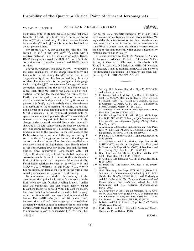
Instability of the Quantum Critical Point of itinerant ferromagnets
holds remains to be studied. We also verified that awayfrom the QCP, when is finite, the q3=2 term transformsinto jqj1 at the smallest q. The interpolation formulabetween the q3=2 and jqj forms is rather involved and wedo not present it here.
For arbitrary D< 3, our calculations yield the ‘‘cor-rection’’ to 1
s in the form jqjD1=2, again with anegative prefactor. In 3D it scales as q2 logjqj. Hence,HMM theory is destroyed for all D 3. For D > 3, thecorrection term is smaller than q2, and HMM theorysurvives.
Charge susceptibility and gauge theory.—We repeatedthe same calculations for the charge susceptibility andfound inD 2 that the singular jqj3=2 terms from the twodiagrams in Fig. 1 cancel each other, and the q2 behaviorsurvives. The same holds for the propagator of the gaugefield — singular jqj3=2 terms from self-energy and vertexcorrection insertions into the particle-hole bubble againcancel each other. We verified the cancellation of non-analytic terms for the second-order diagrams as well.Furthermore, we verified in two orders of perturbationthat the momentum dependence of cq; 0 comes inpowers of q=pF2; i.e., it is entirely due to the existenceof a curvature of the dispersion. Physically, the distinc-tion between spin and charge susceptibilities is in that the=jqj singularity in the dynamical particle-hole re-sponse function (which generates the q3=2 nonanalyticity)is sensitive to a magnetic field but is insensitive to thechange of the chemical potential. Hence, the singularityshows up in the total spin response but does not appear inthe total charge response [14]. Mathematically, this dis-tinction is due to the presence, in the spin case, of thePauli matrices in the vertices of the diagrams in Fig. 1,such that the self-energy and vertex correction diagramsdo not cancel each other. Note that the cancellation ornoncancellation of the singularities is not directly relatedto the conservation laws for charge and spin suscepti-bilities, since conservation laws require only thatcq 0; ! and sq 0; ! vanish but impose noconstraints on the forms of the susceptibilities in the otherlimit of finite q and zero frequency. More specifically,Fermi-liquid relations between s;cq! 0; ! 0 ands;cq 0; !! 0 imply [15] that s;cq! 0; ! 0 !Cst but impose no formal constraints on the form of theactual q dependence in s;cq;! 0 at finite q.
To summarize, we studied the stability of thequantum-critical point for itinerant ferromagnets, in thelimit when the spin-fermion coupling is much smallerthan the bandwidth, and one would naively expectEliashberg theory to be valid. Within Eliashberg theory,the Fermi-liquid is destroyed at criticality, but the mag-netic transition is still continuous and is described bybosonic Hertz-Millis-Moriya action. We demonstrated,however, that in D 3, long-range spatial correlationsassociated with the Landau damping of the bosonic orderparameter field break the Eliashberg theory and give riseto a universal, negative, nonanalytic jqjD1=2 contribu-
tion to the static magnetic susceptibility sq; 0. Thisterm makes the continuous critical theory unstable. Weargued that the actual transition is either towards incom-mensurate ordering or first-order into a commensuratestate. We also demonstrated that singular corrections arespecific to the spin problem, while charge susceptibilityremains analytic at criticality.
It is our pleasure to thank A. Abanov, I. Aleiner,A. Andreev, B. Altshuler, D. Belitz, P. Coleman, S. DasSarma, A. Georges, L. Glazman, A. Finkelstein, Y. B.Kim, T. Kirkpatrick, D. Maslov, A. Millis, M. Norman,O. Parcollet, I. Paul, R. Ramazashvili, Q. Si, and Th.Vojtafor stimulating discussions. The research has been sup-ported by NSF DMR 9979749 (A.V. C.).
[1] See, e.g., G. R. Stewart, Rev. Mod. Phys. 73, 797 (2001),and references therein.
[2] R. Roussev and A. J. Millis, Phys. Rev. B 63, 140504(2001); Z. Wang, W. Mao, and K. Bedell, Phys. Rev. Lett.87, 257001 (2001); for related developments, see alsoP. Coleman, C. Pepin, Q. Si, and R. Ramazashvili,J. Phys. Condens. Matter 13, 723 ( 2001).
[3] A. Chubukov, A. Finkelstein, R. Haslinger, and D. Morr,Phys. Rev. Lett. 90, 077002 (2003).
[4] J. A. Hertz, Phys. Rev. B 14, 1165 (1976); A. Millis, Phys.Rev. B 48, 7183 (1993); T. Moriya, Spin Fluctuations in
Itinerant Electron Magnetism (Springer-Verlag, Berlin,New York, 1985).
[5] A. Abanov, A.V. Chubukov, and J. Schmalian, Adv. Phys.52, 119 (2003); Ar. Abanov, A.V. Chubukov, and A. M.Finkel’stein, Europhys. Lett. 54, 488 (1999).
[6] D. Belitz, T. R. Kirkpatrick, and T. Vojta, Phys. Rev. B 55,9452 (1997).
[7] A.V. Chubukov and D. L. Maslov, Phys. Rev. B 68,155113 (2003); see also A. Houghton, H-J. Kwon, andB. Marston, Adv. Phys. 49, 141 (2000); S. Das Sarma andE. H. Hwang, Phys. Rev. Lett. 83, 164 (1999).
[8] G.Y. Chitov and A. J. Millis, Phys. Rev. Lett. 86, 5337(2001); Phys. Rev. B 64, 054414 (2001).
[9] B. Altshuler, L. B. Ioffe, and A. J. Millis, Phys. Rev. B 52,5563 (1995).
[10] M. Dzero and L. P. Gorkov, Phys. Rev. B 69, 092501(2004)].
[11] G. M. Eliashberg, Sov. Phys. JETP 16, 780 (1963); D. J.Scalapino, in Superconductivity, edited by R. D. Parks(Dekker Inc., NewYork, 1969),Vol. 1, p. 449; F. Marsiglioand J. P. Carbotte, in The Physics of Conventional and
Unconventional Superconductors, edited by K. H.Bennemann and J. B. Ketterson (Springer-Verlag,Berlin, 2002).
[12] A.V. Chubukov, D. Pines, and J. Schmalian, in The Phys-
ics of Superconductors, edited by K. H. Bennemann andJ. B. Ketterson (Springer, New York, 2003), Vol. 1, p. 495.
[13] S.A. Brazovskii, Sov. Phys. JETP 41, 85 (1975).[14] D. Belitz and T. R. Kirkpatrick, Phys. Rev. B 67, 024419
(2003); (unpublished).[15] E. M. Lifshitz and L. P. Pitaevskii, Statistical Physics
(Pergamon Press, Oxford, 1980).
P H Y S I C A L R E V I E W L E T T E R S week ending9 APRIL 2004VOLUME 92, NUMBER 14
147003-4 147003-4
90

PUBLICATION 2
Quantum critical behavior ofitinerant ferromagnets
cond-mat/0605306∗
∗ This publication was still in preparation when this manuscript was written.It recapitulates all the results presented in this first part, including most of thetechnical details. Because of this redundancy, we choose not to include this longpaper here.

Quantum critical behavior of itinerant ferromagnets
92

Appendices
93


APPENDIX A
Bosonic self-energy
In this section, we compute the bosonic self-energy at the one-loop level, in the caseof both free and fully renormalized fermions. We prove that for an external bosonicmomentum on the bosonic mass-shell, this self-energy becomes independent on theactual form of the fermionic self-energy, and reduces to the usual Landau dampingterm, whereas an extra term has to be included if this same external momentum ison the fermionic mass shell.
After performing the sum over spin matrices, we are left with the followingexpression:
Π(q,Ω) = 2Ng
∫d2k dω
(2π)3G(k, ω) G(k + q, ω + Ω). (A.1)
Introducing the angle θ defined by ǫk+q = ǫk + vF q cos θ, this writes:
Π(q,Ω) = Ngm
4π3
∫
dω dǫk dθ1
i(ω + Σ(ω))− ǫk× 1
i(ω + Ω + Σ(ω + Ω))− ǫk − vF q cos θ. (A.2)
Proceeding with a contour integration over ǫk, and noticing that ω and Σ(ω)have the same sign, we get:
Π(q,Ω) = iNgm
2π2
∫ +∞
−∞dω
∫ 2π
0
dθ (θ(ω + Ω)− θ(ω))
× 1
i(Ω + Σ(Ω + ω)− Σ(ω))− vF q cos θ. (A.3)
95

Bosonic self-energy
Performing the integration over θ, and rearranging a little bit the integrationover Ω, we are left with:
Π(q,Ω) = Nmg
πvF
∫ Ω
0
dωSign(Ω)
√
(vF q)2 + (Ω + Σ(Ω− ω) + Σ(ω))2. (A.4)
We know from direct perturbative calculation that the fermionic self-energy goeslike Σ(ω) = ω
1/30 ω2/3, where ω0 ∼ αg. It follows that if the external bosonic momen-
tum is on the bosonic mass-shell, i.e. if q ∼ Ω1/3, it dominates over the frequency-dependent term in the integral, so that:
Π(q,Ω) = Nmg
π
∫ Ω
0
dωSign(Ω)
vF q
= Nmg
πvF
|Ω|q. (A.5)
We recover here the expression of the Landau damping term with a prefactordepending on the details of the interaction considered in our model. This result isindependent on the fermionic self-energy provided that vF q ≫ (Ω + Σ(Ω)).
However, if the external bosonic momentum is on the fermionic mass shell, i.e.if vF q ∼ Σ(Ω), the frequency-dependent term can no longer be neglected. Definingz = ω
Ω, one then has:
Π(q,Ω) = Nmg
π
∣∣∣∣
Ω
Σ(Ω)
∣∣∣∣
∫ 1
0
dz1
√(vF qΣ(Ω)
)2
+ (z2/3 + (1− z)2/3)2
. (A.6)
For the calculations of the static spin susceptibility, we not only need the leadingO(1/q) but also the subleading O(1/q3) terms in Π(q,Ω). Expanding (A.6) in 1/qto first two orders, we find for Ω < ω0:
Π(q,Ω) = γ|Ω|q
(
1− c2Σ2(Ω)
v2q2
)
(A.7)
where c ∼ 1.19878.To simplify the notation, we use the expression for the polarization operator
with the frequency dependence appearing in the denominator, which amounts toplugging the Σ2 term back into the denominator:
Π(q,Ω) = Nmg
π
|Ω|√
(vF q)2 + c2Σ(Ω)2. (A.8)
96

APPENDIX B
Fermionic self-energy
In this section, we compute the fermionic self-energy at the one, two and three looplevels, for an external momentum taken to be on the Fermi surface. We also analyzethe momentum dependence of the one-loop fermionic self-energy.
B.1 One-loop
B.1.1 At the Fermi level
After summing over the spin matrices, the fermionic self-energy at the one-loop levelis given by:
Σ(ω) = 3ig2
∫d2q dΩ
(2π)3G(kF + q, ω + Ω)χ(q,Ω)
=3ig
(2π)3
∫
dθdΩ dq
ξ−2 + q2 + γ |Ω|q
q
i(ω + Ω + Σ(ω + Ω))− vF q cos θ, (B.1)
where we defined θ as the angle between k and q, and considered an externalfermionic momentum k ≃ kF . The i prefactor comes from the convention G−1 =G−1
0 + iΣ.
Since the pole in q from the fermionic propagator is in a definite half-plane, theintegral in q is dominated by poles coming from the bosonic Green’s function, sothat one can perform the integral over the angular variable and simplify the result
97

Fermionic self-energy
as follows:
Σ(ω) = − 3g2
(2π)2
∫
dΩ dqχ0
q3 + γ|Ω|+ qξ−2
q2Sign(ω + Ω)√
(vF q)2 + (ω + Ω + Σ(ω + Ω))2
= − 3g
(2π)2
∫ +∞
−∞dΩ
∫ +∞
0
dqq2Sign(ω + Ω)
vF q
1
q3 + γ|Ω|+ qξ−2. (B.2)
Defining the new variables z = Ωω
and u = vF qω
, this leads to:
Σ(ω) =3g
2π2
ω2
γv3F
∫ 1
0
dz
∫ +∞
0
duu
z + au+ bu3, (B.3)
where we have used a =1
γvF ξ2and b =
ω2
γv3F
Let’s denote by I the last double integral, and define the new variables y =√
ba3z = (ωγξ3)z and t =
√bau = ξω
vFu. Now I reduces to:
I =
(vFξω
)2 ∫ γωξ3
0
dy
∫ +∞
0
dtt
t3 + t+ y
=
(vFξω
)2
h(γωξ3). (B.4)
Substituting this back into our expression for the self-energy:
Σ(ω) =3
2πmξ2h(γωξ3), (B.5)
with the following asymptotic behavior: h(x→ 0) = πx2
and h(x→∞) = πx2/3√3
.
In the two regimes we are interested in, this last result can be rewritten as:
Σ(ω) =
λω for ξ−1 ≫ 1,
ω1/30 ω2/3 for ξ−1 → 0,
(B.6)
where the constant prefactors are defined as:
λ =3
4π
gξ
vF,
ω0 =3√
3
8π3
g3
γv3F
.(B.7)
98

B.1. One-loop
B.1.2 Momentum dependence
For definiteness, we set ξ−1 = 0. We first compute the momentum-dependent partof the one-loop fermionic self-energy at zero external frequency:
Σ(k, ω = 0) = 3ig2
∫d2q dΩ
(2π)3G(k + q,Ω)χ(q,Ω)
=3ig
(2π)3
∫dΩd2q
iΣ(Ω)− ǫk+qq
γ|Ω|+ q3. (B.8)
Expanding ǫk+q = ǫk + vF q cos θ and integrating over θ, we obtain
Σ(k, 0) =3g
4π2
∫
dΩ Sign(Ω)
∫q2dq
q3 + γ|Ω|1
(
(vF q)2 + (Σ(Ω) + iǫk)2)1/2
. (B.9)
At ǫk = 0, the integral vanishes by parity. Expanding to linear order in ǫk we obtain:
Σ(k, 0) = −3iǫk ×g
2π2
∫ ∞
0
dΩ Σ(Ω)
∫q2dq
(q3 + (γ|Ω|))(
(vF q)2 + Σ(Ω)2)3/2
. (B.10)
Simple estimates show that the result depends on the interplay between (γΩ)1/3
and Σ(Ω)/vF . Introducing the scale ωMax, defined as the frequency for which(γΩ)1/3 = Σ(Ω)/vF (see (2.42), and rescaling variables as q = (γωMax)
1/3y, Ω =ωMaxx, we re-write (B.10) as
Σ(k, 0) = −3iǫk ×gωMax
2π2v3FγI (B.11)
where
I =
∫ ∞
0
dx
∫ ∞
0
dyxy2
(x2 + y2)3/2(x+ y3)≃ 1.3308 (B.12)
Substituting ωMax = (γv3F )1/2, we obtain (2.65).
To obtain the frequency dependence of the fermionic density of states at small ω,we have to evaluate the second order term in ǫk at the mass shell, where ǫk = iΣ(ω)and convert the result to real frequencies. We therefore will keep both ω and ǫkfinite, and use
Σ(k, ω) =3ig
(2π)3
∫
dΩd2qq
γ|Ω|+ q3
1
iΣ(ω + Ω)− ǫk+q. (B.13)
Writing, as before, ǫk+q = ǫk + vF q cos θ and integrating over θ, we obtain
Σ(k, ω) =3g
4π2
∫dΩq2dq
γ|Ω|+ q3
sign(ω + Ω)√
(Σ(ω + Ω) + iǫk)2 + (vF q)2
. (B.14)
99

Fermionic self-energy
We assume and then verify that the internal vF q are still larger than Σ(ω + Ω) andǫk, which allows us to expand
Σ(k, ω) = − 3g
8π2v3F
∫
dΩ Sign(ω + Ω)
∫dq
q(γ|Ω|+ q3)
(
Σ(ω + Ω) + iǫk
)2
(B.15)
The lower limit of the momentum integral is (Σ(ω + Ω) + iǫ)k)/vF . At the massshell, iǫk = Σ(ω). Substituting, we find
Σ(k, ω) = − 3g
8π2v3F
∫
dΩ Sign(ω + Ω)
∫dq
q(γ|Ω|+ q3)
(
Σ(ω + Ω)− Σ(ω))2
(B.16)
We will need the contribution which is confined to Ω ∼ ω. The contributions from|Ω| ≫ |ω| diverge in our expansion procedure, and account for the regular O(ǫk)term in the self-energy, and also for regular O(ω) term. The last term is evensmaller in α than the regular (ǫk) term and is totally irrelevant. As Ω ∼ ω is small,
Σ(Ω) ≈ Σ(Ω) = Ω2/3ω1/30 .
Because of the sign factor in the numerator of (B.14), there are two distinctcontributions from Ω ∼ ω. For both of them, the momentum integral is logarithmic(this justifies the expansion) and yields (1/3) log(ω1/ω), where ω1 ∼ N2E2
F/g. Thefirst contribution comes from |Ω| ≤ |ω| and to logarithmic accuracy is
Σ(k, ω)A = − g
8π2v3Fγ
sign(ω)
∫ |ω|
−ω
dΩ
|Ω| (Σ(|ω|+ Ω)− Σ(|ω|))2 logω1
|ω| (B.17)
Rescaling the frequency, we obtain from (B.17)
Σ(k, ω)A = − gI14π2v3
FγΣ(ω)|Σ(ω)| log
ω1
ω. (B.18)
where
I1 =1/2∫
1
−1
dx
|x|((1 + x)3/2 − 1
)2= 0.254 (B.19)
Another comes from |Ω| > |ω|, and is
Σ(k, ω)B =gΣ(ω)
4π2v3Fγ
logω1
|ω|
∫ ∞
|ω|
dΩ
Ω(Σ(|ω|+ Ω) + Σ(Ω− |ω| − 2Σ(Ω))) (B.20)
Rescaling, we obtain
Σ(k, ω)B =gI2
4π2v3Fγ
Σ(ω)|Σ(ω)| logω1
ω. (B.21)
where
I2 =
∫ ∞
1
dx
|x|((1 + x)2/3 + (x− 1)2/3 − 2x2/3
)= −0.195 (B.22)
100

B.2. Two-loop
Combining Σ(k, ω)A and Σ(k, ω)B, we obtain
Σ(k, ω)= −0.45g
4π2v3Fγ
Σ(ω)|Σ(ω)| logω1
ω. (B.23)
on the mass-shell.
B.2 Two-loop
We here compute one of the contributions to the two-loop self-energy, as givenby Fig. 2.1, which originates from the insertion of the vertex correction into theEliashberg self-energy.
We have:
Σ2(ω) ∼ g2
∫
dω1d2q1
∫
dω2d2q2 χ(q1, ω1) χ(q2, ω2) G(kF + q1, ω + ω1)
×G(kF + q2, ω + ω2) G(kF + q1 + q2, ω + ω1 + ω2),
(B.24)
which gives, once we replace each propagator by its full expression:
Σ2(ω) ∼ g2
∫
dω1d2q1
∫
dω2d2q2
q1γ|ω1|+ q3
1
q2γ|ω2|+ q3
2
× 1
iΣ(ω + ω1)− vF q1x1
iΣ(ω + ω2)− vF q2x − q22y
2mB
× 1
iΣ(ω + ω1 + ω2)− vF q1x − vF q2x − q21y
2mB− q22y
2mB
, (B.25)
where we use the shorter notation Σ(ω) = ω + Σ(ω).Integrating successively over q1x and q2x, closing each contour on the upper half-
plane, one has:
Σ2(ω) ∼ mB g2
v2F
∫
dω1
∫
dω2 Θ(ω, ω1, ω2)
∫
dq1y|q1y|
|q1y|3 + γ|ω1|
×∫
dq2y|q2y|
|q2y|3 + γ|ω2|1
(γ2ω1ω2)1/3
1q1yq2y
(γ2ω1ω2)1/3 + iζ(B.26)
where ζ = mBΣ(ω + ω1) + Σ(ω + ω2)− Σ(ω + ω1 + ω2)
(γ2ω1ω2)1/3
and Θ(ω, ω1, ω2) comes
from the choice of a contour for the integration and is given in our case by:
Θ(ω, ω1, ω2) = (θ(ω + ω1)− θ(ω + ω1 + ω2))
×(
θ(ω + ω2)− θ(Σ(ω + ω1 + ω2)− Σ(ω + ω1)))
.(B.27)
101

Fermionic self-energy
It is convenient at this stage to rescale the perpendicular components of thebosonic momenta. Introducing x = q1y/(γ|ω1|)1/3 and y = q2y/(γ|ω2|)1/3, we obtain:
Σ2(ω) ∼ mg2
v2F
∫
dω2
∫
dω1
∫ ∞
0
dxdyΘ(ω, ω1, ω2)
(γ2ω1ω2)2/3
× iζ
x2y2 + ζ2
xy
(1 + x3) (1 + y3),
(B.28)
where we rearranged the double integral over x and y to make it real.Since all internal frequencies typically go like ω, the typical value of ζ is given
by the small parameter β given in (2.53). Expanding the double integral for smallvalues of ζ , the leading contribution from the integral over x and y reads:
∫ ∞
0
dxdy1
x2y2 + ζ2
xy
(1 + x3) (1 + y3)∼ log2 ζ. (B.29)
If one considers now free fermions, it becomes possible to reduce the expressionof the two-loop self-energy to:
Σfree2 (ω) ∼ m2
B g2
v2F
∫ ω
0
dω2
∫ ω
ω−ω2
dω1
log2(
mBω(γ2ω1ω2)2/3
)
γ2ω1ω2
∼ m2B g
2
γv2F
ω
∫ 1
0
dz2
∫ 1
1−z2dz1
log2(m3
Bω
γz1z2
)
z1z2
∼ β2ω log2 ω, (B.30)
where we only kept the leading contribution in the last expression, and β = mB/mNis one of the small parameters defined in the text.
Now, in the case of dressed fermions, we need to take Σ(ω) = ω1/30 ω2/3. The
procedure is identical to the free fermion case, but the final expression is a bit morecomplicated:
ΣDressed2 (ω) ∼ m2g2
γ2v2F
ω1/30 ω2/3
∫ 1
0
dz2
∫ 1
1−z2dz1
1
z1z2
×[(1− z1)2/3 + (1− z2)2/3 + (z1 + z2 − 1)2/3
]
× log2
(1− z1)2/3 + (1− z2)2/3 + (z1 + z2 − 1)2/3
γ2/3
mω1/30
z1/31 z
1/32
. (B.31)
Expanding the log2, one is left with a double integral that only contributes as anumerical prefactor, and the dominant term is then given by:
Σ2(ω) ∼ Σ1(ω) β2 log2 β, (B.32)
where Σ1(ω) = ω1/30 ω2/3 is the self-energy in the Eliashberg theory.
102
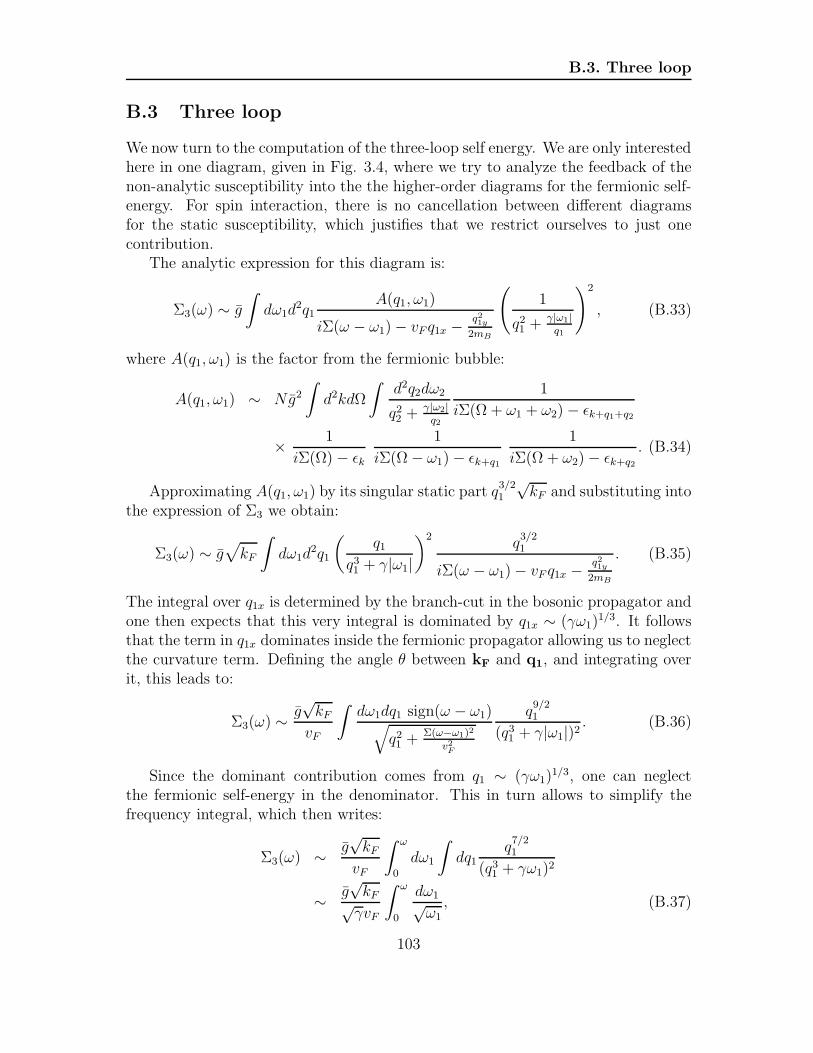
B.3. Three loop
B.3 Three loop
We now turn to the computation of the three-loop self energy. We are only interestedhere in one diagram, given in Fig. 3.4, where we try to analyze the feedback of thenon-analytic susceptibility into the the higher-order diagrams for the fermionic self-energy. For spin interaction, there is no cancellation between different diagramsfor the static susceptibility, which justifies that we restrict ourselves to just onecontribution.
The analytic expression for this diagram is:
Σ3(ω) ∼ g
∫
dω1d2q1
A(q1, ω1)
iΣ(ω − ω1)− vF q1x − q21y
2mB
(
1
q21 + γ|ω1|
q1
)2
, (B.33)
where A(q1, ω1) is the factor from the fermionic bubble:
A(q1, ω1) ∼ Ng2
∫
d2kdΩ
∫d2q2dω2
q22 + γ|ω2|
q2
1
iΣ(Ω + ω1 + ω2)− ǫk+q1+q2
× 1
iΣ(Ω)− ǫk1
iΣ(Ω− ω1)− ǫk+q11
iΣ(Ω + ω2)− ǫk+q2. (B.34)
Approximating A(q1, ω1) by its singular static part q3/21
√kF and substituting into
the expression of Σ3 we obtain:
Σ3(ω) ∼ g√
kF
∫
dω1d2q1
(q1
q31 + γ|ω1|
)2q3/21
iΣ(ω − ω1)− vF q1x − q21y
2mB
. (B.35)
The integral over q1x is determined by the branch-cut in the bosonic propagator andone then expects that this very integral is dominated by q1x ∼ (γω1)
1/3. It followsthat the term in q1x dominates inside the fermionic propagator allowing us to neglectthe curvature term. Defining the angle θ between kF and q1, and integrating overit, this leads to:
Σ3(ω) ∼ g√kF
vF
∫dω1dq1 sign(ω − ω1)√
q21 + Σ(ω−ω1)2
v2F
q9/21
(q31 + γ|ω1|)2
. (B.36)
Since the dominant contribution comes from q1 ∼ (γω1)1/3, one can neglect
the fermionic self-energy in the denominator. This in turn allows to simplify thefrequency integral, which then writes:
Σ3(ω) ∼ g√kF
vF
∫ ω
0
dω1
∫
dq1q7/21
(q31 + γω1)2
∼ g√kF√γvF
∫ ω
0
dω1√ω1
, (B.37)
103

Fermionic self-energy
where we introduced z = q1/(γω1)1/3, so that the integral over z just contribute to
the numerical prefactor.Collecting prefactors, one finally has:
Σ3(ω) ∼ √gω. (B.38)
104

APPENDIX C
Vertex corrections
In this section, we compute the various vertex corrections analyzed in the text.
C.1 q = Ω = 0
Consider first the simplest 3-leg vertex, with strictly zero incoming frequency Ω andmomenta q, as presented in Fig. 2.2a. Its analytic expression writes:
∆g
g
∣∣∣∣q=Ω=0
∼ g2
∫
dωd2p G(kF, ω)2 χ(p, ω)
∼ g
∫dωd2pγ|ω|p
+ p2
1(
iΣ(ω)− vFpx − p2y2mB
)2 ,
where we defined Σ(ω) = ω + Σ(ω) and we have chosen kF along the x axis.
Since both poles coming from the fermionic Green’s functions are in the samehalf plane, the integral over qx is finite only because of the branch cut in the bosonicpropagator. Since at the branch cut px and py are of the same order, we can dropthe curvature term in the fermionic propagators and introduce polar coordinates forthe internal bosonic momentum. Defining θ as the angle between kF and p, andintegrating over it, one has:
∆g
g
∣∣∣∣q=Ω=0
∼ g
∫dωdp
p3 + γ|ω|p2|Σ(ω)|
(
(vFp)2 + Σ(ω)2)3/2
. (C.1)
105

Vertex corrections
Introducing the frequency ωMax up to which bosons are slow modes comparedto fermions, i.e. up to which (γω)1/3 > Σ(ω)/vF , one can split the frequencyintegral into two parts, and define in each of them the reduced momentum z =p/Min((γω)1/3, Σ(ω)/vF ) so that the integral over z only contributes to the numer-ical prefactor, leading to:
∆g
g
∣∣∣∣q=Ω=0
∼ g
∫ ωMax
0
dωΣ(ω)
γv3Fω∼ g
γv3F
Σ(ωMax) (C.2)
One can easily make sure that the frequency ωMax at which (γω)1/3 = Σ(ω)/vFexceeds ω0, such that one should use Σ(ω) = ω to find ωMax. Substituting, weobtain ωMax ∼ (NgEF )1/2, and
∆g
g
∣∣∣∣q=Ω=0
∼ √α (C.3)
C.2 q = 0, Ω finite
Considering the same vertex, now with a finite external frequency, one has:
∆g
g
∣∣∣∣q=0,Ω
∼ g2
∫
dωd2p G(kF + p, ω + Ω)G(kF + p, ω)χ(p, ω)
∼ g
∫dωd2pγ|ω|p
+ p2
1
iΣ(ω)− vFpx − p2y2mB
1
iΣ(ω + Ω)− vFpx − p2y2mB
, (C.4)
where we chose the x axis along kF.
From the pole structure in px of this expression, one expects two contributionsto this integral. A first term comes from the branch cut in the bosonic propagator,however this contribution ultimately leads to the same result as the q = Ω = 0 ver-tex, up to small corrections from the finiteness of Ω. The second contribution arisesfrom taking the poles in the fermionic propagators. At zero external frequency, thesetwo poles were in the same half-plane of px, so we could close the integration contourover a different half-plane and only consider the contribution from the branch cutin the bosonic propagator. At a finite Ω, there is a range where ω and ω + Ω havedifferent signs, and the two poles are in different half-planes of px. The result afterintegration reads:
∆g
g
∣∣∣∣q=0,Ω
∼ g
vF
∫ Ω
0
dω
∫
dpy|py|
γ|ω|+ |py|31
Σ(Ω− ω) + Σ(ω), (C.5)
where we slightly rearranged the frequency integral.
106

C.3. q finite, Ω = 0
Performing the integration over py, we are left with:
∆g
g
∣∣∣∣q=0,Ω
∼ g
γ1/3vF
∫ Ω
0
dωω−1/3
Σ(Ω− ω) + Σ(ω)
∼ g
(ω0γv3F )1/3
∼ Const., (C.6)
where we assumed that Ω is small, i.e. Σ(Ω) = ω1/30 Ω2/3. This vertex thus reduces
to a numerical constant, that does not contain any small parameter.
C.3 q finite, Ω = 0
Conversely, the same vertex taken at finite external momentum q, but zero externalfrequency writes:
∆g
g
∣∣∣∣q,Ω=0
∼ g2
∫
dωd2p G(kF + p + q, ω)G(kF + p, ω)χ(p, ω)
∼ g
∫dωd2pγ|ω|p
+ p2
1
iΣ(ω)− vFpx − p2y2mB
× 1
iΣ(ω)− vF qx − vFpx − p2y2mB− qypy
mB
, (C.7)
where px is the projection of p along kF.
Like its q = 0 counterpart, this vertex is characterized by poles in px from thefermionic propagators lying in the same half-plane. The only nonzero contributionthen comes from the branch cut in the bosonic propagator. At the branch cut,px ∼ py which allows us to neglect the quadratic curvature terms in the fermionicGreen’s functions.
This makes possible a direct integration over py. This integral can be separatedfrom the rest of the expression, and reads:
∫
dpyp
γ|ω|+ p3=
1
|px|
∫ +∞
−∞dz
√1 + z2
(1 + z2)3/2 + γ |ω||px|3
=2p2
x
γ|ω|
∫ +π/2
0
du1
|px|3γ|ω| + (cos u)3
,
(C.8)
where we successively defined z = py/|px| and z = tanu.
107

Vertex corrections
This last integral can be approximated by its asymptotic form, namely:
∫dpy p
γ|ω|+ p3=
π|px| , if |px|3 ≫ γω4π
3√
31
(γ|ω|)1/3 − 12p2xγ|ω| log p2x
(γ|ω|)2/3
+(log 2− 1
2
) p2xγ|ω| , if |px|3 ≪ γω
(C.9)
The only non-vanishing contribution once we take the integral over px comesfrom the log term. After expanding in qx, this contribution reads:
∆g
g
∣∣∣∣q,Ω=0
− ∆g
g
∣∣∣∣q=Ω=0
∼ gvFγqx
∫dω
|ω|
∫
dpxp2x log p2
x(
iΣ(ω)− vFpx)3 . (C.10)
Defining the scaled momentum z = vFpx/Σ(ω) and performing the integrationover z, one obtains two terms, the dominant one being:
∆g
g
∣∣∣∣q,Ω=0
− ∆g
g
∣∣∣∣q=Ω=0
∼ ig
γv2F
qx
∫
|vF qx|
dω
ωlog[iΣ(ω)], (C.11)
where the frequency integral runs over |Σ(ω)| > |vF qx| since as we expanded in vF qx,we assumed that it was smaller than |Σ(ω)|.
Performing the remaining integral, one finds:
∆g
g
∣∣∣∣q,Ω=0
− ∆g
g
∣∣∣∣q=Ω=0
∼ qxkF
log |qx|. (C.12)
C.4 q,Ω finite
Finally, we consider the general vertex where both external bosonic momentum andfrequency are non-zero. In analytic form, this writes:
∆g
g
∣∣∣∣q,Ω
∼ g2
∫
dωd2p G(kF + p + q, ω + Ω)G(kF + p, ω)χ(p, ω)
∼ g
∫dωd2pγ|ω|p
+ p2
1
iΣ(ω)− vFpx − p2y2mB
× 1
iΣ(ω + Ω)− vF qx − vFpx − p2y2mB− qypy
mB
,
where px is defined as px = p · kF.Integrating over px first, there are two contributions. One comes from the branch
cut in the bosonic propagator, and gives similar results to the (q = 0,Ω = 0) and the(q finite, Ω = 0) vertices up to small correction from the finiteness of the external
108

C.4. q,Ω finite
frequency. We neglect it here and focus on the other contribution which comes fromthe poles in the fermionic propagators:
∆g
g
∣∣∣∣q,Ω
∼ ig
vF
∫ Ω
0
dω
∫
dpy|py|
γ|ω|+ |py|3
× 1
iΣ(Ω− ω) + iΣ(ω)− vF qx − qypy
mB
, (C.13)
where the simplification of the frequency integral comes from the poles in px.This vertex correction strongly depends on the interplay between the external
qx, qy and Ω, and is in particular quite sensitive to the momentum anisotropy. Wenow analyze the various possibilities.
For the generic case where qx ∼ qy (we use the notation q to designate themboth), one can neglect the quadratic term in the fermionic dispersion, allowing toperform the integration over py, leaving us with:
∆g
g
∣∣∣∣q,Ω
∼ ig
vFγ1/3
∫ Ω
0
dω ω−1/3
iΣ(Ω− ω) + iΣ(ω)− vF q. (C.14)
Restricting ourselves to the quantum-critical regime (i.e. Ω ≤ ω0) for which Σ(ω) =
ω1/30 ω2/3, one has:
∆g
g
∣∣∣∣q,Ω
= F(vF q
Σ(Ω)
)
, (C.15)
where F(x) =∫ 1
0dzz1/3
1(1−z)2/3+z2/3+ix
, has the following asymptotic behavior:
F(x≪ 1) = O(1)F(x≫ 1) = O
(1x
) (C.16)
If the typical q is on the bosonic mass shell, then q ∼ (γΩ)1/3, and one has:
∆g
g
∣∣∣∣q,Ω
∼ Σ(Ω)
vF q∼ √α
(Ω
ωMax
)1/3
. (C.17)
However, we encountered in previous computations (e.g. self-energies) that astrong anisotropy can be observed between the components of the bosonic momen-tum, with qy ≫ qx. In this case, the full expression of the vertex correction is a bitcomplicated and we choose to present here the most relevant case for which the cur-vature term dominates over vF qx in the fermionic propagator. The vertex correctionthen no longer depends on qx and writes:
∆g
g
∣∣∣∣q,Ω
∼ g
vF
∫ Ω
0
dω
∫ ∞
0
dpypy
γω + p3y
Σ(Ω− ω) + Σ(ω)(
Σ(Ω− ω) + Σ(ω))2
+(qypy
mB
)2 , (C.18)
109

Vertex corrections
Defining u = py/(γω)1/3 and z = ω/Ω, it is possible to rewrite the vertex correctionin this regime as:
∆g
g
∣∣∣∣q,Ω
∼ G(
β(γΩ)1/3
qy
)
(C.19)
where β = mB
Nmand G(x) is the following double integral:
G(x) =
∫ ∞
0
du u
1 + u3
∫ 1
0
dz z−1/3((1− z)2/3 + z2/3
)
((1− z)2/3 + z2/3)2+ u2z2/3
x2
∼ x2 log2 x if x≪ 1. (C.20)
C.5 4-leg vertex
In this paragraph, we compute the renormalized 4-leg vertex Γ2(q,Ω) presented inFig 2.3, which reads:
Γ2(q,Ω) ∼ g2
∫
dω
∫
d2p χs
(Ω + ω
2,p + q
2
)
χs
(Ω− ω
2,q− p
2
)
×G(
Ω + ω
2,kF +
p + q
2
)
G
(Ω− ω
2,kF +
q− p
2
)
. (C.21)
Performing the integration over px, projection of p along kF, we obtain:
Γ2(q,Ω) ∼ g2
vF
∫ Ω
0
dω dpyγ(Ω− ω) + (q2 + p2
y − 2qypy)3/2
× 1
iΣ(
Ω+ω2
)+ iΣ
(Ω−ω
2
)− vF qx − q2y+p2y
4mB
×
√
(q2 + p2y)
2 − 4q2yp
2y
γ(Ω + ω) + (q2 + p2y + 2qypy)3/2
. (C.22)
It is convenient at this stage to define the reduced variables z = ω/Ω and y =py/|qy|:
Γ2(q,Ω) ∼ g(γΩ)1/3
|qy|3∫ 1
0
dz dyγΩ|qy|3 (1− z) + |1− y|3
|1− y2|γΩ|qy|3 (1 + z) + |1 + y|3
× 1
i [(1− z)2/3 + (1 + z)2/3]− vF qxΣ(Ω)− 1+y2
β
(|qy|3γΩ
)2/3(C.23)
where we assumed that Ω ≤ ω0, and we used that in all our computations, theperpendicular component of the bosonic momentum is always either dominant orcomparable to the parallel one, so that one has qy ∼ q.
110

C.5. 4-leg vertex
Comparing this renormalized vertex with the bare one given by Γ1(q,Ω) ∼gq−2
y
1+γ|Ω|
|qy |3
, one has for the ratio of the two:
Γ2
Γ1
∼ (γΩ)1/3
|qy|
∫ 1
0
dz dyγΩ|qy|3 (1− z) + |1− y|3
|1− y2|γΩ|qy|3 (1 + z) + |1 + y|3
× 1
i [(1− z)2/3 + (1 + z)2/3]− vF qxΣ(Ω)− 1+y2
β|qy|2
(γΩ)2/3
(C.24)
which only depends on two parameters: the ratios vF qxΣ(Ω)
and |qy|3γΩ
.In the generic case of an external bosonic momentum on the mass shell, i.e.
qx ∼ qy ∼ (γΩ)1/3 one has:
Γ2
Γ1∼ Σ(Ω)
vF qx∼ √α
(Ω
ωMax
)1/3
. (C.25)
On the contrary, for a typical qx ∼ Σ(Ω)/vF and qy ∼ (γΩ)1/3:
Γ2
Γ1∼ β, (C.26)
up to logarithmic factors.
111

Vertex corrections
112
APPENDIX D
Static spin susceptibility
D.1 Diagrams
In this Appendix we present the details of our calculations of the singular termsin the static spin susceptibility. We discuss in great detail the calculation of thefirst two diagrams in Fig. 3.2 (vertex and self-energy correction diagrams). Thesetwo diagrams can be computed explicitly both away from QCP and at QCP. Welabeled the total contribution from these two diagrams as ΠA(q, 0). The remainingtwo diagrams (their total contribution is ΠB(q, 0)) cannot be computed explicitly atQCP, and we compute them in an approximate scheme.
In explicit form, the first two diagrams in Fig. 3.2 are given by:
Π1a(q, 0) = Γag2
(2π)6
∫
d2Kdωd2ldΩ G(ω, k)2
× G(ω + Ω, k + l)G(ω, k + q)χs(l,Ω) (D.1)
Π1b(q, 0) = Γbg2
(2π)6
∫
d2Kdωd2ldΩ χs(l,Ω)G(ω, k)G(ω, k + q)
×G(ω + Ω, k + l)G(ω + Ω, k + q + l) (D.2)
where Γa,b are numerical prefactors coming from spin summation. Note that forsymmetry reasons, one has to count the first diagram twice, so that the total con-tribution reads:
ΠA(q, 0) = 2Π1a(q, 0) + Π1b(q, 0). (D.3)
113

Static spin susceptibility
D.1.1 First diagram
To prove our point, we try to expand the products of fermionic Green’s functionsinto a simpler form:
G(ω, k)2G(ω + Ω, k + l)G(ω, k + q) =G(ω, k)2G(ω, k + q)
κ(l, ω,Ω)− G(ω, k)G(ω, k + q)
κ(l, ω,Ω)2
+G(ω + Ω, k + l)G(ω, k + q)
κ(l, ω,Ω)2, (D.4)
where κ(l, ω,Ω) = i(Σ(ω + Ω)− Σ(ω))− vF lxThe interest of such a splitting up is that one can reduce this drastically by
performing the integration over k. In fact:∫
dεkG(ω, k)G(ω, k + q) = 0, (D.5)
since all the poles in εk are in the same half-plane.For this reason, we are left with:
Π1a(q, 0) = 2Γag2
(2π)6
∫
d2Kdωd2ldΩ χs(l,Ω)G(ω + Ω, k + l)G(ω, k + q)
κ(l, ω,Ω)2. (D.6)
Let’s keep this expression as it is for the moment and move on to the second diagram.
D.1.2 Second diagram
Following the same path, we can rewrite the product of fermionic Green’s functionsas:
G(ω, k)G(ω + Ω, k + l)G(ω + Ω, k + l + q)G(ω, k + q) =
G(ω, k)G(ω, k + q)−G(ω, k)G(ω + Ω, k + l + q)
κ(l, ω,Ω)2
+G(ω + Ω, k + l)G(ω + Ω, k + l + q)
κ(l, ω,Ω)2
− G(ω + Ω, k + l)G(ω, k + q)
κ(l, ω,Ω)2, (D.7)
with the expression of κ defined above.Once again, the integration over εk may give zero if the poles are in the same
half-plane, which reduces our previous expression to:
Π1b(q, 0) = −Γbg2
(2π)6
∫
d2Kdωd2ldΩ χs(l,Ω)
×(G(ω + Ω, k + l)G(ω, k + q)
κ(l, ω,Ω)2+G(ω, k)G(ω + Ω, k + l + q)
κ(l, ω,Ω)2
)
. (D.8)
114

D.2. Away from the QCP
Changing k into k − q in the second part of the integral, we have:
Π1b(q, 0) = −Γbg2
(2π)6
∫
d2Kdωd2ldΩ χs(l,Ω)
×(G(ω + Ω, k + l)G(ω, k + q)
κ(l, ω,Ω)2+G(ω, k − q)G(ω + Ω, k + l)
κ(l, ω,Ω)2
)
. (D.9)
One can then notice that εk−q = εk − vF q cos θ changes to εk+q if one changes θ intoθ − π. This finally leads to:
Π1b(q, 0) = −2Γbg2
(2π)6
∫
d2Kdωd2ldΩ χs(l,Ω)G(ω + Ω, k + l)G(ω, k + q)
κ(l, ω,Ω)2. (D.10)
From what precedes, we have:
ΠA(q, 0) = 2
(
1− ΓbΓa
)
Π1a(q, 0). (D.11)
Spin summation prefactors can be easily computed, and are given by:
Γa =∑
α,β,γ,δ
σZαβσβγ · σγδσZδα = 6
Γb =∑
α,β,γ,δ
σZαβσβγσZγδσδα = −2
This finally leads to:
ΠA(q, 0) =8
3Π1a(q, 0). (D.12)
D.2 Away from the QCP
In the Fermi-liquid regime we have
ΠA(q, 0) =16Ng2
(2π)6
∫
d2Kdωd2ldΩ1
(i(1 + λ)ω − ǫk)2
1
ξ−2 + l2 + γ |Ω|l
× 1
i(1 + λ)(ω + Ω)− ǫk+l1
i(1 + λ)ω − ǫk+q(D.13)
where we used for the fermionic self-energy Σ(ω) = λω, since we are deep in theFermi liquid phase in this case.
Defining cos θ = k·l|k||l| and cos θ′ = k·q
|k||q| , and integrating over k and ω, one has:
ΠA(q, 0) = i16Nmg2
(2π)5
∫ 2π
0
dθ
∫ 2π
0
dθ′∫ +∞
−∞dΩ
∫ ∞
0
dl l
ξ−2 + l2 + γ|Ω|l
× Ω
(i(1 + λ)Ω− vF l cos θ)2
1
i(1 + λ)Ω− vF q cos θ′ − vF l cos θ. (D.14)
115

Static spin susceptibility
The integral over θ′ then gives:
ΠA(q, 0) = −4Nmg2
π4
∫ π
0
dθ
∫ ∞
0
dΩ
∫ ∞
0
dll
ξ−2 + l2 + γΩl
Ω
((1 + λ)Ω + ivF l cos θ)2
1√
(vF q)2 + (Ω(1 + λ) + ivF l cos θ)2.(D.15)
It is convenient to rescale the variables at this stage, introducing Ω′ = (1+λ)ΩvF q
and l′ = lq, so that the previous expression reduces to:
ΠA(q, 0) = − 4Nmg2
π4vF (1 + λ)2|q|∫ π
0
dθ
∫ +∞
0
dΩ′∫ ∞
0
dl′l
ξ−2 + γvF
1+λΩ′
l′
× Ω′
(Ω′ + il′ cos θ)2
1√
1 + (Ω′ + il′ cos θ)2, (D.16)
where we kept only the leading order in q.Defining z and φ as z cos φ = l′ and z sinφ = Ω′, one is left with:
ΠA(q, 0) = − 4Nmg2
π4vF (1 + λ)2|q|∫ π
0
dθ
∫ ∞
0
dz
∫ π/2
0
dφcosφ
ξ−2 + γvF
1+λtanφ
× z sinφ
(sinφ+ i cosφ cos θ)2
1√
1 + z2 (sinφ+ i cosφ cos θ)2. (D.17)
Subtracting the constant part ΠA(0, 0), and integrating over z, this leads to:
δΠA(q, 0) =4Nmg2
π4vF (1 + λ)2|q|∫ π/2
0
dφ cosφ sinφ
ξ−2 + γvF
1+λtanφ
∫ π
0
dθ
(sinφ+ i cosφ cos θ)4 .
(D.18)The angular integration over θ can be done explicitly and gives:
∫ π
0
dθ
(sin φ+ i cosφ cos θ)4 =π
2sinφ(5 sin2 φ− 3). (D.19)
Substituting this into the expression of δΠA, we are left with the following finalresult:
δΠA(q, 0) = − 2g
π2vF (1 + λ)|q| H
(1 + λ
γvF ξ2
)
, (D.20)
where H is defined as:
H(x) =
∫ π/2
0
dφcosφ sin2 φ(3− 5 sin2 φ)
tanφ+ x. (D.21)
116
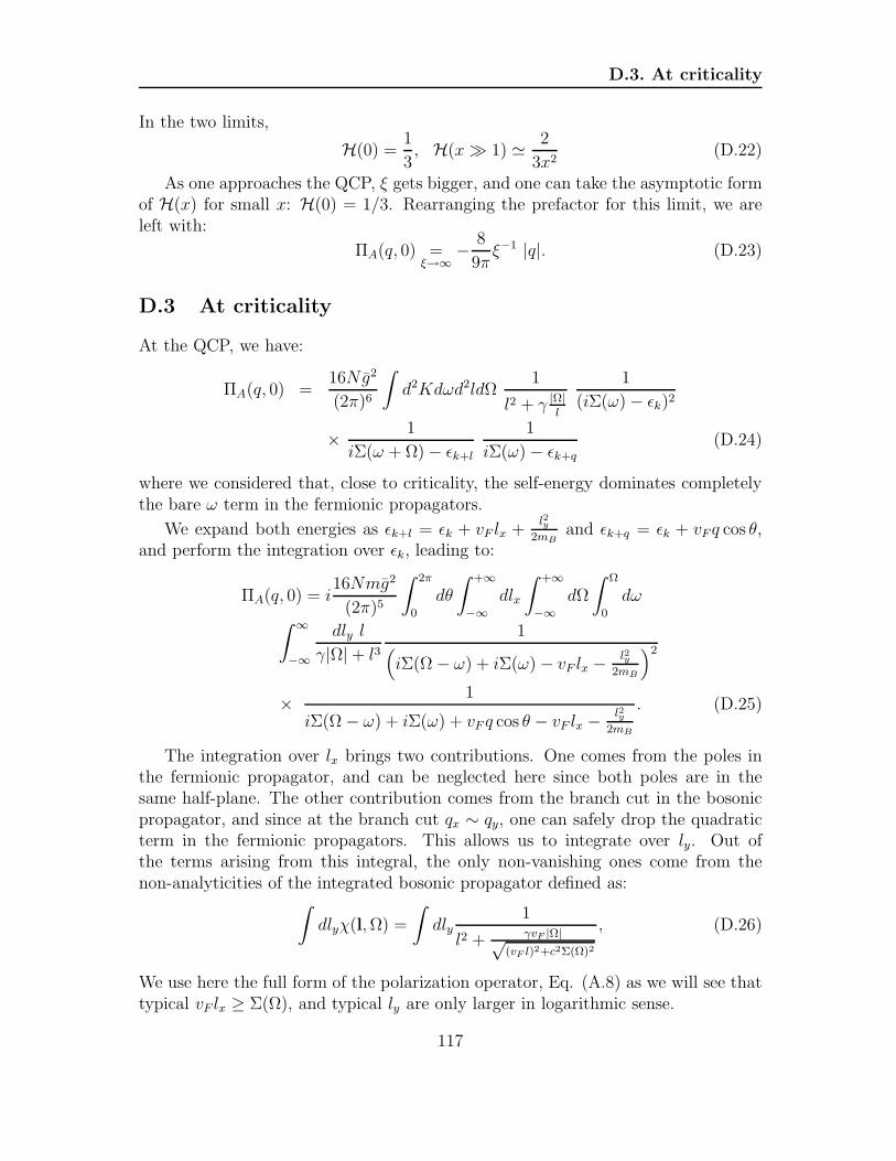
D.3. At criticality
In the two limits,
H(0) =1
3, H(x≫ 1) ≃ 2
3x2(D.22)
As one approaches the QCP, ξ gets bigger, and one can take the asymptotic formof H(x) for small x: H(0) = 1/3. Rearranging the prefactor for this limit, we areleft with:
ΠA(q, 0) =ξ→∞
− 8
9πξ−1 |q|. (D.23)
D.3 At criticality
At the QCP, we have:
ΠA(q, 0) =16Ng2
(2π)6
∫
d2Kdωd2ldΩ1
l2 + γ |Ω|l
1
(iΣ(ω)− ǫk)2
× 1
iΣ(ω + Ω)− ǫk+l1
iΣ(ω)− ǫk+q(D.24)
where we considered that, close to criticality, the self-energy dominates completelythe bare ω term in the fermionic propagators.
We expand both energies as ǫk+l = ǫk + vF lx +l2y
2mBand ǫk+q = ǫk + vF q cos θ,
and perform the integration over ǫk, leading to:
ΠA(q, 0) = i16Nmg2
(2π)5
∫ 2π
0
dθ
∫ +∞
−∞dlx
∫ +∞
−∞dΩ
∫ Ω
0
dω
∫ ∞
−∞
dly l
γ|Ω|+ l31
(
iΣ(Ω − ω) + iΣ(ω)− vF lx − l2y2mB
)2
× 1
iΣ(Ω − ω) + iΣ(ω) + vF q cos θ − vF lx − l2y2mB
. (D.25)
The integration over lx brings two contributions. One comes from the poles inthe fermionic propagator, and can be neglected here since both poles are in thesame half-plane. The other contribution comes from the branch cut in the bosonicpropagator, and since at the branch cut qx ∼ qy, one can safely drop the quadraticterm in the fermionic propagators. This allows us to integrate over ly. Out ofthe terms arising from this integral, the only non-vanishing ones come from thenon-analyticities of the integrated bosonic propagator defined as:
∫
dlyχ(l,Ω) =
∫
dly1
l2 + γvF |Ω|√(vF l)2+c2Σ(Ω)2
, (D.26)
We use here the full form of the polarization operator, Eq. (A.8) as we will see thattypical vF lx ≥ Σ(Ω), and typical ly are only larger in logarithmic sense.
117

Static spin susceptibility
This integral was performed in a slightly different form in (C.9), but the methodis the same: introducing u such that tanu = vF ly√
(vF lx)2+Σ(Ω)2, one has:
∫
dlyχ(l,Ω) =(vF lx)
2 + c2Σ(Ω)2
γv2F |Ω|
∫ π/2
0
du
cos3 u− δ cos2 u+ ǫ, (D.27)
where we introduced δ = c2Σ(Ω)2((vF lx)2+c2Σ(Ω)2)1/2
γv3F |Ω| and ǫ = ((vF lx)2+c2Σ(Ω)2)3/2
γv3F |Ω| .
In the process of integrating over lx, two non-analytic contributions arise from(D.27).
One comes from lx & (γΩ)1/3 and goes like π(γ|Ω|)1/3 . Plugging this back into ΠA
and subtracting ΠA(0, 0), we obtain
δΠ(1)A (q, 0)N ∼ mg2v2
F q2
∫ +∞
−∞
dlx|lx|
∫ +∞
−∞dΩ
∫ Ω
0
dω
(iΣ(Ω− ω) + iΣ(ω)− vF lx)5
where we subtracted ΠA(0, 0) (hence the notation δΠA) and expanded in q.We further simplify the integrals, noticing that the fermionic propagator is dom-
inated by vF lx since lx ∼ (γΩ1/3):
δΠ(1)A (q, 0) ∼ q2Nmg
2
v3F
∫ ωMax
0
dΩ
∫
dlxΩ
l6x
∼ q2Nmg2
v3Fγ
5/3
∫ ωMax
0
dΩ
Ω2/3
∼ √αq2, (D.28)
where we substituted lx ∼ (γΩ1/3) in the last steps.The other non-analytic contribution from (D.27) comes from typical vF lx ∼
Σ(Ω). It can be seen from an expansion of (D.27) for small values of both δ and ǫ,and goes like:
−(vF lx)2 + c2Σ(Ω)2
2v2Fγ|Ω|
log((vF lx)
2 + c2Σ(Ω)2).) (D.29)
One can explicitly verify that to get the logarithm, we only need the polarizationoperator Π(l,Ω) to order 1/l3.
Substituting (D.29) into the expression for ΠA and subtracting the constant part,we obtain:
Π(2)A (q, 0) = i
8Nmg2
(2π)5γvFq
∫ 2π
0
dθ
∫ +∞
−∞dlx
∫ +∞
−∞
dΩ
|Ω|∫ Ω
0
dωcos θ [(vF lx)
2 + c2Σ(Ω)2]
(iΣ(Ω− ω) + iΣ(ω)− vF lx)3
× log ((vF lx)2 + c2Σ(Ω)2)
iΣ(Ω − ω) + iΣ(ω) + vF q cos θ − vF lx. (D.30)
118

D.3. At criticality
Using the θ ←→ −θ symmetry, and splitting the integral over Ω into two parts,one can rearrange this expression as:
Π(2)A (q, 0) = i
Nmg2
cπ5γv2F
q
∫ π
0
dθ
∫ +∞
−∞dz
∫ +∞
0
dΩ
Ω
∫ Ω
0
dω1
Σ(Ω)
× cos θ(1 + z2)(
iΣ(Ω−ω)+Σ(ω)cΣ(Ω)
− z)3
log (1 + z2)
iΣ(Ω−ω)+Σ(ω)cΣ(Ω)
+ vF q cos θcΣ(Ω)
− z, (D.31)
where we defined z = vF lx/(cΣ(Ω)).Let’s now isolate the integral over z, given by:
J =
∫ +∞
−∞dz
(1 + z2) log(1 + z2)
(ia− z)3(ia + b− z) , (D.32)
where a = Σ(Ω−ω)+Σ(ω)cΣ(Ω)
and b = vF q cos θcΣ(Ω)
, and a ≥ 0.
Performing the contour integration in the lower half-plane (where lies the branch-cut), one gets:
J = −2π
∫ ∞
1
dy1− y2
(y + a)3(y + a− ib)
= −2π
∫ ∞
1
dy(1− y2)(y + a+ ib)
(y + a)3 ((y + a)2 + b2). (D.33)
Once (D.33) is plugged back into (D.31), only the imaginary term survives dueto the symmetry of the integral in θ. We are left with:
Π(2)A (q, 0) =
4Nmg2
c2π4γvFq2
∫ π/2
0
dθ
∫ +∞
1
dy
∫ +∞
0
dΩ
∫ 1
0
dw1
Σ(Ω)2
cos2 θ
[c−1 ((1− w)2/3 + w2/3) + y]3
× 1− y2
[y + c−1 ((1− w)2/3 + w2/3)]2+(vF q cos θcΣ(Ω)
)2 , (D.34)
where we changed variables, defining w = ω/Ω.
Introducing the new variable t =(
cΣ(Ω)vF q cos θ
)3/2
, this rewrites:
Π(2)A (q, 0) =
4Nmg2
c3/2π4γv3/2F ω
1/20
q3/2
∫ π/2
0
dθ (cos θ)3/2
×∫ +∞
1
dy
∫ 1
0
dw1
[c−1 ((1− w)2/3 + w2/3) + y]3
×∫ +∞
0
dt1− y2
1 + t4/3 [y + c−1 ((1− w)2/3 + w2/3)]2 . (D.35)
119

Static spin susceptibility
A final change in variables leads to:
Π(2)A (q, 0) =
4Nmg2
c3/2π4γv3/2F ω
1/20
q3/2
∫ π/2
0
dθ (cos θ)3/2
∫ +∞
0
dv1
1 + v4/3
×∫ +∞
1
dy
∫ 1
0
dw1− y2
[c−1 ((1− w)2/3 + w2/3) + y]9/2
(D.36)
where v = t[y + c−1
((1− w)2/3 + w2/3
)]3/2
Performing the integral over y, one is left with three independent integrals con-tributing to the numerical prefactor:
Π(2)A (q, 0) = − 32Nmg2
105π4γv3/2F ω
1/20
q3/2
∫ π/2
0
dθ (cos θ)3/2
∫ +∞
0
dv1
1 + v4/3
×∫ 1
0
dw5c+ 2
((1− w)2/3 + w2/3
)
(c+ (1− w)2/3 + w2/3)5/2
(D.37)
These integrals can be performed separately and read:
∫ π/2
0
dθ (cos θ)3/2 =
√2π3/2
6[Γ(
34
)]2 ≃ 0.8740
∫ +∞
0
dv
1 + v4/3=
3π√
2
4≃ 3.3322
∫ 1
0
dw5c+ 2s(w)
(c+ s(w))5/2≃ 0.9438 (D.38)
and we used the notation s(w) = (1− w)2/3 + w2/3.Collecting all integrals, and rearranging the prefactor, the final result for the
contribution of the first two diagrams then writes:
Π(2)A (q, 0) = −0.1053
√
kF q3/2. (D.39)
D.4 The other two diagrams
The computation of the other two diagrams in Fig. 3.2 can be carried out followingthe same path. Far away from criticality, when γvF ξ
2/(1 + λ) is small, and one canjust expand perturbatively in the interaction, the sum of these two “drag” diagrams,which we label here and in the main text as ΠB, was shown in [41] to be equal toΠA(q, 0) to the leading order in g (which in our model is g3, see (D.20 -D.22). Nearcriticality such simple relation no longer holds, but ΠA(q, 0) and ΠB(q, 0) remain ofthe same sign and of comparable magnitude.
120

D.4. The other two diagrams
At criticality, we obtained for ΠB(q, 0)
ΠB(q, 0) =
√2
33/44π4q3/2√
kF I (D.40)
where in rescaled variables (e.g., momentum is in units of q)
I =
∫
dΩdxx
∫ 2π
0
dθS2(x,Ω, θ)
S1(x,Ω)S1(x+ cos θ,Ω)(D.41)
and S(x,Ω, θ) and S1(x,Ω) are given by
S(x,Ω, θ) =
∫ Ω
0
dω
∫ 2π
0
dθ1iΣ∗ − x cos(θ1)
× 1
iΣ∗ − cos(θ + θ1)− x cos θ1(D.42)
S1(x,Ω) =
∫ Ω
0
dω
x2 + (Σ∗)2(D.43)
where we introduced Σ∗ = Σ∗(ω,Ω) = (Ω− ω)2/3 + ω2/3.We could not evaluate this integral explicitly, and we compute it under two
simplifying assumptions
• we compute S1(x,Ω) by expanding to leading order in (Σ∗/x)2, evaluating thefrequency integral and plugging the result back into the denominator. Thisway, we approximated S1(x,Ω) by
S1(x,Ω) ≈ Ω
x2 + (cΩ2/3)2(D.44)
where c ≈ 1.2 (see (A.6) This procedure is similar to the one which led to(A.8).
• We replace Σ∗ by the same cΩ2/3 in the integrand for S(x,Ω, θ)
• We assume that internal momenta are larger than the external one, i.e x≫ 1(x is measured in units of q), neglected terms O(1) compared to O(x) and setthe lower limit of the integration over x at some number b.
• We choose b by applying the same approximate computation scheme to the firstpart ΠA(q, 0) and requesting that the result coincide with the exact expression,Eq. (D.39).
Carrying out this calculation for ΠB(q, 0) we obtain
Π(2)A (q, 0) ≈ −0.14
√
kF q3/2. (D.45)
This is the result that we cite in the text.
121
Static spin susceptibility
122
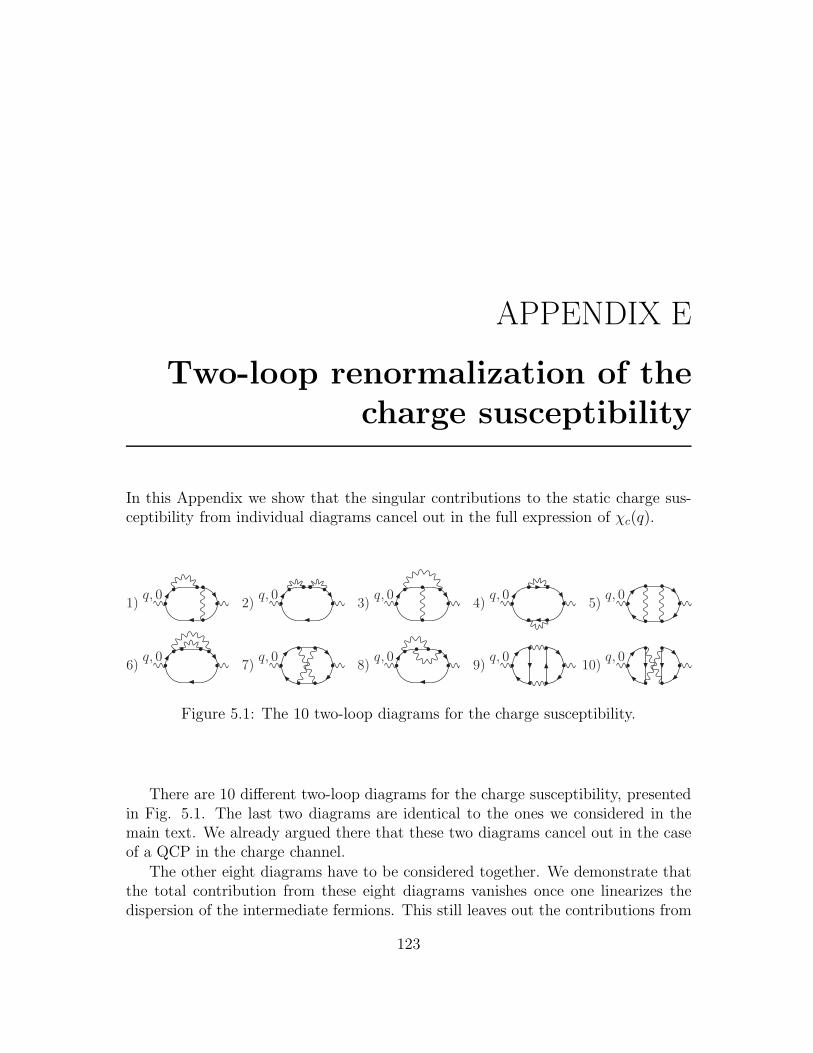
APPENDIX E
Two-loop renormalization of thecharge susceptibility
In this Appendix we show that the singular contributions to the static charge sus-ceptibility from individual diagrams cancel out in the full expression of χc(q).
1)q, 0
2)q, 0
3)q, 0
4)q, 0
5)q, 0
6)q, 0
7)q, 0
8)q, 0
9)q, 0
10)q, 0
Figure 5.1: The 10 two-loop diagrams for the charge susceptibility.
There are 10 different two-loop diagrams for the charge susceptibility, presentedin Fig. 5.1. The last two diagrams are identical to the ones we considered in themain text. We already argued there that these two diagrams cancel out in the caseof a QCP in the charge channel.
The other eight diagrams have to be considered together. We demonstrate thatthe total contribution from these eight diagrams vanishes once one linearizes thedispersion of the intermediate fermions. This still leaves out the contributions from
123

Two-loop renormalization of the charge susceptibility
non-linear terms in the dispersion, but one can show that these contributions areregular.
To begin, consider one of these diagrams, e.g., diagram 7 in Fig. 5.1. In analyticform, the contribution from this diagram is:
Π7(q) = 2
∫
d2q1dω1d2q2dω2 GkGk+qGk+q1Gk+q2+q
×Gk+q1+q2Gk+q1+q2+qχq1χq2 , (E.1)
where we labeled qi = (qi, ωi), and the combinatoric factor 2 comes from the sum-mation over spin indices.
Introduce now
GkGk+qi =1
αqi(Gk −Gk+qi) , (E.2)
whereαqi = iωi − qi cos θi, (E.3)
and θi is the angle between k ≈ kF and qi. Shortening the notations further asq1 ≡ 1 and q2 ≡ 2, using the symbolic notation
∫
1,2for the 6-dimensional integral
over q1 and q2, and applying (E.2), we obtain:
Π7(q) = 2
∫
1,2
χ1χ2
[Gk+qGk+1+2
α21α
22
− Gk+qGk+1+2
α1α2(α1 + α2)2− 2
Gk+qGk+1
α22(α
21 − α2
2)
]
(E.4)
Similarly,
Π8(q) = 2
∫
1,2
χ1χ2
[Gk+qGk+1+2
α1α2(α1 + α2)2− 2
Gk+qGk+1
α21(α
21 − α2
2)
]
(E.5)
and further
Π5(q) = 2
∫
1,2
χ1χ2
[Gk+qGk+1+2
α1α2(α1 + α2)2+ 2
Gk+qGk+1
α21(α
21 − α2
2)
]
(E.6)
Π3(q) = 2
∫
1,2
χ1χ2
[
−Gk+qGk+1+2
α21α
22
+ 2Gk+qGk+1
α21α
22
(α2
1 + α22
α21 − α2
2
)]
(E.7)
Π2(q) = 4
∫
1,2
χ1χ2Gk+qGk+1
α21α
22
(α2
2
α21 − α2
2
)
(E.8)
Π1(q) = 4
∫
1,2
χ1χ2
α21α
22
[
Gk+qGk+1+2α2
2
α21 − α2
2
−Gk+qGk+13α2
2 − α21
α21 − α2
2
]
(E.9)
Π4(q) =
∫
1,2
χ1χ2
α21α
22
[Gk+qGk+1+2 − 2Gk+qGk+1] (E.10)
and finally,
Π6(q) =
∫
1,2
χ1χ2
α21α
22
[
Gk+qGk+1+2α2
1 + α22
(α1 + α2)2− 2Gk+qGk+1
]
(E.11)
Collecting the prefactors for Gk+qGk+1+2 and Gk+qGk+1 from all of the eight contri-butions we find that they do cancel out.
124

APPENDIX F
Mass-shell singularity
In this Appendix, we analyze in more detail the form of the self-energy near thefermionic mass shell. The interest to the mass-shell behavior of the self-energywas triggered by recent studies of the self-energy near a mass shell in a 2D Fermiliquid [33] and for 2D Dirac fermions [56]. In both cases, the lowest-order self-energydiverges at the mass-shell, which forces to re-sum the perturbative series.
At first glance, the same situation holds in our analysis at the QCP. Evaluatingthe self-energy in a two-loop expansion around free fermions and using the fermionicdispersion with the curvature, we obtain near the mass shell [57]
Σ(k, ω) ∼ 1
N2(iω − ǫk)
[
N logiω − ǫkǫk
]2
. (F.1)
This result implies that the quasiparticle residue Z ∝ dΣ/dǫk logarithmically di-verges on the mass shell of free fermions. Without the curvature of the dispersion,the divergence would be stronger than logarithm.
The issue we now have to address is whether Z still diverges on the mass shell ifwe expand around the Eliashberg solution, i.e., around fermions with
G0(k, ω) =1
iΣ(ω)− ǫk, (F.2)
where, we remind, Σ(ω) = ω + Σ(ω).
It turns out that this is not the case: the expansion around the Eliashbergsolution leads to a finite residue Z.
125

Mass-shell singularity
At the two-loop order, we obtain, instead of (F.1):
Σ(k, ω) ∼ 1
N2
∫ 1
0
dz
∫ 1
1−zdz′ (iΣ(ω)ψz,z′ − ǫk)
[
logN(iΣ(ω)ψz,z′ − ǫk)
ǫk
]2
(F.3)
whereψz,z′ = (1− z)2/3 + (1− z′)2/3 + (z + z′ − 1)2/3. (F.4)
For simplicity, we restricted ourselves to the quantum critical regime where Σ(ω) ≈Σ(ω). If ψz,z′ were equal to a constant, as it is when the system is in the Fermi liquidregime, and Σ(ω) = λω, then Z would diverge at ω = ǫ/(1 + λ). However, sinceΣ(Ω−ω) + Σ(ω) does not reduce to Σ(Ω), we have two additional integrations overz and z′, and the logarithmic singularity is washed out. In particular, at ǫk = iΣ(ω),i.e. at the “Matsubara mass shell”, we have
Zeff ∼1
N2
[π2
6log2N − 4.08 logN + 2.88
]
, (F.5)
in which case Zeff is just a constant. Combining this with our earlier result thatthe renormalization of ǫk is also finite, Eq. (2.65), we obtain for the full fermionicGreen’s function at the smallest ω and ǫk
G(k, ω) =Zeff
iΣ(ω)− ǫ∗k, (F.6)
where ǫ∗k differs from ǫk by a constant factor.
126

Part II
Bosonic approach to quantumimpurity models
127


CHAPTER 5
Introduction and motivations
Contents
5.1 Kondo and Anderson models: a brief review . . . . . . . 130
5.1.1 History of the Kondo effect . . . . . . . . . . . . . . . . . 130
5.1.2 Anderson model . . . . . . . . . . . . . . . . . . . . . . . 132
5.1.3 Experimental and theoretical relevance: the revival . . . . 133
5.2 Quantum dots . . . . . . . . . . . . . . . . . . . . . . . . . 135
5.2.1 Charge quantization . . . . . . . . . . . . . . . . . . . . . 135
5.2.2 Coulomb blockade . . . . . . . . . . . . . . . . . . . . . . 136
5.2.3 Kondo physics in quantum dots . . . . . . . . . . . . . . . 137
5.3 Heavy fermions and the Kondo lattice . . . . . . . . . . . 139
5.3.1 Kondo lattice . . . . . . . . . . . . . . . . . . . . . . . . . 139
5.3.2 Heavy fermion: a prototypical Kondo lattice . . . . . . . 141
This first chapter is a general introduction to the Kondo model. After brieflyrecalling the history and the physics behind the Kondo effect, we review some of theexperiments where the Kondo effect plays a major role. This experimental relevanceis used to motivate the present work.
129

Introduction and motivations
5.1 Kondo and Anderson models: a brief review
5.1.1 History of the Kondo effect
The Kondo effect was explained by Jun Kondo in 1964. It solved a 30 year oldexperimental puzzle, known as the resistance minimum. Kondo’s theory howeverwas incomplete, and one had to wait the work of Wilson, ten years later, to fullyunderstand the low-temperature physics of the Kondo effect.
Resistance minimum
For electrons in a perfect lattice, the conductivity at low temperature divergesas there is no scattering, and consequently no current dissipation. At finite tem-perature, the essential mechanism for current dissipation lies in the scattering offphonons. At low enough temperature, the contributions from the phonons decayrapidly, and the scattering by defects and impurities in the metal host become themain source of dissipation. The low-temperature resistance saturates in this caseat a finite value which depends on the number of defects in the material: addingmore of them increases the residual resistance but does not affect the character ofthe temperature dependence.
However, since the pioneering work of de Hass et al. [58], there have been manyobservations of a low temperature increase in the resistance of metals, leading toa minimum of resistance (see Fig. 5.1). The later observation that the minimumdepended on the concentration of impurities indicated it as being an impurity phe-nomenon.
In 1964, Kondo considered the interaction between a single magnetic ion, em-bedded inside a non-magnetic metal, and the conduction electrons of the latter [59].He was motivated by a recent experimental work by Sarachik and collaborators [60]who observed a correlation between the existence of a Curie-Weiss term in the im-purity susceptibility (signaling the existence of local moments) and the occurrenceof the resistance minimum. Convinced that the magnetic character of the impuritywas responsible for the resistance minimum, rather than crystal field effects or theimpurity charge, he considered the following Hamiltonian1:
H =∑
k
∑
α=±ǫkc
†
kαckα + JK∑
k,k′
∑
αβ
S ·(
c†
kα
σαβ
2ck′β
)
(5.1)
where c†
kα and ckα are creation and annihilation operators for the conduction elec-trons, with momentum k and spin α. While the first term is a generic kinetic termfor the band of electrons, the second term describes the interaction between theimpurity spin S and the local density of spin of the conduction electrons.
1This Hamiltonian, often called the “Kondo Hamiltonian”, was not introduced by Kondo butby Zener [61]. Kondo is however the first one to have found the log term in the resistivity.
130
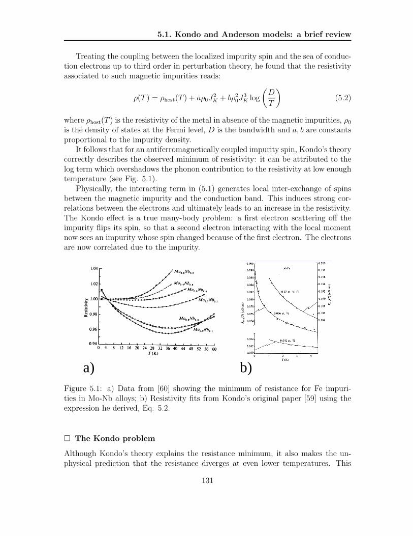
5.1. Kondo and Anderson models: a brief review
Treating the coupling between the localized impurity spin and the sea of conduc-tion electrons up to third order in perturbation theory, he found that the resistivityassociated to such magnetic impurities reads:
ρ(T ) = ρhost(T ) + aρ0J2K + bρ2
0J3K log
(D
T
)
(5.2)
where ρhost(T ) is the resistivity of the metal in absence of the magnetic impurities, ρ0
is the density of states at the Fermi level, D is the bandwidth and a, b are constantsproportional to the impurity density.
It follows that for an antiferromagnetically coupled impurity spin, Kondo’s theorycorrectly describes the observed minimum of resistivity: it can be attributed to thelog term which overshadows the phonon contribution to the resistivity at low enoughtemperature (see Fig. 5.1).
Physically, the interacting term in (5.1) generates local inter-exchange of spinsbetween the magnetic impurity and the conduction band. This induces strong cor-relations between the electrons and ultimately leads to an increase in the resistivity.The Kondo effect is a true many-body problem: a first electron scattering off theimpurity flips its spin, so that a second electron interacting with the local momentnow sees an impurity whose spin changed because of the first electron. The electronsare now correlated due to the impurity.
a) b)Figure 5.1: a) Data from [60] showing the minimum of resistance for Fe impuri-ties in Mo-Nb alloys; b) Resistivity fits from Kondo’s original paper [59] using theexpression he derived, Eq. 5.2.
The Kondo problem
Although Kondo’s theory explains the resistance minimum, it also makes the un-physical prediction that the resistance diverges at even lower temperatures. This
131
Introduction and motivations
divergence signals the breakdown of Kondo’s perturbative treatment. Resummingthe logarithmically divergent terms, a natural scale appears, below which any kindof perturbative expansion is bound to fail. This temperature scale is known as theKondo temperature TK , and is given by:
TK ∼ De−1/(ρ0JK) (5.3)
as one can argue from (5.2), by comparing the last two terms.Anderson’s work on the so-called “poor man’s scaling” [62] inferred that a
ground-state with an infinite coupling develops, the impurity being bound to aconduction electron in a singlet state. The behavior at low-temperature would thenbe similar to that of a non-magnetic impurity, the impurity spin being compensated.
Wilson’s numerical renormalization group confirmed this hypothesis [63]. Hecould obtain definitive results for the ground-state and low-temperature behaviorof the system. Wilson highlighted the existence of a dynamically generated tem-perature scale, corresponding to the Kondo temperature TK , where the systemsundergoes a cross-over towards a strong-coupling regime for the case of an antifer-romagnetic coupling JK . The system is then characterized by the formation of aKondo singlet.
At high temperature, T ≫ TK , the impurity spin and the electrons are onlyweakly coupled: one can compute the properties of the system from a perturbativeexpansion around the free impurity regime. At low temperature, T ≪ TK , oneenters the strong coupling regime: the conduction electrons screen out the impurityspin, forming with it a spin singlet state. Note that in this respect, the Kondo effectis a simple example of asymptotic freedom: the theory is trivial at high energy (freelocal moment), but much more complex at low energy (many-body object).
5.1.2 Anderson model
The Anderson model [64] is a generalization of the simple model used by Kondo,which takes into account charge fluctuations. In this model, the magnetic impurityis a localized electronic orbital, whose charge can now fluctuate. The associatedHamiltonian writes:
H =∑
k
∑
σ=±ǫkc
†
kσckσ + V∑
kσ
(
c†
kσfσ + f†
σckσ
)
+ ǫf∑
σ
f†
σfσ + Unf↑nf↓ (5.4)
where nfσ = f†
σfσ.This model takes into account the generic kinetic term for the band of conduction
electrons, an hybridization V between the localized orbital and the metallic host,the energy ǫf of the orbital, and finally a Coulomb repulsion term on the site of theimpurity.
To get some insight into this model, let’s consider the case V = 0, the so-called “atomic limit” (where the localized states are uncoupled from the conduction
132

5.1. Kondo and Anderson models: a brief review
electrons). In this situation, there are three energy configurations for the states ofthe localized f electrons:
• zero occupation, with a total energy E0 = 0
• single occupation by a spin σ, with an energy E1,σ = ǫf
• double occupation with a spin ↑ and a spin ↓, with energy E2 = 2ǫf + U
If the ground-state corresponds to single occupation, then the system has two-folddegeneracy corresponding to spin 1
2, and displays an associated magnetic moment.
The other two configurations are non-degenerate and therefore non-magnetic.It follows that in the atomic limit, the condition for the formation of a local
moment is that the singly-occupied configuration lies lowest in energy. Turningon the hybridization with the conduction band, we expect that for V ≪ U theground-state of the ion is essentially the same as in the atomic limit. Therefore, theKondo model can be seen as a limiting case of the Anderson one, where the valencefluctuations of the localized orbital can be neglected.
Schrieffer and Wolf [65] used a canonical transformation (which amounts to gen-eralizing the second-order perturbation theory to encompass off-diagonal matrixelements) to prove that if the singly occupied state is the ground-state in the atomiclimit, then the effective Hamiltonian for a small hybridization is obtained by takinginto account virtual excitations to the zero and double occupied states. This effec-tive Hamiltonian reduces to the one used by Kondo, in the local moment regimedefined as U + ǫf > EF and ǫf < EF .
This can be readily seen from (5.4) by taking the limit of infinitely low energyfor the orbital and the Coulomb repulsion: ǫf = −U/2 → ∞. In this regime, onlythe singly-occupied states survive, and they couple to the conduction electrons viaan antiferromagnetic coupling JK ∼ 4V 2/U which comes from virtual hopping ontothe high-energy states of valence 0 and 2.
Note finally that because of the possibility of valence fluctuations, the physics ofthe Anderson model is richer than that of the Kondo model (which cannot treat, e.g.,the mixed valent regime). Quite often, the theoretical formulation of experimentalsetups makes use of the Anderson model, and later reduces to a Kondo model in thelocal moment regime.
5.1.3 Experimental and theoretical relevance: the revival
Why would anyone still want to study a physical phenomenon that was explainedmore than 30 years ago? Although the Kondo effect is a well-known and widelystudied phenomenon, it continues to capture the interest of both theorists and ex-perimentalists [66].
Among the examples of the revival of the Kondo effect (some of which we detailin the next sections), one of the most interesting ones comes from the experimental
133

Introduction and motivations
observation of the Kondo or Abrikosov-Suhl resonance [67, 68]. Due to the formationof the Kondo singlet state, which involves conduction electrons close to the Fermisurface, the Kondo effect results in the presence of an acute perturbation in therenormalized density of states at the Fermi energy: the “Kondo resonance”.
Until very recently, physicists could only infer the role of the Kondo effect bymeasuring bulk properties like the resistance or the magnetic susceptibility. With thedevelopment of nanotechnology and one of its central tools – the Scanning TunnelingMicroscopy or STM – it is now possible to image a surface with atomic resolution,and measure the Kondo resonance from the current versus voltage characteristics.
a) b)Figure 5.2: a) Differential tunnel conductance of the tip at various distances r fromthe impurity, taken from [69]. The anti-resonance close to zero bias is a hallmarkof the Kondo effect. b) Ellipse of atoms with an impurity at one of the foci. Thetop part is a plot of the measured density of states on the surface, revealing a sharppeak located at both foci, even where the impurity is not present.
This has been done experimentally by two groups [70, 71] who measured thedifferential tunnel conductance at the site of the impurity (an atom of Co depositedon gold surface, and Ce on silver). Manoharan and collaborators [69] took it to thenext level by building an ellipse of atoms around a cobalt impurity placed at one ofthe focal points. The STM-measured energy spectrum revealed the existence of aKondo resonance at the site of the impurity but also at the second focus, despite theabsence of any magnetic impurity at that location. Since then, this phenomenon,labeled as “quantum mirage”, has led to many other experimental and theoreticalstudies [72].
134

5.2. Quantum dots
The development of nanotechnology has rekindled interest in the Kondo effect.However, the study of these systems is limited by construction as one cannot modifythe properties of the magnetic impurity or its coupling to the bulk electrons. This isprecisely the next step physicists are aiming at, with the so-called “quantum dots”.
5.2 Quantum dots
The ambition of this section is not to give a detailed review of the quantum dotphysics2, but rather to introduce the main concepts, explain the relevance of theKondo effect in these systems and provide a motivation for our current work.
5.2.1 Charge quantization
Quantum dots are small semiconductor devices, man-made “droplets of charge”ranging from 10 to 1000 nm in size, where the number of trapped electrons canbe tuned precisely by varying external parameters, from one to several thousand.They are made of an isolated patch containing an electron gas, coupled via tunnelbarriers to one or two leads, and capacitively to a gate electrode, allowing to changethe electrostatic potential of the dot (see Fig. 5.3).
These devices are often referred to as “artificial atoms”, as the confinement ofelectrons leads to quantized energy levels as in an atom. The tremendous differencebeing that quantum dots allow one to scan through the entire periodic table bysimply changing a voltage.
The electronic states in the dot can be probed by transport when a small tunnelcoupling is allowed between the dot and the surrounding reservoir of electrons: theso-called source and drain leads. The key idea behind the study of quantum dots,is to create devices where quantum effects, such as the quantization of charge, areimportant. In order to do so, one has to fulfill two conditions:
• work at low temperature:e2
C≫ kBT (where C is the capacitance of the dot)
When tunneling occurs between the dot and the leads, the charge on the islandsuddenly changes by the quantized amount e. The associated change in theCoulomb energy is conveniently expressed in terms of the capacitance C of theisland so that the electrostatic potential increases by an amount Ec = e2/C,known as the charging energy3. This charging energy plays a significant roleonly at temperatures much below it, when states of different charge are wellseparated in energy.
2See [73] for a complete review of the subject, or [74, 66] for a friendly introduction to this field.3For that, we assumed that the Coulomb interaction between the electrons is independent on the
number N of electrons in the island. This is known as the “constant-interaction” model. Despiteits simplicity, this model is remarkably accurate and allows to describe the measurements. For adetailed justification of the model, see the review of Aleiner et al. [75].
135

Introduction and motivations
• restrict to the weak conductance regime: G≪ e2
hThis means that the tunnel barriers must be sufficiently opaque such that theelectrons are located either in the dot or in the leads, and not delocalized overthe whole circuit.
The first criterion can be met by making the dot small (recall that the capacitanceof an object scales with its typical radius), and the second by weakly coupling thedot to the leads.
d'un point quantique d'apres [4. A gau he : depositionMOSFET, onduisant a une depletion du gaz d'ele tron sous-mi rographie ele tronique). A droite : stru ture ylindrique d'unrti iel).point et V est le ourant applique a ses bornes). Commea) b) c)
Figure 5.3: a) Schematic diagram of the lateral and vertical quantum dots (from[73]); b) Top surface of the Single Electron Transistor (SET) used in the experimentsof Goldhaber-Gordon et al. [76]; c) Vertical dot structure (from [77]).
5.2.2 Coulomb blockade
In the regime of quantized charge tunneling mentioned above, the energy of a dotcontaining N + 1 electrons is greater than one containing N electrons: extra energyis therefore needed to add an electron to the dot and no current will flow until thisenergy is provided by increasing the voltage. This phenomenon is known as the“Coulomb blockade”.
Indeed, a voltage Vg applied to the gate can change continuously the island’selectrostatic energy: it lowers the energy of electrons in the droplet relative to theFermi level in the leads. If we sweep Vg, the build up of electrostatic energy iscompensated by tunneling of discrete charges onto the dot. Formally, the potentialenergy of a dot withN electron and a gate voltage Vg is given, in first approximation,by:
E =Q2
2C+QVg =
1
2EcN
(
N − 2CVge
)
(5.5)
Starting from a dot withN electrons and increasing Vg, one reaches a point wherethe energy of the two configurations with N and N + 1 electrons are degenerate.Because of this charge degeneracy, the allowed fluctuation in the number of electronson the dot leads to a current flow and results in peaks of the conductance as afunction of the gate voltage: the so-called “Coulomb oscillations” (see Fig. 5.4).
136

5.2. Quantum dots
a) b)
Figure 5.4: Conductance in the Coulomb blockade regime: a) for a lateral quantumdot [78], showing sharp periodically spaced peaks; b) for a vertical quantum dot[79], showing the appearance of multiplets corresponding to shell filling.
This mechanism allows one to control the current through the dot via a smallchange in the gate voltage Vg. For this reason, this device is also called a “single-electron transistor” (SET).
Refining a bit the model used to derive (5.5), one can take into account theenergy spectrum ǫp of the states trapped on the dot, and consider the case wherethe energy spacing cannot be neglected compared to the charging energy. In thiscase, the energy one has to pay to add an electron to the state p is given by thecharging energy. As soon as this state is filled, the energy cost increases in orderto account for the energy difference between the states p and p + 1, in additionto the charging energy. This leads to Coulomb oscillations organized in multipletsseparated by an energy Ec + ǫp+1 − ǫp, where the peaks inside a given multipletare separated by an energy Ec. This shell structure has been observed in verticalquantum dots [79] and clearly justifies the name “artificial atoms” for these devices(see Fig. 5.4).
5.2.3 Kondo physics in quantum dots
Conventional Kondo effect
We have just seen that a voltage applied to the gate electrode controls the number Nof electrons on the dot. If an odd number of electrons is trapped within the island,the total spin of the dot S is necessarily non-zero. This localized spin, embeddedbetween large reservoirs of electrons, is susceptible to undergo a Kondo effect. Therelevance of the Kondo physics for these systems was predicted theoretically byGlazman and Raikh [80] and Ng and Lee [81]. The basic punch-line is that theformation of a Kondo singlet between this localized spin and the electrons of theleads, is responsible for the development of a peak in the density of states of thelocalized spin (the so-called “Kondo resonance”) pinned at the Fermi energy of the
137

Introduction and motivations
leads. Since the transport properties are determined by electrons with energies closeto the Fermi level, the Kondo resonance is expected to have a dramatic influenceon, e.g., the conductance of the dot.
For small dots, the quantized energy difference between different electronic states(for a given number of electrons N on the island) becomes important. When thetemperature becomes lower than this energy spacing, a system with an odd numberof electrons on the dot effectively behaves as a spin-1/2, coupled to a gas of freefermions (the two leads), and can be described by an Anderson model with thefollowing Hamiltonian:
H =∑
k,σ
∑
a=L,R
ǫkc†
akσcakσ + Ecnd↑nd↓ + ǫ0∑
σ
d†
σdσ +∑
k,σ
∑
a=L,R
Va
(
c†
akσdσ + d†
σcakσ
)
(5.6)where we introduced the c
†
akσ fermionic fields to describe the electrons of the leads,as well as the fermionic d
†
σ for the localized spin of the dot.When the temperature is larger than the coupling between the leads and the dot,
one recovers the Coulomb oscillations and the conductance shows periodically spacedpeaks (not very sharp if the coupling is not small enough). As the temperature islowered, one eventually goes below the Kondo temperature. In this regime, thedevelopment of the Kondo resonance strongly enhances the conductance of the dotprovided that the number of electrons on the dot is odd (as we have just argued inthe previous paragraph). This leads to an even-odd effect on the dot: if the numberof trapped electrons is even, the conductance drops towards zero, whereas if it isodd, it increases dramatically and eventually reaches the unitary value of 2e2/h atlow temperature. The Kondo effect not only suppresses the Coulomb blockade, butis also able to make the dot completely transparent (the conductance is maximal inthe zero temperature limit).
These consequences of the Kondo effect have been observed experimentally [76,82].
New directions
The quantum dots provide new opportunities to control the Kondo effect, and al-though the results described thus far resemble what happens for an impurity in ametal, these devices allow to study regimes inaccessible with magnetic impurities,bringing the Kondo effect to a whole new level.
To name a few examples of these new directions for the Kondo effect, one has:
• the effect of a magnetic field (singlet-triplet transition and associated two-stagescreening) [84];
• the experimental realization of a two-impurity Kondo system using doublequantum dots [85, 86];
138

5.3. Heavy fermions and the Kondo lattice
2
1
0
gate voltage
N+1
N+2
N+3
N+4
N = even
co
nd
ucta
nce
(e
2/h
)
a
−0.5 0.0 0.5 1.0 1.5Vg/U
0
0.5
1
1.5
2
G[e
2 /h]
12 23 3
a
a)
1 K
25 mK
b)
Figure 5.5: a) Experimental observation of the effect of the Kondo resonance onthe conductance of a dot [82]; b) These lineshapes could be recovered theoreticallyusing a numerical renormalization group approach [83].
• the physics out-of-equilibrium (high voltage, three-terminal SET,. . . );
• the coupling of a quantum dot to magnetic leads;
• the proposed experimental setups to explore the two-channel Kondo effect [87]
A lot of these effects require a better theoretical understanding of the Andersonand the Kondo models, in particular out of equilibrium, where very powerful toolslike the Bethe ansatz are not so easy to extend [88]. We believe that some of theunanswered questions that these new directions raise can be, if not solved, at leastbetter formulated, thanks to simple approaches capturing the low-temperature be-havior of the Kondo effect, generalized to encompass the physics out of equilibrium.This is one of our main motivation for the present work.
5.3 Heavy fermions and the Kondo lattice
Another important application of the Kondo effect comes not from the single im-purity physics, but from dense ordered lattices of impurities, and its relevance for awhole family of compounds known as “heavy fermion systems”.
5.3.1 Kondo lattice
In a system containing many dilute impurities, the conduction electrons form withthe network of localized spins, a set of Kondo singlets roughly independent fromeach other. When the density of impurity increases, correlations appear betweenthem, due to the Kondo interaction with the conduction band.
139

Introduction and motivations
RKKY interaction
As early as 1940, Frolich and Nabarro [89] discussed the possibility of a ferromag-netic interaction between nuclear spins mediated by the hyperfine coupling withthe surrounding cloud of electrons. Later on, Ruderman and Kittel [90] computedfrom a second-order perturbation expansion the effective coupling between nuclearspins. Kasuya [91] and Yosida [92] proposed an extension of this mechanism tolocalized inner d-electron spins, coupled via an indirect exchange mediated by theconduction electrons. This long-range spin-spin interaction is now known as theRuderman-Kittel-Kasuya-Yosida or “RKKY interaction”.
When a magnetic moment is introduced into a metal, it polarizes the surroundingcarriers by means of the Kondo interaction and induces Friedel oscillations in thespin density around the magnetic ion [93]. If another local moment is introduced,it couples with the first one, giving rise to the following long-range interaction:
JRKKY (x− x′) = −J2Kχ(x− x′) where χ(q) = 2
∑
k
f(ǫk)− f(ǫk+q)
ǫk+q − ǫk(5.7)
At zero temperature, for a parabolic band, one has:
JRKKY (r) ∼ −J2Kρ0
sin(2kF r)− 2kF r cos(2kF r)
2(2kF r)4(5.8)
where ρ0 is the density of states at the Fermi level, and r is the distance from theimpurity (see Fig. 5.6). The oscillating part with a period 2kF is characteristic ofFriedel oscillations. As a consequence, the sign of the RKKY interaction dependson the distance between the impurities, and the typical strength of the coupling isERKKY ∼ J2
Kρ0.
Donicah’s picture
Comparing the typical energy scale associated to the Kondo (TK ∼ De−1/(ρ0JK))and the RKKY (TRKKY ∼ ρ0J
2K) interactions, one expects for the low temperature
regime:
• for large values of the Kondo coupling constant, TK ≫ TRKKY , one expectsthe Kondo effect to be the dominant interaction, leading to the formation oflocal singlets roughly independent of one another. This suggests the formationof a Fermi liquid ground-state,
• for small values of JK , TRKKY ≫ TK . A magnetically ordered state is favoredin this case. This magnetic order prevents spin-flip processes to occur, andthe Kondo resonance to develop.
140

5.3. Heavy fermions and the Kondo lattice
As one varies the Kondo coupling continuously, the system is expected to gofrom a magnetically ordered to a Fermi liquid ground-state, with a quantum criticalpoint separating the two at zero temperature. These arguments and the associatedpictorial phase diagram that emerges from them (see Fig. 5.6), are known as theDoniach picture [94].
However, it is important to keep in mind the crudeness of these arguments:this description is only qualitative. First of all, the exponential form of the Kondotemperature used in this discussion comes from the single-impurity physics, and mayvery well change substantially once we treat the lattice model. Second, and moreimportantly, both the expressions for TK and JRKKY relies on the assumption of asomewhat large electronic bandwidth. It follows that for JK ∼ D, these expressionsshould not be taken too seriously. It turns out that, as they stand, the Kondocoupling for which both scales are of the same order of magnitude corresponds toJK ∼ D.
a)
AFM
FL
b)
?TK ∼ De−1/(ρ0JK)
TRKKY ∼ ρ0J2K
JK
T
Figure 5.6: a) Illustration of the electron spin polarization (in blue) around a mag-netic impurity (in red) giving rise to Friedel oscillations and inducing an RKKYinteraction between impurity spins; b) Doniach phase diagram, with an antiferro-magnetically ordered phase (AFM) at low JK and a Fermi liquid phase (FL) at largeJK .
5.3.2 Heavy fermion: a prototypical Kondo lattice
There exists a whole family of compounds that can be thought of as a dense latticeof local moments embedded in a metallic host. They are known as “heavy fermions”.
Heavy fermions
In 1975, Andres, Graebner and Ott [95] pointed out that the low-temperature be-havior of CeAl3 is that of a metal, with strongly renormalized physical properties.They had just discovered one of the first examples of heavy fermion metal.
141
Introduction and motivations
Heavy fermion materials are rare-earth or actinide-based compounds, contain-ing f -electron elements (U, Ce, Yb). They are distinguished at low temperaturesby an anomalously large specific heat coefficient, with correspondingly large Pauliparamagnetic susceptibility (here “large” means 2 to 4 orders of magnitude largerthan, say, Cu). These properties can be described within the framework of Landau’sFermi liquid theory, by considering a large renormalized mass, as big as 104 bareelectronic mass, hence the name “heavy fermion” associated to these compounds(see Fig. 5.7).
Microscopically, one of the most important properties of the 4-f and 5-f elementsis the small spatial extent of their radial probability. One can thus consider thatheavy fermion materials are made of localized f orbitals arranged in a periodiclattice, interacting with delocalized conduction electrons.
For this reason, the heavy fermion compounds are thought to be described bythe periodic Anderson model, whose Hamiltonian writes:
H =∑
k
∑
σ=±ǫkc
†
kσckσ + V∑
i,σ
(
c†
iσfiσ + f†
iσciσ
)
+ ǫf∑
i,σ
f†
iσfiσ + Unfi↑nfi↓ (5.9)
where the f electrons hybridize with the conduction electrons c.In practice, due to the large local repulsion, and the weak hybridization of the
4−f and 5−f shells, most lanthanides and actinides-based compounds have stablevalence states and concomitant local magnetic moments, which allows the reductionof the previous Hamiltonian, Eq. (5.9), to the one of the Kondo lattice model.
QCP and Non-Fermi liquid
Heavy fermion materials offer a unique opportunity to study quantum criticalityunder controlled conditions: by applying pressure, doping, or magnetic field, it ispossible to tune the ground-state of the system from a magnetically ordered stateto a Fermi liquid, through a quantum critical point.
A wide body of evidence suggests that the effective mass m∗ of the fermionicquasiparticles in the paramagnetic Fermi liquid diverges as one approaches the QCP.This divergence leads to a breakdown of Landau’s Fermi liquid theory, and the statewhich forms above the QCP is referred to as a non-Fermi liquid4.
Among the wide range of physical properties that departs from the Fermi liquidbehavior at criticality, one sees many common features5 (see Fig. 5.7):
• diverging specific heat coefficient at the QCP:
CvT∼ c log
(T0
T
)
or, more rarely ∼ T−1+λ (5.10)
4This designation, already used in the text for MnSi, actually encompasses a broad range ofdifferent behaviors. Quoting Altshuler: “The difference between a Fermi liquid and a non-Fermiliquid is like the difference between a banana and a non-banana”.
5For a review of the experimental data of the non-Fermi liquid behavior of f -electron metals,see e.g. [96].
142

5.3. Heavy fermions and the Kondo lattice
Compound Cv/T ρ(T )YbRh2Si2 logT TCeCoIn5 T
CeCu6−xAux logT TCeCu6−xAgx logT T 1.1
CeNi2Ge2 logT T 1.4
CeCu2Si2 logT T 1.5
YbAgGe logT TCePd2Si2 T−0.5 T 1.2
a) b)
Figure 5.7: a) Specific heat coefficient and Pauli susceptibility of a few heavy fermionmaterials in the Fermi liquid regime; b) Selected list of heavy fermion compounds,and their associated properties in the quantum critical regime.
with 0.5 ≤ λ ≤ 0.9. This suggests that the effective mass m∗ → ∞ at theQCP.
• quasi-linear resistivity:
ρ(T ) ∼ ρ0 + AT 1+ǫ (5.11)
where 0 ≤ ǫ ≤ 0.6 at the QCP. This quasi-linear behavior is seen on a tem-perature range going from half a decade up to three decades (for Ge-dopedYbRh2Si2 [97]).
• a non-Curie spin susceptibility:
χ−1(T ) = χ−10 + CT a (5.12)
where a < 1.
In addition to this non-Fermi liquid behavior, scaling properties could be mea-sured for a few compounds: in YbRh2Si2, the differential susceptibility exhibits H/Tscaling [98] and in CeCu6−xAux, neutron scattering measurements showed E/T scal-ing in the dynamical spin susceptibility [99].
None of the theoretical approaches devised to date, could explain all of thesefeatures (though some could recover partial results). The key ingredient that isgenerally missing is the competition between the Kondo effect and the develop-ment of magnetic correlations: most approaches have focused on one or the otherunsuccessfully.
143

Introduction and motivations
The bosonic scheme we develop in the next chapters of this manuscript is anattempt at bridging this gap. As we argue in Chapter 6 and 7, such a proceduredoes recover the Fermi liquid behavior (at least the expected thermodynamics) andallows one to study the effect of magnetic correlations. The extension to the lattice- though not yet achieved - could lead to extremely useful insights in building amean-field theory susceptible to describe the quantum phase transition betweenantiferromagnetism and the heavy electron fluid.
144

CHAPTER 6
Single impurity multichannelKondo model
Contents
6.1 Background . . . . . . . . . . . . . . . . . . . . . . . . . . . 146
6.1.1 Generalized Kondo model . . . . . . . . . . . . . . . . . . 146
6.1.2 Strong coupling limit . . . . . . . . . . . . . . . . . . . . . 148
6.1.3 Saddle-point equations . . . . . . . . . . . . . . . . . . . . 151
6.2 Known results . . . . . . . . . . . . . . . . . . . . . . . . . 156
6.2.1 High temperature regime . . . . . . . . . . . . . . . . . . 157
6.2.2 Overscreened case: p0 < γ (OS) . . . . . . . . . . . . . . . 158
6.2.3 Underscreened case: p0 > γ (US) . . . . . . . . . . . . . . 161
6.3 Exactly screened case: p0 = γ (ES) . . . . . . . . . . . . . 165
6.3.1 General belief and counter-arguments . . . . . . . . . . . 165
6.3.2 Spectral functions . . . . . . . . . . . . . . . . . . . . . . 166
6.3.3 Entropy and specific heat . . . . . . . . . . . . . . . . . . 169
6.3.4 Susceptibility and Wilson ratio . . . . . . . . . . . . . . . 171
6.3.5 Scales . . . . . . . . . . . . . . . . . . . . . . . . . . . . . 172
6.4 Conclusion . . . . . . . . . . . . . . . . . . . . . . . . . . . 172
145

Single impurity multichannel Kondo model
In this chapter, we introduce and analyze the antiferromagnetic multichannelKondo model for a single impurity. After deriving the saddle-point equations andrecalling the results known for the overscreened and the underscreened regime, westudy in details the physical properties of the exactly screened scenario.
6.1 Background
6.1.1 Generalized Kondo model
As a starting point, we consider the generalized Kondo model as introduced byCoqblin and Schrieffer [100]. This model is a generalization of the original onestudied by Kondo, where the SU(2) symmetry group has been extended to SU(N).The Hamiltonian then writes:
H =∑
k
N∑
σ=1
ǫkc†kσckσ +
JKN
∑
k,k′
∑
α,β
Sαβc†kβck′α (6.1)
where the spin flavor now runs from 1 to N , and the antiferromagnetic Kondocoupling has been rescaled to preserve the same scaling in N for the kinetic and theinteracting part of the Hamiltonian. The c†kσ and ckσ fields correspond respectivelyto the creation and annihilation of a conduction electron with momentum k andspin index σ.
The impurity spin Sαβ now satisfies the commutation rules of the su(N) algebra,namely:
[Sαβ , Sγδ] = δβγSαδ − δαδSγβ (6.2)
Representation
While any irreducible representation of SU(N) could be used to describe the impu-rity spin, historically, two representations retained attention:
• Schwinger bosons [101]
This amounts to introducing N bosonic fields bα, whose total number is con-strained to be related to the size S of the impurity spin via the relation:
∑
α
b†αbα = P = 2S (6.3)
The Sαβ operator is then defined as:
Sαβ = b†αbβ −P
Nδαβ (6.4)
146
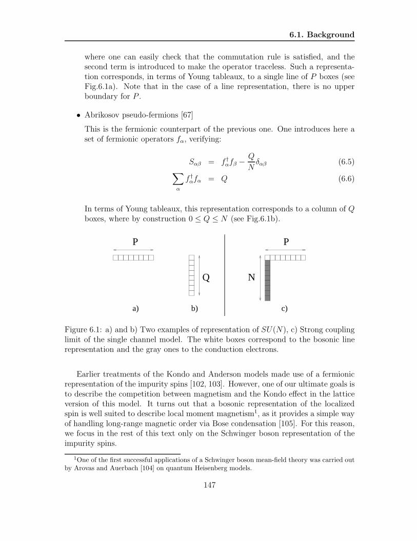
6.1. Background
where one can easily check that the commutation rule is satisfied, and thesecond term is introduced to make the operator traceless. Such a representa-tion corresponds, in terms of Young tableaux, to a single line of P boxes (seeFig.6.1a). Note that in the case of a line representation, there is no upperboundary for P .
• Abrikosov pseudo-fermions [67]
This is the fermionic counterpart of the previous one. One introduces here aset of fermionic operators fα, verifying:
Sαβ = f †αfβ −
Q
Nδαβ (6.5)
∑
α
f †αfα = Q (6.6)
In terms of Young tableaux, this representation corresponds to a column of Qboxes, where by construction 0 ≤ Q ≤ N (see Fig.6.1b).
Q
P P
N
a) b) c)
Figure 6.1: a) and b) Two examples of representation of SU(N), c) Strong couplinglimit of the single channel model. The white boxes correspond to the bosonic linerepresentation and the gray ones to the conduction electrons.
Earlier treatments of the Kondo and Anderson models made use of a fermionicrepresentation of the impurity spins [102, 103]. However, one of our ultimate goals isto describe the competition between magnetism and the Kondo effect in the latticeversion of this model. It turns out that a bosonic representation of the localizedspin is well suited to describe local moment magnetism1, as it provides a simple wayof handling long-range magnetic order via Bose condensation [105]. For this reason,we focus in the rest of this text only on the Schwinger boson representation of theimpurity spins.
1One of the first successful applications of a Schwinger boson mean-field theory was carried outby Arovas and Auerbach [104] on quantum Heisenberg models.
147

Single impurity multichannel Kondo model
Channel index
One can use Young tableaux to investigate the strong coupling solution of the gen-eralized Kondo model: one combines the first box of the line representation witha column of boxes representing the conduction electrons to form a spin singlet.One then notices from Fig. 6.1c, that unless P = 1, this model describes an un-derscreened impurity, where only a fraction of the original spin is screened by theconduction electrons, leaving a residual spin of size S = P−1
2. In order to overcome
this, Parcollet and Georges [106] introduced a multichannel version of the gener-alized Kondo model. The idea is to multiply the number of electronic flavors byintroducing a channel index µ that runs from 1 to K. The Kondo interaction is leftunchanged as no channel anisotropy is introduced. The new Hamiltonian, whichnow has the symmetry SU(N)× SU(K), is given by:
H =∑
k
N∑
σ=1
K∑
µ=1
ǫkc†kσµckσµ +
JKN
∑
k,k′
∑
α,β
∑
µ
b†αbβc†kβµck′αµ (6.7)
where we have replaced the impurity spin operator by the Schwinger boson represen-tation, and dropped the constant term proportional to the total number of electronsat the site of the impurity.
This Hamiltonian is the starting point for all the work presented in this chapter.
6.1.2 Strong coupling limit
The multichannel Kondo Hamiltonian allows us to tune separately the parametersP and K, i.e. the size of the impurity spin and the total number of channels. Thisgives access to three regimes with very different physics. In order to get a first flavorof the physics associated to these regimes, we study the strong coupling behavior ofthe model using arguments due to Nozieres and Blandin [107].
Nozieres-Blandin analysis
In the strong coupling limit, the kinetic energy of the conduction electrons is negli-gible, and finding the ground state then amounts to minimizing the Kondo energy.In this limit, the impurity tends to trap as many electrons as possible (i.e. one perchannel) with spin opposite to the one sitting at the impurity site. This results ina local effective spin of size S − K
2= P−K
2, hence three possibilities:
• K < P : Underscreened
The trapped electrons cannot quench completely the impurity spin, so thatthe dressed impurity remains magnetic with a spin of reduced size. Virtualhopping to the first layer of neighbors with strength t generates a new Kondoeffect between the residual spin and the conduction electrons with a weak
148

6.1. Background
ferromagnetic coupling Jeff ∼ t2
JKwhich vanishes in the infinite coupling limit,
suggesting that the JK →∞ fixed point is stable.
• K = P : Exactly screened
The ground state is non degenerate and the strong coupling fixed point isattractive: the usual Fermi liquid picture applies.
• K > P : Overscreened
Like the underscreened case, this leads to a finite residual spin, weakly coupledto the conduction electrons. However, the sign of this residual spin is oppositeto the starting impurity spin S, so that the effective Kondo coupling betweenthis residual spin and the conduction electrons is now antiferromagnetic: theJK →∞ fixed point is now unstable.
The strong coupling arrangement of spins for the impurity and the trappedelectrons for the various cases is presented in Fig. 6.2.
c)b)a)
Impurityspin
electrons
residualspin
Figure 6.2: Schematic view of the three screening regimes: a) Underscreened case,b) Exactly screened case, c) Overscreened case. The large black arrow correspondsto the impurity spin, the small red ones to the electrons and the green arrow to theresidual spin
Using Young tableaux
As one extends the original symmetry to SU(N), the same kind of arguments holdbut the derivation is more involved. However, there is a much easier and moreconvenient way of describing the physics of the strong coupling limit by using Youngtableaux.
The idea is that for any given line representation of the impurity spin, each boxcan combine with a column of N − 1 boxes representing the conduction electronsin order to form a spin singlet (the Pauli principle imposes that the total number
149

Single impurity multichannel Kondo model
of boxes per column cannot be greater than the spin degeneracy N). For a singlechannel, this is represented by Fig.6.1c. As soon as one increases the number ofchannels, it becomes possible to form a singlet between the second box of the linerepresentation and a column of conduction electrons taken in another channel.
P
N
K
c)
N
P
Ka)
P
N
Kb)
Figure 6.3: a) Underscreened case, b) Exactly screened case, c) Overscreened case.The impurity spin is described by a line of white boxes and the conduction electronsby gray boxes.
For a given size of the impurity spin, i.e. a given length P of the line represen-tation, one can identify three regimes depending on the total number of channels,just like in the SU(2) case. One expects the following strong-coupling limits:
• Underscreened: P > K
The conduction electron screens part of the impurity spin, leaving behinda residual spin of size S = P−K
2. The expected low-energy physics is then
the one of a local moment, decoupled from the conduction electron band atzero temperature. As one departs slightly from this strong-coupling fixedpoint, a weak ferromagnetic effective Kondo interaction is restored signalingthe stability of this fixed point.
• Exactly screened: P = K
The impurity spin is totally screened in this case and forms an antiferromag-netic singlet. The impurity site is then locked and acts as a scattering centerfor the conduction electrons. One expects the low-energy physics to be Fermi-liquid like with a finite phase shift on the site of the impurity.
• Overscreened: P < K
The number of screening channels is too important. A residual spin of sizeS = K−P
2now remains. However, a small departure from this fixed point leads
to a residual antiferromagnetic Kondo interaction, so that the strong-couplingfixed point is unstable and the system flows towards a stable infra-red fixedpoint. One expects from other investigations that this fixed point is non-Fermi-liquid like.
150

6.1. Background
It follows that the generalization of the Kondo model to the SU(N) symmetrygives qualitatively similar results to the SU(2) case, which motivates the study ofthe generalized multichannel Kondo model in the large-N limit.
These three regimes are represented in Fig.6.3, where the impurity spin is de-scribed by white boxes and the conduction electrons by gray ones.
6.1.3 Saddle-point equations
In order to derive the large-N equations, we consider the multichannel Hamiltonianwith a bosonic representation of the impurity spin, where we explicitly include theconstraint on the total number of Schwinger bosons via a Lagrange multiplier. Theaction then reads:
S =
∫ β
0
dτ∑
k,σ,µ
c†kσµ(τ) (∂τ + ǫk) ckσµ(τ) +
∫ β
0
dτ∑
α
b†α(τ) (∂τ − λ(τ)) bα(τ)
+JKN
∑
α,β,µ
∫ β
0
dτ ψ†βµ(τ)ψαµ(τ)b
†α(τ)bβ(τ)
+p0N
∫ β
0
dτ λ(τ)− p0JKN
∫ β
0
dτ∑
α,µ
ψ†αµ(τ)ψαµ(τ) (6.8)
where ψ†αµ = 1√
N∑
k c†kαµ creates an electron in the Wannier state at the impurity
site.
Taking the limit of infinite N , one has to rescale the parameters P and K withN in order to describe a non-trivial case. We then define the following rescaledparameters:
P = p0N K = γN (6.9)
It is important to notice that this rescaling inN preserves the distinction betweenthe three regimes: p0 > γ corresponds to the underscreened case, p0 = γ to theexactly screened case and p0 < γ to the overscreened case.
The first step is to integrate out of the partition function all of the conductionelectrons, apart from the ones at the impurity site. We then decouple the interactingterm by introducing an auxiliary Grassmanian field2 χµ(τ) for every channel index,
2Note that the fields χµ contain no time derivative, so that instantaneously they behave as inertneutral fields.
151

Single impurity multichannel Kondo model
which leaves us with the following action:
S = −∫ β
0
dτdτ ′∑
σ,µ
ψ†σµ(τ)G
−1c0 (τ − τ ′)ψσµ(τ ′)−
1
JK
∫ β
0
dτ∑
µ
χ†µ(τ)χµ(τ)
+p0N
∫ β
0
dτ λ(τ) +
∫ β
0
dτ∑
α
b†α(τ) (∂τ − λ(τ)) bα(τ)
+1√N
∑
α,µ
∫ β
0
dτ(ψ†αµ(τ)bα(τ)χµ(τ) + χ†
µ(τ)b†α(τ)ψαµ(τ)
)(6.10)
where we have dropped the p0JK
Nψ†ψ term since it only contributes to the local
electronic Green’s function to the order 1/N .The bare local conduction electron Green’s function Gc0 is given by:
Gc0(iωn) =∑
k
1
iωn − ǫk(6.11)
The actual choice of the conduction band does not matter much as long as we areinterested in a regime of temperature much smaller than the bandwidth: we onlyprobe the low-energy excitations, and only the density of states at the Fermi levelreally matters.
There are two different ways of obtaining the saddle-point equations for theGreen’s functions. First, we choose to derive them following the work of [106].Then, we derive them from a Luttinger-Ward[108, 109, 110] perspective, as this willturn out to be useful in many aspects in the rest of the text.
Derived from the action
The first step is to integrate the remaining conduction electrons out of the partitionfunction to end up with an effective action depending only on the Schwinger bosonsand the χ fermions:
S =
∫ β
0
dτ∑
α
b†α(τ) (∂τ − λ(τ)) bα(τ)−1
JK
∫ β
0
dτ∑
µ
χ†µ(τ)χµ(τ)
− 1
N
∫ β
0
dτdτ ′∑
µ
χµ(τ′)χ
†
µ(τ) Gc0(τ − τ ′)∑
α
bα(τ′)b
†
α(τ)
+p0N
∫ β
0
dτ λ(τ) (6.12)
It is useful at this stage to introduce the following precursors to the Green’sfunctions:
Nχ(τ, τ′) =
∑
µ
χµ(τ′)χ
†
µ(τ) Nb(τ, τ′) =
∑
α
bα(τ′)b
†
α(τ) (6.13)
152

6.1. Background
One now introduces two new fields labeled Q(τ, τ ′) and Q(τ, τ ′),conjugated re-spectively to Nχ(τ, τ
′) and Nb(τ, τ′). The idea is to generalize to a path-integral
formulation the following result:∫
dXdY e−AXY+Xφ+Y ψ = Const.× eφA−1ψ (6.14)
The partition function can be rewritten as Z =
∫
DQDQDλ e−S(Q,Q,λ) with the
effective action expressed in terms of these new fields:
S(Q, Q, λ) = N
∫ β
0
dτdτ ′ Q(τ, τ ′)G−1c0 (τ − τ ′)Q(τ, τ ′) + p0N
∫ β
0
dτ λ
−N logZb(Q, Q, λ)−K logZχ(Q, Q, λ) (6.15)
where the partial partition functions are defined as:
Zb =
∫
Db†Db e−R β0dτ b†(τ)(∂τ−λ(τ))b(τ)+
R
dτdτ ′Q(τ,τ ′)b(τ ′)b†(τ)
Zχ =
∫
Dχ†Dχ e−R β0 dτ χ†(τ)(∂τ−λ(τ))χ(τ)+
R
dτdτ ′Q(τ,τ ′)χ(τ ′)χ†(τ)
(6.16)
The important element here is that every term in S(Q, Q, λ) scales like N , so thatin the large-N limit one can apply the method of steepest descent. The saddle-pointis such as the derivatives of S(Q, Q, λ) with respect to its variables all vanish:
δS(Q, Q, λ)
δQ(τ, τ ′)= 0 =⇒ Q(τ, τ ′) = −Gc0(τ − τ ′)Gb(τ
′ − τ)
δS(Q, Q, λ)
δQ(τ, τ ′)= 0 =⇒ Q(τ, τ ′) = −γGc0(τ − τ ′)Gχ(τ
′ − τ)
δS(Q, Q, λ)
δλ(τ)= 0 =⇒ p0 = −Gb(τ = 0−) (6.17)
where we use the conventional definition of the Green’s functions as:
Gb(τ) = −〈Tb(τ)b†(0)〉Z = −〈Tb(τ)b†(0)〉Zb
Gχ(τ) = −〈Tχ(τ)χ†
(0)〉Z = −〈Tχ(τ)χ†
(0)〉Zχ
(6.18)
A careful look at (6.18) and (6.16) suggests that Q(τ, τ ′) (resp. Q(τ, τ ′)) istrivially related to the self-energy Σb(τ − τ ′) (resp. Σχ(τ − τ ′)):
Σb(τ) = γGc0(τ)Gχ(−τ) Σχ(τ) = −Gc0(τ)Gb(−τ) (6.19)
where the self-energies are defined as:
G−1b (iνn) = iνn + λ− Σb(iνn) G−1
χ (iωn) = JK − Σχ(iωn) (6.20)
153
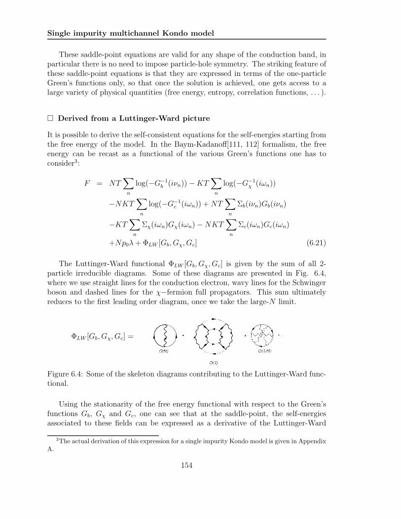
Single impurity multichannel Kondo model
These saddle-point equations are valid for any shape of the conduction band, inparticular there is no need to impose particle-hole symmetry. The striking feature ofthese saddle-point equations is that they are expressed in terms of the one-particleGreen’s functions only, so that once the solution is achieved, one gets access to alarge variety of physical quantities (free energy, entropy, correlation functions, . . . ).
Derived from a Luttinger-Ward picture
It is possible to derive the self-consistent equations for the self-energies starting fromthe free energy of the model. In the Baym-Kadanoff[111, 112] formalism, the freeenergy can be recast as a functional of the various Green’s functions one has toconsider3:
F = NT∑
n
log(−G−1b (iνn))−KT
∑
n
log(−G−1χ (iωn))
−NKT∑
n
log(−G−1c (iωn)) +NT
∑
n
Σb(iνn)Gb(iνn)
−KT∑
n
Σχ(iωn)Gχ(iωn)−NKT∑
n
Σc(iωn)Gc(iωn)
+Np0λ+ ΦLW [Gb, Gχ, Gc] (6.21)
The Luttinger-Ward functional ΦLW [Gb, Gχ, Gc] is given by the sum of all 2-particle irreducible diagrams. Some of these diagrams are presented in Fig. 6.4,where we use straight lines for the conduction electron, wavy lines for the Schwingerboson and dashed lines for the χ−fermion full propagators. This sum ultimatelyreduces to the first leading order diagram, once we take the large-N limit.
ΦLW [Gb, Gχ, Gc] =
Figure 6.4: Some of the skeleton diagrams contributing to the Luttinger-Ward func-tional.
Using the stationarity of the free energy functional with respect to the Green’sfunctions Gb, Gχ and Gc, one can see that at the saddle-point, the self-energiesassociated to these fields can be expressed as a derivative of the Luttinger-Ward
3The actual derivation of this expression for a single impurity Kondo model is given in AppendixA.
154

6.1. Background
functional, leading to:
Σb(τ) =−1
N
δΦLW
δGb(β − τ)=
O(K/N)
Σχ(τ) =−1
K
δΦLW
δGχ(β − τ)=
O(1)
Σc(τ) =−1
NK
δΦLW
δGc(β − τ)=
O(1/N)
(6.22)
Each of these terms contains a factor O(1/N) from the vertices, but the first twoself-energies contain summations over the internal channel or spin indices, elevatingΣb and Σχ to terms of order O(1). However, in the leading order large N approxi-mation, Σc ∼ O(1/N), so that a consistent large N approximation is produced byleaving the conduction electron lines un-dressed.
This provides an alternative diagrammatic derivation of the Parcollet-Georgesapproach.
Causality
It is interesting, now that we have derived the self-consistent equations for theGreen’s functions, to check that they satisfy the causality rules, i.e. that the imag-inary part of the retarded self-energies and Green’s functions have the right sign asa function of frequency.
In order to do so, we start expressing the imaginary part of the retarded self-energy and Green’s function for the Schwinger boson:
G′′b (ν + iδ) =
Σ′′b (ν)
|ω + λ− Σb(ν + iδ)|2(6.23)
Σ′′b (ν + iδ) = πγJ2
K
∫
dΩρc(Ω + ν)ρχ(Ω) [f(Ω + ν)− f(Ω)] (6.24)
where f(ω) is the temperature dependent Fermi function.
From this, it follows that Gb respects the causality rules provided that Σb does.It is then obvious that [f(Ω + ν)− f(Ω)] has the sign of ν for any given value of Ω,so that, assuming both fermionic fields respect causality, one has:
Σ′′b (ν + iδ) ∝ −Sgn(ν) (6.25)
which is one would expect if Gb were causal.
155

Single impurity multichannel Kondo model
The same kind of reasoning extends to the χ−fermion: the causality of Gχ isensured by the causality of Σχ, since it is preserved by the Dyson’s equation. Itsimaginary part is given by:
Σ′′χ(ω + iδ) = −πJ2
K
∫
dΩρc(Ω + ω)ρb(Ω) [f(Ω + ω) + f(Ω)] (6.26)
It is easy to rewrite [f(Ω + ω) + f(Ω)] as a positive function of both frequenciesdivided by tanh
(βΩ2
)which obviously has the sign of Ω for any given value of ω. If
both Gc and Gb respects causality, one has Σ′′χ(ω + iδ) < 0 over the whole range of
frequency, so that Gχ is also causal.As a conclusion, the causality is built into the self-consistent equations, so
that recursively, these rules are respected provided that the starting point at high-temperature is itself causal.
Set of equations
Here is a reminder of the whole set of equations we will refer to, in the rest of thistext:
Dyson’s equations: G−1b (iνn) = iνn + λ− Σb(iνn) (6.27a)
G−1χ (iωn) = JK − Σχ(iωn) (6.27b)
Schwinger boson: Σb(τ) = −γJ2KGc(τ)Gχ(β − τ) (6.27c)
χ−fermion: Σχ(τ) = −J2KGc(τ)Gb(β − τ) (6.27d)
Conduction electron4: ρc(ω) = ρ0Θ(D2 − ω2
)(6.27e)
Constraint: −Gb(τ = 0−) =
∫
dωρb(ω)n(ω) = p0 (6.27f)
where all the spectral functions are defined as ρ(ω) = −1π
ImG(ω + iδ), and n(ω) isthe Bose function.
To conclude, the Kondo problem reduces to this set of coupled integral equationsin the large-N limit. Once these equations are solved, their solution gives access toall physical quantities, from the thermodynamics to the correlation functions.
6.2 Known results
The saddle-point equations (6.27c) and (6.27d) have been studied in great detailsfor both the overscreened and the underscreened cases [106, 113]. It is actually
4We choose a flat band of conduction electron for simplicity but the saddle-point equations areindependent on the actual form of the band. Moreover, as argued before, the actual shape of thedensity of states does not matter at low temperature.
156

6.2. Known results
rather hard to solve them exactly: even though these self-consistent equations arenothing but convolutions, the Dyson’s equations make the self-consistency muchmore difficult to handle analytically than one would expect. It is quite interestingthat the same set of integral equations gives very different results as one tunes theimpurity spin from p0 > γ to p0 < γ. This feature is still not well understood fromthe analytical point of view.
Nevertheless, one can explore some of the properties of these two regimes thanksto two methods:
1. A partial analytic solution at low-temperature. This allows to explore thelow-energy behavior, in particular for the overscreened case where conformalfield theory helps in the derivation of the scaling function in temperature, thebehavior of the entropy and the specific heat.
2. A full numerical solution. This allows to explore the whole range in tempera-ture and in particular the cross-over between the high and the low temperatureregimes.
In the next paragraphs, we recall some of the established results concerning thehigh-temperature and the low-temperature limit for all three regimes of screening.
6.2.1 High temperature regime
At high temperature, the system behaves as a free spin of size s = p0/2: both self-energies are negligible compared to the free part of the Green’s functions. This isindependent on the number of channels since the Kondo interaction is too small toaffect the impurity spin at high temperature.
It follows that the bosonic spectral function is given by a single δ−peak:
ρb(ω) = δ (ω + λ) (6.28)
where the chemical potential λ is set by the constraint (6.27f). It follows thatn(−λ) = p0, so that one can rewrite the chemical potential as:
λHigh T = −T log
(1 + p0
p0
)
(6.29)
Replacing the expression for the bosonic Green’s function into the free energy(6.21), and neglecting all self-energies with respect to the bare propagators, one hasfor the impurity free energy:
FHigh Timp = F − Fbulk = NT
∑
n
log (−iνn − λ) +Np0λ(T ) (6.30)
= NT [p0 log p0 − (p0 + 1) log(p0 + 1)] (6.31)
157

Single impurity multichannel Kondo model
where we have subtracted the contribution from the conduction electron band tothe free energy, labeled Fbulk.
From this, one can easily deduce that the high-temperature limit of the impurityentropy per spin flavor is:
sHigh Timp = − 1
N
∂Fimp
∂T= (p0 + 1) log(p0 + 1)− p0 log p0 (6.32)
Finally, one can compute the local susceptibility: this quantity is defined asthe susceptibility of the system when only the impurity is coupled to the externalmagnetic field (see Appendix B for more details about the difference between localand impurity susceptibility). The local susceptibility then writes:
χloc =1
N2
∫ β
0
dτ∑
αβ
〈Sαβ(τ)Sβα(0)〉 =
∫ β
0
dτGb(τ)Gb(β − τ)
χHigh Tloc =
p0(p0 + 1)
T(6.33)
which, as expected, gives a Curie law with a Curie constant κ depending on the sizeof the spin: κ = p0(p0 + 1).
As the temperature is lowered, all these quantities cross-over to their low-Tcounterpart which now strongly depends on the screening regime considered.
6.2.2 Overscreened case: p0 < γ (OS)
This section is devoted to the results of the overscreened regime. All the analyticalresults presented in this section have been derived in [106] and [113]. However, allthe numerical data have been recomputed for illustrative purposes and as a test forour new set of programs.
Spectral functions
It is possible to extract the low-energy behavior of the Green’s functions in the zerotemperature limit. This derivation relies on a numerical observation, namely thatas the temperature is reduced towards zero, both Green’s functions seem to divergeat zero energy. This can be recast as:
λ− Σb(0 + iδ) −→T→0
0 (6.34)
JK − Σχ(0 + iδ) −→T→0
0 (6.35)
as one can see from the numerical data presented in Fig. 6.5.Using this as a hint, and a power-law ansatz for the Green’s functions, one can
perform a low-energy analysis identical in spirit to the one in [114]. The idea is
158

6.2. Known results
to plug the ansatz into the self-energy equations and to identify the results self-consistently with the starting functions. This analysis leads to the following power-laws for the Green’s functions:
Gb(ω + iδ) ∼ A+θ(ω) + A−θ(−ω)
|ω| γ1+γ
(6.36)
Gχ(ω + iδ) ∼ B+θ(ω) +B−θ(−ω)
|ω| 11+γ
(6.37)
where A± and B± are constants.Both Green’s functions are singular at zero frequency, with a power-law diver-
gence whose exponent does not depend on the size of the spin. This exponent isthe same on both side of the singularity, but the prefactor is different: there is aspectral asymmetry that can be parametrized through the argument θ± of A± (theself-consistency ensures that B± can be expressed in terms of |A±| and θ±).
Thanks to a procedure similar in many aspects to the proof of the Luttingertheorem for Fermi liquids [108, 109], one can relate the size of the spin to the low-energy parameters θ±, which ultimately leads to:
sin θ+ = sin
(π(γ − p0)
1 + γ
)
sin θ− = − sin
(πp0
1 + γ
) (6.38)
Finally, it is important to notice that the singularity at zero frequency is actuallyregularized at finite temperature. From this observation, Parcollet et al. [113] couldinfer a finite temperature ansatz for the Green’s functions that satisfies the saddle-point equations. In the low-energy, low temperature limit, one can see ω/T scalingin the spectral functions, so that at the leading order in temperature:
ρb(ω) ∝ T− γ1+γ φb
(ω
T
)
ρχ(ω) ∝ T− 11+γ φχ
(ω
T
)
(6.39)
where the φb,χ scaling functions have a complicated expression in terms of Γ func-tions. This feature can be seen numerically from inspecting the zero-energy inverseGreen’s function as a function of temperature, which turn out to behave as theexpected power-laws (see Fig. 6.5).
Entropy and specific heat
From the scaling function in temperature, it is possible to compute the free energy atlow temperature, at the saddle point, and from there to extract the residual entropyof the impurity. This turns out to be much more difficult than it seems, since becauseof the ω/T scaling of the spectral function, a small temperature Sommerfeld-likeexpansion is not possible here.
159
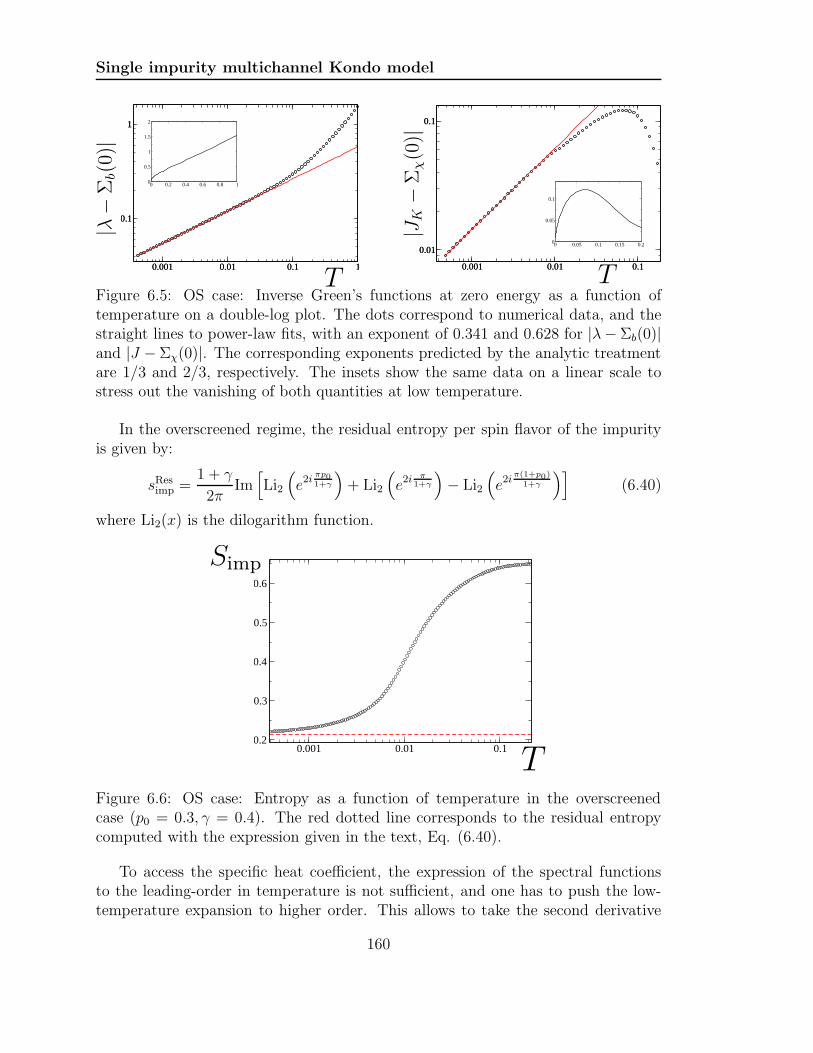
Single impurity multichannel Kondo model
0.001 0.01 0.1 1
0.1
1
0.001 0.01 0.1 1
0.1
1
0.001 0.01 0.1
0.01
0.1
0.001 0.01 0.1
0.01
0.1
0 0.2 0.4 0.6 0.8 10
0.5
1
1.5
2
0 0.05 0.1 0.15 0.20
0.05
0.1
|JK−
Σχ(0
)|
T
|λ−
Σb(0
)|
TFigure 6.5: OS case: Inverse Green’s functions at zero energy as a function oftemperature on a double-log plot. The dots correspond to numerical data, and thestraight lines to power-law fits, with an exponent of 0.341 and 0.628 for |λ−Σb(0)|and |J −Σχ(0)|. The corresponding exponents predicted by the analytic treatmentare 1/3 and 2/3, respectively. The insets show the same data on a linear scale tostress out the vanishing of both quantities at low temperature.
In the overscreened regime, the residual entropy per spin flavor of the impurityis given by:
sResimp =
1 + γ
2πIm[
Li2
(
e2iπp01+γ
)
+ Li2
(
e2iπ
1+γ
)
− Li2
(
e2iπ(1+p0)
1+γ
)]
(6.40)
where Li2(x) is the dilogarithm function.
0.001 0.01 0.10.2
0.3
0.4
0.5
0.6
Simp
TFigure 6.6: OS case: Entropy as a function of temperature in the overscreenedcase (p0 = 0.3, γ = 0.4). The red dotted line corresponds to the residual entropycomputed with the expression given in the text, Eq. (6.40).
To access the specific heat coefficient, the expression of the spectral functionsto the leading-order in temperature is not sufficient, and one has to push the low-temperature expansion to higher order. This allows to take the second derivative
160
6.2. Known results
of the impurity free energy, which leads to the following result for the specific heatcoefficient:
γ > 1 :CvT∼
(1
T
)γ−1γ+1
γ = 1 :CvT∼ log
(1
T
)
γ < 1 :CvT∼ const.
(6.41)
The asymmetry between the γ < 1 and the γ > 1 regimes is an artifact of theKondo model. In the Anderson model, the symmetry is restored and one finds a
diverging specific heat coefficient for γ < 1, namely Cv/T ∼ (1/T )1−γγ+1 .
Susceptibility
It is possible from a conformal field theory point of view to derive the temperaturedependence of the local spin susceptibility at low temperature. The latter turns outto behave as a function of temperature just like the specific heat coefficient, i.e.:
γ > 1 : χloc ∼(
1
T
)γ−1γ+1
γ = 1 : χloc ∼ log
(1
T
)
γ < 1 : χloc ∼ const.
(6.42)
For γ ≥ 1, this can be easily re-derived from the expression of the local suscepti-bility in terms of the bosonic Green’s functions, and the scaling form in temperatureof Gb
5. For γ < 1, however, the prefactor of the divergent term vanishes so that onlya constant term remains in the low temperature limit. Again, this is a peculiarityof the Kondo model and the divergence with the expected power in T is recoveredin the Anderson model.
6.2.3 Underscreened case: p0 > γ (US)
This section is devoted to the results of the underscreened regime. Again, all theanalytical results presented in this section have been derived in [106] and [115], andthe numerical data have been recomputed for illustrative purposes and as a test forour new set of programs.
5The integral brings a power of T and the two powers of Gb a term in T2γ
1+γ .
161

Single impurity multichannel Kondo model
9.5e-07 1e-06 1.05e-06 1.1e-060
5e+07
1e+08
1.5e+08
ρb(ω)
ω/D
-1 -0.5 0 0.5 10
5e+07
1e+08
1.5e+08
Figure 6.7: US case: Bosonic spectral function at T ∼ 10−3TK . The fit is aLorentzian whose width decreases with temperature, consistent with a δ-peak inthe zero temperature limit. In the inset, we show the same spectral function on thescale D.
Spectral functions
We know from the strong coupling analysis that the underscreened regime leadsto a partially screened impurity spin, so that we expect the physics to look like aresidual spin of size p0−γ, weakly ferromagnetically coupled to a bath of conductionelectrons.
It follows that the expected bosonic spectral function looks like the one of a localmoment, with sub-leading terms:
ρb(ω) = δ(ω + µT ) + Φb(ω) (6.43)
where µ = − log(p0−γ+1p0−γ
)
as one expects for the chemical potential associated to a
spin of size p0 − γ.Of course, in order to maintain the constraint as well as the normalization of
this spectral function, one would expect that:
∫
dωΦb(ω) = 0
∫
dωΦb(ω)n(ω) = γ (6.44)
The self-consistency imposes that upon substituting (6.43) into the self-energy
162

6.2. Known results
equation for the χ−fermion, one has:
Σχ(ω) = Φχ(ω) + ρ0J2K(p0 − γ)
[
log
∣∣∣∣
D + ω − µTD − ω + µT
∣∣∣∣− iπΘ(D2 − (ω − µT )2)
]
+ρ0J2K log
(D
2πT
)
− ρ0J2K
[
Ψ
(1
2− iω − µT
2πT
)
+ iπ
2
]
(6.45)
where Φχ(ω) is a sub-leading term arising from Φb(ω), and Ψ(x) is the di-gammafunction.
Noticing that this diverges as log T as T → 0, and plugging it back into the
bosonic self-energy, one has: Σb(ω)− Σb(0) ∼ −γ ω
log T+ . . ., so that our ansatz is
consistent.This finally leaves us with the following inverse Green’s functions at zero energy:
λ− Σb(0) ∼ µT + . . . (6.46)
JK − Σχ(0) ∼ ρ0J2K log T + . . . (6.47)
The divergence of the inverse χ−fermion propagator at zero energy prevents alow-energy analysis like the one carried out for the overscreened case. This loga-rithmic divergence can be interpreted physically as arising from the effective fer-romagnetic coupling between the residual spin and the electronic bath. Since weintroduced the χ fermion to decouple the Kondo interaction, the associated Green’sfunction describes the effective Kondo coupling J∗
K between the residual spin andthe conducting bath: as T → 0, this coupling becomes negative and vanishes like1/ logT , consistent with a marginally irrelevant ferromagnetic coupling.
0 0.01 0.02 0.03 0.04 0.05 0.06-0.08
-0.06
-0.04
-0.02
0
0.001 0.01 0.11
2
3
4
λ−
Σb(0
)
JK−
Σχ(0
)
T TFigure 6.8: US case: Inverse Green’s functions at zero energy as a function oftemperature. The dots correspond to numerical data, and the straight lines to fits:linear in the case of λ− Σb(0) and logarithmic for J − Σχ(0).
The validity of our ansatz is verified from the numerical solution (see Figs. 6.7and 6.8) where one sees the logT dependence of J∗
K , as well as the linear behavior of
163

Single impurity multichannel Kondo model
the renormalized bosonic chemical potential both in the high and low temperatureregime with a change of slope related to the change in the size of the effectiveimpurity spin.
Entropy and Susceptibility
The low-temperature physics is dominated by the local moment physics, since theeffective coupling between the residual spin and the conduction band vanishes asT → 0. As a consequence, both the entropy and the local susceptibility at zerotemperature look like the ones of an isolated spin.
One then expects that the underscreened case at low temperature gives the samebehavior as the ones we obtained for the high-temperature regime only for a spin ofsize p0 − γ instead of p0. It follows that the residual entropy of the underscreenedKondo model is given by:
sLow Timp = (p0 − γ + 1) log(p0 − γ + 1)− (p0 − γ) log(p0 − γ) (6.48)
and the local susceptibility at low-temperature is Curie-like, with a Curie constantκ = (p0 − γ)(p0 − γ + 1):
χLow Tloc ∼ (p0 − γ)(p0 − γ + 1)
T(6.49)
which we could verify numerically, as one can see from Fig. 6.9.
0.001 0.01 0.10.7
0.72
0.74
0.76
0.78
0.8
0 0.02 0.04 0.06 0.080
0.02
0.04
0.06
0.08
0.1
0.12
T T
Simp χ−1loc
a) b)
Figure 6.9: US case: a) Entropy as a function of temperature on a logarithmicscale. The residual entropy at the lowest temperature achieved is very close to thetheoretical value (red dotted line). b) The inverse local susceptibility is linear inboth the high and low-temperature regime, with a net change in slope.
As one takes the γ → p0 limit, one gets closer and closer to the exactly screenedcase, for which one expects the residual entropy to vanish. It can be readily seenfrom Eq. 6.48 that sLow T
imp → 0 as γ → p0.
164

6.3. Exactly screened case: p0 = γ (ES)
6.3 Exactly screened case: p0 = γ (ES)
In this section we study the perfectly screened case which was thought to be a trivialnon-interacting Fermi-liquid as an artifact of the large-N limit. We prove, helpedby a numerical solution of the saddle-point equations, that this is not the case:even though the transport properties are indeed trivial in the large-N limit, one canrecover the thermodynamics of a truly interacting Fermi liquid. The main resultsof this section have been published in the Publication 4, the rest is presented herefor the first time.
6.3.1 General belief and counter-arguments
Previous works [106] on this large-N limit of the multichannel Kondo model fo-cused on both the overscreened and the underscreened regimes, leaving the perfectlyscreened case aside. The general belief was that although the Kondo screening oc-curs at the leading order in N for the impurity, it only happens at a sub-leadingorder for the conduction electrons, so that the impurity doesn’t seem to affect anyproperties of the Fermi liquid, even at the impurity site and one ends up describinga trivial non-interacting Fermi liquid.
This argument was backed up by the results of the Friedel sum rule [93] whichpredicts that the conduction electron phase shift on the impurity is given by δc = π
N
so that both the phase shift and the T−matrix vanish in the large-N limit.Although this argument is correct, the conclusions concerning the trivial Fermi
liquid are not. Indeed, a vanishing phase shift only implies that the transportproperties of the Fermi liquid cannot be recovered in the large-N limit. What wasoriginally missed is that although the conduction electron self-energy is of orderO(1/N), it does participate to the thermodynamics because its effect is multipliedby the N spin components and the K scattering channels producing an O(N) overallcontribution.
This statement is not that obvious if one looks at the impurity free energy. Thelatter is defined as the difference between the total free energy and the bulk one(i.e. the one of the free conduction band). Starting from Eq. 6.21 and removing thebulk free energy Fbulk = −NKT ∑n log
(G−1c0 (iωn)
), one can expand the conduction
electron Green’s function in 1/N , so that the remaining terms look like:
Fimp = NT∑
n
log(−G−1b (iνn))−KT
∑
n
log(−G−1χ (iωn))
+NT∑
n
Σb(iνn)Gb(iνn)−KT∑
n
Σχ(iωn)Gχ(iωn)
+Np0λ+ ΦLW [Gb, Gχ, Gc] (6.50)
This does not contain any explicit dependence on the conduction electron self-energy.However, it is possible from this expression to derive a closed form expression for
165
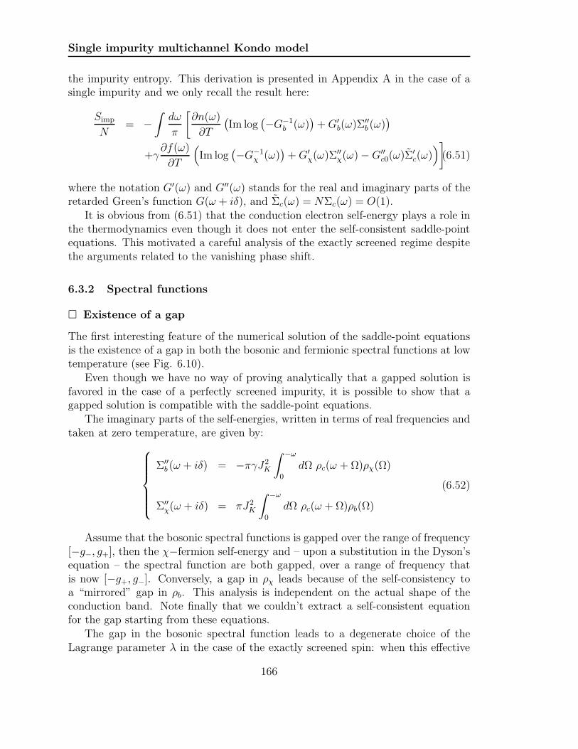
Single impurity multichannel Kondo model
the impurity entropy. This derivation is presented in Appendix A in the case of asingle impurity and we only recall the result here:
Simp
N= −
∫dω
π
[∂n(ω)
∂T
(Im log
(−G−1
b (ω))
+G′b(ω)Σ′′
b (ω))
+γ∂f(ω)
∂T
(
Im log(−G−1
χ (ω))
+G′χ(ω)Σ′′
χ(ω)−G′′c0(ω)Σ′
c(ω))]
(6.51)
where the notation G′(ω) and G′′(ω) stands for the real and imaginary parts of theretarded Green’s function G(ω + iδ), and Σc(ω) = NΣc(ω) = O(1).
It is obvious from (6.51) that the conduction electron self-energy plays a role inthe thermodynamics even though it does not enter the self-consistent saddle-pointequations. This motivated a careful analysis of the exactly screened regime despitethe arguments related to the vanishing phase shift.
6.3.2 Spectral functions
Existence of a gap
The first interesting feature of the numerical solution of the saddle-point equationsis the existence of a gap in both the bosonic and fermionic spectral functions at lowtemperature (see Fig. 6.10).
Even though we have no way of proving analytically that a gapped solution isfavored in the case of a perfectly screened impurity, it is possible to show that agapped solution is compatible with the saddle-point equations.
The imaginary parts of the self-energies, written in terms of real frequencies andtaken at zero temperature, are given by:
Σ′′b (ω + iδ) = −πγJ2
K
∫ −ω
0
dΩ ρc(ω + Ω)ρχ(Ω)
Σ′′χ(ω + iδ) = πJ2
K
∫ −ω
0
dΩ ρc(ω + Ω)ρb(Ω)
(6.52)
Assume that the bosonic spectral functions is gapped over the range of frequency[−g−, g+], then the χ−fermion self-energy and – upon a substitution in the Dyson’sequation – the spectral function are both gapped, over a range of frequency thatis now [−g+, g−]. Conversely, a gap in ρχ leads because of the self-consistency toa “mirrored” gap in ρb. This analysis is independent on the actual shape of theconduction band. Note finally that we couldn’t extract a self-consistent equationfor the gap starting from these equations.
The gap in the bosonic spectral function leads to a degenerate choice of theLagrange parameter λ in the case of the exactly screened spin: when this effective
166

6.3. Exactly screened case: p0 = γ (ES)
chemical potential lies within the gap, the ground-state Schwinger boson occupancy6
locks into the value nb = p0 = γ. Numerically, this manifests itself by a plateau inthe bosonic occupancy as a function of λ, at low temperature (see Fig. 6.10). Such apicture suggests that starting from a solution of the saddle point equations, a smallchange δλ in the bosonic chemical potential leads to another solution, apparentlygiven by the same set of Green’s functions only shifted rigidly in frequency by anamount δλ.
-8 -6 -4 -2 00
0.2
0.4
0.6
0.8
-0.2 -0.1 0 0.1 0.2
-6
-4
-2
0
2
4
6
λa) b)
OS ES US
ω/D
nb
ρb(ω)
Figure 6.10: ES case: a) Bosonic spectral function as a function of frequency fordecreasing temperature. As the gap opens at low energy, both peaks sharpen on theedges of the gapped region. b) Computed bosonic occupancy for γ = 0.3 when thechemical potential λ is varied (p0 not being fixed). The plateau corresponds to anexactly screened case (ES).
Just like the stability of the gap, this last feature is also built into the equations.Assume that Σχ(ω, λ+ δλ) = Σχ(ω − δλ, λ), then thanks to the Dyson’s equation,this property is also verified by Gχ. It follows that, at zero temperature:
Σb(ω, λ+ δλ) = ρ0γJ2K
(∫ −ω
−DdΩ G′
χ(Ω− δλ, λ) + i
∫ 0
−ωdΩ G′′
χ(Ω− δλ, λ)
)
= Σb(ω + δλ, λ)− ρ0γJ2K
∫ 0
−δλdΩ G′′
χ(Ω, λ)
= Σb(ω + δλ, λ) (6.53)
where we used that in the large bandwidth limit D + δλ ≃ D, and the extra termvanishes because of the gap in the χ−fermion spectral function. The rest of theproof is identical: from the rigid shift of Σb it is easy to prove that Gb follows thesame property, which transmits to Σχ via the saddle-point equation in the exact
6The bosonic occupancy is defined as nb = −Gb(τ = 0−), which is set by the constraint to beequal to p0.
167

Single impurity multichannel Kondo model
same way as we have just proved, so that ultimately, one has at zero temperature:
Gb(ω, λ+ δλ) = Gb(ω + δλ, λ)Gχ(ω, λ+ δλ) = Gχ(ω − δλ, λ)
(6.54)
It is legitimate to wonder whether the presence of a gap in the spectral functionsis an artifact of the large-N limit or if it has a deeper physical meaning in whichcase it would extend down to N = 2. We do not, at this stage, have any evidence tosupport either scenarios. However, we can argue that if a gap in the bosonic spectralfunction exists in the SU(2) case, it could be revealed from inspecting the energyspectrum of the bosonic states, e.g. by ways of the Density Matrix RenormalizationGroup.
Renormalized chemical potential
As a consequence of the gapped bosonic spectral function, in the case of the exactlyscreened impurity, the renormalized chemical potential λ∗ = λ−Σb(0) does not van-ish as a function of temperature unlike the overscreened and underscreened regimes.The bosonic Green’s function taken at zero energy is given by Gb(0) = 1/λ∗ and canbe expressed as:
Gb(0) = G′b(0) = −P
∫
dΩρb(Ω)
Ω(6.55)
which is protected by the low-energy gap, and is thus made finite.Another feature that comes from the numerical investigation is the development
of a δ−peak in the bosonic spectral function at the boundary of the gapped regionat positive frequency. Unlike the underscreened case, the position of this peak doesnot evolve as the temperature is lowered, and one can make the following ansatz forthe bosonic spectral function:
ρb(ω) = Aδ(ω − η) + Φb(ω) (6.56)
where A and η are positive constants, and Φb is assumed to be a sub-leading term.Of course, this ansatz is not enough to capture most of the properties of the
perfectly screened impurity but it is sufficient here to self-consistently extract thelow-energy behavior of the Green’s functions. Substituting this ansatz into theequation for the fermionic self-energy, one has:
Σχ(ω) = Φχ(ω) + Aρ0J2K
[
log
(D
2πT
)
−Ψ
(1
2+ω + η
2iπT
)
− iπ2
]
∼T→0
Φχ(ω)− Aρ0J2K log
( |ω + η|D
)
(6.57)
This leads to the following contribution once plugged back into the bosonic self-energy:
Σb(ω)− Σb(η) ∼ B|ω − η|
log |ω − η| (6.58)
168

6.3. Exactly screened case: p0 = γ (ES)
so that our ansatz is consistent.As a conclusion, the inverse Green’s functions at zero energy read:
λ− Σb(0) −→T→0
Const. (6.59)
JK − Σχ(0) −→T→0
Const. (6.60)
where both these constants are finite, which prevents any kind of low-energy analysislike the one carried out for the overscreened impurity. This is verified numerically(see Fig. 6.11) with a saturation observed on about two decades in temperature.
0.001 0.01 0.1
-1.6
-1.4
-1.2
-1
-0.8
-0.6
0.001 0.01 0.1
-1.6
-1.4
-1.2
-1
-0.8
-0.6
0.001 0.01 0.1 1-1.5
-1
-0.5
0
0.001 0.01 0.1 1-1.5
-1
-0.5
0
λ−
Σb(0
)
TT
JK−
Σχ(0
)
Figure 6.11: ES case: Inverse Green’s functions at zero energy as a function oftemperature. The dots correspond to numerical data. The logarithmic scale intemperature is used to underline the saturation at low T .
6.3.3 Entropy and specific heat
The gap in both the bosonic and fermionic spectral functions removes the effect ofboth fields on the low-temperature thermodynamics. Indeed, as the temperatureis lowered, one can only probe the low-energy spectrum of each field: the low-temperature physics is then completely dominated by the conduction electrons sothat the emergence of the gap ultimately reveals a Fermi liquid.
The consequences of a gapped solution on the low-energy physics can readilybe obtained from the impurity entropy defined in (6.51). In the low-temperatureregime, it is useful to replace the derivative of the fermionic and bosonic distributionswith respect to temperature by their derivative with respect to frequency. Using that∂n(ω)∂T
= −ωT
∂n(ω)∂ω
and ∂f(ω)∂T
= −ωT
∂f(ω)∂ω
, one can rewrite the impurity entropy as:
SLowTimp
N=
1
T
∫
dω
[∂n
∂ωsb(ω) +
∂f
∂ωsf (ω)
]
=−1
T
∫
dω
[dsbdω
n(ω) +dsfdω
f(ω)
]
(6.61)
169

Single impurity multichannel Kondo model
where we define
sb = ω
π
(Im log
(−G−1
b
)+G′
bΣ′′b
)
sf = γωπ
(
Im log(−G−1
χ
)+G′
χΣ′′χ −G′′
c0Σ′c
)
One can then perform a Sommerfeld expansion at low temperature, which gives:
SLowTimp
N= −π
2
6T
(
2d2sbdω2
∣∣∣∣ω=0
+d2sfdω2
∣∣∣∣ω=0
)
(6.62)
It turns out that because of the causality properties of the bosonic Green’sfunctions, one has G′′
b (0) = 0 and Σ′′b (0) = 0, which then imposes, after some minor
rearrangement, that d2sb
dω2
∣∣∣ω=0
= 0.
Taking the second derivative of sf and rearranging the remaining terms, noticing
thatdG′′
c0
dω
∣∣∣ω=0
= 0, one has:
d2sfdω2
∣∣∣∣ω=0
=2γ
π
(
dG′χ
dω
∣∣∣∣ω=0
Σ′′χ(0)−G′′
χ(0)dΣ′
χ
dω
∣∣∣∣ω=0
+ πρ0dΣ′
c
dω
∣∣∣∣∣ω=0
)
(6.63)
Recalling that the fermionic spectral function is gapped, this leads to the finalexpression of the low-temperature impurity entropy:
SLowTimp
N= −π
2
3γρ0T
dΣ′c
dω
∣∣∣∣∣ω=0
(6.64)
which is linear in T as one would expect from a Fermi liquid.
Note in particular that the specific heat coefficient, defined as Cv
T=
dSimp
dT, not
only saturates at a constant value at low temperature, but also this constant dependson the renormalized number of channels γ.
The exponential decay of the Fermi and Bose function derivatives imposes thatat a given temperature T , only the frequency range ω ∈ [−T, T ] contributes tothe entropy. As a consequence, as one reaches a temperature of the order of thegap in the spectral functions, the contributions to the entropy coming from boththe Schwinger bosons and the χ−fermions identically vanish. It follows from thisderivation that the typical energy scale over which the Fermi liquid develops (somekind of effective Fermi temperature T ∗) is given by the size ∆g of the gap.
Numerically, one sees a cross-over from the high-temperature regime where theentropy is dominated by the local moment physics and is thus given by a constant, tothe low-temperature regime where it becomes Fermi-liquid like and vanishes linearlywith temperature (see Fig. 6.12).
170
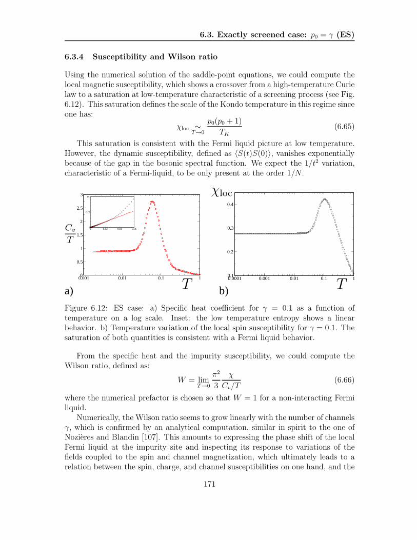
6.3. Exactly screened case: p0 = γ (ES)
6.3.4 Susceptibility and Wilson ratio
Using the numerical solution of the saddle-point equations, we could compute thelocal magnetic susceptibility, which shows a crossover from a high-temperature Curielaw to a saturation at low-temperature characteristic of a screening process (see Fig.6.12). This saturation defines the scale of the Kondo temperature in this regime sinceone has:
χloc ∼T→0
p0(p0 + 1)
TK(6.65)
This saturation is consistent with the Fermi liquid picture at low temperature.However, the dynamic susceptibility, defined as 〈S(t)S(0)〉, vanishes exponentiallybecause of the gap in the bosonic spectral function. We expect the 1/t2 variation,characteristic of a Fermi-liquid, to be only present at the order 1/N .
0.0001 0.001 0.01 0.1 10.1
0.2
0.3
0.4
0.001 0.01 0.1 10
0.5
1
1.5
2
2.5
3
T
CvT
χloc
T
0 0.02 0.04 0.060
0.05
0.1
a) b)
Figure 6.12: ES case: a) Specific heat coefficient for γ = 0.1 as a function oftemperature on a log scale. Inset: the low temperature entropy shows a linearbehavior. b) Temperature variation of the local spin susceptibility for γ = 0.1. Thesaturation of both quantities is consistent with a Fermi liquid behavior.
From the specific heat and the impurity susceptibility, we could compute theWilson ratio, defined as:
W = limT→0
π2
3
χ
Cv/T(6.66)
where the numerical prefactor is chosen so that W = 1 for a non-interacting Fermiliquid.
Numerically, the Wilson ratio seems to grow linearly with the number of channelsγ, which is confirmed by an analytical computation, similar in spirit to the one ofNozieres and Blandin [107]. This amounts to expressing the phase shift of the localFermi liquid at the impurity site and inspecting its response to variations of thefields coupled to the spin and channel magnetization, which ultimately leads to arelation between the spin, charge, and channel susceptibilities on one hand, and the
171

Single impurity multichannel Kondo model
specific heat coefficient on the other hand. The complete derivation is presented inAppendix C.
As a result of this analysis, we expect the Wilson ratio to be given by W = 1+γ,which is the behavior we recover in our numerical solution (see Fig. 6.13). This formis consistent with the Bethe ansatz results [116], taken in the limit of large valuesof N .
Such a Wilson ratio suggests, as we already argued from the entropy, that theexactly screened solution of the saddle-point equations describe an interacting localFermi liquid in the large-N limit.
6.3.5 Scales
We argued, when dealing with the impurity entropy, that the typical energy scaleover which the Fermi liquid develops is given by the size of the gap. From variousother approaches we expect the crossover scale between the high-temperature localmoment physics, and the low-temperature Fermi liquid behavior to be given by theKondo temperature7.
From this reasoning, one expects that the gap roughly goes like the Kondo tem-perature. However, we could not find any analytic derivation that would confirmthis result. One has to stress out that the ansatz we have made concerning thebosonic Green’s functions is not sufficient here to fully explore the relation betweenthe gap and the Kondo temperature, as one would need an explicit form for thesubleading function Φb(ω).
Numerically, there is quite a striking correspondence between the size of the gapand the Kondo temperature, as can be seen on Fig. 6.13.
6.4 Conclusion
In this chapter, we rederived the saddle-point equations associated to the large-Nlimit of the multichannel Kondo model using an extension of the Luttinger-Wardformalism. After recalling the main results of the overscreened and underscreenedregimes, we studied in details the perfectly screened case. We proved that contraryto the common knowledge, this regime does not correspond to a trivial Fermi liquid.Instead, we showed that despite vanishing transport properties due to an artifactof the large-N limit, one can recover the thermodynamics of an interacting Fermiliquid.
The application of this method to the description of, e.g. quantum dot physics,is made difficult by the vanishing T -matrix in the limit of N →∞. An attempt tocure this issue is presented in Chapter 8.
7As one can see, e.g. from the local susceptibility which diverges in 1/T until it reaches theKondo temperature where it just saturates at a constant going like 1/TK .
172

6.4. Conclusion
Number of Kondo temperature TK Gap ∆g in thechannels γ extracted from χimp spectral functions
0.1 0.506 0.3970.2 0.446 0.3720.3 0.390 0.3460.4 0.355 0.3220.5 0.321 0.2990.6 0.286 0.2770.7 0.257 0.2560.8 0.230 0.2360.9 0.208 0.218
W
γ0 0.2 0.4 0.6 0.8 11
1.2
1.4
1.6
1.8
2
0 0.2 0.4 0.6 0.8 11
1.2
1.4
1.6
1.8
2
a) b)
Figure 6.13: ES case: a) Wilson ratio computed for various values of γ (black circles)and compared with the behavior extracted from our Nozieres-Blandin analysis (redline), b) Numerical values of the low-T gap and the Kondo temperature for a givenKondo coupling JK and various γ.
However, an interesting application of this approach lies in the extension tomany impurities. The first step towards this route is presented in Chapter 7, withthe study of a two-impurity system.
173

Single impurity multichannel Kondo model
174

CHAPTER 7
Two-impurity multichannel Kondomodel
Contents
7.1 Large-N equations . . . . . . . . . . . . . . . . . . . . . . . 176
7.1.1 The model . . . . . . . . . . . . . . . . . . . . . . . . . . 176
7.1.2 Saddle-point equations . . . . . . . . . . . . . . . . . . . . 177
7.1.3 General remarks . . . . . . . . . . . . . . . . . . . . . . . 181
7.2 Phase diagram and quantum critical point . . . . . . . . 182
7.2.1 Tools for exploring the phase diagram . . . . . . . . . . . 183
7.2.2 Renormalized Fermi liquid region (I) . . . . . . . . . . . . 184
7.2.3 Magnetically correlated region (II) . . . . . . . . . . . . . 186
7.2.4 Quantum critical region (III) . . . . . . . . . . . . . . . . 187
7.3 Discussion . . . . . . . . . . . . . . . . . . . . . . . . . . . . 189
7.3.1 Jones-Varma critical point . . . . . . . . . . . . . . . . . . 189
7.3.2 Low-temperature physics close to the QCP . . . . . . . . 190
7.3.3 Stability of the critical point . . . . . . . . . . . . . . . . 192
7.4 Conclusion . . . . . . . . . . . . . . . . . . . . . . . . . . . 193
175

Two-impurity multichannel Kondo model
Having demonstrated that the large-N bosonic approach captures the thermo-dynamic properties of the Fermi liquid behavior for the perfectly screened impurity,we show in this chapter that it can also handle magnetic correlations within thetwo-impurity Kondo model. In this chapter, we explore the phase diagram of thetwo-impurity Kondo-Heisenberg model and discuss the similarities with the so-called“Jones-Varma” [117] fixed point in N = 2. The main results of this chapter havebeen published in the Publication 4, the rest is presented here for the first time.
7.1 Large-N equations
7.1.1 The model
We now consider two identical impurities coupled to the same sea of conductionelectrons, and include for generality a Heisenberg-like interaction between the twolocalized spins, generated by other exchange processes not involving the conductionelectrons. The Kondo interaction is the same as we described in the previous chapter.
Motivated by an extension to the lattice, and its relevance for the heavy fermionproblem, we choose to limit ourselves to the case of an antiferromagnetic Heisenbergcoupling between the two impurity spins. Moreover, we choose to follow the argu-ments of Read and Sachdev [118] and describe this Heisenberg interaction in termsof the boson pair operator B12 =
∑
m,σ σb1,m,σb2,m,−σ, where we recast the N spin
indices under the form α = (m, σ) (m running from 1 to N2, and σ = ±).
Following this choice, the Hamiltonian describing the system is now invariantunder spin transformation in the symmetry group Sp(N), subgroup of SU(N) andwrites:
H = Hband +H(1)K +H
(2)K +HH
Hband =∑
k
∑
m,σ
K∑
µ=1
ǫkc†
kmσµckmσµ
H(i)K =
JKN
∑
m,m′
∑
σ,σ′
∑
µ
∑
i=1,2
b†
i,m,σbi,m′,σ′ψ†
im′σ′µψimσµ
HH =JHN
(∑
m,σ
σb†
1,m,σb†
2,m,−σ
)(∑
m′,σ′
σ′b1,m′,σ′b2,m′,−σ′
)
(7.1)
where ψimσµ creates an electron in the Wannier state with spin α = N + σm+ 1−σ2
at the site i.The number of bosons for each site is enforced by the constraint:
HConstraint = −∑
i=(1,2)
λi
(∑
m,σ
b†
i,m,σbi,m,σ − p0N
)
(7.2)
176

7.1. Large-N equations
and we focus in the rest of this chapter on perfectly screened impurities, so that werestrict ourselves to the case where p0 = γ.
Just like the single impurity case treated in the previous chapter, one expects tosee different screening regimes in this model. However, we are not interested herein the exploration of these various scenarios, and restrict ourselves to the exactlyscreened case, fixing the number of channels to match the size of the impurity spins.There is now a new parameter one can tune, namely the Heisenberg coupling, whichnow competes with the Kondo interaction giving access to two different regimes,pictured in Fig. 7.1:
• For a weak Heisenberg coupling, the two impurity spins prefer to form a singletwith the surrounding conduction electrons. We expect to see two perfectlyscreened impurities only weakly coupled to each other. The low-energy physicsis then expected to be Fermi-liquid like.
• Whereas for a strong Heisenberg coupling, a spin singlet between the twoimpurity spins is favored. The impurities are locked in a singlet state andact as a scattering center for the conduction electrons, so that the low-energyphysics is again Fermi-liquid like, but qualitatively different than the regimeof weak Heisenberg coupling.
The most interesting region of the phase diagram turns out to be the crossoverregion between these two regimes.
b)a)
Figure 7.1: Schematic diagram illustrating the two limiting regimes: a) correspondsto the case of a dominant Kondo interaction and b) to a strong Heisenberg coupling.The large black arrows stand for the impurities, the red ones for the electrons.
7.1.2 Saddle-point equations
In order to study the phase diagram of the two-impurity Kondo-Heisenberg model inthe large-N limit, we derive a set of saddle-point equations which we then study by
177

Two-impurity multichannel Kondo model
means of numerical as well as analytical investigation when possible. The derivationof the saddle-point equations is quite similar to the one already presented for thesingle impurity case.
Derivation
As a first step, we decouple the Kondo interaction term for both impurities byintroducing two sets of Grassmanian fields χ1,µ and χ2,µ, where µ is the channelindex, running from 1 to K. After integrating the conduction electrons out of thepartition function, the action reads:
S =
∫ β
0
dτ∑
i,m,σ
b†i,m,σ(τ) (∂τ − λi(τ)) bi,m,σ(τ)−1
JK
∫ β
0
dτ∑
i,µ
χ†i,µ(τ)χi,µ(τ)
− 1
N
∑
i,j
∫ β
0
dτdτ ′∑
µ
χj,µ(τ′)χ
†
i,µ(τ) Gc0(i− j; τ − τ ′)∑
m,σ
bj,m,σ(τ′)b
†
i,m,σ(τ)
+∑
i
∫ β
0
dτ
(
Ơ
i,i(τ)∑
m,σ
σbi,m,σ(τ)bi,m,−σ(τ) + h.c.
)
+N
JH
∑
i
∫ β
0
dτ ∆†
i,i(τ)∆i,i(τ) + p0N∑
i
∫ β
0
dτ λi(τ) (7.3)
where we have decoupled the Heisenberg interaction by introducing a “bond” oper-ator ∆i,i, and i is defined as:
i =
2 if i = 11 if i = 2
(7.4)
Using the symmetry under the exchange 1↔ 2, one can argue that the Lagrangemultipliers λ1 and λ2 are equal: if a solution is obtained with different values ofλ1 and λ2, then the symmetry leads to another solution where these values areexchanged, suggesting that they are most likely equal. The same kind of reasoningsuggests that the bond operators are also trivially related to one another via ∆12 =−∆21. This allows us to define λ and ∆ as:
λi = λ∆i,i = Sgn(i− i)∆ (7.5)
It is useful at this stage to introduce a spinor notation for the Schwinger bosons
178
7.1. Large-N equations
b†
i,m = (b†
i,m,+, bi,m,−) in order to rewrite the action under the following matrix form:
S =∑
i,j
∫ β
0
dτ∑
m
b†
i,m(τ)
[(∂τ − λ(τ)) δij 2Sgn(i− i)∆(τ)δji
−2Sgn(i− i)∆†(τ)δji (−∂τ − λ(τ)) δij
]
bj,m(τ)
− 1
N
∫ β
0
dτdτ ′∑
i,j
Nχ(i, j, τ, τ′)Gc0(i− j; τ − τ ′)Nb(i, j, τ, τ
′)
− 1
JK
∫ β
0
dτ∑
i,µ
χ†i,µ(τ)χi,µ(τ) + 2
N
JH
∫ β
0
dτ ∆†
(τ)∆(τ)
+2p0N
∫ β
0
dτ λ(τ) (7.6)
where the matrix is given in the σ-space, and Nb and Nχ are the precursors of theSchwinger boson and χ−fermion Green’s function defined as:
Nb(i, j, τ, τ′) =
∑
m,σ
bj,m,σ(τ′)b
†
i,m,σ(τ) Nχ(i, j, τ, τ′) =
∑
µ
χjµ(τ′)χ
†
iµ(τ)
(7.7)The method is then similar to the one used for the single impurity problem: one
introduces the new fields Q(i, j, τ, τ ′) and Q(i, j, τ, τ ′) conjugated to Nχ(i, j, τ, τ′)
and Nb(i, j, τ, τ′). This leads to an effective action S(Q, Q, λ,∆) expressed in terms
of these new fields, where every term scales like N so that one can apply the methodof steepest descent. The saddle-point equations now write:
Q(i, j, τ, τ ′) = −Gc0(i− j; τ − τ ′)(
G(++)b (j − i; τ ′ − τ) +G
(−−)b (j − i; τ ′ − τ)
)
Q(i, j, τ, τ ′) = −γGc0(i− j; τ − τ ′)Gχ(j − i; τ ′ − τ)p0 = −1
2
(
G(++)b (i = j; τ = 0−) +G
(−−)b (i = j; τ = 0+)
)
∆
JH=
1
2
∑
i=1,2G(−+)b (i− i; τ = 0−)
(7.8)where the Green’s functions are now defined as:
Gb(i− j; τ) =
[
G(++)b (i− j; τ) G
(+−)b (i− j; τ)
G(−+)b (i− j; τ) G
(−−)b (i− j; τ)
]
=
[−〈Tbi,+(τ)b
†
j,+(0)〉 −〈Tbi,+(τ)bj,−(0)〉−〈Tb†i,−(τ)b
†
j,+(0)〉 −〈Tb†i,−(τ)bj,−(0)〉
]
(7.9)
Gχ(i− j; τ) = −〈Tχi(τ)χ†
j(0)〉 (7.10)
RKKY interaction
It is possible to relate the fields Q and Q to the self-energies of the Schwingerboson and the χ−fermion. From the saddle-point equations, one can see that the
179

Two-impurity multichannel Kondo model
Kondo interaction is responsible for local terms arising from i = j, but also fora cross-term that couples the two impurities to one another. This cross-term willgive rise to a bosonic self-energy in the SU(N) channel, i.e. that renormalizes the−〈Tbi,±(τ)b
†
j,±(0)〉 term (with i 6= j).
This is known as the RKKY interaction [90, 91, 92]. This effective interactionbetween the impurities is mediated by the conduction band and can be tuned byadjusting the distance between the two impurities. However, we assume here thatthis distance is always big enough to neglect the RKKY interaction compared tothe Heisenberg coupling between the impurities1.
Qualitatively, the RKKY and the Heisenberg interactions, although arising froma completely different physics, play the same role as they lead to the establishment ofshort-range antiferromagnetic correlations between the impurities. Moreover, theyare both tunable thanks to an external parameter: the distance R between impuritiesfor the RKKY interaction, and the coupling JH for the Heisenberg one. Our choiceof favoring an Heisenberg-like rather than an RKKY interaction is motivated byreal materials (where the overlap between orbitals of neighboring atoms is generallytaken into account via an Heisenberg coupling), and by the fact that the Heisenbergcoupling is conceptually easier to tackle as no retardation effects are present in thelarge-N limit (whereas one expects the cross-site bosonic self-energy to develop animaginary part due to the RKKY interaction).
Set of equations
From this, it follows that the only non-local terms in our Green’s functions arepresent in the “free” bosonic propagator, and come from the Heisenberg couplingbetween the impurities.
Since the χ−fermion only sees the Kondo interaction, its propagator – along withboth self-energies – is local within our approximation. It then becomes possible toreduce the full set of equations to only local propagators, where the non-locality ofthe Heisenberg interaction manifests itself through a dependence on ∆ of the localbosonic Green’s function.
The problem then reduces to the following set of equations:
Gb(iνn) =−iνn + λ− Σb(−iνn)
(iνn + λ− Σb(iνn)) (−iνn + λ− Σb(−iνn))− 4∆2(7.11)
Σb(τ) = −γJ2KGc(τ)Gχ(β − τ) (7.12)
Gχ(iωn) =1
JK − Σχ(iωn)(7.13)
Σχ(τ) = −J2KGc(τ)Gb(β − τ) (7.14)
1This assumption is motivated by the fact that the RKKY interaction is known to drop veryrapidly with the distance between impurities.
180

7.1. Large-N equations
with the following constraint on λ and ∆:
p0 =
∫
dω n(ω)ρb(ω)
∆
JH= 2∆
∫dω
πn(ω)Im
(1
(ω + λ− Σb(ω)) (−ω + λ− Σb(−ω))∗ − 4∆2
)
(7.15)where we chose not to simplify the factors of ∆ to account for the case where itvanishes.
Note that, just like the single impurity case, these constraints are not invertibleand cannot be written as a simple equality directly involving λ or ∆: one needs theknowledge of the bosonic propagator over the whole range of frequency in order tomeet these constraints.
7.1.3 General remarks
Before trying to solve eqns (7.11)-(7.14), let us analyze some of their properties.
Causality
The equations ruling the evolution of the χ−fermion propagator as a function offrequency are the same as the ones derived in the case of a single impurity, sothat the causality of the χ−fermion self-energy and Green’s function can be provedfollowing the exact same reasoning.
The same argument holds for the bosonic self-energy. The proof of causalityfor the bosonic propagator requires some extra work on (7.11), from which one canextract the following imaginary part:
G′′b (ω) = Im
((−ω + λ− Σb(−ω))∗
(ω + λ− Σb(ω)) (−ω + λ− Σb(−ω))∗ − 4∆2
)
=|ω + λ− Σb(−ω)|2 Σ′′
b (ω)−∆2Σ′′b (−ω)
|(ω + λ− Σb(ω)) (−ω + λ− Σb(−ω))∗ − 4∆2|2∝ −A(ω)Sgn(ω) +B(ω)Sgn(−ω) (7.16)
where A(ω) and B(ω) are positive for any given frequency, and we assumed thatΣb(ω) is causal, so that ultimately G′′
b (ω) ∝ −Sgn(ω), as expected for a causalbosonic propagator.
∆→ 0 limit
Taking the limit of vanishing ∆ in eqns (7.11)-(7.14) leads to the same equations asthe one derived in the case of a single impurity.
181

Two-impurity multichannel Kondo model
The constraint on ∆ (the second equation in (7.15)), corresponding to the saddle-point in this variable, can also be rewritten as:
∆ = −JH〈B12〉 = −JH〈∑
m,σ
σb1,m,σb2,m,−σ〉 (7.17)
In the limit of ∆ → 0, this equation imposes that 〈B12〉 = 0, preventing theformation of pairs of bosons. In this limit, the system behaves as two perfectlyscreened impurities which are decoupled from each other, on average. Since theimpurities are identical, the physical properties averaged over them look like theones of a single impurity with the same spin.
∆→∞ limit
In the limit of large ∆, the Heisenberg interaction dominates and as a first ap-proximation, one can neglect the Kondo interaction: this amounts to neglecting theself-energy inside the bosonic propagator. The bosonic spectral function then reads:
ρb(ω) =λ+ λ∗
2λ∗δ (ω + λ∗) +
λ∗ − λ2λ∗
δ (ω − λ∗) (7.18)
where λ∗ = −√λ2 −∆2. This spectral function is made out of two δ−functions,
peaked at symmetric positions in frequency, so that one can identify a symmetricgap ∆gap = −2λ∗. By construction, λ∗ > λ, but they are both negative so that thebosonic propagator is still causal.
The constraints impose that, in the zero temperature limit:
p0 =
∫ 0
−∞dω ρb(ω) =
λ− λ∗2λ∗
1
JH= 2
∫ 0
−∞dω Im
(Gb(ω)
λ− ω − iδ
) =⇒
λ = −JH(1 + 2p0)
∆2 = 4p0(1 + p0)J2H
(7.19)
It follows that in the large ∆ limit, which corresponds to the large JH limit, thegap in the bosonic spectral function increases with JH . The typical temperatureover which a Fermi liquid develops becomes larger (increasing linearly with JH) butsince the Kondo interaction becomes weaker, this Fermi liquid looks more and morelike a trivial one, with a vanishing specific heat coefficient as JH → ∞. This isconsistent with the picture of two impurities locked in a spin singlet: they onlyweakly renormalize the surrounding Fermi liquid which then looks as if it is non-interacting.
7.2 Phase diagram and quantum critical point
In this section, we solve numerically the set of self-consistent equations for variousvalues of the temperature and the Heisenberg coupling. We can isolate three regions
182

7.2. Phase diagram and quantum critical point
of the (TK/JH , T/JH) phase diagram: a Kondo dominated Fermi liquid, a Heisen-berg dominated Fermi liquid and an intermediate region in between. This crossoverregion between the two Fermi liquids is governed by a quantum critical point, whoseexistence is underlined by the behavior of the phase shift and the entropy.
7.2.1 Tools for exploring the phase diagram
Free energy and entropy
One can generalize the expression of the free energy functional to encompass thecase of a two-impurity Kondo-Heisenberg model. The derivation is quite similar tothe one presented in Appendix A, and the reader is referred to the Publication 3 fora detailed calculation in the more general case of a Kondo lattice, so that we onlymention here the final result for the model Hamiltonian as defined in (7.1). Theaveraged impurity free energy is given by:
Fimp = NT∑
n
[1
2log((−iνn + λ− Σb(−iνn))G−1
b (iνn))
+ Σb(iνn)Gb(iνn)
]
−KT∑
n
[log(−G−1
χ (iωn)) + Σχ(iωn)Gχ(iωn)]+ ΦLW [Gb, Gχ, Gc]
+Np0λ (7.20)
Proceeding similarly to Appendix A, one can carry out the temperature deriva-tive of the impurity free energy, which leads to the following expression for theaveraged impurity entropy:
Simp
N= −
∫dω
π
[∂n(ω)
∂T
(1
2Im log
(
(Gb(−ω))∗G−1b (ω)
)
+G′b(ω)Σ′′
b (ω)
)
+γ∂f(ω)
∂T
(
Im log(−G−1
χ (ω))
+G′χ(ω)Σ′′
χ(ω)−G′′c0(ω)Σ′
c(ω))]
(7.21)
where Gb−1
(ω) = ω + iδ + λ− Σb(ω) and Σc = NΣc.
Sum rules and phase shift
It is possible, using our expression of the impurity free energy to derive sum rulesassociated to the conserved quantities of the system. A detailed proof for a genericHamiltonian is provided in the Publication 3 and we only sketch here the mainaspects of the method and the final result in the case of our two-impurity model.
Each conserved quantity Q which commutes with the Hamiltonian leads to agauge invariance of the underlying quantum fields, such that the action and allphysical properties are invariant under the transformation:
ckµα → eiqcθ(τ)ckµα, χµ → eiqχθ(τ)χµ, bm,σ → eiqbθ(τ)bm,σ (7.22)
183
Two-impurity multichannel Kondo model
where qζ is the gauge charge associated to each field.Provided this gauge invariance is unbroken, one can show that this leads to a
Ward identity at zero temperature, which then allows to write some kind of gener-alized Friedel sum rule for the conserved quantity:
Q =1
πIm[qbN log(−G−1
b (0))− qχK log(−G−1χ (0))− qcNK log(−G−1
c (0))]
(7.23)
where all Green’s functions are retarded ones.Applying (7.23) to the conservation of the total electric charge in the case of
our two-impurity model, one can write the change in the total charge related to theimpurities as:
∆Qe = NKδcπ−Kδχ
π= 0 =⇒ δc =
δχN
(7.24)
where we used that in the large bandwidth limit this change in the total charge isruled by the Anderson-Clogston compensation theorem [119] and goes like O(TK/D),so that it can be neglected. The respective phase shifts2 are defined as:
δc = −Im log (1−Gc0(0)Σc(0)) =N→∞
πρ0Σ′c(0)
Nδχ = Im log (JK − Σχ(0))
(7.25)
The result of (7.24) ensures that, even though the conduction electron phaseshift vanishes in the large-N limit, it is possible to keep track of its evolution atthe order O(1/N), thanks to the χ−fermion phase shift, which stays finite in thelarge-N limit.
Phase diagram
Solving the set of self-consistent equations, and using the above-defined entropy as
a guide, we could map out the
(TKJH
,T
JH
)
phase diagram as presented in Fig. 7.2.
We now proceed to the detailed study of the three regions we could identify in thephase diagram.
7.2.2 Renormalized Fermi liquid region (I)
We saw that in the limit of vanishing ∆, the physics at low temperature is Fermi-liquid like and the physical properties averaged over the two impurities are the onesof a single impurity with identical spin. In the large-N limit, the expected cross-over between the ∆ = 0 and the ∆ 6= 0 region (where pair condensation of bosons
2Note that this definition of the conduction electron phase shift coincides with the argument of
the T -matrix T (ω) = Gc(ω)Σc(ω)Gc0(ω) , up to an additional π.
184

7.2. Phase diagram and quantum critical point
TK/JH
Simp(T, JH)∆ = 0
T
JH
∆ 6= 0
III
III
0.2
0.4
0.6
0.8
0.2 0.4 0.6
0.2
0.1
0.3
0
Figure 7.2: Phase diagram of the two-impurity Kondo-Heisenberg model. The circlesmark the position of a local maximum in the specific heat. The color coded plotcorresponds to the averaged impurity entropy Simp(T, JH). Region (I) correspondsto the renormalized Fermi liquid (dominated by the Kondo interaction). Region (II)corresponds to the magnetically correlated region (dominated by the Heisenberginteraction). Region (III) corresponds to the quantum critical regime.
appears) looks like a sharp phase transition and one can identify a line of departurefrom the unpaired regime (represented as a dotted line in Fig. 7.2). We believethis is a consequence of our mean-field treatment of the Heisenberg interaction, andexpect the cross-over to be recovered once fluctuations are included.
We refer to this Fermi liquid region of the phase diagram, as “Kondo dominated”,since the value of the Heisenberg coupling is still small enough for the Kondo physicsto dominate and the system basically behaves as two impurities screened by theconduction electrons only weakly coupled to each other.
Entropy
As bosonic pairs condense, the linear temperature dependence of the entropy ispreserved at low temperatures, indicating that the Fermi-liquid behavior survives.As the Heisenberg coupling JH is increased, one can observe two effects:
• The typical temperature scale below which the Fermi liquid behavior developsdrops rapidly as one departs from the ∆ = 0 solution. This scale is estimated
185

Two-impurity multichannel Kondo model
from the local maximum of the specific heat linear coefficient (i.e. the inflexionpoint of the entropy curve).
• The specific heat linear coefficient saturates at a low-temperature value thatincreases with the Heisenberg coupling.
This suggests that the range in temperature of the Fermi liquid collapses inparallel with an enhancement of the Fermi liquid renormalized parameters.
Spectral functions
As we argued before, the exactly screened single impurity solution leads to a Fermiliquid with a well-developed gap in the spectral functions confining the Schwingerbosons and the χ−fermions below a temperature of the order of the gap. Thispicture seems to stay valid in the case of the two-impurity system: the spectralfunctions look like the ones of a perfectly screened single impurity, with a gap atlow-energy, and a saturation of both inverse propagators at zero energy.
However, as the Heisenberg coupling is increased, the confining gap shrinks,which is consistent with the drop of the Fermi liquid scale observed from the entropydata.
In this region, the zero-temperature phase shift of the χ−fermion is equal to π.This result can be understood by relating δχ to the sign of the renormalized Kondocoupling constant. Bearing in mind that δχ = Im log (JK − Σχ(0)) = −Im log J∗
K ,one sees that δχ = π corresponds to a residual ferromagnetic coupling J∗
K < 0. Thiscan be understood from a strong coupling point of view, where adding a Schwingerboson to the Fermi liquid ground state increases the impurity spin S → S + 1
2and
leads to a tiny residual underscreened spin and thus to an effective ferromagneticcoupling.
7.2.3 Magnetically correlated region (II)
In the opposite limit of a large Heisenberg coupling, one expects the two impuritiesto screen each other, at which stage the Kondo effect barely plays any role (hencethe denomination “Heisenberg dominated” for the corresponding region of the phasediagram). In the phase diagram, Fig. 7.2, this limit corresponds to the lower partof the T/JH axis. We saw from a brief analysis of the saddle-point equations thatfor JH → ∞, a symmetric gap develops in the bosonic spectral function, and theFermi liquid ground state is given by the original non-interacting conduction band.This behavior is confirmed by our numerical simulation where one sees a symmetricgap, of the order of JH and a vanishing specific heat coefficient indicating that theimpurities do not affect the surrounding conduction bath.
As one slightly departs from this solution (i.e. upon reducing the Heisenbergcoupling), a gap survives in the bosonic spectral function and is still symmetric.
186

7.2. Phase diagram and quantum critical point
Further away, one observes the same kind of features as in the Kondo dominatedregion, namely a drop in the typical temperature scale T ∗ below which a Fermiliquid solution develops (associated to a collapse of the confining gap) as well as anincrease in the specific heat coefficient (see Fig. 7.3).
The low-temperature phase shift of the χ−fermion extracted from the data seemsto vanish, which again can be understood from the point of view of a residual Kondocoupling: δχ = 0 suggests an antiferromagnetic J∗
K > 0. In this region, the localmoments mutually screen each other so that adding a Schwinger boson at any siteleads to a tiny residual spin that can undergo a Kondo effect with the conductionelectrons, hence the antiferromagnetic residual coupling.
0.1 0.2 0.3 0.4 0.50
0.1
0.2
0.3
0.1 0.2 0.3 0.4 0.50
0.1
0.2
0.3
ω/D
CvT
T-0.4 -0.2 0 0.2 0.4
-0.05
0
0.05
0.1
ρb(ω)
a) b)
Figure 7.3: Magnetically correlated region (II): a) Symmetric gap in the bosonicspectral function for JH = 0.7D (red curve) and D (black curve), b) Specific heatcoefficient for JH = D (black circles), JH = 0.7D (red squares) and JH = 0.5D(green diamonds). The arrows mark the position of the Fermi temperature T ∗.
7.2.4 Quantum critical region (III)
Our numerical results indicate that both Fermi liquid regions (I) and (II) collapse atthe same point in the phase diagram, suggesting the presence of a quantum criticalpoint for a value JCH of the Heisenberg coupling.
Signatures of a quantum critical point
The existence of a quantum critical point is confirmed by the following observations:
⊲ Closing gap
As one gets closer to JCH at low temperature, coming from either region of thephase diagram, the gap in the spectral functions shrinks. It turns out that thecollapse of the gap towards zero occurs at the same point as a function of theHeisenberg coupling.
187

Two-impurity multichannel Kondo model
⊲ Jump in the phase shift
Upon increasing the Heisenberg coupling, the phase shift of the χ−fermiongoes from π in the Kondo dominated region, to 0 in the Heisenberg dominatedone. Moreover, because of the confining gap, this phase shift can only be 0 orπ. It follows that the phase shift jumps at the point where the gap closes.
⊲ Residual entropy
Coming from either side of the quantum critical point, and as approaching JCH ,the impurity entropy seems to develop a knee at a finite value before droppingsuddenly towards zero once the temperature is of the order of the gap. Atthe point where the gap closes, i.e. right on top of the critical point, theentropy reaches a finite value and saturates, even at the lowest temperatures,suggesting a finite residual entropy.
0 0.1 0.2 0.3 0.4 0.5
0
0.2
0.4
0.6
0.8
1
TK/JH
δχπ
Figure 7.4: χ-fermion phase shift δχ/π as a function of the Heisenberg coupling atT = 0.02TK . The intermediate values in the quantum critical regime are attributedto the finiteness of the temperature.
Low-energy analysis
The numerical solution suggests that, as one approaches the quantum critical point,not only the gap in the spectral functions closes, but also the real part of the inverseGreen’s functions taken at zero energy vanishes. This allows us to carry out a low-energy analysis at zero temperature, in the spirit of what has been done in the caseof the overscreened single impurity.
188

7.3. Discussion
The technical details of the derivation are provided in Appendix D, and we onlymention the results here. Starting from a power-law ansatz for the propagators, onehas from the self-consistency conditions:
Gb(ω) ∼ AeiθSign(ω)
|ω| 2γ1+2γ
(7.26)
Gχ(ω) ∼ − 1
Aρ0J2K(1 + 2γ)
e−iθSign(ω)Sign(ω)
|ω| 11+2γ
(7.27)
where A and θ are parameters fixed by the constraints.This power-law behavior of the propagators at low-energy is very reminiscent of
what has been obtained in the case of the overscreened single impurity. However,the exponents we obtain are the ones that one would expect from a single impuritymodel with a spin of size 2S
N= γ and a number of channels K
N= 2γ.
Close to the critical point, the exactly screened two-impurity model behaves asan overscreened single impurity with an effective doubling of the screening channels.This last result is quite strong since a lot of properties have been derived concerningthe overscreened single impurity solution and extends to the critical region of ourtwo-impurity model, like e.g. ω/T -scaling, the existence of a residual entropy, . . .
7.3 Discussion
In this section, we highlight the main results of previous studies of two spin-1/2impurities coupled to a bath of conduction electrons via the Kondo interaction andcompare them to our results for the two-impurity multichannel Kondo-Heisenbergmodel. We do recover similar results for the low-temperature behavior (generalizedto a multichannel model) but not for the stability of the critical point.
7.3.1 Jones-Varma critical point
The problem of two spin-1/2 magnetic impurities embedded in a metallic host wasfirst studied by Jones and Varma [117, 120, 121] in the late eighties. They foundthat for a small antiferromagnetic effective coupling between the impurities, thelow-temperature behavior is that of a correlated Kondo effect, i.e. the fixed-pointHamiltonian is that for two independent Kondo impurities but the spin-spin crosscorrelator 〈S1S2〉 is non-zero. For a strong coupling between the impurities, noKondo effect occurs, and the asymptotic phase shift is zero.
In between these two regimes, they found the existence of an unstable non-Fermi liquid fixed point: the so-called “Jones-Varma critical point”. This fixedpoint was then studied in glory details by means of numerical renormalization group[117, 120, 121], conformal field theory [122, 123], and Abelian bosonization [124, 125].
189

Two-impurity multichannel Kondo model
This critical point displays physical properties reminiscent of a two-channel singleimpurity Kondo problem which we analyze in detail in the next paragraph. However,it turns out that this fixed point is unstable with respect to particle-hole asymmetry.Indeed, it was proved by Affleck et al. [123] that the critical point only exists if theHamiltonian is invariant under a general particle-hole transformation of the form:
ǫk′ = −ǫk(k + k′) ·R = 2nπ, n ∈ N
(7.28)
where k′ is a function of k.
7.3.2 Low-temperature physics close to the QCP
We now review some of the results concerning the Jones-Varma critical point (whichwe also identify as the N = 2 case in what follows) and compare them to the resultswe obtained for our quantum critical point. Since we studied a slightly differentmodel (generalization to SU(N) and large number of screening channels), and studyit in the large-N limit, only a qualitative comparison is relevant here.
Two-channel like physics
Our low-energy analysis of the Green’s functions at criticality suggests that at thequantum critical point, the system looks like a single impurity coupled to twice asmany channels of conduction electron. The antiferromagnetic coupling generates asecond set of screening channels
The Jones-Varma critical point was studied using Abelian bosonization, whereit could be mapped onto a two-channel single impurity model [124]. The authoralso argued that the physics responsible for the non-Fermi liquid behavior of thisfixed point was the same as the one of an overscreened single impurity coupled totwo channels of conduction electrons, so that an effective doubling of the originalnumber of channels is also observed in this model.
Entropy
In the case of the Jones-Varma critical point, it was found that the impurity entropysaturates at a finite value of log 2/2 as T → 0 (i.e. half the high temperature value).
In our model, we also find a residual entropy at the QCP at low temperature.According to our low-energy analysis at the QCP, we can argue that this residualentropy is given by the formula derived for the overscreened single impurity, withan effective number of channels γeff = 2p0:
limT→0
simp =1 + 2p0
2πIm
[
Li2
(
e2i
πp01+2p0
)
+ Li2
(
e2i π
1+2p0
)
− Li2
(
e2i
π(1+p0)1+2p0
)]
(7.29)
190

7.3. Discussion
Specific heat coefficient
As one would expect from a two-channel single impurity, the specific heat at theJones-Varma fixed point diverges as a function of temperature like log T .
Using the results of the overscreened single impurity, combined with our low-energy analysis of the two-impurity quantum critical point, we can deduce that thespecific heat diverges at low temperatures for values of the impurity spin such thatp0 ≥ 1/2. In particular, a logarithmic divergence is recovered for p0 = γ = 1/2,which would correspond to the Jones-Varma case, if one were to naively take theN → 2 limit of our result. Moreover, there are two local maxima in the specific heatcoefficient as a function of temperature close to the quantum critical point (hencethe two sets of dots in the region III of the phase diagram). This double bumpfeature suggests a two stage quenching process related to the generation of a secondset of channels. The same behavior is observed as one approaches the Jones-Varmacritical point from the temperature axis (see Fig. 7.5).
0.01 0.1 1
0.1
1
CvT
TFigure 7.5: Specific heat as a function of temperature, close to the QCP. The double-log scale is used to show the presence of two local maxima in the specific heat.
Phase shift
For N = 2, it is convenient to rewrite the total phase shift as the sum of an “even”and “odd” component, δe and δo. This denomination is related to the constructionof even and odd parity fields, obtained after an exact reduction of the originalHamiltonian to a one-dimensional one. It can be proved [123] that the particle-holesymmetry defined in (7.28) ensures that both δe and δo can only take values 0 andπ/2: δe = δo = π/2 in the Kondo-screening phase, and δe = δo = 0 when the
191

Two-impurity multichannel Kondo model
impurities form a singlet. The particle-hole symmetry enforces that the transitionbetween the two regimes can only occur through one or more critical points, hencejustifying the existence of the Jones-Varma critical point in this case.
This is precisely the behavior we observed for the χ−fermion phase shift in ourmodel: at zero temperature, it jumps from π in the renormalized Fermi liquid region,to 0 in the magnetically correlated region. The conduction electron phase shift isthen given by the extension of the sum rule to our two-impurity Hamiltonian. Itfollows that the impurity averaged phase shift for the conduction electrons jumpsfrom δc = π/N to 0 as one increases the inter-impurity coupling.
Uniform susceptibility
We do not notice any remarkable feature in the uniform susceptibility in the lowtemperature limit: it is non-monotonic as a function of the Heisenberg coupling andgrows on both side of the critical region, to finally reach a finite value at the QCP.
This behavior is comparable to the N = 2 case where the uniform susceptibilitysaturates at low temperature for any value of the coupling between impurities.
7.3.3 Stability of the critical point
This is where our results differ most drastically from the ones of the N = 2 case.We saw that for N = 2, the particle-hole symmetry as defined in (7.28) plays
an important role as if it is not respected, the Jones-Varma fixed point no longerexists. This can be argued from the analysis of the phase shifts. In the particle-holesymmetric case, both δe and δo can only take values 0 and π/2, and one goes from aregion where δe = δo = π/2 to a region where δe = δo = 0 through the Jones-Varmacritical point.
When the particle-hole symmetry is broken (or if it does not respect (7.28)), itbecomes possible to cross smoothly from unitary scattering in both even and oddchannels (δe = π/2, δo = π/2) to no scattering at all (δe = 0, δo = 0).
In the large-N limit, the numerical solution always displays a quantum criticalpoint for a given value of the Heisenberg coupling, independently of the particle-holesymmetry of the conduction band. This survival of the Jones-Varma critical pointat large N in the absence of particle-hole symmetry is a consequence of the gap inthe spectral functions. In the Kondo screening regime, the two-impurity sum ruleimposes that:
δe + δo =2π
N(7.30)
whereas, in the magnetically correlated region of the phase diagram, the total phaseshift is 0 since the impurities form a singlet and the surrounding conduction electronsare nearly free.
One could imagine crossing smoothly from one regime to the other but this isprevented by the gap in the spectral functions. If a gap exists, the associated phase
192

7.4. Conclusion
shift for the χ−fermion is forced to be either 0 or π, and one has to go from one tothe other through one or more critical points. As we argued when dealing with theperfectly screened single impurity, the gap is expected to arise independently on theshape of the conduction band, and in particular it is not sensitive to particle-holeasymmetry. On the other hand, our analysis of the limiting case ∆ → ∞ suggeststhe existence of a gap even for a vanishing Kondo effect, i.e. for any conductionband. As a conclusion, we are quite confident that a gapped solution arises in boththe Kondo and the Heisenberg dominated regions, leading to a necessary jump inthe conduction electron phase shift and to the existence of a critical point separatingthese two regimes.
7.4 Conclusion
In this chapter, we studied a system of two impurity coupled via an exchange in-teraction, as well as a Kondo coupling to the bath of conduction electrons. Weproved that our method can capture the magnetic correlations appearing in such asystem. The comparison of our results to the previous approaches applied to thesame system reveals a good qualitative agreement.
A few points deserve some complimentary study.
⊲ Spin-spin cross-correlator and staggered susceptibility
In the Jones-Varma study the cross-correlator between impurities and thestaggered susceptibility show a remarkable behavior as one approaches thecritical point. The staggered susceptibility seems to diverge logarithmicallywith temperature as one approaches the critical point from above, while thespin-spin cross correlator stays finite over the whole phase diagram (includingthe Kondo dominated region) and saturates at a constant value at the criticalpoint.
The observation of such features has not been carried out in our model anddeserves to be addressed.
⊲ Pure Kondo
Another question one might ask concerns the RKKY coupling. We consideredhere a Kondo-Heisenberg model, but one could argue that a pure Kondo two-impurity model could also be studied.
Indeed, it can be readily seen from scaling arguments that the RKKY couplinghas the same scaling as the Heisenberg term, and does not vanish in the large-N limit:
JRKKY ∝(
1√N
)4
︸ ︷︷ ︸
4vertices
× K︸︷︷︸P
µ
∝ N (7.31)
193

Two-impurity multichannel Kondo model
For an antiferromagnetic coupling, this would require to use adjoint represen-tations for the spins. Our first analysis of this model led to the derivation ofsaddle-point equations that look the same as the one derived in this chapterunder the condition that the conduction electron band respect particle-holesymmetry.
Considering the dramatic importance of particle-hole symmetry in the originalJones-Varma fixed point, it is legitimate to wonder whether it affects theexistence of the QCP in this case. Moreover, for the RKKY coupling, it couldalso appear that the retardation effects slightly change the low-energy analysiscarried out for the Kondo-Heisenberg model. We are currently investigatingthese issues.
194

CHAPTER 8
Conserving approximation for thesingle impurity model
Contents
8.1 Model and set of equations . . . . . . . . . . . . . . . . . 196
8.1.1 Infinite U Anderson model . . . . . . . . . . . . . . . . . 196
8.1.2 Conserving approximation . . . . . . . . . . . . . . . . . . 197
8.2 Thermodynamics and transport properties . . . . . . . . 199
8.2.1 Existence of a gap . . . . . . . . . . . . . . . . . . . . . . 199
8.2.2 Thermodynamics and identities . . . . . . . . . . . . . . . 200
8.2.3 Transport properties . . . . . . . . . . . . . . . . . . . . . 204
8.3 The N → 2 limit . . . . . . . . . . . . . . . . . . . . . . . . 206
8.3.1 Spectral functions . . . . . . . . . . . . . . . . . . . . . . 206
8.3.2 Low-energy analysis . . . . . . . . . . . . . . . . . . . . . 207
8.4 What is still missing? . . . . . . . . . . . . . . . . . . . . . 208
8.4.1 Uncontrolled ways of fixing the method . . . . . . . . . . 208
8.4.2 Box representation and matrix models . . . . . . . . . . . 208
8.5 Conclusion . . . . . . . . . . . . . . . . . . . . . . . . . . . 209
195
Conserving approximation for the single impurity model
In this chapter, we go back to the case of a perfectly screened single impurity, andinvestigate a new approach based on a conserving approximation, that cures some ofthe failures of the original large-N method. We show that this method reproducesthe important results of the infinite N limit, and leads to a finite phase shift as wellas a finite T -matrix for the Fermi liquid ground-state at low temperature. The mainresults of this chapter have been published in the Publication 5, the rest is presentedhere for the first time.
8.1 Model and set of equations
We showed in Chapter 6 that the exactly screened multichannel Kondo model, takenin the large-N limit, leads to a solution that displays the low-temperature thermo-dynamics of an interacting Fermi-liquid. Nevertheless, the transport properties arethe ones of a trivial Fermi liquid, with a vanishing T -matrix and phase shift at theimpurity site.
Our main goal in this section is to try to construct a method leading to a Fermiliquid ground-state with both non-trivial thermodynamics and transport properties.Our motivation lies in the extension of such a method to describe the physics ofquantum dots out of equilibrium.
8.1.1 Infinite U Anderson model
As pointed out in [115], it is possible to generalize the large-N limit for the Kondomodel to the infinite U Anderson model. The latter is a slightly different model,known to display a greater variety of behavior than the Kondo model, as it allows,among others, charge fluctuations on the impurity site.
The model we consider here is a generalized multichannel Anderson model givenby the Hamiltonian:
H = HK +Hint
HK =∑
k
N∑
σ=1
K∑
µ=1
ǫkc†
kσµckσµ + ǫ0∑
σ
b†
σbσ
Hint =V√N
∑
k
∑
σ,µ
(
c†
kσµF†
µbσ + b†
σFµckσµ
)
(8.1)
where we extended the spin symmetry group to SU(N). Here c†
kσµ creates a con-duction electron with momentum k, channel index µ and spin index σ. The bilinearproduct b
†
σFµ between a Schwinger boson b†
σ and a slave fermion1 Fµ creates a local-
1Note that for obscure notational reasons, this fermionic field behaves as the particle-holesymmetric of the χ-fermion used in the context of the Kondo model in previous chapters.
196

8.1. Model and set of equations
ized electron, which hybridizes with the conduction electron according to Hint. Theenergy ǫ0 of the singly occupied impurity is taken to be negative.
The constraint preventing the double-occupancy of the impurity site in theN = 2case is replaced here by a constraint on the total number of Schwinger bosons andslave fermions: ∑
σ
b†
σbσ +∑
µ
F†
µFµ = p0 (8.2)
and we enforce that p0 = γ since we restrict ourselves to the case of perfect screening.Following the method of Parcollet and Georges for the Kondo model [106], it is
possible to derive a set of saddle-point equations for the infinite U Anderson modelin the limit N →∞, starting from the action and applying the method of steepestdescent, after a few transformations (see Section 6.1.3). This set of saddle-pointequations reads:
Σb(τ) = −γV 2Gc(τ)GF (τ) (8.3a)
ΣF (τ) = −V 2Gc(β − τ)Gb(τ) (8.3b)
G−1b (iνn) = iνn + λ0 − ǫ0 − Σb(iνn) (8.3c)
G−1F (iωn) = iωn + λ0 − ΣF (iνn) (8.3d)
p0 = −Gb(τ = 0−) + γGF (τ = 0−) (8.3e)
where we use the conventional definition of the imaginary time Green’s function,Gφ(τ) = −〈Tφ(τ)φ
†(0)〉.
A few differences appear compared to the equations governing the Kondo case:the bare propagator of the slave fermion now has a frequency dependence, and theslave fermion F participates in the constraint.
It is possible to recover the Kondo model in the limit:
V → ∞ǫ0 → −∞ with JK =
V 2
−ǫ0fixed (8.4)
In this case, the kinetic bosonic term of the Hamiltonian saturates the constraint
which becomes independent on the slave fermion F . Defining Gχ(τ) = GF (β− τ) ǫ20V 2
and the corresponding self-energy, one recovers in the limit stated in Eq. (8.4) thesaddle-point equations (6.27) of the multichannel Kondo model, with a chemicalpotential λ = λ0 − ǫ0.
8.1.2 Conserving approximation
We showed in Chapter 6 that the saddle-point equations can be derived using theLuttinger-Ward functional. The latter is given by the sum of two-particle irre-ducible diagrams and reduces to a single two-loop diagram in the large-N limit,the other contributions being small in powers of N . Taking the derivative of the
197

Conserving approximation for the single impurity model
Luttinger-Ward functional ΦLW [Gb, GF , Gc] with respect to Gb and GF , one obtainsthe equations for the self-energy of the Schwinger boson and the slave fermion. Thefermionic self-energy can also be derived from the same procedure: it turns out to beunimportant for the low-energy spectral functions as it scales like 1/N , but it playsa significant role in the thermodynamics since it enters in the entropy formula as anoverall O(N) contribution. Note however that, in this case, the conduction electronself-energy Σc is computed at a given temperature using the Green’s functions Gb
and GF obtained from solving the saddle-point equations which are themselves in-dependent on Σc. In other words, the conduction electron self-energy does not enterthe self-consistency loop that only relates Gb and GF , through the correspondingself-energies.
In this paragraph, we proceed in a slightly different manner, even though thestarting point is the same. In the case of the infinite U Anderson model, theLuttinger-Ward functional (Fig. 8.1) looks just the same as in the Kondo model,the only difference coming from a factor V/
√N instead of JK/
√N at the vertex.
ΦLW [Gb, Gχ, Gc] = + ... + ... + ...+ + +
O(1/N)O(1)O(N)
Figure 8.1: Luttinger-Ward functional grouped in powers of 1/N . Schwinger bosonsare represented by solid lines, slave fermions by dashed lines and conduction electronsby double lines.
Instead of taking the limit of infinite N , we consider the conserving approxima-tion which amounts to neglecting all the diagrams in the Luttinger-Ward functional,but the leading order O(N) term. We emphasize that contrary to the large-N limitwhere the reduction of the Luttinger-Ward functional was exact, here this is anapproximation, as for finite N , we do neglect the higher-order terms.
One may wonder at this stage to what extent this differs from the large-Nlimit, since we ultimately consider the contribution of the same, unique diagram.The essential difference is that in the case of the conserving approximation statedabove, the conduction electron self-energy no longer vanishes, and enters the fullself-consistency which now encloses the following set of equations, obtained fromtaking the derivative of ΦLW with respect to the Green’s functions:
Σb(τ) = −γV 2GF (τ)Gc(τ) (8.5a)
ΣF (τ) = −V 2Gb(τ)Gc(β − τ) (8.5b)
Σc(τ) = −γV 2Gb(τ)GF (β − τ) (8.5c)
where Gb, GF and Gc are the fully dressed imaginary-time Green’s functions, andwe introduced the new parameter γ = 1
N.
198

8.2. Thermodynamics and transport properties
The Dyson’s equations for all three propagators now read:
G−1b (iνn) = iνn + λ0 − ǫ0 − Σb(iνn) (8.6a)
G−1F (iωn) = iωn + λ0 − ΣF (iνn) (8.6b)
G−1c (iωn) = G−1
c0 (iωn)− Σc(iωn) (8.6c)
and we choose the bare conduction electron propagator, so that the associated den-sity of states is a flat band, ρc0(ω) = − 1
πImGc0(ω + iδ) = ρ0Θ(D2 − ω2).
As always, one has to enforce the constraint on the total number of bosons andslave fermions by adjusting the chemical potential λ0:
p0 = −Gb(τ = 0−) + γGF (τ = 0−) (8.7)
with p0 = γ in our case, since we focus on the perfectly screened case only.
8.2 Thermodynamics and transport properties
We now solve self-consistently the set of equations (8.5)-(8.6), and study some ofthe properties of the low-temperature solution. We focus on the thermodynamics,to check whether the new self-consistency preserves the Fermi-liquid like features,and on the transport properties, to see whether this new method leads to interestingnon-trivial results.
8.2.1 Existence of a gap
The first important element to stress out is that the full self-consistency does notaffect the existence of the gap. The low-temperature Green’s functions of boththe boson and the slave fermion are gapped at low-energy. Note that the gapalso appears in the conduction electron self-energy, but not in the associated fullpropagator since the bare conduction electron Green’s function contains a finiteimaginary part:
ImGc(ω + iδ) =ImGc0(ω) + |Gc0(ω)|2ImΣc(ω)
|1−Gc0(ω)Σc(ω)|2 (8.8)
This allows to extend the consequences of the gap studied in section 6 to thecase of the infinite U Anderson model:
• Rigid shift
Starting from a given solution of the set of equations (8.5), and applying asmall change of the chemical potential, one obtains a new solution of theequations where the Green’s functions have been shifted in frequency by thechange in λ0. This can be proved analytically from the self-energy equations
199

Conserving approximation for the single impurity model
in a similar way to the Kondo model. Note however that only Gb and GF ,and their associated self-energies can be rigidly shifted, Σc, although gapped,is not sensitive to a shift in the chemical potential λ0:
Σc(ω, λ0 + δλ0) = − γV2
π
∫ 0
−∞dΩ [G′′
b (Ω, λ0 + δλ0) GF (Ω− ω, λ0 + δλ0)∗
−G′′F (Ω, λ0 + δλ0)Gb(Ω + ω, λ0 + δλ0)]
= − γV2
π
∫ 0
−∞dΩ [G′′
b (Ω + δλ0, λ0) GF (Ω− ω + δλ0, λ0)∗
−G′′F (Ω + δλ0, λ0)Gb(Ω + ω + δλ0, λ0)]
= Σc(ω, λ0) +
∫ δλ0
0
dΩ [G′′b (Ω, λ0) GF (Ω− ω, λ0)
∗
−G′′F (Ω, λ0)Gb(Ω + ω, λ0)] (8.9)
where the last integral vanishes due to the gap in both G′′b (ω) and G′′
F (ω).
• Low-temperature behavior
Although the entropy formula changes a little compared to the large-N ap-proach (see next paragraph), one can still argue that the gap in both thebosonic and the fermionic self-energy leads to a low-temperature entropy dom-inated by the contribution from the conduction electrons. We analyze in thenext paragraphs whether this contribution is still Fermi-liquid like.
Finally, the numerical solution of the set of equations suggests that the gapdepends in a non-trivial way on the value of N .
8.2.2 Thermodynamics and identities
Entropy
Following Luttinger and Ward [108, 109, 110], we build the free energy of the sys-tem from the various Green’s functions and the Luttinger-Ward functional. Aftersubtracting the free energy of the conduction electron gas in the absence of theimpurity, we define the impurity free energy as:
Fimp = F − Fbulk = N
∫dω
πn(ω)Im
(log(−G−1
b (ω)) +Gb(ω)Σb(ω))
+K
∫dω
πf(ω)Im
(log(−G−1
F (ω)) +GF (ω)ΣF (ω))
+NK
∫dω
πf(ω)Im
(
log
(G−1c (ω)
G−1c0 (ω)
)
+Gc(ω)Σc(ω)
)
+p0Nλ + ΦLW [Gb, Gχ, Gc0] (8.10)
200

8.2. Thermodynamics and transport properties
Applying the same procedure as the one explained in Appendix A for the caseof the large-N Kondo model, we can extract from (8.10) a closed-form expressionfor the impurity entropy which reads:
Simp = −N∫
dω
π
[∂n(ω)
∂T
(Im log
(−G−1
b (ω))
+G′b(ω)Σ′′
b (ω))
+K∂f(ω)
∂T
(Im log
(−G−1
χ (ω))
+G′χ(ω)Σ′′
χ(ω))
+NK∂f(ω)
∂T
(
Im log
(G−1c (ω)
G−1c0 (ω)
)
+G′c(ω)Σ′′
c (ω)
)]
(8.11)
Numerically, the impurity entropy shows a linear behavior at low temperaturessuggesting that a Fermi-liquid state develops below a given temperature T ∗, ofthe order of the gap in the spectral functions. It is possible from the entropyformula (8.11) to extract an analytic expression of the specific heat coefficient atlow temperature. Taking the derivative with respect to temperature, this leads aftera few rearrangements:
limT→0
CvT
= −π2
3NKρc(0)
dΣ′c
dω
∣∣∣∣ω=0
(8.12)
The conserving approximation applied to the infinite U Anderson model leads tovery similar results to the large-N approach: the low-temperature impurity entropyis Fermi-liquid like in both cases and the saturation of the low temperature specificheat coefficient is given by the same expression provided that one replaces the bareconduction electron spectral function by the full one.
Friedel sum rule
The expression (8.10) of the impurity free energy allows us to derive sum rules forthe conserved quantities. In particular, it is possible to write a sum rule associatedwith the conservation of the total electric charge. Following the method mentionedin section 7.2.1 and detailed in Publication 3, we can write the change in the totalcharge Qe due to the presence of the impurity, as a function of the various Green’sfunctions:
∆Qe = −1
π
[NKIm log (1−Gc0(0)Σc(0))−KIm log
(−G−1
F (0))]
(8.13)
The change in the total charge can also be written explicitly as ∆Qe = nc−nF −n0c , where nc and n0
c corresponds to the number of conduction electron with andwithout the impurity, and nF is the number of slave fermions. Note that nF comeswith a minus sign because the slave fermions have an opposite charge compared tothe conduction electrons (hence the name “holons” often used to designate them).
201

Conserving approximation for the single impurity model
In a similar spirit, one can write another sum rule, for the total number QbF
of Schwinger bosons and slave fermions, since this quantity is conserved due to theexplicit constraint. Following the same method, we have:
QbF =∑
α
〈b†αbα〉+∑
µ
〈F †
µFµ〉
=1
π
[NIm log
(−G−1
b (0))−KIm log
(−G−1
F (0))]
(8.14)
This can be simplified further using that the renormalized chemical potentialλ∗ = G−1
b (0) is real (because of the gap) and negative so that the first term actuallyvanishes at low temperature. Since we focus on the exactly screened case, we imposethat Qbf = K, so that ultimately, the second sum rule, Eq. (8.14), reduces toIm log
(−G−1
F (0))
= −π.Substituting it into (8.13), and recalling that the conduction electron phase shift
is given by δc = −Im log (1−Gc0(0)Σc(0)), we have the following Friedel sum rule:
δc =π
N
K − nFK
+π∆ncNK
=π
N
K − nFK
+O
(TKND
)
(8.15)
where ∆nc = nc − n0c = −NK
π
∫ 0
−∞dω Im (Gc(ω)−Gc0(ω)). According to the
Clogston-Anderson compensation theorem [119], the change in the electronic chargedue to a Kondo or Anderson impurity vanishes in the large bandwidth limit like theratio of the Kondo temperature to the bandwidth, allowing us to replace ∆nc =O(N TK
D).
We determined the conduction electron phase shift from the numerical solutionof the full self-consistent equations, and compared it to the phase shift obtainedfrom plugging the large-N solution into the O(1/N) expression of Σc. The resultsare presented in Fig. 8.2, and show that our conserving approximation preservesthe sum rule (8.15) for each value of N .
Yamada-Yosida-Yoshimori identity
Along with the Friedel sum rule, our conserving approximation preserves some im-portant interrelationships of the Fermi liquid among which the so-called “Yamada-Yosida-Yoshimori” identity, which relates the specific heat coefficient to the spin,charge and channel susceptibilities.
This identity can be derived from Nozieres local Fermi liquid theory [126] whichrelates the quasiparticle spectrum in the Fermi-liquid ground-state to the conductionelectron phase shift, and its response to an applied field, or a change in chemical
202

8.2. Thermodynamics and transport properties
0.1 1 10 100 1000T/TK
0
1
TK χ
0
1
2
Sim
p
0 0.05 0.10
0.2
0.4(a)
(b)
0.1 0.2 0.31/N
0
0.1
0.2
0.3
0.4δ c/
π
(b)
a) b)
Figure 8.2: a) Phase shifts extracted from the calculated T -matrices, for K = 1and nF ≃ 0.04. The solid line stands for (K − nF )/NK and the dashed line showsthe phase shift obtained without imposing the self-consistency on the conductionelectron. b) Entropy and impurity spin susceptibility as a function of temperature,obtained for K = 1 and N = 4. In the inset: the low-temperature entropy shows alinear behavior.
potential. In the context of our generalized multichannel Kondo or Anderson model,this derivation is presented in Appendix C, and the main result reads:
NK(N +K)δCv
C(0)v
= K(N2 − 1)δχs
χ(0)s
+N(K2 − 1)δχf
χ(0)f
+ (N +K)δχc
χ(0)c
(8.16)
where δCv and δχ are, respectively, the change in the specific heat and the suscepti-bility due to the impurity, and χ
(0)s,f,c denote the spin, flavor, and charge susceptibility
in the absence of the impurity.Note that in the special case of the Kondo model, the interaction does not affect
the charge or the channel index so that both χf and χc are zero, and the previousresult (8.16) reduces to the Wilson ratio:
W =δχs/χ
(0)s
δCv/C(0)v
=N(N +K)
N2 − 1(8.17)
where we recover the Bethe ansatz result [116].
Susceptibility
Computing numerically the solution to the full set of self-consistent equations inthe presence of an external magnetic field coupled to both the conduction electronsand the Schwinger bosons, we extract the impurity susceptibility as a function oftemperature. The general shape is similar to the one of the local susceptibility
203

Conserving approximation for the single impurity model
studied in the large-N limit of the perfectly screened impurity: the 1/T behaviorat high temperature crosses over after reaching a maximum, and saturates at afinite value as T → 0. This saturation at low temperature is another hint thatthe conserving approximation does describe some of the physical properties of theFermi-liquid ground-state.
The major difference compared to the large-N limit is that now, despite the gapin the spectral functions, the frequency-dependent susceptibility is not gapped. Thisis because the dynamic spin susceptibility no longer writes as a simple convolution oftwo bosonic propagators like in the large-N limit, and is now made of a whole series ofdiagrams. This same gap in the spectral functions allows one to extend the derivationcarried out by Shiba on the finite U Anderson model [127]: the presence of a finitescale in the excitation spectrum allows one to replace the Matsubara summationsby integrals at low temperatures, so that one can generalize Shiba’s results to theinfinite U Anderson model. In our multichannel version of the Anderson model, theShiba relationship writes:
χ′′s(ω)
ω
∣∣∣∣ω=0
=πN
2K
(χsN
)2
(8.18)
where χs is the impurity spin susceptibility, and the ′′ notation stands for the imag-inary part.
This relationship guarantees that the imaginary part of the frequency-dependentspin susceptibility is linear at low frequencies, ensuring that the spin response func-tion decays as 1/t2 in time, as expected from a Fermi liquid.
8.2.3 Transport properties
We now turn to a discussion of the electron scattering off the impurity.
T -matrix
The electron scattering is determined by the conduction electron T -matrix, definedas:
T (ω + iδ) =Gc(ω + iδ)Σc(ω + iδ)
Gc0(ω + iδ)(8.19)
As the temperature is lowered, a sharp peak develops in the imaginary part ofthe T -matrix, close to the Fermi energy. Unlike the peaks appearing in the spectralfunctions, this feature does not diverge at low temperature, and finally saturates adecade below the Kondo temperature. Note however that the associated structure inthe conduction electron self-energy does diverge as T → 0, and the saturation in theT -matrix arises from a compensation between the numerator and the denominator,both dominated by Σc at low temperature.
204

8.2. Thermodynamics and transport properties
Due to the low-energy gap in the conduction electron self-energy, the T -matrixat the Fermi energy is given by:
T ′′c (0) =
−πρ0Σ′c(0)2
|1 + iπρ0Σ′c(0)|2 =
− tan2 δcπρ0
|1− i tan δc|2
= −sin2 δcπρ0
(8.20)
where we considered the large bandwidth limit, and thus neglected the real part ofthe bare conduction electron Green’s function.
It follows from (8.20) that the fully developed resonance is pinned at the Fermienergy, to the Langreth sum-rule value [128] of −(sin2 δc)/(πρ0). This could beverified numerically, as one can see in Fig. 8.3.
10−2
10−1
100
101
102
103
T/TK
0
0.1
0.2
0.3
Ri /
RUn i
0
0.1
0.2
τ φ−1 π
ρ(0)
/ n i
ω/D
−πρ0ImT (ω)
−0.4 −0.2 00
0.05
0.1
0.15
−0.005 0 0.0050
0.5
1
T/TK
Rimp
RUnimp
b)a)
Figure 8.3: a) T -matrix as a function of frequency for decreasing temperature: aresonance develops close to the Fermi energy. Inset: Magnification of the resonance,the dot marks the value sin2 δc. b) Impurity contribution to the resistivity for twodifferent values of the hybridization.
Resistivity
Various important physical properties, such as the impurity resistivity in the dilutelimit, can be related to the conduction electron T -matrix.
The impurity contribution Ri to the resistivity of the system is connected to thethermal average of the T -matrix:
Ri = niRU
[∫
dω
(
−∂f∂ω
)1
πρ0|T ′′(ω)|
]−1
(8.21)
where RU is the unitary resistivity, and ni is the density of impurities in the dilutelimit.
205

Conserving approximation for the single impurity model
We plot the resistivity for a given set of parameters in Fig. 8.3. This impurityresistivity increases as one lowers the temperature and saturates at a constant valuegiven by:
limT→0
Ri
RU= niπρ0|T ′′(0)| = ni sin
2 δc (8.22)
8.3 The N → 2 limit
Our conserving approximation does not only recover the thermodynamic aspects ofthe Fermi liquid already studied in the large-N limit, but also correctly describesthe transport properties of the system via a finite T -matrix.
It is natural to try to extend this scheme down to the physical case of N → 2,and study whether, in the Kondo limit, this recovers the expected properties of thelocal Fermi liquid, in particular the π/2 conduction electron phase shift and thequadratic frequency dependence of the conduction electron self-energy.
8.3.1 Spectral functions
Low-energy gap
The first important feature to notice as one reduces N , is that the gap in the spectralfunctions shrinks and ultimately seems to close in the limit N → 2.
This leads to two opposite expectations. The closing of the gap looks promisingfor the recovery of the expected conduction self-energy of the local Fermi liquid, as nogap in Σc is known to appear in this case. A collapsing gap is a necessary conditionto get the quadratic dependence of the imaginary part Σ′′
c , characteristic of a Fermiliquid. On the other side, a vanishing gap suggests that both the Schwinger bosonsand the slave fermions contribute to the thermodynamics, which is problematicunless they recombine to generate a Fermi-liquid like behavior.
The absence of a gap also prevents the extension of most of the results concerningthe conserving approximation, as they were derived assuming the presence of a scalein the excitation spectrum.
Conduction electron self-energy
We saw for a given value of N that the low-temperature T -matrix saturates, andthat this saturation was associated to a compensation between numerator and de-nominator of the diverging conduction electron self-energy.
The collapse of the gap does not affect the divergence, and one does not recoverthe quadratic term in frequency, expected for the local Fermi liquid.
This divergence manifests itself at the boundary of the gap, and leads to a dip inthe full conduction electron spectral function which ultimately touches zero at lowtemperature. As one lowers N towards 2, the gap closes and the dip in the spectral
206

8.3. The N → 2 limit
ω/D ω/D-1 0 1 2 3
0
0.1
0.2
0.3
0.4
0.5
-0.1 -0.05 0 0.05 0.1-100
-50
0
50
100
a) b)
-0.1 0 0.1 0.20
0.1
0.2
0.3ρc(ω)ρb(ω)
Figure 8.4: a) Closing of the gap in the bosonic spectral function as one reducesN : 1/N = 0.3 in black, 1/N = 0.4 in red and 1/N = 0.45 in green. b) Conductionelectron spectral function: for bare fermions (black), for 1/N = 0.3 (red), 0.4 (green),and 0.45 (blue). The dip gets deeper and closer to the Fermi energy as N → 2. Inset:tip of the dip for the three previous values of N .
function ρc gets closer to the Fermi energy. This suggests that at low temperature,the solution of the self-consistent equations in the limit of N → 2 might be betterdescribed by a Kondo pseudogap model, where the conduction electron spectralfunction is depleted close to the Fermi energy.
8.3.2 Low-energy analysis
It is known from other studies on the Kondo pseudogap [129, 130, 131] that theactual behavior of the system at low temperature strongly depends on the power-law decay of the spectral function close to the Fermi energy. In our case, this decayrelates to the divergence of the conduction electron self-energy at low temperature,and could be obtained from a low-energy analysis of the set of self-consistent coupledequations (similar to the one carried out for the overscreened single impurity andthe quantum critical regime of the two-impurity model) which becomes possible forN → 2 because of the closing gap.
This low-energy analysis is a bit more difficult than the one carried out in thecase of the two-impurity system, and now involves all three Green’s functions.
Note however that such a low-energy analysis only works well below the Kondotemperature, which itself might vanish in the limit N → 2, as it has been observedin the Kondo pseudogap problem.
We are currently investigating the evolution of the Kondo temperature as afunction of N . If this reveals that TK remains finite as N → 2 (eventually for agiven range of the other parameters), such a low-energy analysis would be clearlycalled on.
207

Conserving approximation for the single impurity model
8.4 What is still missing?
Although the conserving approximation cures some of the drawbacks of the large-N limit, we just argued that it still has some failures. In particular, the low-temperature transport properties are recovered, but not at the level of the conduc-tion electron Green’s function. In this section, we briefly explore the possible waysof fixing these remaining issues.
8.4.1 Uncontrolled ways of fixing the method
It seems that the main missing ingredient of both the large-N and the conservingapproaches is the absence of vertex corrections. However, a full account of thesevertex corrections would not be tractable in any simple way.
A first treatment that might lead to interesting results amounts to neglecting allvertex corrections but the simplest one, for which the external frequencies are takento be zero (see Fig. 8.5). This would lead to a temperature-dependent renormaliza-tion of the Kondo coupling JK .
Although completely uncontrolled, such an approach could lead to some insightconcerning the role of the vertex corrections.
8.4.2 Box representation and matrix models
An idea developed in [132], and earlier in [115], amounts to including on top of thespin index running from 1 to N and the channel index running from 1 to K, a colorindex running from 1 to Q (where both K and Q scale with N). In terms of Youngtableaux, this corresponds to a box representation of the impurity spin, representedin the perfectly screened case by a rectangle of size K ×Q (see Fig. 8.5).
This suggests an analogous treatment to the ones carried out so far. Note howeverthat in this case, the conduction electron no longer plays a special role, since thereare O(N2) flavors of all three fields. As a consequence, all three self-energies are ofthe same order in N , in particular Σc does not vanish in the large-N limit.
Nevertheless, there is a major drawback to this extension. Generalizing theLuttinger-Ward approach derived earlier to this multichannel-multicolor model, onereadily sees that the sum of skeleton diagrams does not reduce to a single contribu-tion, even in the large-N limit. There is a profusion of diagrams of order O(N2),given by the sum of all two-particle irreducible planar diagrams. An attempt toderive the saddle-point equations starting from the action, leads to the introductionof three K × K matrices: Q, Q and λ, analogous to the ones defined in Chapter6. It follows that in the large-N limit, this model is also very hard to solve from apath-integral perspective.
Unfortunately, there is no simple way of resuming this series of diagrams apartfrom introducing two-particle irreducible self-energies, in which case the set of
208

8.5. Conclusion
saddle-point equations is hardly tractable in practice.Cutting the sum to its first two-loop diagram leads precisely to the approach we
studied in this chapter, up to a modification of the prefactors to take into accountthe existence of a new flavor.
P=K
Q
a) b)
Figure 8.5: a) Simple vertex correction entering the renormalization of the Kondocoupling, b) Young tableaux for the box representation of the impurity spin in theexactly screened case.
8.5 Conclusion
In this chapter, we developed a new conserving approach to the exactly screenedinfinite U Anderson model. Unlike the large-N limit studied in Chapter 6, thismethod captures not only the thermodynamic aspects of the local Fermi liquid atlow-temperature, but also the transport properties and some important interrela-tionships typical of the Fermi liquid ground-state.
However, we also proved that although this method cures the main failures of thelarge-N limit, it does not correctly describe the behavior of the conduction electronself-energy, especially in the limit of N → 2.
One of the possible approaches to solve this issue involves an additional colorindex, but turns out to be much more difficult to carry out. This raises the questionof the description of the Kondo physics with this type of formalism. Maybe theKondo problem is too complex to be described by a large-N limit and a simpleset of saddle-point equations, one can then only access some of the physics of thefully quenched Fermi liquid. This might also be an artifact of the current methods,in which case, a more clever approach, involving a different representation of theimpurity spin, or the extension to another symmetry group (e.g. Sp(N)), remainsto be found.
An interesting development of our conserving approximation lies in the study ofnon-equilibrium quantum dots. An extension of our approach can be made usinga Keldysh generalization [133] of the self-consistency equations2. Many features of
2For a comprehensive review of Keldysh formalism, see e.g. [134]
209

Conserving approximation for the single impurity model
our method (conserving properties, recovery of the interacting Fermi liquid, incor-poration of the spin relaxation effects, . . . ) suggest that it will be a robust schemeto examine how spin and conduction electron dephasing effects evolve with voltagein quantum dots.
210

CHAPTER 9
Kondo lattice models: preliminaryresults
Contents
9.1 Kondo lattice model . . . . . . . . . . . . . . . . . . . . . . 212
9.1.1 Model and saddle-point equations . . . . . . . . . . . . . 212
9.1.2 Luttinger sum rule . . . . . . . . . . . . . . . . . . . . . . 214
9.2 Kondo-Heisenberg lattice model . . . . . . . . . . . . . . 215
9.2.1 Model and saddle-point equations . . . . . . . . . . . . . 215
9.2.2 Uncontrolled local approximation . . . . . . . . . . . . . . 217
9.3 Conclusion . . . . . . . . . . . . . . . . . . . . . . . . . . . 220
9.3.1 Looking for a gap . . . . . . . . . . . . . . . . . . . . . . . 220
9.3.2 Kondo hedgehog . . . . . . . . . . . . . . . . . . . . . . . 220
9.3.3 Dynamical mean-field theory . . . . . . . . . . . . . . . . 220
In this chapter, we consider a generalization of the Kondo and Kondo-Heisenbergmodel studied in Chapter 6 and 7 to a lattice. After deriving the large-N equationsfor these models, we explore some possible treatments leading if not to a full solution,at least to some insight concerning the properties displayed by such a system. Mostof this work is very preliminary, and as such, has not been published at the moment.
211

Kondo lattice models: preliminary results
9.1 Kondo lattice model
The Kondo Hamiltonian studied in Chapter 6 in the case of a single impurity caneasily be extended to a large number N of impurities. In this situation, we con-sider a regularly spaced lattice of “impurities”1 in three dimensions, invariant undertranslation.
9.1.1 Model and saddle-point equations
The model
The Hamiltonian of the Kondo lattice is a natural generalization of the single im-purity one, which amounts to considering that the Kondo interaction occurs notonly at the site of the isolated impurity, but at every site of a regular cubic lattice2,leading to:
H = Hband +HKondo where
Hband =∑
k
N∑
α=1
K∑
µ=1
ǫkc†
kαµckαµ
HKondo =JKN
∑
i
∑
α,β
∑
µ
Siαβψ†
iβµψiαµ (9.1)
where ψi is the real-space counterpart of the conduction electron field ck, and weuse a bosonic representation of the lattice spins, with the associated constraint:
Siαβ = b†
iαbiβ −P
Nδαβ (9.2)
∑
α
b†
iαbiα = P (9.3)
The electronic dispersion for the cubic lattice is described by a simple constanthopping term between nearest neighbour of the metallic host lattice:
Hband = −t∑
〈i,j〉
N∑
α=1
K∑
µ=1
c†
iαµcjαµ =⇒ ǫk = −2t (cos(kxa) + cos(kya) + cos(kza))
(9.4)where a is the impurity lattice spacing.
1The term “impurities” is a bit misleading here as it suggests some kind of randomness, whilewe are interested in a regular lattice. We still refer to it though, since this model is a naturalextension of the single-impurity one.
2The structure of the lattice does not matter much at this stage, we restrict ourselves to thecubic case for simplicity.
212

9.1. Kondo lattice model
Moreover, we focus only on the exactly screened regime, for which the size P ofthe impurity line representation equals the number K of channels.
We saw that the typical energy scale over which the Kondo singlet develops isnot given by the Kondo coupling but rather by the Kondo temperature TK . Wealso argued that the Kondo interaction leads, when many impurities are present,to an effective interaction between the localized spins, mediated by the conductionelectron: the so-called RKKY interaction [90, 91, 92]. We presented in Chapter 5Doniach’s picture of the Kondo lattice [94], which predicts from comparing the typ-ical energy scale of the Kondo and RKKY interactions that the system can go froma magnetically ordered state (when TRKKY ≫ TK) to a Fermi liquid ground-state(when TK ≫ TRKKY ) upon increasing the Kondo coupling JK . At zero temperature,this requires the existence of a quantum critical point between the two phases.
Large-N equations
Proceeding exactly as we did in Chapter 6 (say from a path-integral formalism),it is possible to derive the saddle-point equations for this model in the large-Nlimit. This requires the introduction of new fields which are now dependent on theposition in real space, namely Qij(τ, τ
′) and Qij(τ, τ′). These fields are determined
from applying the method of steepest descent, and can be related to the bosonicand fermionic self-energies.
In practice, the generalization of the method to a large number of impuritiesis not more difficult than the original single impurity derivation, and leads to thefollowing set of equations:
Dyson’s equations: G−1b (k, iνn) = iνn + λ− Σb(k, iνn) (9.5a)
G−1χ (k, iωn) = JK − Σχ(k, iωn) (9.5b)
Schwinger boson: Σb(r, τ) = γJ2KGc(r, τ)Gχ(−r,−τ) (9.5c)
χ−fermion: Σχ(r, τ) = −J2KGc(r, τ)Gb(−r,−τ) (9.5d)
Conduction electron: Gc0(k, iωn) =∑
k
1
iωn − ǫk(9.5e)
Constraint: −Gb(r, τ = 0−) = p0δ(r) (9.5f)
Because of the momentum dependence, this set of equations is much more dif-ficult to solve both analytically and numerically: one now has to deal with a con-volution over a four-dimensional space. The full-fledge lattice is a hard problem totackle and one has to think of approximate ways of treating the interesting physicsrelated to this model.
This set of self-consistent equations is only suitable for the description of theFermi-liquid region of the phase diagram. Indeed, the development of magneticordering leads, in this kind of bosonic representation, to a condensation of the
213
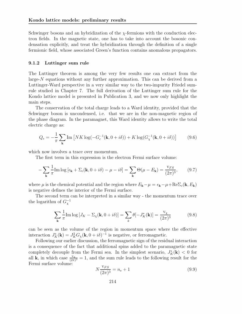
Kondo lattice models: preliminary results
Schwinger bosons and an hybridization of the χ-fermions with the conduction elec-tron fields. In the magnetic state, one has to take into account the bosonic con-densation explicitly, and treat the hybridization through the definition of a singlefermionic field, whose associated Green’s function contains anomalous propagators.
9.1.2 Luttinger sum rule
The Luttinger theorem is among the very few results one can extract from thelarge-N equations without any further approximation. This can be derived from aLuttinger-Ward perspective in a very similar way to the two-impurity Friedel sum-rule studied in Chapter 7. The full derivation of the Luttinger sum rule for theKondo lattice model is presented in Publication 3, and we now only highlight themain steps.
The conservation of the total charge leads to a Ward identity, provided that theSchwinger boson is uncondensed, i.e. that we are in the non-magnetic region ofthe phase diagram. In the paramagnet, this Ward identity allows to write the totalelectric charge as:
Qe = −1
π
∑
k
Im[NK log(−G−1
c (k, 0 + iδ)) +K log(G−1χ (k, 0 + iδ))
](9.6)
which now involves a trace over momentum.The first term in this expression is the electron Fermi surface volume:
−∑
k
1
πIm log [ǫk + Σc(k, 0 + iδ)− µ− iδ] =
∑
k
Θ(µ− Ek) =vFS
(2π)3, (9.7)
where µ is the chemical potential and the region where Ek−µ = ǫk−µ+ReΣc(k, Ek)is negative defines the interior of the Fermi surface.
The second term can be interpreted in a similar way - the momentum trace overthe logarithm of G−1
χ
∑
k
1
πIm log [JK − Σχ(k, 0 + iδ)] =
∑
k
θ[−J∗K(k)] =
vχ(2π)3
(9.8)
can be seen as the volume of the region in momentum space where the effectiveinteraction J∗
K(k) = J2KGχ(k, 0 + iδ)−1 is negative, or ferromagnetic.
Following our earlier discussion, the ferromagnetic sign of the residual interactionis a consequence of the fact that additional spins added to the paramagnetic statecompletely decouple from the Fermi sea. In the simplest scenario, J∗
K(k) < 0 forall k, in which case vχ
(2π)3= 1, and the sum rule leads to the following result for the
Fermi surface volume:N
vFS(2π)3
= ne + 1 (9.9)
214

9.2. Kondo-Heisenberg lattice model
where ne is the electron density per unit cell, per conduction electron channel:ne = Qe/K.
It follows that the total Fermi surface volume expands by one unit per unit cell,due to the Kondo interaction with the lattice of localized spins. To preserve theoverall charge density, the electron Fermi surface volume is forced to enlarge to“screen” the finite background density of charged χ-fermions.
In the magnetically ordered state, the boson field condenses, causing the con-duction and χ fields to hybridize to produce a single species. In this case, the sumrule becomes:
Qe = −1
π
∑
k
Im log[−G−1
f (k, 0 + iδ)]
(9.10)
where Gf is the admixed propagator for the combined conduction and χ fields.The right-hand side cannot be separated into χ and conduction parts, and as
such, defines an admixed set of Fermi surfaces, with an average Fermi surface volumewhich counts the total charge per unit cell:
ne = N〈vAFM〉(2π)3
. (9.11)
If the transition from the paramagnet to the magnetic state occurs via a singlequantum critical point, then our results indicate that the transition in the Fermisurface volume at the second order quantum critical point is abrupt: the total Fermisurface volume jumps as one crosses the QCP.
There have been a number of theoretical speculations [135, 136, 137] that in aKondo or Kondo-Heisenberg lattice model, the conduction electron Fermi surfacemay jump from “large” to “small” as one tunes through the quantum critical point.Recent experimental work based on Hall measurements [138] provide experimentalsupport for this hypothesis.
9.2 Kondo-Heisenberg lattice model
The other important model we defined in previous chapters is the Kondo-Heisenbergmodel, where one considers, on top of the Kondo interaction between the localizedspins and the bath of conduction electrons, a direct exchange between the impurities,described by an Heisenberg interaction. In this section, we extend the two-impuritymodel studied in Chapter 7 to the case of a lattice.
9.2.1 Model and saddle-point equations
The model
Like the model studied in Chapter 7, we choose to restrict ourselves to the an-tiferromagnetic Heisenberg coupling, and describe this interaction in terms of theshort-range bosonic pair operator.
215

Kondo lattice models: preliminary results
The Hamiltonian of the Kondo-Heisenberg lattice, with a bosonic representationof the localized spins, is given by:
H = Hband +HKondo +HHeisenberg where
Hband =∑
k
N∑
α=1
K∑
µ=1
ǫkc†
kαµckαµ
HKondo =JKN
∑
i
∑
α,β
∑
µ
b†
iαbiβψ†
iβµψiαµ
HHeisenberg =JHN
∑
〈i,j〉
(∑
mσ
σb†
i,m,σb†
j,m,−σ
)(∑
m′σ′
σ′bi,m′,σ′bj,m′,−σ′
)
(9.12)
where 〈i.j〉 denotes nearest neighbors, and we recast the N spin indices under theform
(m = 1 . . . N
2, σ = ±
).
Like the Kondo lattice model presented in the previous section, this model isexpected to display (at least) two ground-states in the exactly screened regime: amagnetic state governed by the Heisenberg interaction and for which the Schwingerbosons condense, and a Fermi liquid state where the Kondo interaction dominatesand leads to nearly independent fully quenched impurities.
Large-N equations
After decoupling both the Kondo and the Heisenberg interaction terms, introduc-ing in the process two sets of fields (χi,µ and ∆i,j) and integrating the conductionelectrons out of the partition function, we end up with an effective action that lookslike Eq. (7.3) obtained for the two-impurity system, namely:
S =
∫ β
0
dτ∑
i,m,σ
b†i,m,σ(τ) (∂τ − λi(τ)) bi,m,σ(τ)−1
JK
∫ β
0
dτ∑
i,µ
χ†i,µ(τ)χi,µ(τ)
− 1
N
∑
i,j
∫ β
0
dτdτ ′∑
µ
χj,µ(τ′)χ
†
i,µ(τ) Gc0(i− j; τ − τ ′)∑
m,σ
bj,m,σ(τ′)b
†
i,m,σ(τ)
+∑
〈i,j〉
∫ β
0
dτ
(
Ơ
i,j(τ)∑
m,σ
σbi,m,σ(τ)bj,m,−σ(τ) + h.c.
)
+N
JH
∑
〈i,j〉
∫ β
0
dτ ∆†
i,j(τ)∆i,j(τ) + p0N∑
i
∫ β
0
dτ λi(τ) (9.13)
Since ∆i,j represents a pair of bosons with opposite “spins” (σ is different forthe two bosons involved in the pair), it is symmetric under the exchange σ → −σ,so that it has to be antisymmetric in space: ∆i,j = −∆j,i. We now assume a
216

9.2. Kondo-Heisenberg lattice model
static local solution for the chemical potential λi = λ and the bosonic pair field∆i,j = Sgn(i− j)∆.
We proceed exactly as we did for the two-impurity model studied in Chapter7: after introducing two new fields Q(i, j, τ, τ ′) and Q(i, j, τ, τ ′), we can build aneffective action S(Q, Q, λ,∆) where every term scales like N . Relating the bosonicand fermionic self-energies to the fields Q and Q, the saddle-point equations read:
Σb(r, τ) =
[γJ2
KGχ(−r,−τ)Gc0(r, τ) 00 γJ2
KGχ(r, τ)Gc0(−r,−τ)
]
(9.14a)
Σχ(r, τ) = −J2K
2Gc0(r, τ)
(
G(++)b (−r,−τ) +G
(−−)b (r, τ)
)
(9.14b)
p0 = −1
2
∑
k
[
G(++)b (k, τ = 0−) +G
(−−)b (k, τ = 0+)
]
(9.14c)
|∆|2JH
=1
12
∑
k
G−+b (k, τ = 0−)∆k (9.14d)
where the matrix form is expressed in the space of σ = ± (the χ-fermion propagatorbeing diagonal in this basis), and we considered a cubic structure of spacing a forthe lattice of localized spins.
The Dyson’s equations have the following expression:
G−1b (k, iνn) =
[iνn + λ −∆k
−∆∗k −iνn + λ
]
− Σb(k, iνn) (9.15a)
G−1χ (k, iωn) = JK − Σχ(k, iωn) (9.15b)
where ∆k = −4i∆ [sin(kxa) + sin(kya) + sin(kza)]
9.2.2 Uncontrolled local approximation
As the main additional difficulty of this new set of equations lies in the momen-tum dependence of the propagators, a first simple approximation one can makeamounts to neglecting this very momentum dependence in the self-energies. Suchan approximation is based on the assumption that the relevant physics leading tothe self-energies is local, i.e. that there is very little interplay between the Kondoand Heisenberg mechanisms. This is an uncontrolled approximation as no smallparameter allows us to neglect the non-local terms. However it might be sufficientto capture the competition between the Kondo screening and the development ofmagnetism.
Within this local approximation, our set of equations (9.14) and (9.15) dramat-
217

Kondo lattice models: preliminary results
ically simplifies:
Σb(τ) = −γJ2KGc0(τ)Gχ(β − τ) (9.16a)
Σχ(τ) = −J2KGc0(τ)Gb(β − τ) (9.16b)
Gb(iνn) =∑
k
1
iνn + λ− Σb(iνn)− |∆k|2−iνn+λ−Σb(−iνn)
(9.16c)
Gχ(iωn) =1
JK − Σχ(iωn)(9.16d)
p0 = −Gb(τ = 0−) (9.16e)
|∆|2JH
=1
12
∑
k
T∑
n
eiνn0+
× |∆k|2(iνn + λ− Σb(iνn)) (−iνn + λ− Σb(−iνn))− |∆k|2
(9.16f)
The sum over momentum is evaluated by introducing ηk such as ∆k = 4i∆ηk.We then define a “density function” for ηk:
ρ(η) =∑
k
δ(η − ηk)
=1
2π
∫ +∞
−∞dx eiηx [J0(x)]
3 (9.17)
which allows to replace summations over momentum by integrals over η with thefunction ρ(η), which turns out to be the Fourier transform of the Bessel function ofthe first kind, elevated to the power 3.
-3 -2 -1 0 1 2 30
0.05
0.1
0.15
0.2
0.25
0.3
-3 -2 -1 0 1 2 30
0.05
0.1
0.15
0.2
0.25
0.3
-3 -2 -1 0 1 2 30
0.05
0.1
0.15
0.2
0.25
-3 -2 -1 0 1 2 30
0.05
0.1
0.15
0.2
ρ(η)ρ(η)
η ηb)a)
Figure 9.1: a) Plot of the function ρ(η) obtained by numerical integration, b) Ap-proximate form of the same function, used to compute analytically the summa-tion over momentum. The edges are the same in both cases and go like
√ǫ for
η = ±(3− ǫ).
218

9.2. Kondo-Heisenberg lattice model
We solved numerically the set of equations (9.16) as a function of temperature,for various values of the Heisenberg coupling. To do so, we replaced the functionρ(η) by a slightly modified one (see Fig. 9.1) which allows to perform analyticallythe momentum summations.
We could map out the phase diagram presented in Fig. 9.2. Along with theline separating the ∆ = 0 region, from the region where pairs start condensing, wecould also isolate a region of the phase diagram where a magnetic order develops.This transition line is determined by obtaining a solution of the set of self-consistentequations for increasingly larger values of ∆. At fixed temperature, we obtain a crit-ical ∆c above which the solution for the bosonic spectral function seems to developsome finite weight at zero energy, violating the causality rules. As these rules arebuilt into the equations, this violation signals that the set of equations is no longervalid, which suggests that the Schwinger bosons undergo a condensation.
At low enough fixed temperature, we find a paramagnetic solution in a smallregion of the phase diagram below the transition line. This result suggests thatthere exists a region where both a magnetic and a non-magnetic state are present.As a consequence, we expect the transition towards the magnetic state to be of thefirst order at low temperature.
0 0.1 0.2 0.3 0.4 0.50
0.2
0.4
0.6
0.8
0 0.1 0.2 0.3 0.4 0.50
0.2
0.4
0.6
0.8
TK/JH
〈b〉 6= 0
∆ = 0
∆ 6= 0T
JH
Figure 9.2: Phase diagram of the 3-dimensional lattice with the local approximation.The dashed line separating the region where pair correlations develop is unchangedcompared to the two-impurity model studied earlier. The red line corresponds toa transition towards the magnetic region where Schwinger bosons condense. Thesplitting of this line at low temperature signals the presence of a first order transitioninto the magnetic state.
219

Kondo lattice models: preliminary results
9.3 Conclusion
Very few results can be derived concerning these models without making new as-sumptions. The challenge at this stage is to find clever approximations that wouldcapture the important physics of the problem, while partially allowing a numericalor an analytical treatment of the Kondo lattice model.
9.3.1 Looking for a gap
We saw in our study of the one and two impurity systems that the gap, and moreimportantly the closing of the gap, plays a significant role in the physics of thesystem. In the case of the Kondo lattice, we expect the gap to display a momentumdependence. The study of the gap in momentum space could be very insightful asfor the relevant physics close to the quantum critical point. However, the study ofthe gap involves solving the full set of saddle-point equations.
A first step towards this route is to analyze the necessary conditions for a gap tobe stabilized by the large-N equations. This might already be sufficient to reducethe relevant region of momentum space.
9.3.2 Kondo hedgehog
Another possible way of getting around the many difficulties related to the latticeis to consider a slightly different model. It can be argued that the competitionbetween the Kondo effect and the magnetic ordering can be successfully mimicked byconsidering a cruder version of the Kondo lattice model, where we treat the electronsonly to the extent that they provide spins which tend to be aligned antiparallel tothe localized moments.
This was the reasoning behind Doniach’s Kondo necklace model [94]. The large-N treatment developed here could be extended to a two or three dimensional versionof Doniach’s idea: a Kondo hedgehog model.
9.3.3 Dynamical mean-field theory
As a final example of the possible extensions of our approach to encompass thephysics of the lattice, we mention the Dynamical Mean-Field Theory3 (DMFT).
The use of our approach as an impurity solver or as a two-impurity solver mightlead to interesting results when plugged back into a DMFT scheme. Such a treat-ment of the Kondo lattice model could provide enough of the non-local characterof the system and lead to a better understanding of the important elements of thequantum critical regime.
3A detailed introduction to this technique goes way beyond the scope of this section. For adetailed review on DFMT, the reader is referred to [139]
220

PUBLICATION 3
Sum rules and Ward identities inthe Kondo lattice
Phys. Rev. B, 72, 094430 (2005)

Sum rules and Ward identities in the Kondo lattice
222

Publication 3
Sum rules and Ward identities in the Kondo lattice
P. Coleman,1,2 I. Paul,1,3 and J. Rech1,2,3
1Kavli Institute for Theoretical Physics, Kohn Hall, UCSB Santa Barbara, Santa Barbara, California 93106, USA2Center for Materials Theory, Rutgers University, Piscataway, New Jersey 08855, USA
3SPhT, L’Orme des Merisiers, CEA-Saclay, 91191 Gif-sur-Yvette France
Received 3 May 2005; published 26 September 2005
We derive a generalized Luttinger-Ward expression for the free energy of a many-body system involving a
constrained Hilbert space. In the large-N limit, we are able to explicitly write the entropy as a functional of the
Green’s functions. Using this method we obtain a Luttinger sum rule for the Kondo lattice. One of the
fascinating aspects of the sum rule is that it contains two components: one describing the heavy electron Fermi
surface, the other, a sea of oppositely charged, spinless fermions. In the heavy electron state, this sea of spinless
fermions is completely filled and the electron Fermi surface expands by one electron per unit cell to compen-
sate the positively charged background, forming a “large” Fermi surface. Arbitrarily weak magnetism causes
the spinless Fermi sea to annihilate with part of the Fermi sea of the conduction electrons, leading to a small
Fermi surface. Our results thus enable us to show that the Fermi surface volume contracts from a large to a
small volume at a quantum critical point. However, the sum rules also permit the possible formation of a new
phase, sandwiched between the antiferromagnet and the heavy electron phase, where the charged spinless
fermions develop a true Fermi surface.
DOI: 10.1103/PhysRevB.72.094430 PACS numbers: 75.30.Mb, 75.20.Hr, 71.27.a, 72.15.Qm
I. INTRODUCTION
Sum rules play a vital role in condensed matter physics.The most famous sum rule—the Luttinger sum rule,1–3 de-fines rigorously the volume of the Fermi surface of a Fermiliquid in terms of the density of electrons:
2vFS
2D= ne, 1
where vFS is the Fermi surface volume, ne is the density ofelectrons per unit cell, and D is the dimension. Historically,sum rules have also played an important role in our under-standing of strongly correlated systems. In the context of theKondo effect for example, the Friedel sum rule,4–6
= ne, 2
relating the sum of the scattering phase shifts in channelslabeled by to the number of bound states ne helped toestablish a rigorous foundation for the Abrikosov-Suhlresonance7–9 that develops in Anderson and Kondo impuritymodels. Later, Martin10 applied the Luttinger sum rule to theAnderson lattice model, to argue that heavy electron metalsmust have a “large Fermi surface” that counts both the con-duction electrons and also the localized f electrons,
2vFS
2D= ne + 1. 3
Today, there is a renewed interest in sum rules, in connec-tion with models of strongly correlated electrons. For in-stance, in the context of high-temperature superconductors,which are Mott insulators when undoped, there has been alongstanding debate over whether the “large” Fermi surfacepredicted by Luttinger’s sum rule might be replaced at lowdoping, by a “small” Fermi surface determined by the num-
ber of doped holes.11,12 Related issues arise in the context ofheavy electron systems, where experimental advances havemade it possible to tune through the quantum critical pointthat separates the heavy electron paramagnet from the localmoment antiferromagnet. There have been a number of the-oretical speculations that the Fermi surface of the heavy elec-tron material may jump from “large” to “small” at the quan-tum critical point.13–15 Recent experimental work, based onde Haas–van Alphen measurements16 and Hallmeasurements,17 provide experimental support for this hy-pothesis, but the idea has lacked rigorous theoretical support.
The main difficulty in extending sum rules to stronglycorrelated systems is that the theoretical machinery used anddeveloped by Luttinger and Ward to derive sum rules appliesto models with unprojected Hilbert spaces. About eight yearsago, Affleck and Oshikawa18 demonstrated that such sumrules have a more general existence. By using a modificationof the Leib–Mattis theorem, Affleck and Oshikawa showedthat the “large Fermi surface” that counts both local mo-ments and conduction electrons develops in the one-dimensional S=1/2 Kondo model, even though in this casethe ground state is not a Fermi liquid. More recently,Oshikawa19 has extended this derivation to higher-dimensional Kondo lattices. This work suggests that it oughtto be possible to extend the Luttinger–Ward approach toHamiltonian problems with strong constraints.
In this paper, we show how the original methods of Lut-tinger and Ward can indeed be extended to strongly corre-lated models. A key element of this work is the constructionof a functional relating the free energy of a strongly interact-ing system to the Green’s functions of the projected Hilbertspace. Our approach is based on the use of slave particles,such as a Schwinger boson description for the local momentsin a Kondo lattice. We begin with a generalization of theLuttinger–Ward free energy functional, appropriate for sys-tems of interacting bosons and fermions,20,21 which can becompactly written as
PHYSICAL REVIEW B 72, 094430 2005
1098-0121/2005/729/09443014/$23.00 ©2005 The American Physical Society094430-1
223

Sum rules and Ward identities in the Kondo lattice
F = T Strln− G−1 + G + YG , 4
where Str A=Tr AB−Tr AF denotes the supertrace of a
matrix containing both bosonic B and fermionic F com-ponents where the underline notation is used to denote asum over internal frequencies and a trace over the internalquantum numbers of the matrix. G= G0
−1−−1 is the matrix
describing the fully dressed Green’s function of all elemen-tary particles and fields entering the Lagrangian, includingthe slave particles, where is the self-energy matrix and G0
the bare propagator of the fields. The quantity YG is, dia-
gramatically, the sum of all closed-loop two-particle irreduc-ible skeleton Feynman diagrams. Figure 1 illustrates the sumof diagrams contributing to YG for a Kondo lattice model.
Variations of YG with respect to the Green’s function G
generate the self-energy
YG = − T Str G 5
or
= − Y
G, 6
where the use of the supertrace as the measure for functionalderivatives avoids the need to introduce a relative minus signbetween Fermi and Bose parts of this expression. Diagram-matically, the functional derivative of Y with respect to G
corresponds to “cutting” one of its internal lines. If we trun-cate Y to some order in 1/N, this relationship determines aconserving Kadanoff-Baym approximation.23 For example, ifwe take the generating function for a Kondo lattice illus-trated in Fig. 1c, and differentiate the leading order contri-
bution in the large N expansion with respect to G, we obtainthe following self-energies:
7
where the cross indicates the line that is eliminated by the
functional differential. Each of these terms contains a factor
O1/N from the vertices, but the first two self-energies con-
tain summations over the internal channel or spin indices,
elevating b and to terms of order O1. In the leading-
order large N approximation, cO1/N, so that a consis-
tent large-N approximation is produced by leaving the con-
duction electron lines undressed. This provides an alternative
FIG. 1. Illustrating the Luttinger–Ward functional for the Kondo
lattice. a Fully renormalized propagators for the conduction elec-
trons, fermions, and Schwinger bosons, where 1,N is the
spin index and 1,K the channel index, b Interaction vertices
showing spin and channel indices and c leading skeleton
diagrams for the Luttinger–Ward functional with dependence on
1/N. The first diagram involves two loops carrying spin and chan-
nel quantum numbers, and one pair of vertices and is consequently
of order OKN /N=ON. The second diagram has four loops car-
rying internal quantum numbers and four pairs of vertices, so it is of
order ON2K2 /N4=O1. The final diagram has two quantum num-
ber loops and three pairs of vertices, and is hence of order
ONK /N3O1/N.
COLEMAN, PAUL, AND RECH PHYSICAL REVIEW B 72, 094430 2005
094430-2
224

Publication 3
diagrammatic derivation of the Parcollet–Georges approachto the multichannel Kondo model.24
Each conserved quantity Q that commutes with theHamiltonian leads to a gauge invariance of the underlyingquantum fields, such that the action and all physical proper-ties are invariant under the transformation
t → eitq . 8
Here, q is the gauge charge of the field: it is this quantitythat controls the charge of any physical excitations associ-ated with the field. Provided this gauge invariance is unbro-ken, we show that this leads to a Ward identity at zero tem-perature,
−i
id
2iStrqG
dd
= 0, 9
where the integral runs along the imaginary axis. Luttinger’soriginal work derived the elementary version of this relation-ship for electrons: here it is seen to hold for interacting spe-cies of fields.
Each of these Ward identities leads to a corresponding,generalized Luttinger sum rule given by
Q =1
Im Trq ln− GF
−10 − i , 10
where GF is the complete fermionic Green’s function, involv-ing all fermions involved in the description of the con-strained Hilbert space, including those introduced as slaveparticles. In impurity systems, the trace over the logarithmsreduces to a sum of phase shifts, and the quantity Q is re-placed by Q, the change in Q induced by the impurity. Inthe limit of infinite bandwidth, Q=0, which leads to a mul-tiparticle version of the Friedel sum rule,
0 = q n
, 11
where n is the spin degeneracy associated with the traceover internal quantum numbers of the field . In lattice sys-tems, the trace over the log becomes the Fermi surface vol-ume associated with the field , so that
Q = q n
vFS 2D , 12
where vFS is the Fermi surface volume associated with
field . A closely related Fermi surface sum rule has re-cently been derived by Powell et al. for mixtures of fermionsand bosons in atom traps.25
In this paper we apply these results to the Kondo latticemodel. The key to our approach is the adoption of Schwingerbosons for the description of quantum spins. Schwingerbosons offer a key advantage, because they can describe boththe antiferromagnetic and the heavy electron ground states ofthe Kondo lattice.26 The Kondo effect induces a developmentof a retarded interaction in the spin singlet channel betweenthe electrons and the spins. Formally, this interactionmanifests itself as the mediating field j in the Hubbard-Stratonovich decomposition of the interaction24,27,28
JKS j · c j† c j →
1
Nc j
†b j j
† +1
Nb j
†c j j +
j† j
JK
.
13
Here S j is the spin at site j and c j† creates an electron at site
j. At long times the field develops charge dynamics thatdescribe the scaling of the Kondo interaction in both fre-quency and momentum space. In particular, the − propaga-tor describes the momentum- and frequency-dependentKondo interaction,
− Gk, = 1
JK
+ k, −1
= JK* k, . 14
At each point in momentum space, where the Kondo inter-action scales to strong coupling, G develops a pole. In thisway, the physics of the Kondo effect is intimately linked15 tothe possible emergence of a positively charged, spinlessFermi field—a “holon.”29
Under gauge transformations, the conduction and fieldshave opposite gauge charge,
qc = 1, q = − 1. 15
When we apply the Luttinger–Ward procedure, we find thatthe physical charge density is given by the total volume ofthe electron Fermi surface, minus the volume of the holonFermi surface, as follows:
ne = 2vFS
2D−
v
2D. 16
Here, the volume of the electron Fermi surface is given bythe conventional Luttinger formula,
vFS =1
k
Im lnk + ck,0 − i − + i
= k
− Ek , 17
where is the chemical potential, Ek=k+ck ,Ek is the
renormalized energy of the heavy electrons. Now v is
v =1
k
Im ln 1
JK
+ k,0 − i = k
− JK* k ,
18
where JK* k=−Gk ,0− i.
The meaning of the renormalized coupling constant JK* in
the paramagnetic phase needs a little discussion. This quan-tity describes the residual interaction between the electronfluid and any additional spins that are added to the Fermiliquid ground state. If we add an additional Schwinger bo-
son, increasing S→S+1
2 at a given site, the additional spinunit remains unscreened, because each channel can onlyscreen one spin unit, and all channels are fully screening. Ifb=Enb+1−Enb is the energy to adding one additional
spin, then the residual interaction between the additionalSchwinger boson and the conduction electrons is JK
* b.Since the additional spin decouples, it follows that JK
* has
SUM RULES AND WARD IDENTITIES IN THE KONDO… PHYSICAL REVIEW B 72, 094430 2005
094430-3
225

Sum rules and Ward identities in the Kondo lattice
a zero at =b, JK* b=0. At higher energies, the residual
interaction will become positive, ultimately connecting up tothe single-ion scaling behavior JK
* 1/ lnTK /. Since JK*
passes through zero at =b, it follows that at lower ener-gies b, and in particular, at zero frequency, the residualcoupling must be ferromagnetic, i.e JK
* 00. This, in turn,
means that the Fermi sea of holons is entirely full, v
= 2D, so that
ne = 2vFS
2D− 1. 19
To preserve the overall charge density, the electron Fermisurface volume is forced to enlarge by one unit per spin to“screen” the finite background density of positively chargedholons Fig. 2.
Let us now consider the antiferromagnet. In this case, theSchwinger boson field condenses, and the field becomeshybridized with the conduction electrons. In this case, theholon Fermi surface annihilates with the expanded part of theheavy electron Fermi surface, to reveal a single integrated setof Fermi surface sheets with a “small” volume that enclosesthe total electron count. If the transition from paramagnet toantiferromagnet occurs via a single quantum critical point,then our results indicate that the transition in the Fermi sur-face volume at the second-order quantum critical point isabrupt.30
Perhaps the most interesting aspect of this picture is that itsuggests that the background field of holons can developdynamics. One intriguing possibility is that the holons areliberated when the Fermi surface volume contracts at thequantum critical point. Another more exotic possibility, al-lowed by the Ward identities, is the formation of a separatephase where the holons develop a Fermi surface, so that v
=x2D is partially filled. This “spin-charge” decoupled
phase would be sandwiched between the localized magneticphase and the fully formed paramagnet. Pépin has recentlysuggested that the holons might develop a Fermi surface atthe quantum critical point.15 This might provide a mecha-nism for such a scenario. A good candidate for this phase isthe one-dimensional Haldane S=1 chain, coupled to twoconducting chains to form a one-dimensional, two-channelKondo lattice. Here, the conjectured intermediate phasewould separate a Haldane gap phase and a large Fermi sur-face phase, leading to Friedel oscillations with wave vector
q=2kF
0+ /2x, intermediate between that of the large x
=1 and small x=0 Fermi surface.
This paper is divided up into various parts. In the first wedevelop the Luttinger–Ward free energy expansion for theKondo lattice. Next, we present a new formula for the en-tropy of the interacting fluid, expressed exclusively in termsof the Green’s functions of the particles. We then go on toderive the Luttinger sum rule in a general form for a con-strained system, which we then apply to the Kondo impurityand lattice model. In the final part, we discuss the generalimplications of our sum rule in the Kondo lattice.
II. LUTTINGER WARD EXPRESSION FOR THE KONDO
LATTICE
The Luttinger–Ward approach was originally based onperturbation theory in the strength of the Coulomb interac-tion. In order to develop these methods for strongly interact-ing systems, we need to take account of the constraints in thetheory, requiring a Luttinger–Ward approach appropriate togauge theories. In this respect, our efforts to apply the Lut-tinger Ward approach to the Kondo lattice closely parallelrecent efforts to extend the Luttinger-Ward approach toquark-gluon plasmas.21
Although the Luttinger-Ward functional may be derivednonperturbatively,31 the usefulness of any derived sum rulesrests on the direct relationship between the Green’s functionsthat enter in the functional and physical excitations. Stronglyinteracting systems do not generally provide a natural smallparameter on which to base a perturbation expansion. Ourphilosophy is that to develop this control, we need to definea family of large-N models that, in the infinite-N limit, pro-vide a mean-field description of the phases of interest. In theexpansion about this limit, 1 /N then provides a small param-eter. The large-N solutions constructed this way will ofcourse satisfy the sum rules we derive, but the sum rules areexpected to have a far greater generality.
In the context of our interest in the Kondo lattice, weadopt a family of models given by
20
Here, we have adopted the Schwinger boson representation,where b j
† creates a Schwinger boson at site j, with spincomponent 1,N. The combination b j
† b j=Sj rep-
resents the local spin operator and the system is restricted tothe physical Hilbert space by requiring that
b j†
b j = 2S , 21
at each site j. The index 1,K is a channel index that is
absent in the physical SU2 model, but that is included to
create a family of large-N models. The “filled shell” case2S=K defines a perfectly screened Kondo lattice, and our
discussion will focus on this case. Here ck†
creates a conduc-
tion electron of momentum state k and spin 1,N. c j†
FIG. 2. Schematic diagram illustrating the enlargement of the
Fermi surface in the Kondo lattice a coupling of local moments to
a small Fermi surface; b each spin-boson “ionizes” into an elec-
tron and a “holon,” producing a large electron Fermi surface and a
filled holon Fermi sea.
COLEMAN, PAUL, AND RECH PHYSICAL REVIEW B 72, 094430 2005
094430-4
226

Publication 3
= 1/Nsck† e−ik·x j creates an electron at site j, where Ns is
the number of sites in the lattice. The above model is knownto have a controlled large-N expansion that contains bothmagnetic and paramagnetic solutions when N is taken to in-finity with k=K /N fixed.
To develop a Luttinger–Ward expansion, we shall factor-ize the interaction in terms of a Grassman field j,
HI → j
1
Nc j
†b j j
† + b j†
c j j + j
j† j
JK
,
22
and the Lagrangian becomes
L = k
ck† + kck +
j
b j† + jb j +
j
j† j
JK
+ j
1
Nc j
†b j j
† + b j†
c j j − j
2S j . 23
Note that the Grassman fields j contain no time derivative,and so instantaneously they behave as inert, neutral fields.Here j is the static value of the Lagrange multiplier used toenforce the constraint on each lattice site. At finite tempera-tures the constraint is only enforced on the average, but inthe ground state, the value of the conserved quantities nbj
will be quantized as a step function of the j. In the range j j
− , j+ where j
± are the energy gaps between the
physical ground state and the states with 2S±1 Schwingerbosons at site j, the constraint will be precisely satisfied. Weshall assume that a translationally invariant choice j = isalways available.
For our sum rules, we need to know comparatively littleabout the nature of the ground state excitations. However,from the the large-N solution of this model, we do know thatthere are two main classes of solution to the Kondo lattice:
i The heavy electron phase, where the Schwingerbosons pair condense in either the Cooper channelbi
† b j−† 0 antiferromagnetic interactions or particle-
hole channel bi† b j0 ferromagnetic interactions. In
field-theory language, this is a “Higg’s phase” in which thelocal U1 symmetry is broken and both the spin and holon
excitations can propagate from site to site.ii The magnetic phase, in which the Schwinger bosons
individually condense b j0 to develop long-range mag-
netic order. In this phase, the j fields become hybridizedwith the conduction fields, and Gc and G become diagonalmembers of a single matrix propagator.
In general, we will therefore have to preserve the momen-tum dependence of the propagators. The bare propagators ofthe theory are diagonal in momentum, and given by
Gb0k,in = in3 − 1 −1,
Gc0k,in = in − k
−1,
G0k,in = − JK, 24
where we have written the bare boson propagator as a two-dimensional Nambu propagator, to allow for the possibleintroduction of boson pairing, which develops as antiferro-magnetic correlations begin to grow. Formally, we will com-bine these three propagators into a single propagator, givenby
G−1 = in3 − 1
in − k
−1
JK
− , 25
where is a matrix self-energy. Following Luttinger andWard, we will regard G as a variational function, and as aderived quantity.
We now consider the effect of tuning up the strength ofthe Kondo interaction from zero to JK, by replacing JK
→JK where 0,1, keeping the chemical potential of
the conduction electrons and bosons fixed. Now the partitionfunction is given by
Z = Tre−H = Dc,b,e−0Ld, 26
where Dc ,b , is the measure of the path integral. If we
vary inside this expression, we obtain
dZ
d= Dc,b,
j
0
d 1
2JK
j† j e−0
L d
= Z 1
2JKj
j† j , 27
so that if F=−T ln Z is the free energy, then
dF
d= −
1
2JKj j
† j = −T
2JKTr G , 28
where G is the Green’s function for the fermion and
Tr GKin,kGk , inein0+denotes a trace over the fre-
quency and momentum of G here, ein0+ensures the normal
ordering of the operators. We next consider the expression
F = T Strln− G−1 + G + YG . 29
We will show how this expression generalizes the Luttinger–Ward free energy functional to a mixture of interactingbosons and fermions. Here, we use the notation
StrA TrAB − TrAF in
TrABinein0+
− in
TrAFinein0+30
to denote the “supertrace” over the bosonic and fermionicparts of the matrix A. The “underline” notation is used toindicate a sum over both the frequency variable of A and atrace over the internal quantum numbers of A such as mo-mentum. The supertrace includes a relative minus sign for
SUM RULES AND WARD IDENTITIES IN THE KONDO… PHYSICAL REVIEW B 72, 094430 2005
094430-5
227

Sum rules and Ward identities in the Kondo lattice
the fermionic component of the matrix, and we have explic-itly displayed the trace over the discrete Matsubara Bosein= 2nT and Fermi in= 2n+1T frequencies. In
the above expression, the self-energy matrix =G0−1−G−1.
The quantity YG is the sum of all closed, two-particle irre-
ducible skeleton Feynman graphs for the Free energy.As mentioned earlier, the Luttinger Ward functional YG
has the property that its variation with respect to G generatesthe self-energy matrix,
YG = − T Str G . 31
The variation of the first term in F with respect to G isgiven by
T Strln− G−1 = T Str− G−1 G 32
By using the relation G=G0−1−G−1, the variation in the
second term in F is given by
T StrG0−1 − G−1G = T StrG0
−1G , 33
so that the total variation of F with respect to G,
34
identically vanishes,
F
G= 0. 35
Now the Hubbard–Stratonovich transformation that we havecarried out on the interaction HI assures that the only placethat the coupling constant JK enters, is in G
0−1=−1/JK.
This means that on the rhs of Eq. 29 enters explicitlyonly through =−JK−1− G−1. Then,
36
But by comparison with 28, we see that dF /d=dF /d
and, since F=0= F=0 in the noninteracting case, the
two quantities must be equal for all , i.e.,
F = T Str ln− G−1 + G + YG . 37
There are various points to make about this derivation.i The derivation is very general. Its correctness only
depends on the stationarity of FG with respect to variations
in G and the equivalence between dF /d and dF /d. Thismeans that the above expression will hold for broken sym-metry or “Higg’s phase” solutions that involve off-diagonalcomponents to G.20 In the context of the Kondo lattice, thismeans that G can be extended to include anomalous bosonpairing terms that are driven by short-range antiferromag-netic correlations, or alternatively, off-diagonal terms drivenby long-range magnetism, which mix the conduction and fermions. This expression can also be used to describe super-conducting states, where the conduction electron and propagators will contain off-diagonal terms.
ii Even though the free energy is a functional of threeGreen’s functions, there is no overcounting.
iii The above Free energy functional can be used as abasis for developing conserving approximations that gener-alize the Kadanoff–Baym approach to a constrainedsystem.23 In particular, in the large-N limit, the skeletongraph expansion for Y truncates at the leading diagram Fig.1, providing the basis for a controlled treatment of both themagnetic and the paramagnetic phases of the Kondolattice.24,26
III. ENTROPY FORMULA
In this section, we derive an approximate formula for theentropy of a Luttinger–Ward system that becomes exact inthe large-N limit and in any approximation where the vertexcorrections can be neglected. The result, which we shall de-rive below, is
ST,G = d
TrB,Fdn
dT Im ln− G−1 − i
+ Im Re G , 38
where
n = nf
39
is the matrix containing the Bose or Fermi-Dirac distributionfunctions n= e−1−1, f= e+1−1. The trace is
carried out over the Bose and Fermi components of bothexpressions. Here G and are the self-energies that
have been analytically continued onto the real axis. This ex-pression is extremely useful, for it only involves the low-energy part of the Green’s functions of the particles, anddoes not involve the functional YG. A version of this for-
mula was first quoted in the context of lattice gauge theoryby Blaizot et al.21
Key to our approach is the notion that the Luttinger–Wardfunctional FG can be rewritten in terms of the real fre-
quency Green’s functions. This has the advantage that onedoes not have to deal with the temperature dependence of theMatsubara frequencies. The approach that we adopt is, infact, reminiscent of the Keldysh approach for nonequilibriumsystems.32,33 To preserve the symmetry between bosons andfermions, it proves useful to introduce a kind of “Keldysh”notation, writing
h =1
2+ n =
1
2+ n
1
2− f 40
Use of this function preserves the “supertrace” symmetry ofour approach. Consider the first part of the free energy,
F1 = T Strln− G−1 + G . 41
We replace the summation in this term by an integral overn around the imaginary axis,
COLEMAN, PAUL, AND RECH PHYSICAL REVIEW B 72, 094430 2005
094430-6
228

Publication 3
T StrA → − d
Im StrhA − i , 42
where StrA=TrAB−TrAF is the supertrace over the spa-
tial and internal quantum numbers of A. By distorting thecontour around the real axis, we obtain
F1 = − d
Im Strhln− G−1 + G0
−1 − G−1G−i .
43
If we vary the Green’s function, then we obtain
F1 = − d
Im StrhG−i, 44
where we have employed the notation =G0−1−G−1. In a
similar fashion, when we vary G inside YG, we obtain
Y = d
Im StrhG−i. 45
The condition that the two terms cancel sets G0−1−G−1=,
defining both the real and the imaginary parts of the self-energies in terms of the Green’s functions.
We can exploit the stationarity F /G=0 to simplify thedifferentiation of the free energy with respect to the tempera-ture. When we differentiate F, we can neglect the tempera-ture dependence of the spectral functions,
ST = −dF
dT= −
F
T
G
. 46
The contribution to the entropy from F1 is then
S1 = d
Im Str h
Tln− G−1 − i
+ − iG − i . 47
The temperature derivative of the second term YG in 37requires more careful consideration. The general diagram-matic contribution to Y contains a certain number of fre-quency summations. When we analytically continue thesefrequency summations, distorting the contour integralsaround the branch cuts of the Green’s functions, we pick up“on-shell” contributions from each branch cut of the form
hBGB 48
and
hFGF . 49
These combinations are nothing more than the “Keldysh”Green’s, function well known from nonequilibriumphysics.32,33 In equilibrium, the Keldysh Green’s functionsatisfies the fluctuation dissipation theorem,
GK = GR − GA2h = − 4iGh ,
where GR and GA are the retarded and advanced propagators,respectively. In other words, hGi /4GK. The point
is that we can formally imagine evaluating Y in a generalsteady state, replacing GK→−4igh at the end of the
calculation. It is, however, equally consistent to compute Y
in equilibrium, and substitute gh→gK. The func-
tional Y is closely related to the expectation value of theinteraction energy. If we associate an amplitude with thestrength of each vertex, then the expectation value of theinteraction energy has the expansion
HI = nYnGK,GR,GA ,
where GK,R,A are the fully renormalized nonequilibriumpropagators. The functional Y is the weighted sum
YGK,GR,GA = n
nYnGK,GR,GA .
In this way, we can absorb all thermal functions into theGreen’s functions, so that all temperature dependence is en-tirely contained within the Keldysh Green’s functions. Todifferentiate Y with respect to temperature, we need to deter-mine Y /GK. Unfortunately, Y is not a true generating func-tional for the Keldysh self-energies, and we must be verycareful in taking the next step.
Once we know the variation of Y with respect to theKeldysh Green’s function, we can immediately compute thevariation with respect to temperature. Now, from 45, wesee that we may write
Y = d
StrhG + hG .
50
If we now identify
hG i
4GK,
h i
4K, 51
as the Keldysh components of the propagator and self-energy, respectively, it is very tempting to write
Y = d
Str i
4 GK + i
4 KG .
52
This form would always be correct if Y were a true generat-ing functional for Keldysh propagators. Unfortunately, in theKeldysh approach, the distinction between the “measure-ment” and “response” vertices means that, in general, thedifferential of Y with respect to GK does not generate the realpart of the self-energy. Fortunately, this difficulty vanishes inthe leading large-N approximation, which is sufficient togenerate a wide class of noncrossing approximationschemes. Diagrams involving vertex corrections do not sat-isfy this relationship, and there are corrections to the abovediagram. Interestingly enough, however, our large-N expan-sion does absorb all the “RPA” diagrams of the interactionlines into explicit propagators, enabling the entropy formula
SUM RULES AND WARD IDENTITIES IN THE KONDO… PHYSICAL REVIEW B 72, 094430 2005
094430-7
229

Sum rules and Ward identities in the Kondo lattice
to be derived for interacting collective modes and fermions.With this proviso, we write
Y
GK=
i
4 ,
where =1
2 − i++ i.It is worth making a short diversion at this point to ex-
plicitly demonstrate that this relationship works in the large-N limit. Consider the leading-order form for Y in the large-Nexpansion,
Y1 = K N 1
N 2
T2k,q
GckGq − kGbq , 53
where kink, qin ,q is a shortened space-time nota-
tion. When we carry out the Matsubara sums in this expres-sion, we obtain
Y = − K−
d
d
k,q
GcGGbhhb −1
4 + GcGGbhchb
+ GcGGbhch , 54
where we have used the shorthand notation GcGck, hc
hc, GGq−k, etc., which can be rewritten as
Y =K
4
−
d
2
d
2k,q
ReGRcGKGKb + GKcGRGKb
+ GKcGKGRb + GRGRcGAb . 55
This last expression can also be derived using the Keldyshformalism to calculate the leading-order expression forHI.33 The variation of this expression with respect to GK
gives the leading-order expressions for the boson and con-duction self-energy; thus, for instance,
Y
i
4GKbq
= −i
4k
k
dc
GckGKq − k
+ GKckGq − k
= − kk
dc
GckGq − khq − k
+ GckhkGq − k , 56
where the replacement K→k=K /N occurs because Y con-tains the contribution of all N spin channels of GKb, and weare only differentiating with respect to one of them. Thisresult can be independently confirmed using Matsubara tech-niques.
Let us now return from this digression and continue tocalculate the temperature dependence of Y. When we differ-entiate the general expression with respect to the tempera-ture, we only need to keep track of how each of the thermalfunctions changes. This leads to the contribution
hG =i
4GK → hG +
dhdT
GT
=i
4GK + GK , 57
where
i
4GK =
dhdT
GT . 58
We can now combine these results to obtain
Y
T
G
= d
Str Y
i
4GK
dhdT
G = d
Str dh
dTG , 59
so that
S2 = −Y
T
G
= − d
Strdh
dT Re G .
60
This is a key element in our proof of the entropy equation.When we add S1 and S2 together, S2 partially cancels the
second term in S1, yielding the final answer
S = S1 + S2 = d
Strdh
dT Im ln− G−1z
+ Im zRe Gzz=−i . 61
We may replace h→ n and Str→TrB,F to recover 38. Thereare a few important points to be made about this result.
i Our ability to write the entropy in terms of the Green’sfunctions only works because in the leading-order approxi-mation for Y, there are no hidden collective modes that carrythe entropy.
ii This approach is general, and can, for example, beapplied to the interacting electron gas, and various interact-ing plasmas, such as the quark gluon plasma.21 By treatingthe interaction line as an independent particle photon, theleading-order approximation generates a generalized RPA-Eliashberg scheme for the self-consistent interaction andelectron self-energies. Note that the entropy formula cannotbe used in an RPA scheme in which the interaction line is nottreated as an independent particle,22 and it does not work ifone includes vertex corrections.
iii It may be possible in future work to evaluate a moregeneral expression for Y /GK, permitting one to gener-
alize the entropy formula to higher-order approximationsfor Y.
IV. CONSERVATION LAWS AND SUM RULES
Sum rules are intimately related to the existence of con-served charges. For example, in the Kondo lattice, there are
COLEMAN, PAUL, AND RECH PHYSICAL REVIEW B 72, 094430 2005
094430-8
230

Publication 3
three independent types of conserved charges: the electriccharge in each channel, the total spin, and the conservednumber of bosons at each site. Each conserved charge corre-sponds to a gauge invariance of the Lagrangian. For ex-ample, the electric charge for channel is
Q = k,
ck†
ck, 62
and this quantity is associated with the global gauge trans-formation,
ck → eick, j → e−i j. 63
The opposite sign in the exponents expresses the oppositecharge of the two fields. Similarly, the conserved number ofbosons at each site,
Qbj =
b j†
b j, 64
generates the local gauge transformation,
b j → eibj,b j, j → eibj, j. 65
In phases where these symmetries are unbroken, they giverise to sum rules, which we now derive.
The general form of these gauge transformations is givenby
→ eiq . 66
We can relate this gauge invariance to the conserved chargeby examining how the time-derivative terms in the actionbehave under this transformation. In general, the time deriva-tive part of the action has the form
S0 = 0
d † , 67
where the elements of the diagonal matrix are unity,
=1 for conventional fermions or bosons and zero, =0for Hubbard–Stratonovich fields without any short-time dy-namics, such as the Grassmanian field j introduced in theKondo lattice. We can relate to the frequency dependence
of G0−1,
=dG0
−1
d. 68
Under a time-dependent gauge transformation, the changein the action is given by
S = 0
d †e−iq eiq − S0 = i
0
d Q
= − i0
d Q , 69
where we have commuted the diagonal matrices q and to
obtain
Q = †q . 70
Invariance of the action under time-dependent gauge trans-formations implies that Q=0, i.e., the charge is con-
served. In this way, we see that q is the single-particle
operator associated with the charge Q. Notice that the fullcharge operator only depends on those fields with a timederivative. When the system is probed at short times, onlythese fields carry the charge. However, at long times, it is thegauge charge q that determines the charge of physical low-energy excitations.
Using 70, we can now write the expectation value of thethe charge Q in the following compact form:
Q = †q = −
1
StrqG . 71
At zero temperature, provided there is a scale to the excita-tions, then the summations over discrete Matsubara frequen-cies can be replaced by a continuous integral. In particular,
T StrA → −i
id
2iStrAe0+
, 72
where StrA without an underline indicates a supertrace
purely over the spatial variables of A. This enables us towrite
Q = − −i
id
2iStrqG , 73
where, for clarity, we have temporarily suppressed the con-
vergence factor e0+. Using 68, = dG0
−1 / d, we then
obtain at T=0,
Q = − −i
id
2iStrq
dG0−1
dG . 74
Now let us consider the effect of the gauge transformationon the Free energy. If we carry out a gauge transformation →eiq , with = , then diagrammatically this
has the effect of shifting the frequencies associated with eachpropagator, → +q , where q is the gauge charge ofthe propagating particle. In the zero temperature limit, thisshift in frequency can be made infinitesimally small,
→ .Diagrammatically, the conservation of charges corre-
sponds to the existence of closed loops Fig. 3 in the skel-eton diagrams of Y through which the conserved charge cir-culates. The gauge transformation causes the frequencyvariable in each of these closed loops to shift by an amountq . This change does not affect the value of Y, andvanishing of the change in Y then gives rise to new Wardidentities.
When the frequency around the closed loops is shifted,each propagator entering into Y changes, with G = dG /dq , so that the change in Y at zero temperature
is
SUM RULES AND WARD IDENTITIES IN THE KONDO… PHYSICAL REVIEW B 72, 094430 2005
094430-9
231
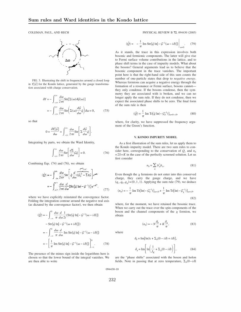
Sum rules and Ward identities in the Kondo lattice
Y = − −i
id
2iStrG
= − −i
id
2iStr
dG
dq = 0, 75
so that
0 =YG
=
−i
id
2iStr
dG
dq .
Integrating by parts, we obtain the Ward Identity,
−i
id
2iStrd
dGq = 0. 76
Combining Eqs. 74 and 76, we obtain
77
where we have explicitly reinstated the convergence factor.Folding the integration contour around the negative real axisas dictated by the convergence factor, we then obtain
Q = − −
0d
d
d
1
2iStrq ln− G−1 − i
− Strq ln− G−1 + i
= − −
0d
d
dIm Strq ln− G−1 − i
= − 1
Im Strq ln− G−1 − i
−
0
. 78
The presence of the minus sign inside the logarithms here ischosen so that the lower bound of the integral vanishes. Weare then able to write
Q = −1
Im Strq ln− G−1 − i
=0
. 79
As it stands, the trace in this expression involves bothbosonic and fermionic components. The latter will give riseto Fermi surface volume contributions in the lattice, and tophase shift terms in the case of impurity models. What aboutthe bosons? General arguments lead us to believe that thebosonic component in the trace vanishes. The importantpoint here is that the right-hand side of this sum counts thenumber of one-particle states that drop to negative energy.Whereas fermions can acquire a negative energy through theformation of a resonance or Fermi surface, bosons cannot—they only condense. If the bosons condense, then the sym-metry they are associated with is broken, and we can nolonger apply the sum rule. If they do not condense, then weexpect the associated phase shifts to be zero. The final formof the sum rule is then
Q =1
Im Trq ln− GF
−1=0−i, 80
where, for clarity, we have suppressed the frequency argu-ment of the Green’s function.
V. KONDO IMPURITY MODEL
As a first illustration of the sum rules, let us apply them tothe Kondo impurity model. There are two sum rules to con-sider here, corresponding to the conservation of Qc and nb
=2S=K in the case of the perfectly screened solution. Let usfirst consider
nb =
b†b. 81
Even though the fermions do not enter into this conservedcharge, they carry the gauge charge, and we haveqc ,qb ,q= 0,1 ,1. Applying the sum rule 79, we deduce
nb = −1
Im Trln− Gb
−1=i +1
Im Trln− G
−1=i,
82
where, for the moment, we have retained the bosonic trace.When we carry out the trace over the spin components of theboson and the channel components of the fermion, weobtain
nb = − Nb
+ K
, 83
where
b = Imln + b0 − i + i ,
= Imln 1
JK
+ 0 − i , 84
are the “phase shifts” associated with the boson and holonfields. Note in passing that at zero temperature, b0− i
FIG. 3. Illustrating the shift in frequencies around a closed loop
in YG for the Kondo lattice, generated by the gauge transforma-
tion associated with charge conservation.
COLEMAN, PAUL, AND RECH PHYSICAL REVIEW B 72, 094430 2005
094430-10
232

Publication 3
and 0− i are purely real. The argument of the logarithm
in b is the renormalized chemical potential *=+b0 of
the boson field. In the “filled shell” configuration 2S=K, theformation of a perfectly screened Kondo singlet generates agap for the addition of extra Schwinger bosons to the groundstate, which forces *0, and b=0, as argued previously. Itfollows that
nb = K
. 85
But nb=K is part of the constraint, so it follows that =.This result can be understood by relating to the sign of therenormalized Kondo coupling constant, as follows:
=
1
Imln 1
JK
+ 0 − i = − JK* . 86
In this way, we see that = corresponds to a residual“ferromagnetic” coupling. This is consistent with ourexpectations, for when an additional Schwinger boson isadded to the Fermi liquid, it increases the impurity spin byone-half unit to form an underscreened Kondo model, wherethe residual spin coupling is indeed ferromagnetic. By con-trast, in an antiferromagnet or spin liquid, the local momentsspins pair condense, mutually screening one another. In thissituation, an additional Schwinger boson at any one site willnow be free to undergo a Kondo effect with the conductionelectrons, so the residual spin coupling is antiferromagnetic.These results are also confirmed in the large-N limit.
Let us now turn to the sum rule derived from the conser-vation of electron charge. Here the conserved quantity is
Qe = k,,
ck,,
†ck,,, 87
and the corresponding gauge charges are qc ,qb ,q= 1,0 ,
−1, so the sum rule becomes
Qe =1
Im Trln− Gc
−1 −1
Im Trln− G
−1 =0−i
.
88
Now in an impurity model, it is convenient to subtract off thetotal charge in the absence of the impurity, given by
Qe0 =
1
Im Trln− Gc0
−1=0−i, 89
where Gc0Gc
0is the noninteracting propagator of the con-
duction electrons. If we subtract this from 88, we can com-bine the conduction electron traces and replace ln−Gc
−1−ln−Gc0
−1=lnGc0Gc−1=ln1−Gc0c. The change in total
charge is then given by
Qe − Qe0 =
1
Im Trln1 − Gc0c=−i
−1
Im Trln− G
−1=−i. 90
According to the Anderson-Clogston compensation theorem,the total change in electron charge due to a Kondo or Ander-
son impurity vanishes in the infinite bandwidth limit, and atfinite bandwidth the change is of the order of the ratio of theKondo temperature to the bandwidth Qc=OTK /D, and
can be neglected.34,35 Setting Qe=Qe−Qe0=0, we obtain
Qe = 0 = NKc
− K
, 91
where we have identified
c = Im Trkln1 − Gc0c=−i, 92
where the trace is purely over momenta. If we expand thelogarithm using a power series, we see that the trace overinternal momenta in 92 is accomplished by replacing the
momentum-dependent Green’s function Gc
0k , by the lo-
cal electron Green’s function g0=kGc0k ,, so that
c = Im ln1 − g0=0−i. 93
In the large bandwidth limit, g0− i→ i, where is the
density of states per spin per channel, so that
c = Im ln1 − i0 . 94
There is thus a direct link between the phase shift of the fermion and that of the conduction electrons. Combining thiswith the earlier result =, we obtain
c =
N=
N. 95
Notice the following.i In the large-N limit, the phase shift identity permits us
to relate the conduction electron phase shift c, which isO1/N to the phase shift , which is finite in the large N
limit. In this way, the sum rules enable us to study the phaseshift and Fermi surface volume changes of the Kondo impu-rity and lattice, in the large-N limit.
ii The development of the conduction electron phaseshift does not occur because conduction electron states dropbeneath the Fermi sea: It is a consequence of the injection ofnew quasiparticle states into the Fermi sea as a response tothe formation of spinless, charged holons.
VI. SUM RULE FOR THE KONDO LATTICE
When we come to consider the Kondo lattice, there are anumber of additional subtleties that must be entertained. Oneof the most important aspects of the discussion here concernsthe possibility that the extremal solutions to FG break the
U1 symmetry of the bosons, to produce “Higg’s” phase in
which the Schwinger bosons either pair condense, or hybrid-ize between sites. In the large-N solutions to the model, thesephases appear to develop as a precursor to the formation ofthe antiferromagnet, where the bosons themselves condense.The main effect on the sum rules is twofold:
i We cannot assume that the fermion is localized. Thisimplies that we must consider the momentum dependence ofthe fermion.
ii Once the Schwinger bosons pair condense, the Wardidentities associated with the conservation of nb no longer
SUM RULES AND WARD IDENTITIES IN THE KONDO… PHYSICAL REVIEW B 72, 094430 2005
094430-11
233

Sum rules and Ward identities in the Kondo lattice
apply, because the Luttinger–Ward functional YG is no
longer invariant under shifts of the boson frequency.However, we can still take advantage of the Ward identity
associated with charge conservation. Provided that theSchwinger boson is uncondensed, i.e., there is no magnetism,then charge conservation guarantees that
−i
id
2iTrFd
dGq = 0 qc = 1,q = − 1 . 96
Now in the paramagnet, the holon and conduction electronfields are unmixed, so we can replace
TrF → Trc + Tr.
This is a special property of the paramagnet. By contrast, inthe antiferromagnet, the Schwinger bosons are condensed, sothe holon and conduction electron fields admix, and both and G contain off-diagonal terms so that TrF remains asingle, integral trace over the two admixed fields.
For the paramagnet, we can write
0 = − −i
id
2iStrd
dGq qc = 1,q = − 1
= −i
id
2iTrdc
dGc −
−i
id
2iTrd
dG
= K−i
id
2i dDk
2DNdck,
dGck,
−dk,
dGk, . 97
It is this identity that permits us to extend the Luttinger sumrule to the case of the paramagnetic Kondo lattice. In theparamagnetic Kondo lattice, the charge sum rule
Qe =1
Im Trln− Gc
−1 − Im Trln− G−1=0−i,
98
now involves a trace over momentum:
Qe
K= N
k
1
Im lnk + ck,0 − i + i
− k
1
Im ln 1
JK
+ k,0 − i . 99
The first term in this expression is the electron Fermi surfacevolume,
k
1
Im lnk + ck,0 − i + i =
k
− Ek =vFS
2D,
100
where the region where Ek =k +Re ck ,Ek is negative, de-
fines the interior of the Fermi surface. The second term canbe interpreted in a similar way—the momentum trace overthe logarithm of G
−1,
k
1
Im ln 1
JK
+ k,0 − i = k
− JK* k =
v
2D,
101
can be seen as the volume of the region in momentum space
where the effective interaction JK* k=−Gk ,0−1 is nega-
tive, or ferromagnetic. Following our earlier discussion, theferromagnetic sign of the residual interaction is a conse-quence of the fact that additional spins added to the statecompletely decouple from the Fermi sea. In the simplest sce-
nario, JK* k0 for all k, in which case v / 2D=1, and the
sum rule becomes
ne =Qe
K= N
vFS
2D− 1, 102
where ne is the electron density per unit cell, per conductionelectron channel. It follows that the total Fermi surface vol-ume expands by one unit per unit cell,
NvFS
2D= ne + 1. 103
Now if there is some region of momentum space where
JK* k is not ferromagnetic, it follows that the fermions will
have a Fermi surface, and the excitation spectrum will nowinvolve charged, spinless fermions. In this phase,
ne =Qe
K= N
vFS*
2D−
v
2D. 104
Such a “spin-charge decoupled” phase could not developfrom a Fermi liquid without a phase transition. As long as theheavy electron fluid does not undergo such a phase transi-tion, the Fermi surface must remain large.
Let us now consider what happens in the antiferromagnet.In the general higher-dimensional case, the boson field con-denses, causing the conduction and fields to hybridize toproduce a single species. In the antiferromagnet, it is morelogical to make a particle-hole transformation of the field,
writing k =−k†
. In this case, q=qc have the same charge,
and the sum rule becomes simply
Qe = 1
Im TrFln− GF
−1=−i
, 105
where GF is the admixed propagator for the combined con-duction and fields. The right-hand side cannot be separatedinto and conduction parts, and, as such, defines an admixedset of Fermi surfaces, with an average Fermi surface volumethat counts the total charge per unit cell,
ne = NvAFM2D
. 106
The Fermi surface volume for the antiferromagnet and theparamagnet must then differ by 1/Nth of a unit cell. In thespecial case of N=2, if the spatial unit cell doubles, thisformal change in Fermi surface volume is indistinguishablefrom the new size of the Brillouin zone. However, even inthis case, we can imagine more general classes of antiferro-
COLEMAN, PAUL, AND RECH PHYSICAL REVIEW B 72, 094430 2005
094430-12
234

Publication 3
magnet, such as an incommensurate helimagnet, where theunit cell size is unchanged, but the total Fermi surface vol-ume must jump.
VII. SPIN-CHARGE SEPARATION AND QUANTUM
CRITICALITY
Although the sum rules do not provide us with any detailsof the dynamics, they provide stringent constraints on theway the spectrum of excitations can evolve in the Kondolattice as we approach the magnetic quantum critical point.
One of the fascinating aspects of our sum rule,
ne = NvFS
2D−
v
2D, 107
is that it suggests that a Kondo lattice may develop low-lying, spinless charged fermionic excitations near a quantumcritical point. This is clearly a controversial idea, the conse-quences of which we now explore in this discussion. If wetake this idea seriously, then two important points seem toemerge.
i In the heavy Fermi liquid, spinons have “ionized” intoelectrons and a background filled sea of holons,
b ↔ e− + + 108
It is this ionization process that lies behind the expansion ofthe Fermi surface and the sum rule.
ii There is an intimate link between the Kondo interac-tion and the formation of holons. The link between thepropagator of the holons and the renormalized Kondo inter-action,
− Gq , =1
1
JK
+ q ,= JK
* q , , 109
implies that poles in the holon spectrum correspond to diver-gences in the Kondo interaction. As magnetism drives theKondo interaction back to weak coupling, we expect J*q ,to pass through infinity, so the holons should become gaplessat some point in this process.
We can, in fact, use the Luttinger–Ward approach to gaininsight into the low-energy thermodynamics of the Kondolattice.3 Provided the replacement of frequency sums by con-tinuous integrals is valid at low-temperatures, Luttinger ar-gued that the low-energy thermodynamics is determined bythe leading logarithm in the free energy functional 4, evalu-ated with the zero-temperature Green’s function. In our case,this leads to the relation
FT T Strln− G0−1 T → 0 ,
where G0 is the zero temperature Green’s function. Carrying
out the frequency integrals, this implies that the low-temperature entropy is given by
110
where the zero-temperature propagators are to be used. Thelast term in this expression provides the T-linear entropy ofthe Fermi liquid; the first two terms are the “spinon” and“holon” contributions. For a Landau Fermi liquid to form,these last terms must clearly be gapped at low temperatures.This feature is observed in the large-N solutions.26 What italso makes clear, however, is that the holons cannot becomegapless without a thermodynamic departure from Fermi liq-uid behavior, which implies some kind of quantum phasetransition.
However, even though the holons are gapped in the Fermiliquid, they can exist as low-lying spinless, charged excita-tions. It is particularly interesting to speculate that the gap toholon formation closes at a quantum critical point. This is apossibility that can be studied in the large-N limit, but thegeneral arguments should hold at finite N, as long as the
Luttinger–Ward approach is valid. One way to go beyond thelarge-N limit is to carry out a fully self-consistent treatmentof the leading Luttinger–Ward free energy functional, updat-ing the conduction electron self-energy and feeding the fullconduction electron Green’s functions into the calculation ofthe self-energy for the and Schwinger boson field. Such anapproximation goes selectively beyond the large-N limit, butit will satisfy the Ward identities. Moreover, assuming thatthe “filled shell” stability of the fully screened ground state isnot an artifact of the large-N limit, we also expect the gap inthe Schwinger boson and the fermion particle spectrum tobe preserved at finite N.
Another way to check the picture emerging from this ap-proach would be to examine low-dimensional systems. Vari-ous authors have examined the possibility of a transitionfrom a small to large Fermi surface in the one-dimensional
SUM RULES AND WARD IDENTITIES IN THE KONDO… PHYSICAL REVIEW B 72, 094430 2005
094430-13
235

Sum rules and Ward identities in the Kondo lattice
spin-1 /2 Kondo lattice.36,37 The difficulty with this model isthat the gaplessness of the Heisenberg spin-1 /2 chain tendsto make the Kondo coupling relevant, no matter how smallthe Kondo temperature. A model that avoids these difficultiesis the S=1, two-channel Kondo lattice. This model involves
a Haldane spin-1 chain coupled via Kondo interactions totwo, one-dimensional, noninteracting Hubbard models, asshown in Fig. 4.
When the Kondo interaction is weak, the Haldane chain isgapped, and the “Fermi surface” of the Kondo lattice issmall, giving rise to Friedel oscillations at wave vector Q
=2kF
0. When the Kondo interaction is strong, a Kondo lat-
tice with a large Fermi surface is expected to form where
Q=2kF
0+. The way these two phases are linked is particu-
larly interesting. If they are linked by a single quantum criti-cal point, then we expect Q to simply jump at this point Fig.4b. However, if the holons form a gapless phase, then overan intermediate range of parameters, we would expect theFriedel oscillations to exhibit an intermediate wave vectorFig. 4c,
Q = 2kF0 + x . 111
ACKNOWLEDGMENTS
We are grateful to Mathew Fisher, Kevin Ingersent, An-dreas Ludwig, Catherine Pépin, and Gergely Zarand for dis-cussions related to this work. This research was supported bythe National Science Foundation Grants No. NSF DMR0312495 and No. PHY99-07949. The authors are thankfulfor the hospitality of the KITP, where most of this researchwas carried out.
1 J. M. Luttinger, Phys. Rev. 119, 1153 1960.2 J. M. Luttinger and J. C. Ward, Phys. Rev. 118, 1417 1960.3 J. M. Luttinger, Phys. Rev. 121, 1251 1961.4 J. Friedel, Philos. Mag. 43, 153 1952.5 J. S. Langer and V. Ambegaokar, Phys. Rev. 121, 1090 1961.6 D. C. Langreth, Phys. Rev. 150, 516 1966.7 A. A. Abrikosov, Physics Long Island City, N.Y. 2, 5 1964.8 H. Suhl, Phys. Rev. 138, A515 1965.9 G. Gruner and A. Zawadowski, in Progress in Low Temperature
Physics, edited by D. F. Brewer North-Holland, Amsterdam,
1978, Vol. VIIB, p. 591.10 R. M. Martin, Phys. Rev. Lett. 48, 362 1982.11 B. I. Shraiman and E. D. Siggia, Phys. Rev. Lett. 62, 1564
1989.12 B. L. Altshuler, A. V. Chubukov, A. Dashevskii A, A. M.
Finkel’stein, and D. K. Morr, Europhys. Lett. 41, 401 1998.13 P. Coleman, C. Pépin, Q. Si, and R. Ramazashvili, J. Phys.: Con-
dens. Matter 13, R723 2001.14 T. Senthil, M. Vojta, and S. Sachdev, Phys. Rev. B 69, 035111
2004.15 C. Pépin, Phys. Rev. Lett. 94, 066402 2005.16 S. Kawarazaki et al., Phys. Rev. B 61, 4167 2000.17 S. Paschen, T. Lühmann, S. Wirth, P. Gegenwart, O. Trovarelli,
Ch. Geibel, F. Steglich, P. Coleman, and Q. Si, Nature London432, 881 2004.
18 M. Oshikawa, M. Yamanaka, and I. Affleck, Phys. Rev. Lett. 78,
1984 1997.19 M. Oshikawa, Phys. Rev. Lett. 84, 3370 2000.20 G. M. Eliashberg, Zh. Eksp. Teor. Fiz. 43, 1005 1962 Sov.
Phys. JETP 16, 780 1963.21 J.-P. Blaizot, E. Iancu, and A. Rebhan, Phys. Rev. D 63, 065003
2001.22 G. M. Carneiro and C. J. Pethick, Phys. Rev. B 11, 1106 1975.23 G. Baym and L. P. Kadanoff, Phys. Rev. 124, 287 1961; G.
Baym, ibid. 127, 1391 1962.24 O. Parcollet and A. Georges, Phys. Rev. Lett. 79, 4665 1997.25 S. Powell, S. Sachdev, and H. P. Buchler, cond-mat/0502299 un-
published.26 J. Rech, P. Coleman, O. Parcollet, and G. Zarand, cond-mat/
0507001 unpublished.27 P. Coleman and C. Pépin, Phys. Rev. B 68, 220405 2003.28 P. Coleman and I. Paul, Phys. Rev. B 70, 035111 2004.29 P. W. Anderson and Z. Zou, Phys. Rev. Lett. 60, 132 1988.30 To avoid the ambiguities of unit cells, it is important here that the
Q vector does not have certain values. For a helimagnet, for
example, we must avoid the commensurate case where Q
= /N , /N , /N, where N=2 is the parameter for an SP 2Ngeneralization.
31 M. Potthoff, cond-mat/0406671 unpublished.32 J. Rammer and H. Smith, Rev. Mod. Phys. 58, 323 1986.33 A. Kamenev, cond-mat/0412296 unpublished.34 A. M. Clogston and P. W. Anderson, Bull. Am. Phys. Soc. 6, 124
1961.35 For a detailed discussion of this point, see Appendix A in P. Cole-
man and I. Paul, Phys. Rev. B 70, 035111 2004.36 J. C. Xavier, E. Novais, and E. Miranda, Phys. Rev. B 65, 214406
2002.37 E. Pivovarov and Q. Si, cond-mat/0304129 unpublished.
FIG. 4. a The two-channel, spin S=1 Kondo chain. b In the
simplest scenario, the transition from a Haldane chain with a small
Fermi surface, to the heavy electron phase with a large Fermi sur-
face will occur via a single phase transition. c The sum rules allow
for an intermediate phase with a Fermi surface that lies between
these two extremes.
COLEMAN, PAUL, AND RECH PHYSICAL REVIEW B 72, 094430 2005
094430-14
236

PUBLICATION 4
Schwinger-boson approach to thefully screened Kondo model
Phys. Rev. Lett., 96, 016601 (2006)

Schwinger-boson approach to the fully screened Kondo model
238

Publication 4
Schwinger Boson Approach to the Fully Screened Kondo Model
J. Rech,1,2,3 P. Coleman,1,2 G. Zarand,1,4 and O. Parcollet3
1Kavli Institute for Theoretical Physics, Kohn Hall, University of California at Santa Barbara, Santa Barbara, California 93106, USA2Center for Materials Theory, Rutgers University, Piscataway, New Jersey 08855, USA
3Service de Physique Theorique, CEA/DSM/SPhT-CNRS/SPM/URA 2306, CEA/Saclay, F-91191 Gif-sur-Yvette Cedex, France4Theoretical Physics Department, Budapest University of Technology and Economics, Budafoki ut 8. H-1521 Hungary
(Received 6 July 2005; published 9 January 2006)
We apply the Schwinger boson scheme to the fully screened Kondo model and generalize the method toinclude antiferromagnetic interactions between ions. Our approach captures the Kondo crossover fromlocal moment behavior to a Fermi liquid with a nontrivial Wilson ratio. When applied to the two-impuritymodel, the mean-field theory describes the ‘‘Varma-Jones’’ quantum phase transition between a valencebond state and a heavy Fermi liquid.
DOI: 10.1103/PhysRevLett.96.016601 PACS numbers: 72.15.Qm, 71.27.+a, 73.43.Nq, 75.20.Hr
Heavy fermion metals have attracted great interest as anarena for the controlled study of magnetic quantum phasetransitions [1]. Several recent observations cannot beunderstood in terms of the established Moriya-Hertz theoryof quantum phase transitions [2– 4], including the diver-gence of the heavy electron masses [5], the near linearity ofthe resistivity [6–9], and E=T scaling in inelastic neutronspectra [10]. The origins of this failure are thought to belinked to the competition between antiferromagnetism andthe screening of local moments via the Kondo effect. Itremains an unsolved challenge to discover the appropriatemean-field description and the corresponding quantumcritical modes which govern these novel quantum phasetransitions [1,11–13].
Large-N methods offer a promising route towards thisgoal. Historically, these methods played a major role in thetheory of classical criticality [14], and more recently, in thetheory of heavy fermion metals [15,16]. However, progresson quantum phase transitions has been hindered by ourinability to capture both the Kondo effect and antiferro-magnetism in the leading large N approximation.
In this Letter, we describe new progress towards thisgoal using Schwinger’s boson representation of spins [17].Unlike traditional fermionic representations of spin [15,16]the Schwinger boson scheme provides a good descriptionof local moment magnetism [17]. However, efforts to gen-eralize this method to the Kondo problem [18,19] havefailed to capture the Fermi liquid physics associated withperfect screening of the moment. Here we solve this prob-lem using a method coinvented by one of us (O. P.) [18]which employs a multichannel Kondo model with Kscreening channels. By tuning the size of the spin S fromS < K=2 to S > K=2, one can describe both the over-screened and underscreened Kondo models. Difficultieswere encountered in past work that appeared to excludetreatment of the perfectly screened case, 2S K. We showhow these difficulties are overcome to reveal the perfectlyscreened Fermi liquid and we demonstrate how thismethod captures the competition with antiferromagnetismin its simplest extension to the two-impurity Kondo model.
We begin with the single impurity Kondo model,
H X
~k;;
~kcy~kc ~k HI nb 2S;
HI JKN
X
y b
yb:
(1)
In this version of the model, cy~k creates a conduction
electron of momentum ~k, channel index 2 1; K, spin
index 2 j; j, where N 2j 1 is even. y
1N s
p P
~kcy~k
creates an electron in the Wannier state at
the origin, where N s is the number of sites in the lattice.
The operator by creates a Schwinger boson (‘‘spinon’’)with spin index 2 j; j. The local spin operator is
represented by S byb =N and the system
is restricted to the physical Hilbert space by requiring
nb P
byb 2S. The final term in H contains a
temperature-dependent chemical potential T that imple-ments the constraint hnbi 2S. We will examine the fullyscreened case 2S K, taking the limit N ! 1 with k K=N fixed.
The first step is to factorize the interaction in terms ofauxiliary spinless fermion fields (‘‘holons’’), ,
HI !X
1
Np y
by H:c:
X
yJK
: (2)
Following the steps outlined by us in earlier work [20], wenow write the free energy as a Luttinger-Ward [21] func-tional of the one particle Green’s functions,
FG TStr lnG1 G10 G1G YG; (3)
where Str A Tr AB Tr AF is the graded (super)trace over the Matsubara frequencies, internal quantumnumbers of the bosonic (B) and fermionic (F) componentsof A. G0 is the bare propagator and G Diag Gb; G; Gc,the fully dressed propagator, where
PRL 96, 016601 (2006)P H Y S I C A L R E V I E W L E T T E R S week ending
13 JANUARY 2006
0031-9007=06=96(1)=016601(4)$23.00 016601-1 2006 The American Physical Society
239

Schwinger-boson approach to the fully screened Kondo model
Gbin in bin10 ;
Gi!n J1K i!n10 ;
Gci!n G1c0 i!n ci!n100 :
(4)
i!n G10 G1 denotes the corresponding self-
energies. Gc0i!n P
~k1=i!n ~k is the bare conduc-
tion electron Green’s function. The quantity YG is thesum of all closed-loop two-particle irreducible skeletonFeynman diagrams. In the large N limit, we take theleading ON contribution to Y (Fig. 1).
The variation of Y with respect to G generates the self-energy Y=G , which yields c 1
NG
Gb. Since c is of order ON1 we use the bareconduction propagatorGc0 in the self-consistent equations,
GbGc0; b kGGc0:(5)
In practice, we solve these equations using a real timerepresentation of the Green’s functions. [See, for example,[19]].
The original work in [18,22] focused primarily on theoverscreened Kondo model, where K > 2S. The perfectlyscreened case presented two difficulties. First, the require-ment that K 2S appeared extremely stringent, the slight-est deviation from this condition leading to singulardepartures from Fermi liquid behavior at low temperatures.Second, the conduction electron phase shift c is =N,suggesting that the effect of the Kondo resonance wouldcompletely vanish in the large N limit.
Two new observations shed new light on this problem.First, the perfectly screened case is a stable ‘‘filled shell’’singlet configuration of the spins, which at strong couplingcorrespond to ‘‘rectangular’’ Young tableau representa-tions of SUN. [23,24]. In our gauge theory descriptionof the Kondo model, this stability manifests itself throughthe formation of a gap in the spinon and holon spectrum.When the chemical potential, , lies within this gap, theground-state Schwinger boson occupancy locks into thevalue nb K 2S (Fig. 2). Moreover, the gap removesthe effect of the spinons and holons at low energies toreveal a Fermi liquid.
Second, although the conduction phase shift c is =N,its effect on the thermodynamics is multiplied by the N
spin components and the K scattering channels, producingan order ON K=N ON contribution to the freeenergy. Moreover, a Ward identity c =N, where
Im ln1 JK0 i is the (finite) holon phase
shift [19,20] enables us to compute the conduction electronscattering in the large N limit.
In the large N limit the entropy [20] is given by
STN
Z d!
dnB!dT
Im lnG1b G0
b00b
kdnF!dT
Im lnG1 G0
00 G00
c0~0c
;
(6)
where frequency labels ! are suppressed in the integrand,nB=F denote the Bose-Fermi functions, and
~c!Nc!Z d
1
2nF
G00Gb!
1
2nB
G00bG
!
(7)
is the rescaled conduction self-energy. The shortened no-tation G! G! i has been used. We can alsocalculate the local magnetic susceptibility
locT 2NZ d!
1
2 nB!
G0b!G00
b!; (8)
where we have taken the magnetic moment of the local
impurity to be M P
sgn byb. Note in passing thatthe dynamic counterpart hStS0i vanishes exponentiallydue to the gap in the bosonic spectral functions, the 1=t2
term characteristic of a Fermi liquid only appearing at thenext order in 1=N.
We have numerically solved the self-consistent equa-tions for the self-energy by iteration, imposing theconstraint at each temperature. Figure 3 shows the
temperature-dependent specific heat coefficient CVT dS
dT
and the full magnetic susceptibility T. There is a smoothcrossover from local moment behavior at high tempera-tures nb1 nb=T to Fermi liquid behavior at lowtemperatures. From a Nozieres-Blandin description of thelocal Fermi liquid [25] (where channel and charge suscep-
FIG. 1. Leading contributions to YG in 1=N expansion.Solid, dashed, and wavy lines, respectively, represent Gc, G,
and Gb. Each vertex is associated with a factor i=
Np
. Bracketedterms are dropped in the large N limit.
FIG. 2. (a) Calculated variation of occupancy as a functional ofboson chemical potential in the ground state for k 0:3 andT=TK 0:005. (b) A spinon gap develops in the fully screenedstate.
PRL 96, 016601 (2006)P H Y S I C A L R E V I E W L E T T E R S week ending
13 JANUARY 2006
016601-2
240
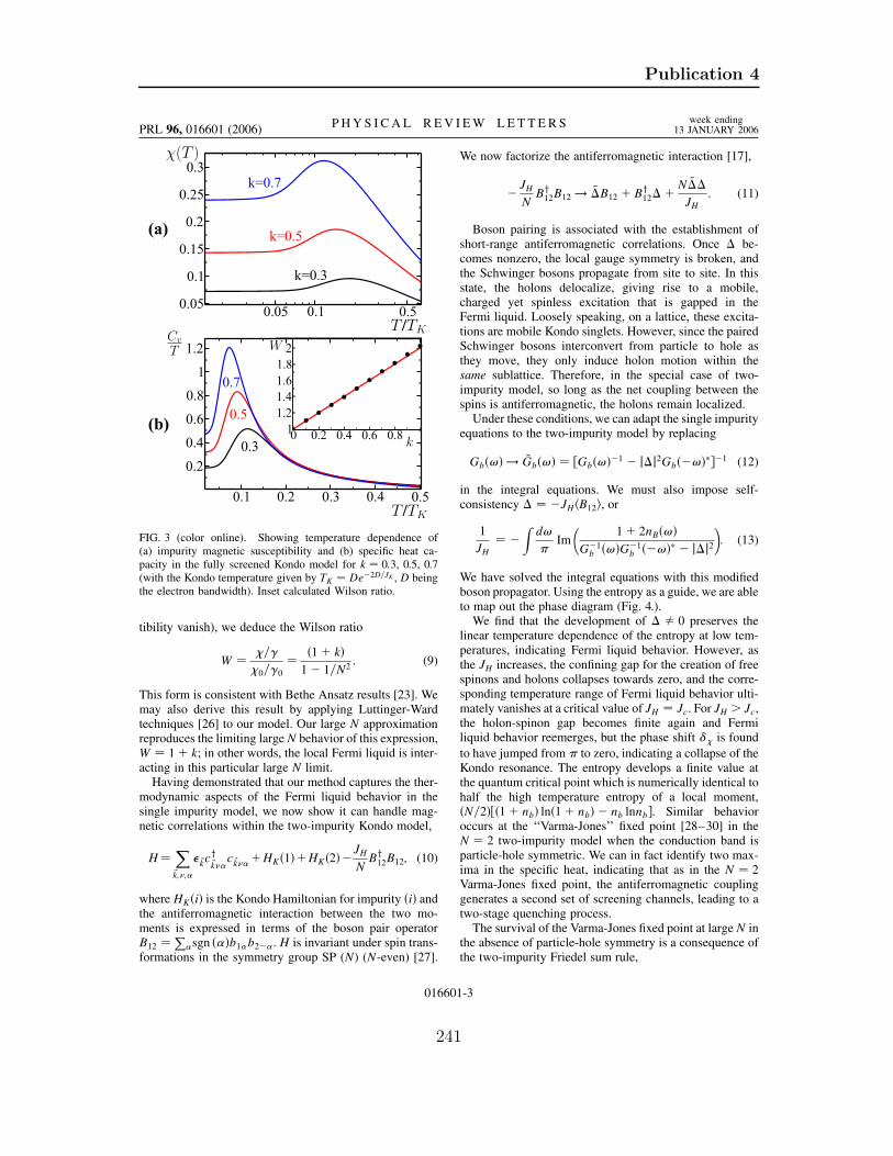
Publication 4
tibility vanish), we deduce the Wilson ratio
W =
0=0
1 k1 1=N2
: (9)
This form is consistent with Bethe Ansatz results [23]. Wemay also derive this result by applying Luttinger-Wardtechniques [26] to our model. Our large N approximationreproduces the limiting largeN behavior of this expression,W 1 k; in other words, the local Fermi liquid is inter-acting in this particular large N limit.
Having demonstrated that our method captures the ther-modynamic aspects of the Fermi liquid behavior in thesingle impurity model, we now show it can handle mag-netic correlations within the two-impurity Kondo model,
HX
~k;;
~kcy~kc ~kHK1HK2
JHNBy12B12; (10)
where HKi is the Kondo Hamiltonian for impurity i andthe antiferromagnetic interaction between the two mo-ments is expressed in terms of the boson pair operatorB12
P
sgn b1b2. H is invariant under spin trans-formations in the symmetry group SP (N) (N-even) [27].
We now factorize the antiferromagnetic interaction [17],
JHNBy12B12 ! B12 By
12 N
JH: (11)
Boson pairing is associated with the establishment ofshort-range antiferromagnetic correlations. Once be-comes nonzero, the local gauge symmetry is broken, andthe Schwinger bosons propagate from site to site. In thisstate, the holons delocalize, giving rise to a mobile,charged yet spinless excitation that is gapped in theFermi liquid. Loosely speaking, on a lattice, these excita-tions are mobile Kondo singlets. However, since the pairedSchwinger bosons interconvert from particle to hole asthey move, they only induce holon motion within thesame sublattice. Therefore, in the special case of two-impurity model, so long as the net coupling between thespins is antiferromagnetic, the holons remain localized.
Under these conditions, we can adapt the single impurityequations to the two-impurity model by replacing
Gb! ! ~Gb! Gb!1 jj2Gb!1 (12)
in the integral equations. We must also impose self-consistency JHhB12i, or
1
JH
Z d!
Im
1 2nB!
G1b !G1
b ! jj2
: (13)
We have solved the integral equations with this modifiedboson propagator. Using the entropy as a guide, we are ableto map out the phase diagram (Fig. 4.).
We find that the development of 0 preserves thelinear temperature dependence of the entropy at low tem-peratures, indicating Fermi liquid behavior. However, asthe JH increases, the confining gap for the creation of freespinons and holons collapses towards zero, and the corre-sponding temperature range of Fermi liquid behavior ulti-mately vanishes at a critical value of JH Jc. For JH > Jc,the holon-spinon gap becomes finite again and Fermiliquid behavior reemerges, but the phase shift is found
to have jumped from to zero, indicating a collapse of theKondo resonance. The entropy develops a finite value atthe quantum critical point which is numerically identical tohalf the high temperature entropy of a local moment,N=21 nb ln1 nb nb lnnb. Similar behavioroccurs at the ‘‘Varma-Jones’’ fixed point [28–30] in theN 2 two-impurity model when the conduction band isparticle-hole symmetric. We can in fact identify two max-ima in the specific heat, indicating that as in the N 2Varma-Jones fixed point, the antiferromagnetic couplinggenerates a second set of screening channels, leading to atwo-stage quenching process.
The survival of the Varma-Jones fixed point at large N inthe absence of particle-hole symmetry is a consequence ofthe two-impurity Friedel sum rule,
FIG. 3 (color online). Showing temperature dependence of(a) impurity magnetic susceptibility and (b) specific heat ca-pacity in the fully screened Kondo model for k 0:3, 0.5, 0.7(with the Kondo temperature given by TK De2D=JK , D beingthe electron bandwidth). Inset calculated Wilson ratio.
PRL 96, 016601 (2006)P H Y S I C A L R E V I E W L E T T E R S week ending
13 JANUARY 2006
016601-3
241

Schwinger-boson approach to the fully screened Kondo model
2
N; (14)
where are the even and odd parity scattering phaseshifts. For N 2, it is possible to cross smoothly fromunitary scattering off both impurities (
2 ), to no
scattering off either ( , 0) while preservingthe sum rule, but forN > 2, the sum rule cannot be satisfiedin the absence of scattering, and the collapse of the Kondoeffect must occur via a critical point.
In conclusion, we have shown that a Schwinger bosonapproach to the fully screened Kondo model can be natu-rally extended to incorporate magnetic interactions. In thesimplest case of a two-impurity Kondo model our approachcaptures the transition between the state where the twoimpurities are antiferromagnetically correlated and theKondo Fermi liquid state. In the large N limit, these twostates are separated by a quantum critical point, a possibleprecursor of an antiferromagnetic quantum critical point.One of the interesting new elements is the appearance ofmobile, yet gapped ‘‘holon’’ excitations in the antiferro-magnetically correlated Fermi liquid. In the two-impuritymodel these holons become gapless at the quantum criticalpoint. Future work will examine whether this same sce-nario also operates at a heavy electron quantum criticalpoint, leading to quantum critical matter with spin-chargedecoupling [1,13].
We are grateful to Matthew Fisher, Kevin Ingersent,Andreas Ludwig, and Catherine Pepin for discussionsrelated to this work. This research was supported by theNational Science Foundation Grants No. DMR-0312495,No. INT-0130446, and No. PHY99-07949, and theHungarian National Science Foundation GrantNo. OTKA T46303. J. R. and O. P. are supported by anACI grant of the French Ministry of Research. The authorswould like to thank the hospitality of the KITP, where partof this research was carried out.
[1] P. Coleman, C. Pepin, Q. Si, and R. Ramazashvili, J. Phys.Condens. Matter 13, R723 (2001).
[2] T. Moriya and J. Kawabata, J. Phys. Soc. Jpn. 34, 639(1973); 35, 669 (1973).
[3] J. A. Hertz, Phys. Rev. B 14, 1165 (1976).[4] A. J. Millis, Phys. Rev. B 48, 7183 (1993).[5] J. Custers et al., Nature (London) 424, 524 (2003).[6] H. v. Lohneysen et al., Phys. Rev. Lett. 72, 3262 (1994).[7] N. Mathur et al., Nature (London) 394, 39 (1998).[8] M. Grosche et al., J. Phys. Condens. Matter 12, L533
(2000).[9] O. Trovarelli et al., Phys. Rev. Lett. 85, 626 (2000).
[10] A. Schroeder et al., Nature (London) 407, 351 (2000).[11] Q. Si, S. Rabello, K. Ingersent, and J. L. Smith, Nature
(London) 413, 804 (2001).[12] T. Senthil, S. Sachdev, and M. Vojta, Physica (Amsterdam)
359-361B, 9 (2005).[13] C. Pepin, Phys. Rev. Lett. 94, 066402 (2005).[14] K. G. Wilson, Phys. Rev. D 7, 2911 (1973).[15] N. Read and D. M. Newns, J. Phys. C 16, 3273 (1983).[16] A. Auerbach and K. Levin, Phys. Rev. Lett. 57, 877
(1986).[17] D. P. Arovas and A. Auerbach, Phys. Rev. B 38, 316
(1988).[18] O. Parcollet and A. Georges, Phys. Rev. Lett. 79, 4665
(1997); O. Parcollet, A. Georges, G. Kotliar, and A.Sengupta, Phys. Rev. B 58, 3794 (1998).
[19] P. Coleman and I. Paul, Phys. Rev. B 71, 035111 (2005).[20] P. Coleman, I. Paul, and J. Rech, Phys. Rev. B 72, 094430
(2005).[21] J. M. Luttinger and J. C. Ward, Phys. Rev. 118, 1417
(1960).[22] O. Parcollet, Ph.D. thesis, 1998, http://www-spht.cea.fr/
pisp/parcollet/ (unpublished).[23] A. Jerez, N. Andrei, and G. Zarand, Phys. Rev. B 58, 3814
(1998).[24] N. Andrei and P. Zinn Justin, Nucl. Phys. B528, 648
(1998).[25] P. Nozieres and A. Blandin, J. Phys. (France) 41, 193
(1980).[26] A. Yoshimori, Prog. Theor. Phys. 55, 67 (1976).[27] N. Read and S. Sachdev, Phys. Rev. Lett. 66, 1773 (1991).[28] B. A. Jones and C. M. Varma, Phys. Rev. Lett. 58, 843
(1987).[29] B. A. Jones, B. G. Kotliar, and A. J. Millis, Phys. Rev. B
39, 3415 (1989).[30] J. Gan, Phys. Rev. Lett. 74, 2583 (1995).
FIG. 4 (color online). Phase diagram for the two-impurityKondo model showing the boundary where boson pairing devel-ops. Color coded contours delineate the entropy around theVarma-Jones fixed point. Black line indicates upper maximumin specific heat, blue line, lower maximum in specific heat wherecrossover into the Fermi liquid takes place. Inset: (a) entropy forvarious values of TK=JH, (b) showing dependence of on
TK=JH at a temperature T=TK 0:02.
PRL 96, 016601 (2006)P H Y S I C A L R E V I E W L E T T E R S week ending
13 JANUARY 2006
016601-4
242

PUBLICATION 5
Conserving many-body approachto the U →∞ Anderson model
cond-mat/0601015

Conserving many-body approach to the U →∞ Anderson model
244

Publication 5
Conserving many body approach to the fully screened, infinite U Anderson model.
Eran Lebanon1, Jerome Rech1,2, P. Coleman1 and Olivier Parcollet21 Center for Materials Theory, Serin Physics Laboratory,
Rutgers University, Piscataway, New Jersey 08854-8019, USA.2 Service de Physique Theorique, CEA/DSM/SPhT - CNRS/SPM/URA
2306 CEA/Saclay, F-91191 Gif-sur-Yvette Cedex, FRANCE
Using a Luttinger Ward scheme for interacting gauge particles, we present a conserving manybody treatment of a family of fully screened infinite U Anderson models that has a smooth cross-over into the Fermi liquid state, with a finite scattering phase shift at zero temperature and aWilson ratio greater than one. We illustrate our method, computing the temperature dependenceof the thermodynamics, resistivity and electron dephasing rate and discuss its future application tonon-equilibrium quantum dots and quantum critical mixed valent systems.
PACS numbers: 73.23.-b, 72.15.Qm, 72.10.Fk
The infinite U Anderson model is a central element inthe theory of heavy electron systems and quantum dots.This model describes a high temperature regime of in-coherent valence and spin fluctuations, separated by acrossover from a low temperature Fermi liquid. Over theyears since it was first solved by the numerical renormal-ization group[1] and Bethe Ansatz[2], there have beenmany attempts to develop alternative diagrammatic ap-proaches with the flexibility to extend to the lattice or tonon-equilibrium situations. Examples include the largeN slave boson approach [3, 4], the non-crossing approx-imation (NCA)[5] and various vertex-corrected versionsof this same model[6]. However, none of these schemesto date is able to capture the smooth cross-over into awell-developed Fermi liquid. In this paper, we present anew diagramatic solution to this long-standing problem.
The root of these difficulties is traced back to the infi-nite U constraint which introduces gauge particles, suchas the slave boson, which carry fractional charge or spin.The challenge then, is to find a consistent and prac-tical scheme by which these particles disappear in thelow-energy Fermi liquid. One approach is to condensethe slave boson, but this replaces the cross-over into theFermi liquid with a fictitious phase transition[3, 4]. Inthe NCA and its various diagrammatic descendants, thepresence of gapless gauge particles prevents the devel-opment of a Kondo resonance which properly satisfiesthe Friedel sum rule[5, 6]. In this paper we extend arecent Schwinger boson description of the Kondo modelto encompass the valence fluctuations of the infinite UAnderson model and we show how the past difficultiesare removed through the development of a gap in theSchwinger boson and slave fermion spectrum. A new ele-ment of the current work, is the use of a Kadanoff Baymscheme that enables us to approximately treat the An-derson model with a finite spin degeneracy N = 2j + 1,while preserving a list of exact conserving relations whichdevelop in the the Fermi liquid. Our method is scalableto a lattice, and can also be extended to non-equilibriumsettings. To demonstrate the method we compute the
temperature dependent thermodynamics, resistivity andelectron dephasing rate in a single impurity model, anddiscuss how the method can be extended to encompass anon-equilibrium environment.
Our starting point is a Schwinger boson representationfor the SU(N) infinite U Anderson model. Schwingerbosons can be used to describe magnetically ordered localmoments, and in the limit of large N , this descriptionbecomes exact[7]. Recent progress [8, 9] has shown howthis scheme can be expanded to encompass the Fermiliquid physics of the Kondo effect. through the study ofa family of “multichannel” Kondo models, in which thenumber of channels K is commensurate with nb = 2S,(K = 2S), where S is the spin of the local moment.By reinstating the valence fluctuations to this model, weobtain the following infinite U Anderson model
H =∑
~kνα
ǫ~kc†~kναc~kνα +
V√N
∑
~kνα
[
c†~kναχ†
νbα + H.c]
+ ǫ0∑
α
b†αbα − λ(Q− 2S). (1)
Here c†~kναcreates a conduction electron with momentum
~k, channel index ν ∈ [1, K], and spin index α ∈ [1, N ].The bilinear product b†αχν between a Schwinger bosonb†α, and a slave fermion (or holon) operator χν creates alocalized electron in the constrained Hilbert space, whichhybridizes with the conduction electrons. The
√N de-
nominator in the hybridization ensures a well-definedlarge N limit. The energy of a singly occupied impu-rity ǫ0 is taken to be negative. The conserved operatorQ =
∑
α b†αbα +∑
ν χ†νχν replaces the no-double occu-
pancy constraint of the infinite U Anderson model, whereQ = 2S = K is required for perfect screening.
The characteristic “Kondo scale” of our model is
TK = D
(Γ
πD
)K/N
exp
−π|ǫ0|Γ
, (2)
where D is the conduction electron half bandwidth, Γ =πρV 2 is the hybridization width and ρ is the conduction
245

Conserving many-body approach to the U →∞ Anderson model
2
electron density of states. The Kondo temperature is de-termined from the high temperature scaling and the pref-actor derives from third order terms in the beta functionthat are finite in the multi-channel large N limit whereK/N = k is fixed. Notice however, that the coefficientrelating low temperature properties, such as the specificheat coefficient γ = a(1/N, k)/TK to the Kondo temper-ature, will in general exhibit non-trivial N dependence.
The next step is to construct the LW functional Y [G].The variation of Y [G] with respect to the full Green’sfunctions Gζ of the conduction, Schwinger boson andslave fermion fields, Σζ = δY/δGζ , self-consistently de-termines the self-energies Σζ of these fields[10, 11]. Y [G]is equal to the sum of all two-particle irreducible freeenergy Feynman diagrams, grouped in powers of 1/N[Fig.1(a)]. In our KB approximation we neglect all butthe leading order O(N) term in the LW functional, andthen impose the full self-consistency generated by thisfunctional. Unlike earlier NCA approaches, the con-straint is implemented order by order in 1/N , by in-cluding fluctuations in the chemical constraint λ. Bytaking the leading order KB approximation we neglectthe fluctuations in the gauge field λ, and concentrateon the properties in the grand canonical ensemble wherethe constraint is imposed on the average. The explicitexpressions for the self-energies are then
Σχ(τ) = V 2Gb(τ)Gc(−τ)
Σb(τ) = −(K/N)V 2Gχ(τ)Gc(τ)
Σc(τ) = (1/N) V 2Gb(τ)Gχ(−τ) (3)
where Gb, Gχ and Gc are the fully dressed imaginarytime Green’s functions of the boson, holon and conduc-tion electrons respectively. Equations (3) are solved selfconsistently, adjusting the chemical potential λ to satisfythe averaged constraint 〈Q〉 = K.
A key step in the derivation of the Ward identities isthe presence of an infrared cutoff in the excitation spec-trum, which permits us to replace Matsubara summa-tions by integrals at low temperatures:
T∑
iωn
→∫
dω
2π
This transformation is the key to derivations of theFriedel sum rule, the Yamada-Yosida and Shiba rela-tionships between susceptibilities, specific heat and spinrelaxation rates[12–14]. Past attempts to develop con-serving approximations to the infinite U Anderson model[15] have run into X-ray singularities in the slave particlespectrum which prevent the above replacement. In themulti-channel approach, the formation of a stable Kondosinglet when 2S = K yields a gap in the spinon andholon spectrum [Fig. 1(c)] which stablizes the Fermi liq-uid at sub-gap energies. This feature permits all of themanipulations previously carried out on the finite U An-derson model to now be extended to infinite U . Each of
+ ... + ... + ...
0.1 0.2 0.31/N
0
0.1
0.2
0.3
0.4
δ c/π
−1 0 1ε/TK
|ImG
b|
+ + +Y[G] =
O(1/N)O(1)O(N)
(a)
(c)(b)
FIG. 1: (a)LW functional expanded in powers of 1/N . Solidline - Schwinger bosons, dashed lines - holons, double lines -conduction electrons. Loops contribute a factor N , vertices afactor 1/
√N . (b) Phase shift extracted from the t-matrix, for
K = 1, nχ ≈ 0.04. Solid line: (K − nχ)/(NK), dotted line,phase shift obtained without self-consistency on conductionlines, (c) Gapped Schwinger boson spectrum in ground-state.
these relationships are satisfied by the use of the leadingLW functional. The Friedel sum rule equates the sumof the electron phase shifts to the charge K − nχ on theimpurity, where nχ is the ground-state holon occupancy,
δc =π
N
K − nχ
K+ O
(TK
ND
)
, (4)
Fig.1(b) shows how the phase shift extracted from thet-matrix in our conserving scheme satisfies this relation.
According to Nozieres Fermi liquid theory[16], thequasiparticle spectrum in the Kondo ground-state is re-lated to the conduction electron phase shift. The changein the phase shift in an applied field, or change in chem-ical potential, is related to the spin, charge and chan-nel susceptibilities, which in turn, leads to a generalized“Yamada-Yosida-Yoshimori” identity[13, 17] describingthe distribution of the NK degrees of freedom amongthe spin, flavor and charge susceptibilities:
NKγ
γ0= K
N2 − 1
N + K
χs
χ0s
+ NK2 − 1
K + N
χf
χ0f
+χc
χ0c
. (5)
Here γ stands for the specific heat coefficient γ = C/T ,and χs, χf and χc stand for the spin, flavor and chargesusceptibilities. χ0
s,f,c denotes the corresponding suscep-tibilities in the absence of the impurity. Our identity (5)reduces to the known results for the Wilson ratio in theone channel model[13] and the Kondo limit[18]. By pre-serving the Friedel sum rule in each channel, our methodautomatically satisfies this relationship.
Various thermodynamic quantities can be extractedfrom the numerical solution of the self-consistent equa-tions. Following [11], the entropy S(T ) is given by
S = −Trζ
∫
dǫdnζ
dT
[
Imln(−G−1
ζ
)+ G′
ζΣ′′ζ
]
, (6)
where the trace denotes a sum over the spin and channelindices of the various fields and nζ is the distribution
246

Publication 5
3
0.1 1 10 100 1000T/TK
0
1
TK χ
0
1
2S
imp
0 0.05 0.10
0.2
0.4
FIG. 2: (a)temperature dependence of impurity entropy Simp.showing linear temperature dependence at low temperature.(b)magnetic susceptibility of impurity vs temperature, calcu-lated for K=1, N=4 (See Fig. 3 ).
function (Fermi for ζ = c, χ and Bose for ζ = b). Gζ
and Σζ respectively denote the retarded Green functionsand self energies. The single and double primes markthe real and imaginary part respectively. The impuritycontribution to the entropy Simp = S − S0, where S0
is the entropy of the bare conduction band, is shown inFig. 2. The linear behavior of the impurity contributionto the entropy at low temperatures marks the saturationof the specific heat coefficient γimp = ∂Simp/∂T and theformation of a local Fermi liquid.
To calculate the spin susceptibility, we couple a smallmagnetic field to the magnetization, defined as
M =∑
α
sgn(α− N + 1
2)
(
b†αbα +∑
~k,ν
c†~kναc~kνα
)
.
The impurity magnetization is obtained by subtractingfrom M the free conduction sea contribution. We com-pute the magnetization by iterating the solutions to self-consistency in a small magnetic field[19]. Fig. (2) showsthe impurity susceptibility χ(T ), which is peaked slightlybelow TK and saturates to a constant in the ground-state.
One of the important conservation laws associated withthe conservation of spin is the Korringa Shiba relation be-tween the dynamic and static spin susceptibility. On theassumption that the gauge particles are gapped, the LWderivation carried out by Shiba on the finite U Ander-son model, can be simply generalized to the infinite Umodel, to obtain χ′′(ω)/ω|ω=0 = (Nπ/K)(χ/N)2. Thisrelationship guarantees that the power-spectrum of themagnetization is linear at low frequencies, ensuring thatthe spin response function decays as 1/t2 in time. Re-markably, a Fermi liquid, with slow gapless spin excita-tions is sandwiched beneath the spinon-holon continuum.
We now turn to a discussion of the electron scatter-ing off the impurity, which is determined by the conduc-tion electron t-matrix, t(z) = Σc
1−G(0)c Σc
, where G0c(z) =
−0.4 −0.2 0ε/D
0
0.05
0.1
0.15
−π
ρ Im
t(ε
+iη
)
−0.005 0 0.0050
0.5
1
FIG. 3: t-matrix for ǫ0/D = −0.2783, Γ/D = 0.16, N = 4and K = 1 (TK/D = 0.002). Main frame: T/D=0.1, 0.08,0.06, 0.04, 0.02, and 0.01. Inset: T/10−4D=10, 8, 6, 4, 2, 1,and 0.5. The dot marks sin2π(K − nχ)/NK
∑
~k(z− ǫ~k)−1 is the bare local conduction electron prop-agator. Various important physical properties, such asthe impurity resistivity and the electron dephasing ratein the dilute limit can be related to this quantity. Fig. 3shows the imaginary part of t(ǫ + iη): as temperature islowered towards TK , a resonance peak develops aroundthe Fermi energy. The peak ultimately saturates abouta decade below the Kondo temperature and the heightof the fully developed resonance at the Fermi energy cor-responds to that predicted by the Langreth sum-rule[12]value −sin2δc/πρ, as shown in Fig.3.
The impurity contribution to the resistivity Ri is re-lated to a thermal average of the t− matrix,
Ri
RU= ni
[∫
dǫ
(
−∂f
∂ǫ
)
|πρImt(ǫ + iη)|−1
]−1
. (7)
where RU is the unitary resistivity of the electron gas andf is the Fermi function. The resistivity (Fig. 4) saturatesat low temperatures at the value niRU sin2 δc.
As a final application of the t-matrix, we compute theelectron dephasing rate τ−1
φ that controls the field depen-dence of weak electron localization. In the cross-over tothe Fermi liquid state, the formation of the Kondo reso-nance gives rise to a peak in the inelastic scattering[20]and electron dephasing rate [21]. In the dilute limit, theimpurity contribution to the dephasing rate is given byτ−1φ = 2ni[−Imt − πρ|t|2] [20, 22, 23]. Fig. 4 shows the
computed temperature dependence of the dephasing rateon the Fermi surface.
Our calculation of the dephasing rate captures thecross-over into the coherent Fermi liquid, but thequadratic temperature dependence of the electron de-phasing rate expected at low temperatures is absent fromthe current work. This is because the electron-electronscattering diagrams responsible for the Fermi-liquid con-tribution to the dephasing rate involve an internal loopof gauge particles which first appears in the subleading
247

Conserving many-body approach to the U →∞ Anderson model
4
10−2
10−1
100
101
102
103
T/TK
0
0.1
0.2
0.3
R 2
e2 ρ(0)
k F
2 / 3m
2 n i
0
0.1
0.2
τ φ−1 π
ρ(0)
/ n i
FIG. 4: The impurity contribution to the resistivity Ri anddephasing rate τ−1
φ as a function of temperature. Solid lines:the parameters used in Fig. 3, dashed lines: Γ = 0.1D.
O(1) terms of the LW functional shown in Fig. 1(a). Wehope to include the effects of these diagrams in futurework by approximating these scattering vertices by theirground-state, on-shell value, which is rigorously relatedto γ by Ward identities [13].
An interesting direction for future development is theextension to non-equilibrium quantum dots[24]. Cal-culations of the Kondo physics of voltage biased quan-tum dots are currently based Keldysh extensions of non-crossing integral equations [25] which do not capture theFermi liquid physics at low voltage bias. These methodscan be readily adapted to the current Schwinger bosonscheme[26]. Many features of our approach, its conserv-ing properties, the inclusion of scaling properties up tothird order in the beta function and its systematic in-corporation of spin relaxation effects on the boson lines,suggest that this will be a robust method to examine howspin and electron dephasing effects evolve with voltage inquantum dots. These methods can also be used to studythe voltage dependence [27] of the distribution functionand noise in magnetically doped mesoscopic wires[28, 29].
One of the striking features of the Schwinger boson ap-proach to the Kondo and infinite U Anderson models, isthe co-existence of a gapless Fermi liquid, sandwiched atlow energies between a gapped spinon and holon fluid,arising as a consequence of the development of bound-states within this fluid. The methods presented here canbe scaled up to the Anderson and Kondo lattice models,where the Friedel sum rule “upgrades” into the Luttingersum rule[11]. Here, the local U(1) symmetry is brokendown to a global one by the pair-condensed Schwingerbosons[30] and the spinons and holons become propagat-ing excitations of the bulk, whose gap is fundamental tothe large Fermi surface. It is this very gap that we ex-pect to collapse at a quantum critical point. The currentwork, which includes the effects of valence fluctuations,provides a powerful framework for exploring this physics.
This work was supported by DOE grant number DE-FE02-00ER45790 and an ACI grant of the French Min-
istry of Research. We are grateful to Natan Andrei andGergely Zarand for discussions related to this work.
[1] K.G. Wilson, Rev. Mod. Phys. 47, 773 (1975).[2] For a review see A. Tsvelik and P.B. Wiegmann, Adv. in
Phys. 32, 453 (1983).[3] A.J. Millis and P.A. Lee, Phys. Rev. B 35, 3394 (1987).[4] P. Coleman, Phys. Rev. B 29, 3035 (1984).[5] N.E. Bickers, Rev. Mod. Phys. 59, 845 (1987).[6] K. Haule et al., Phys. Rev. B 64 155111 (2001)[7] D.P. Arovas, and A. Auerbach, Phys. Rev. B 38, 316
(1988).[8] O. Parcollet, and A. Georges, Phys. Rev. Lett. 79, 4665
(1997).[9] J. Rech, P. Coleman, G. Zarand, and O. Parcollet,Phys.
Rev. Lett. 96, 016601 (2006).[10] J.-P. Blaizot, E. Iancu and A. Rebhan Phys. Rev. D 63,
065003 (2001).[11] P. Coleman, I. Paul, and J. Rech, Phys. Rev. B 72,
094430 (2005).[12] D.C. Langreth, Phys. Rev. 150, 516 (1966).[13] K. Yamada, Prog. Theor. Phys. 53, 970 (1975); K.
Yoshida and K. Yamada, ibid. 53, 1286 (1975).[14] H. Shiba, Prog. Theo. Phys 54, 967 (1975).[15] Y. Kuramoto, Z. Phys. B 53, 37 (1983); P. Coleman,
Phys. Rev. B 28, 5255 (1983); N.E. Bickers, Rev. Mod.Phys. 59, 845 (1987); K. Haule et al., Phys. Rev. B 64,155111 (2001).
[16] P. Nozieres and A. Blandin, J. Physique, 41, 193, 1980.[17] A. Yoshimori, Prog. Theor. Phys 55, 67 (1976).[18] A. Jerez, N. Andrei, and G. Zarand, Phys. Rev. B 58,
3814, (1998).[19] E. Lebanon, A. Schiller, and V. Zevin, Phys. Rev. B 64,
245338 (2001).[20] G. Zarand, L. Borda, J.v. Delft and N. Andrei, Phys.
Rev. Lett. 93, 107204 (2004).[21] C. Van Haesendonck et al., Phys. Rev. Lett. 58, 1968
(1987); R.P. Peters et al., Phys. Rev. Lett. 58, 1964(1987); F.J. Ohkawa, et al., J. Phys. Soc. Jpn. 52, 1701(1983).
[22] T. Micklitz, A. Altland, T.A. Costi, and A. Rosch, cond-mat/0509583 (2005).
[23] C. Bauerle et. al. Phys. Rev. Lett. 95, 266805 (2005).[24] L. Kouwenhoven and L. Glazman, Physics World, 14 33
(2001).[25] N. S. Wingreen and Y. Meir Phys. Rev. B 49, 11040
(1994); P. Nordlander et al.,Phys. Rev. Lett. 83, 808(1999).
[26] A. Posazhennikova, and P. Coleman, Phys. Rev. Lett.94, 036802 (2005).
[27] E. Lebanon, and P. Coleman, Phys. Rev. Lett. 95, 046803(2005).
[28] H. Pothier et al., Phys. Rev. Lett. 79, 3490 (1997); A.Kaminski and L. I. Glazman, Phys. Rev. Lett. 86, 2400(2001); G. Goppert and H. Grabert, Phys. Rev. B 64,033301 (2001).
[29] J. Kroha and A. Zawadowski, Phys. Rev. Lett. 88,176803 (2002).
[30] M. Hermele et al, Phys. Rev. B 70, 214437 (2004).
248

Appendices
249


APPENDIX A
Generalized Luttinger-Wardscheme: free energy and entropy
Contents
A.1 Free energy . . . . . . . . . . . . . . . . . . . . . . . . . . . 251
A.2 Entropy . . . . . . . . . . . . . . . . . . . . . . . . . . . . . 254
In this appendix, we derive the free energy functional and the entropy for a singleimpurity using a Luttinger-Ward picture. The same kind of derivation extends tothe Kondo lattice model and is presented in details in the Publication 3.
A.1 Free energy
The idea of the demonstration is to define a functional of the Green’s functions andto prove that this definition matches the one of the free energy.
The full propagators of the theory are given by the following Dyson’s equations:
G−1b (iνn) = iνn + λ− Σb(iνn) (A.1)
G−1χ (iωn) = JK − Σχ(iωn) (A.2)
G−1c (iωn) = G−1
c0 (iωn)− Σc(iωn) (A.3)
Following Luttinger and Ward, we will regard Gb,c,χ as a variational function,and Σb,c,χ as a derived quantity.
251

Generalized Luttinger-Ward scheme: free energy and entropy
We now consider the effect of tuning up the strength of the Kondo interactionfrom zero to JK , by replacing JK → αJK where α ∈ [0, 1], keeping the chemicalpotential of the conduction electrons and bosons fixed. Now the partition functionis given by
Z = Tr[e−βH] =
∫
D[c, b, χ]e−R β0
Ldτ (A.4)
where D[c, b, χ] is the measure of the path integral. If we vary α inside this expres-sion, we obtain
dZ
dα=
∫
D[c, b, χ]∑
ν
∫ β
0
dτ(JKχ
†νχν)e−
R β0
Ldτ
= βZ × JK∑
ν
〈χ†
νχν〉 (A.5)
so that if F = −T lnZ is the free energy, then
dF
dα= −JK
∑
ν
〈χ†νχjν〉 = −KJKT
∑
n
Gχ(iωn), (A.6)
We next consider the expression
F = NT∑
n
log(−G−1b (iνn))−KT
∑
n
log(−G−1χ (iωn))
−NKT∑
n
log(−G−1c (iωn)) +NT
∑
n
Σb(iνn)Gb(iνn)
−KT∑
n
Σχ(iωn)Gχ(iωn)−NKT∑
n
Σc(iωn)Gc(iωn)
+Np0λ+ ΦLW [Gb, Gχ, Gc] (A.7)
where ΦLW [Gb, Gχ, Gc] is given by the sum of all closed, two-particle irreducibleskeleton Feynman graphs for the Free energy.
As mentioned earlier, the Luttinger Ward functional ΦLW [Gb, Gχ, Gc] has theproperty that its variation with respect to Gb,c,χ generates the self energies,
δΦLW [Gb, Gχ, Gc] = −N∫
dτΣb(τ)δGb(β − τ)−K∫
dτΣχ(τ)δGχ(β − τ)
−NK∫
dτΣc(τ)δGc(β − τ) (A.8)
The variation of the log term in F with respect to Gb,c,χ is given by
δ
(
T∑
n
log(−G−1(iωn))
)
= −T∑
n
G−1(iωn)δG(iωn) (A.9)
252

A.1. Free energy
By using the relation Σ[G] = G−10 −G−1, the variation in the remaining terms in F
is given by
δ
(
T∑
n
Σ(iωn)G(iωn)
)
= T∑
n
G−10 (iωn)δG(iωn) (A.10)
Combining these variations with the one of the Luttinger-Ward functional, onesees that the variations of F with respect to the Green’s functions identically vanish:
δF
δGb
=δF
δGc
=δF
δGχ
= 0. (A.11)
Now the Hubbard Stratonovich transformation that we have carried out on theoriginal Hamiltonian to decouple the Kondo interaction assures that the only placethat the coupling constant αJK enters, is in [G0
χ]−1 = αJK . This means that in the
r.h.s of Eq. (A.7) α enters explicitly only through Σχ = αJK −G−1χ . Then,
dF
dα=
δF
δGb,c,χ︸ ︷︷ ︸
=0
∂Gb,c,χ
∂α+∂F
∂α
= −KJKT∑
n
Gχ(iωn) (A.12)
But by comparison with (A.6), we see that dFdα
= dFdα
and since, F (α = 0) = F (α = 0)in the non-interacting case, the two quantities must be equal for all α, i.e
F = NT∑
n
log(−G−1b (iνn))−KT
∑
n
log(−G−1χ (iωn))
−NKT∑
n
log(−G−1c (iωn)) +NT
∑
n
Σb(iνn)Gb(iνn)
−KT∑
n
Σχ(iωn)Gχ(iωn)−NKT∑
n
Σc(iωn)Gc(iωn)
+Np0λ+ ΦLW [Gb, Gχ, Gc] (A.13)
There are various points to make about this derivation:
• The derivation is very general. Its correctness only depends on the stationarityof F [G] with respect to variations in G and the equivalence between dF/dαand dF/dα.
• The above Free energy functional can be used as a basis for developing con-serving approximations that generalize the Kadanoff Baym approach to a con-strained system[111].
253

Generalized Luttinger-Ward scheme: free energy and entropy
A.2 Entropy
We know from the derivation of the self-energy equations from the Luttinger-Ward
functional that Σc ∼ O
(1
N
)
. It then becomes possible to expand the electronic
Dyson’s equation in powers of 1/N , which in turn leads to the following simplificationin the free energy functional:
−NKT∑
n
log(−G−1c (iωn)) = −NKT
∑
n
log(−G−1c0 (iωn))
+NKT∑
n
Σc(iωn)Gc0(iωn)
−NKT∑
n
Σc(iωn)Gc(iωn) = −NKT∑
n
Σc(iωn)Gc0(iωn)
Combining these two terms, we are left with a term of order N2 that correspondsto the free energy of the free electronic gas. Subtracting this bulk free energy fromthe one we are considering, we are left with the impurity contribution to the freeenergy, which one can write in terms of retarded Green’s functions as:
Fimp
N=
∫dω
πn(ω)Im
(log(−G−1
b (ω)) +Gb(ω)Σb(ω))
+γ
∫dω
πf(ω)Im
(log(−G−1
χ (ω)) +Gχ(ω)Σχ(ω))
+p0λ+1
NΦLW [Gb, Gχ, Gc0] (A.14)
Using the stationarity of the free energy with respect to the Green’s functionsand the chemical potential, one can directly read from (A.14) the expression for theimpurity contribution to the entropy:
Simp
N= −
∫dω
π
∂n(ω)
∂TIm(log(−G−1
b (ω)) +Gb(ω)Σb(ω))
−γ∫dω
π
∂f(ω)
∂TIm(log(−G−1
χ (ω)) +Gχ(ω)Σχ(ω))
− 1
N
∂ΦLW
∂T(A.15)
One now has to work a little on the expression of the Luttinger-Ward functionalin order to extract a closed form expression for its temperature derivative. First ofall, we saw in Chapter 6 that only the leading order diagram of ΦLW survives oncewe take the large-N limit, so that the Luttinger-Ward functional writes:
ΦLW [Gb, Gχ, Gc] = KJ2
∫
dτGc(τ)Gb(β − τ)Gχ(β − τ) (A.16)
254
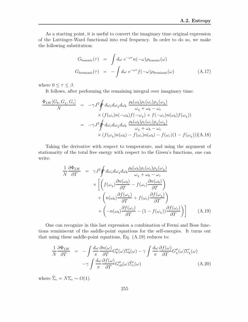
A.2. Entropy
As a starting point, it is useful to convert the imaginary time original expressionof the Luttinger-Ward functional into real frequency. In order to do so, we makethe following substitution:
Gbosonic(τ) =
∫
dω e−ωτn(−ω)ρbosonic(ω)
Gfermionic(τ) = −∫
dω e−ωτf(−ω)ρfermionic(ω) (A.17)
where 0 ≤ τ ≤ β.
It follows, after performing the remaining integral over imaginary time:
ΦLW [Gb, Gχ, Gc]
N= −γJ2
P
∫
dωcdωχdωbρb(ωb)ρc(ωc)ρχ(ωχ)
ωχ + ωb − ωc× (f(ωc)n(−ωb)f(−ωχ) + f(−ωc)n(ωb)f(ωχ))
= −γJ2P
∫
dωcdωχdωbρb(ωb)ρc(ωc)ρχ(ωχ)
ωχ + ωb − ωc× (f(ωχ)n(ωb)− f(ωc)n(ωb)− f(ωc)(1− f(ωχ)))(A.18)
Taking the derivative with respect to temperature, and using the argument ofstationarity of the total free energy with respect to the Green’s functions, one canwrite:
1
N
∂ΦLW
∂T= γJ2
P
∫
dωcdωχdωbρb(ωb)ρc(ωc)ρχ(ωχ)
ωχ + ωb − ωc×[(
f(ωχ)∂n(ωb)
∂T− f(ωc)
∂n(ωb)
∂T
)
+
(
n(ωb)∂f(ωχ)
∂T+ f(ωc)
∂f(ωχ)
∂T
)
+
(
−n(ωb)∂f(ωc)
∂T− (1− f(ωχ))
∂f(ωc)
∂T
)]
(A.19)
One can recognize in this last expression a combination of Fermi and Bose func-tions reminiscent of the saddle-point equations for the self-energies. It turns outthat using these saddle-point equations, Eq. (A.19) reduces to:
1
N
∂ΦLW
∂T= −
∫dω
π
∂n(ω)
∂TG′′b (ω)Σ′
b(ω)− γ∫dω
π
∂f(ω)
∂TG′′χ(ω)Σ′
χ(ω)
−γ∫dω
π
∂f(ω)
∂TG′′c0(ω)Σ′
c(ω) (A.20)
where Σc = NΣc ∼ O(1).
255

Generalized Luttinger-Ward scheme: free energy and entropy
Plugging back the expression for ∂ΦLW
∂Tinto the impurity entropy, one sees that
it cancels some of terms from the first part of the expression. The final entropyformula in the large-N limit then reads:
Simp
N= −
∫dω
π
[∂n(ω)
∂T
(Im log
(−G−1
b (ω))
+G′b(ω)Σ′′
b (ω))
+γ∂f(ω)
∂T
(
Im log(−G−1
χ (ω))
+G′χ(ω)Σ′′
χ(ω)−G′′c0(ω)Σ′
c(ω))]
(A.21)
As it turns out, a somewhat similar version of this entropy formula has been de-rived in the context of lattice gauge theory applied to Quantum Chromo-Dynamics,by Blaizot and collaborators [140]. The first attempts at deriving such a closed-form expression for the entropy trace back to the work of Carneiro and Pethick[141]. Note that, as we argue in Publication 3, this expression cannot be generalizedto any model and applies here because we retain only the lowest order diagram inthe Luttinger-Ward functional.
256
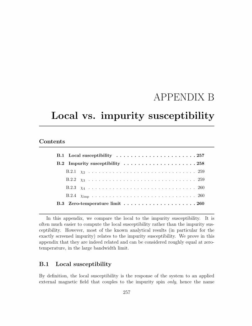
APPENDIX B
Local vs. impurity susceptibility
Contents
B.1 Local susceptibility . . . . . . . . . . . . . . . . . . . . . . 257
B.2 Impurity susceptibility . . . . . . . . . . . . . . . . . . . . 258
B.2.1 χ2 . . . . . . . . . . . . . . . . . . . . . . . . . . . . . . . 259
B.2.2 χ3 . . . . . . . . . . . . . . . . . . . . . . . . . . . . . . . 259
B.2.3 χ4 . . . . . . . . . . . . . . . . . . . . . . . . . . . . . . . 260
B.2.4 χimp . . . . . . . . . . . . . . . . . . . . . . . . . . . . . . 260
B.3 Zero-temperature limit . . . . . . . . . . . . . . . . . . . . 260
In this appendix, we compare the local to the impurity susceptibility. It isoften much easier to compute the local susceptibility rather than the impurity sus-ceptibility. However, most of the known analytical results (in particular for theexactly screened impurity) relates to the impurity susceptibility. We prove in thisappendix that they are indeed related and can be considered roughly equal at zero-temperature, in the large bandwidth limit.
B.1 Local susceptibility
By definition, the local susceptibility is the response of the system to an appliedexternal magnetic field that couples to the impurity spin only, hence the name
257
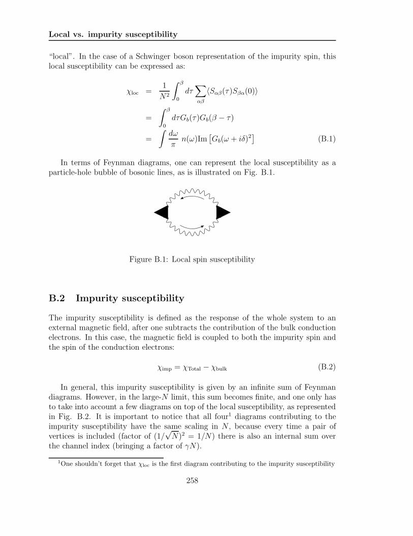
Local vs. impurity susceptibility
“local”. In the case of a Schwinger boson representation of the impurity spin, thislocal susceptibility can be expressed as:
χloc =1
N2
∫ β
0
dτ∑
αβ
〈Sαβ(τ)Sβα(0)〉
=
∫ β
0
dτGb(τ)Gb(β − τ)
=
∫dω
πn(ω)Im
[Gb(ω + iδ)2
](B.1)
In terms of Feynman diagrams, one can represent the local susceptibility as aparticle-hole bubble of bosonic lines, as is illustrated on Fig. B.1.
Figure B.1: Local spin susceptibility
B.2 Impurity susceptibility
The impurity susceptibility is defined as the response of the whole system to anexternal magnetic field, after one subtracts the contribution of the bulk conductionelectrons. In this case, the magnetic field is coupled to both the impurity spin andthe spin of the conduction electrons:
χimp = χTotal − χbulk (B.2)
In general, this impurity susceptibility is given by an infinite sum of Feynmandiagrams. However, in the large-N limit, this sum becomes finite, and one only hasto take into account a few diagrams on top of the local susceptibility, as representedin Fig. B.2. It is important to notice that all four1 diagrams contributing to theimpurity susceptibility have the same scaling in N , because every time a pair ofvertices is included (factor of (1/
√N)2 = 1/N) there is also an internal sum over
the channel index (bringing a factor of γN).
1One shouldn’t forget that χloc is the first diagram contributing to the impurity susceptibility
258
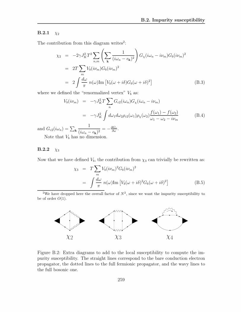
B.2. Impurity susceptibility
B.2.1 χ2
The contribution from this diagram writes2:
χ2 = −2γJ2KT
2∑
n,m
(∑
k
1
(iωn − ǫk)2
)
Gχ(iωn − iνm)Gb(iνm)2
= 2T∑
m
Vb(iνm)Gb(iνm)2
= 2
∫dω
πn(ω)Im
[Vb(ω + iδ)Gb(ω + iδ)2
](B.3)
where we defined the “renormalized vertex” Vb as:
Vb(iνm) = −γJ2KT∑
n
Gc2(iωn)Gχ(iωn − iνm)
= −γJ2K
∫
dω1dω2ρc2(ω1)ρχ(ω2)f(ω1)− f(ω2)
ω1 − ω2 − iνm(B.4)
and Gc2(iωn) =∑
k
1
(iωn − ǫk)2= −∂Gc
∂ω.
Note that Vb has no dimension.
B.2.2 χ3
Now that we have defined Vb, the contribution from χ3 can trivially be rewritten as:
χ3 = T∑
m
Vb(iνm)2Gb(iνm)2
=
∫dω
πn(ω)Im
[Vb(ω + iδ)2Gb(ω + iδ)2
](B.5)
2We have dropped here the overall factor of N2, since we want the impurity susceptibility tobe of order O(1).
χ2 χ3 χ4
Figure B.2: Extra diagrams to add to the local susceptibility to compute the im-purity susceptibility. The straight lines correspond to the bare conduction electronpropagator, the dotted lines to the full fermionic propagator, and the wavy lines tothe full bosonic one.
259

Local vs. impurity susceptibility
B.2.3 χ4
From the diagrammatic representation of χ4, one recognizes the fermionic self-energyΣc defined in Chapter 6. χ4 then writes:
χ4 = −2γNT∑
n
Gc3(iωn)Σc(iωn)
= −2γN
∫dω
πf(ω)Im [Gc3(ω + iδ)Σc(ω + iδ)] (B.6)
where Gc3(iωn) =∑
k
1
(iωn − ǫk)3= 1
2∂2Gc
∂ω2 .
Keep in mind that the conduction electron self-energy is of order O(1/N) so thatthe overall external factor ofN makes this contribution to the impurity susceptibilityof order O(1).
B.2.4 χimp
Putting everything together, one notices that the first three diagrams can be groupedinto a simple form, leading to the final result:
χimp =
∫dω
πn(ω)
[Gb(ω + iδ)2 (1 + Vb(ω + iδ))2]
+2γN
∫dω
πf(ω)Im [Gc3(ω + iδ)Σc(ω + iδ)] (B.7)
B.3 Zero-temperature limit
In the case of a flat band of conduction electron, one can readily compute Gc2 andGc3:
Gc0 = −iπρ0Θ(D2 − ω2)
Gc2 = iπρ0 (δ(ω +D)− δ(ω −D))
Gc3 =−iπ2ρ0 (δ′(ω +D)− δ′(ω −D)) (B.8)
where we considered the large bandwidth limit, for which one can dropped the realpart of Gc0 since it is O(ω/D) smaller than the imaginary part.
From these expressions, one can compute the “renormalized vertex” Vb in thezero-temperature limit:
Vb(ω + iδ) = γρ0J2K
[G′χ(−D)−G′
χ(D)]
(B.9)
260

B.3. Zero-temperature limit
In the large bandwidth limit, the zero-temperature self-energy of the χ−fermionreads:
Σχ(D) = −iπρ0J2Kp0
Σχ(−D) = −iπρ0J2K(1 + p0) (B.10)
Combining all these results, we can rewrite the zero-temperature impurity sus-ceptibility as:
χimp =
(
1 +π2γ(1 + 2p0)(ρoJ)3
[1 + (πρ0Jp0)2] [1 + (πρ0J(1 + p0))2]
)2
χloc+γNρ0dΣ′
c
dω
∣∣∣∣ω=−D
(B.11)
As a conclusion, one can see from this last expression that at zero temperature,in the large bandwidth limit, it is possible to identify the local and the impuritysusceptibility:
D ≫ TK =⇒ χloc ∼T→0
χimp (B.12)
261
Local vs. impurity susceptibility
262

APPENDIX C
Fermi liquid identities
Contents
C.1 Scattering phase shift . . . . . . . . . . . . . . . . . . . . . 263
C.2 Specific heat . . . . . . . . . . . . . . . . . . . . . . . . . . 264
C.3 Susceptibilities . . . . . . . . . . . . . . . . . . . . . . . . . 265
C.3.1 Charge susceptibility . . . . . . . . . . . . . . . . . . . . . 265
C.3.2 Spin susceptibility . . . . . . . . . . . . . . . . . . . . . . 265
C.3.3 Channel susceptibility . . . . . . . . . . . . . . . . . . . . 266
C.4 Results . . . . . . . . . . . . . . . . . . . . . . . . . . . . . . 266
In this appendix, we derive some of the important interrelationships betweenphysical variables of the Fermi liquid, namely the Yamada-Yosida-Yoshimori rela-tionship between spin, charge, flavor susceptibilities and specific heat [142, 143, 144].
Historically, this relationship was obtained from the analysis of a full perturba-tion theory. We present here a derivation similar in spirit to the one of Nozieres andBlandin [107].
C.1 Scattering phase shift
The two basic electron-electron vertices have the following structure:
Γ1 = c†
αµc†
βµ′cβµ′cαµ (C.1)
Γ2 = c†
βµc†
δµ′cγµ′cαµσαβ · σγδ (C.2)
263

Fermi liquid identities
where Γ1 and Γ2 are recast in terms of Feynman diagrams in Fig. C.1, and σαβ is agenerator of SU(N) verifying:
σαβ · σγδ = 2δαδδβγ −2
Nδαβδγδ (C.3)
The most general combination invariant under both spin and channel rotation isthen: ∑
αβµµ′
[
A c†
αµc†
βµ′cβµ′cαµ +B c†
βµc†
αµ′cβµ′cαµ
]
(C.4)
where we kept only the dominant terms in the large-N limit.Considering a small departure from the Fermi liquid fixed point, these interaction
terms are expected to be small, and can be treated within first order perturbationtheory leading to the following effective Hamiltonian:
Heff = 2∑
αβµµ′
[A (1− δαβδµµ′) +B (δαβ − δµµ′)] 〈nβµ′〉nαµ (C.5)
where nαµ = c†
αµcαµ is the number operator, and 〈nαµ〉 its expectation value.One can then determine the scattering phase shift of an incoming conduction
electron with quantum numbers α and µ as a function of the energy ǫ and the elec-tron distribution δ〈nαµ〉 measured from the ground-state. Using the above effectiveHamiltonian, it is possible to reduce the general expression of the phase shift as:
δαµ = δ0 + ǫδ′ +∑
βµ′
φαβψµµ′δ〈nαµ〉
= δ0 + ǫδ′ + φ1
∑
βµ′
(δµµ′ − δαβ) δ〈nβµ′〉+ φ2
∑
βµ′
(1− δαβδµµ′) δ〈nβµ′〉(C.6)
Following [126], the response of this phase shift to various field variations can berelated to the specific heat and the susceptibilities.
C.2 Specific heat
Upon increasing the temperature, the electron energy changes like:
ǫαµ = ǫ− δαµ(ǫ)
πρ0(C.7)
where the phase shift is only given by the first two terms, the change of populationδ〈n〉 due to an increase in temperature being zero.
This leads to the following change in the electronic density of states:
δρ = ρ0
[dǫ
dǫ− 1
]
=δ′
π(C.8)
264

C.3. Susceptibilities
α,µ
α,µ
β,µ
β,µ
’
’
σγδ
γ,µ
δ,µ
’
’
σαβ
a) b)
α,µ
β,µ
Figure C.1: Diagrammatic representation of the two basic electron-electron vertices:a) is the vertex already existing in the absence of the impurity (denoted as Γ1), andb) is the vertex related to the scattering off the impurity (defined as Γ2).
and hence a correction to the specific heat:
δCvCv
=δρ
ρ0=
δ′
πρ0(C.9)
C.3 Susceptibilities
C.3.1 Charge susceptibility
Upon a small change in the chemical potential of the conduction electron Λ, oneprobes the change of the charge susceptibility, which can be expressed in terms ofthe scattering phase shift as:
δχcχc
=1
πρ0
∆δαµ∆Λ
(C.10)
=1
πρ0[δ′ + ρ0φ1(N −K) + ρ0φ2(NK − 1)] (C.11)
where we have used that ǫ ∼ ∆Λ and δ〈n〉 ∼ ρ0∆Λ.
C.3.2 Spin susceptibility
In order to extract the spin susceptibility, one has to apply an external magneticfield that couples to the system: the change in the spin susceptibility is then relatedto the response of the phase shift to this magnetic field in the same fashion as (C.10).
A variation of this magnetic field leads to a change in the electron population〈nαµ〉 ∼ ρ0 Sgn(α− (N + 1)/2), leading to the following result:
δχsχs
=1
πρ0[δ′ − ρ0φ1K − ρ0φ2] (C.12)
265

Fermi liquid identities
C.3.3 Channel susceptibility
Consider now an equivalent of the magnetic field that couples to the channel flavor.The same analysis as before leads to the channel susceptibility:
δχfχf
=1
πρ0
[δ′ + ρ0φ1N − ρ0φ2] (C.13)
where we used that the change of electron population due to a variation of thechannel field is 〈nαµ〉 ∼ ρ0 Sgn(µ− (K + 1)/2).
C.4 Results
Combining (C.9), (C.11), (C.12) and (C.13), one can get rid of the variables δ′, φ1
and φ2 and obtain an expression relating the specific heat and the various suscepti-bilities:
NK(N +K)δCvCv
= K(N2 − 1)δχsχs
+N(K2 − 1)δχfχf
+ (N +K)δχcχc
(C.14)
This relationship extends the Yamada-Yosida-Yoshimori relationship to the general-ized SU(N)×SU(K) Kondo model, in the exactly screened case (in the other scalingregimes, one does not have a Fermi liquid at low temperature and the analysis a laNozieres is no longer valid).
In the case of a Kondo impurity, since the interaction conserves the number ofconduction electron and does not affect the channel index, one expects that δχc = 0and δχf = 0, so that (C.14) directly gives the Wilson ratio:
W =δχs/χsδCv/Cv
=N(N +K)
N2 − 1(C.15)
which recovers the result obtained from Bethe ansatz [116].Finally, in the large-N limit, this expression of the Wilson ratio reduces to:
W = 1 + γ (C.16)
266
APPENDIX D
QCP in the two-impurity model:low-energy analysis
Contents
D.1 Ansatz . . . . . . . . . . . . . . . . . . . . . . . . . . . . . . 267
D.2 Derivation . . . . . . . . . . . . . . . . . . . . . . . . . . . . 268
D.2.1 Bosonic parameters . . . . . . . . . . . . . . . . . . . . . 268
D.2.2 Fermionic parameters . . . . . . . . . . . . . . . . . . . . 269
D.2.3 Analysis of the self-consistent equations . . . . . . . . . . 270
D.3 General remarks . . . . . . . . . . . . . . . . . . . . . . . . 270
D.3.1 Causality . . . . . . . . . . . . . . . . . . . . . . . . . . . 270
D.3.2 Spectral asymmetry . . . . . . . . . . . . . . . . . . . . . 271
In this appendix, we derive the low-energy behavior of the Schwinger boson andχ−fermion propagators, at the quantum critical point, in the case of a two-impurityKondo-Heisenberg model.
D.1 Ansatz
As one approaches the quantum critical point from either side, the numerical solutionsuggests that both inverse propagators vanish at zero energy. Such a behavior
267

QCP in the two-impurity model: low-energy analysis
suggests that the Green’s functions diverge like power-laws at zero frequency. Ourstarting point is then given by the following ansatz for the propagators:
Gb(ω) ∼ A+Θ(ω) + A−Θ(−ω)
|ω|α (D.1)
Gχ(ω) ∼ B+Θ(ω) +B−Θ(−ω)
|ω|β (D.2)
where Θ(ω) is the Heaviside function, A± and B± are complex numbers and we sep-arate the positive from the negative energy sectors in case of a spectral asymmetry.
Since we are interested in what happens at the quantum critical point, weconsider the zero-temperature limit of the saddle-point equations defining the self-energies:
Σb(ω) = −γJ2ρ0
(∫ −D
−ωdΩ G′
χ(Ω) + i
∫ −ω
0
dΩ G′′χ(Ω)
)
Σχ(ω) = J2ρ0
(∫ −D
−ωdΩ G′
b(Ω) + i
∫ −ω
0
dΩ G′′b (Ω)
) (D.3)
where ρ0 = 12D
.
Inserting the ansatz into this set of equations and using Dyson’s equations, weare able to extract a new set of self-consistent equations for the parameters of ouransatz, which can then be solved analytically.
D.2 Derivation
D.2.1 Bosonic parameters
Plugging (D.2) into (D.3a), one has:
Σb(ω > 0) =γJ2ρ0D
1−β
1− β ReB− −γJ2ρ0B
∗−
1− β ω1−β
Σb(ω < 0) =γJ2ρ0D
1−β
1− β ReB− +γJ2ρ0B
∗+
1− β |ω|1−β(D.4)
In the two-impurity model, the Dyson’s equation for the bosonic propagatorreads:
G−1b = ω + λ− Σb(ω)− |∆|2
−ω + λ− Σb(−ω)∗(D.5)
Replacing Σb in this last expression by Eq. (D.4), and expanding in the denom-
268

D.2. Derivation
inator for small frequency, one is left with:
G−1b =
(
λ− γJ2ρ0D1−βReB−
1−β
)2
− |∆|2
λ− γJ2ρ0D1−βReB−
1−β− γJ2ρ0|ω|1−β
1− β(B∗
+Θ(−ω)−B∗−Θ(ω)
)
− |∆|2(
λ− γJ2ρ0D1−βReB−
1−β
)2
γJ2ρ0|ω|1−β1− β (B+Θ(ω)− B−Θ(−ω)) (D.6)
Imposing self-consistency with our original ansatz, one can identify:
(
λ− γJ2ρ0D1−βReB−
1− β
)2
= |∆|2
1
A+
= γJ2ρ0
B∗− − B+
1− β1
A−= γJ2ρ0
B− − B∗+
1− βα = 1− β
(D.7)
D.2.2 Fermionic parameters
One can now do the same procedure for the χ fermions, first inserting (D.1) into(D.3b):
Σχ(ω > 0) = −J2ρ0D
1−α
1− α ReA− +J2ρ0A
∗−
1− α ω1−α
Σχ(ω < 0) = −J2ρ0D
1−α
1− α ReA− −J2ρ0A
∗+
1− α |ω|1−α
(D.8)
Replacing this last expression of Σχ into G−1χ = J − Σχ, one has:
G−1χ (ω) = J +
ρ0J2D1−αReA−1− α − ρ0J
2|ω|1−α1− α
(A∗
−Θ(ω)− A∗+Θ(−ω)
)(D.9)
Again, the self-consistency with the original ansatz imposes:
J +ρ0J
2D1−αReA−1− α = 0
1
B+
= −J2ρ0A
∗−
1− α1
B−=J2ρ0A
∗+
1− αβ = 1− α
(D.10)
269
QCP in the two-impurity model: low-energy analysis
D.2.3 Analysis of the self-consistent equations
From a first look at the set of equations (D.7) and (D.10), one can already see thatA+ = A∗
− and B+ = −B∗−, so that we only focus on A+ and B+ in what follows.
Our set of equations then reduces to:
J +ρ0J
2D1−αReA+
1− α = 0(
λ+γJ2ρ0D
1−βReB+
1− β
)2
= |∆|2
1
A+= −2γJ2ρ0B+
1− β1
B+= −J
2ρ0A+
1− αα + β = 1
(D.11)
From the last three equations, one can extract that:
α =2γ
1 + 2γ(D.12)
β =1
1 + 2γ(D.13)
It is useful at this stage to rewrite A+ = Aeiθ and B+ = Beiφ. Since the productA+B+ is a real negative number, one has θ + φ = π (2π) and ABρ0J
2(1 + 2γ) = 1.Everything can then be re-expressed as a function of A and θ as:
Gb(ω) ∼ AeiθSign(ω)
|ω|2γ
1+2γ
(D.14)
Gχ(ω) ∼ − 1
Aρ0J2(1 + 2γ)
e−iθSign(ω)Sign(ω)
|ω| 11+2γ
(D.15)
D.3 General remarks
D.3.1 Causality
As a first check, one has to make sure that the final expressions we just obtainedsatisfy the causality of the retarded Green’s functions. Looking at the imaginary partof the bosonic propagator, one can immediately see that ImGb(ω) ∼ Sign(ω) sin θ,which has the right properties provided that sin θ is negative.
The same inspection on Gχ leads to ImGχ(ω) ∼ sin θ, so that again the causalityrules are respected provided that sin θ is negative.
270

D.3. General remarks
D.3.2 Spectral asymmetry
It is interesting to notice that in this case there is no spectral asymmetry like the oneobserved for the overscreened single impurity. Indeed, in the case of the two-impuritycritical region, the prefactor is either equal or opposite depending whether one isconsidering the real or the imaginary part of the Green’s functions. This featureseems to be a consequence of the particular Dyson’s equation for the bosonic fieldwhich mixes in this case the positive and negative frequency regions (both Σb(ω)and Σb(−ω) enter the Dyson’s equation giving Gb(ω)).
271

272

Conclusion
The work presented here focused on magnetic quantum critical points, as encoun-tered in systems of strongly interacting fermions. Motivated by the growing numberof experimental systems whose properties cannot be accounted for by the canonicalHertz-Millis-Moriya theory [3, 13, 14], we tried to provide new theoretical elementsto go beyond this description.
In the first part of this work, we studied the ferromagnetic quantum criticalpoint of itinerant metals. Starting from a model describing the interaction betweenlow-energy fermions and spin fluctuations, we constructed a controllable expansionaround a non-Fermi liquid solution in the quantum critical regime. From there,we could prove that the Landau damping of the collective critical modes (relatedto particle-hole excitations) leads to an effective long-range dynamic interaction be-tween fermionic quasiparticles. This interaction is responsible for the emergence of anegative non-analytic correction to the static spin susceptibility, whose consequencesare two-fold:
• a Landau-Ginzburg-Wilson field-theoretical description is no longer applicable,
• the ferromagnetic QCP is unstable below a given energy scale.
Considering the latest experimental evidence on itinerant ferromagnets [21, 22],one could argue, based on our results, that the system would favor a first-orderphase transition towards a ferromagnetic state at low temperature. However, recentattempts to discriminate between a first and a second order phase transition suggestthat the result actually depends on a microscopic scale which itself depends on thematerial.
In the second part of the present work, we studied an extension of the Kondomodel [59], in the limit of large spin degeneracy N and number of channels K[107]. Following the work of Parcollet and Georges [106], we focused on a bosonicrepresentation of the impurity spin. We first studied the case of a single impurityin the large-N limit, restricting ourselves to the regime of exact screening, wherevery little was known. We could prove that the thermodynamical properties ofthe system are the ones of a non-trivial Fermi liquid. Our method unexpectedlydiscovered that a gap develops in the bosonic and fermionic spectral functions, andthat this very gap is intimately related to the emergence of Fermi liquid behaviorat low temperature.
273

We then extended this approach and treated the case of two coupled impurities.We could uncover a point in the phase diagram where the low-temperature solutionis gapless, suggesting the existence of a quantum critical point. This QCP sharesmany similar qualitative features with the so-called “Jones-Varma” critical point[117] studied in the physical N = 2 case.
In order to cure some of the failures of the original large-N treatment (in par-ticular the vanishing transport properties it predicts), we developed a conservingapproximation based on a truncation, at finite N , of the Luttinger-Ward functional.Keeping only the leading order diagram in N , we could derive a slightly modified setof self-consistent equations, whose solution leads to a low-temperature Fermi liquidbehavior in both the thermodynamics and the scattering properties. However, theN → 2 limit does not lead to the expected behavior for the resistivity, signalingthat the truncation is not accurate enough in this limit: vertex corrections becometoo important and can no longer be neglected.
Finally, we derived the equations and some very preliminary results concerningan extension of the large-N approach to a Kondo lattice model.
One key element of our large-N bosonic approach is the existence of a gap in thespectral functions. Indeed, many of our results are somewhat connected to this gap.In the one-impurity case, the gap leads to a confinement of the spinon (b) and holon(χ) excitations, revealing a Fermi liquid ground state. In the two-impurity model,the collapse of the gap as one increases the inter-impurity coupling gives rise to aquantum critical point. In the conserving approximation used on the single-impuritymodel, the gap allows us to extend some important relationships of the Fermi liquid.Quite obviously, an important direction for future work on this topic is to elucidatewhether such a gap exists in the physical N = 2 case.
It is quite tempting to speculate about the robustness of this gap in the N = 2case (which would then be a real feature of the model rather than an artefact of ourapproach), and its consequences for the lattice version of the Kondo model. We haveobserved in the case of two coupled impurities, that the collapse of the confining gapleads to a quantum critical point, along with a whole region of the phase diagramwhere non-Fermi liquid behavior is observed.
Extending this kind of reasoning to the Kondo lattice, this would lead us tothink that in addition to the “magnetic” quantum critical point whose experimentalrealizations can be explained within the Hertz-Millis-Moriya framework, there existsanother family of quantum critical points, not driven by the quantum fluctuations ofa magnetic critical mode, but rather by the deconfinement of the spinon and holonexcitations (which itself might be related to magnetism).
Further work is required to determine how the heavy Fermi liquid could be de-stroyed by such a “spin-charge decoupled” quantum critical point. This obviouslyincludes making predictions concerning the physical properties of the system, pre-dictions that could be compared to current experimental results, or suggest newexperiments to come.
274

Bibliography
[1] T. Andrews Phil. trans. Roy. Soc., vol. 159, p. 575, 1869.
[2] L.D. Landau and E.M. Lifshitz, Statistical Physics Part 1. Pergamon, 3rdEd., 1994.
[3] J.A. Hertz Phys. Rev. B, vol. 14, p. 1165, 1976.
[4] P. Coleman and A.J. Schofield Nature, vol. 433, p. 226, 2005.
[5] H. v. Lohneysen, T. Pietrus, G. Portisch, H. G. Schlager, A.Schroder, M. Sieck and T. Trappmann Phys. Rev. Lett., vol. 72, p. 3262,1994.
[6] J. Custers, P. Gegenwart, H. Wilhelm, K. Neumaier, Y. Tokiwa, O.Trovarelli, C. Geibel, F. Steglich, C. Pepin and P. Coleman Nature,vol. 424, p. 524, 2003.
[7] J. Hubbard Proc. Roy. Soc. A, vol. 276, p. 238, 1963.
[8] E.C. Stoner Rep. Prog. Phys., vol. 11, p. 43, 1946.
[9] M.T. Beal-Monod Sol. St. Comm., vol. 14, p. 677, 1974.
[10] J.A. Hertz and M.A. Klenin Phys. Rev. B, vol. 10, p. 1084, 1974.
[11] L.D. Landau JETP, vol. 16, p. 203, 1946.
[12] T. Moriya and A. Kawabata J. Phys. Soc. Jpn, vol. 34, p. 639, 1973.
[13] T. Moriya, Spin fluctuations in itinerant electron magnetism. eds. Springer-Verlag, 1985.
[14] A.J. Millis Phys. Rev. B, vol. 48, p. 7183, 1993.
[15] A.P. Murani, A. Tari and B.R. Coles J. Phys. F, vol. 4, p. 1769, 1974.
[16] M. Nicklas, M. Brando, G. Knebel, F. Mayr, W. Trinkl and A. LoidlPhys. Rev. Lett., vol. 82, p. 4268, 1999.

BIBLIOGRAPHY
[17] D.A. Sokolov, M.C. Aronson, W. Gannon and Z. Fisk Phys. Rev. Lett.,vol. 96, p. 116404, 2006.
[18] C. Pfleiderer, M. Uhlarz, S.M. Hayden, R. Vollmer, H. vonLohneysen, N.R. Bernhoeft and G.G. Lonzarich Nature, vol. 412, p. 58,2001.
[19] S. S. Saxena, P. Agarwal, K. Ahilan, F.M. Grosche, R.K.W. Hasel-wimmer, M.J. Steiner, E. Pugh, I.R. Walker, S.R. Julian, P. Mon-thoux, G.G. Lonzarich, A. Huxley, I. Sheikin, D. Braithwaite and J.Flouquet Nature, vol. 406, p. 587, 2000.
[20] D. Aoki, A.D. Huxley, E. Ressouche, D. Braithwaite, J. Flouquet,J.-P. Brison, E. Lhotel and C. Paulsen Nature, vol. 413, p. 613, 2001.
[21] M. Uhlarz, C. Pfleiderer and S.M. Hayden Phys. Rev. Lett., vol. 93,p. 256404, 2004.
[22] C. Pfleiderer and A.D. Huxley Phys. Rev. Lett., vol. 89, p. 147005, 2002.
[23] C. Pfleiderer, G.J. McMullan, S.R. Julian and G.G. Lonzarich Phys.Rev. B, vol. 55, p. 55, 1997.
[24] N. Doiron-Leyraud, I. R. Walker, L. Taillefer, M. J. Steiner, S. R.Julian and G. G. Lonzarich Nature, vol. 425, p. 595, 2003.
[25] C. Pfleiderer, D. Reznik, L. Pintschovius, H. von Lohneysen, M.Garst and A. Rosch Nature, vol. 427, p. 227, 2004.
[26] D. Belitz, T.R. Kirkpatrick and T. Vojta Phys. Rev. B, vol. 55, p. 9452,1997.
[27] C.J. Pethick and G.M. Carneiro Phys. Rev. A, vol. 7, p. 304, 1973.
[28] A.V. Chubukov and D.L. Maslov Phys. Rev. B, vol. 69, p. 121102(R),2004.
[29] A.V. Chubukov and D.L. Maslov Phys. Rev. B, vol. 68, p. 155113, 2003.
[30] B.L. Altshuler, L.B. Ioffe and A.J. Millis Phys. Rev. B, vol. 50, p. 14048,1994.
[31] J. Gan and E. Wong Phys. Rev. Lett., vol. 71, p. 4226, 1993.
[32] Ar. Abanov, A. V. Chubukov and J. Schmalian, The physics of Super-conductors. K.H. Bennemann and J.B. Ketterson eds, Springer, 2003, 2003.
276

BIBLIOGRAPHY
[33] A.V. Chubukov, D.L. Maslov, S. Gangadharaiah, L.I. Glazman Phys.Rev. B, vol. 71, p. 205112, 2005.
[34] L. B. Ioffe and A. I. Larkin Phys. Rev. B, vol. 39, p. 8988, 1989.
[35] P. A. Lee Phys. Rev. Lett., vol. 63, p. 680, 1989.
[36] M.J. Lawler, D.G. Barci, V. Fernandez, E. Fradkin and L. OxmanPhys. Rev. B, vol. 73, p. 085101, 2006.
[37] A.V. Chubukov and D.V. Khveshchenko cond-mat/0604376.
[38] G.M. Eliashberg Sov. Phys. JETP, vol. 16, p. 780, 1963.
[39] Ar. Abanov and A. V. Chubukov Phys. Rev. Lett., vol. 93, p. 255702,2004.
[40] A. Chubukov, A. Finkelstein, R. Haslinger and D. Morr Phys. Rev.Lett., vol. 90, p. 077002, 2003.
[41] D. L. Maslov and A. V. Chubukov unpublished.
[42] G. Y. Chitov and A. J. Millis Phys. Rev. Lett., vol. 86, p. 5337, 2001.
[43] G. Y. Chitov and A. J. Millis Phys. Rev. B, vol. 64, p. 0544414, 2001.
[44] A.V. Chubukov, D.L. Maslov and A. J. Millis Phys. Rev. B, vol. 73,p. 045128, 2006.
[45] V. M. Galitski, A. V. Chubukov and S. Das Sarma Phys. Rev. B,vol. 71, p. 201302, 2005.
[46] J. Betouras, D. Efremov and A. Chubukov Phys. Rev. B, vol. 72,p. 115112, 2005.
[47] V. Oganesyan, S. A. Kivelson and E. Fradkin Phys. Rev. B, vol. 64,p. 195109, 2001.
[48] W. Metzner, D. Rohe and S. Andergassen Phys. Rev. Lett., vol. 91,p. 066402, 2003.
[49] L. Dell’Anna and W. Metzner Phys. Rev. B, vol. 73, p. 045127, 2006.
[50] H. Y. Kee and Y. B. Kim J. Phys. Cond. Matt., vol. 16, p. 3139, 2004.
[51] A. J. Millis, A. J. Schofield, G. G. Lonzarich and S. A. Grigera Phys.Rev. Lett., vol. 88, p. 217204, 2002.
277
BIBLIOGRAPHY
[52] D. Belitz, T. R. Kirkpatrick and T. Vojta Rev. Mod. Phys., vol. 77,p. 579, 2005.
[53] S.A. Brazovskii Sov. Phys. JETP, vol. 41, p. 85, 1975.
[54] D. Belitz, T. R Kirkpatrick and A. Rosch Phys. rev. B, vol. 73,p. 054431, 2006.
[55] D. Belitz, T. R Kirkpatrick and A. Rosch cond-mat/0604427.
[56] A.V. Chubukov and A.M. Tsvelik cond-mat/0511708.
[57] D. Maslov private communication.
[58] W.J. de Haas, J.H. de Boer and G.J.van den Berg Physica, vol. 1,p. 1115, 1934.
[59] J. Kondo Prog. Theor. Phys., vol. 32, p. 37, 1964.
[60] M. Sarachik, E. Corenzwit and L.D. Longinotti Phys. Rev. A, vol. 135,p. 1041, 1964.
[61] C. Zener Phys. Rev., vol. 81, p. 440, 1951.
[62] P.W. Anderson J. Phys. C, vol. 3, p. 2439, 1970.
[63] K.G. Wilson Rev. Mod. Phys., vol. 47, p. 773, 1975.
[64] P.W. Anderson Phys. rev., vol. 124, p. 41, 1961.
[65] J.R. Schrieffer and P.A. Wolf Phys. Rev., vol. 149, p. 491, 1966.
[66] L.I. Glazman and L.P. Kouwenhoven Physics World, vol. 14, p. 33, 2001.
[67] A.A. Abrikosov Physics, vol. 2, p. 5, 1965.
[68] H. Suhl Phys. Rev., vol. 138, p. A515, 1965.
[69] H.C. Manoharan, C.P. Lutz and D.M. Eigler Nature, vol. 403, p. 512,2000.
[70] V. Madhavan, W. Chen, T. Jamneala, M.F. Crommie and N.S.Wingreen Science, vol. 280, p. 567, 1998.
[71] J. Li and W.-D. Schneider Phys. Rev. Lett., vol. 80, p. 2893, 1998.
[72] G.A. Fiete and E.J. Heller Rev. Mod. Phys., vol. 75, p. 933, 2003.
278

BIBLIOGRAPHY
[73] L.P. Kouwenhoven, C.M. Marcus, P.L. McEuen, S. Tarucha, R.M.Westervelt and N.S. Wingreen, Mesoscopic electron transport. eds L.L.Sohn, L.P. Kouwenhoven and G.Schon (Kluwer), 1997.
[74] L.P. Kouwenhoven and C.M. Marcus Physics World, vol. 11, p. 35, 1998.
[75] I.L. Aleiner, P.W. Brouwer and L.I. Glazman Phys. Rep., vol. 358,p. 309, 2002.
[76] D. Goldhaber-Gordon, H. Shtrikman, D. Mahalu, D. Abusch-Magder, U. Meirav and M.A. Kastner Nature, vol. 391, p. 156, 1998.
[77] S. Tarucha, D.G. Austing, S. Sasaki, Y. Tokura, W. van der Wieland L.P. Kouwenhoven Appl. Phys. A, vol. 71, p. 367, 2000.
[78] M.A. Kastner Ann. Phys. (Leipzig), vol. 9, p. 885, 2000.
[79] S. Tarucha, D.G. Austing, T. Honda, R.J. van der Hage and L. P.Kouwenhoven Phys. Rev. Lett., vol. 77, p. 3613, 1996.
[80] L.I. Glazman and M.E. Raikh JETP Lett., vol. 47, p. 452, 1990.
[81] T.K. Ng and P. Lee Phys. Rev. Lett., vol. 61, p. 1768, 1988.
[82] W.G. van der Wiel, S. De Franceschi, T. Fujisawa, J.M. Elzerman,S. Tarucha and L.P. Kouwenhoven Science, vol. 289, p. 2105, 2000.
[83] T.A. Costi, Concepts in Electron Correlations. eds A.C.Hewson and V.Zlatic(Kluwer), 2003.
[84] M. Pustilnik, L.I. Glazman, D.H. Cobden and L.P. KouwenhovenLecture Notes in Physics, vol. 579, p. 3, 2001.
[85] H. Jeong, A.M. Chang and M.R. Melloch Science, vol. 293, p. 2221,2001.
[86] N. J. Craig, J. M. Taylor, E. A. Lester, C. M. Marcus, M. P. Hansonand A. C. Gossard Science, vol. 304, p. 565, 2004.
[87] Y. Oreg and D. Goldhaber-Gordon Phys. Rev. Lett., vol. 90, p. 136602,2003.
[88] P. Mehta and N. Andrei cond-mat/0508026.
[89] H. Frolich and F.R.N. Nabarro Proc. Roy. Soc. A, vol. 175, p. 382, 1940.
[90] M.A. Ruderman and C. Kittel Phys. Rev., vol. 96, p. 99, 1954.
279

BIBLIOGRAPHY
[91] T. Kasuya Prog. Theor. Phys., vol. 16, p. 45, 1956.
[92] K. Yosida Phys. Rev., vol. 106, p. 893, 1957.
[93] J. Friedel Phil. Mag., vol. 43, p. 153, 1952.
[94] S. Doniach Physica B, vol. 91, p. 231, 1977.
[95] K. Andres, J. Graebner and H. Ott Phys. Rev. Lett., vol. 35, p. 1779,1975.
[96] G.R. Stewart Rev. Mod. Phys., vol. 73, p. 797, 2001.
[97] J. Custers, Quantum-critical behavior in the heavy-fermion compoundsYbRh2Si2 and CeIn3−xSnx. PhD thesis, Technische Universitat Dresden, 2004.
[98] P. Gegenwart, Y. Tokiwa, K. Neumaier, C. Geibel and F. Steglichcond-mat/0406260.
[99] A. Schroeder, G. Aeppli, R. Coldea, M. Adams, O. Stockert, H.von Lohneysen, E. Bucher, R. Ramazashvili and P. Coleman Nature,vol. 407, p. 351, 2000.
[100] B. Coqblin and J.R. Schrieffer Phys. Rev., vol. 185, p. 847, 1969.
[101] J. Schwinger, Quantum theory of angular momentum. Academic, New York,1965.
[102] N. Read and R.M. Newns J. Phys. C, vol. 16, p. 3273, 1983.
[103] A. Auerbach and K. Levin Phys. Rev. Lett., vol. 57, p. 877, 1986.
[104] D.P. Arovas and A. Auerbach Phys. Rev. B, vol. 38, p. 316, 1988.
[105] J.E. Hirsch and S. Tang Phys. Rev. B, vol. 39, p. 2850, 1989.
[106] O. Parcollet and A. Georges Phys. Rev. Lett., vol. 79, p. 4665, 1997.
[107] P. Nozieres and A. Blandin Journal de Physique, vol. 41, p. 193, 1980.
[108] J.M. Luttinger Phys. Rev., vol. 119, p. 1153, 1960.
[109] J.M. Luttinger and J.C. Ward Phys. Rev., vol. 118, p. 1417, 1960.
[110] J.M. Luttinger Phys. Rev., vol. 121, p. 1251, 1961.
[111] G. Baym Phys. Rev., vol. 127, p. 1391, 1962.
[112] G. Baym and L.P. Kadanoff Phys. Rev., vol. 124, p. 287, 1961.
280

BIBLIOGRAPHY
[113] O. Parcollet, A. Georges, G. Kotliar and A. Sengupta Phys. Rev. B,vol. 58, p. 3794, 1998.
[114] E. Muller-Hartmann Z. Phys. B, vol. 57, p. 281, 1984.
[115] O. Parcollet, Effet Kondo et modeles quantiques desordonnes: limites degrand-N . PhD thesis, Universite Paris VI, 1998.
[116] A. Jerez, N. Andrei and G. Zarand Phys. Rev. B, vol. 58, p. 3814, 1998.
[117] B.A. Jones and C.M. Varma Phys. Rev. Lett., vol. 58, p. 843, 1987.
[118] N. Read and S. Sachdev Phys. Rev. Lett., vol. 66, p. 1773, 1991.
[119] A.M. Clogston and P.W. Anderson Bull. Am. Phys. Soc., vol. 6, p. 124,1961.
[120] B.A. Jones, C.M. Varma and J.W. Wilkins Phys. Rev. Lett., vol. 61,p. 125, 1988.
[121] B.A. Jones and C.M. Varma Phys. Rev. B, vol. 40, p. 324, 1989.
[122] I. Affleck and A.W.W. Ludwig Phys. Rev. Lett., vol. 68, p. 1046, 1992.
[123] I. Affleck, A.W.W. Ludwig and B.A. Jones Phys. Rev. B, vol. 52,p. 9528, 1995.
[124] J. Gan Phys. Rev. Lett., vol. 74, p. 2583, 1995.
[125] J. Gan Phys. Rev. B, vol. 51, p. 8287, 1995.
[126] P. Nozieres J. Low Temp. Phys., vol. 17, p. 31, 1974.
[127] H. Shiba Prog. Theor. Phys., vol. 54, p. 967, 1975.
[128] D.C. Langreth Phys. Rev., vol. 150, p. 516, 1966.
[129] D. Withoff and E. Fradkin Phys. Rev. Lett., vol. 64, p. 1835, 1990.
[130] K. Ingersent and Q. Si Phys. Rev. Lett., vol. 89, p. 076403, 2002.
[131] M. Vojta Phys. Rev. Lett., vol. 87, p. 097202, 2001.
[132] P. Coleman and I. Paul Phys. Rev. B, vol. 70, p. 1, 2004.
[133] L.V. Keldysh JETP, vol. 20, p. 1018, 1965.
[134] J. Rammer and H. Smith Rev. Mod. Phys., vol. 58, p. 323, 1986.
281

BIBLIOGRAPHY
[135] P. Coleman, C. Pepin, Q. Si and R. Ramazashvili J. Cond Matt, vol. 13,p. R723, 2001.
[136] T. Senthil, S. Sachdev and M. Vojta Physica B, vol. 9, p. 359, 2005.
[137] C. Pepin Phys. Rev. Lett., vol. 94, p. 066402, 2005.
[138] S. Paschen, T. Luhmann, S. Wirth, P. Gegenwart, O. Trovarelli, Ch.Geibel, F. Steglich, P. Coleman and Q. Si Nature, vol. 432, p. 881, 2004.
[139] A. Georges, G. Kotliar, W. Krauth and M.J. Rozenberg Rev. Mod.Phys., vol. 68, p. 13, 1996.
[140] J.-P. Blaizot, E. Iancu and A. Rebhan Phys. Rev. D, vol. 63, p. 065003,2001.
[141] G. M. Carneiro and C. J. Pethick Phys. Rev. B, vol. 11, p. 1106, 1975.
[142] K. Yamada Prog. Theor. Phys., vol. 53, p. 970, 1975.
[143] K. Yosida and K. Yamada Prog. Theor. Phys., vol. 53, p. 1286, 1975.
[144] A. Yoshimori Prog. Theor. Phys., vol. 55, p. 67, 1976.
282


AbstractIt took several years after the idea of a zero-temperature phase transition emerged
to realize the impact of such a quantum critical point over a large region of the phasediagram. Observed in many experimental examples, this quantum critical regime is notyet understood in details theoretically, and one needs to develop new approaches. In thefirst part, we focused on the ferromagnetic quantum critical point. After constructing acontrolled approach allowing us to describe the quantum critical regime, we show throughthe computation of the static spin susceptibility that the ferromagnetic quantum criticalpoint is unstable, destroyed internally by an effective dynamic long-range interaction gen-erated by the Landau damping. In the second part, we revisit the exactly screened singleimpurity Kondo model, using a bosonic representation of the local spin and treating it inthe limit of large spin degeneracy N. We show that, in this regime, the ground-state is anon-trivial Fermi liquid, unlike what was advocated by previous similar studies. We thenextend our method to encompass the physics of two coupled impurities, for which ourresults are qualitatively comparable to the ones obtained from various approaches carriedout in the past. We also develop a Luttinger-Ward formalism, enabling us to cure some ofthe drawbacks of the original method used to describe the single impurity physics. Finally,we present the main ideas and the first results for an extension of the method towardsthe description of a Kondo lattice, relevant for the understanding of the quantum criticalregime of heavy fermion materials.
Keywords: Quantum critical point, Itinerant ferromagnetism, Eliashberg theory, Kondoeffect, Schwinger bosons, Large-N approach, Luttinger-Ward formalism.
ResumeIl aura fallu plusieurs annees apres que l’idee d’une transition de phase a temperature
nulle emerge pour que l’on comprenne l’impact d’un tel point critique quantique sur unevaste region du diagramme de phase. Observe dans de nombreux exemples experimentaux,ce regime critique quantique n’est toutefois pas encore bien compris sur le plan theoriqueet necessite de nouvelles approches. Dans une premiere partie, nous nous interessons aupoint critique quantique ferromagnetique. Apres avoir construit une approche controleepermettant de decrire le regime critique quantique, nous montrons au travers de la suscep-tibilite statique de spin que le point critique quantique ferromagnetique est instable, detruitpar une interaction effective dynamique a longue portee generee par l’amortissement deLandau des fluctuations de spin. Dans une seconde partie, nous revisitons le cas d’uneimpurete Kondo exactement ecrantee avec une representation bosonique du spin local etdans une limite de grande degenerescence de spin N. Nous montrons que dans ce regime,l’etat fondamental est un liquide de Fermi non-trivial contrairement a ce qui etait com-munement admis. Nous etendons alors notre methode au cas de deux impuretes coupleesou nos resultats coıncident qualitativement avec les approches deja existantes. Ensuite,nous developpons un formalisme de Luttinger-Ward capable de pallier certains defautsde l’approche originale pour la description d’une impurete isolee. Enfin, nous detaillonsles bases ainsi que les premiers resultats de l’extension a un reseau Kondo de momentslocaux, pertinent pour la comprehension du regime critique quantique des materiaux detype fermions lourds.
Mots cles : Point critique quantique, Ferromagnetisme itinerant, Theorie d’Eliashberg,Effet Kondo, Bosons de Schwinger, Methode de grand-N , Formalisme de Luttinger-Ward.

![Microscopic and macroscopic creativity [Comment]](https://static.fdokumen.com/doc/165x107/63222cba63847156ac067f99/microscopic-and-macroscopic-creativity-comment.jpg)