Phase Transition Phenomenain Electronic Systems and in Systems

with Quenched Field and Bond Randomness

by

Alexis alicov

B.A., Mathematics, University of California, Berkeley 1989)B.A., hysics, University of California, Berkeley 1989)

Submitted to the Department of Physicsin partial fulfillment of the requirements for the degree of

Doctor of Philosophy

at the

MASSACHUSETTS INSTITUTE OF TECHNOLOGY

August 1994

Massachusetts Institute of Technology 1994. All rights reserved.

Author ............................................ .................Department of Physics

I August 16, 1994

Certified by ........................................................A. Nihat Berker

Professor of PhysicsThesis Supervisor

Accepted by .... . . . . . . . . . . . . . ' - - '3 . . . . . . . .A ft-WA" . . . . . . . . . . . . . . . . . . . .

George F. KosterProfessor of Physics

Chairman of Graduate CommitteeMASSACHUSt-TrS INSTITUTe

OF TECHNOLOGY

,OCT 141994

U13RAMS

Scienc6

I dedicate this thesis to my wife, Betty Tung Lee, who has given wsuch happmess over the fast nine years.

in Electronic Systems and in Systems

with Quenched Field and Bond Randomness

by

Alexis Falicov

Submitted to the Department of Physicson August 16, 1994, in partial fulfillment of the

requirements for the degree ofDoctor of Philosophy

AbstractThe oject of this thesis is to use both theoretical and computational tools to de-duce the influence that disorder, randomness, and quantum mechanics have on thephase diagrams and finite-temperature statistical mechanics of systems that undergophase transitions., In all stages of the thesis, our studies involve techniques to solvefor the partition function of the system under consideration. The renormalization-group, Monte arlo studies and a new method called the Gaussian Density Annealingtechnique were tools used to this end.

We first studied the finite-temperature phase diagram of the t-J model of electronicconduction. A position-space renormalization-group technique was used to obtain thephase diagram, electron densities, and nearest-neighbor correlation functions in one,two and three dimensions. A new phase and a remarkably complex phase diagramwith multiple reentrances at all temperature scales were obtained.

We studied next the effect of quenched randomness on systems that undergo bothfirst- and second-order transitions. We investigated the influence of both randomlyquenched magnetic fields, on the Ising model for magnetism, and quenched bondrandomness, o the Blume-Emery-Griffiths model for tricritical and critical-endpointphenomena. The fixed points were isolated and, using both numerical and theoreticaltechniques, it was shown that the fixed points dominated by randomness have newproperties, completely dissimilar from the properties of the pure system.

Although our theoretical predictions for quenched bond randomness were verifiedexperimentally in the phase transitions of 'He-'He mixtures in aerogel, several neweffects also appeared. We proposed a theory as to the cause, and constructed a newmodel to reproduce these effects. Monte Carlo techniques were used to investigatethe finite-temperature phase diagram and the -effect of temperature on the behaviorof the order parameter. We found that our model correctly matched the experimentalresults and were in complete agreement with our theoretical predictions.

'The last ivestigation involves a study of the finite-temperature properties of

Phase T�ransition Phenomena

the TIP3P model of water molecules using a new technique called Gaussian DensityAnnealing. I obtained and then solved a set of differential equations in temperature,and reproduced many of the finite-temperature effects seen in the real system.

Thesis Supervisor: A. Nihat BerkerTitle: Professor of Physics

I would first nd foremost like to express my sincere thanks and gratitude to myadvisor, A. Nihat Berker. Not only did he provide the guidance and motivation forthis work, but also at each stage of my research, he was there with both emotionaland ntellectual support. Regardless of whether I was stuck on some minor problemor was anxious to show some new results, he was always able to make time for me.I tank him for his friendship, patience, understanding, and willingness to share hiswealth of knowledge with others.

I would like to thank Professor Mehran Kardar, Professor John D. Joannopoulos,Professor Patrick A. Lee, and Professor A. Nihat Berker for their excellent teachinghere at M.I.T. Not only did they convey knowledge, but also managed to share theirlove of physics with all their students.

I wish to express my gratitude to Professor Edward H. Farhi and Professor JohnD. Joannopoulos for taking time from their busy lives to read my thesis and offertheir comment-Is nd suggestions.

I owe much to the large group of friends: Jim Olness, Oren and Ruth Bergman,Robert and Lynne Meade, Michael Berry, Rainer Gawlick, Christine Jolls, Boris Fayn,Edward Neymark, Oliver Bardon, Daniel Aalberts, Bill Hoston, Menke Ubbens, PierreVilleneuve, Carlie Collins, Luc Boivin, Frank DiFilippo, Michael Hughes, AndrewRappe, and Jorgen Sogaard-Andersen who made my stay here in Boston an enjoyableexperience.

I am grateful to my office mates Daniel Aalberts, Bill Hoston, Alkan Kabak�ioglu,Ricardo Paredes, and Roland Netz for helpful discussions and for making the workingenvironment More pleasant.

I would like to thank my parents Leopoldo M. Falicov and Marta Puebla Falicovand my godparents Martha Ramirez Luehrmann and Arthur Luehrmann for theircontinuing love and support of my endeavours.

I am very grateful to my brother Ian Falicov. His ability to overcome all obstacles,his joy of life, and his extraordinary compassion for all those around him have alwaysbeen an inspiration for me. I owe much to his friendship.

Finally, I would especially like to thank my wife Betty Tung Lee. She has sharedall my joys and helped me through the low points. She never had doubts about myabilities and was always willing to take time from her busy schedule to discuss myresearch. None of this thesis would have been possible without her support, and I amextremely grateful to her for her patience and love.

This research was supported by the U.S. Joint Services Electronics Program Con-tract No. DAAL03-92-C0001, the U.S. Department of Energy Grant No. DE-FG02-92ER45473, te U.S. National Science Foundation Grant No. DMR-90-22933, andby a U.S. National Science Foundation Graduate Fellowship.

Acknowledgments

Contents

I Introduction: Phase Transitions and Critical Phenomena 12

2 Phase Transitions in Quantum Systems 22

2.1 Introduction . . . . . . . . . . . . . . . . . . . . . . . . . . . . . . . . 22

2.2 Finite-Temperature Phase Diagram of the t-J Model: Renormalization-

G roup Theory . . . . . . . . . . . . . . . . . . . . . . . . . . . . . . . 25

2.3 Derivation of the Recursion Relations . . . . . . . . . . . . . . . . . . 43

2.4 Characterization of the Fixed Points in Three Dimensions . . . . . . 47

3 The Random-Field Ising Model 50

3.1 Introduction . . . . . . . . . . . . . . . . . . . . . . . . . . . . . . . . 50

3.2 Renormalization-Group Theory of the Random-Field Ising Model in

Three Dim ensions . . . . . . . . . . . . . . . . . . . . . . . . . . . . . 52

3.3 Calculational Details . . . . . . . . . . . . . . . . . . . . . . . . . . . 65

4 T�ricritical and Critical-Endpoint Phenomena under Random Bonds 68

4.1 Introduction . . . . . . . . . . . . . . . . . . . . . . . . . . . . . . . . 68

4.2 Tricritical and Critical-EndpointPhenomena under Random Bonds 70

4.3 Computational Details . . . . . . . . . . . . . . . . . . . . . . . . . . 82

4.4 Fixed Point Properties . . . . . . . . . . . . . . . . . . . . . . . . . . 83

5 The Phase ransit ions of Helium Mixtures in Porous Media 87

5.1 Introduction . . . . . . . . I. . . . . . . . . . . . . . . . . . . . . . . . 87

6

5.2 A Correlated Random-Chemical-Potential Model for the Phase Tran-

sitions f Helium Mixtures in Porous Media 89

6 Gaussian Density Annealing Study of Water

6.1. A bstract . . . . . . . . . . . . . . . . . . . . . .

6.2 Introduction . . . . . . . . . . . . . . . . . . . .

6.3 M ethods . . . . . . . . . . . . . . . . . . . . . .

6.3.1 The Traditional GDA Equations . . . . .

6.3.2 The Modified GDA Equations . . . . . .

6.3.3 The TIP3P Model of Water . . . . . . .

6.3.4 The Effective Potentials . . . . . . . . .

6.3.5 Rapid Evaluation of the Potentials . . .

6.3.6 Integration of the Differential Equations

6.4 R esults . . . . . . . . . . . . . . . . . . . . . . .

6.5 Current Projects . . . . . . . . . . . . . . . . .

101

102

103

105

105

107

108

108

110

III

112

116

120

120

122

122

124

124

126

........................

............

............

............

............

............

............

............

............

............7 Conclusions and Future Prospects

7 I The t-J Model . . . . . . . . . . . . . . . ... . . . . . . . . .

7.2 The Random-Field Model . . . . . . . . . . . . . . . . . . .

7.3 The Random-Bond Model . . . . . . . . . . . . . . . . . . .

7.4 The hase Transitions of Helium Mixtures in Porous Media

7.5 The (-'TDA Study of Water . . . . . . . . . . . . . . . . . . .

Biographical Note

7

List of Figures

2-1 Typical temperature versus chemical potential cross-section and calcu-

lated critical temperatures versus relative hopping strength for the t-J

m odel in d= . . . . . . . . . . . . . . . . . . . . . . . . . . . . . . . . 30

2-2 Typical temperature versus chemical potenial cross-sections of the finite-

temperature phase diagram for the t-J model in 3 . . . . . . . . . . 32

2-3 Typical temperature versus electron density cross-section of the phase

diagram for the t-J model in 3 . . . . . . . . . . . . . . . . . . . . . 33

2-4 Electron densities, kinetic energies, and nearest-neighbor density-density

and spin-spin correlation functions at constant temperature 1/J=0.61

as a function of chemical potential for the t-J model in d3 . . . . . . 36

2-5 Electron densities, kinetic energies, and nearest-neighbor density-density

and spin-spin correlation functions at constant temperature I/J=0.23

as a function of chemical potential for the t-J model in d3 . . . . . . 37

2-6 Kinetic energies and nearest-neighbor density-density and spin-spin

correlation functions at constant temperatures of I/J--0.61 and I/J--0.23

as a function of electron density for the t-J model in 3 . . . . . . . 38

2-7 Nearest-neighbor spin-spin correlations per nearest-neighbor electrons

as a function of pair occupation at temperatures I/J-0.61 and I/J-0.23

for the t-J m odel in d_3 . . . . . . . . . . . . . . . . . . . . . . . . . . 39

3-1 Phase diagram of the random-field Ising model in 3 . . . . . . . . . 56

8

3-2 Projections of the unstable strong-coupling fixed distribution that con-

trols the random-field phase boundary between the ferromagnetic and

param agnetic phases . . . . . . . . . . . . . . . . . . . . . . . . . . . . 57

3-3 Calculated magnetization values versus temperature I/J, for various

random-field strengths . . . . . . . . . . . . . . . . . . . . . . . . . . . 60

3-4 Calculated magnetization values versus random-field strengths, at the

tem prature I/J-0.01 . . . . . . . . . . . . . . . . . . . . . . . . . . . 60

3-5 Illustration of the cell technique used to represent the probability dis-

tribution . . . . . . . . . . . . . . . . . . . . . . . . . . . . . . . . . . 65

4-1 Effect, of bond randomness on tricritical and critical-endpoint phase

diagram s in d-_2 . . . . . . . . . . . . . . . . . . . . . . . . . . . . . 76

4-2 Effect, of bond randomness on tricritical and critical-endpoint phase

diagram s in d= 3 . . . . . . . . . . . . . . . . . . . . . . . . . . . . . 77

4-3 The random-bond tricritical fixed distribution in d3 .. . . . . . . . . 784-4 Global connectivity of the 9 fixed points governing the random-bond

tricritical phase diagram for d=3 . . . . . . . . . . . . . . . . . . . . . 85

4-5 Global connectivity of the 9 fixed points governing the random-bond

critical endpoint phase diagram for d=3 . . . . . . . . . . . . . . . . . 86

5-1 Calculated phase diagram for 'He-'He mixtures with no aerogel and

with 5.09% aerogel . . . . . . . . . . . . . . . . . . . . . . . . . . . . . 92

5-2 Stereoscopic computer aerogel, used in our study . . . . . . . . . . . . 93

5-3 Calculated 'He concentrations C4 and superfluid order parameters M

in 'He_4 lie mixtures, for opposite scans in chemical-potential difference

A at fixed temperature I/i . . . . . . . . . . . . . . . . . . . . . . . . 94

5-4 Calculated superfluid order parameter per 4He atom, MIC4, as a func-

tion of temperature IIJ at fixed low 4 He concentration C4 in 509%

aerogel, with and without 'He . . . . . . . . . . . . . . . . . . . . . . . 97

9

6-1 Results of GDA study on 20 water molecules in a box of side length

8.42A with periodic boundary conditions . . . . . . . . . . . . . . . . .114

10

List of Tables

2.1 The 13 fixed points found for the t-J model in d3 . . . . . . . . . . 48

4.1 Averages and standard deviations for three of the novel randomness-

dominated fixed distributions for the random-bond BEG model in d3 75

4.2 Complete listing of the 16 fixed points found in the d3 random-bond

B EG m odel . . . . . . . . . . . . . . . . . . . . . . . . . . . . . . . . 84

4.3 Relevant, eigenvalue exponents for all 16 fixed points in the d=3 random-

bond BEG m odel . . . . . . . . . . . . . . . . . . . . . . . . . . . . . 85

11

Chapter I

Introduction,: Phase Transitions

and Critical Phenomena

The concept of phase transitions is well known to anyone who has put a cube of

ice into a glass. After a period of time, the ice will melt and become a liquid.

This observation, often taken for granted, reveals some incredible effects that take

place. The first is that systems can completely change their properties. Ice is an

incompressible, rigid, and regular solid. Water, on the other hand, is a fluid; it does

not support transverse stresses and completely adapts to the shape of its container.

Not only is it remarkable that a single substance can have such dissimilar properties,

but what is most impressive is that one can interconvert between these two "phases" of

the same substance by a simple change in temperature. The study of phase transitions

and critical phenomena can be thought of as the study of the transformation of one

type of matter to another.

Until recently, the theoretical study of phase transitions had been limited to sim-.

ple systems such as the Ising model of magnetism. Although these idealized models

reproduce many of the physical properties of more complicated systems, they neglect

many effects that drastically influence their theoretical predictions. To explain the

properties of real materials, existing models must be refined and new models created.

As we solve these new systems, we obtain not only new insight into the phase transi-

tions that we have seen, but also new theoretical predictions that are the cornerstones

12

of modern research.

In these investigations I have sought to include two effects that are present in

all real systems: quantum mechanics and quenched disorder. Quantum mechanics

underlies all aspects of phase transitions, including the nature of the chemical bond,

the ferinionic properties of electrons, and superfluidity. Disorder is also present in

the form of defects, impurities, and in the intrinsic structures of certain materials. I

have therefore, tried to incorporate these effects and investigate how they influence

the finite-temperature phase transitions of these systems.

Thermodynamics tells us that all systems seek to minimize their free energy,

F _- U - TS. There is, however, competition in the free energy between the energy

U, which tends to prefer an ordered state, and the entropy S, which tends to favor

disorder. Thus, in its simplest manifestation, the study of phase transitions is the

study of the cmpetition between order and disorder. When one has a sharp transition

from an ordered state to a disordered state, one can say that the system has undergone

a phase transition. The order parameter can then be defined as a quantity whose

"thermal average" vanishes on one side of the transition but not the other.

This explanation, however, is extremely simplistic in its approach. There are

phase transitions at zero temperature, where entropy does not play a role- transitions

between two ordered phases; and even, as in the case of the liquid-gas transition, a

transition between two disordered states. Thus, we would like to obtain a more general

definition. It is i this regard that statistical mechanics has come to play the dominant

role. In all the systems that we will be considering, there are a nearly infinite number

of particles while the density of these particles remains finite. We can therefore

use the principles of statistical mechanics and describe the system in terms of both

intrinsic variables, which do not depend, and extrinsic variables, which do depend

on the number of particles. The connection between statistics and thermodynamics

13

comes as a result of the statistical definition of the free energyl

In Tr e,3HF - (I. )13

where is 11kBT, H is the Hamiltonian of the system and the trace denotes a diagonal

sum over all the p ossible states of the system.

For a classical system, where the Hamiltonian is diagonal, the free energy reduces

toEjF - (1.2)

where E denotes the total energy for some state i. Once the coordinates of all the

particles are given, the energy of such a "state" immediately follows.

In the case of a quantum system, however, the Hamiltonian is not necessarily

diagonal. In this case, the Trace denotes a diagonal sum of the exponential of the

Hamiltonian matrix. It can also be rewritten as:

E,\ e -F - (1-3)

where E represent the energy eigenvalues of a matrix representation of H. It is only

for the eigenstates of the Hamiltonian matrix that the free energy for a quantum

system, Eq. 1.3), has the same form as that for a classical system, Eq. 1.2).

The free energy varies continuously as one changes either the temperature or the

interaction strengths of the system. In addition, the thermal average of a measurable

quantity can often be related to first derivatives of the free energy. There is, however,

no restriction that prevents a discontinuity in the slope of the free energy. Since

thermal averages are related to derivatives of the free energy, if the derivative of F

with respect to some quantity (call it x) has a discontinuity, the intensive quantity

M (1.4)N 0x

'H. E. Stanley, Introduction to Phase Transitions and Critical Phenomena, OxfordUniversity Press, New York 1971).

14

undergoes a jmp. This quantity m can then be related to the order parameter

described above. Such a transition is called a first-order transition

The presence of discontinuities in higher derivatives of the free energy demarcate

the presence of higher-order transitions. Thus a general definition for a phase tran-

sition obtains, and allows for transitions between any two phases. The properties of

the system under consideration are then determined by locating the phase transitions,

characterizing the properties of the transition, and identifying the phases on either

side.

The critical properties of the system can be characterized quantitatively.' In all

the systems that we are considering, a phase transition is either of first- or second-

order. In first-order transitions, the order parameter has a discontinuity at the tran-

sition. This leads to quantities, such as the latent heat, which characterize the mag-

nitude of this jump. For second-order transitions, the treatment is much more subtle.

The order parameter will be continous while first derivatives of the order parameter,

which correspond. to second derivatives of the free energy, will be discontinuous. We

can characterize all the properties of a second-order transition by introducing the

concept of the critical exponents.

Close to a critical point (a second-order transition) one observes properties that

obey power laws that are not integers. Thus if we consider as an example a magnetic

system, the magnetization m IMI, where M is total magnetic moment per particle,

is continuous aross the transition. Above the critical temperature, the magnetization

is zero. Below the critical temperature (but very close to it), the order parameter

grows as

,m (T - T),3, (1-5)

where �, not a integer, is one of a large class of quantities, known collectively as the

critical exponents, which characterize any second-order transition. These exponents,

along with the phase diagram, can be used to compare the theoretical predictions

with the experimental results.

2 p. Pfeuty and G. Toulouse, Introduction to the Renormalization Group and to CriticalPhenomena, Jolin Wiley Sons 1977).

15

There are several common critical exponents which are cited in the literature.

These are associated directly with derivatives of the free energy. One, known as ,

was defined in Eq. (1.5). The other is associated with the specific heat c, which is

singular in the neighborhood of the critical temperature T as

c - IT - T1-0'. (1-6)

The other two major critical exponents are related to the two-point correlation

function G (2) (r). If M = (S(r)) is the order parameter of the system, where the

brackets denote thermal averaging, then

(2) (r -G = (S (0) S (S (0)) (S (1-7)

When r is large and T -_ T, the asymptotic form for G (2) (r) goes as

G (2) (,r , 1 (1-8)rd-2+,q

On the other hand, if r is large and 0:� IT - 1T, < 1,

(2)G (1.9)

where �, known as the correlation length, diverges as

� - IT - -v. (I. 0)

and v are measures of the long-range correlations within the system.

This is by no means a complete listing of all the critical exponents, but the four

listed above are the most common, and, in fact, are calculated for several systems

within this thesis. Thus, if we one wants to compare theoretical predictions with

the experimental results, one possible avenue is to calculate the free energy, extract

the order parameter, determine its behavior as a function of temperature, and then

calculate the critical exponents. All these calculations, however, hinge on being able

16

to alculate the free energy of the system under consideration.

There are two distinct problems with evaluating the free energy of Eq. (1.1). The

first is that there are a nearly infinite number of states over which one must take the

trace. Each element of the diagonal does not necessarily have the same value, and

so evaluating such a trace becomes non-trivial. The second problem is that if the

Hamiltonian is not diagonal, it is not a simple matter to calculate the exponential of

that matrix. One ust then either find a basis in which the Hamiltonian is diagonal,

or find a way I-lo exponentiate a non-diagonal matrix. 3

For a very long time, these two complications have rendered all but the most

simple problems intractable. Techniques to study these systems must rely on approx-

imations such as perturbation theory, simplifying assumptions such as non-interacting

particles, or other approximations which seek to reduce the complexity of the prob-

lem. The development of the renormalization-group technique and the advent of

high-speed computers with efficient algorithms have been two of the most widely

used tools in the investigation of the critical properties of matter.

In a now-famous paper published in 1966,' Kadanoff presented arguments which,

he maintained., ould allow one to simplify calculations in the critical regime and

extract the critical exponents without ever working out the partition function. This

was then formulated quantitatively by Wilson 5who introduced the renormalization-

group techniques. The basis of the renornalization-group is that by performing a

partial trace over the partition function, one can reduce the complexity of the problem

while still retaining any "essential" properties.

Given that tere are few exact solutions for most models of complex systems in

thermal equilibrium, it is natural to ask whether one can use a computer to simulate

these systems. This is not a trivial question, since the concept of phase transitions

rests on the fct that there are a nearly infinite number of particles. The question

is, more properly, whether we can reproduce the properties of the infinite system by

'These techniques are equivalent, but a combination of the two was used in our research.'L.P. Kadanoff Pysics 2 263 1966)."K.G. Wilson and J. Kogut, Phys. Rep. 12C, 75 1974).

17

investigating the properties of a finite subset of that system. As the speeds of com-

puters have increased, new techniques have become available that make this possible.

In fact, entire fields, such as Monte Carlo studies and Molecular Dynamics simula-

tions, use the speed and power of modern computers to elucidate finite-temperature

behavior.

In this thesis, we used both the renormalization-group and new computational

tools to investigate the critical properties of several systems. We extended the

renormalization-group techniques to both quantum systems and systems with

quenched disorder, and developed computer algorithms to aid in these investigations.

We also created realistic, new models to duplicate the properties seen in real systems,

and studied these models using both theoretical and numerical tools.

The first chapter investigates the effects that occur as a result of introducing both

quantum mechanics and fermionic anticommutation relations to a many-body Hamil-

tonian. In quantum mechanics, the choice of an arbitrary basis does not necessarily

diagonalize the Hamiltonian. If we wish to study the properties of such a system, we

must therefore introduce ways of calculating the density matrix

P = e

when the Hamiltonian is non-diagonal.

Of all the quantum systems, perhaps the most compelling is the study of phase

transitions in fermionic systems. Superconductivity, the metal-insulator transition,

ferroelectricity, ferromagnetism, antiferromagnetism, and many other effects come

about because electrons are spin-' fermions.' Most studies of these systems have2

focused on the zero-temperature behavior, a daunting task just by itself. We, however,

have decided to take a different approach. In the first chapter, we applied the theory

of the renormalization-group to determine the finite-temperature properties of the

t-J model of electronic conduction. By directly using this approach on the mny-

body Hamiltonian, we obtained the complete finite-temperature phase diagrams in

'C. Kittel, Introduction to Solid State Physics, John Wiley Sons 1986).

18

one, two, and three dimensions. Our investigations have revealed qualitatively new

features including the presence of a new phase, heretofore never before seen in any

theoretical study. Perhaps more importantly, our studies have opened a new avenue

of research fo te finite-temperature studies of quantum systems.

In the next I-Iwo chapters we investigated the effect of quenched randomness on

systems that ndergo phase transitions. We started, in Chapter 2 by examining the

influence of quenched random-fields. When a system undergoes a phase transition

from a disordered to an ordered state, an effect known as spontaneous symmetry

breaking, where the ordered state lacks some symmetry that is present in the Hamil-

tonian, occurs. In the case of a magnetic system, for example, the symmetry that

is broken is te rotational symmetry of the total magnetic moment. A field, on the

other hand, cuples directly to the symmetry that is broken; for instance, a magnetic

field in the example above. Some time ago, general theoretical arguments were used

to predict that the presence of fields that are positionally dependent, but of random

orientation and strength, known as the random-field problem, completely change the

nature of a phase diagram that exhibits symmetry breaking transitions. Using a

model for magnetism, we verified these predictions, and showed that any amount of

randomness completely changes the critical properties of the system. In addition, by

the introduction of new computational tools, we were able not only to characterize

numerically but also to prove rigorously some limits on these critical properties. In

the process, a, longstanding dispute over the nature of the order-disorder transition

in the presence of quenched field randomness, was finally settled.

In Chapter 3 we continued our investigations into the effects of quenched ran-

domness by examining how the presence of quenched random bonds influence phase

diagrams and critical properties. While a field is not invariant under a symmetry

present in the Hamiltonian, a bond is defined as an interaction strength that preserves

7the symmetries that are broken in the transition. As an example, if a magnetic sys

tem has ferromagnetic interaction strengths that have a positionally dependent value,

that is an example of random-bond criticality. Although originally tought to play

7A. N. Berker, Physica A 194, 72 1993).

19

an innocuous role, it has been shown that the introduction of random-bonds has a

drastic effect on systems that undergo first-order transitions. We have investigated

the effects of random bonds on both symmetry breaking and non-symmetry break-

ing first-order transitions as well as to both tricritical and critical-endpoint phase

diagrams. Changes to the phase diagrams were determined, the fixed points were

identified, and the properties of the phase boundaries were obtained. In addition,

several longstanding problems, including the characterization of the random-bond

tricritical point, were resolved.

While investigating the effects of quenched randomness, we sought to verify our

predictions by examining the experimental results from systems with quenched disor-

der. With the explosion of the number of experiments being performed in porous

media, there were a multitude of new experimental realizations of systems with

quenched randomness. In particular, the studies of 3e_4 He mixtures in aerogels,

presented itself as an ideal situation to study the effects of quenched random bonds.

Recent results from these experiments have verified all our theoretical predictions. In

addition, several new, heretofore unexplained, effects appeared. The third chapter

involves our investigation into these surprising results. It was our belief that these

new effects came as a result of the particular structure of aerogels. In order to con-

firm our hypothesis, we performed extensive computer studies on a new theoretical

model. This model was constructed to contain all the essential properties present in

the experimental system. Our studies verified our theory, and we obtained excellent

agreement with the experimental results.

In the final chapter, I combined the techniques developed from our investigations

of quantum systems and systems with quenched disorder to study the properties of

water. Water is one of the most important materials in all aspects of science: biology,

chemistry, physics, and even earth sciences. It is therefore remarkable that with

all its importance, a general prediction of the phase diagram of this substance has

eluded theoretical examination. The reason for this is twofold. The first is that any

investigation of the critical porperties of water requires detailed knowledge about the

water molecule itself. This includes the nature of both chemical and hydrogen bonding

20

as well as accurate information about the masses and other intrinsic properties of the

component atoms. The second reason comes because of the intrinsic properties of

water itself. Water has an extremely polar, non-linear structure in which the strength

of the bonding dpends very sensitively on the angle and distance of separation. As

a result, the free, energy of the system possesses many local minima separated by

high energy briers. This is qualitatively similar to the difficulties encountered in

the quenched random systems. Using a new technique known as Gaussian Density

Annealing, I proposed a form for the density matrix which immediately yielded a

set of differential equations in temperature that were then integrated to give the

finite-temperature behavior. Because of the extreme complexity of the model, new

computational tools were derived and implemented. This technique has led to a

multitude of nw prospects, including the possibility of applying the method to large

complex systems such as macromolecules in solution.

All these ivestigations show the extreme richness and complexity present in sys-

tems that undergo phase transitions. The five chapters outlined above illustrate many

problems that are of current interest. In general, the power of new tools, both compu-

tational and teoretical, are illustrated and exploited. Although there are still many

unanswered questions in the fields of electronic systems and systems with quenched

randomness, what I have sought to do is predict, explain, and understand the micro-

scopic basis of te properties of these systems.

21

Chapter 2

Phase Transitions. in Quantum

Systems

2.1 Introduction

The discovery of the high-temperature superconducing (HTSC) ceramics' was the

culmination of a series of experiments that showed the importance of the finite tem-

perature studies of strongly interacting electron systems. It soon became apparent

that the properties of these new materials were manifestations of true many-body

phenomena. As a result, there was a renewed interest in model systems that might

be able to reproduce some of the new finite-temperature effects that were seen in

these materials.

Although originally derived as an approximate solution to the Hubbard model in

the limit of large U, the discovery of the HTSC compounds sparked a renewed interest

in the t-J model in its own right. The HTSC materials have a lamellar structure

composed of square planar sheets of copper oxides. Each copper site has a spin of

magnitude -_ ' which is replaced with vacant sites upon doping. Thus these2

materials are well-described by the t-J model of electronic conduction. 2 In the single-

band version of this model, each site is described as either being vacant or possessing a

1J.G. Bednorz and K.A. Miffler, Z. Phys. B 64, 189 1986).2F.C. Mang and T.M. Rice, Phys Rev. 37, 3759 1988).

22

single electron. There is, however, no double occupation of the sites. The band energy

is approximated y a single, nearest-neighbor term t, and the spins interact through

a nearest-neighbor antiferromagnetic exchange term J [see Eq. 21)]. Such a model

has been solved exactly in one dimension at a few values of Jlt- A general solution

to the t-J model, however, has eluded discovery. The reason is that the Hamiltonian,

because of the lack of double occupancy, is always in the strong-coupling limit. As

a result, there is no small parameter upon which to do a single particle perturbative

expansion. One must therefore deal with the complete, second-quantized, many-body

states.

Most theoretical studies have focused on the finite-temperature results as exten-

sions of the zero-temperature properties. For example, mean-field solutions solve the

problem by converting the many-body Hamiltonian to a single-particle Hamiltonian

where all energy levels up to the Fermi energy are filled. The finite-temperature re-

sults are then obtained by replacing the Fermi energy by the Fermi filling function. 3

This, however, implies that all the finite-temperature effects must be present in the

zero-temperature phase diagram.

We, however, are particularly interested in the finite-temperature properties of

these quantum systems. Based on our experience with phase transitions in classi-

cal systems, we sought to modify the position-space renormalization-group (PSRG)

technique for se in quantum systems. The power of the PSRG technique is that it

allows one to valuate the trace of the density matrix at finite temperatures. Since

one deals directly with the many-body states, it is well-suited for application to the

t-J model.

In the PSRG technique, as with all renormalization-group techniques, one per-

forms a partial trace of the density matrix and obtains a system with identical struc-

ture, thinned out degrees of freedom, and "renormalized" interaction strengths. De-

termining these ew interaction strengths as a function of the old strengths leads to

�Crecursion relations" which contain all the information necessary to determine the

phase diagrams, te fixed points, and the properties of all the phases. This type

3see, for example, C Kittel, Introduction to Solid State Physics, John Wile Sons (1986).

23

of approach nicely complements the existing techniques, which focus on the zero-

temperature behavior.

24

t-J Model: Renormalization-Group Theory

Alexis Falicov and A. Nihat Berker

Department of Physics, Massachusetts Institute of Technology.

Cambridge, Massachusetts 02139, USA

Abstract

The finite-temperature phase diagram of the t-J model of elec-

tronic conduction is calculated in d dimensions, using the

Migdal-Kadanoff renormalization-group procedure. No finite-

temperature phase transition in d = and a finite-temperature

first-order boundary ending at a critical point in d = 2 are found.

In d = 3 a remarkably complex multicritical phase diagram is

found, with a new phase, between hole dopings of 03 and 04

and emperatures 1/J below 04, in which the hopping strength

t renormalizes to infinity under resealing. Our results are con-

firmed by comparison of calculated electron densities, kinetic en-

ergies, and nearest-neighbor density-density and spin-spin corre-

lation functions with exact finite-cluster results.

PACS Numbers: 71.27.+a, 05.30.Fk, 64.60.Cn, 75.10.Lp

Running Title: Finite-Temperature Phase Diagram of the t-J Model

25

2.2 Finite-Temperature Phase Diagram of the

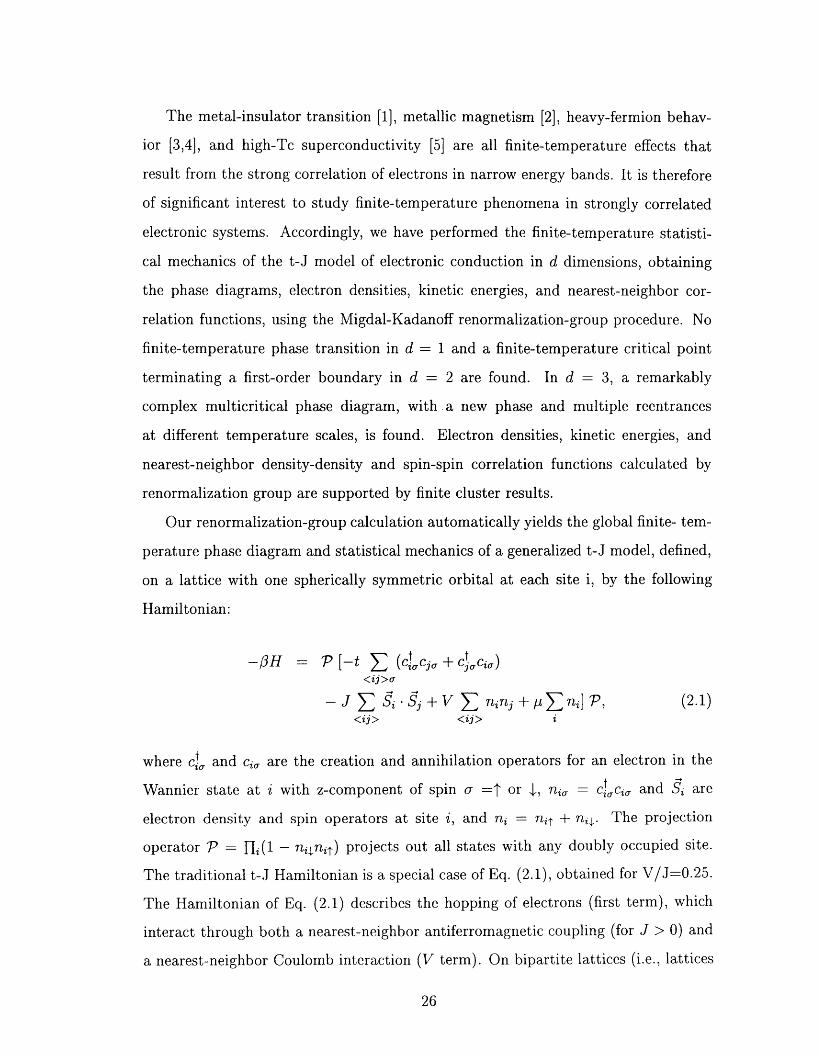
The metal-insulator transition [1], metallic magnetism 2 heavy-fermion behav-

ior 34], and high-Tc superconductivity [5] are all finite-temperature effects that

result from the strong correlation of electrons in narrow energy bands. It is therefore

of significant interest to study finite-temperature phenomena in strongly correlated

electronic systems. Accordingly, we have performed the finite-temperature statisti-

cal mechanics of the t-J model of electronic conduction in d dimensions, obtaining

the phase diagrams, electron densities, kinetic energies, and nearest-neighbor cor-

relation functions, using the Migdal-Kadanoff renormalization-group procedure. No

finite-temperature phase transition in d 1 and a finite-temperature critical point

terminating a first-order boundary in d 2 are found. In d = 3 a remarkably

complex multicritical phase diagram, with a new phase and multiple reentrances

at different temperature scales, is found. Electron densities, kinetic energies, and

nearest-neighbor density-density and spin-spin correlation functions calculated by

renormalization group are supported by finite cluster results.

Our renormalization-group calculation automatically yields the global finite- tem-

perature phase diagram and statistical mechanics of a generalized t-J model, defined,

on a lattice with one spherically symmetric orbital at each site i, by the following

Hamiltonian:

-OH - P [-t (ct qj, + ',ci,)C�

Si §j + V E ninj + p En-] P, (2.1)<ii> <ii> i

where ct and ci, are the creation and annihilation operators for an electron in the

Wannier state at Z' with z-component of spin T or �, ni, = ct ci, and are

electron density and spin operators at site Z', and ni -_ nit ni�. The projection

operator = Hi(I - nilnit) projects out all states with any doubly occupied site.

The traditional t-J Hamiltonian is a special case of Eq. 21), obtained for V/J=0.25.

The Hamiltonian of Eq. 21) describes the hopping of electrons (first term), which

interact through both a nearest-neighbor antiferromagnetic coupling (for J > ) and

a nearest-neighbor Coulomb interaction (V term). On bipartite lattices lattices

26

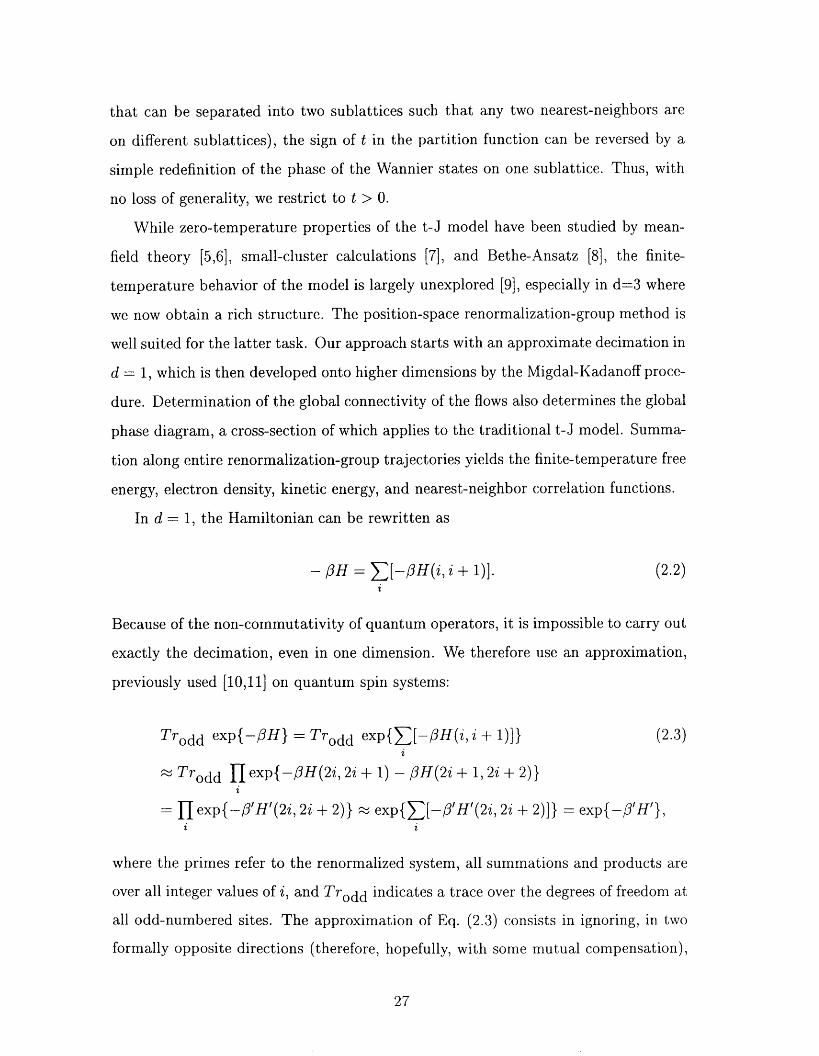
that can be separated into two sublattices such that any two nearest-neighbors are

on different sublattices), the sign of t in the partition function can be reversed by a

simple redefinition of the phase of the Wannier states on one sublattice. Thus, with

no loss of generality, we restrict to t > .

While zero-temperature properties of the t-J model have been studied by mean-

field theory 5,6-1, small-cluster calculations 7 and Bethe-Ansatz [81, the finite-

temperature behavior of the model is largely unexplored 9 especially in d=3 where

we now obtain a rich structure. The position-space renormalization-group method is

well suited for the latter task. Our approach starts with an approximate decimation in

d 1, which is ten developed onto higher dimensions by the Migdal-Kadanoff proce-

dure. Determination of the global connectivity of the flows also determines the global

phase diagram, a cross-section of which applies to the traditional t-J model. Summa-

tion along entire renormalization-group trajectories yields the finite-temperature free

energy, electron density, kinetic energy, and nearest-neighbor correlation functions.

In d 1, the Hamiltonian can be rewritten as

- OH = E[-OH(i, i + 1)]. (2.2)i

Because of the non-commutativity of quantum operators, it is impossible to carry out

exactly the decimation, even in one dimension. We therefore use an approximation,

previously used 0,11] on quantum spin systems:

Trodd expf -OHJ - Trodd expf [-OH(i, i + 1)] (2-3)Tr + 1 - OH(2i + 1, 2i 21

odd expf -OH(2i, 2Z

exp O'H'(2i, 2i 2 exp f O'H'(2i 2 2 exp O'H'J,

where the primes refer to the renormalized system, all summations and products are

over all integer values of i, and Trodd indicates a trace over the degrees of freedom at

all odd-numbered sites. The approximation of Eq. 23) consists in ignoring, in two

formally opposite directions (therefore, hopefully, with some mutual compensation),

27

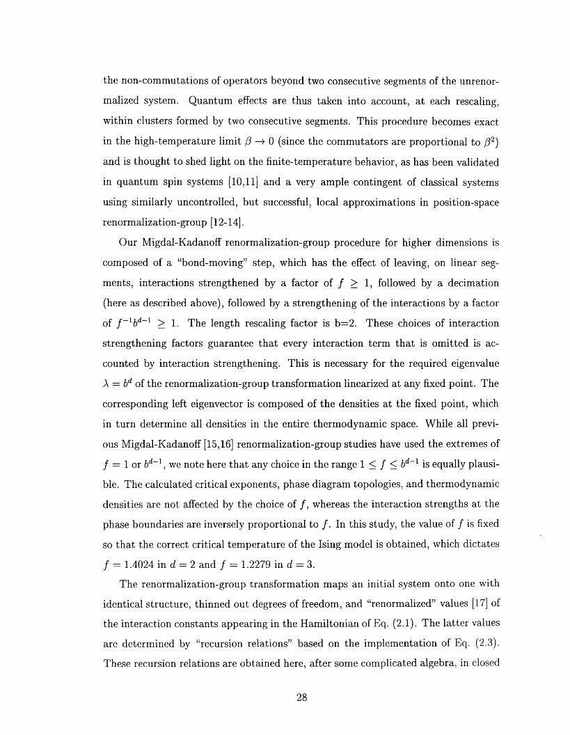
the non-commutations of operators beyond two consecutive segments of the unrenor-

malized system. Quantum effects are thus taken into account, at each resealing,

within clusters formed by two consecutive segments. This procedure becomes exact

in the high-temperature limit -� 0 (since the commutators are proportional to 01)

and is thought to shed light on the finite-temperature behavior, as has been validated

in quantum spin systems [10,111 and a very ample contingent of classical systems

using similarly uncontrolled, but successful, local approximations in position-space

renormalization-group 12-14].

Our Migdal-Kadanoff renormalization-group procedure for higher dimensions is

composed of a "bond-moving" step, which has the effect of leaving, on linear seg-

ments, interactions strengthened by a factor of f > followed by a decimation

(here as described above), followed by a strengthening of the interactions by a factor

of f -b d-1 > The length resealing factor is b=2. These choices of interaction

strengthening factors guarantee that every interaction term that is omitted is ac-

counted by interaction strengthening. This is necessary for the required eigenvalue

A = b d of the renormalization-group transformation linearized at any fixed point. The

corresponding left eigenvector is composed of the densities at the fixed point, which

in turn determine all densities in the entire thermodynamic space. While all previ-

ous Migdal-Kadanoff 15,16] renormalization-group studies have used the extremes of

f I orb , we note here that any choice in the ranged-1 d-1 is equally plausi-

ble. The calculated critical exponents, phase diagram topologies, and thermodynamic

densities are not affected by the choice of f, whereas the interaction strengths at the

phase boundaries are inversely proportional to f In this study, the value of f is fixed

so that the correct critical temperature of the Ising model is obtained, which dictates

f = 14024 in d -_ 2 and f -_ 12279 in d 3.

The renormalization-group transformation maps an initial system onto one with

identical structure, thinned out degrees of freedom, and "renormalized" values 17 of

the interaction constants appearing in the Hamiltonian of Eq. 21). The latter values

are determined by "recursion relations" based on the implementation of Eq. (2-3).

These recursion relations are obtained here, after some complicated algebra, in closed

28

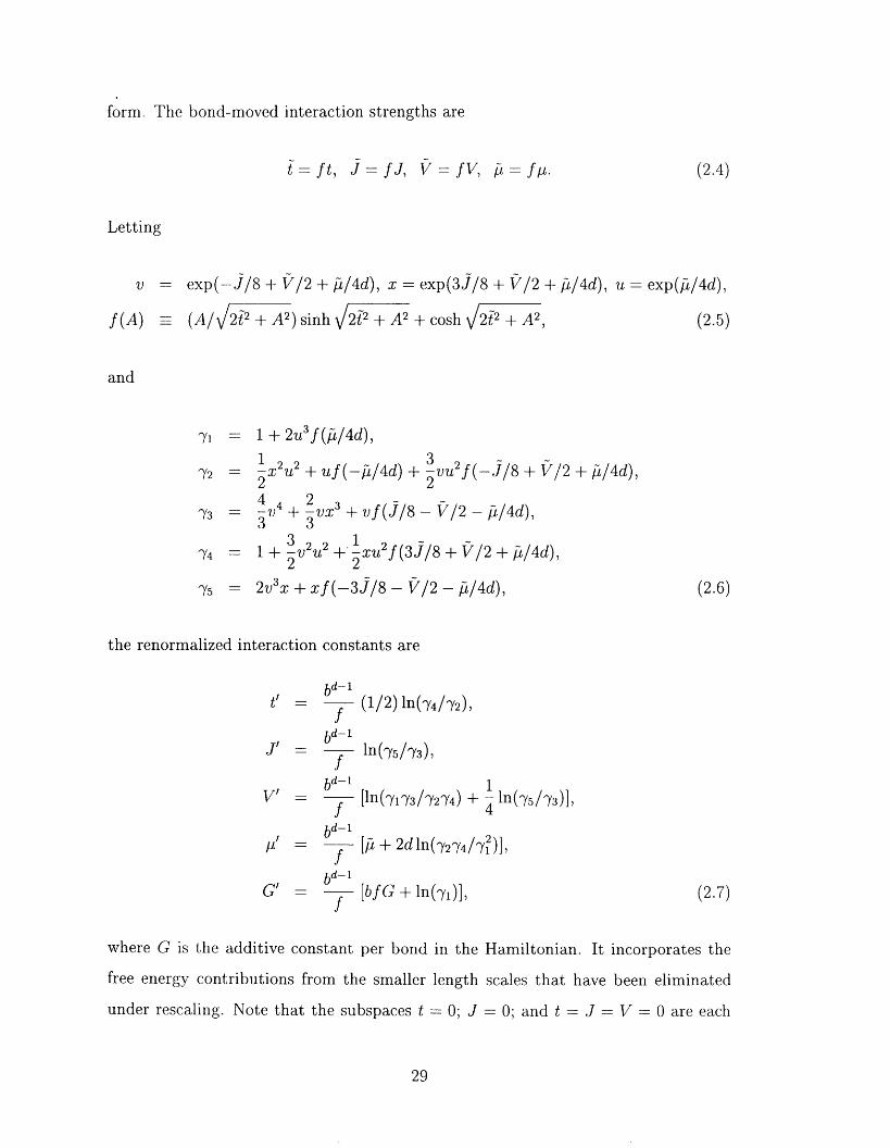
form.. The bond-moved interaction strengths are

t=ft, -fil VfV1 �=fft- (2.4)

Letting

= exp(--j/8 + f/2 + fil4d), x = exp(3j/8 + f/2 + A14d), u = exp(A/4d),r_�� -= (A/ V 2P + A2) sinh V/2P + �A2 + cosh V/2�P+ �A2, (2.5)

V

f (A)

and

-yj- I 2u 3f (�/4d),

1 2 2 3 2f(72 - _x U + Uf (-Al4d) + VU _J/8 + V/2 + A14d),2 2

4 4 2 373 _V + VX + vf j/8 - f/2 - A14d),3 3

3 2 2 1 2f74 + V U + xU (3j/8 + �'/2 + A14d),

2 2

-y5 2v3x + xf (-3j/8 - fr/2 - A14d),

the renormalized interaction constants are

(2-6)

tl bd-1- f (1/2) n(-y4

bd-1i = In(-y5/-y3),

f-I

f - bu-'V - fbd-1

A = fbd-1

G =f

1/1N),

I[In(_Y1_Y31_Y2_Y4) + - n(-y5/-y3)],

4

[A + 2d n(-y2-y4 /_y2)],1

[bf G In -yi)], (2.7)

where G is the additive constant per bond in the Hamiltonian. It incorporates the

free nergy contributions from the smaller length scales that have been eliminated

under resealing. Note that the subspaces t 0; J = and t = J = V = are each

29

f A A AV. 4

0__�I_--q

0$_4

=S

;4 0.20C14

c-

o

E_

n

I I(a) t/i = 02V/J = 025

F -II

d D

I i I

U v.'+

U;__4

M;--4

U

C14 0.2E�U

F_1__qMU

-4�-4

U

nV-2 -1.5 -1 1j 4

Chemical Potential g/J Hopping Strength t/J

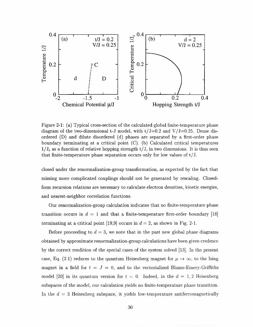
Figure 21: (a) Typical cross-section of the calculated global finite-temperature phasediagram of the two-dimensional t-J model, with t/J-0.2 and V/J=0.25. Dense dis-ordered (D) and dilute disordered (d) phases are separated by a first-order phaseboundary terminating at a critical point (C). (b) Calculated critical temperaturesI/J, as a function of relative hopping strength t/J, in two dimensions. It is thus seenthat finite-temperature phase separation occurs only for low values of t/j.

closed under the renormalization-group transformation, as expected by the fact that

missing more complicated couplings should not be generated by resealing. Closed-

form recursion relations are necessary to calculate electron densities, kinetic energies,

and nearest-neighbor correlation functions.

Our renormalization-group calculation indicates that no finite-temperature phase

transition occurs in d I and that a finite-temperature first-order boundary [18]

terminating at a critical point 19,9] occurs in d = 2 as shown in Fig. 2-1.

Before proceeding to d -_ 3 we note that in the past new global phase diagrams

obtained by approximate renormalization-group calculations have been given credence

by the correct rendition of the special cases of the system solved 13]. In the present

case, Eq. 21) reduces to the quantum Heisenberg magnet for -� 00, to the Ising

magnet in a field for t -_ J -_ 0, and to the vectorialized Blume-Emery-Griffiths

model 20] in its quantum version for t -_ 0. Indeed, in the d = 1 2 Heisenberg

subspaces of the model, our calculation yields no finite-temperature phase transition.

In the d = 3 Heisenberg subspace, it yields low-temperature antiferromagnetically

30

(for J > ) or ferromagnetically (J < ) ordered phases, each separated by a second-

order transition from the high-temperature disordered phase. The antiferrornagnetic

ition temperature calculated here to be 122 tmes the ferromagnetic transition

temperature, to be compared with the value of 1 14 for this ratio from series expansion

[21]. All of the latter behavior, as well as the behavior of the Ising model with field

and the multicritical global phase diagram of the quantum BEG model support the

validity of the global calculation.

Returning to the generalized t-J model of Eq. 21) a novel and intricate global

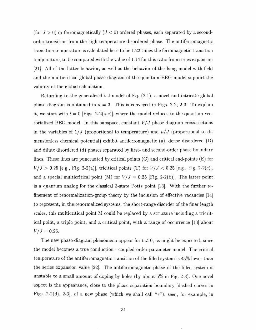
phase diagram. is obtained in d 3 This is conveyed in Figs. 22 23. To explain

it, we start with t [Figs. 2-2(a-c)], where the model reduces to the quantum vec-

torialized BEG odel. In this subspace, constant V/J phase diagram cross-sections

in the variables f IIJ (proportional to temperature) and plJ (proportional to di-

mensionless chemical potential) exhibit antiferromagnetic (a), dense disordered (D)

and dilute disordered (d) phases separated by first- and second-order phase boundary

lines. These ines are punctuated by critical points (C) and critical end-points (E) for

VIJ > 025 [e.g., Fig. 2-2(a)], tricitical points (T) for VIJ < 025 [e.g., Fig. 2-2(c)],

and a special multicritical point (M) for VIJ -_ 025 [Fig. 2-2(b)]. The latter point

is a quantum nalog for the classical 3-state Potts point [13]. With the further re-

finement of renormalization-group theory by the inclusion of effective vacancies 14]

to represent, in te renormalized systems, the short-range disorder of the finer length

scales, this multicritical point M could be replaced by a structure including a tricrit-

ical point, a triple point, and a critical point, with a range of occurrence 13] about

VIJ -_ 0.25.

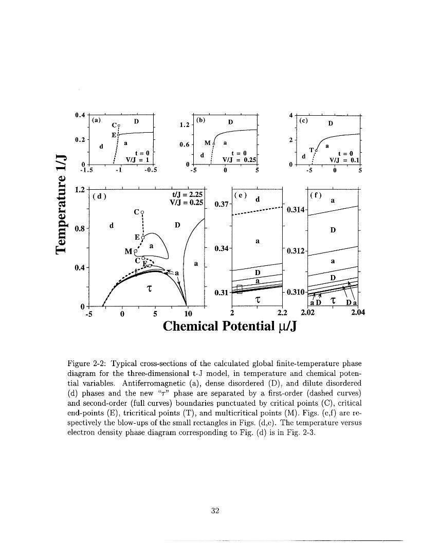
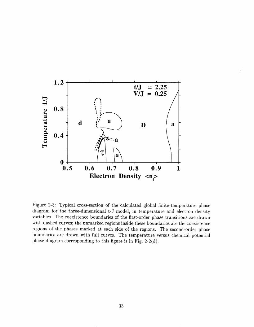
The new phase-diagram phenomena appear for t 1-L 0, as might be expected, since

the model becomes a true conduction - coupled order parameter model. The critical

temperature ofthe antiferromagnetic transition of the filled system is 43% lower than

the series expansion value 22]. The antiferromagnetic phase of the filled system is

unstable to a small amount of doping by holes (by about 5% in Fig. 23). One novel

aspect is the appearance, close to the phase separation boundary [dashed curves in

Figs. 2-2(d) 23], of a new phase (which we shall call "T" ),seen, for example, in

31

(e) d

a

D

T

0.4 -

0.2 -

11V -1.

4

2

0

(a) Co D

E&___��I: a

dI: t = J V/ = I

(b) D

M ra__��I

d : t = . V = 025

W D

T t = d I'1. V/ = .1

1.2 -

0.6 -

0I I-1 -0.5 6

0.37-

0.34-

0.31-

5 -5 6 55 -5

W

14-)M

4)

E-4

1.2

0.8

f ) a

D

a

IT

0.314-

0.312-

0.4

0

0.310-

2.02 2.04-5 0 5

Figure 22: Typical cross-sections of the calculated global finite-temperature phasediagram for the three-dimensional t-J model, in temperature and chemical poten-tial variables. Antiferromagnetic (a), dense disordered (D), and dilute disordered(d) phases and the new -r" phase are separated by a first-order (dashed curves)and second-order (full curves) boundaries punctuated by critical points (C), criticalend-points (E), tricritical points (T), and multicritical points (M). Figs. (ef) are re-spectively the blow-ups of the small rectangles in Figs. (de). The temperature versuselectron density phase diagram corresponding to Fig. (d) is in Fig. 23.

32

10 2 2.2

Chemical Potential Wj

1.2

r_�

w 0.8

*-4etW

= 0.4CZW

00.5 0.6 0.7 0.8 0.9 1

Electron Density <ni>

Figure 23: Typical cross-section of the calculated global finite-temperature phasediagram for the three-dimensional t-J model, in temperature and electron densityvariables. The coexistence boundaries of the first-order phase transitions are drawnwith dashed curves; the unmarked regions inside these boundaries are the coexistenceregions of the phases marked at each side of the regions. The second-order phaseboundaries are drawn with full curves. The temperature versus chemical potentialphase iagram corresponding to this figure is in Fig. 2-2(d).

33

Figs. 2-2(d) 23 for tIJ -_ 225 and VIJ = 025, which applies to the traditional

t-J model. This phase, to our knowledge never seen before finite-temperature

phase transition theories, is the only volume of the extended phase diagram in which,

after multiple rescalings, the hopping strength t does not renormalize to zero. In

fact, all the interaction constants (t, J, V, /t) renormalize to infinite strengths, while

their ratios eventually remain constant at Jlt = 2 y1t = 3/2, IIt 6 and t -�

oo a typical behavior for the renormalization-group sink 13] of a low-temperature

phase. A distinctive feature is that at this sink, which as usual epitomizes the entire

thermodynamic phase that it attracts, the electron density n), obtained as usual

from the left eigenvector with eigenvalue V of the recursion matrix, has the non-

unit, non-zero value of (n-) = 23. This feature makes strong-coupling conduction

possible by having the system non-full and non-empty of electrons, and has also not

been seen previously.

Another feature is the appearance of several islands of the antiferromagnetic phase,

as seen in Figs. 2-2(d) 23. The islands are bounded by first- and second-order phase

transitions adorned by the various special points already mentioned above. Thus,

a multiply reentrant phase diagram topology obtains. The antiferromagnetic phase

also occurs as a narrow sliver, within the disordered phase reaching zero temperature

between the antiferromagnetic and "T" phases. The appearance of the antiferromag-

netic islands at dopings in the neighborhood of the "T" phase (see Fig 23) indicates

that, when the hopping strength t increases under resealing, antiferromagnetically

long-range correlated states acquire substantial off-diagonal elements, which lowers

the free energy of the antiferromagnetic phase.

The transition between the new "T" and disordered phases is second-order, con-

trolled by a redundant triplet structure of fixed points at (t*, P, V*, p* = 084,

1.22, 223, 12.91), 069, 138, 103, 415), 074, 342, 208, 152) with the re-

spective relevant eigenvalue exponents y 1.001 0993 1009, corresponding to the

critical exponents -_ 0999 and a -- 0.997. Although the latter numbers are to be

taken only as indicative, in view of the approximations, the fact that the eigenvalue

exponents of the three redundant fixed points are so close to each other points to

34

internal consistency in the calculation. On the less dense side of the boundary of the

T" phase, a "amellar" sequence of antiferromagnetic slivers and disordered inlets

occurs, at several temperature scales, as seen in Figs. 2-2(ef). Our results on the

finite-temperature hase diagram of the t-J model can be categorized as follows:

1. At the coarsest temperature scale, a new -F" phase occurs as a distinct thermo-

dynamic phase in a narrow interval, e.g., between 30% and 40% doping and at

temperatures IIJ < 04 in Fig. 2-3. The antiferromagnetic phase of the filled

system is ustable to a small amount of doping (about 5% in Fig. 23), but the

antiferromagnetic long-range correlations are enhanced in the neighborhood of

the "T" hase.

2. Islands of the antiferromagnetic phase appear within the disordered phase.

3. On the less, ense side of the boundary of the "T" phase, a fine structure of

narrow antiferromagnetic slivers and narrow disordered inlets occur at several

temperature scales.

4. t low electron densities, nearest-neighbor ferromagnetic correlations occur.

It would be most interesting to know whether these new results survive the re-

moval or lessening of the approximations made here. Our treatment is, of course, an

approximate study of the t-J model, due to the mistreatment of some of the com-

mutation relations Eq. 23)] and due to the Migdal-Kadanoff bond-moving. Our

treatment is also, simultaneously, a lesser approximation to the statistical mechanics

of he t-J model on a d-dimensional hierarchical lattice 23]: Bond-moving is exact,

but, te mistreatment of some of the commutation relations remains. It would be

rewarding if the new phase diagram survives at least for the physical realization of

the t-J model on hierarchical lattices.

We have calculated electron densities, average kinetic energies per nearest-neighbor

site pairs

t t t tMj = CiTCjT + CjTCiT + ci�cj� + i .�Ci�) (2.8)

35

-II.

---- , . I I I t

0.8

A

�� 04V

0

A 0-fcc*.--0.2.

t CnV -0.4

I I- i

- ----------- ---------------- ---\

I I I

I

.......

-10 0 10

I 1 1 1 1 1 1 1 I! 1 1 I I I- -------------- �%. I __V _

AoilC�_ 0. 5V

n

A

;�_ 0. -V

n -------- j---------L------ L_

10 0 10 -10 0 10

Chemical Potential [t/j

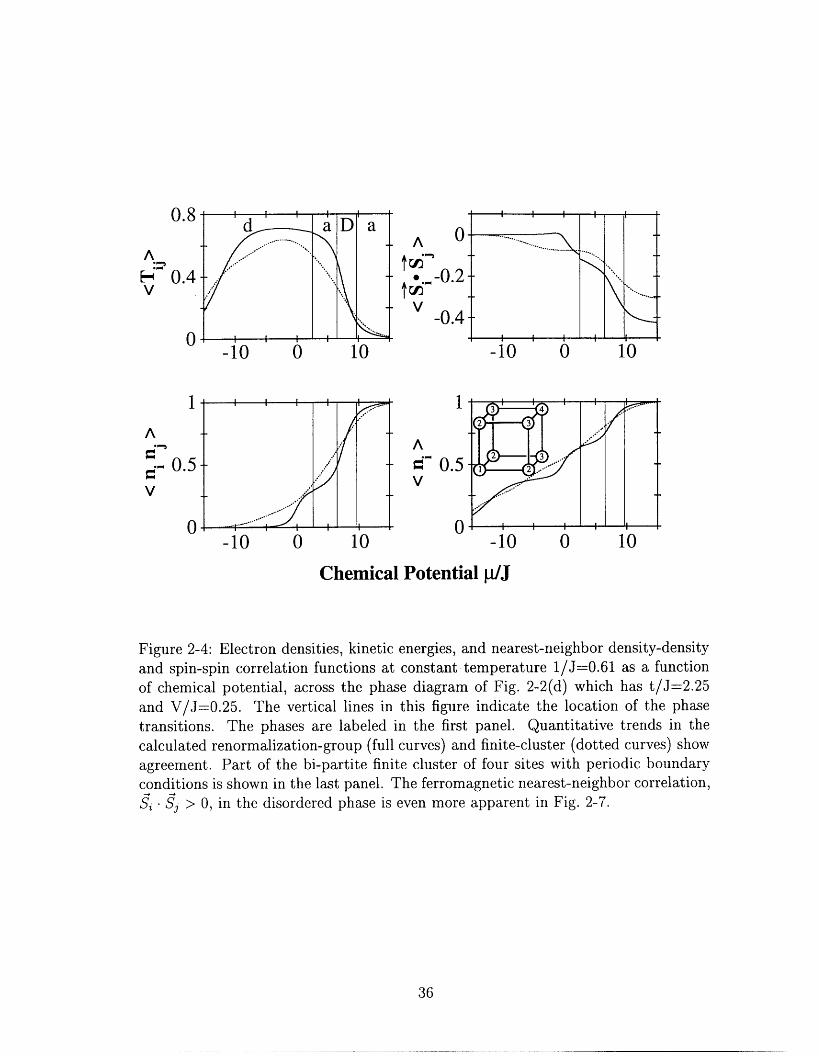
Figure 24: Electron densities, kinetic energies, and nearest-neighbor density-densityand spin-spin correlation functions at constant -temperature 1/J=0.61 as a functionof chemical potential, across the phase diagram of Fig. 2-2(d) which has t/J--2.25and V/J-0.25. The vertical lines in this figure indicate the location of the phasetransitions. The phases are labeled in the first panel. Quantitative trends in thecalculated renormalization-group (full curves) and finite-cluster (dotted curves) showagreement. Part of the bipartite finite cluster of four sites with periodic boundaryconditions is shown in the last panel. The ferrornagnetic nearest-neighbor correlation,Si - Sj > 0, in the disordered phase is even more apparent in Fig. 27.

36

-10 0 10

I

0.80-Atcc

Cn

t -V

A

E-4V

-0.2-0.4

0

'I I

A

j:�_ 0. 5V

0

i.

I

A

cc

V

0.5

00-10 10

37

Chemical Potential WJ

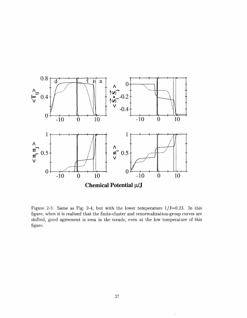
Figure 25: Same as Fig. 24, but with the lower temperature I/J=0.23. In thisfigure, when it is realized that the finite-cluster and renormalization-group curves areshifted, good agreement is seen in the trends, even at the low temperature of thisfigure.

i

_"I_-____--_-_................

II

i i

i i I

.7��

i i

0 0.5 1

i

f) 0I I

0.8

A

F-0 0. 4V

0

0.8

0.4

0

0

-0.2

A 0fcc*.--0.2

t UnV

-0.4

U. )0 I

1 1

0.5

A

gr

V

0.5

0 01

38

I/J = 061 1/j = 023

Electron Density < ni >

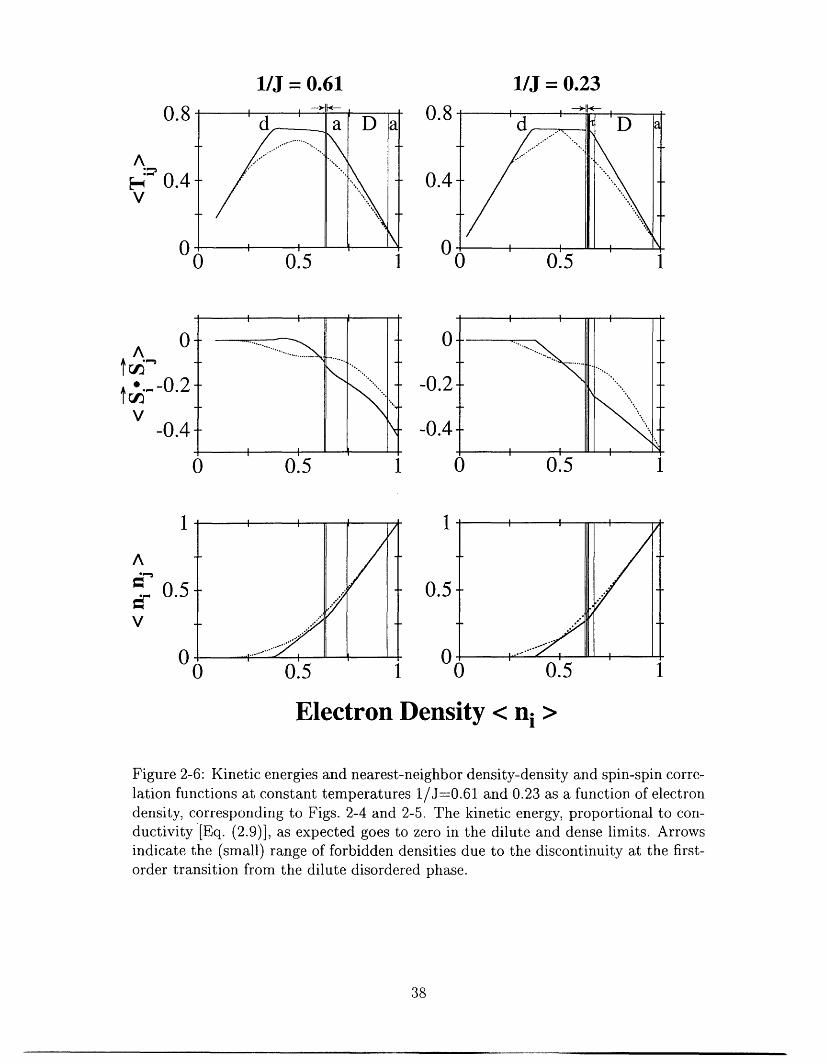
Figure 26: Kinetic energies and nearest-neighbor density-density and spin-spin corre-lation functions at constant temperatures I/J-0.61 and 023 as a function of electrondensity, corresponding to Figs. 24 and 25. The kinetic energy, proportional to con-ductivity .[Eq. 29)], as expected goes to zero in the dilute and dense limits. Arrowsindicate the (small) range of forbidden densities due to the discontinuity at the first-order transition from the dilute disordered phase.

AF-t

. WN

0V

A

t -0. -0

F*t r"�

L��d T D a

-1 .. I

I 11 -IIie. - -

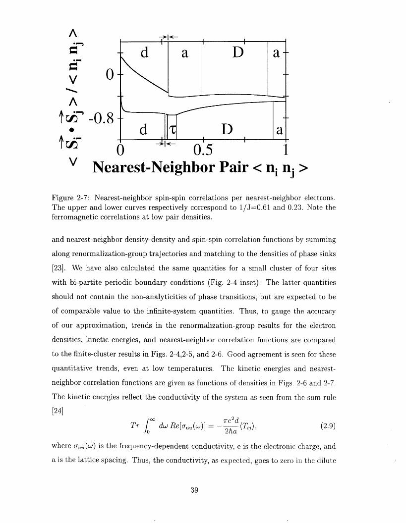
W-4 0 11 0. -) IV Nearest-Neighbor Pair < ni nj >

Figure 27: Nearest-neighbor spin-spin correlations per nearest-neighbor electrons.The upper and lower curves respectively correspond to I/J-0.61 and 023. Note theferromagnetic orrelations at low pair densities.

and nearest-neighbor density-density and spin-spin correlation functions by summing

along renormalization-group trajectories and matching to the densities of phase sinks

[23]. We have also calculated the same quantities for a small cluster of four sites

with bipartite periodic boundary conditions (Fig. 24 inset). The latter quantities

should not contain the non-analyticities of phase transitions, but are expected to be

of comparable value to the infinite-system quantities. Thus, to gauge the accuracy

of our approximation, trends in the renormalization-group results for the electron

densities, kinetic energies, and nearest-neighbor correlation functions are compared

to the finite-cluster results in Figs. 24,2-5, and 26. Good agreement is seen for these

quantitative trends, even at low temperatures. The kinetic energies and nearest-

neighbor correlation functions are given as functions of densities in Figs. 26 and 27.

The kinetic energies reflect the conductivity of the system as seen from the sum rule

[24]00 2d

Tr 10 dw Re (w) 2ha (Tij), (2-9)

where (w) is te frequency-dependent conductivity, e is the electronic charge, and

a is the lattice spacing. Thus, the conductivity, as expected, goes to zero in the dilute

39

and dense limits.

We thank Patrick Lee and Maurice Rice for useful conversations. This research

was supported by the JSEP Contract No. DAAL 03-92-CO001. AF acknowledges

partial support from the NSF Predoctoral Fellowship Program.

40

REFERENCES

[1] N.F. Mott, Rev. Mod. Phys. 40, 677 1968).

[2] F.C. Zhang and T.M. Rice, Phys. Rev. 37, 3759 1988).

[3] G.R. Stewart, Rev. Mod. Phys. 56, 765 1984).

[4] P. Fulde, J. Keller, and G. Zwicknagl, Solid State Phys. 41, 1988).

[5] P.W. Anderson, Science 235, 1196 1987).

[6] G. Baskaran, Z. Zhou, and P.W. Anderson, Solid State Commun. 63, 973

(1987).

[7] J.K. Freericks and L.M. Falicov, Phys. Rev. 42, 4960 1990).

[8] P.A. Bares, C. Blatter, and M. Ogata, Phys. Rev. 44, 130 (1991).

[9] One previous calculation is S.A. Cannas and C. Tsallis, Phys. Rev. 46,

6261 (1992). These authors did not derive the closed-form recursion relations,

but implemented them numerically. They did not obtain the new phase, the

corresponding phase diagram structure, the electron densities, kinetic energies,

and corelation functions obtained here.

[10] M. Suzuki nd H Takano, Phys. Lett. A 69, 426 (1979).

[11.] Ii. Takano and M Suzuki, J. Stat. Phys. 26, 635 1981).

[12] Th. Niemeijer and J.M.J. van Leeuwen, Phys. Rev. Lett. 31, 1411 1973).

[13] AX Berker and M Wortis, Phys. Rev. 14, 4946 1976).

[14] 13. Nienh.uis AX Berker, E.K. Riedel, and M. Schick, Phys. Rev. Lett. 43,

737 1979).

[151 A.A. Migdal, Zh. Eksp. Teor. Fiz. 69, 1457 1975) [Sov. Phys. - JETP 42, 743

(1976)].

41

[16] L.P. Kadanoff, Ann. Phys. (N.Y.) 100, 359 1976).

[17] Note that after the first renormalization, the system is quantitatively mapped

onto one consisting of sites from only one of the two sublattices of the original

system. Ferromagnetic couplings between these sites are perfectly consistent

with antiferromagnetic order in the original system, as can be seen from the

calculated nearest-neighbor correlation function Si -Si in Figs. 24 25 and 26.

The latter calculation establishes the antiferromagnetism of the original system

with no ambiguity. Under the first renormalization, the critical point of the

totally filled antiferromagnetic system maps onto the critical point of the totally

filled ferromagnetic system. The antiferromagnetic critical temperature is thus

here calculated to be 122 times the ferromagnetic critical temperature, to be

compared with the value of 114 for this ratio from series expansion (Ref.[21]).

[18] S.A. Kivelson, V.J. Emery, and H.Q. Lin, Phys. Rev. 42, 6523 1990).

[19] W.O. Putikka, M.U. Luchini, and T.M. Rice, Phys. Rev. Lett. 68, 538 (1992).

[20] A.N. Berker and D.R. Nelson, Phys. Rev. 19, 2488 1979).

[211 G.S. Rushbrooke and P.J. Wood, Mol. Phys 6 409 (1963).

[22] G.S. Rushbrooke, G.A. Baker, Jr., and P.J. Wood, in Phase Transitions and

Critical Phenomena, eds. C. Domb and M.S. Green (Academic, New York,

1984), vol 3 p. 306.

[23] A.N. Berker and S. Ostlund, J. Phys. C 12, 4961 (1979).

[24] D. Baeriswyl, C. Gros, and T.M. Rice, Phys. Rev B 35, 8391 1987).

42

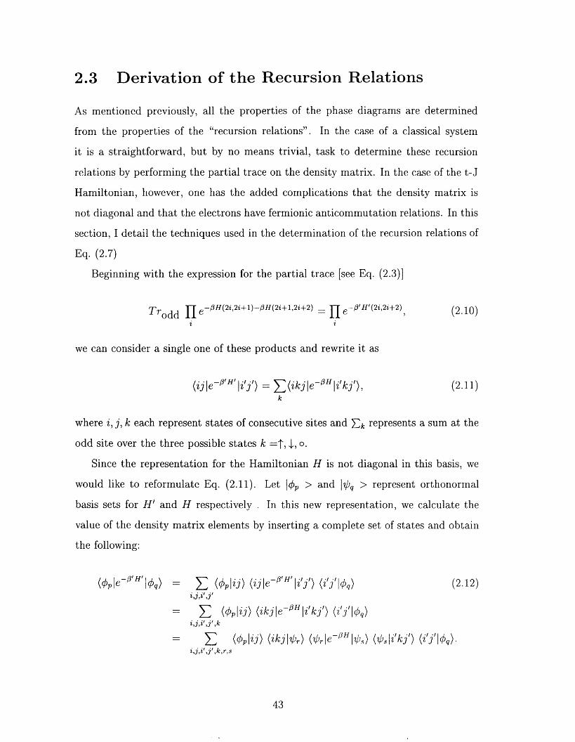
2.3 Derivation of the Recursion Relations

As mentioned previously, all the properties of the phase diagrams are determined

frOD-1 the properties of the "recursion relations". In the case of a classical system

it is a straightforward, but by no means trivial, task to determine these recursion

relations by performing the partial trace on the density matrix. In the case of the t-J

Hamiltonian, however, one has the added complications that the density matrix is

not diagonal ad that the electrons have fermionic anticommutation relations. In this

section, I detail the techniques used in the determination of the recursion relations of

Eq. 27)

Beginning with the expression for the partial trace [see Eq. 23)]

Trodd H e- OH(2i,2i+1)-OH(2i+1,2i+2 = ri e- OIHI(2i,2i+2) (2.10)i i

we can consider a single one of these products and rewrite it as

(ij I -- "'H I "J" E ( Zkj I e- - 3 H I " kj'),k

where i, j, k each represent states of consecutive sites and k represents a sum at the

odd site over the three possible states k T, �, o.

Since the representation for the Hamiltonian H is not diagonal in this basis, we

would like to reformulate Eq. 211). Let lop > and 10q > represent orthonormal

basis sets for H' and H respectively In this new representation, we calculate the

value of the density matrix elements by inserting a complete set of states and obtain

the following:

Of HI Z) Zj '31 HIz(Ople- l Oq) (Opl 'le- W (2.12)ijiljf

I e-)3H JI q)(OpIzj) Z'k] I ik ('1

ijiljlk(Oplzj) Zk3j0,) (Oje-OHjO,)

z,],ij',krs

43

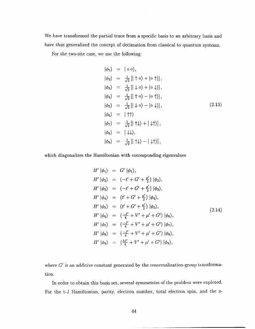
We have transformed the partial trace from a specific basis to an arbitrary basis and

have thus generalized the concept of decimation from classical to quantum systems.

For the two-site case, we use the following

101)

102)

103)

104)

105)

106)

107)

108)

1 09)

= lo 0),

27i 1 T 0) lo V,

2 11 � 0) lo �)]

2 [I 0) lo V

2 11 � 0) lo �)],

= I TT)

2I [I T� I )] 1

- 1114),

= V1_ [I W I T)] 12

(2.13)

which diagonalizes the Hamiltonian with corresponding eigenvalues

H'101)

H' 102)

H' 103)

H' 104)

H' 105)

H' 106)

H' 107)

H' 108)

H'109)

G' IO,),

(-t' G+ 1" 12),2

G'+ 1" 13),2

(t' G+ " 14),2

+ G' + 1 ) 15),2

J + V + ' + G 16),4

(-J + V+ IL'+ G 17),4

J + V + 2 + G) 108),4

(3j + V + IY + G I 9),4

(2.14)

by the renormalization-group transforma-

symmetries of the problem were exploted.

number, total electron spin, and the z-

where G' is an additive constant generated

tion.

In order to obtain this basis set, several

For the t-J Hamiltonian, parity, electron

44

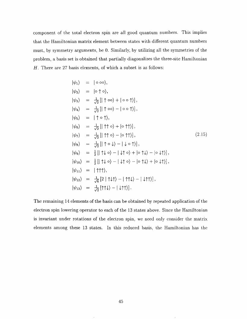
component of the total electron spin are all good quantum numbers. This implies

that the Hamiltonian matrix element between states with different quantum numbers

must, by symmetry arguments, be 0. Similarly, by utilizing all the symmetries of the

problem, a basis set is obtained that partially diagonalizes the three-site Hamiltonian

H. There are 27 basis elements, of which a subset is as follows:

I 01) I 00),

102) 10 T 0),

I 03) [TOO)+IOOT)I,vf2

104) 1 [I 00) 0 T,xF2

105) T 0 T),

1'06) 1 [I TT ) + 1 MIV2

107) I [I TT ) 10 TT)I, (2.15)V2

108) 1 [I 0 T)]72=

09) I [I T� 0) I �T 0) lo T�) lo WI

1010) 1 [I T� 0) I �T 0 lo W + lo V

I ITT),

1012) 2 T�T) - I T�) �TT)] ,v/6

1013) ' [M - I-,f2

The remaining 4 elements of the basis can be obtained by repeated application of the

electron spin lowering operator to each of the 13 states above. Since the Hamiltonian

is invariant uder rotations of the electron spin, we need only consider the matrix

elements among these 13 states. In this reduced basis, the Hamiltonian has the

45

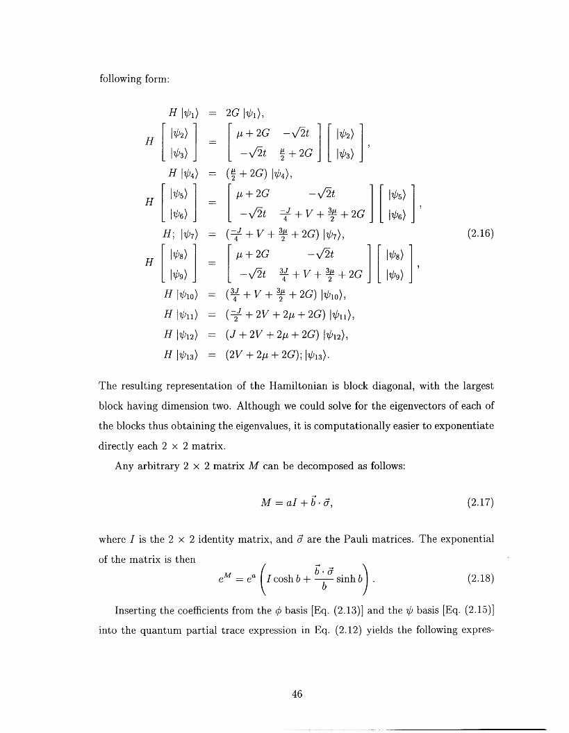
following form:

-H IV),)

H 102)

-I 03)

-H 104)

H 105)

- 106)

H 17)

H 108)

I 9)

H 01o)

H 111)

H 1012)

H 113)

2G

I-t+2G -v/2t 102)"2t IL

-v 2 + 2G 03)

+ 2G 14),2

I-L + 2G - V2t

-v2t - + V 3 G4 2

(- + V 3 2G) 107),4 2

+ 2G - V2t

-v2t 3 + V + �L + 2G4 2

= (3 + V 3 2G) 101o),4 2

= (-j + 2V + 2/i + 2G) 1011),2

= (J + 2V + 21.L + 2G 112),

= (2V + 2/z + 2G); 1013)-

(2.16)

The resulting representation of the Hamiltonian is block diagonal, with the largest

block having dimension two. Although we could solve for the eigenvectors of each of

the blocks thus obtaining the eigenvalues, it is computationally easier to exponentiate

directly each 2 x 2 matrix.

Any arbitrary 2 x 2 matrix M can be decomposed as follows:

M = aI + � -6, (2.17)

where I is the 2 x 2 identity matrix, and are the Pauli matrices. The exponential

of the matrix is then

e = a I cosh b +b sinh b .b

(2.18)

Inserting the coefficients from the basis [Eq. 2.13)] and the O basis Eq. 2.15)]

into the quantum partial trace expression in Eq. 212) yields the following expres-

46

105)

I ")

108)

I o

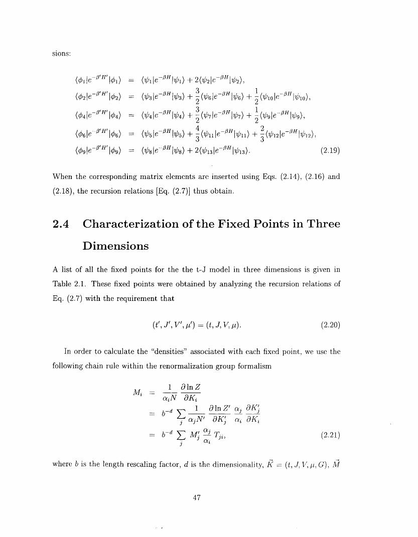
sions:

101)

(02le-01HI I 02)

�041e_ '31 HI 104)

= (,olle-OH101) 2 02 le-OH I 02),

3 -OH I OH- ('03 le OH 103 + ('06 le 106 + - (0 i I - 1010),2 2

I) OHI 07 + 2 (0 I -, I 9),

-OH 3= (04 le, 104) + -('07

2

(06le- Ol HI 14)6)

(ogle-OW I 09)

-OH 4 OH 2 OH= (05 I 105) + - (Oil e- 11011) +- (012le- 1012),

3 3

=: V)81e-OH 108) + 20131COH 1013) (2.19)

When the corresponding matrix elements are inserted using Eqs. 214), 216) and

(2.18), the recursion relations [Eq. 27)] thus obtain.

2.4 Characterization of the Fixed Points in Three

Dimensions

A list of all the fixed points for the the t-J model in three dimensions is given in

Table 21. These fixed points were obtained by analyzing the recursion relations of

Eq. 27) with the requirement that

(tf, J/, V/, '41) - t J V, it) (2.20)

In order to calculate the "densities" associated with each fixed point, we use the

following chain ule within the renormalization group formalism

- I aln ZA aiN aKi0 In Z' aj,OKj ai

= b-d 1:Ifi ajN

- -d 1: 11 Tai 'i,

i(2.21)

where b is the length resealing factor, d is the dimensionality, K (t, J, 17 it, G), M

47

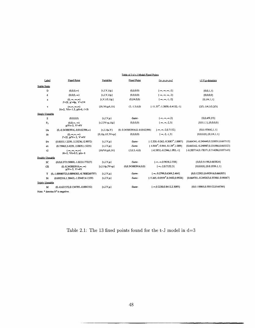
Table of 3-d t-J Model Fixed Poinja

Fixed Point iYIJ2-X3-YAILaw

Stable Sinks

D

d

a

Fixed Point t.J.V.IL-dcnqitics

(0,0,0,-)(0,0,0,--)

J'=2J, R4g, V=J'/4

1/t=2, Vt=-1.5, P/t=6, t=2t

itJVI/R)(tJ.VI/g)

(tV I /J I /L)

(J/tV/twtl/t)

(0,0,0,0)

(0,0,0,0)

(OJ/4,0,0)

(2,-1.5,6,O) (- 155*,-1.5859,-0.4152,-1)

(0,0,1,1)(0,0,0,0)

(0,1/4,1,1)

(2/3,-1/4,1/3,2/3)

Singly Unstabi

S (0,0,0,0)

F2 (0,0,-,--)

p/V=-3, V=4V

Da (0,-0.343883916,-0.0162396,-)

daJ'=2J, IIN=-3, V'--4V

Dc (0.8352,1.2239,-2.23236,12.9072)

dr (0.73965,3.4229,-2.0829,1.5235)

,c2J/t=2, V/t--0.5, Wt=-6

(tJVA)ftJ,3V+VI/gl

ftJI/RV)(0,1/gI/J,3V+g)

((,JVR)ltJVR)

(J/t/V/tWtl/t)

-Sarne-

(0,0,0,0)

(0.0,4/9,2/3)

(0,0,1,1),(0,0,0,0)

(0,-0.343883916,0,-0.0162396)

(0,0,0,0)

(--,--,-2,0.7152) (0,0.193642,1,1)

10,0,0,0), (0, 1/4, 1,1 I

-2.320,0.562,03OW 1.0007)

(-4.844*,-0.944,-0.139*, 1.0091

(-0.5852,-0.2346,1.093,- 1)

(--,--,0.9658,2.558)(--,-2,0.7152,3)

-Sarne-

-Sarne-

(2,0.5,-6,O)

(0.664341,-0.249449,0.335031,0.667515)

10.665162,-0.248981,0.331986,0.665322)

( -0.285714,0.178571,0.714286,0.857143)

10,0,0.51196,0.6658241

10.0,0,0), (0,0. 19 36, 1,1 )

(0,0. 122921,0.495916.0.666305)

(0.664701,-0.249263,0.333661,0.66667)

10,0. 1 18865,0.505122,0.66766)

abk(0,0,0.272158869,-1.0221177227)

(0,-0.343883916,-,--)p/V=-3, V'=4V

Doubly Unst

SC

CE

197)

ltJVR) -Sarne-jtJI/g,3V+g) (0,0.343883916,0,0)

-Sarne- (--,-0.2799.0.6369,2.4641

-Sarne- 1-5.265,-0.0554*,0.3402,0.9928)

T (O.-I.00980723,0.0098303,-0.7808269�

S-t (0.692316,1.38463,-1.03487,4.1539

Triply Unstable

M (0,-0.621572,0.134705,-0.884232)

Note: * denotes by is negative.

ltJVA)(tJVg)

tJVR ) -Sarne- (--,0.2230,0.8412,2.5093)

48

Table 21: The 13 fixed points found for the t-J model in d=3

are the densities associated with k, N is the number of sites, is the number of

interactions of type i per site, 4 and the primes represent the renormalized system.

The entire formalism hinges on the identity

- OF = In Z In Z = 01F', (2.22)

which results frorn preserving the trace of the density matrix Trp Z.

The "densities" correspond, in the cases of t, J, V, ft, to the kinetic energy, nearest

neighbor spin-spin correlation function, nearest neighbor density-density correlation

function, and the electron densities. At the fixed points, one must have

A - Ml' = M�* 1 (2.23)

which are thus the left eigenvalues of the matrix 'i Ti with eigenvalue b d . The critical

exponents for each fixed point are determined from the eigenvalues of Tj- evaluated

at the fixed point'. The fixed point densities, the critical exponents, and the locations

of all the fixed pints for the t-J model in d = 3 are listed in Table 2 L

The recursion relation of Eq. 221) immediately yields the electron densities,

kinetic energies, and nearest-neighbor correlation functions for the entire phase dia-

grain. One starts with the initial interaction strengths and repeatedly performs the

recursion relations of Eq. 2.7) until one is arbitrarily close to a fixed point. One then

replaces the renormalized density Mi' in Eq. 2.21) by the density at the fixed point

Mj* arid obtains the corresponding densities at the initial point. This technique is

extraordinarily powerful in that all the properties of the phase diagrams are contained

within the recursion relations themselves.

4cti = 3 for the borid-type interactions (t, J, V, g) and ozi = 1 for for the site interaction .

49

Chapter 3

The Random-Field Ising 1\4odel

3.1 Introduction

By now, there can be no argument that the presence of random fields drastically

affects the phase diagrams of systems that undergo phase transitions. Theoretical

arguments have shown that any amount of quenched field randomness destroys long-

range order in two dimensions.' Let us consider a well-examined problem in two-

dimensional physics: krypton adsorbed on graphite. This system has undergone ex-

tensive theoretical and experimental investigation, including detailed renormalization-

group treatments.' The surface of graphite, however, is inherently imperfect. No

matter how well it is constructed, there will be some, albeit small, amount of defects

on the surface. Since the phase transition involves the preferential adsorption of the

krypton on the surface, defects couple to the symmetry broken in the transition and

should therefore destroy all long-range order. Experimentally, however, there is a

clear indication of a first-order transition. The question arises as to how that can be

possible.

These are the types of questions that have motivated us to examine the effect of

quenched field randomness. There are a multitude of unresolved problems in even the

simplest models, and we seek to develop an extremely detailed technique to examine

'Y. Imry and SA. Ma, Phys. Rev. Lett. 35, 1399 (1975).'A. N. Berker, S. Ostlund, and F A. Putnam, Phys. Rev. 17, 3650 (1978).

50

these effects. Civen the prevalence of disorder in every aspect of phase transitions,

it becomes of rucial importance to determine in which situations these effects are

measurable.

In addition, we wish to develop a methodolgy to be used for the study of other sys-

tems with quenched randomness. As opposed to pure systems, systems with quenched

disorder are dscribed by probability distributions in the interaction strengths. Ef-

ficient techniques to describe these distributions are important in all fields of phase

transitions, aniJ we seek to develop a methods that will have widespread applications

for these types of problems.

51

the Random-Field Ising Model

in Three Dimensions

Alexis Falicov and A. Nihat Berker

Department of Physics, Massachusetts Institute of Technology.

Cambridge, Massachusetts 02139, USA

Susan R. McKay

Department of Physics and Astronomy, University of Maine

Orono, Maine 04469, USA

Abstract

A highly detailed renormalization-group study is applied to the

equilibrium statistical mechanics of the random-field Ising model

in three dimensions, with analysis of the renormalization-group

flows of over 8,500,000 quantities that determine the quenched

probability distribution. We determine the strong-coupling fixed

distribution that controls the finite-temperature phase boundary.

This boundary is second-order but has a magnetization behavior

that is phenomenally close to a discontinuity, with the exponent

0 = 0.020±0.0005. Magnetization curves are calculated, demon-

strating that, for example, the calculated M changes from to

0.407, almost half saturation, as (T - T)IT, is varied from

to 02947 x 10-16. However, a rigorous argument is given show-

ing that the magnetization M cannot be truly discontinuous at

phase transitions controlled by a strong-coupling random-field

fixed distribution, in renormalization-group studies that employ

the Migdal-Kadanoff local recursion relations.

PACS Numbers: 75.10.Nr, 05.70.Jk, 64.60.Fr, 75.40.Cx

Running Title: Random-Field Ising Model in Three Dimensions

52

3.2 Renormalization-Group Theory of

The effect, on long-range order, of a field randomly coupling to the ordering de-

grees of freedom presents a fundamentally novel question and still missing answers,

after close to two decades since the first query [1]. Experiments 21 require a theo-

retical answer in non-equilibrium effects. Nonetheless, a resolution of the equilibrium

theory of the random-field problem is an important step, which can be provided by

detailed application of position-space renormalization-group theory.

Position-space renormalization-group theory 37] encompasses the quantitative

study of the bhavior under resealing of the quenched probability distribution p(Ki)

for the random interaction strengths ki, where the vector stands for a set of different

interaction types at locality i. This resealing behavior is given by the functional

recursion relation

K,' fj dki p(k,) 6 (K-," - Rf ki (3-1)

where the primes refer to the rescaled system, fl(fkjj) is a local recursion relation

for the interactions, and the positional index i runs through the localities of the

unrenormalized system that effectively influence the renormalized interactions at the

renormalized locality i. A basic premise is that the crux of this problem lies in

the convolution given in Eq. 31), i.e., that the novelties brought by the quenched

randomness derive from the proper treatment of the functional integration in the

equation, rather than the precise form of the local recursion relation. The integration

complicates, after a few rescalings, even the simplest starting distribution. Thus, the

level of approximation is defined by the level of detail of the form into which the

renormalized distribution is forced.

The Hamiltonian of the random-field Ising model is

- H E Jsj sj + 1: Hi si, (3.2)<ij> i

where si = ±1 at each site i of a cubic lattice, < ij > indicates summation over all

nearest-neighbor pairs of sites, and H = ±Hj are the random-fields which occur

53

with equal probability. This Hamiltonian can be rewritten as

- OH -_ 1 [sis + Hj + Htj s' sj (3-3)<ij> 2 2

where j is, on the cubic lattice, on the increasing coordinate side of i. Under

renormalization-group transformation, the nearest-neighbor coupling J acquires ran-

domness as well, and the recursion of the coupled probability distribution

p(Jij, Hij, H� ) of the interactions kj Jjj, Hij, Hi must be considered. Thezj zj

local recursion relation was obtained using the Migdal-Kadanoff procedure 89 in

d -_ 3 dimensions, with a length resealing factor of b -_ 2 First, a "bond-moving" is

performed, combining groups of b d-1 -_ 4 interactions:

JO jilil + ji2j2 + ji3h + ji4j4I

HO Hilil + Hi2j2 Hi3j3 Hi4j4)

H tj Hz!, .1 + H 1 + H 1 + H 1 - (3.4)1232 Z333 24J4'

Second, a decimation is performed, yielding the renormalized interactions:

Jilli, (Li - L2 - L3 + L4)/4,

Hi', j, (Li - L4)/2,

Hi'ltj, (L2 - L3) /2,

where

tLi In[ exp(jij + f1ij + jjk + ftk) + exp(-jij +H�j - JJ k - HjkHj zj + Jjk - Hjk)],

L2 in[ exp(iij + J�jj - jjk + J + exp(-jij +

L3 In[ exp(-jij - ft!zj + Jjk + Hik) + exp(Jij - Hij - J, k HjkL4 In[ exp(-jij - fl�. - Hij + Jjk Hjk)]- (3-5)

1] Jjk + Hjk) + exp(Jij

Eqs. 3.4) and 3-5) are approximate recursion relations for the cubic lattice and,

54

simultaneously,, exact recursion relations for a three-dimensional hierarchical lattice

[10].

As mentioned above, the crux of our calculation consists in the evaluation of

the probability convolution in Eq. 31), which we now detail. The initial quenched

probability distribution has two symmetries,

p(Jij, Hij, Hi = (Jij, Hij -HI p(Jij, -Hij, H (3-6)

ij Tj ij

which are preserved under the renormalization-group transformation and which are

calculationally exploited in the steps described below. The probability distribution

V(Jjj, Hj, Ht ) is represented by histograms. Each histogram is characterized by four

quantities, Jij, Hj, Ht, and p, where the latter is the associated probability. Our

calculation consists of the following steps:

1 The histograms are placed on a grid in the space of interactions Jij, Hj, H-

All histograms that fall within the same grid cell are combined in such a way

as to preserve the averages and standard deviations of the interactions. The

histograms that fall outside the grid, representing a very small probability, are

similarly combined into a single histogram.

2 Two distributions are convoluted as in Eq. 31 with kiljl I 2j2 = kilil +

K i2j2 , regenerating the original number of histograms.

I The previous two steps are repeated. This completes the implementation of

bond-mo-ving, Eq. 34), for quenched random interactions.

4 The two steps are again repeated, but this time with fi as given by the decima-

tion of E. 35).

This completes te entire renormalization-group transformation, yielding the h-

tograms for te renormalized quenched probability distribution Ji',j,, H,j,, Htj,).

Our most detailed calculations have used up to 2133,060 independent (Hij, H > )Ij

histograms, with corresponding renormalization-group flows of up to 8532,240 quan-

tities.

55

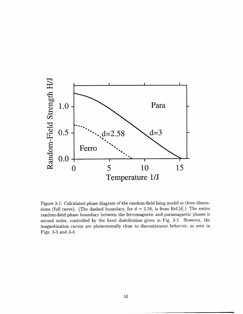
�-nI-

UO

0':� 1.0$--4

Cn7�r-.-q

0 0.54�

00r41. 0.0�.\j

C4 0 5 to 15Temperature I J

Figure 31: Calculated phase diagram of the random-field Ising model in three dimen-sions (full curve). (The dashed boundary, for d - 258, is from Ref.[4].) The entirerandom-field phase boundary between the ferromagnetic and paramagnetic phases issecond order, controlled by the fixed distribution given in Fig. 32. However, themagnetization curves are phenomenally close to discontinuous behavior, as seen inFigs. 33 and 34.

56

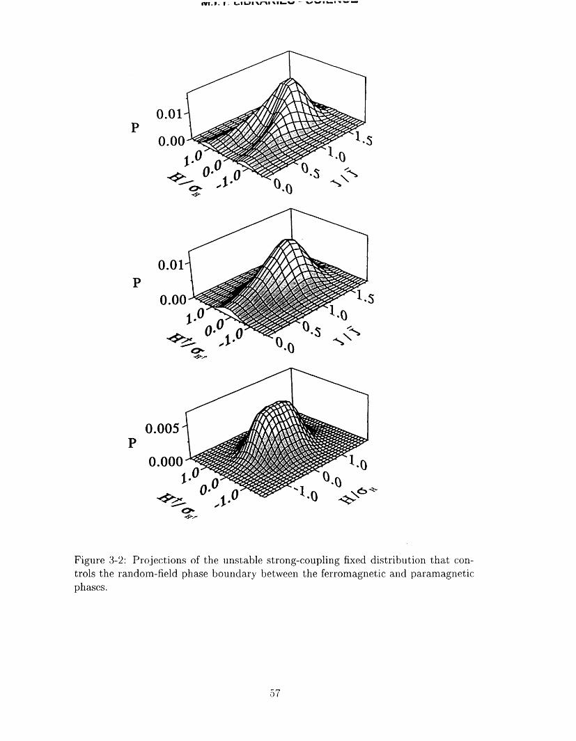
VVI.N. V ILJIIr-%v,%WL-w

0.P

0

0.01

S

PS0.0(

_tP-4>-,-

P

Figure 32: Projections of the unstable strong-coupling fixed distribution that con-trols the randorn-field phase boundary between the ferromagnetic and paramagneticphases.

57

0.005

0.00C

_-!Pt_C7.

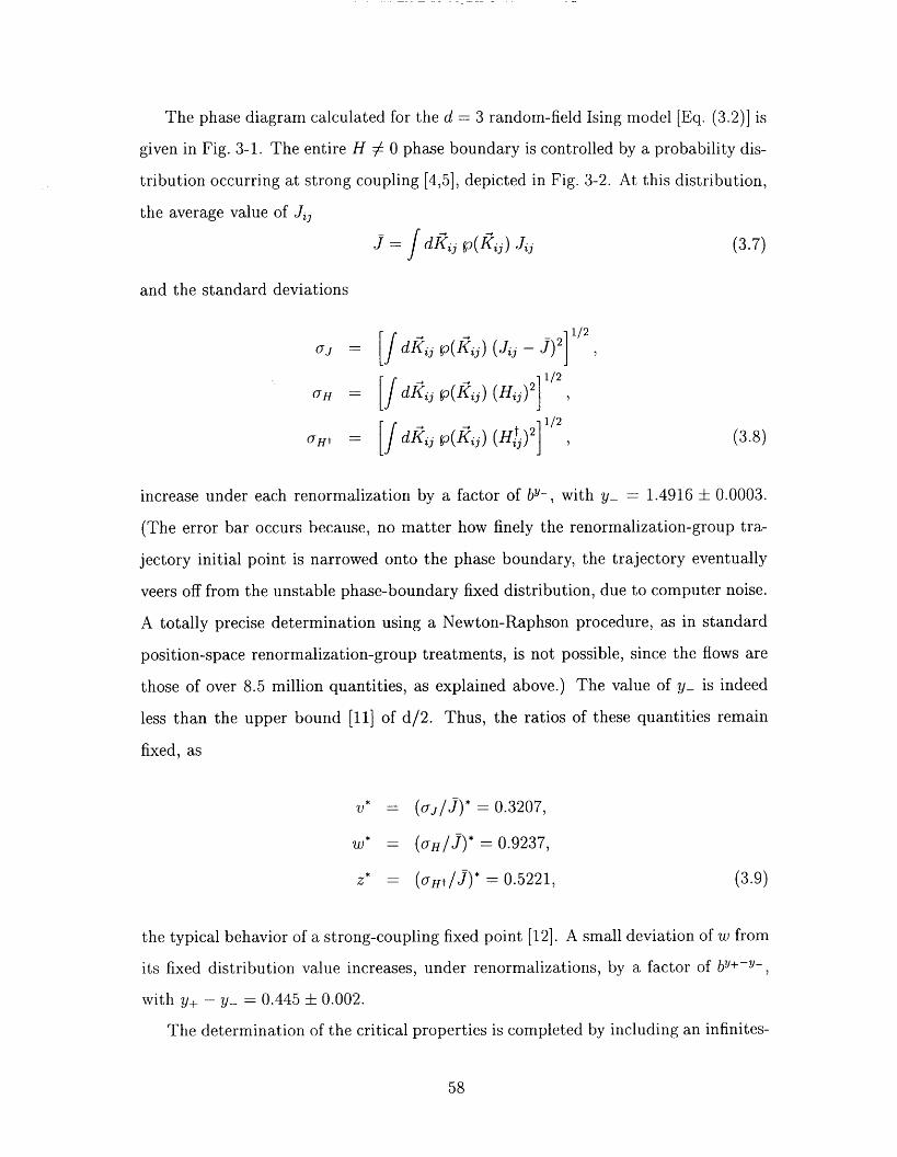
The phase diagram calculated for the d 3 random-field Ising model Eq. 32) is

given in Fig. 31. The entire H phase boundary is controlled by a probability d-

'but' ing at strong coupling 4,5], depicted in Fig. 32. At this distribution,

the average value of Jij

dkij V(kij) Jij (3.7)

and the standard deviations

j)2 /2OIJ dkij p(kij) (Jij - I

/2GrH dkij pkij) (Hij)2 I

OIHt dki p(kij) (H� 21/2 (3-8)1j) I

increase under each renormalization by a factor of by-, with y- 1.4916 0.0003.

(The error bar occurs because, no matter how finely the renormalization-group tra-

jectory initial point is narrowed onto the phase boundary, the trajectory eventually

veers off from the unstable phase-boundary fixed distribution, due to computer noise.

A totally precise determination using a Newton-Raphson procedure, as in standard

position-space renormalization-group treatments, is not possible, since the flows are

those of over 8.5 million quantities, as explained above.) The value of y- is indeed

less than the upper bound [11] of d/2. Thus, the ratios of these quantities remain

fixed, as

V (uilJ) 0.3207,

W* (UHIJ)* 0.9237,

z 0.5221, (3.9)

the typical behavior of a strong-coupling fixed point 12]. A small deviation of w from

its fixed distribution value increases, under renormalizations, by a factor of by+-Y-,

with y - y- 0445 ± 0002.

The determination of the critical properties is completed by including an nfinites-

58

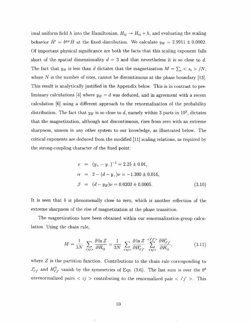
irnal uniform field h into the Hamiltonian, Hj - Hj + h, and evaluating the scaling

behavior hl' -- bYH ft at the fixed distribution. We calculate yH 29911 ± 00002.

Of important physical significance are both the facts that this scaling exponent falls

short of the spatial dimensionality d - 3 and that nevertheless it is so close to d.

The fact that yH is less than d dictates that the magnetization M -_ < si > IN,

where N is the number of sites, cannot be discontinuous at the phase boundary [13].

This result is aalytically justified in the Appendix below. This is in contrast to pre-

liminary calculations 4 where yff = d was deduced, and in agreement with a recent

calculation 6 sing a different approach to the renormalization of the probability

distribution. Te fact that yH is so close to d, namely within 3 parts in 0', dictates

that the magnetization, although not discontinuous, rises from zero with an extreme

sharpness, unseen in any other system to our knowledge, as illustrated below. The

critical exponents are deduced from the modified [11] scaling relations, as required by

the strong-coupling character of the fixed point:

v (y+ - y_)-1 -_ 225 ± .01,

a 2 - d - y-)v = 1-390 ± 0016,

0 (d - yff)v = 00200 ± 0.0005. (3-10)

It is seen that b is phenomenally close to zero, which is another reflection of the

extreme sharpness of the rise of magnetization at the phase transition.

The magnetizations have been obtained within our renormalization-group calcu-

lation. Using te chain rule,

13M_ I alnZ I a In Z < > li',j,E I3N allij 3N M, (9H,.<ij> < ZJ > I] < >

where Z is the partition function. Contributions to the chain rule corresponding to

Jlj, and 1"'ifftj, vanish by the symmetries of Eqs. 36). The last sum is over the b d

unrenormalized prs < ij > contributing to the renormalized pair < "'J > This

59

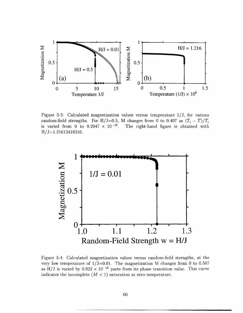
H/ = 1216

(b)I -

I

I-

I I

r.-40+-IM-�i0r_UOM

r_0. -4

M

N.t0toM

0.5 0.5

000.5 1

Temperature (I/J) X 106

0 1.50 5 10 15

Temperature 1/J

values versus temperature 1/J, for variousM changes from to 0407 as (T - T)IT,

The right-hand figure is obtained with

Figure 33: Calculated magnetizationrandom-field strengths. For H/J-0.5,is varied from to 02947 x 10-".H/J--1.21613418316.

I I I I I I

0. r..q

N

rIb�uCZ$

0. -

01.1 I 1.2

I

1.31.0

60

1 = .01I

Random-Field Strength w = H/J

Figure 34: Calculated magnetization values versus random-field strengths, at thevery low temperature of I/J-0.01. The magnetization M changes from to 0567as H/J is varied by 0822 x10-16 parts from its phase transition value. This curveindicates the incomplete (M < ) saturation at zero temperature.

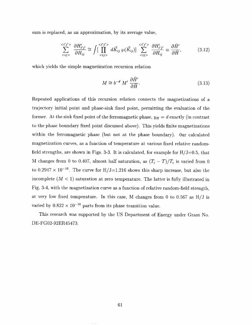
sum is replaced, as an approximation, by its average value,

<ifjl:> <i/j/> Mj',j, Mlallij dKjj p(Kij)] qHjj - aft (3-12)

<�ZJ> <ij> <ii>

which yields the simple magnetization recursion relation

M b -d MI (3.13)aH'

Repeated applications of this recursion relation connects the magnetizations of a

trajectory initial point and phase-sink fixed point, permitting the evaluation of the

former. At the sink fixed point of the ferromagnetic phase, yH d exactly (in contrast

to te hase bundary fixed point discussed above). This yields finite magnetizations

within the ferromagnetic phase (but not at the phase boundary). Our calculated

magnetization urves, as a function of temperature at various fixed relative random-

field strengths, are shown in Figs. 33. It is calculated, for example for H/J-0.5, that

M changes from to 0407, almost half saturation, as (T - T)IT, is varied from

to 02947 x 10---16 - The curve for H/J-1.216 shows this sharp increase, but also the

incomplete (M < ) saturation at zero temperature. The latter is fully illustrated in

Fig. 34, with the magnetization curve as a function of relative random-field strength,

at very low fixed temperature. In this case, M changes from to 0567 as H/J is

varied by 0822 x 10-16 parts from its phase transition value.

This research was supported by the US Department of Energy under Grant No.

DE-FG02-92EII45473.

61

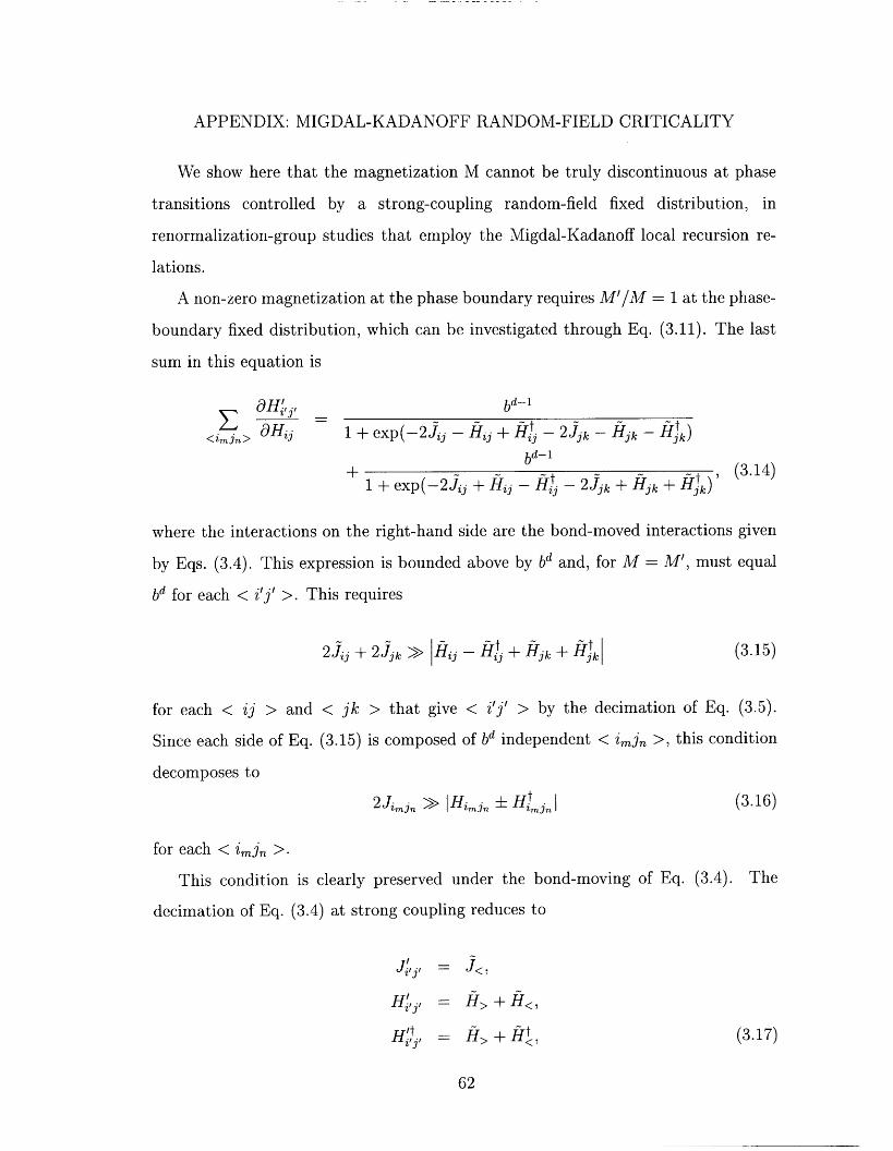
APPENDIX: MIGDAL-KADANOFF RANDOM-FIELD CRITICALITY

We show here that the magnetization M cannot be truly discontinuous at phase

transitions controlled by a strong-coupling random-field fixed distribution, in

renormalization-group studies that employ the Migdal-Kadanoff local recursion re-

lations.

A non-zero magnetization at the phase boundary requires M'IM I at the phase-

boundary fixed distribution, which can be investigated through Eq. 311). The last

sum in this equation is

b d-1

t<imin> allij I + exp (- 2 ij - ftij + H tj - 2 J k H k HJ'k)

bd-1+ t t (3.14)1 + exp(-2Jij + Hj - Hj - 2JJk + Hjk + Hjk

where the interactions on the right-hand side are the bond-moved interactions given

by Eqs. 34). This expression is bounded above by b d and, for M M', must equal

bd for each < " > This requires

T�ij t tJj 2 J k > Hi + Hjk + Hjk (3-15)

for each < 'J > and < jk > that give < " > by the decimation of Eq. (3-5).

Since each side of Eq. 3.15) is composed of b d independent < >, this condition

decomposes to

Jmj,, I Himj,, ± H j (3-16)

for each < im) >.

This condition is clearly preserved under the bond-moving of Eq. 34). The

decimation of Eq. 3.4) at strong coupling reduces to

Jill i I J<

Hi',il H> + H<,

H��.' H> + f (3.17)Z <

62

where the subscripts on the right-hand side refer to the relative values of Jij and Jjk-

It is clear from Eqs. 317) that the condition of Eq. 316) cannot be maintained,

under repeated renormalization-group transformations, for all localities. Thus, the

sum in Eq. 314) does not equal b d and M'IM :� 1, so that M = at the phase-

boundary fixed distribution and, therefore, along the entire phase boundary.

63

REFERENCES

[1] Y. Imry and S.-k- Ma, Phys. Rev. Lett. 35, 1399 1975).

[2] J.P. Hill, T.R. Thurston, R.W. Erwin, M.J. Ramstad, and R.J. Birgeneau, Phys.

Rev. Lett. 66, 3281 1991).

[31 D. Andelman and A.N. Berker, Phys. Rev. 29, 2630 1984).

[4] S.R. McKay and A.N. Berker, J. Appl. Phys. 64, 5785 1988).

[5] S.R. McKay and A.N. Berker, in New Trends in Magnetism, eds. M. D. Coutinho-

Filho and S. M. Rezende (World Scientific, Singapore, 1990).

[6] M.S. Cao and J. Machta, Phys. Rev. 48, 3177 1993).

[7] AX Berker and A. Falicov, Tr- J. Phys. 18, 347 (1994).

[8] A.A. Migdal, Zh. Eksp. Teor. Fiz. 69, 1457 1975) [Sov. Phys - JETP 42, 743

(1976)].

[9] L.P. Kadanoff, Ann. Phys. (N.Y.) 100, 359 1976).

[10] AX Berker and S. Ostlund, J. Phys. C 12, 4961 (1979).

[11 A Berker and S.R. McKay, Phys. Rev. 33, 4712 (1986).

[12] AX Berker and M. Wortis, Phys. Rev. 14, 4946 (1976).

[13] B. Nienhuis and M. Nauenberg, Phys. Rev. Lett. 35, 477 1975).

64

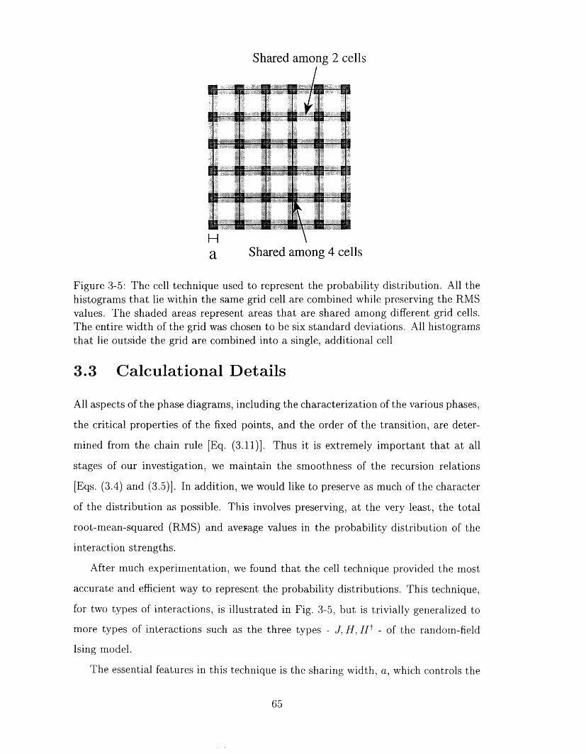
XA !K.:"' a 0

. ... ..... ..

Shared among 2 cells

Ha Shared among 4 cells

Figure 35: Th cll technique used to represent the probability distribution. All thehistograms that-, lie within the same grid cell are combined while preserving the RMSvalues. The shaded areas represent areas that are shared among different grid cells.The entire width of the grid was chosen to be six standard deviations. All histogramsthat lie outside the grid are combined into a single, additional cell

3.3 Calculational Details

All aspects of the phase diagrams, including the characterization of the various phases,

the ritical properties of the fixed points, and the order of the transition, are deter-

mined from the cain rule [Eq. 311)]. Thus it is extremely important that at all

stages of our investigation, we maintain the smoothness of the recursion relations

[Eqs. 34) and (3.5)]. In addition, we would like to preserve as much of the character

of the distribution as possible. This involves preserving, at the very least, the total

root-mean-squared (RMS) and aver-age values in the probability distribution of the

interaction strengths.

After much xperimentation, we found that the cell technique provided the most

accurate and efficient way to represent the probability distributions. This technique,

for two types interactions, is illustrated in Fig 35, but is trivially generalized to

more types of interactions such as the three types - J, H, Ht - of the random-field

Ising model.

The essential features in this technique is the sharing width, a, which controls the

65

smoothness of the recursion relations. As this width approaches zero, the recursion

relations lose smoothness. Consider the following scenario: a single histo ram with

finite probability is just to one side of a grid line. By just slightly changing the

initial conditions, this histogram can be moved to the other side of the grid line, thus

creating a finite change in the probability distribution at some stage in the recursion

relations. An infinitesimal change in the initial conditions results in a finite change at

a later stage. Quite contrary to being an unlikely scenario, we found in all cases with

zero width, that the phase boundaries were controlled by single histograms crossing

cell boundaries. To avoid these spurious results, we therefore introduced the sharing

width a.

As a histogram approaches a cell boundary, the sharing width determines the con-

tribution of that point to neighboring cells. The width is defined so that a histogram

exactly on the boundary contributes equally to both adjoining cells. Such a technique

preserves the smoothness of the recursion relations [Eqs. 34) and 3.5)], which is of

crucial importance in a problem where the difference between 29906 and 30000 is

the difference between a second- and first-order transition.

One does not, however, wish to set the value of a to an excessively large value. Not

only would this result in a smeared probability distribution, but also would drastically

increases the computation time. We found that a = .10 was a good compromise,

although several studies were done at various widths. It was found that as long as

a > 004, the results tended to be, reassuringly, insensitive to the exact value used.

In our representation of the probability distribution, we considered only J, H, HI >

0, exploiting the symmetries present in the problem [Eqs. 3.6)]. We represented each

cell by the total probability and the RMS values of J H and H for the totality

of histograms within that cell. Since the average of H and H are always 0, such

a technique preserves both the average and RMS values of H and H for the entire

distribution.

The strong-coupling fixed distribution that controls the random-field phase bound-

ary between the ferromagnetic and paramagnetic phases involves the competition be-

tween J and H. This dictates that we should treat all interactions on an equal basis.

66

It is for this reason that we represent the cell value of J by its RMS value, even though

neither the average, nor the RMS of J within the entire distribution is preserved.'

As a control, e also ran a few studies where the average value of J instead of the

RMS value was used. We found that this had no influence on the numerical results

for either the hase diagrams or the critical exponents.

The majority of our results were obtained by using five cell divisions for each type

of interaction for a total of 126 cells. To determine the accuracy of our methods,

however, studies with up to nine divisions, for a total of 730 cells, were used. In all

cases, however., the entire grid was centered on the averages of the distribution. The

w'dths of the cells were determined by requiring that the totality of the cells span six

standard deviations for each type of interaction.

'As one lets te total number of cells increase, however, the errors go to zero.

67

Chapter 4

Tricritical and Critical-Endpoint

Phenomena under Random Bonds

4.1 Introduction

Originally, it was thought that quenched random bonds had little effect on properties

of systems that undergo phase transitions. In complete contrast to the original beliefs,

the presence of bond randomness, in fact, has a drastic effect on systems that undergo

first-order phase transitions.' For d < 2 it is now believed that symmetry-breaking

first-order transitions are converted to second-order, while non-symmetry-breaking

transitions are eliminated, even with infinitesimal amounts of randomness. In d > 2,

a threshold amount of randomness is necessary.1

Although these arguments seem quite general, the prospects are actually quite

far-reaching. Consider the possibility of having water go smoothly from liquid to gas

at room temperature and pressure. It is not beyond notice that several important

materials, including freon, were selected precisely for that property. In addition

to being theoretically fascinating, there may be several practical consequences in

being able to eliminate a first-order transition. Many new materials with random

structures, including aerogels and other porous materials, may provide the key to

'A. N. Berker, J. Appl. Phys 70, 5491 (1991).

68

-- - I i� 1, . - I I 7r

such manipulations.

Based on our success with the random-field systems, we decided to extend our

techniques to a random-bond system. Although many of these models have existed

for some time, several fundamental questions remain unresolved. As an example,

consider the following: if one has a first-order transition that changes to a second-

order transition at some combination of the interaction strengths (a tricritical point),

one may ask wat happens to this phase diagram when quenched bond randomness is

introduced. The second-order transition line should be unaffected by the presence of

quenched random bonds.' At the very least, however, the elimination of a first-order

transition must-, have a significant effect upon the nature of the phase diagram.

It was shown for a second-order transition,' that the self-consistency condition

for well-defined critical properties unaffected by bond randomness is a negative spe-

cific heat exponent a. The extension of these arguments to first- and second-order

strong-coupling-, fixed points, allows one to use eigenvalue exponents for a particular

fixed point to etermine its stability towards the introduction of quenched random-

ness. These general arguments are not limited only to first- and second-order strong

coupling fixed oints but also apply to tricritical, critical endpoint, and multicritical

topologies as well.

One of the simplest systems that contains both first- and second-order transitions,

as well as tricritical and critical-endpoint phase diagrams, is the well-known Blume-

Emery-Griffiths odel. Application of the stability criteria mentioned above, show

that in d = 3 the pure-system tricritical and critical points are unstable to the

presence of infinitesimal amounts of bond randomness. One now begs the question of

what will appear in their place.

The resolution to these problems as well as the investigation into the effects of

quenched disorder into other systems was the motivation that led us to this system.

We used various theoretical and analytic tools to elucidate many of the unsolved

problems in this field. In addition, many new and unexpected results were found.

2Only if the critical exponent a is less than zero.3A. B. Harris, J. Phys. C 7 1671 1974).

69

Phenomena under Random Bonds

Alexis Falicov and A Nihat Berker

Department of Physics, Massachusetts Institute of Technology.

Cambridge, Massachusetts 02139, USA

Abstract

The effect of bond randomness is studied by renormalization-

group theory. In three dimensions, the pure-system tricritical

point is replaced by a line segment of second-order transitions

dominated by randomness and bounded by a multicritical point

and a random-bond tricritical point, which vanishes at zero tem-

perature at threshold randomness. This topology indicates a

violation of the empirical universality principle. The random-

bond tricritical. point renormalizes onto the fixed distribution of

random-field Ising criticality. The critical-endpoint phase dia-

gram is converted to the new topology at threshold randomness.

PACs Numbers: 64.60.Kw, 05.70.Jk, 75.10.Nr, 75.40.Cx

Running Title: Tricritical Phenomena under Random Bonds

70

4.2 T�ricritical and Critical-Endpoint

Although originally thought to play a rather innocuous role, quenched bond ran-domness can drastically affect first-order phase transitions. Thus, symmetry-break'

I ing

first-order phase transitions are converted to second-order phase transitions by in-

finitesimal bond randomness for spatial dimensionality d <2 and by bond randomness

beyond a threshold strength for d > 2 as indicated by general arguments 1-4] that are

supported, for d < 2 by rigorous mathematical work [5] and renormalization-group

calculations 6]. We present here renormalization-group calculations for d = 3 on the

effects of quenched bond randommness on a system that exhibits first-order phase

transitions within tricritical and critical-endpoint phase diagrams. We find that new

second-order phase transitions are introduced, in violation of the empirical univer-

sality principle. Furthermore, the effect of quenched bond randomness on tricritical

points, a long-standing question mark, receives a surprising and simple answer below.

A microscopic model that exhibits first-order phase transitions within tricritical

and critical-endpoint phase diagrams is the Blume-Emery-Griffiths model 7 with

Hamiltonian

- H Jsj sj + 1: K2 82 AS2 (4.1)i j<ij> <ij'> i

where i 0, ±1 at each site i of a lattice and < i > indicates summation over all

nearest-neighbor pairs of sites. This Hamiltonian can be rewritten as

8282 (82 2) (82 _ S2)],OH [Jsisj + K +D + Dt (4.2)i j i<Z3 >

where is, on the cubic lattice, on the increasing coordinate side of i. The ordered

phases of this model are up-magnetized, (Si > 0, and down-magnetized, (Si) < .

The symmetry that is broken is global spin-reversal symmetry. Since each of the

tern-is in the amiltonian above is invariant under this symmetry, the correspond-

ing coupling cnstants, J, K, D, Dt, are bond strengths. Bond randomness obtains

when the bond strengths vary randomly across the system, governed by a quenched

pro bability distribution Jij, Kij, D -j, Di.)Zj

The renorn-lalization-group solution of the quenched random system is via the

71

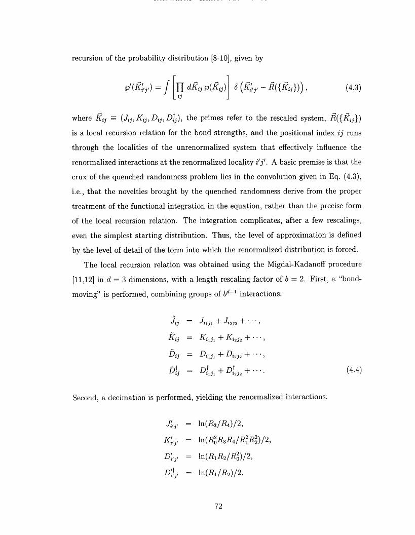
recursion of the probability distribution [8-10], given by

VIAT) dkij Vkij) 6 ki',j - jkjjj)) (4.3)ij

where kj = Jij, Kij, Dij, Di.), the primes refer to the rescaled system,

zj f?,

is a local recursion relation for the bond strengths, and the positional index ij runs

through the localities of the unrenormalized system that effectively influence the

renormalized interactions at the renormalized locality Vj'. A basic premise is that the

crux of the quenched randomness problem lies in the convolution given in Eq. 43),

i.e., that the novelties brought by the quenched randomness derive from the proper

treatment of the functional integration in the equation, rather than the precise form

of the local recursion relation. The integration complicates, after a few rescalings,

even the simplest starting distribution. Thus, the level of approximation is defined

by the level of detail of the form into which the renormalized distribution is forced.

The local recursion relation was obtained using the Migdal-Kadanoff procedure

[11,12] in d - 3 dimensions, with a length resealing factor of b = 2 First, a bond-

moving" is performed, combining groups of V-1 interactions:

jij jilil + ji2j2 +

Kii Kilil + Ki2j2 +

Dij Dj1jl + D i2j2 +

bt Di +DI +. (4.4)13 till 1232

Second, a decimation is performed, yielding the renormalized interactions:

Jilli, ln(R3/R4)/2,Ki',j, ln(R 2 R3R4/R 2R 2)/2,

0 2

D ln(RlR2/R 2) /2,i 0

Di 11j, ln(RI/R2) /2

72

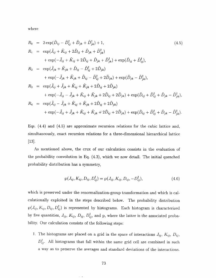
where

Ro = 2 exp(bi - bt + fjk D J + 1 (4.5)Ri = exp(jij + ki + 2f)ij + bjk + ftk)

+ exp(-jij + k�j + 2bi + fjk + blk) + exp(bij + bl.),3

R2 exp(j3k kj k + bij- bt + 2f)jk)

+ exp(-3k + k3k + bij - bt + 2b3k) + exp(bjk ')jtk),

R3 exp jjj+ jk kij + kjk+ 2bij + 2f)jk)

+ exp(-j - 3k kij + k3k+ 2Aj + 2bjk) + exp(b.j + bt + bjk f)tk),R4 exp( Ji,, Ji k +Kij + Kjk+ 2Djj + 2Djk)

exp(-jj + jjk+ kij + kik + 2ij + 2bjk) + exp(b - bt + bik - ftk)'

Eqs. 44) and 45) are approximate recursion relations for the cubic lattice and,

simultaneously., exact recursion relations for a three-dimensional hierarchical lattice

[13].

As mentioned above, the crux of our calculation consists in the evaluation of

the probability convolution in Eq. 43), which we now detail. The initial quenched

probability distribution has a symmetry,

p(Jij, Kij, Dj D. = ij, K , Dj, -Dt.), (4.6)13 3 23

which is preserved under the renormalization-group transformation and which is cal-

culationally exploited in the steps described below. The probability distribution

p(jij, fij, Dj, Dj) is represented by histograms. Each histogram is characterized

by five quantities Jij, Kij, Dj, Dt., and p, where the latter is the associated proba-13

bility. Our calculation consists of the following steps:

1. The histograms are placed on a grid in the space of interactions Jij, Kij, Dj,

Dt All histograms that fall within the same grid cell are combined in such

a way as to preserve the averages and standard deviations of the interactions.

73

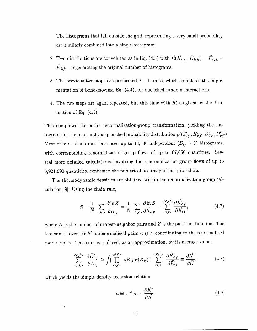
The histograms that fall outside the grid, representing a very small probability,

are similarly combined into a single histogram.

2. Two distributions are convoluted as in Eq. 43) with K-ij,, Ri2h) --':: kilil +

Ki 2 J2 regenerating the original number of histograms.

3. The previous two steps are performed d - I times, which completes the imple-

mentation of bond-moving, Eq. 44), for quenched random interactions.

4. The two steps are again repeated, but this time with R) as given by the deci-

mation of Eq. 4.5).

This completes the entire renormalization-group transformation, yielding the his-

tograms for the renormalized quenched probability distribution Ji',j,, Ki',j,, D',j,, Di'ftj,).

Most of our calculations have used up to 13,530 independent DI > 0) histograms,

with corresponding renormalization-group flows of up to 67,650 quantities. Sev-

eral more detailed calculations, involving the renormalization-group flows of up to

3,921,890 quantities, confirmed the numerical accuracy of our procedure.

The thermodynamic densities are obtained within the renormalization-group cal-

culation 9]. Using the chain rule,

<iljl>1 O In Z 1 9 In Z YKi',j,n = E �� - E �� . E 7 (4.7)N <ij> 9ij N <jj>,9Kj',j, <ij> aj

where N is the number of nearest-neighbor pairs and Z is the partition function. The

last sum is over the b d unrenormalized pairs < ij > contributing to the renormalized

pair < ij' >. This sum is replaced, as an approximation, by its average value,

<iljf> <i/j'/> - -<"j'> aj',j, , Mj'y 9K'E �_ � - I[ 11 dkij V (kij) I - - (4.8)<ij> aKij <ij> <ii> aKij ak,

which yields the simple density recursion relation

ii - b-d ji, ak' (4.9)aK

74

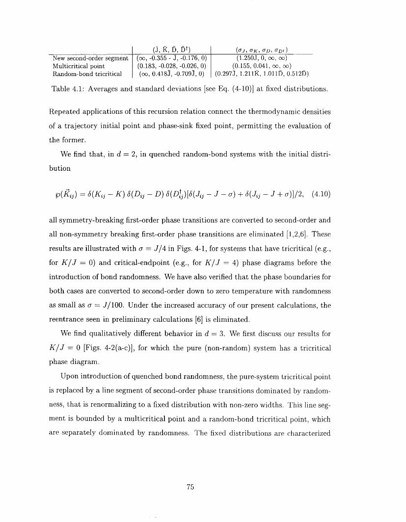
- -, 0 f(J, K Y) (O'J i OK) OD i 17 D tNew second-order segment (oo, 0.355 - J, 0.176, 0) (1.250J, 0, oc, oo)Multicritical point (0.183, 0.028, 0.026, 0) (0-155 0041, oc, oo)Random-bond tricritical (oo, 0.418j, -0.709j, 0) (0.297J, 1.211k, I0110, 0.512D)

Table 41: Averages and standard deviations [see Eq. 4-10)] at fixed distributions.

Repeated applications of this recursion relation connect the thermodynamic densities

of a trajectory initial point and phase-sink fixed point, permitting the evaluation of

the former.

We find that, in d 2 in quenched random-bond systems with the initial distri-

bution

p(-Kij = 6(Ki (Dt-)[J(Jjj - J - a) 6j - J + o)]12, 410)

j - K) (Dij - D) �j

all symmetry-breaking first-order phase transitions are converted to second-order and

all non-symmetry breaking first-order phase transitions are eliminated [1,2,6]. These

results are illustrated with a = J14 in Figs 41, for systems that have tricritical (e.g.,

for KIJ = 0) and critical-endpoint (e.g., for KIJ = 4 phase diagrams before the

introduction of ond randomness. We have also verified that the phase boundaries for

both cases are converted to second-order down to zero temperature with randomness

as small as a = J1100. Under the increased accuracy of our present calculations, the

reentrance seen in preliminary calculations 6 is eliminated.

We find qualitatively different behavior in d = I We first discuss our results for

KIJ -_ [Figs. 4-2(a-c)], for which the pure (non-random) system has a tricritical

phase diagram.

Upon introduction of quenched bond randomness, the pure-system tricritical point

is replaced by a line segment of second-order phase transitions dominated by random-

ness, that is renormalizing to a fixed distribution with non-zero widths. This line seg-

ment is bounded by a multicritical point and a random-bond tricritical point, which

are sparately dminated by randomness. The fixed distributions are caracterized

75

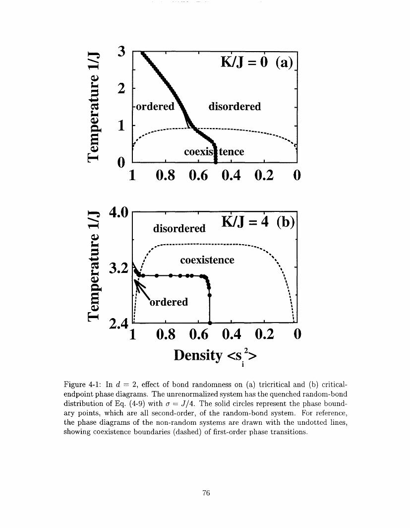
3

2

1

0

r.-IW

;z*Ni

CZ

W

5E*

1 0.8 06 04 02 0

4.0

3.2

2.4

r_�

W

:z-*Nil

CZ

W

F_-�

I

I-------------------------------------

aI

II

I

I

aIIIIIIII

tence

1 0.8 06 04 02 0

76

IkI = (b)disordered

of coexis,

0 a 0 __ 0 SO -

.I rderedII

I __ I

Density <S 2>i

Figure 41: In d = 2 effect of bond randomness on (a) tricritical and (b) critical-endpoint phase diagrams. The unrenormalized system has the quenched random-bonddistribution of Eq. 49) with = J14. The solid circles represent the phase bound-ary points, which are all second-order, of the random-bond system. For reference,the phase diagrams of the non-random systems are drawn with the undotted lines,showing coexistence boundaries (dashed) of first-order phase transitions.

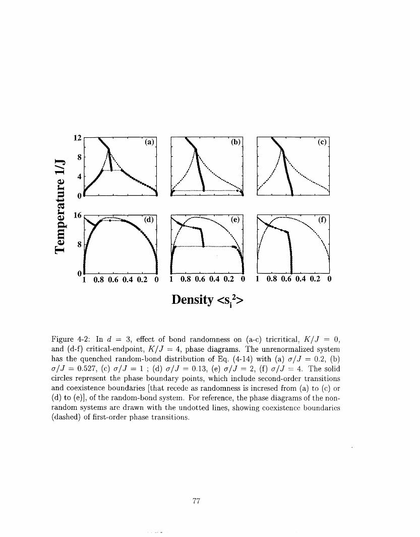
12

.......... ....................

LW�Lj to

5W 8

a

I- (e) - M .

I %.%i........ ................ I.. I % -

44 IIII

I

1 0.8 06 04 02 1 0.8 06 04 02 1 0.8 06 04 02

Density<S.2>I

Figure 42: In d = 3 effect of bond randomness on (a-c) tricritical, KIJ 0,and (d-f) critical-endpoint, KIJ 4 phase diagrams. The unrenormalized systemhas the quenched random-bond distribution of Eq. 414) with (a) oIJ = 02, (b)uIJ 0527, (c) oIJ I d) oIJ = 013, (e) oIJ = 2 (f) aIJ = 4 The solidcircles represent the phase boundary points, which include second-order transitionsand coexistence boundaries [that recede as randomness is incresed from (a) to (c or(d) to (e)], of the random-bond system. For reference, the phase diagrams of the non-random systems are drawn with the undotted lines, showing coexistence boundaries(dashed) of first-order phase transitions.

77

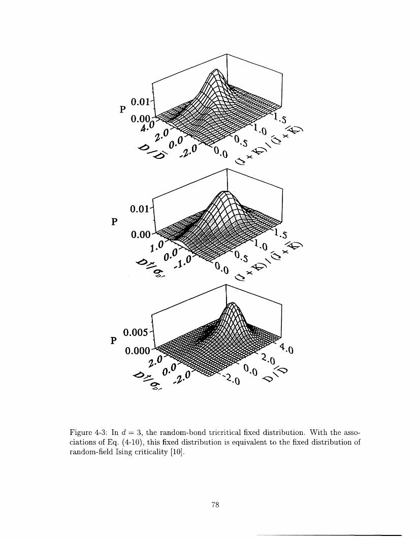
p

II

0.01p

O.OC

-e>

S

K

p0

Figure 43: In d 3 the random-bond tricritical fixed distribution. With the asso-ciations of Eq. 40), this fixed distribution is equivalent to the fixed distribution ofrandom-field Ising criticality [10].

78

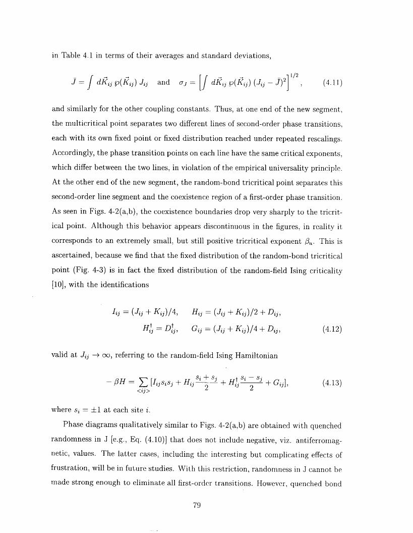
in Table 41 in terms of their averages and standard deviations,

_)2 1/2i dRij Vkij) Jjj and o - f dkij pkij) (Jij J

and similarly for the other coupling constants. Thus, at one end of the new segment,

the multicritical point separates two different lines of second-order phase transitions,

each with its own fixed point or fixed distribution reached under repeated rescalings.

Accordingly, the phase transition points on each line have the same critical exponents,

which differ between the two lines, in violation of the empirical universality principle.

At the other end of the new segment, the random-bond tricritical point separates this

second-order line segment and the coexistence region of a first-order phase transition.

As seen in Figs. 4-2(ab), the coexistence boundaries drop very sharply to the tricrit-

ical point. Although this behavior appears discontinuous in the figures, in reality it

corresponds to an extremely small, but still positive tricritical exponent This is

ascertained, because we find that the fixed distribution of the random-bond tricritical

point (Fig. 43) is in fact the fixed distribution of the random-field Ising criticality

[10], with the ientifications

Iij - (Jij + Kij)14, Hij (Jij + Kjj 2 Dj,

H� - Dt Gij - (Jij + Kij)14 + Dj, (4.12)

valid at, Jij oo, referring to the random-field Ising Hamiltonian

- OH [Iijsisj + Hj + H1. st - si. G] (4.13)2 2<ii>

where si -_ ± at each site

Phase diagrams qualitatively similar to Figs. 4-2(ab) are obtained with quenched

randomness in J [e.g., Eq. 410)] that does not include negative, viz. antiferromag-

netic, values. he latter cases, including the interesting but complicating effects of

frustration, will. b in future studies. With this restriction, randomness in J cannot be

made strong enough to eliminate all first-order transitions. However, quenched bond

79

randomness, without the calculational complication of frustration, can be studied

with the initial distribution

p(Kij - j - J) 6Kij - K) [6(Dij - D - ,) 6Dt.) + 6(Dj - D + o) 6(Dt-),I Z 1]

6(Dij - D) 6(Dt - ,) + 6(D- - D) 6(Dt + o)]14. (4.14)ij 13 ij

Recall that the symmetry that is broken is global spin-reversal symmetry and, since

each of the terms in the Hamiltonian of Eq. 41) is invariant under this symmetry,

each of the corresponding coupling constants, J, K, D, or Dt, is a bond strength.

Thus, Fig. 4-2(c) shows that, with sufficient amount of quenched bond randomness,

the first-order phase transition is entirely eliminated via the random-bond tricritical

point reaching zero temperature.

Figs. 4-2(d-f) show our results for KIJ 4 for which the pure system has a

critical-endpoint phase diagram. For small amounts of bond randomness, the critical-

endpoint phase diagram persists, with the isolated critical point lowered in tempera-

ture and transformed to a random-field Ising critical point [Fig. 4-2(d)]. This can be

seen from the very precipitous behaviour of the coexistence boundary, correspond-

ing to a very small but positive critical exponent 14,10]. As bond randomness

is increased, the random-bond tricritical phase diagram [Fig. 4-2(e)] and the fully

second-order phase diagram [Fig. 4-2(f)] are obtained. These phase diagrams have

been discussed above.

This research was supported by the US Department of Energy under Grant No.

DE-FG02-92ER45473.

80

REFERENCES

[1 AX Berker, J. Appl. Phys. 70, 5941 1991).

[2] A.N. Berker, Physica A 194, 72 1993).

[31 AX Berker and A. Falicov, Tr. J. Phys. 18, 347 1994).

[41 For the conversion of first-order phase transitions to second-order by infinites-

imal bond randomness, the crossover dimension was reported in Refs. [11 and

[2] as d, 2 for n = I component microscopic degrees of freedom and as d, -_ 4

for n > 2 component microscopic degrees of freedom. The latter is incorrect

and is hereby corrected as d, - 2 for all systems. The reason for this is that

the free energy increase due to the interface created by an ordered island inside

a disordered region (or vice versa) scales as L d-I with the linear extent L of

the island, even for n > 2 This can also be inferred from the effective-vacancy

renormalization-group argument and Fig. I in Ref. [1].

[5] J. Wehr nd M. Aizenman, Phys. Rev. Lett. 62, 2503 1989).

[6] K. Hui and AX Berker, Phys. Rev. Lett. 62, 2507 1989); 63, 2433(E) (1989).

[71 M. Blume, V.J. Emery, and R.B. Griffiths, Phys. Rev. A 4 1071 (1971).

[8] D. Andelman and AX Berker, Phys. Rev. 29, 2630 1984).

[9.1 S.R. McKay and AX Berker, J. Appl. Phys. 64, 5785 1988).

[10] A. Falicov AX Berker, and S.R. McKay, M.I.T.-Maine preprint (1994).

[11] A.A. Migdal, h. Eksp. Teor. Fiz. 69, 1457 1975) [Sov. Phys. - JETP 42, 743

(1976)].

[121 L.P. Kad-anoff, Ann. Phys. (N.Y.) 100, 359 1976).

1 3] AX Berker and S. Ostlund, J. Phys. C 12, 4961 1979).

14'1 M.S. Cao ad J. Machta, Phys. Rev. 48, 3177 1993).

81

Due to additional complications in the random-bond Blume-Emery-Griffiths model,

several new methods, in addition to the cell technique (see Fig. 35) were developed for

the representation of the probability distributions. The first complication is that both

D and K can take both positive and negative values, which results in an ambiguity

in the sign of the RMS values within each cell. In order to resolve this problem, we

preserve the averages, instead of the RMS values, of J, K, D within each cell. The

symmetry of the problem [Eq. 4.6)] dictates that the average of Dt will remain zero.

Thus for that one variable, we use the RMS values. Therefore, at the end of this stage

in our procedure, our distribution has the same average values but different standard

deviations from the original distribution.

For systems with quenched randomness, the standard deviation is essential to de-

termine the lower critical dimension of a system.' It is therefore of crucial importance

to preserve the standard deviations. This is accomplished by the following transfor-

mation. We calculate the new standard deviations and divide this by the standard

deviations of the original distribution. This gives us a scaling factor for each dimen-

sion. We then shift every point by a factor proportional to its distance from the

distribution averages multiplied by the scaling factor. It can be shown that such a

procedure is

1. analytic,

2. preserves the averages of the distribution,

3. preserves the standard deviations of the distribution, and

4. becomes exact as the number of grid points is increased.

This technique allowed us to determine the properties of all the fixed points with

extreme accuracy.

4A. N. Berker, Phys. Rev. 29, 5243 (1984).

82

4.3 Computational Details

As opposed to the random-field Ising model, however, many of the fixed distribu-

tions wre not spread over the entire space of the interaction strengths. In fact, many

distributions seemed to bunch on single lines, although analytic expressions for these

lines eluded discovery. As a result, it was necessary to increase the sharing width. We

found, in this cse, that b > 02 provided the numerical stability necesary to analyze

the fixed dstributions.

4.4 Fixed Point Properties

A total of 16 fixed points, both pure or dominated by randomness, were found. Three

of the new fixed points are listed in Table 4 1. A complete listing of all the fixed points

we found is listed in Table 42, along with our best estimates for their locations and

w'dths. The corresponding relevant eigenvalue exponents for each of these fixed points

is given in Table 43. One notes that many of the exponents differ considerably

between the corresponding pure and randomness-dominated points. For instance,

comparison of the pure system tricritical point T* with the random-bond tricritical

point T*, shows that both the locations of the fixed points and their eigenvalue

exponents are completely different, signifying new critical properties.

As an example, we have provided the connectivities of all the fixed points present

in both the random-bond tricritical (Fig. 44) and the random-bond critical endpoint

phase diagrams (Fig 45). The actual phase diagrams are shown in Fig. 42. Note the

presence of the new segment of second-order transitions (C,), within the random-bond

tricritical phase diagram.

83

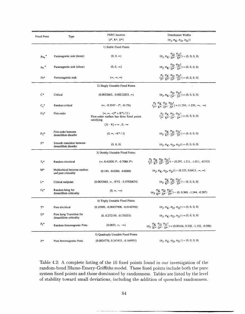
Fixed Point Type PSRG location Distribution Widths(J*, K*, D*) ((FJ, OK OD, Dt)

1) Stable Fixed Points

Paramagnetic sink (dense) (0 0 (0j, !D ant (0, 0, 0, 0)P4 'UK, D* D*

Pa-* Paramagnetic sink (dilute) (0 0 (OJ, OK, OD ODf (0 0 0 0)D* D*

Gi K OD !DtFe* Ferromagnetic sink -_ = 0 0 0 0)

K*' D* D*

2) Singly Unstable Fixed Points

OD Or)tC* Critical (0.0652663, 0.00212833, (0j, OK, = (0, 0 0 0)

D* D*

Cr* Random critical -0.3547 - J*, -0. 176) OJ OK D ODt (1.250, 1.250,K* ' D* -D*

F3 * First-order -(J* + K*) / 2 Gi K OD GDtFirst-order surface has three fixed points 5 I K* D* (0 0 0 0)satisfying

QJ - K) 0,

F2 * First-order between (0, -, -K* 2 OK OD ODt (0 0 0 0)dense/dilute disorder K*' D* D*

S* Smooth transition between (0 0 0)dense/dilute disorder (GJ, OK, 'JD, GDO (0 0 0 0)

3) Doubly Unstable Fixed Points

Tr* Random tricritical 0.41830 J*, 0.7086 J*) OJ K D D t (0.297 1211, -1.011, 0.512)J` K*' D* D*

M* Multicritical between random (0. 183, 0.0280, 0.0260) (OJ, OK, OD, ODt = (0. 155 00413 and pure criticality

L* Critical endpoint (0.0652663, -, -K*/2 - 0.37920674) (0j, OK D ODt I 01 0 0)K*' D*' (0

Gr* Random Ising for (01 -1 OK D ODtdense/dilute criticality J' K*' D*' D* 1.244, 0.587)

4) Triply Unstable Fixed Points

T* Pure tricritical (0. 10369, 0.00437906, 0.0142938) (OJ, OK, OD, OD0 = , 0, 0, 0)

G* Pure Ising Transition for (0, 0.272159, 0.170353) (0j, OK, OD, ODt) = , 0, 0, 0)dense/dilute criticality

Pr* Random ferromagnetic Potts (0.0655, OK �113 F) t (0.00166 0328, 1.152, -0.588)li�((YJ, K* ,D* D*

5) Quadruply Unstable Fixed Points

(OJ OK'OD'ODt) = 0'0'0'0)P* Pure ferromagnetic Potts (0.0824776, 0.247433, 0.164955)

Table 4-2: A complete listing of the 16 fixed points found in our investigation of therandom-bond Blume-Emery-Griffiths model. These fixed points include both the puresystem fixed points and those dominated by randomness. Tables are listed by the levelof stability toward small deviations, including the addition of quenched randomness.

84

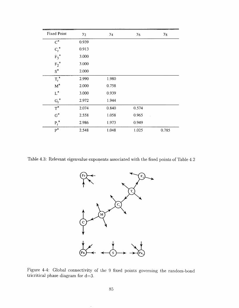
Fixed Point Y2 Y4 Y6 Y8

C* 0.939

Cr 0.913

F3 3.000

F 3.0002

S * 2.000

T 2.990 1.980r

M 2.000 0.758

L 3.000 0.939

G 2.972 1.944r

T 2.074 0.840 0.574

G 2.558 1.058 0.965

Pr 2.986 1.973 0.949

P * 2.548 1.048 1.025 0.785

Table 43: Relevant eigenvalue exponents associated with the fixed points of Table 42

Figure 44: Global connectivity of the 9 fixed points governing the random-bondtricritical phase iagram for d3.

85

a

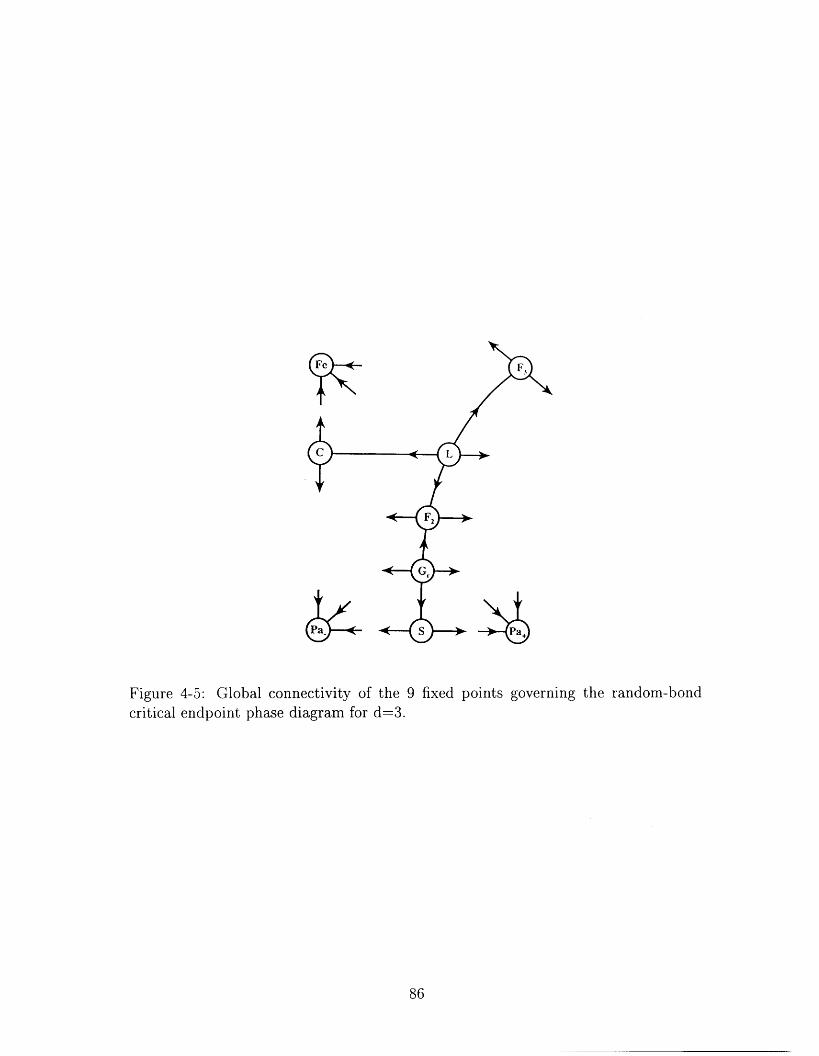
Figure 45: Global connectivity of the 9 fixed points governing the random-bondcritical endpoint phase diagram for d3.

86

I a

Chapter

The Phase Transitions of Helium

T\4ixtures in Porous \edia

5.1 Introduction

Aerogels, which are extremely light and stiff materials that can be manufactured with

porosities as high as 98%, have thermal and mechanical properties of great practical

value. For example, the thermal conductivity of aerogel tiles is about 00 times

smaller than tat of fully dense silica glass. They are, however, transparent to visible

light while at the same time being structurally rigid. All these properties make them

ideal for use ai isulating material in window panes.

The structure of aerogels, however, also makes them ideal candidates for the study

of quenched rndomness in systems that undergo phase transitions. As was deter-

mined from light, x-ray, and neutron scattering experiments, aerogels have a dilute,

random, and interconnected structure with pore sizes on many length scales. The ran-

dom nture of he aterial makes them ideal candidates to investigate the properties

of quenched randomness, while the porosity of the material allows for the insertion

of fluids.

The preferential adsorption, on the component silica strands, of one type of fluid

versus another, allows for the possibility of an experimentally accessible system which

may be a realization of either random-field or random-bond criticality. This was

87

verified by several experiments, including liquid-gas, binary-liquid and liquid crystal

studies in aerogels. It was therefore with great interest that we examined the results

from these systems.

One particular result, that was of theoretical interest to us, was the phase diagram

of 'He-'He systems in aerogel. This type of experiment, a realization of a random-

bond situation, allowed for the application of results from our renormalization-group

studies of the Blume-Emery-Griffiths model with quenched random bonds. We had

predicted that the second-order A line should extend down to zero temperature and

the tricritical phase diagram should disappear. Both these predictions were verified

experimentally.

There were in addition, however, new unexpected results: the appearance of a

phase separation entirely within the the superfluid phase and the onset of superfluid-

ity occurring at a small (about 5%) doping of 4He. The verification of our theoretical

predictions suggested that these new phenomena were a result of the correlated na-

ture of the randomness within the aerogel structure, as opposed to the uncorrelated

randomness present in our previous theoretical studies.

To examine all possibilities, it became necessary to construct a model that re-

flected the actual structure present in the aerogels. Once the structure was obtained,

the phase diagram could be investigated using the Monte Carlo technique. After

extensive investigation, our theories were verified and the novel experimental results

were duplicated.

88

Model for the Phase T�ransitions of Helium

Mixtures in Porous Media

Alexis Falicov and A. Nihat Berker

Department of Physics, Massachusetts Institute of Technology.

Cambridge, Massachusetts 02139, USA

Abstract

A lattice model is constructed for 3He_4 He mixtures in porous

media, characterized by correlated random chemical-potential

differences between isotopes. Sites with high chemical-potential

differences form a random connected porous structure, similar

to silica strands in aerogel. We find by Monte Carlo simulation

that the bulk tricritical phase diagram is replaced: The A-line

extends to zero temperature, as had been theoretically predicted

sorne time ago, and phase separation occurs within the superfluid

phase. These findings and the behavior of the order parameter

agree with recent experiments.

PACS Numbers: 67.60.Fp, 05.70.Fh, 64.60.Kw, 75.10.Nr

Running Title: Model for Helium Mixtures in Porous Media

89

5.2 A Correlated Random-Chemical-Potential

It has been argued that the introduction of quenched bond randomness has a dras-

tic effect on all temperature-driven first-order phase transitions [1,2]. If the first-order

phase transition involves symmetry breaking, it is converted to a second-order phase

transition, according to the argument. It now appears that this general prediction has

been confirmed experimentally with 'He-'He mixtures in aerogel 3 In the present

work, we analyze this experiment by constructing and studying a microscopic model

for 'He-'He mixtures in aerogel. We find that the first-order portion of the super-

fluid phase transition is converted to second-order, as mentioned above, -and that a

distinct phase separation occurs within the superfluid phase, understandably within

the context of the theoretical argument 12]. These results, as well as our calculated

order parameter behavior, agree with the experiment [3].

Silica aerogel is a highly porous material composed of silica strands in a random,

dilute, interconnected structure 46]. The high porosity allows the immersion of a

fluid, into a fixed randomly varying microscopic environment depending on the degree

of proximity of silica strands. Thus, an ideal platform obtains to study the effect of

quenched randomness on collective behavior and has already been used to examine

binary-liquid 7], liquid-gas [8], and liquid-crystal 91 phase transitions. In these cases,

however, the quenched randomness imposed by the aerogel couples directly to the or-

dering degrees of freedom, thus yielding a random-field situation [10,11]. 'He_4 He

mixtures in aerogel are qualitatively different from the aforementioned cases. The

random nature of the aerogel does not couple to the ordering, namely superfluid, de-

grees of freedom, but couples to the non-ordering degrees of freedom of concentration

fluctuations. Because of its higher mass, therefore lower zero-point motion, 'He has

a higher preference to reside close to the aerogel strands, whose random distribution

thus yields a random yet correlated (by the connectivity of the strands) chemical-

potential difference situation. In this problem, the chemical-potential difference is a

bond type of interaction, since it is invariant under the (superfluid) symmetry that

is broken at the phase transition. Thus, 'He-'He mixtures in aerogel yield a random-

bond situation.

A microscopic model introduced for bulk 'He_4 He mixtures (no aerogel) is the

90

Blume-Emery-(3fiffiths (BEG) model 12], with Hamiltonian

82S2 AS2-OH-E Js.sj E K<1]> <I]>

where si -_ 0, 4:1 at each site of a lattice and < j > indicates summation over all

nearest-neighbcir airs of sites. Occupation of site i by a 'He or 4He atom is repre-

sented by si or si ±1, respectively, with the sign in the latter case representing

the superfluid degree of freedom. Under this identification, J is a potential promoting

superfluidity, K -. K33+ K44- 2K34 reflects the (small) difference in interactions be-

tween the isotopes, and A is the chemical-potential difference between the isotopes.

All of these quantities have been rendered dimensionless by absorption of a factor of

0. The results shown here for mixtures are for K 0. This model yields the phase

diagram for bulk 3He_4 He mixtures [open circles in Fig. 51(a)], where the superfluid

and normal fluid are separated by a second-order phase boundary (the so-called A-

line) at high temperatures and high 4He concentrations and by the coexistence region

of a first-order phase transition at low temperatures.

We therefore odel 3 e_4 He mixtures in aerogel with the BEG model, but with a

chemical-potential difference that is site-dependent, Ai, with lower values occurring

along the randomly connected strands. Randomness in Ai does not break up-down

symmetry in si a.k.a. superfluid ordering symmetry), and therefore is an example of

quenched bond randomness. In fact, under scale change, the two other bond strengths

in Eq. (5. 1) also become random as Jij and Kij, but of course no random fields

are generated [13,14]. Renormalization-group calculations on the BEG model with

uncorrelated quenched bond randomness have shown that the first-order transitions

are converted t second-order transitions 13,14].

Here, to study 3He_4 He mixtures in aerogel, correlations (along the strands) in the

quenched random chemical-potential differences are used [15]. We have performed

Monte Carlo smulations on L x L x L cubic lattices, for 1 < L < 16, with periodic

boundary conditions, using the standard Metropolis importance sampling method.

The first part f our analysis was to tcgrow" a random, connected structure that

91

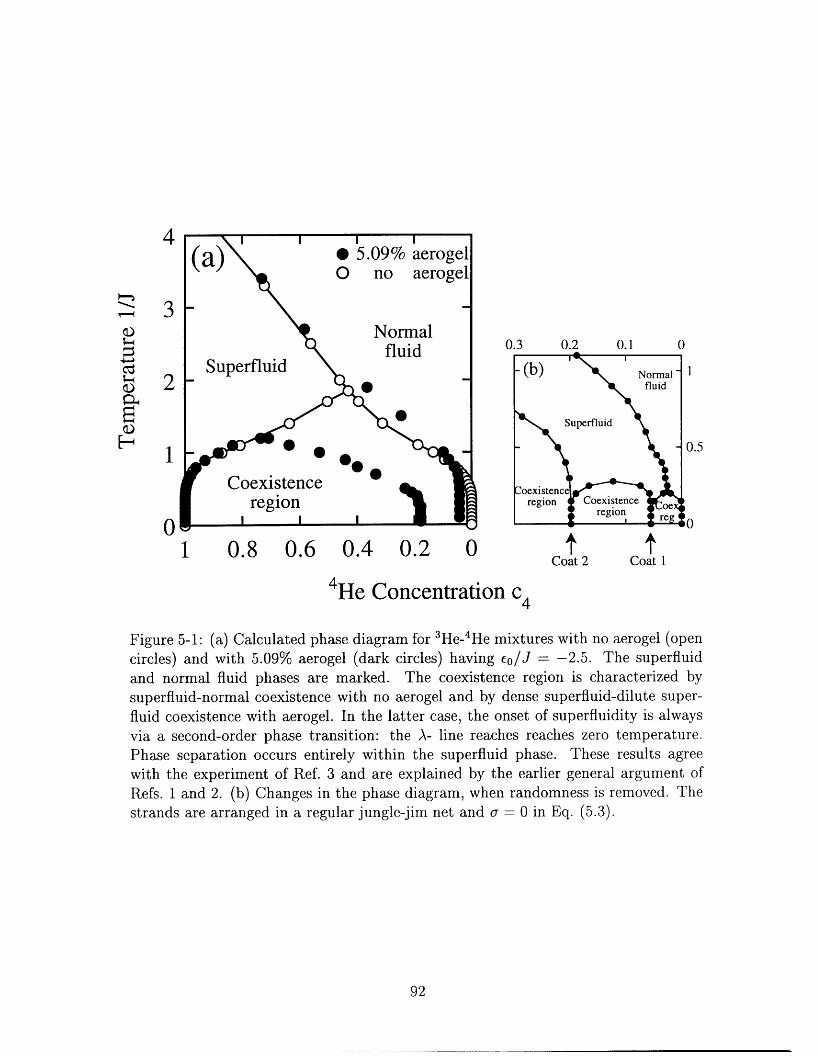
4

�-n3

U;-.4;Z+-jM;..4U 21:14

FiU

F-� I

n

0.3 0.2 0.1 0

.5

- 1 t tCoat 2 Coat

4 He Concentration c4

Figure 5-1: (a) Calculated phase diagram for 'He-'He mixtures with no aerogel (opencircles) and with 509% aerogel (dark circles) having IJ 2.5. The superfluidand normal fluid phases are marked. The coexistence region is characterized bysuperfluid-normal coexistence with no aerogel and by dense superfluid-dilute super-fluid coexistence with aerogel. In the latter case, the onset of superfluidity is alwaysvia a second-order phase transition: the A line reaches reaches zero temperature.Phase separation occurs entirely within the superfluid phase. These results agreewith the experiment of Ref 3 and are explained by the earlier general argument ofRefs. and 2 (b) Changes in the phase diagram, when randomness is removed. Thestrands are arranged in a regular 'ungle-jim net and a = in Eq. (5-3).

92

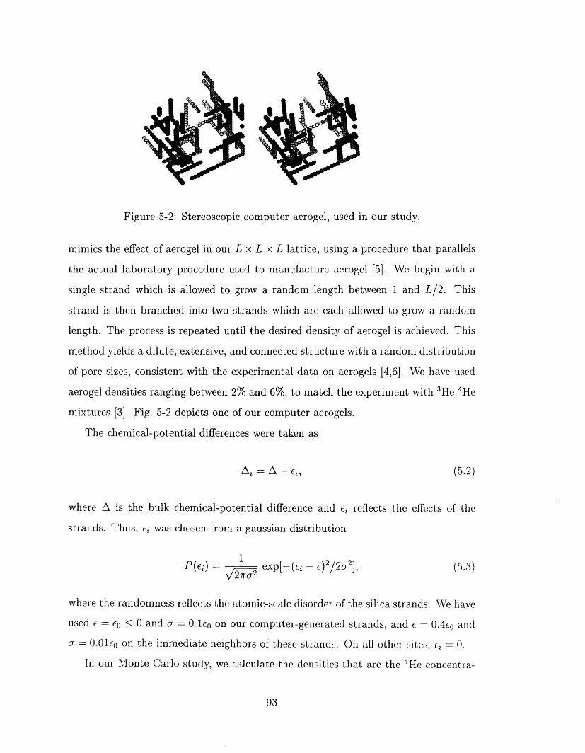
Figure 52: Stereoscopic computer aerogel, used in our study.

mimics the effect-, of aerogel in our L x L x L lattice, using a procedure that parallels

the actual laboratory procedure used to manufacture aerogel [5]. We begin with a

single strand which is allowed to grow a random length between I and L12. This

strand is then branched into two strands which are each allowed to grow a random

length. The process is repeated until the desired density of aerogel is achieved. This

method yields a dilute, extensive, and connected structure with a random distribution

of pore sizes, consistent with the experimental data on aerogels 46]. We have used

aerogel densities ranging between 2 and 6, to match the experiment with 3He_4 He

mixtures 3 Fig 52 depicts one of our computer aerogels.

The chemical-potential differences were taken as

Ai = A ,Ei, (5.2)

where A is the bulk chemical-potential difference and i reflects the effects of the

strands. Thus, ci was chosen from a gaussian distribution

P (,E ex 2/2 U2], (5-3)1 �727ro,2

where the randomness reflects the atomic-scale disorder of the silica strands. We have

used E < and. = .1co on our computer-generated strands, and = 0.4co and

o = 0-01t0 on the immediate neighbors of these strands. On all other sites, = .

In our Monte Carlo study, we calculate the densities that are the 'He concentra-

93

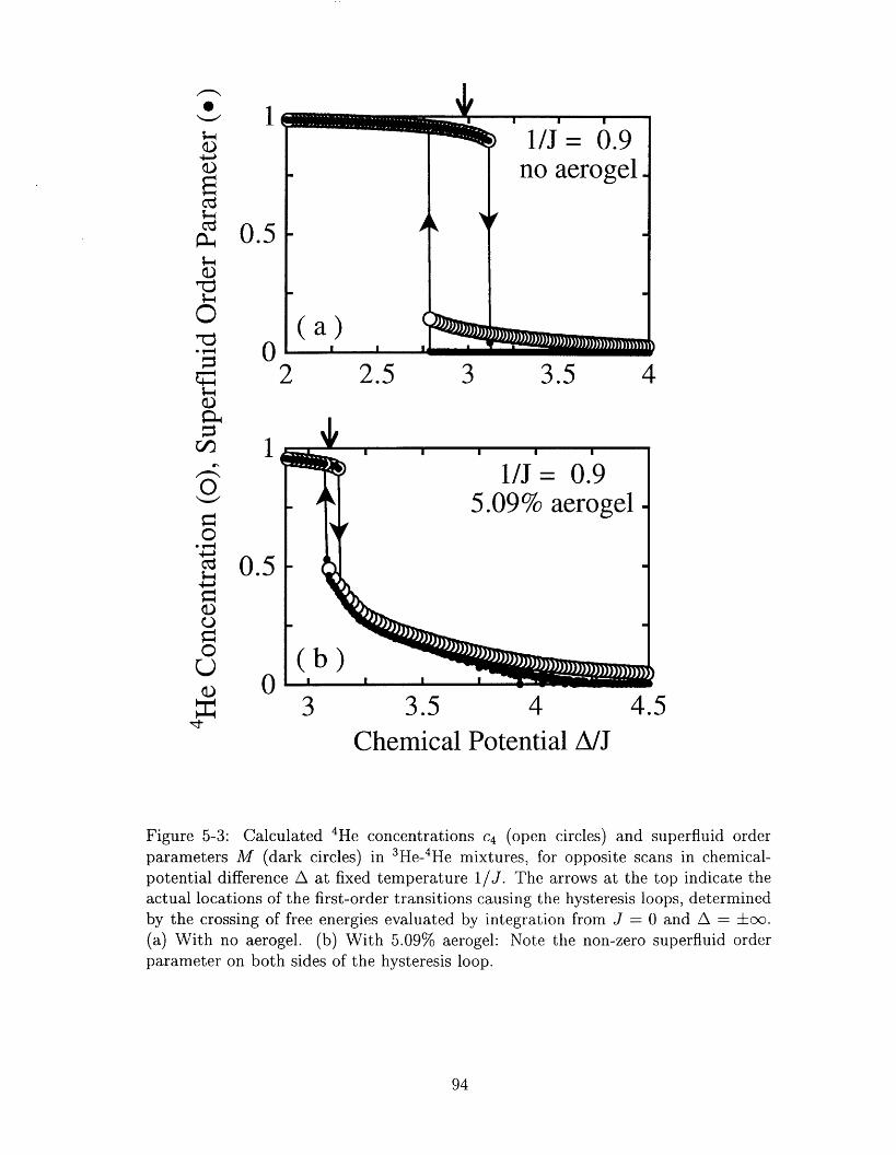
I___/ I

U4_jU�iM

t� 0.5P-.4

U7�

0

7:$. -4 n

N-f

C;� 2 2.5 3 3.5 4U0-%

:ZCn I

.11

0rI

. r..�0

Ajct 0.5;--q

0Ur40

U nI_X

3 3.5 4 4.5Chemical Potential A/J

Figure 53: Calculated 4He concentrations C4 (open circles) and superfluid orderparameters M (dark circles) in 3He_4 He mixtures, for opposite scans in chemical-potential difference A at fixed temperature 11J. The arrows at the top indicate theactual locations of the first-order transitions causing the hysteresis loops, determinedby the crossing of free energies evaluated by integration from J and A = 00.

(a) With no aerogel. (b) With 509% aerogel: Note the non-zero superfluid orderparameter on both sides of the hysteresis loop.

94

tion,

C4 s' IN, (5.4)

where N = L' is the number of sites, and the superfluid order parameter,

M -_ (1: si) IN. (5-5)i

Fig. 5-3(a) shows these densities for opposite scans of the chemical-potential difference

A at, fixed temperature 11J, in the absence of aerogel A first-order phase transition

can be seen by the hysteresis in these densities. The actual location of the transition

was determined by the crossing of free energies evaluated by integration from J 0

and D ±oo. Fig. 5-3(b) shows the same scans, but with 509% aerogel. A first-

order phase transition is again seen by the hysteresis, but with the striking feature

that the superfluid order parameter, M, although discontinuous at this first-order

transition, is non-zero on both sides of the hysteresis loop. It goes to zero at a

higher chemical-potential difference, without discontinuity, as a second-order phase

transition.

Our calculated phase diagram for 'He_4 He mixtures in 509% aerogel is given by

the dark circles in Fig. 51(a). The onset of superfluidity always occurs as a second-

order phase transition: This phase boundary, the so-called A-line, stretches from high

temperatures and high 4He concentrations to zero temperature and very low 'He

concentrations. A phase separation, terminating at an isolated critical point, occurs

inside the superfluid phase. The open circles in Fig. 51(a) show, for comparison,

our calculated hase diagram of 'He-'He mixtures with no aerogel. The two features

mentioned above merge, to give the well-known phase diagram with the A-line termi-

nating at a finite-temperature tricritical point and the onset of superfluidity at lower

temperatures occurring with phase separation. All of these findings are in complete

agreement with experiment [3].

The features of the phase diagram for 'He-'He mixtures in 509% aerogel can be

understood from general results for quenched randomness:

95

1. The superfluid transition at low temperatures and low 'He concentrations oc-

curs in the vicinity of the aerogel strands. This transition of the 'He atoms

in the vicinity of the aerogel strands is subject to quenched bond randomness,

due to both the random chemical-potential differences and the random connec-

tivity of the strands. General arguments 12] indicate that symmetry-breaking

temperature-driven first-order phase transitions are converted to second-order

by infinitesimal quenched bond randomness for spatial dimensions d < d, and

by a treshold amount of such randomness for d > d,. The crossover dimen-

sion is d = 2 for all transitions 16]. The threshold is needed to overcome the

interfacial free energy increase due to the formation of ordered islands inside

disordered regions and vice versa. The system of 'He atoms in the vicinity of

the aerogel strands is tenuously connected, so that the interfacial free energy

increase is low and understandably the randomness present in the system is

above the small threshold for the conversion from first-order to second-order

phase transitions.

2. The phase separation phenomenon occurs away from the aerogel strands. For

this transition, the order parameter is the 'He concentration and a quenched

random-field situation exists due to the random chemical-potential differences

at the peripheral aerogel strands. A phase transition is eliminated 171 by in-

finitesimal quenched field randomness for d < d, but a threshold amount of such

randomness is needed 18,19] for d > d,. For a one-component order parame-

ter, as is the case here, d, 2 The phase transition occurs in the quasi-bulk

system of 'He-'He away from the aerogel strands, while the field randomness

comes from the tenuous peripheral aerogel strands. Understandably, this ran-

domness is below threshold: the transition is depressed in temperature, but not

eliminated.

For comparison, we have repeated our calculations after removing randomness

from the system: The strands were arrayed in a regular jungle-jim pattern and the

distribution widths in Eq. 5-3) were set to zero. Fig. 5-1 (b) shows the changes in the

96

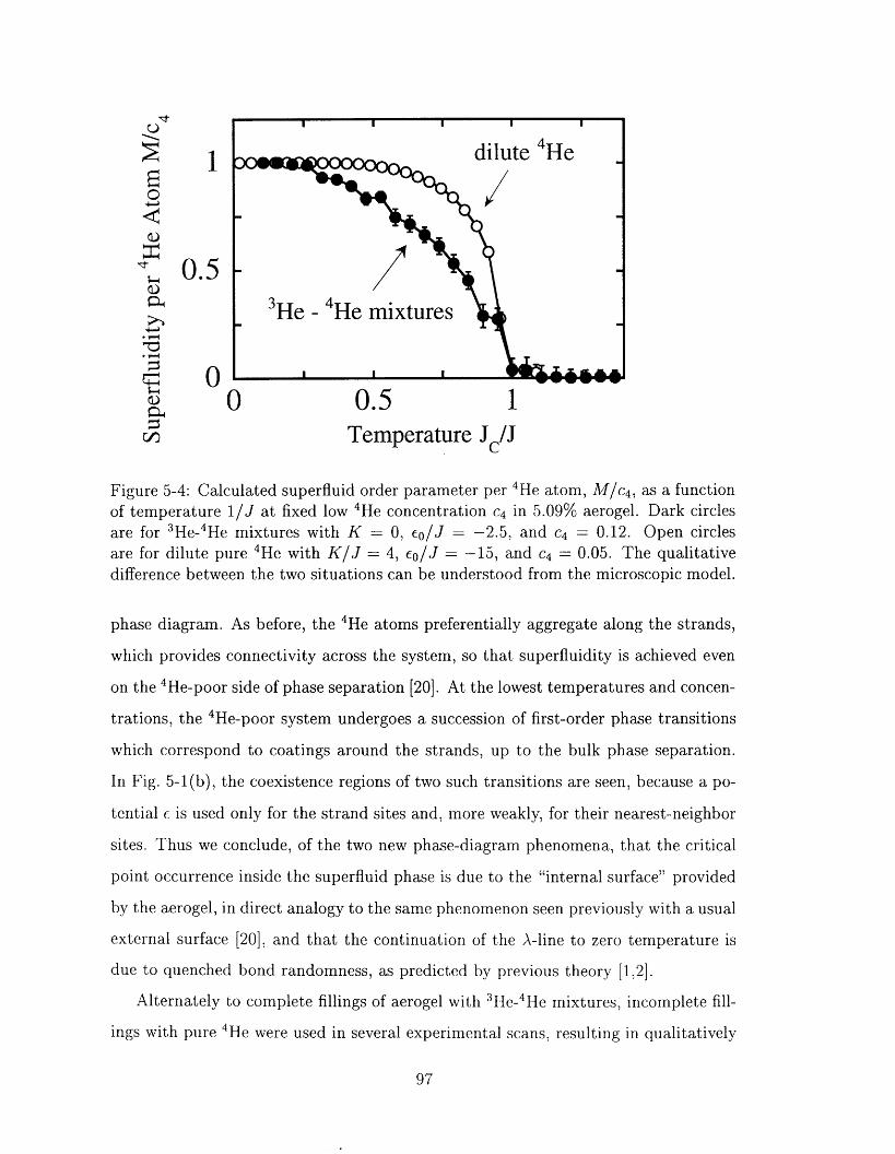
'T-U

IE0+_j

U

"t o.5;__4

U

C:)o

4__j

�1

U_ n0.5Temperature J/i

Figure 54: Calculated superfluid order parameter per 4He atom, MIC4, as a functionof temperature IIJ at fixed low 4 He concentrations in 509% aerogel. Dark circlesare for 'He_4 He mixtures with K 0, EIJ -2.5, and C4 012. Open circlesare for dilute pre 4He with KIJ 4, EIJ -15, and C4 0.05. The qualitativedifference between the two situations can be understood from the microscopic model.

phase diagram. As before, the 4He atoms preferentially aggregate along the strands,

which provides connectivity across the system, so that superfluidity is achieved even

on te 4He-poor side of phase separation 20]. At the lowest temperatures and concen-

trations, the 'He-poor system undergoes a succession of first-order phase transitions

which correspond to coatings around the strands, up to the bulk phase separation.

In Fig. 51(b), the coexistence regions of two such transitions are sen, because a po-

tential c- is used only for the strand sites and, more weakly, for their nearest-neighbor

sites. Thus we onclude, of the two new phase-diagram phenomena, that the critical

point ocurrence inside the superfluid phase is due to the "internal surface" provided

by te aerogel, n irect analogy to the same phenomenon seen previously with a usual

external surface 20], and that the continuation of the A-line to zero temperature is

due to quenched bond randomness, as predicted by previous theory 12].

Alternately to complete fillings of aerogel with 'He-'He mixtures, incomplete fill-

ings with pure He were used in several experimental scans, resulting in qualitatively

97

different superfluidity behaviors as a function of temperature [3]. Our model is also

immediately applicable to the latter experiments, with si now representing the

vacuum. This physical system requires larger 1Eil, representing the full binding en-

ergy of 'He rather than the effective binding energy difference between the isotopes,

and a larger K K44+ Koo - 2K40 = K44, which represents the full 'He-'He van

der Waals interaction rather than the interaction differences between isotopes. Our

calculated temperature scans at fixed low 4He concentration for both experiments

are plotted together in Fig 54. It is seen that the decay of superfluidity sets in at

low temperatures and is much more gradual for the mixture, in agreement with the

experiment. The microscopic explanation is apparent from our model: At these low

concentrations of 4He, most of the 4He atoms are in the vicinity of the acrogel strands

and superfluidity occurs through these 4He atoms maintaining connectivity along the

strands. As temperature is increased, a 4He atom could be "boiled" away from the

vicinity of the strands, decreasing superfluidity, at the energy increase of q J + qK -,Ej,

where q is an effective coordination number of the order of 5. As explained above, K

and ci reflect the isotopic differences for the mixtures and the full energies for dilute

pure 'He. The latter constitute a much higher energy price and the process does not

occur. Superfluidity disappears much more abruptly, in standard order parameter

behavior at a phase transition, through the dephasing of the connected 'He.

This research was supported by the U.S. Department of Energy under Grant No.

DE-FG02-92ER45473.

98

REFERENCES

[ I

.1 A.N. Bericer, J. Appl. Phys. 70, 5941 1991).

[2..1 A.N. Berker, Physica A 194, 72 (1993).

[3] S.B. Kim, J. Ma, and M.H.W. Chan, Phys. Rev. Lett. 71, 2268 1993)

[4..1 D.W. Schaefer and K.D. Keefer, Phys. Rev. Lett. 56, 2199 1986).

[5.1 J. Fricke, Sci. Am. 258, 92 1988).

[6. A. Hasmy, E. Anglaret, M. Foret, J. Pelous, and R Jullien, Phys. Rev. B to

be published 1994).

[7. J.V. Maher, W.I. Goldburg, D.W. Pohl, and M. Lanz, Phys. Rev. Lett. 53 60

(1984).

[8] A.P.Y. Wong and M.W.H. Chan, Phys. Rev. Lett. 65, 2567 1990).

[9. T. Bellini, N.A. Clark, C.D. Muzny, L. Wu, CW. Garland, D.W. Schaefer, and

B.J. Oliver, Phys. Rev. Lett. 69, 788 1992).

[10' F. Brochard and P.G. de Gennes, J. Phys.-Lett. 44, L785 1983).

P.G. de ('ennes, J. Phys. Chem. 88, 6469 (1984).

[12.1 M. Blume, VJ. Emery, and R.B. Griffiths, Phys. Rev A 1071 (1971)..

[13'] K. Hui and.A.N. Berker, Phys. Rev. Lett. 62, 2507 (1989)- 63, 2433(E) 1989).

[14' A.. Falicov an AX Berker, MIT preprint (1994).

[15] For a study with uncorrelated quenched random D, see A. Maritan, M. Ceplak,

M.R. Swift, F. Toigo, and J.R. Banavar, Phys. Rev. Lett. 69, 221 1992).

[16] For the cnversion of first-order phase transitions to second- order by infinites-

imal bon-I randomness, the crossover dimension was reported in Refs. 1] and

[2] as d, =:- 2 for n I component microscopic degrees of freedom and as d = 4

99

for n > 2 component microscopic degrees of freedom. The latter is incorrect

and is hereby corrected as d = 2 for all systems. The reason for this is that

the free energy increase due to the interface created by an ordered island inside

a disordered region (or vice versa) scales as L d-I with the linear extent L of

the island, even for n > 2 This can also be inferred from the effective-vacancy

renormalization-group argument and Fig. I in Ref. [1].

[17] Y. mry and S.-k. Ma, Phys. Rev. Lett. 35, 1399 1975).

[18] S.R. McKay and A.N. Berker, J. Appl. Phys. 64, 5785 1988).

[19] A. Falicov, A.N. Berker, and S.R. McKay, M.I.T.-Maine preprint (1994).

[20] J.-P. Rornagnan, J.-P. Laheurte, J.-C. Noiray, and W.F. Saam, J. Low Temp.

Phys. 30, 425 1978).

100

Gaussian

101

Chapter 6

Density Annealing

Study of VVater

Alexis Falicov

Department of Physics, Massachusetts Institute of Technology.

Cambridge, Massachusetts 02139

Abstract

The Gaussian Density Annealing technique is applied to a sys-

tem of water molecules. The differential equations that govern

the evolution of these distributions are obtained and solved A

new algorithm, known as the Fourier Sum method, as well the

traditional Fast Multipole Algorithm are implemented for rapid

evaluation of the potentials. The results for groups of up to 200

water molecules are presented. The possibility of applying this

technique to more sophisticated systems, such as aequeous solu-

tions of proteins and bipolar membranes, is discussed.

PACS Numbers: 64.70.-p, 05.20.Gg, 82.20.Wt, 87.15--v

102

6.1- Gaussian Density Annealing Study of Water

As a material, water plays an essential part in many aspects of science. For biology,

it is the dominant solvent: it appears in all forms of life, and is the force responsible

for the formation of membranes and biological structures. For chemistry, the study

of aequeous slutions is of crucial importance: the theory of acid-base chemistry,

biochemistry, nd even organic synthesis, rely on its unique properties. But it is for

physicists that water seems to have a special appeal. The molecule itself has a simple

structure, and yet, to this day, there are no satisfactory theoretical models that can

reproduce its entire phase diagram.

Studies of ater have included many differing techniques of which most can be

divided into oe of two categories. The first category, which include all microscopic

techniques, involves the determination of the finite-temperature properties by in-

cluding interactions, determined empirically or from first-principle calculations, at

the molecular level. Once the appropriate equations of motions are applied, the

total macroscopic properties are extracted. An example is solving the many-body

quanturn-mechanical Hamiltonian using the supersoft pseudopotential technique to

obtain the many-body ground-state and the low-lying excited states [1]. Another

example is the use of Molecular Dynamics simulations 2-4], where the evolution of

the system is dtermined by the classical Newtonian equations of motion. In all such

similar cases, one uses the microscopic structures and attempts to solve the exact,

many-body equations of motion.

These techniques, however, are extremely limited in determining many finite-

temperature poperties. Quantum mechanical solutions are analytically tractable

only for very sall systems, currently up to 40 water molecules, and at very low

temperatures. Molecular Dynamics, on the other hand, is limited by the very small

time scales, on the order of femtoseconds, necessary for evaluating the forces acting

on each particle. The microscopic techniques, that have been successful at deter-

mining structural and dynamical properties, have been ineffective at determining the

macroscopic phase behavior of water 3,41.

103

6.2 Introduction

The second category involves solving the equilibrium statistical mechanics of a

computationally tractable system that contains the necessary physical parameters.

One example is the Potts Lattice Gas [5] a model that represents the various ro-

tational configurations of each molecule as possible states at each site of a regular

lattice. Determination of the effective nearest-neighbor potentials immediately yields

qualitatively correct phase diagrams. In such models, however, it is difficult to get

quantitative agreement and, in addition, studies of more complex systems, such as

aeqeous mixtures and biomolecules in solution, are not possible.

The failure to reproduce quantitatively the phase diagram of water can be un-

derstood from relatively intuitive physical arguments. Firstly, the success of many

techniques in solid state physics rests on the idea of symmetry. As an example, the

entire field of band structure calculations was founded on the basis that the atoms in

a solid form a regular array. Water, on the other hand, forms a disordered fluid As

a result, many principles, such as symmetries and group theory, which had enormous

success with regular solids, do not find application here.

Another difficulty can be understood from studies of spin glasses and disordered

systems, where the free energy contains many local minima, each separated by tall

barriers [6]. The internal structure of water molecules contain orientational as well

as positional degrees of freedom, which result in free energy surfaces qualitatively

similar to those encountered in spin glasses and frustrated systems 7 For traditional

approaches, such as Monte Carlo and Molecular Dynamics studies, this implies that

the initial configurations used in the simulations must be relatively close, in positional

space, to the eventual equilibrium configuration. Not only does this require foresight

about the final structure, but it is also a violation of the ergodic hypothesis [8] on

which both techniques are based.

In this chapter, I utilize the efficient representation of probability distributions

to determine the finite-temperature properties of a system of water molecules To

avoid the problems mentioned above, I use a promising new technique known as

Gaussian Density Annealing (GDA) [101. This procedure is similar in principle to

the simulated annealing technique 9 in that both start with the hypothesis that

104

the initial configuration at high temperatures can be detemined. As opposed to

GDA, in simulated annealing an additional method, such as Molecular Dynamics

is needed to euilibrate the system at each temperature. The temperature is then

lowered and the system is re-equilibrated. The rate of temperature change, called the

cooling schedule, is determined by the range of energy scales. Unfortunately, for most

molecular systems including water, this optimal cooling schedule is computationally

forbidden. The GDA approach, on the other hand, simulates the annealing of the

equilibrium density distribution directly in temperature. As a result, this provides an

excellent new tool to study the phase diagram of systems by directly analyzing their

temperature-dependent behavior.

6.3 Methods

6.3.1 The '-Traditional GDA Equations

To obtain the GDA differential equations, we start from the normalized equilibrium

density distribution

Pe q e (6-1)

where H(rp) is the classical Hamiltonian and Z(o) f drdpexp(-OH) is the par-

tition function [10]. For any property A(rp), we can define the statistical average

as

(A) dr dP Peq (r, p) A (r, p). (6.2)

The temperature ependence of (A) is found by differentiating Eq. 62) with respect

to IlkbT, which yields:

d�A) (HA) (A) H). (6.3)do

TO obtain te finite-temperature behavior, we seek an approximate solution for

the quilibrium dnsity distribution at arbitrary temperature. We assume that the

105

integrals over the momenta have been carried out, and that the total N-body density

distribution pN(r N, ) can be represented as a Hartree product of the distributions

Pk (rk, ) of the N individual particles

Np I (,r N, = 11 Pk (rk, )

k=1(6-4)

The technique of Gaussian Density Annealing comes from approximating each

single particle density distribution as a single Gaussian packet in three dimensions

(6-5)

where we have neglected writing the explicit temperature dependences of ro and a

for notational simplicity.

The differential equations that govern the evolution of the center and width of

each Gaussian are determined by substituting r and (r - ro)' for A in Eq. 63),

obtaining the following:

Orok

'goOa 2kao

-92V k V),

4 2 V),- - _Ok k3

(6-6)

where V) is the potential averaged over the density distribution

(V) I d',r p (r ', ) V (r ') (6-7)

In particular, if the potential is a pairwise sum over two-particle interaction potentials,

then

(V = 1: I dri f drj pi ri) pj (rj) V (r - rj) i��j.

(6.8)

Eqs. 66), 67), and 6.8) are what are referred to as the GDA algorithm. Exami-

nation of the equations above immediately yields the following:

1. At infinite temperature (�=O), all phase points are equally likely. We can there-

106

0 2-

Pk (rk' M - (2,7r o, 2) -3/2 exp - I Tk - kk 2 O'k 7

fore choose an initial condition where Ok is effectively infinite for any choice of

r'. The quations of motion are then integrated starting at O using Eq. 6-6)k

until the desired final temperature is reached.

2. The center of the Gaussians move under the influence of V). This potential is

qualitatively different from the many-body potential V due to the "smoothing"

effect of integrating over Gaussians, which removes spin-glass-like states that

trap particles at local minima of the free energy [10].

6.3.2 The Modified GDA Equations

In the case of water, each oxygen atom is bonded to two hydrogen atorns. We modify

the Gaussian probability distribution for each water molecule as

0 2-

(2 7)-1,2 (0,2 U2,f I ,2 -1,2 exp ro - -r 0 (6-9)P('rO,'rOHI, 7OH2) 0 0 OH2) 2 010

2- 2-1 roH, - ro rOH2 - T 0

exp - OH1 exp OH22 O'OH1 2 O'OH 2

where ro is the vector representing the coordinate of the oxygen and roH, and roH2

are vectors that give the relative coordinates of the two hydrogens with repect to

their bonded oxygen. The differential equations are similarly modified and yield the

following:

i9ro0 - -01 2 + VH2�V)a)3 0 VO (V) + V (V)

aroOHI 2-01 Hi H (V)

aroOH2 2- _01OH2 II2(V)ao

00,0 - - 013 V2 V),ao 6 0

a(TO I - - I or 3HJ V2 j(V)ja,3 6 0 H

aO'OH2 - - I 013 V2 (6.10)ao 6 OH2 H2 (V)'

107

These equations describe the evolution in temperature of the oxygen and oxygen-

hydrogen vectors and standard deviations in terms of the effective "forces" on each

of the three atoms.

6.3.3 The TIP3P Model of Water

We use the TIP3P representation of water [II] to determine the intrinsic parame-

ters of the water molecules. This model, used extensively in Molecular Dynamics

simulations, sets the equilibrium O-H distance to 0-9572A and the equilibrium H-

O-H angle as 104.52'. Hydrogen bonding is introduced by the placement of partial

charges of -0-834e on the oxygens and 0.417e on each of the hydrogens, where e is

the fundamental unit of charge.

The bond potentials are obtained from CHARMM 12], a computer program

that uses empirical energy functions to model macromolecular systems. The oxygen-

hydrogen empirical potential function was taken to be of the form

V = k ( jr _ 2, (6.11)

with k = 450.0 kcal/mole-A 2 and ro=0.9572A. The H-0-H angle potential was taken

to be of the form

V = ko( - 00)2, (6-12)

2where is the angle between the three atoms, ko 55.0 kcal/mole-A and 0--104.52'.

The potential of Eq. 6.12) is a three body potential. We replace such a potential by

a two-body term, of the form in Eq. 611) placed between the two hydrogens, with2

k 160.2 kcal/mole-A and ro 1.5139A.

6.3.4 The Effective Potentials

Given two Gaussian distributions with centers ro and ro and standard deviations oi0 0and oj, the transformation of the two-body potential V(ri, rj) ---� V(r, aj; r , aj) in

108

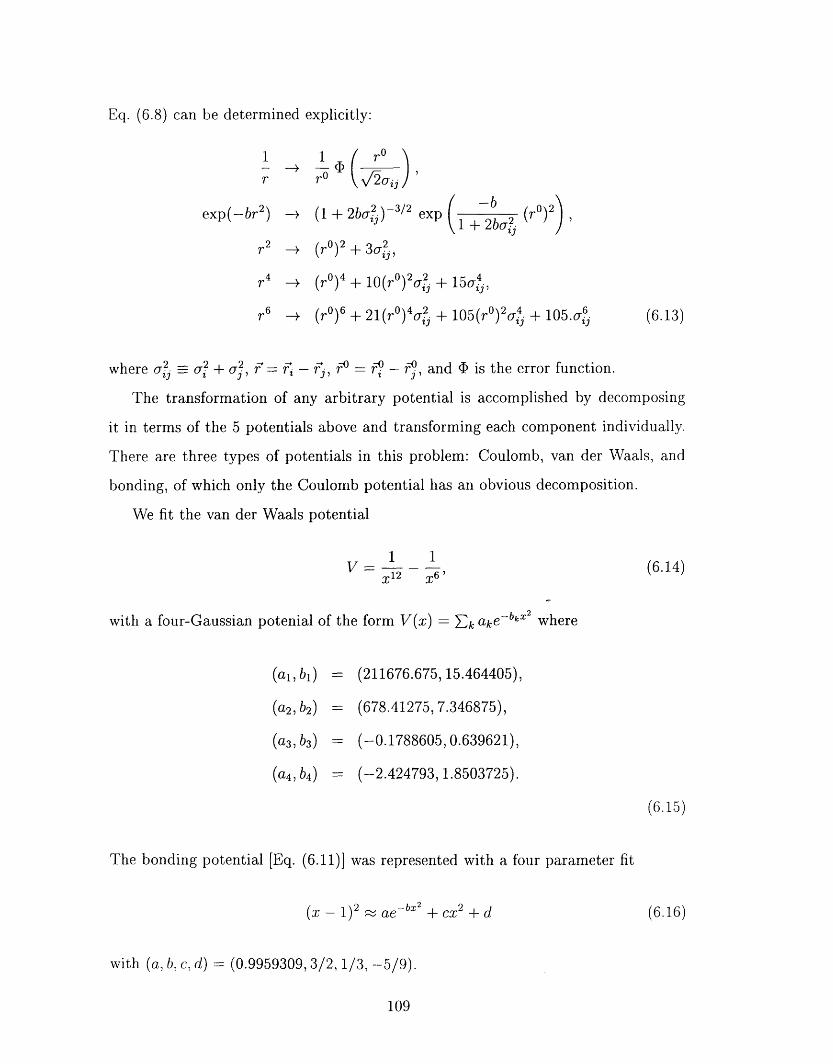
Eq. 68) can e determined explicitly:

1 ro0 'I) __01. � Ir r v/2 II

,r2 0,2 -1/2 -b 0)2exp(-b (I + 2b ij exp I + 2ba?. (r

r2 (r 0)2 + 3o,2ij

r4 (r 0)4 10(ro )20,2 + 15 0,4ij ij

6 0)6 )4U2 (,rO)20,4 .0,6r (r + 21 (ro ..+ 105 .. + 105 ..23 tj Z3 (6-13)

2 = , + 2 - - --, 0 where oj - , oj, r = ri - j, r - - ro and (D is the error function.I

The transformation of any arbitrary potential is accomplished by decomposing

it in terms of the potentials above and transforming each component individually.

There are three types of potentials in this problem: Coulomb, van der Waals, and

bonding, of which only the Coulomb potential has an obvious decomposition.

We fit the van, der Waals potential

V __ I X12 X61

(6.14)

with a four-Gaussian potenial of the form V(x) = Ek ake-bkX2where

(a,, b)

(a2, b2)

(a3, b3)

(a4, b4)

= 211676.675, 15.464405),

= 678.41275, 7.346875),

= (-0.1788605,0.639621),

= (-2.424793,1.8503725).

(6.15)

The bonding potential [Eq. 611)] was represented with a four parameter fit

(X _ 2 ;::z:� ae -bX2 + CX2 + d

with (a, b, c, d) : (O 9959309 32 13, - 5/9).

(6-16)

109

6.3.5 Rapid Evaluation of the Potentials

The evaluation of the pairwise potenials is nominally a N(N - 1/2 process where N

is the total number of atoms in the system. Using a traditional, brute force pairwise

summation, one is limited to 50-100 water molecules. We therefore seek alternate

methods that would allow us to evaluate the potentials more rapidly. There are two

techniques that we used: the Fourier Sum method and the Fast Multipole algorithm

[13].

1 developed the Fourier Sum method specifically for the GDA algorithm to cal-

culate the potentials for a system of particles in a cubic box with periodic boundary

conditions. The periodic boundary conditions require that only discrete number of

reciprocal lattice vector contribute to any Fourier transform. For each K we

calculate the Fourier component of the total oxygen and hydrogen densities

I K2U2

K e e 2P i=O

20-2_iK fi -. !K (6.17)K - - I: P i=H

The sums denote sums over all particles of a specific type. The total potential can

therefore be written as

3 (fiQ fiO - 0 -0 -HR OH -H -OR HO -H -H= L V (6-18)2 K - k + PkP V + PRP V + PRP-K -K K

where, for example, - 90 is the Fourier transform of the total 0-0 potential. WhenV�

the mimimum. standard deviation is no smaller than L110, where L is the system size,

this sum converges after only 00-200 wave vectors. After evaluation of the potential

from Eq. 618), terms included due to the self-energies for each of the particles and

the interactions between bonded hydrogens and oxygens are subtracted, thus yielding

the total intermolecular potentials due to Coulomb and van der Waals interactions.

Differentiation of Eq. 618) yields the gradient and Laplacians V2 used in the

differential equations [Eq. (6-10)]. The Fourier Sum method converges very rapidly

110

when the distributions are wide, i.e., at high temperature. In addition, the evaluation

of all the potentials is proportional to nKN, where N is the number of particles and nK

is the number f vectors used in the sum. Thus, for wide distributions, this technique

is linear in the number of particles.

When the distributions are narrow, i.e., at low temperatures, we use an alternate

technique known as the Fast Multipole (FM) algorithm 13]. The FM algorithm works

well at low temperatures. In this technique, the entire system is divided up into small

cells in which the multipole expansions are calculated. These multpoles are then used

to determine the potential at any particle due to the particles contained within all

other cells of the system. Such a method requires that all standard deviations be

small enough so that the transformed Coulomb potential

r(6-19)

r T2ojj r

where r is the 'length of a single cell. To allow us to use this technique, we require

that the largest, standard deviation be no larger than L/8.

The overlap between the two approaches allows for a smooth transition from the

Fourier Sum to the FM sum. In the intermediate regimes, a combination of the two

techniques can be used. Both the FM and Fourier Sum methods scale linearly with

the number of articles and thus allow for the evaluation of much larger systems.

6.3.6 Integration of the Differential Equations

Once the potentials are evaluated, we must integrate the differential equations [Eq. 6. 1 0)

until the desired final temperature is reached. Although predictor-corrector tech-

niques 2 are favored in Molecular Dynamics, we used Richardson Extrapolation and

the Bulirsch-Stoer Method 14]. This technique is outlined as follows:

1. A single 13ulirsch-Stoer step takes us from temperature to 3 A, where is

not a small quantity.

III

2. A sequence of separate attempts is made to cross this interval using an increasing

number of steps: 2 4 6 8, 10, 12 -

3. The value for each coordinate at A is extrapolated to an infinite number of

steps by a rational function extrapolation, known as Richardson Extrapolation.

4. The entire procedure is repeated until the desired final temperature is reached.

This technique is the best known way to obtain high-accuracy solutions to ordinary

differential equations with minimal computational effort.

6.4 Results

In my first studies, I began with 50 water molecules in a cell of length 11.43A, yielding

the desired density of Igm/cm 3. Random initial configurations with widths of 8A for

both the oxygen and oxygen-hydrogen Gaussians were used. I found that the standard

deviations for the M and H2 Gaussians [see Eq. 69)] collapsed to 0.001A at

temperatures of more than 100kcal--48000'K. The widths of the Gaussian reduced

much more slowly, reaching a comparable width of .001A at 0.5kcal--244'K.

Analysis of Eq. 6-10) immediately yields the reason for the rapid collapse. The

differential equations for the widths depend on the effective forces on each of the three

component atoms of each molecule. The bonding and angle potentials, however, are

intramolecular in character, and therefore, by Newton's third law, do not contribute

to the differential equation for . The energy scales of these potentials, however,

are the dominant terms that control the evolution of uoff 1 and H2, which results

in the rapid collapse of these quantities.

By approximating the relative O-H vector probability distributions as symmetric

Gaussians, we have coupled different interactions in the problem. A uniform Gaussian

assumes that all fluctuations in the position of the particles are approximately of the

same order. Fluctuations in the bond lengths, with energies on the order of 100kcal,

however, are much more expensive energetically than fluctuations due to rotations of

the molecules, which are on the order of O. Ikcal.

112

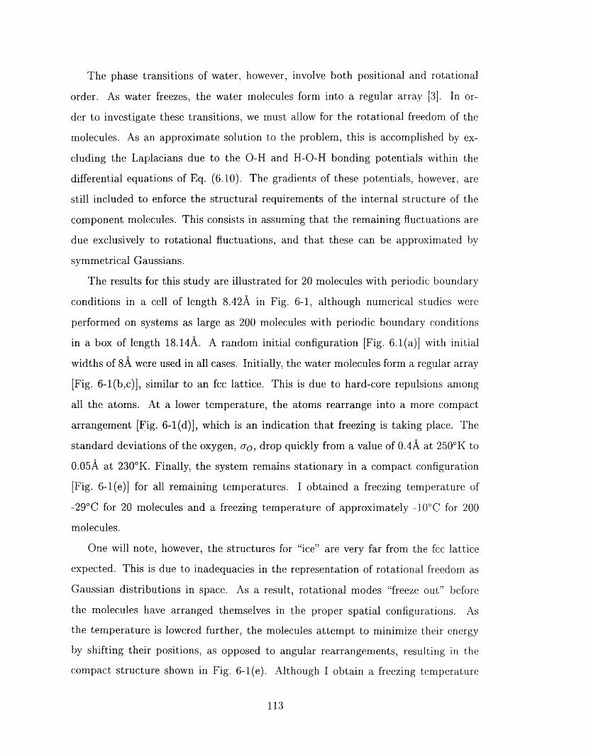
The phase transitions of water, however, involve both positional and rotational

order. As water freezes, the water molecules form into a regular array [3]. In or-

der to investigate these transitions, we must allow for the rotational freedom of the

molecules. As an approximate solution to the problem, this is accomplished by ex-

cluding the aplacians due to the O-H and H-O-H bonding potentials within the

differential equations of Eq. 610). The gradients of these potentials, however, are

still included to enforce the structural requirements of the internal structure of the

component molecules. This consists in assuming that the remaining fluctuations are

due xclusively to rotational fluctuations, and that these can be approximated by

symmetrical Gaussians.

The results for this study are illustrated for 20 molecules with periodic boundary

conditions in a cell of length 8.42A in Fig. 61, although numerical studies were

performed on sstems as large as 200 molecules with periodic boundary conditions

in a box of length 18.14A. A random initial configuration [Fig. 6.1(a)] with initial

widths of A were sed in all cases. Initially, the water molecules form a regular array

[Fig. 61(bc)], similar to an fcc lattice. This is due to hard-core repulsions among

all te atoms. t a lower temperature, the atoms rearrange into a more compact

arrangement [Fig. 61(d)], which is an indication that freezing is taking place. The

standard deviations of the oxygen, , drop quickly from a value of OAA at 250'K to

0.05A at 2300K. Finally, the system remains stationary in a compact configuration

[Fig. 61(e)] for all remaining temperatures. I obtained a freezing temperature of

-290C for 20 molecules and a freezing temperature of approximately -10'C for 200

molecules.

One will note, owever, the structures for "ice" are very far from the fcc lattice

expected. This is due to inadequacies in the representation of rotational freedom as

Gaussian distributions in space. As a result, rotational modes "freeze out" before

the molecules hve arranged themselves in the proper spatial configurations. As

the temperature is lowered further, the molecules attempt to minimize teir energy

by shifting their positions, as opposed to angular rearrangements, resulting in the

compact structure shown in Fig. 61(e). Although I obtain a freezing temperature

113

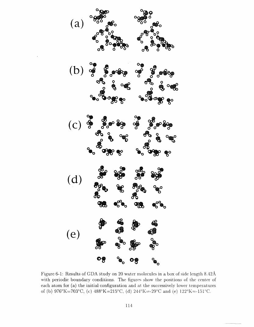
A"a

- AftMAR0 6 0

11%

Art-Al. ..

P41A 040

100

Afto

ayAb

11�

A 5

f%-,Ak

O"epAb 040

to

a

b

d

114

r%-

C

I

cop &'� C

A 7t Ot

T

Om Aft

091C�P &(�P

0% 4 O'V

to

AM

of ,

99

Ca % 00 C

Aft

OCUI

WV

0 r%T) QA 69(*

'10% I

%O 0-9 C�O

Figure 61: Results of GDAS''tudy on 20 water molecules in a box of side length 8.42A'th periodic boundary conditions. The figure, sow the positions of the center of

each atom for (a) the initial configuration and at, the successively lower temperaturesof (b) 976'K=703'C, (c) 488'K-215'C, (d) 244'K=-29'C and (e) 122'K--151'C.

that, is of the (,correct order of magnitude, I am unable to reproduce the symmetry

breaking that ccurs as one goes from the liquid to solid states.

115

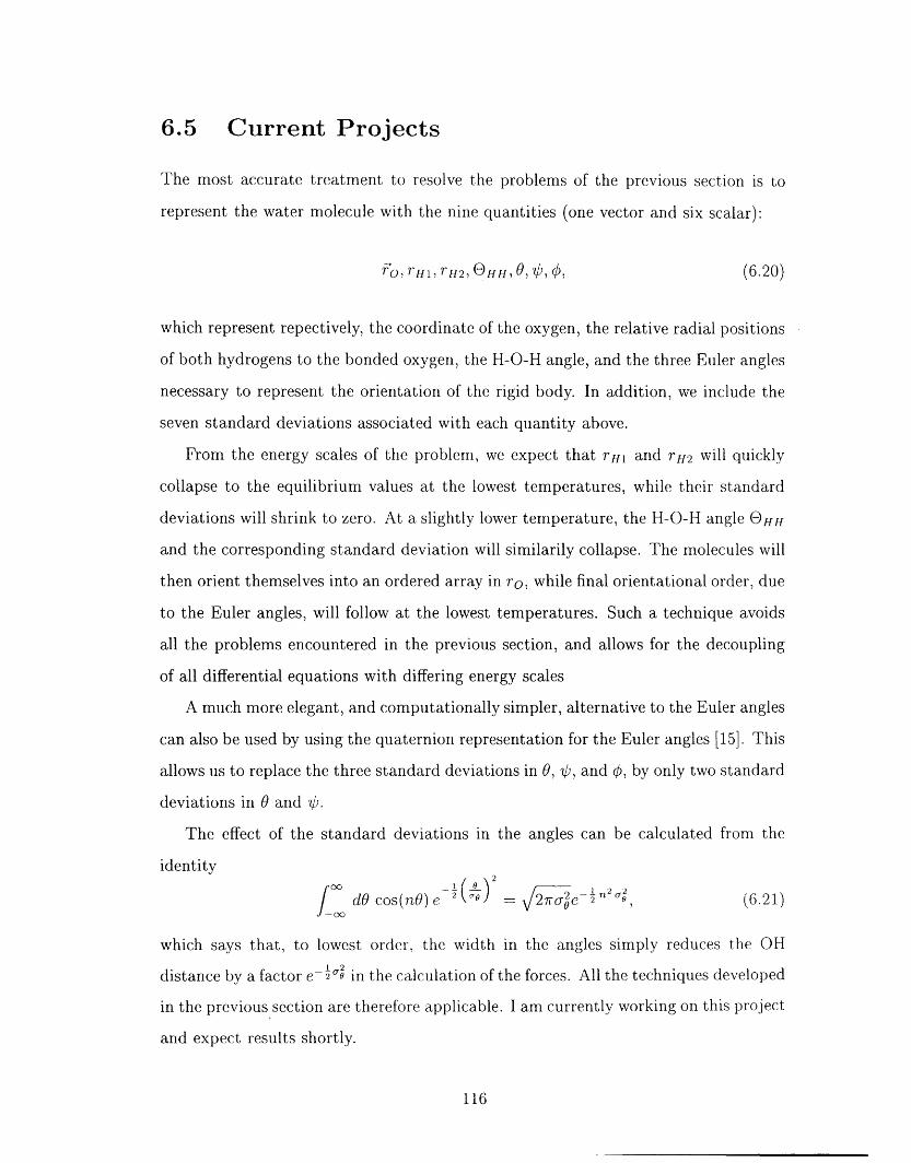
The most accurate treatment to resolve the problems of the previous section is to

represent the water molecule with the nine quantities (one vector and six scalar):

FoIrHil rH2) OHH, 0 V)i 07 (6.20)

which represent repectively, the coordinate of the oxygen, the relative radial positions

of both hydrogens to the bonded oxygen, the H-O-H angle, and the three Euler angles

necessary to represent the orientation of the rigid body. In addition, we include the

seven standard deviations associated with each quantity above.

From the energy scales of the problem, we expect that rHi and rH2 will quickly

collapse to the equilibrium values at the lowest temperatures, while their standard

deviations will shrink to zero. At a slightly lower temperature, the H-O-H angle OHH

and the corresponding standard deviation will similarity collapse. The molecules will

then orient themselves into an ordered array in r, while final orientational order, due

to the Euler angles, will follow at the lowest temperatures. Such a technique avoids

all the problems encountered in the previous section, and allows for the decoupling

of all differential equations with differing energy scales

A much more elegant, and computationally simpler, alternative to the Euler angles

can also be used by using the quaternion representation for the Euler angles 15]. This

allows us to replace the three standard deviations in 0, �b, and , by only two standard

deviations in and .

The effect of the standard deviations in the angles can be calculated from the

identity00 )2 2 0,22 9 1 n7T,70200 do cos (no) F2 e (6.21)

which says that, to lowest order, the width in the angles simply reduces te OHe 72

distance by a factor 2 in the calculation of the forces. All the techniques developed

in the previous section are therefore applicable. I am currently working on this project

and expect results shortly.

116

6.5 Current Pro'ects

If sch a technique is succesful I intend to apply this technique to more compli-

cated systems, 'In particular the study of phase transitions in self-assembling systems,

such as membranes, and macromolecules, such as long hydrocarbons, in solution. In

such cases, one mst introduce three additional variables, specifying the relative posi-

tions, and thre aditional widths for each atom within the molecules. The techniques

developed in this section, however, will still apply in these cases.

This research was supported by the U.S. National Science Foundation Grant No.

I)MR-90-22931

117

REFERENCES

[1] K. Laasonen, M. Sprik, M. Parrinello, and R. Car, J. Chem. Phys. 99, 9080

(1993).

[2] A. Rahman and F. H Stillinger J Chem. Phys. 55, 3336 (1971).

[3 T A. Weber and F. H. Stillinger, J. Phys. Chem 87, 4277 1983).

[4 F H Stillinger and A. Rahman J Chem. Phys. 60, 1545 1974).

[5] A. N. Berker, S. Ostlund, and F. A. Putnam, Phys. Rev. 17, 3650 978).

[61 B. A. Berg, T. elik, and U. Hansmann, Europhys. Lett. 22, 63 1993).

[7] J. E. Straub, A. B. Rashkin, and D. Thirumalai, J. Am. Chem. Soc. 116, 2049

(1994).

[81 The ergodic hypothesis states that as one follows the evolution of a particular

system, it is statistically equivalent to the evolution of an ensemble of systems

(see Ref. [15]).

[9] S. Kirkpatrick, C. D. Gelatt, and M. P. Vecchi, Science 220, 671 1983).

[10] J. Ma and J. E. Straub, to be published in J. Chem. Phys. 1994).

[111 W. L. Jorgensen, J. Chandrasekhar, J. D. Madura, R W Impey, and M L.

Klein, J. Chem. Phys. 79, 926 1983).

[121 B. R. Brooks, R. E. Bruccoleri, B. D Olafson, D J States, S. Swaminathan,

and M. Karplus, J. Comp. Chem. 4 187 (1983).

[13] L. F. Greengard, The Rapid Evaluation of Potential Fields in Particle Systems,

M.I.T. Press 1988).

[14] W. H. Press, S. A. Teukolsky, W. T. Vetterling, and B. P. Flannery, Numerical

Recipes in C, 2nd Ed., Cambridge Univ. Press 1992).

118

[15 M P. Allen and D. J. Tldesley, Computer Simulation of Liquids, Oxford Urn-

versity Press 1987).

119

Chapter 7

Conclusions and Future Prospects

7.1 The t-J Model

The techniques developed in this section allowed the investigation of the finite-

temperature phase diagram of the t-J model of electronic conduction. Although

our renormalization-group recursion relations contain several uncontrolled approxi-

mations, we were able to duplicate, in all special cases of the system solved, the

correct phase behavior. We found that there are no finite temperature phase transi-

tions in one dimension. In two dimensions, we found that the entire phase diagram is

controlled by a single line on which phase separations occur. In three dimesions we

found multiple reentrances on several temperature scales and the existence of a new

phase, never before seen in the studies of finite-temperature phase transitions.

One prospect that is very appealing, is to determine more about the properties

of the new phase "T -It is extrordinarily suggestive of the superconducting phase

present in the new HTSC materials. As a first step, we must consider determining

the order parameter of the transition. The renormalization-group immediately yields

the phase diagrams and the order of the transition, but does not explicitly deter-

mine the order parameter. For example, in the case of the Ising model, the order

parameter is the spontaneous magnetization m. One cannot, however, determine this

from renormalization-group theory util one includes an external field, within the

Hamiltonian, conjugate to a quantity wose thermal average is the order parameter

120

of te system, i.e., a magnetic field in the case of the Ising model. To determine

the order parameter for the t-J model, one must introduce additional terms in the

Hamiltonian wich will be the analogue the magnetic field for the Ising model. This

is a very active area of research in our group and promises to reveal much more about

the properties f the t-J model. Several possibilities that deserve investigation are:

the superconducting order parameter, the existence of the Meissner effect, and the

calculation of dynamical properties such as the conductivity.

In addition, it would like to investigate the influence that our approximations have

on the phase diagrams of the system. One future prospect is to use small clusters to

determine the renormalized interaction strengths. The use of small clusters involves

the diagonalization of much larger matrices 6561 x 6561 in the case of an eight site

cluster). We do, however, possess all the tools of group theory, and several exact

solutions of and 16 site clusters already exist. It would be extremely interesting to

combine small cluster calculations and renormalization-group techniques to explore

quantum finite-temperature phase transitions.

Finally, it ould also be rewarding to apply this technique to other quantum sys-

tems. Two obvious choices would be the generalized Hubbard model' and the Falicov-

Kimball model,,' although many other candidates exist. The generalized quantum

decimation Eq. 212)] is the key step in all these calculations. Once all the matrix

elements can b determined, the phase diagram and all the properties of the phases

immediately follow. All these cases illustrate the richness present within the field of

quantum phas tansitions, of which I have only touched one corner. In addition,

our techniques ave demonstrated the versatility of te renormalization-group in the

general field of phase transitions.

'J. Hubbard, Proc. R. Soc. London, Ser. A 276, 238 1963); 227, 237 1964); 281, 401 1964);285, 542 (1965)- ZL6, 82 (1966)- 296, 100 1967).

2L. M. Falicov and J. C. Kimball, Phys. Rev. Lett. 22, 997 1969).

121

7.2 The Random-Field Model

We applied an extremely detailed renormalization-group study to the random-field

Ising model in three dimensions. We found that the finite temperature boundary,

for any arnount of randomness, is controlled by by a single fixed distribution. This

boundary is second-order, but has a magnetization exponent phenomenally close

to zero.

Given the plethora of experimental studies being performed in aerogels and in

disordered media, we must now apply the theories to the actual systems. Current

possible applications include liquid crystals in aerogels, binary fluids in porous materi-

als, and even disordered antiferromagnets. All present possible avenues of theoretical

investigation.

In addition to these classical systems, there is an enormous amount of research

being done in the fields of disordered quantum systems. We would like to expand the

above results to new types of system with quenched disorder. Of particular interest is

the study of the disordered two-dimensional electron gas. If one includes the random

magnetic effects due to magnetic impurities, it may be possible to combine the theory

of quenched disorder with the theory of phase transitions of quantum systems. This

presents itself as an ideal opportunity to combine several aspects in the investigation

of a new experimental system.

7.3 The Random-Bond Model

As was seen in our study of the Blume-Emery-Griffiths model with quenched bond

randomness, the phase diagram is extremely rich and detailed. The introduction of

randomness completely changes all aspects of the phase diagram. It is therefore to

be expected that similar effects would be present in any system with quenched bond

randomness.

In reality, however, the separation between quenched random fields and bonds is

not a clear line in either experimental or theroretical models. Although the introduc-

122

tion of random bonds cannot, by symmetry considerations, introduce true random

fields, a random field mechanism may nevertheless occur, evidenced by the appearance

of critical points with Ising random-field criticality within a random bond system.

In experimental systems, the separation is even blurrier. Most experimental sys-

'th quenched disorder possess a combination of the two effects. One area of

active resrearch is the combination of these two theoretical investigations together

into a single, random-field-random-bond problem. Already there are some general

physical arguments that provide glimpse into a new area of research that have the

potential to contain completely new phenomena. 3

In addition, the techniques developed here for the representation of probability

distributions, hve widespread applications. These techniques allow one to introduce

quenched randomness to any system to which has been studied using the renormal-

ization group. ne uses the general functional recursion relation [Eq. 31)] and uses

the appropriate local recursion relations. This technique can be applied to both

momentum-space and functional renormalization-group techniques with equal accu-

racy.

The degree f ccuracy obtained from our calculations also has many applications

in the methodology for the representation of probability distributions. In many tech-

niques, an analytical form, such as a Gaussian, is assumed as a form for a probability

distribution anc-I then the parameters are adjusted to the data. Results, which may

involve convolutions of these distributions, are often analytically ntractable We

have presented a technique where the distribution is dscretized, but still contains ex-

tremely detaile iformation. No particular form has been assumed and, in addition,

convolutions ar rplaced by finite sums over a collection of cells.

3A. N. Berker and A. Falicov, Tr. J. Phys. 18, 347 (1994).

123

Porous Media

We constructed a lattice model for 'He-'He mixtures in porous media, characterized

by correlated random chemical-potential differences between isotopes. We found, by

Monte Carlo simulation, that the bulk tricritical phase diagram was replaced: The

A-line extends to zero temperature, as had been theoretically predicted some time

ago, and phase separation occurs within the superfluid phase.

We were able to construct a model that duplicated the experimental conditions

present in aerogels. As a first step, this model can now be used to study other phase

transitions, such as the previously mentioned binary-liquid, liquid-gas and liquid crys-

tal transitions in aerogels. In addition, we can use this technique to examine the effect

of correlated randomness on the random-field problem, hich, until now, has been

largely unexplored.

The main result that is shown by this investigation is the extreme utility of sim-

plified models. In order to duplicate the results seen in the experiments, we needed

only to include certain effects. We did not, for example, need to include quantum

mechanics or, Bose-Einstein statistics to examine this problem. This illustrates one

of the key elements within phase transition theory: much of the information about

phase transitions in extremely complex systems can be learned from studies on simpler

models.

7.5 The GDA Study of Water

In this section we developed new tools that were used to study the finite-temperature

properties of a complex system. We used the Gaussian Density Annealing technique to

obtain the qualitatively correct phase diagram of water at high densities. In addition,

several new computational tools., that allow for extension of this method to much

larger systems, were developed.

As was noted in the last chapter, these results are part of a current project tat

124

7.4 The Phase ransitions of Helium Mixtures in

is under nvestigation. Although many of the results are preliminary, I believe they

show the great, promise available in such a technique. Water contains all the forces

that are required to determine the finite-temperature properties of many systems. Of

particular importance may be the application of this methods to biological molecules.

Water is the driving force in the formation of most biological structures. In addi-

tion to membranes, it is believed that hydrophobic-hydrophilic interactions are one of

the dominant orces that lead to the unique folding states of proteins. Biomolecules

also contain ny of the problems present within the studies of water, including the

existence of glassy-like local minima in the free energy. The GDA technique has a

potential of application to anv system with a rugged free-energy surface, where one

is interested in the finite-temperature properties,

125

Biographical Note

The author was born on February 11, 1968 in Chicago to Leopoldo M. Falicov,

a physicist, and Marta Puebla Falicov, an artist. Soon after that, he moved to

Berkeley where his father had received an appointment to the University of California

at Berkeley. Alexis, along with his twin brother Ian, attended schools in several

countries, including Denmark, France, and England, before finishing their secondary

educations at Berkeley High School where, during his last year, Alexis met Betty Lee,

his wfe-to-be.

After graduation, he attended the University of California at Berkeley, double

majoring in Mathematics and Physics. Throughout his college years, he was very

active in sports, teaching tennis during the summer months. He also enjoyed music,

especially playing the piano. His thesis in Physics, under Professor Harry Bingham,

involved the measurement of the photoproduction cross-section of the a2 meson. His

thesis in Mathematics, under Professor Alberto Grunbaum, involved selective spin

inversion in nuclear magnetic resonance.

He graduated Summa cum Laude and then continued his studies in Physics at

the Massachusetts Institute of Technology. His studies involved the theoretical in-

vestigation of phase transitions and critical phenomena under the watchful eye of his

advisor, Professor A. Nihat Berker. During his studies, Alexis was a teaching assis-

tant in graduate quantum theory, and an instructor for both "superconductivity" and

"phase transitions and renormalization-group theory". After graduation, Alexis will

be returning to California as a Postdoctoral Research Fellow in the Department of

Pharmaceutical Chemistry at the University of California at San Francisco. He will

be working on rational drug design and the protein folding problem while his wife

pursues her residency in surgery at the medical department at the same niversity.

126