Modeling of macroscopic anisotropies due to surface effects in ...
176
Modeling of macroscopic anisotropies due to surface effects in magnetic thin films and nanoparticles. by Roc´ ıo Yanes D´ ıaz Advisor: Oksana Fesenko Morozova Tutor: Farkhad Aliev A thesis submitted to Universidad Aut´ onoma de Madrid for the degree of Doctor en Ciencias F´ ısicas Departmento F´ ısica de la Materia Condensada MARCH 2011
-
Upload
khangminh22 -
Category
Documents
-
view
1 -
download
0
Transcript of Modeling of macroscopic anisotropies due to surface effects in ...

Modeling of macroscopic anisotropies
due to surface effects in magnetic
thin films and nanoparticles.
by
Rocıo Yanes Dıaz
Advisor: Oksana Fesenko MorozovaTutor: Farkhad Aliev
A thesis submitted to Universidad Autonoma de Madrid
for the degree of
Doctor en Ciencias Fısicas
Departmento Fısica de la Materia Condensada
MARCH 2011

ii
c© Rocıo Yanes Dıaz, 2011.

iii
Except where acknowledged in the customary manner, the
material presented in this thesis is, to the best of my knowl-
edge, original and has not been submitted in whole or part
for a degree in any university.
Rocıo Yanes Dıaz

iv
Es necesario esperar, aunque la esperanza haya de verse siempre frustrada, pues la
esperanza misma constituye una dicha, y sus fracasos, por frecuentes que sean, son
menos horribles que su extincion.
Samuel Johnson
Contents
Resumen ix
1 Introduction 1
1.1 Magnetic nanoparticles and thin films . . . . . . . . . . . . . . . . . . . 1
1.2 Size effects in nanomagnets . . . . . . . . . . . . . . . . . . . . . . . . . 3
1.3 Surface effects in nanomagnets . . . . . . . . . . . . . . . . . . . . . . . 5
1.4 The magnetic anisotropy . . . . . . . . . . . . . . . . . . . . . . . . . . . 7
1.4.1 Magneto-crystalline anisotropy . . . . . . . . . . . . . . . . . . . 8
1.4.2 Surface magnetic anisotropy . . . . . . . . . . . . . . . . . . . . . 9
1.4.3 The shape magnetic anisotropy . . . . . . . . . . . . . . . . . . . 12
1.5 Experimental approach . . . . . . . . . . . . . . . . . . . . . . . . . . . . 13
1.5.1 Effective and surface anisotropies . . . . . . . . . . . . . . . . . . 13
1.5.2 Surface anisotropy and thin films magnetism . . . . . . . . . . . 15
1.6 The challenge of modeling of magnetic nanoparticles and thin films . . . 17
1.7 About this thesis . . . . . . . . . . . . . . . . . . . . . . . . . . . . . . . 19
2 Multi-spin nanoparticle as an effective one spin problem 21
2.1 Introduction . . . . . . . . . . . . . . . . . . . . . . . . . . . . . . . . . . 21
2.2 Model . . . . . . . . . . . . . . . . . . . . . . . . . . . . . . . . . . . . . 22
2.2.1 Shape and surface of nanoparticles . . . . . . . . . . . . . . . . . 22
2.2.2 Localized spin (atomistic or Heisenberg) model . . . . . . . . . . 23
2.3 Analytical background . . . . . . . . . . . . . . . . . . . . . . . . . . . . 24
2.3.1 Second-order surface-anisotropy energy E2 . . . . . . . . . . . . . 25
2.3.2 First-order surface-anisotropy energy E1 . . . . . . . . . . . . . . 27
2.3.3 Mixed contribution to the energy E21 . . . . . . . . . . . . . . . . 27
2.3.4 Effective one spin problem (EOSP) approximation . . . . . . . . 28
2.4 Numerical method . . . . . . . . . . . . . . . . . . . . . . . . . . . . . . 29
2.5 Effective energy landscapes of spherical nanoparticles . . . . . . . . . . . 30
2.6 Effective energy landscapes of elongated nanoparticles . . . . . . . . . . 35
2.7 Effective energy landscape of an octahedral nanoparticle . . . . . . . . . 36
2.8 Effective energy landscape in cobalt nanoparticle . . . . . . . . . . . . . 38
2.9 Conclusions . . . . . . . . . . . . . . . . . . . . . . . . . . . . . . . . . . 43
v
vi Contents
Conclusiones . . . . . . . . . . . . . . . . . . . . . . . . . . . . . . . . . . . . 44
3 Energy barriers of magnetic multispin nanoparticles with Neel surface
anisotropy 45
3.1 Motivation . . . . . . . . . . . . . . . . . . . . . . . . . . . . . . . . . . 45
3.1.1 Phenomenological expression for the effective anisotropy con-
stant in a system with surface anisotropy . . . . . . . . . . . . . 46
3.2 Energy barriers from the effective one spin problem (EOSP) . . . . . . . 47
3.3 Dependence of the energy barrier on the value of the surface anisotropy
constant ks . . . . . . . . . . . . . . . . . . . . . . . . . . . . . . . . . . 49
3.4 Dependence of the energy barrier on the system size . . . . . . . . . . . 52
3.5 On the applicability of the formula Keff = K∞ + 6Ks/D . . . . . . . . . 54
3.6 Modeling of energy barriers in cobalt nanoparticle . . . . . . . . . . . . 56
3.7 Conclusions . . . . . . . . . . . . . . . . . . . . . . . . . . . . . . . . . . 59
Conclusiones . . . . . . . . . . . . . . . . . . . . . . . . . . . . . . . . . . . . 60
4 The constrained Monte Carlo method and temperature dependence
of the macroscopic anisotropy in magnetic thin films 61
4.1 Motivation and introduction . . . . . . . . . . . . . . . . . . . . . . . . . 61
4.2 The constrained Monte Carlo method . . . . . . . . . . . . . . . . . . . 64
4.2.1 Algorithm . . . . . . . . . . . . . . . . . . . . . . . . . . . . . . . 64
4.2.2 Free energy and restoring torque . . . . . . . . . . . . . . . . . . 65
4.2.3 Numerical procedure . . . . . . . . . . . . . . . . . . . . . . . . . 66
4.2.4 Tests of the method . . . . . . . . . . . . . . . . . . . . . . . . . 68
4.3 Temperature dependence of macroscopic anisotropy in thin films with
Neel surface anisotropy . . . . . . . . . . . . . . . . . . . . . . . . . . . . 74
4.3.1 The temperature dependence of the total effective anisotropy in
thin films with surface anisotropy. . . . . . . . . . . . . . . . . . 74
4.3.2 Temperature dependence of the effective surface anisotropy in
thin films. . . . . . . . . . . . . . . . . . . . . . . . . . . . . . . . 77
4.3.3 Modeling the effect of the anisotropy re-orientation due to the
surface effects . . . . . . . . . . . . . . . . . . . . . . . . . . . . . 80
4.3.4 The scaling of the macroscopic anisotropy with the magnetization 83
4.4 Conclusion . . . . . . . . . . . . . . . . . . . . . . . . . . . . . . . . . . 86
Conclusiones . . . . . . . . . . . . . . . . . . . . . . . . . . . . . . . . . . . . 87
5 Temperature dependence of the surface anisotropy in nanoparticles 89
5.1 Introduction . . . . . . . . . . . . . . . . . . . . . . . . . . . . . . . . . . 89
5.2 Temperature dependence of macroscopic anisotropy in magnetic nanopar-
ticles . . . . . . . . . . . . . . . . . . . . . . . . . . . . . . . . . . . . . . 90
5.2.1 Temperature dependence of the effective anisotropies in nanopar-
ticle with sc lattice structure . . . . . . . . . . . . . . . . . . . . 90

Contents vii
5.2.2 Temperature dependence of the effective anisotropies in nanopar-
ticles with fcc lattice structure . . . . . . . . . . . . . . . . . . . 93
5.2.3 Scaling exponent . . . . . . . . . . . . . . . . . . . . . . . . . . . 96
5.3 Conclusions . . . . . . . . . . . . . . . . . . . . . . . . . . . . . . . . . . 98
Conclusiones . . . . . . . . . . . . . . . . . . . . . . . . . . . . . . . . . . . . 100
6 Multiscale modeling of magnetic properties of Co \Ag thin films 101
6.1 Introduction . . . . . . . . . . . . . . . . . . . . . . . . . . . . . . . . . . 101
6.2 Density functional theory . . . . . . . . . . . . . . . . . . . . . . . . . . 103
6.2.1 Hohenberg-Kohn theorems . . . . . . . . . . . . . . . . . . . . . 103
6.2.2 Kohn-Sham scheme . . . . . . . . . . . . . . . . . . . . . . . . . 103
6.2.3 Approximation for the exchange-correlation energy Exc[n] . . . . 104
6.2.4 Screened Korringa-Kohn-Rostoker Green’s function method . . . 105
6.3 ”Ab-initio” modeling of bulk Co and its interfaces . . . . . . . . . . . . 106
6.3.1 The studied system . . . . . . . . . . . . . . . . . . . . . . . . . . 107
6.3.2 Work function . . . . . . . . . . . . . . . . . . . . . . . . . . . . 109
6.3.3 Spin and orbital moments . . . . . . . . . . . . . . . . . . . . . . 110
6.3.4 Exchange interactions . . . . . . . . . . . . . . . . . . . . . . . . 114
6.3.5 Magneto-crystalline anisotropy energy . . . . . . . . . . . . . . . 123
6.4 Temperature-dependent macroscopic properties . . . . . . . . . . . . . . 129
6.4.1 Magnetostatic interaction . . . . . . . . . . . . . . . . . . . . . . 130
6.4.2 Implementation of the exchange tensor interaction . . . . . . . . 131
6.4.3 Temperature-dependent magnetization . . . . . . . . . . . . . . . 132
6.4.4 Temperature-dependent anisotropy . . . . . . . . . . . . . . . . . 132
6.5 Conclusions . . . . . . . . . . . . . . . . . . . . . . . . . . . . . . . . . . 134
Conclusiones . . . . . . . . . . . . . . . . . . . . . . . . . . . . . . . . . . . . 136
A Appendix A 139
A.1 Hamiltonian of the spin system in the adiabatic approximation . . . . . 139
A.2 Contribution to total uniaxial anisotropy due to ”two-site” anisotropy . 140
A.3 Determination of one-site anisotropy energy . . . . . . . . . . . . . . . . 141
Bibliography 145
List of Publications of R. Yanes 161
Agradecimientos 163

viii Contents
Resumen1
El rapido desarrollo de la nanotecnologıa lleva a una drastica reduccion del tamano de
los dispositivos magneticos hasta dimensiones por debajo de la micra, lo que supone
un incremento de la relacion entre la superficie y el volumen del sistema. Por lo tanto,
es logico suponer que los efectos de superficie en sistemas de dimensiones tan reducidas
seran muy relevantes y afectaran al comportamiento magnetico global de multiples
formas.
Dentro de los sistemas magneticos de escala nanoscopica cabe destacar las nanopartıculas
y las pelıculas ultra-delgadas por sus interesantes propiedades. Estos sistemas pueden
presentar una anisotropıa de superficie elevada, ademas de otros efectos de superfi-
cie como: reduccion de la imanacion de saturacion, aumento del momento orbital,
modificacion de la interaccion de canje en la superficie, relajacion de la red cristalina,
oxidacion, etc. Multiples trabajos experimentales demuestran como el comportamiento
magnetico de los sistemas nanoscopicos cambia con respecto al material masivo. Por
ejemplo, las nano-partıculas magneticas presentan anisotropıa de superficie elevada lo
que frecuentemente conduce a un aumento de su temperatura de bloqueo en com-
paracion con el valor correspondiente a los parametros de volumen.
El trabajo realizado en esta tesis esta enfocado en la investigacion de los efectos de
superficie en sistemas magneticos, empleando para ello las simulaciones numericas.
Las simulaciones numericas ocupan un lugar importante a la hora de determinar el
comportamiento de complejos y diversos sistemas magneticos. Los calculos numericos
permiten conocer la distribucion de la imanacion a escala nanometrica en relacion con
las propiedades intrınsecas y extrınsecas de las nano-partıculas y pelıculas delgadas.
Los metodos de simulaciones utilizados en este trabajo estan englobados dentro
del esquema de simulaciones multiescala que pretenden enlazar calculos a diferentes
escalas.
En esta tesis en concreto se han trabajado en los siguientes temas:
a) Estudio de partıculas individuales como sistemas multiespın.
Para partıculas con diametros de unos pocos nanometros es de esperar que la
influencia de los efectos superficiales produzca alguna no colinealidad en la con-
figuracion de los espines, dependiente de la magnitud de la anisotropıa superfi-
cial. Estas no colinealidades producen unas anisotropıas efectivas, de modo que
1Las conclusiones en castellano se hayan despues de cada capıtulo
ix
x Resumen
podemos describir una nanopartıcula multiespın como una macroespın pero con
anisotropıas adicionales. La metodologıa esta basada en el Hamiltoniano de tipo
Heisenberg y en el metodo de multiplicadores de Lagrange para mapear el com-
portamiento multiespın a un solo macroespın. La anisotropıa de superficie fue
modelada aplicando un modelo de Neel. Como parte de este estudio se obtuvieron
los paisajes de energıa (dependencia angular de la energıa magnetica del sistema
con respecto a la direccion de la imanacion) de nanopartıculas magneticas. Se es-
tudiaron los paisajes de energıa para nanopartıculas con diferentes formas, redes
cristalinas, anisotropıa magnetocristalina ası como la intensidad de la anisotropıa
de superficie. Ademas se estudiaron las barreras de energıa extrayendose de el-
las los valores de la anisotropıa efectiva del sistema. Posteriormente se analizo
la dependencia de la anisotropıa efectiva con el tamano del sistema y el rango
de validez de la formula fenomenologica Keff = KV + 6DKS que relaciona la
anisotropıa effectiva con la anisotropıa de volumen, la anisotropıa de superficie y
el diametro de la nanopartıcula. En concreto, motivados por el trabajo experi-
mentandel grupo del Dr. J. Bartolome modelamos nanopartıculas de cobalto con
diversos recubrimientos Al2O3, Au, Cu, examinando los paisajes de energıa, las
barreras de energıa y las anisotropıas efectivas de dichas nanopartıculas, al variar
su forma y la fuerza de la anisotropıa de superficie.
b) Estudio del comportamiento de la anisotropıa magnetica con la temper-
atura.
En esta seccion se estudio como se ve afectada la anisotropıa magnetica efectiva
por la temperatura en nano-partıculas y pelıculas ultra-delgadas. Es bien cono-
cido que en un sistema cuya anisotropıa efectiva es de caracter uniaxial o cubico
esta se comporta siguiendo la ley de Callen-Callen, al menos a bajas temperat-
uras. No obstante, en sistemas mas complejos con efectos de superficie impor-
tantes, como es el caso de las laminas delgadas o las nano-partıculas magneticas,
este comportamiento no esta claro. Con el fin de analizar la dependencia de la
anisotropıa magneto-cristalina efectiva con la temperatura, se llevaron a cabo
diversas simulaciones magneticas utilizando el algoritmo de Monte Carlo con lig-
adura (CMC) desarrollado recientemente conjuntamente con el Dr. P. Asselin
(Seagate Technology) en el curso de este trabajo de tesis. Se analizo la depen-
dencia termica de la anisotropıa efectiva en laminas delgadas y nanopartıculas
(esfericas y octaedricas truncadas) con diferentes configuraciones de los ejes faciles
del sistema. Se observo que cuando nuestro sistema en estudio presenta com-
peticion entre la anisotropıa de superficie y la magnetrocristallina, se puede pro-
ducir por efecto de la temperatura una reorientacion de ejes faciles del sistema.
xi
c) Estudio multiescala de laminas magneticas delgadas.
Desafortunadamente, en este momento una descripcion cuantica a todas las es-
calas (temporal, espacial, etc.) resulta imposible. Adicionalmente, los modelos
”ab-initio” no pueden calcular directamente las dependencias termicas de los
parametros macroscopicos tales como anisotropıas efectivas. Sin embargo, los
calculos ”ab-initio” pueden obtener los parametros magneticos intrınsecos. En
este contexto, se han realizado modelizaciones multiescala con el fin de extraer
parametros atomısticos y parametrizar el Hamiltoniano clasico. Dentro de este
esquema se han estudiado las propiedades magneticas de laminas delgadas de
Co ((100) y (111)) y Co/Ag (con diferente interfaz (100) o (111)) mono o bi-
capas de Ag. De los calculos ”ab-initio” se extrajeron parametros locales tales
como anisotropıa, momento magnetico y canje para posteriormente calcular la
anisotropıa efectiva macroscopica de la superficie y su dependencia termica.

xii Resumen
1Introduction
1.1 Magnetic nanoparticles and thin films
The rapid development of nanotechnology leads to a drastic reduction in the size of
magnetic devices to dimensions below one micron and thus to an increase in the ra-
tio between the surface and the volume of the system. It is clear that the surface
effects in such low dimensional systems will become very important and will affect the
overall magnetic behavior in multiple ways. Within the nanoscale magnetic systems,
nanoparticles and ultra-thin films are examples of systems where surface effects play
an important role in their magnetic properties.
Ultra-thin magnetic films are widely used for technological applications such as mag-
netic recording or micro-electromechanical applications. The use of magnetic multi-
layers has offered multiple applications such as magnetic recording heads and sensors.
The magnetic layers in magneto-resistive heads or spin valves for example, have thick-
ness below than 10 nm. The ultra-thin films are normally grown on non-magnetic
substrates and their coating is a widely used method to protect them from oxidation.
Both under and top layers can change the structural and magnetic properties of a
magnetically active thin film and allow the engineering of its properties.
Nanoparticles have various important technological applications such as in high-
frequency electric circuits for mobile phones [1]; for magnetic refrigerators; data stor-
age devices [2, 3] or in biomedicine [4, 5] (for drug delivery, imaging, sensing and
hyperthermia for tumor therapy).
The application of magnetic nano-particles in data storage devices, has been a
1
2 Introduction
strong driven force for the development of new methods for growing well-define mag-
netic nanoparticles with controllable sizes ranging from a few nanometers up to tens of
nanometers. The magnetic storage requires that each magnetic particle behaves as a
mono-domain particle and that its magnetic state is thermally stable and switchable.
This means that it does not easily lose its magnetization direction once the external
magnetic field is removed and that the field necessary to reverse the magnetization of
the particle does not exceed the field produced by the read head of the hard disk. Also
it is necessary to consider the effect of the interactions between magnetic particles on
the signal-noise-ratio (SNR).
The magnetic thermal stability and the blocking temperature are defined by the
relevant magnetic energy barrier. The magnetic energy barrier is proportional to the
nanoparticle diameter and the macroscopic magnetic anisotropy value. Additional pos-
sibility to control the energy barrier is provided by the surface modification, for exam-
ple, the oxidation of nanoparticle may increase the energy barrier via the exchange-bias
effect [6, 7]. Magnetic nanoparticles embedded in non-magnetic matrices, such as Co in
Au, Ag or Cu have also been reported to have a larger blocking temperature [8–10], as
compared to the value given by pure Co. The combination of materials with different
magnetic properties, as in the case of core-shell nanoparticles, allows to control the
energy barrier almost independently from the coercive field [7, 11, 12].
In the case of biomedical applications we have to take into account diverse fac-
tors: we must not only evaluate the magnetic behavior of the system but also its
bio-compatibility, specifically if we work with ”in vivo” (inside the human body) ap-
plications . The nanomagnets also can be used in biomedical applications ”in vitro”
(out of the body) which main use is in diagnostic. Additionally, for biomedicine appli-
cations, nanoparticle’s surface should be functionalized to act in a biological media or
to deliver the drugs. This is known to alter the magnetic properties.
Successful application of magnetic nanoparticles in the areas listed above is strongly
dependent on the stability of the particle under a range of different conditions. Ad-
ditionally it is necessary that the nanoparticles have a narrow shape and size dis-
tributions, which implies sophisticated techniques of nanoparticle growth. Magnetic
nanoparticles are also very often embedded in non-magnetic matrices to avoid oxida-
tion.
In principle, we can divide the preparation of nanoparticles into two groups, de-
pending on the growth strategy used:
Top-down These methods start from the bulk material which is decomposed into in-
creasingly smaller fragments. The method includes widely used deposition tech-
nique such as sputtering, laser ablation, etc.
Bottom-up These methods grow nanoparticles via the nucleation of numerous atoms,
obtaining particles with a diameter of 1 to 50 nm and narrow size distribution.
The typical example of this kind of growth techniques is the chemical synthesis.
1.2 Size effects in nanomagnets 3
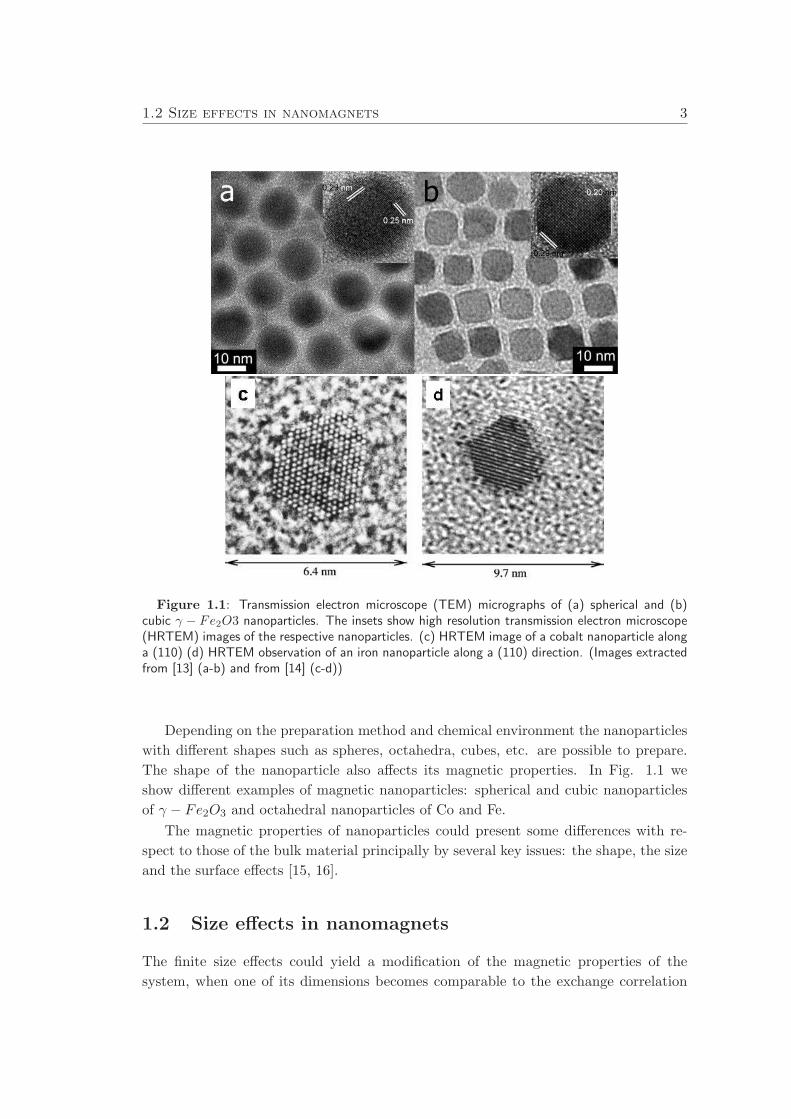
Figure 1.1: Transmission electron microscope (TEM) micrographs of (a) spherical and (b)cubic γ − Fe2O3 nanoparticles. The insets show high resolution transmission electron microscope(HRTEM) images of the respective nanoparticles. (c) HRTEM image of a cobalt nanoparticle alonga (110) (d) HRTEM observation of an iron nanoparticle along a (110) direction. (Images extractedfrom [13] (a-b) and from [14] (c-d))
Depending on the preparation method and chemical environment the nanoparticles
with different shapes such as spheres, octahedra, cubes, etc. are possible to prepare.
The shape of the nanoparticle also affects its magnetic properties. In Fig. 1.1 we
show different examples of magnetic nanoparticles: spherical and cubic nanoparticles
of γ − Fe2O3 and octahedral nanoparticles of Co and Fe.
The magnetic properties of nanoparticles could present some differences with re-
spect to those of the bulk material principally by several key issues: the shape, the size
and the surface effects [15, 16].
1.2 Size effects in nanomagnets
The finite size effects could yield a modification of the magnetic properties of the
system, when one of its dimensions becomes comparable to the exchange correlation
4 Introduction
length of the system. The most important finite size effects in nanoparticles are the
single domain limit and the super-paramagnetic limit.
The macroscopic materials can present a null net magnetization in the absence of
applied magnetic field, inclusive if the material is ferromagnetic, it is due to the fact
that when the system size is above a certain value, the division of the system into
magnetic domains is energetically favorable. If the size of the system is under a certain
cutoff, denominated single domain radius (Rsd), the system prefers a mono-domain
state. This phenomenon was initially predicted by Frenkel and Doefman [17]. The
single domain radius depends on the magnetic parameters of the system (exchange
parameter, saturation magnetization, anisotropy constant) and typically lies in the
range of a few tens of nanometers.
If the size of the system continues to decrease then the nanoparticle becomes super-
paramagnetic (SP), due to thermal fluctuations and the reduction of the energy barrier
of the system. In this state a magnetic particle presents a large magnetic moment and
behaves like a giant paramagnetic moment with a fast response to an applied magnetic
field and negligible coercivity and remanence.
Thermal measurements have become an important part of the characterization of
magnetic nanoparticles systems. Often these measurements include a complex influ-
ence of interparticle interactions. However, in other cases, measurements on dilute
systems can provide information on individual particles. The results show that even in
these cases the extracted information is not always consistent with the approximation
picturing the particle as a macroscopic magnetic moment, and this is usually attributed
to surface effects.
If the nanoparticle size decreases more, the surface effects start to play a important
role and deviations from the collinear spin arrangement appear. When the magnetic
properties of magnetic nanoparticles are dominated by the surface effects, the ideal
model of a macro-spin formed by all the spins of the particle pointing in the direction
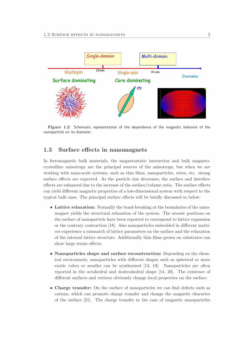
of the anisotropy easy axis could be no more valid. The schematic representation of
the size effects in nanoparticles is presented in Fig. 1.2.
Finite size effects also have important consequences in the magnetization behavior
of thin films. Indeed, when the film thickness is smaller than the exchange correlation
length, the magnetization is homogeneous through the thin film thickness. In these
conditions the magnetostatic interactions tend to place the magnetization in-plane
competing with the surface anisotropy effects.
1.3 Surface effects in nanomagnets 5
Figure 1.2: Schematic representation of the dependence of the magnetic behavior of thenanoparticle on its diameter.
1.3 Surface effects in nanomagnets
In ferromagnetic bulk materials, the magnetostatic interaction and bulk magneto-
crystalline anisotropy are the principal sources of the anisotropy, but when we are
working with nano-scale systems, such as thin films, nanoparticles, wires, etc. strong
surface effects are expected. As the particle size decreases, the surface and interface
effects are enhanced due to the increase of the surface/volume ratio. The surface effects
can yield different magnetic properties of a low-dimensional system with respect to the
typical bulk ones. The principal surface effects will be briefly discussed in below:
• Lattice relaxation: Normally the bond-breaking at the boundaries of the nano-
magnet yields the structural relaxation of the system. The atomic positions on
the surface of nanoparticle have been reported to correspond to lattice expansion
or the contrary contraction [18]. Also nanoparticles embedded in different matri-
ces experience a mismatch of lattice parameters on the surface and the relaxation
of the internal lattice structure. Additionally thin films grown on substrates can
show large strain effects.
• Nanoparticles shape and surface reconstruction: Depending on the chem-
ical environment, nanoparticles with different shapes such as spherical or more
exotic cubes or neadles can be synthesized [13, 19]. Nanoparticles are often
reported in the octahedral and dodecahedral shape [14, 20]. The existence of
different surfaces and vertices obviously change local properties on the surface.
• Charge transfer: On the surface of nanoparticles we can find defects such as
cations, which can promote charge transfer and change the magnetic character
of the surface [21]. The charge transfer in the case of magnetic nanoparticles
6 Introduction
coated with polymers is also known to occur [22], as well as in nanoparticles with
organic molecules or embedded in different non-organic matrices.
• Oxidation: Metallic nanoparticles are chemically active and are easily oxidized
in air, resulting generally in a reduction or even loss of the total magnetic moment.
For instance, cobalt is a typical ferromagnetic (FM) material, nevertheless its
oxide CoO has an anti-ferromagnetic (AFM) character [23], in a similar way as
Ni and NiO [24]. Additionally, when the surface of Co or Ni nanoparticles is
oxidized, we find a system with two different magnetic phases which could lead
to new magnetic phenomena. For example, this kind of a composite material
(FM-AFM or vice-versa) could present the exchange bias effect [25–27].
• Variation of the magnetic moment: In ferromagnetic systems the magnetic
moment may be enhanced by reducing the dimensionality [28]. Magnetic moment
enhancement with decreasing size has been observed experimentally and theoret-
ically in metallic nano-clusters of Fe, Co, Ni, etc. [29–32]. Therefore in systems
like metallic ferromagnet nanoparticles where a large fraction of the spins belong
to the surface, one could expect an increment of the system’s magnetization.
• Surface spin disorder: A reduction of the saturation magnetization, Ms, has
been observed experimentally in nanoparticles. Initially, this reduction has been
explained by models which postulated the existence of a ”dead” magnetic layer
at the surface [33], however there are other theories that relate the origin of that
effect with the existence of a canted spin configuration at the surface [34], or the
spin-glass-like spin state [35]. But up to now, the origin of the canting of the
spins in fine particles is an object of a continuing discussion [15].
• Surface anisotropy Another surface-driven effect is the enhancement of the
magnetic anisotropy with decrease of the system size [32, 36, 37]. That increment
is assumed to be originated by the anisotropy at surface and has been detected
experimentally in nanoparticles of Co, Fe, etc. [8, 10, 38]. Also a systematic
study with different coatings has revealed that they can influence to the effective
anisotropy.
• Variation of the exchange interaction at surface: The variation of the
exchange interaction energy at surface has been reported from a theoretical point
of view in thin films [39, 40] and also has been observed in magnetic nanoparticles.
For example, Ni1−xCux material has shown a drop of the Curie temperature of
the system as the concentration of Cu is increased. Such a decrease of Tc is
associated to the variation of the exchange interaction strength at the surface
[41].
In practice it is impossible to separate these effects and consequently, all of them
are normally embedded in the phenomenological concept of the ”surface anisotropy”.
1.4 The magnetic anisotropy 7
The detailed theoretical description of real experimental situation is almost impossible
due to competition of many effects and large dispersion of individual nanoparticles
properties.
1.4 The magnetic anisotropy
It is known that the magnetization M tends to orient preferentially along one or several
axes in magnetic solids. The magnetic anisotropy energy is defined as the energy term
that describes the dependence of the internal energy on the direction of the magne-
tization, and it may be originated by the crystalline electric field of the solid, by the
shape or surface of the magnetic body, by mechanical stress etc. Usually the magnetic
anisotropy energy has the symmetry of the crystal structure of the material and it is
invariant to the inversion of the magnetization. These facts mean that the magnetic
anisotropy energy must be an expansion of even functions of the angles enclosed by
the magnetization and the magnetic axes. Hereafter we present the expressions of the
magnetic anisotropy energy density (Eani) for the most frequent cases:
Cubic symmetry We denote αi; i = 1, 2, 3 as the cosines of the angles between the
magnetization and the axes X;Y;Z parallel to the fourfold axes. Then Eani has
the following form:
Eani = K1(α21α
22 + α2
1α23 + α2
3α22) +K2α
21α
22α
23 + ... (1.1)
Tetragonal symmetry If we denote θ and ϕ as the angles in polar coordinates, and
Z as the axis parallel to the sixfold axis [001], then Eani has the following form:
Eani = K1 sin2(θ) +K2 sin4(θ) +K3 sin6(θ) +K4 sin6(θ) cos(6ϕ) + ... (1.2)
Quadratic symmetry In this symmetry there is a fourfold axis [001], and Z is the
axis parallel to that axis. Then Eani has the following form:
Eani = K1 sin2(θ) +K2 sin4(θ) +K3 sin4(θ) cos(4ϕ) + ... (1.3)
Uniaxial symmetry The first terms in the expansion of Eani in the case of the tetrag-
onal, rhombohedral and quadratic symmetries are the same. Usually the next
term in the expansion is at least one order of magnitude smaller. Then if we
restrict the expansion to the first term, we obtain that Eani is of the second order
and only depends on the angle between the magnetic moment and the axis of the
highest symmetry θ, in the following form:
Eani = K1 sin2(θ). (1.4)
This kind of magnetic anisotropy can also be found in amorphous material sub-
mitted to stress or isotropic magnetic material annealed under the presence of a
magnetic field.
8 Introduction
The values above [Ki(i = 1, 2, 3, 4...)] are the anisotropy constants with dimension
[energy/volume]. These parameters depend on the temperature and material and they
can range from around 100 erg/cm3 in soft materials, passing through 104 − 105
erg/cm3 for 3d metals of cubic symmetry like Ni, Fe, etc., to 107 − 108 erg/cm3 in
some rare earth alloys and L10 compound such as FePt and CoPt. In practice, Ki is
usually derived from experiments (ferromagnetic resonance, magnetization curve, etc)
as an empirical constant.
The total magnetic anisotropy can be the result of several contributions: the
magneto-crystalline anisotropy (MCA), surface anisotropy, shape anisotropy, magne-
tostriction anisotropy, exchange anisotropy etc.
1.4.1 Magneto-crystalline anisotropy
Magneto-crystalline anisotropy (MCA) is one of the most important energy contribu-
tions in magnetic materials and it is generated by the atomic structure and bonding in
the magnetic material. Attempts to understand its microscopic origin have been taking
place since many years ago. As proposed by Van Vleck [42], the origin to the MCA
energy is the spin-orbit coupling interaction (SOC), which is the term that links the
spatial and spin parts of the wave functions. In the case of a central potential V (r),
its interaction is given as:
HSO = ξ(r)L · S (1.5)
ξ(r) =1
4m2c2r
dV (r)
dr(1.6)
where m is the mass of the electron, c is the speed of light in the vacuum, r is the
distance from the nuclei, L and S are orbital and spin moments. We would like to note
that this form of the SOC term has been used in almost all cases. Although the potential
(V (r)) is not generally central, nevertheless as dV (r)dr has its maxim contribution close to
the nuclei, where V (r) is approximated as the central potential, thus the approximation
of SOC (1.5) is generally accepted.
Theoretically the magneto-crystalline anisotropy is determined from the evaluation
of the difference of the system’s energy when the magnetization is orientated along the
easy and hard axes. If other contributions such as the magnetostatic energy can be
neglected, then the MCA is given by the anisotropy due to the spin-orbit coupling:
∆ESO = 〈HSO〉hard − 〈HSO〉easy = ζ[〈L · S〉hard − 〈L · S〉easy] > 0 (1.7)
where ζ = 〈ξ(r)〉 is the spin-orbit coupling constant. This way the magnetization of the
system in the hard direction requires an input of energy into the system. The principal
difficulty in the study of the MCA is its small size, for example in transition metals
MCA is of the order of µeV , which is usually in the limit of accuracy of theoretical
calculations.

1.4 The magnetic anisotropy 9
1.4.2 Surface magnetic anisotropy
As we have mentioned previously, the magnetic anisotropy can be increased when the
size of the system is reduced. It is usually explained by the existence of the surface
anisotropy different to the bulk one.
Neel in 1954 was the first to suggest the existence of this kind of anisotropy. After
that many experimental evidences have corroborated that claim [43], and there exist
multiple works on calculation of the surface anisotropy from the first principles [44–
46]. An important point that we should take into account is that for small particles
or clusters or ultrathin films where the number of spin at surface is large, the surface
anisotropy can easily dominate the bulk one, especially in cubic materials.
Figure 1.3: Shematic drawing illustrating the Neel pair model.
The Neel model of the surface magnetic anisotropy
The modeling of the surface anisotropy contribution is a complex field of research. Neel
proposed a phenomenological model of the surface anisotropy called after that the ”Neel
surface anisotropy (NSA) model”. The model assumes an origin of the anisotropy bas-
ing on the lack of the atomic bonds on the surface of a crystal. The surface anisotropy
contribution is described as a pair-interaction of spins in the following way:
HNSAi =
L(rij)
2
zi∑
j=1
(−→s i ·−→e ij)
2, (1.8)
−→e ij =−→r ij
rij,
−→r ij = −→r i −−→r j .
Here zi is the number of nearest neighbors of the surface spin i, (known as the coordina-
tion number), −→s i is a unit vector pointing along the magnetization direction,rij is the
distance between spin i and j, −→e ij is the unit vector connecting the spin i to its nearest
neighbor j, the factor 1/2 is added in order not to count twice the pair interaction and
10 Introduction
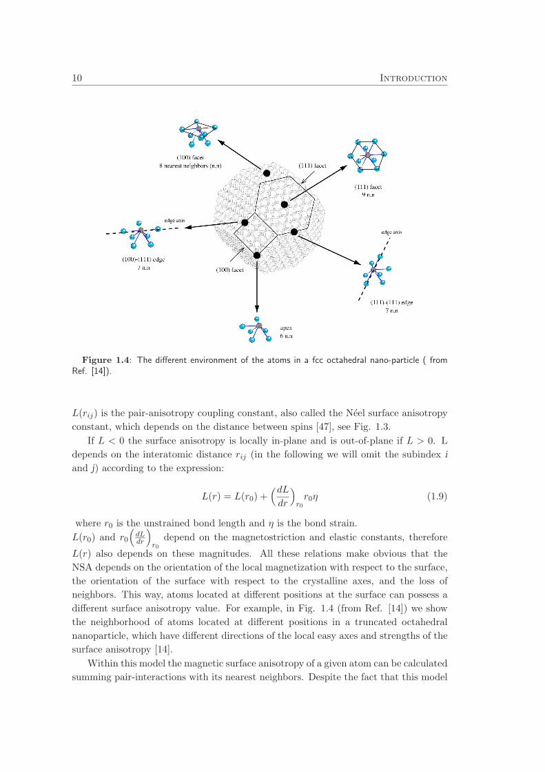
Figure 1.4: The different environment of the atoms in a fcc octahedral nano-particle ( fromRef. [14]).
L(rij) is the pair-anisotropy coupling constant, also called the Neel surface anisotropy
constant, which depends on the distance between spins [47], see Fig. 1.3.
If L < 0 the surface anisotropy is locally in-plane and is out-of-plane if L > 0. L
depends on the interatomic distance rij (in the following we will omit the subindex i
and j) according to the expression:
L(r) = L(r0) +(dL
dr
)
r0r0η (1.9)
where r0 is the unstrained bond length and η is the bond strain.
L(r0) and r0
(
dLdr
)
r0depend on the magnetostriction and elastic constants, therefore
L(r) also depends on these magnitudes. All these relations make obvious that the
NSA depends on the orientation of the local magnetization with respect to the surface,
the orientation of the surface with respect to the crystalline axes, and the loss of
neighbors. This way, atoms located at different positions at the surface can possess a
different surface anisotropy value. For example, in Fig. 1.4 (from Ref. [14]) we show
the neighborhood of atoms located at different positions in a truncated octahedral
nanoparticle, which have different directions of the local easy axes and strengths of the
surface anisotropy [14].
Within this model the magnetic surface anisotropy of a given atom can be calculated
summing pair-interactions with its nearest neighbors. Despite the fact that this model
1.4 The magnetic anisotropy 11
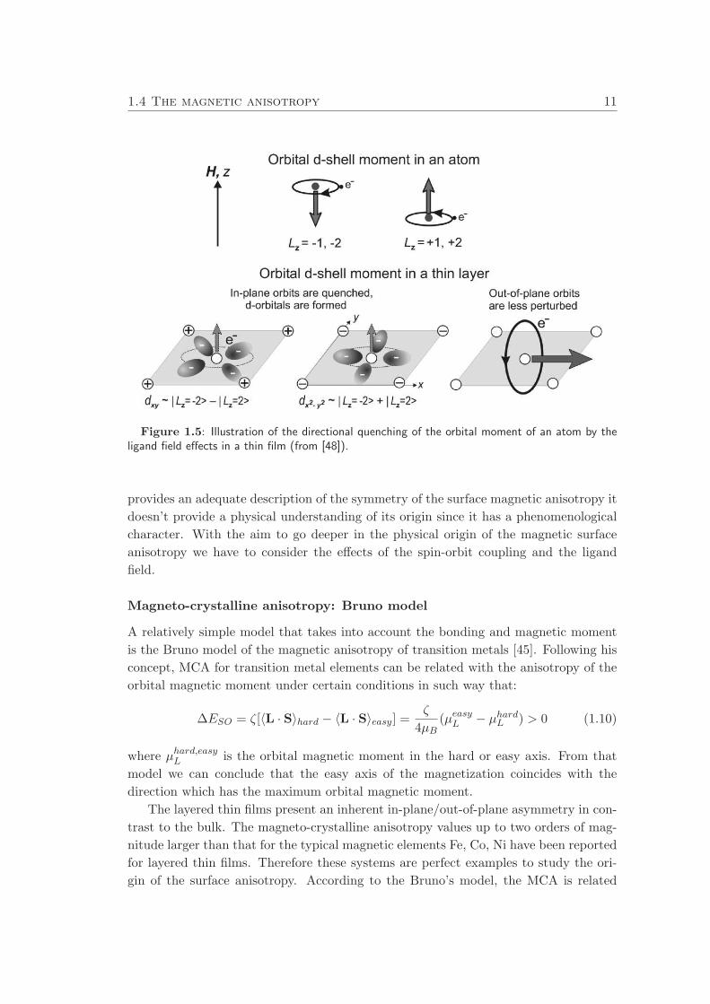
Figure 1.5: Illustration of the directional quenching of the orbital moment of an atom by theligand field effects in a thin film (from [48]).
provides an adequate description of the symmetry of the surface magnetic anisotropy it
doesn’t provide a physical understanding of its origin since it has a phenomenological
character. With the aim to go deeper in the physical origin of the magnetic surface
anisotropy we have to consider the effects of the spin-orbit coupling and the ligand
field.
Magneto-crystalline anisotropy: Bruno model
A relatively simple model that takes into account the bonding and magnetic moment
is the Bruno model of the magnetic anisotropy of transition metals [45]. Following his
concept, MCA for transition metal elements can be related with the anisotropy of the
orbital magnetic moment under certain conditions in such way that:
∆ESO = ζ[〈L · S〉hard − 〈L · S〉easy] =ζ
4µB(µeasyL − µhardL ) > 0 (1.10)
where µhard,easyL is the orbital magnetic moment in the hard or easy axis. From that
model we can conclude that the easy axis of the magnetization coincides with the
direction which has the maximum orbital magnetic moment.
The layered thin films present an inherent in-plane/out-of-plane asymmetry in con-
trast to the bulk. The magneto-crystalline anisotropy values up to two orders of mag-
nitude larger than that for the typical magnetic elements Fe, Co, Ni have been reported
for layered thin films. Therefore these systems are perfect examples to study the ori-
gin of the surface anisotropy. According to the Bruno’s model, the MCA is related
12 Introduction
with the anisotropy bonding and its relation with the ligand field. To illustrate this
concept we consider a d electron in a free atom and in an atom contained in a planar
geometry with other four atoms which can have negative or positive charge, see Fig.
1.5. In the planar geometry the d electron suffers the effects of the Coulomb repulsion
or attraction depending on the charge of its neighbors, altering its orbital with respect
to the free one. This way we can see the effects on the magnetic moment due to the
ligand field. We can observe a partial break of the degeneracy of the d orbital, one can
group the d orbitals into in-plane and out of plane, and we may quantitatively relate
the anisotropy of the orbital moment with the anisotropy of the bonding environment.
The corresponding orbital moment along the normal of the bonding plane is quenched,
however in the case of the moment in-plane with respect to the bond plane this is not
so. Due to the loss of neighbors at the surface the orbital motion perpendicular to
the bonding plane is less disturbed and the in-plane orbital momentum is unquenched.
This leads to an anisotropic orbital moment and to the surface anisotropy, according
to the Bruno’s model.
Therefore the exchange interaction is responsible for the creation of the spin mag-
netic moment and the ligand field creates anisotropic orbitals. The spin and orbital
moments are linked by the spin-orbit coupling and the orbital moment is locked in a
particular direction. The interplay of all these factors creates the surface magnetro-
crystalline anisotropy.
We should have in mind that the Bruno model is illustrative and may be too simple
in real situations. As it has been indicated by Andersson [49], the Bruno model could
be not adequate in the analysis of magnetic systems with high spin-orbit coupling.
1.4.3 The shape magnetic anisotropy
Magnetostatic are other sources of the total magnetic anisotropy called the macroscopic
shape anisotropy. This concept is clear in the case of homogeneous magnetization in
a ellipsoid, where the demagnetization tensor can be introduced in such way that the
demagnetization field can be defined as:
HD = −DM (1.11)
where D is the demagnetization tensor, HD is the demagnetization field and M is the
magnetization of the system. Thus the density magnetostatic energy can be described
as:
EM = 2πMDM (1.12)
If the semiaxes a, b, and c of the ellipsoid represent the axes of the coordination system
the D is a diagonal tensor. An arbitrary direction of the magnetization with respect
to the semiaxes can be characterized by the direction cosine αa,αb, and αc. The tensor
1.5 Experimental approach 13
is given by:
D =
Da 0 0
0 Db 0
0 0 Dc
(1.13)
and the magnetostatic energy density can be written as:
EM = 2πMs(Daα2a + Dbα
2b + Dcα
2c) . (1.14)
For thin films, magnetostatic interaction leads to an additional anisotropy favoring the
in-plane anisotropy. In the case of elongated nanoparticles, magnetostatic interactions
produce an additional easy axis parallel to the long dimensions.
1.5 Experimental approach
Many techniques are available in our days to measure the magnetic properties of nano-
magnets. The challenge lays in measurements of not only macroscopic properties which
are generally achieved by the magnetometry measurements but in measurements of
local properties at nanoscale. In the past decade several techniques have provided
important measurements with the aim to understand surface effects in magnetic films
and nanoparticles:
X-ray absorption magnetic circular dichroism (XMCD) This technique was
pioneered by Schutz and co-workers [50]. It is based on the changes in the absorption
cross section of a magnetic material and uses circularly polarized photons [51]. Through
the well-known sum rules it allows to determine the relation between the orbital and
the spin magnetic moments µL/µs. A big advantage of this technique is that it is
element specific and it is able to identify moment orientations in ultrathin films and
monolayer magnetic materials. The X-ray microscopy also allows imaging with 100
nm. resolution.
(Micro-)Superconducting Quantum Interface Device (µ) − SQUID is a
powerful technique to measure the net magnetization on a nanometer-size sample [52].
In 2001 Jamet et. al. have done the first magnetization reversal study on individual
Co nanoparticle (D = 20 nm.) using a new µ − SQUID setup. From those measure-
ments they deduced the magnetic anisotropy magnitude [20] and that the behavior of
individual nanoparticles follows the Neel-Arrhenius law [53].
1.5.1 Effective and surface anisotropies
In experimental situation and basing on macroscopic measurements, different con-
tributions to anisotropy are difficult to distinguish and the concept of the ”effective
anisotropy” is used. The meaning of the concept is not clear and it is probably highly
dependent on the employed experimental method, such as the magnetization work, the
14 Introduction
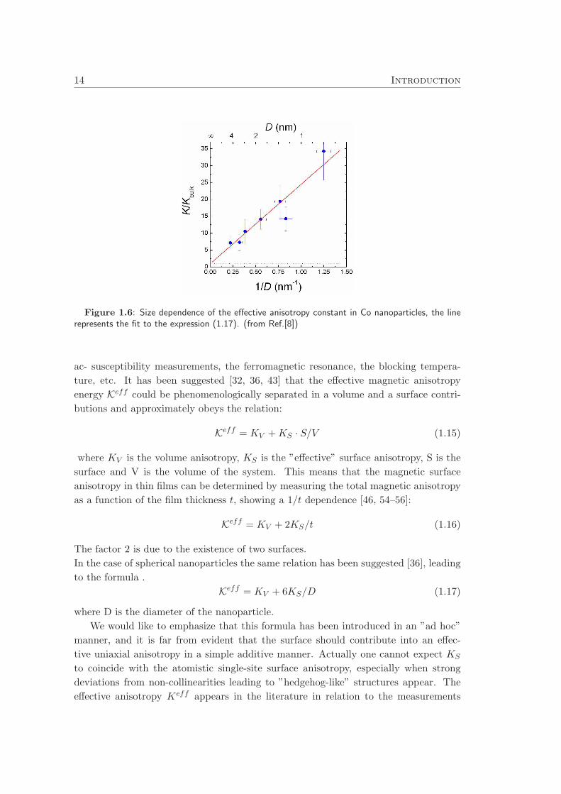
Figure 1.6: Size dependence of the effective anisotropy constant in Co nanoparticles, the linerepresents the fit to the expression (1.17). (from Ref.[8])
ac- susceptibility measurements, the ferromagnetic resonance, the blocking tempera-
ture, etc. It has been suggested [32, 36, 43] that the effective magnetic anisotropy
energy Keff could be phenomenologically separated in a volume and a surface contri-
butions and approximately obeys the relation:
Keff = KV +KS · S/V (1.15)
where KV is the volume anisotropy, KS is the ”effective” surface anisotropy, S is the
surface and V is the volume of the system. This means that the magnetic surface
anisotropy in thin films can be determined by measuring the total magnetic anisotropy
as a function of the film thickness t, showing a 1/t dependence [46, 54–56]:
Keff = KV + 2KS/t (1.16)
The factor 2 is due to the existence of two surfaces.
In the case of spherical nanoparticles the same relation has been suggested [36], leading
to the formula .
Keff = KV + 6KS/D (1.17)
where D is the diameter of the nanoparticle.
We would like to emphasize that this formula has been introduced in an ”ad hoc”
manner, and it is far from evident that the surface should contribute into an effec-
tive uniaxial anisotropy in a simple additive manner. Actually one cannot expect KS
to coincide with the atomistic single-site surface anisotropy, especially when strong
deviations from non-collinearities leading to ”hedgehog-like” structures appear. The
effective anisotropy Keff appears in the literature in relation to the measurements
1.5 Experimental approach 15
of energy barriers of nanoparticles, extracted from the magnetic viscosity or dynamic
susceptibility measurements. Generally speaking, the surface anisotropy should affect
both the minima and the saddle points of the energy landscape in this case. It is clear
that while the measurement of viscosity are related to the saddle point, the magnetic
resonance measurements depend on the stiffness of the energy minima modified by the
surface effects. Thus the meaning of the Keff is different for different measurement
techniques.
Despite its rather ”ad hoc” character, this formula has become the basis of many
experimental studies with the aim to extract the surface anisotropy (see, e.g., Refs. [8,
32, 57]) because of its mere simplicity.
In Fig. 1.6 we present some experimental results (from Ref. [8]) where the effective
anisotropy is plotted as a function of the inverse of the diameter of Co nanoparticle
(which is supposed to have a spherical shape) and is fitted to the expression of Keff
similar to Eq.(1.17).
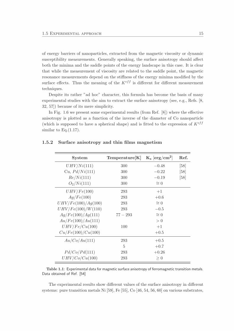
1.5.2 Surface anisotropy and thin films magnetism
System Temperature[K] Ks [erg/cm2] Ref.
UHV/Ni(111) 300 −0.48 [58]
Cu, Pd/Ni(111) 300 −0.22 [58]
Re/Ni(111) 300 −0.19 [58]
O2/Ni(111) 300 ∼= 0
UHV/Fe(100) 293 +1
Ag/Fe(100) 293 +0.6
UHV/Fe(100)/Ag(100) 293 ∼= 0
UHV/Fe(100)/W (110) 293 −0.5
Ag/Fe(100)/Ag(111) 77 − 293 ∼= 0
Au/Fe(100)/Au(111) > 0
UHV/Fe/Cu(100) 100 +1
Cu/Fe(100)/Cu(100) +0.5
Au/Co/Au(111) 293 +0.5
5 +0.7
Pd/Co/Pd(111) 293 +0.26
UHV/Co/Cu(100) 293 ≥ 0
Table 1.1: Experimental data for magnetic surface anisotropy of ferromagnetic transition metals.Data obtained of Ref. [54]
The experimental results show different values of the surface anisotropy in different
systems: pure transition metals Ni [59], Fe [55], Co [46, 54, 56, 60] on various substrates,
16 Introduction
orientations and overlayers or alloys such as MnSb [61]. The data are shown in Table
1.1.
In general, the easy axis of the magnetization in thin film is determined by the
competition between the magnetocrystalline anisotropy, the magnetostatic energy and
the surface anisotropy. The experimental progress in growing epitaxial magnetic thin
films and multilayer down to monolayer thickness has revealed a wealth of interesting
phenomena, such as the perpendicular magnetic anisotropy (PMA), which consist of a
preference for the magnetization to lie along the normal to the plane of the magnetic
film. The use of a magnetic system that presents PMA as a magnetic storage media
has been shown as a good strategy to improve the storage density.
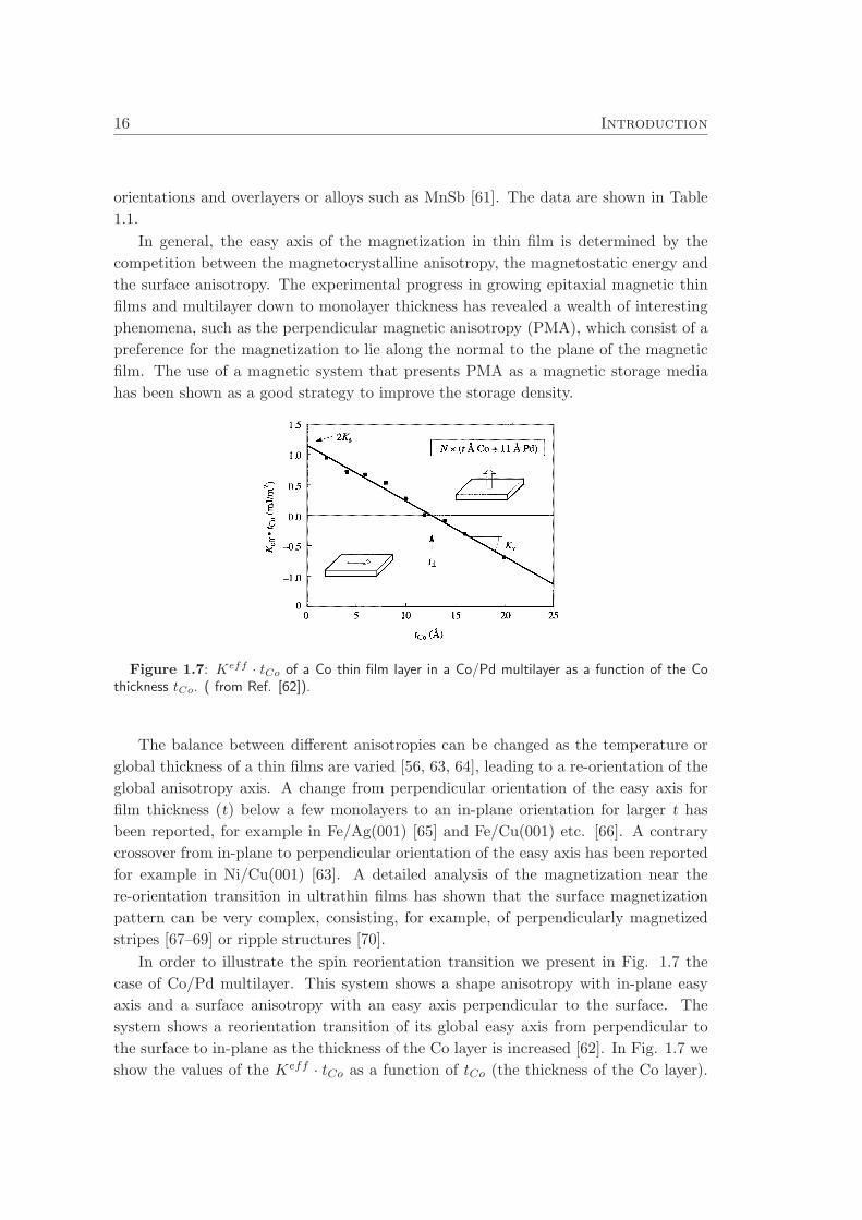
Figure 1.7: Keff · tCo of a Co thin film layer in a Co/Pd multilayer as a function of the Cothickness tCo. ( from Ref. [62]).
The balance between different anisotropies can be changed as the temperature or
global thickness of a thin films are varied [56, 63, 64], leading to a re-orientation of the
global anisotropy axis. A change from perpendicular orientation of the easy axis for
film thickness (t) below a few monolayers to an in-plane orientation for larger t has
been reported, for example in Fe/Ag(001) [65] and Fe/Cu(001) etc. [66]. A contrary
crossover from in-plane to perpendicular orientation of the easy axis has been reported
for example in Ni/Cu(001) [63]. A detailed analysis of the magnetization near the
re-orientation transition in ultrathin films has shown that the surface magnetization
pattern can be very complex, consisting, for example, of perpendicularly magnetized
stripes [67–69] or ripple structures [70].
In order to illustrate the spin reorientation transition we present in Fig. 1.7 the
case of Co/Pd multilayer. This system shows a shape anisotropy with in-plane easy
axis and a surface anisotropy with an easy axis perpendicular to the surface. The
system shows a reorientation transition of its global easy axis from perpendicular to
the surface to in-plane as the thickness of the Co layer is increased [62]. In Fig. 1.7 we
show the values of the Keff · tCo as a function of tCo (the thickness of the Co layer).

1.6 The challenge of modeling of magnetic nanoparticles and thin films17
The reorientation transition is indicated in the figure by the change of Keff sign. If
Keff > 0 the easy axis of the system is perpendicular to the surface, and the easy axis
of the system is in plane if Keff < 0.
1.6 The challenge of modeling of magnetic nanoparticles
and thin films
The understanding of the origin of the surface anisotropy and its influence on the
magnetic behavior of thin films and nanoparticles relies on the modeling. Electronic
structure calculations have been proven to explain the physical reasons behind the
existence of several surface effects such as the spin polarization. The main problem,
however, lies in the fact that although these calculations are reasonably good in deter-
mining the difference between spin up and spin down populations, they are often not
accurate enough to calculate the anisotropy value. Besides this fact, the calculations
are mostly limited to small systems only and to zero temperatures.
The full quantum mechanical treatment of a 5 nm nanoparticle is still not feasi-
ble. The modeling of magnetic nanoparticles from the first-principle side is, therefore,
normally limited to small clusters of hundreds of atoms [71, 72] and cannot take into
account to a full extend the spin non-collinearities, their dynamics and temperature.
Larger magnetic nanoparticles of 10 nm diameter are normally modeled using the
Heisenberg model. An important role of spin non-collinearities [73] in understanding
the magnetic behavior of nanoparticles has been reported using these types of studies.
This so-called ”atomistic” description [74–79] is relied on the Heisenberg-type Hamilto-
nian and can include spin dynamics and temperature. As a handicap these calculations
use phenomenological surface anisotropy models, such as the transverse anisotropy one
[75]. One of the most justified models for the surface anisotropy is the widely-used
Neel surface anisotropy model [14, 47, 74] which will be also used in the present thesis.
The challenge, however, is the understanding of not only individual nanoparticles
but their ensembles, where the distributions of individual properties and interactions
play an important role. This is normally done using the representation of each nanopar-
ticle as one macrospin [80, 81].
As for the thin films modeling, although intrinsic surface effects, based on the elec-
tronic interactions are localized on few layers, the magnetic exchange correlation length
makes the surface anisotropy to influence the magnetic structure down to nanometers
distance inside the material and may cause the inhomogeneous magnetization. The
correct account for the domain structure belongs to the area of micromagnetism - a
”continuous” approximation which has been proven to be very useful, especially in
understanding the hysteresis and dynamics of nanostructures with dimensions up to
several microns [82].
Therefore, one of the challenges of theoretical modeling in magnetism is the proper
18 Introduction
account of its multiscale character. The physics of magnetism in materials involve
many length, energy and time scales. And, unfortunately at this moment, a unified
description of all these scales on the same footing is impossible.
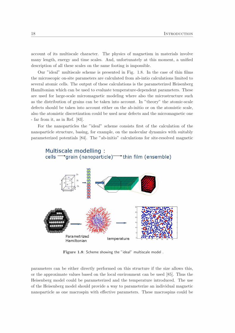
Our ”ideal” multiscale scheme is presented in Fig. 1.8. In the case of thin films
the microscopic on-site parameters are calculated from ab-intio calculations limited to
several atomic cells. The output of these calculations is the parameterized Heisenberg
Hamiltonian which can be used to evaluate temperature-dependent parameters. These
are used for large-scale micromagnetic modeling where also the microstructure such
as the distribution of grains can be taken into account. In ”theory” the atomic-scale
defects should be taken into account either on the ab-initio or on the atomistic scale,
also the atomistic discretization could be used near defects and the micromagnetic one
- far from it, as in Ref. [83].
For the nanoparticles the ”ideal” scheme consists first of the calculation of the
nanoparticle structure, basing, for example, on the molecular dynamics with suitably
parameterized potentials [84]. The ”ab-initio” calculations for site-resolved magnetic
Figure 1.8: Scheme showing the ”ideal” multiscale model .
parameters can be either directly performed on this structure if the size allows this,
or the approximate values based on the local environment can be used [85]. Thus the
Heisenberg model could be parameterized and the temperature introduced. The use
of the Heisenberg model should provide a way to parameterize an individual magnetic
nanoparticle as one macrospin with effective parameters. These macrospins could be
1.7 About this thesis 19
used for the modeling of an ensemble of nanoparticles to study the effects of interactions.
We should note that even this scheme is too ambitious for the present state of art
and its development is making the first steps. Also this scheme is too simplified, since
as we mentioned above, the surface anisotropy, for example, has multiple ingredients,
many of them related to the presence of defects. The precise knowledge of defects on
the atomistic scale and its consequences is basically not available.
1.7 About this thesis
We would like to indicate that a unified treatment of the whole magnetic problem and
its temporal, length and energy scales is in nowadays a challenge. We have concentrated
our efforts in some parts and problems related to the total multiscale scheme.
This thesis presents a theoretical study of the magnetic behavior of the low dimen-
sional systems such as nanoparticles and thin films. Most of the magnetic parameters
used in the study correspond to the cobalt fcc ones. We have selected the Co because
it is one of the typical and widely used for applications magnetic material.
This thesis presents the way to parameterize multispin particle as an effective
macrospin with mixed anisotropy (a combination of an uniaxial and a cubic contri-
butions), which has been done in Chapter 2 and Chapter 3. Since the ab-initio
calculations on nanoparticles of reasonable sizes, taking account of all on-site param-
eters are not feasible at the present moment, we have used a phenomenological Neel
surface anisotropy model. The variety of nanoparticles with different shapes, under-
lying structures, strengths of the surface anisotropy, etc has been investigated. Such
approximation will in the future open the doors for modeling of an assemble of nanopar-
ticles as a set of effective macrospins which implicitly takes into account the effects of
the surface, underlying lattice structure and shape.
During the work on this thesis the method of the constrained Monte Carlo has
been developed in collaboration with Dr. P. Asselin (Seagate Technology, USA) and
co-workers. This new method allows to evaluate numerically the dependence on tem-
perature of the magnetic anisotropy in magnetic nanoparticles and thin films. We have
used it in the study of the dependence on temperature of the magnetic anisotropy
in magnetic thin films and nanoparticles with Neel surface anisotropy, in Chapter 4
and Chapter 5. In those chapters of the thesis we have analyzed the applicability of
the new method, have studied the deviations from the Callen-Callen law of the depen-
dence on temperature of macroscopic magnetic anisotropy in the presence of the surface
anisotropy. We have also studied the re-orientation transition in thin films with the
surface anisotropy. Finally, we also show the possibility to have a temperature-induced
transition from cubic (due to surface effects) to uniaxial macroscopic anisotropy in
nanoparticles.
In Chapter 6 we use a multiscale scheme, starting from the ”ab-initio” calculations
and using a fully relativistic screened Khon-Korringa-Rostocker (SKKR) method [86].

20 Introduction
The ”ab-initio” simulations have been performed with a code supplied by Dr. L.
Szunyogh from Budapest University, Hungary. The magnetic properties of Co (bulk),
semi-infinite Co ((100) and (111)), Co((100)\Ag and Co(111)\Ag system are studied.
The use of this method allows to extract local magnetic parameters and parameterize
the Heisenberg Hamiltonian. Inside the multi-scale scheme, the constrained Monte
Carlo method is applied to evaluate the temperature-dependent parameters, including
the macroscopic anisotropy in the presence of the Ag surface.
2Multi-spin nanoparticle as an effective one spin
problem
2.1 Introduction
Since the ”ab-initio” treatment of a magnetic nanoparticle remains a future challenge,
in this chapter we consider a nanoparticle treated as a multi-spin problem but within
a classical atomic spin approach. Even in this case, the investigation of the thermal
magnetization switching of a multi-spin nanoparticle is a real challenge. We are faced
with complex many-body aspects with the inherent difficulties related with the analysis
of the energy potential and its extrema. This analysis is unavoidable since it is a
crucial step in the calculation of the relaxation time and thereby in the study of the
magnetization stability against thermal fluctuations. As such, a question arises whether
it is possible to map the behavior of a multi-spin nanoparticle onto that of a simpler
model system as one effective magnetic moment, without loosing its main features
such as surface anisotropy, lattice structure, size and shape, and more importantly
the spin non-collinearities they entail. A first answer to this question was given in
Ref. [74] where it was shown that when the surface anisotropy is much smaller than
the exchange parameter and in the absence of the core anisotropy, the single-site Neel
surface anisotropy contribution to the particle’s effective energy is of the fourth order
in the net magnetization components, of the second order in the surface anisotropy
constant, and is proportional to a surface integral. The latter accounts for the lattice
structure and the particle’s shape. Later it has been shown that in a more general
situation with the core anisotropy, taken as uniaxial, the energy of the multi-spin
21
22 Multi-spin nanoparticle as an effective one spin problem
particle could be modelled by that of an effective potential containing both uniaxial
and cubic anisotropy terms [87].
In this chapter we investigate this issue in a more extensive way by considering other
lattice structures, particle’s shapes and different anisotropies in the core. For this pur-
pose, we compute the energy potential of the multi-spin particle using the Lagrangian
multiplier method [74] and fit it to the appropriate effective energy potential.
2.2 Model
2.2.1 Shape and surface of nanoparticles
In this study we show that the magnetic behavior of small particles is very sensitive to
the surface arrangement, shape of the particles and underlying crystallographic struc-
ture. To investigate the various tendencies, we have considered particles cut from
lattices with the simple cubic (sc) and face-centered cubic (fcc). Although experi-
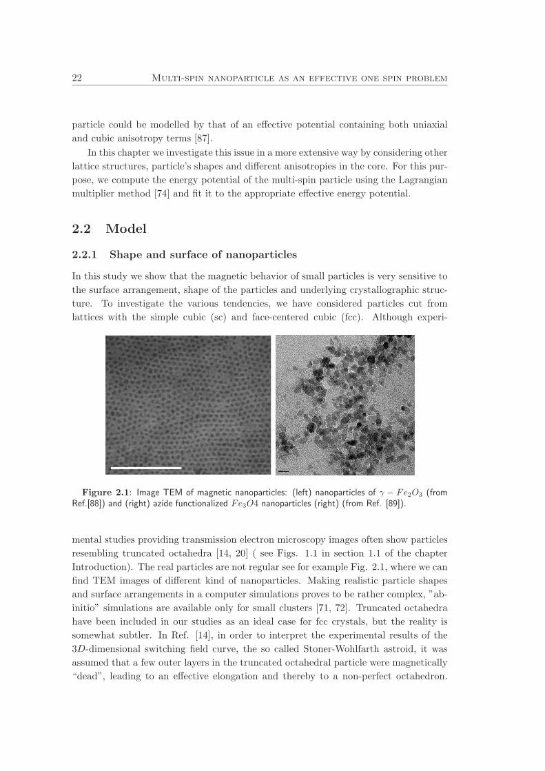
Figure 2.1: Image TEM of magnetic nanoparticles: (left) nanoparticles of γ − Fe2O3 (fromRef.[88]) and (right) azide functionalized Fe3O4 nanoparticles (right) (from Ref. [89]).
mental studies providing transmission electron microscopy images often show particles
resembling truncated octahedra [14, 20] ( see Figs. 1.1 in section 1.1 of the chapter
Introduction). The real particles are not regular see for example Fig. 2.1, where we can
find TEM images of different kind of nanoparticles. Making realistic particle shapes
and surface arrangements in a computer simulations proves to be rather complex, ”ab-
initio” simulations are available only for small clusters [71, 72]. Truncated octahedra
have been included in our studies as an ideal case for fcc crystals, but the reality is
somewhat subtler. In Ref. [14], in order to interpret the experimental results of the
3D-dimensional switching field curve, the so called Stoner-Wohlfarth astroid, it was
assumed that a few outer layers in the truncated octahedral particle were magnetically
“dead”, leading to an effective elongation and thereby to a non-perfect octahedron.

2.2 Model 23
Producing such a faceted elongated particle by somehow cutting the latter is an arbi-
trary procedure. In order to minimize the changes in the surface structure caused by
elongation, we assumed a spherical particle or introduced elliptical elongation along
the easy axis. This kind of structure has been the basis of many theoretical studies
using the Heisenberg Hamiltonian (see, e.g., Refs. [74, 75, 87, 90–94]).
Figure 2.2: Two particles cut from fcc structure: spherical (left) and truncated octahedron(right).
Regarding the arrangement on the particle’s surface, an appropriate approach would
be to use molecular-dynamic techniques [84, 95, 96] based on the empirical potentials
for specific materials. This would produce more realistic non-perfect surface structures,
more representative of what it is hinted to experimentally. However, these potentials
exist only for some specific materials and do not fully include the complex character
of the surface. Moreover, the particles thus obtained (see, e.g. Ref. [18]), may have
non-symmetric structures, and may present some dislocations. All these phenomena
lead to rich and different behavior of differently prepared particles.
In the present chapter, and in order to illustrate the general tendency of the mag-
netic behavior, we mostly present results for particles with ”pure” non-modified sur-
faces, namely spheres, ellipsoids and truncated octahedra cut from regular lattices.
Even in this case, the surface arrangement may appears to be very different (see Fig.
2.2) leading to a rich magnetic behavior.
2.2.2 Localized spin (atomistic or Heisenberg) model
We consider a magnetic nanoparticle of N spins in the many-spin approach, i.e., tak-
ing account of its intrinsic properties such as the lattice structure, shape, and size.
This also includes the (nearest-neighbor) exchange interactions, single-site core and
surface anisotropy. The magnetic properties of such a multi-spin particle (MSP) can
be described by the anisotropic Heisenberg model of classical spins Si (with |Si| = 1).
H = −1
2J∑
i,j
Si · Sj + Hanis. (2.1)
where J is the exchange parameter.

24 Multi-spin nanoparticle as an effective one spin problem
The anisotropy energy Hanis will be different if we are working with core spins or
surface spins. For core spins, i.e., those spins with full coordination, the anisotropy
energy Hanis is taken either as uniaxial with easy axis along z and a constant Kc (per
atom), that is
Hunianis = −Kc
Nc∑
i=1
S2i,z (2.2)
or cubic,
Hcubanis =
1
2Kc
Nc∑
i=1
(
S4i,x + S4
i,y + S4i,z
)
(2.3)
where Nc is the number of core spins in the particle. For surface spins the anisotropy
is taken according to the Neel’s surface anisotropy model (referred to in the sequel as
NSA), expressed as:
HNSAanis =
Ks
2
Ns∑
i=1
zi∑
j=1
(Si · uij)2 , (2.4)
where Ns is the number of surface spins, zi the number of nearest neighbors of site i,
and uij - a unit vector connecting this site to its nearest neighbors labeled by j.
Dipolar interactions are known to produce an additional ”shape” anisotropy. How-
ever, in the atomistic description, their role in describing the spin non-collinearities is
negligible as compared to that of all other contributions. In order to compare particles
with the same strength of anisotropy in the core, we assume that the shape anisotropy
is included in the core uniaxial anisotropy and neglect the dipolar energy contribution
to the spin non-collinearities. We also assume that in the ellipsoidal nanoparticles the
anisotropy easy axis is parallel to the elongation direction.
All physical constants will be measured with respect to the exchange coupling J
(unless explicitly stated otherwise), so we define the reduced constants,
kc ≡ Kc/J, ks ≡ Ks/J. (2.5)
The core anisotropy constant will be taken as kc ≃ 0.01, and kc ≃ 0.0025. The latter
constant in real units corresponds to Kc ≃ 3.2×10⁻¹⁷ erg/atom and is similar to cobalt
fcc value. On the other hand, the surface anisotropy constant ks is unknown ”a priori”
and will be varied.
2.3 Analytical background
In Refs. [73, 74, 87, 97] analytical as well as numerical calculations showed that a
multi-spin particle, cut from a sc lattice, and when its surface anisotropy is small with
respect to the exchange coupling, may be modeled by an effective one-spin particle
(EOSP), i.e., a single macroscopic magnetic moment m representing the net magnetic
2.3 Analytical background 25
moment of the multi-spin particle. The energy of this EOSP (normalized to JN ) may
be written as
EEOSP =(
Ec + E1 + E2 + E21)
. (2.6)
The E1 is the first-order anisotropy energy with surface contribution, E2 is the second-
order anisotropy energy with surface contribution, E21 is a mixed contribution to the
energy that is second order in surface anisotropy and first order in core anisotropy and
Ec is the core anisotropy energy (per spin).
The Ec energy has the following form:
Ec =Nc
Nkc
−m2z uniaxial,
12(m4
x +m4y +m4
z) cubic,
(2.7)
The other three contributions (E1, E2 and E21) stem from the surface, which we
discuss now.
2.3.1 Second-order surface-anisotropy energy E2
In Ref. [74] a spherical multi-spin nanoparticle was considered, the anisotropy in the
core was ignored and the surface anisotropy was taken as NSA. Using the continuous
approximation for N ≫ 1 the authors evaluated the surface energy density ES(m,n),
where m is the magnetization and n is the normal to the surface. The equilibrium
magnetization satisfied the Brown’s condition [98]:
m×Heff = 0, Heff = HA + J∆m (2.8)
here Heff is the total effective field, J is the exchange constant, ∆ is the Laplace
operator and HA is the anisotropy field, that in this case is due entirely to the surface.
HA = −dES
dmδ(r −R), (2.9)
here R represents the radius of the spherical particle.
For the case of Ks≪ J we can suppose that the deviations of m of the homogeneous
state m0 are small and the problem can be linearized.
m(r) ∼= m0 + ψ(r,m0), ψ = |ψ| ≪ 1 (2.10)
The correction ψ is the solution of the internal Neumann boundary problem for a
sphere:
∆ψ = 0,δψ
δr
∣
∣
∣
r=R= f(m,n) (2.11)
f(m,n) = −1
J
[dES(m0, r)
dm−(dES(m0, r)
dm·m0
)
m0
]
(2.12)
26 Multi-spin nanoparticle as an effective one spin problem
Then, solving the corresponding Neumann problem by the Green’s function technique,
we obtain:
ψ(r,m) =1
4π
∫
Sd2r′G(r, r′)f(m,n) (2.13)
where G(r, r′)is the Green function. Computing the energy of the multi-spin particle, it
was found that the corresponding effective energy is of the 4th−order in the components
of the net magnetic moment m and the 2nd−order in the surface anisotropy constant
ks, that is
E2 = k2∑
α=x,y,z
m4α, (2.14)
with
k2 = κk2sz. (2.15)
κ is a surface integral that depends on the underlying lattice, shape, and the size of
the particle and also on the surface-anisotropy model. For instance, κ ≃ 0.53466 for
a spherical particle cut from an sc lattice, with NSA. We would like to note that the
contribution (2.14) scales with the system’s volume and thus could renormalize the
volume anisotropy of the nanoparticle.
The equation (2.15) was obtained analytically for Ks ≪ J in the range of the
particle size large enough (N ≫ 1) but small enough so that δψ remains small. Being
δψ ∼ N 1/3Ks/J , the angle of order which describes the noncollinearity of the spins that
results from the competition of the exchange interaction and the surface anisotropy 1.
Since k2 is nearly size independent (i.e. the whole energy of the particle scales
with the volume), it is difficult to experimentally distinguish between the core cubic
anisotropy and the one due to the second order surface contribution (see discussion
later on). The physical reason for the independence of k2 on the system size is the
deep penetration of the spin non-collinearities into the core of the particle. This means
that the angular dependence of the non-collinearities also contributes to the effective
anisotropy. Interestingly this implies that the influence of the surface anisotropy on the
overall effective anisotropy is not an isolated surface phenomena and is dependent on
the magnetic state of the particle. We note that this effect is quenched by the presence
of the core anisotropy which could screen the effect at a distance of the order of domain
wall width from the surface.
The energy contribution E2 has also been derived in the presence of core anisotropy
[73] and numerically tested in Ref. [87]. Similar conclusions also apply for the case of
the transverse surface anisotropy, Ref. [87].
1Since the applicability conditions for Eqs. (2.14, 2.15) are usually not fully satisfied, numerical
calculations yield k2 slightly dependent on the system size [74].
2.3 Analytical background 27
2.3.2 First-order surface-anisotropy energy E1
In Ref. [74] the case of non-symmetrical particles was also discussed. More precisely,
for small deviations from spheres and cubes, i.e., for weakly ellipsoidal or weakly rect-
angular particles, there is a corresponding weak first-order contribution E1 that adds
up to E2. Hence, for an ellipsoid of revolution with axes a and b = a(1 + ǫ), ǫ ≪ 1,
cut out of an sc lattice so that the ellipsoid’s axes are parallel to the crystallographic
direction, one has that the first order anisotropy is given by [97]:
E1 = −k1m2z . (2.16)
where
k1 ∼ ksN−1/3ǫ , (2.17)
i.e. the E1 energy contribution scales with the surface of the system.
It is necessary to mention that for crystal shapes such as spheres and cubes the
contribution E1 vanishes by symmetry.
The ratio of the second to the first order surface contributions is:
E2E1
∼ ksN 1/3
ǫ, (2.18)
It can be significant even for Ks ≪ J due to the combined influence of the large particle
size and the small deviation from symmetry, ǫ≪ 1 .
2.3.3 Mixed contribution to the energy E21
Taking into account the core anisotropy analytically to describe corrections to Eq.
(2.14) due to the screening of the spin noncollinearities in the general case is difficult.
However, one can consider this effects perturbatively, at least to clarify the validity
limits of expression (2.14). In Ref. [97], the use of the general method outlined above
(see section 2.3.1) led to a Helmholtz equation. In this case, there is no exact Green’s
function and as such the perturbation theory was used to write the Green’s function
G in the presence of core anisotropy as the sum of the exact Green’s function G(0),
obtained in the absence of core anisotropy, and a correction G(1). The perturbation
parameter:
(2.19)
Therefore, upon using G = G(0) + p2αG(1) in the energy, it was found that G(1) leads
to a new contribution of the surface anisotropy which is also of the 2nd−order in the
surface anisotropy constant ks and the first order in kc.
E21 = k21 g(m) (2.20)
with
k21 = κ (kcNs) k2s (2.21)
28 Multi-spin nanoparticle as an effective one spin problem
where κ is another surface integral whose integrand contains G(1). g(m) is a function
of mα [97] which comprises, among other contributions, both the 2nd- and the 4th-order
contributions in spin components. For example, if we work with spherical coordinates
(θ, ϕ) for an sc lattice
g(θ, ϕ = 0) = − cos2 θ + 3 cos4 θ − 2 cos6 θ,
which is shown later to give an agreement with the numerical simulations, see Fig. 2.5.
The contribution (2.20), called here the core-surface mixing (CSM) contribution,
should satisfy k21 . k2 which requires:
NsKc/J . 1 (2.22)
This is exactly the condition that the screening length is still much greater than the
linear size of the particle. For larger system sizes the perturbative treatment becomes
invalid.
2.3.4 Effective one spin problem (EOSP) approximation
Consequently, collecting all the contributions, one can model the energy of a multi-spin
particle with an effective energy potential in the form:
EEOSP = −keffuam2z −
1
2keffca
∑
α=x,y,z
m4α. (2.23)
The subscripts ua/ca stand for uniaxial/cubic anisotropy, respectively.
Now, we note that due to the contributions (2.16) and (2.20), even when the core
anisotropy is not uniaxial, the effective energy contains two uniaxial contributions
induced by the surface, one is due to elongation given by (2.16) and the other to the
mixing between the core and the surface given by (2.20). Hence, the 2nd−order term
keffua in (2.23) takes into account these two contributions. Similarly, the 4th−order term
keffca is a result of the surface contributions (2.14) and part of (2.20), and may also
contain a contribution from the core if the latter has a cubic anisotropy.
To clarify the dependence on the system size and the surface anisotropy constants
of the different energy contributions to EOSP we summarized them in Tab. 2.1.
Although the analytical expressions are only established so far for sc lattices, they
do provide us with a general form of the effective energy potential which allows us
to investigate the different tendencies of the nanoparticle behavior, taking account of
various contributions to its energy. These approximate expressions are also very useful
in the interpretation of numerical results.
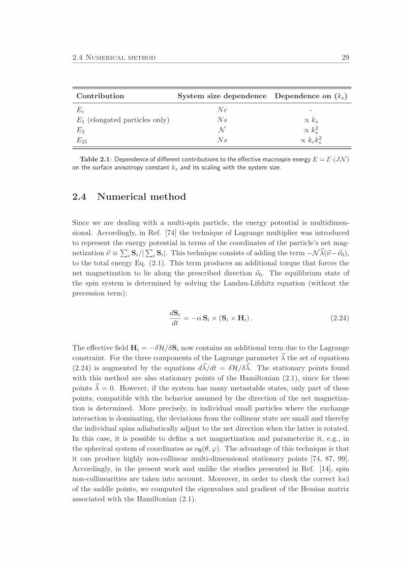
2.4 Numerical method 29
Contribution System size dependence Dependence on (ks)
Ec Nc -
E1 (elongated particles only) Ns ∝ ksE2 N ∝ k2sE21 Ns ∝ kck
2s
Table 2.1: Dependence of different contributions to the effective macrospin energy E = E ·(JN )on the surface anisotropy constant ks and its scaling with the system size.
2.4 Numerical method
Since we are dealing with a multi-spin particle, the energy potential is multidimen-
sional. Accordingly, in Ref. [74] the technique of Lagrange multiplier was introduced
to represent the energy potential in terms of the coordinates of the particle’s net mag-
netization ~ν ≡∑
i Si/|∑
i Si|. This technique consists of adding the term −N~λ(~ν−~ν0),
to the total energy Eq. (2.1). This term produces an additional torque that forces the
net magnetization to lie along the prescribed direction ~ν0. The equilibrium state of
the spin system is determined by solving the Landau-Lifshitz equation (without the
precession term):
dSi
dt= −αSi × (Si ×Hi) . (2.24)
The effective field Hi = −δH/δSi now contains an additional term due to the Lagrange
constraint. For the three components of the Lagrange parameter ~λ the set of equations
(2.24) is augmented by the equations d~λ/dt = δH/δ~λ. The stationary points found
with this method are also stationary points of the Hamiltonian (2.1), since for these
points ~λ = 0. However, if the system has many metastable states, only part of these
points, compatible with the behavior assumed by the direction of the net magnetiza-
tion is determined. More precisely, in individual small particles where the exchange
interaction is dominating, the deviations from the collinear state are small and thereby
the individual spins adiabatically adjust to the net direction when the latter is rotated.
In this case, it is possible to define a net magnetization and parameterize it, e.g., in
the spherical system of coordinates as ν0(θ, ϕ). The advantage of this technique is that
it can produce highly non-collinear multi-dimensional stationary points [74, 87, 99].
Accordingly, in the present work and unlike the studies presented in Ref. [14], spin
non-collinearities are taken into account. Moreover, in order to check the correct loci
of the saddle points, we computed the eigenvalues and gradient of the Hessian matrix
associated with the Hamiltonian (2.1).
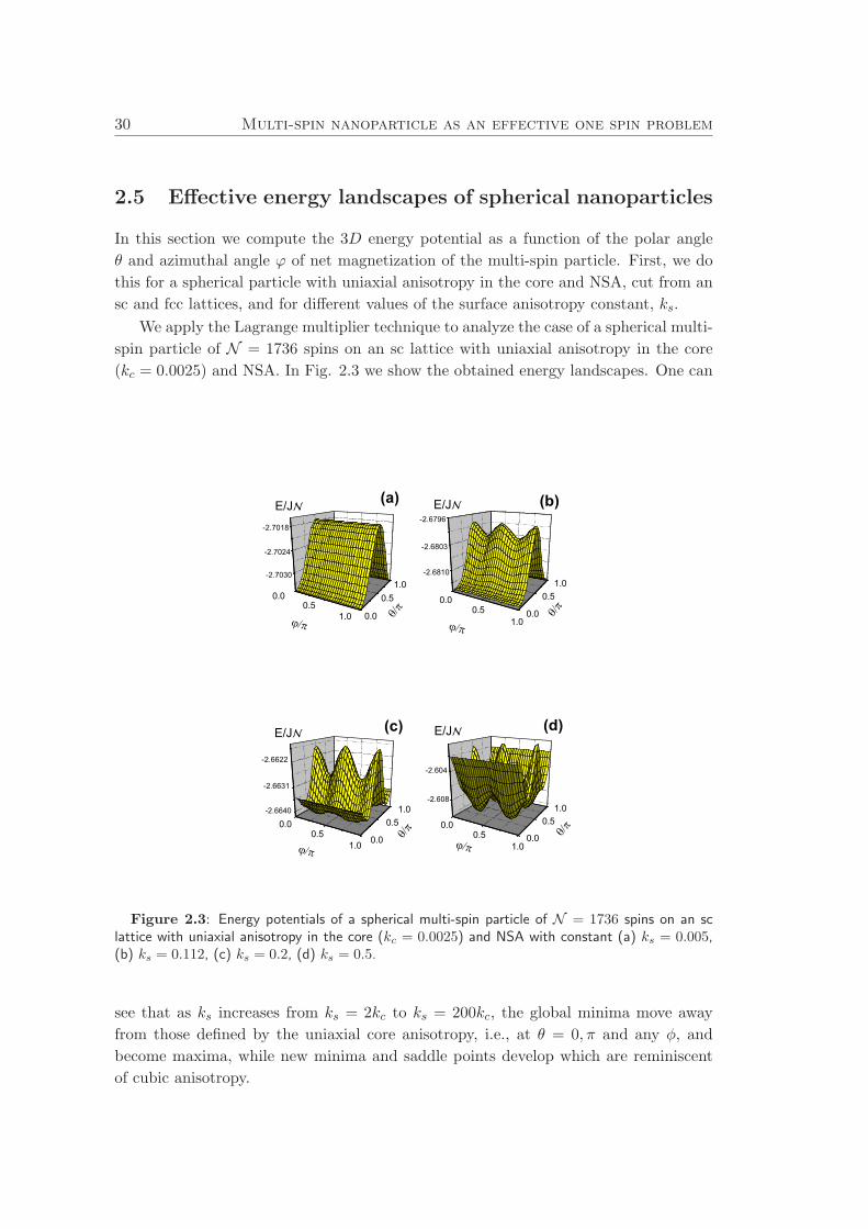
30 Multi-spin nanoparticle as an effective one spin problem
2.5 Effective energy landscapes of spherical nanoparticles
In this section we compute the 3D energy potential as a function of the polar angle
θ and azimuthal angle ϕ of net magnetization of the multi-spin particle. First, we do
this for a spherical particle with uniaxial anisotropy in the core and NSA, cut from an
sc and fcc lattices, and for different values of the surface anisotropy constant, ks.
We apply the Lagrange multiplier technique to analyze the case of a spherical multi-
spin particle of N = 1736 spins on an sc lattice with uniaxial anisotropy in the core
(kc = 0.0025) and NSA. In Fig. 2.3 we show the obtained energy landscapes. One can
0.00.5
1.0 0.0
0.51.0
-2.7030
-2.7024
-2.7018
0.00.5
1.00.0
0.51.0
-2.6810
-2.6803
-2.6796
0.00.5
1.0 0.0
0.51.0-2.6640
-2.6631
-2.6622
0.00.5
1.00.0
0.51.0
-2.608
-2.604
(a) (b)
(c)
E/J E/J
E/J E/J (d)
Figure 2.3: Energy potentials of a spherical multi-spin particle of N = 1736 spins on an sclattice with uniaxial anisotropy in the core (kc = 0.0025) and NSA with constant (a) ks = 0.005,(b) ks = 0.112, (c) ks = 0.2, (d) ks = 0.5.
see that as ks increases from ks = 2kc to ks = 200kc, the global minima move away
from those defined by the uniaxial core anisotropy, i.e., at θ = 0, π and any φ, and
become maxima, while new minima and saddle points develop which are reminiscent
of cubic anisotropy.
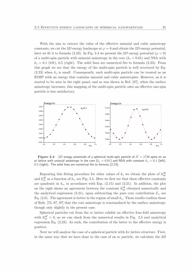
2.5 Effective energy landscapes of spherical nanoparticles 31
With the aim to extract the value of the effective uniaxial and cubic anisotropy
constants, we cut the 3D energy landscape at ϕ = 0 and obtain the 2D energy potential,
later we fit it to formula (2.23). In Fig. 2.4 we present the 2D energy potential (ϕ = 0)
of a multi-spin particle with uniaxial anisotropy in the core (kc = 0.01) and NSA with
ks = 0.1 (left), 0.5 (right). The solid lines are numerical fits to formula (2.23). From
this graph we see that the energy of the multi-spin particle is well recovered by Eq.
(2.23) when ks is small. Consequently, such multi-spin particle can be treated as an
EOSP with an energy that contains uniaxial and cubic anisotropies. However, as it is
started to be seen in the right panel, and as was shown in Ref. [87], when the surface
anisotropy increases, this mapping of the multi-spin particle onto an effective one-spin
particle is less satisfactory.
0.0 0.2 0.4 0.6 0.8 1.0-0.001
0.000
0.001
0.002
0.003
0.004
0.005
0.006
0.007
Energy/J
ks=0.1
0.0 0.2 0.4 0.6 0.8 1.0
0.000
0.002
0.004
0.006
0.008
0.010
Energy/J
ks=0.5
Figure 2.4: 2D energy potentials of a spherical multi-spin particle of N = 1736 spins on ansc lattice with uniaxial anisotropy in the core (kc = 0.01) and NSA with constant ks = 0.1 (left),0.5 (right). The solid lines are numerical fits to formula (2.23).
Repeating this fitting procedure for other values of ks we obtain the plots of keffuaand keffca as a function of ks, see Fig. 2.5. Here we first see that these effective constants
are quadratic in ks, in accordance with Eqs. (2.15) and (2.21). In addition, the plot
on the right shows an agreement between the constant keffua obtained numerically and
the analytical expression (2.21), upon subtracting the pure core contribution Ec, see
Eq. (2.6). The agreement is better in the regime of small ks. These results confirm those
of Refs. [73, 87, 97] that the core anisotropy is renormalized by the surface anisotropy,
though only slightly in the present case.
Spherical particles cut from the sc lattice exhibit an effective four-fold anisotropy
with keffca < 0, as we can check from the numerical results in Fig. 2.5 and analytical
expression Eq. (2.23). As such, the contribution of the latter to the effective energy is
positive.
Next we will analyze the case of a spherical particle with fcc lattice structure. First,
in the same way that we have done in the case of an sc particle, we calculate the 3D
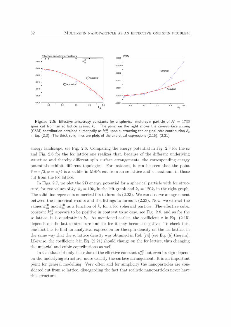
32 Multi-spin nanoparticle as an effective one spin problem
0.1 0.2 0.3 0.4 0.5-0.025
-0.020
-0.015
-0.010
-0.005
0.000
0.005
ks
keffca
Numerical
keffca
Analytical
Effective anisotropy constants
keffua
0.1 0.2 0.3 0.4 0.5-0.0001
0.0000
0.0001
0.0002
0.0003
0.0004
0.0005
ks
Numerical
Analytical
CSM
Figure 2.5: Effective anisotropy constants for a spherical multi-spin particle of N = 1736spins cut from an sc lattice against ks. The panel on the right shows the core-surface mixing
(CSM) contribution obtained numerically as keffua upon subtracting the original core contribution Ecin Eq. (2.3). The thick solid lines are plots of the analytical expressions (2.15), (2.21).
energy landscape, see Fig. 2.6. Comparing the energy potential in Fig. 2.3 for the sc
and Fig. 2.6 for the fcc lattice one realizes that, because of the different underlying
structure and thereby different spin surface arrangements, the corresponding energy
potentials exhibit different topologies. For instance, it can be seen that the point
θ = π/2, ϕ = π/4 is a saddle in MSPs cut from an sc lattice and a maximum in those
cut from the fcc lattice.
In Figs. 2.7, we plot the 2D energy potential for a spherical particle with fcc struc-
ture, for two values of ks: ks = 10kc in the left graph and ks = 120kc in the right graph.
The solid line represents numerical fits to formula (2.23). We can observe an agreement
between the numerical results and the fittings to formula (2.23). Now, we extract the
values keffua and keffca as a function of ks for a fcc spherical particle. The effective cubic
constant keffca appears to be positive in contrast to sc case, see Fig. 2.8, and as for the
sc lattice, it is quadratic in ks. As mentioned earlier, the coefficient κ in Eq. (2.15)
depends on the lattice structure and for fcc it may become negative. To check this,
one first has to find an analytical expression for the spin density on the fcc lattice, in
the same way that the sc lattice density was obtained in Ref. [74] (see Eq. (6) therein).
Likewise, the coefficient κ in Eq. (2.21) should change on the fcc lattice, thus changing
the uniaxial and cubic contributions as well.
In fact that not only the value of the effective constant keffca but even its sign depend
on the underlying structure, more exactly the surface arrangement. It is an important
point for general modelling. Very often and for simplicity the nanoparticles are con-
sidered cut from sc lattice, disregarding the fact that realistic nanoparticles never have
this structure.
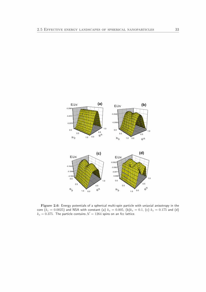
2.5 Effective energy landscapes of spherical nanoparticles 33
0.0
0.5
1.0 0.0
0.5
1.0
-5.2578
-5.2572
-5.2566
0.0
0.5
1.0 0.0
0.5
1.0
-5.2056
-5.2048
0.0
0.5
1.0 0.0
0.5
1.0
-5.1654
-5.1648
-5.1642
0.0
0.5
1.0 0.0
0.5
1.0-5.0580
-5.0571
-5.0562
-5.0553
(a) (b)
(c)
E/J E/J
E/J E/J(d)
Figure 2.6: Energy potentials of a spherical multi-spin particle with uniaxial anisotropy in thecore (kc = 0.0025) and NSA with constant (a) ks = 0.005, (b)ks = 0.1, (c) ks = 0.175 and (d)ks = 0.375. The particle contains N = 1264 spins on an fcc lattice.
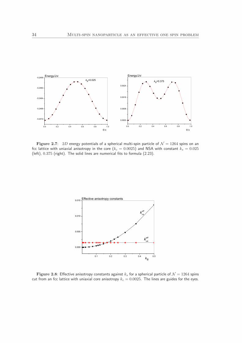
34 Multi-spin nanoparticle as an effective one spin problem
0.0 0.2 0.4 0.6 0.8 1.0
-5.2472
-5.2468
-5.2464
-5.2460
-5.2456ks=0.025
Energy/J
0.0 0.2 0.4 0.6 0.8 1.0
0.0000
0.0008
0.0016
0.0024
Energy/J
ks=0.375
Figure 2.7: 2D energy potentials of a spherical multi-spin particle of N = 1264 spins on anfcc lattice with uniaxial anisotropy in the core (kc = 0.0025) and NSA with constant ks = 0.025(left), 0.375 (right). The solid lines are numerical fits to formula (2.23).
0.1 0.2 0.3 0.4 0.5
0.000
0.005
0.010
0.015
keffca
Effective anisotropy constants
keffua
ks
Figure 2.8: Effective anisotropy constants against ks for a spherical particle of N = 1264 spinscut from an fcc lattice with uniaxial core anisotropy kc = 0.0025. The lines are guides for the eyes.
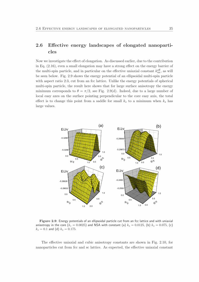
2.6 Effective energy landscapes of elongated nanoparticles 35
2.6 Effective energy landscapes of elongated nanoparti-
cles
Now we investigate the effect of elongation. As discussed earlier, due to the contribution
in Eq. (2.16), even a small elongation may have a strong effect on the energy barrier of
the multi-spin particle, and in particular on the effective uniaxial constant keffua , as will
be seen below. Fig. 2.9 shows the energy potential of an ellipsoidal multi-spin particle
with aspect ratio 2:3, cut from an fcc lattice. Unlike the energy potentials of spherical
multi-spin particle, the result here shows that for large surface anisotropy the energy
minimum corresponds to θ = π/2, see Fig. 2.9(d). Indeed, due to a large number of
local easy axes on the surface pointing perpendicular to the core easy axis, the total
effect is to change this point from a saddle for small ks to a minimum when ks has
large values.
0.00.5
1.0 0.0
0.5
1.0-5.3296
-5.3288
0.0
0.5
1.0 0.0
0.5
1.0
-5.29872
-5.29848
0.0
0.5
1.0 0.0
0.5
1.0
-5.28632
-5.28628
0.0
0.5
1.0 0.0
0.5
1.0
-5.2500
-5.2495
E/J
E/J
(a) (b)
(c) (d)
E/J
E/J
Figure 2.9: Energy potentials of an ellipsoidal particle cut from an fcc lattice and with uniaxialanisotropy in the core (kc = 0.0025) and NSA with constant (a) ks = 0.0125, (b) ks = 0.075, (c)ks = 0.1 and (d) ks = 0.175.
The effective uniaxial and cubic anisotropy constants are shown in Fig. 2.10, for
nanoparticles cut from fcc and sc lattice. As expected, the effective uniaxial constant
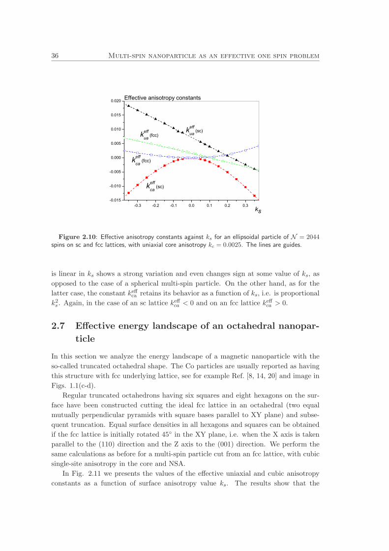
36 Multi-spin nanoparticle as an effective one spin problem
-0.3 -0.2 -0.1 0.0 0.1 0.2 0.3-0.015
-0.010
-0.005
0.000
0.005
0.010
0.015
0.020 Effective anisotropy constants
ks
keffua (sc) keff
ua (fcc)
keffca (fcc)
keffca (sc)
Figure 2.10: Effective anisotropy constants against ks for an ellipsoidal particle of N = 2044spins on sc and fcc lattices, with uniaxial core anisotropy kc = 0.0025. The lines are guides.
is linear in ks shows a strong variation and even changes sign at some value of ks, as
opposed to the case of a spherical multi-spin particle. On the other hand, as for the
latter case, the constant keffca retains its behavior as a function of ks, i.e. is proportional
k2s . Again, in the case of an sc lattice keffca < 0 and on an fcc lattice keffca > 0.
2.7 Effective energy landscape of an octahedral nanopar-
ticle
In this section we analyze the energy landscape of a magnetic nanoparticle with the
so-called truncated octahedral shape. The Co particles are usually reported as having
this structure with fcc underlying lattice, see for example Ref. [8, 14, 20] and image in
Figs. 1.1(c-d).
Regular truncated octahedrons having six squares and eight hexagons on the sur-
face have been constructed cutting the ideal fcc lattice in an octahedral (two equal
mutually perpendicular pyramids with square bases parallel to XY plane) and subse-
quent truncation. Equal surface densities in all hexagons and squares can be obtained
if the fcc lattice is initially rotated 45◦ in the XY plane, i.e. when the X axis is taken
parallel to the (110) direction and the Z axis to the (001) direction. We perform the
same calculations as before for a multi-spin particle cut from an fcc lattice, with cubic
single-site anisotropy in the core and NSA.
In Fig. 2.11 we presents the values of the effective uniaxial and cubic anisotropy
constants as a function of surface anisotropy value ks. The results show that the
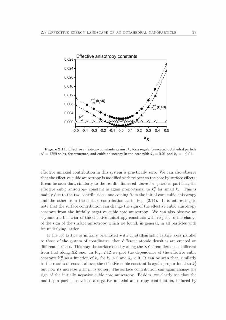
2.7 Effective energy landscape of an octahedral nanoparticle 37
-0.5 -0.4 -0.3 -0.2 -0.1 0.0 0.1 0.2 0.3 0.4 0.5
0.000
0.004
0.008
0.012
0.016
0.020
0.024
0.028
keffca (kc
>0)
ks
Effective anisotropy constants
keffca (kc
<0)
keffua
Figure 2.11: Effective anisotropy constants against ks for a regular truncated octahedral particleN = 1289 spins, fcc structure, and cubic anisotropy in the core with kc = 0.01 and kc = −0.01.
effective uniaxial contribution in this system is practically zero. We can also observe
that the effective cubic anisotropy is modified with respect to the core by surface effects.
It can be seen that, similarly to the results discussed above for spherical particles, the
effective cubic anisotropy constant is again proportional to k2s for small ks. This is
mainly due to the two contributions, one coming from the initial core cubic anisotropy
and the other from the surface contribution as in Eq. (2.14). It is interesting to
note that the surface contribution can change the sign of the effective cubic anisotropy
constant from the initially negative cubic core anisotropy. We can also observe an
asymmetric behavior of the effective anisotropy constants with respect to the change
of the sign of the surface anisotropy which we found, in general, in all particles with
fcc underlying lattice.
If the fcc lattice is initially orientated with crystallographic lattice axes parallel
to those of the system of coordinates, then different atomic densities are created on
different surfaces. This way the surface density along the XY circumference is different
from that along XZ one. In Fig. 2.12 we plot the dependence of the effective cubic
constant keffca as a function of ks for kc > 0 and kc < 0. It can be seen that, similarly
to the results discussed above, the effective cubic constant is again proportional to k2sbut now its increase with ks is slower. The surface contribution can again change the
sign of the initially negative cubic core anisotropy. Besides, we clearly see that the
multi-spin particle develops a negative uniaxial anisotropy contribution, induced by
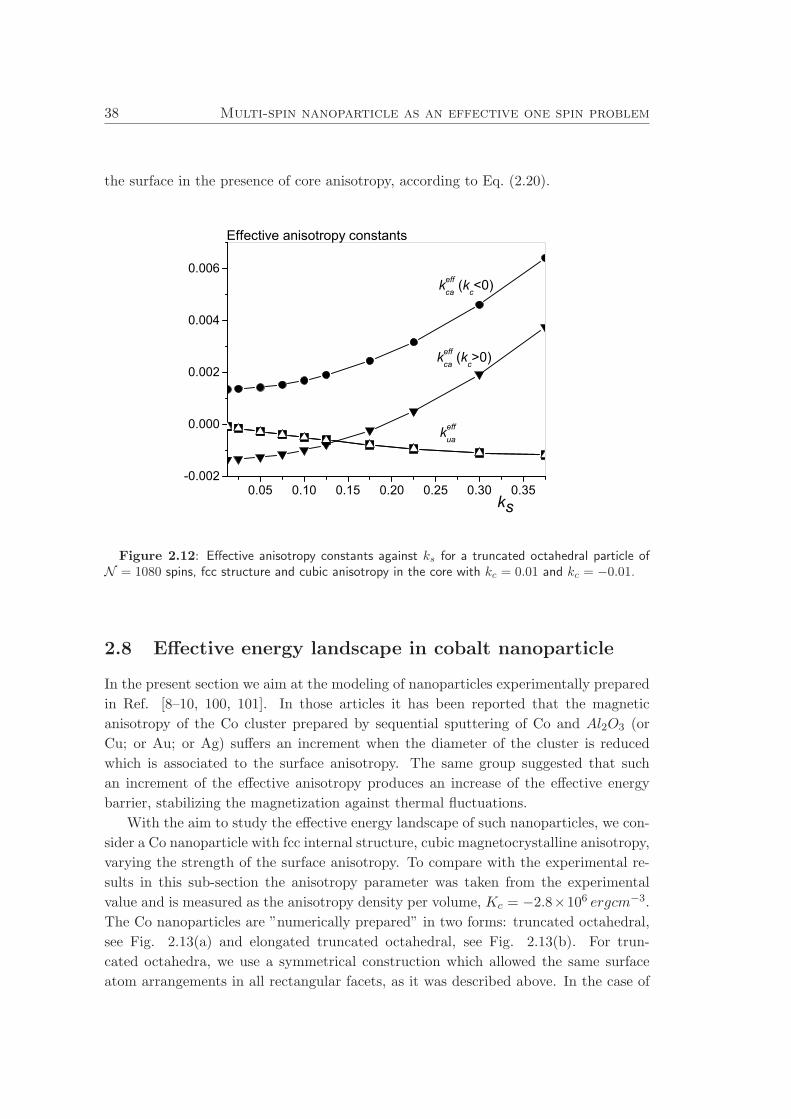
38 Multi-spin nanoparticle as an effective one spin problem
the surface in the presence of core anisotropy, according to Eq. (2.20).
0.05 0.10 0.15 0.20 0.25 0.30 0.35-0.002
0.000
0.002
0.004
0.006
ks
Effective anisotropy constants
keffca (kc<0)
keffca (kc>0)
keffua
Figure 2.12: Effective anisotropy constants against ks for a truncated octahedral particle ofN = 1080 spins, fcc structure and cubic anisotropy in the core with kc = 0.01 and kc = −0.01.
2.8 Effective energy landscape in cobalt nanoparticle
In the present section we aim at the modeling of nanoparticles experimentally prepared
in Ref. [8–10, 100, 101]. In those articles it has been reported that the magnetic
anisotropy of the Co cluster prepared by sequential sputtering of Co and Al2O3 (or
Cu; or Au; or Ag) suffers an increment when the diameter of the cluster is reduced
which is associated to the surface anisotropy. The same group suggested that such
an increment of the effective anisotropy produces an increase of the effective energy
barrier, stabilizing the magnetization against thermal fluctuations.
With the aim to study the effective energy landscape of such nanoparticles, we con-
sider a Co nanoparticle with fcc internal structure, cubic magnetocrystalline anisotropy,
varying the strength of the surface anisotropy. To compare with the experimental re-
sults in this sub-section the anisotropy parameter was taken from the experimental
value and is measured as the anisotropy density per volume, Kc = −2.8×10⁶ ergcm−3.
The Co nanoparticles are ”numerically prepared” in two forms: truncated octahedral,
see Fig. 2.13(a) and elongated truncated octahedral, see Fig. 2.13(b). For trun-
cated octahedra, we use a symmetrical construction which allowed the same surface
atom arrangements in all rectangular facets, as it was described above. In the case of
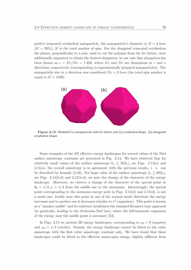
2.8 Effective energy landscape in cobalt nanoparticle 39
perfect truncated octahedral nanoparticle, the nanoparticle’s diameter is D = 4.5nm
(N = 2951), N is the total number of spin. For the elongated truncated octahedron
the planes, perpendicular to z-axis, used to cut the polygon from the fcc lattice, were
additionally separated to obtain the desired elongation, in our case that elongation has
been chosen as e = Dz/Dx = 1.228, where Dz and Dx are dimensions in z and x
directions, respectively (corresponding to experimentally prepared nanoparticles). The
nanoparticle size in x direction was considered Dx = 3.1nm (the total spin number is
equal to N = 1439).
Figure 2.13: Modeled Co nanoparticles with fcc lattice and (a) octahedral shape. (b) elongatedoctahedral shape.
Some examples of the 3D effective energy landscapes for several values of the Neel
surface anisotropy constants are presented in Fig. 2.14. We have observed that for
relatively small values of the surface anisotropy ks . 50|kc|, see Figs. 2.14(a) and
2.15(a), the overall anisotropy is in agreement with the previous results, i. e. can
be described by formula (2.23). For large value of the surface anisotropy ks & 60|kc|,
see Figs. 2.14(b-d) and 2.15(b-d), we note the change of the character of the energy
landscape. Moreover, we observe a change of the character of the special point at
θ0 = π/2, ϕ = π/4 from the saddle one to the maximum. Interestingly, the special
point corresponding to the minimum energy path in Figs. 2.14(d) and 2.15(d), is not
a usual one: locally near this point in one of the normal mode directions the energy
increases and in another one it decreases (similar to x3 expansion). This point is known
as a ”monkey saddle” and its existence invalidates the standard Kramers-type approach
(in particular, leading to the Arrhenius-Neel law), where the full-harmonic expansion
of the energy near the saddle point is necessary [53].
In Figs. 2.15 we present 2D energy landscapes, corresponding to ϕ0 = 0 (squares)
and ϕ0 = π/4 (circles). Namely, the energy landscape cannot be fitted to the cubic
anisotropy with the first cubic anisotropy constant only. We have found that these
landscapes could be fitted to the effective macro-spin energy, slightly different from
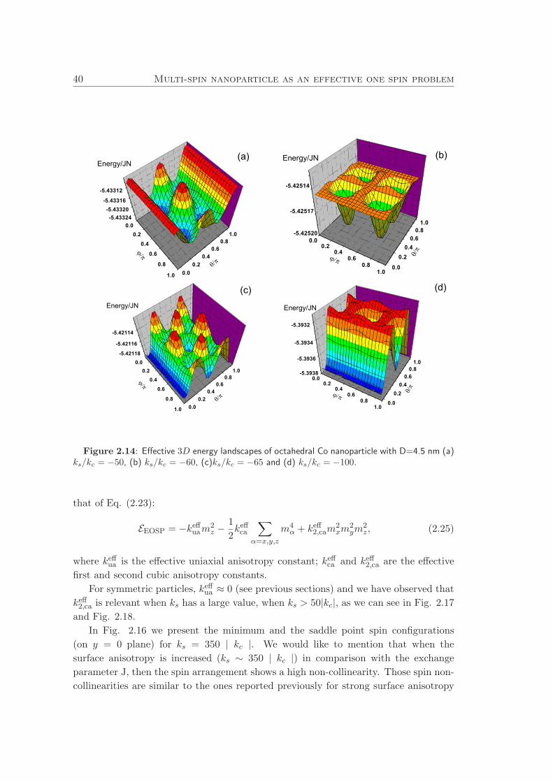
40 Multi-spin nanoparticle as an effective one spin problem
0.00.2
0.40.6
0.81.0
0.0
0.20.40.60.81.0
-5.3938
-5.3936
-5.3934
-5.3932
Energy/JN
0.00.2
0.4
0.6
0.8
1.0 0.00.2
0.40.6
0.81.0
-5.42118
-5.42116
-5.42114
Energy/JN
0.00.2
0.40.6
0.81.0
0.0
0.20.40.60.81.0
-5.42520
-5.42517
-5.42514
Energy/JN
0.00.2
0.4
0.6
0.8
1.0 0.00.2
0.40.6
0.81.0
-5.43324-5.43320
-5.43316
-5.43312
Energy/JN(a) (b)
(c) (d)
Figure 2.14: Effective 3D energy landscapes of octahedral Co nanoparticle with D=4.5 nm (a)ks/kc = −50, (b) ks/kc = −60, (c)ks/kc = −65 and (d) ks/kc = −100.
that of Eq. (2.23):
EEOSP = −keffuam2z −
1
2keffca
∑
α=x,y,z
m4α + keff2,cam
2xm
2ym
2z, (2.25)
where keffua is the effective uniaxial anisotropy constant; keffca and keff2,ca are the effective
first and second cubic anisotropy constants.
For symmetric particles, keffua ≈ 0 (see previous sections) and we have observed that
keff2,ca is relevant when ks has a large value, when ks > 50|kc|, as we can see in Fig. 2.17
and Fig. 2.18.
In Fig. 2.16 we present the minimum and the saddle point spin configurations
(on y = 0 plane) for ks = 350 | kc |. We would like to mention that when the
surface anisotropy is increased (ks ∼ 350 | kc |) in comparison with the exchange
parameter J, then the spin arrangement shows a high non-collinearity. Those spin non-
collinearities are similar to the ones reported previously for strong surface anisotropy
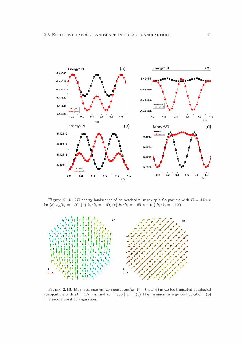
2.8 Effective energy landscape in cobalt nanoparticle 41
0.0 0.2 0.4 0.6 0.8 1.0
-5.3938
-5.3936
-5.3934
-5.3932
=0 = /4
Energy/JN (d)
0.0 0.2 0.4 0.6 0.8 1.0
-5.42118
-5.42116
-5.42114
-5.42112
(c)
=0 = /4
Energy/JN
0.0 0.2 0.4 0.6 0.8 1.0
-5.42520
-5.42518
-5.42516
-5.42514
Energy/JN
=0 = /4
(b)
0.0 0.2 0.4 0.6 0.8 1.0-5.43328
-5.43324
-5.43320
-5.43316
-5.43312
-5.43308
=0 = /4
Energy/JN (a)
Figure 2.15: 2D energy landscapes of an octahedral many-spin Co particle with D = 4.5nmfor (a) ks/kc = −50, (b) ks/kc = −60, (c) ks/kc = −65 and (d) ks/kc = −100.
Figure 2.16: Magnetic moment configurations(on Y = 0 plane) in Co fcc truncated octahedralnanoparticle with D = 4.5 nm. and ks = 350 | kc |: (a) The minimum energy configuration. (b)The saddle point configuration.
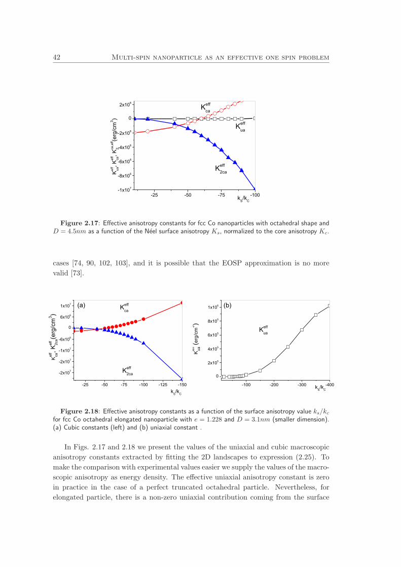
42 Multi-spin nanoparticle as an effective one spin problem
-25 -50 -75 -100-1x10⁷
-8x10⁶
-6x10⁶
-4x10⁶
-2x10⁶
0
2x10⁶
Kef
fua
, Kef
fca
, Kca
,eff
2(e
rg/c
m3 )
kS/kC
Keffua
Keffca
Keff2ca
Figure 2.17: Effective anisotropy constants for fcc Co nanoparticles with octahedral shape andD = 4.5nm as a function of the Neel surface anisotropy Ks, normalized to the core anisotropy Kc.
cases [74, 90, 102, 103], and it is possible that the EOSP approximation is no more
valid [73].
-25 -50 -75 -100 -125 -150
-2x10⁷
-2x10⁷
-1x10⁷
-6x10⁶
0
6x10⁶
1x10⁷
Kef
fca
, Kef
f2c
a(erg
/cm
3 )
Keff2ca
Keffca
kS/kC
(a)
-100 -200 -300 -400
0
2x10⁵
4x10⁵
6x10⁵
8x10⁵
1x10⁶
Kef
fua
(erg
/cm
3 )
kS/kC
Keffua
(b)
Figure 2.18: Effective anisotropy constants as a function of the surface anisotropy value ks/kcfor fcc Co octahedral elongated nanoparticle with e = 1.228 and D = 3.1nm (smaller dimension).(a) Cubic constants (left) and (b) uniaxial constant .
In Figs. 2.17 and 2.18 we present the values of the uniaxial and cubic macroscopic
anisotropy constants extracted by fitting the 2D landscapes to expression (2.25). To
make the comparison with experimental values easier we supply the values of the macro-
scopic anisotropy as energy density. The effective uniaxial anisotropy constant is zero
in practice in the case of a perfect truncated octahedral particle. Nevertheless, for
elongated particle, there is a non-zero uniaxial contribution coming from the surface
2.9 Conclusions 43
effect, see Fig. 2.18(b). However its value is much smaller than the additional cubic
anisotropy.
In both cases of octahedral and elongated particles the effective macroscopic first
cubic anisotropy constant changes the sign, see Figs. 2.17 and 2.18(a), and therefore
the easy axis of the system changes its position, as have been shown clearly in Figs.
2.15 and 2.14.
2.9 Conclusions
The main results of the study of the energy landscape in magnetic nanoparticles with
different lattices, shapes and the Neel surface anisotropy model are summarized as
follows:
• Our numerical calculations have shown that the magnetic behavior of the nanopar-
ticles with Neel surface anisotropy is consistent with the effective one spin particle
(EOSP) model with uniaxial and cubic anisotropies. The strength and sign of
these additional effective anisotropy constants are dependent on many parame-
ters, including the shape and elongation of the particle, and the underlying crystal
structure which produces different spin surface arrangement.
• We have compared the analytical and numerical results for the energy landscapes
for many-spin particles cut from sc lattice obtaining a very good agreement.
• We have observed that the cubic anisotropy contribution due to the surface of
magnetic nanoparticles has an opposite sign in the case of sc and fcc underlying
lattice structures.
• We have studied numerically the effective energy of Co multi-spin nanoparticle
with an octahedral shape, fcc lattice structure and cubic core anisotropy as a
function of the surface anisotropy magnitude. The results indicate that the sur-
face anisotropy introduces an additional first and second order cubic anisotropy.
For elongated particles they also induce an additional uniaxial anisotropy.
44 Multi-spin nanoparticle as an effective one spin problem
Conclusiones
Se ha estudiado la dependencia angular de la energıa total con respecto a la direccion
de la imanacion (paisajes de energıa) de nanopartıculas magneticas con diferentes for-
mas, redes cristalinas y valores de la anisotropıa de superficie. En estos sistemas la
anisotropıa de superficie se ha modelado usando el modelo de interacciones a pares tipo
Neel. Los principales resultados son los siguientes:
• Nuestras simulaciones muestran que el comportamiento magnetico de las nanopartıculas
con anisotropıa de superficie tipo Neel se puede modelar como el de una partıcula
macroespın efectiva con anisotropıa mixta (combinacion de anisotropıa uniaxial
y cubica). El valor y el signo de las anisotropıas efectivas dependen de multiples
parametros, por un lado de la forma y el alargamiento de las nanopartıculas y
por otro -de la estructura cristalina que origina diferentes ordenamientos de los
momentos magneticos en la superficie.
• Se obtiene un buen acuerdo al comparar los calculos analıticos con los numericos
para los paisajes de energıa de las nanopartıculas multi-espın con estructura
cristalina tipo simple cubica.
• Se observan signos opuestos para el termino de anisotropıa cubica originada por
la superficie si la nanopartıcula posee una red cristalina sc o fcc.
• Se han estudiado las nanopartıculas de cobalto con una forma octaedrica trun-
cada perfecta o alargada con estructura cristalina tipo fcc, anisotropıa en el nucleo
de la partıcula tipo cubica y anisotropıa de superficie tipo Neel. Los resultados
obtenidos de los paisajes de energıa indican que la anisotropıa de superfice in-
duce dos contribuciones a la anisotropıa cubica efectiva del sistema: de primer y
segundo orden. En el caso de partıculas alargadas se observa que la anisotropıa
de superficie induce ademas una anisotropıa uniaxial.
3Energy barriers of magnetic multispin
nanoparticles with Neel surface anisotropy
3.1 Motivation
How long the magnetization can remain fixed in a determinate direction is one of the key
questions in magnetism, or equivalently the determination of the stability of a magnetic
system. It is worth pointing out here that any discussion of magnetic stability will
involve evaluation of the energy barrier separating the two magnetic states, because
this controls the energy required to change magnetic moment of a system from one
direction to another by means of thermal activation. The probability of the switching
of the magnetization is related to the energy barrier through the Arrhenius-Neel law
[53].
f(t) = f0 exp− ∆E
KBT . (3.1)
Here the prefactor f0 is the attempt frequency, ∆E is the energy barrier, KB is the
Boltzmann constant, and T is the temperature of the system.
Experimentally the relevant energy barrier ∆E may be extracted from the mea-
surement of the blocking temperature TB. It has been widely reported that the sur-
face effects can modify the energy barrier through a modification of the ”effective
anisotropy”, Keff [9, 14, 20, 32, 36]. The effective anisotropy constant simply may be
defined through the energy barrier as:
Keff = ∆E/V, (3.2)
45
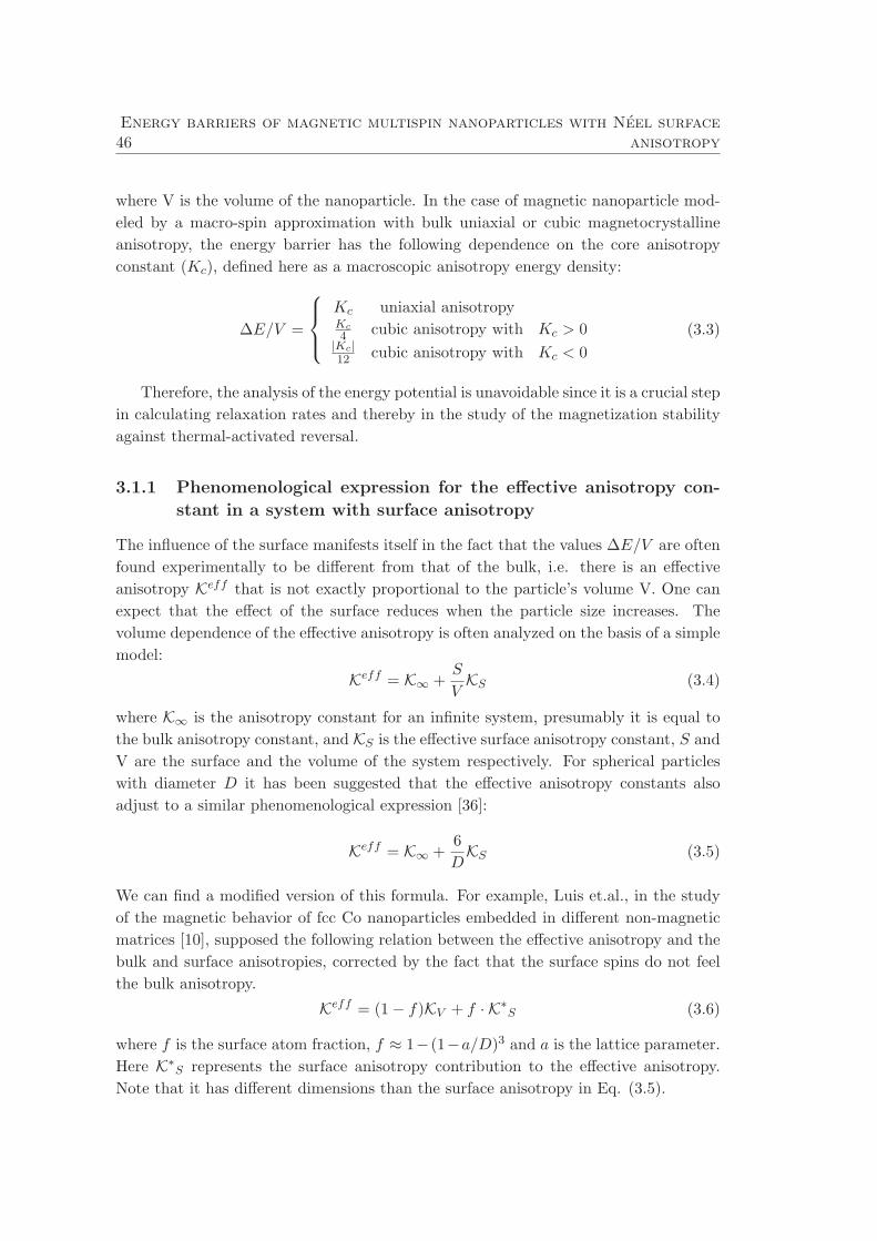
46Energy barriers of magnetic multispin nanoparticles with Neel surface
anisotropy
where V is the volume of the nanoparticle. In the case of magnetic nanoparticle mod-
eled by a macro-spin approximation with bulk uniaxial or cubic magnetocrystalline
anisotropy, the energy barrier has the following dependence on the core anisotropy
constant (Kc), defined here as a macroscopic anisotropy energy density:
∆E/V =
Kc uniaxial anisotropyKc
4 cubic anisotropy with Kc > 0|Kc|12 cubic anisotropy with Kc < 0
(3.3)
Therefore, the analysis of the energy potential is unavoidable since it is a crucial step
in calculating relaxation rates and thereby in the study of the magnetization stability
against thermal-activated reversal.
3.1.1 Phenomenological expression for the effective anisotropy con-
stant in a system with surface anisotropy
The influence of the surface manifests itself in the fact that the values ∆E/V are often
found experimentally to be different from that of the bulk, i.e. there is an effective
anisotropy Keff that is not exactly proportional to the particle’s volume V. One can
expect that the effect of the surface reduces when the particle size increases. The
volume dependence of the effective anisotropy is often analyzed on the basis of a simple
model:
Keff = K∞ +S
VKS (3.4)
where K∞ is the anisotropy constant for an infinite system, presumably it is equal to
the bulk anisotropy constant, and KS is the effective surface anisotropy constant, S and
V are the surface and the volume of the system respectively. For spherical particles
with diameter D it has been suggested that the effective anisotropy constants also
adjust to a similar phenomenological expression [36]:
Keff = K∞ +6
DKS (3.5)
We can find a modified version of this formula. For example, Luis et.al., in the study
of the magnetic behavior of fcc Co nanoparticles embedded in different non-magnetic
matrices [10], supposed the following relation between the effective anisotropy and the
bulk and surface anisotropies, corrected by the fact that the surface spins do not feel
the bulk anisotropy.
Keff = (1 − f)KV + f · K∗S (3.6)
where f is the surface atom fraction, f ≈ 1− (1−a/D)3 and a is the lattice parameter.
Here K∗S represents the surface anisotropy contribution to the effective anisotropy.
Note that it has different dimensions than the surface anisotropy in Eq. (3.5).
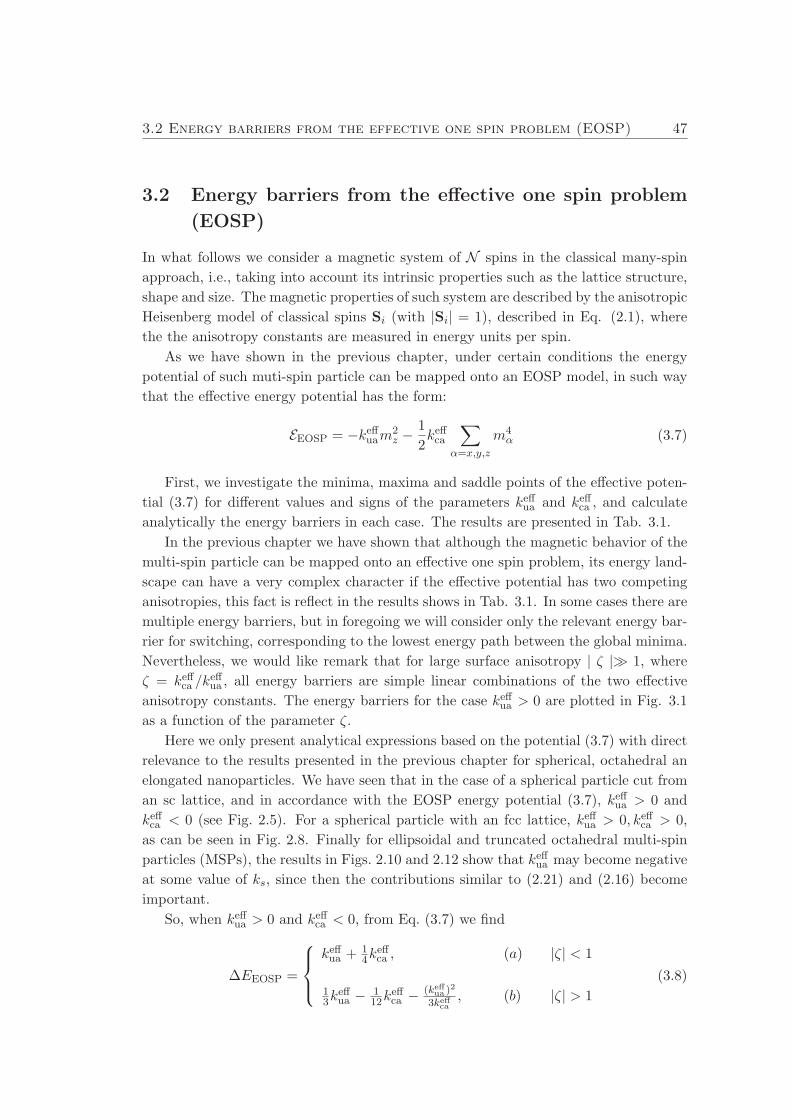
3.2 Energy barriers from the effective one spin problem (EOSP) 47
3.2 Energy barriers from the effective one spin problem
(EOSP)
In what follows we consider a magnetic system of N spins in the classical many-spin
approach, i.e., taking into account its intrinsic properties such as the lattice structure,
shape and size. The magnetic properties of such system are described by the anisotropic
Heisenberg model of classical spins Si (with |Si| = 1), described in Eq. (2.1), where
the the anisotropy constants are measured in energy units per spin.
As we have shown in the previous chapter, under certain conditions the energy
potential of such muti-spin particle can be mapped onto an EOSP model, in such way
that the effective energy potential has the form:
EEOSP = −keffuam2z −
1
2keffca
∑
α=x,y,z
m4α (3.7)
First, we investigate the minima, maxima and saddle points of the effective poten-
tial (3.7) for different values and signs of the parameters keffua and keffca , and calculate
analytically the energy barriers in each case. The results are presented in Tab. 3.1.
In the previous chapter we have shown that although the magnetic behavior of the
multi-spin particle can be mapped onto an effective one spin problem, its energy land-
scape can have a very complex character if the effective potential has two competing
anisotropies, this fact is reflect in the results shows in Tab. 3.1. In some cases there are
multiple energy barriers, but in foregoing we will consider only the relevant energy bar-
rier for switching, corresponding to the lowest energy path between the global minima.
Nevertheless, we would like remark that for large surface anisotropy | ζ |≫ 1, where
ζ = keffca /keffua , all energy barriers are simple linear combinations of the two effective
anisotropy constants. The energy barriers for the case keffua > 0 are plotted in Fig. 3.1
as a function of the parameter ζ.
Here we only present analytical expressions based on the potential (3.7) with direct
relevance to the results presented in the previous chapter for spherical, octahedral an
elongated nanoparticles. We have seen that in the case of a spherical particle cut from
an sc lattice, and in accordance with the EOSP energy potential (3.7), keffua > 0 and
keffca < 0 (see Fig. 2.5). For a spherical particle with an fcc lattice, keffua > 0, keffca > 0,
as can be seen in Fig. 2.8. Finally for ellipsoidal and truncated octahedral multi-spin
particles (MSPs), the results in Figs. 2.10 and 2.12 show that keffua may become negative
at some value of ks, since then the contributions similar to (2.21) and (2.16) become
important.
So, when keffua > 0 and keffca < 0, from Eq. (3.7) we find
∆EEOSP =
keffua + 14k
effca , (a) |ζ| < 1
13k
effua − 1
12keffca − (keffua )
2
3keffca, (b) |ζ| > 1
(3.8)

48Energy barriers of magnetic multispin nanoparticles with Neel surface
anisotropy
Table 3.1: Energy barriers for effective one-spin particle. The critical angle θc(ϕ) is defined bycos2 θc(ϕ) = (keffua +keffua (sin4 ϕ+ cos4 ϕ))/(keffca (1 + sin4 ϕ+ cos4 ϕ)) and ϕ is the azimuthal angle.
keffua > 0
ζ = keffca /keffua Minima (θ, ϕ) Saddle points(θ, ϕ) Energy barriers, ∆EEOSP
−∞ < ζ < −1 θc(π/4);π/4 π/2;π/4 keffua3 − keffca
12 − (keffua )2
3keffca(1.1)
θc(π/4);π/4 θc(π/2);π/2 −keffua6 − keffca
12 − (keffua )2
12keffca(1.2)
−1 < ζ < 0 0; 0 π/2; 0 keffua + keffca4 (2)
0 < ζ < 1 0;π/2 π/2;π/2 keffua (3)
1 < ζ < 2 θc(0);π/2 θc(π/2);π/2 keffua2 + keffca
4 + (keffua )2
4keffca(4.1)
π/2;π/2 θc(π/2);π/2 −keffua2 + keffca
4 + (keffua )2
4keffca(4.2)
2 < ζ <∞ 0;π/2 θc(π/2);π/2 keffua2 + keffca
4 + (keffua )2
4keffca(5.1)
π/2;π/2 π/2;π/4 keffca4 (5.2)
π/2;π/2 θc(π/2);π/2 −keffua2 + keffca
4 + (keffua )2
4keffca(5.3)
keffua < 0
−∞ < ζ < −1 π/2;π/2 θc(π/2);π/2 −keffua2 + keffca
4 + (keffua )2
4keffca(6.1)
π/2; 0 π/2;π/4 keffca4 (6.2)
0;π/2 θc(π/2);π/4 keffua2 + keffca
4 + (keffua )2
4keffca(6.3)
−1 < ζ < 0 π/2; 0 π/2;π/4 keffca4 (7)
0 < ζ < 1 π/2;π/4 π/2;π/2 keffca4 (8)
1 < ζ < 2 π/2;π/4 θc(π/2);π/2 −keffua2 + (keffua )
2
4keffca(9)
2 < ζ <∞ θc(π/4);π/4 π/2;π/4 −keffua6 − keffca
12 − (keffua )2
3keffca(10.1)
θc(π/4);π/4 θc(π/2);π/2 keffua3 − keffca
12 − (keffua )2
12keffca(10.2)
In the case keffca > 0, the energy barriers read,
∆EEOSP =
keffua , keffua > 0 (a)
14k
effca , keffua < 0 (b)
|ζ| < 1
12k
effua + 1
4keffca + (keffua )
2
4keffca(c) |ζ| > 1.
(3.9)
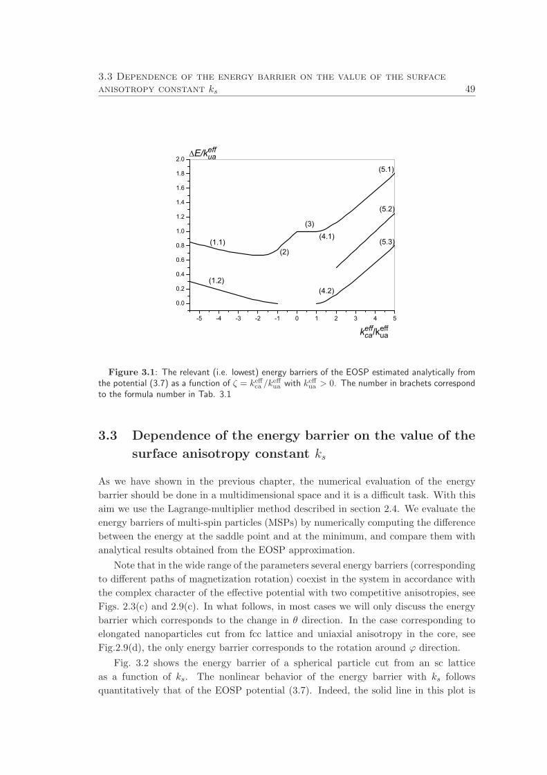
3.3 Dependence of the energy barrier on the value of the surfaceanisotropy constant ks 49
-5 -4 -3 -2 -1 0 1 2 3 4 5
0.0
0.2
0.4
0.6
0.8
1.0
1.2
1.4
1.6
1.8
2.0
(1.1) (5.3)
(5.2)
(5.1)
(4.2)
(3)
(2)
keffca/keffua
E/keffua
(1.2)
(4.1)
Figure 3.1: The relevant (i.e. lowest) energy barriers of the EOSP estimated analytically fromthe potential (3.7) as a function of ζ = keffca /k
effua with keffua > 0. The number in brachets correspond
to the formula number in Tab. 3.1
3.3 Dependence of the energy barrier on the value of the
surface anisotropy constant ks
As we have shown in the previous chapter, the numerical evaluation of the energy
barrier should be done in a multidimensional space and it is a difficult task. With this
aim we use the Lagrange-multiplier method described in section 2.4. We evaluate the
energy barriers of multi-spin particles (MSPs) by numerically computing the difference
between the energy at the saddle point and at the minimum, and compare them with
analytical results obtained from the EOSP approximation.
Note that in the wide range of the parameters several energy barriers (corresponding
to different paths of magnetization rotation) coexist in the system in accordance with
the complex character of the effective potential with two competitive anisotropies, see
Figs. 2.3(c) and 2.9(c). In what follows, in most cases we will only discuss the energy
barrier which corresponds to the change in θ direction. In the case corresponding to
elongated nanoparticles cut from fcc lattice and uniaxial anisotropy in the core, see
Fig.2.9(d), the only energy barrier corresponds to the rotation around ϕ direction.
Fig. 3.2 shows the energy barrier of a spherical particle cut from an sc lattice
as a function of ks. The nonlinear behavior of the energy barrier with ks follows
quantitatively that of the EOSP potential (3.7). Indeed, the solid line in this plot is
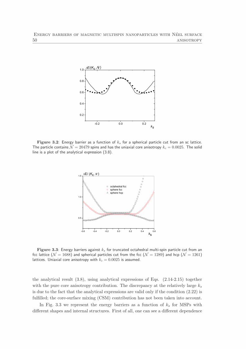
50Energy barriers of magnetic multispin nanoparticles with Neel surface
anisotropy
-0.2 0.0 0.2
0.2
0.4
0.6
0.8
1.0
ks
E/(Kc )
Figure 3.2: Energy barrier as a function of ks for a spherical particle cut from an sc lattice.The particle contains N = 20479 spins and has the uniaxial core anisotropy kc = 0.0025. The solidline is a plot of the analytical expression (3.8).
-0.6 -0.4 -0.2 0.0 0.2 0.4 0.6
0.5
1.0
1.5
octahedral fccsphere fccsphere hcp
ks
E/ (Kc )
Figure 3.3: Energy barriers against ks for truncated octahedral multi-spin particle cut from anfcc lattice (N = 1688) and spherical particles cut from the fcc (N = 1289) and hcp (N = 1261)lattices. Uniaxial core anisotropy with kc = 0.0025 is assumed.
the analytical result (3.8), using analytical expressions of Eqs. (2.14-2.15) together
with the pure core anisotropy contribution. The discrepancy at the relatively large ksis due to the fact that the analytical expressions are valid only if the condition (2.22) is
fulfilled; the core-surface mixing (CSM) contribution has not been taken into account.
In Fig. 3.3 we represent the energy barriers as a function of ks for MSPs with
different shapes and internal structures. First of all, one can see a different dependence

3.3 Dependence of the energy barrier on the value of the surfaceanisotropy constant ks 51
on ks as compared to MSPs with the sc lattice. In the present case, i.e., keffua > 0, keffca >
0, the energy barriers are given by Eqs. (3.9)(a) and (c). For small values of ks, for
which |ζ| < 1, the energy barrier, in the first approximation neglecting the CSM term,
is independent of ks. Accordingly, the nearly constant value of the energy barrier,
coinciding with that of the core, is observed for multi-spin particles in a large range of
ks. For larger ks, the energy barrier increases, since keffua > 0 for multi-spin particles
cut from an fcc lattice. At very large values of ks, i.e., ks & 100kc the energy barriers
depend approximately linearly on ks and may have values larger than that inferred
from the pure core anisotropy.
The energy barriers for ellipsoidal multi-spin particles are shown in Fig. 3.4. Note
-0.2 -0.1 0.0 0.1 0.2 0.30.0
0.4
0.8
1.2
1.6
a/c=0.81
a/c=0.6667
ks
E/ (Kc )
Figure 3.4: Energy barriers versus ks of ellipsoidal multi-spin particles with different aspectratio (a/c = 0.6667,N = 21121, and a/c = 0.81,N = 21171, with uniaxial core anisotropykc = 0.0025. The solid lines are linear fits.
that in this case the effective uniaxial anisotropy constant keffua is a linear function of ks,
according to the analytical results (2.16), (2.17) and the numerical results presented
in Fig. 2.10. In this case the value of the energy barrier is not symmetric with respect
to the change of the sign of ks. This is due to the fact that for ks < 0 the effective
uniaxial constant is a sum of the core anisotropy and the first-order contribution owing
to elongation. On the contrary, when ks > 0, the ”effective core anisotropy” keffua is
smaller than the pure core anisotropy Ec in Eq. (2.6). This means that at some ks the
effective uniaxial anisotropy constant (keffua) may change sign. At the same time the
effective cubic anisotropy keffua remains positive and is proportional to k2s . Accordingly,
at the vicinity of the point at which keffca ≈ 0, rapid changes of the character of the
energy landscape occur as we have shown in Fig. 2.10 in the previous chapter.
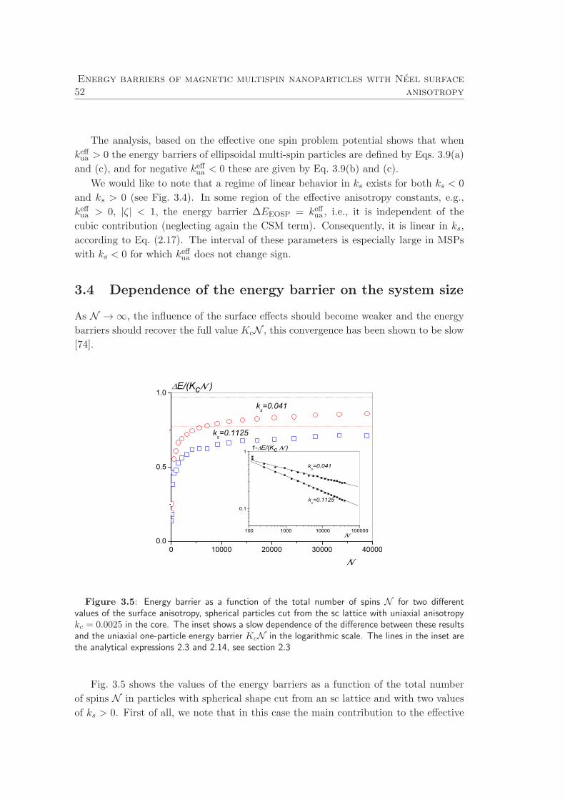
52Energy barriers of magnetic multispin nanoparticles with Neel surface
anisotropy
The analysis, based on the effective one spin problem potential shows that when
keffua > 0 the energy barriers of ellipsoidal multi-spin particles are defined by Eqs. 3.9(a)
and (c), and for negative keffua < 0 these are given by Eq. 3.9(b) and (c).
We would like to note that a regime of linear behavior in ks exists for both ks < 0
and ks > 0 (see Fig. 3.4). In some region of the effective anisotropy constants, e.g.,
keffua > 0, |ζ| < 1, the energy barrier ∆EEOSP = keffua , i.e., it is independent of the
cubic contribution (neglecting again the CSM term). Consequently, it is linear in ks,
according to Eq. (2.17). The interval of these parameters is especially large in MSPs
with ks < 0 for which keffua does not change sign.
3.4 Dependence of the energy barrier on the system size
As N → ∞, the influence of the surface effects should become weaker and the energy
barriers should recover the full value KcN , this convergence has been shown to be slow
[74].
0 10000 20000 30000 400000.0
0.5
1.0
100 1000 10000 100000
0.1
1
ks=0.1125
ks=0.041
1- E/(Kc )
ks=0.1125
ks=0.041
E/(Kc )
Figure 3.5: Energy barrier as a function of the total number of spins N for two differentvalues of the surface anisotropy, spherical particles cut from the sc lattice with uniaxial anisotropykc = 0.0025 in the core. The inset shows a slow dependence of the difference between these resultsand the uniaxial one-particle energy barrier KcN in the logarithmic scale. The lines in the inset arethe analytical expressions 2.3 and 2.14, see section 2.3
Fig. 3.5 shows the values of the energy barriers as a function of the total number
of spins N in particles with spherical shape cut from an sc lattice and with two values
of ks > 0. First of all, we note that in this case the main contribution to the effective
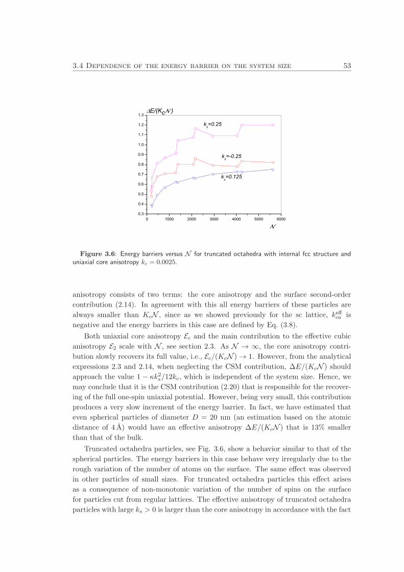
3.4 Dependence of the energy barrier on the system size 53
0 1000 2000 3000 4000 5000 60000.3
0.4
0.5
0.6
0.7
0.8
0.9
1.0
1.1
1.2
1.3
ks=0.125
ks=-0.25
ks=0.25
E/(Kc )
Figure 3.6: Energy barriers versus N for truncated octahedra with internal fcc structure anduniaxial core anisotropy kc = 0.0025.
anisotropy consists of two terms: the core anisotropy and the surface second-order
contribution (2.14). In agreement with this all energy barriers of these particles are
always smaller than KcN , since as we showed previously for the sc lattice, keffca is
negative and the energy barriers in this case are defined by Eq. (3.8).
Both uniaxial core anisotropy Ec and the main contribution to the effective cubic
anisotropy E2 scale with N , see section 2.3. As N → ∞, the core anisotropy contri-
bution slowly recovers its full value, i.e., Ec/(KcN ) → 1. However, from the analytical
expressions 2.3 and 2.14, when neglecting the CSM contribution, ∆E/(KcN ) should
approach the value 1 − κk2s/12kc, which is independent of the system size. Hence, we
may conclude that it is the CSM contribution (2.20) that is responsible for the recover-
ing of the full one-spin uniaxial potential. However, being very small, this contribution
produces a very slow increment of the energy barrier. In fact, we have estimated that
even spherical particles of diameter D = 20 nm (an estimation based on the atomic
distance of 4 A) would have an effective anisotropy ∆E/(KcN ) that is 13% smaller
than that of the bulk.
Truncated octahedra particles, see Fig. 3.6, show a behavior similar to that of the
spherical particles. The energy barriers in this case behave very irregularly due to the
rough variation of the number of atoms on the surface. The same effect was observed
in other particles of small sizes. For truncated octahedra particles this effect arises
as a consequence of non-monotonic variation of the number of spins on the surface
for particles cut from regular lattices. The effective anisotropy of truncated octahedra
particles with large ks > 0 is larger than the core anisotropy in accordance with the fact

54Energy barriers of magnetic multispin nanoparticles with Neel surface
anisotropy
0 10000 20000 30000 40000 50000
0.0
0.5
1.0
1.5
2.0
2.5
3.0
3.5
4.0
4.5
ks=-0.1125
ks=-0.041
ks=0.041
E/(Kc )
Figure 3.7: Energy barriers as a function of the particle size for ellipsoidal particles with internalsc structure, uniaxial anisotropy kc = 0.0025 and different values of ks.
that keffca is positive for fcc structures and the energy barriers are defined by Eqs. (3.9).
Finally, in Fig. 3.7 we present the energy barriers of ellipsoidal particles with dif-
ferent values of ks. According to formulas (3.9)(b) and (c), particles with ks < 0 have
energy barriers larger than that inferred from the core anisotropy, and for those with
ks > 0 the energy barriers are smaller. In this case, the energy barrier scales with the
number of surface spins Ns (see Fig. 3.8), in agreement with the first-order contribution
from elongation (2.17).
3.5 On the applicability of the formula Keff = K∞ + 6Ks/D
The results presented above show that in the most general case, studied here, of a
multi-spin particle with Neel surface anisotropy, this formula is not applicable, for the
following reasons:
(i) It assumes that the overall anisotropy of the particle remains uniaxial. However, we
have shown that the surface anisotropy induces an additional cubic contribution.
(ii) It assumes that the surface anisotropy always enhances that in the core. In this
and the previous sections we saw that both situations can arise.
(iii) It is implicitly based on the hypothesis that the core and surface anisotropies
are additive contributions. As we have seen above for large ks the energy barrier
indeed can be represented as a sum of the effective cubic and uniaxial anisotropies.

3.5 On the applicability of the formula Keff = K∞ + 6Ks/D 55
However, the cubic anisotropy term is proportional to k2s , which is inconsistent
with formula (3.5).
(iv) It assumes linear dependence of energy barriers on the parameter 1/D, or equiv-
alently Ns/N .
Consequently, spherical or octahedral particles cannot be described by formula (3.5),
since in this case:
(i) No term linear in ks is obtained.
(ii) No term scales as the ratio of the surface-to-volume number of spins Ns/N .
However, in the case of elongated particles with a not too large surface anisotropy, i.e.,
|ζ| < 1, the energy barriers are independent of the effective cubic anisotropy. In this
case, for weakly ellipsoidal particles, for example, we may write
∆EEOSP = keffua ≈ kcNc/N +A|ks|/N1/3 (3.10)
where A is a parameter that depends on the particle’s elongation and surface arrange-
ment, and which is positive for ks < 0 and negative in the opposite case. Hence, the
behavior is as predicted by this formula (3.5). The approximately linear behavior in
Ns/N was also observed in the case of large surface anisotropy ζ >> 1 (see Fig. 3.1).
However, in this case at N → ∞, the “uniaxial anisotropy term” K∞ is renormalized
by the effective cubic anisotropy keffca ∼ k2s . In Fig. 3.8 we plot the energy barriers of
small ellipsoidal particles with sc structure, aspect ratio 2:3, and ks < 0 from Fig. 3.7.
For such particles, the formula (3.5) should be modified as Keff = K∞ + |Ks|Ns/N .
Accordingly, in Fig. 3.8 we plot the energy barrier against Ns/N . These data are well
fitted to straight lines, especially when small particle sizes are removed. We note that
in the case of relatively small surface anisotropy ks = −0.041 (though 17 times larger
than that in the core), the full core anisotropy K∞ = Kc/v ( v is the atomic volume)
can be extracted. However, for the larger surface anisotropy ks = −0.1125, K∞ is
renormalized by the surface contribution, defined by Eq. (2.15). On the other hand,
it is not possible to extract the value of ks, since the exact proportionality coefficient
of Eq. (2.17) (the value of A in Eq. 3.10) is dependent on the particles surface ar-
rangement and elongation. The effective anisotropy constant Ks obtained from this fit
is much smaller than the input value, namely, for ks/kc = 45 we obtain from the fit
(ks/kc)eff = 4.3.
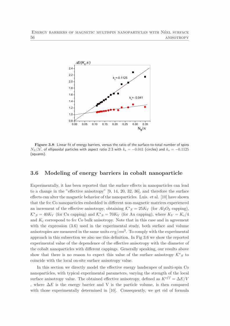
56Energy barriers of magnetic multispin nanoparticles with Neel surface
anisotropy
0.00 0.05 0.10 0.15 0.20 0.25 0.30 0.350.8
1.0
1.2
1.4
1.6
1.8
2.0
2.2
2.4
ks=-0.1125
ks=- 0.041
E/(Kc )
Ns/
Figure 3.8: Linear fit of energy barriers, versus the ratio of the surface-to-total number of spinsNS/N , of ellipsoidal particles with aspect ratio 2:3 with ks = −0.041 (circles) and ks = −0.1125(squares).
3.6 Modeling of energy barriers in cobalt nanoparticle
Experimentally, it has been reported that the surface effects in nanoparticles can lead
to a change in the ”effective anisotropy” [9, 14, 20, 32, 36], and therefore the surface
effects can alter the magnetic behavior of the nanoparticles. Luis. et al. [10] have shown
that the fcc Co nanoparticles embedded in different non-magnetic matrices experienced
an increment of the effective anisotropy, obtaining K∗S = 25KV (for Al2O3 capping),
K∗S = 40KV (for Cu capping) and K∗
S = 70KV (for Au capping), where KV = Kc/4
and Kc correspond to fcc Co bulk anisotropy. Note that in this case and in agreement
with the expression (3.6) used in the experimental study, both surface and volume
anisotropies are measured in the same units erg/cm3. To comply with the experimental
approach in this subsection we also use this definition. In Fig 3.6 we show the reported
experimental value of the dependence of the effective anisotropy with the diameter of
the cobalt nanoparticles with different cappings. Generally speaking, our results above
show that there is no reason to expect this value of the surface anisotropy K∗S to
coincide with the local on-site surface anisotropy value.
In this section we directly model the effective energy landscapes of multi-spin Co
nanoparticles, with typical experimental parameters, varying the strength of the local
surface anisotropy value. The obtained effective anisotropy, defined as Keff = ∆E/V
, where ∆E is the energy barrier and V is the particle volume, is then compared
with those experimentally determined in [10]. Consequently, we get rid of formula
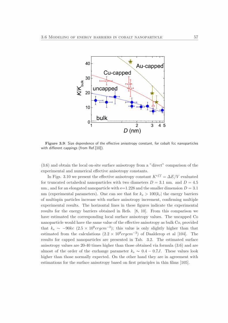
3.6 Modeling of energy barriers in cobalt nanoparticle 57
Figure 3.9: Size dependence of the effective anisotropy constant, for cobalt fcc nanoparticleswith different cappings (from Ref.[10]).
(3.6) and obtain the local on-site surface anisotropy from a ”direct” comparison of the
experimental and numerical effective anisotropy constants.
In Figs. 3.10 we present the effective anisotropy constant Keff = ∆E/V evaluated
for truncated octahedral nanoparticles with two diameters D = 3.1 nm. and D = 4.5
nm., and for an elongated nanoparticle with e=1.228 and the smaller dimensionD = 3.1
nm (experimental parameters). One can see that for ks > 100|kc| the energy barriers
of multispin particles increase with surface anisotropy increment, confirming multiple
experimental results. The horizontal lines in these figures indicate the experimental
results for the energy barriers obtained in Refs. [8, 10]. From this comparison we
have estimated the corresponding local surface anisotropy values. The uncapped Co
nanoparticle would have the same value of the effective anisotropy as bulk Co, provided
that ks ∼ −90kc (2.5 × 10⁸ergcm−3); this value is only slightly higher than that
estimated from the calculations (2.2 × 10⁸ergcm−3) of Daalderop et al [104]. The
results for capped nanoparticles are presented in Tab. 3.2. The estimated surface
anisotropy values are 20-40 times higher than those obtained via formula (3.6) and are
almost of the order of the exchange parameter ks ∼ 0.4 − 0.7J . These values look
higher than those normally expected. On the other hand they are in agreement with
estimations for the surface anisotropy based on first principles in thin films [105].
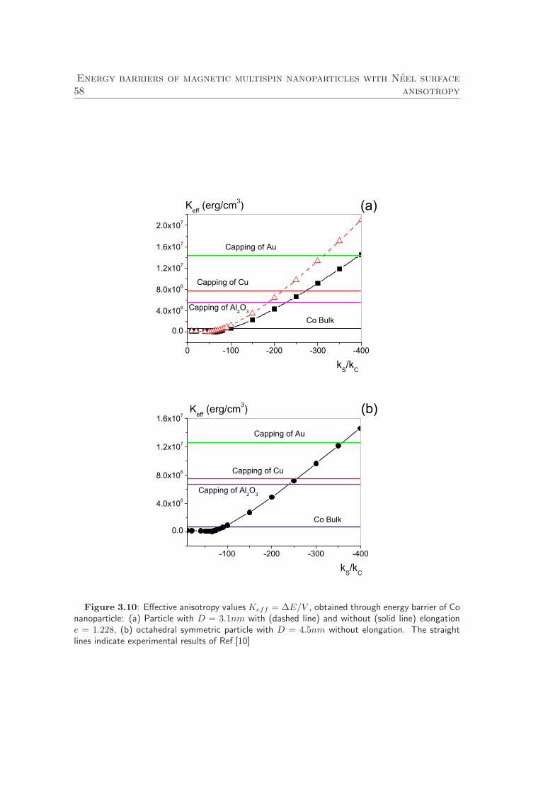
58Energy barriers of magnetic multispin nanoparticles with Neel surface
anisotropy
0 -100 -200 -300 -400
0.0
4.0x10⁶
8.0x10⁶
1.2x10⁷
1.6x10⁷
2.0x10⁷
Capping of Au
Capping of Cu
Capping of Al2O3
Co Bulk
Keff (erg/cm3)
kS/kC
(a)
-100 -200 -300 -400
0.0
4.0x10⁶
8.0x10⁶
1.2x10⁷
1.6x10⁷(b)
Co Bulk
Capping of Al2O3
Capping of Cu
Capping of Au
Keff (erg/cm3)
kS/kC
Figure 3.10: Effective anisotropy values Keff = ∆E/V , obtained through energy barrier of Conanoparticle: (a) Particle with D = 3.1nm with (dashed line) and without (solid line) elongatione = 1.228, (b) octahedral symmetric particle with D = 4.5nm without elongation. The straightlines indicate experimental results of Ref.[10]

3.7 Conclusions 59
Table 3.2: Surface anisotropy constant for Co nanoparticle with different capping, extracted bycomparison between simulation and experimental results in Ref.[10].
Capping Al2O3 Cu Au
ks/|kc| Ks/J ks/|kc| Ks/J ks/|kc| Ks/J
Octahedral D=3.1nm 228.92 0.447 273.01 0.532 396.29 0.773
Octahedral D=4.5nm 237.63 0.467 257.60 0.503 360.45 0.703
Elongated particle 187.258 0.365 219.37 0.428 314.076 0.613
3.7 Conclusions
In summary we have evaluated the energy barriers for multispin magnetic nanoparticles
with different underlying lattice, shapes, sizes and with the Neel surface anisotropy
model. The main results are summarized as follows:
• The energy barriers evaluated in a multidimensional space are complex functions
of the system parameters and multiple saddle points can exist. Only in the case
of | ζ |≫ 1, where ζ = keffca /keffua , all energy barriers are simple linear combinations
of the two effective anisotropy constants.
• We have found energy barriers larger than KcN value for all studied symmetric
nanoparticles with very large surface anisotropy, ks & 100kc, or for elongated
particles with ks < 0. This confirms a well-known fact that the surface anisotropy
may contribute to the enhancement of the thermal stability of a magnetic particle.
• We have analyzed the behavior of the energy barriers of different magnetic nanopar-
ticles as a function of their sizes. We have observed that the influence of the sur-
face become weaker when the size of the particle is increased. The energy barriers
value recovers the full value KcN when N → ∞, with very slow convergence.
• We have found that the effective anisotropy values extracted from the energy
barriers measurements are consistent with the formula Keff = K∞ + 6DKS only
for elongated nanoparticles. This formula is never fulfilled in perfect spherical or
truncated octahedral nanoparticles.
• We have studied Co fcc nanoparticles prepared experimentally in Ref. [10] varing
the strength of the surface anisotropy constant. The energy barriers were fitted
to the experimentally measured energy barriers values for nanoparticles with
different cappings, Al2O3, Cu and Au [8, 10]. From this comparison we obtained
the local surface anisotropy values which are almost of the order of the exchange
parameter ks ∼ 0.4 ÷ 0.7J .

60Energy barriers of magnetic multispin nanoparticles with Neel surface
anisotropy
Conclusiones
En este capıtulo hemos evaluado las barreras de energıa de nanopartıculas magneticas
multiespın con diferentes redes cristalinas, formas, tamanos y anisotropıa de superficie
tipo Neel. Los principales resultados de este estudio se resumen a continuacion:
• Las barreras de energıa evaluadas en un espacio multidimensional son funciones
muy complejas de los parametros del sistema. Solo en el caso | ζ |≫ 1, donde
ζ = keffca /keffua , todas las barreras de energıa son una simple combinacion lineal de
la anisotropıa cubica y uniaxial.
• En el caso de las nanopartıculas simetricas estudiadas, hemos encontrado que
los valores de las barreras de energıa son mayores de KcN para valores de
la anisotropıa de superficie altos, ks & 100kc, y tambien en el caso de las
nanopartıculas alargadas con ks < 0. Esto confirma el hecho de que la anisotropıa
de superficie puede contribuir al incremento de la estabilidad termica de las
partıculas magneticas.
• Hemos estudiado el comportamniento de las barreras de energıa para diversos
tipos de nanopartıculas magneticas en funcion de su tamano. Observamos que
a medida que el tamano del sistema aumenta la influencia de la superficie dis-
minuye, de tal forma que para N → ∞ la barrera de energıa recupera el valor
KcN .
• Hemos analizado la validez de la formula Keff = K∞ + 6DKS . Para ello hemos
obtenido el valor de la anisotropıa efectiva a partir de la barrera de energıa, obser-
vando que la formula solo es valida en el caso de nanopartıculas alargadas y nunca
se cumple en el caso de nanopartıculas perfectamente esfericas u octaedricas trun-
cadas.
• Hemos modelado nanopartıculas de cobalto con estructura cristalina fcc similares
a las preparadas experimentalmente en Ref. [10]. Las nanopartıculas estaban
recubiertas de diferentes materiales. Hemos modelado este efecto variando la
magnitud de la anisotropıa de superficie. A partir del valor de la barrera de en-
ergıa hemos obtenido numericamente el valor de la anisotropıa magnetica efectiva
de las nanopartıculas, y de la comparacion directa con los datos experimentales
obtuvimos el valor de la anisotropıa de superficie local asociada a cada recubrim-
iento Al2O3, Cu y Au. El valor de la anisotropıa de superficie local obtenida
oscilaba entre ks ∼ 0.4 ÷ 0.7 J.
4The constrained Monte Carlo method and
temperature dependence of the macroscopic
anisotropy in magnetic thin films
4.1 Motivation and introduction
The temperature dependence of magnetocrystalline anisotropy of pure ferromagnets has
been well known for decades, following the Callen-Callen theory [106], who established
a scalling law of the anisotropy K with magnetization M. Examples of the systems
following this law and classed as pure ferromagnets in the anisotropic sense include
Gd with uniaxial anisotropy (K ∝ M3) and Fe with cubic anisotropy (K ∝ M10), in
contrast there are other systems such as magnetic transition metal alloys that exhibit
more complex temperature dependence. For example, the anisotropy of FePt alloy has
been demonstrated to follow K ∝M2,09 law [107] or CoPt alloy that shows a K ∝M2
dependence [108].
Recently, the high temperature behavior of magnetic anisotropy has become impor-
tant due to the applications in heat-assisted magnetic recording (HAMR) [109–111].
The idea of HAMR is based on the heating of the recording media to decrease the
writing field of the high anisotropy media (such as FePt) to values compatible with
the writing fields provided by conventional recording heads. Since the writing field is
proportional to the anisotropy field Hk = 2K(T )/M(T ), the knowledge of the scal-
ing behavior of the anisotropy K with the magnetization M has become a paramount
61
62The constrained Monte Carlo method and temperature dependence of
the macroscopic anisotropy in magnetic thin films
consideration for HAMR[112]. It should be noted that even in relatively simple sys-
tems, a simple scaling behavior predicted by the Callen-Callen theory is only valid
at temperatures far from the Curie temperature. The systems proposed for HAMR
applications can also include more complex composite media such as soft/hard bilay-
ers [113], FePt/FeRh with metamagnetic phase transition [114, 115], or exchange-bias
systems [7].
The evaluation of the temperature dependence of magnetic anisotropy is also im-
portant for the modeling of the laser-induced demagnetization processes. The thermal
decrease of the anisotropy during the laser-induced demagnetization has been shown
to be responsible for the optically-induced magnetization precession [116]. Thus the
ability to evaluate the temperature dependence of the anisotropy in complex systems
at arbitrary temperatures is highly desired from the fundamental and applied perspec-
tives.
In this sense magnetic thin films with surface anisotropy are a representative ex-
ample of this more complicated situation. Since the surface anisotropy has a differ-
ent temperature dependence from the bulk, multiple experiments on thin films have
demonstrated the occurrence of the spin re-orientation transition from an out-of-plane
to in-plane magnetization as a function of the temperature and the thin film thick-
ness [54, 56, 63, 66, 117–120]. The possibility to engineer the re-orientation transition
also requires the capability to evaluate the temperature dependence of the surface
anisotropy independently from the bulk.
In this chapter we introduce the constrained Monte Carlo method (in the following
CMC) for the calculation of the macroscopic temperature dependence of the mag-
netic anisotropy. We will show the possibility to calculate the temperature-dependent
anisotropies in principle with this method. When CMC is combined with detailed
magnetic information, such as that available from ab-initio methods (see Ref. [121]
and also chapter 6), forms a very powerful method of engineering the temperature
dependent properties of a magnetic system. The flexibility of the constrained Monte
Carlo method allows for a thorough investigation of the temperature dependence of
the Neel surface anisotropy. Since the constrained Monte Carlo is a new method first
we test the method and later we investigate the temperature behavior of the surface
anisotropy in thin films.
Thin films have attracted a lot of research interest over the past 50 years and so
a large body of experimental data exists [66, 118, 122]. Nevertheless, achieving good
experimental data on the temperature dependence of surface anisotropy requires the
creation of very thin films with very sharp interfaces, which has only been technologi-
cally feasible within the last decade. This is because the influence of surface anisotropy
is usually determined by varying the thickness of the magnetic layer, so that volume
and surface contributions can be separated. For thick films the volume component
strongly dominates the overall anisotropy, leading to a large degree of uncertainty in
the strength of the surface contribution.
4.1 Motivation and introduction 63
The present chapter is divided into the following sections:
- In section 4.2 we describe the constrained Monte Carlo algorithm and
perform several tests.
- In the section 4.3 we present the results of the temperature dependence
of the effective magnetic anisotropy in thin films with Neel surface
anisotropy.
- And finally, in section 4.4 we summarize the conclusions of these studies.
Atomistic model
We consider a magnetic system of N spins in the classical many-spin approach, i.e.,
taking account of its intrinsic properties such as the lattice structure and system size.
The magnetic properties of such system are described by the anisotropic Heisenberg
model for classical spins Si (with |Si| = 1). The Hamiltonian includes the (nearest-
neighbor) exchange interactions, single-site bulk (Kc) and Neel surface anisotropy (Ks):
H = −1
2J∑
i,j
Si · Sj + Hanis. (4.1)
where J is the exchange parameter.
The anisotropy energy Hanis will be different if we are working with bulk spins or
surface spins. For bulk spins, i.e., those spins with full coordination, the anisotropy
energy Hanis is taken either as uniaxial with easy axis along z and anisotropy constant
Kc (per atomic volume), that is
Hunianis = −Kc
Nc∑
i=1
ViS2i,z (4.2)
or cubic,
Hcubanis = −
1
2Kc
Nc∑
i=1
Vi(
S4i,x + S4
i,y + S4i,z
)
(4.3)
where Vi is the volume of the atomic atom i, Nc is the number of bulk spins in the thin
film. For surface spins the anisotropy is taken according to the Neel’s model, expressed
as:
HNSAanis =
Ks
2
Ns∑
i=1
zi∑
j=1
Vi (Si · uij)2 , (4.4)
where Ns is the number of surface spins, zi the number of nearest neighbors of site i,
and uij a unit vector connecting this site to its nearest neighbors labeled by j.
The magnetic systems modeled in this chapter are thin films. The magnetic pa-
rameters of the system under study are presented in table 4.1.
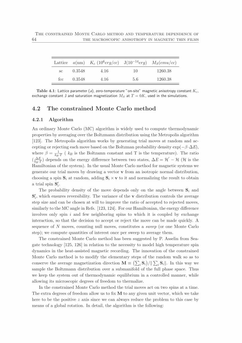
64The constrained Monte Carlo method and temperature dependence of
the macroscopic anisotropy in magnetic thin films
Lattice a(nm) Kc (106erg/cc) J(10−14erg) MS(emu/cc)
sc 0.3548 4.16 10 1260.38
fcc 0.3548 4.16 5.6 1260.38
Table 4.1: Lattice parameter (a), zero-temperature ”on-site” magnetic anisotropy constant Kc,exchange constant J and saturation magnetization MS at T = 0K, used in the simulations.
4.2 The constrained Monte Carlo method
4.2.1 Algorithm
An ordinary Monte Carlo (MC) algorithm is widely used to compute thermodynamic
properties by averaging over the Boltzmann distribution using the Metropolis algorithm
[123]. The Metropolis algorithm works by generating trial moves at random and ac-
cepting or rejecting each move based on the Boltzman probability density exp(−β ·∆E),
where β = 1kB ·T ( kB is the Boltzamn constant and T is the temperature). The ratio
( ∆E
kB ·T ) depends on the energy difference between two states, ∆E = H′
− H (H is the
Hamiltonian of the system). In the usual Monte Carlo method for magnetic systems we
generate our trial moves by drawing a vector v from an isotropic normal distribution,
choosing a spin Si at random, adding Si ×v to it and normalizing the result to obtain
a trial spin S′i.
The probability density of the move depends only on the angle between Si and
S′i, which ensures reversibility. The variance of the v distribution controls the average
step size and can be chosen at will to improve the ratio of accepted to rejected moves,
similarly to the MC angle in Refs. [123, 124]. For our Hamiltonian, the energy difference
involves only spin i and few neighboring spins to which it is coupled by exchange
interaction, so that the decision to accept or reject the move can be made quickly. A
sequence of N moves, counting null moves, constitutes a sweep (or one Monte Carlo
step); we compute quantities of interest once per sweep to average them.
The constrained Monte Carlo method has been suggested by P. Asselin from Sea-
gate technology [125, 126] in relation to the necessity to model high temperature spin
dynamics in the heat-assisted magnetic recording. The innovation of the constrained
Monte Carlo method is to modify the elementary steps of the random walk so as to
conserve the average magnetization direction M ≡(∑
i Si
)
/‖∑
i Si‖. In this way we
sample the Boltzmann distribution over a submanifold of the full phase space. Thus
we keep the system out of thermodynamic equilibrium in a controlled manner, while
allowing its microscopic degrees of freedom to thermalize.
In the constrained Monte Carlo method the trial moves act on two spins at a time.
The extra degrees of freedom allow us to fix M to any given unit vector, which we take
here to be the positive z axis since we can always reduce the problem to this case by
means of a global rotation. In detail, the algorithm is the following:
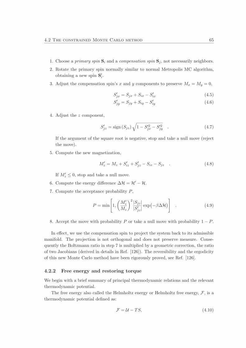
4.2 The constrained Monte Carlo method 65
1. Choose a primary spin Si and a compensation spin Sj , not necessarily neighbors.
2. Rotate the primary spin normally similar to normal Metropolis MC algorithm,
obtaining a new spin S′i.
3. Adjust the compensation spin’s x and y components to preserve Mx = My = 0,
S′jx = Sjx + Six − S′
ix (4.5)
S′jy = Sjy + Siy − S′
iy (4.6)
4. Adjust the z component,
S′jz = sign (Sjz)
√
1 − S′2jx − S′2
jy . (4.7)
If the argument of the square root is negative, stop and take a null move (reject
the move).
5. Compute the new magnetization,
M ′z = Mz + S′
iz + S′jz − Siz − Sjz . (4.8)
If M ′z ≤ 0, stop and take a null move.
6. Compute the energy difference ∆H = H′ −H.
7. Compute the acceptance probability P ,
P = min
[
1,
(
M ′z
Mz
)2 |Sjz|
|S′jz|
exp(
−β∆H)
]
. (4.9)
8. Accept the move with probability P or take a null move with probability 1 − P .
In effect, we use the compensation spin to project the system back to its admissible
manifold. The projection is not orthogonal and does not preserve measure. Conse-
quently the Boltzmann ratio in step 7 is multiplied by a geometric correction, the ratio
of two Jacobians (derived in details in Ref. [126]). The reversibility and the ergodicity
of this new Monte Carlo method have been rigorously proved, see Ref. [126].
4.2.2 Free energy and restoring torque
We begin with a brief summary of principal thermodynamic relations and the relevant
thermodynamic potential.
The free energy also called the Helmholtz energy or Helmholtz free energy, F , is a
thermodynamic potential defined as:
F = U − TS, (4.10)
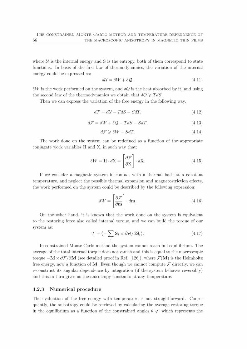
66The constrained Monte Carlo method and temperature dependence of
the macroscopic anisotropy in magnetic thin films
where U is the internal energy and S is the entropy, both of them correspond to state
functions. In basis of the first law of thermodynamics, the variation of the internal
energy could be expressed as:
dU = δW + δQ. (4.11)
δW is the work performed on the system, and δQ is the heat absorbed by it, and using
the second law of the thermodynamics we obtain that δQ > TdS.
Then we can express the variation of the free energy in the following way.
dF = dU − TdS − SdT, (4.12)
dF = δW + δQ− TdS − SdT, (4.13)
dF > δW − SdT. (4.14)
The work done on the system can be redefined as a function of the appropriate
conjugate work variables H and X, in such way that:
δW = H · dX =
[
∂F
∂X
]
· dX. (4.15)
If we consider a magnetic system in contact with a thermal bath at a constant
temperature, and neglect the possible thermal expansion and magnetostriction effects,
the work performed on the system could be described by the following expression:
δW =
[
∂F
∂m
]
· dm. (4.16)
On the other hand, it is known that the work done on the system is equivalent
to the restoring force also called internal torque, and we can build the torque of our
system as:
T =⟨
−∑
i
Si × ∂H/∂Si
⟩
. (4.17)
In constrained Monte Carlo method the system cannot reach full equilibrium. The
average of the total internal torque does not vanish and this is equal to the macroscopic
torque −M×∂F/∂M (see detailed proof in Ref. [126]), where F(M) is the Helmholtz
free energy, now a function of M. Even though we cannot compute F directly, we can
reconstruct its angular dependence by integration (if the system behaves reversibly)
and this in turn gives us the anisotropy constants at any temperature.
4.2.3 Numerical procedure
The evaluation of the free energy with temperature is not straightforward. Conse-
quently, the anisotropy could be retrieved by calculating the average restoring torque
in the equilibrium as a function of the constrained angles θ, ϕ, which represents the

4.2 The constrained Monte Carlo method 67
polar and azimuthal angles of the magnetization from the easy axis. The torque acting
on a system with mixed anisotropy (combination of uniaxial and cubic anisotropies)
depends on the azimuthal and rotational angles in the following way:
T (θ, ϕ) = −Keffua (T ) sin(2θ)−
1
2Keff
ca (T ) sin(2θ)
(
sin2(θ)
(
sin4(ϕ)+cos4(ϕ)
)
−cos2(θ)
)
.
(4.18)
If we evaluate the restoring torque at ϕ = 0, we obtain that:
T (θ, 0) = −Keffua (T ) sin(2θ) −
1
2Keff
ca (T ) sin(4θ). (4.19)
Thus, it is possible to obtain the values of anisotropy constants of the system and their
behavior at different temperatures evaluating the torque curve.
In practice we first initialize the system with uniform magnetization in a direction
of our choice (θ, ϕ), away from the anisotropy axes, where we expect a nonzero torque.
Next we evolve the system by constrained Monte Carlo until the length of the mag-
netization reaches equilibrium. We then take a thermodynamic average of the torque
over the number of constrained Monte Carlo “sweeps”. We repeat at other orientations
and we finally reconstruct the anisotropy constants from the angular dependence of the
torque.
Torque curves for a generic system with uniaxial and cubic anisotropy are shown
in Fig. 4.1. The symbols show the calculated torque and the curves are fitted to a
sin (2θ) dependence in the uniaxial case and to a sin(4θ) dependence when the system
has cubic anisotropy, where θ is the angle from the easy axis. The sin (2θ)[
sin(4θ)]
0,00 0,25 0,50 0,75 1,00-1,00
-0,75
-0,50
-0,25
0,00
0,25
0,50
0,75
1,00
Sys
tem
Tor
que
/KC
Angle from easy axis /
T=10K T=100K T=500K
0.00 0.25 0.50 0.75 1.00
-0.50
-0.25
0.00
0.25
0.50
Sys
tem
Tor
que
/KC
Angle from easy axis /
T=10K T=100K T=500K
Figure 4.1: Simulated angular dependence of the restoring torque for a thin film with a simplecubic lattice, periodic boundary conditions and Tc close to 1100K, at temperatures 10 K, 100 K,and 500 K. (Left) Thin film with uniaxial anisotropy with easy axis parallel to Z axis. (Right) Thinfilm with cubic anisotropy with one of the easy axes parallel to Z axis.
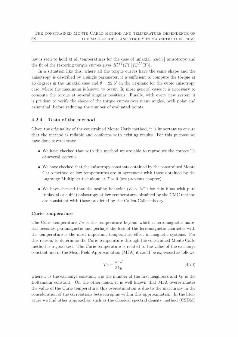
68The constrained Monte Carlo method and temperature dependence of
the macroscopic anisotropy in magnetic thin films
law is seen to hold at all temperatures for the case of uniaxial[
cubic]
anisotropy and
the fit of the restoring torque curves gives Keffua (T )
[
Keffca (T )
]
.
In a situation like this, where all the torque curves have the same shape and the
anisotropy is described by a single parameter, it is sufficient to compute the torque at
45 degrees in the uniaxial case and θ = 22.5◦ in the xz-plane for the cubic anisotropy
case, where the maximum is known to occur. In more general cases it is necessary to
compute the torque at several angular positions. Finally, with every new system it
is prudent to verify the shape of the torque curves over many angles, both polar and
azimuthal, before reducing the number of evaluated points.
4.2.4 Tests of the method
Given the originality of the constrained Monte Carlo method, it is important to ensure
that the method is reliable and conforms with existing results. For this purpose we
have done several tests:
• We have checked that with this method we are able to reproduce the correct Tc
of several systems.
• We have checked that the anisotropy constants obtained by the constrained Monte
Carlo method at low temperatures are in agreement with those obtained by the
Lagrange Multiplier technique at T = 0 (see previous chapter).
• We have checked that the scaling behavior (K ∼ Mγ) for thin films with pure
(uniaxial or cubic) anisotropy at low temperatures obtained by the CMC method
are consistent with those predicted by the Callen-Callen theory.
Curie temperature
The Curie temperature Tc is the temperature beyond which a ferromagnetic mate-
rial becomes paramagnetic and perhaps the loss of the ferromagnetic character with
the temperature is the most important temperature effect in magnetic systems. For
this reason, to determine the Curie temperature through the constrained Monte Carlo
method is a good test. The Curie temperature is related to the value of the exchange
constant and in the Mean Field Approximation (MFA) it could be expressed as follows:
Tc =z · J
3kB(4.20)
where J is the exchange constant, z is the number of the first neighbors and kB is the
Boltzmann constant. On the other hand, it is well known that MFA overestimates
the value of the Curie temperature, this overestimation is due to the inaccuracy in the
consideration of the correlations between spins within this approximation. In the liter-
ature we find other approaches, such as the classical spectral density method (CSDM)
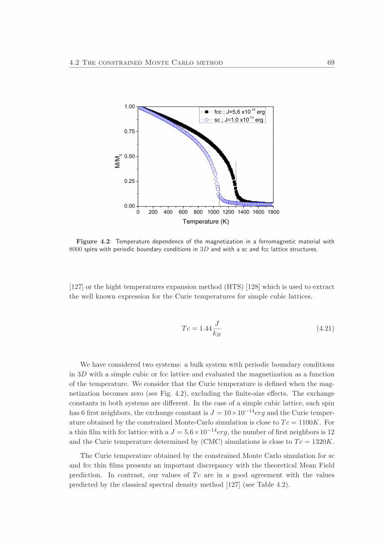
4.2 The constrained Monte Carlo method 69
0 200 400 600 800 1000 1200 1400 1600 18000.00
0.25
0.50
0.75
1.00
M/M
0
Temperature (K)
fcc ; J=5,6 x10⁻¹⁴ erg sc ; J=1,0 x10⁻¹³ erg
Figure 4.2: Temperature dependence of the magnetization in a ferromagnetic material with8000 spins with periodic boundary conditions in 3D and with a sc and fcc lattice structures.
[127] or the hight temperatures expansion method (HTS) [128] which is used to extract
the well known expression for the Curie temperatures for simple cubic lattices.
Tc = 1.44J
kB(4.21)
We have considered two systems: a bulk system with periodic boundary conditions
in 3D with a simple cubic or fcc lattice and evaluated the magnetization as a function
of the temperature. We consider that the Curie temperature is defined when the mag-
netization becomes zero (see Fig. 4.2), excluding the finite-size effects. The exchange
constants in both systems are different. In the case of a simple cubic lattice, each spin
has 6 first neighbors, the exchange constant is J = 10×10−14erg and the Curie temper-
ature obtained by the constrained Monte-Carlo simulation is close to Tc = 1100K. For
a thin film with fcc lattice with a J = 5.6×10⁻¹⁴erg, the number of first neighbors is 12
and the Curie temperature determined by (CMC) simulations is close to Tc = 1320K.
The Curie temperature obtained by the constrained Monte Carlo simulation for sc
and fcc thin films presents an important discrepancy with the theoretical Mean Field
prediction. In contrast, our values of Tc are in a good agreement with the values
predicted by the classical spectral density method [127] (see Table 4.2).
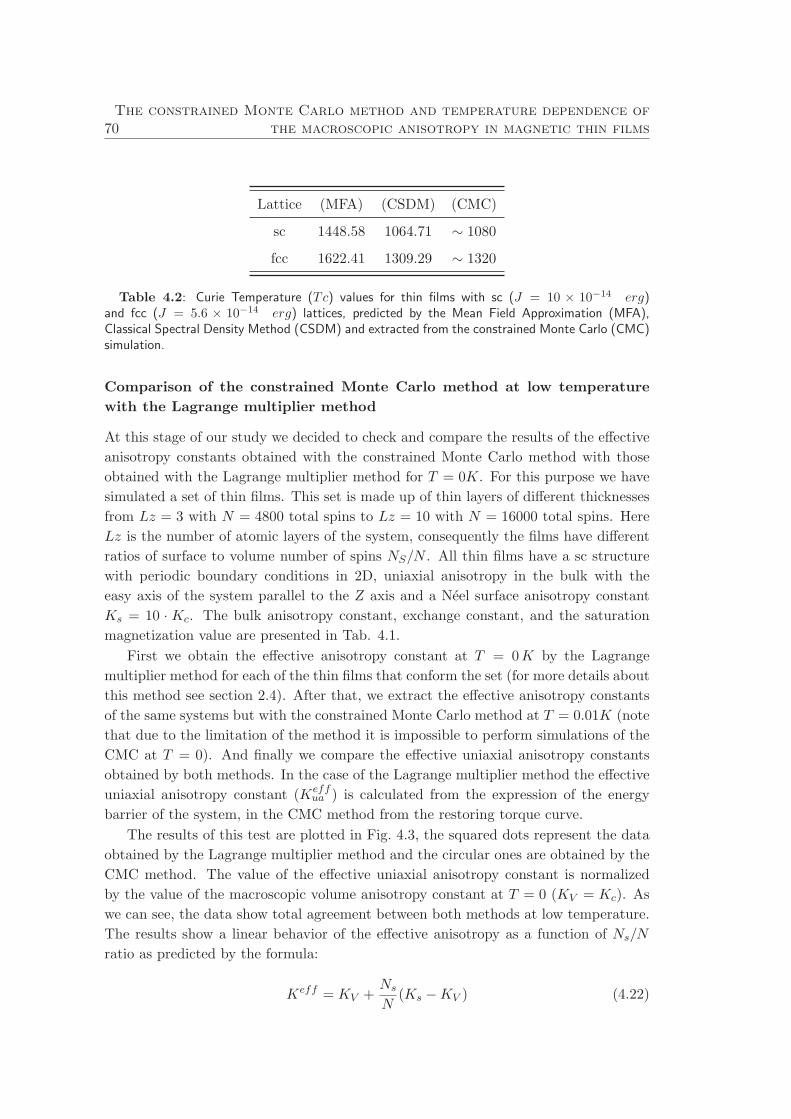
70The constrained Monte Carlo method and temperature dependence of
the macroscopic anisotropy in magnetic thin films
Lattice (MFA) (CSDM) (CMC)
sc 1448.58 1064.71 ∼ 1080
fcc 1622.41 1309.29 ∼ 1320
Table 4.2: Curie Temperature (Tc) values for thin films with sc (J = 10 × 10−14 erg)and fcc (J = 5.6 × 10⁻¹⁴ erg) lattices, predicted by the Mean Field Approximation (MFA),Classical Spectral Density Method (CSDM) and extracted from the constrained Monte Carlo (CMC)simulation.
Comparison of the constrained Monte Carlo method at low temperature
with the Lagrange multiplier method
At this stage of our study we decided to check and compare the results of the effective
anisotropy constants obtained with the constrained Monte Carlo method with those
obtained with the Lagrange multiplier method for T = 0K. For this purpose we have
simulated a set of thin films. This set is made up of thin layers of different thicknesses
from Lz = 3 with N = 4800 total spins to Lz = 10 with N = 16000 total spins. Here
Lz is the number of atomic layers of the system, consequently the films have different
ratios of surface to volume number of spins NS/N . All thin films have a sc structure
with periodic boundary conditions in 2D, uniaxial anisotropy in the bulk with the
easy axis of the system parallel to the Z axis and a Neel surface anisotropy constant
Ks = 10 · Kc. The bulk anisotropy constant, exchange constant, and the saturation
magnetization value are presented in Tab. 4.1.
First we obtain the effective anisotropy constant at T = 0K by the Lagrange
multiplier method for each of the thin films that conform the set (for more details about
this method see section 2.4). After that, we extract the effective anisotropy constants
of the same systems but with the constrained Monte Carlo method at T = 0.01K (note
that due to the limitation of the method it is impossible to perform simulations of the
CMC at T = 0). And finally we compare the effective uniaxial anisotropy constants
obtained by both methods. In the case of the Lagrange multiplier method the effective
uniaxial anisotropy constant (Keffua ) is calculated from the expression of the energy
barrier of the system, in the CMC method from the restoring torque curve.
The results of this test are plotted in Fig. 4.3, the squared dots represent the data
obtained by the Lagrange multiplier method and the circular ones are obtained by the
CMC method. The value of the effective uniaxial anisotropy constant is normalized
by the value of the macroscopic volume anisotropy constant at T = 0 (KV = Kc). As
we can see, the data show total agreement between both methods at low temperature.
The results show a linear behavior of the effective anisotropy as a function of Ns/N
ratio as predicted by the formula:
Keff = KV +Ns
N(Ks −KV ) (4.22)
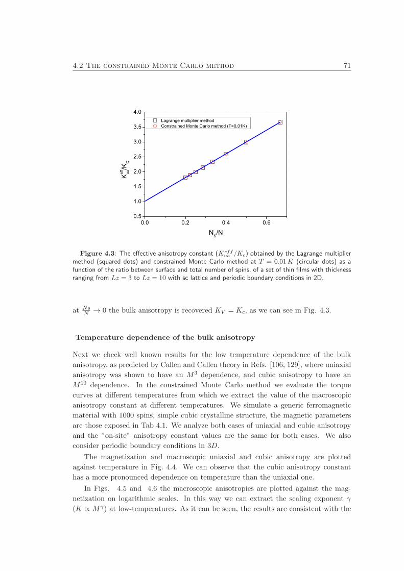
4.2 The constrained Monte Carlo method 71
0.0 0.2 0.4 0.60.5
1.0
1.5
2.0
2.5
3.0
3.5
4.0
Lagrange multiplier method Constrained Monte Carlo method (T=0,01K)
Kef
fua
/KC
NS/N
Figure 4.3: The effective anisotropy constant (Keffua /Kc) obtained by the Lagrange multiplier
method (squared dots) and constrained Monte Carlo method at T = 0.01K (circular dots) as afunction of the ratio between surface and total number of spins, of a set of thin films with thicknessranging from Lz = 3 to Lz = 10 with sc lattice and periodic boundary conditions in 2D.
at NsN → 0 the bulk anisotropy is recovered KV = Kc, as we can see in Fig. 4.3.
Temperature dependence of the bulk anisotropy
Next we check well known results for the low temperature dependence of the bulk
anisotropy, as predicted by Callen and Callen theory in Refs. [106, 129], where uniaxial
anisotropy was shown to have an M3 dependence, and cubic anisotropy to have an
M10 dependence. In the constrained Monte Carlo method we evaluate the torque
curves at different temperatures from which we extract the value of the macroscopic
anisotropy constant at different temperatures. We simulate a generic ferromagnetic
material with 1000 spins, simple cubic crystalline structure, the magnetic parameters
are those exposed in Tab 4.1. We analyze both cases of uniaxial and cubic anisotropy
and the ”on-site” anisotropy constant values are the same for both cases. We also
consider periodic boundary conditions in 3D.
The magnetization and macroscopic uniaxial and cubic anisotropy are plotted
against temperature in Fig. 4.4. We can observe that the cubic anisotropy constant
has a more pronounced dependence on temperature than the uniaxial one.
In Figs. 4.5 and 4.6 the macroscopic anisotropies are plotted against the mag-
netization on logarithmic scales. In this way we can extract the scaling exponent γ
(K ∝ Mγ) at low-temperatures. As it can be seen, the results are consistent with the
72The constrained Monte Carlo method and temperature dependence of
the macroscopic anisotropy in magnetic thin films
0 200 400 600 800 1000 1200 14000.00
0.25
0.50
0.75
1.00
KEFF(Uniaxial) Mag KEFF(Cubic)
KE
FF/K
C; M
/M0
Temperature (K)
Figure 4.4: Temperature dependence of magnetization, macroscopic uniaxial and cubicanisotropies, for a ferromagnetic material with N = 1000 spins and a simple cubic lattice withperiodic boundary conditions in 3D.
-1.2 -1.0 -0.8 -0.6 -0.4 -0.2 0.0-3.0
-2.5
-2.0
-1.5
-1.0
-0.5
0.0
Data Linear Fit at low temperatures
Log(
Kef
fua
/KC)
Log(M/M0)
=2,997
-0.03 -0.02 -0.01 0.00-0.10
-0.08
-0.06
-0.04
-0.02
0.00
Data Linear Fit at low temperatures
Log(
Kef
fua
/KC)
Log(M/M0)
=2,997
Figure 4.5: Temperature scaling of the anisotropy versus magnetization of a ferromagneticmaterial with N = 1000 moments, a simple cubic lattice, uniaxial anisotropy and periodic boundaryconditions in 3D, for the whole temperature range (Left) and the fitting at low-temperatures (Right).
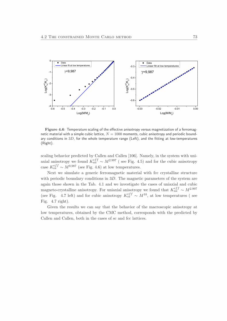
4.2 The constrained Monte Carlo method 73
-0.6 -0.5 -0.4 -0.3 -0.2 -0.1 0.0-4
-3
-2
-1
0
Data Linear fit at low temperatures.
Log(
Kef
fca
/KC)
Log(M/M0)
=9,987
-0.03 -0.02 -0.01 0.00
-0.6
-0.5
-0.4
-0.3
Data Linear fitt at low temperatures
Log(
Kef
fca
/KC)
Log(M/M0)
=9,987
Figure 4.6: Temperature scaling of the effective anisotropy versus magnetization of a ferromag-netic material with a simple cubic lattice, N = 1000 moments, cubic anisotropy and periodic bound-ary conditions in 3D, for the whole temperature range (Left), and the fitting at low-temperatures(Right).
scaling behavior predicted by Callen and Callen [106]. Namely, in the system with uni-
axial anisotropy we found Keffua ∼ M2.997 ( see Fig. 4.5) and for the cubic anisotropy
case Keffca ∼M9,987 (see Fig. 4.6) at low temperatures.
Next we simulate a generic ferromagnetic material with fcc crystalline structure
with periodic boundary conditions in 3D. The magnetic parameters of the system are
again those shown in the Tab. 4.1 and we investigate the cases of uniaxial and cubic
magneto-crystalline anisotropy. For uniaxial anisotropy we found that Keffua ∼ M2.997
(see Fig. 4.7 left) and for cubic anisotropy Keffca ∼ M10, at low temperatures ( see
Fig. 4.7 right).
Given the results we can say that the behavior of the macroscopic anisotropy at
low temperatures, obtained by the CMC method, corresponds with the predicted by
Callen and Callen, both in the cases of sc and fcc lattices.
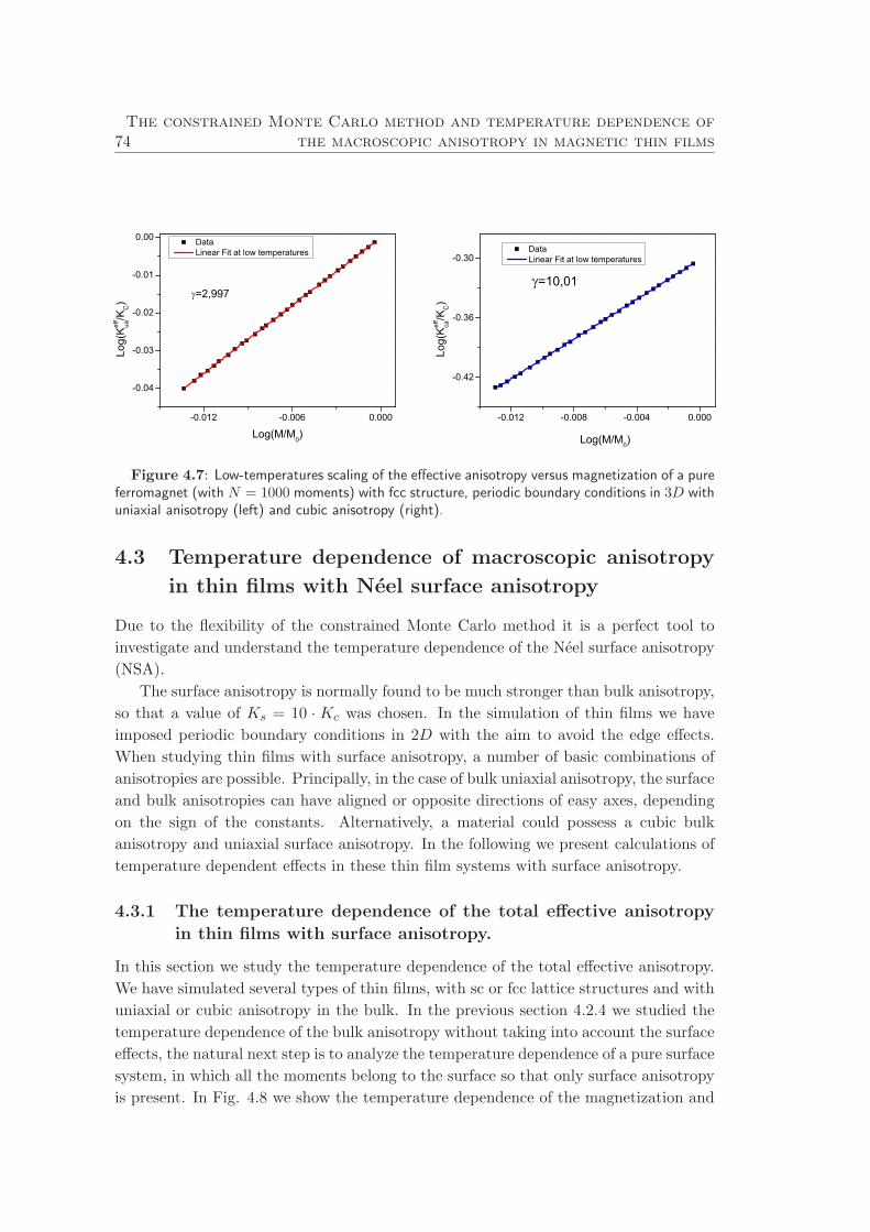
74The constrained Monte Carlo method and temperature dependence of
the macroscopic anisotropy in magnetic thin films
-0.012 -0.006 0.000
-0.04
-0.03
-0.02
-0.01
0.00
=2,997
Data Linear Fit at low temperatures
Log(
Kef
fua
/KC)
Log(M/M0)-0.012 -0.008 -0.004 0.000
-0.42
-0.36
-0.30
Data Linear Fit at low temperatures
Log(
Kef
fca
/KC)
Log(M/M0)
=10,01
Figure 4.7: Low-temperatures scaling of the effective anisotropy versus magnetization of a pureferromagnet (with N = 1000 moments) with fcc structure, periodic boundary conditions in 3D withuniaxial anisotropy (left) and cubic anisotropy (right).
4.3 Temperature dependence of macroscopic anisotropy
in thin films with Neel surface anisotropy
Due to the flexibility of the constrained Monte Carlo method it is a perfect tool to
investigate and understand the temperature dependence of the Neel surface anisotropy
(NSA).
The surface anisotropy is normally found to be much stronger than bulk anisotropy,
so that a value of Ks = 10 · Kc was chosen. In the simulation of thin films we have
imposed periodic boundary conditions in 2D with the aim to avoid the edge effects.
When studying thin films with surface anisotropy, a number of basic combinations of
anisotropies are possible. Principally, in the case of bulk uniaxial anisotropy, the surface
and bulk anisotropies can have aligned or opposite directions of easy axes, depending
on the sign of the constants. Alternatively, a material could possess a cubic bulk
anisotropy and uniaxial surface anisotropy. In the following we present calculations of
temperature dependent effects in these thin film systems with surface anisotropy.
4.3.1 The temperature dependence of the total effective anisotropy
in thin films with surface anisotropy.
In this section we study the temperature dependence of the total effective anisotropy.
We have simulated several types of thin films, with sc or fcc lattice structures and with
uniaxial or cubic anisotropy in the bulk. In the previous section 4.2.4 we studied the
temperature dependence of the bulk anisotropy without taking into account the surface
effects, the natural next step is to analyze the temperature dependence of a pure surface
system, in which all the moments belong to the surface so that only surface anisotropy
is present. In Fig. 4.8 we show the temperature dependence of the magnetization and
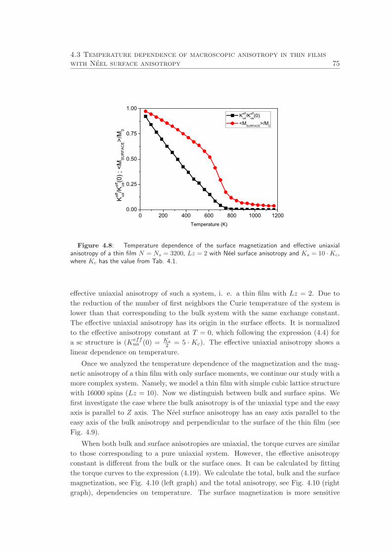
4.3 Temperature dependence of macroscopic anisotropy in thin filmswith Neel surface anisotropy 75
0 200 400 600 800 1000 12000.00
0.25
0.50
0.75
1.00
Kef
fua
/Kef
fua
(0) ;
<M
SU
RFA
CE>/
M0
Temperature (K)
Keffua
/Keffua
(0) <M
SURFACE>/M
0
Figure 4.8: Temperature dependence of the surface magnetization and effective uniaxialanisotropy of a thin film N = Ns = 3200, Lz = 2 with Neel surface anisotropy and Ks = 10 ·Kc,where Kc has the value from Tab. 4.1.
effective uniaxial anisotropy of such a system, i. e. a thin film with Lz = 2. Due to
the reduction of the number of first neighbors the Curie temperature of the system is
lower than that corresponding to the bulk system with the same exchange constant.
The effective uniaxial anisotropy has its origin in the surface effects. It is normalized
to the effective anisotropy constant at T = 0, which following the expression (4.4) for
a sc structure is (Keffua (0) = Ks
2 = 5 ·Kc). The effective uniaxial anisotropy shows a
linear dependence on temperature.
Once we analyzed the temperature dependence of the magnetization and the mag-
netic anisotropy of a thin film with only surface moments, we continue our study with a
more complex system. Namely, we model a thin film with simple cubic lattice structure
with 16000 spins (Lz = 10). Now we distinguish between bulk and surface spins. We
first investigate the case where the bulk anisotropy is of the uniaxial type and the easy
axis is parallel to Z axis. The Neel surface anisotropy has an easy axis parallel to the
easy axis of the bulk anisotropy and perpendicular to the surface of the thin film (see
Fig. 4.9).
When both bulk and surface anisotropies are uniaxial, the torque curves are similar
to those corresponding to a pure uniaxial system. However, the effective anisotropy
constant is different from the bulk or the surface ones. It can be calculated by fitting
the torque curves to the expression (4.19). We calculate the total, bulk and the surface
magnetization, see Fig. 4.10 (left graph) and the total anisotropy, see Fig. 4.10 (right
graph), dependencies on temperature. The surface magnetization is more sensitive
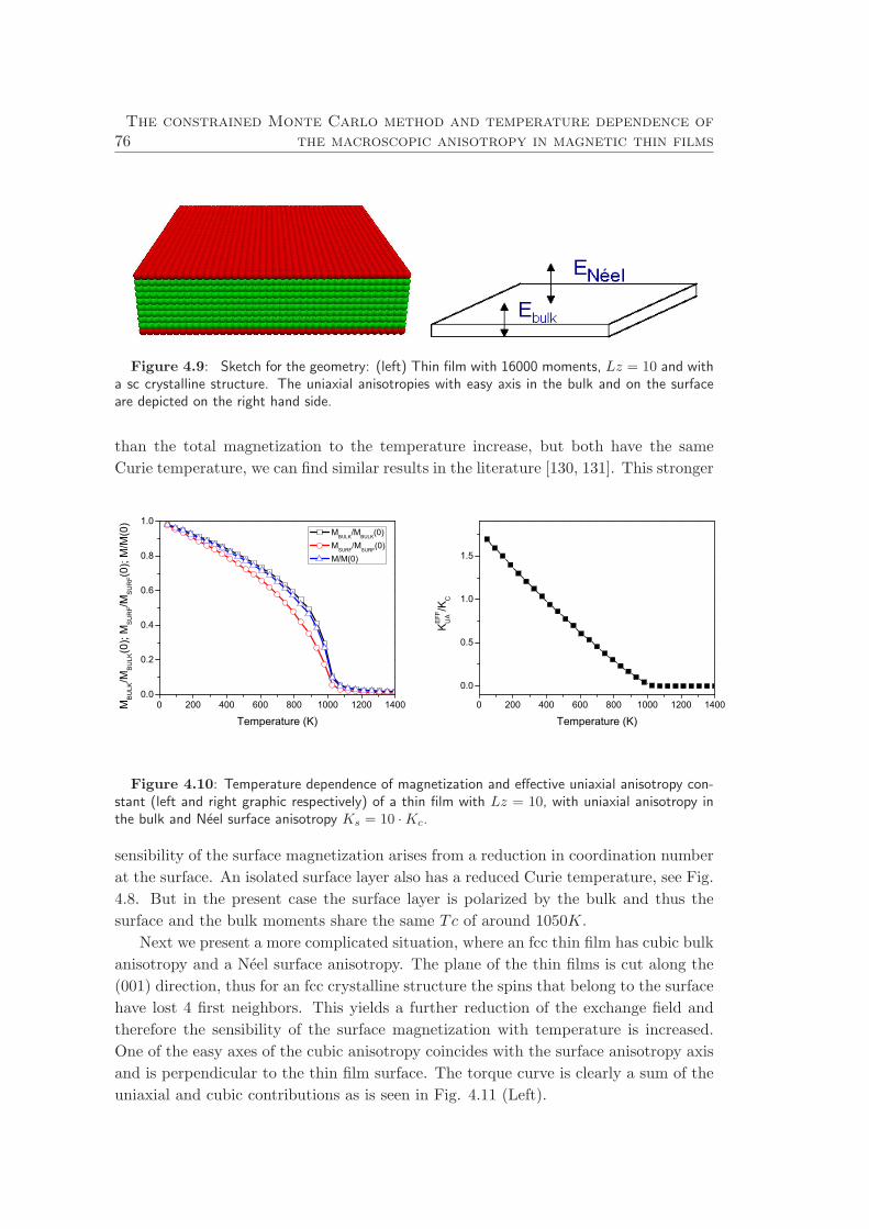
76The constrained Monte Carlo method and temperature dependence of
the macroscopic anisotropy in magnetic thin films
Figure 4.9: Sketch for the geometry: (left) Thin film with 16000 moments, Lz = 10 and witha sc crystalline structure. The uniaxial anisotropies with easy axis in the bulk and on the surfaceare depicted on the right hand side.
than the total magnetization to the temperature increase, but both have the same
Curie temperature, we can find similar results in the literature [130, 131]. This stronger
0 200 400 600 800 1000 1200 14000.0
0.2
0.4
0.6
0.8
1.0
MB
ULK
/MB
ULK
(0);
MS
UR
F/MS
UR
F(0);
M/M
(0)
Temperature (K)
MBULK
/MBULK
(0) M
SURF/M
SURF(0)
M/M(0)
0 200 400 600 800 1000 1200 1400
0.0
0.5
1.0
1.5
KE
FFU
A/K
C
Temperature (K)
Figure 4.10: Temperature dependence of magnetization and effective uniaxial anisotropy con-stant (left and right graphic respectively) of a thin film with Lz = 10, with uniaxial anisotropy inthe bulk and Neel surface anisotropy Ks = 10 ·Kc.
sensibility of the surface magnetization arises from a reduction in coordination number
at the surface. An isolated surface layer also has a reduced Curie temperature, see Fig.
4.8. But in the present case the surface layer is polarized by the bulk and thus the
surface and the bulk moments share the same Tc of around 1050K.
Next we present a more complicated situation, where an fcc thin film has cubic bulk
anisotropy and a Neel surface anisotropy. The plane of the thin films is cut along the
(001) direction, thus for an fcc crystalline structure the spins that belong to the surface
have lost 4 first neighbors. This yields a further reduction of the exchange field and
therefore the sensibility of the surface magnetization with temperature is increased.
One of the easy axes of the cubic anisotropy coincides with the surface anisotropy axis
and is perpendicular to the thin film surface. The torque curve is clearly a sum of the
uniaxial and cubic contributions as is seen in Fig. 4.11 (Left).
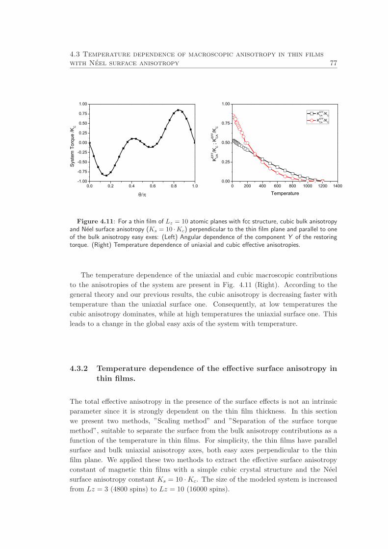
4.3 Temperature dependence of macroscopic anisotropy in thin filmswith Neel surface anisotropy 77
0.0 0.2 0.4 0.6 0.8 1.0-1.00
-0.75
-0.50
-0.25
0.00
0.25
0.50
0.75
1.00
Sys
tem
Tor
que
/KC
0 200 400 600 800 1000 1200 14000.00
0.25
0.50
0.75
1.00
KE
FFU
A/K
C ;
KE
FFC
A/K
C
Temperature
KEFFUA
/KC
KEFFCA
/KC
Figure 4.11: For a thin film of Lz = 10 atomic planes with fcc structure, cubic bulk anisotropyand Neel surface anisotropy (Ks = 10 ·Kc) perpendicular to the thin film plane and parallel to oneof the bulk anisotropy easy exes: (Left) Angular dependence of the component Y of the restoringtorque. (Right) Temperature dependence of uniaxial and cubic effective anisotropies.
The temperature dependence of the uniaxial and cubic macroscopic contributions
to the anisotropies of the system are present in Fig. 4.11 (Right). According to the
general theory and our previous results, the cubic anisotropy is decreasing faster with
temperature than the uniaxial surface one. Consequently, at low temperatures the
cubic anisotropy dominates, while at high temperatures the uniaxial surface one. This
leads to a change in the global easy axis of the system with temperature.
4.3.2 Temperature dependence of the effective surface anisotropy in
thin films.
The total effective anisotropy in the presence of the surface effects is not an intrinsic
parameter since it is strongly dependent on the thin film thickness. In this section
we present two methods, ”Scaling method” and ”Separation of the surface torque
method”, suitable to separate the surface from the bulk anisotropy contributions as a
function of the temperature in thin films. For simplicity, the thin films have parallel
surface and bulk uniaxial anisotropy axes, both easy axes perpendicular to the thin
film plane. We applied these two methods to extract the effective surface anisotropy
constant of magnetic thin films with a simple cubic crystal structure and the Neel
surface anisotropy constant Ks = 10 ·Kc. The size of the modeled system is increased
from Lz = 3 (4800 spins) to Lz = 10 (16000 spins).
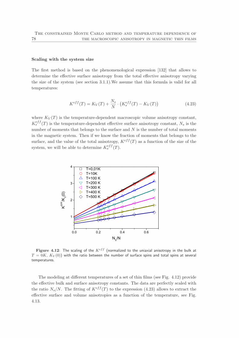
78The constrained Monte Carlo method and temperature dependence of
the macroscopic anisotropy in magnetic thin films
Scaling with the system size
The first method is based on the phenomenological expression [132] that allows to
determine the effective surface anisotropy from the total effective anisotropy varying
the size of the system (see section 3.1.1).We assume that this formula is valid for all
temperatures:
Keff (T ) = KV (T ) +Ns
N·(
Keffs (T ) −KV (T )
)
(4.23)
where KV (T ) is the temperature-dependent macroscopic volume anisotropy constant,
Keffs (T ) is the temperature-dependent effective surface anisotropy constant, Ns is the
number of moments that belongs to the surface and N is the number of total moments
in the magnetic system. Then if we know the fraction of moments that belongs to the
surface, and the value of the total anisotropy, Keff (T ) as a function of the size of the
system, we will be able to determine Keffs (T ).
0.0 0.2 0.4 0.6
1
2
3
4
T=0,01K T=10K T=100 K T=200 K T=300 K T=400 K T=500 K
KE
FF/K
V(0
)
NS/N
Figure 4.12: The scaling of the Keff (normalized to the uniaxial anisotropy in the bulk atT = 0K, KV (0)) with the ratio between the number of surface spins and total spins at severaltemperatures.
The modeling at different temperatures of a set of thin films (see Fig. 4.12) provide
the effective bulk and surface anisotropy constants. The data are perfectly scaled with
the ratio Ns/N . The fitting of Keff (T ) to the expression (4.23) allows to extract the
effective surface and volume anisotropies as a function of the temperature, see Fig.
4.13.
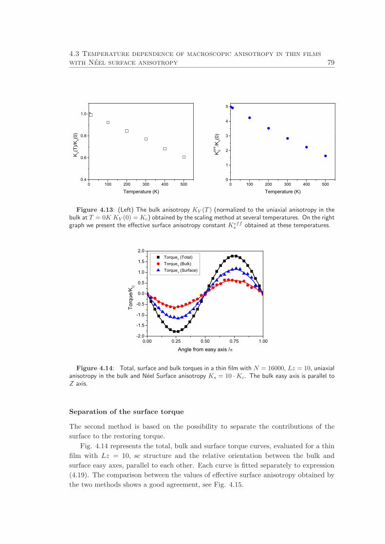
4.3 Temperature dependence of macroscopic anisotropy in thin filmswith Neel surface anisotropy 79
0 100 200 300 400 5000.4
0.6
0.8
1.0
KV(T
)/KV(0
)
Temperature (K)0 100 200 300 400 500
0
1
2
3
4
5
KE
FFS
/KV(0
)
Temperature (K)
Figure 4.13: (Left) The bulk anisotropy KV (T ) (normalized to the uniaxial anisotropy in thebulk at T = 0K KV (0) = Kc) obtained by the scaling method at several temperatures. On the rightgraph we present the effective surface anisotropy constant Keff
s obtained at these temperatures.
0.00 0.25 0.50 0.75 1.00-2.0
-1.5
-1.0
-0.5
0.0
0.5
1.0
1.5
2.0
TorqueY (Total)
TorqueY (Bulk)
TorqueY (Surface)
Torq
ue/K
C
Angle from easy axis /
Figure 4.14: Total, surface and bulk torques in a thin film with N = 16000, Lz = 10, uniaxialanisotropy in the bulk and Neel Surface anisotropy Ks = 10 ·Kc. The bulk easy axis is parallel toZ axis.
Separation of the surface torque
The second method is based on the possibility to separate the contributions of the
surface to the restoring torque.
Fig. 4.14 represents the total, bulk and surface torque curves, evaluated for a thin
film with Lz = 10, sc structure and the relative orientation between the bulk and
surface easy axes, parallel to each other. Each curve is fitted separately to expression
(4.19). The comparison between the values of effective surface anisotropy obtained by
the two methods shows a good agreement, see Fig. 4.15.
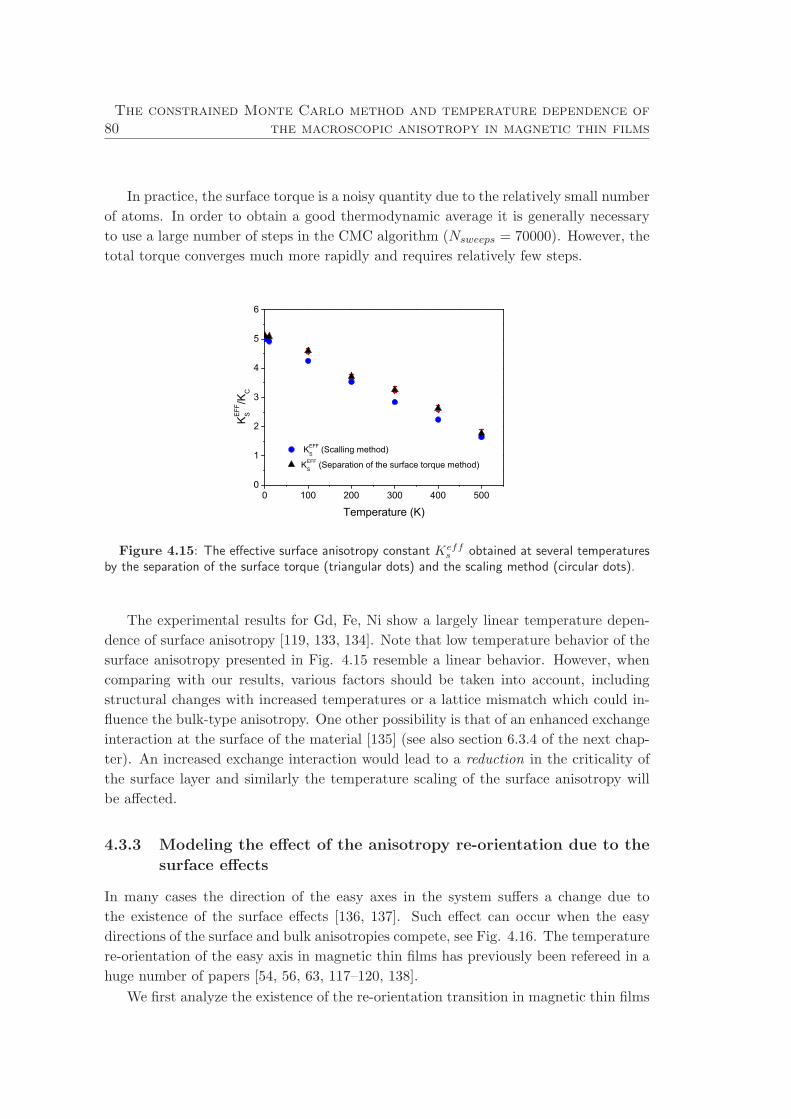
80The constrained Monte Carlo method and temperature dependence of
the macroscopic anisotropy in magnetic thin films
In practice, the surface torque is a noisy quantity due to the relatively small number
of atoms. In order to obtain a good thermodynamic average it is generally necessary
to use a large number of steps in the CMC algorithm (Nsweeps = 70000). However, the
total torque converges much more rapidly and requires relatively few steps.
0 100 200 300 400 5000
1
2
3
4
5
6
KE
FFS
/KC
Temperature (K)
KEFFS
(Scalling method)
KEFFS
(Separation of the surface torque method)
Figure 4.15: The effective surface anisotropy constant Keffs obtained at several temperatures
by the separation of the surface torque (triangular dots) and the scaling method (circular dots).
The experimental results for Gd, Fe, Ni show a largely linear temperature depen-
dence of surface anisotropy [119, 133, 134]. Note that low temperature behavior of the
surface anisotropy presented in Fig. 4.15 resemble a linear behavior. However, when
comparing with our results, various factors should be taken into account, including
structural changes with increased temperatures or a lattice mismatch which could in-
fluence the bulk-type anisotropy. One other possibility is that of an enhanced exchange
interaction at the surface of the material [135] (see also section 6.3.4 of the next chap-
ter). An increased exchange interaction would lead to a reduction in the criticality of
the surface layer and similarly the temperature scaling of the surface anisotropy will
be affected.
4.3.3 Modeling the effect of the anisotropy re-orientation due to the
surface effects
In many cases the direction of the easy axes in the system suffers a change due to
the existence of the surface effects [136, 137]. Such effect can occur when the easy
directions of the surface and bulk anisotropies compete, see Fig. 4.16. The temperature
re-orientation of the easy axis in magnetic thin films has previously been refereed in a
huge number of papers [54, 56, 63, 117–120, 138].
We first analyze the existence of the re-orientation transition in magnetic thin films
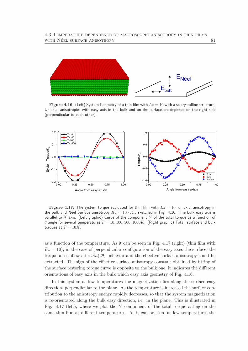
4.3 Temperature dependence of macroscopic anisotropy in thin filmswith Neel surface anisotropy 81
Figure 4.16: (Left) System Geometry of a thin film with Lz = 10 with a sc crystalline structure.Uniaxial anisotropies with easy axis in the bulk and on the surface are depicted on the right side(perpendicular to each other).
0.00 0.25 0.50 0.75 1.00-0.2
-0.1
0.0
0.1
0.2
Sys
tem
Tor
que/
KC
Angle from easy axis
T=10 T=100 T=500 T=1000
0.00 0.25 0.50 0.75 1.00-1.0
-0.5
0.0
0.5
1.0
Total Bulk Surface
Torq
ue/K
C
Angle from easy axis/
Figure 4.17: The system torque evaluated for thin film with Lz = 10, uniaxial anisotropy inthe bulk and Neel Surface anisotropy Ks = 10 ·Kc, sketched in Fig. 4.16. The bulk easy axis isparallel to X axis. (Left graphic) Curve of the component Y of the total torque as a function ofθ angle for several temperatures T = 10, 100, 500, 1000K. (Right graphic) Total, surface and bulktorques at T = 10K.
as a function of the temperature. As it can be seen in Fig. 4.17 (right) (thin film with
Lz = 10), in the case of perpendicular configuration of the easy axes the surface, the
torque also follows the sin(2θ) behavior and the effective surface anisotropy could be
extracted. The sign of the effective surface anisotropy constant obtained by fitting of
the surface restoring torque curve is opposite to the bulk one, it indicates the different
orientations of easy axis in the bulk which easy axis geometry of Fig. 4.16.
In this system at low temperatures the magnetization lies along the surface easy
direction, perpendicular to the plane. As the temperature is increased the surface con-
tribution to the anisotropy energy rapidly decreases, so that the system magnetization
is re-orientated along the bulk easy direction, i.e. in the plane. This is illustrated in
Fig. 4.17 (left), where we plot the Y component of the total torque acting on the
same thin film at different temperatures. As it can be seen, at low temperatures the
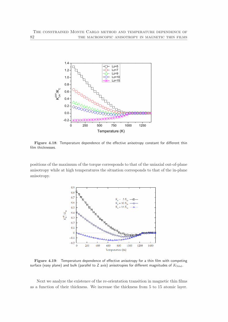
82The constrained Monte Carlo method and temperature dependence of
the macroscopic anisotropy in magnetic thin films
0 250 500 750 1000 1250
-0.2
0.0
0.2
0.4
0.6
0.8
1.0
1.2
1.4
K
EFF
UA
/KC
Temperature (K)
Lz=5 Lz=7 Lz=9 Lz=10 Lz=15
Figure 4.18: Temperature dependence of the effective anisotropy constant for different thinfilm thicknesses.
positions of the maximum of the torque corresponds to that of the uniaxial out-of-plane
anisotropy while at high temperatures the situation corresponds to that of the in-plane
anisotropy.
Figure 4.19: Temperature dependence of effective anisotropy for a thin film with competingsurface (easy plane) and bulk (parallel to Z axis) anisotropies for different magnitudes of KNeel.
Next we analyze the existence of the re-orientation transition in magnetic thin films
as a function of their thickness. We increase the thickness from 5 to 15 atomic layer.
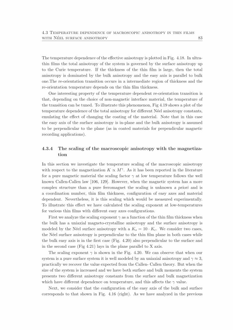
4.3 Temperature dependence of macroscopic anisotropy in thin filmswith Neel surface anisotropy 83
The temperature dependence of the effective anisotropy is plotted in Fig. 4.18. In ultra-
thin films the total anisotropy of the system is governed by the surface anisotropy up
to the Curie temperature. If the thickness of the thin film is large, then the total
anisotropy is dominated by the bulk anisotropy and the easy axis is parallel to bulk
one.The re-orientation transition occurs in a intermediate region of thickness and the
re-orientation temperature depends on the thin film thickness.
One interesting property of the temperature dependent re-orientation transition is
that, depending on the choice of non-magnetic interface material, the temperature of
the transition can be tuned. To illustrate this phenomenon, Fig 4.19 shows a plot of the
temperature dependence of the total anisotropy for different Neel anisotropy constants,
emulating the effect of changing the coating of the material. Note that in this case
the easy axis of the surface anisotropy is in-plane and the bulk anisotropy is assumed
to be perpendicular to the plane (as in coated materials for perpendicular magnetic
recording applications).
4.3.4 The scaling of the macroscopic anisotropy with the magnetiza-
tion
In this section we investigate the temperature scaling of the macroscopic anisotropy
with respect to the magnetization K ∝ Mγ . As it has been reported in the literature
for a pure magnetic material the scaling factor γ at low temperature follows the well
known Callen-Callen law [106, 129]. However, when the magnetic system has a more
complex structure than a pure ferromagnet the scaling is unknown a priori and is
a coordination number, thin film thickness, configuration of easy axes and material
dependent. Nevertheless, it is this scaling which would be measured experimentally.
To illustrate this effect we have calculated the scaling exponent at low-temperatures
for various thin films with different easy axes configurations.
First we analyze the scaling exponent γ as a function of the thin film thickness when
the bulk has a uniaxial magneto-crystalline anisotropy and the surface anisotropy is
modeled by the Neel surface anisotropy with a Ks = 10 ·Kc. We consider two cases,
the Neel surface anisotropy is perpendicular to the thin film plane in both cases while
the bulk easy axis is in the first case (Fig. 4.20) also perpendicular to the surface and
in the second case (Fig 4.21) lays in the plane parallel to X axis.
The scaling exponent γ is shown in the Fig. 4.20. We can observe that when our
system is a pure surface system it is well modeled by an uniaxial anisotropy and γ ≈ 3,
practically we recover the value expected from the Callen- Callen theory. But when the
size of the system is increased and we have both surface and bulk moments the system
presents two different anisotropy constants from the surface and bulk magnetization
which have different dependence on temperature, and this affects the γ value.
Next, we consider that the configuration of the easy axis of the bulk and surface
corresponds to that shown in Fig. 4.16 (right). As we have analyzed in the previous
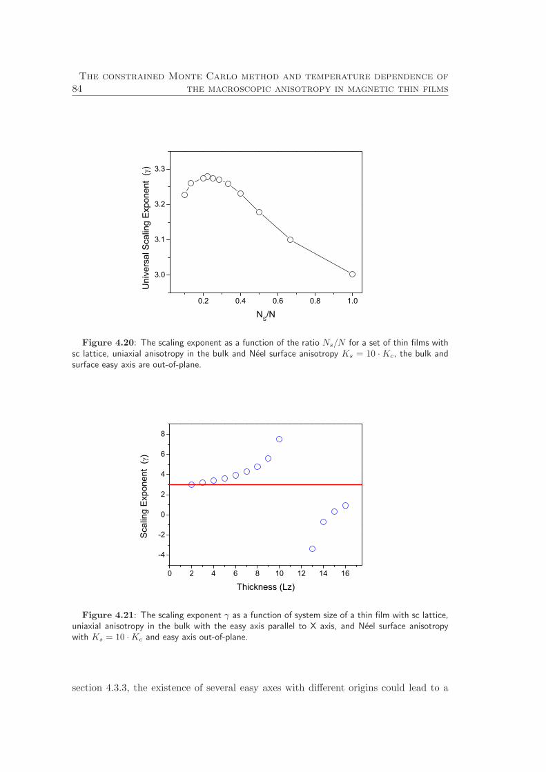
84The constrained Monte Carlo method and temperature dependence of
the macroscopic anisotropy in magnetic thin films
0.2 0.4 0.6 0.8 1.0
3.0
3.1
3.2
3.3
U
nive
rsal
Sca
ling
Exp
onen
t (
)
NS/N
Figure 4.20: The scaling exponent as a function of the ratio Ns/N for a set of thin films withsc lattice, uniaxial anisotropy in the bulk and Neel surface anisotropy Ks = 10 ·Kc, the bulk andsurface easy axis are out-of-plane.
0 2 4 6 8 10 12 14 16
-4
-2
0
2
4
6
8
Sca
ling
Exp
onen
t (
)
Thickness (Lz)
Figure 4.21: The scaling exponent γ as a function of system size of a thin film with sc lattice,uniaxial anisotropy in the bulk with the easy axis parallel to X axis, and Neel surface anisotropywith Ks = 10 ·Kc and easy axis out-of-plane.
section 4.3.3, the existence of several easy axes with different origins could lead to a

4.3 Temperature dependence of macroscopic anisotropy in thin filmswith Neel surface anisotropy 85
re-orientation transition with temperature. The re-orientation transition has the con-
sequence that the scaling exponent of the effective anisotropy constant with the average
magnetization is not monotonic, as we can see in Fig. 4.21, where the scaling exponent
of systems with Lz = 2 ÷ 16 is plotted. The scaling exponent increases from γ & 3
(when the total anisotropy is dominated by the surface anisotropy), diverges at the
re-orientation transition and later recovers the value γ ∼ 3 (when the total anisotropy
is dominated by the bulk one) with increased thin film thickness (see Fig. 4.21). The
negative value of the scaling exponent is related to a non-monotonic dependence of the
effective anisotropy on temperature, related to the orientation transition, as seen in
Fig. 4.19.
In general the magnetic behavior of a thin film depends on the character of it
surface, if it is coated, if it is free, etc. It is natural to ask the question on how the
scaling exponent is affected by the surface. With the aim to answer this question, we
have simulated the effect of different cappings on our thin film, varying the value of
the Neel surface anisotropy parameter. We have modeled a thin film with a sc lattice
structure (Lz = 5), the bulk anisotropy is uniaxial and the Neel surface anisotropy
constant is changed in the range from Ks = Kc to Ks = 100 · Kc. In Fig. 4.22 we
present the calculated value of the scaling exponent. When the value of the surface
anisotropy per spin is smaller than the bulk one, the scaling factor is smaller than that
predicted by the Callen-Callen theory (γ = 3). If the effective surface anisotropy per
spin is larger than the bulk one, the scaling factor calculated is larger than 3 and γ ≈ 3
at Ks = 2Kc.
0 10 20 30 40 50 60 70 80 90 1002.8
3.0
3.2
3.4
Sca
ling
Exp
onen
t ()
KS/KC
Figure 4.22: Scaling exponent of a thin film, with sc lattice structure, Lz = 5 as a function ofthe Neel surface anisotropy normalized to the bulk anisotropy constant (Kc).
86The constrained Monte Carlo method and temperature dependence of
the macroscopic anisotropy in magnetic thin films
To summarize this section we conclude that the scaling exponent for thin films
with uniaxial anisotropy in the bulk and surface anisotropy at low temperatures is
different than that predicted by the Callen-Callen theory, and depends on the system
size. The increment of γ has its origin in the fact that the moments on the surface have
a reduction of the number of the nearest neighbors, therefore the surface magnetization
is more sensible to the temperature than the total magnetization. Also we have to note
that the value of the surface anisotropy constant itself is different from the bulk one,
and this could induce a change in the value of γ.
4.4 Conclusion
From our results we can conclude the following:
• The constrained Monte Carlo method is capable to evaluate temperature-dependent
properties. We have shown its novel capability to evaluate the temperature de-
pendence of the magnetic anisotropy, which is an important quantity for techno-
logical applications in hard magnetic materials. In the case of bulk materials we
recovered numerically the analytical scaling law of Callen and Callen.
• We have also shown that the method enables the separation of the temperature
dependent surface anisotropy as an intrinsic system parameter, independent of the
thin film thickness. Our results demonstrate a linear temperature dependence of
the surface anisotropy, consistent with the experimental results in Gd [133, 134],
Ni [134] and Fe [119] grown on different substrates.
• We have also shown that the competition between the surface and the bulk
anisotropies could produce a re-orientation of the effective easy axis. The re-
orientation temperature depends on the system size.
• We have investigated the scaling of the anisotropy in thin films with magnetiza-
tion. In ultrathin films without bulk moments, the surface anisotropy scales with
the surface magnetization following the Callen-Callen law as corresponds to the
uniaxial case. In other cases with both surface and bulk anisotropy contributions
we report no universal scaling behavior of the effective anisotropy.
4.4 Conclusion 87
Conclusiones
En esta seccion de la tesis hemos hecho un estudio numerico del comportamiento
termico de laminas delgadas ferromagneticas con anisotropıa de superficie tipo Neel.
De nuestros resultados se puede concluir lo siguiente:
• Hemos demostrado que el nuevo metodo ”Monte Carlo con ligaduras” es ca-
paz de evaluar la dependencia termica de propiedades magneticas tales como
la imanacion del sistema. Ademas utilizamos esta capacidad para evaluar la
dependencia con la temperatura de la anisotropıa magnetica, parametro muy
importante por sus posibles aplicaciones tecnologicas en materiales magneticos
duros. En el caso de anisotropıa magnetica de un sistema bulk recuperamos
numericamente el escalado de la ley de Callen-Callen.
• Ademas hemos mostrado que este nuevo metodo es capaz de obtener la dependen-
cia termica de la ansiotropıa de superficie como parametro intrınseco del sistema,
independientemente del grosor de la pelıcula delgada. Nuestros resultados mues-
tran una dependencia lineal de la anisotropıa de superficie con la temperatura,
consistente con resultados experimentales como en el caso de Gd [133, 134], Ni
[134] y Fe [119], crecidos sobre diferentes substratos.
• Por otro lado, se ha mostrado que la competicion entre la anisotropıa de superficie
y la de volumen puede producir una re-orientacion de los ejes faciles magneticos
del sistema con la temperatura. A su vez se ha observado que la temperatura de
re-orientacion presenta una dependencia del grosor de la pelıcula.
• Hemos investigado el escalado de la anisotropıa con la imanacion en laminas
delgadas, observando que, para pelıculas magneticas ultra-delgadas donde to-
dos los momentos magneticos pertenecen a la superficie la anisotropıa escala con
la imanacion de superficie siguiendo la ley de Callen-Callen a bajas temperat-
uras. En otros casos con ambas contribuciones (de superficie y de volumen) a la
anisotropıa, observamos que no existe un comportamiento universal del escalado
de la anisotropıa efectiva del sistema.

88The constrained Monte Carlo method and temperature dependence of
the macroscopic anisotropy in magnetic thin films
5Temperature dependence of the surface
anisotropy in nanoparticles
5.1 Introduction
We have demonstrated in the previous chapters the relevance of surface effects in
nanoparticles and nanostructures: the Neel surface anisotropy can induce additional
macroscopic anisotropies which affect the magnetic behavior of the system. For nanopar-
ticles in chapter 2 we have investigated the influence of surface anisotropy at zero tem-
perature, in particular highlighting the effects of spin non-collinearities. The most no-
ticeable effect of these non-collinearities is the appearance of effective cubic anisotropy
caused by large values of the surface anisotropy constant Ks. It is reasonable to ask
the question, what happens to these effective anisotropies with the additional spin non-
collinearities due to the thermal disordering. Also from the Callen-Callen theory one
can see that cubic and uniaxial type anisotropies have very different temperature de-
pendencies. Thus it is an open question whether the surface induced cubic anisotropy
in nanoparticles also shows such a strong temperature dependence. This is what we
aim to address in the present chapter.
In the present chapter we consider spherical and truncated octahedral nanopar-
ticles cut from the face-centered cubic (fcc) and simple cubic (sc) internal structures.
Nanoparticles have the diameter D ≈ 3nm with approximately N = 1200÷1500 atoms
depending on the underlying structure and shape, and D ≈ 7nm with approximately
N = 6300 atoms. To model the magnetic behavior we use an anisotropic Heisenberg
model similar to that described in section 4.1.
89

90 Temperature dependence of the surface anisotropy in nanoparticles
We have taken into account the exchange interaction with nearest-neighbor ex-
change energy only ( we use J = 1.0 × 10⁻¹³erg for sc and J = 5.6 × 10⁻¹⁴erg for fcc
lattices). For core spins, we use the magneto-crystalline anisotropy in the uniaxial or
cubic form, with the core anisotropy value Kc = 4.16 × 10⁶erg/cm3. For surface spins
(spins with not full coordination number) we use the Neel surface anisotropy model,
with varying Ks.
5.2 Temperature dependence of macroscopic anisotropy
in magnetic nanoparticles
To evaluate the temperature dependence of the macroscopic anisotropy constant we
use the constrained Monte Carlo method (CMC) introduced in the section 4.2 of the
previous chapter. The CMC is an algorithm of the Monte Carlo type which allows to
include both thermodynamic fluctuations and entropy into the evaluation of macro-
scopic quantities such as the temperature dependent magnetic anisotropy. Differently
to chapter 2, the internal energy in this case is substituted by the free energy F . We
retrieve the anisotropy constants by calculating the average restoring torque in the
equilibrium as a function of the constrained magnetization direction M0(θ, ϕ), where
(θ, ϕ) are the constrained polar and azimuthal angles. θ, ϕ.
T =⟨
−∑
i
Si × ∂H/∂Si
⟩
≈ −M× ∂F/∂M. (5.1)
where T is the restoring torque, Si is the localized spin moment at site i (| Si |= 1),
and M is the average magnetization M ≡(∑
i Si
)
/‖∑
i Si‖. The simulated angular
dependence of the torque at ϕ = 0 is then fitted to
T (θ) = −Keffua (T ) sin(2θ) −
1
2Keff
ca (T ) sin(4θ). (5.2)
from which the effective uniaxial (Keffua ) and cubic Keff
ca anisotropies are extracted as
a function of temperature.
5.2.1 Temperature dependence of the effective anisotropies in nanopar-
ticle with sc lattice structure
The first study that we have to do when we analyze the temperature dependence of
the effective anisotropy of the nanoparticle is to evaluate this parameter at T = 0K,
similar to chapter 2. In Fig. 5.1 we present the plot of 2D energy landscapes for a
spherical nanoparticle with uniaxial anisotropy cut from sc internal lattice as a function
of the constrained angle θ for two values of the constrained angle ϕ = 0, π/4 and the
surface anisotropy constants Ks = 10Kc, 50Kc, 100Kc. The onset of the additional
cubic anisotropy is clearly seen in a different value of the energy in the maximum at
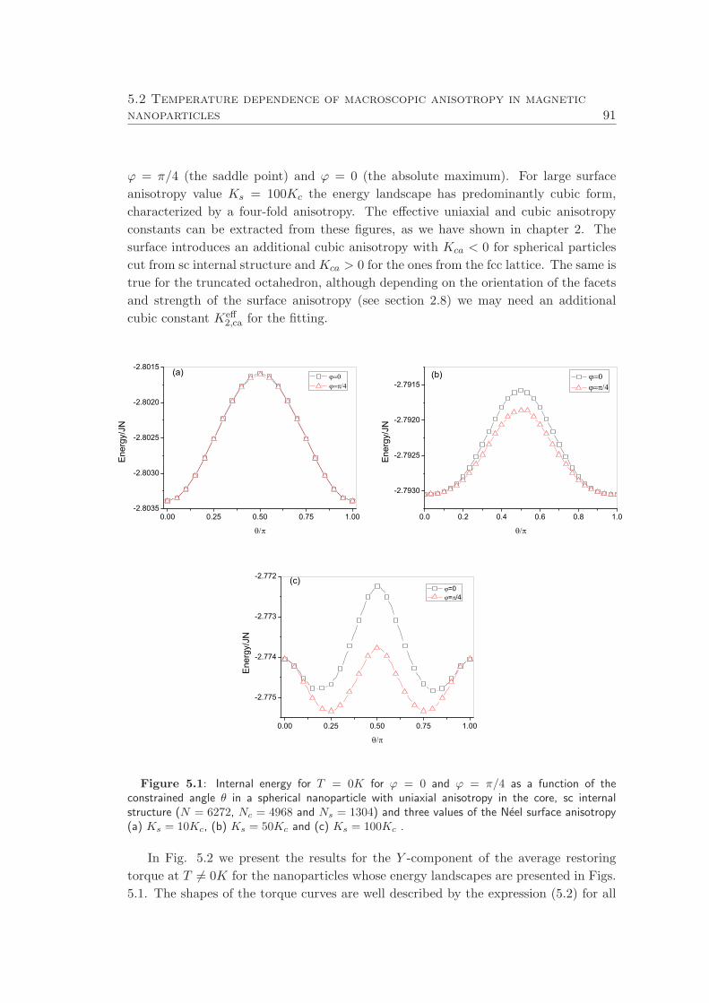
5.2 Temperature dependence of macroscopic anisotropy in magneticnanoparticles 91
ϕ = π/4 (the saddle point) and ϕ = 0 (the absolute maximum). For large surface
anisotropy value Ks = 100Kc the energy landscape has predominantly cubic form,
characterized by a four-fold anisotropy. The effective uniaxial and cubic anisotropy
constants can be extracted from these figures, as we have shown in chapter 2. The
surface introduces an additional cubic anisotropy with Kca < 0 for spherical particles
cut from sc internal structure and Kca > 0 for the ones from the fcc lattice. The same is
true for the truncated octahedron, although depending on the orientation of the facets
and strength of the surface anisotropy (see section 2.8) we may need an additional
cubic constant Keff2,ca for the fitting.
0.00 0.25 0.50 0.75 1.00-2.8035
-2.8030
-2.8025
-2.8020
-2.8015
Ene
rgy/JN
(a)
0.0 0.2 0.4 0.6 0.8 1.0
-2.7930
-2.7925
-2.7920
-2.7915Ene
rgy/JN
(b)
0.00 0.25 0.50 0.75 1.00
-2.775
-2.774
-2.773
-2.772
Ene
rgy/JN
=0 = /4
(c)
Figure 5.1: Internal energy for T = 0K for ϕ = 0 and ϕ = π/4 as a function of theconstrained angle θ in a spherical nanoparticle with uniaxial anisotropy in the core, sc internalstructure (N = 6272, Nc = 4968 and Ns = 1304) and three values of the Neel surface anisotropy(a) Ks = 10Kc, (b) Ks = 50Kc and (c) Ks = 100Kc .
In Fig. 5.2 we present the results for the Y -component of the average restoring
torque at T 6= 0K for the nanoparticles whose energy landscapes are presented in Figs.
5.1. The shapes of the torque curves are well described by the expression (5.2) for all
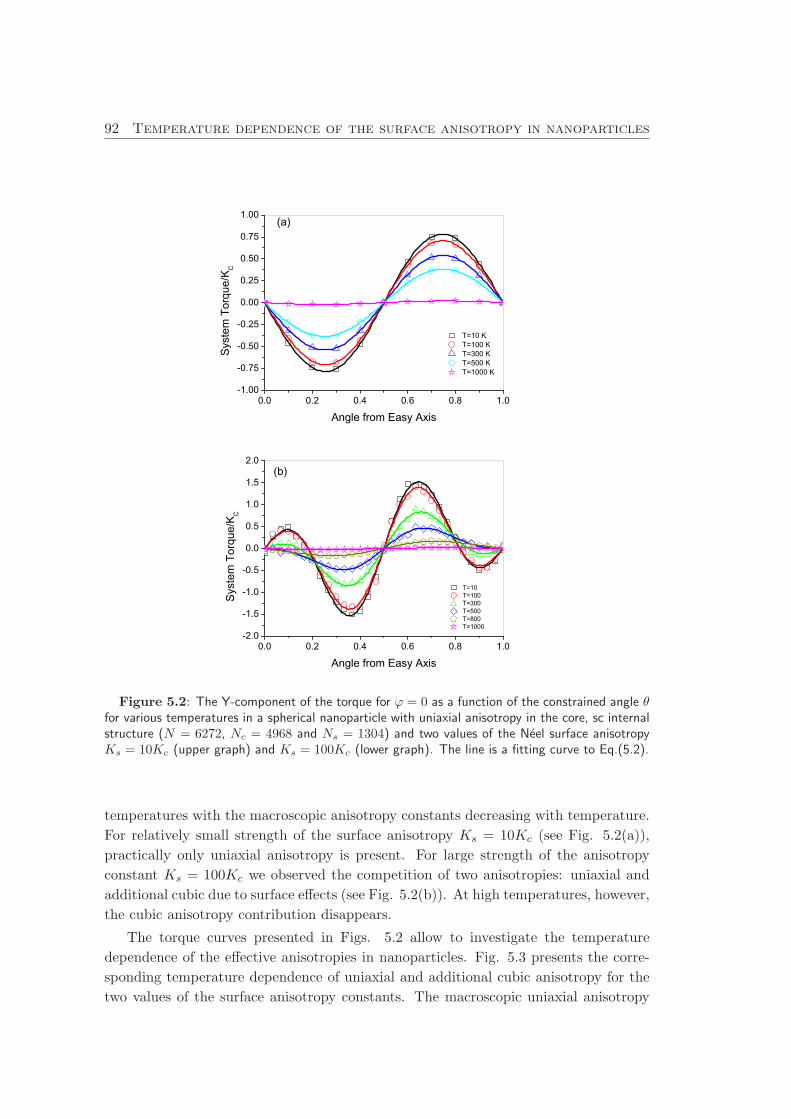
92 Temperature dependence of the surface anisotropy in nanoparticles
0.0 0.2 0.4 0.6 0.8 1.0-1.00
-0.75
-0.50
-0.25
0.00
0.25
0.50
0.75
1.00
T=10 K T=100 K T=300 K T=500 K T=1000 K
Sys
tem
Tor
que/
KC
Angle from Easy Axis
(a)
0.0 0.2 0.4 0.6 0.8 1.0-2.0
-1.5
-1.0
-0.5
0.0
0.5
1.0
1.5
2.0
T=10 T=100 T=300 T=500 T=800 T=1000
Sys
tem
Tor
que/
KC
Angle from Easy Axis
(b)
Figure 5.2: The Y-component of the torque for ϕ = 0 as a function of the constrained angle θfor various temperatures in a spherical nanoparticle with uniaxial anisotropy in the core, sc internalstructure (N = 6272, Nc = 4968 and Ns = 1304) and two values of the Neel surface anisotropyKs = 10Kc (upper graph) and Ks = 100Kc (lower graph). The line is a fitting curve to Eq.(5.2).
temperatures with the macroscopic anisotropy constants decreasing with temperature.
For relatively small strength of the surface anisotropy Ks = 10Kc (see Fig. 5.2(a)),
practically only uniaxial anisotropy is present. For large strength of the anisotropy
constant Ks = 100Kc we observed the competition of two anisotropies: uniaxial and
additional cubic due to surface effects (see Fig. 5.2(b)). At high temperatures, however,
the cubic anisotropy contribution disappears.
The torque curves presented in Figs. 5.2 allow to investigate the temperature
dependence of the effective anisotropies in nanoparticles. Fig. 5.3 presents the corre-
sponding temperature dependence of uniaxial and additional cubic anisotropy for the
two values of the surface anisotropy constants. The macroscopic uniaxial anisotropy
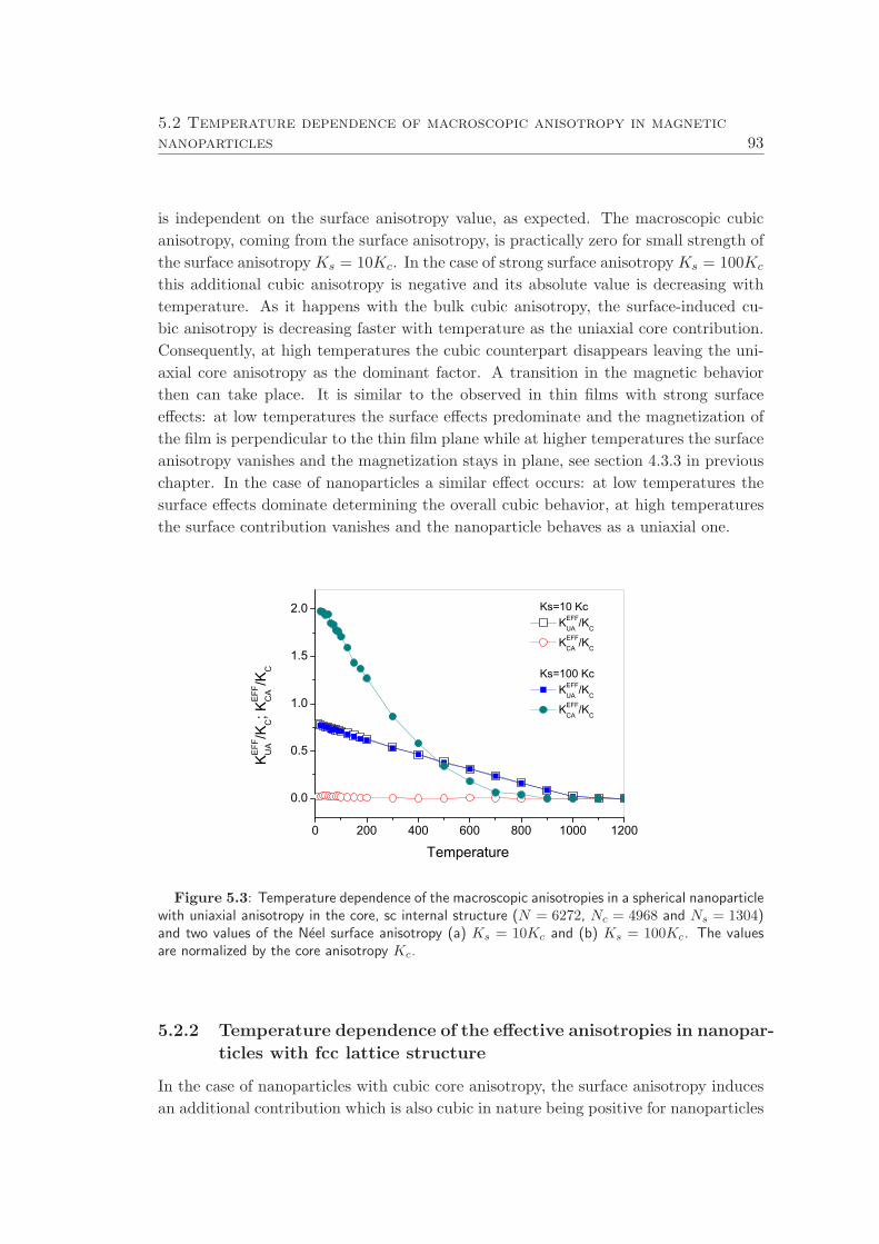
5.2 Temperature dependence of macroscopic anisotropy in magneticnanoparticles 93
is independent on the surface anisotropy value, as expected. The macroscopic cubic
anisotropy, coming from the surface anisotropy, is practically zero for small strength of
the surface anisotropy Ks = 10Kc. In the case of strong surface anisotropy Ks = 100Kc
this additional cubic anisotropy is negative and its absolute value is decreasing with
temperature. As it happens with the bulk cubic anisotropy, the surface-induced cu-
bic anisotropy is decreasing faster with temperature as the uniaxial core contribution.
Consequently, at high temperatures the cubic counterpart disappears leaving the uni-
axial core anisotropy as the dominant factor. A transition in the magnetic behavior
then can take place. It is similar to the observed in thin films with strong surface
effects: at low temperatures the surface effects predominate and the magnetization of
the film is perpendicular to the thin film plane while at higher temperatures the surface
anisotropy vanishes and the magnetization stays in plane, see section 4.3.3 in previous
chapter. In the case of nanoparticles a similar effect occurs: at low temperatures the
surface effects dominate determining the overall cubic behavior, at high temperatures
the surface contribution vanishes and the nanoparticle behaves as a uniaxial one.
0 200 400 600 800 1000 1200
0.0
0.5
1.0
1.5
2.0
KE
FFU
A/K
C; K
EFF
CA
/KC
Temperature
Ks=10 Kc KEFF
UA/K
C
KEFFCA
/KC
Ks=100 Kc KEFF
UA/K
C
KEFFCA
/KC
Figure 5.3: Temperature dependence of the macroscopic anisotropies in a spherical nanoparticlewith uniaxial anisotropy in the core, sc internal structure (N = 6272, Nc = 4968 and Ns = 1304)and two values of the Neel surface anisotropy (a) Ks = 10Kc and (b) Ks = 100Kc. The valuesare normalized by the core anisotropy Kc.
5.2.2 Temperature dependence of the effective anisotropies in nanopar-
ticles with fcc lattice structure
In the case of nanoparticles with cubic core anisotropy, the surface anisotropy induces
an additional contribution which is also cubic in nature being positive for nanoparticles
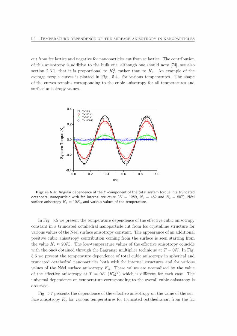
94 Temperature dependence of the surface anisotropy in nanoparticles
cut from fcc lattice and negative for nanoparticles cut from sc lattice. The contribution
of this anisotropy is additive to the bulk one, although one should note [74], see also
section 2.3.1, that it is proportional to K2s , rather than to Ks. An example of the
average torque curves is plotted in Fig. 5.4. for various temperatures. The shape
of the curves remains corresponding to the cubic anisotropy for all temperatures and
surface anisotropy values.
0.0 0.2 0.4 0.6 0.8 1.0-0.4
-0.2
0.0
0.2
0.4 T=10 K T=100 K T=500 K T=1000 K
Sys
tem
Tor
que
/KC
Figure 5.4: Angular dependence of the Y -component of the total system torque in a truncatedoctahedral nanoparticle with fcc internal structure (N = 1289, Nc = 482 and Ns = 807), Neelsurface anisotropy Ks = 10Kc and various values of the temperature.
In Fig. 5.5 we present the temperature dependence of the effective cubic anisotropy
constant in a truncated octahedral nanoparticle cut from fcc crystalline structure for
various values of the Neel surface anisotropy constant. The appearance of an additional
positive cubic anisotropy contribution coming from the surface is seen starting from
the value Ks ≈ 20Kc. The low-temperature values of the effective anisotropy coincide
with the ones obtained through the Lagrange multiplier technique at T = 0K. In Fig.
5.6 we present the temperature dependence of total cubic anisotropy in spherical and
truncated octahedral nanoparticles both with fcc internal structures and for various
values of the Neel surface anisotropy Ks. These values are normalized by the value
of the effective anisotropy at T = 0K (Keffca ) which is different for each case. The
universal dependence on temperature corresponding to the overall cubic anisotropy is
observed.
Fig. 5.7 presents the dependence of the effective anisotropy on the value of the sur-
face anisotropy Ks for various temperatures for truncated octahedra cut from the fcc
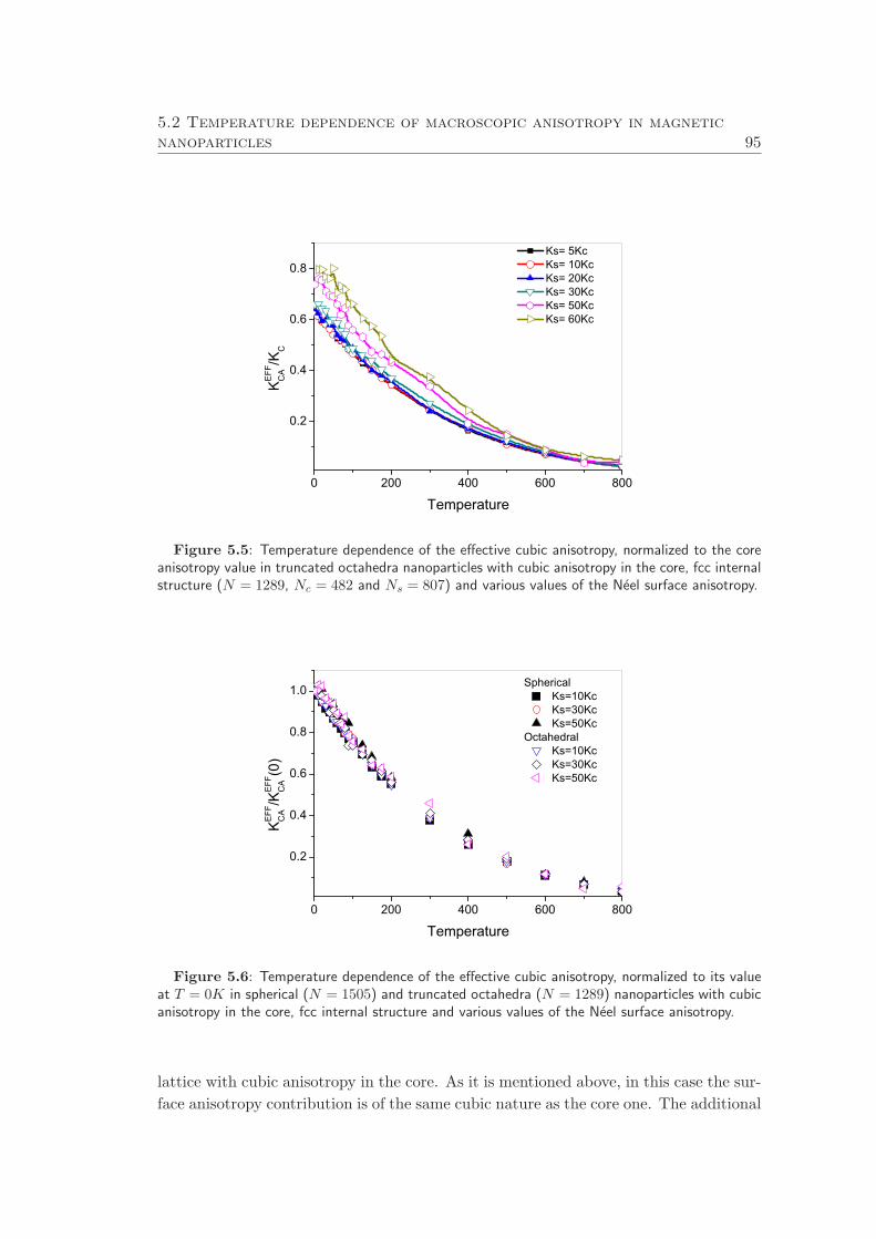
5.2 Temperature dependence of macroscopic anisotropy in magneticnanoparticles 95
0 200 400 600 800
0.2
0.4
0.6
0.8KEFF
CA/K
C
Temperature
Ks= 5Kc Ks= 10Kc Ks= 20Kc Ks= 30Kc Ks= 50Kc Ks= 60Kc
Figure 5.5: Temperature dependence of the effective cubic anisotropy, normalized to the coreanisotropy value in truncated octahedra nanoparticles with cubic anisotropy in the core, fcc internalstructure (N = 1289, Nc = 482 and Ns = 807) and various values of the Neel surface anisotropy.
0 200 400 600 800
0.2
0.4
0.6
0.8
1.0
KEFF
CA/K
EFF
CA(0)
Temperature
Spherical Ks=10Kc Ks=30Kc Ks=50Kc
Octahedral Ks=10Kc Ks=30Kc Ks=50Kc
Figure 5.6: Temperature dependence of the effective cubic anisotropy, normalized to its valueat T = 0K in spherical (N = 1505) and truncated octahedra (N = 1289) nanoparticles with cubicanisotropy in the core, fcc internal structure and various values of the Neel surface anisotropy.
lattice with cubic anisotropy in the core. As it is mentioned above, in this case the sur-
face anisotropy contribution is of the same cubic nature as the core one. The additional

96 Temperature dependence of the surface anisotropy in nanoparticles
0 10 20 30 40 50 60
0.2
0.4
0.6
0.8
KEFF
CA/K
C
Néel Surface anisotropy KS/KC
T=10 K T=100 K T=400 K
Figure 5.7: The effective cubic anisotropy as a function of the Neel surface anisotropy parameterin truncated octahedra nanoparticle with cubic anisotropy in the core, fcc internal structure (N =1289, Nc = 482 and Ns = 807) and for various temperatures.
surface contribution is expected to be proportional to K2s , see section 2.3.1 in chapter
2. Consequently, all the data were fitted to this theoretically predicted dependence.
The extracted values Keffc (T ) are consistent with the ones calculated independently.
The corresponding formula Keff (T ) = Keffc (T ) + AKSurf (T ) (KSurf (T ) ∼ K2
s ) may
be viewed as the one substituting the original formula (3.5). Unfortunately, the pa-
rameter A dependence on the system size is not trivial as is discussed in section 3.5 in
chapter 3, since it depends on the surface density of spins. The latter is not smooth
as a function of the nanoparticle diameter, due to the fact that small nanoparticles do
not have uniform spin density on their surfaces.
5.2.3 Scaling exponent
Finally, we would like to discuss the scaling behavior of the effective anisotropy on the
nanoparticle magnetisation K ∝Mγ . The Callen-Callen theory [106] states that in the
bulk γ = 3 for uniaxial anisotropy and γ = 10 for the cubic one.
Similar to what happens in magnetic thin films, in magnetic nanoparticles the
surface magnetization has a faster temperature dependence than the core one, see Fig.
5.8, sharing the same Curie temperature. This arises due to a reduction in coordination
number at the surface leading to a reduced exchange and a strong surface anisotropy
pointing perpendicularly to the surface. At the same time the fully coordinated core
effectively polarizes the surface layer, resulting in a shared value for Tc. The surface
anisotropy value has very little effect on the temperature dependence of the overall
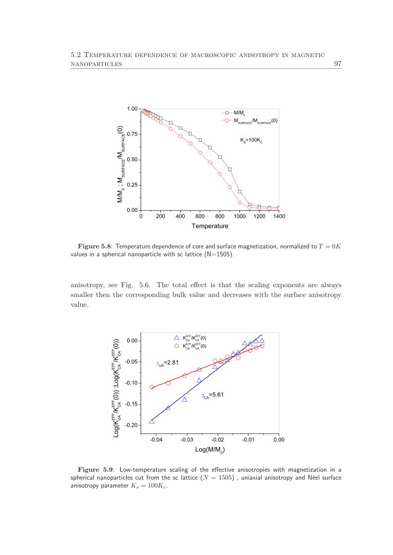
5.2 Temperature dependence of macroscopic anisotropy in magneticnanoparticles 97
0 200 400 600 800 1000 1200 14000.00
0.25
0.50
0.75
1.00
M/M
0 ; M
SU
RFA
CE/M
SU
RFA
CE(0
)
Temperature
M/M0
MSURFACE
/MSURFACE
(0)
KS=100K
C
Figure 5.8: Temperature dependence of core and surface magnetization, normalized to T = 0Kvalues in a spherical nanoparticle with sc lattice (N=1505).
anisotropy, see Fig. 5.6. The total effect is that the scaling exponents are always
smaller then the corresponding bulk value and decreases with the surface anisotropy
value.
-0.04 -0.03 -0.02 -0.01 0.00
-0.20
-0.15
-0.10
-0.05
0.00
UA=2.81
KEFFCA /KEFF
CA (0)
KEFFUA /KEFF
UA (0)
Log(
KE
FFU
A/K
EFF
UA
(0))
;Log
(KE
FFC
A/K
EFF
CA
(0))
Log(M/M0)
CA=5.61
Figure 5.9: Low-temperature scaling of the effective anisotropies with magnetization in aspherical nanoparticles cut from the sc lattice (N = 1505) , uniaxial anisotropy and Neel surfaceanisotropy parameter Ks = 100Kc.

98 Temperature dependence of the surface anisotropy in nanoparticles
For example, in Fig. 5.9 we present the scaling of the uniaxial and cubic anisotropy
constants with the magnetization at low temperatures (up to ≈ 200K) in a spherical
nanoparticle with uniaxial core anisotropy. Note that no scaling behavior is observed
in the whole temperature range. The low temperature scaling exponents are lower than
the corresponding bulk values and depend on the surface anisotropy value.
0 10 20 30 40 50 607.0
7.5
8.0
8.5
9.0
Néel Surface anisotropy KS/KC
Sca
ling
Exp
onen
et (
)
Spherical particle . Octhedral particle.
Figure 5.10: Scaling exponents as a function of Neel surface anisotropy constant in spherical(N = 1505) and truncated octahedra (N = 1289) nanoparticles with cubic anisotropy in the coreand fcc internal structure.
A similar effect is produced in spherical and truncated octahedral nanoparticles
with cubic core anisotropy. In Fig. 5.10 we present the scaling exponent as a function
of Neel surface anisotropy constant in nanoparticles with spherical and octahedral
shapes, fcc internal structure, cubic anisotropy in the core and approximately the
same nanoparticle’s diameter D ≈ 3nm. The scaling exponents are lower than the
corresponding bulk values and weakly depend on the surface anisotropy value, see Fig.
5.10. In fact, the scaling exponent decreases as a function of the surface anisotropy
value due to a faster decrease of the magnetization on the surface.
5.3 Conclusions
The main results of the study of the temperature dependence of the macroscopic
anisotropy in nanoparticles within the Neel surface anisotropy model, with different
lattices and shapes are summarized as follows:
• By means of the constrained Monte Carlo method, we have been able to evaluate
the temperature dependence of macroscopic anisotropies in nanoparticles with
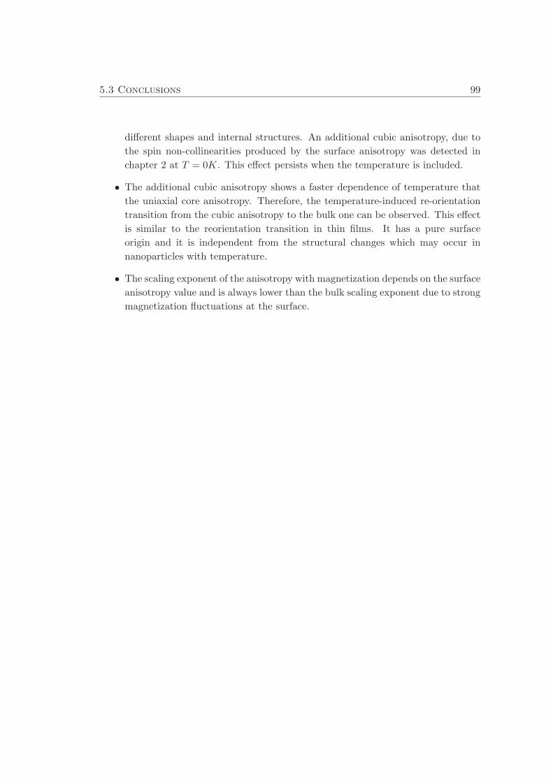
5.3 Conclusions 99
different shapes and internal structures. An additional cubic anisotropy, due to
the spin non-collinearities produced by the surface anisotropy was detected in
chapter 2 at T = 0K. This effect persists when the temperature is included.
• The additional cubic anisotropy shows a faster dependence of temperature that
the uniaxial core anisotropy. Therefore, the temperature-induced re-orientation
transition from the cubic anisotropy to the bulk one can be observed. This effect
is similar to the reorientation transition in thin films. It has a pure surface
origin and it is independent from the structural changes which may occur in
nanoparticles with temperature.
• The scaling exponent of the anisotropy with magnetization depends on the surface
anisotropy value and is always lower than the bulk scaling exponent due to strong
magnetization fluctuations at the surface.
100 Temperature dependence of the surface anisotropy in nanoparticles
Conclusiones
En esta seccion estudiamos la dependencia de la anisotropıa macroscopica con la tem-
peratura en nanopartıculas magneticas con diferentes redes cristalinas, formas y fuerza
de la anisotropıa de superficie Neel. Los principales resultamos han sido sintetizados
en los siguientes puntos:
• Por medio del algoritmo ” Monte Carlo con ligaduras” hemos sido capaces de
evaluar la dependencia termica de la anisotropıa magnetica de nanopartıculas
con diferentes formas y redes cristalinas. En nuestro estudio observamos que la
anisotropıa cubica efectiva adicional que aparecıa en el comportamiento global
de la nanopartıcula, debido a las no-colinealidades en la configuracion de espines
originadas por la anisotropıa de superficie a T = 0K (ver capıtulo 2), persiste
cuando se tienen en cuanta los efectos de temperatura.
• La anisotropıa cubica efectiva muestra una mayor dependencia con la temper-
atura que la anisotropıa uniaxial. Por tanto, los efectos de temperatura pueden
producir una transicion desde una anisotropıa efectiva cubica (originada por la su-
perficie) a la correspondiente al volumen. Este efecto es similar a la re-orientacion
observada en laminas delgadas, tratandose de un efecto puramente de superficie
e independiente de posibles cambios estructurales que puedan ocurrir en la red
por efectos de temperatura.
• El exponente del escalado de la anisotropıa con la imanacion del sistema depende
del valor de la ansiotropıa de superficie y es siempre inferior al valor del escalado
para el caso de volumen, esto es debido a las fuertes fluctuaciones de la imanacion
en la superficie.
6Multiscale modeling of magnetic properties of
Co \ Ag thin films
6.1 Introduction
Magnetism has a quantum origin and magnetization processes depend on the atomic
magnetic moments, the exchange interaction, the spin-orbit coupling, etc. For this
reason the ”ab-initio” calculations can be useful to obtain the intrinsic magnetic pa-
rameters. But from the computational point of view these calculations are very ex-
pensive, they require long time and limit the system size to several hundred atoms.
Therefore an ”ab-initio” study of a macroscopic system is intractable. Additionally,
the complete account of temperature fluctuations and dynamics on ”ab-initio” level
remains a future challenge. In this situation, multiscale modeling can provide a de-
scription on all scales using results from one scale as input parameters to the model
of the next scale. Thus the ”ab-initio” calculations (on a system with a small size)
provide the magnetic parameters which will be included in the atomistic simulations.
In these atomistic simulations we can take into account the temperature effects and
obtain the temperature dependence of the magnetic parameters. The thermodynamic
evaluation of macroscopic parameters such as temperature-dependent magnetization
Ms(T ), anisotropy K(T ) [126] and exchange stiffness A(T) [139] can be used later as
an input to large-scale micromagnetic simulations, based, for example on open source
programs such as Magpar [140] or OOMMF [141]. This ”hierarchichal” multiscale
scheme was proposed in Ref. [121]. A scheme of this model is represented in Fig. 6.1.
101
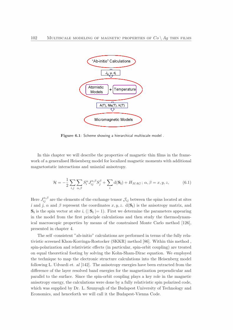
102 Multiscale modeling of magnetic properties of Co \Ag thin films
Figure 6.1: Scheme showing a hierarchical multiscale model .
In this chapter we will describe the properties of magnetic thin films in the frame-
work of a generalised Heisenberg model for localized magnetic moments with additional
magnetostatic interactions and uniaxial anisotropy.
H = −1
2
∑
i,j
∑
α,β
Sαi J
α,βij Sβ
j +∑
i
d(Si) +HMAG ; α, β = x, y, z, (6.1)
Here Jα,βij are the elements of the exchange tensor Jij between the spins located at sites
i and j, α and β represent the coordinates x, y, z. d(Si) is the anisotropy matrix, and
Si is the spin vector at site i, (| Si |= 1). First we determine the parameters appearing
in the model from the first principle calculations and then study the thermodynam-
ical macroscopic properties by means of the constrained Monte Carlo method [126],
presented in chapter 4.
The self -consistent ”ab-initio” calculations are performed in terms of the fully rela-
tivistic screened Khon-Korringa-Rostocker (SKKR) method [86]. Within this method ,
spin-polarization and relativistic effects (in particular, spin-orbit coupling) are treated
on equal theoretical footing by solving the Kohn-Sham-Dirac equation. We employed
the technique to map the electronic structure calculations into the Heisenberg model
following L. Udvardi et. al [142]. The anisotropy energies have been extracted from the
difference of the layer resolved band energies for the magnetization perpendicular and
parallel to the surface. Since the spin-orbit coupling plays a key role in the magnetic
anisotropy energy, the calculations were done by a fully relativistic spin polarized code,
which was supplied by Dr. L. Szunyogh of the Budapest University of Technology and
Economics, and henceforth we will call it the Budapest-Vienna Code.

6.2 Density functional theory 103
6.2 Density functional theory
Probably the most widely used theory for quantitative prediction in condensed matter
physics is the density functional theory (DFT), originally developed by Hohenberg and
Kohn [143]. This theory has the advantage that it does not require adjustable parame-
ters from experiments, in principle only fundamental constants as the speed of light in
vacuum, Planck’s constant, electron charge, etc. are taken from the experiment. DFT
allows to calculate the ground-state properties of materials: total energy, ground-state
lattice constants, electronic structure etc. In magnetism it appeared to be particularly
usefull for calculation of spin-dependent band structure in transition metals, such as
Co.
Density functional theory promotes the electron density n(r) instead of the many
particle wave function as the key variable, on which the calculation of all other observ-
ables can be based.
6.2.1 Hohenberg-Kohn theorems
Density functional theory relies on the theorems of Hohenberg and Kohn [144]. These
two theorems could be summarized in the following: (I) That the ground state of a
many-electron system (under the effects of an external potential) is uniquely defined
by the ground-state electron density, and (II) The existence of an energy functional of
the density E[n] that is minimal for the ground state density n0(r) giving the ground
state energy.
6.2.2 Kohn-Sham scheme
The electron density corresponding to the ground state can be calculated using a vari-
ational principle, we know that every n 6= n0 has E[n] > E0 = E[n0]. In this way
Kohn and Sham added a tremendous addendum in 1965 [144], within their variational
scheme an auxiliary system of non-interacting electrons is introduced. It is assumed
that the ground state density of this hypothetical non-interacting electrons system is
the same as that of the original interacting system.
In addition, the Kohn-Sham approach to the interacting electrons problem is to
rewrite the Hohenberg-Kohn expression for the energy functional corresponding to the
ground state as follows:
EKS = TNI [n] + Eext[n] + EH [n] + Exc[n], (6.2)
where TNI is the kinetic energy of the non-interacting electron system. Eext is the
energy due to the external potential (external potential means that it is due to the
atomic nuclei), and it has the following form:
Eext[n] =
∫
d3rVext(~r)n(~r), (6.3)
104 Multiscale modeling of magnetic properties of Co \Ag thin films
EH is the Hartree energy, which can be expressed as a functional of the electron density
of the system as follows:
EH [n] = −e2
2
∫
d3r
∫
d3(~r′)n(~r)n(~r′)
| ~r − ~r′ |, (6.4)
and finally, Exc is the so called exchange correlation energy term which includes ”all
remaining” contributions.
We have to note that in practice the correct Exc term is unknown, for this rea-
son the determination of such functional requires some approximation, and it is this
approximation which determines the accuracy of the method.
6.2.3 Approximation for the exchange-correlation energy Exc[n]
In the literature one can find several approximations of the Exc[n], for instance,the local
density approximation (LDA) [144, 145], the general gradient approximation (GGA)
[146], etc. LDA is a rather simple approximation which has yielded accurate results in
many cases, and may be expressed in the form:
Exc[n] ≈ ELDAxc [n] =
∫
n(~r)ǫLDAxc (n(~r))d3r (6.5)
where ǫLDAxc is the exchange-correlation energy per particle for a homogeneous electron
gas of density n(~r). Within this approximation it is assumed that the energy Exc of
a system with an inhomogeneous electron distribution n(~r) at each point (~r) has the
same value as in the case of homogeneous electron gas with the same density.
We are working with a magnetic system, therefore we have to use an approximation
that takes into account the spin-polarization of the system, for this reason we used a
generalization of the LDA approximation for a spin polarized system: local spin density
approximation (LSDA) [147]. In the case of spin-polarized calculations, the spin density
~m(~r) has to be included and the non-spin polarized density n is replaced by the density
matrix n(~r). The density matrix can be expressed as:
n(~r) = n(~r) · 1 + σ · ~m(~r); (6.6)
σ represents the Pauli matrices and 1 is the unit matrix.
In this context the Kohn-Sham equation (KSE) may be expressed by:
(
−~2
2m∇2 + Veff (~r) + σ · ~Beff (~r) − Ei
)
( ψi↑(~r)
ψi↓(~r)
)
= 0 (6.7)
where ψi↑;↓(~r) are the resulting eigenfunctions of the auxiliary non-interacting system.
These eigenstates are dependent on the eigenenergy Ei and on the spin up or down (↑; ↓)
configuration, with respect to the local magnetization direction µ(~r) along the effective
magnetic field ~Beff (~r). Veff (~r) is the effective potential which collects the contributions
6.2 Density functional theory 105
of the external potential, the Hartree and the exchange-correlation potentials, the last
one in practice is unknown and must be approximated.
We have to complete the set of Kohn-Sahm equations with the charge and spin
density ones:
n(~r) =∑
Ei≤EF
(
| ψi↑(~r) |2 + | ψi↓(~r) |
2)
(6.8)
~m(~r) = µ(~r)∑
Ei≤EF
(
| ψi↑(~r) |2 − | ψi↓(~r) |
2)
(6.9)
Another condition that has to be satisfied is the charge conservation. This requirement
allows us to determine the Fermi level EF , from the next relation:
N =
∫
n(~r)d3r =
∫
d3r∑
Ei≤EF
(
| ψi↑(~r) |2 + | ψi↓(~r) |
2)
(6.10)
The equations (6.7-6.10) are the set of equations that must be solved self-consistently
in the DFT calculations to obtains the ground state energy of the system.
Note that in principle the Kohn-Sham equation corresponds to a non-relativistic
formulation of the DFT. If we work within the relativistic DFT for instance, in the
case where the spin-orbit coupling (SOC) can not be treated as a perturbation term,
we have to replace the Kohn-Sham equation by the corresponding Kohn-Sham-Dirac
equation (KSDE).
6.2.4 Screened Korringa-Kohn-Rostoker Green’s function method
The Korringa-Kohn-Rostoker (KKR) method was developed initially by Korringa in
1947 [148] who used the multiple-scattering theory to solve the Schrodinger equation
and determine the band structure of a periodic solid. Seven years later Kohn and
Rostoker [149] proposed a method equivalent to the Korringa one but using Green’s
functions, called in our days the Korringa-Kohn-Rostoker (KKR) method. Perhaps the
most important characteristic of the KKR method is that its formal structure does not
change when going from non-relativistic to relativistic description.
The KKR method has undergone several improvements since the late forties. One of
these improvements is the so-called screened Korringa-Kohn-Rostoker (SKKR) method.
The SKKR method allows to calculate the electronic properties of surface, interface
and in general layered systems with periodicity only in two dimensions, within the
frame work of multiple-scattering theory without any further approximations.
In multiple scattering theory the scattering path operator (τ(E)) from which the
Green function and electronic properties are calculated, is given in terms of the struc-
ture constant G(E), and the single-site scattering matrix t(E):
τ(E) =
[
t−1(E) −G(E)
]−1
. (6.11)
106 Multiscale modeling of magnetic properties of Co \Ag thin films
2D periodicity leads in principle to infinite matrix. However, the screening method
allows to transform G(E) to the screened structure constants, which have spatial short-
range. In general the screening results in the fact that layers interact only up to a
certain number of neighboring layers. For a layered structure it is convenient to divide
the parent lattice in three regions, a left semi-infinite system (L), a right semi-infinite
(R), and an intermediate interface region, the properties of which to be calculated.
This formal partitioning of the parent infinite system implies that the inverse of the
scattering path operator M also has the form [150]:
M =
MLL MLI 0
MIL MII MIR
0 MRI MRR
. (6.12)
This shape is a direct consequence of the short-range of the structure constant.
Using the concept of principal layer [151], which is defined so that it interacts only
with nearest-neighbors principal layers, one can rewrite the structure constants, and
consequently the inverse of the scattering path operators, in tridiagonal form. From
them the Green function of the system can be calculated from a decimation technique
[152, 153].
The free energy derived in the frame work of the fully relativistic SKKR method
at zero temperature is approximated by:
F =
∫ EF
−∞dε(
ε− EF
)
n(ε) = −
∫ EF
−∞dεN(ε), (6.13)
where EF is the Fermi energy of the system, n(ε) is the density of states (DOS), and
N(ε) is the integrated density of states. Using the Lloyd’s formula [154], the free energy
can be written as follow:
F = −1
πIm
∫ EF
−∞dεTr ln τ(ε), (6.14)
where τ(ε) = {τij(ε)} is the site-angular momentum representation of the scattering
path operator, which can be expressed as a function of the site-diagonal single scattering
matrix t(ε) = {ti(ε)δij} and the structure constants G0(ε) = {G0,ij(ε)(1− δij)}, in the
following way:
τ(ε) =
(
t−1(ε) −G0(ε)
)−1
. (6.15)
6.3 ”Ab-initio” modeling of bulk Co and its interfaces
The ”ab-initio” calculations presented in this thesis are based on the fully relativistic
Screened Korringa-Kohn-Rostoker (SKKR) Green’s function method [86]. Within this
method the spin-polarization and the relativistic effects are treated on equal theoretical
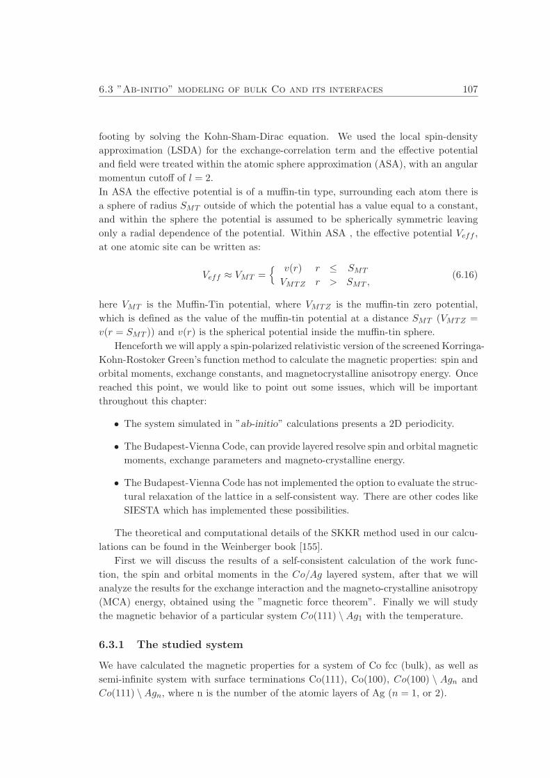
6.3 ”Ab-initio” modeling of bulk Co and its interfaces 107
footing by solving the Kohn-Sham-Dirac equation. We used the local spin-density
approximation (LSDA) for the exchange-correlation term and the effective potential
and field were treated within the atomic sphere approximation (ASA), with an angular
momentun cutoff of l = 2.
In ASA the effective potential is of a muffin-tin type, surrounding each atom there is
a sphere of radius SMT outside of which the potential has a value equal to a constant,
and within the sphere the potential is assumed to be spherically symmetric leaving
only a radial dependence of the potential. Within ASA , the effective potential Veff ,
at one atomic site can be written as:
Veff ≈ VMT ={ v(r) r ≤ SMT
VMTZ r > SMT ,(6.16)
here VMT is the Muffin-Tin potential, where VMTZ is the muffin-tin zero potential,
which is defined as the value of the muffin-tin potential at a distance SMT (VMTZ =
v(r = SMT )) and v(r) is the spherical potential inside the muffin-tin sphere.
Henceforth we will apply a spin-polarized relativistic version of the screened Korringa-
Kohn-Rostoker Green’s function method to calculate the magnetic properties: spin and
orbital moments, exchange constants, and magnetocrystalline anisotropy energy. Once
reached this point, we would like to point out some issues, which will be important
throughout this chapter:
• The system simulated in ”ab-initio” calculations presents a 2D periodicity.
• The Budapest-Vienna Code, can provide layered resolve spin and orbital magnetic
moments, exchange parameters and magneto-crystalline energy.
• The Budapest-Vienna Code has not implemented the option to evaluate the struc-
tural relaxation of the lattice in a self-consistent way. There are other codes like
SIESTA which has implemented these possibilities.
The theoretical and computational details of the SKKR method used in our calcu-
lations can be found in the Weinberger book [155].
First we will discuss the results of a self-consistent calculation of the work func-
tion, the spin and orbital moments in the Co/Ag layered system, after that we will
analyze the results for the exchange interaction and the magneto-crystalline anisotropy
(MCA) energy, obtained using the ”magnetic force theorem”. Finally we will study
the magnetic behavior of a particular system Co(111) \Ag1 with the temperature.
6.3.1 The studied system
We have calculated the magnetic properties for a system of Co fcc (bulk), as well as
semi-infinite system with surface terminations Co(111), Co(100), Co(100) \ Agn and
Co(111) \Agn, where n is the number of the atomic layers of Ag (n = 1, or 2).
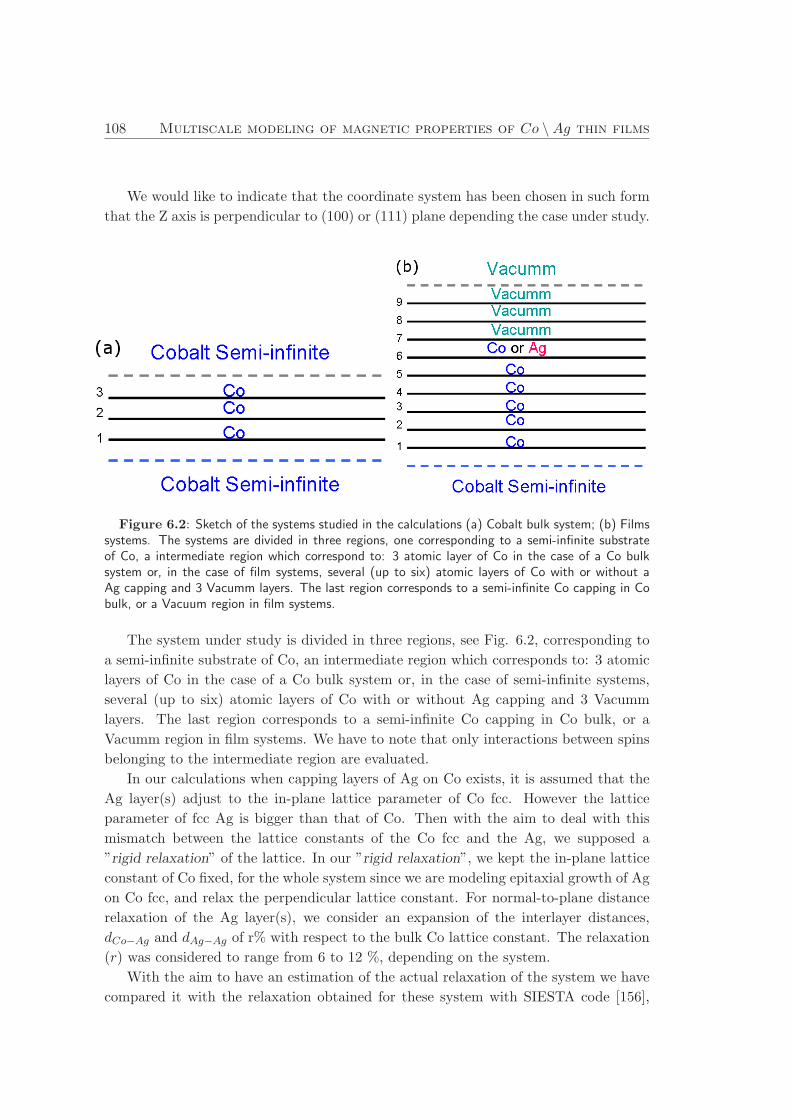
108 Multiscale modeling of magnetic properties of Co \Ag thin films
We would like to indicate that the coordinate system has been chosen in such form
that the Z axis is perpendicular to (100) or (111) plane depending the case under study.
Figure 6.2: Sketch of the systems studied in the calculations (a) Cobalt bulk system; (b) Filmssystems. The systems are divided in three regions, one corresponding to a semi-infinite substrateof Co, a intermediate region which correspond to: 3 atomic layer of Co in the case of a Co bulksystem or, in the case of film systems, several (up to six) atomic layers of Co with or without aAg capping and 3 Vacumm layers. The last region corresponds to a semi-infinite Co capping in Cobulk, or a Vacuum region in film systems.
The system under study is divided in three regions, see Fig. 6.2, corresponding to
a semi-infinite substrate of Co, an intermediate region which corresponds to: 3 atomic
layers of Co in the case of a Co bulk system or, in the case of semi-infinite systems,
several (up to six) atomic layers of Co with or without Ag capping and 3 Vacumm
layers. The last region corresponds to a semi-infinite Co capping in Co bulk, or a
Vacumm region in film systems. We have to note that only interactions between spins
belonging to the intermediate region are evaluated.
In our calculations when capping layers of Ag on Co exists, it is assumed that the
Ag layer(s) adjust to the in-plane lattice parameter of Co fcc. However the lattice
parameter of fcc Ag is bigger than that of Co. Then with the aim to deal with this
mismatch between the lattice constants of the Co fcc and the Ag, we supposed a
”rigid relaxation” of the lattice. In our ”rigid relaxation”, we kept the in-plane lattice
constant of Co fixed, for the whole system since we are modeling epitaxial growth of Ag
on Co fcc, and relax the perpendicular lattice constant. For normal-to-plane distance
relaxation of the Ag layer(s), we consider an expansion of the interlayer distances,
dCo−Ag and dAg−Ag of r% with respect to the bulk Co lattice constant. The relaxation
(r) was considered to range from 6 to 12 %, depending on the system.
With the aim to have an estimation of the actual relaxation of the system we have
compared it with the relaxation obtained for these system with SIESTA code [156],
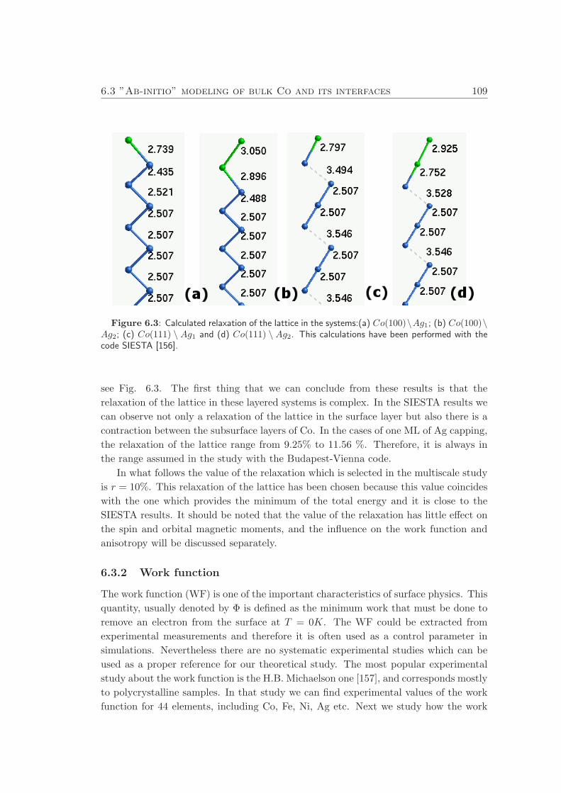
6.3 ”Ab-initio” modeling of bulk Co and its interfaces 109
Figure 6.3: Calculated relaxation of the lattice in the systems:(a) Co(100)\Ag1; (b) Co(100)\Ag2; (c) Co(111) \ Ag1 and (d) Co(111) \ Ag2. This calculations have been performed with thecode SIESTA [156].
see Fig. 6.3. The first thing that we can conclude from these results is that the
relaxation of the lattice in these layered systems is complex. In the SIESTA results we
can observe not only a relaxation of the lattice in the surface layer but also there is a
contraction between the subsurface layers of Co. In the cases of one ML of Ag capping,
the relaxation of the lattice range from 9.25% to 11.56 %. Therefore, it is always in
the range assumed in the study with the Budapest-Vienna code.
In what follows the value of the relaxation which is selected in the multiscale study
is r = 10%. This relaxation of the lattice has been chosen because this value coincides
with the one which provides the minimum of the total energy and it is close to the
SIESTA results. It should be noted that the value of the relaxation has little effect on
the spin and orbital magnetic moments, and the influence on the work function and
anisotropy will be discussed separately.
6.3.2 Work function
The work function (WF) is one of the important characteristics of surface physics. This
quantity, usually denoted by Φ is defined as the minimum work that must be done to
remove an electron from the surface at T = 0K. The WF could be extracted from
experimental measurements and therefore it is often used as a control parameter in
simulations. Nevertheless there are no systematic experimental studies which can be
used as a proper reference for our theoretical study. The most popular experimental
study about the work function is the H.B. Michaelson one [157], and corresponds mostly
to polycrystalline samples. In that study we can find experimental values of the work
function for 44 elements, including Co, Fe, Ni, Ag etc. Next we study how the work
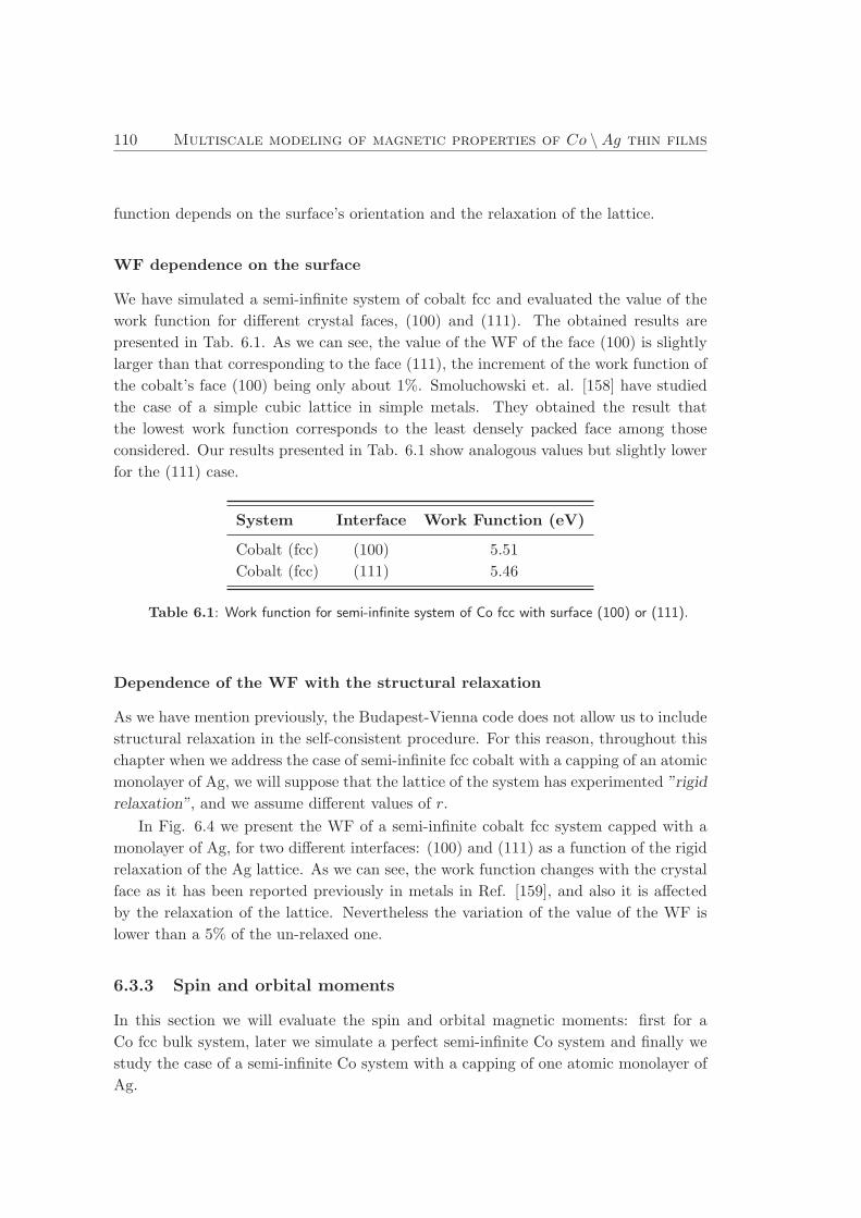
110 Multiscale modeling of magnetic properties of Co \Ag thin films
function depends on the surface’s orientation and the relaxation of the lattice.
WF dependence on the surface
We have simulated a semi-infinite system of cobalt fcc and evaluated the value of the
work function for different crystal faces, (100) and (111). The obtained results are
presented in Tab. 6.1. As we can see, the value of the WF of the face (100) is slightly
larger than that corresponding to the face (111), the increment of the work function of
the cobalt’s face (100) being only about 1%. Smoluchowski et. al. [158] have studied
the case of a simple cubic lattice in simple metals. They obtained the result that
the lowest work function corresponds to the least densely packed face among those
considered. Our results presented in Tab. 6.1 show analogous values but slightly lower
for the (111) case.
System Interface Work Function (eV)
Cobalt (fcc) (100) 5.51
Cobalt (fcc) (111) 5.46
Table 6.1: Work function for semi-infinite system of Co fcc with surface (100) or (111).
Dependence of the WF with the structural relaxation
As we have mention previously, the Budapest-Vienna code does not allow us to include
structural relaxation in the self-consistent procedure. For this reason, throughout this
chapter when we address the case of semi-infinite fcc cobalt with a capping of an atomic
monolayer of Ag, we will suppose that the lattice of the system has experimented ”rigid
relaxation”, and we assume different values of r.
In Fig. 6.4 we present the WF of a semi-infinite cobalt fcc system capped with a
monolayer of Ag, for two different interfaces: (100) and (111) as a function of the rigid
relaxation of the Ag lattice. As we can see, the work function changes with the crystal
face as it has been reported previously in metals in Ref. [159], and also it is affected
by the relaxation of the lattice. Nevertheless the variation of the value of the WF is
lower than a 5% of the un-relaxed one.
6.3.3 Spin and orbital moments
In this section we will evaluate the spin and orbital magnetic moments: first for a
Co fcc bulk system, later we simulate a perfect semi-infinite Co system and finally we
study the case of a semi-infinite Co system with a capping of one atomic monolayer of
Ag.
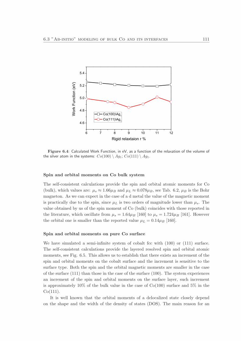
6.3 ”Ab-initio” modeling of bulk Co and its interfaces 111
6 7 8 9 10 11 12
4.6
4.8
5.0
5.2
5.4
Wor
k Fu
nctio
n (e
V)
Rigid relaxtaion r %
Co(100)\Ag1
Co(111)\Ag1
Figure 6.4: Calculated Work Function, in eV, as a function of the relaxation of the volume ofthe silver atom in the systems: Co(100) \Ag1; Co(111) \Ag1.
Spin and orbital moments on Co bulk system
The self-consistent calculations provide the spin and orbital atomic moments for Co
(bulk), which values are: µs ≈ 1.66µB and µL ≈ 0.078µB, see Tab. 6.2, µB is the Bohr
magneton. As we can expect in the case of a d metal the value of the magnetic moment
is practically due to the spin, since µL is two orders of magnitude lower than µs. The
value obtained by us of the spin moment of Co (bulk) coincides with those reported in
the literature, which oscillate from µs = 1.64µB [160] to µs = 1.724µB [161]. However
the orbital one is smaller than the reported value µL = 0.14µB [160].
Spin and orbital moments on pure Co surface
We have simulated a semi-infinite system of cobalt fcc with (100) or (111) surface.
The self-consistent calculations provide the layered resolved spin and orbital atomic
moments, see Fig. 6.5. This allows us to establish that there exists an increment of the
spin and orbital moments on the cobalt surface and the increment is sensitive to the
surface type. Both the spin and the orbital magnetic moments are smaller in the case
of the surface (111) than those in the case of the surface (100). The system experiences
an increment of the spin and orbital moments on the surface layer, such increment
is approximately 10% of the bulk value in the case of Co(100) surface and 5% in the
Co(111).
It is well known that the orbital moments of a delocalized state closely depend
on the shape and the width of the density of states (DOS). The main reason for an

112 Multiscale modeling of magnetic properties of Co \Ag thin films
1 2 3 4 5 61.25
1.50
1.75
2.00
Co(100) Co(111)
Atomic Layer
Spi
n at
omic
mom
ent (
S/
B)
Sur
face
1 2 3 4 5 60.04
0.06
0.08
0.10
0.12
Co (100) Co (111)
Orb
ital m
agne
tic m
omen
t (
L/B)
Atomic Layer
Sur
face
Figure 6.5: The layered resolved spin (left) and orbital (right) moments for a semi-infinite fccCo(100) and Co(111) system, where the surface is at the atomic layer number 6.
increment of the orbital and spin moments at the surface is the modification of DOS
[161]. This can have different origins as for example:
(i) The reduction of the crystal field at the surface leads to an enhancement of the
orbital moment.
(ii) The d band becomes narrower at the surface due to the reduce number of nearest-
neighbors.
Spin and orbital moments on Co \Ag1 interface
Unfortunately, a perfect free layer of a Co is difficult to obtain at ambient condition due
to oxidation, lattice imperfection, etc. With the purpose of exploring its experimental
properties it is often covered by another protective layer. ”A-priori” the orbital and
spin moments could be affected by this protective capping. We have analyzed how the
Ag capping over the Co semi-infinite system can affect the orbital and spin moment.
In Fig. 6.6 we show the layered resolved values of the spin and orbital moments for
a semi-infinite Co capped by a monolayer of Ag: Co(100) \Ag1 and Co(111) \Ag1. It
is seen that both the spin and orbital moments are affected by the existence of the Ag
capping. The orbital and spin moments of Co experience a variation with respect to the
volume one, such modification depends on the orientation of the interface of Co \ Ag.
We can observe that the spin magnetic moment in the case of Co with a monolayer
capping of silver presents a reduction of its value with respect to the Co bulk one, on
both (100) and (111) interfaces. In contrast to the spin moment, the orbital magnetic
moment is increased in the same systems.
With the aim to summarize our results, we present in Tab. 6.2 the spin and orbital
atomic moments of Co in several systems. We can observe that Co presents different
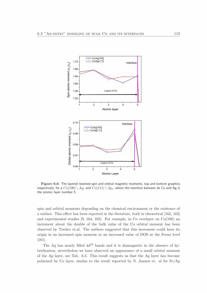
6.3 ”Ab-initio” modeling of bulk Co and its interfaces 113
1 2 3 4 5
1.52
1.56
1.60
1.64
1.68
1.72
Spi
n at
omic
mom
ent (
S/
)
Atomic layer
Co\Ag[100] Co\Ag[111]
Interface
Layers of Co
1 2 3 4 50.06
0.07
0.08
0.09
0.10
Interface
Layers of CoOrb
ital a
tom
ic m
omen
t (L
)
Atomic Layer
Co/Ag[100] Co/Ag[111]
Figure 6.6: The layered resolved spin and orbital magnetic moments, top and bottom graphicsrespectively, for a Co(100) \Ag1 and Co(111) \Ag1, where the interface between de Co and Ag isthe atomic layer number 5.
spin and orbital moments depending on the chemical environment or the existence of
a surface. This effect has been reported in the literature, both in theoretical [162, 163]
and experimental studies [9, 164, 165]. For example, in Co overlayer on Cu(100) an
increment about the double of the bulk value of the Co orbital moment has been
observed by Tischer et.al. The authors suggested that this increment could have its
origin in an increased spin moment or an increased value of DOS at the Fermi level
[161].
The Ag has nearly filled 4d10 bands and it is diamagnetic in the absence of hy-
bridization, nevertheless we have observed an appearance of a small orbital moment
of the Ag layer, see Tab. 6.3. This result suggests us that the Ag layer has become
polarized by Co layer, similar to the result reported by N. Joauen et. al for Fe/Ag
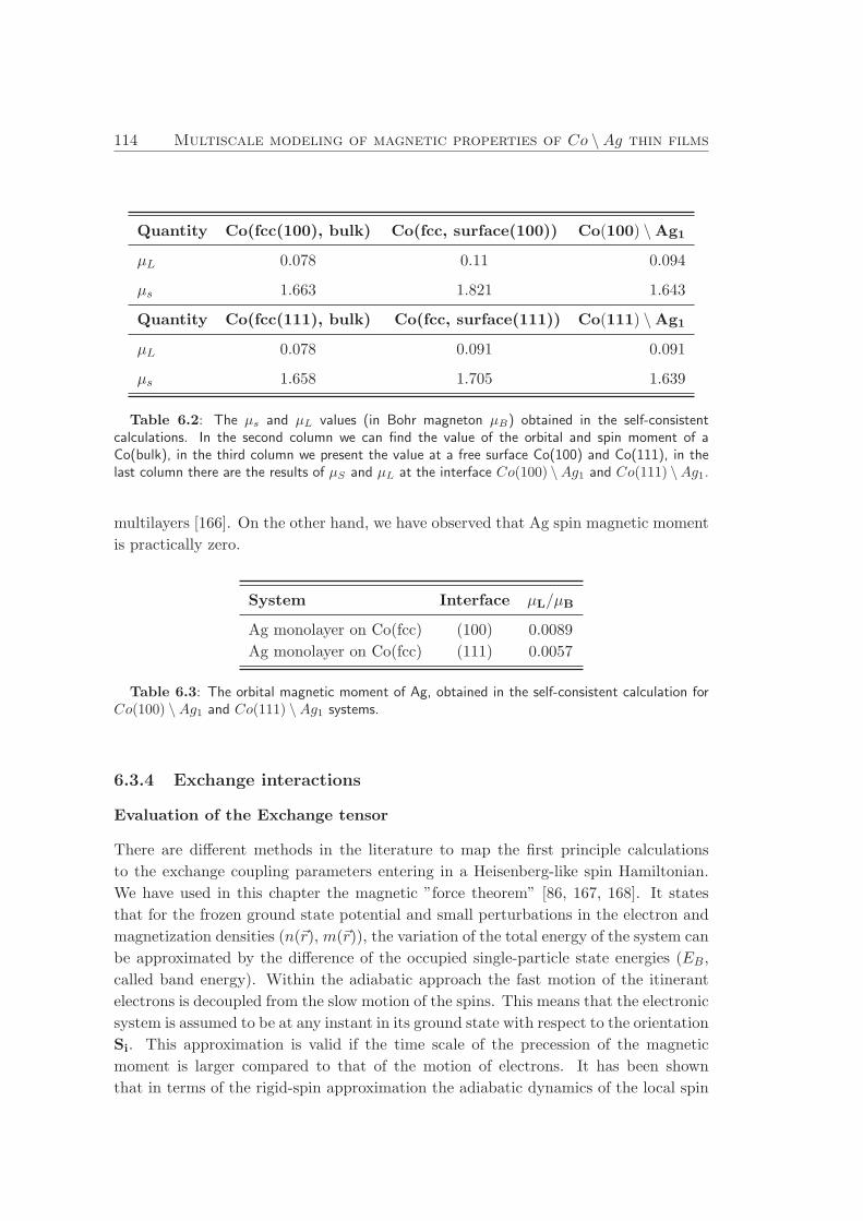
114 Multiscale modeling of magnetic properties of Co \Ag thin films
Quantity Co(fcc(100), bulk) Co(fcc, surface(100)) Co(100) \Ag1
µL 0.078 0.11 0.094
µs 1.663 1.821 1.643
Quantity Co(fcc(111), bulk) Co(fcc, surface(111)) Co(111) \Ag1
µL 0.078 0.091 0.091
µs 1.658 1.705 1.639
Table 6.2: The µs and µL values (in Bohr magneton µB) obtained in the self-consistentcalculations. In the second column we can find the value of the orbital and spin moment of aCo(bulk), in the third column we present the value at a free surface Co(100) and Co(111), in thelast column there are the results of µS and µL at the interface Co(100) \Ag1 and Co(111) \Ag1.
multilayers [166]. On the other hand, we have observed that Ag spin magnetic moment
is practically zero.
System Interface µL/µB
Ag monolayer on Co(fcc) (100) 0.0089
Ag monolayer on Co(fcc) (111) 0.0057
Table 6.3: The orbital magnetic moment of Ag, obtained in the self-consistent calculation forCo(100) \Ag1 and Co(111) \Ag1 systems.
6.3.4 Exchange interactions
Evaluation of the Exchange tensor
There are different methods in the literature to map the first principle calculations
to the exchange coupling parameters entering in a Heisenberg-like spin Hamiltonian.
We have used in this chapter the magnetic ”force theorem” [86, 167, 168]. It states
that for the frozen ground state potential and small perturbations in the electron and
magnetization densities (n(~r), m(~r)), the variation of the total energy of the system can
be approximated by the difference of the occupied single-particle state energies (EB,
called band energy). Within the adiabatic approach the fast motion of the itinerant
electrons is decoupled from the slow motion of the spins. This means that the electronic
system is assumed to be at any instant in its ground state with respect to the orientation
Si. This approximation is valid if the time scale of the precession of the magnetic
moment is larger compared to that of the motion of electrons. It has been shown
that in terms of the rigid-spin approximation the adiabatic dynamics of the local spin

6.3 ”Ab-initio” modeling of bulk Co and its interfaces 115
moments is described by the Landau-Lifshitz equation [169].
MriSri = −2µB~
δF
δSri× Sri (6.17)
where Mri is the magnitude of the spin-moment of the spin i of the atomic layer r, Sri
is a unit vector pointing along the spin-quantization axis in the cell at site i of layer r,
F is the free-energy of the system and ~ is the reduced Planck constant.
We will rewrite Eq. (6.17) into spherical coordinates (θri;ϕri), with polar and az-
imuthal angles, respectively, measured from the spin-quantization axis. Selecting the
corresponding reference system and adopting the harmonic approximation, we can ex-
pand the Hamiltonian up to the second order of the free-energy F in angular variables1.
After that we can relate such Hamiltonian with a generalized Heisenberg Hamiltonian
and determine the exchange matrix.
The exchange matrix can be determined in ferromagnetic states by calculating
the derivatives of the free energy, with respect to three orthogonal directions of the
magnetization: X, Y and Z, see Ref. [142]. Then we get the following results for the
magnetization parallel to the X direction:
δ2F
δϕiδϕj= Jyyij ;
δ2F
δθiδθj= Jzzij ;
δ2F
δϕiδθj= −Jyzij ;
δ2F
δθiδϕj= −Jzyij .
For the magnetization parallel to the Y direction:
δ2F
δϕiδϕj= Jxxij ;
δ2F
δθiδθj= Jzzij ;
δ2F
δϕiδθj= −Jxzij ;
δ2F
δθiδϕj= −Jzxij .
For the magnetization parallel to the Z direction:
δ2F
δϕiδϕj= Jyyij ;
δ2F
δθiδθj= Jxxij ;
δ2F
δϕiδθj= −Jyxij ;
δ2F
δθiδϕj= −Jxyij .
Here i and j are different spin sites. In the way described above we have calculated the
exchange tensor Jij within the SKKR method using a full-relativistic description.
The exchange tensor Jij is a matrix 3 × 3, its elements can be noted by Jαβij where
α, β = x, y, z. It Jij can be decomposed into three terms as in Ref. [142]:
Jij = JijI + J Sij + J A
ij , (6.18)
where I is the unit matrix and Jij is the isotropic part of the exchange tensor:
Jij =1
3
∑
α
Jααij ; α = x, y, z . (6.19)
This term is the parameter normally used as a classical exchange constant.
1See Refs. [142, 155] or appendix A.1 for more details
116 Multiscale modeling of magnetic properties of Co \Ag thin films
The second term J Sij is the traceless symmetric anisotropic exchange tensor and it
is defined by
J Sij =
1
2
(
Jij + J Tij
)
− JijI, (6.20)
where J Tij is the transpose of the exchange tensor.
The third term J Aij is the antisymmetric exchange matrix and it is given by
J Aij =
1
2
(
Jij − J Tij
)
. (6.21)
Then we can rewrite the exchange part of the Hamiltonian (6.1) as a function of the
isotropic, symmetric anisotropic and antisymmetric exchange as follows:
Hex = −1
2
∑
i,j
Si
(
JijI + J Sij + J A
ij
)
Sj (6.22)
This equation could be simplified in the following form:
Hex = −1
2
∑
i,j
JijSiSj −1
2
∑
i,j
SiJSijSj −
1
2
∑
i,j
SiJAij Sj . (6.23)
The corresponding inter-site antisymmetric exchange interaction can be cast in the
form, known as the Dzyaloshinsky-Moriya interaction.
SiJAij Sj = Dij
(
Si × Sj
)
, (6.24)
where Dij is the Dzyaloshinsky-Moriya vector.
Finally,
Hex = −1
2
∑
i,j
JijSiSj −1
2
∑
i,j
SiJSijSj −
1
2
∑
i,j
Dij
(
Si × Sj
)
. (6.25)
Isotropic exchange interactions
The first term in equation (6.25) represents the isotropic exchange contribution. Usu-
ally the exchange interaction is a short-range interaction, and practically vanishes be-
yond the fifth nearest neighbors as we can see in Fig. 6.7.
The calculated values of the isotropic exchange interactions are shown as a function
of the distance between Co atoms in a bulk Co fcc system and a semi-infinite Co fcc with
(100) surface . In both cases we observe that the first nearest-neighbor exchange pair
interactions have a ferromagnetic character, also we can see the oscillating behavior of
the parameter Jij with the distance. The order of magnitude of the isotropic exchange
interaction is in agreement with those presented in Refs. [170, 171] for the cases of thin
films of Co on Cu(001) and for Co bulk [40, 172].
We have to note the increment of the exchange pair interaction when the spins are
close to the surface. This effects is clearly observed in the right pannel of Fig. 6.7.
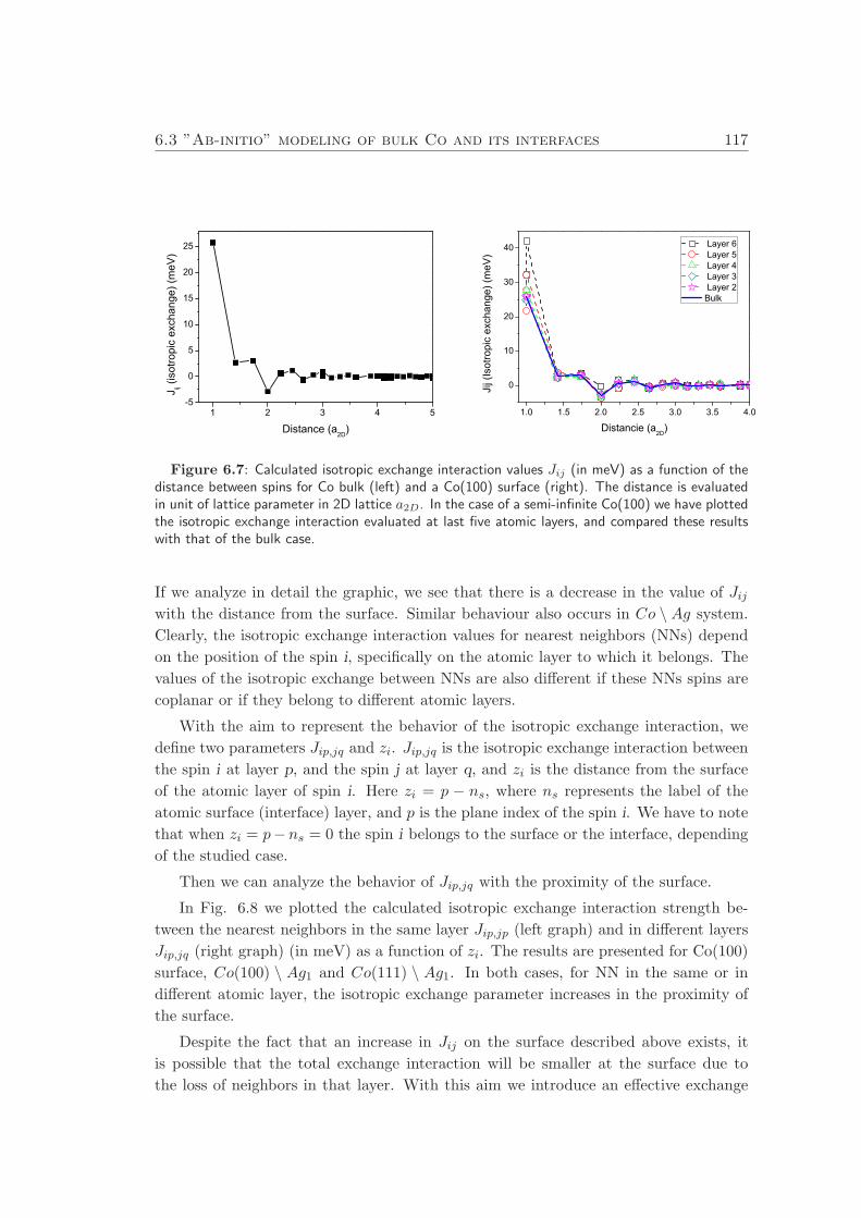
6.3 ”Ab-initio” modeling of bulk Co and its interfaces 117
1 2 3 4 5-5
0
5
10
15
20
25
J ij (iso
tropi
c ex
chan
ge) (
meV
)
Distance (a2D)1.0 1.5 2.0 2.5 3.0 3.5 4.0
0
10
20
30
40
Jij (
Isot
ropi
c ex
chan
ge) (
meV
)
Distancie (a2D)
Layer 6 Layer 5 Layer 4 Layer 3 Layer 2 Bulk
Figure 6.7: Calculated isotropic exchange interaction values Jij (in meV) as a function of thedistance between spins for Co bulk (left) and a Co(100) surface (right). The distance is evaluatedin unit of lattice parameter in 2D lattice a2D. In the case of a semi-infinite Co(100) we have plottedthe isotropic exchange interaction evaluated at last five atomic layers, and compared these resultswith that of the bulk case.
If we analyze in detail the graphic, we see that there is a decrease in the value of Jijwith the distance from the surface. Similar behaviour also occurs in Co \ Ag system.
Clearly, the isotropic exchange interaction values for nearest neighbors (NNs) depend
on the position of the spin i, specifically on the atomic layer to which it belongs. The
values of the isotropic exchange between NNs are also different if these NNs spins are
coplanar or if they belong to different atomic layers.
With the aim to represent the behavior of the isotropic exchange interaction, we
define two parameters Jip,jq and zi. Jip,jq is the isotropic exchange interaction between
the spin i at layer p, and the spin j at layer q, and zi is the distance from the surface
of the atomic layer of spin i. Here zi = p − ns, where ns represents the label of the
atomic surface (interface) layer, and p is the plane index of the spin i. We have to note
that when zi = p−ns = 0 the spin i belongs to the surface or the interface, depending
of the studied case.
Then we can analyze the behavior of Jip,jq with the proximity of the surface.
In Fig. 6.8 we plotted the calculated isotropic exchange interaction strength be-
tween the nearest neighbors in the same layer Jip,jp (left graph) and in different layers
Jip,jq (right graph) (in meV) as a function of zi. The results are presented for Co(100)
surface, Co(100) \ Ag1 and Co(111) \ Ag1. In both cases, for NN in the same or in
different atomic layer, the isotropic exchange parameter increases in the proximity of
the surface.
Despite the fact that an increase in Jij on the surface described above exists, it
is possible that the total exchange interaction will be smaller at the surface due to
the loss of neighbors in that layer. With this aim we introduce an effective exchange
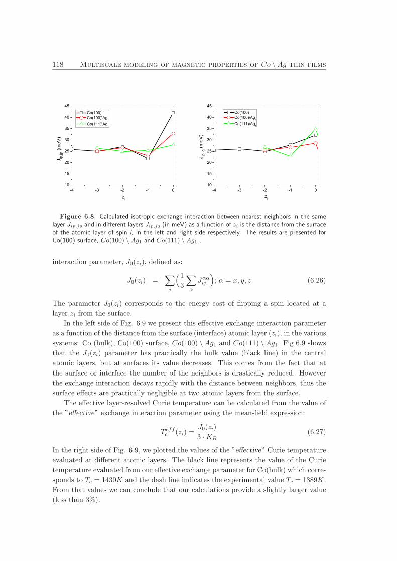
118 Multiscale modeling of magnetic properties of Co \Ag thin films
-4 -3 -2 -1 010
15
20
25
30
35
40
45
J ip,jp
(meV
)
zi
Co(100) Co(100)\Ag
1
Co(111)\Ag1
-4 -3 -2 -1 010
15
20
25
30
35
40
45 Co(100) Co(100)\Ag
1
Co(111)\Ag1
J ip,jq
(meV
)zi
Figure 6.8: Calculated isotropic exchange interaction between nearest neighbors in the samelayer Jip,jp and in different layers Jip,jq (in meV) as a function of zi is the distance from the surfaceof the atomic layer of spin i, in the left and right side respectively. The results are presented forCo(100) surface, Co(100) \Ag1 and Co(111) \Ag1 .
interaction parameter, J0(zi), defined as:
J0(zi) =∑
j
(1
3
∑
α
Jααij
)
; α = x, y, z (6.26)
The parameter J0(zi) corresponds to the energy cost of flipping a spin located at a
layer zi from the surface.
In the left side of Fig. 6.9 we present this effective exchange interaction parameter
as a function of the distance from the surface (interface) atomic layer (zi), in the various
systems: Co (bulk), Co(100) surface, Co(100) \Ag1 and Co(111) \Ag1. Fig 6.9 shows
that the J0(zi) parameter has practically the bulk value (black line) in the central
atomic layers, but at surfaces its value decreases. This comes from the fact that at
the surface or interface the number of the neighbors is drastically reduced. However
the exchange interaction decays rapidly with the distance between neighbors, thus the
surface effects are practically negligible at two atomic layers from the surface.
The effective layer-resolved Curie temperature can be calculated from the value of
the ”effective” exchange interaction parameter using the mean-field expression:
T effc (zi) =
J0(zi)
3 ·KB(6.27)
In the right side of Fig. 6.9, we plotted the values of the ”effective” Curie temperature
evaluated at different atomic layers. The black line represents the value of the Curie
temperature evaluated from our effective exchange parameter for Co(bulk) which corre-
sponds to Tc = 1430K and the dash line indicates the experimental value Tc = 1389K.
From that values we can conclude that our calculations provide a slightly larger value
(less than 3%).

6.3 ”Ab-initio” modeling of bulk Co and its interfaces 119
-4 -3 -2 -1 0250
300
350
400
J 0(zi) (
meV
)
zi
Co(100) Surface Co(100)\Ag
1
Co(111)\Ag1
Co (Bulk)
-5 -4 -3 -2 -1 01000
1100
1200
1300
1400
1500
Tc (Bulk) Calculated Tc (Bulk) Experiment Tc (Co(100) Surface) Tc (Co(100)\Ag1) Tc (Co(111)\Ag1)
T CU
RIE
(K)
zi
Figure 6.9: Calculated effective exchange interaction parameter J0(zi) (in meV) and effectiveCurie temperature T eff
c (left and right side respectively) layered resolved for Co(bulk), Co(100),Co(100) \ Ag1 and Co(111) \ Ag1 systems. Here zi represents the distance from the surface orinterface of the system.
Symmetric anisotropic exchange tensor
The second term in equation (6.25) represents the symmetric anisotropic exchange cou-
pling (similar to that described in Refs. [107, 173]) and it is known as an ”anisotropic
exchange” or a ”two-site anisotropy”. We defined it previously as:
J Sij =
1
2
(
Jij + J Tij
)
− JijI.
As it will be seen later, J Sij is one of the important contributions to the macroscopic
anisotropy. For example, in the case of FePt, J Sij term is the key for the understanding
of the deviation in the exponent of the power-law dependence of the anisotropy with
the magnetization K ∝ M2.09 [107, 174], from the theoretical K ∝ M3 law given by
the Callen-Callen theory [106, 129].
The contribution of the symmetric part of the exchange matrix interaction to the
Hamiltonian (HSExc) can be written as follows:
HSExc = −1
2
∑
i,j
SiJSijSj .
The double sum is over all i 6= j. Now we try to analyze the effective symmetric
exchange contribution of the exchange matrix interaction at a layer zi. For this purpose
we define J Szi as:
J Szi =
∑
j
J Sij , (6.28)
We have evaluated the effective symmetric exchange contributions for Co(100),
Co(100) \Ag1 and Co(111) \Ag1 systems 2.
2In the systems under study the Z axis is perpendicular to the surface

120 Multiscale modeling of magnetic properties of Co \Ag thin films
In the first place, we would like to comment the characteristic features of these
contributions: In the case of Co(100) and Co(100)\Ag1, we observe that the symmetric
anisotropic exchange matrix has the form:
J Szi = Azi
−12 0 0
0 −12 0
0 0 1
(6.29)
and could lead to an effective uniaxial anisotropy in the direction perpendicular to the
plane of the surface, which could be one of the principal contributions to the effective
anisotropy 3.
In the Co(111)\Ag1 system, we observe a little different behavior. In this system the
effective symmetric exchange contribution J SZi is a matrix whose non-diagonal elements
are in practice negligible, and it has the following form:
J Szi =
Azi11 0 0
0 Azi22 0
0 0 Azi33
(6.30)
Here unlike what happens in the cases of a semi-infinite Co(100) and a Co(100) \Ag1systems, the diagonal elements have the property Azi
11 6= Azi22 6= Azi
33. Also we have
observed that | Azi33 |>| A
zi11 | and | Azi
33 |>| Azi22 | and Azi
33 has an opposite sign than the
other two elements.
Antisymmetric anisotropic exchange tensor
The third term in equation (6.25) represents the Dzyaloshinsky-Moriya (DM) inter-
action [175, 176]. The DM contribution to the Hamiltonian of the system has the
following form:
HexDM = −
1
2
∑
i,j
Dij
(
Si × Sj
)
, (6.31)
where the Dij is Dzyaloshinsky-Moriya vector and is defined as:
Dxij =
1
2(Jyz
ij − Jzyij )
Dyij =
1
2(Jxz
ij − Jzxij )
Dzij =
1
2(Jxy
ij − Jyxij )
Dij is zero if sites i and j experience an inversion symmetry. Therefore, this contribution
is practically zero in bulk system. Nevertheless the DM term can be enhanced near
the magnetic surface due to the reduction of the symmetry. It also tends to lower
3See appendix A.2 for a detailed description of the derivation of the effective uniaxial anisotropy
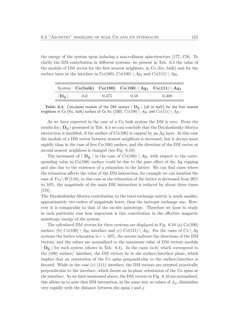
6.3 ”Ab-initio” modeling of bulk Co and its interfaces 121
the energy of the system upon inducing a non-collinear spin-structure [177, 178]. To
clarify the DM contribution in different systems, we present in Tab. 6.4 the value of
the module of DM vector for the first nearest neighbors, in Co (fcc, bulk) and for the
surface layer or the interface in Co(100), Co(100) \Ag1 and Co(111) \Ag1.
System Co(bulk) Co(100) Co(100) \Ag1 Co(111) \Ag1
| Dij | 0.0 0.475 0.58 0.408
Table 6.4: Calculated module of the DM vectors | Dij | (all in meV) for the first nearestneighbors in Co (fcc, bulk) surface of Co fcc (100), Co(100) \Ag1 and Co(111) \Ag1.
As we have expected in the case of a Co bulk system the DM is zero. From the
results for | Dij | presented in Tab. 6.4 we can conclude that the Dzyaloshinsky-Moriya
interaction is modified, if the surface of Co(100) is capped by an Ag layer. In this case
the module of a DM vector between nearest neighbors is increased, but it decays more
rapidly than in the case of free Co(100) surface, and the direction of the DM vector at
second nearest neighbors is changed (see Fig. 6.10).
The increment of | Dij | in the case of Co(100) \ Ag1 with respect to the corre-
sponding value in Co(100) surface could be due to the pure effect of the Ag capping
and also due to the existence of a relaxation in the lattice. We can find cases where
the relaxation affects the value of the DM interaction, for example we can mention the
case of Fe2 \W (110), in this case as the relaxation of the lattice is decreased from 26%
to 10%, the magnitude of the main DM interaction is reduced by about three times
[178].
The Dzyaloshinsky-Moriya contribution to the total exchange matrix is much smaller,
approximately two orders of magnitude lower, than the isotropic exchange one. How-
ever it is comparable to that of the on-site anisotropy. Therefore we have to study
in each particular case how important is this contribution in the effective magnetic
anisotropy energy of the system.
The calculated DM vectors for three systems are displayed in Fig. 6.10 (a) Co(100)
surface, (b) Co(100) \ Ag1 interface and (c) Co(111) \ Ag1. For the cases of Co \ Ag
systems the lattice relaxation is r = 10%, the arrows indicate the directions of the DM
vectors, and the values are normalized to the maximum value of DM vectors module
| Dij | for each system (shows in Tab. 6.4). In the cases (a-b) which correspond to
the (100) surface/ interface, the DM vectors lie in the surface/interface plane, which
implies that an orientation of the Co spins perpendicular to the surface/interface is
favored. While in the case (c) (111) interface, the DM vectors are oriented practically
perpendicular to the interface, which favors an in-plane orientation of the Co spins at
the interface. As we have mentioned above, the DM vectors in Fig. 6.10 are normalized,
this allows us to note that DM interaction, in the same way as values of Jij , diminishes
very rapidly with the distance between the spins i and j.
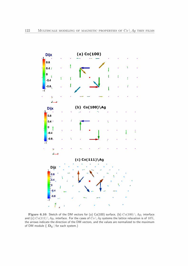
122 Multiscale modeling of magnetic properties of Co \Ag thin films
Figure 6.10: Sketch of the DM vectors for (a) Co(100) surface, (b) Co(100) \ Ag1 interfaceand (c) Co(111) \Ag1 interface. For the cases of Co \Ag systems the lattice relaxation is of 10%,the arrows indicate the direction of the DM vectors, and the values are normalized to the maximumof DM module (| Dij | for each system.)
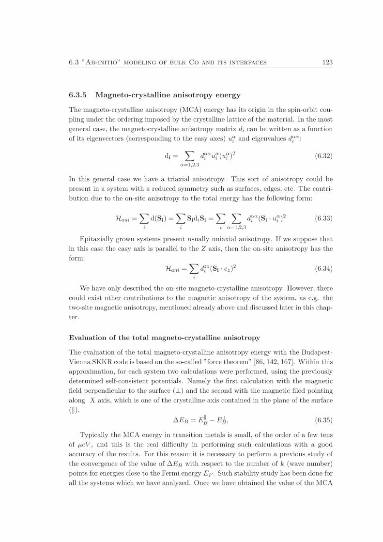
6.3 ”Ab-initio” modeling of bulk Co and its interfaces 123
6.3.5 Magneto-crystalline anisotropy energy
The magneto-crystalline anisotropy (MCA) energy has its origin in the spin-orbit cou-
pling under the ordering imposed by the crystalline lattice of the material. In the most
general case, the magnetocrystalline anisotropy matrix di can be written as a function
of its eigenvectors (corresponding to the easy axes) uαi and eigenvalues dααi :
di =∑
α=1,2,3
dααi uαi (uαi )T (6.32)
In this general case we have a triaxial anisotropy. This sort of anisotropy could be
present in a system with a reduced symmetry such as surfaces, edges, etc. The contri-
bution due to the on-site anisotropy to the total energy has the following form:
Hani =∑
i
d(Si) =∑
i
SidiSi =∑
i
∑
α=1,2,3
dααi (Si · uαi )2 (6.33)
Epitaxially grown systems present usually uniaxial anisotropy. If we suppose that
in this case the easy axis is parallel to the Z axis, then the on-site anisotropy has the
form:
Hani =∑
i
dzzi (Si · ez)2 (6.34)
We have only described the on-site magneto-crystalline anisotropy. However, there
could exist other contributions to the magnetic anisotropy of the system, as e.g. the
two-site magnetic anisotropy, mentioned already above and discussed later in this chap-
ter.
Evaluation of the total magneto-crystalline anisotropy
The evaluation of the total magneto-crystalline anisotropy energy with the Budapest-
Vienna SKKR code is based on the so-called ”force theorem” [86, 142, 167]. Within this
approximation, for each system two calculations were performed, using the previously
determined self-consistent potentials. Namely the first calculation with the magnetic
field perpendicular to the surface (⊥) and the second with the magnetic filed pointing
along X axis, which is one of the crystalline axis contained in the plane of the surface
(‖).
∆EB = E‖B − E⊥
B , (6.35)
Typically the MCA energy in transition metals is small, of the order of a few tens
of µeV , and this is the real difficulty in performing such calculations with a good
accuracy of the results. For this reason it is necessary to perform a previous study of
the convergence of the value of ∆EB with respect to the number of k (wave number)
points for energies close to the Fermi energy EF . Such stability study has been done for
all the systems which we have analyzed. Once we have obtained the value of the MCA
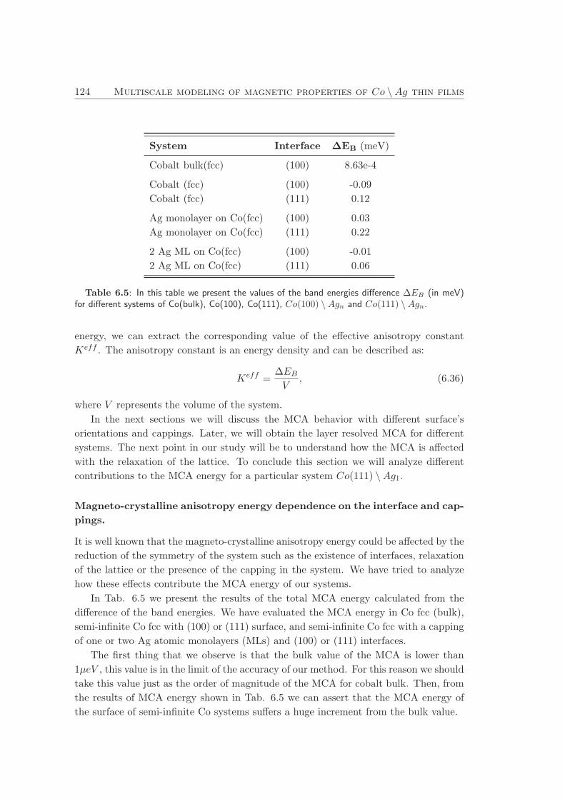
124 Multiscale modeling of magnetic properties of Co \Ag thin films
System Interface ∆EB (meV)
Cobalt bulk(fcc) (100) 8.63e-4
Cobalt (fcc) (100) -0.09
Cobalt (fcc) (111) 0.12
Ag monolayer on Co(fcc) (100) 0.03
Ag monolayer on Co(fcc) (111) 0.22
2 Ag ML on Co(fcc) (100) -0.01
2 Ag ML on Co(fcc) (111) 0.06
Table 6.5: In this table we present the values of the band energies difference ∆EB (in meV)for different systems of Co(bulk), Co(100), Co(111), Co(100) \Agn and Co(111) \Agn.
energy, we can extract the corresponding value of the effective anisotropy constant
Keff . The anisotropy constant is an energy density and can be described as:
Keff =∆EB
V, (6.36)
where V represents the volume of the system.
In the next sections we will discuss the MCA behavior with different surface’s
orientations and cappings. Later, we will obtain the layer resolved MCA for different
systems. The next point in our study will be to understand how the MCA is affected
with the relaxation of the lattice. To conclude this section we will analyze different
contributions to the MCA energy for a particular system Co(111) \Ag1.
Magneto-crystalline anisotropy energy dependence on the interface and cap-
pings.
It is well known that the magneto-crystalline anisotropy energy could be affected by the
reduction of the symmetry of the system such as the existence of interfaces, relaxation
of the lattice or the presence of the capping in the system. We have tried to analyze
how these effects contribute the MCA energy of our systems.
In Tab. 6.5 we present the results of the total MCA energy calculated from the
difference of the band energies. We have evaluated the MCA energy in Co fcc (bulk),
semi-infinite Co fcc with (100) or (111) surface, and semi-infinite Co fcc with a capping
of one or two Ag atomic monolayers (MLs) and (100) or (111) interfaces.
The first thing that we observe is that the bulk value of the MCA is lower than
1µeV , this value is in the limit of the accuracy of our method. For this reason we should
take this value just as the order of magnitude of the MCA for cobalt bulk. Then, from
the results of MCA energy shown in Tab. 6.5 we can assert that the MCA energy of
the surface of semi-infinite Co systems suffers a huge increment from the bulk value.
6.3 ”Ab-initio” modeling of bulk Co and its interfaces 125
From equation (6.35) we can conclude that ∆E > 0 means that the energy of
the system is lower when the moments of the system are oriented in the direction
perpendicular to the surface, therefore the magnetization prefers to align perpendicular
to the surface. In the opposite situation, when ∆E < 0 the magnetization of the system
prefers to align parallel to the surface of the sample. In the case of a Co(100) system,
∆E < 0, this implies that the easy axis of the system is contained in the plane of
the surface of the sample. At the same time, the magnitude of the MCA energy has
increased two order of magnitude with respect to the bulk case. Now if we cover this
system with an atomic monolayer of silver, an abrupt change of MCA energy occurs
and the easy axis becomes perpendicular to the surface of the sample.
On the other hand, in the case of a Co(111) system, ∆E > 0 then the easy axis of
the system is perpendicular to the surface of the sample, and the value of the MCA is
higher than that of the Co(100). Now we analyze what happens with the MCA energy
if we coat the system with a ML of Ag, we find that the easy axis of the system does
not change, being also in this case perpendicular to the surface.
Our calculations of the MCA energy of the Co (fcc) system with one atomic mono-
layer of Ag capping suggest us that the existence of this capping induces an increase
in the MCA energy and favors a perpendicular orientation of the magnetization. Nev-
ertheless, if the width of the Ag capping is increased up to 2MLs the MCA energy
is reduced with respect to the case of a capping by one ML of Ag and is close to the
results of the corresponding pure surface.
In brief, the MCA energy depends closely on the proximity and characteristics of
the surface or interface. The MCA energy is larger in the case of (111) surface or
interface than in the (100) case.
Understanding the origin of the MCA is a complex task, due to the difficulty that
involve this kind of studies. Nevertheless several authors suggest an interpretation of
the MCA as a function of the symmetry breaking or asymmetry of the bonding at
magnetic surface or interface [179]. The concept of Bruno suggests that under certain
assumptions the magnetic anisotropy energy is related with an anisotropy of the orbital
moment and the anisotropy bonding [45], see section 1.4.2. In the case of fcc lattice
with surface/interface (111) the number of NN in the surface/interface is 6 in contrast
to the 4 NN in surface/interface (100). Then the effect of the ligand field is stronger
in the case of (111) than in the case of (100), this suggests that the orbital moment
of the surface/interface (111) is more quenched than of the surface/interface (100),
in agreement with our calculated µL for this surface. Therefore the variation of the
magnetic moment in-plane and out-of-plane is stronger in the (111) case. Basing on
the Bruno’s model this fact can explain the larger value of the MCA energy on (111)
surface/ interface.
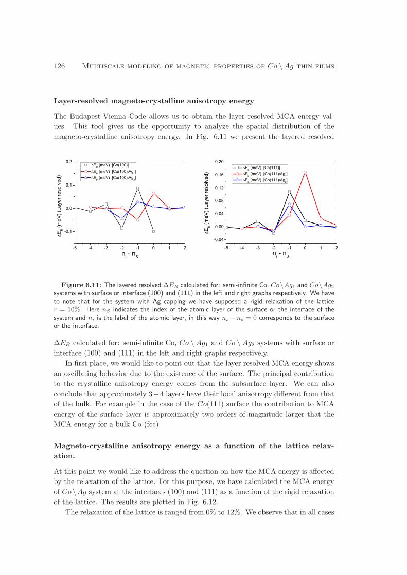
126 Multiscale modeling of magnetic properties of Co \Ag thin films
Layer-resolved magneto-crystalline anisotropy energy
The Budapest-Vienna Code allows us to obtain the layer resolved MCA energy val-
ues. This tool gives us the opportunity to analyze the spacial distribution of the
magneto-crystalline anisotropy energy. In Fig. 6.11 we present the layered resolved
-5 -4 -3 -2 -1 0 1 2
-0.1
0.0
0.1
0.2
EB (m
eV) (
Laye
r res
olve
d)
ni - nS
EB (meV) [Co(100)]
EB (meV) [Co(100)\Ag
1]
EB (meV) [Co(100)\Ag
2]
-5 -4 -3 -2 -1 0 1 2
-0.04
0.00
0.04
0.08
0.12
0.16
0.20
EB (meV) [Co(111)]
EB (meV) [Co(111)\Ag
1]
EB (meV) [Co(111)\Ag
2]
EB (m
eV) (
Laye
r res
olve
d)
ni - nS
Figure 6.11: The layered resolved ∆EB calculated for: semi-infinite Co, Co\Ag1 and Co\Ag2systems with surface or interface (100) and (111) in the left and right graphs respectively. We haveto note that for the system with Ag capping we have supposed a rigid relaxation of the latticer = 10%. Here nS indicates the index of the atomic layer of the surface or the interface of thesystem and ni is the label of the atomic layer, in this way ni − ns = 0 corresponds to the surfaceor the interface.
∆EB calculated for: semi-infinite Co, Co \ Ag1 and Co \ Ag2 systems with surface or
interface (100) and (111) in the left and right graphs respectively.
In first place, we would like to point out that the layer resolved MCA energy shows
an oscillating behavior due to the existence of the surface. The principal contribution
to the crystalline anisotropy energy comes from the subsurface layer. We can also
conclude that approximately 3−4 layers have their local anisotropy different from that
of the bulk. For example in the case of the Co(111) surface the contribution to MCA
energy of the surface layer is approximately two orders of magnitude larger that the
MCA energy for a bulk Co (fcc).
Magneto-crystalline anisotropy energy as a function of the lattice relax-
ation.
At this point we would like to address the question on how the MCA energy is affected
by the relaxation of the lattice. For this purpose, we have calculated the MCA energy
of Co\Ag system at the interfaces (100) and (111) as a function of the rigid relaxation
of the lattice. The results are plotted in Fig. 6.12.
The relaxation of the lattice is ranged from 0% to 12%. We observe that in all cases
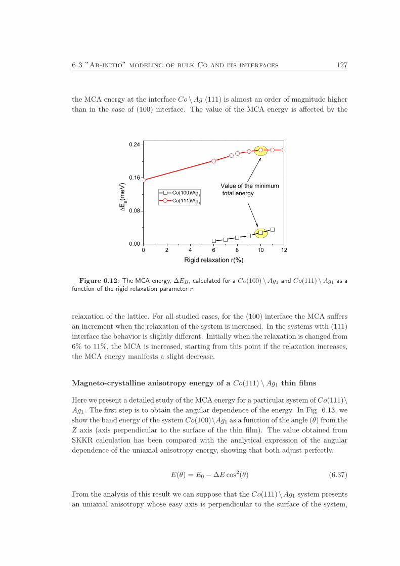
6.3 ”Ab-initio” modeling of bulk Co and its interfaces 127
the MCA energy at the interface Co \Ag (111) is almost an order of magnitude higher
than in the case of (100) interface. The value of the MCA energy is affected by the
0 2 4 6 8 10 120.00
0.08
0.16
0.24
EB(m
eV)
Rigid relaxation r(%)
Co(100)\Ag1
Co(111)\Ag1
Value of the minimum total energy
Figure 6.12: The MCA energy, ∆EB , calculated for a Co(100) \Ag1 and Co(111) \Ag1 as afunction of the rigid relaxation parameter r.
relaxation of the lattice. For all studied cases, for the (100) interface the MCA suffers
an increment when the relaxation of the system is increased. In the systems with (111)
interface the behavior is slightly different. Initially when the relaxation is changed from
6% to 11%, the MCA is increased, starting from this point if the relaxation increases,
the MCA energy manifests a slight decrease.
Magneto-crystalline anisotropy energy of a Co(111) \Ag1 thin films
Here we present a detailed study of the MCA energy for a particular system of Co(111)\
Ag1. The first step is to obtain the angular dependence of the energy. In Fig. 6.13, we
show the band energy of the system Co(100)\Ag1 as a function of the angle (θ) from the
Z axis (axis perpendicular to the surface of the thin film). The value obtained from
SKKR calculation has been compared with the analytical expression of the angular
dependence of the uniaxial anisotropy energy, showing that both adjust perfectly.
E(θ) = E0 − ∆E cos2(θ) (6.37)
From the analysis of this result we can suppose that the Co(111)\Ag1 system presents
an uniaxial anisotropy whose easy axis is perpendicular to the surface of the system,
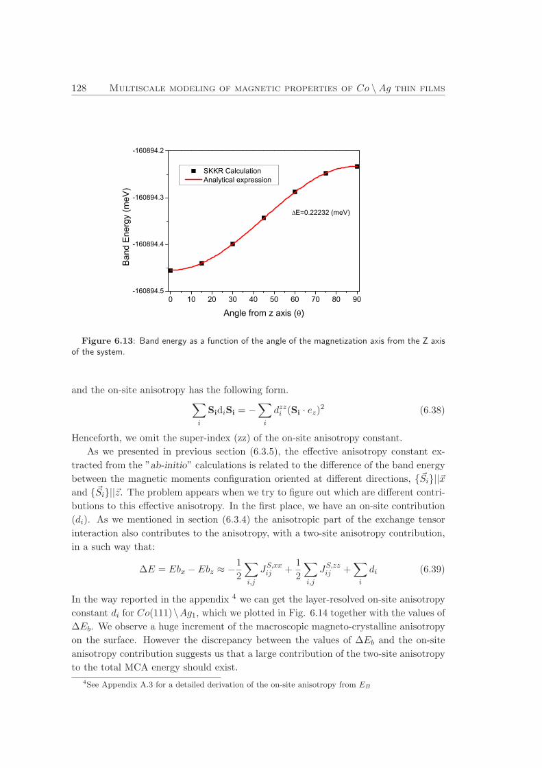
128 Multiscale modeling of magnetic properties of Co \Ag thin films
0 10 20 30 40 50 60 70 80 90-160894.5
-160894.4
-160894.3
-160894.2
SKKR Calculation Analytical expression
Ban
d E
nerg
y (m
eV)
Angle from z axis ( )
E=0.22232 (meV)
Figure 6.13: Band energy as a function of the angle of the magnetization axis from the Z axisof the system.
and the on-site anisotropy has the following form.∑
i
SidiSi = −∑
i
dzzi (Si · ez)2 (6.38)
Henceforth, we omit the super-index (zz) of the on-site anisotropy constant.
As we presented in previous section (6.3.5), the effective anisotropy constant ex-
tracted from the ”ab-initio” calculations is related to the difference of the band energy
between the magnetic moments configuration oriented at different directions, {~Si}||~x
and {~Si}||~z. The problem appears when we try to figure out which are different contri-
butions to this effective anisotropy. In the first place, we have an on-site contribution
(di). As we mentioned in section (6.3.4) the anisotropic part of the exchange tensor
interaction also contributes to the anisotropy, with a two-site anisotropy contribution,
in a such way that:
∆E = Ebx − Ebz ≈ −1
2
∑
i,j
JS,xxij +
1
2
∑
i,j
JS,zzij +
∑
i
di (6.39)
In the way reported in the appendix 4 we can get the layer-resolved on-site anisotropy
constant di for Co(111)\Ag1, which we plotted in Fig. 6.14 together with the values of
∆Eb. We observe a huge increment of the macroscopic magneto-crystalline anisotropy
on the surface. However the discrepancy between the values of ∆Eb and the on-site
anisotropy contribution suggests us that a large contribution of the two-site anisotropy
to the total MCA energy should exist.
4See Appendix A.3 for a detailed derivation of the on-site anisotropy from EB
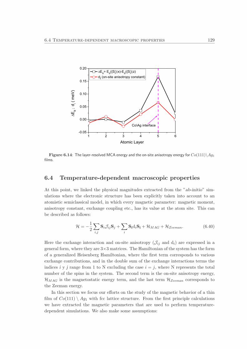
6.4 Temperature-dependent macroscopic properties 129
1 2 3 4 5 6-0.05
0.00
0.05
0.10
0.15
0.20
EB
d i ( m
eV)
Atomic Layer
EB= EB({Si} x)-EB({Si} z) di (on-site anisotropy constant)
Co\Ag interface
Figure 6.14: The layer-resolved MCA energy and the on-site anisotropy energy for Co(111)\Ag1films.
6.4 Temperature-dependent macroscopic properties
At this point, we linked the physical magnitudes extracted from the ”ab-initio” sim-
ulations where the electronic structure has been explicitly taken into account to an
atomistic semiclassical model, in which every magnetic parameter: magnetic moment,
anisotropy constant, exchange coupling etc., has its value at the atom site. This can
be described as follows:
H = −1
2
∑
i,j
SiJijSj +∑
i
SidiSi + HMAG + HZeeman. (6.40)
Here the exchange interaction and on-site anisotropy (Jij and di) are expressed in a
general form, where they are 3×3 matrices. The Hamiltonian of the system has the form
of a generalized Heisenberg Hamiltonian, where the first term corresponds to various
exchange contributions, and in the double sum of the exchange interactions terms the
indices i y j range from 1 to N excluding the case i = j, where N represents the total
number of the spins in the system. The second term is the on-site anisotropy energy,
HMAG is the magnetostatic energy term, and the last term HZeeman corresponds to
the Zeeman energy.
In this section we focus our efforts on the study of the magnetic behavior of a thin
film of Co(111) \ Ag1 with fcc lattice structure. From the first principle calculations
we have extracted the magnetic parameters that are used to perform temperature-
dependent simulations. We also make some assumptions:
130 Multiscale modeling of magnetic properties of Co \Ag thin films
1. We assume that the Ag magnetic moments, exchange and anisotropy are neg-
ligible due to their small values. Then the Hamiltonian takes into account Co
moments only.
2. In our simulations there are no external applied magnetic field, therefore the
Zeeman contribution to the total energy is zero.
3. Although the ”ab-initio” results (see section 6.3.3) showed some increment of the
spin and orbital Co moments at the interface of the Co(111) \Ag system, in the
first approximation to the problem we assume that the cobalt’s moments are the
same as those in the bulk system. As is shown in Table (6.2) these modifications
are in practice negligible.
6.4.1 Magnetostatic interaction
The magnetostatic self energy is the interaction of a distribution of a magnetization
vector with the magnetic field created by this distribution itself. This energy term is
normally written in the following way:
EM = −1
2
∫
M ·H′dv, (6.41)
where the integration is over the volume of the ferromagnetic system, taken as a contin-
uum. Due to its long range character, the magnetostatic interaction generally depends
on the shape of the system, and it is responsible for the existence of magnetic domains.
Usually this contribution leads to the commonly called shape anisotropy, and becomes
important in thin films where it often produces in-plane alignment of moments. The
proper calculation of the magnetostatic energy belongs to the area of micromagnetism
and is computationally costly.
As a first approximation of the magnetostatic anisotropy energy, we used a simpli-
fied version of the demagnetization factor approach valid for thin films with homoge-
neous magnetization [180]. Then the density of energy per volume could be written as
an additional anisotropy term [181, 182].
EM = KSH · cos2(θ), (6.42)
where KSH = 2πM2s in c.g.s. unit system. The magnetization makes an angle (θ) to
the plane normal. The magnetostatic anisotropy energy is thus minimized for an angle
of θ = π/2, this implies all the moments lying in the plane of the thin film.
The saturation magnetization Ms is related at T = 0K to the atomic magnetic
moment µ through:
Ms =µ
V0, (6.43)
V0 represents the atomic volume. In the case of an fcc lattice the atomic volume is
related with the lattice parameter a as V0 = a3/4 (for Co a = 0.3548 nm). As we can see
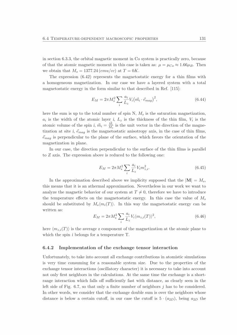
6.4 Temperature-dependent macroscopic properties 131
in section 6.3.3, the orbital magnetic moment in Co system is practically zero, because
of that the atomic magnetic moment in this case is taken as: µ = µCo ≈ 1.66µB. Then
we obtain that Ms = 1377.24 (emu/cc) at T = 0K.
The expression (6.42) represents the magnetostatic energy for a thin films with
a homogeneous magnetization. In our case we have a layered system with a total
magnetostatic energy in the form similar to that described in Ref. [115]:
EM = 2πM2s
∑
i
aiLzVi(
~mi · ~emag
)2, (6.44)
here the sum is up to the total number of spin N, Ms is the saturation magnetization,
ai is the width of the atomic layer i, Lz is the thickness of the thin film, Vi is the
atomic volume of the spin i, ~mi =~Mi
Msis the unit vector in the direction of the magne-
tization at site i, ~emag is the magnetostatic anisotropy axis, in the case of thin films,
~emag is perpendicular to the plane of the surface, which favors the orientation of the
magnetization in plane.
In our case, the direction perpendicular to the surface of the thin films is parallel
to Z axis. The expression above is reduced to the following one:
EM = 2πM2s
∑
i
aiLzVim
2z,i. (6.45)
In the approximation described above we implicity supposed that the |M| = Ms,
this means that it is an athermal approximation. Nevertheless in our work we want to
analyze the magnetic behavior of our system at T 6= 0, therefore we have to introduce
the temperature effects on the magnetostatic energy. In this case the value of Ms
should be substituted by Ms〈mi(T )〉. In this way the magnetostatic energy can be
written as:
EM = 2πM2s
∑
i
aiLzVi〈mz,i(T )〉2, (6.46)
here 〈mz,i(T )〉 is the average z component of the magnetization at the atomic plane to
which the spin i belongs for a temperature T.
6.4.2 Implementation of the exchange tensor interaction
Unfortunately, to take into account all exchange contributions in atomistic simulations
is very time consuming for a reasonable system size. Due to the properties of the
exchange tensor interactions (oscillatory character) it is necessary to take into account
not only first neighbors in the calculations. At the same time the exchange is a short-
range interaction which falls off sufficiently fast with distance, as clearly seen in the
left side of Fig. 6.7, so that only a finite number of neighbors j has to be considered.
In other words, we consider that the exchange double sum is over the neighbors whose
distance is below a certain cutoff, in our case the cutoff is 5 · (a2D), being a2D the
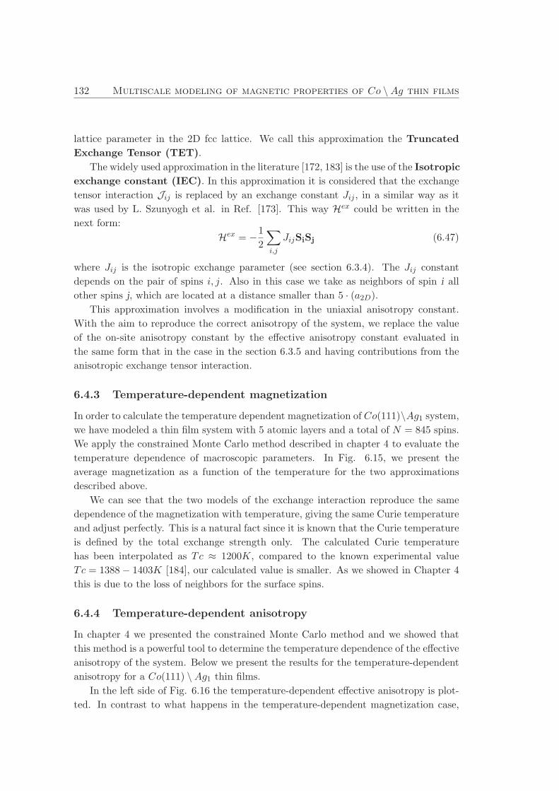
132 Multiscale modeling of magnetic properties of Co \Ag thin films
lattice parameter in the 2D fcc lattice. We call this approximation the Truncated
Exchange Tensor (TET).
The widely used approximation in the literature [172, 183] is the use of the Isotropic
exchange constant (IEC). In this approximation it is considered that the exchange
tensor interaction Jij is replaced by an exchange constant Jij , in a similar way as it
was used by L. Szunyogh et al. in Ref. [173]. This way Hex could be written in the
next form:
Hex = −1
2
∑
i,j
JijSiSj (6.47)
where Jij is the isotropic exchange parameter (see section 6.3.4). The Jij constant
depends on the pair of spins i, j. Also in this case we take as neighbors of spin i all
other spins j, which are located at a distance smaller than 5 · (a2D).
This approximation involves a modification in the uniaxial anisotropy constant.
With the aim to reproduce the correct anisotropy of the system, we replace the value
of the on-site anisotropy constant by the effective anisotropy constant evaluated in
the same form that in the case in the section 6.3.5 and having contributions from the
anisotropic exchange tensor interaction.
6.4.3 Temperature-dependent magnetization
In order to calculate the temperature dependent magnetization of Co(111)\Ag1 system,
we have modeled a thin film system with 5 atomic layers and a total of N = 845 spins.
We apply the constrained Monte Carlo method described in chapter 4 to evaluate the
temperature dependence of macroscopic parameters. In Fig. 6.15, we present the
average magnetization as a function of the temperature for the two approximations
described above.
We can see that the two models of the exchange interaction reproduce the same
dependence of the magnetization with temperature, giving the same Curie temperature
and adjust perfectly. This is a natural fact since it is known that the Curie temperature
is defined by the total exchange strength only. The calculated Curie temperature
has been interpolated as Tc ≈ 1200K, compared to the known experimental value
Tc = 1388 − 1403K [184], our calculated value is smaller. As we showed in Chapter 4
this is due to the loss of neighbors for the surface spins.
6.4.4 Temperature-dependent anisotropy
In chapter 4 we presented the constrained Monte Carlo method and we showed that
this method is a powerful tool to determine the temperature dependence of the effective
anisotropy of the system. Below we present the results for the temperature-dependent
anisotropy for a Co(111) \Ag1 thin films.
In the left side of Fig. 6.16 the temperature-dependent effective anisotropy is plot-
ted. In contrast to what happens in the temperature-dependent magnetization case,
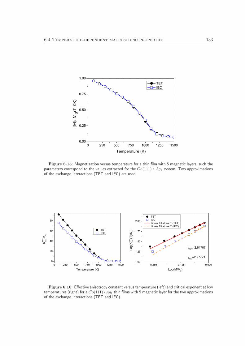
6.4 Temperature-dependent macroscopic properties 133
0 250 500 750 1000 1250 15000.00
0.25
0.50
0.75
1.00
S(T
=0K
)
Temperature (K)
TET IEC
Figure 6.15: Magnetization versus temperature for a thin film with 5 magnetic layers, such theparameters correspond to the values extracted for the Co(111) \Ag1 system. Two approximationsof the exchange interactions (TET and IEC) are used.
0 250 500 750 1000 1250 15000
20
40
60
80
TET IEC
KE
FFU
A/K
C
Temperature (K)-0.250 -0.125 0.000
1.00
1.25
1.50
1.75
2.00
TET IEC Linear Fit at low T (TET) Linear Fit at low T (IEC)
Log(
KE
FFU
A(T
)/KC)
Log(M/M0)
TET=2.64707
IEC=2.97721
Figure 6.16: Effective anisotropy constant versus temperature (left) and critical exponent at lowtemperatures (right) for a Co(111)\Ag1 thin films with 5 magnetic layer for the two approximationsof the exchange interactions (TET and IEC).

134 Multiscale modeling of magnetic properties of Co \Ag thin films
the use of the isotropic exchange constant modifies the results.
The effective value at T = 0K is also different being larger in the case of full but
truncated exchange tensor than for the isotropic exchange constant approximation.
Such an increment of the initial effective anisotropy is due to the fact that in the first
case the ”two-site” anisotropy and the DM interaction are included explicitly. The DM
interaction favors the orientation of the magnetization in plane, leading to a reduction
of the anisotropy out-of-plane, but the contribution of the ”two-site” anisotropy favors
the anisotropy perpendicular to the surface of the sample and this contribution is
more important leading to a net increment of the anisotropy out-of-plane. The IEC
approximation includes these contributions in a modified ”uniaxial anisotropy” which
is obviously wrong.
We have also calculated the low-temperature scaling exponents γ of the anisotropy
with magnetization and we have observed that in the case of TET γ ≈ 2.69 and in
the case of IEC γ ≈ 3. That discrepancy of the results is due to that in TET case
and differently to IEC approximation we have taken into account the total exchange
matrix, which has an important contribution of the ”two-site” anisotropy. As it has
been shown by Mryrasov et al. [185] this term is responsible of the deviation from
γ = 3 exponent (typical for uniaxial anisotropy) in the case of FePt.
6.5 Conclusions
From our results we can conclude the following:
• We have constructed an effective semiclassical (spin localized) Heisenberg Hamil-
tonian, passing the magnetic information from ”ab-initio” calculations to the
atomistic level.
• We have shown that the magnetic moment in Co thin films is affected by the
existence of the surface and the capping. In the case of Co \ Ag thin films we
observed a polarization of the Ag layer. However, the modifications of the spin
and the orbital magnetic moment of Ag are small.
• We have obtained the layer resolved effective anisotropy constant and observed
that it has experienced a huge increment due to the breaking of symmetry on the
surface. Also we have shown that its character could be changed by the surface
capping. A transformation from a system with easy axis perpendicular to the
plane to the one with easy plane anisotropy by one or two layers of Ag capping
has been predicted.
• The symmetry breaking of the surface induces an increment in the value of
the exchange interaction. Also it leads to an asymmetry of the exchange ten-
sor interaction in the direction Z perpendicular to the surface. This, together
6.5 Conclusions 135
with the Dzyaloshinsky-Moriya interaction contributes to an overall macroscopic
anisotropy.
• In the case of a thin film Co(111) \ Ag1 we have discussed different exchange
interaction contributions, and the temperature dependence of the macroscopic
magnetization and anisotropy. We have observed that the magnetization depen-
dence on the temperature can be reproduced both with the truncated exchange
tensor and within the isotropic exchange constant approximation . Nevertheless
the dependence of the anisotropy on the temperature is highly dependent on the
correct account of the exchange interaction. This indicates that the IEC is not
able to provide a correct temperature dependence of the magnetic properties of
the system, in this case we should use a total exchange matrix.
136 Multiscale modeling of magnetic properties of Co \Ag thin films
Conclusiones
Para resumir, hemos realizado un estudio multiescala del las propiedades magneticas
de diversos sistemas. En primer lugar obtuvimos los parametros magneticos locales
del Co semi-infinito con superficies (100) y (111), Co(100) \ Agn y Co(111) \ Agncon n=1,2, utilizando para ello simulaciones ”ab-initio”. Posteriormente haciendo uso
del algoritmo CMC estudiamos el comportamiento magnetico de una lamina delgada
Co(111) \Ag1. A continuacion indicamos las principales conclusiones de este estudio:
• En primer lugar hemos observado que el momento magnetico del Co se ve afectado
por la existencia de la superficie o del recubrimiento de Ag, variando su valor con
respecto al de volumen. En el caso de laminas delgadas de Co\Ag se detecto una
pequena polarizacion de la capa de Ag. Aun ası, la modificacion del momento
orbital de la plata y del espın del Co son en general pequenos.
• Hemos obtenido la energıa magneto-cristalina resuelta por capas y observamos
que esta experimenta un gran aumento en la superficie. Ademas mostramos que
el caracter de la anisotropıa efectiva puede ser alterado por el recubrimiento de
plata, observando una reorientacion del eje facil magnetico del sistema al recubrir
el Co con una o dos capas atomicas de Ag.
• La ruptura de simetrıa cristalina en la superficie induce un incremento del valor
de la interaccion de canje, ası como una asimetrıa en la interacion de canje en
la direccion Z (direccion perpendicular a la superficie). Estos factores conjun-
tamente con la interaccion Dzyaloshinsky-Moriya contribuyen a la anisotropıa
global del sistema.
• En laminas delgadas de Co(111) \ Ag1 donde existe una ruptura abrupta de la
simetrıa cristalina hemos encontrado que la principal contribucion a la anisotropıa
magnetica global del sistema no es la anisotropıa ”on-site” sino la ”two-site”.
• En el caso de una lamina delgada de Co(111) \ Ag1 discutimos las diferentes
contribuciones de canje y la dependencia con la temperatura de la imanacion
y la anisotropıa macroscopica. En el estudio de la dependencia termica de la
imanacion, se observo que este comportamiento puede ser reproducido tanto si
tomamos la interaccion de canje con su naturaleza exacta, como una interaccion
tensorial a multiples vecinos, o si la tomamos de una forma aproximada como una
constante de canje renormalizada (IEC). Sin embargo la dependencia termica de
la ansiotropıa se ve afectada sustancialmente con la aproximacion utilizada para
la interaccion de canje. Esto indica que la aproximacion (IEC) no es capaz
de proporcionar una correcta dependencia termica de la ansiotropıa global del
sistema.
6.5 Conclusions 137
• Hemos mostrado que aunque nos encontramos en los primeros pasos de nuestro
estudio tenemos la capacidad de realizar un estudio multiescla desde calculos ”ab-
initio” hasta un modelo atomıstico de las propiedades macroscopicas de laminas
delgadas.

138 Multiscale modeling of magnetic properties of Co \Ag thin films
AAppendix A
A.1 Hamiltonian of the spin system in the adiabatic ap-
proximation
Within the rigid-spin approximation the adiabatic dynamics of local spin moments is
described by the Landau-Lifshitz equation.
MriSri = −2µB~
δF
δSri× Sri (A.1)
where Sri is a unit vector pointing along the spin-quantization axis in the atomic cell
at the site i of the layer r, Mri is the magnitude of the spin moment and F is the free
energy of the system. If we are working in spherical coordinates then we can write Sri
as a function of the polar and azimuthal angles θri and ϕri respectively.
Sri = (sin θri cosϕri, sin θri sinϕri, cos θri) (A.2)
Rewriting the dynamical equation into spherical coordinates, the equations of motion
for the angles θri and ϕri are given by:
Mrϕri sin θri =2µB~
δF
δθri(A.3)
−Mrθri sin θri =2µB~
δF
δϕri, (A.4)
implicitly in these equations we supposed that the magnitude of the spin moment Mri
depends only on the atomic layer for the spins i.
139
140 Appendix A
If we choose the polar axis of the reference system (Z) perpendicular to the mag-
netization in the ferromagnetic state, the system of equations (A.3 and A.4) can be
linearized
Mrϕri =2µB~
δF
δθri
∣
∣
∣
θ=π
2,ϕ=0
(A.5)
−Mrθri =2µB~
δF
δϕri
∣
∣
∣
θ=π
2,ϕ=0
(A.6)
These equations are the canonical equations for the generalized coordinates qri and
momenta pri which are defined as:
qri =(Mr
µB
)1/2ϕri (A.7)
pri =(Mr
µB
)1/2θri (A.8)
Therefore doing an expansion up to the second order of the free energy in the angular
variables, the corresponding Hamiltonian can be written as:
H =1
~
∑
ri,sj
(
qriAri,sjqsj + qriBri,sjpsj + priBsj,riqsj + priCri,sjpsj)
, (A.9)
with
Ari,sj =(Mr
µB
)1/2 δ2F
δϕriδϕsj
∣
∣
∣
θ=π
2,ϕ=0
(Ms
µB
)1/2(A.10)
Bri,sj =(Mr
µB
)1/2 δ2F
δϕriδθsj
∣
∣
∣
θ=π
2,ϕ=0
(Ms
µB
)1/2(A.11)
Cri,sj =(Mr
µB
)1/2 δ2F
δθriδθsj
∣
∣
∣
θ=π
2,ϕ=0
(Ms
µB
)1/2(A.12)
A.2 Contribution to total uniaxial anisotropy due to ”two-
site” anisotropy
In chapter 6 we have shown that the contribution of the symmetric part of the exchange
matrix interaction to the Hamiltonian (HSExc) can be written as follows:
HSExc = −1
2
∑
i,j
SiJSijSj . (A.13)
The double sum is over all i 6= j. If we analyze only the contribution of the spin i, we
obtain that it is described by:
HSExci = −
1
2
∑
j
SiJSijSj = −
1
2Si(∑
j
J SijSj) . (A.14)
A.3 Determination of one-site anisotropy energy 141
In the case when the state of the system has the ferromagnetic order, where all the unit
vectors Si are pointing out in the same direction, we can rewrite the last expression as:
HSExci = −
1
2Si(∑
j
J Sij )Sj , (A.15)
being (∑
j JSij ) the effective symmetric contribution of the exchange interaction at layer
zi, it has been defined previously as J Szi . As we have shown in the chapter 6.3.4, for
Co(100) and Co(100) \Ag1 the J Szi has the following form:
J Szi =
∑
j
J Sij = Azi
−12 0 0
0 −12 0
0 0 1
(A.16)
This expression can be separated in two contributions,
J Szi = Azi
−12 0 0
0 −12 0
0 0 1
=
−Azi
2
1 0 0
0 1 0
0 0 1
+Azi
0 0 0
0 0 0
0 0 32
(A.17)
Therefore we have that:
HSExci =
Azi
4SiSj −AziSi
0 0 0
0 0 0
0 0 32
Sj , (A.18)
This formula can be simplified as:
HSExci =
Azi
4SiSj −
3Azi
4Si,zSj,z , (A.19)
The first term on the right hand side (r.h.s) of this equation is isotropic and does not
contribute to the anisotropy of the system, but it can modify the isotropic part of the
exchange interaction. If we remember the initial hypothesis of the ferromagnetic state
of the system, the second term in the (r.h.s.) of the equation A.19 can be expressed
as: −3Azi
4 S2i,z and this formula is analogous to that of the expression for the uniaxial
anisotropy with easy axis parallel to the Z axis.
In conclusion the ”two-site” anisotropy can contribute to the effective uniaxial anisotropy
under the assumptions mentioned above.
A.3 Determination of one-site anisotropy energy
Suppose that we describe the properties of a magnetic system with an anisotropic
Heisenberg Hamiltonian as follows:
H = −1
2
∑
i,j
SiJijSj −∑
i
d(Si) (A.20)

142 Appendix A
where Jij and d(Si) are matrices 3 × 3. If we assume that the on-site anisotropy is
uniaxial and its easy axis is parallel to Z axis, we can rewrite the Hamiltonian as:
H = −1
2
∑
i,j
SiJijSj −∑
i
SidiSi (A.21)
di =
0 0 0
0 0 0
0 0 dzzi
(A.22)
In spherical coordinates we can write Si as a function of the polar and azimuthal
angles θi and ϕi, respectively.
Si = (sin θi cosϕi, sin θi sinϕi, cos θi) (A.23)
and evaluate the second derivatives with respect to the polar and azimuthal angles.
∂2Si
∂θ2i= −(sin θi cosϕi, sin θi sinϕi, cos θi) = −Si (A.24)
∂2Si
∂ϕ2i
= −(sin θi cosϕi, sin θi sinϕi, 0) (A.25)
If the spin i belongs to the plane XY then Eq. (A.25) is reduced to :
∂2Si
∂ϕ2i
= −Si (A.26)
Now we evaluate the second derivatives with respect to the polar and azimuthal angles
of the energy:
∂2E{Si}
∂θ2i= −
∂2
∂θ2i
(
SidiSi
)
−1
2
∑
j,j 6=i
∂2Si
∂θ2iJijSj −
1
2
∑
j,j 6=i
SiJij∂2Sj
∂θ2i(A.27)
∂2E{Si}
∂ϕ2i
= −∂2
∂ϕ2i
(
SidiSi
)
−1
2
∑
j,j 6=i
∂2Si
∂ϕ2i
JijSj −1
2
∑
j,j 6=i
SiJij∂2Sj
∂ϕ2i
(A.28)
Due to the fact that the spin variables are independent, the equations above can
be reduced to:
∂2E{Si}
∂θ2i= −
∂2
∂θ2i
(
SidiSi
)
−1
2
∑
j,j 6=i
∂2Si
∂θ2iJijSj (A.29)
∂2E{Si}
∂ϕ2i
= −∂2
∂ϕ2i
(
SidiSi
)
−1
2
∑
j,j 6=i
∂2Si
∂ϕ2i
JijSj (A.30)

A.3 Determination of one-site anisotropy energy 143
The free energy of the system F is related with the second derivatives above:
F(θi, ϕi) =∂2E{Si}
∂θ2i−∂2E{Si}
∂ϕ2i
= −( ∂2
∂θ2i−
∂2
∂ϕ2i
)(
SidiSi
)
−∑
j,j 6=i
(∂2Si
∂θ2i−∂2Si
∂ϕ2i
)
JijSj
(A.31)
Taking into account the hypothesis that the on-site anisotropy is uniaxial Eq. (A.22),
this expression can be reduced to:
F(θi, ϕi) = −( ∂2
∂θ2i−
∂2
∂ϕ2i
)(
dzzi cos2 θi
)
−∑
j,j 6=i
(∂2Si
∂θ2i−∂2Si
∂ϕ2i
)
JijSj (A.32)
Therefore we can calculate the on-site anisotropy constant dzzi evaluating the free energy
at θi = π/2
F(θi, ϕi)∣
∣
∣
θi=π/2= 2dzzi cos(2θ)
∣
∣
∣
θi=π/2= −2dzzi (A.33)
with
dzzi = −1
2F(θi, ϕi)
∣
∣
∣
θi=π/2(A.34)

144 Appendix A
Bibliography
[1] C. Desvaux, C. Amiens, P. Fejes, P. Renaud, M. Respaud, P. Lecante, E. Snoeck,
and C. Bruno. Multimillimetre-large superlattices of air-stable iron-cobalt
nanoparticles. Nat. Mater. 4, 750 (2005).
[2] S. Sun, C. B. Murray, D. Weller, L. Folks, and A. Moser. Monodisperse FePt
nanoparticles and ferromagnetic FePt nanocrystal superlattices. Science 287,
1989 (2000).
[3] S. Rusponi, T. Cren, N. Weiss, M. Epple, P. Buluschek, L. Claude, and
H. Brune. The remarkable difference between surface and step atoms in the mag-
netic anisotropy of two-dimensional nanostructures. Nat. Mater 2, 546 (2003).
[4] P. Tartaj, M. del Puerto Morales, S. Veintemillas-Verdaguer, T. Gonzalez-
Carreno, and C. J. Serna. The preparation of magnetic nanoparticles for ap-
plications in biomedicine. J. Phys. D: Appl. Phys. 36, R182 (2003).
[5] A. K. Gupta and M. Gupta. Synthesis and surface engineering of iron oxide
nanoparticles for biomedical applications. Biomaterials 26, 3995 (2005).
[6] V. Skumryev, S. Stoyanov, Y. Zhang, G. Hadjipanayis, D. Givord, and J. Nogues.
Beating the superparamagnetic limit with exchange bias. Nature 423, 850 (2003).
[7] R. F. L. Evans, R. Yanes, O. Mryasov, R. W. Chantrell, and O. Chubykalo-
Fesenko. On beating the superparamagnetic limit with exchange bias. Europhys.
Lett. 88, 57004 (2009).
[8] F. Luis, J. M. Torres, L. M. Garcıa, J. Bartolome, J. Stankiewicz, F. Petroff,
F. Fettar, J.-L. Maurice, and A. Vaures. Enhancement of the magnetic anisotropy
of nanometer-sized Co clusters: Influence of the surface and of interparticle in-
teractions. Phys. Rev. B 65, 094409 (2002).
[9] J. Bartolome, L. M. Garcıa, F. Bartolome, F. Luis, R. Lopez-Ruiz, F. Petroff,
C. Deranlot, F. Wilhelm, A. Rogalev, P. Bencok, N. B. Brookes, L. Ruiz, and
J. M. Gonzalez-Calbet. Magnetic polarization of noble metals by Co nanoparticles
in M -capped granular multilayers ( M = Cu , Ag, and Au): An X-ray magnetic
circular dichroism study. Phys. Rev. B 77, 184420 (2008).
145

146 Bibliography
[10] F. Luis, F. Bartolome, F. . Petroff, J. Bartolome, L. M. Garcıa, C. Deranlot,
H. Jaffres, M. J. Martınez, P. Bencok, F. Wilhelm, A. Rogalev, and N. B. Brookes.
Tuning the magnetic anisotropy of Co nanoparticles by metal capping. Europhys.
Lett. 76, 142 (2006).
[11] F. Garcia-Sanchez, O. Chubykalo-Fesenko, O. Mryasov, P. Asselin, and R. W.
Chantrell. Switching and thermal stability properties of bilayer thin films: Single
versus multigrain cases. J. Appl. Phys. 103, 07F505 (2008).
[12] G. R. Aranda, O. Chubykalo-Fesenko, R. Yanes, J. Gonzalez, J. J. del Val, R. W.
Chantrell, Y. K. Takahashi, and K. Hono. Coercive field and energy barriers in
partially disordered FePt nanoparticles. J. Appl. Phys. 105, 07B514 (2009).
[13] G. Salazar-Alvarez, J. Qin, V. Sepelak, I. Bergmann, M. Vasilakaki, K. N.
Trohidou, J. D. Ardisson, W. A. A. Macedo, M. Mikhaylova, M. Muhammed,
M. D. Baro, and J. Nogues. Cubic versus spherical magnetic nanoparti-
cles: The role of surface anisotropy. J. Am. Chem. Soc. 130, 13234 (2008).
http://pubs.acs.org/doi/pdf/10.1021/ja0768744.
[14] M. Jamet, W. Wernsdorfer, C. Thirion, V. Dupuis, P. Melinon, A. Perez, and
D. Mailly. Magnetic anisotropy in single clusters. Phys. Rev. B 69, 024401
(2004).
[15] X. Batlle and A. Labarta. Finite-size effects in fine particles: magnetic and
transport properties. J. Phys. D: Appl. Phys. 35, R15 (2002).
[16] A. Weddemann, I. Ennen, A. Regtmeier, C. Albon, A. Wolf, K. Eckstadt, N. Mill,
J. Peter, Michaeland Mattay, C. Plattner, and A. Sewald, Norbert andfd Hutten.
Review and outlook: from single nanoparticles to self-assembled monolayers and
granular GMR sensors. Beilstein J. Nanotechnol. 1, 75 (2010).
[17] J. Frenkel and J. Doefman. Spontaneous and induced magnetisation in ferromag-
netic bodies. Nature 126, 274 (1930).
[18] R. Evans, U. Nowak, F. Dorfbauer, T. Shrefl, O. Mryasov, R. W. Chantrell, and
G. Grochola. The influence of shape and structure on the Curie temperature of
Fe and Co nanoparticles. J. Appl. Phys. 99, 08G703 (2006).
[19] A. G. Roca, R. Costo, A. F. Rebolledo, S. Veintemillas-Verdaguer, P. Tartaj,
T. Gonzalez-Carreno, M. P. Morales, and C. J. Serna. Progress in the preparation
of magnetic nanoparticles for applications in biomedicine. J. Phys. D: Appl. Phys.
42, 224002 (2009).
[20] M. Jamet, W. Wernsdorfer, C. Thirion, D. Mailly, V. Dupuis, P. Melinon, and
A. Perez. Magnetic anisotropy of a single cobalt nanocluster. Phys. Rev. Lett.
86, 4676 (2001).

Bibliography 147
[21] J. M. D. Coey, K. Wongsaprom, J. Alaria, and M. Venkatesan. Charge-transfer
ferromagnetism in oxide nanoparticles. J. Phys. D: Appl. Phys. 41, 134012
(2008).
[22] L. F. Cotica, I. A. Santos, E. M. Girotto, E. V. Ferri, and A. A. Coelho. Surface
spin disorder effects in magnetite and poly(thiophene)-coated magnetite nanopar-
ticles. J. Appl. Phys. 108, 064325 (2010).
[23] W. H. Meiklejohn and C. P. Bean. New magnetic anisotropy. Phys. Rev. 105,
904 (1957).
[24] S. A. Makhlouf, H. Al-Attar, and R. Kodama. Particle size and temperature
dependence of exchange bias in NiO nanoparticles. Solid State Commun. 145, 1
(2008).
[25] W. H. Meiklejohn and C. P. Bean. New magnetic anisotropy. Phys. Rev. 102,
1413 (1956).
[26] J. Nogues and I. K. Schuller. Exchange bias. J. Magn. Magn. Mat. 192, 203
(1999).
[27] O. Iglesias, X. Batlle, and A. Labarta. Modelling exchange bias in core/shell
nanoparticles. J. Phys.: Condens. Matter 19, 406232 (2007).
[28] F. Liu, M. R. Press, S. N. Khanna, and P. Jena. Magnetism and local order: Ab
initio tight-binding theory. Phys. Rev. B 39, 6914 (1989).
[29] S. N. Khanna and S. Linderoth. Magnetic behavior of clusters of ferromagnetic
transition metals. Phys. Rev. Lett. 67, 742 (1991).
[30] S. E. Apsel, J. W. Emmert, J. Deng, and L. A. Bloomfield. Surface-enhanced
magnetism in nickel clusters. Phys. Rev. Lett. 76, 1441 (1996).
[31] K. W. Edmonds, C. Binns, S. H. Baker, S. C. Thornton, C. Norris, J. B. Goed-
koop, M. Finazzi, and N. B. Brookes. Doubling of the orbital magnetic moment
in nanoscale Fe clusters. Phys. Rev. B 60, 472 (1999).
[32] M. Respaud, J. M. Broto, H. Rakoto, A. R. Fert, L. Thomas, B. Barbara,
M. Verelst, E. Snoeck, P. Lecante, A. Mosset, J. Osuna, T. O. Ely, C. Amiens,
and B. Chaudret. Surface effects on the magnetic properties of ultrafine cobalt
particles. Phys. Rev. B 57, 2925 (1998).
[33] A. E. Berkowitz, W. J. Schuele, and P. J. Flanders. Influence of crystallite size
on the magnetic properties of acicular γ-Fe2O3 particles. J. Appl. Phys. 39, 1261
(1968).
148 Bibliography
[34] J. M. D. Coey. Noncollinear spin arrangement in ultrafine ferrimagnetic crystal-
lites. Phys. Rev. Lett. 27, 1140 (1971).
[35] R. H. Kodama. Magentic nanoparticles. J. Magn. Magn. Mat. 200, 359 (1999).
[36] F. Bødker, S. Mørup, and S. Linderoth. Surface effects in metallic iron nanopar-
ticles. Phys. Rev. Lett. 72, 282 (1994).
[37] E. Tronc, A. Ezzir, R. Cherkaoui, C. Chaneac, M. Nogues, H. Kachkachi, D. Fio-
rani, A. Testa, J. Greneche, and J. Jolivet. Surface-related properties of γ-Fe2o3nanoparticles. J. Magn. Magn. Mat. 221, 63 (2000).
[38] J. E. Lima, E. D. Biasi, M. V. Mansilla, M. E. Saleta, F. Effenberg, L. M. Rossi,
R. Cohen, H. R. Rechenberg, and R. D. Zysler. Surface effects in the magnetic
properties of crystalline 3 nm ferrite nanoparticles chemically synthesized. J.
Appl. Phys. 108, 103919 (2010).
[39] M. Hamedoun, K. Bouslykhane, H. Bakrim, A. Hourmatallah, and N. Benzakour.
Coupling and surface effects in magnetic thin films. Physica A 358, 102 (2005).
[40] L. Szunyogh, L. Udvardi, J. Jackson, U. Nowak, and R. Chantrell. Atomistic spin
model based on a spin-cluster expansion technique: Application to the IrMn3/Co
interface. Phys. Rev. B 83, 024401 (2011).
[41] I. Apostolova and J. M. Wesselinowa. Possible low-Tc nanoparticles for use in
magnetic hyperthermia treatments. Solid State Commun. 149, 986 (2009).
[42] J. H. van Vleck. On the anisotropy of cubic ferromagnetic crystals. Phys. Rev.
52, 1178 (1937).
[43] U. Gradmann. Magnetism in oligatomic films. J. Appl. Phys. 40, 1182 (1969).
[44] J. G. Gay and R. Richter. Spin anisotropy of ferromagnetic films. Phys. Rev.
Lett. 56, 2728 (1986).
[45] P. Bruno. Tight-binding approach to the orbital magnetic moment and magne-
tocrystalline anisotropy of transition-metal monolayers. Phys. Rev. B 39, 865
(1989).
[46] R. H. Victora and J. M. MacLaren. Theory of magnetic interface anisotropy.
Phys. Rev. B 47, 11583 (1993).
[47] L. Neel. Anisotropie magnetique superficielle et surstructures d’orientation. J.
Phys. Radium 15, 225 (1954).
[48] L. Stohr and H. Siegmann. Magnetism from: fundamentals to nanoscale dynamics
(Springer, 2006).
Bibliography 149
[49] C. Andersson, B. Sanyal, O. Eriksson, L. Nordstrom, O. Karis, D. Arvanitis,
T. Konishi, E. Holub-Krappe, and J. H. Dunn. Influence of ligand states on the
relationship between orbital moment and magnetocrystalline anisotropy. Phys.
Rev. Lett. 99, 177207 (2007).
[50] G. Schutz, W. Wagner, W. Wilhelm, P. Kienle, R. Zeller, R. Frahm, and
G. Materlik. Absorption of circularly polarized x-rays in iron. Phys. Rev. Lett.
58, 737 (1987).
[51] J. Stohr. Exploring the microscopic origin of magnetic anisotropies with X-ray
magnetic circular dichroism (XMCD) spectroscopy. J. Magn. Magn. Mat. 200,
470 (1999).
[52] A. Ney, P. Poulopoulos, M. Farle, and K. Baberschke. Absolute determination of
Co magnetic moments: Ultrahigh-vacuum high-Tc SQUID magnetometry. Phys.
Rev. B 62, 11336 (2000).
[53] W. F. Brown. Thermal fluctuations of a single-domain particle. Phys. Rev. 130,
1677 (1963).
[54] P. Bruno and J. P. Renard. Magnetic surface anistropy of transition metal ultra-
thin films. Appl. Phys. A 49, 499 (1989).
[55] H. J. Elmers and U. Gradmann. Magnetic anisotropies in Fe(110) films on
W(110). Appl. Phys. A 51, 255 (1990).
[56] A. P. N. Dinia and H. Danan. Spectral-density method for classical systems:
Heisenberg ferromagnet. J. App. Phys. 84, 5668 (1998).
[57] E. Tronc, D. Fiorani, M. Nogues, A. Testa, F. Lucari, F. D’Orazio, J. Greneche,
W. Wernsdorfer, N. Galvez, C. Chaneac, D. Mailly, and J. Jolivet. Surface effects
in non-interacting and interacting γ-Fe2O3 nanoparticles. J. Magn. Magn. Mat.
262, 6 (2003).
[58] U. Gradmann. Magnetic surface anisotropies. J. Magn. Magn. Mat. 54-57, 733
(1986).
[59] G. Bochi, C. A. Ballentine, H. E. Inglefield, C. V. Thompson, and R. C.
O’Handley. Evidence for strong surface magnetoelastic anisotropy in epitaxial
Cu/Ni/Cu(001) sandwiches. Phys. Rev. B 53, R1729 (1996).
[60] Z. Kurant, R. Gieniusz, A. Maziewski, M. Tekielak, W. Stefanowicz, I. Sveklo,
V. Zablotskii, A. Petroutchik, L. Baczewski, and A. Wawro. Changes in magnetic
properties of ultrathin cobalt films as induced by Mo, V, Au overlayers. J. Magn.
Magn. Mat. 316, e511 (2007).
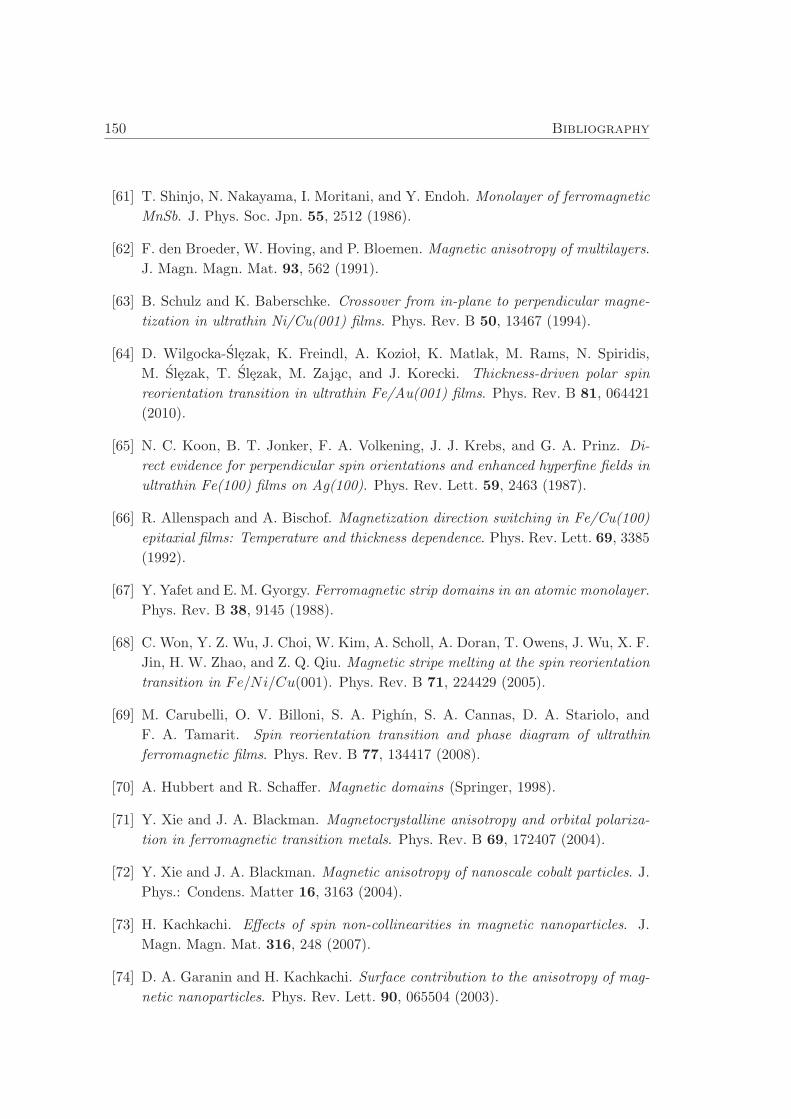
150 Bibliography
[61] T. Shinjo, N. Nakayama, I. Moritani, and Y. Endoh. Monolayer of ferromagnetic
MnSb. J. Phys. Soc. Jpn. 55, 2512 (1986).
[62] F. den Broeder, W. Hoving, and P. Bloemen. Magnetic anisotropy of multilayers.
J. Magn. Magn. Mat. 93, 562 (1991).
[63] B. Schulz and K. Baberschke. Crossover from in-plane to perpendicular magne-
tization in ultrathin Ni/Cu(001) films. Phys. Rev. B 50, 13467 (1994).
[64] D. Wilgocka-Slezak, K. Freindl, A. Kozio l, K. Matlak, M. Rams, N. Spiridis,
M. Slezak, T. Slezak, M. Zajac, and J. Korecki. Thickness-driven polar spin
reorientation transition in ultrathin Fe/Au(001) films. Phys. Rev. B 81, 064421
(2010).
[65] N. C. Koon, B. T. Jonker, F. A. Volkening, J. J. Krebs, and G. A. Prinz. Di-
rect evidence for perpendicular spin orientations and enhanced hyperfine fields in
ultrathin Fe(100) films on Ag(100). Phys. Rev. Lett. 59, 2463 (1987).
[66] R. Allenspach and A. Bischof. Magnetization direction switching in Fe/Cu(100)
epitaxial films: Temperature and thickness dependence. Phys. Rev. Lett. 69, 3385
(1992).
[67] Y. Yafet and E. M. Gyorgy. Ferromagnetic strip domains in an atomic monolayer.
Phys. Rev. B 38, 9145 (1988).
[68] C. Won, Y. Z. Wu, J. Choi, W. Kim, A. Scholl, A. Doran, T. Owens, J. Wu, X. F.
Jin, H. W. Zhao, and Z. Q. Qiu. Magnetic stripe melting at the spin reorientation
transition in Fe/Ni/Cu(001). Phys. Rev. B 71, 224429 (2005).
[69] M. Carubelli, O. V. Billoni, S. A. Pighın, S. A. Cannas, D. A. Stariolo, and
F. A. Tamarit. Spin reorientation transition and phase diagram of ultrathin
ferromagnetic films. Phys. Rev. B 77, 134417 (2008).
[70] A. Hubbert and R. Schaffer. Magnetic domains (Springer, 1998).
[71] Y. Xie and J. A. Blackman. Magnetocrystalline anisotropy and orbital polariza-
tion in ferromagnetic transition metals. Phys. Rev. B 69, 172407 (2004).
[72] Y. Xie and J. A. Blackman. Magnetic anisotropy of nanoscale cobalt particles. J.
Phys.: Condens. Matter 16, 3163 (2004).
[73] H. Kachkachi. Effects of spin non-collinearities in magnetic nanoparticles. J.
Magn. Magn. Mat. 316, 248 (2007).
[74] D. A. Garanin and H. Kachkachi. Surface contribution to the anisotropy of mag-
netic nanoparticles. Phys. Rev. Lett. 90, 065504 (2003).
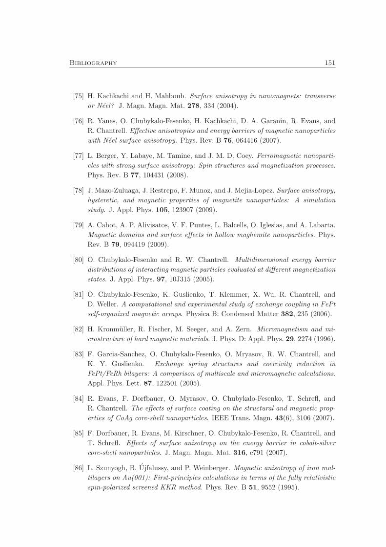
Bibliography 151
[75] H. Kachkachi and H. Mahboub. Surface anisotropy in nanomagnets: transverse
or Neel? J. Magn. Magn. Mat. 278, 334 (2004).
[76] R. Yanes, O. Chubykalo-Fesenko, H. Kachkachi, D. A. Garanin, R. Evans, and
R. Chantrell. Effective anisotropies and energy barriers of magnetic nanoparticles
with Neel surface anisotropy. Phys. Rev. B 76, 064416 (2007).
[77] L. Berger, Y. Labaye, M. Tamine, and J. M. D. Coey. Ferromagnetic nanoparti-
cles with strong surface anisotropy: Spin structures and magnetization processes.
Phys. Rev. B 77, 104431 (2008).
[78] J. Mazo-Zuluaga, J. Restrepo, F. Munoz, and J. Mejia-Lopez. Surface anisotropy,
hysteretic, and magnetic properties of magnetite nanoparticles: A simulation
study. J. Appl. Phys. 105, 123907 (2009).
[79] A. Cabot, A. P. Alivisatos, V. F. Puntes, L. Balcells, O. Iglesias, and A. Labarta.
Magnetic domains and surface effects in hollow maghemite nanoparticles. Phys.
Rev. B 79, 094419 (2009).
[80] O. Chubykalo-Fesenko and R. W. Chantrell. Multidimensional energy barrier
distributions of interacting magnetic particles evaluated at different magnetization
states. J. Appl. Phys. 97, 10J315 (2005).
[81] O. Chubykalo-Fesenko, K. Guslienko, T. Klemmer, X. Wu, R. Chantrell, and
D. Weller. A computational and experimental study of exchange coupling in FePt
self-organized magnetic arrays. Physica B: Condensed Matter 382, 235 (2006).
[82] H. Kronmuller, R. Fischer, M. Seeger, and A. Zern. Micromagnetism and mi-
crostructure of hard magnetic materials. J. Phys. D: Appl. Phys. 29, 2274 (1996).
[83] F. Garcia-Sanchez, O. Chubykalo-Fesenko, O. Mryasov, R. W. Chantrell, and
K. Y. Guslienko. Exchange spring structures and coercivity reduction in
FePt/FeRh bilayers: A comparison of multiscale and micromagnetic calculations.
Appl. Phys. Lett. 87, 122501 (2005).
[84] R. Evans, F. Dorfbauer, O. Myrasov, O. Chubykalo-Fesenko, T. Schrefl, and
R. Chantrell. The effects of surface coating on the structural and magnetic prop-
erties of CoAg core-shell nanoparticles. IEEE Trans. Magn. 43(6), 3106 (2007).
[85] F. Dorfbauer, R. Evans, M. Kirschner, O. Chubykalo-Fesenko, R. Chantrell, and
T. Schrefl. Effects of surface anisotropy on the energy barrier in cobalt-silver
core-shell nanoparticles. J. Magn. Magn. Mat. 316, e791 (2007).
[86] L. Szunyogh, B. Ujfalussy, and P. Weinberger. Magnetic anisotropy of iron mul-
tilayers on Au(001): First-principles calculations in terms of the fully relativistic
spin-polarized screened KKR method. Phys. Rev. B 51, 9552 (1995).
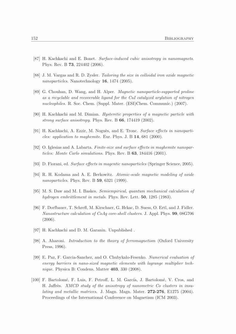
152 Bibliography
[87] H. Kachkachi and E. Bonet. Surface-induced cubic anisotropy in nanomagnets.
Phys. Rev. B 73, 224402 (2006).
[88] J. M. Vargas and R. D. Zysler. Tailoring the size in colloidal iron oxide magnetic
nanoparticles. Nanotechnology 16, 1474 (2005).
[89] G. Chouhan, D. Wang, and H. Alper. Magnetic nanoparticle-supported proline
as a recyclable and recoverable ligand for the CuI catalyzed arylation of nitrogen
nucleophiles. R. Soc. Chem. (Suppl. Mater. (ESI)Chem. Communic.) (2007).
[90] H. Kachkachi and M. Dimian. Hysteretic properties of a magnetic particle with
strong surface anisotropy. Phys. Rev. B 66, 174419 (2002).
[91] H. Kachkachi, A. Ezzir, M. Nogues, and E. Tronc. Surface effects in nanoparti-
cles: application to maghemite. Eur. Phys. J. B 14, 681 (2000).
[92] O. Iglesias and A. Labarta. Finite-size and surface effects in maghemite nanopar-
ticles: Monte Carlo simulations. Phys. Rev. B 63, 184416 (2001).
[93] D. Fiorani, ed. Surface effects in magentic nanoparticles (Springer Science, 2005).
[94] R. H. Kodama and A. E. Berkowitz. Atomic-scale magnetic modeling of oxide
nanoparticles. Phys. Rev. B 59, 6321 (1999).
[95] M. S. Daw and M. I. Baskes. Semiempirical, quantum mechanical calculation of
hydrogen embrittlement in metals. Phys. Rev. Lett. 50, 1285 (1983).
[96] F. Dorfbauer, T. Schrefl, M. Kirschner, G. Hrkac, D. Suess, O. Ertl, and J. Fidler.
Nanostructure calculation of CoAg core-shell clusters. J. Appl. Phys. 99, 08G706
(2006).
[97] H. Kachkachi and D. M. Garanin. Unpublished .
[98] A. Aharoni. Introduction to the theory of ferromagnetism (Oxford University
Press, 1996).
[99] E. Paz, F. Garcia-Sanchez, and O. Chubykalo-Fesenko. Numerical evaluation of
energy barriers in nano-sized magnetic elements with lagrange multiplier tech-
nique. Physica B: Condens. Matter 403, 330 (2008).
[100] F. Bartolome, F. Luis, F. Petroff, L. M. Garcıa, J. Bartolome, V. Cros, and
H. Jaffres. XMCD study of the anisotropy of nanometric Co clusters in insu-
lating and metallic matrices. J. Magn. Magn. Mater. 272-276, E1275 (2004).
Proceedings of the International Conference on Magnetism (ICM 2003).
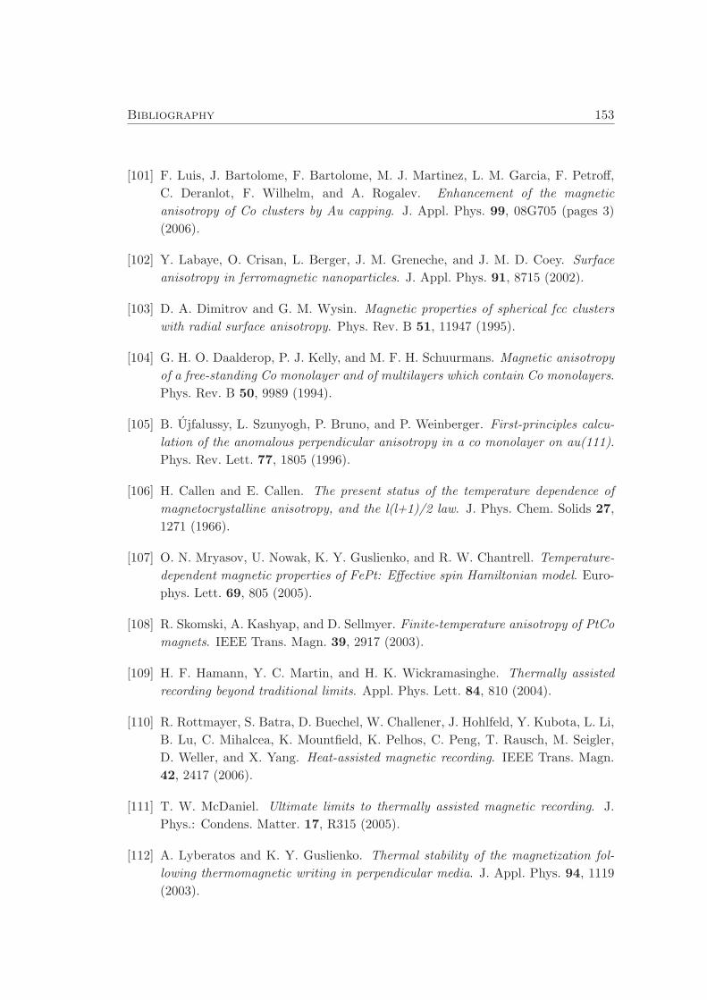
Bibliography 153
[101] F. Luis, J. Bartolome, F. Bartolome, M. J. Martinez, L. M. Garcia, F. Petroff,
C. Deranlot, F. Wilhelm, and A. Rogalev. Enhancement of the magnetic
anisotropy of Co clusters by Au capping. J. Appl. Phys. 99, 08G705 (pages 3)
(2006).
[102] Y. Labaye, O. Crisan, L. Berger, J. M. Greneche, and J. M. D. Coey. Surface
anisotropy in ferromagnetic nanoparticles. J. Appl. Phys. 91, 8715 (2002).
[103] D. A. Dimitrov and G. M. Wysin. Magnetic properties of spherical fcc clusters
with radial surface anisotropy. Phys. Rev. B 51, 11947 (1995).
[104] G. H. O. Daalderop, P. J. Kelly, and M. F. H. Schuurmans. Magnetic anisotropy
of a free-standing Co monolayer and of multilayers which contain Co monolayers.
Phys. Rev. B 50, 9989 (1994).
[105] B. Ujfalussy, L. Szunyogh, P. Bruno, and P. Weinberger. First-principles calcu-
lation of the anomalous perpendicular anisotropy in a co monolayer on au(111).
Phys. Rev. Lett. 77, 1805 (1996).
[106] H. Callen and E. Callen. The present status of the temperature dependence of
magnetocrystalline anisotropy, and the l(l+1)/2 law. J. Phys. Chem. Solids 27,
1271 (1966).
[107] O. N. Mryasov, U. Nowak, K. Y. Guslienko, and R. W. Chantrell. Temperature-
dependent magnetic properties of FePt: Effective spin Hamiltonian model. Euro-
phys. Lett. 69, 805 (2005).
[108] R. Skomski, A. Kashyap, and D. Sellmyer. Finite-temperature anisotropy of PtCo
magnets. IEEE Trans. Magn. 39, 2917 (2003).
[109] H. F. Hamann, Y. C. Martin, and H. K. Wickramasinghe. Thermally assisted
recording beyond traditional limits. Appl. Phys. Lett. 84, 810 (2004).
[110] R. Rottmayer, S. Batra, D. Buechel, W. Challener, J. Hohlfeld, Y. Kubota, L. Li,
B. Lu, C. Mihalcea, K. Mountfield, K. Pelhos, C. Peng, T. Rausch, M. Seigler,
D. Weller, and X. Yang. Heat-assisted magnetic recording. IEEE Trans. Magn.
42, 2417 (2006).
[111] T. W. McDaniel. Ultimate limits to thermally assisted magnetic recording. J.
Phys.: Condens. Matter. 17, R315 (2005).
[112] A. Lyberatos and K. Y. Guslienko. Thermal stability of the magnetization fol-
lowing thermomagnetic writing in perpendicular media. J. Appl. Phys. 94, 1119
(2003).
154 Bibliography
[113] F. G. Sanchez, O. Chubykalo-Fesenko, O. Mryasov, and R. Chantrell. Multiscale
modelling of hysteresis in FePt/FeRh bilayer. Physica B: Condensed Matter 372,
328 (2006).
[114] J.-U. Thiele, S. Maat, and E. E. Fullerton. FeRh/FePt exchange spring films for
thermally assisted magnetic recording media. Appl. Phys. Lett. 82, 2859 (2003).
[115] K. Y. Guslienko, O. Chubykalo-Fesenko, O. Mryasov, R. Chantrell, and D. Weller.
Magnetization reversal via perpendicular exchange spring in FePt/FeRh bilayer
films. Phys. Rev. B 70, 104405 (2004).
[116] U. Atxitia, O. Chubykalo-Fesenko, N. Kazantseva, D. Hinzke, U. Nowak, and
R. W. Chantrell. Micromagnetic modeling of laser-induced magnetization dy-
namics using the Landau-Lifshitz-Bloch equation. Appl. Phys. Lett. 91, 232507
(2007).
[117] A. Berger and H. Hopster. Nonequilibrium magnetization near the reorientation
phase transition of Fe/Ag(100) films. Phys. Rev. Lett. 76, 519 (1996).
[118] I.-G. Baek, H. G. Lee, H.-J. Kim, and E. Vescovo. Spin reorientation transition
in Fe(110) thin films: The role of surface anisotropy. Phys. Rev. B 67, 075401
(2003).
[119] A. Enders, D. Peterka, D. Repetto, N. Lin, A. Dmitriev, and K. Kern. Tempera-
ture dependence of the surface anisotropy of Fe ultrathin films on Cu(001). Phys.
Rev. Lett. 90, 217203 (2003).
[120] M. Farle. Ferromagnetic resonance of ultrathin metallic layers. Rep. Progr. Phys.
61, 755 (1998).
[121] N. Kazantseva, D. Hinzke, U. Nowak, R. W. Chantrell, U. Atxitia, and
O. Chubykalo-Fesenko. Towards multiscale modeling of magnetic materials: Sim-
ulations of FePt. Phys. Rev. B 77, 184428 (2008).
[122] B. C. Chuang D.S. and O. R.C. Surface and step magnetic anisotropy. Phys.
Rev. B 51, 11947 (1995).
[123] N. Metropolis, A. Rosenbluth, M. Rosembluth, A. Teller, and E. Teller. Equation
of state calculations by fast computing machines. J. Chem. Phys. 21, 1087 (1953).
[124] J. M. Gonzalez, O. A. Chubykalo, and R. S. Rueda. A micromagnetic approach,
based on the Monte Carlo algorithm, to the thermally activated magnetization
reversal processes. J. Magn. Magn. Mat. 203, 18 (1999).
[125] R.Evans. Ph.D. thesis, University of York,UK (2009).
Bibliography 155
[126] P. Asselin, R. F. L. Evans, J. Barker, R. W. Chantrell, R. Yanes, O. Chubykalo-
Fesenko, D. Hinzke, and U. Nowak. Constrained Monte Carlo method and calcu-
lation of the temperature dependence of magnetic anisotropy. Phys. Rev. B 82,
054415 (2010).
[127] L. S. Campana, A. C. D’Auria, M. D’Ambrosio, U. Esposito, L. De Cesare,
and G. Kamieniarz. Spectral-density method for classical systems: Heisenberg
ferromagnet. Phys. Rev. B 30, 2769 (1984).
[128] G. A. Baker, H. E. Gilbert, J. Eve, and G. S. Rushbrooke. High-temperature
expansions for the spin 1/2 Heisenberg model. Phys. Rev. 164, 800 (1967).
[129] C. Zener. Classical theory of the temperature dependence of magnetic anisotropy
energy. Phys. Rev. 96, 1335 (1954).
[130] K. Binder and P. C. Hohenberg. Surface effects on magnetic phase transitions.
Phys. Rev. B 9, 2194 (1974).
[131] T. Kaneyoshi. Surface magnetism; magnetization and anisotropy at a surface. J.
Phys.: Condens. Matter 3, 4497 (1991).
[132] C. Chappert and P. Bruno. Magnetic anisotropy in metallic ultrathin films and
related experiments on cobalt films. J. Appl. Phys. 64, 5736 (1988).
[133] G. Andre, A. Aspelmeier, B. Schulz, M. Farle, and K. Baberschke. Temperature
dependence of surface and volume anisotropy in Gd/W(110). Surface Science
326, 275 (1995).
[134] M. Farle, W. Platow, A. N. Anisimov, B. Schulz, and K. Baberschke. The tem-
perature dependence of magnetic anisotropy in ultra-thin films. J. Mag. Magn.
Matt. 165(74), 4 (1997).
[135] A. Buruzs, P. Weinberger, L. Szunyogh, L. Udvardi, P. I. Chleboun, A. M. Fis-
cher, and J. B. Staunton. Ab initio theory of temperature dependence of magnetic
anisotropy in layered systems: Applications to thin Co films on Cu(100). Phys.
Rev. B 76, 064417 (2007).
[136] J. B. Staunton, L. Szunyogh, A. Buruzs, B. L. Gyorffy, S. Ostanin, and L. Ud-
vardi. Temperature dependence of magnetic anisotropy: An ab initio approach.
Phys. Rev. B 74, 144411 (2006).
[137] D. Pescia and V. L. Pokrovsky. Perpendicular versus in-plane magnetization in
a 2D Heisenberg monolayer at finite temperatures. Phys. Rev. Lett. 65, 2599
(1990).

156 Bibliography
[138] B. Dieny and A. Vedyayev. Crossover from easy-plane to perpendicular anisotropy
in magnetic thin films: canted anisotropy due to partial coverage or interfacial
roughness. Europhys. Lett. 25, 723 (1994).
[139] U. Atxitia, D. Hinzke, O. Chubykalo-Fesenko, U. Nowak, H. Kachkachi, O. N.
Mryasov, R. F. Evans, and R. W. Chantrell. Multiscale modeling of magnetic
materials: Temperature dependence of the exchange stiffness. Phys. Rev. B 82,
134440 (2010).
[140] URL http://www.magpar.net/.
[141] URL http://math.nist.gov/oommf/.
[142] L. Udvardi, L. Szunyogh, K. Palotas, and P. Weinberger. First-principles rel-
ativistic study of spin waves in thin magnetic films. Phys. Rev. B 68, 104436
(2003).
[143] P. Hohenberg and W. Kohn. Inhomogeneous Electron Gas. Phys. Rev. 136, B864
(1964).
[144] W. Kohn and L. J. Sham. Self-consistent equations including exchange and cor-
relation effects. Phys. Rev. 140, A1133 (1965).
[145] L. Hedin and B. I. Lundqvist. Explicit local exchange-correlation potentials. J.
Phys. C: Solid State Phys. 4, 2064 (1971).
[146] J. P. Perdew, J. A. Chevary, S. H. Vosko, K. A. Jackson, M. R. Pederson, D. J.
Singh, and C. Fiolhais. Atoms, molecules, solids, and surfaces: Applications of
the generalized gradient approximation for exchange and correlation. Phys. Rev.
B 46, 6671 (1992).
[147] U. von Barth and L. Hedin. A local exchange-correlation potential for the spin
polarized case. J. Phys. C: Solid State Phys. 5, 1629 (1972).
[148] J. Korringa. On the calculation of the energy of a Bloch wave in a metal. Physica
13, 392 (1947).
[149] W. Kohn and N. Rostoker. Solution of the Schrodinger equation in Periodic
Lattices with an Application to Metallic Lithium. Phys. Rev. 94, 1111 (1954).
[150] L. Szunyogh, B. Ujfalussy, P. Weinberger, and J. Kollar. Self-consistent localized
KKR scheme for surfaces and interfaces. Phys. Rev. B 49, 2721 (1994).
[151] M. C. Munoz, V. R. Velasco, and F. Garcia-Moliner. Surface and interface
electronic structure calculations with empirical tight binding models. Physica
Scripta 35, 504 (1987).
Bibliography 157
[152] M. P. L. Sancho, J. M. L. Sancho, J. M. L. Sancho, and J. Rubio. Highly con-
vergent schemes for the calculation of bulk and surface green functions. J. Phys.
F: Met. Phys. 15(4), 851 (1985).
[153] M. C. Munoz, V. R. Velasco, and F. Garcıa-Moliner. Electronic structure of
AlAs-GaAs superlattices. Phys. Rev. B 39, 1786 (1989).
[154] P. Lloyd. Wave propagation through an assembly of spheres: II. The density of
single-particle eigenstates. Proc. Phys.l Soc. 90(1), 207 (1967).
[155] J. Zabloud, R. Hammerling, L. Szunyogh, and P. Weinberger. Electron Sacttering
in Solid Matter: A Theoretical and Computational treatise, vol. 147 of Series in
solid state science (Springer, 2005).
[156] N. S. Gonzalez, S. Gallego, and M. C. Munoz. Private communication .
[157] H. B. Michaelson. The work function of the elements and its periodicity. J. Appl.
Phys. 48, 4729 (1977).
[158] R. Smoluchowski. Anisotropy of the electronic work function of metals. Phys.
Rev. 60, 661 (1941).
[159] N. D. Lang and W. Kohn. Theory of metal surfaces: Work function. Phys. Rev.
B 3, 1215 (1971).
[160] P. Soderlind, O. Eriksson, B. Johansson, R. C. Albers, and A. M. Boring. Spin
and orbital magnetism in Fe-Co and Co-Ni alloys. Phys. Rev. B 45, 12911 (1992).
[161] M. Tischer, O. Hjortstam, D. Arvanitis, J. Hunter Dunn, F. May, K. Baberschke,
J. Trygg, J. M. Wills, B. Johansson, and O. Eriksson. Enhancement of orbital
magnetism at surfaces: Co on Cu(100). Phys. Rev. Lett. 75, 1602 (1995).
[162] O. Eriksson, A. M. Boring, R. C. Albers, G. W. Fernando, and B. R. Cooper.
Spin and orbital contributions to surface magnetism in 3d elements. Phys. Rev.
B 45, 2868 (1992).
[163] R. Wu, D. Wang, and A. J. Freeman. First principles investigation of the validity
and range of applicability of the X-ray magnetic circular dichroism sum rule.
Phys. Rev. Lett. 71, 3581 (1993).
[164] N. Nakajima, T. Koide, T. Shidara, H. Miyauchi, H. Fukutani, A. Fujimori, K. Iio,
T. Katayama, M. Nyvlt, and Y. Suzuki. Perpendicular magnetic anisotropy
caused by interfacial hybridization via enhanced orbital moment in Co/Pt mul-
tilayers: Magnetic circular x-ray dichroism study. Phys. Rev. Lett. 81, 5229
(1998).
158 Bibliography
[165] H. A. Durr, S. S. Dhesi, E. Dudzik, D. Knabben, G. van der Laan, J. B. Goed-
koop, and F. U. Hillebrecht. Spin and orbital magnetization in self-assembled Co
clusters on Au(111). Phys. Rev. B 59, R701 (1999).
[166] N. Jaouen, F. Wilhelm, A. Rogalev, J. Goulon, L. Ortega, J. M. Tonnerre, and
A. Yaresko. Electronic and magnetic interfacial states of Ag in an Ni81Fe19/Ag
coupled multilayer. J. Phys.: Condens. Matter 20, 095005 (2008).
[167] A. I. Liechtenstein, M. I. Katsnelson, V. P. Antropov, and V. A. Gubanov. Lo-
cal spin density functional approach to the theory of exchange interactions in
ferromagnetic metals and alloys. J. Magn. Magn. Mat. 67, 65 (1987).
[168] B. L. Gyorffy, A. J. Pindor, J. Staunton, G. M. Stocks, and H. Winter. A first-
principles theory of ferromagnetic phase transitions in metals. J. Phys. F: Metal
Phys. 15, 1337 (1985).
[169] V. P. Antropov, M. I. Katsnelson, B. N. Harmon, M. van Schilfgaarde, and
D. Kusnezov. Spin dynamics in magnets: Equation of motion and finite temper-
ature effects. Phys. Rev. B 54, 1019 (1996).
[170] L. Szunyogh and L. Udvardi. Ab initio calculation of Heisenberg parameters in
thin magnetic films. Philosophical Magazine B 78, 617 (1998).
[171] L. Szunyogh and L. Udvardi. Ab initio calculation of Heisenberg parameters and
Curie temperatures in thin magnetic films. J. Magn. Magn. Mat. 198-199, 537
(1999).
[172] P. Mavropoulos. Multiscale modelling of magnetic materials: From the total
energy of the homogeneous electron gas to the Curie temperature of ferromagnets.
Multiscale Sim. Met. Mol. Science 42, 271 (2009).
[173] L. Szunyogh, B. Lazarovits, L. Udvardi, J. Jackson, and U. Nowak. Giant mag-
netic anisotropy of the bulk antiferromagnets IrMn and IrMn3 from first prin-
ciples. Phys. Rev. B 79, 020403 (2009).
[174] J. B. Staunton, S. Ostanin, S. S. A. Razee, B. L. Gyorffy, L. Szunyogh, B. Gi-
natempo, and E. Bruno. Temperature dependent magnetic anisotropy in metallic
magnets from an ab initio electronic structure theory: L10-ordered FePt. Phys.
Rev. Lett. 93, 257204 (2004).
[175] I. Dzyaloshinsky. A thermodynamic theory of ”weak” ferromagnetism of antifer-
romagnetics. J. Phys. Chem. Solids 4, 241 (1958).
[176] T. Moriya. Anisotropic superexchange interaction and weak ferromagnetism.
Phys. Rev. 120, 91 (1960).
Bibliography 159
[177] A. Crepieux and C. Lacroix. Dzyaloshinsky-Moriya interactions induced by sym-
metry breaking at a surface. J. Magn. Magn. Mat. 182, 341 (1998).
[178] A. Antal, B. Lazarovits, L. Balogh, L. Udvardi, and L. Szunyogh. Multi-
escale studies of complex magnetism of nanostructures based on first principles.
Philosoph. Magazine 88, 2715 (2008).
[179] D.-S. Wang, R. Wu, and A. J. Freeman. First-principles theory of surface mag-
netocrystalline anisotropy and the diatomic-pair model. Phys. Rev. B 47, 14932
(1993).
[180] C. Kittel. Theory of the structure of ferromagnetic domains in films and small
particles. Phys. Rev. 70, 965 (1946).
[181] R. Drautz and M. Fahnle. Spin-cluster expansion: Parametrization of the general
adiabatic magnetic energy surface with ab initio accuracy. Phys. Rev. B 69,
104404 (2004).
[182] R. Drautz and M. Fahnle. Parametrization of the magnetic energy at the atomic
level. Phys. Rev. B 72, 212405 (2005).
[183] M. Pajda, J. Kudrnovsky, I. Turek, V. Drchal, and P. Bruno. Ab initio calcula-
tions of exchange interactions, spin-wave stiffness constants, and Curie temper-
atures of Fe, Co, and Ni. Phys. Rev. B 64, 174402 (2001).
[184] R. Skomski. Nanomagnetics. J. Phys.: Condens. Matter 15(20), R841 (2003).
[185] A. B. Shick and O. N. Mryasov. Coulomb correlations and magnetic anisotropy
in ordered L10 CoPt and FePt alloys. Phys. Rev. B 67, 172407 (2003).

160 Bibliography
List of Publications of R. Yanes
[1 ] R. Yanes, O. Chubykalo-Fesenko, H. Kachkachi, D. A. Garanin, R. Evans, and R.
W. Chantrell ”Effective anisotropies and energy barriers of magnetic nanoparti-
cles with Neel surface anisotropy”, Phys. Rev. B, vol. 40, page 2140, (2007).
[2 ] M. Jaafar, R. Yanes ,A. Asenjo, O. Chubykalo-Fesenko, M. Vazquez, E.M. Gonzalez
y J. L. Vicent. ”Field induced vortex dynamics in magnetic Ni nanotriangles”,
Nanotechnology , vol. 19, page 285717, (2008).
[3 ] G.R. Aranda; O. Chubykalo-Fesenko; R. Yanes; J. Gonzalez; J.J. del Val; R. W.
Chantrell; Y. K. Takahashi and K. Huno. ”Coercive field and Energy Barriers
in partially disorded FePt nanoparticle”. J. Appl. Phys., vol. 105, page 07B514,
(2009).
[4 ] R. Yanes and O. Chubykalo-Fesenko. ”Modelling of the influence of the Neel sur-
face anisotropy on the enhancement of the magnetic anisotropy in Co nanoparti-
cle”. J. Phys. D: Appl. Phys, vol. 42, page 055013, (2009).
[5 ] R. Yanes , R. Rozada, F. Garcia-Sanchez, O. Chubykalo-Fesenko,P. M. Pimentel,
B. Leven, B. Hillebrands. ”Modeling of microwave-assisted switching in micron-
size magnetic ellipsoids”. Phys. Rev. B, vol. 79, page 224427, (2009).
[6 ] R.F.L. Evans, R. Yanes, O. Mryasov, R.W. Chantrell and O. Chubykalo-Fesenko.
”On beating the superparamagnetic limit with exchange bias”. EPL, vol. 88, page
57004, (2009).
[7 ] M. Jaafar, R. Yanes, D. Perez de Lara, O. Chubykalo-Fesenko, A. Asenjo, E.M.
Gonzalez, J.V. Anguita, M. Vazquez and J.L. Vicent. ”Control of the chirality
and polarity of magnetic vortices in triangular nanodots”. Phys. Rev. B, vol.
81, page 054439, (2010.)
[8 ] P. Asselin, R.F.L. Evans, J. Barker, R.W. Chantrell, R. Yanes, O. Chubykalo-
Fesenko, D. Hinzke and U. Nowak. ”Constrained Monte Carlo method and cal-
culation of the temperature dependence of magnetic anisotropy”. Phys. Rev. B,
vol. 82, page 054415, (2010).
161
162 Bibliography
[9 ] R. Yanes, O. Chubykalo-Fesenko, R.F.L. Evans and R.W. Chantrell ”Tempera-
ture dependence of the effective anisotropies in magnetic nanoparticles with Neel
surface anisotropy”. J. Phys. D: Appl. Phys, vol. 43, page 474009, (2010).
Agradecimientos
Esta es la seccion mas gratificante de toda esta tesis, es en este punto donde puedo
expresar mi agradecimiento a todas esas personas que me han ayudado a lo largo de
estos anos.
En primer lugar me gustarıa darle las gracias a mi directora de tesis Oksana Fesenko
por brindarme la posibilidad de entrar en este mundo, por sus valiosos consejos, por
su confianza y en esta ultima fase por entender mi frustracion en los malos momentos.
Me gustarıa agradecer a mi tutor Dr. Farkhad Aliev por su disponibilidad.
Gracias a los Prof. Hamid Kachkachi, Prof. Roy W. Chantrell. y Prof. Laszlo
Szunyogh por sus discusiones sobre fısica y por su calurosa acogida en mis estancias.
Tambien me gustarıa agradecer a Dr. J. Palomares, Dr. F. Cebollada, y Prof. J.
Gonzalez, su acogida en el grupo y su apoyo a lo largo de estos anos.
Esta tesis no se podrıa haber llevado a cabo sin la ayuda inestimable de Juan
Manuel Rodrıguez Puerta (Juanma), por acudir con una sonrisa en mi ayuda cada vez
que el cluster o MAGPAR me ponıa contra las cuerdas, muchas gracias.
Gracias a Felipe becario senior a mi llegada al grupo ahora flamante post-doc por
haberme facilitado la entrada en el mundo del magnetismo y por su ayuda con todos
mis problemas de compilacion.
Gracias a Silvia Gallego y M. Carmen Munoz por su ayuda intentando que en-
tendiera algo de los calculos SKKR.
Gracias a Elvira (la mejor DJ) por su vision entusiasta de la vida.
Gracias a Unai por ser tan buen companero, a pesar de sus chistes.
Gracias a Virginia por compartir este duro camino de la tesis, por convencerme
para hacer el camino de Santiago y sobre todo por su amistad.
Gracias a Samuel, Rafa y Jesus mis compis del despacho 168 con ellos compartı
grandes momentos, escuche muchas horas de Radio 3 y aprendı mucho.
Gracias a Ruben, Almudena, Laura, Yorexis, Ezzouhra, Javier companeros tem-
porales o permanentes del despacho 159, por conseguir que todos los dias tengan una
sonrisa.
Estos agradecimientos no estarıan completos si no menciono a Javier Mendez, Jorge
Iribas, Arturo Baro, Nacho Jimenez, Marıa Moreno con los que he compartido muchas
bromas y risas en la hora de la comida, gracias a todos por aceptar a esta becaria en
su grupo y permitirme conocer a unas bellısimas personas.
163

164 Agradecimientos
Gracias a mis amigos del ICMM Aldo, Ramon, Karin, Lucıa, Lidia, Mercedes,
Karla, Miriam, Wagner, ası como a los amigos que encontre en mis estancias Richard,
Natalia, Attila, Eva por los gratos momentos.
Y como existe vida mas alla del ICMM, gracias a Conchi por su amistad, por su
apoyo continuo y sincero, y por escuchar todas mis charlas aunque creo que la aburrıan,
en definitiva por estar ahı. Gracias tambien a Mar, Manolo y Noemı por las cenas y
las paellitas los domingos, me habeis hecho sentir en casa.
Por ultimo no puedo dejar de agradecer a mi familia. Agradecer a esas personas
que me han dado su afecto y su carino desde que no levantaba un palmo del suelo, a
mis padres Pedro y Josefa, por todo el amor que me han dado. Gracias a mis hermanos
Natalia, Pedro y Jose por sus consejos, su carino y su apoyo incondicional.