NETWORKS AND HETEROGENEOUS MEDIA doi:10.3934/nhm.2015.10.209c©American Institute of Mathematical SciencesVolume 10, Number 1, March 2015 pp. 209–221

EFFECT OF ANISOTROPIES

ON THE MAGNETIZATION DYNAMICS

Laura M. Perez, Jean Bragard and Hector Mancini

Departamento de Fısica y Matematicas Aplicadas

Universidad de Navarra, Pamplona, 31080, Spain

Jason A. C. Gallas

Departamento de Fısica

Universidade Federal da Paraıba, 58051-970 Joao Pessoa, Brazil

andInstitute for Multiscale Simulation

Friedrich-Alexander-Universitat Erlangen-Nurnberg

Nagelsbachstraße 49b, 91052 Erlangen, Germany

Ana M. Cabanas

Instituto de Alta Investigacion

Universidad de Tarapaca, Casilla 7D, Arica, Chile

Omar J. Suarez

Instituto de Alta InvestigacionUniversidad de Tarapaca, Casilla 7D, Arica, Chile

andDepartamento de Matematicas y Fısica

Universidad de Sucre, A.A. 406, Sincelejo, Colombia

David Laroze

Instituto de Alta InvestigacionUniversidad de Tarapaca, Casilla 7D, Arica, Chile

and

SUPA School of Physics and AstronomyUniversity of Glasgow, Glasgow G12 8QQ, United Kingdom

Abstract. We report a systematic investigation of the magnetic anisotropyeffects observed in the deterministic spin dynamics of a magnetic particle in

the presence of a time-dependent magnetic field. The system is modeled bythe Landau-Lifshitz-Gilbert equation and the magnetic field consists of twoterms, a constant term and a term involving a harmonic time modulation. Weconsider a general quadratic anisotropic energy with three different preferen-

tial axes. The dynamical behavior of the system is represented in Lyapunovphase diagrams, and by calculating bifurcation diagrams, Poincare sections and

Fourier spectra. We find an intricate distribution of shrimp-shaped regular is-land embedded in wide chaotic phases. Anisotropy effects are found to play akey role in defining the symmetries of regular and chaotic stability phases.

2010 Mathematics Subject Classification. Primary: 37M25, 65P20; Secondary: 65P99.Key words and phrases. Spin dynamics, anisotropy, chaos, Lyapunov exponents, Fourier

analysis.

209

210 LAURA M. PEREZ ET AL.

1. Introduction. The understanding of the dynamical processes involved in themagnetization of generic nanoparticles is a quite interesting and challenging prob-lem. Indeed, this problem contains several complex phenomena which include mul-tistability, quasiperiodicity, deterministic chaos, as well as complicated pattern for-mation and evolution [54, 41, 32]. Experimentally, the detection and classificationof such complex behaviors is a virtually impossible task because it presupposes theability of tuning material properties continuously over rather extended parameterranges and external conditions. Theoretically, the description of stability phaseshas been frequently restricted to the study of fixed-points, Hopf bifurcations andother simple informations which are routinely derived from the equations of motion.

However, the availability of fast computer clusters combined with realistic modelsoffer the possibility to simulate more complicated dynamical processes numericallylike, e.g. periodic solutions with arbitrary period length and waveforms, and to dis-cover novel material properties of interest. In this context, a first problem that needsto be tackled is the determination of the control parameter regions that supportchaotic and regular behaviors. More specifically, one needs to compute phase dia-grams displaying chaotic and regular stable phases, their extension and the detailedshape of their boundaries. When dealing with nonlinear dynamical systems, phasediagrams are frequently restricted to just a few isolated curves displaying boundariesbetween steady-state (fixed-points) solutions and solutions emerging immediatelyafter them, either by Hopf or by other simple bifurcations. Furthermore, existingphase diagrams tend to focus on unstable mathematical phenomena and/or situa-tions that are not accessible in the laboratory. Even though deterministic chaos hasbeen studied intensively for over 30 years, phase diagrams detailing the structure ofchaotic phases with high-resolution have started to be reported only quite recently.For recent surveys on this subject see, for example, Refs. [45, 29].

Nonlinear problems have been widely studied in magnetism [54, 41, 32]. Modelswere used both for discrete [3, 52, 34, 35, 36, 46, 15, 37, 38, 44] and for continuousmagnetic systems [41, 32, 4, 17, 18, 50, 51]. Recently, the chaotic behavior of an uni-axial anisotropic particle under a periodic magnetic field was studied in Refs.[15, 37].Several experiments of chaotic behaviors in magnetic systems have been reported[30, 1, 8, 16]. Typical magnetic samples are yttrium iron garnet spheres [30]. It isworth mentioning that ferromagnetic resonance techniques have allowed to uncoverdifferent routes to chaos, such as period-doubling cascades, quasi-periodic routesto chaos, or intermittent routes. This obviously implies that there is no univer-sal mechanism leading to chaos in these systems and, therefore, that a theoreticaldescription turns out to be highly non-trivial.

The characterization of the chaotic and regular phases using two-dimensionalphase diagrams displaying the largest Lyapunov of the exponents for a paramet-rically driven uni-axial anisotropic magnetic particle has been recently studied inRefs.[15, 37]. Since this type of anisotropy is a special one [41, 19], the aim of thepresent manuscript is to investigate a more general system where one combines dif-ferent anisotropy axes. This new assumption on the structure of the anisotropy willmodify the dynamical behaviors of the particles. The main goal of the present studyis to illustrate this more general setup. To this end, we have solve numerically thedimensionless Landau-Lifshitz-Gilbert (LLG) equation containing a general qua-dratic anisotropic energy. The paper is organized as follows: In Section 2, the

ANISOTROPY EFFECTS ON MAGNETIZATION DYNAMICS 211

theoretical model for a magnetic particle with a general quadratic anisotropy en-ergy is presented. In Section 3 we report the numerical simulations together with adiscussion of the results. Finally, our conclusions are presented in Section 4.

2. Theoretical model. Let us consider a magnetic particle and assume that itcan be represented by a magnetic monodomain of magnetization M governed bythe dimensionless LLG equation

κdm

dτ= −m× Γ− ηm× (m× Γ) , (1)

where m = M/Ms, τ = t|γ|Ms and κ = 1 + η2 [41, 3]. Here Ms is the sat-uration magnetization that leads to |m| = 1, and γ is the gyromagnetic factor,which is associated with the electron spin and whose numerical value is approx-imately given by |γ| = |γe|µ0 ≈ 2.21 × 105mA−1s−1. Here, η denotes the di-mensionless phenomenological damping coefficient, a material property typicallyin the range from 10−4 to 10−3 in garnets and 10−2, or larger in cobalt or innickel or in permalloy [37], giving 1/κ ≈ 0.99 ' 1. Typical experimental valuesof Ms are, e.g. Ms[Co] ≈ 1.42 × 106A/m ≈ 17.8 kOe for cobalt materials and

Ms[Ni] ≈ 4.8 × 105A/m ≈ 6 kOe for nickel materials, leading to |γ|Ms[Co] ≈308GHz and |γ|Ms[Ni] ≈ 106GHz, respectively. Hence, the corresponding time

scales are (|γ|Ms)−1 ≈ 3ps and (|γ|Ms)

−1 ≈ 6ps, respectively. Let us remark thatin these materials the macrospin approximation (monodomain particles) is valid forparticles sizes in the range of 10−20nm, because for smaller sizes surface anisotropyeffects (not included in the present study) are relevant [7] and for larger sizes non-uniform magnetic states appear, like vortices in cobalt nanodots. In addition, theshape of the particle plays an important role in the macrospin approximation [33].Finally, the fact that |m| is conserved implies automatically that Eq. (1) describespure rotations of the magnetization in 3D space.

The effective magnetic field, denoted by Γ in Eq.(1), is given by

Γ = h +

3∑j=1

αj (m · nj) nj , (2)

where h is the external magnetic field and αj measures the anisotropy along the njaxis, such that subindexes (1, 2, 3) represent the principal axes. We denote themin Cartesian coordinates as (x, y, z). We apply an external magnetic field h thatcomprises both, a constant longitudinal and a periodic transverse part with fixedamplitude and frequency

h = h0 + hT sin (Ωτ) , (3)

where h0 (‖z), hT (⊥z) and Ω are time independent. With this dimensional scaling,the dimensionless fields and frequencies are h = H/Ms and Ω = ω/ (γMs). Sincethe amplitude of field and the frequency are measured in units of Ms and (γMs),respectively, one finds that for cobalt or nickel materials the typical order of mag-nitude is 100 − 101 kOe and GHz. Here, we vary these values in the same range ofmagnitude.

The second term of the right-hand-side of the Eq. (2) corresponds to the anisotr-opy field. This term comes from anisotropy energy which essentially takes intoaccount the fact that the magnetic properties depend of the direction in which theyare measured [19]. This energy has contributions from different natures, like crystal,magneto-static, or shape anisotropy.

212 LAURA M. PEREZ ET AL.

To first-order of approximation, the characterization of the anisotropy effect isobtained by including the quadratic terms of m in the magnetic energy. In theprincipal axes representation, these terms give our prototype field [41, 19]. Let usremark that there are two special cases. The first one, called uniaxial anisotropy,involves two coefficients which are zero. The standard configuration for this caseis αx = αy = 0, and αz 6= 0. The second particular case, that we call bi-axialanisotropy, occurs when only a single coefficient is zero, for instance αz = 0. Thecoefficients αj are related to the physical values through αj = 2Kj/(µ0M

2s ) −

Nj where Kj are the physical anisotropy constants and Nj are the dimensionlessdemagnetizing factors which depend of the particle shape [33, 48, 49, 10]. The valuesof the anisotropy can be positive or negative, depending on the specific material andsample shape in use [19, 42].

From the dynamical point of view, it is worth mentioning that anisotropic parti-cles under stationary magnetic field have been studied previously in some particularcases in Ref. [41] and uni-axial anisotropic particles under time-dependent magneticfield have been numerically characterized in Refs. [3, 46, 15, 37, 38].

Finally, let us remark that for zero damping (η = 0) and without parametric forc-ing (hx = hy = 0) Eq.(1) is conservative, and its dynamics can be derived from afree energy functional, giving stationary or periodic solutions. Therefore, the inclu-sion of the dissipation and the oscillatory injection of energy drives the precessionaldynamics into multiple instabilities. In such circumstance the magnetization of theparticle may exhibit complex dynamical behavior, e.g., quasi-periodicity, and chaos[3, 15, 37]. In the next Section we provide a more exhaustive characterization ofthe chaotic regime, including its dependence on the anisotropy constants as well ason the magnetic field amplitudes, which shows elaborate and entangled patterns.

3. Simulations. This Section is divided into two parts. In the first subsection webriefly discuss the quantities, which we use to characterize temporal regimes, andin the second one some numerical results and their analysis are provided.

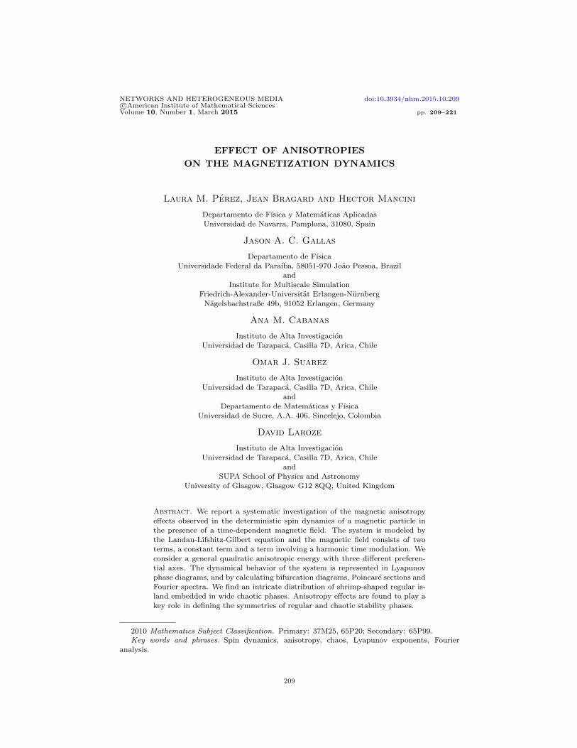
Figure 1. (Color online) Phase diagrams displaying the largestLyapunov exponent (LLE) color-coded as a function of the ampli-tudes hx and hy for αx = αy = 1.0 (left) and αx = −αy = 1.0(right). The fixed parameters are: Ω = 1.0, hz = 0.1, αz = 0 andη = 0.05. The resolutions are ∆hx = ∆hy = 0.01.

ANISOTROPY EFFECTS ON MAGNETIZATION DYNAMICS 213

3.1. Dynamical indicators. First, we characterize the dynamics of Eq. (1) byevaluating the Lyapunov exponents (LEs). This method consists of quantifyingthe divergence between two initially close trajectories of a vector field [55, 28].In general, for an effective N-dimensional dynamical system described by a set ofequations, dXi

/dτ = F i (X, τ), the ith-Lyapunov exponent is given by

λi = limτ→∞

(1

τln

(∥∥δXiτ

∥∥∥∥δXi0

∥∥))

, (4)

where ‖δXiξ‖ is the distance between the trajectories of the ith-component of the

vector field at time ξ. They can be ordered from the largest to the smallest: λ1 ≥λ2 ≥ .... ≥ λN . The first exponent is the largest Lyapunov exponent (LLE). Dueto the fact that the LLG equation conserves the modulus of the magnetization |m|and that the applied magnetic field is time dependent, the effective dimension of thephase space is three. From a dynamical system point of view, only the largest LLEmay become positive for a system of dimension three. Therefore, by exploring thedependence of the LLE on the different parameters of the system, one can identifyareas in control parameter space, where the dynamics is chaotic (LLE positive),and those showing nonchaotic dynamics (LLE vanishing or negative). Nevertheless,let us comment that since we are dealing with a one-frequency forced system, atleast one of its Lyapunov exponents is always zero; hence the simplest attractor isa periodic orbit. Another possibility is to have two or three Lyapunov exponentsequal to zero and in these cases the system exhibits a two or three-frequency quasi-periodic behavior.

Apart from the Lyapunov spectrum analysis, there are other methods of quan-tifying the dynamical behavior of a system, for example, the Fourier spectrum,Poincare sections, or correlation functions just to mention few of them [54, 41, 52,34, 3, 46, 15, 20, 39]. The classical technique to understand the time series of eachcomponents of m is to take the Fast Fourier Transform (FFT) which gives a com-plex discrete signal, S ($), in frequency space $ = ($1, ..., $n), producing a set ofpairs $k, S ($k). For this signal we calculate its power spectrum |S ($)|. In gen-eral, when |S ($)| has a finite number of discrete peaks, the time series is regular,while if there is a continuum of peaks, the series can be chaotic. Let us mentionthat the bifurcation diagrams using Poincare sections of the magnetization angles,given by m = (cosφ sin θ, sinφ sin θ, cos θ), was employed in Ref. [3] while the localmaximum of a specific component of m was used in Ref. [46]. In these diagrams,when there is a continuum of points in the variable the behavior is quasi-periodicor chaotic.

3.2. Numerical results. Many numerical schemes have been used to resolve theLLG equation [41] and to avoid numerical artifacts, it is convenient to solve Eq. (1)in the Cartesian coordinates [3]. In order to find the chaotic regimes, we haveintegrated Eq. (1) via a standard fourth-order Runge-Kutta integration scheme witha fixed time step dτ = 0.01 guaranteeing a precision of 10−8 for the magnetizationfield. The Lyapunov exponents are calculated using the technique exposed in Refs.[15, 55], such that the LEs are calculated for a time span of τ = 32768 units of timeafter an initial transient time of τ = 1024 units has been discarded. The Gram-Schmidt orthogonalization process is performed after every δτ = 1. The error Errin the evaluation of the LEs has been checked by using Err = σ (λM ) /max (λM ),where σ(λM ) is the standard deviation of the maximum positive LE. In all cases

214 LAURA M. PEREZ ET AL.

studied here Err is of the order of 1% or less, which is sufficiently small for thepurpose of the present analysis.

Figure 2. (Color online) Phase diagrams displaying the largestLyapunov exponent (LLE) color-coded as a function of the am-plitudes hz and hx for (αx, αy, αz) = (4.0, 0,−1.0) (left) and(αx, αy, αz) = (0, 4.0, 1.0) (right). The fixed parameters are:Ω = 1.0, hy = 1.0 and η = 0.05. The resolutions are ∆hz = ∆hx =0.01.

The main results are given in Figs. 1–6. In particular, we discuss the influenceof the magnetic field amplitudes and the anisotropy constants on the dynamics.The choice of parameters ensures realistic values and avoids possible artifacts dueto a specific system and, therefore, provides a general description. Due to the largenumber of control parameters involved in the system, we fix Ω = 1 and η = 0.05 forthe rest of the manuscript.

We compute two-dimensional phase diagrams illustrating the magnitude of theLLE as a function of two parameters. This allows us to determine the parameterranges that lead to chaotic dynamics, i.e. positive LLEs, and those showing regular(periodic or quasi-periodic) dynamics, LLEs zero or negative. In addition, followinga technique explained in Ref. [28], we use an iterative zoom resolution process toinvestigate further the dependence of the dynamics upon very small variations ofsystem parameters. This technique is generally used for studying dynamical sys-tems that contain chaotic phases with highly complicated and interesting boundarytopologies, e.g., curves where networks of stable islands of regular oscillations withever-increasing periodicities accumulate systematically.

Figure 1 shows a color-coded LLE phase diagram as a function of the oscilla-tory field amplitudes hx and hy for a bi-axial anisotropic particle (αz = 0). Theleft panel displays the case when both anisotropy constants have the same value(αx = αy = 1). In this case, the chaotic regions appear in a circular symmetricfashion pointing out an invariance of the LEs with respect to the orientation ofhT . Since the occurrence of chaos is independent of initial conditions and sincethere is only a single basin of attraction for the dynamics, the orientation of hT

in the perpendicular plane is irrelevant for the position of the regions with positiveLEs. We observe that no chaos is found for small amplitudes of the oscillatory

ANISOTROPY EFFECTS ON MAGNETIZATION DYNAMICS 215

transverse field and that by increasing the field amplitudes, regions with chaos andregions with regular dynamics alternate. The right panel in Fig. 1 shows the casewhen anisotropy constants have opposite signs (αx = −αy = 1). We observe thatthe circular symmetry is broken and a pattern of chaotic-regular regions appears.Nevertheless, the LLE has a mirror-inversion symmetry with respect to hy = 0 andhx → −hx. We can also observe that for small values of both amplitudes, approx-imately inside the region, 0.761h2

x + 1.1hxhy + 8.232h2y = 1, the system presents

regular states.

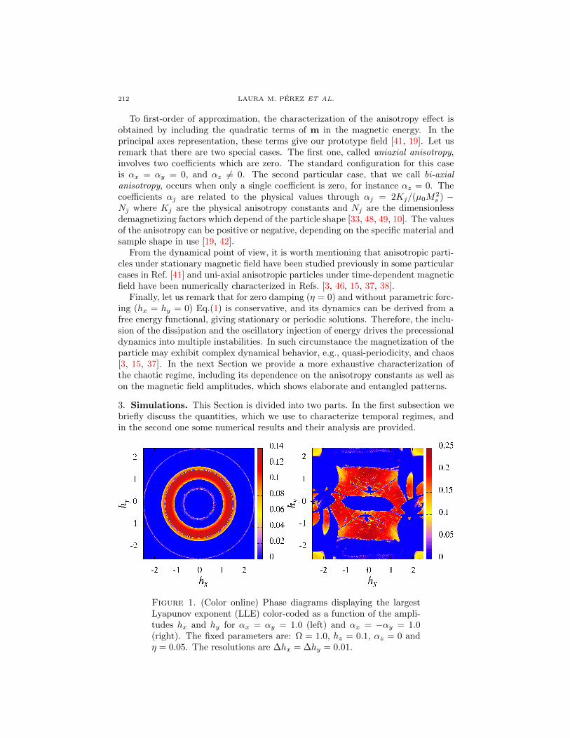
Figure 3. (Color online) (left) Magnification of the white box inthe left panel of Figure 2. (right) Magnification of the white box inthis left panel. The resolutions are (∆hz,∆hx) = (0.0032, 0.00166)and (∆hz,∆hx) = (2.0× 10−4, 7.5× 10−5), respectively.

Figure 2 shows a color-coded LLE phase diagram given as a function of the fieldamplitudes hx and hz of the periodic transverse and constant longitudinal fields,respectively. We focus on two different cases of bi-axial anisotropic particle. In theleft panel the principal axes are (x, z), while in the second panel they are (y, z).In the left panel we can observe that for the complete range of hz studied, regularsolutions are found for small values of hx (hx . 0.3). For intermediate and largevalues of hz, one observes again an alternation of chaotic and regular regions ashx increases. On the other hand, the right panel of Fig. 2 shows that chaos issuppressed for small values of both fields approximately inside the disk defined byh2x + h2

z = 1.2. Chaotic behavior is not observed for intermediate and higher valuesof longitudinal field (hz & 3) irrespective of the value of hx, indicating that thelongitudinal field stabilizes the system. In the rest of the plotted area the chaoticregions are not compact, but contain many areas of regular dynamics for specificvalues of the field amplitudes.

In oder to explore in more detail the transitions among chaotic and regular states,Figure 3 shows two successive magnifications of the left panel of Figure 2. Thesemagnifications are performed with higher resolution. In the left phase diagramwe can observe that there are special types of regular islands inside of chaoticregion. In fact, these islands have the shape of shrimps, structures that were firstdiscovered in the Henon map [27] and, subsequently, have been found abundantly inmultiple branches of physics [28, 40, 21, 53, 23, 26, 11, 12, 43, 6, 2, 22]. Finally, themagnification seen on the right panel of Figure 3 reveals an interesting pattern in the

216 LAURA M. PEREZ ET AL.

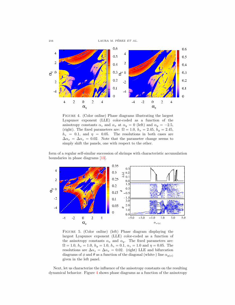
Figure 4. (Color online) Phase diagrams illustrating the largestLyapunov exponent (LLE) color-coded as a function of theanisotropy constants αz and αx at αy = 0 (left) and αy = −2.5,(right). The fixed parameters are: Ω = 1.0, hx = 2.45, hy = 2.45,hz = 0.1, and η = 0.05. The resolutions in both cases are∆αx = ∆αz = 0.02. Note that the parameter change seems tosimply shift the panels, one with respect to the other.

form of a regular self-similar succession of shrimps with characteristic accumulationboundaries in phase diagrams [13].

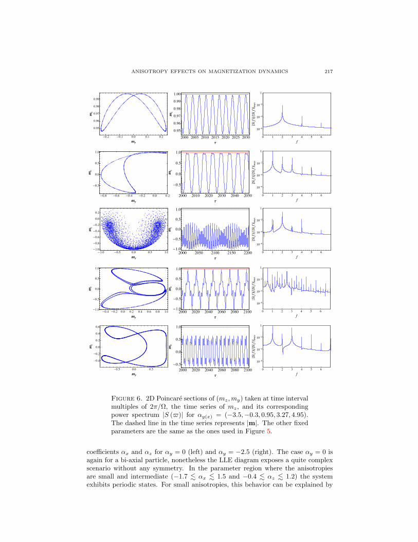
Figure 5. (Color online) (left) Phase diagram displaying thelargest Lyapunov exponent (LLE) color-coded as a function ofthe anisotropy constants αx and αy. The fixed parameters are:Ω = 1.0, hx = 1.0, hy = 1.0, hz = 0.1, αz = 1.0 and η = 0.05. Theresolutions are ∆αz = ∆αx = 0.02. (right) LLE and bifurcationdiagrams of φ and θ as a function of the diagonal (white-) line αy(x)

given in the left panel.

Next, let us characterize the influence of the anisotropy constants on the resultingdynamical behavior. Figure 4 shows phase diagrams as a function of the anisotropy

ANISOTROPY EFFECTS ON MAGNETIZATION DYNAMICS 217

2000 2050 2100 2150 2200-1.0

-0.5

0.0

0.5

1.0

t

mz

0 1 2 3 4 5 6

10-6

10-4

10-2

1.

f†SHfL§ê†SHfL§ m

ax-1.0 -0.5 0.0 0.5 1.0

-1.0

-0.8

-0.6

-0.4

-0.2

0.0

0.2

my

mz

-0.8 -0.6 -0.4 -0.2 0.0 0.2

-0.5

0.0

0.5

1.0

my

mz

2000 2010 2020 2030 2040 2050

-0.5

0.0

0.5

1.0

t

mz

0 1 2 3 4 5 6

10-6

10-4

10-2

1.

f

†SHfL§ê†SHfL§ m

ax

-0.2 -0.1 0.0 0.1 0.2

0.95

0.96

0.97

0.98

0.99

my

mz

2000 2005 2010 2015 2020 2025 2030

0.95

0.96

0.97

0.98

0.99

1.00

t

mz

0 1 2 3 4 5 6

10-6

10-4

10-2

1.

f

†SHfL§ê†SHfL§ m

ax

0 1 2 3 4 5 6

10-6

10-4

10-2

1.

f

†SHfL§ê†SHfL§ m

ax

2000 2020 2040 2060 2080 2100-0.5

0.0

0.5

1.0

t

mz

-0.5 0.0 0.5

-0.4

-0.2

0.0

0.2

0.4

0.6

my

mz

0 1 2 3 4 5 6

10-6

10-4

10-2

1.

f

†SHfL§ê†SHfL§ m

ax

-0.4 -0.2 0.0 0.2 0.4 0.6 0.8 1.0-1.0

-0.5

0.0

0.5

1.0

my

mz

2000 2020 2040 2060 2080 2100-1.0

-0.5

0.0

0.5

1.0

t

mz

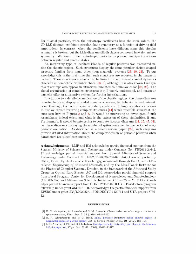
Figure 6. 2D Poincare sections of (mz,my) taken at time intervalmultiples of 2π/Ω, the time series of mz, and its correspondingpower spectrum |S ($)| for αy(x) = (−3.5,−0.3, 0.95, 3.27, 4.95).The dashed line in the time series represents |m|. The other fixedparameters are the same as the ones used in Figure 5.

coefficients αx and αz for αy = 0 (left) and αy = −2.5 (right). The case αy = 0 isagain for a bi-axial particle, nonetheless the LLE diagram exposes a quite complexscenario without any symmetry. In the parameter region where the anisotropiesare small and intermediate (−1.7 . αx . 1.5 and −0.4 . αz . 1.2) the systemexhibits periodic states. For small anisotropies, this behavior can be explained by

218 LAURA M. PEREZ ET AL.

the fact that nonlinear terms are small and the constant field plays the major rolein the dynamics. For negative values of αx almost above the curve with equation,αz = 0.04165α2

x + 0.45833αx + 4.25, the system behaves in a regular fashion. Notethat inside the main chaotic areas there are still windows without chaos. On theother hand, the right panel of Figure 4 shows the diagram for a complete anisotropicparticle (αj 6= 0). We can observe a similar pattern which is slightly rotated andelongated with respect to the previous frame. Here, the approximate line overwhich the system has regular states is given by αz = 0.17α2

x + 1.32αx + 3.5, suchthat αx < 0.

The leftmost panel in Figure 5 displays a phase diagram as a function of theanisotropy coefficients αx and αy at αz = 1.0. This diagram shows symmetricbehaviors under reflection about the diagonal line αy = αx, We call this diagonalαy(x) and indicate it by a dashed line in the figure. For negative values of bothconstants one can observe that the states are periodic approximately inside theregion, α2

x + α2y = 3.72. The same happens for the region above the curve αy =

0.0625α2x + 0.525αx + 3.3 when αx . 0.5 and for the region below the curve αy =

−1.64α2x + 13.97αx − 28.46 when αx & 2.6. In the remaining areas the system

is mainly chaotic but contains complex topological islands of regular behaviors.To explore in more detail the dynamical behaviors occurring in the diagonal line,αy(x), the right panel of Figure 5 presents a comparison of the LLE and bifurcationdiagrams of the angular variables (φ, θ). By increasing the parameter, we observethat the system starts in a periodic state and makes an abrupt transition to a chaoticbehavior. After that, an alternation of regular and chaotic behaviors is found uponfurther increase of αy(x). In addition, with the comparison of the LLE and thebifurcation diagrams one can determine precisely the segments where the regularphases correspond to periodic or quasi-periodic states. For instance, quasi-periodicoscillations can be identified in range (0.032, 1.77).

In order to illustrate different nonchaotic regimes appearing along the αy(x) diag-onal, in Figure 6 we show a 2D Poincare section of (mz,my) at time-intervals mul-tiple of 2π/Ω, the time series of mz, and its corresponding power spectrum |S ($)|for five representative values of αy(x), namely −3.5,−0.3, 0.95, 3.27 and 4.95. Fromthis figure, one sees that for −3.5 and −0.3 the system presents periodic states,while the other three parameters exhibits more complex quasiperiodic behaviors.In fact for αy(x) = 0.95 the Poincare section shows a semi-torus.

4. Final remarks. The dynamics of the magnetization of an anisotropic particlein the simultaneous presence of a constant and a periodic time-dependent externalmagnetic field has been studied in the framework of the Landau-Lifshitz-Gilbertequation.

In previous works, we investigated the control parameter space for particles un-der conditions of uniaxial anisotropy [15] and also when subjected to a quasiperiodicmagnetic field[38]. In contrast, here we considered the more general situation of par-ticles under bi-axial anisotropy. We determined the regions in control parameterspace where positive Lyapunov exponents (chaos) exist and the theoretical bound-aries for the thresholds of the chaotic regime. We performed extensive numericalcalculations of Lyapunov exponents while varying simultaneously two selected con-trol parameters. This resulted in detailed stability charts of the chaotic and regularphases as a function of these parameters.

In this more general situation, we now find anisotropy to play an important role increating an additional number of novel possible dynamical behaviors for the particle.

ANISOTROPY EFFECTS ON MAGNETIZATION DYNAMICS 219

For bi-axial particles, when the anisotropy coefficients have the same values, the2D LLE-diagram exhibits a circular shape symmetry as a function of driving fieldamplitudes. In contrast, when the coefficients have different signs this circularsymmetry is broken, but the LLE-diagram still displays a composed inversion mirrorsymmetry. We found driven anisotropic particles to present multiple transitionsbetween regular and chaotic states.

An interesting type of localized islands of regular patterns was discovered in-side the chaotic regions. Such structures display the same peculiar shrimp-shapedstructure familiar from many other (non-magnetic) systems [27, 40, 21]. To ourknowledge this is the first time that such structures are reported in the magneticcontext. These structures are known to be linked to the universal class of dynamicsobserved in homoclinic Shilnikov chaos [53, 5], although it is also known that spi-rals of shrimps also appear in situations unrelated to Shilnikov chaos [23, 26]. Theglobal organization of complex structures is still poorly understood, and magneticparticles offer an alternative system for further investigations.

In addition to a detailed classification of the chaotic regions, the phase diagramsreported here also display extended domains where regular behavior is predominant.Some time ago, the control space of a damped-driven Duffing oscillator was shownto display certain recurring complex structures [14] which resemble somewhat theones seen here in Figures 2 and 3. It would be interesting to investigate if suchresemblance indeed exists and what is the extension of these similarities, if any.Furthermore, it should be interesting to compute isospike diagrams [24, 25, 47, 31],i.e. phase diagrams displaying the number of spikes contained in one period of everyperiodic oscillation. As described in a recent review paper [29], such diagramsprovide detailed information about the complexification of periodic patterns whenparameters are tuned continuously.

Acknowledgments. LMP and HM acknowledge partial financial support from theSpanish Ministry of Science and Technology under Contract No. FIS2011-24642.JB acknowledges partial financial support from Spanish Ministry of Science andTechnology under Contract No. FIS2011-28820-C02-02. JACG was supported byCNPq, Brazil, by the Deutsche Forschungsgemeinschaft through the Cluster of Ex-cellence Engineering of Advanced Materials, and by the Max-Planck Institute forthe Physics of Complex Systems, Dresden, in the framework of the Advanced StudyGroup on Optical Rare Events. AC and DL acknowledge partial financial supportfrom Basal Program Center for Development of Nanoscience and Nanotechnology(CEDENNA) and Millennium Scientific Initiative, P10 − 022 − F . OJS acknowl-edges partial financial support from CONICYT-FONDECYT Postdoctoral programfellowship under grant 3130678. DL acknowledges the partial financial support fromEPSRC under grant EP/L002922/1, FONDECYT 1120764 and UTA-project 8750-12.

REFERENCES

[1] F. M. de Aguiar, A. Azevedo and S. M. Rezende, Characterization of strange attractors inspin-wave chaos, Phys. Rev. B, 39 (1989), 9448–9452.

[2] H. A. Albuquerque and P. C. Rech, Spiral periodic structure inside chaotic region in

parameter-space of a Chua circuit, Int. J. Circuit Theory. App., 40 (2012), 189–194.[3] L. F. Alvarez, O. Pla and O. Chubykalo, Quasiperiodicity, bistability, and chaos in the Landau-

Lifshitz equation, Phys. Rev. B , 61 (2000), 11613–11617.

220 LAURA M. PEREZ ET AL.

[4] I. V. Barashenkov, M. M. Bogdan and V. I. Korobov, Stability diagram for the phase-lockedsoliton of the parametrically driven, damped nonlinear Schrodinger equation, Europhys. Lett.,

15 (1991), 113–118.

[5] R. Barrio, A. Shilnikov and L. P. Shilnikov, Kneadings, symbolic dynamics and paintingLorenz chaos, Int. J. Bif. Chaos, 22 (2012), 1230016, 24pp.

[6] R. Barrio, F. Blesa and S. Serrano, Topological changes in periodicity hubs of dissipativesystems, Phys. Rev. Lett., 108 (2012), 214102.

[7] X. Batlle and A. Labarta, Finite-size effects in fine particles: Magnetic and transport prop-

erties, J. Phys. D, 35 (2002), R15–R42.[8] J. Becker, F. Rodelsperger, Th. Weyrauch, H. Benner, W. Just and A. Cenys, Intermittency

in spin-wave instabilities, Phys. Rev. E , 59 (1999), 1622–1632.

[9] M. Beleggia, S. Tandon, Y. Zhu and M. De Graef, On the magnetostatic interactions betweennanoparticles of arbitrary shape, J. Magn.Magn. Mater , 278 (2004), 270–284.

[10] M. Beleggia and M. De Graef, General magnetostatic shape–shape interactions, J.

Magn.Magn. Mater , 285 (2005), L1–L10.[11] C. Bonatto, J. Garreau and J. A. C. Gallas, Self-similarities in the frequency-amplitude space

of a loss-modulated CO2 laser, Phys. Rev. Lett., 95 (2005), 143905.

[12] C. Bonatto and J. A. C. Gallas, Periodicity hub and nested spirals in the phase diagram of asimple resistive circuit, Phys. Rev. Lett., 101 (2008), 054101.

[13] C. Bonatto and J. A. C. Gallas, Accumulation boundaries: Codimension-two accumulation ofaccumulations in phase diagrams of semiconductor lasers, electric circuits, atmospheric and

chemical oscillators, Phil. Trans. R. Soc. A, 366 (2008), 505–517.

[14] C. Bonatto, J. A. C. Gallas and Y. Ueda, Chaotic phase similarities and recurrences in adamped-driven Duffing oscillator, Phys Rev. E , 77 (2008), 026217.

[15] J. Bragard, H. Pleiner, O. J. Suarez, P. Vargas, J. A. C. Gallas and D. Laroze, Chaotic

dynamics of a magnetic nanoparticle, Phys. Rev. E , 84 (2011), 037202.[16] J. Cai, Y. Kato, A. Ogawa, Y. Harada, M. Chiba and T. Hirata, Chaotic dynamics during

slow relaxation process in magnon systems, J. Phys. Soc. Jap., 71 (2002), 3087–3091.

[17] M. G. Clerc, S. Coulibaly and D. Laroze, Interaction law of 2D localized precession states,Europhys. Lett., 90 (2010), 38005.

[18] M. G. Clerc, S. Coulibaly and D. Laroze, Localized waves in a parametrically driven magnetic

nanowire, Europhys. Lett., 97 (2012), 30006.[19] B. D. Cullity and C. D. Graham, Introduction to Magnetic Materials, 2nd edition, J. Wiley

IEEE Press, New Jersey, 2009.[20] W. L. Ditto, M. L. Spano, H. T. Savage, S. N. Rauseo, J. Heagy and E. Ott, Experimental

observation of a strange nonchaotic attractor, Phys. Rev. Lett., 65 (1990), 533–536.

[21] W. Facanha, B. Oldeman and L. Glass, Bifurcation structures in two-dimensional maps: Theendoskeletons of shrimps, Phys. Lett. A, 377 (2013), 1264–1268.

[22] R. E. Francke, T. Poschel and J. A. C. Gallas, Zig-zag networks of self-excited periodicoscillations in a tunnel diode and a fiber-ring laser, Phys. Rev. E , 87 (2013), 042907.

[23] J. G. Freire and J. A. C. Gallas, Non-Shilnikov cascades of spikes and hubs in a semiconductor

laser with optoelectronic feedback, Phys. Rev. E , 82 (2010), 037202.

[24] J. G. Freire and J. A. C. Gallas, Stern-Brocot trees in the periodicity of mixed-mode oscilla-tions, Phys. Chem. Chem. Phys., 13 (2011), 12191–12198.

[25] J. G. Freire and J. A. C. Gallas, Stern-Brocot trees in cascades of mixed-mode oscillationsand canards in the extended Bonhoeffer-van der Pol and the FitzHugh-Nagumo models ofexcitable systems, Phys. Lett. A, 375 (2011), 1097–1103.

[26] J. G. Freire, C. Cabeza, A. Marti, T. Poschel and J. A. C. Gallas, Antiperiodic oscillations,

Nature Sci. Rep., 3 (2013), 01958.[27] J. A. C. Gallas, Structure of the parameter space of the Henon map, Phys. Rev. Lett., 70

(1993), 2714–2717.[28] J. A. C. Gallas, The structure of infinite periodic and chaotic hub cascades in phase diagrams

of simple autonomous flows, Int. J. Bifur. Chaos, 20 (2010), 197–211; and references therein.

[29] M. R. Gallas, M. R. Gallas and J. A. C. Gallas, Distribution of chaos and periodic spikes in athree-cell population model of cancer, Eur. Phys. J. Special Topics, 223 (2014), 2131–2144.

[30] G. Gibson and C. Jeffries, Observation of period doubling and chaos in spin-wave instabilities

in yttrium iron garnet, Phys. Rev. A, 29 (1984), 811–818.[31] A. Hoff, D. T. da Silva, C. Manchein and H. A. Albuquerque, Bifurcation structures and

transient chaos in a four-dimensional Chua model, Phys. Lett. A, 378 (2014), 171–177.

ANISOTROPY EFFECTS ON MAGNETIZATION DYNAMICS 221

[32] M. Lakshmanan, The fascinating world of the Landau-Lifshitz-Gilbert equation: An overviewPhilos. Trans. R. Soc. Lond. Ser. A Math. Phys. Eng. Sci., 369 (2011), 1280–1300.

[33] P. Landeros, J. Escrig, D. Altbir, D. Laroze, J. d’Albuquerque e Castro and P. Vargas, Scaling

relations for magnetic nanoparticles, Phys. Rev. B, 65 (2005), 094435.[34] D. Laroze and P. Vargas, Dynamical behavior of two interacting magnetic nanoparticles, Phys.

B , 372 (2006), 332–336.[35] D. Laroze and L. M. Perez, Classical spin dynamics of four interacting magnetic particles on

a ring, Phys. B , 403 (2008), 473–477.

[36] D. Laroze, P. Vargas, C. Cortes and G. Gutierrez, Dynamics of two interacting dipoles, J.Magn. Magn. Mater., 320 (2008), 1440–1448.

[37] D. Laroze, O. J. Suarez, J. Bragard and H. Pleiner, Characterization of the chaotic magnetic

particle dynamics, IEEE Trans. On Magnetics, 47 (2011), 3032–3035.[38] D. Laroze, D. Becerra-Alonso, J. A. C. Gallas and H. Pleiner, Magnetization dynamics under

a quasiperiodic magnetic field, IEEE Trans. On Magnetics, 48 (2012), 3567–3570.

[39] D. Laroze, P. G. Siddheshwar and H. Pleiner, Chaotic convection in a ferrofluid, Commun.Nonlinear Sci. Numer. Simulat., 18 (2013), 2436–2447.

[40] E. N. Lorenz, Compound windows of the Henon map, Physica D , 237 (2008), 1689–1704.

[41] D. Mayergoyz, G. Bertotti and C. Serpico, Nonlinear Magnetization Dynamics in Nanosys-tems, Elsevier, North Holland, 2009; and references therein.

[42] R. C. O’Handley, Modern Magnetic Materials: Principles and Applications, Wiley Inter-science, New York, 1999.

[43] D. F. M. Oliveira, M. Robnik and E. D. Leonel, Shrimp-shape domains in a dissipative kicked

rotator, Chaos, 21 (2011), 043122, 6pp.[44] L. M. Perez, O. J. Suarez, D. Laroze and H. L. Mancini, Classical spin dynamics of anisotropic

Heisenberg dimers, Cent. Eur. J. Phys., 11 (2013), 1629–1637.

[45] A. Sack, J. G. Freire, E. Lindberg, T. Poschel and J. A. C. Gallas, Discontinuous spirals ofstable periodic oscillations, Nature Sci. Rep., 3 (2013), 03350.

[46] R. K. Smith, M. Grabowski and R. E. Camley, Period doubling toward chaos in a driven

magnetic macrospin, J. Magn. Magn. Mater., 322 (2010), 2127–2134.[47] S. L. T. Souza, A. A. Lima, I. R. Caldas, R. O. Medrano-T and Z. O. Guimaaes-Filho, Self-

similarities of periodic structures for a discrete model of a two-gene system, Phys. Lett. A,

376 (2012), 1290–1294.[48] S. Tandon, M. Beleggia, Y. Zhu and M. De Graef, On the computation of the demagnetization

tensor for uniformly magnetized particles of arbitrary shape. Part I: Analytical approach, J.Magn.Magn. Mater, 271 (2004), 9–26.

[49] S. Tandon, M. Beleggia, Y. Zhu and M. De Graef, On the computation of the demagnetization

tensor for uniformly magnetized particles of arbitrary shape. Part II: Numerical approach, J.Magn.Magn. Mater, 271 (2004), 27–38.

[50] D. Urzagasti, D. Laroze, M. G. Clerc and H. Pleiner, Breather soliton solutions in a paramet-rically driven magnetic wire, Europhys. Lett., 104 (2013), 40001.

[51] D. Urzagasti, A. Aramayo and D. Laroze, Soliton-antisoliton interaction in a parametrically

driven easy-plane magnetic wire, Phys. Lett. A, 378 (2014), 2614–2618.

[52] D. V. Vagin and P. Polyakov, Control of chaotic and deterministic magnetization dynamicsregimes by means of sample shape varying, J. App. Phys, 105 (2009), 033914.

[53] R. Vitolo, P. Glendinning and J. A. C. Gallas, Global structure of periodicity hubs in Lya-punov phase diagrams of dissipative flows, Phys. Rev. E , 84 (2011), 016216.

[54] P. E. Wigen (Ed.), Nonlinear Phenomena and Chaos in Magnetic Materials, World Scientific,

Singapore, 1994.

[55] A. Wolf, J. B. Swift, H. L. Swinney and J. A. Vastano, Determining Lyapunov exponentsfrom a time series, Physica D , 16 (1985), 285–317.

Received July 2014; revised December 2014.

E-mail address: lperez.17@alumni.unav.es

E-mail address: jbragard@unav.es

E-mail address: hmancini@unav.es

E-mail address: jgallas@fisica.ufpb.br

E-mail address: ana.cabanas.plana@gmail.com

E-mail address: ojsuarez1@yahoo.com

E-mail address: dlarozen@uta.cl