arX

iv:1

006.

4581

v2 [

quan

t-ph

] 2

4 Ju

n 20

10APS/123-QED

Analytical solution of thermal magnetization on memory stabilizer structures

Yu Tomita, C. Ricardo Viteri, and Kenneth R. Brown∗

Schools of Chemistry and Biochemistry; Computational Science and Engineering; and Physics,

Georgia Institute of Technology, Atlanta, Georgia 30332, USA

(Dated: June 25, 2010)

We return to the question of how the choice of stabilizer generators affects the preservationof information on structures whose degenerate ground state encodes a classical redundancy code.Controlled-not gates are used to transform the stabilizer Hamiltonian into a Hamiltonian consistingof uncoupled single spins and/or pairs of spins. This transformation allows us to obtain an analyticalpartition function and derive closed form equations for the relative magnetization and susceptibility.These equations are in agreement with the numerical results presented in [Phys. Rev. A 80, 042313(2009)] for finite size systems. Analytical solutions show that there is no finite critical temperature,Tc= 0, for all of the memory structures in the thermodynamic limit. This is in contrast to thepreviously predicted finite critical temperatures based on extrapolation. The mismatch is a resultof the infinite system being a poor approximation even for astronomically large finite size systems,where spontaneous magnetization still arises below an apparent finite critical temperature. Weextend our analysis to the canonical stabilizer Hamiltonian. Interestingly, Hamiltonians with two-body interactions have a higher apparent critical temperature than the many-body Hamiltonian.

PACS numbers: 03.67.Lx, 03.67.Pp, 64.60.an, 64.60.De, 75.10.Hk, 75.10.Pq, 75.40.Mg, 75.40.Cx, 89.75.Da

I. INTRODUCTION

The equivalent of a magnetic memory for quantuminformation would consist of a macroscopic number ofqubits with multi-qubit interactions that create a sin-gle stable qubit memory. The free energy of the systemwould depend upon an external control to spontaneouslybreak global symmetry in the presence of environment-induced fluctuations. Kitaev’s toric code in a four di-mensional lattice would achieve this task [1, 2], but itsimplementation seems currently unlikely. Bravyi andTerhal have recently shown that a two-dimensional self-correcting quantum memory may not exist [3]. If dimen-sionality is an engineering limitation, the solution maybe self-correcting memories of finite size based on con-catenated codes in which the number of qubits involvedin each interaction grows with the lattice size [4]. Theclassical concatenated triple modular redundancy code inthe formalism of quantum stabilizers using the standardchoice of generators fulfills this prerequisite for classicalmemory.The stabilizer for a subspace is defined as the group

of Pauli operators that act trivially on a code space andwhose eigenvalues are +1. The code space is the de-generate ground state of a Hamiltonian built from thestabilizer elements with negative couplings. The triple-modular redundancy code is a textbook example for in-troducing the idea of stabilizer error correcting codes [5].Classical error correcting codes represent a subset ofquantum error correcting codes that only protect againstclassical bit-flip errors but not phase errors [6]. At eachlevel of concatenation k, the logical bit consists of three

∗ Author to whom correspondence should be addressed. Electronic

mail: ken.brown@chemistry.gatech.edu

bits of level k− 1, and correction works by majority voteat the lowest level first and then working up. The k-thlevel of concatenated code contains 3k bits or classicalspins, and it can always correct a maximum of 2k − 1errors on the physical bits. The increase of k leads tomany-body operators that test the parity of 2

3 × 3k bitsat once. This exponential increase in the many-body na-ture of the Hamiltonian makes the physical constructionof such a system unrealistic.

An alternative choice uses only elements that test apairwise agreement. This set of Pauli operators gener-ates the same stabilizer group and represent an IsingHamiltonian with characteristic thermodynamic and ki-netic properties. Using Monte Carlo simulations, we ex-amined the thermal magnetization of this pairwise choiceof stabilizers (Structure 1 in Fig. 1) and the effect ofadding non-independent stabilizers to the Hamiltonian(Structures 2 and 3) [6]. For Structure 1, 3k − 1 inde-pendent stabilizer elements form a tree. Structures 2 and3 are modifications that include cycles in the structure.The cycles are equivalent to choosing an overcomplete setof stabilizer generators.

In this paper, we analytically evaluate the choice ofstabilizer generators on the preservation of information. Specifically, a unitary operator is constructed fromcontrolled-not gates that converts a Hamiltonian repre-senting an Ising tree into a Hamiltonian of uncoupledspins in a magnetic field. Applying the same unitaryoperator to the tree-like graphs of Structures 2, 3, and 4yields partition functions corresponding to a collection ofindependent single spins and independent pairs of spins.A slight modification of the sequence allows us to calcu-late the analytical magnetization of the canonical stabi-lizer Hamiltonian. The results presented here agree withour previous numerical work for relatively small, finite-size systems. Closed form partition functions for each

2

Ising Basis

U

Structure 1

Structure 2

Structure 4

Structure 3

Free-Spin Basis

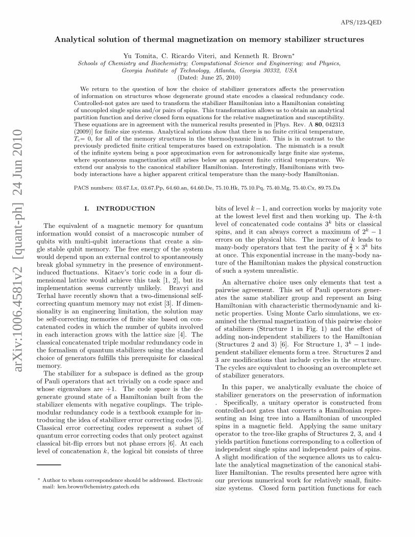
FIG. 1. Transformation of the memory stabilizer structuresgenerated by two body interactions from the Ising basis tothe free-spin basis. Black dots and open circles are spin sites(qubits), and the lines show pairs of interacting spins (gener-ators). In the free-spin basis, the black dot without interac-tions is a single free spin, open circles are independent spinsin a magnetic field, and the connected circles are independentpairs of interacting spins in a magnetic field. The interactionstrength J is constant (see Eq. 1). The total number of bitsincreases with concatenation level, k, as 3k. Only k = 3 levelstructures are shown.

of the four self-correcting memory structures allow us toexamine the problem at much larger k.

A direct measurement of the degree of preservation ofthe information can be read from the spontaneous mag-netization at zero magnetic field. Below a certain temper-ature, a single spin, s0, is sufficient to bias the system intoone of the two states of broken symmetry. The finite-sizesystem develops spontaneous magnetization and the sin-

gle order parameter m0 = (∑N−1

j=0 〈s0sj〉)/N approaches

the value of 1 [7]. The stability of the structure, as mea-sured by the temperature range in whichm0 is preserved,depends on the energy barrier that separates the twoground states and the number of pathways that traversethe barrier.Structure 1 is an example of an Ising tree with free

boundaries. The Ising model on Cayley trees results inpartition functions that are equivalent to free spins [8, 9].Our previous analysis, based on N = 81, 243, 729, and2187 bits (k = 4 − 7) and under the assumption thatFisher’s finite-size scaling method [10] applies to thesetype of Ising graphs, yielded a non-zero Tc. But contraryto Sierpinski fractals [11–13], where a few data pointsseem to be enough to forecast Tc correctly, the finite-

size scaling fails to describe magnetic susceptibility peaksshifted away from Tc=0. For Ising trees and for Sierpin-ski gaskets, the relative magnetization approaches zeroin the thermodynamic limit [9, 14–16], but it persists forvery large systems (comparable to the number of hadronsin the universe)[8, 17]. The nature of the magnetic phasetransition for an infinite system is not applicable to sys-tems of laboratory dimensions. We find similar behav-ior in Structures 2, 3, and 4, but with higher apparentcritical temperatures (defined as the temperature wheremagnetic susceptibility reaches its maximum). Surpris-ingly, the canonical choice of elements to generate theconcatenated three-bit error-correction code exhibits thelowest of the finite-size apparent critical temperatures.

II. CNOT TRANSFORMATIONS AND ISING

SYSTEMS

The algebra of controlled-nots (CNOTs) and Pauli Zoperators from quantum computation is used to findanalytical solutions for the internal energy and mag-netization of the Ising structures in Fig. 1. Follow-ing standard notation, the spin or qubit basis is labeled|0〉 and |1〉 with the Pauli Z operator in the computa-tional basis acting as Z |x〉 = (−1)x |x〉, where x equals0 or 1. The controlled-not operation on two qubitscan be written compactly in the computational basis asCNOT (1, 2) |x1〉 |x2〉 = |x1〉 |x2 ⊕ x1〉 where qubit 1 isthe control qubit and ⊕ represents addition modulo 2.Through out this manuscript, we take advantage of thefollowing relations:

CNOT (j, k)CNOT (j, k) = I

ZjZj = I

CNOT (j, k)ZjCNOT (j, k) = Zj

CNOT (j, k)ZkCNOT (j, k) = ZjZk

CNOT (j, k)ZjZkCNOT (j, k) = Zk.

The last two relationships convert between Ising cou-plings, ZjZk, and local magnetic fields, Zk. The re-peated application of CNOT transformations is an ex-plicit method to obtain the zero-field partition functionfor any Ising tree Hamiltonian ofN spins, which is alwaysequivalent to a single free spin and N − 1 independentspins in a magnetic field [9]. The same transformationapplied to trees that are graphs with a few cycles re-sults in partition functions of clusters of spins. All ofthese partition functions are products of partition func-tions of few spins and do not lead to any singularities ofthe zero-field thermodynamic response functions. Theydo, however, lead to differences in magnetic behavior.

3

III. ANALYTICAL SOLUTION FOR THE

PARTITION FUNCTION

The stabilizer is defined as all the products of Paulioperators that act trivially on the code space. For thebit-flip code, we can choose any set of pairwise Ising in-teractions that generates the stabilizer operators. Thesegenerators form a Hamiltonian that is similar to the fer-romagnetic Ising model,

H = −J∑

〈i,j〉

ZiZj , (1)

where 〈i, j〉 indicates a sum over nearest neighbors, andJ sets the energy scale of the problem with temperaturemeasured in units of J/kB . The choice of generatorsdetermines the structure and properties of the system[6].

1. Ising trees

A tree is a connected graph without cycles or loops.As a result, there is one and only one path between anytwo nodes. In an Ising tree, the nodes represent bits andthe edges represent the Ising interaction. Each node,n, is connected to a single parent, np, and one or morechildren, nc. If the node n is at a distance d from theroot, the parent is at a distance d−1, and the children areat a distance d+1. For convenience, we define a functionD that converts labels to the minimum distances fromthe root, e.g., if D(n) = d then D(nc) = d+ 1. We labeleach node by its number and its parent’s number to makeexplicit the tree nature of the graph. The Hamiltonianfor N spins is then written as

H = −J

N−1∑

n=0

∑

nc

Z[np,n]Z[n,nc], (2)

and the Z operator on the root is labeled Z[0,0] althoughthe root has no parent.The CNOT ([np, n], [n, nc]) operator transforms

Z[np,n]Z[n,nc] into Z[n,nc], but also transformsZ[n,nc]Z[nc,ngc] into Z[np,n]Z[n,nc]Z[nc,ngc], where gclabels the children of the children. By applying CNOTSfirst at the outermost connections (leaves) and thenmoving inwards, we can effectively transform all of theIsing terms into single spin terms.We define

U =

dmax−1∏

d=0

∏

D(n)=d

CNOT ([np, n], [n, nc]) (3)

and the product implies right multiplication. Applyingthis unitary to the Hamiltonian of Eq. 2 yields

H ′ = UHU †

= −J

N∑

n=1

Z[np,n], (4)

which represents N − 1 spins in a magnetic field and onefree spin. We will refer to this basis as the free-spin basis

and the original computational basis as the Ising basis.U is the transformation matrix between the two bases(see Fig. 1).In Ising trees, every qubit, except the root, has

the Hamiltonian H1 = −JZ in the free-spin basis.The partition function is then simply the product ofthe partition function of a single spin in a magneticfield: Q1 = exp (J/kBT ) + exp (−J/kBT ). The ther-modynamic density matrix for a single spin is ρ =1/2[I2×2 + tanh(J/kBT )Z]. The density matrix is usedto calculate the polarization in the free-spin basis, ǫ =Tr [Zρ] = tanh(J/kBT ), and the internal energy, <E1 >= −JTr[Zρ] = −Jǫ. The total thermal densitymatrix for all of the N spins is a tensor product overindependent spin density matrices,

ρtotal = ⊗N−1n=0 ρ[nd,n] = I2×2 ⊗

N−1n=1 ρ, (5)

and the total internal energy is then < Etotal >=Tr[H ′ρtotal] = −J(N − 1)ǫ.

2. Ising trees with cycles

The CNOT Ising tree transformation can also be ap-plied to graphs that can be decomposed into a spanningtree and Ising couplings between spins with the sameparent (siblings). The Hamiltonian for N spins is now

H = −J

N−1∑

n=0

∑

nc

Z[np,n]Z[n,nc] − J∑

〈n,m〉np=mp

Z[np,n]Z[np,m]

(6)and the same unitary of Eq. 3 transforms it to the free-spin basis, thus

H ′ = −JN∑

n=1

Z[np,n] − J∑

〈n,m〉np=mp

Z[np,n]Z[np,m]. (7)

This is the Hamiltonian of one free spin and finite Isinggraphs of sibling spins in non-zero magnetic field.Here we examine connections only between sibling

pairs, that is the triangular cycles in Structures 2, 3,and 4 (Fig. 1). In this case, there are three types ofspins: i) the root which is depolarized in the free-spinbasis and has 〈E0〉 = 0, ii) the spin that is not connectedto a sibling and is described by H1 = −JZ, which isequivalent to a spin in a magnetic field, and iii) spinsthat are connected to a sibling that have the two-spinHamiltonian H2 = −J(Zi + Zj + ZiZj). The expectedenergy of the spins with the magnetic field Hamiltonian is〈E1〉 = −Jǫ with magnetization ǫ = tanh(J/kBT ). Thepartition function of the siblings is Q2 = exp (3J/kBT )+3 exp (−J/kBT ), and the two-spin density matrix is then

4

ρi,j = 1/4(I4x4 + αZi + αZj + αZiZj), where

α =exp (3J/kBT )− exp (−J/kBT )

exp (3J/kBT ) + 3 exp (−J/kBT ). (8)

The energy is < E2 >= −3Jα, and the magnetization ofa single spin is α.The total internal energy is the sum of energies for

the three types of spin, < Etotal >=< E1 > N1+ <E2 > N2/2 = −J(ǫN1 +

32αN2). The internal energies

for Structure 1, Structure 2, Structure 3, and Structure4 are then −Jǫ(3k − 1), −J [ǫ(3k−1 − 1) + 3

2α(2 · 3k−1)],

−J 32α(3

k − 1), and −J [ǫ(2 · 3k−1) + 32α(3

k−1 − 1)], re-spectively.The expectation value of the operators constructed

from products of Z’s can be calculated quickly from thedensity matrices for the three spin types. The root isunpolarized, ρ0 = 1/2I2x2, and as a consequence any op-erator that contains Z[0,0] will be zero. The single spinswill contribute ǫ per Z. The paired spins are correlatedand will contribute α for individual Z’s (Zi, Zj) or theproduct (ZiZj). These rules are sufficient to calculatethe magnetic properties of the system and have a suc-cinct description in terms of the geometry.

A. Calculation of the magnetization and the

magnetic susceptibility

The magnetization operator in the computational or

Ising basis is M =∑N−1n=0 Z[np,n] and its expectation

value is zero by symmetry. The product of the mag-netization of each spin and the magnetization of the rootdefine the relative magnetization operator

M =N−1∑

n=0

Z[0,0]Z[np,n]. (9)

The root spin is sufficient to bias the system into oneof the two states that break the symmetry [7], and the⟨

M⟩

/N is non-zero in the thermodynamic limit when

the system is in a ferromagnetic phase. The square ofthe magnetization relates to the magnetic susceptibilityper spin as follows:

χ =

⟨

M2⟩

−⟨

M⟩2

NkBT=

⟨

M2⟩

−⟨

M⟩2

NkBT(10)

Each of the Znp,n operators must be transformed intothe free-spin basis in order to calculate the magneticproperties. The basis transformation of Eq. 3 maps eachZnp,n operator onto a product of Z’s. When n is at adistance d from the root, the transformation yields

UZ[nd−1,n]U† = Z[nd−1,n]Z[nd−2,nd−1]...Z[0,n1]Z[0,0], (11)

with each parent labeled as nd−1. The operator Z[np,n]

becomes a product of Z’s on every node on the path fromthe root to the spin n.

1 2

3

4

5 6 7

8

9

0

(a) (b)

1 2

3

4

5 6 7

8

9

0

FIG. 2. Example of labeling edges in (a) trees and (b) tree-likegraphs to calculate the magnetic properties based on pathsbetween nodes (see text).

The key observation is that the local magnetizationoperators in the Ising basis are transformed into paths inthe free-spin basis. Calculations can then be performedusing the paths as follows:

• Label the edges of the tree-like graph with pairedsiblings by α, if the edge is part of a triangle, or byǫ, otherwise.

• Define Path(n, l) as the product of the edge labelsbetween nodes n and l along the shortest path.

Fig. 2 shows a tree and related tree-like graphwith the edges labeled. As an example we calcu-late Path(4, 9). For the tree (Fig. 2a), Path(4, 9) =Path(4, 1)Path(1, 5)Path(5, 9) = ǫ3. In the tree-like graph (Fig. 2b), there is a shortcut betweenthe paired sibling nodes 4 and 5 and Path(4, 9) =Path(4, 5)Path(5, 9) = ǫα.As shown in Appendix A, the magnetic thermody-

namic averages can be related to the paths as

〈M〉 =

N−1∑

n=0

Path(0, n) (12)

and

〈M2〉 =

N−1∑

n=0

N−1∑

l=0

Path(n, l). (13)

For trees, these expressions simplify to

〈M〉 =

dmax∑

d=0

f(d)ǫd (14)

and

〈M2〉 = N +

2dmax∑

d=1

2φ(d)ǫd, (15)

where f(d) is the number of nodes a distance d from theroot and φ(d) is the number of unidirectional paths oflength d.In summary, notice that in the Ising basis, H encodes

the geometry by selecting which spins are paired (Eq. 1),

5

and that the magnetization operator is independent ofthe connectivity of the N spins. In the free-spin basis,H ′ is independent of the graph for trees with N nodes(Eq. 4), and the geometry is now encoded in the magne-tization operator (Eq. 12).This is well illustrated by calculating the magnetiza-

tion for two simple examples: a line of N -spins and N−1spins connected to a central spin. In both cases the trans-formation to the free-spin basis results in a Hamiltonianof N − 1 spins in a magnetic field and a single free spin.As a result, the partition function and density matrix inthe free-spin basis are equivalent; however, the magneti-zations are quite different. For a line, f(d) = 1, therefore⟨

M⟩

=∑N−1

d=0 ǫd converges to 1/(1 − ǫ) in the limit of

large N . This yields the familiar result that the magne-tization per spin is vanishingly small for T > 0. For thecentral spin case, d = 1 or 0 and f(1) = N − 1, with

the resulting magnetization being⟨

M⟩

= (N − 1)ǫ+ 1.

The system has non-zero magnetization per spin for allT <∞.Below we use the equations derived in this section to

find analytical expressions for the magnetization and thesusceptibility of the stabilizer structures of Fig. 1. All ofthese systems grow in size as N = 3k as they are basedon the concatenation of three units of 3k−1 spins at eachlevel k. The path from the root to the furthermost spinis of length dmax = k.

1. Structure 1

In the Ising tree labeled Structure 1 of size N = 3k,the number of nodes at distance d from the root is

f(d, k) = 2d(

k

d

)

, (16)

and according to Eq. 14, the expected relative magneti-zation of Structure 1 at level k is then

⟨

M(k)⟩

S1=

k∑

d=0

2d(

k

d

)

ǫd = (1 + 2ǫ)k. (17)

One can understand the result by imagining building upthe tree level-by-level. The level k adds 2 nodes to everynode in a level k − 1 tree. The paths between nodesand the root in the inner k − 1 tree are the same, andthe leaves add two paths that are one edge longer. Thisresults in the recursion formula:

⟨

M(k)⟩

S1= (1 + 2ǫ)

⟨

M(k − 1)⟩

S1. (18)

Notice that this last equation also generates Eq. 17, thusthe relative magnetization per spin at zero magnetic fieldis

m0S1(k) =

⟨

MS1(k)⟩

N=

(

1 + 2ǫ

3

)k

, (19)

which vanishes in the limit of large k for all ǫ < 1 andT > 0. In order to calculate the magnetic susceptibilityusing Eq. 10, we need to first evaluate the magnetizationsquared operator. Starting from k − 1, two leaves areadded to every node. Each path of length d > 0 on thek − 1 tree now has two extra leaves on each end. Thisresults in one path of length d, four paths of length d+1,and four paths of length d + 2. For the 3k−1 paths ofd = 0, there are now two paths of length one, one pathof length two, and two new paths of zero length. Usingthese observations and defining φ1(d, k) as the numberof paths of distance d between two spins, Eq. 15 can bewritten recursively:

⟨

M2(k)⟩

S1= 3k +

2k∑

d=1

2φ1(d, k)

= 3k−1(

1 + 2 + 4ǫ+ 2ǫ2)

+(

1 + 4ǫ+ 4ǫ2)

2(k−1)∑

d=1

2φ1(d, k − 1)

= (1 + 2ǫ)2⟨

M2(k − 1)⟩

S1

+2(1− ǫ2)3k−1. (20)

The solution to the recursion formula is

⟨

M2(k)⟩

S1= (1 + 2ǫ)2k + 2(1− ǫ2)(1 + 2ǫ)2(k−1)

{

1− [3/(1 + 2ǫ)2]k

1− 3/(1 + 2ǫ)2

}

(21)

and the magnetic susceptibility per spin is then

χS1(k) =2(1− ǫ2)(1 + 2ǫ)2(k−1){1− [3/(1 + 2ǫ)2]k}

NkBT [1− 3/(1 + 2ǫ)2].

(22)

2. Structure 2

Structure 2 is similar to Structure 1 but the leavesare connected forming triangular cycles. The number ofspins at the minimum distance d from the root is the sameas in Structure 1 but now there are single spins and spinpairs in the free-spin basis. For paths that include leafspins from Structure 1, the magnetization needs to in-

6

clude the polarization of a spin pair, α. Structure 2 with3k spins is equivalent to Structure 1 with 3k−1 spins witha sibling pair connected to each spin. The magnetizationis then

⟨

M(k)⟩

S2= (1 + 2α)

⟨

MS1(k − 1)⟩

. (23)

The thermodynamic average of⟨

M2⟩

for a Structure

2 of 3k nodes can be built from a Structure 1 with 3k−1

nodes by examining the extra shortest paths due to theattached outer cycles. The main difference is that thetwo new nodes connected to the k − 1 structure are adistance 1 apart instead of a distance 2. The result isthat

⟨

M2(k)⟩

S2= (1 + 2α)2

⟨

M2(k − 1)⟩

S1

+2 · 3k−1(

1 + α− 2α2)

(24)

and

χS2(k) =(1 + 2α)2χS1(k − 1) + 2

(

1 + α− 2α2)

/kBT

3.

(25)

3. Structure 3

In this structure, each spin is part of a triangular cy-cle, and all spins but the root are paired spins. Thethermodynamic average of the magnetization is identicalto Structure 1 except the polarization is now α insteadof ǫ.

⟨

M(k)⟩

S3= (1 + 2α)k. (26)

The magnetization squared depends on the number ofshortest paths between all spins, which is quite differentfrom Structure 1 due to shortcuts made by triangularcycles. Applying the same building method of addingnodes to the core yields the following recursion relation

⟨

M2(k)⟩

S3= (1 + 2α)2

⟨

M2(k − 1)⟩

S3

+2(1 + α− 2α2)3k−1, (27)

whose solution is:

⟨

M2(k)⟩

S3= (1 + 2α)2k + 2(1 + α− 2α2)(1 + 2α)2(k−1)

{

1− [3/(1 + 2α)2]k

1− 3/(1 + 2α)2

}

. (28)

The magnetic susceptibility is then

χS3(k) =2(1 + α− 2α2)(1 + 2α)2(k−1)

NkBT

×{1− [3/(1 + 2α)2]k}

[1− 3/(1 + 2α)2]. (29)

4. Structure 4

In Structure 4, each of the spins form part of triangularcycles except the outer nodes. The relationship betweenStructure 4 and Structure 3 is similar to the relationshipbetween Structure 2 and Structure 1, and the magneti-zation properties are calculated to be

⟨

M(k)⟩

S4=

⟨

M(k − 1)⟩

S3(1 + 2ǫ), (30)

⟨

M2(k)⟩

S4= (1 + 2ǫ)

2 ⟨M2(k − 1)

⟩

S3

+2 · 3k−1(

1− ǫ2)

, (31)

and

χS4(k) =(1 + 2ǫ)2χS3(k − 1) + 2

(

1− ǫ2)

/kBT

3.(32)

B. Extension to the Canonical Stabilizers

The stabilizer formalism of quantum computing definesa subspace of n-qubits by a set of commuting observ-ables that are products of Pauli matrices on the n-qubitsand have the value of 1 on the subspace. The stabilizergenerators are independent operators, trace orthogonal,and commute with one another. As a result, there isalways a unitary transformation which maps the stabi-lizer elements to Z operators on independent spins. Fur-thermore, this unitary can be constructed from CNOTs,Hadamards, and Pauli matrices [5].

Structure 1 is derived from the three-qubit classicalstabilizer code. The choice of generators is chosen toform an Ising tree, and this is not the standard choice.The standard choice is to use logical Ising interactions atevery level of encoding. This choice results in generatorsthat are multi-qubit interactions which grow exponen-tially with the level of encoding.

The transformation that takes the stabilizer elementsto independent Z’s is closely related to the transforma-tion used for Structures 1, 2, 3 and 4. Instead of simplyapplying the CNOTs with the control on the inner nodeand then progressing inward, the control is alternatedfrom inner to outer. A comparison of the two transfor-mations is shown for 9 qubits in Fig. 3. For Structures1, 2, 3, and 4 only A and B are applied. For the full

7

A A' B B'

00

01

02

10

11

12

20

21

22

FIG. 3. A description of U as a quantum computing circuitfor 9 qubits. For the tree and tree-like structures examined,the CNOTs are applied with the control towards the rootstarting from the leaves and then moving down layers untilthe root (A,B). For the full-stabilizer, the direction of controlis alternated before applying the CNOTs at the next layer (A,A′, B, B′).

stabilizer, A, A′, B, and B′ are all applied. The detaileddescription of the transformation can be found in the Ap-pendix B. The expected relative magnetization and themagnetization squared are respectively:

⟨

M(k)⟩

= 1 + 2ǫ

{

1− [(2 + ǫ)ǫ3]k

1− (2 + ǫ)ǫ3

}

(33)

and

⟨

M2(k)⟩

= 3k + 2 · 3k−1ζ

[

1− (ζ2/3)k

1− (ζ2/3)

]

, (34)

where ζ = (2 + ǫ)ǫ.

IV. RESULTS AND DISCUSSION

A. Apparent Critical Temperature for Finite Size

Systems

The analytical results obtained from Eqs. 22, 25 and29 match perfectly with our previous Monte Carlo sim-ulations [6]. As an example, Fig. 4 compares the closedform equation of the magnetic susceptibility for Struc-ture 3 with numerical simulations of systems of varioussizes. The susceptibilities are calculated using the ther-modynamic statistics of 5 × 104 independent spin con-figurations generated with Wolff cluster simulations atdifferent temperatures.

0 0.5 1 1.5 2 2.50

20

40

60

80

T

χ

k=4k=5k=6k=7

FIG. 4. Magnetic susceptibilities per spin as a function oftemperature T in units of J/kB for different concatenationlevels of Structure 3. The solid lines are calculated from Eq. 29and the symbols are the result of Monte Carlo simulations [6]using 5× 104 independent spin configurations.

For finite-size self-correcting memories, the susceptibil-ity as a function of temperature shows a maximum whichoccurs at an apparent critical temperature T χmax(N). Itis clear from Fig. 4 that this temperature decreases withsystem size as expected. Finite size effects replace thedivergences at the thermodynamic critical point by fi-nite peaks shifted away from Tc [10, 18]. Previously [6],we used a first order approximation to estimate theseshifts for the case of susceptibility. A fit of T χmax againstthe system size N gave us an estimate for Tc, χ0 andν′. With only four data points, we forecasted a finiteTc. Analytical solutions for the magnetic susceptibilitypermit the study of bigger systems and present a morecomplete picture of the finite-size effects on the magneticproperties. We obtain T χmax(N) numerically and Fig. 5compares them for the four Ising stabilizer structures,the canonical stabilizer, and the 1D Ising model as afunction of total number of spins in a double log scale,log10(log3(N)). The numerical calculation of T χmax for the1D Ising model of systems bigger than 318 spins resultsin a numeric underflow. The dotted line in the figure isan extrapolation using a two parameters fit of the solidline to the equation T χmax= ak−b.In the limit of systems of infinite size, Eqs. 17, 23, 26,

30, and 33 reveal that the only temperature at which m0

takes the exact value of one is Tc= 0. It is seen in Fig. 5that T χmax converges very slowly to zero with system size.Based on the closed form equations this prolonged decaycannot be captured by a simple first order equation inN−1/ν′

nor by any finite power expansion in N with-out including an offset. We cannot calculate numericallythe size of memory stabilizers with a T χmax of practicallyzero before we run into numerical overflow. As shown inthe figure, memory stabilizers utilizing all the observablematter in the universe will still behave as a finite-size sys-tem with almost all of their spins correlated at a finite

8

0.75 1 1.25 1.5 1.75 2 2.250

0.2

0.4

0.6

0.8

1

1.2

log10

(k )

Tm

axχ

Structure 1Structure 2Structure 3Structure 4Stabilizer1D Ising1D approx.

FIG. 5. Temperature of maximum relative magnetic suscepti-bility Tχ

max for different memory stabilizers of sizes that spanfrom tens to 1095 spins. Note that 1.70 and 2.23 in the ab-scissa correspond respectively to the Avogadro’s number andto the predicted number of hadrons in the observable uni-verse [8].

apparent critical temperature on the order of J/kB. Thisis in contrast to the linear spin case where T χmax rapidlyapproaches zero with increasing system size. For 3 spins,Structure 1 and the line are equivalent with T χmax= 1.07.We can then ask how many spins are required to reach acertain T χmax. As an example, a maximum susceptibilityof T χmax= 0.29 is achieved using 36 spins in a line, but itwould require a Structure 1 of 3313 spins. This presentsan interesting challenge as these networked spin systemsstand in contrast to our standard notion of what size thethermodynamic limit is appropriate.

The thermal stability of the information encodedinto finite systems for the four structures and the full-stabilizer can be related to T χmax (Fig. 5). The choice ofstabilizers leads to a significant change in this apparentcritical temperature. Two thirds of the spins in Structure2 form closed cycles, and the other third of spins form acore that is the same as a k− 1 Structure 1. As expectedfor small systems, Structure 2 remains magnetized for abroader range of temperatures than Structure 1. Simi-larly, Structure 4, with 2/3 of its spins as free leaves, isless stable to temperature driven fluctuations than Struc-ture 3. The cores of Structures 1 and 2, and Structures 3and 4, account for 1/3 of the spins, and they show similarmagnetic behavior in the astronomical limit of large k.The canonical choice of stabilizer elements remains mag-netized below a broad range of temperatures, and showsthe same long ranged order properties, but under thisthermodynamic criteria, is a less efficient memory stabi-lizer than the simpler pairwise interaction geometries.

B. Power-law Correlations and Finite Size Effects

Assuming that there is a relation between a 1-D pathof correlated spins and the total size of the system,L = N1/d, we can define a correlation length exponentscaled to the system size ν′ = ν · d. The dimension, d, ofeach of the structures of Fig. 1 is unknown. According tothe standard scaling hypothesis, and provided that thesystem size is large enough, the following scaling prop-erties are expected at the critical point: c(N) ∝ N

αν′ ,

m(N) ∝ N− β

ν′ , and χ(N) ∝ Nγ

ν′ [18]. Closed formequations for the magnetization and the magnetic sus-ceptibility can be used to calculate critical exponents.An analytical formula for the relative magnetization

critical exponent can be obtained by equating the rela-

tive magnetization per spin to the N− β

ν′ power law. Af-ter simplification of the exponent k, the β/ν′ critical ex-ponent can be written in terms of the logarithm of therelative magnetization as follows:

β/ν′ = 1−ln(ψ)

ln(3), (35)

where ln(ψ) = ln(〈M〉)/k. For Structures 1 and 3, ψ isindependent of k and we find ψ1 = 1+2ǫ and ψ3 = 1+2α,respectively. For Structures 2 and 4, ψ depends weakly

on k as ψ2 = ψ1

(

ψ3

ψ1

)1/k

and ψ4 = ψ3

(

ψ1

ψ3

)1/k

. The

power law for the relative magnetization per spin canthus be written as a function of any arbitrary tempera-ture:

m0(T ) = N−[1− ln(ψ(T ))ln(3) ]. (36)

This last equation reduces the magnetic susceptibility ofEqs. 22 and 29 to the form:

χ(k, T ) = A(k, T ) · (3k)−2β/ν′+1, (37)

where for Structures 1 and 3 A is

A(k, T )S1 =(1 − ǫ2)[(1 + 2ǫ)2k − 3k]

kBT (2ǫ2 + 2ǫ− 1)(1 + 2ǫ)2k(38)

and

A(k, T )S3 =(1 + α− 2α2)[(1 + 2α)2k − 3k]

kBT (2α2 + 2α− 1)(1 + 2α)2k, (39)

respectively. As T approaches the thermodynamic crit-ical temperature of Tc = 0, the A function of Eqs. 38and 39 is independent of the system size and convergesrespectively to

A(T )S1 ≃(1− ǫ2)

kBT (2ǫ2 + 2ǫ− 1)(40)

and

A(T )S3 ≃(1 + α− 2α2)

kBT (2α2 + 2α− 1). (41)

9

0 0.5 1 1.5 2

0

0.2

0.4

0.6

0.8

1A

S1

k=6k=50Eq. 40

0 0.5 1 1.5 2

0

0.1

0.2

0.3

0.4

AS

3

T

k=4k=50Eq. 41

(a)

(b)

FIG. 6. Power law proportionality function A(k, T ) for (a)Structure 1 and (b) Structure 3. Solid lines are calculatedusing Eqs. 38 and 39 while the circles come from the approxi-mations of Eqs. 40 and 41. In a broad region of temperaturesnear the thermodynamic critical point, these simple equationsare enough to define a magnetization power law on N for anysystem size.

In this limit, the magnetic susceptibility can be writ-ten as the well known formula χ(N) = A(T ) · N

γ

ν′ .Examining Eq. 37, we find that γ/ν′ + 2β/ν′ = 1,which matches the Rushbrooke and Josephson scaling lawd = γ/ν+2β/ν if written as a function of the correlationsize exponent ν′. Fig. 6 tests the temperature regionin which this approximation holds for all system sizes.There is a broad temperature region where the magneticproperties are well described by N and temperature de-pendent critical exponents.

The set of critical exponents obtained numerically forparticular ill-predicted critical temperatures (see TablesIV and V of Ref. [6]) match very well with those calcu-lated using Eq. 35 and the hyperscaling relation. Theseapparent critical temperatures fall in the temperature re-gion in which Eqs. 40 and 41 hold.

We find that there is a broad temperature region aboveTc where the β/ν′ exponent is almost zero (it is strictlyzero only at T = 0). Complementary, and for the samebroad temperature region, the γ/ν′ critical exponentreaches almost the value of one. The interpretation issimple: the number of correlated spins grows almost atthe same rate as N . Spins that present long ranged cor-relations develop a net macroscopic alignment when aninfinitesimal magnetic field is applied [7].

V. CONCLUSION

We use CNOT gates to transform the Hamiltonian ofstabilizer structures into a Hamiltonian consisting of un-coupled single and pairs of spins. In the original basis,the Hamiltonian encodes the geometry by selecting whichbits interact. The magnetization operator is independentof the graph forN spins. In the free spin basis, the Hamil-tonian is independent of the graph for N spins and thegeometry is now encoded in the magnetization operator.This transformation allows us to obtain an analytical par-tition function and closed form equations for the effectivemagnetization and susceptibility with respect to a centralspin.The analytical solutions match very well with the nu-

merical results presented previously[6] for finite size sys-tems of N ≤ 38 spins. With a slight modification ofthe transformation sequence we calculate the analyticalmagnetization and susceptibility of the canonical stabi-lizer Hamiltonian.In our previous calculation based on four values of k,

we forecast a finite critical temperature for systems ofinfinite size. Our analytical solution shows that this pre-diction is incorrect. After applying a sequence of CNOToperations on the four stabilizer Hamiltonians studied inthis work, the partition function results in a collection offree elements. The interactions represented in the mag-netization operator yield to graphs that have a transitionfrom magnetic to random at Tc=0 in the thermodynamiclimit. However, they possess unusual long-range-orderproperties as previously observed in hierarchical systemswhich also have Tc=0 (e.g.: Sierpinski gaskets [17] andCayley trees [8]). The memory stabilizer structures de-velop spontaneous magnetization below an apparent crit-ical temperature for unrealistically large systems. Therelative magnetization persists below a finite tempera-ture for systems of N = 3200 spins. For a practical im-plementation, the infinite system is a poor approxima-tion, and it remains poor even for finite systems that areastronomical in size. This conflicts with our notion ofthe thermodynamic limit, where the infinite system welldescribes crystalline solids of few billion unit cells [17].First order finite-size scaling analysis is incomplete and

fails to describe the slow decrease of T χmax with the sys-tem size for all structures. For systems with no phasetransition at finite temperatures, the shift away from Tccannot be written as a simple power expansion in N1/ν′

.The partition function of the systems, and its first andsecond derivatives with respect to an external magneticfield, do not present critical points. They are continu-ous, well behaved, and show spontaneous magnetizationfor a broad range of temperatures. In the broad regionnear Tc=0, scaling properties of the magnetization andmagnetic susceptibility satisfy power-laws as a functionof N .The memory stabilizers presented in this work do not

show a phase transition in the thermodynamic sense.However, for a wide range of temperatures and finite

10

size, there are many long paths of correlated spins thatgo through the structure resulting in a net macroscopicmagnetization. These structures have free energy func-tions that spontaneously break global symmetry in thepresence of environment-induced fluctuations, thus theystabilize the memory.We arrive to similar conclusions as in our previous

work [6]. Fig. 5 suggests that one way to increase the ap-parent critical temperature for a system of a given finite-size is by adding generators to each spin site. Struc-ture 3 is the best self-correcting memory as it has thebroadest range of temperatures in which the system re-mains magnetized. The four simple two-body-interactionstructures investigated have different levels of connectiv-ity. We find that the relationship between coordinationnumber and the apparent finite size critical temperatureT χmax is not obvious. The number of generators is lessimportant than the structure. The canonical stabilizerHamiltonian seems to be thermodynamically a less sta-ble memory than the simpler pairwise based constructionwith the minimum number of generators (Structure 1),but it is more stable than the Ising chain. Kinetically,the canonical stabilizer could be the the most impervi-

ous to fluctuations. For systems with all of the spinsaligned, the lowest excited state energy for Structure 1is 2J from the ground state, but this gap grows as 2kJfor the canonical stabilizer. The multi-body interactionsof the canonical stabilizer result in many large kineticbarriers that may be advantageous for preserving certainspin configurations.

Finally, the exploration of stabilizer Hamiltonians de-fined by geometries of non-integer dimensions could yieldself-correcting quantum memories with few multi-qubitinteractions. Small finite size systems show an unusualorder preservation for a broad range of temperaturesmaking them suitable for a practical implementation ofpassive error correction.

ACKNOWLEDGMENTS

Authors thank Keisuke Fujii for pointing out that itis possible to obtain an analytical partition function forStructure 1 by applying a CNOT transformation. Thiswork was supported by Georgia Institute of Technology.

[1] A. Y. Kitaev, Ann. Phys. 303, 2 (2003).[2] E. Dennis, A. Kitaev, A. Landahl, and J. Preskill, J.

Math. Phys. 43, 4452 (2002).[3] S. Bravyi and B. Terhal, New. J. Phys. 11, 043029 (2009).[4] D. Bacon, Phys. Rev. A 78, 042324 (2008).[5] M. A. Nielsen and I. L. Chuang, Quantum computation

and quantum information (Cambridge University Press,2000).

[6] C. R. Viteri, Y. Tomita, and K. R. Brown, Phys. Rev. A80, 042313 (Oct 2009).

[7] D. Chandler, Introduction to Modern Statistical Mechan-

ics (Oxford University Press Inc., New York, 1987).[8] B. D. Stosic, T. Stosic, and I. P. Fittipaldi, Physica A

355, 346 (2005).[9] T. P. Eggarter, Phys. Rev. B 9, 2989 (1974).

[10] M. E. Fisher and M. N. Barber, Phys. Rev. Lett. 28,1516 (1972).

[11] J. Carmona, U. Marconi, J. Ruiz-Lorenzo, and A. Taran-con, Phys. Rev. B 58, 14387 (1998).

[12] P. Monceau, M. Perreau, and F. Hebert, Phys. Rev. B58, 6386 (1998).

[13] P. Monceau and M. Perreau, Phys. Rev. B 63, 184420(2001).

[14] E. Muller-Hartmann and J. Zittartz, Phys. Rev. Lett. 33,893 (Oct 1974).

[15] Y. Gefen, A. Aharony, Y. Shapir, and B. B. Mandelbrot,J. Phys. A-Math. Gen. 17, 435 (1984).

[16] Y. Gefen, B. B. Mandelbrot, and A. Aharony, Phys. Rev.Lett. 45, 855 (1980).

[17] S. H. Liu, Phys. Rev. B 32, 5804 (1985).[18] M. E. J. Newman and G. T. Barkema, Monte Carlo Meth-

ods in Statistical Physics (Oxford University Press Inc.,New York, 1999).

Appendix A: Trees and trees with cycles

For an Ising tree, there is only one path between anytwo nodes n and l. We define Pl,n as the product ofZ operators of all of the nodes on the path between nand l on the spanning tree (including n and l). Thetransformation of Eq. 11 can then be written succinctlyas

UZ[np,n]U† = P0,n (A1)

and M transforms to

UMU † =∑

n

UZ[np,n]U† =

∑

n

P0,n. (A2)

The expected value must be zero by symmetry and this iseasy to confirm since each term contains the root factorZ[0,0]. Applying the transformation to the M operatorof Eq. 9, results in

UMU † =∑

n

UZ[np,n]Z[0,0]U†

=∑

n

P0,nP0,0

=∑

n

Z[nd−1,n]Z[nd−2,nd−1]...Z[0,n1]Z[0,0]Z[0,0]

=∑

n

Z[nd−1,n]...Z[0,n1]

=∑

n

Pn,n1 . (A3)

11

Note that none of the terms contain Z[0,0] and the numberof Z factors in each term is the distance between n andthe root.The expectation value of the magnetization is the prod-

uct of the polarization of all the spins on the path fromn to n1 in the free-spin basis. For the structures studiedin Section III A, the spins that are in sibling pairs havepolarization α and otherwise have polarization ǫ (exceptthe root). This leads the relative magnetization to be

⟨

M⟩

=∑

n

αcnǫD(n)−cn , (A4)

where cn is the number of spins that are in a pair betweenthe root and n. One can express this graphically by la-beling every edge in the graph with an ǫ if it is not partof a triangle, and with an α if it is part of a triangle (seeFig. 2). One then starts from a node and multiplies thelabel of the edges between the node and the root on thespanning tree. Summing over all nodes yields Eq. 12, anda comparison to Eq. A3 shows that Path(0, n) = 〈Pn,n1〉.

The magnetization operator squared, M2 = M2, inthe transformed basis is

UM2U † =∑

n,l

UZ[lp,l]Z[np,n]U†

=∑

n,l

P0,lP0,n. (A5)

The product of P0,l and P0,n results in the Z’s that arein the intersection of the paths from the root to l, andfrom the root to n, to cancel. The Z operator on thelast node in common is ZLast(l,n), and this node is in-cluded in the path from l to n on the spanning tree. Asan example, consider node 4 and node 9 of Fig. 2. ThenP0,4 = Z[1,4]Z[0,1]Z[0,0], P0,9 = Z[5,9]Z[1,5]Z[0,1]Z[0,0], andP4,9 = Z[1,4]Z[1,0]Z[1,5]Z[5,9]. Node 1 is the last nodein common and, as a result, P0,4P0,9 = P4,9Z[0,1] andZ[0,1] = ZLast(4,9). These operators are the same forFig. 2(a) and (b), but the expectation values differ asexplained below.Eq. A5 is simplified to:

UM2U † =∑

n,l

Pl,nZLast(l,n). (A6)

To calculate the expectation value of Pl,nZn,l, we mustconsider three cases. In the first case, the node n iscontained in the path between the root and l or vice-versa, and ZLast(l,n) equals Z[np,n] or Z[lp,l], respectively.The expectation value of Pl,nZn,l is simply the polar-ization of spins on the path from l to n excluding thenode Last(l, n). The polarization of each node is the la-bel of the edge connecting it to its parent and as a result〈Pn,lZn,l〉 = Path(n, l). In the second case, the two nodesafter the last node are not part of the same triangle. Thepolarization of spins at these nodes are independent andagain 〈Pn,lZn,l〉 = Path(n, l). In the third case, the twonodes after the last node are part of the same triangle.

The polarizations are not independent and two Z’s yielda single α. This is equivalent to taking a shortcut, andfor all cases, 〈Pn,lZn,l〉 = Path(n, l). Combining theseobservations with Eq. A6, we obtain

⟨

M2⟩

=∑

n,l

Path(n, l). (A7)

Appendix B: Canonical Stabilizer

To define the full stabilizer, it is useful to start at thetop level and work down. At level k there is one qubit(labeled 0), composed of three level k − 1 qubits labeled00, 01, and 02. We can define the logical operator as

Z(k)0 = Z

(k−1)00 Z

(k−1)01 Z

(k−1)02 (B1)

and the highest order stabilizer elements as

A(k)01 = Z

(k−1)00 Z

(k−1)01

A(k)02 = Z

(k−1)00 Z

(k−1)02 . (B2)

Continuing this procedure, we define

Z(j)η = Z

(j−1)η0 Z

(j−1)η1 Z

(j−1)η2

A(j)η1 = Z

(j−1)η0 Z

(j−1)η1

A(j)η2 = Z

(j−1)η0 Z

(j−1)η2 (B3)

and one composite operator,

A(j)η0 = A

(j)η1A

(j)η2 , (B4)

where η is a k − j + 1 string of trits. It is convenientto consider η as a number in base 3. Also, we introducefour useful identities:

A(j)η1 Z

(j)η = Z

(j−1)η2 (B5)

A(j)η2 Z

(j)η = Z

(j−1)η1 (B6)

A(j)η0 Z

(j)η = Z

(j−1)η0 (B7)

A(j)ηt A

(j)ηt = I. (B8)

Note how the products of Aj−1 with Zj interchange the1 and 2 labels.The Hamiltonian is

H =

k∑

j=1

2∑

x=1

3k−j−1∑

η=0

Ajηx, (B9)

and there exists a unitary that transforms A’s to singlequbit Z’s. The chosen unitary performs the followingtransformation:

UAjηxU† = Zηx0(j−1)

UAjη0U† = UAjη1U

†UAjη2U†

= Zη10(j−1)Zη20(j−1) , (B10)

12

where 0l is a string of l zeros and x = 1 or 2. Everyphysical qubit is denoted by a k + 1 trit string with thefirst trit set to zero. This will transform the 3k− 1 stabi-lizer elements into 3k − 1 single Z operators. To furtherspecify the unitary, we set

UZk0U† = Z0k+1 . (B11)

An explicit construction of U is as follows. Arrang-ing the spins on the tree that defines Structure 1 andstarting at the spins at the maximum distance from theroot, dmax, apply CNOT (ndmax−1, ndmax) between allspins connected on the graph at this distance. Thenapply CNOT (ndmax , ndmax−1) to the same spins. Thenmove up one level and repeat the procedure first apply-ing CNOT (ndmax−2, ndmax−1) at this distance and thenCNOT (ndmax−1, ndmax−2). Continue to the root. If weonly used the CNOTs that are controlled by parents,we have the same unitary as Structure 1. Switching toCNOTs that are controlled by children allows us to trans-form logical Z’s into Z’s on single spins. The unitary isshown as a circuit for k = 2 in Fig. 3.U †ZµU must be determined to calculate the magneti-

zation. This is possible by constructing Zµ from stabi-lizer elements and Zk0 using Eqs. B5, B6, and B7. If wewrite µ = µkµk−1...µ1µ0, one can show that

Zµ = Zk0

k∏

j=1

Ajµkµk−1...µj−1, (B12)

where

µj = (2µj) mod 3 (B13)

which exchanges 1’s for 2’s and follows from Eqs. B5 andB6.Zk0 is the product of Z on all spins, and the element

Zk0Ak0x is the product of all spins on a single k − 1 level

qubit. Geometrically, each Aj splits off one block of 3j−1

spins from a block of 3j level. Each A reduces the totalnumber of spin operators by 1/3 until we reach a singlequbit operator.To calculate the magnetic properties, we examine the

transformed product of two Z operators, Zµ and Zν . As-sume that µ and ν agree in the first q+1 trits, the productis then

ZµZν =

Zk0

k∏

j=1

Ajµkµk−1...µj−1

·

Zk0

k∏

j=1

Ajνkνk−1...νj−1

=

k−q∏

j=1

Ajµkµk−1...µj−1Ajνkνk−1...νj−1

(B14)

After the transformation UZµZνU†, each remaining

Ajη{1,2} corresponds to a single Z operator and each Ajη0corresponds to two Z operators. The Z’s will be uniquebetween µ and ν except for the only case where η agrees,

Ak−qµkµk−1...µk−q−1and Ak−qνkνk−1...νk−q−1

. The number of in-

dependent Z’s in UZµZνU† denotes an effective distance

between µ and ν,

δ(µ, ν) = 2(k − q − 1) + zeros(µk−q−2...µ0)

+zeros(νk−q−2...ν0)

+2µk−q−1·νk−q−1/2 (B15)

in which q+1 is the number of leading trits that agree inµ and ν, and zeros(µj ...µ0) counts the number of zerosin the string µj ...µ0. The first trits that do not agree,µk−q−1 and νk−q−1, result in 1 or 2 independent Z’s de-pending on whether either trit equals zero. For a givenq, the minimal effective distance between the spins is2k − 2q − 1.Calculating the relative magnetization requires com-

puting the effective distances between the root Z0k+1 andall other spins Zµ. Clearly, the number of leading tritsthat agree are the number of leading zeros in µ, L(µ).The result is

δ(0k+1, µ) = 2(k − L(µ)− 1) + (k − L(µ)− 1)

+zeros(µk−L(µ)−2...µ0) + 1

= 3k − 4L(µ) + zeros(µ)− 2. (B16)

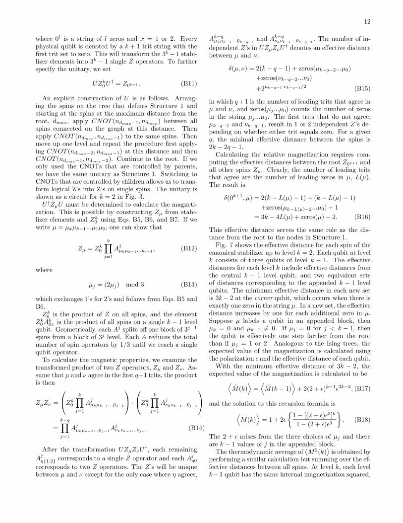
This effective distance serves the same role as the dis-tance from the root to the nodes in Structure 1.Fig. 7 shows the effective distance for each spin of the

canonical stabilizer up to level k = 2. Each qubit at levelk consists of three qubits of level k − 1. The effectivedistances for each level k include effective distances fromthe central k − 1 level qubit, and two equivalent setsof distances corresponding to the appended k − 1 levelqubits. The minimum effective distance in each new setis 3k− 2 at the corner qubit, which occurs when there isexactly one zero in the string µ. In a new set, the effectivedistance increases by one for each additional zero in µ.Suppose µ labels a qubit in an appended block, thenµk = 0 and µk−1 6= 0. If µj = 0 for j < k − 1, thenthe qubit is effectively one step farther from the rootthan if µj = 1 or 2. Analogous to the Ising trees, theexpected value of the magnetization is calculated usingthe polarization ǫ and the effective distance of each qubit.With the minimum effective distance of 3k − 2, the

expected value of the magnetization is calculated to be⟨

M(k)⟩

=⟨

M(k − 1)⟩

+ 2(2 + ǫ)k−1ǫ3k−2, (B17)

and the solution to this recursion formula is

⟨

M(k)⟩

= 1 + 2ǫ

{

1− [(2 + ǫ)ǫ3]k

1− (2 + ǫ)ǫ3

}

. (B18)

The 2 + ǫ arises from the three choices of µj and thereare k − 1 values of j in the appended block.The thermodynamic average of

⟨

M2(k)⟩

is obtained byperforming a similar calculation but summing over the ef-fective distances between all spins. At level k, each levelk−1 qubit has the same internal magnetization squared,

13

1 0 1

k=0

k=1 Z01 Z00 Z02

Z0

k=2

0

1

4

0

5

1

4

454Z011 Z010 Z012

Z001 Z000 Z002

Z021 Z020 Z022

FIG. 7. The effective distances of the canonical stabilizer upto k = 2. For each k the black dot represents the root qubit.The corresponding Zµ is written next to each qubit. Thenumbers shown on the right are the effective distances fromthe root to the qubit at the same position. The bold boxcontains the effective distances inherited from the level k− 1.

⟨

M2(k − 1)⟩

. To compute the effective distances between

qubits in k − 1 blocks, we determine how many trits arerequired to distinguish a pair of physical qubits. It takesa single trit to determine which two logical blocks arepaired. Each block contains qubits labeled by k − 1 dif-ferent trits. Similar to the magnetization, each trit con-tributes a factor of 2 + ǫ, but now there are a total of2k− 1 choices. The minimum effective distance betweentwo sets is also 2k−1, since only the leading trit can agree(q=0). Overall, the thermodynamic average of

⟨

M2⟩

isexpressed as

⟨

M2(k)⟩

= 3⟨

M2(k − 1)⟩

+2(2 + ǫ)2k−1ǫ2k−1, (B19)

and the solution to the recursion is given by

⟨

M2(k)⟩

= 3k + 2 · 3k−1ζ

k−1∑

j=0

ζ2j

3j

= 3k + 2 · 3k−1ζ

[

1− (ζ2/3)k

1− (ζ2/3)

]

, (B20)

where ζ = (2 + ǫ)ǫ.