Magnetization of the plasma sheet

Richard L. KaufmannDepartment of Physics, University of New Hampshire, Durham, New Hampshire, USA

W. R. Paterson and L. A. FrankDepartment of Physics and Astronomy, University of Iowa, Iowa City, Iowa, USA

Received 17 July 2003; revised 18 May 2004; accepted 29 June 2004; published 30 September 2004.

[1] Long-term-averaged three-dimensional data-based models were made of the�30 < x <�10, jyj < 15, jzj < 5 RE plasma sheet region. The average magnetic moments hmi andChew-Goldberger-Low (CGL) double adiabatic parameters a? and ak were evaluated forions and electrons. It was shown that restricting the observations to those taken within0.2 RE of the Bx = 0 point gave both a good determination of conditions at the neutral sheetand enough data points for reliable averages. Large pitch angle anisotropies woulddevelop if the CGL parameters were constant along drift paths. In contrast, pitch anglescattering was so rapid that the observed plasma remained almost isotropic and it was theCGL parameters that varied markedly along the drift paths. Frequent ion scattering isexplained by the chaotic nature of ion orbits, but electrons usually spiral around magneticfield lines even at the neutral sheet. Electron scattering by an average of 90� was neededduring the 1 min it takes for a typical flux tube to undergo a net earthward displacement of0.1 RE. A fast flow flux tube could move several Earth radii during this characteristicscattering time period. Rapid electron scattering also provides a mechanism to divertperpendicular current to form Birkeland current, produces diffusion, and generates a heatflux. The long-term-averaged magnetization vector M was evaluated and used to calculatethe magnetization or bound current density jm = r �M. The magnetization current and analmost oppositely directed perpendicular free or guiding center drift current jf werestrongest near the neutral sheet. Their sum, the total perpendicular current density j?, wasan order of magnitude smaller than either jm or jf in this region. INDEX TERMS: 2764

Magnetospheric Physics: Plasma sheet; 2744 Magnetospheric Physics: Magnetotail; 2708 Magnetospheric

Physics: Current systems (2409); 2760 Magnetospheric Physics: Plasma convection; KEYWORDS: electric

currents, magnetotail, plasma sheet

Citation: Kaufmann, R. L., W. R. Paterson, and L. A. Frank (2004), Magnetization of the plasma sheet, J. Geophys. Res., 109,

A09212, doi:10.1029/2003JA010148.

1. Introduction

1.1. Three-Dimensional Data-Based Models

[2] This paper is based on an analysis of three-dimen-sional (3-D) long-term-averaged data-based models ofparticles and fields in the plasma sheet. Magnetic fieldswere measured on the Geotail satellite by the magneticfield (MGF) detectors [Kokubun et al., 1994], and particlemeasurements were made by the comprehensive plasmainstrumentation (CPI) detectors [Frank et al., 1994]. Plasmaand field measurements were averaged within boxes spreadthroughout the �30 < x < �10 RE, jyj < 15 RE region. Both3 � 3 RE and 6 � 6 RE x-y boxes were used with 6 years ofdata. The ion count rates were low near the plasma sheetboundary layer and in the lobes, so the present analysis waslimited to the central plasma sheet (CPS), or the region fromthe neutral sheet out to jzj = 5 RE.

[3] The techniques used to create data-based models weredescribed by Kaufmann et al. [2002]. Briefly, the observa-tions first were sorted into boxes according to the GSM xand y trajectory locations and bx = P/PBx. In this expression,P is the isotropic part of the ion plus electron pressuretensor, and PBx = Bx

2/2m0 is the magnetic field pressureassociated with only the x component of B. The bx sortingparameter was used rather than the ordinary plasma bbecause bx becomes infinite at the neutral sheet, which isdefined here as the sheet on which Bx = 0. Data pointshaving very large bx therefore are present during everycrossing of the neutral sheet. Sorting on the basis of theordinary b can completely miss current sheet crossings forwhich b never exceeds whatever value is selected to definethe neutral sheet region.[4] After sorting data into (x, y, bx) boxes the z location of

each box was calculated using the momentum equation andthe assumption of long-term-averaged x force balance[Kaufmann et al., 2002]. Calculating the z thicknesses ofthe boxes determines the shape of each field line and assures

JOURNAL OF GEOPHYSICAL RESEARCH, VOL. 109, A09212, doi:10.1029/2003JA010148, 2004

Copyright 2004 by the American Geophysical Union.0148-0227/04/2003JA010148$09.00

A09212 1 of 14

that the x components of the electromagnetic, inertial, andpressure forces are balanced in the 3-D models. The fullpressure tensor was used to calculate the pressure force.Force balance in the z direction and charge neutrality alsowere assured by adjusting ion and electron calibrationfactors. Kaufmann et al. [2001] described the calibrationprocedure, and Figure 10 of their study showed how well zforces were balanced in models based on 2 years of data.The force-balanced feature is one of the principal advan-tages of the plasma and field models used here. All z valuesin this paper refer to these calculated distances from theneutral sheet. The GSM z location of the trajectory was notused anywhere in the analysis. Finally, the data wereinterpolated to a fixed set of z locations to produce auniform (x, y, z) array of averaged fluid parameters.[5] One limitation of this study is that only long-term

averages of the fluid parameters could be evaluated. Theminute-to-minute variations of some parameters were largerthan their long-term averages [Angelopoulos et al., 1993;Borovsky et al., 1997]. Another limitation arose because thetechniques used to create the 3-D models treated B and allplasma parameters in the same manner. The components ofBwere simply averaged in each (x, y, bx) box. This resulted inthe consistent treatment of all particle and field averages andderivatives. We could not, however, retain the desired sim-plicity and consistency of the analysis and also add therequirement that r B = 0. In contrast, empirical magneticfield models use analytic expressions for B or the vectorpotential A, which contain adjustable parameters that are fitto give a good approximation to the measurements. Thesemodels are constrained to maintainr B = 0 to a high degreeof accuracy [Tsyganenko and Stern, 1996]. We evaluatedr B/r � B in each box to see how much the model r Bdeviated from zero. The average magnitude of this ratio wastypically 0.1 or less throughout the studied region.

1.2. Fluid Parameters

[6] Kaufmann et al. [2001, 2002, 2003] concentrated onthe average 3-D distributions of parallel and perpendicularelectric current densities, particle pressure, and the aniso-tropies of electron and ion distribution functions. This paperinvestigates the contributions of ions and electrons toseveral parameters related to the long-term-averaged orstatic plasma magnetization vector

M ¼Xs

ns Msh i; ð1Þ

where ns is the number density of particles of species s. Themagnitude of the magnetic moment is ms = msv?s

2 /2B for asingle nonrelativistic particle which is spiralling around amagnetic field line, where v?s is the perpendicular velocityand ms is the mass. The average magnetic moment for adistribution of particles can be written as

Msh i ¼ �T?s B=B2; ð2Þ

where the temperature T is expressed in energy units. Theclosely related Chew-Goldberger-Low (CGL) double adia-batic equations [Chew et al., 1956] are discussed in section 3.[7] Section 4 contains plots of M. The magnetization or

bound current density

jm ¼ r�M ð3Þ

and the perpendicular part of the free or guiding center driftcurrent density jf = r � H are evaluated in section 5. Theterm ‘‘magnetization current’’ will be used in the remainderof this paper instead of ‘‘bound current,’’ which is morecommonly used in electrodynamics, because M is theparameter that is determined by the observations. Incontrast, the term ‘‘free current,’’ which is typically usedin electrodynamics, will be used rather than ‘‘guiding centerdrift current’’ in this paper. The term free current wasselected to avoid confusion because ions in the plasma sheetfollow various chaotic orbits rather than the typical spiralorbits usually associated with guiding center studies. Themajor physical difference between jm and jf is thatmagnetization currents do not involve any net displacementof a particle after one orbital period. Magnetization currentstherefore are divergence-free and cannot be diverted to formBirkeland currents. The free currents involve a netdisplacement of particles after one orbit, so they cantransfer charge to or from the point at which perpendicularcurrent is diverted to form Birkeland currents.[8] In one relevant study, Kan and Baumjohann [1990]

used Active Magnetosphere Particle Tracer Explorers/IonRelease Module data to determine the average ion magneticmoment. This paper also included a discussion of the CGLequations. Several satellite experiments have shown that theplasma is nearly isotropic at the neutral sheet [Stiles et al.,1978; Kistler et al., 1992; Kaufmann et al., 2002]. Processesthat can maintain isotropy have been studied by Heinemannand Wolf [2001], who compared effects of elastic scatteringto effects of thermalization in the plasma sheet. This workwas carried out in connection with global simulations. Herewe investigate particle scattering rates from the long-term-averaged data-based modeling perspective.[9] This paper emphasizes 3-D aspects of the central

plasma sheet. Three-dimensional information reveals thechanges of fluid parameters both along an average flux tubeand also in the x and y directions at the neutral sheet. Thislatter information allows one to follow changes that would beseen by an observer moving at the average drift velocity.

2. Magnetic Moments

[10] Chaotic orbital motion results in the breakdown of theion magnetic moment adiabatic invariant mi near z = 0 beyondabout x = �10 RE [Chen and Palmadesso, 1986; Buchnerand Zelenyi, 1989; Kaufmann et al., 1994; Delcourt andMartin, 1999]. As a result, most anisotropic ion distributionfunctions fi(v) that are incident on the neutral sheet will leavehaving an approximately isotropic angular distribution.[11] Typical electron orbits are not chaotic in the average

field studied here. If me was conserved and all electronsdrifted together, then electron drift paths in the neutral sheetwould be the same as the contours of constant averageelectron magnetic moment magnitude hmei. Sections 2.1–2.3 will describe a practical method to determine hmsi at theneutral sheet from the data and will examine constant hmsicontours. A quantitative estimate of the pitch angle scatteringtime constant is presented in section 3.

2.1. Variations Along a Flux Tube

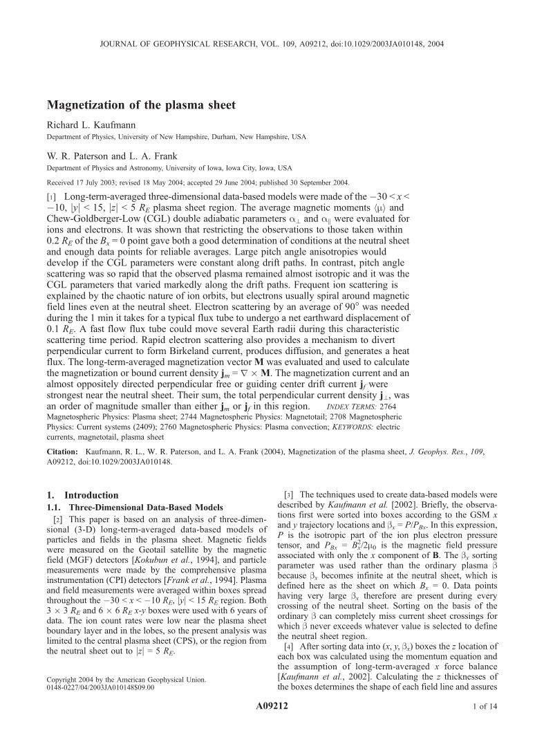
[12] Figure 1 shows the field lines obtained using 6 yearsof Geotail data. Field lines were traced starting at z = 0 and

A09212 KAUFMANN ET AL.: MAGNETIZATION OF THE PLASMA SHEET

2 of 14

A09212

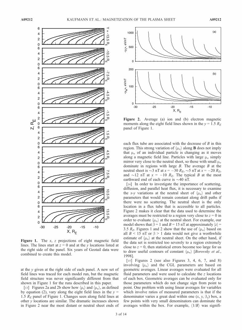
at the y given at the right side of each panel. A new set offield lines was traced for each model run, but the magneticfield structure was never significantly different from thatshown in Figure 1 for the runs described in this paper.[13] Figures 2a and 2b show how hmii and hmei, as defined

by equation (2), vary along the eight field lines in the y =1.5 RE panel of Figure 1. Changes seen along field lines atother y locations are similar. The dramatic increases shownin Figure 2 near the most distant or neutral sheet ends of

each flux tube are associated with the decrease of B in thisregion. This strong variation of hmsi along B does not implythat ms of an individual particle is changing as it movesalong a magnetic field line. Particles with large ms simplymirror very close to the neutral sheet, so those with small msdominate in regions with large B. The average B at theneutral sheet is 3 nT at x = �30 RE, 5 nT at x = �20 RE,and 12 nT at x = �10 RE. The typical B at the mostearthward end of each curve is 40 nT.[14] In order to investigate the importance of scattering,

diffusion, and parallel heat flux, it is necessary to examinethe x-y variations at the neutral sheet of hmsi and otherparameters that would remain constant along drift paths ifthere were no scattering. The neutral sheet is the onlylocation in a flux tube that is accessible to all particles.Figure 2 makes it clear that the data used to determine theaverages must be restricted to a region very close to z = 0 inorder to evaluate hmsi at the neutral sheet. For example, ourmodel shows that b = 1 and B = 15 nT at approximately jzj =3.5 RE. Figures 1 and 2 show that the use of hmsi based onall B < 15 nT or b > 1 data would not give a worthwhileestimate of hmsi at the neutral sheet. On the other hand, ifthe data set is restricted too severely to a region extremelyclose to z = 0, then statistical errors become too large for usto draw useful contours of constant hmsi [Borovsky et al.,1998].[15] Figures 2 (see also Figures 3, 4, 6, 7, and 8)

involving hmsi and the CGL parameters are based ongeometric averages. Linear averages were evaluated for allfluid parameters and were used to calculate the z locationsof each box. Geometric averages can be evaluated only forthose parameters which do not change sign from point topoint. One problem with using linear averages for variableswhich involve ratios of measured parameters is that if thedenominator varies a great deal within one (x, y, bx) box, afew points with very small denominators can dominate theaverages within the box. For example, h1/Bi was signifi-

Figure 1. The x, z projections of eight magnetic fieldlines. The lines start at z = 0 and at the y locations listed atthe right side of the panel. Six years of Geotail data werecombined to create this model.

Figure 2. Average (a) ion and (b) electron magneticmoments along the eight field lines shown in the y = 1.5 RE

panel of Figure 1.

A09212 KAUFMANN ET AL.: MAGNETIZATION OF THE PLASMA SHEET

3 of 14

A09212

cantly different from 1/hBi when linear averages weretaken. In contrast, the above two ratios are the same whenusing geometric averages. Contours of hmsi based onlinear averages had magnitudes 50% larger than those inFigure 2. The shapes of the hmsi contours were similar forthe two averaging methods. The differences between linearand geometric averages can be much larger for otherparameters, as will be discussed in section 3. Averagingmethods also become important when dealing with productsor ratios of correlated parameters.

2.2. Determining hhhMeiii at the Neutral Sheet

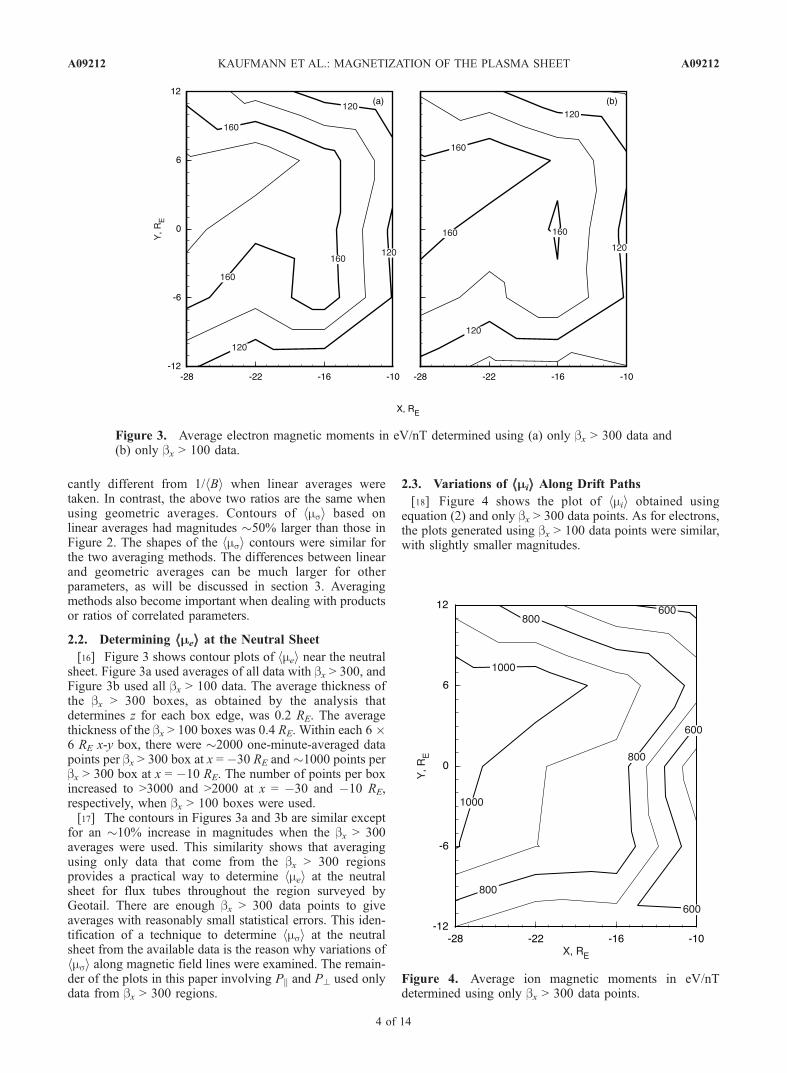
[16] Figure 3 shows contour plots of hmei near the neutralsheet. Figure 3a used averages of all data with bx > 300, andFigure 3b used all bx > 100 data. The average thickness ofthe bx > 300 boxes, as obtained by the analysis thatdetermines z for each box edge, was 0.2 RE. The averagethickness of the bx > 100 boxes was 0.4 RE. Within each 6 �6 RE x-y box, there were 2000 one-minute-averaged datapoints per bx > 300 box at x = �30 RE and 1000 points perbx > 300 box at x = �10 RE. The number of points per boxincreased to >3000 and >2000 at x = �30 and �10 RE,respectively, when bx > 100 boxes were used.[17] The contours in Figures 3a and 3b are similar except

for an 10% increase in magnitudes when the bx > 300averages were used. This similarity shows that averagingusing only data that come from the bx > 300 regionsprovides a practical way to determine hmei at the neutralsheet for flux tubes throughout the region surveyed byGeotail. There are enough bx > 300 data points to giveaverages with reasonably small statistical errors. This iden-tification of a technique to determine hmsi at the neutralsheet from the available data is the reason why variations ofhmsi along magnetic field lines were examined. The remain-der of the plots in this paper involving Pk and P? used onlydata from bx > 300 regions.

2.3. Variations of hhhMiiii Along Drift Paths

[18] Figure 4 shows the plot of hmii obtained usingequation (2) and only bx > 300 data points. As for electrons,the plots generated using bx > 100 data points were similar,with slightly smaller magnitudes.

Figure 3. Average electron magnetic moments in eV/nT determined using (a) only bx > 300 data and(b) only bx > 100 data.

Figure 4. Average ion magnetic moments in eV/nTdetermined using only bx > 300 data points.

A09212 KAUFMANN ET AL.: MAGNETIZATION OF THE PLASMA SHEET

4 of 14

A09212

[19] Figure 5 shows the ion perpendicular bulk velocityu?i based only on measurements made at 1.5 RE < jzj <2.5 RE and averaged over 3 � 3 RE x-y boxes. Theperpendicular bulk velocities tended to be largest at theneutral sheet and to decrease as jzj increases. Averages ofthe x component u?xi and y component u?yi of u?i were 70and 25% larger, respectively, in the jzj < 0.2 RE box than thevelocities in Figure 5. However, there were many fewer datapoints in the thin jzj < 0.2 RE boxes, so these averages gavea much more erratic pattern than that shown in Figure 5.Using 6 � 6 RE boxes produced a smooth flow patternwhich was qualitatively similar to Figure 5 even at jzj <0.2 RE but contained only one fourth as many independentlyevaluated flow vectors. At jzj = 5 RE the average u?xi wasless than half that in Figure 5. The average u?yi was smalland erratic at jzj = 5 RE, with most measurements showingflow from dusk to dawn rather than the dawn to dusk patternin Figure 5.[20] Angelopoulos et al. [1993], Huang and Frank

[1994], Paterson et al. [1998], and Hori et al. [2000]presented qualitatively similar flow patterns based on datafrom several satellites. These results all involved averagesover much thicker z regions, e.g., using all data with b >0.5, so they could not study the z dependence of flowvelocities.[21] One conclusion from Figures 3–5 is that the con-

tours of constant hmsi do not resemble the observed flowpatterns. This shows that hmei and hmii were not constantalong drift paths. However, the variations of hmsi wererelatively modest. The averages in Figures 3 and 4 remained

within 25% of hmei = 160 eV/nT and hmii = 800 eV/nTthroughout the region studied.

3. CGL Double Adiabatic Parameters

[22] The CGL double adiabatic magnetohydrodynamic(MHD) relations have been used in many geophysicalstudies. Recent papers have used these relations to examinelow-frequency waves [Ferriere and Andre, 2002], inter-change and bursty bulk flows [Ji and Wolf, 2003], themagnetosheath [Hau, 1996; Samsonov and Pudovkin,2000], and collisionless shocks [Gueret et al., 1998]. Someof these papers introduced more general versions of doubleadiabatic relations [Hau, 1996; Samsonov and Pudovkin,2000]. Here we will only consider the original CGLparameters and examine which of the assumptions associ-ated with their invariance fail.[23] The CGL equations were derived by expanding f (v)

in powers of a small parameter, substituting this into thecollisionless Boltzmann equation, and integrating. Theexpansion assumed that the plasma was quasi-uniform, withthe characteristic length for spatial variations being muchlarger than the gyroradius and the Debye length [Chew etal., 1956; Rossi and Olbert, 1970]. Similarly, the plasmawas assumed to be quasi-static, with only small variationsduring a cyclotron period or during an electron plasmaoscillation period. The derivation also assumed that Ek = 0,or that conductivity was infinite along a field line, and thatthe pressure tensor was diagonal and gyrotropic in themagnetic field aligned frame

Ps ¼ P?s1þ Pks � P?s� �

bb; ð4Þ

where 1 is the unit tensor and b is a unit vector along B. Theinfinite set of fluid equations obtained by the expansionprocedure was cut off by assuming that the parallel heat fluxcan be neglected. If all of the above assumptions are valid,then the CGL parameters

a?s ¼ P?s

nsBð5Þ

aks ¼PksB

2

n3sð6Þ

are constant along drift paths. These parameters can becombined, giving

a ¼ a2?ak

� �1=3¼ P2?Pk

n5

� �1=3: ð7Þ

There are many geophysical situations for which theassumptions needed to derive the CGL relations are notvalid, so that a?s and aks change along drift paths. Thepurpose of this section is to examine the spatial variations ofthe long-term-averaged a?s and aks at the neutral sheet. Astudy of these variations will provide quantitative informa-tion regarding the breakdown of some assumptions.[24] Since equation (5) is essentially the same as the

magnitude of the average magnetic moment equation (2),Figures 3 and 4 also illustrate the observed variations of

Figure 5. Average ion perpendicular flow vectors for1.5 < jzj < 2.5 RE.

A09212 KAUFMANN ET AL.: MAGNETIZATION OF THE PLASMA SHEET

5 of 14

A09212

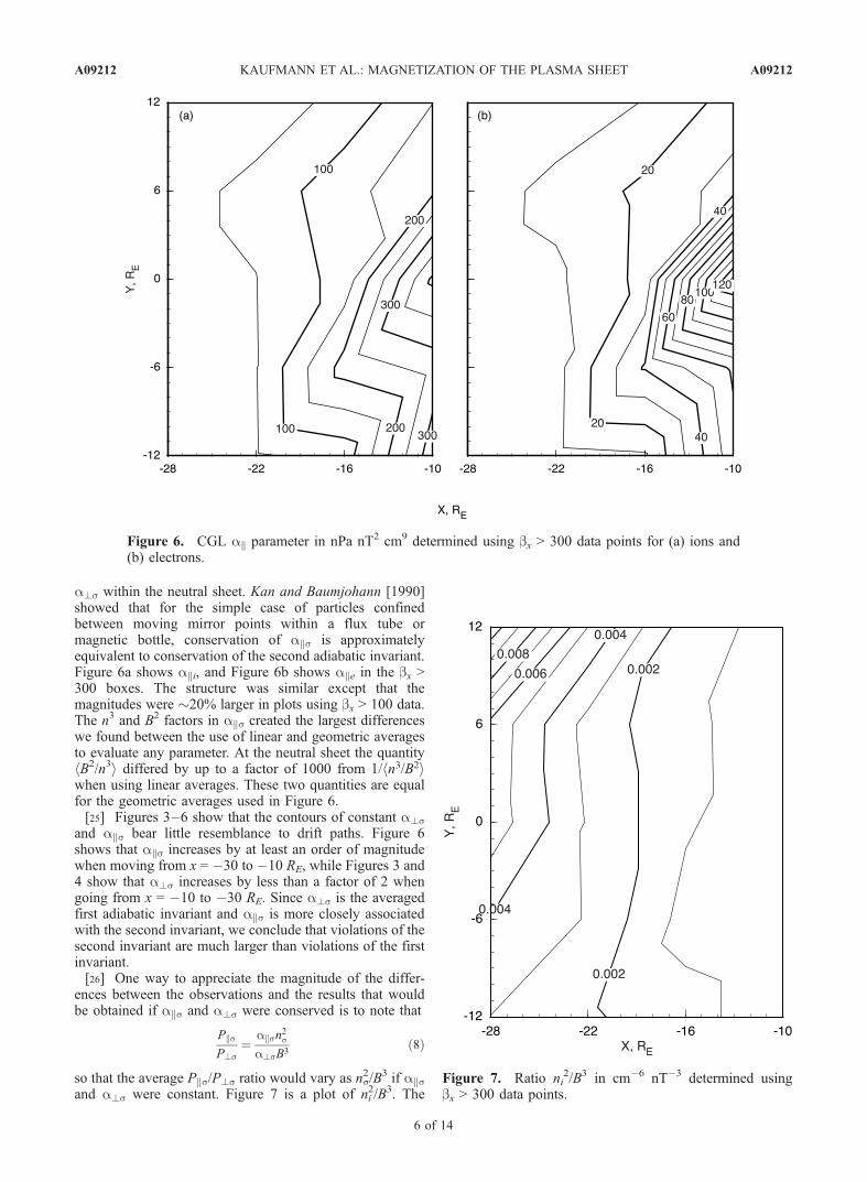
a?s within the neutral sheet. Kan and Baumjohann [1990]showed that for the simple case of particles confinedbetween moving mirror points within a flux tube ormagnetic bottle, conservation of aks is approximatelyequivalent to conservation of the second adiabatic invariant.Figure 6a shows aki, and Figure 6b shows ake in the bx >300 boxes. The structure was similar except that themagnitudes were 20% larger in plots using bx > 100 data.The n3 and B2 factors in aks created the largest differenceswe found between the use of linear and geometric averagesto evaluate any parameter. At the neutral sheet the quantityhB2/n3i differed by up to a factor of 1000 from 1/hn3/B2iwhen using linear averages. These two quantities are equalfor the geometric averages used in Figure 6.[25] Figures 3–6 show that the contours of constant a?s

and aks bear little resemblance to drift paths. Figure 6shows that aks increases by at least an order of magnitudewhen moving from x = �30 to �10 RE, while Figures 3 and4 show that a?s increases by less than a factor of 2 whengoing from x = �10 to �30 RE. Since a?s is the averagedfirst adiabatic invariant and aks is more closely associatedwith the second invariant, we conclude that violations of thesecond invariant are much larger than violations of the firstinvariant.[26] One way to appreciate the magnitude of the differ-

ences between the observations and the results that wouldbe obtained if aks and a?s were conserved is to note that

Pks

P?s¼

aksn2s

a?sB3ð8Þ

so that the average Pks/P?s ratio would vary as ns2/B3 if aks

and a?s were constant. Figure 7 is a plot of ni2/B3. The

Figure 6. CGL ak parameter in nPa nT2 cm9 determined using bx > 300 data points for (a) ions and(b) electrons.

Figure 7. Ratio ni2/B3 in cm�6 nT�3 determined using

bx > 300 data points.

A09212 KAUFMANN ET AL.: MAGNETIZATION OF THE PLASMA SHEET

6 of 14

A09212

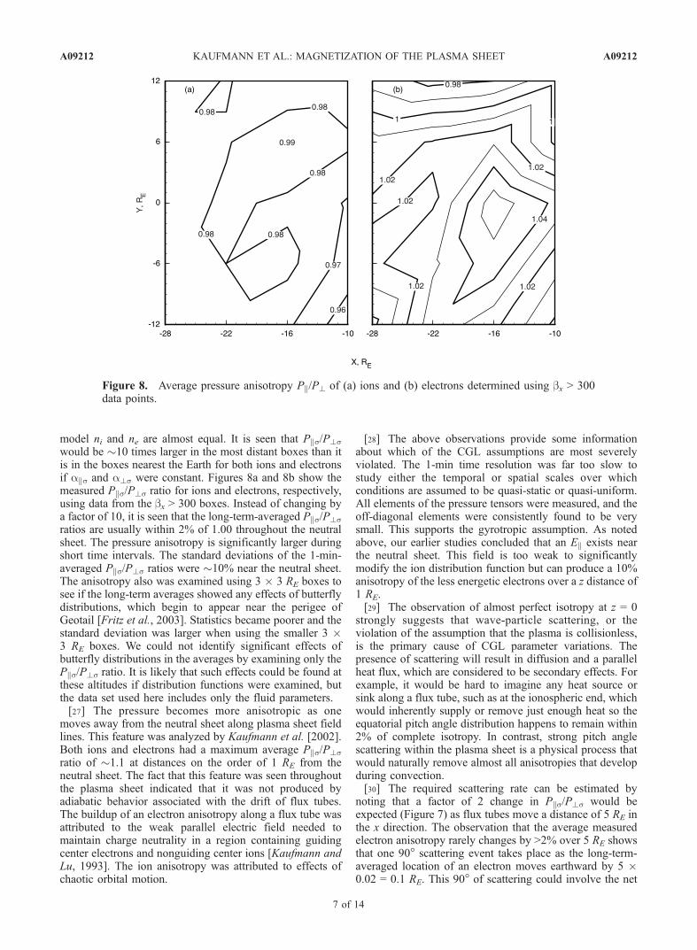
model ni and ne are almost equal. It is seen that Pks/P?swould be 10 times larger in the most distant boxes than itis in the boxes nearest the Earth for both ions and electronsif aks and a?s were constant. Figures 8a and 8b show themeasured Pks/P?s ratio for ions and electrons, respectively,using data from the bx > 300 boxes. Instead of changing bya factor of 10, it is seen that the long-term-averaged Pks/P?sratios are usually within 2% of 1.00 throughout the neutralsheet. The pressure anisotropy is significantly larger duringshort time intervals. The standard deviations of the 1-min-averaged Pks/P?s ratios were 10% near the neutral sheet.The anisotropy also was examined using 3 � 3 RE boxes tosee if the long-term averages showed any effects of butterflydistributions, which begin to appear near the perigee ofGeotail [Fritz et al., 2003]. Statistics became poorer and thestandard deviation was larger when using the smaller 3 �3 RE boxes. We could not identify significant effects ofbutterfly distributions in the averages by examining only thePks/P?s ratio. It is likely that such effects could be found atthese altitudes if distribution functions were examined, butthe data set used here includes only the fluid parameters.[27] The pressure becomes more anisotropic as one

moves away from the neutral sheet along plasma sheet fieldlines. This feature was analyzed by Kaufmann et al. [2002].Both ions and electrons had a maximum average Pks/P?sratio of 1.1 at distances on the order of 1 RE from theneutral sheet. The fact that this feature was seen throughoutthe plasma sheet indicated that it was not produced byadiabatic behavior associated with the drift of flux tubes.The buildup of an electron anisotropy along a flux tube wasattributed to the weak parallel electric field needed tomaintain charge neutrality in a region containing guidingcenter electrons and nonguiding center ions [Kaufmann andLu, 1993]. The ion anisotropy was attributed to effects ofchaotic orbital motion.

[28] The above observations provide some informationabout which of the CGL assumptions are most severelyviolated. The 1-min time resolution was far too slow tostudy either the temporal or spatial scales over whichconditions are assumed to be quasi-static or quasi-uniform.All elements of the pressure tensors were measured, and theoff-diagonal elements were consistently found to be verysmall. This supports the gyrotropic assumption. As notedabove, our earlier studies concluded that an Ek exists nearthe neutral sheet. This field is too weak to significantlymodify the ion distribution function but can produce a 10%anisotropy of the less energetic electrons over a z distance of1 RE.[29] The observation of almost perfect isotropy at z = 0

strongly suggests that wave-particle scattering, or theviolation of the assumption that the plasma is collisionless,is the primary cause of CGL parameter variations. Thepresence of scattering will result in diffusion and a parallelheat flux, which are considered to be secondary effects. Forexample, it would be hard to imagine any heat source orsink along a flux tube, such as at the ionospheric end, whichwould inherently supply or remove just enough heat so theequatorial pitch angle distribution happens to remain within2% of complete isotropy. In contrast, strong pitch anglescattering within the plasma sheet is a physical process thatwould naturally remove almost all anisotropies that developduring convection.[30] The required scattering rate can be estimated by

noting that a factor of 2 change in Pks/P?s would beexpected (Figure 7) as flux tubes move a distance of 5 RE inthe x direction. The observation that the average measuredelectron anisotropy rarely changes by >2% over 5 RE showsthat one 90� scattering event takes place as the long-term-averaged location of an electron moves earthward by 5 �0.02 = 0.1 RE. This 90� of scattering could involve the net

Figure 8. Average pressure anisotropy Pk/P? of (a) ions and (b) electrons determined using bx > 300data points.

A09212 KAUFMANN ET AL.: MAGNETIZATION OF THE PLASMA SHEET

7 of 14

A09212

effect of many small angle scattering events. Since the long-term-averaged earthward drift speed is on the order of10 km/s, a net 90� of electron scattering is needed aboutevery minute. Typical electron bounce times are on theorder of 10 s. The chaotic ions, which become nearlyisotropic during each neutral sheet interaction, have bouncetimes on the order of 10 min.[31] Angelopoulos et al. [1993] and Borovsky et al. [1997]

showed that fluctuations are so large that the average driftspeed hjvsji is several times larger than the magnitude of theaverage bulk velocity us = jhvsij. These fluctuations willsmooth the observed average variations of aks and a?s. Atypical flux tube will move back and forth by a distance onthe order of 1 RE during the minute required for the long-term-averaged location to move 0.1 RE earthward. The CGLparameters therefore would be conserved while an averageflux tube moves back and forth by 1 RE, or while a flux tubemoves several Earth radii during a fast flow event.

4. Magnetization Vector

4.1. Electrons

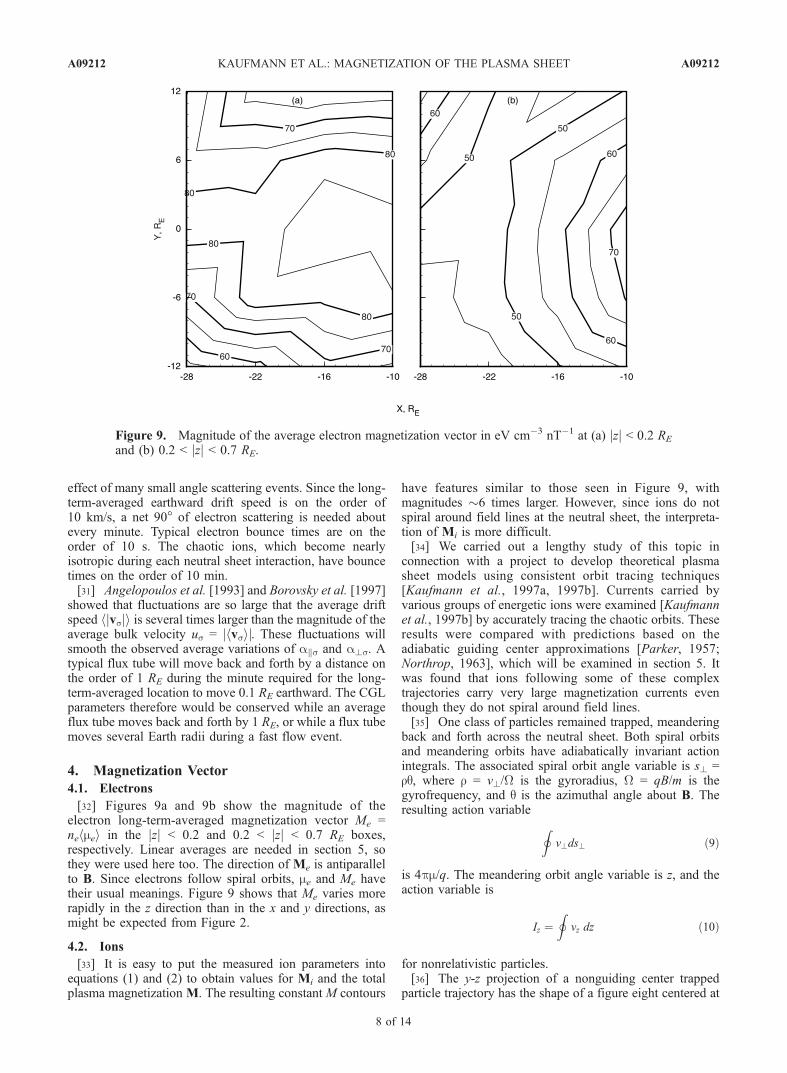
[32] Figures 9a and 9b show the magnitude of theelectron long-term-averaged magnetization vector Me =nehmei in the jzj < 0.2 and 0.2 < jzj < 0.7 RE boxes,respectively. Linear averages are needed in section 5, sothey were used here too. The direction of Me is antiparallelto B. Since electrons follow spiral orbits, me and Me havetheir usual meanings. Figure 9 shows that Me varies morerapidly in the z direction than in the x and y directions, asmight be expected from Figure 2.

4.2. Ions

[33] It is easy to put the measured ion parameters intoequations (1) and (2) to obtain values for Mi and the totalplasma magnetization M. The resulting constant M contours

have features similar to those seen in Figure 9, withmagnitudes 6 times larger. However, since ions do notspiral around field lines at the neutral sheet, the interpreta-tion of Mi is more difficult.[34] We carried out a lengthy study of this topic in

connection with a project to develop theoretical plasmasheet models using consistent orbit tracing techniques[Kaufmann et al., 1997a, 1997b]. Currents carried byvarious groups of energetic ions were examined [Kaufmannet al., 1997b] by accurately tracing the chaotic orbits. Theseresults were compared with predictions based on theadiabatic guiding center approximations [Parker, 1957;Northrop, 1963], which will be examined in section 5. Itwas found that ions following some of these complextrajectories carry very large magnetization currents eventhough they do not spiral around field lines.[35] One class of particles remained trapped, meandering

back and forth across the neutral sheet. Both spiral orbitsand meandering orbits have adiabatically invariant actionintegrals. The associated spiral orbit angle variable is s? =rq, where r = v?/W is the gyroradius, W = qB/m is thegyrofrequency, and q is the azimuthal angle about B. Theresulting action variable

Iv?ds? ð9Þ

is 4pm/q. The meandering orbit angle variable is z, and theaction variable is

Iz ¼I

vz dz ð10Þ

for nonrelativistic particles.[36] The y-z projection of a nonguiding center trapped

particle trajectory has the shape of a figure eight centered at

Figure 9. Magnitude of the average electron magnetization vector in eV cm�3 nT�1 at (a) jzj < 0.2 RE

and (b) 0.2 < jzj < 0.7 RE.

A09212 KAUFMANN ET AL.: MAGNETIZATION OF THE PLASMA SHEET

8 of 14

A09212

z = 0 that drifts slowly in the y direction. Figure 5 of Larsonand Kaufmann [1996] shows a sample trapped orbit. Suchorbits create strong magnetization currents jm from dusk todawn near z = 0 and slightly larger jm from dawn to dusk atz0 < jzj < 2 z0, where

z0 ¼ mv= qBxy z0ð Þ� �

ð11Þ

is the point at which the Bxy magnetic field becomes strongenough to turn a particle of mass m, velocity v, and charge qback toward the neutral sheet and Bxy

2 = Bx2 + By

2. In themagnetic field model shown in Figure 1, z0 is 0.7 RE for atypical observed ion and shows little dependence on x or y.A particle on a figure eight orbit that did not drift wouldreturn to its starting point after one oscillation period, so itwould carry no free current. The strong dawnward jm at jzj <z0 and the strong duskward jm at z0 < jzj < 2 z0 would cancelif integrated from z = 0 to jzj > 2 z0.[37] Whereas trapped particles remain near the neutral

sheet for an extended period of time, Speiser [1965]investigated a class of nonguiding center orbits that mirrorat low altitudes and spend only brief intervals near theneutral sheet. Speiser particles spiral around field lines formost of such an orbit and cross an orbital separatrix nearjzj = 2 z0. These particles then meander back and forthacross the neutral sheet for a short period as they drift alonga path with a semicircular projection in the x-y plane. Afterthis, they leave the neutral sheet region to resume spiralmotion. Although m is nearly constant during the spiralportions of these orbits and Iz is nearly constant during themeandering portion, in general, neither is conserved nearthe separatrix. The magnetic moment often is substantiallydifferent before and after the neutral sheet interaction. Mostof the net drift of a Speiser particle takes place while it is atjzj < 2 z0. This free current jf is from dawn to dusk in theneutral sheet. A weak dusk to dawn current is presentbeyond jzj = 2 z0 [Kaufmann et al., 1997b].[38] The orbits of nonguiding center particles with mirror

points intermediate between the trapped and Speiserextremes have been referred to as cucumber orbits [Buchnerand Zelenyi, 1989]. Depending on their distribution ofmirror points, a group of such particles can carry cross-tailcurrent in either direction at the neutral sheet. The cross-tailcurrent is from dusk to dawn at jzj somewhat smaller thanthe average location of the mirror point of a group ofcucumber particles and from dawn to dusk at larger jzj.Figures 2 and 3 of Larson and Kaufmann [1996] showtypical Speiser orbits, with mirror points far away from theneutral sheet, and cucumber orbits, with mirror points closerto the neutral sheet but beyond jzj = 2 z0.[39] The chaotic nature of plasma sheet ions often causes

them to move from one type of orbit to another during aneutral sheet interaction. The resulting substantial change inmirror points from orbit to orbit shows that the secondadiabatic invariant changes markedly. The angle variable iss, the arc length along a field line, for the second invariantaction variable

J ¼I

mvk ds: ð12Þ

[40] When a group of particles was specifically selectedso that it was dominated by ions on trapped orbits or by ions

on Speiser orbits [Kaufmann et al., 1997b], it was foundthat these groups carried currents that differed substantiallyfrom the currents predicted by the adiabatic guiding centerdrift equations. These select groups had highly anisotropicdistribution functions. When various groups of particlesfollowing trapped, cucumber, and Speiser orbits were mixedtogether to produce a nearly isotropic self-consistent plasmasheet, then the full plasma was consistently found to carrycurrents that were very close to those predicted by theadiabatic guiding center equations. Usadi et al. [1996]reached a similar conclusion by comparing the adiabaticdrift equations to the actual drifts of groups of nonguidingcenter particles. These studies therefore show that becausethe overall plasma is observed to be nearly isotropic, the useof equations (1) and (2) provides a reasonable estimate ofthe total plasma magnetization vector. In section 5 wetherefore will use equations (1), (2), and (3) to estimate jm.

5. Calculated Magnetization and Free CurrentDensities

[41] The total average plasma sheet current density iscoupled, through Ampere’s law, to the average observedmagnetic field j = (1/m0)r � B. For some applications it isnecessary to separate the total perpendicular current intoperpendicular magnetization jms and free jfs componentsand to separate the currents carried by ions and electrons.For example, Kaufmann et al. [2003] used the 3-D data-based models to examine the buildup of parallel current jkwithin the CPS. Since jms is divergence-free, it is only theperpendicular jfs portion of the total current that can bediverted to create a steady jk. Detectors in the topsideionosphere have shown that it is electrons which carry thebulk of the observed jk even within upgoing ion beams[Kaufmann and Kintner, 1984], so it is jfe that is of interestto studies of the source of Birkeland current in the CPS.Another reason for separating jfs and jms is because theycontribute differently to kinetic and fluid plasma instabil-ities [Ichimaru, 1973]. It is only the drift associated with jfsthat is involved in the kinetic resonant particle instabilitieswith perpendicularly propagating plasma waves. The totalperpendicular current is involved in MHD and certain otherkinetic instabilities.

5.1. Adiabatic Drift Equations

[42] The adiabatic guiding center expressions for theperpendicular magnetization and free current densities are[Parker, 1957; Northrop, 1963]

jms ¼ B

B2� rP?s �

P?s

BrB�

Pks

B2B rð ÞB

� �ð13Þ

jf s ¼ B

B2� P?s

BrBþ

Pks

B2B rð ÞBþ nsms u rð Þu� nsqsE

� �

þ jcs; ð14Þ

and the total perpendicular current density is

j? ¼Xs

jms þ jf s

: ð15Þ

A09212 KAUFMANN ET AL.: MAGNETIZATION OF THE PLASMA SHEET

9 of 14

A09212

The magnetization current terms are the pressure or densityplus temperature gradient current, the part of the rB currentassociated with the area of a gyroorbit and the period ofgyration, and the part of the field line curvature currentassociated with orbit crowding. These terms involve onlythe circular component of the motion of a spiralling particle,not any net displacement of the particle’s guiding center.[43] The free current terms are the part of the rB drift

associated with the net displacement produced by thespatially varying gyroradius of meandering particles, thecentrifugal force portion of the curvature drift, polarizationdrift associated with spatial variations of the perpendicularbulk speed, the E � B drift, and diffusion associatedwith collisions or other scattering processes. These termsall result in a net displacement of a particle after onegyroperiod so they can continuously supply particles to aflux tube that carries a steady Birkeland current. Gravita-tional drift has not been included in equation (14) becauseits magnitude is very small in the plasma sheet. The netcross-tail displacement of chaotic particles after one fullfigure eight-shaped orbit, the meandering portion of Speiserorbits, and the net displacement after a full cucumber orbitall contribute to the free current.[44] Several terms cancel when evaluating j? using

equation (15). The rB terms in equations (13) and (14)cancel when jms and jfs are added. The E � B terms cancelin the sum over species if the plasma is neutral. One featurethat may seem confusing is that the expression typicallyused to evaluate jk by calculating r � j? for an isotropicslow flow plasma involves using r � j? = r (B �rP/B2) [Vasyliunas, 1970; Wolf, 1983]. Since rP appearsonly in jm, which is divergence-free, it might seem as if thisterm should not appear in a calculation of jk. However, it isbecause r jm = 0 that the divergence of the first term inequation (13) is equal to the divergence of the other two termsin equation (13) and therefore is the same as the divergenceof the first two terms in equation (14) in an isotropicplasma. Since all other terms in equation (14) are eitherzero or neglected when flow is slow and the species arecombined in equation (15), r jf is correctly given by theusual expression which contains only the rP term.

5.2. Current Density Evaluation Methods

[45] The technique that has almost always been used todetermine j? in either the ionosphere [Zmuda andArmstrong, 1974; Iijima and Potemra, 1978; Weimer,2001] or the magnetotail [Tsyganenko et al., 1993;Israelevich et al., 2001] is to use Ampere’s law andmeasurements of B. Section 4 concluded that Ms can beadequately approximated using equations (1) and (2). Ittherefore is possible to apply this same technique, usingequation (3), to determine jms for each species. Since theperpendicular free current density is given by jf = j? � jm,the availability of j? only for the sum of all species meansthat jf can be evaluated only for the sum of all species.

5.3. Current Density Results

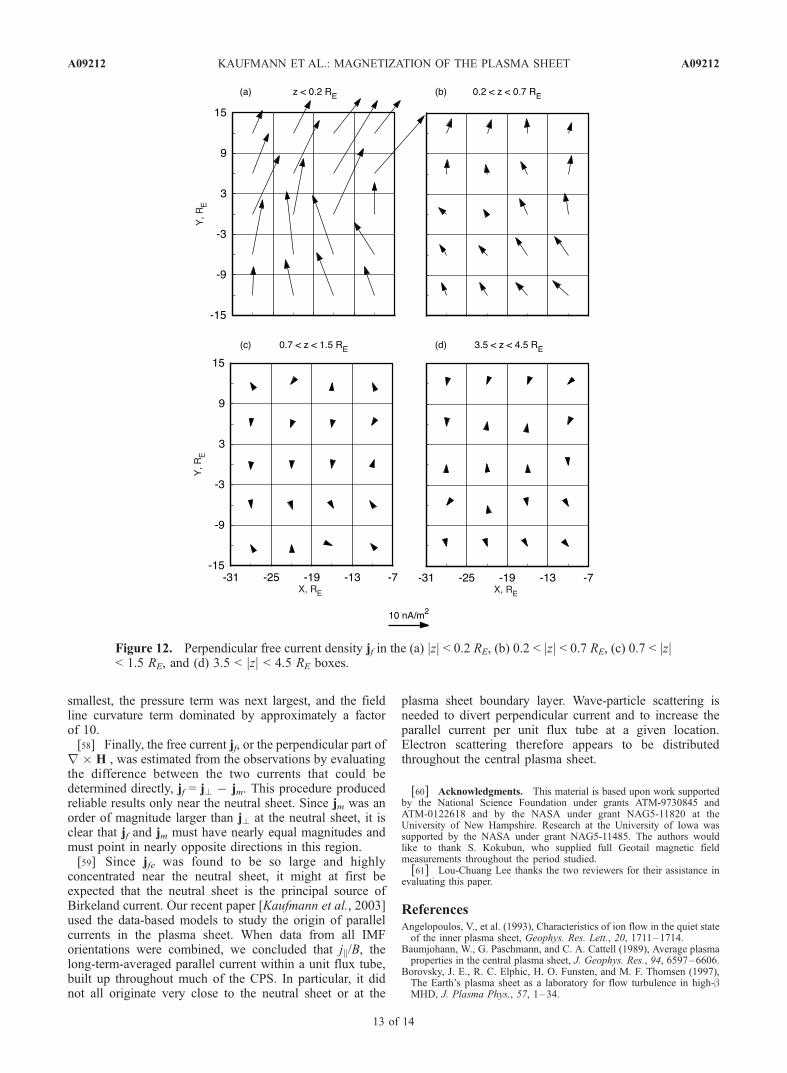
[46] Figure 10 shows j? for the three z boxes closest tothe neutral sheet and for one box at larger z. These resultsare based on evaluating r � B using all data from 6 yearsof measurements. The first three z boxes are from runs thatkept Northern and Southern Hemisphere data separate so

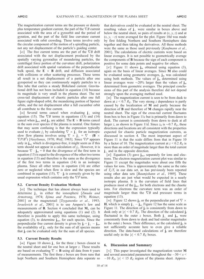
that derivatives could be evaluated at the neutral sheet. Theresulting values of j? were similar in boxes above andbelow the neutral sheet, so pairs of results at (x, y, z) and at(x, y, �z) were averaged for the plot. Figure 10d was madeby first folding Northern and Southern Hemisphere datatogether and then taking the derivatives. All these methodswere the same as those used previously [Kaufmann et al.,2001]. The calculations of electric currents were based onlinear averages. It is not possible to geometrically averagethe components of B because the sign of each component ispositive for some data points and negative for others.[47] Figure 11 shows jm obtained using equation (3),

again on the basis of linear averages. Since M also couldbe evaluated using geometric averages, jm was calculatedusing both methods. The values of jm determined usinglinear averages were 20% larger than the values of jmdetermined from geometric averages. The principal conclu-sions of this part of the analysis therefore did not dependstrongly upon the averaging method used.[48] The magnetization current is seen to be from dusk to

dawn at z < 0.7 RE. The very strong z dependence is partlycaused by the localization of M and partly because thedirection of B and therefore of M changes rapidly near theneutral sheet. The sign of the cross-tail current fluctuatesfrom box to box in Figure 11c but is primarily from dawn todusk. The current is consistently from dawn to dusk at alllarger z, as shown in Figure 11d. Since z0 is 0.7 RE, thesedirections and locations are all consistent with the propertiesexpected for chaotic particle magnetization currents, asdiscussed in section 4. The most important aspect ofFigure 11 is that the scale differs from that in Figure 10by a factor of 10. The magnetization current at z < 0.2 RE ismore than an order of magnitude larger than the total currentj? and in the opposite direction.[49] Equation (3) gave jms separately for ions and elec-

trons. The electron magnetization current plot was similar toFigure 11 except the magnitudes were about one fifth thevalues for ions. This is approximately the same as the ratioof Te/Ti in our data set, as has previously been reportedusing other data sets [Baumjohann et al., 1989]. Theseresults also are just what would be expected in a nearlyisotropic plasma. It is the curvature of field lines thatproduces most of the jms for both electrons and the chaoticions. For electrons the curvature term was an order ofmagnitude larger than the rB and pressure terms inequation (13).[50] Figure 12 shows jf, or the perpendicular part of r �

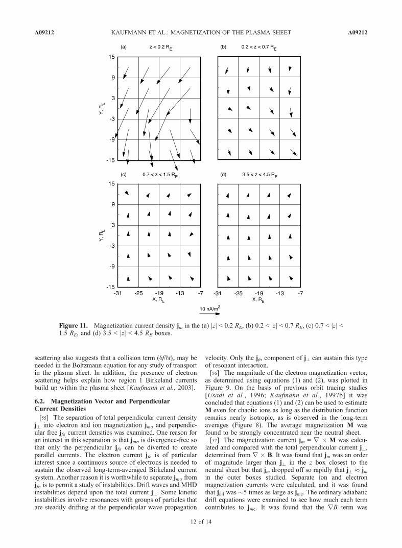
H, which is simply j? � jm. Figure 12 has the same scale asFigure 11. The direction of jf is consistently from dawn todusk only at jzj < 0.7 RE. The direction of the calculated jffluctuated in the outer z boxes. Both j? and jm wereconsistently from dawn to dusk and had similar magnitudesin the outer z boxes. Their difference, or the calculated jf, isnot sufficiently accurate here to even give a reliabledirection. The data-based calculations of jf are thereforeuseful only in the jzj < 0.7 RE boxes.

6. Discussion and Summary

[51] This paper investigated the magnetization vector Mand several associated parameters throughout the �30 < x <�10 RE, jyj < 15 RE region of the plasma sheet. Approx-

A09212 KAUFMANN ET AL.: MAGNETIZATION OF THE PLASMA SHEET

10 of 14

A09212

imately 100,000 one-minute-averaged plasma sheet datapoints were available per year. All data from 6 years ofCPI particle and MGF measurements taken on the Geotailsatellite were combined for the analysis. As a result, onlylong-term-averaged conditions were studied.

6.1. Average Magnetic Moments and CGL Parameters

[52] The Chew-Goldberger-Low (CGL) double adiabaticparameters a?s and aks [Chew et al., 1956] were evaluatedas a part of the data-based modeling procedure. Theparameter a?s is essentially the same as the averagemagnetic moment hmsi. Since hmsi varies rapidly alongmagnetic field lines near the equator, it was necessary toinvestigate this spatial dependence so a procedure could bedeveloped to determine hmsi at the neutral sheet. Weconcluded that averaging all data with bx > 300 providedboth a good estimate of hmsi at jzj < 0.2 RE and enough datato give consistent results (Figures 3 and 4). It was found thata?s or hmsi at the neutral sheet tended to decrease as onemoved earthward and toward the flanks but varied by only25% from the value averaged throughout the region studied.

[53] Contours of constant aks changed much moredramatically in the region studied. This parameter, whichis related to the second adiabatic invariant, increased by anorder of magnitude when moving from the most tailward tothe most earthward boxes (Figure 6). It also was shown(Figure 7) that the Pk/P? ratio at the neutral sheet would beexpected to change by approximately a factor of 10 asparticles drift through the region studied if the CGLparameters remained constant. In contrast, this ratio variedby only 2% from 1.00, or perfect isotropy. Since ionsfollow chaotic orbits, the fact that they were scattered andbecame isotropic during each interaction with the neutralsheet was not surprising. However, electrons follow spiralguiding center orbits, and they remained almost equallyisotropic at the neutral sheet. It was estimated that electronswere scattered by 90� in 1 min, or the time required for anaverage flux tube to undergo a net earthward displacementof 0.1 RE in the plasma sheet.[54] The presence of strong electron and ion scattering

has several important consequences. Such scattering resultsin diffusion and an associated parallel heat flux. Strong

Figure 10. Total perpendicular current density j? in the (a) jzj < 0.2 RE, (b) 0.2 < jzj < 0.7 RE, (c) 0.7 <jzj < 1.5 RE, and (d) 3.5 < jzj < 4.5 RE boxes.

A09212 KAUFMANN ET AL.: MAGNETIZATION OF THE PLASMA SHEET

11 of 14

A09212

scattering also suggests that a collision term (df/dt)c may beneeded in the Boltzmann equation for any study of transportin the plasma sheet. In addition, the presence of electronscattering helps explain how region 1 Birkeland currentsbuild up within the plasma sheet [Kaufmann et al., 2003].

6.2. Magnetization Vector and PerpendicularCurrent Densities

[55] The separation of total perpendicular current densityj? into electron and ion magnetization jms and perpendic-ular free jfs current densities was examined. One reason foran interest in this separation is that jms is divergence-free sothat only the perpendicular jfs can be diverted to createparallel currents. The electron current jfe is of particularinterest since a continuous source of electrons is needed tosustain the observed long-term-averaged Birkeland currentsystem. Another reason it is worthwhile to separate jms fromjfs is to permit a study of instabilities. Drift waves and MHDinstabilities depend upon the total current j?. Some kineticinstabilities involve resonances with groups of particles thatare steadily drifting at the perpendicular wave propagation

velocity. Only the jfs component of j? can sustain this typeof resonant interaction.[56] The magnitude of the electron magnetization vector,

as determined using equations (1) and (2), was plotted inFigure 9. On the basis of previous orbit tracing studies[Usadi et al., 1996; Kaufmann et al., 1997b] it wasconcluded that equations (1) and (2) can be used to estimateM even for chaotic ions as long as the distribution functionremains nearly isotropic, as is observed in the long-termaverages (Figure 8). The average magnetization M wasfound to be strongly concentrated near the neutral sheet.[57] The magnetization current jm = r � M was calcu-

lated and compared with the total perpendicular current j?,determined from r � B. It was found that jm was an orderof magnitude larger than j? in the z box closest to theneutral sheet but that jm dropped off so rapidly that j? � jmin the outer boxes studied. Separate ion and electronmagnetization currents were calculated, and it was foundthat jmi was 5 times as large as jme. The ordinary adiabaticdrift equations were examined to see how much each termcontributes to jme. It was found that the rB term was

Figure 11. Magnetization current density jm in the (a) jzj < 0.2 RE, (b) 0.2 < jzj < 0.7 RE, (c) 0.7 < jzj <1.5 RE, and (d) 3.5 < jzj < 4.5 RE boxes.

A09212 KAUFMANN ET AL.: MAGNETIZATION OF THE PLASMA SHEET

12 of 14

A09212

smallest, the pressure term was next largest, and the fieldline curvature term dominated by approximately a factorof 10.[58] Finally, the free current jf, or the perpendicular part of

r � H , was estimated from the observations by evaluatingthe difference between the two currents that could bedetermined directly, jf = j? � jm. This procedure producedreliable results only near the neutral sheet. Since jm was anorder of magnitude larger than j? at the neutral sheet, it isclear that jf and jm must have nearly equal magnitudes andmust point in nearly opposite directions in this region.[59] Since jfe was found to be so large and highly

concentrated near the neutral sheet, it might at first beexpected that the neutral sheet is the principal source ofBirkeland current. Our recent paper [Kaufmann et al., 2003]used the data-based models to study the origin of parallelcurrents in the plasma sheet. When data from all IMForientations were combined, we concluded that jk/B, thelong-term-averaged parallel current within a unit flux tube,built up throughout much of the CPS. In particular, it didnot all originate very close to the neutral sheet or at the

plasma sheet boundary layer. Wave-particle scattering isneeded to divert perpendicular current and to increase theparallel current per unit flux tube at a given location.Electron scattering therefore appears to be distributedthroughout the central plasma sheet.

[60] Acknowledgments. This material is based upon work supportedby the National Science Foundation under grants ATM-9730845 andATM-0122618 and by the NASA under grant NAG5-11820 at theUniversity of New Hampshire. Research at the University of Iowa wassupported by the NASA under grant NAG5-11485. The authors wouldlike to thank S. Kokubun, who supplied full Geotail magnetic fieldmeasurements throughout the period studied.[61] Lou-Chuang Lee thanks the two reviewers for their assistance in

evaluating this paper.

ReferencesAngelopoulos, V., et al. (1993), Characteristics of ion flow in the quiet stateof the inner plasma sheet, Geophys. Res. Lett., 20, 1711–1714.

Baumjohann, W., G. Paschmann, and C. A. Cattell (1989), Average plasmaproperties in the central plasma sheet, J. Geophys. Res., 94, 6597–6606.

Borovsky, J. E., R. C. Elphic, H. O. Funsten, and M. F. Thomsen (1997),The Earth’s plasma sheet as a laboratory for flow turbulence in high-bMHD, J. Plasma Phys., 57, 1–34.

Figure 12. Perpendicular free current density jf in the (a) jzj < 0.2 RE, (b) 0.2 < jzj < 0.7 RE, (c) 0.7 < jzj< 1.5 RE, and (d) 3.5 < jzj < 4.5 RE boxes.

A09212 KAUFMANN ET AL.: MAGNETIZATION OF THE PLASMA SHEET

13 of 14

A09212

Borovsky, J. E., M. F. Thomsen, and R. C. Elphic (1998), The driving of theplasma sheet by the solar wind, J. Geophys. Res., 103, 17,617–17,639.

Buchner, J., and L. M. Zelenyi (1989), Regular and chaotic charged particlemotion in magnetotaillike field reversals: 1. Basic theory of trappedmotion, J. Geophys. Res., 94, 11,821–11,842.

Chen, J., and P. J. Palmadesso (1986), Chaos and nonlinear dynamics ofsingle-particle orbits in a magnetotaillike magnetic field, J. Geophys.Res., 91, 1499–1508.

Chew, G. F., M. L. Goldberger, and F. E. Low (1956), The Boltzmannequation and the one-fluid hydromagnetic equations in the absence ofparticle collisions, Proc. R. Soc. London, Ser. A, 236, 112–118.

Delcourt, D. C., and R. F. Martin Jr. (1999), Pitch angle scattering nearenergy resonances in the geomagnetic tail, J. Geophys. Res., 104, 383–394.

Ferriere, K. M., and N. Andre (2002), A mixed magnetohydrodynamic-kinetic theory of low-frequency waves and instabilities in homogeneous,gyrotropic plasmas, J. Geophys. Res., 107(A11), 1349, doi:10.1029/2002JA009273.

Frank, L. A., K. L. Ackerson, W. R. Paterson, J. A. Lee, M. R. English, andG. L. Pickett (1994), The comprehensive plasma instrumentation (CPI)for the GEOTAIL spacecraft, J. Geomagn. Geoelectr., 46, 23–37.

Fritz, T. A., M. Alothman, J. Bhattacharjya, D. L. Matthews, and J. Chen(2003), Butterfly pitch-angle distributions observed by ISEE-1, Planet.Space Sci., 51, 205–219.

Gueret, B., B. Lembege, and G. Belmont (1998), Laws for electron pressurevariations across a collisionless shock, J. Geophys. Res., 103, 327–334.

Hau, L.-N. (1996), Nonideal MHD effects in the magnetosheath, J. Geo-phys. Res., 101, 2655–2660.

Heinemann, M., and R. A. Wolf (2001), Relationships of models of theinner magnetosphere to the Rice Convection Model, J. Geophys. Res.,106, 15,545–15,554.

Hori, T., K. Maezawa, Y. Saito, and T. Mukai (2000), Average profile of ionflow and convection electric field in near-Earth plasma sheet, Geophys.Res. Lett., 27, 1623–1626.

Huang, C. Y., and L. A. Frank (1994), A statistical survey of the centralplasma sheet, J. Geophys. Res., 99, 83–95.

Ichimaru, S. (1973), Basic Principles of Plasma Physics: A StatisticalApproach, Benjamin, White Plains, N. Y.

Iijima, T., and T. A. Potemra (1978), Large-scale characteristics of field-aligned currents associated with substorms, J. Geophys. Res., 83, 599–615.

Israelevich, P. L., A. I. Ershkovich, and N. A. Tsyganenko (2001), Magneticfield and electric current density distribution in the geomagnetic tail,based on Geotail data, J. Geophys. Res., 106, 25,919–25,927.

Ji, S., and R. A. Wolf (2003), Double-adiabatic MHD theory for motion ofa thin magnetic filament and possible implications for bursty bulk flows,J. Geophys. Res., 108(A5), 1191, doi:10.1029/2002JA009655.

Kan, J. R., and W. Baumjohann (1990), Isotropized magnetic-momentequation of state for the central plasma sheet, Geophys. Res. Lett., 17,271–274.

Kaufmann, R. L., and P. M. Kintner (1984), Upgoing ion beams: 2. Fluidanalysis and magnetosphere-ionosphere coupling, J. Geophys. Res., 89,2195–2210.

Kaufmann, R. L., and C. Lu (1993), Cross-tail current: Resonant orbits,J. Geophys. Res., 98, 15,447–15,465.

Kaufmann, R. L., C. Lu, and D. J. Larson (1994), Cross-tail current, field-aligned current, and By, J. Geophys. Res., 99, 11,277–11,295.

Kaufmann, R. L., D. J. Larson, I. D. Kontodinas, and B. M. Ball (1997a),Force balance and substorm effects in the magnetotail, J. Geophys. Res.,102, 22,141–22,154.

Kaufmann, R. L., I. D. Kontodinas, B. M. Ball, and D. J. Larson (1997b),Nonguiding center motion and substorm effects in the magnetotail,J. Geophys. Res., 102, 22,155–22,168.

Kaufmann, R. L., B. M. Ball, W. R. Paterson, and L. A. Frank (2001),Plasma sheet thickness and electric currents, J. Geophys. Res., 106,6179–6193.

Kaufmann, R. L., C. Lu, W. R. Paterson, and L. A. Frank (2002), Three-dimensional analyses of electric currents and pressure anisotropies inthe plasma sheet, J. Geophys. Res., 107(A7), 1103, doi:10.1029/2001JA000288.

Kaufmann, R. L., W. R. Paterson, and L. A. Frank (2003), Birkelandcurrents in the plasma sheet, J. Geophys. Res., 108(A7), 1299,doi:10.1029/2002JA009665.

Kistler, L. M., E. Mobius, W. Baumjohann, G. Paschmann, and D. C.Hamilton (1992), Pressure changes in the plasma sheet during substorminjections, J. Geophys. Res., 97, 2973–2983.

Kokubun, S., T. Yamamoto, M. H. Acuna, K. Hayashi, K. Shiokawa, andH. Kawano (1994), The Geotail magnetic field experiment, J. Geomagn.Geoelectr., 46, 7–21.

Larson, D. J., and R. L. Kaufmann (1996), Structure of the magnetotailcurrent sheet, J. Geophys. Res., 101, 21,447–21,461.

Northrop, T. G. (1963), The Adiabatic Motion of Charged Particles, Wiley-Interscience, Hoboken, N. J.

Parker, E. N. (1957), Newtonian development of the dynamical propertiesof ionized gases of low density, Phys. Rev., 107, 924–933.

Paterson, W. R., L. A. Frank, S. Kokubun, and T. Yamamoto (1998),Geotail survey of ion flow in the plasma sheet: Observations between10 and 50 RE, J. Geophys. Res., 103, 11,811–11,825.

Rossi, B., and S. Olbert (1970), Introduction to the Physics of Space,McGraw-Hill, New York.

Samsonov, A. A., and M. I. Pudovkin (2000), Application of the boundedanisotropy model for the dayside magnetosheath, J. Geophys. Res., 105,12,859–12,867.

Speiser, T. W. (1965), Particle trajectories in model current sheets: 1. Ana-lytic solutions, J. Geophys. Res., 70, 4219–4226.

Stiles, G. S., E. W. Hones Jr., S. J. Bame, and J. R. Asbridge (1978), Plasmasheet pressure anisotropies, J. Geophys. Res., 83, 3166–3172.

Tsyganenko, N. A., and D. P. Stern (1996), Modeling the global magneticfield of the large-scale Birkeland current systems, J. Geophys. Res., 101,27,187–27,198.

Tsyganenko, N. A., D. P. Stern, and Z. Kaymaz (1993), Birkeland currentsin the plasma sheet, J. Geophys. Res., 98, 19,455–19,464.

Usadi, A., R. A. Wolf, M. Heinemann, and W. Horton (1996), Does chaosalter the ensemble averaged drift equations?, J. Geophys. Res., 101,15,491–15,514.

Vasyliunas, V. M. (1970), Mathematical models of magnetospheric convec-tion and its coupling to the ionosphere, in Particles and Fields in theMagnetosphere, edited by B. M. McCormac, pp. 60 –71, D. Reidel,Norwell, Mass.

Weimer, D. R. (2001), Maps of ionospheric field-aligned currents as afunction of the interplanetary magnetic field derived from DynamicsExplorer 2 data, J. Geophys. Res., 106, 12,889–12,902.

Wolf, R. A. (1983), The quasi-static (slow-flow) region of the magneto-sphere, in Solar-Terrestrial Physics: Principles and Theoretical Founda-tions, edited by R. L. Carovillano and J. M. Forbes, pp. 303–368,D. Reidel, Norwell, Mass.

Zmuda, A. J., and J. C. Armstrong (1974), The diurnal flow pattern offield-aligned currents, J. Geophys. Res., 79, 4611–4619.

�����������������������L. A. Frank and W. R. Paterson, Department of Physics and Astronomy,

University of Iowa, Iowa City, IA 52242-1479, USA. (frank@iowasp.physics.uiowa.edu; paterson@iowasp.uiowa.edu)R. L. Kaufmann, Department of Physics, University of New Hampshire,

DeMeritt Hall, 9 Library Way, Durham, NH 03824-3568, USA.(dick.kaufmann@unh.edu)

A09212 KAUFMANN ET AL.: MAGNETIZATION OF THE PLASMA SHEET

14 of 14

A09212