A&A 516, A17 (2010)DOI: 10.1051/0004-6361/200913542c© ESO 2010

Astronomy&

Astrophysics

Structure of the heliospheric current sheet from plasma convectionin time-dependent heliospheric models

A. Czechowski1, M. Strumik1, J. Grygorczuk1, S. Grzedzielski1, R. Ratkiewicz1, and K. Scherer2

1 Space Research Centre, Polish Academy of Sciences, Bartycka 18A, 00-716 Warsaw, Polande-mail: ace@cbk.waw.pl

2 Institut für Theoretische Physik IV, Ruhr Universitat Bochum, 44780 Bochum, Germanye-mail: kls@tp4.rub.de

Received 24 October 2009 / Accepted 23 February 2010

ABSTRACT

Context. The heliospheric current sheet is a plasma layer dividing the heliosphere into the regions of different magnetic field polar-ity. Since it is very thin compared to the size of the system, it is difficult to incorporate into the numerical models of the heliosphere.Because of the solar magnetic field reversals and the diverging and slowing down plasma flow in the outer heliosphere, the heliosphericcurrent sheet is expected to have a complicated structure, with important consequences for transport processes in the heliosheath.Aims. We determine the shape and time evolution of the current sheet in selected time-dependent 3-D models of the heliosphere,assuming that the heliospheric current sheet is a tangential discontinuity convected by the plasma flow.Methods. We have derived the shape of the heliospheric current sheet at a given time by following the plasma flow lines originatingat the neutral line on the source surface surrounding the Sun. The plasma flow was obtained from numerical MHD or gas-dynamicalsolutions.Results. The large-scale structure of the magnetic field polarity regions and the heliospheric current sheet in time-dependent asym-metric models of the heliosphere differs from the results obtained in simpler models. In particular, in the forward heliosheath it ischaracterized by secondary folds in the heliospheric current sheet that are caused by the solar wind latitudinal variation over the solarcycle. We present examples illustrating some cases of interest: a “bent” current sheet, and the HCS structure during the magnetic fieldreversal at the solar maximum. We also discuss the evolution of the magnetic polarity structure in the region close to the heliopause.

Key words. magnetic fields – plasmas – solar wind

1. Introduction

The heliospheric current sheet (HCS) is a narrow plasma layerthat divides the heliosphere into the regions with different (open)magnetic field polarity. In interplanetary magnetic field observa-tions it appears as a boundary between the magnetic sectors. Theobservations made during the crossings of the HCS by the space-craft (Winterhalter et al. 1994; Zhou et al. 2005) show that it isvery thin (of the order of 103−104 km within few AU from theSun) and that the magnetic field does not pass through zero butinstead rotates inside the HCS (Smith 2001, 2008). There arealso observations of magnetic reconnection at the HCS (Goslinget al. 2006). The large-scale picture of the current sheet emerg-ing from the observations is incomplete, but the results are con-sistent with the idea that the current sheet can be traced backto the tilted “neutral line” at the source surface surrounding(and corotating with) the Sun and that the current sheet shapeis determined by plasma convection (see the reviews by Smith2001, 2008).

Near solar maximum the HCS extends to high ecliptic lat-itudes, as confirmed by Ulysses data (Balogh & Smith 2001;Smith et al. 2001). In this case the very simple picture of the neu-tral line tilted almost perpendicular to solar equator was founduseful to interpret the results (Smith et al. 2001), although morecomplicated forms of the neutral line are suggested by the ob-servations of the magnetic field on the solar surface.

In the distant heliosphere, the observations of the HCS aredue to Voyagers. The sector structure at long distances is moredifficult to observe but there is no evidence of fundamentalchange, like tearing or merging, in the HCS (Smith 2001). Whenobserved, the sector structure was found to be less regular thanat shorter distances from the Sun (Burlaga et al. 2003), probablydue to interaction of different solar wind streams.

After crossing of the termination shock, the Voyagers con-tinue observing the sector structure (Burlaga et al. 2006, 2007,2009), implying that the HCS extends into the inner heliosheath.With the distance from the termination shock increasing and thedistance to the heliopause going down, the plasma flow deviatesmore and more from the radial flow (Richardson et al. 2009).This must have consequences for the shape of the HCS and forthe magnetic field structure.

In a pioneering work, Nerney et al. (1991, 1993, 1995) de-rived a model of the global structure of the magnetic field inthe heliosphere (including the inner heliosheath) based on MHDtheory and a simple analytical expression for the heliosphericplasma flow. According to their model, the magnetic field formsalternating unipolar and mixed polarity field sectors correspond-ing to past solar minimum and solar maximum periods. Themixed polarity regions include the heliospheric current sheet.These sectors take the form of “shells” which surround the Sunand expand due to convection by the heliospheric plasma flow.In the inner heliosheath these shells are pressed together due to

Article published by EDP Sciences Page 1 of 10

A&A 516, A17 (2010)

slowing down of the outward flow. In result, the thickness ofthe magnetic polarity regions decreases towards the heliopause,reaching unrealistically low values and signalling the limit to themodel applicability.

Nerney, Suess and Schmahl model is based on the kinematicapproximation: that is, the effect of the magnetic field on theplasma flow is not considered. In particular, the axisymmetricstagnation point leads to the unphysical infinity in the magneticfield strength/plasma density ratio at the heliopause (Nerneyet al. 1995; Pudovkin & Semenov 1977a,b). However, the gen-eral structure of the plasma flow of their model is also charac-teristic of all presently studied solutions of the flow dynamicsor MHD equations used to model the heliosphere. As long asthe magnetic field structure is frozen into the flow, the pile up ofalternating mixed and unipolar magnetic polarity regions alongthe heliopause is a general consequence of the magnetic fieldreversal at the maximum of the solar cycle.

The structure of the heliospheric magnetic field followingfrom these considerations may be important for many reasons.One is that the tightly folded current sheet near the heliopauseis a likely site of magnetic reconnection. Another is the effectof mixed polarity field on the transport of charged particles. Asshown by Jokipii & Levy (1977), drift along the HCS is im-portant for modulation of galactic cosmic rays; the effects of awavy HCS were also considered (Miyake et al. 2005; Usoskinet al. 2008) Penetration of small charged grains into the helio-sphere is facilitated by effective reduction of the magnetic fieldin the mixed polarity regions (Landgraf 2000; Czechowski &Mann 2003). Also, the distribution of energetic (>28 keV) parti-cles in the heliosheath, which can now be studied in detail thanksto Voyager observations (Decker et al. 2005, 2008; Stone et al.2005, 2008), is likely to be affected by the drift along the foldedcurrent sheet extending to high latitudes.

Motivated by these prospective applications, we developed acode which permits effective calculation of the shape of the he-liospheric current sheet including the region of the heliosheathand the vicinity of the heliopause. This code can be used withany given model of the heliospheric plasma flow and conse-quently extends the study of Nerney, Suess and Schmahl to fully3-dimensional, time-dependent and asymmetric models of theheliosphere.

Similarly to the method of Nerney, Suess and Schmahl, ourmethod is not self-consistent, since the effect of the HCS on theplasma flow is not taken into account. Self consistent solutionsrequire numerical simulations. However, including the HCS inthe numerical simulations is very difficult and presently avail-able solutions are not adequate for some applications (see dis-cussion in Sect. 4.2). If our basic assumption that the HCS isapproximately a passively convected discontinuity is acceptable,our approach is useful for study of the HCS structures which upto now could not be described by numerical models.

In this work we present some results obtained in this ap-proach concerning the shape of the HCS. We study the effectof time dependence of the flow (on the solar cycle time scale)and of various asymmetries of the heliosphere on the structureof the HCS. The models of the heliosphere used below are dif-ferent versions of the MHD numerical models derived from themodel of Ratkiewicz et al. (1998). We also include two versionsof the Bonn model (Fahr et al. 2000), with the magnetic fieldintroduced in the kinematic approximation.

In the vicinity of the heliopause, our results, similarly tothose of Nerney, Suess and Schmahl, lead to a pile-up of themagnetic polarity regions originating during the past solar cy-cles. Clearly, a major rearrangement of the magnetic field and

the plasma flow must take place there to avoid unphysical com-pression of the regions with alternating polarity. Here we assumethat it occurs in the immediate vicinity (within some distance Δ)of the heliopause, so that the Nerney, Suess and Schmahl pictureremains valid in the larger part of the inner heliosheath. Note thatmany of the features of the heliospheric current sheet describedby our model (like secondary folding) extend to the distance offew tens AU from the heliopause, so that the value of Δ as highas few AU is still consistent with most of our results.

We cannot predict the result of this rearrangement, but wepoint out two possibilities (Sect. 4.3). One is that the alternat-ing unipolar and mixed-polarity layers near the heliopause willbe replaced by a region of disordered field. The global struc-ture of the heliospheric magnetic field is then of the same typeas that of Nerney, Suess and Schmahl. The other is that, nearthe heliospheric stagnation point, reconnection opens a “hole”in the alternating polarity layers and that this “hole” fills withthe unipolar field corresponding to the most recent solar mini-mum. This leads to a picture which, in the forward heliosheath,is similar to the results obtained from some (simplified) numeri-cal MHD calculations.

In Sect. 2, we present briefly our basic assumptions, the mod-els of the heliosphere used in our calculations and the methodused to calculate the HCS. In Sect. 3 our results for the HCSstructure in the heliosphere, including the inner heliosheath, arepresented. In Sect. 4 we compare our results to numerical mod-els and consider possible solutions to the pile up problem. Theconclusions are summarized in Sect. 5.

2. Method

We assume that the magnetic field in the heliosphere is deter-mined by the boundary conditions, specified at the (spherical)source surface surrounding and corotating with the Sun, and bythe freezing-in equations for the given plasma flow outside thesource surface. The radius of the source sphere is of the order offew R�: for the large-scale structure of the HCS the exact valueis unimportant, and we use R� in our calculations. The plasmaflows are obtained from two different models of the heliosphere:

(A) The MHD model of Ratkiewicz et al. (1998) in two versions:(A1) time-stationary, with isotropic solar wind outflow fromthe Sun, and (A2) the modified version to incorporate thelatitude-dependent (fast and slow) and time-dependent so-lar wind flow. The model includes the interstellar magneticfield, with strength and orientation chosen to produce a helio-sphere with large asymmetry. The same interstellar field con-figuration was used for an attempt to explain the asymmetryin the termination shock found by Voyagers (Ratkiewicz &Grygorczuk 2008). The model includes the effects of charge-exchange with the background neutral gas, but in a verycrude approximation: the neutral gas density and velocity istaken to be constant over the whole region (Ratkiewicz et al.2008). The interplanetary magnetic field is also simplified:since the code (which uses a fixed grid) is unable to deal witha thin current sheet, the field is assumed to have the samepolarity everywhere inside the heliosphere. This presumesthat the presence of HCS (taken to be a passively convecteddiscontinuity) has no strong influence on the flow and thatthe magnetic pressure distribution is not strongly affected byneglecting the field polarity. The heliospheric current sheetgenerated by our code is calculated independently of the in-terplanetary magnetic field following from the MHD model:we use only the velocity field.

Page 2 of 10

A. Czechowski et al.: Structure of heliospheric current sheet

In the MHD model (both A1 and A2 versions) we assume:the interstellar magnetic field strength 3.8 μG; direction to-wards (λ, β) = (68◦, −35◦) (λ, β denote the ecliptic longi-tude and latitude, respectively); interstellar medium inflowdirection towards (74.7◦, −5.2◦); neutral hydrogen back-ground density 0.11 cm−3; electron density in the interstellarmedium 0.11 cm−3; temperature of the interstellar medium6400 K. The inner boundary conditions are (density scaled to1 AU): slow solar wind speed 376 km s−1; density 6.36 cm−3;temperature 51 109 K; fast solar wind speed 752 km s−1; den-sity 3.18 cm−3; temperature 51 109 K. In model A1 the solarwind parameters are as for the slow wind.

(B) The Bonn model (Fahr et al. 2000) subsequently developedby Scherer (e.g. Scherer & Fahr 2003a,b). The model isbased on the numerical solution for the axisymmetric flowwith 5 components: thermal plasma, pick-up protons, neu-tral hydrogen, anomalous cosmic rays and galactic cosmicrays. The symmetry axis is the interstellar medium inflowdirection. Magnetic fields are not included. The neutral gasis treated as a single fluid, which is known to be a verycrude approximation. We use different versions of the model:(B1) time-stationary, and (B2) time-dependent with the solarwind flow speed varying over the solar cycle.

The parameters used in the Bonn model: interstellar medium:neutral hydrogen density 0.2 cm−3; electron density 0.04 cm−3;temperature 8000 K; solar wind: slow wind speed 300 km s−1;density (scaled to 1 AU) 6.25 cm−3; fast wind speed 800 km s−1;density = 2.32 cm−3; temperature 2×105 K (both fast and slow).

These models have a common disadvantage of using a fixedgrid. In consequence, they can at best be considered as providingsample flows with the global structure and dimensions approx-imating the real heliosphere. The limited grid resolution is thereason why some effects of interest, like the HCS evolution inthe presence of short time scale variations in the plasma flowvelocity, couldn’t be included in the present study.

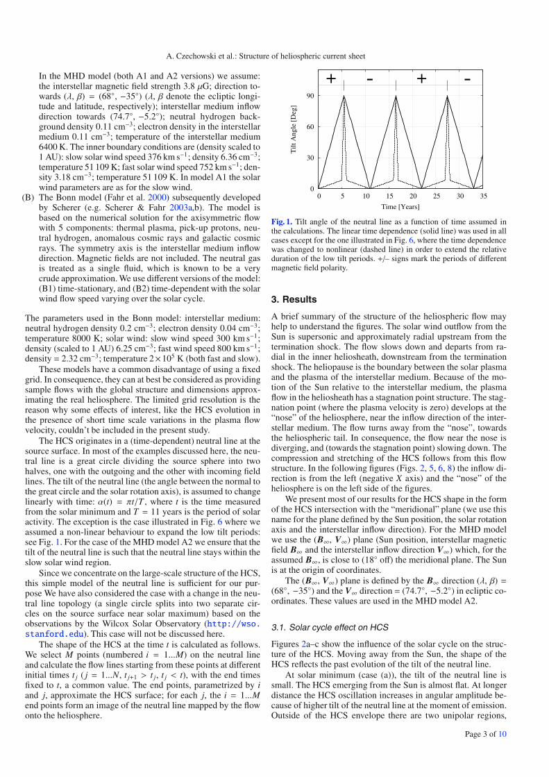
The HCS originates in a (time-dependent) neutral line at thesource surface. In most of the examples discussed here, the neu-tral line is a great circle dividing the source sphere into twohalves, one with the outgoing and the other with incoming fieldlines. The tilt of the neutral line (the angle between the normal tothe great circle and the solar rotation axis), is assumed to changelinearly with time: α(t) = πt/T , where t is the time measuredfrom the solar minimum and T = 11 years is the period of solaractivity. The exception is the case illustrated in Fig. 6 where weassumed a non-linear behaviour to expand the low tilt periods:see Fig. 1. For the case of the MHD model A2 we ensure that thetilt of the neutral line is such that the neutral line stays within theslow solar wind region.

Since we concentrate on the large-scale structure of the HCS,this simple model of the neutral line is sufficient for our pur-pose We have also considered the case with a change in the neu-tral line topology (a single circle splits into two separate cir-cles on the source surface near solar maximum) based on theobservations by the Wilcox Solar Observatory (http://wso.stanford.edu). This case will not be discussed here.

The shape of the HCS at the time t is calculated as follows.We select M points (numbered i = 1...M) on the neutral lineand calculate the flow lines starting from these points at differentinitial times t j ( j = 1...N, t j+1 > t j, t j < t), with the end timesfixed to t, a common value. The end points, parametrized by iand j, approximate the HCS surface; for each j, the i = 1...Mend points form an image of the neutral line mapped by the flowonto the heliosphere.

0

30

60

90

0 5 10 15 20 25 30 35

Tilt

Ang

le [

Deg

]

Time [Years]

+ - + -

Fig. 1. Tilt angle of the neutral line as a function of time assumed inthe calculations. The linear time dependence (solid line) was used in allcases except for the one illustrated in Fig. 6, where the time dependencewas changed to nonlinear (dashed line) in order to extend the relativeduration of the low tilt periods. +/– signs mark the periods of differentmagnetic field polarity.

3. Results

A brief summary of the structure of the heliospheric flow mayhelp to understand the figures. The solar wind outflow from theSun is supersonic and approximately radial upstream from thetermination shock. The flow slows down and departs from ra-dial in the inner heliosheath, downstream from the terminationshock. The heliopause is the boundary between the solar plasmaand the plasma of the interstellar medium. Because of the mo-tion of the Sun relative to the interstellar medium, the plasmaflow in the heliosheath has a stagnation point structure. The stag-nation point (where the plasma velocity is zero) develops at the“nose” of the heliosphere, near the inflow direction of the inter-stellar medium. The flow turns away from the “nose”, towardsthe heliospheric tail. In consequence, the flow near the nose isdiverging, and (towards the stagnation point) slowing down. Thecompression and stretching of the HCS follows from this flowstructure. In the following figures (Figs. 2, 5, 6, 8) the inflow di-rection is from the left (negative X axis) and the “nose” of theheliosphere is on the left side of the figures.

We present most of our results for the HCS shape in the formof the HCS intersection with the “meridional” plane (we use thisname for the plane defined by the Sun position, the solar rotationaxis and the interstellar inflow direction). For the MHD modelwe use the (B∞, V∞) plane (Sun position, interstellar magneticfield B∞ and the interstellar inflow direction V∞) which, for theassumed B∞, is close to (18◦ off) the meridional plane. The Sunis at the origin of coordinates.

The (B∞, V∞) plane is defined by the B∞ direction (λ, β) =(68◦, −35◦) and the V∞ direction = (74.7◦, −5.2◦) in ecliptic co-ordinates. These values are used in the MHD model A2.

3.1. Solar cycle effect on HCS

Figures 2a–c show the influence of the solar cycle on the struc-ture of the HCS. Moving away from the Sun, the shape of theHCS reflects the past evolution of the tilt of the neutral line.

At solar minimum (case (a)), the tilt of the neutral line issmall. The HCS emerging from the Sun is almost flat. At longerdistance the HCS oscillation increases in angular amplitude be-cause of higher tilt of the neutral line at the moment of emission.Outside of the HCS envelope there are two unipolar regions,

Page 3 of 10

A&A 516, A17 (2010)

-100

-50

0

50

100

-100

(a)

+

--

-50 0 50 100

Y [

AU

]

X [AU]

-100

-50

0

50

100

-100

(b)

+

--

-50 0 50 100

Y [

AU

]

X [AU]

-100

-50

0

50

100

-100 -50 0 50 100

Y [

AU

]

X [AU]

(c)

Fig. 2. Intersection of the heliospheric current sheet structure with the(B∞, V∞) plane at a) minimum, b) intermediate phase, and c) maximumof the solar cycle for the MHD model A2. Interstellar inflow directionis horizontal from the left. Sun is at the origin of coordinates. Directionnorth is approximately down.

each corresponding to a definite field polarity: + for outgoing, –for incoming. The region filled by the HCS is not unipolar, sincethe polarity changes on each crossing of the HCS: the mixed-polarity region. The “wavelength” (2 × distance between thesubsequent folds) of the HCS is given by the local plasma ve-locity times the solar rotation time. The abrupt decrease of the“wavelength” (tightening of the folds) marks the position of thetermination shock. Beyond the termination shock the plasma ve-locity continues to decrease and the HCS becomes more tightlyfolded. The mixed polarity region filled with HCS expands inlatitude because of diverging plasma flow and further increase

Fig. 3. The heliospheric current sheet in model A1 near the Sun at solarmaximum. The Sun is at the origin of coordinates, inside the shell.

of the tilt. The grey area marks the parts of the HCS emittedwithin 1 year from the solar maximum.

In the intermediate phase (b), the point of minimum tilt ofthe HCS moved already beyond the termination shock. Near theSun the angular amplitude of the HCS is now increasing towardsthe Sun because of the approach of the next solar maximum.The mixed polarity region seen in case (a) is now compressed(the region to the left of the minimum tilt point): a new mixed-polarity region is starting to build up.

At solar maximum (case (c)), the HCS near the Sun extendsto all latitudes. New unipolar regions will appear after the maxi-mum, with reversed polarity.

For completeness, we show here also the evolution of theHCS structure near the Sun following from our model duringfield reversal. Near the solar maximum, the HCS in the vicinityof the Sun takes the form of a spiral “snail shell” shown in Fig. 3for the moment of time t immediately after the reversal. In ourmodel the HCS consists of the plasma packets emerging fromthe neutral line on the source surface and moving outward withthe plasma flow. Each of the “meridional” lines at the surfaceof the shell links the points that emerged from the neutral line atthe same moment of time; the “parallel” lines link the points thatstarted from the same point of the neutral line at different times.

Figure 4 shows the intersection of the HCS with the merid-ional plane (a) and with the (B∞, V∞) plane (b) within 20 AUfrom the Sun: the sections of the “snail shell” similar to thatshown in Fig. 3. The dotted line marks the plasma flow linesemerging from the solar poles. At the moment of field reversalthe neutral line passes through the solar poles. In consequence,the HCS surface passes through the flow lines emerging fromthe solar poles. At the moment of time to which the figure cor-responds (about a month after the magnetic field reversal) thispart of the HCS moved already to the distance of about 10 AUfrom the Sun. This can be seen (shown by the bold line) in theintersection with the “meridional” plane which contains the so-lar rotation axis (Fig. 4a, bold lines) but not with the (B∞, V∞)plane (Fig. 4b) because the latter is too distant from the solarrotation axis.

Our model of the solar wind flow and the neutral line evo-lution (great circle in uniform rotation) is meant to describe thelarge-scale HCS structure. It is too simple for a realistic descrip-tion of the HCS structure near the Sun. For calculations with thisaim, using the neutral line and the solar wind evolution based

Page 4 of 10

A. Czechowski et al.: Structure of heliospheric current sheet

-20

-10

0

10

20

-20 -10 0 10 20

Y [

AU

]

X [AU]

+-

+

-

+

-

-

+

-

+

(a)

-20

-10

0

10

20

-20 -10 0 10 20

Y [

AU

]

X [AU]

+-

+

-

+

-

-

+

-

+

(b)

Fig. 4. Intersection of the heliospheric current sheet in model A1(shortly after solar maximum) with a) the meridional plane and b) the(B∞, V∞) plane. North is approximately downwards. Note the apparentabrupt change in the HCS structure (bold lines) when the HCS surfacepasses through the solar rotation axis. The (B∞, V∞) plane (b)) is tiltedtoo far from the solar axis for this passage to be visible.

on observations but restricted to within 5 AU from the Sun, seeRiley et al. (2002).

3.2. Global structure

The plasma flow lines emerging from the solar equator form asurface (“solar equatorial surface”) that divides the heliosphereinto two parts (“hemispheres”) each filled by the plasma comingout of one of the solar hemispheres. The parts of the HCS thatemerge from the Sun during the periods close to the solar min-ima (low tilt of the neutral line) would be close to this dividingsurface. However, the field reversals during solar maxima implythat no definite polarity can be assigned to any hemisphere: in-stead, the unipolar regions of opposite polarity alternate in eachhemisphere, and must be separated from each other by appro-priate boundary regions (mixed polarity regions), that containthe parts of the current sheet emerging from highly tilted neutralline. The mixed polarity regions form “shells” around the Sun(Figs. 5, 6). Together with unipolar regions, these expand withthe plasma flow and (in the forward part of the heliosphere) ul-timately approach the heliopause. With the assumption that con-vection solely determines the field structure, these “shells” can-not intersect and the inner “shell” must stay inside the outer one.

Figure 5 shows the intersection of the HCS (calculated forthe MHD model A2) with the (B∞, V∞) plane at solar minimum.

Fig. 5. Intersection of the heliospheric current sheet with the (B∞, V∞)plane at solar minimum for time-dependent MHD model (A2). Plus andminus signs denote the polarity (field lines emerging or incoming rela-tive to the source surface) of the unipolar field regions. The heliopauseis marked HP. Interstellar inflow is from the left. Direction to north isapproximately downwards.

Fig. 6. Intersection of the heliospheric current sheet with the meridionalplane at solar minimum for the model with increased angle between thesolar equator and the inflow direction of the interstellar matter (see thediscussion in the text). The time-stationary MHD model (A1) is used.Interstellar inflow is from the left. Direction to north is approximatelydownwards.

The wavy current sheet inside the termination shock is clearlyvisible. Beyond the shock the distance between the subsequentwaves becomes too short to distinguish them: the dark areasin the figure are filled by oscillating current sheet (the detailedstructure can be seen in Fig. 2a which show part of Fig. 5 inexpanded view). Three “rings” represent the expanding mixedpolarity regions surrounding the Sun. They originate from threepreceding solar maximum periods (high tilt of the neutral line)and are filled by the HCS extending to high heliolatitudes.Printed in grey are the parts of the HCS that originated within1 year from a solar maximum. Not shown are the parts of theHCS originating earlier than 3.5 11-year periods before the il-lustrated minimum: these parts would appear between the he-liopause and the outer ring. The white regions are unipolar. Thepolarity of the neighbouring unipolar regions alternates.

Another aspect of the HCS global structure is illustrated byFig. 6. In this case we exaggerated the angle between the inter-stellar inflow direction and the solar equator plane in order toincrease the deflection of the solar equatorial surface and of the

Page 5 of 10

A&A 516, A17 (2010)

-230

-228

-226

-224

-222

-220

-56 -54 -52 -50 -48 -46

Y [

AU

]

X [AU]

Fig. 7. A fragment of Fig. 5 showing the signature of a bent HCS. Thenarrow white gap is the unipolar region flanked by two mixed polarityregions filled by the oscillating HCS. For two solar rotations the HCStilt is low enough to keep it within 1–2 AU from the bent solar equatorialsurface. This low tilt segment of the HCS is seen bridging the gap.

HCS. Also, in order to make the HCS deflection more visible,the tilt of the neutral line was assumed to be low for most of thetime, except for short periods near the solar maxima. The HCS(the low tilt parts) can be clearly seen to be bent to the north(downward in the figure). The high tilt parts of the current sheetform shells, in this case thinner than in Fig. 5. The plasma flowis derived from model A1 (isotropic solar wind).

In Fig. 5, with a more realistic choice of model parameters(stagnation point close to the solar equator plane, higher tilt ofthe neutral line for most of the time), the bent (deflected) currentsheet structure is partly obscured. The solar equatorial surface isstill bent, but the deflection occurs close to the heliopause, in-side the layer of mixed polarity. Also, only small parts of theHCS (those with very low tilt) stay close to the bent solar equa-torial surface: most of the HCS oscillates between north- andsouth-deflected plasma flow lines, and is stretched in both direc-tions away from the solar equatorial surface. The expanded frag-ment of Fig. 5 including a very low tilt HCS segment which in-dicates the position of the bent solar equatorial surface is shownin Fig. 7.

Figures 8a–c show the HCS intersection with the meridionalplane for other models of the heliospheric plasma flow: a ver-sion of the analytical model of Suess & Nerney (1990), and twoversions of the Bonn model: B1 and B2. The interstellar inflowdirection is here assumed to be perpendicular to the solar ro-tation axis, so that the solar equatorial surface is not bent (wehave also considered the case of correctly oriented solar axisand found that the global structure of the HCS was not stronglyaffected). The time-stationary version of the Bonn model (B1)gives a structure close to the model of Suess and Nerney. Themain difference is due to the plasma flow velocity distribution inthe heliotail: in all the models presented here except Suess andNerney the plasma flow slows down near the centre of the he-liotail. The time-dependent isotropic solar wind version of theBonn model (B2) is similar.

Since the Bonn model is axisymmetric, the flow lines areplanar. In particular, the lines emerging from the solar polesstay in the meridional plane. Near these flow lines the mixedpolarity regions narrow down to a single sheet, separating theunipolar regions of different polarity (compare Fig. 4). For themodel B2 with time dependent solar wind (Fig. 8c) these partsof HCS carry also the imprint of interactions between fast andslow streams of the solar wind. Except for the vicinity of the flow

Fig. 8. Intersection of the heliospheric current sheet structure with themeridional plane for different models of the heliosphere at solar mini-mum: a) a version of the analytical model of Suess and Nerney (the partof the HCS inside the termination shock is not shown), and two versionsof the Bonn model: b) B1 and c) B2.

lines emerging from the poles the boundary between the unipo-lar regions is much thicker (a mixed polarity region includingmany folds of the HCS).

In Fig. 9 we show a fragment of HCS near the flow lineemerging from the south solar pole in the 3D asymmetricmodel A2. The figure shows the intersection of the HCS with thesurface containing the flow line coming out of the pole. Againthe boundary between the unipolar regions (white areas) reducesto a single sheet near the polar flow line.

3.3. Secondary folds

In Fig. 5 the mixed-polarity regions near the heliopause in themodel A2 show secondary folding: that is, the layers filled withthe folded HCS bend and fold on themselves. More detailed viewis shown in Fig. 10. We find that this secondary folding appearsin the cases where the solar wind depends on both latitude andtime (A2 but not B2, where the wind is not latitude dependent).

Page 6 of 10

A. Czechowski et al.: Structure of heliospheric current sheet

145

150

155

160

165

170

170 180 190 200 210 220 230

Y [

AU

]

X [AU]

Fig. 9. The HCS structure near the flow line emerging from a solar polein the MHD model. Along this flow line the unipolar sectors of oppositepolarity are separated by a single sheet (compare Fig. 4). Elsewhere,the boundary between the unipolar regions is a mixed polarity regionincluding many folds of the HCS.

100

120

140

160

180

200

220

240

-50 0 50 100 150 200

Y [

AU

]

X [AU]

Fig. 10. Detailed view of “secondary fold” structure of the heliosphericcurrent sheet which appears in the model A2 (a part of Fig. 5).

The formation of the fold can be traced back to the evolution ofthe constant flow time surfaces in the plasma flow. At long dis-tance from the Sun, most of the HCS area become close in shapeto these surfaces. This is because, for any pair of points on thesection of the HCS situated between the two nearest extremes inheliolatitude, the flow time from the Sun differs by at most 1/2of the solar rotation time. At long distances from the Sun thisis short compared to the overall flow time. Figure 11 presentstwo constant time surfaces for the model A2. The first is stillwithin the termination shock and reflects the two-component so-lar wind structure near solar minimum. The second correspondsto a later moment of time, when the flow reached the heliosheath:the boundary between the fast and slow sectors evolves into thefold that corresponds to the secondary fold in the HCS.

In the inner heliosphere, the deformations of the HCS due tovariations of the plasma velocity field were considered by Suess& Hildner (1985) and Pizzo (1994).

3.4. HCS and mixed polarity sectors near the heliopause

Convection with the plasma flow moves any given fragment ofthe HCS from the inner heliosphere, where the spacing betweenthe HCS folds is large, to the heliosheath, where the spacing

Fig. 11. Constant-time surface for short (at the top) and long (at thebottom) flow-time for the time-dependent MHD model (A2).

0.0001

0.001

0.01

0.1

1

10

0.1 1 10 100 1000

Δ r

[AU

]

s [AU]

X Y -Y

Fig. 12. Distance Δr between folds of the heliospheric current sheet asa function of distance s from the heliopause along the following direc-tions: a) interstellar upwind (X), b) crosswind, south (Y), c) crosswind,north (−Y).

decreases and the HCS is stretched by the diverging flow. Thefreezing-in constraint forbids alternating mixed polarity and theunipolar regions to cross each other, implying that the magneticpolarity regions from previous solar cycles pile up at the he-liopause.

As noted before, this pile-up leads to the ultimately nonreal-istic compression of the magnetic polarity layers and of the foldsin the HCS. We do not know how the situation is resolved. Somespeculations are presented in Sect. 4.3.

Figure 12 shows the distance between the subsequent foldsof the HCS as a function of the distance from the heliopause.The plots are for three different radial directions in the (B∞, V∞)plane: the interstellar upwind (marked X: towards the “nose”

Page 7 of 10

A&A 516, A17 (2010)

Fig. 13. View of the HCS (model A2, solar minimum) with the plasmaflow lines (projected on the (B∞, V∞) plane) terminating in 5 selectedpoints on the HCS. The trajectory reaching the points (4) and (5) avoidsthe vicinity of the stagnation point.

0.01

0.1

1

10

-18 -16 -14 -12 -10 -8 -6 -4 -2 0

Δ r

[AU

]

t [years]

(1) (2) (3) (4)(5)

Fig. 14. Estimated distance Δr between the subsequent folds in the HCSas a function of time along the flow lines shown in Fig. 13.

of the heliosphere), cross-wind towards south (+Y), and cross-wind towards north (−Y). It can be seen that, near the heliopause(within ∼5 AU for the forward direction), the spacing betweenthe folds decreases approximately linearly with the distancefrom the heliopause. This can be understood as a consequenceof a similar (approximately linear) decrease with distance fromthe heliopause in the flow velocity component v⊥ perpendicu-lar to the heliopause. Let the linear formula v⊥(s) = v⊥(L)s/Lhold for s ≤ L where s is the distance from the heliopause. Thespacing Δr between the folds is then approximately given by

Δr/s = [exp(2|v⊥(L)/L|trot) − 1] (1)

where trot is the period of solar rotation. Taking v⊥(L) =10 km s1, L = 10 AU and trot ∼ 2 × 106 s it follows thatΔr/s ∼ 0.01. This agrees with our results showing that the spac-ing between the folds in the HCS can be as low as 0.01 AU atthe distance of the order of few AU from the heliopause.

The probability of survival of a fragment of the HCS as it ap-proaches the pile-up region may depend on its history. Figure 13shows examples of plasma flow lines (projected on the (B∞, V∞)plane) terminating in selected points on the HCS. Figure 14 plotsthe estimated distance Δr between the subsequent folds in theHCS along these flow lines. A low value of Δr indicates that thefolds of the HCS are tightly compressed. We see that the trejec-tories terminating in the points (5) and (4) do not pass through

the region of very low Δr. If the probability of destruction ofthe HCS increases for tightly folded HCS, then the points far-ther away from the heliopause: (5) and (4) are less likely to beaffected than the other points. Note that the part of the HCS thatavoids the high compression region includes a part (point (5)) ofthe secondary fold structure.

4. Discussion

4.1. Interstellar magnetic field and the structureof the heliosphere

In the approximate model of the Sun with spherically symmetricsolar wind outflow and with the magnetic fields neglected the he-liosphere would be axisymmetric, with the symmetry axis alongthe direction of motion of the Sun relative to the local interstel-lar cloud. The effect of the interstellar magnetic field, as derivedfrom theory and numerical simulations (for a review see Zank1999), is to cause the deformation of the heliosphere which af-fects both the shape of the outer boundary and the structure of theinternal flow: in particular, the shape of the termination shock isalso changed. Until recently, there were no observations permit-ting determination of the interstellar magnetic field in the localinterstellar medium.

Voyager observations in the heliosheath and the most recentdata from IBEX provided new information about the structureof the distant regions of the heliosphere and the parameters ofthe interstellar magnetic field. The boundary conditions for theMHD model used in our study are close to the values implied bythose recent observations.

We assume the interstellar magnetic field of relatively highstrength 3.8 μG and direction towards ecliptic (longitude, lati-tude) = (68◦, −35◦) or Galactic (210◦, −33◦) which correspondsto the angle 30◦ relative to the interstellar helium inflow direc-tion and 20◦ relative to the hydrogen deflection plane (the planedefined by the interstellar neutral helium and interstellar neutralhydrogen velocities).

The interstellar magnetic field affects the shape of the he-liopause and of the termination shock. In particular, the differ-ence in distance to the termination shock measured by Voyager 1(94 AU) and Voyager 2 (84 AU) is in part attributed to the inter-stellar magnetic field. The model of the interstellar field usedin our calculations was found to be able to explain this differ-ence in the framework of the stationary model of the heliosphere(Ratkiewicz & Grygorczuk 2008). It is also close to the resultsof Opher et al. (2009) (3.7–5.5 μG field strength, angle 20◦−30◦relative to interstellar inflow and about 30◦ from the Galacticplane).

The recent energetic neutral atoms observations by IBEXfound a ribbon structure of enhanced emission, thought to becaused by the interstellar magnetic field and reflecting its orien-tation. Heerikhuisen et al. (2010) reproduce the ribbon structureseen in the IBEX data using the field (parallel to the hydrogendeflection plane) of strength 3 μG directed towards (224◦, 41◦)which is (apart from the overall sign change) within about 20◦from our direction. The difference in sign of the interstellar fieldshould not change its effect on the heliosphere, unless the ef-fects of reconnection between the solar and interstellar magneticfields would be important.

The interstellar magnetic field used in our MHD modelsis therefore close to the presently favoured values. The fieldstrength and orientation following from the observations aresuch that one expects a large effect on the structure of the distantheliosphere and in particular on the shape of the heliopause. The

Page 8 of 10

A. Czechowski et al.: Structure of heliospheric current sheet

strongly asymmetric heliosheath used as a basis for our studymay be consequently a reasonable qualitative approximation toreality.

One must, however, keep in mind that the present numericalmodels of the heliosphere are still very incomplete and even thebest available boundary conditions may not guarantee a correctdescription of the plasma flow in the heliosheath. In particular,the instability effects (Dasgupta et al. 2006) may be importantnear the heliopause.

4.2. Relation to the numerical models of the heliosphericcurrent sheet

Numerical models of the heliosphere that include the HCS en-counter two challenges. One is that the HCS is very thin. Theother is the need to deal with the consequences of the magneticfield reversals.

Magnetic field reversals lead to alternating polarity regions.The heliospheric plasma flow causes a pile-up of these structuresnear the heliopause. To describe this process requires not onlya very high resolution. The model must be also time dependentand the calculation must run over the period of time long enoughto include more than one solar cycle. Finally, the model shouldinclude the necessary physics to resolve the problems related tothe pile-up: for instance, ideal MHD is not sufficient to describereconnection.

To our knowledge, the most complete numerical calcula-tion up to now is the one by Pogorelov and Borovikov (unpub-lished) which includes tilted current sheet, has the resolution of0.01 AU and follows the HCS evolution to the region beyondthe termination shock. However, it does not reach the vicinityof the heliopause. The structure of the HCS emerging from thiscalculation is similar to the results presented here, with the HCSconvected by the plasma flow and the HCS folds tightening be-yond the termination shock.

The published models are much more simplified (Lindeet al. 1998; Washimi & Tanaka 2001; Opher et al. 2003, 2006;Pogorelov 2006; Pogorelov et al. 2004, 2006, 2009). In particu-lar, the effect of the magnetic field reversals on the HCS is notincluded. Pogorelov et al. (2009) consider the field reversals butthe HCS is not resolved.

The simplified models are a necessary stage in developmentof more complete ones, but can be inadequate for concrete ap-plications.

We give two examples:

(1) solar magnetic field effect on charged particles entering theheliosphere. Since the simplified models ignore the sectorstructure of the magnetic field, the reduction of the effectivemagnetic field leading to the increased probability of parti-cle penetration into the inner solar system (Landgraf 2000;Czechowski & Mann 2003) is missing from these models;

(2) bending of the HCS. In calculations with low tilt heliosphericcurrent sheet, the current sheet was found to avoid the stag-nation point by bending into the northern or the southernparts of the heliosheath, with the shape of the heliopause be-coming asymmetric in result (Pogorelov et al. 2004). If thesolar cycle would be taken into account, the HCS would ex-tend to all latitudes and so could not avoid the stagnationpoint in this way. The effect on the shape of the heliopauseis then in doubt.

Numerical MHD models of the heliosphere that include the he-liospheric magnetic field and the current sheet have clearly an

Fig. 15. Schematic view of two scenarios for the magnetic field structurein the forward heliosheath. In the figure on the left the layers of tightlyfolded HCS alternating with unipolar regions become replaced near theheliopause by a turbulent region of disordered magnetic field. In thefigure on the right a unipolar region reaches the heliopause in result ofdestroying the previous magnetic field structure by reconnection. Thegrey rings represent the mixed polarity regions and the thin line thebent solar equatorial surface. HP marks the heliopause.

advantage over the non self-consistent approaches like the oneused in this paper. However, the effects due to non-realisticmodel assumptions or numerical effects must be understood andeliminated. In the meantime, the numerical simulations need tobe supplemented by other methods.

4.3. Pile-up region in the forward heliosheath

As noted in the Introduction, we assume that in the immedi-ate vicinity of the heliopause (within distance Δ) magnetic fieldmust be rearranged to avoid unphysical compression of the po-larity sectors or the HCS. Here we briefly discuss two of thepossible results of this rearrangement, illustrated in Fig. 15.

One possibility is that the mixed polarity field would becomedisordered. In the region near the heliopause there are reasons toexpect increased turbulence (Fahr et al. 1986; Borovikov et al.2008), in particular in the plasma velocity field. This may com-bine with magnetic reconnection and lead to the HCS and themagnetic field structure with less long-range order. It is possiblethat unrealistic compression could then be avoided. The over-all picture would still be similar to that of Nerney, Suess andSchmahl, with the mixed polarity regions near the heliopausefilled by the disordered field and fragmented current sheetsrather than the regularly alternating field and continuous HCS.

Another possibility is that, near the nose of the heliopause,the unipolar regions would extend to the heliopause. This couldoccur as follows. Assume that at the heliopause the field isunipolar, with negative polarity. It is approached by the expand-ing positive polarity region from the following solar minimum.Between the unipolar regions there is a mixed-polarity layer. A“hole” in this layer may be created by reconnection betweenthe alternating fields within the layer. The negative polarity fieldnear the heliopause may then reconnect with the positive polar-ity field in the newly arriving unipolar region, so that the “hole”extends to the heliopause. The edges of the “hole” are convectedaway from the “nose” by the diverging plasma flow, while the“hole” fills up by the newly arrived plasma with positive polar-ity field.

Page 9 of 10

A&A 516, A17 (2010)

The magnetic field would then form a unipolar layer next tothe nose of the heliopause, with the polarity changing over the11 year solar cycle. Farther away from the nose the structure ofthe field would be the same as that of Nerney et al. (1991, 1993,1995).

This scenario requires that very near the heliopause there isstill a clear difference between unipolar and mixed polarity sec-tors and that the reconnection is effective enough to destroy theunipolar layer adjacent to the heliopause. The reason we men-tion this possibility is that it is similar to the results of simplifiednumerical models (see Sect. 4.2) which, however, do not includethe polarity reversal effects.

5. Conclusions

We followed the pioneering work by Nerney et al. (1991, 1993,1995) by extending their calculations of global magnetic fieldstructure in the heliosphere to more elaborate models of the he-liospheric plasma flow. We assumed that the magnetic field isfrozen into the plasma and that the HCS is a tangential disconti-nuity, passively convected with the plasma flow.

The global HCS structure following from the highly asym-metric and time-dependent model of the heliosphere differs insome respects from that obtained by Nerney, Suess and Schmahlin a much simpler (axisymmetric, time-stationary and incom-pressible flow) model. It is similar in that the magnetic field inthe heliosphere forms expanding unipolar regions separated byshells of mixed polarity, and that there is a mixed polarity layernear the heliopause. The differences include: the HCS secondaryfolding caused by the time- and latitude dependent solar wind;bending of the solar equatorial surface due to asymmetry in thestagnation point position; effect of the nonuniform flow in theheliotail on the shape of the different polarity regions.

Near the heliopause the alternating layers of different polar-ity become increasingly compressed by the slowing plasma flow.On approaching the heliopause this compression becomes unre-alistically high. This is a general consequence of combining theideal MHD equations for the heliosphere with the solar cyclevariation of the magnetic field, including the polarity reversals.To find out how the problem is resolved requires a more detailedstudy of the physical processes near the heliopause and of thephysics of the HCS.

Numerical simulations of the HCS are necessary to under-stand the HCS structure. These simulations are very difficult be-cause of the need for a very high resolution. The results availableat present are based on simplified assumptions and are not ade-quate for some applications. Our approach, which combines theresults of the flow simulations with a description of the HCSbased on simple assumptions about its dynamics, has an advan-tage of being able to model the situations difficult to describein a self-consistent simulation. Such models may be useful for astudy of the charged particles dynamics in the inner heliosheath.Acknowledgements. We acknowledge support from the Polish Ministry ofScience and Higher Education grant 4T12E 002 30. R.R. was supported by thePolish Ministry of Science and Higher Education grant N N203 4159 33.

ReferencesBalogh, A., & Smith, E. J. 2001, Space Sci. Rev., 97, 147Borovikov, S. N., Pogorelov, N. V., Zank, G. P., & Kryukov, I. A. 2008, ApJ,

682, 1404Burlaga, L. F., Ness, N. F., & Richardson, J. D. 2003, J. Geophys. Res., 108,

8028

Burlaga, L. F., Ness, N. F., & Acuna, M. H. 2006, in Physics of the InnerHeliosheath: Voyager Observations, Theory and Future Prospects, 5th IGPPInternational Astrophysics Conference, ed. J. Heerikhuisen, V. Florinski, G. P.Zank, & N. V. Pogorelov, AIP Conf. Proc., 858, 122

Burlaga, L. F., Ness, N. F., & Acuña, M. H. 2007, ApJ, 668, 1246Burlaga, L. F., Ness, N. F., Acuña, M. H., et al. 2009, ApJ, 692, 1125Czechowski, A., & Mann, I. 2003, J. Geophys. Res., 108, A10, LIS 13-1Dasgupta, B., Florinski, V., Heerikhuisen, J., & Zank, G. P. 2006, in Physics of

the Inner Heliosheath: Voyager Observations, Theory and Future Prospects,5th IGPP International Astrophysics Conference, ed. J. Heerikhuisen, V.Florinski, G. P. Zank, & N. V. Pogorelov, AIP Conf. Proc., 858, 51

Decker, R. B., Krimigis, S. M., Roelof, E. C., et al. 2005, Science, 309, 2020Decker, R. B., Krimigis, S. M., Roelof, E. C., et al. 2008, Nature, 454, 67Fahr, H. J., Kausch, T., & Scherer, K. 2000, A&A, 357, 268Fahr, H. J., Neutsch, W., Grzedzielski, S., Macek, W., & Ratkiewicz-Landowska,

R. 1986, Space Sci. Rev., 43, 329Gosling, J. T., McComas, D. J., Skoug, R. M., & Smith, C. W. 2006, GRL, 33,

L17102Heerikhuisen, J., Pogorelov, N. V., Zank, G. P., et al. 2010, ApJ, 708, L126Jokipii, J. R., & Levy, E. H. 1977, ApJ, 213, L85Landgraf, M. 2000, J. Geophys. Res., 105, A5, 10303Linde, T. J., Gombosi, T. I., Roe, P. L., Powell, K. G., & DeZeeuw, D. L. 1998,

J. Geophys. Res., 103, A2, 1889Miyake, S., & Yanagita, S. 2005, in Proceedings of 29th International Cosmic

Ray Conference, Pune, 101Nerney, S., Suess, S. T., & Schmahl, E. J. 1995, J. Geophys. Res., 100, A3, 3463Nerney, S., Suess, S. T., & Schmahl, E. J. 1993, J. Geophys. Res., 98, A9, 15169Nerney, S., Suess, S. T., & Schmahl, E. J. 1991, A&A, 250, 556Opher, M., Liewer, P. C., Gombosi, T. I., et al. 2003, ApJ, 591, L61Opher, M., Stone, E. C., & Liewer, P. C. 2006, ApJ, 640, L71Opher, M., Alouani Bibi, F., Toth, G., et al. 2009, Nature, 462, 1036Pizzo, V. J. 1994, J. Geoph. Res., 99, A3, 4185Pogorelov, N. V., Borovikov, S. N., Zank, G. P., & Ogino, T. 2009, ApJ, 696,

1478Pogorelov, N. V. 2006, in Physics of the Inner Heliosheath: Voyager

Observations, Theory and Future Prospects, 5th IGPP InternationalAstrophysics Conference, ed. J. Heerikhuisen, V. Florinski, G. P. Zank, &N. V. Pogorelov, AIP Conf. Proc., 858, 3

Pogorelov, N. V., Zank, G. P., & Ogino, T. 2004, ApJ, 614, 1007Pogorelov, N. V., Zank, G. P., & Ogino, T. 2006, ApJ, 644, 1299Pudovkin, M. I., & Semenov, V. S. 1977a, Ann. Geophys., 33, 429Pudovkin, M. I., & Semenov, V. S. 1977b, Ann. Geophys., 33, 423Ratkiewicz, R., & Grygorczuk, J. 2008, Geophys. Res. Lett., 35, No. 23, CiteID

L23105Ratkiewicz, R., Barnes, A., Molvik, G. A., et al. 1998, A&A, 335, 363Ratkiewicz, R., Ben-Jaffel, L., & Grygorczuk, J. 2008, Astron. Soc. Pac. Conf.

Ser., 385, 189Richardson, J. D., Stone, E. C., Kasper, J. C., Belcher, J. W., & Decker, J. B.

2009, GRL, 36, L10102Riley, P., Linker, J. A., & Mikic, Z. 2002, JGR, 107, A7, 1136Scherer, K., & Fahr, H. J. 2003a, Geophys. Res. Lett., 30, No. 2, 17-1Scherer, K., & Fahr, H. J. 2003b, Annnales Geophys., 21, 1303Schwadron, N. A., Bzowski, M., Crew, G. B., et al. 2009, Science, 326, 966Smith, E. J. 2001, J. Geophys. Res., 106, No. A8, 15819Smith, E. J., Balogh, A., Forsyth, R. J., & McComas, D. J. 2001, Geophys. Res.

Lett., 28, 4159Smith, E. J. 2008, in The heliosphere through the solar activity cycle, ed. A.

Balogh, L. J. Lanzerotti, & S. T. Suess, Springer Praxis Books (Berlin,Heidelberg: Springer), 79

Stone, E. C., Cummings, A. C., McDonald, F. B., et al. 2005, Science, 309, 2017Stone, E. C., Cummings, A. C., McDonald, F. B., et al. 2008, Nature, 454, 71Suess, S. T., & Hildner, E. 1985, J. Geophys. Res., 90, A10, 9461Suess, S. T., & Nerney, S. 1990, J. Geophys. Res., 95, 6403Suess, S. T., & Nerney, S. 1993, Geophys. Res. Lett., 20, 329Usoskin, I. G., Alanko-Huotari, K., Mursula, K., & Kovaltsov, G. A. 2008,

in Proceedings of the 30th International Cosmic Ray Conference, ed. R.Caballero, J. C. D’Olivo, G. Medina-Tanco, L. Nellen, F. A. Sanchez, & J.F. Valdes-Galicia, Univ. Nacional Autonoma de Mexico, Mexico City, 1, 459

Washimi, H., & Tanaka, T. 2001, Adv. Space Res., 27, 509Winterhalter, D., Smith, E. J., Burton, M. E., Murphy, N., & McComas, D. J.

1994, JGR, 99, 6667Zank, G. P. 1999, Space Sci. Rev., 89, 413Zhou, X.-Y., Smith, E. J., & Winterhalter, D. 2005, in Proceedings of Solar Wind

11-SOHO 16, Connecting Sun and Heliosphere, Whistler, Canada 12–17 June

Page 10 of 10