
Examination of plasma current spikes and general analysis of ...
149
Examination of plasma current spikes and general analysis of H-mode shots in the tokamak COMPASS Arne Van Londersele Supervisor: Ereprof. Dr. Ir. Guido Van Oost Counsellor: Dr. Jan Stockel Master’s dissertation submitted in order to obtain the academic degree of Master of Science in Engineering Physics Department of Applied Physics Chairman: Prof. Dr. Ir. Christophe Leys Faculty of Engineering and Architecture Academic year 2013-2014
-
Upload
khangminh22 -
Category
Documents
-
view
0 -
download
0
Transcript of Examination of plasma current spikes and general analysis of ...

Examination of plasma current spikes and general
analysis of H-mode shots in the tokamak COMPASS
Arne Van Londersele
Supervisor: Ereprof. Dr. Ir. Guido Van OostCounsellor: Dr. Jan Stockel
Master’s dissertation submitted in order to obtain the academic degree ofMaster of Science in Engineering Physics
Department of Applied PhysicsChairman: Prof. Dr. Ir. Christophe LeysFaculty of Engineering and ArchitectureAcademic year 2013-2014

i
Allowance to loan
The author gives permission to make this master dissertation available for consultation andto copy parts of this master dissertation for personal use. In the case of any other use, thelimitations of the copyright have to be respected, in particular with regard to the obligationto state expressly the source when quoting results from this master dissertation.
Arne Van Londersele June 2, 2014

ii
Preface and acknowledgement
This thesis discusses research performed on the tokamak COMPASS. This device is installedin the Institute of Plasma Physics (IPP) in Prague. I lived in this city for four months as partof an Erasmus exchange project in the winter semester of 2013. In the beginning, the subjectof my thesis was not sharply defined. The primary goal was to discuss some H-mode shotswith NBI heating. The current spikes were discovered in the middle of my stay in Pragueand they became a new part of my thesis. Generally, I had a lot of freedom in this thesis.I decided to make it my goal to explain the fusion research performed at the IPP as goodas possible to someone with very basic knowledge of science. I also took the liberty to saysomething more about the energy problem and fusion research in general in the first chapters.
My whole Erasmus project and work at the IPP was an amazing experience. Although, I hadunderestimated the amount of work a little bit. It was very instructive to work in this tech-nical environment. I learned a lot about fusion research and the different kind of diagnostictools, but also about Czech culture and habitats. Further, I also followed some courses at theCzech Technical University and I lived in the Masarykova student dorm where I met a lot ofnew friends with different nationalities.
I would like to thank everyone who contributed to this thesis. In the first place, prof. J.Stockel, not only for answering all my questions, but also for his experience as a thesiscounsellor. He motivated me from the beginning to already do a lot of work in Prague, sothat I would not get in troubles once I would be back in Belgium. I also want to thank allother scientists and technicians at the IPP that helped me, especially J. Havlicek for sharinghis knowledge about the current spikes and a lot of other things, and R. Dejarnac for givingme the information I need to analyse the Langmuir probe data. But also E. Stefanikovaand M. Peterka for their Thomson scattering profiles (Figure 3.25) and T. Markovic for hisstatistics about the ELM frequency and the power through the separatrix (Figure 4.8). Manythanks go to prof. G. Van Oost to recommend me this thesis and to be my thesis supervisor,and also to prof. J.-M. Noterdaeme who also shared his ideas about the current spikes. Ithink I could have contacted both of them much more than I did.
iii
Onderzoek van pieken in de plasmastroom en algemeneanalyse van H-mode shots in de tokamak COMPASS
door
Arne Van Londersele
Masterproef ingediend tot het behalen van de academische graad vanMaster in de ingenieurswetenschappen: toegepaste natuurkunde
Promoter: Ereprof. Dr. Ir. Guido Van OostBegeleider: Dr. Jan Stockel
Vakgroep Toegepaste NatuurkundeVoorzitter: Prof. Dr. Ir. Christophe Leys
Universiteit GentAcademiejaar 2013-2014
Samenvatting
Deze master thesis situeert zich in het vakgebied van de kernfusie. In onze moderne wereldis een nieuwe vorm van propere energie een punt bovenaan onze verlanglijst - of dat zou hetalleszins moeten zijn. Een mogelijke oplossing hiervoor zou kunnen geboden worden doorkernfusie, de manier waarop sterren zoals de zon hun energie creeren. Deze energiebronzou ons, indien ze uitvoerbaar is op Aarde, voor eeuwig kunnen voorzien in onze energiebe-hoefte. De moeilijkheid bestaat erin om de juiste omgeving te creeren waarin fusiereactieskunnen doorgaan. Een mogelijkheid is de tokamak configuratie. Hierbij wordt een heetplasma gecreeerd dat in evenwicht wordt gehouden door sterke magneetvelden. Sinds de jarenzeventig zijn al heel wat tokamaks gebouwd over heel de wereld. Een ervan is COMPASS. Dittoestel bevond zich oorspronkelijk in Culham, maar is ondertussen verplaatst naar het Insti-tute of Plasma Physics (IPP) in Praag. Deze tokamak heeft een louter experimentele functie:het is niet de bedoeling om er energie mee te maken en die om te zetten naar een bruikbarevorm zoals electriciteit, maar eerder om gegevens te verzamelen die waardevol kunnen zijnin het kader van grotere en duurdere tokamaks die deel uitmaken van de weg naar centralesdraaiende op fusie-energie. Een volgende stap op deze weg is ITER. Deze tokamak en al zijnbijkomende infrastructuur wordt momenteel gebouwd door een internationale samenwerkingwaarin het merendeel van de industrielanden betrokken is. Het onderzoek dat verricht wordtin het IPP is heel interessant met het oog op ITER, omdat COMPASS een paar belangrijkegelijkaardige kenmerken heeft en bijvoorbeeld ook gebruik maakt van zogenaamde neutralbeam injection (NBI), een techniek die gebruikt wordt om de fusiebrandstof op te warmenom zo de juiste omstandigheden te creeren waaronder fusiereacties kunnen doorgaan.

iv
De studie die uiteengezet wordt in dit werk is tweedelig. Eerst worden vijf COMPASS shotsbestudeerd die allemaal het H-mode regime bereikten. Dit is een toestand waarbij het plasmazeer goed gecontroleerd wordt door de magneetvelden en er een opmerkelijke reductie is inhet aantal plasmadeeltjes dat botst met de binnenzijde van de tokamak. Het is het stan-daardregime waarin ITER zal werken. Vier van deze geanalyseerde shots maakten gebruikvan de NBI. Aangezien het extra vermogen dat de NBI toevoegt aan het plasma niet gewetenis, werd in deze thesis getracht hier een schatting van te maken op basis van de energiebal-ans van het hele systeem. Startend van data afkomstig van spectroscopie, interferometers,Thomson verstrooiing en sondes worden conclusies getrokken met betrekking tot verschillendeplasmaparameters zoals deeltjes- en energieopsluitingstijden, het drempelvermogen om overte gaan tot H-mode, de temperatuur en dichtheid van het plasma, enzoverder.
In het tweede deel wordt een fenomeen besproken dat misschien zelfs nog nooit eerder iswaargenomen in andere tokamaks. Het gaat hier om merkwaardige pieken in de plasmastroomdie gelijktijdig optreden met bepaalde instabiliteiten die afgekort ELMs worden genoemd, endit op zeer korte tijdschaal. Verschillende plasma parameters worden kwalitatief en kwanti-tatief onderzocht. Er worden argumenten gegeven die bepaalde verklaringen voor de piekenafbreken en er worden suggesties gegeven voor mogelijke oorzaken. Er wordt vermoeden datde pieken te maken hebben met de zelf-inductie van het plasma en de wederzijdse inductiesmet componenten van de tokamak. Een andere denkpiste heeft te maken met zeer korstondigesprongen in de punten waar het plasma de divertor aan de onderzijde van de tokamak raakt.Deze werden reeds enkele jaren terug ook gevonden in JET (een andere tokmak, de beste dieer op dit moment is) en daar heeft men aangetoond dat deze kunnen verantwoordelijk zijnvoor een opmerkelijke daling van de plasmastroom. Er zouden simulaties moeten gemaaktworden om beide hypothesen te testen. De pieken in de plasmastroom op zich zijn niet echtschadelijk voor de werking van de tokamak, maar de studie ervan kan helpen om ELMs beterte begrijpen. Deze instabiliteiten vormen een probleem voor ITER aangezien ze gepaard gaanmet grote energieverliezen. Het is daarom van uitermate groot belang dat de oorzaken vanELMs goed gekend zijn, zodat software en apparatuur gemaakt kan worden om ze ondercontrole te houden.
Trefwoorden: kernfusie, tokamak, COMPASS, H-mode, current spikes
Contents
1 Thermonuclear fusion 1
1.1 Existing energy sources and their problems . . . . . . . . . . . . . . . . . . . 1
1.1.1 The world energy problem . . . . . . . . . . . . . . . . . . . . . . . . . 1
1.1.2 Fossil fuels . . . . . . . . . . . . . . . . . . . . . . . . . . . . . . . . . 3
1.1.3 Nuclear fission . . . . . . . . . . . . . . . . . . . . . . . . . . . . . . . 4
1.1.4 Renewables . . . . . . . . . . . . . . . . . . . . . . . . . . . . . . . . . 6
1.1.5 Energy efficiency . . . . . . . . . . . . . . . . . . . . . . . . . . . . . . 10
1.1.6 Hydrogen fuel cell . . . . . . . . . . . . . . . . . . . . . . . . . . . . . 11
1.2 Thermonuclear fusion . . . . . . . . . . . . . . . . . . . . . . . . . . . . . . . 11
1.2.1 Plasma . . . . . . . . . . . . . . . . . . . . . . . . . . . . . . . . . . . 11
1.2.2 Fusion reaction . . . . . . . . . . . . . . . . . . . . . . . . . . . . . . . 12
1.2.3 Properties of fusion fuels . . . . . . . . . . . . . . . . . . . . . . . . . . 13
1.2.4 Triple product . . . . . . . . . . . . . . . . . . . . . . . . . . . . . . . 14
1.2.5 Confinement . . . . . . . . . . . . . . . . . . . . . . . . . . . . . . . . 18
1.2.6 Historical evolution of the tokamak . . . . . . . . . . . . . . . . . . . . 20
1.3 Fusion: pros and cons . . . . . . . . . . . . . . . . . . . . . . . . . . . . . . . 26
2 The tokamak COMPASS 29
2.1 Introduction . . . . . . . . . . . . . . . . . . . . . . . . . . . . . . . . . . . . . 29
2.2 Vacuum vessel . . . . . . . . . . . . . . . . . . . . . . . . . . . . . . . . . . . 30
2.2.1 Design . . . . . . . . . . . . . . . . . . . . . . . . . . . . . . . . . . . . 30
2.2.2 Cleaning procedure . . . . . . . . . . . . . . . . . . . . . . . . . . . . . 31
2.2.3 Conservation of vacuum . . . . . . . . . . . . . . . . . . . . . . . . . . 32
2.2.4 Fuel . . . . . . . . . . . . . . . . . . . . . . . . . . . . . . . . . . . . . 33
2.3 Magnetic coils . . . . . . . . . . . . . . . . . . . . . . . . . . . . . . . . . . . . 33
2.3.1 Central solenoid . . . . . . . . . . . . . . . . . . . . . . . . . . . . . . 33
2.3.2 Toroidal and poloidal field coils . . . . . . . . . . . . . . . . . . . . . . 33
2.3.3 Power supplies . . . . . . . . . . . . . . . . . . . . . . . . . . . . . . . 34
2.4 Heating system . . . . . . . . . . . . . . . . . . . . . . . . . . . . . . . . . . . 36
2.4.1 Ohmic heating . . . . . . . . . . . . . . . . . . . . . . . . . . . . . . . 36
2.4.2 Neutral beam injection (NBI) . . . . . . . . . . . . . . . . . . . . . . . 36
2.5 Diagnostics . . . . . . . . . . . . . . . . . . . . . . . . . . . . . . . . . . . . . 42
2.5.1 Control room . . . . . . . . . . . . . . . . . . . . . . . . . . . . . . . . 42
2.5.2 Magnetic diagnostics . . . . . . . . . . . . . . . . . . . . . . . . . . . . 43
2.5.3 Microwave diagnostics . . . . . . . . . . . . . . . . . . . . . . . . . . . 48
2.5.4 Spectroscopic diagnostics . . . . . . . . . . . . . . . . . . . . . . . . . 51
xi

xii CONTENTS
2.5.5 Beam and particle diagnostics . . . . . . . . . . . . . . . . . . . . . . . 542.5.6 Probe diagnostics . . . . . . . . . . . . . . . . . . . . . . . . . . . . . . 56
2.6 Feedback control system . . . . . . . . . . . . . . . . . . . . . . . . . . . . . . 592.6.1 Radial equilibrium . . . . . . . . . . . . . . . . . . . . . . . . . . . . . 602.6.2 Vertical equilibrium . . . . . . . . . . . . . . . . . . . . . . . . . . . . 602.6.3 Plasma current control . . . . . . . . . . . . . . . . . . . . . . . . . . . 61
2.7 Recharge time . . . . . . . . . . . . . . . . . . . . . . . . . . . . . . . . . . . . 612.8 Safety . . . . . . . . . . . . . . . . . . . . . . . . . . . . . . . . . . . . . . . . 622.9 Goals . . . . . . . . . . . . . . . . . . . . . . . . . . . . . . . . . . . . . . . . 62
3 H-mode operation in COMPASS 633.1 Introduction . . . . . . . . . . . . . . . . . . . . . . . . . . . . . . . . . . . . . 633.2 General discharge evolution . . . . . . . . . . . . . . . . . . . . . . . . . . . . 63
3.2.1 Start-up . . . . . . . . . . . . . . . . . . . . . . . . . . . . . . . . . . . 633.2.2 Tokamak confinement modes . . . . . . . . . . . . . . . . . . . . . . . 643.2.3 Edge Localized Modes (ELMs) . . . . . . . . . . . . . . . . . . . . . . 66
3.3 Shot #4073: the first achievement of H-mode . . . . . . . . . . . . . . . . . . 683.3.1 Preset parameters . . . . . . . . . . . . . . . . . . . . . . . . . . . . . 683.3.2 Spectroscopy . . . . . . . . . . . . . . . . . . . . . . . . . . . . . . . . 683.3.3 Electron density . . . . . . . . . . . . . . . . . . . . . . . . . . . . . . 723.3.4 Global particle confinement . . . . . . . . . . . . . . . . . . . . . . . . 743.3.5 Global energy confinement . . . . . . . . . . . . . . . . . . . . . . . . 753.3.6 Divertor Langmuir probes . . . . . . . . . . . . . . . . . . . . . . . . . 77
3.4 Shot #4267: first shot after cleaning . . . . . . . . . . . . . . . . . . . . . . . 823.4.1 Preset parameters . . . . . . . . . . . . . . . . . . . . . . . . . . . . . 823.4.2 Spectroscopy . . . . . . . . . . . . . . . . . . . . . . . . . . . . . . . . 823.4.3 Electron density . . . . . . . . . . . . . . . . . . . . . . . . . . . . . . 833.4.4 Global particle confinement . . . . . . . . . . . . . . . . . . . . . . . . 843.4.5 Global energy confinement . . . . . . . . . . . . . . . . . . . . . . . . 843.4.6 Divertor Langmuir probes . . . . . . . . . . . . . . . . . . . . . . . . . 843.4.7 Thomson scattering . . . . . . . . . . . . . . . . . . . . . . . . . . . . 86
3.5 Shot #5909: NBI power calculations . . . . . . . . . . . . . . . . . . . . . . . 883.5.1 Preset parameters . . . . . . . . . . . . . . . . . . . . . . . . . . . . . 883.5.2 Spectroscopy . . . . . . . . . . . . . . . . . . . . . . . . . . . . . . . . 883.5.3 Electron density . . . . . . . . . . . . . . . . . . . . . . . . . . . . . . 883.5.4 Global particle confinement . . . . . . . . . . . . . . . . . . . . . . . . 903.5.5 Global energy confinement . . . . . . . . . . . . . . . . . . . . . . . . 903.5.6 Divertor ball-pen probes . . . . . . . . . . . . . . . . . . . . . . . . . . 913.5.7 Fast visible camera . . . . . . . . . . . . . . . . . . . . . . . . . . . . . 91
3.6 Shot #6109: H-L transition . . . . . . . . . . . . . . . . . . . . . . . . . . . . 943.6.1 Preset parameters . . . . . . . . . . . . . . . . . . . . . . . . . . . . . 943.6.2 Spectroscopy . . . . . . . . . . . . . . . . . . . . . . . . . . . . . . . . 943.6.3 Electron density . . . . . . . . . . . . . . . . . . . . . . . . . . . . . . 953.6.4 Global particle confinement . . . . . . . . . . . . . . . . . . . . . . . . 973.6.5 Global energy confinement . . . . . . . . . . . . . . . . . . . . . . . . 973.6.6 Fast Visible Camera . . . . . . . . . . . . . . . . . . . . . . . . . . . . 97
3.7 Shot #6313: ohmic H-mode . . . . . . . . . . . . . . . . . . . . . . . . . . . 99
CONTENTS xiii
3.7.1 Preset parameters . . . . . . . . . . . . . . . . . . . . . . . . . . . . . 993.7.2 Spectroscopy . . . . . . . . . . . . . . . . . . . . . . . . . . . . . . . . 993.7.3 Electron density . . . . . . . . . . . . . . . . . . . . . . . . . . . . . . 993.7.4 Global particle confinement . . . . . . . . . . . . . . . . . . . . . . . . 1003.7.5 Global energy confinement . . . . . . . . . . . . . . . . . . . . . . . . 1013.7.6 Divertor ball-pen probes . . . . . . . . . . . . . . . . . . . . . . . . . . 103
3.8 Conclusion . . . . . . . . . . . . . . . . . . . . . . . . . . . . . . . . . . . . . 1043.8.1 ELMs . . . . . . . . . . . . . . . . . . . . . . . . . . . . . . . . . . . . 1043.8.2 Impurities . . . . . . . . . . . . . . . . . . . . . . . . . . . . . . . . . . 1043.8.3 Particle and energy confinement . . . . . . . . . . . . . . . . . . . . . 1043.8.4 NBI . . . . . . . . . . . . . . . . . . . . . . . . . . . . . . . . . . . . . 1053.8.5 Thermal energy . . . . . . . . . . . . . . . . . . . . . . . . . . . . . . . 1053.8.6 H-mode threshold power . . . . . . . . . . . . . . . . . . . . . . . . . . 1063.8.7 Edge pedestal . . . . . . . . . . . . . . . . . . . . . . . . . . . . . . . . 106
4 Current spikes 1074.1 Qualitative analysis . . . . . . . . . . . . . . . . . . . . . . . . . . . . . . . . 1074.2 Quantitative analysis . . . . . . . . . . . . . . . . . . . . . . . . . . . . . . . . 1104.3 Conclusion . . . . . . . . . . . . . . . . . . . . . . . . . . . . . . . . . . . . . 114
4.3.1 What is not the cause? . . . . . . . . . . . . . . . . . . . . . . . . . . 1144.3.2 So, what is the cause? . . . . . . . . . . . . . . . . . . . . . . . . . . . 114
5 General conclusions and suggestions for future work on COMPASS 117
Appendices 120
A Drift velocity 120
B Density reconstruction 121
C Divertor Langmuir probes 123
D Estimation of PNBI for shot #5909 124
E Current spikes algorithms 129E.1 Algorithm 1 . . . . . . . . . . . . . . . . . . . . . . . . . . . . . . . . . . . . . 129E.2 Algorithm 2 . . . . . . . . . . . . . . . . . . . . . . . . . . . . . . . . . . . . . 130
Bibliography 132


Chapter 1
Thermonuclear fusion
1.1 Existing energy sources and their problems
1.1.1 The world energy problem
Ever after the industrial revolution at the end of the 18th century, the world energy con-sumption has not stopped growing. Technical inventions followed each other making dailylife a lot easier. As a consequence, the world population has been booming exponentiallyduring the last century, increasing the demand for energy. This self-reinforcing process seemsunstoppable for the moment and the question is how many people our planet can hold. Even-tually, the world population will have to stagnate, but before that we encounter yet anotherproblem: is there enough energy to fulfil next generations in their needs and what will be theimpact of this increasing energy consumption on the Earth?
It is difficult to find subjective information about these issues. Economics and politics influ-ence almost all publications. Often is referred to the data collected by Vaclav Smil, presentedin Figure 1.1a. This bar graph demonstrates the strongly increasing use of energy from lastcentury and the importance of fossil fuels (coal, oil and natural gas). They currently pro-vide more than 80% of our energy. Especially oil plays a big role, which was unfortunatelydemonstrated by the oil crisis of the 1970s-1980s. Figure 1.1b confirms that this trend hascontinued throughout the last decades and that the economical crisis of 2009-2010 temporar-ily reduced the energy use. Table 1.1 shows the average energy use per person listed for somecountries. The range is striking: the average inhabitant of Iceland consumed about 150 timesmore energy than someone from Eritrea in the year 2011. The energy use is not necessarilyrelated to the climate in the specific country: the warm Arabic countries - where oil is cheap- are abundantly present in the top 12. The two giants China and India, with both about1.3 billion inhabitants, are added to show that their economical growth will have big conse-quences. Especially India, where the people use about one third of the amount used by theaverage earthling, will contribute significantly to a steep increase in energy demand duringthe coming decades. Furthermore, still 1.3 billion people lack electricity and 2.6 billion lackclean cooking facilities according to IEA [1]. These - for Western standards - unthinkablesituations will have to be solved in the near future.
1

2 CHAPTER 1. THERMONUCLEAR FUSION
(a) (b)
Figure 1.1: World energy mix. [2] [3]
Table 1.1: Energy use per capita and per country in 2011. [4]
ranking country energy [GJ]1 Iceland 754.512 Qatar 731.583 Trinidad and Tobago 659.034 Kuwait 437.155 Brunei 395.946 Oman 350.967 Luxembourg 337.938 United Arab Emirates 311.099 Bahrain 308.83
10 Canada 306.7411 United States 295.3612 Saudi Arabia 283.0113 Singapore 271.0014 Finland 270.8615 Norway 238.5916 Australia 231.2017 Belgium 224.6618 Korea, Rep. 219.7419 Sweden 217.9920 Russian Federation 214.7558 China 85.23
108 India 25.78135 Bangladesh 8.60136 Eritrea 5.42
world 76.67

1.1. EXISTING ENERGY SOURCES AND THEIR PROBLEMS 3
It is not easy to say how long our current energy resources will last. According to the WorldEnergy Council 2013 [5], still new fuel sources are discovered and new extraction techniquesare invented, the best example being shale gas that is exploited in the US and is also get-ting popular here. Europe however faces the problem that the continent consists of differenttypes of subsoils which impedes the commercialization of shale gas production plants. Thesurvey [5] also states that if the unconventional oil resources, including oil shale, oil sands,extra heavy oil and natural bitumen are taken into account, the global oil reserves will befour times larger than the current conventional reserves. On the other hand, some expertsclaim that the fossil fuel supply has almost reached its peak and that other methods will failto fill the gap following after it [6]. According to [3], the known conventional resources ofcoal, oil and natural gas will supply for 108, 52 and 55 years respectively at the current rateof consumption. The identified resources of uranium, the fuel for nuclear fission, should besufficient for over 100 years of supply based on current requirements. These numbers are moreor less in accordance with other reliable sources such as [5] and [7]. They are however notabsolute: if Underground Coal Gasification (UCG) gets accepted, it will provide electricityfor a thousand extra years [8].
The impact of the increasing energy consumption is very clear these days. Climate change,rising sea level, ozone depletion, meltdowns, radioactive waste, nuclear weapons, oil wars,deforestation, loss of biodiversity, air pollution, smog, ecological footprint, ... are daily mediaissues. The answer to the question whether we live in a sustainable society is negative. Climateconferences and resulting goals (Kyoto protocol, 1997) have to limit the exhaust of greenhousegases which is mainly a problem caused by fossil fuels. The Non-Proliferation Treaty of 1968has to assure the peaceful use of nuclear energy. Several nuclear disasters, amongst thema very recent one in Japan, have turned the public opinion more than ever against nuclearpower plants. Renewable energy sources have not reached high efficiencies yet and are oftentoo dependent on geological and/or climatological factors. All of this raises the question ifthere is no better way to create our energy. In next subsections, the currently available energyproduction methods are discussed. It ends with a brief part about the hydrogen fuel cell whichis rather future stuff. After that, our journey in the scientific world of nuclear fusion begins.
1.1.2 Fossil fuels
Fossil fuels are the remainder of buried dead organisms of typically millions of years old. Asmore and more soil is accumulated above the organic material, the pressure and temperatureincrease and it is transformed to fuel by natural processes such as anaerobic decomposition,i.e. breakdown by microbes in the absence of oxygen. This technique is also used by man forwaste treatment and to create renewable fuels. However, creating renewables with the sameenergy content as fossil fuels is impossible in human time-scale.
Fossil fuels react exothermic with oxygen. In other words, when they are burned energy isreleased by the breaking of old and the forming of new chemical bonds. The chemical reactionfor natural gas, which is mainly composed of methane, is under ideal conditions
CH4 (g) + 2O2 (g)→ CO2 (g) + 2H2O (l) + 891kJ/mol (1.1)
The problem associated with this reaction is that CO2 gas is created, which absorbs and re-emits infra-red light warming up the Earth’s surface and atmosphere. Today, Carbon Capture

4 CHAPTER 1. THERMONUCLEAR FUSION
and Storage (CCS), i.e. the removal and long-term storage of CO2 from the atmosphere intocarbon storage areas, is the only large-scale technology which could make a significant impacton the CO2 emissions from fossil fuels. Natural gas is the cleanest burning fossil fuel. Coaland oil are chemically more complex than natural gas, and when combusted, they releasea variety of potentially harmful chemicals into the air like toxic and acid rain gases (NOx,SOx,...). Crude coal even contains some radioactive uranium and thorium. According toresearch of the US Geological Survey [9] this refers only to a concentration of 1-4 ppm in thefeed coal and the tenfold after combustion in the bottom ash, which is still in the range ofcommon soils and rocks. The leach in the air in the form of fly ash is however a possiblethread. Coal and natural gas are the cheapest way to produce electricity at the moment. Oilis mainly used in car engines.
1.1.3 Nuclear fission
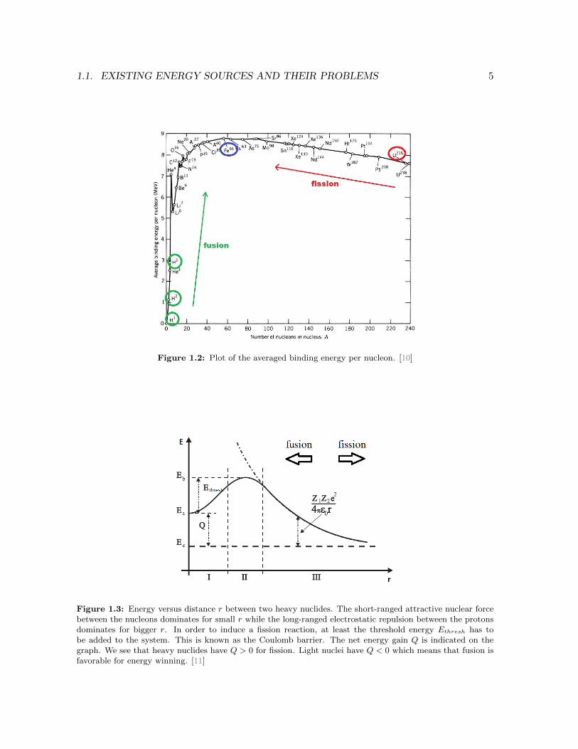
In contrast to fossil fuel burning, fission reactions are not driven by chemical interactionsbut by the much stronger nuclear force. The binding energy1 per nucleon is shown in Figure1.2. Since this curve is concave and reaches its maximum for iron (Z=56), energy will bereleased by splitting heavier nuclei or melting together lighter nuclei. This first process iscalled nuclear fission, and is the technique used in nuclear power plants nowadays. The otherprocess is called nuclear fusion, the subject of this thesis. The general fission reaction executedin nuclear power plants is the chain reaction
10n + 235
92 U→ A1Z1
X1 + A2Z2
X2 +N 10n + γ + 200MeV (1.2)
with
A1 +A2 +N = 235 (1.3)
Z1 + Z2 = 92 (1.4)
Indeed, the reaction products are not always the same. Common fission products are barium(Z1=56) and krypton (Z2=36). Usually, the number of electrons created per reaction N is2 or 3. To start the reaction, a free neutron is absorbed by uranium-235, turning it brieflyinto uranium-236. This unstable excited state breaks down creating two smaller nuclei, someneutrons and gamma rays. The neutrons are used to induce subsequent fission reactions. Thekinetic energy of the fission products and the radiant energy of the γ rays heat the workingfluid in the reactor which is usually water (H2O, occasionally D2O). This hot water is used toproduce steam in a secondary circuit that drives the steam turbines and generates electricity.The gained 200MeV per reaction is a theoretical value, calculated using Einstein’s famousrelation
∆E = ∆m · c2 (1.5)
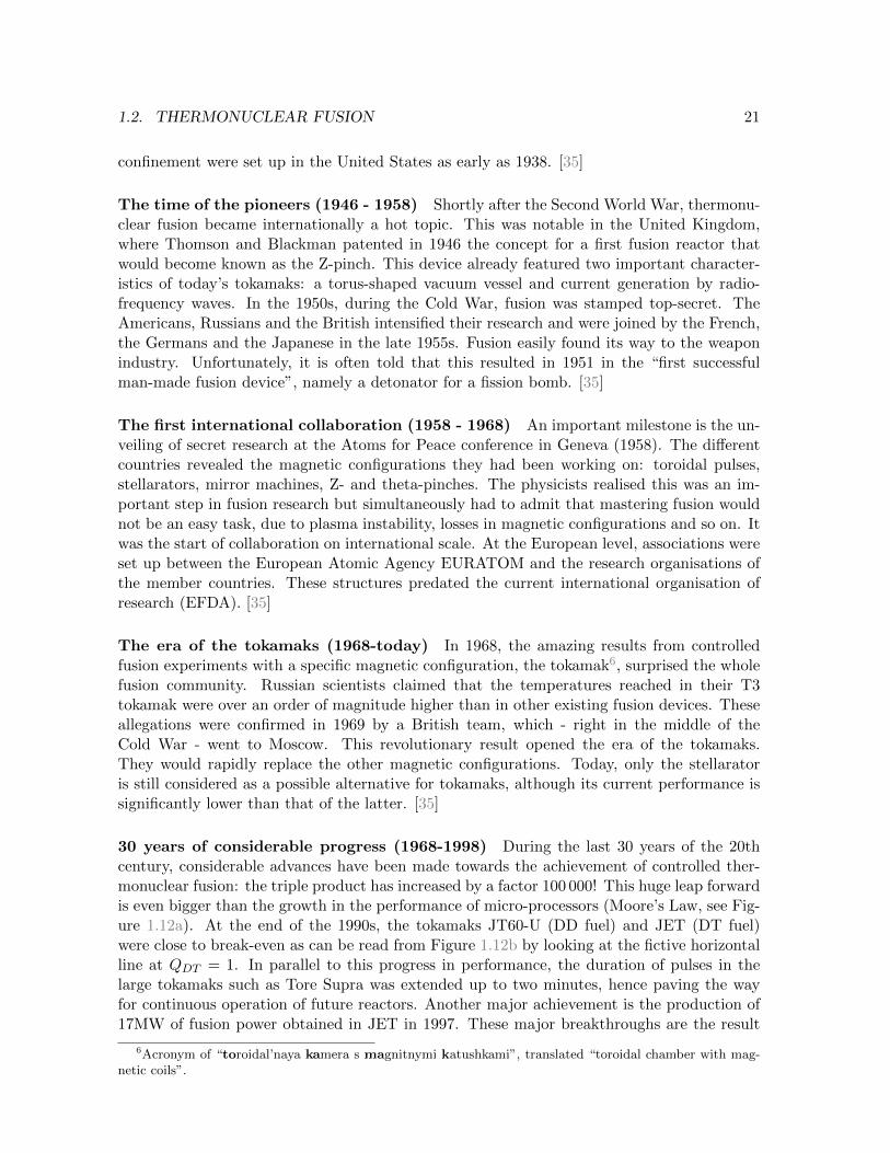
where the mass difference between U-235 and the fission products is determined experimen-tally. A neutron is needed to induce the decay of U-235 since the energy barrier Ethresh asseen in Figure 1.3 is about 6MeV and the binding energy released by the capture of an extraneutron is about 7-8MeV as can be seen in Figure 1.2. The surplus of energy brings theformed U-236 in an excited state. In order to make U-236 even more unstable the kineticenergy of the neutron can be increased. In this case, one speaks about a fast-neutron reactor,otherwise a thermal-neutron reactor.
1.1. EXISTING ENERGY SOURCES AND THEIR PROBLEMS 5
Figure 1.2: Plot of the averaged binding energy per nucleon. [10]
Figure 1.3: Energy versus distance r between two heavy nuclides. The short-ranged attractive nuclear forcebetween the nucleons dominates for small r while the long-ranged electrostatic repulsion between the protonsdominates for bigger r. In order to induce a fission reaction, at least the threshold energy Ethresh has tobe added to the system. This is known as the Coulomb barrier. The net energy gain Q is indicated on thegraph. We see that heavy nuclides have Q > 0 for fission. Light nuclei have Q < 0 which means that fusion isfavorable for energy winning. [11]

6 CHAPTER 1. THERMONUCLEAR FUSION
Theoretically, according to reactions (1.1) and (1.2), the fission of one mole U-235 generatesmore than 20 million times the energy released by burning a mole of CH4. Furthermore, thedensity of uranium is much higher than that of CH4. Hence, the energy contained in 1g ofU-235 is many orders of magnitude bigger than that of 1g CH4, which is of course an asset ofnuclear energy. Another advantage of nuclear power plants is the absence of greenhouse gasemissions. The bad side of nuclear fission is that the by-products are long-lived β-emittersand that the chain reactions cannot be stopped in worst case scenarios, resulting in a so-called “meltdown” of the fission reactor. The big catastrophic nuclear accidents in ThreeMile Island (US,1979), Chernobyl (Ukrain,1986) and Fukushima (Japan,2011) have sloweddown or even reversed the growth of nuclear fission in a lot of countries. The public opinionis turned more than ever against fission energy and the extra costs and approval times fornuclear power plants to fit the safety regulations are out of proportion. Japan used to be oneof the countries with a high share of nuclear power (30%) in its electricity mix. Today, Japanhas only two of its 54 reactors in operation [5]. Belgium, with a nuclear power generationof more than 50% in its earlier energy mix, signed to close all its nuclear power plants by 2025.
Pressing CO2 standards make that nuclear power still has a future, especially if the thoriumreactor breaks through. This type of reactor, using thorium as input instead of uranium, isclaimed to produce less harmful radioactive waste and to be proliferation-resistant. Besides,thorium is more abundant than uranium so it could be a way to limit our CO2 emission duringthe next centuries. But more importantly, much safer reactor designs are possible. Thoriumalone cannot sustain the chain reaction. It first has to absorb slow neutrons to transform intoU-233, an artificial version of uranium that is fissile. This different fuel cycle lends thoriumreactors to be designed “sub-critical”, i.e. they need external input of neutrons to keep thereaction going. These neutrons can for example be created by a proton beam incident on alead target. If the proton beam is switched off, the reactor stops. With this kind of design,meltdowns are impossible. The difficulty is to create a proton beam with the right amountof energy. This should be feasible with the modern particle accelerators. [12]
1.1.4 Renewables
Biomass & waste
Bluntly speaking, biomass energy is generated by the combustion of plants, directly or indi-rectly after conversion to biofuels like ethanol and biodiesel. It is the most primitive energysource: historically, humans have harnessed biomass-derived energy since the time when peo-ple began burning wood to make fire. This renewable energy source has a recycle aspect:industrial waste and by-products can often be transformed to biofuels, and for example allrotting garbage releases methane gas which could be captured and used as an energy source.Bioenergy is controversial because of the food-or-energy dilemma, which also involves issueslike land and fresh water scarcity. Besides, it is not a clean energy source: CO, CO2, NOx
and SOx emissions are often intrinsic to these kind of combustions. Nevertheless, biodieselcould be a good alternative for gasoline.
1The energy input needed to split a nucleus entirely into its constituting particles called nucleons.

1.1. EXISTING ENERGY SOURCES AND THEIR PROBLEMS 7
Water
Hydro power is a widely used form of renewable energy mentioned apart in Figure 1.1a and1.1b because of its significant contribution in the world energy mix. The working principleis based on the ancient watermill. The flow of water in rivers or the hydrostatic pressureof water kept in reservoirs (dams) is a mechanical form of energy which is converted withwater turbines into rotational energy and thereafter to electricity. More or less the same ideacan also be used for water which has already been diverted for use elsewhere, in a municipalwater system for example. Besides, water storage can be used to supply high peak demands.At times of low electrical demand, excess generation capacity is used to pump water into ahigher reservoir. When there is higher demand, water is released back into the lower reservoirthrough a turbine. And there are plenty of other techniques where water power is used togenerate electricity. Nevertheless, most hydroelectric power comes from dams. It is a cleanmethod with no direct waste or emission of harmful gases. Unfortunately, the number ofpossible locations for such hydro power plants is limited due to the need for a big lake whichimposes a geographical and climatological condition.
Photovoltaic (PV)
The use of solar energy is growing strongly around the world, partially due to the rapidlydeclining solar panel manufacturing costs (see Figure 1.4). In 2007, solar energy accountedfor about 0.1% of the world energy consumption. This share is believed to increase to 1.2% in2030 [13]. The world’s overall solar energy resource potential is around 5.6GJ/m2/year [13].According to Figure 1.1b, this means that an area of 525 000km2 - or 0.1% of the Earth’stotal surface area - covered by ideal solar cells suffices to foresee in all our energy needs at themoment. You could think that this is feasible, but unfortunately the used resource potentialis an overestimation and solar cells are far from ideal. For the moment, commercial panelsconvert about 20% of the incident sun light to electricity. Luckily, a lot of improvement is stillpossible. The research group of the Fraunhofer Institute for Solar Energy Systems in Freiburgpublished in September 2013 that they constructed a new solar cell with 44.7% efficiency [14].The concerned solar cell is not of the conventional silicon type, but a III-V multi-layer type,which originally came from space technology. Here, several cells made out of different III-Vsemiconductor materials are stacked on top of each other. The single subcells absorb differentwavelength ranges of the solar spectrum, making this technology very efficient. Also the 2010Nobel Prize winner graphene, i.e. a carbon sheet of one atom thick, looks very promising forhigh-performance solar cells [15]. Scientists are optimistic to reach the goal of 50% within thenext years. However, even with these high efficiencies solar parks still need to have immensedimensions in order to create the same power output as fossil fuel and nuclear power plants.Besides, solar power is unreliable as it is not always available in the same amount. It is perfectas an additional clean2 source of energy, but probably not more than that. It is for examplealso very useful for stand-alone applications reaching from space stations to parking meters.
There also exist other techniques to convert sun light to electricity. Concentrated solar power(CSP) uses mirrors with sun trackers to concentrate a lot of light in one point to drive aconventional heat engine. Most of the CSP plants are parabolic-trough plants. Here, linearparabolic reflectors heat a working fluid that is placed in the focal line. Spain is the world
2The environmental damage by the production process of the solar cells taken aside.

8 CHAPTER 1. THERMONUCLEAR FUSION
Figure 1.4: Left : Evolution of the global cumulative installed PV capacity. Right : The global PV moduleprice learning curve for c-Si wafer-based and CdTe modules. [16]
leader in CSP with a total capacity of 2.2GW.
Wind
Wind is in the first place useful to produce mechanical power if we think about sail boats andold windmills, but it has also proven itself to be an interesting tool to generate clean elec-tricity. Last years, driven by the government’s subsidies, big wind farms were built on landand at sea. The world wind energy capacity has been doubling about every three and a halfyears since 1990. The total electricity generation in 2011 was around 377TWh, roughly equalto Australia’s annual electricity consumption [5]. China, Germany, Denmark and the US aresome examples of countries that create a lot of wind energy. Unfortunately, wind power alsostruggles with the problem that it is not always available. As governments begin to cut theirsubsidies to renewable energy, the business environment becomes less attractive to potentialinvestors. Lower subsidies and growing costs of material input will have a negative impact onthe wind industry in the near future.
The windmill park in Zeebrugge was one of the first wind energy projects in Europe. It wasbuilt in 1986 as a demonstration project to give interested companies the know-how theyneeded. So already in the nineties, wind energy was subsidized. If we have to be honest, notenough progress has been made since then to keep on financing this technology. Luckily, arevolution is coming soon. The future of wind turbines lays in the sky. As there is more windenergy available at higher altitudes and this at a constant rate, we have to search for windover there. This is of course nothing new: the trend seen in conventional wind turbines isthat they always become bigger and bigger. So, what is the difference? We are now speakingabout an altitude of 300-600m. This is impossible with the classical wind turbine technology.Therefore, some American companies already have prototypes of how the next generation ofwind turbines will hopefully look like, the so-called airborne wind turbines. The first one isdesigned by Makani and looks like a kite that circles around in the air (see Figure 1.5a). Asecond type is property of Altaeros and is some kind of balloon with a turbine inside (seeFigure 1.5b). Next to the fact that these airborne wind turbines can catch more wind atthe higher altitudes, they are also easy to install at less convenient locations like for exampleabove the ocean3, and besides they are much cheaper than classical turbines with a tower.
3They only need to connect a rope to something on the ground.

1.1. EXISTING ENERGY SOURCES AND THEIR PROBLEMS 9
(a) (b)
Figure 1.5: (a) The “kite” prototype of Makani compared to classical wind turbines [17] [18]. (b) The“balloon” prototype of Altaeros [19].
On the other hand, this new technology is again a step back in terms of power generated perturbine. [17]
Geothermal
In a geothermal power plant, hot steam is pumped up and cold water pulled down to under-ground natural reservoirs. These geothermal reservoirs appear in regions of volcanic activity,i.e. near the boundaries of tectonic plates or at hotspots, and also in regions of above-normalheat production through radioactive decay of minerals. This renewable energy source is clean(there is no creation of direct waste or harmful gases) and unlike wind and solar energy, whichare more dependent upon weather fluctuations and climate changes, geothermal resources arealways available. While the carrier medium for geothermal electricity (water) must be prop-erly managed, the source of geothermal energy, the Earth’s heat, will be available indefinitelyin human time-scale. The only disadvantage is that the number of sites where such a powerplant can be built is limited because of the need for a geothermal reservoir. According tothe Geothermal Energy Association [20], the world capacity of geothermal electricity wasabout 11.224GW in 2012 which is about 0.0007% of the total energy use that year. However,the same idea of using the Earth’s heat is recently applied to households under the name“geothermal heat pumps”. A network of underground pipes - not as deep as for power plantsof course - is used to support the central heating system by exchanging heat with the crustal.
Ocean
The ocean covers 71% of the Earth’s surface and contains a lot of energy in different forms.It would be a shame not to exploit this energy resource. The general term ‘ocean power’ canbe subdivided in several techniques to produce electricity such as tidal power, wave power,ocean thermal energy conversion, ocean current power, ocean wind power and osmotic power.Of these, the first three are the most well-developed technologies. While the kinetic energyfrom marine and tidal waves can be relatively easily converted to electricity by turbines, theconversion of wave power poses bigger technical challenges. A wide variety of wave energyconverter designs exists. Ocean thermal energy conversion uses the temperature differencebetween cooler deep water and warmer surface water to run a heat engine. Osmotic power orsalinity gradient power can be exploited for energy extraction through reverse electro-dialysisand osmotic processes working between ocean water with high and river water with low salt

10 CHAPTER 1. THERMONUCLEAR FUSION
concentration. Worldwide, ocean energy’s share in the total electricity generation is negligible.It is projected to increase by 2030, albeit only modestly. Ocean energy industries are at anearly stage of development. Commercial applications of ocean energy have been limited totidal barrage power plants in France (240MW) and Canada (20MW), but major new tidalbarrage plants are under construction in the Republic of Korea.[21] [22]
1.1.5 Energy efficiency
As stated by the laws of thermodynamics, energy can be converted from one form to another,but these actions have a price: the amount of useful energy decreases in every step. Not allenergy stored in for example fossil fuels is used for its final purpose, and also the energy thathas reached its final form is often wasted in many ways. Energy efficiency is associated withthe part of the initial energy stored in fuels that is useful in the end.
Every step of the entire energy conversion chain still has enormous margins for improvedefficiency. However, not only technological innovations but also economics play an importantrole in this story. Energy efficient technologies will only break through if there is enougheconomical benefit associated with it, and if there are no implementation barriers. Somepossibilities to improve the overall efficiency of our energy are summed here for the maintechnology groups:
• In power generation, the average efficiency of coal-fired plants for example is 34% [5],in sharp contrast with the 94% of the multi-fuel Avedore Power Station in Denmark[23]. Cogeneration, the combined production of electrical power and useful heat, cancertainly improve the efficiency. Other options are repowering, combined cycle powerstations,...
• In transmission and distribution electricity losses reach up to 12% and above [5]. Thismay be diminished by better management, strategically better locations of the powerplants, personal energy generation with for example solar panels, better storage tech-niques, less resistive cables, .... Promising for this last one is the upcoming carbontechnology which will hopefully introduce low-weight and low-loss conductors. In thisrespect, carbon nanotubes seem to be the future [24]. Concerning the better manage-ment, an important role will be played in the near future by so-called smart grids. Theincreasing amount of solar and wind energy, which are highly variable, forces us to adaptour current distribution system. Smart grids will be able to act on changes in the localenergy production or consumption in an automated fashion using ICT. Germany forexample has a huge installed capacity of solar and wind power that sometimes - on verysunny days or when it storms - causes negative electricity prices! The craziest part ofthis whole story is that pumped-storage hydroelectricity is purposely wasted when thishappens. And you cannot blame the managers of these water reservoirs because theyare making a lot of money by doing it! Some legislative obstacles at the moment are thereal problem. It is time that the European Union becomes a real union and fully opensits borders for energy transport from one member state to the other. When Germanyhas excess electricity, this should be easily guided to places elsewhere in Europe whereit can be used. The design of smart grids that regulate all of this, is very complex buta must for the future.

1.2. THERMONUCLEAR FUSION 11
Figure 1.6: Global electricity demand by application. [5]
• Buildings account for nearly 40% of the total energy consumption globally and it isestimated that potential energy savings in buildings could reach between 20 and 40%[5]. This can be accomplished with better insulation, the use of fluorescent lamps or evensky lights instead of the traditional incandescent light bulbs,... According to Figure 1.6,about 40% of our energy goes to motors. This means that the development of lightervehicles is certainly a help. Of course, also the behaviour of the consumer plays a veryimportant role.
1.1.6 Hydrogen fuel cell
The basic idea of hydrogen technology is to replace electricity with hydrogen as energy carrier.This implies the production of hydrogen, the transport and storage of hydrogen and theconversion to electricity by hydrogen fuel cells in the end application, for example a hydrogenvehicle. The fuel cell releases electrical energy throughout redox reactions and needs thecontinuous input of fuel and oxygen or air for that purpose (see Figure 1.7). Some assets:
• Hydrogen (H2) can be easily produced from water, biomass, biogas, natural gas,...
• It poses an efficient way to store energy.
• It provides an efficient solution for combined heat and power generation, both at indus-trial and domestic level.
• Hydrogen offers a significant reduction of green house gas emissions (hydrogen oxidationonly produces water at point of use) and a reduction in air pollution.
The manufacturers of fuel cell vehicles (FCV) have reached the point where vehicles thatcould be sold in 2015 would fulfil the costumers’ expectations. However, the high cost andthe lack of refuelling stations still pose a big problem. We can expect to see more and morehydrogen vehicles in the near future. Germany for example is currently placing refuellinginfrastructure and wants a self-sustaining FCV business by 2020. [25] [26]
1.2 Thermonuclear fusion
1.2.1 Plasma
Plasmas are ionized gases. Hence, they consist of positively charged ions and negativelycharged electrons, as well as neutral particles. This quasi-neutral ensemble features a collective

12 CHAPTER 1. THERMONUCLEAR FUSION
Figure 1.7: Hydrogen fuel cell.
behaviour described by the hydromagnetic equations of plasma motion. Plasma is also knownas “the fourth state of matter” next to solids, fluids and gases. Despite that plasmas do notappear very much on Earth (lightening, aurora borealis,...) , it is very common in the restof the universe: more than 99% of the known matter is in the plasma state, stars being thebest example. Mankind has succeeded to reproduce plasmas on Earth. Two main groups oflaboratory plasmas exist: the high-temperature plasmas and the so-called low-temperatureplasmas or gas discharges. The last ones are used in TL-lamps, plasma displays, gas lasers,surface treatment, biomedical applications, air and water cleaning,... From now on, however,the term ‘plasma’ will refer to high-temperature plasmas, which are used in fusion processes.
1.2.2 Fusion reaction
Fusion occurs when light nuclei are melted together to form heavier nuclei with more averagebinding energy per nucleon. One could ask himself which fusion reactions are the easiest toexecute on Earth.
First of all, there is the Coulomb barrier between both nuclei which has to be overcome be-fore the strong nuclear force takes over (recall Figure 1.2). This barrier is proportional to theproduct of the charges of both nuclei, so the fuels must have a low atomic number. Mind thatthe nuclei do not have to go over the whole barrier. As we know from quantum mechanics,the nuclei can also tunnel through it.
Secondly, the cross-section of the fusion reaction should be as high as possible in the feasibletemperature range. As we can see from Figure 1.8 , the deuterium-tritium reaction is mostsuitable.
21D + 3
1T→ 42He (3.52MeV) + 1
0n (14.08MeV) (1.6)
This reaction produces helium nuclei, also called α-particles, with a kinetic energy of Eα =3.52MeV and neutrons with a kinetic energy of En = 14.08MeV. As neutrons are electricallyneutral they can leave the magnetic confinement of a tokamak (see later) and their energy isused to produce electricity. The α-particles, however, are charged and cannot escape. Theirenergy is - in the best case - used as an extra heating source for the plasma.
Thirdly, the energy release per reaction should be as high as possible to produce net energy.

1.2. THERMONUCLEAR FUSION 13
Figure 1.8: Fusion cross-sections of different low-Z fusion reactions expressed in barn units (=10−28m2).More relevant however is 〈σF v〉, the averaging of the product of fusion cross-section and particle velocity overthe velocity distribution. [27]
1.2.3 Properties of fusion fuels
Deuterium
Deuterium (D) is a non-radioactive isotope of hydrogen with one neutron (and of courseone proton and one electron). It can be gained by electrolysis of water (D2O electrolysesmore difficult and remains behind), by distillation of liquid hydrogen or by various chemicaladsorption techniques. According to estimations the energy content of all deuterium in theworld’s oceans should be enough to supply humanity longer than the Sun will burn. So, it isimportant that we learn to use the D-D fusion reaction in the long-term.
Tritium
Tritium (T) is a radioactive isotope of hydrogen with two neutrons. It is a β-emitter with ahalf-life of about 12.3 years. The decay reaction is given by
31T→ 3
2He + e− + νe (1.7)
The electron emitted during the decay has not got enough energy to cross the dead layer ofour skin. So, extracorporeal tritium is harmless. When inhaled or ingested, however, tritiumcan be very nasty: it damages our body from the inside and causes cancer. Since tritiumis able to replace one or more ordinary hydrogen isotopes in water or organic molecules, iteasily contaminates our water or food cycle. Fortunately, there is already some experiencewith tritium because it is a common by-product in present nuclear power plants. Due to itsshort half-life, tritium does not appear naturally in big enough amounts. Therefore, it hasto be created somehow. This will be done by surrounding the vessel with a lithium blanket.The fusion reaction produces high-energetic neutrons which react with lithium as follows
63Li + 1
0n→ 31T + 4
2He + 4.80MeV (1.8)73Li + 1
0n→ 31T + 4
2He +10 n− 2.87MeV (1.9)

14 CHAPTER 1. THERMONUCLEAR FUSION
The radioactive tritium is therefore made in the fusion reactor and immediately consumed asfuel. The real fuels of a fusion power station are therefore deuterium and lithium, eliminatingthe need to transport radioactive fuels outside of the reactor. [28]
Lithium
Lithium (Li) is a silver-white alkali metal. The only naturally occurring isotopes are Li-6(7.42%) and Li-7 (92.58%). Due to its high reactivity, lithium never occurs freely in nature,and instead, only appears in compounds, which are usually ionic. It occurs in a number ofminerals, but due to its solubility as an ion, it is present in ocean water and is commonlyobtained from brines and clays. There exists no accurate information about the world lithiumresources. The booming lithium-ion industry could form a threat, especially if the electricor hybrid cars become a real success in the next years. However, with its 0.17ppm presencein sea water, cheaper and more efficient extraction techniques would make lithium virtuallyinexhaustible. [28]
1.2.4 Triple product
Three plasma parameters need to be high in order to get sustained fusion: the plasma tem-perature, the fuel density and the energy confinement time. Their product is called the fusiontriple product. For D-T fusion to occur, this product has to exceed a certain minimum value.This value was already calculated in 1955 by the British scientist John Lawson. The wholeconcept is now known as the Lawson criterion.
Temperature (T)
In order to overcome their natural repulsive Coulomb forces, the positively charged plasmaions need to have enough energy. In the high-temperature-limit the plasma particles can beconsidered being in thermodynamic equilibrium, which implies together with the assumptionof solely elastic collisions that their velocity has a Maxwell-Boltzmann distribution. In otherwords, under these conditions a plasma can be described by the kinetic gas theory which saysthat the most probable energy ε and the average energy 〈E〉 of the plasma particles are givenby
ε = kBT (1.10)
〈E〉 =3
2kBT (1.11)
So, one can conclude that the plasma temperature indeed should be high in order to make fu-sion possible. As a side note, we mention that equation (1.10) is used to express temperaturesin units of energy: 1eV is about 10 000K.
Density (n)
As seen from Figure 1.8, the cross-sections of the fusion reactions are in general very small.This means that high fuel densities are needed in order to attain the required reaction rates.In fact, only the density of the fuel has to be high. Impurity atoms and helium ions from thefusion reaction itself - the “ash” - have to be controlled, because they dilute the plasma andhinder optimal operation of the fusion device.

1.2. THERMONUCLEAR FUSION 15
Energy confinement time (τE)
The energy confinement time is a measure for how long a plasma is able to retain its heatright after the external heating sources are turned off. It is defined as the ratio of the thermalenergy contained in the plasma and the power losses at that same moment. The energyconfinement time increases substantially with plasma size. This imposes a minimum volumeconstraint on fusion devices.
Power balance and Lawson Criterion for D-T fusion
To understand the origin of the Lawson Criterion, one has to look at the power balance of aD-T fusion reactor:
∂W
∂t= Pα + PH − PBr − PL > 0 (1.12)
This says that in order to have net accumulation of thermal energy W in the plasma, the sumof the power generated by α-particle heating (Pα) and by external heating sources (PH) hasto be bigger than the power losses. These losses are split up in bremsstrahlung losses (PBr)on the one hand and all other conduction, convection and radiation losses (PL) on the otherhand. The energy of the neutrons is not spend on heating the plasma but is converted toelectricity.
Bremsstrahlung losses are well understood. They are caused by the acceleration of chargedparticles in the electrostatic field of other charged particles. In fusion devices this concernsmainly the deflection of electrons in the electric field of ions. Bremsstrahlung occurs in thex-ray domain where the plasma is optically thin: its energy is not absorbed by the plasma andconsequently it is lost. The bremsstrahlung losses in a plasma of volume V are approximatedby (see [29])
PBr = 5.35 · 10−37Z2effneniV T
12 Watt (T in keV) (1.13)
where Zeff is the effective atomic number defined as
Zeff =
∑iniZ
2i∑
iniZi
(1.14)
The occurrence of Zeff in this equation is easy to understand: nuclei with higher electricalcharge cause higher electron accelerations and consequently higher radiation losses. There-fore, it is very important to prevent the introduction of high-Z impurities into the plasma.
The underlying physics of the other losses is not clear. Experiments show a more or lessexponential drop after switching off the fusion apparatus. This effect is in accordance withknown heat losses: the same happens for example when the central heating of a building isswitched off. This exponential behaviour is mathematically translated into
PL =W
τE(1.15)
where the empirical energy confinement time τE is introduced. Indeed, substituting this intothe power balance (1.12) without any of the other power terms, i.e. there is no external

16 CHAPTER 1. THERMONUCLEAR FUSION
heating (PH = 0) and the α-particle heating and bremsstrahlung losses cancel each other out(Pα = PBr), gives
∂W
∂t= −W
τE, (1.16)
and solving this first order differential equation results in the proposed exponential drop.
W (t) = W (0) e− tτE (1.17)
In what comes next, we will use however yet another energy confinement time which includesthe radiation losses PBr and is easier to measure. It is defined by equation (1.18).
PL + PBr =W
τ∗E(1.18)
The thermal energy of the whole plasma column is given by
W = 3nkBTV (1.19)
which is easily calculated using equation (1.11) and keeping in mind that the plasma consistsof ions as well as electrons with the same particle density4 and temperature. The total fueldensity is denoted by n.
For nD = nT = n/2, the total fusion power is given by
PF =n2
4〈σF v〉EFV (1.20)
and the heating by α-particles has a similar expression, namely
Pα =n2
4〈σF v〉EαV (1.21)
where σF is the fusion cross-section, v the particle velocity and ‘〈 〉’ the averaging over thevelocity distribution. Eα is the energy released in the form of kinetic energy of α-particlesafter one fusion reaction, namely 3.52MeV. The total energy released by one fusion reaction,carried by α-particles as well as neutrons, is five times bigger (about 17.6MeV).
The external heating responsible for the contribution PH could be ohmic heating, neutralbeam injection, electron/ion cyclotron heating resonance, or maybe even another technique.The expression for PH is undefined. However, it can be related to the total fusion power PFby introducing the so-called power enhancement factor Q.
PH =PFQ
=5PαQ
(1.22)
This quantity has two values that need special attention: Q = 1 (break-even) and Q = ∞(ignition). This last one occurs if the number of fusion reactions per second is sufficientlyhigh, so that the heating caused by the α-particles makes the use of external heating systems
4Assumption of quasi-neutrality of the plasma: nD + nT = ne = n.

1.2. THERMONUCLEAR FUSION 17
redundant. The name ‘ignition’ is in analogy with the burning of fossil fuels.
Based on equations (1.18), (1.19), (1.21) and (1.22), it is now possible to rewrite the powerbalance (1.12) as
n · τ∗E >12kBT
〈σF v〉Eα(
1 + 5Q
) (1.23)
Making use of the approximation (see [30])
〈σF v〉 ≈ 1.1 · 10−24 · T 2 m3 s−1 (T in keV) (1.24)
which is valid in the range 10-20keV (see Figure 1.9a), this results in the Lawson criterion5
breakeven : n20 · T · τ∗E > 5 m−3 keV s
ignition : n20 · T · τ∗E > 30 m−3 keV s
(1.25)
(1.26)
An estimation of the minimum temperature needed for D-T fusion can be made by solving(1.27) for T .
PF = PBr (1.27)
This describes the hypothetical situation where the plasma energy remains constant, thereare no external heating sources (ignition), the only losses are due to bremsstrahlung of thefusion fuel (Zeff = 1) and all energy released by the fusion reactions - also the energy of theneutrons - is used to cancel these bremsstrahlung losses. These are the absolute minimumconditions that have to be fulfilled in order to be able to create an ignited plasma that doesnot create electricity. The actual lower bound for the temperature is certainly much bigger,since impurities are unavoidable and also non-radiative losses occur in reality. Using equations(1.13) and (1.20), the condition (1.27) can be transformed to
〈σF v〉 = 1.52 · 10−25T12 (1.28)
We can solve this equation by using experimental data for 〈σF v〉. This is done in Figure 1.9b.It shows that
Tmin ≈ 2 keV (1.29)
This is an estimation of the minimum ignition temperature executed by the writer of thismaster thesis. It is in reasonable consistence with the value of 4keV which is claimed in [31].Typical desired values for tokamaks (see next paragraph) are
n = 1020 m−3 (1.30)
T = 10 keV (= 108 K) (1.31)
τ∗E = 3 s (1.32)
Stars like our Sun reach the ignition condition for multiple fusion reactions. Their huge masscreates gravitational forces strong enough to confine their plasma and reach high densities.Besides, their big volume implies a high energy confinement time and the large amount ofplasma particles makes that there are enough particles in the tail of the Maxwell-Boltzmanndistribution with enough energy - or in other words temperature - to undergo fusion.
5The notation n20 is used to denote n · 10−20.

18 CHAPTER 1. THERMONUCLEAR FUSION
(a) (b)
Figure 1.9: Maxwell averaged cross-section 〈σF v〉 for D-T fusion according to experimental fitting performedby Bosch and Hale (see [30]). (a) The parabolic approximation (1.24) is reliable for temperatures in the range10-20keV. (b) Determination of the minimum ignition temperature based on equation (1.28). Both curvesintersect at T ≈ 2keV.
1.2.5 Confinement
Because no material on Earth is capable of withstanding the high fusion temperatures, onehas to appeal to non-contact methods to confine the plasma. Two main techniques are used:inertial confinement and magnetic confinement.
Inertial confinement
In the first technique, a cryogenic (supercooled) pellet of fusion fuel is heated by powerfullasers or ion beams. The outer layers are turned into plasma which expands due to heatabsorption. As a reaction to this, the rest of the pellet implodes due to its inertia so that theignition condition is fulfilled and fusion reactions in the pellet create energy. This principle isused in hydrogen bombs but is also attempted in controlled fusion reactors. It is particularlypopular in the United States, where at the end of last year a breakthrough took place inthe National Ignition Facility (NIF): for the first time in history, the released fusion energyexceeded the energy deposited in the fusion fuel during the implosion. The setup and workingprinciple are explained in Figure 1.10. However, a lot of energy was first wasted to reach thestate of implosion and besides a lot of the laser energy was lost throughout the conversionfrom UV light to x-rays. This makes that the energy production is still less than 1% of thetotal laser energy. The most important problems are the non-symmetrical shape of the pelletwhen it is heated and the mixing of the plastic of the fuel capsule with the fuel itself. Tocontrol these two effects, the laser energy has to be somewhat lowered, while its full capacityis needed to reach ignition, i.e. a fusion chain reaction that burns a significant portion ofthe fuel. The process of self-heating by α-particles, which is vital for ignition, has beendemonstrated during the experiments at NIF. [32]
Magnetic confinement: the tokamak concept
The other technique uses high magnetic fields to confine the fusion fuel that is first ionized.This is the principle used in tokamaks such as COMPASS and is the topic of this thesis. The-oretically speaking, the biggest difference between both confinement methods is that inertialfusion speculates on a high fuel density n, while magnetic fusion rather aims at a large τE .

1.2. THERMONUCLEAR FUSION 19
(a) (b) (c)
Figure 1.10: Inertial confinement fusion at NIF. (a) The interior of the target chamber. A scientist can beseen on the left. The target positioner is on the right. The target is a metallic case called a hohlraum thatholds the fuel capsule. (b) The golden hohlraum cylinder is just a few millimetres wide. (c) Illustration ofthe working principle. A series of laser beams is pointed to the apertures at both ends of the hohlraum, whichcontains a fusion target the size of a small pea. The laser beams strike the inside walls of the golden canconverting their UV light into x-rays. These x-rays then bathe the capsule creating tremendous pressure andcrushing the fuel capsule. Now, conditions are reached for fusion reactions to occur. [33]
The temperature has the same order of magnitude for both.
For particles with charge q in the presence of a magnetic field Newton’s second law of motionstates
mdv
dt= q(v×B) (1.33)
In physical terms, this means that the particles gyrate around the magnetic field lines. Thiscan be better understood if one transforms the expression to
dv
dt= ω × v (1.34)
where ω is the angular speed of the gyration given by
ω = −qBm
(1.35)
Given the fact that for circular motion v⊥ = ωρ - where v⊥ is the component of the velocityvector v in the gyration plane - the radius of gyration is given by
ρ =
∣∣∣∣mv⊥qB∣∣∣∣ (1.36)
The easiest way to invoke electromagnetic confinement would be by using a cylindrical setupwhere electrical currents in the windings at the cylinder surface create a homogeneous mag-netic field in the cylinder body (see Figure 1.11a). However, it is clear that this setup causeslosses at both open ends of the cylinder. An obvious solution is to bend the cylinder andform a torus. However, in this case the problem of electromagnetic confinement has becomea lot more difficult. According to Ampere’s law, the toroidal magnetic field is then given by
Bt =µ0NI
2πr(1.37)
with N the number of toroidal coils, I the current driven through them, and r the distancefrom the main axis of the torus. The appearing r-dependence is very important since it

20 CHAPTER 1. THERMONUCLEAR FUSION
(a) (b)
(c) (d)
Figure 1.11: (a) Cylindrical confinement with leaks at both ends [34]. (b) Toroidal confinement with chargeseparation [34]. (c) Transformer principle with ferromagnetic core. (d) Central solenoid. Remark the helicaltrajectory of the magnetic field lines/plasma particles in the last two figures.
implies a non-zero B×∇B drift. This means that plasma particles with opposite signs driftin opposite directions, as is demonstrated in Figure 1.11b. This charge separation inducesan electric field which - together with the magnetic field - pushes the plasma away from themain axis of the torus (see Appendix A). As a conclusion, one sees that it is necessary tocounteract the charge separation. This can be done by using a higher current through thetoroidal field coils as the drift velocity is inversely proportional to this current, but a betterway is to deform the magnetic field a little bit, which can be done by means of a plasmacurrent combined with some poloidal field coils that are positioned around the perimeterof the vessel (tokamak) or by creating specifically shaped external coils (stellarator). Theplasma current referred to is induced in the tokamak by means of the transformer principle.The tokamak can have a ferromagnetic core - for example iron - as shown in Figure 1.11c. Inthis case a current through the primary winding induces a current in the secondary winding,namely the plasma. The tokamak may also have a so-called air core, which means that thereis a central solenoid going through the center of the toroidal tokamak vessel having a mutualinductance with the plasma ring. When this central solenoid conducts a varying current againa plasma current will be formed. This can be seen in Figure 1.11d.
1.2.6 Historical evolution of the tokamak
The “Prehistoric Period” (1905 - 1938). After Einstein’s publication of the mass-energy equivalence E = mc2 in 1905, it took a few years until scientists discovered its realimportance. In the nineteen twenties, the British physicist F.W. Aston measured the massdefect of helium and suggested nuclear fusion as a possible energy source. It would not takelong before astronomers made the link with the stars. The first experiments with magnetic
1.2. THERMONUCLEAR FUSION 21
confinement were set up in the United States as early as 1938. [35]
The time of the pioneers (1946 - 1958) Shortly after the Second World War, thermonu-clear fusion became internationally a hot topic. This was notable in the United Kingdom,where Thomson and Blackman patented in 1946 the concept for a first fusion reactor thatwould become known as the Z-pinch. This device already featured two important character-istics of today’s tokamaks: a torus-shaped vacuum vessel and current generation by radio-frequency waves. In the 1950s, during the Cold War, fusion was stamped top-secret. TheAmericans, Russians and the British intensified their research and were joined by the French,the Germans and the Japanese in the late 1955s. Fusion easily found its way to the weaponindustry. Unfortunately, it is often told that this resulted in 1951 in the “first successfulman-made fusion device”, namely a detonator for a fission bomb. [35]
The first international collaboration (1958 - 1968) An important milestone is the un-veiling of secret research at the Atoms for Peace conference in Geneva (1958). The differentcountries revealed the magnetic configurations they had been working on: toroidal pulses,stellarators, mirror machines, Z- and theta-pinches. The physicists realised this was an im-portant step in fusion research but simultaneously had to admit that mastering fusion wouldnot be an easy task, due to plasma instability, losses in magnetic configurations and so on. Itwas the start of collaboration on international scale. At the European level, associations wereset up between the European Atomic Agency EURATOM and the research organisations ofthe member countries. These structures predated the current international organisation ofresearch (EFDA). [35]
The era of the tokamaks (1968-today) In 1968, the amazing results from controlledfusion experiments with a specific magnetic configuration, the tokamak6, surprised the wholefusion community. Russian scientists claimed that the temperatures reached in their T3tokamak were over an order of magnitude higher than in other existing fusion devices. Theseallegations were confirmed in 1969 by a British team, which - right in the middle of theCold War - went to Moscow. This revolutionary result opened the era of the tokamaks.They would rapidly replace the other magnetic configurations. Today, only the stellaratoris still considered as a possible alternative for tokamaks, although its current performance issignificantly lower than that of the latter. [35]
30 years of considerable progress (1968-1998) During the last 30 years of the 20thcentury, considerable advances have been made towards the achievement of controlled ther-monuclear fusion: the triple product has increased by a factor 100 000! This huge leap forwardis even bigger than the growth in the performance of micro-processors (Moore’s Law, see Fig-ure 1.12a). At the end of the 1990s, the tokamaks JT60-U (DD fuel) and JET (DT fuel)were close to break-even as can be read from Figure 1.12b by looking at the fictive horizontalline at QDT = 1. In parallel to this progress in performance, the duration of pulses in thelarge tokamaks such as Tore Supra was extended up to two minutes, hence paving the wayfor continuous operation of future reactors. Another major achievement is the production of17MW of fusion power obtained in JET in 1997. These major breakthroughs are the result
6Acronym of “toroidal’naya kamera s magnitnymi katushkami”, translated “toroidal chamber with mag-netic coils”.

22 CHAPTER 1. THERMONUCLEAR FUSION
(a)(b)
Figure 1.12: (a) The evolution of the triple product is faster than Moore’s law for transistors [37]. (b)Triple product vs. plasma centre temperature with indication of existing fusion devices and reactor relevantconditions like break-even and ignition [28].
of 30 years of progress achieved on tokamaks. Our technological know-how as well as ourknowledge of the physical processes have been significantly enhanced in this period. Some ofthe improvements to the tokamak design invented those years include non-circular plasmas,internal divertors and limiters, but also superconducting magnets, and operation in the so-called high confinement mode or H-mode. Table 1.2 sums most of the operational tokamaks7
around the world. This is only a small portion of the estimated 200 tokamaks that existedonce. [35]
Current state of affairs: focus on ITER In order to reach the ignition condition neededfor future fusion reactors, the triple product still has to be improved by a factor of around10, including some margin. Furthermore, the duration of the pulses must be lengthened sincepower plants require reactors in continuous operation. The achievement of these goals needextra funds and since the further development of fusion technology is to everyone’s advan-tage, this lead to the idea of an international cooperation on the Geneva Superpower Summit(1985). Seven parties - the European Union, China, India, Japan, South Korea, Russia andthe United States - decided to join their forces. The project was named ITER which is Latinfor “the way”. It is a large-scale scientific experiment intended to prove the viability of fusionas an energy source. The two main goals are a power enhancement factor Q = 10 and apulse duration of about 300s. “ITER will not produce electricity, but it will resolve criticalscientific and technical issues in order to take fusion to the point where industrial applicationscan be designed [38].” The ITER Agreement was officially signed by ministers from the sevenmembers on 21 November 2006. A Broader Approach agreement for complementary researchand development was signed in February 2007 between Europe and Japan. It established aframework for Japan to conduct R&D in support of ITER over a period of ten years. ITER iscurrently under construction in Cadarache, a small village in South-France. The deadline isplanned for 2020 and one hopes to execute discharges with the proposed properties in 2027.
7It is difficult to find reliable sources concerning this matter. Table 1.2 is based on Wikipedia and [36].

1.2. THERMONUCLEAR FUSION 23
Table 1.2: Operational tokamaks around the world.
name(s) first operation current residenceTM1-MH, Castor, Golem 1960 CTU, Prague (Czech Republic)T-10 1975 Kurchatov Institute, Moscow (Russia)TEXTOR 1978 Julich (Germany)JET 1983 Culham (UK)Novillo Tokamak 1983 Mexico City (Mexico)HT-6B, IR-T1 1983 Tehran (Iran)JT-60 1985 Naka (Japan)DIII-D 1986 General Atomics, San Diego (US)STOR-M 1987 Saskatoon (Canada)Tore Supra 1988 CEA, Cadarache (France)Aditya 1989 IPR, Gandhinagar (India)COMPASS, COMPASS-D 1989 IPP, Prague (Czech Republic)FTU 1990 Frascati (Italy)ISTTOK 1991 IPFN, Lisbon (Portugal)ASDEX Upgrade 1991 Garching (Germany)H-1 NF 1992 ANU, Canberra (Australia)Alcator C-Mod 1992 MIT, Cambridge (US)TCV 1992 EPFL, Lausanne (Switzerland)TCABR 1994 Sao Paulo (Brazil)HT-7 1995 Hefei (China)Pegasus Toroidal Experiment 1998 Madison (US)MAST 1999 Culham (UK)NSTX 1999 Princeton (US)HL-2A 2002 Chengdu (China)SST-1 2005 IPR, Gandhinagar (India)HT-7U, EAST 2006 Hefei (China)KSTAR 2008 Daejon (South Korea)

24 CHAPTER 1. THERMONUCLEAR FUSION
Figure 1.13: Left : ITER scaling law for τE . [39] Right : Scale of European tokamaks with cross-sectionsimilar to ITER. [40]
[38]
Half a century of tokamak research has resulted in following scaling law for the energy con-finement time of ITER-like machines running in H-mode (see [39]):
τE = 0.0562R1.97a0.58κ0.78I0.93p n0.4119 B0.15t A0.19P−0.69 (1.38)
with
R the major radius8 [m],
a the minor radius9 [m],
κ the elongation10 [-],
Ip the plasma current [MA],
n19 the electron density [1019 m−3],
Bt the toroidal magnetic field [T],
A the mean atomic mass of the main plasma species [amu],
P the power externally applied to the plasma [MW].
In order to attain the energy confinement time necessary for the proposed pulse durationand power enhancement factor, ITER will be much larger than any existing tokamak, witha plasma volume of 830m3. Furthermore, superconducting coils will generate high magneticfields of about 13 Tesla. Therefore, they have to be cooled by supercritical helium at 4K.Together with the aimed plasma temperatures of 150 million K, this poses a real challenge:one wants to create the highest and lowest temperatures on Earth a few metres removed from
8Distance from the central axis of the tokamak to the center of the plasma.9Radius of the cross-section of the plasma (not the vessel).
10Ratio of the height of the plasma measured from the equatorial plane and the plasma minor radius.
1.2. THERMONUCLEAR FUSION 25
(a)
(b)
(c)
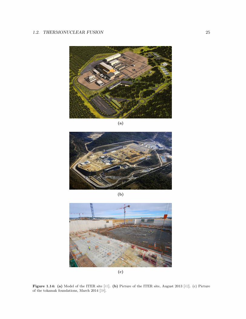
Figure 1.14: (a) Model of the ITER site [41]. (b) Picture of the ITER site, August 2013 [42]. (c) Pictureof the tokamak foundations, March 2014 [38].

26 CHAPTER 1. THERMONUCLEAR FUSION
each other. The scaling law is tested for real tokamak data in Figure 1.13. In order to obtaina reliable scaling law, tokamaks of different sizes are needed. This makes small tokamaks likeCOMPASS with a lot of ITER similarities very valuable. For more information about theevolution of the ITER project as well as some details about the different parts of the machine- the magnetic coils, the vessel, the divertor array, the lithium blanket, the cryostat,... - onecan surf to the official ITER website [38]. Some models and pictures of the ITER site areshown in Figure 1.14.
And what after ITER? Hopefully ITER will show that it is indeed possible to use fusionfor commercial energy production. The next step then is the construction of DEMO, ademonstration power plant. Scientists and engineers of the Broader Approach are alreadythinking about the conceptual design of this machine. According to the original agreement,DEMO should put its first fusion power into the grid as early as 2040. Probably, therewill however be some delay, because ITER experiences already some difficulties and is notperfectly on schedule any more. The cost of the project has already been tripled since itsstart, and for example the US is already thinking to set a limit to its annual funding, whichwould slow the project further down. [43]
1.3 Fusion: pros and cons
Some major advantages of fusion are:
• The needed amount of fuel is very small in contrast to fossil fuel burning. The fuelshave a very large energy density: 1g DT = 26000kWh, 1g coal = 3Wh. [44]
• The fuels are abundant and geographically widespread. Deuterium can be extractedfrom sea water. Tritium is made by neutron bombardment of lithium, which eventuallyshould also be possible to extract from sea water. Almost everywhere on Earth fusionfuels are available. There is no motivation for an “oil war”.
• Fusion does not give rise to toxic, greenhouse or acid rain gasses in contrast to fossilfuel burning.
• The reactors are inherently safe. “Meltdown” situations are physically impossible.There is only a small amount of fuel present in the reactor region, enough for a fewtens of seconds operation. Accidents are self-limiting.
• Fusion offers no efficient way to create nuclear weapons. The only useful substancepresent is tritium, but it is produced and consumed in the reactor. There is sometritium inventory, but it is too small. The heavy water (D2O) storages present in thedeuterium production site could be used to form nuclear weapons if they are in badhands.
• Fusion leaves no long-lived highly radioactive waste. The small tritium inventory and theneutron-activated structural materials of the reactor form the biggest threats. However,tritium is short-lived and only dangerous in case of incorporation, and the structuralmaterials can be selected so that after 100 years only low level radioactive waste remains.

1.3. FUSION: PROS AND CONS 27
Figure 1.15: Radiotoxicity.[45]
The total amount of radioactive material produced is of the same order of magnitude asfor fission reactors, but the radiotoxicity11 is much smaller: there is a huge drop duringthe first 50-100 years to the level of coal ash and even lower (see Figure 1.15). A goodselection of the used reactor materials permits after 100 years to clear 30-40% of thewaste and to (partially) recycle about 60%. Only 1% of the waste is long-living, buthas a low level of radioactivity. [44]
• Fusion allows quite compact large-scale power plants of 1GW and more in contrast torenewables.
• Fusion allows to build baseload power plants. It has no variable character such as solarand wind power.
Some major disadvantages of fusion are:
• The fusion reaction is difficult to start. Fusion research had already taken off very wellin 1950 and still no net energy producing fusion device is manufactured. The physicalmodelling of plasmas in fusion devices is very complex as is the technical design. Hightemperatures have to be reached in pure high vacuum amongst other challenges.
• The costs for high-technological fusion research is enormous. There are not enoughinvestments and the governments’ subsidies were for a long time insufficient.
• Nuclear waste is unavoidable. Neutron radiation originating from the fusion reactionswill induce radioactivity in surrounding materials and the inside of the reactor will becontaminated with tritium. Careful material selection and design can however limit theamount and lifetime of the nuclear waste.
• As the energy confinement time τE increases with plasma volume, fusion reactors musthave a minimum size and small-scale power plants are infeasible.
11Radiotoxicity is a measure for the detrimental effect of an incorporated radioactive substance on the humanbody. It is defined as the ratio of the radiation dose (expressed in Sv=J/kgequivalent) and the incorporatedactivity (expressed in Bq=# decays/s) summed over all isotopes.

28 CHAPTER 1. THERMONUCLEAR FUSION
[28] [44]

Chapter 2
The tokamak COMPASS
2.1 Introduction
All experiments treated in this work were performed on the COMPASS tokamak at the In-stitute of Plasma Physics (IPP) of the Academy of Sciences in Prague (Czech Republic).Originally, COMPASS was designed and built in Culham Centre for Fusion Energy (UnitedKingdom) in the eighties. Its name, which is a contraction of the words ‘compact’ and ‘assem-bly’, points to the fact that it is a rather small device. The appendix ‘D’ is now often addedbecause of its D-shaped vacuum vessel. This vessel replaced the original circular shaped onein 1992 and enabled the achievement of high plasma confinement (H-mode). The most im-portant parameters of COMPASS are listed in Table 2.1.
Due to its size, shape and capability of operating in H-mode regime, COMPASS plays animportant role in the ITER project. There are only two other tokamaks in Europe withsimilar ITER-like properties: JET (Culham,UK) and ASDEX-U (Garching, Germany). JETis the biggest in rank, COMPASS the smallest. Given the huge complexity of the physicalprocesses acting during tokamak discharges, it is impossible to make one stable simulationthat takes everything into account. So, one has to rely on experiments and extrapolations todetermine the design parameters of ITER. These extrapolations improve if more data fromdifferently sized tokamaks is available. Since COMPASS is one of the only small tokamakscapable of H-mode operation, its data is very valuable.
Table 2.1: General parameters of COMPASS. [46]
parameter current max value predicted max value
major radius R 0.56m 0.56mminor radius a 0.23m 0.23mplasma current Ip 350kA 350kAtoroidal magnetic field Bt 1.8T 2.1Tvacuum pressure 2 · 10−6 Pa 1 · 10−6 Paelongation κ 1.8 1.8plasma shape circular, elongated, D-shape circular, elongated, D-shapepulse length 0.35s 0.50sNBI heating undetermined 2× 350kW
29
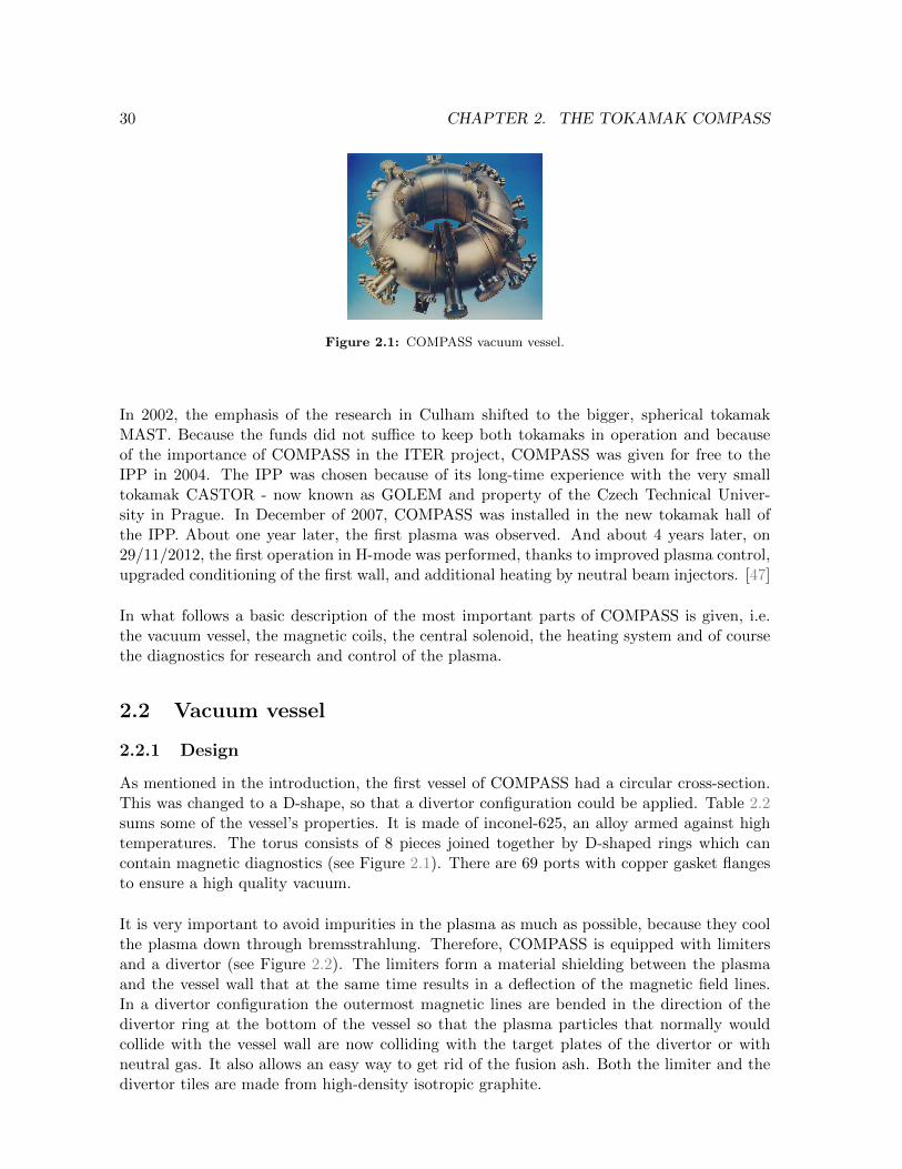
30 CHAPTER 2. THE TOKAMAK COMPASS
Figure 2.1: COMPASS vacuum vessel.
In 2002, the emphasis of the research in Culham shifted to the bigger, spherical tokamakMAST. Because the funds did not suffice to keep both tokamaks in operation and becauseof the importance of COMPASS in the ITER project, COMPASS was given for free to theIPP in 2004. The IPP was chosen because of its long-time experience with the very smalltokamak CASTOR - now known as GOLEM and property of the Czech Technical Univer-sity in Prague. In December of 2007, COMPASS was installed in the new tokamak hall ofthe IPP. About one year later, the first plasma was observed. And about 4 years later, on29/11/2012, the first operation in H-mode was performed, thanks to improved plasma control,upgraded conditioning of the first wall, and additional heating by neutral beam injectors. [47]
In what follows a basic description of the most important parts of COMPASS is given, i.e.the vacuum vessel, the magnetic coils, the central solenoid, the heating system and of coursethe diagnostics for research and control of the plasma.
2.2 Vacuum vessel
2.2.1 Design
As mentioned in the introduction, the first vessel of COMPASS had a circular cross-section.This was changed to a D-shape, so that a divertor configuration could be applied. Table 2.2sums some of the vessel’s properties. It is made of inconel-625, an alloy armed against hightemperatures. The torus consists of 8 pieces joined together by D-shaped rings which cancontain magnetic diagnostics (see Figure 2.1). There are 69 ports with copper gasket flangesto ensure a high quality vacuum.
It is very important to avoid impurities in the plasma as much as possible, because they coolthe plasma down through bremsstrahlung. Therefore, COMPASS is equipped with limitersand a divertor (see Figure 2.2). The limiters form a material shielding between the plasmaand the vessel wall that at the same time results in a deflection of the magnetic field lines.In a divertor configuration the outermost magnetic lines are bended in the direction of thedivertor ring at the bottom of the vessel so that the plasma particles that normally wouldcollide with the vessel wall are now colliding with the target plates of the divertor or withneutral gas. It also allows an easy way to get rid of the fusion ash. Both the limiter and thedivertor tiles are made from high-density isotropic graphite.

2.2. VACUUM VESSEL 31
Figure 2.2: Left : Inside of the COMPASS vessel. Right : Picture made by EDICAM with indication of theseparatrix, i.e. the boundary between closed and open field lines, and other nomenclature for a D-shapedplasma.
Table 2.2: Vessel parameters. [48]
parameter value
material inconel-625thickness 3mmvolume 1m3
surface area 8m2
toroidal resistance 0.63mΩpoloidal resistance 0.25mΩbasic vacuum 10−6Pabake-out temperature 150Climiter/divertor material graphite
The vessel is pumped by a vacuum system, which consists of a vacuum pump and two turbomolecular pumps with a pumping speed of 500l/s each. All vacuum pumps are oil-free toprevent the release of impurities. [48]
2.2.2 Cleaning procedure
After the vessel has been opened for maintenance, adjustments or repairs the inside has to becleaned from impurities and the vacuum has to be re-established. The first action is pump-ing the vessel down to about 19Pa by a vacuum pump. When the pressure is at this level,the turbo molecular pump starts and decreases the pressure down to values in the order of10−6Pa. Because there is an equilibrium between the molecules in gas and the molecules ab-sorbed by the surface of the vessel, some molecules will always stay on the vessel wall. Whenthe pressure drops and so less gas molecules are present, more of these absorbed moleculeswill be released and pumped away. To speed up this process the vessel is being heated toabout 150C for several days1. The absorbed molecules at the surface of the vessel get morekinetic energy and are able to leave the surface this way. This process is called bake-out.We already saw in paragraph 1.2.5 how one uses the transformer principle in a tokamak toinduce a plasma current. The beauty of this transformer configuration is that when there areno charged particles in the vessel, it is not the plasma but the vessel itself that acts as the
1About 5, depending on the amount of impurities on the surface.

32 CHAPTER 2. THE TOKAMAK COMPASS
secondary winding. In other words, the vessel is ohmically heated by applying a large alter-nating current to the central solenoid. A gradual temperature increase is required becausethe different parts of the tokamak have a different coefficient of expansion and if the heatingwould go to fast, some of the components would expand faster than others and cracks couldappear. So therefore it takes about 6 hours to get to the 150C.
After the bake-out still not all the impurities are removed from the vessel wall. Thereforea second cleaning process, called Glow Discharge Cleaning (GDC) is performed next. Here,extremely pure helium gas is put in the vessel. Next, a graphite electrode, located inside thetokamak vessel in the limiter shadow, is positively biased, so that the helium breaks downand a part of it is ionized. Finally, the positively charged helium ions bombard the negativelycharged vessel, desorbing the last remaining impurities. These are again removed by thevacuum pump. [48]
The GDC is often combined with boronization of the vacuum vessel: during the heliumdischarge o-carborane (C2B10H12) is sublimated and forms a hard boron-containing coatingon the vessel wall. During the actual operation of the tokamak this low-Z coating reduces theinteractions of the plasma particles and the impurities with the wall material in addition to animprovement of the vacuum condition by gettering oxygen. Oxygen is in particular importantfor carbon-based plasma-facing materials - like the limiters and divertor in COMPASS - dueto its ability to form CO and CO2 with very high erosion yields near to unity, i.e. almostevery O-atom falling in on the C-containing PFM will chemically react and erode the PFM.Boronization is an inevitable procedure to achieve H-mode. [49] [50] [51]
2.2.3 Conservation of vacuum
To ensure that there are no leaks at the connection pieces between the vessel and the equip-ment, copper rings are used. This technique requires the two couplers to have a knife edgewhich deforms the copper ring placed between them when they are pressed together. Thisresults in a very tight seal. Normally, copper rings can only be used once.
It is possible to install appliances to the vacuum vessel while it is vacuum because there areairtight valves between the vacuum vessel and the appliance. After installation the valvecan only be opened if the appliance itself is cleaned and made vacuum. Therefore about thesame procedure as for the vacuum vessel is followed: first the appliance is pumped to a verylow pressure, and then heating strips are put on it to bake the appliance in order to removeimpurities from the contact surfaces.
In order to detect leaks, one applies helium gas puffs near the weak spots where leaks can beexpected. For example, after installing an appliance, one will introduce a puff of helium inthe surroundings of the new appliance2 and analyse the air pumped from the appliance bya spectrometer to see whether there is helium present and in what quantity. Helium is usedbecause it is almost the smallest molecule and it has a very low appearance in the atmosphere.[48]
2At the outside of course.

2.3. MAGNETIC COILS 33
2.2.4 Fuel
The working gas was originally hydrogen, but nowadays deuterium is used because this makesthe research more ITER-relevant. Experiments with tritium will never happen at COMPASSbecause of safety reasons, but several attempts have been done with helium as working gas.[48]
The D-D fusion reaction
21D + 2
1D → 31T + 1
1p (50%) (2.1)
→ 32He + 1
0n (50%) (2.2)
has a very low 〈σF v〉 and by consequence its occurrence is almost zero. For typical electrontemperatures in COMPASS, which is about 1keV, 〈σF v〉 is not even mentioned in Figure 1.8.It is definitely far below 10−26m3s−1. Hence, the fusion energy released by the few reactionsthat occur in this machine is negligible.
2.3 Magnetic coils
2.3.1 Central solenoid
During operation, a gradually increasing current Is is sent through the central copper solenoid.This creates a toroidal electric field
Et =Ls,p2πr
dIsdt
(2.3)
Here, Ls,p is the mutual inductance of the solenoid and the plasma. This electric field exerts atoroidal force on the charged plasma particles. As the electrons are much lighter than the ions,they are more accelerated. A plasma current is produced. It is clear that the pulse length ofthe central solenoid is limited since Is cannot increase forever. Compared to tokamaks withferromagnetic cores however very high plasma currents can be reached. These last ones havethe disadvantage to be subject to hysteresis: Beyond a certain maximum current through theprimary winding, the magnetic flux does not change enough any more due to the occurringsaturation.
2.3.2 Toroidal and poloidal field coils
As mentioned in paragraph 1.2.5, the magnetic coil system of a tokamak consists of toroidalfield (TF) coils, maintaining the basic confinement of the plasma, and poloidal field (PF)coils, correcting the plasma position in the horizontal as well as the vertical direction. COM-PASS has got 16 TF coils which are located outside the PF coils and which are positionedat an equal distance from each other. They each consist of two L-shaped pieces connectedby screws. The electromagnetic expansion forces acting on the two joints are countered by ahydraulic preload system. Both the TF and PF coils are made of copper which implies en-ergy losses due to their resistance. Therefore, these copper coils have to be water-cooled. InITER these losses are unacceptable and thus superconducting coils will be used. The majordrawback of superconductivity is that it is lost above a critical magnetic field.

34 CHAPTER 2. THE TOKAMAK COMPASS
Figure 2.3: PF coil configuration of COMPASS.
The PF coils are depicted in Figure 2.3. The whole PF coil system is made up of four differentparts, each with its own power supply and its own function:
• Magnetizing field (MF) coils: Together with the central solenoid they set up and sustainthe plasma current. They strongly reduce the stray magnetic field of the central solenoid.
• Shaping field (SF) coils: They create the desired plasma shape. Different configurationsare possible: circular, single-null-divertor configuration (SND)3 , single-null-divertorconfiguration with high triangularity (SNT)4 ,... For all shots that will be discussed inthis thesis, the shape was programmed to be SNT.
• Equilibrium field (EF) coils: They correct the position of the plasma over long time-scales. The vertical magnetic field prevents the plasma column from expanding in theradial direction.
• Feedback (F) coils: The fast feedback coils provide position control of the plasma onshort time-scales. The BR circuit creates a horizontal (radial) magnetic field for fastfeedback control of the vertical plasma position, the BV circuit creates a vertical mag-netic field for fast feedback control of the horizontal plasma position.
[28] [52]
2.3.3 Power supplies
COMPASS needs an electrical input power of 50-60MW for about 2-3 seconds. Since thegrid at the campus of the Academy of Sciences in Prague can only deliver 1.5MW, an energystorage system had to be designed and constructed. The choice fell on the installation oftwo flywheel generators. These machines are able to store huge amounts of rotational energycarried by a very heavy rotor that is kept in the horizontal plane by bearings and is “flying”on a thin layer of oil. The flywheel generators are each able to deliver 35MW during a pulseof about 3s. They are first loaded for 40 minutes to get a rotation speed of 1700rpm. After
3The single-null-divertor configuration (SND) has a plasma shape with only one x-point. The x-point canbe seen in Figure 2.2. It is the point where the magnetic field lines cross each other.
4The plasma triangularity δ is defined as the horizontal distance between the plasma major radius and thex-point. An average value for the discharges performed with COMPASS is δ = 0.35-0.40. Remark that inTable 2.1 SND and SNT are present under the name ‘D-shape’.

2.3. MAGNETIC COILS 35
Figure 2.4: Scheme of the power supply system. [46] [53]
the pulse, 1300rpm remains and it takes another 10 minutes to regain the used energy. Theoutput is an AC current of 85Hz. Note that thanks to the flywheel generators COMPASSdoesn’t need any capacitor banks to store energy and release it as a pulse in contrast to othertokamaks like for example GOLEM. [48] [53]
Every big energy user among the components of COMPASS (the TF and PF coils, the NBI)all have their own power supply that has to be fed by the flywheel generators. The circuit thatregulates all this, is shown in Figure 2.4. The two flywheel generators (A and B) provide theirpower to the local three-phase 6.3kV grid. Switches allow to uncouple generator B which thenonly supplies the TF coils. Generator B is only used when maximal toroidal fields (Bt = 2.1T)are required, which is not always the case. Afterwards, the AC voltage three-phase 6.3kV istransformed by three-winding transformers (T3A, T3B, T4, T5 and T6) and rectified in 12- or24-pulse thyristor converters (∼ / =), which control the DC current in the tokamak coils. ThePF coils are connected by four cables in quadrupole configuration (see Figure 2.5e) and anassembly of eight copper plate busbars with alternating polarity is used for the TF coils (seeFigure 2.5c), leading to minimization of the stray fields in the vicinity of the tokamak. Thecurrent needed for the TF coils is so high that the repulsive forces between the cables wouldbe too big to form a quadrupole. Transformers T8, T9 and T10 supply the auxiliary systems(NBI and feedback system) by AC three-phase 400V. The converter control system and otherequipment are supplied via transformers T17 and T18. The magnetizing field power suppliescontain some auxiliary capacitor banks (see the box with ‘OH start’). These are used forexample in the start-up circuit to turn off the thyristors in order to get a plasma start-up asefficient as possible. The flywheel-generators are placed outside the assembly hall in a special

36 CHAPTER 2. THE TOKAMAK COMPASS
sound-proof building with a 6m thick concrete base to counteract the vibrations, while thelocal control of the power supply system, transformers, and the switching station are locatedin the assembly hall. The thyristor rectifiers are installed in the tokamak hall. Figure 2.5creates an image of the IPP building. [53]
2.4 Heating system
2.4.1 Ohmic heating
Ohmic heating is inherent to the tokamak concept. The plasma current Ip heats the plasmaaccording to
POH = RpI2p (2.4)
Since the plasma resistance Rp obeys
Rp ∝ T− 3
2e , (2.5)
ohmic heating becomes less efficient after a while and a limited plasma temperature of around2-3keV can be reached. We saw however in paragraph 1.2.4 that for a satisfying fusion reactionrate 10-20keV is required. So additional plasma heating sources are needed. COMPASS usestwo neutral beam injectors, but other options are heating by electromagnetic waves (ECRH,ICRH) and internal heating by α-particles in case of D-T fusion which is only possible ifthe α-particles have enough time to give their energy to the plasma, i.e. they do not collideimmediately with the vessel wall. [48] [54]
2.4.2 Neutral beam injection (NBI)
Working principle
The basic idea of neutral beam injection is to shoot neutral atoms with a large unidirectionalkinetic energy into the plasma, where they ionize, get captured by the confining magneticfields and exchange their energy with the other plasma particles by collisions resulting in anincreasing plasma temperature. Remark that the atoms indeed have to be neutral to pene-trate the magnetic fields. On the one hand the beam needs to have sufficient energy so thatthe atoms are ionized in the plasma center and not in the plasma edge, but on the other handthis energy may not be too large to avoid shine-through losses, i.e. losses due to the collisionof the beam with the vessel wall.
Briefly summarized, the NBI system makes ions, accelerates them and neutralizes them be-fore entering the tokamak vessel. The basic internal mechanism of a neutral beam injector isdemonstrated in Figure 2.6a. First, the neutral gas5 is puffed to the plasma box, where it isionized by an RF source and a dense plasma is formed. Next, the plasma ions are extractedand accelerated by four grids as seen in Figure 2.6b. These grids are bended to focus thebeam and are at an electrical potential of respectively 40kV, 32kV, -0.5kV and 0kV. One cansee from the total potential difference that the ions will have a maximum energy of 40keVwhen they pass the last grid. Then, the ion beam enters the neutralizer chamber where the
5Normally, atoms with the same atomic number as the plasma fuel. In case of COMPASS usually hydrogen(in the past) or deuterium (now) is used.

2.4. HEATING SYSTEM 37
(a) (b)
(c) (d) (e)
(f) (g)
Figure 2.5: (a) ground plan of the IPP, (b) the tokamak COMPASS itself on the 2nd floor of the tokamakhall, (c) TF coil busbars, (d) 1st floor of the tokamak hall, (e) PF coil cables, (f) transformers, (g) flywheelgenerators.

38 CHAPTER 2. THE TOKAMAK COMPASS
(a) (b)
Figure 2.6: (a) Basic working principle of NBI. (b) Accelerating grids. [55]
ions are converted to fast neutral particles by charge exchange collisions. The third gridwith negative voltage is used to prevent secondary electrons created in the neutralizer fromgoing back in the direction of the plasma box. At last, after the remaining unneutralized ionsare deflected by a magnet to the ion dump, the created neutral beam is ready to enter thetokamak vessel. Of course it is undesirable that some neutral particles of the neutralizing gasenter the tokamak vessel. These “cold” particles would only cool the plasma down. Hence, acryopumping system removes the slow neutral particles that passed the magnet.
In case that the neutral gas for the NBI system of COMPASS is deuterium (D2), the ion beamgoing from the plasma box to the neutralizer chamber will consist mainly of deuterons (D+),but also of molecular ions like D+
2 or even D+3 , and impurity ions. In the neutralizer chamber,
these ions collide with neutral deuterium gas and with 78% chance they pick up an electronfrom the low-energetic molecule and thus become neutral6. The particles practically conservetheir energy and momentum after the collision. The general charge exchange reaction fordeuterium is as follows
D+ + D2 → D + D+2 (2.6)
But as mentioned before, there are also these molecular ions. These ions will be dissociatedin the neutralizer into single ions and atoms.
D+2 + D2 → D+ + D + D2 (2.7)
D+2 + D2 → D + D + D+
2 (2.8)
D+3 + D2 → D + D + D + D+
2 (2.9)
The consequence is that the original energy and momentum of the molecular ion is equallydivided among its constituents after the dissociation reaction. The resulting atoms of D+
2 havean energy of only half the original energy, these of D+
3 only one third. A similar argumentationcan be made in case the NBI gas is hydrogen. According to the manufacturer the neutralparticle beam will then have following energy spectrum: 70% of the particles will have thefull energy of 40keV, about 25% will have only 20keV and about 5% will have an energy ofabout 13keV. The impurities only represent a very small fraction of the neutral beam. Thesevalues still have to be confirmed by measurements. Besides, the corresponding percentagesfor deuterium have to be determined. This is planned for the near future. [48]
6In case of hydrogen this chance is only 68%.

2.4. HEATING SYSTEM 39
(a)
(b)
(c) (d)
Figure 2.7: COMPASS Neutral Beam Injectors. Technical schemes of (a) lateral view and (b) top view withcryopump system. Pictures of (c) lateral and (d) frontal view. [55]

40 CHAPTER 2. THE TOKAMAK COMPASS
Detailed description of the COMPASS Neutral Beam Injectors
The ion source is essentially a RF discharge plasma generator (specs 4MHz, 30kW) thatcreates ions, equipped with 4 grids on different potentials to accelerate the ions. Each grid has887 holes of 4mm diameter. The total ion beam has a diameter of 167mm. The whole systemis surrounded by an electrostatic and a magnetic shield to protect the ion source against thestray fields from the tokamak (see Figure 2.7d). During shots the grid edges are cooled withwater, whereas between shots they are cooled through radiation. Cooling is necessary to avoiddeformation of the grids. A few tenths of a millimetre can lead to poor focus.
The neutralizer contains a thick gas target. In case of COMPASS, the deuterium gas flowused for the ion source suffices. No extra gas puffing is needed. The ion beam undergoes sub-sequent charge exchange reactions (ion, neutral, ion, neutral,...). The efficiency is determinedby the ratio of the cross-sections of both reactions. These cross-sections depend on the energyof the incoming ions. For a voltage of 40kV over the grids 78% of the ions is neutralized. Thebending magnet is a coil of 26 turns and a current of 338A is flowing through it to send thepositively and the negatively charged ions to the right ion dump.
There are two copper ion dumps. The lower one has to catch the positively charged ions. Itis water-cooled because the power of the positively charged beam can be up to 200kW. Theupper one has to catch the negatively charged ions. It is not cooled because only about 1.5%of the ions is negatively charged.
The cryopump is composed of two cryopanels, each with an active surface of 0.3m2 (seeFigure 2.7b). These cryopanels are connected to a 4K closed-cycle refrigerator system whichworks with liquid nitrogen7. By condensing and even solidifying the slow (“cold”) neutral par-ticles in the vacuum tank on the 4K cryoplates these unwanted particles are kept away fromentering the tokamak vessel. The cryopanels provide a pumping speed of about 100 000 l/s.
To test the neutral beam injector it is possible to place a calorimeter as a target on the beampath. This calorimeter is V-shaped in order to reduce the power density at the copper surface.There are 4 thermocouples at each side of the target: left, right, above and below. Thesethermocouples are placed 2mm from the irradiated surface so they can give an estimationof the beam power at the beam axis, the beam position and the eventual divergence of thebeam. The calorimeter has to be cooled with water, but even correctly cooled it cannot survivea pulse at full power (300ms, 350kW). For tests the pulse length is therefore limited to 100ms.
The aiming device is a diaphragm located at the output of the vacuum tank. It uses 4detectors to adjust the beam axis. These detectors measure the flux of the neutral particlesusing secondary emission. Like all the other equipments, the aiming device is water-cooled.
The COMPASS tokamak has got two such neutral beam injectors as described above. Theseare placed in a co-injection configuration, as seen in Figure 2.8a, which increases the plasmarotation. If for example in other tokamaks this extra plasma rotation is unwanted, one canopt for the balanced injection configuration (Figure 2.8b). The two COMPASS neutral beam
7Remark that liquid nitrogen is only responsible for the precooling to a temperature of 70K. The remainingcooling is done by a sophisticated compressor refrigerator.

2.4. HEATING SYSTEM 41
(a) (b)
Figure 2.8: NBI duo configurations: (a) co-injection and (b) balanced injection. [57]
injectors have a tangential orientation, in contrast to ITER where the injectors are orientedperpendicular to the vacuum vessel. Due to the small size of COMPASS there would be a lotof shine-through losses if the NBI was perpendicular to the vacuum vessel. [56]
Beam power delivered to the plasma
In next chapter, we will often encounter the standard applied grid voltage of 40kV accom-panied by a current expressed in Amperes. These two quantities are preprogrammed by thetokamak operators at the IPP and can be adjusted for every shot. Their product gives theNBI power right behind the accelerating grid. In order to know the power added to theplasma, some complications have to be kept in mind:
• The neutralizer has an efficiency of 78% according to the manufacturer.
• Reactions (2.7)-(2.9) cause part of the neutral particles to have 1/2 and 1/3 of themaximum energy of 40keV.
• Due to the geometry of COMPASS, the injectors are not installed at the foreseen dis-tance from the plasma. The longer beam trajectory certainly decreases the beam poweradded to the plasma. It definitely has also negative consequences for the focus of theneutral beam.
• There may be shine-through losses.
The exact effects of the second and third point are unknown for the moment. This is veryimpractical since the NBI power is an important quantity to solve the energy balance andto determine the energy confinement time. Both neutral beam injectors have a design valueof 350kW. However, until now only measurements with one injector at full power and oneinjector at half its power are possible. These are issues that still have to be investigated.
Attenuation of the neutral beam in the plasma
In the plasma there are 3 ionization channels:
ionization by plasma electrons : D + e− → D+ + e− + e− 〈σeve〉/vb (2.10)
ionization by plasma ions : D + D+ → D+ + D+ + e− σi (2.11)
charge exchange collision : D + D+ → D+ + D σch (2.12)

42 CHAPTER 2. THE TOKAMAK COMPASS
Here, vb is the begin velocity of the neutral deuterium atoms, ve is the velocity of the plasmaelectrons and ‘〈 〉’ represents the integration over the electron velocity distribution. All cross-sections σ depend on the velocity vb, and σe also depends on the electron temperature.
The intensity of the neutral beam decreases along the path through the plasma by the differ-ential equation
dI(x)
dx= −n(x)
(〈σeve〉vb
+ σi + σch
)I(x) (2.13)
For the beam energy of COMPASS - approximately 40keV - holds:
〈σeve〉/vb = 1.0 · 10−20m2 (Te ≈ 1keV) (2.14)
σi = 1.4 · 10−20m2 (2.15)
σch = 6.5 · 10−20m2 (dominating) (2.16)
This means that the total cross-section for the beam attenuation is given by
σtot = 9.0 · 10−20m2 (2.17)
If we assume a homogeneous plasma with density n(x) = n0, the beam intensity attenuatesexponentially by
I(x) = I0e−σtotn0x (2.18)
and the normalized beam power delivered by the neutral beam to the plasma is then givenby
P (x)
P0= 1− I(x)
I0= 1− e−σtotn0x (2.19)
For a path length through the COMPASS plasma of about 1m - considering the tangentialsetup of the neutral beam injectors - one can estimate the density n0 at which the beampower is almost fully absorbed by the plasma before reaching the vessel wall as
n0 = 6.0 · 1019m−3 (2.20)
For this average density P (1m)P0
< 1%. This gives us an idea when we have to start the NBIto avoid big shine-through losses. [55]
2.5 Diagnostics
2.5.1 Control room
During operation of COMPASS the control room looks like Figure 2.9. By ways of introduc-tion to this diagnostics section, we summarise the data shown on the six panels in front ofthe room. From left to right the panels show
1. Plasma temperature and density as a function of the distance from the plasma center,using the Thomson scattering diagnostic.
2. Time evolution of the main plasma parameters: plasma current, plasma density, loopvoltage, total visible radiation, Dα emission, hard x-ray radiation,...
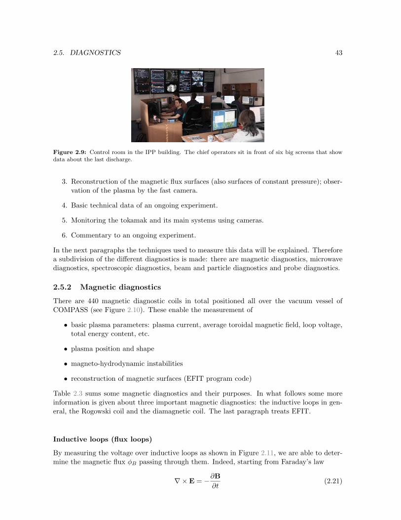
2.5. DIAGNOSTICS 43
Figure 2.9: Control room in the IPP building. The chief operators sit in front of six big screens that showdata about the last discharge.
3. Reconstruction of the magnetic flux surfaces (also surfaces of constant pressure); obser-vation of the plasma by the fast camera.
4. Basic technical data of an ongoing experiment.
5. Monitoring the tokamak and its main systems using cameras.
6. Commentary to an ongoing experiment.
In the next paragraphs the techniques used to measure this data will be explained. Thereforea subdivision of the different diagnostics is made: there are magnetic diagnostics, microwavediagnostics, spectroscopic diagnostics, beam and particle diagnostics and probe diagnostics.
2.5.2 Magnetic diagnostics
There are 440 magnetic diagnostic coils in total positioned all over the vacuum vessel ofCOMPASS (see Figure 2.10). These enable the measurement of
• basic plasma parameters: plasma current, average toroidal magnetic field, loop voltage,total energy content, etc.
• plasma position and shape
• magneto-hydrodynamic instabilities
• reconstruction of magnetic surfaces (EFIT program code)
Table 2.3 sums some magnetic diagnostics and their purposes. In what follows some moreinformation is given about three important magnetic diagnostics: the inductive loops in gen-eral, the Rogowski coil and the diamagnetic coil. The last paragraph treats EFIT.
Inductive loops (flux loops)
By measuring the voltage over inductive loops as shown in Figure 2.11, we are able to deter-mine the magnetic flux φB passing through them. Indeed, starting from Faraday’s law
∇×E = −∂B
∂t(2.21)
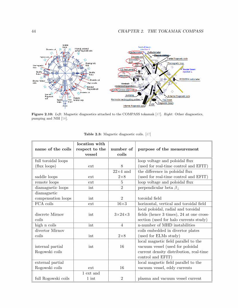
44 CHAPTER 2. THE TOKAMAK COMPASS
Figure 2.10: Left : Magnetic diagnostics attached to the COMPASS tokamak [47]. Right : Other diagnostics,pumping and NBI [58].
Table 2.3: Magnetic diagnostic coils. [47]
location withname of the coils respect to the number of purpose of the measurement
vessel coils
full toroidal loops loop voltage and poloidal flux(flux loops) ext 8 (used for real-time control and EFIT)
22×4 and the difference in poloidal fluxsaddle loops ext 2×8 (used for real-time control and EFIT)
remote loops ext 5 loop voltage and poloidal flux
diamagnetic loops int 2 perpendicular beta β⊥diamagneticcompensation loops int 2 toroidal field
FCA coils ext 16×3 horizontal, vertical and toroidal field
local poloidal, radial and toroidaldiscrete Mirnov int 3×24×3 fields (hence 3 times), 24 at one cross-coils section (used for halo currents study)
high n coils int 4 n-number of MHD instabilities
divertor Mirnov coils embedded in divertor platescoils int 2×8 (used for ELMs study)
local magnetic field parallel to theinternal partial int 16 vacuum vessel (used for poloidalRogowski coils current density distribution, real-time
control and EFIT)
external partial local magnetic field parallel to theRogowski coils ext 16 vacuum vessel, eddy currents
1 ext andfull Rogowski coils 1 int 2 plasma and vacuum vessel current

2.5. DIAGNOSTICS 45
and integrating both sides over the surface enclosed by the loop combined with Green’stheorem, we find
ε =
∮∂S
E · dl = −∂φB∂t
(2.22)
or
φB(t) = −t∫
0
ε(τ) dτ (2.23)
with ε the voltage across the loop. The appearing integration over time is executed by ananalogue integrator circuit.
Figure 2.11: Flux loop.
The 8 full toroidal loops are a type of inductive loops that is worth extra mentioning. Inthis case ε is the so-called loop voltage. From this loop voltage, one can easily determine thetoroidal electric field by
Et =Uloop2πr
(2.24)
where r is the radius of the toroidal loop. These loops are also used to measure the poloidalmagnetic flux, which is used by EFIT to reconstruct the magnetic flux surfaces.
Rogowski coils
Rogowski coils are used in Ampere meters but also in tokamaks to measure the plasma currentand the vacuum vessel current. They are composed of a helically wound solenoid with a returncenter conductor so that the coil has no net loop around the current carrying conductor orplasma, and are usually encased in a Faraday shield to avoid electrostatic pickup (Figure2.12). If we define A as the surface area of the windings, N the total number of windings andl the length of the return loop, than Faraday’s law (see equation (2.22)) says
ε = −NA∂Bp∂t
(2.25)
There is no contribution of the toroidal magnetic field because there is no net loop aroundthe plasma. Next, applying Ampere’s law
∇×B = µ0J + µ0ε0∂E
∂t(2.26)
revealsBpl = µ0Itor (2.27)

46 CHAPTER 2. THE TOKAMAK COMPASS
where the electric field is channelled by the Faraday shield. Combining equations (2.25) and(2.27) we find the relationship between the voltage over the Rogowski coil and the plasmacurrent (Ip = Itor)
ε = −µ0ANl
∂Ip∂t
(2.28)
or
Ip(t) = − l
µ0AN
t∫0
ε(τ) dτ (2.29)
Again an analogue circuit is used to solve the time integration. The shape of this contour isirrelevant, as is the angle between the Rogowski coil and the enclosed current.
Figure 2.12: Rogowski coil with basic integrator circuit.
Diamagnetic coils
The toroidal field is a superposition of
• Of course, the magnetic field generated by the TF coils which is the biggest contribution.
• The diamagnetic effect: the particle gyration decreases the toroidal field.
• The paramagnetic effect: the poloidal component of the plasma current increases thetoroidal field.
Since the first contribution is so much bigger than the others, very sensitive diagnostic devicesare needed in order to measure the diamagnetic and paramagnetic effects. Next figure showsone setup used to measure these effects. The so-called diamagnetic coil consists of two coilswound around the vessel, their radii smaller than that of the TF coils. The Bt coil containsthe plasma column and consequently measures the total magnetic flux. The vacuum field coilor compensation coil is wound around the vessel many times, is then moved a few millimetresradially outwards and finally wound back. It measures only the contribution of the TF coils.The difference in magnetic flux ∆φ between both coils is given by
∆φ = ∆φpara + ∆φdia =µ20
8πBtI2p −
µ0BtW⊥ (2.30)
Here, W⊥ denotes the thermal plasma energy in the poloidal cross-section [J/m]. This formulaallows to calculate the total thermal energy stored in the plasma as
Wth =3
2W⊥2πR (2.31)

2.5. DIAGNOSTICS 47
Figure 2.13: Diamagnetic coil. [59]
with R the major radius. The factor 3/2 is needed for the transition from two to three dimen-sions, the factor 2πR describes the path length of the plasma center in the toroidal direction.[59]
The data measured by the diamagnetic coil from above is stored under the name ‘diamag-net PP Energy’. Another method to measure W goes exactly the same except that the fieldgenerated by the TF coils is derived from measurements of the TF coil currents with Rogowskicoils. This data can be found in ‘diamagnet PP EnergyBT’. Both methods should give thesame result. The problem is the presence of crosstalk from different sources to the compensa-tion coil and the Rogowski coils. The majority of them can be quantified in a vacuum shot,but the crosstalk from the plasma current cannot. The difference between the two signals isdirectly proportional to Ip. It is not known which of the two is correct... if there even is oneexactly correct. [60]
EFIT
EFIT, or Equilibrium FITting code, performs an equilibrium reconstruction based on severalinput parameters (plasma parameters and tokamak geometry) by iteratively solving the Grad-Shafranov equation
∇p = J×B (2.32)
which expresses the balance of pressure forces and magnetic forces in a fusion device inquasi-stationary state. In this way information is obtained about the magnetic configuration,plasma shape and position, current and pressure profile, stored energy, plasma-β and safetyfactor q. The actual Grad-Shafranov equation is another form of equation (2.32), namely
Lψ = R∂p
∂ψ+
1
2µ0R
∂(RBt)
∂ψ(2.33)
with L the elliptical operator
L = − ∂
∂R
(1
µ0R
∂
∂R
)− ∂
∂Z
(1
µ0R
∂
∂Z
)(2.34)
and ψ the poloidal flux function defined as
ψ =1
2π
∫S
B · dS (2.35)
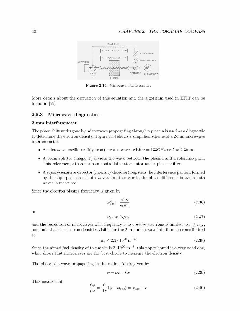
48 CHAPTER 2. THE TOKAMAK COMPASS
Figure 2.14: Microwave interferometer.
More details about the derivation of this equation and the algorithm used in EFIT can befound in [59].
2.5.3 Microwave diagnostics
2-mm interferometer
The phase shift undergone by microwaves propagating through a plasma is used as a diagnosticto determine the electron density. Figure 2.14 shows a simplified scheme of a 2-mm microwaveinterferometer:
• A microwave oscillator (klystron) creates waves with ν = 133GHz or λ ≈ 2.3mm.
• A beam splitter (magic T) divides the wave between the plasma and a reference path.This reference path contains a controllable attenuator and a phase shifter.
• A square-sensitive detector (intensity detector) registers the interference pattern formedby the superposition of both waves. In other words, the phase difference between bothwaves is measured.
Since the electron plasma frequency is given by
ω2p,e =
e2neε0me
(2.36)
orνp,e ≈ 9
√ne (2.37)
and the resolution of microwaves with frequency ν to observe electrons is limited to ν ≥ νp,e,one finds that the electron densities visible for the 2-mm microwave interferometer are limitedto
ne ≤ 2.2 · 1020 m−3 (2.38)
Since the aimed fuel density of tokamaks is 2 ·1020 m−3, this upper bound is a very good one,what shows that microwaves are the best choice to measure the electron density.
The phase of a wave propagating in the x-direction is given by
φ = ωt− kx (2.39)
This means thatdϕ
dx=
d
dx(φ− φvac) = kvac − k (2.40)

2.5. DIAGNOSTICS 49
with ϕ the phase difference between the plasma wave and the reference wave. Using thesimplified8 dispersion relation of transversal waves in a plasma
ω2 = ω2p,e + c2k2 (2.41)
this can be written as
dϕ
dx=
ωc− ω
c
√1−
ω2p,e
ω2
(2.42)
Supposing not too high electron densities we can assume that
ω2p,e
ω2≈ 0 (2.43)
This allows a first order Taylor expansion resulting in
dϕ
dx=ω
c
(1
2
ω2p,e
ω2
)=
1
2ωcω2p,e (2.44)
The experimental observed phase shift ∆ϕ is then
∆ϕ =1
2ωc
L∫0
ω2p,e dx =
1
2ωc
e2
ε0me
L∫0
ne dx =1
2ωc
e2
ε0me〈ne〉L (2.45)
with L the transmission length through the plasma. In this way we obtain the line-integratedaverage electron density 〈ne〉.
Since for the total intensity observed by the detector of the interferometer holds that9
Itot = 2I0[1 + cos(∆ϕ)] , (2.46)
the output will show interference fringe jumps when ∆ϕ is a multiple of 2π. The numberof these jumps in a plasma discharge depends on 〈ne〉 and L. The phase shift generated bythe COMPASS plasma on the frequency 133GHz reaches commonly several tens of fringes.Utilization of two near frequencies, namely ν1 = 133GHz (interferometer 1) and ν2 = 131GHz(interferometer 2), propagating through the plasma in opposite directions, enables to avoidthe fringes as much as possible. The total setup is a so-called unambiguous interferometer. Anoutput without fringes is a necessary condition for a feedback system controlling the density.For this purpose, not only the phase difference between the reference and probing wave isdetermined (as is done in the case of both interferometer 1 and 2), but the mutual phasedifference between both probing waves is registered as well. According to Figure 2.15 andequation (2.45), this mutual phase difference is given by
∆ϕm = ∆ϕ2 −∆ϕ1 =1
2c
e2
ε0me
ω1 − ω2
ω1ω2〈ne〉L (2.47)
8Assumptions: (1) influence of magnetic fields, i.e. of cyclotron frequencies, can be neglected (2) plasmafrequency of deuterons is negligible compared to plasma frequency of electrons.
9General expression for interference of waves with the same amplitude. Both plasma beam and refer-ence beam have (approximately) the same intensity when they hit the detector, namely their common initialintensity I0.

50 CHAPTER 2. THE TOKAMAK COMPASS
Figure 2.15: Unambiguous interferometer of COMPASS. [47]
This shows that the mutual phase difference increases circa 66.5 times slower with increasingelectron density than the two separate phase differences. The unambiguous interferometer isinstalled in the vertical direction at R = 0.56m. This means that the waves cross the plasmaalong the plasma vertical diameter, or in other words
L = 2aκ = 2 · 0.23 · 1.8 = 0.828 m (2.48)
which holds for maximum minor radius and maximum elongation. We can now make anestimation of the electron density 〈ne〉∗ for which the unambiguous interferometer outputreaches the first fringe. This is done by setting ∆ϕm equal to 2π and solving the equation for〈ne〉. This results in
〈ne〉∗ = 7.8 · 1019 m−3 (2.49)
When the electron density reaches this value, the data stored in the COMPASS database willmake a jump and the next data points should be incremented by this value.
At present, the interferometer is equipped with two phase detectors: one is based on AD8302ICs, the other on logic circuits. This first detector gives two outputs: one that uses sixAD8302 ICs and has a 360 phase range, and one that uses only one AD8302 IC and has aphase range of 180. The second detector gives a “triggered” output. All three signals have aDC component which should be removed. The initial DC level of the triggered interferometeris set by a trigger signal. The stored 〈ne〉 values are calculated assuming that the transmissionlength is equal to two times the plasma minor radius. Thus, if we want to know the truevalue of 〈ne〉, we have to divide by the plasma elongation.
Also remark that the linear relation ∆ϕ ∝ 〈ne〉 only holds for relatively small electron densitiesaccording to the assumption (2.43). So, for higher densities - starting from about 1020m−3 -this is not true any more and a more exact formula has to be used. [31] [47] [61] [62]
Microwave reflectometer
Plasmas are reflective for certain waves. This fact is for example used by radio stations thatuse the ionosphere to reflect their radio waves so that regions that are normally unreachable
2.5. DIAGNOSTICS 51
due to the spherical surface of the Earth, are nevertheless able to receive them. This sameprinciple is used in tokamaks: the reflectometer emits microwaves in the range of frequenciesfor which the plasma is reflective and observes the ones that are reflected. Based on therelation between the cut-off frequency of the plasma and the electron density, this methodis able to measure the electron density in the plasma edge. As seen from equation (2.41)the cut-off frequency can be approached by the plasma frequency10 and so the relation withthe electron density is immediately clear11. On the COMPASS tokamak frequencies between18GHz and 90GHz are used to measure electron densities of 0.4−10 ·1019m−3. Starting fromthe delay of the received microwave the reflectometer knows at which position in the plasmathe wave was reflected. Advantages of this technique are that no mathematical transformsare needed to calculate the density in one point and that the low power waves do not perturbthe plasma . The reflectometer is installed and it often does measurements, but the electrondensity is not routinely reconstructed from the raw data. [47]
ECE/EBW radiometer
According to its most general definition a radiometer is a sensitive microwave receiver thatis able to determine the temperature of an object by analysing its thermal noise. Besides itswide use in astronomy it is also used to study radiation of tokamak plasmas. It focuses onthe electron cyclotron emission (ECE). This is the radiation generated by the gyration of anelectron along a magnetic field line. We know from equation (1.35) that this radiation has afrequency
ωc,e =eB
me(2.50)
But also harmonics of ωc,e are emitted. Since the magnetic field and thereby the ECE fre-quency is inversely proportional to the radial position r of the electron, the inner electronswill emit higher frequency radiation than the outer electrons. The radiometer of the COM-PASS tokamak can measure in two frequency bands: 26.5-40GHz and 60-90GHz. The firstrange is devoted to the study of the 1st harmonics or the so-called electron Bernstein waves(EBW). The second range is used to study the 2nd harmonics. Since these last ones radiatelike a black body, they are used to determine the radial profile of the electron temperature.The radiometer is capable of doing measurements, but it is not routinely used. Currently, thedevice is not installed. [47]
2.5.4 Spectroscopic diagnostics
Thomson scattering
Thomson scattering is a laser-aided diagnostic used to perform well localized measurementsof the electron temperature and density. It uses the physical principle of Doppler broadening:monochromatic light reflected from particles moving at relativistic velocities will be broadeneddue to the Doppler effect, which is described by the formula
ω =
√c+ u
c− uω0 (2.51)
10For the wave number k to be real, the frequency of the wave ω has to be bigger than the electron plasmafrequency ωp,e.
11It is namely given by equation (2.36).

52 CHAPTER 2. THE TOKAMAK COMPASS
(a) (b)
Figure 2.16: (a) Poloidal cross-section with laser path and view of the objectives. (b) Laser operatingmodes. [63]
where c is the speed of light, u is the velocity component of the reflecting particles in thedirection of the objective, and ω0 is the original frequency specified by the laser. As theelectrons are the particles with the lowest mass present in the tokamak, they will have thehighest velocities and consequently they will be responsible for the dominant Doppler shift.This means that the spectral width of the scattered light is a measure for the electron tem-perature: a higher electron temperature implies higher velocities of the electrons - and so ahigher u in equation (2.51) - and by consequence bigger Doppler shifts. On the other hand,the intensity is a measure for the plasma density: as more plasma particles are present, morereflections will occur and more light will be captured by the objectives.
COMPASS uses two Nd:YAG lasers (1064nm wavelength, 1.5J energy, 7ns pulse duration,30Hz repetition rate). The laser beams are guided by optical fibres to a quartz window po-sitioned under the Brewster angle at the top of the vacuum vessel (see Figure 2.16). Thescattered light is captured by two objectives: one for the core plasma and one for the edgeplasma. Then, it is sent to a polychromator that by use of mirrors, filters and photodiodesunravels the spectral composition of the scattered light in the form of multiple analogue elec-trical signals. Finally, these signals go through an analogue-digital converter and are furtheranalysed to determine the electron temperature and density. The laser light that passes theplasma without scattering leaves the vessel and is stopped by the so-called beam dump. [47]
The two lasers can operate in different regimes: they can be fired simultaneously, with doublerepetition rate (60Hz) or in “double-pulse mode” with arbitrary pulse separation from 1µsto 16.6ms (see Figure 2.16b). The first case is used to measure low electron densities and toreduce the statistical error. The last one allows observation of fast events in the plasma, likethe influence of edge localized modes (see later) on the pedestal profiles. [63]
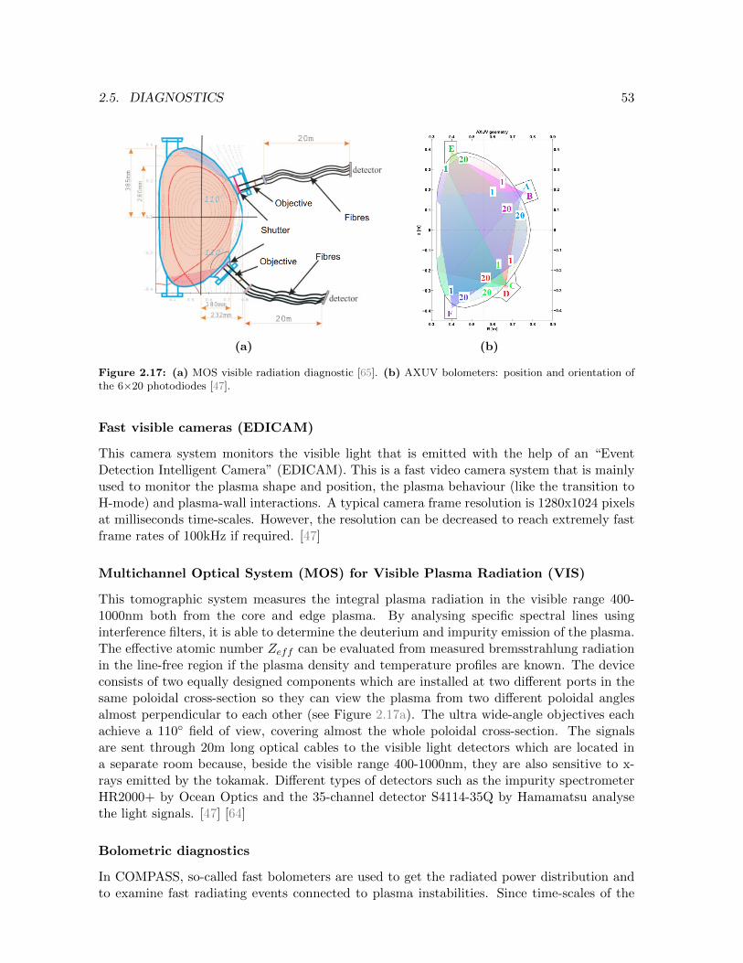
2.5. DIAGNOSTICS 53
(a) (b)
Figure 2.17: (a) MOS visible radiation diagnostic [65]. (b) AXUV bolometers: position and orientation ofthe 6×20 photodiodes [47].
Fast visible cameras (EDICAM)
This camera system monitors the visible light that is emitted with the help of an “EventDetection Intelligent Camera” (EDICAM). This is a fast video camera system that is mainlyused to monitor the plasma shape and position, the plasma behaviour (like the transition toH-mode) and plasma-wall interactions. A typical camera frame resolution is 1280x1024 pixelsat milliseconds time-scales. However, the resolution can be decreased to reach extremely fastframe rates of 100kHz if required. [47]
Multichannel Optical System (MOS) for Visible Plasma Radiation (VIS)
This tomographic system measures the integral plasma radiation in the visible range 400-1000nm both from the core and edge plasma. By analysing specific spectral lines usinginterference filters, it is able to determine the deuterium and impurity emission of the plasma.The effective atomic number Zeff can be evaluated from measured bremsstrahlung radiationin the line-free region if the plasma density and temperature profiles are known. The deviceconsists of two equally designed components which are installed at two different ports in thesame poloidal cross-section so they can view the plasma from two different poloidal anglesalmost perpendicular to each other (see Figure 2.17a). The ultra wide-angle objectives eachachieve a 110 field of view, covering almost the whole poloidal cross-section. The signalsare sent through 20m long optical cables to the visible light detectors which are located ina separate room because, beside the visible range 400-1000nm, they are also sensitive to x-rays emitted by the tokamak. Different types of detectors such as the impurity spectrometerHR2000+ by Ocean Optics and the 35-channel detector S4114-35Q by Hamamatsu analysethe light signals. [47] [64]
Bolometric diagnostics
In COMPASS, so-called fast bolometers are used to get the radiated power distribution andto examine fast radiating events connected to plasma instabilities. Since time-scales of the

54 CHAPTER 2. THE TOKAMAK COMPASS
order of microseconds are required, photo-detectors are used as they provide a high temporalresolution in contrast to for example temperature-dependent resistors. Six arrays (A, B, C,D, E and F) of twenty photodiodes record the total radiation in a spectral range from ultra-violet up to soft x-rays in the poloidal cross-section of COMPASS (see Figure 2.17b). Thesemeasurements do not give information on local properties. To this end, special mathemat-ical transformations have to be performed. Under certain assumptions of symmetry thesecalculations can be simplified and only an inverse Abel transformation has to be applied. [47]
Soft x-ray diagnostics
The SXR diagnostics are bolometers - arrays of 35 silicon photodiodes on a chip - that onlymeasure soft x-ray intensities. This selection is achieved by using a thin beryllium foil. Softx-rays are linked to bremsstrahlung (see paragraph 1.2.4) and therefore they are extremelyvaluable to examine impurities. [47]
Hard x-ray diagnostics
High-energetic x-rays, better known as hard x-rays, are measured by a detector placed some-where in the tokamak hall separated from the tokamak itself. The detector consists of ascintillator and a photomultiplier. The scintillator converts the high-energetic photons to vis-ible photons. The photomultiplier then converts the energy of these photons to an amplifiedelectrical current making use of the photoelectric effect and secondary emission by well posi-tioned electrodes in a vacuum tube. Unfortunately, this detector is also sensitive to neutrons.[46]
High dispersion spectrometer
This device is used to determine amongst others the toroidal and poloidal rotation velocity ofthe edge plasma starting from Doppler shift measurements of carbon triplet lines 1s22s3s→1s22s3p (≈465nm). Next to this, it is also used to measure the motional Stark effect of the Dαline (≈656nm) from the NBI. The spectrometer is equipped with a high speed camera withhigh quantum efficiency, which enables time resolutions up to 2ms. The rotation velocitiesare still not measured, and currently the spectrometer is not installed. At the moment, theCOMPASS team is working on CXRS12 diagnostics. Rotation measurements will be part ofthis new project. [47] [58] [60]
2.5.5 Beam and particle diagnostics
Lithium beam emission spectroscopy (BES)
In the BES system of COMPASS, a beam of neutral Li atoms is directed into the plasma,where the Li atoms excite or ionize by colliding with the plasma particles. The excited Liatoms then radiate at a wavelength of 670.8nm (2p-2s transition) to get back to their lowerenergy state. This radiation is detected by a slow-measuring CCD camera on top of the vesseland by fast-measuring avalanche photodiodes (APD) at the bottom of the vessel. This canbe seen in Figure 2.18a. In case of Li, this radiation is very weakly dependent on the electrontemperature, and so the intensity measured by the detectors is a measure for the electron
12Charge eXchange Recombination Spectroscopy.

2.5. DIAGNOSTICS 55
(a)
(b)
Figure 2.18: (a) Li-BES system [47]. (b) Scanning method of Li-BES [47].
density. The detection system measures the beam radiation along multiple lines of sight. Thelight detected in a measurement channel originates from the intersection of the beam and theline of sight. If the beam is scanned up and down using deflection plates, different points inthe plasma are investigated. Performing a series of measurements at a set of different beampositions, the whole two-dimensional density profile can be reconstructed, although not ona rectangular grid of points, as can be seen in Figure 2.18b. For the moment, there are noreliable experimental data from the Li-BES system. [47]
In Figure 2.18a also an atomic beam probe (ABP) detector is shown. It is used to determinethe poloidal magnetic field perturbation and the edge plasma current profile. For a profounddescription is referred to [66].
Neutral particle analyser
The charge exchange reactions in the hot plasma also create neutral particles, namely hydro-gen and deuterium, which can leave the magnetic confinement. A neutral particle analyseris positioned outside the tokamak vessel and captures some of these neutral particles. Theseparticles first pass through a gas which ionizes them. The resulting ions keep their energyand momentum. Then, a bending magnet separates protons and deuterons based on theirdifferent masses. Finally, they are each detected by an array of 12 detectors which determinesthe energy distribution. The NPA is not yet connected. [47]

56 CHAPTER 2. THE TOKAMAK COMPASS
Figure 2.19: Neutral particle analyser. [47]
Neutron detector
Very recently, a neutron detector is installed. It is actually the same device as the HXR de-tector - consisting of a scintillator plus photomultiplier and placed somewhere in the tokamakhall 5m removed from the tokamak itself - but shielded by a 10cm wide wall of lead bricks toavoid the registration of HXR emission from the tokamak plasma. [46]
2.5.6 Probe diagnostics
An electric probe is basically a conducting object placed in the plasma and connected to acircuit to measure the voltage or current induced in it. Probes have to fulfil two requirements:they have to withstand the high temperatures of the plasma and they have to be small inorder to disturb the plasma as little as possible. Scientists play with externally applied probepotentials and currents, to measure
• the IV characterstic (V is swept)
• the ion saturation current (V < −100V)
• the floating potential (I = 0)
Probe diagnostics are loved for their extremely high frequency, which is only limited by thequality of the data acquisition system.
Divertor probes
Langmuir Probes. The COMPASS tokamak is equipped with an array of 39 Langmuirprobes embedded in the divertor tiles (see Figure 2.20). A triangular shaped time-varyingvoltage is applied to these probes allowing them to sweep between a positive and a negativepotential. Assuming that the electron velocity has a Maxwell-Boltzmann distribution, whichis typical for high-temperature plasmas, the IV characteristic obtained by comparing themeasured current through the probe to the applied voltage can be fitted by
I = I+sat
[1− α(V − Vf )− e
V−VfTe[eV]
](2.52)

2.5. DIAGNOSTICS 57
Figure 2.20: Langmuir probe array (39 probes) in the divertor region of COMPASS. [47]
with I the current through the probe, V the probe voltage, Vf the floating potential13 , α aparameter to cope with a possible lack of saturation, Te the electron temperature expressedin eV and I+sat the ion saturation current given by
I+sat = eZnicsA (2.53)
where Z is the atomic number of the ions (equals 1 without impurities), ni the ion densitywhich equals the electron density for a quasi-neutral deuterium plasma, A the contact surfaceof the probe and cs the ion sound speed. This last quantity is in turn given by
cs =
√kB(ZTe + γiTi)
mi(2.54)
with mi the ion mass and γi the adiabatic coefficient of the ions which can take on values be-tween 1 and 314. Assuming thermodynamic equilibrium (Ti ≈ Te) one is able to find ne and Te.
A typical IV characteristic is given in Figure 2.21. The current obviously saturates for negativevalues of V meaning that α = 0. A high enough negative probe potential repels all electronsfrom entering the probe and only the current caused by the positively charged plasma ionsis what remains. For increasing probe potential the behaviour of the curve is determinedby the electron current. The exponential decrease leads to the determination of the electrontemperature. The current will be zero for a positive value of V , namely the floating potential.This phenomenon can be explained as follows: for a small positive value of V the plasmaelectrons will form a Debye shield around the probe repelling other electrons while they arenot inducing a current in the probe. There exists no equivalent ion shield because ions have amuch higher mobility than electrons. The encircled part of the graph is called the ion branch.Formula (2.52) is applicable to this part of the IV curve. As you might guess, the otherpart is called the electron branch. There, the exponential behaviour is determined by the iontemperature and the saturation current consists solely of electrons. This current is given by
I−sat =1
4e nece,th(1− γsee)A (2.55)
where the factor 1/4 accounts for the isotropic spatial dimensions and γsee for the secondaryelectron emission at the probe surface. As mentioned before, the electrons are assumed to
13Remark that I = 0 for V = Vf .14In a classical gas γ is related to the degrees of freedom N : γ = 1+ 2
N. It is a measure for the compressibility.

58 CHAPTER 2. THE TOKAMAK COMPASS
Figure 2.21: Representation of a Langmuir probe measurement (left) and a typical resulting IV characteristic(right). [48]
have a Maxwell-Boltzmann velocity distribution, meaning that the saturation current is afunction of the thermal velocity
ce,th =
√8kBTeπme
(2.56)
[67]
The above described fitting method starts from the assumption that we are dealing with aMaxwellian plasma. Since this is not always the case, especially for low-temperature plasmas,it is more reliable to use the theory of Druyvesteyn [68]. He starts from an expression for theelectron energy distribution function (EEDF), which is proportional to the second derivativeof the IV characteristic, to calculate the electron density and the electron temperature. Yetanother method, based on the first derivative of the IV characteristic, is discussed in [69].
Ball-pen probes. Ball-pen probes consist of a conical conductor (the collector) placed ina ceramic tube at adjustable height. This height determines the effective probe surface A inequations (2.53) and (2.55). Due to the different gyration radii of electrons and ions and alot of other more complicated effects like E ×B drift, the effective surfaces of electrons andions are different. Well thought out design of the ball-pen probes makes it possible to have awide range of collector heights for which I+sat ≈ I
−sat, which implies that they directly measure
the plasma potential φ if they are in floating potential mode. This can be theoreticallydemonstrated as follows. Equation (2.52) is equivalent to
I = I+sat − I−sate
V−φTe[eV] (2.57)
if the plasma potential is taken as reference instead of the floating potential. Using the factthat I = 0 for V = Vf , we derive
Vf = φ− Te ln
(I−satI+sat
)(2.58)
which shows indeed that Vf = φ if both saturation currents are the same. Very interesting isthe combination of a ball-pen and Langmuir probe close to each other, since their data allowsto calculate the electron temperature with very high time resolution:
Te[eV] =φBPP − V LP
f
2.2(2.59)

2.6. FEEDBACK CONTROL SYSTEM 59
Figure 2.22: Draft of a ball-pen probe with non-withdrawn collector showing the different used materialsand the bigger gyration radius of ions compared to electrons (left), and a picture of the corresponding realball-pen probe (right). [70]
Here, 2.2 is a typical value for the natural logarithm occurring in equation (2.58) in case of adeuterium plasma15. [67] [70]
Reciprocating probes
Next to the divertor probes also horizontal reciprocating probes are installed on the COM-PASS tokamak to gather data deeper into the plasma, namely in the scrape-off layer. Theseare probes mounted on a fast pneumatic manipulator reciprocating quickly (within 0.1 sec-ond) in and out to avoid overheating, which would cause impurity release and destruction ofthe probe head. The probe head consists of 5 Langmuir probes and 3 ball-pen probes, whichmeasure
• radial profiles of the plasma potential φ, electron density ne and temperature Te
• plasma velocity along the magnetic field
• fluxes of particles and energy towards the wall
• ion temperature Ti
[71]
2.6 Feedback control system
To maintain plasmas as long as possible, especially non-circular shaped ones, a fast feedbacksystem controlling the radial and vertical plasma position is indispensable. The choice of thedata fed to the feedback system is far from obvious since it has to be inert to changes inother plasma parameters. Therefore, data extracted from different diagnostic coils is testedin simulations with elliptical shaped plasmas (see Figure 2.23) [72]. Following combinationsof internal partial rogowski (IPR) coils seem to be the best choice.
Bh(R,Z) = 3 · IPR5 + IPR3 − 3 · IPR13 − IPR15 (2.60)
Bv(R,Z) = 1.2 · IPR8 + IPR9 + 1.2 · IPR10 (2.61)
15In case the working gas is hydrogen this is 2.8

60 CHAPTER 2. THE TOKAMAK COMPASS
The values of the newly introduced variables Bh and Bv form look-up tables for the radialposition R and vertical position Z, which are used in the feedback code implemented in thereal-time controller MARTe (Multi-threaded Application Real-Time executor). MARTe isrunning in two threads with two different speeds. The fast thread runs in a loop of 20kHzand contains amongst others the module for the calculation of the plasma position. The slowthread runs in a loop of 2kHz and is used mostly for communication with the main powersupplies. [72]
2.6.1 Radial equilibrium
In the approximation of a circular and high aspect ratio plasma16, radial equilibrium is fulfilledby the vertical magnetic field17
Bz =µ0Ip4πR
[ln
(8R
a
)− 3
2+ βp +
li2
](2.62)
where R is the radial plasma position, a the plasma minor radius, βp the poloidal beta18 andli the internal inductance between the plasma center and the edge at r = a. As mentionedin paragraph 2.3.2, two types of PF coils are responsible for the radial equilibrium: theequilibrium field coils (EF) and the fast feedback coils (BV). As its name says, the last oneacts much faster. The EF circuit uses a proportional-integral (PI) control scheme:
IEF,req = KP1 · Ip +KP2 · (Rreq −Rmeas) +KI1 ·t∫
0
(Rreq −Rmeas) dt+KP3 · IBV,meas (2.63)
Here, the radial position Rmeas is determined by the algorithm based on IPR coil measure-ments as described above. The BV circuit takes care of the fast disturbances. It calculatesits requested current IBV,req starting only from the radial position error Rreq − Rmeas, alsowith a PI controller (though PID19 is available). In theory, the superposition of the verticalmagnetic fields generated by both circuits, should approximate equation (2.62). However,three parameters do not appear in the controller code, namely a, βp and li. They are indi-rectly taken into account by the Ip-term of equation (2.63) since they all influence the currentdistribution inside the plasma. The tokamak operators can manually preset Rreq on shot toshot basis to achieve the desired plasma position. [60] [74]
2.6.2 Vertical equilibrium
The radial field (BR) circuit handles vertical disturbances by use of a PD regulator. [74]
16The major radius is much bigger than the minor radius, i.e. R a.17For a derivation of this formula, see [73].18The plasma-β is defined as the ratio of the plasma pressure to the magnetic energy density: nkBT
B2/2µ0. It is
a measure for the efficiency of the magnetic confinement. The toroidal β depends on the external magneticfield created by the TF coils. It has an economical aspect: since the TF coils are the biggest reactor cost, ahigh toroidal β is desired. The poloidal β contains the current-induced poloidal field and is important for theradial equilibrium.
19Proportional-integral-derivative controller.

2.7. RECHARGE TIME 61
Figure 2.23: IPR feedback simulation with elliptical shaped plasma. Note the positions of the IPR coilsalong the vessel surface. [72]
2.6.3 Plasma current control
The output of the power supply of the central solenoid is controlled by a PID regulator thatminimises the error Ip,req − Ip,meas. Since Is needs to increase gradually as explained inparagraph 2.3.1, this means that the PID controller determines the change dIs
dt . The currentin the central solenoid (and more generally in the MF coils) can be expressed as
Is = Is,meas +
(dIsdt
)PID
∆t (2.64)
where ∆t is the time between two iterations. [60] [74]
2.7 Recharge time
COMPASS needs typically 30 minutes between two consecutive discharges. The major timeconsuming actions are
• pumping the vessel again to a good vacuum (takes the most time)
• recovery of the speed of the flywheel generator(s)
• reading and storing data in the database
• performing some calculations (for example by EFIT)
• performing some modifications to the torus hall if necessary
• preprogramming the next shot
• charging the auxiliary capacitor banks
EFIT processes the data from important shots with a higher sampling rate at night to mini-mize the time lost between shots. [46]

62 CHAPTER 2. THE TOKAMAK COMPASS
2.8 Safety
COMPASS does not produce any radioactive waste. However, during operation some neutronradiation and x-rays are produced. These are harmless outside the tokamak hall. Further,a protection system is made for the two high power lasers used for the Thomson scatteringdiagnostic.
2.9 Goals
COMPASS is an experimental reactor, not aimed to produce actual fusion reactions. Itsresearch is focused on the edge plasma studies relevant to ITER, e.g. pedestal and ELMphysics (see later in paragraph 3.2.3). Also the L-H transition is intensively examined. Moreexactly its power threshold and hysteresis behaviour. Further, the feasibility of NBI heatingand some diagnostics, for example the atomic beam probe, is studied. And the developmentof new techniques for improved data acquisition and analysis was originally a main goal. [40]

Chapter 3
H-mode operation in COMPASS
3.1 Introduction
In this chapter, useful data from COMPASS experiments will be shown and widely discussed.Here, we examine in particular the behaviour of the plasma parameters around the transitionfrom L-mode to H-mode, and we try to learn more about H-mode. We also focus on theinfluence of neutral beam injection. The reader is first informed about the different phasesand confinement modes of a standard tokamak discharge with special attention for ELMs.Then, the analytical part of this thesis begins. Data from different diagnostics are discussedfor five H-mode shots: the very first shot that reached H-mode at the IPP (#4073), a shotimmediately after a glow discharge cleaning (#4267), a shot with three NBI intervals and moreaccurate data of the ohmic heating power (#5909), a shot with an H-L transition (#6109)and finally a shot with only ohmic heating (#6313). Indeed, the last shot is the only shotwithout additional heating from the NBI. At the end of the chapter, some conclusions aremade by comparing the different shots.
3.2 General discharge evolution
3.2.1 Start-up
After vacuum pumping, the tokamak vessel is filled with deuterium to a pressure in the range0.02-0.2Pa. The first step in the actual start-up process is the pre-ionization: some freeelectrons are generated in the vessel by an external electron source. In COMPASS this isa VUV lamp, but other possibilities are an electron gun, an RF wave generator or just thecosmic background radiation. In the next step, a sequence of processes is triggered, namely:
1. activation of the data acquisition system
2. powering of the TF coils
3. powering of the central solenoid
The third trigger pulse is sent when the toroidal magnetic field has reached a reasonable level.The changing current in the central solenoid induces a toroidal electric field in the vacuumvessel.
63

64 CHAPTER 3. H-MODE OPERATION IN COMPASS
The following step, namely the plasma breakdown, can be split up in two phases, each with dif-ferent underlying physics: the avalanche phase and the Coulomb phase. During the avalanchephase collisions between electrons and deuterium molecules dominate. The electrons from thepre-ionization are accelerated by the toroidal electric field and once they have enough kineticenergy they will ionize deuterium when they collide resulting in one extra electron for eachionizing collision. Thus, the ionization happens exponentially. For an ionization of about 5%the density of ions and electrons has reached the point where the Coulomb interactions be-tween them are so strong that electron-ion collisions start to dominate. The current increasesand magnetic surfaces are formed during this Coulomb phase so that the confinement of theplasma increases significantly. At the end of the Coulomb phase the plasma is fully ionized.[75]
3.2.2 Tokamak confinement modes
After the plasma breakdown, the current starts ramping up going hand in hand with ohmicheating. This phase is characterized by the lack of additional heating. The plasma confine-ment is very good. Years of research have shown that the confinement deteriorates withincreasing power coupled to the plasma (see for example the ITER scaling law (1.38)). How-ever, since the plasma resistance has a bad temperature dependence, additional heating isneeded to reach the ignition condition for future fusion reactors.
From the moment extra heating sources are applied (e.g. NBI), the tokamak is said to be inlow confinement (L) mode. As its name says, the discharge has now stepped back with regardto confinement. Be careful: the term ‘L-mode’ often has a more general meaning and is notalways related to additional heating. In the literature, ohmic heating and L-mode are oftenmixed which may be confusing. In this master thesis is started from the definition given above.
When the heating power has reached a certain threshold, the discharge enters the high con-finement (H) mode. A transport barrier is set up at the plasma edge, retaining heat andparticles in its core (see Figure 3.1). This transport barrier is physically translated into ahigh gradient in the plasma pressure p = nkT at the plasma edge: a pressure pedestal. Alsothe density and temperature profiles show such a pedestal. These can be interpreted as par-ticle and energy barriers respectively. Both theoretical models and experimental observationsindicate a strong dependence of the overall confinement in the core on the pedestal height. [76]
Other tokamak operation modes exist. Their appearance is often dependent on tokamak ge-ometry and know-how of controlling certain plasma parameters.
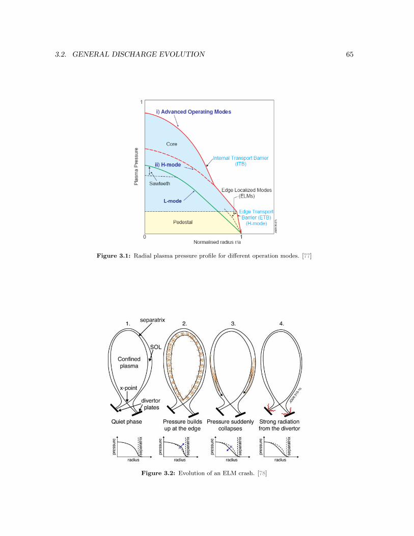
3.2. GENERAL DISCHARGE EVOLUTION 65
Figure 3.1: Radial plasma pressure profile for different operation modes. [77]
Figure 3.2: Evolution of an ELM crash. [78]

66 CHAPTER 3. H-MODE OPERATION IN COMPASS
3.2.3 Edge Localized Modes (ELMs)
In H-mode, especially right after the L-H transition, the plasma is very sensitive to certaininstabilities called edge localized modes (ELMs). This is a phenomenon where the pressurepedestal falls down and rebuilds itself. An ELM cycle is typically described by 4 steps (seeFigure 3.2):
1. A steep pressure gradient is built during H-mode.
2. The pressure gradient exceeds a certain critical value leading to the onset of many smallturbulent eddies at the edge.
3. The edge plasma is lost to the scrape-off layer where it flows along the magnetic fieldlines towards the divertor.
4. The lost plasma hits the divertor plates hereby producing a distinctive peak in the Dαradiation1.
During the instability, the edge pressure is reduced until the plasma becomes stable again.Then the process is ready to repeat itself. In theory, the cycle can go on indefinitely if nothingchanges to the conditions.
ELMs can be classified in 3 groups according to the emerging changes in plasma parametersduring the crash:
• Type-1: These ELMs are also known as “large” or “giant” ELMs because the Dαradiation shows large isolated bursts. The pressure gradient at the edge is close to thetheoretical stability limit (“ideal ballooning”, see Figure 3.3) or even beyond it. Therepetition frequency is 10Hz or less - which is very low compared to the other ELMtypes - and increases together with the heating power. They are known to cause upto 10-15% drops in the plasma energy. The degradation of the plasma confinement issmaller than with other ELMs. They are, on the other hand, most detrimental to thedivertor plates.
• Type-2: These ELMs require strongly-shaped plasmas, i.e. with high elongation andtriangularity, and a rather high plasma density and edge safety factor. The Dα burstsare smaller and the repetition rate is higher than that of type-1 ELMs, while the con-finement stays almost as good. Virtually nothing is known about how the frequencyand amplitude of type-2 ELMs depend on the power coupled to the plasma. Theyare sometimes called “grassy” ELMs. This terminology is somewhat confusing becausetype-3 ELMs also look grassy.
• Type-3: These ELMs are characterised by small and frequent Dα bursts. Therefore,another name is “small” ELMs. The instability is driven by electric currents and appearswhen plasma resistivity is rather high, i.e. when the edge temperature is rather low.The repetition frequency is found to decrease with increasing heating power. They areobserved for powers near the H-mode threshold power and produce small energy dumps.More exactly 1-3% of the stored energy is lost. The plasma confinement is degradedmore than with other ELMs. Compared to type-2 ELMs, they appear in poorly confinedplasmas.
1Visible light emitted by excited deuterium, see later.

3.2. GENERAL DISCHARGE EVOLUTION 67
Figure 3.3: Peeling and ballooning model of ELMs. [81]
While they have many negative effects, the beneficial effect of ELMs in providing density con-trol and limiting the core plasma impurity content in high confinement discharges should notbe overlooked. Indeed, H-mode has the advantage of having an improved energy confinementtime τE , but the disadvantage of having a particle barrier which keeps radiating impurities inthe plasma core. ELMs could be used to remove impurities from the plasma core from timeto time, if one succeeds to control them. They however do more harm than good.
In fact, ELMs represent a big problem for ITER. It is not yet clear whether an efficient way willbe found to suppress or mitigate them without loss of energy confinement. Therefore, a newoperation regime, the so-called improved confinement (I) mode is now experimentally studied.This regime exhibits improved energy confinement and is ELM-free, but the density remainsconstant. This implies that impurities are not accumulated in the plasma. Technically, thisregime can be achieved by reversing the toroidal magnetic field, so that the B×∇B drift ofthe ions is directed upwards and not towards the x-point (recall Figure 1.11b). [46] [78] [79][80]
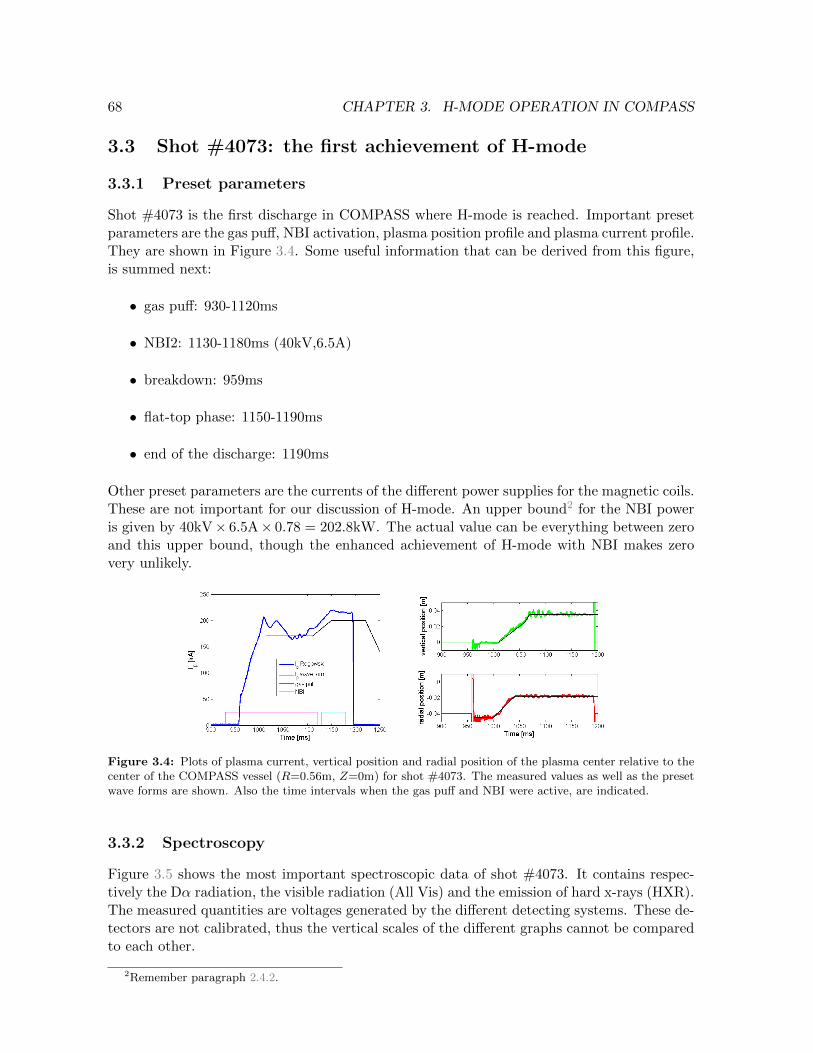
68 CHAPTER 3. H-MODE OPERATION IN COMPASS
3.3 Shot #4073: the first achievement of H-mode
3.3.1 Preset parameters
Shot #4073 is the first discharge in COMPASS where H-mode is reached. Important presetparameters are the gas puff, NBI activation, plasma position profile and plasma current profile.They are shown in Figure 3.4. Some useful information that can be derived from this figure,is summed next:
• gas puff: 930-1120ms
• NBI2: 1130-1180ms (40kV,6.5A)
• breakdown: 959ms
• flat-top phase: 1150-1190ms
• end of the discharge: 1190ms
Other preset parameters are the currents of the different power supplies for the magnetic coils.These are not important for our discussion of H-mode. An upper bound2 for the NBI poweris given by 40kV× 6.5A× 0.78 = 202.8kW. The actual value can be everything between zeroand this upper bound, though the enhanced achievement of H-mode with NBI makes zerovery unlikely.
Figure 3.4: Plots of plasma current, vertical position and radial position of the plasma center relative to thecenter of the COMPASS vessel (R=0.56m, Z=0m) for shot #4073. The measured values as well as the presetwave forms are shown. Also the time intervals when the gas puff and NBI were active, are indicated.
3.3.2 Spectroscopy
Figure 3.5 shows the most important spectroscopic data of shot #4073. It contains respec-tively the Dα radiation, the visible radiation (All Vis) and the emission of hard x-rays (HXR).The measured quantities are voltages generated by the different detecting systems. These de-tectors are not calibrated, thus the vertical scales of the different graphs cannot be comparedto each other.
2Remember paragraph 2.4.2.
3.3. SHOT #4073: THE FIRST ACHIEVEMENT OF H-MODE 69
Dα and visible radiation
First of all, we remark that the two first curves are very similar. This may not surprise yousince the All Vis signal is a superposition of all visible wavelengths and thus also includes thedominating Dα line. Secondly, it has to be stressed that the Dα radiation is an extremelyimportant signal for our discussion of H-mode: the Dα signal contains the signature of H-mode. This will be explained... During operation, the deuterium fuel gas in the tokamak isexcited and ionized. The excited deuterium atoms emit light with a wavelength of 656.3nm(Dα line) radiated by electrons jumping from the 3th to the 2nd shell. This light is capturedby the Multichannel Optical System3. The Dα radiation is strongest during the plasma start-up because the lower amount of energy available in the tokamak at that moment increasesthe chance of an excitation reaction against an ionization reaction. This peak is omittedfrom Figure 3.5 since we are more interested in the L-H transition. After the start-up phasethe plasma is fully ionized and the Dα radiation is coming from newly injected neutral fuelparticles4, but also from fuel particles that are desorbed by the vessel wall - a process that iscalled wall recycling. As the confinement of the plasma keeps increasing less and less particlescollide with the vessel wall. H-mode implies that this second source of Dα radiation, namelydesorption of deuterium from the vessel wall, is very small. The transition from L- to H-modecan be observed as an abrupt drop in the Dα radiation. Scientists are very glad to see thisdrop. From Figure 3.5 it is clear that the transition to H-mode took place around t=1141ms:at that moment the average intensity of the Dα radiation is approximately divided by two.We see in Figure 3.5 that around this transition the Dα radiation shows distinct spikes. Theseare Edge Localized Modes. There are 3 ELMs at the end of L-mode, the first one occurring att=1140ms, and 4 ELMs in the beginning of H-mode, the last one being at t=1145ms (see alsoFigure 3.9). During the subsequent ELM-free H-mode the Dα radiation stays constant whilethe All Vis radiation slowly increases, because impurities are better confined and consequentlymore excited. The better confinement implies that the plasma touches the wall less whichmeans that there should be less impurities. However, there is obviously an impurity influx.This impurity accumulation goes on until a major instability occurs and a lot of the thermalenergy is lost at once, ending the discharge at t=1190ms. Such an instability is called adisruption. As a last note, remark that the fluctuations in the Dα and All Vis radiation arereduced after switching off the NBI at t = 1180ms.
Hard x-rays
Hard x-rays are produced by plasma-wall interactions and by runaway electrons. These areelectrons that are produced “when the collisional drag force is lower than the electric drivingforce [82]”. In other words, these electrons collide less with other plasma particles than normaland are accelerated until they are non-Maxwellian particles with a lot of kinetic energy.They are only produced during abnormal events such as disruptions. The bremsstrahlungemitted by these highly accelerated electrons is in the hard x-ray range. Curiously, the HXRscintillation detector picks something up after the NBI is started. You could say that the HXRsignal is the signature of the NBI operation, but be carefull: the HXR signal keeps showinghigh values after the NBI is turned off. The most reasonable explanation for the correlationbetween the NBI operation and the increased HXR values is the creation of neutrons. Indeed,
3See paragraph 2.5.4.4Deuterium puffing and neutral beam injection.

70 CHAPTER 3. H-MODE OPERATION IN COMPASS
Figure 3.5: Spectroscopic data of #4073. The yellow area indicates the NBI.
neutrons are also registered by the scintillation detector. Recently, a neutron detector wasinstalled and confirmed this hypothesis.
Soft x-rays
Another interesting spectroscopic signal is the soft x-ray radiation. As the SXR signal mea-sures the bremsstrahlung radiation, we know from equation (1.13) that following proportion-ality holds for the measured intensity
ISXR ∝ n2eZ2effT
12e (3.1)
The SXR intensities registered by detectors 18-30 are plotted in Figure 3.6. The position andline of sight of these SXR detectors are shown in Figure 3.7. The data is detrended so thatwe can clearly observe the appearance of a sawtooth pattern from the moment the NBI isturned on. These sawteeth indicate a build-up of electron density and temperature, followedby an instability causing a fast drop. The sawtooth oscillation is one of the fundamentalinstabilities in tokamaks, and is therefore also indicated in Figure 3.1. This phenomenonseems to happen when additional heating is coupled tot the plasma. When a sawtoothcrash occurs, hot electrons are sent rapidly from the plasma core to the cooler plasma edge,flattening the temperature profile. Figure 3.6 shows this electron transport throughout theplasma: the sawteeth in the plasma edge (detectors 18-20 and 30) are inverse with respect tothe sawteeth in the plasma core (detectors 23-26). The inversion occurs at the q=1 surfacewhich designates the most stable part of the whole plasma. The safety factor q expresseshow many toroidal rotations are necessary for a single rotation of a magnetic field line in thepoloidal direction. For tokamaks with circular cross-section and large aspect ratio (R a),this is approximately given by
q =a
R
BtBp
(3.2)
This tells us something about the stability of the plasma: If q is a rational number, the mag-netic field line bites in its own tail after several turns, but if it is an irrational number thefield line travels around the whole magnetic surface. You can feel intuitively that the latteris less stable. The most stable situation occurs when q equals one.

3.3. SHOT #4073: THE FIRST ACHIEVEMENT OF H-MODE 71
Figure 3.6: Soft x-ray radiation for shot #4073. The data is detrended and smoothed. All signals are on thesame scale. The vertical distance between two consecutive signals is 0.2µW. Photodiode 22 did not work welland is omitted.
(a) (b)
Figure 3.7: Reconstruction of the q=1 surface at (a) t = 1140ms and (b) t = 1170ms.
Figure 3.8: Radial distribution of the safety factor q in the mid-plane calculated by EFIT.
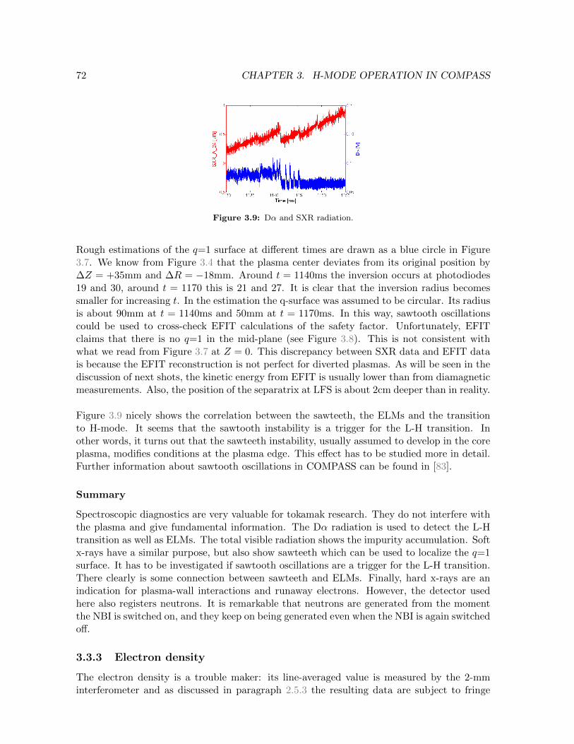
72 CHAPTER 3. H-MODE OPERATION IN COMPASS
Figure 3.9: Dα and SXR radiation.
Rough estimations of the q=1 surface at different times are drawn as a blue circle in Figure3.7. We know from Figure 3.4 that the plasma center deviates from its original position by∆Z = +35mm and ∆R = −18mm. Around t = 1140ms the inversion occurs at photodiodes19 and 30, around t = 1170 this is 21 and 27. It is clear that the inversion radius becomessmaller for increasing t. In the estimation the q-surface was assumed to be circular. Its radiusis about 90mm at t = 1140ms and 50mm at t = 1170ms. In this way, sawtooth oscillationscould be used to cross-check EFIT calculations of the safety factor. Unfortunately, EFITclaims that there is no q=1 in the mid-plane (see Figure 3.8). This is not consistent withwhat we read from Figure 3.7 at Z = 0. This discrepancy between SXR data and EFIT datais because the EFIT reconstruction is not perfect for diverted plasmas. As will be seen in thediscussion of next shots, the kinetic energy from EFIT is usually lower than from diamagneticmeasurements. Also, the position of the separatrix at LFS is about 2cm deeper than in reality.
Figure 3.9 nicely shows the correlation between the sawteeth, the ELMs and the transitionto H-mode. It seems that the sawtooth instability is a trigger for the L-H transition. Inother words, it turns out that the sawteeth instability, usually assumed to develop in the coreplasma, modifies conditions at the plasma edge. This effect has to be studied more in detail.Further information about sawtooth oscillations in COMPASS can be found in [83].
Summary
Spectroscopic diagnostics are very valuable for tokamak research. They do not interfere withthe plasma and give fundamental information. The Dα radiation is used to detect the L-Htransition as well as ELMs. The total visible radiation shows the impurity accumulation. Softx-rays have a similar purpose, but also show sawteeth which can be used to localize the q=1surface. It has to be investigated if sawtooth oscillations are a trigger for the L-H transition.There clearly is some connection between sawteeth and ELMs. Finally, hard x-rays are anindication for plasma-wall interactions and runaway electrons. However, the detector usedhere also registers neutrons. It is remarkable that neutrons are generated from the momentthe NBI is switched on, and they keep on being generated even when the NBI is again switchedoff.
3.3.3 Electron density
The electron density is a trouble maker: its line-averaged value is measured by the 2-mminterferometer and as discussed in paragraph 2.5.3 the resulting data are subject to fringe

3.3. SHOT #4073: THE FIRST ACHIEVEMENT OF H-MODE 73
(a) (b)
Figure 3.10: (a) Raw line-averaged electron density divided by the maximum elongation κmax = 1.8 for thethree different ambiguous interferometer signals. (b) Plasma elongation calculated by EFIT.
failing. Figure 3.10a is a plot of the raw data from the COMPASS database divided by themaximum plasma elongation, namely 1.8. This is of course an underestimation of the realelectron density since the elongation is most of the time smaller than 1.8 as can be seen inFigure 3.10b. We first of all remark that there is an offset on each channel which has to beremoved. Secondly, we notice that the red and green curves are physically impossible: theelectron density should rise in ohmic regime and certainly in H-mode. Besides, the greenchannel even has negative values if the offset is removed! Everything suggests to take theblue channel to discuss the electron density of shot #4073.
However, also the blue curve (6xAD8302) performs strange behaviour: during H-mode itreaches 〈ne〉 ≈ 7.45 · 1019m−3 and then suddenly drops to its offset value. This drop can beexplained by the plasma reaching its first interference fringe. In paragraph 2.5.3 we estimatedthe critical value 〈ne〉∗ for this fringe to be 7.8 · 1019m−3 for a plasma elongation of 1.8. So,this is a plausible explanation. In Figure 3.11 is the corrected electron density 〈ne〉 plottedbased on the blue channel (6xAD8302). This plot was made by using the algorithm describedin appendix B. We see how the electron density gradually rises, then it suddenly drops a littlebit around t=1040-1045ms due to the ELMs that go along with the transition to H-mode,thereafter it increases very fast during H-mode and finally it falls down very fast when thedisruption takes place. It is remarkable that between the gas puff and the NBI activity, thedensity keeps rising. Apparently, there is some kind of improved particle confinement at thatmoment.
As a last remark, we note that the red curve (1xAD8302) only has two differences comparedto the blue one (6xAD8302):
• It has a slightly different offset.
• When the electron density reaches the value 〈ne〉 ≈ 3.361 · 1019m−3 (about half thefirst-fringe-density of the blue curve) it goes over to mirroring the blue curve.
The fringe-failing occurs at exactly the same moment. The mirror behaviour is explained bythe fact that the red channel has a phase detector with a range of only 180. This phasedetector is therefore never used in data analysis.

74 CHAPTER 3. H-MODE OPERATION IN COMPASS
Figure 3.11: Reconstructed line-averaged electron density for shot #4073.
3.3.4 Global particle confinement
In its most general form the global particle balance is given by
dN0
dt+
dN+
dt= ΓIN − ΓOUT (3.3)
This equation says that the change in the amount of neutral and positively charged plasmaparticles equals the influx of neutral particles5 minus the outflux of neutral and positivelycharged particles. In other words, it expresses the conservation of the number of nuclei in theabsence of fusion reactions.
For a deuterium plasma without impurities these neutral particles are deuterium atoms (N0 =ND) and these positively charged particles are deuterons (N+ = ND+). We further usefollowing assumptions (and facts):
• The plasma is fully ionized: ND=0 ; and as a consequence the outflux ΓOUT consistsonly of charged particles and is assumed proportional to ND+
• The ingoing neutral particles ionize immediately: dNDdt = 0
• Deuterium has only one electron: ND+ = Ne
Now, we can rewrite the particle balance as
dNe
dt= ΓIN −
Ne
τp(3.4)
where
ΓIN = Γgas puff + ΓNBI + Γre−emission by wall (3.5)
Ne
τp= ΓOUT = Γabsorption by wall + Γdivertor pump (3.6)
5Charged particles cannot penetrate the magnetic field.
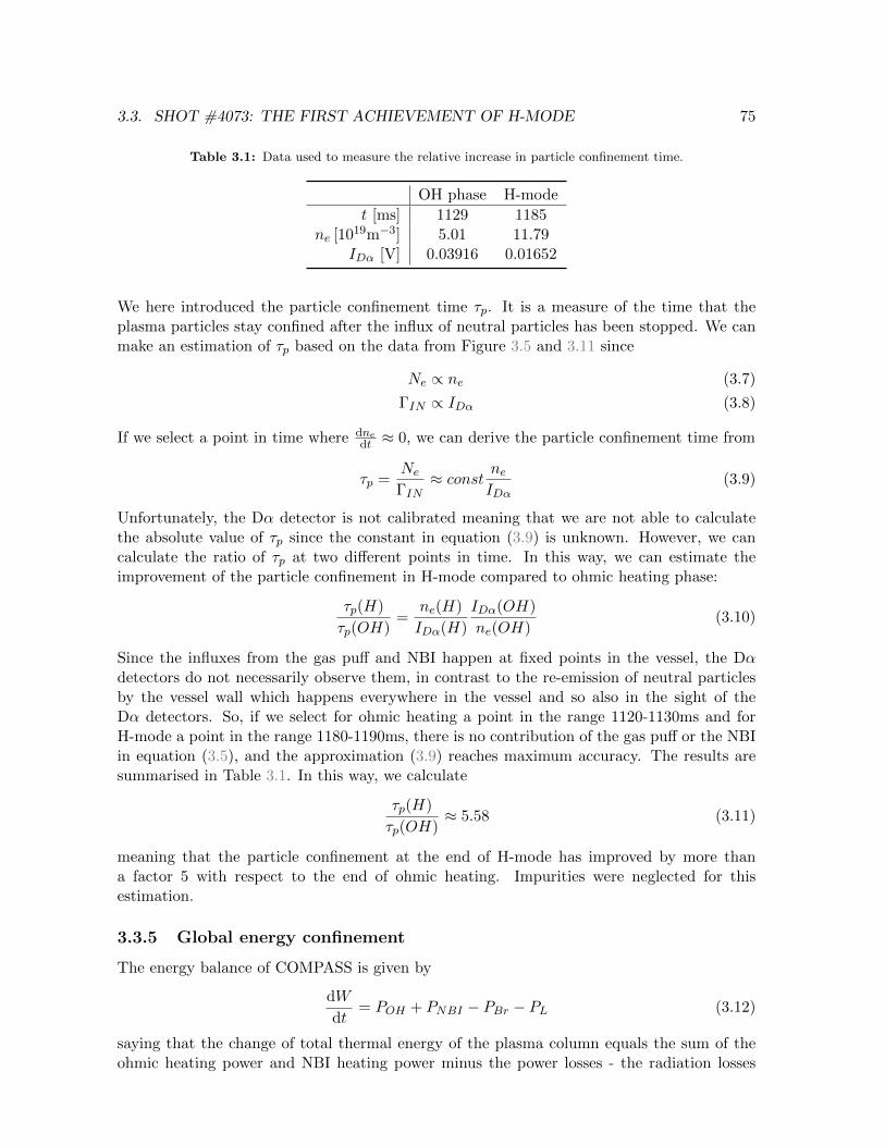
3.3. SHOT #4073: THE FIRST ACHIEVEMENT OF H-MODE 75
Table 3.1: Data used to measure the relative increase in particle confinement time.
OH phase H-mode
t [ms] 1129 1185ne [1019m−3] 5.01 11.79
IDα [V] 0.03916 0.01652
We here introduced the particle confinement time τp. It is a measure of the time that theplasma particles stay confined after the influx of neutral particles has been stopped. We canmake an estimation of τp based on the data from Figure 3.5 and 3.11 since
Ne ∝ ne (3.7)
ΓIN ∝ IDα (3.8)
If we select a point in time where dnedt ≈ 0, we can derive the particle confinement time from
τp =Ne
ΓIN≈ const ne
IDα(3.9)
Unfortunately, the Dα detector is not calibrated meaning that we are not able to calculatethe absolute value of τp since the constant in equation (3.9) is unknown. However, we cancalculate the ratio of τp at two different points in time. In this way, we can estimate theimprovement of the particle confinement in H-mode compared to ohmic heating phase:
τp(H)
τp(OH)=
ne(H)
IDα(H)
IDα(OH)
ne(OH)(3.10)
Since the influxes from the gas puff and NBI happen at fixed points in the vessel, the Dαdetectors do not necessarily observe them, in contrast to the re-emission of neutral particlesby the vessel wall which happens everywhere in the vessel and so also in the sight of theDα detectors. So, if we select for ohmic heating a point in the range 1120-1130ms and forH-mode a point in the range 1180-1190ms, there is no contribution of the gas puff or the NBIin equation (3.5), and the approximation (3.9) reaches maximum accuracy. The results aresummarised in Table 3.1. In this way, we calculate
τp(H)
τp(OH)≈ 5.58 (3.11)
meaning that the particle confinement at the end of H-mode has improved by more thana factor 5 with respect to the end of ohmic heating. Impurities were neglected for thisestimation.
3.3.5 Global energy confinement
The energy balance of COMPASS is given by
dW
dt= POH + PNBI − PBr − PL (3.12)
saying that the change of total thermal energy of the plasma column equals the sum of theohmic heating power and NBI heating power minus the power losses - the radiation losses

76 CHAPTER 3. H-MODE OPERATION IN COMPASS
Figure 3.12: Left : Ohmic heating power. We assume L = 1µH. Right : Thermal energy calculated by EFIT.
due to bremsstrahlung separately mentioned. If we compare this to equation (1.12), we seethat PH = POH + PNBI and that PF = 0 as there is no mentionable amount of fusion powercreated by COMPASS. Substituting equation (1.18), we find for the energy confinement time
τ∗E =W
POH + PNBI − dWdt
(3.13)
The total thermal energy W stored in the plasma can be deduced either from plasma diamag-netism or from EFIT calculations. The NBI power injected in the plasma is an uncertainty(remember paragraph 2.4.2). Therefore, we can reasonably estimate the energy confinementtime before and after the neutral beam injection. The most general equation for the ohmicheating power is
POH = Ip
(Uloop − L
dIpdt− Ip
dL
dt
)(3.14)
Here, Uloop is the loop voltage felt by the plasma, which is slightly different from the loopvoltage felt by any toroidal flux loop6, Ip is the plasma current and L is the total plasmaself-inductance. Indeed, the total self-inductance of the plasma changes during operation.Scientists at the IPP are working on a program code to calculate L(t), but for now we justneglect this term. Besides, we are interested in H-mode, which usually occurs at the flat-top phase of the discharge, so we can normally also omit the second term. However, shot#4073 only has a small flat-top phase at the end of the discharge as can be seen from Figure3.4, so we will need the second term. We can estimate the total plasma self-inductance byusing the formula for a homogeneous current through a 1-turn loop with circular cross section(µ0 = 4π · 10−7Hm−1, R = 0.56m, a = 0.20m)7
L = µ0R
[ln
(8R
a
)− 1.75
]= 0.96µH (3.15)
This agrees pretty well with the value of 1µH obtained by EFIT. There are 8 flux loops tomeasure the loop voltage. Because some of them are used in the feedback control system,their voltages are integrated over time. This makes it difficult to average the voltages ofall loops which should normally be the best solution. Therefore, we only use the signal‘loop voltage Flux loop 01’. This flux loop is localized in the mid-plane at the high fieldside. The ohmic heating power POH and thermal energy W are shown in Figure 3.12. Only
6Other mutual inductances regarding the poloidal field coils for example.7Table 2.1 gives a maximum value. More common achieved minor radii are approximately 0.20m.

3.3. SHOT #4073: THE FIRST ACHIEVEMENT OF H-MODE 77
Table 3.2: Data used to calculate the energy confinement time and NBI power.
OH phase start NBI H-mode
t [ms] 1109.5 1130 1185.2W [kJ] 3.243 3.692 5.490
dWdt [kW] 41.47 64.54 -10.64
POH [kW] 270.1 195.6 311.2PNBI [kW] 0 129.3 0
τ∗E [ms] 14.18 14.18 17.06
EFIT data was accessible for the plasma energy of this shot due to the adoption of anotherdata-acquisition architecture8 after shot #4609. Remark that the corrected ohmic heatingpower shows negative values which is impossible. To obtain an estimation of the energyconfinement time as accurate as possible, we select points where
dIpdt ≈ 0, i.e. where the red
and green curve of Figure 3.12 overlap. The chosen data are summed in Table 3.2 togetherwith the resulting energy confinement times. We assume that the plasma energy curve isintrinsically smooth. If we would not smooth this data out with the Matlab smooth-functionor with a polynomial fit, the derivative would contain very high values which are physicallyimpossible. According to Table 3.2, τ∗E has improved by a factor 1.20 between ohmic heatingat t=1109.5ms and H-mode at t=1185.2ms. More accurate calculations demand better datafor Uloop as well as knowledge of L(t) and PNBI . We can make an estimation of PNBI if weassume that τ∗E remains constant in the time interval 1109.5-1130ms. Like Table 3.2 shows,we find as estimation for PNBI a value of 129.3kW.
3.3.6 Divertor Langmuir probes
As seen in paragraph 2.5.6, COMPASS has an array consisting of 39 Langmuir probes9 in thedivertor region, LP1 being at the high field side and LP39 at the low field side. A scheme ofthe circuit used for the probe measurements is shown in Figure 3.13. The tokamak operatorscan choose the potential that is applied to the probes. This is represented by the PC-Kepcobranch. The plasma-induced current through the Langmuir probes is measured over a re-sistor by a differential amplifier and then saved in the COMPASS database. In case of shot#4073, R is 1Ω and the amplification factor is 2. This means that the data retrieved fromthe database has to be divided by 2 in order to get the real current through the probes. Onechose for a swept potential for this shot in order to be able to derive the IV characteristic asdiscussed in paragraph 2.5.6 . The resulting potential and current signals for LP2 around thetime of the L-H transition are also shown in Figure 3.13. We see that the probe potential isswept with a frequency of 1kHz. The ion-saturation current diminishes in H-mode and showsspikes caused by the ELMs. If we compare multiple probes (see Figure 3.14), we observe thesame properties but the currents are in general smaller as the probe is located closer to thelow field side and there is an increasing time delay for the ELMs towards the high field side.
8D-tAcq instead of ATCA.9However, probes 1, 20, 33, 34, 35, 36, 37, 38 and 39 were not activated or did not seem to work fine for
shot #4073.

78 CHAPTER 3. H-MODE OPERATION IN COMPASS
Figure 3.13: Lef t: Scheme showing how the probe potential is created and the current measured. Right : theresulting time-varying potential and current signals for probe 2 of shot #4073.
Figure 3.14: Time-varying current of LP2 (HFS), LP15 (private region) and LP32 (LFS).
Next, some IV characteristics are plotted in Figure 3.15 for some specific points in time to-gether with the corresponding exponential fit following equation (2.52). Hereby, we make theassumption that we are dealing with a Maxwellian plasma. The algorithm used to determinethe different parameters uses
• α = 0, i.e. there is saturation
• I+sat = mean(Iprobe(Vprobe < −50 V))
• Vf = mean(Vprobe(|Iprobe| < 0.02 A))
• Te is determined by searching the minimum error (method of least squares)
E =∑
probe data
[Iprobe − I+sat
(1− e
Vprobe−VfTe[eV]
)]2(3.16)

3.3. SHOT #4073: THE FIRST ACHIEVEMENT OF H-MODE 79
Figure 3.15: IV characteristic of LP2 at t=1135-1135.5ms and t=1195-1195.5ms. The black spots are theoriginal data points. The red line is the exponential fit. I+sat, Vf and Te are summed above the graph.
The active surface area A of the Langmuir probes is in the range 5.78-6.89mm2, the smallestvalues for the probes in the private region (see Appendix C). With this information we areable to calculate the electron density at the probe level. We hereby make the approximationsZ = 1, i.e. there are no impurities, and γi=1. The electron temperature and density areplotted in Figure 3.16 versus time for different probes. Note that due to the 1kHz swept po-tential, the best time resolution is only 0.5ms. Therefore, it could be possible that the ELMsfor example are not visible. Apparently, the average electron temperature is about 40eV forall of the investigated probes. Remark that the data scattering of the Te signal is reduced inH-mode. There is no extraordinary behaviour at the L-H transition, no observable effects ofELMs. The electron density is highest for LP19. All three curves show a sudden increase indensity at t = 1032ms. This is the time when the plasma is elongated enough to touch thedivertor. As can be seen in Figure 3.10b, the plasma then reaches its maximum elongation.The L-H transition is again not very good visible, except maybe for the curve of LP2: there,the density drops from about 0.85 · 1019m−3 to 0.55 · 1019m−3, accompanied by some spikesat 1137-1146ms, and thereafter it increases steadily during H-mode.
Maybe more interesting to examine than the time evolution of the divertor parameters, isthe spatial distribution of them along the divertor array. This is plotted in Figure 3.17 forthree different points in time: t = 1110ms in ohmic regime, t = 1141ms around the L-Htransition and t = 1185ms in H-mode. Only for the second point, the NBI was active. We seean increased electron temperature around LP10 and LP17 which are probably the positionsof the strike points, i.e. where the open field lines of the D-shaped plasma strike the divertorplates. The density, on the other hand, shows a down-sloping trend towards the LFS withsome high peaks around LP18-LP21 - especially at the end of H-mode - immediately followedby some kind of “shadow”, a small well in the pattern at LP22.
The strike points can be localized by plotting the spatial distribution of the ion saturationcurrent and searching the maxima. Their positions, according to Figure 3.18a on the onehand and EFIT on the other hand, are summarized in Table 3.3. The time-evolution of theradial position of the strike points determined by EFIT is shown in Figure 3.18b. This radialposition is converted in Table 3.3 to the nearest Langmuir probe. For the radial position ofeach Langmuir probe is referred to Appendix C.

80 CHAPTER 3. H-MODE OPERATION IN COMPASS
(a) Electron temperature at LP2 (b) Electron density at LP2
(c) Electron temperature at LP9 (d) Electron density at LP9
(e) Electron temperature at LP19 (f) Electron density at LP19
Figure 3.16: Time-varying plasma parameters of LP2, LP9 (HFS strike point) and LP19 (LFS strike point).
(a) (b)
Figure 3.17: Spatial distribution of (a) Te and (b) ne along the divertor probe array.
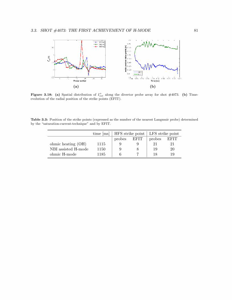
3.3. SHOT #4073: THE FIRST ACHIEVEMENT OF H-MODE 81
(a) (b)
Figure 3.18: (a) Spatial distribution of I+sat along the divertor probe array for shot #4073. (b) Time-evolution of the radial position of the strike points (EFIT).
Table 3.3: Position of the strike points (expressed as the number of the nearest Langmuir probe) determinedby the “saturation-current-technique” and by EFIT.
time [ms] HFS strike point LFS strike point
probes EFIT probes EFITohmic heating (OH) 1115 9 9 21 21NBI assisted H-mode 1150 9 8 19 20ohmic H-mode 1185 6 7 18 19

82 CHAPTER 3. H-MODE OPERATION IN COMPASS
3.4 Shot #4267: first shot after cleaning
This is an interesting shot, because it is the first shot that is performed after a GDC of thevacuum vessel. We expect a clear reduction in the amount of impurities.
3.4.1 Preset parameters
Again, we summarize the basic preset parameters and compare them with the measuredplasma current and plasma position.
• Gas puff: 930-1100ms
• NBI2: 1120-1175ms (40kV, 9.7A, 302.6kW upper bound)
• breakdown: 959ms
• flat-top phase: 1011-1173ms
• end of the discharge: 1174ms
Figure 3.19: Plots of plasma current, vertical position and radial position of the plasma center relative tothe center of the COMPASS vessel (R=0.56m, Z=0m) for shot #4267. The measured values as well as thepreset wave forms are shown. Also the time intervals when the gas puff and NBI were active, are indicated.
3.4.2 Spectroscopy
Due to the preliminary cleaning all radiation intensities are very low. The L-H transition isnow almost invisible in the Dα radiation. According to the All Vis signal it occurs aroundt=1110ms. Almost no impurity accumulation is observed. There are several ELMs: about10 small ELMs with a frequency of 1kHz and thereafter 16 bigger ELMs with a frequency of0.3kHz. The repetition rate decreases at t = 1128ms, a few milliseconds after the activation ofthe NBI. This negative relation between the repetition rate and the coupled power indicatesthat these are type-3 ELMs. The shot ends with a disruption at t = 1174ms. The hardx-rays appear again when the NBI is turned on. There also is a HXR spike around the L-Htransition. The SXR data again shows the typical sawtooth oscillations. According to Figure3.19, the plasma center is displaced by ∆Z = +5mm and ∆R = −8mm. An estimation ofthe q=1 surface is drawn in Figure 3.20c. Its radius is about 80mm. According to EFIT, theq=1 surface intersects the mid-plane at R ≈ 0.52m and at R ≈ 0.60m (see Figure 3.20d),which means that the radius should be about 40mm according to EFIT. We however alreadyknow that EFIT is not 100% correct. On the other hand, the smaller radius could be an

3.4. SHOT #4267: FIRST SHOT AFTER CLEANING 83
(a) (b)
(c) (d)
Figure 3.20: (a) Spectroscopic data of #4267. The yellow area indicates the NBI. (b) Soft x-ray radiationfor shot #4267. The data is not detrended. All signals are on the same scale (order of magnitude 1µW).The impurity accumulation is clearly visible. The graph is flat at the end because the intensity exceeds thephotodiode’s maximum. (c) Reconstruction of the q=1 surface at t > 1120ms. (d) Radial distribution of thesafety factor q in the mid-plane calculated by EFIT.
indication that the q=1 surface is not circular but rather elliptical, as could be expected foran elongated plasma.
3.4.3 Electron density
The electron density is low. There even are no fringe jumps. Between the gas puff andthe NBI activity, the density drops, since there is no external source that adds particlesto the plasma10. Somewhere in this time interval without gas puff or NBI, namely aroundt = 1110ms, the spectroscopic signals show improved confinement: H-mode is already reachedwithout the help of NBI heating. The shot is never in L-mode. There is no significant increaseof the electron density during H-mode.
10The behaviour of shot #4073 was rather exceptional.
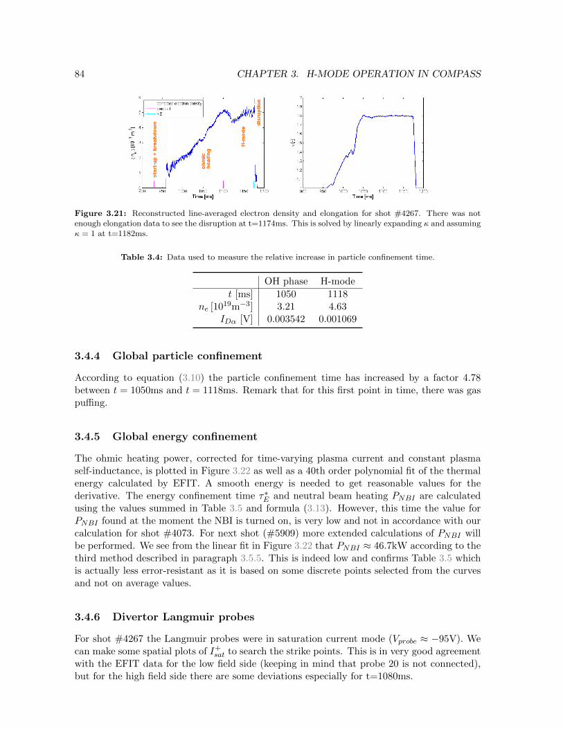
84 CHAPTER 3. H-MODE OPERATION IN COMPASS
Figure 3.21: Reconstructed line-averaged electron density and elongation for shot #4267. There was notenough elongation data to see the disruption at t=1174ms. This is solved by linearly expanding κ and assumingκ = 1 at t=1182ms.
Table 3.4: Data used to measure the relative increase in particle confinement time.
OH phase H-mode
t [ms] 1050 1118ne [1019m−3] 3.21 4.63
IDα [V] 0.003542 0.001069
3.4.4 Global particle confinement
According to equation (3.10) the particle confinement time has increased by a factor 4.78between t = 1050ms and t = 1118ms. Remark that for this first point in time, there was gaspuffing.
3.4.5 Global energy confinement
The ohmic heating power, corrected for time-varying plasma current and constant plasmaself-inductance, is plotted in Figure 3.22 as well as a 40th order polynomial fit of the thermalenergy calculated by EFIT. A smooth energy is needed to get reasonable values for thederivative. The energy confinement time τ∗E and neutral beam heating PNBI are calculatedusing the values summed in Table 3.5 and formula (3.13). However, this time the value forPNBI found at the moment the NBI is turned on, is very low and not in accordance with ourcalculation for shot #4073. For next shot (#5909) more extended calculations of PNBI willbe performed. We see from the linear fit in Figure 3.22 that PNBI ≈ 46.7kW according to thethird method described in paragraph 3.5.5. This is indeed low and confirms Table 3.5 whichis actually less error-resistant as it is based on some discrete points selected from the curvesand not on average values.
3.4.6 Divertor Langmuir probes
For shot #4267 the Langmuir probes were in saturation current mode (Vprobe ≈ −95V). Wecan make some spatial plots of I+sat to search the strike points. This is in very good agreementwith the EFIT data for the low field side (keeping in mind that probe 20 is not connected),but for the high field side there are some deviations especially for t=1080ms.

3.4. SHOT #4267: FIRST SHOT AFTER CLEANING 85
Figure 3.22: Left : Ohmic heating power. We assume L = 1µH. Right : Thermal energy calculated by EFIT.
Table 3.5: Data used to calculate the energy confinement time and NBI power.
OH phase ohmic H-mode start NBI NBI H-mode
t [ms] 1040.6 1115.1 1120 1139.9W [kJ] 4.408 3.611 3.638 4.586
dWdt [kW] -103.2 -3.957 25.55 25.16
POH [kW] 325.9 224.1 229.1 240PNBI [kW] 0 0 26.27 26.27
τ∗E [ms] 10.27 15.83 15.83 19.02
(a) (b)
Figure 3.23: (a) Spatial distribution of I+sat along the divertor probe array for shot #4267. Probes 1, 20, 36and 39 are not connected. The data is averaged over 1ms. (b) Time-evolution of the radial position of thestrike points (EFIT).
Table 3.6: Position of the strike points (expressed as the number of the nearest Langmuir probe) determinedby the “saturation-current-technique” and by EFIT.
time [ms] HFS strike point LFS strike point
probes EFIT probes EFITohmic heating (OH) 1080 7 11 19 20NBI assisted H-mode 1120 11 10 19 20ohmic H-mode 1160 9 8 19 19

86 CHAPTER 3. H-MODE OPERATION IN COMPASS
3.4.7 Thomson scattering
The Thomson scattering device measures the Te and ne profiles along the vertical chord. Thevertical distributions of Te and ne for shot #4267 are shown in Figure 3.24 for four differentvalues of t around the L-H transition. We note in particular the increase in temperature of thecore plasma for t > 1110ms. It seems that the maximum pedestal height is reached earlier bythe electron density than by the electron temperature. The particle barrier is formed fasterthan the energy barrier.
(a) (b)
Figure 3.24: Vertical distribution of (a) the electron temperature and(b) the electron density according toThomson scattering.
One is able to map these vertical profiles to the mid-plane by using the EFIT reconstruction11.The radial profile of Te in the core plasma is well fitted by a modified Gauss function (mgauss)
F = Te,P + (Te,0 − Te,P )e−(
rWC
)1+W2C
(3.17)
while the radial profile of Te in the pedestal is fitted by
F =Te,P − Te,SOL
2
[mtanh
(M − r2WP
, s
)+ 1
]+ Te,SOL (3.18)
where the modified hyperbolic tangent (mtanh) is defined as
mtanh(x, y) =(1 + xy)ex − e−x
ex + e−x(3.19)
and with
r the horizontal distance with respect to the plasma center, not a parameter but thevariable on the horizontal axis
Te,0 the electron temperature at the plasma center (ψn = 0)
Te,P the electron temperature at the “knee” of the pedestal
11This is reflected in the ψn (pronounced “psi”) on the horizontal axis of Figure 3.25, which is a normalizedform of the poloidal flux function introduced in paragraph 2.5.2. The generally used normalization is: ψn = 0in the plasma center and ψn = 1 on the separatrix.

3.4. SHOT #4267: FIRST SHOT AFTER CLEANING 87
Te,SOL the electron temperature at the scrape-off layer, i.e. the plasma region with openfield lines (see Figure 2.1). This parameter is an offset value and is often fixed to zero.
WC the width of the plasma core (achieved by for example least squares fitting)
WP the width of the pedestal, approximately given by the horizontal distance betweenthe “knee” and the separatrix (ψn = 1)
M the pedestal position read from the horizontal axis, which is approximately given bythe middle of the segment defined by WP
s the slope of the mtanh where it connects to the core profile
The mgauss-fit for the core plasma is invented by E. Stefanikova and M. Peterka, who bothwork at the IPP. The mtanh-fit of the pedestal was already described in the literature. At themoment, they are working on an improved version of their fitting code that will automaticallygenerate a smooth transition between the mgauss and the mtanh. Now, they are connectedby using weighted averages which is not optimal. The corresponding fit for shot #4267 att = 1165ms is drawn in Figure 3.25. [49] [84]
(a) (b)
(c) (d)
Figure 3.25: Radial distribution of the electron temperature Te and electron density ne measured by Thomsonscattering. The fitting parameters are indicated in figures (a) and (b).

88 CHAPTER 3. H-MODE OPERATION IN COMPASS
3.5 Shot #5909: NBI power calculations
This shot is interesting to make an estimation of the NBI power absorbed by the plasma:there are three short NBI pulses in a row and more accurate data about POH is available.Further, the ball-pen probes were activated for this shot. This is interesting to check theELMs in another way.
3.5.1 Preset parameters
Again, we summarize the basic preset parameters and compare them with the measuredplasma current and plasma position.
• Gas puff: 970-1060ms
• NBI1: 1060-1069ms, 1076-1084ms, 1091-1105ms (250kW upper bound)
• breakdown: 959ms
• flat-top phase: 1073-1122ms
• end of the discharge: 1122.5ms
Figure 3.26: Plots of plasma current, vertical position and radial position of the plasma center relative tothe center of the COMPASS vessel (R=0.56m, Z=0m) for shot #5909. The measured values as well as thepreset wave forms are shown. Also the time intervals when the gas puff and NBI were active, are indicated.
3.5.2 Spectroscopy
The L-H transition takes place around t=1065ms. This shot shows about 15 clear ELMs.There is no recognizable period between the ELMs, probably due to the on and off switchingof the NBI. The discharge ends with a disruption.
3.5.3 Electron density
This time, the fringe jumps really cause big problems to reconstruct the line-averaged electrondensity: the jumps are incomplete (see red part in Figure 3.27d), which destroys the algorithm.The triggered signal (green curve) looks the best one for this shot. However, Figure 3.27bshows an unrealistic spike right before the disruption. It is caused by the fact that the densitydata remains high while the elongation is already dropping. There is probably an error in thedensity data: there are no fringe jumps that bring the curve back to the actual zero.

3.5. SHOT #5909: NBI POWER CALCULATIONS 89
(a) (b)
(c) (d) (e)
Figure 3.27: (a) Spectroscopic data of #5909. The yellow area indicates the NBI. (b) Reconstructed line-averaged electron density shot #5909. The spike at the end seems to be incorrect. (c) Raw line-averagedelectron density divided by κmax = 1.8. (d) Incomplete fringe jump in 6xAD8302 interferometer signal.(e) Plasma elongation calculated by EFIT, linearly extrapolated by making the assumption that κ = 1 att = 1131ms.
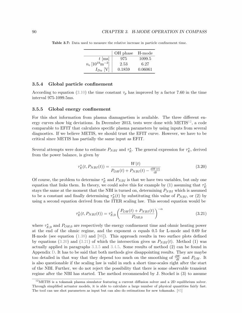
90 CHAPTER 3. H-MODE OPERATION IN COMPASS
Table 3.7: Data used to measure the relative increase in particle confinement time.
OH phase H-mode
t [ms] 975 1099.5ne [1019m−3] 2.53 6.27
IDα [V] 0.1859 0.06061
3.5.4 Global particle confinement
According to equation (3.10) the time constant τp has improved by a factor 7.60 in the timeinterval 975-1099.5ms.
3.5.5 Global energy confinement
For this shot information from plasma diamagnetism is available. The three different en-ergy curves show big deviations. In December 2013, tests were done with METIS12, a codecomparable to EFIT that calculates specific plasma parameters by using inputs from severaldiagnostics. If we believe METIS, we should trust the EFIT curve. However, we have to becritical since METIS has partially the same input as EFIT.
Several attempts were done to estimate PNBI and τ∗E . The general expression for τ∗E , derivedfrom the power balance, is given by
τ∗E(t, PNBI(t)) =W (t)
POH(t) + PNBI(t)− dW (t)dt
(3.20)
Of course, the problem to determine τ∗E and PNBI is that we have two variables, but only oneequation that links them. In theory, we could solve this for example by (1) assuming that τ∗Estays the same at the moment that the NBI is turned on, determining PNBI which is assumedto be a constant and finally determining τ∗E(t) by substituting this value of PNBI , or (2) byusing a second equation derived from the ITER scaling law. This second equation would be
τ∗E(t, PNBI(t)) = τ∗E,0
(POH(t) + PNBI(t)
POH,0
)−α(3.21)
where τ∗E,0 and POH,0 are respectively the energy confinement time and ohmic heating powerat the end of the ohmic regime, and the exponent α equals 0.5 for L-mode and 0.69 forH-mode (see equation (1.38) and [86]). This approach results in two surface plots definedby equations (3.20) and (3.21) of which the intersection gives us PNBI(t). Method (1) wasactually applied in paragraphs 3.3.5 and 3.4.5. Some results of method (2) can be found inAppendix D. It has to be said that both methods give disappointing results. They are maybetoo detailed in that way that they depend too much on the smoothing of dW
dt and POH . Itis also questionable if the scaling law is valid in such a short time-scales right after the startof the NBI. Further, we do not reject the possibility that there is some observable transientregime after the NBI has started. The method recommended by J. Stockel is (3) to assume
12METIS is a tokamak plasma simulator featuring a current diffusion solver and a 2D equilibrium solver.Through simplified actuator models, it is able to calculate a large number of physical quantities fairly fast.The tool can use shot parameters as input but can also do estimations for new tokamaks. [85]
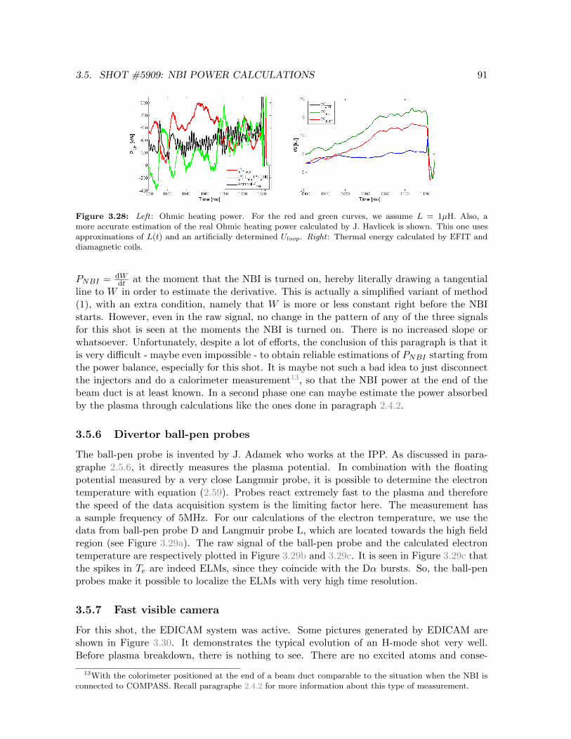
3.5. SHOT #5909: NBI POWER CALCULATIONS 91
Figure 3.28: Left : Ohmic heating power. For the red and green curves, we assume L = 1µH. Also, amore accurate estimation of the real Ohmic heating power calculated by J. Havlicek is shown. This one usesapproximations of L(t) and an artificially determined Uloop. Right : Thermal energy calculated by EFIT anddiamagnetic coils.
PNBI = dWdt at the moment that the NBI is turned on, hereby literally drawing a tangential
line to W in order to estimate the derivative. This is actually a simplified variant of method(1), with an extra condition, namely that W is more or less constant right before the NBIstarts. However, even in the raw signal, no change in the pattern of any of the three signalsfor this shot is seen at the moments the NBI is turned on. There is no increased slope orwhatsoever. Unfortunately, despite a lot of efforts, the conclusion of this paragraph is that itis very difficult - maybe even impossible - to obtain reliable estimations of PNBI starting fromthe power balance, especially for this shot. It is maybe not such a bad idea to just disconnectthe injectors and do a calorimeter measurement13, so that the NBI power at the end of thebeam duct is at least known. In a second phase one can maybe estimate the power absorbedby the plasma through calculations like the ones done in paragraph 2.4.2.
3.5.6 Divertor ball-pen probes
The ball-pen probe is invented by J. Adamek who works at the IPP. As discussed in para-graphe 2.5.6, it directly measures the plasma potential. In combination with the floatingpotential measured by a very close Langmuir probe, it is possible to determine the electrontemperature with equation (2.59). Probes react extremely fast to the plasma and thereforethe speed of the data acquisition system is the limiting factor here. The measurement hasa sample frequency of 5MHz. For our calculations of the electron temperature, we use thedata from ball-pen probe D and Langmuir probe L, which are located towards the high fieldregion (see Figure 3.29a). The raw signal of the ball-pen probe and the calculated electrontemperature are respectively plotted in Figure 3.29b and 3.29c. It is seen in Figure 3.29c thatthe spikes in Te are indeed ELMs, since they coincide with the Dα bursts. So, the ball-penprobes make it possible to localize the ELMs with very high time resolution.
3.5.7 Fast visible camera
For this shot, the EDICAM system was active. Some pictures generated by EDICAM areshown in Figure 3.30. It demonstrates the typical evolution of an H-mode shot very well.Before plasma breakdown, there is nothing to see. There are no excited atoms and conse-
13With the colorimeter positioned at the end of a beam duct comparable to the situation when the NBI isconnected to COMPASS. Recall paragraphe 2.4.2 for more information about this type of measurement.

92 CHAPTER 3. H-MODE OPERATION IN COMPASS
(a)(b)
(c)
Figure 3.29: (a) Ball-pen probes and Langmuir probes in a divertor tile. (b) Raw floating potential datafrom ball-pen probe D. (c) Electron temperature in the divertor area (HFS) measured by ball-pen probe Dand Langmuir probe L, smoothed by a factor 1000. ELMs are visible in the (divertor) electron temperatureand in the Dα radiation.
(a) t = 985.7ms (b) t = 1001.6ms (c) t = 1041.4ms
(d) t = 1062.6ms (e) t = 1107.7ms (f) t = 1126.3ms
Figure 3.30: (a) circular plasma shape, (b) plasma is elongated, (c) plasma is further elongated and touchesthe divertor, (d) plasma reaches H-mode, (e) plasma-wall interactions, (f) disruption

3.5. SHOT #5909: NBI POWER CALCULATIONS 93
quently there is no visible radiation. Suddenly, there is a flash. This first light is more orless homogeneous, but very quickly a circular shape is formed. This circle is elongated untilthe plasma touches the divertor, which can be seen as a bright strip at the bottom of thepictures. Then suddenly, the boundaries of the plasma are very sharp: H-mode is reached.The plasma is now visibly very good confined. The plasma boundary is significantly sharperat the HFS in H-mode. This could be a sign that this region has an increased density gradient.During H-mode, some plasma-wall interactions happen and are well captured by EDICAM.Sometimes the whole picture is very bright for a short time. This is probably due to ELMs.Finally, a lot of plasma-wall interactions happen and the shot ends. This is the disruption.

94 CHAPTER 3. H-MODE OPERATION IN COMPASS
3.6 Shot #6109: H-L transition
Some of the recent shots, namely #6105, #6106, #6108, #6109, #6110, #6131, #6135,#6146 and #6147, show extraordinary behaviour: for some reason, the plasma goes fromH-mode to L-mode. It is interesting to examine one of these shots.
3.6.1 Preset parameters
Again, we summarize the basic preset parameters and compare them with the measuredplasma current and plasma position.
• Gas puff: 970-1100ms
• NBI2: 1120-1240ms (40kV,10A, 312kW upper bound)
• breakdown: 959ms
• flat-top phase: 1035-1160ms
• end of the discharge: 1244ms
Figure 3.31: Plots of plasma current, vertical position and radial position of the plasma center relative tothe center of the COMPASS vessel (R=0.56m, Z=0m) for shot #6109. The measured values as well as thepreset wave forms are shown. Also the time intervals when the gas puff and NBI were active, are indicated.Remark that the radial plasma position deviates from the preset wave form.
3.6.2 Spectroscopy
Looking at the Dα signal, we clearly observe different phases. First the Dα radiation is flatand relatively low. This is L-mode. At t=1133.5ms, the plasma goes over to H-mode, whichis visible as a sudden drop in the Dα radiation. At, t=1168.5ms, the plasma falls back toL-mode preceded by a big spike in the Dα radiation. At t=1197ms, H-mode is reached again.Finally, at t=1244ms, the discharge ends with a disruption. We note that aside from theexpected impurity accumulation, there also clearly is an increase in the fuel particles. Thiscan be explained by the long activity of the NBI, which actually adds fuel particles to theplasma. The HXR signal gives away the time when the NBI was started. The H-L transi-tion occurs together with the start of the current ramp-up. Maybe this is a trigger. Thishypothesis is however investigated for the other shots that show H-L transitions and most ofthe time the current was in flat-top phase during these events. Plausible explanations for theH-L transition are the impurity accumulation, or the occurrence of a giant (type-1) ELM, ora combination of both.

3.6. SHOT #6109: H-L TRANSITION 95
(a) (b)
(c)
(d)
Figure 3.32: (a) Spectroscopic data of #6109. The yellow area indicates the NBI. (b) Soft x-ray radiationfor shot #6109. The data is detrended and smoothed. All signals are on the same scale. The vertical distancebetween two consecutive signals is 1.6µW. (c) Reconstruction of the q=1 surface at t > 1170ms. (d) Radialdistribution of the safety factor q in the mid-plane calculated by EFIT.
The SXR signals again show sawtooth oscillations. A reconstruction of the q=1 surface isrepresented in Figure 3.32c. The plasma center is shifted by ∆Z = +20mm and ∆R = +5mmand the inversion happens at photodiodes 21 and 31. In the approximation of a circular q=1surface, we find a radius of about 70mm this way. This time, our estimation is consistentwith EFIT. Figure 3.32d shows that according to EFIT, the q=1 surface should intersect theZ = 0 line at R ≈ 0.496m and R ≈ 0.646m. This is more or less what we see on Figure 3.32c.
3.6.3 Electron density
Again, the triggered interferometer signal (green curve) seems to be the best choice, butunfortunately there are again some errors in this data because fringe jumps are missing atthe end to let the signal go to the actual zero. It was very difficult to reconstruct the electrondensity for this shot. After the H-L transition, the data shows strange behaviour. Comparingto what happens with the blue curve, we decided that the density drops about 1 · 1019m−3
after the H-L transition. This should not surprise you, since a lower confinement goes handin hand with a lower electron density.

96 CHAPTER 3. H-MODE OPERATION IN COMPASS
(a)(b)
Figure 3.33: (a) Raw line-averaged electron density divided by κmax = 1.8 for the three different ambiguousinterferometer signals. (b) Plasma elongation calculated by EFIT. There was not enough elongation data tosee the disruption at t=1244ms. This is solved by linearly expanding κ and assuming κ = 1 at t=1250ms.
Figure 3.34: Reconstructed electron density for shot #6109.

3.6. SHOT #6109: H-L TRANSITION 97
Figure 3.35: Left : Ohmic heating power. We assume L = 1µH. Right : Thermal energy calculated by EFITand diamagnetic coils.
3.6.4 Global particle confinement
Since we are not sure about the density data after the H-L transition, we only compare τp’sbefore t=1169ms. According to equation (3.10) the time constant τp has only improved bya factor 1.51 in the time interval 1083-1157.5.5ms. This may be related to the steep linearincrease of Dα radiation during H-mode.
Table 3.8: Data used to measure the relative increase in particle confinement time.
OH phase H-mode
t [ms] 1083 1157.5ne [1019m−3] 5.92 7.63
IDα [V] 0.1167 0.09963
3.6.5 Global energy confinement
This time all three energy signals clearly show an increased slope when the NBI is switchedon at t = 1120ms. So, we can apply the third method based on the time-derivative of thethermal energy in order to estimate PNBI . According to Figure 3.35, we find this way:
PEFITNBI ≈ 100.3kW
P diaNBI ≈ 151.8kW
P diaBTNBI ≈ 146.3kW
3.6.6 Fast Visible Camera
Some frames captured by EDICAM are shown in Figure 3.36. We see how the plasma origi-nally had a circular shape, is elongated, touches the divertor, reaches the first L-mode followedby the first H-mode, emits more visible radiation at the end of H-mode compared to the be-ginning,... Unfortunately the system stopped recording after the first H-mode. There arestrong plasma-wall interactions at the poloidal rings during several milliseconds. Maybe, theboron layer was not so good there.
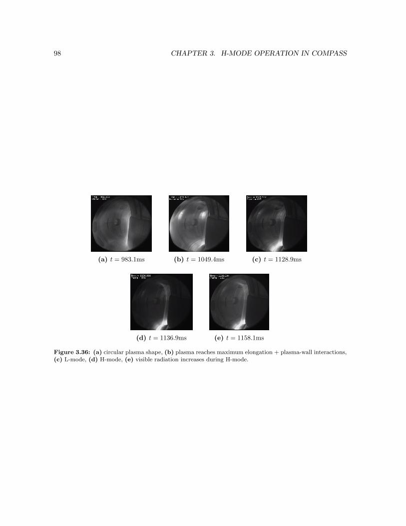
98 CHAPTER 3. H-MODE OPERATION IN COMPASS
(a) t = 983.1ms (b) t = 1049.4ms (c) t = 1128.9ms
(d) t = 1136.9ms (e) t = 1158.1ms
Figure 3.36: (a) circular plasma shape, (b) plasma reaches maximum elongation + plasma-wall interactions,(c) L-mode, (d) H-mode, (e) visible radiation increases during H-mode.

3.7. SHOT #6313: OHMIC H-MODE 99
3.7 Shot #6313: ohmic H-mode
During this shot, H-mode was achieved without the help of extra heating by NBI.
3.7.1 Preset parameters
Again, we summarize the basic preset parameters and compare them with the measuredplasma current and plasma position.
• Gas puff: 970-1200ms
• NBI: no
• breakdown: 959ms
• flat-top phase: 1072-1168.5ms
• end of the discharge: 1170ms
Figure 3.37: Plots of plasma current, vertical position and radial position of the plasma center relative tothe center of the COMPASS vessel (R=0.56m, Z=0m) for shot #6313. The measured values as well as thepreset wave forms are shown. Also the time intervals when the gas puff and NBI were active, are indicated.
3.7.2 Spectroscopy
The L-H transition happens at t=1077ms. This is followed by five small ELMs, an ELM-freepart of about 20 milliseconds, 13 ELMs with increasing repetition frequency - starting with200Hz which is pretty low - and finally a disruption which ends the discharge. The totalvisible radiation indicates the presence of impurities. The discharge ends with a disruptionat t = 1170ms. The HXR signal is zero except at the L-H transition and at disruption.Apparently, there was a problem with the data acquisition during this shot. The SXR signalsare all flat and incorrect. What we would expect is a signal that increases during H-modedue to the impurity accumulation and that does not show sawtooth oscillations, becausesawtooth oscillations are related to additional heating. These expectations are confirmed bythe examination of several other ohmic H-mode signals without NBI.
3.7.3 Electron density
Only the 6xAD8302 interferometer measurement was successful for this shot. Unfortunately,this signal shows again incomplete fringe jumps, and so the whole density profile could not

100 CHAPTER 3. H-MODE OPERATION IN COMPASS
Figure 3.38: Spectroscopic data of shot #6313.
(a)(b)
Figure 3.39: (a) Raw line-averaged electron density divided by κmax = 1.8 for the three different ambiguousinterferometer signals. (b) Plasma elongation calculated by EFIT.
be reconstructed. However, the transition to H-mode is very clear: after a small drop, theelectron density starts to rise very steeply as high confinement is achieved.
3.7.4 Global particle confinement
Again, the known density data is limited, so we are forced to search a point in time nearby theL-H transition with approximately dne
dt ≈ 0. According to equation (3.10) the time constantτp has improved by a factor 8.67 in the small time interval 1041.1-1085.1ms. This is mainlycaused by a huge relative drop in IDα.
Table 3.9: Data used to measure the relative increase in particle confinement time.
OH phase H-mode
t [ms] 1041.1 1085.1ne [1019m−3] 5.13 5.76
IDα [V] 0.4227 0.05474

3.7. SHOT #6313: OHMIC H-MODE 101
Figure 3.40: Reconstructed line-averaged electron density. It is too difficult to reconstruct the whole curvedue to incomplete fringe jumps.
3.7.5 Global energy confinement
The ohmic heating power as well as the energy confinement time are estimated for this shot.This time, the NBI was not active so there is no unknown term and the power balance isexactly solvable. Further, the neo-Alcator scaling relation is checked for this shot. Thisempirical relation claims that the energy confinement time of ohmic discharges increaseslinearly with electron density for low densities
τE [ms] = 6.6 aR2 q95√κ 〈ne,19〉 (3.22)
until it saturates to the valueτE,s [ms] = 64 aRBt
√κ (3.23)
Our density data of this shot is only known for t < 1089ms. Further, we only look at points fort > 1072ms so that the plasma is in flat-top phase14 and has reached its equilibrium positionand maximum elongation. In this time window holds that a ≈ 0.185m, R ≈ 0.55m, q95 ≈ 3.0,κ ≈ 1.8 and Bt ≈ 1.21T. Indeed, a new variable appeared in equation (3.22), namely q95.This is the safety factor at the 95% flux surface, i.e. at the plasma edge. The resultingτ∗E(〈ne〉)-plot is shown in Figure 3.42a. Here, τ∗E was computed using equation (3.24). Inother words, it was taken from Figure 3.41c.
τ∗E =WEFIT
Ip
(Uloop − LdIp
dt
)− dWEFIT
dt
(3.24)
In COMPASS’ former life at Culham, the same plot was made. At that time, the energyconfinement time was calculated using equation (3.25)15.
τE =Wdia
IpUloop − dWdiadt
(3.25)
14Our estimation of POH is more or less correct in this case.15So, note that τE in Figure 3.42b actually denotes τ∗E , i.e. the radiation losses due to bremsstrahlung are
included, but to be consistent with this figure the same notation is used here.

102 CHAPTER 3. H-MODE OPERATION IN COMPASS
(a) (b)
(c) (d) (e)
Figure 3.41: (a) Ohmic heating power, assuming L = 1µH. (b) Thermal energy calculated by EFIT anddiamagnetic coils. (c)-(e) τ∗E versus time calculated in three different ways.
If we compare the neo-Alcator curves for both plots (now and in Culham, see Figure 3.42b),we see that the saturation occurs at higher density and higher confinement time. This up-ward shift can be explained as follows: Nowadays, COMPASS is running in a Single NullTriangularity (SNT) configuration, where the plasma takes up most of the volume in thevacuum vessel, whereas in Culham COMPASS was running in a Single Null Divertor (SND)configuration with a much smaller plasma volume and by consequence a smaller confinementtime. Further, we observe some similarities: Most of the data points exceed neo-Alcator,and the energy confinement time is highest for ELM-free H-mode and lowest in OH regime.But also some differences occur: The ELMy regime is for example clearly distinguishablefrom OH regime in Figure 3.42a while this is not the case for Figure 3.42b. This is prob-ably because only a very limited amount of data was used here, and only for one shot. [69] [87]
We note from Figures 3.41c, 3.41d and 3.41e that if we use the more accurate formula forPOH , non-physical values appear in the beginning of the discharge when the flat-top phase isnot reached yet and
dIpdt can fluctuate a lot. On the other hand, we note that Figure 3.41c
has the best vertical scale to fit the neo-Alcator relation (see Figure 3.42a). Especially thevalues for τ∗E resulting from diamagnetism measurements are much too big. So, an exactcomparison between the data derived from diamagnetism for both Culham and the IPP isnot possible. Also remark that if the less correct formula for the ohmic heating power is used,namely POH = IpUloop, a clear increase in the energy confinement time is observed aroundthe transition to H-mode.

3.7. SHOT #6313: OHMIC H-MODE 103
(a) (b)
Figure 3.42: (a) τ∗E versus 〈ne〉 for t ∈ [1072ms, 1089ms] and the neo-Alcator scaling law (black line). Theinterval only contains one ELM. (b) The same graph when COMPASS was still in Culham (L-mode hereactually denotes ohmic regime). [69]
Figure 3.43: ELMs visible in the (divertor) electron temperature and in the Dα radiation.
3.7.6 Divertor ball-pen probes
During this shot, the ball-pen probes were active which means that we can again make a plotof the electron temperature on the HFS divertor plates. The ELMs are very good visible (seeFigure 3.43). From analysing both Figure 3.29c and 3.43, we can state that there is almost nocorrelation between the height of the Dα bursts and the height of the Te spikes. The electrontemperature is a measure for the energy of the ELM plasma when it hits the divertor plates,while the spikes in the Dα radiation are a measure for the amount of neutral gas in front ofthe divertor plates that is excited due to the ELMs. So, to excite a lot of neutral gas andcreate a large Dα burst, the ELM has to give up a lot of its energy and by consequence thetemperature registered by the divertor plates will be lower. On the other hand, the ELMneeds to have enough energy and the neutral gas has to be dense enough to create manyexcitations. This could explain why we do not observe a clear correlation.
104 CHAPTER 3. H-MODE OPERATION IN COMPASS
3.8 Conclusion
3.8.1 ELMs
There is unclarity about the type of ELMs observed in COMPASS. In the past, when COM-PASS was still in Culham, there were type-1 and type-3 ELMs. However, now at the IPPin Prague, COMPASS is running in SNT configuration with high triangularity and so itwould not be so strange if also type-2 ELMs appeared. Unfortunately, these are difficult todistinguish from type-3 ELMs. The ELMs of some of the last shots such as #6316, whichis analysed in the next chapter, have a frequency that increases with the power across theseparatrix. These could be type-1 ELMs. Most of the observed ELMs at the IPP are thoughtto be type-3 ELMs.
3.8.2 Impurities
It is notable that somehow impurities are accumulated during H-mode. This effect evenoccurs in the first shots after glow discharge cleaning, although it is much smaller than forother shots. Together with the fact that the impurity accumulation also exists during ohmicH-mode, this tells us that the impurities originate from the vessel wall rather than from theneutral beam injectors. The impurities are not only observed in the All Vis signal but also inthe AXUV signals as can be seen for example in Figure 3.44. This is the radiation rangingfrom UV light to soft x-rays that is captured by fast bolometers. The line of sight of thedifferent AXUV bolometer chips is shown in Figure 2.17b. The chosen bolometers point tothe plasma core. Chips D and F are in the divertor region and by consequence their data ishigher in magnitude. Figure 3.44a nicely shows the ELMs in the AXUV F 10 signal. Figure3.44b clearly illustrates how fast the impurities are lost when H-mode is terminated. Thislinear accumulation of impurities is clearly something typical for H-mode. The impuritiesreleased by the vessel wall enter the plasma but have a difficult time leaving the plasma againbecause they are so well confined. They emit bremsstrahlung due to their acceleration in theelectromagnetic fields. It is often thought that these radiation losses induce the disruptionthat ends the discharge. All shots discussed in this chapter end with a disruption, but this iscertainly not always the case. On the other hand, a lot of other possible causes exist for thesedisruptions. Finally, remark that one has to be careful with the interpretation of the AXUV
signals. As they contain SXR radiation they are possibly proportional to n2eT1/2e Zeff along
their line of sight. The temperature dependence is low enough, but it has to be investigated ifthe increase of the signals can be attributed to increasing plasma density or to accumulationof impurities. Nevertheless, there are enough examples here above where the All Vis radiationas well as the AXUV signals are rising while the density is more or less constant. Therefore,the AXUV signals are interpreted as accumulation of impurities.
3.8.3 Particle and energy confinement
In the literature, H-mode is characterized by an increase in particle as well as energy confine-ment. This last property is one of our goals in improving the triple product. The improvedparticle confinement, however, has some disadvantageous consequences. It is the basis ofimpurity accumulation in the plasma core during H-mode.

3.8. CONCLUSION 105
(a) (b)
Figure 3.44: AXUV signals of (a) shot #4267 and (b) shot #6109.
The improved particle confinement has been demonstrated for all five shots. For every shotexcept #6109, the particle confinement time increases by a factor 4 or more. The improvementin energy confinement is less drastic. Energy confinement times lay typically between 10 and30 milliseconds16. The expected improvement due to H-mode is not well observed. In the firstfour shots, the NBI could be blamed for this, but also in the last shot with ohmic H-modeno real improvement is established. It has to be mentioned that the data available for thecalculations were not optimal: the thermal energy, the NBI power as well as the ohmic heatingpower17 are uncertain. The lack of a big increase in τ∗E can also be explained physically bythe presence of high radiation losses due to impurity accumulation. These losses could beresponsible for a decrease in τ∗E which cancels out the effect of H-mode. However, as we cansee from the spectroscopic data, this impurity accumulation happens linearly. This kind oflinear behaviour cannot be found back in graphs of τ∗E .
3.8.4 NBI
The exact NBI power is a mystery at the moment. The reason why was already explained inparagraph 2.4.2. Only an upper bound determined by the preprogrammed current of the ionsource and the voltage over the accelerating grids is known. The fraction of this upper boundthat is really transferred to the plasma was estimated in this chapter to be 15-65% (see Table3.11).
Table 3.10: Fraction of NBI power captured by the palsma (based on EFIT data).
upper bound [kW] estimation [kW] fraction [-]#4073 202.8 129.3 63.8%#4267 302.6 46.7 15.4%#6109 312 100.3 32.1%
3.8.5 Thermal energy
A similar problem exists for the thermal energy W . Together with the NBI power, thisquantity is important to solve the energy balance and to determine the energy confinement
16If EFIT data is used for the energy, otherwise it is higher (20-100ms).17Since we do not know the plasma self-inductance and actually also not the exact loop voltage.

106 CHAPTER 3. H-MODE OPERATION IN COMPASS
time. However, three different signals are given and it is not yet determined which of themis the best one. For shots #5909, #6109 and #6313, the energy balance was solved for all ofthem and every time EFIT came out as “winner”. Actually, none of them gave really goodresults, but the values found for the confinement time based on the diamagnetic energieswere the worst. They gave extremely high or even negative confinement times. Furthermore,METIS - another code that calculates amongst others the thermal energy - also confirms thatEFIT gives the best results.
3.8.6 H-mode threshold power
The H-mode threshold power lost through the separatrix is calculated as
Pth = POH + PNBI −dW
dt(3.26)
Since the NBI power is unknown, we will estimate it to be 40% of the upper bound specifiedby the settings of the tokamak operators. The results can be compared to the scaling law,adopted from [88] (Bt = 1.2T, a = 0.20m, R = 0.56m).
P scth [MW] = 2.15 〈ne,20〉0.78B0.77t a0.96R ≈ 0.296 〈ne,20〉0.78 (3.27)
The resemblance between the scaling law and the measured Pth is very bad.
Table 3.11: H-mode threshold power calculation.
POH [kW] PNBI [kW] dWdt [kW] 〈ne,20〉 [1020m−3] Pth [kW] P scth [kW]
#4073 234.5 81.1 35.3 0.529 280.3 180.1#4267 126.9 121.0 -5.42 0.510 153.32 175.1#5909 311.9 38.52 0.577 192.7#6109 (1) 82.6 124.8 105.2 0.669 102.2 216.3#6109 (2) 75.5 124.8 -3.7 204.0#6313 530.2 0 48.9 0.548 481.3 185.2
3.8.7 Edge pedestal
H-mode is characterized by the presence of an edge pedestal in the radial temperature anddensity profiles. This big temperature gradient is the physical translation of the aimed en-ergy barrier, while the density gradient stands for a particle barrier. These pedestals can beobserved with the Thomson Scattering diagnostic. This has been discussed for shot #4267 to-gether with a formula to fit the radial profile. The pedestal height of the electron temperatureis typically 200-300eV, that of the electron density 4-6·1019m−3 18.
18This has been investigated for several other shots.

Chapter 4
Current spikes
In the autumn of 2013, shots were executed with higher plasma currents due to improvedknow-how of the IPP scientists and technicians. J. Havlicek was the one who discovered aninteresting phenomenon: the plasma current Ip performs distinct spikes of magnitude 1kAand width 0.2ms, often preceded by a drop. It was asked to the writer of this thesis to makesome statistical analysis of these spikes and to come with an idea about the origin of thespikes.
4.1 Qualitative analysis
Various plasma parameters are analysed. The effect of ELMs on them is summed next:
• Dα radiation: bursts indicating the presence of ELMs, see Fig.4.1
• plasma current Ip: big spikes simultaneously observed with ELMs, see Fig.4.1
• diamagnetic energy Wdia: spikes, see Fig.4.1
• poloidal β: drops, see for example Figure 4.2
• line-averaged electron density 〈ne〉: no extraordinary behaviour
• loop voltage from FL1 (mid-plane, HFS): no extraordinary behaviour, see for exampleFigure 4.3
• vertical plasma position: sometimes clear drops, see for example Figure 4.4
• radial plasma position: nothing
• vertical field (IPR1 and IPR9): small disturbances before the ELMs are seen in the Dαradiation
• fast feedback current IBV : no clear correlation (also modulations in ELM-free region)
107

108 CHAPTER 4. CURRENT SPIKES
Figure 4.1: Dα radiation, plasma current and diamagnetic energy of shot #6311.

4.1. QUALITATIVE ANALYSIS 109
Figure 4.2: βp for shot #5943. The sample frequency is 10kHz. The green vertical lines indicate the timesat which ELMs occur according to the Dα radiation. These green lines will return in a lot of other figures.
Figure 4.3: Loop voltage for shot #5943. There is no extraordinary behaviour during ELMs.
Figure 4.4: Vertical position measured by the feedback control system for shot #5905. The sample frequencyis 20kHz.

110 CHAPTER 4. CURRENT SPIKES
ELMs cause by definition drops in the plasma energy. However, it is strange that also spikesoccur. Besides, only the signal of the diamagnetic coil with compensation coil shows ELM-related effects. Perhaps, the EFIT signal is not sampled fast enough to see the small spikes.The other diamagnetic energy signal maybe contains too much noise. However, after sendingthe data of this last one through a low-pass filter, still nothing special is observed.
The drops in βp are probably related to the drops in Wdia. As can be seen from equation(4.1), the poloidal beta depends on the thermal energy of the plasma, the poloidal magneticfield and the plasma volume. The drops in βp are not always that clear, so a quantitativeanalysis of βp was not done.
βp =nkBT
B2p/2µ0
∝ W
B2pV
(4.1)
Further, ELMs are known to cause drops in the vertical position. According to [89] forexample, these drops can be unreal and the consequence of ELMs influencing the verticalposition measurement. In the case of COMPASS the vertical position measurement is doneby internal partial Rogowski coils. ELMs create short-lived magnetic perturbations1 whichcould induce eddy currents in those coils. The observer would think that the plasma wasvertically displaced while there actually was no change. On the other hand, [89] tells thatELMs can also cause real vertical drops of the plasma position owing to modifications of theplasma current profile. In up-down asymmetric configurations, such as the SNT configurationused in COMPASS, these changes in the current profile imply rapid vertical displacements ofthe plasma current centroid.
4.2 Quantitative analysis
The measurement of the plasma current spikes is complicated by the presence of modula-tions with the same order of frequency which are caused by the non-ideal thyristors of thepower supplies. The oscillations caused by the power supplies can be observed in Figure 4.1.Note that there is no correlation between the current spikes and the phase of the modulations.
What follows is an extended analysis of the spikes visible in the Dα radiation, the plasmacurrent and the diamagnetic energy. To this end, a series of short Matlab codes was used.The algorithms for these codes are found in Appendix E. The measured quantities are theabsolute height of the Dα bursts (I denotes intensity here)
∆Dα = IDα,max − IDα,min , (4.2)
the relative height of the current spikes given by
∆Ip,rel =Ip,max − Ip,minIp,average
(4.3)
and the relative height2 of the energy spikes given by
∆Wrel =Wdia,max −Wdia,min
Wdia,average(4.4)
1These are by the way also observed, see the summation above.2Since there is uncertainty about the correctness of the diamagnetic energy data, this is a necessity.

4.2. QUANTITATIVE ANALYSIS 111
Here, Wdia denotes the diamagnetic energy measured by the diamagnetic coil with compensa-tion coil. The results are shown in Figure 4.5 and Figure 4.6. Apparently, there is a positiverelation between the Dα spikes and the current spikes: if one quantity increases, the otherquantity increases too. This is even more true for the relation between the current spikes andthe energy spikes. There is obviously a linear behaviour. The datasets obey following linearfits3:
∆Ip,rel = 0.009 ∆Dα+ 0.0006 R2 = 0.2740 (4.5)
∆Ip,rel = 0.2411 ∆Wrel + 0.0002 R2 = 0.6295 (4.6)
The spikes are four times more dominant in the diamagnetic energy than in the plasma cur-rent.
We however have to be careful with this data. It is sometimes suspected that there is crosstalkbetween the diamagnetic coils and the plasma current. This would explain the nice linearrelation, and why we do not see only drops but also spikes in the diamagnetic energy. Onewould expect to see only a drop in Wdia: the physical description of ELMs implies energylosses. On the other hand, equation (4.6) shows that the spikes are more dominant in theenergy, which may be an indication that the plasma energy influences the plasma current andnot the other way around. Another reason why we must carefully interpret these two plots,is because of human errors: The Matlab code generates plots that allow to control whetherthe code did a good job, so that the bad data points can be removed. Only the clear spikesmade it to the final plots presented here. This means that for example ELMs without currentspikes are neglected because the spikes were stamped “indistinguishable from the rest of thecurve”.
Remark that all analysed ELMs have a relative energy drop - followed or not followed bya small spike - of less than 3%, which is an indication that all of them are type-3. Shot#6316 shows the typical Dα graph for a discharge with small and frequent type-3 ELMs rightafter L-H transition, followed by higher and more isolated type-1 ELMs, as can be seen inFigure 4.7. Although, some of these bigger ELMs are also mentioned in Figure 4.6 and clearlyhave a relative energy drop that is much too small to be type-1. On the other hand, powercalculations for different shots with similar pattern in the Dα radiation have shown that forthese bigger ELMs the power increases with the frequency, which is generally accepted as thesignature for type-1 ELMs (see Figure 4.8).
3R2 is the coefficient of determination calculated with Microsoft Excel 2007.

112 CHAPTER 4. CURRENT SPIKES
0
0,001
0,002
0,003
0,004
0,005
0,006
0,007
0,008
0 0,05 0,1 0,15 0,2 0,25 0,3 0,35 0,4 0,45
ΔIp
_re
l [-]
ΔDα [V]
#5905
#5909
#5912
#5914
#5916
#5926
#5928
#5938
#5943
#5944
#5987
#6000
#6007
#6012
#6013
#6058
#6061
#6062
#6064
#6065
#6099
#6105
#6131
#6132
#6133
#6146
#6301
#6306
#6309
#6310
#6311
#6313
#6316
Figure 4.5: Data analysis: relative plasma current spikes versus absolute Dα spikes.

4.2. QUANTITATIVE ANALYSIS 113
0
0,001
0,002
0,003
0,004
0,005
0,006
0,007
0,008
0 0,05 0,1 0,15 0,2 0,25 0,3 0,35 0,4 0,45
ΔIp
_re
l [-]
ΔDα [V]
#5905
#5909
#5912
#5914
#5916
#5926
#5928
#5938
#5943
#5944
#5987
#6000
#6007
#6012
#6013
#6058
#6061
#6062
#6064
#6065
#6099
#6105
#6131
#6132
#6133
#6146
#6301
#6306
#6309
#6310
#6311
#6313
#6316 0
0,001
0,002
0,003
0,004
0,005
0,006
0,007
0,008
0 0,005 0,01 0,015 0,02 0,025 0,03
ΔIp
_re
l [-]
ΔW_rel [-]
#5905
#5909
#5912
#5914
#5916
#5926
#5928
#5938
#5943
#5944
#5987
#6000
#6007
#6012
#6013
#6058
#6061
#6062
#6064
#6065
#6099
#6105
#6131
#6132
#6133
#6146
#6301
#6306
#6309
#6310
#6311
#6313
#6316
Figure 4.6: Data analysis: relative plasma current spikes versus relative spikes in diamagnetic energy.
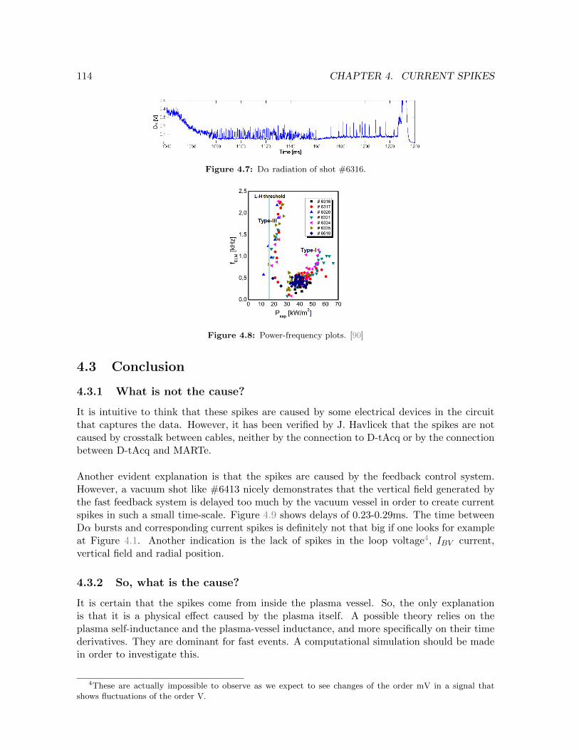
114 CHAPTER 4. CURRENT SPIKES
Figure 4.7: Dα radiation of shot #6316.
Figure 4.8: Power-frequency plots. [90]
4.3 Conclusion
4.3.1 What is not the cause?
It is intuitive to think that these spikes are caused by some electrical devices in the circuitthat captures the data. However, it has been verified by J. Havlicek that the spikes are notcaused by crosstalk between cables, neither by the connection to D-tAcq or by the connectionbetween D-tAcq and MARTe.
Another evident explanation is that the spikes are caused by the feedback control system.However, a vacuum shot like #6413 nicely demonstrates that the vertical field generated bythe fast feedback system is delayed too much by the vacuum vessel in order to create currentspikes in such a small time-scale. Figure 4.9 shows delays of 0.23-0.29ms. The time betweenDα bursts and corresponding current spikes is definitely not that big if one looks for exampleat Figure 4.1. Another indication is the lack of spikes in the loop voltage4, IBV current,vertical field and radial position.
4.3.2 So, what is the cause?
It is certain that the spikes come from inside the plasma vessel. So, the only explanationis that it is a physical effect caused by the plasma itself. A possible theory relies on theplasma self-inductance and the plasma-vessel inductance, and more specifically on their timederivatives. They are dominant for fast events. A computational simulation should be madein order to investigate this.
4These are actually impossible to observe as we expect to see changes of the order mV in a signal thatshows fluctuations of the order V.

4.3. CONCLUSION 115
Figure 4.9: Vacuum shots #3928 (left) and #6413 (right). IBV : Current in the PF coils of the fast feedbacksystem. The linear drift caused by the analogue integrator is removed. BIPR1: Vertical magnetic field measuredby the internal partial Rogowski coil at the low field side of the mid-plane. BIPR9: Vertical magnetic fieldmeasured by the internal partial Rogowski coil at the high field side of the mid-plane. The setup of the internalpartial Rogowski coils can be seen in Figure 2.23. Remark that IPR1 and IPR9 point in opposite direction.
Another explanation that is worth investigating, is given in [91] and [92]. These articlespropose that ELMs go along with previously closed edge field lines suddenly breaking open.When this happens, plasma energy and plasma current are released along the open field lines.This leads to the formation of a new equilibrium with a smaller separatrix. One could saythat the plasma edge “peels away”. This is actually a new kind of instability that cannot becategorized under ‘peeling and ballooning instabilities’ since the plasma boundary is typicallyheld fixed throughout the computational simulation of these last ones. This whole processis characterized by very fast jumps of the strike points, in time-scales of 1ms and less. Ifthe divertor tiles are positioned vertically - as is the case for JET - the strike points jumpupwards. In plasmas with strike points arriving at horizontal target plates - as is the casefor COMPASS - the inner strike point would move inward and the outer outward. Modellingindicates that these jumps can be associated with losses in plasma current and in βp. This“peel-off instability” is however fundamentally different from the change in equilibrium thatwould be derived simply from a reduction in βp, as it works in much smaller time-scales.Figures 4.10-4.12 confirm that the HFS strike point of shots #5943 and #6313 indeed jumpstowards lower R during ELMs and that the LFS strike point of shot #5943 jumps towardshigher R. This last effect is however less clear. We observe jumps of 1cm and more. Sincethe curves have been smoothed by a factor 1000, the actual jumps are much bigger and muchfaster. The small time-scales of the jumps require a signal with high sample frequency (atleast 1kHz) in order to detect them. The probe data used in Figures 4.10-4.12 is therefore anexcellent choice. The jumps are not so well observed by EFIT which samples at frequenciesof only 1-10kHz. There, the jumps are very small and can only be distinguished from theother fluctuations in the signal with the help of the Dα radiation.

116 CHAPTER 4. CURRENT SPIKES
Figure 4.10: Radial position of the HFS strike point of shot #6313. This is computed by searching theprobe with maximum saturation current. Therefore, probes in the HFS region were selected, namely probes6-12. Appendix C was used to convert probe numbers to radial positions. The sample frequency is 5MHz.The resulting curve has been smoothed by a factor 1000.
Figure 4.11: Radial position of the HFS strike point of shot #5943. This is computed by searching the probewith maximum saturation current. Therefore, probes in the HFS region were selected, namely probes 5, 6, 7,8, 10,12 and 13. Appendix C was used to convert probe numbers to radial positions. The sample frequency is5MHz. The resulting curve has been smoothed by a factor 1000.
Figure 4.12: Radial position of the LFS strike point of shot #5943. This is computed by searching theprobe with maximum saturation current. Therefore, probes in the LFS region were selected, namely probes15, 16, 20, 21, 23, 24 and 25. Appendix C was used to convert probe numbers to radial positions. The samplefrequency is 5MHz. The resulting curve has been smoothed by a factor 1000.

Chapter 5
General conclusions and suggestionsfor future work on COMPASS
This master thesis consisted of two main tasks: The first one was to analyse several shots thatachieved the H-mode regime. This includes amongst others the examination of ELMs, im-purities, energy confinement and particle confinement. The goal of this task was not strictlydelineated. There was a lot of space for experimentation with data from different diagnos-tic tools. Besides, it was a continuation of older work such as [51]. The second task was togather some statistical data about spikes that were observed in the plasma current and to pro-vide an explanation why they occur. It is the first time that these current spikes are described.
The huge amount of freedom for this thesis permitted to do some additional stuff and to beinventive. An improved reconstruction of the line-averaged electron density 〈ne〉 was aimedfor example. To this end, a Matlab code was written based on a paper found on the web,namely [93]. The code removes the offset, filters the high-frequent noise, removes the fringejumps and takes the plasma elongation into account. The code is certainly useful, though itfails when incomplete fringe jumps occur. Further, there was also experimented a lot withprobe data and with scaling laws.
Since the Dα detector is not calibrated, it is impossible to calculate the absolute value of theparticle confinement time. So, we cannot compare τp of COMPASS with τp of other tokamakswhich is a shame. On the other hand, we are still able to compare different values of τp at dif-ferent times and examine the improvement of the particle confinement in H-mode for example.Energy confinement calculations on the other hand struggle with another problem: the powerbalance cannot be solved exactly since the NBI power is unknown. We only know that it issomething between zero and some upper bound determined by the preprogrammed currentof the ion source and the voltage over the accelerating grids inside the NBI system, and thatit is very unlikely to be zero. It was attempted to estimate this power term in several waysstarting from the power balance and making certain assumptions, but without good results.As a consequence it is also difficult to estimate the improvement in energy confinement timein H-mode when the NBI is active. The attempts to solve the power balance with NBI powerterm took a lot of time. For an actual discussion of numerical results is referred to section 3.8.
117

Figures 4.5 and 4.6 definitely form the most important part of this thesis. The height of thecurrent spikes was examined in more than 30 shots and compared to the diamagnetic energyand the Dα radiation. We can conclude from these figures that there is a positive relationbetween the height of the Dα bursts and the relative height of the plasma current spikes, andthat there even is a strongly linear behaviour between the relative height of the current spikesand the relative height of the diamagnetic energy spikes. Relative heights were used becausethere are some uncertainties in the diamagnetic energy. Probably there is some crosstalkbetween the plasma current and the diamagnetic coil.
It is proven that the current spikes cannot be caused by the feedback system and further itis known that they are also not caused by crosstalk between cables. We could think of twoexplanations for these current spikes:
1. They are caused by fast changes in the plasma self-inductance and in the plasma-vesselinductance.
2. They are caused by strike point jumps which are associated to closed field lines breakingopen at the plasma edge followed by the formation of a smaller separatrix. Simulationsperformed by the staff of JET have shown that these strike point jumps can be respon-sible for a significant drop in the plasma current (much too big compared to the 1kAdrops observerd in COMPASS). However, the strike point jumps are clearly observedin COMPASS using probe data. If they are indeed the cause of the current spikes, westill have to try to understand why the plasma current (and often also the diamagneticenergy) first drops a little bit, but then increases a lot more, forming a spike instead ofonly a drop.
It is not clear whether the observed current spikes are immediately associated with plasmadegradation, but as they appear simultaneously with ELMs, their study can be important toenrich our knowledge of ELMs. These instabilities do degenerate the plasma as they diminishthe plasma energy, and pose an issue concerning ITER. Further investigation of the currentspikes could even show that we have to revise our current models of ELMs. But that is stilla long way off.
Possibilities for further work on COMPASS are:
• Still improve the reconstruction of the line-averaged electron density from interferometerdata. Find out why those incomplete fringe jumps occur.
• Calibrate the Dα detector.
• Try somehow to determine which thermal energy signal is correct (WEFIT , Wdia orWdiaBT ?), maybe by using plasma simulators.
• Disconnect the neutral beam injectors (maybe better both of them since one can workon full capacity and the other not) and do a calorimeter measurement, so that we atleast know the output power at the end of the beam duct. Maybe there are morepractical methods based on the newly installed neutron detector.
118

119
• Try to calculate the plasma self-inductance L(t) as accurate as possible1. This helpsto solve the energy balance since it influences the ohmic heating power and will maybealso help to find an explanation for the current spikes.
• Make a plasma simulation that takes into account the plasma self-inductance (andmaybe also the plasma-vessel inductance), and try to find an explanation for the currentspikes.
• Take contact with the staff of JET and try to link the found strike point jumps to theirobservations in JET. Maybe their simulation code can be used.
1J. Havlicek is working on a code.

Appendix A
Drift velocity
The motion of a charged particle in an inhomogeneous magnetic field is constituted of
1. a gyration around an instantaneous guiding centre due to v⊥.
2. a translation along the field line of the guiding centre with velocity v‖.
3. a drift with velocity vD of the instantaneous guiding centre due to the inhomogeneity.The drift velocity vD is partially due to v⊥ (the gradient drift) and partially due to v‖(the centrifugal drift). The exact expression is:
vD =1
4
mv2⊥qB4
(B×∇B2
)+mv2‖
qB4[B× (B · ∇)B] (A.1)
Assuming a force-free magnetic field, i.e. B× (∇×B) = 0, and local thermal equilibrium ofthe plasma, this can be simplified to
vD =kT
qB4
(B×∇B2
)(A.2)
In case of an ideal torus configuration, the magnetic field only has a toroidal component givenby
Bt =µ0Ip2πr
(A.3)
ans so
∇B = −Br
er (A.4)
This gradient causes a drift velocity
vD =4πkT
µ0qIper × et (A.5)
The q dependence results in a charge separation, which in its turn generates an electric fieldthat drifts the plasma away from the central axis. This so-called Hall-drift is given by
vD,Hall =E×B
B2(A.6)
A vertical equilibrium field is needed to counteract this radially outwards motion of the plasmacolumn. [31]
120

Appendix B
Density reconstruction
Goal: reconstruct the line-averaged electron density from interferometer data.
Algorithm:
1. Send interferometer data through a (windowing) low-pass filter with cut-off at 10kHz.
2. Remove offset.
3. Convolute the resulting data with the kernel function
g(t, wk) =
−1wkM
, −wk < t1
wkM, t < wk
0 , rest
(B.1)
where M is the difference between the absolute maximum and absolute minimum of thedensity data and wk = wf/α with wf an estimation of halve the width of a fringe jumpand α smaller than unity and here chosen to be 1/3.
4. Mathematics claims that this convolution shows distinct spikes with maximum heightequal to 1−α/2. So we take a fraction of this value as our threshold. Positive spikes rep-resent downsloping fringe jumps and negative spikes represent upsloping fringe jumps.
5. Now that the fringe jumps are located, we remove the density data that are part of thejump, which is very accurately estimated by the interval [tjump − wk, tjump + wk], andwe bring the data after the jump on the same level as the data before the jump.
6. Division by the elongation κ, which is linearly interpolated (and even extrapolated withsome assumptions) to maintain a rich enough amount of data.
This algorithm is based on [93].
121

122 APPENDIX B. DENSITY RECONSTRUCTION
Figure B.1: Left : The basic pattern of a fringe jump, the kernel function and their convolution. tA and tB arethe start and the stop times of a fringe jump. Right : Some mathematical information about the convolutionfor the case wf <
12wk. [93]

Appendix C
Divertor Langmuir probes
Table C.1: Radial position R and effective surface area A of the divertor Langmuir probes.
Probe R [m] A [mm2] Probe R [m] A [mm2] Probe R [m] A [mm2]
1 0.3960 6.62 14 0.4520 6.13 27 0.5155 6.382 0.4000 6.53 15 0.4569 5.99 28 0.5202 6.523 0.4038 6.49 16 0.4619 5.84 29 0.5249 6.504 0.4076 6.44 17 0.4669 5.78 30 0.5296 6.525 0.4114 6.44 18 0.4719 5.83 31 0.5342 6.656 0.4152 6.44 19 0.4768 5.87 32 0.5388 6.737 0.4192 6.43 20 0.4817 5.96 33 0.5433 6.758 0.4236 6.40 21 0.4866 6.09 34 0.5478 6.779 0.4279 6.39 22 0.4915 6.21 35 0.5523 6.8610 0.4326 6.39 23 0.4963 6.32 36 0.5567 6.8811 0.4373 6.36 24 0.5012 6.14 37 0.5611 6.9112 0.4421 6.29 25 0.5060 6.16 38 0.5654 6.9313 0.4470 6.21 26 0.5108 6.23 39 0.5697 6.89
123

Appendix D
Estimation of PNBI for shot #5909
First of all a short recapitulation of the three methods described in paragraph 3.5.5 to estimatePNBI :
• Method 1: τ∗E remains constant during NBI activity and is equal to an average of itslast values before the NBI was switched on.
PNBI(t) =dW
dt(t) +
W (t)
τ∗E,0− POH(t) (D.1)
• Method 2: Search the intersection of the two surfaces given byτ∗E(t, PNBI(t)) = W (t)
POH(t)+PNBI(t)−dW (t)dt
τ∗E(t, PNBI(t)) = τ∗E,0
(POH(t)+PNBI(t)
POH,0
)−α (D.2)
where α is 0.5 for L-mode and 0.69 for H-mode (ITER scaling laws).
• Method 3: Plot W (t) and estimate dWdt at the moment the NBI is switched on by
drawing a tangential line. The NBI power can be approximated by the found number.
The last method is infeasible for this shot as there is no observable change in W (t) at the mo-ment the NBI is switched on. For all three other methods, smoothing of the different plasmaparameters is very important, especially for the energy data derived from diamagnetism sincethe sample rate is much bigger for these signals. For all figures shown in this appendix, thedatasets Wdia and WdiaBT are reduced by a factor 100, all W are smoothed by a factor 5, andtheir derivatives are smoothed by a factor 5 in case of EFIT and by a factor 100 in case ofdiamagnetism. The ohmic heating power for Figure D.2, which shows the results of method1, is smoothed by a factor 50. For Figures D.3-D.5, which show the results of method 2, it issmoothed by a factor 50, 100 or 1000. Also the determination of τ∗E,0 and POH,0 is important.For Figure D.2 they are calculated by manually selecting a part of the τ∗E(t, PNBI = 0) curveand averaging. For Figures D.3-D.5 they are calculated by averaging over the time interval[t0− 2ms, t0− 0.1ms], where t0 is the time when the NBI was turned on. Figure D.1 is addedto have an idea of how POH looks like for the different smoothing factors that are used inthese figures.
124

125
Figure D.1: The artificially calculated ohmic heating power POH of shot #5909 for three different smoothingfactors (SF).
(a) EFIT (b) Dia (c) DiaBT
Figure D.2: Results of method 1.

126 APPENDIX D. ESTIMATION OF PNBI FOR SHOT #5909
(a) EFIT, 50 (b) EFIT, 100 (c) EFIT, 1000
(d) Dia, 50 (e) Dia, 100 (f) Dia, 1000
(g) DiaBT, 50 (h) DiaBT, 100 (i) DiaBT, 1000
Figure D.3: Results of method 2 for t = 1060−1069ms. The number under the figure denotes the smoothingfactor of POH .

127
(a) EFIT, 50 (b) EFIT, 100 (c) EFIT, 1000
(d) Dia, 50 (e) Dia, 100 (f) Dia, 1000
(g) DiaBT, 50 (h) DiaBT, 100 (i) DiaBT, 1000
Figure D.4: Results of method 2 for t = 1076−1084ms. The number under the figure denotes the smoothingfactor of POH .

128 APPENDIX D. ESTIMATION OF PNBI FOR SHOT #5909
(a) EFIT, 50 (b) EFIT, 100 (c) EFIT, 1000
(d) Dia, 50 (e) Dia, 100 (f) Dia, 1000
(g) DiaBT, 50 (h) DiaBT, 100 (i) DiaBT, 1000
Figure D.5: Results of method 2 for t = 1091−1105ms. The number under the figure denotes the smoothingfactor of POH .

Appendix E
Current spikes algorithms
E.1 Algorithm 1
Goal: find time and height of Dα spikes
Algorithm:
1. Estimate the average spike width yourself by looking at the original graph (±0.3ms).
2. Choose between:
(a) Send IDα through a bandpass filter with fmin = 200Hz and fmax = 10kHz.
(b) Remove the linear background signal in H-mode.
3. Search for possible spikes1:
IDα > c · std(IDα) (E.1)
with c a tunable parameter implemented as the ‘sensitivity’ and set equal to 1.5. Thisresults in groups of duplicates.
4. Distinguish the groups from each other by searching consecutive spikes that are fartherfrom each other than the estimated average spike width. ⇒ dummy spikes
5. Look for the maximum value in each group.
6. Plot the signal and indicate the found spikes with vertical lines.
1std=standard deviation
129

130 APPENDIX E. CURRENT SPIKES ALGORITHMS
Figure E.1: Illustration of the algorithm for shot #6058. The blue curve is the Dα radiation modified bystep 2. The red horizontal line is the threshold 1.5 · std(IDα). The red dots are the possible spikes resultingfrom step 3. The green dots are the dummy spikes resulting from step 4. The arrow indicates the maximumbetween two dummies as described in step 5.
E.2 Algorithm 2
Goal: measure less distinct spikes in for example the plasma current or the plasma energy,starting from the times when bursts occur in the Dα radiation.
Algorithm:
1. Send the data through a (widowing) low-pass filter with fc = 10kHz.
2. Search for the time tmax when the maximum occurs around the given time i of the Dαburst (∆t is the sample period of 0.5µs):
for k = 20→ 1 doj = k∆twhile data(i+ j) > data(i) do
i = timewhen data reaches itsmaximum in the time interval [i, i+ j]end whilewhile data(i− j) > data(i) do
i = timewhen data reaches itsmaximum in the time interval [i− j, i]end while
end fortmax = i
3. Search for the time tmin when the minimum occurs in front of the determined maximum(∆t is the sample period of 0.5µs, i = tmax − 50∆t):
for k = 50→ 1 doj = k∆twhile data(i+ j) < data(i) do
i = timewhen data reaches itsminimum in the time interval [i, i+ j]end whilewhile data(i− j) < data(i) do
i = timewhen data reaches itsminimum in the time interval [i− j, i]end while
end fortmin = i

E.2. ALGORITHM 2 131
4. Calculate the difference between the determined maxima and minima. This is definedas the spike height.
5. Plot the signal and indicate the maxima and minima by respectively green and red lines.Now, control manually if the code has done a good job and remove the badly calculatedspike heights.
Figure E.2: Resulting plot of the MeasureSpikes algorithm for shot #6311.

Bibliography
[1] “World Energy Outlook 2013 - Executive Summary”. IAE - http://www.iea.org/Textbase/npsum/WEO2013SUM.pdf.
[2] “Energy Vision 2013 - Energy Transitions: Past and Future”. World EconomicForum - http://www3.weforum.org/docs/WEF_EN_EnergyVision_Report_2013.pdf.
[3] “BP Statistical Review of World Energy - June 2013”. BP - http://www.bp.com/content/dam/bp/pdf/statistical-review/statistical_review_of_world_energy_2013.pdf.
[4] http://www.worldbank.org/.
[5] “World Energy Resources”. World Energy Council - http://www.worldenergy.org/wp-content/uploads/2013/09/Complete_WER_2013_Survey.pdf, 2013.
[6] W. Zittel et al. “Fossil and Nuclear Fuels - the Supply Outlook”. Energy Watch Group/Ludwig-Boelkow-Foundation/Reiner-Lemoine-Foundation, March 2013.
[7] J. Ongena and G. Van Oost. “Energy for Future Centuries. Will Fusion be an Inex-haustible, Safe and Clean Energy Source?”. Transactions of Fusion Technology, Vol.61,2T, p.3, January 2001.
[8] F. Pearce. “tot het laatste kooltje”, New Scientist (Nederlandstalige editie), p.44-51,June 2014.
[9] R. Zielinski et al. “Radioactive Elements in Coal and Fly Ash: Abundance, Forms,and Environmental Significance”. U.S. Geological Survey Fact Sheet FS-163-97, October1997.
[10] http://courses.engr.illinois.edu/npre201/coursematerial/nuclear_physics/lecture20notes/binding_energy.html.
[11] F. Vanmassenhove and G. Maenhout. “Theorie van de kernreactor. Deel 1: het punt-model.”, Syllabus (Ghent University), 2008.
[12] C. Rubbia. “Sub-critical Thorium reactors”, Conference for Sustainable Energy Systems2050, Stockholm, September 2013.
[13] “Australian Energy Resource Assessment 2013”. Chapter 10: “Solar Energy”. http://arena.gov.au/files/2013/08/Chapter-10-Solar-Energy.pdf.
132

BIBLIOGRAPHY 133
[14] “World Record Solar Cell with 44.7% Efficiency”. http://www.ise.fraunhofer.de/en/press-and-media/press-releases/presseinformationen-2013/world-record-solar-cell-with-44.7-efficiency, September 2013.
[15] J. Wang et al. “Low-Temperature Processed Electron Collection Layers ofGraphene/TiO2 Nanocomposites in Thin Film Perovskite Solar Cells”, Nano Letters,Vol.14, No.2, p.724-730, 2014.
[16] “Renewable energy technologies: cost analysis series. Solar Photovoltaics.”, IRENAworking paper, June 2012.
[17] A. Martin. “Eolien : lavenir se joue en altitude”, Winning article of the Shape yourFuture in Energy contest of Sia Partners and Elia 2014.
[18] http://www.google.com/makani/.
[19] http://www.altaerosenergies.com/.
[20] D. Jennejohn et al. “Geothermal: International Market Overview”. http://geo-energy.org/pdf/reports/2012-GEA_International_Overview.pdf,May 2012.
[21] S. Mehrangiz et al. “Various Technologies for Producing Energy from Wave: A Review”,International Journal of Smart Grid and Clean Energy, Vol.2, No.2, May 2013.
[22] “Australian Energy Resource Assessment 2013”. Chapter 11: “Ocean Energy”. http://arena.gov.au/files/2013/08/Chapter-11-Ocean-Energy.pdf.
[23] http://www.dongenergy.com/en/business%20activities/generation/activities/central_power_stations/pages/avedoere_power_station.aspx.
[24] Y. Zhao et al. “Iodine doped carbon nanotube cables exceeding specific electrical con-ductivity of metals”, Nature, Scientific Reports, Vol.1, No.83, September 2011.
[25] “Fuel Cell and Hydrogen technologies in Europe”. New-IG. http://www.fch-ju.eu/, 2011.
[26] D. Greene. “Status and Prospects of the Global Automotive Fuel Cell Industry andPlans for Deployment of Fuel Cell Vehicles and Hydrogen Refueling Infrastructure”,Oak Ridge National Laboratory, July 2013.
[27] National Physical Laboratory. Kaye & Laby. Tables of Physical & Chemical Constants- http://www.kayelaby.npl.co.uk/atomic_and_nuclear_physics/4_7/4_7_4.html.
[28] O. Van Hoey. “Visible light measurements on the COMPASS tokamak”. Master thesis(Gent University), 2010.
[29] J. Wesson. “Tokamaks”, Oxford Science Publications, 4th edition, 2011.
[30] S Azetni and J. Meyer-ter Vehn. “The Physics of Inertial Fusion: Beam-Plasma Inter-action, Hydrodynamics, Hot Dense Matter”, April 2004.

134 BIBLIOGRAPHY
[31] G. Van Oost. “High Temperature Plasma Physics”, Syllabus (Ghent University), 2012.
[32] O. A. Hurricane et al. “Fuel Gain Exceeding Unity in an Inertially Confined FusionImplosion”, Nature, Vol.506, p.343-348, February 2014.
[33] Official website of NIF - https://lasers.llnl.gov/media/photo-gallery.
[34] M. Groth. “Tokamaks and Tokamak Physics - Part A”, Presentation for the courseFusion Energy Technology, Aalto University, 2013.
[35] CEA website - http://www-fusion-magnetique.cea.fr/gb/fusion/histoire/site_historique.htm.
[36] http://www.tokamak.info/.
[37] K. Ikeda. “ITER on the road to fusion energy”, IOP Publishing. Nuclear Fusion, Vol.50,December 2009.
[38] Official website of ITER - www.iter.org.
[39] F. Wagner. “The Physics Basis of ITER Confinement”, AIP Conference Proceedings,Vol.1095, p.31-53, February 2009.
[40] Official website of IPP ASCR - http://www.ipp.cas.cz/Tokamak/index?m=comp.
[41] EURATOM-OAW website - http://www.oeaw.ac.at/euratom/international_e.html.
[42] T. Vey. “Iter : un reacteur de fusion plein d’avenir”. http://www.lefigaro.fr/,September 2013.
[43] http://fire.pppl.gov/.
[44] G. Van Oost. “Lectures on some Aspects of Fusion Technology”. Presentation for thecourse ‘Plasma and Fusion Technology’ at Ghent University, 2013.
[45] Belgian ITER site - http://iter.rma.ac.be/en/sustain/Environment/index.php.
[46] J. Stockel, oral or by email explanation.
[47] Official website of IPP ASCR - http://www.ipp.cas.cz/Tokamak/euratom/index.php/en/compass-diagnostics.
[48] T. Van Laer. “Probe Measurements on the COMPASS Tokamak”. Master thesis (XIOSHogeschool Limburg), 2012.
[49] R. Panek. “Characterization of H-mode in the COMPASS tokamak”. ITPA Meeting,Prague, April 2014.
[50] A. Kirschner. “Plasma-Wall Interaction in Fusion Experiments”, Guest Lecture for thecourse ‘Plasma and Fusion Technology’ at Ghent University, April 2013.

BIBLIOGRAPHY 135
[51] R. Panek et al. “Characterization of Ohmic and NBI heated H-mode in the COMPASStokamak”. 40th EPS Conference on Plasma Physics, p.4.103, 2013.
[52] J. Havlicek et al. “Status of Magnetic Diagnostics on COMPASS”, WDS’10 Proceedingsof Contributed Papers, Part 2, p.1217, 2010.
[53] J. Zajac et al. “Power supply system for the COMPASS tokamak re-installed at theIPP, Prague”. Proceeding of the 25th Symposium on Fusion Technology, Elsevier. FusionEngineering and Design, Vol.84, p.2020-2024, June 2009.
[54] J. Stockel. “Plasma confinement in tokamaks”, European Summer School in PlasmaPhysics, Prague, August 2009.
[55] J. Stockel et al. “Additional plama heating in tokamaks by the neutral beam injection”.Kudowa School, Presentation, June, 2012.
[56] F. Marguet. “Additional plasma heating by neutral beam heating on COMPASS”. Masterthesis (Erasmus Mundus in Nuclear Fusion), 2013.
[57] R. Panek et al. “Reinstallation of the COMPASS-D Tokamak in IPP ASCR”, Czechoslo-vak Journal of Physics, Vol.56, 2006.
[58] T. Odstrcil. “Study of visible plasma radiation by high resolution spectroscopy at addi-tional plasma heating by neutral beams injection on the COMPASS tokamak”, Masterthesis (Czech Technical University), 2012.
[59] J. Havlicek and I. Duran. “Magnetic diagnostics - Introduction”. SUMTRAIC 2010,Presentation, August 2010.
[60] J. Havlicek, oral or by email explanation.
[61] COMPASS’ own wiki.
[62] J. Zajac, oral or by email explanation.
[63] P. Bohm et al. “Laser system for high resolution Thomson scattering diagnostics on theCOMPASS tokamak”, Review of Scientific Instruments, Vol.81, October 2010.
[64] D.I. Naydenkova et al. “Progress in Multi channel Optical System for Visible PlasmaRadiation Measurement at COMPASS Tokamak”, WDS’10 Proceedings of ContributedPapers, Part II, p.1821, 2010.
[65] D. Naydenkoval et al. “The Multichannel System for Visible Plasma Radiation Mea-surements in the COMPASS Tokamak”, 3rd EFDA Transport Topical Group Meeting,Cordoba, September 2010.
[66] M. Berta et al. “Concept of an Atomic Beam Probe diagnostic on COMPASS tokamak”.36th EPS Conference on Plasma Physics.
[67] R. Schneider. “Plasma edge physics for tokamaks”, 2001.
[68] B. Crowley et al. “Electron Energy Distribution Function Measurements by LangmuirProbe in ITER like Negative Ion Sources”, AIP Conference Proceedings, Vol.925, p.193-207, 2007.

136 BIBLIOGRAPHY
[69] M. Dimitrova et al. “Plasma Parameters in the COMPASS Divertor During OhmicPlasmas”, Contributions to Plasma Physics, Vol.54, No.3, p.255-260, 2007.
[70] J. Adamek. “Ball-pen probe”. Plasma Physics in Science and Technology, EuropeanSummer School, Presentation. http://ppst-2009.physik.uni-greifswald.de/AdamekBPP.pdf, 2009.
[71] J. Adamek et al. “Fast ion temperature measurements using ball-pen probes in the SOLof ASDEX Upgrade during L-mode”. 38th EPS Conference on Plasma Physics, p.1.059,2011.
[72] F. Janky et al. “Determination of the plasma position for its real-time control in theCOMPASS tokamak”. Proceedings of the 26th Symposium of Fusion Technology, Else-vier. Fusion Engineering and Design, Vol.86, p.1120-1124, October 2011.
[73] A. Wootton. “Magnetic Fields and Magnetic Diagnostics for Tokamak Plasmas”, p.45-50,2008.
[74] F. Valcarcel et al. “The COMPASS Tokamak Plasma Control Software Performance”,IEEE. Real Time Conference, May 2010.
[75] J. Stockel. “Plasma start-up in tokamaks ”, Winter School, Marianska, January 2010.
[76] P. Snyder et al. “Edge localized modes and the pedestal: A model based on coupledpeelingballooning modes”, Physics of Plasmas, Vol.9, No.5, May 2002.
[77] CEA website - http://www-fusion-magnetique.cea.fr/gb/fusion/physique/modesconfinement.htm.
[78] J. Mlynar. “Focus on: JET”. ref: EFD-R(07)01, 2007.
[79] D.N. Hill. “A Review of ELMs in Divertor Tokamaks”, 12th International Conferenceon Plasma Surface Interactions in Controlled Fusion Devices, 1996.
[80] D.G. Whyte et al. “I-Mode: An H-Mode Energy Confinement Regime with L-ModeParticle Transport in Alcator C-Mod.”, IOP Publishing. Nuclear Fusion, Vol.50, No.10,August 2010.
[81] P. B. Snyder et al. “Edge localized modes and the pedestal: A model based on coupledpeeling-ballooning modes”, Physics of Plasmas, Vol.9, No.5, May 2002.
[82] S. Putvinski. “Runaway Electrons in Tokamaks and Their Mitigation in ITER”, IAEATCM on Energetic Particles, Austin, September 2011.
[83] M. Imrisek et al. “Observation of Sawtooth Oscillations in the COMPASS Tokamak”,WDS’13 Proceedings of Contributed Papers, part 2, p.67-72, 2013.
[84] E. Stefanikova, oral or by email explanation.
[85] http://fusenet.eu/node/342.
[86] http://wiki.fusenet.eu/wiki/Scaling_law.
BIBLIOGRAPHY 137
[87] T. S. Daugbjerg, S. Chaidez, and A. Gogoleva. “Global Energy Balance for OhmicPlasmas”, EMTRAIC 2013.
[88] Y.R. Martin et al. “Power requirement for accessing the H-mode in ITER”, Journal ofPhysics: Conference Series, Vol.123, 2008.
[89] F. Hofmann et al. “Effects of ELMs on the Measurement of Vertical Plasma Position inTCV and JET”, IOP Publishing. Nuclear Fusion, Vol.42, January 2002.
[90] J. Stockel and COMPASS team. “h-mode studies on the COMPASS tokamak”. IAEATechnical Meeting on RUSFD, San Jose, Costa Rica, January 2014.
[91] E. R. Solano et al. “Current loss and strike point movement during ELMs in JET”, 30thEPS Conference on Controlled Fusion and Plasma Physics, ECA Vol.27A, p.1.106, July2003.
[92] E.R. Solano et al. “ELMs and strike point movements”, IOP Publishing. Nuclear Fusion,Vol.48, No.6, April 2008.
[93] A. Ejiriy, K. Shinoharaz, and K. Kawahatay. “An algorithm to remove fringe jumpsand its application to microwave reflectometry”, Plasma Physics and Controlled Fusion,Vol.39, p.1963-1980, 1997.