Annales Geophysicae (2004) 22: 2525–2533SRef-ID: 1432-0576/ag/2004-22-2525© European Geosciences Union 2004

AnnalesGeophysicae

Multi-scale analysis of turbulence in the Earth’s current sheet

M. Volwerk 1,3, Z. Voros1, W. Baumjohann1, R. Nakamura1, A. Runov1, T. L. Zhang1, K.-H. Glassmeier2,R. A. Treumann3, B. Klecker3, A. Balogh4, and H. Reme5

1IWF, OAW, Graz, Austria2TU Braunschweig, Germany3MPE Garching, Germany4Imperial College, London, UK5CESR, Toulouse, France

Received: 26 August 2003 – Revised: 4 May 2004 – Accepted: 14 May 2004 – Published: 14 July 2004

Part of Special Issue “Spatio-temporal analysis and multipoint measurements in space”

Abstract. A multi-scale analysis of magnetotail turbulencein the Earth’s tail current sheet is presented based on Clus-ter magnetometer observations. Both Fourier and waveletanalysis is used to describe the spectral index and scaling in-dices of the turbulence for different frequency regions. Flowsin the tail are very important for driving the observed tur-bulence. There is a strong correlation between the maxi-mum perpendicular flow velocity and the turbulence powerfor maximum velocities 150≤v⊥,max≤400 km/s. At highermaximum flow velocities the turbulence power levels out,showing a saturation of the generation mechanism. The sus-pected presence of breaks in the slope of the spectrum at twofrequencies (f1 andf2) can be confirmed forf1≈0.08 Hz,but based on the data analysis the second break atf2 is ex-pected at a frequency higher than 12.5 Hz, where the datacannot significantly be evaluated. A schematic turbulencepower spectrum is presented based on the Cluster magneticfield measurements. Dependent on the presence of BBFs thespectral index or scaling index varies significantly.

Key words. Magnetospheric physics (magnetotail; plasmasheet; plasma waves and instabilities)

1 Introduction

The frequency scalings of the spectral power in the Earth’smagnetotail current sheet have been studied by many (see,e.g. Hoshino et al., 1994; Borovsky et al., 1997; Zelenyiet al., 1998; Sigsbee et al., 2001; Borovsky and Funsten,2003; Volwerk et al., 2003; Voros et al., 2003). The goalof such investigations is to (1) come to a general view ofthe spectral properties of the turbulence; (2) what spectralindices to expect for which frequency intervals; (3) whereand when to expect a break in the spectral index; (4) the di-

Correspondence to:M. Volwerk(martin.volwerk@assoc.oeaw.ac.at)

mensionality of the turbulence and (5) an indication of thepower cascade. This paper is mainly concerning points 1, 2and 3; for points 4 and 5 we would like to direct the readerto Volwerk et al. (2003), Voros et al. (submitted, 20041) andBorovsky and Funsten (2003) and references therein. Manyschematics have been presented in which it is posited thatthere are three different spectral indices:p1 for f <f1; p2for f1<f <f2 and p3 for f >f2. For example, Hoshinoet al. (1994) have shown thatf1≈0.04 Hz in Geotail datataken atxGSM≈205RE, whereas Volwerk et al. (2004) findf1≈0.08 Hz from Cluster data taken atR≈19RE.

In this paper we combine and expand on the results fromVolwerk et al. (2003) and Voros et al. (2003). In these papersthe data from the magnetic field experiment (Balogh et al.,2001) are investigated for their turbulence scaling properties,combined with flow information from the plasma experiment(Reme et al., 2001). The plasma flows are probably the maindrivers of the turbulence in the current sheet and, therefore,they play an important role in our study. Discussions on thecharacteristics of high-speed plasma flows, or bursty bulkflows (BBFs), can be found in, for example, Baumjohannet al. (1990), Angelopoulos et al. (1994) and Nakamura et al.(2002). We will show that the turbulent spectra have a breakat low frequencies,f1, but our data are insufficient to show abreak at high frequencies,f2. We also show that the break atf1 is strongly related to BBFs, and that at high frequenciesthe spectral index shows large differences between flow andno-flow intervals.

The data that are used in this paper were obtained when theCluster spacecraft had their apogee in the Earth’s magnetotailat a radial distance of∼19RE . The inter-spacecraft separa-tion distance was 1800 km in 2001 and 4000 km in 2002. Us-ing the full capabilities of the Cluster magnetometer up to a

1Voros, Z., Baumjohann, W., Nakamura, R., Volwerk, M.,Runov, A., Zhang, T. L., Eichelberger, H. U., Treumann, R.,Georgescu, E., Balogh, A., Klecker, B., and Reme, H.: Magneticturbulence in the plasma sheet, J. Geophys. Res., submitted, 2004.

2526 M. Volwerk et al.: Multi-scale turbulence analysis

102

103

−2

−1.5

−1

−0.5

0

0.5

1

1.5

2

βlo

= 3.97 ± 0.18

rclo

= 0.61

Log

0.1

Hz

Pow

er (

nT2 /H

z)

maximum v⊥ (km/s)

βhi

= 1.00 ± 0.27

rchi

= 0.40

102

103

2

2.2

2.4

2.6

2.8

3

3.2

3.4

3.6

3.8

4

p = 2.88 ± 0.22

Spe

ctra

l Ind

ex

maximum v⊥ (km/s)

Fig. 1. The top panel shows the low frequency turbulence for 0.08≤f ≤1 Hz for 68 intervals of 12 min near the neutral sheet. The leftpanel shows the total power in the turbulence as a function of the maximum perpendicular flow velocity during the 12-min interval. Thestars and triangles represent C1 and C3, respectively. The pluses show the velocity dependence of the spectral power determined by Baueret al. (1995a) for the frequency interval 0.03≤f ≤0.13 Hz. The velocity dependence of the spectral power is fitted for velocity intervals150≤v⊥,max≤400 km/s and 350≤v⊥,max≤1100 km/s. The bottom panel shows the spectral index as a function of maximum perpendicularflow velocity.

sampling rate of 67 Hz, we will construct a spectral diagramfor a broad frequency range, taking into account various de-pendencies on, i.e. the flow velocity of the plasma in the tail.

2 Data analysis techniques

We will first review the data analysis techniques that havebeen used in the papers that form the basis of this paper.

2.1 High-velocity low-frequency spectral analysis

An analysis of the low-frequency turbulence in the Earth’scurrent sheet has been performed by Volwerk et al. (2003).They used 12-min intervals of data near the neutral sheet,covering the local time region between 21:00 and 03:00 LT,for both 2001 and 2002. The data were transformed to amean field-aligned coordinate system. The spectral analysiswas performed on 2 Hz sampled data, giving a Nyquist fre-quency offNy=1 Hz and the spectra were averaged over 7harmonics with a frequency resolution of1f =1.4 mHz. Itwas found that the power in the compressional componentwas much stronger than the left- and right-hand polarisedwave power (see also Bauer et al., 1995a; 1995b; Volwerket al., 2004). A lower limit was set to the maximum perpen-dicular flow velocity,v⊥,max>150 km/s. Only then does thefrequency interval in which we are interested, 0.08≤f ≤1 Hz,show power above the magnetometer noise level.

A summary plot of all data is shown in Fig. 1. For theturbulent power in the frequency range 0.08≤f ≤1.0 Hz theyfound that it was highly dependent on the maximum perpen-dicular flow velocity,v⊥,max measured during the interval.

The spectral index of the turbulence is shown to bep=2.88±0.22 with no dependence on the flow velocity. Thisvalue is much larger than Kolmogorov (p=5/3) and close towhat one would expect for quasi-2-D turbulence. For pure2-D turbulence one would expect thatp=3 (Frisch, 1995).The occurrence of quasi-2-D turbulence is dependent on aregion that is limited in one direction on scales longer thanthe extension of the region in the third dimension. This isnatural for the Earth’s current sheet, which is limited in thez-direction.

Interestingly it is found that the power in the turbulencecan be described as:

P ≡ P(f, v) ∝ f −pvβ , (1)

so not only is there the usual frequency dependence ofthe spectral power,f −p, but also a velocity dependencevβ . In the paper by Volwerk et al. (2003) the datawere split up in three local time regions: pre-midnight(12:00–23:00 LT); midnight (23:00–01:00 LT) and post-midnight (01:00–03:00 LT). It was shown that two dif-ferent regions could be identified for the velocity depen-dence. Forv⊥,max≤400 km/s the turbulent power increasesstrongly with slopesβpre=4.51±0.24, βmid=3.82±0.65and βpost=3.45±0.16 (in the total data set we findβlo=3.76±0.21, see Fig. 1).

We transform the frequency spectra to wave num-ber space under the assumption that the slope of thespectrum does not change (Borovsky et al., 1997), i.e.P(f )∝f −p

→P(k)∝k−p. This results in a wave spectrum:

P ≡ P(k, v) ∝ vβ−pk1−D−p, (2)

M. Volwerk et al.: Multi-scale turbulence analysis 2527

whereD is the dimensionality of the problem, in this caseD=1 (see Volwerk et al., 2003 for a discussion of this value).This dependence on the flow velocity can be explained whenthe wave power is generated by a streaming instability, mostlikely the Kelvin-Helmholtz instability (KHI) on the bound-ary between the flow channel and the ambient magneto-tail. Transformed to wave number space one finds that thepower grows linearly with the maximum velocity (βlo≈3.76,p≈2.88), what one would expect for the KHI:

P = 2γP with γ ∝ v. (3)

At higher velocities,v⊥,max>400 km/s, the spectral powerbecomes saturated, demonstrated by a much smaller slopefor the velocity dependence. For this region it was found thatβpre=1.95±0.20,βmid=1.20±0.45 andβpost=1.44±0.50 (inthe total data set we findβhi=1.06±0.48, see Fig. 1). Onefinds that the spectral power becomes independent from theflow velocity or even inversely dependent on it (βhi≈1.06,p≈2.88), showing clearly the saturation of the generatinginstability. Indeed, Melrose (1986) states that “if the KHIdevelops too fast, the resuling turbulent mixing can reducethe shear below this threshold, thereby suppressing the insta-bility”.

For even lower frequenciesf ≤0.06 Hz, containing the Pi2band (8–25 mHz), the 12-min intervals are too short to obtainan accurate spectral index. We will return to this frequencyband later in the case studies in Sect. 3.

2.2 High-frequency wavelet analysis

In order to investigate higher-frequency turbulence than inthe previous section, we cannot suffice with 2-Hz sampleddata and just regular spectral analysis. The signals at higherfrequencies are embedded in a high noise region. Therefore,for selected events, Voros et al. (2003; submitted, 20041)studied the normal and burst mode (22 Hz and 67 Hz, respec-tively) magnetic field data with a discrete wavelet technique.Again, a relationship is sought between the spectral powerand the frequency:

P(f ) ∝ cf f −αS, (4)

where nowcf andαS are determined by a wavelet estimator.This estimator involves a semi-parametric wavelet techniquebased on a fast pyramidal algorithm, which allows unbiasedestimations of the scaling parameterscf andα (Abry et al.,2000). A discrete wavelet transform of the time series is per-formed over a dyadic grid of scale (j ) and time (t) and foreach octave the varianceµj of the discrete wavelet coeffi-cients is calculated:

µj =1

nj

nj∑t=1

d2(j, t) ∝ 2jαcf , (5)

wherenj are the number of coefficients at octave (scale)j

andd(j, t) is the discrete wavelet coefficient. The parame-terscf andα are then found by linear regression of the log-arithm of the varianceµ with respect to the observed scalej

100

101

102

0

0.5

1

1.5

2

2.5

3

α

cfsn

BX −− 2001−09−07

s/c 1 s/c 3

αmod

=1.5

αmod

=2

αmod

=2.5

αmod

=3

noise level s/c 1 (Bx)

noise level s/c 3 (Bx)

A B

B1 A1

Fig. 2. The scaling parameter correction curves for two spacecraft(C1 and C3) for scalej=4. For known signal-to-noise ratios,cfsn,it is shown from synthetic data that for small values the true scalingα is recovered incorrectly and needs to be corrected. The graph alsoshows the difference in noise level for C1 and C3. A, B, A1 and B1represent the examples studied in the case studies, respectively, for27 August 2001 and 13 September 2002.

(intercept and slope, respectively); for a full description, seeVoros et al. (2004). We choose to describe the “spectral in-dex” byαS, to clarify the different analysis technique used.

As at higher frequencies the signal-to-noise ratio becomesvery small; a check of the feasibility of this procedure isneeded. Therefore, Voros et al. (submitted, 20041) haveused quiet magnetotail intervals and embedded artificial sig-nals, with known scaling parameters and reminiscent of sig-nals expected to be found in the magnetotail, and performedthe wavelet analysis to find these scaling parameters. It wasshown that depending on the signal-to-noise ratio,cfsn and onthe scalej , recovery of the scaling parameters was possible.For different frequency ranges (or scalesj ) the time win-dow used was optimized to recover the synthetic signals. Byvarying the signal-to-noise level, the known scaling pareme-ters were recovered with varying accuracy, and were usuallyunderestimated. The correction curves showed the correctvalue ofαS for a measuredαS,m. Covering a large parameterspace ofcfsn andj , Voros et al. (submitted, 20041) createdthese correction curves which can be applied to the deter-mination of the scaling parameters from active magnetotaildata. The correction curves were computed by embeddingartificial signals to quiet time measurements on 7 September2001. Examples of these curves for C1 and C3 can be seenin Fig. 2, and these curves will be used in this paper.

The main problems in this process are: determining thesignal-to-noise ratio,cfsn (the noise level for each space-craft is different); and the width of the window in which the

2528 M. Volwerk et al.: Multi-scale turbulence analysis

−5

0

5

10

15

20

25

30

0

0.5

1

1.5

2

2.5

3

0

3

6

9

12

0130 0200 0230 0300 0330 0400 0430 0500

−600

−400

−200

0

200

400

600

BX

(j3,j

4)

(j1,j

2)

α

cfsn

V⊥ x

[nT]

[km/s]

2001−08−27

s/c 1 s/c 3

UT

A B

Fig. 3. Top panel: TheBx for 27 August 2001, for C1 (black) andC3 (green). Next panel: The wavelet scaling parameterα for scales(j1, j2) and(j3, j4). Next panel: The signal-to-noise estimatorcfsndefined as the relative power of interceptscfsn=cactivity/<cnoise>.Bottom panel:x-component of the perpendicular flow velocity. Thecorrection of the scaling parameterαS for A and B are shown inFig. 2.

wavelet transform is performed. The latter problem can besolved by using a synthetic data set and for each scale the op-timal width of the window can be found by trial. The differ-ent noise levels for each spacecraft can be determined. Thismakes sure that each spacecraft has its own set of correctioncurves, as shown in Fig. 2. The first problem is not so trivial,but using the data one can construct a quantity determined bythe “relative power of intercepts” from the wavelet analysis.In the wavelet scalogram the intercept at scalej=0 is deter-mined for the noise (from the quiet time data) and for activedata, i.e. thecfs describing the spectral powerP(f ). Fromanalysis of synthetic data one finds that this relative powerof intercepts,cfsn=cactivity/〈cnoise〉, is an adequate quantityto describe the signal-to-noise ratio. We note that〈cnoise〉 isindependent of the location of the Cluster spacecraft; for fur-ther details, see Voros et al. (submitted, 20041).

For selected intervals containing bursty bulk flows (BBFs;see, e.g. Baumjohann et al., 1990; Angelopoulos et al., 1994)the (corrected) scaling parameters have been determined. Itis found that in the absence of flow in the magnetotailcfsn≈1,and only during fast flows does one find thatcfsn>1 and isscaling information available. From the correction curves inFig. 2 it is clear that forcfsn�100 the scaling parameterα

for small scales(j1, j2)=(0.08, 0.33) s needs to be corrected,

Table 1. Statistical evaluation of large-scaleαLS for 27 August2001, for two different conditions. Cond. 1: Based on small scales:BBF when αSS>0.9 and cfsn>2; non-BBF whenαSS<0.4 andcfsn<1.1; Cond. 2: Based on perpendicular velocity: BBF whenv⊥,xy>300 km/s; non-BBF whenv⊥,xy<100 km/s.

Bx By BzC1 C1 C1

Cond. αLS BBF 2.55±0.04 2.56±0.06 2.53±0.081 αLS non-BBF 1.7±0.3 2.1±0.3 2.1±0.2

Cond. αLS BBF 2.6±0.1 2.6±0.1 2.6±0.12 αLS non-BBF 1.9±0.3 2.1±0.3 2.1±0.3

C3 C3 C3

Cond. αLS BBF 2.59±0.04 2.59±0.04 2.52±0.061 αLS non-BBF 1.6±0.4 1.8±0.4 1.9±0.2

Cond. αLS BBF 2.6±0.1 2.6±0.1 2.5±0.12 αLS non-BBF 1.5±0.4 1.7±0.4 2.0±0.3

whereas at larger scales(j3, j4)=(0.7, 11) s the scaling pa-rameters can be trusted. Thecfsn seems to correlate best withthe perpendicular plasma flow,v⊥.

Figure 3 shows the wavelet analysis results forBx for 27August 2001. During the interval 01:10–05:00 UT on 27August 2001, the Cluster spacecraft were near thezGSM=0plane, in the post-midnight magnetotail (xGSM∼−19RE).The correlation betweenv⊥ andcfsn is clear, whenever thereare BBFs the signal-to-noise ratio increases. This is similarto what was observed in the low-frequency turbulence, wherethe perpendicular flow velocity had to exceed 150 km/s forthe whole frequency interval to show power above the noiselevel. The results from the wavelet analysis can be found inTable 1. Two different kinds of conditions are put onto thedata:

1. Based on small scales: BBF whenαSS>0.9 andcfsn>2;non-BBF whenαSS<0.4 andcfsn<1.1;

2. Based on perpendicular velocity: BBF whenv⊥,xy>300 km/s; non-BBF whenv⊥,xy<100 km/s.

For both conditions on the data we find that for BBF typeof data the scalingαLS≈2.6, where the large scale indicatestime scales of 0.7–11 s or frequency scale of 1.4–0.09 Hz,overlapping with the spectral analysis region in the previoussection. Indeed, we find that during fast flows the scalingindex is similar between the two methods (i.e. spectral anal-ysis and wavelet analysis), 2.88±0.22 and 2.6±0.1. In thecase of non-BBF periods we find that 1.5≤αLS≤2.1, whichis very close to a Kolmogorov spectrum (αkol=5/3).

For the smaller scales, i.e.(j1, j2)=(0.08, 0.33) s, orfor the frequency range 12.5–3 Hz it was found that thecfsn�100 (see Fig. 3); thus the values forαSS must be cor-rected using the curves in Fig. 2. This shows that for theidentified regions of BBFs the wave power can be described

M. Volwerk et al.: Multi-scale turbulence analysis 2529

−20

−10

0

10

20

30

Bx

−20

−10

0

10

20

30

By

−20

−10

0

10

20

30

Bz

1 1.5 2 2.5 3 3.5 4 4.5 5 5.5 60

10

20

30

Bm

UT

10−3

10−2

10−1

100

10−2

10−1

100

101

102

103

104

Frequency (Hz)

pC1

= 1.86

Pow

er (

nT2 /H

z)

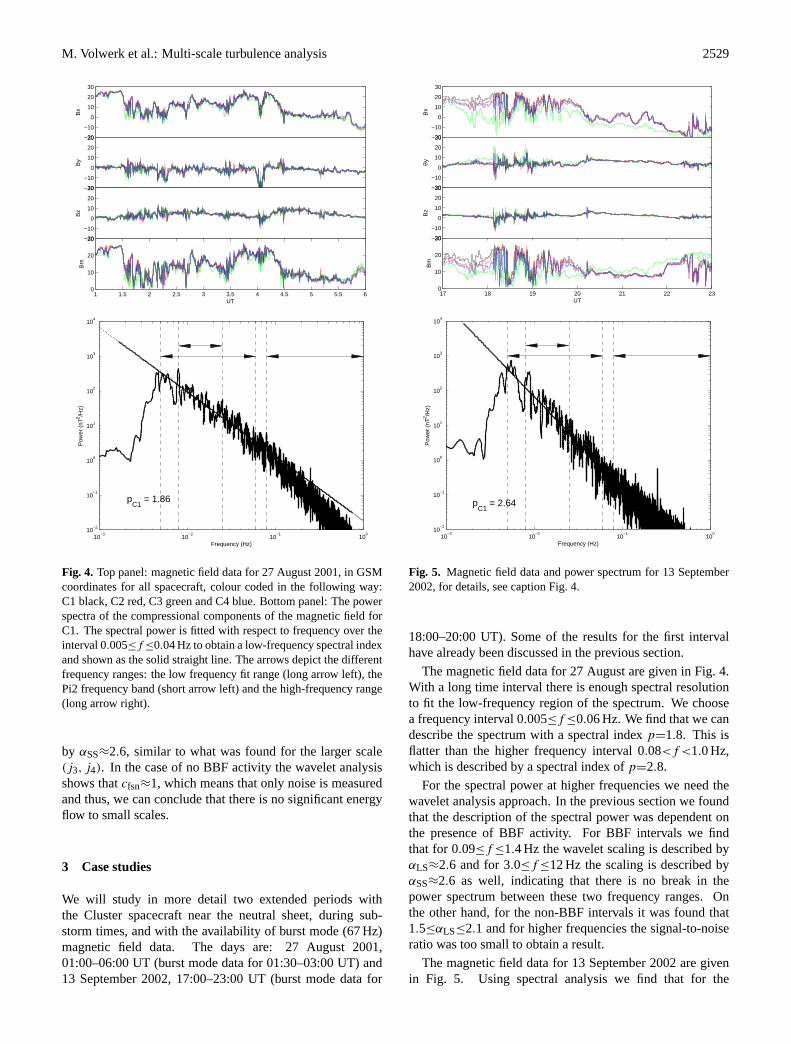
Fig. 4. Top panel: magnetic field data for 27 August 2001, in GSMcoordinates for all spacecraft, colour coded in the following way:C1 black, C2 red, C3 green and C4 blue. Bottom panel: The powerspectra of the compressional components of the magnetic field forC1. The spectral power is fitted with respect to frequency over theinterval 0.005≤f ≤0.04 Hz to obtain a low-frequency spectral indexand shown as the solid straight line. The arrows depict the differentfrequency ranges: the low frequency fit range (long arrow left), thePi2 frequency band (short arrow left) and the high-frequency range(long arrow right).

by αSS≈2.6, similar to what was found for the larger scale(j3, j4). In the case of no BBF activity the wavelet analysisshows thatcfsn≈1, which means that only noise is measuredand thus, we can conclude that there is no significant energyflow to small scales.

3 Case studies

We will study in more detail two extended periods withthe Cluster spacecraft near the neutral sheet, during sub-storm times, and with the availability of burst mode (67 Hz)magnetic field data. The days are: 27 August 2001,01:00–06:00 UT (burst mode data for 01:30–03:00 UT) and13 September 2002, 17:00–23:00 UT (burst mode data for

−20

−10

0

10

20

30

Bx

−20

−10

0

10

20

30

By

−20

−10

0

10

20

30

Bz

17 18 19 20 21 22 230

10

20

30

Bm

UT

10−3

10−2

10−1

100

10−2

10−1

100

101

102

103

104

Frequency (Hz)

pC1

= 2.64

Pow

er (

nT2 /H

z)

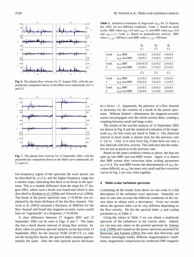
Fig. 5. Magnetic field data and power spectrum for 13 September2002, for details, see caption Fig. 4.

18:00–20:00 UT). Some of the results for the first intervalhave already been discussed in the previous section.

The magnetic field data for 27 August are given in Fig. 4.With a long time interval there is enough spectral resolutionto fit the low-frequency region of the spectrum. We choosea frequency interval 0.005≤f ≤0.06 Hz. We find that we candescribe the spectrum with a spectral indexp=1.8. This isflatter than the higher frequency interval 0.08<f <1.0 Hz,which is described by a spectral index ofp=2.8.

For the spectral power at higher frequencies we need thewavelet analysis approach. In the previous section we foundthat the description of the spectral power was dependent onthe presence of BBF activity. For BBF intervals we findthat for 0.09≤f ≤1.4 Hz the wavelet scaling is described byαLS≈2.6 and for 3.0≤f ≤12 Hz the scaling is described byαSS≈2.6 as well, indicating that there is no break in thepower spectrum between these two frequency ranges. Onthe other hand, for the non-BBF intervals it was found that1.5≤αLS≤2.1 and for higher frequencies the signal-to-noiseratio was too small to obtain a result.

The magnetic field data for 13 September 2002 are givenin Fig. 5. Using spectral analysis we find that for the

2530 M. Volwerk et al.: Multi-scale turbulence analysis

−500

0

500

1000

v x

C1

−500

0

500

v y

−500

0

500

v z

1 2 3 4 5 60

500

1000

1500

v t

UT

−500

0

500

1000

v x

C3

−500

0

500

v y

−500

0

500

v z

1 2 3 4 5 60

500

1000

1500

v t

UT

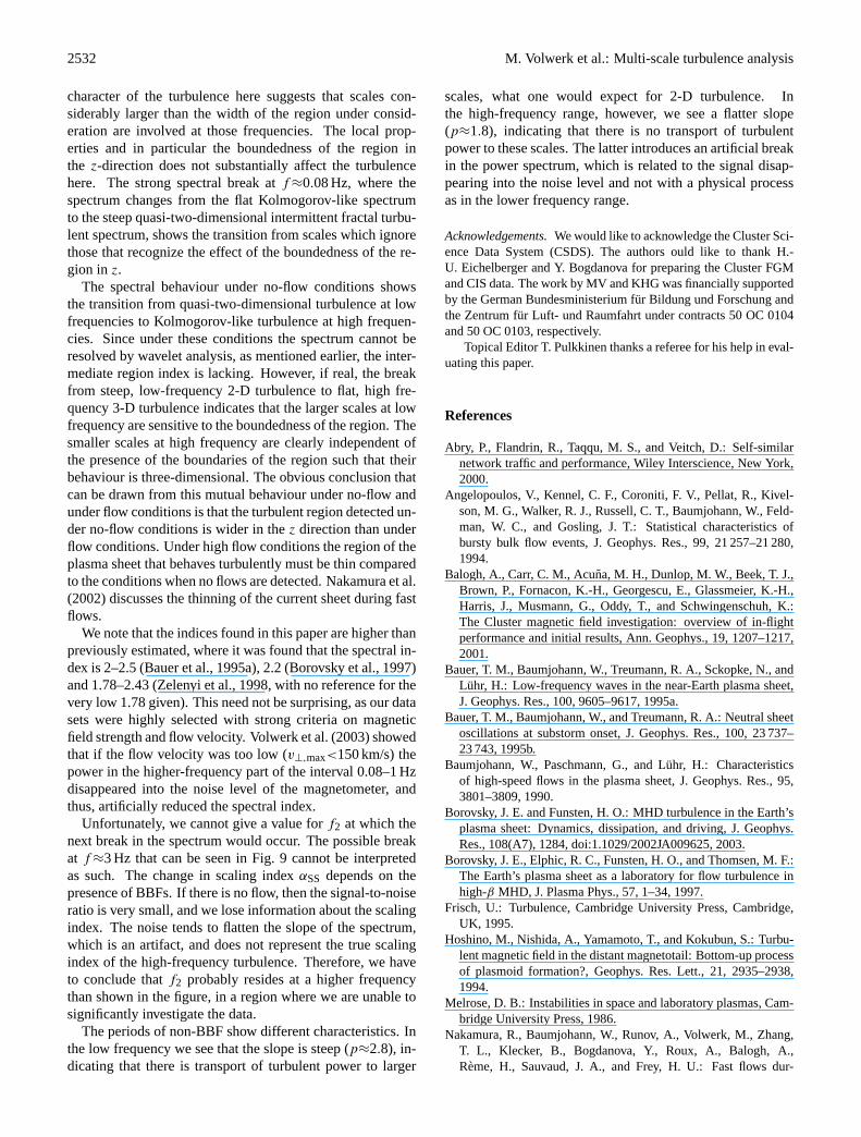
Fig. 6. The plasma flow velocity for 27 August 2001, with the per-pendicular component shown as the filled curve underneath, for C1and C3.

−500

0

500

1000

v x

C1

−500

0

500

v y

−500

0

500

v z

17 18 19 20 21 22 230

500

1000

1500

v t

UT

−1000

−500

0

500

v x

C3

−500

0

500

v y

−500

0

500

v z

17 18 19 20 21 22 230

500

1000

1500

v t

UT

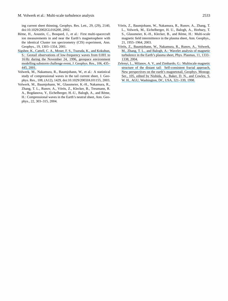
Fig. 7. The plasma flow velocity for 13 September 2002, with theperpendicular component shown as the filled curve underneath, forC1 and C3.

low-frequency region of the spectrum the wave power canbe described byp≈2.6, and the higher frequency range hasa similar slope, indicating that there is no break in the spec-trum. This is a notable difference from the slope for 27 Au-gust 2001, where such a break was found and which is alsodescribed in Hoshino et al. (1994) and Volwerk et al. (2004).The break in the power spectrum nearf ≈0.08 Hz was ex-plained by the finite thickness of the fast flow channel. Vol-werk et al. (2003) assumed a thickness of 4000 km for theflow channel and found that magneto-acoustic waves wouldhave an “eigenmode” at a frequencyf ≈0.06 Hz.

A clear difference between 27 August 2001 and 13September 2002 can be seen in Figs. 6 and 7. The latterday has a much shorter interval of strong flow activity. In-deed, when we perform spectral analysis on the data from 13September 2002, for the interval 19:00–23:00 UT, i.e. takeout the strong flow bursts, the spectral index remains approx-imately the same. Only the total spectral power decreases

Table 2. Statistical evaluation of large-scaleαLS for 13 Septem-ber, 2002, for two different conditions. Cond. 1: Based on smallscales: BBF whenαSS>0.9 andcfsn>2; non-BBF whenαSS<0.4and cfsn<1.1; Cond. 2: Based on perpendicular velocity: BBFwhenv⊥,xy>300 km/s; non-BBF whenv⊥,xy<100 km/s.

Bx By BzC1 C1 C1

Cond. αLS BBF 2.3±0.2 2.2±0.2 2.4±0.31 αLS non-BBF 1.0±0.3 1.2±0.3 2.0±0.1

Cond. αLS BBF 2.42±0.15 2.5±0.2 2.4±0.22 αLS non-BBF 1.3±0.5 1.7±0.5 2.2±0.2

C3 C3 C3

Cond. αLS BBF 2.5±0.2 2.3±0.2 2.3±0.31 αLS non-BBF 0.9±0.4 1.0±0.5 1.3±0.5

Cond. αLS BBF 2.5±0.1 2.4±0.2 2.6±0.12 αLS non-BBF 1.4±0.6 1.5±0.6 1.6±0.6

by a factor∼2. Apparently, the presence of a flow channelis necessary for the creation of a break in the power spec-trum. Without limitedz-dimensions the magneto-acousticwaves can propagate over the whole current sheet, creating acoupling between small and large scales.

The results of the wavelet analysis of 13 September 2002are shown in Fig. 8 and the statistical evaluation of the large-scaleαLS for this event are listed in Table 2. The observedinterval in burst mode is shorter than for the previous case(∼2 h vs.∼4 h). It is clear from Fig. 8 that there are only afew intervals with flow activity. This indicates that the statis-tics are not as good as in the previous case.

Based on the same condition criteria as above, the data aresplit up into BBF and non-BBF events. Again, it is shownthat BBF events after correction show scaling parametersαLS≈2.4. For non-BBF events the determination ofαLS be-comes difficult, ascfsn becomes very small and the correctioncurves in Fig. 2 are very close together.

4 Multi-scalar turbulent spectrum

Combining all the results from above we can come to a fulldescription of the turbulent wave spectrum. Naturally wehave to take into account the different conditions of the cur-rent sheet to obtain such a description. From our resultsabove the spectral index can be very different depending onthe flow activity. We list the spectral indexp and scalingparameterαS in Table 3.

Using the values in Table 3 we can obtain a multiscalespectrum of the turbulence in the current sheet. Indeed,we can now put values to the posited spectrum by Zelenyiet al. (1998) and expand on the power spectrum presented byBorovsky and Funsten (2003) (but note that Borovsky andFunsten investigate totally different magnetospheric condi-tions, magnetotail compression by northward IMF magnetic

M. Volwerk et al.: Multi-scale turbulence analysis 2531

Table 3. The spectral indicesp and scaling parametersαS as deter-mined from the spectral and wavelet analysis. Average values forflow and no-flow intervals are given.

Freq. Range flow no-flow flow no-flowHz p p αS αS

0.005≤f ≤0.04 ∼1.8 ∼2.8 NA NA0.08≤f ≤1.0 ∼2.8 NA ∼2.6 NA3.0≤f ≤12.5 NA NA ∼2.6 ∼1.8

clouds, whereas we investigate substorm-related phenom-ena). We find that there is one possible spectral break atf1≈0.08 Hz, and no real evidence for a second spectral breakat higher frequencies. The smaller scaling parameterαLS forthe high frequency range must be regarded critically, as thesignal-to-noise ratios for non-BBF events are very small andthus, some of the information in the data may be lost in thenoise. In Fig. 9 we show the results as obtained in this paper.The solid boxes show the slopes for BBF conditions and thestriped boxes for non-BBF conditions. The shaded regionsshow the possible variation in slopes as given by the errorbars.

5 Discussion

We have investigated the spectral power scaling with respectto frequency for the magnetic wave activity observed in theEarth’s tail current sheet. It was proposed that in the powerspectra there would be two breaks at frequencies usually la-belledf1 andf2 or f∗ andf∗∗. It was shown by Hoshinoet al. (1994) thatf1≈0.04 Hz and similarly by Volwerk et al.(2004) thatf1≈0.08 Hz and Bauer et al. (1995a) noticed abreak in the spectrumf1≈0.03 Hz. This seems to be a wellestablished frequency range forf1. However, Zelenyi et al.(1998) studied thez-component of the magnetic field andfound that it showed a “two-kink behaviour” with turn-overfrequenciesf∗≈0.01 Hz andf∗∗≈0.25 Hz. This is not inagreement with the results presented in this paper. It is notfeasible to putf1≡f∗. Also, our results show no indicationof a break atf∗∗≈0.25 Hz.

An interesting detail in our results is that in the frequencyrange 0.08≤f ≤1 Hz, which was investigated both by Fourierspectral analysis and wavelet analysis, the spectral index was2.6 and 2.8, respectively. In the intermediate frequency rangethere is strong overlap between the powers determined fromspectra and wavelet analyses under flow conditions, suggest-ing that the spectral index is more of the order of 2.6±0.1.Physically this implies that the turbulence is not strictly two-dimensional in the presence of strong flows, but rather it isintermittent such that the dimensionality is fractal 2<D<3with scales substantially smaller than the width of the re-gion (in this case the flow channel) inz-direction contribut-ing. The presence of smaller scale structures contributingto the turbulence is also suggested by the index in the high-

−20

−10

0

10

20

0

0.5

1

1.5

2

2.5

3

0

3

6

9

12

15

1800 1830 1900 1930 2000

−800

−400

0

400

800

2002−09−13

BX [nT]

α

cfsn

V⊥ X [km/s]

UT

A1 B1

(j1,j2)

(j3,j4)

Fig. 8. Wavelet analysis of the data from 13 September 2002 insimilar form as Fig. 3. The correction of the scaling parameterαSfor A1 and B1 are shown in Fig. 2.

10−3

10−2

10−1

100

101

1.5

2

2.5

3

Frequency (Hz)

Slo

pe

Spectral Slopes for Turbulence Power Spectrum

Fig. 9. A schematic for the slope of the power spectrum as deducedin this paper for different frequency ranges, determination methodsand flow activity. Blue: Spectral analysis; Red: Wavelet analysis.The solid boxes are for BBF intervals and the striped boxes are fornon-BBF periods. For the numerical values of the slopes, see Ta-ble 3.

frequency range found from the wavelet analysis, which isidentical to that in the intermediate frequency range, suggest-ing no spectral break at those higher frequencies.

It is interesting to also comment on the flat Kolmogorov-like spectra obtained from the spectral analysis in thevery low-frequency range. This quasi-three-dimensional

2532 M. Volwerk et al.: Multi-scale turbulence analysis

character of the turbulence here suggests that scales con-siderably larger than the width of the region under consid-eration are involved at those frequencies. The local prop-erties and in particular the boundedness of the region inthe z-direction does not substantially affect the turbulencehere. The strong spectral break atf ≈0.08 Hz, where thespectrum changes from the flat Kolmogorov-like spectrumto the steep quasi-two-dimensional intermittent fractal turbu-lent spectrum, shows the transition from scales which ignorethose that recognize the effect of the boundedness of the re-gion in z.

The spectral behaviour under no-flow conditions showsthe transition from quasi-two-dimensional turbulence at lowfrequencies to Kolmogorov-like turbulence at high frequen-cies. Since under these conditions the spectrum cannot beresolved by wavelet analysis, as mentioned earlier, the inter-mediate region index is lacking. However, if real, the breakfrom steep, low-frequency 2-D turbulence to flat, high fre-quency 3-D turbulence indicates that the larger scales at lowfrequency are sensitive to the boundedness of the region. Thesmaller scales at high frequency are clearly independent ofthe presence of the boundaries of the region such that theirbehaviour is three-dimensional. The obvious conclusion thatcan be drawn from this mutual behaviour under no-flow andunder flow conditions is that the turbulent region detected un-der no-flow conditions is wider in thez direction than underflow conditions. Under high flow conditions the region of theplasma sheet that behaves turbulently must be thin comparedto the conditions when no flows are detected. Nakamura et al.(2002) discusses the thinning of the current sheet during fastflows.

We note that the indices found in this paper are higher thanpreviously estimated, where it was found that the spectral in-dex is 2–2.5 (Bauer et al., 1995a), 2.2 (Borovsky et al., 1997)and 1.78–2.43 (Zelenyi et al., 1998, with no reference for thevery low 1.78 given). This need not be surprising, as our datasets were highly selected with strong criteria on magneticfield strength and flow velocity. Volwerk et al. (2003) showedthat if the flow velocity was too low (v⊥,max<150 km/s) thepower in the higher-frequency part of the interval 0.08–1 Hzdisappeared into the noise level of the magnetometer, andthus, artificially reduced the spectral index.

Unfortunately, we cannot give a value forf2 at which thenext break in the spectrum would occur. The possible breakat f ≈3 Hz that can be seen in Fig. 9 cannot be interpretedas such. The change in scaling indexαSS depends on thepresence of BBFs. If there is no flow, then the signal-to-noiseratio is very small, and we lose information about the scalingindex. The noise tends to flatten the slope of the spectrum,which is an artifact, and does not represent the true scalingindex of the high-frequency turbulence. Therefore, we haveto conclude thatf2 probably resides at a higher frequencythan shown in the figure, in a region where we are unable tosignificantly investigate the data.

The periods of non-BBF show different characteristics. Inthe low frequency we see that the slope is steep (p≈2.8), in-dicating that there is transport of turbulent power to larger

scales, what one would expect for 2-D turbulence. Inthe high-frequency range, however, we see a flatter slope(p≈1.8), indicating that there is no transport of turbulentpower to these scales. The latter introduces an artificial breakin the power spectrum, which is related to the signal disap-pearing into the noise level and not with a physical processas in the lower frequency range.

Acknowledgements.We would like to acknowledge the Cluster Sci-ence Data System (CSDS). The authors ould like to thank H.-U. Eichelberger and Y. Bogdanova for preparing the Cluster FGMand CIS data. The work by MV and KHG was financially supportedby the German Bundesministerium fur Bildung und Forschung andthe Zentrum fur Luft- und Raumfahrt under contracts 50 OC 0104and 50 OC 0103, respectively.

Topical Editor T. Pulkkinen thanks a referee for his help in eval-uating this paper.

References

Abry, P., Flandrin, R., Taqqu, M. S., and Veitch, D.: Self-similarnetwork traffic and performance, Wiley Interscience, New York,2000.

Angelopoulos, V., Kennel, C. F., Coroniti, F. V., Pellat, R., Kivel-son, M. G., Walker, R. J., Russell, C. T., Baumjohann, W., Feld-man, W. C., and Gosling, J. T.: Statistical characteristics ofbursty bulk flow events, J. Geophys. Res., 99, 21 257–21 280,1994.

Balogh, A., Carr, C. M., Acuna, M. H., Dunlop, M. W., Beek, T. J.,Brown, P., Fornacon, K.-H., Georgescu, E., Glassmeier, K.-H.,Harris, J., Musmann, G., Oddy, T., and Schwingenschuh, K.:The Cluster magnetic field investigation: overview of in-flightperformance and initial results, Ann. Geophys., 19, 1207–1217,2001.

Bauer, T. M., Baumjohann, W., Treumann, R. A., Sckopke, N., andLuhr, H.: Low-frequency waves in the near-Earth plasma sheet,J. Geophys. Res., 100, 9605–9617, 1995a.

Bauer, T. M., Baumjohann, W., and Treumann, R. A.: Neutral sheetoscillations at substorm onset, J. Geophys. Res., 100, 23 737–23 743, 1995b.

Baumjohann, W., Paschmann, G., and Luhr, H.: Characteristicsof high-speed flows in the plasma sheet, J. Geophys. Res., 95,3801–3809, 1990.

Borovsky, J. E. and Funsten, H. O.: MHD turbulence in the Earth’splasma sheet: Dynamics, dissipation, and driving, J. Geophys.Res., 108(A7), 1284, doi:1.1029/2002JA009625, 2003.

Borovsky, J. E., Elphic, R. C., Funsten, H. O., and Thomsen, M. F.:The Earth’s plasma sheet as a laboratory for flow turbulence inhigh-β MHD, J. Plasma Phys., 57, 1–34, 1997.

Frisch, U.: Turbulence, Cambridge University Press, Cambridge,UK, 1995.

Hoshino, M., Nishida, A., Yamamoto, T., and Kokubun, S.: Turbu-lent magnetic field in the distant magnetotail: Bottom-up processof plasmoid formation?, Geophys. Res. Lett., 21, 2935–2938,1994.

Melrose, D. B.: Instabilities in space and laboratory plasmas, Cam-bridge University Press, 1986.

Nakamura, R., Baumjohann, W., Runov, A., Volwerk, M., Zhang,T. L., Klecker, B., Bogdanova, Y., Roux, A., Balogh, A.,Reme, H., Sauvaud, J. A., and Frey, H. U.: Fast flows dur-

M. Volwerk et al.: Multi-scale turbulence analysis 2533

ing current sheet thinning, Geophys. Res. Lett., 29, (29), 2140,doi:10.1029/2002GL016200, 2002.

Reme, H., Aoustin, C., Bosqued, J., et al.: First multi-spacecraftion measurements in and near the Earth’s magnetosphere withthe identical Cluster ion spectrometry (CIS) experiment, Ann.Geophys., 19, 1303–1354, 2001.

Sigsbee, K., Cattell, C. A., Moser, F. S., Tsuruda, K., and Kokubun,S.: Geotail observations of low-frequency waves from 0.001 to16 Hz during the November 24, 1996, geospace environmentmodelling substorm challenge event, J. Geophys. Res., 106, 435–445, 2001.

Volwerk, M., Nakamura, R., Baumjohann, W., et al.: A statisticalstudy of compressional waves in the tail current sheet, J. Geo-phys. Res., 108, (A12), 1429, doi:10.1029/2003JA101155, 2003.

Volwerk, M., Baumjohann, W., Glassmeier, K.-H., Nakamura, R.,Zhang, T. L., Runov, A., Voros, Z., Klecker, B., Treumann, R.A., Bogdanova, Y., Eichelberger, H.-U., Balogh, A., and Reme,H.: Compressional waves in the Earth’s neutral sheet, Ann. Geo-phys., 22, 303–315, 2004.

Voros, Z., Baumjohann, W., Nakamura, R., Runov, A., Zhang, T.L., Volwerk, M., Eichelberger, H. U., Balogh, A., Horbury, T.S., Glassmeier, K.-H., Klecker, B., and Reme, H.: Multi-scalemagnetic field intermittence in the plasma sheet, Ann. Geophys.,21, 1955–1964, 2003.

Voros, Z., Baumjohann, W., Nakamura, R., Runov, A., Volwerk,M., Zhang, T. L., and Balogh, A.: Wavelet analysis of magneticturbulence in the Earth’s plasma sheet, Phys. Plasmas, 11, 1333–1338, 2004.

Zelenyi, L., Milanov, A. V., and Zimbardo, G.: Multiscale magneticstructure of the distant tail: Self-consistent fractal approach,New perspectives on the earth’s magnetotail, Geophys. Monogr.Ser., 105, edited by Nishida, A., Baker, D. N., and Cowley, S.W. H., AGU, Washington, DC, USA, 321–339, 1998.