Exploring the Earth’s Subsurface with Virtual

Seismic Sources and Receivers

Heather Johan Nicolson

B.Sc. Hons. Geophysics, 2006

University of Edinburgh

Thesis submitted in fulfilment of

the requirements for the degree of

Doctor of Philosophy

School of Geosciences

University of Edinburgh

2011

To Mum and Dad. Thank you.

“If you are going through hell, keep going.”

Winston Churchill

Acknowledgments

First and foremost I would like to thank my supervisors Andrew Curtis and Brian

Baptie for their patience, advice and support. Additionally, I thank the School of

Geosciences and the British Geological Survey for funding my Ph.D. studentship.

The seismology group at the British Geological Survey have been a mine of

knowledge and support during my time with them. Thank you Lars, Susanne, Aiofe,

Glenn, Davie, Julian and Richard.

Several people have provided data for this project. Thank you to Shiela Peacock

from AWE Blacknest for kindly providing me with a year of data from the UKNet

array. Thanks also to Matt Davis and Nicky White at the University of Cambridge

for hosting me during a visit to Cambridge and allowing me to use data from the

BISE project.

A number of undergraduate students have completed their honours project with me

over the years. Thanks to Hazel, Robin, Malcolm, Ryan and Erica for spotting

problems with the data and generally keeping me on my toes.

Some of my most lasting memories of my postgraduate experience will undoubtedly

be of times spent with my “Team Curtis” friends, in particular Tom, David, Simon,

Mohammad and Suzannah. Cheers guys!

I would also like to give thanks to my officemates in Murchison House; Adam,

Isabel, Joanna, Anish, Martin and Yungyie. It has been a pleasure to work with you

all over the years. Many of the other staff members at the BGS have been

particularly good to me while I have been doing my PhD. I particular I wish to thank

Steve, Scott and Ruth from IT Support, Gail the librarian and the security staff.

My employers, Wood Mackenzie, have been incredibly understanding while I

juggled the start of a new career and finishing my Ph.D. and I am extremely grateful

for their support.

I must apologise to my best friends; Louise, Annabelle, Marian, Anna and Diane. I

am sorry for not being around much in the last few years, especially at times when

you needed me. Thank you all so much for sticking by me and I promise you will be

seeing a lot more of me from now on!

I would never have been able to complete this project without the unwavering and

unconditional support of Duncan. You have been my rock and I am so grateful for

everything you have done for me, from making me cups of tea to listening to my

worries. Most of all, thank you for always having faith in me, especially at those

times when I have had none in myself.

Lastly I wish to say thank you to my Mum, Dad and Martin. You have kindly

supported me through my higher education and I am extremely grateful for all the

opportunities you have given me. I could never have done this without your love and

support. I hope I have made you proud.

Declaration

I declare that this thesis has been composed solely by myself and that it has not been

submitted, either in whole or in part, in any previous application for a degree. Except

where otherwise acknowledged the work presented is entirely my own.

Heather Johan Nicolson

xii

Abstract

Traditional methods of imaging the Earth’s subsurface using seismic waves require

an identifiable, impulsive source of seismic energy, for example an earthquake or

explosive source. Naturally occurring, ambient seismic waves form an ever-present

source of energy that is conventionally regarded as unusable since it is not impulsive.

As such it is generally removed from seismic data and subsequent analysis. A new

method known as seismic interferometry can be used to extract useful information

about the Earth’s subsurface from the ambient noise wavefield. Consequently,

seismic interferometry is an important new tool for exploring areas which are

otherwise seismically quiet, such as the British Isles in which there are relatively few

strong earthquakes.

One of the possible applications of seismic interferometry is the ambient noise

tomography method (ANT). ANT is a way of using interferometry to image

subsurface seismic velocity variations using seismic (surface) waves extracted from

the background ambient vibrations of the Earth. To date, ANT has been used to

successfully image the Earth’s crust and upper-mantle on regional and continental

scales in many locations and has the power to resolve major geological features such

as sedimentary basins and igneous and metamorphic cores.

In this thesis I provide a review of seismic interferometry and ANT and apply these

methods to image the subsurface of north-west Scotland and the British Isles. I show

that the seismic interferometry method works well within the British Isles and

illustrate the usefulness of the method in seismically quiet areas by presenting the

first surface wave group velocity maps of the Scottish Highlands and across the

British Isles using only ambient seismic noise. In the Scottish Highlands, these maps

show low velocity anomalies in sedimentary basins such as the Moray Firth and high

velocity anomalies in igneous and metamorphic centres such as the Lewisian

xiii

complex. They also suggest that the Moho shallows from south to north across

Scotland, which agrees with previous geophysical studies in the region.

Rayleigh wave velocity maps from ambient seismic noise across the British Isles for

the upper and mid-crust show low velocities in sedimentary basins such as the

Midland Valley, the Irish Sea and the Wessex Basin. High velocity anomalies occur

predominantly in areas of igneous and metamorphic rock such as the Scottish

Highlands, the Southern Uplands, North-West Wales and Cornwall. In the lower

crust/upper mantle, the Rayleigh wave maps show higher velocities in the west and

lower velocities in the east, suggesting that the Moho shallows generally from east to

west across Britain. The extent of the region of higher velocity correlates well with

the locations of British earthquakes, agreeing with previous studies that suggest

British seismicity might be influenced by a mantle upwelling beneath the west of the

British Isles.

Until the work described in Chapter 6 of this thesis was undertaken in 2009, seismic

interferometry was concerned with cross-correlating recordings at two receivers due

to a surrounding boundary of sources, then stacking the cross-correlations to

construct the inter-receiver Green’s function. A key element of seismic wave

propagation is that of source-receiver reciprocity i.e. the same wavefield will be

recorded if its source and receiver locations and component orientations are reversed.

By taking the reciprocal of its usual form, in this thesis I show that the impulsive-

source form of interferometry can also be used in the opposite sense: to turn any

energy source into a virtual sensor. This new method is demonstrated by turning

earthquakes in Alaska and south-west USA into virtual seismometers located beneath

the Earth’s surface.

Contents

Acknowledgments vii

Declaration x

Abstract xii

Contents

1. Introduction 1

1.1 Seismic Interferometry 3

1.2 Seismic Interferometry and Ambient Noise Tomography in the

British Isles

9

1.3 Geological Setting of the British Isles 14

1.4 Main Objectives of the Thesis and Thesis Overview 24

2. Theory of Virtual Seismic Sources and Sensors 29

2.1 Seismic Interferometry and Time-Reversed Acoustics 29

2.2 Green’s Functions Representations for Seismic Interferometry 36

2.3 Receivers on a Free Surface, One-sided Illumination and Stationary

Phase

53

2.4 Virtual Seismometers in the Subsurface of the Earth from Seismic

Interferometry

59

2.5 Source Receiver Interferometry 74

2.6 Group Velocity Dispersion Measurements of Surface Waves from

Passive Seismic Interferometry

75

2.7 Surface Wave Travel-time Tomography 83

2.8 Concluding Remarks 90

3. Processing Ambient Noise Data for Seismic Interferometry and

Surface Wave Tomography in the British Isles

93

3.1 Ambient Seismic Noise Dataset for the British Isles 93

3.2 Processing Ambient Noise Data for Passive Seismic Interferometry 99

3.3 Surface Wave Dispersion Measurements 112

3.4 Estimating Travel-time Uncertainties 115

3.5 Surface Wave Travel-time Tomography Using FMST 124

3.6 Concluding Remarks 129

4. Ambient Noise Tomography of the Scottish Highlands 131

4.1 Ambient Noise Tomography of the Scottish Highlands 131

4.2 Rayleigh Wave Ambient Noise Tomography 137

5. Ambient Noise Tomography of the British Isles 167

5.1 Station Distribution for Ambient Noise Tomography in the British

Isles

167

5.2 Chequerboard Resolution Tests 171

5.3 Rayleigh Wave Group Velocity Maps 190

5.4 Interpretation 208

6. Creating Virtual Receivers in the Sub-surface of the Earth from

Seismic Interferometry

217

6.1 Summary 217

6.2 Introduction 218

6.3 Verification of Virtual Sensors 222

6.4 Conclusions 230

7. Discussion 233

7.1 Computational Issues 233

7.2 Additional Inversions for All British Isles Stations and Across the

North Sea

236

7.3 Ambient Noise Tomography across the North Sea 239

7.4 Limitations of Ambient Noise Tomography 243

7.5 Virtual Receiver Interferometry 247

7.6 Future Work 253

8. Conclusions 265

8.1 Ambient Noise Tomography of the British Isles

8.2 Limitations for Ambient Noise Tomography in the British Isles and

North Sea

267

8.3 Constructing Virtual Receivers in the Earth’s Subsurface from

Seismic Interferometry

268

References 271

Appendix A – Station Codes, Networks and Locations 287

Appendices B, C, D and E are contained on the DVD provided with

this thesis

1

Chapter 1

Introduction

Over the last decade, a new method known as seismic interferometry has

revolutionised seismology. Traditionally, seismologists analyse waves from

earthquakes or artificial energy sources that travel through the Earth, in order to

make inferences about Earth’s subsurface structure and properties. However, ambient

seismic noise - seismic waves caused by wind, ocean waves, rock fracturing and

anthropogenic activity - also travel through the Earth constantly. Somewhere within

its complex wavefield, ambient seismic noise must therefore also contain similar

information about the Earth’s subsurface.

Typically, much time and effort is invested in removing this contaminating “noise”

from seismic data in order to enhance coherent signals. This is because until around

2003 it was not known how to extract useful subsurface information from the noise.

The emergence of seismic interferometry theory (e.g. Wapenaar, 2003; 2004;

Campillo and Paul, 2003; van-Manen et al., 2005; 2006; 2007; Wapenaar and

Fokkema, 2006; Slob et al., 2007; Curtis et al., 2009; Curtis and Halliday, 2010a,b;

Wapenaar et al., 2011) has allowed us to decode the information contained in the

ambient noise wavefield to create a useful signal, in fact an artificial seismogram,

2

from what used to be called noise. This new seismogram can then be used to image

the subsurface of the Earth using traditional tomographic or imaging methods.

Ambient noise tomography (ANT), a method of using interferometry to image

subsurface seismic velocity variations using seismic (surface) waves extracted from

the background ambient vibrations of the Earth, allows us to uncover new

information about the Earth which is difficult to achieve with traditional seismic

methods. For example, stable continental interiors tend to be seismically quiet. If

sufficient ambient seismic noise propagates through such an area however, ANT

offers us the opportunity to image the Earth’s shallow subsurface which would

otherwise be difficult to accomplish using local earthquake tomography methods.

Some of the most interesting continental regions on Earth are covered by vast areas

of water, e.g. Hudson Bay in Canada. Again, ANT allows us to record information

about the subsurface of such areas without the need for expensive ocean-bottom

seismometer equipment (e.g. Pawlack et al., 2011). To date, surface wave

components of inter-receiver Green’s functions have been most successfully

reconstructed from ambient seismic noise. Fortunately, many established methods to

analyze seismic surface waves are already widely used by surface-wave

seismologists. In addition, ANT might be utilized as an important reconnaissance

method, preceding more detailed study of an area using traditional controlled or

passive source methods.

In this chapter I introduce the method of seismic interferometry by describing the

historical background of its development, giving particular attention to passive

seismic interferometry, and briefly summarising the basic theory. In this section I

also introduce a new branch of seismic interferometry, virtual sensor interferometry,

which has been developed as part of this work. I then justify and demonstrate why

the region studied in this thesis, namely the British Isles, is ideally suited to apply

passive seismic interferometry. Subsequently, I provide a brief geological and

structural setting for the British Isles and describe previous seismic studies in the

region. Next, I state the main aims of this thesis and I provide an overview of its

contents as a guide to the reader. To finish I list the work that has been published

during this study.

1. Introduction

3

1.1 Seismic Interferometry

1.1.1 Development of Seismic Interferometry

The field of wavefield interferometry has developed between the domains of physics,

acoustics and geophysics, although within the geophysics community it is commonly

referred to as seismic interferometry. The use of wavefield or seismic interferometry

has increased spectacularly in recent years - in this time, it has been applied in many

novel ways to retrieve useful signals from background noise sources (e.g. Rickett and

Claerbout, 1999; Lobkis and Weaver, 2001; Weaver and Lobkis, 2001; Campillo and

Paul, 2003; Shapiro and Campillo, 2004; Sabra et al., 2005a; 2005b; Shapiro et al.,

2005; Yang et al., 2007; Draganov et al., 2006; Bensen et al., 2007; Bensen et al.,

2008; Yang et al., 2008; Yang and Ritzwoller, 2008; Zheng et al., 2008) and active

or impulsive sources (e.g. Bakulin and Calvert, 2006; Slob et al., 2007; Lu et al.,

2008; King et al., 2011), for computing or modelling synthetic waveforms (van-

Manen et al., 2005; 2006; 2007), and for noise prediction and removal from data

(Curtis et al., 2006; Dong et al., 2006; Halliday et al., 2007; 2008; 2010; Halliday

and Curtis, 2008, 2009).

The basic idea of the seismic interferometry method is that the so-called Green’s

function between two seismic stations (seismometers) can be estimated by cross-

correlating long time series of ambient noise recorded at the stations. A Green’s

function between two points may be thought of as the seismogram recorded at one

location due to an impulsive or instantaneous source of energy (actually a strain

source) at the other. The importance of a Green’s function is that it contains

information about how energy travels through the Earth between the two locations.

Traditional seismological methods extract such information to make inferences about

the Earth’s subsurface.

Claerbout (1968) proved that it was possible to construct the Green’s function from

one point on the Earth’s surface back to itself (i.e. the Green’s function describing

how energy travels down into the Earth’s subsurface from a surface source, and then

reflects back to the same point on the surface) without ever using a surface source.

4

Instead, the Green’s function could be constructed by cross-correlating a seismic

wavefield that has travelled from an energy source deep in the subsurface to the same

point on the Earth’s surface with itself. Claerbout’s conjecture, that the same process

would work to create seismograms between any two points on or inside the three-

dimensional Earth, remained intriguing and unproven for more than twenty years.

The idea was revisited in 1988 when Cole (1988; 1995) attempted to validate

Claerbout’s conjecture using a dense array of passively recording geophones on the

Stanford University campus. Unfortunately Cole was unsuccessful in observing the

reflected waves from cross-correlations across the array.

The first demonstration of Claerbout’s conjecture occurred in 1993, although

somewhat unexpectedly on the Sun rather than on the Earth. Duvall et al. (1993)

showed that “time-versus-distance” seismograms can be computed between pairs of

locations on the Sun’s surface by cross-correlating recordings of solar surface noise

at a grid of locations measured with the Michelson Doppler Imager. Rickett and

Claerbout (1999) summarised the application of noise cross-correlation in

helioseismology and thus conjectured for the Earth that “by cross-correlating noise

traces recorded at two locations on the surface, we can construct the wave-field that

would be recorded at one of the locations if there was a source at the other” (Rickett

and Claerbout, 1999). The conjecture was finally proven mathematically by

Wapenaar (2003; 2004), Snieder (2004) and van-Manen et al. (2005) for acoustic

media, by van-Manen et al. (2006) and Wapenaar and Fokkema (2006) for elastic

media, and was demonstrated in laboratory experiments by Lobkis and Weaver

(2001), Weaver and Lobkis (2001), Derode et al. (2003) and Larose et al. (2005).

Thereafter these methods became common practice in seismology.

The first empirical seismological demonstrations were achieved by Campillo and

Paul (2003), Shapiro and Campillo (2004) and Sabra et al. (2005a), who showed that

by cross-correlating recordings of a diffuse seismic noise wavefield at two

seismometers, the resulting cross-correlation function approximates the surface wave

components of the Green’s function between the two receivers as if one of the

receivers had actually been a source. Surface waves travel around the Earth trapped

1. Introduction

5

against the surface but vibrating throughout the crust and mantle. It is these waves

that are now usually synthesised and analysed by seismic interferometry studies.

1.1.2 Basic Theory of Seismic Interferometry

The theory behind interferometry is relatively straightforward to understand and

apply. Consider the situation shown in Figure 1.1(a). Two receivers (e.g.

seismometers) at positions r1 and r2 are surrounded by energy sources located on an

arbitrary surrounding boundary S. The wavefield emanating from each source

propagates into the medium in the interior of S and is recorded at both receivers. Say

the signals recorded at the two receivers are then cross-correlated. If the cross-

correlations from all of the sources are subsequently stacked (added together), the

energy that travelled along paths between r1 and r2 will add constructively, whereas

energy that did not travel along these paths will add destructively. Hence, the

resulting signal will approximate the Green’s function between r1 and r2, as if one of

the receivers had actually been a source (Figure 1.1(b)) [Wapenaar, 2003; 2004]. We

therefore refer to this Green’s function as a seismogram from a “virtual” (imaginary)

source at the location of one of the receivers (r1).

The above is for the case where each source is fired sequentially and impulsively.

For the case of random noise, one can imagine that a surface S exists such that it

joins up all of the noise sources. Since noise sources may all fire at the same, or at

overlapping times, their recorded signals at the two receivers are already summed

together, hence the stacking step above has already taken place quite naturally. As

shown by Wapenaar (2004) for acoustic media, and by van-Manen et al. (2006) and

Wapenaar and Fokkema (2006) for elastic media, the inter-receiver Green’s function

is approximated by the cross-correlation of the noise recordings provided that (i) the

noise sources themselves are uncorrelated (i.e., they are independent of each other),

(ii) the surface S is large (far from the two receivers), (iii) certain conditions on the

type of noise sources are met and (iv) that the noise is recorded for a sufficiently long

time period. While it is usually unclear whether all of these conditions are met in

practice, experience shows that the results are nevertheless useful.

6

Figure 1.1. A schematic explanation of the seismic interferometry method. (a) Two receivers

(triangles) are surrounded by a boundary S of sources (explosions), each of which sends a wavefield

into the interior and exterior of S (wavefronts shown). (b) The seismic interferometry method turns

one of the receivers (r1) into a source. (c) Sources located within the grey regions contribute the

most to the Green’s function computation. (d) In Chapters 2 and 6 we use reciprocity to approximate

the same Green’s function given energy sources at x1 and x2 recorded at receivers on S.

In the early applications of seismic interferometry it was recognised that two key

conditions of the method were that the wave-fields must be diffuse, i.e., waves

should propagate from all directions equally, and hence that the sources should

entirely surround the medium of interest (Weaver and Lobkis, 2002), and that both

monopolar (e.g. explosive, pressure or displacement) and dipolar (e.g. strain) sources

were required on the boundary. Therefore, the path to using ambient seismic noise

for seismic interferometry was not immediately obvious since (i) the ambient wave-

field is not diffuse, (ii) the distribution of noise sources around any boundary S tends

to be inhomogeneous, and (iii) there is no guarantee that the sources are of both

monopolar and dipolar nature.

1.1.3 Seismic Interferometry Using Ambient Seismic Noise

Despite the problems discussed above, Campillo and Paul (2003), Shapiro and

Campillo (2004) and Sabra et al. (2005a) showed that surface waves, in particular

Rayleigh waves (a type of seismic surface wave), could be obtained by cross-

correlating ambient seismic noise across the United States. The two conditions of the

method (i.e. the two cross-correlated wave-fields should be diffuse and both

monopole and dipole sources are required on the surrounding boundary) can be met

for the ambient noise field given firstly that a long time period of noise can be used,

for example a year or more, and secondly that waves scatter in a very complex

(a) (b) (c) (d)

1. Introduction

7

manner in the Earth’s crust. Thus the azimuthal distribution of recorded noise will

tend to homogenise (Campillo and Paul, 2003; Yang and Ritzwoller, 2008). Snieder

(2004) also showed that the seismic sources located around the extensions of the

inter-receiver path (Figure 1.1(c)) contribute most to the interferometric Green’s

function construction, and so a whole boundary of sources is not necessary in order

to approximate the inter-receiver Green’s function. Finally, Wapenaar and Fokkema

(2006) showed that the Green’s function can also be approximated using only

monopolar sources, provided that these are distributed randomly in space (i.e.

provided that the boundary S is rough), or provided that they were (i.e., boundary S

was) sufficiently far from either receiver.

In the first applications of surface wave tomography using interferometric surface

waves from ambient noise, Shapiro et al. (2005) cross-correlated one month of

ambient noise data recorded on EarthScope US-Array stations across California.

They measured short-period Rayleigh wave group speeds for hundreds of inter-

receiver paths and used them to construct tomographic maps of California. The maps

agreed very well with the known geology of the region. For example, low velocity

anomalies are co-located with sedimentary basins such as the San Joaquin Basin, and

high velocity anomalies are associated with the high, igneous mountain ranges such

as the Sierra Nevada.

Almost simultaneously, Sabra et al. (2005b) produced interferometric surface waves

by cross-correlating 18 days of ambient noise recorded on 148 stations in southern

California. The tomographic maps they produced agree well with the known geology

and previous seismic studies in the region. Since then, surface wave tomography

using interferometric Rayleigh and Love waves, commonly referred to simply as

ambient noise tomography, has become an increasingly employed method to

successfully produce subsurface velocity models on regional and continental scales

in areas such as the United States (e.g. Bensen et al., 2008; Lin et al., 2008; Shapiro

et al., 2005; Sabra et al., 2005b; Liang and Langston, 2008), Australia (Arroucau et

al., 2010; Rawlinson et al., 2008; Saygin and Kennett, 2010), New Zealand (Lin et

al., 2007; Behr et al., 2010), Antarctica (Pyle et al., 2010), Iceland (Gudmundsson et

al., 2007), China (Zheng et al., 2008; Li et al., 2009; Zheng et al., 2010), South

8

Africa (Yang et al., 2008b), Europe (Villaseñor et al., 2007; Yang et al., 2007), South

Korea (Cho et al., 2007), the Tibetan Plateau (Yao et al., 2006; Yao et al., 2008; Li et

al., 2009) and, in this thesis, the British Isles.

1.1.4 Virtual Sensor Interferometry

Until the work described in Chapter 6 of this thesis was undertaken in 2009, seismic

interferometry was concerned with cross-correlating recordings at two receivers due

to a surrounding boundary of sources, then stacking the cross-correlations to

construct the inter-receiver Green’s function (Figure 1.1(c)). Therefore, given a

suitable receiver geometry, no real earthquake sources are required to image the

Earth’s subsurface. The global distribution of earthquakes is strongly biased towards

active margins and mid-ocean ridges; hence interferometry eases the constraints

imposed by this bias. However, the global receiver distribution is also strongly

biased. The global distribution of earthquakes and receivers will be illustrated later in

Chapter 6 (Figure 6.1).

More than two-thirds of the Earth’s surface is covered by liquid water or ice,

rendering receiver installation difficult and expensive. Even many land-based areas

have few receivers due to geographical or political inhospitability (e.g. Tibetan and

Andean plateaus, Central Africa – Figure 6.1). Hence, most of the Earth’s subsurface

can only be interrogated using long earthquake-to-receiver, or receiver-to-receiver

paths of energy propagation. This provides relatively poor spatial resolution of some

of the most intriguing tectonic, geological and geophysical phenomena such as mid-

ocean ridges and plate convergence zones, and consequently there is a need for data

to be recorded locally to such phenomena.

A key element of seismic wave propagation is that of source-receiver reciprocity i.e.

the same wavefield will be recorded if its source and receiver locations and

component orientations are reversed. With this in mind it is straightforward to

imagine a scenario, alternative to that shown in Figure 1.1(c), where two seismic

sources are surrounded by a boundary of receivers (Figure 1.1(d)). By taking the

reciprocal of its usual form, in Chapters 2 and 6 we show that the impulsive-source

form of interferometry can also be used in the opposite sense: to turn any energy

1. Introduction

9

source into a virtual sensor. In Chapter 6 we use this to turn earthquakes in Alaska

and south-west USA into virtual seismometers located beneath the Earth’s surface.

1.2 Seismic Interferometry and Ambient Noise Tomography in the

British Isles

Since interferometry does not depend on the location of sources, rather only the

location of the receivers (which is the factor usually under our control), the

resolution of ambient noise tomography in aseismic regions can be much greater than

local surface wave tomography using earthquakes. The British Isles do experience

earthquakes but these tend to be fairly small and infrequent (Baptie, 2010), and are

biased in distribution towards the western parts of mainland Britain (Figure 1.2).

This limits our ability to perform detailed local earthquake surface wave

tomography.

Tele-seismic earthquakes are recorded on seismometers in the British Isles, however

the short period surface waves that are required to image the upper-crust tend to be

attenuated over the long distances the waves must travel before being recorded. In

addition, there is normally some error in the source location of earthquakes, whereas

by using interferometry we know precisely the locations of our “virtual” earthquakes,

since we choose where to place our seismometers.

Background seismic noise tends to be dominated by the primary and secondary

oceanic microseisms (around 12-14 seconds and 6-8 seconds period respectively).

Other sources of ambient seismic noise include micro-seismic events, wind and

anthropogenic noise. The British Isles are an archipelago located adjacent to the

Eurasian continental shelf, bounded by the Atlantic Ocean to the west, the North Sea

to the east and the Norwegian Sea to the north. Therefore they are surrounded on

three sides by a constant, reliable source of ocean derived ambient seismic noise.

Taking into account these aspects of the seismic interferometry method, the

characteristics of ambient seismic noise and the limitations on traditional

tomography methods in the region, it follows that the British Isles are ideally situated

to apply seismic interferometry and ambient noise tomography.

10

Figure 1.2. Historical distribution of British earthquakes (red dots) from the late 1300’s to 1970.

Since passive seismic interferometry relies on the geometry of seismic receiver

locations only, and requires no impulsive sources like earthquakes in order to obtain

useful seismograms (Green’s functions), the technique is particularly suited to

application in seismically quiescent areas. Figure 1.3 shows a comparison between

real Rayleigh waves (a type of seismic surface wave) from a British earthquake and

Rayleigh waves extracted purely from ambient noise by interferometry. A

seismogram from the ML = 4.2 Folkestone earthquake in April 2007 was recorded at

station CWF, approximately 246km away in central England (Figure 1.3(a) and (b)).

The Rayleigh waves arrive between 80 seconds and 120 seconds after the

earthquake’s origin time. Soon thereafter, the British Geological Survey installed

station TFO very close (~5km) to the epicentre in order to monitor the aftershock

sequence (Figure 1.3(a)). Figure 1.3(c) shows five to ten second period Rayleigh

waves synthesised by cross-correlating three months (June, July and August 2007) of

daily seismic noise recordings at TFO and CWF. The real five to ten second period

Rayleigh waves from the Folkestone earthquake recorded at CWF shown in Figure

1. Introduction

11

1.3 (b) are compared directly with the seismogram constructed from ambient or

background noise alone in Figure 1.3(d).

The real and synthesised waves are not exactly the same because the earthquake

focus and station TFO are not co-located, and due to the other theoretical

approximations described in section 1.1.3. Nevertheless, the similarity between the

two seismograms is clear, showing that within the British Isles we can obtain real

seismograms from virtual energy sources by using only recordings of background

ambient seismic noise.

Figure 1.3. (a) Location map showing stations CWF and TFO (triangles) and the epicentre of the

Folkestone earthquake (star); (b) Real earthquake recording at CWF (the horizontal bar indicates the

surface (Rayleigh) wave energy); (c) Cross-correlation between three months of ambient noise

recorded at TFO and CWF; (d) Comparison of waveforms in (b) and (c). All waveforms are band-pass

filtered between 5 and 10 seconds. The Rayleigh waves arrive between 80 seconds and 120 seconds

after the earthquake occurred.

12

Figure 1.4(a) shows a cross-correlation gather for the ray-paths indicated by the

black lines in Figure 1.4(b). In this case station HPK is acting as the virtual source

and notice that the individual time series are plotted as a function of virtual source-

receiver separation. Increasing offset between the source and receivers causes an

increasing delay in the arrival time of propagating seismic energy, known as move-

out, which is clearly observable on the cross-correlation gather. The two red lines

also plotted represent propagation velocities of 2kms-1

and 3.5kms-1

, approximately,

which are typical surface wave velocities in continental crust. The interferometric

surface waves shown in Figure 1.4(a) are therefore propagating with realistic surface

wave velocities.

Figure 1.4. (a) Cross-correlation gather for ray-paths shown in (b). Red lines represent propagation

velocities of 2kms-1

(right) and 3.5kms-1

(left), approximately. All waveforms are band-passed

between 5 and 10 seconds. (b) Black lines represent the ray-paths between seismic stations (red

triangles) with an associated waveform shown in (a).

(a) (b)

HPK

1. Introduction

13

The surface-wave parts of inter-receiver Green’s functions generally appear

particularly clearly in seismograms constructed from seismic interferometry. This is

because strong sources of seismic noise are in general restricted to locations within

or on the Earth’s crust. Surface waves travel along the interfaces between different

layers; within the Earth, they propagate particularly strongly within the crust and

upper-mantle. Seismic surface waves can be divided into Love waves, which have

transverse horizontal motion (perpendicular to the direction of propagation), and

Rayleigh waves, which have longitudinal (parallel to the direction of propagation)

and vertical motion. Both of these types of surface waves are observable on cross-

correlations of ambient seismic noise in the British Isles (Figure 1.5).

Figure 1.5. 5 to 10 second period (a) Rayleigh and (b) Love surface waves between MILN (near

Kinross, Perthshire) and KYLE (near Skye, Scottish Highlands) constructed from two years of vertical

and horizontal (tangential) ambient noise recordings.

One particularly useful property of surface waves, which will be discussed in more

detail in Section 2.5, is that they are dispersive: the longer period waves within a

packet of surface wave energy have a longer wavelength and hence penetrate deeper

into the Earth. Given that seismic velocity generally increases with depth, these

longer period waves usually travel faster than the shorter period, and hence shorter

wavelength, surface waves since these are sensitive to the seismically slower

HPK

14

velocities at shallower depths. On a seismogram, it is therefore normal to observe

long period surface waves arriving earlier than short period surface waves. This

property is clearly observable on interferometric surface waves in the British Isles

(Figure 1.6).

By splitting an observed surface wave into individual frequencies or periods, we can

calculate the speed at which different frequencies in the surface wave travel. Since

different frequencies are sensitive to different depths, study of surface wave

dispersion allows us to infer information about how seismic velocity varies with

depth in the Earth (e.g. Dziewonski et al., 1969; 1972). Inverting surface wave

velocities at different periods measured for many paths within a given region to

obtain models of the Earth’s velocity structure with depth is known as surface wave

tomography. Therefore, since interferometric surface waves are dispersive, they can

be used to perform ambient noise surface wave tomography in the British Isles.

Figure 1.6. Raw, broad-band cross-correlation stack of approximately 6 months of noise data

between JSA (Jersey) and KESW (Keswick, Lake District). Note that the longer period waves arrive

earlier than the shorter period waves.

1.3 Geological Setting of the British Isles

The British Isles are an archipelago located adjacent to the Eurasian continental shelf

in an intra-plate setting. The region is composed of a complex amalgamation of

several terranes (Bluck et al., 1992), from Laurentian North West of the Highland

Boundary fault to Avalonian South East of the Iapetus Suture. The region has

1. Introduction

15

suffered a turbulent tectonic past and evidence of geological events from every

period since the Precambrian can be found imprinted on its ~30km thickness of rock.

Figure 1.7 shows a schematic summary of the main terranes of the British Isles

separated by the major regional unconformities related to orogenic events.

Figure 1.7. Schematic map of the main geological terranes of the British Isles. Solid black lines

represent the major tectonic boundaries and unconformities. WBF – Welsh Borderland Fault-zone;

SUF – Southern Uplands Fault; HBF – Highland Boundary Fault; GGF – Great Glen Fault; MTZ – Moine

Thrust Zone; OIF – Outer Islands Fault. From Woodcock and Strachan (2000).

1.3.1 Geological History

A thorough description of the geological history of the British Isles is given by

Woodcock and Strachan (2000) however we provide a summary here. The most

significant orogeny to have affected the British Isles is the Caledonian, which

occurred across the Ordovician, Silurian and Devonian periods (~510-380Ma)

(Wilson, 1966; Dewey, 1969). This collision event eventually resulted in the

16

amalgamation of the Avalonian micro-continent (which included England, Wales

and South East Ireland) with the edge of the continent Laurentia (which included

Scotland and North West Ireland) (Figure 1.8(a)), and the formation of an alpine

style mountain range (Figure 1.8(d)). This amalgamation resulted in the closure of

the Iapetus Ocean, which is marked by the Iapetus Suture running from the North

East of England, almost along the present day border between Scotland and England,

across the Irish Sea and towards the South West corner of Ireland (McKerrow and

Soper, 1989; Soper et al., 1992).

Figure 1.8. Schematic cross-sections through four principle stages of the Caledonian Orogeny. (a)

Prior to the Ordovician (510Ma), Laurentia and Avalonia are separated by the Iapetus Ocean. (b)

Earliest Ordovician, Laurentian margin becomes destructive. (c) Accretion of volcanic arc and

ophiolite sequence onto Laurentian margin during early Ordovician. (d) Main Caledonian collision

event in late Silurian (410Ma) forming the Caledonian fold mountain belt. From Arrowsmith (2003)

after Doyle et al. (1994).

(d)

(c)

(b)

(a)

1. Introduction

17

Prior to the Caledonian orogeny, the northern and southern parts of the British Isles

suffered very different geological histories. The Laurentian part, North of the Iapetus

Suture, is dominated by high-grade metamorphic complexes such as the Archaean

Lewisian gneisses and thick, folded Torridonian sandstones in the far north-west;

thick meta-sedimentary sequences like the Moine supergroup north of the Great Glen

fault; Schists and other meta-sediments of the Dalradian supergroup and plutonic

granites north of the Highland Boundary Fault; aeolian sediments such as Old Red

Sandstones and volcanics of Devonian and Carboniferous age in the Midland Valley;

Ordovician and Silurian sandstones and mudstones of the Southern Uplands

immediately north of the Iapetus Suture.

Before the onset of the main Caledonian event, Laurentia was affected by the

Grampian orogeny (Dewey and Shackelton, 1984). The Grampian involved a

collision between a volcanic arc that formed above a southward-dipping, intra-

oceanic subduction zone in the northern Iapetus and the Laurentian margin,

following a switch in the direction of subduction (Figure 1.8(b)). The remnants of the

volcanic arc were accreted onto Laurentia to form the Midland Valley terrane.

Material from an accretionary prism which was produced on the southern boundary

of Laurentia was pushed up to form the Southern Uplands terrane (Figure 1.8(c)).

Following significant strike-slip displacements along the Great Glen and Highland

Boundary faults, the northern terranes settled into their approximate present day

relative positions (Figure 1.8(d)).

The Avalonian terrane south of the Iapetus suture suffered a shorter and simpler

history prior to the Caledonian event. During the late Neoproterozoic it formed part

of the Eastern Avalonia crustal block, on the eastern margin of Gondwana. The

Channel Islands and north-west France were located on a separate, adjacent block

known as Armorica. The eastern margin of Gondwana was destructive, characterised

by oceanic-continental convergence, and therefore a series of island arc volcanics

and marginal basins are recorded in the Neoproterozoic rocks of Armorica and

Avalonia. Armorica and Avalonia form part of the Cadomian orogenic belt, which

extends eastward into central Europe and is dominated by granitic plutons and

deformed volcano-sedimentary sequences. Subduction related compressive

18

deformation had ceased by the late Precambrian, however some tectonic activity

continued into the Cambrian along the Menai Strait Line in Wales (Woodcock and

Strachan, 2000). By the Cambrian, Armorica and Avalonia were reasonably stable

crustal blocks, eventually rifting away from Gondwana to form micro-continents,

until their collision with Laurentia during the later Caledonian and Variscan

orogenies.

Much of the evidence of the Avalonian terrane is covered by younger Variscan cycle

rocks across England and Wales. The end of the Variscan cycle was marked by the

Variscan, or Hercynian, orogeny in the late Carboniferous, which in the British Isles

mainly affected the south-west of England. During the late Devonian and

Carboniferous the Armorican micro-continent, which had rifted away from the

northern margin of Gondwana in the late Ordovician, collided with Avalonia forming

the Variscan mountain belt in North America and Europe. Evidence of this mountain

belt in the British Isles can be found in the Variscides of south-west England, which

are separated from the more weakly deformed rocks to the north by the Variscan

Front. Towards the end of the Variscan orogeny a large granite batholith was

emplaced in the area that now forms Devon and Cornwall. Eventually the remainder

of Gondwana was amalgamated with Laurentia, causing the closure of the Rheic

Ocean and forming the supercontinent Pangaea. Thus, by the early Permian, the

components of the British Isles crust had amassed approximately into their present

day relative positions.

During the Jurassic and Cretaceous, the supercontinent Pangaea began to split apart.

The central Atlantic started spreading first followed by the south, which resulted in

the rotation of Africa. This movement closed the Tethys Ocean and eventually

pushed Africa into Eurasia to form the Alps. Evidence of the Alpine Orogeny in the

British Isles can be found as gentle folding in the South of England. The opening of

the Atlantic caused crustal extension in the British Isles, forming large rift basins

throughout the mainland and North Sea.

Although these rift basins were formed by subsidence, the British Isles have

experienced up to three kilometres (locally) of uplift and exhumation. The cause of

1. Introduction

19

this is controversially thought to be under-plating of buoyant igneous material due to

the North Atlantic opening over the Icelandic plume (Brodie and White, 1994; Nadin

et al., 1995; Nadin et al., 1997; Bijwaard and Spakman, 1999; Kirstein and

Timmerman, 2000; Foulger, 2002; Bott and Bott, 2004; Anell et al., 2009 etc). This

effect coupled with the epeirogenic uplift of the British Isles in response to the last

ice age, has kept the region “higher” than expected. The western parts of the British

Isles form part of the North Atlantic Tertiary Igneous Province (NATIP), a large

igneous province composed of flood basalts, sill and dyke intrusions stretching from

West Greenland to Denmark. In the British Isles, features of the NATIP are

particularly evident in the west of Scotland and Ireland, for example the columnar

basalts of the Giants Causeway.

1.3.2 Previous Seismic Studies of the British Isles

Previous studies of the subsurface structure of the British Isles considered relatively

few seismic stations and/or were limited to using offshore shots, quarry blasts or

teleseismic earthquakes as seismic energy sources (for example Bamford et al., 1976;

Kaminski et al., 1976; Assumpção and Bamford, 1978; Bamford et al. 1978; Barton,

1992; Asencio et al., 2003; Arrowsmith, 2003; Kelly et al., 2007; Hardwick, 2008).

In this section I provide a brief overview of previous seismic studies that focus on the

lithospheric structure of the British Isles.

1.3.2.1 Seismic Reflection and Refraction Profiles across the British Isles

Since the 1950’s, seismic reflection and refraction profiles have been recorded at

many locations around the globe providing images of the lithospheric structure

beneath the survey areas. Typically, the global coverage of these seismic data is

sparse and unevenly distributed. North-west Europe is relatively unique in that it has

good coverage of deep seismic reflection profiles due to extensive scientific research

and hydrocarbon exploration across the region (e.g. Christie, 1982; Blundell et al.,

1985; Matthews, 1986; McGeary et al., 1987; Lowe and Jacob, 1989; Chadwick and

Pharaoh, 1998; Clegg and England, 2003; Shaw Champion et al., 2006). Figure 1.9

gives a summary of many of the seismic profiles that exist within the British Isles

and surrounding seas.

20

Figure 1.9. Location map of wide-angle seismic profiles (pink and blue lines) across the British Isles

and the surrounding area. From Kelly et al. (2007).

For example, the Lithospheric Seismic Profile in Britain (LISPB) experiment was

originally planned as a 1000km seismic line across the British Isles, between two

major off-shore shot points near Cape Wrath in Scotland and in the English Channel,

to produce detailed crustal velocity cross-sections. Subsequent sea-shots and land

shots were added to produce reversed and overlapping lines, from 180 to 400km

distance, in order to resolve crustal structure. The measurement stations were rolled

out across the UK mainland in four segments; ALPHA, BETA, GAMMA (Figure 1.9

profile number 47) and DELTA (Figure 1.9 profile number 48). Bamford et al.

(1976), Kaminski et al. (1976), Bamford et al. (1977), Bamford et al. (1978),

Assumpção and Bamford (1978) and Barton (1992) present crustal thickness and

velocity-depth models beneath the British Isles from LISPB data. There is some

disagreement however between the results of LISPB and of other onshore seismic

1. Introduction

21

profiles. For example, where the LISPB profile intersects the Caledonian Suture

Seismic Project (CSSP) profile (Figure 1.9 profile number 22), the LISPB model of

Barton (1992) gives a P-wave velocity of 6.9kms-1

for the lower crust whereas the re-

modelled CSSP data of Al-Kindi et al. (2003) gives a P-wave velocity of 7.9kms-1

(Shaw Champion et al., 2006).

Kelly et al. (2007) present a regional model of 3-D variation in P-wave velocity for

North West Europe from the wide angle reflection and refraction profiles shown in

Figure 1.9. Each profile was sampled at 5km intervals giving a sequence of 1-D

velocity-depth functions, which were subsequently sampled at 100m intervals in

depth using linear interpolation. The velocity structure is constructed by interpolating

the 1-D profiles using a 3-D kriging method. Kriging involves using computed

knowledge of the spatial continuity of a variable (for example velocity or Moho

depth) in the form of a semi-variogram or covariance in order to estimate the

variable’s value away from known data points (Kelly et al., 2007). The resulting

velocity model shows lateral and vertical variations in structure and crustal thickness,

with a horizontal resolution of 40km and vertical of 1km for the upper crust and 2km

for the lower crust. The model agrees well with other models, such as the widely

used crustal model CRUST2.0 (Bassin et al., 2000). The main differences between

the models are in the sedimentary and shallow marine areas which are poorly

resolved by CRUST2.0, whereas the Kelly et al. (2007) model provides much greater

detail. The use of kriging to construct the model allows the uncertainty in the

velocity structure to be calculated. Assessment of the uncertainty in the Kelly et al.

(2007) model shows that, as expected, the structure is poorly constrained in areas that

are located far from the input seismic profiles, particularly in the south east onshore

British Isles, which has poor data coverage.

The aim of the Reflections Under the Scottish Highlands (RUSH) experiment was to

investigate the structure and evolution of the crust and upper mantle beneath northern

Scotland. Phase one (RUSH-I) of the experiment involved a small deployment of

nine broadband seismometers from September 1999 to November 2000. Phase two

of the experiment (RUSH-II) followed in the summer of 2001 when 24 broadband

seismometers were deployed for around two years, forming a rectilinear array in

22

North West Scotland (Figure 3.3). The station spacing was approximately 15 to 20

kilometres. Asencio et al. (2003) compare the velocity discontinuities measured in

north-west Scotland from teleseismic receiver functions (computed for RUSH-I

stations and selected BGS permanent short period and broadband stations) with those

observed in marine reflection and wide-angle reflection-refraction profiles shot off

the north coast of Scotland. Bastow et al. (2007) present results of shear wave

splitting analysis under the RUSH-II experiment region using data recorded on

RUSH-II stations. They show that the strength and orientation of anisotropy vary

considerably across Scotland, mainly following Precambrian and Caledonian

structural trends. Di Leo et al. (2009) use teleseismic P-wave receiver functions to

determine variations in crustal thickness and VP/VS ratio beneath the RUSH-II

seismic array. Their results show a mean crustal thickness of 28km, which varies

from 23km in the north eastern highlands to >30km near the Highland Boundary

Fault, and a sharp increase in crustal thickness of ~4.5km in the region north west of

the Moine Thrust. The VP/VS ratio does not vary significantly across the study area.

1.3.2.2 Tomographic Studies of the British Isles

The continental European region experiences a relatively high rate of seismicity and

has a dense coverage of seismometers, therefore it has been the subject of many

surface wave tomographic studies on regional and local scales (Marquering and

Sneider, 1996; Curtis et al., 1998; Ritzwoller and Levshin, 1998; Villasenor et al.,

2001; Pilidou et al., 2004, 2005; Fry et al., 2008; Peter et al., 2008; Weidle and

Maupin, 2008; Schivardi and Morelli, 2009; etc). While these studies have provided

higher resolution images of the lithospheric velocity structure of Europe, the British

Isles are often located toward the edge of these models and represented by only a

small number of seismic stations.

Yang et al. (2007) present surface wave maps across Europe using 12 months of

ambient noise data recorded on approximately 125 broadband seismometers (5 of

which are located within the British Isles). Surface wave group dispersion curves are

measured between 8 and 50 seconds period, and group speed maps at periods from

10 to 50 seconds are subsequently computed. The model is parameterised on a 1° by

1. Introduction

23

1° grid and the average resolution of the maps is estimated to be approximately

100km at 10 seconds period; however this worsens with increasing period and

towards the periphery of the model area. Figure 1.10 shows Rayleigh wave group

speed maps for 10 and 20 seconds period from Yang et al. (2007). Note that the

British Isles are located directly on the edge of the map where uncertainties are

highest and the west coast is truncated.

Figure 1.10. Estimated group speed maps at (a) 10 second and (b) 20 seconds period from Yang et al.

(2007). Colour-scale is presented as a percentage perturbation from the average across the map.

Arrowsmith (2003) and Arrowsmith et al. (2005) present the first high resolution

seismic model of the upper mantle beneath the British Isles. Approximately 10,000

teleseismic P-wave arrival times recorded in the UK, Ireland and France for events

occurring between 1994 and 2001 were inverted to produce images of the upper

mantle, down to 400km depth. There is no model resolution for the crust, however a

crustal correction was applied during the inversion procedure to ensure that velocity

anomalies in the model do not originate in the crust. Significant velocity anomalies

are found at depths of 50 to 250 km, in particular low velocities are observed beneath

areas with high gravity anomalies, high topography, and areas experiencing

epeirogenic uplift, which correlate well with the locations of British earthquakes

(Figure 1.2). This model suggests that crustal uplift in the British Isles is controlled

by mantle convection and that a mantle upwelling beneath Britain is related to the

Icelandic plume.

(a) (b)

24

Hardwick (2008) presents a 3-D tomographic model covering most of England,

Wales and into the Irish Sea. This is the first study where local British earthquakes

have been used to produce high resolution 3-D images of P-wave velocity and P to S

wave velocity ratio in the region. To account for the low seismicity of the British

Isles, over 1000 earthquakes occurring between 1982 and 2006 were used. The

resulting tomography models suggest a strong correlation between Palaeocene and

Caledonian magmatism, regional velocity anomalies and the locations of British

earthquakes. For example a regional VP anomaly in the lower crust beneath the

eastern Irish Sea is attributed to magmatic under-plating where seismic events are

located along its eastern and southern borders. In addition, earthquakes occur around

the edges of local VP/Vs anomalies in the mid to lower crust, particularly beneath the

Ordovician volcanics of Snowdonia in Wales. However, the models of Hardwick

(2008) are only resolved across an area covering Wales, the English Midlands and

the Irish Sea.

1.4 Main Objectives of this Thesis and Thesis Overview

In this section I state the overall aims of the project and I provide an overview of the

thesis.

1.4.1 Aims of this Thesis

The main aims of this study are:

1. To amalgamate a dataset of ambient seismic noise recorded in the British

Isles and north-western Europe.

2. To apply the seismic wavefield interferometry method to the new British

noise dataset in order to compute surface wave Green’s functions across the

British Isles and North Sea.

3. To measure group velocity dispersion curves of the resulting interferometric

surface waves in order to extract group travel-times for all possible raypaths.

4. To apply the iterative, non-linear inversion scheme of Rawlinson and

Sambridge (2005) to compute surface wave tomographic maps at a variety of

periods across the study region.

1. Introduction

25

5. To enhance our understanding of the subsurface structure of the British Isles

and North Sea region.

6. To introduce a new branch of seismic wavefield interferometry, virtual sensor

interferometry, where a seismic source can be turned into a virtual sensor in

the Earth’s subsurface.

1.4.2 Thesis Overview

In Chapter 2 I describe the underlying theory applied in this thesis. I explain the

theory for the inter-receiver seismic interferometry method, where a seismic sensor

can be turned into a virtual source. Then I extend the theory for the new inter-source

seismic interferometry method where, conversely, a seismic source can be turned

into a virtual sensor. I subsequently describe the method I use to measure group

dispersion of surface waves extracted from seismic noise in the British Isles. I finish

the chapter by explaining how the group dispersion measurements can be inverted to

produce tomographic maps.

In Chapter 3 I introduce the ambient noise dataset amalgamated for use in this study.

I then describe the processing flow that is used to compute interferometric surface

wave Green’s functions from raw, ambient seismic noise. In Chapter 3 I also

describe how surface wave group dispersion measurements are made, how

uncertainties in these measurements are calculated and finally how the surface wave

travel-time tomography code of Nick Rawlinson at the Australian National

University is implemented.

In Chapter 4 I show that the seismic interferometry method works well within the

Scottish Highlands, and illustrate the usefulness of the method in seismically quiet

areas by presenting the first Rayleigh wave group velocity maps of the Scottish

Highlands using only ambient seismic noise. This chapter contains the first published

results of seismic interferometry and ambient noise tomography in the Scottish

Highlands as well as the first surface wave tomography study of the Scottish

Highlands at this level of detail. I also explore the resolution of the data across the

study area and the effects of different choices of damping and smoothing parameters

on the tomographic inversion.

26

In Chapter 5 I present the first Rayleigh wave group velocity maps of the whole

British Isles using only ambient seismic noise. Again I explore the resolution of the

data across the study area and I also discuss what the tomographic maps produced by

this study reveal about the subsurface structure of the British Isles. I consider the

possible interpretations of the main features of the tomographic maps and draw

correlations with previous geophysical studies of the region.

In Chapter 6 I describe how we compute surface wave seismograms between two

earthquakes by turning one of the earthquakes into a virtual receiver. This work has

been published in Nature Geoscience as Curtis et al. (2009) and was the focus of a

press release that attracted media interest. My main contribution to this work was to

develop the practical processing method required to apply virtual-receiver

interferometry and I produced all of the examples shown. I also provided some

assistance to Andrew Curtis and David Halliday in developing the theory of the

method.

Chapter 7 discusses the issues, limitations and questions that have emerged from the

results of this thesis. To finish I consider possible future research that is suggested by

this project.

In Chapter 8 I summarise the main conclusions of this thesis and the overall

contribution of the project to the field of study.

1.4.3 Publication List

In this section I list the publications that have resulted from this study.

Curtis, A., Nicolson, H., Halliday, D., Trampert, J. & Baptie, B., 2009.

Virtual seismometers in the subsurface of the Earth from seismic interferometry.

Nature Geoscience 2(10), 700–704.

Nicolson, H., Curtis, A., Baptie, B. & Galetti, E., 2011. Seismic

Interferometry and Ambient Noise Tomography in the British Isles. Proceedings of

the Geologist’s Association, 10.1016/j.pgeola.2011.04.002.

1. Introduction

27

Nicolson, H., Curtis, A. & Baptie, B., 2011. Rayleigh wave tomography of

the British Isles from ambient noise, in preparation.

Curtis, A., Nicolson, H., Halliday, D., Trampert, J. & Baptie, B., 2008,

Chicken or Egg? Turning Earthquakes Into Virtual Seismometers, American

Geophysical Union, Fall Meeting 2008, abstract #S23D-02.

Nicolson, H., Curtis, A. & Baptie, B., 2009. Ambient Noise Tomography of

the British Isles, Eos Trans. AGU, 90(52), Fall Meet. Suppl., Abstract T51B-1517.

28

29

Chapter 2

Theory of Virtual Seismic Sources and Sensors

In this chapter I describe the underlying theory applied in this thesis. Firstly I explain

the theory for the “traditional” inter-receiver seismic interferometry method, where a

seismic sensor can be turned into a virtual source. Then I extend the theory for the

new inter-source seismic interferometry method where, conversely, a seismic source

can be turned into a virtual sensor. In this chapter I also describe the method I use to

measure group dispersion of surface waves extracted from seismic noise in the

British Isles. I finish the chapter by explaining how the group dispersion

measurements can be inverted to produce tomographic maps.

2.1 Seismic Interferometry and Time-Reversed Acoustics

2.1.1 Basics of Time-Reversed Acoustics

In the early part of the 1990‟s, Cassereau and Fink began a new field of study known

as time reversed acoustics (Cassereau and Fink, 1992; Fink, 1992, 1997; Derode et

al., 1995; Draeger and Fink, 1999; Fink and Prada, 2001). The basis of time reversed

acoustics is that in a lossless acoustic medium, the acoustic wave equation is

invariant to time reversal i.e. if a wavefield u(x,t) is a solution to the acoustic wave

equation then u(x,-t) is also a solution. Imagine that a source x, in an acoustic, loss-

less medium, emits a pressure wavefield P(x,t) that is recorded on a surrounding

30

boundary S. Secondary monopole and dipole sources are created on S, where the

boundary conditions on S are associated with the time-reversed components of the

wavefield that was recorded there. The initial wavefield is then time-reversed and

back-propagated from the secondary sources, converging back onto the original

source point (imagine ripples on a pond when a stone is thrown in, reversed in time).

The time reversed wavefield at any point x and time t in the medium can be written

as

(2.1)

(Curtis et al., 2009) where is the Green‟s function of the acoustic medium,

is the gradient of the Green‟s function with respect to primed

(boundary) coordinates, ρ is the density of the medium, n is the normal to the

boundary S, and are the time-reversed pressure field and its

gradient and * denotes convolution. Since there is no source term in equation 2.1 to

absorb the energy in the converged, time-reversed wavefield, it will immediately

diverge again after it arrives at the source point.

Time-reversed acoustics was demonstrated in an ultrasonic experiment by Derode et

al. (1995) illustrated in Figure 2.1. A 1μs pulse is emitted by a piezoelectric source at

A (Figure 2.1(a)) and propagates through a scattering medium which consists of

2000 steels rods of 0.8mm diameter distributed randomly. The long, scattered

wavefield is recorded at an array of transducers at B. The recordings at B are time-

reversed and emitted from the transducer locations at B, propagate back through the

scattering medium and are recorded at the original source position A (Figure 2.1(b)).

The signal received at A, shown in Figure 2.1(c), has a duration similar to the

original source pulse. A surprising result of the experiment was that the convergence

of the time-reversed wavefield at A was better resolved when the scatterers were

present than when they were removed.

2. Theory of Virtual Seismic Sources and Sensors

31

Figure 2.1. Illustration of a time-reversal experiment from Derode et al. (1995). (a) A source pulse is

emitted from A, propagates through a scattering medium and is recorded at the transducer array at

B. (b) Time reversed wavefield emitted at B propagated back through the scattering medium and

converges at A. (c) Signal recorded at original source position.

2.1.2 The Virtual Source Method

Bakulin and Calvert (2004, 2006) utilised time-reversed acoustics in their virtual

source method, whereby the reflection response between two receivers located in a

borehole is obtained by cross-correlating wavefields due to surface sources and

summing over the sources. Wapenaar et al. (2010b) provide a concise review of the

virtual source method. That is, say that an acquisition geometry such as that in Figure

(a)

(b)

(c)

32

2.2 exists, where seismic point sources are located on the Earth‟s surface and

receivers are distributed along a sub-horizontal borehole in the subsurface. The

down-going wavefield from a surface source S is recorded at downhole receiver xA

and can represented by

where is

the Green‟s function between the ith source at

and receiver at xA, s(t) is the

source wavelet time function and * represents convolution (Wapenaar et al., 2010b).

Similarly, the up-going wavefield recorded at receiver xB that has travelled from the

point source at

and has then been reflected at the target reflector, can be

described as

.

Figure 2.2. Schematic explanation of the “virtual source method” (Bakulin and Calvert 2004, 2006).

Point sources are located at the Earth’s surface and receivers are located in a subsurface borehole.

Cross-correlation and stacking of the time-reversed down-going and reflected up-going wavefields

yields the wavefield between xB and a virtual source at xA. From Wapenaar et al. (2010b).

By invoking the principle of source-receiver reciprocity, whereby a source and

receiver can be interchanged and their resulting wavefield remains the same,

. That is, a wavefield emitted by a downhole source

at xA is recorded at receivers along the surface at

. If all of the

2. Theory of Virtual Seismic Sources and Sensors

33

wavefields are time-reversed and emitted from their corresponding

locations, the resulting back-propagated wavefield would focus on downhole

location xA and then diverge again just like an actual source at xA. This is analogous

to the experimental result in Figure 2.1(b). In this application, the back-propagation

step is not actually performed, but as a signal-processing based alternative the time-

reversed recordings at xA are convolved with the reflected recordings at xB, then the

convolutions are stacked over all surface source positions as

(2.2)

(Wapenaar et al., 2010b). The resulting function is the response at

receiver xB due to a source at xA i.e. where SS-

(t)is the autocorrelation of the real source functions s(t). In other words, the

downhole receiver at xA has been transformed into a virtual source, allowing the

target subsurface to be imaged below the complex overburden, which often obscures

the desired image.

2.1.3 Green’s Function Retrieval from Time Reversed Acoustics

Derode et al. (2003a,b) show that time-reversed acoustics can apply to the retrieval

of Green‟s functions by cross-correlation of coda waves, based on physical

arguments. I summarise their arguments briefly here. Consider a closed, lossless

medium containing randomly distributed scatterers, a source point (xS) and two

receivers (xA and xB), such as that shown in Figure 2.3(a). If a source of impulsive

energy is emitted at xS, the subsequent recordings at xA and xB will be

and respectively. Cross-correlating these two recordings gives

(2.3)

where * denotes convolution. Therefore the impulse response between xA and xB,

, can be obtained, provided that the term can be

deconvolved. This is a relation known as the “cavity equation” (Draeger and Fink,

1999).

34

However, this relation does not hold in an open medium. In order to obtain

in this case, the geometry requires a continuous boundary of source

points to surround the medium, following the Helmholtz-Kirchoff theorem, such that

they form a perfect time reversal device. Now imagine a time reversal experiment

where an impulsive source is emitted from xA at t=0 and is recorded at receivers

distributed continuously along the bounding surface (Figure 2.3(b)). Since the

outgoing wavefield, , is recorded at every point on the boundary no

information is lost, therefore it is a perfect time reversal device. The wavefield

recorded on the boundary is time-reversed then back-propagated through the

scattering medium and since no information was lost, it will travel backwards in time

exactly, refocusing at xA at t=0 (Figure 2.3(c)). Note that since no “acoustic sink”

exists at xA, once the wavefield converges at its original source location it will

immediately begin to diverge again (de Rosny and Fink, 2002).

Figure 2.3. Schematic overview of Green’s function retrieval by time reversed acoustics. (a) A closed,

lossless medium (or cavity) containing many randomly distributed scatterers (black dots), a source

(xS) and two receivers (xA and xB); (b) a wavefield emitted at xA travels through an open, scattering

medium and is recorded on a continuous, enclosing boundary of receivers xS; (c) the time reversed

wavefield emitted at xS focuses back onto xA; (d) cross-correlating the wavefields at xA and xB due to

sources on the boundary and stacking over all xS yields the Green’s function between xA and xB as if

xA had been a source.

G (xB, xA, t)

G (xB, xS, t)

G (xA, xS, t)

(a) (b)

(c) (d)

2. Theory of Virtual Seismic Sources and Sensors

35

The wavefield recorded at any point x’ within the boundary will be

proportional to the superposition of the forward propagating wavefield from xA and

the time reversed wavefield from xS, which may be written

. (2.4)

Wapenaar et al. (2005) describe the term as the “propagator” and

as the “source”. The former propagates the source function from the

time reversal surface to all points x’, eventually focussing at xA and t=0. Hence, the

wavefield at any location x’ at time t may be thought of as the response to a virtual

source located at xA.

However as discussed previously, xA is a receiver location, not a source, and the time

reversal boundary xS consists of continuously distributed sources not receivers

(Figure 2.3(d)). Therefore, the real wavefield emitted by the sources on the

surrounding boundary xS and converging towards xA will provide an acausal

(negative time) contribution to the wavefield at x’. The wavefield then converges at

xA at time t=0 and immediately diverges, re-propagating through the medium and

providing the causal contribution to the wavefield recorded at x’. Hence, the

wavefield recorded at x’ and time t due to a virtual source at xA will have both a

causal and acausal part, representing the converging and diverging wavefields from

xA as

(2.5)

(Wapenaar et al., 2005).

The paths of propagation between x’ and xA and conversely between xA and x’ are

the same; however they are travelled in opposite directions, represented by causal

and acausal terms. If we assume that the medium is unchanging, we can apply the

source-receiver reciprocity theorem (i.e. ) to equation 2.4 to

give

(2.6)

36

(Wapenaar et al., 2005). Combining equations 2.5 and 2.6 for a particular point xB in

the medium gives

(2.7)

which is now more recognisable as an interferometric relationship. Equation 2.7

states that cross-correlating wavefields recorded at xA and xB due to sources on a

boundary xS and stacking over all sources gives the full response (i.e. it contains both

the direct wave and the scattered coda) at xB due to a virtual source at xA, derived

from principles of time-reversed acoustics (Figure 2.3(d)). Derode et al. (2003a,b)

validate their argument using ultrasonic experiments and also discuss the possibility

of decreasing the number of sources required and using different source types such as

noise. These ideas will be explored in subsequent sections in this chapter.

2.2 Green’s Function Representations for Seismic Interferometry

The results of Derode et al. (2003a,b) discussed in the previous section present

intuitive and physical arguments for seismic interferometry based on time-reversed

acoustics. However, these arguments are not mathematically complete. Another

approach that allows us to derive exact expressions for seismic interferometry is by

utilising source-receiver reciprocity, as was applied in the previous section, which is

based on Rayleigh‟s reciprocity theorem. This theorem simply states that the same

signal will be obtained between a source and receiver if the source and receiver

locations are exchanged i.e. sources and receivers can be used interchangeably. In

this section I summarise the derivation of Green‟s function representations for

seismic interferometry based on Rayleigh‟s reciprocity theorem as shown by

Wapenaar (2003; 2004), van-Manen et al. (2005; 2006) and Wapenaar and Fokkema

(2004; 2006). I also discuss the approximations that must be made in order to link the

reciprocity derivations to equation 2.7.

2.2.1 Acoustic and Elastodynamic Reciprocity Theorems

A reciprocity theorem relates two acoustic states that may exist in the same medium

or domain (de Hoop, 1988; Fokkema and van den Berg, 1993). Examples include the

2. Theory of Virtual Seismic Sources and Sensors

37

source-receiver reciprocity theorem for sound waves as discussed earlier, and

Lorentz reciprocity for electromagnetism, where an electric field recording remains

unchanged if the current source and measurements point are exchanged. Consider an

acoustic wavefield that can be described by an acoustic pressure and a

particle velocity where x is the Cartesian coordinate vector

and t denotes time. The temporal Fourier transform of can be defined as

(2.8)

where j denotes the imaginary unit and ω is the angular frequency. In a lossless,

inhomogeneous medium, and obey the following equation of motion

and stress-strain relation

(2.9)

(2.10)

where is the partial derivative in the xi direction, is the mass density and is the

compressibility of the medium, is the external volume force density and is a

source distribution in terms of the volume injection rate density (Wapenaar and

Fokkema, 2006).

For two acoustic states, denoted by subscripts A and B, occurring within a spatial

volume D enclosed by a bounding surface ∂D, Wapenaar and Fokkema (2006) show

that the Rayleigh reciprocity theorem is

(2.11)

where n is a normal vector pointing outwards from the bounding surface ∂D. Terms

involving products in the frequency domain, such as correspond to

convolution in the time domain, hence this reciprocity theorem is known as being of

convolution type.

Since we have assumed that the medium in which the two acoustic states A and B

exist is lossless, their wave equations are invariant to time reversal. In the time

38

domain, we represented time reversal by exchanging t for –t. In the frequency

domain, the equivalent to represent time reversal is complex conjugation, denoted by

superscript *. Therefore, and are also solutions of equations 2.9 and 2.10,

with corresponding source terms and By time-reversing acoustic state A, the

equivalent Rayleigh reciprocity theorem is then

. (2.12)

In this case, terms involving products such as correspond to cross-correlation in

the time domain hence this is a reciprocity theorem of the correlation type.

Now consider an elastodynamic wavefield that can be described by a stress tensor

and a particle velocity . The corresponding equation of motion and

stress-strain relation are

(2.13)

(2.14)

where is the compliance of the medium and is the external deformation rate

density.

For two elastodynamic states, denoted by subscripts A and B, which exist within a

volume D enclosed by a bounding surface ∂D, Wapenaar and Fokkema (2006) show

that their Rayleigh reciprocity theorem is

(2.15)

utilising symmetry relations such that and . Following similar

reasoning as for equation 2.11, this is the elastodynamic reciprocity theorem of

convolution type.

Again the medium is assumed to be lossless, therefore wave equations governing

propagation within it are invariant to time reversal. Hence, and

are also

2. Theory of Virtual Seismic Sources and Sensors

39

solutions to equations 2.13 and 2.14, with corresponding source terms and

.

By time-reversing elastodynamic state A, the equivalent Rayleigh reciprocity

theorem is then

. (2.16)

Following similar reasoning as for equation 2.12, this is the elastodynamic

reciprocity theorem of correlation type.

2.2.2 Acoustic Green’s Function Representations

By substituting acoustic Green‟s functions in place of the wavefields in the acoustic

correlation type reciprocity theorem (equation 2.12), one can obtain acoustic Green‟s

function representations. In this section I describe how the acoustic Green‟s

representations can be derived and how they can be modified for application in

seismic interferometry, following Wapenaar and Fokkema (2006).

Consider an open, lossless, inhomogeneous acoustic medium. Two points xA and xB

exist within a volume D, some sub-volume of the medium, which is bounded by a

surface ∂D. The definition of ∂D is arbitrary so long as it encloses xA and xB. Impulse

volume injection rate sources are initiated at xA and xB, which can be described by

(2.17)

. (2.18)

It is assumed that forces external to D are zero in this case. The wavefields that

would be recorded at locations x in D due to the sources at xA and xB can thus be

expressed as acoustic Green‟s functions as follows

(2.19)

(2.20)

(2.21)

40

. (2.22)

The Green‟s function describes the frequency domain response at x due

to an impulsive source at xA. Similarly, describes the frequency domain

response at x due to an impulsive source at xB. Substituting equations 2.17 to 2.22

into equation 2.12 yields

(2.23)

.

The source-receiver reciprocity relation for the acoustic Green‟s function can be

written . Applying this relation to equation 2.23 gives

(2.24)

.

The left hand side of equation 2.24 is the superposition of the Green‟s function

between xA and xB and its time-reverse. , the causal Green‟s function

between xA and xB, can be obtained by extracting the causal part of this

superposition. The terms on the right hand side of equation 2.24 are the responses at -

xA and xB due to monopole ( ) and dipole ( ) sources at x on ∂D. Furthermore,

the products and are cross-correlations in the time domain.

Therefore, equation 2.24 states that the Green‟s function between xA and xB can be

obtained by cross-correlating the observed wavefields at xA and xB due to impulsive

sources at x on ∂D and integrating over ∂D (Figure 2.4). This forms the basis of

seismic interferometry. Note that equation 2.24 is mathematically exact and the

resulting Green‟s function contains the direct wave between xA and xB

as well as all scattered waves, from both inside and outside D.

2. Theory of Virtual Seismic Sources and Sensors

41

Figure 2.4. Equation 2.24 states that the Green’s function between xA and xB can be obtained by

cross-correlating the observed wavefields at xA and xB due to impulsive sources at x on ∂D and

integrating over ∂D. The dominant contribution to H(xA,xB,t) is due to sources located within the

stationary points (grey ovals) that lie around the inter-receiver line (dashed grey line). Adapted from

Wapenaar and Fokkema (2006).

2.2.2.1 Modifications of Acoustic Green’s Function Representations for Seismic

Interferometry

Equation 2.24 gives the exact Green‟s function between xA and xB. However,

applying it to seismic interferometry in this form is not ideal since both monopole

and dipole sources are required at the source positions x on ∂D. Also, so far

impulsive sources have been assumed, which is unrealistic. These concerns are

particularly problematic for application to passive seismic data, where only naturally

occurring sources are available.

In order to address the issues discussed above, Wapenaar and Fokkema (2006) first

assume that the medium occurring at and outside of the enclosing boundary ∂D is

homogeneous, with a constant velocity c and mass density ρ. By making a high

frequency approximation, such that dominant wavelengths in the wavefield are small

in comparison to the scale of the inhomogeneities in the medium, the derivatives of

the Green‟s functions can be estimated by multiplying each constituent of the

wavefield by . k is the wave number such that and α is the angle

between the corresponding raypath and n, the normal to ∂D. This estimation also

Ĝ(xA, xB, t)

Ĝ( xB, x, t)

Ĝ(xA, x, t)

x

xB

xA

n

∂D

42

requires that the waves leave the boundary perpendicularly, hence the volume of the

medium and the radius of ∂D are large. The dominant contribution to the Green‟s

function between xA and xB is due to sources located in stationary points, i.e., those

sources which lie close to the intersection of ∂D and the inter-receiver line (Figure

2.4). At these points on ∂D, the angle α is very similar for both Green‟s functions

and . Therefore, the two terms on the right hand side of

equation 2.24 will be approximately equal but will be opposite in sign. Consequently

(2.25)

which is now in the form of an approximation to equation 2.24 involving only one

cross-correlation under the surface integral on the right hand side. The cost of this

approximation is that spurious events will exist in the reconstructed Green‟s

function. However, Wapenaar and Fokemma (2006) show that if ∂D is suitably

irregular, as it would be in the real Earth, the contribution of the spurious events can

be ignored.

A particular issue with applying equation 2.24 to seismic interferometry is that both

monopole and dipole sources are required on ∂D. If only monopole sources are

employed, the dipole term must be approximated using the

monopole response . To do this, the individual constituents of the

monopole response can be multiplied by

as discussed

earlier. The angle α is generally unknown, therefore the dipole response may be

approximated by

(2.26)

consequently equation 2.25 becomes

. (2.27)

2. Theory of Virtual Seismic Sources and Sensors

43

If ∂D is a sphere with a very large radius, all rays will be normal to ∂D ( ) then

the approximation in equation 2.27 is reasonable. Normally this is not the case and so

the resultant Green‟s function reconstructed from equation 2.27 will contain spurious

events and considerable amplitude errors. However, the phase of equation 2.27 is not

altered by the approximation in equation 2.26 therefore it can still be used for seismic

interferometry.

Inverse Fourier transforming both sides of equation 2.27 into the time domain gives

. (2.28)

This is almost equal to the result of Derode et al. (2003a,b) from time-reversal in

equation 2.7, differing only by a factor of

.

So far it has been assumed that the sources on ∂D are impulse point sources.

However, if they are not then it can no longer be assumed that the recorded

wavefields correspond to a Green‟s function. Say for now that the sources are

transient i.e. they are band-limited such that they can be characterised by a source

wavelet denoted by or in the frequency domain. For transient sources,

the recorded wavefields at xA and xB due to a source at x must be rewritten as

(2.29)

. (2.30)

The power spectrum of the sources can be defined as

. (2.31)

Using 2.29 to 2.31, the equivalent result to equation 2.27 for transient sources is

(2.32)

44

where is some average power spectrum and is a type of shaping filter,

which compensates for the different power spectra of the transient sources and is

defined by

(2.33)

(Wapenaar and Fokkema, 2006). The shapes of the power spectra of the transient

sources can be quite different. Therefore applying a shaping filter in this way by

using a common average spectrum allows signals from two sources to be cross-

correlated, even if their source spectra are not similar, which would be the case in the

real Earth. One further complication in applying equation 2.32 for seismic

interferometry is that the wavefield due to each source must be recorded separately.

For passive seismic interferometry using ambient noise this is impossible since in the

real Earth, the noise sources will produce complex waveforms and may occur

overlapping in time or with undetectable origin times. However, the requirement to

record each wavefield separately is not necessary when the sources are uncorrelated

noise sources. Assume that the sources at x on ∂D are now noise sources that can be

defined as , or equivalently . The wavefields recorded at locations xA

and xB may now be given as integrals over all simultaneous noise sources on ∂D

(2.34)

. (2.35)

The noise sources are assumed to be uncorrelated and so this means that

(2.36)

where the brackets denote the spatial average and is the power spectrum of

the noise. The cross-correlation of the observed wavefields at xA and xB is

. (2.37)

Substituting equation 2.37 into 2.27 gives

2. Theory of Virtual Seismic Sources and Sensors

45

. (2.38)

This result is perfectly suited for seismic interferometry, since the stacking step is

performed naturally due to the simultaneous noise sources and so separate recordings

of the observed wavefields at xA and xB are not required. Unfortunately however, no

correction can be made using this equation for different power spectra of the

simultaneous noise sources as in equation 2.32. Transforming equation 2.38 into the

time domain gives

. (2.39)

Equation 2.39 states that cross-correlating the observed wavefields at xA and xB due

to simultaneous noise sources, at x on ∂D, gives the causal and acausal acoustic

Green‟s functions that would be observed at xA if xB had been a source.

2.2.3 Elastodynamic Green’s Function Representations

By substituting elastic Green‟s functions in place of the wavefields in the elastic

correlation type reciprocity theorem (equation 2.16), one can obtain so-called elastic

Green‟s function representations. In this section I describe how the elastic Green‟s

representations can be derived and how they can be modified for application in

seismic interferometry.

Consider an open, lossless, inhomogeneous elastic medium. Two points xA and xB

exist within a volume D, some sub-volume of the medium, which is bounded by a

surface ∂D. The definition of ∂D is arbitrary so long as it encloses xA and xB. Impulse

point force sources are initiated at xA and xB, which can be described, in the

frequency domain, by

(2.40)

. (2.41)

46

It is assumed that deformation sources external to D are zero in this case. The

wavefields that would be recorded at locations x in D due to the sources at xA and xB

can thus be expressed as elastodynamic Green‟s functions as follows

(2.42)

(2.43)

(2.44)

(2.45)

where , the stiffness, is the inverse of the compliance tensor .

The Green‟s function describes the frequency domain response at x

due to an impulsive source at xA. Similarly, describes the frequency

domain response at x due to an impulsive source at xB. The superscripts v (particle

velocity), τ (strain) and f (deformation) signify the observed (first subscript) and

source (second superscript) quantities. The subscripts i, and j signify the relevant

components of the observed quantity, p and q the source quantity. Substituting

equations 2.40 to 2.45 into equation 2.16 yields

(2.46)

.

The source-receiver reciprocity relation for the elastodynamic Green‟s function can

be written . Applying this relation to equation 2.46 gives

(2.47)

2. Theory of Virtual Seismic Sources and Sensors

47

where the source in equation 2.41 has been replaced by a deformation point source

.

The left hand side of equation 2.47 is the superposition of the Green‟s function

between xA and xB and its time-reverse. , the causal Green‟s function

between xA and xB, can be obtained by extracting the causal part of this

superposition. The terms on the right hand side of equation 2.47 are the responses at -

xA and xB due to impulsive sources at x on ∂D. Furthermore, the products are

cross-correlations in the time domain. Therefore, equation 2.47 states that the

elastodynamic Green‟s function between xA and xB can be obtained by cross-

correlating the observed wavefields at xA and xB due to impulsive sources at x on ∂D

and integrating over ∂D (Figure 2.5). This forms the basis of elastodynamic seismic

interferometry. Note that equation 2.47 is mathematically exact and the resulting

Green‟s function contains the direct wave between xA and xB as well

as all scattered waves, from both inside and outside D.

Figure 2.5. Equation 2.47 states that the Green’s function between xA and xB can be obtained by

cross-correlating the observed wavefields at xA and xB due to impulsive sources at x on ∂D and

integrating over ∂D. The dominant contribution to is due to sources located within

the stationary points (grey ovals) that lie around the inter-receiver line (dashed grey line). Adapted

from Wapenaar and Fokkema (2006).

x

xB

xA

n

∂D

48

2.2.3.1 Modifications of Elastodynamic Green’s Function Representations for Seismic

Interferometry

Similar to the situation for the acoustic interferometry equation in 2.24, equation 2.47

is the exact elastodynamic Green‟s function between xA and xB, however applying it

to seismic interferometry in this form it is not ideal since both monopole and dipole

sources are required at the source positions x on ∂D. Also, so far impulsive sources

have been assumed, which is unrealistic. These concerns are particularly problematic

for application to passive seismic data where only naturally occurring sources are

available.

Ideally, equation 2.47 would have only one cross-correlation on its right hand side,

similar to the time reversal result in equation 2.7. In order to combine the two cross-

correlations in equation 2.47 into one, Wapenaar and Fokkema (2006) first assume

that the medium occurring at and outside of the enclosing boundary ∂D is

homogeneous and isotropic, with constant P and S wave velocities cP and cS

respectively, and mass density ρ. Wapenaar and Fokkema (2006) derive in detail an

approximation of equation 2.47 involving only one correlation product under the

surface integral on the right hand side, which may be written as

. (2.48)

The subscript K takes values of 0, 1, 2 and 3, representing a summation from 0 to 3.

For K=0, the superscript signifies that the sources at x are P-wave sources and for

K=1,2,3 these sources are S-wave sources with different polarisations. Therefore the

summation K is a summation over the P and S wave sources on ∂D.

Although equation 2.48 is simpler to compute than equation 2.47, again both

monopole and dipole source are required on ∂D. If only monopole sources are

employed, the dipole term must be approximated using the

monopole response . To do this, the individual P-wave constituents of

2. Theory of Virtual Seismic Sources and Sensors

49

the monopole response are multiplied by

and the

S-wave constituents by

, where α(x) and β(x) are

the angles between the appropriate P or S wave and the normal vector to ∂D. Since

α(x) and β(x) are generally unknown, the dipole response may be approximated by

. (2.49)

There is no summation over K in this case since the superscript K signifies P or S

wave velocity according to

. (2.50)

Consequently, equation 2.48 becomes

. (2.51)

If ∂D is a sphere with a very large radius, all rays will be normal to ∂D ( )

then the approximation in equation 2.49 is reasonable. Normally this is not the case

and so the resultant Green‟s function reconstructed from equation 2.51 will contain

spurious events and considerable amplitude errors. However, the phase of equation

2.51 is not altered by the approximation in equation 2.49, therefore it can still be

used for seismic interferometry.

So far it has been assumed that the sources on ∂D are impulse point sources.

However, if they are not then it can no longer be assumed that the recorded

wavefields correspond to a Green‟s function. Assume for now that the sources are

transient i.e. they are band-limited such that they can be characterised by a source

wavelet denoted by or in the frequency domain. For transient

sources, the recorded wavefields at xA and xB due to a source at x must be rewritten

as

50

(2.52)

. (2.53)

The power spectrum of the sources can be defined as

. (2.54)

Using 2.52 to 2.54, the equivalent result to equation 2.51 for transient sources is

(2.55)

where is some average power spectrum and is a type of shaping filter

which compensates for the different power spectra of the transient sources and is

defined by

. (2.56)

The shapes of the power spectra of the transient sources can be quite different.

Therefore applying a shaping filter in this way by using a common average spectrum

allows signals from two sources to be cross-correlated, even if their source spectra

are not similar, which would be the case in the real Earth. The sources on ∂D do not

have equal importance; sources located at stationary points on ∂D will provide the

dominant contribution to the reconstructed Green‟s function between xA and xB.

Equation 2.56 is well suited for seismic interferometry; however, one further

complication is that the wavefield due to each source must be recorded separately.

For passive seismic interferometry using ambient noise this is impossible since in the

real Earth, the noise sources will produce complex waveforms and may occur

overlapping in time or with undetectable origin times. However, the requirement to

record each wavefield separately is not necessary when the sources are uncorrelated

noise sources. Assume that the sources at x on ∂D are now noise sources that can be

2. Theory of Virtual Seismic Sources and Sensors

51

defined as , or equivalently . The wavefields recorded at locations

xA and xB may now be given as integrals over all simultaneous noise sources on ∂D

(2.57)

(2.58)

The noise sources are assumed to be uncorrelated and so this means that

(2.59)

where the brackets denote the spatial average and is the power spectrum of

the noise. When and on ∂D, the noise sources and

are assumed to be mutually uncorrelated. The cross-correlation of the observed

wavefields at xA and xB is

. (2.60)

Substituting equation 2.60 into 2.51 gives

. (2.61)

This result is perfectly suited for seismic interferometry, again the stacking step is

taken care of by the simultaneous nature of the noise sources and so separate

recordings of the observed wavefields at xA and xB are not required. Unfortunately

however, no correction can be made for different power spectra of the simultaneous

noise sources as in equation 2.55. Wapenaar and Fokkema (2006) show that

transforming equation 2.61 into the time domain gives

. (2.62)

Equation 2.62 states that cross-correlating the observed wavefields at xA and xB due

to simultaneous noise sources, at x on ∂D, gives the causal and acausal

52

elastodynamic Green‟s functions that would be observed at xA if xB had been a

source.

2.2.4 Green’s Functions Representation for Seismic Interferometry – Concluding

Remarks

Sections 2.2.1 to 2.2.3.1 describe mathematically complete acoustic and

elastodynamic Green‟s Function representations for seismic interferometry from

cross-correlations of wavefields recorded at two locations xA and xB in a lossless,

homogeneous medium. At no point was a wavefield required to be diffuse and the

system was entirely open. The exact Green‟s function representations given in

equations 2.24 and 2.47 however are not ideally suited for application to seismic

interferometry, especially when the seismic energy sources are passive. Therefore a

number of approximations had to be made in order to reduce the computation to one

correlation product, represent dipole sources in terms of monopole sources and

accommodate the use of transient and uncorrelated noise sources.

The required assumptions and approximations are: the medium at and outside of the

bounding surface is homogeneous and isotropic; all components of the acoustic

dipole wavefield are multiplied by and the P-wave and S-wave

constituents of the elastic dipole wavefield are multiplied by and

respectively; the radius of the bounding surface is large therefore the

incident waves arrive perpendicularly and hence and are zero; in the case

of transient and uncorrelated noise sources the recorded wave-fields are not

analogous to Green‟s functions and must be convolved with a source spectrum. The

sources used in this study are noise sources, which we assume to be uncorrelated;

however, note that no correction currently exists for a case when the noise sources

are correlated.

Not all sources surrounding the medium of interest are equally important. Sources

located at stationary points contribute the most to a Green‟s Function reconstruction

by seismic interferometry and a complete, continuous boundary of sources is not

necessary. This will be discussed further in the next section.

2. Theory of Virtual Seismic Sources and Sensors

53

2.3 Receivers on a Free Surface, One-sided Illumination and Stationary

Phase

The acoustic and elastodynamic Green‟s Function representations for seismic

interferometry given in equations 2.24 and 2.47 are mathematically exact when the

boundary of sources enclosing the receivers of interest is completely surrounding and

continuous. However in the real Earth the receivers are likely to be located where we

are logistically restricted to placing them; at the Earth‟s free surface. Additionally,

the boundary of sources may be incomplete or illuminate the area of interest from

one side only. Furthermore, as discussed in the previous section, not all sources used

in a seismic interferometry application are of equal importance to the reconstructed

Green‟s Function. Sources located on so-called stationary points constructively

interfere and hence provide the greatest contribution to the result whereas sources

located elsewhere interfere destructively and their contribution is cancelled out. In

this section I describe how the seismic interferometry method remains robust in spite

of these limitations and conditions.

2.3.1 Receivers Located on a Free Surface

In most practical applications of seismic interferometry, a completely surrounding

boundary of sources is unavailable. However, an inter-receiver Green‟s Function can

still be obtained if the missing part of the enclosing boundary is a free-surface. Say

that the surrounding boundary, ∂D, can be defined by where

is part of the Earth‟s free surface and is an arbitrary surface in depth. Also say

that the receivers xA and xB are located on (Figure 2.6). Consider again the

elastodynamic reciprocity theorem of the correlation type in equation 2.16 and set the

sources within ∂D, , , and , to be zero (Wapenaar and Fokemma,

2006). Therefore the integral over the entire domain D on the left hand side of

equation 2.16 disappears. The boundary integrals over and are considered

separately such that

. (2.63)

54

Since the traction at a free surface is zero except where a source of traction is

applied, sources can be written for the free surface part of ∂D in terms of the

boundary conditions at . In other words, the free-surface acts as a mirror, so no

real sources are required on this part of the enclosing surface. The source tractions at

xA and xB may then be written

(2.64)

. (2.65)

The particle velocities at xA and xB on are then

(2.66)

. (2.67)

The superscript τ denotes the traction sources at xA and xB. Substituting equations

2.64 to 2.67 into equation 2.63 and applying source-receiver reciprocity gives

. (2.68)

The right hand side of equation 2.63 can be calculated by expressing the wavefields

at in a similar way to equations 2.42 to 2.45 except with the superscripts f

swapped for τ. Substituting these equations into the right hand side of equation 2.63,

applying source-receiver reciprocity and including the result in equation 2.68 yields

(2.69)

.

From equation 2.69, the Green‟s Function between xA and xB, two receivers on the

Earth's free surface, can be obtained by cross-correlating and stacking over sources

on , the non-free surface part of ∂D, only.

2. Theory of Virtual Seismic Sources and Sensors

55

Figure 2.6. Equation 2.69 states that the Green’s function between xA and xB can be obtained by

cross-correlating the observed wavefields at xA and xB due to impulsive sources at x on ∂D1 and

integrating over ∂D1. Adapted from Wapenaar and Fokkema (2006).

Equivalently for an acoustic medium, the acoustic pressure at the free-surface

disappears and the Green‟s Function between xA and xB can be obtained by cross-

correlating and stacking over sources on , the non-free surface part of ∂D, only.

2.3.2 One-Sided Illumination

In passive seismic interferometry applications, a free surface is generally not

available as part of the geometry and so a complete enclosing boundary does not

exist (Figure 2.7). For example, the dominant source of passive seismic noise may be

due to ocean waves interacting with a coastline. Therefore, the seismic receivers

onshore will record energy coming from one dominant direction. The cross-

correlation function computed between two receivers has a positive and a negative

part, representing energy travelling in opposite directions between the stations. In the

case of one-sided illumination, the cross-correlation with be asymmetrical in time

and spurious events will occur due to incomplete cancellation by missing sources.

56

Figure 2.7. One-sided illumination. Sources occur on ∂D0 only (for example a coastline) and so the

remaining part of the surrounding boundary, ∂D1, makes no contribution to the Green’s Function

retrieval between xA and xB. Adapted from Wapenaar (2006).

Wapenaar (2006) shows that if the domain D is sufficiently inhomogeneous,

scatterers within it will act as secondary sources to the real sources on , similar to

how the Earth‟s free surface acted as a mirror in section 2.3.1. This allows the

problem to tend towards the case of a perfectly enclosing boundary of sources and so

the reconstructed Green‟s function will be approximately complete and temporally

symmetric. Using ambient seismic noise for passive seismic interferometry however,

can continue to cause asymmetry of the cross-correlation due to the irregular

distribution of naturally occurring sources.

2.3.3 Contribution of Stationary Phase Points

Snieder (2004) showed that sources, either real or secondary, are not required along

the entire enclosing boundary in a seismic interferometry application. The inter-

receiver Green‟s Function can still be obtained accurately due to the constructive

interference of primary and scattered energy that propagates along the inter-receiver

line (Figures 2.4 and 2.5).

2. Theory of Virtual Seismic Sources and Sensors

57

Wapenaar et al. (2010a) demonstrate stationary phase analysis using a simple

numerical example shown in Figure 2.8. Consider a lossless medium with a constant

propagation velocity c = 2000ms-1

and two receivers xA and xB separated by 1200m

(Figure 2.8(a)). Many point sources are located at random radii, between 2000 and

3000m, and with equal azimuthal separation, . The responses at xA and

xB due to each source are cross-correlated and the resulting cross-correlations are

shown in Figure 2.8(b) as a function of , which is known as a correlation gather.

The result of stacking all of the traces in Figure 2.8(b) is given in Figure 2.8(c). This

is the numerical Green‟s Function between xA and xB. The randomness of the source

locations gives rise to the noise between the causal and acausal arrivals in Figure

2.8(c). Replacing the point sources with noise sources acting simultaneously and

performing the required single cross-correlation yields the result in Figure 2.8(d).

The point sources have finite frequency content, therefore the sources that lie in a

Fresnel zone (dashed arcs in Figure 2.8(a) and dashed lines in Figure 2.8(b)) around

the inter-receiver line contribute most to the constructed signals, not just the sources

at exactly and . Note that the Fresnel zones coincide with the

points of the travel-time curve that are stationary with respect to or boundary

source location in Figure 2.8(b). The Fresnel zones are centred on the stationary

points of the cross-correlation travel-time curve and their width is calculated based

on the distance between the sources and receivers and the frequency of the signal.

Events occurring outside these zones interfere destructively and contribute nothing

coherent to the results in Figure 2.8 (c) and (d).

Therefore, an inter-receiver Green‟s Function can be obtained by seismic

interferometry if primary or secondary sources exist in Fresnel zones (or volumes in

a 3D case) around the extension of the inter-receiver line (ray traced through the

medium‟s velocity structure). The sources there will correspond to stationary points

on the associated travel-time curve, providing the coherent contribution to the

Green‟s Function reconstruction. Sources existing at other locations on the

surrounding boundary will destructively interfere and contribute nothing to the

resulting Green‟s function. However, if incomplete destructive interference occurs,

noise will be included in the inter-receiver Green‟s Function.

58

Figure 2.8. (a) Point sources (black dots) illuminating receivers at xA and xB. Dashed arcs represent

Fresnel zones around the inter-receiver line. (b) Cross-correlation gather for each source between xA

and xB. Dashed lines signify Fresnel zones, which coincide with stationary points. (c) Stack of all the

traces in (b), i.e., the numerical Green’s function between xA and xB. (d) Result of single cross-

correlation between xA and xB when the sources are replaced with simultaneous, noise sources.

From Wapenaar et al. (2010a).

(a)

(b) (c) (d)

2. Theory of Virtual Seismic Sources and Sensors

59

2.4 Virtual Seismometers in the Subsurface of the Earth from Seismic

Interferometry

So far, this chapter has considered the traditional form of wavefield interferometry,

where waves recorded at two receiver locations from a surrounding boundary of

wave sources are correlated to find the Green‟s function between the two locations

(Figure 2.9(a)). Curtis et al. (2009) show that the opposite case is also possible,

where the Green‟s function between two source locations, such as earthquakes, can

be reconstructed by correlating the waves recorded due to the two sources at a

surrounding boundary of receivers (Figure 2.9(b)). In this chapter I describe how we

use a novel form of seismic interferometry to construct an artificial or „virtual‟ sensor

from any energy source.

Figure 2.9. (a) To-date seismic interferometry estimates the Green’s function between the locations

of two receivers (triangles) at x1 and x2, by cross-correlating waves radiating from energy sources

(stars), on some boundary S surrounding volume V . (b) In this chapter we use reciprocity to

approximate the same Green’s function given energy sources at x1 and x2 recorded at receivers on S.

(c) Snieder (2004) showed that for either the (left or) centre case, the Green’s function can be

approximated using only (sources) receivers around the extension of the x1 – x2 line (within the grey

areas). From Curtis et al. (2009).

In Chapter 6 we use this new form of interferometry to turn earthquakes in Alaska

and south-west USA into virtual seismometers located beneath the Earth‟s surface.

Such sensors measure the same spatial and temporal quantities that were represented

(a) (b) (c)

60

in the radiation pattern of the original energy source; since earthquakes impart strain,

their corresponding virtual seismometers measure strain caused by passing seismic

waves. By definition, earthquakes are located within the Earth‟s solid interior, so

virtual seismometers can be located non-invasively inside solid bodies. Earthquakes

occur precisely within many tectonically active areas in which there are often no real

seismometers; their corresponding virtual seismometers provide local windows into

such geological phenomena. This work thus enables real-time, non-invasive, sub-

surface seismic strain monitoring in areas of greatest geological interest.

As shown previously, there are differences in methodology between acoustic and

elastic cases; therefore, they are treated separately in the following sections.

2.4.1 Acoustic Case

Consider an acoustic medium containing two locations x1 and x2, enclosed by a

surrounding boundary S. Say the initial pressure wavefield and

was that recorded on S from an impulsive source at some point x1 within the interior

of S. Equation 2.1 reverses the entire wavefield throughout the interior of S, and

hence can be used to compute the time-reversed wavefield (including all high-order

interactions) at any such location, not only at the original source location. By

measuring the time-reversed wavefield in a second location x2, the Green‟s function

and its time reverse (due to the expansion of the time-reversed source field after

convergence at x1) between the source point x1 and the second point x2 is observed as

(2.70)

Source-receiver reciprocity gives , so we can rewrite

equation 2.70 so that it involves only sources on the boundary enclosing the medium:

2. Theory of Virtual Seismic Sources and Sensors

61

(2.71)

Equation 2.71 represents the Green‟s state with impulsive sources at locations x on

the surface S recorded at locations x1 and x2. Now, say instead an impulsive source

was fired at location x2, and the resulting pressure signals and

were recorded at points on S (using tilde to denote quantities derived

directly from measured data in practice). By reciprocity, we would record the same

signals as the case where the source occurred at and was recorded at x2, i.e.,

and

. If a second source fires

at location x1 we obtain similarly and

. Hence, by applying reciprocity to either of the acoustic equations 2.70

or 2.71 we obtain the result,

(2.72)

which in the frequency domain becomes (dropping angular frequency dependence

from the notation),

. (2.73)

The left side of equations (2.72) and (2.73) is the so-called homogenous Green‟s

function, in the frequency domain, between the

two source locations, and is obtained using Green‟s functions from x1 and x2 to the

boundary location (Figure 2.9(c)).

62

2.4.2 Elastic Case

Equivalents of equations 2.70 and 2.71 for an elastic medium are found to be:

(2.74)

and

, (2.75)

respectively (e.g. van-Manen et al. (2006)). In the elastic case, c is the elastic

stiffness tensor, n is the normal vector to surface S, is the ith component

of the particle displacement Green‟s tensor at location x1 for a unidirectional point

force in direction j at location x , and

is the partial derivative of the

Green‟s tensor in the k direction with respect to primed coordinates.

Equation 2.75 represents the Green‟s state in which impulsive, unidirectional, force

sources at locations on the surface S are recorded at locations x1 and x2. Now, say

three impulsive, unidirectional force sources in coordinate directions j were fired at

location x2, and for each the three resulting particle displacement vectors in

directions i, and

, were recorded at points on S. We

can obtain the Green‟s functions used in equation 2.75 by reciprocity:

and

. If a second

source fires at location x1 we obtain similarly

and

. Hence, by applying reciprocity to either of

equations 2.74 or 2.75 we obtain the result,

2. Theory of Virtual Seismic Sources and Sensors

63

, (2.76)

which in the frequency domain becomes (dropping angular frequency dependence

from the notation),

. (2.77)

The left side of equations 2.76 and 2.77 is the elastic homogenous Green‟s function,

in the frequency domain, between the two

source locations (Figure 2.9(b)).

2.4.3 Acoustic and Elastic Cases

The right side of equations 2.72 and 2.73 (2.76 and 2.77) involve only time-domain

cross-correlation (frequency-domain multiplications with complex conjugate) of

Green‟s functions recorded on the surface S with sources at x1 and x2. The left side,

on the other hand, gives the homogenous Green‟s function between the two source

locations. That is, these equations convert the recorded data into the data that would

have been recorded if the previous source location x2 had in fact been a receiver

location. This is achieved without any approximations, and without any

synthetically-modelled Green‟s functions. For each source point the equations

require one (pressure) source in the acoustic case, and three (unidirectional force)

sources in the elastic case. It also seems that derivative (dipole) sources are required,

but below we will show that these can be dispensed with while still obtaining good

approximations to the results.

64

2.4.4 Non-Impulsive Sources

Now say the two sources at x1 and x2 emitted a wavefield with source signatures

represented by the temporal-frequency spectra and , respectively. In

the acoustic case, recordings on S would take forms similar to

for i =1,2, and the cross-correlation operation in equation 2.73 gives,

. (2.78)

In the time domain then, the same cross-correlation operation gives the homogeneous

Green‟s function convolved with the cross-correlation of the two source wavelets.

In the elastic case, if all three components of each of the two sources are excited with

the same source temporal-frequency signature, and respectively for

sources 1 and 2, then the cross-correlation operations in equation 2.77 give,

(2.79)

.

Again, in the time domain, the same cross-correlation operation gives the

homogeneous Green‟s function convolved with the cross-correlation of the two

source wavelets.

2.4.5 Moment Tensor Sources

In Chapter 6 we wish to apply the above theory to recordings of earthquake sources

from within the earth. This requires that we create corresponding expressions from

moment tensor-style sources rather than unidirectional force sources. It also requires

that we develop approximations for cases where we do not have separate records for

each individual component of the Green‟s function but instead have a set of

recordings from a single source comprising a combination of different source

2. Theory of Virtual Seismic Sources and Sensors

65

components. In order to adapt the interferometric formulae to include moment

tensors we must first apply changes that allow for the inclusion of strain sources,

which correspond to single components of the moment tensor matrix. To do this we

apply spatial derivatives to each of the source locations in equation 2.77, i.e.

(2.80)

where is the spatial derivative applied at x2 and is the spatial derivative applied

at x1. Note that the resulting Green's function is the elastic homogeneous Green's

function modulated by two independent spatial derivatives.

We can consider these strain components to represent single force couples (i.e., a

pair of opposing forces defined as Mij, acting in the i-direction, separated in the j-

direction). If the sources at x1 and x2 consist of single couples then we may use

equation 2.80 to construct spatial derivatives of the homogeneous Green‟s function.

However, if the source consists of a combination of couples (e.g., a double-couple

Earthquake source, or an explosion) then we must make alterations to equation 2.80.

For such sources we define a moment tensor M,

, (2.81)

and from Aki and Richards (2002) the displacement at x1 due to this moment tensor

source at x2 is given by , where Einstein‟s summation convention

applies. This Green‟s function is the ith component of displacement, at x1

due to a moment tensor source at x2.

For the case where we would like to obtain the Green‟s function between two

earthquake sources we alter equation 2.80 by inserting moment tensors, M1 and M

2

at the corresponding source positions x1 and x2:

66

. (2.82)

The resulting interferometric Green‟s functions are modulated by both of these

moment tensors. The term

is the nth component of

traction, , at the boundary due to a moment tensor source. Using this

definition, and the definition of displacement above we re-write equation 2.82 in

terms of displacement and traction,

. (2.83)

2.4.6 Monopole Seismometers

The right hand side of equation 2.82 requires both monopole (displacement, ) and

dipole (traction, ) recordings of the energy from both moment tensor sources.

Real-world seismometers only record displacement (or a time derivative thereof). In

the case of particle-displacement seismometers one can usually approximate equation

2.82 as

(2.84)

for some constant K. This is similar to approximations made in virtual source

interferometry where only monopole sources are typically available (for example,

Halliday and Curtis (2008) show how such an approximation can be made for surface

waves, and derive a value of K specific to that case. Also see the approximations

made in sections 2.2.2.1 and 2.2.3.1 of this thesis).

If particle-velocity seismometers are used, the time-derivatives of each of the

displacements on the right of equation 2.84 are measured. The left side of

2. Theory of Virtual Seismic Sources and Sensors

67

equation 2.84 is then obtained by taking minus (due to the complex conjugate in

) a double integration in time of the right side, giving

. (2.85)

Equivalently we obtain the strain rate on the left using,

. (2.86)

2.4.7 Surface Waves

We illustrate the above in the particular case of surface waves since to-date most

applications have used that wave type. This elucidates results from real data

presented in Chapter 6.

Figure 2.10. Plan view showing geometric variables used to describe the surface wave Green’s

function. The dashed line indicates the North-South fault geometry at the virtual receiver.

2.4.7.1 Surface Wave Green’s Functions

We now further assume that the portion of the Earth in which we are interested can

be approximated by a lossless, horizontally layered medium, and that in this medium

68

the wavefield is dominated by (or can be represented by) surface waves. To simplify

our expressions by avoiding cross-mode inter-correlations we also assume that only a

single surface wave mode is present or dominant (or that modes have been separated

prior to any application of interferometry, see Halliday and Curtis (2008)). We use a

strain operator to define the spatial derivatives,

, (2.87)

where is the wavenumber associated with the νth surface wave mode and φ is the

azimuth of the horizontal projection of the source-receiver path (Figure 2.10). The

Green‟s function representing a single force couple is given by applying the strain

operator to equation 14 of Snieder (2002),

, (2.88)

where z is positive downwards. Here is the ith component of the polarisation

vector, given for Rayleigh waves as,

, (2.89)

and for Love waves as,

, (2.90)

where X is the horizontal offset between the locations x1 and x2, and

are

the horizontal and vertical Rayleigh wave eigen-functions respectively, and is

the horizontal Love wave eigenvector. To simplify the expression the modal

normalization is assumed (Sneider, 2002), where , , and

are the

phase velocity, group velocity and kinetic energy for the current mode respectively.

This Green‟s function is for a single frequency, and in the following we assume

2. Theory of Virtual Seismic Sources and Sensors

69

summation over the relevant frequency range. Note that when we refer specifically to

Rayleigh waves or Love waves we use superscripts R and L, as in equations 2.89 and

2.90.

First we use equation 2.88 to define the surface wave Green‟s function representing

the particle displacement at x2 due to the general moment tensor source at

x1. For Rayleigh waves this is with components,

(2.91)

(2.92)

(2.93)

and where GR denotes the Rayleigh wave component of the Green‟s function.

For Love waves the equivalent displacements are defined as,

(2.94)

(2.95)

. (2.96)

where GL denotes the Love wave component of the Green‟s function.

70

2.4.7.2 Surface Wave Interferometry

We can now define the forward time part of the interferometric surface wave Green‟s

function (the left side of equation 2.85) as,

. (2.97)

On the right side of this equation, the right square bracket is equal to the

displacement u of the appropriate surface wave. The left square bracket shows that

the virtual receiver strain-response function is represented by all , the

components of the moment tensor of event 2, since

is simply the p,i

component of strain. Hence, the virtual receiver at location x2 measures the same

components of strain as occurred in the original earthquake source mechanism.

Using equation 2.97 we can predict phase differences between interferometric

estimates using different source types of moment tensor forms M1 and M

2, since we

know the form of the strain operator (equation 2.87). While we may not necessarily

know the different eigenvectors required to define and the above

equation also shows their effect on the phase of the surface wave.

To give a feeling for what recordings virtual sensors detect, we consider a general

moment tensor source M1 at location x1 recorded at a virtual receiver at location x2

constructed from a range of canonical example moment tensor sources. This range

includes a strike-slip, a thrust, a normal earthquake event and an explosion. For a

fault oriented in the North-South direction (dashed line in Figure 2.10 (above)) we

derive explicit expressions for both Love and Rayleigh waves from an event with a

general moment tensor recorded at a virtual receiver with the three different source

types. Although we have fixed the orientation of the fault plane to be North-South

trending, we allow a general azimuth of the (horizontal projection of the) virtual

receiver–to-source path. All of the following equations can therefore be applied to

2. Theory of Virtual Seismic Sources and Sensors

71

any fault plane geometry simply by rotating the co-ordinate axes such that the fault-

plane at the virtual receiver lies in the i2 direction.

Strike-Slip Virtual Sensor

The scalar moment tensor for a pure left-lateral strike-slip event on a North-South

trending fault (denoted MSS

) is then given by M12=M21=1 with all other Mij=0.

Equation 2.97 then becomes for Rayleigh waves:

, (2.98)

Hence, a virtual receiver constructed from such a strike-slip event (left side of the

above equation) measures the quantity on the right side, which is a scaled version of

one of the horizontal components of particle displacement at location x2, i.e.

(2.99)

or

. (2.100)

The terms and correspond to horizontal spatial derivatives (cf.

equation 2.87). Hence, the resulting surface waves in the preceding two equations are

spatial derivatives in the i2 (i1) direction of the horizontal component of particle

displacement in the i1 (i2) direction, respectively. In terms of strain e, the equations

represent recordings of twice the e12 and e21 components at the virtual receiver,

respectively.

For Love waves we obtain

(2.101)

Hence, for Love waves the virtual receiver measures the sum of the horizontal

derivative in the i1 direction of the particle displacement in the i2 direction, with the

72

horizontal derivative in the i2 direction of the particle displacement in the i1 direction.

Again, this corresponds to the sum of the e12 and e21 components of strain at the

virtual-receiver position.

Thus the strike-slip vertical receiver for this fault configuration is equivalent to

recording various combinations of horizontal strain for both Love and Rayleigh

waves.

Thrust Virtual Sensor

The moment tensor (MTF

) for a thrust event on a North-South trending fault is given

by M11 = -1 and M33 = 1 with all other Mij = 0. For Rayleigh waves we then obtain,

, (2.102)

and from equation (2.91) and (2.93) this is equivalent to

. (2.103)

So in this configuration, a virtual receiver constructed from a reverse fault measures

the difference between the e33 and e11 components of strain.

For Love waves on the other hand we obtain,

, (2.104)

or

, (2.105)

which is equivalent to recording the -e11 or e22 components of strain. This is because

there is no component corresponding to M33 in the Love wave Green‟s function in a

horizontally-layered, isotropic, 1-dimensional medium, and in this case e22 = -e11.

2. Theory of Virtual Seismic Sources and Sensors

73

Thus the thrust vertical receiver for this fault configuration is equivalent to recording

various combinations of horizontal and vertical strains for Love and Rayleigh waves.

Normal Virtual Sensor

The moment tensor for a normal fault is simply the negative of that for the thrust

fault. Hence, by applying sign reversals to the above moment tensors we obtain the

results for a normal virtual sensor.

Exploding receiver

Finally we consider the case of a virtual receiver constructed from an explosive

source. The moment tensor, MEX

, then has M11 = M22 = M33 = 1, with all other Mij=

0. The result is simply the sum of the diagonal components of the strain tensor

e11+e22+e33, i.e.

, (2.106)

for Rayleigh waves and,

, (2.107)

for Love waves (since again there is no component corresponding to M33 in this Love

wave Green‟s function).

2.4.7.3 Moment Tensor Summary

The above examples illustrate how we can use theoretical Green's functions to

investigate the effect of cross-correlating recordings from two sources that can be

represented by moment tensors. We find that, by using moment tensor sources at

virtual-receiver locations the resulting surface wave estimates can be considered to

be combinations of spatial derivatives of particle displacement (i.e. strain sensors).

Moment tensors are readily available for most sizeable earthquakes, hence similar

74

analysis to the above can be used to understand the different Green's functions

estimated using virtual receiver seismic interferometry for real earthquakes. This

may be important as in conventional earthquake seismology, data contains a receiver

response function and a moment tensor source function. However, in virtual receiver

interferometry the moment tensor at the virtual receiver location becomes a moment-

tensor sensor. Conventional approaches to data analysis may therefore require some

development in order to use this new data type.

2.5 Source-Receiver Interferometry

So far in this chapter I have shown that seismic wavefield interferometry can be used

to construct Green‟s function estimates between pairs of receivers or equivalently

pairs of energy sources. Curtis (2009) and Curtis and Halliday (2010a) introduce a

third form of seismic interferometry: source-receiver interferometry. This new form

combines the methodologies of virtual-source and virtual-receiver interferometry (as

described in previous sections of this chapter) to estimate the Green‟s function

between a real source and real receiver pair, by turning the former into a virtual

receiver and the latter into a virtual source using only energy from surrounding

sources and recorded at surrounding receivers. For example, consider the situation

shown in Figure 2.11 where a source at x1 and a receiver at x2 are surrounded by a

boundary of sources, S, and a boundary of receivers, S’. Curtis and Halliday (2010a)

use Green‟s functions representation theorems, similar to those used in section 2.2, to

derive a formula that estimates the Green‟s function between x1 and x2 which, for an

acoustic case, may be written

. (2.108)

2. Theory of Virtual Seismic Sources and Sensors

75

Figure 2.11. Schematic geometry for Green’s function estimation by source-receiver interferometry.

Receivers are represented by blue triangles and sources by red stars. From Curtis and Halliday

(2010a).

The integrals within the square brackets in equation 2.108 describe a first step which

turns source x1 into a virtual receiver by using the boundary S’ to estimate the

Green‟s functions between x1 and each source on S. The second step involves the

integral over S in equation 2.108 which estimates the Green‟s function between the

receiver at x2 and the new virtual receiver at x1. The potential applications of source-

receiver interferometry will be discussed further in chapter 7.

2.6 Group Velocity Dispersion Measurements of Surface Waves from

Passive Seismic Interferometry

In this section I give a brief introduction to surface waves and surface wave

dispersion, and then describe how we measure fundamental mode surface wave

group travel times from dispersion curves.

2.6.1 Surface Waves

The surface-wave parts of inter-receiver Green‟s functions appear particularly clearly

in seismograms constructed from seismic interferometry. This is because strong

sources of seismic noise are in general restricted to locations within or on the Earth‟s

crust. Surface waves travel along the interfaces between different layers; within the

76

Earth, they propagate particularly strongly within the crust and upper-mantle.

Therefore surface waves are important sources of data for exploring the lithosphere.

The two main types of seismic surface wave are Love waves, which have transverse

horizontal motion (perpendicular to the direction of propagation), and Rayleigh

waves, which have longitudinal (parallel to the direction of propagation) and vertical

motion.

2.6.2 Group and Phase Velocity

A full derivation of group and phase velocity is given by Hobbs (2008) and I provide

a summary here. Say that for one dimensional surface wave propagation in the x

direction, the displacement u can be described by

(2.109)

where c is the phase speed (i.e. the speed at which any particular phase such as a

peak or trough travels) and may depend on the angular frequency ω. For a particular

frequency ω, or wavenumber k where k = ω / c, a solution to equation 2.109 is

. (2.110)

The general solution of equation 2.109 can be obtained by summing or integrating

over all k or ω as

(2.111)

or

(2.112)

where the amplitude terms g(ω) and A(k) can be computed from the initial

conditions.

If varies linearly with then the velocity of wave propagation, , is

constant. Therefore individual waves within the surface wave with different

frequencies, and hence different wavelengths, all propagate with the same velocity.

In the real Earth however, it is more likely that the relationship between ω and k is

2. Theory of Virtual Seismic Sources and Sensors

77

non-linear i.e. ω = Ω(k). In this case, each frequency, or wavelength, travels with a

different velocity v where .

A narrow band of frequencies ∆ω, centred on some frequency ω0, in the surface

wave packet will propagate with the group velocity. The contribution of this band of

frequencies to the total integral in equation 2.111 can be written

. (2.113)

Say that g(ω) = h(ω)eiφ(ω)

where h(ω) and φ(ω) are the spectral amplitude and the

phase. The contribution in equation 2.113 can then be rewritten

. (2.114)

By expanding the exponent in equation 2.114 as a Taylor series about ω0 and

evaluating the integral, by assuming that the amplitude h(ω) varies slowly (i.e. only

to second order) around ω0, it can be shown that the real displacement is

(2.115)

where

. Therefore the wave motion in the surface

wave packet is a cosine function which is modulated by a

function. The cosine

part of the wave motion propagates with the phase velocity, c(ω0), while the

modulating part propagates with the group velocity,

.

The highest amplitude of the displacement in equation 2.115 will occur when X = 0,

therefore the main contribution to the total energy will take place when

(2.116)

consequently

. Hence,

.

Therefore, the group velocity and phase velocity can be related by

78

. (2.117)

2.6.3 Surface Wave Dispersion

One particularly useful property of surface waves is that they are dispersive: the

longer period waves within a surface wave packet have a longer wavelength and

hence penetrate deeper into the Earth. Given that seismic velocity generally increases

with depth, these longer period waves tend to have faster group velocities than the

shorter period, and hence shorter wavelength, surface waves since these are sensitive

to the seismically slower velocities at shallower depths (Figure 2.12). By separating

an observed surface wave seismogram, either real or interferometric, into individual

periods or equivalently frequencies (typically by applying a narrow band-pass filter

centred on the target frequency), we can measure the speed with which energy at

each frequency (i.e. the group velocity) has travelled between a real earthquake, or a

virtual source, and a seismometer.

Since different frequencies are sensitive to different depths, this allows us to infer

information about how seismic velocity varies with depth in the real Earth.

Typically, periods below about twenty seconds are mainly sensitive to crustal

structure and properties, and above twenty seconds are also sensitive to properties of

the upper mantle. Inverting this surface wave dispersion data either for maps of the

speed of travel of surface waves at different periods across a particular region of the

Earth, or for the Earth‟s velocity structure with depth, is known as surface wave

tomography.

Surface wave dispersion can be represented as a dispersion curve, which is a plot of

the speed of travel of a surface wave versus period. For example Figure 2.13 shows

typical surface wave group and phase velocity dispersion curves for average

continental crust. Notice that in general, phase velocities are faster than group

velocities and Love waves tend to travel faster than Rayleigh waves.

2. Theory of Virtual Seismic Sources and Sensors

79

Figure 2.12. Cross-correlation of approximately 6 months of noise data between JSA (Jersey) and

KESW (Keswick, Lake District). The raw, broad-band, interferometric Rayleigh wave is shown at the

top and progressively longer-period band-passes are given below. Horizontal bars show the

approximate location of the dominant surface wave energy in each case. Note that the longer period

waves arrive earlier than the shorter period waves.

Figure 2.13. Surface group and phase velocity dispersion curves for typical continental crust. From

Fowler (2005) after Knopoff and Chang (1977). The group velocity is the speed at which the whole

group or packet of waves making up the surface wave propagates, whereas the phase velocity is the

speed at which the phase of one particular frequency within the surface wave travels.

Broadband

5 – 15 secs

10 to 25 secs

20 to 30 secs

25 to 40 secs

80

2.6.4 Measuring Surface Wave Dispersion Using a Multiple Phase-Matched Filter

Method

A fundamental property of Rayleigh and Love waves is that they propagate as a

series of different fundamental and higher modes, which are related to solutions of

their governing wave equations (Aki & Richards 2002). We concentrate our efforts

on the fundamental modes since they are normally the most easily identified modes

in our interferometric surface wave estimates. Once cross-correlations have been

computed for a station pair and stacked over time giving us our inter-receiver surface

wave seismogram, a group velocity dispersion curve is estimated for the fundamental

mode of the resulting virtual surface wave. We do this by using the multiple phase-

matched filter method of Herrmann (1973) and Herrmann (2005). The fundamental

mode is isolated from other unwanted arrivals such as those due to higher mode

surface waves or high frequency noise. Its dispersion properties can then be

computed and group velocities for all possible periods are picked interactively.

The first step involves applying, in the frequency domain, a series of narrow

Gaussian filters centred on successive frequencies to the surface wave signal. Say

that a single mode, dispersed surface wave can be represented in the frequency

domain by

–

(2.118)

(Herrmann, 2005). A narrowband, Gaussian filter is designed as:

(2.119)

where is the centre frequency of the filter and α is a parameter defining the width

of the filter, which generally increases as the source-receiver separation increases.

Applying the filter in equation 2.119 to the surface wave signal in equation 2.118

retains only the signal that exists within the narrow band of the filter. The filtered

surface wave signal is

2. Theory of Virtual Seismic Sources and Sensors

81

–

. (2.120)

The group velocity of each filtered signal is calculated from the peak arrival

time of its envelope function, which can then be plotted as a function of frequency to

produce a dispersion curve. The dispersion points located on the maximum energy

contour are interactively picked resulting in a first estimate of the fundamental mode

dispersion curve. Following this, a phase-matched filter (Herrin and Goforth, 1977)

may be applied around the picked dispersion curve if considered necessary to further

isolate the fundamental mode. The phase-matched filter is a linear filter where the

Fourier phase of the filter is made equal to that of the signal (Herrin and Goforth,

1977). Any other energy (such as overtones, reflections from crustal heterogeneities,

other interfering arrivals etc) is removed from the filtered signal so that when the

energy is dispersed again the fundamental mode is better isolated. The multiple and

phase-matched filters can be applied iteratively until a satisfactory measurement of

the fundament mode dispersion has been made.

Figure 2.14(a) shows a typical fundamental mode Rayleigh wave dispersion curve.

The left hand side of the plot shows the amplitude spectrum of the input waveform.

The centre part of Figure 2.14(a) is the velocity-period dispersion plot, where the

black symbols represent the group velocities of the filtered envelope peak arrivals.

The fundamental mode is generally denoted by the black square symbol. The

different colours correspond to amplitude contours, where red represents the highest

amplitude and blue the lowest. The right hand side of Figure 2.14(a) shows the

unfilered input waveform and the red lines between the centre and right plots connect

parts of the waveform on the right with their corresponding velocities. Figure 2.14(b)

shows the dispersion curve from Figure 2.14(a) after the fundamental mode estimate

has been picked. The chosen points are highlighted on the dispersion curve and the

amplitude spectrum. Figure 2.14(c) shows the resulting dispersion curve after the

phase matched filter has been applied. Noisy energy from unwanted arrivals has

been largely removed and the fundamental mode is better isolated.

82

Figure 2.14. (a) Group velocity dispersion plot between JSA and KESW. The left hand side shows the

amplitude spectrum of the input waveform. The centre part is the velocity-period dispersion plot.

The fundamental mode is shown by the black square symbol. Red contours represent high

amplitudes and blue contours low amplitudes. The right hand side shows the unfilered input

waveform. (b) Fundamental mode dispersion curve is picked interactively, with picked points

highlighted in white. (c) Dispersion curve from (a) and (b) after phase matched filter is applied.

(a)

(b)

(c)

2. Theory of Virtual Seismic Sources and Sensors

83

2.7 Surface Wave Travel-time Tomography

Tomography is a method of imaging slices (the Greek word “tomos” means slice)

through a medium by using recorded wave energy that has travelled through the

medium (Rawlinson and Sambridge, 2003). Tomography was first used in medical

imaging, where a map or slice through a patient‟s body can be computed from X-

rays, since different materials in the body, such as bone, muscle and soft tissue, will

absorb the X-rays by differing amounts. Later, seismologists adopted the term

tomography to describe the method of similarly computing slices through the Earth

using seismic waves. Typically, source-receiver travel times of seismic waves are

inverted for sub-surface velocity structure. The sources may be artificial, local

earthquakes, teleseismic earthquakes or in our case ambient seismic noise. Inversion

of body wave travel times is the most straightforward application of seismic

tomography since body waves are most easily extracted from a seismogram and there

is an uncomplicated relationship between their travel-time and wave speed.

However, as we have seen, the surface wave part of a seismogram contains important

information about the Earth‟s lithospheric structure. Since ambient noise

interferometry tends to produce the surface wave component of Green‟s functions

between two receivers, surface wave travel-time tomography is ideally suited to

image the lithosphere using interferometric surface waves.

In this section I describe the iterative, non-linear surface wave tomography scheme

of Rawlinson et al. (2006) used in this project in order to produce maps of sub-

surface shear wave velocity for the British Isles. First I introduce the seismic

tomography problem, and then describe the fast-marching method used to solve the

forward part of the problem. I finish by describing the sub-space inversion scheme of

Rawlinson et al. (2006), which we use to compute our inverse step.

2.7.1 Introduction to Seismic Tomography

Say that the distribution of some property of the Earth‟s sub-surface (such as the

seismic group or phase velocity) is represented by some model parameters m and a

dataset d of, for example travel-times, can be computed through the model for some

84

geometry of sources and receivers. The dataset can be written as where G is

a forward operator that relates the data and the model parameters. If a real set of

observed travel-times, dobs, is recorded between the sources and receivers and an

initial estimate of the model parameters, m0, exists then the difference

is a measure of how well the model estimate satisfies the

observed data and hence how well it represents the real Earth. If G is a linear

operator then

(2.121)

The goal of seismic tomography is to make changes to the estimated model

parameters until the difference between the observed and estimated datasets (the left

hand side of equation 2.121) becomes acceptably small, subject to so-called

regularisation constraints that the seismologist might impose such as damping and

smoothing. The final model will be an estimation of the real Earth structure whose

accuracy will depend on how well the model parameter estimates fit the observed

data, errors in the observed travel-times, any assumptions made when defining the

model parameters, the accuracy of the determination of for any m, and degree to

which the model parameters are constrained by the data (Rawlinson and Sambridge,

2003).

Seismic tomography inherently involves solving an inverse problem. Rawlinson and

Sambridge (2003) describe four main steps involved in producing a tomographic

image from observed seismic data; the last three of which may be iterated:

1. Definition of Model Parameters. The Earth property that is desired to be

mapped must be represented by a set of model parameters, such as property values at

discrete nodes, across the area or volume of the Earth that is of interest. An initial

estimate of these model parameters is used as m0 above.

2. Forward Step. The estimated travel-time dataset is calculated for model

estimate m0 using the forward operator G.

3. Inverse Step. The model parameters are adjusted with the aim that the

calculated data will fit the observed data better than in the previous iteration.

2. Theory of Virtual Seismic Sources and Sensors

85

4. Solution Assessment. The difference between the model and observed data

is analysed. If the difference is adequately small, the current model estimated is

accepted.

Typically the model parameters of a seismic tomography problem will be defined as

the velocities of a spatial tiling of blocks, or cells, of constant velocity (or slowness),

or as a grid of velocity nodes related by an interpolator function such as a cubic

spline. Classical methods to compute forward travel-times (i.e. step 2 above) include

ray tracing techniques and the tracking of wavefronts across a grid by solving the

eikonal equation (equation 2.124). Step 3, the inversion step where adjustments are

made to model parameters in order to better satisfy the observed data subject to any

regularisation constrains, is normally solved by gradient, back-projection or global

optimisation methods.

Seismic tomography problems tend to be under-determined, such that there are more

unknowns than can be constrained by the available data. Therefore there will be

many solution models that fit the observed data and the final choice of model will be

the simplest that provides an acceptable fit to the data and is geologically realistic.

In a continuous velocity medium v(x), the travel-time of a particular ray may be

written

(2.122)

where L is the associated ray-path and

is an integration along the whole ray-

path (Rawlinson and Sambridge, 2003). Note that equation 2.122 is non-linear since

the integration along the ray-path depends on the ray-path which in turn depends on

the unknown velocity field v(x). One possible way of solving this problem is first to

linearise equation 2.122 and then perform iterative, non-linear tomography (e.g.

Hole, 1992; Weiland et al., 1995; McQueen and Lambeck, 1996; Rawlinson and

Houseman, 1998; Graeber and Asch, 1999; Bijwaard and Spakman, 2000; Gorbatov

et al., 2000; Graeber et al., 2002; Rawlinson and Urvoy, 2006; Rawlinson et al.,

2006; Arroucau et al., 2010).

86

Equation 2.122 can be linearised as a relationship between travel-time residuals and

velocity perturbations about a reference model, considering Fermat‟s Principle that

for fixed end points and to first order, the travel-time along a ray-path is stationary

with respect to small perturbations in the path (Rawlinson and Sambridge, 2003).

This linearised relationship may be written

(2.123)

where is the slowness (inverse velocity) of the medium. The limitation of

purely linear tomography however, is that the estimated travel-times are calculated

only once through the original reference model, i.e., step 2 above. Iterative, non-

linear tomography also includes the assumption of stationary travel-time with respect

to ray-path perturbations. However, calculations of the model travel-times are

computed at step 2 and changes to the velocity model in step 3 are made and

assessed (step 4) after which steps 2 to 4 are iterated in order to take account of the

non-linearity of the problem.

2.7.2 Solving the Forward Step Using the Fast Marching Method

In this project we use the Fast Marching Method of Sethian and Popovici (1999), a

grid-based eikonal solver, to calculate forward travel times through the model space.

The eikonal equation, which describes how a seismic wavefront travels through an

elastic medium, can be written

(2.124)

where T is the travel-time of the wavefront. The Fast Marching method tracks the

wavefront of the first arrival through the medium along a narrow band of grid points.

The travel-times of the grid points are updated by recalculating the eikonal equation

at each time step and the next point to be included in the narrow band is chosen

subject to an upwind entropy scheme. In other words, the subsequent grid points are

chosen based on the direction of the flow of information through the medium. For

example, if a wave is propagating from left to right one would use information from

2. Theory of Virtual Seismic Sources and Sensors

87

the left, the “upwind” direction, to compute the solution to the right, the “downwind”

direction (Sethian and Popovici, 1999).

This concept is explained in Figure 2.15. Grid points are classified as alive, close or

far with respect to whether they have been passed by the narrow band (upwind –

black dots), are part of the current narrow band (white dots) or have yet to be passed

by the narrow band (downwind – grey dots). The narrow band can essentially be

regarded as the propagating wavefront. The method begins at a source point and

calculates the travel-time from this point to all of its immediate neighbouring points,

which become the narrow band (Figure 2.16(a)). The point with the shortest travel-

time is chosen as the next alive point (Figure 2.16(b)) and its neighbouring points are

updated such that if they were close points already their travel-times are recalculated,

and if they were far points they are added to the narrow band and their travel-times

are calculated for the first time (Figure 2.16(c)). This scheme is repeated as the

narrow band travels downwind, tracking the first arrival through the medium.

Since the Fast Marching method is a finite difference (i.e. at each grid point,

derivatives of partial differential equations are instead approximated by linear

combinations of function values) eikonal solver it is quicker than ray tracing methods

(Rawlinson and Sambridge, 2005) and tends to be more robust, especially in

complex media (Sethian and Popovici, 1999; Rawlinson and Sambridge, 2003;

Rawlinson et al., 2006). The Fast Marching method is also unconditionally stable

compared with other finite difference methods, which fail when the gradient of the

travel-time field is discontinuous; for example, where a wavefront crosses itself

(Rawlinson and Sambridge, 2005). The Fast Marching method however includes an

entropy condition such that once a point has been passed by the narrow band it

cannot be passed again.

The upwind scheme, for a 3-D grid, can be described by

(2.125)

88

where

(2.126)

, (2.127)

is the model slowness at grid point and δx is the grid spacing (Rawlinson

and Sambridge, 2003). Equation 2.125 is a quadratic form of the travel-time equation

for a travel-time Tijk.

Figure 2.15. Schematic diagram demonstrating alive (black dots), close (white dots) and far (grey

dots) points. From Rawlinson and Sambridge (2005).

Figure 2.16. Explanation of how the Fast Marching method propagates the narrow band through a

gridded medium. (a) The traveltimes to the nearest neighbours from the first alive point (black dot)

are calculated. (b) The neighbours become the narrow band (grey dots). The narrow band point with

the smallest traveltime is chosen as the next alive point. (c) The neighbours to the second alive point

that are not already in the narrow band are added to it. All narrow band traveltimes are recalculated

and the point with the smallest traveltime is chosen as the next alive point. From Rawlinson and

Sambridge (2003).

(a) (b) (c)

2. Theory of Virtual Seismic Sources and Sensors

89

2.7.3 Inversion of Surface Wave Travel-times

Step 3 of the tomography method involves solving the inverse problem by adjusting

the model parameters, subject to regularisation constraints, in order to fit the

observed data (e.g. Tarantola and Valette, 1982). Rawlinson et al. (2006) compute

this step using the subspace inversion scheme of Kennett et al. (1988) which we

summarise here. The inverse problem can be solved by minimising an objective

function , and other quantities, of the form

(2.128)

where are the predicted arrival time residuals, are the observed

residuals, is the reference model, is the matrix of model parameters, is the

a priori data covariance matrix, is the a priori model covariance matrix, is a

smoothing operator and and are the damping and smoothing parameters, which

define the relative weights with which constraints in and should be applied,

thus helping to combat solution non-uniqueness, respectively. In other words,

minimising the first term on the right hand side finds a model that fits the data and

the last two terms penalise models which deviate too far from the reference model.

New solution models are produced iteratively by perturbing the current model by a

small amount (i.e. ) and calculating the corresponding . A

final solution is obtained when the change in between successive iterations

becomes acceptably small.

A subspace inversion method to solve the linearised inverse step involves projecting

a quadratic approximation of onto an n-dimensional subspace of the model

space. Where the objective function is in the form given in equation 2.128, the

adjustment or perturbation to the model at a given iteration can be written

(2.129)

(Rawlinson and Sambridge, 2003) where A is the projection matrix (of the

approximation onto the n-dimensional subspace) such that (the basis

90

vectors of the subspace), G is a matrix of the Fréchet derivatives and is the gradient

vector, where . The basis vectors spanning the n-dimensional subspace,

, are based on the gradient vector in the model space, , and the Hessian

matrix of second order partial derivatives, (where ). When

looking for a solution to equation 2.129, the first search will be in the direction of

steepest ascent i.e. . Subsequent searches will be in the directions given by

for where H is the matrix of second order partial derivatives,

or the Hessian matrix. Singular value decomposition (SVD) is used to ensure that

linear dependence between the different is avoided. When n is large, may not

span all dimensions and so SVD can identify the redundant basis vectors which are

then removed from the projection matrix.

Once the projection matrix A has been calculated, the model perturbation and

hence for the given iteration can be computed. The Fast Marching method and

subspace inversion method are applied iteratively to take account of the non-linearity

of the tomography problem. In ambient noise tomography problems, a travel path

potentially exists for every pair of seismic receivers although not every pair will have

a measured travel-time value associated with it. This situation leads to a large,

greatly underdetermined inverse problem. However, the tomographic method of

Rawlinson et al. (2006) we use remains stable and efficient under these conditions.

2.8 Concluding Remarks

In subsequent chapters I apply the methods described here as follows. In Chapter 3 I

describe how the theory of inter-station interferometry explained in sections 2.1, 2.2

and 2.3 is applied in practice to construct interferometric Rayleigh waves across the

British Isles from ambient seismic noise. Here I also describe how the surface wave

dispersion curve analysis and tomographic inversion methods illustrated in sections

2.6 and 2.7 are implemented. In Chapters 4 and 5 I apply the inter-station seismic

interferometry, dispersion curve analysis and surface wave tomography methods to

image the crust of the Scottish Highlands and the British Isles respectively. In

Chapter 6 I use the new inter-receiver interferometry method described in section 2.4

to turn earthquakes in the Aleutian-Alaska subduction zone and California into

2. Theory of Virtual Seismic Sources and Sensors

91

virtual seismometers. The implications of the source-receiver interferometry method,

introduced in section 2.5, will be discussed further in Chapter 7.

92

93

Chapter 3

Processing Ambient Noise Data for Seismic Interferometry

and Surface Wave Tomography in the British Isles

One of the most important factors in any high resolution tomography study is the use

of high quality seismic data. A major part of this study has been the assembly of a

high quality ambient seismic noise dataset for the British Isles. In this chapter I

describe the data used in this study, and how it can be processed in order to construct

Rayleigh surface waves from ambient seismic noise by applying seismic

interferometry. I begin by describing the various station networks and data types

used, and explain the pre-processing that must be applied to data from each station.

Following this, I demonstrate and justify each processing step required to apply the

passive seismic interferometry method to ambient noise data. I then describe how

surface wave group dispersion measurements are made, how uncertainties in these

measurements are calculated and finally how the surface wave travel-time

tomography code developed by Nick Rawlinson, of the Australian National

University, is implemented.

3.1 Ambient Seismic Noise Dataset for the British Isles

The ambient noise data used in this study have been recorded continuously on

stations belonging to several seismic networks across the region: the British

94

Geological Survey (BGS) seismic network in the United Kingdom; the Dublin

Institute for Advanced Studies (DIAS) network in the Republic of Ireland; the

Reflections Under the Scottish Highlands (RUSH-II) temporary deployment across

the Scottish Highlands; the Atomic Weapons Establishment (AWE) Blacknest

nuclear monitoring array across England and southern Scotland; British Isles Seismic

Experiment stations across England, Wales and Ireland; and finally Observatories

and Research Facilities for European Seismology (ORFEUS) stations in France,

Belgium, Netherlands, Germany, Denmark and Norway (Figure 3.1).

Figure 3.1. Station location map. Red triangles – BGS and ORFEUS Broadband. Black triangles – BGS

short period. Blue triangles – AWE Blacknest. Yellow triangles – RUSH II. Orange triangles – British

Isles Seismic Experiment.

3. Processing Ambient Seismic Noise

95

3.1.1 British Geological Survey Broadband and Short Period Network

The British Geological Survey broadband network used in this study consists of the

20 three component seismometers shown in Figure 3.2. These stations are a mix of

Nanometrics Trillium 240, Guralp CMG3T and Guralp CMG3TD instruments. Many

of the stations have been recording seismic data continuously since the early 2000s

and all have been recording continuously for over a year at the time of writing. Data

from all stations is stored at the Seismic Observatory within Murchison House in

Edinburgh as hour long files, with a sampling rate of 100Hz, in SEISAN format.

These were converted into SAC (Seismic Analysis Code) format (Goldstein et al.,

2003; Goldstein and Snoke, 2005) and concatenated into files of 1 day (24 hours) in

length from midnight to midnight. Three component data (east, north and vertical)

were available for all broadband stations and vertical component data were available

for all short period stations in this network.

Figure 3.2. Location map of BGS broadband (red triangles) and short period (black triangles) stations.

96

3.1.2 Reflections Under the Scottish Highlands (RUSH-II) Temporary Network

The RUSH-II network used in this study was a temporary deployment of twenty-four

broadband seismometers (Streckeisen STS-2 seismometers and REFTEK recorders).

The stations were deployed in the summer of 2001, in the shape of three

perpendicular lines with a station separation of approximately 15km, forming a 2-D

array across the Great Glen Fault in the Scottish Highlands (Figure 3.3). The main

aims of the deployment were to determine the regional extent of major mantle

reflectors beneath Scotland and to examine the relationship between any identified

upper mantle reflectors and known Palaeozoic lithospheric-scale structures (Asencio

et al., 2001). All twenty-four stations were installed by August 2001 and data were

recorded almost continuously (except for a gap of approximately 6 months in 2002)

for two-years. All available long period data (with a sampling rate of 1Hz) were

downloaded from IRIS (Incorporated Research Institutions for Seismology) for each

station in SAC format as files of 24 hours length from midnight to midnight. Three

component data (east, north and vertical) were available for all stations in this

network.

Figure 3.3. Location map of RUSH-II stations (yellow triangles).

3. Processing Ambient Seismic Noise

97

3.1.3 AWE Blacknest Array

One year of continuous data from 1996 were provided by AWE Blacknest for twelve

stations from their UKNet array (Figure 3.4). This array formed part of the United

Kingdom’s pioneering effort to record teleseismic earthquakes and explosions on

broadband seismic instruments, therefore advancing research of earthquake source

mechanisms, deep-Earth structure, detection and location of distant seismic events

and detection of sub-surface nuclear test explosions (Douglas, 2001). The stations in

the UKNet array are a combination of Geotech S11 and Guralp broadband

instruments. Data were provided as files of 24 hours length from midnight to

midnight for each station in SAC format. Only vertical component data were

available for all stations in this network.

Figure 3.4. Location map of AWE Blacknest stations (blue triangles).

3.1.4 British Isles Seismic Experiment

Continuous data for seven broadband stations in England and Ireland (Figure 3.5)

were obtained from the British Isles Seismic Experiment (BISE) at the University of

98

Cambridge. These stations form part of a wider project to construct seismic receiver

functions across the southern British Isles (Davis, 2010). Data were available for

approximately one year from across 2006 until 2008 and were converted into SAC

format. Three component data (east, north and vertical) were available for all stations

in this array.

Figure 3.5. Location map of British Isles Seismic Experiment stations (orange triangles).

3.1.5 Orfeus European Broadband Stations

Data from ten broadband, three component stations across France, Belgium,

Netherlands, Germany, Denmark and Norway were obtained from ORFEUS (Figure

3.6). These stations were chosen due to their location close to the northwest shore of

mainland Europe. Therefore they may allow us to extend our models of the British

Isles eastwards and also to image the North Sea area. Most of the stations have been

recording seismic data continuously since the early 2000s and data from 2002

onwards were downloaded as individual day files via ftp from the ORFEUS website

then converted into SAC (Seismic Analysis Code) format. Three component data

(east, north and vertical) were available for all stations used.

More details of each station used in this project can be found in Appendix A.

3. Processing Ambient Seismic Noise

99

Figure 3.6. Location map of ORFEUS European stations (red triangles).

3.2 Processing Ambient Noise Data for Passive Seismic Interferometry

Processing seismic noise data for application to passive seismic interferometry and

ANT involves four principal stages: (1) individual station pre-processing; (2) cross-

correlation between stations pairs and temporal stacking; (3) measurement of surface

wave group velocities from dispersion curves; (4) uncertainty analysis and choice of

suitable measurements. The steps involved in these stages are summarised in Figure

3.7. This project has utilised over 250Gb of raw ambient noise data so it is important

that this processing procedure is as fully automated as possible. Our processing

scheme mostly follows that of Bensen et al. (2007) - where it does not I will explain

the reasons why. In this section I describe and justify processing steps (1) and (2)

that I have used to process ambient seismic noise data recorded in the British Isles in

order to extract surface wave information from seismic interferometry. Subsequent

sections in this chapter will discuss steps (3) and (4).

100

Figure 3.7. Schematic summary of data processing flow. Modified from Bensen et al. (2007).

3. Processing Ambient Seismic Noise

101

3.2.1 Step One: Individual Station Pre-processing

Raw ambient seismic noise data is not ideally suited for seismic interferometry. The

pre-processing step aims to prepare the waveform data (for each station) in order to

enhance the broadband coherent noise signal, and to suppress unwanted signals such

as earthquakes and instrument abnormalities.

Cut to 24 hours Length, Remove Mean and Trend

We use Seismic Analysis Code (SAC) to process seismic noise and apply the seismic

interferometry method (Goldstein et al., 2003; Goldstein and Snoke, 2005). Data

from all stations were converted into SAC format if not in this format already. The

first pre-processing step is to cut the noise data into files of 24 hours length, from

midnight to midnight. Following this the mean and linear trend is removed from each

file. The mean is removed to ensure that the y-axis (amplitude) of the contained

signal is centred on zero. Linear trends in seismic data, for example those due to

diurnal heating of the ground around a seismometer or daily tides, can introduce

constant group delays. Since the cross-correlation part of an interferometry

application depends on the relative time-lag between signals, it is important to

remove these instrumental time delays. A least-squares fit to a straight line is

calculated through each day file and then subtracted from the data.

Remove Instrumental Response

The data used in this project come from numerous seismic networks and hence

various types of seismic instruments are involved. Therefore it is important to

remove the associated instrument response from all files. The instrumental response

of a linear, time-invariant system such as a seismometer can be represented by the

locations of the poles and zeros of the transformed impulse response (Aki and

Richards, 2002). The time-continuous, analogue stage of recording in a seismic

sensor typically has a frequency response that is the ratio of two complex

polynomials. For example, a sensor with a relationship between input ground motion

and output ground motion of the form

102

(3.1)

will have, via a Laplace Transform (i.e.

), the response

(3.2)

(Aki and Richards, 2002). The numerator and denominator of equation 3.2 are

polynomials which can be factorised and expressed in terms of their roots:

(3.3)

where the roots of the numerator (z1,z2,....,zm) are the zeros and the roots of the

denominator (p1,p2,....,pn) are the poles of the instrument response.

I use the transfer function within SAC to deconvolve the instrument response from

each day file using the poles and zeros for the corresponding station. Seismometers

are typically set to record displacement, velocity or acceleration of the ground

motion; I transform all waveforms to be of velocity type. Since all seismometers

have zero response at zero frequency, it is necessary to modify the very low

frequency part of the response. Also, the signal-to-noise ratio at high frequencies can

be poor, therefore it is advantageous to damp the response at high frequencies (SAC

Manual, 2010). Hence, the data are also band-passed filtered at this stage. Four

frequency limits, 2.5, 5, 50 and 100 seconds, are set where the filter has unit

amplitude between 5 and 50 seconds, zero amplitude below 2.5 and above 100

seconds and the filters applied between 2.5 and 5 and between 50 and 100 are quarter

cycles of a cosine wave.

Data Decimation

All of the seismic stations used in this study are digital recording systems, therefore

they each have a rate or frequency with which they sample the incoming seismic

data. The sampling rate for the stations used here is typically 20, 40 or 100 samples

per second. Processing the large quantity of data we have used here with high

sampling rates such as these would require a huge amount of storage space and

3. Processing Ambient Seismic Noise

103

processing power. Therefore we chose to decimate all data to a sampling rate of one

sample per second. The disadvantage of this decimation process is that it imposes a

limit on the lowest period of signal that can be recovered in the data. However, this

limit is lower than the surface wave period range that we are interested in here.

Temporal Normalisation

According to Bensen et al. (2007) the most important pre-processing step is that of

temporal normalisation. The purpose of this step is to remove the influence of large

amplitude events such as earthquakes, instrumental abnormalities and other non-

stationary noise sources from the cross-correlations. Earthquakes are a particular

barrier to an automated removal process since they occur unpredictably in time,

small earthquakes may not be contained in the standard catalogues and the arrival

times of some phases, especially short period surface waves, are not known

accurately. Therefore any removal process must be data-adaptive.

Bensen et al. (2007) compare five methods of temporal normalisation: one-bit

normalisation, where only the sign of the amplitude is retained (i.e. all positive

amplitudes are replaced with “1” and all negative amplitudes with “-1”); amplitude

clipping, where all amplitudes above the rms amplitude for that day are clipped;

setting thirty minutes of the waveform to zero if the amplitude is above a user

defined level; running absolute mean normalisation, whereby the waveform at the

centre of a fixed time window is weighted by the inverse of the average absolute

amplitude in the time window; water-level normalisation, in which any amplitudes

above some multiple of the daily rms amplitude are down-weighed iteratively until

they are all below a pre-defined water-level. Figure 3.8 shows a comparison of these

five normalisation methods applied to a time-series containing a MS=7.2 event in

Afghanistan recorded at ANMO (Albuquerque, New Mexico, USA).

Figure 3.9 shows a comparison of twelve month correlations between stations

ANMO and HRV (Harvard, Massachusetts, USA), where the different temporal

normalisation methods have been applied. The best results, showing clear surface

wave arrivals and good signal to noise ratios, come from applying one-bit, running

absolute mean or water-level temporal normalisation.

104

Figure 3.8. Comparison of temporal normalisation methods; all waveforms are band-passed

between 20 and 100 seconds period to enhance earthquake signal. (a) raw recording at ANMO; (b)

one-bit normalisation; (c) rms amplitude clipping; (d) automated event removal; (e) running absolute

mean normalisation; (f) water-level normalisation. From Bensen et al. (2007).

Figure 3.9. Comparison of twelve month cross-correlations using different temporal normalisation

methods. Panels (a) to (f) correspond to the panels in Figure 3.8. From Bensen et al. (2007).

(a)

(b)

(c)

(d)

(e)

(f)

(a)

(b)

(c)

(d)

(e)

(f)

3. Processing Ambient Seismic Noise

105

Bensen et al. (2007) favour the running absolute mean method since it offers greater

adaptability to individual data sets, for example noise data recorded within an area of

high seismicity. The running absolute mean and water-level normalisation methods

are the most computationally expensive described here, while one-bit normalisation

is the least. Also, since there is negligible difference between the resulting waveform

in panels (e) and (b) in Figure 3.9 and the British Isles is generally a seismically quiet

region, I decided to use the one-bit normalisation method in order to temporally

normalise the noise data used in this project. One-bit normalisation is performed in

SAC by dividing a data file by its absolute values; therefore positive amplitudes are

set to a value of positive one and negative amplitudes are set to a value of negative

one.

Spectral Normalisation

The frequency spectrum of the Earth’s ambient seismic noise field is not flat, i.e.,

energy is not represented equally at all frequencies. It peaks at around fifteen and

seven seconds, associated with the primary and secondary oceanic microseisms

respectively. It also increases at longer periods, typically above fifty seconds, due to

the Earth’s hum. Figure 3.10(a) shows the frequency spectrum of one day of seismic

noise, which has been temporally normalised. The effects of the oceanic microseisms

and Earth’s hum are clearly observable. Figure 3.10(b) shows the spectrum in Figure

3.10(a) after spectral whitening has been performed, i.e., the spectral minima are

enhanced and the spectral peaks are damped.

The aim of the spectral whitening step during data processing is to broaden the

spectrum of the ambient noise data and therefore broaden the frequency content of

the resulting cross-correlations. This allows measurement of dispersion curves over a

wider frequency range in a later stage of processing. Figure 3.11 compares whitened

and non-whitened cross-correlations and their associated amplitude spectra for one

month of noise between CCM (Cathedral Cove, Montana, USA) and SSPA (Standing

Stone, PA, USA). The non-whitened result is dominated by energy in the primary

and secondary microseism bands. The whitened result however contains energy over

a wider frequency range.

106

Figure 3.10. Comparison of (a) raw and (b) whitened amplitude spectra for one day of ambient noise

data recorded at HRV. The grey box highlights a consistent source at 26 seconds originating in the

Gulf of Guinea. Adapted from Bensen et al. (2007).

Figure 3.11. Comparison of whitened and non-whitened cross-correlations between CCM and SSPA.

(a) Non-whitened cross-correlation; (b) spectrally whitened cross-correlation; (c) amplitude

spectrum of (a); (d) amplitude spectrum of (b). From Bensen et al. (2007).

(a)

(b)

Earth Hum

Secondary Microseism

Primary Microseism

(a)

(b)

(c)

(d)

3. Processing Ambient Seismic Noise

107

Spectral whitening is performed in SAC using the whiten command. This process

adds white noise to the data and hence flattens the spectrum of the desired waveform.

3.2.2 Step Two: Cross-correlation and Temporal Stacking

After all pre-processing steps have been applied, daily cross-correlations can be

computed for every possible station pair. The cross-correlations may then be

“stacked”, or added together, over the desired length of time for example weekly,

monthly or yearly. Since cross-correlation is a linear process, stacking shorter time

windows is equivalent to cross-correlating over a longer time series which spans the

entire length of time.

3.2.2.1 Cross-correlation

A cross-correlation function is a measure of similarity or overlap between two data

sets, functions or in our case time series. Say two time series f(t) and g(t) exist, where

g(t) is shifted relative to f(t) by some time lag τ. The cross-correlation of f(t) and g(t)

is given by

. (3.4)

Imagine the response due to a band limited noise source at x in a 1-D medium with a

velocity of 2kms-1

, is recorded at two receivers xA and xB (Wapenaar et al., 2010a).

The example responses are shown in Figure 3.12. Notice that the same noise

“arrivals” at xA arrive 0.6 seconds later at xB, illustrated by the black ovals and

dashed arrows. The two receivers are separated by a distance of 1200m therefore the

time lag between energy arriving at one then the other is 0.6 seconds (τ in equation

3.4). Cross-correlating the recordings in Figure 3.12(a) and (b) gives the Green’s

function between xA and xB convolved with the autocorrelation of the noise source.

The resulting cross-correlation function is shown in Figure 3.12 (c). Note that the

main energy in the cross-correlation function arrives at 0.6 seconds.

Now say that there are two uncorrelated, band limited noise sources in the 1-D

medium, a leftward propagating wave-field originating at one and a rightward

propagating wave-field at the other (Wapenaar et al., 2010a). The corresponding

108

responses recorded at xA and xB are shown in Figure 3.13(a) and (b) respectively.

Note that since these responses are both superpositions of the leftward and rightward

propagating wave-fields, they are not time shifted versions of each other like in

Figure 3.13(a) and (b). Cross-correlating the recordings in Figure 3.13(a) and (b)

gives the Green’s function between xA and xB convolved with the autocorrelation of

the noise source (equation 2.62). The resulting cross-correlation function is shown in

Figure 3.13(c).

The cross-correlation function is two sided, symmetric around zero time, with

arrivals at 0.6 and -0.6 seconds. The causal (positive time) arrival corresponds to the

first Green’s function on the left hand side of equation 2.62 and the acausal (negative

time) arrival corresponds to the second Green’s function on the left hand side of

equation 2.62. In other words, the positive arrival represents the energy travelling in

the direction from xA towards xB and the negative arrival represents the energy

travelling from xB towards xA.

Figure 3.12. (a) Response recorded at xA and (b) response recorded at xB due to a noise source at x.

(c) Cross-correlation of the waveforms in (a) and (b). From Wapenaar et al. (2010a).

(a)

(b)

(c)

3. Processing Ambient Seismic Noise

109

Figure 3.13. (a) Response recorded at xA and (b) response recorded at xB due to two noise sources.

(c) Cross-correlation of the waveforms in (a) and (b). From Wapenaar et al. (2010a).

Figure 3.14 shows typical cross-correlations across the Scottish Highlands. As

described above, the positive and negative lag times represent energy travelling in

opposite directions between the pair of stations. Note that the cross-correlation

functions can be asymmetric around zero delay time. This occurs when the ambient

noise travels predominantly in one direction between the stations, and is a common

characteristic of British interferometry due to the proximity of the Atlantic Ocean to

the West, which is the dominant noise source. For example in Figure 3.14(b) the

arriving energy is predominantly on the positive (or causal) part of the cross-

correlation, indicating that the ambient noise travelled dominantly in a direction from

station STOR towards CAWD, so generally from West to East. Conversely, in Figure

3.14(c) the arriving energy is predominantly on the negative (acausal) component

therefore the seismic noise travelled dominantly from KYLE towards RANN. Since

asymmetry of the cross-correlations is prevalent in the British data and it is not

always clear whether the causal or acausal component is better, I use the symmetric-

component of the cross-correlation (i.e. the average of its causal and acausal parts) as

my estimate of each inter-station seismogram.

(a)

(b)

(c)

110

Figure 3.14. Typical cross-correlations across the Scottish Highlands from ambient noise recordings.

(a) Time-symmetric cross-correlation between CLUN and BASS; (b) one-sided, dominantly causal

cross-correlation between STOR and CAWD; (c) one-sided, dominantly acausal cross-correlation

between RANN and KYLE. Waveforms are band-passed between 5 and 10 seconds period. (d) Station

location map. Black arrows represent the causal direction of propagation between virtual source and

receiver.

Cross-correlation of daily time-series was performed using the correlate command in

SAC. This command computes the auto-correlation of the “source” station recording

and the cross-correlation between the “source” station recording and the “receiver”

station recording. Only the cross-correlation result is retained. Some inter-receiver

paths are too short or too long to give a reliable measurement, however cross-

correlations are calculated between every possible pair and the selection of

trustworthy data is made at a later stage of processing. Prior to cross-correlation, the

daily time-series were inspected visually and days with a significant amount of “off-

time” (approximately greater than twenty percent) or containing obvious glitches

such as spikes are unused.

3.2.2.2 Temporal Stacking and Signal Emergence

To obtain the best results from seismic interferometry, a long time series should be

used (van-Manen et al., 2005; 2006). Equally, processing, storing and cross-

correlating time-series of several years in length would be extremely inefficient.

Therefore seismic interferometry applications with seismic noise use time series of

shorter length, typically 12 or 24 hours, as I have used in this study. Stacking the

3. Processing Ambient Seismic Noise

111

resulting daily cross-correlations gives a result equivalent to cross-correlating over

the entire time period. Stacking involves adding the un-weighted, daily cross-

correlations for a station-pair together and I perform this step using the Signal

Stacking Subroutine in SAC. Figure 3.15 shows a number of daily cross-correlations

between stations ABER and INCH. The result of stacking these cross-correlations is

shown at the top of the figure. Surface waves can be observed to consistently arrive

at around -60 seconds on the daily cross-correlations and emerge clearly on the

stacked result.

Figure 3.15. Daily cross-correlations for 2001 between ABER and INCH. The y-axis denotes the day of

year of the corresponding time-series. Top – result of stacking all daily cross-correlations.

112

On average, stacking over an increasing number of days improves the signal to noise

ratio of the stacked cross-correlations. Figure 3.16 shows an example of the

emergence of the Rayleigh wave signal and improvement of the signal to noise ratio

as the number of daily cross-correlations included in a stack increases from one day

to one week, one month and 229 days. As the stacking time increases, the coherent

arrivals are enhanced whereas the incoherent noise becomes progressively

suppressed.

Figure 3.16. Emergence of Rayleigh waves for stacks over increasingly longer time periods between

ABER and INCH.

3.3 Surface Wave Dispersion Measurements

In section 2.5 I described the theory of the multiple phase-matched filter method that

I use to measure surface wave group dispersion curves. In this section I first describe

how the stacked cross-correlations must be prepared before their dispersion

properties can be measured. I then explain how the multiple phase-matched filter

method of Herrmann (1973) and Herrmann (2005) is implemented to measure

interferometric surface wave dispersion curves across the British Isles.

3.3.1 Preparing Earthquake-like Files

After surface waves have been constructed from ambient seismic noise using seismic

interferometry, they can be applied to exactly the same methods as traditional

One Day

One Week

One Month

229 Days

3. Processing Ambient Seismic Noise

113

earthquake surface waves. However, the stacked cross-correlations are not in the

form of a conventional earthquake, file which is required by the multiple phase-

matched filter software used to measure group dispersion in this study. Firstly, they

have a negative as well as a positive time part, whereas earthquake files start at zero

and have a positive time part only. Secondly they are missing required information in

their header records such as an event origin time, the GMT start time of the file,

event location and station location.

As discussed in section 3.2.2.1, cross-correlations across the British Isles tend to be

asymmetric around zero time since the sources of the ambient noise wavefield are

dominated by the Atlantic Ocean. Therefore I use the symmetric component of the

stacked cross-correlations in subsequent processing. The symmetric component is

computed by separating the positive and negative parts, reversing the negative and

adding it to the positive. It is worth noting however, that by using the symmetric

component in this way, there is potential for some information to be lost. Only 1500

seconds of the symmetric component is retained since this provides a time window

more than long enough for energy propagating along the longest inter-receiver path

we use to arrive.

The GMT start time for all symmetric component files is arbitrarily set to be

midnight on the first of January 1970. Next, the origin time of the “virtual” event is

set to the start of each file. Finally, the event location is defined as the location of the

“source” station for each station-pair and the station location is set as the location of

the “recording” station. The inter-station azimuth and distance fields in the header

file are automatically populated using this information. The symmetric component

interferometric surface waves are now in a suitable format to measure their

corresponding group velocity dispersion curves.

3.3.2 do_mft

The software used in this study to measure surface wave group dispersion is the

do_mft program, which is part of the Computer Programs for Seismology package

(Herrmann, 2005). The program is operated using a simple graphical interface and

114

uses the method described in section 2.6 to compute surface wave dispersion curves

from selected waveforms and perform multiple filter analysis if required.

Upon executing the software, the first display screen provides a list of suitable SAC

waveform files that can be selected in the current directory. The user selects the file

that they wish to process and the next display screen shows the SAC header

information for the selected file. This information, such as the station and event

locations, distance, sampling frequency, etc, can be reviewed but cannot be changed.

At this stage the user can return to the first screen and choose a different file or they

can proceed to the final selection screen. This final stage allows the user to choose

the parameters that the program will use to compute the surface wave dispersion

curve. For example, the user can set the lower and upper limits of periods to process,

the lower and upper limits of velocity to display, whether to plot absolute or mean

relative values and the filter α parameter. Running the software will then compute the

surface wave dispersion curve for the selected waveform. The curve is shown on an

interactive screen, as described in section 2.6.4.

An important part of setting up the do_mft software for processing waveforms is

choosing the correct value for the α parameter. The α parameter is associated with

the width of the Gaussian filter, as described by equation 2.119, and Herrmann

(2005) suggests that it should increase with increasing distance. Following the

suggestions given by Herrmann (2005), I used the values given in Table 3.1 as a

guide for choosing the α parameter for each waveform based on its inter-station

distance.

Previous ANT studies have typically included a step to remove stacks with poor

signal-to-noise ratio from the dataset, prior to application of surface wave dispersion

analysis (e.g. Bensen et al., 2007). This is because the dispersion curve analysis step

is normally automated and so poor data must be removed before the routine attempts

to pick a bad dispersion curve, which may lead to anomalous travel-times being

calculated. I have not included a step to take out stacks with bad signal to noise ratios

prior to the dispersion measurement step. Given that I have picked the group speed

3. Processing Ambient Seismic Noise

115

dispersion curves manually, files with poor signal-to-noise ratio are taken out of the

dataset naturally since their curves are generally un-pickable.

Inter-station Distance (km) α

125 3.00

250 6.25

500 12.5

1000 25.0

2000 50.0

Table 3.1. Choices of filter α parameter based on inter-station distance (after Herrmann (2005)).

3.4 Estimating Travel-time Uncertainties

While the output measurement from the multiple phase-matched filter step described

above is the average group velocity along a raypath, what is actually measured

during the multiple phase-matched filter process is the arrival time of the wave

packet at each individual frequency (see section 2.6.4). Hence, the quantity actually

measured is considered to be travel-time and uncertainty in the dataset is due to

errors in time. Possible sources of error in the travel-times of interferometric surface

waves in the British Isles may be measurement uncertainty, anisotropy, propagation

off the great circle path due to lateral inhomogeneities and other shifts in the group

delay times that could potentially be introduced at various stages of the recording and

processing of ambient noise data (Schivardi and Morelli, 2009).

In this section I describe how travel-time uncertainties are estimated for

interferometric surface waves in this study. First I discuss how we can exploit the

inherent repeatability of surface waves derived from ambient seismic noise to

calculate travel-time uncertainties. I then describe how we estimate uncertainties for

ray-paths when an error from the repeatability of the measurements is unobtainable.

116

3.4.1 Repeatability of Surface Waves derived from Ambient Seismic Noise

Estimating uncertainties for real earthquake surface wave travel-times is particularly

difficult. Rarely, multiple earthquakes may be co-located or propagation paths

between two stations may be very similar, which would allow an uncertainty to be

measured. Typically, however, only average error statistics are available.

Conversely, interferometric surface waves derived from ambient seismic noise are

naturally repetitive.

The basis for utilising temporal repeatability to estimate uncertainties in previous

applications of passive seismic interferometry is that the dominant sources of the

ambient noise wavefield change throughout the year. For example, the energy

provided by oceanic microseisms in the North Atlantic will vary between the

northern hemisphere summer and winter. In previous studies, for example Yang et al.

(2007), Bensen et al. (2007) and Lin et al. (2007), surface wave group speed

dispersion is measured on overlapping 3 month long stacks as well as a 12 month

long stack. These 3 month stacks are long enough to produce a reliable Green’s

function estimate in most cases and will also reveal the seasonal variability of the

measurements. The dispersion measurements from the 12 month stacks are used for

tomography, and uncertainties are estimated by calculating the standard deviation of

the 3 month stack dispersion measurements.

3.4.2 Estimating Travel-time Uncertainties from Random Stacks of Ambient Seismic

Noise Cross-correlations

The stations used in this study often do not record simultaneously for long periods of

time, although it may still be possible to obtain a reliable Green’s function estimate

to use for tomography by stacking the available daily cross-correlations. However, it

is unfeasible to estimate uncertainties using seasonal stacks as described above.

Therefore, where possible we measure four estimates of the surface wave

fundamental mode dispersion curve for each station pair. Each curve is constructed

by stacking an equal number of randomly chosen days, and where each individual

day can appear in only one random stack, thus each stack provides a completely

3. Processing Ambient Seismic Noise

117

independent group velocity estimate. Where the volume of data allows, we aim to

include 90 daily cross-correlations in each random stack in order to agree with

previous studies that generally use 3 months of data in seasonal stacks. If the total

number of daily cross-correlations for a station pair totals less than 360 (4x90) then

the number of random days included in each stack is set to be the total number of

daily cross-correlations divided by 4. However if the number of days in a random

stack will be less than 20, random stacks are not constructed for that station pair

since this was found to be the minimum limit for obtaining a reliable measurement

along some of our inter-station paths.

Figure 3.17(a)-(d) show examples of 4 symmetric-component stacks between ABER

and INCH, each constructed from 30 randomly selected daily cross-correlations. The

4 waveforms are superimposed in Figure 3.17(e). Equivalent envelope functions are

shown in Figure 3.17(f)-(j). The coherent surface wave arrival is similar in each case

and the peak envelope arrives at a similar time. The corresponding group dispersion

curves for the random stacks in Figure 3.17(a)-(d) are shown in Figure 3.18. Observe

that the curves are very similar and so the standard deviation and hence travel-time

uncertainty will be small for the periods shown.

Figure 3.19(a)-(d) show another example of 4 symmetric-component stacks between

EDI and GAL. This time each stack is constructed from 90 randomly selected daily

cross-correlations. The 4 waveforms are superimposed in Figure 3.19(e). Equivalent

envelope functions are shown in Figure 3.19(f)-(j). The coherent surface wave arrival

is still reasonably similar in each case, and the peak envelope arrives at a similar

time, however the fit between the waveforms is more variable than in the previous

example. The corresponding group dispersion curves for the random stacks in Figure

3.19(a)-(d) are shown in Figure 3.20. Notice that in this example, the dispersion

curves for each stack are fairly different and therefore the standard deviation and

subsequent uncertainty estimate is likely to be larger than in the previous example.

118

Figure 3.17. (a)-(d) Stacks of 30 random daily cross-correlations between ABER and INCH. (e)

Superimposed waveforms from (a) to (d). (f)-(j) Equivalent envelope functions for (a) to (e).

Figure 3.18. (a)-(d) Fundamental mode Rayleigh dispersion curves corresponding to the stacks of 30

random daily cross-correlations given in Figure 3.17 (a) to (e).

(a)

(b)

(c)

(d)

(e)

(f)

(g)

(h)

(i)

(j)

(a) (b)

(c) (d)

3. Processing Ambient Seismic Noise

119

Figure 3.19. (a)-(d) Stacks of 90 random daily cross-correlations between EDI and GAL. (e)

Superimposed waveforms from (a) to (d). (f)-(j) Equivalent envelope functions for (a) to (e).

Figure 3.20. (a)-(d) Fundamental mode Rayleigh dispersion curves corresponding to the random

stacks given in Figure 3.19 (a) to (e).

(a)

(b)

(c)

(d)

(e)

(f)

(g)

(h)

(i)

(j)

(a) (b)

(c) (d)

120

For each inter-station path where 4 dispersion curves can be measured, the standard

deviation of these curves provides an estimation of the uncertainty of the arrival time

of the wave packet at each individual period. The standard deviation is given by

4

1

2

4

1

i

ix (3.5)

where xi is the arrival time measured at a particular period and μ is the mean of the 4

dispersion measurements at that period.

3.4.3 Estimating Travel-time Uncertainties from Cross-correlation Time and Inter-

station Distance

Following removal of poor data and due to differences in the timing of stations being

active, a number of the inter-source paths in this study do not exhibit enough daily

cross-correlations in order to estimate travel-time uncertainties as described in the

previous section. However, removing these paths completely from the dataset

significantly reduces that path coverage of the study area. For example, Figure 3.21

compares the number of paths with associated uncertainty measurements with the

number including paths with no uncertainty measurement at 10 seconds period.

Figure 3.21. Comparison of (a) only paths with an associated uncertainty and (b) including paths with

no uncertainty estimate for 10 seconds period.

(a) (b)

3. Processing Ambient Seismic Noise

121

Two of the main causes of uncertainty in the travel-time measurements are due to the

number of days included in the total cross-correlation stack and the inter-station

distance. Therefore, if it is possible to determine the relationships between cross-

correlation time, inter-source distance and travel-time uncertainty then they can be

used to calculate an estimate of the travel-time uncertainty for paths based on these

parameters.

For all paths which have an associated travel-time uncertainty, I plotted cross-

correlation time in days and inter-station distance versus uncertainty. The resulting

plots for a number of periods are given in Figures 3.22 and 3.23.

By examining the plots of cross-correlation time versus travel-time uncertainty in

Figure 3.22, it is difficult to see any clear relationship between the two parameters.

Following on from section 3.2.2.2, we would expect to see a decrease in uncertainty

as the number of days included in a stack increases. However, there are major

differences in the quality of data from the many seismic stations used in this study.

For example, good-quality surface waves can be obtained between stations in the

RUSH-II network by stacking around 30 daily cross-correlations. Conversely, for

some paths crossing the North Sea, no surfaces waves are obtained even when over

1000 daily cross-correlations are stacked. The issues regarding construction of

surface waves across the North Sea are discussed further in section 7.3.

Now considering the plots of inter-station distance versus travel-time uncertainty

shown in Figure 3.23, a relationship, while weak, can be inferred. In general, the

travel-time uncertainty can be observed to increase as inter-station distance increases.

I modelled best-fit lines through the plots shown in Figure 3.23, as indicated by the

black curves. The equations of these best-fit lines were used to calculate estimates of

travel-time uncertainty for paths with no measured uncertainty, based on their inter-

station distance. Since the relationship between inter-station distance and travel-time

uncertainty is weak and the best-fit lines in Figure 3.23 are relatively poor, I doubled

the uncertainty estimates calculated using this method to make them more

conservative.

122

Figure 3.22. Plots of total cross-correlation time in days versus travel-time uncertainty in seconds for

the periods shown.

3. Processing Ambient Seismic Noise

123

Figure 3.23. Plots of inter-station distance in kilometres versus travel-time uncertainty in seconds for

the periods shown.

124

3.5 Surface Wave Travel-time Tomography Using FMST

In this section I describe how the iterative, non-linear surface wave tomography

scheme, explained in section 2.7 of this thesis, is applied to produce maps of sub-

surface shear wave velocity for the British Isles. The method is applied using the

FMST Fortran 90 software package developed by Nick Rawlinson at the Australian

National University.

3.5.1 Calculating Forward Travel-Times through a 2-D Velocity Model with the Fast

Marching Method

The first program in the FMST package uses the Fast Marching method, a grid-based

eikonal solver described in section 2.7.2, to calculate forward travel-times through a

model defined in 2-D spherical shell coordinates (θ,φ). A program is also provided to

generate starting models parameterised by a 2-D grid of velocity nodes, with bi-cubic

B-spline interpolation yielding a smooth, continuous velocity medium. The region of

interest is defined by limits of latitude and longitude and the number of grid points in

θ and φ are chosen. Note that the choice of the number of grid points in θ and φ will

determine the minimum length-scale of structure that can be represented by the

model. For example, consider the 3° by 3° area shown in Figure 3.24. If the number

of nodes in θ and φ is chosen to be 4 (Figure 3.24(a)), the nodes will have a spacing

of 1° and the minimum length-scale of structure that can be represented by this grid

is 2°. If the number of nodes in θ and φ is chosen to be 7 (Figure 3.24(b)), the nodes

will have a spacing of 0.5° and the minimum length-scale of structure that can be

represented by this grid is 1°. If the number of nodes in θ and φ is chosen to be 13

(Figure 3.24(c)), the nodes will have a spacing of 0.25° and the minimum length-

scale of structure that can be represented by this grid is 0.5°.

The choice of the velocity node grid of the starting model also defines the inversion

grid of the solution model. Clearly, choosing a finer grid of nodes will provide a

solution model with more detailed resolution. However, this will come with the

expense of greater computation time. The issue of computation time will be

discussed further in Chapter 7.

3. Processing Ambient Seismic Noise

125

Figure 3.24. Velocity node grids over a 3° by 3° area for a number of grid spacings; (a) 1° by 1°, (b)

0.5° by 0.5°, (c) 0.25° by 0.25°.

The nodes of the velocity model can be chosen to be; (i) constant velocity, (ii)

constant velocity with Gaussian noise applied, (iii) constant background velocity

with a chequer-board pattern superimposed, or (iv) constant background velocity

with random spikes or structure superimposed. The first two choices are used as

starting models for tomographic inversions and the second two choices are useful

synthetic Earth models for testing dataset resolution.

Once a starting velocity model has been generated, forward travel-times are

calculated through it using the Fast Marching method program provided. A number

of input files are required by the program. The first of these files define the source

and receiver locations. For ambient noise tomography applications these files are

identical. The observed travel-time file consists of three columns, with a line

corresponding to each source-receiver combination, strictly following the structure

described in Figure 3.25. The first column contains either a “1” or “0”, signifying

whether the corresponding source-receiver pair does or does not, respectively, have

an associated travel-time. The second and third columns contain the observed travel-

time and uncertainty measurements, in seconds, where they exist. It would be

possible to calculate forward travel-times and Fréchet derivatives for every source–

receiver pair, although the computational time required would be significant.

Therefore the program also refers to the file of observed travel-times and computes

forward travel-times and Fréchet derivatives for the necessary paths only, i.e. those

with a “1” flag in column one of the observed travel-times file.

(a) (b) (c)

126

Figure 3.25. Schematic explanation of the structure of the observed travel-time file for N sources and

M receivers.

The inversion grid, defined above, is the grid of velocity nodes that will be adjusted

during the inversion step in order to reduce the difference between the observed and

predicted travel-times. The forward travel-times are calculated by solving the eikonal

equation over the propagation grid, a regular re-sampling of the inversion grid. The

point spacing of the propagation grid is defined as a function of the inversion grid

spacing via a user-defined dicing factor. The dicing factor specifies how many

propagation grid cells span the length of one inversion grid cell. The advantage of

using this approach is that the propagation grid spacing will always be smaller than

the minimum length-scale of resolvable structure defined by the inversion grid.

Consider the example shown in Figure 3.26. The inversion grid is represented by the

black dots and has a spacing of 1° by 1°. In Figure 3.26(a) the propagation grid,

represented by the smaller, grey dots, has a spacing of 0.5° by 0.5°. Therefore the

propagation grid dicing factor is 2x2 and as shown in the example, two propagation

cells span the length of one inversion grid cell. In Figure 3.26(b), the dicing factor is

chosen to be 4x4 and therefore four propagation cells span the length of one

inversion grid cell. Choosing a dicing factor to give a very fine propagation grid

3. Processing Ambient Seismic Noise

127

allows the forward travel-time field to be calculated more accurately. However there

is a trade-off with computation time, especially over a large area of interest and a

reasonably fine inversion grid.

Figure 3.26. Schematic explanation of the difference between the inversion grid (black dots) and the

propagation grid (grey dots) for dicing factors of (a) 2x2 and (b) 4x4.

One important, possible source of error in the Fast Marching method over a regular

grid is due to high wavefront curvature close to a source location, leading to poor

approximations of wave-fronts using the propagation grid only. Therefore the Fast

Marching method program also allows the user to define a finer grid of nodes around

each source point. This finer mesh of nodes provides a more accurate approximation

of the high-curvature parts of the wavefront close to source locations. The extent and

spacing of the refined source grids are user defined, involving a re-sampling of the

propagation grid near to the source locations using another dicing factor. When a

wavefront leaves the source point and travels across the refined grid, as soon as it

arrives at the edge of the propagation grid it is immediately mapped onto the courser

propagation grid.

Running the Fast Marching method program yields the source-receiver travel-times

and associated Fréchet derivatives through the current velocity model. It can also

give the source-receiver raypaths, by tracking the gradient of the travel-time field

from receiver back to source, and wavefronts, which are the isochron contours of the

travel-time field.

(a) (b)

128

3.5.2 Inversion Routine

The inversion program contained in the FMST package applies the sub-space

inversion routine described in section 2.7.3, to perform locally linearised inversion of

the surface wave travel-time dataset. A starting model is generated and the forward

travel-times and Fréchet derivatives are calculated as described in the previous

section. A number of parameters can be set by the user before running the inversion

program. The damping factor stops the solution model from deviating too far from

the starting model, and the smoothing factor constrains the solution model so that

extreme variations in structure are not included. These regularisation parameters help

to combat the non-uniqueness of an under-constrained inversion problem, and

represent a trade-off between a close fit to the observational data and geologically

realistic solution models. The user can also choose to take account of latitude in the

smoothing parameter, since along lines of longitude the model velocity nodes will

become closer together with increasing latitude. Given that the variation in latitude is

relatively small across our study area I chose not to take account of latitude effects.

The inversion method used here is described in section 2.7.3 as a subspace method,

since it essentially projects the full inversion problem onto a smaller n-dimensional

model space. This method then requires the inversion of an n x n matrix whereas the

full matrix may be very much larger and mainly redundant for ambient noise

tomography applications. The user can therefore also define the size of n, the

subspace dimension. Increasing the value of n consequently increases the amount of

time required to solve the inverse problem, though this is still generally less than the

time required to solve the forward part of the problem. I choose n to be 10, however

during the inversion computation Singular Value Decomposition is used to

orthogonalise the resultant set of n vectors. As a result, any redundant vectors are

discarded and the sub-space dimension is reduced by the program.

The other input files required by the inversion program are the source and receiver

locations, the observed travel-times file, the starting model and current model as

defined by the inversion grid, the model forward travel-times and Fréchet

derivatives.

3. Processing Ambient Seismic Noise

129

3.5.3 Performing an Iterative, Non-linear Tomographic Inversion

The inversion routine described in the previous section is locally linearised.

However, as discussed in section 2.7.1, seismic tomography is inherently a non-

linear problem. If the forward Fast Marching method and sub-space inversion

routines described in section 3.5.1 and 3.5.2 are applied repeatedly, the inversion

scheme can be described as iterative, non-linear and the non-linearity of the

relationship between travel-time and velocity is accounted for.

The FMST package includes a shell script that repeatedly executes the programs

used to calculate forward travel-times and performing the inversion computation for

a given number of iterations. On testing, I found that most problems converge after

approximately 6 iterations, therefore I use this number in all subsequent inversions.

3.6 Concluding Remarks

Processing ambient noise data for seismic interferometry and surface wave

tomography is both labour - and computation - intensive. Since the data are recorded

continuously and long time periods are beneficial, the volume of data required can be

very large, up to hundreds of gigabytes, as was used in this project. Therefore it has

been important to be organised with respect to storage and decimation of data and to

automate as much of the processing workflow shown in Figure 3.7 as possible. The

advantages and limitations of the data processing flow followed in this study are

discussed further in Chapter 7.

130

131

Chapter 4

Ambient Noise Tomography of the Scottish Highlands

One of the main aims of this thesis is to apply the iterative, non-linear inversion

scheme described in Chapter 2 to compute surface wave tomographic maps at a

variety of periods across the study region in order to enhance our understanding of

the subsurface structure of the British Isles and North Sea region. In this chapter I

present the first Rayleigh wave group velocity maps of the Scottish Highlands from

ambient noise tomography.

4.1 Ambient Noise Tomography of the Scottish Highlands

Earthquakes do occur in Scotland, but they tend to be infrequent and of small

magnitude (Baptie, 2010). Our extensive knowledge of the surface geology of

Scotland provides us with many important constraints on its tectonic evolution.

However, a lack of local earthquake tomography and detailed wide-angle seismic

studies in the region means that its crustal seismic velocity structure is not

particularly well constrained compared to some other continental regions. In

addition, until the early 2000’s only a small number of broadband seismometers were

located in Scotland leading to poor station coverage for detailed tomographic studies.

Here we apply ANT to a dense, continuously recording, network of broadband

132

seismometers that cross many of the major tectonic and terrane boundaries in

Scotland. In so doing we traverse approximately 2 billion years of the geological

record; from Precambrian basement, through the Caledonian orogeny to Tertiary

volcanism associated with the opening of the North Atlantic.

The Reflections Under the Scottish Highlands (RUSH-II) network used in this study

was a temporary deployment of twenty-four broadband seismometers. Initially

deployed in the summer of 2001 in the shape of three perpendicular profiles with a

station separation of approximately 15km, the array forms a 2-D array spanning the

Great Glen Fault in the Scottish Highlands (Figure 3.3, Figure 4.1). The main aims of

the deployment were to determine the regional extent of major mantle reflectors

beneath Scotland and to examine the relationship between any identified upper

mantle reflectors and known Palaeozoic lithospheric-scale structures (Asencio et al.,

2001). All twenty-four stations were installed by August 2001 and data were

recorded almost continuously (except for a gap of approximately 6 months in 2002)

for two-years.

Bastow et al. (2007) describe the characteristics of the RUSH-II network in greater

detail. A particularly interesting point to note from the Bastow et al. (2007) study

was that they had to employ novel stacking techniques to suppress micro-seismic

noise that contaminated the desired tele-seismic shear wave data. The abundance of

ocean derived micro-seismic noise was such a problem because it lay in almost the

same frequency range as the tele-seismic shear waves. Therefore the strong micro-

seismic noise that propagates across Scotland creates a significant limitation for tele-

seismic studies, but a considerable opportunity for ANT.

4.1.1 Geological Setting of the Scottish Highlands

For such a small country, the geology of Scotland is incredibly complex. The region

is composed of a complicated amalgamation of several terranes (Bluck et al., 1992),

from the Archaean Hebridean terrane north west of the Moine Thrust fault to the

Silurian and Ordovician rocks of the Southern Uplands terrane, immediately north of

the Iapetus Suture. The region has suffered a turbulent tectonic past and evidence of

geological events from every period since the Precambrian can be found imprinted

4. Ambient Noise Tomography of the Scottish Highlands

133

on its ~30km thickness of rock. Figure 4.1 shows a schematic summary of the main

terranes of Scotland, separated by the major structural boundaries and overlain by the

RUSH station locations. A thorough description of the geology of the Scottish

Highlands is given by Trewin (2002), however, we provide a brief summary here.

Figure 4.1. Scottish terrane and station location map for RUSH II array across the Scottish Highlands.

Solid black lines represent the major tectonic and structural boundaries. SUF – Southern Uplands

fault; HBF – Highland Boundary fault; GGF – Great Glen fault; MTZ – Moine Thrust Zone. From

Woodcock and Strachan (2000).

The remote Hebridean Terrane is bounded to the north by the Outer Hebrides Fault

and to the south by the Moine Thrust Zone. This terrane is composed of three

principal rock units: (i) the Archaean to Palaeoproterozoic Lewisian Gneisses,

overlain unconformably by (ii) Neoproterozoic, fluvial Torridonian sandstones,

which are in turn overlain by (iii) Cambrian to Ordovician clastic and carbonate

marine shelf deposits. The Lewisian basement complex is formed from a variety of

gneissose rocks with a very complex history that outcrop extensively on the Outer

and Inner Hebrides and along the far north-west coast of the Scottish mainland. The

thick (up to 6km) Torridonian Sandstones were deposited in continental rift valleys

134

or on the forelands of Rodinia, before the opening of the Iapetus Ocean. They

outcrop widely in the north-west Scottish mainland and on the islands of Skye,

Raasay and Rhum. Additionally, the Torridonian Sandstone subcrop extends as far as

the Minch Fault to the west and the Great Glen Fault, 125km to the southwest of

Rhum. The Cambro-Ordovician shelf deposits are approximately 1km thick and were

deposited on a marine shelf on the passive margin of Laurentia. They lie

unconformably on the Torridonian and Lewisian and extend over a distance of

approximately 250km, from the north coast of Scotland to Skye. The Moine Thrust

Zone marks the north-west extent of the Caledonides on the British Isles, such that it

separates the relatively undeformed foreland of the Hebridean Terrane from the

extensively deformed, orogenic hinterland across the rest of the Scotland Highlands.

Displacement along the Moine Thrust occurred as a result of NW-SE compression

during the Caledonian orogeny (the most significant orogenic event to have affected

the British Isles which resulted in the collision of Laurentia, Baltica and Avalonia

and the closure of the Iapetus Ocean).

The geology of the Northern Highlands Terrane, bounded by the Moine Thrust to the

North and the Great Glen Fault to the south, is dominated by the Caledonian high-

grade meta-sedimentary sequences of the Moine supergroup. The supergroup

sediments were deposited as sands, silts and muds in a shallow marine environment

on the margin of Laurentia, and were metamorphosed as a result of the Caledonian

orogeny. This event caused tens of kilometres of movement on the Moine Thrust

Zone resulting in multiple phases of extensive recumbent folding of the Moine

Supergroup. Gneissose inliers outcrop extensively across the Northern Terrane and

are thought to represent uplifted sections of the basement complex on which the

Moine Supergroup sediments were deposited. Geochemical, lithological and zircon

dating studies have concluded that the inliers show similarities to the Lewisian

gneisses (Woodcock and Strachan, 2000) and are therefore likely to have similar

seismic characteristics. Dextral movement along the Great Glen Fault during the

Carboniferous shifted the Northern Highland terrane northwards with respect to the

Grampian Terrane. Therefore it may be reasonable to expect a difference in velocity

structure across the Great Glen Fault.

4. Ambient Noise Tomography of the Scottish Highlands

135

The Grampian terrane, bounded by the Great Glen Fault to the north, is dominated

geologically by the Dalradian Supergroup. The Dalradian sediments were deposited

between ~800 and ~470Ma, consisting of a wide variety of facies such as rift basin

sediments, deep marine turbidites, shallow marine sediments, tidal quartzites and

glacial boulder beds. Dalradian sedimentation is thought to have resulted in a total

deposited thickness of ~25km. The Grampian terrane was widely metamorphosed

during the Caledonian orogeny, where the Dalradian was tightly folded and sheared

along predominantly NE-SW striking structures. Following this, younger granites,

such as the Cairngorms and Glencoe, were intruded into the Northern and Grampian

Highlands, their magmas likely to have originated from a subduction zone plunging

northwards beneath Laurentia. It is likely that these large igneous centres have

different seismic properties to the surrounding rock and therefore may be observable

features of a detailed tomographic study across Scotland. Devonian sediments can be

found along the Moray Firth coast and were deposited within the Orcadian Basin, the

source material eroded from the surrounding Caledonian Mountains. These

sediments are expected to appear as a low velocity anomaly located within

seismically faster metamorphic rocks.

The Highland Boundary Fault marks the southern boundary of the metamorphic

Caledonides of the Scottish Highlands and the northern limit of the Midland Valley

terrane. This terrane is dominated by sediments of Devonian and Carboniferous age,

such as the Old and New Red Sandstones and Carboniferous basin limestones.

Previous geophysical studies, for example the Midland Valley Investigation by

Seismology (three seismic refraction profiles across upper Palaeozoic basins in the

Midland Valley), suggest that approximately 4 to 8 km of sediment overlies high

velocity basement rock in the Midland Valley (Dentith and Hall, 1989; 1990).

During the Carboniferous intense, intra-plate volcanism, associated with crustal

reorganisation and thinning due to the Variscan orogeny in the south of England,

affected the Midland Valley.

The Southern Uplands terrane lies between the Southern Upland Fault and the

Iapetus Suture, a line representing the closure of the Iapetus Ocean due to the

collision of Laurentia and Avalonia during the Caledonian orogeny. This terrane is

136

dominated by an imbricate thrust zone of Ordovician and Silurian graywackes and

shales, thought to originate as an accretionary prism that formed on the Laurentian

margin above the northward plunging subduction zone that closed the Iapetus Ocean.

The Southern Upland terrane is outside our area of interest in this study.

4.1.2 Seismic Interferometry across the Scottish Highlands

We have applied the ambient noise tomography method to noise data recorded on all

24 RUSH-II broadband seismometers, following the data processing procedure as

described in detail in Chapter 3. Cross-correlations are computed for each day

between as many station pairs as possible and these are then stacked over the total

time period available for each pair. Cross-correlations between stations with a

separation of less than 50km are rejected. This is because cross-correlations between

stations that are separated by smaller distances do not produce useful results. Figure

4.2 shows typical cross-correlations across the Scottish Highlands.

Figure 4.2. Typical cross-correlations across the Scottish Highlands from ambient noise recordings.

(a) Symmetric component cross-correlations from one year of seismic noise. Inter-receiver distance

with respect to MILN increases from top to bottom. (b) Dashed arrow shows direction of

propagation from MILN towards the northwest. Waveforms are band-passed between 5 and 10

seconds period.

(a) (b)

4. Ambient Noise Tomography of the Scottish Highlands

137

In this example, seismic station MILN has been turned into the “virtual” source and

the waveforms shown are symmetric component cross-correlations from

approximately one year of noise between MILN and stations located at increasing

distance towards the northwest (Figure 4.2(b)). Move-out of the Rayleigh wave

arrivals, i.e. the waves take longer to travel from the “source” station to more distant

stations, can be clearly observed.

4.2 Rayleigh Wave Ambient Noise Tomography

The aim of the tomography step is to estimate the seismic surface wave velocity at

different periods across the northwest Scottish Highlands, given the dataset described

above which defines only the average velocity between station pairs. Since the

travel-time measurements occur along multiple paths, we use the iterative, non-linear

inversion method described in Chapter 2. This method makes small adjustments to a

homogeneous velocity starting model, recalculating the travel-times through this

model at each iteration, until the differences between calculated and observed travel-

times are acceptably small, subject to regularisation constraints, which aim to avoid

geologically unrealistic models (Rawlinson and Sambridge, 2005). We use the

FMST tomography package developed by Nick Rawlinson at the Australian National

University to perform our Rayleigh wave tomography. In this section I first describe

the resolving power of the RUSH-II dataset by applying a chequerboard style

resolution test. Next I present the first Rayleigh wave group velocity tomography

maps of the Scottish Highlands from ambient seismic noise. Finally I provide an

interpretation of the Rayleigh wave maps and compare these new results with

previous geological and geophysical studies.

4.2.1 Chequerboard Resolution Tests

Before a tomographic inversion is performed with real surface wave travel time data,

it is important to test how well the geometry of stations and virtual sources might

resolve the subsurface structure. This is done by generating known, synthetic

(artificial) velocity models to represent the Earth’s subsurface, generating synthetic

data for each model, performing tomography on the synthetic data and testing how

138

well the resulting velocity model estimates match the original synthetic Earth

models. A commonly used test of the resolution of a problem is to use the so called

chequerboard test (e.g. Iyer and Hirahara, 1993). Synthetic inter-station travel-times

are calculated using the same station geometry as for the real data, but through a

velocity model consisting of a grid of alternating faster and slower velocity cells

resembling a chequer board (Figure 4.3(a)). These synthetic travel times are then

treated as the “observed” travel-times to determine the resolving power of the given

geometry. Figure 4.3 shows the result of a synthetic chequerboard resolution test for

the RUSH-II stations used in this study (shown in Figure 4.1).

Figure 4.3. Results of chequerboard resolution test. (a) synthetic chequerboard model, cell size

~25km; (b) recovered solution model using Rayleigh waves filtered around 5 seconds period; (c)

recovered solution model using Rayleigh waves filtered around 12 seconds period; (d) synthetic

chequerboard model, cell size ~50km; (e) recovered solution model using Rayleigh waves filtered

around 20 seconds period.

(a) (b) (c)

(d) (e)

4. Ambient Noise Tomography of the Scottish Highlands

139

Figure 4.3(a) shows a chequerboard model where the cells are approximately 25 by

25 km in size and Figure 4.3(b) and (c) shows the recovered solution models using

Rayleigh waves with 5 and 12 seconds period, respectively. Figure 4.3(d) shows a

chequerboard model where the cells are approximately 50 by 50 km in size and

Figure 4.3(e) shows the recovered solution model for 20 seconds period. Only

raypaths for which a real travel-time measurement at the specified period exists have

their equivalent synthetic travel-time included in the appropriate inversions.

Therefore these tests are expected to give a reasonably realistic idea of the resolving

power of the data at each period.

Note that some smearing of the chequerboard pattern occurs towards the edges of the

resolvable area, although it is generally recovered well in each case. Also note,

however, that the examples given in Figure 4.3 are for a best-case-scenario where

minimal regularisation is applied. The damping and smoothing regularisation

parameters for the tests shown in Figure 4.3 were chosen to be zero. However, the

iterative, non-linear tomography algorithm that we use is itself an implicit regulariser

since it defines well-constrained (i.e. large) features first then less-well defined (i.e.

smaller) features during later iterations. Since a finite number of iterations are

performed, the algorithm implicitly removes structures that are poorly constrained,

which is a form of inherent regularisation. Errors and uncertainties in the real data

may require more severe regularisation and hence degrade the resolution further.

Since the travel-time data are calculated between stations, there is no data coverage

outside the area enclosed by the seismometer array, therefore the chequerboard

pattern is not resolved here as expected. For the 5 and 12 second period tests, the

resolution in the area enclosed by the array is excellent, hence we conclude that the

data coverage here is sufficient to resolve features down to roughly 25km length-

scale and above. 25km length-scale chequerboard test results for different

combinations of damping and smoothing parameter values are shown in Figure 4.5

and Figure 4.10, for 5 seconds period and 12 seconds period respectively. These

results show that 25km length-scale features are still well resolved when damping

and smoothing is applied. At 20 seconds period, 25km length-scale features are

poorly resolved since strong smearing occurs (Figure 4.16). For the 20 seconds

140

period test in Figure 4.3, resolution within the area enclosed by the array is still good

however the smallest chequerboard size that can be recovered well at this period is

50 by 50 km. This is because the number of travel-time measurements decreases with

increasing period. At longer periods, and hence longer wavelengths, surface waves

will only be constructed between stations separated by longer distances therefore

there are fewer potential station pairs. Additionally, the dominant sources of seismic

noise are less energetic at longer periods (typically above 15 seconds) and so surface

waves are less well constructed. Therefore the raypath coverage has been

significantly depleted by 20 seconds (Figure 4.4).

Figure 4.4. Raypaths (black lines) for (a) 5, (b) 12 and (c) 20 seconds period.

Figures 4.5 to 4.17 show the results of resolution tests for 5, 12 and 20 seconds

periods for a number of different chequerboard sizes and combinations of damping

and smoothing values (for clarity, only the results for values of 0, 2, 5, 8 and 10 are

shown since the final tomography maps are chosen from corresponding combinations

with these values). For 5 and 12 seconds, features of 20km length-scale (Figure 4.6

and Figure 4.11) and 18km length-scale (Figure 4.7 and Figure 4.12) are poorly

resolved across most of the study area. Features with a length-scale of 15km (Figure

4.8 and Figure 4.13) are largely unresolved over the entire study area when damping

and smoothing is applied, indicating that this is the likely limit of resolution. In order

to confirm this, a further test is performed for smaller features of 12.5km length-

(a) (b) (c) 5 seconds 12 seconds 20 seconds

423 paths 258 paths 81 paths

4. Ambient Noise Tomography of the Scottish Highlands

141

scale. The results of this test are given in Figures 4.9 and 4.14 and show that almost

all resolution at this level has been lost when damping and smoothing is applied.

For 20 seconds period, 50km length-scale chequerboard test results for different

combinations of damping and smoothing parameter values are shown in Figure 4.15.

These results show that 50km length-scale features are still well resolved when

damping and smoothing is applied. Figure 4.17 shows the result of a 12.5km length-

scale chequerboard test using the 20 second period raypaths. No features are resolved

at this level therefore again we conclude that the limit of resolution has been

exceeded.

It is also worth noting that ray theory will also impose a limit on the length-scale of

structure that is resolvable by the data, i.e., the wavelength of the seismic waves

should be smaller that the length-scale of the target heterogeneities (e.g. Wang and

Dahlen, 1995; Ritzwoller et al., 2002; Ferreira and Woodhouse, 2007). Say that the

average velocity at the periods considered here is approximately 3.1 kms-1

. Therefore

the wavelengths, and hence lower limits of resolvable length-scale according to ray

theory, for 5 seconds, 12 seconds and 20 seconds period are approximately 15 km,

37km and 62km, respectively. Hence, at 5 seconds period the 12.5km chequerboard

test is carried out beyond the limit of ray theory and the 15km chequerboard test is

approaching this limit. At 12 and 20 seconds period, all of the chequerboard tests

involve length-scales that are below the limit defined by ray theory.

142

Figure 4.5. 5 second period chequerboard resolution test for 25km squares; 12.5km inversion grid.

4. Ambient Noise Tomography of the Scottish Highlands

143

Figure 4.6. 5 second period chequerboard resolution test for 20km squares; 10km inversion grid.

144

Figure 4.7. 5 second period chequerboard resolution test for 18km squares; 9km inversion grid.

4. Ambient Noise Tomography of the Scottish Highlands

145

Figure 4.8. 5 second period chequerboard resolution test for 15km squares; 7.5km inversion grid.

146

Figure 4.9. 5 second period chequerboard resolution test for 12.5km squares; 6.25km inversion grid.

4. Ambient Noise Tomography of the Scottish Highlands

147

Figure 4.10. 12 second period chequerboard resolution test for 25km squares; 12.5km inversion grid.

148

Figure 4.11. 12 second period chequerboard resolution test for 20km squares; 10km inversion grid.

4. Ambient Noise Tomography of the Scottish Highlands

149

Figure 4.12. 12 second period chequerboard resolution test for 18km squares; 9km inversion grid.

150

Figure 4.13. 12 second period chequerboard resolution test for 15km squares; 7.5km inversion grid.

4. Ambient Noise Tomography of the Scottish Highlands

151

Figure 4.14. 12 second period chequerboard resolution test for 12.5km squares; 6.25km inversion

grid.

152

Figure 4.15. 20 second period chequerboard resolution test for 50km squares; 25km inversion grid.

4. Ambient Noise Tomography of the Scottish Highlands

153

Figure 4.16. 20 second period chequerboard resolution test for 25km squares; 12.5km inversion grid.

154

Figure 4.17. 20 second period chequerboard resolution test for 12.5km squares; 6.25km inversion

grid.

4. Ambient Noise Tomography of the Scottish Highlands

155

4.2.2 Rayleigh Wave Group Velocity Maps

Using a 2-D tomography scheme similar to that applied by Rawlinson and

Sambridge (2005), Rawlinson et al. (2006) and Rawlinson and Urvoy (2006)

(described in Chapters 2 and 3), we inverted travel-time datasets for 5, 12 and 20

seconds period. We chose to use a 7.5 by 7.5 km grid for the inversions since this is

much smaller than the minimum length-scale that is well resolved by the data, as

discussed in the previous section. Therefore it will minimise any leakage of true

Earth structure at length-scales smaller than the resolvable feature size

(approximately >25 km) into our maps (Trampert and Snieder, 1996).

The starting models were homogeneous, which is not an uncommon practise in

seismic tomography, where the velocities were chosen to be the average measured

for that period. However, it is worth noting that as with any particular starting model,

using a homogeneous model can potentially bias the solution, since the solution

might represent a locally-best rather than a globally optimal data fit within the model

space.

Tomographic maps were produced for many different combinations of regularisation

parameters and the weighted root mean square of the data residuals was calculated

for each map such that

N

i i

i

W

x

NRMS

12

21

, (4.1)

where N is the number of ray-paths, and xi and σi are the travel-time residual and

uncertainty associated with each raypath i. The result is a dimensionless number that

provides a measure of the normalised misfit of the computed data post-inversion

through the estimated Earth model, for which the a priori uncertainty of the data is

taken into account. As an approximate guide, if the value of RMSW is significantly

greater than 1 then the data fit is potentially significantly affected by the influence of

the choice of regularisation parameters. However if the value of RMSW is less than 1

then the solution model fits the observed data to within data uncertainties. In order to

allow for statistical uncertainty or variation in RMSW we choose our upper limit for

156

RMSW to be 1.3. Initial inversions that were found to have high RMSW values have

their highest residual paths removed sequentially from subsequent inversions until

their RMSW value falls below the acceptable threshold. The main features of the

computed maps are all robust to this removal step, which is nevertheless

advantageous, as it ensures that particularly anomalous data (which are probably due

to some undetected error in the semi-automated processing sequence) do not affect

the final results.

The size of the inverse problems solved for each map are described in table 4.1

which shows the number of model parameters (i.e. velocity inversion grid points –

see section 3.5.1) and the final number of raypaths used at each period following the

removal step described above. Note that the number of unknowns solved during the

inversion, i.e. the model parameters, is much larger that the number of observed data.

Period Number of Model Parameters Final Number of Raypaths

5 3795 166

12 3795 239

20 3795 81

Table 4.1. Summary of inverse problem size. The total number of model parameters quoted here

describes the whole inversion grid over the entire map area, including those not located within the

area of station coverage. In practise, the number of parameters constrained during the inversion

routine will be smaller than the total number of model parameters since we apply regularisation.

Figures 4.18, 4.19 and 4.20 show the resulting Rayleigh wave group speed maps for

different combinations of damping and smoothing values for 5, 12 and 20 seconds

respectively. Maps located above and to the left of the blue contours are not

considered since they have had zero damping and smoothing applied or they are

geologically unrealistic. Maps located below and to the right of the blue contours as

well as above and to the left of the red contours have corresponding RMSW values

that are below, equal or round to our chosen threshold of 1.3 and they provide

sensible results. Therefore these maps are acceptable to be considered for selection as

4. Ambient Noise Tomography of the Scottish Highlands

157

the final resulting map for the given period. Note that the main features of the maps

are robust to different choices of regularisation parameters, therefore we can

conclude that they are probably due to real geological heterogeneities. This model

selection method has not worked well for the 20 second period maps since the RMSW

value for each combination of damping and smoothing is below 1. The inversion

problem is greatly under-determined in this case (table 4.1) and so there may not be

enough measurements to compute a statistically meaningful RMSW value.

Additionally, the uncertainties of the travel-time measurements tend to increase with

increasing period.

The final choice of Rayleigh wave group velocity maps are shown in Figure 4.21.

For each period, there is little difference between each acceptable map located within

the red contour line therefore it is difficult to choose one representative map. In each

case, we chose the map which has the smallest amount of damping and largest

amount of smoothing applied as well as an acceptable RMSW value. Hence for 5

seconds the final map chosen corresponds to zero damping and eight smoothing. For

12 and 20 seconds the final maps chosen correspond to zero damping and ten

smoothing. For comparison with the Rayleigh wave maps, Figure 4.22 shows surface

geology, gravity and aeromagnetic maps of Scotland.

158

Figure 4.18. 5 second period Rayleigh wave maps for a combination of damping and smoothing

values. The calculated RMSW value for each map is also shown in the top left hand corners. Maps

located within the red contour line are acceptable since they are geologically realistic and have an

RMSW value lower than our chosen threshold of 1.3.

4. Ambient Noise Tomography of the Scottish Highlands

159

Figure 4.19. 12 second period Rayleigh wave maps for a combination of damping and smoothing

values. The calculated RMSW value for each map is also shown in the top left hand corners. Maps

located within the red contour line are acceptable since they are geologically realistic and have an

RMSW value lower than our chosen threshold of 1.3. Note that the zero damping and zero smoothing

map has saturated values.

160

Figure 4.20. 20 second period Rayleigh wave maps for a combination of damping and smoothing

values. The calculated RMSW value for each map is also shown in the top left hand corners. Note that

the zero damping and zero smoothing and zero damping and two smoothing maps have saturated

values.

4. Ambient Noise Tomography of the Scottish Highlands

161

162

4. Ambient Noise Tomography of the Scottish Highlands

163

4.2.3 Interpretation and Discussion

A number of interesting geological features can be identified on the Rayleigh wave

maps in Figure 4.21, although they do not all obviously match to the terrane structure

of Scotland and geology and geophysical maps in Figure 4.22. Overall, shallow

sediments are shown as low velocities - in contrast, higher velocities often

characterise igneous and metamorphic rocks. In addition, there is a general increase

in velocity from south-east to north-west across the Scottish Highlands at all periods.

For the 5 second map, which is sensitive to the shallow upper crust above

approximately 8km depth, low velocity anomalies are identified in the Midland

Valley and Moray Firth sedimentary basins. However it is worth noting that these

anomalies occur at the very edges of the area with acceptable resolution. A transition

from low to high velocity is observable in the southern highlands, co-located with the

Central Dalradian Boundary (Figure 4.22(a)). A similar transition from higher to

lower values can also be observed in this area on the gravity anomaly map of

Scotland (Figure 4.22(b)). Trewin (2002) suggests that there is geological and

geophysical evidence for the continuation of the Midland Valley northwards beyond

the Highland Boundary Fault, with the true crustal terrane boundary hidden by the

Dalradian in the Southern Highlands. Our results also suggest that the true crustal

boundary at depth between the Midland Valley and Grampian terranes is located

approximately 35km to the north west of the Highland Boundary Fault.

The low velocity anomaly in the Moray Firth basin extends toward the south west

and northwards along the north east coast. This feature agrees well with a strong

positive anomaly on the aeromagnetic map in Figure 4.22(c). The low velocities

close to the coast can likely be attributed to the thick, sedimentary pull-apart basin in

the Moray Firth and to the Devonian sediments situated along the north east coast.

A relatively fast anomaly in the region of Dunmaglass, centred at approximately (-

4.4°E, 57.2°N), cannot be easily correlated with features of the surface geology,

magnetic and gravity maps. Although its origin is unclear, comparisons with the

locations of major faults across Scotland show that the southern and northern

margins of the Dunmaglass anomaly appear to be approximately bounded by faults

164

(Figure 4.23). A strong low velocity anomaly north of the Great Glen Fault correlates

reasonably well with the Loch Eil group of the Moine supergroup (Figure 4.22(a)).

Fast velocity anomalies in the very north west of mainland Scotland are coincident

with the old Lewisian rock of the Hebridean terrane and can also be associated with

gravity and magnetic anomalies. A slight bulge in the east of the fast velocity

anomaly here may be attributed to the Assynt culmination, which can be identified

on the surface geology and gravity maps in Figure 4.22. Immediately to the south-

east of the Assynt culmination a low velocity anomaly is co-located with the Lairg

gravity low (Leslie et al., 2010), located on the gravity map in Figure 4.22(b) at

approximately (-4.5°E, 58.0°N). One result of movement on thrust faults, such as the

Sgurr Beag thrust, throughout the Northern Highlands terrane is that in some areas

Lewisian rocks have been uplifted nearer to the surface. Small, high velocity

anomalies in the Northern Highlands terrane may be due to some of these features

(which may or may not be observable in the surface Geology). For example, the

isolated fast velocity feature at (-4.7°E, 57.5°N) is approximately co-located with the

Scardroy inlier, a known Lewisian inlier in central Ross-shire. Overall, the 5 second

map shows a gradual increase in seismic velocity from south-east to north-west

across Scotland.

The 12 second map is sensitive to seismic velocity anomalies down to the mid-crust

at around 15km depth. Low velocity anomalies again coincide with the Midland

Valley and the Moray Firth basin. The low velocity region that was observed north of

the Great Glen at 5 seconds period can be seen to extend northwards into the

Northern Highlands terrane and appears to track along the Glenfinnan group,

terminating immediately north east of the Carn Chuinneag pluton (Figure 4.22(a)).

The western part of the Dunmaglass anomaly is still present at 12 seconds however

the eastern part appears to have moved and now extends toward the south east. The

high velocity anomaly ascribed to the Lewisian complex in the far northwest at 5

seconds is also present at 12 seconds.

4. Ambient Noise Tomography of the Scottish Highlands

165

Figure 4.23. 5 second Rayleigh wave group speed map from Figure 4.21(a) overlain by the major

surface faults of Scotland.

The 20 second map is sensitive down to a depth of approximately 30km. Although

this map is certainly of lower resolution than those at 5 and 12 seconds period, a

general increase in velocity from south to north can be observed. 30km depth is

consistent with the average crustal thickness in the Scottish Highlands. Therefore the

velocity structure here can be explained by a shallowing of the Moho northwards

across the region, since the 20 second period surface waves are sensitive to more and

more high velocity mantle material towards the north. Interpreted depths of the Moho

across Scotland range from 36km in the Midland Valley to 22km off Cape Wrath

(Trewin, 2002), and this is also consistent with the results of the LISPB experiments

in Scotland (e.g. Bamford et al., 1978; Barton, 1992). The sharp increase in crustal

thickness observed by Di Leo et al. (2009) west of the Moine thrust is not observed

in our results.

166

167

Chapter 5

Ambient Noise Tomography of the British Isles

One of the main aims of this thesis is to apply the iterative, non-linear inversion

scheme described in Chapters 2 and 3 to compute surface wave tomographic maps at

a variety of periods across the study region in order to enhance our understanding of

the subsurface structure of the British Isles and North Sea region. In this chapter I

present the first Rayleigh wave group velocity maps across the British Isles from

ambient noise tomography. I begin by describing and explaining the choice of station

distribution used to construct the maps and then illustrate the resolution of the dataset

through chequerboard testing. I then present Rayleigh wave velocity maps for a

number of periods across the British Isles. I finish by considering the possible

interpretations of the main features of the tomographic maps and draw correlations

with previous studies of the region.

5.1 Station Distribution for Ambient Noise Tomography in the British

Isles

The station geometry shown in Figure 3.1 and described in section 3.1 of this thesis

is not ideal for tomographic applications since the station distribution is highly

uneven. The inclusion of the RUSH-II network gives dense station coverage across

Scotland, except for the central Highlands and the north-east coast. The station

coverage across southern Scotland and northern England is relatively sparse,

168

especially along the east coast. The station distribution across the Irish Sea, Wales

and England is reasonably uniform except for gaps in the West Midlands and along

the south coast. The stations on continental Europe are separated by fairly long

distances and of course there are no stations located within the North Sea.

Chequerboard tests using the full set of stations show that the achievable resolution is

extremely variable across the study region. For example, Figure 5.1. shows the

resolution power of the full British Isles dataset (i.e. using paths associated with all

stations in Figure 3.1) at 18 seconds period for four different chequerboard sizes. The

2° by 2° cells are resolved extremely well across the British mainland and reasonably

well across the southern North Sea and parts of onshore Europe. For 1° by 1° cells

the resolution across the British mainland is still very good, although almost all

resolution is lost across the North Sea and Europe. For 0.5° by 0.5° cells, the

resolution is still reasonable over most of the United Kingdom and is still very good

across the Scottish Highlands. However, only individual raypaths are now resolved

across the North Sea and Europe. For 0.25° by 0.25° cells, resolution has been

degraded across most of the United Kingdom. However, excellent resolution is still

obtained in the north-west Scottish Highlands. Therefore resolution across the entire

study area ranges from around 2° to below 0.25°.

In order to make the resolution across the British Isles more even and therefore allow

us to use a uniform inversion grid, we decided to re-sample the stations to be

included from the RUSH-II network. The stations were chosen such that they cover

as much of the area defined by the network as possible and, in conjunction with other

nearby stations from the BGS network, have relatively equal separation.

5. Ambient Noise Tomography of the British Isles

169

Figure 5.1. Resolution power of the full British Isles dataset (i.e. using paths associated with all

stations in Figure 3.1) at 18 seconds period for four different chequerboard sizes: (a) 2° by 2°; (b) 1°

by 1°; (c) 0.5° by 0.5°; and (d) 0.25° by 0.25°.

(a) (b)

(c) (d)

170

In this study, surface waves are poorly constructed across the North Sea from passive

seismic interferometry. We find that for some paths crossing the central and northern

North Sea, no surface waves are obtained even when over 1000 daily cross-

correlations are stacked. The results are slightly improved for paths crossing the

southern North Sea although these paths are still poor compared with overland paths.

We therefore choose to exclude the North Sea paths from the subsequent inversions

in this chapter. The issues regarding surface wave construction and ambient noise

tomography across the North Sea are discussed further in Chapter 7.

The resulting 63 stations used to compute Rayleigh wave maps of the British Isles in

this chapter are shown in Figure 5.2.

Figure 5.2. Location map of stations (blue triangles) used to construct Rayleigh wave velocity maps

for the British Isles in this chapter.

5. Ambient Noise Tomography of the British Isles

171

We have applied the ambient noise tomography method to noise data recorded on the

63 broadband and short period seismometers shown in Figure 5.2, following the data

processing procedure as described in detail in Chapter 3. Similar to section 4.1.2,

cross-correlations between stations with a separation of less than 50km are rejected

since cross-correlations between stations that are separated by smaller distances do

not produce useful results. Cross-correlations are computed for each day between as

many station pairs as possible and these are then stacked over the total time period

available for each pair. Travel-times measured from stacks over the total time period

are used as the input travel-times for tomographic inversion. Using the method

described in section 3.4.2, travel-time uncertainties are calculated from the standard

deviation of dispersion curves measured for four, independent stacks of randomly

chosen daily cross-correlations.

For paths where a travel-time uncertainty cannot be estimated from four random

stacks we use the method described in section 3.4.3 to calculate an uncertainty

estimate based on the inter-station distance. To check that these paths do not add

anomalous structures to the Rayleigh wave maps, we perform all subsequent

inversions twice – once for paths with an associated uncertainty measurement only

and again including paths with uncertainties estimated from their inter-station

distance. Therefore if the maps using all paths (i.e. those with uncertainty

measurements plus those with uncertainty estimates with distance) generally agree

with the features of the maps using well-constrained paths only, then we can be

reasonably confident that any extra or more detailed structure shown by these maps

is realistic.

5.2 Chequerboard Resolution Tests

As discussed in section 4.2.1, it is important to test how well the geometry of stations

and virtual sources in Figure 5.2 might resolve the subsurface structure, before a

tomographic inversion is performed with real surface wave travel time data.

Similarly to Chapter 4, we do this by: generating known, synthetic, chequerboard

velocity models to represent the Earth’s subsurface; generating synthetic data for

each model; performing tomography on the synthetic data and testing how well the

172

resulting velocity model estimates match the original synthetic Earth models.

Synthetic inter-station travel-times are calculated using the same station geometry as

for the real data, but through a velocity model consisting of a grid of alternating

faster and slower velocity cells resembling a chequerboard. These synthetic travel

times are then treated as the “observed” travel-times to determine the resolving

power of the given geometry for many combinations of damping and smoothing

parameters. Only raypaths for which a real travel-time measurement at the specified

period exists have their equivalent synthetic travel-time included in the appropriate

inversions. Additionally we combine the synthetic travel-times with the real

uncertainties for corresponding paths. Therefore we expect these tests to give a

reasonably realistic idea of the resolving power of the data at each period.

In this chapter we present Rayleigh wave maps for 5, 6, 8, 10, 12, 15, 18, 20, 25 and

30 seconds period. Figures 5.3 to 5.17 show the results of synthetic chequerboard

resolution tests for 5, 15 and 30 seconds using all paths (i.e. combining those with

uncertainty measurements and those with uncertainty estimates from inter-station

distance). The chequerboard test results for all periods can be found in Appendix B.

In addition, the chequerboard test results at all periods, where only paths with an

associated uncertainty measurement are included, can be found in Appendix C.

5.2.1 Assessment of Chequerboard Resolution Tests

For all chequerboard tests shown, there is no resolution across western Ireland, the

North Sea and mainland Europe as expected, since these areas are outside of the data

coverage in all cases. At 5 seconds period, the 2° by 2° and 1° by 1° cell

chequerboards (Figures 5.3 and 5.4) are very well resolved for most combinations of

damping and smoothing. For the 1° by 1° cell chequerboard, some smearing occurs

towards the edges of the resolvable area, particularly in the Irish Sea, English

Channel, along the east coast and across the Northern Isles. At a cell size of 0.5° by

0.5° (Figure 5.5), the resolution has started to degrade across most of the British Isles

and smearing at the edges is more pronounced. Some structure is still resolved

however in southern Scotland and the English Midlands. Note that increasing the

5. Ambient Noise Tomography of the British Isles

173

Figure 5.3. 5 second period chequerboard resolution test for 2° by 2° cells; 1° by 1° inversion grid.

174

Figure 5.4. 5 second period chequerboard resolution test for 1° by 1° cells; 0.5° by 0.5° inversion

grid.

5. Ambient Noise Tomography of the British Isles

175

Figure 5.5. 5 second period chequerboard resolution test for 0.5° by 0.5° cells; 0.25° by 0.25°

inversion grid.

176

Figure 5.6. 5 second period chequerboard resolution test for 0.25° by 0.25° cells; 0.125° by 0.125°

inversion grid.

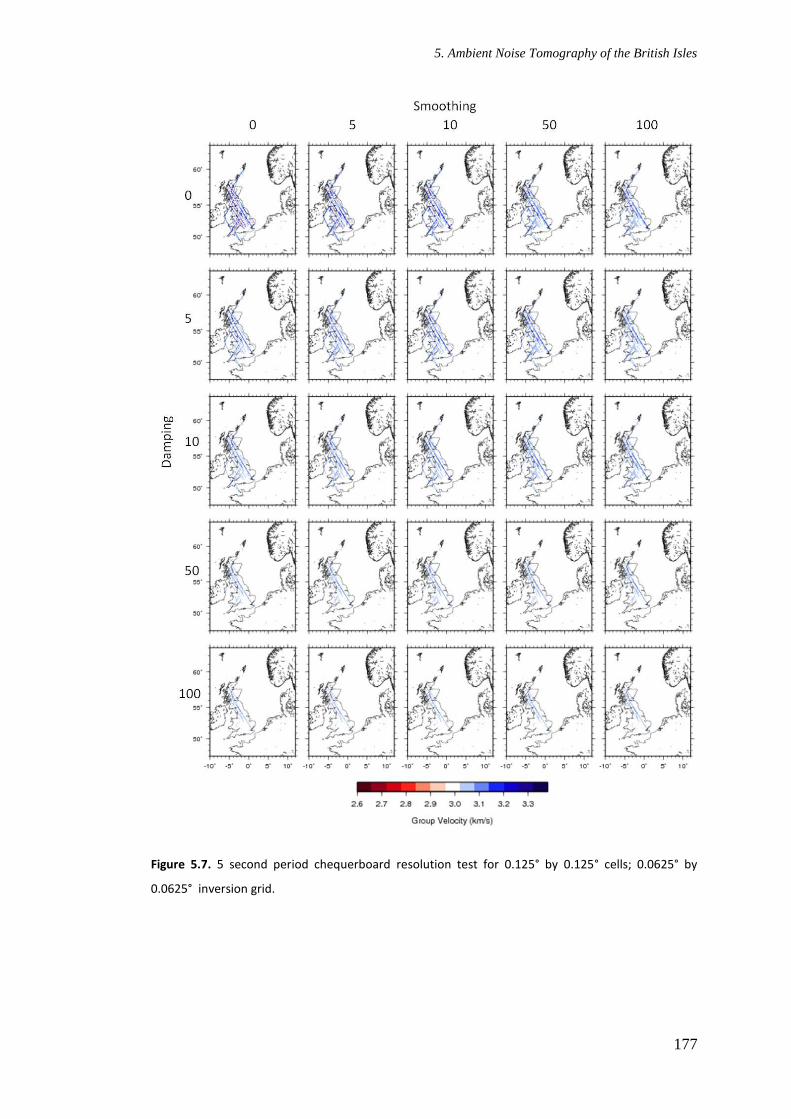
5. Ambient Noise Tomography of the British Isles

177

Figure 5.7. 5 second period chequerboard resolution test for 0.125° by 0.125° cells; 0.0625° by

0.0625° inversion grid.

178

Figure 5.8. 15 second period chequerboard resolution test for 2° by 2° cells; 1° by 1° inversion grid.

5. Ambient Noise Tomography of the British Isles

179

Figure 5.9. 15 second period chequerboard resolution test for 1° by 1° cells; 0.5° by 0.5° inversion

grid.

180

Figure 5.10. 15 second period chequerboard resolution test for 0.5° by 0.5° cells; 0.25° by 0.25°

inversion grid.

5. Ambient Noise Tomography of the British Isles

181

Figure 5.11. 15 second period chequerboard resolution test for 0.25° by 0.25° cells; 0.125° by 0.125°

inversion grid.

182

Figure 5.12. 15 second period chequerboard resolution test for 0.125° by 0.125° cells; 0.0625° by

0.0625° inversion grid.

5. Ambient Noise Tomography of the British Isles

183

Figure 5.13. 30 second period chequerboard resolution test for 2° by 2° cells; 1° by 1° inversion grid.

184

Figure 5.14. 30 second period chequerboard resolution test for 1° by 1° cells; 0.5° by 0.5° inversion

grid.

5. Ambient Noise Tomography of the British Isles

185

Figure 5.15. 30 second period chequerboard resolution test for 0.5° by 0.5° cells; 0.25° by 0.25°

inversion grid.

186

Figure 5.16. 30 second period chequerboard resolution test for 0.25° by 0.25° cells; 0.125° by 0.125°

inversion grid.

5. Ambient Noise Tomography of the British Isles

187

Figure 5.17. 30 second period chequerboard resolution test for 0.125° by 0.125° cells; 0.0625° by

0.0625° inversion grid.

188

damping parameter tends to cause greater degradation of the resolution than changes

to the smoothing parameter. For a 0.25° by 0.25° cell size (Figure 5.6), the resolution

across the whole of the British Isles has been almost completely lost and we

conclude that this is the lower limit of resolution. To confirm this, we present a

further set of chequerboards with a length-scale of 0.125° by 0.125° (Figure 5.7). No

cells are resolvable at 5 seconds for this length-scale.

At 15 seconds period, the 2° by 2° cell chequerboard (Figure 5.8) is reasonably well

resolved for combinations of lower values of damping and smoothing. The edges of

the resolvable area show significant smearing however. At higher values of damping

and smoothing the resolution across the whole of the United Kingdom is

considerably degraded. For 1° by 1° cells (Figure 5.9), some structure is resolved

across England although resolution is poor across the remainder of the study area.

For a 0.5° by 0.5° cell size (Figure 5.10), the resolution across the whole of the

British Isles has been almost completely lost and we conclude that this is the lower

limit of resolution. No structure is resolved at 15 seconds for the 0.25° by 0.25° and

0.125° by 0.125° chequerboards (Figures 5.11 and 5.12 respectively).

At 30 seconds period, the 2° by 2° cell chequerboard (Figure 5.13) is very poorly

resolved for combinations of lower values of damping and smoothing across the

entire study area. No structure is resolved for any of the smaller length-scale

chequerboard tests (Figures 5.14 to 5.17) at 30 seconds period. Therefore we can

conclude that these results represent the limit of resolution. This result is not

surprising since the number of paths at 30 seconds is significantly smaller than at 5

seconds.

In general, the capability of the inversion scheme, described in Chapters 2 and 3, that

we apply here to resolve the chequerboard structure is good. We therefore expect that

it can be successfully applied to real travel-time data for the British Isles. As

discussed in section 4.2.2, we choose the node spacing of our inversion grid to be

much smaller than the minimum length-scale that is well resolved by the data. This

ensures that we minimise any leakage of true Earth structure at length-scales smaller

than the resolvable feature size into our maps (Trampert and Snieder, 1996). From

5. Ambient Noise Tomography of the British Isles

189

the chequerboard results described above, and similarly for those shown in Appendix

B, the inversion grids chosen for our periods of interest are shown in Table 5.1.

Period (s) Inversion Grid

5 0.125° by 0.125°

6 0.125° by 0.125°

8 0.125° by 0.125°

10 0.25° by 0.25°

12 0.25° by 0.25°

15 0.25° by 0.25°

18 0.25° by 0.25°

20 0.5° by 0.5°

25 0.5° by 0.5°

30 0.5° by 0.5°

Table 5.1. Inversion grid node spacings and corresponding periods.

As we discussed in section 4.2.1, note again that ray theory will also impose a limit

on the length-scale of structure that is resolvable by the data, i.e., the wavelength of

the seismic waves should be smaller that the length-scale of the target heterogeneities

(e.g. Wang and Dahlen, 1995; Ritzwoller et al., 2002; Ferreira and Woodhouse,

2007). Table 5.2 shows the average velocity at the periods considered here and the

corresponding wavelengths, and hence lower limits of resolvable length-scale

according to ray theory.

Hence, for a number of periods, the chequerboard tests shown here are carried out

beyond the limit of ray theory. For example, at 5 seconds period the 0.125°

chequerboard test is approaching the limit of ray theory. Similarly at 30 seconds

period, the 1°, 0.5°, 0.25° and 0.125° chequerboard tests involve length-scales that

are around or below the limit defined by ray theory.

190

Period (s) Average Velocity (km/s) Wavelength/Length-scale (km)

5 2.727 14

6 2.763 17

8 2.831 23

10 2.875 29

12 2.893 35

15 2.972 45

18

20

25

30

2.968

2.996

3.076

3.169

53

60

77

95

Table 5.2. Average velocity and corresponding wavelength for the periods considered in this chapter.

5.3 Rayleigh Wave Group Velocity Maps

Using the 2-D iterative, non-linear tomography scheme described in Chapters 2 and

3, we inverted Rayleigh wave travel-time datasets for 5, 6, 8, 10, 12, 15, 18, 20, 25

and 30 seconds period. The inversion grid spacing in each case was chosen according

to Table 5.1 and for each the propagation grid dicing level was set to be 5 x 5. This

propagation grid was chosen because it minimised the computation time of the

forward part of the problem using the Fast Marching method without strongly

altering the features of the tomographic maps. Similar to the inversion performed in

Chapter 4, the starting models were homogeneous, where the velocities were chosen

to be the average measured for that period. The average velocities for each period are

given in Table 5.2. Note that the average velocity generally increases with increasing

period as we might expect.

5.3.1 Selection of Final Rayleigh Wave Velocity Maps

Using the same method described in section 4.2.2, tomographic maps were computed

for many different combinations of damping and smoothing parameters, and the

weighted root mean square of the data residuals was calculated for each map using

equation 4.1. As described previously, the RMSW result is a dimensionless number

that provides a measure of the normalised misfit of the computed data post-inversion

5. Ambient Noise Tomography of the British Isles

191

through the estimated Earth model, for which the a priori uncertainty of the data is

taken into account. We assumed in section 4.2.2 that, as an approximate guide, if the

value of RMSW is significantly greater than 1 then the data fit is potentially

significantly affected by the influence of the choice of regularisation parameters.

However if the value of RMSW is less than 1 then the solution model fits the observed

data to within data uncertainties.

Initial inversions that were found to have high RMSW values have their highest

residual paths removed sequentially from subsequent inversions until their RMSW

value reduces to below an acceptable threshold. In Chapter 4 we chose this threshold

to be 1.3 in order to allow for some statistical variability in the RMSW values. The

main features of the computed maps are generally robust to this removal step, which

is applied to ensure that anomalous data are unlikely to contaminate the final results.

Figures 5.18, 5.19 and 5.20 show the resulting Rayleigh wave group speed maps for

different combinations of damping and smoothing values at 5, 15 and 30 seconds

period respectively. The resulting maps for all periods can be found in Appendix D.

In addition, the resulting maps at all periods, where only paths with an associated

uncertainty measurement are included, can be found in Appendix E. Maps located

above and to the left of the blue contours are not considered since they have had zero

damping and smoothing applied and/or they are geologically unrealistic. Maps

located below and to the right of the blue contours as well as above and to the left of

the red contours have corresponding RMSW values that are acceptable and they

provide geologically sensible results. Therefore these maps are considered for

selection as the final resulting map for the given period. Note also that the main

features of the maps are robust to different choices of regularisation parameters

therefore we can be fairly confident that they are likely due to real Earth structure as

resolved by the data.

For a number of inversions, it was difficult to get the RMSW values for the maps to

reduce to close to 1. This was a particular problem at lower periods. In some cases it

was impossible to reduce the RMSW value to approximately 1 without removing over

80% of the paths from the travel-time dataset and at this stage all interesting features

192

are lost from the maps. Therefore we decided to slightly relax our requirement to

have RMSW values close to 1 for these problem maps in order to retain as many paths

as possible.

This problem is itself an interesting conclusion since it most likely means that the

method we have used to measure uncertainty is not giving the correct values. What

“data error” actually means for inversions is the difference between the predicted

(modelled) and measured data, in our case travel-times. This error therefore includes:

(i) the measurement error (i.e. the error involved in measuring the observed travel-

times) and (ii) the modelling error, which is due to the inability of the inversion

scheme to model the observed data. The modelling error will be affected by factors

such as the parameterisation of the problem and the physics involved with modelling

the predicted data not being appropriate for the specific problem.

The cause of the problem related to improper estimation of the inversion “data error”

by calculating the RMSW for each map is likely to be measurement error. Figures

3.22 and 3.23 give some idea of the measurement errors inherent in the observed

data. Many of the dispersion curves across the British Isles were of relatively poor

quality and in addition, since they were picked manually the opinion and experience

of the user will have a significant effect on the consistency of the measurements and

therefore the measurement error, compared with an automated procedure.

The size of the inverse problems solved for each map are described in table 5.3, for

maps constructed using well constrained paths plus paths with uncertainties

estimated from inter-station distance, and in table 5.4 for maps constructed using

well constrained paths only. The tables shows the number of model parameters (i.e.

velocity inversion grid points – see section 3.5.1) and the final number of raypaths

used at each period following the removal step described above. Note that the

number of unknowns solved during the inversion, i.e. the model parameters, is much

larger that the number of observed data.

5. Ambient Noise Tomography of the British Isles

193

Period (s) Number of Model Parameters Final Number of Raypaths

5

6

8

10

9009

9009

9009

2397

205

361

527

422

12 2397 536

15

18

20

25

30

2397

2397

675

675

675

552

560

517

403

196

Table 5.3. Summary of inverse problem size for maps constructed using well constrained paths plus

paths with uncertainties estimated from inter-station distance. The total number of model

parameters quoted here describes the whole inversion grid over the entire map area, including those

not located within the area of station coverage. In practise, the number of parameters constrained

during the inversion routine will be smaller than the total number of model parameters since we

apply regularisation.

Period Number of Model Parameters Final Number of Raypaths

5

6

8

10

9009

9009

9009

2397

214

247

270

214

12 2397 175

15

18

20

25

30

2397

2397

675

675

675

143

133

104

38

6

Table 5.4. Summary of inverse problem size for maps constructed using well constrained paths only.

The total number of model parameters quoted here describes the whole inversion grid over the

entire map area, including those not located within the area of station coverage. In practise, the

number of parameters constrained during the inversion routine will be smaller than the total

number of model parameters since we apply regularisation.

194

The final choice of Rayleigh wave group velocity maps at each period are shown in

Figures 5.21 to 5.30. For comparison, we show maps constructed using well

constrained paths plus paths with uncertainties estimated from inter-station distance

as well as maps constructed using well constrained paths only. For each period, there

is little difference between each acceptable map located between the blue and red

contour lines therefore it is difficult to choose one representative map. As we did in

Chapter 4, in each case we chose the map which has the smallest amount of damping

and largest amount of smoothing applied as well as an acceptable RMSW value.

5. Ambient Noise Tomography of the British Isles

195

Figure 5.18. 5 second period Rayleigh wave maps for a combination of damping and smoothing

values. The calculated RMSW value for each map is also shown in the bottom right-hand corners.

Maps located within the red contour line are acceptable since they are geologically realistic and have

an acceptable RMSW value.

196

Figure 5.19. 15 second period Rayleigh wave maps for a combination of damping and smoothing

values. The calculated RMSW value for each map is also shown in the bottom right-hand corners.

Maps located within the red contour line are acceptable since they are geologically realistic and have

an acceptable RMSW value.

5. Ambient Noise Tomography of the British Isles

197

Figure 5.20. 30 second period Rayleigh wave maps for a combination of damping and smoothing

values. The calculated RMSW value for each map is also shown in the bottom right-hand corners.

Maps located within the red contour line are acceptable since they are geologically realistic and have

an acceptable RMSW value.

198

Figure 5.21. Rayleigh wave group velocity maps of the British Isles at 5 seconds period from cross-

correlations of ambient seismic noise between the stations shown in Figure 5.2 for (a) well

constrained paths and paths with uncertainties estimated from inter-station distance; (b) well-

constrained paths only.

(a) (b)

5. Ambient Noise Tomography of the British Isles

199

Figure 5.22. Rayleigh wave group velocity maps of the British Isles at 6 seconds period from cross-

correlations of ambient seismic noise between the stations shown in Figure 5.2 for (a) well

constrained paths and paths with uncertainties estimated from inter-station distance; (b) well-

constrained paths only.

(a) (b)

200

Figure 5.23. Rayleigh wave group velocity maps of the British Isles at 8 seconds period from cross-

correlations of ambient seismic noise between the stations shown in Figure 5.2 for (a) well

constrained paths and paths with uncertainties estimated from inter-station distance; (b) well-

constrained paths only.

(a) (b)

5. Ambient Noise Tomography of the British Isles

201

Figure 5.24. Rayleigh wave group velocity maps of the British Isles at 10 seconds period from cross-

correlations of ambient seismic noise between the stations shown in Figure 5.2 for (a) well

constrained paths and paths with uncertainties estimated from inter-station distance; (b) well-

constrained paths only.

(a) (b)

202

Figure 5.25. Rayleigh wave group velocity maps of the British Isles at 12 seconds period from cross-

correlations of ambient seismic noise between the stations shown in Figure 5.2 for (a) well

constrained paths and paths with uncertainties estimated from inter-station distance; (b) well-

constrained paths only.

(a) (b)

5. Ambient Noise Tomography of the British Isles

203

Figure 5.26. Rayleigh wave group velocity maps of the British Isles at 15 seconds period from cross-

correlations of ambient seismic noise between the stations shown in Figure 5.2 for (a) well

constrained paths and paths with uncertainties estimated from inter-station distance; (b) well-

constrained paths only.

(a) (b)

204

Figure 5.27. Rayleigh wave group velocity maps of the British Isles at 18 seconds period from cross-

correlations of ambient seismic noise between the stations shown in Figure 5.2 for (a) well

constrained paths and paths with uncertainties estimated from inter-station distance; (b) well-

constrained paths only.

(a) (b)

5. Ambient Noise Tomography of the British Isles

205

Figure 5.28. Rayleigh wave group velocity maps of the British Isles at 20 seconds period from cross-

correlations of ambient seismic noise between the stations shown in Figure 5.2 for (a) well

constrained paths and paths with uncertainties estimated from inter-station distance; (b) well-

constrained paths only.

(a) (b)

206

Figure 5.29. Rayleigh wave group velocity maps of the British Isles at 25 seconds period from cross-

correlations of ambient seismic noise between the stations shown in Figure 5.2 for (a) well

constrained paths and paths with uncertainties estimated from inter-station distance; (b) well-

constrained paths only.

(a) (b)

5. Ambient Noise Tomography of the British Isles

207

Figure 5.30. Rayleigh wave group velocity maps of the British Isles at 30 seconds period from cross-

correlations of ambient seismic noise between the stations shown in Figure 5.2 for (a) well

constrained paths and paths with uncertainties estimated from inter-station distance; (b) well-

constrained paths only.

(a) (b)

208

5.4 Interpretation

A number of interesting geological features can be identified on the Rayleigh wave

maps in Figures 5.21 to 5.30. Overall, shallow sediments are shown as low velocities

- in contrast, igneous and metamorphic rocks tend to be characterised by higher

velocities. In addition, there is a general increase in velocity from south-east to north-

west across the British Isles at most periods. For ease of discussion I split the

following interpretation into three sections, broadly covering the upper crust, mid-

crust and lower crust/upper mantle.

5.6.1 Upper Crust – 5, 6 and 8 Seconds

The maps at 5, 6 and 8 seconds period shown in Figures 5.21 to 5.23 are sensitive to

the shallow upper crust, to depths of around 8, 10 and 12 km respectively. These

maps have generally good resolution across most of mainland Britain and an

inversion grid of 0.125° by 0.125° was used to compute them, meaning that we

might expect to resolve structures with a minimum length-scale of 0.25°.

Caledonian, NW-SE trending structures across northern Britain are generally well

resolved at 5, 6 and 8 seconds period. High velocities across the Scottish Highlands

are consistent with the crystalline Lewisian and Dalradian complexes. South of the

Highland Boundary fault and north of the Southern Uplands fault, a NW-SE trending

low velocity anomaly is consistent with the dominantly sedimentary rocks of the

Midland Valley. The lowest velocity part of the Midland Valley occurs across the

Firth of Forth syncline. Immediately south of the Midland Valley, a high velocity,

NW-SE trending anomaly across the Southern Uplands can be attributed to the

siltstones, wackes and felsic plutons of the Southern Uplands accretionary complex.

The relationship between these Caledonian features and the terrane structure of

Scotland is clearly illustrated in Figure 5.31.

Another feature of the upper-crustal maps that becomes more apparent in Figure

5.31(b) is the significant slow anomaly in the English Midlands, approximately

located within the Midland Platform. The Midland Platform, or Microcraton, is a

region of Precambrian basement that remained relatively undeformed during the

5. Ambient Noise Tomography of the British Isles

209

Caledonian and Variscan orogenies and is surrounded by softer, deformed rocks. We

would therefore expect to obtain high velocities for the Midland Platform, similar to

previous studies (e.g. Arrowsmith, 2003). However our results show a persistent low

velocity anomaly in the region of the Midland Platform at most periods. Low

velocities are also found to the south of the Variscan Front in the Wessex Basin and

between the northern apex of the Midland Platform and the Irish Sea in the

Worcester and Chester Mesozoic Basins. An extensive low velocity anomaly occurs

in the Irish Sea basin at 5, 6 and 8 seconds period.

Figure 5.31. Rayleigh wave velocity map for 5 seconds period from Figure 5.21(a) overlain by (a)

major fault-lines of the UK; (b) Terrane boundaries from Figure 1.7, after Woodcock and Strachan

(2000).

(a) (b)

210

Other high velocity anomalies in the upper crust can be attributed to granitic

intrusions in Cornwall and north-west Wales and the limestone rocks of the Pennines

in northern England. Fast velocities are also obtained to the east and north-east of the

Midland Platform. This feature does not obviously correlate with the known geology

of eastern England however it is co-located with a series of positive magnetic

anomalies (Figure 5.34) and a gravity high structure (Figure 5.35). More detailed

study is required to determine whether it is a real, structural feature or an artefact of

the data inversion.

5.6.2 Mid-Crust – 10, 12, 15 and 18 seconds

The 10, 12, 15 and 18 second maps are sensitive to depths of approximately 15 to

30km. The resolution for these maps is degraded compared with the maps at 5, 6 and

8 seconds, therefore we expect to be able to resolve features with a minimum length-

scale of 0.5°. High velocities associated with metamorphic and igneous rocks in the

Scottish Highlands, the Southern Uplands, North West Wales and Cornwall observed

for the upper crust are still present at the mid-crustal level. A high velocity anomaly

east of the Midlands Platform can also still be observed on the 10, 12, 15 and 18

second maps.

Low velocity anomalies that were attributed to the Irish Sea, Chester, Worcester and

Wessex basins are still present at 10, 12 and 15 seconds. Low velocities in the

Midland Valley of Scotland are less pronounced at these periods. Dentith and Hall

(1989; 1990) suggest, from seismic refraction studies across the Midland Valley, that

approximately 4 to 8 km of sediment overlies high velocity basement rock in the

Midland Valley. Therefore it is likely that the maps sensitive down to mid-crustal

depths are showing the basement rock rather than the overlying lower velocity

sediments in the Midland Valley.

5.6.3 Lower Crust/Upper Mantle – 20, 25 and 30 seconds

The 20, 25 and 30 second maps are sensitive down to approximately 30, 32 and 35

km depth, respectively. The 20 second map is likely to represent the base of the

crust. Low velocities are still seen in the eastern Irish Sea and across the Midland

5. Ambient Noise Tomography of the British Isles

211

Platform and Wessex Basin. The general features of the maps change significantly at

25 and 30 seconds. In Figures 5.29 and 5.30, the British Isles can almost be split

north to south down the centre, with higher velocities in the west and lower velocities

in the east. The depths approximately represented by these maps are consistent with

the average Moho depth across the British Isles (~30km). Figure 5.32 shows a map

of Moho depth under the British Isles as derived by Chadwick and Pharaoh (1998).

In general, the Moho shallows from east to west across the British Isles. This is

consistent with our maps at 25 and 30 seconds which show a transition from lower to

higher velocity from east to west at approximately Moho depth. Figure 5.33 shows

the 25 second velocity map from Figure 5.29(a) overlain by the historical distribution

of British earthquakes shown in Figure 1.2. There is a good correlation between the

distribution of British earthquakes and the higher velocity area on the map. The

velocity of this region is higher relative to the average at this period, which is

measured over predominantly crustal lithosphere. This suggests that more mantle

material is being sampled by the longer period Rayleigh waves and therefore that the

crust is thinner here.

This observation agrees with the results of previous studies, which suggest that one

control of seismicity in the British Isles is thermal weakening of thinned crust above

a mantle upwelling beneath the western British Isles (e.g. Bott and Bott, 2004;

Arrowsmith et al., 2005). These studies, which target deeper Earth structure than we

do here, describe a low velocity anomaly in the upper mantle beneath the western

British Isles. The anomaly is interpreted as low since it is compared to the

surrounding mantle whereas the anomaly we observe here is high with respect to

lower velocity crustal lithosphere. The high velocity anomaly at 25 seconds also

correlates well with a positive gravity anomaly down the west side of the British

Isles on the long period gravity map shown in Figure 5.35.

212

Figure 5.32. Moho depth beneath the British Isles. From Chadwick and Pharaoh (1998).

5. Ambient Noise Tomography of the British Isles

213

Figure 5.33. Rayleigh wave group velocity map of the British Isles at 25 seconds period from Figure

5.30. Historical distribution of British earthquakes as shown in Figure 1.2 represented by small, black

circles.

214

Figure 5.34. Shaded relief aeromagnetic anomaly map of the British Isles. Negative anomalies are

represented by the blue colours and positive anomalies by red. Reproduced with permission from

the British Geological Survey.

5. Ambient Noise Tomography of the British Isles

215

Figure 5.35. Long-period gravity anomaly map for the British Isles; Bouguer anomaly onshore and

Free-Air anomaly offshore. Gravity lows are represented by the blue colours and gravity highs by red.

Reproduced with permission from the British Geological Survey.

216

217

Chapter 6

Creating Virtual Receivers in the Sub-surface of the Earth

from Seismic Interferometry

The following chapter describes how we compute surface wave seismograms

between two earthquakes by turning one of the earthquakes into a virtual receiver. A

more detailed explanation of the method is given in Chapter 2 of this thesis. This

work has been published in Nature Geoscience as Curtis et al. (2009).

6.1 Summary

Seismologists image the Earth’s interior by analysing recordings of propagating

seismic waves. The global array of permanent seismometers that records seismic

energy is confined almost exclusively to accessible and secure, land-based sites. This

limits the resolution of subsurface images, and results in relatively few local

measurements from areas of great geological and tectonic interest such as mid-ocean

ridges, the Tibetan and Andean plateaus and subduction zones (Bijwaard and

Spakman, 2000). Here we show that a novel form of seismic interferometry

(Campillo and Paul, 2003; Shapiro and Campillo, 2004; Shapiro et al., 2005; Gerstoft

et al., 2006) can be used to construct an artificial or ‘virtual’ sensor from any energy

source. We use this to turn earthquakes in Alaska and south-west USA into virtual

seismometers located beneath the Earth’s surface. Such sensors measure the same

spatial and temporal quantities that were represented in the radiation pattern of the

218

original energy source; since earthquakes impart strain, their corresponding virtual

seismometers measure strain caused by passing seismic waves. By definition

earthquakes are located within the Earth’s solid interior, so virtual seismometers can

be located non-invasively inside solid bodies. Earthquakes occur precisely within

many tectonically active areas in which there are often no real seismometers; their

corresponding virtual seismometers provide local windows into such geological

phenomena. This work thus enables real-time, non-invasive, sub-surface seismic

strain monitoring in areas of greatest geological interest.

6.2 Introduction

To interrogate the Earth’s subsurface at greater than a few kilometres depth,

traditional seismology analyses seismic wave energy from earthquakes. Other energy

recorded in seismograms, such as ambient Earth oscillation, is considered noise and

is excluded from analysis. Since 2003, however, methods of seismic interferometry

have been developed to synthesise impulsive-source seismograms from ambient

noise recorded at two seismic receivers (e.g. Campillo and Paul, 2003; Chapter 2).

These seismograms simulate the situation where energy from a relatively impulsive,

imagined or ‘virtual’ source occurring at the location of one receiver was recorded by

the other.

Until the work described in this chapter was undertaken in 2009, seismic

interferometry was concerned with cross-correlating recordings at two receivers due

to a surrounding boundary of impulsive or noise sources, then stacking the cross-

correlations to construct the inter-receiver Green’s function (Chapters 2, 3, 4 and 5).

Given a suitable receiver geometry, interferometry obviates the need for actual

earthquake sources to image the Earth (Claerbout, 1968; Campillo and Paul, 2003;

Wapenaar, 2003; Wapenaar and Fokkema, 2004; Wapenaar et al., 2004; van-Manen

et al., 2005, 2006; Wapenaar and Fokkema, 2006).

Although in principle interferometry frees seismologists from constraints imposed by

the global distribution of earthquakes which is strongly biased towards active

margins and mid-ocean ridges, the global receiver distribution is also strongly biased

6. Creating Virtual Receivers in the Sub-surface of the Earth from Seismic Interferometry

219

(Figure 6.1). More than two-thirds of the Earth’s surface is covered by liquid water

or ice, rendering receiver installation difficult and expensive. Even many land-based

areas have few receivers due to geographical or political inhospitability (e.g., Tibetan

and Andean plateaus, Central Africa – Figure 6.1). Hence, most of the Earth’s

subsurface can only be interrogated using long earthquake-to-receiver, or receiver-to-

receiver paths of energy propagation. This provides relatively poor spatial resolution

of some of the most intriguing tectonic, geological and geophysical phenomena such

as mid-ocean ridges and plate convergence zones, and consequently there is a need

for data to be recorded locally to such phenomena.

By taking the reciprocal of its usual form, we showed in Chapter 2 that the

impulsive-source form of interferometry can also be used in the opposite sense: to

turn any energy source into a virtual sensor. In this form, we apply interferometry

using sources enclosed within a boundary of receivers (Figure 2.9(b)). This approach

is related to that of Hong and Menke (2006), but they used the passive-noise (rather

than impulsive source) form of interferometry. We demonstrate a substantial

improvement over their results. Snieder (2004) showed that it is not always necessary

to have an entire enclosing boundary, provided sources are located within a cone

around the extension of the inter-event path (Figure 2.9(c)). We make use of the

latter geometrical approximation in our examples.

To illustrate this new method simply we use real-station recordings of the 2008

Sichuan earthquake from the Caltech Regional Seismic Network to construct

seismograms recorded by two virtual receivers, in the Alaskan subduction zone and

in California, respectively. These virtual receivers and real stations lie approximately

on a great circle with the Sichuan earthquake (Figure 6.2(e)). It is assumed that

seismic energy will travel along this path between the various chosen locations. For

each Californian station located around the great circle path (i.e. located within the

areas of stationary phase) the seismograms for the Sichuan and virtual receiver

earthquakes are cross-correlated, then the resulting cross-correlations are summed. In

Figure 6.2 we show the real recordings of the Sichuan earthquake at stations located

close to each virtual receiver (Figure 6.2 (a) and (c)), and the resulting virtual

receiver records (Figure 6.2 (b) and (d)).

220

Figure 6.1. Global distribution of earthquakes of magnitude > 5 since 1973 (black circles) and 13,000

NEIC-listed seismometers (red triangles). From Curtis et al. (2009).

6. Creating Virtual Receivers in the Sub-surface of the Earth from Seismic Interferometry

221

Figure 6.2. Comparison of virtual and real receiver recordings of 2008 Sichuan earthquake using the

configuration in (e). (a) Real recording at MLAC in California; (b) virtual receiver recording at event

within 40km of MLAC; (c) real recording at KDAK in Alaska; (d) virtual receiver recording at event

within 260km of KDAK. All vertical component. (e) Location map. Earthquakes (red stars); seismic

stations (yellow triangles); great circle path (solid, black line).

(e)

(b)

(c)

(d)

(a)

222

The real and virtual traces should not be exactly the same since the virtual-receiver

records strain whereas real receivers measure displacement (or derivatives thereof).

In addition, the stations used for comparison are not co-located with the virtual

receivers and the California-based array only spans a fraction of a complete

boundary of seismometers. Nevertheless, it is clear to see the similarity between the

real and virtual receiver recordings, especially for the Californian virtual receiver.

6.3 Verification of Virtual Sensors

A potential problem in verifying virtual receiver recordings is that real strain-sensors

do not exist in the Earth’s subsurface close to earthquakes; therefore we cannot

compare the real and virtual signals directly. The components of strain that are

recorded by a virtual receiver are determined by the spatio-temporal response of its

parent earthquake: those constructed from purely normal and purely thrust

earthquakes thus measure strains in a vertical-horizontal plane, while those from

strike-slip earthquakes measure strain in the purely horizontal plane. Those

constructed from subsurface explosions or implosions measure volumetric expansion

of the rock mass (the solid-body equivalent of a pressure sensor in a fluid (Curtis and

Robertsson, 2002)).

In section 2.4 we present a general acoustic and elastic formulation for constructing

virtual sensors using interferometry. We also develop theory for the particular case of

an earthquake double-couple moment tensor source radiating Rayleigh- and Love-

surface waves, since to-date seismic interferometry has derived useful information

largely from the reconstruction of surface waves. We thus derive precisely which

components of surface wave strain are recorded by virtual-receivers constructed from

canonical normal, thrust, and strike-slip earthquakes, as well as explosion sources,

allowing verification of the method by comparison with directly recorded

seismograms in these cases (see Table 6.1).

6. Creating Virtual Receivers in the Sub-surface of the Earth from Seismic Interferometry

223

Thrust Fault Earthquake e33 - e11

Normal Earthquake e11 - e33

Strike-Slip Earthquake e12 + e21

Isotropic Explosion e11 + e22 + e33

Table 6.1. Combinations of strain components eij measured for each source mechanism. We use a

left-handed coordinate system with axes 1, 2 and 3 pointing East, North and down, respectively. The

earthquake fault plane is assumed to be oriented (strike) northwards; the strike-slip fault plane is

vertical while the thrust and normal fault planes have 45 degrees dip. No fault is assumed for the

explosion.

Since the match in Figure 6.2 is not perfect, we consider test cases using earthquake

and receiver geometries that allow a more in-depth analysis of the method. To make

direct comparisons with real seismograms possible, in principle one could construct

horizontal strain measurements by computing scaled differences between closely-

spaced seismometers (Curtis and Robertsson, 2002), but in the frequency range

considered here (15s-33s period) across south-west USA this is generally not

possible since the seismometer distribution is spatially aliased. Instead we derive

estimates of the scaled horizontal strain in a direction in-line with the source-to-

seismometer path by taking time-derivatives of measured seismograms. This results

in frequency-domain multiplication by iω = ick, where ω and k are temporal and in-

line spatial frequencies, respectively, and c is phase velocity. Thus we approximate a

spatial derivative (multiplication by ik) assuming that the unknown phase velocity c

does not change rapidly within the frequency band considered (we also took account

of the azimuth of propagation, which can change the sign of the horizontal strain

estimates). There is no equivalent operation to approximate vertical strains in the

examples presented above. Vertical strain measurements from virtual receivers

therefore constitute new information about Earth vibrations.

224

If an earthquake is considered to be temporally-impulsive with moment tensor M1,

and is recorded by a virtual sensor constructed from another earthquake with moment

tensor M2, the data consist of a sum of strain Green’s functions between the locations

of the two earthquakes, scaled by the product of the respective moment tensor

components (equation 2.83 to 2.86). However, earthquake sources are also generally

non-impulsive. If Wi(ω) is the frequency domain representation of the source time

function of earthquake i, the seismograms recorded at the virtual sensor are

modulated by W2(ω)W1(ω)* (equations 2.78 and 2.79). Hence, if for example the two

source time functions were similar, W2(ω) ≈ W1(ω), the recorded data would consist

of inter-earthquake strain Green’s functions modulated by the autocorrelation of the

source time function, shifted in time by t2 - t1, where ti is the origin time of

earthquake i. We remove that time shift in the results herein. As a consequence,

compared to a zero-phase seismometer, residual phase shifts in the virtual sensor

records are caused by differences between the two source time functions W1 and W2.

Figure 6.3 shows earthquakes and stations used for verification. Two earthquakes

with approximately canonical (strike-slip and normal) moment tensor sources were

chosen to be converted into virtual sensors because (i) seismometers (MLAC and

R06C) exist in their local vicinity for comparison, (ii) they had a well-constrained

moment tensor source mechanism, (iii) they had the lowest possible magnitude

subject to constraints (i) and (ii) and hence are spatially and temporally as localised

as possible, reducing associated relative phase differences between recordings on

seismometers and virtual sensors. Source times used for the seismometer recordings

are those from the International Seismology Centre (ISC) catalogue; no Centroid

Moment Tensor (CMT) source mechanism and timing was available.

We analysed seismograms from two other earthquakes recorded on these virtual

sensors, one chosen to have source-to-virtual sensor path aligned roughly east-west,

the other chosen to have a roughly perpendicular path. We compare strain recordings

of these events on the virtual sensors with estimates of strain constructed from

recordings of particle velocity from the neighbouring seismometers (see section 2.4).

6. Creating Virtual Receivers in the Sub-surface of the Earth from Seismic Interferometry

225

Figure 6.3. South-West USA Location Map. Earthquakes (red stars) numbered 1 to 4; seismic stations

used in interferometry (blue triangles); seismic stations for comparison (yellow triangles); focal

mechanisms of virtual receivers are shown as standard lower-hemisphere projections near to their

locations. Dashed lines indicate inter-Earthquake paths, solid lines connected by arcs indicate the

region within which receivers were located for each Earthquake pair.

Virtual sensors were constructed by integrating (summing) un-weighted recordings at

a subset of other available seismometers that did not include either comparison

seismometer (equation 2.86). Each subset consisted of seismometers within a cone

around the propagation path direction at the virtual sensor (Figure 6.3), since these

are expected to record the main energy that integrates constructively within the

virtual receiver seismogram (Snieder, 2004). Conclusions herein are robust to

changes in the subtending angle. The azimuth of propagation between the real

earthquake and virtual seismometer is important since it changes the sign of the

horizontal strain recordings; therefore, as discussed previously, it is also taken into

account when comparing with real earthquake recordings.

1

2

3

4

226

Figure 6.4. Comparison of recordings of earthquake 1 by the strike-slip virtual receiver 3 and the real

seismometer MLAC: seismograms (top) and envelope functions (bottom) recorded at the virtual

receiver (solid line) and the inverted time-derivative of the radial-component seismogram from

MLAC (dashed). Signals are constructed by cross-correlation and stacking of 20 stations from the

USArray and Berkeley seismic networks (Figure 6.3). Amplitudes are normalised and all traces are

band-passed between 15 and 33 seconds.

A virtual sensor constructed from the strike-slip earthquake 3 oriented at 45 degrees

to the East-West energy propagation path (Figure 6.3) measures the sum of e12 and

e21 components of strain (Table 6.1). A comparable scaled strain measurement can be

calculated from the neighbouring seismometer by taking the (negative of the) time-

derivative of the radial component of velocity. Figure 6.4 shows a comparison

between this time derivative and the virtual receiver record. The group arrival of the

main energy matches to within 5s, as does the phase. A phase mismatch of 5s is

easily accounted for by the difference between temporal responses of virtual and real

seismometers as described in Chapter 2.

6. Creating Virtual Receivers in the Sub-surface of the Earth from Seismic Interferometry

227

Figure 6.5. Similar to Figure 6.4, but here using the normal virtual receiver 4 (solid), and the direct

recording is the inverted, vertical-component seismogram from seismometer R06C (dashed). Virtual

receiver records are constructed using 15 stations from the USArray and Berkeley seismic networks

(Figure 6.3).

Figure 6.5 shows the same event recorded by the virtual sensor constructed from the

N-S oriented normal-faulting earthquake 4. This virtual receiver measures the

difference between the e33 and e11 components of strain. There is no easy way to

construct a comparison measurement for the e33 component from the real

seismometer so in Figure 6.5 the comparison seismogram is simply the vertical

component of particle velocity. As expected, while the energy group arrival times are

again well matched, the phases differ markedly.

We can construct a comparison seismogram for the e11 component by taking the time

derivative of the radial component of velocity of the real seismometer recording.

Figure 6.6 shows that the fit is excellent hence, for this event at this station, the

228

signal is probably dominated by the horizontal strain component e11. Since the

vertical strain component is approximately related to the derivative of the Rayleigh

wave eigenfunctions with depth beneath the virtual receiver, we infer that that

eigenfunction is likely to be approximately constant with depth at the earthquake

location.

Figure 6.6. Similar to Figure 6.4, but here the dashed, direct recording is the inverted, time derivative

of the radial-component recording from seismometer R06C (dashed). Lower panel is the equivalent

result obtained using the method of Hong and Menke (2006).

Previously, Hong and Menke (2006) estimated virtual seismograms by a different

method. They added active source recordings together to generate pseudo-noise

sequences and then applied the passive-noise form of interferometry to estimate

inter-source responses (i.e. they sum over receivers, then cross-correlate).

Unfortunately, accurate seismogram construction from passive noise requires much

longer time series than are afforded by typical earthquake seismograms (van-Manen

et al., 2006), and consequently in Figure 6.6 we show that their method produces

relatively less accurate seismogram approximations. Our approach is different: we

6. Creating Virtual Receivers in the Sub-surface of the Earth from Seismic Interferometry

229

use the impulsive source form of interferometry by first cross-correlating responses

and only then summing over receivers. This requires only the actual, recorded

seismograms at each receiver.

Figure 6.7. Similar to Figure 6.4, but compares recordings of earthquake 2 at the normal virtual

receiver and the real seismometer R06C: the inverted, vertical component seismogram is shown

(dashed). Signals are constructed by cross-correlation and stacking of 14 stations from the USArray

and Berkeley seismic networks (Figure 6.3).

Vertical strains are fundamentally new measurements provided by the virtual

sensors. We can isolate the vertical derivative measurement by looking at

seismograms from earthquakes occurring along-strike of the normal virtual sensor. In

this geometry the e11 component is zero, leaving only the e33 component (equation

2.103). Figure 6.7 shows the vertical strain seismogram recorded on the normal

virtual receiver from the southernmost earthquake in Figure 6.3. Again, the energy

group arrival time is reasonable given that observed on the vertical particle velocity

230

record, while the phase of the vertical strain is an example of a new type of

measurement to seismology.

6.4 Conclusions

Although we formulated theory only for acoustic and elastic wave propagation (see

section 2.4), this can be extended into forms appropriate for diffusive, attenuating,

electromagnetic or electro-kinetic energy propagation (Slob et al., 2007; Slob and

Wapenaar, 2007; Sneider, 2007; Sneider et al., 2007). It is applied here to earthquake

sources, but we could equally construct virtual sensors from fractures occurring in

stressed solid material in a laboratory, or from impulsive pressure sources in liquid or

gas, provided energy from such sources is recorded at an appropriately placed array

of receivers.

The inter-earthquake seismogram is obtained by back-projecting data recorded from

one earthquake through the empirically-recorded Green’s functions from another, an

explicit elastic expression of the acoustic time-reversal experiment of Derode et al.,

(2003). However, the method also converts the data from particle displacement (or

time derivatives thereof) at the real seismometers to strain, due to seismic waves at

the subsurface locations, to match the type of the original source. Also, since this

method essentially back-projects recordings to the virtual sensor location, it is

equally possible to back-project other signals such as passive noise recordings to

either or both of the pair of subsurface source locations. This offers the possibility to

monitor inter-earthquake Green’s functions as a function of time either before or

after the original earthquakes occurred, by using standard passive-noise

interferometry (Campillo and Paul, 2003; Shapiro and Campillo, 2004; Shapiro et al.,

2005; Gerstoft et al., 2006).

In the exploration industry seismic-frequency strain recordings have been shown to

be particularly useful for wavefield analysis and subsurface imaging (Curtis and

Robertsson, 2002; Robertsson and Curtis, 2002). The direct, non-invasive sensitivity

to strain provided by the virtual seismometers introduced here is the first such

measurement within the interior of a solid. This holds the promise to analyse stress-

6. Creating Virtual Receivers in the Sub-surface of the Earth from Seismic Interferometry

231

or strain-triggering of earthquakes by passing seismic waves, for example, since no

other method has the potential to provide such deep, or such widely distributed

measurements of the strain field in the Earth’s subsurface.

232

233

Chapter 7

Discussion

In this thesis I have shown that seismic interferometry can be successfully applied to

construct surface waves across the British Isles using only ambient seismic noise.

Following this I presented the first Rayleigh wave group velocity maps of the

Scottish Highlands and the British Isles using the ambient noise tomography method.

I then showed that seismic interferometry can be applied in the opposite sense by

turning earthquakes in Alaska and California into seismic receivers. In this chapter I

discuss the issues, limitations and questions that have emerged from the results of

this thesis, and to finish I consider possible future research that is suggested by this

project.

7.1 Computational Issues

Processing ambient seismic noise data for seismic interferometry requires large

amounts of data. Furthermore, the human and computational labour required to go

from raw data to surface wave velocity maps is intensive. The processing method

described in Chapter 3 was semi-automated, which significantly reduced the amount

of effort required to process and organise such a large dataset. However, a number of

computational issues were identified, which should be considered for future

applications and these are discussed in this section.

234

7.1.1 Run-time of Tomographic Inversion Computations

The iterative, non-linear inversion scheme described in sections 2.7 and 3.5 is a very

complex computation. There are a number of factors concerning the parameterisation

of an inversion problem which have a significant effect on the run-time of a

tomographic inversion.

The first of these is the size of the area of interest. Obviously the larger this area is,

the greater the number of velocity nodes that will be included in the inversion grid.

Similarly the choice of node spacing is important since choosing a finer grid will

increase the computation time required. As discussed in section 3.5.2, the forward

calculation of model travel-times using the Fast Marching method requires greater

computation time than the inversion step, since the entire travel-time field is

calculated. Therefore the choice of the propagation grid spacing, and subsequently

the refined source grid spacing, is also important.

Since the choice of the inversion grid spacing is based on the minimum length-scale

of structure that can be resolved by the data, there is little flexibility in increasing this

grid spacing to decrease the computation time. Therefore compromises must be made

regarding the limit of the area of interest and the propagation grid spacing to ensure

that the computation time to perform a tomographic inversion is minimised. Firstly,

the area of interest, and therefore the limit of the inversion and propagation grid, is

defined as the nearest whole degree of latitude or longitude beyond the area of

station coverage. In doing so we ensure that all of the inter-station paths are

contained within the area of interest while reducing the amount of unresolved area

that is included in the calculation. Reducing the node spacing of the propagation grid

is likely to lead to degradation in the accuracy of the calculated travel-time field.

Even after taking the time saving measures described above, the run-times for a

tomographic inversion are relatively long. For example, for an inversion covering the

whole study area including the North Sea, using an inversion grid of 22,833 nodes

giving a node spacing of 0.125° by 0.125°, setting a dicing level of 5x5 for the

propagation grid and performing six iterations takes approximately 25 minutes to run

on two Intel Xeon processors each with a speed of 1.6GHz. If this same inversion is

7. Discussion

235

also carried out for 25 combinations of damping and smoothing parameters and for 5

separate periods, the total run-time will be approximately 52 hours.

7.1.2 Surface-wave Dispersion Curve Measurement and Continuous Updating of

Surface Wave Maps

The most labour intensive step of the processing flow described in Chapter 3 is that

of measuring surface wave dispersion. The dispersion curves are picked manually

and making the measurements in this way allows the user to identify and account for

glitches in the dispersion curves such as jumps and spectral holes which may not be

properly dealt with by an automated procedure. This leads to higher-quality

measurements being included in the dataset. While each curve can be measured fairly

rapidly as the user becomes experienced, the huge number of curves involved makes

this step an extremely time consuming task. For example, 423 paths were used for

the 5 second period case shown in Figure 4.4(a). If we say that for every path: (i) a

pick is made for the stack of all daily cross-correlations, (ii) four curves

corresponding to stacks of randomly chosen daily cross-correlations for uncertainty

analysis are also picked, and, (iii) 3 multiple filter iterations are performed on

average for each curve. Therefore for this one period, there are 6345 possible curves,

each of which must be picked manually.

Ambient seismic noise provides a constant, reliable source for ANT. Therefore an

important, potential advantage for its application in the British Isles is the ability to

continually add more data and hence continually improve the resolution of the sub-

surface models. Such a system is already being implemented by the Centre for

Imaging the Earth’s Interior at the University of Colorado. The team track the

progression of the USArray (which is described further in section 7.4.2) across the

United States and the ANT method is applied to all contemporaneously recording

stations on a monthly basis.

In order to realistically implement a similar project in the British Isles, it would be

important to semi-automate the dispersion curve measurement process. The USArray

ANT applications described above measure dispersion curves using an automated

frequency-time analysis method (Bensen et al., 2007), which applies a series of

236

Gaussian filters to the chosen waveform, similar to the phase-matched filter method

applied here. The processing flow described in Chapter 3 of this thesis must therefore

be modified to incorporate the automated routine of Bensen et al. (2007) or automate

the multiple phase-matched filter method that is currently applied manually.

7.2 Additional Inversions for All British Isles Stations and Across the

North Sea

In Chapter 5, ANT was applied to a subset of the seismic stations shown in Figure

3.1. This was due to a high degree of variation in resolution across the study area and

poor construction of surface waves across the North Sea. In this section I show some

results of tomographic inversions using all of the stations in Figure 3.1 and compare

them to the corresponding results from Chapters 4 and 5.

Figure 7.1 shows a comparison between the 5 second period Rayleigh wave map for

the RUSH-II study shown in Figure 4.21(a) and the corresponding part of the 5

second period map using all stations shown in Figure 3.1. In general the maps agree

well. A high velocity anomaly attributed to the Lewisian Gneiss complex is present

in both maps and the velocities are comparable (3.3 to 3.4 km/s). A low velocity

anomaly observed to the north of the Great Glen fault in Chapter 4 is also observed

on the map in Figure 7.1(b), as is a higher velocity anomaly to the south. Low

velocities associated with the Moray Firth and Midland Valley basins are clearly

observable on both maps.

Figure 7.2 shows a comparison between the 5 second period Rayleigh wave map for

the British Isles study shown in Figure 5.22(a) and the corresponding part of the 5

second period map using all stations shown in Figure 3.1. Again the maps agree well.

High velocity anomalies associated with igneous and metamorphic rocks in the

Scottish Highlands, Southern Uplands, North-West Wales and Cornwall are

generally co-located between both maps. The low velocity anomalies identified in

the Midland Valley, Irish Sea and Midland Platform also compare between the maps.

More detailed structure can be observed on the map in Figure 7.2(b) however the

station locations are also shown on this map and in some cases, the more detailed

7. Discussion

237

structure is likely to be due to proximity to stations/sources rather than real Earth

geology.

Figure 7.1. (a) Rayleigh wave tomography map at 5 seconds period from Figure 4.21(a). (b) Rayleigh

wave group velocity map at 5 seconds period using all stations shown in Figure 3.1. Only the same

area as Figure 7.1(a) is shown.

Figure 7.3 shows a Rayleigh wave group velocity map at 18 seconds period using all

stations in Figure 3.1. From Figure 5.1(a), the resolution of a 2° by 2° chequerboard

across the North Sea at this period is generally poor. We choose to use a 1° by 1°

inversion grid for this inversion since we can be fairly confident that no leakage of

Earth structure at smaller length-scales occurs and if any structure of at least 2°

length-scale is resolvable, then it will be included in the map. The main feature of the

map is a low velocity anomaly across the North Sea sedimentary basin and into the

low-lying countries of continental Europe. The map also clearly shows the boundary

238

between low velocities in the North Sea and higher velocities within the onshore

British Isles. Problems related to imaging beneath the North Sea using ANT will be

discussed further in the next section.

Figure 7.2. (a) Rayleigh wave tomography map at 5 seconds period from Figure 5.22(a). (b) Rayleigh

wave group velocity map at 5 seconds period using all stations shown in Figure 3.1. Only the same

area as Figure 7.2(a) is shown. Station locations are represented by small, black triangles.

7. Discussion

239

Figure 7.3. Rayleigh wave group velocity map at 18 seconds period using all stations shown in Figure

3.1. An inversion grid spacing of 1° by 1° was used for this inversion, therefore the minimum length-

scale resolvable is 2° by 2°.

7.3 Ambient Noise Tomography across the North Sea

Lin et al. (2006) show that it is possible to obtain interferometric surface waves

across an ocean basin. They present year-long cross-correlations of ambient seismic

noise between continental and oceanic island stations across the Pacific Ocean. The

resulting surface-waves prove that seismic noise is also coherent over long oceanic

paths as it is over continental paths. These results lead us to postulate that passive

seismic interferometry and high resolution ambient noise tomography may be

possible across the North Sea.

The North Sea is a relatively shallow (< ~700m) epicontinental sea separating the

British Isles from continental North-West Europe, up to approximately 600km at its

240

widest point. The North Sea is characterised as a failed rift system, which was

formed due to crustal extension and thinning during the Jurassic and Triassic,

associated with the break-up of Pangaea and the opening of the Atlantic Ocean. The

subsurface of the North Sea is therefore dominated by graben and horst structures.

Sea-floor spreading continued into the Cretaceous and following the cessation of

rifting in the Cenozoic, regional thermal subsidence due to lithospheric cooling

occurred forming a significant sedimentary basin.

Numerous previous studies have described problems regarding strong attenuation of

surface waves, in particular higher-mode crustal guided waves known as Lg waves,

across the North Sea (e.g. Gregersen, 1984; Kennett et al., 1985). Gregersen (1984)

suggests that poor propagation of Lg waves across the North Sea is related to crustal

thinning beneath the Jurassic-Cretaceous graben structures and observes that the

attenuation effects are most pronounced in the shorter period part of the Lg

wavetrain. Figure 7.4 shows the quality of transmission of Lg waves for a number of

paths crossing the North Sea from Gregersen (1984).

In general these results show that paths crossing the central and northern North Sea

have poor Lg wave transmission and paths crossing the southern North Sea or

overland only have good Lg transmission. The location of the paths also suggests that

there is a relationship between Lg transmission and propagation through the Central

and Viking grabens. Kennett et al. (1985) also observe good Lg propagation for paths

within the British Isles, Norway and between Germany and Denmark but poor Lg

propagation for paths crossing the central North Sea grabens.

Maupin (1989) studied the effect of strong lateral heterogeneity on Lg wave

propagation by performing numerical modelling of 1 Hz Lg waves through a 2-D

model of the Central Graben. The results of these models do not predict the observed

attenuation of Lg waves across the North Sea. Therefore Maupin (1989) suggests that

the large-scale structure of the North Sea grabens does not sufficiently explain the

attenuation effect. Other subsurface features which might account for Lg wave

attenuation in the North Sea include scattering by lower crustal basaltic intrusions

and zones of extensive faulting.

7. Discussion

241

Figure 7.4. Lg wave transmission quality for a number of paths in the North Sea region. Solid black

lines represent good transmission. Dashed black lines represent poor transmission. Black, hatched

areas define the approximate area of the Central North Sea, Viking and Moray Firth grabens.

Modified from Gregersen (1984).

Deniz Mendi et al. (1997) apply a 2D finite difference technique to propagate

seismic wavefields through realistic North Sea models. The advantage of using a

finite difference scheme is that it allows Moho topography and sedimentary basins to

be modelled in greater detail than the studies described above. The results show that

Lg wave energy is lost due to slowing by the thick low-velocity sediments, scattering

by heterogeneities within the sediments and leakage of shear waves from the crust

into the upper mantle. However, as with the other studies discussed here, these

effects are not sufficient to fully explain the Lg wave blockage observed in the North

Sea. This is also true for models where crustal thinning and the thickness of

sediments is more pronounced than in the real North Sea. Intrinsic attenuation must

therefore also be an important factor. However Deniz Mendi et al. (1997) show that

the attenuation factor, Q, required to explain the blockage is much higher than would

be expected for the North Sea.

We may expect to observe similar problems of surface wave propagation across the

central and northern North Sea from interferometric surface waves. We find that for

some paths crossing the central and northern North Sea, no surface waves are

242

obtained even when over 1000 daily cross-correlations are stacked. The results are

slightly improved for paths crossing the southern North Sea, although these paths are

still poor compared with overland paths. These observations are illustrated in Figure

7.5. No surface waves are observed for paths crossing the central North Sea – EDI-

KONO, EDI – MUD and CWF – KONO. Note that multiple years of data are stacked

to produce the results shown. Relatively good quality surface waves are obtained for

paths CWF – BUG and BUG – MUD, which cross the southern North Sea and from

Germany to Denmark respectively. These results agree well with those obtained by

Gregersen (1984). However, a fairly good result is also obtained for path LRW –

BER which crosses the Viking Graben in the northern North Sea. Therefore, we

agree that the surface wave blockage problem in the North Sea cannot be explained

entirely by the geometry of the graben structures.

The problems observed in this project regarding cross-North Sea paths may be due to

the known surface wave blockage in the central and northern North Sea.

Alternatively the poor construction of interferometric surface waves for these paths

may be due to the cross-correlation method that we have applied and this concept

will be discussed further in section 7.6.2.

Figure 7.5. Comparison of paths crossing different parts of the North Sea. (a) station location map,

raypaths between stations represented by solid black lines. (b) Total cross-correlation stacks for the

raypaths shown in (a).

(a) (b)

7. Discussion

243

7.4 Limitations of Ambient Noise Tomography

In this section I discuss the limitations of passive seismic interferometry and some of

the advances that have been made to the method since the work in this thesis was

undertaken to address these issues. Future applications of passive seismic

interferometry should take account of these advances to obtain more robust and

accurate results than those obtained in this study. I then discuss some of the specific

limitations that I have identified regarding the application of ANT in the British

Isles.

7.4.1 Limitations of Seismic Interferometry

In section 2.2 and 2.3 of this thesis I describe the assumptions and approximations

that had to be made to seismic interferometry theory in order to make it applicable to

passive noise data. These are: (i) that the noise sources themselves are uncorrelated

(i.e. they are independent of each other), (ii) the boundary surface of noise sources is

large (far from the receivers of interest), (iii) certain conditions on the type of noise

sources are met, (iv) that the noise is recorded for a sufficiently long time period, (v)

in the case of transient and uncorrelated noise sources the recorded wave-fields are

not analogous to Green’s functions and must be convolved with a source spectrum,

(vi) the medium of interest is lossless; and (vii) the sources located around the so-

called stationary points provide the main contribution to the Green’s function

computation. It is usually unclear whether all of these conditions are met in practice,

although we have shown in this thesis that the results obtained are nevertheless

useful.

If the ambient noise field is assumed to be equipartitioned (i.e. “the eigenmodes of

the medium are excited with the same level of energy and a random phase” (Stehly et

al., 2008)), the medium of interest is lossless and a closed surface of noise sources is

used, theory has shown that the full Green’s function can be reconstructed (e.g.

Wapenaar, 2004; Halliday and Curtis, 2008). However in real applications this is

rarely the case. Additionally, since the condition of equipartitioning is generally not

met, the accuracy of the interferometric surface waves obtained, and also therefore

the subsequent travel-time measurements and velocity maps derived from them, is

244

degraded. Unevenly distributed sources and directionally biased wavefields have also

been shown to give rise to errors and spurious arrivals in the resulting cross-

correlations (e.g. Sneider et al., 2006; Stehly et al., 2006; 2007; Halliday and Curtis,

2008; Yang and Ritzwoller, 2008). Although the overall effect of these errors on

interferometric results using ambient noise is small (Yang and Ritzwoller, 2008;

Tsai, 2009; Yao and van der Hilst, 2009), as interferometry and ANT applications

become more accurate and higher resolution, correct treatment of these biases and

errors will be important.

Some of the methods suggested for correcting errors in interferometric Green’s

functions include: cross-correlating the coda of cross-correlations, which can be

better equipartitioned than their parent ambient noise field (Stehly et al., 2008); from

knowledge of the noise energy distribution and velocity model, which can be that

derived from uncorrected ANT (Yao and van der Hilst, 2009); directional balancing

of a seismic wavefield by measuring and adjusting the amplitudes of incoming

seismic energy on an array of receivers to allow unbiased cross-correlations to be

calculated (Curtis and Halliday, 2010b); more accurately focussing the virtual source

in space and time by multi-dimensionally deconvolving the interferometric Green’s

function by a point spread function, which describes the spatio-temporal spread of

the virtual source (e.g. Wapenaar et al., 2011).

We showed in Figure 3.14 that cross-correlations in the British Isles tend to be

asymmetric. Therefore the ambient seismic wavefield across the area is likely to be

highly directionally biased. It would be advantageous to study the characteristics of

ambient seismic noise in the British Isles and their influence on surface waves

derived by interferometry in greater detail, in order to decide whether a correction

like those described above should be applied.

7.4.2 Limitations of Ambient Noise Tomography in the British Isles

The seismometer network for ANT in the British Isles used in this study is not ideal

(Figure 3.1). There are major gaps in geographical distribution, particularly in north-

east England, in the West Midlands around Worcestershire and Warwickshire and in

the central Highlands and north-east of Scotland. Additionally, there are many station

7. Discussion

245

pairs that do not overlap in time. For example, the quality of data from the RUSH-II

network is very high and it is well suited to high-resolution studies like that

described in Chapter 4 of this thesis. However the stations recorded data for a period

of two years over 2001 to 2003 and overlap with only a small number of other

stations in the British Isles that were also recording at this time. Therefore there are

few paths connecting the RUSH-II network to other parts of the British Isles.

As discussed in sections 4.2.1 and 5.2.1, there are potential limitations in the results

presented in this thesis due to the use of ray theory. In general, the validity of ray

theory is breached as the wavelength of the signal tends to the length-scale of the

structural heterogeneity. As discussed earlier, some of the chequerboard tests involve

cells with length-scales smaller than the approximate wavelength of the

corresponding period. It is important to keep this limitation in mind when

interpreting structures in the final tomography maps, since ray theory imposes a

lower boundary on the length-scale of structure that can be resolved at each period.

In future studies, it would be advantageous to account for these so called finite-

frequency effects in the inversions, e.g., Ritzwoller et al. (2002).

Some of the most successful applications of ANT to date have been in the United

States (e.g. Shapiro et al., 2005; Lin et al., 2008; Yang et al., 2008a) and a major part

of this success has been the implementation of the EarthScope USArray project. The

project was inaugurated in 2004 and its main aim is to roll-out a dense network of

seismometers across the continental United States over 15 years to record local,

regional and tele-seismic earthquakes. The USArray consists of four main

components1:

(1) Transportable Array. This array consists of 400 high-quality seismometers

that are installed in temporary locations with a spacing of approximately

70km for 18-24 months. At the end of this period the instruments are lifted

and moved westwards to new locations. Over the life of the program, over

2000 locations will have housed a seismometer. Data from Transportable

1 www.usarray.org

246

Array stations are well suited for imaging the top 70km of the Earth’s

subsurface.

(2) Flexible Array. This is a pool of hundreds of seismometers that are available

to deploy temporarily for more targeted imaging studies.

(3) Reference Network. This is a network of permanent instruments with a

uniform spacing of approximately 300km that provides baseline

measurements for the Transportable and Flexible Arrays.

(4) Magnetotelluric Network. A small number of permanent and temporary

magnetotelluric sensors are deployed alongside the USArray seismometers.

The installation plan for USArray seismometers is shown in Figure 7.6. Although the

main aim of the USArray project is to record earthquake data, the stations record

seismic noise continuously, and the data are available in near real-time from the IRIS

Data Management Centre. The ability to perform ANT on such a dense network of

high-quality, regularly spaced seismometers has provided the opportunity to develop

novel, large-scale, high resolution models of the crust and upper mantle across the

United States.

In the future it may be advantageous to implement a similar project across the British

Isles and Europe. This would allow the development of higher resolution, sub-

surface models from ANT than those presented by Yang et al. (2007) for Europe and

in this thesis for the British Isles. A dense, regular grid of stations across Europe

would also be beneficial for other seismic applications such as high-resolution tele-

seismic and local earthquake tomography, virtual-receiver interferometry and

earthquake and hazard monitoring.

7. Discussion

247

Figure 7.6. Installation plan for USArray seismometers. Instrument localities are represented by

coloured dots where the colour corresponds to the proposed year of installation (from

www.usarray.org).

7.5 Virtual Receiver Interferometry

In Chapter 2 and Chapter 6 of this thesis I introduced a new form of seismic

interferometry, virtual receiver interferometry, whereby a source of energy such as

an earthquake can be turned into a virtual receiver in the sub-surface of the Earth.

Recently, the virtual receiver method has become an important new tool in the field

of seismic interferometry. In this section I describe how the virtual-receiver method

has developed since the work in this thesis was undertaken and discuss the resulting

implications.

The virtual-receiver method has the potential to greatly improve the resolution of

images of the Earth’s subsurface. Figure 6.1 shows that the distribution of sources

and receivers of seismic energy are spatially strongly biased. Consequently most of

the Earth’s subsurface can only be interrogated using long earthquake-to-receiver, or

receiver-to-receiver paths of energy propagation. The methods presented here also

248

allow source-to-source paths to be used, potentially spanning some of the previously

poorly sampled regions of the Earth with relatively short paths. Also, since the

virtual receivers inherit the spatio-temporal response function of their parent

earthquake sources they essentially behave as a strain-meter. Implementing a

physical instrument to measure strain in a solid body is very difficult. However,

creating virtual receivers using earthquakes allows us to non-invasively locate a

strain-meter in the Earth’s subsurface, directly within areas of great geological

interest such as subduction zones and mid ocean ridges.

Since the virtual receiver method essentially back-projects recordings to the virtual

sensor location, it is equally possible to back-project other signals such as passive

noise or aftershock recordings to either or both of the pair of subsurface source

locations. This offers the possibility to monitor inter-earthquake Green’s functions as

a function of time either before or after the original earthquakes occurred, by using

standard passive-noise interferometry (Campillo and Paul, 2003; Shapiro and

Campillo, 2004; Shapiro et al., 2005; Gerstoft et al., 2006).

In Figure 6.2, the surface waves are clearly retrieved by the virtual receiver method.

However it also appears that body waves may be present in the virtual receiver

waveform. For example, the S-waves arrive at approximately 1600 seconds in the

real earthquake recording in Figure 6.2(a). Energy can also be seen to arrive at 1600

seconds in the virtual receiver recording in Figure 6.2(b). Tonegawa and Nishida

(2010) apply the virtual-receiver interferometry method to retrieve inter-source body

waves between subduction zone earthquakes. The earthquakes occurred at depths of

300 to 500 km beneath the Bonin Islands and recordings were used from stations in

central Japan that were positioned around the stationary point, which is located using

a ray tracing technique (Figure 7.7).

7. Discussion

249

Figure 7.7. Schematic description of the relative source, surface receiver and stationary point

locations and the zone of propagation considered in the Tonegawa and Nishida (2010) study (from

Tonegawa and Nishida (2010)).

The direct, inter-source P-waves are reconstructed by isolating the direct P-wave

parts of the real earthquake recordings by cutting a window around the theoretical

arrival time, cross-correlating, then stacking over all stations located in the region of

the stationary phase point. The direct, inter-source S-waves are similarly

reconstructed by using the isolated direct S-wave arrivals. Figure 7.8 shows the

resulting inter-source P-, SH- and SV- waves.

Tonegawa and Nishida (2010) note two conditions for successful reconstruction of

inter-source body waves. Firstly, the seismic stations used should be distributed near

to the stationary point within a zone which has a relatively large size at the Earth’s

surface. Hence the number of stations which observe the stationary point, and can

therefore be included in the stacking stage, is increased. Secondly, the amplitude of

the direct body wave recordings should be large, which requires low levels of noise

at the seismic stations and favourable source radiation patterns.

250

Figure 7.8. Resulting inter-earthquake (a) P- and (b) SV- and SH-waves plotted as a function of

theoretical arrival time (from Tonegawa and Nishida (2010)).

In section 2.5 of this thesis I introduced another new branch of seismic

interferometry, source-receiver interferometry. This new method combines the

methodologies of virtual-source and virtual-receiver interferometry, which has been

developed as part of this thesis, to estimate the Green’s function between a real

source and real receiver pair by applying a double integral over sources and receivers

(equation 2.108).

At first it may seem redundant to re-construct the Green’s function between a real

source and receiver pair; however there are many possible applications of source-

receiver interferometry. For example, say that the real receiver at x2 in Figure 2.11

was not recording when the source at x1 was fired. However, since the source-

receiver interferometry method only requires recordings between the source and

surrounding boundary of receivers and vice versa, the Green’s function between x1

and x2 can still be obtained if the receiver was recording when the surrounding

boundary of sources were active. Hence, data for novel source-receiver paths can be

constructed from that recorded during an existing seismic survey without having to

perform further acquisition.

Halliday et al. (2010) use the virtual-receiver method to turn vibroseis sources into

virtual-receivers and use the resulting virtual surface wave recordings to remove the

(a) (b)

7. Discussion

251

ground roll from real recordings in the survey. Other interferometric methods of

ground roll removal, such as Halliday et al. (2007) and Dong et al. (2006), which

utilise virtual sensor or virtual receiver interferometry, require real receivers to be co-

located with each source. This geometry is unlikely to ever occur in a real seismic

survey. However, using the source-receiver interferometry method instead would

allow virtual source recordings required for surface wave removal to be constructed

between a virtual source and virtual receiver at the locations required (Curtis and

Halliday (2010a)).

Curtis and Halliday (2010a) show that it is also possible to combine active and

passive sources as well as virtual source and virtual receiver interferometry to

construct a source-receiver Green’s function. For example, imagine the case shown

in Figure 7.9, where a further boundary of passive noise sources surrounds the

geometry originally shown in Figure 2.11. The Green’s functions between the

receiver at x2 and the receivers on S’ can be estimated from the passive noise sources

using virtual source interferometry. These Green’s functions can then be combined

with the active source Green’s functions between x1 and S’ and between S and S’ in

equation 2.108 to yield the Green’s function between x1 and x2.

Figure 7.9. The geometry of sources and receivers shown in Figure 2.11 now surrounded by a further

boundary of passive noise sources (red explosions) (from Curtis and Halliday (2010)).

252

In section 2.1.2 I described the virtual source method of Bakulin and Calvert (2004,

2006), whereby the reflection response between two receivers located in a borehole

can be obtained by cross-correlating wavefields due to surface sources and summing

over the sources (Figure 2.2). Equivalently, using the virtual-receiver method

presented here, a seismic source located in the subsurface such as a micro-seismic

event occurring near a hydrocarbon reservoir may be turned into a virtual receiver

(Figure 7.10). Non-invasively positioning receivers close to subsurface targets in this

way can help to improve the resolution of reservoir imaging (Wapenaar et al.,

2010b). Note however that imaging using virtual receivers requires knowledge of the

location of their parent sources, whereas recording seismograms on the virtual

receivers does not.

Figure 7.10. The virtual source method geometry shown in Figure 2.2 can be reconfigured in terms of

the virtual receiver method. A real receiver at the Earth’s surface records the direct and reflection

responses from two micro-seismic events located near a target in the subsurface. Cross-correlation

and stacking over all surface receiver locations yields the reflection response that would be recorded

at one micro-seismic source due to the other (from Wapenaar et al., 2010b).

7. Discussion

253

7.6 Future Work

In this section I consider possible future research that is suggested by this project.

7.6.1 Testing Tomography Results and Further Inversions

The Rayleigh wave velocity maps presented in this thesis were constructed from

homogeneous velocity starting models. This is not an uncommon practise in

seismology. However, as with any particular starting model, using a homogeneous

model can potentially bias the solution since it might represent a locally-best rather

than a globally optimal data fit within the model space. It would be beneficial for

future applications of ANT in the British Isles to use more complex crustal starting

models to check whether improved inversions are obtained. For example, the British

Geological Survey use a series of 1-D velocity models across the British Isles for

earthquake hypocentre location (Booth et al., 2002). These models may provide a

more realistic starting model for future ANT inversions.

1-D models of shear-wave velocity can also be estimated from surface wave group

velocity dispersion curves (e.g. Herrmann, 2005). In future applications, dispersion

curves derived from interferometric surface waves could be used to construct 1-D

velocity models. This would allow for direct comparison of the ambient noise

interferometry results with previous studies of velocity structure with depth, for

example Moho depth (e.g. Chadwick and Pharaoh, 1998; Bastow et al., 2007)

An important future application of ANT in the British Isles will be the construction

of 3-D models of shear-wave velocity with depth. 3-D models of crust and upper-

mantle structure from ambient seismic noise have already been successfully applied

on regional and continental scales (e.g. Yao et al., 2006; Yang et al., 2008; Bensen et

al., 2009). Bensen et al. (2009) describe a two step process for constructing 3-D

velocity models from 2-D tomographic maps at a number of periods. First, dispersion

curves are computed for each geographical grid point from the tomographic maps.

Secondly, the dispersion curves are inverted with respect to a known reference

velocity structure model to give the 1-D shear-wave structure for each grid point.

The 1-D shear-wave models are then interpolated over all grid points to give a 3-D

model volume. Since 2-D tomographic maps from ambient noise now exist at a

254

number of periods for the British Isles, it may be possible to use a similar scheme to

construct 3-D models of crust and upper-mantle structure for the region. 3-D

structure models would allow for more detailed and direct comparison with other

crustal and upper mantle studies of the British Isles, such as those described in

section 1.3.2. This would also provide a rigorous test of the results obtained in this

thesis.

7.6.2 Improving the Application of ANT to the North Sea

As discussed in sections 5.1 and 7.3, problems were encountered during this study

regarding the construction of surface waves across the North Sea from passive

seismic interferometry. It would be beneficial to future applications to understand

this issue further and increase the number of quality paths across the North Sea.

Since the dataset for this project was amalgamated, a number of new seismometer

stations have been added to the BGS broadband network. For example, new stations

DRUM near Stonehaven and HMNX near Hailsham in East Sussex will help to

improve the resolution of the east cost of the British Isles and increase the number of

cross-North Sea paths. For similar reasons it would also be advantageous to include

more stations from continental north-west Europe. Additionally, interferometric

surface wave dispersion data could be combined with data from real earthquakes

located in the North Sea recorded on the same British and European stations.

Another method of improving the resolution of the North Sea area is to also include

data from ocean bottom seismometers (OBS) located on the North Sea floor, for

example the OBS system deployed at the Statfjord oil field on the Norwegian shelf

(Lindholm and Marrow, 1990). Lin et al. (2006) show that coherent ambient seismic

noise is recorded on OBS instruments and useful cross-correlations are obtained

between OBS and onshore continental stations. However they also show that long

period local noise is a problem for OBS data. The noise is likely to be caused by

tilting of the instrument due to fluid flow and deformation of the sea floor around the

instrument due to under water gravity waves (Lin et al., 2006). Therefore for OBS to

be included in ANT applications for periods above around 20 seconds the unwanted

long period signals must be removed. For example the noise may be removed using

7. Discussion

255

the method of Crawford et al. (2006) which involves the horizontal seismometer

components and a co-located differential pressure gauge.

We have assumed that the dominant source of noise in this study is the Atlantic

Ocean (see section 3.2.2.1), however the North Sea may also be a significant source

of microseismic noise. This may be a reason why interferometric surface waves are

poorly reconstructed for cross-North Sea paths. Consider the simple example shown

in Figure 7.11(b). Say the signal due to a seismic source located between two

receivers is recorded at those receivers. If the two recordings are cross-correlated,

because the relative time lag in this case will be negative the cross-correlation

process would not yield a result. Cross-convolution is a similar operation to cross-

correlation with the difference that one of the input waveforms is reversed. Therefore

if the two recordings are instead convolved, the relative time lag is now positive and

the resulting cross-convolution function should yield the inter-receiver Green’s

function.

Therefore if the North Sea is a significant source of ambient seismic noise then the

geometry of the problem is similar to that shown in Figure 7.11(b) where the noise

source is located between the receivers. Hence when we attempt to cross-correlate

recordings for cross-North Sea paths this may explain why good results are not

achieved. Consequently, for future applications it would be important to test whether

convolving ambient noise recordings for cross-North Sea station pairs yields

improved results.

Figure 7.11. Simplified geometries for (a) cross-correlation and (b) convolution type interferometry

where the explosions represent source locations and the triangles represent receiver locations.

(a)

(b)

256

7.6.3 Love Wave Ambient Noise Tomography and Shear-Wave Splitting

Although the surface wave maps presented in this thesis are for Rayleigh velocities

only, we showed in section 1.2 and Figure 1.5 that it is also possible to construct

Love waves from ambient seismic noise in the British Isles. This therefore suggests

that Love wave tomography for the British Isles is also possible. However the data

processing scheme describe in Chapter 3 of this thesis is designed for application to

vertical component noise data. In order to process horizontal component data, and

therefore compute Love Waves, the processing scheme requires a number of

adjustments which I describe further below. Firstly the north and east horizontal

components must be rotated into transverse and radial directions. Secondly, since the

temporal and spectral normalisation steps introduce non-linear changes to the data,

the order of the processing steps is important and so the processing flow described so

far must be applied in a slightly different way.

Rotation of Horizontal Components

The north and east components of seismic noise data must be rotated into the radial

and transverse components according to the illustration in Figure 7.12. For a station

pair, both the radial and transverse components point to the same direction for each

station. The header of the day files for each station are changed temporarily such that

the event location is set to be the location of station 1 and the receiver location is set

to be the location of station 2. The components for each station are then rotated to the

great circle path between the two stations, where the north component will be directed

along the angle given by the station-event back azimuth plus or minus 180 degrees and

so this component therefore points from the “virtual” event towards the station. The

east component is then rotated into a transverse direction, ninety degrees with respect

to the radial direction. The rotation of horizontal components is performed in SAC

using the rotate command.

7. Discussion

257

Figure 7.12. Illustration of how radial and transverse components are defined between two seismic

stations.

Revised Processing Flow for Horizontal Components

Since the temporal and spectral normalisation data processing steps introduce non-

linear changes to the data, the order that the processing steps are applied to the data is

important. Therefore the processing flow described in section 3.2.1 requires a

number of adjustments to be made before it can be used to process horizontal

component data. Immediately prior to the temporal normalisation stage, an extra step

is added to rotate the horizontal components for both stations of the current station

pair using the method described above. Next, the transverse components for each

station are temporally and spectrally whitened using the same method as described in

section 3.2.1. The whitened transverse day-files are then cross-correlated to give a

transverse-transverse cross-correlation which will contain Love wave energy. The

day long cross-correlations are then stacked for each station pair as before.

Shear-Wave Splitting

A significant advantage for studying both Love and Rayleigh waves from seismic

interferometry in the British Isles is that seismic anisotropy can perhaps be

understood better across the region. For example, Bastow et al. (2007) use the

RUSH-II network to study shear-wave splitting across Scotland. They argue that the

shallow lithosphere may account for much of the anisotropy observed during shear-

258

wave splitting analysis of teleseismic SKS phases. Therefore since passive seismic

interferometry using the RUSH-II stations yields dominantly crustal surface waves

and if a wide range of great-circle path azimuths are available between the RUSH-II

stations pairs, then it may be possible to test whether the SKS splitting observed by

Bastow et al. (2007) in Scotland can be attributed to crustal heterogeneities.

7.6.4 Combining Interferometry with Real Earthquake Surface Waves

Some previous ANT tomography studies have combined data from interferometric

and real earthquake surface waves (e.g. Yang et al., 2008a,b; Yao et al., 2006; 2008).

Although the British Isles are generally regarded as seismically quiet, earthquakes do

occur (Figure 1.2) and potential therefore exists to combine interferometric and

earthquake surface wave data in the British Isles. Future applications could also

combine data from Mediterranean, North Sea and Mid-Atlantic Ridge earthquakes.

These data can be used to calculate inter-station phase velocities for the British Isles

using e.g. the two-event method of Romanowicz (1982) and Curtis and Woodhouse

(1997).

Combining interferometric and earthquake data in the ways described above will add

more data to the British Isles set and may improve the resolution of the subsurface

models. Crucially it could also provide a rigorous, independent test for the velocities

derived from passive seismic interferometry. Additionally, since earthquake surface

waves have more broadband frequency content, dispersion measurements can be

made at longer periods than for interferometric surface waves. This would allow us

to construct velocity maps at greater depths into the upper mantle. Also, since

passive seismic interferometry allows us to construct detailed models of the Earth’s

crustal structure, these could be used to improve the crustal corrections required for

mantle tomography.

There is also potential to combine models constructed from interferometric surface

waves with existing models constructed from real earthquake data. For example, the

maps shown in this thesis could be combined with the models of Hardwick (2008), as

discussed in section 1.3.2.2, across an area covering Wales, the English Midlands

7. Discussion

259

and the Irish Sea. This would provide a model with greater resolution in the crust that

also extends into the upper mantle.

7.6.5 Virtual Receiver Interferometry

In this thesis I have shown that the virtual-receiver method is becoming an important

tool for seismic interferometry. In industrial seismology, further work with the

virtual-receiver method is likely to involve utilising the method for subsurface

imaging, for example Figure 7.10. In addition, combining virtual-receiver

interferometry with conventional inter-source interferometry (i.e. the source-receiver

method described in section 2.5 and section 7.5 above) allows an unprecedented

amount of flexibility in the geometry of seismic surveys. For example, if a receiver is

not functioning when a shot is fired, as long as it has recorded another shot as part of

the survey and the shot in question was recorded by some other receivers then it is

possible to construct the signal that the non-functioning receiver would have

recorded without the need for costly repeat acquisition. In general however,

traditional methods of acquiring and processing industrial seismic data are not

compatible with the application of seismic interferometry. Therefore modifications to

these methods must be developed before virtual-receiver and source-receiver

interferometry can be easily applied to seismic data.

In earthquake seismology, one of the main future applications of the virtual-receiver

method is likely to be as a tool to explore geologically interesting areas. Within a

volcano, for example, turning a volcanic tremor into a virtual-receiver using the

seismic monitoring network would allow a strain-meter to be placed within the

volcano itself. Subsequently, it would be possible to back-project ambient noise to

the virtual-sensor, providing a non-invasive way to constantly monitor sub-surface

changes from within the volcanic system. This method would be particularly suited

to volcanic islands since they are surrounded by a constant, reliable source of

oceanic-derived ambient seismic noise.

It would be useful to explore and verify the virtual receiver method further by using

synthetic seismograms generated from realistic, complex Earth models via, for

example, the spectral-element method (e.g. Komatitsch and Tromp, 1999). This

260

method combines the finite element and the spectral methods to calculate synthetic

seismograms through a 3D model (Komatitsch and Tromp, 1999). These tests would

allow us to better understand the effects of event and station geometry, source

moment tensor solution and velocity heterogeneities on the construction of virtual

receiver seismograms.

As discussed earlier, virtual receivers essentially record strain in the Earth’s

subsurface. In chapter 6, we constructed estimates of the scaled horizontal strain by

taking time-derivatives of measured seismograms to compare with our virtual

receiver recordings. There is potential in the future to compare virtual receiver strain

measurements with recordings from real strain measurements in the subsurface. For

example, the Plate Boundary Observatory2 (PBO) involves a network of borehole

seismometers, strainmeters and tiltmeters, forming the geodetic part of the

EarthScope array across the western US. If an event occurs close to one of the

strainmeters it may be possible to compare real and virtual strain recordings due to a

second event.

The virtual-receiver method could also be used to image the sub-surface of

geologically interesting areas where local seismic monitoring is difficult, such as

subduction zones or mid-ocean ridges. Figures 7.13 and 7.14 show preliminary

results of using the virtual receiver method to record a mid-ocean ridge earthquake

on another mid-ocean ridge. In Figure 7.13(a), earthquake 1 occurred on a transform

fault along the East Pacific Rise and earthquake 2 on the West Chile Rise. Both

earthquakes were recorded on the stations shown, located along the South American

coastline. Station LPAZ is located on the great circle path between the two

earthquakes, as indicated by the black curve. Unfortunately, no real seismometer is

located close to either earthquake 1 or 2 for comparison, as we were able to do in

Chapter 6. However, another event, earthquake 3, is co-located with earthquake 2

and so the two virtual- receiver recordings between earthquake 1 – earthquake 2 and

earthquake 1 – earthquake 3 can be compared. The moment tensor solutions for the

earthquakes are shown, plotted at their epicentre locations. The moment tensor

2 http://pbo.unavco.org/

7. Discussion

261

solution for earthquake 3 is shown in the top left hand corner of Figure 7.13(a). The

corresponding seismograms recorded at LPAZ are given in Figure 7.13(a), (b) and

(c).

Figure 7.14(a) and (b) show the results of applying the virtual receiver method using

the earthquakes and stations shown in Figure 7.13. For both earthquake pairs, the

surface waves are clearly observable between approximately 500 and 600 seconds.

The inter-event distance is 2110km and taking the peak travel time of the surface

waves to be around 500 seconds gives a group speed of around 4km/s. The results in

Figure 7.14 have been band-pass filtered between 0.03 and 0.07 Hz and the surface

waves are sensitive to about 40km depth. A Rayleigh wave velocity of 4km/s is

consistent with shear wave speeds at this depth for oceanic paths (Fowler, 2005). In

Figure 7.14(a) and (b), energy also appears to arrive at around 100 and 250 seconds,

which might be interpreted as P- and S-wave arrivals, respectively.

Figure 7.14(c) shows a comparison of the two virtual-receiver recordings made at

earthquakes 2 and 3. The two waveforms are very similar and the slight offset

between them is due to the fact that the two virtual-receivers are not exactly co-

located. Nevertheless, this example shows that the virtual-receiver recordings are

repeatable, reproducible and reliable. The results shown here are preliminary, and

more analysis is required to verify that the waveforms represent realistic wave

propagation between the two locations. However they demonstrate that future

applications using virtual-receivers in seismically active areas, where no local

seismometers are available to substantiate the constructed recordings, are possible.

262

Figure 7.13. (a) Location map. Seismic stations represented by blue triangles. Moment-tensor

solutions for earthquakes 1 and 2 are shown at their respective epicentre locations. The moment-

tensor solution for earthquake 3 is shown in the top left hand corner and is co-located with

earthquake 2. (b), (c), (d) show the raw seismograms for earthquakes 1, 2 and 3 respectively.

(a)

(b)

(c)

(d)

Earthquake 1

Earthquake 2

Earthquake 3

7. Discussion

263

Figure 7.14. (a) virtual-receiver recording of earthquake 1 at earthquake 2; (b) virtual-receiver

recording of earthquake 1 at earthquake 3; (c) superposition of waveforms in (a) – dashed line, and

(b) – solid line. Waveforms band-pass filtered between 0.03 and 0.07 Hz.

(a)

(b)

(c)

Earthquake 1 – Earthquake2

Earthquake 1 – Earthquake3

264

265

Chapter 8

Conclusions

In this chapter I summarise the main conclusions that can be drawn from this thesis

and highlight the major contributions of the project to the field of study.

8.1 Ambient Noise Tomography of the British Isles

Traditional methods of imaging the Earth’s subsurface using seismic waves require

an identifiable, impulsive source of seismic energy, for example an earthquake or

explosive source. Naturally occurring, ambient seismic waves form an ever-present

source of energy that is conventionally regarded as unusable since it is not impulsive.

As such it is generally removed from seismic data and subsequent analysis. In this

thesis I have described how a new method known as seismic interferometry can be

used to extract useful information about the Earth’s subsurface from the ambient

noise wavefield. Consequently, I have shown that seismic interferometry is an

important new tool for exploring areas which are otherwise seismically quiet by

applying the method within the British Isles.

One of the possible applications of seismic interferometry is the ambient noise

tomography method (ANT). ANT is a way of using interferometry to image

subsurface seismic velocity variations using seismic (surface) waves extracted from

the background ambient vibrations of the Earth. To date, ANT has been used to

266

successfully image the Earth’s crust and upper-mantle on regional and continental

scales in many locations and has the power to resolve major geological features such

as sedimentary basins and igneous and metamorphic cores.

In this thesis I have provided a review of seismic interferometry and ANT and

applied these methods to image the subsurface of north-west Scotland and the British

Isles. I have shown that the seismic interferometry method works well within the

British Isles and illustrated the usefulness of the method in seismically quiet areas by

presenting the very first surface wave group velocity maps of the Scottish Highlands

and across the British Isles using only ambient seismic noise.

In Chapter 4 I presented Rayleigh wave maps for the Scottish Highlands that show

low velocity anomalies in sedimentary basins such as the Moray Firth and high

velocity anomalies in igneous and metamorphic centres such as the Lewisian

complex. They also suggest that the Moho shallows from south to north across

Scotland which agrees with previous geophysical studies in the region. In addition,

these maps represent the first tomographic crustal study of the region at this level of

detail.

In Chapter 5 I presented Rayleigh wave maps at a number of periods across the

British Isles. In the upper and mid-crust the maps show low velocities in sedimentary

basins such as the Midland Valley, the Irish Sea and the Wessex Basin. High velocity

anomalies occur predominantly in areas of igneous and metamorphic rock such as

the Scottish Highlands, the Southern Uplands, North West Wales and Cornwall.

Interestingly, our maps show a persistent, robust low velocity anomaly in the region

of the Midlands Microcraton, which we would have expected to be a high velocity

structure. In the lower crust/upper mantle, the Rayleigh wave maps show a split

approximately down the centre of the United Kingdom, with higher velocities in the

west and lower velocities in the east. The extent of the region of higher velocity

correlates well with the locations of British earthquakes, agreeing with previous

studies, which suggest that British seismicity might be influenced by a mantle

upwelling beneath the west of the British Isles (e.g. Bott and Bott, 2004; Arrowsmith

et al., 2005).

8. Conclusions

267

8.2 Limitations for Ambient Noise Tomography in the British Isles and

North Sea

Processing ambient seismic noise data for seismic interferometry requires large

amounts of data. Furthermore, the human and computational labour required to go

from raw data to surface wave velocity maps is intensive. The processing method

described in Chapter 3 was semi-automated, which significantly reduced the amount

of effort required to process and organise such a large dataset. The most labour

intensive step of the processing method is that of measuring surface wave dispersion.

The dispersion curves are picked manually and making the measurements in this way

leads to higher-quality measurements being included in the dataset, however the

huge number of curves involved makes this step an extremely time consuming task.

Ambient seismic noise provides a constant, reliable source for ANT. Therefore an

important, potential advantage for its application in the British Isles is the ability to

continually add more data and hence continually improve the resolution of the sub-

surface models. In order to realistically implement such a project in the British Isles,

it would be important to fully or semi-automate the dispersion curve measurement

process.

The problems observed in this project regarding cross-North Sea paths may be due to

the known surface wave blockage in the central and northern North Sea.

Alternatively the poor construction of interferometric surface waves for these paths

may be due to the cross-correlation, rather than cross-convolution, interferometry

method that we have applied.

The seismometer network for in the British Isles used in this study is not ideal for

application to ambient noise tomography. There are major gaps in geographical

distribution, particularly in north-east England, in the West Midlands around

Worcestershire and Warwickshire and in the central Highlands and north-east of

Scotland. Several new broadband stations have been installed recently such as

DRUM near Stonehaven and HMNX near Hailsham in East Sussex, which will help

268

to improve the resolution of the east cost of the British Isles and increase the number

of cross-North Sea paths.

Unevenly distributed sources and directionally biased wavefield have been shown to

give rise to errors and spurious arrivals in the resulting cross-correlations (e.g.

Sneider et al., 2006; Stehly et al., 2006; 2007; Halliday and Curtis, 2008; Yang and

Ritzwoller, 2008). Although the overall effect of these errors on interferometric

results using ambient noise is small (Yang and Ritzwoller, 2008; Tsai, 2009; Yao and

van der Hilst, 2009), as interferometry and ANT applications become more accurate

and higher resolution, correct treatment of these biases and errors will be important.

We showed in Figure 3.14 that the ambient seismic wavefield across the British Isles

is likely to be highly directionally biased. It would be advantageous to study the

characteristics of ambient seismic noise in the British Isles and their influence on

surface waves derived by interferometry in greater detail, in order to decide whether

a correction (e.g. Stehly et al., 2008; Yao and van der Hilst, 2009; Curtis and

Halliday, 2010b; Wapenaar et al., 2011) should be applied.

8.3 Constructing Virtual Receivers in the Earth’s Subsurface from

Seismic Interferometry

Until the work described in Chapter 6 of this thesis was undertaken in 2009, seismic

interferometry was concerned with cross-correlating recordings at two receivers due

to a surrounding boundary of sources, then stacking the cross-correlations to

construct the inter-receiver Green’s function. A key element of seismic wave

propagation is that of source-receiver reciprocity, i.e., the same wavefield will be

recorded if its source and receiver locations and component orientations are reversed.

By taking the reciprocal of its usual form, in chapter two of this thesis I showed that

the impulsive-source form of interferometry can also be used in the opposite sense:

to turn any energy source into a virtual sensor. This new method was demonstrated in

Chapter 6 by turning earthquakes in Alaska and south-west USA into virtual

seismometers located beneath the Earth’s surface and using them to record the 2008

Sichuan earthquake and local earthquakes in California.

8. Conclusions

269

The virtual-receiver method is a brand new branch of interferometry and it has

opened up the possibility to change the way we consider the geometry of seismology

problems. The direct, non-invasive sensitivity to strain provided by the virtual

seismometers introduced in this thesis is the first such measurement within the

interior of a solid. This holds the promise to analyse stress- or strain-triggering of

earthquakes by passing seismic waves, for example, since no other method has the

potential to provide such deep, or such widely distributed measurements of the strain

field in the Earth’s subsurface. Also, since the virtual-receiver method essentially

back-projects recordings to the virtual sensor location, it is equally possible to back-

project other signals such as passive noise recordings to either or both of the pair of

subsurface source locations. This offers the possibility to monitor inter-earthquake

Green’s functions as a function of time either before or after the original earthquakes

occurred, by using standard passive-noise interferometry (Campillo and Paul, 2003;

Shapiro and Campillo, 2004; Shapiro et al., 2005; Gerstoft et al., 2006).

270

271

References

Aki, K. & Richards, P., 2002. Quantitative Seismology, 2nd

Edition. J. Ellis,

Sausalito, CA. University Science Books.

Al-Kindi, S., White, N., Sinha, M, England, R. & Tiley, R., 2003. The trace

of a hot convective sheet. Geology, 31, 207-210.

Anell, I., Thybo, H. & Artemieva, I., 2009. Cenozoic uplift and subsidence in

the North Atlantic region: Geological evidence revisited. Tectonophysics, 474(1-2),

78-105.

Arroucau, P., Rawlinson, N. & Sambridge, M., 2010. New insight into

Cainozoic sedimentary basins and Palaeozoic suture zones in southeast Australia

from ambient noise surface wave tomography. Geophysical Research Letters, 37,

L07303.

Arrowsmith, S., 2003. A tomographic investigation of upper mantle processes

beneath the British Isles. Ph.D. Thesis, University of Leeds.

Arrowsmith, S., Kendall, M., White, N., VanDecar, J. & Booth, D., 2005.

Seismic imaging of a hot upwelling beneath the British Isles. Geology, 33(5), 345-

348.

Asencio, E., Knapp, J., Owens, T. & Helffrich, G., 2001. The Reflection

Under the Scottish Highlands (RUSH-II) Experiment: Broadband definition of upper

mantle structures. Eos Trans. AGU, 82, Fall Meet. Suppl., Abstract S12D-0644.

Asencio, E., Knapp, J., Owens, T. & Helffrich, G., 2003. Mapping fine-scale

heterogeneities within the continental mantle lithosphere beneath Scotland:

Combining active and passive source seismology. Geology, 31, 447-480.

Assumpçao, M. & Bamford, D., 1978. LISPB V. Studies of crustal shear

waves. Geophysical Journal of the Royal Astronomical Society, 54, 61-73.

Bakulin, A. & Calvert, R., 2004. Virtual Source: new method for imaging and

4D below complex overburden. 74th Annual International Meeting, SEG (Expanded

Abstracts), 2477-2480.

272

Bakulin, A. & Calvert, R., 2006. The virtual source method: Theory and case

study. Geophysics, 71, SI139-SI150.

Bamford, D., Faber, S., Jacob, B., Kaminski, W., Nunn, K., Prodehl, C.,

Fuchs, K., King, R. & Willmore, P., 1976. A lithospheric seismic profile in Britain -

I. Preliminary results. Geophysical Journal of the Royal Astronomical Society, 44,

145-160.

Bamford, D., Nunn, D., Prodehl, C. & Jacob, B., 1977. LISPB–III. Upper

crustal structure of northern Britain. Journal of the Geological Society, 133, 481-488.

Bamford, D., Nunn, K., Prodehl, C. & Jacob, B., 1978. LISPB IV. Crustal

structure of northern Britain. Geophysical Journal of the Royal Astronomical Society,

54, 43-60.

Baptie, B., 2010. Seismogenesis and state of stress in the UK.

Tectonophysics, 482, 150-159.

Barton, P., 1992. LISPB revisited: a new look under the Caledonides of

northern Britain. Geophysical Journal International, 110, 371-391.

Bassin, C., Laske, G. & Masters, G., 2000. The Current Limits of Resolution

for Surface Wave Tomography in North America. EOS Trans. AGU, 81, F897.

Bastow, I., Owens, T., Helffrich, G. & Knapp, J., 2007. Spatial and temporal

constraints on sources of seismic anisotropy: Evidence from the Scottish highlands.

Geophysical Research Letters, 34(5).

Behr, Y., Townend, J., Bannister, S. & Savage, M.K., 2010. Shear velocity

structure of the Northland Peninsula, New Zealand, inferred from ambient noise

correlations. Journal of Geophysical Research, 115, B05309.

Bensen, G., Ritzwoller, M., Barmin, M., Levshin, A., Moschetti, M., Shapiro,

N. & Yang, Y., 2007. Processing seismic ambient noise data to obtain reliable broad-

band surface wave dispersion measurements. Geophysical Journal International,

169, 1239-1260.

Bensen, G.D., Ritzwoller, M.H. & Shapiro, N.M., 2008. Broadband ambient

noise surface wave tomography across the United States. Journal of Geophysical

Research, 113(B5), 1-21.

Bensen, G.D., Ritzwoller, M.H. & Yang, Y., 2009. A 3-D shear velocity

model of the crust and uppermost mantle beneath the United States from ambient

seismic noise. Geophysical Journal International, 177(3), 1177-1196.

References

273

Bijwaard, H. & Spakman, W., 1999. Tomographic evidence for a narrow

whole mantle plume below Iceland. Earth and Planetary Science Letters, 166, 121-

126.

Bijwaard, H. & Spakman, W., 2000. Non-linear global P-wave tomography

by iterated linearized inversion. Geophysical Journal International, 141(1), 71-82.

Bluck, B., Gibbons, W. & Ingham, J., 1992. Terranes. In J. Cope, J. Ingham,

& P. Rawson Atlas of Palaeogeography and Lithofacies. The Geological Society of

London Memoirs, 1-4.

Blundell, D., Hurich, C. & Smithson, S., 1985. A model for the MOIST

seismic reflection profile, N Scotland. Journal of the Geological Society of London,

142, 245-258.

Booth, D., Bott, J. & O'Mongain, A., 2002. The UK seismic velocity model

for earthquake location - a baseline review. British Geological Survey Internal

Report IR/01/188.

Bott, M. & Bott, J., 2004. The Cenozoic uplift and earthquake belt of

mainland Britain as a response to an underlying hot, low-density upper mantle.

Journal of the Geological Society of London, 161(1994), 19-29.

Brodie, J. & White, N., 1994. Sedimentary basin inversion caused by igneous

underplating: Northwest European continental shelf underplating: Northwest

European continental shelf. Geology, 22(2), 147-150.

Campillo, M. & Paul, A., 2003. Long-range Correlations in the Diffuse

Seismic Coda. Science, 299(5606), 547 - 549.

Cassereau, D. & Fink, M., 1992. Time-reversal of ultrasonic fields. IEEE

Transactions on Ultrasonics, Ferroelectrics and Frequency Control, 39, 579-592.

Chadwick, R. & Pharaoh, T., 1998. The seismic reflection Moho beneath the

United Kingdom and adjacent areas. Tectonophysics, 299, 255-279.

Cho, K., Herrmann, R., Ammon, C., Lee, K., 2007. Imaging the Upper Crust

of the Korean Peninsula by Surface-Wave Tomography. The Bulletin of the

Seismological Society of America, 97(1(B), 198-207.

Christie, P., 1982. The interpretation of refraction experiments in the North

Sea. Philosophical Transactions of the Royal Society, A305, 101-111.

Claerbout, J., 1968. Synthesis of a layered medium from its acoustic

transmission response. Geophysics, 33(2), 246-269.

274

Clegg, B. & England, R., 2003. Velocity structure of the UK continental shelf

from a compilation of wide-angle and refraction data. Geological Magazine, 140(4),

453-467.

Cole, S., 1988. Examination of a passive seismic dataset using beam steering.

Stanford Exploration Project Report, 57, 417–426.

Cole, S., 1995. Passive seismic and drill-bit experiments using 2-D arrays.

Ph.D. Thesis, Stanford University.

Crawford, W., Stephen, R. & Bolmer, S., 2006. A Second Look at Low-

Frequency Marine Vertical Seismometer Data Quality at the OSN-1 Site off Hawaii

for Seafloor, Buried, and Borehole Emplacements. Bulletin of the Seismological

Society of America, 96(5), 1952-1960.

Curtis, A. & Woodhouse, J., 1997. Crust and upper mantle shear velocity

structure beneath the Tibetan plateau and surrounding regions from inter-event

surface wave phase velocity inversion. Journal of Geophysical Research, 102(B6).

Curtis, A., Trampert, J., Snieder, R., Dost, B., 1998. Eurasian fundamental

mode surface wave phase velocities and their relationship with tectonic structures.

Journal of Geophysical Research, 103(B11), 26919-26947.

Curtis, A. & Robertsson, J., 2002. Volumetric wavefield recording and near-

receiver group velocity estimation for land seismics. Geophysics, 67, 1602-1611.

Curtis, A., Gerstoft, P., Sato, H., Snieder, R. & Wapenaar, K., 2006. Seismic

Interferometry - Turning Noise into Signal. The Leading Edge, 25(9), 1082-1092.

Curtis, A., Nicolson, H., Halliday, D., Trampert, J. & Baptie, B., 2009.

Virtual seismometers in the subsurface of the Earth from seismic interferometry.

Nature Geoscience, 2(10), 700–704.

Curtis, A., 2009. Source-receiver seismic interferometry. 79th Annual

International Meeting, SEG, Expanded Abstracts, 3655–3659.

Curtis, A. & Halliday, D., 2010a. Source-receiver wave field interferometry.

Physical Review E, 81, 046601.

Curtis, A. & Halliday, D., 2010b. Directional balancing for seismic and

general wavefield interferometry. Geophysics, 75(1), SA1–SA14.

Davis, M., 2010. A receiver function study of the crust and mantle beneath

the British Isles. Ph.D. Thesis, University of Cambridge.

References

275

de Hoop, M., 1988. Time-domain reciprocity theorems for acoustic wave

fields in fluids with relaxation. Journal of the Acoustical Society of America, 84,

1877-1882.

de Rosny, J. & Fink, M., 2002. Overcoming the Diffraction Limit in Wave

Physics Using a Time-Reversal Mirror and a Novel Acoustic Sink. Physical Review

E., 89, 124301.

Deniz Mehdi, C., Ruud, B. & Husebye, E., 1997. The North Sea Lg-blockage

puzzle. Geophysical Journal International, 130, 669-680.

Dentith, M. & Hall, J., 1989. MAVIS: an upper crustal seismic refraction

experiment in the Midland Valley of Scotland. Geophysical Journal International,

99, 627-643.

Dentith, M. & Hall, J., 1990. MAVIS: geophysical constraints on the

structure of the Carboniferous basin of West Lothian. Transactions of the Royal

Society of Edinburgh, 81, 117-126.

Derode, A., Roux, P. & Fink, M., 1995. Robust acoustic time reversal with

high-order multiple scattering. Physical Review Letters, 75, 4206-4209.

Derode, A., Larose, E., Campillo, M. & Fink, M., 2003. How to estimate the

Green’s function of a heterogeneous medium between two passive sensors?

Application to acoustic waves. Applied Physics Letters, 83(15), 3054–3056.

Derode, A., Larose, E., Tanter, M., de Rosny, J., Tourin, A., Campillo, M. &

Fink, M., 2003. Recovering the Green's function from field-field correlations in an

open scattering medium. Journal of the Acoustical Society of America, 113(6), 2973-

2976.

Dewey, J., 1969. Evolution of the Caledonian/Appalachian orogen. Nature,

222, 124-129.

Dewey, J. & Shackleton, R., 1984. A model for the evolution of the

Grampian tract in the early Caledonides and Appalachians. Nature, 312, 115-121.

Di Leo, J., Bastow, I.D. & Helffrich, G., 2009. Nature of the Moho beneath

the Scottish Highlands from a receiver function perspective. Tectonophysics, 479,

214-222.

Dong, S., He, R. & Schuster, G., 2006. Interferometric prediction and least

squares subtraction of surface waves. 76th Annual International Meeting, SEG

(Expanded Abstracts), 2783-2786.

Douglas, A., 2001. The UK broadband seismology network. Astronomy and

Geophysics, 42, 2.19-2.21.

276

Doyle, P., Bennett, M. & Baxter, A., 1994. The key to Earth history: An

Introduction to Stratigraphy, Wiley.

Draeger, C. & Fink, M., 1999. One-channel time-reversal in chaotic cavities:

Theoretical limits. Journal of the Acoustical Society of America, 105, 611-617.

Draganov, D., Wapenaar, K. & Thorbecke, J., 2006. Seismic interferometry:

Reconstructing the earth's reflection response. Geophysics, 71, SI61-SI70.

Duvall, T., Jefferies, S., Harvey, J. & Pomerantz, M., 1993. Time-distance

helioseismology. Nature, 362, 430-432.

Dziewonski, A., Bloch, S. & Landisman, M., 1969. A technique for analysis

of transient seismic signals. Bulletin of the Seismological Society of America, 59,

427-444.

Dziewonski, A., Mills, J. & Bloch, S., 1972. Residual dispersion

measurement—a new method of surface-wave analysis. Bulletin of the Seismological

Society of America, 62, 129-139.

Ferreira, A. & Woodhouse, J., 2007. Source, path and receiver effects on

seismic surface waves. Geophysical Journal International, 168, 109–132.

Fink, M., 1992. Time-reversal of ultrasonic fields: Basic principles. IEEE

Transactions on Ultrasonics, Ferro-electrics, and Frequency Control, 39, 555-566.

Fink, M., 1997. Time reversed acoustics. Physics Today, 50, 34-40.

Fink, M. & Prada, C., 2001. Acoustic time-reversal mirrors. Inverse

Problems, 17, R1-R38.

Fokkema, J. & van dem Berg, P., 1993. Seismic applications of acoustic

reciprocity, Elsevier Science Publishing Company, Inc.

Foulger, G., 2002. Plumes, or plate tectonic processes? Astronomy and

Geophysics, 43, 6.19-6.23.

Fowler, C., 2005. The Solid Earth: An Introduction to Global Geophysics, 2nd

Edition, Cambridge University Press.

Fry, B., Boschi, L., Ekström, G. & Giardini, D., 2008. Europe-Mediterranean

tomography: High correlation between new seismic data and independent

geophysical observables. Geophysical Research Letters, 35, L04301.

Gerstoft, P., Sabra, K., Roux, P., Kuperman, W. & Fehler, M., 2006. Green's

function extraction and surface-wave tomography from microseisms in Southern

California. Geophysics, 71(4), S123-S131.

References

277

Graeber, F. & Asch, G., 1999. Three-dimensional models of P wave velocity

and P-to-S velocity ratio in the southern central Andes by simultaneous inversion of

local earthquake data. Journal of Geophysical Research, 104(B9), 20,237-20,256.

Graeber, F., Houseman, G. & Greenhalgh, S., 2002. Regional teleseismic

tomography of the western Lachlan Orogen and the Newer Volcanic Province,

southeast Australia. Geophysical Journal International, 149, 249-266.

Gregersen, S., 1984. Crustal structure anomalies detected with Lg waves in

grabens near continenal margins in Greenland and in the North Sea. Marine

Geophysical Researches, 6, 409-413.

Goldstein, P., Dodge, D., Firpo, M. & Minner, L., 2003. SAC2000: Signal

processing and analysis tools for seismologists and engineers. The IASPEI

International Handbook of Earthquake and Engineering Seismology, Lee, W.H.K.,

Kanamori, H., Jennings, P.C. & Kisslinger, C., Academic Press, London.

Goldstein, P. & Snoke, A., 2005. SAC Availablility for the IRIS Community.

Incorporated Institutions for Seismology Data Management Centre, Electronic

Newsletter.

Gorbatov, A., Widiyantoro, S., Fukao, Y. & Gordeev, E., 2000. Signature of

remnant slabs in the North Pacific from P-wave tomography. Geophysical Journal

International, 142(1), 27-36.

Gudmundsson, Ó., Khan, A. & Voss, P., 2007. Rayleigh-wave group-velocity

of the Icelandic crust from correlation of ambient seismic noise. Geophysical

Research Letters, 34, L14314.

Halliday, D., Curtis, A., van-Manen, D.-J. & Robertsson, J., 2007.

Interferometric surface wave isolation and removal. Geophysics, 72(5), A69-A73.

Halliday, D., Curtis, A. & Kragh, E., 2008. Seismic surface waves in a

suburban environment - active and passive interferometric methods. The Leading

Edge, 27(2), 210-218.

Halliday, D. & Curtis, A., 2008. Seismic interferometry, surface waves and

source distribution. Geophysical Journal International, 175(3), 1067-1087.

Halliday, D. & Curtis, A., 2009. Seismic interferometry of scattered surface

waves in attenuative media. Geophysical Journal International, 178(1), 419-446.

Halliday, D., Curtis, A., Vermeer, P., Strobbia, C., Glushchenko, A., van-

Manen, D.-J. & Robertsson, J., 2010. Interferometric ground-roll removal:

Attenuation of direct and scattered surface waves in single-sensor data. Geophysics,

75(2), SA15-SA25.

278

Hardwick, A., 2008. New insights into the crustal structure of the England,

Wales and Irish Seas areas from local earthquake tomography and associated

seismological studies. Ph.D. Thesis, University of Leicester.

Herrin, E. & Goforth, T., 1977. Phase matched filters: application to the study

of Rayleigh waves. Bulletin of the Seismological Society of America, 67, 1259-1275.

Herrmann, R., 1973. Some aspects of bandpass filtering of surface waves.

Bulletin of the Seismological Society of America, 63, 663-671.

Herrmann, R., 2005. Surface waves, receiver functions and crustal structure.

Computer Programs in Seismology. Version 3.30, St.Louis University.

Hobbs, B., 2008. Seismology 4 Lecture Notes. University of Edinburgh,

unpublished.

Hole, J., 1992. Nonlinear High-Resolution Three-Dimensional Seismic

Travel Time Tomography. Journal of Geophysical Research, 97(B5), 6553-6562.

Hong, T. & Menke, W., 2006. Tomographic investigation of the wear along

the San Jacinto fault, southern California. Physics of the Earth and Planetary

Interiors, 155(3-4), 236-248.

IRIS, 2010. Seismic Analysis Code Users Guide. Available at:

http://www.iris.edu/software/sac/manual.html.

Iyer, H. & Hirahara, K., 1993. Seismic Tomography: Theory and Practise.

Chapman and Hall, London.

Kaminski, W., Bamford, D., Prodehl, C. & Jacob, B., 1976. A lithospheric

seismic profile in Britain - II. Preliminary report on the recording of a local

earthquake. Journal of Geophysics, 42, 103-110.

Kelly, A. England, R. & Maguire, P., 2007. A Crustal seismic velocity model

for the UK, Ireland and surrounding seas. Geophysical Journal International, 171(3),

1172-1184.

Kennett, B., Gregersen, S., Mykkeltveit, S. & Newmark, R., 1985. Mapping

of crustal heterogeneity in the North Sea basin via the propagation of Lg-waves.

Geophysical Journal of the Royal Astronomical Society, 83, 299-306.

Kennett, B., Sambridge, M. & Williamson, P., 1988. Subspace methods for

large inverse problems with multiple parameter classes. Geophysical Journal, 94,

237-247.

King, S., Curtis, A. & Poole, T., 2010. Interferometric velocity analysis using

physical and non-physical energy. Geophysics, 76(1), 35-49.

References

279

Kirstein, L. & Timmerman, M., 2000. Evidence of the proto-Iceland plume in

northwestern Ireland at 42 Ma from helium isotopes. Journal of the Geological

Society, 157(5), 923.

Knopoff, L. & Chang, F., 1977. The inversion of surface wave dispersion

data with random errors. Journal of Geophysics, 43, 299-310.

Komatitsch, D. & Tromp, J., 1999. Introduction to the spectral element

method for three-dimensional seismic wave propagation. Geophysical Journal

International, 139, 806-822.

Larose, E., Derode, A., Clorennec, D., Margerin, L. & Campillo, M., 2005.

Passive retrieval of Rayleigh waves in disordered elastic media. Physical Review E,

72(4), 046607.

Leslie, G., Krabbendam, M., Kimbell, G. & Strachan, R., 2010. Regional-

scale lateral variation and linkage in ductile thrust architecture: the Oykel Transverse

Zone, and mullions, in the Moine Nappe, NW Scotland. The Geological Society of

London Special Publication, 335, 359-381.

Li, H., Su, W., Wang, C.W. & Huang, Z., 2009. Ambient noise Rayleigh

wave tomography in western Sichuan and eastern Tibet. Earth and Planetary Science

Letters, 282, 201-211.

Liang, C. & Langston, C., 2008. Ambient seismic noise tomography and

structure of eastern North America. Journal of Geophysical Research, 113, B03309.

Lin, F., Ritzwoller, M. & Shapiro, N., 2006. Is ambient noise tomography

across ocean basins possible? Geophysical Research Letters, 33, L14304.

Lin, F., Ritzwoller, M., Townend, J., Bannister, S. & Savage, M., 2007.

Ambient noise Rayleigh wave tomography of New Zealand. Geophysical Journal

International, 170(2), 649-666.

Lin, F., Moschetti, M. & Ritzwoller, M., 2008. Surface wave tomography of

the western United States from ambient seismic noise: Rayleigh and Love wave

phase velocity maps. Geophysical Journal International, 173(1), 281-298.

Lindholm, C. & Marrow, P., 1990. Ocean bottom seismometers in the

northern North Sea: Experience and preliminary results with the Statfjord OBS.

Bulletin of the Seismological Society of America, 80(4), 1014-1025.

Lobkis, O. & Weaver, R., 2001. On the emergence of the Green’s function in

the correlations of a diffuse field. The Journal of the Acoustical Society of America,

110(6), 3011.

280

Lowe, C. & Jacob, A., 1989. A north-south profile across the Caledonian

suture zone in Ireland. Tectonophysics, 168, 297-318.

Lu, R., Willis, M., Campman, X., Ajo-Franklin, J. & Toksoz, M., 2008.

Redatuming through a salt canopy and target-oriented salt-flank imaging.

Geophysics, 73, S63-S71.

Marquering, H. & Snieder, R., 1996. Surface-wave velocity structure beneath

Europe, the northeastern Atlantic and western Asia from waveform inversion

including surface wave mode coupling. Geophysical Journal International, 127, 238-

304.

Matthews, D., 1986. Seismic reflections from the lower crust around Britain.

The nature of the lower continental crust. Geological Society of London Special

Publication, pp. 11-22.

Maupin, V., 1989. Numerical modelling of Lg wave propagation across the

North Sea Central Graben. Geophysical Journal International, 99, 273-283.

McGeary, S., Cheadle, M., Warner, M. & Blundell, D., 1987. Crustal

structure of the continental shelf around Britain derived from BIRPS deep seismic

profiling. Petroleum Geology of North West Europe. Brooks, J. & Glennie, K.,

Institute of Petroleum, pp. 33-41.

McKerrow, W. & Soper, N., 1989. The Iapetus suture in the British Isles.

Geology Magazine, 126, 1-8.

McQueen, H. & Lambeck, K., 1996. Determination of crustal structure in

central Australia by inversion of traveltime residuals. Geophysical Journal

International, 126, 645-662.

Nadin, P., Kusznir, N. & Toth, J., 1995. Transient regional uplift in the Early

Tertiary of the northern North Sea and the development of the Iceland Plume.

Journal of the Geological Society, 152, 953-958.

Nadin, P., Kusznir, N. & Cheadle, M., 1997. Early Tertiary plume uplift of

the North Sea and Faeroe-Shetland Basins. Earth and Planetary Science Letters, 148,

109-127.

Pawlack, A., Eaton, D., Bastow, I., Kendall, J., Hellfrich, G., Wookey, J. &

Snyder, D., 2010. Crustal structure beneath Hudson Bay from ambient-noise

tomography: Implications for basin formation. Geophysical Journal International,

184(1), 65-82.

Peter, D., Boschi, L., Deschamps, F., Fry, B., Ekström, G. & Giardini, D.,

2008. Surface-wave tomography: finite-frequency shear-velocity inversions for the

European-Mediterranean region. Geophysical Research Letters, 35, L16315.

References

281

Pilidou, S., Priestley, K., Gudmundsson, Ó. & Debayle, E., 2004. Upper

mantle S-wave speed heterogeneity and anisotropy beneath the North Atlantic from

regional surface wave tomography: the Iceland and Azores plume. Geophysical

Journal International, 159, 1057-1076.

Pilidou, S., Priestley, K., Debayle, E. & Gudmundsson, Ó., 2005. Rayleigh

wave tomography in the North Atlantic: high resolution images of Iceland, Azores

and Eifel mantle plumes. Lithos, 79, 453-474.

Pyle, M., Wiens, D., Nyblade, A. & Anandakrishnan, S., 2010. Crustal

structure of the Transantarctic Mountains near the Ross Sea from ambient seismic

noise tomography. Journal of Geophysical Research, 115, B11310.

Rawlinson, N. & Houseman, G., 1998. Inversion for interface structure using

teleseismic traveltime residuals. Geophysical Journal International, 133(3), 756-772.

Rawlinson, N. & Sambridge, M., 2003. Seismic traveltime tomography of the

crust and lithosphere. Advances in Geophysics, 46, 81-186.

Rawlinson, N. & Sambridge, M., 2005. The fast marching method: an

effective tool for tomographic imaging and tracking multiple phases in complex

layered media. Exploration Geophysics, 36, 341-350.

Rawlinson, N. & Urvoy, M., 2006. Simultaneous inversion of active and

passive source datasets for 3-D seismic structure with application to Tasmania.

Geophysical Research Letters, 33(24), 1-5.

Rawlinson, N., Reading, A. & Kennett, B., 2006. Lithospheric structure of

Tasmania from a novel form of teleseismic tomography. Journal of Geophysical

Research-Solid Earth, 111(B2), B02301.

Rawlinson, N., Sambridge, M. & Saygin, E., 2008. A dynamic objective

function technique for generating multiple solution models in seismic tomography.

Geophysical Journal International, 174, 295-308.

Rickett, J. & Claerbout, J., 1999. Acoustic daylight imaging via spectral

factorization: Helioseismology and reservoir monitoring. The Leading Edge, 18

(957).

Ritzwoller, M. & Levshin, A., 1998. Eurasian surface wave tomography:

Group velocities. Journal of Geophysical Research-Solid Earth, 103(B3).

Ritzwoller, M., Shapiro, N., Barmin, M. & Levshin, A., 2002. Global surface

wave diffraction tomography. Journal of Geophysical Research, 107, 2335.

282

Robertsson, J. & Curtis, A., 2002. Wavefield separation using densely

deployed, three component, single sensor groups in land surface seismic recordings.

Geophysics, 67(5).

Romanowicz, B., 1982. Constraints on the structure of the Tibet Plateau from

pure phase velocities of Love and Rayleigh waves. Journal of Geophysical Research,

87, 6865-6883.

Sabra, K., Gerstoft, P., Roux, P., Kuperman, W. & Fehler, M., 2005a.

Extracting time-domain Green's function estimates from ambient seismic noise.

Geophysical Research Letters, 32(3), 1-5.

Sabra, K., Gerstoft, P., Roux, P., Kuperman, W. & Fehler, M ., 2005b.

Surface wave tomography from microseisms in Southern California. Geophysical

Research Letters, 32, L14311.

Saygin, E. & Kennett, B., 2010. Ambient seismic tomography of Australian

continent. Tectonophysics, 481, 116-125.

Schivardi, R. & Morelli, A., 2009. Surface wave tomography in the European

and Mediterranean region. Geophysical Journal International, 177(3), 1050-1066.

Sethian, J. & Popovici, A., 1999. 3-D traveltime computation using the fast

marching method. Geophysics, 64(2), 516-523.

Shapiro, N. & Campillo, M., 2004. Emergence of broadband Rayleigh waves

from correlations of the ambient seismic noise. Geophysical Research Letters, 31(7),

1615–1619.

Shapiro, N., Campillo, M., Stehly, L. & Ritzwoller, M., 2005. High-

resolution surface-wave tomography from ambient seismic noise. Science,

307(5715), 1615-1618.

Shaw Champion, M., White, N., Jones, S. & Priestley, K., 2006. Crustal

velocity structure of the British Isles; a comparison of receiver functions and wide-

angle seismic data. Geophysical Journal International, 166, 795-813.

Slob, E. & Wapenaar, K., 2007. Electromagnetic Green's functions retrevial

by cross- correlation and cross-convolution in media with losses. Geophysical

Research Letters, 34, L05305-L05307.

Slob, E., Draganov, D. & Wapenaar, K., 2007. Interferometric

electromagnetic Green's functions representations using propagation invariants.

Geophysical Journal International, 169, 60-80.

References

283

Snieder, R., 2002. Scattering of surface waves. Scattering and Inverse

Scattering in Pure and Applied Science. Pike, R. & Sabatier, P., San Diego:

Academic Press, 562-577.

Snieder, R., 2004. Extracting the Green’s function from the correlation of

coda waves: A derivation based on stationary phase. Physical Review E, 69, 046610.

Snieder, R., Wapenaar, K. & Larner, K., 2006. Spurious multiples in seismic

interferometry of primaries. Geophysics, 71, SI111-SI124.

Snieder, R., 2007. Extracting the Green's function of attenuating

heterogeneous media from uncorrelated waves. Journal of the Acoustical Society of

America, 121, 2637-2643.

Snieder, R., Wapenaar, K. & Wegler, U., 2007. Unified Green's function

retrieval by cross-correlation; connection with energy principles. Physical Review E,

75, 036103.

Soper, N., England, R., Snyder, D. & Ryan, P., 1992. The Iapetus suture in

England, Scotland and eastern Ireland: a reconciliation of geological and deep

seismic data. Journal of the Geological Society of London, 149, 697-700.

Stehly, L., Campillo, M. & Shapiro, N., 2006. A study of the seismic noise

from its long-range correlation properties. Journal of Geophysical Research, 111, 1-

12.

Stehly, L., Campillo, M. & Shapiro, N., 2007. Traveltime measurements from

noise correlation: Stability and detection of instrumental time-shifts. Geophysical

Journal International, 171(1), 233-230.

Stehly, L., Campillo, M., Froment, B. & Weaver, R., 2008. Reconstructing

Green's function by correlation of the coda of the correlation (C3) of ambient seismic

noise. Journal of Geophysical Research, 113, B11306.

Tarantola, A. & Valette, B., 1982. Inverse Problems = Quest for Information.

Journal of Geophysics, 50, 159-170.

Tonegawa, T. & Nishida, K., 2010. Inter-source body wave propagations

derived from seismic interferometry. Geophysical Journal International, 183, 861-

868.

Trampert, J. & Snieder, R., 1996. Model Estimations Biased by Truncated

Expansions: Possible Artifacts in Seismic Tomography. Science, 271, 1257-1260.

Trewin, N., 2002. Geology of Scotland, 4th Edition, Geological Society

Publishing House.

284

Tsai, V., 2009. On establishing the accuracy of noise tomography travel-time

measurements in a realistic medium. Geophysical Journal International, 178, 1555-

1564.

van-Manen, D., Robertsson, J. & Curtis, A., 2005. Modeling of wave

propagation in inhomogeneous media. Physical Review Letters, 94, 164301-164304.

van-Manen, D., Curtis, A. & Robertsson, J., 2006. Interferometric modeling

of wave propagation in inhomogeneous elastic media using time reversal and

reciprocity. Geophysics, 71(4), SI47-SI60.

van-Manen, D., Robertsson, J. & Curtis, A., 2007. Exact wavefield

simulation for finite-volume scattering problems. Journal of the Acoustical Society of

America, 122(4), 115-121.

Villaseñor, A., Ritzwoller, M., Levshin, A., Barmin, M., Engdahl, E.,

Spakman, W. & Trampert, J., 2001. Shear velocity structure of central Eurasia from

inversion of surface wave velocities. Physics of the Earth and Planetary Interiors,

123, 169-184.

Villaseñor, A. Yang, Y., Ritzwoller, Michael H. & Gallart, J., 2007. Ambient

noise surface wave tomography of the Iberian Peninsula: Implications for shallow

seismic structure. Geophysical Research Letters, 34(11), 1-5.

Wang, Z. & Dahlen, F., 1995. Validity of surface-wave ray theory on a

laterally heterogeneous earth. Geophysical Journal International, 123, 757-773.

Wapenaar, K., 2003. Synthesis of an inhomogeneous medium from its

acoustic transmission response. Geophysics, 68(5).

Wapenaar, K., 2004. Retrieving the elastodynamic Green’s function of an

arbitrary homogeneous medium by cross correlation. Physical Review E, 69, 046610.

Wapenaar, K. & Fokkema, J., 2004. Reciprocity Theorems for Diffusion,

Flow, and Waves. Journal of Applied Mechanics, 71(1), 145-150.

Wapenaar, K., Thorbecke, J. & Draganov, D., 2004. Relations between

reflection and transmission responses of three-dimensional inhomogeneous media.

Geophysical Journal International, 156, 179-194.

Wapenaar, K., Fokkema, J. & Snieder, R., 2005. Retrieving the Green's

function in an open system by cross-correlation: a comparison of approaches.

Journal of the Acoustical Society of America, 118, 2783-2786.

Wapenaar, K., 2006. Green's function retrieval by cross-correlation in case of

one-sided illumination. Geophysical Research Letters, 33, L19304 1-6.

References

285

Wapenaar, K. & Fokkema, J., 2006. Green's function representations for

seismic interferometry. Geophysics, 71, S133-S144.

Wapenaar, K., Draganov, D., Snieder, R., Campman, X. & Verdel, A., 2010a.

Tutorial on seismic interferometry. Part I: Basic principles. Geophysics, 75(5), 195-

209.

Wapenaar, K., Slob, E., Snieder, R. & Curtis, A., 2010b. Tutorial on seismic

interferometry. Part II: Underlying theory and new advances. Geophysics, 75(5),

211–227.

Wapenaar, K., Ruigrok, E., van der Neut, J. & Draganov, D., 2011. Improved

surface-wave retrieval from ambient seismic noise by multi-dimensional

deconvolution. Geophysical Research Letters, 38, L01313.

Weaver, R. & Lobkis, O., 2001. Ultrasonics without a source: Thermal

fluctuation correlations at MHz frequencies. Physical Review Letters, 87(13),

134301.

Weaver, R. & Lobkis, O., 2002. On the emergence of the Green's function in

the correlations of a diffuse field: pulse-echo using thermal phonons. Ultrasonics,

40(1-8), 435-439.

Weidle, C. & Maupin, V., 2008. An upper-mantle S-wave velocity model for

Northern Europe from Love and Rayleigh group velocities. Geophysical Journal

International, 175, 1154-1168.

Weiland, C., Steck, L., Dawson, P. & Korneev, V., 1995. Nonlinear

teleseismic tomography at Long Valley caldera, using three‐dimensional minimum

travel time ray tracing. Journal of Geophysical Research, 100(B10), 20,379-20,390.

Wilson, J., 1966. Did the Atlantic close and then re-open?. Nature, 211, 676-

681.

Woodcock, N. & Strachan, R., 2000. Geological History of Britain and

Ireland, Blackwell Science.

Yang, Y., Ritzwoller, M., Levshin, A. & Shapiro, N., 2006. Ambient noise

Rayleigh wave tomography across Europe. Geophysical Journal International,

168(1), 259.

Yang, Y. & Ritzwoller, M., 2008. Characteristics of ambient seismic noise as

a source for surface wave tomography. Geochemistry, Geophysics, Geosystems, 9(2).

Yang, Y., Ritzwoller, M., Lin, F., Moschetti, M. & Shapiro, N, 2008a.

Structure of the crust and uppermost mantle beneath the western United States

revealed by ambient noise and earthquake tomography. Journal of Geophysical

Research, 113(B12), 1-9.

286

Yang, Y., Li, A. & Ritzwoller, M., 2008b. Crustal and uppermost mantle

structure in southern Africa revealed from ambient noise and teleseismic

tomography. Geophysical Journal International, 174(1), 235-248.

Yao, H., van der Hilst, R. & de Hoop, M., 2006. Surface-wave array

tomography in SE Tibet from ambient seismic noise and two-station analysis -

I.Phase velocity maps. Geophysical Journal International, 166, 732-744.

Yao, H., Beghein, C. & van der Hilst, R., 2008. Surface wave array

tomography in SE Tibet from ambient seismic noise and two-station analysis - II.

Crustal and upper-mantle structure. Geophysical Journal International, 173, 205-

219.

Yao, H. & van der Hilst, R., 2009. Analysis of ambient noise energy

distribution and phase velocity bias in ambient noise tomography, with application to

SE Tibet. Geophysical Journal International, 179, 1113-1132.

Zheng, S., Sun, X., Song, X., Yang, Y. & Ritzwoller, M., 2008. Surface wave

tomography of China from ambient seismic noise correlation. Geochemistry,

Geophysics, Geosystems, 9, Q05020.

Zheng, X., Jiao, W., Zhang, C. & Wang, L., 2010. Short-Period Rayleigh-

Wave Group Velocity Tomography through Ambient Noise Cross-Correlation in

Xinjiang, Northwest China. Bulletin of the Seismological Society of America, 100,

1350-1355.

287

Appendix A – Station Codes, Networks and Locations

Station Name Network Latitude (°N) Longitude (°E)

BHM BN/UKNet 51.21 1.17

BKN BN/UKNet 51.36 -1.19

BUW BN/UKNet 51.41 -1.22

CWF BN/UKNet 52.74 -1.31

EKB BN/UKNet 55.34 -3.18

HEA BN/UKNet 51.36 -1.26

LLW BN/UKNet 52.85 -3.67

LPW BN/UKNet 52.11 -4.07

MMY BN/UKNet 54.18 -1.87

SBD BN/UKNet 52.91 -3.26

SCK BN/UKNet 52.88 0.75

WOL BN/UKNet 51.31 -1.22

APAB BISE 52.30 1.48

CKWD BISE 53.61 -7.30

DEND BISE 51.87 -0.06

HLMB BISE 52.52 -2.88

IOM BISE 54.18 -4.63

MRAO BISE 52.16 0.05

SLNM BISE 54.21 -6.02

BER NS 60.38 5.34

BSEG GR 53.94 10.32

BUG GR 51.45 7.26

DOU FR 50.10 4.60

DSB GE 53.25 -6.38

HGN NL 50.76 5.93

HLG GE 54.18 7.88

KONO IU 59.65 9.60

MUD DK 56.46 9.17

RENF FR 48.00 -1.67

ABER XK - RUSH II 56.63 -3.92

ALTA XK - RUSH II 58.29 -4.41

BADG XK - RUSH II 58.03 -4.88

BASS XK - RUSH II 58.48 -4.20

BENH XK - RUSH II 57.61 -5.31

288

BOBR XK - RUSH II 57.91 -4.33

BOHN XK - RUSH II 56.91 -4.80

CARR XK - RUSH II 57.47 -5.57

CASS XK - RUSH II 57.98 -4.61

CAWD XK - RUSH II 57.43 -3.89

CLUN XK - RUSH II 57.15 -5.21

CREG XK - RUSH II 56.94 -4.52

DALL XK - RUSH II 56.83 -4.22

DUND XK - RUSH II 57.87 -5.26

GARY XK - RUSH II 57.08 -4.96

HOYT XK - RUSH II 58.83 -3.24

INCH XK - RUSH II 58.15 -4.97

KYLE XK - RUSH II 57.26 -5.49

MILN XK - RUSH II 56.28 -3.45

NOVR XK - RUSH II 57.69 -4.41

POLY XK - RUSH II 58.00 -5.11

RANN XK - RUSH II 56.71 -4.11

ROGR XK - RUSH II 58.03 -4.17

STOR XK - RUSH II 58.24 -5.38

EAB LOWNET 56.19 -4.34

EAU LOWNET 55.85 -3.45

EBH LOWNET 56.25 -3.51

EBL LOWNET 55.77 -3.04

ESY LOWNET 55.92 -2.61

HEX DEVON 51.07 -3.80

HGH HEREFORD 51.64 -2.81

KBI KEYWORTH 53.25 -1.53

KWE KEYWORTH 53.02 -1.84

LMK LEEDS 53.46 -0.33

MCD MORAY 57.58 -3.25

MDO MORAY 57.44 -4.36

MME MORAY 57.31 -2.96

MVH MORAY 57.93 -4.18

SKP SWINDON 51.72 -0.81

CCA GB 50.19 -5.23

CWF GB 52.74 -1.31

DYA GB 50.44 -3.93

EDI GB 55.92 -3.19

ELSH GB 51.15 1.13

ESK GB 55.32 -3.21

FOEL GB 52.89 -3.20

289

GAL GB 54.87 -4.71

GVIE GB 57.10 -4.56

HLM GB 52.52 -2.88

HPK GB 53.96 -1.62

HTL GB 50.99 -4.48

JSA GB 49.19 -2.17

KESW GB 54.59 -3.10

KPL GB 57.34 -5.65

LRW GB 60.14 -1.18

MCH GB 52.00 -3.00

ORE GB 58.55 -3.76

PGB GB 55.81 -4.48

SOFL GB 62.07 -6.97

STNC GB 53.09 -2.21

SWN GB 51.51 -1.80

WLF GB 53.29 -4.40