Organic Sulfur-Bearing Species as Subsurface Carbon ...
241
University of Calgary PRISM: University of Calgary's Digital Repository Graduate Studies The Vault: Electronic Theses and Dissertations 2019-09-12 Organic Sulfur-Bearing Species as Subsurface Carbon Storage Vectors Yim, Calista Yim, C. (2019). Organic Sulfur-Bearing Species as Subsurface Carbon Storage Vectors (Unpublished master's thesis). University of Calgary, Calgary, AB. http://hdl.handle.net/1880/110919 master thesis University of Calgary graduate students retain copyright ownership and moral rights for their thesis. You may use this material in any way that is permitted by the Copyright Act or through licensing that has been assigned to the document. For uses that are not allowable under copyright legislation or licensing, you are required to seek permission. Downloaded from PRISM: https://prism.ucalgary.ca
-
Upload
khangminh22 -
Category
Documents
-
view
0 -
download
0
Transcript of Organic Sulfur-Bearing Species as Subsurface Carbon ...
University of Calgary
PRISM: University of Calgary's Digital Repository
Graduate Studies The Vault: Electronic Theses and Dissertations
2019-09-12
Organic Sulfur-Bearing Species as Subsurface Carbon
Storage Vectors
Yim, Calista
Yim, C. (2019). Organic Sulfur-Bearing Species as Subsurface Carbon Storage Vectors
(Unpublished master's thesis). University of Calgary, Calgary, AB.
http://hdl.handle.net/1880/110919
master thesis
University of Calgary graduate students retain copyright ownership and moral rights for their
thesis. You may use this material in any way that is permitted by the Copyright Act or through
licensing that has been assigned to the document. For uses that are not allowable under
copyright legislation or licensing, you are required to seek permission.
Downloaded from PRISM: https://prism.ucalgary.ca

UNIVERSITY OF CALGARY
Organic Sulfur-Bearing Species as Subsurface Carbon Storage Vectors
by
Calista Yim
A THESIS
SUBMITTED TO THE FACULTY OF GRADUATE STUDIES
IN PARTIAL FULFILMENT OF THE REQUIREMENTS FOR THE
DEGREE OF MASTER OF SCIENCE
GRADUATE PROGRAM IN GEOLOGY AND GEOPHYSICS
CALGARY, ALBERTA
SEPTEMBER, 2019
© Calista Yim 2019

ii
Abstract
To tackle climate change issues, this study investigates whether residual biomass can be
converted to a suitable form for permanent subsurface sequestration. Natural sulfurization
processes in sedimentary organic matter are investigated as mechanisms to generate biologically
refractory water-soluble organic molecules. Such molecular vectors could be sequestered in
shallow, saline, contaminated aquifers through solubility trapping. Sulfur-rich oils were analyzed
with gas chromatography mass spectrometry and Fourier transform ion cyclotron resonance mass
spectrometry to reveal molecular compositions of complex organosulfur compounds in such oils.
Sulfurized compounds including C20-28, C35 and C40 species were detected with double bond
equivalent values suggesting the occurrence of sulfurized lipids. Laboratory sulfurization
experiments on lipids yielded products with up to 7 sulfur atoms, which suggests labile
biomolecules can be altered to biologically refractory molecules. Biodegradation resistance and
water solubility estimates of various model compounds show sulfinyl functional groups
improves water solubility and biodegradation resistance of molecules.

iii
Preface
This thesis investigates an innovative potential solution to sequestering atmospheric carbon in
the geosphere to reach global targets to limit climate change. The Alternative Vectors for Carbon
Storage (AVECS) research project recreates carbon sequestration through the development of
biologically refractory and water soluble molecules using sulfurized organic compounds. This
idea was inspired by organic sulfur compounds found in sulfur-rich oils which are known to be
resistant to microbial attack. To develop and assess this approach, the geochemistry of sulfur-
rich oils and the environmental settings which form organic sulfur compounds were analyzed
(Chapter 2 and 3). The results from the molecular analysis of sulfur-rich oils assisted in the
development and understanding of sulfur incorporation reactions into organic molecules. A
method was developed to extract sulfur-rich hydrocarbon fractions from organic materials in
Chapter 4, which can be used for future oxidation experiments to increase water solubility of the
refractory molecule. In Chapter 5, chemical modelling software was used to estimate the
solubility and biodegradation resistance of various putative model compounds that might serve
as carbon storage vectors. Chapter 6 involves laboratory sulfurization experiments on lipids and
carbohydrates.
Chapter 1 reports the background to the severity of climate change and how the AVECS project
is different from current carbon sequestration methods.
Chapter 2 discusses the importance of the sulfur commodity, why it was selected for chemical
reactions in the AVECS project and the sulfur cycle.
Chapter 3 shows the results from molecular analysis of sulfur-rich oils from Peace River oil
sands (Alberta), Jianghan Basin (China) and Rozel Point (United States). The oils were analyzed
with the GC-MS and FTICR-MS to determine environmental conditions that promote sulfur
incorporation processes into organic matter.
Chapter 4 demonstrates the process of method development for the separation and isolation of
different sulfur compound classes in sulfur-rich oils. The sulfur-rich fractions are separated into
reactive and non-reactive fractions and can be directly oxidized in future oxidation experiments.
Chapter 5 utilizes ChemAxon and EPI Suite software to generate a depiction of the ideal
AVECS molecule, which is carbon-rich, water soluble and biodegradation resistant. Molecular
compounds such as lipids, carbohydrates, glycerol and long hydrocarbon chains were modified

iv
with sulfur and oxygenated functional groups to identify how sulfur incorporation and oxidation
affect the solubility and rate of biodegradation for organic molecules.
Chapter 6 shows the experimental process and results for laboratory sulfurization experiments
on lipids (cholesterol, squalene, linolenic acid and β-carotene) and carbohydrates (glucose, starch
and sucrose).
Chapter 7 provides ideas and suggestions for future work to advance project.
This thesis includes original unpublished work by Calista Yim. I was involved in most aspects of
the work presented in the thesis including oil sample processing, computer modelling, method
development for sulfur species fractionation and laboratory sulfurization experiments and
geochemical interpretations. Laboratory staff, from the Petroleum Reservoir Group (PRG) at the
University of Calgary, assisted my project in running various samples on the Fourier transform
ion cyclotron resonance mass spectrometer (FTICR-MS) and gas chromatography mass
spectrometer (GC-MS). Oil samples were collected by the PRG group (University of Calgary).
Furthermore, Renzo C. Silva provided expertise and assistance in processing FTICR-MS data
plots. The sulfur content (weight %) in oil samples were measured by the Applied Geochemistry
group – Isotope Science Lab at the University of Calgary.

v
Acknowledgements
This research was undertaken thanks in part to funding from the Canada First Research
Excellence Fund (CFREF).
I have learned so much from many individuals since the start of Master of Science degree
in 2017. I would like to first express my gratitude for my supervisors Dr. Steve Larter and Dr.
Haiping Huang for always providing me with guidance, wisdom and patience. I really enjoyed
my thesis project and I would like to thank my supervisors for inspiring my interest in
geochemistry and negative emissions technologies. Despite their busy schedules, my supervisors
have always found a way to make time to guide me through my endless questions and concerns.
I am thankful for my supervisory committee, which also included Dr. Lloyd Snowdon
and Dr. Benjamin Tutolo, for their time and insightful discussions with me. I truly appreciate my
committee’s constructive feedback which improved my research and thesis work.
I have received so much support and kindness from every member of the PRG research
Group at the University of Calgary. The expertise and wisdom from Kim Nightingale, Priyanthi
Weerawardhena, and Melisa Brown have assisted me in fine-tuning my laboratory skills, trouble
shooting problems, and their encouraging words have helped me push through problem after
problem. I am deeply grateful for Susan Dooley for supporting me through hard times and who
was my shoulder to lean on when my grandpa passed away in February 2019. I would like to
thank Dr. Thomas Oldenburg, Dr. Jagoš Radović, and Dr. Renzo Silva for generously sharing
their technical expertise and life experiences with me. I really appreciate Ryan Snowdon for his
technical assistance. I am so grateful for Dr. Aprami Jaggi, and Dr. Qianru Wang for their
continuous encouragement and for helping me navigate through my graduate studies.
I am deeply appreciative of Keith Lau for being my rock and my greatest supporter
throughout my undergraduate and graduate studies. I am also indebted to my dear parents,
Patrick and Cissy, and my loving sisters, Amanda and Brianna, for their unconditional love.

vi
Dedication
To my dear grandparents, mom and dad

vii
Table of Contents
Abstract .............................................................................................................................. ii
Preface ............................................................................................................................... iii Acknowledgements ............................................................................................................v Dedication ......................................................................................................................... vi Table of Contents ............................................................................................................ vii List of Tables .................................................................................................................... xi
List of Figures ................................................................................................................. xiv List of Abbreviations .....................................................................................................xxv
Chapter One: Introduction ..............................................................................................1
1.1 What is Global Warming? .............................................................................................1 1.2 Paris Agreement .............................................................................................................1
1.3 Complexities ..................................................................................................................3 1.4 Severity of Climate Change ...........................................................................................4
1.5 The Carbon Cycle ..........................................................................................................6 1.6 Greenhouse Gas Effect ..................................................................................................7 1.7 Carbon Capture and Storage ........................................................................................10
1.7.1 Carbon Storage in Saline Aquifers .......................................................................11 1.8 Research Objective ......................................................................................................14
1.9 Thesis Summary...........................................................................................................17 1.10 Conclusions ................................................................................................................19
Chapter Two: Sulfur Incorporation in Natural Settings .............................................20
2.1 Introduction ..................................................................................................................20 2.1.2 A Solution to Two Problems ................................................................................21 2.1.3 Why Sulfur? ..........................................................................................................23
2.1.3 Geochemical Sulfur Cycle ....................................................................................25
2.2 Sulfur Incorporation During Early Diagenesis ............................................................25 2.2.1 Assimilatory Sulfate Reduction ............................................................................26 2.2.2 Dissimilatory Sulfide Oxidization ........................................................................27 2.2.3 Dissimilatory Sulfate Reduction ...........................................................................28
2.2.4 Other Mechanisms ................................................................................................29 2.2.5 Sulfur Oxidizing and Reducing Microorganisms .................................................30
2.3 Sulfur in the Environment ............................................................................................31 2.3.1 Sulfur Sinks ...........................................................................................................32
2.3.2 Stratified Lacustrine Waters .................................................................................33 2.3.3 Marine, Lagoonal and Coastal Environments .......................................................34 2.3.4 Hydrothermal Vents ..............................................................................................35

viii
2.4 Generation of Sulfur-Rich Crude Oils .........................................................................35 2.4.1 Organic Sulfur Compounds ..................................................................................37 2.4.2 Sulfurized Lipids ...................................................................................................38 2.4.3 Sulfurized Carbohydrates .....................................................................................39
2.5 Microbial Recalcitrance of Sulfur Compounds ...........................................................40
2.5.1 AVECS Molecule .................................................................................................42
Chapter Three: Molecular Analysis of Sulfur-rich Oils and Sulfurization in Natural
Settings ..............................................................................................................................44
3.1 Introduction ..................................................................................................................44
3.2 Sulfur Incorporation Mechanisms................................................................................46
3.2.1 Steroids and Hopanoids ........................................................................................48 3.2.2 Carotenoids ...........................................................................................................48
3.3 Sample Selection and Geological Background ............................................................50
3.3.1 Peace River Oil Sands ...........................................................................................51 3.3.2 Rozel Point ............................................................................................................53
3.3.3 Jianghan Basin ......................................................................................................54 3.3.4 Bohai Bay Basin ...................................................................................................55
3.4 Methodology ................................................................................................................58
3.4.1 Elemental Sulfur Analysis ....................................................................................58
3.4.2 Florisil – Small Scale Separation (SSS) ...............................................................58 3.4.3 Solid Phase Extraction (SPE) ...............................................................................59 3.4.4 Liquid Chromatography on Silver Nitrate Impregnated Silica Gel: .....................59
3.5 Mass Spectral Data Processing and Analysis ..............................................................59 3.5.1 GC-MS ..................................................................................................................59 3.5.2 FTICR-MS ............................................................................................................60
3.6 Results and Discussion ................................................................................................60 3.6.1 GC-MS ..................................................................................................................60
3.6.1.1 Biomarkers ...................................................................................................60 3.6.1.2 Source and Depositional Environment .........................................................61
3.6.1.3 Thermal Maturity ..........................................................................................69 3.6.1.4 Biodegradation .............................................................................................71
3.6.2 FTICR-MS ............................................................................................................74 3.6.2.1 Chemical Composition of Organic Sulfur Compounds ................................74 3.6.2.2 Carbon Number Distribution ........................................................................76 3.6.2.3 Double Bond Equivalents .............................................................................78
3.7 GC-MS and FTMS Data Summary..............................................................................81

ix
3.8 Sulfur Incorporation Environmental Conditions .........................................................83
3.9 Conclusions ..................................................................................................................85
Chapter Four: Sulfur Species Fractionation .................................................................86
4.1 Introduction ..................................................................................................................86
4.2 Reactive and Non-Reactive Sulfur Compound Classes ...............................................87 4.2.1 Fractionation Method ............................................................................................88
4.3 Liquid Chromatography on Silver Nitrate Impregnated Silica Gel .............................89 4.3.1 Experiment Design by Wei et al. (2012) ..............................................................91
4.3.2 Materials ...............................................................................................................92 4.3.3 Results and Discussion .........................................................................................92
4.4 Method Development Process .....................................................................................94 4.4.1 Trial One ...............................................................................................................94 4.4.2 Trial Two ..............................................................................................................98
4.4.3 Trial Three ..........................................................................................................103 4.4.4 Trial Four ............................................................................................................107
4.4.4.1 Sulfur Compounds Standard Preparation ...................................................107 4.4.4.2 Method ........................................................................................................108
4.4.5 Trial Five .............................................................................................................110
4.4.6 Trial Six Final Procedure ....................................................................................114
4.5 Analytical Methods ....................................................................................................115 4.5.1 GC-MS ................................................................................................................115 4.5.2 FT-MS .................................................................................................................115
4.6 Results and Discussion ..............................................................................................116 4.6.1 GC-MS Analysis .................................................................................................116 4.6.2 FTICR-MS ..........................................................................................................119
4.7 Conclusions and Future Work ...................................................................................122
Chapter 5 Solubility and Biodegradation Rate Predictions for Model Organic Sulfur
Compounds Using Quantitative Structure-Activity Relationships (QSAR) ............124
5.1 Introduction ................................................................................................................124
5.2 Methods......................................................................................................................125 5.2.1 EPI Suite .............................................................................................................125 5.2.2 ChemAxon ..........................................................................................................126

x
5.3 Results and Discussion ..............................................................................................127 5.3.1 Experiment 1 – Sulfurization and Oxidation of Lipids .......................................127 5.3.2 Experiment 2 – Sulfurization and Oxidation of Sulfurized Carbohydrates ........135 5.3.3 Experiment 3 – Sulfurization and Oxidation of Isoprenoids ..............................137 5.3.4 Experiment 4 – Sulfurization and Oxidation of Glycerol ...................................141
5.3.5 Experiment 5 – Sulfurization and Oxidation of Hydrocarbons ..........................144
5.3.6 Experiment 6 – The Biodegradation Rate of Oxidized OSC ............................1448
5.4 Conclusions: ...............................................................................................................151
Chapter Six: Sulfurization of Organic Molecules .......................................................153
6.1 Introduction ................................................................................................................153
6.2 Experimental Methods ...............................................................................................153 6.2.1 Lipid Sulfurization Reactions .............................................................................153 6.2.2 Carbohydrate Sulfurization Attempts .................................................................155
6.3 Analytical Methods ....................................................................................................157 6.3.1 Freeze-Dry ..........................................................................................................157
6.3.2 FTICR-MS Analysis ...........................................................................................157 6.3.3 ChemAxon ..........................................................................................................158
6.4 Results ........................................................................................................................158
6.4.1 Experiment 1: Lipid Sulfurization for 5 days .....................................................158
6.4.2 Experiment 2: Lipid Sulfurization for 30 days ...................................................159
6.4.3 Experiment 3: Lipid Sulfurization for 30 days at 50°C .......................................160
6.4.4 Experiment 4: Carbohydrate Sulfurization for 30 days at 50°C ..........................165
6.5 Discussion ..................................................................................................................165 6.5.1 Viable products for AVECS processing .............................................................166
6.6 Conclusions ................................................................................................................167
Chapter 7 Conclusions and Future Work ...................................................................168
References ........................................................................................................................173 Appendix ..........................................................................................................................186

xi
List of Tables
Table 1.1 Summary of the consequences which occur with less than 1.5°C increase in
temperature, 1.5°C to 2°C temperature increase and warming of 3°C. (Hoegh-Guldberg
et al., 2018). ............................................................................................................................ 6
Table 1.2 Anthropogenic greenhouse gas (GHG) emissions and the corresponding average
residence time in the atmosphere. (IPCC, 2007, 2013; EPA, 2013; Crank and Jacoby,
2015). .................................................................................................................................... 10
Table 1.3 Strength and weaknesses of Carbon Capture and Storage (CCS) technology. BHT
refers to bottom-hole temperature (BHT) and EOR refers to enhanced oil-
recovery.(Gislason et al., 2014; Tawiah et al., 2018; Harrison et al., 2019). ....................... 16
Table 1.4 Strengths and weaknesses of early-stage Alternative Vectors for Carbon Storage
(AVECS) technology. In comparison to established CCS technology, AVECS
technology has potential to reduce costs through utilizing inexpensive reactants and
more globally accessible environments such as shallow saline contaminated aquifers as
carbon storage locations. ....................................................................................................... 17
Table 2.1 World production and reserves (all sulfur forms) in 2018. Units are in thousands of
metric tons. (Apodaca, 2019). ............................................................................................... 22
Table 2.2 Sulfur and sulfuric acid consumption in the United States (Apodaca, 2018). Units
are in thousands of metric tons. ........................................................................................ 23
Table 2.3 Sulfur species and corresponding oxidation states. * Thiosulfate has one sulfur
atom that is reduced and the other is oxidized. (Modified after Bertrand et al., 2015) ........ 25
Table 2.4 Four lineages of anoxic phototrophic bacteria. ............................................................. 31
Table 2.5 Examples of reactive and non-reactive sulfur compound classes in petroleum
(Lobodin et al., 2015b). ......................................................................................................... 37
Table 2.6 Sulfur-containing functional groups and corresponding carbon skeletons which
form organic sulfur compounds identified in nature (Modified from Sinninghe Damsté
and De Leeuw, (1990). .......................................................................................................... 39
Table 3.1 Sulfur-rich crude oil sample set and sulfur content (weight %) was retrieved
through elemental sulfur analysis. Bluesky, Gething Reno and West Cadotte field oils
were collected from research of Adams et al. (2013). .......................................................... 51
Table 3.2 Lithology and basin evolution of the Cangdong sag which consists of the same
formations as the Dongying depression except the Es4 member of the Shahejie
formation does not extend to the Cangdong sag. .................................................................. 56

xii
Table 3.3 Pr/Ph ratios for sulfur-rich oil sample set. All values are below 1.0, which suggests
anoxic source rock depositional settings. Bluesky (BS), Gething Reno (GR), West
Cadotte (WC), Rozel Point (RP), Shahejie formation (S) and Jianghan Basin (JH). ........... 61
Table 3.4 Summary of source, depositional environment, maturity and biodegradation on
biomarker ratios of sulfur-rich oil sample set. ...................................................................... 83
Table 4.1 Mass balance calculation for trial three elutions. Hexane was eluted first, followed
by DCM (dichloromethane) and lastly DCM and acetone. The total input mass in the
silver-ion column was 20 mg of whole oil, the total output mass (calculated from the
sum of each fraction) was 10.7 mg. This means that the accumulation of material in the
column is estimated to be 9.3 mg. ....................................................................................... 107
Table 4.2 Trial 4 elution order starts with hexane and ends with acetone/acetonitrile. The
concentration (volume/volume) for each solvent and the volume used to elute the two
different classes of sulfur compounds. ................................................................................ 108
Table 5.1 The molecular formula and weight fraction of each model compound and the
corresponding estimated water solubility, carbon solubility and biodegradation rank (0 -
5). Degradation time for biodegradation rank values: 3.25 – 5.00 = days to hours, >2.75
- 3.25 = weeks, >2.25 - 2.75 = weeks to months, >1.75 - 2.25 = months, <1.75 =
recalcitrant. The target carbon solubility for AVECS molecules is 15 kg C/ m3 and the
target biodegradation rank is <1.75. The best model compounds within each category
(lipids, carbohydrates, alkanes, water soluble compounds, and insoluble hydrocarbons)
are highlighted in yellow as they show greatest carbon solubility and most
biodegradation resistance compared to the other molecules within the same category...... 131
Table 5.2 Sulfurized and oxidized cholesterol exhibits highest carbon solubility (0.0965 kg
C/m3), followed by linolenic acid derivatives (0.0022 kg C/m
3). Squalene species show
negligible carbon solubility (2.24E-07 kg C/m3). ............................................................... 135
Table 5.3 BIOWIN 3 (ultimate biodegradation survey model) was used to determine the
biodegradation rate value for molecule (Ui) (EPA, 2011)………………………………...151
Table 6.1 Model compounds selected for lipid sulfurization experiments. ................................ 154
Table 6.2 All reactants and corresponding molar ratios and amounts used in the lipid
sulfurization experiments. Molar ratios and choice of reagents followed methods by De
Graaf et al. (1992) and Schouten et al. (1993). ................................................................... 154
Table 6.3 Reactants and sulfurized products from each experiment and the corresponding
measured mass to charge (m/z) and ion formulae as indicated in FTICR-MS plots. .......... 163
Table 6.4 Organic sulfur compound products from the reaction of squalene, linolenic acid
and β-Carotene with elemental sulfur and NaHS in DMF under different lipid
xiii
sulfurization conditions. Weight of sulfurized products were measured after liquid-
liquid and rotavapor solvent extraction. .............................................................................. 164
Table 6.5 The molecular formula, biodegradation rank and estimated water solubility of lipid
compounds (squalene, linolenic acid, B-carotene) and the sulfurized forms produced
from lipid experiment #3 (highlighted in yellow). The degradation rate for
biodegradation rank values: 3.25 – 5.00 = days to hours, >2.75 - 3.25 = weeks, >2.25 -
2.75 = weeks to months, >1.75 - 2.25 = months, <1.75 = recalcitrant. The target
solubility for AVECS molecules is 15 kg C/ m3 and the target biodegradation rank is
<1.75. .................................................................................................................................. 167

xiv
List of Figures
Figure 1.1 Temperature changes and evolution in comparison to the pre-industrial era and the
temperature projection trend for the near future. (Allen et al., 2018). .................................... 2
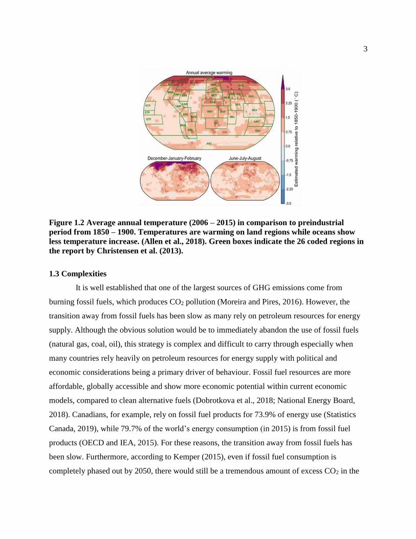
Figure 1.2 Average annual temperature (2006 – 2015) in comparison to preindustrial period
from 1850 – 1900. Temperatures are warming on land regions while oceans show less
temperature increase. (Allen et al., 2018). Green boxes indicate the 26 coded regions in
the report by Christensen et al. (2013). ................................................................................... 3
Figure 1.3 CO2 Concentration (ppm) measured at the Mauna Loa Conservatory by Scripps
Institution of Oceanography since 1958. CO2 concentrations have been increasing since
the industrial revolution (mid-18th century). (Keeling et al., 2001) ........................................ 5
Figure 1.4 Percentage of major GHG emissions in the U.S in 2017. Percentages do not add
up to 100% due to rounding. (U.S. Environmental Protection Agency, 2019) ...................... 9
Figure 1.5 The main sources of carbon dioxide emissions in the U.S. in 2017. (U.S.
Environmental Protection Agency, 2019) ............................................................................... 9
Figure 1.6 Stratigraphic column showing the Basal Cambrian Sand (BCS) CO2 storage
complex from the Quest CCS project operated by Shell Canada. (Tawiah et al., 2018). ..... 12
Figure 1.7 (a) Saline aquifers (blue) present in Canada and the U.S. (National Energy
Technology Laboratory, 2007). (b) Location and outline of the Western Canada
Sedimentary Basin (WCSB) which includes the Alberta Basin and Williston Basin.
(Singh et al., 2017). ............................................................................................................... 13
Figure 1.8 Salinity concentration of the hydrostratigraphic unit (HSU) of the Wapiti
formation - Belly River Group strata in the Alberta Basin (Alberta Geological Survey,
2019). .................................................................................................................................... 14
Figure 1.9 Diagram indicating thesis chapters which includes an introduction to the purpose
of this research and what the AVECS project is (Chapter 1). Sulfur incorporation
processes in natural settings are explored in Chapter 2. Molecular analysis was
conducted on sulfur-rich oils to reveal the environmental settings which contributed to
the oil generation and the structure of organic sulfur compounds found in the oils were
discussed in Chapter 3. The method development process for isolating sulfur-rich
hydrocarbon fractions is discussed in detail in Chapter 4. Then, Chapter 5 identifies how
sulfur incorporation and oxidation affects hydrocarbon solubility and biodegradation
rate using chemical modelling software. In Chapter 6, laboratory sulfurization
experiments were tested on lipids and carbohydrates (Chapter 6) and conclusions and
future work (Chapter 7). ....................................................................................................... 18
Figure 2.1 Increasing elemental sulfur stockpiles at Fort McMurray, Alberta, Canada (AER,
2017). .................................................................................................................................... 22

xv
Figure 2.2 Biogeochemical systems in marine sediment. Sulfate-reducing bacteria thrive in
the presence of organic matter and anoxic conditions (Goldhaber, 2005)............................ 27
Figure 2.3 The sulfur cycle pathways. In numerical order, pathways 1 to 4 refer to
assimilatory sulfate reduction, mineralization (sulfhydrization), dissimilatory sulfate-
reduction and dissimilatory sulfide oxidation (Bertrand et al., 2015). ................................. 29
Figure 2.4 Sulfur metabolism pathways. Assimilatory sulfate reduction (blue). Sulfur
oxidation (green). Elemental sulfur disproportionation (purple)( Fike et al., 2015). ........... 30
Figure 2.5 Sulfur cycle, sulfur reservoirs and different sulfur flux pathways. DMS refers to
dimethyl sulfide and COS refers to carbon oxysulfide (Bertrand et al., 2015)..................... 31
Figure 2.6 Organic matter sinks below the anoxic boundary and activates sulfate reduction
pathways in fresh water lakes (modified after Fenchel et al., 2012). ................................... 34
Figure 2.7 Four main sulfur compound classes found in petroleum (Modified after Han et al.,
2018) ..................................................................................................................................... 37
Figure 2.8 Examples of polycyclic aromatic sulfur heterocycles (PASH). Image from Nocun
and Andersson, (2012). ......................................................................................................... 40
Figure 2.9 (a) Second degradation pathway for dibenzothiophene (DBT), which targets
carbon-sulfur bonds and preserves carbon-carbon bonds. DszA , DszB, DszC refers to
different proteins in organism Rhodococcus erythropolis. (b) Third degradation pathway
by Brevibacterium species which completely mineralizes DBT. (Modified from Gogoi
and Bezbaruah, 2002). .......................................................................................................... 42
Figure 3.1 The transformation from phytane carbon skeleton to cyclic organic sulfur
compounds during diagenesis through two pathways: intramolecular sulfur
incorporation and intermolecular sulfur addition reactions. (Kohnen et al. 1991) ............... 47
Figure 3.2 a) Sulfur compounds form through intramolecular incorporation of polysulphides
(Kohnen et al., 1991). b) General scheme for sulfur incorporation into unsaturated lipid
precursors (Sinninghe Damsté et al., 1989). ......................................................................... 47
Figure 3.3 Intramolecular sulfur incorporation into double bonds of isoprenoids. Diagenesis
of kerogen forms saturated, aromatic and organic sulfur compound products. (Peters et
al 2005). ................................................................................................................................ 48
Figure 3.4 There are more than 600 types of natural carotenoids, however the carotenoids
shown above are the most abundant in marine environments. Isorenieratene and
Chlorobactene are common in green sulfur bacteria. (Peters et al., 2005b) ......................... 50
Figure 3.5 Geologic timescale and the Peace River area which is comprised of the Bullhead
and Fort St. John Groups. (Modified from AER, 2017 and Adams et al., 2013) ................. 52

xvi
Figure 3.6 The location of Peace River oil samples. Sulfur-rich oils were collected form
Gething Reno Field (green), West Cadotte (purple) and Bluesky formation (blue).
Modified from Jennifer Adams et al. (2012). ....................................................................... 52
Figure 3.7 Location of Rozel Point on map. (Utah Geological Survey, 2005)............................. 53
Figure. 3.8 The Jianghan basin located in Hubei province of China and the location of the
Qianjiang depression. (Modified after Brassell et al., 1988) ................................................ 54
Figure 3.9 Location of Bohai Bay basin and the Dongying depression where the Shahejie
formation lies. ....................................................................................................................... 56
Figure 3.10 Schematic map showing the Dongying depression within the Bohai Bay Basin
and the lithology facies of source rocks: a) ES4 member and b) ES3 member (Li et al.,
2003). .................................................................................................................................... 57
Figure 3.11 Formation of pristane and phytane from phytol side chain of chlorophyll is
dependent on oxic and anoxic environmental conditions. .................................................... 62
Figure 3.12 Cross plot of dibenzothiophene/phenanthrene (DBT/P) vs pristane/ phytane
(Pr/Ph) to determine source rock depositional environments (modified after Hodairi and
Philp, 2012). Sulfur-rich oil samples Rozel Point (RP), Jianghan (JH), Gething Reno
(GR) fall in the marine carbonate and lacustrine zone (purple square) and the ratios
indicate that source rocks from Bluesky (BS), West Cadotte (WC), and Shahejie (S)
were deposited in mainly lacustrine environments (blue square). ........................................ 63
Figure 3.13 Gammacerane index 10*(GAM/GAM+30H) and pristane/phytane (Pr/Ph) ratio
for sulfur-rich oil sample set. High gammacerane indices indicate increased water
salinity, water stratification or natural sulfurization processes. ............................................ 64
Figure 3.14 m/z 191 Chromatogram showing homohopanes (C31 – C35) distribution in sulfur-
rich crude oil samples from: (a) Bluesky Formation, (b) Gething-Reno Formation, (c)
West Cadotte field, (d) Rozel Point, (e) Jianghan Basin and (f) Shahejie Formation.
GAM represents gammacerane.. ........................................................................................... 67
Figure 3.15 Homohopane Index (C35/ C31-C35) and Norhopane/hopane (C29/C30) which are
source and depositional setting indicators. High homohopane indices (>0.09) suggests
high redox potential, anoxic reducing environments, marine sources, and bacterial input
from bacteriohopanetetrol (Peters et al., 2005) ..................................................................... 67
Figure 3.16 Ternary diagram with relative distribution of C27, C28 and C29 sterane
abundances. ........................................................................................................................... 68
Figure 3.17 Biomarkers which are indicative of the degree of thermal maturity:
dibenzothiophene/phenanthrene (DBT/P) is plotted against 28, 30-bisnorhopane/ 25, 28,
30-trisnorhopane (BNH/TNH). ............................................................................................. 69

xvii
Figure 3.18 Thermal maturity parameters C31 homolog (22S/22S+22R) and C29 sterane
(20S/20S+20R). .................................................................................................................... 70
Figure 3.19 Biomarker biodegradation scale which ranks biodegradation severity based on
the presence of hydrocarbon classes. L, M, H refers to lightly biodegraded, moderately
biodegraded and heavily biodegraded, respectively. (Peters and Moldowan, 1993). ........... 72
Figure 3.20 m/z 85 chromatograms which show n-alkane and isoprenoid distributions in
sulfur-rich crude oil samples from: (a) Bluesky formation, (b) Gething-Reno formation,
(c) West Cadotte field, (d) Rozel Point, (e) Jianghan Basin and (f) Shahejie formation.
IS1 represents squalane internal standard. ............................................................................ 74
Figure 3.21 Organic sulfur compound fractions obtained from liquid chromatography using
silver nitrate impregnated silica gel compared to whole oils. ●, indicates radical atoms.
RMI, relative monoisoptopic intensity (a) Liquid chromatography method removed
hydrocarbons and enhanced sulfur intensities (b) Whole oils. ............................................. 76
Figure 3.22 The relative monoisotopic intensity (RMI) and carbon number distributions for
sulfur-rich oil sample set. Rozel Point oil (red) shows high intensity peaks at C20, C29
and C40. Jianghan Basin oil (orange) shows peaks at C20, C24, C26, C28, C30, and C40.
Shahejie oil (black) also shows similar peaks at C14, C27, C29, and C40. Alberta oils (blue,
green, pink) are depleted in low carbon numbers but show increased RMI for higher
carbon number classes. ......................................................................................................... 77
Figure 3.23 Double bond equivalent distributions. (a) Radical S1 class. (b) Protonated S1
class. Black circle emphasizes DBE 1 peak which is unique only to Jianghan Basin oil..... 78
Figure 3.24 Carbon distribution for radical sulfur class S1 at a) DBE 2 b) DBE 3 c) DBE 5
and d) DBE 6. ....................................................................................................................... 79
Figure 3.25 (a) Double bond equivalent (DBE) distribution for sulfur class S3. (b) Carbon
number distribution for sulfur class S3 at DBE 7……………………………………………………………………..80
Figure 3.26 (a) DBE distribution for sulfur class S5. (b) Carbon number distribution for sulfur
class S5 at DBE 13. ............................................................................................................... 81
Figure 4.1 AVECS pathways to determine organic compounds which have potential to form
biologically refractory water soluble organic molecules. Pathway 1 refers to utilizing
sulfurization reaction on organic biomass waste and pathway 2 refers to isolating sulfur-
rich fractions from sulfur-rich oils and analyzing the S containing compounds as models
for AVECS molecules. .......................................................................................................... 86
Figure 4.2 Sulfur compound structures and reactivity classification. (Modified after Lobodin
et al., 2015) ........................................................................................................................... 88

xviii
Figure 4.3 Polycyclic aromatic sulfur heterocycles commonly found in petroleum (PASH)
(Wang and Stout, 2007) ........................................................................................................ 88
Figure 4.4 Interaction and bonding between silver ions and double bonds. The complexes
between the silver-ion and double bond are a type of charge-transfer mechanism. The
unsaturated compound donates an electron to the silver ion and results in the formation
of a sigma bond between the orbitals of the double bond and silver ion. Ag+ represents
silver-ions. (Modified after Nikolova-Damyanova, 2018). .................................................. 91
Figure 4.5 Silver nitrate impregnated silica gel column design following methods by Wei et
al. (2012). The S1 fraction (saturated hydrocarbons) was eluted with 3mL of hexane,
followed by 8mL DCM eluted the S2 fraction (non-reactive OSC), and lastly the S3
fraction (reactive sulfides) were eluted with 2 mL of acetone. ............................................. 92
Figure 4.6 Cloudy S3 fraction (eluted with acetone) which contained crystal-like precipitate.
Acetone was evaporated with nitrogen gas. The S3 fraction was soluble in toluene,
however the precipitate was only miscible with methanol. Therefore, the sample was
redissolved in toluene and passed through a glass wool column to remove any
particulates. ........................................................................................................................... 94
Figure 4.7 Acetone fraction from blank columns (no sample). (A) Silica gel-only column
shows no precipitate. (B) Silver nitrate impregnated silica gel column shows crystal-like
precipitate. ............................................................................................................................. 94
Figure 4.8 The silver-ion column was modified with reduced volume of AgNO3 impregnated
silica gel and less whole oil analyte, compared to original experiment design by Wei et
al. (2012), to improve sulfur compounds separation and prevent precipitation. The S1
fraction was eluted first with 3 mL of hexane, followed by 8 mL of DCM which eluted
the S2 fraction, and lastly the S3 fraction was eluted with 2 mL of acetone. ....................... 95
Figure 4.9 S3 fraction (acetone elution) from trial one method development (see Fig. 4.8 for
column design). A) Precipitate formed as fraction was concentrated using nitrogen gas.
B) White crystal-like precipitate is observed at the bottom acetone fraction from the
blank column. ........................................................................................................................ 96
Figure 4.10 Comparison of GC-MS chromatograms. (A) Total ion chromatogram of
Athabasca sulfur-rich whole oil from S2 fraction (eluted with DCM). (B) Extracted ion
chromatogram of Athabasca sulfur-rich whole oil from S2 fraction. (C) Total ion
chromatogram of Athabasca whole oil from S3 fraction (eluted with acetone). (D)
Extracted ion chromatogram of Athabasca whole oil from S3 fraction. Non-reactive
aromatic sulfur compounds shown in extracted ion chromatograms: dibenzothiophenes
(m/z 184) (black), methyldibenzothiophene (m/z 198)(blue), dimethyldibenzothiophenes
(m/z 212)(red), naphthobenzothiophene (m/z 234) (grey) and
methylnaphthobenzothiophene (m/z 248)(yellow). .............................................................. 97

xix
Figure 4.11 1.0 mg of DBT (dibenzothiophene) standard loaded into a silver-ion column
comprised of 0.400g of silica gel and 0.200g of silver nitrate (10 wt%) impregnated
silica gel. The column was first eluted with 8.0 mL of DCM followed by 8.0 mL of
acetone. ................................................................................................................................. 99
Figure 4.12 Total ion chromatograms. A) DCM fraction which shows (m/z 184) DBT peak
and B) acetone fraction indicate that DBT was eluted fully into DCM fraction. ................. 99
Figure 4.13 Trial two of silver nitrate impregnated silica gel column method development.
One silver-ion column (left) was loaded with 1 mg of dibenzothiophene (DBT) standard
and the other silver-ion column (right) was loaded with 20 mg of Athabasca whole oil.
Each column was eluted with four different solvents and the elutions were collected in
separate fractions. The first elution involved 8 mL of DCM, followed by 8 mL of
acetone, then toluene and lastly tetrahydrofuran (THF). .................................................... 100
Figure 4.14 Trial two sulfur fractionation elutions. Top images represent elution which came
from column on the right which contained 20mg of whole oil. Bottom images are from
left column which was loaded with 1 mg of DBT standard. Precipitate was observed in
acetone fractions from both columns. DCM = dichloromethane, ACET = acetone, TOL
= toluene, THF = tetrahydrofuran. ...................................................................................... 101
Figure 4.15 Chromatograms from the silver-ion column containing whole oil. (A) The
dichloromethane (DCM) elution shows several aromatic sulfur compounds. (B) Acetone
fraction shows some aromatic sulfur compounds, but less than the DCM fraction.
Contaminants (benzenes) and unknown compounds are observed in the toluene fraction
(C) and tetrahydrofuran fraction (D). Dibenzothiophenes (DBT),
methyldibenzothiophene (MDBT), dimethyldibenzothiophenes (DMDBT),
naphthobenzothiophene (NBT), methylnaphthobenzothiophene (MNBT). ....................... 102
Figure 4.16 Trial three column design to prevent silver-ion leakage and precipitate from
forming in acetone fraction. ................................................................................................ 104
Figure 4.17 Trial three method development. A) Column design with silver nitrate
impregnated silica gel sandwiched between two layers of plain silica gel. B) Eluates
starting from the left: Hexane, DCM, DCM to acetone following gradual polarity
increase and pure acetone fraction. ..................................................................................... 104
Figure 4.18 Extracted ion chromatograms (m/z 134, 148, 176, 212, 234, 248). (A) Whole oil.
(B) Hexane elution. (C) Dichloromethane (DCM) and acetone gradient fraction. (D)
Pure acetone fraction. Higher molecular weight sulfur compounds, such as
dibenzothiophene and methylnaphthobenzothiophene, are observed in the DCM and
acetone gradient fraction, while lower molecular weight sulfur compounds such as
sulfides are more dominant in the pure acetone fraction. ................................................... 106

xx
Figure 4.19 (A) Extracted ion chromatogram showing five pure sulfur compounds that make
up the standard: thiophene, thiolane, 1-benzothiophene, dibutyl sulfide and
dibenzothiophene. (B) The sulfur compounds were identified through mass
chromatography with target ions 84, 88, 134, 146 and 184, respectively. ......................... 110
Figure 4.20 Trial four column design. ........................................................................................ 110
Figure 4.21 Left column loaded with 10 μL of sulfur compounds standard, the center column
is loaded with 5 mg of sulfur-rich whole oil from the Athabasca oil sands, and the
column on the right is loaded with 5 mg of Athabasca whole oil as well as 10 μL of
sulfur compounds standard. ................................................................................................ 111
Figure 4.22 Fractions which eluted from the silver-ion column which was loaded with 10 μl
of sulfur standard. (A) S1 fraction (hexane elution) show no sulfur compounds. (B)
Aromatic sulfur compounds (thiophenes, 1-benzothiophene and dibenzothiophene) were
identified in the S2 fraction (DCM/acetone gradient elution) from target ions 84, 134
and 184. (C) Sulfide compounds (thiolane and dibutyl sulfide) were identified in the S3
fraction (acetone/acetonitrile elution). ................................................................................ 113
Figure 4.23 The colour of the S1 eluate was monitored to ensure that coloured aromatic
compounds do not break through in the S1 fraction (hexane eluate). This was done by
watching the movement of coloured fronts within the silver-ion column. ......................... 115
Figure 4.24 Extracted ion chromatogram of the Athabasca oil S1 fraction (hexane eluate) oil
in experiment trial 6. Saturated hydrocarbons are present and sulfur compounds were
not observed in this fraction. ............................................................................................... 117
Figure 4.25 Extracted ion chromatogram of the S2 fraction (hexane/DCM eluate) of
Athabasca oil in experiment trial 6. Aromatic sulfur compounds 1-benzothiophene
(DBT) and dibenzothiophene (DBT) are present in this fraction. .................................... 118
Figure 4.26 Extracted ion chromatogram of the S3 fraction of Athabasca oil in experiment
trial 6. Non-aromatic sulfur compounds, thiolane and dibutyl sulfide, are present in this
fraction. ............................................................................................................................... 118
Figure 4.27 FTICR-MS plot showing compound class distribution for Athabasca whole oil
(black), S2 fraction (dark grey) and S3 fraction (light grey). Relative monoisotopic
intensity (RMI) is the signal measured from a fragment ion that is made up of the most
abundant natural isotope of each atom in the molecular ion............................................... 119
Figure 4.28 FTICR-MS plot shows compound class distribution for oil fractions from Rozel
Point (red), Jianghan Basin (blue), and Athabasca oil sands (grey). (A) Fraction #2 or
the S2 fraction shows predominantly 1 to 3 sulfur atoms per molecule. (B) Fraction #3
or the S3 fraction shows 1 to 5 sulfur atoms per molecule and also mixed nitrogen-
oxygen and nitrogen-sulfur molecules. ............................................................................... 120

xxi
Figure 4.29 FTICR-MS DBE distribution for Athabasca whole oil (black), S2 fraction (dark
grey) and S3 fraction (light grey). ....................................................................................... 121
Figure 5.1 Formation of thiolane and thiophene through intramolecular incorporation of
polysulphides (after Kohnen et al., 1991). .......................................................................... 125
Figure 5.2 Sulfurization and oxidation of squalene model compounds. (A) Squalene. (B)
Sulfur incorporation into squalene results in the formation of two thiolanes. (Bi)
Subsequent oxidation forms sulfoxide groups. (Bii) The most oxidized state (two
sulfone groups) of the sulfurized squalene model compound............................................. 128
Figure 5.3 Hypothesized pathway for forming sulfurized steroids in Ace Lake Sediments.
Inorganic sulfur species react with both 5a-stan-3-ones and 5B-stan-3-ones to form
sulfurized steroids. Furthermore, the transformation from stanones to stanols is a
reversible process. (After Kok et al., 2000). ....................................................................... 129
Figure 5.4 Sulfurization and oxidation of steroid model compounds. (C) Cholesterol. (D)
Sulfur incorporation into hydroxyl group. (Di) Addition of a sulfonate group after
oxidation. (E) Sulfur incorporation into hydroxyl group and the formation of thiolane
through double bond reduction. (Ei) Subsequent oxidation forms sulfonate and sulfoxide
groups. (Eii) The most oxidized state of the sulfurized cholesterol model compound
includes sulfonate and sulfone groups. ............................................................................... 130
Figure 5.5 Weight fraction of oxygen and carbons and the influence on carbon solubility for
derivative lipid molecules (kg C/m3). Increasing carbon solubility is indicated by the
increased bubble size. See Table 5.1 for carbon solubility values for modified
compounds: squalene (Bi, Bii), b) cholesterol (Di – Eii), c) linolenic acid (F-Gii). .......... 133
Figure 5.6 Sulfurization and oxidation of linolenic acid model compounds. (F) Linolenic
acid. (G) Sulfur incorporation into double bonds to form thiolane. (Gi) Oxidation results
in the addition of a sulfoxide group. (Gii) Subsequent oxidation forms sulfone group,
which is the most oxidized state of the sulfurized linolenic acid model compound. .......... 134
Figure 5.7 Weight fraction of carbon and oxygen to carbon solubility for sulfurized and
oxidized squalene (Bi), cholesterol (Ei) and linolenic acid (Gi) model compound
modifications. ...................................................................................................................... 134
Figure 5.8 Monosaccharides: arabinose (H), lyxose (I), and xylose (J) and corresponding
sulfurized products (Hi, Ii, Ji) which formed in the carbohydrate sulfurization
experiments by van Dongen et al. (2003). .......................................................................... 136
Figure 5.9 Pentose monosaccharides (H, I, and J) show higher carbon solubility (399 kg/m3)
compared to sulfurized carbohydrates (Hi, Ii, and J) with carbon solubility of 1.53
kg/m3. .................................................................................................................................. 137

xxii
Figure 5.10 Inorganic sulfur species incorporate into phytol and phytadiene to form sulfur
bounded phytane derived structures (van Dongen, 2003)................................................... 138
Figure 5.11 Sulfurization and oxidation of isoprenoid model compounds. (K) Phytol. (L)
Sulfurization forms thiophene. (Li) Oxidation forms sulfone group. (M) Sulfur
incorporation into phytol forms thiolane structure. (Mi) Oxidation results in the addition
of a sulfoxide group. (Mii) Subsequent oxidation forms sulfone group. ............................ 139
Figure 5.12 The sulfurized isoprenoids with thiolane (orange) show a slightly higher carbon
solubility (2.19E-07 kg C/m3) compared to the isoprenoid which formed thiophenes
(blue) (1.34E-07 kg C/m3). ................................................................................................. 140
Figure 5.13. Oxidation of isoprenoid thiolane (M, orange) showed increased carbon solubility
through the addition of sulfoxide to model compound (Mi, blue). Model compound (Mi)
shows greater carbon solubility compared sulfurized model compound (Mii, gray) which
consists of a sulfone group. ................................................................................................. 140
Figure 5.14 Sulfurization and oxidation of glycerol model compounds. (N) Glycerol. Sulfur
incorporation occurs at hydroxyl groups in glycerol to form thiols (O, P, and Q).
Oxidation of sulfurized glycerol model compounds form sulfonate groups (Oi, Pi, and
Qi). ...................................................................................................................................... 141
Figure 5.15 Effect of thiol groups on carbon solubility of glycerol. (See Fig. 5.14 for
progression of N, O, P and Q) ............................................................................................. 142
Figure 5.16 The effect on carbon solubility due to the addition of sulfonate groups on
sulfurized glycerol (See Fig. 5.14 Q and Qi). ..................................................................... 143
Figure 5.17 A fullerene molecule (C60) that is also informally known as the carbon
buckyball. The fullerene molecule could be a potential model compound for the ideal
AVECS molecule. ............................................................................................................... 145
Figure 5.18 Sulfur incorporation into tri-unsaturated C37 hydrocarbon. After Sinninghe
Damsté et al. (1989). ........................................................................................................... 145
Figure 5.19 Sulfurization and oxidation of C30
hydrocarbon chains. (R) C30
H62
. Conceptual
sulfur incorporation form thiolanes (S, T, and U). Oxidation of sulfurized C30
hydrocarbons form sulfoxide groups (Si, Ti, and Ui). ........................................................ 146
Figure 5.20 Sulfurization and oxidation of C60 hydrocarbon chains. (V) C30H62. Conceptual
sulfur incorporation form thiolanes (W and X). Oxidation of sulfurized C30
hydrocarbons form sulfoxide groups (Wi and Xi). ............................................................. 146

xxiii
Figure 5.21 The effect of number of thiolane-1-oxide groups on the carbon solubility in water
for (a) C30 H62 and (b) C60 H122. Green horizontal line delimits AVECS target water
solubility (> 15 kg C/m3). ................................................................................................... 147
Figure 5.22 Sulfurized and oxidized model compounds (from each experiment) with the
greatest carbon solubility. Lipids (Ei), carbohydrates (Hi), isoprenoids (Mi), glycerol
(Qi), hydrocarbon chains (Ui and Xi). ................................................................................ 149
Figure 5.23 Biodegradation rate of oxidized OSC (Ei, Hi, Mi, Qi, Ui, Xi). See figure 5.22 for
structures. Red data points are recalcitrant. Yellow indicates biodegradation will take
weeks to months, and green indicates biodegradation will take weeks (EPA, 2011). ........ 150
Figure 5.24 Process for sulfolane synthesis. Sulfolane is synthesized by the reaction between
1,3-butadiene (1) with sulfur dioxide (2) to form sulfolene (3). The hydrogenation of
sulfolene forms sulfolane (4). (Tilstam, 2012; Bak et al., 2018). ....................................... 151
Figure 6.1 Analytical scheme of lipid sulfurization experiments ............................................... 155
Figure 6.2 Liquid-liquid extraction on sulfurized β-carotene reaction mixtures. ....................... 155
Figure 6.3 (a) Carbohydrate sulfurization experimental set up. (b) Addition of pure copper
flakes to remove excess elemental sulfur. Copper turns black (copper sulfide)
instantaneously. (c). After 24 hours of stirring, the entire solution appears black. ............ 156
Figure 6.4 (a) Pasteur pipette filled with pure copper granules and glass wool. (b) Copper
turns black after eluting sulfurized sample through the column. ........................................ 157
Figure 6.5.a) Sulfurized carbohydrates in freeze-dry machine after removing excess sulfur b)
Freeze dried sulfurized carbohydrates. From the left: sucrose, glucose, starch and blank. 157
Figure 6.6 FTICR-MS mass spectrum showing peak intensity, mass to charge (m/z) ion and
molecular formula. Sulfurization of squalene (C30H52S) was detected in experiment #1
(lipid sulfurization for 5 days). ........................................................................................... 159
Figure 6.7 Possible organic sulfur compound structure with molecular formula C30H52S.
Sulfurization of squalene in experiment #1 (lipid sulfurization for 5 days) may have
formed one thiolane intramolecularly. ................................................................................ 159
Figure 6.8 FTICR-MS mass spectrum showing peak intensity, mass to charge (m/z) ion and
molecular formula. Sulfurized squalene (C30H54S2) is detected in experiment #2 (lipid
sulfurization for 30 days). ................................................................................................... 159
Figure 6.9 Possible organic sulfur compound structure with molecular formula C30H54S2.
Sulfurization of squalene (experiment #2 - lipid sulfurization for 30 days) may have
formed two thiolanes intramolecularly. .............................................................................. 160

xxiv
Figure 6.10 Possible organic sulfur compound structure with molecular formula C18H32O2S2.
Sulfurization of linolenic acid (experiment #3 - lipid sulfurization for 30 days at 50°C)
may have formed two thiolanes intramolecularly. .............................................................. 160
Figure 6.11 FTICR-MS mass spectrum showing peak intensity, mass to charge (m/z) ion and
molecular formula. Sulfurized linolenic acid (C18H32O2S2) is detected in experiment
#3 (lipid sulfurization for 30 days at 50°C). ....................................................................... 161
Figure 6.12 Possible organic sulfur compound structure with molecular formula C30H54S4.
Sulfurization of squalene (experiment #3 - lipid sulfurization for 30 days at 50°C) may
have formed four thiolanes intramolecularly. ..................................................................... 161
Figure 6.13 FTICR-MS mass spectrum showing peak intensity, mass to charge (m/z) ion and
molecular formula. Sulfurized squalene (C30H54S4) is detected in experiment #3 (lipid
sulfurization for 30 days at 50°C). ...................................................................................... 162
Figure 6.14 FTICR-MS mass spectrum showing peak intensity, mass to charge (m/z) ion and
computed ion formula. Sulfurized β-carotene (C40H68S7) is detected in experiment #3
(lipid sulfurization for 30 days at 50°C). ............................................................................ 163
Figure 6.15 Possible organic sulfur compound structure with molecular formula C40H68S7.
Sulfurization of β-Carotene (experiment #3 - lipid sulfurization for 30 days at 50°C)
may have formed four thioanes and 3 thiolanes intramolecularly. ..................................... 163
Figure 6.16 (a) Chemical structure of linolenic acid (C18H30O2) compared to possible
sulfurized linolenic acid structures (b) C18H34O2S and (c) C18H32O2S2, which are
molecular formulas extrapolated from the FTICR-MS mass spectrum (Fig. 6.11). ........... 165

xxv
List of Abbreviations
Symbol Definition
APPI Atmospheric Pressure Photo Ionization
APPI-P Atmospheric Pressure Photo Ionization in Positive ion mode
AVECS
BT
Alternative Vectors for Carbon Storage
Benzothiophene
BCS Basal Cambrian Sands
CCS Carbon Capture and Storage
CH4 Methane
CO2 Carbon Dioxide
Da Dalton
DBE Double Bond Equivalent
DBT Dibenzothiophene
DCM:MeOH Dichloromethane:Methanol
FTICR-MS Fourier Transform Ion Cyclotron Resonance Mass Spectrometry
GC-MS Gas Chromatography- Mass Spectrometry
GHG Greenhouse Gas
HC Hydrocarbon
IPCC Intergovernmental Panel on Climate Change
Kg C/m3 Kilograms of Carbon per Cubic Meter
mD millidarcy
Mg/L Milligrams per Litre
μm Micromolar
μL Microlitre
MS Mass Spectrometry
m/z Mass to Charge Ratio
MeOH Methanol
NDC Nationally Determined Contributions

xxvi
NO3 Nitrous Oxide
OSC Organic Sulfur Compounds
PASH Polycyclic Aromatic Sulfur Heterocycles
ppm Parts Per Million
RMI Relative Monoisotopic Intensity
S Sulfur
SPE Solid Phase Extraction
SSS Small-Scale Separation
THF Tetrahydrofuran
Wt Weight

1
Chapter One: Introduction
This thesis involves the discussion, analysis and development of a potential carbon sequestration
method inspired by natural sulfurization processes in sedimentary organic matter.
1.1 What is Global Warming?
Over the past 170 years, scientists observed the climate to follow an increasing warming
trend for both air and sea temperatures. This increase in surface temperatures is known as the
global warming phenomenon and temperatures are expected to continue to rise unless more
stringent policies on carbon management are enforced and development and application of
carbon negative technology is accelerated. Some argue that this trend belongs to earth’s natural
climate fluctuations while abundant empirical evidence shows recent global warming is
predominantly human-induced (Keeling et al., 2001; Wong, 2015; Hoegh-Guldberg et al., 2018).
Anthropogenic factors, such as greenhouse gas (GHG) emissions from transportation and
industrial uses, have strongly contributed to long term global changes in temperature. Some
consequences of global warming and rising atmospheric carbon dioxide levels include sea level
rise, ocean acidification, and extreme weather activity (Wong, 2015). As a result of these effects
over the past several decades, most countries are concerned and acknowledge climate change as
a high priority global threat.
1.2 Paris Agreement
In an effort to implement global initiatives of environmental remediation and desirable
pathways to delay increasingly warm climates, the Paris Agreement was established in 2016 to
unite 130 countries to prevent future temperatures from increasing no more than 2°C above
temperatures during the pre-industrial era (1850 – 1900) (Lewis, 2016). However, the ideal
global target is less than 1.5◦C increase above pre-industrial levels (Allen et al., 2018). As of
2017, the average global temperature increase, since the pre-industrial era, is estimated to be
1.04°C (Fig. 1.1) and temperatures are increasing up to 0.33°C per decade (Allen et al., 2018).
Despite these global averages, 20-40% of the world population live in areas that have already
reached 1.5°C (Fig. 1.2). Over the past few decades, more warming is observed in land regions
and, especially, in the Artic where a 1.0°C increase per decade has been recorded over the past

2
30 years (Christensen et al., 2013). Furthermore, the current nationally determined GHG
reductions for the period from 2016-2030 will not only fail to limit global warming to 1.5°C but
is, in fact, projecting towards a 3 – 4°C temperature increase by 2100 (Allen et al., 2018).
Figure 1.1 Temperature changes and evolution in comparison to the pre-industrial era and
the temperature projection trend for the near future. (Allen et al., 2018).
3
Figure 1.2 Average annual temperature (2006 – 2015) in comparison to preindustrial
period from 1850 – 1900. Temperatures are warming on land regions while oceans show
less temperature increase. (Allen et al., 2018). Green boxes indicate the 26 coded regions in
the report by Christensen et al. (2013).
1.3 Complexities
It is well established that one of the largest sources of GHG emissions come from
burning fossil fuels, which produces CO2 pollution (Moreira and Pires, 2016). However, the
transition away from fossil fuels has been slow as many rely on petroleum resources for energy
supply. Although the obvious solution would be to immediately abandon the use of fossil fuels
(natural gas, coal, oil), this strategy is complex and difficult to carry through especially when
many countries rely heavily on petroleum resources for energy supply with political and
economic considerations being a primary driver of behaviour. Fossil fuel resources are more
affordable, globally accessible and show more economic potential within current economic
models, compared to clean alternative fuels (Dobrotkova et al., 2018; National Energy Board,
2018). Canadians, for example, rely on fossil fuel products for 73.9% of energy use (Statistics
Canada, 2019), while 79.7% of the world’s energy consumption (in 2015) is from fossil fuel
products (OECD and IEA, 2015). For these reasons, the transition away from fossil fuels has
been slow. Furthermore, according to Kemper (2015), even if fossil fuel consumption is
completely phased out by 2050, there would still be a tremendous amount of excess CO2 in the

4
atmosphere that will require removal, hence carbon negative technologies are needed to reach
global environmental targets and prevent climate change from worsening.
There are other complexities besides fossil fuel consumption and economics, which slow
climate policy implementation. Extreme weather news reports have appeared more frequently in
the media spotlight especially during the last decade. However, media rarely informs the
audience the seriousness of climate change, which causes many communities to have trouble
understanding the correlation between anthropogenic activity, greenhouse gases and climate
change (Wong, 2015). In other words, if people do not understand the seriousness of global
warming, policies and implementations will not be supported and communities will not put in
effort to reach environmental targets. While many realize the importance of conserving energy
and becoming less wasteful, the public is only willing to make minimal changes to daily habits
because they do not see the scientific evidence of climate change and the human activity that is
causing it. Citizens in developed countries are often shielded from sites such as overflowing
landfills and fossil fuel combustion, therefore this often leads to the public misunderstand that
climate change is a future problem for generations to come when, in reality, it is a problem that is
affecting us now.
Scientific information and evidence on climate change is most definitely challenging to
communicate to the general public in a concise manner, especially when most audiences are
generally interested in other current events. For example, information that is difficult to convey
include different types of greenhouses gases and the fact that carbon dioxide (CO2) is one of the
most impactful gases as it not only prevents outbound infrared radiation from leaving the
atmosphere, but it also takes several centuries to vanish from the atmosphere (Wong, 2015).
1.4 Severity of Climate Change
As of 2019, the carbon dioxide concentration measured at the Mauna Loa observatory in
Hawaii is 414.30 parts per million (ppm) (Fig. 1.3). Compared to pre-industrial concentrations
before 1958 which was 280 ppm (Keeling et al., 2001), CO2 levels have increased nearly 48%
since the industrial revolution. These levels are the highest CO2 concentrations recorded in the
last 800,000 years and 68% of this increase occurred in the last 50 years (Wong, 2015).

5
Figure 1.3 CO2 Concentration (ppm) measured at the Mauna Loa Conservatory by Scripps
Institution of Oceanography since 1958. CO2 concentrations have been increasing since the
industrial revolution (mid-18th century). (Keeling et al., 2001)
The largest contributors to this exponential increase of atmospheric carbon dioxide come
from the combustion of fossil fuels for electricity, transportation and production of industrial
materials (Bui et al., 2018). Many suggest that the solution to slow climate change is to minimize
fossil fuel usage and consume less energy, however convincing the average person to drive less
or utilize more environmentally-friendly products is difficult and has shown limited success.
After all, most people refuse to make habit changes if they do not believe the problem will affect
them directly. Table 1.1 shows the many effects of climate change that are currently happening
even with a warming of less than 1.5°C. Such effects include food and crop scarcity, insufficient
water supply, and human and organism mortality (Hoegh-Guldberg et al., 2018).

6
Table 1.1 Summary of the consequences which occur with less than 1.5°C increase in
temperature, 1.5°C to 2°C temperature increase and warming of 3°C. (Hoegh-Guldberg et
al., 2018).
1.5 The Carbon Cycle
To understand why industrial emissions affect earth’s environment and how atmospheric
CO2 can be captured from a source and be safely stored away in a sink, it is essential to first

7
decipher what occurs throughout the carbon cycle. The carbon cycle involves a complex
sequence of events that allows carbon to propagate through the four spheres of earth:
atmosphere, biosphere, hydrosphere and lithosphere. In the atmosphere, carbon exists as carbon
dioxide, which is absorbed by plants for photosynthesis to generate energy. Living organisms in
the biosphere consume these plants and continue to pass carbon to other living organisms that are
higher up in the food chain. Then, the carbon is eventually released back into the atmosphere or
hydrosphere as carbon dioxide when land animals, aquatic creatures or plants respire. As animals
or plants decay, the carbon atoms that make up their organic structures enter the lithosphere.
Then with pressure, heat, and time, the carbon forms resources such as coal, oil and natural
gases. Energy suppliers and other key emitters utilize petroleum resources to generate energy and
products through combustion, which causes lithospheric carbon to enter the atmosphere at an
accelerated rate. Consequently, excessive atmospheric carbon exists due to anthropogenic
induced processes, thus creating a greenhouse effect on earth. Furthermore, natural carbon sinks
are depleting due to anthropogenic land use which has greatly reduced vegetative species that
have the ability to absorb and store carbon.
1.6 Greenhouse Gas Effect
The greenhouse effect begins when sunlight comes in contact with the earth’s surface.
Some of the inbound sunlight passes through earth’s atmosphere and becomes absorbed, while
some is re-radiated as infrared radiation from the earth’s surface. Furthermore, some of the light
is reflected from the atmosphere as outbound energy into space. The accumulation of greenhouse
gases in the atmosphere acts as an infrared radiation absorber which retains re-radiated infrared
energy in the atmosphere (Wong, 2015). The extra radiation becomes trapped in and beneath
earth’s atmosphere and the cycle repeats as the GHG layer becomes thicker and surface
temperatures increase due to incoming energy that is trapped as heat.
There are several types of GHGs including nitrous oxide (N2O), methane (CH4), water
vapor (H2O), fluorinated gases, and the most well-known carbon dioxide (CO2). The common
characteristic among these abundant GHGs is that they are all polyatomic molecules, this means
that the molecules are comprised of three or more atoms, and each atom may have a different
electronegativity. The unbalanced sharing of electrons on an atomic level is what makes GHG
molecules strong absorbers of infrared energy. Furthermore, each GHG has a different infrared
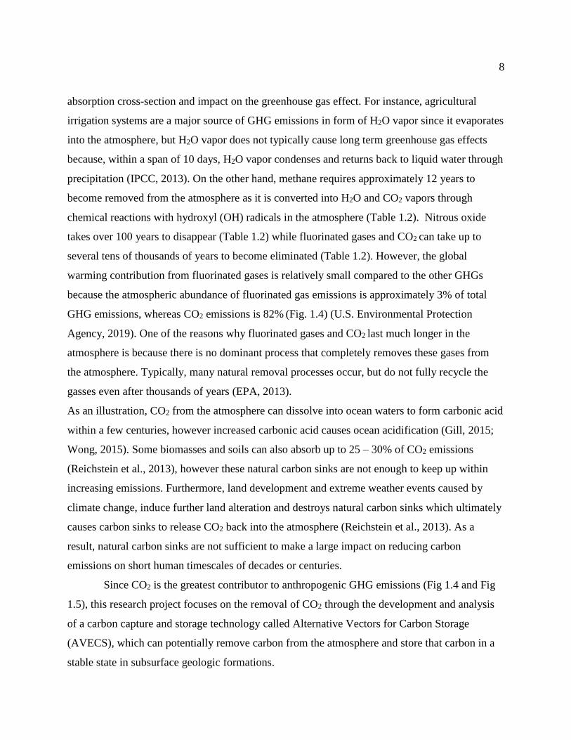
8
absorption cross-section and impact on the greenhouse gas effect. For instance, agricultural
irrigation systems are a major source of GHG emissions in form of H2O vapor since it evaporates
into the atmosphere, but H2O vapor does not typically cause long term greenhouse gas effects
because, within a span of 10 days, H2O vapor condenses and returns back to liquid water through
precipitation (IPCC, 2013). On the other hand, methane requires approximately 12 years to
become removed from the atmosphere as it is converted into H2O and CO2 vapors through
chemical reactions with hydroxyl (OH) radicals in the atmosphere (Table 1.2). Nitrous oxide
takes over 100 years to disappear (Table 1.2) while fluorinated gases and CO2 can take up to
several tens of thousands of years to become eliminated (Table 1.2). However, the global
warming contribution from fluorinated gases is relatively small compared to the other GHGs
because the atmospheric abundance of fluorinated gas emissions is approximately 3% of total
GHG emissions, whereas CO2 emissions is 82% (Fig. 1.4) (U.S. Environmental Protection
Agency, 2019). One of the reasons why fluorinated gases and CO2 last much longer in the
atmosphere is because there is no dominant process that completely removes these gases from
the atmosphere. Typically, many natural removal processes occur, but do not fully recycle the
gasses even after thousands of years (EPA, 2013).
As an illustration, CO2 from the atmosphere can dissolve into ocean waters to form carbonic acid
within a few centuries, however increased carbonic acid causes ocean acidification (Gill, 2015;
Wong, 2015). Some biomasses and soils can also absorb up to 25 – 30% of CO2 emissions
(Reichstein et al., 2013), however these natural carbon sinks are not enough to keep up within
increasing emissions. Furthermore, land development and extreme weather events caused by
climate change, induce further land alteration and destroys natural carbon sinks which ultimately
causes carbon sinks to release CO2 back into the atmosphere (Reichstein et al., 2013). As a
result, natural carbon sinks are not sufficient to make a large impact on reducing carbon
emissions on short human timescales of decades or centuries.
Since CO2 is the greatest contributor to anthropogenic GHG emissions (Fig 1.4 and Fig
1.5), this research project focuses on the removal of CO2 through the development and analysis
of a carbon capture and storage technology called Alternative Vectors for Carbon Storage
(AVECS), which can potentially remove carbon from the atmosphere and store that carbon in a
stable state in subsurface geologic formations.

9
Figure 1.4 Percentage of major GHG emissions in the U.S in 2017. Percentages do not add
up to 100% due to rounding. (U.S. Environmental Protection Agency, 2019)
Figure 1.5 The main sources of carbon dioxide emissions in the U.S. in 2017. (U.S.
Environmental Protection Agency, 2019)

10
Table 1.2 Anthropogenic greenhouse gas (GHG) emissions and the corresponding average
residence time in the atmosphere. (IPCC, 2007, 2013; EPA, 2013; Crank and Jacoby, 2015).
Greenhouse Gas (GHG) Average Residence Time in
Atmosphere
Water (H2O) Vapor 10 days
Methane (CH4) 11.2 ± 1.3 years
Nitrous Oxides (N2O) 131 ± 10 years
Fluorinated Gases 3,000 to 50,000 years Carbon Dioxide (CO
2) 200 - 100,000 years +
1.7 Carbon Capture and Storage
Carbon Capture and Storage (CCS) is also known as geologic CO2 sequestration and it is
a process that decarbonizes global emissions through net removal of CO2 from the atmosphere by
storing CO2 in deep subsurface reservoirs with impermeable seals. CCS technology, such as the
Shell Quest CCS project, works by capturing gaseous CO2 and then injecting highly compressed
CO2 (often at supercritical state or dense-phase) into deep saline aquifers or other geologic
formations. When CO2 reaches supercritical state at high pressures and temperatures, it displays
characteristics of both gas and liquid. Since supercritical CO2 is denser than CO2 gas, it occupies
less volume and enables more efficient storage into geologic storage complexes (Wong, 2015).
However, supercritical CO2 is more buoyant than brine water in saline aquifers, therefore several
existing natural impermeable seal layers within the storage complex are essential to prevent CO2
from escaping the storage site. This type of CCS mechanism is the most common type CO2
storage mechanism known as structural trapping, and it is estimated to safely store CO2 for
approximately 1000 years (Hauck et al., 2012).
There are other processes which trap CO2, however. Several authors have noted mineral
trapping as a process which may permanently sequester CO2 in the subsurface (Thomson, 2009;
Wong, 2015; Harrison et al., 2019). The mineralization process occurs when dissolved CO2
reacts with surrounding host rock, which then releases metal cations that combine with carbon
and oxygen to form carbonate minerals (Harrison et al., 2019). As a result, CO2 is converted to a
stable solid state. Therefore CO2 mobility and leakage concerns are lessened. However, mineral
precipitation often occurs gradually over long geological timescales and can take up to 10,000

11
years or more, depending on the reactivity of the rocks and the abundance of carbonate-forming
cations within the geologic storage complex, to form carbonate minerals (Harrison et al., 2019).
1.7.1 Carbon Storage in Saline Aquifers
Deep saline aquifers are geological formations comprised of permeable sedimentary rock
saturated with brine. Furthermore, saline aquifers have large storage capacities and CO2
dissolution processes occur in brine which makes saline aquifers favorable for CCS projects
(Emami-Meybodi, 2015; Tawiah et al., 2018). There are several saline aquifers in Canada,
however, not all are suitable for geologic supercritical CO2 sequestration as many geologic
parameters must be met to ensure safe storage (Table 1.3). An example of an acceptable deep
saline aquifer for CCS is the one located in the north-east of Edmonton (Alberta, Canada) known
as the Basal Cambrian Sands (BCS) of the Western Canadian Sedimentary Basin (Tawiah et al.,
2018). Since August 2015, the BCS aquifer has been used for the Quest CCS project (operated
by Shell) and over 4 million tons of CO2 has been stored within the BCS storage complex in a
period of four years (Shell Canada, 2019).
The composition of the BCS aquifer is dominantly sandstone with an average thickness
of 45 m and it is approximately 2000 m beneath the surface (Fig. 1.6). In addition, the total
dissolved solids (TDS) concentration in the BCS storage area is approximately 300,000 mg/L
(Hauck et al., 2012). Typically, aquifer waters with more than 10 000 mg/L of TDS are suitable
for CCS projects, as high TDS levels indicates that the water is unacceptable for use as water
supply and has low economic value (Bruant et al., 2002). Moreover, the BCS deep saline aquifer
is a suitable storage location for CCS is because it has a large CO2 storage area of approximately
450,000 km2, good porosity (17%) and high permeability (1000 mD) sandstones, and several
layers of thick impermeable seals which overlay the BCS injection target unit (Fig. 1.6) (Hauck
et al., 2012; Tawiah et al., 2018). It is estimated that the Quest CCS project will continue to
capture and store CO2 at a rate of 1 million tons per year for the next 25 years within the BCS
aquifer.

12
Figure 1.6 Stratigraphic column showing the Basal Cambrian Sand (BCS) CO2 storage
complex from the Quest CCS project operated by Shell Canada. (Tawiah et al., 2018).
There are many other saline aquifers located within sedimentary basins in Canada (Fig.
1.7) (Natural Resources Canada, 2016). For example, in the Alberta Basin, the salinity of saline
aquifers range from 600 mg/L to 15,000 mg/L (Fig. 1.8). While the depths of saline aquifers in
Alberta range from ≤ 500 m to 3500 m (Nakevska et al., 2017). Although there are other saline
aquifers, many may not be suitable for structural trapping of supercritical CO2 due to reasons
such as shallow storage depths and lack of impermeable seal layers. However, could such saline
aquifers be suitable for storing another form of carbon besides supercritical CO2? This thesis
researches a different route called the Alternative Vectors for Carbon Storage (AVECS) project,
which may allow shallow saline aquifers with high TDS concentrations or other contaminants to
act as possible carbon storage locations for AVECS molecules. In brief, the AVECS molecule is
designed to be water soluble, therefore carbon can be trapped through a mechanism known as
solubility trapping where carbon-rich molecules are dissolved into fluids in the aquifer and the
fluid gradually become denser as more carbon dissolves. The dissolved carbon-rich fluid
eventually sinks to the bottom of the formation. Solubility trapping occurs on a faster timescale
compared to mineral trapping (Gislason et al., 2014), but it is less stable compared to
mineralization as carbon is trapped within fluids rather than in a solid mineral. However,

13
solubility trapping is regarded as a more stable carbon storage mechanism compared to structural
trapping (Gislason et al., 2014; Harrison et al., 2019). Therefore shallow saline aquifers can be
considered for storing AVECS molecules through solubility trapping as there is less concern for
caprock or high-pressure reservoir requirements to maintain supercritical phases. One of the
reasons why the AVECS route is considered is because it may provide more opportunities to
utilize geographically abundant shallow saline aquifers which are unsuitable for supercritical
CO2 storage.
Figure 1.7 (a) Saline aquifers (blue) present in Canada and the U.S. (National Energy
Technology Laboratory, 2007). (b) Location and outline of the Western Canada
Sedimentary Basin (WCSB) which includes the Alberta Basin and Williston Basin. (Singh
et al., 2017).

14
Figure 1.8 Salinity concentration of the hydrostratigraphic unit (HSU) of the Wapiti
Formation - Belly River Group strata in the Alberta Basin. (Alberta Geological Survey,
2019).
1.8 Research Objective
Energy companies are implementing renewable energy technologies to supply the
world’s energy demand, however it will require time to gradually transition from relying heavily
on fossil fuel energy sources to utilizing primarily renewable energy. Therefore, innovative and
inexpensive technologies which can remove carbon emissions from the atmosphere are desired,
as fossil fuels will continue to remain as a main source of global energy for the next few decades.
More importantly, there is no single solution to climate change, but rather a team of solutions is
needed to tackle this massive challenge. The more negative emissions technologies that are
available, the greater the chance of reaching global targets which may prevent catastrophic
damage caused by continuous warming of the earth. Therefore, in this thesis project, a new
potential carbon negative technology (Alternative Vectors for Carbon Storage — AVECS) is
explored and developed.
The AVECS route is inspired by geologic CO2 sequestration and natural sulfurization
processes (discussed in Chapter 2). The AVECS approach (Table 1.4) differs from traditional

15
CCS (Table 1.3) because it aims to reduce carbon capture cost by utilizing inexpensive reactants
such as abundant sulfur resources and carbon-rich biomass waste to form biodegradation
resistant molecules. Furthermore, AVECS molecules will undergo oxidation reactions, in future
work, to increase water solubility to enable solubility trapping in shallow saline aquifers and
reduce concerns for potential leaks which can alter the environment or cause catastrophic
eruptions (Bruant et al., 2002).

16
Table 1.3 Strengths and weaknesses of Carbon Capture and Storage (CCS) technology.
BHT refers to bottom-hole temperature (BHT) and EOR refers to enhanced oil-recovery.
(Gislason et al., 2014; Tawiah et al., 2018; Harrison et al., 2019).
Technology Strengths WeaknessesThe Quest CCS project by Shell
captures 1 million tons of CO2 per
year
Frequent and continuous monitoring
required
Excellent rock volume and storage
capacities in deep saline aquifers
Relatively short time period of storage
(~1000 years) depending on environment
and caprock integrity
Minor pressure buildup in aquifer
system when pressure is monitored
carefully
CCS is affected by non-isothermal
conditions and water vaporization rate (ex.
Increased BHT in the summer decreases
CO2 injectivity rate by 5 - 8%)
CO2 injection rates increases in
the winter as BHT is lower
CO2 - rich fluids may dissolve rocks and
compromise caprock integrity, induce salt
dissolution and precipitation which leads to
porosity and permeability impairment
CO2 injections may also be used
for EOR applications
Carbon capture is typically five times or
more expensive compared to the carbon
storage component
Several different ways of CO2
trapping is possible such as
through solubility, structural and
mineralizaiton trapping.
Potential leakage pathways include
boreholes, fractures and compromised
caprock. Leakage of hazardous trace
minerals, different brine and pH water
compositions may enter overlying
freshwater aquifers.
Requires distinct geological parameters such
as deep saline aquifers (>2 km) with many
natural seals, minimal structural complexity,
and must be far away from wells and fresh
water resources for storage in sedimentary
rock. Difficult to locate deep saline aquifers
that meet such requirements
Capture Capture
and Storage
(CCS)
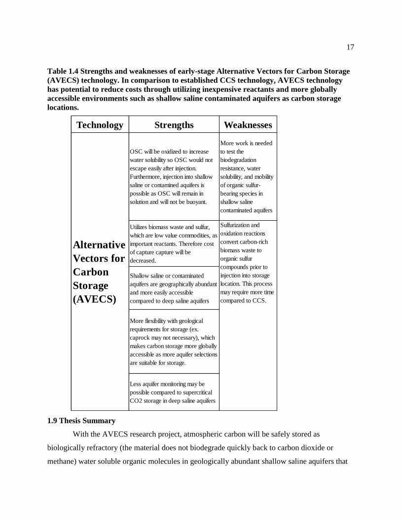
17
Table 1.4 Strengths and weaknesses of early-stage Alternative Vectors for Carbon Storage
(AVECS) technology. In comparison to established CCS technology, AVECS technology
has potential to reduce costs through utilizing inexpensive reactants and more globally
accessible environments such as shallow saline contaminated aquifers as carbon storage
locations.
1.9 Thesis Summary
With the AVECS research project, atmospheric carbon will be safely stored as
biologically refractory (the material does not biodegrade quickly back to carbon dioxide or
methane) water soluble organic molecules in geologically abundant shallow saline aquifers that
Technology Strengths Weaknesses
OSC will be oxidized to increase
water solubility so OSC would not
escape easily after injection.
Furthermore, injection into shallow
saline or contamined aquifers is
possible as OSC will remain in
solution and will not be buoyant.
More work is needed
to test the
biodegradation
resistance, water
solubility, and mobility
of organic sulfur-
bearing species in
shallow saline
contaminated aquifers
Utilizes biomass waste and sulfur,
which are low value commodities, as
important reactants. Therefore cost
of capture capture will be
decreased.
Shallow saline or contaminated
aquifers are geographically abundant
and more easily accessible
compared to deep saline aquifers
More flexibility with geological
requirements for storage (ex.
caprock may not necessary), which
makes carbon storage more globally
accessible as more aquifer selections
are suitable for storage.
Less aquifer monitoring may be
possible compared to supercritical
CO2 storage in deep saline aquifers
Alternative
Vectors for
Carbon
Storage
(AVECS)
Sulfurization and
oxidation reactions
convert carbon-rich
biomass waste to
organic sulfur
compounds prior to
injection into storage
location. This process
may require more time
compared to CCS.

18
have been contaminated naturally (by petroleum, for example), or through human activity. The
approach to develop such molecules is to convert organic waste material to organic sulfur
compounds (OSC) (by using sulfurization reactions), which are biodegradation resistant. This
thesis (Fig. 1.9) focuses on understanding sulfur incorporation reactions in natural settings
(Chapter 2), molecular analysis of sulfur-rich oils which are comprised of different OSC
(Chapter 3), development of a method for isolating sulfur-rich hydrocarbon fractions (Chapter 4),
identification on how sulfur incorporation and oxidation affects hydrocarbon solubility and
biodegradation rate using chemical modelling software (Chapter 5), laboratory sulfurization
experiments on lipids (Chapter 6) and conclusions and future work (Chapter 7).
Figure 1.9 Diagram indicating thesis chapters which includes an introduction to the
purpose of this research and what the AVECS project is (Chapter 1). Sulfur incorporation
processes in natural settings are explored in Chapter 2. Molecular analysis was conducted
on sulfur-rich oils to reveal the environmental settings which contributed to the oil
generation and the structure of organic sulfur compounds found in the oils were discussed
in Chapter 3. The method development process for isolating sulfur-rich hydrocarbon
fractions is discussed in detail in Chapter 4. Then, Chapter 5 identifies how sulfur
incorporation and oxidation affects hydrocarbon solubility and biodegradation rate using
chemical modelling software. In Chapter 6, laboratory sulfurization experiments were
tested on lipids and carbohydrates (Chapter 6) and conclusions and future work (Chapter
7).

19
1.10 Conclusions
Current carbon sequestration methods are effective, however more tools are needed to
reach global targets to prevent warming beneath 1.5°C. The AVECS project aims to develop a
sustainable and cost-effective carbon storage method which stores atmospheric carbon in the
subsurface — such as geographically abundant shallow saline aquifers. Biodegradation resistant
organic species, found in oils, provide conceptual templates of molecular structures which might
represent AVECS molecules adapted to convert carbon-rich biomass materials into molecules
which are: (1) Resistant to biodegradation and oxidation, and (2) water soluble for injection into
polluted shallow saline aquifers. The approach to chemically modify biomass to form non-
biodegradable carbon-rich molecules is to use reactions involving sulfur, which will be discussed
in following chapters. Additionally, for future work discussed in chapter 7, oxygenated
functional groups and oxidation reactions will be used to improve water solubility of the carbon
molecule. As part of government strategies to alleviate anthropogenic carbon emission effects,
cost effective and globally deployable technologies are needed to permanently remove CO2 from
the atmosphere.

20
Chapter Two: Sulfur Incorporation in Natural Settings
2.1 Introduction
Sulfur is a unique chemical element to study because it is considered both an
environmental contaminant as well as an essential commodity to sustain agriculture life and
industry. Sulfur exists in several forms including: elemental sulfur (S8), organosulfur
compounds, metal sulfides and gasses. It is estimated that the world houses 5 billion metric tons
of elemental sulfur reserves in natural gas, petroleum, oil sands, metal ores and evaporitic and
volcano deposits. As well, an estimate of 600 billion tons of elemental sulfur situates in rocks
rich in organic matter such as coal and oil shale which require extraction methods to produce
(Apodaca, 2019). The estimated worldwide total sulfur recovery (all forms) in 2018 was 80
million metric tons (Mt) (Table 2.1).
Sulfur is not only abundant but also an inexpensive natural resource due to an imbalance
in the sulfur market where sulfur production exceeds demand and consumption. In 2015,
worldwide sulfur consumption was nearly equivalent to sulfur production, however an
undoubted surplus of sulfur is predicted to emerge in the future (Apodaca, 2018). Reasons for a
predicted increase in sulfur production is because sulfur recovery is not governed by sulfur
demand, but rather, a function of demand for fossil fuels and metals (AER, 2018). When low
sulfur content fossil fuel sources become depleted in the future, more refineries will turn to
process high sulfur content crude oils for sulfur recovery to improve fossil fuel quality.
Furthermore, sulfur present in crude oil leads to corrosion on refinery equipment and catalyst
deactivation in chemical reactions needed for refining processes (Demirbas et al., 2015).
Petroleum refineries are required to reduce sulfur content in fossil fuels to meet
international environmental laws by continuously improving the efficiency of sour gas
processing and crude oil refining. Furthermore, developing countries are expected to strive
towards higher environmental standards. Typically this is accomplished through the modified
Claus process, the industry standard, for the majority of worldwide sulfur recovery (Chandra
Srivastava, 2012). In this process, H2S is converted to elemental sulfur and removed through
combustion of sulfur-rich fossil fuels. However, this process leads to sulfur dioxide (SO2)
emission, which is corrosive and hazardous especially when mixed with rain water to form acid

21
rain. Therefore, environmental protection acts are becoming more stringent over time to ensure
hazards caused by SO2 emissions and combustion of sulfur-rich fossil fuels are limited. In
Canada, the maximum amount of sulfur allowed in gasoline was 40 mg/ kg in 2016, now
petroleum refineries are required to produce fossil fuels with less than 12 mg/kg of sulfur by
January 1, 2020 (Government of Canada, 2019). In summary, sulfur production will continue to
rise as fossil fuel demand increases and because of further sulfur content reductions in fossil
fuels by international environmental protection acts to improve air quality. In 2018, over 90% of
sulfur produced was used for producing sulfuric acid, which is then used for mining metal ores
and as fertilizers (Apodaca, 2019). While elemental sulfur is mainly used in petroleum refining
processes and agriculture (Table 2.2). The gap between sulfur supply and demand will continue
widen as sulfur consumption has not been able to meet sulfur production since 2015 and other
uses for elemental sulfur have not increased for many years, hence sulfur stockpiles are
accumulating around the world, such as the ones found in Alberta, Canada (Fig. 2.1) (Apodaca,
2018).
2.1.2 A Solution to Two Problems
To limit global warming from reaching 1.5°C warmer than pre-industrial levels would
require major advancements in innovative technology and rapid shift towards sustainable
development in society. Otherwise, failure for global commitment to meet 1.5°C pathways will,
inevitably, lead to irreversible consequences which cause harm to all life forms on earth (Allen et
al., 2018). The current pathway to progress is to ensure national reductions in GHG emissions,
which will cumulatively contribute to limiting warming, however the present intended
contributions from each nation will not limit warming to 1.5°C. In fact, it is estimated that
current GHG emissions reductions are insufficient, and by 2100 will project towards a global
warming of 3–4°C compared to pre-industrial temperatures (UNFCCC, 2016). Reducing global
emissions attempts to limit or slow global warming, but to lower global surface temperatures
requires net removal of anthropogenic CO2 emissions (Allen et al., 2018).
The AVECS research project targets large scale net negative removal of CO2 and, at the
same time, utilizes elemental sulfur as a key element in sulfurization reactions which will also
alleviate the sulfur surplus problem. AVECS technology is unique in the sense that it approaches
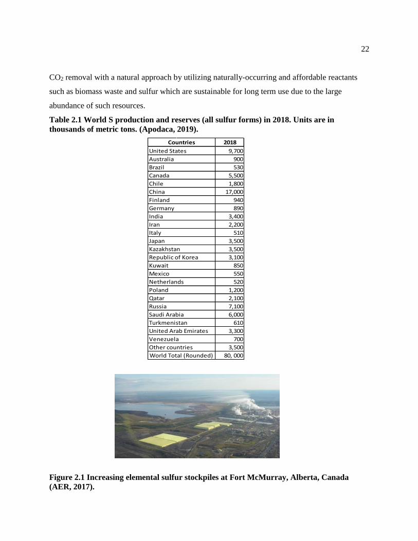
22
CO2 removal with a natural approach by utilizing naturally-occurring and affordable reactants
such as biomass waste and sulfur which are sustainable for long term use due to the large
abundance of such resources.
Table 2.1 World S production and reserves (all sulfur forms) in 2018. Units are in
thousands of metric tons. (Apodaca, 2019).
Figure 2.1 Increasing elemental sulfur stockpiles at Fort McMurray, Alberta, Canada
(AER, 2017).
2018
9,700
900
530
5,500
1,800
17,000
940
890
3,400
2,200
510
3,500
3,500
3,100
850
550
520
1,200
2,100
7,100
6,000
610
3,300
700
3,500
80, 000
Venezuela
Other countries
World Total (Rounded)
Poland
Qatar
Russia
Saudi Arabia
Turkmenistan
United Arab Emirates
Japan
Kazakhstan
Republic of Korea
Kuwait
Mexico
Netherlands
China
Finland
Germany
India
Iran
Italy
Countries
United States
Australia
Brazil
Canada
Chile

23
Table 2.2 Sulfur and sulfuric acid consumption in the United States (Apodaca, 2018). Units
are in thousands of metric tons.
2.1.3 Why Sulfur?
Sulfur exists in a variety of states and species, including minerals in rocks, soluble sulfate
in oceans, gases and in organic matter (Kellogg et al., 1972). Sulfur has an atomic number of 16,
is multivalent and classified under the non-metallic group. Furthermore, sulfur exists as four
stable isotopes 32S (92%), 33S, 34S (4.2%) and 36S. Besides the different isotopes, sulfur also
exists in several oxidation states from –2 (sulfide) to +6 (sulfate) (Table 2.3). These sulfur forms
are known as inorganic sulfur species and the most abundant forms include sulfides (S2-), sulfate
(SO42-), and elemental sulfur (S0) (Bertrand et al., 2015). Elemental sulfur is a unique form of
sulfur as it is inert and water insoluble. Furthermore, it is typically unaffected by moisture,

24
ambient temperatures and microbes. Due to these properties, elemental sulfur is commonly used
as a fungicide and antibacterial agent in agriculture and pharmaceutical practices (Araujo et al.,
2017). Less stable forms of inorganic sulfur include the sulfide ion (S2-), sulfhydryl ion (HS-) and
hydrogen sulfide (H2S) (Bertrand et al., 2015), which are all present in earth’s spheres. In the
atmosphere, H2S transforms into sulfur dioxide (SO2) in the presence of oxygen. H2S is
considered a contaminant in the oil and gas industry, while SO2 is an air pollutant (Kellogg et al.,
1972). About 108 tonnes of gaseous SO2 and sulfur trioxide (SO3) emissions are released into the
atmosphere each year and emanate from burning fossil fuels, emissions from coal-fired plants
and other industrial processes (Gill, 2015). However, government regulations have managed to
reduce sulfur oxide emissions by 64% from 2010 to 2016 (Mos et al., 2019). Oceans house large
amounts of dissolved SO42-
which can escape into the atmosphere as sulfate aerosol particles,
also known as sea spray, when ocean bubbles burst at the water-air interface. (Edwards, 1998;
Jacobson et al., 2000). The lithosphere holds natural reservoirs of sulfur in rocks and sediments
specifically in sulfate minerals such as gypsum (CaSO4·2H2O) and anhydrite (CaSO4). Other
natural abundant sulfur minerals include pyrite (FeS2), cinnabar (HgS) and galena (PbS). In the
biosphere, sulfur species are present in organic matter as sulfur compounds, which form
important building blocks in the structure of protein and amino acids (Bertrand et al., 2015).
Particularly interesting to the AVECS project are organic sulfur compounds (OSC),
which received great focus in the past several decades, particularly in the petroleum industry, as
sulfur compounds are undesirable due to the fact that it causes environmental damage, equipment
corrosion and low quality fuel (Wardencki, 2000). Many research studies are directed at
developing techniques to purify crude oil, natural gas and coal by removing sulfur impurities.
But the benefits of OSC are not overlooked; in crude oils, OSC are known to display resistance
to microbial degradation. As a result, the difference with AVECS technology is sulfurized
organic compounds are formed rather than eliminated and the processes behind OSC formation
underpin this project. AVECS goals are to design and test reactions which simulate natural
sulfurization processes to form biologically refractory, water-soluble organic molecules for
storage in shallow, saline, contaminated aquifers as a potential carbon sequestration method. In
order for AVECS to be feasible and globally accessible, the technology must be reproducible and

25
economically sustainable by using low cost resources. Therefore sulfur is a suitable reactant for
potentially generating AVECS products.
Table 2.3 Sulfur species and corresponding oxidation states. * Thiosulfate has one sulfur
atom that is reduced and the other is oxidized. (Modified after Bertrand et al., 2015)
2.1.3 Geochemical Sulfur Cycle
Sulfur flows from different reservoirs driven by sulfur metabolism and redox reactions
(Bertrand et al., 2015). Whether a mineral or organic sulfur compound is formed is strongly
dependent on the redox state of the environmental conditions, microbial activity, availability of
inorganic sulfur species and organic matter. These factors must harmonize together to form
organic sulfur compounds (Adam et al., 1993). It is hypothesized that organic sulfur compounds
in sediments are formed when sulfides or polysulfides (Sx-2) react with functionalities in aliphatic
and aromatic lipid compounds and become incorporated into the chemical structure (Bertrand et
al., 2015). The sulfur cycle resets when organic sulfur compounds become degraded and release
simpler sulfur compounds and inorganic sulfur forms (Fig. 2.3). There are several other
pathways, discussed in the next section, which naturally produce inorganic sulfur and organic
sulfur compounds.
2.2 Sulfur Incorporation During Early Diagenesis
Wherever there is readily available inorganic sulfur, organic molecules and an active
microbial community, organic sulfur compounds are usually created. In general, when organic
matter decomposes and undergoes diagenesis at shallow depths, aerobic microorganisms
consume available oxygen to catabolize organic matter. When oxygen becomes depleted,
Sulfur Species Chemical Formula Oxidation State
Sulfate SO₄²¯ +VI
Sulfite SO₃²¯ +V
Sulfur Dioxide SO₂ +IV
Thiosulfate * S₂O₃²¯ +II
Elemental Sulfur S° 0
Sulfide S²¯ -II

26
microorganisms seek other compounds to use as an electron acceptor, such as sulfate, for
anaerobic respiration (White, 2013). At the same time, organic sulfur in dead organisms is
mineralized and released into the environment as inorganic sulfur with the aid of aerobic and
anaerobic microorganisms. Released sulfides and other inorganic sulfur forms may experience
assimilatory reduction by organisms or from direct assimilation of sulfide which allows for
reintroduction of sulfur into cellular structures (Bertrand et al., 2015). For instance, sulfur
containing amino acids degrade to form sulfides and polysulfides (Sx2-), which react with
functional groups in aliphatic and aromatic compounds present in organic matter to form more
complex and higher molecular weight organic sulfur compounds (Bertrand et al., 2015).
2.2.1 Assimilatory Sulfate Reduction
Sulfate reduction is a process that most often occurs in anoxic zones in sediments (Fig.
2.2), at depths where molecular oxygen is depleted and where sediment surfaces are occupied
with organic matter supply (Sass and Cypionka, 2007). Anaerobic microorganisms, such as
bacterium Desulfovibrio, thrive under anoxic conditions by using sulfate in place of oxygen for
respiration (Schiff, 2008). Sulfate becomes reduced during anaerobic respiration and is utilized
to oxidize other substrates; this process releases H2S and provides energy for sulfate reducers.
Whereas, assimilatory sulfate reduction is a process used by plants and prokaryotes to
form organic compounds such as proteins, carbohydrates, steroids and phenols by assimilating
inorganic sulfur compounds to use as building blocks for cell components (Bertrand et al., 2015).
Some organisms reduce sulfate with oxidation state (+6) to sulfide (-2) (Fig. 2.3), while other
organisms reduce sulfate to thiols to generate enzymes and sulfur-containing amino acids.
Assimilatory sulfate reduction is one of the main pathways for sulfur incorporation into organic
matter. Furthermore, when organic matter decomposes, sulfurized organic compounds mineralize
and release inorganic sulfur (sulfides). This process is also known as mineralization. Afterwards,
the sulfur cycle continues with dissimilatory sulfide oxidation (Fike et al., 2015).

27
Figure 2.2 Biogeochemical systems in marine sediment. Sulfate-reducing bacteria thrive in
the presence of organic matter and anoxic conditions (Goldhaber, 2005).
2.2.2 Dissimilatory Sulfide Oxidization
In sulfide oxidation, a variety of sulfur oxidizing bacteria (SOB) are involved in the
transformation of reduced sulfur compounds to sulfate as inorganic compounds are used by SOB
to obtain carbon and hydrogen sources (Kleinjan et al., 2003). Certain species of SOB, such as
purple and green phototrophic bacteria, are only capable of executing one intermediate step in
the oxidation sequence: sulfide, elemental sulfur, thiosulfate, tetrathionate, sulfite and lastly
sulfate (Fig. 2.3) (Bertrand et al., 2015). Phototrophic sulfur bacteria use solar energy during
photosynthesis and reduced sulfur compounds as electron donors as a form of carbon fixation
which, in turn, oxidizes sulfide to sulfur. Interestingly, elemental sulfur produced by certain SOB
species is stored as sulfur globules in the interior and exterior of the bacteria cell membrane
(Kleinjan et al., 2003).

28
2.2.3 Dissimilatory Sulfate Reduction
This type of energy, growth and respiratory mechanism occurs most often in reduced and
anoxic marine sediment environments and used mostly by archaea and prokaryotic sulfate-
reducers (Fig. 2.3). During this process, elemental sulfur and oxidized sulfur forms such as
sulfate (SO42-), sulfite (SO3
2-) and thiosulfate (S2O32-) are reduced to sulfides (S2-) through
oxidation of an electron donor by microorganisms (Canfield et al., 2005). Simply, this energy
generating mechanism respires sulfate, the electron acceptor, and emits H2S, similar to how
aerobes respire oxygen and release carbon dioxide to generate energy. This mechanism is
utilized when aerobic respiration is not possible, but anaerobic microorganisms in marine
sediment typically favor the following electron acceptors in the order: nitrate, manganese oxides,
iron oxides and lastly sulfates (Fig 2.2). Although sulfate is the least favorable terminal electron
acceptor, it is 50 times higher in concentration compared to the other electron acceptors.
Therefore, making dissimilatory sulfate reduction a dominant anaerobic respiration process
(Goldhaber, 2005). Another factor that influences sulfate reducing activity is the amount and
quality of food available. For example, certain species of sulfate reducers can only metabolize
low molecular weight organic compounds, such as alcohols, dicarboxylic acids, amino acids,
fatty acids (up to C20) and sugars which have undergone precursor fermentation metabolic
processes by other organisms (Bertrand et al., 2015). Some sulfate-reducing strains are able to
metabolize aliphatic and aromatic hydrocarbons in subsurface reservoirs, which cause H2S
accumulation or souring in oil reservoirs thus corrosion and reservoir plugging (Gieg et al.,
2011). To summarize, sulfate reducers have generated many different metabolic pathways to
metabolize inorganic and organic compounds to ensure survival in diverse environments
(Bertrand et al., 2015).

29
Figure 2.3 The sulfur cycle pathways. In numerical order, pathways 1 to 4 refer to
assimilatory sulfate reduction, mineralization (sulfhydrization), dissimilatory sulfate-
reduction and dissimilatory sulfide oxidation (Bertrand et al., 2015).
2.2.4 Other Mechanisms
In some environments, inorganic sulfur species are used as both an electron donor and
acceptor (Fig. 2.4) where sulfides form from reduction of the electron acceptor and sulfates form
from the oxidation of the electron donor (Bertrand et al., 2015). This mechanism, where a
compound with an intermediate oxidation state like elemental sulfur, allows conversion to other
compounds with higher and lower oxidation states (Bertrand et al., 2015). As a result,
microorganisms which cannot use sulfate as an electron acceptor may use elemental sulfur
instead to produce reduced sulfur compounds (Bertrand et al., 2015). There are a variety of sulfur
reducing species which exist in many settings, many of which are abundant in geothermal
environments, areas rich in elemental sulfur, marine or brackish waters and areas where
phototrophic green bacteria thrive. Sulfur is often used as the final electron acceptor during
oxidation of cellular materials in the dark. However, there are also thiosulfate reducers which
specialize in utilizing thiosulfate as an electron acceptor. Sulfides trapped in sediment can react

30
with ferrous iron to form iron sulfide (FeS), pyrite (FeS2) and elemental sulfur in anoxic
environments (Bertrand et al., 2015).
Figure 2.4 Sulfur metabolism pathways. Assimilatory sulfate reduction (blue). Sulfur
oxidation (green). Elemental sulfur disproportionation (purple) (Fike et al., 2015).
2.2.5 Sulfur Oxidizing and Reducing Microorganisms
Anoxic phototrophic bacteria (Table 2.4) use reduced compounds to obtain electrons in
the presence of light during photosynthesis. Electron donors for this type of bacteria are
hydrogen sulfide, reduced sulfur compounds, and other organic compounds of low molecular
weight or degraded organic material from anaerobic respiration (Bertrand et al., 2015). There are
two groups of anoxic phototrophic bacteria: sulfur and non-sulfur bacteria. Sulfur bacteria use
reduced sulfur compounds as electron donors which, after oxidation and photosynthesis, form
elemental sulfur and sulfate. On the other hand, non-sulfur bacteria utilize photo-oxidized
organic compounds. In particular, anoxic bacteria can be distinguished by 2 colors, purple and
green, as the colors indicate the intracellular pigments within the organisms
(bacteriochlorophylls and carotenoids). Purple sulfur bacteria typically form above green sulfur
bacteria as they require more light and have lower sulfide tolerance (Casamayor et al., 2001).

31
Table 2.4 Four lineages of anoxic phototrophic bacteria.
2.3 Sulfur in the Environment
The sulfur cycle closely resembles the carbon cycle as carbon storage compartments are
often also sulfur reservoirs. Other than a smaller reservoir size, sulfur moves between different
reservoirs on earth similarly to carbon (Fig. 2.5). Furthermore, sulfur fluxes occur in the form of
reduced sulfur compounds and oxidized sulfur compounds where concentrations are dependent
on the environment and ecosystem (Bertrand et al., 2015). The sulfur cycle is maintained by a
balance, known as sulfuretum, which means the amount of sulfide oxidized is relatively equal to
the amount of sulfate reduced (Kleinjan et al., 2003). For example, sulfate reducers degrade
organic matter and produce reduced compounds. The concentration of reduced sulfur compounds
vary in different environments, which, in turn, affect oxidation pathways and dominance of
certain microorganisms which oxidize reduced sulfur compounds.
Figure 2.5 Sulfur cycle, sulfur reservoirs and different sulfur flux pathways. DMS refers to
dimethyl sulfide and COS refers to carbon oxysulfide (Bertrand et al., 2015).

32
2.3.1 Sulfur Sinks
Environments and ecosystems which contribute to the functioning of the sulfur cycle are
explored in this section (Bertrand et al., 2015). In the biogeochemical sulfur cycle, there are
three main sinks where sulfur accumulates. First is sulfate minerals such as gypsum (CaSO4 ●
2H2O), which form in evaporitic environments that have increased metal, oxygen and sulfate
concentration (Fenchel et al., 2012). Weathering of sulfur-rich calcareous rocks releases sulfides
and sulfates into the surrounding environment (Edwards, 1998). Second is in ferrous sulfide
minerals which occur when H2S reacts with iron to form pyrite (FeS2), other iron sulfide
minerals or metal sulfide ores. On the other hand, the generation of organic sulfur compounds is
strongly dependent on the presence or absence of reactive iron or other metal minerals. For
example, the process of converting iron oxides to iron sulfides occurs more quickly than the
reaction between organic matter and reduced sulfur species. Which means that organic sulfur
compounds are unlikely to form in an environment with reactive metals because sulfur species
tend to be consumed quickly (Fenchel et al., 2012).
Lastly, sulfur compounds are found in biomass, sediments and oils (Kohnen, 1991).
Atmospheric sulfur dioxide and inorganic sulfur in soils are often absorbed by plants and
organisms for growth. Particularly in freshwater and wetland areas, there is lack of dissimilatory
sulfate reduction activity. Therefore sulfides formed from sulfur mineralization can be
incorporated into plant biomass to form organic sulfur compounds that make up structural
elements (Fenchel et al., 2012). When organic matter becomes metabolized and decomposed by
microorganisms, some organic and inorganic sulfur forms are released back into the environment
while others undergo diagenesis and catagenesis to form sulfur-rich oils. Sulfur regains access to
the atmosphere when fossil fuels are combusted (Edwards, 1998). In summary, organic sulfur
compounds mostly form in environments where there is low metal concentration, high microbial
activity and accumulation of reduced and oxidized sulfur forms (Kohnen, 1991). Examples of
environments which require sulfur cycling processes to sustain life are discussed below.

33
2.3.2 Stratified Lacustrine Waters
Lakes can be separated into layers or stratified through density, temperature, salinity and
water chemistry (Bertrand et al., 2015). During the summer, solar radiation warms the lake
surface and creates a temperature gradient from the warm lake surface to the cold lake floor. This
type of stratification is known as a thermocline and it separates the upper warm commonly, oxic
layer (epilimnion) from the colder, dense and anoxic water layer below (hypolimnion) (Fig. 2.6).
Due to the density of the hypolimnion, it rarely mixes with the epilimnion, however this layer
still receives organic matter from microorganisms living in the epilimnion above. Anoxic
phototrophic bacteria (red, green, and brown), typically develop in the upper part of the
hypolimnion where there is sufficient light energy and sulfides (Casamayor et al., 2001).
However, for deep lakes, green sulfur phototrophic bacteria thrive in the hypolimnion because
this type of bacteria contain abundant carotenoids and bacteriochlorophyll pigments, which are
effective at capturing long wavelengths of light beyond the usual visible spectrum. Furthermore,
green sulfur bacteria have higher pigment content as an adaptation in response to light limitation
(Casamayor et al., 2001).
The stratification intensity within a lake impacts the sulfur reduction-oxidation rate.
Lakes with increased sulfur cycling have features such as a permanent chemocline or temporary
oxic-anoxic interface, sulfate availability and organic matter supply. Sulfate enters the water
system through weathering of rock minerals, organic sulfur compounds, and leakage of
wastewater and acid mine drainage. Typically, sulfate concentration in fresh water lakes range
from 10 - 500 μM, however mesotrophic and eutrophic lakes have higher sulfate concentrations
ranging from 700 -800 μM. High sulfate concentrations in water promote optimal conditions for
sulfur reducing bacteria which further induces the productivity of sulfur oxidizing prokaryotes
that live in the warm oxygenated waters above, and are responsible for reoxidizing sulfides that
escape from the anoxic community below thus producing sulfate for sulfate-reducers. On the
contrary, acidic lakes often lack sulfur reduction processes as sulfate concentration is low and
microbial activity is diminished. As a result of stratification in lakes, active gradients of sulfides
and sulfates are created by sulfur reducing and oxidizing communities which flourish in non-
acidic waters with high sulfate and organic matter availability (Bertrand et al., 2015).

34
Figure 2.6 Organic matter sinks below the anoxic boundary and activates sulfate reduction
pathways in fresh water lakes (modified after Fenchel et al., 2012).
2.3.3 Marine, Lagoonal and Coastal Environments
Most organic matter in fresh and marine waters become consumed and remineralized by
microorganisms. However under certain environmental conditions, a small percentage escapes
mineralization and becomes buried and preserved in sediment (Raven et al., 2016). One
favorable setting which generates biodegradation resistant sulfur-rich organic matter is at coastal
environments. Fresh water from run off, precipitation and rivers intermix with marine water at
coastal environments such as lagoons and estuaries. Run off water is typically rich in organic
matter due to nutrients and effluent coming from agriculture, industries and municipalities.
Organic matter in these waters becomes remineralized by aerobic microorganisms, which also
encourages anoxic conditions in deeper waters. Similarly, when marine and freshwater mix in
coastal environments, sulfate from marine waters supports sulfate reducing activity and sulfide
production in sediments and surface waters. The most productive area for sulfate reducing
activity is in shallow sediments and the interface between water and sediment because abundant
organic compound input and sulfate is available for sulfur oxidizing microorganisms to develop.
In summary, the activity of sulfur oxidizing and sulfate reducing communities depend on
gradients of sulfide in stratified water columns, light intensity and dioxygen concentrations.
Occasionally in warm weather, the anoxic zone dominates the majority of the water column and
can even move the anoxic and oxic interface up to where air meets water. In this scenario, sulfide

35
accumulates due to increased sulfate reduction activity. Certain species of purple sulfur bacteria
thrive in environments with high sulfide concentration and can also store elemental sulfur within
their cellular composition. In situations where there is limited light or oxygen, these bacteria
utilize stored sulfur forms as an electron acceptor during organic matter degradation (Bertrand et
al., 2015).
2.3.4 Hydrothermal Vents
Oceanic hydrothermal vents are often located in the same areas as mid ocean ridges
where there is a divergent boundary between two tectonic plates on the deep sea floor. In this
setting, cold seawater entering earth’s crust becomes exposed to high temperatures and becomes
enriched in metal ions. Then heated fluids resurface from hydrothermal vents, which are rich in
reduced sulfur and ionic compounds, and mixes with cold oxygenated ocean waters. Many
microorganisms that grow in these environments use the fluids as energy resources. Moreover,
symbiotic relationships occur between marine animals that live around hydrothermal vents and
sulfur-oxidizing bacteria. The symbiotic activity involves animals providing substrates for sulfur
bacteria and these bacteria, in return, supply metabolized organic matter for dietary needs of
marine animals (Bertrand et al., 2015).
2.4 Generation of Sulfur-Rich Crude Oils
Crude oils are complex and contain thousands of compounds which change depending on
the source rock, thermal maturity, and degree of biodegradation of the oil. However, all
petroleum forms are mainly comprised of carbon, hydrogen and heteroatoms (Han et al., 2018).
Within the heteroatom class, sulfur is the most abundant element in petroleum because it
accounts for 0.03 to 14.0 wt% of the entire petroleum content (Sinninghe Damsté et al., 1987;
Han et al., 2018). The average sulfur content for most crude oils is 0.65% (Sinninghe Damsté
and Orr, 1990). Typically, the lower the sulfur content, the sweeter the crude oil is described as,
which is defined as a higher quality oil that requires less processing to remove unwanted sulfur
compounds (Han et al., 2018a). According to Han et al. (2018), crude oil is considered sweet if it
has less than 0.42 wt% of sulfur. Crude oils with high sulfur content are generally derived from
carbonate or evaporitic rock formations while low sulfur content oils originate from clastic

36
sedimentary environments (Orr and Sinninghe Damsté, 1990). Sulfur exists in oils as four main
compound classes: thiols, sulfides, disulfides, and thiophenes (Lobodin et al., 2015). These sulfur
compound classes comprise mixtures of organically bound S compounds that vary from low to
high molecular weight. There is a range of possibilities for what sulfur compound structures
form in oils and that is dependent on the source of the oil as well as environmental settings
(temperature, maturity and degree of biodegradation). In this section, the variables which affect
sulfur content and molecular type in oils and formation of organic sulfur compounds in
petroleum from sulfur incorporation processes with organic matter are explored.
The first factor is the sulfur content of the kerogen source. Kerogen is the precursor of oil
and it is derived from primary production organic matter which has been exposed to diagenesis
in aquatic depositional environments, where biochemicals are converted to complex polymeric
species in the kerogen which is then altered through catagenesis during deep burial, to produce
oil (Orr and Sinninghe Damsté, 1990). Inorganic sulfur species such as H2S and polysulfides
have a tendency to react with certain functional groups and precursor organic molecules to form
sulfur-rich kerogen during early diagenesis (Aizenshtat et al., 1995). In particular, biomolecules
with double bond functionalities, such as lipids and carbohydrates are favored. A secondary
influence on sulfur compound composition in petroleum is thermal maturity. As thermal maturity
increases, more non-sulfur compounds form which dilute the concentration of sulfur compounds
(Adam et al., 1993). Therefore, sulfur content is typically highest in early mature oils when
source rock generation temperatures are low and have yet to degrade weak carbon-sulfur and
sulfur-sulfur bonds within sulfur-rich kerogen and high molecular weight components in crude
oils such as resins and asphaltenes (Orr and Sinninghe Damsté, 1990). It is important to identify
the processes and chemical groups which trigger sulfurization reactions in organic matter to
further understand how to utilize sulfurization reactions and organic compounds as a mechanism
for carbon storage. By understanding how sulfur is incorporated into biodegradation resistant
crude oil molecules, this may provide routes to facilitate the production of sulfur-containing
biologically refractory molecules suitable as AVECS species.

37
Table 2.5 Examples of reactive and non-reactive sulfur compound classes in petroleum
(Lobodin et al., 2015b).
Reactive Non- reactive
Thiols Sulfides Polysulfides Aromatics
1-dodecanethiol thiolane dihexyl disulfide 1-benzothiophene
1-hexadecanethiol dibutyl sulfide dibenzyl disulfide dibenzothiophene
1-octadecanethiol ethyl phenyl sulfide 1,2-benzodiphenylene
dibenzyl sulfide diphenyl sulfide
benzyl phenyl sulfide
Figure 2.7 Four main sulfur compound classes found in petroleum (modified after Han et
al., 2018)
Out of the main sulfur compounds present in crude oil (Table 2.5; Fig. 2.7), mercaptans or thiols
make a small fraction of total sulfur content in oils. Mercaptans often form volatile sulfur
compounds which are converted to toxic H2S upon burial and heating. Processing oil converts
mercaptans to disulfides to meet crude oil specifications. Besides these sulfur compounds, H2S,
elemental sulfur, sulfones, sulfoxides can be found in bitumen and heavy oil fractions. In
particular, sulfones and sulfoxides form through oxidation processes in shallow reservoirs (Han
et al., 2018a).
2.4.1 Organic Sulfur Compounds
It is hypothesized that organic sulfur compounds form from the interaction between
organic matter and reactive sulfur compounds (Aizenshtat et al., 1995). However, organic matter
with varieties of double bond functionalities has increased chances of sulfur incorporation into
its molecular structure (Adam et al., 1993). From analyzing biomarkers and characterizing sulfur
species in petroleum on a molecular level, it is fascinating to observe that a small volume of
crude oil can reveal geological history as to how the oil formed and the organic matter it was

38
formed from. It is believed that double bond functionalities play an important role in forming
organic sulfur compounds because many sulfur-rich oils are comprised of biomarkers which
indicate precursors were comprised of organic molecules such as isoprenoids, carotenoids,
steranes and hopanes which all contain double bond functionalities (Adam et al., 1993). These
molecules are commonly found in carbohydrates and lipids of living organisms. In Chapter 3,
sulfur incorporation mechanisms into organic matter are discussed in further detail based on
double bond equivalents, carbon and heteroatom class distributions of compounds found in the
oils and biomarker data obtained from molecular analysis of sulfur-rich oils.
2.4.2 Sulfurized Lipids
H2S and polysulfides are common in the biosphere because they form structural elements
in protein and provide unique functions in amino acids. For instance, disulfide linkages form
readily and are commonly seen in amino acids such as cysteine and homocysteine. Besides
amino acids, several studies have identified organic sulfur compounds in crude oil and sediment
which formed from carbon skeletons such as isoprenoids and hopanoids, which are components
found in lipids (Table 2.6). The origin of these sulfur structures are believed to result from H2S
and polysulfide incorporation into functionalized lipids which then undergo cyclisation to form
organic sulfur compounds (Kohnen, 1991). Furthermore, sulfur as dioctadecyl disulfide was
discovered in sediment which consisted of remains of a species of marine coral after anaerobic
degradation (Ciereszko and Youngblood, 1971). Research studies have attempted to understand
the earth’s paleoenvironment by analyzing sediments and oils which contain microfossils and
chemical fossils, known as biomarkers, which are organic compounds with structural
information that can indicate the depositional environment, source rock, thermal maturity and
degree of oil biodegradation. In the research by Sinninghe Damsté et al. (1989), sulfurized lipids
were discovered to be useful biomarkers for indicating organic matter source, microbial activity
and overall biogeochemical sulfur cycle (Kohnen, 1991). In Chapter 3, FTICR-MS analysis on
sulfur-rich oils was used to indicate that lipid structures such as carotenoids, squalene and
steroids are susceptible to sulfur incorporation.

39
Table 2.6 Sulfur-containing functional groups and corresponding carbon skeletons which
form organic sulfur compounds identified in nature (modified from Sinninghe Damsté and
De Leeuw, (1990).
2.4.3 Sulfurized Carbohydrates
Carbohydrates also provide living organisms with carbon and energy as it is an essential
building block for plant tissues, biomass and ocean dissolved organic matter (Van Dongen,
2003). Since carbohydrates are used by many living organisms in different ways, it is thought to
undergo remineralization or breakdown quickly during early diagenesis and is rarely preserved in
the sedimentary record. However, a small percentage of organic matter (0.1 – 1.0%) escapes the
remineralization process and forms organic carbon found in sedimentary organic matter, fossil
fuels and other petroleum products, after diagenetic and catagenesis processes (Van Dongen,
2003). Research studies suggest carbohydrates may be preserved through sulfurization processes
that are driven by environmental conditions that are anoxic, sulfate reducing, and have low iron
concentrations (Van Dongen, 2003). To verify these conditions, laboratory sulfurization
experiments by Sinninghe Damsté et al. (1998) showed sulfurized carbohydrate-rich algal cell
material formed alkylthiophenes after pyrolysis which closely resembled alkylthiophene
distributions found in kerogen. This indicates that sulfurized carbohydrates are mostly likely the
precursor of the dominant alkylthiophenes with C5-7 carbon skeletons identified in the pyrolysate
kerogen because the sulfurized carbohydrates were also composed of C5-7 linear alkanes. The
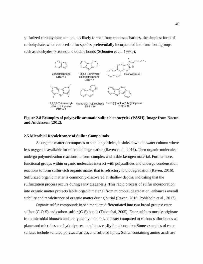
40
sulfurized carbohydrate compounds likely formed from monosaccharides, the simplest form of
carbohydrate, when reduced sulfur species preferentially incorporated into functional groups
such as aldehydes, ketones and double bonds (Schouten et al., 1993b).
Figure 2.8 Examples of polycyclic aromatic sulfur heterocycles (PASH). Image from Nocun
and Andersson (2012).
2.5 Microbial Recalcitrance of Sulfur Compounds
As organic matter decomposes to smaller particles, it sinks down the water column where
less oxygen is available for microbial degradation (Raven et al., 2016). Then organic molecules
undergo polymerization reactions to form complex and stable kerogen material. Furthermore,
functional groups within organic molecules interact with polysulfides and undergo condensation
reactions to form sulfur-rich organic matter that is refractory to biodegradation (Raven, 2016).
Sulfurized organic matter is commonly discovered at shallow depths, indicating that the
sulfurization process occurs during early diagenesis. This rapid process of sulfur incorporation
into organic matter protects labile organic material from microbial degradation, enhances overall
stability and recalcitrance of organic matter during burial (Raven, 2016; Pohlabeln et al., 2017).
Organic sulfur compounds in sediment are differentiated into two broad groups: ester
sulfate (C-O-S) and carbon-sulfur (C-S) bonds (Tabatabai, 2005). Ester sulfates mostly originate
from microbial biomass and are typically mineralized faster compared to carbon-sulfur bonds as
plants and microbes can hydrolyze ester sulfates easily for absorption. Some examples of ester
sulfates include sulfated polysaccharides and sulfated lipids. Sulfur-containing amino acids are
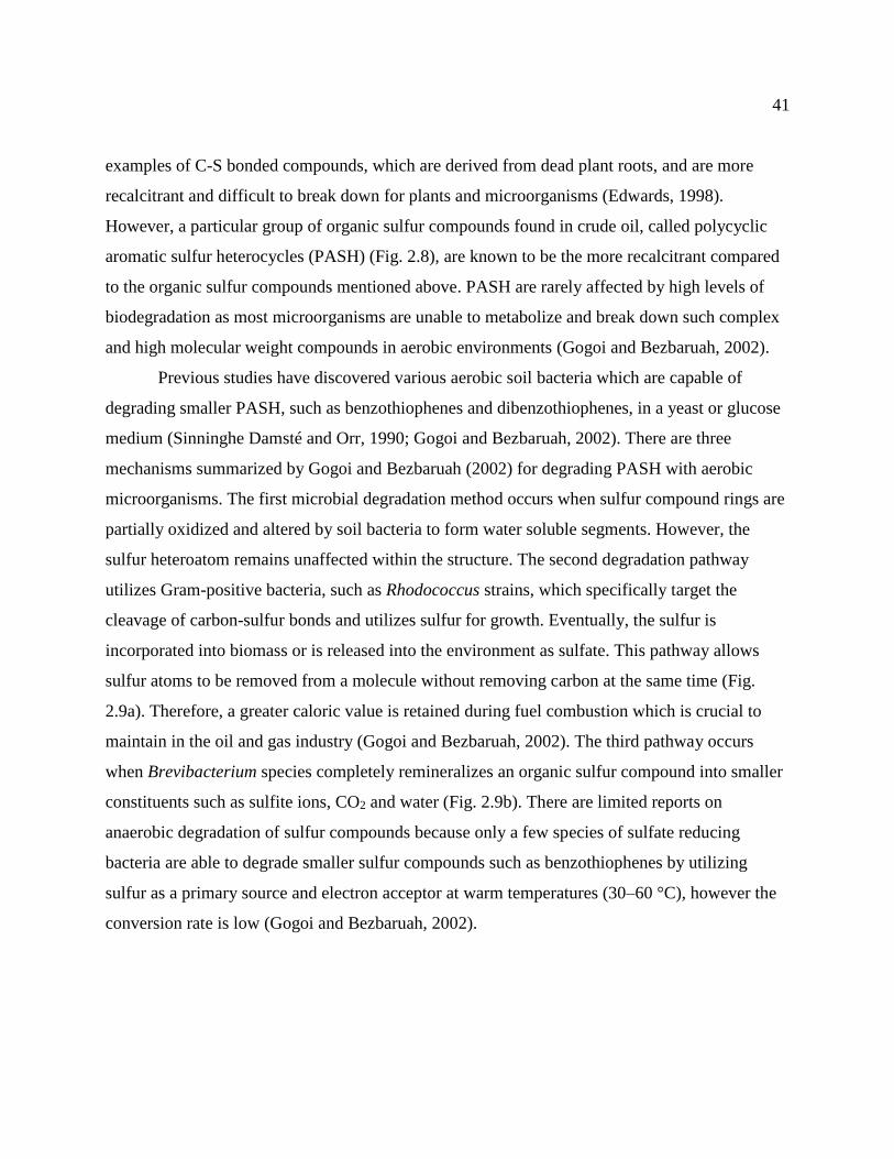
41
examples of C-S bonded compounds, which are derived from dead plant roots, and are more
recalcitrant and difficult to break down for plants and microorganisms (Edwards, 1998).
However, a particular group of organic sulfur compounds found in crude oil, called polycyclic
aromatic sulfur heterocycles (PASH) (Fig. 2.8), are known to be the more recalcitrant compared
to the organic sulfur compounds mentioned above. PASH are rarely affected by high levels of
biodegradation as most microorganisms are unable to metabolize and break down such complex
and high molecular weight compounds in aerobic environments (Gogoi and Bezbaruah, 2002).
Previous studies have discovered various aerobic soil bacteria which are capable of
degrading smaller PASH, such as benzothiophenes and dibenzothiophenes, in a yeast or glucose
medium (Sinninghe Damsté and Orr, 1990; Gogoi and Bezbaruah, 2002). There are three
mechanisms summarized by Gogoi and Bezbaruah (2002) for degrading PASH with aerobic
microorganisms. The first microbial degradation method occurs when sulfur compound rings are
partially oxidized and altered by soil bacteria to form water soluble segments. However, the
sulfur heteroatom remains unaffected within the structure. The second degradation pathway
utilizes Gram-positive bacteria, such as Rhodococcus strains, which specifically target the
cleavage of carbon-sulfur bonds and utilizes sulfur for growth. Eventually, the sulfur is
incorporated into biomass or is released into the environment as sulfate. This pathway allows
sulfur atoms to be removed from a molecule without removing carbon at the same time (Fig.
2.9a). Therefore, a greater caloric value is retained during fuel combustion which is crucial to
maintain in the oil and gas industry (Gogoi and Bezbaruah, 2002). The third pathway occurs
when Brevibacterium species completely remineralizes an organic sulfur compound into smaller
constituents such as sulfite ions, CO2 and water (Fig. 2.9b). There are limited reports on
anaerobic degradation of sulfur compounds because only a few species of sulfate reducing
bacteria are able to degrade smaller sulfur compounds such as benzothiophenes by utilizing
sulfur as a primary source and electron acceptor at warm temperatures (30–60 °C), however the
conversion rate is low (Gogoi and Bezbaruah, 2002).

42
Figure 2.9 (a) Second degradation pathway for dibenzothiophene (DBT), which targets
carbon-sulfur bonds and preserves carbon-carbon bonds. DszA , DszB, DszC refers to
different proteins in organism Rhodococcus erythropolis. (b) Third degradation pathway by
Brevibacterium species which completely mineralizes DBT. (Modified from Gogoi and
Bezbaruah, 2002).
2.5.1 AVECS Molecule
Processes incorporating sulfur into organic matter occur rapidly under favorable
environmental conditions and can enhance chemical stability and biodegradation recalcitrance of
organic compounds during burial. The potential for utilizing sulfurization processes as a carbon
sequestration mechanism for storing carbon-rich organic compounds from biomass waste into
shallow depths such as contaminated saline aquifers will be evaluated in this thesis. In order to
identify suitable AVECS molecules or refractory sulfur compounds, it is essential to further
investigate how organic sulfur compounds are generated naturally in the environment. The next
chapter explores sulfur compounds found in sulfur-rich oils and the conditions which encourage

43
sulfurization of organic matter. The conditions and reactants required to initiate sulfurization
processes will be simulated in laboratory sulfurization experiments in Chapter 6.

44
Chapter Three: Molecular Analysis of Sulfur-rich Oils and Sulfurization in Natural
Settings
3.1 Introduction
The AVECS approach to limit increasing atmospheric CO2 concentrations, as introduced
in Chapter 1, is to modify carbon-rich biomass through sulfurization reactions to form a soluble
and inert molecule which will be stored within the pores of shallow and contaminated saline
aquifers. Sulfur is regarded as a natural preservative as it makes organic matter less susceptible
to biodegradation (Raven, 2016), therefore making the sulfurization process an important factor
influencing the diagenetic pathways of organic matter (Lu et al., 2013b). Organic sulfur
compounds form through natural sulfurization processes such as assimilatory sulfate reduction
and dissimilatory sulfate reduction, which occur in organic-rich environments that are depleted
in oxygen (Amrani, 2014; Bertrand et al., 2015). The goal of this chapter is to determine the lab
conditions that facilitate sulfurization and investigate the chemical and structural composition of
sulfurized organic compounds from sulfur-rich oils collected from Alberta, China and United
States using two analytical methods: gas chromatography-mass spectrometry (GC-MS) and
Fourier Transform Ion Cyclotron Resonance Mass Spectrometry (FTICR-MS).
In the past, many studies were carried out to understand when and how sulfurized organic
matter forms (Sinninghe Damsté et al., 1987; Sinninghe Damsté and Orr, 1990; Sinninghe
Damsté and De Leeuw, 1990; Richnow et al., 1993). However, most studies were conducted
over two decades ago and, since then, GC-MS and FTICR-MS technology has improved to
enhance accuracy and resolution for molecular analysis of oil. Mass spectrometers are a power
analytical tool that is used for analysis and identification of chemical compounds. Many
technological advancements have been made to mass spectrometers since the 1990s (Rabanaque
Berdié et al., 2012) including improved separation to reduce peak overlap and co-elution of
compounds with similar boiling points (Han et al., 2018b). The impactful research studies
conducted on the geochemistry of sulfur compounds in fossil fuels from the 1980s to early 2000s
utilized the GC-MS to attempt to elucidate the structure of organic sulfur compounds (Orr and
White, 1990). It was a difficult task to identify the structure of sulfur compounds solely based on
the mass spectra. Typically, a pure standard or access to reference sulfur compounds stored in
the National Institute of Standards and Technology (NIST) is required to assist in compound and

45
structural identification in spectra. However, both support tools were not as widely established
as present day. Even in modern day, if one does not know what to expect in the spectra, it can
still be challenging to identify what standards are needed to assist in compound identification.
Therefore, the GC-MS may not be the best analytical tool to use for determining the structure of
novel sulfur compounds without reference spectra. The full scan mode, in which qualitative
identification of the sample is detected as a wider mass range is selected (m/z = 50 – 400) to
identify unknown or novel compounds. However, this mode often decreases the detection
sensitivity because the detector spends less time monitoring specific ions of interest. Therefore,
novel compounds with low abundance may become overshadowed as the entire spectra is often
normalized to the peak with highest intensity (Rabanaque Berdié et al., 2012).
Furthermore, complex macromolecules like PASH are often not be detected by the GC-
MS because GC-MS analyses are most suitable for analyzing low molecular weight hydrocarbon
compounds (Lu et al., 2013a). Therefore, in this chapter, the GC-MS is used to identify and
quantify prominent biomarkers to delineate environmental deposition and source rock properties
of sulfur-rich oils. The FTICR-MS is used alongside to identify the carbon number distribution,
double bond equivalents (DBE) and number of sulfur heteroatoms in organic sulfur compounds
present in sulfur-rich oils. Recent studies (Lu et al., 2013a, 2014; Liu and Kujawinski, 2015)
utilize the FTICR-MS as a tool to distinguish the elemental composition of sulfur oils. This
chapter focuses on combining FTICR-MS data with GC-MS data to further understand the
relationship between OSC abundance, formation and depositional environments and organic
matter source.
In this chapter, sulfur-rich oils from Peace River oil sands (Alberta), Jianghan Basin
(China) and Rozel Point (United States) were analyzed with the GC-MS and FTICR-MS to
determine depositional environmental conditions that provoke sulfur incorporation processes into
organic matter, the organic structures that are prone to sulfurization, and the types of OSC
structures discovered in sulfur-rich oils. Although the oils were collected from different
countries, the results show commonality in terms of chemical properties and environmental
influences. Biomarkers indicate that the oils underwent similar environmental conditions and
these settings were the main contributions to forming high sulfur content oils.

46
3.2 Sulfur Incorporation Mechanisms
During early diagenesis, H2S and polysulfides enter a carbon framework through
intramolecular incorporation and form thiolanes, 1,2-dithianes and thiophenes (Kohnen et al.,
1991; Schaeffer et al., 2006). Sinninghe Damsté et al.(1989) hypothesized that thiophenes are
diagenetic products of thiolanes because thiophenes have higher stability compared to the other
sulfur compounds. Likewise, thiane compounds are less stable in nature and are possibly
intermediates in thiolane formation.
Thiolanes form when H2S (HS-) incorporates directly into functional groups or between
two double bond followed by cyclization and carbon skeletal rearrangement (Fig. 3.1) (Kohnen
et al., 1991). Lipid molecules such as squalene, steroids and hopanoids are chemical structures
with several functional groups and are often discovered as sulfurized compounds in oils. Under
diagenetic conditions, thiolanes transform into thiophenes (Fig. 3.2). The formation of thiolanes
and thiophenes, as discussed above, are a form of intramolecular sulfur incorporation. However
Adam et al. (1993) proposed that intermolecular sulfur addition and linkages are the most
favorable process to form sulfur compounds (Fig. 3.1). In contrast, the data and results from this
chapter suggest OSC formation is predominantly through intramolecular sulfur incorporation.
Several studies (Kohnen et al., 1991; Hofmann et al., 1992; Pohlabeln et al., 2017) propose OSC
formation through intermolecular sulfur incorporation into low molecular weight functionalized
molecules to form sulfur-rich macromolecules. The reason for this proposal is because sulfur
fractions were analyzed with the GC-MS by utilizing Raney Ni and MeLi/MeI treatment which
cleaves sulfide linkages and degrades sulfur compounds to meet molecular weight detection
limits (50 – 500 Da) of the GC-MS. Therefore, it was believed that biomarker hydrocarbon
classes such as isoprenoids, hopanoids and steroids are connected by sulfur linkages to form a
sulfur-rich geomacromolecule (Kohnen et al.,1991). The development of the FTICR-MS enabled
this study to analyze whole sulfur-rich fractions without additional derivatization or
desulfurization techniques as the FTICR-MS has high molecular weight detection limits (150 –
60 000 Da) and can detect heteroatoms like sulfur and double bond equivalents (Han et al.,
2018b). For these reasons, a more accurate representation of OSC structure is presented with the
use of the FTICR-MS as the structural pattern of sulfur compounds is not altered. The main
disadvantage with using FTICR-MS, in this study, is it does not show sulfur compound isomers

47
nor the position of sulfur atoms within the chemical structure.
Figure 3.1 The transformation from phytane carbon skeleton to cyclic organic sulfur
compounds during diagenesis through two pathways: intramolecular sulfur incorporation
and intermolecular sulfur addition reactions. (Kohnen et al. 1991)
Figure 3.2 a) Sulfur compounds form through intramolecular incorporation of polysulfides
(Kohnen et al., 1991). b) General scheme for sulfur incorporation into unsaturated lipid
precursors (Sinninghe Damsté et al., 1989).

48
3.2.1 Steroids and Hopanoids
Squalene is an unsaturated hydrocarbon, isoprenoid and lipid that is a precursor to
steroids and hopanoids. The enzyme known as squalene-hopene cyclase enables squalene to
cyclize and form pentacyclic triterpenes (Peters et al., 2005a). One of the major products of this
reaction is production of tetrahymanol, which is the precursor of gammacerane before diagenesis
processes. Tetrahymanol is mainly sourced from green sulfur bacteria and also halophilic
bacteria. Therefore the chemical structure of squalene, steroids and hopanoids may be important
structural elements for sulfur incorporation processes to occur. Additionally, sulfur incorporation
can occur before the cyclization reaction of squalene to triterpenoids as inorganic sulfides are
prone to incorporate into the squalene matrix at double bond function groups (Fig. 3.3).
Furthermore, Lu et al. (2014) postulates sulfur incorporation mechanisms target certain
functional groups in organic compounds such as hydroxyl groups, double bonds and carbonyl
groups. Such functional groups are present in sterols, which are often preserved in sediment. The
preservation and stability of sterols is enhanced further when sulfur is incorporated into steroids.
Figure 3.3 Intramolecular sulfur incorporation into double bonds of isoprenoids.
Diagenesis of kerogen forms saturated, aromatic and organic sulfur compound products.
(Peters et al., 2005).
3.2.2 Carotenoids
Carotenoids are a type of unsaturated molecule composed of series of isoprene units (Fig.
3.4). They are naturally occurring pigments found in a variety of marine organisms such as
plankton, algae, and photosynthetic organisms such as purple and green sulfur bacteria (Liaaen-
Jensen and Andrewes, 1985). These organisms and bacteria typically utilize carotenoids to

49
strengthen lipid membranes (Repeta and Gagosian, 1987; Peters et al., 2005a). There are two
main groups of carotenoids: carotenes and xanthophylls. The difference between the two is
bacteria typically use carotenes, which consists of mostly hydrocarbons, while plants more
commonly synthesize xanthophylls which are oxygen-containing terpenoids (Cai et al., 2005).
Carotenoids are normally destroyed during diagenesis because it is a water-soluble type pigment
and is easily oxidized. Also, the cleavage of polyene units within the carotenoid structure occurs
during diagenesis and increased thermal stress. However, when carotenoids are present in
sediment, it is often a strong indicator of reducing conditions in marine or lacustrine depositional
settings since carotenoid carbon skeletons were observed to become preserved only in highly
reducing conditions (Peters et al., 2005a).
Moreover, Peters et al. (2005a) propose the double bonds in the polyene units of
carotenoids, especially β-carotene, react more easily with inorganic sulfides in hypersaline
anoxic marine environments to form organic sulfur compounds. Frank et al. (2000) also
discusses how the conjugated double bonds in carotenoids are highly reactive and can change
orientations or form epoxides depending on environmental conditions such as in the presence of
limited or excess light energy. For instance, under anoxic, lacustrine and low sulfur conditions,
β-carotene is commonly reduced to β-carotane. It was believed that the presence of β-carotane
became detached from intermolecular sulfur linkages that formed sulfur-rich geomacromolecules
(Peters et al., 2005a). For example, Chen et al. (1996) observed abundant β-carotane in the first
member (ES1) of the Shahejie Formation. This formation, as mentioned above, was deposited
under hypersaline and highly restrictive lacustrine waters, however the sulfur content of each oil
was low (>0.5 wt%). Low sulfur concentrations may be the reason why β-carotene transformed
to β-carotane without undergoing sulfur incorporation reactions. Additionally, Chen et al. (1996)
notes the ES3 member of the Shahejie Formation is comprised of clastic shales and mudstones.
The clay and metallic minerals in this source rock may out compete organic matter for sulfidic
species which restricts sulfur incorporation into organic compounds.

50
Figure 3.4 There are more than 600 types of natural carotenoids, however the carotenoids
shown above are the most abundant in marine environments. Isorenieratene and
Chlorobactene are common in green sulfur bacteria. (Peters et al., 2005b)
3.3 Sample Selection and Geological Background
Six sulfur-rich crude oil samples were collected from various locations around the world
(Table 3.1). Three samples are from Peace River region in Alberta, Canada: (1) Bluesky
Formation, (2) Gething Formation and (3) West Cadotte Member. One sample is from Rozel
Point from Box Elder County, Utah (U.S.A). One oil is from the Jianghan Basin, China. The last
oil is derived from the 4th member of the Shahejie Formation (Es4) and it was collected from
offshore of Bohai Bay Basin, China.
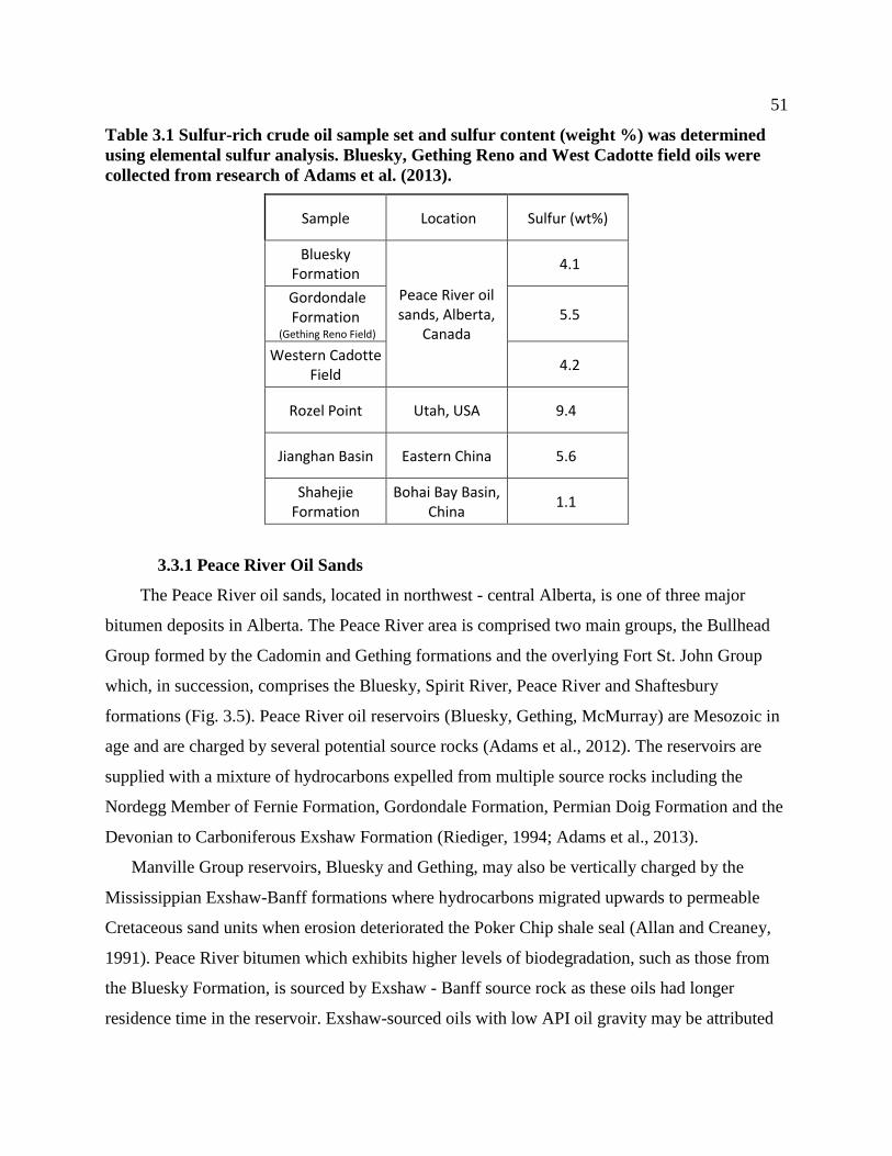
51
Table 3.1 Sulfur-rich crude oil sample set and sulfur content (weight %) was determined
using elemental sulfur analysis. Bluesky, Gething Reno and West Cadotte field oils were
collected from research of Adams et al. (2013).
Sample Location Sulfur (wt%)
Bluesky Formation
Peace River oil sands, Alberta,
Canada
4.1 Gordondale Formation
(Gething Reno Field) 5.5
Western Cadotte Field
4.2
Rozel Point Utah, USA 9.4
Jianghan Basin Eastern China 5.6
Shahejie Formation
Bohai Bay Basin, China 1.1
3.3.1 Peace River Oil Sands
The Peace River oil sands, located in northwest - central Alberta, is one of three major
bitumen deposits in Alberta. The Peace River area is comprised two main groups, the Bullhead
Group formed by the Cadomin and Gething formations and the overlying Fort St. John Group
which, in succession, comprises the Bluesky, Spirit River, Peace River and Shaftesbury
formations (Fig. 3.5). Peace River oil reservoirs (Bluesky, Gething, McMurray) are Mesozoic in
age and are charged by several potential source rocks (Adams et al., 2012). The reservoirs are
supplied with a mixture of hydrocarbons expelled from multiple source rocks including the
Nordegg Member of Fernie Formation, Gordondale Formation, Permian Doig Formation and the
Devonian to Carboniferous Exshaw Formation (Riediger, 1994; Adams et al., 2013).
Manville Group reservoirs, Bluesky and Gething, may also be vertically charged by the
Mississippian Exshaw-Banff formations where hydrocarbons migrated upwards to permeable
Cretaceous sand units when erosion deteriorated the Poker Chip shale seal (Allan and Creaney,
1991). Peace River bitumen which exhibits higher levels of biodegradation, such as those from
the Bluesky Formation, is sourced by Exshaw - Banff source rock as these oils had longer
residence time in the reservoir. Exshaw-sourced oils with low API oil gravity may be attributed

52
to higher levels of biodegradation and low thermal history of the reservoir. Typically, heavy
crude oils require additional heat production technology for bitumen extraction. On the other
hand, deposits which are producible through cold production are generally located in the western
part of Peace River received more significant contributions from Gordondale source rock as
these oils are higher in sulfur content, less mature and have greater API gravity (Fig. 3.6)
(Adams et al., 2013).
Figure 3.5 Geologic timescale and the Peace River area which is comprised of the Bullhead
and Fort St. John Groups. (Modified from AER, 2017 and Adams et al., 2013)
Figure 3.6 The location of Peace River oil samples. Sulfur-rich oils were collected from
Gething Reno Field (green), West Cadotte (purple) and Bluesky formation (blue). Modified
from Adams et al. (2012).

53
3.3.2 Rozel Point
Rozel Point is a small peninsula located in the northern area of Great Salt Lake (Utah,
USA). The Great Salt Lake is separated into two parts, the north arm and south arm, due to
railway construction during the 1960s. The north arm, in particular, is high in salinity because it
is isolated from fresh water sources which come from snow melt by the Wasatch Mountain
Range (Fig. 3.7). Oil seep occurrences at Rozel Point are common and many oil seeps come
from shallow reservoirs, bedrock fractures at the lake bottom and from faults (Sei and Fathepure,
2009). Rozel Point oil is Miocene to Pliocene in age with high sulfur content (up to 14 wt%) and
has high viscosity. Furthermore, the source rock originated from an organic-rich playa lake
sediment deposit (Sinninghe Damsté et al., 1989; Richnow et al., 1993). The reservoir is
comprised of a porous basaltic rock layer interbedded with limestone and is approximately 1 m
thick and located 24 m below the subsurface (Eardley, 1963; Milligan, 2005). Rozel Point oil
migrated from source beds to the reservoir layer through faults and fractures, which also extend
to the surface lake bottom generating oil seeps that are visible when lake levels are low
(Milligan, 2005).
Figure 3.7 Location of Rozel Point. (Utah Geological Survey, 2005)

54
3.3.3 Jianghan Basin
The Jianghan basin, located in Eastern China, is comprised of five major tectonic units
with the Qianjiang depression being the most significant structure since most oil production
takes place in this region from the Eocene Qianjiang Formation (Fig. 3.8) (Philp and Fan, 1987).
Oils from the Qianjiang depression are sourced from the Qianjiang Formation and Xingouzui
Formation, which were deposited in anoxic, sulfate-reducing and saline lacustrine environments
during the late Cretaceous to Paleogene (Carroll and Bohacs, 2001; Hou et al., 2017). Due to
cycles of marine transgression and progradation activity, hot paleoclimate, and clastic sediment
deposition from lacustrine systems, over 220 evaporitic layers interlaced with shales and
sandstones formed the Jianghan Basin source rocks (Philp and Fan, 1987; Wang et al., 2008;
Hou et al., 2017). In addition, the Wangchang anticline, which overlies the alternating halite
layered source rocks, act as a seal to prevent hydrocarbons from migrating vertically. Lateral
accumulation is the main pathway for hydrocarbons coming from the Qianjiang Formation.
However, overlying fractured rock caused by tectonic compression and extension allows
minimal vertical migration. Therefore the Qianjiang Formation is suspected to act as both the
source rock and reservoir (Philp and Fan, 1987; Huang and Hinnov, 2014; Hou et al., 2017).
Upper Qianjiang sections act as the oil reservoir while the deeper sections and Xingouzui
formation embody the source rock.
Figure 3.8 The Jianghan basin located in Hubei province of China and the location of the
Qianjiang depression. (Modified after Brassell et al., 1988)

55
3.3.4 Bohai Bay Basin
The Bohai Bay Basin is a rift basin that is situated near the coast of eastern China (Fig.
3.9) (Wu et al., 2007). It is approximately 200,000 km2 in area and shaped by eight depressions,
five uplifts and many faults that formed during the Paleogene (Li et al., 2003; Luo et al., 2017).
The defining feature of Bohai Bay Basin is the Dongying depression, which formed when the
subsidence rate exceed the rate of deposition during the Neogene. Several formations constitute
the Dongying depression area such as the Kongdian, Shahejie, Dongying, Guanao, Minhuazhen
and Pingyuan formations (Table 3.2). Of these formations, the Shahejie formation is known as
the formation with greatest oil-producing potential (Li et al., 2003). The Shahejie Formation is
comprised of four sub members, Es4 (bottom) to Es1 (top) which was deposited during the
Eocene –Oligocene (Table 3.2). Es3 and Es4 members are important as they are potential source
rocks (Fig. 3.10). The deposition of Es4 was dominantly in a saline lacustrine setting.
Furthermore, the Es4 member is divided into two layers: (1) 40 m of organic-rich shale and (2)
300 m of mudstones and fine sandstones interbedded with gypsum and halite. Well-preserved
reef carbonates and algal fossils in basaltic dust rock were discovered in the upper part Es4,
which suggests a brackish or saline depositional settings (Li et al., 2003). Li et al. (2003)
hypothesized that during the deposition of Es4 member, intense faulting activity caused the
Dongying depression to separate into blocks. Afterwards, lake water evaporated which lead to
hypersaline lacustrine conditions. Over time, water level fluctuations brought clastic rocks along
the edges of lake forming alluvial fan shaped deposits. The lateral stratigraphy for Es4 sediments
changes clastics rocks then micritic limestone and lastly gypsum-halite from the edge of the
basin towards the depocenter (Li et al., 2003). Above lies the Es3 member, another source rock of
Bohai Bay Basin that is rich in organic matter and is approximately an 800 m layer of mudstone.
Oils in the Bohai Bay Basin vary greatly in sulfur content (ranging from 0.03% to 14.7%). High
S oils (>5.0%) have been recovered from Es2, Es3 and Es4 members of Jinxian sag of the Bohai
Bay Basin in the study by Cai et al. (2005).
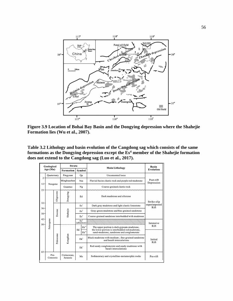
56
Figure 3.9 Location of Bohai Bay Basin and the Dongying depression where the Shahejie
Formation lies (Wu et al., 2007).
Table 3.2 Lithology and basin evolution of the Cangdong sag which consists of the same
formations as the Dongying depression except the Es4 member of the Shahejie formation
does not extend to the Cangdong sag (Luo et al., 2017).

57
Figure 3.10 Schematic map showing the Dongying depression within the Bohai Bay Basin
and the lithology facies of source rocks: a) ES4 member and b) ES3 member (Li et al.,
2003).

58
3.4 Methodology
3.4.1 Elemental Sulfur Analysis
The sulfur-rich oils were was analyzed with the Costech 4010 elemental analyzer using the EAS
Clarity software. Sulfur content (wt%) data (Table 3.1) was obtained by the Applied
Geochemistry group – Isotope Science Lab (AGg – ISL) at the University of Calgary. The
Isotope Science Lab used the following Costech EA parameters: (1) helium carrier flow = 90
ml/min, 5ml of O2(gas) was delivered by the umicro loop for flash combustion, (2) the single tube
quartz reactor was at 1000 ºC, (3) the stainless steel ultratorr union at bottom of the reactor was
held at approximately 120 ºC, (4) combustion of water was removed by a Mg(ClO4)2 chemical
water trap immediately post reaction. GC separation of N2/CO2 from SO2 was achieved using a
custom built Porapak QS 50/80 x 0.8m pyrex glass column maintained at 110 ºC. Approximately
2 to 4mg of sample oil was weighed into smooth walled tin cups (Elemental Microanalysis p/n:
D4059) and cold welded shut using an in-house crimping tool. Sulfanilamide (Elementar
p/n:15.00-0062) was weighed at a range of weights and included in each day's sequence for
calibration and interspersed between each unknown (oil) sample. Flash-combustion was
achieved by careful timing of the umicro pulse of O2(gas) exactly at the time of sample drop.
Signal responses were measured by the on-board TCD. Baseline separation of N2/CO2 - SO2
peaks was approximately 30 seconds. Calibration curves were created for each day's sequence
and corrections were calculated through the Clarity software.
3.4.2 Florisil – Small Scale Separation (SSS)
The sulfur-rich oils were fractionated using liquid chromatography. Oil samples were de-
asphalted with a modified procedure of Bastow et al. (2007). About 50 mg of each sample was
accurately weighed in vials and 10 µL of standard containing naphthalene-d8, phenanthrene-d10,
1,1-binaphthyl, squalane, cholestane-d4, and adamantane-d16 was added to each vial with a
syringe to quantify the individual compounds in each sample. A small amount of
dichloromethane (DCM) was added to mobilize the heavy hydrocarbons. Samples were
transferred into Florisil® (magnesium silicate) columns which were pre-washed with pentane.
Then 5 mL of hexane was gradually added into each column followed by 3 mL of DCM. The
eluates, known as the SSS fraction, were collected in the same vial and placed under nitrogen gas
to concentrate to 0.5 mL.

59
3.4.3 Solid Phase Extraction (SPE)
To prepare saturate fractions for GC-MS, short column pipettes were plugged with cotton
wool and 0.6 g of silica gel (particle size 0.063-0.200 mm; 70-230 mesh) were prepared for each
sample. Pentane was used to flush and pack pipettes. Approximately 20 mg of the SSS fraction
was loaded on to the silica gel. GC-MS auto sampler vials were placed underneath the pipette
and 2.0 mL of pentane was added slowly into each pipette using a syringe in 50 µl increments.
The eluted saturated hydrocarbon fraction was concentrated using nitrogen to 200 µL then 1.0
mL of hexane was added on top prior to GC-MS injection. For the aromatic hydrocarbon
fractions, 8.0 mL vials were placed under the pipettes and 2.0 mL of DCM was added into each
pipette and collected. The fraction was then concentrated with nitrogen to 0.5 mL. The same vial
was placed under the pipettes where 2.0 mL of isopropyl alcohol (IPA) was added for further
elution. The fractions were evaporated to 0.5 mL and transferred into auto sampler vials for GC-
MS analysis.
3.4.4 Liquid Chromatography on Silver Nitrate Impregnated Silica Gel
Liquid chromatography was used to obtain organic sulfur compound (OSC) fractions for
FTICR-MS. Methods were modified from (Wei et al., 2012). For each sample, 300 mg of silica
gel impregnated with silver nitrate (10 wt% of silica gel) was activated at 105 °C for 3 h and
loaded on to a 146 mm Pasteur pipette column plugged with small amounts of cotton wool. The
rest of the column was filled with silica gel (70-230 mesh) activated at 225 °C for 16 h. About 50
mg of oil sample was weighed, mixed with several drops of hexane to mobilize it and loaded on
top of the silica gel. To obtain saturated HC, aromatic HC and OSC fractions, samples were
eluted with 3 mL of hexane, 8 mL of DCM and 2 mL of acetone, respectively. Our interest was
the OSC fraction as saturated and aromatic HC fractions have been obtained through GC-MS
preparation. This technique allowed cyclic sulfides to complex with Ag+ that were retained in
the silica gel column. Elution with acetone then displaced OSC compounds and allowed polar
OSC to elute which were collected as the OSC fraction.
3.5 Mass Spectral Data Processing and Analysis
3.5.1 GC-MS
Saturated and aromatic HC fractions were analyzed in full scan mode using a GC-MS
instrument (7890B GC and 5977 MS). The GC capillary columns are HP-5MS (30 m × 0.25 mm

60
× 0.25 µm). The temperature program initially operated at 40 °C for 5 minutes, followed by a
4 °C/min increase to 325 °C where it was held at this temperature for 15 minutes. Helium was
used as carrier gas at a flow rate of 1.0 mL/min (Huang et al., 2015). Data were processed with
GC/MSD ChemStation software.
3.5.2 FTICR-MS
OSC fractions and whole oil samples were analyzed with a 12 T Bruker SolariX mass
spectrometer in atmospheric pressure photoionization positive ion (APPI-P) mode. APPI-P mode
was selected to analyze OSC fractions as it has enhanced ability to recognize sulfur compounds
in complex organic mixtures without additional structural alteration or preparation methods
(Purcell et al., 2007; Radović et al., 2016). Fractions and samples were diluted with toluene to
0.25 mg/mL and infused into the krypton lamp ionization source (10.6 eV) using a syringe pump
that delivered 200 µL/h. The transfer temperature was set to 400 °C while nebulizer pressure was
at 1.0 bar. To tune the instrument and assess calibration efficiency, reference sample from
Athabasca bitumen was used and reserpine (C33H40N2O9) was added. Ions ranging from m/z 150
to 1500 were isolated by a linear quadrupole and accumulated over 110 ms in the collision cell,
before being transferred to the ICR cell. Spectra were collected in absorption mode using an
algorithm from (Kilgour et al., 2013; Qi et al., 2013). FTICR–MS raw data were processed using
CaPA v.1 (Aphorist Inc.) software.
3.6 Results and Discussion
3.6.1 GC-MS
3.6.1.1 Biomarkers
Biomarkers are often referred to as geochemical fossils because these are molecules which
have lost most functional groups but have still retained and preserved the original carbon
skeleton of a precursor molecule which originated from a particular organism or only available in
certain environments. Biomarkers give rise to information such as a particular class of organism,
age of the organic matter source, depositional setting, oxic or anoxic conditions in which the
petroleum source rock formed (White, 2013).

61
3.6.1.2 Source and Depositional Environment
Isoprenoids such as C19 pristane (Pr) and C20 phytane (Ph) are useful indicators for
organic matter source input as well as source rock depositional setting. Pristane and phytane are
two types of acyclic isoprenoids which originated from the phytyl side chain of chlorophyll. A
combination of diagenesis and anoxic or oxic environmental conditions triggered the cleavage
and transformation of phytyl to phytol (White, 2013). In oxic conditions, phytol converts to
pristane through oxidation and decarboxylation processes while phytol is converted to phytane in
anoxic conditions through reduction (Fig. 3.11). According to Peters et al. (2005b), a Pr/Ph ratio
of less than 1 indicates anoxic source rock depositional conditions and values < 0.8 indicates
hypersaline or carbonate environments.
The Pr/Ph ratios of the oil samples are low and range between 0 to 0.77 (Table. 3.3),
which suggests the source rock for sulfur-rich oils were deposited in anoxic hypersaline or
carbonate settings (Peters et al., 2005b). However, the Pr/Ph ratio was not available for Bluesky
as nearly all n-alkanes and isoprenoids were absent likely due to biodegradation.
Table 3.3 Pr/Ph ratios for sulfur-rich oil sample set. All values are below 1.0, which
suggests anoxic source rock depositional settings. Bluesky (BS), Gething Reno (GR), West
Cadotte (WC), Rozel Point (RP), Shahejie Formation (S) and Jianghan Basin (JH).

62
Figure 3.11 Formation of pristane and phytane from phytol side chain of chlorophyll is
dependent on oxic and anoxic environmental conditions.
The sulfur content of the samples has a direct proportional relationship with the
concentration of dibenzothiophene (DBT) (Fig. 3.12). The oils with higher sulfur content display
greater value of dibenzothiophene to phenanthrene (DBT/P) ratio. In studies by Hodairi and
Philp (2012) and Li et al.(2003), a DBT/P vs. Pr/Ph cross plot was used to determine source rock
and depositional settings. In Fig. 3.12, the ratios infer source rocks of sulfur-rich sample set were
deposited in lacustrine, brackish or marine water environments. All samples fall in one of two
groups: marine or lacustrine. It appears the oils which are less enriched in sulfur (< 5.0 wt%)
(WC, SH and BS) fall in the lacustrine sulfate-poor zone (blue square). Lacustrine waters
generally do not have sufficient sulfate , compared to marine waters, to enrich organic matter and
kerogen with sulfur unless there is presence of water stratification or chemocline which promotes
sulfate cycling activity by sulfate-reducing bacteria (Peters et al., 2005). On the other hand, oils
which are more enriched in sulfur (> 5.0 wt %) (RP, JH and GR) fall within the sulfur-rich
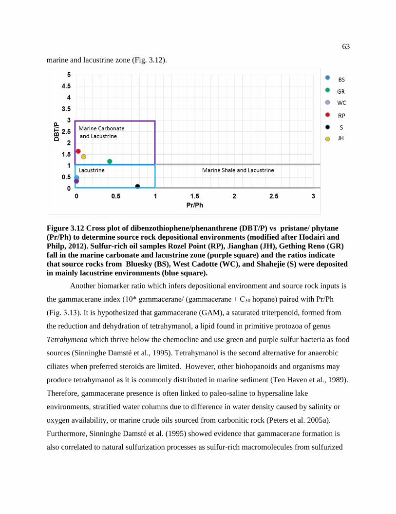
63
marine and lacustrine zone (Fig. 3.12).
Figure 3.12 Cross plot of dibenzothiophene/phenanthrene (DBT/P) vs pristane/ phytane
(Pr/Ph) to determine source rock depositional environments (modified after Hodairi and
Philp, 2012). Sulfur-rich oil samples Rozel Point (RP), Jianghan (JH), Gething Reno (GR)
fall in the marine carbonate and lacustrine zone (purple square) and the ratios indicate
that source rocks from Bluesky (BS), West Cadotte (WC), and Shahejie (S) were deposited
in mainly lacustrine environments (blue square).
Another biomarker ratio which infers depositional environment and source rock inputs is
the gammacerane index (10* gammacerane/ (gammacerane + C30 hopane) paired with Pr/Ph
(Fig. 3.13). It is hypothesized that gammacerane (GAM), a saturated triterpenoid, formed from
the reduction and dehydration of tetrahymanol, a lipid found in primitive protozoa of genus
Tetrahymena which thrive below the chemocline and use green and purple sulfur bacteria as food
sources (Sinninghe Damsté et al., 1995). Tetrahymanol is the second alternative for anaerobic
ciliates when preferred steroids are limited. However, other biohopanoids and organisms may
produce tetrahymanol as it is commonly distributed in marine sediment (Ten Haven et al., 1989).
Therefore, gammacerane presence is often linked to paleo-saline to hypersaline lake
environments, stratified water columns due to difference in water density caused by salinity or
oxygen availability, or marine crude oils sourced from carbonitic rock (Peters et al. 2005a).
Furthermore, Sinninghe Damsté et al. (1995) showed evidence that gammacerane formation is
also correlated to natural sulfurization processes as sulfur-rich macromolecules from sulfurized

64
lipids released gammacerane upon artificial diagenesis and catagenesis which cleaved weak C-
S bonds in sulfur-rich macromolecules.
Peters et al. (2005a) summarizes the trend that suggests hypersaline lacustrine deposits
and highly reducing conditions are high gammacerane indices and low Pr/Ph ratios as these
conditions favor production of tetrahymanol which is the precursor of gammacerane.
Figure 3.13 Gammacerane index 10*(GAM/GAM+30H) and pristane/phytane (Pr/Ph) ratio
for sulfur-rich oil sample set. High gammacerane indices indicate increased water salinity,
water stratification or natural sulfurization processes.
All sulfur-rich oils show a gammacerane and Pr/Ph ratio that is less than 1.0, except for
Jianghan (JH) oil, which exhibits the a gammacerane index of 7.1 which shows it formed in a
different environment compared to the rest of the sample set. JH oil shows greater gammacerane
concentration possibly because organic matter may have been exposed to highly reducing and
hypersaline conditions. Although Rozel Point oil contains high wt% S like Jianghan oil, it has a
low gammacerane index that is comparable to the other oils in the sample set. This plot suggests
RP source rock was not deposited in a hypersaline environment with water stratification or low
thermal maturity which prevented cleavage of C-S bonds in sulfur-rich kerogen thus preventing
the release of gammacerane. Since all the sulfur-rich oils display low Pr/Ph ratios (< 1), reducing
environments appear to be a common environmental factor for generating sulfur-rich oils.
According to Peters et al. (2005a), gammacerane is abundant in marine crude oils from carbonate
source rocks. Presence of this biomarker also suggests increased salinity or presence of a
stratified water column during sediment deposition.

65
The homohopane index is defined as C35/(C31 to 35) homohopanes and this index is
commonly used as an indicator for environment redox potential, bacterial source input as well as
thermal maturity (Peters and Moldowan, 1993). Typically, abundant homohopane distribution
suggests marine, carbonate or evaporitic, or highly reducing environments because homohopanes
(C31-35) originate from the precursor bacteriohopanetetrol, which is a biochemical structure found
in prokaryotes that thrive in the above environmental settings (Peters et al., 2005a). The
homohopane indices for the sulfur-rich oil sample set ranges from 0.03 to 0.13 (Fig. 3.15).
According to Mohialdeen et al.(2015), homohopane indices above 0.09 is considered high.
Therefore, the oils from Jianghan basin and Alberta show a relatively high homohopane, which
suggests these oils originated source rocks deposited in reducing marine or evaporitic
environments. Furthermore, C35 homolog predominance is often observed in immature sulfur-
rich oils, however in Fig. 3.14, the sulfur-rich oils show low homohopane indices and, rather, C31
is more favored and peak height decreases sequentially from C31 to C35. Homohopanes are often
affected by thermal maturity and will decrease in abundance with increasing maturity. According
to Peters and Moldowan (1993), during the catagenesis of source rock containing sulfur-rich
bitumen, kerogen-bound homohopanes may also crack as conditions reach the oil window, thus
increasing the concentration of C31 homologs. Low homohopane indices may also indicate
suboxic depositional conditions (Peters and Moldowan, 1993).

66

67
Figure 3.14 m/z 191 Chromatogram showing homohopanes (C31 – C35) distribution in
sulfur-rich crude oil samples from: (a) Bluesky Formation, (b) Gething-Reno Formation,
(c) West Cadotte field, (d) Rozel Point, (e) Jianghan Basin and (f) Shahejie Formation.
GAM represents gammacerane (non-regular hopane).
The norhopane/hopane (C29/C30) is a biomarker ratio which is useful for indicating source
and maturity information. Norhopane abundance typically increases with thermal maturity as
norhopane is more stable than hopane. From this information, it appears Alberta sulfur-rich oils
(Fig. 3.15) are more thermally mature compared to the other oils as the Bluesky, Gething-Reno
and West Cadotte oils show slightly higher C29/C30H values (0.78 – 0.83) whereas oils from
Rozel Point, Jianghan Basin and Shahejie show lower C29/C30H values (0.13 – 0.30) which
suggests lower thermal maturity.
Fig. 3.15 Homohopane Index (C35/ C31-C35) and norhopane/hopane (C29/C30) which are
source and depositional setting indicators. High homohopane indices (>0.09) suggests high
redox potential, anoxic reducing environments, marine sources, and bacterial input from
bacteriohopanetetrol (Peters et al., 2005)
Steranes (C27-C28-C29) are biomarkers which are commonly used in conjunction in a
ternary diagram (Fig. 3.16) to distinguish organic matter source input, different source rocks or
facies within the same source (Peters et al., 2005a). Most steranes are derived from sterols which
originate from terrigenous organic matter, algae and eukaryotic organisms, while sterols are less
commonly produced by prokaryotes (Mohialdeen et al., 2015). For instance, C27 sterol precursors
are most abundant in phytoplankton and marine organisms. High concentrations of C28 may
relate to lacustrine algae or limnic environments and C29 steranes indicate contributions from

68
terrigenous higher plants, cyanobacteria and primitive algae (Mohialdeen et al., 2015).
Furthermore, high levels of steranes may also be indicative of a clay-poor source rock (Peters et
al., 2005a). Many sulfur-rich oils originate from sulfur-rich kerogen, which means the kerogen is
likely clay-poor and contains low metal concentrations which would not compete with organic
matter for sulfur incorporation. Whereas, clay-rich marine clastic rocks contain metal oxides
which out compete organic matter for H2S utilization thus generate low-sulfur kerogen. In Fig.
3.16, all oils, except for the oil from Gething-Reno, are located in the lower center of the ternary
plot which shows C27, C28 and C29 sterol abundance are relatively equal except C27 and C28 show
a slightly higher abundance. Therefore, the data suggests source rocks of the Alberta oils,
Jianghan Basin, Rozel Point and Shahejie Formation inherited contributions from mixtures of
terrigenous non-marine and marine inputs. On the other hand, Gething-Reno oil shows a clear
C29 predominance which implies Gething-Reno source rock received more non-marine higher
plants or cyanobacteria contributions and hence the abundance of C29 steranes.
Figure 3.16 Ternary diagram with relative distribution of C27, C28 and C29 sterane
abundances.

69
3.6.1.3 Thermal Maturity
Thermal maturity is referred to as the temperature conditions at which kerogen reacts to
generate petroleum. Kerogen begins to break down to hydrocarbons during catagenesis and when
it reaches the oil window which are temperatures of 100–150°C and at depths of approximately
2–3 km (Peters and Moldowan, 1993; White, 2013). The level of thermal maturation of kerogen
can be indicated through pentacyclic triterpanes such as 28,30-bisnorhopane (BNH) and
25,28,30-trisnorhopane (TNH), which are derived from chemotrophic bacteria which thrive in
anoxic-oxic interfaces and bacterial reworking in sediments (Peters et al., 2005b). As well, BNH
and TNH degrade and crack at the same time therefore the ratio BNH/TNH is relatively constant.
However high abundance of BNH/TNH may also indicate source rock deposition in clay poor
and anoxic conditions (Peters et al., 2005b). While BNH/TNH ratios decrease as source rocks
reach thermal maturity and generate oil (Peters et al., 2005a).
Figure 3.17 Biomarkers which are indicative of the degree of thermal maturity:
dibenzothiophene/phenanthrene (DBT/P) is plotted against 28,30-bisnorhopane/ 25,28,30-
trisnorhopane (BNH/TNH).
In Fig. 3.17, the cross plot shows that the higher the sulfur content in oil, the greater the
DBT/P ratio. DBT/P ratios are highest for Rozel Point and lowest for Shahejie Formation, which
correlate closely to measured sulfur content values in Table 3.1. DBT/P and BNH/TNH show an
inverse relationship where the higher the sulfur content, the lower the BNH/TNH ratio. If high
BNH/TNH and sulfur content were observed, then this proportional relationship would infer that
the oils have high thermal maturity (Adams et al., 2013). As well, the BNH/TNH ratio typically
decreases as source rocks mature and reach the oil generation window. This theory is applicable
to oil from the Shahejie Formation which has the lowest DBT/P ratio and also low BNH/TNH.
Since Shahejie oil is less enriched in sulfur (1.1%), Peters et al. (2005a) suggest low BNH/TNH

70
ratio, especially for low sulfur oils, indicate that source rock has reached oil generation
maturation as BNH and TNH become depleted with increasing maturity.
Figure 3.18 Thermal maturity parameters C31 homolog (22S/22S+22R) and C29 sterane
(20S/20S+20R).
A thermal maturity parameter which is particularly useful for showing immature to early
generation oils is the 22S/(22S+ 22R) homohopane isomerization ratio (Peters et al., 2005a).
Terpanes (C31 or C32 homohopanes) are measured using m/z 191 chromatogram and the
isomerization that occurs at C-22 typically occurs early in thermal processes of oil where C-22R
configuration is biologically produced but is converted to C-22S as thermal maturity increases,
therefore high ratio between 22R and 22S is indicative of immature oils (Peters et al., 2005a).
Peters et al. (2005) states that 22S/(22S+22R) ratios below 0.54 suggest oils are early mature
while ratios between 0.57-0.62 suggest mature oils which have reached the oil-generative
window.
Sterane 20S/(20S+20R) isomerization is also a thermal maturity parameter which is
indicative of immature to mature oils. It is measured with m/z 217 chromatogram of C29 sterane.
Similarly, the C-20R configuration occurs naturally in organisms containing steroids and with
increasing maturity, C-20R gradually converts to C-20S configuration. C29 is most commonly
used because C27 and C28 steranes often show co-eluting peaks hence C29 provides more
accuracy. Low maturity oils often show a 20S/(20S+20R) ratio for C29 sterane between 0.23–
0.36 (Li et al., 2003) and the higher the ratio, the more mature the oil. However both thermal

71
maturity parameters can be influenced by biodegradation and selective removal of steranes.
Meanwhile, Ten Haven et al. (1985) suggested that immature oils which originate from
hypersaline source rocks can appear mature with the sterane 20S/(20S+20R) ratio. Fig. 3.18
shows a cross plot between C31 homolog [22S/(22S+22R)] and C29 sterane [20S/(20S+20R)].
Early mature oils and bitumen show isomerization at C-22 for homohopanes and C-20
isomerization in regular steranes (Peters et al., 2005a). The sulfur-rich oil samples show C31
22S/(22S + 22R) ratios between 0.44 -0.62 and C29 20/(20S+20R) ratio is between 0.29 and 0.41.
Both thermal maturity parameters infer that Rozel Point oil is immature, whereas the rest of the
oils are mature and fall in the oil generative window. Furthermore, Peters et al. (2005) suggests
that the accuracy for these two thermal maturity ratios may be influenced by organic facies and
biodegradation. For instance, immature extracts may show greater maturity than reality
especially for oils from hypersaline rocks because unusual sterane diagenetic pathways can
occur. Ten Haven et al. (1985) also noted source rocks deposited in hypersaline conditions can
exhibit mature hopane patterns even when source rocks barely reach the oil window. Therefore,
even though thermal maturity parameters infer sulfur-rich oils from Alberta, Jianghan and
Shahejie are mature, the ratios may exhibit higher maturity than actuality as source rocks were
deposited in hypersaline environments (Sinninghe Damsté et al., 1987).
3.6.1.4 Biodegradation
The Peters and Moldowan (PM) biomarker biodegradation scale (Fig. 3.19) is a ranking
system used to determine the level and extent of biodegradation of oil (Peters and Moldowan,
1993). This system assesses the extent of biodegradation based on the abundance and enrichment
of different hydrocarbon classes in oil. Typically, resins, polar molecules, asphaltenes and
hydrocarbon classes such as naphthalenes and phenanthrenes are chemically more resistant to
microbial degradation compared to n-alkanes and isoprenoids (Peters et al., 2005a). Oftentimes,
it is difficult to determine a clear division between the levels of biodegradation because more
resistant compounds may start to biodegrade before less resistant compounds are fully removed.
Also, complex petroleum systems may contain paleobiodegraded oils mixed with fresh oil
charges (Bennett et al., 2006) and show deviation away from the common order of selective

72
biodegradation observed in the biodegradation scale. Therefore, the biodegradation scale is
most accurate when used as a range rather than a specific number.
Figure 3.19 Biomarker biodegradation scale which ranks biodegradation severity based on
the presence of hydrocarbon classes. L, M, H refers to lightly biodegraded, moderately
biodegraded and heavily biodegraded, respectively. (Peters and Moldowan, 1993).

73

74
Figure 3.20 m/z 85 chromatograms which show n-alkane and isoprenoid distributions in
sulfur-rich crude oil samples from: (a) Bluesky Formation, (b) Gething-Reno Formation,
(c) West Cadotte field, (d) Rozel Point, (e) Jianghan Basin and (f) Shahejie Formation.
Figure magnification for West Cadotte oil (c) shows dominance of C17 and phytane in m/z
85 and m/z 183 chromatograms. IS1 represents squalane internal standard.
Chromatograms (m/z 85) of the saturated HC fraction (Fig. 3.20) show most of the n-
alkanes series are absent in all sulfur-rich oil samples except for the Shahejie Formation (Fig
3.20f) while long chain n-alkanes C20 to C30 are preserved in oils from the Gething-Reno field
and Jianghan Basin (Fig. 3.20b and e). According to the Peters and Moldowan (PM)
biodegradation scale (Fig. 3.19), the sulfur-rich oils from China are lightly to moderately
biodegraded as some n-alkanes and acyclic isoprenoids are depleted. Jianghan oil (Fig. 3.20e) is
depleted in short chain n-alkanes, but isoprenoids (Pr and Ph) and medium (C12 to C30) to long (>
C30) n-alkane chains are abundant, which means Jianghan oil has a PM level between 2 and 3. As
for the Shahejie Formation (Fig. 3.20f), isoprenoids, a distribution of n-alkanes including short
chain n-alkanes (< C12) remain, which indicates biodegradation extent has reached approximately
PM level 2. In comparison, Alberta (Fig.3.20 a, b, c) and Rozel Point (Fig. 3.20 d) oils are
moderately to severely biodegraded. Out of the all sulfur-rich oils, Bluesky oil appears most
biodegraded because all n-alkanes and isoprenoids are absent, but tricyclic terpanes and hopanes
remain, therefore the oil from the Bluesky formation is most likely PM level 4, which is heavily
biodegraded. Rozel Point and West Cadotte oil both share similarities in the m/z 85
chromatogram (Fig. 3.20c and d) because both oils show depletion in n-alkanes and isoprenoids
except C17, selectively preserved pristane, and phytane. Overall, the oil samples have a PM
biodegradation level between 2 and 4 (Peters et al., 2005b).
3.6.2 FTICR-MS
3.6.2.1 Chemical Composition of Organic Sulfur Compounds
Whole oils (Fig. 3.21a) and their OSC counterpart fractions (Fig. 3.21b) were analyzed
with the FTICR-MS and showed the relative monoisotopic intensity for hydrocarbon and
heteroatom compound (N, O, S) classes. Relative monoisotopic intensity (RMI, % of sample) is
defined as the intensity signal measured from a fraction of the most abundant natural element of
each atom rather than average intensity between all isotopes of each atom, and the fraction is
normalized against the sum of all monoisotopic intensities (Carr et al., 2000).
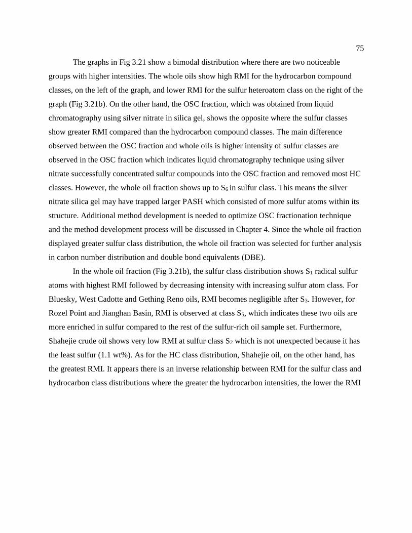
75
The graphs in Fig 3.21 show a bimodal distribution where there are two noticeable
groups with higher intensities. The whole oils show high RMI for the hydrocarbon compound
classes, on the left of the graph, and lower RMI for the sulfur heteroatom class on the right of the
graph (Fig 3.21b). On the other hand, the OSC fraction, which was obtained from liquid
chromatography using silver nitrate in silica gel, shows the opposite where the sulfur classes
show greater RMI compared than the hydrocarbon compound classes. The main difference
observed between the OSC fraction and whole oils is higher intensity of sulfur classes are
observed in the OSC fraction which indicates liquid chromatography technique using silver
nitrate successfully concentrated sulfur compounds into the OSC fraction and removed most HC
classes. However, the whole oil fraction shows up to S6 in sulfur class. This means the silver
nitrate silica gel may have trapped larger PASH which consisted of more sulfur atoms within its
structure. Additional method development is needed to optimize OSC fractionation technique
and the method development process will be discussed in Chapter 4. Since the whole oil fraction
displayed greater sulfur class distribution, the whole oil fraction was selected for further analysis
in carbon number distribution and double bond equivalents (DBE).
In the whole oil fraction (Fig 3.21b), the sulfur class distribution shows S1 radical sulfur
atoms with highest RMI followed by decreasing intensity with increasing sulfur atom class. For
Bluesky, West Cadotte and Gething Reno oils, RMI becomes negligible after S3. However, for
Rozel Point and Jianghan Basin, RMI is observed at class S5, which indicates these two oils are
more enriched in sulfur compared to the rest of the sulfur-rich oil sample set. Furthermore,
Shahejie crude oil shows very low RMI at sulfur class S2 which is not unexpected because it has
the least sulfur (1.1 wt%). As for the HC class distribution, Shahejie oil, on the other hand, has
the greatest RMI. It appears there is an inverse relationship between RMI for the sulfur class and
hydrocarbon class distributions where the greater the hydrocarbon intensities, the lower the RMI

76
for sulfur classes.
Figure 3.21 Organic sulfur compound fractions obtained from liquid chromatography
using silver nitrate impregnated silica gel compared to whole oils. ●, indicates radical
atoms. RMI, relative monoisotopic intensity (a) Liquid chromatography method removed
hydrocarbons and enhanced sulfur intensities (b) Whole oils.
3.6.2.2 Carbon Number Distribution
The oils from Bluesky, Gething Reno and West Cadotte show close relationships because
the carbon distribution shows the oils overlap to form a smooth bell curve with greatest RMI
from C28 to C36 (Fig. 3.22). The overlap is likely due to the genetic similarity between the
Alberta oils as these oils were exposed to similar depositional conditions, thermal processes and
biodegradation as the Alberta oils formed within close proximity (Fig. 3.6). The GC-MS results
show Alberta oils experienced greater levels of biodegradation and increased thermal maturity
compared to the oils from Rozel Point and Jianghan Basin. These conditions removed short and
medium chain n-alkanes during biodegradation which may explain why the carbon number

77
distribution for the Alberta oils is depleted in low carbon numbers but shows increased RMI is
observed for higher carbon number classes.
Other oils which show close resemblance are the oils from Rozel Point and Jianghan
Basin. Several overlapping peaks are prominent from C20 to C40 and the presence of these peaks
may be influenced by low thermal maturity and light biodegradation which allowed precursor
compounds to survive microbial attacks or degradation due to thermal processes. Rozel Point oil
shows high intensity peaks at C20, C29 and C40 while Jianghan Basin oil peaks from C20, C24, C26,
C28, C30, and C40. Shahejie oil also shows similar peaks at C14, C27, C29, and C40. The carbon
number distribution provides information about the molecular structure of precursor compounds
thus gives rise to the organic matter source and depositional environment which form sulfur-rich
oils. For instance, the intensity peak at C20 could be abundance of phytane or a C20 isoprenoid
thiolane which commonly forms in anoxic conditions. Furthermore, the C29 peak could be
enrichment of C29 steranes which come from algae contributions (steroids). Lastly, the intense
peak at C40 could be carotenoids which are also abundant in plants, algae and anoxic bacteria
which utilize carotenoids for capturing long wavelengths of light in deep lakes (Casamayor et al.,
2001; French et al., 2015). Similarly the same results are seen with Jianghan oil but with a
distinct even/odd carbon number preference from C20 to C40 which may be associated with
isoprenoid thiophenes and thiolanes. Shahejie has a slight odd/even predominance from C25 to
C29 and C29 abundance is recognized as indicating terrigenous input to the source (Peters et al.,
2005b).
Figure 3.22 The relative monoisotopic intensity (RMI) and carbon number distributions for
sulfur-rich oil sample set. Rozel Point oil (red) shows high intensity peaks at C20, C29 and
C40. Jianghan Basin oil (orange) shows peaks at C20, C24, C26, C28, C30, and C40. Shahejie oil
(black) also shows similar peaks at C14, C27, C29, and C40. Alberta oils (blue, green, pink) are

78
depleted in low carbon numbers but show increased RMI for higher carbon number
classes.
Figure 3.23 Double bond equivalent distributions. (a) Radical S1 class. (b) Protonated S1
class. Black circle emphasizes DBE 1 peak which is unique only to Jianghan Basin oil.
3.6.2.3 Double Bond Equivalents
Double bond equivalents (DBE) is measure of unsaturation in a molecule and
unsaturation is defined as the number of ring systems, double bonds or both. The radical and
protonated sulfur class S1 and the DBE distribution for the whole oil fraction is presented in Fig.
3.23. Protonated refers to even numbered protonated molecular ions and radical refers to odd
numbered electron ion species (Raffaelli and Saba, 2003). Since RMI is greater with radical
ionization (Fig. 3.20a), in this study onwards, interpretation and discussions will be based on
radical sulfur classes.
From the order of lowest to highest DBE, Jianghan Basin oil shows intense peaks at DBE
1 and 3, then Rozel Point oil at DBE 5 and 6, Shahejie Formation oil and the Alberta oils show
overlapping peaks at DBE 6 with Gething Reno showing a slightly more intense signal.
Furthermore, an interesting note is the Alberta oils appear to have a slight preference towards
odd numbered DBEs at DBE 5, 7 and 9. Overall, the sulfur rich oil sample set shows a non-
symmetric bimodal DBE distribution where high intensities are observed in low DBE numbers
for Jianghan Basin oil and all sulfur-rich oils show peak overlap at DBE 6. DBE analysis shows
OSC with DBE 1(Fig. 3.23a), this observation is unique only to Jianghan Basin oil.
The carbon number distribution for DBE 1 (Fig. 3.24a) mainly shows the Jianghan Basin
with strong even/odd n-alkane predominance from C20 to C30, which may be related to precursors

79
containing C28 and C30 tetracyclic steranes that come from squalene biochemical precursors
(C30H50) and marine organic matter source contributions (Peters et al., 2005b). Lu et al. (2004)
also studied Jianghan Basin oils using the FTICR-MS and hypothesized that enrichment of C20
sulfur compounds come from the sulfurization of phytanic acid and phytol. Intense peaks
observed at C22–C30 represent sulfurized short-chain steranes such as thiolane steranes or cyclic
thioethers as these structures have one sulfur atom and DBE 1 (Lu et al., 2014).
Figure 3.24 Carbon distribution for radical sulfur class S1 at (a) DBE 2 (b) DBE 3 (c) DBE
5 and (d) DBE 6.
Fig. 3.24b shows DBE 3 is a major structural component in oils from Jianghan Basin and
Rozel. The RMI for the other oils are insignificant. When compared to the carbon number
distribution, both Jianghan and Rozel Point have peaks distributed from C20 to C40, however
Jianghan is more enriched in C20 which could be a series of thiophenes or cyclic thioethers with
three rings such as isoprenoid thiophenes (Lu et al., 2014) or the origins of Jianghan may be
from the incorporation of sulfur into phytol (Brassell et al., 1988) as GC-MS results showed high
phytane abundance in Jianghan and Rozel Point. In Fig. 3.24c, Rozel Point shows an intense
peak at DBE 5 that is enriched with C26 to C30, this combination suggests presence of sulfurized

80
steranes with 4 rings cyclized with thioethers to form thiolane steranes (Kok et al., 2000a;
Yang et al., 2013). At DBE 6 in Fig. 3.24d, Alberta oils display a slight right-skewed bell curve
distribution and the carbon number range between C20 to C30 show a higher intensity. This
distribution for Alberta oils could be explained by the presence of benzothiophenes series
attached to medium-chain carbons, such as isoprenoid benzothiophenes because benzothiophenes
have a DBE of 6. In contrast, Rozel Point, Jianghan and Shahejie show high intensity peaks
coinciding at C28-29, C35 and C40. Possible structures which satisfy these characteristics are
sulfurized homohopanes such as C35 pentakishomohopane which has 5 rings and originates from
bacteriohopanoid precursors which incorporated sulfur to form cyclic thioethers and increased
DBE to 6 (Schaeffer et al., 2006). This possibility is likely as GC-MS data also showed high
abundance of C35 homohopane especially for Jianghan Basin oil.
Figure 3.25 (a) Double bond equivalent (DBE) distribution for sulfur class S3. (b) Carbon
number distribution for sulfur class S3 at DBE 7.
The next most abundant sulfur class is S3 (Fig. 3.23a) and further analysis in DBE
distribution in class S3 is shown in Fig. 3.25a. In this figure, oil from Shahejie Formation did not
contain sulfur class S3, but the other oils do and two distinct groups are recognized. Rozel Point
and Jianghan Basin oil differ from Alberta oils because they show lower DBE distributions
which range from 2-10 and intensity peaks are observed at odd DBE numbers such as DBE 3, 5,
6, and 9 with the greatest intensity peak at DBE 7 for Jianghan Basin. Compared to the Alberta
oils which have higher DBE distributions that range from DBE = 3 to 25. High DBE numbers
implies many possibilities for OSC chemical structures (Lu et al., 2014), therefore OSC in
Alberta oils may comprise of more aromatic rings and double bonds within S3 containing
chemical structures compared to Rozel Point and Jianghan Basin OSC structures. Furthermore,
Alberta oils exhibit a bell curve DBE distribution where RMI gradually increases to DBE 14 and

81
descends to zero by DBE 25. This trend could indicate S3-containing OSC structures in
Alberta oils preferentially form structures between DBE 10-14. In Fig. 3.25b, Rozel Point and
Jianghan Basin oil show an intense peak at C40 with DBE 7. This carbon number distribution
pattern is recognized again in sulfur class S5 in Fig. 3.26a where Rozel Point and Jianghan Basin
oils are the only ones which encompass sulfur class S5-containing OSC and a strong intensity
peak is observed at DBE 13. When the carbon number distribution for this peak (S5 class and
DBE 13) was analyzed in Fig. 3.26b, a dominant peak at C40 is observed for both Rozel Point
and Jianghan Basin samples. The chemical OSC structure complies with these characteristics
(C40, DBE 13 and class S5) could possibly be sulfurized carotenoids such as carotenes
(hydrocarbons only) and xanthophylls (oxygen-containing).
Figure 3.26 (a) DBE distribution for sulfur class S5. (b) Carbon number distribution for
sulfur class S5 at DBE 13.
3.7 GC-MS and FTMS Data Summary
GC-MS biomarker analysis indicates sulfur-rich oils in this sample set originate from
reducing and anoxic source rock depositional environments. The Pr/Ph ratios (< 0.8) and low
DBT/P ratio suggest marine or lacustrine depositional settings. Furthermore, the presence of
gammacerane infers hypersaline or stratified water columns as the precursor of gammacerane,
tetrahymena protozoa, thrive in these conditions. The abundance of steranes suggests clay-poor
source rock and organic matter contribution from cyanobacteria, marine and non-marine
organisms. The source rocks for all sulfur-rich oils show similarities. For instance, the
Gordondale member is an important source rock to Peace River oils and it is comprised of
laminated calcitic mudstones (Asgar-Deen et al., 2004). Rozel Point source rock is comprised of

82
anhydrites and calcareous dark shales and siltstones (Bortz, 1984) and the Qianjiang and
Xingouzui formations are main source rocks in the Jianghan Basin and it is comprised of
evaporitic halite layers interbedded with shale and sandstone (Wang et al., 2008). Cai et al.
(2005) also recognized the Shahejie Formation was deposited in anoxic waters because the
presence of mudstones is indicative of poor water circulation and the interbedded carbonates
infers hypersaline and arid environments which form evaporites in shallow marine or lacustrine
settings.
The thermal maturity indicators show oils range from immature to mature indicated by
the terpane R and S isomers where the naturally occurring R isomer is converted to S isomer
with increasing thermal maturity. In addition, the BNH/TNH ratio decreases as oils reach
thermal maturity however low BNH and TNH is observed when exposed to sulfate reducing
conditions. Overall, the oils fall within the immature to early mature zone where Rozel Point oil
is the least mature followed by Jianghan Basin, the Alberta oil and lastly the Shahejie Formation.
Moderate to heavy biodegradation is observed in the sulfur-rich oils from the absence of
short chain n-alkanes and isoprenoids. This study on the sulfur-rich oils from Peace River oil
sands agrees with the maturity and biodegradation levels previously studied by (Adams et al.,
2013). In their study, oil from the Gething Reno field, sourced from sulfur-rich Gordondale
Member (Anderson et al., 2015), exhibited lower thermal maturity, higher sulfur content and
biodegradation compared to Bluesky and West Cadotte oil despite the close proximity in
distance between the Peace River oils.
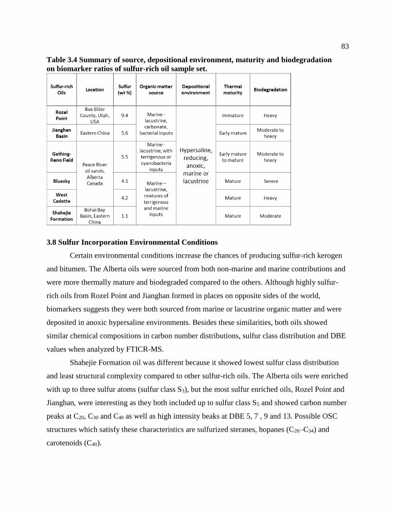
83
Table 3.4 Summary of source, depositional environment, maturity and biodegradation
on biomarker ratios of sulfur-rich oil sample set.
3.8 Sulfur Incorporation Environmental Conditions
Certain environmental conditions increase the chances of producing sulfur-rich kerogen
and bitumen. The Alberta oils were sourced from both non-marine and marine contributions and
were more thermally mature and biodegraded compared to the others. Although highly sulfur-
rich oils from Rozel Point and Jianghan formed in places on opposite sides of the world,
biomarkers suggests they were both sourced from marine or lacustrine organic matter and were
deposited in anoxic hypersaline environments. Besides these similarities, both oils showed
similar chemical compositions in carbon number distributions, sulfur class distribution and DBE
values when analyzed by FTICR-MS.
Shahejie Formation oil was different because it showed lowest sulfur class distribution
and least structural complexity compared to other sulfur-rich oils. The Alberta oils were enriched
with up to three sulfur atoms (sulfur class S3), but the most sulfur enriched oils, Rozel Point and
Jianghan, were interesting as they both included up to sulfur class S5 and showed carbon number
peaks at C20, C30 and C40 as well as high intensity beaks at DBE 5, 7 , 9 and 13. Possible OSC
structures which satisfy these characteristics are sulfurized steranes, hopanes (C26–C34) and
carotenoids (C40).

84
From the molecular analysis of sulfur-rich oils, source input biomarkers indicate
organic matter input include bacteria, terrigenous plants and marine organisms which are
comprised of steroids, hopanoids and carotenoids in its cellular structure. Furthermore, in the
GC-MS and FTICR-MS results section, carotenoids appear to have incorporated sulfur
intramolecularly indicated by high DBE by FTICR-MS data analysis. It is possible that high
abundance of inorganic sulfur species is required to initiate sulfur incorporation into carotenoids.
If sulfur concentration is low, carotenoids may convert to saturated hydrocarbons instead due to
degradation.
As for the environmental conditions, sulfur-rich kerogens were produced under anoxic,
hypersaline, marine or lacustrine with stratified water conditions. These environments are also
typically where sulfate reducing bacteria thrive and produce H2S. Moreover, poor circulation in
anoxic waters enhances H2S concentrations. Since H2S is toxic to most aerobic organisms,
increased H2S can cause organic matter decomposition and deposition. However, H2S can also
convert to polysulfides and elemental sulfur, which becomes incorporated into organic matter or
combines with metals to form rocks (Peters et al., 2005). Cai et al. (2005) also agrees that sulfur
incorporation into functionalized labile hydrocarbons is mainly facilitated by bacterial sulfate
reducing communities. As inorganic sulfur species become incorporated into functional groups
of labile hydrocarbon skeletons, saturated hydrocarbons become depleted, in comparison to the
aromatics, as more thiophenic sulfur compounds form. Also, biodegradation typically attacks
saturated hydrocarbons first which then further increases the sulfur content in residual petroleum.
Cai et al. (2005) also noted that sulfur content in petroleum tends to decrease with
increasing burial depth as source rocks typically produce sulfur-rich oils at low maturity where
burial depth is less than 2400 m. Furthermore, Cai et al. (2005) suggests petroleum with high
sulfur enrichment (>5%) typically forms at paleotemperatures of less than 80 °C. However, the
temperatures which promote bacterial sulfate reduction rates vary from 27 °C–90 °C depending
the type of sulfate reducing bacteria and environmental setting (Kallmeyer and Boetius, 2004;
Sawicka et al., 2012).
In summary, based on the literature and from experimental findings, it is hypothesized
that six conditions that occur concurrently to form sulfur-rich oils and OSC: (1) anoxic, reducing,
hypersaline marine or lacustrine depositional settings, (2) active anaerobic bacterial sulfate

85
reduction activity, (3) organic matter input from bacteria, marine and terrigenous organisms
which are rich in reactive functional groups such as those found in steroids, hopanoids or
carotenoids, (4) formation of type I or II kerogen that is enriched in sulfur, (5) shallow source
rock burial depth and low thermal maturity (<80 °C), (6) moderate biodegradation which
selectively removes n-alkanes and increases sulfur content in residual oil.
3.9 Conclusions
Sulfur-rich oils were analyzed with the GC-MS and FTICR-MS after isolating sulfur-rich
fractions from each oil by utilizing liquid chromatography with silver nitrate impregnated silica
gel. Sulfur enriched fractions were collected from the utilization of silver nitrate. However, high
molecular weight OSC that had several sulfur atoms (> S4) were likely retained in the silver
nitrate column and were not eluted with organic solvents. Method development on this technique
is discussed and further optimized in Chapter 4.
The whole oils which were most enriched in sulfur were oils from Rozel Point and
Jianghan Basin. Both oils showed molecules which were composed of up to S5 in sulfur class
and carbon number peaks at C20, C30 and C40 as well as high intensity peaks at double bond
equivalent (DBE) 5, 7, 9 and 13. These results indicate that organic matter sulfurization occurred
intramolecularly as up to five sulfur atoms were incorporated within a molecule. Possible
organosulfur compound structures that match results from FTICR-MS analysis include sulfurized
steranes, hopanes (C26–C34) and carotenoids (C40) (French et al., 2015).
Many factors facilitate sulfur incorporation reactions into organic matter. From the GC-
MS and FTICR-MS findings, it is hypothesized that factors which encourage sulfurization
processes include anoxic hypersaline environments, low thermal maturity, organic matter input
from organisms which are structurally comprised of steroids, hopanoids and carotenoids, and low
to moderate biodegradation exposure. These conditions provide guidance towards the variables
needed to sulfurize carbon-rich biomass and form water soluble organic molecules for storage
into shallow saline aquifers. Lab sulfurization experiments on lipids such as squalene and β-
carotene are discussed in Chapter 6.

86
Chapter Four: Sulfur Species Fractionation
4.1 Introduction
Apart from utilizing sulfurization reactions on biomass waste material to form organic
sulfur compounds, another method to identify the putative chemical species that meet the goals
of the project is to isolate sulfur compounds that are already present in sulfur-rich oils (Fig. 4.1).
Sulfur-rich fractions can be extracted from crude oil, then oxidation reactions can react with
sulfur compounds to form biologically refractory water soluble organic molecules. The various
sulfur compounds in oils present models for organic compounds that could be used as AVECS
targets for synthesis. There are several varieties of sulfur compounds in oil–some are classified
as reactive sulfides as these types of sulfur compounds are corrosive and damage metallic
refinery equipment at elevated temperatures (240–380 °C). While non-reactive sulfur compounds
are considered noncorrosive and commonly make up to 2/3 of the total sulfur content in sulfur-
rich oils (Fig 4.2) (Lobodin et al., 2015).
Liquid chromatography methods in the literature (Wei et al., 2012) utilize activated silver
nitrate impregnated silica gel, however, this method did not work in a dry climate (Calgary,
Canada) as the silica gel became very reactive and held onto most components including the
desired sulfur-rich fraction. Therefore, this chapter discusses the method development process
for optimizing the use of silver nitrate impregnated silica gel, to extract and isolate reactive and
non-reactive classes of sulfur compounds, under low humidity conditions.
Figure 4.1 AVECS pathways to determine organic compounds which have potential to
form biologically refractory water soluble organic molecules. Pathway 1 refers to utilizing

87
sulfurization reaction on organic biomass waste and pathway 2 refers to isolating sulfur-
rich fractions from sulfur-rich oils and analyzing the S containing compounds as models
for AVECS molecules.
4.2 Reactive and Non-Reactive Sulfur Compound Classes
There are various sulfur compound structures in crude oil and the molecular weight of
these complex OSC range from 600 to 4000 Daltons (Adam et al., 1993). Some examples of
reactive organic sulfur compounds include thiolanes, disulfides (RSSR) and thiols (RSH) (Fig.
4.2). Furthermore, Giles et al. (2017) describes reactive OSC as molecules comprised of at least
one redox active sulfur atom, or sulfur-containing functional group, and has the potential to
oxidize or reduce other biomolecules. Thiols, also known as mercaptans, constitute a small
fraction of total S in crude oils and have a low molecular weight and low boiling point (<200
°C), as thiols are typically smaller sulfur compounds comprised of less than 8 carbon atoms
(Lobodin et al., 2015). Reactive OSC also include acyclic and cyclic sulfides. Acyclic sulfides
are open chain compounds such as dibutyl sulfide, while cyclic sulfides connect to form a ring
and form OSC such as thiolane and thiane. Acyclic and cyclic sulfides are also low in molecular
weight, but sulfides and disulfides with alkyl groups have higher molecular weight and boiling
point. Aliphatic sulfides constitute a greater fraction in sulfur-rich oils compared to mercaptans
(Gogoi and Bezbaruah, 2002).
Non-reactive sulfur compounds are aromatic compounds with more structural
complexity, higher molecular weight and boiling point. Due to these characteristics, non-reactive
sulfur compounds are the most recalcitrant types of OSC (Gogoi and Bezbaruah, 2002).
Generally, it is observed that the greater the molecular weight and complexity of an aromatic
OSC or PASH, the more biodegradation resistant the compound is. Examples of non-reactive
sulfur compounds include benzothiophene, dibenzothiophene and other PASH (Fig. 4.2 and Fig.
4.3).

88
Figure 4.2 Sulfur compound structures and reactivity classification. (Modified after
Lobodin et al., 2015)
Figure 4.3 Polycyclic aromatic sulfur heterocycles commonly found in petroleum (PASH)
(Wang and Stout, 2007)
4.2.1 Fractionation Method
One method for separating sulfur compounds from crude oil is known as ligand exchange
chromatography (LEC). This method uses metals that have affinity for sulfur such as silver
(Ag+), Palladium (Pd2+) and Zinc (Zn2+) (de Menezes et al., 2016). The metal is adsorbed onto a
stationary silica gel phase where sulfur-rich fractions are eluted with solvents with increasing

89
eluent strength (Lobodin et al., 2015a). Wei et al.(2012) utilized liquid chromatography on
silver nitrate impregnated silica gel and showed successful separation of sulfur compounds into
mercaptans, sulfides and aromatic sulfur compounds. Silver nitrate impregnated silica gel is
commonly used to separate olefins compounds, but it has also been used to separate classes of
polycyclic aromatic sulfur heterocycles (PASH) (Wei et al., 2012; de Menezes et al., 2016).
Therefore, this method was adapted in this chapter to separate and identify sulfur compounds in
sulfur-rich oils. However, several issues arose with this method as the silver nitrate impregnated
silica gel was overactive and retained both sulfur and non-sulfur containing compounds. It is
hypothesized that the amount of silver nitrate used and heat activated silica gel technique by Wei
et al. (2012) did not accommodate low humidity conditions in Calgary, Canada. This chapter
discusses the method development processes, including adjustments made to the column design,
sample input and solvents, which were implemented to optimize liquid chromatography on silver
nitrate impregnated silica gel for use in low humidity environments to fractionate reactive and
non-reactive sulfur classes from sulfur-rich oils.
4.3 Liquid Chromatography on Silver Nitrate Impregnated Silica Gel
Silver-ion liquid chromatography is a relatively inexpensive and simple technique that
was originally used for separating different classes of lipid compounds. However, this technique
has been adapted to separate various classes of sulfur compounds in crude oil such as aromatic
sulfur compounds, sulfides, disulfides and mercaptans (Poole, 2003). Lobodin et al.(2015)
demonstrated formation of stable charged complexes between organic sulfur compounds with
silver cations. Moreover, cyclic sulfides, disulfides and mercaptans form even stronger
complexes with silver cations compared to aromatic sulfur compounds (Wei et al., 2012;
Lobodin et al., 2015b). The silver ions interact with unsaturated organic compounds through
forming reversible charge-transfer complexes between silver ions (electron acceptor) and double
bonds in unsaturated compounds (electron donor). Silver-ion chromatography techniques are
well established in planar arrangement or in silver-ion thin layer chromatography (TLC),
however the use of conventional liquid chromatography using silver-ions in a silica gel column
requires more experimentation (Holčapek, 2017). There are several factors that influence the
retention of double bond rich organic compounds, such as the overall molecular structure of the

90
organic compound, number of double bonds, distance between double bonds, amount of silver
ions present in stationary phase and the choice of mobile phase (Holčapek, 2017). Furthermore,
the stability of the complexes increase as more double bonds interact with silver ions (Poole,
2003). However there are other complexities that influence the stability of complex bonding
between silver ions and double bonds in the complexed organic molecule. For example,
increasing chain length of a compound decreases complex stability, while cis isomers form
stronger complexes compared to trans isomers.
Sulfur content typically increases in the order of the following crude oil fractions:
saturated hydrocarbons < aromatic hydrocarbons < resins < asphaltenes (Gogoi and Bezbaruah,
2002). To extract sulfur-rich fractions from crude oil, saturated hydrocarbons are first removed,
through liquid chromatography using silver nitrate impregnated silica gel. Most non-sulfur
containing saturated hydrocarbons pass through the silver-ion column unimpeded, while sulfur
compounds are adsorbed onto the silver nitrate impregnated silica gel due to the strong affinity
between silver ions and double bonds in sulfur compounds. Once non-sulfur containing
hydrocarbons are removed, high eluent strength solvents are used to separate different sulfur
compound class fractions. The silver ions embedded in the silica gel, the stationary phase, form
strong bonds with reactive sulfidic compounds, followed by non-reactive (aromatic) sulfur
compounds and strongest bonds with mercaptans (Holčapek, 2017). Therefore, solvents with
increasing polarity and eluent strength were required to elute the strongly retained sulfur
compounds. Although silver-ion liquid chromatography is relatively simple to set up and can
present good separation (Wei et al., 2012), this technique, however, is seldom used due to
drawbacks such as poor reproducibility and leakage of silver ions into mobile phase (Holčapek,
2017). Many variables from the sulfur fractionation method by Wei et al.(2012) were adjusted
and the method development process is discussed below.

91
Figure 4.4 Interaction and bonding between silver ions and double bonds. The complexes
between the silver-ion and double bond are a type of charge-transfer mechanism. The
unsaturated compound donates an electron to the silver ion and results in the formation of
a sigma bond between the orbitals of the double bond and silver ion. Ag+ represents silver-
ions. (Modified after Nikolova-Damyanova, 2018).
4.3.1 Experiment Design by Wei et al. (2012)
The liquid chromatography procedure using silver nitrate impregnated silica gel by Wei
et al. (2012), to generate a sulfur-rich fraction was followed closely with two exceptions. (1)
Sulfur-rich oils were not spiked with deuterated diamondoids and thiaadamantane internal
standards , as the purpose of the study by Wei et al. (2012) was to determine presence of
thiadiamondoids (indicative of thermochemical sulfate reduction) in oils, which is not a focus in
this research of separating different classes of sulfur compounds. (2) Silica gel was not activated
at 225 °C for 16 hours and silver nitrate impregnated silica gel was not activated at 105 °C for 3
hours. Due to low humidity weather conditions in Calgary, Canada, non-activated silica gel was
already dehydrated and ready for use. Heating silica gel in past experiments caused over
activation and retention of important compounds in the column despite continuous elution. In
liquid chromatography on silver nitrate impregnated silica gel experiments conducted by Wei et
al. (2012), silica gel was activated following the above conditions as humidity levels Texas, USA
are greater than Calgary and may require silica gel activation for optimal function.
For each column, 300 mg of silver nitrate impregnated silica gel (10 wt% AgNO3) was
loaded into a 146 mm Pasteur pipette column that was plugged with small amounts of cotton
wool. The rest of the column was filled with 400 mg of silica gel (Aldrich, pore size 60A, 220-
440 mesh, particle size, 35-75um). About 50 mg of whole oil from the Athabasca oil sands (4.0
wt% S) was weighed and loaded on top of the silica (Fig. 4.5). Due to the polarity of silica gel,
non-polar components tend to elute first during chromatography. To obtain the sulfur-rich
fractions, samples were eluted with hexane (3 mL), dichloromethane (DCM) (8 mL) and acetone
(2 mL) which eluted fractions S1, S2 and S3 respectively. The S1 fraction should contain non-
sulfur containing saturated hydrocarbons, S2 are non-reactive aromatic sulfur compounds and S3
are the reactive sulfidic compound class. The reactive sulfur compounds are eluted last because
Ag+ ions form strongest complexes with sulfides. Cyclic and acyclic sulfides are eluted with
acetone, as acetone forms an even stronger complex with Ag+.

92
Figure 4.5 Silver nitrate impregnated silica gel column design following methods by Wei et
al. (2012). The S1 fraction (saturated hydrocarbons) was eluted with 3mL of hexane,
followed by 8 mL DCM eluted the S2 fraction (non-reactive OSC), and lastly the S3
fraction (reactive sulfides) were eluted with 2 mL of acetone.
4.3.2 Materials
Analytical grade solvents used in this experiment include n-hexane (C6H14),
dichloromethane (CH2Cl2) and acetone (C3H6O) and were purchased from VWR and Fisher
Scientific. Silica gel (60 Å, 220-440 mesh, 35-75 μm), silver nitrate (ACS reagent, >99.0%) were
purchased from Sigma-Aldrich. Sulfur-rich crude oil sample is from Athabasca oil sands (4.0
wt% S) (Alberta, Canada).
4.3.3 Results and Discussion
The silver ion column experiment following the design and procedures by Wei et al.
(2012) appeared fairly dark even after elutions with hexane, DCM and acetone (Fig. 4.5). The
dark column suggests the presence of strongly retained compounds, or the amount of Athabasca

93
whole oil (50 mg) loaded into the column was excessive and did not result in proper
compound class separations. Furthermore, the reactive sulfidic fraction (S3), which was
obtained from 2 mL of acetone eluent, appeared cloudy and white crystal-like precipitate formed
when the fraction (S3) was concentrated to 500 μl (Fig. 4.6). The precipitate which formed could
not be redissolved in acetone nor DCM. To remove the precipitate, prior to FTICR-MS and GC-
MS analysis, most of the S3 fraction could be dissolved with toluene except for the precipitate.
Therefore, the dissolved portion (in toluene) was filtered with a glass wool column (Fig. 4.6), the
precipitate was successfully filtered out in the glass wool and was only soluble in methanol. It
was hypothesized that the precipitate is possibly silver chloride and formed due to leakage of
silver ions.
To confirm whether the white precipitate was associated with the silver impregnated
silica gel, two blank columns were prepared. One was filled only with silica gel, while the other
column followed the same silver-ion column design by Wei et al (2012) except whole oil sample
was not loaded at the top. The same solvent elution order was used: 3 mL hexane, 8 mL DCM,
and 2 mL acetone for both columns. White precipitate formed in the S3 fraction which was
eluted with acetone from the silver nitrate impregnated silica gel column (Fig. 4.7). Precipitate
was not observed in any of the other fractions including those from the silica gel-only column.
According to Lobodin et al. (2015), sulfur compounds, such as mercaptans, can react with silver
ions to form insoluble salts. From the experiment results, insoluble particulates may have leaked
out of the column during elution with acetone, as silver compounds are slightly soluble in
acetone. Due to strong retention of compounds remaining in the column and the additional
measures taken to remove the precipitate, material loss and contaminants were introduced into
the samples. In summary, further method development is needed to optimize sulfur species
fractionation, remove the precipitate, and decrease the retention strength in column.
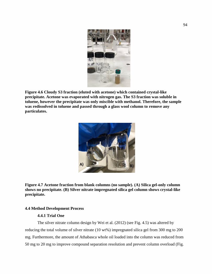
94
Figure 4.6 Cloudy S3 fraction (eluted with acetone) which contained crystal-like
precipitate. Acetone was evaporated with nitrogen gas. The S3 fraction was soluble in
toluene, however the precipitate was only miscible with methanol. Therefore, the sample
was redissolved in toluene and passed through a glass wool column to remove any
particulates.
Figure 4.7 Acetone fraction from blank columns (no sample). (A) Silica gel-only column
shows no precipitate. (B) Silver nitrate impregnated silica gel column shows crystal-like
precipitate.
4.4 Method Development Process
4.4.1 Trial One
The silver nitrate column design by Wei et al. (2012) (see Fig. 4.5) was altered by
reducing the total volume of silver nitrate (10 wt%) impregnated silica gel from 300 mg to 200
mg. Furthermore, the amount of Athabasca whole oil loaded into the column was reduced from
50 mg to 20 mg to improve compound separation resolution and prevent column overload (Fig.

95
4.8). In this trial, two columns were made following the design in Fig. 4.8. One column was
loaded with 20 mg of Athabasca whole oil analyte, and the other was a blank column with no oil
sample. Then, the amounts and order of solvent elutions were kept the same to retrieve fractions:
S1, S2, and S3 from hexane, DCM, and acetone, respectively.
Figure 4.8 The silver-ion column was modified with reduced volume of AgNO3
impregnated silica gel and less whole oil analyte, compared to original experiment design
by Wei et al. (2012), to improve sulfur compounds separation and prevent precipitation.
The S1 fraction was eluted first with 3 mL of hexane, followed by 8 mL of DCM which
eluted the S2 fraction, and lastly the S3 fraction was eluted with 2 mL of acetone.
Despite the changes in reducing the volume of silver nitrate impregnated silica gel and
amount of crude oil analyte in the column, insoluble precipitate formed in the S3 fraction
(acetone elution) when the fraction was concentrated with nitrogen gas. Precipitate was also
present in the acetone elution from the blank column (Fig. 4.9). The precipitate was removed
from both S3 fractions to prepare for FTICR-MS analysis, and the results showed unknowns and
contaminants in the acetone fractions. It is hypothesized that the unknowns and contaminants
were introduced into the fraction during the extra processing measures required to remove the
precipitates. Furthermore, GC-MS results of the S2 fraction (eluted with DCM) show non-
reactive aromatic sulfur compounds such as dibenzothiophenes and naphthobenzothiophenes

96
(Fig. 4.10 A & B). There are also some aromatic sulfur compounds in the S3 fraction
(acetone) (Fig. 4.10 C & D), which suggests the sulfur compound separation could be improved,
as aromatic sulfur compounds are not expected to be in the S3 fraction.
A hypothesis for why aromatic sulfur compounds are present in the S3 acetone fraction
may be because there is oversaturation of silver ions in the column which has caused silver ion
leakage and precipitate occurrence (Fig. 4.9), and the silver ion impregnated silica gel may have
strongly retained other hydrocarbon compounds in addition to sulfur compounds (hence the
darkness in the column in Fig. 4.8) which resulted in mediocre separation of sulfur species
classes. Organic solvents with greater elution strength or affinity to silver ions may elute retained
compounds trapped within silver nitrate silica gel.
Figure 4.9 S3 fraction (acetone elution) from trial one method development (see Fig. 4.8 for
column design). A) Precipitate formed as fraction was concentrated using nitrogen gas. B)
White crystal-like precipitate is observed at the bottom acetone fraction from the blank
column.
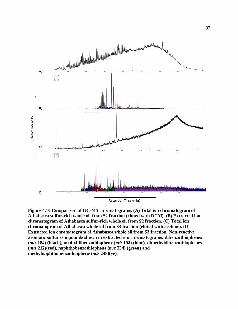
97
Figure 4.10 Comparison of GC-MS chromatograms. (A) Total ion chromatogram of
Athabasca sulfur-rich whole oil from S2 fraction (eluted with DCM). (B) Extracted ion
chromatogram of Athabasca sulfur-rich whole oil from S2 fraction. (C) Total ion
chromatogram of Athabasca whole oil from S3 fraction (eluted with acetone). (D)
Extracted ion chromatogram of Athabasca whole oil from S3 fraction. Non-reactive
aromatic sulfur compounds shown in extracted ion chromatograms: dibenzothiophenes
(m/z 184) (black), methyldibenzothiophene (m/z 198) (blue), dimethyldibenzothiophenes
(m/z 212)(red), naphthobenzothiophene (m/z 234) (green) and
methylnaphthobenzothiophene (m/z 248)(ye).

98
4.4.2 Trial Two
In attempts to release sulfur compounds from strong complexes with silver nitrate
impregnated silica gel, additional solvents, toluene and tetrahydrofuran, were used to experiment
if retention was affected by different solvents which varied in polarity and functionalities. In
addition, the darkness observed in the silver nitrate impregnated silica gel may be due to
oxidation, as the silver nitrate silica gel section of the column typically begins to darken when
solvent is introduced into the column such as when hexane was used to pack the column and
remove air bubbles. When oxidized species are introduced into the silver nitrate column, it could
lead to strong retention that is irreversible (Holčapek, 2017). Therefore, all mobile phase eluents
(hexane, DCM, acetone, toluene and tetrahydrofuran) were prepared fresh at the beginning of the
experiment and nitrogen gas was pumped into the solvents to remove oxygen and prevent
oxidation of silver nitrate impregnated silica gel, which could reduce the effectiveness for sulfur
compound class separations. As well, aluminum foil was used to cover the exterior of the column
to minimize photo-oxidation.
According to Gvirtzman et al. (2015) and Lobodin et al. (2015), Ag+ ions form stronger
complexes with sulfidic compounds compared to aromatic sulfur compounds. Therefore,
theoretically, aromatic sulfur compounds should elute before reactive sulfidic compounds
(sulfides and disulfides). To test this theory, a silver-ion column following the same design as in
the trial one experiment (Fig. 4.8) was loaded with 1.0 mg of dibenzothiophene -2,8-
dicarbaldehyde (DBT) standard (Sigma-Aldrich) instead of whole oil sample (Fig. 4.11). The
purpose for using DBT standard in the silver-ion column was to determine if 10 wt% silver
nitrate impregnated silica gel successfully retained dibenzothiophene (an aromatic sulfur
compound) until elution with DCM, and whether the acetone fraction was free from DBT, since
sulfur compound fractionation experiments by Wei et al. (2012) and Lobodin et al. (2015)
showed aromatic sulfur compounds were eluted with DCM and sulfidic compounds were eluted
with acetone.

99
Figure 4.11 1.0 mg of DBT (dibenzothiophene) standard loaded into a silver-ion column
comprised of 0.400g of silica gel and 0.200g of silver nitrate (10 wt%) impregnated silica
gel. The column was first eluted with 8.0 mL of DCM followed by 8.0 mL of acetone.
Figure 4.12 Total ion chromatograms. A) DCM fraction which shows (m/z 184) DBT peak
and B) acetone fraction indicates that DBT was eluted fully into DCM fraction.
The results from the silver-ion column loaded with DBT standard showed the DBT eluted with
DCM (Fig. 4.12A), and the acetone fraction was free of DBT standard (Fig. 4.12B).
Next, the same column design was used except with an additional column which was
loaded with 20 mg of whole oil sample (Fig. 4.13). The same amounts and types of solvents

100
(DCM and acetone) were used for elution. In addition to these solvents, toluene and
tetrahydrofuran was used to experiment if these solvents had a complexing effect on Ag+ to
release sulfidic compounds and other material that is retained in the column (Fig. 4.13). Toluene
was selected as it is a good solvent for dissolving non-polar compounds and hydrocarbons.
Tetrahydrofuran is a versatile solvent that can be used to dissolve polar and non-polar
compounds and it is known to form strong complexes with certain metal ions. Also, Holčapek
(2017) indicated that a combination of chlorinated solvents such as DCM along with a small
addition of higher polarity solvents may assist in eluting compounds that are strongly retained in
the column. Use of aqueous solvents are discouraged as anions could cause silver ions to
precipitate out of the column and crude oil is also not soluble in aqueous solvents (Holčapek,
2017).
Figure 4.13 Trial two of silver nitrate impregnated silica gel column method development.
One silver-ion column (left) was loaded with 1 mg of dibenzothiophene (DBT) standard and
the other silver-ion column (right) was loaded with 20 mg of Athabasca whole oil. Each
column was eluted with four different solvents and the elutions were collected in separate
fractions. The first elution involved 8 mL of DCM, followed by 8 mL of acetone, then
toluene and lastly tetrahydrofuran (THF).
Each solvent was prepared fresh at the beginning of the experiment and the solvents were
bubbled with nitrogen to minimize oxygen concentrations which may react with silver nitrate in
the column and cause oxidation. The solvent elution order was completed as follows: DCM,

101
acetone, toluene and lastly THF. 8 mL of each solvent was used as this amount eluted a
fraction or band of the analyte. Furthermore, by the eighth milliliter of added solvent, colorless
eluate fluid was observed and it indicated that a stronger affinity solvent could be used to elute
other analyte components which are more strongly adhered to the silica gel. Four separate
fractions were collected from each column (Fig. 4.13). Several minutes after the final elution
with tetrahydrofuran, the acetone fraction settled and some precipitate formed at the bottom of
the vial (Fig. 4.14). The acetone fraction, from the Athabasca whole oil column, formed a dark
brown-black precipitate which would not redissolve in acetone nor DCM. This precipitate
observation also occurred in the acetone fraction from the original experiment (Fig. 4.6) and
method development trial one (Fig. 4.9). In addition, a clear to white crystal-like precipitate
formed in the acetone fraction from the DBT loaded column. The crystal-like precipitate
appeared similar to the precipitate occurrences which were observed in the original and trial one
experiments (Fig. 4.7B and Fig. 4.9B).
Figure 4.14 Trial two sulfur fractionation elutions. Top images represent elution which
came from column on the right which contained 20 mg of whole oil. Bottom images are
from left column which was loaded with 1 mg of DBT standard. Precipitate was observed
in acetone fractions from both columns. DCM = dichloromethane, ACET = acetone, TOL =
toluene, THF = tetrahydrofuran.
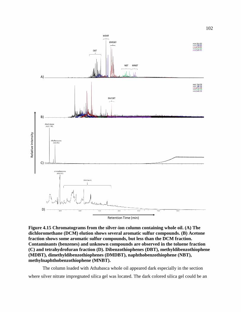
102
Figure 4.15 Chromatograms from the silver-ion column containing whole oil. (A) The
dichloromethane (DCM) elution shows several aromatic sulfur compounds. (B) Acetone
fraction shows some aromatic sulfur compounds, but less than the DCM fraction.
Contaminants (benzenes) and unknown compounds are observed in the toluene fraction
(C) and tetrahydrofuran fraction (D). Dibenzothiophenes (DBT), methyldibenzothiophene
(MDBT), dimethyldibenzothiophenes (DMDBT), naphthobenzothiophene (NBT),
methylnaphthobenzothiophene (MNBT).
The column loaded with Athabasca whole oil appeared dark especially in the section
where silver nitrate impregnated silica gel was located. The dark colored silica gel could be an

103
indication that a lot of material is still retained within the column, since photo-oxidation risk
was minimized with aluminum foil and oxygen was removed from the solvents with nitrogen
gas. From the chromatograms in Fig. 4.15, thiophenic sulfur compounds were most abundant in
the DCM fraction (Fig. 4.15A), but these compounds were also present in small amounts in the
acetone fraction (Fig. 4.15B). As for toluene and THF fractions, there were no detectable sulfur
compounds and only contaminants, such as alkylated benzenes, and unknowns were observed.
Therefore, it was concluded that toluene and THF were not favorable solvents to use in this
experiment.
4.4.3 Trial Three
One of the most challenging aspects of these experiments was determining the reason for
precipitate formation and how the column design could be altered to prevent silver-ion related
precipitates from leaking out of the column. There are three hypotheses as to why precipitate
forms: 1) silica gel is oversaturated with silver nitrate, 2) silver compounds are slightly soluble in
acetone and precipitates over time, or 3) chlorine ions (Cl-) from dichloromethane combine with
silver ions from the silver nitrate to form silver chloride precipitate. Since silver nitrate is slightly
soluble in acetone, silver ions could be released when acetone is introduced into the silver nitrate
impregnated silica gel, then the silver ions may combine with dichloromethane or other
haloalkane remnants in the column to form silver chloride.
To resolve these speculations, a new column design was developed to trap potential
silver-ion leakages. A thin layer of silica gel (50 mg) was arranged at the bottom of the column,
followed by a layer of silver nitrate impregnated silica gel (150 mg) over top. Silver nitrate
impregnation was decreased to 5 wt% on the silica gel to reduce the possibility oversaturation of
silver nitrate on silica gel. Lastly, 400 mg of silica gel was layered on top of the silver nitrate
impregnated silica gel (Fig. 5.5).

104
Figure 4.16 Trial three column design to prevent silver-ion leakage and precipitate from
forming in acetone fraction.
Furthermore, in addition to the changes made to the column design, other changes include using
a gradual gradient of increasing solvent polarity. 20 mg of Athabasca whole oil was first eluted
with hexane to remove saturates then by DCM which eluted aromatic sulfur compounds. After
DCM elution, the solvent polarity was gradually increased until from DCM (100), DCM/Acetone
(80:20), (50:50), (70:30) and then acetone (100). Solvent was passed through the column until
the eluate was colorless. Furthermore, the column was covered with aluminum foil to minimize
photo-oxidation.
Figure 4.17 Trial three method development. A) Column design with silver nitrate
impregnated silica gel sandwiched between two layers of plain silica gel. B) Eluates starting

105
from the left: Hexane, DCM, DCM to acetone following gradual polarity increase and
pure acetone fraction.
The changes in the column design and the gradual increase in solvent polarity assisted in
preventing precipitate from forming in the fractions (Fig. 4.17B). However, the column (Fig.
4.17A) still appeared dark as compounds may still be strongly retained. GC-MS analysis was
performed and key sulfur compounds, including sulfides and aromatic sulfur compounds, were
monitored using mass chromatography with target ions of m/z 134, 148, 176, 212, 234, and 248
(Fig. 4.18) to determine which eluate contained the most sulfur compounds and whether the
chromatography experiment separated compounds effectively.
The chromatograms showed the hexane fraction (Fig. 4.18B) closely resembled the
whole oil (Fig. 4.18A). The eluted fraction using DCM/acetone consists of higher molecular
weight compounds such as dibenzothiophene and methylnaphthobenzothiophene; which were
identified on the GC-MS using mass chromatography at m/z 212 and m/z 248, respectively (Fig.
4.18C). On the other hand, the pure acetone fraction eluted lower molecular weight sulfur
species, such as dibutyl sulfide and benzothiophenes identified on GC-MS using mass
chromatography at m/z 134 and m/z 146 (Fig. 4.18D). However, both the DCM/acetone fraction
and pure acetone fraction exhibited relatively low abundance of sulfur compounds. Due to the
low abundance of sulfur compounds identified in the DCM/acetone and pure acetone fractions
(Fig. 4.18C and D), it is speculated that an ample amount of material is still confined within the
column. Furthermore, the total weight of each fraction was measured to estimate how much
material is still retained in the column after elutions (Table 4.1).

106
Figure 4.18 Extracted ion chromatograms (m/z 134, 148, 176, 212, 234, 248). (A) Whole oil.
(B) Hexane elution. (C) Dichloromethane (DCM) and acetone gradient fraction. (D) Pure
acetone fraction. Higher molecular weight sulfur compounds, such as dibenzothiophene
and methylnaphthobenzothiophene, are observed in the DCM and acetone gradient
fraction, while lower molecular weight sulfur compounds such as sulfides are more
dominant in the pure acetone fraction.

107
Table 4.1 Sample weights for trial three elutions. Hexane was eluted first, followed by
DCM (dichloromethane) and lastly DCM and acetone. The total input mass in the silver-
ion column was 20 mg of whole oil, the total output mass (calculated from the sum of each
fraction) was 10.7 mg. This means that the accumulation of material in the column is
estimated to be 9.3 mg.
Fraction
Output
Sample
Weight
(mg)
Input Mass
(mg)
Total
Output
Mass (mg)
Accumulation
(Input - Output)
(mg)
Hexane 4.8 20.0 10.7 9.3 DCM/Acetone 2.4
Pure Acetone 3.5
According to the accumulation calculation in Table 4.1, the total output mass was
measured to be 10.7 mg and since 20 mg of whole oil was loaded into the column, it is estimated
that 9.3 mg of sample material remains accumulated in the column. The amount of accumulation
in the column is nearly half of the loaded input mass and this amount suggests that the column is
still strongly retaining oil components within the silver nitrate impregnated silica gel, and the
weight % of silver nitrate should be further reduced from 5% to 1% to lower retention strength.
In addition, the amount of input mass (20 mg of whole oil) should also be further reduced to
prevent column overload and poor chromatographic separation of oil components.
4.4.4 Trial Four
4.4.4.1 Sulfur Compounds Standard Preparation
10 mg of each pure sulfur compound (purchased from Sigma Aldrich): thiophene (99+%),
thiolane (99+%), 1-benzothiophene (>99.0%), dibutyl sulfide (>99.0%) and dibenzothiophene
(>99.0%) were dissolved with small amounts of DCM and transferred to a 25.0 mL volumetric
flask to make a sulfur compounds standard. For the best liquid chromatography results, 10 μL of
sulfur standard was loaded into the column (Fig. 4.20), which is approximately 0.001 to 0.01ug
of each sulfur compound. It is important to store the sulfur compounds standard in the
refrigerator and to minimize the amount of light exposure on the standard. The lower molecular
weight compounds, such as thiolane and thiophenes, are highly volatile and the concentrations

108
can decrease quickly with improper storage.
4.4.4.2 Method
To better understand when sulfur compounds are released with various elution solvents,
10 μL of sulfur compound standards were loaded into a slightly different column design where
25 mg of silver nitrate (1 wt%) impregnated silica gel was used in the column (Fig. 4.20). Mobile
phases started with hexane, DCM, acetone and acetonitrile with gradual increase in polarity and
eluent strength (Table 4.2). To determine the type and volume of solvent needed to elute
aromatic sulfur compounds and sulfidic compounds, every 0.5 mL eluted constituted a fraction
and was collected in GC-MS vials. In total, 60 fractions were collected, but every third fraction
was analyzed by the GC-MS. After repeating the experiment several times, it was discovered that
the bottom silica gel layer of 50 mg was unnecessary when solvent polarity was gradually
increased from hexane to acetonitrile (Table 4.2).
Table 4.2 Trial 4 elution order starts with hexane and ends with acetone/acetonitrile. The
concentration (volume/volume) for each solvent and the volume used to elute the two
different classes of sulfur compounds.
Based on the detection of the sulfur compounds standard in the GC-MS chromatograms
(Fig. 4.19), it was possible to delineate the exact amount of solvent needed to elute aromatic
sulfur compounds, cyclic and acyclic sulfur compounds. Following the solvent elution order in
Mobile Phases
(in order) Concentration
(v:v)
Volume used (mL)
Identified Compounds
Hexane 100 3 Saturated Hydrocarbons
Hexane/DCM 50:50 2
Thiophene, 1-Benzothiophene,
Dibenzothiophene
Aromatic Sulfur
Compounds
20:80 3
DCM 100 3
DCM/Acetone
70:30 1
Thiolane, Dibutyl sulfide
Sulfides (acyclic and
cyclic)
50:50 1
30:70 1
Acetone 100 3
Acetone/Acetonitrile 50:50 2

109
Table 4.2, 3 mL of hexane eluted the saturated hydrocarbons, 5 mL of Hex/DCM combined
with 3 mL of DCM eluted aromatic sulfur compounds (thiophene, 1-benzothiophene (BT) and
dibenzothiophene (DBT)). The sulfides, thiolane and dibutyl sulfide, were eluted with 3 mL of
DCM/Acetone (1 mL of each concentration), 3 mL of acetone and 2 mL of acetone/acetonitrile
(50:50). Lobodin et al. (2015) discussed how sulfidic species could be eluted with acetonitrile as
this solvent also forms stronger complexes with Ag+ ions than sulfidic compounds.
(A)

110
(B)
Figure 4.19 (A) Extracted ion chromatograms showing five pure sulfur compounds that
make up the standard: thiophene, thiolane, 1-benzothiophene, dibutyl sulfide and
dibenzothiophene. (B) The sulfur compounds were identified through mass
chromatography with target ions 84, 88, 134, 146 and 184, respectively.
Figure 4.20 Trial four column design.
4.4.5 Trial Five
Following the findings from trial four, the same column design (Fig. 4.20) was used and
three columns were prepared: (1) one column was loaded with 10 μL of sulfur compounds

111
standard only, (2) one column with 5 mg of whole oil only, and (3) one column with 5 mg of
whole oil and 10 μL of sulfur compounds standard. Trial four provided clarity in the amount of
each solvent needed to elute the two different sulfur classes. The first fraction, labelled as S1,
was eluted with hexane (3 mL) should have no sulfidic nor aromatic sulfur compounds, however
this step provides a preliminary cleansing step to remove non-sulfur containing saturated
hydrocarbons. The second fraction (S2) was eluted with 5 mL of Hex/DCM combined with 4 mL
of DCM and it should contain all aromatic sulfur compounds (Table 5.2). The third fraction (S3)
was eluted with 3 mL of DCM/Acetone, 3 mL of acetone and 2 mL of acetone/acetonitrile and
should contain the cyclic sulfides (thiolane) and acyclic sulfides (dibutyl sulfide).
Figure 4.21 Left column loaded with 10 μl of sulfur compounds standard, the center
column is loaded with 5 mg of sulfur-rich whole oil from the Athabasca oil sands, and the
column on the right is loaded with 5 mg of Athabasca whole oil as well as 10 μl of sulfur
compounds standard.
GC-MS analysis of all fractions showed anticipated sulfur compound class separation
results in the column which was loaded with sulfur compounds standard only. The fractions from
this particular column, such as the S1 fraction (3 mL of hexane) showed no sulfur compounds as
expected (Fig. 4.22A). Then, the aromatic sulfur compounds (thiophene, 1-BT and DBT) were
identified in the S2 fraction (eluted with DCM/acetone gradient) (Fig. 4.22B), then thiolane and
dibutyl sulfide was identified in fraction S3 (eluted with acetone/acetonitrile gradient) (Fig.
4.22C).

112
However, in the two columns which contained whole oil, the sulfur compound
separations were not as clearly outlined. There were sulfur compounds observed in the S1
fractions, which should actually only consist of saturated non-sulfur hydrocarbons. Furthermore,
the separation between aromatic and saturated sulfur compounds were not as clear-cut as the
column loaded with sulfur compounds standard only. The current column design and solvent
ratio performs well with sulfur standards, however, when oil is involved the chromatographic
response is not as effective. This is likely due to the many highly polar compounds in crude oil
sorbing to the chromatographic substrate and affecting the retention behaviour of the column.
There were sulfur compounds observed in the S1 fraction, sulfidic compounds were found in S2
fraction, and thiolane was not observed in any of the fractions. Although the sulfur compound
class separation was not as sharp as the standard loaded column, the procedures completed in this
trial were still effective at separating aromatic from saturated sulfur compounds. The amount of
solvent used for each fraction could be adjusted to improve sulfur compound separations
involving crude oil.

113
Figure 4.22 Fractions which eluted from the silver-ion column which was loaded with 10
μL of sulfur standard. (A) S1 fraction (hexane elution) show no sulfur compounds. (B)
Aromatic sulfur compounds (thiophenes, 1-benzothiophene and dibenzothiophene) were
identified in the S2 fraction (DCM/acetone gradient elution) from target ions 84, 134 and
184. (C) Sulfide compounds (thiolane and dibutyl sulfide) were identified in the S3 fraction

114
(acetone/acetonitrile elution).
4.4.6 Trial Six Final Procedure
The experiment was repeated again with the same column design as seen in Fig. 4.21,
except, in this trial, the volume of each solvent was adjusted to improve sulfur compound class
separations in silver-ion columns loaded with whole oils. To prevent aromatic sulfur compounds
from eluting into the S1 fraction (should have saturated hydrocarbons only), the amount of
hexane used was reduced to 1 mL. The S1 fraction was carefully monitored as it was eluted with
1 mL to ensure that the fraction was colorless because saturated hydrocarbons are typically
colorless, while aromatic compounds have a faint yellow to brown color. Before the yellow-
brown aromatic compounds reached the cotton plug, collection of the S2 fraction immediately
began (Fig. 4.23). Then, 5 mL of hexane/DCM eluent followed by 2 mL of DCM was used to
elute fraction S2. Compared to trial 5, 1 mL less of DCM was used to prevent sulfides (the S3
fraction) from entering the S2 fraction (aromatic compounds). In summary, 1 mL of hexane was
used to elute S1 fraction, followed by 5 mL of Hexane/DCM and 3 mL of DCM was to elute the
S2 fraction. Lastly, the S3 fraction solvent volumes were kept the same as trial five (see Table
4.2 for solvent volumes and concentrations).

115
Figure 4.23 The colour of the S1 eluate was monitored to ensure that coloured aromatic
compounds do not break through in the S1 fraction (hexane eluate). This was done by
watching the movement of coloured fronts within the silver-ion column.
4.5 Analytical Methods
4.5.1 GC-MS
GC-MS settings were adjusted, from Chapter 3 Methodology, to follow GC-MS analysis
settings from Lobodin et al. (2015). The temperature program was shortened to 3 minutes at 50
°C, then temperatures increased at 10 °C/min to a final temperature of 325 °C where it was held
at this temperature for 15 minutes. These adjustments improved detection of low molecular
weight compounds with low boiling points such as thiophene and thiolane.
4.5.2 FT-MS
See Chapter 3 Methodology. APPI positive ion mode was selected to analyze OSC
fractions and generate all plots below as it has enhanced ability to recognize aromatic species
and sulfur compounds in complex organic mixtures.

116
4.6 Results and Discussion
4.6.1 GC-MS Analysis
The GC-MS results from analysis of the eluates from experiment trial six showed
effective separation of sulfur compound classes in Athabasca whole oil. The S1 fraction (hexane
eluate) contained no sulfur compounds as the purpose of this step was to remove the saturated
hydrocarbons and other low boiling fractions, which were not of interest (Fig. 4.24). The S2
fraction (hexane/DCM eluate), contained the aromatic sulfur compound class which includes
DBT and 1-BT (Fig. 4.25). Lastly, the S3 fraction (acetone eluate) contained dibutyl sulfide and
thiolane (Fig. 4.26). The solvent volumes and column design effectively separated the different
sulfur compounds into non-reactive (thiophenic) fraction and more reactive (thiolane, dibutyl
sulfide) fractions when Athabasca oil was chromatographed together with calibrating sulfur
standards. The Athabasca oil used is moderately sulfur-rich (4.0 wt% sulfur). Since the silver-ion
chromatography technique was successful with the Athabasca oil, the Rozel Point oil (9.4 wt%
sulfur) and Jianghan basin oil (5.6 wt% S) was tested using the same column design and solvent
volumes in trial six, to observe if this method worked for high sulfur content oils. The GC-MS
analysis showed the separation was not as effective because small amounts of thiolane and
dibutyl sulfide, which should be in the S3 fraction, broke through into the S2 fraction. However,
the S1 fraction remains clear of sulfur compounds (see appendix A1). The sulfides may have
been introduced into the S2 fraction likely due to the high sulfur content in Rozel Point and
Jianghan oil and the presence of numerous other more polar species which sought to the column
and deactivated it allowing premature breakthrough of the desired components. Additionally, the
silver nitrate impregnated silica gel may have been oversaturated and could not complex with
sulfur. Therefore, this sulfur fractionation technique may only be suitable for oils which are
moderately rich (< 4.0 wt%) in sulfur. In future work, it would be possible to further modify the
technique to deal with more polar oils.

117
Figure 4.24 Extracted ion chromatogram of the Athabasca oil S1 fraction (hexane eluate)
oil in experiment trial 6. Saturated hydrocarbons are present and sulfur compounds were
not observed in this fraction.

118
Figure 4.25 Extracted ion chromatogram of the S2 fraction (hexane/DCM eluate) of
Athabasca oil in experiment trial 6. Aromatic sulfur compounds 1-benzothiophene (DBT)
and dibenzothiophene (DBT) are present in this fraction.
Figure 4.26 Extracted ion chromatogram of the S3 fraction of Athabasca oil in experiment
trial 6. Non-aromatic sulfur compounds, thiolane and dibutyl sulfide, are present in this
fraction.

119
4.6.2 FTICR-MS
In addition to the separation of aromatic and non-aromatic sulfur compound fractions, it
is important to determine which sulfur fraction (S2 or S3) was more enriched in sulfur species
and how the fractions compare with the whole oil. In Fig. 4.27, the compound class distribution
for Athabasca whole oil obtained by FTMS analysis show the S2 fraction and S3 fraction in
APPI positive ion mode. When comparing the fractions to the whole oil, the S2 fraction shows
the highest total ion intensity for radical S class. This indicates that this fraction is comprised of
mostly sulfides or sulfur compounds with one sulfur atom within the molecular structure. The S3
fraction shows a wider range of sulfur compound classes and less hydrocarbons. This
observation shows that the sulfur fractionation method was effective at removing saturated
hydrocarbons and eluting compounds which are enriched with up to three sulfur atoms.
Furthermore, the S2 fraction (sulfides and low molecular weight sulfur compounds) make up a
greater portion of OSC in crude whole oil compared to the S3 fraction (aromatic OSC with
multiple sulfur atoms within molecule).
Figure 4.27 FTICR-MS plot showing compound class distribution for Athabasca whole oil
(black), S2 fraction (dark grey) and S3 fraction (light grey). Relative monoisotopic intensity
(RMI) is the signal measured from a fragment ion that is made up of the most abundant
natural isotope of each atom in the molecular ion.

120
Although the extracted GC-MS chromatograms showed ineffective sulfur species
fractionation for Rozel Point and Jianghan oils (See appendix A2 to A5), the FTICR-MS plots in
Fig. 4.28 show the trial six fractionation method was effective at eluting sulfur compounds with
fewer sulfur atoms (1-3) per molecule in the S2 fraction (Fig. 4.28A), and up to five sulfur atoms
per molecule as well as mixed nitrogen-oxygen and sulfur molecules in the S3 fraction (Fig
4.28B).
Figure 4.28 FTICR-MS plot shows compound class distribution for oil fractions from Rozel
Point (red), Jianghan Basin (blue), and Athabasca oil sands (grey). (A) Fraction #2 or the
S2 fraction shows predominantly 1 to 3 sulfur atoms per molecule. (B) Fraction #3 or the
S3 fraction shows 1 to 5 sulfur atoms per molecule and also mixed nitrogen-oxygen and
nitrogen-sulfur molecules.

121
Furthermore, the FTICR-MS DBE distribution for Athabasca oil (Fig. 4.29) shows the
similarity between the whole oil and S2 fraction where component abundance peaks are
observed at DBE 6 and 9. This infers that the whole oil and the aromatic sulfur compound (S2)
fraction are enriched in benzothiophenes (DBE 6) and dibenzothiophenes (DBE 9). The S3
fraction, on the other hand, shows a right skewed distribution towards lower DBE values, which
may suggest that the S3 fraction is enriched in OSC with multiple thiolane or thiane structures.
While the carbon number species distribution for Athabasca oil (Fig. 4.30) shows a bell curve
with a small peak at C14. This peak may indicate presence of dimethyldibenzothiophenes
(C14H12S).
Figure 4.29 FTICR-MS DBE distribution for Athabasca whole oil (black), S2 fraction
(dark grey) and S3 fraction (light grey).

122
Figure 4.30 FTICR-MS carbon number distribution for Athabasca whole oil (black), S2
fraction (dark grey) and S3 fraction (light grey).
4.7 Conclusions and Future Work
I developed a revised method for separating organic sulfur compound rich oils into
various fractions using silver-ion chromatography. Liquid chromatography using silver nitrate
impregnated silica gel on sulfur-rich oils was effective at separating aromatic and non-aromatic
sulfur compounds into two different fractions (S2 and S3). This method worked particularly well
for the Athabasca sulfur-rich oil which contained less sulfur content compared to the Rozel Point
and Jianghan Basin oils. This method, however, was not as effective for oils with high sulfur
content (>5.0 wt%) as the GC-MS extracted chromatograms show presence of sulfides in the
aromatic sulfur compound fraction indicating that with more polar oils early breakthrough of
species is common in the chromatographic columns. Nonetheless, this method is still useful for
separating OSC with low sulfur atom numbers from compounds in later fractions with higher
sulfur atom numbers. Thus, though not perfect the method had some utility in comparing the
different sulfur species in oils.
Throughout the method development process, there were several drawbacks to this
separation technique which required several trials and modifications to the column design,
solvent polarity and eluate volume. One of the drawbacks included silver-ion leakage in the

123
mobile phase which occurred when solvent polarity increased abruptly. Therefore, gradual
increase in solvent the polarity following the order from hexane, dichloromethane, acetone to
acetonitrile are recommended eluents to prevent silver-ion leakage into mobile phase.
Mercaptans (R-SH) form the strongest bonds with silver-ions and future work should
include investigation of eluting an S4 fraction where mercaptans (thiols) are eluted. In the
method described by Lobodin et al. (2015), mercaptans are eluted with 6 mL of hydrochloric
acid (HCl): methanol (MeOH), then 12 mL of toluene:MeOH, followed by another 6 mL of
HCl:MeOH then lastly elution with another 12 mL of toluene. Afterwards, the top organic
toluene phase is isolated and passed through a sodium sulfite column to remove any water which
may have formed from the reaction between HCl and MeOH. The isolated mercaptans fraction
can be directly analyzed, however, mercaptan or thiol standards are needed for more accurate
detection of mercaptans using GC-MS analysis. Other future work includes expanding the scale
of the fractionations to enable large scale fractionation using larger columns and volume of oil
samples to produce sulfur-enriched fractions for oxidation reactions.
By analyzing various heavily to severely biodegraded oils from natural petroleum
reservoirs, the biodegradation resistant compounds found included: (1) aromatic sulfidic
compounds with 1 to 3 sulfur atoms, (2) non-aromatic sulfur containing compounds with one to
five sulfur atoms and (3) mixed nitrogen oxygen and sulfur compounds with up to three sulfur
atoms. If suitably functionalized with oxidation, these sulfur compounds could have enhanced
water solubility and be suitable AVECS targets for manufacture through the reaction of abundant
elemental sulfur (from the petroleum industry), with various biomass precursors such as
agricultural waste materials. Moreover, in Chapter 5, aromatic thiophenic compounds, sulfidic
compounds, and mercaptans are tested in molecular modelling modification experiments, using
computer modelling software, to test potential subsequent oxidation on sulfur compounds to
assess the types of structures which are most likely to have desirable AVECS properties of high
water solubility and low biodegradation reactivity.

124
Chapter 5 Solubility and Biodegradation Rate Predictions for Model Organic Sulfur
Compounds Using Quantitative Structure-Activity Relationships (QSAR)
5.1 Introduction
During early diagenesis, H2S and polysulfides react with sedimentary organic matter
through intramolecular incorporation and commonly form thiolanes, 1,2-dithianes and
thiophenes (Kohnen et al., 1991; Schaeffer et al., 2006). It was suggested by Sinninghe Damsté
et al. (1989) that thiophenes are diagenetic products of thiolanes, as thiophenes have higher
stability compared to the other sulfur compounds (Fig. 5.1). Thiane compounds, formed from
tetra- and penta-sulfides are less stable in nature and are possibly intermediates in thiolane
formation. With lipid molecules, thiolanes form when H2S (HS-), incorporates directly into
functional groups or adjacent to multiple double bond sites, followed by cyclization and carbon
skeletal rearrangement (Fig. 5.1) (after Kohnen et al., 1991), shows thiophene compounds can be
diagenetic products of thiolanes, however thiolanes were used as the dominant model sulfur
functional group setting for the following molecular modelling modification experiments due to
its higher water solubility compared to thiophenes and thianes.
This chapter focuses on how different putative sedimentary molecular groups, lipids and
carbohydrates, respond to sulfur incorporation and potential subsequent oxidation to assess the
types of structures most likely to have desirable AVECS properties of high water solubility and
low biodegradation reactivity. Certain functional groups and double bond positions affect where
sulfur gets incorporated in an organic structure (Sinninghe Damsté et al., 1989). For instance,
model sulfurized lipids and carbohydrates were analyzed using ChemAxon and EPI suite
software to discover the interactions between functionalized organic molecules with sulfur and
how water solubility and biodegradation rates vary when oxygenated groups or sulfur are
incorporated into organic molecules. Moreover, this chapter discusses and predicts chemical
modification patterns which can be adapted to creating an ideal AVECS molecule.
The selected carbon sequestration target for AVECS molecules is 15 kg C/m3 and was
determined based on a comparison between the carbon sequestration density (160 kg C/m3) of
supercritical CO2 CCS technology (Aydin et al., 2010), and the amount of total organic carbon
(TOC) present in boiler blowdown oil sands produced water (2.4 kg/m3) (Maiti et al., 2012). If

125
AVECS molecules have a carbon sequestration potential of 15 kg C/m3, it is estimated that 6 Gt
of carbon could be sequestered into 1% of shallow saline aquifer reserves in Alberta
(approximately 400 km3) (Alberta Energy Regulator, 2019).
Figure 5.1 Formation of thiolane and thiophene through intramolecular incorporation of
polysulfides (after Kohnen et al., 1991).
5.2 Methods
A set of model organic compounds (see Table 5.1) which includes lipids, carbohydrates,
alkanes, glycerol, and long-chain hydrocarbons were selected because they act as models of
potential extracts from biomass waste material that may react with sulfur and subsequent
oxidation to create AVECS molecules. The model organic compounds were used to test and
predict the relationship between a chemical’s molecular structure and its solubility and
biodegradation resistance. The Estimation Programs Interface (EPI) Suite TM and ChemAxon
software were used to establish chemical models which allow a water solubility estimate and the
likeliness for a molecule to be biodegraded to be determined. This relationship between a
chemical’s molecular structure and its activity is known as a quantitative structure-activity
relationship (QSAR) (Tropsha, 2010).
5.2.1 EPI Suite
The EPI SuiteTM software was developed by the U.S. Environmental Protection Agency
(EPA) and it is a tool that estimates the chemical properties and environmental fate of organic

126
and inorganic chemicals which lack experimental data. The properties of interest for this training
set include water solubility and biodegradation susceptibility. These characteristics are divided
into individual modules where predicting water solubility can be run by the modules
(WATERNT) and biodegradation resistance with BIOWIN. BIOWIN estimates the probability
for an organic compound to undergo both aerobic and anaerobic biodegradation in the presence
of mixed populations of microbes. There are several different BIOWIN models but BIOWIN 3
was used in this study as it estimates the time required for complete ultimate biodegradation to
occur in a typical aquatic environment through a fragment-based method. Ultimate
biodegradation means parent compounds are broken down to carbon dioxide, water, elements or
new resistant materials. BIOWIN retrieves structure fragment constants (see Appendix A6) that
are derived from the EPA database (consisting of 200 compounds) in which biodegradation
experts measured the time required to for each compound to reach complete biodegradation. The
measured biodegradation time for each compound was used to compute a biodegradation scale
for fragments within the compounds. The fragments were rated on a scale from 1 (recalcitrant) to
5 (takes hours to biodegrade) (Fig. 5.12). If the studied molecule does not consist of any of the
36 fragments stored in the BIOWIN model library, then the only factor that is used to estimate
the biodegradation rate of the molecule is its molecular weight (EPA, 2011). The biodegradation
rank for AVECS targets is below 1 as this indicates that the molecule is recalcitrant.
The WATERNT module estimates water solubility at 25 °C through the fragment-based
method as well except WATERNT retrieves fragment constants (see Appendix A7) from the
EPA database which consists of the measured water solubility of over 6000 measured organic
compounds.
5.2.2 ChemAxon
ChemAxon was used to draw the model organic compounds to generate a simplified
molecular input line entry syntax (SMILES). SMILES or the International Union of Pure and
Applied Chemistry (IUPAC) name are two options that can be entered into the WATERNT
program. Then WATERNT program then identifies the water solubility of each atom to atom
connection based on the SMILES input. The more fragments the database recognizes, the more
accurate the estimations (EPA, 2011). After water solubility is determined, additional

127
calculations were made to convert water solubility (mg/L) to carbon solubility (kg/m3) in water.
In this research, carbon solubility is defined as the estimated amount of carbon (in kilograms)
which dissolves into a cubic meter of water at 25 °C and at atmospheric pressure (1 atm). The
carbon solubility (equation 5.2) is calculated by multiplying the weight fraction of carbon
(equation 5.1) by water solubility, then applying the mg/L to kg/m3 conversion factor of 0.001.
Carbon Weight Fraction = 12.01 (g
mol) ∗ Number of carbon atoms in molecule
Total Molecular Weight of Molecule (g
mol)
(Equation 5.1)
Carbon Solubility = (carbon weight fraction) * (water solubility 𝑚𝑔
𝐿) * (0.001)
(Equation 5.2)
5.3 Results and Discussion
5.3.1 Experiment 1 – Sulfurization and Oxidation of Lipids
From an organic geochemistry perspective, lipid structures are most likely to be
preserved in kerogens for petroleum formation, compared to carbohydrates and proteins (White,
2013). Furthermore, an abundance of sulfurized lipid compounds were discovered as molecular
markers and biomarkers in crude oils and sediments by Sinninghe Damsté et al. (1989). As well,
lipids were easily accessible in past studies for sulfurization experiments and sulfurized products
were GC amendable due to their relatively low molecular weight (<800 Da) and non-polar nature
(Kohnen, 1991). Kohnen et al. (1993) and Sinninghe Damsté et al. (1989) both agree the
locations of C-S bonds in sulfurized lipid compounds are related to specific positions of double
bonds and functional groups in precursor molecules. Typically lipid precursors which possess
double bonds allow accessibility for sulfur incorporation especially when two double bonds are
separated by (CH2)n where n= 0–3 (Fig. 5.1). See appendix A1 for discussion.
Using the process described above as a guideline for lipid sulfurization, two thiolanes
were added to the double bonds within squalene (Fig 5.2 A) to simulate the general process of
sulfurization into unsaturated lipid precursors as suggested by Sinninghe Damsté al. (1989).

128
There were two suitable locations for the thiolane sulfur placement in squalene as shown by
Schouten et al. (1994). Afterwards all remaining double bonds were removed to simulate natural
processes which includes double bond reductions to accommodate sulfur and hydrogen atoms
(Libes, 2009). Sulfurized squalene (Fig 5.2 B) was oxidized to form sulfoxides (Fig 5.2 Bi) and
sulfones (Fig 5.2 Bii). The weight fraction of oxygen and carbon of each modified molecule was
plotted against carbon solubility to understand how increasing the carbon number or oxygens in a
molecule would affect solubility of carbon (Fig. 5.2a). Since adding oxygen atoms typically
increases molecular polarity and water solubility, it was anticipated that molecule Bii would
exhibit the highest water solubility. Surprisingly, molecule Bi, with two thiolan-1-one groups
incorporated into squalene, responded with highest estimated water solubility. The optimum
atomic ratio for increased carbon solubility for squalene is AO:C = 2:30 (see Table 5.1, Bi).
Figure 5.2 Sulfurization and oxidation of squalene model compounds. (A) Squalene. (B)
Sulfur incorporation into squalene results in the formation of two thiolanes. (Bi)
Subsequent oxidation forms sulfoxide groups. (Bii) The most oxidized state (two sulfone
groups) of the sulfurized squalene model compound.
Kohnen et al. (1993) and Kok et al. (1993) discovered strong preference for sulfur
incorporation into steroidal compounds. In the study by Kohnen et al. (1993), various
methylthio-cholestane isomers were discovered in organic sulfur-rich sediment and in crude oils
from the Rozel Point and Jianghan Basin. Furthermore, Kok et al. (1993) identified sulfurized
sterols in sediments from Ace Lake, Antarctica which may have formed from the replacement of
a steroidal ketone or hydroxyl group, at the C-3 position of stanones or stanols, by a thiol group
(Fig. 5.3). In addition, Lu et al. (2013) suggested the double bonds located on the cyclohexane or
cyclopentane rings of certain steroid compounds react with inorganic sulfur species to form
thiolanes, thiophenes or thianes.

129
Figure 5.3 Hypothesized pathway for forming sulfurized steroids in Ace Lake Sediments.
Inorganic sulfur species react with both 5a-stan-3-ones and 5B-stan-3-ones to form
sulfurized steroids. Furthermore, the transformation from stanones to stanols is a
reversible process. (After Kok et al., 2000).
Based on above interpretations for steroid sulfurization, cholesterol (Fig. 5.4 C), a type
of steroid compound, was modified to form two sulfurized steroid molecules (Fig. 5.4 D) and
(Fig. 5.4 E). The thiol group on molecule D (Fig. 5.4) was oxidized to sulfonate (Fig. 5.4 Di).
However, highest carbon solubility (Fig. 5.5b) was achieved with molecule Ei (Fig. 5.4) where it
is composed of one sulfonate and one sulfone group. The oxygen to carbon atomic ratio for
molecule Ei is Ao:c = 4:27 and the carbon solubility is 0.0956 kg C/m3 (see Table 5.1).
Although the carbon solubility increased by a factor of over 2 000 000 from molecule E
to molecule Ei due to the oxidation additions, the carbon solubility is much below AVECS target
solubility of 15 kg C/m3. Furthermore, the aerobic biodegradation rank of sulfurized lipids is
1.87, which means that it will take several months for such compounds to biodegrade. The sulfur
to carbon atomic ratio (AS:C) = 27:2 (Table 5.1) improved the biodegradation rank of cholesterol
(2.08) to model compound Ei (1.87). The ideal AVECS biodegradation rank is less than 1, as this
indicates that the molecule is recalcitrant. In summary, sulfurized and oxidized steroid
compounds may not be a feasible pathway to produce water-soluble and biodegradation resistant
AVECS molecules. Other model compounds with a greater water solubility as a starting base
may be a better suited for sulfurization and oxidation modifications.

130
Figure 5.4 Sulfurization and oxidation of steroid model compounds. (C) Cholesterol. (D)
Sulfur incorporation into hydroxyl group. (Di) Addition of a sulfonate group after
oxidation. (E) Sulfur incorporation into hydroxyl group and the formation of thiolane
through double bond reduction. (Ei) Subsequent oxidation forms sulfonate and sulfoxide
groups. (Eii) The most oxidized state of the sulfurized cholesterol model compound
includes sulfonate and sulfone groups.

131
Table 5.1 The molecular formula and weight fraction of each model compound and the
corresponding estimated water solubility, carbon solubility and biodegradation rank (0 -5).
Degradation time for biodegradation rank values: 3.25 – 5.00 = days to hours, >2.75 - 3.25
= weeks, >2.25 - 2.75 = weeks to months, >1.75 - 2.25 = months, <1.75 = recalcitrant. The
target carbon solubility for AVECS molecules is 15 kg C/ m3 and the target biodegradation
rank is <1.75. The best model compounds within each category (lipids, carbohydrates,
alkanes, water soluble compounds, and insoluble hydrocarbons) are highlighted in yellow
as they show greatest carbon solubility and most biodegradation resistance compared to
the other molecules within the same category.

132
Model Compounds Number of atoms / molecule
Molecular Weight
Weight Fraction Water
Solubility
Carbon Solubility
Biodegradation
Rank
C H O S Total g/mol C H O S Total (mg/L) (kg C/m3) (0 - 5)
Lip
ids
A 30 50 0 0 30 410.71 0.88 0.12 0.00 0.00 1.00 6.64E-10 5.82E-13 B 30 58 0 2 90 482.91 0.75 0.12 0.00 0.13 1.00 4.83E-07 3.60E-10 Bi 30 58 2 2 92 514.90 0.70 0.11 0.06 0.12 1.00 0.00032 2.24E-07
Bii 30 58 4 2 94 546.90 0.66 0.11 0.12 0.12 1.00 0.00002087 1.37E-08 C 27 46 1 0 74 386.65 0.84 0.12 0.04 0.00 1.00 0.00361 3.03E-06 2.08
D 27 46 0 1 74 402.71 0.81 0.12 0.00 0.08 1.00 2.87E-05 2.31E-08 Di 27 46 3 1 77 450.71 0.72 0.10 0.11 0.07 1.00 0.554 0.00040 E 27 46 0 2 75 434.78 0.75 0.11 0.00 0.15 1.00 5.07E-05 3.78E-08 Ei 27 46 4 2 79 498.78 0.65 0.09 0.13 0.13 1.00 147.08 0.0956 1.86
Eii 27 46 5 2 80 514.77 0.63 0.09 0.16 0.12 1.00 37.64 0.0237 F 18 39 2 0 59 287.50 0.75 0.14 0.11 0.00 1.00 0.099 0.000074 3.25
G 18 34 2 1 55 314.52 0.69 0.11 0.10 0.10 1.00 0.022 0.000015 Gi 18 34 3 1 56 330.52 0.65 0.10 0.15 0.10 1.00 3.4 0.0022 Gii 18 34 4 1 57 346.52 0.62 0.10 0.18 0.09 1.00 0.884 0.00055
Car
bo
hyd
rate
s
H 5 10 5 0 20 150.13 0.40 0.07 0.53 0.00 1.00 1.00E+06 399.93 3.50
Hi 15 22 9 1 47 378.39 0.48 0.06 0.38 0.08 1.00 3223 1.53 2.92
I 5 10 5 0 20 150.13 0.40 0.07 0.53 0.00 1.00 1.00E+06 399.93 Ii 15 22 9 1 47 378.39 0.48 0.06 0.38 0.08 1.00 3223 1.53 J 5 10 5 0 20 150.13 0.40 0.07 0.53 0.00 1.00 1.00E+06 399.93 Ji 15 22 9 1 47 378.39 0.48 0.06 0.38 0.08 1.00 3223 1.53
Alk
anes
K 20 40 1 0 61 296.53 0.81 0.14 0.05 0.00 1.00 0.01075 8.71E-06 2.70
L 20 36 0 1 57 308.56 0.78 0.12 0.00 0.10 1.00 0.000172 1.34E-07 Li 20 36 2 1 59 340.56 0.71 0.11 0.09 0.09 1.00 0.0325 2.29E-05 M 20 40 0 1 61 312.59 0.77 0.13 0.00 0.10 1.00 0.000285 2.19E-07 Mi 20 40 1 1 62 328.59 0.73 0.12 0.05 0.10 1.00 0.04403 3.22E-05 2.47
Mii 20 40 2 1 63 344.59 0.70 0.12 0.09 0.09 1.00 0.01145 7.98E-06
Wat
er
Solu
ble
s (G
lyci
ne)
N 3 8 3 0 14 92.09 0.39 0.09 0.52 0.00 1.00 1.00E+06 391.16 O 3 8 2 1 14 108.16 0.33 0.07 0.30 0.30 1.00 1.00E+06 333.07 Oi 3 8 5 1 17 156.15 0.23 0.05 0.51 0.21 1.00 1.00E+06 230.70 P 3 8 1 2 14 124.22 0.29 0.07 0.13 0.52 1.00 36957 10.72 Pi 3 8 7 2 20 220.22 0.16 0.04 0.51 0.29 1.00 1.00E+06 163.59 Q 3 8 0 3 14 140.29 0.26 0.06 0.00 0.69 1.00 428.62 0.11 Qi 3 8 9 3 23 284.28 0.13 0.03 0.51 0.34 1.00 1.00E+06 126.73 3.14
Insoluble
HC
R 30 62 0 0 92 422.81 0.85 0.15 0.00 0.00 1.00 4.23E-07 3.60E-10 S 30 60 0 1 91 452.86 0.80 0.13 0.00 0.07 1.00 4.53E-07 3.60E-10 Si 30 60 1 1 92 468.86 0.77 0.13 0.03 0.07 1.00 4.69E-07 3.60E-10

133
Figure 5.5 Weight fraction of oxygen and carbon and the influence on carbon solubility for
derivative lipid molecules (kg C/m3). Increasing carbon solubility is indicated by the
increased bubble size. See Table 5.1 for carbon solubility values for modified compounds:
squalene (Bi, Bii), b) cholesterol (Di – Eii), c) linolenic acid (F-Gii).
With linolenic acid (Fig. 5.6 F), Sinninghe-Damsté et al. (1988) showed sulfur
incorporation occurred between the double bonds of a di-unsaturated fatty acids to form a
thiolane or thiophene. Although linolenic acid is a tri-unsaturated fatty acid, only one thiolane
ring can form. Currently, there are no studies that show the formation of an OSC through H2S or
polysulfide incorporation with saturated chain carboxylic acids, which is why the extent of
sulfurizing linolenic acid is the formation of one thiolane related to the mid-chain double bonds
(Fig. 5.6 G). Similarly to squalene, improvement in water solubility (Table 5.1) was observed
with the addition of a sulfoxide group (Fig 5.6 Gi) compared to the addition of a sulfone group
Bii
0.00
0.02
0.04
0.06
0.08
0.10
0.12
0.14
0.16
0.18
0.20
0.00 0.20 0.40 0.60 0.80 1.00
Wei
ght
Fra
ctio
n o
f O
xyge
n
Weight Fraction of Carbon
Squalene
Cholesterol
Linolenic Acid
Gii
Eii
Ei
Gi
F
GDi
Bi
E
C
(hypothetical)
T 30 56 0 3 89 512.96 0.70 0.11 0.00 0.19 1.00 5.13E-07 3.60E-10 Ti 30 56 3 3 92 560.95 0.64 0.10 0.09 0.17 1.00 0.00641 4.12E-06 U 30 50 0 6 86 603.10 0.60 0.08 0.00 0.32 1.00 6.03E-07 3.60E-10
Ui 30 50 6 6 92 699.10 0.52 0.07 0.14 0.28 1.00 2.35E+05 121.10 1.65
V 60 122 0 0 182 843.60 0.85 0.15 0.00 0.00 1.00 8.44E-07 7.20E-10
W 60 110 0 6 176 1023.89 0.70 0.11 0.00 0.19 1.00 1.02E-06 7.20E-10
WI 60 110 6 6 182 1119.89 0.64 0.10 0.09 0.17 1.00 1.19E-06 7.66E-10
X 60 100 0 11 171 1174.14 0.61 0.09 0.00 0.30 1.00 1.17E-06 7.18E-10
Xi 60 98 12 12 182 1396.18 0.52 0.07 0.14 0.28 1.00 3.45E+04 17.8 0.11

134
(Fig. 5.6 Gii). Out of the three lipid model compounds (squalene, cholesterol and linolenic acid),
sulfurized and oxidized cholesterol (Fig 5.4 Ei) exhibited highest carbon solubility followed by
linolenic acid (Fig 5.5 Gi), and squalene (Fig 5.2 Bi) which showed negligible carbon solubility
(Table 5.1). The lipid model compound modifications with greatest carbon solubility are plotted
in Fig. 5.3.
Figure 5.6 Sulfurization and oxidation of linolenic acid model compounds. (F) Linolenic
acid. (G) Sulfur incorporation into double bonds to form thiolane. (Gi) Oxidation results in
the addition of a sulfoxide group. (Gii) Subsequent oxidation forms sulfone group, which is
the most oxidized state of the sulfurized linolenic acid model compound.
Figure 5.7 Weight fraction of carbon and oxygen to carbon solubility for sulfurized and
oxidized squalene (Bi), cholesterol (Ei) and linolenic acid (Gi) model compound
modifications.

135
Table 5.2 Sulfurized and oxidized cholesterol exhibits highest carbon solubility (0.0965 kg
C/m3), followed by linolenic acid derivatives (0.0022 kg C/m
3). Squalene species show
negligible carbon solubility (2.24E-07 kg C/m3).
Molecule Description Carbon solubility
(kg C/m3) Bi sulfurized and oxidized squalene 2.24E-07 Ei sulfurized and oxidized cholesterol 0.096 Gi sulfurized and oxidized linolenic acid 0.0022
5.3.2 Experiment 2 – Sulfurization and Oxidation of Sulfurized Carbohydrates
Carbohydrates are the most abundant group of bio-organic compounds in living
organisms and commonly make up to 50% of the dry weight in organic matter in the biosphere
(van Dongen, 2003). All living organisms utilize carbohydrates for metabolic needs, which is
why carbohydrates were not believed to be well preserved in substantial amounts in sediments.
However, van Dongen et al. (2003) showed carbohydrates have the potential to be preserved
through sulfurization and this reaction may be an important pathway for preserving organic
matter in sediments. Usually, a small fraction of organic matter (0.1–1%) escapes
remineralization by microorganisms and enters the geosphere (van Dongen et al., 2003). Over
geological time, this small fraction results in the accumulation of carbon material in the
subsurface which makes up the largest pool of organic carbon on earth (van Dongen et al., 2003).
In the carbohydrate sulfurization study by van Dongen et al. (2003a), the researchers
attempted to sulfurize arabinose, lyxose, and xylose (See Fig. 5.8 H, I, J, respectively), which
are monosaccharides, the simplest form of carbohydrates, commonly found in aquatic and
terrigenous organisms. Their reaction mixtures did not reveal any GC amenable products after
sulfurization so they thought sulfurization produced high molecular weight OSC. In an attempt to
identify the OSC structures, van Dongen et al. (2003a) were able to identify thioacetates and
acetylated hydroxyl groups which formed after methyllithium/methyl iodide and alditol acetate
treatments. Their results showed the three most abundant OSC that formed (Fig 5.8 Hi, Li and
Ji), which were acetylated monosaccharides with one sulfur atom that replaced the oxygen
originally at position one. van Dongen et al. (2003a) concluded that monosaccharides can be

136
sulfurized with reduced inorganic species reacting preferentially with carbonyl functional
groups, however hydroxyl groups were relatively inert. Schouten et al. (1993) also investigated
the reactivity of hydroxyl groups with sulfur and determined that hydroxyl groups are inert and
do not incorporate sulfur unless the hydroxyl groups dehydrate (prior to sulfurization) and form
double bonds, which do react with inorganic sulfur species (Schouten et al., 1993b).
Figure 5.8 Monosaccharides: arabinose (H), lyxose (I), and xylose (J) and corresponding
sulfurized products (Hi, Ii, Ji) which formed in the carbohydrate sulfurization experiments
by van Dongen et al. (2003).
Additional molecular modifications were not applied on carbohydrate OSC (Figure 5.8
Hi, Li and Ji) as these molecules were observed as sulfurized products from carbohydrate
sulfurization experiments by van Dongen et al. (2003a). However, EPI suite was used to estimate
and compare the carbon solubility of monosaccharides with the sulfurized products which
underwent sulfurization and alditol acetate treatment. Since the monosaccharides are isomers,
EPI suite was not able to detect any differences in solubility based on the stereochemistry of
molecules. Therefore the monosaccharides (H, I, and J) showed the same solubility (399 kg
C/m3 and the sulfurized carbohydrates (Hi, Ii, and Ji) also showed the same carbon solubility
(1.53 kg C/m3) (see Fig. 5.9).

137
Figure 5.9 Pentose monosaccharides (H, I, and J) show higher carbon solubility (399 kg/m3)
compared to sulfurized carbohydrates (Hi, Ii, and J) with carbon solubility of 1.53 kg/m3.
In Figure 5.9, it is observed that monosaccharides have much higher carbon solubility
and the oxygen to carbon atomic ratio for pentose monosaccharides is AO:C = 5:5. As for
sulfurized carbohydrates the atomic ratio is AO:C = 9:15. It appears that when the atomic ratios
(AO:C) are near 1:1, where the number of carbon atoms and oxygen atoms are near equivalent in a
molecule, increased carbon solubility is observed. Furthermore, the carbon solubility for
sulfurized carbohydrates is 1.53 kg C/m3 and that is closer to AVECS targets of 15 kg C/m3
compared to utilizing sulfurized lipids as model compounds, which had an estimated carbon
solubility of 0.095 kg C/m3. However, the estimated biodegradation rank for sulfurized
carbohydrates is 2.92 (see Table 5.1), which means that these compounds would likely degrade
in a matter of weeks. The sulfur to carbon atomic ratio for sulfurized carbohydrates is AS/C: 1:15
and the addition of sulfur improved the biodegradation rank from 3.50 (monosaccharides) to 2.92
(sulfurized carbohydrates). The lower the biodegradation rank, the more biodegradation resistant
the compound is.
5.3.3 Experiment 3 – Sulfurization and Oxidation of Isoprenoids
C20 isoprenoid thiophene structures are abundant and widespread in recent and ancient
marine sediments (Sinninghe Damsté et al., 1988). The occurrence of this compound was
explained by Brassell et al. (1986) who hypothesized sulfur was incorporated into phytol or

138
phytadiene through intramolecular processes to form alkyl thiophene structures (Fig. 5.10).
Sinninghe Damsté et al. (1987) also explained that sulfurization typically occurred at specific
positions with double bonds or functional groups within the precursor molecule and form OSC
structures in isoprenoids.
Figure 5.10 Inorganic sulfur species incorporate into phytol and phytadiene to form sulfur
bounded phytane derived structures (van Dongen, 2003).
The intramolecular sulfurization approach for isoprenoids (Fig. 5.10) identified by
Sinninghe Damsté et al. (1988) and Brassell et al. (1996) was used as a guide for molecular
modifications to phytol (Fig. 5.11 K) to create thiophene (Fig. 5.11 L) and thiolane (Fig. 5.11 M)
OSC structures. Since sulfurized isoprenoids with thiolanes are slighlty more soluble than
thiophenes (Fig. 5.12), the focus was placed on improving the solubility of the isoprenoid
thiolane (Fig. 5.11 M) through oxidation to create sulfoxide (Fig. 5.11 Mi) and sulfone groups
(Fig. 5.11 Mii) (Fig. 5.13). The modification results show the best combination to improve
carbon solubility of isoprenoid model compounds (by 150 times compared to phytol) is atomic
ratio (AO:C) = 1:20 where the weight fraction of carbon is 0.73 and weight fraction of oxygen is
0.05 (Table 5.1 Mi). The biodegradation rank of model compound Mi is 2.47, which suggests
this compound takes weeks to months to biodegrade (Table 5.1). Furthermore, the sulfur to
carbon atomic ratio for model compound Mi (AS:C= 1:20) showed increased biodegradation
resistance compared to phytol (biodegradation rank = 2.70). Therefore, the addition of a sulfur
atom to alkanes and isoprenoids improves biodegradation resistance, however, the carbon
solubility and biodegradation rank of sulfurized and oxidized isoprenoid compounds are far
below AVECS targets. There are limited functional groups in isoprenoid compounds which are
reactive to inorganic sulfur species for sulfur incorporation and this makes it difficult to improve

139
biodegradation resistance. In addition, alkanes are insoluble in water, but there are also limited
sites to increase the AO:C ratio. A different model compound with greater water solubility and
more reactive functional groups may be a better candidate for reaching AVECS goals.
Figure 5.11 Sulfurization and oxidation of isoprenoid model compounds. (K) Phytol. (L)
Sulfurization forms thiophene. (Li) Oxidation forms sulfone group. (M) Sulfur
incorporation into phytol forms thiolane structure. (Mi) Oxidation results in the addition of
a sulfoxide group. (Mii) Subsequent oxidation forms sulfone group.

140
Figure 5.12 The sulfurized isoprenoids with thiolane (orange) show a slightly higher carbon
solubility (2.19E-07 kg C/m3) compared to the isoprenoid which formed thiophenes (blue)
(1.34E-07 kg C/m3).
Figure 5.13 Oxidation of isoprenoid thiolane (M, orange) showed increased carbon
solubility through the addition of sulfoxide to model compound (Mi, blue). Model

141
compound (Mi) shows greater carbon solubility compared sulfurized model compound
(Mii, gray) which consists of a sulfone group.
5.3.4 Experiment 4 – Sulfurization and Oxidation of Glycerol
The next compound of interest for modifications is glycerol (Fig. 5.14 N), as it is a highly
water-soluble compound and is major byproduct from biodiesel production (Yang et al., 2012).
Glycerol is already water-soluble but the question is — does the sulfurization of glycerol affect
its high solubility and degradation resistance? Following the sulfur incorporation process for
cholesterol, sulfur reacts with the hydroxyl groups in glycerol to form thiols (Fig. 5.14 O, P, and
Q).
Figure 5.14 Sulfurization and oxidation of glycerol model compounds. (N) Glycerol. Sulfur
incorporation occurs at hydroxyl groups in glycerol to form thiols (O, P, and Q). Oxidation
of sulfurized glycerol model compounds form sulfonate groups (Oi, Pi, and Qi).

142
Figure 5.15 Effect of thiol groups on carbon solubility of glycerol. (See Fig. 5.14 for
progression of N, O, P and Q)
The results in Fig. 5.15 show that as thiol groups are incorporated into glycerol, the solubility
decreases by approximately 14% for the first thiol (N), then 96% for the second thiol (P) and by
the third thiol group, model compound (Q) becomes insoluble as 99% of glycerol’s original
solubility is removed. Next to consider is whether oxidation of thiol groups to sulfonates will
improve water solubility.
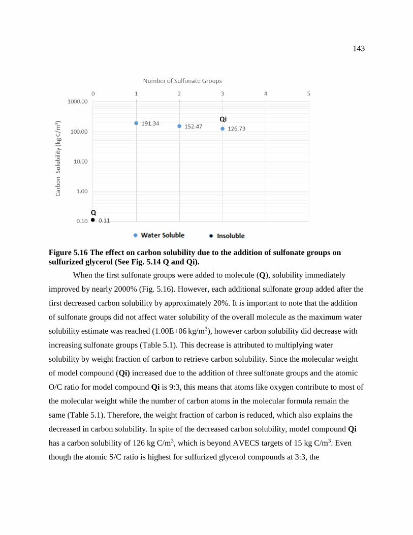
143
Figure 5.16 The effect on carbon solubility due to the addition of sulfonate groups on
sulfurized glycerol (See Fig. 5.14 Q and Qi).
When the first sulfonate groups were added to molecule (Q), solubility immediately
improved by nearly 2000% (Fig. 5.16). However, each additional sulfonate group added after the
first decreased carbon solubility by approximately 20%. It is important to note that the addition
of sulfonate groups did not affect water solubility of the overall molecule as the maximum water
solubility estimate was reached (1.00E+06 kg/m3), however carbon solubility did decrease with
increasing sulfonate groups (Table 5.1). This decrease is attributed to multiplying water
solubility by weight fraction of carbon to retrieve carbon solubility. Since the molecular weight
of model compound (Qi) increased due to the addition of three sulfonate groups and the atomic
O/C ratio for model compound Qi is 9:3, this means that atoms like oxygen contribute to most of
the molecular weight while the number of carbon atoms in the molecular formula remain the
same (Table 5.1). Therefore, the weight fraction of carbon is reduced, which also explains the
decreased in carbon solubility. In spite of the decreased carbon solubility, model compound Qi
has a carbon solubility of 126 kg C/m3, which is beyond AVECS targets of 15 kg C/m3. Even
though the atomic S/C ratio is highest for sulfurized glycerol compounds at 3:3, the

144
biodegradation rank is 3.14, which indicates that such compounds will degrade in weeks to
months.
In summary, sulfurization and oxidation of glycerol compounds meets carbon solubility
targets for AVECS, but not biodegradation resistance. Furthermore, the reactivity of hydroxyl
groups with sulfur is uncertain as discussed in Experiment 2 (Schouten et al., 1993b) .
Furthermore, the addition of sulfonate groups may increase water solubility, but not carbon
solubility, for model compounds like sulfurized glycerol. This means that the optimum carbon
solubility is reached when there is only one sulfonate group in sulfurized glycerol (Q).
Increasing oxidation any further results in less efficient carbon storage.
5.3.5 Experiment 5 – Sulfurization and Oxidation of Hydrocarbons
The ideal AVECS molecule should not only have a carbon solubility of at least 15 kg
C/m3, but also possess as many carbon atoms as possible, such as a fullerene molecule (Fig.
5.17) that is also known as carbon buckyball (C60), as it would improve the effectiveness of
carbon subsurface storage. To construct the ideal AVECS molecule with optimal balance of
carbon solubility and rich carbon content, long C30H62 (Fig. 5.19 R) and C60H122 hydrocarbon
chains (Fig. 5.20 V) were conceptually modified to further achieve other desired characteristics
of an AVECS molecule. However, it was difficult to apply modifications on the fullerene
molecule (using ChemAxon software) due to constrained 2D view of the molecule. Hence,
hydrocarbon chains were selected instead for modification experiments.
Similar to the sulfur incorporation study into long hydrocarbon chains (Fig. 5.18) by
Sinninghe Damsté et al. (1989), thiolanes were incorporated for molecule modification
experiments along the C30 hydrocarbon chain to increase biodegradation resistance (Fig. 5.19 U
and Fig. 5.20 X).

145
Figure 5.17 A fullerene molecule (C60) that is also informally known as the carbon
buckyball. The fullerene molecule could be a potential model compound for the ideal
AVECS molecule.
Figure 5.18 Sulfur incorporation into tri-unsaturated C37 hydrocarbon. After Sinninghe
Damsté et al. (1989).

146
Figure 5.19 Sulfurization and oxidation of C30 hydrocarbon chains. (R) C30H62. Conceptual
sulfur incorporation form thiolanes (S, T, and U). Oxidation of sulfurized C30
hydrocarbons form sulfoxide groups (Si, Ti, and Ui).
Figure 5.20 Sulfurization and oxidation of C60 hydrocarbon chains. (V) C30H62. Conceptual
sulfur incorporation form thiolanes (W and X). Oxidation of sulfurized C30 hydrocarbons
form sulfoxide groups (Wi and Xi).
Since hydrocarbons chains (Table 5.1 R and V) are very insoluble to begin with, adding
thiolanes across the chains did not affect the structures’ carbon solubility in water. Despite the
differences in thiolane additions, molecules (R and U) and (V and X) all have similar carbon
solubility values (Table 5.1).
From experiments 1 and 3, it was observed that the addition of sulfoxide to thiolane
contributed to the most improvement in carbon solubility, therefore thiolane-1-oxides were
added to the hydrocarbon chains to examine how it affected solubility.

147
Figure 5.21 The effect of number of thiolane-1-oxide groups on the carbon solubility in
water for (a) C30H62 and (b) C60H122. Green horizontal line delimits AVECS target water
solubility (> 15 kg C/m3).
In Fig. 5.21a, each additional thiolane-1-oxide added to the C30H62 hydrocarbon chain gradually
increased carbon solubility from 3.60*10-10 kg C/m3 up to a maximum of 121 kg C/m3 with six
thiolane-1-oxides (Fig. 5.19 Ui). On the other hand in Fig. 5.21b, the addition of thiolane-1-oxide
gradually increases solubility until the eighth group is added after which a sharper increase in
solubility is observed. Furthermore, molecule Xi, the C60 hydrocarbon chain with 12 thio-1-
oxides (Fig. 5.20), had an estimated carbon solubility of 17.81 kg C/m3, which meets AVECS
148
targets. In addition, the estimated biodegradation rank of molecule Xi is 0.11 (Table 5.1), which
also meets AVECS targets, as values under one indicate that the molecule has high recalcitrance.
5.3.6 Experiment 6 – The Biodegradation Rate of Oxidized OSC
Several factors affect the biodegradation rate of compounds including aromaticity, high
molecular weight, alkylation and functional groups. Essentially, any chemical characteristic that
makes the molecule more structurally complex will increase the time it takes for the compound
to biodegrade because microorganisms will take longer to transform parent compounds to
metabolites. In the experiments above, EPI suite showed high solubility for oxidized sulfurized
compounds. For this experiment, the biodegradation rate for oxidized sulfur compounds (with
highest carbon solubility) from each experiment was estimated using BIOWIN software (Fig.
5.22). This experiment narrows down the model compounds which have potential to form the
ideal AVECS molecule which is both water soluble and resistant to biodegradation.

149
Figure 5.22 Sulfurized and oxidized model compounds (from each experiment) with the
greatest carbon solubility. Lipids (Ei), carbohydrates (Hi), isoprenoids (Mi), glycerol (Qi),
hydrocarbon derived chains (Ui and Xi).

150
Figure 5.23 Biodegradation rate of oxidized OSC (Ei, Hi, Mi, Qi, Ui, Xi). See figure 5.22 for
structures. Red data points are recalcitrant. Yellow indicates biodegradation will take
weeks to months, and green indicates biodegradation will take weeks (EPA, 2011).
Usually, organic molecules which are water-soluble are typically easily biodegradable.
In Fig. 5.23, the glycerol model compound Qi (Fig. 5.22) follows this assumption as it has high
carbon solubility and high biodegradation rank (>3.25). On the other hand, the carbohydrate
model compound Hi (Fig. 5.22) shows a different pattern where it has low carbon solubility, but
relatively high biodegradation rank. In contrast, the data point that stands out is the hydrocarbon
derived model compound Ui (Fig. 5.22), which exhibits high carbon solubility (121 kg C/m3)
and is recalcitrant (biodegradation rate = 1.65). The characteristics of model compound Ui meets
AVECS targets.
In Fig. 5.23, the biodegradation rate of each model compound was calculated based on
the sum of the molecule weight parameter and an equation constant. However, the BIOWIN
software does not account for significant fragments, such as the thiolane-1-oxides, that are within
the molecule (Table 5.3). Because these structural features are not considered in this software,
the estimated biodegradation rate may not be reliable as the biodegradation rate of a molecule
may be over- or under-estimated.
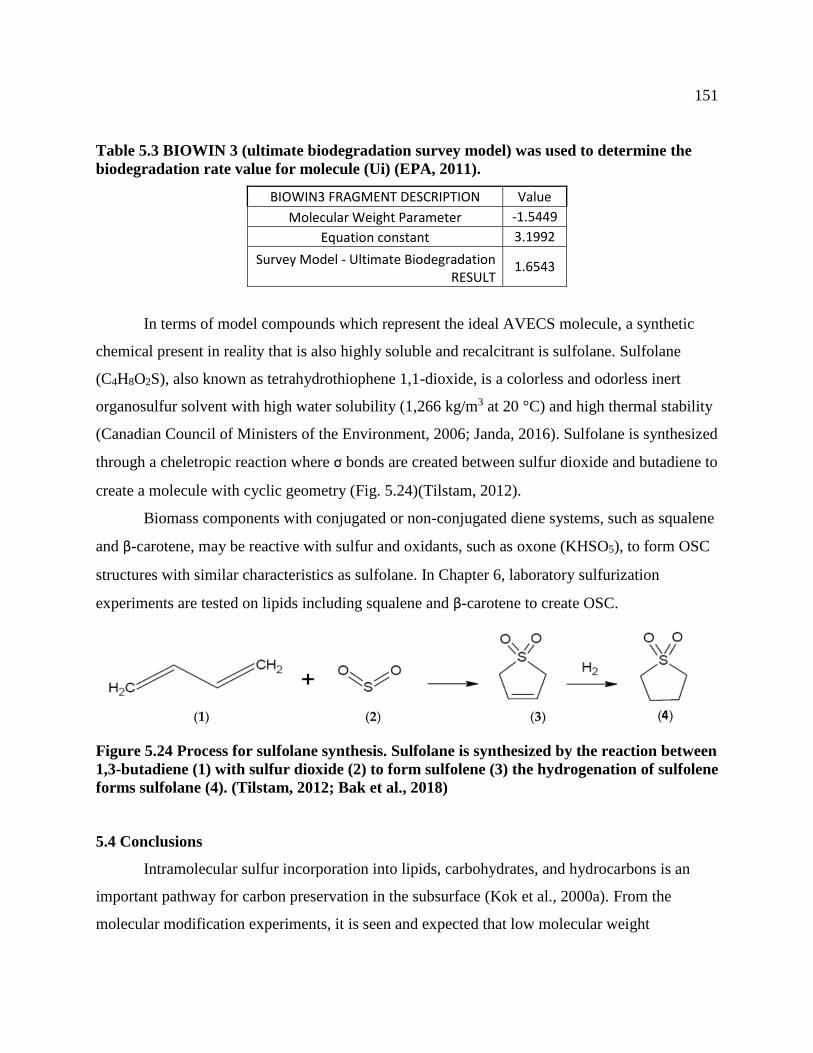
151
Table 5.3 BIOWIN 3 (ultimate biodegradation survey model) was used to determine the
biodegradation rate value for molecule (Ui) (EPA, 2011).
BIOWIN3 FRAGMENT DESCRIPTION Value
Molecular Weight Parameter -1.5449
Equation constant 3.1992
Survey Model - Ultimate Biodegradation RESULT
1.6543
In terms of model compounds which represent the ideal AVECS molecule, a synthetic
chemical present in reality that is also highly soluble and recalcitrant is sulfolane. Sulfolane
(C4H8O2S), also known as tetrahydrothiophene 1,1-dioxide, is a colorless and odorless inert
organosulfur solvent with high water solubility (1,266 kg/m3 at 20 °C) and high thermal stability
(Canadian Council of Ministers of the Environment, 2006; Janda, 2016). Sulfolane is synthesized
through a cheletropic reaction where σ bonds are created between sulfur dioxide and butadiene to
create a molecule with cyclic geometry (Fig. 5.24)(Tilstam, 2012).
Biomass components with conjugated or non-conjugated diene systems, such as squalene
and β-carotene, may be reactive with sulfur and oxidants, such as oxone (KHSO5), to form OSC
structures with similar characteristics as sulfolane. In Chapter 6, laboratory sulfurization
experiments are tested on lipids including squalene and β-carotene to create OSC.
Figure 5.24 Process for sulfolane synthesis. Sulfolane is synthesized by the reaction between
1,3-butadiene (1) with sulfur dioxide (2) to form sulfolene (3) the hydrogenation of sulfolene
forms sulfolane (4). (Tilstam, 2012; Bak et al., 2018)
5.4 Conclusions
Intramolecular sulfur incorporation into lipids, carbohydrates, and hydrocarbons is an
important pathway for carbon preservation in the subsurface (Kok et al., 2000a). From the
molecular modification experiments, it is seen and expected that low molecular weight

152
compounds have high water solubility while high molecular weight compounds exhibit low
solubility. What was unexpected was increased oxidation, oftentimes, reduced carbon solubility.
For example, derivatives of lipids with sulfone functionalities (Bii, Fig. 5.2) showed less
improvement in carbon solubility compared to lipid derivatives with sulfoxide functionalities
molecules (Bi, Fig. 5.2). The solubility-improving sulfoxide group was further modified to
thiolane-1-oxides and incorporated into long hydrocarbon chains (in Experiment 5), which
increased water solubility by several orders of magnitude. Although the modification
experiments showed sulfurized and oxidized model compounds with improved water solubility
and biodegradation resistance, the estimated values and results may not be accurate. As a result
of the lack of fragments and functional groups in the BIOWIN and WATERNT training set
coefficient database, water solubility and biodegradation rate predictions may be under or over-
estimated (U.S. Environmental Protection Agency, 2000) (See appendix A1 and A2 for chemical
fragments database).
The recommendations for types of compounds which are more likely to possess AVECS
molecule qualities (carbon solubility of 15 kg C/m3 and biodegradation rank below 1) are model
compounds which consist of many hydrocarbon atoms and double bond functionalities, as
double bonds are observed to be reactive sites for sulfur incorporation to form thiolane or
thiophene structures, which increases the overall biodegradation resistance of the molecule.
Organic compounds which are rich in carbon and is comprised of diene systems are terpenoids,
such as carotenoids (C40), which are commonly sourced from plants. Furthermore, sulfoxide and
sulfone functional groups are effective at improving water solubility of model compounds.

153
Chapter Six: Sulfurization of Organic Molecules
6.1 Introduction
Several research studies have attempted to simulate natural sulfurization reactions on
sedimentary organic species such as phytol, monosaccharides and octanal in laboratory
conditions (De Graaf et al., 1992; Schouten et al., 1993a; Van Dongen et al., 2003b).
In this chapter, lipids (β-carotene, cholestane, linolenic acid, and squalene) undergo three
separate laboratory sulfurization experiments with elemental sulfur (S8), sodium sulfite
(Na2SO3), sodium hydrosulfide (NaHS), and dimethylformamide (DMF) as reagents. In addition,
carbohydrate sulfurization (using glucose, starch and sucrose) was attempted for a duration of 30
days at 50 °C, but sulfurized material was not observed. Sulfurized lipids yielded products with
up to 7 sulfur atoms within their structure. FTICR-MS was mainly used to analyze the sulfurized
products as the sulfurized lipids were not GC amenable and formed unresolved complex
mixtures (UCM). Laboratory sulfurization experiments on organic molecules advances towards
AVECS goals of altering residual carbon-rich biomass for permanent sequestration in the
subsurface by sulfur incorporation into lipids to produce biologically refractory species from
biomass.
6.2 Experimental Methods
6.2.1 Lipid Sulfurization Reactions
Lipids (Table 6.1) underwent three separate laboratory sulfurization experiments: (1) 5
days at ambient temperatures, (2) 30 days at ambient temperatures and (3) 30 days at 50 °C (Fig.
6.1) using elemental sulfur (S8), sodium sulfite (Na2SO3), sodium hydrosulfide (NaHS), and
N,N-dimethylformamide (DMF) to sulfurize the reactants. Reactants (Table 6.2) were purchased
from Prochem, Sigma Aldrich and TCI Chemicals. Lipid sulfurization reactions followed
methods by De Graaf et al. (1992) and Schouten et al. (1994). The model lipid compound,
elemental sulfur and anhydrous sodium hydrosulfide were transferred into a round bottom flask
following a molar ratio of 1:10:25 respectively. Reactants were dissolved in 25 mL of N,N-
dimethylformamide. For the heated sulfurization experiment, which lasted for 30 days, the
mixture was heated to 50 °C and stirred at 1000 rpm for 30 consecutive days. Aluminum foil was
wrapped around each flask to ensure minimal light exposure. After 30 days, a solution of water

154
and sodium sulfite was added to quench the reaction. The sulfurized lipid compounds were
separated from the aqueous phase using hexane and liquid-liquid extraction (Fig. 6.2). The
extraction was repeated three times before hexane was evaporated with a rotavapor to
concentrate the products.
Table 6.1 Model compounds selected for lipid sulfurization experiments.
Model
Compound Purity Molecular
Formula β-Carotene ≥97.0% C
40H
56
5α –
Cholestane
– 2,2,4,4-d4
≥99% C27
H48
Linolenic
acid >70.0% C
18H
30O
2
Squalene >98.0% C30
H50
Table 6.2 All reactants and corresponding molar ratios and amounts used in the lipid
sulfurization experiments. Molar ratios and choice of reagents followed methods by De
Graaf et al. (1992) and Schouten et al. (1993).
Reactants Molar Ratio
(mmol) Amount
Model Compounds
β-Carotene
1
0.537 g
Cholestane 0.387 g
Linolenic acid 0.278 g
Squalene 0.411 g
Reagents
Elemental sulfur 25 0.80 g
Na2SO3 19.8 2.5 g
NaHS 10 0.56 g
N,N-Dimethylformamide 323 25 mL

155
Figure 6.1 Analytical scheme of lipid sulfurization experiments
Figure 6.2 Liquid-liquid extraction on sulfurized β-carotene reaction mixtures.
6.2.2 Carbohydrate Sulfurization Attempts
Carbohydrate sulfurization experiments followed closely to the experimental methods
described by Kok et al. (2000). In this study, 0.0011 mol of each carbohydrate compound (200
mg glucose, 376.5 mg sucrose, 376.5 mg starch) was dissolved in 6 ml of deionized water, then

156
combined with 560 mg of NaHS and 16 mg of elemental sulfur. The mixture was heated to 50 °C
and stirred at 800 rpm for 30 days. After the reaction, elemental sulfur was removed from the
extracts by adding small amounts of cleaned activated copper flakes (Sigma-Aldrich) into the
mixture (Fig. 6.3). The mixture was magnetically stirred for 24 hours. All added copper
converted to copper sulfide, which formed due to presence of sulfides. A 50:50 mixture of
MeOH and DCM was used to dissolve the sulfurized starch mixture, then copper flakes were
filtered from sample mixture using 20-25 μm pore size Whatman filter paper and deionized
water. Afterwards, 146 mm Pasteur pipettes were plugged with glass wool and filled two-thirds
full with granular copper (20-30 mesh) from J.T. Baker. The sulfurized mixtures were pipetted
into the copper columns until the mixture showed no reaction with copper (Fig. 6.4). Two
copper-filled columns were needed to extract excess elemental sulfur from each sample.
Following filtration steps, the samples were freeze dried 3 days and formed solid powder
material (Fig. 6.5).
Figure 6.3 (a) Carbohydrate sulfurization experimental set up. (b) Addition of pure copper
flakes to remove excess elemental sulfur. Copper turns black (copper sulfide)
instantaneously. (c). After 24 hours of stirring, the entire solution appears black.

157
Figure 6.4 (a) Pasteur pipette filled with pure copper granules and glass wool. (b) Copper
turns black after eluting sulfurized sample through the column.
Figure 6.5 (a) Sulfurized carbohydrates in freeze-dryer after removing excess sulfur (b)
Freeze dried sulfurized carbohydrates. From the left: sucrose, glucose, starch and blank.
6.3 Analytical Methods
6.3.1 Freeze-Dry
Sulfurized carbohydrates were freeze dried using the Freezone Freeze Dryer- Labconco machine
provided by the Energy Bioengineering and Geomicrobiology group at the University of
Calgary, Calgary Canada.
6.3.2 FTICR-MS Analysis
The sulfurized lipid and carbohydrate samples were analyzed with a 12 T Bruker SolariX
mass spectrometer in atmospheric pressure photoionization positive ion (APPI-P) mode. The
APPI-P ionization technique efficiently ionizes polar and non-polar species, structurally diverse

158
compounds and sulfur compounds in complex organic mixtures without the use of chemical
derivatization nor special sample preparation strategies (Purcell et al., 2007; Oldenburg et al.,
2014). See FTICR-MS methods in Chapter 3 for more instrument details. Furthermore,
monoisotopic peak intensities, displayed in the figures below, do not reflect the actual abundance
of compounds present in the sample. As well, the chemical structures and molecular formulas
assigned to sulfur-containing lipid peaks are speculative, as FTICR-MS software utilizes
absolute mass accuracy and isotopic patterns to compute a molecular formula to each
investigated peak. In addition, peaks which are left unassigned with a molecular formula do not
contain sulfur and are not discussed further.
6.3.3 ChemAxon
ChemAxon was used to draw possible chemical structures of sulfurized lipids based on the
computed molecular formula assigned to the peak of interest.
6.4 Results
6.4.1 Experiment 1: Lipid Sulfurization for 5 days
Minimal sulfurization occurred with squalene (C30H50) and formed sulfurized squalene (C30H52S)
(Fig. 6.6 and Fig. 6.7) (Table 6.3). Sulfurization was not observed in other lipids.

159
Figure 6.6 FTICR-MS mass spectrum showing peak intensity, mass to charge (m/z) ion and
molecular formula. Sulfurization of squalene (C30H52S) was detected in experiment #1
(lipid sulfurization for 5 days).
Figure 6.7 Possible organic sulfur compound structure with molecular formula C30H52S.
Sulfurization of squalene in experiment #1 (lipid sulfurization for 5 days) may have formed
one thiolane intramolecularly.
6.4.2 Experiment 2: Lipid Sulfurization for 30 days
Increased sulfurization occurred in squalene (see Fig. 6.9 for potential OSC structure of
C30H54S2), but other lipids do not exhibit sulfurization (Fig. 6.8) (Table 6.3).
Figure 6.8 FTICR-MS mass spectrum showing peak intensity, mass to charge (m/z) ion and
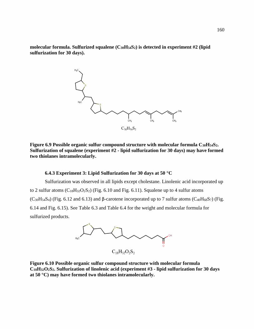
160
molecular formula. Sulfurized squalene (C30H54S2) is detected in experiment #2 (lipid
sulfurization for 30 days).
Figure 6.9 Possible organic sulfur compound structure with molecular formula C30H54S2.
Sulfurization of squalene (experiment #2 - lipid sulfurization for 30 days) may have formed
two thiolanes intramolecularly.
6.4.3 Experiment 3: Lipid Sulfurization for 30 days at 50 °C
Sulfurization was observed in all lipids except cholestane. Linolenic acid incorporated up
to 2 sulfur atoms (C18H32O2S2) (Fig. 6.10 and Fig. 6.11). Squalene up to 4 sulfur atoms
(C30H54S4) (Fig. 6.12 and 6.13) and β-carotene incorporated up to 7 sulfur atoms (C40H68S7) (Fig.
6.14 and Fig. 6.15). See Table 6.3 and Table 6.4 for the weight and molecular formula for
sulfurized products.
Figure 6.10 Possible organic sulfur compound structure with molecular formula
C18H32O2S2. Sulfurization of linolenic acid (experiment #3 - lipid sulfurization for 30 days
at 50 °C) may have formed two thiolanes intramolecularly.

161
Figure 6.11 FTICR-MS mass spectrum showing peak intensity, mass to charge (m/z) ion
and molecular formula. Sulfurized linolenic acid (C18H32O2S2) is detected in experiment #3
(lipid sulfurization for 30 days at 50 °C).
Figure 6.12 Possible organic sulfur compound structure with molecular formula C30H54S4.
Sulfurization of squalene (experiment #3 - lipid sulfurization for 30 days at 50 °C) may
have formed four thiolanes intramolecularly.

162
Figure 6.13 FTICR-MS mass spectrum showing peak intensity, mass to charge (m/z) ion
and molecular formula. Sulfurized squalene (C30H54S4) is detected in experiment #3 (lipid
sulfurization for 30 days at 50 °C).

163
Figure 6.14 FTICR-MS mass spectrum showing peak intensity, mass to charge (m/z) ion
and computed ion formula. Sulfurized β-carotene (C40H68S7) is detected in experiment #3
(lipid sulfurization for 30 days at 50 °C).
Figure 6.15 Possible organic sulfur compound structure with molecular formula C40H68S7.
Sulfurization of β-carotene (experiment #3 - lipid sulfurization for 30 days at 50 °C) may
have formed four thianes and 3 thiolanes intramolecularly.
Table 6.3 Reactants and sulfurized products from each experiment and the corresponding
measured mass to charge (m/z) and ion formulae as indicated in FTICR-MS plots.
Reactant/ Products Measured m/z Ion Formula
Experiment 1 Squalene 410.3904 C30H50
Sulfurized Squalene 444.3781 C30H52S
Experiment 2 Squalene 410.3903 C30H50
Sulfurized Squalene 444.3779 C30H52S 478.3656 C30H54S2
Experiment 3
Linolenic Acid 278.224 C18H30O2
Sulfurized Linolenic
Acid
312.2117 C18H32O2S 314.2273 C18H34O2S 344.1837 C18H32O2S2
Squalene 410.3903 C30H50
Sulfurized Squalene
444.3779 C30H52S 478.3656 C30H54S2 510.3375 C30H54S3 544.3257 C30H54S4
β-Carotene 536.4373 C40H56 570.425 C40H58S

164
Sulfurized β-
Carotene
604.4127 C40H60S2 638.4004 C40H62S3 672.388 C40H64S4
706.3757 C40H66S5 740.3633 C40H68S6 772.3353 C40H68S7
Table 6.4 Organic sulfur compound products from the reaction of squalene, linolenic acid
and β-Carotene with elemental sulfur and NaHS in DMF under different lipid sulfurization
conditions. Weights of sulfurized products were measured after liquid-liquid and
rotavapor solvent extraction.
Conditions Reaction Products
Total Weight of Products (mg)
Experiment 1 Ambient
temperatures/ 5 days
Sulfurized Squalene 79.2
Experiment 2 Ambient
temperatures/ 30 days
Sulfurized Squalene 72.8
Experiment 3 50 °C / 30 days
Sulfurized Linolenic Acid 40.2
Sulfurized Squalene 233
Sulfurized β-Carotene 74.9

165
6.4.4 Experiment 4: Carbohydrate Sulfurization for 30 days at 50 °C
Sulfurized carbohydrate products were not detected through FTICR-MS analysis.
6.5 Discussion
The experiment series which exhibited most sulfurization of the model compounds was
the third lipid sulfurization experiment, which ran for 30 days at 50 °C. In this experiment, three
of the four lipids were sulfurized and incorporated 2 to 7 sulfur atoms within the chemical
structure. In addition, the total weight of products was greatest in experiment 3 (Table 6.4),
which may be indicative that increased temperatures and time duration of experiment allowed for
more product formation due to increased polysulfide interactions with lipids. Based on the
product weights, squalene may be most reactive to sulfurization reactions followed by β-
carotene, linolenic acid, and then cholestane. In Chapter 3, it was hypothesized that squalene, β-
carotene and steroid skeletons such as those related to such as cholestane, formed major amounts
of OSC in sulfur-rich oils. From the results of this experiment, it appears that the double bond
functional groups in squalene (DBE= 6) and β-carotene (DBE = 13), are more prone to
sulfurization with the reagents used, compared to linolenic acid and cholestane. Linolenic acid
also displayed minor levels of sulfurization with the addition of heat. However, it is also likely
due to preferential sulfur incorporation at double bond functionalities since the calculated
molecular formulas in Fig. 6.11, show C18H34O2S and C18H32O2S2, which suggests the carboxyl
functional group was likely not the preferential location for sulfur incorporation as the oxygen
atoms are not replaced with sulfur (Fig. 6.16).
Figure 6.16 (a) Chemical structure of linolenic acid (C18H30O2) compared to possible
sulfurized linolenic acid structures (b) C18H34O2S and (c) C18H32O2S2, which are molecular
formulas extrapolated from the FTICR-MS mass spectrum (Fig. 6.11).
Van Dongen et al.(2003) showed sulfurization of monosaccharides and the importance of
carbonyl functional groups in monosaccharides as reactive sites with carbonyl functionalities
becoming replaced with sulfur. Although, in experiment 4, similar sulfurization procedures such

166
as time duration, temperature and carbohydrate materials followed Van Dongen et al.(2003),
sulfurized products were not observed. Some possibilities which may have contributed to such
results are (1) the process of removing excess sulfur using filter paper and granular copper may
have removed important sulfur compounds, (2) The extraction process may have been inefficient
at recovering highly oxygenated species or (3) structural loss of carbohydrates due to freeze
drying process. Levi and Karel (1995) reported collapsed carbohydrate systems often show poor
rehydration capabilities when time and temperature during the freeze dry process are under sub-
optimal conditions. Poor rehydration was observed in experiment four as freeze dried
carbohydrate samples formed large amounts of precipitate upon rehydration for FTICR-MS
analysis.
6.5.1 Viable products for AVECS processing
Of the lipid sulfurization experiments, the compound which would be most suitable for
AVECS processing is sulfurized β-carotene (C40H68S7) as it has a biodegradation rank of 0.85
estimated by BIOWIN software (See Chapter 5 for more details on BIOWIN), which meets
AVECS goals as a biodegradation rank <1.75 that suggests the compound is recalcitrant (Table
6.5). Furthermore, β-carotene is comprised of many carbon atoms (C40), double bond
functionalities, which are reactive sites for sulfur incorporation hence the incorporation of seven
sulfur atoms within the structure (C40H68S7), and carotenoids are abundant in nature and are
commonly found in bacteria, molds and algae (Bogacz-Radomska and Harasym, 2018). In
addition, industrial bioresidues and waste agricultural products are rich in carotenoids as many
animals (waste water, crustacean shells and fish scales) and vegetables (peels and seeds) are
sources of carotenes and xanthophylls (Martins and Ferreira, 2017). Inexpensive and abundant
sources of carbon-rich biomass waste material with double bond functionalities like carotenoids
are feasible sources for future AVECS processing. However, the estimated solubility of
sulfurized β-carotene (C40H68S7) is low (Table 6.5), but future oxidation experiments may
increase solubility of sulfurized compounds to meet AVECS targets of 15 kg C/m3.

167
Table 6.5 The molecular formula, biodegradation rank and estimated water solubility of
lipid compounds (squalene, linolenic acid, B-carotene) and the sulfurized forms produced
from lipid experiment #3 (highlighted in yellow). The degradation rate for biodegradation
rank values: 3.25 – 5.00 = days to hours, >2.75 - 3.25 = weeks, >2.25 - 2.75 = weeks to
months, >1.75 - 2.25 = months, <1.75 = recalcitrant. The target solubility for AVECS
molecules is 15 kg C/ m3 and the target biodegradation rank is <1.75.
6.6 Conclusions
Increasing temperatures from ambient temperatures to 50 °C and increasing the time
duration of experiments improved sulfurization of lipids. Squalene was most reactive to
sulfurization experiments as squalene was sulfurized in each attempted experiment, but
sulfurized squalene (C30H54S4) does not meet biodegradation rank targets for future AVECS
processing. However, organic species with similar characteristics as carotenoids may be viable
model compounds for future AVECS processing to create organic sulfur bearing species for
carbon storage, as sulfurized β-Carotene (C40H68S7) is estimated to be recalcitrant to
biodegradation. Furthermore, a desirable structural characteristic in AVECS molecules are
conjugated double bond systems, as such sites are most reactive to sulfur incorporation compared
to carboxyl, carbonyls and hydroxide functional groups. Following similar sulfurization
conditions as lipid sulfurization experiments did not result in FTICR-MS detection of sulfurized
carbohydrate products.
Model Compounds Molecular Formula
Biodegradation Rank
Water Solubility
(mg/L)
Squalene C30H50 2.29 4.10E-07
Sulfurized Squalene C30H54S4 1.99 5.43E-07
Linolenic Acid C18H30O2 3.24 0.099
Sulfurized Linolenic Acid C18H32O2S2 2.8 0.05175
B-Carotene C40H56 1.58 5.37E-07
Sulfurized β-Carotene C40H68S7 0.85 7.73E-07

168
Chapter 7 Conclusions and Future Work
Net zero CO2 emissions must be achieved in less than 15 years to remain 1.5 °C of
warming below pre-industrial levels (Rogelj et al., 2018). This means globally deployable
technologies which have potential to permanently remove CO2 from the atmosphere or achieve
negative emissions are needed urgently to limit catastrophic environmental and societal
consequences caused by climate change. This thesis addressed the research question of whether
it is possible to utilize sulfurized residual biomass waste material as a form of carbon
sequestration. To answer this question, initial stages of AVECS technology was designed and
developed to understand the future prospective of using such route as an alternative carbon
sequestration method. AVECS technology uses molecules derived from biomass and
sulfurization reactions involving elemental sulfur and polysulfides to create biologically
refractory and water-soluble organic sulfur species for subsurface carbon storage.
The approach to developing AVECS technology was to first explore the geochemical
sulfur cycle and recognize how natural sulfurization processes occur in sedimentary organic
matter. Then, sulfur-rich oils were analyzed with the GC-MS and FTICR-MS to determine the
structural composition of sulfurized organic compounds in crude oils and the lab conditions that
facilitate sulfurization of organic matter. The results from the analysis of Rozel Point and
Jianghan Basin oils showed extensive intramolecular sulfur incorporation, as up to five sulfur
atoms were discovered within molecules. These sulfurized molecules were also dominated by
species comprised of carbon numbers C20, C30 and C40 with double bond equivalent values of 5,
7, 9 and 13. Possible organic sulfur compound structures that match these results include
sulfurized steranes, hopanes and carotenoids. As for the conditions which facilitate sulfur
incorporation and preservation reactions and processes in organic matter, include anoxic
hypersaline environments, low thermal maturity, organic matter input from organisms which are
rich in steroids, hopanoids and carotenoids, and low to moderate biodegradation exposure.
The method development process for separating sulfur compound-rich oils into various
fractions using liquid chromatography on silver nitrate impregnated silica gel was revised, and
the method was effective at separating aromatic and non-aromatic sulfur compounds in crude oil
with less than 4 wt% S. The different biodegradation resistant sulfur compounds which were

169
found in heavily to severely biodegraded oil included (1) non-aromatic sulfidic compounds with
one to three sulfur atoms such as thiolanes and sulfides, and (2) aromatic sulfur compounds with
one to five sulfur atoms such as thiophenes and dibenzothiophenes. These biodegradation
resistant sulfur compounds can be used as model systems, to test future studies on oxidation
reactions and serve as AVECS targets for compounds that could form biologically refractory
sulfur-containing species through reaction of elemental sulfur sources with various biomass
precursors (agricultural waste). In future work, it would be possible to further modify the
technique to deal with more polar and sulfur enriched oils. In addition to S1 (saturated
hydrocarbons), S2 (aromatic sulfur compounds), and S3 (non-aromatic sulfur compounds)
fractions, future work should include investigation of eluting a S4 (mercaptans) fraction.
Modelled solubility and biodegradation resistance estimations were evaluated for various
model compounds including aromatic thiophenic compounds, sulfidic compounds, and
mercaptan compounds which were derived from biodegraded sulfur-rich oils. Using computer
modelling software, the results showed low molecular weight compounds have high water
solubility, while high molecular weight compounds exhibited low solubility. Moreover,
incorporating sulfinyl or sulfonyl functionality into organic structures showed increased
biodegradation recalcitrance as well as improvement in water solubility. The recommendations
for types of compounds which are more likely to possess AVECS molecule qualities (carbon
solubility of 15 kg C/m3 and biodegradation rank below 1) are model compounds which are
enriched in carbon atoms and consist of many double bond functionalities. Double bonds are
observed to be the most reactive sites for sulfur incorporation to form thiolane or thiophene
structures. These structures increase the overall biodegradation resistance of the molecule.
Organic compounds which are enriched in carbon and have diene double bond systems include
terpenoids, such as carotenoids (C40), which are commonly sourced from plants.
Laboratory sulfurization experiments were conducted on lipid molecules at 50 °C for a
time duration of 30 days. The sulfurized products included sulfur incorporation of up to two
sulfur atoms in linolenic acid, five sulfur atoms in squalene and seven atoms in β-carotene. The
outcomes from the lipid sulfurization experiments are: (1) organic species with similar
characteristics as carotenoids may be the most viable for future AVECS processing, as sulfurized

170
β-Carotene (C40H68S7) is estimated to be recalcitrant to biodegradation through computer
modelling software. Furthermore, a desirable structural characteristic in compounds for AVECS
processing are conjugated double bond systems, as such sites are most reactive to sulfur
incorporation compared to carboxyl, carbonyls and hydroxide functional groups.
In summary, the work in this thesis has contributed new insights in the prospects of
utilizing organic sulfur bearing species as a carbon sequestration method. Key findings which are
important for further advancements in AVECS technology include:
(1) Organic sulfur compounds extracted from biodegraded sulfur-rich oils appear to have
precursor characteristics which resemble sulfurized steroids, hopanoids and carotenoids. It is
hypothesized that such precursor chemicals are receptive to natural sulfurization due to
abundance of reactive chemical sites, such as double bond functionalities. For future AVECS
processing, model compounds with characteristics that resemble OSC found in biodegraded
oils may be more reactive to sulfurization reactions and serve as possible carbon storage
vectors. Intramolecular sulfur incorporation at double bonds typically form thiolane or
thiophene structures.
(2) The revised liquid chromatography on silver nitrate impregnated silica gel method is
effective at separating sulfur rich oils (< 4wt%) into non-aromatic and aromatic sulfur
compound fractions. These fractions could be used to test effectiveness of future oxidation
reactions.
(3) Computer modelling estimations on various model compounds showed sulfinyl and sulfonyl
functionalities were most effective at increasing both aerobic biodegradation recalcitrance
and water solubility of organic compounds.
(4) Lipid sulfurization experiments at increased temperatures and time durations showed that
squalene and β-carotene incorporated most sulfur atoms compared to the other lipids in the
sample set. The diene double bond systems within the terpenoids likely contributed a strong
role in successful intramolecular sulfur incorporation.
(5) From the results of the lipid sulfurization experiments, terpenoids with double bond systems
may be viable for future AVECS processing. Terpenoids, such as β-carotene, are commonly

171
sourced from plants and are abundant in biomass waste materials such as fruit peels and
seeds.
AVECS has potential to flourish as a carbon sequestration technology as it utilizes
biomass waste material as a carbon source and sulfurization reactions which helps the global
sulfur surplus dilemma. In addition, AVECS molecules will be stored in shallow, saline and
contaminated aquifers which are geographically abundant and have no economic value. The
results from this research study illustrates that organic compounds with double bond systems,
such as terpenoids, can be sulfurized to increase the overall biodegradation resistance of the
organic compound, however this raises a question—what will occur if AVECS molecules
biodegraded? If sulfurized organic compounds are biodegraded, it would release CO2 in the
storage site or shallow saline aquifer. It would be worthwhile to investigate rates of release to see
if AVECS species can be safely stored in shallow aquifer settings on say a 1000 year timescale.
Future work for further advancements in the AVECS project includes:
(1) Explore other approaches to reduce energy input and time duration for conducting
sulfurization experiments as these reductions will positively impact the overall cost.
(2) Test oxidation reactions to convert S into SOx functional groups to increase water-solubility
of organic sulfur compounds. Possible oxidations reactions could include potassium
peroxymonosulfate (oxone) as it is an oxidizing agent that converts sulfides to sulfoxides or
sulfones (Trost and Curran, 1981).
(3) Biodegradation tests (See Appendix A8), established by AVECS summer students through
dissolved organic carbon (DOC) measurements, can be applied to potential sulfurized and
oxidized organic compounds.
(4) Sulfolane degradation tests using biotic and abiotic strategies (see Appendix A9) can be used
to test the recalcitrance of AVECS molecules in natural settings, as sulfolane is a synthetic
chemical that represents the ideal AVECS molecule (highly soluble and recalcitrant).
Therefore, AVECS molecules should have a similar response to sulfolane degradation tests
in nature.

172
(5) Lastly, life cycle assessment on the feasibility of AVECS routes for negative emission
technologies and potential carbon storage in shallow, saline, contaminated aquifers are also
important future steps in this research study.

173
References
Adam, P., Schmid, J.C., Mycke, B., Strazielle, C., Connan, J., Huc, A., Riva, A., Albrecht, P.,
1993. Structural investigation of nonpolar sulphur cross-linked macromolecules in petroleum.
Geochimica et Cosmochimica Acta 57, 3395–3419.
Adams, J., Larter, S., Bennett, B., Huang, H., 2012. Oil charge migration in the Peace River Oil
Sands and surrounding region. GeoConvention 2012: Vision 1–7.
Adams, J., Larter, S., Bennett, B., Huang, H., Westrich, J., van Kruisdijk, C., 2013. The dynamic
interplay of oil mixing, charge timing, and biodegradation in forming the Alberta Oil Sands:
Insights from geologic modeling and biogeochemistry. Heavy-oil and Oil-sand Petroleum
Systems in Alberta and Beyond 23–102.
AER, 2017. Table of Formations. Alberta Geological Survey. URL
https://ags.aer.ca/activities/table-of-formation.htm (accessed 5.5.19).
AER, Alberta Energy Regulator, 2017. Industrial Minerals and Stones: Sulfur. Retrieved from:
ags.aer.ca/activities/industrial-minerals-and-stones.htm
AER, Alberta Energy Regulator, 2018. ST98: 2018 Alberta’s Energy Reserves &
Supply/Demand Outlook.
Aizenshtat, Z., Krein, E.B., Vairavamurthy, M.A., Goldstein, T.P., 1995. Role of sulfur in the
transformations of sedimentary organic matter: A mechanistic overview. Geochemical
Transformations of Sedimentary Sulfur 612, 16–37.
Allan, J., Creaney, S., 1991. Oil families of the Western Canada Basin. Bulletin of Canadian
Petroleum Geology 39, 107–122.
Allen, M.R., Dube, O.P., Solecki, W., Aragón-Durand, F., Cramer, W., Humphreys, S.,
Kainuma, M., Kala, J., Mahowald, N., Mulugetta, Y., Perez, R., Wairiu, M., Zickfeld, K., 2018.
In: Global Warming of 1.5 °C. An IPCC Special Report on the impacts of global warming of
1.5°C above pre-industrial levels and related global greenhouse gas emission pathways, in the
context of strengthening the global response to the threat of climate change, sustainable
development, and efforts to eradicate poverty [Masson-Delmotte, V., P. Zhai, H.-O. Pörtner, D.
Roberts, J. Skea, P.R. Shukla, A. Pirani, W. Moufouma-Okia, C. Péan, R. Pidcock, S. Connors,
J.B.R. Matthews, Y. Chen, X. Zhou, M.I. Gomis, E. Lonnoy, T. Maycock, M. Tignor, and T.
Waterfield (eds.)]. In Press.
Amrani, A., 2014. Organosulfur compounds: Molecular and isotopic evolution from biota to oil
and gas. Annual Review of Earth and Planetary Sciences 42, 733–768.

174
Anderson, S., Filewich, C., Lyster, S., MacCormack, K., 2015. Using a 3-D geological model
and petroleum data analyses to help mitigate environmental impacts of heavy oil and bitumen
production. Petroleum Abstracts 55, 102.
Apodaca, L.E., 2018. 2015 Minerals Yearbook: Sulfur. U.S. Geological Survey, 16.
Apodaca, L.E., 2019. Sulfur, Mineral Commodity Summaries. U.S. Geological Survey, 160 -161
Araujo, L.D., Vannevel, S., Buica, A., Callerot, S., Fedrizzi, B., Kilmartin, P.A., du Toit, W.J.,
2017. Indications of the prominent role of elemental sulfur in the formation of the varietal thiol
3-mercaptohexanol in Sauvignon blanc wine. Food Research International 98, 79–86.
Asgar-Deen, M., Riediger, C., Hall, R., 2004. The Gordondale Member: designation of a new
member in the Fernie Formation to replace the informal “ Nordegg Member ” nomenclature of
the subsurface of west-central Alberta. Bulletin of Canadian Petroleum Geology 52, 201–214.
Aydin, G., Karakurt, I., Aydiner, K., 2010. Evaluation of geologic storage options of CO2:
Applicability, cost, storage capacity and safety. Energy Policy 38, 5072–5080.
Bachu, S., 2015. Review of CO2 storage efficiency in deep saline aquifers. International Journal
of Greenhouse Gas Control 40, 188–202.
Bastow, T.P., van Aarssen, B.G.K., Lang, D., 2007. Rapid small-scale separation of saturate,
aromatic and polar components in petroleum. Organic Geochemistry 38, 1235–1250.
Bennett, B., Fustic, M., Farrimond, P., Huang, H., Larter, S.R., 2006. 25-Norhopanes: Formation
during biodegradation of petroleum in the subsurface. Organic Geochemistry 37, 787–797.
Bertrand, J.-C., Bonin, P., Caumette, P., Gattuso, J.-P., Grégori, G., Guyoneaud, R., Le Roux, X.,
Matheron, R., Poly, F., 2015. Biogeochemical Cycles, in: Bertrand, J.-C., Caumette, P., Lebaron,
P., Matheron, R., Normand, P., Sime-Ngando, T. (Eds.), Environmental Microbiology:
Fundamentals and Applications: Microbial Ecology. Springer Netherlands, Dordrecht, pp. 511–
617.
Bogacz-Radomska, L., Harasym, J., 2018. β-Carotene-properties and production methods. Food
Quality and Safety 2, 69–74.
Bortz, L.C., 1984. Heavy-Oil Deposit, Great Salt Lake, Utah. Denver, Colorado.Reference
incomplete?
Brassell, S.C., Eglinton, G., Sheng, G., Fu, J., 1988a. Biological markers in lacustrine Chinese
oil shales. Lacustrine Petroleum Source Rocks 40, 299–308.

175
Bruant, R.G., Celia, M.A., Guswa, A.J., Peters, C.A., 2002. Safe storage of CO2 in deep saline
aquifers. Environmental Science & Technology 36, 240–245.
Bui, M., Adjiman, C.S., Bardow, A., Anthony, E.J., Boston, A., Brown, S., Fennell, P.S., Fuss,
S., Galindo, A., Hackett, L.A., Hallett, J.P., Herzog, H.J., Jackson, G., Kemper, J., Krevor, S.,
Maitland, G.C., Matuszewski, M., Metcalfe, I.S., Petit, C., Puxty, G., Reimer, J., Reiner, D.M.,
Rubin, E.S., Scott, S.A., Shah, N., Smit, B., Trusler, J.P.M., Webley, P., Wilcox, J., Mac Dowell,
N., 2018. Carbon capture and storage (CCS): The way forward. Energy and Environmental
Science 11, 1062–1176.
Cai, C., Worden, R.H., Wolff, G.A., Bottrell, S., Wang, D., Li, X., 2005. Origin of sulfur rich
oils and H2S in Tertiary lacustrine sections of the Jinxian Sag, Bohai Bay Basin, China. Applied
Geochemistry 20, 1427–1444.
Canfield, D., Kristensen, E., Thamdrup, B., 2005. Aquatic geomicrobiology (Advances in marine
biology). Academic Press, San Diego.
Carr, S.A., Burlingame, A.L., Baldwin, M.A., 2000. The meaning and usage of the terms
monoisotopic mass, average mass, mass resolution, and mass accuracy for measurements of
biomolecules. Mass Spectrometry in Biology & Medicine 553–561.
Carroll, A.R., Bohacs, K.M., 2001. Lake-type controls on petroleum source rock potential in
nonmarine basins. American Association of Petroleum Geologists Bulletin 85, 1033–1053.
Casamayor, E.O., Mas, J., Pedros-Alio, C., 2001. In situ assessment on the physiological state of
purple and green sulfur bacteria through the analyses of pigment and 5S rRNA content.
Microbial Ecology 42, 427–437.
Chandra Srivastava, V., 2012. An evaluation of desulfurization technologies for sulfur removal
from liquid fuels. RSC Advances 2, 759–783.
Chen, J., Bi, Y., Zhang, J., Li, S., 1996. Oil-source correlation in the Fulin Basin, Shengli
petroleum province, East China. Organic Geochemistry 24, 931–940.
Christensen, J.H., Kumar, K.K., Aldrian, E., An, S.-I., Cavalcanti, I.F.A., Castro, M. de, Dong,
W., Goswami, P., Hall, A., Kanyanga, J.K., Kitoh, A., Kossin, J., Lau, N.-C., Renwick, J.,
Stephenson, D.B., Xie, S.-P., T. Zhou, 2013. Climate phenomena and their relevance for future
regional climate change. Climate Change 2013 the Physical Science Basis: Working Group I
Contribution to the Fifth Assessment Report of the Intergovernmental Panel on Climate Change
9781107057, 1217–1308.
Ciereszko, L.S., Youngblood, W.W., 1971. n-Hexadecyl and n-octadecyl disulfides in
“sediment” derived from the Gorgonian Pseudoplexaura parosa (Houttuyn). Geochemica et
Cosmochimica Acta 35, 851–853.

176
Crank, J.P., Jacoby, L.S., 2015. Crime, Violence, and Global Warming. Taylor & Francis, New
York.
De Graaf, W., Sinninghe Damsté, J.S., de Leeuw, J.W., 1992. Laboratory simulation of natural
sulphurization: I. Formation of monomeric and oligomeric isoprenoid polysulphides by low-
temperature reactions of inorganic polysulphides with phytol and phytadienes. Geochimica et
Cosmochimica Acta 56, 4321–4328.
de Menezes, E.W., Benvenutti, E.V., Zini, C.A., Bjerk, T.R., Pereira, M.B., Caramão, E.B.,
2016. Silver bonded to silica gel applied to the separation of polycyclic aromatic sulfur
heterocycles in heavy gas oil. Journal of Chromatography A 1470, 104–110.
Demirbas, A., Alidrisi, H., Balubaid, M.A., 2015. API gravity, sulfur content, and
desulfurization of crude oil. Petroleum Science and Technology 33, 93–101.
Dobrotkova, Z., Lukas, A., Singh, J., 2018. Energy Efficiency in Industry, Energy Efficiency in
Industry. doi:10.4324/9780203216286
Eardley, A.J., 1963. Oil Seeps at Rozel Point.Reference incomplete
Environmental Protection Agency (EPA), 2011. Estimating Physical / Chemical and
Environmental Fate Properties with EPI Suite TM. Sustainable Futures / P2 Framework Manual.
EPA-748-B12-001, 1–22.
EPA, 2013. Climate Change Indicators: Greenhouse Gases.Reference incomplete
Emami-Meybodi, H., 2015. Solubility trapping of carbon dioxide in deep saline aquifers.
Reference incomplete
Fenchel, T., King, G.M., Blackburn, T.H., 2012. Microbial Biogeochemical Cycling and the
Atmosphere, in: Bacterial Biogeochemistry. Academic Press, pp. 183–219.
French, K.L., Rocher, D., Zumberge, J.E., Summons, R.E., 2015. Assessing the distribution of
sedimentary C40 carotenoids through time. Geobiology 13, 139–151.
GESAMP, 2019. High level review of a wide range of proposed marine geoengineering
techniques. GESAMP Reports and Studies 98, 143.
Giles, G., Nasim, M., Ali, W., Jacob, C., 2017. The reactive sulfur species concept: 15 years on.
Antioxidants 6, 38.
Gill, R., 2015. Chemical Fundamentals of Geology and Environmental Geoscience, 3rd ed. John
Wiley & Sons, Incorporated.

177
Gislason, S.R., Broecker, W.S., Gunnlaugsson, E., Snæbjörnsdóttir, S., Mesfin, K.G.,
Alfredsson, H.A., Aradottir, E.S., Sigfusson, B., Gunnarsson, I., Stute, M., Matter, J.M.,
Arnarson, M.T., Galeczka, I.M., Gudbrandsson, S., Stockman, G., Wolff-Boenisch, D.,
Stefansson, A., Ragnheidardottir, E., Flaathen, T., Gysi, A.P., Olssen, J., Didriksen, K., Stipp, S.,
Menez, B., Oelkers, E.H., 2014. Rapid solubility and mineral storage of CO2 in basalt. Energy
Procedia 63, 4561–4574
Gogoi, B.K., Bezbaruah, R.L., 2002. Biotransformations: Bioremediation Technology for Health
and Environmental Protection. Reference incomplete
Goldhaber, M.B., 2005. Sulfur-rich Sediments, in: Sediments, Diagenesis, and Sedimentary
Rocks : Treatise on Geochemistry. Elsevier Science & Technology, pp. 257–288.
Government of Canada, 2019. Sulphur in Gasoline Regulations.
Gvirtzman, Z., Said-Ahmad, W., Ellis, G.S., Hill, R.J., Moldowan, J.M., Wei, Z., Amrani, A.,
2015. Compound-specific sulfur isotope analysis of thiadiamondoids of oils from the
Smackover Formation, USA. Geochimica et Cosmochimica Acta 167, 144–161.
Han, Y., Zhang, Y., Xu, C., Hsu, C.S., 2018. Molecular characterization of sulfur-containing
compounds in petroleum. Fuel 221, 144–158.
Harrison, A.L., Tutolo, B.M., DePaolo, D.J., 2019. The role of reactive transport modeling in
geologic carbon storage. Elements 15, 93–98.
Hauck, T.E., Peterson, J., Melnik, A., Bachu, S., 2012. Geology and hydrogeology of the basal
aquifer in the prairie region of Canada: Characterization for CO2 Storage. GeoConvention 2012
10–11.
Hoegh-Guldberg, O., Jacob, D., Taylor, M., Bindi, M., Brown, S., Camilloni, I., Diedhiou, A.,
Djalante, R., Ebi, K.L., Engelbrecht, F., Guiot, J., Hiijoka, Y., Mehrotra, S., Payne, A.,
Seneviratne, S.I., Thomas, A., Warren, R., Zhou, G., 2018. Impacts of 1.5°C of Global Warming
on Natural and Human Systems, in: Impacts of 1.5oC Global Warming on Natural and Human
Systems. In: Global Warming of 1.5°C. An IPCC Special Report on the Impacts of Global
Warming of 1.5°C above Pre-Industrial Levels and Related Global Greenhouse Gas Emission
Pathways, in the Context of Strengthening the Global Response to the Threat of Climate Change,
Sustainable Development, and Efforts to Eradicate Poverty [Masson-Delmotte, V., P. Zhai, H.-
O. Pörtner, D. Roberts, J. Skea, P.R. Shukla, A. Pirani, W. Moufouma-Okia, C. Péan, R.
Pidcock, S. Connors, J.B.R. Matthews, Y. Chen, X. Zhou, M.I. Gomis, E. Lonnoy, T. Maycock,
M. Tignor, and T. Waterfield (eds.)]. In Press.
Hodairi, T.A., Philp, R.P., 2012. Biomarker characteristics of crude oils from the Murzuq Basin,
SW Libya. Journal of Petroleum Geology 35, 255–271.
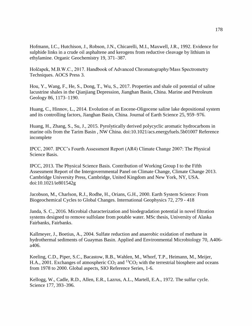
178
Hofmann, I.C., Hutchison, J., Robson, J.N., Chicarelli, M.I., Maxwell, J.R., 1992. Evidence for
sulphide links in a crude oil asphaltene and kerogens from reductive cleavage by lithium in
ethylamine. Organic Geochemistry 19, 371–387.
Holčapek, M.B.W.C., 2017. Handbook of Advanced Chromatography/Mass Spectrometry
Techniques. AOCS Press 3.
Hou, Y., Wang, F., He, S., Dong, T., Wu, S., 2017. Properties and shale oil potential of saline
lacustrine shales in the Qianjiang Depression, Jianghan Basin, China. Marine and Petroleum
Geology 86, 1173–1190.
Huang, C., Hinnov, L., 2014. Evolution of an Eocene-Oligocene saline lake depositional system
and its controlling factors, Jianghan Basin, China. Journal of Earth Science 25, 959–976.
Huang, H., Zhang, S., Su, J., 2015. Pyrolytically derived polycyclic aromatic hydrocarbons in
marine oils from the Tarim Basin , NW China. doi:10.1021/acs.energyfuels.5b01007 Reference
incomplete
IPCC, 2007. IPCC’s Fourth Assessment Report (AR4) Climate Change 2007: The Physical
Science Basis.
IPCC, 2013. The Physical Science Basis. Contribution of Working Group I to the Fifth
Assessment Report of the Intergovernmental Panel on Climate Change, Climate Change 2013.
Cambridge University Press, Cambridge, United Kingdom and New York, NY, USA.
doi:10.1021/ie801542g
Jacobson, M., Charlson, R.J., Rodhe, H., Orians, G.H., 2000. Earth System Science: From
Biogeochemical Cycles to Global Changes. International Geophysics 72, 279 - 418
Janda, S. C., 2016. Microbial characterization and biodegradation potential in novel filtration
systems designed to remove sulfolane from potable water. MSc thesis, University of Alaska
Fairbanks, Fairbanks.
Kallmeyer, J., Boetius, A., 2004. Sulfate reduction and anaerobic oxidation of methane in
hydrothermal sediments of Guaymas Basin. Applied and Environmental Microbiology 70, A406-
a406.
Keeling, C.D., Piper, S.C., Bacastow, R.B., Wahlen, M., Whorf, T.P., Heimann, M., Meijer,
H.A., 2001. Exchanges of atmospheric CO2 and 13CO2 with the terrestrial biosphere and oceans
from 1978 to 2000. Global aspects, SIO Reference Series, 1-6.
Kellogg, W., Cadle, R.D., Allen, E.R., Lazrus, A.L., Martell, E.A., 1972. The sulfur cycle.
Science 177, 393–396.

179
Kemper, J., 2015. Biomass and carbon dioxide capture and storage: A review. International
Journal of Greenhouse Gas Control 40, 401–430.
Kilgour, D.P.A., Neal, M.J., Soulby, A.J., O’Connor, P.B., 2013. Improved optimization of the
Fourier transform ion cyclotron resonance mass spectrometry phase correction function using a
genetic algorithm. Rapid Communications in Mass Spectrometry 27, 1977–1982.
Kleinjan, W.E., Keizer, A., Janssen, A.J.H., 2003. Elemental Sulfur and Sulfur-Rich Compounds
I. Biologically Produced Sulfur. Topics in Current Chemistry 230, 167- 188
Kohnen, M.E.L., 1991. Sulfurised Lipids in Sediments: The Key to Reconstruct
Palaeobiochemicals and their Origin. PhD thesis, Technische Universiteit Delft, Delft.
Kohnen, M.E.L., Sinninghe Damsté, J.S., Kock-van Dalen, A. c., Jan, W.D.L., 1991. Di- or
polysulphide-bound biomarkers in sulphur-rich geomacromolecules as revealed by selective
chemolysis. Geochimica et Cosmochimica Acta 55, 1375–1394.
Kohnen, M.E.L., Sinninghe Damsté, J.S., Ten Haven, H.L., kock.-Van Dalen, A.C., Schouten,
S., De Leeuw, J.W., 1991. Identification and geochemical significance of cyclic di-and
trisulphides with linear and acyclic isoprenoid carbon skeletons in immature sediments.
Geochimica et Cosmochimica Acta 55, 3685–3695.
Kohnen, M.E.L., Sinninghe Damsté, J.S., Baas, M., Kock-van Dalen, A.C., de Leeuw, J.W.,
1993. Sulphur-bound steroid and phytane carbon skeletons in geomacromolecules: Implications
for the mechanism of incorporation of sulphur into organic matter. Geochimica et Cosmochimica
Acta 57, 2515–2528.
Kok, M.D., Schouten, S., Sinninghe Damsté, J.S., 2000. Formation of insoluble,
nonhydrolyzable, sulfur-rich macromolecules via incorporation of inorganic sulfur species into
algal carbohydrates. Geochimica et Cosmochimica Acta 64, 2689–2699.
Kok, M.D., Rijpstra, W.I.C., Robertson, L., Volkman, J.K., Sinninghe Damsté, J.S., 2000. Early
steroid sulfurisation in surface sediments of a permanently stratified lake (Ace Lake, Antarctica).
Geochimica et Cosmochimica Acta 64, 1425–1436.
Levi, G., Karel, M., 1995. Volumetric shrinkage (collapse) in freeze-dried carbohydrates above
their glass transition temperature. Food Research International 28, 145–151.
Lewis, S.L., 2016. The Paris Agreement has solved a troubling problem. Nature 532, 283.
Li, S., Pang, X., Li, M., Jin, Z., 2003. Geochemistry of petroleum systems in the Niuzhuang
south slope of Bohai Bay Basin - Part 1: Source rock characterization. Organic Geochemistry 34,
389–412.

180
Liaaen-Jensen, S., Andrewes, A.G., 1985. 8 Analysis of carotenoids and related polyene
pigments. Methods in Microbiology 18, 235–255.
Libes, S., 2009. The origin of petroleum in the marine environment. Introduction to Marine
Biogeochemistry 1–34.
Liu, Y., Kujawinski, E.B., 2015. Chemical composition and potential environmental impacts of
water-soluble polar crude oil components inferred from esi FT-ICR MS. PLoS ONE 10, 1–18.
Lobodin, V. V., Robbins, W.K., Lu, J., Rodgers, R.P., 2015. Separation and characterization of
reactive and non-reactive sulfur in petroleum and its fractions. Energy and Fuels 29, 6177–6186.
Lu, H., Peng, P., Hsu, C.S., 2013a. Geochemical explication of sulfur organics characterized by
fourier transform ion cyclotron resonance mass spectrometry on sulfur-rich heavy oils in Jinxian
Sag, Bohai Bay Basin, Northern China. Energy and Fuels 27, 5861–5866.
Lu, H., Shi, Q., Lu, J., Sheng, G., Peng, P., Hsu, C.S., 2013b. Petroleum sulfur biomarkers
analyzed by comprehensive two-dimensional gas chromatography sulfur-specific detection and
mass spectrometry. Energy and Fuels 27, 7245–7251.
Lu, H., Shi, Q., Ma, Q.L., Shi, Y., Liu, J.Z., Sheng, G.Y., Peng, P.A., 2014. Molecular
characterization of sulfur compounds in some special sulfur-rich Chinese crude oils by FT-ICR
MS. Science China Earth Sciences 57, 1158–1167.
Luo, Liang, Qi, J., Li, H., Dong, Y., Zhang, S., Zhang, X., Yu, X., Luo, Lingyan, 2017.
Geometry and evolution of the Cangdong Sag in the Bohai Bay Basin, China: Implications for
subduction of the Pacific Plate. Scientific Reports 7, 15393.
Maiti, A., Sadrezadeh, M., Guha Thakurta, S., Pernitsky, D.J., Bhattacharjee, S., 2012.
Characterization of boiler blowdown water from steam-assisted gravity drainage and silica-
organic coprecipitation during acidification and ultrafiltration. Energy and Fuels 26, 5604–5612.
Martins, N., Ferreira, I.C.F.R., 2017. Wastes and by-products: Upcoming sources of carotenoids
for biotechnological purposes and health-related applications. Trends in Food Science and
Technology 62, 33–48.
Milligan, M., 2005. “Bubblin’’ Crude at Rozel Point, Box Elder County, Utah. Utah Geological
Survey Notes. Geosights Article 37, 3.
Mohialdeen, I.M.J., Hakimi, M.H., Al-Beyati, F.M., 2015. Biomarker characteristics of certain
crude oils and the oil-source rock correlation for the Kurdistan oilfields, northern Iraq. Arabian
Journal of Geosciences 8, 507–523.
Moreira, D., Pires, J.C.M., 2016. Bioresource technology atmospheric CO2 capture by algae:
Negative carbon dioxide emission path. Bioresource Technology 215, 371–379.

181
National Energy Board, 2018. Canada’s Energy Future 2018: An Energy Market Assessment.
Nakevska, N., Brinsky, J., Singh, A., 2017. Mapping groundwater conditions of deep saline
formations in West-Central Alberta. Natural Resources Canada, 17.
Nikolova-Damyanova, B., 2018. Principles of Silver Ion Complexation with Double Bonds,
Lipid Analysis. AOCS Lipid Library, 181-237.
Nocun, M., Andersson, J.T., 2012. Argentation chromatography for the separation of polycyclic
aromatic compounds according to ring number. Journal of Chromatography A 1219, 47–53.
OECD, IEA, 2015. Fossil Fuel Energy Consumption (% of total).
Oldenburg, T.B.P., Brown, M., Bennett, B., Larter, S.R., 2014. The impact of thermal maturity
level on the composition of crude oils, assessed using ultra-high resolution mass spectrometry.
Organic Geochemistry 75, 151–168.
Orr, W.L., 1977. Sulfur in heavy oils, oils sands and oils shales. Oil Sand and Oil Shale
Chemistry 22, 223–243.
Orr, W.L., White, C.M., 1990. ACS Symposium Series: Geochemistry of Sulfur in Fossil Fuels.
American Chemical Society, Dallas, Texas.
Orr, W., Sinninghe Damsté, J.S., 1990. Geochemistry of sulphur in petroleum systems.
Geochemistry of Sulphur in Fossil Fuels. American Chemical Society Symposium 429, 2–29.
Peters, K.E., Moldowan, J.M., 1993. Biomarker Guide: Interpreting Molecular Fossils in
Petroleum and Ancient Sediments, Illustrate. ed. Prentice Hall.
Peters, K.E., Walters, C.C., Moldowan, J.M., 2005a. The Biomarker Guide: Biomarkers and
Isotopes in the Environment and Human History, Volume 1. ed. Cambridge University Press.
Peters, K.E., Walters, C.C., Molodowan, J.M., 2005b. The Biomarker Guide, Volume 2. ed.
Cambridge University Press.
Philp, R.P., Fan, Z., 1987. Geochemical investigation of oils and source rocks from Qianjiang
Depression of Jianghan Basin, a terrigenous saline basin, China. Organic Geochemistry 11, 549–
562.
Pohlabeln, A.M., Gomez-Saez, G. V., Noriega-Ortega, B.E., Dittmar, T., 2017. Experimental
evidence for abiotic sulfurization of marine dissolved organic matter. Frontiers in Marine
Science 4, 1–11.
Poole, C.F., 2003. The Essence of Chromatography. Elsevier Science.

182
Purcell, J.M., Juyal, P., Kim, D.-G., Rodgers, R.P., Hendrickson, C.L., Marshall, A.G., 2007.
Sulfur speciation in petroleum: Atmospheric pressure photoionization or chemical derivatization
and electrospray ionization Fourier transform ion cyclotron resonance mass spectrometry.
Energy & Fuels 21, 2869–2874.
Qi, Y., Li, H., Wills, R.H., Perez-Hurtado, P., Yu, X., Kilgour, D.P.A., Barrow, M.P., Lin, C.,
O’Connor, P.B., 2013. Absorption-mode Fourier transform mass spectrometry: The effects of
apodization and phasing on modified protein spectra. Journal of the American Society for Mass
Spectrometry 24, 828–834.
Raven, M.R., Sessions, A.L., Adkins, J.F., Thunell, R.C., 2016. Rapid organic matter
sulfurization in sinking particles from the Cariaco Basin water column. Geochimica et
Cosmochimica Acta 190, 175–190.
Rabanaque Berdié, L., Casals I Ribes, I., Fernández Vidal, I., Jáuregui Pallarés, O., Marimon
Corbella, R.M., Perona Moreno, J., Casamitjana, T., 2012. Basics of Mass Spectrometry. Centres
Científics i Tecnològics. Universitat de Barcelona.
Radović, J.R, Silva, R.C., Snowdon, R.W., Brown, M., Larter, S., Oldenburg, T.B.P., 2016. A
rapid method to assess a broad inventory of organic species in marine sediments using ultra-high
resolution mass spectrometry 1273–1282.
Raffaelli, A., Saba, A., 2003. Atmospheric pressure photoionization mass spectrometry. Journal
of the American Society for Mass Spectrometry 15, 203–211.
Raven, M.R., 2016. Organic Matter Sulfurization in the Modern Ocean, PhD thesis, California
Institute of Technology, Pasadena.
Reichstein, M., Bahn, M., Ciais, P., Frank, D., Mahecha, M.D., Seneviratne, S.I., Zscheischler,
J., Beer, C., Buchmann, N., Frank, D.C., Papale, D., Rammig, A., Smith, P., Thonicke, K., Van
Der Velde, M., Vicca, S., Walz, A., Wattenbach, M., 2013. Climate extremes and the carbon
cycle. Nature 500, 287–295.
Repeta, D.J., Gagosian, R.B., 1987. Carotenoid diagenesis in recent marine sediments-I. The
Peru continental shelf (15 S, 75 W)*. Geochimica et Cosmochimica Acta 51, 1001–1009.
Richnow, Hans H., Jenisch, A., Michaelis, W., 1993. The chemical structure of macromolecular
fractions of a sulfur-rich oil. Geochimica et Cosmochimica Acta 57, 2767–2780.
Riediger, C.L., 1994. Migration of “Nordegg’’ oil in the Western Canada Basin. How much and
how far?” Bulletin of Canadian Petroleum Geology 42, 63–73.

183
Rogelj, J., Shindell, D., Jiang, K., Fifita, S., Forster, P., Ginzburg, V., Handa, C., Kheshgi, H.,
Kobayashi, S., Kriegler, E., Mundaca, L., Seferian, R., Vilarino, M.V., 2018. Mitigation
Pathways Compatible With 1.5°C in the Context of Sustainable Development. In: Global
Warming of 1.5°C. An IPCC Special Report on the Impacts of Global Warming of 1.5°C above
Pre-Industrial Levels and Related Global Greenhouse Gas Emission Pathways, in the context of
strengthening the global response to the threat of climate change, sustainable development, and
efforts to eradicate poverty [Masson-Delmotte, V., P. Zhai, H.-O. Pörtner, D. Roberts, J. Skea,
P.R. Shukla, A. Pirani, W. Moufouma-Okia, C. Péan, R. Pidcock, S. Connors, J.B.R. Matthews,
Y. Chen, X. Zhou, M.I. Gomis, E. Lonnoy, T. Maycock, M. Tignor, and T. Waterfield (eds.)]. In
Press.
Sass, H., Cypionka, H., 2007. Response of sulphate-reducing bacteria to oxygen, in: Sulphate-
Reducing Bacteria: Environmental and Engineered Systems. pp. 167–184.
Sawicka, J.E., Jørgensen, B.B., Brüchert, V., 2012. Temperature characteristics of bacterial
sulfate reduction in continental shelf and slope sediments. Biogeosciences 9, 3425–3435.
Schaeffer, P., Adam, P., Philippe, E., Trendel, J.M., Schmid, J.C., Behrens, A., Connan, J.,
Albrecht, P., 2006. The wide diversity of hopanoid sulfides evidenced by the structural
identification of several novel hopanoid series. Organic Geochemistry 37, 1590–1616.
Schiff, J.A., 2008. Sulphur in Biology: Pathways of Assimilatory Sulphate Reduction in Plants
and Microorganisms. John Wiley & Sons.
Schouten, S., de Graaf, W., Sinninghe Damsté, J.S., van Driel, G.B., de Leeuw, J.W., 1994.
Laboratory simulation of natural sulfurization. 2. Reaction of multi-functionalized lipids with
inorganic polysulfides at low-temperatures. Organic Geochemistry 22, 825–834.
Schouten, S., Pavlović, D., Sinninghe Damsté, J.S., de Leeuw, J.W., 1993. Selective cleavage of
acyclic sulphide moieties of sulphur-rich geomacromolecules by superheated methyl iodide.
Organic Geochemistry 20, 911–916.
Schouten, S., van Driel, G.B., Sinninghe Damsté, J.S., de Leeuw, J.W., 1993. Natural
sulphurization of ketones and aldehydes: A key reaction in the formation of organic sulphur
compounds. Geochimica et Cosmochimica Acta 57, 5111–5116.
Sei, A., Fathepure, B.Z., 2009. Biodegradation of BTEX at high salinity by an enrichment
culture from hypersaline sediments of Rozel Point at Great Salt Lake. Journal of Applied
Microbiology 107, 2001–2008.
Singh, A., Palombi, D., Nakevska, N., Jensen, G., Rostron, B., 2017. An efficient approach for
characterizing basin-scale hydrodynamics. Marine and Petroleum Geology 84, 332–340.

184
Sinninghe Damsté, J.S., De Leeuw, J.W., Kock-Van Dalen, A.C., De Zeeuw, M.A., Lange, F.
De, Irene, W., Rijpstra, C., Schenck, P.A., 1987. The occurrence and identification of series of
organic sulphur compounds in oils and sediment extracts. I. A study of Rozel Point Oil (U.S.A.).
Geochimica et Cosmochimica Acta 51, 2369–2391.
Sinninghe Damsté, J.S., 1988. Organically-Bound Sulphur in the Geosphere: a Molecular
Approach. PhD thesis, Technische Universiteit Delft, Delft.
Sinninghe Damsté, J.S., Eglinton, T.I., De Leeuw, J.W., Schenck, P.A., 1989. Organic sulphur in
macromolecular sedimentary organic matter: I. Structure and origin of sulphur-containing
moieties in kerogen, asphaltenes and coal as revealed by flash pyrolysis. Geochimica et
Cosmochimica Acta 53, 873–889.
Sinninghe Damsté, J.S., Rijpstra, W.I.C., De Leeuw, J.W., Schenck, P.A., 1989. The occurrence
and identification of series of organic sulphur compounds in oils and sediment extracts: II. Their
presence in samples from hypersaline and non-hypersaline palaeoenvironments and possible
application as source, palaeoenvironmental and matur. Geochimica et Cosmochimica Acta 53,
1323–1341.
Sinninghe Damsté, J.S., Rijpstra, W.I.C., Kock-van Dalen, A.C., de Leeuw, J.W., Schenck, P.A.,
1989. Quenching of labile functionalised lipids by inorganic sulphur species: Evidence for the
formation of sedimentary organic sulphur compounds at the early stages of diagenesis.
Geochimica et Cosmochimica Acta 53, 1343–1355.
Sinninghe Damsté, J.S., Orr, W., 1990. Geochemistry of sulphur in petroleum systems.
Geochemistry of Sulphur in Fossil Fuels 2–29.
Sinninghe Damsté, J.S., De Leeuw, J.W., 1990. Analysis, structure and geochemical significance
of organically-bound sulphur in the geosphere: State of the art and future research. Organic
Geochemistry 16, 1077–1101.
Sinninghe Damsté, J.S., Kenig, F., Koopmans, M.P., Köster, J., Schouten, S., Hayes, J.M., de
Leeuw, J.W., 1995. Evidence for gammacerane as an indicator of water column stratification.
Geochimica et Cosmochimica Acta 59, 1895–1900.
Sinninghe Damsté, J.S., Kok, M.D., Köster, J., Schouten, S., 1998. Sulfurized carbohydrates: An
important sedimentary sink for organic carbon? Earth and Planetary Science Letters 164, 7–
Reference incomplete
Statistics Canada, 2019. Report on Energy Supply and Demand in Canada – 2017 Preliminary.
Tabatabai, M.A., 2005. Sulfur in soils. Soil Science Society of America Journal 91–97.

185
Tawiah, P., Duer, J., Bryant, S., Larter, S., Brien, S.O., 2018. CO2 Injectivity Behaviour - Field
Observations from the Quest CCS Operations. GHGT-14 1–14.
Ten Haven, H.L., De Leeuw, J.W., Schenck, P.A., 1985. Organic geochemical studies of a
Messinian evaporitic basin, northern Apennines (Italy) I: Hydrocarbon biological markers for a
hypersaline environment. Geochimica et Cosmochimica Acta 49, 2181–2191
Ten Haven, H.L., Rohmer, M., Rullkötter, J., Bisseret, P., 1989. Tetrahymanol, the most likely
precursor of gammacerane, occurs ubiquitously in marine sediments. Geochimica et
Cosmochimica Acta 53, 3073–3079.
Thomson, G., 2009. Burying carbon dioxide in underground saline aquifers: Political folly or
climate change fix? Program on Water Issues. Munk Centre for International Studies. University
of Toronto.
Tropsha, A., 2010. Best practices for QSAR model development, validation, and exploitation.
Molecular Informatics 29, 476–488.
Trost, B.M., Curran, D.P., 1981. Chemoselective oxidation of sulfides to sulfones. Tetrahedron
Letters 22, 1287–1290.
UNFCCC, 2016. Aggregate effect of the intended nationally determined contributions: an
update. Synthesis Report. Framework Convention on Climate Change. Conference of the Parties
22 session, 2–75.
U.S. Environmental Protection Agency, 2015. National Greenhouse Gas Emissions and Sinks.
EPA Web Archive.
Van Dongen, B.E., 2003. Natural sulfurization of carbohydrates in marine sediments:
consequences for the chemical and carbon isotopic composition of sedimentary organic matter.
Geologica Ultraiectina 224, 1–149.
Van Dongen, B.E., Schouten, S., Sinninghe Damsté, J.S., 2002. Carbon isotope variability in
monosaccharides and lipids of aquatic algae and terrestrial plants. Marine Ecology Progress
Series 232, 83–92.
Van Dongen, B.E., Schouten, S., Baas, M., Geenevasen, J.A.J., Sinninghe Damsté, J.S., 2003.
An experimental study of the low-temperature sulfurization of carbohydrates. Organic
Geochemistry 34, 1129–1144.
Wang, Z., Stout, S.A., 2007. Oil Spill Environmental Forensics: Fingerprinting and Source
Identification. Academic Press.

186
Wang, P., Zhang, D., Xu, G., Xiao, T., Song, F., Cai, B., 2008. Geochemical features of light
hydrocarbons of typical salt lake oils sourced from Jianghan Basin, China. Organic
Geochemistry 39, 1631–1636.
Wardencki, W., 2000. Sulfur Compounds: Gas Chromatography. Encyclopedia of Separation
Science.
Wei, Z., Walters, C.C., Moldowan, J.M., Mankiewicz, P.J., Pottorf, R.J., Xiao, Y., Maze, W.,
Nguyen, P.T.H., Madincea, M.E., Phan, N.T., Peters, K.E., 2012. Organic Geochemistry
Thiadiamondoids as proxies for the extent of thermochemical sulfate reduction. Organic
Geochemistry 44, 53–70.
White, W.M., 2013. Geochemistry, 1st ed. Wiley-Blackwell, Ithaca, New York, USA.
Williams, D.P., Tarantino, L.M., Hubbard, W.K., 2019. Review of the Primary National
Ambient Air Quality Standards for Sulfur Oxides. Environmental Protection Agency. Federal
Register 84, 9866-9907.
Wong, K.V., 2015.Climate Change. Momentum Press, 2015. ProQuest Ebook Central.
Wu, S., Dong, D., Yu, Z., Zou, D., 2007. Geophysical evaluation methods for buried hill
reservoirs in the Jiyang superdepression of the Bohai Bay basin, eastern China. Journal of
Geophysics and Engineering 4, 148–159.
Yang, C., Wang, Z., Liu, Y., Yang, Z., Li, Y., Shah, K., Zhang, G., Landriault, M., Hollebone,
B., Brown, C., Lambert, P., Liu, Z., Tian, S., 2013. Aromatic steroids in crude oils and petroleum
products and their applications in forensic oil spill identification. Environmental Forensics 14,
278–293.

187
Appendix A
Appendix A1. Extracted ion chromatogram results Rozel Point oil (a) S1 fraction, (b) S2
fraction, (c) S3 fraction, and Jianghan Basin oil (d) S1 fraction, (e) S2 fraction and (f) S3
fraction. The fractionation technique was not as effective compared to Athabasca oil. Reactive
sulfides (thiolane and dibutyl sulfide) which were supposed to elute in S3 fraction were
observed in the S2 fraction. See Figure 5.8 for sulfur compound standards.

188

189

190
Appendix A2. FTICR-MS compound class distribution for (a) Rozel Point and (b)
Jianghan Basin oil.

191
Appendix A3. FTICR-MS DBE distribution for (a) Rozel Point and (b) Jianghan Basin oil.

192
Appendix A4. FTICR-MS carbon number distribution for (a) Rozel Point and (b) Jianghan
Basin oil.

193
Appendix A5. FTICR-MS compound class distribution for Rozel Point (red), Jianghan
Basin oil (blue) and Athabasca oil (black).

194
Appendix A6. BIOWINTM (v4.10) Ultimate Biodegradation Model Fragments and
Coefficient database.
There are 36 main fragments and molecular weight parameters which were obtained and
averaged from the analysis of 200 compounds by experts. (U.S. Environmental Protection
Agency, 2000). Training Set
FRAGMENT DESCRIPTION COEFFICIENT Fragment Count**
========================================== ===================== --------------
ULTIMATE PRIMARY MIN MAX Num
***
========= ========= ===== ===== ===
=
Nitroso [-N-N=O] -0.38513 0.01848 - 1 1
Linear C4 terminal chain [CCC-CH3] 0.29834 0.26907 - 3 26
Aliphatic alcohol [-OH] 0.15997 0.12945 - 4 18
Aromatic alcohol [-OH] 0.05638 0.03969 - 3 21
Aliphatic acid [-C(=O)-OH] 0.364605 0.38557 - 1 10
Aromatic acid [-C(=O)-OH] 0.08787 0.00775 - 1 6
Aldehyde [-CHO] 0.02232 0.19664 - 1 5
Ester [-C(=O)-O-C] 0.14021 0.22896 - 4 25
Amide [-C(=O)-N or -C(=S)-N] -0.05421 0.20543 - 1 13
Triazine ring (symmetric) -0.24586 -0.05752 - 1 4
Aliphatic chloride [-CL] -0.17318 -0.10061 - 3 14
Aromatic chloride [-CL] -0.20660 -0.16534 - 6 27
Aliphatic bromide [-Br] 0.02895 0.03538 - 6 2
Aromatic bromide [-Br] -0.13600 -0.15351 - 5 4
Aromatic iodide [-I] -0.04494 -0.12707 - 2 2
Aromatic fluoride [-F] -0.40694 0.01346 - 1 1

195
Carbon with 4 single bonds & no hydrogens -0.21212 -0.15344 - 3 32
Aromatic nitro [-NO2] -0.16959 -0.10838 - 2 13
Aliphatic amine [-NH2 or -NH-] 0.02444 0.04328 - 1 7
Aromatic amine [-NH2 or -NH-] -0.13495 -0.10838 - 2 23
Cyanide / Nitriles [-C#N] -0.08238 -0.06520 - 2 11
Sulfonic acid / salt -> aromatic attach 0.14221 0.02162 - 2 8
Sulfonic acid / salt -> aliphatic attach 0.19259 0.17714 - 2 4
Polyaromatic hydrocarbon (4 or more rings) -0.79934 -0.70224 - 1 2
Pyridine ring -0.21417 -0.01874 - 1 8
Aromatic ether [-O-aromatic carbon] -0.05812 0.07712 - 1 11
Aliphatic ether [C-O-C] -0.00867 -0.00974 - 5 16
Ketone [-C-C(=O)-C-] -0.02248 -0.02222 - 4 10
Tertiary amine -0.25480 -0.28800 - 2 10
Phosphate ester 0.15373 0.46535 - 1 7
Alkyl substituent on aromatic ring -0.07485 -0.06853 - 2 36
Azo group [-N=N-] -0.30036 -0.05279 - 1 3
Carbamate or Thiocarbamate -0.04671 0.19363 - 1 6
Trifluoromethyl group [-CF3] -0.51296 -0.27440 - 1 2
Unsubstituted aromatic (3 or less rings) -0.58591 -0.34280 - 1 1
Unsubstituted phenyl group (C6H5-) 0.02201 0.00489 - 3 22
Molecular Weight Parameter -0.00220987 -0.001442756 - - -
Molecular Weight ----- ----- 53.06 697.65 -
Equation Constant 3.19917051 3.847737 - - -
** - Minimum and Maximum number of instances of the fragment in any training set
compound. Minimum is always zero.
*** - Number of compounds in the 200 compound training set containing the fragment.

196
Appendix A7. WATERNT Fragment & Correction Factor Descriptions & Coefficients
The current version of WATERNT used a total training set of 1128 compounds. The derived
fragments and correction factors are as follows:
Number
compounds
Max
occurrences
Fragment Description Coefficient containing
fragment
in any one
compound
-CH3 [aliphatic carbon] -0.32127 612 6
-CH2- [aliphatic carbon] -0.53702 416 14
-CH [aliphatic carbon] -0.52852 188 6
C [aliphatic carbon - No H, not tert] -1.05164 34 2
=CH2 [olefinic carbon] -0.47888 44 2
=CH- or =C< [olefinic carbon] -0.36460 117 6
#C [acetylenic carbon] -0.28293 7 2
-OH [hydroxy, aliphatic attach] 1.60124 78 4
-O- [oxygen, aliphatic attach] 1.27460 46 3
-NH2 [aliphatic attach] 1.96561 58 2
-NH- [aliphatic attach] 2.13570 71 2
-N< [aliphatic attach] 1.96432 64 2
-CL [chlorine, aliphatic attach] -0.28720 65 6
-CL [chlorine, olefinic attach] -0.58670 16 6
-F [fluorine, aliphatic attach] -0.15800 26 5
-F [fluorine, olefinic attach] -0.05591 2 2
-Br [bromine, aliphatic attach] -0.56883 24 2
-Br [bromine, olefinic attach] -0.41966 1 2
-I [iodine, aliphatic attach] -1.07733 5 2
Aromatic Carbon (C-H type) -0.33586 700 15
Aromatic Nitrogen [max count of 1 allowed] 1.92553 62 1
-CL [chlorine, aromatic attach] -0.48781 202 10
-Br [bromine, aromatic attach] -0.56614 27 6
-OH [hydroxy, aromatic attach] 1.65780 81 1
-N [aliphatic N, one aromatic attach] 1.27489 104 1
-O- [oxygen, one aromatic attach] 0.19797 52 3
-O- [aliphatic O, two aromatic attach] 0.31806 4 1
-CHO [aldehyde, aliphatic attach] 1.10629 8 1
-CHO [aldehyde, aromatic attach] 0.65423 10 1
-C(=O)- [carbonyl, aliphatic attach] 1.05667 37 2
-C(=O)- [carbonyl, one aromatic attach] 1.00038 7 1
-C#N [cyano, aliphatic attach] 0.80635 10 2

197
-CðN [cyano, aromatic attach] -0.32546 5 2
-NO2 [nitro, aliphatic attach] 0.34153 6 1
-NO2 [nitro, aromatic attach] -0.19151 65 3
-COOH [acid, aliphatic attach] 1.18078 60 1
-COOH [acid, aromatic attach] 0.05680 55 2
-N=O [nitroso] -0.45992 12 1
-S- [aliphatic sulfur,one aromatic attach] -0.42393 12 1
Aromatic Sulfur -0.27429 15 1
-C(=O)O [ester, aliphatic attach] 0.57575 51 5
-C(=O)O [ester, aromatic attach] 0.70058 32 2
-F [fluorine, aromatic attach] 0.14286 11 2
-C(=O)N [aliphatic attach] -0.24262 68 2
-C(=O)N [aromatic attach] -0.79463 16 2
-NC(=S)N- [thiourea] -4.23842 5 1
-SH [aliphatic attach] -0.38719 3 1
Aromatic Carbon (C-substituent type) -0.53995 718 12
-S- [aliphatic attach] -0.09926 11 3
S=P [thio=phosphorus] 0.87740 39 2
-O-P [aliphatic attach] -0.38266 56 4
-O-P [aromatic attach] -0.57006 29 3
-S-P [sulfur, phosphorus attach] -0.97614 19 3
O=P 3.27482 23 1
-N-P [nitrogen, phosphorus attach] -0.04017 6 2
-I [aromatic attach] -1.40688 5 1
-SO2-N [aromatic attach] -1.20034 29 2
-SO2- [aromatic attach] 1.43056 2 1
-NC(=O)N- [urea] -2.60207 44 1
-O-N [oxygen, nitrogen attach] -0.12332 4 1
Aromatic Oxygen 0.36677 12 1
-OC(=O)N [carbamate] -1.08088 23 2
-C(=O)- [carbonyl, olefinic attach] 0.11034 24 2
-ONO2 [aliphatic attach] -0.28464 4 3
-N- [aliphatic N, two aromatic attach] 0.69882 12 1
Aromatic n=O [nitrogen oxide] 2.45192 1 1
-SS- [disulfide] -1.12316 2 1
Aromatic Nitrogen [5-member ring] 0.52650 30 3
-S- [aliphatic S, two aromatic attach] -0.28517 8 1
-C(=O)- [two aromatic attach, in ring] -0.29534 1 2
-OH [combined multiple aromatic attach] 2.62371 12 1
-S-C(=O)-N- [Thiocarbamate] -1.31223 3 1
Olefinic Carbon [two aromatic attach] 0.21070 1 1
-S(=O)- [sulfoxide, aromatic attach] 2.48195 1 1

198
-N=C=S [isothiocyanate, aliphatic attach] -0.62933 1 1
-N=C=S [isothiocyanate, aromatic attach] -1.04381 2 1
-tert Carbon [3 or more carbon attach] -0.57735 81 4
-SH [thiol, aromatic attach] -0.72008 1 1
Ketone in a ring [olefin, aromatic attach] 0.09637 1 2
-N=N- [Azo] -0.26511 2 1
-CH2- [aliphatic carbon, cyclic] -0.33084 99 8
-SO2-N [aliphatic attach] 0.03908 3 2
-OH [hydroxy, nitrogen attach] 0.34519 2 1
-N [multi aliphatic N, 1 aromatic attach] 1.75391 37 1
-O- [aliphatic, 2 aromatic attach, cyclic] -0.28163 12 2
-COOH [combined multi-aliphatic attach] 1.36027 5 1
-COOH [acid, olefinic attach] 0.46464 7 2
Carbonyl, non-cyclic, two aromatic attach 1.06545 3 1
Aldehyde, [-N-CHO; aromatic attach] 0.01671 1 1
Aldehyde, [-N-CHO; aliphatic attach] 0.00691 3 1
-S(=O)- [sulfoxide, aliphatic attach] 2.06660 5 1
-SO2- [sulfone, aliphatic attach] 1.46100 4 1
-SO2-O [sulfonate, aromatic attach] -0.71767 3 1
SO2 [two aromatic attach] -0.17566 5 1
-N-SO2-N- [sulfamide] -2.05175 4 1
-CO-CO [aromatic attach] 0.07721 4 2
-C(=S)N- [aliphatic attach] -1.56100 2 1
-S-C= [S to aliphatic, double bonded C] 0.02050 2 1
-Si- [silicon, aliphatic attach (not oxy)] -2.38500 4 1
-OH [phosphorus attach] -0.63350 4 2
Aromatic nitrogen [+5 valence type; no H] 4.53400 2 1
-S- [aliphatic sulfur, 2 nitrogen attach] -0.67133 3 1
-Hg- [mercury] -0.74550 5 1
Formaldehyde experimental value - constant 0.87200 1 1
ðC [acetylenic carbon-acetylenic attach] -0.35375 2 2
S=C=S [carbon disulfide, experimental] -2.05900 1 1
-C(=O)-S [thioester, aliphatic attach] 0.58900 1 1
-O-SO2-O- [sulfate, linear] -2.61750 2 1
-CO-CO [aliphatic attach] 0.21953 3 2
-C(=O)-SH [aliphatic attach] 0.31367 3 2
-OC(=O)O- [carbonate,aliphatic attach] 0.36800 2 1
CðN-C=N [cyano, -C=N attach] 0.27800 2 1
-C(=S)N- [aromatic attach] -0.94800 1 1
CðN-S [cyano, sulfur attach] -0.08551 3 3
-SO2-OH [sulfonic], [coef*(1+0.3*(NUM-
1))]
3.84950 4 1

199
O=C=O [carbon dioxide, experimental] -1.72400 1 1
-O- [oxygen, two silicon attach, linear] -3.40000 0 0
-O- [oxygen, two silicon attach, cyclic] -2.70000 0 0
Number compds Max
occurrences
Correction Factor Description Coefficient containing
fragment
in any one
compound
Hydrocarbon [unsubst. alkane] correction -1.50129 15 1
Hydrocarbon [unsub mono-olefin] correction -0.85243 9 1
Ring reaction -> ortho to aromatic acid 0.65626 19 2
Aliphatic alcohol(mono) on aromatic struct 0.38134 20 1
Ring ortho reaction -> -OH / -COOH -1.77658 4 1
Ring reaction -> -OH / -COOH (non-ortho) -0.99298 5 1
Ring ortho reaction -> -OH / -NO2 -1.20202 11 2
Ring reaction -> -OH / -CHO -0.95018 3 1
Ring reaction -> -OH / -ester -1.41678 6 1
Ring reaction -> -Amino / -OH -1.17596 6 1
Ring reaction -> -Amino / -NO2 -0.77862 4 1
Ring reaction -> -Amino/ -COOH (non-
ortho)
-0.55123 5 1
Ring reaction -> -Amino/ -COOH (ortho) -1.51383 2 1
Ring reaction -> -Amino / -ester -0.90295 9 1
Reaction -> -OH / nitrogen (arom 6-ring) -2.52977 5 1
Di-COOH (non-ortho) aromatic ring -1.15945 2 1
C-O-C-O-C structure correction -0.74557 7 3
Fused aliphatic ring corrections (>5) 0.26117 22 6
HO-C-C(=O)-C-OH structure correction -2.74903 7 1
HO-C-C(=O)-C-O- structure correction -2.58251 6 1
-C-C(=O)-C-OH structure correction -1.29494 4 1
-CO-N-CO-N-CO- structure correction -0.27800 15 1
-N-CO-N-CO- structure correction -1.72804 6 1
Amino triazine/pyrazine/pyrimidine correc. -1.46411 16 3
Ring rx -> Halogen ortho to arom nitrogen -0.54407 10 2
Amino acid (alpha-position) correction -1.84779 13 1
Alcohol - amino acid correction -1.31839 2 1
Ring rx -> di-,poly-COOH N-aromatic ring -2.42816 6 1
Ring rx -> N-aromatic/non-ortho
COOH(mono)
-1.45266 2 1
-S(=O)-N-S(=O)- structure correction 1.56916 2 1

200
Mono-halo acetamide [-NH-CO-C-halo] -0.49490 6 1
Di-N urea/acetamide aromatic correction 0.68745 13 2
Sulfur (+4) charged-halide type 3.80000 0 0
Number compds Max
occurrences
Estimated Fragment Description Coefficient containing
fragment
in any one
compd
-OC(=O)O- [carbonate,cyclic] 1.16500 1 1
-O-C(=S)-N- [thiocarbamate] -2.88833 3 1
-O-SO2-O- [sulfate, cyclic] -1.76700 1 1
-O-SO-O- [sulfite, linear] -1.39500 1 1
-O-SO-O- [sulfite, cyclic] -1.85333 3 1
P-O-P [oxygen, two phosphorus attach] -1.07100 1 1
-C(=O)-SH [aromatic attach] -1.67100 1 1
-C(=S)-O [aliphatic attach] -0.85675 4 1
U.S. Environmental Protection Agency, 2000. On-Line WATERNT User’s Guide Water
Solubility Estimation -Fragment Methodology.

201
Appendix A8. OECD DOC Die-Away Biodegradation Test Procedures
1) MINERAL MEDIUM
a. Stock Solutions
i. A – KH2PO4 (6.8 g), K2HPO4 (17.2 g) NaHPO4 · 2H2O (26.4 g), NH4Cl
(0.4g) dissolved in 800 mL DI water
ii. B – MgSO4 · 6H2O (18.0 g) into 800 mL
iii. C – CaCl2 · 2H2O (29.0 g) into 800 mL
iv. D – FeCl3 (0.2g) into 800 mL
b. Mineral Medium; 10 mL A, into 800 mL, add 1 mL B, 1 mL C, 1 mL D, top off
to 1 L
Check with pH paper that the pH is around 7
*add a drop of diluted HCl into stock solution before preparation of mineral medium, if
precipitate forms make new stock solution
* use new mineral medium for each BDT run, dispose of extra M.M. in inorganic waste
2) INOCULUM
a. 1 part soil (stored in fridge three), 4 parts mineral medium e.g. ~25 mL soil in 100
mL M.M., into a container, with a stir bar, stir at 350 rpm, physically agitate to
get a homogeneous mixture
b. may stir overnight if necessary
c. Save ~5 mL in a 8 mL vial (label “inoculum – date”) for future analysis
3) SAMPLE COMPOUND
a. Calculate DOC (if possible) to make a test solution with ~20 ppm of Carbon in DI
water in 100 mL volumetric flask
b. Check if soluble in Mineral Medium, if not dissolve an appropriate amount of
sample into 1 L DI water for addition to Test Flasks
4) TEST FLASKS
Replicates are important as there can be large variation because of the inconsistency in
the soil concentration, and bacterial activity
a. Sample Flask (x3)
i. 100mL of M.M.
ii. sufficient amount of compound to have a DOC of 10 ppm-40 ppm
(aim for 20 ppm)
iii. 15 mL of inoculum
iv. top off solution to 125 mL with mineral medium
v. add stir bar – stir @ 350 rpm
vi. wrap flasks in tin foil (completely dark) and loosely cover top with tin foil
(aerobic)

202
vii. label as compound i, ii, and iii
b. Control Flask (x2)
i. 100 mL of M.M.
ii. 15 mL of inoculum
iii. top of solution to 125 mL with mineral medium
iv. add stir bar – stir @350 rpm
v. wrap flasks in tin foil (completely dark) and loosely cover top with tin foil
(aerobic)
vi. label flasks control i, ii
5) TESTING
a. Shake flasks before sampling. Take between 0.1 mL – 0.25 mL of solution from
flask with a pipet, dilute in 10 mL volumetric flask with DI water (note: do not
want to take >1 mL to keep the volume as consistent as possible)
b. Mix thoroughly
c. Follow DOC procedure to test on TIC/TOC
d. Test Regularly; at least twice within 24 h, if stable test every couple days (i.e.
once a day if declining >5% rate, and every 2-3 days if slower)
6) CALCULATING %BIODEGRADATION
𝐷(𝑡) = (1 − [𝐶(𝑡) − 𝐶𝑏(𝑡)
𝐶(𝑜) − 𝐶𝑏(𝑜)]) ∗ 100
D(t) = %degradation at time t
C(t) = mean concentration of sample flasks at time t
Cb(t) = mean concentration of control flasks at time t
C(o) = initial mean concentration of sample flasks
Cb(o) = initial mean concentration of control flasks
*graphical representation has been %biodeg (percent) over time (hours)

203
Appendix A9. Literature Review on Remediation Strategies to Treat Sulfolane
Contaminated Sites by Calista Yim.
ABSTRACT
Sulfolane is a water miscible contaminant that is used in petroleum refining operations to
extract aromatic and sulfur compounds. Sulfolane typically leaks or spills from these facilities
and if it enters the soil and groundwater, it will travel as a function of groundwater velocity,
hydraulic gradient and hydraulic conductivity. The toxicity of sulfolane in humans is not well
understood but sulfolane has been observed to cause neurological damage and death in lab
animals and aquatic organisms (CCME, 2006). Several sulfolane remediation studies are
discussed in this paper including natural attenuation, biotic and abiotic remediation strategies.
Each method was evaluated to determine the efficiency and effectiveness in degrading sulfolane
and minimizing other impacts of sulfolane on the environment such as formation of intermediate
products.
INTRODUCTION
Sulfolane (C4H8O2S), also known as tetrahydrothiophene 1,1 – dioxide, is a colorless and
odorless inert organosulfur solvent with high hydrophilicity and high thermal stability (Fig. 1)
(Janda, 2016). It was invented over half a century ago as part of the Shell Sulfinol gas
sweetening process and since then it has been used extensively in Canada where sulfur-rich
petroleum is abundant (Saint-Fort, 2006). This chemical is used extensively at many sour-gas
processing plants because it is efficient at removing toxic levels of polar compounds such as
H2S, CO2, COS, CS2 and mercaptans from natural gas (Mehrabani-Zeinabad, 2016). As well, due
to its high thermal stability, natural gas plant operators find sulfolane cost-effective to use as it
can be easily regenerated and reused. However, accidental spills and leakages often occur at
landfills and surface storage ponds, with insufficient lining and monitoring systems, and allow
sulfolane to escape into the environment (CCME, 2006). When sulfolane reaches the
environment, it immediately penetrates through soils, wetlands near the plant site, vadose zone
and infiltrate groundwater (Izadifard et al., 2018).
It is important to understand that sulfolane has unique chemical properties unlike any

204
other contaminant. Sulfolane has low vapor pressure which means that it is non-volatile and
cannot be easily detected through the olfactory system (CCME, 2006). Also, it has low octanol-
water partition coefficient (Kow = 0.1 to 0.01) which means sulfolane is highly miscible in the
aqueous phase but does not interact with organic particles (Stewart, 2010). Besides these water-
like characteristics, it is moderately basic and has high thermal stability with a boiling point of
285 oC (Headley et al., 2002). Once sulfolane contamination sites are identified, groundwater
and sediment samples are collected and prepared for analysis with the gas chromatography mass
spectrometry, liquid chromatography (positive ion) and electrospray negative ionization to
analyze vegetation extracts in aqueous solutions (Headley et al., 2002).
Since sulfolane behaves similarly to water, it has great potential to migrate far from
contaminated sites, travel at a velocity of groundwater flow and pose a high risk for animals and
humans (Izadifard et al., 2018). In one of many cases, a sulfolane spill incident that occurred in
2004 at the North Pole refinery in Alaska has affected over 1500 households and is still
spreading to this day (Saint-Fort, 2006). Which is why understanding the chemical
characteristics of sulfolane is essential in determining the mobility of sulfolane in the subsurface
and its potential to reach areas that pose as a risk for humans and animals (Saint-Fort, 2006).
Currently, the effect of sulfolane in humans is poorly understood however sulfolane has
been administered in high doses to lab rats and guinea pigs and its toxicological properties are
well documented with animals (Anderson et al., 1977). Sulfolane was observed to be toxic for
lab animals when doses exceeded 200 mg/kg. Some of symptoms which indicated sulfolane
toxicity are convulsions, seizures, depression and other neurological damage. Surprisingly,
sulfolane exhibits low toxicity to aquatic plants and organisms unless administered in high
concentrations (>1000 mg/L) (CCME, 2006; Headley et al., 2002; Doucette et al., 2005). The
Canadian Council of Ministers for the Environment (CCME) established the tolerable daily
intake of sulfolane for humans to be 0.0097 mg/kg*day while the limit in soil is 0.8 mg/kg for
land use based on the toxicological information on sulfolane collected from several studies on
animals and aquatic organisms (CCME, 2006).
Despite these health risks, sulfolane is an emerging contaminant that has been in use for
over five decades and is still widely used today. The persistent effect of sulfolane in the

205
environment and its impact on human health are not well understood, therefore more research is
needed to understand the behaviour and fate of sulfolane in the environment (Janda, 2016). In
addition, appropriate remediation strategies, discussed in this paper, can be implemented to
minimize impact of sulfolane on the environment.
NATURAL ATTENTUATION AND BIOLOGICAL REMEDIATION STRATEGIES
If nature can stop the rapid spread of sulfolane in the environment and degrade the
contaminant over time, it would be the most cost-effective remediation method. Unfortunately,
Izadifard et al. (2018) stated that natural processes are not effective in sulfolane removal. Since
sulfolane has high water solubility, the main transport mechanism in contaminated environments
is ground water flow or advection. Saint Fort (2006) studied the natural attenuation of sulfolane
through sorption onto soil and subsurface materials collected near a sour gas plant facility north
of Calgary. This study also explored sulfolane biodegradation under aerobic and anaerobic
conditions in the presence of nitrogen. The sample materials collected included sand, silt and
clay, but Saint Fort (2006) suggests the subsurface materials were ineffective against slowing the
rate of sulfolane. Despite manipulating the different sorbent materials in which sulfolane was
passed through, the ionic strength of the contaminant solution and environment temperature,
Saint Fort (2006) could not detect significant amounts sulfolane biodegradation under anaerobic
conditions. In the study by Luther et al. (1998), the researchers also concluded that classic
aquifer material had negligible impact on sulfolane sorption except their laboratory results
showed sulfolane had better adsorption response with clay minerals compared to soil organic
matter. In both anaerobic experiments by Saint Fort (2006) and Luther et al. (1998), microcosms
continued to produce CO2, which indicated that the sulfolane concentrations used was not toxic
to the microorganisms, however the microbial community did not identify sulfolane as a food
source.
Fedorak and Coy (1996) demonstrated that aerobic conditions improved sulfolane
biodegradation in both soil and groundwater samples but minimal degradation was observed
under anoxic conditions. Saint Fort (2006) observed most sulfolane loss at sample depths of 0 -
0.20 m where aerobic microbial biodegradation was most active. Furthermore, Saint Fort (2006)
recognized that biodegradation rates decreased with increasing depth, but improvement was seen

206
in biodegradation rates when additional nitrogen was supplied to microcosms at a 25 oC
environment. On the other hand, Greene and Fedorak (2001) reported an increase in the rate of
sulfolane biodegradation when phosphate supplementation was administered to aerobic
microcosms. For natural sulfolane biodegradation to occur, Saint Fort (2006) concluded that
microorganisms showed increased sulfolane biodegradation rate when supplied with oxygen,
nitrogen and warm environments (25 oC). Whereas the results from the study by Greene &
Fedorak (1998), showed most optimal microbial biodegradation of contaminated sediments when
temperatures were between 8 – 28 oC, when sufficient oxygen, nitrogen and phosphorus was
supplied and coupled with Mn (IV) and nitrate-reducing conditions. Janda (2016) also noted that
the addition of nitrogen and phosphorus stimulated biodegradation at a Canadian natural gas
plant, but it was not clear whether the soils were nutrient-deficient to begin with or if the nutrient
addition was applicable to all sulfolane contamination sites. However, Saint Fort (2006) and
Greene and Fedorak (2001) both agree that oxygen and warm environmental temperatures are
essential elements for successful sulfolane biodegradation. Adjusting the environment
temperatures for in situ aerobic biodegradation may be an issue especially for sulfolane
contamination in colder regions such as Canada.
The study by Kasanke and Leigh (2017) examined the sulfolane degradation rate in
presence of other hydrocarbon contaminants and with limited nutrients supply. Similar to the
results from Saint Fort (2006) and Greene and Fedorak (2001), Kansanke and Leigh (2017)
observed aerobic sulfolane biodegradation as well except only under nitrate, sulfate and iron
reducing conditions and nutrients amendments was not seen to accelerate biodegradation rates in
sediment unlike the studies by Saint Fort (2006) and Greene and Fedorak (2001). However
nutrient supplementation was more successful in stimulating aerobic degradation in groundwater.
Another perspective regarding aerobic biodegradation addressed by (ARCADIS, 2013) relates to
the intermediate products that are produced during the sulfolane degradation reactions. Some
intermediates produced may be easily biodegraded or are identified as food sources for microbial
communities, however other intermediates may be more toxic to human health than sulfolane
(ARCADIS, 2013).

207
Chou and Swatloski (1983) studied sulfolane biodegradation in refinery wastewater using
mixed microbe cultures but biodegradation ceased when sulfuric acid formed as a product and
decreased pH which could not be tolerated by the microbe cultures. Then Greene and Fedorak
(1998) attempted to isolate pure cultures of sulfolane-degrading bacteria but showed difficulty in
obtaining aerobic bacteria. The researchers then used pH sensitive agar as a medium to develop
the sulfolane degrading colony and showed success in identifying and isolating the bacteria.
Despite successfully isolating the sulfolane-degrading bacteria under laboratory conditions, these
bacteria may not survive and thrive in natural environments.
Another natural sulfolane attenuation method is to utilize wetland plants and vegetation to
absorb sulfolane contaminated waters. Doucette et al. (2005) discovered wetland plants, around a
sour gas facility, had greater concentrations of contaminants in their structural composition.
Inspired by this discovery, they conducted sulfolane uptake experiments using cattails (Typha
Latifolia), which are common in wetlands. Despite sulfolane being one of the largest
contaminants in groundwater, it was not toxic to the cattails because sulfolane is a neutral
compound which gets readily passed through the cattails' root membrane. Therefore, wetland
plants may play a significant role in sulfolane removal in aqueous settings, that is, if the plants
do not release sulfolane during decomposition or winter dormancy (Doucette et al., 2005).
ABIOTIC REMEDIATION STRATEGIES
In situ biological remediation strategies using microcosms are often more cost effective
than abiotic remediation strategies but biotic strategies may not always be successful for
degrading sulfolane at every contamination site as it is difficult to test what stimulates
microorganisms to quickly biodegrade sulfolane when each environment varies in temperature,
sulfolane-degrading bacteria and nutrient supplies (Saint Fort, 2006; Greene et al., 2001 and
Kasanke and Leigh (2017). However consistent results are often seen with active oxidation
processes used to treat and degrade sulfolane (ARCADIS et al., 2013). In the study by Yu et al.
(2016), they discovered that sulfolane would degrade fastest under UVC irradiation in
combination with oxidants such as H2O2 or O3. Both Yu et al. (2016) and Izadifard et al. (2017)
agree that neither H2O2 nor O3 alone could degrade sulfolane efficiently, but the combination of

208
using both oxidants (Fig. 2) could degrade more than 90% of sulfolane in 1 hour (Yu et al.,
2016). Furthermore, UVA radiation only worked well with oxidant TiO2 (Fig. 3) and showed
90% of sulfolane degraded in 1.5 hours (Yu et al., 2016). Izadifard et al. (2017) also tested
oxidation methods using UV radiation with O3 and found the rate of sulfolane degradation to be
even greater when calcium peroxide and lime (CaO) was used with ozone (Fig. 4) to degrade
sulfolane in water. Izadifard et al. (2017) hypothesized that CaO had a significant impact on the
reaction efficiency by raising the pH of the overall reaction and the calcium ions can bind with
intermediate products during sulfolane degradation to form insoluble precipitates. Yu et al.
(2016) concluded in their study that utilizing two oxidants (O3 and H2O2) was most effective at
achieving higher degradation rates with sulfolane. But in the study by Izadifard et al. (2017),
they showed that their CaO2/UV system worked 40% faster than systems using UV and O3. Both
Mehrabani-Zeinabad et al. (2016) and Izadifard et al. (2017) investigated the mineralization of
sulfolane using UV/O3/ H2O2 in a tubular reactor except Mehrabani-Zeinabad et al. (2016)
investigated the mineralization of sulfolane through measuring the amount of CO2, H2O and
sulfate produced while Izadifard et al. (2017) mineralized sulfolane by forming CaCO3.
Interestingly, Mehrabani-Zeinabad et al. (2016) claims that high alkalinity (CO3 2-
concentrations) conditions can quench hydroxyl radicals and inhibit degradation, but Izadifard et
al. (2017) showed results with improvement in sulfolane biodegradation occurring at high
alkaline pH conditions when CaO was used with O3/ UV system. In summary, using CaO along
with O3/ UV may be more efficient than using O3/ UV alone as this method suggested by
Izadifard et al. (2017) can be used as in situ treatment for sulfolane contaminated groundwater
and this method required less treatment time, 30% less ozone and CaO is readily available.
However, Mehrabani-Zeinabad et al. (2016) explains that laboratory sulfolane biodegradation
results are not representative of what occurs in natural environments as their sulfolane
degradation rates were lower in contaminated groundwater compared to experimental lab results.
Izadifard et al. (2017) does also discuss the disadvantages of using oxidants because oxidants
have low solubility and stability in water and high production cost. In addition, reactions
between ozone and organic matter forms aldehydes and carboxylic acids, both of which do not
react with ozone which may result in a low kinetic reaction.

209
CONCLUSION
The effect of sulfolane in humans has not been documented, but the toxic effects of
sulfolane has been observed in lab animals. The chemical properties and characteristics of
sulfolane is well established such as its ability to percolate effortlessly into soils and sediments
therefore making natural attenuation through subsurface aquifer materials ineffective. However,
potential natural attenuation is observed with using wetland cattail plants to absorb sulfolane
contaminated waters. Anaerobic biodegradation is also ineffective at removing sulfolane but
aerobic conditions show more promising results depending on the oxygen supply, nutrient
amendments and reducing conditions of the contaminated site. Advanced oxidation processes
(AOP) uses a combination of ultraviolet radiation, oxidants and calcium peroxide or lime to
break down or mineral sulfolane. AOP are efficient and show much faster degradation results
compared to aerobic biodegradation which can take several days whereas AOP may take several
hours. Each remediation method has its own benefits and disadvantages but it is important to
consider all possibilities for remediation, natural, abiotic or biotic degradation methods,
depending on the budget and time allowed for each contaminated site. Sulfolane is a persistent
contaminant with high infiltration ability. Sulfolane has affected many areas and residents for the
past several decades (CCME, 2006), to prevent the risk of sulfolane exposure to humans and
animals, continued research in this area is needed to determine in situ degradation methods
which are also stable and cost effective.
Figures in Appendix A9
Figure 1. Chemical structure of sulfolane (Saint-Fort, 2006)

210
Figure 2. Degradation of sulfolane using oxidants and UV radiation. (a) UVA, (b) UVC, (c)
H2O2, (d) O3, (e) H2O2 + O3 (Yu et al., 2016).
Figure 3. Degradation of sulfolane using UVA radiation and oxidants (Yu et al., 2016)

211
Figure 4. Degradation of sulfolane using CaO2/O3 compared to UV/O3 (Izadifard et al. 2017)
Figure 5. Degradation of sulfolane using UV radiation combined with O3 and H2O2 (Izadifard et
al. 2017).

212
Appendix A9 References:
Andersen, M.E., Jones, R.A., Mehl, R.G., Hill, T.A., Kurlansik, L., Jenkins Jr., L.J., 1977. The
inhalation toxicity of sulfolane (tetrahydrothiophene – 1,1-dioxide). Toxicology and Applied
Pharmacology 40, 463-472.
ARCADIS, 2013. Interim Remedial Action Plan Addendum, Flint Hill Resources Alaska, LLC
[Online].
Bak, A., Kozik, V., Dybal, P., Kus, S., Swietlicka, A., Jampilek, J., 2018. Sulfolane: Magic
extractor or bad actor? Pilot-scale study on solvent corrosion potential. Sustainability
(Switzerland) 10. doi:10.3390/su10103677
Brassell, S.C., Lewis, C.A., De Leeuw, J.W., De Lange, F., Sinninghe Damsté, J.S., 1986.
Isoprenoid thiophenes: Novel products of sediment diagenesis? Nature.
Canadian Council of Ministers of the Environment, 2006. Canadian Environmental Quality
Guidelines for Sulfolane : Water and Soil, Environment.
Doucette, W.J., Chard, J.K., Moore, B.J., Staudt, W.J., Headley, J. V., 2005. Uptake of sulfolane
and diisopropanolamine (DIPA) by cattails (Typha latifolia). Microchemical Journal 81,
41–49.
Fedorak, P.M., Coy, D.L., 1996. Biodegradation of sulfolane in soil and groundwater samples
from a sour gas plant site. Environmental Technology (United Kingdom) 17, 1093–1102.
Greene, E.A., Fedorak, P.M., 1998. A differential medium for the isolation and enumeration of
sulfolane-degrading bacteria. Journal of Microbiological Methods 33, 255–262.
Greene, E.A., Fedorak, P.M., 2001. Nutrient stimulation of sulfolane biodegradation in a
contaminated soil from a sour natural gas plant and in a pristine soil. Environmental
Technology (United Kingdom) 22, 619–629.
Headley, J. V., Fedorak, P.M., Dickson, L.C., 2002. A review of analytical methods for the
determination of sulfolane and alkanolamines in environmental studies. Journal of AOAC
International 85, 154–162.
Izadifard, M., Achari, G., Langford, C.H., 2018. Mineralization of sulfolane in aqueous solutions
by Ozone/CaO2and Ozone/CaO with potential for field application. Chemosphere 197,
535–540.
Janda, S.C., 2016. Microbial Characterization and Biodegradation potential in novel filtration
systems designed to remove sulfolane from potable water. University of Alaska Fairbanks.
Kasanke, C.P., Leigh, M.B., 2017. Factors limiting sulfolane biodegradation in contaminated
subarctic aquifer substrate. PLoS ONE 12, 1–17.
Kohnen, M.E.L., Sinninghe Damsté, J.S., Baas, M., Dalen, A.C.K. van, de Leeuw, J.W., 1993.
Sulphur-bound steroid and phytane carbon skeletons in geomacromolecules: Implications
for the mechanism of incorporation of sulphur into organic matter. Geochimica et
Cosmochimica Acta 57, 2515–2528.
Kohnen, M.E.L., Sinninghe Damsté, J.S., Ten Haven, H.L., kock.-Van Dalen, A.C., Schouten,
S., De Leeuw, J.W., 1991. Identification and geochemical significance of cyclic di-and
trisulphides with linear and acyclic isoprenoid carbon skeletons in immature sediments.
Geochimica et Cosmochimica Acta 55, 3685–3695.

213
Kok, M.D., Rijpstra, W.I.C., Robertson, L., Volkman, J.K., Sinninghe Damsté, J.S., 2000. Early
steroid sulfurisation in surface sediments of a permanently stratified lake (Ace Lake,
Antarctica). Geochimica et Cosmochimica Acta 64, 1425–1436.
Libes, S., 2009. The Origin of Petroleum in the Marine Environment. Introduction to Marine
Biogeochemistry 1–34.
Lu, H., Peng, P., Hsu, C.S., 2013. Geochemical explication of sulfur organics characterized by
fourier transform ion cyclotron resonance mass spectrometry on sulfur-rich heavy oils in
Jinxian Sag, Bohai Bay Basin, Northern China. Energy and Fuels 27, 5861–5866.
Mehrabani-Zeinabad, M., Calgary, A., 2016. University of Calgary Advanced Oxidative
Processes for Treatment of Emerging Contaminants in Water.
Saint-Fort, R., 2006. Sulfolane attenuation by surface and subsurface soil matrices. Journal of
Environmental Science and Health - Part A Toxic/Hazardous Substances and
Environmental Engineering. doi:10.1080/10934520600623109
Schaeffer, P., Adam, P., Philippe, E., Trendel, J.M., Schmid, J.C., Behrens, A., Connan, J.,
Albrecht, P., 2006. The wide diversity of hopanoid sulfides evidenced by the structural
identification of several novel hopanoid series. Organic Geochemistry 37, 1590–1616.
Schouten, S., Degraaf, W., Sinninghe Damsté, J.S., Vandriel, G.B., De Leeuw, J.W., 1994.
Laboratory simulation of natural sulfurization .2. Reaction of multi-functionalized lipids
with inorganic polysulfides at low-temperatures. Organic Geochemistry 22, 825–834.
Schouten, S., van Driel, G.B., Sinninghe Damsté, J.S., de Leeuw, J.W., 1993. Natural
sulphurization of ketones and aldehydes: A key reaction in the formation of organic sulphur
compounds. Geochimica et Cosmochimica Acta 57, 5111–5116.
Sinninghe-Damsté, J.S.S., De Leeuw, J.W., Schenck, P.., 1988. Organically-Bound Sulphur in
the Geosphere: a Molecular Approach. Technische Universiteit Delft PhD., 287.
Sinninghe Damsté, J.S., Rijpstra, W.I.C., Kock-van Dalen, A.C., De Leeuw, J.W., Schenck,
P.A., 1989. Quenching of labile functionalised lipids by inorganic sulphur species:
Evidence for the formation of sedimentary organic sulphur compounds at the early stages of
diagenesis. Geochimica et Cosmochimica Acta 53, 1343–1355.
Sinninghe Damsté, J.S., De Leeuw, J.W., Kock-Van Dalen, A.C., De Zeeuw, M.A., Lange, F.
De, Irene, W., Rijpstra, C., Schenck, P.A., 1987. The occurrence and identification of series
of organic sulphur compounds in oils and sediment extracts. I. A study of Rozel Point Oil
(U.S.A.). Geochimica et Cosmochimica Acta 51, 2369–2391.
Sinninghe Damsté, J.S., Rijpstra, W.I.C., De Leeuw, J.W., Schenck, P.A., 1989. The occurrence
and identification of series of organic sulphur compounds in oils and sediment extracts: II.
Their presence in samples from hypersaline and non-hypersaline palaeoenvironments and
possible application as source, palaeoenvironmental and matur. Geochimica et
Cosmochimica Acta 53, 1323–1341.
Stewart, O., 2010. Sulfolane Technical Assistance and Evaluation Report 61. Reference
incomplete?
Tilstam, U., 2012. Sulfolane: A versatile dipolar aprotic solvent. Organic Process Research and
Development 16, 1273–1278.
U.S. Environmental Protection Agency, 2000. On-Line WATERNT User’s Guide Water
Solubility Estimation -Fragment Methodology.
Van Dongen, B.E., Schouten, S., Baas, M., Geenevasen, J.A.J., Sinninghe Damsté, J.S., 2003.

214
An experimental study of the low-temperature sulfurization of carbohydrates. Organic
Geochemistry 34, 1129–1144.
White, W.M., 2013. Geochemistry, 1st ed. Wiley-Blackwell, Ithaca, New York, USA.
Yang, F., Hanna, M.A., Sun, R., 2012. Value-added uses for crude glycerol-a byproduct of
biodiesel production. Biotechnology for B 5, 1–10.
Yu, L., Mehrabani-Zeinabad, M., Achari, G., Langford, C.H., 2016. Application of UV based
advanced oxidation to treat sulfolane in an aqueous medium. Chemosphere 160, 155–161.