dissertation enhancement of coupled surface / subsurface flow ...

DISSERTATION

ENHANCEMENT OF COUPLED SURFACE / SUBSURFACE FLOW MODELS IN

WATERSHEDS: ANALYSIS, MODEL DEVELOPMENT, OPTIMIZATION, AND USER

ACCESSIBILITY

Submitted by

Seonggyu Park

Department of Civil and Environmental Engineering

In partial fulfillment of the requirements

For the Degree of Doctor of Philosophy

Colorado State University

Fort Collins, Colorado

Fall 2018

Doctoral Committee:

Advisor: Ryan T. Bailey

Neil S. Grigg

Michael J. Ronayne

Thomas Sale

Copyright by Seonggyu Park 2018

All Rights Reserved

ii

ABSTRACT

ENHANCEMENT OF COUPLED SURFACE / SUBSURFACE FLOW MODELS IN

WATERSHEDS: ANALYSIS, MODEL DEVELOPMENT, OPTIMIZATION, AND USER

ACCESSIBILITY

The shortage of freshwater supply has been recognized as one of the most critical and global

issues. Population growth, land use, and climate change are exacerbating current and future

stresses on freshwater scarcity. Many techniques and methods have been developed and used to

quantify water resources at the regional scale, including large-scale watershed models.

However, the majority of large-scale watershed models are lumped hydrologic models that

ignore or treat simplistically the flow of groundwater and its interaction with surface water

features. Integrated surface water – groundwater models are being used more frequently, but no

systematic approach of model construction, sensitivity analysis, parameter estimation, and

uncertainty analysis has been provided. In addition, there is a need to develop tools for

constructing these models, for ease of implementation in watersheds worldwide.

This dissertation establishes a general framework for implementing and applying integrated

surface water-groundwater models to address water management questions in watersheds and

river basins. These methods include model construction, sensitivity and uncertainty analysis,

parameter estimation for coupled groundwater/surface water models, using the integrated surface

water-groundwater model SWAT-MODFLOW as an example modeling tool, thereby providing

a general framework for implementation and use of integrated hydrologic models. All project

objectives are illustrated through a model application to the Middle Bosque River watershed

iii

(471 km2) in central Texas, a region that relies on groundwater and surface water to satisfy water

demand.

Model construction is facilitated through the development of a graphical user interface (GUI)

tool, QSWATMOD. The GUI is developed as a plug-in tool for QGIS, an open-source, free

graphical information system. QSWATMOD was applied to the Middle Bosque River Watershed

in Texas to demonstrate the linkage between existing SWAT and MODFLOW. The visualization

of the results from the SWAT-MODFLOW simulation is beneficial in displaying model output

and comparing with observed streamflow and groundwater data. QSWATMOD can be a

valuable tool in assisting users to create and manage SWAT-MODFLOW projects, allowing

coupled surface water/groundwater models to become more accessible to a broader hydrologic

modelling community.

Parameter estimation and uncertainty analysis is performed using the PEST software, with

new pre-processing and post-processing algorithms developed to modify and assess jointly land

surface and hydrogeological parameters. The monthly NSE values of streamflow discharge for

calibration and validation were calculated to be 0.45 and 0.66, respectively, and for whole

simulation was 0.55, which are considered acceptable for monthly stream discharge (≥ 0.5). The

PBIAS value for calibration reveals a small percent under-prediction (2.62), but a large percent

over-prediction (-16.79) for validation probably due to an overestimation of baseflow between

storm events. The patterns of the hydrographs of simulated hydraulic heads for both locations are

similar to their observed data, the daily R2 values for two observation wells are considered low

because the simulated hydraulic heads show less fluctuation, or a small percent under-prediction

compared to their observed values.

iv

The water resources from surface and sub-surface domains were assessed simultaneously.

For the hydrologic fluxes, results demonstrate a high spatial-temporal variability in simulated

hydraulic head, recharge rates and surface-subsurface water interaction rates, which can have a

profound impact on watershed management. For example, the spatio-temporal variation of

recharge and groundwater discharge maps can help identify potential areas of nutrient loading

from the aquifer to the stream network or of pollution infiltration from surface to the aquifer. In

addition, this area could be used to support decisions about alternative management strategies in

the areas of landuse change, climate change, water allocation, and pollution control.

Sensitivity analysis is performed to determine the controlling land surface and hydrogeologic

factors on hydrologic responses of the watershed (streamflow, water table elevation). The results

from the composite sensitivity (CSP) show in general the significance of the land surface

parameters in controlling streamflow and groundwater level The normalized sensitivity

coefficient (NSC) of the land surface parameters also is higher than for the hydrogeological

properties; however, the aquifer properties (K, Sy) do exhibit a moderate influence particularly

for alluvium and terrace deposits, which are near-surface geologic units and thus have a control

and land surface processes and associated surface runoff and streamflow in the MBRW system.

Analysis of the simulation uncertainties of hydrologic responses (streamflow, water table

elevation, watershed water balance) is performed with the impact of short-term climatic events

and future development scenario. For the impact of short-term climatic events, results show

climate events such as drought, multi-year drought, and extreme flooding events have a

significant impact on surface water storage, groundwater storage, and watershed fluxes (recharge,

groundwater-surface water interaction, lateral flow, surface runoff). Besides, the results show

that even the same intensity and length of a stress or even its pre-conditions on different

v

hydrologic response variables can result in their response time, scales and durations in a very

different way. Results from groundwater development scenario (aquifer-storage-recovery) show

injecting water results in higher changes in water table than extracting water from the aquifer

(similar to scale change of hydrological responses and water balance). The results suggest that

their response time, scales and durations not only vary but also are influenced by pre-conditions

(i.e. soil moisture, water table), their distances to pumping wells.

The proposed modelling framework for model construction, parameter estimation, sensitivity

and uncertainty analysis can assist in implementing and applying integrated surface water-

groundwater models for estimating watershed water resource and analysing the effect of changes

in land use, population, and climate. Keys to the framework are the ability to jointly estimate

land surface and hydrogeological parameters and quantify their impact on hydrologic responses

(streamflow, water table elevation, GW-SW interactions). This framework, particularly if used

with SWAT-MODFLOW, can facilitate the use of integrated models worldwide to assist with

finding technical solutions to water issues.

vi

ACKNOWLEDGEMENTS

I wonder whether my advisor (Dr. Ryan Bailey) has ever been frustrated with my slow

progress on the dissertation. But, even if he did, he always told me “You will do great!”. He

never let me doubt myself and always fully supported me. For that, I am truly thankful.

I would also like to thank my defense committee members, Prof. Neil S. Grigg

, Dr. Michael J. Ronayne and Dr. Thomas Sale. All of them were incredibly tolerant to my

(literally) last minute submissions. I am so grateful for their encouragement and insightful

comments.

Of course, it would be almost impossible for me to complete my Ph.D., without never ending

joyful talks to my colleagues and research comments from them. I would especially never forget

“Thursday food meeting”.

vii

DEDICATION

To the most beautiful woman in the universe,

my amazing wife, Yun,

whose unconditional love and sacrificial care for me and our children

made it possible for me to complete my Ph.D.,

and to our children,

Elliot and Eliana,

who are indeed a gift from the Lord.

viii

TABLE OF CONTENTS

ABSTRACT …………………………………………………………………………………….ii

ACKNOWLEDGEMENTS ........................................................................................................... vi

DEDICATION .............................................................................................................................. vii

TABLE OF CONTENTS ............................................................................................................. viii

LIST OF TABLES ........................................................................................................................ xii

LIST OF FIGURES ..................................................................................................................... xiii

CHAPTER 1 LITERATURE REVIEW AND RESEARCH OVERVIEW ................................... 1

1.1. Objective and expected significance .................................................................................... 1

1.2. Background .......................................................................................................................... 2

1.3. Significance of research ....................................................................................................... 4

1.4. Organization of the dissertation ........................................................................................... 5

REFERENCES ............................................................................................................................... 6

CHAPTER 2 ................................................................................................................................. 10

A QGIS-BASED GRAPHICAL USER INTERFACE FOR APPLICATION AND

EVALUATION OF SWAT-MODFLOW MODELS ................................................................... 10

2.1. Introduction ........................................................................................................................ 10

2.2. Development and Application of QSWATMOD .............................................................. 13

2.2.1. QSWATMOD Overview and Development ............................................................... 13

2.2.2. Pre-Processing Tab ..................................................................................................... 16

2.2.3. Simulation Tab ............................................................................................................ 21

2.2.4. Post-Processing Tab .................................................................................................... 22

ix

2.3. Conclusion ......................................................................................................................... 24

REFERENCES ............................................................................................................................. 25

CHAPTER 3 ................................................................................................................................. 29

QUANTIFYING EFFECT OF DECADAL AND EXTREME CLIMATE EVENTS ON

WATERSHED WATER RESOURCES AND FLUXES USING SWAT-MODFLOW ............. 29

3.1. Introduction ........................................................................................................................ 30

3.2. Methodology ...................................................................................................................... 34

3.2.1. Study area.................................................................................................................... 34

3.2.2. Three-Dimensional Groundwater Model Development ............................................. 36

3.2.3. SWAT model construction ......................................................................................... 42

3.2.4. SWAT-MODFLOW Model ........................................................................................ 43

3.2.5. Parameter estimation for the coupled SWAT-MODFLOW model ............................ 44

3.2.6. Estimating Water Resource Availability .................................................................... 46

3.2.7. Quantifying Hydrological Responses to Climate Events............................................ 46

3.3. Results and Discussion ...................................................................................................... 48

3.3.1. Initial head interpolation ............................................................................................. 48

3.3.2. Model corroboration ................................................................................................... 50

3.3.3. Spatio-Temporal Variation of Hydrologic Fluxes ...................................................... 52

3.3.4. Water resource availability ......................................................................................... 57

3.3.5. Hydrological responses to climate events ................................................................... 58

3.4. Summary and conclusions ................................................................................................. 63

REFERENCES ............................................................................................................................. 65

x

CHAPTER 4 ................................................................................................................................. 74

A FRAMEWORK FOR QUANTIFYING UNCERTAINTY, SENSITIVITY, AND

ESTIMATING PARAMETERS FOR INTEGRATED SURFACE WATER - GROUNDWATER

MODELS ...................................................................................................................................... 74

4.1. Introduction ........................................................................................................................ 75

4.2. Methodology ...................................................................................................................... 79

4.2.1. General Framework for Integrated SW-GW Models.................................................. 79

4.2.2. Model Construction and Setup.................................................................................... 82

4.2.3. Estimation of SWAT and MODFLOW Parameters ................................................... 86

4.2.4. Sensitivity Analysis .................................................................................................... 89

4.2.5. Uncertainty Analysis for Model Scenarios ................................................................. 92

4.3. Results and Discussion ...................................................................................................... 93

4.3.1. Parameter Estimation .................................................................................................. 93

4.3.2. Sensitivity Analysis .................................................................................................... 95

4.3.3. Simulation Uncertainties for Groundwater Development Scenario ........................... 97

4.4. Summary and Conclusions ............................................................................................... 99

REFERENCES ........................................................................................................................... 102

CHAPTER 5 ............................................................................................................................... 105

CONCLUSIONS AND FUTURE WORK ................................................................................. 105

5.1. A QGIS-based graphical user interface for application and evaluation of SWAT-

MODFLOW models ............................................................................................................... 105

xi

5.2. Quantifying effect of decadal and extreme climate events on watershed water resources

and fluxes using SWAT-MODFLOW .................................................................................... 106

5.3. A framework for quantifying uncertainty, sensitivity, and estimating parameters for

integrated surface water - groundwater models ...................................................................... 108

5.4. General Conclusions ........................................................................................................ 109

APPENDIX A ............................................................................................................................. 110

APPENDIX B ............................................................................................................................. 114

xii

LIST OF TABLES

Table 2.1. Summary Characteristics of the SWAT and MODFLOW models.............................. 13

Table 2.2. Process time for QSWATMOD functions for the Middle Bosque River Watershed. . 20

Table 3.1. Hydraulic-conductivity conceptualization and parameterization ……………………42

Table 3.2 Variables in SWAT-MODFLOW simulations ............................................................. 46

Table 3.3 Initial ranges and calibrated values for the selected parameters during streamflow

discharge and hydraulic head calibration. ..................................................................................... 50

Table 3.4 Comparison statistics (NSE; R2; PBIAS) between the observed and simulated

hydrograph at the stream gauge near the confluence of the Sycan and Sprague Rivers (Fig. 3.1)

for calibration (1993 – 2005), validation (2005 – 2012), and whole simulation of the SWAT-

MODFLOW model ....................................................................................................................... 51

xiii

LIST OF FIGURES

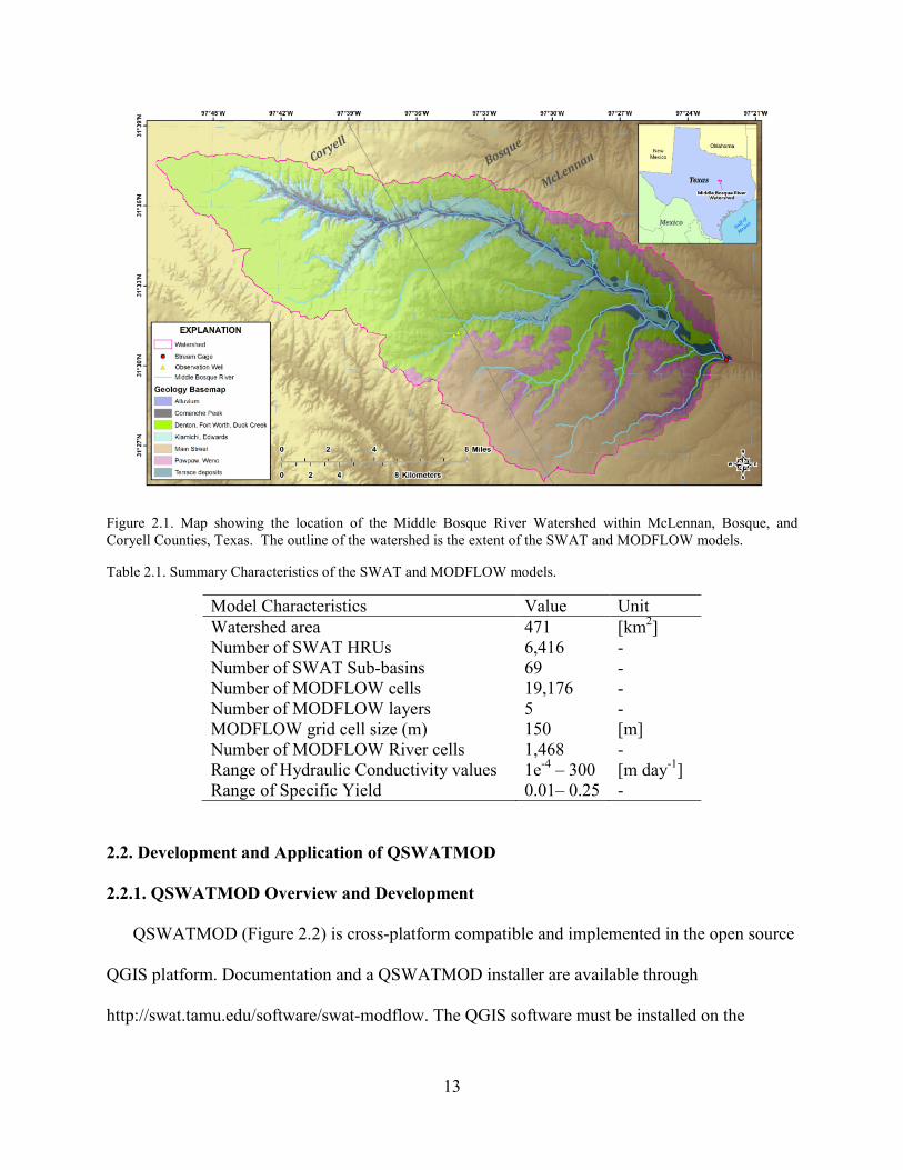
Figure 2.1. Map showing the location of the Middle Bosque River Watershed within McLennan,

Bosque, and Coryell Counties, Texas. The outline of the watershed is the extent of the SWAT

and MODFLOW models............................................................................................................... 13

Figure 2.2. Main QSWATMOD GUI platform. ........................................................................... 15

Figure 2.3. Schematic showing the Pre-processing, Configuration, and Post-processing modules

of QSWATMOD to prepare inputs and visualize results for a SWAT-MODFLOW simulation. 15

Figure 2.4. QSWATMOD interface for the Pre-processing tab, using shapefiles from the Middle

Bosque River Watershed............................................................................................................... 16

Figure 2.5. MODFLOW tab within the Pre-Processing tab, which loads information to create a

single-layer MODFLOW model. .................................................................................................. 18

Figure 2.6. River connections a) Option1: MODFLOW River Package; b) Option 2: River

Parameters estimated using SWAT River Network and User Inputs; c) Modified MODFLOW

River Package; and d) Interface for Identification of River Cells. ............................................... 19

Figure 2.7. QSWATMOD interface for a) Simulation Tab; b) Configuration Settings (in

“swatmf_link.txt” file). ................................................................................................................. 22

Figure 2.8. QSWATMOD interface for Post-processing tab, showing results from the Middle

Bosque SWAT-MODFLOW simulation. ..................................................................................... 23

Figure 3.1. Location map showing the position of the study area within McLennan, Bosque, and

Coryell Counties, Texas. Physiographic map showing the provinces composing and surrounding

the study area. These include the Washita Prairie and Lampasas Cut Plain……………………..35

Figure 3.2. Monthly averages for precipitation and temperature (max, mean, and min) in the

Middle Bosque River Watershed, 1980 – 2012. ........................................................................... 36

xiv

Figure 3.3. The Comanche peak limestone and the many shale units within the Georgetown

formation form receding zones beneath the harder limestone units overlying them. A softer

portion within the Edwards Limestone many times also forms receding zone. ........................... 38

Figure 3.4. Monthly and annual total precipitation during the model corroboration period with a

drought year of 1999 and a flood year of 2004. ............................................................................ 48

Figure 3.5. Different rainfall patterns in a) drought scenario with 6 different ratios (0.25, 0.5,

0.75, 1.25, 1.5, 1.75) multiplying by the original precipitation rates in 1999 and in b) flood

scenarios using two pre-conditions, i.e., wet with the original precipitation data and dry with the

deletion of 3-day rainfall events before the storm condition scenarios (5, 10, 15, and 20 inches).

....................................................................................................................................................... 48

Figure 3.6 Variograms for the 28 observed water levels: a) original values with residuals; b)

residuals with model fitted. ........................................................................................................... 49

Figure 3.7. Interpolated initial hydraulic head with the de-trended 28 observed water level data

using the ordinary kriging method and the spherical model. ........................................................ 49

Figure 3.8. Observed and SWAT-MODFLOW simulated time series of stream discharge (m3/s),

and the statistics (R2, NSE, PBIAS) for calibration (1993 – 2005) and validation (2006 – 2012)

periods for the outlet of the Middle Bosque River watershed ...................................................... 51

Figure 3.9. Hydrographs of measured and simulated hydraulic head for CO1L and CO2D wells

in the Middle Bosque River watershed. ........................................................................................ 52

Figure 3.10. a) Simulated cell-wise annual average hydraulic head (m); b) Spatially-varying

annual average recharge (mm) in the Middle Bosque watershed as simulated by the coupled

SWAT-MODFLOW model .......................................................................................................... 53

xv

Figure 3.11. Changes from annual average hydraulic head (m) for the months of March, June,

September and December over the 1993–2012 period ................................................................. 54

Figure 3. 12. Average annual recharge rates (mm) for the months of March, June, September and

December over the 1970–2003 period .......................................................................................... 55

Figure 3.13. Departure from annual average groundwater discharge rates (m3/day) for the months

of March, June, September and December over the 1993–2012 period ....................................... 56

Figure 3. 14. Time series of monthly water resource availability in the Middle Bosque River

watershed ...................................................................................................................................... 58

Figure 3.15. Streamflow discharges with 6 different ratios (0.25, 0.5, 0.75, 1.25, 1.5, 1.75)

multiplying by the original precipitation rates in the controlling year of 1999 / to post-controlling

year of 2000 for the drought scenarios. ........................................................................................ 59

Figure 3.16. Hydraulic head elevations with 6 different ratios (0.25, 0.5, 0.75, 1.25, 1.5, 1.75)

multiplying by the original precipitation rates in 1999 for the drought scenarios ........................ 59

Figure 3.17. Relative changes in each element of water balance with 6 different ratios (0.25, 0.5,

0.75, 1.25, 1.5, 1.75) multiplying by the original precipitation rates in 1999 for the drought

scenarios ........................................................................................................................................ 60

Figure 3.18. Streamflow discharge relative changes with different storm events (5, 10, 15, 20

inches) after a wet or dry pre-condition ........................................................................................ 61

Figure 3.19. Hydraulic head elevations with different storm events (5, 10, 15, 20 inches) after a

wet or dry pre-condition................................................................................................................ 61

Figure 3.20. Relative changes in each element of water balance with different storm events (5, 10,

15, 20 inches) after a wet or dry pre-condition ............................................................................. 62

xvi

Figure 4.1. Framework for constructing, calibrating, and applying integrated surface water-

groundwater models within a watershed system .......................................................................... 81

Figure 4.2. Location map showing the position of the study area within McLennan, Bosque, and

Coryell Counties, Texas. Physiographic map showing the provinces composing and surrounding

the study area. These include the Washita Prairie and Lampasas Cut Plain. ................................ 84

Figure 4.3. Schematic diagram for automatic calibration for both land surface and

hydrogeological parameters .......................................................................................................... 87

Figure 4.4. Observed and simulated results provided by the ensemble of parameter sets time

series of stream discharge (m3/s), and the statistics (R

2, NSE, PBIAS) for calibration period

(1993 – 2012) for the outlet of the Middle Bosque River watershed ........................................... 94

Figure 4.5. the hydrographs of measured and simulated hydraulic head for the observation wells

(CO1L from 10/21/1985 – 3/7/1986 and CO2D from 11/30/1985 – 2/1/1986) ........................... 95

Figure 4.6. Model input composite sensitivities (CSP) for signature measures of streamflow

discharge and two water table elevations in the Middle Bosque watershed. Circle plot shows the

set of CSP calculated for model inputs. The CSP indices are illustrated in coloured groups

showing in clockwise order the sensitivities of selected land surface parameters in green, of river

bed conductance in red, of 9 hydraulic conductivity zones, and of 9 specific yield zones. ......... 96

Figure 4.7. Model input Normalized Sensitivity Coefficient (NSC) for signature measures of a)

streamflow discharge and two water table elevations and b) streamflow discharge only. Circle

plot shows the set of NSC calculated for model inputs. The NSC indices are illustrated in

coloured groups showing in clockwise order the sensitivities of selected land surface parameters

in green, of river bed conductance in red, of 9 hydraulic conductivity zones, and of 9 specific

yield zones. ................................................................................................................................... 97

xvii

Figure 4.8. Effect of the aquifer storage and recovery scenarios on groundwater levels ............. 98

Figure 4.9. Normalized Sensitivity Coefficient (NSC) on water balance in (upper) calibrated

model and (lower) with groundwater development scenario ........................................................ 99

1

CHAPTER 1 LITERATURE REVIEW AND RESEARCH OVERVIEW

1.1. Objective and expected significance

The overall aim of this dissertation is to develop a framework for implementing and applying

integrated surface water-groundwater models to address water management questions in

watersheds and river basins. These methods include model construction, sensitivity and

uncertainty analysis, parameter estimation for coupled groundwater/surface water models, using

the integrated surface water-groundwater model SWAT-MODFLOW as an example modeling

tool, thereby providing a general framework for implementation and use of integrated hydrologic

models. This overall aim will be accomplished by through the following specific objectives:

(1) Develop an easy-to-use workflow for users preparing input data, configuring simulation

settings, and visualizing and interpreting results. The GUI is developed as a plug-in tool

for QGIS, an open-source, free graphical information system. The development of a

QGIS-based graphical user interface for the SWAT-MODFLOW model will allow

coupled surface water/groundwater models to become more accessible to the broad

hydrologic modeling community.

(2) Quantify surface water resources, groundwater resources, and water flux rates between

storage components as impacted by multi-decadal climate patterns and extreme climate

events (major drought, storms) in a semi-arid regional-scale watershed.

(3) Develop a methodology to optimize a SWAT-MODFLOW model automatically.

Parameter estimation and composite sensitivity analysis are performed using the PEST

software, with new pre-processing and post-processing algorithms developed to modify

and assess jointly land surface and hydrogeological parameters.

2

(4) Perform local sensitivity analysis (LSA) with one-at-time (OAT) approach to evaluate

the individual controlling land surface and hydrogeologic factors on hydrologic

responses of the watershed (streamflow, water table elevation).

(5) Perform an analysis of the simulation uncertainties of hydrologic responses (streamflow,

water table elevation, watershed water balance) with the impact of short-term climatic

events and future development scenario.

1.2. Background

A variety of methods have been used to quantify water resources for watersheds, river basins,

or other geographical areas. These techniques include lumped water balance hydrologic models

over large geographical regions and global scales (Alcamo et al., 1997; Döll et al., 2003; Alcamo

et al., 2003; Wada et al., 2010), the use of satellite observations such as with GRACE (Gravity

Recovery and Climate Experiment) (Rodell et al., 2007; Longuevergne et al., 2010; Famiglietti

et al., 2011; Feng et al., 2013; Voss et al., 2013), and physically-based spatially-distributed

hydrologic models. Whereas large-scale lumped models neglect groundwater storage, GRACE

results often are limited to estimating changes in groundwater storage, become uncertain at small

spatial scales (less than a few hundred km), and are dependent on the accuracy in accounting for

soil moisture change. In addition, changes in surface water storage are difficult to estimate.

Physically-based, spatially-distributed coupled land surface/subsurface hydrologic models

such as SWAT (Arnold et al., 1998); CATHY (Camporese et al., 2009), ParFlow (Kollet and

Maxwell, 2006), GSFLOW (Markstrom et al., 2008), and SWAT-MODFLOW (Bailey et al.,

2016) can be used to estimate components of groundwater and surface water storage. Model

applications range from global scale (de Graaf et al., 2015; de Graaf et al., 2017), to continental

scale (Schuol et al., 2008; Abbaspour et al., 2015; Maxwell et al., 2015), to river basins and

3

catchments (Gauthier et al, 2009; Perrin et al., 2012; Morway et al., 2013; Tanvir Hassan et al.,

2014; Tian et al., 2015; Bailey et al., 2016). Whereas the global-scale and continental-scale

models provide global trends in groundwater supply, results are neither accurate enough nor

resolved enough to assist in conjunctively managing groundwater and surface water resources at

the regional scale. Smaller-scale studies often focus on fluxes (Perrin et al., 2012; Tanvir Hassan

et al., 2014; Bailey et al., 2016) and hydrologic responses to management practices (Morway et

al., 2013; Tian et al., 2015), rather than an assessment of stored volumes of groundwater and

surface water through decadal periods, which are required to assist with water management.

These coupled flow models, however, include substantial uncertainties with respect to input

data, forcing data, initial and boundary conditions, model structure, and parameter non-

uniqueness due to a lack of data and poor knowledge of hydrological response mechanisms (Ye

et al., 2008; Doherty and Welter, 2010; Shi and Zhou, 2010; Zhang et al., 2011; Gupta et al.,

2012; Foglia et al., 2013). These uncertainties have negative effects on the model accuracy,

thereby inducing uncertainties in the simulated results. Therefore, if hydrologic models are to be

used to as decision-making aids, the uncertainty associated with model calibration and model

predictions must be assessed (Gallagher and Doherty, 2007). In addition, these coupled flow

models often are not used extensively due to the level of complexity of preparing input data,

configuring model options, executing models, and interpreting results (Barthel and Banzhaf,

2016; Nielsen et al., 2017). In particular, preparing input data for coupled hydrological models is

often a slow, tedious, and error-prone process. To save time and avoid errors, Bailey et al. (2017)

developed SWATMOD-Prep, a stand-alone graphical user interface (GUI) that facilitates

preparing linkage files for a SWAT-MODFLOW model simulation (Bailey et al., 2016). The

4

GUI, however, does not provide geographical context and does not allow linkage between an

already existing SWAT model with an existing MODFLOW model.

Overall, no systematic approach of model construction and use has been provided for the

coupled surface-subsurface flow models, limiting their wide application. There is a need for a

generalized approach to perform UA, quantify the influence of the vast array of model

parameters and factors on watershed response (e.g. stream discharge, groundwater head) through

SA, develop a systematic approach to parameter estimation for both land surface and

hydrogeological parameters, thereby providing modelling results that assess both groundwater

and surface water resources accurately in a watershed setting while relaying the degree of

uncertainty to decision makers.

1.3. Significance of research

This dissertation presents a framework for implementing and applying integrated surface

water-groundwater models to address water management questions in watersheds and river

basins. Model construction is facilitated through the development of a graphical user interface

(GUI) tool, QSWATMOD capable of generating required input files, configuring simulation

settings, and visualizing and interpreting results. A methodology to optimize a SWAT-

MODFLOW model is presented with automatic calibration process and sensitivity analysis using

PEST software through the development of new pre-processing and post-processing algorithms

to modify and assess jointly land surface and hydrogeological parameters. In addition, the local

sensitivity analysis (LSA) with one-at-time (OAT) approach is presented to evaluate the

individual controlling land surface and hydrogeologic factors on hydrologic responses of the

watershed (streamflow, water table elevation). Under climatic events and future development

scenario, an analysis of the simulation uncertainties of hydrologic responses is performed.

5

The proposed modelling framework and a QGIS-based graphical user interface for the

SWAT-MODFLOW model can facilitate the use of integrated models worldwide to assist with

finding technical solutions to water issues. Results can help enhance understanding regarding the

spatio-temporal patterns of hydraulic head elevation, recharge, surface-subsurface water

interaction and the water resource availability and the hydrological responses under climatic and

future development scenarios.

1.4. Organization of the dissertation

The dissertation is organized in four chapters. The second chapter presents a paper under

revision by a journal, presenting a graphical user interface for SWAT-MODFLOW models; the

third chapter is a paper currently under review by a journal, quantifies effect of decadal and

extreme climate events on watershed water resources and fluxes using SWAT-MODFLW; the

fourth chapter demonstrates a framework for quantifying uncertainty, sensitivity, and estimating

parameters for integrated surface water - groundwater models; and the fifth chapter provides

conclusions and recommendations for future research.

6

REFERENCES

Abbaspour, K.C., Rouholahnejad, E., Vaghefi, S., Srinivasan, R., Yang, H. and Klove, B. (2015)

'A continental-scale hydrology and water quality model for Europe: Calibration and

uncertainty of a high-resolution large-scale SWAT model', Journal of Hydrology, 524, 733-

752, available: http://dx.doi.org/10.1016/j.jhydrol.2015.03.027.

Alcamo, J., Doll, P., Henrichs, T., Kaspar, F., Lehner, B., Rosch, T. and Siebert, S. (2003)

'Development and testing of the WaterGAP 2 global model of water use and availability',

Hydrological Sciences Journal-Journal Des Sciences Hydrologiques, 48(3), 317-337,

available: http://dx.doi.org/10.1623/hysj.48.3.317.45290.

Bailey, R., Rathjens, H., Bieger, K., Chaubey, I. and Arnold, J. (2017) 'SWATMOD-PREP:

GRAPHICAL USER INTERFACE FOR PREPARING COUPLED SWAT-MODFLOW

SIMULATIONS', Journal of the American Water Resources Association, 53(2), 400-410,

available: http://dx.doi.org/10.1111/1752-1688.12502.

Bailey, R.T., Wible, T.C., Arabi, M., Records, R.M. and Ditty, J. (2016) 'Assessing regional-

scale spatio-temporal patterns of groundwater-surface water interactions using a coupled

SWAT-MODFLOW model', Hydrological Processes, 30(23), 4420-4433, available:

http://dx.doi.org/10.1002/hyp.10933.

Barthel, R. and Banzhaf, S. (2016) 'Groundwater and Surface Water Interaction at the Regional-

scale - A Review with Focus on Regional Integrated Models', Water Resources Management,

30(1), 1-32, available: http://dx.doi.org/10.1007/s11269-015-1163-z.

Camporese, M., Paniconi, C., Putti, M. and Salandin, P. (2009) 'Ensemble Kalman filter data

assimilation for a process-based catchment scale model of surface and subsurface flow',

Water Resources Research, 45, available: http://dx.doi.org/10.1029/2008wr007031.

7

de Graaf, G., Bartley, D., Jorgensen, J. and Marmulla, G. (2015) 'The scale of inland fisheries,

can we do better? Alternative approaches for assessment', Fisheries Management and

Ecology, 22(1), 64-70, available: http://dx.doi.org/10.1111/j.1365-2400.2011.00844.x.

de Graaf, I.E.M., van Beek, R., Gleeson, T., Moosdorf, N., Schmitz, O., Sutanudjaja, E.H. and

Bierkens, M.F.P. (2017) 'A global-scale two-layer transient groundwater model:

Development and application to groundwater depletion', Advances in Water Resources, 102,

53-67, available: http://dx.doi.org/10.1016/j.advwatres.2017.01.011.

Doll, P., Kaspar, F. and Lehner, B. (2003) 'A global hydrological model for deriving water

availability indicators: model tuning and validation', Journal of Hydrology, 270(1-2), 105-

134, available: http://dx.doi.org/10.1016/s0022-1694(02)00283-4.

Famiglietti, J.S., Lo, M., Ho, S.L., Bethune, J., Anderson, K.J., Syed, T.H., Swenson, S.C., de

Linage, C.R. and Rodell, M. (2011) 'Satellites measure recent rates of groundwater depletion

in California's Central Valley', Geophysical Research Letters, 38, available:

http://dx.doi.org/10.1029/2010gl046442.

Feng, W., Zhong, M., Lemoine, J.M., Biancale, R., Hsu, H.T. and Xia, J. (2013) 'Evaluation of

groundwater depletion in North China using the Gravity Recovery and Climate Experiment

(GRACE) data and ground-based measurements', Water Resources Research, 49(4), 2110-

2118, available: http://dx.doi.org/10.1002/wrcr.20192.

Gallagher, M. and Doherty, J. (2007) 'Parameter estimation and uncertainty analysis for a

watershed model', Environmental Modelling & Software, 22(7), 1000-1020, available:

http://dx.doi.org/10.1016/j.envsoft.2006.06.007.

Gauthier, M.J., Camporese, M., Rivard, C., Paniconi, C. and Larocque, M. (2009) 'A modeling

study of heterogeneity and surface water-groundwater interactions in the Thomas Brook

8

catchment, Annapolis Valley (Nova Scotia, Canada)', Hydrology and Earth System Sciences,

13(9), 1583-1596, available: http://dx.doi.org/10.5194/hess-13-1583-2009.

Hassan, S.M.T., Lubczynski, M.W., Niswonger, R.G. and Su, Z. (2014) 'Surface-groundwater

interactions in hard rocks in Sardon Catchment of western Spain: An integrated modeling

approach', Journal of Hydrology, 517, 390-410, available:

http://dx.doi.org/10.1016/j.jhydrol.2014.05.026.

Kollet, S.J. and Maxwell, R.M. (2006) 'Integrated surface-groundwater flow modeling: A free-

surface overland flow boundary condition in a parallel groundwater flow model', Advances

in Water Resources, 29(7), 945-958, available:

http://dx.doi.org/10.1016/j.advwatres.2005.08.006.

Longuevergne, L., Scanlon, B.R. and Wilson, C.R. (2010) 'GRACE Hydrological estimates for

small basins: Evaluating processing approaches on the High Plains Aquifer, USA', Water

Resources Research, 46, available: http://dx.doi.org/10.1029/2009wr008564.

Maxwell, S. (2005) '2005 update on water industry consolidation trends', Journal American

Water Works Association, 97(10), 34-36.

Nielsen, A., Bolding, K., Hu, F.J. and Trolle, D. (2017) 'An open source QGIS-based workflow

for model application and experimentation with aquatic ecosystems', Environmental

Modelling & Software, 95, 358-364, available:


Perrin, J., Ferrant, S., Massuel, S., Dewandel, B., Marechal, J.C., Aulong, S. and Ahmed, S.

(2012) 'Assessing water availability in a semi-arid watershed of southern India using a semi-

distributed model', Journal of Hydrology, 460, 143-155, available:


9

Schuol, J., Abbaspour, K.C., Srinivasan, R. and Yang, H. (2008) 'Estimation of freshwater

availability in the West African sub-continent using the SWAT hydrologic model', Journal of

Hydrology, 352(1-2), 30-49, available: http://dx.doi.org/10.1016/j.jhydrol.2007.12.025.

Tian, Y., Zheng, Y., Wu, B., Wu, X., Liu, J. and Zheng, C. (2015) 'Modeling surface water-

groundwater interaction in arid and semi-arid regions with intensive agriculture',

Environmental Modelling & Software, 63, 170-184, available:


Voss, K.A., Famiglietti, J.S., Lo, M.H., de Linage, C., Rodell, M. and Swenson, S.C. (2013)

'Groundwater depletion in the Middle East from GRACE with implications for transboundary

water management in the Tigris-Euphrates-Western Iran region', Water Resources Research,

49(2), 904-914, available: http://dx.doi.org/10.1002/wrcr.20078.

Wada, Y., van Beek, L.P.H., van Kempen, C.M., Reckman, J., Vasak, S. and Bierkens, M.F.P.

(2010) 'Global depletion of groundwater resources', Geophysical Research Letters, 37,

available: http://dx.doi.org/10.1029/2010gl044571.

10

CHAPTER 2

A QGIS-BASED GRAPHICAL USER INTERFACE FOR APPLICATION AND

EVALUATION OF SWAT-MODFLOW MODELS

Highlights

This article presents QSWATMOD, a QGIS-based graphical user interface for application

and evaluation of SWAT-MODFLOW models. QSWATMOD includes: (i) pre-processing

modules to prepare input data for model execution, (ii) configuration modules for SWAT-

MODFLOW options, and (iii) post-processing modules to view and interpret model results.

QSWATMOD, written in Python, creates linkage files between SWAT and MODFLOW models,

runs a simulation, and displays results (e.g. streamflow, groundwater head), within the open

source Quantum Geographic Information System (QGIS) environment. QSWATMOD is

equipped with functionalities that assist in storing and retrieving user and default configuration

settings and parameter values, performing the linkage and simulation processes, and uses various

geo-processing functionalities (e.g., selection, intersection, union, geometry) of QGIS. The use

of QSWATMOD is demonstrated through an application to the 471 km2 Middle Bosque River

Watershed in central Texas. As the number of SWAT-MODFLOW users grows worldwide,

QSWATMOD can be a valuable tool to assist in creating and managing SWAT-MODFLOW

projects.

2.1. Introduction

Many techniques and methods have been developed to quantify water resources at the

regional scale, including large-scale watershed models. While many models focus principally on

surface water (Postel et al., 1996; Vorosmarty et al., 2000; Alcamo et al., 2002; Oki et al., 2006)

11

and therefore ignore the availability of groundwater and its important interaction with surface

water (Winter et al., 1998; Sophocleous et al., 2002; Karl et al., 2009), a new generation of

models employ a more sophisticated approach in coupling land surface and subsurface

hydrologic processes (e.g. ParFlow, Kollet and Maxwell, 2006; GSFLOW, Markstrom et al.,

2008; SWAT-MODFLOW, Kim et al., 2008; HydroGeoSphere, Therrien et al., 2010; CATHY,

Camporese et al., 2010; FEFLOW, Diersch, 2013). These coupled flow models, however, often

are not used extensively due to the level of complexity of preparing input data, configuring

model options, executing models, and interpreting results (Barthel and Banzhaf, 2016; Nielsen et

al., 2017). In particular, preparing input data for coupled hydrological models is often a slow,

tedious, and error-prone process. To save time and avoid errors, Bailey et al. (2017) developed

SWATMOD-Prep, a stand-alone graphical user interface (GUI) that facilitates preparing linkage

files for a SWAT-MODFLOW model simulation (Bailey et al., 2016). The GUI, however, does

not provide geographical context and does not allow linkage between an already existing SWAT

model with an existing MODFLOW model.

This article presents QSWATMOD, a QGIS-based GUI plugin that allows an existing SWAT

model and a MODFLOW model to be linked within a geographical information system (GIS)

setting, thus facilitating model preparation and model results viewing. The linkage is based on

the SWAT-MODFLOW modeling code of Bailey et al. (2016), in which MODFLOW-NWT

(Niswonger et al., 2011) is imbedded within the SWAT 2012 modeling code (Revision 591) to

simulate groundwater flow and groundwater-surface water interactions. This new GUI handles a

variety of scenarios for connecting MODFLOW river cells with SWAT subbasin channels for

groundwater-surface water flow interactions. The availability of QSWATMOD can allow

coupled surface water/groundwater models to become more accessible to a broad hydrologic

12

modeling community, particularly since the tool is based on the free and open-source QGIS

platform. The features and capabilities of QSWATMOD are demonstrated through an application

to the Middle Bosque River Watershed (471 km2) in the Texas-Gulf region of central Texas

(Figure 2.1). The Middle Bosque River Watershed is predominantly comprised of either pasture

(65.4 % of area) or farms (20.3 %), with minor land covers of forests (8.5 %) and residential

areas (3.2%) (USGS, 2007). The Middle Bosque River dissects the Edwards Limestone and has

therefore produced major groundwater discharge and stream seepage areas (Cannata, 1988).

Several tributaries feed the Middle Bosque River, with a streamflow gage measuring at the outlet.

Subsurface geology consists of mainly sedimentary (limestone) rocks (Cannate, 1988; Pearson,

2007), with two observation wells located near the river. The climate of the study area is

characterized by semi-arid conditions, with long hot summers and brief mild winters. The annual

precipitation between 1985 and 2012 ranges from about 340 to 950 mm/year. Individual, basic

SWAT and MODFLOW models of the watershed were constructed for the purpose of

demonstration (see Table 2.1 for details). Preliminary results of an uncalibrated model are

compared with observation data (streamflow and groundwater head) to demonstrate the result

viewing features of QSWATMOD.

13

Figure 2.1. Map showing the location of the Middle Bosque River Watershed within McLennan, Bosque, and

Coryell Counties, Texas. The outline of the watershed is the extent of the SWAT and MODFLOW models.

Table 2.1. Summary Characteristics of the SWAT and MODFLOW models.

Model Characteristics Value Unit

Watershed area 471 [km2]

Number of SWAT HRUs 6,416 -

Number of SWAT Sub-basins 69 -

Number of MODFLOW cells 19,176 -

Number of MODFLOW layers 5 -

MODFLOW grid cell size (m) 150 [m]

Number of MODFLOW River cells 1,468 -

Range of Hydraulic Conductivity values 1e-4

– 300 [m day-1

]

Range of Specific Yield 0.01– 0.25 -

2.2. Development and Application of QSWATMOD

2.2.1. QSWATMOD Overview and Development

QSWATMOD (Figure 2.2) is cross-platform compatible and implemented in the open source

QGIS platform. Documentation and a QSWATMOD installer are available through

http://swat.tamu.edu/software/swat-modflow. The QGIS software must be installed on the

14

system prior to the installation of QSWATMOD. We recommend installing the latest “long term

release (LTR)” version of QGIS through OSgeo4W, a binary distribution of open source

geospatial software (https://trac.osgeo.org/osgeo4w). QSWATMOD has been tested in the latest

version of QGIS (Las Palmas 2.18.21). QSWATMOD has dependencies to third-party Python

packages including FloPy3 (Bakker et al., 2016), Pandas (McKinney et al., 2010), OpenCV

(Bradski et al., 2000), and pyshp. These packages will be installed automatically in the

designated Python environment after QSWATMOD is activated in QGIS. QSWATMOD has the

option of creating a new project or opening a saved existing project from a previous session

(Figure 2.3). A project consists of a QGIS file (*.qgs), which stores the information of QGIS

status, loaded layers, user settings, and a project directory, which holds all project inputs and

outputs. Default user inputs and simulation settings are stored in a designated SQLite (Hipp et al.,

2015) project database. QSWATMOD includes its own built-in plotting functions based on

Matplotlib (Hunter et al., 2007). The tabs of QSWATMOD (Figure 2.2) are “Pre-Processing”,

“Simulation”, and “Post-Processing”, which will be summarized in the next sections. All data

processing is based on the pre-processing, configuration, and post-processing modules as

outlined in Figure 2.3.

15

Figure 2.2. Main QSWATMOD GUI platform.

Figure 2.3. Schematic showing the Pre-processing, Configuration, and Post-processing modules of QSWATMOD to

prepare inputs and visualize results for a SWAT-MODFLOW simulation.

16

2.2.2. Pre-Processing Tab

The main role of the Pre-Processing tab is to guide users to specify paths to the folders

containing input files, prepare MODFLOW data, and perform geo-processing routines to link the

two models. Shapefiles for the river network, subbasins, and HRUs from an existing SWAT

model are required (Figure 2.4).

Figure 2.4. QSWATMOD interface for the Pre-processing tab, using shapefiles from the Middle Bosque River

Watershed.

2.2.2.1. SWAT Inputs

QSWATMOD creates copies of all SWAT model input files and associated GIS files (rasters,

vectors) in the project folder once users specify the path to an existing SWAT model. The copied

HRU, sub-basin, and river network shapefiles are then imported to the QGIS canvas. These

shapefiles are available with the original SWAT model created using either ArcSWAT (Olivera

et al., 2006) or QSWAT (Dile et al., 2016). HRU shapefiles should be created with no thresholds

so that the entire land surface area is covered by Disaggregated HRUs (DHRUs), single polygons

17

that will be intersected with MODFLOW grid cells for passing SWAT HRU data to the

MODFLOW grid (Bailey et al., 2016).

2.2.2.2. MODFLOW Options

QSWATMOD provides the user with three options for MODFLOW (Figure 2.4):

1) MODFLOW model files and grid shapefile are available;

2) MODFLOW model files are available but there is no grid shapefile; and

3) MODFLOW model has not yet been constructed.

The first option guides users to specify the path to an existing MODFLOW model and

MODFLOW grid shapefile, with the latter requiring the same projection as the SWAT shapefiles.

For the second option, the user specifies the coordinate of the North-West corner of the

MODFLOW boundary or, as default, the MODFLOW grid area is based on the extent of the

SWAT subbasin shapefile, with both reading cell information (width, depth, top elevation) from

the MODFLOW discretization file (*.dis). The MODFLOW grid shapefile (mf_grid.shp) is then

created and the cell information is added to the attribute table of the MODFLOW grid shapefile

(see Figure 2A.1 in Appendix A).

Through the third option, a simple MODFLOW model, powered by the FloPy3 (Bakker et al.,

2016) package, is developed (Figure 2.5). First, a folder to store MODFLOW input files is

created. A model name is then created by the user and DEM and boundaries of the watershed are

uploaded (Figure 2.5). The MODFLOW grid is established using specified width (X) and depth

(Y) of grid cells, and the cells are intersected with the SWAT river network to establish River

cells. River bed properties are specified by the user to estimate conductance values for each river

cell, and aquifer properties can be specified by a single value or a raster. The ratio of horizontal

K to vertical K (horizontal anisotropy) and layer type are also specified. Finally, the “Write

MODFLOW Information” button is selected to write input files to the model folder. Locations

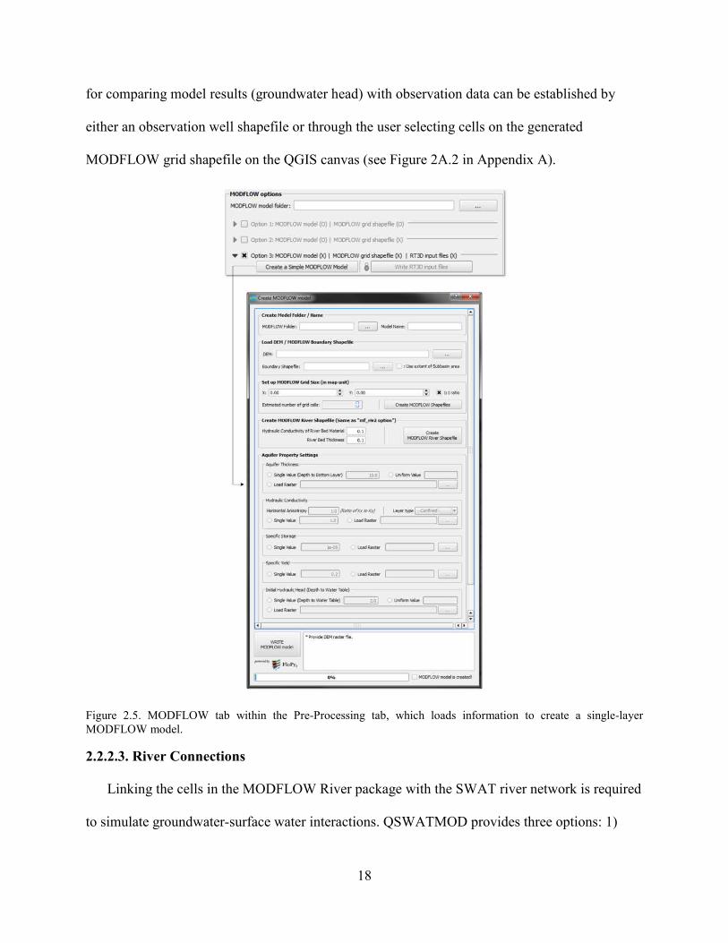
18

for comparing model results (groundwater head) with observation data can be established by

either an observation well shapefile or through the user selecting cells on the generated

MODFLOW grid shapefile on the QGIS canvas (see Figure 2A.2 in Appendix A).

Figure 2.5. MODFLOW tab within the Pre-Processing tab, which loads information to create a single-layer

MODFLOW model.

2.2.2.3. River Connections

Linking the cells in the MODFLOW River package with the SWAT river network is required

to simulate groundwater-surface water interactions. QSWATMOD provides three options: 1)

19

Use Only MODFLOW river package, 2) Use Only SWAT river network, and 3) Use Both

MODFLOW and SWAT (Figure 6d). For the first option, QSWATMOD extracts river cell

values (river stage, river bed conductance, river bottom elevation) from the MODFLOW River

package file (*.riv), and then writes these values into the attribute table of a new “mf_riv1.shp”

shapefile. For the second option, QSWATMOD creates the “mf_riv2.shp” by intersecting the

MODFLOW grid with the SWAT river network shapefile and then calculates the river cell

parameters for each river cell based on information provided by the SWAT river network (DEM,

stream length and width) and user inputs (thickness and hydraulic conductivity of river bed

material). For the third option, the existing MODFLOW river cells are compared to the SWAT

river network (Figure 2.6e) to determine if river cells should be added. The user then decides

which information will be used for the new cells.

Figure 2.6. River connections a) Option1: MODFLOW River Package; b) Option 2: River Parameters estimated

using SWAT River Network and User Inputs; c) Modified MODFLOW River Package; and d) Interface for

Identification of River Cells.

20

2.2.2.4. Linking Process

Through the linking process (Figure 2.4), the HRUs are disaggregated to create DHRUs,

which are then intersected with MODFLOW grid cells. MODFLOW river cells are identified

using the SWAT stream network or other river connection options (see Section 2.2.2.3), and the

set of river cells within each subbasin are identified for mapping groundwater-surface water

exchange rates from river cells to SWAT subbasin channels. These generated shapefiles are

used to create the four required SWAT-MODFLOW linkage files (“swatmf_dhru2hru.txt”,

“swatmf_dhru2grid.txt”, “swatmf_grid2dhru.txt”, and “swatmf_river2grid.txt”; see Bailey et al.,

2016), which are stored in the project folder.

For the Middle Bosque model, the second option for the MODFLOW model was used with

reading the origin coordinates of the subbasin shapefile. To identify the river cells, the “Use

ONLY MODFLOW river package” option was chosen. The time required by QSWATMOD to

create the DHRUs, the MODFLOW grid cells, identify the river cells and create the “river_grid”

shapefile, create the “hru_dhru” and “dhru_grid” shapefiles, and write the linkage files was 5.5 s,

6.2 s, 0.5 s, 297.7 s, and 4.8 s, respectively. A total of 12,366 DHRUs were created and 1,468

river cells were identified to link with the SWAT river network. In addition, the first

development option for the MODFLOW grid, and the second and third options of “Identify

River Cells” were tested (Table 2.2).

Table 2.2. Process time for QSWATMOD functions for the Middle Bosque River Watershed.

Process Processing Time

[Second]

Creating MODFLOW grid cells

- Import a grid shapefile and write MODFLOW

info.

- Create a grid shapefile and write MODFLOW

info.

4.5

5.5

Identifying River cells and create river_grid

- Use ONLY MODFLOW river package

- Use ONLY SWAT river network (additional

6.2

8.6

21

time)

- Use Both MODFLOW and SWAT (additional

time)

5.5

Checking MODFLOW inputs 0.5

Linking 297.7

Writing linkage files 4.8

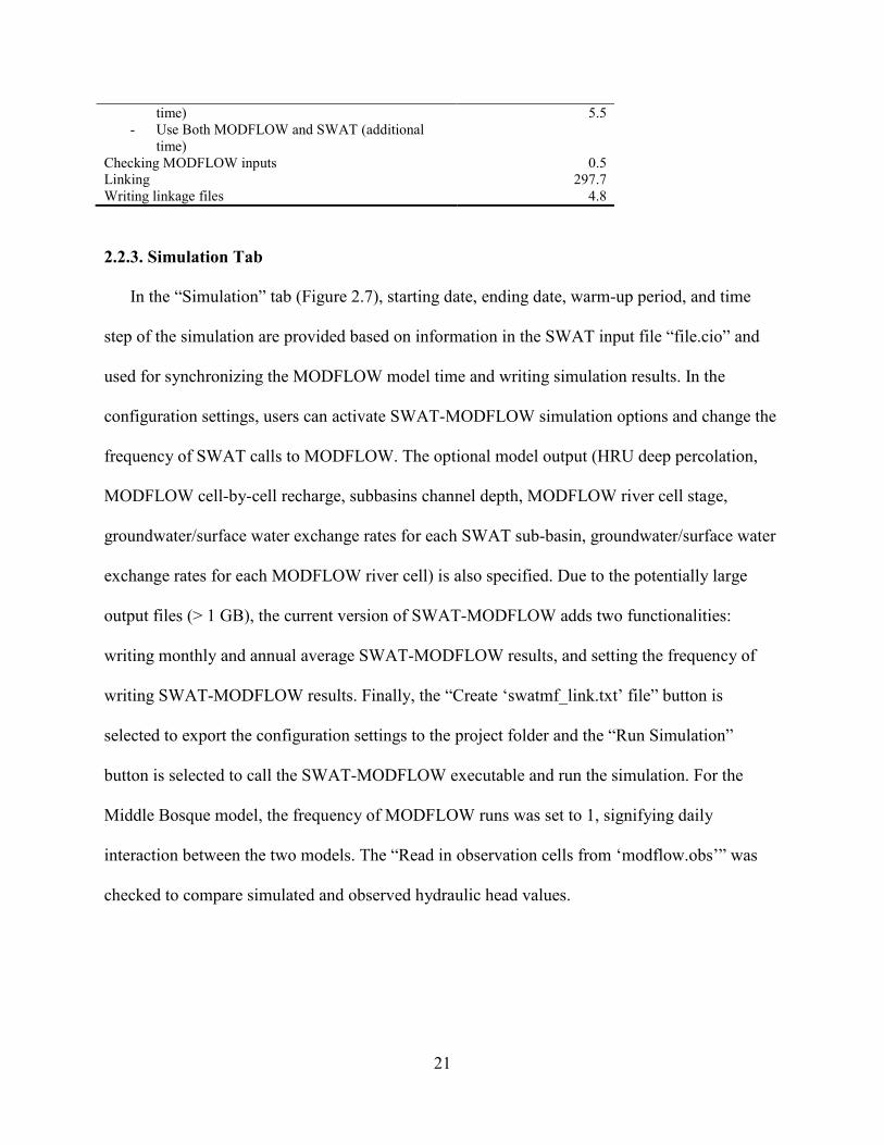
2.2.3. Simulation Tab

In the “Simulation” tab (Figure 2.7), starting date, ending date, warm-up period, and time

step of the simulation are provided based on information in the SWAT input file “file.cio” and

used for synchronizing the MODFLOW model time and writing simulation results. In the

configuration settings, users can activate SWAT-MODFLOW simulation options and change the

frequency of SWAT calls to MODFLOW. The optional model output (HRU deep percolation,

MODFLOW cell-by-cell recharge, subbasins channel depth, MODFLOW river cell stage,

groundwater/surface water exchange rates for each SWAT sub-basin, groundwater/surface water

exchange rates for each MODFLOW river cell) is also specified. Due to the potentially large

output files (> 1 GB), the current version of SWAT-MODFLOW adds two functionalities:

writing monthly and annual average SWAT-MODFLOW results, and setting the frequency of

writing SWAT-MODFLOW results. Finally, the “Create ‘swatmf_link.txt’ file” button is

selected to export the configuration settings to the project folder and the “Run Simulation”

button is selected to call the SWAT-MODFLOW executable and run the simulation. For the

Middle Bosque model, the frequency of MODFLOW runs was set to 1, signifying daily

interaction between the two models. The “Read in observation cells from ‘modflow.obs’” was

checked to compare simulated and observed hydraulic head values.

22

Figure 2.7. QSWATMOD interface for a) Simulation Tab; b) Configuration Settings (in “swatmf_link.txt” file).

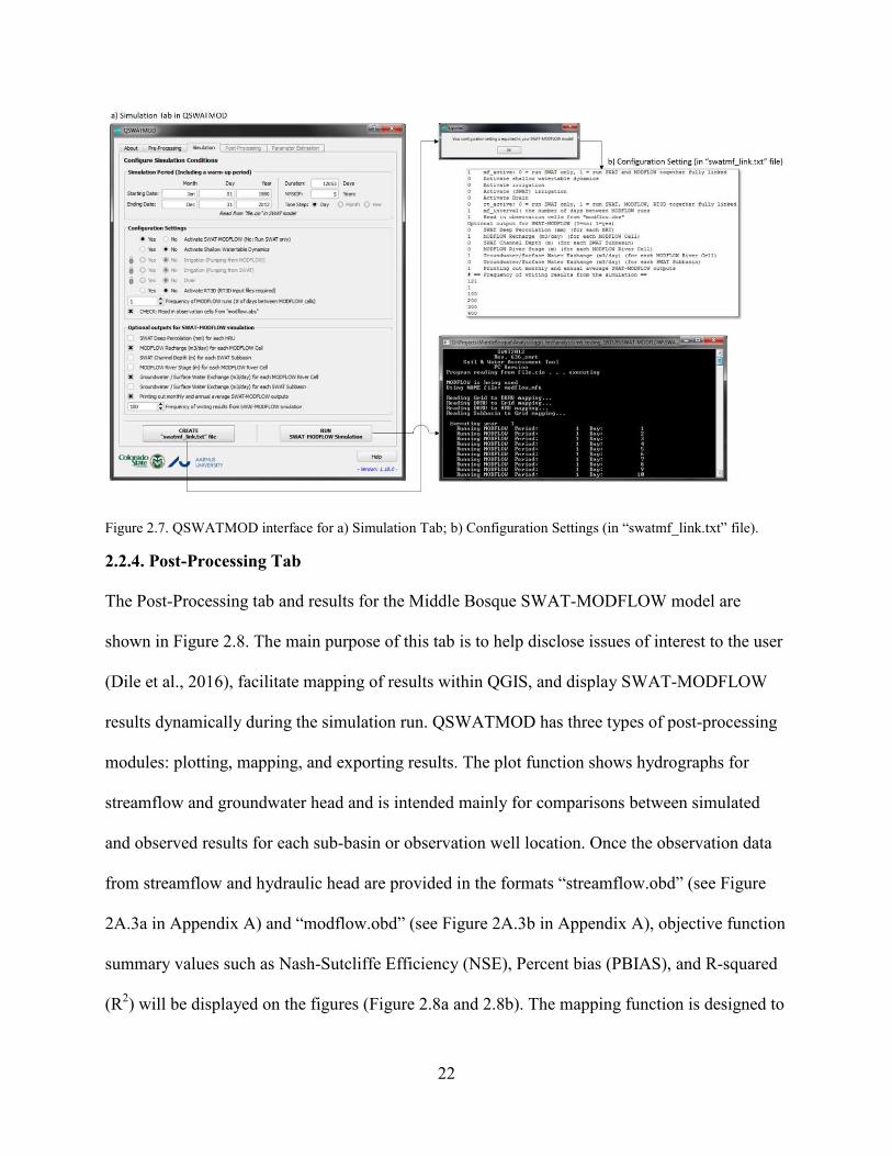
2.2.4. Post-Processing Tab

The Post-Processing tab and results for the Middle Bosque SWAT-MODFLOW model are

shown in Figure 2.8. The main purpose of this tab is to help disclose issues of interest to the user

(Dile et al., 2016), facilitate mapping of results within QGIS, and display SWAT-MODFLOW

results dynamically during the simulation run. QSWATMOD has three types of post-processing

modules: plotting, mapping, and exporting results. The plot function shows hydrographs for

streamflow and groundwater head and is intended mainly for comparisons between simulated

and observed results for each sub-basin or observation well location. Once the observation data

from streamflow and hydraulic head are provided in the formats “streamflow.obd” (see Figure

2A.3a in Appendix A) and “modflow.obd” (see Figure 2A.3b in Appendix A), objective function

summary values such as Nash-Sutcliffe Efficiency (NSE), Percent bias (PBIAS), and R-squared

(R2) will be displayed on the figures (Figure 2.8a and 2.8b). The mapping function is designed to

23

show maps of recharge (Figure 2.8c) and groundwater head (Figure 2.8d) on the QGIS canvas.

After users specify the period of visualization, the data are exported to a shapefile and stored in

its attribute table.

Figure 2.8. QSWATMOD interface for Post-processing tab, showing results from the Middle Bosque SWAT-

MODFLOW simulation.

Visualizing the spatially distributed patterns of surface and groundwater interactions,

watershed boundaries, and river networks for watersheds are performed using the “pyshp”

package (Figure 2.8e). Once users create the figures for the period of visualization, the figures

can be converted to a single video clip by selecting the “Save to Video” icon, according to the

“DPI” and “FPS” settings (see Video 2A.4 in Appendix A). The water balance option reads the

SWAT “output.std” file and uses precipitation, surface runoff, lateral flow, groundwater flow to

streams, deep percolation to groundwater, soil water, seepage from streams to the aquifer, and

groundwater volume to display a time series of water balance components (Figure 2.8f). Except

for spatially distributed groundwater head and recharge values, users can export all results to

24

text-formatted files, including simulated observed data and objective functions (see Figure 2A.5

in Appendix A).

2.3. Conclusion

QSWATMOD, a QGIS-based graphical user interface for SWAT-MODFLOW models, was

developed to provide an easy-to-use workflow for users preparing input data, configuring

simulation settings, and visualizing and interpreting results. QSWATMOD includes options for

using an existing MODFLOW or creating a new one, with a variety of options for linking

MODFLOW river cells with SWAT subbasins for groundwater-surface water interactions.

QSWATMOD was applied to the Middle Bosque River Watershed in Texas to demonstrate the

linkage between existing SWAT and MODFLOW. The visualization of the results from the

SWAT-MODFLOW simulation is beneficial in displaying model output and comparing with

observed streamflow and groundwater data. QSWATMOD can be a valuable tool in assisting

users to create and manage SWAT-MODFLOW projects, allowing coupled surface

water/groundwater models to become more accessible to a broader hydrologic modelling

community.

25

REFERENCES

Bailey, R., Rathjens, H., Bieger, K., Chaubey, I. and Arnold, J. (2017) 'SWATMOD-Prep:

graphical user interface for preparing coupled SWAT-MODFLOW simulations’, Journal of

the American Water Resources Association, 53(2), 400-410, available:

http://dx.doi.org/10.1111/1752-1688.12502.





Bakker, M., Post, V., Langevin, C.D., Hughes, J.D., White, J.T., Starn, J.J., and Fienen, M.N.,

2016, FloPy v3.2.6: U.S. Geological Survey Software Release, 19 March 2017,

http://dx.doi.org/10.5066/F7BK19FH

Barthel, R. and Banzhaf, S., 2016. Groundwater and surface water interaction at the regional-

scale–A review with focus on regional integrated models. Water Resources Management,

30(1), pp.1-32, available: https://doi.org/10.1007/s11269-015-1163-z

Camporese, M., Paniconi, C., Putti, M. and Orlandini, S., 2010. Surface‐subsurface flow

modeling with path‐based runoff routing, boundary condition‐based coupling, and

assimilation of multisource observation data. Water Resources Research, 46(2), available:

https://doi.org/10.1029/2008WR007536.

Cannata, S.L., 1988. Hydrogeology of a portion of the Washita Prairie Edwards aquifer: central

Texas (Doctoral dissertation, Baylor University).

26

Diersch, H.J.G., 2013. FEFLOW: finite element modeling of flow, mass and heat transport in

porous and fractured media. Springer Science & Business Media, available:

https://doi.org/10.1007/978-3-642-38739-5.

Dile, Y.T., Daggupati, P., George, C., Srinivasan, R. and Arnold, J., 2016. Introducing a new

open source GIS user interface for the SWAT model. Environmental modelling & software,

85, pp.129-138, available: https://doi.org/10.1016/j.envsoft.2016.08.004.

Hipp, D. R., Kennedy, D., Mistachkin, J., (2015) SQLite (Version 3.8.10.2) [Computer

software]. SQLite Development Team. Retrieved 2015-06-15. Available from

<https://www.sqlite.org/src/info/2ef4f3a5b1d1d0c4>

Hunter, J.D. (2007) 'Matplotlib: A 2D graphics environment', Computing in Science &

Engineering, 9(3), 90-95, available: http://dx.doi.org/10.1109/mcse.2007.55.

Kim, N.W., Chung, I.M., Won, Y.S. and Arnold, J.G., 2008. Development and application of the

integrated SWAT–MODFLOW model. Journal of hydrology, 356(1), pp.1-16, available:

https://doi.org/10.1016/j.jhydrol.2008.02.024.

Markstrom, S.L., Niswonger, R.G., Regan, R.S., Prudic, D.E. and Barlow, P.M., 2008.

GSFLOW-Coupled Ground-water and Surface-water FLOW model based on the integration

of the Precipitation-Runoff Modeling System (PRMS) and the Modular Ground-Water Flow

Model (MODFLOW-2005) (No. 6-D1). Geological Survey (US).

McKinney, W., 2010, June. Data structures for statistical computing in python. In Proceedings of

the 9th Python in Science Conference (Vol. 445, pp. 51-56). Austin, TX: SciPy.

Neitsch, S. L., Arnold, J. G., Kiniry, J. R., & Williams, J. R. (2011). Soil and water assessment

tool theoretical documentation version 2009. Texas Water Resources Institute, available:

http://hdl.handle.net/1969.1/128050.

27

Nielsen, A., Bolding, K., Hu, F. and Trolle, D., 2017. An open source QGIS-based workflow for

model application and experimentation with aquatic ecosystems. Environmental Modelling &

Software, 95, pp.358-364, available: https://doi.org/10.1016/j.envsoft.2017.06.032.

Oki, T. and Kanae, S. (2006) 'Global hydrological cycles and world water resources', Science,

313(5790), 1068-1072, available: http://dx.doi.org/10.1126/science.1128845.

Park, C., Lee, J., Koo, M., 2013. Development of a fully-distributed daily hydrologic feedback

model addressing vegetation, land cover, and soil water dynamics (VELAS). J. Hydrol. 493,

43–56. http://dx.doi.org/10.1016/j.jhydrol.2013.04.027.

Pearson, D.K., 2013. Geologic database of Texas: Project summary, Database contents, and

user’s guide: Document prepared by the US Geological Survey for the Texas Water

Development Board, Austin, 22 p.

Poeter, E.P. and Hill, M.C., 1998. Documentation of UCODE, a computer code for universal

inverse modeling. DIANE Publishing, available: https://doi.org/10.1016/s0098-

3004(98)00149-6.

Sophocleous, M., 2002. Interactions between groundwater and surface water: the state of the

science. Hydrogeology journal, 10(1), pp.52-67, available: https://doi.org/10.1007/s10040-

001-0170-8.

Karl, T.R. ed., 2009. Global climate change impacts in the United States. Cambridge University

Press.

Therrien, R., McLaren, R.G., Sudicky, E.A. and Panday, S.M., 2010. HydroGeoSphere: a three-

dimensional numerical model describing fully-integrated subsurface and surface flow and

solute transport. Groundwater Simulations Group, University of Waterloo, Waterloo, ON.

28

Vorosmarty, C.J., Green, P., Salisbury, J. and Lammers, R.B. (2000) 'Global water resources:

Vulnerability from climate change and population growth', Science, 289(5477), 284-288,

available: http://dx.doi.org/10.1126/science.289.5477.284.

Winter, T.C., 1998. Ground water and surface water: a single resource (Vol. 1139). DIANE

Publishing Inc.

29

CHAPTER 3

QUANTIFYING EFFECT OF DECADAL AND EXTREME CLIMATE EVENTS ON

WATERSHED WATER RESOURCES AND FLUXES USING SWAT-MODFLOW

Highlights

Combined use of groundwater resources and surface water resources is essential to provide

reliable water supply in the coming decades. This study provides the methodology whereby

available surface water and groundwater resources and the impact of climate events on these

resources can be quantified in semi-arid regions using the coupled SWAT-MODFLOW

modelling code. Methodology is demonstrated for the Middle Bosque watershed (471 km2) in the

Texas-Gulf region of central Texas, which is subject to both major drought and flooding

conditions. Model results are tested against both streamflow and groundwater levels. Results

show strong spatio-temporal variability of groundwater head, recharge to the water table,

surface-subsurface exchange flow rates, and other watershed water balance components.

Recharge rates are highest along the river corridor, with rates up to 221 mm/year, and water table

levels can fluctuate up to 7 m. Results from interactions between groundwater and surface water

show that the majority of surface - subsurface interactions is groundwater discharge to the stream,

with a few locations where stream water seeps to the aquifer. Extreme drought conditions result

in approximately a 50% decrease in streamflow, but only a 0.05% decrease in groundwater levels

near streams. Lateral flow and soil water decrease by over 50%, but groundwater flow to streams

only decreases by 2%. For intense storms (20 inches), streamflow increases by 2,000%, but

groundwater levels only by 0.4%, although the change persists much longer (years) than the

change in streamflow. Surface runoff and soil deep percolation are affected the most, followed

30

stream seepage, lateral flow, and groundwater flow to streams. Pre-conditions (e.g. soil water

content) has a significant impact on the duration of drought/storm impact on water balance

components. Results enhance understanding regarding the spatio-temporal patterns of system-

response variables and water balance components in watersheds, which can aid decisions about

alternative management strategies in the areas of landuse change, climate change, water

allocation, pollution control and groundwater development scenarios.

3.1. Introduction

The shortage of freshwater supply is one of the most critical and global issues facing society

currently and within the coming decades. As groundwater becomes a more significant resource

for drinking water and irrigation water in many regions worldwide and also affects important

ecological functions (Dams et al., 2012), conjunctive management of surface water and

groundwater within a watershed system becomes important (Wrachien and Fasso, 2002;

Cosgrove and Johnson, 2005; Liu et al., 2013; Singh et al., 2015), particularly during periods of

water scarcity. In addition to quantifying the time-dependent volumes of both surface water and

groundwater, estimating the water fluxes between storage components (e.g. stream channels,

soils, aquifer) of the watershed is also important for understanding trends in storage change. The

impact of changes in climate patterns, climate events, population growth, and land use on

watershed water resources may also be significant (Postel et al., 1996; Cosgrove and Rijsberman,

2000; Vorosmarty et al., 2000; Döll et al., 2003; Oki and Kanae, 2006; Murray et al, 2012), and

thus should also be assessed to assist with future water management.

A variety of methods have been used to quantify water resources for watersheds, river basins,

or other geographical areas. These techniques include lumped water balance hydrologic models

31

over large geographical regions and global scales (Alcamo et al., 1997; Döll et al., 2003; Alcamo

et al., 2003; Wada et al., 2010), the use of satellite observations such as with GRACE (Gravity

Recovery and Climate Experiment) (Rodell and Famiglietti, 2003; Rodell et al., 2007;

Longuevergne et al., 2010; Famiglietti et al., 2011; Feng et al., 2013; Voss et al., 2013), and

physically-based spatially-distributed hydrologic models. Whereas large-scale lumped models

neglect groundwater storage, GRACE results often are limited to estimating changes in

groundwater storage, become uncertain at small spatial scales (less than a few hundred km), and

are dependent on the accuracy in accounting for soil moisture change. In addition, changes in

surface water storage are difficult to estimate.

Physically-based, spatially-distributed coupled land surface/subsurface hydrologic models

such as SWAT (Arnold et al., 1998); CATHY (Camporese et al., 2009), ParFlow (Kollet and

Maxwell, 2006), GSFLOW (Markstrom et al., 2008), and SWAT-MODFLOW (Bailey et al.,

2016) can be used to estimate components of groundwater and surface water storage. Model

applications range from global scale (de Graaf et al., 2015; de Graaf et al., 2017), to continental

scale (Schuol et al., 2008; Abbaspour et al., 2015; Maxwell et al., 2015), to river basins and

catchments (Gauthier et al, 2009; Perrin et al., 2012; Morway et al., 2013; Tanvir Hassan et al.,

2014; Tian et al., 2015; Bailey et al., 2016). Whereas the global-scale and continental-scale

models provide global trends in groundwater supply, results are neither accurate enough nor

resolved enough to assist in conjunctively managing groundwater and surface water resources at

the regional scale. Smaller-scale studies often focus on fluxes (Perrin et al., 2012; Tanvir Hassan

et al., 2014; Bailey et al., 2016) and hydrologic responses to management practices (Morway et

al., 2013; Tian et al., 2015), rather than an assessment of stored volumes of groundwater and

surface water through decadal periods, which are required to assist with water management.

32

The effect of climate on water storage and water fluxes within a watershed setting should

also be estimated for regional-scale water management of both groundwater and surface water.

Numerous studies have used groundwater models, land surface models, and coupled land

surface/subsurface models to assess the impact of climate on water storage, with an emphasis

placed on future climate scenarios. As examples, Scibek and Allen (2006) and Scibek et al.,

(2007) used Global Circulation Model (GCM) forcing to estimate recharge, groundwater levels,

and groundwater surface-water interactions through the year 2099 in British Columbia, Canada,

using MODFLOW. Woldeamlak and de Smedt (2007) used MODFLOW to estimate impact of

future (2050-2099) wet and dry climate scenarios on a 575 km2 groundwater system in Belgium.

Goderniaux et al. (2009), also for Belgium, applied HydroGeoSphere to determine the impact of

climate on groundwater reserves and surface water flow through 2080 under six climate model

scenarios. Ali et al. (2012) assess climate scenario impact on groundwater levels in Australia for

the year 2030, and Meixner et al. (2016) quantified the effect of climate change on groundwater

recharge in the western United States. The SWAT model has been used extensively to estimate

the impact of future climate on patterns of land surface fluxes (water yield, surface flow,

groundwater recharge, lateral flow) for Ontario (Jyrkama and Sykes, 2007), California (Ficklin et

al., 2009), Iran (Vaghefi et al., 2013), Africa (Faramarzi et al., 2013), Australia (Tweed et al.,

2009; Brown et al., 2015), and globally (Haddeland et al., 2010). Surfleet and Tullos (2014)

used GSFLOW to investigate future climate change impact on surface runoff, streamflow, and

overland flow for a 4700 km2 area in Oregon.

These studies, however, focus on long-term climate impact rather than near-term or current

climate events that often pose more immediate stress on regional water supply or region

infrastructure. Such severe climate events include drought, multi-year drought, and extreme

33

flooding events. The impact of these climate events on surface water storage, groundwater

storage, and watershed fluxes (recharge, groundwater-surface water interaction, lateral flow,

surface runoff) should be quantified under a variety of event magnitudes. This will assist in

understanding short-term and long-term hydrologic response of a watershed system to these

events, and also assist regional water managers in forecasting water supply.

In this study, the recently developed SWAT-MODFLOW modelling code of Bailey et al.

(2016) is used to quantify surface water resources, groundwater resources, and water flux rates

between storage components as impacted by multi-decadal climate patterns and extreme climate

events (major drought, storms) in a semi-arid regional-scale watershed. The Middle Bosque

watershed (area of 471 km2) in the Texas-Gulf region of central Texas, prone to both severe

drought and intense storms, is used as an example. Spatio-temporal patterns of groundwater

hydraulic head, recharge as calculated deep percolation, groundwater–surface water interaction

and water resources availability (global water balance) are explored throughout the watershed

during the (1980-2012) period using the SWAT-MODFLOW model. Using the tested model, the

impact of severe drought, experienced during 1999, on hydrologic responses and watershed

water storage, will be quantified. The impact of high-rainfall storm events also will be assessed,

using hypothetical storm events based on the largest recorded thunderstorm events in central

Texas. Results will aid in understanding hydrological responses to decadal and short-term

climatic events and thereby assist with water management for the region in conjunctively using

groundwater and surface water.

34

3.2. Methodology

3.2.1. Study area

The Middle Bosque River Watershed (MBRW) includes portions of McLennan, Bosque, and

Coryell counties (Figure 3.1). There are sedimentary rocks from the Washita and Fredericksburg

Groups of early Cretaceous, and Comanchean age. The formation of the Washita Group is the

Georgetown Limestone including Main Street, Pawpaw, Weno, Denton, Fort Worth, Duck Creek,

and Kiamichi members (Cannata, 1988; Pearson, 2007). The two formations of the

Fredericksburg Group, the Edwards Limestone and Comanche Peak Limestone, are used in the

study area. The altitude of the study region varies from 367 m at the highest point on the

northwestern edge to 161 m on the eastern edge. The MBRW is predominantly comprised of

either pasture (65.4 % of area) or farms (20.3 % of area), with minor land covers of forests (8.5 %

of area), and residential areas (3.2% of area) (USGS, 2007). The Middle Bosque River dissects

the Edwards Limestone and has therefore produced major groundwater discharge and stream

seepage areas (Cannata, 1988).

35

Figure 3.1. Location map showing the position of the study area within McLennan, Bosque, and Coryell Counties,

Texas. Physiographic map showing the provinces composing and surrounding the study area. These include the

Washita Prairie and Lampasas Cut Plain.

The climate of the study area is characterized by semi-arid, with long hot summers and brief

mild winters (Figure 3.2). The warmest month, August, has an average maximum temperature of

36.5 Co while the coldest month, January, has an average minimum temperature of 2.8 C

o (U.S.

Depth. of Commerce, Weather Bureau, 1980 -2012). The annual precipitation ranges from about

602 to 1560 mm/year. The wettest months of a normal year are May and October with average

precipitation amounts of 118 and 110 mm respectively, while the driest months are July and

December with average precipitation amounts of 54 and 48 mm respectively. Monthly twenty-

two-year averages for temperature (max, mean, and min) and precipitation (mean) are shown in

Figure 3.2.

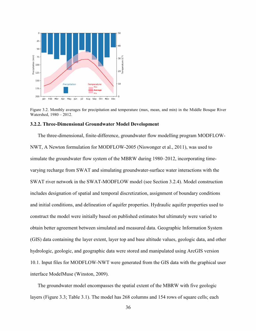
36

Figure 3.2. Monthly averages for precipitation and temperature (max, mean, and min) in the Middle Bosque River

Watershed, 1980 – 2012.

3.2.2. Three-Dimensional Groundwater Model Development

The three-dimensional, finite-difference, groundwater flow modelling program MODFLOW-

NWT, A Newton formulation for MODFLOW-2005 (Niswonger et al., 2011), was used to

simulate the groundwater flow system of the MBRW during 1980–2012, incorporating time-

varying recharge from SWAT and simulating groundwater-surface water interactions with the

SWAT river network in the SWAT-MODFLOW model (see Section 3.2.4). Model construction

includes designation of spatial and temporal discretization, assignment of boundary conditions

and initial conditions, and delineation of aquifer properties. Hydraulic aquifer properties used to

construct the model were initially based on published estimates but ultimately were varied to

obtain better agreement between simulated and measured data. Geographic Information System

(GIS) data containing the layer extent, layer top and base altitude values, geologic data, and other

hydrologic, geologic, and geographic data were stored and manipulated using ArcGIS version

10.1. Input files for MODFLOW-NWT were generated from the GIS data with the graphical user

interface ModelMuse (Winston, 2009).

The groundwater model encompasses the spatial extent of the MBRW with five geologic

layers (Figure 3.3; Table 3.1). The model has 268 columns and 154 rows of square cells; each

37

cell measures 150 m by 150 m (22,500 m2). The grid was generated in the USA Contiguous

Albers equal area conic coordinate system (North American Datum of 1983, units: meter). The

grid origin is located at the northwest corner of the model area (easting -169,236.1 m, northing

952,645.5 m). In general, grid cells were initially specified as active where a hydrological unit

from the SWAT model is present and inactive where it is absent. Hydraulic properties of the

hydrogeologic units were specified using the Upstream Weighting (UPW) Package of

MODFLOW-NWT (Niswonger et al., 2011). In the UPW Package, each layer may be specified

as either confined or convertible. Cells in layers specified as confined are assumed to have an

unvarying saturated thickness, regardless of the calculated head, and do not become inactive if

the calculated head is below the cell bottom. Cells in layers specified as convertible are

simulated as having head-dependent saturated thickness when the calculated head is below the

cell top, and these cells are deactivated if the head is below the cell bottom. Each of the layers

except the Comanche limestone is unconfined in at least part of its extent (see Figure 3). The

model layers representing a confining unit, which is composed primarily of fine-grained

materials (Cannata, 1988) that are not expected to drain substantially as heads decline, were

specified as confined.

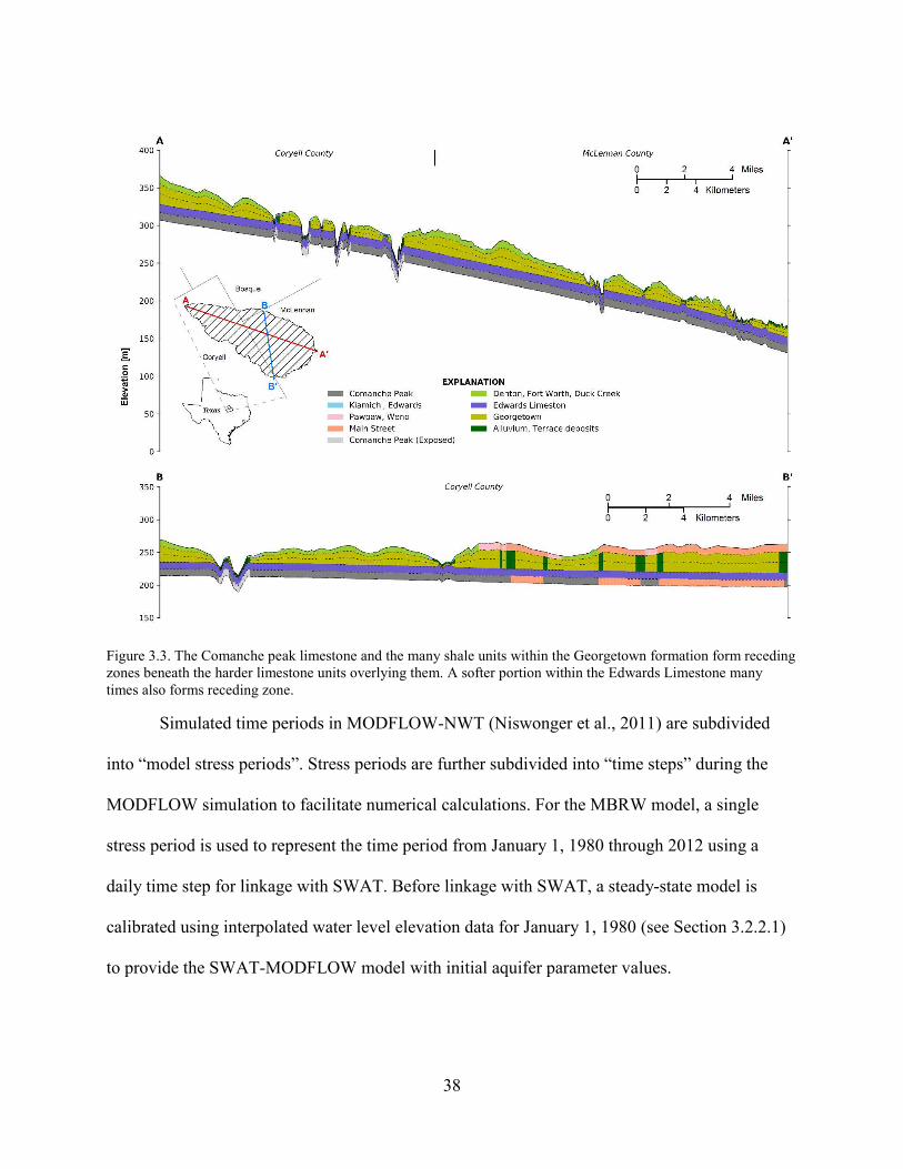
38

Figure 3.3. The Comanche peak limestone and the many shale units within the Georgetown formation form receding

zones beneath the harder limestone units overlying them. A softer portion within the Edwards Limestone many

times also forms receding zone.

Simulated time periods in MODFLOW-NWT (Niswonger et al., 2011) are subdivided

into “model stress periods”. Stress periods are further subdivided into “time steps” during the

MODFLOW simulation to facilitate numerical calculations. For the MBRW model, a single

stress period is used to represent the time period from January 1, 1980 through 2012 using a

daily time step for linkage with SWAT. Before linkage with SWAT, a steady-state model is

calibrated using interpolated water level elevation data for January 1, 1980 (see Section 3.2.2.1)

to provide the SWAT-MODFLOW model with initial aquifer parameter values.

39

3.2.2.1. Initial Head Interpolation for Groundwater model

Groundwater level data from 28 observations wells and a geostatistical method which is

based on Regionalized Variable theory (RVT) (Matheron, 1963) were used to interpolate initial

groundwater head elevation in the study area The concept of the theory is that interpolation from

points in space should not be based on smooth continuous object, but based on a stochastic

model that takes into consideration the various trend original set of points. The theory considers

there are three types of relationships within any dataset and they are as follows:

- structural part (trend),

- correlated variation, and

- uncorrelated variation or noise.

The RVT is also based on random functions and the measurements are assumed to be a

realization of a particular random function for a given position, some restrictions have to be

made on the data. These restrictions are called stationarity hypothesis (Journel and Huigbregts,

1978). The order of the stationarity hypothesis will depend on the order of the statistical

moments required to be stationary. Thus, when second order stationarity is required, at least the

first and second order moments (mean, variance and covariance) must be stationary.

Therefore, to make proper use of Geostatistics, at least the intrinsic hypothesis must be

fulfilled (Journel and Huigbregts, 1978). The intrinsic hypothesis requires that the mean and the

semi-variance depend strictly on the separation distance between samples and not on the

coordinate position of the data. When the intrinsic hypothesis cannot be satisfied it is because the

data has some trend which must be removed before the data can be adequately analysed through

Geostatistics (Vieira et al., 1983). One very simple way to remove a trend is by fitting a trend

surface by least squares and subtracting it from the original data, generating a new variable

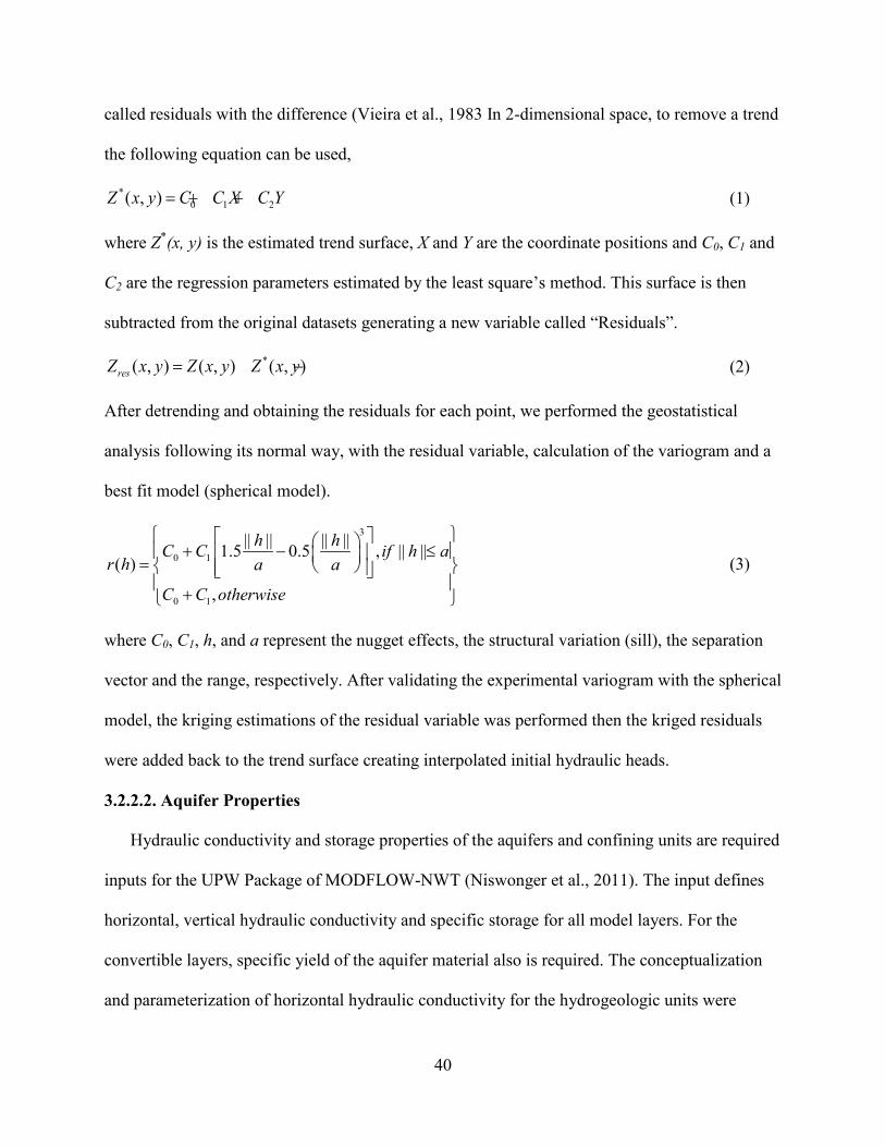
40

called residuals with the difference (Vieira et al., 1983 In 2-dimensional space, to remove a trend

the following equation can be used,

*

0 1 2( , )Z x y C C X C Y= + + (1)

where Z*(x, y) is the estimated trend surface, X and Y are the coordinate positions and C0, C1 and

C2 are the regression parameters estimated by the least square’s method. This surface is then

subtracted from the original datasets generating a new variable called “Residuals”.

*( , ) ( , ) ( , )resZ x y Z x y Z x y= − (2)

After detrending and obtaining the residuals for each point, we performed the geostatistical

analysis following its normal way, with the residual variable, calculation of the variogram and a

best fit model (spherical model).

3

0 1

0 1

|| || || ||1.5 0.5 , || ||

( )

,

h hC C if h a

r h a a

C C otherwise

+ − ≤ =

+

(3)

where C0, C1, h, and a represent the nugget effects, the structural variation (sill), the separation

vector and the range, respectively. After validating the experimental variogram with the spherical

model, the kriging estimations of the residual variable was performed then the kriged residuals

were added back to the trend surface creating interpolated initial hydraulic heads.

3.2.2.2. Aquifer Properties

Hydraulic conductivity and storage properties of the aquifers and confining units are required

inputs for the UPW Package of MODFLOW-NWT (Niswonger et al., 2011). The input defines

horizontal, vertical hydraulic conductivity and specific storage for all model layers. For the

convertible layers, specific yield of the aquifer material also is required. The conceptualization

and parameterization of horizontal hydraulic conductivity for the hydrogeologic units were

41

summarized in Table 1. Note that the conceptualization schemes described in the table

incorporate simplifying assumptions. The Washita Prairie Edwards aquifer is an unconfined

aquifer with the water table commonly less than 20 feet below the surface (Cannata, 1988). The

aquifer is contained in the Edwards and Georgetown Limestones with the Comanche Peak

Limestone forming the lower confining unit (Fig. 3.1 and 3.3). Where major streams completely

dissect the Edwards Limestone, additional boundaries are formed where large amounts of water

are lost through groundwater discharge to streams.

Parameterization of the hydraulic conductivity distributions for the Georgetown Limestone,

Edwards Limestone, and Comanche Peak Limestone (Cannata, 1988) used the zoned

parameterization approach as shown in Fig. 1 and 3. Georgetown Limestone is divided into

various Rock Units: Kc (Comanche Peak), Kdfdc (Denton, Fort Worth, and Duck Creek), Kked

(Kiamichi, Edwards), Kms (Mainstreet), Kpw (Pawpaw, Weno), Qal (Alluvium), and Qt

(Terrace deposits) (Cannata, 1988; Pearson, 2013) (Table 1). The Texas geologic map shapefile

(Pearson, 2013) and published estimates (Cannata, 1988) were used to assign a parameter

distribution to the five layers. Hydrogeologic units represented as confined were assigned values

of specific storage; units represented as convertible from confined to unconfined conditions were

assigned values of both specific storage and specific yield. A specific-storage value of the

confining unit was determined from published estimates in model input and specific-yield values

were estimated by PEST using the SWAT-MODFLOW and their spatial distribution were

determined for each hydrogeologic unit zone.

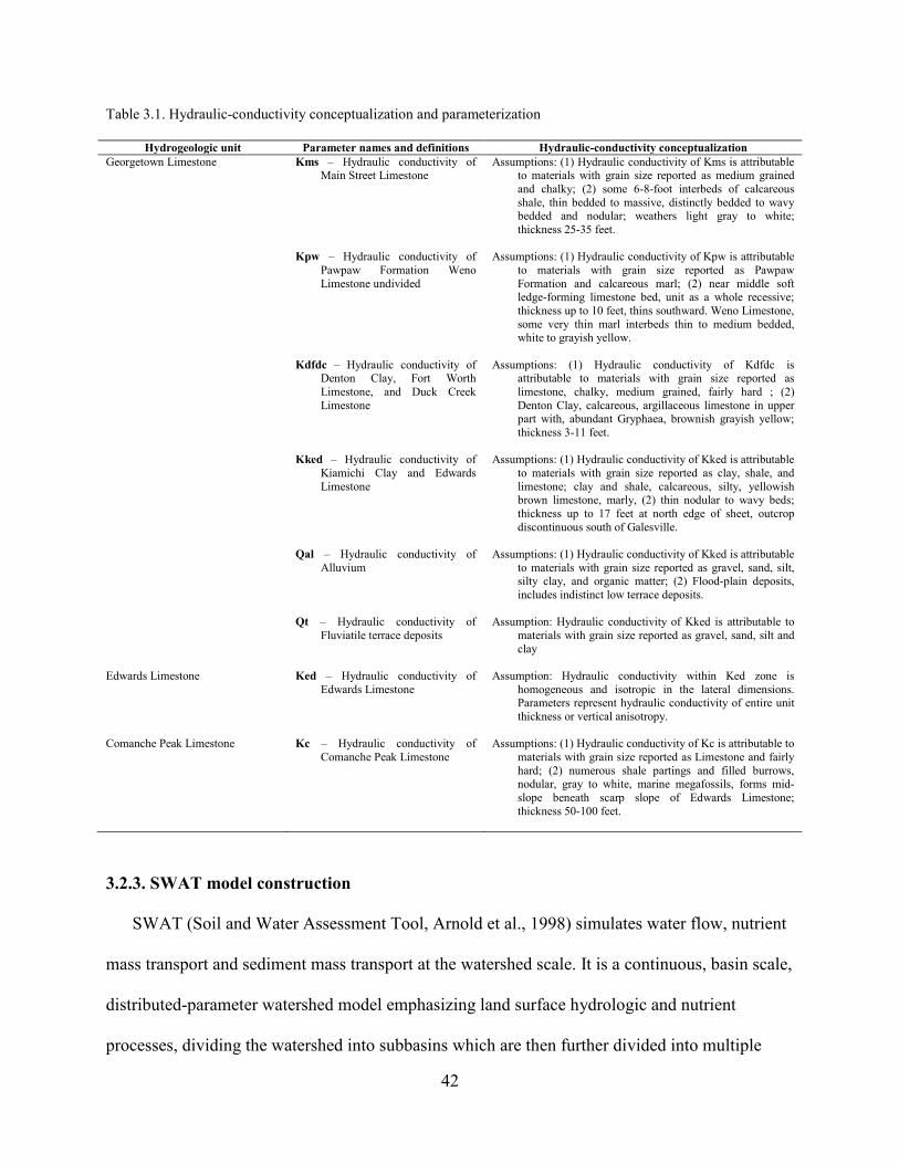
42

Table 3.1. Hydraulic-conductivity conceptualization and parameterization

Hydrogeologic unit Parameter names and definitions Hydraulic-conductivity conceptualization

Georgetown Limestone Kms – Hydraulic conductivity of Main Street Limestone

Assumptions: (1) Hydraulic conductivity of Kms is attributable to materials with grain size reported as medium grained

and chalky; (2) some 6-8-foot interbeds of calcareous

shale, thin bedded to massive, distinctly bedded to wavy bedded and nodular; weathers light gray to white;

thickness 25-35 feet.

Kpw – Hydraulic conductivity of

Pawpaw Formation Weno

Limestone undivided

Assumptions: (1) Hydraulic conductivity of Kpw is attributable

to materials with grain size reported as Pawpaw

Formation and calcareous marl; (2) near middle soft ledge-forming limestone bed, unit as a whole recessive;

thickness up to 10 feet, thins southward. Weno Limestone,

some very thin marl interbeds thin to medium bedded, white to grayish yellow.

Kdfdc – Hydraulic conductivity of Denton Clay, Fort Worth

Limestone, and Duck Creek

Limestone

Assumptions: (1) Hydraulic conductivity of Kdfdc is attributable to materials with grain size reported as

limestone, chalky, medium grained, fairly hard ; (2)

Denton Clay, calcareous, argillaceous limestone in upper part with, abundant Gryphaea, brownish grayish yellow;


Kked – Hydraulic conductivity of

Kiamichi Clay and Edwards

Limestone

Assumptions: (1) Hydraulic conductivity of Kked is attributable

to materials with grain size reported as clay, shale, and

limestone; clay and shale, calcareous, silty, yellowish brown limestone, marly, (2) thin nodular to wavy beds;

thickness up to 17 feet at north edge of sheet, outcrop

discontinuous south of Galesville.

Qal – Hydraulic conductivity of

Alluvium

Assumptions: (1) Hydraulic conductivity of Kked is attributable

to materials with grain size reported as gravel, sand, silt, silty clay, and organic matter; (2) Flood-plain deposits,

includes indistinct low terrace deposits.

Qt – Hydraulic conductivity of

Fluviatile terrace deposits

Assumption: Hydraulic conductivity of Kked is attributable to

materials with grain size reported as gravel, sand, silt and

clay

Edwards Limestone Ked – Hydraulic conductivity of

Edwards Limestone

Assumption: Hydraulic conductivity within Ked zone is

homogeneous and isotropic in the lateral dimensions. Parameters represent hydraulic conductivity of entire unit

thickness or vertical anisotropy.

Comanche Peak Limestone Kc – Hydraulic conductivity of

Comanche Peak Limestone

Assumptions: (1) Hydraulic conductivity of Kc is attributable to

materials with grain size reported as Limestone and fairly

hard; (2) numerous shale partings and filled burrows, nodular, gray to white, marine megafossils, forms mid-

slope beneath scarp slope of Edwards Limestone;


3.2.3. SWAT model construction

SWAT (Soil and Water Assessment Tool, Arnold et al., 1998) simulates water flow, nutrient

mass transport and sediment mass transport at the watershed scale. It is a continuous, basin scale,

distributed-parameter watershed model emphasizing land surface hydrologic and nutrient

processes, dividing the watershed into subbasins which are then further divided into multiple

43

unique combinations (Hydrologic Response Units HRUs) of land use, soil type and topographic

slope for which detailed water, nutrient and sediment mass balance calculations are performed.

The SWAT model can also quantify hydrological components of water resources, e.g. surface

runoff and deep aquifer recharge (blue water), soil water (green water) and actual

evapotranspiration (green water).

A pre-calibrated SWAT model for the MBRW was used for the SWAT-MODFLOW

simulation. In the SWAT model, a total of 69 subbasins were delineated based on a Digital

Elevation Model (DEM). No thresholds were set for the HRU definition, resulting in 1,693

HRUs. Seven different land covers (Agricultural Land-generic, Forest-deciduous, Forest-mixed,

Pasture, Residential-Low Density, Water, and Wetlands-forested) were included.

3.2.4. SWAT-MODFLOW Model

A SWAT-MODFLOW was created using the constructed MODFLOW and SWAT

models. The process of linking SWAT HRUs and subbasins with MODFLOW grid cells and

River cells is described in Bailey et al. (2016). The linkage process creates text files containing

the information necessary to convert model output from HRUs to geographically located

disaggregated Hydrologic Response Units (DHRUs), from DHRs to MODFLOW grid cells, and

from SWAT sub-basin rivers to MODFLOW River cells. With the linkage files, the SWAT

model can pass HRU-calculated soil deep percolation as recharge to the grid cells of

MODFLOW, and then the MODFLOW model passes MODFLOW-calculated groundwater–

surface water interaction fluxes (either groundwater discharge or stream seepage to the subbasin

stream channels of SWAT. With this approach, SWAT calculates the volume of overland flow

and soil lateral flow to streams, MODFLOW calculates the volume of groundwater discharge to

streams, and SWAT routes the water through the stream network of the watershed.

44

Groundwater–surface water interaction is simulated using the River package of MODFLOW,

with Darcy’s law used to calculate the volumetric flow of water Qleak [L3/T] through the cross-

sectional flow area between the aquifer and the stream channel

( )str gw

leak bed str str

bed

h hQ K L P

Z

− = × ×

(4)

where Kbed is river bed hydraulic conductivity [L/T], Lstr is the length of the stream [L], Pstr is the

wetted perimeter of the stream [L], hstr is river stage [L], hgw is the hydraulic head of

groundwater [L], and zbed is the thickness of the river bed [L]. Qleak is negative if groundwater

flows to the river (i.e. groundwater hydraulic head hgw is above the river stage hstr), and positive

if river water seeps into the aquifer. These calculations are performed for any grid cell through

which a stream passes, with cells identified initially through spatial intersection of the SWAT

stream network with MODFLOW grid cells.

SWAT-MODFLOW is a single compileable FORTRAN code, in which MODFLOW is

called by the main SWAT code, thereby replacing the original SWAT groundwater module.

Upon reading input data for both the SWAT and MODFLOW models, the simulation runs

through the repeated daily process of SWAT HRU calculations, passing data to MODFLOW,

running MODFLOW, passing data to SWAT and routing water through the watershed’s stream

network, through the end of the simulation.

3.2.5. Parameter estimation for the coupled SWAT-MODFLOW model

Parameter estimation for hydrologic models can be accomplished using a variety of methods.

SWAT-CUP (SWAT Calibration Uncertainty Procedures) has been used extensively for SWAT

model calibration and uncertainty analysis and includes Generalized Likelihood Uncertainty

Estimation (GLUE) (Beven and Binley, 1992), Parameter Solution (ParaSol) (van Griensven and

Meixner, 2006), and Sequential Uncertainty FItting (SUFI-2) (Abbaspour, et al., 2007). Many

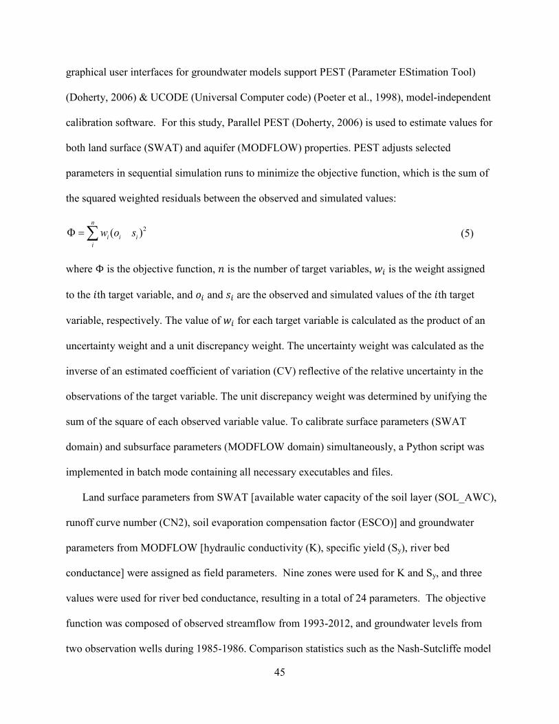
45

graphical user interfaces for groundwater models support PEST (Parameter EStimation Tool)

(Doherty, 2006) & UCODE (Universal Computer code) (Poeter et al., 1998), model-independent

calibration software. For this study, Parallel PEST (Doherty, 2006) is used to estimate values for

both land surface (SWAT) and aquifer (MODFLOW) properties. PEST adjusts selected

parameters in sequential simulation runs to minimize the objective function, which is the sum of

the squared weighted residuals between the observed and simulated values:

2( )n

i i i

i

w o sΦ = −∑ (5)

where Φ is the objective function, 𝑛 is the number of target variables, 𝑤𝑖 is the weight assigned

to the 𝑖th target variable, and 𝑜𝑖 and 𝑠𝑖 are the observed and simulated values of the 𝑖th target

variable, respectively. The value of 𝑤𝑖 for each target variable is calculated as the product of an

uncertainty weight and a unit discrepancy weight. The uncertainty weight was calculated as the

inverse of an estimated coefficient of variation (CV) reflective of the relative uncertainty in the

observations of the target variable. The unit discrepancy weight was determined by unifying the

sum of the square of each observed variable value. To calibrate surface parameters (SWAT

domain) and subsurface parameters (MODFLOW domain) simultaneously, a Python script was

implemented in batch mode containing all necessary executables and files.

Land surface parameters from SWAT [available water capacity of the soil layer (SOL_AWC),

runoff curve number (CN2), soil evaporation compensation factor (ESCO)] and groundwater

parameters from MODFLOW [hydraulic conductivity (K), specific yield (Sy), river bed

conductance] were assigned as field parameters. Nine zones were used for K and Sy, and three

values were used for river bed conductance, resulting in a total of 24 parameters. The objective

function was composed of observed streamflow from 1993-2012, and groundwater levels from

two observation wells during 1985-1986. Comparison statistics such as the Nash-Sutcliffe model

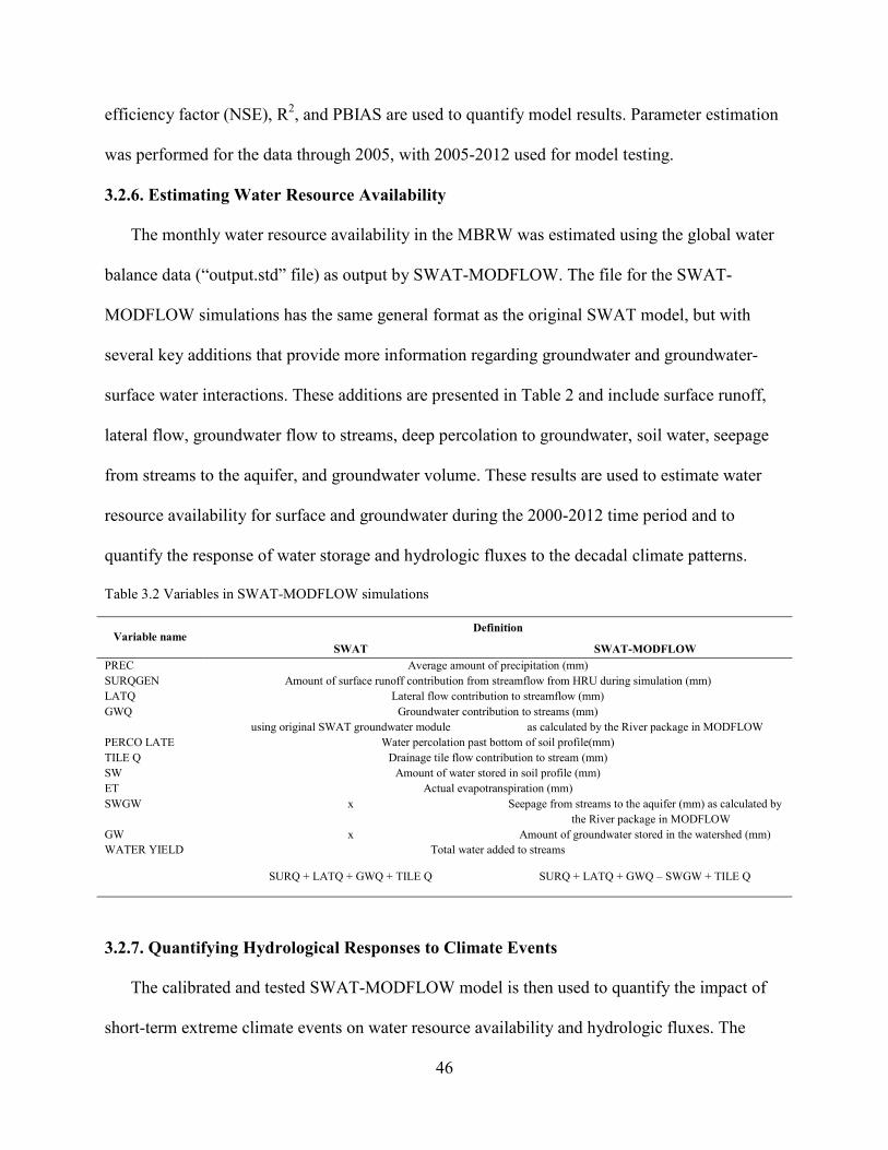
46

efficiency factor (NSE), R2, and PBIAS are used to quantify model results. Parameter estimation

was performed for the data through 2005, with 2005-2012 used for model testing.

3.2.6. Estimating Water Resource Availability

The monthly water resource availability in the MBRW was estimated using the global water

balance data (“output.std” file) as output by SWAT-MODFLOW. The file for the SWAT-

MODFLOW simulations has the same general format as the original SWAT model, but with

several key additions that provide more information regarding groundwater and groundwater-

surface water interactions. These additions are presented in Table 2 and include surface runoff,

lateral flow, groundwater flow to streams, deep percolation to groundwater, soil water, seepage

from streams to the aquifer, and groundwater volume. These results are used to estimate water

resource availability for surface and groundwater during the 2000-2012 time period and to

quantify the response of water storage and hydrologic fluxes to the decadal climate patterns.

Table 3.2 Variables in SWAT-MODFLOW simulations

Variable name Definition

SWAT SWAT-MODFLOW

PREC Average amount of precipitation (mm)

SURQGEN Amount of surface runoff contribution from streamflow from HRU during simulation (mm)

LATQ Lateral flow contribution to streamflow (mm)

GWQ Groundwater contribution to streams (mm)

using original SWAT groundwater module as calculated by the River package in MODFLOW

PERCO LATE Water percolation past bottom of soil profile(mm)

TILE Q Drainage tile flow contribution to stream (mm)

SW Amount of water stored in soil profile (mm)

ET Actual evapotranspiration (mm)

SWGW x Seepage from streams to the aquifer (mm) as calculated by

the River package in MODFLOW

GW x Amount of groundwater stored in the watershed (mm)

WATER YIELD Total water added to streams

SURQ + LATQ + GWQ + TILE Q SURQ + LATQ + GWQ – SWGW + TILE Q

3.2.7. Quantifying Hydrological Responses to Climate Events

The calibrated and tested SWAT-MODFLOW model is then used to quantify the impact of

short-term extreme climate events on water resource availability and hydrologic fluxes. The

47

impact of a severe year-long drought and thunderstorm, each of varying intensity for a suite of

scenarios, are assessed.

During the simulation period, the 1999 climate year was used for analysis of drought impact

(see Fig. 4). This drought was the cause of many deaths in the central Texas area, and the Dallas

airport reported 26 consecutive days of 100oF. Only 602 mm fell during the entire year

(compared to an annual average of 950 mm), with the months of August-September with little

rainfall (23mm). To determine the impact of varying intensity of drought on watershed

hydrology, 6 different scenarios were simulated by multiplying the original precipitation rates of

1999 by a factor of 0.25, 0.5, 0.75, 1.25, 1.5, 1.75, respectively. The monthly precipitation depths

(mm) for the 6 drought scenario simulations are shown in Figure 3.5a, in comparison with the

original monthly rainfall depths of 1999.The storm event uses rainfall depths based on intense

thunderstorm (in terms of rainfall depth per day) in recorded hydrologic history in central Texas.

On September 9, 1921, a thunderstorm produced 480 mm (19 inches) of rain in Austin, Texas

(Bishop, 1977), leading to strong flooding in the region. The short-term and long-term effect of

such a storm on watershed water storage and hydrologic fluxes is investigated in this study by

imposing a similar storm on the 2000-2013 simulation period, during 2004 (see Figure 3.4). The

storm event scenario uses two pre-conditions, i.e., wet and dry, since antecedent conditions likely

effect the hydrologic response of the storm event. Similar to the drought event, storms of

varying intensity are simulated, with daily rainfall depths set to 5, 10, 15, and 20 inches. The

storm event scenario uses two pre-conditions, wet and dry, since antecedent soil moisture and

shallow groundwater tables likely effect the hydrologic response of the storm event, making a

total of 8 storm simulations (Figure 3.5).

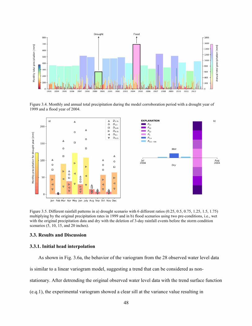
48

Figure 3.4. Monthly and annual total precipitation during the model corroboration period with a drought year of

1999 and a flood year of 2004.

Figure 3.5. Different rainfall patterns in a) drought scenario with 6 different ratios (0.25, 0.5, 0.75, 1.25, 1.5, 1.75)

multiplying by the original precipitation rates in 1999 and in b) flood scenarios using two pre-conditions, i.e., wet

with the original precipitation data and dry with the deletion of 3-day rainfall events before the storm condition

scenarios (5, 10, 15, and 20 inches).

3.3. Results and Discussion

3.3.1. Initial head interpolation

As shown in Fig. 3.6a, the behavior of the variogram from the 28 observed water level data

is similar to a linear variogram model, suggesting a trend that can be considered as non-

stationary. After detrending the original observed water level data with the trend surface function

(e.q.1), the experimental variogram showed a clear sill at the variance value resulting in

49

following the intrinsic hypothesis after the trend removal (Fig. 7.6b). The kriging estimation of

the residuals with the values of sill and range fitting to the spherical model were performed and

then the kriged residuals were added to the trend surface, creating the initial interpolated

hydraulic head as shown in Fig. 3.7, ranging from 170 to 342 m above MSL.

Figure 3.6 Variograms for the 28 observed water levels: a) original values with residuals; b) residuals with model

fitted.

Figure 3.7. Interpolated initial hydraulic head with the de-trended 28 observed water level data using the ordinary

kriging method and the spherical model.

50

3.3.2. Model corroboration

PEST stopped after 288 simulations through 7 iterations, the parameter estimation process

stopped. The distribution of calibrated hydraulic conductivities and specific yields for the

SWAT-MODFLOW model are presented in in Table 3.3. The highest hydraulic conductivity

value is estimated to be 990 m/day, within the alluvium zone in the first layer, and the lowest

hydraulic conductivity value is 0.10 m/day, at exposed-Comanche Peak Limestone in the first

layer. The range of specific yield values varies from 0.05 to 0.35.

Table 3.3 Initial ranges and calibrated values for the selected parameters during streamflow discharge and hydraulic

head calibration.

Parameter Description Initial range

(relative change)

Calibrated

value

CN2 Initial SCS runoff number for moisture condition II (-0.40 – 0.10) (-0.11)

SOL_AWC Available water capacity of the soil layer (mm H2O mm soil-1

) 0.10 – 0.90 0.85

ESCO Soil evaporation compensation factor 0.10 – 0.90 0.74

cond_1 Riverbed hydraulic conductance (m/day) - upper 0.1 – 100 3.65

cond_2 Riverbed hydraulic conductance (m/day) - middle 0.1 – 100 3.18

cond_3 Riverbed hydraulic conductance (m/day) - lower 0.1 – 100 6.18

Kdfdc Hydraulic conductivity of Denton Clay, Fort Worth Limestone, and

Duck Creek Limestone

5.00E-03 - 100 1.03

Qal Hydraulic conductivity of Alluvium 50 - 3000 989.57

Kc Hydraulic conductivity of Comanche Peak Limestone (exposed) 2.00E-02 – 50 9.91E-02

Kked Hydraulic conductivity of Kiamichi Clay and Edwards Limestone 2.00E-02 – 50 3.33

Kms Hydraulic conductivity of Main Street Limestone 1.00E-03 – 10 10.00

Kpw Hydraulic conductivity of Pawpaw Formation Weno Limestone

undivided

2.00E-02 – 50 0.34

Qt Hydraulic conductivity of Fluviatile terrace deposits 50 - 3000 984.52

George Hydraulic conductivity of Georgetown Limestone 0.5 - 50 17.27

Edward Hydraulic conductivity of Edwards Limestone 1 - 100 10.37

Ed_sy Specific yield of Edwards Limestone 0.05 – 0.35 0.35

gg_sy Specific yield of Georgetown Limestone 0.05 – 0.35 5.66E-02

Kc_sy Specific yield of Comanche Peak Limestone (exposed) 0.05 – 0.35 0.35

Kd_sy Specific yield of Denton Clay, Fort Worth Limestone, and Duck

Creek Limestone

0.05 – 0.35 5.21E-02

Kk_sy Specific yield of Kiamichi Clay and Edwards Limestone 0.05 – 0.35 5.00E-02

Km_sy Specific yield of Main Street Limestone 0.05 – 0.35 0.35

Qal_sy Specific yield of Alluvium 0.05 – 0.35 5.00E-02

Qt_sy Specific yield of Fluviatile terrace deposits 0.05 – 0.35 0.29

Kpw_sy Specific yield of Pawpaw Formation Weno Limestone undivided 0.05 – 0.35 5.00E-02

Observed and simulated streamflow discharges for the gauge site on the Middle Bosque river

(see Figure 3.1 for location) is shown in Figure 3.8 resulting in good similarity of the SWAT-

51

MODFLOW simulation with the observed data. The monthly NSE values of streamflow

discharge for calibration and validation were calculated to be 0.45 and 0.66, respectively, and for

whole simulation was 0.55, which are considered acceptable for monthly stream discharge (≥ 0.5)

(Moriasi et al., 2007) (Table 3.4). The monthly R2 for validation also shows a better result than

its calibration. The PBIAS value for calibration reveals a small percent under-prediction (2.62),

but a large percent over-prediction (-16.79) for validation probably due to the slightly different

behavior in the periods of low stream flow.

Figure 3.8. Observed and SWAT-MODFLOW simulated time series of stream discharge (m3/s), and the statistics

(R2, NSE, PBIAS) for calibration (1993 – 2005) and validation (2006 – 2012) periods for the outlet of the Middle

Bosque River watershed

Table 3.4 Comparison statistics (NSE; R2; PBIAS) between the observed and simulated hydrograph at the stream

gauge near the confluence of the Sycan and Sprague Rivers (Fig. 3.1) for calibration (1993 – 2005), validation (2005

– 2012), and whole simulation of the SWAT-MODFLOW model

Statistical Comparison Calibration Validation Total

NSE 0.45 0.66 0.55

R2 0.45 0.68 0.56

PBIAS 2.62 -16.79 -3.65

Figure 3.9 shows the hydrographs of measured and simulated hydraulic head for the

observation wells (CO1L from 10/21/1985 – 3/7/1986 and CO2D from 11/30/1985 – 2/1/1986)

(see Figure3.1 for location). Although the patterns of the hydrographs of simulated hydraulic

52

heads for both locations are similar to their observed data, the daily R2 values for two

observation wells are considered low because the simulated hydraulic head from CO1L shows

less fluctuation compared to its observed value and from CO2D about 1 meter lower than the

observed value. Although there are limited transient groundwater level data, field work in the

watershed indicates an extremely shallow water table (< 20 ft), particularly in low areas along

drainage tributaries, such as for CO1L and CO2D (see Figure 3.1), and that historically most

groundwater rises dramatically after rainfall events (see Figure 3.9b) (Easterling et al., 2001).

Figure 3.9. Hydrographs of measured and simulated hydraulic head for CO1L and CO2D wells in the Middle

Bosque River watershed.

3.3.3. Spatio-Temporal Variation of Hydrologic Fluxes

Simulated cell-wise annual average hydraulic head (m) is shown in Figure 3.10a, ranging

from 178 to 328 m above MSL. The spatial variation of annual average hydraulic head is similar

to the ground surface elevation, with highest water table elevation occurring in the high surface

elevation regions of the MBRW and lowest water table occurring along the main corridor of the

Middle Bosque river. Average annual recharge (mm/year) is shown in Figure3.10b, with the

highest recharge rates (~ 221mm/year) along the stream network and low recharge rates (2

mm/year) in the regions far from the stream network suggesting a high spatial variability in

simulated recharge rates. It’s because in the SWAT-MODFLOW simulation, the SWAT model

53

passed a soil deep percolation calculated by the combination (HRU) of different slope, land use

and soil types as recharge to the grid cells of the MODFLOW.

The changes in the hydraulic head during the simulation period is shown in the maps of

Figure 3.10, displayed as a departure from the annual average hydraulic head for the months of

March, June, September and December. Except the southern region (latitude: 310

30N longitude:

970 35W) and north-east edge (latitude: 31

0 35N longitude: 97

0 25W) of the MBRW (change in

drawdown over 1 meters), slight increases occur for the months of March, June and December

and slight decreases for September. In the southern region and north-east edge of the study area,

the highest increase is estimated to be 7 meters for March and the highest decrease of drawdowns

6.7 meters for September.

Figure 3.10. a) Simulated cell-wise annual average hydraulic head (m); b) Spatially-varying annual average recharge

(mm) in the Middle Bosque watershed as simulated by the coupled SWAT-MODFLOW model

54

Figure 3.11. Changes from annual average hydraulic head (m) for the months of March, June, September and

December over the 1993–2012 period

The spatio-temporal variation in water table elevation is mainly affected by recharge,

calculated from the daily recharge values passed from SWAT to MODFLOW. Thus, the results

from spatio-temporal drawdowns should be correlated to the results from spatio-temporal

recharge. As seen in Figure 3.11, the highest decline of groundwater head occurs in September,

due to the relatively low monthly recharge for September during the 1993 – 2012 period. The

highest average annual recharge rate is estimated to be 25 mm for March and December,

occurring along the main corridor of the Middle Bosque river in the same pattern of annual

average recharge distribution (see Figure 3.10b and Figure 3.12).

55

Figure 3. 12. Average annual recharge rates (mm) for the months of March, June, September and December over the

1970–2003 period

Figure 3.13 (centre chart) shows the annual average interaction rates (m3/day) between

groundwater and surface water for each MODFLOW River Cell. Positive values indicate

groundwater discharge to the stream network, and negative values indicate stream seepage to the

aquifer. The highest interaction rates occur in a section (easting: -130,236 m, northing: 938,678

based on UTM coordinate system) of the main corridor of the Middle Bosque river

approximately 1 km from the watershed outlet. The majority of surface - subsurface interactions

shows groundwater discharge to the stream, with a few locations where stream water seeps to the

aquifer. This is in agreement with the field observations of Cannata (1988), that “where major

streams completely dissect the Edwards Limestone, additional boundaries are formed where

large amounts of water are lost through discharge to streams”. This is also in agreement with the

observations of Bishop (1977) for the overall Bosque basin that the presence of impermeable

rock in the lower sections of the basin produces a large input of flood and runoff water. The

56

change in the spatial pattern of groundwater discharge during the year is shown in Figure 3.13,

displayed as a departure from the average annual rates for the months of March (maximum

groundwater discharge, Figure 3.13a) and September (minimum groundwater discharge, Figure

3.13d).

Figure 3.13. Departure from annual average groundwater discharge rates (m3/day) for the months of March, June,

September and December over the 1993–2012 period

Results demonstrate a high spatial-temporal variability in simulated hydraulic head, recharge

rates and surface-subsurface water interaction rates, which can have a profound impact on

watershed management. For instance, the spatio-temporal variation of recharge and groundwater

discharge maps can help identify potential areas of nutrient loading from the aquifer to the

stream network or of pollution infiltration from surface to the aquifer. In addition, this area could

be used to support decisions about alternative management strategies in the areas of landuse

change, climate change, water allocation, and pollution control.

57

3.3.4. Water resource availability

The monthly water resource availability in the MBRW is shown through a time series of

water balance components in Figure 3.14. Components are based on depths (mm) for basin-wide

values. The range of the amount of Soil Water (SW) is to be estimated to vary from 20.75 mm in

August 2011, with the minimum amount of 0.14 mm for Lateral Flow (LATQ), to 243.83 mm in

February 2005 during the 1993 – 2012 period. The amount of extractable groundwater (GW)

stored in the watershed ranges from 6370 mm (result not shown in Figure 3.14) to 6765 mm,

with about 400 mm difference. The amount of Surface Runoff (SURQ) is estimated to vary from

0 (several events) to 119 mm (May 2007). Regarding surface-subsurface water exchange, GWQ

and SWGW can be used for verifying the results of the spatio-temporal patterns of groundwater–

surface water interaction. The minimum values of GWQ and SWGW are estimated to be 5.2

(February 1996, result not shown in Figure 3.14) and 0 mm (several events), and the maximum

values 9.8 (March 2005) and 0.06 mm (May 2007), respectively, demonstrating the high

groundwater contribution to the stream for most of the study area. For water percolation to

aquifer (PERCO), the highest PERCO (88.99 mm) occurs in November 2004 and no PERCO in

several events.

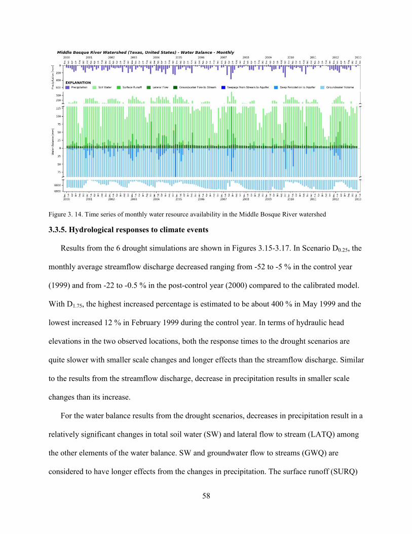
58

Figure 3. 14. Time series of monthly water resource availability in the Middle Bosque River watershed

3.3.5. Hydrological responses to climate events

Results from the 6 drought simulations are shown in Figures 3.15-3.17. In Scenario D0.25, the

monthly average streamflow discharge decreased ranging from -52 to -5 % in the control year

(1999) and from -22 to -0.5 % in the post-control year (2000) compared to the calibrated model.

With D1.75, the highest increased percentage is estimated to be about 400 % in May 1999 and the

lowest increased 12 % in February 1999 during the control year. In terms of hydraulic head

elevations in the two observed locations, both the response times to the drought scenarios are

quite slower with smaller scale changes and longer effects than the streamflow discharge. Similar

to the results from the streamflow discharge, decrease in precipitation results in smaller scale

changes than its increase.

For the water balance results from the drought scenarios, decreases in precipitation result in a

relatively significant changes in total soil water (SW) and lateral flow to stream (LATQ) among

the other elements of the water balance. SW and groundwater flow to streams (GWQ) are

considered to have longer effects from the changes in precipitation. The surface runoff (SURQ)

59

shows high sensitivity and instantaneous response to the increased precipitation with larger scale

changes compared to the other elements. Noteworthily, the total groundwater contained in the

watershed (GW) results in a slight decrease (~ -3%) in its volume with the highest increased

precipitation scenario (D1.75). In addition, the amount of seepage from streams to the aquifer in

the MBRW is too small to be influenced by the drought scenarios conditions.

Figure 3.15. Streamflow discharges with 6 different ratios (0.25, 0.5, 0.75, 1.25, 1.5, 1.75) multiplying by the

original precipitation rates in the controlling year of 1999 / to post-controlling year of 2000 for the drought

scenarios.

Figure 3.16. Hydraulic head elevations with 6 different ratios (0.25, 0.5, 0.75, 1.25, 1.5, 1.75) multiplying by the

original precipitation rates in 1999 for the drought scenarios

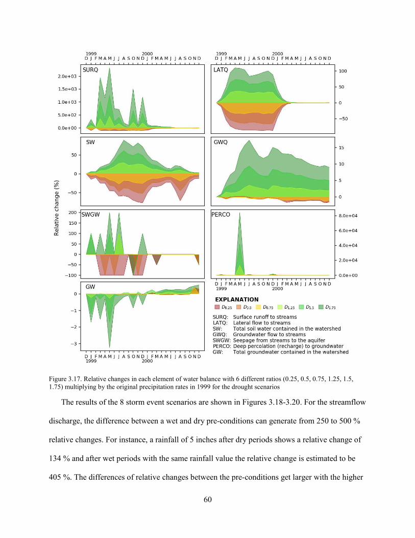
60

Figure 3.17. Relative changes in each element of water balance with 6 different ratios (0.25, 0.5, 0.75, 1.25, 1.5,

1.75) multiplying by the original precipitation rates in 1999 for the drought scenarios

The results of the 8 storm event scenarios are shown in Figures 3.18-3.20. For the streamflow

discharge, the difference between a wet and dry pre-conditions can generate from 250 to 500 %

relative changes. For instance, a rainfall of 5 inches after dry periods shows a relative change of

134 % and after wet periods with the same rainfall value the relative change is estimated to be

405 %. The differences of relative changes between the pre-conditions get larger with the higher

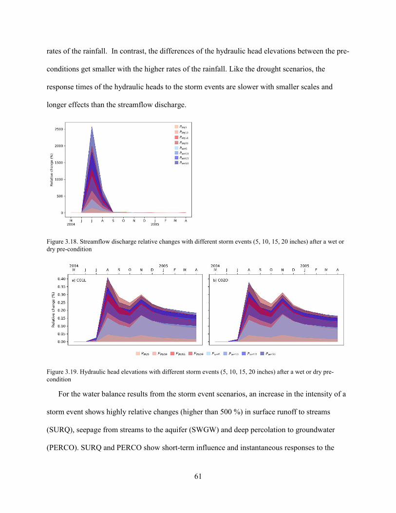
61

rates of the rainfall. In contrast, the differences of the hydraulic head elevations between the pre-

conditions get smaller with the higher rates of the rainfall. Like the drought scenarios, the

response times of the hydraulic heads to the storm events are slower with smaller scales and

longer effects than the streamflow discharge.

Figure 3.18. Streamflow discharge relative changes with different storm events (5, 10, 15, 20 inches) after a wet or

dry pre-condition

Figure 3.19. Hydraulic head elevations with different storm events (5, 10, 15, 20 inches) after a wet or dry pre-

condition

For the water balance results from the storm event scenarios, an increase in the intensity of a

storm event shows highly relative changes (higher than 500 %) in surface runoff to streams

(SURQ), seepage from streams to the aquifer (SWGW) and deep percolation to groundwater

(PERCO). SURQ and PERCO show short-term influence and instantaneous responses to the

62

storm events. For LATQ, GWQ and PERCO the dry pre-condition before the storm events

causes high relative changes compared to the wet pre-condition because an unsaturated soil

condition driven by the long-dried periods sucks more water from the storm events and sends it

to the streams (LATQ) and induces more recharge (PERCO) that goes to groundwater. In

addition, the lowered river stage because of the long-dried periods causes more groundwater

flow to the streams (GWQ) after the storm events in the dry pre-condition than the wet pre-

condition.

Figure 3.20. Relative changes in each element of water balance with different storm events (5, 10, 15, 20 inches)

after a wet or dry pre-condition

These results show climate events such as drought, multi-year drought, and extreme flooding

events have a significant impact on surface water storage, groundwater storage, and watershed

63

fluxes (recharge, groundwater-surface water interaction, lateral flow, surface runoff). Besides,

the results show that even the same intensity and length of a stress or even its pre-conditions on

different hydrologic response variables can result in their response time, scales and durations in a

very different way. For instance, response times for sub-surface related-hydrologic responses

such as water table and GWQ are slower than surface related-hydrologic responses such as

streamflow discharge, SURQ, SW, and PERCO. Their response durations also quite different

which sub-surface related-hydrologic responses are longer than surface related-hydrologic

responses.

3.4. Summary and conclusions

This study investigates the water resource availability in the Middle Bosque River watershed

(471 km2) in the Texas-Gulf region of central Texas during the 1993 – 2012 period. The three-

dimensional, finite-difference, groundwater flow modelling program MODFLOW-NWT was

used to construct the Middle Bosque River Watershed sub-surface system during 1980–2012,

and it incorporates time-varying recharge from the pre-calibrated SWAT model. The linked

SWAT-MODFLOW model of the Middle River Watershed is tested and calibrated against

streamflow and groundwater level using the auto-calibration process by the PEST tool with the

post-processing in the batch mode. Model output includes cell-wise hydraulic head, recharge,

and surface-subsurface water interaction, demonstrating a high spatio-temporal variability and

correlations between the results. Regarding the water resource availability, the SWAT-

MODFLOW model can simulate the water balance from surface and sub-surface domains

simultaneously based on time series analysis and the results show the high temporal variation of

the elements in the water balance. Using the calibrated model, the impact of precipitation on the

streamflow discharge, hydraulic head elevation, and water resource availability was assessed

64

under different rainfall scenarios. The results show that their response time, scales and durations

not only vary but also can influenced by their pre-conditions.

This study helps enhance understanding regarding the spatio-temporal patterns of hydraulic

head elevation, recharge, surface-subsurface water interaction and the water resource availability

and the hydrological responses with different rainfall patterns that support decisions about

alternative management strategies in the areas of landuse change, climate change, water

allocation, pollution control and groundwater development scenarios.

65

REFERENCES

Abbaspour, K.C., Rouholahnejad, E., Vaghefi, S., Srinivasan, R., Yang, H. and Klove, B. (2015)

'A continental-scale hydrology and water quality model for Europe: Calibration and

uncertainty of a high-resolution large-scale SWAT model', Journal of Hydrology, 524, 733-

752, available: http://dx.doi.org/10.1016/j.jhydrol.2015.03.027.

Alcamo, J., Doll, P., Henrichs, T., Kaspar, F., Lehner, B., Rosch, T. and Siebert, S. (2003)

'Development and testing of the WaterGAP 2 global model of water use and availability',

Hydrological Sciences Journal-Journal Des Sciences Hydrologiques, 48(3), 317-337,

available: http://dx.doi.org/10.1623/hysj.48.3.317.45290.

Alcamo, J., Döll, P., Kaspar, F. and Siebert, S., 1997. Global change and global scenarios of

water use and availability: an application of WaterGAP 1.0. Center for Environmental

Systems Research (CESR), University of Kassel, Germany, 1720.

Ali, R., McFarlane, D., Varma, S., Dawes, W., Emelyanova, I., Hodgson, G. and Charles, S.

(2012) 'Potential climate change impacts on groundwater resources of south-western

Australia', Journal of Hydrology, 475, 456-472, available:


Arnold, J.G., Srinivasan, R., Muttiah, R.S. and Williams, J.R. (1998) 'Large area hydrologic

modeling and assessment - Part 1: Model development', Journal of the American Water

Resources Association, 34(1), 73-89, available: http://dx.doi.org/10.1111/j.1752-

1688.1998.tb05961.x.



66



Beven, K. and Binley, A. (1992) 'THE FUTURE OF DISTRIBUTED MODELS - MODEL

CALIBRATION AND UNCERTAINTY PREDICTION', Hydrological Processes, 6(3), 279-

298, available: http://dx.doi.org/10.1002/hyp.3360060305.

Bishop, A.L., 1977. Flood potential of the Bosque Basin. Baylor University, Department of

Geology.

Brown, S.C., Versace, V.L., Lester, R.E. and Walter, M.T. (2015) 'Assessing the impact of

drought and forestry on streamflows in south-eastern Australia using a physically based

hydrological model', Environmental Earth Sciences, 74(7), 6047-6063, available:

http://dx.doi.org/10.1007/s12665-015-4628-8.

Camporese, M., Paniconi, C., Putti, M. and Salandin, P. (2009) 'Ensemble Kalman filter data

assimilation for a process-based catchment scale model of surface and subsurface flow',

Water Resources Research, 45, available: http://dx.doi.org/10.1029/2008wr007031.

Cannata, S.L., 1988. Hydrogeology of a portion of the Washita Prairie Edwards aquifer: central

Texas (Doctoral dissertation, Baylor University).

Cosgrove, B. and Rijsberman, F., 2000. World water vision. J HYDRAUL RES, 38(4), p.57.

Cosgrove, D.M. and Johnson, G.S. (2005) 'Aquifer management zones, based on simulated

surface-water response functions', Journal of Water Resources Planning and Management-

Asce, 131(2), 89-100, available: http://dx.doi.org/10.1061/(asce)0733-9496(2005)131:2(89).

Dams, J., Salvadore, E., Van Daele, T., Ntegeka, V., Willems, P. and Batelaan, O. (2012)

'Spatio-temporal impact of climate change on the groundwater system', Hydrology and Earth

System Sciences, 16(5), 1517-1531, available: http://dx.doi.org/10.5194/hess-16-1517-2012.

67

de Graaf, G., Bartley, D., Jorgensen, J. and Marmulla, G. (2015) 'The scale of inland fisheries,

can we do better? Alternative approaches for assessment', Fisheries Management and

Ecology, 22(1), 64-70, available: http://dx.doi.org/10.1111/j.1365-2400.2011.00844.x.

de Graaf, I.E.M., van Beek, R., Gleeson, T., Moosdorf, N., Schmitz, O., Sutanudjaja, E.H. and

Bierkens, M.F.P. (2017) 'A global-scale two-layer transient groundwater model:

Development and application to groundwater depletion', Advances in Water Resources, 102,

53-67, available: http://dx.doi.org/10.1016/j.advwatres.2017.01.011.

De Wrachien, D. and Fasso, C.A. (2002) 'Conjunctive use of surface and groundwater: Overview

and perspective', Irrigation and Drainage, 51(1), 1-15, available:

http://dx.doi.org/10.1002/ird.43.

Doherty, J., 2006. PEST Model-Independent Parameter Estimation, V10. 1, Papadopulos. SS,

Inc., Bethesda, MA

Doll, P., Kaspar, F. and Lehner, B. (2003) 'A global hydrological model for deriving water

availability indicators: model tuning and validation', Journal of Hydrology, 270(1-2), 105-

134, available: http://dx.doi.org/10.1016/s0022-1694(02)00283-4.

Famiglietti, J.S., Lo, M., Ho, S.L., Bethune, J., Anderson, K.J., Syed, T.H., Swenson, S.C., de

Linage, C.R. and Rodell, M. (2011) 'Satellites measure recent rates of groundwater depletion

in California's Central Valley', Geophysical Research Letters, 38, available:

http://dx.doi.org/10.1029/2010gl046442.

Faramarzi, M., Abbaspour, K.C., Vaghefi, S.A., Farzaneh, M.R., Zehnder, A.J.B., Srinivasan, R.

and Yang, H. (2013) 'Modeling impacts of climate change on freshwater availability in

Africa', Journal of Hydrology, 480, 85-101, available:


68

Feng, W., Zhong, M., Lemoine, J.M., Biancale, R., Hsu, H.T. and Xia, J. (2013) 'Evaluation of

groundwater depletion in North China using the Gravity Recovery and Climate Experiment

(GRACE) data and ground-based measurements', Water Resources Research, 49(4), 2110-

2118, available: http://dx.doi.org/10.1002/wrcr.20192.

Ficklin, D.L., Luo, Y., Luedeling, E. and Zhang, M. (2009) 'Climate change sensitivity

assessment of a highly agricultural watershed using SWAT', Journal of Hydrology, 374(1-2),

16-29, available: http://dx.doi.org/10.1016/j.jhydrol.2009.05.016.

Gauthier, M.J., Camporese, M., Rivard, C., Paniconi, C. and Larocque, M. (2009) 'A modeling

study of heterogeneity and surface water-groundwater interactions in the Thomas Brook

catchment, Annapolis Valley (Nova Scotia, Canada)', Hydrology and Earth System Sciences,

13(9), 1583-1596, available: http://dx.doi.org/10.5194/hess-13-1583-2009.

Goderniaux, P., Brouyere, S., Fowler, H.J., Blenkinsop, S., Therrien, R., Orban, P. and

Dassargues, A. (2009) 'Large scale surface-subsurface hydrological model to assess climate

change impacts on groundwater reserves', Journal of Hydrology, 373(1-2), 122-138,

available: http://dx.doi.org/10.1016/j.jhydrol.2009.04.017.

Haddeland, I., Heinke, J., Voss, F., Eisner, S., Chen, C., Hagemann, S. and Ludwig, F. (2012)

'Effects of climate model radiation, humidity and wind estimates on hydrological simulations',

Hydrology and Earth System Sciences, 16(2), 305-318, available:

http://dx.doi.org/10.5194/hess-16-305-2012.

Hassan, S.M.T., Lubczynski, M.W., Niswonger, R.G. and Su, Z. (2014) 'Surface-groundwater

interactions in hard rocks in Sardon Catchment of western Spain: An integrated modeling

approach', Journal of Hydrology, 517, 390-410, available:


69

Journel, A.G. and Huijbregts, C.J., 1978. Mining geostatistics. Academic press.

Jyrkama, M.I. and Sykes, J.F. (2007) 'The impact of climate change on spatially varying

groundwater recharge in the grand river watershed (Ontario)', Journal of Hydrology, 338(3-4),

237-250, available: http://dx.doi.org/10.1016/j.jhydrol.2007.02.036.

Kollet, S.J. and Maxwell, R.M. (2006) 'Integrated surface-groundwater flow modeling: A free-

surface overland flow boundary condition in a parallel groundwater flow model', Advances

in Water Resources, 29(7), 945-958, available:

http://dx.doi.org/10.1016/j.advwatres.2005.08.006.

Liu, J.G., Zang, C.F., Tian, S.Y., Yang, H., Jia, S.F., You, L.Z., Liu, B. and Zhang, M. (2013)

'Water conservancy projects in China: Achievements, challenges and way forward', Global

Environmental Change-Human and Policy Dimensions, 23(3), 633-643, available:

http://dx.doi.org/10.1016/j.gloenvcha.2013.02.002.

Longuevergne, L., Scanlon, B.R. and Wilson, C.R. (2010) 'GRACE Hydrological estimates for

small basins: Evaluating processing approaches on the High Plains Aquifer, USA', Water

Resources Research, 46, available: http://dx.doi.org/10.1029/2009wr008564.

Markstrom, S.L., Niswonger, R.G., Regan, R.S., Prudic, D.E. and Barlow, P.M., 2008.

GSFLOW-Coupled Ground-water and Surface-water FLOW model based on the integration

of the Precipitation-Runoff Modeling System (PRMS) and the Modular Ground-Water Flow

Model (MODFLOW-2005). US Geological Survey techniques and methods, 6, p.240.

Mateus, C., Tullos, D.D. and Surfleet, C.G. (2015) 'HYDROLOGIC SENSITIVITY TO

CLIMATE AND LAND USE CHANGES IN THE SANTIAM RIVER BASIN, OREGON',

Journal of the American Water Resources Association, 51(2), 400-420, available:

http://dx.doi.org/10.1111/jawr.12256.

70

Matheron, G., 1963. Principles of geostatistics. Economic geology, 58(8), pp.1246-1266

Maxwell, S. (2005) '2005 update on water industry consolidation trends', Journal American

Water Works Association, 97(10), 34-36.

Meixner, T., Manning, A.H., Stonestrom, D.A., Allen, D.M., Ajami, H., Blasch, K.W.,

Brookfield, A.E., Castro, C.L., Clark, J.F., Gochis, D.J., Flints, A.L., Neff, K.L., Niraula, R.,

Rodell, M., Scanlon, B.R., Singha, K. and Walvoord, M.A. (2016) 'Implications of projected

climate change for groundwater recharge in the western United States', Journal of Hydrology,

534, 124-138, available: http://dx.doi.org/10.1016/j.jhydrol.2015.12.027.

Murray, C.J.L., Rosenfeld, L.C., Lim, S.S., Andrews, K.G., Foreman, K.J., Haring, D., Fullman,

N., Naghavi, M., Lozano, R. and Lopez, A.D. (2012) 'Global malaria mortality between 1980

and 2010: a systematic analysis', Lancet, 379(9814), 413-431.

Niswonger, R.G., Panday, S. and Ibaraki, M., 2011. MODFLOW-NWT, a Newton formulation

for MODFLOW-2005. US Geological Survey Techniques and Methods, 6(A37), p.44.

Oki, T. and Kanae, S. (2006) 'Global hydrological cycles and world water resources', Science,

313(5790), 1068-1072, available: http://dx.doi.org/10.1126/science.1128845.

Pearson, D.K., 2013. Geologic database of Texas: Project summary, Database contents, and

user’s guide: Document prepared by the US Geological Survey for the Texas Water

Development Board, Austin, 22 p.

Perrin, J., Ferrant, S., Massuel, S., Dewandel, B., Marechal, J.C., Aulong, S. and Ahmed, S.

(2012) 'Assessing water availability in a semi-arid watershed of southern India using a semi-

distributed model', Journal of Hydrology, 460, 143-155, available:


71

Postel, S.L., Daily, G.C. and Ehrlich, P.R. (1996) 'Human appropriation of renewable fresh

water', Science, 271(5250), 785-788, available:

http://dx.doi.org/10.1126/science.271.5250.785.

Rodell, M., Chen, J.L., Kato, H., Famiglietti, J.S., Nigro, J. and Wilson, C.R. (2007) 'Estimating

groundwater storage changes in the Mississippi River basin (USA) using GRACE',

Hydrogeology Journal, 15(1), 159-166, available: http://dx.doi.org/10.1007/s10040-006-

0103-7.

Schuol, J., Abbaspour, K.C., Srinivasan, R. and Yang, H. (2008) 'Estimation of freshwater

availability in the West African sub-continent using the SWAT hydrologic model', Journal of


Scibek, J. and Allen, D.M. (2006) 'Modeled impacts of predicted climate change on recharge and

groundwater levels', Water Resources Research, 42(11), available:

http://dx.doi.org/10.1029/2005wr004742.

Scibek, J., Allen, D.M., Cannon, A.J. and Whitfield, P.H. (2007) 'Groundwater-surface water

interaction under scenarios of climate change using a high-resolution transient groundwater

model', Journal of Hydrology, 333(2-4), 165-181, available:


Tian, Y., Zheng, Y., Wu, B., Wu, X., Liu, J. and Zheng, C. (2015) 'Modeling surface water-

groundwater interaction in arid and semi-arid regions with intensive agriculture',

Environmental Modelling & Software, 63, 170-184, available:


72

Tweed, S., Leblanc, M. and Cartwright, I. (2009) 'Groundwater-surface water interaction and the

impact of a multi-year drought on lakes conditions in South-East Australia', Journal of


Vaghefi, S.A., Mousavi, S.J., Abbaspour, K.C., Srinivasan, R. and Arnold, J.R. (2015)

'Integration of hydrologic and water allocation models in basin-scale water resources

management considering crop pattern and climate change: Karkheh River Basin in Iran',

Regional Environmental Change, 15(3), 475-484, available:

http://dx.doi.org/10.1007/s10113-013-0573-9.

van Griensven, A., Meixner, T., Grunwald, S., Bishop, T., Diluzio, A. and Srinivasan, R. (2006)

'A global sensitivity analysis tool for the parameters of multi-variable catchment models',

Journal of Hydrology, 324(1-4), 10-23, available:


Vieira, S.R., Hatfield, J.L., Nielsen, D.R. and Biggar, J.W. (1983) 'GEOSTATISTICAL

THEORY AND APPLICATION TO VARIABILITY OF SOME AGRONOMICAL

PROPERTIES', Hilgardia, 51(3), 1-75.

VIEIRA, S.R., MILLETE, J., Topp, G.C. and Reynolds, W.D., 2002. Handbook for geostatistical

analysis of variability in soil and climate data. Tópicos em ciência do solo, 2, pp.1-

citation_lastpage.

Vorosmarty, C.J., Green, P., Salisbury, J. and Lammers, R.B. (2000) 'Global water resources:

Vulnerability from climate change and population growth', Science, 289(5477), 284-288,

available: http://dx.doi.org/10.1126/science.289.5477.284.

Voss, K.A., Famiglietti, J.S., Lo, M.H., de Linage, C., Rodell, M. and Swenson, S.C. (2013)

'Groundwater depletion in the Middle East from GRACE with implications for transboundary

73

water management in the Tigris-Euphrates-Western Iran region', Water Resources Research,

49(2), 904-914, available: http://dx.doi.org/10.1002/wrcr.20078.

Wada, Y., van Beek, L.P.H., van Kempen, C.M., Reckman, J., Vasak, S. and Bierkens, M.F.P.

(2010) 'Global depletion of groundwater resources', Geophysical Research Letters, 37,

available: http://dx.doi.org/10.1029/2010gl044571.

Wilson, D.J., Western, A.W., Grayson, R.B., Berg, A.A., Lear, M.S., Rodell, M., Famiglietti,

J.S., Woods, R.A. and McMahon, T.A. (2003) 'Spatial distribution of soil moisture over 6

and 30 cm depth, Mahurangi river catchment, New Zealand', Journal of Hydrology, 276(1-4),

254-274, available: http://dx.doi.org/10.1016/s0022-1694(03)00060-x.

Winston, R.B., 2009. ModelMuse: a graphical user interface for MODFLOW-2005 and PHAST

(p. 52). Reston, VA: US Geological Survey.

Woldeamlak, S.T., Batelaan, O. and De Smedt, F. (2007) 'Effects of climate change on the

groundwater system in the Grote-Nete catchment, Belgium', Hydrogeology Journal, 15(5),

891-901, available: http://dx.doi.org/10.1007/s10040-006-0145-x.

74

CHAPTER 4

A FRAMEWORK FOR QUANTIFYING UNCERTAINTY, SENSITIVITY, AND

ESTIMATING PARAMETERS FOR INTEGRATED SURFACE WATER -

GROUNDWATER MODELS

Highlights

Hydrologic models often are used as aids in the water resources and environment planning

and management in watersheds and river basins. These models, however, are fraught with

uncertainty due to inaccurate model structures, indefinite magnitude of system stresses, and

uncertain values of system parameters. This study proposed a general framework for performing

sensitivity analysis, parameter estimation, and uncertainty analysis for integrated surface water-

groundwater models, using the SWAT-MODFLOW modelling code as an example. The PEST

software tool is used to jointly estimate the values and sensitivity of both land surface (SWAT)

and subsurface (MODFLOW) parameters in a single automated calibration method. The monthly

NSE values of streamflow discharge for calibration and validation were calculated to be 0.45 and

0.66, respectively, and for whole simulation was 0.55, which are considered acceptable for

monthly stream discharge (≥ 0.5). Sensitivity analysis shows that land surface parameters have a

strong control on streamflow and groundwater levels, followed by hydraulic conductivity and

specific yield of the near-surface geologic units. Predictive uncertainty is demonstrated via an

aquifer-storage-recovery groundwater development scenario, with water for injection diverted

from the Middle Bosque River. Results are provided with uncertainty bands, and show that

injecting water results in larger changes in water table level (increase of 2.1 m) than extracting

75

water (decrease of 1.2 m) from the aquifer, suggesting that response time, scales and durations

are influenced by pre-conditions (i.e. soil moisture, water table). Effect of the scenario on

streamflow was negligible. The proposed modelling work-flow can assist in implementing and

applying integrated surface water-groundwater models for estimating watershed water resource

and analysing the effect of changes in land use, population, and climate. This framework,

particularly if used with SWAT-MODFLOW, can facilitate the use of integrated models

worldwide to assist with finding technical solutions to water issues.

4.1. Introduction

Distributed hydrological models have been used extensively over the past three decades

(Beven, 2010) to aid in decision making for water resources planning and management and

environmental management within watershed systems (Mulet and Nicklow, 2005; Gallagher and

Doherty, 2007; Cloke and Pappenberger, 2009; Park et al., 2013; Abbaspour et al., 2015), often

through evaluating alternative watershed management strategies. In addition, as population

growth, land use change, and climate change intensify current and future stresses on freshwater

(Postel et al., 1996; Cosgrove and Rijsberman, 2000; Vorosmarty et al., 2000; Doll et al., 2003;

Oki and Kanae, 2006; Murray et al, 2012), combined use of surface water and groundwater

resources often becomes essential in many river basins to provide reliable water supply

(Wrachien and Fasso, 2002; Cosgrove and Johnson, 2005; Liu et al., 2013; Singh et al., 2015).

Hydrologic models, however, include substantial uncertainties with respect to input data,

forcing data, initial and boundary conditions, model structure, and parameter non-uniqueness due

to a lack of data and poor knowledge of hydrological response mechanisms (Ye et al., 2008;

Doherty and Welter, 2010; Shi and Zhou, 2010; Zhang et al., 2011; Gupta et al., 2012; Foglia et

76

al., 2013). These uncertainties have negative effects on the model accuracy, thereby inducing

uncertainties in the simulated results. Therefore, if hydrologic models are to be used to as

decision-making aids, the uncertainty associated with model calibration and model predictions

must be assessed (Gallagher and Doherty, 2007). The general modelling approach requires a

sequence of methods, including preliminary sensitivity analysis (SA) (“screening”) to determine

which parameters govern hydrologic responses in a given watershed; parameter estimation, to

identify values of specified parameters; uncertainty analysis (UA), to determine the uncertainty

in the model outputs that result from uncertainty in the model inputs/parameters; and final SA to

evaluate how much each input/parameter contributes to the output uncertainty (Jakeman et al.,

2006; Razavi et al., 2012; Wu and Liu, 2012; Nan et al., 2011; Song et al., 2011; Loosvelt et al.,

2013). Ideally, SA and UA should be performed in tandem as both are essential parts of model

development and quality assurance. UA can be applied to model results during the model

calibration and testing phases, and also to the application of models for scenario analysis

(“predictive uncertainty”), e.g. when investigating the effect of future management strategies,

climate change, etc. on hydrologic responses and water resources of a watershed.

Conducting comprehensive SA and UA methods for watershed-scale hydrologic models

often is performed using lumped, semi-distributed models such as the Soil and Water

Assessment Tool (SWAT) (Arnold et al., 1998) or the Hydrological Simulation Program –

FORTRAN (HSPF) (Bicknell et al., 2001). SWAT applications include Muleta and Nicklow

(2005) to the Big Creek watershed, Illinois (133 km2); Yang et al. (2007) to the Thur River basin,

Switzerland; Li et al. (2010) to the Yingluoxia watershed in China (10,000 km2); Shen et al.

(2012) to the Daning River watershed in China (4,426 km2); Wu and Liu (2012) to the Cedar

River Basin in Iowa; and Abbaspour et al. (2015) to the European continent, with the latter

77

model providing information support to the European Water Framework Directive. HSPF

applications include Gallagher and Doherty (2007) to the Contentnea Creek Basin, North

Carolina (2,600 km2) and Jia and Culver (2008) to a small watershed (90 km

2) in Virginia. These

studies applied a variety of SA and UA methods, including the Generalized Likelihood

Uncertainty Estimation (GLUE) (Beven and Binley, 1992) and Markov Chain Monte Carlo

(MCMC). The majority of these studies applied UA only to parameter uncertainty during the

model calibration and testing periods, and not to any predictive scenario analysis. For the model

SWAT, these have been incorporated into the software tool SWAT-CUP (SWAT Calibration

Uncertainty Procedures) (Abbaspour, 2011), which includes GLUE, Parameter Solution (ParaSol)

(van Griensven and Meixner, 2006), and Sequential Uncertainty FItting (SUFI-2) (Abbaspour, et

al., 2007).

There are, however, two principal drawbacks with the SA/UA studies using the SWAT and

HSPF models, and any other lumped, moderately-distributed hydrologic model. First,

applications of these models focus solely on stream discharge as the system response of concern.

This is in part due to 1) a focus on surface water to satisfy river basin water needs, but also on 2)

the simplistic treatment of groundwater flow and groundwater-surface water (GW-SW)

interactions in the model structure. Second, due to simplistic treatment of groundwater flow and

GW-SW, the models do not include all watershed variables that could affect the main hydrologic

responses (surface runoff, infiltration, lateral flow, groundwater recharge, GW-SW, and

streamflow), with governing watershed variables being input data, weather data, soil properties,

and aquifer properties. The exclusion of physically-based, distributed groundwater flow

modelling and GW-SW from hydrologic model applications likely simplifies the watershed

78

system beyond what is appropriate in many river basins, and thereby neglects the uncertainty

associated with a combination of land surface and subsurface hydrologic parameters.

Several recent studies (Surfleet and Tullos, 2013; Wu et al., 2014) have attempted to include

SA/UA methods for integrated surface water-groundwater models. Both used the GSFLOW

model (Markstrom et al., 2008), which includes both land surface and subsurface hydrological

processes a coupled PRMS (Leavesley et al., 1983) and MODFLOW (Harbaugh, 2005) approach.

The study of Surfleet and Tullos (2013) applied GSFLOW to a 4,700 km2 river basin in Oregon,

assessing uncertainty associated with climate change predictions. Wu et al. (2014) provided a

framework for applying UA to the 9,097 km2 Zhangye Basin, China using GSFLOW,

investigating the response of ET, soil moisture, infiltration, recharge, surface leakage, GW-SW

exchange, groundwater level, and streamflow. Their methodology, however, uses manual

calibration rather than automatic calibration, due to the computational burden, and also does not

use the full GSFLOW model in UA, rather using a simplified, surrogate model (Wu et al., 2014).

They state that “automatic calibration for such complex models is extremely challenging and

deserves a separate study”.

Overall, no systematic approach of model construction and use has been provided for the

coupled surface-subsurface flow models, limiting their wide application. There is a need for a

generalized approach to perform UA, quantify the influence of the vast array of model

parameters and factors on watershed response (e.g. stream discharge, groundwater head) through

SA, develop a systematic approach to parameter estimation for both land surface and

hydrogeological parameters, thereby providing modelling results that assess both groundwater

and surface water resources accurately in a watershed setting while relaying the degree of

uncertainty to decision makers.

79

In this study, we present a framework to quantify sensitivity analysis, uncertainty analysis,

and parameter estimation for coupled groundwater/surface water models, using the newly

developed SWAT-MODFLOW code (Bailey et al., 2016) as an example modeling code. Thus,

this paper serves as a guideline for applying integrated surface water-groundwater models

generally, and for applying SWAT-MODFLOW models specifically, with several components of

the framework requiring details specific to SWAT and MODFLOW. Application of the

framework is demonstrated for a watershed in central Texas. Parameter estimation and

uncertainty analysis is performed using PEST (Parameter ESTimation tool) (Doherty, 2006),

with new pre-processing and post-processing algorithms developed to modify and assess jointly

land surface hydrologic parameters (SWAT model) and hydrogeological parameters

(MODFLOW). Sensitivity analysis is performed to determine controlling factors on hydrological

responses. To demonstrate the implementation of uncertainty in scenario analysis, we include a

groundwater development scenario (aquifer storage and recovery using river water and a set of

pumping wells) that uses an ensemble of plausible model parameter sets. Uncertainty in both

streamflow and groundwater levels are assessed.

4.2. Methodology

The general framework for quantifying uncertainty, sensitivity, and estimating parameters for

the coupled surface water-groundwater model will be presented, with each phase of the process

illustrated by application to a SWAT-MODFLOW model constructed for the Middle Bosque

River Watershed in central Texas.

4.2.1. General Framework for Integrated SW-GW Models

The general framework for constructing, calibrating, and applying integrated surface water-

groundwater models within a watershed system is shown by the flow chart in Figure 4.1. The

80

framework includes phases for quantifying uncertainty, sensitivity, and estimating parameters for

the integrated models. The framework is divided into a) “Model construction” and b)

“Framework for sensitivity, uncertainty analysis, parameter estimation”. Whereas the details of a)

are specific to SWAT-MODFLOW applications, b) is general to all integrated surface water-

groundwater models. Details for each sub-section of a) and b) are provided in the remaining sub-

sections of Section 2. Only a brief outline is presented here.

81

Figure 4.1. Framework for constructing, calibrating, and applying integrated surface water-groundwater models

within a watershed system

For a), a SWAT model and MODFLOW model are constructed to utilize the SWAT-

MODFLOW modelling code of Bailey et al. (2016). Details regarding these two models are

82

provided in Section 4.2.2 SWAT requires land use, soil, and digital elevation model (DEM)

layers to delineate the watershed and create the set of hydrologic response units (HRUs),

whereas MODFLOW requires aquifer unit layering, aquifer properties, aquifer stresses, and a

finite difference grid. The two models are linked via geo-processing routines to create linkage

files as inputs for the SWAT-MODFLOW model.

The b) segment consists of 1) model parameterization, 2) PEST, and 3) evaluation of

parameter sensitivities, using 4) the Hydrological model and 5) assessment of model output.

PEST is used since it is a model-independent program, capable of working with any hydrologic

model executable. Using the interaction between PEST and the Hydrological model, both

traditional parameter estimation, based on the use of only a few parameters, and highly-

parameterized regularized inversion based on the use of hundreds of parameters, can be

performed. PEST also has options for parallelizing simulation runs across multiple processors on

the same machine, across machines, and across networks. The impacts of model inputs and

parameters on hydrological responses (streamflow, groundwater levels, groundwater-surface

water exchange rates) can be assessed with 3) sensitivity analysis, and the model can be used to

assess future development scenarios as a part of a 5) predictive uncertainty analysis.

4.2.2. Model Construction and Setup

A SWAT-MODFLOW model is constructed for the Middle Bosque River Watershed

(MBRW) (Figure 4.2) (471 km2) in the Texas-Gulf region of central Texas. This watershed is

selected due to the presence of both surface water and groundwater resources, with groundwater

interacting strongly with stream water in the surficial geologic system. The model simulation

time is 1980-2012. Complete details of the SWAT-MODFLOW model are provided in Park et al.

(2018), with only major aspects described here.

83

The MBRW covers portions of McLennan, Bosque, and Coryell counties (Figure 4.2) with

sedimentary rocks from the Washita and Fredericksburg Groups of early Cretaceous, and

Comanchean age. The formation of the Washita Group is the Georgetown Limestone including

Main Street, Pawpaw, Weno, Denton, Fort Worth, Duck Creek, and Kiamichi members (Cannata,

1988; Pearson, 2007). The two formations of the Fredericksburg Group, the Edwards Limestone

and Comanche Peak Limestone, are used in the study area. The altitude of the study region varies

from 367 m at the highest point on the north-western edge to 161 m on the eastern edge. The

MBRW is predominantly comprised of pasture (65.4 % of area) and farms (20.3 % of area), with

minor land covers of forests (8.5 % of area), and residential areas (3.2% of area) (USGS, 2007).

The Middle Bosque River dissects the Edwards Limestone and has therefore produced major

groundwater discharge and stream seepage areas (Cannata, 1988). The climate of the study area

is characterized by semi-arid, with long hot summers and brief mild winters, ranging from an

average of 36.5oC in August to 2.8

oC in January (U.S. Depth. of Commerce, Weather Bureau,

1980 -2012). The annual precipitation ranges from about 602 to 1560 mm/year.

SWAT is a continuous, basin scale, distributed-parameter watershed model emphasizing land

surface hydrologic processes, dividing the watershed into subbasins which are then further

divided into multiple unique combinations (Hydrologic Response Units: HRUs) of land use, soil

type and topographic slope for which detailed water mass balance calculations are performed.

The SWAT model for MBRW has a total of 69 subbasins, delineated based on a Digital

Elevation Model (DEM) of the region. No thresholds were set for the HRU definition, resulting

in 1,693 HRUs. Seven different land covers (Agricultural Land-generic, Forest-deciduous,

Forest-mixed, Pasture, Residential-Low Density, Water, and Wetlands-forested) were included.

84

Figure 4.2. Location map showing the position of the study area within McLennan, Bosque, and Coryell Counties,

Texas. Physiographic map showing the provinces composing and surrounding the study area. These include the

Washita Prairie and Lampasas Cut Plain.

MODFLOW-NWT (Niswonger et al., 2011) is a three-dimensional, finite-difference,

groundwater flow modelling program that is used to simulate groundwater head and

groundwater-surface water interactions for the MBRW. The model grid has 268 columns and

154 rows of square cells; each cell measures 150 m by 150 m (22,500 m2) with five layers

including 10 different hydrogeologic zones (Park et al., 2018). The grid was generated in the

USA Contiguous Albers equal area conic coordinate system (North American Datum of 1983,

units: meter). Geologic layers represented as layers in the model are the Georgetown Limestone

and the Edwards Limestone, with the Georgetown Limestone divided into the following units:

Comanche Peak Denton; Fort Worth, and Duck Creek; Kiamichi, Edwards; Mainstreet; Pawpaw,

Weno; Alluvium; and Terrace deposits (Cannata, 1988; Pearson, 2013). Initial hydraulic aquifer

properties (hydraulic conductivity K, specific yield Sy, specific storage Ss) for the geologic layers

85

are based on published literature. Initial head for each grid cell is estimated using interpolated

values from 28 observation wells in 1980.

SWAT-MODFLOW (Bailey et al., 2016) is a single FORTRAN code in which MODFLOW

is called a subroutine by SWAT, with subroutines that pass data between the two modeling

systems. For each day of the simulation period, the following process is performed:

1. SWAT performs land surface and soil water processes for each HRU;

2. SWAT maps HRU soil percolation MODFLOW’s Recharge package and subbasin

stream channel depths to MODFLOW’s River package;

3. MODFLOW solves the groundwater flow equation for hydraulic head at each grid cell;

secondary equations calculate volumetric exchange rates between groundwater and

streams using the River package;

4. MODFLOW passes simulated hydraulic head to each HRU, and estimated SW-GW

exchange rate to each subbasin stream;

5. SWAT routes all water yield (surface runoff, lateral flow, groundwater discharge)

through the watershed stream network.

When MODFLOW is used, the original SWAT groundwater module is turned off. Linkage

between SWAT HRUs and subbasins to the MODFLOW grid is performed using spatial pre-

processing methods in a geographical information system (GIS) such as ArcMap or QGIS.

Specific procedures include separating HRUs into geographically located disaggregated

Hydrologic Response Units (DHRUs), intersecting DHRs and MODFLOW grid cells, and

intersecting SWAT subbasins and MODFLOW River cells. Linkage data are summarized in four

text files that are included with all SWAT and MODFLOW input files. Preparation of the linkage

data can be performed using either a step-by-step tutorial or graphical user interface (GUI) tools.

86

For the latter, two tools have been created: SWATMOD-Prep (Bailey et al., 2017), a stand-alone

python-based GUI that readers in SWAT GIS shape files and creates a single-layer MODFLOW

model; or QSWATMOD (Park et al., 2018), a plugin for QGIS that can link SWAT with an

existing MODFLOW model and display maps and simulations results in the QGIS canvas.

4.2.3. Estimation of SWAT and MODFLOW Parameters

PEST (Doherty, 2006) is used to perform automatic calibration for both land surface and

hydrogeological parameters of the coupled SWAT-MODFLOW model. PEST was chosen for

this framework due to its model-independent nature. PEST adjusts selected parameters in

sequential simulation runs to minimize the objective function, which is the sum of the squared

weighted residuals between the observed and simulated values:

2( )n

i i i

i

w o sΦ = −∑ (1)

where Φ is the objective function, 𝑛 is the number of target variables, 𝑤𝑖 is the weight assigned

to the 𝑖th target variable, and 𝑜𝑖 and 𝑠𝑖 are the observed and simulated values of the 𝑖th target

variable, respectively. The value of 𝑤𝑖 for each target variable is calculated as the product of an

uncertainty weight and a unit discrepancy weight. The uncertainty weight is calculated as the

inverse of an estimated coefficient of variation (CV) reflective of the relative uncertainty in the

observations of the target variable. The unit discrepancy weight is determined by unifying the

sum of the square of each observed variable value.

PEST requires three types of input files. These are:

• Template files, one for each model input file in which parameters to be estimated are

defined, containing placeholders for parameter values so that the PEST program can

insert updated parameter values;

87

• Instruction files, one for each model output file on which model-generated observations

exist; and

• Control file, supplying PEST with the names of all template and instruction files, the

names of the corresponding model input and output files, the problem size, control

variables, initial parameter values, measurement values and weights, etc.

The overall method of using PEST to estimate SWAT-MODFLOW land surface and

hydrogeological parameters is summarized in Figure 4.3. The 4 main program executables used

for the method are (1) PEST.exe; (2) SWAT-MODFLOW.exe; 3) Swat_Edit.exe; and 4)

exSimValue.py. The programs are called sequentially in batch mode, according to the following

steps:

Figure 4.3. Schematic diagram for automatic calibration for both land surface and hydrogeological parameters

1. SWAT-MODFLOW.exe is called and runs to completion. For the MBRW model, it runs

for 1980-2012, generating simulated streamflow, groundwater head, GW-SW exchange

rates, and watershed water balance terms;

88

2. exSimValue.py is called: this Python script passes simulated values (streamflow, water

table) from the SWAT-MODFLOW output files to PEST. Some of the code is shown in

Figure 4.3. The script extracts all simulated outputs from the SWAT (output.rch for

subbasin streamflow) and MODFLOW (swatmf_out_MF_obs for head at observation

locations) output files and stores them in files that match the PEST instruction files. The

“model.in” SWAT file and the parameter value file (PVAL) for MODFLOW are used for

the template files to replace parameters defined in the files. If the PVAL package of

MODFLOW is not used to list parameter values, other input files such as River (RIV),

Upstream Weighting (UPW), and boundary condition packages in MODFLOW could be

used for template files to designate parameters to be modified by PEST.

3. PEST.exe is called. It obtains simulated outputs and observation data from instruction

files. Based on the objective function results of a simulation, PEST distributes new

parameter values to the MODFLOW files which have companion template files.

4. Swat_Edit.exe is called. SWAT requires a set of files, containing information on soil

properties, land management, surface water routing, nutrient ratios and concentrations,

etc. for each subbasin and each HRU. Thus, changing a parameter for SWAT requires the

editing of thousands of input files. SWAT_Edit.exe, part of the SWAT Editor program

(Abbaspour et al., 2007), automates the editing of SWAT input files. When new

parameter values are provided by PEST, SWAT_Edit.exe replaces parameters in the

SWAT input files based on a setting in the “model.in” file.

In batch mode, PEST first calls the “SWAT_Edit.exe” program, replacing parameters in the

SWAT input files by reading the “model.in” file, then runs SWAT-MODFLOW to start the

iterative parameter estimation process. The simulation loop continues until a better fit between

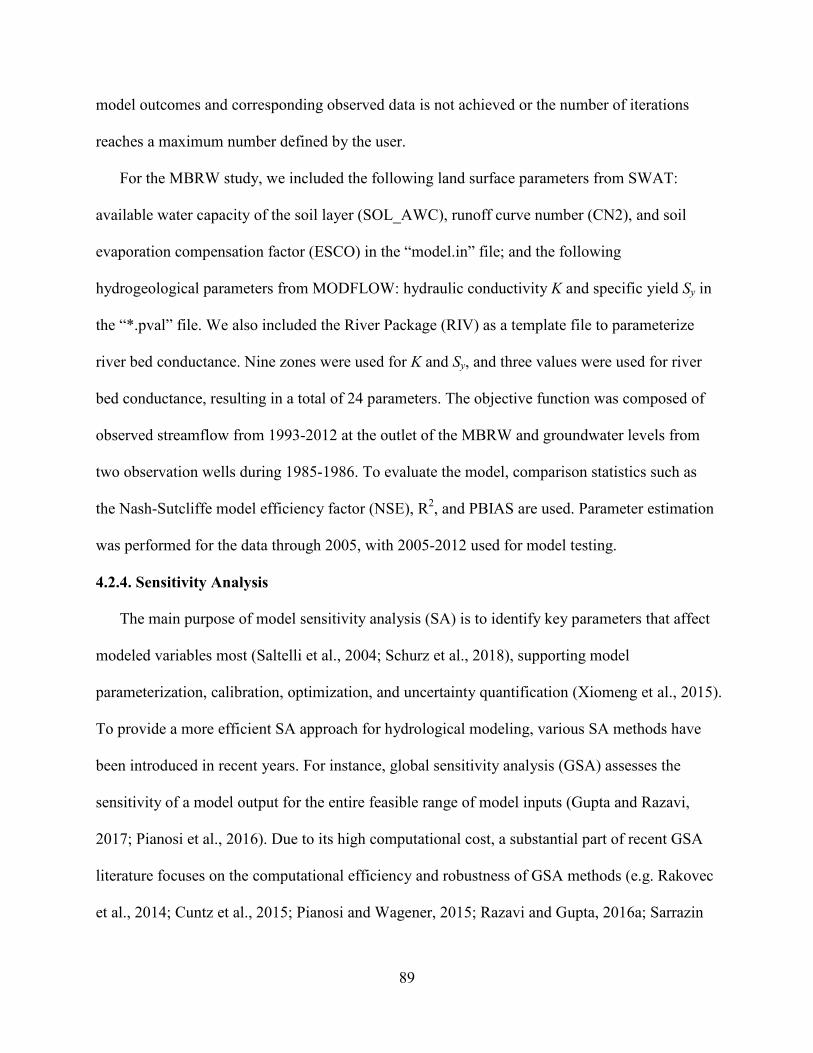
89

model outcomes and corresponding observed data is not achieved or the number of iterations

reaches a maximum number defined by the user.

For the MBRW study, we included the following land surface parameters from SWAT:

available water capacity of the soil layer (SOL_AWC), runoff curve number (CN2), and soil

evaporation compensation factor (ESCO) in the “model.in” file; and the following

hydrogeological parameters from MODFLOW: hydraulic conductivity K and specific yield Sy in

the “*.pval” file. We also included the River Package (RIV) as a template file to parameterize

river bed conductance. Nine zones were used for K and Sy, and three values were used for river

bed conductance, resulting in a total of 24 parameters. The objective function was composed of

observed streamflow from 1993-2012 at the outlet of the MBRW and groundwater levels from

two observation wells during 1985-1986. To evaluate the model, comparison statistics such as

the Nash-Sutcliffe model efficiency factor (NSE), R2, and PBIAS are used. Parameter estimation

was performed for the data through 2005, with 2005-2012 used for model testing.

4.2.4. Sensitivity Analysis

The main purpose of model sensitivity analysis (SA) is to identify key parameters that affect

modeled variables most (Saltelli et al., 2004; Schurz et al., 2018), supporting model

parameterization, calibration, optimization, and uncertainty quantification (Xiomeng et al., 2015).

To provide a more efficient SA approach for hydrological modeling, various SA methods have

been introduced in recent years. For instance, global sensitivity analysis (GSA) assesses the

sensitivity of a model output for the entire feasible range of model inputs (Gupta and Razavi,

2017; Pianosi et al., 2016). Due to its high computational cost, a substantial part of recent GSA

literature focuses on the computational efficiency and robustness of GSA methods (e.g. Rakovec

et al., 2014; Cuntz et al., 2015; Pianosi and Wagener, 2015; Razavi and Gupta, 2016a; Sarrazin

90

et al., 2016), but also on increasing the insight into modeled systems from certain number of

model computations (e.g. Borgonovo et al., 2017; Dai et al., 2017; Guse et al., 2016a; Massmann

et al., 2014; Razavi and Gupta, 2016a). Compared to GSA, the complexity and computational

demand of a local sensitivity analysis (LSA) are low.

PEST provides a companion program called SENSAN, which adopts LSA that employs a

one-at-a-time (OAT) approach. The OAT approach evaluates the impact of changing values of

each parameter on modeled variables one at a time (Saltelli and Annoni, 2010; Baroni and

Tarantola, 2014), i.e. model output responses are calculated through sequentially varying each of

the model parameters and by fixing all other parameters to their nominal values, often taken from

literatures. The combination of nominal values for all the model parameters under inspection can

be called the “control” scenario (Saltelli et al., 2008). Sensitivity for a particular model output

can be calculated as the difference between that model output and the pertinent model output

“nominal” value, divided by the difference between the current parameter set and the parameter

nominal values. If only a single parameter P differs from the nominal set, the sensitivity for a

particular model output Ф is defined as:

0

0P P

Φ−Φ−

(2)

where Ф0 and P0 are model output and parameter nominal values and Ф and P is the model

output and parameter values pertaining to a particular model run. The normalized sensitivity

coefficient (or sensitivity index) is calculated by:

0 0

0 0

| | | |

| | | |

PNSC

P P

Φ−Φ= ×

− Φ (3)

91

where the NSC is a dimensionless positive number, whose value indicates the relative

importance of parameter P on the model output Ф, i.e. the relative sensitivity of the particular

model output Ф with respect to the changing of the particular model parameter P.

As a by-product of the results from the parameter estimation process by PEST, the

“composite parameter sensitivity” can be provided (Tang et al., 2007; Doherty 2015). Based

on the contents of the Jacobian matrix, PEST calculates a figure related to the sensitivity with

respect to each parameter of all observations (with the latter weighted as per user-assigned

weights). Thus, the “composite sensitivity” of parameter i is defined as:

1/2t

iii

J QJcsp

n

= (4)

where J is the Jacobian matrix and Q is the cofactor matrix which in most cases is a diagonal

matrix whose elements are composed of squared weights for model outputs. The number of

outputs, n, is the number of data records, which in the application to the MBRW are the data

points from the time series of streamflow and water table elevation. Thus, cspi is the normalized

magnitude of the Jacobian matrix column with respect to parameter i.

Although LSA and composite parameter sensitivity are limited to a univariate analysis of

parameter impacts on model outputs resulting in non-correlated input parameters, which is often

not the case for hydrological models (Rosolem et al., 2012; Baroni and Tarantola, 2014; Schurz

et al., 2018) due to their low computational demands and their easy accesses to the evaluation of

individual parameter sensitivities on individual hydrological responses (water table, streamflow,

surface-subsurface interaction, global water balance, etc.), LSA and composite parameter

sensitivity are used in this study to investigate how land surface hydrologic parameters (SWAT

model) and hydrogeological parameters (MODFLOW) affect hydrological responses. 10%

relative change in each parameter was used for the OAT analysis with the nominal value. These

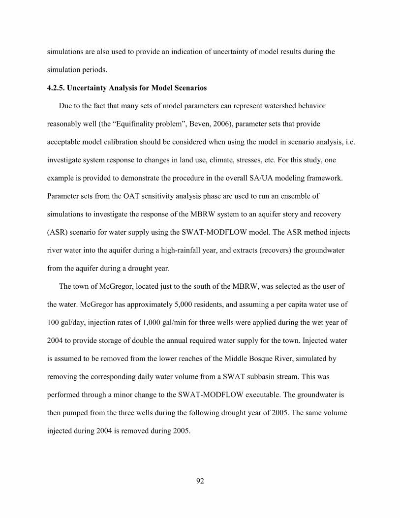
92

simulations are also used to provide an indication of uncertainty of model results during the

simulation periods.

4.2.5. Uncertainty Analysis for Model Scenarios

Due to the fact that many sets of model parameters can represent watershed behavior

reasonably well (the “Equifinality problem”, Beven, 2006), parameter sets that provide

acceptable model calibration should be considered when using the model in scenario analysis, i.e.

investigate system response to changes in land use, climate, stresses, etc. For this study, one

example is provided to demonstrate the procedure in the overall SA/UA modeling framework.

Parameter sets from the OAT sensitivity analysis phase are used to run an ensemble of

simulations to investigate the response of the MBRW system to an aquifer story and recovery

(ASR) scenario for water supply using the SWAT-MODFLOW model. The ASR method injects

river water into the aquifer during a high-rainfall year, and extracts (recovers) the groundwater

from the aquifer during a drought year.

The town of McGregor, located just to the south of the MBRW, was selected as the user of

the water. McGregor has approximately 5,000 residents, and assuming a per capita water use of

100 gal/day, injection rates of 1,000 gal/min for three wells were applied during the wet year of

2004 to provide storage of double the annual required water supply for the town. Injected water

is assumed to be removed from the lower reaches of the Middle Bosque River, simulated by

removing the corresponding daily water volume from a SWAT subbasin stream. This was

performed through a minor change to the SWAT-MODFLOW executable. The groundwater is

then pumped from the three wells during the following drought year of 2005. The same volume

injected during 2004 is removed during 2005.

93

Simulated streamflow, groundwater level, and SW-GW exchange rates are analyzed to

determine the short-term and long-term effects of the ASR scenario on watershed response.

Using the ensemble of parameter sets, the corresponding ensemble of hydrologic responses

incorporates uncertainty in model parameters and yields a band of results that can assist in water

management decisions.

4.3. Results and Discussion

4.3.1. Parameter Estimation

PEST stopped after 288 simulations through 7 iterations. The highest hydraulic conductivity

value is estimated to be 990 m/day, within the alluvium zone in the first layer, and the lowest

hydraulic conductivity value is 0.10 m/day, at exposed-Comanche Peak Limestone in the first

layer. The range of specific yield values varies from 0.05 to 0.35.

Observed streamflow (m3/s) and simulated streamflow at the MBRW outlet is shown in

Figure 4.4, with the simulated results provided by the ensemble of parameter sets used in the 24

OAT simulations. ensemble of parameter sets. The best simulated parameter set shows good

similarity between the SWAT-MODFLOW simulation and the observed data: the monthly NSE

values of streamflow discharge for the calibration and testing periods were calculated to be 0.45

and 0.66, respectively, 0.55 for the entire simulation, considered to be “acceptable” (≥ 0.5) for

monthly stream discharge (Moriasi et al., 2007). The monthly R2 for the testing period also

shows a better result than for the calibration period. The PBIAS value for the calibration period

reveals a small percent under-prediction (2.62), but a large percent over-prediction (-16.79) for

the testing period, probably due to the slightly different behavior in the periods of low stream

flow between the two period.

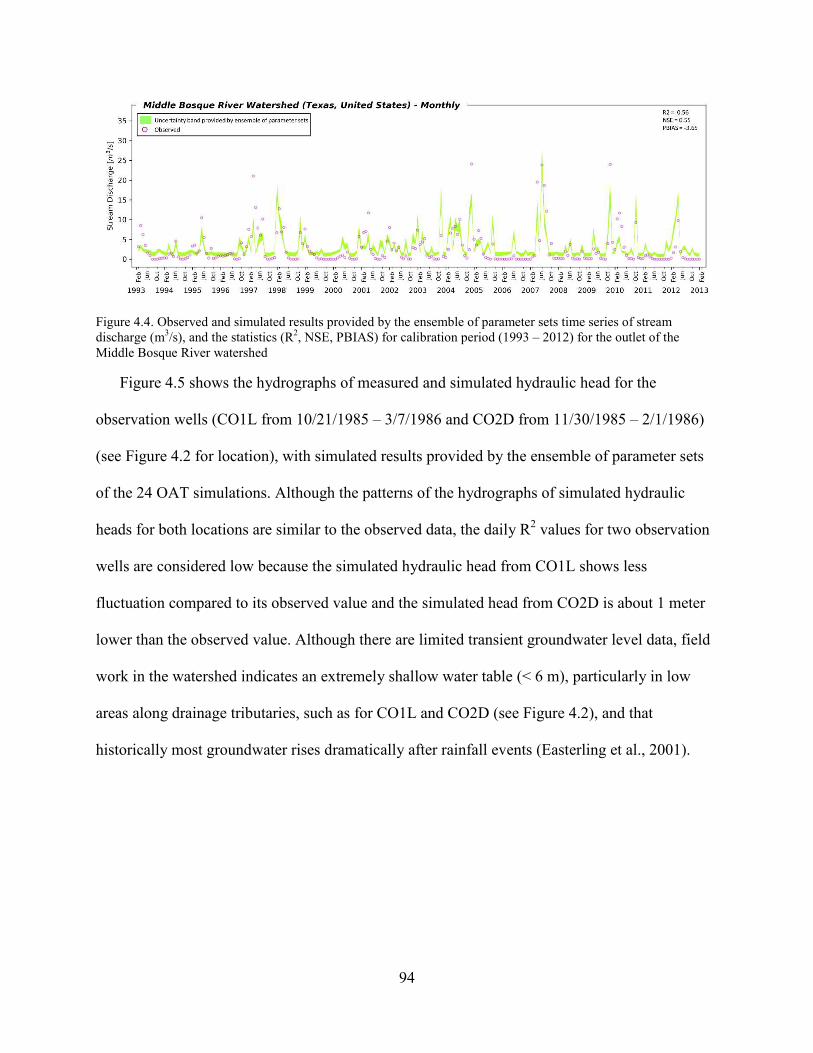
94

Figure 4.4. Observed and simulated results provided by the ensemble of parameter sets time series of stream

discharge (m3/s), and the statistics (R

2, NSE, PBIAS) for calibration period (1993 – 2012) for the outlet of the

Middle Bosque River watershed

Figure 4.5 shows the hydrographs of measured and simulated hydraulic head for the

observation wells (CO1L from 10/21/1985 – 3/7/1986 and CO2D from 11/30/1985 – 2/1/1986)

(see Figure 4.2 for location), with simulated results provided by the ensemble of parameter sets

of the 24 OAT simulations. Although the patterns of the hydrographs of simulated hydraulic

heads for both locations are similar to the observed data, the daily R2 values for two observation

wells are considered low because the simulated hydraulic head from CO1L shows less

fluctuation compared to its observed value and the simulated head from CO2D is about 1 meter

lower than the observed value. Although there are limited transient groundwater level data, field

work in the watershed indicates an extremely shallow water table (< 6 m), particularly in low

areas along drainage tributaries, such as for CO1L and CO2D (see Figure 4.2), and that

historically most groundwater rises dramatically after rainfall events (Easterling et al., 2001).

95

Figure 4.5. the hydrographs of measured and simulated hydraulic head for the observation wells (CO1L from

10/21/1985 – 3/7/1986 and CO2D from 11/30/1985 – 2/1/1986)

4.3.2. Sensitivity Analysis

The composite sensitivities (CSP) were calculated by PEST for the three land surface

parameters, three river bed conductance values, 9 hydraulic conductivity zones, and 9 specific

yield zones on simulated model results (streamflow at the MBRW outlet, groundwater levels at

the two observation wells), and shown in Figure 4.2. The CSP values show in general the

significance of the land surfaces parameters (CN2, ESCO, SOL_AWC) for the simulation of

streamflow and groundwater level. The CSP values range from 0.24 to 0.38 for the land surface

parameters. The CSP of CN2 was the highest, whereas the CSP of the river bed conductance

were negligible (Figure 4.6). The CSP for the K and Sy zones are also low. This likely is due to

the high weight attributed to streamflow, with the land surface parameters governing streamflow

more than hydrogeological parameters. Also, the locations of the two groundwater observation

points are close to one of the tributaries of the Middle Bosque River, so that the water table is

continuously high in the shallow subsurface.

96

Figure 4.6. Model input composite sensitivities (CSP) for signature measures of streamflow discharge and two water

table elevations in the Middle Bosque watershed. Circle plot shows the set of CSP calculated for model inputs. The

CSP indices are illustrated in coloured groups showing in clockwise order the sensitivities of selected land surface

parameters in green, of river bed conductance in red, of 9 hydraulic conductivity zones, and of 9 specific yield

zones.

For the model used in this study, the LSA (OAT) approach is better suited for investigating

the control of each parameter on streamflow and groundwater hydraulic head. Figure 4.7 shows

results of the OAT approach, with Figure 4.7a showing the Normalized Sensitivity Coefficient

(NSC) for streamflow and groundwater head, and Figure 4.7b showing the NSC for streamflow

only. Similar to the CSP, the NSC of the land surface parameters is higher than for the

hydrogeological properties; however, the aquifer properties (K, Sy) do exhibit a moderate

influence particularly for alluvium and terrace deposits, which are near-surface geologic units

and thus have a control and land surface processes and associated surface runoff and streamflow

in the MBRW watershed system. When analyzing influence solely on streamflow (Figure 4.7b),

the relative effect of the parameters is the same as when analyzing jointly streamflow and

groundwater head. Riverbed conductance does not show a strong control in either analysis

97

(results shown in Figure 4.7a or 4.7b), likely because exchange rates between surface water and

groundwater are not of sufficient magnitude to change streamflow significantly.

Figure 4.7. Model input Normalized Sensitivity Coefficient (NSC) for signature measures of a) streamflow

discharge and two water table elevations and b) streamflow discharge only. Circle plot shows the set of NSC

calculated for model inputs. The NSC indices are illustrated in coloured groups showing in clockwise order the

sensitivities of selected land surface parameters in green, of river bed conductance in red, of 9 hydraulic

conductivity zones, and of 9 specific yield zones.

4.3.3. Simulation Uncertainties for Groundwater Development Scenario

The effect of the aquifer storage and recovery scenarios on groundwater levels is shown in

Figure 4.8. The results from OB1 shows the maximum increase in water table is 2.1 meters in

Dec. For OB2 the maximum increase is 2.1 meters in Jul. 2004 and decrease is 1.2 m in Dec.

2005. OB3 shows that the maximum increase is 2.4 meters in Nov. 2004 and decrease is 1.4 m in

Dec. 2005.OB5 results in the highest water table increase (5.3m) in Dec. 2004 and smallest

(1.1m) in Dec. 2005. In general, injecting water results in higher changes in water table than

extracting water from the aquifer (similar to scale change of hydrological responses and water

balance). The results show that their response time, scales and durations not only vary but also

98

are influenced by pre-conditions (i.e. soil moisture, water table), their distances to pumping wells.

Figure 4.8. Effect of the aquifer storage and recovery scenarios on groundwater levels

These results can be used by regional water managers and planners to determine long-term

effects of aquifer storage and recovery on the stream system and the aquifer system.

The Normalized Sensitivity Coefficient (NSC) on water balance from the calibrated model

and with groundwater development scenario is shown in Figure 4.9. For the calibrated model,

NSC on water balance ranges from 0 to 10.3 (PERCO). The aquifer properties (K, Sy) exhibit a

moderate influence particularly for alluvium and terrace deposits, which are near-surface

geologic units and thus have a control and land surface processes and associated surface runoff

and streamflow in the MBRW watershed system. The lateral flow (LATQ) and groundwater

deep percolation (PERCO) components of the water balance show moderate influences by all 9

99

hydrogeologic zones with respect to their specific yields suggesting parameters related to

porosities resulting in higher sensitivities. The results from NSC in groundwater development

scenario show decreases in 9 Sy sensitivities on hydrologic responses (water components)

suggesting the addition of a decision parameter (pumping or injecting) can reduce the

sensitivities of the hydrogeologic parameters.

Figure 4.9. Normalized Sensitivity Coefficient (NSC) on water balance in (upper) calibrated model and (lower) with

groundwater development scenario

4.4. Summary and Conclusions

This paper introduces a general framework for quantifying sensitivity, uncertainty, and

parameter values for integrated surface water-groundwater models. Using the SWAT-

MODFLOW modelling code as an example integrated model, the framework outlines the phases

100

of model construction, parameter estimation and sensitivity analysis, uncertainty analysis, and

model application to scenario analysis. PEST is used as the software tool for parameter

estimation and sensitivity analysis, with an accompanying Local Sensitivity Analysis (LSA) used

to provide uncertainty around the best-calibrated parameter set. A methodology is developed for

PEST in which both SWAT (land surface, stream, soil) parameters and MODFLOW

(hydrogeological) parameters can be estimated jointly during the PEST iterations. Uncertainty in

model predictions, i.e. scenario analysis is provided using the simulations used in the LSA.

The framework is applied to the Middle Bosque River watershed (471 km2), located in

central Texas. The SWAT-MODFLOW model for the watershed is calibrated by estimating the

values of 24 parameters (land surface parameters, hydraulic conductivity for geologic units,

specific yield for geologic units, riverbed conductance) and comparing model output with

streamflow at the watershed outlet and groundwater levels at two observation wells. The land

surface parameters (available water capacity of the soil layer, runoff curve number, soil

evaporation compensation factor) had the strongest control on streamflow and groundwater head,

followed by specific yield and hydraulic conductivity of the alluvium material and near-surface

terrace deposits. The model was then applied to an aquifer storage and recovery scenario to store

water during wet years and extract groundwater during drought years. Results show the influence

of this groundwater development scenario on hydrologic response (streamflow, water table

elevation, GW-SW interactions) and overall watershed water balance, with uncertainty bands of

simulation results provided to provide decision makers with possible ranges of responses.

The proposed modelling framework can assist in implementing and applying integrated

surface water-groundwater models for estimating watershed water resource and analysing the

effect of changes in land use, population, and climate. Keys to the framework are the ability to

101

jointly estimate land surface and hydrogeological parameters and quantify their impact on

hydrologic responses (streamflow, water table elevation, GW-SW interactions). This framework,

particularly if used with SWAT-MODFLOW, can facilitate the use of integrated models

worldwide to assist with finding technical solutions to water issues.

102

REFERENCES

Abbaspour, K.C., Vejdani, M., Haghighat, S. and Yang, J., 2007, December. SWAT-CUP

calibration and uncertainty programs for SWAT. In MODSIM 2007 International Congress

on Modelling and Simulation, Modelling and Simulation Society of Australia and New

Zealand (pp. 1596-1602).

Abbaspour, K.C., 2011. Swat-Cup2: SWAT Calibration and Uncertainty Programs Manual

Version 2, Department of Systems Analysis, Integrated Assessment and Modelling (SIAM),

Eawag. Swiss Federal Institute of Aquatic Science and Technology, Duebendorf, Switzerland.

106 p.

Abbaspour, K.C., Rouholahnejad, E., Vaghefi, S., Srinivasan, R., Yang, H., and B. Klove (2015),

A continental-scale hydrology and water quality model for Europe: Calibration and

uncertainty of a high-resolution large-scale SWAT model. Journal of Hydrology 524, 733-

752.

Bailey, R.T., Wible, T.C., Arabi, M., Records, R.M., and J. Ditty (2016), Assessing regional-


SWAT-MODFLOW model. Hydrological Processes 30, 4420-4433.

Bailey, R., Rathjens, H., Bieger, K., Chaubey, I., and J. Arnold (2017), SWATMOD-Prep:

Graphical user interface for preparing coupled SWAT-MODFLOW simulations. J American

Water Resources Association 53(2), 400-410.

Beven, K. (2006). A manifesto for the equifinality thesis. Journal of Hydrology, 320(1-2), 18-36.

Bicknell, B.R., J.C. Imhoff, J.L. Kittle, Jr., T.H. Jobes, and A.S. Donigian, Jr., 2001.

Hydrological Simulation Program –FORTRAN (HSPF), User’s Manual for Version 12.0.

USEPA, Athens, Georgia.

103

Gallagher, M., and J. Doherty (2007), Parameter estimation and uncertainty analysis for a

watershed model. Environmental Modelling & Software 22, 1000-1020.

Li, Z., Shao, Q., Xu, Z., and X. Cai (2010), Analysis of parameter uncertainty in semi-distributed

hydrologic models using bootstrap method: A case study of SWAT model applied to

Yingluoxia watershed in northwest China. Journal of Hydrology 385, 76-83.

Muleta, M.K. and J.W. Nicklow (2005), Sensitivity and uncertainty analysis coupled with

automatic calibration for a distributed watershed model. Journal of Hydrology 306, 127-145.

Park, S., Nielsen, A., Bailey, R.T., Trolle, D., and K. Bieger (2018), A QGIS-based graphical

user interface for application and evaluation of SWAT-MODFLOW models. Environmental

Modelling & Software, in Second Review.

Poeter, Eileen P., Mary C. Hill, Dan Lu, Claire R. Tiedeman, and Steffen Mehl, 2014,

UCODE_2014, with new capabilities to define parameters unique to predictions, calculate

weights using simulated values, estimate parameters with SVD, evaluate uncertainty with

MCMC, and more: Integrated Groundwater Modeling Center Report Number GWMI 2014-

02.

Shen, Z.Y., Chen, L., and T. Chen (2012), Analysis of parameter uncertainty in hydrological and

sediment modeling using GLUE method: a cast study of SWAT model applied to Three

Gorges Reservoir Region, China. Hydrol. Earth Syst. Sci. 16, 121-132.

Surfleet, C.G., and D. Tullos (2013), Uncertainty in hydrologic modelling for estimating

hydrologic response due to climate change (Santiam River, Oregon), Hydrological Processes

27, 3560-3576.

Wu, B., Zheng, Y., Tian, Y., Wu, X., Yao, Y., Han, F., Liu, J., and Chunmiao Zheng (2014),

Systematic assessment of the uncertainty in integrated surface water-groundwater modeling

104

based on the probabilistic collocation method. Water Resources Research, doi:

10.1002/2014WR015366.

Wu, Y., and S. Liu (2012), Automating calibration, sensitivity and uncertainty analysis of

complex models using the R package Flexible Modeling Environment (FME): SWAT as an

example. Environmental Modelling & Software 31, 99-109.

Yang, J., Reichert, P., and K.C. Abbaspour (2007), Bayesian uncertainty analysis in distributed

hydrologic modelling: A case study in the Thur River basin (Switzerland). Water Resources

Research 43, doi:10.1029/2006WR005497.

105

CHAPTER 5

CONCLUSIONS AND FUTURE WORK

The research presented in this dissertation summarizes efforts providing a general framework

for implementation and use of integrated surface water-groundwater hydrologic models. The

efforts included developing an easy-to-use workflow (QSWATMOD) for model construction,

configuring simulation settings, and visualizing and interpreting results and a general framework

for performing sensitivity analysis, parameter estimation, and uncertainty analysis for integrated

surface water-groundwater models, using the SWAT-MODFLOW modelling code as an example.

The model also was applied to a central Texas watershed to investigate the influence of drought

and high-intensity storm events on water resources and watershed water balance components.

5.1. A QGIS-based graphical user interface for application and evaluation of SWAT-

MODFLOW models

• Conclusions:

- A new graphical user interface (QSWATMOD) is introduced to facilitate the

linkage of SWAT and MODFLOW models.

- QSWATMOD is created as a QGIS plug-in tool, which allows maps of SWAT

and MODFLOW domains and variables to be easily viewed on the QGIS map

canvas.

- QSWATMOD requires an existing SWAT model and can link with an existing

MODFLOW model or a single-layer MODFLOW model created within the QGIS

environment.

106

- QSWATMOD runs a SWAT-MODFLOW simulation and allows for viewing of

system responses such as stream discharge, groundwater head, groundwater

recharge, and groundwater-surface interactions.

- QSWATMOD can compare model results with observed stream discharge and

groundwater level data.

- QSWATMOD can be a valuable tool in assisting users to create and manage

SWAT-MODFLOW projects, allowing coupled surface water/groundwater

models to become more accessible to a broader hydrologic modelling community.

• Future work:

- Introduction of dynamic plots for streamflow discharge and water table elevation

- Implementation of help option including beginner’s guide and tutorial

- Implementation of RT3D option creating input files to help users simulate solute

transports

- Migration to a new version of QGIS (QGIS3)

- Introduction of parameter estimation providing basic input files for PEST

5.2. Quantifying effect of decadal and extreme climate events on watershed water resources

and fluxes using SWAT-MODFLOW

• Conclusions:

- Model outputs: cell-wise hydraulic head, recharge, and surface-subsurface water

interaction, demonstrate a high spatio-temporal variability and correlations

between the results.

107

- Water balance from surface and sub-surface domains was simulated

simultaneously based on time series analysis and the results show high temporal

variation of water balance components.

- Using the calibrated model, the impact of precipitation on streamflow discharge,

hydraulic head elevation, and water resource availability was assessed under

different rainfall scenarios. The results show that their response time, scales and

durations not only vary but also are influenced by pre-conditions (i.e. soil

moisture).

- This study helps enhance understanding regarding the spatio-temporal patterns of

hydraulic head elevation, recharge, surface-subsurface water interaction and the

water resource availability and the hydrological responses with different rainfall

patterns that support decisions about alternative management strategies in the

areas of land use change, climate change, water allocation, pollution control and

groundwater development scenarios.

• Future work:

- Optimize the SWAT-MODFLOW model of the MBRW by finding the optimal

spatio-temporal discretization (e.g. grid cell size, time step size); report general

guidelines regarding adoption of grid cells size and time step size for integrated

surface water-groundwater models.

- Perform analysis of effect on baseflow in the study area

Setting up boundary conditions for MODFLOW model

Check streamflow and water table for each subbasin

Check groundwater discharge for each subbasin

108

Perform comprehensive simulation of solute transport in this study area

(coupled surface-subsurface hydrologic systems) using the linked SWAT-

MODFLOW-RT3D model.

5.3. A framework for quantifying uncertainty, sensitivity, and estimating parameters for

integrated surface water - groundwater models

• Conclusions:

- A methodology is developed for automatic parameter estimation in which SWAT

(land surface, stream, soil) parameters and MODFLOW (hydrogeological)

parameters can be estimated jointly using the PEST software program.

- Uncertainty in model predictions, i.e. scenario analysis is provided using the

simulations used in a Local Sensitivity Analysis method.

- The proposed modelling framework can assist in implementing and applying

integrated surface water-groundwater models for estimating watershed water

resource and analysing the effect of changes in land use, population, and climate.

- This framework, particularly if used with SWAT-MODFLOW, can facilitate the

use of integrated models worldwide to assist with finding technical solutions to

water issues.

• Future work:

- Introduction of methods for Global sensitivity analysis (GSA) application and the

visual analysis of uncertainties for integrated surface water – groundwater models

- Introduction of methods for future change and development scenarios with global

climate models (GCM) and land use change.

109

5.4. General Conclusions

The presented modelling methodology with SWAT-MODFLOW can facilitate model use

worldwide to find technical solutions to water issues. These issues include water supply, the

impact of groundwater development on groundwater supply and surface water depletion, the

movement and remediation of contaminants (nutrients, trace elements) in the watershed system,

the mobilization and presence of salt ions and their effect on water quality and crop yield, and

transboundary groundwater conflicts.

110

APPENDIX A

Supplementary Material for (CHAPTER 2)

A QGIS-based graphical user interface for application and evaluation of SWAT-MODFLOW

models

Seonggyu Park

1, *, Anders Nielsen

2, Ryan T. Bailey

1, Dennis Trolle

2, Katrin Bieger

3

1Dept. of Civil and Environmental Engineering, Colorado State University, Fort Collins, CO, USA

2Aarhus University, Department of Bioscience, Vejlsøvej, Silkeborg, Denmark

3Blackland Research & Extension Center, Texas A&M AgriLife, Temple, TX, United States

*Correspondence to: Seonggyu Park ([email protected]); Tel: 970-889-9081, Fax: 970-491-

7727

Environmental Modelling & Software

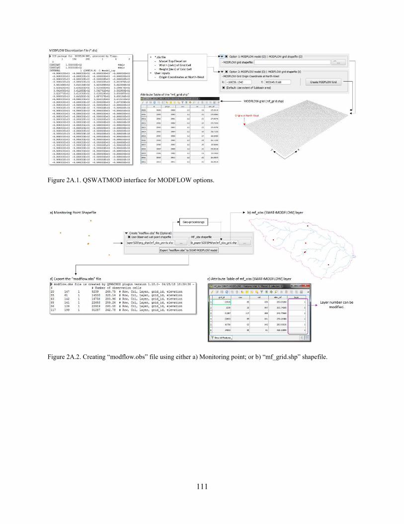
111

Figure 2A.1. QSWATMOD interface for MODFLOW options.

Figure 2A.2. Creating “modflow.obs” file using either a) Monitoring point; or b) “mf_grid.shp” shapefile.

112

Figure 2A.3. Observation file formats (Tab delimited) for a) “streamflow.obd”; and b) “modflow.obd” files. These

data will be compared to SWAT-MODFLOW output once the simulation has finished.

output.mp4 (Command Line)

Video 2A.4. Annual Average Surface and Groundwater Interactions from 1980 – 2011 for the Middle Bosque River

Watershed.

113

Figure 2A.5. Exported files for a) streamflow and observation values; b) water table elevation and observation

values; c) groundwater and surface water interaction for a specific date; and d) water balance for the period of a

simulation.

114

APPENDIX B

QSWATMOD (a part of source code)

# -*- coding: utf-8 -*-

"""

/***************************************************************************

QSWATMOD / MODFLOW function

A QGIS plugin

This plugin displays the result of SM simulation

-------------------

begin : 2017-08-02

git sha : $Format:%H$

copyright : (C) 2017 by Seonggyu and Dr. Anders

email : [email protected]

***************************************************************************/

/***************************************************************************

* *

* This program is free software; you can redistribute it and/or modify *

* it under the terms of the GNU General Public License as published by *

* the Free Software Foundation; either version 2 of the License, or *

* (at your option) any later version. *

* *

***************************************************************************/

"""

import os

import os.path

import posixpath

import ntpath

import shutil

import glob

import processing

from PyQt4.QtSql import QSqlDatabase, QSqlQuery, QSqlTableModel

from PyQt4.QtCore import *

from PyQt4.QtCore import QCoreApplication

from PyQt4.QtGui import *

from PyQt4 import QtGui, uic

import numpy as np

# import pandas as pd

from qgis.core import QgsProject

import distutils.dir_util

from datetime import datetime

# import modules related flopy

import flopy

import flopy.utils.binaryfile as bf

from osgeo import gdal

from QSWATMOD.QSWATMOD import *

from QSWATMOD.QSWATMOD_dialog import QSWATMODDialog

from QSWATMOD.pyfolder import modflow_functions

from QSWATMOD.pyfolder import writeMF

from QSWATMOD.pyfolder import db_functions

from QSWATMOD.pyfolder import linking_process

#

FORM_CLASS, _ = uic.loadUiType(os.path.join(os.path.dirname(__file__), 'ui/createMFmodel.ui'))

115

class createMFmodelDialog(QDialog, FORM_CLASS):

def __init__(self, iface):

QDialog.__init__(self)

self.iface = iface

self.setupUi(self)

# def __init__(self, parent = None):

# super(createMFmodelDialog, self).__init__(parent)

# self.setupUi(self)

# self.pushButton_TxtInOut.clicked.connect(self.test)

# def test(self):

# options = QtGui.QFileDialog.DontResolveSymlinks | QtGui.QFileDialog.ShowDirsOnly

# directory = QtGui.QFileDialog.getExistingDirectory(None,

# "QFileDialog.getExistingDirectory()",

# "self.dlg.Lakemodel_directory.text()", options)

# if directory:

# proj = QgsProject.instance()

# Project_Name = QFileInfo(proj.fileName()).baseName()

# Out_folder_temp = QgsProject.instance().readPath("./")

# Out_folder = os.path.normpath(Out_folder_temp + "/" + Project_Name + "/" + "existingModel" + "/" + "SWAT-MODFLOW")

# #distutils.dir_util.remove_tree(Out_folder)

# distutils.dir_util.copy_tree(directory, Out_folder)

# #self.dlg.Lakemodel_directory.setText(Out_folder)

# #self.DB_Update_Lakemodel_Directory()

# #time.sleep(1)

# # Check file extension

# file_check = os.path.abspath(os.path.join(Out_folder, "tr_041316.nam"))

# if os.path.isfile(file_check) is True:

# msgBox = QMessageBox()

# msgBox.setText("The MODLFOW folder was succesfully copied")

# msgBox.exec_()

# self.lineEdit_TxtInOut.setText(Out_folder)

# else:

# msgBox = QMessageBox()

# msgBox.setText("There was a problem copying the folder")

# msgBox.exec_()

#------------------------------------------------------------------------------------------------

self.checkBox_ratio.setCheckState(Qt.Checked)

self.pushButton_createMFfolder.clicked.connect(self.createMFfolder)

self.pushButton_loadDEM.clicked.connect(self.loadDEM)

self.checkBox_use_sub.toggled.connect(self.use_sub_shapefile)

self.pushButton_create_MF_shps.clicked.connect(self.create_MF_shps)

# -----------------------------------------------------------------------------------------------

self.radioButton_aq_thic_single.toggled.connect(self.aqufierThickness_option)

self.radioButton_aq_thic_uniform.toggled.connect(self.aqufierThickness_option)

self.radioButton_aq_thic_raster.toggled.connect(self.aqufierThickness_option)

self.pushButton_aq_thic_raster.clicked.connect(self.loadBotElev)

self.radioButton_hk_single.toggled.connect(self.hk_option)

self.radioButton_hk_raster.toggled.connect(self.hk_option)

self.pushButton_hk_raster.clicked.connect(self.loadHK)

self.comboBox_layerType.clear()

self.comboBox_layerType.addItems([' - Confined - ', ' - Convertible - '])

self.radioButton_ss_single.toggled.connect(self.ss_option)

self.radioButton_ss_raster.toggled.connect(self.ss_option)

116

self.pushButton_ss_raster.clicked.connect(self.loadSS)

self.radioButton_sy_single.toggled.connect(self.sy_option)

self.radioButton_sy_raster.toggled.connect(self.sy_option)

self.pushButton_sy_raster.clicked.connect(self.loadSY)

self.radioButton_initialH_single.toggled.connect(self.initialH_option)

self.radioButton_initialH_uniform.toggled.connect(self.initialH_option)

self.radioButton_initialH_raster.toggled.connect(self.initialH_option)

self.pushButton_initialH_raster.clicked.connect(self.loadInitialH)

self.pushButton_writeMF.clicked.connect(self.writeMF)

self.DB_Pull_mf_inputs() # instant call

self.pushButton_reset.clicked.connect(self.DB_resetTodefaultVal)

self.pushButton_create_mf_riv_shapefile.clicked.connect(self.create_mf_riv)

# Retrieve info

self.retrieve_ProjHistory_mf()

#---------------------------------------------------------------------------------------------

QObject.connect(self.doubleSpinBox_delc, SIGNAL("valueChanged(double)"), self.esti_ngrids)

QObject.connect(self.doubleSpinBox_delr, SIGNAL("valueChanged(double)"), self.esti_ngrids)

QObject.connect(self.doubleSpinBox_delc, SIGNAL("valueChanged(double)"), self.set_delr)

#-------------------------------------------------------------------------------------------------

##### QUESTIONS!! Is this function should be here too? ######

def dirs_and_paths(self):

global QSWATMOD_path_dict

# project places

Projectfolder = QgsProject.instance().readPath("./")

proj = QgsProject.instance()

Project_Name = QFileInfo(proj.fileName()).baseName()

# definition of folders

org_shps = os.path.normpath(Projectfolder + "/" + Project_Name + "/" + "GIS/org_shps")

SMshps = os.path.normpath(Projectfolder + "/" + Project_Name + "/" + "GIS/SMshps")

SMfolder = os.path.normpath(Projectfolder + "/" + Project_Name + "/" + "SWAT-MODFLOW")

Table = os.path.normpath(Projectfolder + "/" + Project_Name + "/" + "GIS/Table")

SM_exes = os.path.normpath(Projectfolder + "/" + Project_Name + "/" + "SM_exes")

exported_files = os.path.normpath(Projectfolder + "/" + Project_Name + "/" + "exported_files")

QSWATMOD_path_dict = {'org_shps': org_shps,

'SMshps': SMshps,

'SMfolder': SMfolder,

'Table': Table,

'SM_exes': SM_exes,

'exported_files': exported_files}

return QSWATMOD_path_dict

# def dirs_and_paths(self):

# # project places

# Projectfolder = QgsProject.instance().readPath("./")

# proj = QgsProject.instance()

# Project_Name = QFileInfo(proj.fileName()).baseName()

# # definition of folders

# org_shps = os.path.normpath(Projectfolder + "/" + Project_Name + "/" + "GIS/org_shps")

# SMshps = os.path.normpath(Projectfolder + "/" + Project_Name + "/" + "GIS/SMshps")

# SMfolder = os.path.normpath(Projectfolder + "/" + Project_Name + "/" + "SWAT-MODFLOW")

# Table = os.path.normpath(Projectfolder + "/" + Project_Name + "/" + "GIS/Table")

# SM_exes = os.path.normpath(Projectfolder + "/" + Project_Name + "/" + "SM_exes")

# return org_shps, SMshps, SMfolder, Table, SM_exes

def DB_Pull_mf_inputs(self):

db = db_functions.db_variable(self)

117

query = QtSql.QSqlQuery(db)

query.exec_("SELECT user_val FROM mf_inputs WHERE parNames = 'ss' ")

LK = str(query.first()) # What does LK do?

self.lineEdit_ss_single.setText(str(query.value(0)))

# ...

def DB_push_mf_userVal(self):



query.prepare("UPDATE mf_inputs SET user_val = :UP1 WHERE parNames = 'ss'")

query.bindValue (":UP1", self.lineEdit_ss_single.text())

query.exec_()

def DB_resetTodefaultVal(self):

msgBox = QMessageBox()

msgBox.setWindowIcon(QtGui.QIcon(':/newPrefix/pics/logo.png'))

response = msgBox.question(self, 'Set to default?',

"Are you sure you want to reset the current aquifer property settings to the default values?",

QMessageBox.Yes | QMessageBox.No, QMessageBox.No)

if response == QMessageBox.Yes:



query.exec_("SELECT default_val FROM mf_inputs WHERE parNames = 'ss' ")

LK = str(query.first())

self.lineEdit_ss_single.setText(str(query.value(0)))

self.DB_push_mf_userVal()

def retrieve_ProjHistory_mf(self):

QSWATMOD_path_dict = self.dirs_and_paths()

# Define folders and files

SMfolder = QSWATMOD_path_dict['SMfolder']

org_shps = QSWATMOD_path_dict['org_shps']

SMshps = QSWATMOD_path_dict['SMshps']

# retrieve DEM

if os.path.isfile(os.path.join(org_shps, 'DEM.tif')):

self.lineEdit_loadDEM.setText(os.path.join(org_shps, 'DEM.tif'))

else:

self.textEdit_mf_log.append("* Provide DEM raster file.")

def createMFfolder(self):

settings = QSettings()

if settings.contains('/QSWATMOD/LastInputPath'):

path = unicode(settings.value('/QSWATMOD/LastInputPath'))

else:

path = ''

options = QtGui.QFileDialog.DontResolveSymlinks | QtGui.QFileDialog.ShowDirsOnly

title = "create MODFLOW folder"

mffolder = QFileDialog.getExistingDirectory(None, title, path, options)

mffolder_path = self.lineEdit_createMFfolder.setText(mffolder)

return mffolder_path

# navigate to the DEM raster from SWAT

def loadDEM(self):


settings = QSettings()

if settings.contains('/QSWATMOD/LastInputPath'):

path = unicode(settings.value('/QSWATMOD/LastInputPath'))

else:

path = ''

title = "Choose DEM rasterfile"

inFileName = QFileDialog.getOpenFileName(None, title, path, "Rasterfiles (*.tif);; All files (*.*)")

118

if inFileName:

settings.setValue('/QSWATMOD/LastInputPath', os.path.dirname(unicode(inFileName)))

Out_folder = QSWATMOD_path_dict['org_shps']

inInfo = QFileInfo(inFileName)

inFile = inInfo.fileName()

pattern = os.path.splitext(inFileName)[0] + '.*'

baseName = inInfo.baseName()

# inName = os.path.splitext(inFile)[0]

inName = 'DEM'

for f in glob.iglob(pattern):

suffix = os.path.splitext(f)[1]

if os.name == 'nt':

outfile = ntpath.join(Out_folder, inName + suffix)

else:

outfile = posixpath.join(Out_folder, inName + suffix)

shutil.copy(f, outfile)

if os.name == 'nt':

DEM = ntpath.join(Out_folder, inName + ".tif")

else:

DEM = posixpath.join(Out_folder, inName + ".tif")

layer = QgsRasterLayer(DEM, '{0} ({1})'.format("DEM","SWAT"))

# Put in the group

root = QgsProject.instance().layerTreeRoot()

swat_group = root.findGroup("SWAT")

QgsMapLayerRegistry.instance().addMapLayer(layer, False)

swat_group.insertChildNode(0, QgsLayerTreeLayer(layer))

self.lineEdit_loadDEM.setText(DEM)

return DEM

def loadHK(self):

writeMF.loadHK(self)

def loadBotElev(self):

writeMF.loadBotElev(self)

def loadSS(self):

writeMF.loadSS(self)

def loadSY(self):

writeMF.loadSY(self)

def loadInitialH(self):

writeMF.loadInitialH(self)

def use_sub_shapefile(self):

from PyQt4 import QtCore, QtGui, QtSql


try:

input1 = QgsMapLayerRegistry.instance().mapLayersByName("sub (SWAT)")[0]

#provider = layer.dataProvider()

if self.checkBox_use_sub.isChecked():

name = "mf_boundary"

name_ext = "mf_boundary.shp"

output_dir = QSWATMOD_path_dict['org_shps']

# output_file = os.path.normpath(output_dir + "/" + name)

mf_boundary = os.path.join(output_dir, name_ext)

processing.runalg("qgis:dissolve", input1, True, None, mf_boundary)

# defining the outputfile to be loaded into the canvas

layer = QgsVectorLayer(mf_boundary, '{0} ({1})'.format("mf_boundary","MODFLOW"), 'ogr')

119

# Put in the group


mf_group = root.findGroup("MODFLOW")


mf_group.insertChildNode(0, QgsLayerTreeLayer(layer))

#subpath = layer.source()

self.lineEdit_boundary.setText(mf_boundary)

except:



msgBox.setWindowTitle("What the FXXXX!")

msgBox.setText("There is no 'sub' shapefile!")

msgBox.exec_()

# self.dlg.checkBox_default_extent.setChecked(0)

# return layer

def create_MF_grid(self): # Create fishnet based on user inputs


input1 = QgsMapLayerRegistry.instance().mapLayersByName("mf_boundary (MODFLOW)")[0]

ext = input1.extent()

xmin = ext.xMinimum()

xmax = ext.xMaximum()

ymin = ext.yMinimum()

ymax = ext.yMaximum()

delc = float(self.doubleSpinBox_delc.value())

delr = float(self.doubleSpinBox_delr.value())

nx = round((xmax - xmin) / delc)

ny = round((ymax - ymin) / delr)

ngrid = abs(int(nx*ny))

MF_extent = "{a},{b},{c},{d}".format(a = xmin, b = xmax, c = ymin, d = ymax)

#

name = "mf_grid"

name_ext = "mf_grid.shp"


output_file = os.path.normpath(output_dir + "/" + name)

# running the acutal routine:

processing.runalg("qgis:vectorgrid", MF_extent, delc,delr,0, output_file)

# Define the outputfile to be loaded into the canvas

mf_grid_shapefile = os.path.join(output_dir, name_ext)

layer = QgsVectorLayer(mf_grid_shapefile, '{0} ({1})'.format("mf_grid","MODFLOW"), 'ogr')

# Put in the group





def create_grid_id_ii(self):

self.layer = QgsMapLayerRegistry.instance().mapLayersByName("mf_grid (MODFLOW)")[0]

provider = self.layer.dataProvider()

if self.layer.dataProvider().fields().indexFromName("grid_id") == -1:

field = QgsField("grid_id", QVariant.Int)

provider.addAttributes([field])

self.layer.updateFields()

# I don't know

120

grid_id = self.layer.dataProvider().fields().indexFromName("grid_id")

feats = self.layer.getFeatures()

self.layer.startEditing()

for i, f in enumerate(feats):

self.layer.changeAttributeValue(f.id(), grid_id, i+1)

self.layer.commitChanges()

time = datetime.now().strftime('[%m/%d/%y %H:%M:%S]')

self.textEdit_mf_log.append(time+' -> ' + "'grid_id' has been created ...")

else:


self.textEdit_mf_log.append(time+' -> ' + "'grid_id' already exists ...")

# for elev, not using *.dis file. instead using DEM

def create_row_col_elev_mf_ii (self):

import math


self.layer = QgsMapLayerRegistry.instance().mapLayersByName("mf_grid (MODFLOW)")[0]

provider = self.layer.dataProvider()

# from qgis.core import QgsField, QgsExpression, QgsFeature

if self.layer.dataProvider().fields().indexFromName( "row" ) == -1:

field = QgsField("row", QVariant.Int)



# Create Column field

if self.layer.dataProvider().fields().indexFromName( "col" ) == -1:

field = QgsField("col", QVariant.Int)



# Get the index numbers of the fields

# elev_mean = self.layer.dataProvider().fields().indexFromName( "elev_mean" )

row = provider.fields().fieldNameIndex("row")

col = provider.fields().fieldNameIndex("col")

# Change name

for field in self.layer.pendingFields():

if field.name() == 'elev_mean':


idx = self.layer.fieldNameIndex(field.name())

self.layer.renameAttribute(idx, "elev_mf")


# Get number of rows and of columns









nx = math.ceil(abs(abs(xmax) - abs(xmin)) / delc)

ny = math.ceil(abs(abs(ymax) - abs(ymin)) / delr)

# Get row and column lists

iy = [] # row

ix = [] # col

for i in range(1, ny + 1):

for j in range(1, nx + 1):

ix.append(j)

iy.append(i)

121

# Get features (Find out a way to change attribute values using another field)

feats = self.layer.getFeatures()


# add row number

for f, r, c in zip(feats, iy, ix):

self.layer.changeAttributeValue(f.id(), row, r)

self.layer.changeAttributeValue(f.id(), col, c)

# self.layer.changeAttributeValue(f.id(), elev_mf, elev)

# self.layer.changeAttributeValue(f[grid_id] - 1, row, r)

# self.layer.changeAttributeValue(f[grid_id] - 1, col, c)


# ======= Update automatically when 1:1 ratio is checked

def set_delr(self, value):

if self.checkBox_ratio.isChecked():

self.doubleSpinBox_delr.setValue(value)

# ======= Estimate number of grid cells

def esti_ngrids(self):

import math


try:








if delc !=0 and delr !=0:

nx = math.ceil(abs(abs(xmax) - abs(xmin)) / delc)

ny = math.ceil(abs(abs(ymax) - abs(ymin)) / delr)

ngrid = abs(int(nx*ny))

else:

ngrid = ' '

except:

ngrid = ' '

self.lcdNumber_numberOfgrids.display(unicode(ngrid))

# ========== createMF_active

def create_mf_act_grid(self):

from PyQt4 import QtCore, QtGui, QtSql


input1 = QgsMapLayerRegistry.instance().mapLayersByName("mf_grid (MODFLOW)")[0]


name = "mf_grid_active"

name_ext = "mf_grid_active.shp"


# output_file = os.path.normpath(os.path.join(output_dir, name))

# Select features by location

processing.runalg('qgis:selectbylocation', input1, input2, ['intersects'], 0, 0)

# Save just the selected features of the target layer

mf_grid_act_shp = os.path.join(output_dir, name_ext)

QgsVectorFileWriter.writeAsVectorFormat(input1, mf_grid_act_shp,

"utf-8", input1.crs(), "ESRI Shapefile", 1)

# Deselect the features

processing.runalg('qgis:selectbylocation', input1, input2, ['intersects'], 0, 2)

122

layer = QgsVectorLayer(mf_grid_act_shp, '{0} ({1})'.format("mf_act_grid","MODFLOW"), 'ogr')

# Put in the group





def create_MF_shps(self):

self.progressBar_mf.setValue(0)

self.create_MF_grid()


self.textEdit_mf_log.append(time+' -> ' + 'MODFLOW grid is created ...')


QCoreApplication.processEvents() # it works as F5 !! Be careful to use this for long geoprocessing

# Create grid_id

self.create_grid_id_ii()


self.textEdit_mf_log.append(time+' -> ' + 'MODFLOW grid id is added ...')


QCoreApplication.processEvents()

# Extract elevation

self.getElevfromDem()



self.textEdit_mf_log.append(time+' -> ' + 'Extrating elevation info from DEM is done ... ...')


# Extract elevation

self.create_row_col_elev_mf_ii()



self.textEdit_mf_log.append(time+' -> ' + 'Writing row and col ... ...')


# Get active cells

self.create_mf_act_grid()



self.textEdit_mf_log.append(time+' -> ' + 'MODLFOW active grid is created ...')


self.mf_act_grid_delete_NULL()


self.cvtElevToR()



self.textEdit_mf_log.append(time+' -> ' + 'Done!')





msgBox.setWindowTitle("Created!")

msgBox.setText("MODFLOW shapefiles were created!")

msgBox.exec_()

# sp 03-20-18 : Change input1 mf_act_grid to mf_grid

def getElevfromDem(self):

from qgis.analysis import QgsZonalStatistics

123

input1 = QgsMapLayerRegistry.instance().mapLayersByName("mf_grid (MODFLOW)")[0]

input2 = QgsMapLayerRegistry.instance().mapLayersByName("DEM (SWAT)")[0]

provider = input2.dataProvider()

rpath = provider.dataSourceUri()

zoneStat = QgsZonalStatistics (input1, rpath, 'elev_', 1, QgsZonalStatistics.Mean)

zoneStat.calculateStatistics(None)

def cvtElevToR(self):




extlayer = QgsMapLayerRegistry.instance().mapLayersByName("mf_grid (MODFLOW)")[0]

input1 = QgsMapLayerRegistry.instance().mapLayersByName("mf_act_grid (MODFLOW)")[0]

# get extent

ext = extlayer.extent()





extent = "{a},{b},{c},{d}".format(a = xmin, b = xmax, c = ymin, d = ymax)

name = 'top_elev'

name_ext = "top_elev.tif"


output_raster = os.path.join(output_dir, name_ext)

processing.runalg("gdalogr:rasterize",

input1,

"elev_mf",1,delc,delr,

extent,

False,5,"-9999",0,75,6,1,False,0,"",

output_raster)

# fileInfo = QFileInfo(output_raster)

# path = fileInfo.filePath()

# baseName = fileInfo.baseName()

# for raster no 'ogr'

layer = QgsRasterLayer(output_raster, '{0} ({1})'.format("top_elev","MODFLOW"))

# Put in the group





def mf_act_grid_delete_NULL(self):

layer = QgsMapLayerRegistry.instance().mapLayersByName("mf_act_grid (MODFLOW)")[0]

provider = layer.dataProvider()

request = QgsFeatureRequest().setFilterExpression('"elev_mf" IS NULL' )

request.setSubsetOfAttributes([])

request.setFlags(QgsFeatureRequest.NoGeometry)

layer.startEditing()

for f in layer.getFeatures(request):

layer.deleteFeature(f.id())

layer.commitChanges()

def create_mf_riv(self):

### ============================================ why!!!!!!!!!!!!!!!!!!!!!!!!

self.dlg = QSWATMODDialog()

self.dlg.groupBox_river_cells.setEnabled(True) # not working

124

self.dlg.radioButton_mf_riv2.setChecked(1) # not working

### ============================================

modflow_functions.mf_riv2(self)

linking_process.river_grid(self)

linking_process.river_grid_delete_NULL(self)

linking_process.rgrid_len(self)

linking_process.delete_river_grid_with_threshold(self)

modflow_functions.rivInfoTo_mf_riv2_ii(self)

modflow_functions.riv_cond_delete_NULL(self)

writeMF.create_layer_inRiv(self)


#-------------------------------------------------------------------------------

def aqufierThickness_option(self):

# Single

if self.radioButton_aq_thic_single.isChecked():

self.lineEdit_aq_thic_single.setEnabled(True)

self.lineEdit_aq_thic_uniform.setEnabled(False)

self.lineEdit_aq_thic_raster.setEnabled(False)

self.pushButton_aq_thic_raster.setEnabled(False)

# Uniform

elif self.radioButton_aq_thic_uniform.isChecked():

self.lineEdit_aq_thic_uniform.setEnabled(True)

self.lineEdit_aq_thic_single.setEnabled(False)

self.lineEdit_aq_thic_raster.setEnabled(False)

self.pushButton_aq_thic_raster.setEnabled(False)

# Raster

elif self.radioButton_aq_thic_raster.isChecked():

self.lineEdit_aq_thic_raster.setEnabled(True)

self.pushButton_aq_thic_raster.setEnabled(True)

self.lineEdit_aq_thic_single.setEnabled(False)

self.lineEdit_aq_thic_uniform.setEnabled(False)

# else:

# self.lineEdit_aq_thic_single.setEnabled(False)

# self.lineEdit_aq_thic_uniform.setEnabled(False)

# self.lineEdit_aq_thic_raster.setEnabled(False)

# self.pushButton_aq_thic_raster.setEnabled(False)

def hk_option(self):

if self.radioButton_hk_single.isChecked():

self.lineEdit_hk_single.setEnabled(True)

self.lineEdit_vka.setEnabled(True)

self.comboBox_layerType.setEnabled(True)

self.lineEdit_hk_raster.setEnabled(False)

self.pushButton_hk_raster.setEnabled(False)

elif self.radioButton_hk_raster.isChecked():

self.lineEdit_hk_raster.setEnabled(True)

self.pushButton_hk_raster.setEnabled(True)

self.lineEdit_vka.setEnabled(True)

self.comboBox_layerType.setEnabled(True)

self.lineEdit_hk_single.setEnabled(False)

# else:

# self.lineEdit_hk_single.setEnabled(False)

def ss_option(self):

if self.radioButton_ss_single.isChecked():

self.lineEdit_ss_single.setEnabled(True)

self.lineEdit_ss_raster.setEnabled(False)

self.pushButton_ss_raster.setEnabled(False)

elif self.radioButton_ss_raster.isChecked():

125

self.lineEdit_ss_raster.setEnabled(True)

self.pushButton_ss_raster.setEnabled(True)

self.lineEdit_ss_single.setEnabled(False)

def sy_option(self):

if self.radioButton_sy_single.isChecked():

self.lineEdit_sy_single.setEnabled(True)

self.lineEdit_sy_raster.setEnabled(False)

self.pushButton_sy_raster.setEnabled(False)

else:

self.lineEdit_sy_raster.setEnabled(True)

self.pushButton_sy_raster.setEnabled(True)

self.lineEdit_sy_single.setEnabled(False)

def initialH_option(self):

if self.radioButton_initialH_single.isChecked():

self.lineEdit_initialH_single.setEnabled(True)

self.lineEdit_initialH_uniform.setEnabled(False)

self.lineEdit_initialH_raster.setEnabled(False)

self.pushButton_initialH_raster.setEnabled(False)

elif self.radioButton_initialH_uniform.isChecked():

self.lineEdit_initialH_single.setEnabled(False)

self.lineEdit_initialH_uniform.setEnabled(True)

self.lineEdit_initialH_raster.setEnabled(False)

self.pushButton_initialH_raster.setEnabled(False)

else:

self.lineEdit_initialH_single.setEnabled(False)

self.lineEdit_initialH_uniform.setEnabled(False)

self.lineEdit_initialH_raster.setEnabled(True)

self.pushButton_initialH_raster.setEnabled(True)

def writeMF(self):

self.DB_push_mf_userVal()

from QSWATMOD.pyfolder.writeMF import extentlayer

self.textEdit_mf_log.append(" ")

self.textEdit_mf_log.append("- Exporting MODFLOW input files...")

# '''

self.checkBox_mfPrepared.setChecked(0)


writeMF.createBotElev(self)



writeMF.cvtBotElevToR(self)



writeMF.createHK(self)



writeMF.cvtHKtoR(self)



writeMF.createSS(self)



writeMF.cvtSStoR(self)

126



writeMF.createSY(self)



writeMF.cvtSYtoR(self)



writeMF.createInitialH(self)



writeMF.cvtInitialHtoR(self)



# '''

writeMF.writeMFmodel(self)


self.checkBox_mfPrepared.setChecked(1)

dissertation enhancement of coupled surface / subsurface flow ...

Documents

Transcript of dissertation enhancement of coupled surface / subsurface flow ...