
DISSERTATION - CORE
108
DISSERTATION Titel der Dissertation Modeling and Simulation of Field-Effect Biosensors Verfasserin Dipl.-Math. Alena Bulyha angestrebter akademischer Grad Doktorin der Naturwissenschaften (Dr.rer.nat) Wien, im Juni 2011 Studienkennzahl lt. Studienblatt: A 091 405 Dissertationsgebiet lt. Studienblatt: Mathematik Betreuer: Univ.-Prof. Dr. Norbert J. Mauser co-Betreuer: Privatdoz. Dr. Clemens Heitzinger
-
Upload
khangminh22 -
Category
Documents
-
view
0 -
download
0
Transcript of DISSERTATION - CORE

DISSERTATION
Titel der Dissertation
Modeling and Simulation of Field-Effect Biosensors
Verfasserin
Dipl.-Math. Alena Bulyha
angestrebter akademischer Grad
Doktorin der Naturwissenschaften (Dr.rer.nat)
Wien, im Juni 2011
Studienkennzahl lt. Studienblatt: A 091 405Dissertationsgebiet lt. Studienblatt: MathematikBetreuer: Univ.-Prof. Dr. Norbert J. Mauserco-Betreuer: Privatdoz. Dr. Clemens Heitzinger


Acknowledgements
I am very grateful to Prof. Dr. Norbert J. Mauser and Dr. Clemens Heitzinger for their
supervision and their constant and efficient support of my work. I am also thankful to Prof.
Dr. Christoph W. Uberhuber for introducing me into the field of my current PhD study.
I thank my supervisors for their openness and believe that I can handle challenges, and in
particular, for their patience and sympathy. I am really glad that I had got this opportunity
to learn from you and I hope that we will collaborate a lot in the future.
Further I want to thank my colleagues Stefan Baumgartner, Marina Rehrl, Nathalie
Tassotti and Dr. Martin Vasicek, who worked with me and with whom I discussed many
ideas. You were always willing to share your knowledges. I thank Dr. Hans-Peter Stimming
and Dr. Nikolaos Sfakianakis, who helped me to solve mathematical problems.
I also thank Frau Stefanie Preuss for most efficient and friendly support in all adminis-
trative matters.
Furthermore I am grateful to my family, especially to my husband Sergei, for their trust
in me and for their sympathetic support during my study.
This work was supported by the Austrian Science Fund (FWF) via the projects W8:
”Wissenschaftskolleg: Differential Equations” and P20871-N13: ”Mathematical Models and
Characterization of BioFETs”, the Viennese Fund for Science and Technology (WWTF)
via the project MA09-28 ”Mathematics and Nanosensors” and the Stadt Wien - Austrian
Academy of Sciences via the project ”Multi-Scale Modeling and Simulation of Field-Effect
Nano-Biosensors” (Jubilaumsfond). Also, we acknowledge funding from the European Com-
mission via the Marie-Curie project: ”European Doctoral School in Mathematics: Differential
Equations with Applications in Science and Engineering (DEASE)” (No. MEST-CT-2005-
021122).
iii


Abstract
This work is motivated by the need for a theoretical understanding of the functioning of
field-effect biosensors or BioFETs (Field-Effect Transistors). The field-effect biosensor is a
complex multi-scale system where a semiconductor device is coupled to a biologically sensitive
layer (receptors or probes) that detects analyte biomolecules (targets), for instance DNA, in
an electrolyte. The principle of BioFETs is the following: when the analyte biomolecules
bind to the surface receptors, the charge distribution at the surface changes; that modulates
the electrostatic potential in the semiconductor and, thus, its conductance, which can be
measured.
The modeling of such BioFET sensors must take into account the electrostatics and the
geometry of the liquid, of the probe and the target molecules in the boundary layer, the
binding efficiency of the probes and targets, the electrostatics and the conductance of the
semiconducting transducer and the device geometry. Note that the bio-physical and the nano-
electronic parts define very different length scales, and therefore, they have to be considered
separately and then coupled in a self-consistent manner.
In this thesis we provide a general mathematical concept to deal with transistors with
DNA-modified insulator-electrolyte interface. For that we describe the functioning of the
system as a whole and suggest corresponding segmentation for further treatment as well as
the compilation procedures for previously segmented model. Besides a mathematical analysis
of partial differential equations occurring in the model the main focus of the work is the
modeling and simulation of the processes that occur in the bio-physical part of the sensors.
The simulation of the bio-functionalized surfaces poses special requirements on the Monte-
Carlo simulations and these are addressed by the algorithm. The constant-voltage ensemble
enables us to include the correct boundary conditions; the DNA (deoxyribonucleic acid)
strands can be rotated with respect to the surface; and several molecules can be placed into
a single simulation box in order to achieve good statistics in the case of low ionic concen-
trations, i.e. under conditions that are typically observed in experiments. Simulation results
are presented for the leading example of surfaces functionalized with PNA (peptide nucleic
acid) and with single- and double-stranded DNA in a sodium-chloride electrolyte. These
quantitative results make it possible to quantify the screening of the biomolecule charge due
to the counter-ions around the biomolecules and the electrical double layer. The resulting
concentration profiles show a three-layer structure and non-trivial interactions between the
electric double layer and the counter-ions.
We also identify the binding efficiency of the receptors to the DNAs of interest. For
that we investigate the diffusive transport of the charged biomolecules and the two types of
the chemical reactions near the functionalized surface, i.e. specific and non-specific binding.
The well-posed problem is formulated, discretized and solved. We also present a simulation
results and examine the diffusion and reaction processes as well as their interaction.
Furthermore, an approach is developed for device characterization that allows to deter-
v

mine the biological noise of the system and to identify the signal-to-noise ratio. We focus
on the stochastic processes that occur at the functionalized surface. The chemical Langevin
equation for a binding (i.e. association and dissociation) processes occurring at the func-
tionalized surface is obtained. The binding efficiency of the biomolecules, the signal and the
biological noise of the device are specified and calculated. The simulation results for binding
efficiency and for signal-to-noise ratio are presented, compared and analyzed with respect to
the response time.
Our mathematical modeling yields qualitative understanding of important properties of
BioFETs and helps to provide high performance algorithms for predictive simulations.
vi

Zusammenfassung
Die dieser Arbeit zugrunde liegende Motivation ist die Notwendigkeit des theoretischen Ver-
stehens der Arbeitsweise von Feld-Effekt Biosensoren oder BioFETs (Feld-Effekt Transis-
toren). Der Feld-Effekt Biosensor ist ein komplexes ”Multi-skalen” System. Der Halbleiter ist
hierbei an die biologisch-empfindliche Schicht (bestehend aus Rezeptoren/Proben) gekoppelt,
welche die zu erfassenden Analytmolekule (Targets), wie etwa DNS, in einer Elektrolytlosung
detektiert. Das Grundprinzip von BioFETs ist im Folgenden kurz erlautert: Wenn sich
Analyt-Biomolekule an Oberflachenrezeptoren binden, andert sich die Ladungsverteilung
nahe der Oberflache. Dies fuhrt zu einer messbaren Anderung von elektrostatischem Poten-
zial und Leitwert im Halbleiter.
Neben zahlreicher anderer Faktoren muss die Modellierung von BioFET Sensoren auch
die Elektrostatik und Geometrie von Flussigkeitsbestandteilen und Biomolekulen, die Bin-
dungseffizienz ebendieser Probe- und Targetmolekule auf der Grenzschicht, die Elektrostatik
und Leitfahigkeit des Halbleitertransducers sowie die Sensorgeometrie berucksichtigen. Hi-
erbei ist zu beachten, dass die bio-physikalischen und nano-elektronischen Bestandteile des
Sensors von stark unterschiedlichem Langenmaßstab sind und somit getrennt betrachtet wer-
den mussen und dann auf selbst-konsistente Art und Weise verbunden werden.
Diese Dissertation gibt ein allgemeines mathematisches Konzept fur Transistoren, deren
Grenzschicht zwischen Isolator und Elektrolytlosung mit DNA modifiziert wurde. Dafur
beschreiben wir die Arbeitsweise des Systems als Ganzes und schlagen eine Segmentierung
in Einzelmodelle vor, ebenso wie eine Methode zur spateren Zusammenfuhrung der einzelnen
Modellbestandteile. Neben einer mathematischen Analysis von partiellen Diffentialgleichun-
gen des Modells ist die Hauptaufmerksamkeit hierbei auf die Modellierung und Simulation
von Prozessen gerichtet, die in der bio-physikalische Bestandteilen des Sensors auftreten.
Die Simulation von bio-funktionalisierten Oberflachen stellen bestimmte Anforderun-
gen an die Simulation, welche mit einem Monte Carlo Algorithmus verwirklichen werden.
Das konstantgehaltene Potenzial ermoglicht hierbei die Berucksichtigung der zugehorigen
prazisen Randbedingungen: DNS-Strange konnen an der Oberflache rotiert werden und
mehrere Molekule konnen sich in einem Simulationsteilgebiet aufhalten. Letztere Bedin-
gung ist notwendig um eine gute Statistik im Fall niedriger Ionenkonzentration zu erhalten.
Die Simulationsergebnisse reprasentieren Oberflachen die mit PNS (Peptid-Nukleinsaure)
und mit einzel und doppelstrangigen DNS-Molekulen (Desoxyribonukleinsaure) funktional-
isiert sind und sich in einer Natriumchloridflussigkeit befinden. Diese quantitativen Ergeb-
nisse ermoglichen ein Screening der Biomolekulladungen, bedingt durch die Anwesenheit von
Gegenionen in der Nahe von Biomolekulen und elektrischen Doppelschicht. Die Simulation-
sergebnissen zeigen drei-schichtige Strukturen ebenso wie eine nicht triviale Wechselwirkung
zwischen der elektrischen Doppelschicht und den Gegenionen.
Wir bestimmen ebenso die Bindungseffizienz zwischen Rezeptoren und DNS-Molekulen.
Dafur erforschen wir den diffusiven Transport der geladenen Biomolekule ebenso wie die bei-
den moglichen Arten von chemischen Reaktionen in der Nahe der funktionalisierten Oberflache,
vii

genauer gesagt die spezifische und nicht spezifische Bindung. Dieses wohldefinierte Problem
wurde mathematisch formuliert, diskretisiert und numerisch gelost. Daruber hinaus prasen-
tieren wir Simulationsergebnisse zu den untersuchten Diffusions- und Reaktionsprozessen,
ebenso wie ihre wechselseitige Beeinflussung.
Außerdem wurde ein Verfahren zur Charakterisierung von Biosensoren entwickelt, welches
das biologische Rauschen des Systems ermitteln kann. Wir konzentrieren uns hierbei auf
stochastische Prozesse, die in der Nahe der funktionalisierten Oberflache auftreten. Die
chemische Langevin Gleichung wurde zur Beschreibung von Assoziations- und Dissoziation-
sprozessen an der Oberflache hergeleitet. Die Bindungseffizienz der Biomolekule, das Signal
und das biologische Rauschen des Sensors wurden spezifiziert und kalkuliert. Die Simulation-
sergebnisse zu Bindungseffizienz und Signal-to-Noise Ratio wurden dargestellt, und bezuglich
Antwortzeit verglichen und analysiert.
Unsere mathematisches Modell leistet somit einen maßgeblichen Beitrag zum qualitativen
Verstandnis der wichtigen Eigenschaften von BioFET Sensoren und liefert einen Hochleis-
tungsalgorithmus zur Vorhersage verschiedenster Vorgange im Sensor.
viii
Contents
Acknowledgments ix
Abstract ix
Zusammenfassung ix
Contents ix
1 Introduction 1
2 DNA-modified FET 7
2.1 Physical structure: basic charged components . . . . . . . . . . . . . . . . . . 7
2.2 Mathematical models of charged BioFET-components . . . . . . . . . . . . . 9
2.2.1 Electrons and holes . . . . . . . . . . . . . . . . . . . . . . . . . . . . . 10
2.2.2 Biomolecules . . . . . . . . . . . . . . . . . . . . . . . . . . . . . . . . 13
2.2.3 Electrolyte ions . . . . . . . . . . . . . . . . . . . . . . . . . . . . . . . 17
2.2.4 Hydrogen ions . . . . . . . . . . . . . . . . . . . . . . . . . . . . . . . 19
2.2.5 Insulator . . . . . . . . . . . . . . . . . . . . . . . . . . . . . . . . . . 22
2.3 Conclusions . . . . . . . . . . . . . . . . . . . . . . . . . . . . . . . . . . . . . 22
3 Electrolyte solution in the equilibrium state 25
3.1 Atomistic model . . . . . . . . . . . . . . . . . . . . . . . . . . . . . . . . . . 26
3.1.1 Simulation domain . . . . . . . . . . . . . . . . . . . . . . . . . . . . . 26
3.1.2 Metropolis Monte Carlo simulation in the constant-voltage ensemble . 27
3.1.3 Chemical potential . . . . . . . . . . . . . . . . . . . . . . . . . . . . . 29
3.1.4 Electrostatic potential energy . . . . . . . . . . . . . . . . . . . . . . . 30
ix

CONTENTS
3.2 Simulation results . . . . . . . . . . . . . . . . . . . . . . . . . . . . . . . . . 34
3.3 Conclusions . . . . . . . . . . . . . . . . . . . . . . . . . . . . . . . . . . . . . 40
4 Transport of charged biomolecules with chemical reactions near the surface
43
4.1 Continuum model for the analyte flow . . . . . . . . . . . . . . . . . . . . . . 43
4.1.1 Adsorption of biomolecules: specific and non-specific binding . . . . . 43
4.1.2 Model equations . . . . . . . . . . . . . . . . . . . . . . . . . . . . . . 45
4.2 Discretized model . . . . . . . . . . . . . . . . . . . . . . . . . . . . . . . . . . 54
4.2.1 Conservative scheme . . . . . . . . . . . . . . . . . . . . . . . . . . . . 54
4.2.2 Stability and convergence . . . . . . . . . . . . . . . . . . . . . . . . . 56
4.3 Simulation results . . . . . . . . . . . . . . . . . . . . . . . . . . . . . . . . . 58
4.4 Conclusions . . . . . . . . . . . . . . . . . . . . . . . . . . . . . . . . . . . . . 61
5 Self-consistent model 63
5.1 Compilation procedures . . . . . . . . . . . . . . . . . . . . . . . . . . . . . . 64
5.2 Simulation results . . . . . . . . . . . . . . . . . . . . . . . . . . . . . . . . . 66
5.3 Conclusions . . . . . . . . . . . . . . . . . . . . . . . . . . . . . . . . . . . . . 70
6 Stochastic processes at the functionalized surface 71
6.1 Interaction processes . . . . . . . . . . . . . . . . . . . . . . . . . . . . . . . . 71
6.2 Chemical Langevin equation at the surface . . . . . . . . . . . . . . . . . . . 72
6.3 Signal-to-Noise Ratio . . . . . . . . . . . . . . . . . . . . . . . . . . . . . . . . 74
6.4 Simulation results . . . . . . . . . . . . . . . . . . . . . . . . . . . . . . . . . 78
6.5 Conclusions . . . . . . . . . . . . . . . . . . . . . . . . . . . . . . . . . . . . . 83
A Variables and units 85
B Theorems 87
Bibliography 89
Curriculum Vitae 97
x
Chapter 1
Introduction
The detection and quantification of particular biomolecules is highly important in many areas
of science and industry. Nowadays, the molecule-specific detectors or sensors are increasingly
applied for the quality assurance in agriculture, food and pharmaceutical industries, for moni-
toring of environmental pollutants and biological warfare agents, for medical diagnostics, and
for medical and pharmaceutical research and development, for instance, in proteomics and
drug discovery. The new technology that is based on FET concept (field-effect transistor)
combined with biologically modified surface layers (biologically sensitive field-effect transis-
tors or devices, BioFETs or BioFEDs) is considered as a promising approach to sensitively
and selectively detect the biomolecules of interest in the investigated samples, such a blood
or physiological solution, in a fast and efficient way.
Since 1962, when L. C. Clark and C. Lyons [10] demonstrated for the first time ”the
possibilities for use of enzyme layers trapped between membranes used with electrodes” for
sensing (so-called ”enzyme electrode”), many efforts have been made in the field of biosensors
and many different types of the devices have been developed [47,52,81].
The basic concept of biosensors is the integration of biologically active materials (or
receptors) with a suitable transducer, which is usually coupled to an appropriate data pro-
cessing system [48, 61]. The receptors are immersed into an electrolyte solution with the
biomolecules (or analyte) of interest. As the receptors contact with the analyte molecules, a
change in physical or chemical parameters of the system occurs. The transducer part convert
these changes into a quantifiable (e.g. electrical, mechanical or optical) signal [34], then the
response signal is processed and displayed in a suitable form. The specificity of the response
is regulated by the placement and nature of the receptors, as well as by the nature of the
detector.
The biological recognition element is a crucial part of the biosensor device. Different
types of the biological materials of various complexity are used as recognition elements: from
single biomolecules (e.g. nucleic acids, enzymes, proteins, antibodies) to living biological
systems (e.g. cells, tissue slices, intact organs, microorganisms) [61]. The receptors also
1
Introduction
distinguish from each other by the nature of the interaction processes: bio-catalytic (enzyme),
immunological (antibody) and bio-affinity (DNA). Thus, the BioFETs can be classified by the
type of the receptor: DNA-modified FET, enzyme-modified FET, immunologically modified
FET with antibody-antigen binding and cell-based BioFET.
A wide variety of the transducer methods have been developed, which can be divided into
labeled and label-free types. The labeled methods rely on the detection of specific labels, for
instance fluorescence-, radioactive-, enzymatic-labels, etc., which have to be linked to analyte
molecules. The label-free methods are based on the direct measurement of the physical change
in the system that occurs during the reaction processes.
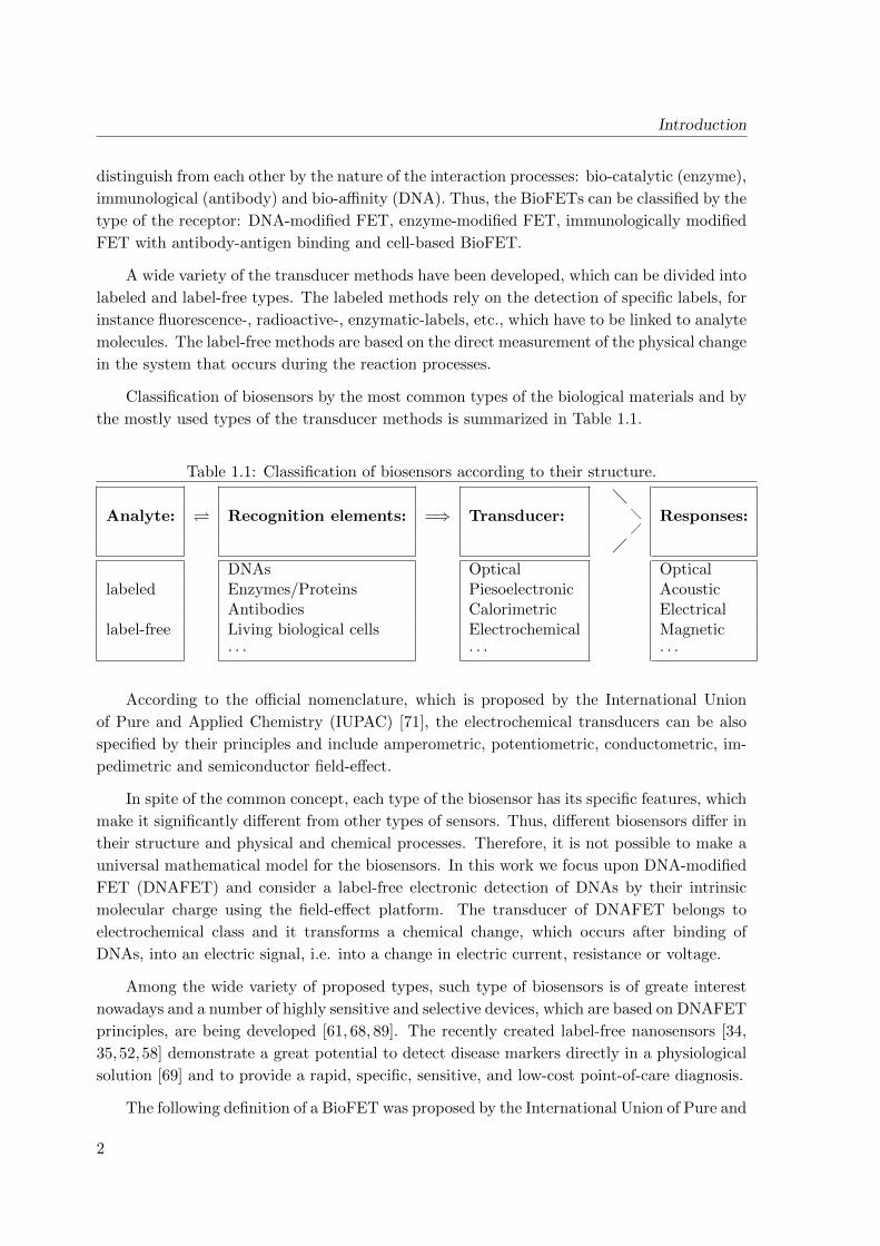
Classification of biosensors by the most common types of the biological materials and by
the mostly used types of the transducer methods is summarized in Table 1.1.
Table 1.1: Classification of biosensors according to their structure.
Analyte: Recognition elements: =⇒ Transducer:
Responses:
DNAs Optical Optical
labeled Enzymes/Proteins Piesoelectronic AcousticAntibodies Calorimetric Electrical
label-free Living biological cells Electrochemical Magnetic· · · · · · · · ·
According to the official nomenclature, which is proposed by the International Union
of Pure and Applied Chemistry (IUPAC) [71], the electrochemical transducers can be also
specified by their principles and include amperometric, potentiometric, conductometric, im-
pedimetric and semiconductor field-effect.
In spite of the common concept, each type of the biosensor has its specific features, which
make it significantly different from other types of sensors. Thus, different biosensors differ in
their structure and physical and chemical processes. Therefore, it is not possible to make a
universal mathematical model for the biosensors. In this work we focus upon DNA-modified
FET (DNAFET) and consider a label-free electronic detection of DNAs by their intrinsic
molecular charge using the field-effect platform. The transducer of DNAFET belongs to
electrochemical class and it transforms a chemical change, which occurs after binding of
DNAs, into an electric signal, i.e. into a change in electric current, resistance or voltage.
Among the wide variety of proposed types, such type of biosensors is of greate interest
nowadays and a number of highly sensitive and selective devices, which are based on DNAFET
principles, are being developed [61, 68, 89]. The recently created label-free nanosensors [34,
35,52,58] demonstrate a great potential to detect disease markers directly in a physiological
solution [69] and to provide a rapid, specific, sensitive, and low-cost point-of-care diagnosis.
The following definition of a BioFET was proposed by the International Union of Pure and
2
Introduction
Applied Chemistry (IUPAC) [71]: ”An electrochemical biosensor is a self-contained integrated
device, which is capable of providing specific quantitative or semi-quantitative analytical
information using a biological recognition element (biochemical receptor) which is retained
in direct spatial contact with an electrochemical transduction element.”
The development of biosensors is a multi-disciplinary research area that involves knowl-
edge from solid state physics, bio- and electro-chemistry, electronics, mathematics and com-
puter sciences. Because of the complexity of the biosensor functioning, the progress in the
sensor technology is being accompanied by the development of mathematical models for par-
ticular processes that occur in each part of the developed devices.
The mathematical modeling facilitates a deeper understanding and simulation of indi-
vidual processes and interactions of the parts of the system with each other, which enables
an assessment of the functioning of the system as a whole. As a result, the modeling helps
to predict the effect of changes to the system, to optimize the system performance and to
improve the device design.
Since the invention of metal-oxide-semiconductor field-effect transistor (MOSFET) math-
ematical models have been developed for studies of semiconducting transducers, such as
Poisson, Boltzmann, Vlasov, Drift-Diffusion equations, etc. [43,44,86], which are widely used
nowadays. According to the goal of the investigation we select and further evolve the required
model and corresponding numerical methods [19,41].
The studies of the behavior of liquids range from the observation of Brownian motion to
the processing of ion-sensitive field-effect transistors (ISFETs). The various approaches for
the simulation of liquids and the corresponding mathematical treatment include deterministic
(e.g. Molecular Dynamic, Poisson-Boltzmann) as well as stochastic (e.g. Monte Carlo)
methods, which describe the molecular model of liquid, the ion transport and the charge
screening effect. For example, the Molecular Dynamic method [3, 21], which is based on
the solution of Newton’s equation of motion, is used to obtain the dynamic property of
many-particle system. The Poisson-Boltzmann theory [13, 39, 49, 63, 70] allows to study the
electric double-layer near the objects of simple geometry. The various modifications of the
Monte Carlo methods have been developed and applied to study the behavior of static liquid
[3, 9, 42,46,74,76].
The studies of the transport of the biological species, which initially were performed in
the field of physiology and cell and molecular biology, are contributing today to the research
in the field of biosensors. In general, the mass transport occurs by both diffusion and convec-
tion. The spread of particles through random motion (diffusion) is described by the diffusion
equation. From the previous studies the limitations of sensors due to potentially slow trans-
port by diffusion in the static solution are known [64]. Temperature or pressure gradients
between the chip and the analyte give rise to convection. This can be an advantageous effect,
since it accelerates the transport of the analyte towards the sensor surface in contrast to the
time-limiting properties of a pure diffusion mechanism. Furthermore, the pumps and the mi-
crofluidic system, such a those that have been developed in [68], can be used as efficient tools
3
Introduction
for reducing the response times of particular sensors. Because many biomolecules are charged
their transport is also influenced by the electric field, whereas the velocity of ion migration
is described by the Nernst-Planck equation [11, 75]. In summary, the diffusion equation, the
Nernst-Planck, Navier-Stokes, Poisson Equations can be used to describe transport processes
in liquids [65,75,88].
The crucial part in the biosensor functioning is the chemical reactions, which occur
between the different constituents and, in particular, between the receptors and the analyte
molecules. Since the discovery of the double-helix structure of DNA the research on the
DNA sensors has been constantly growing [1, 22, 23, 26]. The functioning principle of the
DNA sensors (e.g. DNA-modified FET) is based on the hybridization of mobile DNA strands
with immobilized DNA strands of known sequence to form a double-helix. The overall duplex
formation, which depends on the rate of DNA transport and on the rate of the hybridization
reaction, has been studied by many research groups [33, 54, 84, 85]. According to previous
reports, the produced biological signal is a complex function of different effects, among them
the specific and non-specific binding processes [17], hybridization of mismatched and partially
matched DNA [55] etc.
As in all sensors, the most important parameter of biosensor systems is their signal-to-
noise ratio (SNR). Some processes, due to their stochastic nature, result in a random signal
fluctuation and, therefore, produce corresponding noise. One can distinguish between the
following sources of noise, i.e. between the corresponding random processes, that appear in
the BioFET [14, 40]: the thermal motion of carriers both in the semiconductor and in the
electrolyte, the impurities in the conductive channel, the recombination and the generation
of electron-hole pairs, the motion of the DNA strands in the electrolyte, the adsorption and
the desorption of DNAs to the surface, and the hybridization and the dissociation processes.
The random motion and the interaction of biomolecules produces the so-called biological
noise [28,29], which is of the main interest for our research.
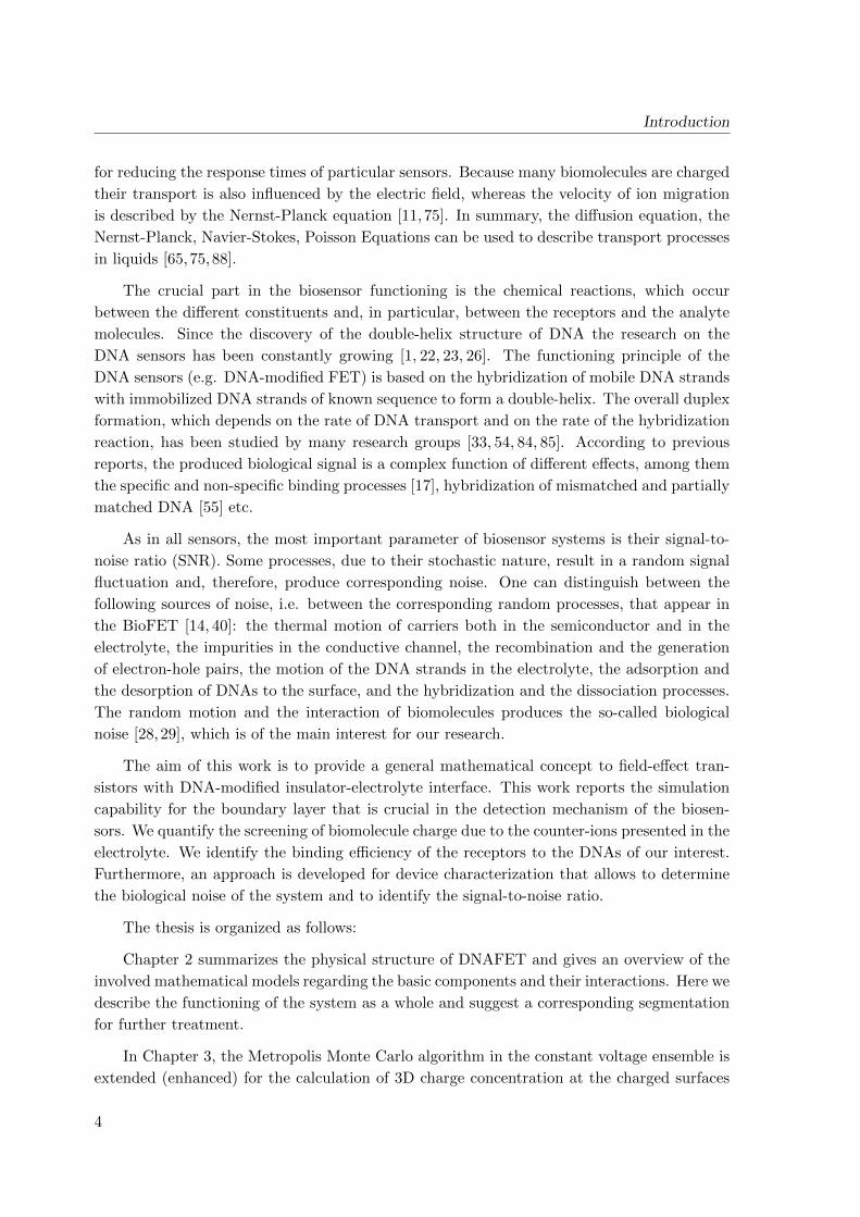
The aim of this work is to provide a general mathematical concept to field-effect tran-
sistors with DNA-modified insulator-electrolyte interface. This work reports the simulation
capability for the boundary layer that is crucial in the detection mechanism of the biosen-
sors. We quantify the screening of biomolecule charge due to the counter-ions presented in the
electrolyte. We identify the binding efficiency of the receptors to the DNAs of our interest.
Furthermore, an approach is developed for device characterization that allows to determine
the biological noise of the system and to identify the signal-to-noise ratio.
The thesis is organized as follows:
Chapter 2 summarizes the physical structure of DNAFET and gives an overview of the
involved mathematical models regarding the basic components and their interactions. Here we
describe the functioning of the system as a whole and suggest a corresponding segmentation
for further treatment.
In Chapter 3, the Metropolis Monte Carlo algorithm in the constant voltage ensemble is
extended (enhanced) for the calculation of 3D charge concentration at the charged surfaces
4
Introduction
functionalized with PNA, single-stranded DNA and double-stranded DNA oligomers. The
algorithm and all the interaction potentials between the various charge carries are described in
detail. Simulation results of the ionic charge concentrations (Na+Cl−) at the functionalized
surface and within the inter-molecular space are also presented and discussed.
In Chapter 4, we investigate the diffusive transport of the charged biomolecules and two
types of the chemical reactions near the functionalized surface, i.e. specific and non-specific
binding. The well-posed problem is formulated, discretized and solved. We also present a
simulation results and examine the diffusion and reaction processes as well as their interaction.
In Chapter 5, we consider the connection between different model algorithms and sug-
gest the compilation procedures for previously segmented model. The influence of different
parts on each other is presented and discussed. The result of self-consistent simulation is
demonstrated as well.
In Chapter 6, we focus on the stochastic processes that occur at the functionalized sur-
face. The chemical Langevin equation for binding (i.e. association and dissociation) processes
occurring at the functionalized surface is obtained. The binding efficiency of the biomole-
cules, the signal and the biological noise of the device are specified and calculated. The
simulation results for binding efficiency and for signal-to-noise ratio are presented, compared
and analyzed with respect to the response time.
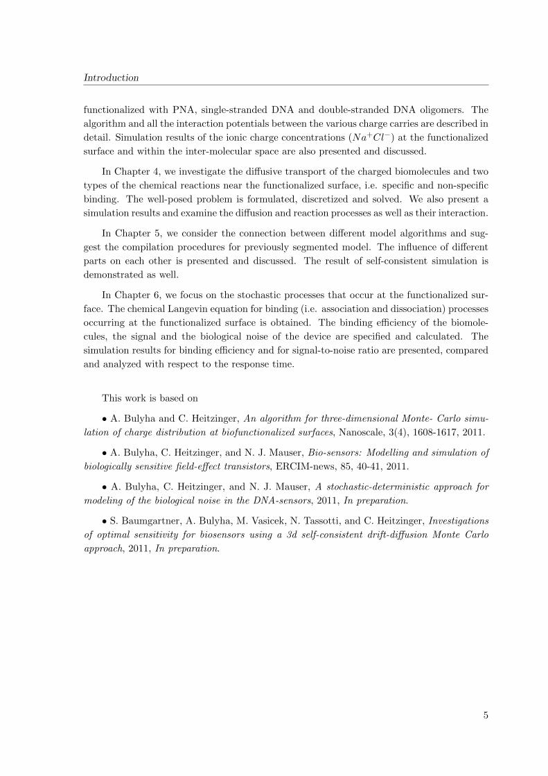
This work is based on
• A. Bulyha and C. Heitzinger, An algorithm for three-dimensional Monte- Carlo simu-
lation of charge distribution at biofunctionalized surfaces, Nanoscale, 3(4), 1608-1617, 2011.
• A. Bulyha, C. Heitzinger, and N. J. Mauser, Bio-sensors: Modelling and simulation of
biologically sensitive field-effect transistors, ERCIM-news, 85, 40-41, 2011.
• A. Bulyha, C. Heitzinger, and N. J. Mauser, A stochastic-deterministic approach for
modeling of the biological noise in the DNA-sensors, 2011, In preparation.
• S. Baumgartner, A. Bulyha, M. Vasicek, N. Tassotti, and C. Heitzinger, Investigations
of optimal sensitivity for biosensors using a 3d self-consistent drift-diffusion Monte Carlo
approach, 2011, In preparation.
5

Chapter 2
DNA-modified FET
2.1 Physical structure: basic charged components
In the past decade the research in the semiconductor field-effect sensors has moved to a
technology that is based on nanowires with biologically modified surface layers (biologically
sensitive field-effect transistors or devices, BioFETs or BioFEDs) and a number of highly
sensitive and selective devices have been developed [61, 68, 89]. The mostly common device
structure is shown schematically in Fig. 2.1 and includes source (S), drain (D), backgate (G),
a semiconductor layer between the source and the drain, and an insulator surrounding the
transducer [67,68].
The idea for sensing with field-effect transistors was introduced several decades ago and
realized in MOSFETs (metal-oxide-semiconductor field-effect transistor). In standard de-
vices, a semiconductor (such as silicon) is connected to metal (or polycrystalline silicon)
source and drain, through which a current is injected and collected, respectively.
To control and manipulate the electrical properties of semiconductors different doping
concentrations are used, i.e. the intentional incorporation of atomic impurities into material.
By doping of silicon with elements, like phosphorus or arsenic, which are electron donors,
the extra valence electrons are added and the transducer become an electrically conductive
n-type semiconductor (n-Si). Aluminium, boron and gallium, for instance, are missing the
valence electron and behave as an acceptor. Doping with these elements creates holes in the
silicon lattice that are free to move. Such elements belong to p-type dopant and form an
electrically conductive p-type semiconductor (p-Si).
The conductance of a MOSFET between the source and the drain is switched on and
off by a voltage on the gate. Therefor, the gate electrode is a third metal contact coupled
to the transducer through a thin dielectric layer. In the case of p-Si, the negative gate
voltage, i.e., the negative net-charge at the interface between the transducer and the gate,
leads to an accumulation of positive holes at the reverse side of this interface and generates
a corresponding increase in conductance. In contrary, the positive net-charge will deplete
7
DNA-modified FET
carriers and will lead to a decrease in the conductance. Such type of sensing is called field-
effect and it can be used in planar [1, 56, 57] and nanowire devices [50, 51, 68]. Due to
different sensitivity of planar devices and nanowires [16], the device geometry is significant
in mathematical modeling.
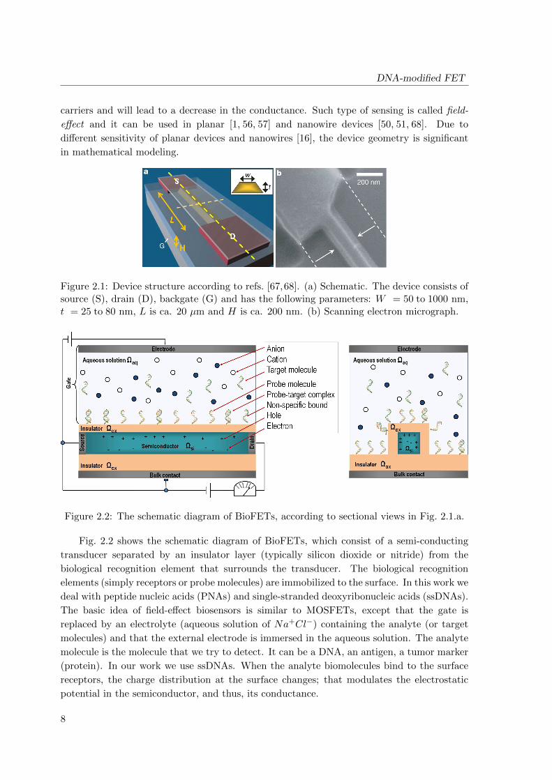
Figure 2.1: Device structure according to refs. [67,68]. (a) Schematic. The device consists ofsource (S), drain (D), backgate (G) and has the following parameters: W = 50 to 1000 nm,t = 25 to 80 nm, L is ca. 20 µm and H is ca. 200 nm. (b) Scanning electron micrograph.
Figure 2.2: The schematic diagram of BioFETs, according to sectional views in Fig. 2.1.a.
Fig. 2.2 shows the schematic diagram of BioFETs, which consist of a semi-conducting
transducer separated by an insulator layer (typically silicon dioxide or nitride) from the
biological recognition element that surrounds the transducer. The biological recognition
elements (simply receptors or probe molecules) are immobilized to the surface. In this work we
deal with peptide nucleic acids (PNAs) and single-stranded deoxyribonucleic acids (ssDNAs).
The basic idea of field-effect biosensors is similar to MOSFETs, except that the gate is
replaced by an electrolyte (aqueous solution of Na+Cl−) containing the analyte (or target
molecules) and that the external electrode is immersed in the aqueous solution. The analyte
molecule is the molecule that we try to detect. It can be a DNA, an antigen, a tumor marker
(protein). In our work we use ssDNAs. When the analyte biomolecules bind to the surface
receptors, the charge distribution at the surface changes; that modulates the electrostatic
potential in the semiconductor, and thus, its conductance.
8

DNA-modified FET
Recent experiments have shown the possibility of detecting biomolecules by the effect of
their intrinsic charge on the conductance of a semiconducting nanowire transducer [22]. How-
ever, despite the remarkable experimental progress in this field, the theoretical understanding
of the field-effect sensors is still incomplete [34,37,58,61,62]. In order to achieve a quantitative
understanding, a precise knowledge of the charge concentration in the surface layer is neces-
sary; such a knowledge can up to now only be provided by simulations. Experiments have
shown that it is possible to detect biomolecules through the effects of their intrinsic charges
onto the conductance of a semiconductor transducer. However, a quantitative understanding
of the field-effect functioning and of the crucial boundary-layer electrostatics is missing [62].
Moreover, a hybridization event is highly efficient and specific. Therefore, a deep understand-
ing of the adsorption process of charged macromolecules onto a charged surface and of the
binding of probe and target molecules are very important for sensor applications [69].
Thus, we can conclude that the modeling of such BioFET sensors must take into account
the electrostatics and the geometry of the liquid, the probe and the target molecules in the
boundary layer, the binding efficiency of the probes and targets, the electrostatics and the
conductance of the semiconducting transducer, and the device geometry.
2.2 Mathematical models of charged BioFET-components
Let Ω be a bounded domain in Rd, d = 1, 2 or 3 occupied by BioFET with boundary ∂Ω.
According to the BioFET structure [see Fig. 2.2] the total domain Ω is split into disjoint
subsets Ω = ΩOx∪ΩSi∪ΩLiq corresponding to the insulator (oxide), the transducer (silicon),
and the electrolyte (liquid), respectively. The boundary of the domain is assumed to consist
of a Neumann part and a Dirichlet part ∂Ω = ∂ΩN ∪ ∂ΩD, where the Dirichlet part ∂ΩD =
∂Ωos ∪ ∂Ωod ∪ ∂Ωob ∪ ∂Ωoe corresponds to Ohmic contacts: source, drain, bulk contact and
reference electrode.
According to the chosen device geometry the actual permitivity ε is the piecewise constant
function.
ε(x) :=
εOx = ε0ε1 ∈ R in ΩOx,
εSi = ε0ε2 ∈ R in ΩSi,
εLiq = ε0ε3 ∈ R in ΩLiq,
where ε0 denotes the permittivity of vacuum and εi are dielectric constants.
In our model we discern an internal electrical potential ΨI , which is produced by a local
electric field, and a potential ΨE that is induced by an externally applied electric field. Thus,
the total potential in the whole domain Ω is ψ(t,x) := ΨI(t,x) + ΨE(t,x). We assume that
the external electrical potential ΨE is given. The internal electrical potential ΨI can be
9
DNA-modified FET
obtained via Poisson equation.
−∇ · (ε(x)∇ΨI(x)) = q %(x), in Ω ⊂ Rd, (2.1)
where %(x) is a charge concentration in the whole domain Ω. In general, % is a sum of fixed
charge concentrations %i and the carrier distributions Ci
%(x) :=∑i
zi
(%i(x) + Ci(x)
),
where i defines the species, zi is the corresponding valence, and q is elementary charge. Ci(x)
are unknown and shall be obtained by other models.
As it is mentioned in section Section 2.1 we deal with different charged species, which
can be arranged in the following categories:
in the insulator ΩOx:
• the charge of the insulator;
in the semiconductor ΩSi:
• the electrons and the holes;
in the liquid ΩLiq:
• the anions and the cations;
• the probe, the target molecules, the probe-target complexes
and the non-specifically bounded molecules;
• the hydrogen ions.
Such partition is chosen due to significant differences in size, concentrations and motion
behavior; and each category will be investigated separately.
2.2.1 Electrons and holes
First we consider the nano-electronic part with electrons and holes as charge carriers in the
sub-domain ΩSi, and identify two main sources for current flow:
• diffusion of the electrons and the holes due to concentration gradients,
• drift of the electrons and the holes caused by the electric potential gradient.
The total flows of the electrons and the holes are determined by the linear superposition of
the diffusion and the drift processes.
Hence, the appropriate mathematical model for the transport of electrons and holes inside
of the transducer is the system of the drift-diffusion equations (2.2) - (2.5) coupled to the
Poisson equation. For the electron current density Jn and for the hole current density Jp in
the silicon domain ΩSi we use a model that has been proposed e.g. in Refs. [43, 44]:
10
DNA-modified FET
∇ · Jn(ΨI , n) = q R, (2.2)
∇ · Jp(ΨI , p) = −q R, (2.3)
Jn = Dn∇n(x)− µnn(x)∇ΨI(x), (2.4)
Jp = −Dp∇p(x)− µpp(x)∇ΨI(x), (2.5)
where n and p are the concentrations of the electrons and the holes, the positive coefficients
µn and µp are the electron and the hole mobility, respectively. The diffusion coefficients Dn
and Dp are related to mobilities by Einstein’s relations
Dn := Uth µn,
Dp := Uth µp.
Uth stands for the thermal voltage given by Uth := kBT/q, where kB denotes the Boltzmann’s
constant, q is the elementary charge, and T is the temperature.
The term R in the equations (2.2) and (2.3) describes difference of the rates of recombi-
nation and generation of electron-hole pairs and is called a recombination-generation rate.
Recombination processes are exothermic (associated with energy release); they occur when
a conduction electron becomes a valence electron and neutralizes a hole. Generation is an
endothermic process (it requires energy) that occurs when a valence electron becomes a con-
duction electron and leaves a hole. In thermal equilibrium there is a dynamic balance between
the recombination and the generation rates, i.e., n p = n2in.
Various energy transition processes exist, which determine the recombination-generation
rate, namely, two-particle transition, three-particle transition and impact ionization. The
impact ionization is a pure generation process, which occurs at a high electric field. The
modeling of three-particle transition is only significant, if a high-injection condition must be
investigated. In our case we assume a low electric field and a low injection, and consider only
the two-particle transition process, which is described by the Shockley-Read-Hall term:
R =n p− n2
in
τp(n+ nin) + τn(p+ nin),
where nin is the intrinsic density (i.e., in silicon at the room temperature), τn and τp are the
life-times of electrons and holes, under the assumption that they are not doping-dependent.
Typical values for τn and τp are 10−6s and 10−5s, respectively.
The performance of the semiconductor is mainly determined by its doping profile. Hence,
the control of it remains very important [12]. This physical parameter can be modeled by
using modern solid state physics or, according to recent publication [53], but also a direct
measurement is possible. In order to control the electrical behavior of the devices, the maxi-
mal doping concentration shall be significantly larger than the intrinsic carrier concentration
at the operating temperature. For simplicity we keep the dopant distribution constant so
11
DNA-modified FET
that
%d + %a nin,
where %d and %a denote the concentration of electrically active donor and acceptor atoms,
respectively. For instance, %ad := %d + %a = 2 × 10¹⁸ [q cm−3] and nin := 1010 [q cm−3] for
silicon at the room temperature.
We consider source and drain as Ohmic contacts and assume that the space charge
vanishes, and the system is in thermal equilibrium, i.e.
p(x)− n(x) + %ad = 0,
n p = n2in.
Thus, the Dirichlet boundary condition at the Ohmic contacts is written as follows
n(x) =%ad +
√%2ad + 4n2
in
2x ∈ ∂Ωos ∪ ∂Ωod,
p(x) =−%ad +
√%2ad + 4n2
in
2x ∈ ∂Ωos ∪ ∂Ωod.
The boundary potential consists of the externally applied potential ΨE and the potential
produced by the doping Ψbi, the so-called built-in potential.
ΨI(x) = ΨE + Ψbi x ∈ ∂Ωos ∪ ∂Ωod.
The Ψbi is chosen in such a way that the device is in thermal equilibrium, i.e., the current
density vanishes Jn = Jp = 0 and ΨI = Ψbi in the equations (2.4) and (2.5), which implies
Ψbi = Uth ln(%ad +
√%2ad + 4n2
in
2nin
).
The applied potential as well as the concentrations of the electrons and holes at the back-gate
(bulk contact) and at the reference electrode are given, i.e.,
ΨI(x) = Ψb, n(x) = nb, p(x) = pb x ∈ ∂Ωob,
ΨI(x) = Ψe, n(x) = ne, p(x) = pe x ∈ ∂Ωoe,
where nb, ne, pb, pe ≥ 0.
Everywhere else we use the Neumann conditions
∂ΨI(x)
∂~n= 0,
∂n(x)
∂~n= 0,
∂p(x)
∂~n= 0 x ∈ ∂ΩN ,
where ~n is the outward pointing normal vector.
12
DNA-modified FET
2.2.2 Biomolecules
We consider an isolated sensor that is immersed into an analyte solution. The reactive solid
surface ∂Ωs of area A of the sensor is functionalized with CP,0 receptors (probe molecules) per
unit area, and the solution contains target molecules with initial concentration CT,0 mol per
liter. We will use below the notations P , T , PT for probe, target molecules and probe-target
complexes, respectively. The probe-target complex PT is a molecule after hybridization event;
and CPT,0 is the corresponding initial concentration. We also denote the non-specifically
bounded molecules as nT and their initial concentration as CnT,max.
The crucial aspects of modeling are simulation of the chemical reactions at the func-
tionalized surface and the simulation of transport of target molecules in the analyte solution
to the active sensor area. There are several mechanisms, which create the flow of analyte
molecules:
• Diffusion is random motion of molecules;
• Convection is caused by the bulk motion of fluids;
• Migration is the movement of charged particles in response to a local electric field;
• In addition, the pump is essential for the fast response times.
Definition 2.2.1. The net movement of molecules through a unit area per unit time in
a given direction is known as a flux. In general, the flux is defined for any transported
quantity [75].
Therefore, the total flux is J(t,x) = JD(t,x) + JC(t,x) + JM (t,x), where JD, JC and
JM correspond to diffusion, convection and migration transport mechanisms, respectively.
The transport of target molecules in the analyte solution to the active sensor area must
be taken into account to carry out the time-dependent simulations. In our model, the change
of the concentration CT (t,x) of the target molecules is described by the continuum equation:
∂CT (t,x)
∂t+∇ · J(t,x) = 0, x ∈ Ω, (2.6)
where J(t,x) characterizes the flow process in the analyte solution.
Chemical reactions
We consider two types of reversible chemical reactions, namely, a specific and a non-specific
binding, which we can define as follows.
specific binding :
• association or hybridization is a process of binding of two complementary strands
of deoxyribonucleic acid (DNA) to create a double-stranded DNA oligomers;
• dissociation or denaturation is an opposite to association process,
by which double-stranded DNA oligomers separate into single strands
13
DNA-modified FET
through the breaking of hydrogen bonds between the bases.
non-specific binding :
• adsorption is a direct binding of targets from the bulk phase to the surface;
• desorption is an opposite to adsorption process,
by which the biomolecule is released from the surface.
Note that association and dissociation are more general processes, but in our case they are
synonyms to hybridization and denaturation, respectively.
We assume that target molecules bind to the receptors and unbind from them with rates
ra and rd, respectively. The rates ka and kd characterize the adsorption and desorption
processes. Such first order reversible reactions can be depicted schematically as given by the
equation below.
P + Tkakd
B (2.7)
The hybridization depends on the density of the single (unbounded) probe molecules
and on the concentration of free (unbounded) target molecules, i.e. on transport of analyte
molecules to the functionalized surface; the adsorption depends on the concentration of the
non-specifically bounded molecules at the maximum altitude and also on the concentration of
unbounded target molecules; whereas the opposite processes are proportional to the density
of the specifically or non-specifically bounded molecules, respectively. Thus, the dynamics of
the binding processes is given by
dCBdt
= (·)aCP CT − (·)dCB, (2.8)
where index B denotes PT or nT , Ci is an appropriate concentration, and pair (·)a, (·)dcorresponds to ra, rd or ka, kd rate coefficients, respectively.
Definition 2.2.2. The chemical equilibrium is understood as a balance between association
and dissociation events, i.e. dCBdt = 0.
Definition 2.2.3. The time, during which the number of probe-target complexes reaches its
chemical equilibrium value (or at least a detectable quantity), determines the response time
of the sensor.
To describe the selectively adsorbing surface with probe molecules on it we use the Robin
boundary conditions
∇CT (t,x) · ~n = −u(t,x, CP , CT , CPT ), x ∈ ∂Ωs, (2.9)
where ~n is the unit normal vector pointing outward to the surface ∂Ω and the function
u(t,x, CP , CT , CPT ) specifies chemical reactions at the surface.
14
DNA-modified FET
For purely reflective (inert) walls we use the Neumann boundary conditions
∇CT (t,x) · ~n = 0, x ∈ ∂Ω \ ∂Ωs. (2.10)
The case of a ’limited reaction’, when the transport of analyte molecules is much more
faster than the binding reaction (i.e., under assumption CT (t, 0) ≈ c0, for instance for small
sensors), is described in [65]. The solution of Eq.(2.8) in the equilibrium state is given by
CPT (∞)
CP,0≡ c
1 + c,
where c = c0rdra
, irrespectively of how long the sensor takes to equilibrate.
Diffusion
We assume that there are no reaction processes far away from the functionalized surface and
only elastic collisions occur between the biomolecules. Therefore, the kinetic energy and the
momentum are conserved. The random nature of such collisions leads to a random motion of
biomolecules and gives rise to their diffusion. The diffusion of the species in a dilute solution
under the influence of a concentration gradient is governed by the Fick’s first law and is
expressed as
JD(t,x) := −D∇CT (t,x),
where D := D(x) is a diffusion coefficient or diffusivity. In general, the diffusivity is a function
of space and depends on the temperature, the pressure, the fluid viscosity, and on the type
(size and shape) of the molecule. The diffusion coefficient for rod-like molecules is given in
Section 4.3.
Convection
The bulk motion of fluid causes also the motion of biomolecules. Such convective flux is
proportional to the hydrodynamic velocity field ν and is given as follows
JC(t,x) := νCT (t,x).
Definition 2.2.4. The fluid is compressible if the change in pressure or temperature results
in a change in density. In the incompressible fluid the density is constant, i.e. ρ = const.
The fluid density is defined as mass per unit volume ρ = m/Vu.
From the second Newton’s law ma = F applied to a unit volume we obtain the equation
of motion according to used model for fluid. The vector a is a fluid acceleration that includes
15
DNA-modified FET
the velocity change with respect to time and the convective acceleration, and is given by
a = ∂ν∂t +ν ·∇ν. F is a sum of forces, which are applied to the body and the surfaces. The body
forces act on the body and include gravity Fg and electromagnetic forces Fe. Electromagnetic
forces occur when an electromagnetic field interacts with electrically charged particles. The
surface forces act on the surface of the control volume and include pressure Fp and viscous
stress Fv. The forces are expressed as
Fg = ρ g Vu,
Fe = Fc = −%E Vu = %∇ψ Vu,Fp = −∇p Vu,Fv = ∇ · vs Vu,
where g is the gravitational acceleration, E is the applied electrical field, % is the charge
density, p is the pressure, and vs is the viscous stress tensor. Here Fc is the Coulomb force.
For incompressible Newtonian fluid with viscosity µf holds ∇ · vs = µf∆ν.
Hence, the velocity field ν for incompressible Newtonian fluid in applied electrical field
is governed by the following Navier-Stokes equation
ρ∂ν(t,x)
∂t+ ρ ν(t,x) · ∇ν(t,x) = µf ∆ν(t,x) + ρ g + %∇ψ(t,x). (2.11)
where % = q(C1 − C2), q is the elementary charge, while C1 and C2 are concentrations of
cations and anions, respectively.
Under the assumption that the step in space is proportional to the biomolecule length
and is much larger then the radius of the fluid molecules, we can use the Neumann boundary
condition
∇ν(t,x) · ~n = 0, (2.12)
where ~n is the unit normal vector pointing outward to ∂ΩLiq.
Migration
Because the DNAs are charged molecules, their transport is influenced by the internal as well
as by the external electric field. The internal electrical field arises due to the differences in
ion concentrations and from the accumulation of charges at the active surface layer. The flux
JM is a product of the concentration and the velocity of migration JM = CT vm.
The velocity can be obtained from the drag forces Fd = NA fd vm, where NA is Avogadro’s
number, and fd is the friction drag coefficient. For a sphere of radius r this coefficient is well
known and is equal to fd = 6π µf r. Otherwise, the friction drag coefficient is inversely
proportional to diffusivity fd = kB T/D, where kB is the Boltzmann constant, and T is the
temperature. The absolute value of the drag forces is equal to those of the electric forces
16

DNA-modified FET
acting on a mol of ions, but their directions are opposite.
Fd = −Fe = −zT qNA∇ψ,
where zT is the net charge on the target molecule.
Hence, the transport of the biomolecules is proportional to the electrical potential gra-
dient ∇ψ(t,x), where the total potential ψ is given as above ψ(t,x) := ΨI(t,x) + ΨE(t,x).
JM (t,x) := −D zT q
kBTCT (t,x)∇ψ(t,x),
where D > 0, zT , q, kB and T are the diffusivity, the net charge on the target molecule, the
elementary charge, the Boltzmann constant and the temperature, respectively.
All these processes shall be taken into account in the development of the algorithms for
the diffusion-convection-migration (DCM) problem with chemical reactions near the func-
tionalized surface.
Pumps
The precise control of the transport of biomolecules is required to achieve a fast response times
of biosensor. According to recent publications, different types of the integrated micro-pumps
have been developed for flow modulation in microfluidic systems. The pumps are based on
monitoring of the pressure [15] or the temperature [59] gradients, or of the electric field [88].
Pumps can also create the flow by stirring. In particular cases the pumps can maintain the
given constant flow rates; in other cases the fluid speed is uncontrolled (in literature such
pumps are sometimes denoted as mixers). In the case of an embedded pump we can localize
the dominant process and simplify the problem, e.g., for the embedded mechanical pump we
can assume that the stirring is a dominant process and, therefore, the velocity ν is given and
it is constant in time.
In general, the velocity field should be calculated dependent on the modeled pump and
the properties of the used fluid.
2.2.3 Electrolyte ions
A crucial aspect of the modeling is the calculation of the charge distribution in bio-functionalized
surface layers. The standard continuum model is the mean-field Poisson equation, in which
the free charges are treated as points and included in the model via Boltzmann statistics.
−∇ · (εLiq(x)∇ΨI(x)) = q(%s(x) +
∑i
ziC∞i e−zi β(ΨI−ΦF )
)in ΩLiq,
17

DNA-modified FET
where %s(x) is the charge density near the functionalized surface, i defines the species type,
C∞i is the bulk concentration of the species i, zi is the corresponding valency, β = q/(kB T ),
q is the elementary charge, and εLiq is the actual permittivity. ΦF corresponds to the Fermi
level.
The classical Poisson-Boltzmann theory is successfully used to study the planar electric
double layer and the electrolyte bulk. In our case the charge density %s(x) has to be carefully
modeled.
To calculate the motion of the analyte molecules we can also use the model that has been
described before for the target molecules with corresponding concentration and diffusivity. In
this case the boundary conditions given in (2.12) should be modified to include the geometry
of the biomolecules.
According to the recent experimental results [4, 72] and simulations [66, 76], both the
electrostatic and the hard-sphere collisions are sensitive to the ion size. It is also essential to
consider mixed-valence ionic systems, since the electrolyte is usually buffered. Because the
applied voltage between the electrodes and the bulk concentrations of the ions are controlled
in experiments, their influence on the ionic concentrations has also to be investigated. The
Metropolis Monte Carlo (MMC) algorithm in the constant-voltage ensemble is the appropriate
numerical method, which requires the description of the complex chemical systems in terms
of a realistic atomic model, the computation of the interaction forces and the minimizing of
the energy.
Input parameters:
type of the biomolecules and their length;
angle between biomolecule and surface;
length of linkers;
type (radius and valence) of the electrolyte ions and their minimum number in the box;
concentration of the used ions;
minimum height of box;
number of molecules at the surface;
distance between them;
type (charge) of the insulator;
pH-value of water;
initial value of chemical potential;
applied potential.
MMC algorithm:
1. Construct the simulation box:
adapt height and width of box with account to the chosen input parameters;
put the biomolecules and the linkers on their places.
2. Build a random state of the system:
put every electrolyte ions onto a random place in the box.
18
DNA-modified FET
3. Generate randomly a new state of the system by
changing the placement of ions in the simulation box:
by translation of the ions inside of the box;
by insertion or deletion of ions;
by transferring a random amount of charges between the electrodes.
4. Propose the new state as a follow-up of the current state.
5. Recalculate the chemical potential if it is necessary.
6. Calculate the change in the energy of the system dE (energy difference),
which is caused by the movement of charges.
7. If the move would bring the system to a state with lower energy (i.e., dE < 0)
the new state will be unconditionally accepted;
otherwise the move will be allowed with a certain probability.
8. To calculate the chemical potential µ:
repeat step 2-7 until |µnew − µold| ≤ δ 1.
9. To calculate the charge distribution of ions:
repeat step 2-7 with fixed chemical potential
until the desired (required) smoothness of the calculated charge profiles is achieved.
In the case of DNAFET, we can construct arbitrary single- and double-stranded oligomers
of B-DNA as left-handled helical molecules with Watson-Crick base pairs, which have the anti-
parallel organization of the sugar-phosphate chains. We assume that the partial charges of
the backbone are given and calculate the atomic coordinates of base pairs by using the data
from [80]. The charge of the sugar-phosphate backbone can be also calculated by using the
GROMACS package [78]. Each oligomer is bound to the surface by a linker. The PNA and
DNA oligomers and their linkers are modeled as impenetrable cylinders with two hemispheres
of the same radius at the top and at the bottom. PNA oligomers are modeled by uncharged
cylinders, and ssDNA and dsDNA oligomers carry the charges of the phosphate groups of
the backbone on their outside just as in B-DNA oligomers. The linkers are orthogonal to
the surface so that they touch the surface. The upper hemisphere of the linker overlaps with
the lower hemisphere of the oligomer and acts as a flexible joint. Hence the oligomers can be
rotated with respect to the surface.
2.2.4 Hydrogen ions
According to the acid-base theory, the water molecule can act both as a base and as an acid
ion, i.e. the water molecule is able to gain a hydrogen ion H+ or to lose it. Hence, two
molecules of water dissociate into hydronium (H3O+) and hydroxide (OH−) ions:
H2O + H2O OH− + H3O+
19
DNA-modified FET
This process is known as self-ionization reaction. The concentration of hydroxide ions is
specified by the pH-value, so that
C(H+) C(OH−) = 10−14,
where C denotes the concentration. The same ionization processes, which occur at the
insulator-electrolyte interface, induce the charge of the insulator.
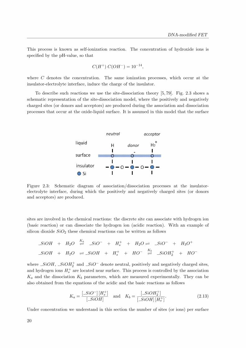
To describe such reactions we use the site-dissociation theory [5, 79]. Fig. 2.3 shows a
schematic representation of the site-dissociation model, where the positively and negatively
charged sites (or donors and acceptors) are produced during the association and dissociation
processes that occur at the oxide-liquid surface. It is assumed in this model that the surface
Figure 2.3: Schematic diagram of association/dissociation processes at the insulator-electrolyte interface, during which the positively and negatively charged sites (or donorsand acceptors) are produced.
sites are involved in the chemical reactions: the discrete site can associate with hydrogen ion
(basic reaction) or can dissociate the hydrogen ion (acidic reaction). With an example of
silicon dioxide SiO2 these chemical reactions can be written as follows
SiOH + H2OKa SiO− + H+
s + H2O SiO− + H3O+
SiOH + H2O SiOH + H+s + HO−
Kb SiOH+
2 + HO−
where SiOH, SiOH+2 and SiO− denote neutral, positively and negatively charged sites,
and hydrogen ions H+s are located near surface. This process is controlled by the association
Ka and the dissociation Kb parameters, which are measured experimentally. They can be
also obtained from the equations of the acidic and the basic reactions as follows
Ka =[ SiO−] [H+
s ]
[ SiOH]and Kb =
[ SiOH+2 ]
[ SiOH] [H+s ]. (2.13)
Under concentration we understand in this section the number of sites (or ions) per surface
20
DNA-modified FET
area and denote it as [ · ]. Thus, the concentration of hydrogen ions at the surface is
[H+s ]2 =
Ka
Kb
[ SiOH+2 ]
[ SiO−].
Therefore, the net surface charge %s is the difference of the concentrations of acceptors and
donors multiplied by the elementary charge q
%s = q([ SiOH+
2 ]− [ SiO−]). (2.14)
Note that the surface is not charged if the equation [H+s ]2 = Ka
Kbholds.
The total number of sites per unit area Ns is the sum of the concentrations of all binding
types
Ns = [ SiOH] + [ SiOH+2 ] + [ SiO−]. (2.15)
The relation between hydrogen ions at the surface and in the bulk is given by the Boltzmann
equation.
[H+s ] = [H+
b ] e−βψs ,
ln[H+b ]− ln[H+
s ] = βψs,
where β := q/kB T , q is the elementary charge, kB is the Boltzmann’s constant, T is the
temperature, and ψs denotes the potential difference between the surface and the bulk of the
liquid. If we combine equations (2.13) - (2.15) with the Boltzmann equation we obtain the
equation for the surface potential
ln[H+b ]− ln
√Ka
Kd= βψs +
2
ew − e−w,
2.303(
log10[H+b ]− log10
√Ka
Kd
)= βψs + sinh−1w,
where
w =%s
2 q Ns
√1
KaKb
Next we use the facts that the negative logarithm of base 10 of hydrogen ion concentration
is given as pH value and the isoelectric point pI is the pH at which a surface carries no net
electrical charge, i.e. [ SiOH+2 ] = [ SiO−]. These parameters are determined as follows
pH := − log10[H+b ] and pI := − log10
√Ka
Kd.
Using linearized Gouy-Chapman-Stern model we can approximate the surface charge as
%s = ψs ΥDL, where ΥDL = 20µFcm−1 is the double layer capacitance.
21
DNA-modified FET
Hence, we can simplify the equation
2.303(pI − pH
)= βψs + sinh−1 ψs
β γ, (2.16)
where γ := 2 q Ns√KaKb
βΥDL.
On the other hand, γ is a measured parameter and determines the ψs to pH relation.
According to [5] the value of γ = 0.14 has been experimentally determined for SiO2. The
isoelectric point for silicon dioxide is about pI ≈ 2.2. Therefore, the insulator-electrolyte
interface is negatively charged if pH > 2.2.
2.2.5 Insulator
According to the site-dissociation theory we assume that the insulator is charge-neutral in
ΩOx and is charged at the insulator-electrolyte interface ∂ΩOx. Thus, the homogeneous
Laplace’s equation holds in the insulator layer
−εOx∆ΨI(x)) = 0, in ΩOx,
with a constant charge at the insulator-electrolyte interface
−εOx∆ΨI(x)) = q %Ox, on ∂ΩOx.
We use the Neumann conditions for the inert boundary
∂ΨI(x)
∂~n= 0, on∂ΩN ,
where ~n is the outward pointing normal vector.
2.3 Conclusions
The modeling of BioFET sensors is complicated by the fact that they comprise a biophysical
(biomolecular) and a nano-electronic parts with different length scales. The microscopic scale
is governed by the length of single biomolecules, which are typically in the range of a few to
some dozen nano-meters. The macroscopic scale is defined by the dimensions of the whole
sensor, which is larger by several orders of magnitude. Therefore, solving of the Poisson
equation is not possible in the whole domain. Both parts have to be considered separately
and then coupled together in a self-consistent manner.
According to the considerations made in Section 2.2.2 - Section 2.2.4 the biophysical
part of the biosensor can be described by coupling the Poisson equation, the Navier-Stokes
equations and the diffusion-convection-migration problem with reactive boundary conditions
in k-dimensional parameter space. In this case we deal with time-varying boundaries. Because
22
DNA-modified FET
the electrolyte solution is always buffered with other ions to keep the pH-value constant, the
parameter space will be larger than eight, i.e., k > 8. Due to the large number of unknowns
and complicated boundary conditions it is necessary to consider separately the transport of
biomolecules and the movement of electrolyte ions.
The Metropolis Monte Carlo method in constant-voltage ensemble can be used to inves-
tigate the ionic concentrations near the groups of charged objects with various geometries
and sizes. Because the commonly used concentration of the electrolyte varies from 1M to
10−3M the numbers of the electrolyte ions and the hydrogen ions can differ by several orders
of magnitude. Therefore, the simultaneous application of the MMC algorithm for both types
of ions requires a very large simulation box or, otherwise, leads to unsatisfactory statistics.
Thus, the contribution of the hydrogen ions to our model shall be calculated separately.
To simplify the model it is useful to reformulate the DCM problem to one-parameter
space and to rewrite the time-depending boundary conditions to suitable Neumann and (or)
Dirichlet boundary conditions. Depending on the geometry of the microfluidic channel and
the sensor, the one-, two-, or three-dimensional version of the equations should be selected.
23

Chapter 3
Electrolyte solution in the
equilibrium state
The standard continuum model for the electrostatics of biomolecules is the mean-field Poisson
equation with a Boltzmann term for the concentration of the mobile charges, then called the
Poisson-Boltzmann equation [13, 63, 70]. In this continuum model the mobile charges are
treated as point charges and included using Boltzmann statistics. The classical Poisson-
Boltzmann theory is successful to study the planar electric double layer and the electrolyte
bulk. Also various modifications of the Poisson-Boltzmann approach have been developed
and applied to study the electric double layer around a uniformly charged spherical colloid
particle [49] and around an infinitely large and uniformly charged cylinder [39].
However, there are experimental results which show the effect of ion size on diffusion
in alkali halides [4] (e.g., NaCl) or at the surface [72] that cannot be explained by Poisson-
Boltzmann theory. Also recent simulations [66, 76, 77] show that both the electrostatic and
hard-sphere collisions are sensitive to ion size. To include the finite-size effects of small ions,
various methods have been developed. These include canonical and grand canonical Monte
Carlo (MC) simulations [3,42,46,74] and density-functional theory [9,76]. The advantages and
disadvantages of such methods for mixed-sized ions systems are discussed in the literature [7,
9,76,83]. MC simulations agree better with experimental data since the finite size of the ions
is taken into account.
Although electrical double layers have been extensively studied near planar, uniformly
charged surfaces [6,36,74] and around isolated, infinitely large and uniformly charged cylinders
[25, 82, 83], the ionic concentrations near groups of charged objects with various geometries
and sizes at surfaces have been investigated much less.
Since field-effect sensors are extremely sensitive to screening effects and the voltages are
applied across the devices in experiments, correct boundary conditions must be used in self-
consistent simulations. Furthermore, in experiments very low ionic concentrations are used.
To arrive at good statistics in MC simulations, this implies that a large simulation domain
25
Electrolyte solution in the equilibrium state
must be used. Since the distance between biomolecules is also small in experiments [54], this
requires the capability to include several molecules in a single simulation domain (see Fig. 1).
Additionally, since the electrolyte is usually buffered, it is essential to consider not only
mixed-size, but also mixed-valence ionic systems. Therefore the valence of the ions can be
specified as an input parameter in the MC algorithm. Finally, to calculate the electrostatic
free energy of various orientations of the biomolecules [31, 70], the PNA and DNA strands
can be rotated in the MC algorithm.
These requirements were taken into account in the development of the Metropolis Monte
Carlo (MMC) algorithm and hence this work solves the problem of simulating the electro-
statics of biofunctionalized surfaces at the microscopic scale for sensor applications.
3.1 Atomistic model
The classical MMC algorithm is extended to include the effects of biomolecules such as PNA,
ssDNA, and dsDNA on ionic charge distributions near charged boundaries in an electrolyte.
We treat the constant-voltage ensemble as an extension of the grand-canonical ensemble,
i.e, the voltage applied to the electrodes is a controlled parameter. Another parameter that
has to be constant during the simulation is the bulk ionic concentration. This is achieved
using the chemical potential energy, which has to be calibrated using the iterative algorithm
described below.
3.1.1 Simulation domain
The simulation domain (see Fig. 3.1) consists of a finite box [−W,W ]× [−W,W ]× [−H,H]
with H ≥ 2W that is bounded in the z-coordinate by two sheets. The interior of the box
contains an electrolyte solution and one or more immobile (macro-)molecules arranged in a
Cartesian grid. It is reasonable and convenient to take periodic boundary conditions in the
x- and y-directions which are parallel to the sheets. The box has hard, impenetrable walls at
z = −H and z = H carrying uniform surface charge of densities ρ and 0, respectively. Two
additional charge densities σ1 and σ2 are associated with the sheets and are adjusted to the
desired potential difference. If there is one molecule, it is linked at the center of the lower
wall at (0, 0,−H). If the box contains more molecules, they are arranged in an equidistant
grid and each molecule is centered in its grid cell.
The box confines N1 cations (e.g., Na) with charge q1, N2 anions (e.g., Cl) with charge
q2, and N3 partial charges of the molecule with charges q3,i (e.g., the phosphate groups of
the DNA backbone). It is required that the whole system is electrically neutral, i.e.,
4W 2(σ1 + σ2 + ρ) +N1q1 +N2q2 +
N3∑i=1
q3,i = 0.
26
Electrolyte solution in the equilibrium state
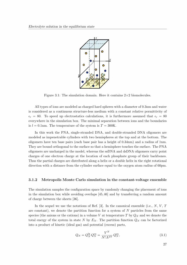
Figure 3.1: The simulation domain. Here it contains 2×2 biomolecules.
All types of ions are modeled as charged hard spheres with a diameter of 0.3nm and water
is considered as a continuous structure-less medium with a constant relative permittivity of
εr = 80. To speed up electrostatics calculations, it is furthermore assumed that εr = 80
everywhere in the simulation box. The minimal separation between ions and the boundaries
is l = 0.1nm. The temperature of the system is T = 300K.
In this work the PNA, single-stranded DNA, and double-stranded DNA oligomers are
modeled as impenetrable cylinders with two hemispheres at the top and at the bottom. The
oligomers have ten base pairs (each base pair has a height of 0.34nm) and a radius of 1nm.
They are bound orthogonal to the surface so that a hemisphere touches the surface. The PNA
oligomers are uncharged in the model, whereas the ssDNA and dsDNA oligomers carry point
charges of one electron charge at the location of each phosphate group of their backbones.
Thus the partial charges are distributed along a helix or a double helix in the right rotational
direction with a distance from the cylinder surface equal to the oxygen atom radius of 60pm.
3.1.2 Metropolis Monte Carlo simulation in the constant-voltage ensemble
The simulation samples the configuration space by randomly changing the placement of ions
in the simulation box while avoiding overlaps [45, 46] and by transferring a random amount
of charge between the sheets [36].
In the sequel we use the notations of Ref. [3]. In the canonical ensemble (i.e., N , V , T
are constant), we denote the partition function for a system of N particles from the same
species (the anions or the cations) in a volume V at temperature T by QN and we denote the
total energy of the system in state N by EN . The partition function QN can be factorized
into a product of kinetic (ideal gas) and potential (excess) parts,
QN = QigN Q
exN =
V N
N ! Λ3NQexN , (3.1)
27
Electrolyte solution in the equilibrium state
where the volume V is 8(W − l)2(H − l) and Λ is the thermal de-Broglie wavelength of the
particles in an ideal gas at the specified temperature, i.e., Λ =√h2/(2πmkBT ). The excess
part in the canonical ensemble is
QexN = V −N
∫e−βEN (r) dr.
We denote the difference in electrostatic potential energy between two configurations by
Utot and the chemical potential energy by µ. (To simplify notation we write Utot instead of
∆Utot in the following.) As usual T denotes the temperature, kB the Boltzmann constant, and
β := 1/(kBT ). The probability that the system occupies state N is pN = Q−1N exp(−βEN )
and therefore the ratio of the probabilities of the old state N and the new state M can be
written aspNpM
= ν e−β∆E ,
where ν := QM/QN and ∆E := EN − EM depends on the ensemble of the system. The
transition to the next configuration is possible by four processes and is chosen with the
following probabilities P = pN/pM :
(1) translation of an ion with probability P = min(1, e−βUtot),
(2) insertion of an ion with probability P = min(1, νe−βUtot+βµ),
(3) deletion of an ion with probability P = min(1, νe−βUtot−βµ), and
(4) charge transfer between the two sheets with probability
P = min(1, e−βUtot+βAΦσ).
In case (1), the translation of an ion, the temperature T , the number of the ions (N = M)
and the volume of the system V are constant. Therefore, QigNQ
exN = Qig
MQexM = Q(N,V, T )
and hence ν = 1. Furthermore the total energy of the system in a certain state is equal to
the electrostatic potential in this state, i.e., ∆E = Utot.
In cases (2) and (3) ions are exchanged with the surrounding, but the chemical potential µ,
the temperature T , and the volume V remain constant and we have
Q(µ, V, T ) = Q(N,V, T )∑N
eβµN .
Hence for the insertion of an ion we have
∆E = ∆Utot − µ,
ν =QigN+1
QigN
=V
(N + 1)Λ3.
28
Electrolyte solution in the equilibrium state
Case (3), the deletion of an ion, is symmetrical to the insertion and we find
ν =NΛ3
V,
∆E = ∆Utot + µ.
In order to retain the charge neutrality of the simulation box, insertion and deletion of
ions are always performed pairwise, i.e., both an anion and a cation are inserted or deleted in
one step. We therefore rewrite the partition function QN from (3.1) for two types of particles,
namely anions and cations, as
QN1+N2 = QN1 QN2 =V N1
1 V N22
N1!N2! Λ3N11 Λ3N2
2
QexN1QexN2.
This yields µ = µ1 + µ2 and ν = ν1 ν2, where the indices 1, 2 denote the particle species.
In case (4), the charge transfers between sheets, the voltage difference Φ between the
sheets remains constant in addition to the canonical ensemble. The partition function can
be written as an integral over the possible charge densities σ of the sheet,
Q(N,V, T,Φ) =
∫σQ(N,V, T )eβAΦσ dσ,
where A is the area of the sheet. In this case we have ν = 1 and ∆E = ∆Utot −AΦσ, where
the charge density σ is transferred between the two sheets (see also Section 3.1.4). The
equation σ1 = −σ2 always holds for charge densities of the sheets. Since the whole system
is neutral, the number of ions is chosen so that the charge of the molecules and the surface
charge ρ are compensated.
3.1.3 Chemical potential
The chemical potential µi of the ith species is defined as the change in the Helmholtz free
energy upon insertion of a test particle, i.e.,
µi =
(∂AH∂N
)NjV T
,
where the index means that the volume V , the temperature T , and the other particle num-
bers Nj (j 6= i) are constant. The Helmholtz free energy of the canonical ensemble is given
by
AH = −kBT lnQ(N,V, T )
= −kBT lnQig(N,V, T )− kBT lnQex(N,V, T )
= AigH +Aex
H
29
Electrolyte solution in the equilibrium state
and hence the chemical potential is
µi =∂Aig
H
∂N+∂Aex
H
∂N= µig
i + µexi .
Therefore the excess chemical potential is the difference between the chemical potential of a
given species and that of an ideal gas under the same conditions. The chemical potential of
an ideal gas is given by
µigi =− kBT
∂ lnQig
∂N= −kBT ln
QigN+1
QigN
= −kBT lnV
NΛ3,
ρi :=Λ3N
V.
where ρi is the target density of the ith species. This yields
µi = kBT ln ρi + µexi . (3.2)
The excess chemical potential µexi can be calculated iteratively [42] as follows. After starting
with an estimated value like µexi = −1 or µex
i = 0, in each iteration step n the value of µexi,n
is calculated by
µexi,n := µi,n−1 − kBT ln〈ρ〉n, (3.3)
where 〈ρ〉n is the average particle density of the previous step.
Combining the probabilities of insertion or deletion of an ion (see Section 3.1.2) and the
identity Λ3 = exp(ln Λ3) with (3.2) and (3.3), we find that the probabilities do not depend
on the thermal de-Broglie wavelength, i.e., Λ = 1.
3.1.4 Electrostatic potential energy
The total potential energy Utot of the system can be divided into several terms due to the
superposition principle and hence we can consider the interaction between each pair of charge
types and calculate the corresponding potential energies separately. In the following, the
indices I, S, and P denote ions, sheets, and partial charges of the molecule.
The movements of charges, resulting in changes in the potential energy terms, can be
divided into three groups:
1. Utot = UIS + UII + UIP by translation, insertion, or deletion of ions;
2. Utot = USS + USI + USP by charge transfer between the two sheets; and
3. Utot = UPS + UPI + UPP by movements and deformations of the molecule.
In the following we describe the calculations of the potential energy that are required
30
Electrolyte solution in the equilibrium state
for the probability calculation in the MC loop. The variables and their units or values are
summarized in Appendix A.
The term UIS
In the grand-canonical ensemble, the term UIS describes charge-sheet interactions by
UIS = − 1
2εqiσr, (3.4)
where qi is a particle charge, ε is the permittivity, σ is the charge density of the sheet, and r
is distance between the ion and the sheet, which is measured along the z-axis. We denote the
elementary charge by q and the valence of an ion by zi = qi/q. To save computation time, we
set q∗ := q√
β4πε , z
∗i := q∗zi, and σ∗ := q∗σ/q. Hence the calculation for the ith ion is simply
βUIS,i = −2πz∗i σ∗r,
where the values z∗i are kept in a look-up table.
The term UII
The second term includes two types of Coulomb charge-charge interaction: the interaction
UCII of ion i with ions inside the cell and the interaction UoutII of ion i with its mirror images
in the surrounding cells to treat the long-range contributions of the Coulomb forces [6, 74].
The term UCII is the Coulomb charge-charge interaction
UCII =1
4πε
qiqjr,
between two ions in a homogeneous medium, where ql is a particle charge and r is the distance
between the ions. With the notation above we have
βUCII,i =∑j,j 6=i
z∗i z∗j
r.
Analogously to the method described in Ref. [6] and [74], the interaction between the
test particle i and an outside charged plane of size L× L carrying a uniform charge density
of qj/L2 is written as
UoutII (i, j) = U∞II (i, j)− U in
II(i, j),
where U∞II (i, j) is the potential energy of the particle i and an infinite sheet corresponding
to the ion qj . This potential energy is given by (3.4) with σ = qj/L2 and r = d. The second
term is the interaction between the test particle i and an inside charged plane and is given
31
Electrolyte solution in the equilibrium state
by
U inII(i, j) =
qi4πε
qjL2
∫ L/2
−L/2
∫ L/2
−L/2
dxdy
r(x, y)
=qi
4πε
qjL
(−2 ln
(−1 + 2
√1/2 + (d/L)2
1 + 2√
1/2 + (d/L)2
)(3.5)
− 4d
Larctan
(1
4d/L√
1/2 + (d/L)2
)),
where d is the distance between a particle and a plane (along the z-axis). This yields
βUSII,i = β∑j,j 6=i
(U∞II (i, j)− U inII (i, j)
)= 2
∑j,j 6=i
z∗i z∗j
L
(−π d
L+ ln
(−1 + 2
√1/2 + (d/L)2
1 + 2√
1/2 + (d/L)2
)
+ 2d
Larctan
(1
4d/L√
1/2 + (d/L)2
)).
The term UIP
The term UIP , i.e., the interaction between an ion and a partial charge of a molecule, is
calculated analogously to UII .
The term USS
In the constant-voltage ensemble, the charge density σ is transferred between the two sheets.
We denote the distance between the sheets by d, the area of the sheets by A, and the charge
densities of the sheet at z = −H by σ1 and the one at z = H by σ2. The charge transfer
between the two sheets can be described as an axially parallel transport of charge q′ from an
infinitesimal segment of one sheet to the corresponding segment of the second sheet.
The term USS describes the interaction between the sheet of area A and the infinite
sheet. Using (3.4) with r = d and qi = q′ and integrating, we hence find
USS = − 1
2εσσAd, (3.6)
where we have used∫A q′dxdy = σA. This yields
βUSS = −2πσ∗σ∗Ad.
32
Electrolyte solution in the equilibrium state
The terms USI and USP in the constant-voltage ensemble
The charge transfer between two sheets can be treated as a decrease of the charge density by
σ of one sheet and the corresponding increase of charge density at the second sheet. In the
constant-voltage ensemble, the terms USI and USP describe the interactions between a sheet,
whose charge density is changed, and a point charge qj (the charge of an ion or a partial
charge of a molecule). Analogously to the calculations for the term UII , we have to take into
account the long-range contributions from the rest of the boxes.
Again we split this term into the sheet-charge interaction U qSI and the interaction between
the sheet (of area A) and the outside charged plane corresponding to the point charge qj , i.e.,
USI(j) = U qSI(j) +(U∞SI(j)− U in
SI(j)).
Using (3.5) with qi = σA, where A = L2, we find
U inSI(j) =
σ
4πεqj
∫ L/2
−L/2
∫ L/2
−L/2
1
r(x, y)dxdy,
where r(x, y) :=√x2 + y2 + d2 and d is the distance between the sheet and the point charge.
The potential energy dU qSI of qj due to an infinitesimal segment dxdy of the sheet with
charge q′ = σdxdy can be written as
dU qSI(j, x, y) =qj
4πε
σdxdy
r(x, y).
By integrating over all infinitesimal segments we find U qSI(j) = U inSI(j).
The interaction U∞SI(j) between the sheet of area A and the infinite sheet corresponding
to the point charge qj is found from (3.6) using a charge density of σ = qj/L2 for the infinite
sheet. We have
U∞SI(j) = − 1
2εσqjr,
where r is distance between the ion and the sheet.
Hence we finally have
βUSI = −2π∑j
σ∗z∗j r.
The terms UPI , UPS, and UPP
In this work we assume the molecule to be rigid, and therefore we always have
UPI = UPS = UPP = 0.
33
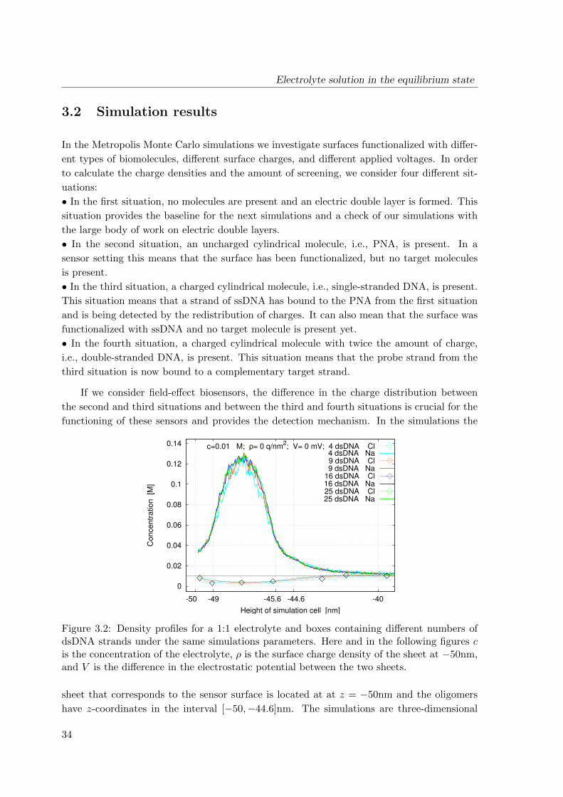
Electrolyte solution in the equilibrium state
3.2 Simulation results
In the Metropolis Monte Carlo simulations we investigate surfaces functionalized with differ-
ent types of biomolecules, different surface charges, and different applied voltages. In order
to calculate the charge densities and the amount of screening, we consider four different sit-
uations:
• In the first situation, no molecules are present and an electric double layer is formed. This
situation provides the baseline for the next simulations and a check of our simulations with
the large body of work on electric double layers.
• In the second situation, an uncharged cylindrical molecule, i.e., PNA, is present. In a
sensor setting this means that the surface has been functionalized, but no target molecules
is present.
• In the third situation, a charged cylindrical molecule, i.e., single-stranded DNA, is present.
This situation means that a strand of ssDNA has bound to the PNA from the first situation
and is being detected by the redistribution of charges. It can also mean that the surface was
functionalized with ssDNA and no target molecule is present yet.
• In the fourth situation, a charged cylindrical molecule with twice the amount of charge,
i.e., double-stranded DNA, is present. This situation means that the probe strand from the
third situation is now bound to a complementary target strand.
If we consider field-effect biosensors, the difference in the charge distribution between
the second and third situations and between the third and fourth situations is crucial for the
functioning of these sensors and provides the detection mechanism. In the simulations the
0
0.02
0.04
0.06
0.08
0.1
0.12
0.14
-40 -44.6-45.6 -49 -50
Concentr
ation [M
]
Height of simulation cell [nm]
c=0.01 M; ρ= 0 q/nm2; V= 0 mV; 4 dsDNA Cl
4 dsDNA Na9 dsDNA Cl9 dsDNA Na
16 dsDNA Cl16 dsDNA Na25 dsDNA Cl25 dsDNA Na
Figure 3.2: Density profiles for a 1:1 electrolyte and boxes containing different numbers ofdsDNA strands under the same simulations parameters. Here and in the following figures cis the concentration of the electrolyte, ρ is the surface charge density of the sheet at −50nm,and V is the difference in the electrostatic potential between the two sheets.
sheet that corresponds to the sensor surface is located at at z = −50nm and the oligomers
have z-coordinates in the interval [−50,−44.6]nm. The simulations are three-dimensional
34
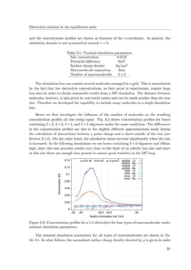
Electrolyte solution in the equilibrium state
and the concentration profiles are shown as function of the z-coordinate. In general, the
simulation domain is not symmetrical around z = 0.
Table 3.1: Nominal simulation parameters.Salt concentration 0.01MPotential difference 0mVSurface charge density 0q/nm2
Macromolecule separation 8nmNumber of macromolecules 3× 3
The simulation box can contain several molecules arranged in a grid. This is necessitated
by the fact that low electrolyte concentrations, as they occur in experiments, require large
box sizes in order to obtain reasonable results from a MC simulation. The distance between
molecules, however, is also given by real-world values and can be much smaller than the box
size. Therefore we developed the capability to include many molecules in a single simulation
box.
Hence we first investigate the influence of the number of molecules on the resulting
concentration profiles all else being equal. Fig. 3.2 shows concentration profiles for boxes
containing 2× 2, 3× 3, 4× 4, and 5× 5 oligomers under the same conditions. The differences
in the concentration profiles are due to the slightly different approximations made during
the calculation of interactions between a point charge and a sheet outside of the box (see
Section 3.1.4). On the other hand, the simulation times increase significantly when the size
is increased. In the following simulations we use boxes containing 3× 3 oligomers and 100nm
high, since this size provides results very close to the limit of an infinite box size and since
at this size there are enough ions present to ensure good statistics in the MC loop.
0
0.02
0.04
0.06
0.08
0.1
0.12
0.14
-40 -44.6-45.6 -49 -50
Concentr
ation [M
]
Height of simulation cell [nm]
c=0.01 M; V=0 mV; ρ= 0 q/nm2; dsDNA Cl
dsDNA NassDNA ClssDNA Na
PNA ClPNA Nanone Clnone Na
Figure 3.3: Concentration profiles for a 1:1 electrolyte for four types of macromolecules undernominal simulation parameters.
The nominal simulation parameters for all types of macromolecules are shown in Ta-
ble 3.1. In what follows, the normalized surface charge density denoted by ρ is given in units
35
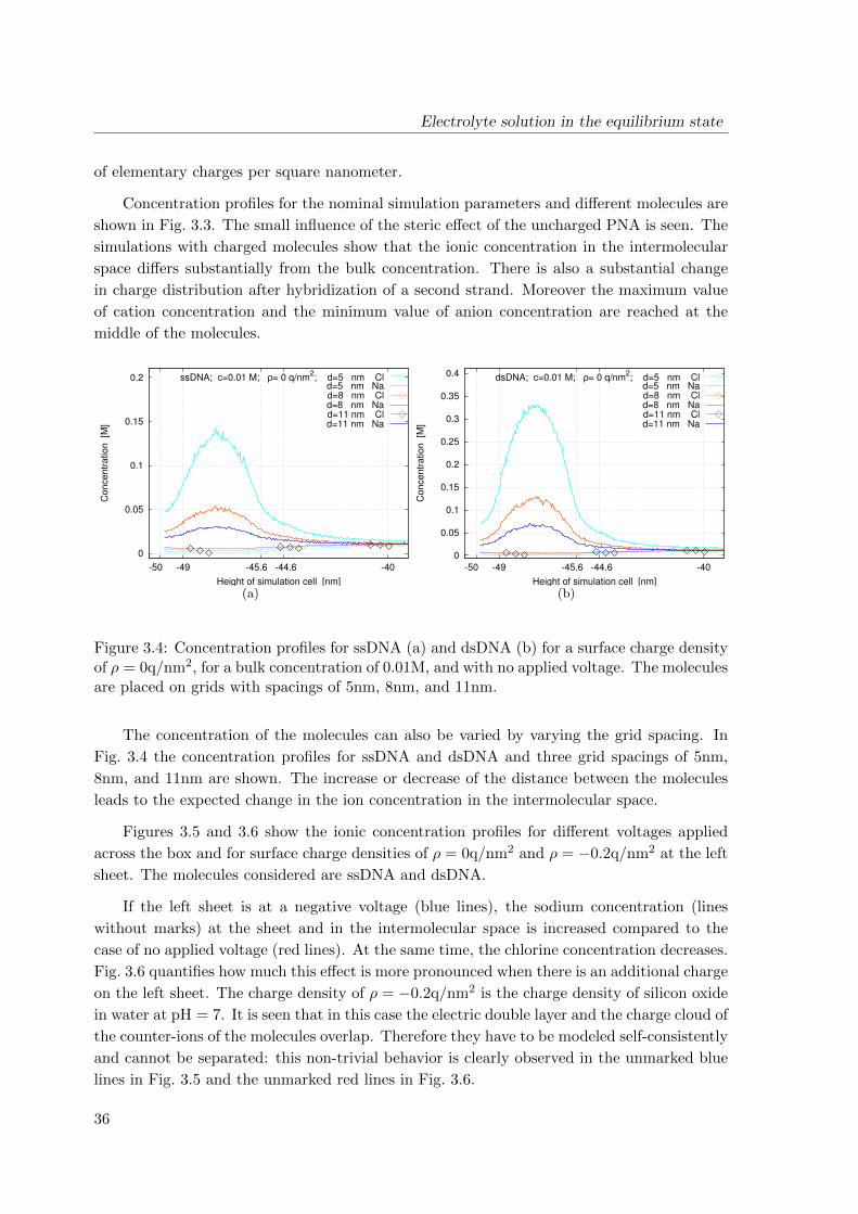
Electrolyte solution in the equilibrium state
of elementary charges per square nanometer.
Concentration profiles for the nominal simulation parameters and different molecules are
shown in Fig. 3.3. The small influence of the steric effect of the uncharged PNA is seen. The
simulations with charged molecules show that the ionic concentration in the intermolecular
space differs substantially from the bulk concentration. There is also a substantial change
in charge distribution after hybridization of a second strand. Moreover the maximum value
of cation concentration and the minimum value of anion concentration are reached at the
middle of the molecules.
0
0.05
0.1
0.15
0.2
-40 -44.6-45.6 -49 -50
Co
nce
ntr
atio
n
[M]
Height of simulation cell [nm]
ssDNA; c=0.01 M; ρ= 0 q/nm2; d=5 nm Cl
d=5 nm Nad=8 nm Cld=8 nm Nad=11 nm Cld=11 nm Na
(a)
0
0.05
0.1
0.15
0.2
0.25
0.3
0.35
0.4
-40 -44.6-45.6 -49 -50
Co
nce
ntr
atio
n
[M]
Height of simulation cell [nm]
dsDNA; c=0.01 M; ρ= 0 q/nm2; d=5 nm Cl
d=5 nm Nad=8 nm Cld=8 nm Nad=11 nm Cld=11 nm Na
(b)
Figure 3.4: Concentration profiles for ssDNA (a) and dsDNA (b) for a surface charge densityof ρ = 0q/nm2, for a bulk concentration of 0.01M, and with no applied voltage. The moleculesare placed on grids with spacings of 5nm, 8nm, and 11nm.
The concentration of the molecules can also be varied by varying the grid spacing. In
Fig. 3.4 the concentration profiles for ssDNA and dsDNA and three grid spacings of 5nm,
8nm, and 11nm are shown. The increase or decrease of the distance between the molecules
leads to the expected change in the ion concentration in the intermolecular space.
Figures 3.5 and 3.6 show the ionic concentration profiles for different voltages applied
across the box and for surface charge densities of ρ = 0q/nm2 and ρ = −0.2q/nm2 at the left
sheet. The molecules considered are ssDNA and dsDNA.
If the left sheet is at a negative voltage (blue lines), the sodium concentration (lines
without marks) at the sheet and in the intermolecular space is increased compared to the
case of no applied voltage (red lines). At the same time, the chlorine concentration decreases.
Fig. 3.6 quantifies how much this effect is more pronounced when there is an additional charge
on the left sheet. The charge density of ρ = −0.2q/nm2 is the charge density of silicon oxide
in water at pH = 7. It is seen that in this case the electric double layer and the charge cloud of
the counter-ions of the molecules overlap. Therefore they have to be modeled self-consistently
and cannot be separated: this non-trivial behavior is clearly observed in the unmarked blue
lines in Fig. 3.5 and the unmarked red lines in Fig. 3.6.
36
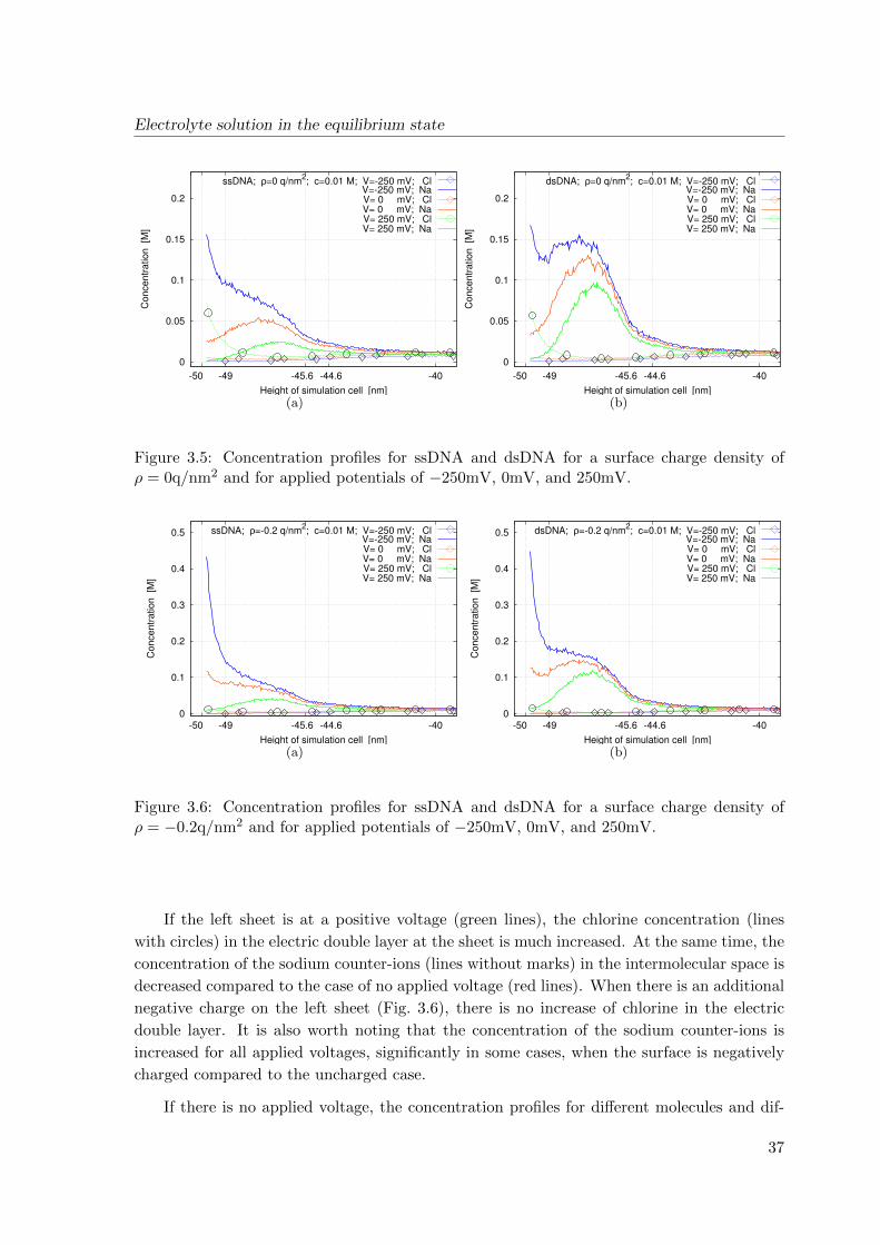
Electrolyte solution in the equilibrium state
0
0.05
0.1
0.15
0.2
-40 -44.6-45.6 -49 -50
Co
nce
ntr
atio
n
[M]
Height of simulation cell [nm]
ssDNA; ρ=0 q/nm2; c=0.01 M; V=-250 mV; Cl
V=-250 mV; NaV= 0 mV; ClV= 0 mV; NaV= 250 mV; ClV= 250 mV; Na
(a)
0
0.05
0.1
0.15
0.2
-40 -44.6-45.6 -49 -50
Co
nce
ntr
atio
n
[M]
Height of simulation cell [nm]
dsDNA; ρ=0 q/nm2; c=0.01 M; V=-250 mV; Cl
V=-250 mV; NaV= 0 mV; ClV= 0 mV; NaV= 250 mV; ClV= 250 mV; Na
(b)
Figure 3.5: Concentration profiles for ssDNA and dsDNA for a surface charge density ofρ = 0q/nm2 and for applied potentials of −250mV, 0mV, and 250mV.
0
0.1
0.2
0.3
0.4
0.5
-40 -44.6-45.6 -49 -50
Co
nce
ntr
atio
n
[M]
Height of simulation cell [nm]
ssDNA; ρ=-0.2 q/nm2; c=0.01 M; V=-250 mV; Cl
V=-250 mV; NaV= 0 mV; ClV= 0 mV; NaV= 250 mV; ClV= 250 mV; Na
(a)
0
0.1
0.2
0.3
0.4
0.5
-40 -44.6-45.6 -49 -50
Co
nce
ntr
atio
n
[M]
Height of simulation cell [nm]
dsDNA; ρ=-0.2 q/nm2; c=0.01 M; V=-250 mV; Cl
V=-250 mV; NaV= 0 mV; ClV= 0 mV; NaV= 250 mV; ClV= 250 mV; Na
(b)
Figure 3.6: Concentration profiles for ssDNA and dsDNA for a surface charge density ofρ = −0.2q/nm2 and for applied potentials of −250mV, 0mV, and 250mV.
If the left sheet is at a positive voltage (green lines), the chlorine concentration (lines
with circles) in the electric double layer at the sheet is much increased. At the same time, the
concentration of the sodium counter-ions (lines without marks) in the intermolecular space is
decreased compared to the case of no applied voltage (red lines). When there is an additional
negative charge on the left sheet (Fig. 3.6), there is no increase of chlorine in the electric
double layer. It is also worth noting that the concentration of the sodium counter-ions is
increased for all applied voltages, significantly in some cases, when the surface is negatively
charged compared to the uncharged case.
If there is no applied voltage, the concentration profiles for different molecules and dif-
37
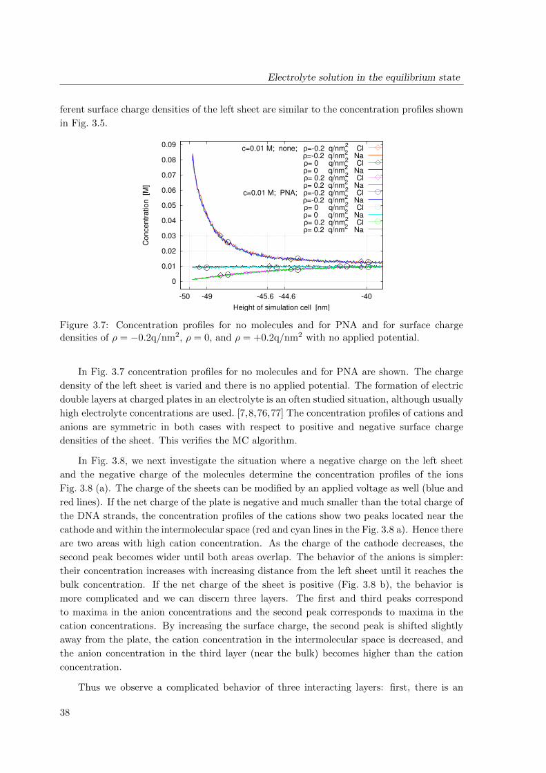
Electrolyte solution in the equilibrium state
ferent surface charge densities of the left sheet are similar to the concentration profiles shown
in Fig. 3.5.
0
0.01
0.02
0.03
0.04
0.05
0.06
0.07
0.08
0.09
-40 -44.6-45.6 -49 -50
Concentr
ation [M
]
Height of simulation cell [nm]
c=0.01 M; none; ρ=-0.2 q/nm2 Cl
ρ=-0.2 q/nm2 Na
ρ= 0 q/nm2 Cl
ρ= 0 q/nm2 Na
ρ= 0.2 q/nm2 Cl
ρ= 0.2 q/nm2 Na
c=0.01 M; PNA; ρ=-0.2 q/nm2 Cl
ρ=-0.2 q/nm2 Na
ρ= 0 q/nm2 Cl
ρ= 0 q/nm2 Na
ρ= 0.2 q/nm2 Cl
ρ= 0.2 q/nm2 Na
Figure 3.7: Concentration profiles for no molecules and for PNA and for surface chargedensities of ρ = −0.2q/nm2, ρ = 0, and ρ = +0.2q/nm2 with no applied potential.
In Fig. 3.7 concentration profiles for no molecules and for PNA are shown. The charge
density of the left sheet is varied and there is no applied potential. The formation of electric
double layers at charged plates in an electrolyte is an often studied situation, although usually
high electrolyte concentrations are used. [7,8,76,77] The concentration profiles of cations and
anions are symmetric in both cases with respect to positive and negative surface charge
densities of the sheet. This verifies the MC algorithm.
In Fig. 3.8, we next investigate the situation where a negative charge on the left sheet
and the negative charge of the molecules determine the concentration profiles of the ions
Fig. 3.8 (a). The charge of the sheets can be modified by an applied voltage as well (blue and
red lines). If the net charge of the plate is negative and much smaller than the total charge of
the DNA strands, the concentration profiles of the cations show two peaks located near the
cathode and within the intermolecular space (red and cyan lines in the Fig. 3.8 a). Hence there
are two areas with high cation concentration. As the charge of the cathode decreases, the
second peak becomes wider until both areas overlap. The behavior of the anions is simpler:
their concentration increases with increasing distance from the left sheet until it reaches the
bulk concentration. If the net charge of the sheet is positive (Fig. 3.8 b), the behavior is
more complicated and we can discern three layers. The first and third peaks correspond
to maxima in the anion concentrations and the second peak corresponds to maxima in the
cation concentrations. By increasing the surface charge, the second peak is shifted slightly
away from the plate, the cation concentration in the intermolecular space is decreased, and
the anion concentration in the third layer (near the bulk) becomes higher than the cation
concentration.
Thus we observe a complicated behavior of three interacting layers: first, there is an
38
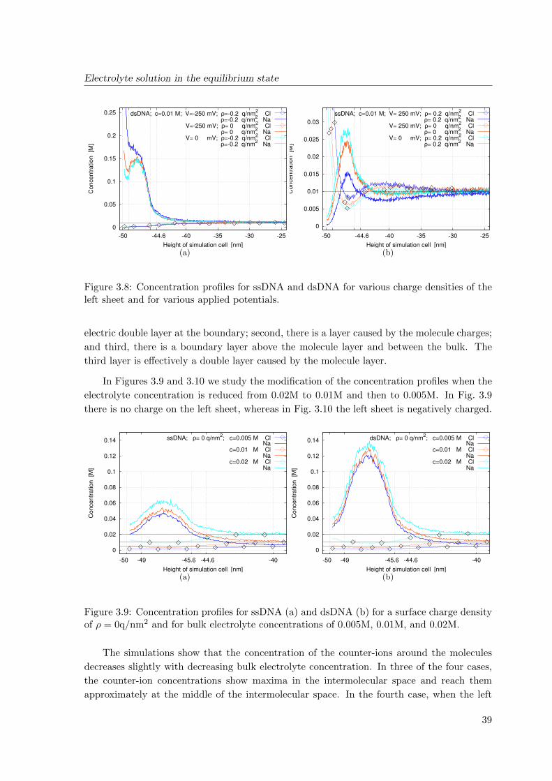
Electrolyte solution in the equilibrium state
0
0.05
0.1
0.15
0.2
0.25
-25-30-35-40 -44.6 -50
Co
nce
ntr
atio
n
[M]
Height of simulation cell [nm]
dsDNA; c=0.01 M; V=-250 mV; ρ=-0.2 q/nm2 Cl
ρ=-0.2 q/nm2 Na
V=-250 mV; ρ= 0 q/nm2 Cl
ρ= 0 q/nm2 Na
V= 0 mV; ρ=-0.2 q/nm2 Cl
ρ=-0.2 q/nm2 Na
(a)
0
0.005
0.01
0.015
0.02
0.025
0.03
-25-30-35-40 -44.6 -50
Co
nce
ntr
atio
n
[M]
Height of simulation cell [nm]
ssDNA; c=0.01 M; V= 250 mV; ρ= 0.2 q/nm2 Cl
ρ= 0.2 q/nm2 Na
V= 250 mV; ρ= 0 q/nm2 Cl
ρ= 0 q/nm2 Na
V= 0 mV; ρ= 0.2 q/nm2 Cl
ρ= 0.2 q/nm2 Na
(b)
Figure 3.8: Concentration profiles for ssDNA and dsDNA for various charge densities of theleft sheet and for various applied potentials.
electric double layer at the boundary; second, there is a layer caused by the molecule charges;
and third, there is a boundary layer above the molecule layer and between the bulk. The
third layer is effectively a double layer caused by the molecule layer.
In Figures 3.9 and 3.10 we study the modification of the concentration profiles when the
electrolyte concentration is reduced from 0.02M to 0.01M and then to 0.005M. In Fig. 3.9
there is no charge on the left sheet, whereas in Fig. 3.10 the left sheet is negatively charged.
0
0.02
0.04
0.06
0.08
0.1
0.12
0.14
-40 -44.6-45.6 -49 -50
Co
nce
ntr
atio
n
[M]
Height of simulation cell [nm]
ssDNA; ρ= 0 q/nm2; c=0.005 M Cl
Nac=0.01 M Cl
Nac=0.02 M Cl
Na
(a)
0
0.02
0.04
0.06
0.08
0.1
0.12
0.14
-40 -44.6-45.6 -49 -50
Co
nce
ntr
atio
n
[M]
Height of simulation cell [nm]
dsDNA; ρ= 0 q/nm2; c=0.005 M Cl
Nac=0.01 M Cl
Nac=0.02 M Cl
Na
(b)
Figure 3.9: Concentration profiles for ssDNA (a) and dsDNA (b) for a surface charge densityof ρ = 0q/nm2 and for bulk electrolyte concentrations of 0.005M, 0.01M, and 0.02M.
The simulations show that the concentration of the counter-ions around the molecules
decreases slightly with decreasing bulk electrolyte concentration. In three of the four cases,
the counter-ion concentrations show maxima in the intermolecular space and reach them
approximately at the middle of the intermolecular space. In the fourth case, when the left
39
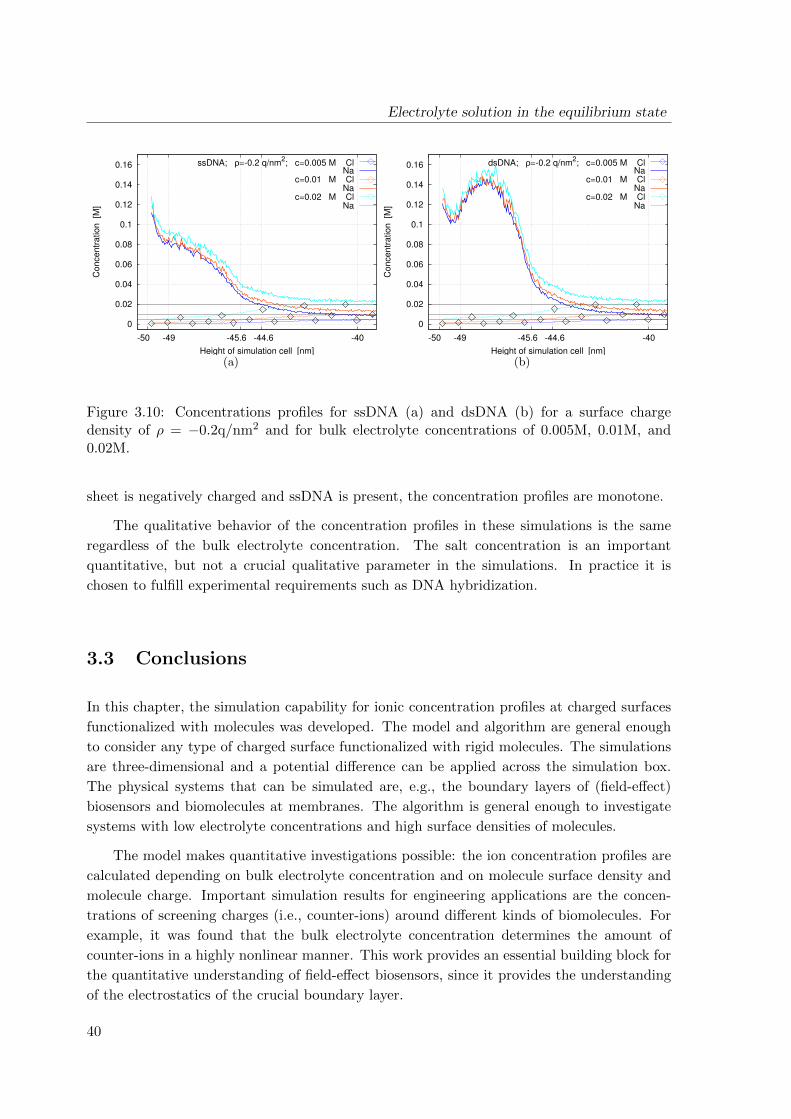
Electrolyte solution in the equilibrium state
0
0.02
0.04
0.06
0.08
0.1
0.12
0.14
0.16
-40 -44.6-45.6 -49 -50
Co
nce
ntr
atio
n
[M]
Height of simulation cell [nm]
ssDNA; ρ=-0.2 q/nm2; c=0.005 M Cl
Nac=0.01 M Cl
Nac=0.02 M Cl
Na
(a)
0
0.02
0.04
0.06
0.08
0.1
0.12
0.14
0.16
-40 -44.6-45.6 -49 -50
Co
nce
ntr
atio
n
[M]
Height of simulation cell [nm]
dsDNA; ρ=-0.2 q/nm2; c=0.005 M Cl
Nac=0.01 M Cl
Nac=0.02 M Cl
Na
(b)
Figure 3.10: Concentrations profiles for ssDNA (a) and dsDNA (b) for a surface chargedensity of ρ = −0.2q/nm2 and for bulk electrolyte concentrations of 0.005M, 0.01M, and0.02M.
sheet is negatively charged and ssDNA is present, the concentration profiles are monotone.
The qualitative behavior of the concentration profiles in these simulations is the same
regardless of the bulk electrolyte concentration. The salt concentration is an important
quantitative, but not a crucial qualitative parameter in the simulations. In practice it is
chosen to fulfill experimental requirements such as DNA hybridization.
3.3 Conclusions
In this chapter, the simulation capability for ionic concentration profiles at charged surfaces
functionalized with molecules was developed. The model and algorithm are general enough
to consider any type of charged surface functionalized with rigid molecules. The simulations
are three-dimensional and a potential difference can be applied across the simulation box.
The physical systems that can be simulated are, e.g., the boundary layers of (field-effect)
biosensors and biomolecules at membranes. The algorithm is general enough to investigate
systems with low electrolyte concentrations and high surface densities of molecules.
The model makes quantitative investigations possible: the ion concentration profiles are
calculated depending on bulk electrolyte concentration and on molecule surface density and
molecule charge. Important simulation results for engineering applications are the concen-
trations of screening charges (i.e., counter-ions) around different kinds of biomolecules. For
example, it was found that the bulk electrolyte concentration determines the amount of
counter-ions in a highly nonlinear manner. This work provides an essential building block for
the quantitative understanding of field-effect biosensors, since it provides the understanding
of the electrostatics of the crucial boundary layer.
40

Electrolyte solution in the equilibrium state
It was found that due to the presence of the charged molecules, the ionic concentration
profiles generally exhibit a three-layer structure. The first layer is the electric double layer
due to the charged surface, the second layer is due to counter-ions between the molecules,
and the third layer is a boundary layer above the layer of the biomolecules. The interaction
between the electric double layer and the counter-ions is non-trivial and necessitates this kind
of quantitative investigation that we presented.
41

Chapter 4
Transport of charged biomolecules
with chemical reactions near the
surface
4.1 Continuum model for the analyte flow
We consider the same sensor as in Section 2.1 and begin with the specification of the sensing
system: the target molecules wander diffusively through the solution and bind to the probes,
which are linked to the surface. In the case of a uniform viscosity, constant temperature and
pressure, the diffusivity D will be independent of position. Note that the diffusivity depends
in general on the type (size and shape) of the molecule. It will be described more precisely
in Section 4.3. In our model we keep this parameter constant. Furthermore, we consider a
non-specific adsorption of targets to the surface, where CnT (t) denotes a concentration for
such molecules (referred further as non-specifically adsorbed molecules). For simplicity, we
assume that all probe molecules are attached to the surface, and that the initial concentrations
CT,0 and CP,0 are uniform; the initial concentration of probe-target complexes and non-
specifically adsorbed molecules are equal to zero CPT,0 = CnT,0 = 0. In this work we focus
on the selectively adsorbing boundary conditions, which are a crucial part of the modeling of
the biosensors, and which are, despite of the remarkable experimental progress in this field,
still not clearly understood by experimentalists. Thus, for instance, the two types of the
adsorption, specific and non-specific, are not very well distinguished in the experiments.
4.1.1 Adsorption of biomolecules: specific and non-specific binding
The proposed model is based upon two mechanisms of adsorption: the direct binding of
targets from the bulk phase to probe molecules and the non-specifically adsorption of target
molecules to the surface. If the chemical reaction between biomolecules has an association
43
Transport of charged biomolecules with chemical reactions near the surface
rate ra > 0, and disassociation rate rd > 0, and ka ≥ 0 and kd ≥ 0 represent the non-specific
adsorption and desorption, then from the law of mass action we obtain the following relations
at the surface ∂Ωs
∂CPT (t)
∂t= raCT (t, xs)
(CP,0 − CPT (t)
)−rdCPT (t), (4.1)
∂CnT (t)
∂t= kaCT (t, xs)
(CnT,max(t)− CnT (t)
)−kdCnT (t), (4.2)
with initial data:
CPT (t=0) = CnT (t=0) = 0,
where xs is located near ∂Ωs, the terms CP (t) := CP,0−CPT (t) and CT (t, xs) := CT (t, x=xs)
describe the concentration of single probe molecules and free target molecules, respectively,
i.e., those molecules, which are not bounded at the time t. CnT,max is a concentration of
non-specific adsorption at the maximum altitude. Under the assumption that single species
do not overlap, it is determined to be
CnT,max(t) =1− πR2
PCP (t)− πR2PTCPT (t)
πR2T
<1
πR2T
,
where RP , RT and RPT are radius of probes, targets and probe-target complexes including
a distance of closest approach, respectively. In the case of RP = RPT the concentration is
constant and equal to CnT,max= (1− πR2PTCP,0)/πR2
T .
We also fix the CT (t, xs) =: c∗ in the eqns. (4.1) and (4.2). In this case the functions at
the right-hand side are everywhere differentiable in CPT and CnT . Moreover, the absolute
values of the derivatives are bounded above by rac∗ and kac
∗, respectively. Thus, they are
Lipschitz continuous in CPT and CnT and continuous in t ∈ [0, T ]. According to Picard-
Lindelof Theorem the ordinary differential equations (4.1) and (4.2) with initial conditions
have unique solutions, which depend on CT (t, xs) in our case, and are given for t > 0 as
follows:
0 < CPT (t) =raCT (t, xs) CP,0rd + raCT (t, xs)
(1− e−(raCT (t,xs)+rd)t
)≤
CP,0rd
raCT (t,xs) + 1< CP,0, (4.3)
0 < CnT (t) =kaCT (t, xs) CnT,maxkd + kaCT (t, xs)
(1− e−(kaCT (t,xs)+kd)t
)< CnT,max(t), (4.4)
where CT (t, xs) > max− rdra,−kd
ka will be determined below in (4.6).
The concentrations CPT (t) and CnT (t) at the time interval (0, T ] are equal to zero only if
there are no reaction processes, i.e., ra = rd =ka =kd = 0 . Therefore, we assume for further
considerations that rdra
kdka> 0.
44
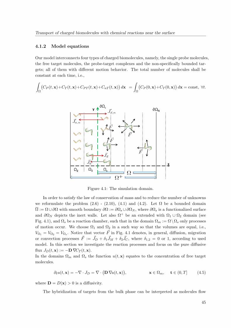
Transport of charged biomolecules with chemical reactions near the surface
4.1.2 Model equations
Our model interconnects four types of charged biomolecules, namely, the single probe molecules,
the free target molecules, the probe-target complexes and the non-specifically bounded tar-
gets; all of them with different motion behavior. The total number of molecules shall be
constant at each time, i.e.,∫Ω
(CP (t,x)+CT (t,x)+CPT (t,x)+CnT (t,x)
)dx =
∫Ω
(CP (0,x)+CT (0,x)
)dx = const, ∀t.
Figure 4.1: The simulation domain.
In order to satisfy the law of conservation of mass and to reduce the number of unknowns
we reformulate the problem (2.6) - (2.10), (4.1) and (4.2). Let Ω be a bounded domain
Ω := Ω∪ ∂Ω with smooth boundary ∂Ω := ∂Ωs ∪ ∂ΩN , where ∂Ωs is a functionalized surface
and ∂ΩN depicts the inert walls. Let also Ω+ be an extended with Ω1 ∪ Ω2 domain (see
Fig. 4.1), and Ωs be a reaction chamber, such that in the domain Ωm := Ω\Ωs only processes
of motion occur. We choose Ω1 and Ω2 in a such way so that the volumes are equal, i.e.,
VΩ1 = VΩ2 = VΩs . Notice that vector ~F in Fig. 4.1 denotes, in general, diffusion, migration
or convection processes ~F := ~JD + δ1~JM + δ2
~JC , where δ1,2 = 0 or 1, according to used
model. In this section we investigate the reaction processes and focus on the pure diffusive
flux JD(t,x) := −D∇CT (t,x).
In the domains Ωm and Ωs the function u(t,x) equates to the concentration of free target
molecules.
∂tu(t,x) = −∇ · JD = ∇ ·(D∇u(t,x)
), x ∈ Ωm, t ∈ (0, T ] (4.5)
where D = D(x) > 0 is a diffusivity.
The hybridization of targets from the bulk phase can be interpreted as molecules flow
45
Transport of charged biomolecules with chemical reactions near the surface
~Ja through the surface ∂Ωs and their accumulation in Ω1. The denaturation is an opposite
process and is described by flow ~Jd.
The reversible non-specific adsorption is depicted in our model as jump ~Ja,n to the domain
Ω2 and desorption is a backward jump ~Jd,n .
We assume that the non-specifically adsorbed target molecules will bind to a single probe
only after their desorption, i.e., at another time step. We also assume that the chemical
reaction is one-dimensional (in x-direction) and the movement of analyte molecules is three-
dimensional. We suppose that after hybridization the target can be bound to another probe
molecule only after its movement to another place.
Thus, the non-specifically adsorbed targets are located in Ω2 and the probe-target complexes
are accumulated in Ω1, i.e., the function u(t, x), x ∈ Ω1 or Ω2, is associated with probe-target
complexes and with non-specifically bounded targets.
0 ≤ CPT (t) = u(t, xs−1) < CP,0 and ∂tCPT (t) = ∂tu(t, xs−1), xs−1 ∈ Ω1, t ∈ (0, T ]
0 ≤ CnT (t) = u(t, xs−2) < CnT,max and ∂tCnT (t) = ∂tu(t, xs−2), xs−2 ∈ Ω2, t ∈ (0, T ]
In such an interpretation it is enough to control the number of target molecules disregarding
their state of binding. Ω1 and Ω2 can be simply considered as ”look-up” domains for specific
and non-specific binding, respectively.
Now we can argue that any interaction between single P and free T molecules at time
t only occurs if x(t) ∈ Ωs, i.e. the target and probe molecules are close to another, where
x(t) is the location of the analyte molecule at the time t. The same assumptions we make
for non-specific reactions. Let ~n be a unit normal vector pointing outward to the surface.
In the domain Ωs the flows ~Jd and ~Ja have opposite directions, i.e., ~Ja · ~n > 0, ~Jd · ~n < 0.
Moreover, there are no flow ~F through the surfaces ∂Ωs and ∂ΩN , i.e., ~F · ~n ≤ 0. To satisfy
the last inequality, we extend (expand) the diffusion function in Ω+ as follows
D(t, x) = 0 in Ω1 ∪ Ω2 ∪ ∂Ωs,
0 < D ≤D(t, x) ≤ D ≤ 1 in Ω,
D(t, x) = 0, on ∂Ω+.
Thus, the Eq. (4.6) describes the flow near the functionalized surface.
∂tu(t, xs) =−∇ ·(JD(t, xs)
)− ra u(t, xs)
(CP,0 − u(t, xs−1)
)+rd u(t, xs−1) (4.6)
− ka u(t, xs)(CnT,max − u(t, xs−2)
)+kd u(t, xs−2),
where xs ∈ Ωs, xs−1 ∈ Ω1, xs−2 ∈ Ω2 and t ∈ (0, T ].
In Ω1 the both flows ~Ja and ~Jd change their directions, i.e., ~Ja · ~n < 0, ~Jd · ~n > 0.
Analogously we consider the flows ~Ja,n and ~Jd,n. Hence, the equations (4.1) and (4.2) can be
46
Transport of charged biomolecules with chemical reactions near the surface
rewritten as
∂tu(t, xs−1) = ra u(t, xs)(CP,0 − u(t, xs−1)
)−rd u(t, xs−1), (4.7)
∂tu(t, xs−2) = ka u(t, xs)(CnT,max − u(t, xs−2)
)−kd u(t, xs−2), (4.8)
where xs ∈ Ωs, xs−1 ∈ Ω1, xs−2 ∈ Ω2 and t ∈ (0, T ].
Thus, we consider the initial-boundary-value problem u(t, x) : (0, T ]×Ω+ 7→ R described
by the equations (4.5)-(4.8) with initial conditions
u(t=0, x) = uI(x) :=
CT,0, x ∈ Ωs ∪ Ωm, ,
0, x ∈ Ω1 ∪ Ω2,(4.9)
and with Neumann boundary conditions at the inert walls
∂u(t, x)
∂~n= 0, x ∈ ∂ΩN , (4.10)
where ~n is the outward unit normal vector along ∂ΩN and CP,0, CT,0, CnT,max, ra, rd, ka and
kd are the given constants, i.e. the experimentally measured quantities, and rdra 1 and
kdka 1.
Lemma 4.1.1. Law of mass conservation .
The solution u(t,x) of the initial-boundary-value problem (4.5)-(4.10) satisfies the global law
of mass conservation: ∫Ω+
u(t,x) dx =
∫Ω+
uI(x) dx = const,
‖u(t,x)‖L1(Ω+) = ‖uI(x)‖L1(Ω+) <∞, ∀t,
where uI(x) is the initial concentration of target molecules given by (4.9)
and dx=dx dy dz if Ω+ ⊂ R3.
Proof. Let Ω+\Ωm = Ωs ∪ Ω1 ∪ Ω2 and Ω = Ωm ∪ Ωs be the same as described above.
Due to the special choice of domains Ω1 and Ω2, the function u(t, xs) ∈ Ωs can be specified
in the domain Ω+ \ Ωm as a function
us(t,x) = u(t, xs) in Ωs and us(t,x) = 0 in Ωm ∪ Ω1 ∪ Ω2.
Analogously we can write for u(t, xs−1) ∈ Ω1, u(t, xs−2) ∈ Ω2 and u(t, x) ∈ Ωm
u1(t,x) = u(t, xs−1) in Ω1 and u1(t,x) = 0 in Ωm ∪ Ωs ∪ Ω2,
u2(t,x) = u(t, xs−2) in Ω2 and u2(t,x) = 0 in Ωm ∪ Ωs ∪ Ω1,
u0(t,x) = u(t, x) in Ωm and u0(t,x) = 0 in Ωs ∪ Ω1 ∪ Ω2.
47
Transport of charged biomolecules with chemical reactions near the surface
We integrate ∂tu(t,x) over domain Ω+∫Ω+
∂tu(t,x) dx =
∫Ωm
∇ ·(D∇u0(t,x)
)dx +
∫ΩΩ+\Ωm
∇ ·(D∇us(t,x)
)dx
−∫
ΩΩ+\Ωm
(ra us(t,x)
(CP,0 − u1(t,x)
)−rd u1(t,x)
)dx
−∫
ΩΩ+\Ωm
(ka us(t,x)
(CnT,max − u2(t,x)
)−kd u2(t,x)
)dx
+
∫ΩΩ+\Ωm
(ra us(t,x)
(CP,0 − u1(t,x)
)−rd u1(t,x)
)dx
+
∫ΩΩ+\Ωm
(ka us(t,x)
(CnT,max − u2(t,x)
)−kd u2(t,x)
)dx.
Hence, the mass conservation law in differential form can be written as∫Ω+
∂tu(t,x) dx =
∫Ω+
∇ ·(D(x)∇u(t,x)
)dx = −
∫Ω+
∇ · JD(t,x) dx.
We apply the divergence theorem and use the definition of diffusion on the boundary ∂Ω+
∂t
∫Ω+
u(t,x) dx =
∫∂Ω+
(D(x)∇u(t,x)
)·~n dx = 0.
This implies the global law of mass conservation∫Ω+
u(t,x) dx =
∫Ω+
uI(x) dx = const.
For the above suggested model we will give in the next section a discretized conservative
scheme and demonstrate that the mass can be conserved exactly. To show the existence,
uniqueness and properties of the solution we consider an equivalent problem using (4.3) and
(4.4) under new notations. Let u1(t, u) and u2(t, u) be the unique solutions of (4.7) and (4.8),
respectively, and denote the second and the third terms in eq. (4.6) as b(t, u) and f(t, u).
u1(t, u) =ra u(t, x) CP,0rd + ra u(t, x)
(1− e−(ra u(t,x)+rd)t
)t ∈ (0, T ], x ∈ Ωs, (4.11)
u2(t, u) =ka u(t, x) CnT,maxkd + ka u(t, x)
(1− e−(ka u(t,x)+kd)t
)t ∈ (0, T ], x ∈ Ωs, (4.12)
d := d(x) =
1, t ∈ (0, T ], x ∈ Ωm,
0, t ∈ (0, T ], x ∈ Ωs,(4.13)
48
Transport of charged biomolecules with chemical reactions near the surface
b(t, x, u) :=
1, t ∈ (0, T ], x ∈ Ωm,
ra(CP,0 − u1(t, u)
)+ka
(CnT,max − u2(t, u)
), t ∈ (0, T ], x ∈ Ωs,
(4.14)
f(t, x, u) :=
0, t ∈ (0, T ], x ∈ Ωm,
rdu1(t, u) + kdu2(t, u), t ∈ (0, T ], x ∈ Ωs,(4.15)
∂tu(t, x) =∇ ·(a∇u(t, x)
)−(b(t, u)− d
)u(t, x) + f(t, u), t ∈ (0, T ], x ∈ Ω, (4.16)
∂u(t, x)
∂~n=0, t ∈ (0, T ], x ∈ ∂ΩN ,
u(t, x) =0 t ∈ (0, T ], x ∈ ΩD,
u(t, x) =uI t = 0, x ∈ Ω, (4.17)
a :=D(x) ∈ (0, 1], t ∈ (0, T ], x ∈ Ω.
u denotes that its value is obtained at the earlier iterative step. To solve the initial-boundary-
value problem (4.11) - (4.17) we use the following algorithm. We start with b = b(uI) and
f = f(uI), then solve the equation (4.16) and then recalculate the coefficients b(t, u) = b(t, u)
and f(t, u) = f(t, u).
Lemma 4.1.2. The solution of the initial-boundary-value problem (4.5)-(4.10) and, therefor,
the solution of the equivalent systems (4.11)-(4.16) is unique and it is non-negative in (0, T ]×Ωm and strictly positive in (0, T ]×Ωs.
Proof. We choose u = c+ v, where c is a positive constant equal to inf uI .
If ‖v‖C(Ω+) ≤ c, the function u will be non-negative.
Since u fulfills the law of mass conservation, we can estimate
‖v‖C(Ω+) ≤ ‖v‖L1(Ω+) = ‖u− c‖L1(Ω+) =∫
Ω+ u dx−∫
Ω+ c dx =∫
Ω+ uI dx−∫
Ω+ c dx = 0 ≤ c.This give us a non-negativity of u.
Next we consider the function u ≡ 0. It satisfies the equation (4.6) only if u1 = 0 and u2 = 0,
i.e., at the time t = 0, and will be strictly positive in (0, T ]×Ωs.
Assume that v1 and v2 are two different (v1 6≡ v2) solutions of our problem.
‖v1‖L1(Ω+) − ‖v2‖L1(Ω+) = ‖uI‖L1(Ω+) − ‖uI‖L1(Ω+) = 0.
On the other hand∫
Ω+ v1 dx−∫
Ω+ v2 dx =∫
Ω+(v1 − v2) dx = 0 if v1 ≡ v2.
Thus, we can conclude that the solution is unique.
Due to the inequalities (4.3) and (4.4), we get in the domain (0, T ]×Ωs the following
49
Transport of charged biomolecules with chemical reactions near the surface
estimates
0 < u1(t, u) ≤ra uCP,0rd + ra u
< CP,0,
0 < u2(t, u) < CnT,max,
0 < b ≤ b(t, u) < raCP,0 + kaCnT,max =: b, (4.18)
0 < f ≤ f(t, u) < rdCP,0 + kdCnT,max =: f. (4.19)
Lemma 4.1.3. Let F (t, u) := −(b(t, u) − d(x)
)u(t, x) + f(t, u) for u ∈ Ω be a non-linear
part of the Eq. (4.16), where d(t, u), b(t, u), and f(t, u) are given by the Eqs. (4.13) - (4.15),
respectively. The function F : R→ R is Lipschitz continuous in u and continuous in t.
Proof. In the proof we only consider the inhomogeneity in the domain Ωs, because the func-
tion F is equal to zero in the domain Ωm.
F (t, u) =− b(t, u)u(t, x) + f(t, u)
=− raCP,0 u− kaCnT,max u+ (ra u+ rd)u1 + (ka u+ kd)u2
=− raCP,0 u− kaCnT,max u+ raCP,0 u(1− e−(ra u+rd)t
)+kaCnT,max u
(1− e−(ka u+kd)t
)The function F is everywhere differentiable in u with the following derivative
F′u = raCP,0 (1− e−(rd+rau)t) + r2
a CP,0 t u e−(rd+rau)t − raCP,0
+ kaCnT,max (1− e−(kd+kau)t) + k2a CnT,max t u e
−(kd+kau)t − kaCnT,max
We analyze the function u e−(rd+rau)t. It is concave for t ∈ (0, T ] and u ≥ 0 and its derivative(u e−(rd+ra u)t
)′
u= e−t(u ra+rd)(1− t u ra)
has a root in 1t ra
. Hence, this function is bounded
u e−(rd+rau)t ≤ 1
t ra
Similarly we estimate
u e−(kd+kau)t ≤ 1
t ka
The functions 1 − e−(rd+rau)t and 1 − e−(kd+kau)t are located between 0 and 1 for t ∈ (0, T ]
and u ≥ 0.
Therefore, the absolute value of the derivative is bounded above by a constant that does not
depend on time.
|F ′u| ≤ CP,0 ra + CnT,max ka.
50
Transport of charged biomolecules with chemical reactions near the surface
This in particular implies a growth estimate
|F (y)| ≤ cF(
1− |y|)
for each y ∈ R and some constant cF , which does not depend on y.
Hence, the diffusion equation with reactive boundary conditions has been reformulated
to the well-studied initial-boundary-value parabolic problem and we can apply the standard
theory for linear parabolic PDE given, for instance, in Ref. [18].
Let φ be a test function in H10 ([0, T ]×Ω). Multiplying the equation (4.16) by φ and
applying partial integration over Ω, we can rewrite it in following form
〈u, φ〉+B[u, φ; t] = (F, φ), (4.20)
∂u(t, x)
∂~n=0, t ∈ (0, T ], x ∈ ∂ΩN , (4.21)
u(t, x) =0 t ∈ (0, T ], x ∈ ΩD, (4.22)
u(t, x) =uI t = 0, x ∈ Ω, (4.23)
where 〈u, φ〉 is a duality pairing of the functions from H−1(Ω) and H10 (Ω), B[u, φ; t] is a
time-dependent bilinear form in H10 (Ω), (F, φ) is an inner product in L2(Ω), and the function
F is defined as above.
Definition 4.1.1. ( Weak solution)
The function u ∈ L2(
0, T ;H10 (Ω)
)with its time derivative u ∈ L2
(0, T ;H−1(Ω)
)is a weak
solution of (4.11) - (4.17) if
• it solves the equation (4.16) in weak sense, i.e., solves the Eq. (4.20) for each φ ∈H1
0 ([t0, T0]×Ω) and for initial data uI ∈ L2(Ω);
• it satisfies the boundary-value conditions (4.21) and (4.22).
Theorem 4.1.4. (Existence of weak solution)
The initial-boundary-value problem (4.5)-(4.10) has a weak solution u(t,x) in L2(
0, T ;H10 (Ω)
)for all t ∈ (0, T ] and in C
(0, T ;L2(Ω)
)for a.e. t ∈ (0, T ].
Proof. We consider a space K := C(
[t0, T0];L2(Ω))
with the norm
‖v‖K = maxt∈[t0,T0]
‖v(t)‖L2(Ω)
We linearize the equation (4.20) by setting F (t, u) = F (t, u∗) =: Fu and apply the existence
theory for linear parabolic equations, where u∗ ∈ K is a given function and, by consequence
of the growth estimate, F (t, u∗) ∈ L2(t0, T0;L2(Ω)
).
51
Transport of charged biomolecules with chemical reactions near the surface
Let u be the unique weak solution of the linearized initial-boundary-value problem given
by (4.20) - (4.23), i.e., it satisfies
∂tu−∇ ·D∇u = Fu (4.24)
for each φ ∈ H10 ([t0, T0]×Ω).
We define Gu∗ = u so that G : K → K. Additionally, we choose v∗ ∈ K and define
v := Gv∗. Consequently v satisfies
∂tv −∇ ·D∇v = Fv, (4.25)
where Fv := F (t, v∗). After subtracting (4.25) from (4.24) and under notations w := u− v =
Gu∗ −Gv∗ and Fw := Fu − Fv we write
∂tw −∇ ·D∇w = Fw (4.26)
Note that ∂t(w2) = 2w ∂tw and∫Ω∇wD∇w dx = wD∇w|∂Ω −
∫ΩwD∇w dx = −
∫ΩwD∇w dx,
because D(x)|∂Ω = 0. Multiplying by 2w and integrating over Ω we obtain
2
∫Ωw ∂tw dx− 2
∫Ωw∇ ·D∇w dx = 2
∫ΩwFw dx,
∂t
∫Ωw2 dx− 2D
∫Ω
(∇w)2 dx = 2
∫ΩwFw dx.
Hence
∂t‖w‖2L2(Ω) + 2D ‖w‖2H10 (Ω) = 2(w,Fw).
We find(F (u∗) − F (v∗)
)2≤ cw
(u∗ − v∗
)2= cw(w∗)2 from the Lipschitz continuity of
function F , where cw is a square Lipschitz constant, which does not depend on u∗ and v∗,
and w∗ := u∗ − v∗.
2(w,Fw) ≤ 2(|w| |Fw|) = 2
∫Ω|w|, |Fw| dx ≤ 2
∫Ω
(δ2|w|2 +
1
2δ|Fw|2
)dx
= δ‖w‖2L2(Ω) + δ−1‖Fw‖2L2(Ω) ≤ δ‖w‖2L2(Ω) + δ−1cw‖w∗‖2L2(Ω) for ∀δ > 0.
Using the Poincare-Friedrich inequality ‖w‖2L2(Ω) ≤ cpf‖w‖2H1
0 (Ω)we calculate
∂t‖w‖2L2(Ω) ≤ δ cpf ‖w‖2H1
0 (Ω) − 2D ‖w‖2H10 (Ω) + δ−1cw ‖w∗‖2L2(Ω).
The therm δ cpf ‖w‖2H10 (Ω)− 2D ‖w‖2
H10 (Ω)
can be eliminated, if we choose δ sufficiently small,
52
Transport of charged biomolecules with chemical reactions near the surface
i.e., δ < 2Dcpf
and δ < 1 at the same time. Hence, we estimate
∂t‖w‖2L2(Ω) ≤ cw‖w∗‖2L2(Ω) ≤ cw‖w
∗‖2K. (4.27)
Integrating this inequality from t0 to τ ∈ [t0, T0] we obtain
‖w(τ)‖2L2(Ω) ≤ cw∫ τ
t0
‖w∗‖2K dτ ≤ cw δT ‖w∗‖2K,
where ‖w∗‖2K does not depend on t. Because the left-hand side is valid for each τ ∈ [t0, T0]
we can maximize it with respect to τ
‖Gu∗ −Gv∗‖2K ≤ cw δT ‖u∗ − v∗‖2K,
‖Gu∗ −Gv∗‖K ≤√cw δT ‖u∗ − v∗‖K.
Therefore, we conclude that the mapping G is a strict contraction if√cw δT < 1.
Selecting T0 > 0 so small that δT < c−1w we can apply Banach’s fixed point theorem to find a
weak solution on some small time interval.
To find a weak solution existing on the full interval [0, T ] we apply iteratively the following
schema:
• Start with t0 := 0 and initial conditions u(t0) = uI , find the weak solution u0 on the time
interval [t0, t0 + δT ].
• Continue with t1 := t0 + δT and initial conditions u(t1) = u0, find the weak solution u1 on
the time interval [t1, t1 + δT ].
•After finitely many steps we construct our weak solution.
Let ϕε1 and ϕε2 be mollifiers in t of u, where ε1 and ε2 are real numbers from (0, 1].
Set σ := maxε1, ε2 and extend the function u to the larger time interval I := [t0−σ, T0 +σ],
i.e., u ∈ L2(I;H10 (Ω)). Next we consider two sets of smooth functions uε1 := ϕε1 ∗ u and
uε2 := ϕε2 ∗ u, where ∗ denotes a convolution and uε1 , uε2 ∈ K.
We repeat the same calculations as above until (4.27) with w∗ := ϕε1 ∗ u∗ − ϕε2 ∗ u∗,w := uε1 − uε2 and Fw := F (t, ϕε1 ∗ u∗)− F (t, ϕε2 ∗ u∗) to find
∂t‖uε1 − uε2‖2L2(Ω) ≤ cw‖ϕε1 ∗ u∗ − ϕε2 ∗ u∗‖2K.
Hence
‖uε1(τ)− uε2(τ)‖2L2(Ω) ≤ ‖uε1(s)− uε2(s)‖2L2(Ω) + cw
∫ τ
s‖ϕε1 ∗ u∗ − ϕε2 ∗ u∗‖2K dτ
for all t0 ≤ s < t ≤ T0. We fix all points s ∈ (t0, T0) for which uε1(s)→ u(s) in L2(Ω).
We maximize the left-hand side with respect to τ and take a limes
limε1,ε2→0
‖uε1 − uε2‖2K ≤ limε1,ε2→0
(‖uε1(s)− uε2(s)‖2L2(Ω) + cw δT ‖ϕε1 ∗ u∗ − ϕε2 ∗ u∗‖2K
)
53
Transport of charged biomolecules with chemical reactions near the surface
Therefore, the smooth functions uε1ε1∈(0,1] converge in K to a v ∈ K, where v :=
limε2→0uε2. Due to uε1(t) → u(t) for a.e. t, we conclude u = v a.e.. If we chose t0 := 0 and
T0 := T , we obtain the statement of the theorem.
Theorem 4.1.5. Es exists a constant
M = max
supΩ|uI |, sup
(0,T ]×∂Ω|uD|
+
sup(0,T ]×Ω f
inf(0,T ]×Ω b,
which does not depend on t, such that
maxΩ|u| ≤M.
Proof. We define the operator L as follows
Lu := ∂tu−∇ ·(a∇u
)+(b− c)u = f.
Consider the functions u−M and u+M , where M is defined as
M = max
supΩ|uI |, sup
(0,T ]×∂Ω|uD|
+
sup(0,T ]×Ω f
inf(0,T ]×Ω b,
where inf(0,T ]×Ω
b and sup(0,T ]×Ω
f are given by the estimations (4.18) and (4.19).
L(u−M) = Lu− (b− c)M =
−M ≤ 0 x ∈ Ωm,
f − bM ≤ 0 x ∈ Ωs,
L(u+M) = Lu+ (b− c)M = f + (b− c)M ≥ 0.
According weak maximum principle maxΩ
(u−M) ≤ 0 and
minΩ
(u+M) ≥ −max∂Ω−min(u+M, 0) = 0, u+M |∂Ω= M , i.e.,
maxΩ
u ≤M and maxΩ
u ≥ minΩu ≥ −M , therefor max
Ω|u| ≤M .
4.2 Discretized model
4.2.1 Conservative scheme
For the discretization of our model we have chosen the finite-difference scheme, because, as
we will see later on, such numerical approximation conserves the particles exactly.
For simplicity we skip in this section the indices k and l and use a notation uji := uji,k,l.
54
Transport of charged biomolecules with chemical reactions near the surface
Let u(tj , xi, yk, zl) = uji,k,l := CT (tj , xi, yk, zl) be a new discretized variable, where ujs−1 and
ujs−2 correspond to CPT (tj) and CnT (tj), respectively. We define discretized operators as
L(i, k, l) :=uj+1i,k,l − u
ji,k,l
∆t,
Lx(i, k, l) :=1
∆x(dxi+1
uji+1 − uji
∆x− dxi
uji − uji−1
∆x),
where dxi = D(xi − ∆x2 , yk, zl) or dxi =
√D(xi, yk, zl)D(xi−1, yk, zl) and, hence, dxs = 0
and dxs+Nx= dxs+Nx−1. Analogously we can write Ly(i, k, l), Lz(i, k, l), dyk and dzl . The
functionalized surface is located at s and Nx + 3 is a number of space grid points.
In summary, the system of equations for j = 0, ..., Nt, k = 1, ..., Ny and l = 1, ..., Nz are
detailed as follows
L(i, k, l) =Lx(i, k, l) + Ly(i, k, l) + Lz(i, k, l) i = s+ 1, ..., s− 1 +Nx, (4.28)
L(s, k, l) =Lx(s, k, l) + Ly(s, k, l) + Lz(s, k, l)
− ra(CP,0 − ujs−1
)ujs + rdu
js−1 (4.29)
− ka(CnT,max − ujs−2
)ujs + kdu
js−2,
L(s− 1, k, l) =ra(CP,0 − ujs−1
)ujs − rdu
js−1, (4.30)
L(s− 2, k, l) =ka(CnT,max − ujs−2
)ujs − kdu
js−2, (4.31)
BC: ujs−1+Nx= ujs+Nx
, (4.32)
IC: u0i = CT,0, i = s+ 1, ..., s− 1 +Nx, (4.33)
IC: u0s−2 = u0
s−1 = 0. (4.34)
Lemma 4.2.1. The discretized model (4.28)-(4.34) satisfies the law of mass conservation.
Proof. The integral of CT over Ω+ in discretized form can be obtained from Eqs. (4.28)-(4.31)
by summing the uj+1i over all space grid points with s = 2.
Nx+1∑i=0
uj+1i =
Nx+1∑i=0
uji +∆t
∆x2
(Nx+1∑i=3
(dxi+1u
ji+1 − d
xi+1u
ji − d
xi u
ji + dxi u
ji−1
)+dx3u
j3 − d
x3u
j2
)︸ ︷︷ ︸
=0
(4.32)= NxCT,0 = const.
Note, that in 3-d case∑uj+1i,k,l = NxNyNzCT,0 = const, because the chemical reaction is
one-dimensional.
55
Transport of charged biomolecules with chemical reactions near the surface
4.2.2 Stability and convergence
Theorem 4.2.2. (Stability) Let uji be the solution of (4.28)-(4.34) and D = D.
Then, under the CFL-conditions ∆t ≤ min∆x2
4D , ∆y2
2D , ∆z2
2D , 12rd, 1
2kd, 1
4raCP,0, 1
4kaCnT,max,
∀T > 0 there exists a positive constant c, such that ‖uj‖l1 ≤ c‖u0‖l1, by j∆t = T .
Proof. The definition of norm in l1 is
‖uj‖l1 = h∑i,k,l
|uji,k,l| = h∑k,l
Nx+1∑i=0
|uji |
= h∑k,l
(Nx+1∑i=3
|uji |+ |uj0|+ |u
j1|+ |u
j2|),
where h = ∆x∆y∆z, i = 0, ..., Nx + 1, k = 1, ..., Ny and l = 1, ..., Nz.
|uj0| ≤ CP,0 and |uj1| ≤ CnT,max.
Under notations a1,i = dxi∆t
∆x2 , (note a1,i = 0 for i = 0, 1, Nx + 2),a2 = kaCnT,max∆t, a3 = raCP,0∆t, a4 = kd∆t, a5 = rd∆t, a6 = ka∆t, a7 = ra∆t and
τ = ∆t we consider the following absolute values
Nx+1∑i=3
|uji |(4.28)
=
Nx+1∑i=3
| a1,i+1uj−1i+1 + (1− a1,i+1 − a1,i)u
j−1i + a1,iu
j−1i−1 + τLy(i, k, l) + τLz(i, k, l) |,
|uj0|(4.31)
= | a1,0uj−10 + (1− a1,1u
j−10 − a1,0u
j−10 − a4)uj−1
0 + (a2 − a6uj−10 )uj−1
2 + a1,1uj−10 |,
| uj1 |(4.30)
= | a1,1uj−11 + (1− a1,2 − a1,1 − a5)uj−1
1 + (a3 − a7uj−11 )uj−1
2 + a1,2uj−11 |,
|uj2|(4.29)
= | a1,3uj−13 +
(a1,2 + (1− a1,3 − a1,2)− (a2 − a6u
j−10 )− (a3 − a7u
j−11 )
)uj−1
2
+ a5uj−11 + a4u
j−10 + τLy(2, k, l) + τLz(2, k, l) |
≤ a1,2|uj−12 |+ a1,3|uj−1
3 |+ a5|uj−11 |+ a4|uj−1
0 |+ |τLy(i, k, l)|+ |τLz(i, k, l)|
+
((1− a1,3 − a1,2)− (a2 − a6u
j−10 )− (a3 − a7u
j−11 )
)|uj−1
2 |.
The terms Ly(i, k, l) and Lz(i, k, l) appear in two- and three-dimensional cases, respectively,
and will be considered separately. Note that Ly(i, k, l) = Lz(i, k, l) = 0 for i = 0, 1 .
Here 0 ≤ a1,i ≤ 1/4, 1/2 ≤ 1− a1,i+1 − a1,i ≤ 1, 0 ≤ a4 ≤ 1/2, 0 ≤ a5 ≤ 1/2,
0 ≤ a2 − a6uj−10 ≤ a2 ≤ 1/4, 0 ≤ a3 − a7u
j−10 ≤ a3 ≤ 1/4,
0 ≤ 1− a1,i+1 − a1,i − a4 ≤ 1, 0 ≤ 1− a1,i+1 − a1,i − a5 ≤ 1,
0 ≤ 1− a1,i+1 − a1,i − (a2 − a6uj−10 )− (a3 − a7u
j−11 ) ≤ 1, for all i ∈ [0, Nx + 3].
56
Transport of charged biomolecules with chemical reactions near the surface
After summation and multiplication with h/3 we obtain the following inequality
‖uj‖l1 ≤h
3
∑i,k,l
(a1,i|uj−1
i |+ (1− a1,i+1 − a1,i)|uj−1i |+ a1,i+1|uj−1
i |)
+h
3
∑i,k,l
|τLy(i, k, l)|+h
3
∑i,k,l
|τLz(i, k, l)|
=h
3
∑i,k,l
|uj−1i |+ h
3
∑i,k,l
|τLy(i, k, l)|+h
3
∑i,k,l
|τLz(i, k, l)|.
Under analogous notations b1,k = dyk∆t
∆x2 , where dyk = d(i, k, l), d(i, k, l) = 0 for i =
0, 1, Nx + 2, and under CFL-conditions the coefficient estimations are
0 ≤ b1,k ≤ 1/2, 0 ≤ 1− b1,k+1 − b1,k ≤ 1.
Ny∑k=1
|τLy(i, k, l)| =Ny∑k=1
| b1,k+1uj−1k+1 + (1− b1,k+1 − b1,k)uj−1
i + b1,kuj−1k−1 |,
0 = b1,1uj−11 − b1,1uj−1
0 ,
Ny∑k=1
|τLy(i, k, l)| ≤Ny∑k=1
(b1,k|uj−1
k |+ (1− b1,k+1 − b1,k)|uj−1k |+ b1,k+1|uj−1
k |)
=
Ny∑k=1
|uj−1k |.
Analogously we treat the therm Lz(i, k, l) and obtain the following estimation
‖uj‖l1 ≤ h∑i,k,l
|uj−1i,k,l| = c‖uj−1 ‖l1
After recursive estimation we can find a constant c, such that ‖uj‖l1 ≤ c‖u0‖l1 .
Theorem 4.2.3. (Convergence) Let U(t,x) be an exact smooth solution of the well-posed
initial value problem (4.5)-(4.10). The numerical method (4.28)-(4.34) with diffusion coef-
ficients defined above under CFL-conditions from Theorem 4.2.2 has convergence of order
(∆t,∆x,∆y2,∆z2), i.e.,
‖U(t, x)− uji‖ = O(∆t,∆x,∆y2,∆z2).
Proof. From standard convergence theory for finite-difference scheme the diffusion equation
has convergence of order (∆t,∆x2,∆y2,∆z2). It is easy to see, by using the Taylor-expansion,
that the reaction terms from Eqs. (4.29)-(4.31), which apear only in x-direction, degrade the
57
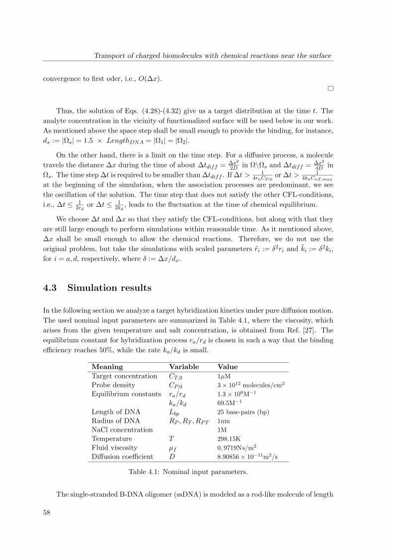
Transport of charged biomolecules with chemical reactions near the surface
convergence to first oder, i.e., O(∆x).
Thus, the solution of Eqs. (4.28)-(4.32) give us a target distribution at the time t. The
analyte concentration in the vicinity of functionalized surface will be used below in our work.
As mentioned above the space step shall be small enough to provide the binding, for instance,
dx := |Ωs| = 1.5 × LengthDNA = |Ω1| = |Ω2|.
On the other hand, there is a limit on the time step. For a diffusive process, a molecule
travels the distance ∆x during the time of about ∆tdiff = ∆x2
2D in Ω\Ωs and ∆tdiff = ∆x2
4D in
Ωs. The time step ∆t is required to be smaller than ∆tdiff . If ∆t > 14raCP,0
or ∆t > 14kaCnT,max
at the beginning of the simulation, when the association processes are predominant, we see
the oscillation of the solution. The time step that does not satisfy the other CFL-conditions,
i.e., ∆t ≤ 12rd
or ∆t ≤ 12kd
, leads to the fluctuation at the time of chemical equilibrium.
We choose ∆t and ∆x so that they satisfy the CFL-conditions, but along with that they
are still large enough to perform simulations within reasonable time. As it mentioned above,
∆x shall be small enough to allow the chemical reactions. Therefore, we do not use the
original problem, but take the simulations with scaled parameters ri := δ2ri and ki := δ2ki,
for i = a, d, respectively, where δ := ∆x/dx.
4.3 Simulation results
In the following section we analyze a target hybridization kinetics under pure diffusion motion.
The used nominal input parameters are summarized in Table 4.1, where the viscosity, which
arises from the given temperature and salt concentration, is obtained from Ref. [27]. The
equilibrium constant for hybridization process ra/rd is chosen in such a way that the binding
efficiency reaches 50%, while the rate ka/kd is small.
Meaning Variable Value
Target concentration CT,0 1µM
Probe density CP,0 3× 10¹² molecules/cm2
Equilibrium constants ra/rd 1.3× 10⁶M−1
ka/kd 69.5M−1
Length of DNA Lbp 25 base-pairs (bp)
Radius of DNA RP , RT , RPT 1nm
NaCl concentration 1M
Temperature T 298.15K
Fluid viscosity µf 0, 9719Ns/m2
Diffusion coefficient D 8.90856× 10⁻¹¹m2/s
Table 4.1: Nominal input parameters.
The single-stranded B-DNA oligomer (ssDNA) is modeled as a rod-like molecule of length
58
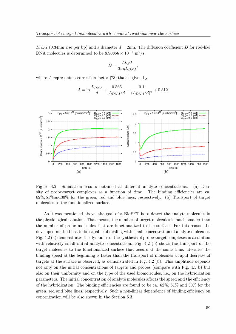
Transport of charged biomolecules with chemical reactions near the surface
LDNA (0.34nm rise per bp) and a diameter d = 2nm. The diffusion coefficient D for rod-like
DNA molecules is determined to be 8.90856× 10⁻¹¹m2/s.
D =AkBT
3πηLDNA,
where A represents a correction factor [73] that is given by
A = lnLDNAd
+0.565
LDNA/d− 0.1
(LDNA/d)2+ 0.312.
0
0.5
1
1.5
2
2.5
3
0 200 400 600 800 1000 1200 1400 1600 1800
Co
nce
ntr
atio
n ×
10
12
[nu
mb
er/
cm
2]
Time [s]
CP,0 = 3 × 10¹²
[number/cm2]; CT,0 = 2.0 [µM]
CT,0 = 1.0 [µM]CT,0 = 0.5 [µM]
(a)
0
0.5
1
1.5
2
2.5
0 200 400 600 800 1000 1200 1400 1600 1800
Co
nce
ntr
atio
n
[µM
]
Time [s]
CP,0 = 3 × 10¹²
[number/cm2]; CT,0 = 2.0 [µM]
CT,0 = 1.0 [µM]CT,0 = 0.5 [µM]
(b)
Figure 4.2: Simulation results obtained at different analyte concentrations. (a) Den-sity of probe-target complexes as a function of time. The binding efficiencies are ca.62%, 51%and30% for the green, red and blue lines, respectively. (b) Transport of targetmolecules to the functionalized surface.
As it was mentioned above, the goal of a BioFET is to detect the analyte molecules in
the physiological solution. That means, the number of target molecules is much smaller than
the number of probe molecules that are functionalized to the surface. For this reason the
developed method has to be capable of dealing with small concentration of analyte molecules.
Fig. 4.2 (a) demonstrates the dynamics of the synthesis of probe-target complexes in a solution
with relatively small initial analyte concentration. Fig. 4.2 (b) shows the transport of the
target molecules to the functionalized surface that occurs at the same time. Because the
binding speed at the beginning is faster than the transport of molecules a rapid decrease of
targets at the surface is observed, as demonstrated in Fig. 4.2 (b). This amplitude depends
not only on the initial concentrations of targets and probes (compare with Fig. 4.5 b) but
also on their uniformity and on the type of the used biomolecules, i.e., on the hybridization
parameters. The initial concentration of analyte molecules affects the speed and the efficiency
of the hybridization. The binding efficiencies are found to be ca. 62%, 51% and 30% for the
green, red and blue lines, respectively. Such a non-linear dependence of binding efficiency on
concentration will be also shown in the Section 6.3.
59
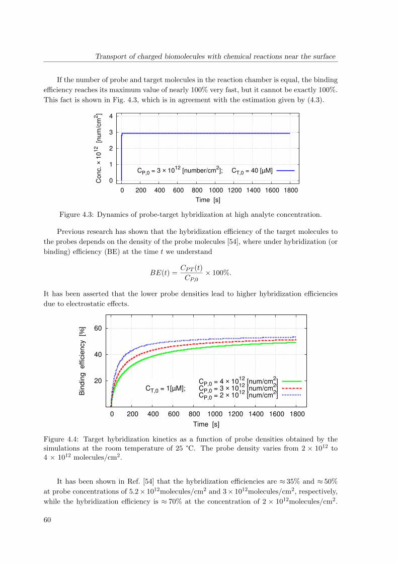
Transport of charged biomolecules with chemical reactions near the surface
If the number of probe and target molecules in the reaction chamber is equal, the binding
efficiency reaches its maximum value of nearly 100% very fast, but it cannot be exactly 100%.
This fact is shown in Fig. 4.3, which is in agreement with the estimation given by (4.3).
0
1
2
3
4
0 200 400 600 800 1000 1200 1400 1600 1800
Conc.
× 10
12 [n
um
/cm
2]
Time [s]
CP,0 = 3 × 10¹²
[number/cm2]; CT,0 = 40 [µM]
Figure 4.3: Dynamics of probe-target hybridization at high analyte concentration.
Previous research has shown that the hybridization efficiency of the target molecules to
the probes depends on the density of the probe molecules [54], where under hybridization (or
binding) efficiency (BE) at the time t we understand
BE(t) =CPT (t)
CP,0× 100%.
It has been asserted that the lower probe densities lead to higher hybridization efficiencies
due to electrostatic effects.
20
40
60
0 200 400 600 800 1000 1200 1400 1600 1800
Bin
din
g
eff
icie
ncy
[%]
Time [s]
CP,0 = 4 × 10¹²
[num/cm2]
CT,0 = 1[µM]; CP,0 = 3 × 10¹²
[num/cm2]
CP,0 = 2 × 10¹²
[num/cm2]
Figure 4.4: Target hybridization kinetics as a function of probe densities obtained by thesimulations at the room temperature of 25 °C. The probe density varies from 2 × 10¹² to4 × 1012 molecules/cm2.
It has been shown in Ref. [54] that the hybridization efficiencies are ≈ 35% and ≈ 50%
at probe concentrations of 5.2× 10¹²molecules/cm2 and 3× 10¹²molecules/cm2, respectively,
while the hybridization efficiency is ≈ 70% at the concentration of 2 × 10¹²molecules/cm2.
60

Transport of charged biomolecules with chemical reactions near the surface
Fig. 4.4 shows the correlation between the probe density and hybridization obtained by our
simulations. Despite of the absence of the electrostatic effects, a slight difference of binding
efficiencies is observed, as demonstrated in Fig. 4.4.
0
0.5
1
1.5
2
2.5
3
0 200 400 600 800 1000 1200 1400 1600 1800
Co
nce
ntr
atio
n ×
10
12
[nu
mb
er/
cm
2]
Time [s]
CT,0 = 1[µM]; CP,0 = 4 × 10¹²
[number/cm2]
CP,0 = 3 × 10¹²
[number/cm2]
CP,0 = 2 × 10¹²
[number/cm2]
(a)
0
0.2
0.4
0.6
0.8
1
1.2
0 200 400 600 800 1000 1200 1400 1600 1800
Co
nce
ntr
atio
n
[µM
]Time [s]
CT,0 = 1[µM]; CP,0 = 4 × 10¹²
[number/cm2]
CP,0 = 3 × 10¹²
[number/cm2]
CP,0 = 2 × 10¹²
[number/cm2]
(b)
Figure 4.5: Simulation results obtained at different probe densities. (a) Density of probe-target complexes as a function of time. (b) Transport of target molecules to the functionalizedsurface.
The comparison of graphics in Fig. 4.4 and Fig. 4.5 demonstrates that a higher probe
density (green lines) leads to a faster binding process at the beginning and to a decrease
of total analyte concentration in the solution. Therefore, the transport of target molecules
to the functionalized surface decreases as well (see Fig. 4.5 b). Accordingly, the weaker
transport, despite of the generation of a larger amount of molecules (Fig. 4.5 a), results in a
lower binding efficiency (Fig. 4.4).
4.4 Conclusions
In this chapter we deal with the different types of the chemical reactions occurring near
the functionalized surface. We also focus on the influence of the diffusion transport of target
molecules on the efficiency of the hybridization process. The diffusions equation with the time-
varying boundary conditions comprising the chemical reactions at the surface is transformed
to well-studied reaction-diffusion problem with Neumann and Dirichlet boundary conditions.
Moreover, the number of unknowns is reduced to one.
The developed model and algorithm are applicable for the small initial concentration of
the analyte molecules and for the specific as well the non-specific chemical reactions. The
model is also suitable for modeling of the immobilization of probe molecules to the surface. In
this case ra = rd = 0 and ka and kd are appropriate immobilization parameters. The resulting
equations was implemented by using the discretized conservative scheme. That allowed to
conserve exactly the total number of biomolecules, which are present in the system.
61

Transport of charged biomolecules with chemical reactions near the surface
The model can be easily expanded to include the hybridization of mismatched and par-
tially matched DNA [55]. In this case we shall consider two additional ODE, like (4.7), with
corresponding hybridization parameters, and modify the equation (4.6) in an analogous way.
In the simulation step we study the effect of the diffusive mass transport on the rate of the
reactions and can conclude that, even with the weak transport, a difference in the calculated
binding efficiencies is observed. We also found that the non-specific chemical reaction play
the major role in a detection mechanism because it affects the speed of the hybridization
process by reducing the number of free target molecules.
62
Chapter 5
Self-consistent model
We consider the same problem as in Section 2.2 with the same definitions. In order to couple
the microscopic and the macroscopic simulations together, the original Poisson equation (2.1)
is replaced by a homogenized problem, which has been proposed in refs. [30,32,60]. The left-
hand side of the homogenized Poisson equation depends on the distribution of the electrons
and the holes, and no longer depends on the charge distributions of the analyte ions and the
biomolecules
−∇ · (ε(x)∇ΨI(x)) = % (5.1)
% =
q(p(x)− n(x) + %d − %a), in ΩSi,
0 in ΩOx,
0 in ΩLiq,
where ε is the permitivity, n and p are the concentrations of the electrons and holes, %d and
%a denote the concentrations of electrically active donor and acceptor atoms, respectively.
We define the border between ΩLiq and ΩOx as Γ with ”+”-side from ΩLiq-direction
and ”−”-side from ΩOx-direction, i.e., Γ+ and Γ−, respectively. We also denote the internal
potential calculated at the interface from the side of the liquid (i.e., at Γ+) as ΨI(x+, y, z)
and at the interface Γ− as ΨI(x−, y, z). The link between the insulator and the aqueous
solution is realized by the following interface conditions
ΨI(x+, y, z)−ΨI(x−, y, z) = − DεOx
, (5.2)
εLiq ΨI(x+, y, z)− εOx ΨI(x−, y, z) = −C, (5.3)
where C is the macroscopic surface charge density, which causes the jump in the electric field,
and D is the macroscopic dipole moment density, which causes the jump in the potential. Cand D are unknown parameters, which shall be obtained from the microscopic simulations.
Note that the notation % is defined for oxide-surface charge density.
63
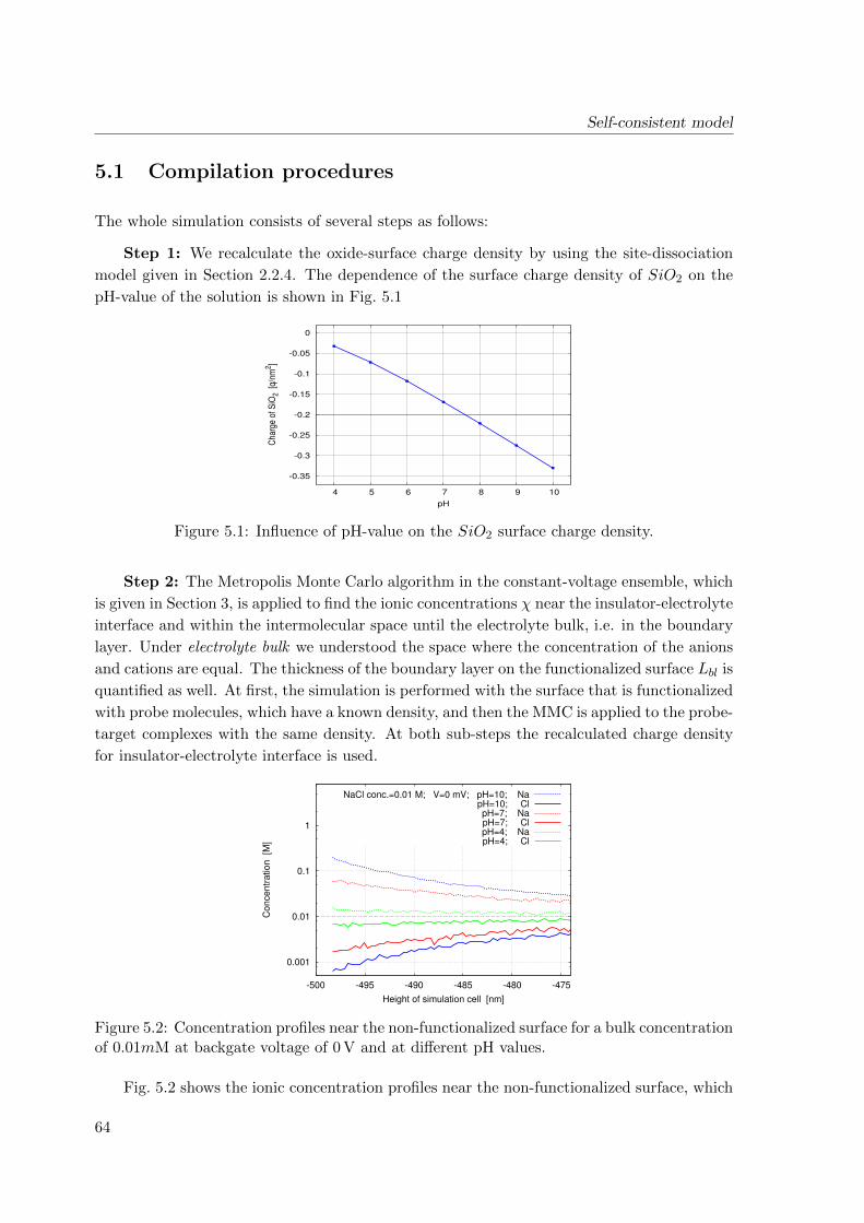
Self-consistent model
5.1 Compilation procedures
The whole simulation consists of several steps as follows:
Step 1: We recalculate the oxide-surface charge density by using the site-dissociation
model given in Section 2.2.4. The dependence of the surface charge density of SiO2 on the
pH-value of the solution is shown in Fig. 5.1
-0.35
-0.3
-0.25
-0.2
-0.15
-0.1
-0.05
0
4 5 6 7 8 9 10
Cha
rge
of S
iO2
[q/n
m2 ]
pH
Figure 5.1: Influence of pH-value on the SiO2 surface charge density.
Step 2: The Metropolis Monte Carlo algorithm in the constant-voltage ensemble, which
is given in Section 3, is applied to find the ionic concentrations χ near the insulator-electrolyte
interface and within the intermolecular space until the electrolyte bulk, i.e. in the boundary
layer. Under electrolyte bulk we understood the space where the concentration of the anions
and cations are equal. The thickness of the boundary layer on the functionalized surface Lbl is
quantified as well. At first, the simulation is performed with the surface that is functionalized
with probe molecules, which have a known density, and then the MMC is applied to the probe-
target complexes with the same density. At both sub-steps the recalculated charge density
for insulator-electrolyte interface is used.
0.001
0.01
0.1
1
-500 -495 -490 -485 -480 -475
Co
nce
ntr
atio
n
[M]
Height of simulation cell [nm]
NaCl conc.=0.01 M; V=0 mV; pH=10; NapH=10; ClpH=7; NapH=7; ClpH=4; NapH=4; Cl
Figure 5.2: Concentration profiles near the non-functionalized surface for a bulk concentrationof 0.01mM at backgate voltage of 0 V and at different pH values.
Fig. 5.2 shows the ionic concentration profiles near the non-functionalized surface, which
64
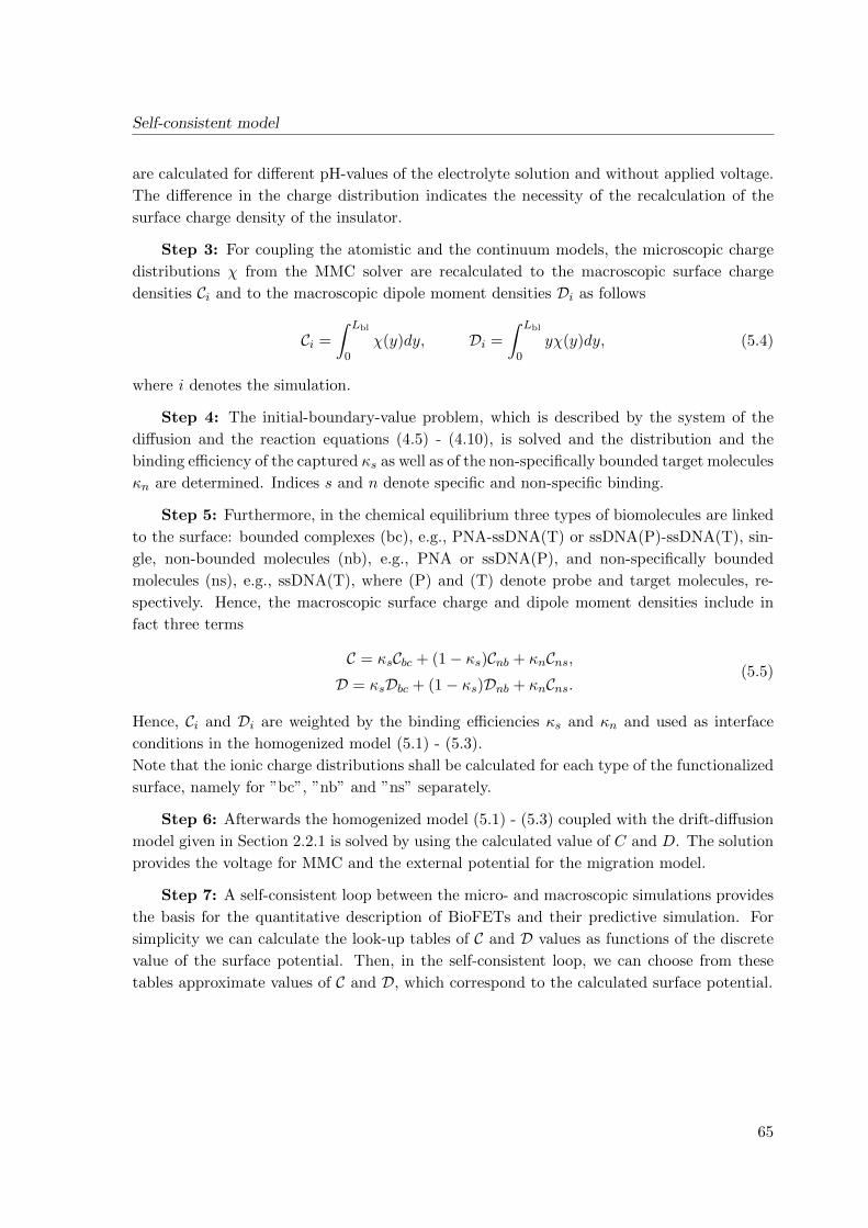
Self-consistent model
are calculated for different pH-values of the electrolyte solution and without applied voltage.
The difference in the charge distribution indicates the necessity of the recalculation of the
surface charge density of the insulator.
Step 3: For coupling the atomistic and the continuum models, the microscopic charge
distributions χ from the MMC solver are recalculated to the macroscopic surface charge
densities Ci and to the macroscopic dipole moment densities Di as follows
Ci =
∫ Lbl
0χ(y)dy, Di =
∫ Lbl
0yχ(y)dy, (5.4)
where i denotes the simulation.
Step 4: The initial-boundary-value problem, which is described by the system of the
diffusion and the reaction equations (4.5) - (4.10), is solved and the distribution and the
binding efficiency of the captured κs as well as of the non-specifically bounded target molecules
κn are determined. Indices s and n denote specific and non-specific binding.
Step 5: Furthermore, in the chemical equilibrium three types of biomolecules are linked
to the surface: bounded complexes (bc), e.g., PNA-ssDNA(T) or ssDNA(P)-ssDNA(T), sin-
gle, non-bounded molecules (nb), e.g., PNA or ssDNA(P), and non-specifically bounded
molecules (ns), e.g., ssDNA(T), where (P) and (T) denote probe and target molecules, re-
spectively. Hence, the macroscopic surface charge and dipole moment densities include in
fact three terms
C = κsCbc + (1− κs)Cnb + κnCns,D = κsDbc + (1− κs)Dnb + κnCns.
(5.5)
Hence, Ci and Di are weighted by the binding efficiencies κs and κn and used as interface
conditions in the homogenized model (5.1) - (5.3).
Note that the ionic charge distributions shall be calculated for each type of the functionalized
surface, namely for ”bc”, ”nb” and ”ns” separately.
Step 6: Afterwards the homogenized model (5.1) - (5.3) coupled with the drift-diffusion
model given in Section 2.2.1 is solved by using the calculated value of C and D. The solution
provides the voltage for MMC and the external potential for the migration model.
Step 7: A self-consistent loop between the micro- and macroscopic simulations provides
the basis for the quantitative description of BioFETs and their predictive simulation. For
simplicity we can calculate the look-up tables of C and D values as functions of the discrete
value of the surface potential. Then, in the self-consistent loop, we can choose from these
tables approximate values of C and D, which correspond to the calculated surface potential.
65
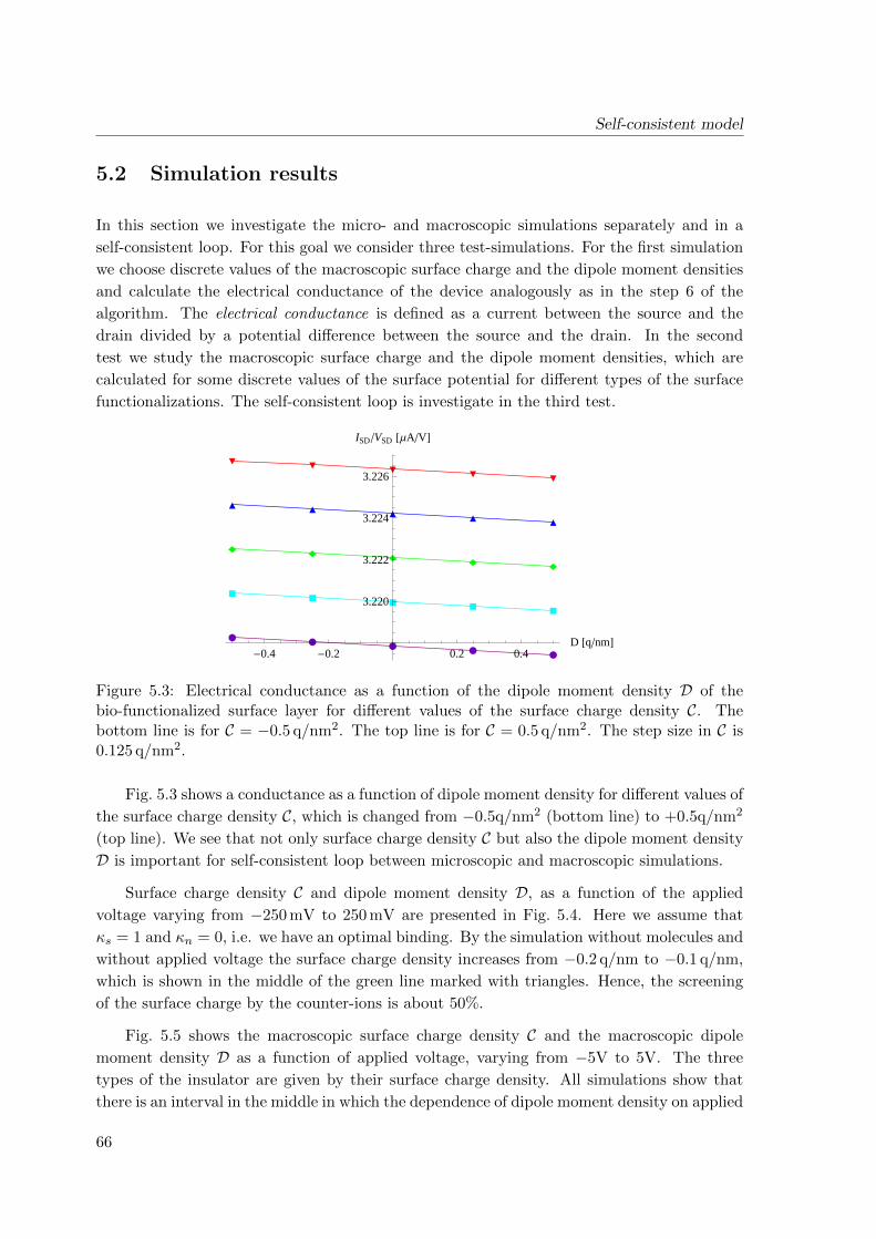
Self-consistent model
5.2 Simulation results
In this section we investigate the micro- and macroscopic simulations separately and in a
self-consistent loop. For this goal we consider three test-simulations. For the first simulation
we choose discrete values of the macroscopic surface charge and the dipole moment densities
and calculate the electrical conductance of the device analogously as in the step 6 of the
algorithm. The electrical conductance is defined as a current between the source and the
drain divided by a potential difference between the source and the drain. In the second
test we study the macroscopic surface charge and the dipole moment densities, which are
calculated for some discrete values of the surface potential for different types of the surface
functionalizations. The self-consistent loop is investigate in the third test.
ææ
ææ
æ
àà
àà
à
ìì
ìì
ì
òò
òò
ò
ôô
ôô
ô
-0.4 -0.2 0.2 0.4D @qnmD
3.220
3.222
3.224
3.226
ISDVSD @ΜAVD
Figure 5.3: Electrical conductance as a function of the dipole moment density D of thebio-functionalized surface layer for different values of the surface charge density C. Thebottom line is for C = −0.5 q/nm2. The top line is for C = 0.5 q/nm2. The step size in C is0.125 q/nm2.
Fig. 5.3 shows a conductance as a function of dipole moment density for different values of
the surface charge density C, which is changed from −0.5q/nm2 (bottom line) to +0.5q/nm2
(top line). We see that not only surface charge density C but also the dipole moment density
D is important for self-consistent loop between microscopic and macroscopic simulations.
Surface charge density C and dipole moment density D, as a function of the applied
voltage varying from −250 mV to 250 mV are presented in Fig. 5.4. Here we assume that
κs = 1 and κn = 0, i.e. we have an optimal binding. By the simulation without molecules and
without applied voltage the surface charge density increases from −0.2 q/nm to −0.1 q/nm,
which is shown in the middle of the green line marked with triangles. Hence, the screening
of the surface charge by the counter-ions is about 50%.
Fig. 5.5 shows the macroscopic surface charge density C and the macroscopic dipole
moment density D as a function of applied voltage, varying from −5V to 5V. The three
types of the insulator are given by their surface charge density. All simulations show that
there is an interval in the middle in which the dependence of dipole moment density on applied
66
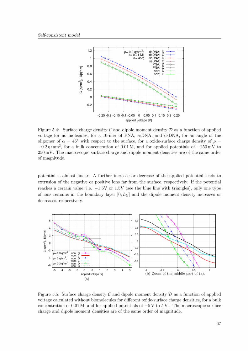
Self-consistent model
-0.2
0
0.2
0.4
0.6
0.8
1
1.2
-0.25 -0.2 -0.15 -0.1 -0.05 0 0.05 0.1 0.15 0.2 0.25
C [
q/n
m2],
D
[q/n
m]
applied voltage [V]
ρ=-0.2 q/nm2; dsDNA; D
c= 0.01 M; dsDNA; Cα= 45°; ssDNA; D
ssDNA; C PNA; D PNA; C non; D non; C
Figure 5.4: Surface charge density C and dipole moment density D as a function of appliedvoltage for no molecules, for a 10-mer of PNA, ssDNA, and dsDNA, for an angle of theoligomer of α = 45 with respect to the surface, for a oxide-surface charge density of ρ =−0.2 q/nm2, for a bulk concentration of 0.01 M, and for applied potentials of −250 mV to250 mV. The macroscopic surface charge and dipole moment densities are of the same orderof magnitude.
potential is almost linear. A further increase or decrease of the applied potential leads to
extrusion of the negative or positive ions far from the surface, respectively. If the potential
reaches a certain value, i.e. −1.5V or 1.5V (see the blue line with triangles), only one type
of ions remains in the boundary layer [0;Lbl] and the dipole moment density increases or
decreases, respectively.
-6
-4
-2
0
2
4
6
-5 -4 -3 -2 -1 0 1 2 3 4 5
C [
q/n
m2],
D
[q/n
m]
Applied voltage [V]
ρ=-0.3 q/nm2; non; D
non; Cρ= 0 q/nm
2; non; D
non; Cρ= 0.3 q/nm
2; non; D
non; C
(a)
-0.9
-0.6
-0.3
0
0.3
0.6
0.9
-1 -0.5 0 0.5 1
(b) Zoom of the middle part of (a).
Figure 5.5: Surface charge density C and dipole moment density D as a function of appliedvoltage calculated without biomolecules for different oxide-surface charge densities, for a bulkconcentration of 0.01 M, and for applied potentials of −5 V to 5 V . The macroscopic surfacecharge and dipole moment densities are of the same order of magnitude.
67

Self-consistent model
In Fig. 5.6 the simulations of the surface charge density and the dipole moment density
with different molecules and an uncharged insulator are compared. The appreciable difference
especially in value of the dipole moment density is shown for the small and positive applied
voltage.
-4
-2
0
2
4
6
-4 -3 -2 -1 0 1 2 3 4
C [
q/n
m2],
D
[q/n
m]
Applied voltage [V]
ρ= 0 q/nm2; non; D
non; Cρ= 0 q/nm
2; ssDNA; D
ssDNA; Cρ= 0 q/nm
2; dsDNA; D dsDNA; C
(a)
-0.2
-0.1
0
0.1
0.2
0.3
-0.2 -0.1 0 0.1 0.2
(b) Zoom of the middle part of (a)
Figure 5.6: Surface charge density C and dipole moment density D as a function of appliedvoltage for no molecules, for a 10-mer of ssDNA and dsDNA, for an angle of the oligomer ofα = 45 with respect to the surface, for an uncharged oxide-surface, for a bulk concentrationof 0.01 M, and for applied potentials of −4 V to 4 V. The macroscopic surface charge anddipole moment densities are of the same order of magnitude.
In the last test-simulation we consider a small rectangular semiconductor with measure-
ments 10nm×13nm×100nm that is shown in Fig. 5.7(a). The source, the drain, the electrode
and the bulk contacts have applied potentials of −1V, 0V, 0V and −3.8V, respectively. The
input parameters for MMC solve are given in the Table 5.1. Here the optimal binding is as-
Table 5.1: The input parameters for MMC solver.Input parameters Value
type of the biomolecules ssDNAlength of the biomolecules 10bpangle between biomolecule and surface 90length of linkers 1nmtype of the electrolyte ions Na+Cl−
concentration of the used ions 0.001Mnumber of molecules at the surface 3× 3distance between them 8nmcharge of the insulator −0.2q/nm2
sumed. Fig. 5.7 show the electrical potential as a function of space which is calculated in the
self-consistent loop with the microscopic model. The figures (b), (c) and (d) display potentials
at the cross sections of the device, which are made in the middle of the semiconductor.
68
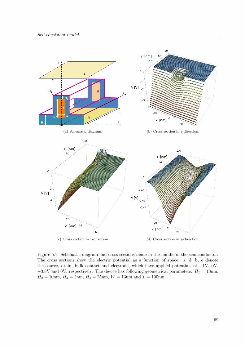
Self-consistent model
(a) Schematic diagram. (b) Cross section in z-direction.
(c) Cross section in x-direction. (d) Cross section in y-direction.
Figure 5.7: Schematic diagram and cross sections made in the middle of the semiconductor.The cross sections show the electric potential as a function of space. s, d, b, e denotethe source, drain, bulk contact and electrode, which have applied potentials of −1V, 0V,−3.8V and 0V, respectively. The device has following geometrical parameters: H1 = 18nm,H2 = 10nm, H3 = 2nm, H4 = 25nm, W = 13nm and L = 100nm.
69
Self-consistent model
5.3 Conclusions
We present a self-consistent 3D model for DNA-modified FET. This model consists of four
general parts which are connected with each other via the compilation scheme. The advantage
of this technique is that the transport of the target molecules, the surface reactions, and the
liquid behavior are modeled independently from the physical part of the model of our sensor
and, therefore, can be correctly approximated by using a necessary and a judicious tradeoff
between realism and simplicity.
We find the influence of the charge and especially of the dipole moment densities of the
boundary layer to the electrical conductance. And we can conclude that the thickness of
the boundary layer is significant for the response signal. We also study the influence of the
applied potential (between the functionalized surface and the electrode) to the surface charge
and dipole moment and find that only small and opposite to the net surface charge voltage
has a noticeable influence. Therefore, the change in dipole moment after binding of analyte
molecules effects the detection mechanism.
70
Chapter 6
Stochastic processes at the
functionalized surface
We consider an isolated sensor that is immersed in an analyte solution. The reactive solid
surface ∂Ωs of area A of the sensor is functionalized with CP,0 receptors (probe molecules) per
unit area, and the solution contains target molecules with initial concentration CT,0 mole per
liter. We will use below the notations P and T for probe and target molecules, respectively.
We denote the molecule after binding event as PT (probe-target complex) and its initial
concentration as CPT,0.
Hence we work with following concentration functions:
CT = CT (t,x), CP = CP (t) and CPT = CPT (t), where
0 ≤ CT (t,x) ≤ CT,0, 0 ≤ CP (t) ≤ CP,0 and 0 ≤ CPT (t) ≤ min[CT,0, CP,0].
We also assume initial the concentrations CT,0 and CP,0 to be uniform and CPT,0 = 0.
6.1 Interaction processes
The association and dissociation processes which occur at the surface xs can be schematically
depicted as follows
(T )txs + (P )txsra (PT )t+τxs (6.1)
(PT )txsrd (P )t+τxs + (T )t+τxs (6.2)
The equation (6.1) denotes a binding process of target molecules T , which are located in
position xs at the time t, with probe molecules P , where captured molecules PT are build
during a small interval τ := ∆t. Analogously the equation (6.2) describes dissociation pro-
cesses, in which the probes and targets are generated.
The rates λa and λd of the association and dissociation processes are characterized by the
71
Stochastic processes at the functionalized surface
constants ra and rd, respectively.
Number of binding events per unit time and unit area:
λa :=CPT (t+ τ)− CPT (t)
τ= raCT (t, xs)CP (t) (6.3)
Number of dissociation events per unit time and unit area:
λd :=CP (t+ τ)− CP (t)
τ= rdCPT (t) (6.4)
6.2 Chemical Langevin equation at the surface
To quantify the biological noise of the system we treat the reaction at the surface as a stochas-
tic process, i.e., the bond of probe and target molecules occur in an essentially random man-
ner. Langevin equations for chemical reactions inside some fixed volume have been discussed
recently in [24,33]. Here we obtain the Langevin equation for a association/dissociation pro-
cesses at the surface.
We consider a system of nP particles (probe molecules) at the time t = jτ (τ := ∆t) with
following indicator function
ωji =
1 i-th probe is bounded at the time t = jτ,
0 otherwise,
where ωji are independent random variables, and i = 1, 2, ..., nP . In these notations the
number of probe-target complexes PT and the number of single probes P at the time t can
be written as∑
i ωji and nP −
∑i ω
ji respectively. We denote a new random variable X(t) :=∑
i ωji
A which describes the dynamic state of the system, where t = jτ and X(t) ∈ [0, ..., CP,0].
Lemma 6.2.1. (The chemical Langevin equation at the surface)
Let Xt := X(t) be a stochastic variable describing the probe-target binding at the time t. The
binding process id specified by the first order chemical reactions occurring at the functionalized
surface xs, which are given by equations (6.1) and (6.2). Let d[B1(t)]dt and d[B2(t)]
dt be statisti-
cally independent Gaussian white noises according to association and dissociation processes,
respectively. Then the evolution of X(t) from the given initial state X(0) = x0 is described
by the following equation
dXt
dt= ra
(CP,0 −Xt
)CT (t, xs)− rdXt
+
√ra
(CP,0 −Xt
)CT (t, xs)
d[B1(t)]
dt−√rdXt
d[B2(t)]
dt(6.5)
Proof. Let Ka(Xt, t) and Kd(Xt, t) be numbers of association and dissociation events, respec-
tively, which occur in the subsequent time interval [t, t + τ ]. The change in PT complexes
72
Stochastic processes at the functionalized surface
during the small time interval τ can be written as follows
Xt+τ −Xt = Ka(Xt, t)−Kd(Xt, t), (6.6)
Ka(Xt, t) =(CP,0 −X(t)
)pa,
Kd(Xt, t) = X(t)pd,
where pa is a probability that one single probe molecule will react in the next time interval τ
(association event has occurred) and pd is a probability of dissociation process of one complex
PT , which can be derived from the equations (6.3) and (6.4).
pa =CPT (t+ τ)− CPT (t)
CP (t)
(6.3)= τraCT (t, xs),
pd =CP (t+ τ)− CP (t)
CPT (t)
(6.4)= τrd
Thus, the rates λa and λd can be defined as functions of Xt
λa(Xt) :=Ka(Xt, t)
τ= raCT (t, xs)
(CP,0 −Xt
)(6.7)
λd(Xt) :=Kd(Xt, t)
τ= rdXt
Remark. Let pa be a probability that the free target is bounded during the time interval τ (association
event has occurred).
pa :=CPT (t+ τ)− CPT (t)
CT (t, xs)
(6.3)= raτCP (t) = raτ
(CP,0 −X(t)
).
In this case the expectation of the first term on the right-hand side of the eq. (6.6) can be written as
Ka(Xt, t) = CT (t, xs)raτ(CP,0 −X(t)
),
where CT (t, xs) is the number of free targets at the surface. Putting all together we obtain the same
rate λa as in (6.7).
If τ is large enough, i.e., τλa 1 and τλd 1 (it means that more then one events
occurs during this time interval), the random variables Kj(Xt, t), j = a, d are statistically
independent Poisson random variables Pj(λj(Xt), τ) with mean value and variance equal to
τλj(Xt). Pj(λj(Xt), τ) can be approximated by a normal random variable with the same
mean and variance, i.e., Nj(τλj(Xt), τλj(Xt)).
We rewrite the equation (6.6) by using τ = ∆t→ dt, Xt := X(t) and the linear combination
theorem for normal random variables N (m,σ2) = m+ σN (0, 1).
X(t+ dt) = X(t) + λa(Xt)dt− λd(Xt)dt (6.8)
+√λa(Xt)
√dtNa(0, 1)−
√λd(Xt)
√dtNd(0, 1)
73
Stochastic processes at the functionalized surface
X(t+ dt) = Xt +(ra(CP,0 −Xt)CT (t, xs)− rdXt
)dt
+√ra(CP,0 −Xt)CT (t, xs)
√dtNa(0, 1)−
√rdXt
√dtNd(0, 1) (6.9)
dXt
dt= ra
(CP,0 −Xt
)CT (t, xs)− rdXt
+
√ra
(CP,0 −Xt
)CT (t, xs)
d[B1(t)]
dt−√rdXt
d[B2(t)]
dt(6.10)
Equations (6.9) and (6.10) are called standard-form and white-noise form Langevin equa-
tions, respectively, where d[B1(t)]dt = Na(0,1)√
dtand d[B2(t)]
dt = Nd(0,1)√dt
are statistically independent
Gaussian white noises.
Remark. Eq. (6.5) in integral form with initial condition is
X(t) = X(0)−∫ t
0
(X(s)
(raCP,0 + rd
)+raCP,0CT (s, xs)
)ds (6.11)
+
∫ t
0
√ra
(CP,0 −X(s)
)CT (t, xs)dB1(s)−
∫ t
0
√rdX(s)dB2(s),
X(t)∣∣∣t=0
= 0
6.3 Signal-to-Noise Ratio
As in all sensors, the most important characteristics of biosensor systems is their signal-to-
noise ratio (snr). In this paper we regard the biological noise. To find this ratio, we should
identify the signal as well as noise sources.
Definition 6.3.1. If we consider hybridization events occurring at the time t as signals X(t),
the noise can defined as a standard deviation of the probe-target complexes and the snr will
be the expectation of captured molecules over the corresponding standard deviation
snr(t) =E[X(t)]√Var
[X(t)
] .Remark. In physics the signal-to-noise ratio is usually expressed in decibels (dB) given by
the formula: 10× log10(snr).
Lemma 6.3.1. The signal-to-noise ratio can be computed explicitly
snr(t) =1− e−δt√
b3e−3δt − b2e−2δt + b1e−δt + b0,
74
Stochastic processes at the functionalized surface
and is bounded in time
0 < snr(t) ≤√rardCP,0CT (t, xs) <
√rardCP,0y, , ∀t > 0,
where b0, b1, b2, b3 and δ are functions of CT (t, xs) and y is a constant.
Proof. For simplicity we use the following notations y(t) := CT (t, xs) and c := CP,0.
• The expectation
We consider the equation (6.5) and calculate the mean value of its left and right part:
dE[X(t)]
dt= −E[X(t)]
(rd + ray(t)
)+rac y(t)
The solution is a function of y(t)
E[X(t)] =ray(t) c
rd + ray(t)
(1− e−(ray(t)+rd)t
). (6.12)
• The variance: The SDE under following notations u(X) = ray(t)(c − X(t)
)and
v(X) = rdX(t) is
dXt
dx= u(Xt)− v(Xt) +
√u(Xt)
d[B1(t)]
dt−√v(Xt)
d[B2(t)]
dt
Applying Ito’s formula [2] to H(Xt) := X2(t) , where ∂H(Xt)∂x = 2X(t), ∂2H(Xt)
∂x2 = 2,∂H(Xt)∂t = 0, and because H(Xt) does not depend explicitly on t, we have
dH(Xt) =∂H(Xt)
∂t+∂H(Xt)
∂xdX +
1
2
∂2H(Xt)
∂x2
(u(Xt) + v(Xt)
)dt
d(Xt)2 = 2X
(u(Xt)dt− v(Xt)dt+
√u(Xt)d[B1(t)]−
√v(Xt)d[B2(t)]
)+
(u(Xt) + v(Xt)
)dt
dX2(t) =
(u(X) + v(X) + 2
(u(x)− v(X)
)X(t)
)dt
+ 2√u(X)X(t)d[B1(t)]− 2
√v(X)X(t)d[B2(t)]
=
(ray(t)
(c−X(t)
)+2ray(t)
(c−X(t)
)X(t) + rdX(t)− 2rdX
2(t)
)dt
+
√4ray(t)
(c−X(t)
)X2(t) d[B1(t)]−
√4rdX3(t) d[B2(t)]
75
Stochastic processes at the functionalized surface
dX2(t)
dt=X2(t)
(−2ray(t)− 2rd
)+X(t)
(ray(t)(2c− 1) + rd
)+ray(t)c
+
√4ra
(c−X(t)
)X2(t)y(t)
d[B1(t)]
dt−√
4rdX3(t)d[B2(t)]
dt
By taking the expectation, we have
E[dX2(t)
dt
]=dE[X2(t)
]dt
=− E[X2(t)
](2ray(t) + 2rd
)+ E
[X(t)
](ray(t)(2c− 1) + rd
)+ray(t)c
where E[X(t)
]is given by (6.12).
The solution of the equation above is a function of y(t)
E[X2(t)
]=E[X(t)
](ray(t)(2c− 1) + rd
)+ray(t)c
2(ray(t) + rd)
(1− e−2(ray(t)+rd)t
).
Therefore Var[X(t)
]= E
[X2(t)
]−(E[X(t)
])2.
• The signal-to-noise ratio
Let us introduce the following notations:
r := ra/rd, δ := ray(t) + rd,
α := ry(t) + 1, β := ry(t)c, γ := ry(t)− 1,
a1 :=βγ
2α2, a2 :=
β
2α, a3 :=
β2
α2.
Then the mean value and the variance of process Xt will be
E[X(t)
]=√a3(1− e−δt),
Var[X(t)
]= (a3 − a1)e−3δt − (a1 + a2)e−2δt − (a2 − 3a3)e−δt + (a2 − a1).
Thus,
snr(t) =1− e−δt√
b3e−3δt − b2e−2δt + b1e−δt + b0,
where b0 := 1β , b1 := γ
2β − 3, b2 := α+γ2β and b3 := 1− γ
2β .
• In the equilibrium state
The number of target molecules at the surface in chemical equilibrium can be either calculated
by using, for instance, diffusion equation or can be kept constant y(∞) = CT (∞, xs) < ε
76
Stochastic processes at the functionalized surface
CT,0, where ε is a small constant. Because the system doesn’t have any external influence
(interaction), we expect that in the chemical equilibrium the balance between association and
dissociation processes exists, i.e.
limt→∞
dE[X(t)]
dt= −E[X(∞)]
(rd + ray∞
)+ray∞CP,0 = 0,
where X∞ := X(∞) is the notation of bounded probes X(t) if the system is in equilibrium.
0 ≤ E∞ := E[X∞
]=
ray∞c
rd + ray∞<∞. (6.13)
limt→∞
E[X2(t)
]= E
[X2(∞)
]=E∞
(ray∞(2c− 1) + rd
)+ray∞c
2(ray∞ + rd).
As a result
Var[X(∞)
]=
rard c y∞(ray∞ + rd)2
and snr(∞) =
√rardy∞c.
The model equations for evaluation of CT (t, xs) (and accordingly of y∞) and their solution
are considered in the section Section 4.1. Thus, y∞ = y = const < ∞ (see Theorem 4.1.4)
and the snr is bounded in time
0 < snr(t) <
√rardyCP,0, ∀t > 0.
Therefore, the lower estimation of standard deviation is given by
0 <
√ra rd c y∞
ray∞ + rd=: εσ ≤ σ
[X(∞)
]=√Var
[X(∞)
](6.14)
From (6.12) and (6.13) we can also calculate the expectation of binding efficiency (BE),
which is the fraction of all receptors that are bound to analyte molecules:
E[BE(t)] =ra y(t)
rd + ra y(t)
(1− e−(ray(t)+rd)t
)×100% (6.15)
E[BE(∞)
]=
ra y∞rd + ra y∞
× 100%.
77
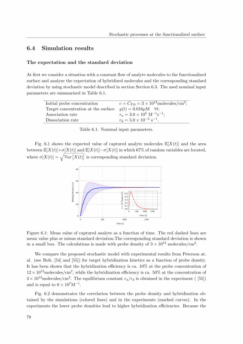
Stochastic processes at the functionalized surface
6.4 Simulation results
The expectation and the standard deviation
At first we consider a situation with a constant flow of analyte molecules to the functionalized
surface and analyze the expectation of hybridized molecules and the corresponding standard
deviation by using stochastic model described in section Section 6.3. The used nominal input
parameters are summarized in Table 6.1.
Initial probe concentration c = CP,0 = 3× 10¹²molecules/cm2;Target concentration at the surface y(t) = 0.016µM ∀t;Association rate ra = 3.0× 10⁵ M−1s−1;Dissociation rate rd = 5.0× 10⁻³ s−1.
Table 6.1: Nominal input parameters.
Fig. 6.1 shows the expected value of captured analyte molecules E[X(t)] and the area
between E[X(t)]+σ[X(t)] and E[X(t)]−σ[X(t)] in which 67% of random variables are located,
where σ[X(t)] =√Var
[X(t)
]is corresponding standard deviation.
×××××××××××××××××××××××××××××××××××××××××××××××××××××××××××××××××××××××××××××××××××××××××××
0 500 1000 15000.0
0.1
0.2
0.3
0.4
0.5
Time @sD
Σ´
1012
@num
cm2
D
0 500 1000 1500
0
20
40
60
80
Time @sD
Bin
ding
effi
cien
cy@%
D
Figure 6.1: Mean value of captured analyte as a function of time. The red dashed lines aremean value plus or minus standard deviation.The corresponding standard deviation is shownin a small box. The calculations is made with probe density of 3× 10¹² molecules/cm2.
We compare the proposed stochastic model with experimental results from Peterson at.
al. (see Refs. [54] and [55]) for target hybridization kinetics as a function of probe density.
It has been shown that the hybridization efficiency is ca. 10% at the probe concentration of
12× 1012molecules/cm2, while the hybridization efficiency is ca. 50% at the concentration of
3× 10¹²molecules/cm2. The equilibrium constant ra/rd is obtained in the experiment ( [55])
and is equal to 6× 10⁷M−1.
Fig. 6.2 demonstrates the correlation between the probe density and hybridization ob-
tained by the simulations (colored lines) and in the experiments (marked curves). In the
experiments the lower probe densities lead to higher hybridization efficiencies. Because the
78
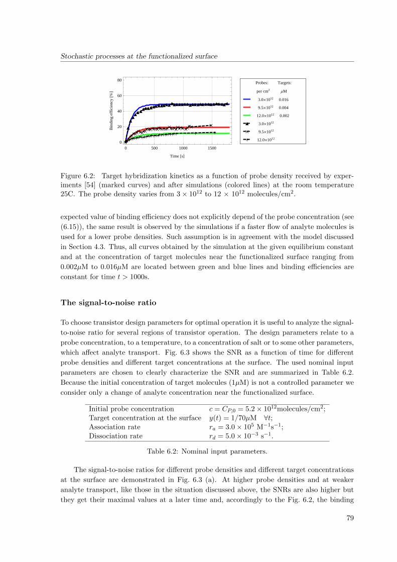
Stochastic processes at the functionalized surface
ò
ò
ò
òò
òòòòòòòòòòòòò
òòòòòòòòòòòòòòòòòòòòòò
´´
´´´´´´´´´´´´´´´´´
´ ´
++++++++++++++++++++++++++++++ + +
0 500 1000 15000
20
40
60
80
Time @sD
Bin
ding
effi
cien
cy@%
D
+ 12.0´1012
´ 9.5´1012
ò 3.0´1012
12.0´1012 0.002
9.5´1012 0.004
3.0´1012 0.016
per cm2 ΜM
Probes: Targets:
Figure 6.2: Target hybridization kinetics as a function of probe density received by exper-iments [54] (marked curves) and after simulations (colored lines) at the room temperature25C. The probe density varies from 3× 10¹² to 12 × 1012 molecules/cm2.
expected value of binding efficiency does not explicitly depend of the probe concentration (see
(6.15)), the same result is observed by the simulations if a faster flow of analyte molecules is
used for a lower probe densities. Such assumption is in agreement with the model discussed
in Section 4.3. Thus, all curves obtained by the simulation at the given equilibrium constant
and at the concentration of target molecules near the functionalized surface ranging from
0.002µM to 0.016µM are located between green and blue lines and binding efficiencies are
constant for time t > 1000s.
The signal-to-noise ratio
To choose transistor design parameters for optimal operation it is useful to analyze the signal-
to-noise ratio for several regions of transistor operation. The design parameters relate to a
probe concentration, to a temperature, to a concentration of salt or to some other parameters,
which affect analyte transport. Fig. 6.3 shows the SNR as a function of time for different
probe densities and different target concentrations at the surface. The used nominal input
parameters are chosen to clearly characterize the SNR and are summarized in Table 6.2.
Because the initial concentration of target molecules (1µM) is not a controlled parameter we
consider only a change of analyte concentration near the functionalized surface.
Initial probe concentration c = CP,0 = 5.2× 10¹²molecules/cm2;Target concentration at the surface y(t) = 1/70µM ∀t;Association rate ra = 3.0× 10⁵ M−1s−1;Dissociation rate rd = 5.0× 10⁻³ s−1.
Table 6.2: Nominal input parameters.
The signal-to-noise ratios for different probe densities and different target concentrations
at the surface are demonstrated in Fig. 6.3 (a). At higher probe densities and at weaker
analyte transport, like those in the situation discussed above, the SNRs are also higher but
they get their maximal values at a later time and, accordingly to the Fig. 6.2, the binding
79

Stochastic processes at the functionalized surface
0 1000 2000 3000 4000 5000 60000.0
0.5
1.0
1.5
2.0
2.5
Time @sD
SNR
´10
6
2.0´1012 140
3.0´1012 150
5.2´1012 170
9.5´1012 190
12.0´1012 1100
per cm2 ΜM
Probes: Targets:A
B
0 1000 2000 3000 4000 5000 60000.0
0.5
1.0
1.5
2.0
2.5
Time @sD
SNR
´10
6
C
0 1000 2000 3000 4000 5000 60000.0
0.5
1.0
1.5
2.0
2.5
3.0
Time @sD
SNR
´10
6
Figure 6.3: Signal-to-noise ratios (A) for different probe densities and different target con-centrations at the surface, (B) for different target concentrations at the surface and thesame probe density of 5.2× 10¹²molecules/cm2, and (C) for different probe densities and thesame target concentration of 1/70µM at the surface. In all simulations the association anddissociation rates are ra = 3.0× 10⁵ M−1s−1 and rd = 5.0× 10⁻³ s−1.
efficiencies of captured analyte are smaller. Contrariwise, in the case of the lowest probe
density and the highest analyte transport the value of the SNR is the smallest, but the
advantage of the later case consist in the highest binding efficiency. In Fig. 6.3 (b) the
SNR is compared for probe density of 5.2 × 10¹²molecules/cm2 and different flows of target
molecules to the surface, which vary from 1100µM to 1
40µM. The raise of the flow generates
an increase in SNR and reduces the time, during which the SNR reaches its maximal value.
In Fig. 6.3 (c), we investigate the situation, where the different probe densities and the fixed
target concentration of 170µM at the surface determine the signal-to-noise ratio. The increase
of the initial amount of the probe molecules induces the rise in the SNR at the same time.
Fig. 6.4 shows the standard deviation in linear (a) an logarithmic (b) scales, which are
calculated with nominal parameters. By analyzing Fig. 6.4 and Fig. 6.3 we can identify
five time intervals. in which the standard deviation increases I1 = [0, 100] or decreases
I2 = [100, 1000] rapidly, an interval with weak depletion I3 = [1000, 2000], an interval I4 =
[2000, 3300], where 1 > σ ≥ εσ > 0 and an interval I5 = [2000,∞] with a constant standard
deviation σ = εσ, where εσ is lower bound of standard deviation, given by (6.14). In the first
three regions the SNR is small. Despite of the fact that the binding efficiency is constant
after 1000s, the standard deviation gives rise to SNR only in the fourth interval and keeps it
80
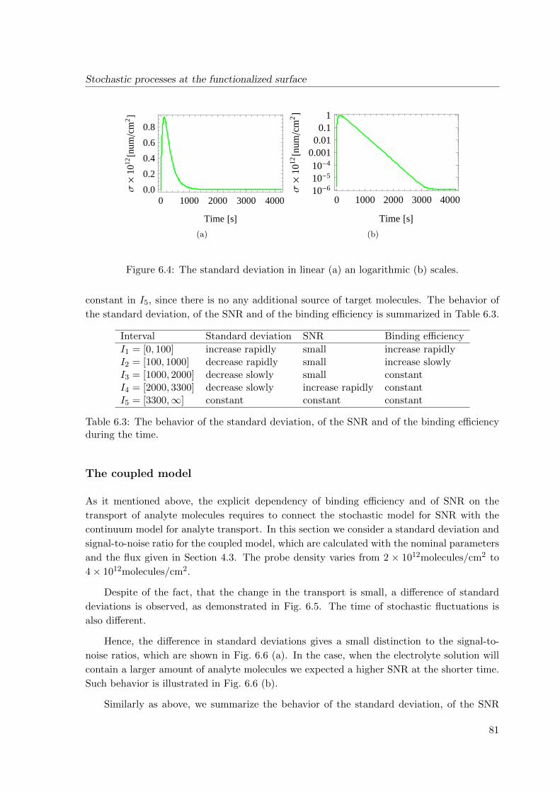
Stochastic processes at the functionalized surface
0 1000 2000 3000 40000.0
0.2
0.4
0.6
0.8
Time @sD
Σ´
1012
@num
cm2
D
(a)
0 1000 2000 3000 400010-610-510-4
0.0010.010.1
1
Time @sD
Σ´
1012
@num
cm2
D
(b)
Figure 6.4: The standard deviation in linear (a) an logarithmic (b) scales.
constant in I5, since there is no any additional source of target molecules. The behavior of
the standard deviation, of the SNR and of the binding efficiency is summarized in Table 6.3.
Interval Standard deviation SNR Binding efficiency
I1 = [0, 100] increase rapidly small increase rapidlyI2 = [100, 1000] decrease rapidly small increase slowlyI3 = [1000, 2000] decrease slowly small constantI4 = [2000, 3300] decrease slowly increase rapidly constantI5 = [3300,∞] constant constant constant
Table 6.3: The behavior of the standard deviation, of the SNR and of the binding efficiencyduring the time.
The coupled model
As it mentioned above, the explicit dependency of binding efficiency and of SNR on the
transport of analyte molecules requires to connect the stochastic model for SNR with the
continuum model for analyte transport. In this section we consider a standard deviation and
signal-to-noise ratio for the coupled model, which are calculated with the nominal parameters
and the flux given in Section 4.3. The probe density varies from 2 × 10¹²molecules/cm2 to
4× 10¹²molecules/cm2.
Despite of the fact, that the change in the transport is small, a difference of standard
deviations is observed, as demonstrated in Fig. 6.5. The time of stochastic fluctuations is
also different.
Hence, the difference in standard deviations gives a small distinction to the signal-to-
noise ratios, which are shown in Fig. 6.6 (a). In the case, when the electrolyte solution will
contain a larger amount of analyte molecules we expected a higher SNR at the shorter time.
Such behavior is illustrated in Fig. 6.6 (b).
Similarly as above, we summarize the behavior of the standard deviation, of the SNR
81
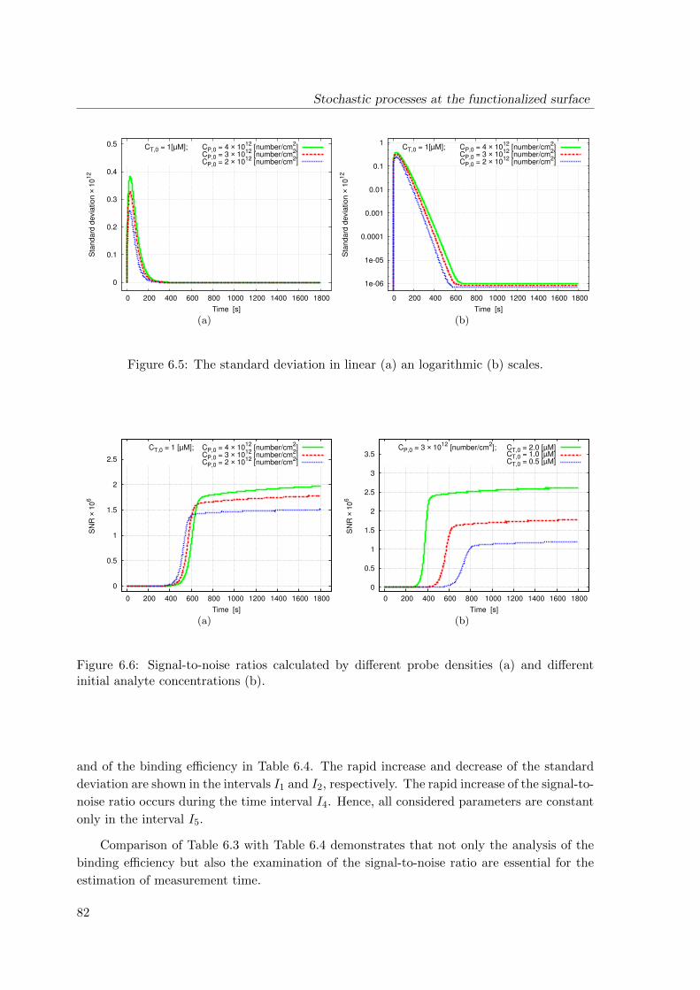
Stochastic processes at the functionalized surface
0
0.1
0.2
0.3
0.4
0.5
0 200 400 600 800 1000 1200 1400 1600 1800
Sta
nd
ard
de
via
tio
n ×
10
12
Time [s]
CT,0 = 1[µM]; CP,0 = 4 × 10¹²
[number/cm2]
CP,0 = 3 × 10¹²
[number/cm2]
CP,0 = 2 × 10¹²
[number/cm2]
(a)
1e-06
1e-05
0.0001
0.001
0.01
0.1
1
0 200 400 600 800 1000 1200 1400 1600 1800
Sta
nd
ard
de
via
tio
n ×
10
12
Time [s]
CT,0 = 1[µM]; CP,0 = 4 × 10¹²
[number/cm2]
CP,0 = 3 × 10¹²
[number/cm2]
CP,0 = 2 × 10¹²
[number/cm2]
(b)
Figure 6.5: The standard deviation in linear (a) an logarithmic (b) scales.
0
0.5
1
1.5
2
2.5
0 200 400 600 800 1000 1200 1400 1600 1800
SN
R ×
10
6
Time [s]
CT,0 = 1 [µM]; CP,0 = 4 × 10¹²
[number/cm2]
CP,0 = 3 × 10¹²
[number/cm2]
CP,0 = 2 × 10¹²
[number/cm2]
(a)
0
0.5
1
1.5
2
2.5
3
3.5
0 200 400 600 800 1000 1200 1400 1600 1800
SN
R ×
10
6
Time [s]
CP,0 = 3 × 10¹²
[number/cm2]; CT,0 = 2.0 [µM]
CT,0 = 1.0 [µM]CT,0 = 0.5 [µM]
(b)
Figure 6.6: Signal-to-noise ratios calculated by different probe densities (a) and differentinitial analyte concentrations (b).
and of the binding efficiency in Table 6.4. The rapid increase and decrease of the standard
deviation are shown in the intervals I1 and I2, respectively. The rapid increase of the signal-to-
noise ratio occurs during the time interval I4. Hence, all considered parameters are constant
only in the interval I5.
Comparison of Table 6.3 with Table 6.4 demonstrates that not only the analysis of the
binding efficiency but also the examination of the signal-to-noise ratio are essential for the
estimation of measurement time.
82
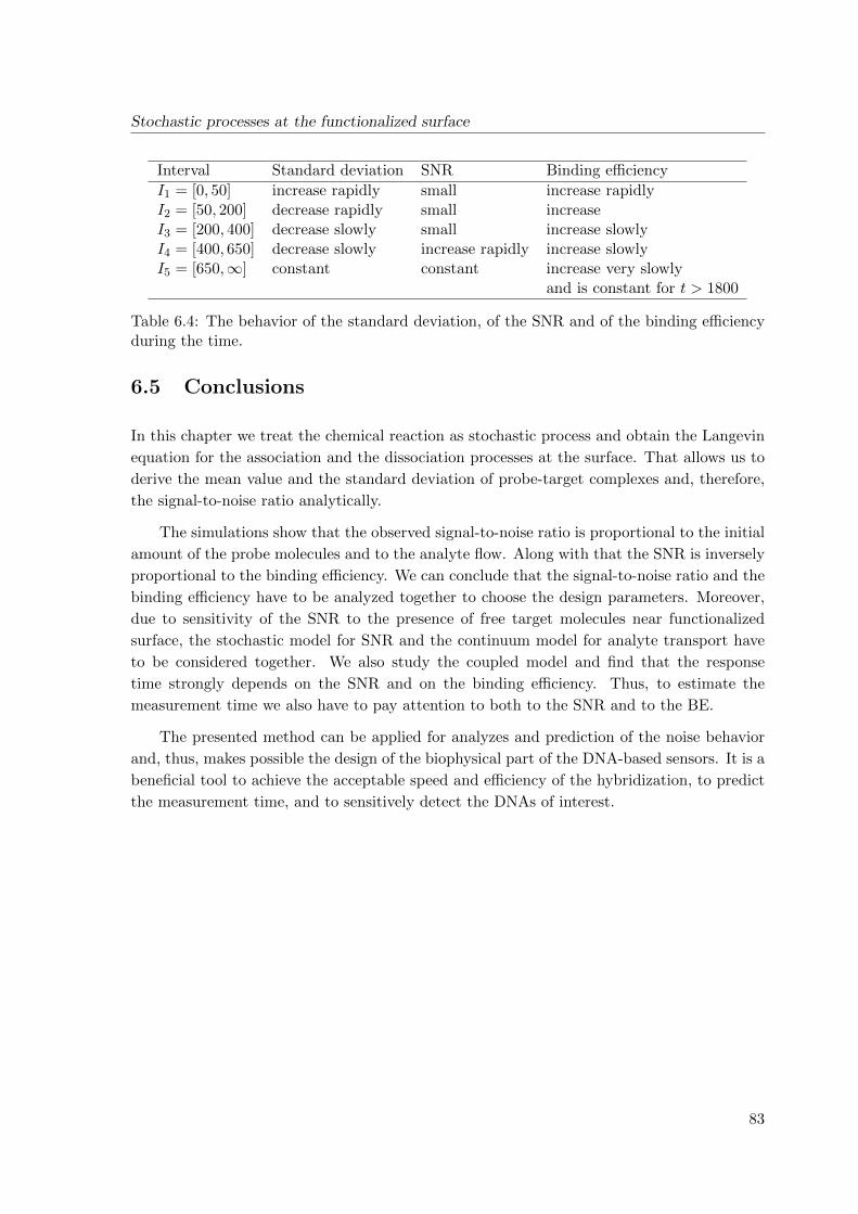
Stochastic processes at the functionalized surface
Interval Standard deviation SNR Binding efficiency
I1 = [0, 50] increase rapidly small increase rapidlyI2 = [50, 200] decrease rapidly small increaseI3 = [200, 400] decrease slowly small increase slowlyI4 = [400, 650] decrease slowly increase rapidly increase slowlyI5 = [650,∞] constant constant increase very slowly
and is constant for t > 1800
Table 6.4: The behavior of the standard deviation, of the SNR and of the binding efficiencyduring the time.
6.5 Conclusions
In this chapter we treat the chemical reaction as stochastic process and obtain the Langevin
equation for the association and the dissociation processes at the surface. That allows us to
derive the mean value and the standard deviation of probe-target complexes and, therefore,
the signal-to-noise ratio analytically.
The simulations show that the observed signal-to-noise ratio is proportional to the initial
amount of the probe molecules and to the analyte flow. Along with that the SNR is inversely
proportional to the binding efficiency. We can conclude that the signal-to-noise ratio and the
binding efficiency have to be analyzed together to choose the design parameters. Moreover,
due to sensitivity of the SNR to the presence of free target molecules near functionalized
surface, the stochastic model for SNR and the continuum model for analyte transport have
to be considered together. We also study the coupled model and find that the response
time strongly depends on the SNR and on the binding efficiency. Thus, to estimate the
measurement time we also have to pay attention to both to the SNR and to the BE.
The presented method can be applied for analyzes and prediction of the noise behavior
and, thus, makes possible the design of the biophysical part of the DNA-based sensors. It is a
beneficial tool to achieve the acceptable speed and efficiency of the hybridization, to predict
the measurement time, and to sensitively detect the DNAs of interest.
83

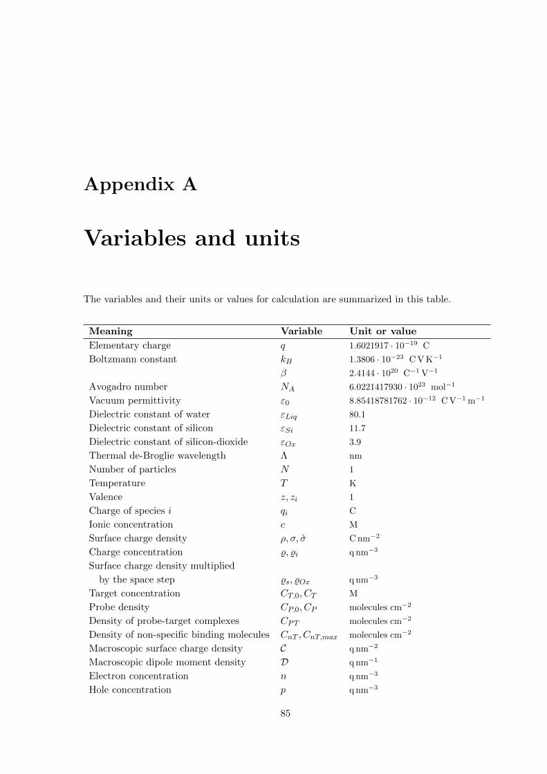
Appendix A
Variables and units
The variables and their units or values for calculation are summarized in this table.
Meaning Variable Unit or value
Elementary charge q 1.6021917 · 10−19 C
Boltzmann constant kB 1.3806 · 10−23 C V K−1
β 2.4144 · 1020 C−1 V−1
Avogadro number NA 6.0221417930 · 1023 mol−1
Vacuum permittivity ε0 8.85418781762 · 10−12 C V−1 m−1
Dielectric constant of water εLiq 80.1
Dielectric constant of silicon εSi 11.7
Dielectric constant of silicon-dioxide εOx 3.9
Thermal de-Broglie wavelength Λ nm
Number of particles N 1
Temperature T K
Valence z, zi 1
Charge of species i qi C
Ionic concentration c M
Surface charge density ρ, σ, σ C nm−2
Charge concentration %, %i q nm−3
Surface charge density multiplied
by the space step %s, %Ox q nm−3
Target concentration CT,0, CT M
Probe density CP,0, CP molecules cm−2
Density of probe-target complexes CPT molecules cm−2
Density of non-specific binding molecules CnT , CnT,max molecules cm−2
Macroscopic surface charge density C q nm−2
Macroscopic dipole moment density D q nm−1
Electron concentration n q nm−3
Hole concentration p q nm−3
85
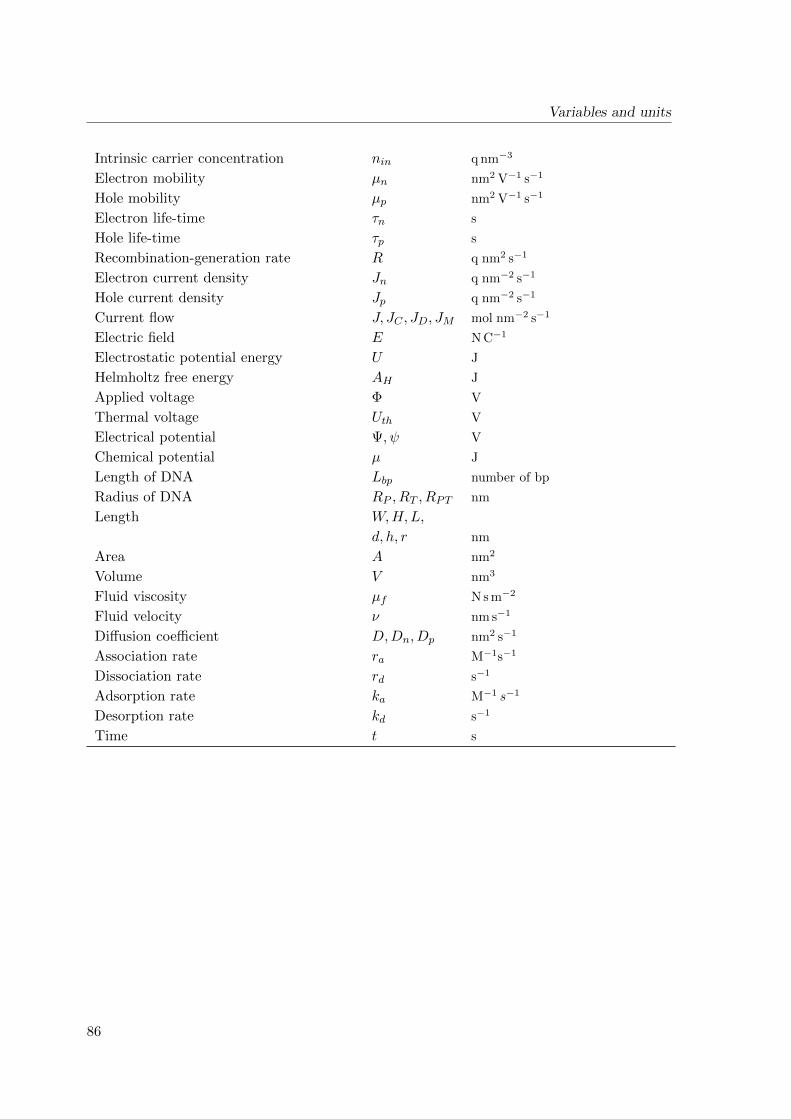
Variables and units
Intrinsic carrier concentration nin q nm−3
Electron mobility µn nm2 V−1 s−1
Hole mobility µp nm2 V−1 s−1
Electron life-time τn s
Hole life-time τp s
Recombination-generation rate R q nm2 s−1
Electron current density Jn q nm−2 s−1
Hole current density Jp q nm−2 s−1
Current flow J, JC , JD, JM mol nm−2 s−1
Electric field E N C−1
Electrostatic potential energy U J
Helmholtz free energy AH J
Applied voltage Φ V
Thermal voltage Uth V
Electrical potential Ψ, ψ V
Chemical potential µ J
Length of DNA Lbp number of bp
Radius of DNA RP , RT , RPT nm
Length W,H,L,
d, h, r nm
Area A nm2
Volume V nm3
Fluid viscosity µf N s m−2
Fluid velocity ν nm s−1
Diffusion coefficient D,Dn, Dp nm2 s−1
Association rate ra M−1s−1
Dissociation rate rd s−1
Adsorption rate ka M−1 s−1
Desorption rate kd s−1
Time t s
86

Appendix B
Theorems
Theorem B.0.1. (Banach’s Fixed Point Theorem [18])
Assume G : K → K is a nonlinear mapping, and suppose that
‖Gu−Gu∗‖ ≤ γ‖u− u∗‖ u, u∗ ∈ K
for some constant γ < 1. Than G has a unique fixed point.
Theorem B.0.2. (Gauss’ Divergence Theorem [20, 87])
Le Ω be a bounded domain in R3 satisfying the following conditions
(a) The boundary S = ∂Ω of Ω consists of a finite number of smooth surfaces.
(b) Any straight line parallel to any of the coordinate axes either intersects S at a finite
number of points or has a whole interval common with S.
Let F = (P,Q,R) be a vector field defined in Ω such that each of the components P,Q,R
are in C1(Ω) ∪ C0(Ω) and integral∫Ω∇ · F dv :=
∫∫∫Ω
(∂xP + ∂yQ+ ∂zR
)dx dy dz
is convergent. Then ∫Ω∇ · F dv :=
∫S
F · ~n dσ
where ~n is the outward pointing normal vector, and dσ is the element of surface on S.
87
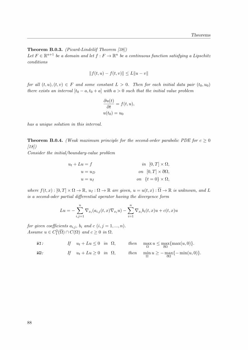
Theorems
Theorem B.0.3. (Picard-Lindelof Theorem [38])
Let F ∈ Rn+1 be a domain and let f : F → Rn be a continuous function satisfying a Lipschitz
conditions
‖f(t, u)− f(t, v)‖ ≤ L‖u− v‖
for all (t, u), (t, v) ∈ F and some constant L > 0. Then for each initial data pair (t0, u0)
there exists an interval [t0 − a, t0 + a] with a > 0 such that the initial value problem
∂u(t)
∂t= f(t, u),
u(t0) = u0
has a unique solution in this interval.
Theorem B.0.4. (Weak maximum principle for the second-order parabolic PDE for c ≥ 0
[18])
Consider the initial/boundary-value problem
ut + Lu = f in [0, T ]× Ω,
u = uD on [0, T ]× ðΩ,
u = uI on t = 0 × Ω,
where f(t, x) : [0, T ]×Ω→ R, uI : Ω→ R are given, u = u(t, x) : Ω→ R is unknown, and L
is a second-oder partial differential operator having the divergence form
Lu = −n∑
i,j=1
∇xi(ai,j(t, x)∇xiu)−n∑i=1
∇xibi(t, x)u+ c(t, x)u
for given coefficients ai,j, bi and c (i, j = 1, ..., n).
Assume u ∈ C21 (Ω) ∩ C(Ω) and c ≥ 0 in Ω.
W1: If ut + Lu ≤ 0 in Ω, then maxΩ
u ≤ maxðΩmax(u, 0).
W2: If ut + Lu ≥ 0 in Ω, then minΩu ≥ −max
ðΩ−min(u, 0).
88
Bibliography
[1] M.H. Abouzar, A.M. Pedraza, Schoning, and A. Poghossian, Label-free DNA hybridiza-
tion and denaturation detection by means of field-effect nanoplate SOI capacitors func-
tionalized with gold nanoparticles, Proc. Eurosensors XXIV (Linz, Austria), vol. 5, Pro-
cedia Engineering, sep 2010, pp. 918–921. 4, 8
[2] Edvard Allen, Modeling with Ito stochastic differential equations, Springer-Verlag, 2007.
75
[3] M. P. Allen and D. J. Tildesley, Computer simulation of liquids, Oxford University Press,
Oxford, New York, 1987. 3, 25, 27
[4] Gerda Ara and James G. Mullen, Effect of ion size on diffusion in alkali halides, Phys.
Rev. 143 (1966), no. 2, 663–665. 18, 25
[5] P. Bergveld and A. Sibbald, Analytical and biomedical applications of ion-selective field-
effect transistors, Elsevier, Amsterdam, 1988. 20, 22
[6] D. Boda, K.-Y. Chan, and D. Henderson, Monte Carlo simulation of an ion-dipole mix-
ture as a model of an electrical double layer, JCHEP 109 (1998), no. 17, 7362–7371. 25,
31
[7] D. Boda, W. R. Fawcett, D. Henderson, and S. Soko lowski, Monte Carlo, density func-
tional theory, and Poisson–Boltzmann theory study of the structure of an electrolyte near
an electrode, JCHEP 116 (2002), no. 16, 7170–7176. 25, 38
[8] D. Boda, D. Henderson, and K.-Y. Chan, Monte Carlo study of the capacitance of the
double layer in a model molten salt, JCHEP 110 (1999), no. 11, 5346–5350. 38
[9] D. Boda, D. Henderson, P. Plaschko, and W. R. Fawcett, Monte Carlo and density func-
tional theory study of the electrical double layer: The dependence of the charge/voltage
relation on the diameter of the ions, Mol. Simulat. 30 (2004), no. 2-3, 137–141. 3, 25
[10] Leland C. Clark and Champ Lyons, Electrode systems for continuous monitoring in
cardiovascular durgery, Ann. N. Y. Acad. Sci. 102 (1962), 29–45. 1
[11] H. Cohen and J.W. Cooley, The numerical solution of the time-dependent Nernst-Planck
equations, J. Biophys. 5 (1965), no. 2, 257–268. 4
89
BIBLIOGRAPHY
[12] Y. Cui, X. F. Duan, J. T. Hu, and C. M. Lieber, Doping and electrical transport in
silicon nanowires, J. Phys. Chem. B 104 (2000), 5213–5216. 11
[13] P. Debye and E. Huckel, Zur Theorie der Elektrolyte. I. Gefrierpunktserniedrigung und
verwandte Erscheinungen, Physikalische Zeitschrift 24 (1923), no. 9, 185–206. 3, 25
[14] M. J. Deen, M. W. Shinwari, and J. C. Ranuarez, Noise considerations in field-effect
biosensors, J. Appl. Phys. 100 (2006), 074703/1–8. 4
[15] Rory Dijkink and Claus-Dieter Ohl, Laser-induced cavitation based micropump, Lab Chip
8 (2008), 1676–1681. 17
[16] N. Elfstrom, R. Juhasz, I. Sychugov, T. Engfeldt, A. E. Karlstrom, and J. Linnros,
Surface charge sensitivity of silicon nanowires: Size dependence, Nano Lett. 7 (2007),
no. 9, 2608–2612. 8
[17] David Erickson, Dongqing Li, and Ulrich J. Krull, Modeling of DNA hybridisation ki-
netics for spatially resolved biochip, Anal. Biochem. 317 (2003), no. 2, 186–200. 4
[18] L. C. Evans, Partial differential equations, Oxford University Press, 1998. 51, 87, 88
[19] E. Fatemi and F. Odeh, Upwind finite difference solution of Boltzmann equation applied
to electron transport in semiconductor devices, JCOMP2 108 (1993), no. 2, 209–217. 3
[20] R. P. Feynman, R. B. Leighton, and M. Sands, The feynman lectures on physic.
ii. mainly electromagnetism and matter, Addison-Wesley Publishing Company, Mas-
sachusetts, 2005. 87
[21] Daan Frenkel and Berend Smit, Understanding molecular simulation, academic press,
London WC1X 8RR, UK, 2002. 3
[22] J. Fritz, E. B. Cooper, S. Gaudet, P. K. Sorger, and S. R. Manalis, Electronic detection
of DNA by its intrinsic molecular charge, PRONA 99 (2002), no. 22, 14142–14146. 4, 9
[23] Z. Gao, A. Agarwal, A. D. Trigg, N. Singh, C. Fang, C.-H. Tung, Y. Fan, K. D. Bud-
dharaju, and J. Kong, Silicon nanowire arrays for label-free detection of DNA, Analytical
Chemistry A 79 (2007), no. 9, 3291–3297. 4
[24] Daniel T. Gillespie, The chemical Langevin equation, J. Chem. Phys. 113 (2000), no. 1,
297–306. 72
[25] Teena Goel, Chandra N. Patra, Swapan K. Ghosh, and Tulsi Mukherjee, Three compo-
nent model of cylindrical electric double layers containing mixed electrolytes: A system-
atic study by Monte Carlo simulations and density functional theory, J. Chem. Phys.
132 (2010), no. 19, 194706. 25
[26] J. Hahm and C. M. Lieber, Direct ultrasensitive electrical detection of DNA and DNA
sequence variations using nanowire nanosensors, Nano Lett. 4 (2004), no. 1, 51–54. 4
90
BIBLIOGRAPHY
[27] Zhang Hai-Lang and Han Shi-Jun, Viscosity and density of water + sodium chloride +
potassium chloride solutions at 298.15 K, J. Chem. Eng. Data 41 (1996), no. 3, 516–520.
58
[28] A. Hassibi, R. Navid, R. W. Dutton, and T. H. Lee, Comprehensive study of noise
processes in electrode electrolyte interfaces, J. Appl. Phys. 96 (2004), no. 2, 1074–1082.
4
[29] A. Hassibi, S. Zahedi, R. Navid, R. W. Dutton, and T. H. Lee, Biological shot-noise
and quantum-limited signal-to-noise ratio in affinity-based biosensors, J. Appl. Phys. 97
(2005), 084701/1–10. 4
[30] Clemens Heitzinger, Rick Kennell, Gerhard Klimeck, Norbert Mauser, Michael McLen-
nan, and Christian Ringhofer, Modeling and simulation of field-effect biosensors
(BioFETs) and their deployment on the nanoHUB, J. Phys.: Conf. Ser. 107 (2008),
012004/1–12. 63
[31] Clemens Heitzinger, Yang Liu, Norbert Mauser, Christian Ringhofer, and Robert Dut-
ton, Calculation of fluctuations in boundary layers of nanowire field-effect biosensors, J.
Comput. Theor. Nanosci. 7 (2010), no. 12, 1–7. 26
[32] Clemens Heitzinger, Norbert Mauser, and Christian Ringhofer, Multiscale modeling of
planar and nanowire field-effect biosensors, siaja 70 (2010), no. 5, 1634–1654. 63
[33] Desmond J. Higham, Modeling and simulation chemical reactions, SIAM Rev. 50 (2008),
no. 2, 347–368. 4, 72
[34] Heather K. Hunt and Andrea M. Armani, Label-free biological and chemical sensors,
Nanoscale 2 (2010), no. 9, 1544–1559. 1, 2, 9
[35] S. Ingebrandt, Y. Hana, F. Nakamuraa, A. Poghossian, M.J. Schoning, and A. Of-
fenhausser, Label-free detection of single nucleotide polymorphisms utilizing the differen-
tial transfer function of field-effect transistors, Biosens. Bioelectron. 22 (2007), no. 12,
2834–2840. 2
[36] K. Kiyohara and K. Asaka, Monte Carlo simulation of electrolytes in the constant voltage
ensemble, JCHEP 126 (2007), 214704. 25, 27
[37] J. F. Klemic, E. Stern, and M. A. Reed, Hotwiring biosensors, Nature Biotechnology 19
(2001), 924–925. 9
[38] Rainer Kress, Numerical analysis, Springer-Verlag, New York, Berlin, Heidelberg, 1998.
88
[39] Murray A. Lampert and Richard S. Crandall, Nonlinear Poisson–Boltzmann theory for
polyelectrolyte solutions: The counterion condensate around a line charge as a δ-function,
Chem. Phys. Lett. 72 (1980), 481–486. 3, 25
91
BIBLIOGRAPHY
[40] D. Landheer, G. Aers, W. R. McKinnon, M. J. Deen, and J. C. Ranuarez, Model
for the field effect from layers of biological macromolecules on the gate of metal-oxide-
semiconductor transistors, J. Appl. Phys. 98 (2005), 044701/1–15. 4
[41] A. Majorana and R. M. Pidatella, A finite difference scheme solving the Boltzmann–
Poisson system for semiconductor devices, JCOMP2 174 (2001), no. 2, 649–668. 3
[42] A. Malasics, D. Gillespie, and D. Boda, Simulating prescribed particle densities in the
grand canonical ensemble using iterative algorithms, JCHEP 128 (2008), 124102. 3, 25,
30
[43] P. A. Markowich, The stationary semiconductor device equations, Springer-Verlag, Wien,
1986. 3, 10
[44] P. A. Markowich, C. A. Ringhofer, and C. Schmeiser, Semiconductor equations, Springer-
Verlag, Wien, 1990. 3, 10
[45] N. Metropolis, A. W. Rosenbluth, M. N. Rosenbluth, A. H. Teller, and E. Teller, Equation
of state calculations by fast computing machines, JCHEP 21 (1953), 1087–1092. 27
[46] N. Metropolis and S. Ulam, The Monte Carlo method, JAMES 44 (1949), 335–341. 3,
25, 27
[47] P. Nair and M. Alam, Design considerations of silicon nanowire biosensors, IEEE Trans.
El. Dev. 54 (2007), no. 12, 3400–3408. 1
[48] Liviu Nicu and Thierry Le’ichle, Biosensors and tools for surface functionalization
from the macroto the nanoscale: The way forward, J. Appl. Phys. 104 (2008), no. 11,
111101/1–15. 1
[49] C. W. Outhwaite and L. B. Bhuiyan, A modified Poisson–Boltzmann analysis of the
electric double layer around an isolated spherical macroion, Molecular Physics 74 (1991),
no. 2, 367–381. 3, 25
[50] Won II Park, Gengfeng Zheng, Xiaocheng Jiang, Bozhi Tian, and Charles M. Lieber,
Controlled synthesis of millimeter-long silicon nanowires with uniform electronic prop-
erties, Nano Lett. 8 (2008), no. 9, 3004–3009. 8
[51] F. Patolsky, B. P. Timko, G. Yu, Y. Fang, A. B. Greytak, G. Zheng, and C. M. Lieber,
Detection, stimulation, and inhibition of neuronal signals with high-density nanowire
transistor arrays, SCIEN 313 (2006), 1100–1104. 8
[52] F. Patolsky, G. Zheng, and C. M. Lieber, Fabrication of silicon nanowire devices for
ultrasensitive, label-free, real-time detection of biological and chemical species, Nature
Protocols 1 (2006), no. 4, 1711–1724. 1, 2
[53] Daniel E. Perea, Eric R. Hemesath, Edwin J. Schwalbach, Jessica L. Lensch-Falk, Pe-
ter W. Voorhees, and Lincoln J. Lauhon, Direct measurement of dopant distribution in
92
BIBLIOGRAPHY
an individual vapour-liquid-solid nanowire, Nature Nanotechnology 4 (2009), 315–319.
11
[54] A. W. Peterson, R. J. Heaton, and R. M. Georgiadis, The effect of surface probe density
on DNA hybridization, Nucleic Acids Res. 29 (2001), no. 24, 5163–5168. 4, 26, 60, 78,
79
[55] A. W. Peterson, L. K. Wolf, and R. M. Georgiadis, Hybridization of mismatched or
partially matched DNA at surfaces, J. Am. Chem. Soc. 124 (2002), no. 49, 14601–14607.
4, 62, 78
[56] A. Poghossian, M.H. Abouzar, F. Amberger, D. Mayerb, Y. Hanb, S. Ingebrandt, A. Of-
fenhausser, and M.J. Schoning, Field-effect sensors with charged macromolecules: Char-
acterisation by capacitance-voltage, constant-capacitance, impedance spectroscopy and
atomic-force microscopy methods, Biosens. Bioelectron. 22 (2007), no. 9-10, 2100–2107.
8
[57] A. Poghossian, M.H. Abouzar, and M.J. Schoning, Capacitance-voltage and impedance
characteristics of field-effect EIS sensors functionalised with polyelectrolyte multilayers,
ITBM-RBM 29 (2008), no. 2-3, 149–154. 8
[58] A. Poghossian, A. Cherstvy, S. Ingebrandt, A. Offenhauser, and M. J. Schoning, Possi-
bilities and limitations of label-free detection of DNA hybridization with field-effect-based
devices, Sensors and Actuators B 111-112 (2005), 470–480. 2, 9
[59] Andreas Richter, Stephan Klatt, Georgi Paschew, and Christian Klenke, Micropumps
operated by swelling and shrinking of temperature-sensitive hydrogels, Lab Chip 9 (2009),
613–618. 17
[60] Christian Ringhofer and Clemens Heitzinger, Multi-scale modeling and simulation of
field-effect biosensors, ECS Transactions 14 (2008), no. 1, 11–19. 63
[61] M. J. Schoning and A. Poghossian, Recent advances in biologically sensitive field-effect
transistors (BioFETs), Analyst 127 (2002), 1137–1151. 1, 2, 7, 9
[62] , Bio FEDs (field-effect devices): State-of-the-art and new directions, Electro-
analysis 18 (2006), no. 19-20, 1893–1900. 9
[63] K. A. Sharp and B. Honig, Electrostatic interactions in macromolecules: Theory and
applications, Annu. Rev. Biophys. Biophys. Chem. 19 (1990), 301–332. 3, 25
[64] P. E. Sheehan and L. J. Whitman, Detection limits of nanoscale biosensors, Nano Lett.
5 (2005), no. 4, 803–807. 3
[65] T. M. Squires, R. J. Messinger, and S. R. Manalis, Making it stick: Convection, reaction
and diffusion in surface-based biosensors, Nature Biotechnology 26 (2008), no. 4, 417–
426. 4, 15
93
BIBLIOGRAPHY
[66] S.Ravindran and J.Wu, Ion size effect on colloidal forces within the primitive model,
Condensed Matter Physics 8 (2005), no. 2, 377–388. 18, 25
[67] E. Stern, Label-free sensing with semiconducting nanowires, Ph.D. thesis, Yale Univer-
sity, 2007. 7, 8
[68] E. Stern, J. F. Klemic, D. A. Routenberg, P. N. Wyrembak, D. B. Turner-Evans, A. D.
Hamilton, D. A. LaVan, T. M. Fahmy, and M. A. Reed, Label-free immunodetection with
CMOS-compatible semiconducting nanowires, NATURE 445 (2007), 519–522. 2, 3, 7, 8
[69] E. Stern, A. Vacic, N. K. Rajan, J. M. Criscione, J. Park, B. R. Ilic, D. J. Mooney,
M. A. Reed, and T. M. Fahmy, Label-free biomarker detection from whole blood, Nature
Nanotechnology 5 (2009), 138 – 142. 2, 9
[70] A. H. Talasaz, M. Nemat-Gorgani, Y. Liu, P. StA¥hl, R. W. Dutton, M. Ronaghi, and
R. W. Davis, Prediction of protein orientation upon immobilization on biological and
nonbiological surfaces, PRONA 103 (2006), no. 40, 14773–14778. 3, 25, 26
[71] Daniel R. Theavenot, Klar Toth, Richard A. Durst, and George S. Wilson, Electrochemi-
cal biosensors: recommended definitions and classification, Pure Appl. Chem. 71 (1999),
no. 12, 2333–2348. 2, 3
[72] Aleksey M. Tikhonov, Ion-size effect at the surface of a silica hydrosol, J. Chem. Phys.
130 (2009), no. 2, 024512. 18, 25
[73] M. M. Tirado, C. L. Martinez, and J. G. Delatorre, Comparison of theories for the
translational and rotational diffusion coefficients of rod-like macromolecules. application
to short DNA fragmentsl, J. Chem. Phys. 81 (1984), no. 4, 2047–2052. 59
[74] G. M. Torrie and J. P. Valleau, Electrical double layers. I. Monte Carlo study of a
uniformly charged surface, JCHEP 73 (1980), no. 11, 5807–5816. 3, 25, 31
[75] George A. Truskey, Fan Yuan, and David F. Katz, Transport phenomena in biological
systems, Pearson Prentice Hall, New Jersey, 2004. 4, 13
[76] M. Valisko, D. Boda, and G. Gillespie, Selective adsorbtion of ions with different diameter
and valence at highly-charged interfaces, J. Phys. Chem. C 111 (2007), no. 43, 15575–
15585. 3, 18, 25, 38
[77] M. Valisko, D. Henderson, and D. Boda, Competition between the effects of asymme-
tries in ion diameters and charges in an electrical double layer studied by Monte Carlo
simulations and theories, J. Phys. Chem. B 108 (2004), no. 42, 16548–16555. 25, 38
[78] D. van der Spoel, E. Lindahl, B. Hess, Carsten Kutzner, A. R. van Buuren, E. Apol,
P. J. Meulenhoff, D. P. Tieleman, A. L. T. M. Sijbers, K. A. Feenstra, R. van Drunen,
and H. J. C. Berendsen, Gromacs user manual version 4.0, 2006, http://www.gromacs.
org/@api/deki/files/82/=gromacs4_manual.pdf. 19
94
BIBLIOGRAPHY
[79] R. E. G. van Hal, J. C. T. Eijkel, and P. Bergveld, A novel description of ISFET sen-
sitivity with the buffer capacity and double-layer capacitance as key parameters, Sensors
and Actuators B 24-25 (1995), 201–205. 20
[80] A. H.-J. Wang, G. J. Quigley, F. J. Kolpac, J. L. Crawford, J. H. van Boom, G. van der
Marel, and A. Rich, Molecular structure of a left-handed double helical DNA fragment
at atomic resolution, Nature 282 (1979), no. 13, 680–686. 19
[81] J. Wang, E. Palecek, P. E. Nielsen, G. Rivas, X. Cai, H. Shiraishi, N. Dontha, D. Luo,
and P. A. M. Farias, Peptide nucleic acid probes for sequence-specific DNA biosensors,
JAMEC1 118 (1996), no. 33, 7667–7670. 1
[82] Ke Wang, Yang-Xin Yu, and Guang-Hua Gao, Density functional study on the structures
and thermodynamic properties of small ions around polyanionic dna, Phys. Rev. E 70
(2004), no. 1, 011912. 25
[83] Ke Wang, Yang-Xin Yu, Guang-Hua Gao, and Guang-Sheng Luo, Density-functional
theory and Monte Carlo simulation study on the electric double layer around DNA in
mixed-size counterion system, JCHEP 123 (2005), no. 23, 234904. 25
[84] James G. Wetmur, Hybridisation and renaturation kinetics of nucleic acids, Anna. Rev.
Biophys. Bioeng 5 (1976), 337–361. 4
[85] James G. Wetmur and Norman Davidson, Kinetics of renaturation of DNA, J. Mol. Biol.
31 (1968), no. 3, 349–370. 4
[86] X. Wu and X. Xu, Degenerate semiconductor device equations with temperature effect,
Nonlinear Analysis 65 (2006), no. 2, 321–337. 3
[87] E. G. Zachmanoglou and Dale W. Thoe, Introduction to partial differential equations
with applications, Dover Publications, Mineola, N. Y. 11501, 1987. 87
[88] Yi Zhang, Thomas C. Gamble, Alexander Neumann, Gabriel P. Lopez, Steven R. J.
Brueck, and Dimiter N. Petsev, Electric field control and analyte transport in Si/SiO2
fluidic nanochannels, Lab Chip 8 (2008), 1671–1675. 4, 17
[89] G. Zheng, F. Patolsky, Y. Cui, W. U. Wang, and C. M. Lieber, Multiplexed electrical de-
tection of cancer markers with nanowire sensor arrays, Nature Biotechnology 23 (2005),
1294–1301. 2, 7
95

Curriculum Vitae of Alena Bulyha
Alena Bulyha graduated from the Belarussian State University, Minsk with specialization
in Mathematics. Diploma work was carried out at the Institute of Engineering Cybernetics
/ Academy of Sciences of Belarus, Minsk on the subject ”Development of Algorithms and
Programs for Detailed Control of Topographical Data Reliability” under supervision of Prof.
Dr. Sergey V. Ablameyko with grade ”excellent”.
After graduating from the University Alena had the following research works:
on software development for application in physics and chemistry, cooperation with the
Radiation Physics and Chemistry Problems Institute / Academy of Sciences of Belarus;
on geometry algorithms with certified results at the Institute of Informatics, Mainz Uni-
versity, Germany in group of Prof. Dr. Elmar Schomer ”Algorithmic Geometry and Com-
puter Graphics”;
on developing of practical software applications for recognition of batch shapes (Gemen-
gelagen) for glass production industry, feasibility study, cooperation with Mainz University
and Schott AG company, Mainz, Germany.
Alena began her PhD studies in October 2007 at the Institute for Analysis and Scientific
Computing, Vienna University of Technology, Austria on the subject ”Modeling and Simula-
tion of Field-Effect Biosensors” under supervision of Prof. Dr. Christoph W. Uberhuber and
Dr. Clemens Heitzinger. Since Januar 2008 she has carried out her studies at the Faculty
of Mathematics, University of Vienna, Austria under supervision of Prof. Dr. Nortbert J.
Mauser and Dr. Clemens Heitzinger.
Publications on subject of thesis
1. A. Bulyha and C. Heitzinger, An algorithm for three-dimensional Monte-Carlo simu-
lation of charge distribution at biofunctionalized surfaces, Nanoscale, 3(4), 1608-1617,
2011.
2. A. Bulyha, C. Heitzinger and N. J. Mauser, Bio-sensors: Modelling and simulation of
biologically sensitive field-effect transistors, ERCIM-news, 85, 40-41, 2011.
3. A. Bulyha, C. Heitzinger, and N. J. Mauser, A stochastic-deterministic approach for
modelling of the biological noise in the DNA-sensors, 2011, In preparation.
4. S. Baumgartner, A. Bulyha, M. Vasicek, N. Tassotti, and C. Heitzinger, Investigations
of optimal sensitivity for biosensors using a 3d self-consistent drift-diffusion Monte
Carlo approach, 2011, In preparation.
Contributions to academic conferences and workshops
1. A. Bulyha, C. Heitzinger and N. J. Mauser (2010) Stochastic models of signal and
noise in field-effect biosensors. Poster at the Nanosensors for Industrial Application
(NANOSENS 2010), Dec. 2-3, 2010, Tech Gate Vienna, Austria.
97
2. S. Baumgartner, A. Bulyha, C. Heitzinger and N. J. Mauser (2010) Self-Consistent
3D Simulations of BioFETs. Talk at the Nanosensors for Industrial Application
(NANOSENS 2010), Dec. 2-3, 2010, Tech Gate Vienna, Austria.
3. A. Bulyha (2010) Modeling of stochastic processes in field-effect biosensors. Talk at the
4nd Annual Meeting ”DEASE Summer-school”, May 17-21, 2010 Hammamet, Tunisia.
4. A. Bulyha, C. Heitzinger, and N. Mauser (2009) Simulation of biofunctionalized surface
layers using a Monte Carlo algorithm. Talk at the 216th Meeting of the Electrochemical
Society (ECS), Oct. 4-9, 2009, Vienna, Austria, Book of abstracts.
5. A. Bulyha (2009) Simulation of Biofunctionalized Surface Layers of Field-Effect Sen-
sors. Talk at the 3nd Annual Meeting ”DEASE Summer-school”, May 27-30, 2009,
IACM - FORTH and University of Crete, Heraklion, Crete.
6. C. Heitzinger, A. Bulyha, N. J. Mauser, C. Ringhofer, Y. Liu, R. Dutton (2008) Stochas-
tic and Continuum Models of Biofunctionalized Surface Layers for Multi-Scale Modeling
of Field-Effect. Talk at the Nanosensors for Industrial Application (NANOSENS 2008),
Sept. 29-30, 2008, Tech Gate Vienna, Austria.
7. A. Bulyha (2008) Modeling and Simulation of Field-Effect Biosensors. Talk at the 2nd
Annual Meeting ”DEASE Summer-school”, Sept. 18-20, 2008, University of Hamburg
and Hamburg University of Technology, Hamburg, Germany.
98