GRANULOMETRY, CHEMISTRY AND PHYSICAL INTERACTIONS OF

NON-COLLOIDAL PARTICULATE MATTER TRANSPORTED BY URBAN STORM WATER

A Dissertation

Submitted to the Graduate Faculty of the Louisiana State University and

Agricultural and Mechanical College in partial fulfillment of the

requirements for the degree of Doctor of Philosophy

in

The Department of Civil and Environmental Engineering

by Hong Lin

B.S., Xian University of Architecture and Technology, 1996 M.S., Xian University of Architecture and Technology, 1999

May, 2003

ii

ACKNOWLEDGMENTS

I am grateful for the chance to be here, Louisiana State University, to pursue my Ph.D degree.

I would like to thank Dr. John J. Sansalone, my advisor for his guidance and support throughout

my three and half years’ doctorate program. His family embraced me as a friend since I landed on

this continent and I feel being taken good care. Dr. Sansalone’s great character as a scholar and his

consistent encouragement as an advisor guide me through the journey to reach my academic goals.

I also thank Dr. Vijay Singh, Dr. Vadake Srinivasan, Dr. Linbing Wang and Dr. Chang for serving on

my graduate committee. Their advices and assistance in my research are invaluable.

I am grateful to all of my colleagues in the engineering annex building – Ping Zhou, Zheng

Teng, Chad Cristina, Erin Krielow, Christopher Dean, Aimee Blazier, Tianpeng Guo, Gaoxiang

Ying, Yuhong Sheng and Jonathan Kolich – for their assistance and fellowship.

I am further indebted to Luke Wall and Craig Brown who provided great assistance in the

laboratory during this research.

Finally, I would like to thank my family and friends back in China and here in United States,

especially my husband Gang Feng. Without their love and unwearying support, this work would

not have been possible.

iii

TABLE OF CONTENTS

ACKNOWLEDGMENTS .............................................................................................................. ii LIST OF TABLES........................................................................................................................ vii LIST OF FIGURES ....................................................................................................................... ix ABSTRACT...................................................................................................................................xv CHAPTER 1 INTRODUCTION ...................................................................................................1 References ...................................................................................................6 CHAPTER 2 GRANULOMETRY OF NON-COLLOIDAL PARTICULATE MATTER

TRANSPORTED BY URBAN RAINFALL-RUNOFF .........................................9 Summary .....................................................................................................9 Introduction .................................................................................................9 Previous Studies ........................................................................................12 Objectives ..................................................................................................14 Methodology..............................................................................................14 Experimental Site Characteristics .................................................14 Sample Collection ..........................................................................17 Analytical Methods .......................................................................18 Results and Analysis .................................................................................26 Differentiation of Solid Fractions .................................................26 Granulometry of Suspended Fraction ...........................................29 Granulometry of Sediment Fraction .............................................33 Conclusions ...............................................................................................43 Implications for Best Management Practices ...........................................44 References .................................................................................................44 Nomenclature ............................................................................................48

CHAPTER 3 GRANULOMETRIC-BASED DISTRIBUTION OF METALS FOR NON-COLLOIDAL PARTICULATE MATTER TRANSPORTED BY URBAN RAINFALL-RUNOFF .....................................................................49 Summary ...................................................................................................49 Introduction ...............................................................................................49

Previous Studies ........................................................................................50 Objectives ..................................................................................................52 Methodology..............................................................................................52 Phase Fractionation for Equilibrium Analysis ..............................52 Sediment Collection ......................................................................53 Metal Digestion ..............................................................................54

Metal Analysis – ICP/MS .............................................................54 Statistical Estimation of the Difference ........................................55

iv

Pearson’s Correlation Analysis .....................................................56 Power Law Model .........................................................................56

Results and Analysis .................................................................................57 Metal Partitioning in Dissolved and Particulate Phase ..................57 Granulometric-Based Metal Distributions in Sediments ...............61 Cumulative Effects in Sediments Transported by Urban Rainfall-Runoff .................................................79 Conclusions................................................................................................81 Implications for Best Management Practices ............................................81 References .................................................................................................82 Nomenclature ............................................................................................84 CHAPTER 4 MORPHOLOGY, COMPOSITION AND FRACTAL CHARACTERISTICS OF NON-COLLOIDAL PARTICULATE SUBSTRATES TRANSPORTED BY URBAN RAINFALL-RUNOFF .....................................................................85 Summary ...................................................................................................85 Introduction ...............................................................................................85 Background on Scanning Electron Microscopy ........................................90 Objectives ..................................................................................................91 Methodology..............................................................................................92 Sample Collection..........................................................................92 Sample Preparation ........................................................................92 SEM Analysis ................................................................................93 Image Processing and Analyses.....................................................93 Determination of Fractal Dimensions............................................94 Mineral Identification for Particulate Matter in Sediment ............96 Surface Charge Determination.......................................................96 Results........................................................................................................97 Morphology of Particulate Matter in Urban Rainfall-Runoff........97 Mineral Identification ..................................................................103 Chemical Composition of Particulate Matter ..............................103 Surface Charge and PZC..............................................................106 Conclusions..............................................................................................106 References................................................................................................107 Nomenclature ..........................................................................................110 CHAPTER 5 SEDIMENTATION OF NON-COLLOIDAL PARTICULATE MATTER

TRANSPORTED BY URBAN RAINFALL-RUNOFF .....................................112 Summary .................................................................................................112 Settling Velocity – A Review of the Literature .......................................112 Settling Velocity Fundamentals...................................................114 Modified Settling Velocity Formulas ..........................................115 Settling Velocity of Particles of Various Shapes.........................119 Methods for Determining Settling Velocity ................................123 The Effect of Turbulence .............................................................128 Wall Effect in Cylindrical Column..............................................129

v

Objectives ................................................................................................130 Methodology............................................................................................131

Materials – Urban Rainfall-runoff Particles ................................131 Methods........................................................................................133 Results and Anaysis .................................................................................140 Conclusions .............................................................................................148 Implications for Best Management Practices ..........................................153 References ...............................................................................................153 Nomenclature ..........................................................................................156 CHAPTER 6 COAGULATION AND FLOCCULATION OF PARTICULATE MATTER

TRANSPORTED BY URBAN RAINFALL-RUNOFF .....................................160 Summary .................................................................................................160 Introduction..............................................................................................161 Unique Characteristics of Urban Rainfall-runoff ........................163 Characteristics of Particles in Wastewater...................................164 Characteristics of Particles in Natural River Water.....................165 Coagulation and Flocculation Processes......................................166 Coagulants and Flocculants .........................................................167 Objectives ................................................................................................169 Methodology............................................................................................169 Sample Collection........................................................................169 Jar Test Design.............................................................................170 Jar Test Procedure........................................................................171 Settling Column Tests..................................................................171 Floc Characterization ...................................................................173 Results and Analysis ................................................................................173 Jar Test for Rainfall-runoff ..........................................................173 Jar Test for Wastewater ...............................................................174 Jar Test for Natural River Water..................................................175 Settling Column Tests..................................................................175 Floc Characteristics......................................................................177 Conclusions..............................................................................................177 References................................................................................................178 CHAPTER 7 COAGULATION AND AGGREGATION MODEL INCORPORATING

FRACTAL THEORIES FOR PARTICULATES IN URBAN RAINFALL-RUNOFF.........................................................................................212

Summary .................................................................................................212 Introduction..............................................................................................212

Coagulation Processes .................................................................213 Classical Flocculation Model.......................................................214 Modified Flocculation Model ......................................................215 Macroscopic Approach to the Flocculation Process....................225 Fractal Coagulation Model ..........................................................226 Objectives ................................................................................................228 Model and Methodology..........................................................................228

vi

Results ......................................................................................................235 Conclusions..............................................................................................236 References................................................................................................241 Nomenclature ..........................................................................................244 CHAPTER 8 SUMMARY AND CONCLUSIONS ..................................................................246 VITA ...........................................................................................................................................251

vii

LIST OF TABLES

Table 2.1 Central tendency analysis for particle size distribution based on Φ50 ...................23 Table 2.2 Uniformity analysis of particle size distribution based on σΙ ................................23 Table 2.3 Symmetry (Sk) and Kurtosis (KG) of particle size distribution..............................23 Table 2.4 Summary of solid fractions and rainfall characteristics for 12 storm events occurred at Baton Rouge, Louisiana......................................................................27 Table 2.5 Statistic summary of different solid fractions in rainfall-runoff at Baton Rouge I-10 site ..................................................................................................................28 Table 2.6 Median diameter and Φ size of suspended fraction...............................................32 Table 2.7 Summary of statistical characteristics of particle size distribution for the sediments at Baton Rouge site ...............................................................................35 Table 2.8 Summary of particle size distribution characteristics for the sediments at Baton Rouge site ................................................................................................36 Table 2.9 Statistical characteristics of particle size distribution for the grit at Baton Rouge site ....................................................................................................36 Table 2.10 Summary of statistical characteristics of particle size distribution for the sediments collected from four different sites...................................................37 Table 2.11 Summary of particle size distribution characteristics for the sediments at Baton Rouge site ....................................................................................................37 Table 3.1 Partitioning of metals – dissolved and particulate fractions in urban rainfall-runoff.........................................................................................................59 Table 3.2 Adjusted factors for the predicative metal mass model βα cfcf MMe = for non-colloidal sediments collected out of eight individual storm events in Baton Rouge, Louisiana.....................................................................................77 Table 3.3 Adjusted factors for the predicative metal mass model βα cfcf MMe = for long-term (seasonal length) accumulated non-colloidal sediments from four urban storm water catchments ...............................................................78 Table 3.4 Residual errors of power law model βα cfcf MMe = in the prediction of metal mass for incremental sediments ...................................................................78

viii

Table 3.5 Comparison of metal mass between incremental and cumulative sediment for

Baton Rouge site ....................................................................................................79 Table 3.6 Comparison of metal fraction for fine gradation (<75-µm) between incremental and cumulative sediment from Baton Rouge site ..............................79 Table 5.1 Summary of a series of expressions for vt of discrete natural non-cohesive particles ................................................................................................................116 Table 5.2 Parameter determination for Equation 26 for different ranges of Reynold’s numbers ..............................................................................................122 Table 5.3 Scaling relationships between settling velocity tv and characteristic length l

(Johnson 1996).....................................................................................................122 Table 5.4 Size gradations of mechanical sieve analysis ......................................................132 Table 5.5 Modeled settling velocity using Newton’s law for the particles entrained in the grit chamber at Baton Rouge I-10 site (Assume T=20 °C)............................135 Table 5.6 Modeled settling velocity using Newton’s law for particles in the sedimentation tank at Baton Rouge I-10 site (Assume T=20 °C)........................136 Table 5.7 Experimental design – sampling time for the column test...................................138 Table 5.8 Modeled settling velocity using Newton’s law for fine particles (< 250 µm)

Assuming density = 2.50 g/cm3, T=20 °C. ..........................................................140 Table 5.9 Comparison of measured and modeled settling velocity for visible individual

non-colloidal particles..........................................................................................143 Table 5.10 Comparison of measurement of Imhoff cone and settling column for visible

individual non-colloidal particles ........................................................................143 Table 6.1 Experimental matrix for C/F with coagulants or flocculants...............................170 Table 7.1 Collision frequency functions for the coalesced fractal sphere model ................229 Table 7.2 Settling velocity for particles in urban rainfall-runoff.........................................232 Table 7.3 Determination of k size category – upper and lower limit of particle size k .......233 Table 7.4 Fixed parameter used in the model ......................................................................234

ix

LIST OF FIGURES

Figure 2.1 Location of Baton Rouge experimental site – I-10 City Park Lake Overpass.......15 Figure 2.2 Profile view of sampling system at Baton Rouge experimental site .....................16 Figure 2.3 Location and view of Little Rock site 1 – I-30 at I-440 at I-530 ...........................16 Figure 2.4 Location and view of Little Rock site 2 – I-40 at I-30 west ..................................17 Figure 2.5 Location and view of New Orleans Site – I-10 at east of Bonnabel Blvd .............17 Figure 2.6 Illustration of solids fractions in urban rainfall-runoff ..........................................20 Figure 2.7 Relationship of turbidity and suspended solid concentration (SSC)......................29 Figure 2.8 Solid fractions in storm water runoff for twelve observed storm events at Baton Rouge site ....................................................................................................30 Figure 2.9 Total volume concentration and power law fit for the number distribution ..........31 Figure 2.10 Cumulative size distribution for the sediments collected at Baton Rouge I-10 site distribution from twelve storm events .....................................................34 Figure 2.11 Cumulative size distribution for the sediments collected at four different sites (Sediments from Baton Rouge sites combined sediments from sedimentation tank and grit chamber)....................................................................34 Figure 2.12 Mean and standard deviation trends for granulometric-based density of particulate materials captured from 12 individual rainfall-runoff events at the Baton Rouge site .............................................................................................38 Figure 2.13 Mean and standard deviation trends for granulometric-based density of accumulated (multiple rainfall-runoff events) sediments collected from Baton Rouge, Little Rock and New Orleans sites.............................. 40 Figure 2.14 Specific surface area and surface area (based on 1000-g dry mass) for sediments from twelve observed individual storms at Baton Rouge site.........40 Figure 2.15 Specific surface area and total surface area (based on 1000-g of sediments) for the sediments from four urban transportation sites in three USA cities...........41 Figure 2.16 Surface charge and PZC for the particles across size gradation ............................42 Figure 3.1 Equilibrium of metal partitioning in dissolved and particulate phase before and after settling.....................................................................................................60

x

Figure 3.2 Incremental and cumulative particle mass distribution for the sediments from eight discrete storm events at Baton Rouge site............................................62 Figure 3.3 The incremental and cumulative particulate-bound metal concentration gradations for Baton Route site..............................................................................63 Figure 3.4 Total metal mass (based on 1000-g dry solids) and cumulative metal mass for Cr, Cu, As, Cd, Pb and Zn .....................................................................................64 Figure 3.5 Granulometric mass distribution for the long-term seasonal cumulative sediments from four different urban transportation sites.......................................66 Figure 3.6 Metal concentration (µg/g), total incremental metal mass (mg) and cumulative metal mass fraction as a function of particle gradation; (a) Cr (b) Cu (c) As (d) Cd (e) Pb (f) Zn. ..............................................................67 Figure 3.7 Total metal and finer fraction (<75 µm) metal mass in the cumulative sediments from four transportation sites ...............................................................73 Figure 3.8 Finer metal fraction (< 75µm) in the cumulative seasonal sediments collected from four urban transportation sites. ......................................................74 Figure 3.9 Power law model βα cfcf MMe = Application for the sediments collected from eight individual storm events occurred at Baton Rouge site ........................75 Figure 3.10 Power law model βα cfcf MMe = Application for the long term sediments collected from four urban transportation sites .......................................................76 Figure 3.11 Comparison of metal concentration in event-based and cumulative sediments from Baton Rouge site ..........................................................................80 Figure 4.1 Illustration of Euclidean geometry and fractal geometry ......................................88 Figure 4.2 BEI (Backscattered electron image) of storm water particulates prepared in thin section. Degree of grayness indicates the density. Lighter objects have higher density. ......................................................................95 Figure 4.3 An example of traced individual particles based on their SEM image..................95 Figure 4.4 Secondary electron images (SEI) of the particulates from various gradations in urban rainfall-runoff ..........................................................................................98 Figure 4.5 Typical particulate morphology from SEI (calibration bar 20-µm) ......................99

xi

Figure 4.6 Fractal dimension distribution (D1) obtained from SEI image and BEI image respectively for particles in urban rainfall-runoff..............................100 Figure 4.7 Fractal dimensions (D1 and D2) developed from BEI..........................................101 Figure 4.8 Fractal dimension developed by SEI (fine particles) and optical images (larger particles) ...................................................................................................102 Figure 4.9 Mineral identification for the particulate matter in urban storm runoff...............103 Figure 4.10 Backscattered electron image for the thin section of the sediment mixture ........104 Figure 4.11 Energy dispersive spectrum for the specific particles in BEI ..............................105 Figure 4.12 Surface charge for different gradations of particulate matter in urban runoff .....108 Figure 4.13 Point of zero charge as a function of particle size for the storm water particulates ...........................................................................................................108 Figure 5.1 Stationary settling column ...................................................................................125 Figure 5.2 UFT-type Settling column ...................................................................................125 Figure 5.3 ASTON- Settling column (in mm) ......................................................................125 Figure 5.4 Recirculating column (in cm) ..............................................................................128 Figure 5.5 Profile view of experimental site sampling system .............................................132 Figure 5.6 Sampling schematic for the settling column........................................................139 Figure 5.7 Imhoff cones and sampling schematic.................................................................139 Figure 5.8 Density of solids deposited by urban storm runoff..............................................141 Figure 5.9 Settling velocity measurement for individual particles (180-2000 µm) from grit chamber and sedimentation tank ..........................................................142 Figure 5.10 Initial particle number distribution and volumetric concentration for the suspended particles in grit chamber and sedimentation tank.........................145 Figure 5.11 Particle size distribution (PSD) in the settling column test for the materials from grit chamber as a function of time (min) .....................................146 Figure 5.12 Particle size distribution (PSD) in the settling column test for the materials from sedimentation tank as a function of time (min) ..........................149

xii

Figure 5.13 Settling velocity distribution for fine size particles (d in µm) ............................150 Figure 5.14 Mean and standard deviation of measured settling velocities distributions under quiescent conditions for discrete stormwater particles. .............................151 Figure 5.15 Particle size distribution in Imhoff cone test for the particles from the Grit chamber ........................................................................................................152 Figure 5.16 Particle size distribution in Imhoff cone test for the particles from the sedimentation tank (a) Mean size and total volume concentration as a function of settling time ........................................................152 Figure 6.1 Illustration of settling column employed in the experiment ................................172 Figure 6.2 Coagulation and flocculation jar-test of alum for stormwater .............................179 Figure 6.3 Coagulation and flocculation jar-test of FeCl3 for stormwater............................180 Figure 6.4 Coagulation and flocculation jar-test of CP1 (charge density 20%) for stormwater......................................................................................................181 Figure 6.5 Coagulation and flocculation jar-test of CP2 (charge density 5%) for stormwater......................................................................................................182 Figure 6.6 Coagulation and flocculation jar-test of AP1 (charge density 30%) for stormwater......................................................................................................183 Figure 6.7 Coagulation and flocculation jar-test of AP2 (charge density 10%) for stormwater......................................................................................................184 Figure 6.8 Turbidity and total suspended solids (SSC) for C/F jar-test of stormwater.........185 Figure 6.9 Removal of turbidity and SSC for C/F jar-test of stormwater .............................185 Figure 6.10 Coagulation and flocculation jar-test of alum for wastewater .............................186 Figure 6.11 Coagulation and flocculation jar-test of FeCl3 for wastewater............................187 Figure 6.12 Coagulation and flocculation jar-test of CP1 (charge density 20%) for wastewater .....................................................................................................188 Figure 6.13 Coagulation and flocculation jar-test of CP2 (charge density 5%) for wastewater......................................................................................................189 Figure 6.14 Coagulation and flocculation jar-test of AP1 (charge density 30%) for wastewater......................................................................................................190

xiii

Figure 6.15 Coagulation and flocculation jar-test of AP2 (charge density 10%) for wastewater......................................................................................................191 Figure 6.16 Turbidity and Total suspended solids (SSC) for C/F jar-test of wastewater .......192 Figure 6.17 Removal of turbidity and SSC for C/F jar-test of wastewater .............................192 Figure 6.18 Coagulation and flocculation jar-test of alum for river water..............................193 Figure 6.19 Coagulation and flocculation jar-test of FeCl3 for river water ............................194 Figure 6.20 Coagulation and flocculation jar-test of CP1 (charge density 20%) for river water ......................................................................................................195 Figure 6.21 Coagulation and flocculation jar-test of CP2 (charge density 5%) for river water ......................................................................................................196 Figure 6.22 Coagulation and flocculation jar-test of AP1 (charge density 30%) for river water ......................................................................................................197 Figure 6.23 Coagulation and flocculation jar-test of AP2 (charge density 10%) for river water ......................................................................................................198 Figure 6.24 Turbidity and total suspended solids (SSC) for C/F jar-test of river water .........199 Figure 6.25 Removal of turbidity and SSC for C/F jar-test of river water..............................199 Figure 6.26 Quiescent settling column test for stormwater (T- top sampling port, B- bottom sampling port, t – retention hours) .................200 Figure 6.27 Stormwater coagulation and flocculation with alum (30mg/L)...........................201 Figure 6.28 Column test results for stormwater ......................................................................202 Figure 6.29 Quiescent settling column test for wastewater.....................................................203 Figure 6.30 Wastewater coagulation and flocculation with FeCl3..........................................204 Figure 6.31 Column test results for wastewater ......................................................................205 Figure 6.32 Quiescent settling column test for river water .....................................................206 Figure 6.33 River water coagulation and flocculation with AP1.............................................207 Figure 6.34 Column test results for river water.......................................................................208

xiv

Figure 6.35 Floc formed in jar-test with alum for stormwater (a, b), AP for river water (c, d), CP for wastewater (e, f)...............................................209 Figure 7.1 DLVO theory-Potential energy diagram..............................................................216 Figure 7.2 Illustration of coalesced fractal sphere model (CFS)...........................................226 Figure 7.3 Side view of settling column (all units in mm)....................................................231 Figure 7.4 Fractal CFS-C/F model simulation of PSD at different depth (t = 20min) for Euclidean particles (D=3.0) in the settling column under different collision efficiency (α=0.02, 0.2 and 1.0) compared to measured PSD at t = 0 and t = 20min. .................................................................237 Figure 7.5 Fractal CFS-C/F model simulation of PSD at different depths (t = 20min) for fractal particles (D=2.5) in the settling column under different collision efficiency α=0.02, 0.2 and 1.0) compared to measured PSD at t = 0 and t = 20min. ..........................................................................................238 Figure 7.6 Fractal CFS-C/F model simulation of PSD at different depths (t = 20min) for fractal particles (D=2.2) in the settling column under different collision efficiency (α=0.02, 0.2 and 1.0) compared to measured PSD at t = 0 and t = 20min...............................................................................................239 Figure 7.7 Comparison of CFS-C/F model simulation of PSD at different depths (t = 20min) for Euclidean and fractal particles in the settling column, assuming collision efficiency of 0.2. ...................................................................240 Figure 7.8 CFS-C/F-Sedimentation model simulation of particle size distribution in the settling column after 20-min sedimentation . ............................................241

xv

ABSTRACT

Urban rainfall-runoff is a major source of anthropogenic pollutions to the natural water bodies.

Particulate matter generated from anthropogenic environments and activities is a constituent of

environmental concern as well as a carrier substrate for reactive contaminants such as heavy

metals. The discharge of these particulate materials may adversely affect the beneficial use of the

receiving waters, flora or fauna. Partitioning, transport and transformation of particulate-bound

contaminants are determined by their granulometry, physical and geochemical properties of

particulate carriers. Previous research emphasized in the transport of colloidal and suspended

particles in urban rainfall-runoff from an environmental perspective. The settleable and sediment

material transported by urban rainfall-runoff were ignored though they are a major granulometric

fraction which may contain most of the sorbed or transported constituents such as heavy metals,

organics or inorganics. In this dissertation research, the entire flow section of rainfall-runoff was

captured in a sedimentation tank from an elevated section of Interstate 10 in Baton Rouge,

Louisiana. Particulate matters in the catchment were analyzed for solid fractions, metal

partitioning and distribution, fractal nature, morphology, chemical composition, and settling

characteristics. Coagulation and flocculation is a dynamic mechanism in urban rainfall-runoff

because of the unsteady hydrodynamic conditions and short residence time. Natural

coagulation/flocculation (C/F) as well as coagulants/flocculants assisted C/F were studied for

particles in urban rainfall-runoff. A coagulation and flocculation model incorporating fractal

geometry and sedimentation mechanism was applied to simulate the evolution of particle size

distribution in a 2-m settling column test. The overarching objective of this research is to facilitate

decision-making with respect to urban runoff management, regulations, treatment and potential

disposal of runoff sediment residuals.

1

CHAPTER 1. INTRODUCTION

According to national water quality inventory report (USEPA 1996), urban rainfall-runoff is

the leading source of impairments to surveyed estuaries and the third largest source of water

quality impairments to surveyed lakes. Unlike natural landscapes such as forests, wetlands, and

grasslands, impervious surfaces like pavement, bridges and parking lots do not allow

precipitation slowly percolate into the ground. Rainwater remains above the surface,

accumulates, and forms runoff in large volume. Urbanization increases the variety and amount of

pollutants transported to receiving waters. Contaminants from vehicles and activities associated

with road and highway construction and maintenance are washed off roads and roadsides when it

rains or snow melts. A large amount of runoff pollution is carried directly to natural water

bodies. Increased pollutant loads can cause damage to the biota, foul drinking water supplies,

and make recreational areas unsafe.

Contaminants in urban rainfall-runoff pollution include sediments, oil and grease, metals,

debris, road salts, fertilizers, pesticides, and herbicides (USEPA 1995).

With the development of urbanization, land is deforested or cleared to build roads or bridges.

The rate of erosion increases due to the removal of the original vegetation cover and the

exposure of the soil thereafter. Soil particles are easily washed away by rainfall-runoff. These

particles settle out of the water in a lake, stream or bay onto aquatic plants, rock and the bottom

as sediments, which prevent sunlight from reaching aquatic plants, clog fish gills, choke other

organisms, and can smother fish spawning and nursery areas. Other pollutants such as heavy

metals and pesticides adhere to sediments and are transported with them. Those pollutants

degrade water quality and can harm aquatic life by interfering with photosynthesis, respiration,

growth and reproduction.

2

Metal elements from natural sources such as minerals in rocks, vegetation, sand, and salt are

insignificant. Major metal pollutions originate from different parts of vehicle such as worn tires,

brake linings, weathered paint and its exhaust. Heavy metals are toxic to aquatic life and can

potentially contaminate ground water.

Debris is another contaminant source in urban rainfall-runoff. Grass and shrub clippings, pet

waste, food containers, and other household wastes and litter can lead to unsightly and polluted

waters. Pet waste from urban areas can add enough nutrients to estuaries to cause eutrophication.

New developments should attempt to maintain the runoff volume at predevelopment levels

by using structural controls and pollution prevention strategies (USEPA 1995). Management

plans and practices are designed to protect sensitive ecological areas, minimize land

disturbances, and retain natural drainage and vegetation. Controlling runoff from existing urban

areas tends to be relatively expensive compared to managing runoff from new developments.

Best management practices (BMPs) such as storm water retention/detention ponds, grass strips,

temporary sediment traps, silt fences, and diversion trenches are means to reduce runoff

pollution.

The stochastic nature and variability of both flow volume and duration are fundamental

constraints when considering storm runoff treatment design. Hydrologic factors play an

important role in the selection of treatment alternatives. In order to understand the unique

characteristics of urban rainfall-runoff, the granulometric phases in natural waters and

wastewater were discussed as well.

In natural waters under most hydrodynamic (steady, dry weather flows) and residence time

conditions (days to weeks or longer) (Alexander et al. 1989), the colloidal and suspended

fractions predominate in the water column since the settleable and sediment fractions have

3

separated from the water column at much shorter residence time and the stream power (the

stream’s ability to move sediment or sediment-transport capacity, a function of specific weight of

water, flow rate and water surface slope, FISRWG 1998) is not sufficient to entrain these coarser

fractions. However, in flowing natural waters such as streams and rivers, the coarser settleable

and sediment material can be transported along the channel bed as bed load (FISRWG 1998).

Much research has focused on both the transport of colloidal and suspended material in the water

column from an environmental perspective as well as the settleable and sediment material as bed

load from a sediment transport and hydraulic perspective (Roth et al. 2001; Alber 2000,

Michelbach and Wohrle 1993a, b). Long residence time and equilibrium conditions have allowed

coagulation and flocculation to occur and a steady-state granulometry to result.

In wastewater flows, residence time varies from several hours to days. Under most

hydrodynamic condition which either as turbulent gravity or pressure flows in conveyance pipes,

the colloidal and suspended fractions are well mixed with a separate bed load of settleable and

grit material forming under low gradient conditions (Tchobanoglous and Burton 1991). The

flow depths vary from centimeter (cm) to meter (m) depending on conveyance infrastructure.

Under highly turbulent and entraining conditions at the entrance to most publicly owned

treatment works (POTWs) the colloidal and suspended material is mixed with the settleable bed

load material. One of the first preliminary unit operations in a POTW is separation of the

settleable and grit material, conventionally in a grit chamber. Smaller material and larger

organic material pass through the grit chamber and into the primary clarifier. The primary

clarifier is typically designed using conventional overflow rate theory to remove organic

settleable material and organic/inorganic suspended material. Basin loading is typically ranging

from 24.42 to 32.56 (m3/m2·d), and settling efficiency for suspended solids is in the range of 50

4

to 70% (Tchobanoglous and Burton 1991). After primary clarification in the POTW, biological

or oxidative treatment follows and finally secondary clarification provides particle separation for

remaining suspended materials. The secondary clarifier is also typically designed using

conventional overflow rate theory to remove biological flocs and remaining mainly-inorganic

suspended material. POTWs with tertiary treatment or coagulation/flocculation may separate the

colloidal fraction. The long residence time in conveyance pipe, mixing conditions and

equilibrium established have allowed coagulation/flocculation to occur and a steady-state

granulometry to result.

In urban rainfall-runoff at the upper end of the urban watershed under most hydrodynamic

(unsteady, turbulent wet weather flows and shallow depth flows) and residence time conditions

(minutes to hours), the colloidal and suspended fractions are mixed with the settleable and

sediment fractions in a relatively shallow water column (mm to cm). With residence time of

these particles in rainfall-runoff generally less than several hours and with unsteady flow,

equilibrium and steady-state floc development has not occurred by the time such flows are

treated in-situ or regionally for an urban catchment. This makes urban rainfall-runoff unique

from natural waters and wastewater. Coagulation/flocculation and floc-breakup are still active

processes at the location of many in-situ treatments at the upper end of the urban watershed.

While the settleable and sediment fractions may be carried as a type of bed load, the shallow

flow depths result in a much greater interaction between the various fractions and there is not as

great of a vertical separation between the fractions because sufficient time or depth is not

available.

The historical argument has been that the fraction of stormwater particles predominates in the

fine size category (< 100-µm) (Randall et al. 1982; Kobriger, 1984; Ball and Abustan 1995;

5

Donovan and Pfender 1997; Jacopin et al. 1999; Drapper et al. 2000), therefore, the focus has

been towards the suspended fraction. Much of this is due to conventional automated sampler

development and widespread usage over the last two decades for stormwater runoff and

combined sewage overflows (CSOs). The problem with automated sampling is multiple. First,

the technical limitations of automatic samplers prevent them from providing data representative

of particle size distributions particularly when sand-size material is in transport (Edwards and

Glysson 1999). For example, automatic sampler with a typical sample hose of ¼ inch ID

(Discrete stormwater sampler SS101, Global water instrumentation Inc.; 3700C Compact

Portable Sampler, ISCO) can not uptake particles greater than ¼ inches. Increased intake

diameter may be necessary to capture larger grain sizes but will lead to reduced intake velocity at

the same pumping rate, which can compromise measured suspended sediment concentration.

Secondly, automatic sampler is not capable of collecting isokinetic sample, which is defined as

the velocity in the sample’s nozzle being approximately equal to that of the stream velocity

(USGS 2001). The intake tube inlet end is rarely orientated towards the flow patterns to be

sampled. The intake tube cross-sectional area is many times smaller than the total cross-section

of flow yet not much larger than the d50 of the sediment particles. There is no assurance that the

location that the tube is placed is representative, that the location has the representative gradation

of particles with respect to the entire cross-section and that the tube can intake a representative

gradation from the settleable and sediment fractions.

As a result of the above problems, past research has inadvertently missed the granulometric

and environmentally important fraction whose capture is critical to the success of urban rainfall-

runoff treatment in the future and therefore receiving water quality. Much research has focused

on the transport of colloidal and suspended material in storm runoff from an environmental

6

perspective (Rostad et al. 1995; Gromaire-Mertz 1999; Furumai et al. 2002) but ignored the

settleable and sediment material as a major granulometric fraction and as an environmental

fraction that may contain most of the sorbed or transported constituents such as heavy metals,

organics or inorganics.

The goal of this dissertation research is to study granulometry, chemistry and physical

interactions of non-colloidal particulate matter transported by urban rainfall-runoff through the

collection of the entire gradation of particulates in the rainfall-runoff. There are six major

chapters of this research. Chapter 2 characterized the granulometry of non-colloidal particulate

matter transported by urban rainfall-runoff. Chapter 3 studied granulometric-based distribution

of metal elements for non-colloidal particulate matter transported by urban rainfall-runoff.

Chapter 4 investigated the morphology, composition and fractal characteristics of these non-

colloidal particulate matters. Chapter 5 evaluated the sedimentation of non-colloidal particulate

matter through experimental settling column tests. Chapter 6 studied the coagulation and

flocculation of the particulate matter transported by urban rainfall-runoff. In chapter 7, a

coagulation and flocculation model incorporating fractal theories was applied to simulate the

particle size distribution in a settling column test. The research aims to provide guidance for

treatability, regulation and control of non-colloidal particulate matter.

REFERENCES

Alber, M. (2000). “Settleable and non-settleable suspended sediments in the Ogeechee River Estuary, Georgia, USA.” Estuarine Costal and Shelf Science. 50(6), 805-816.

Alexander, S. C., and Alexander, E. C. Jr. (1989). “Residence times of Minnesota ground waters.” Minnesota Academy of Sciences Journal, 55(1), 48-52.

Ball, J.E., and Abustan, I. (1995). “An investigation of particle size distribution during storm events from an urban catchment.” Melbourne, Australia, The second International Symposium on Urban Stormwater Management, 531-535.

7

Donovan, T., Pfender, J. (1997). The Wisconsin storm water manual: Hydrology (G3691-2), Wisconsin Department of Natural Resources.

Drapper, D., Tomlinson, R. and Williams, P. (2000). “Pollutant concentrations in road runoff: Southeast Queensland case study.” J. Enviro. Engrg., ASCE, 126(4), 313-320.

Edwards, T.K., and Glysson, G.D. (1999). “Field methods for measurement of fluvial sediment.” USGS Techniques of Water-Resources Investigations Book 3, chap. C2, 80.

FISRWG (1998). Stream corridor restoration: principles, processes, and practices. Federal Interagency Stream Restoration Working Group (FISRWG).

Furumai, H., Balmer, H., and Boller, M. (2002). “Dynamic behavior of suspended pollutants and particle size distribution in highway runoff.” Wat. Sci. Tech. 46 (11-12), 413-418.

Gromaire-Mertz, M.C., Garnaud, S., Gonzalez, A., and Chebbo, G. (1999). “Characterization of urban runoff pollution in Paris.” Wat. Sci. Tech., 39(2), 1-8.

Jacopin, C., Bertrand-Krajewski, J., and Desbordes, M. (1999). “Characterization and settling of solids in an open, grassed, stormwater sewer network detention basin.” Wat. Sci. Tech. 39(2), 135-144.

Kobringer, N.P. (1984). Volume I. Sources and Migration of Highway Runoff Pollutants. FHWA/RD-84/057. Federal Highway Administration, Rexnord, EnviroEnergy Technology Center, Milwaukee, WI.

Michelbach, S., and Wohrle, C. (1993a). “Settleable solids in a combined sewer system, settling characteristics, heavy metals, efficiency of storm water tanks.” Wat. Sci. Tech. 27 (5-6), 153-164.

Michelbach, S., and Wohrle, C. (1993b). “Settleable solids in a combined sewer system – settling characteristics – pollution load – storm water tanks.” Wat. Sci. Tech. 27 (12), 187-190.

Randall, C.W. (1982). Stormwater detention ponds for water quality control. Stormwater Detention Facilities Planning, Design, Operation and Maintenance. New York. American Society of Civil Engineers

Roth, D. A., Taylor, H. E., Domagalski, J., Dileanis, P., Peart, D. B., Antweiler, R. C., Alpers, C. N. (2001). “Distribution of inorganic mercury in Sacramento river water and suspended colloidal sediment material.” Environ. Contam. Toxicol. 40, 161-172.

Rostad, C.E., Bishop, L.M., Ellis, G.S., Leiker, T.J., Monsterleet, S.G., and Pereira, W.P. (1995). “Organic contaminant data for suspended sediment from the Mississippi River and some of its tributaries.” USGS, Open-File Report 93-360.

8

Schmidt, D. S., Dent, J. D., and Schmidt, R. A. (1996). “Measurements of charge-to-mass ratios on individual blowing snow particles.” Proceedings of the International Snow Science Workshop, Banff, Canada.

Tchobanoglous, G., and Burton, F. (1991). Wastewater engineering, treatment, disposal, reuse. Metcalf & Eddy.

USEPA. (1995). Controlling nonpoint source runoff pollution from roads, highways and bridges, EPA-841-F-95-008a.

USEPA. (1996). Managing urban runoff, EPA841-F-96-004G.

USGS. (2001). A synopsis of technical issues for monitoring sediment in highway and urban runoff, Open-File Report 00-497.

Walker, D., Passfield, G., and Phillips, S. (1997) “Stormwater sediment properties and land use in Tea Tree Gully, south Australia.” AWWA 17th Federal convention, proceedings 2.

9

CHAPTER 2. GRANULOMETRY OF NON-COLLOIDAL PARTICULATE MATTER TRANSPORTED BY URBAN RAINFALL-RUNOFF

SUMMARY

Urban rainfall-runoff is a significant source of anthropogenic particulate matter,

colloids and solutes. While constitutes such as metals or organics are potentially a

concern in any phase, the particulate matter itself represents an environmental and

ecological concern. The physical granulometric characteristics of the particulate matter

play an import role with respect to hydrodynamic transport, particulate-solute interaction,

and eventual fate of both the particulate matter and solute. This study examines the

physical granulometry of non-colloidal particulate matter from a series of urban

transportation sites in three Southern USA cities. While size gradations were nominally

separated into dissolved, suspended, settleable and sediment designations, gradation at all

sites ranged in size from 1 to 10,000 µm. Results indicate that the suspended fraction d50v

[mean ( x ), standard deviation (s) ] was [10.36, 4.69] µm, Sρ was [2.40, 0.19] g/cm3

from all twelve rainfall-runoff events. In contrast, the number based d50n was [1.62, 0.04]

µm for the suspended fraction. Results indicate that the d50 for the sediment fraction was

[172, 63.35] for all twelve rainfall-runoff events, and [421, 219.43] for the sediment

fraction for all four sites. Over 50% of SA was associated with the particulate gradation

>250-µm. Results suggest that a solute mass can preferentially partition to the gradation

of particles with predominant SA.

INTRODUCTION

Issues related to the quality of storm water generated from urban areas of the USA

have received increasing attention over the last decades. Stormwater runoff from urban

10

areas is a leading cause of impairment to U.S. water bodies which did not meet water

quality standards (National Water Quality Inventory 1998). Water quality impacts from

urban runoff can be significant particularly in environmentally or ecologically sensitive

areas such as wetlands, ground-water recharge zones, and drinking water supply

watersheds. Anthropogenic activities, pavement, tire interaction, and vehicular part

abrasion are sources of the solids in urban storm runoff, ranging from rapidly soluble,

submicron particles to insoluble gravel-size aggregates abraded from the paved urban

surface (Muschack 1990). During storm events, this heterogeneous particulate matter is

transported by urban storm water into the receiving environment. As a consequence of

the large expands of pavement in developed urban areas, hydrology and hydraulics have

been altered, resulting in a more effective conveyance of anthropogenic particulate

matter. These surface and drainage alterations in our constructed environments generate

increased peak flow, increased flow volume and decreased lag time (Bedient and Huber

1992). As a result, stormwater in constructed urban environment has greater capacity to

mobilize and transport dissolved, colloidal and particulate constituents in a heterogeneous

mixture, which includes metal and organic constituents. Particulate matter is a potential

reservoir for both chemical constituents and toxicity (Gjessing et al. 1984).

High concentrations of dissolved solids can contribute to a decrease in photosynthesis

and water clarity. The dissolved ions may also combine with toxic compounds and heavy

metals leading to an increase in water temperature. The settleable potion of total

suspended solids (TSS) can cause imbalance in the biota, depletion of dissolved oxygen

and reduction of the pH in the water body. Settleable solids may also reduce conveyance

capacities and increase dredging frequencies and cost (James 1999).

11

Particulate matter in storm water ranges from nanometer-sized colloidal organic

material to millimeter-sized sand, silt and gravel, more than six-order of magnitude

(Makepeace 1995). Suspended solids in urban storm runoff are reported to have a range

of 1.0 – 2,582 mg/L. Dissolved solids in urban stormwater have been found at a range of

27 – 2,792 mg/L. Among those contaminants that are of greatest concern, Pb is reported

associating predominantly with suspended solids (Morrison, Revitt and Ellis 1990); while

Cd and Cu are considered primarily associating with dissolved solids in storm runoff. Zn

is mostly related to dissolved solids, although it will adsorb to suspended sediment and

especially colloidal particles (Makepeace 1995). Many of the organic contaminants are

also associated with suspended solids.

Best management practices (BMPs) are primarily designed to remove TSS and

contaminants adsorbed to particles (James 1999). Gravitational settling is the

predominant process for pollutant removal in storm runoff treatment. Studies report TSS

reductions for wet detention basins range from 20-98%, generally greater than 50%

(Schueler 1992). Measured field data indicated that 60-70% of settable particulate urban

sediments can be settled out within the first 6 hours of retention with the remaining

settling out over the next 2 days (Sansalone 1998).

The physical granulometric characteristics of particulate matter play an import role

with respect to hydrodynamic transport, particulate-solute interaction, and eventual fate

of both the particulate matter and solute. Knowledge of such granulometry is critical for

effective treatability, control and regulatory frameworks for storm water discharges and

the receiving environment.

12

PREVIOUS STUDIES

The focus on measurement of suspended solids has led to misleading conclusions that

mass-based gradations in urban rainfall-runoff are primarily suspended. In many cases,

settleable-sediment fractions are separated upstream, poorly sampled or not considered.

A study in a stormwater sewage detention basin found that solids from the upper layer (0-

10 cm) contained 62% fine materials smaller than 100-µm with a median diameter d50 of

78-µm (Jacopin et al. 1999). Ball and Abustan (1995) carried out the study on particle

size distribution in a residential catchment in Sydney. An automatic water sampler was

connected to a trigger device to sample storm events. Particle size distribution for

particles less than 600-µm showed particles less than 100-µm represented 70% to 92% of

the total mass. In a study conducted by the Federal Highway Administration (Kobriger

1984), the particle size distribution (PSD) of the highway storm runoff indicated that 80%

of the particles were less than 88-µm. PSD analysis of road runoff in southeast

Queensland showed a significant proportion of the sediment found in the runoff was less

than 100-µm (Drapper et al. 2000). The median diameters by volume for 21 sites studied

were mostly less than 100-µm.

In contrast, studies that capture the entire cross-section of flow or sample close to the

location of solids entrainment have shown that the majority of the original particle mass

in urban rainfall-runoff and snowmelt are in settleable-sediment range (>250-400 µm).

Sartor and Boyd (1972) investigated street surface runoff contaminants in storm water

runoff and found that the total solids were composed of 6% of materials less than 43-µm,

37% ranged from 43 to 246-µm and 57% greater than 246-µm. Shaheen (1975) in a

similar study found that in particles deposited on highways about 10% was less than 75-

13

µm, 32% between 75 and 250-µm, 24% between 250 and 420-µm, 19% between 420 and

850-µm and 15% between 850 and 3350-µm. Study by Sansalone (1997) investigated

rainfall-runoff from a freeway and found 10% of the mass was less than 100-µm, 25%

was from 100 to 400-µm, 15% was from 400 to 600-µm, 20% was from 600 to 1,000-µm

and 30% was from 1000 to 10,000-µm. These studies suggest that the majority of the

total suspended solid is transported as material larger than approximately 250-400 µm.

Solids recovery in these studies did not employ automated samplers.

Automatic samplers are only capable of entraining and representatively sampling the

suspended and finer settleable fraction. They usually cannot sample the entire gradation

of particles, especially large grain size particles which settle quickly. By definition, the

upper limit of sand-size material has the median diameter of 2-mm (Gray et al. 2000).

Commonly used sampling procedures that employ automatic peristaltic pumps to draw

samples would underestimate the total solids load because of their inability to sample the

larger material carried in storm water. Suspended solids concentration (SSC) method

instead of total suspended solid (TSS) analysis was recommended for the analytical

procedure of sand-rich storm water. SSC data were produced by measuring the dry

weight of all the sediment from a known volume of a water-sediment mixture.

Suspended particulate containing high concentrations of organic matter and certain

clay minerals has the ability to adsorb significant quantities of chemical components.

Clays and organic floccules tend to concentrate in the smaller size fractions and adsorb

more contaminants per unit volume or mass due to their relatively large specific surface

area (Horowitz et al. 1990). Because of the large surface areas of silts, clays and organic

matter and the scavenging nature of oxides, these suspended particulate is also the major

14

transport medium for heavy metals (Louma 1989, Sinclair et al. 1989). Study on

suspended particulate matter characteristics in the Lower Cape Fear River System

(Roberts et al. 1999) showed that although organic suspended solids increased with

rainfall, approximately 90% of suspended materials consisted of inorganic material

following periods of excessive rain. Therefore, efforts to control urban rainfall-runoff

contributions to the Cape Fear River focused on retaining the inorganic fraction.

OBJECTIVES

There were three objectives in this study. The first objective was to differentiate and

examine the various solid fractions in urban rainfall-runoff through capturing the entire

runoff flow from an elevated urban transportation section. The second objective was to

examine the fundamental granulometry of non-colloidal particulate matter in sediment

fraction transported by urban rainfall-runoff. The final objective was to investigate the

difference and similarity between granulometric and physical parameters for different

sites.

METHODOLOGY

Experimental Site Characteristics

The experimental site is located at the Interstate-10 city park lake overpass (Figure

2.1) at Baton Rouge, Louisiana. The total span over water of this elevated stretch is 270-

m and the eastbound carries an average daily traffic load of 70,400 vehicles. The bridge

pavement was constructed from a Portland cement concrete. Mean annual precipitation at

the site is 1460 mm/year. This site was designed as a National Pollutant Discharge

Elimination System (NPDES) Phase II region. Figure 2.2 showed a profile view of the

site and the runoff collection system. Rainfall-runoff from the eastbound highway surface

15

was collected through the collection trough and transported by the collection pipe. Runoff

traveled through the grit chamber where a small solid fraction was separated from the

main flow and the rest of solids were carried into the 2130-L sedimentation tank.

Besides Baton Rouge site, sediments from three other urban transportation sites from

two Southern USA cities (Little Rock and New Orleans) were also studied. There are two

sites located in Little Rock. One of the site is located at the intersection of I-30, I-440 and

I-530 (referred as Little Rock site 1), and the other site is located at I-40 and I-30 west

(referred as Little Rock site 2). Figure 2.3 and Figure 2.4 showed the location of the two

sites. Sampling site at New Orleans is located on the east of I-10 and Bonnabel Lane

(Figure 2.5).

I-10City Park Lake

City Park Golf Course

Dalrym

ple Dr.

Residensial Area

300 m

Experimentsite

I-10

LSU

N

Figure 2.1 Location of Baton Rouge experimental site – I-10 City Park Lake Overpass

16

80-L Grit Chamber

Collection Pipe

Collection Trough

Eastbound I-10

Bridge Deck

Recycle Pump

Draining Pipe

2130-L Settling Basin

Figure 2.2 Profile view of sampling system at Baton Rouge experimental site

Railroad

Four

che

Cre

ek

I-30

I-30

U.S

. Rou

te 6

5

I-440

I-440

300 m

Downtown Little Rock N

Experiment siteCatch basin

(a) Location of Little Rock site 1 (b) Storm water collection ditch

Figure 2.3 Location and view of Little Rock site 1 – I-30 at I-440 at I-530

17

North Little Rock

300 m

Experiment site

I - 30 Jacks

onvil

le Blvd

.

I - 40

NGarland AveGoshenHeights

(a) Location of Little Rock (LR) site 2 (b) Storm water collection ditch – LR site 2 Figure 2.4 Location and view of Little Rock site 2 – I-40 at I-30 west

Bon

nabe

l Blv

d.

700 mAirline Hwy

I-10Bonnabel Place

Site

Downtown New Orleans

I-10

I-610

N

Figure 2.5 Location and view of New Orleans Site – I-10 at east of Bonnabel Blvd

Sample Collection

Twelve discrete rainfall events occurring between January 19 and June 27, 2002 were

monitored and runoff was collected at Baton Rouge I-10 site. Two recycling pumps

resuspended the sediments and kept the tank well mixed when sampling. Collection of

samples for laboratory analysis was carried out by two approaches. First approach was to

18

collect thirty 1-L and 500-mL aqueous samples from the well-mixed tank. Thirty samples

are required in terms of a valid statistical analysis. The second approach was to obtain

sediments in the rainfall-runoff collection system. The sedimentation tank was allowed to

settle for two days after sampling aqueous portion. The tank was then siphoned and the

concentrated runoff was collected from the draining pipe at the bottom and brought back

to the lab. Sediments in the grit chamber were also collected.

For the other three sites, sediments were collected from the storm catch basin along

the road. Samples from Little Rock were collected on August 4, 2001, and sample from

New Orleans was collected on August 25, 2001. Since the above samples were sediments

deposited accumulatively by the urban rainfall-runoff, cumulative sediments from Baton

Rouge site were also collected for comparison. The sediment samples were accumulated

through nine storm events between January 1, 2001 and April 24, 2001.

Analytical Methods

Solid fractionation

Gustafsson and Gschwend (1997) proposed a classification scheme that separates

particulate matter in aquatic systems into three categories: dissolved, colloidal and

gravitoidal. Gravitoids are particles that are significantly affected by gravitational

settling. Size 0.45 µm is considered to be the cutoff between dissolved and particulate.

The critical size separating colloids and gravitoids is determined by the dynamic

transference of smaller particles by coagulation and gravitational sedimentation (Grant et

al. 2001). The distinction between gravitoids and colloids is a function of total solids

concentration (Gustafsson and Gschwend 1997). In present study, solids were categorized

19

into four pools: dissolved, suspended, settleable and sediment. Settleable fraction is an

indication of treatability through gravitational separation.

The entire runoff flow was collected at Baton Rouge site for the solid fraction

analysis. The operational cut-off size to separate dissolved fraction is still 0.45-µm.

Settleable solid is determined using Imhoff cone according to the Standard Method 2540

F. In this study, those particulate matters settled out in 1-hour Imhoff cone settling test

are considered as “settleable” solids. Those particles remaining in Imhoff suspension

after 1-hr are defined as suspended fraction. Mass of settleable solids in the entire flow

stream therefore can be calculated according to the settleable fraction (mL/L), total runoff

volume (L), water content (%) and density (g/cm3). Since the entire rainfall-runoff flow

was captured, through siphoning the suspension, settleable solids and sediments are left

behind (assuming settled suspended fraction after 1-hr is insignificant during siphoning).

Sediment fraction can be obtained through mass balance, and it includes all settled solid

excluding the fraction settled within 1-hour. An illustration of solid fraction in the

sedimentation tank was shown in Figure 2.6.

The Imhoff cone procedure is as follows: Fill an Imhoff cone to the one-liter mark

with a well-mixed sample. Allow sample to settle in the Imhoff cone for 45 minutes.

Gently stir the sample with a glass rod to release the suspended matter clinging to the

sides of the Imhoff cone. Allow sample settle for an additional 15 minutes. Record the

volume of settleable solids (in mL) in the Imhoff cone. Settleable solids were retrieved

and concentrated for density analysis. All aqueous samples were analyzed for suspended

solid concentration (SSC), volatile suspended solid (VSS), and total dissolved solid

(TDS) following the Standard Method 2540. Suspended solids were filtered and

20

concentrated for density analysis. A laser diffraction type of particle analyzer LISST-

Portable (Sequoia Tech Inc.) was used to analyze the particle size distribution for the

suspension of Imhoff cone settling test. Measurable size is ranging from 1.25 to 250 µm.

Ultrasonic dispersion of samples before particle analysis was needed to prevent them

from coagulation.

GritChamber

Suspended solids

Settleable solids(1-hour Imhoff test)

All solidstransported by urban rainfall-runoff

Sediments

Dissolved solids

Cla

rifie

r

Grit

(0.45-µm)

(15-µm)

(75-µm)

Settling Basin

Figure 2.6 Illustration of solids fractions in urban rainfall-runoff

Solids collected from the entire runoff-flow went through a series of analysis. After

air-dried under a constant temperature of 40°C, solids obtained were disaggregated and

sieved through a set of graded mechanic sieves ranging from 9.5 mm (#3/8) through 25

µm (#500). Sieve analysis follows the standard procedure ASTM D422 (ASTM 1993).

Particle size is defined by sieve diameter, which is the width of the minimum square

aperture through which the particle passes (Allen 1990). Dry solids separated on each of

the stainless steel sieves were weighed and stored separately in round clear sample

bottles.

21

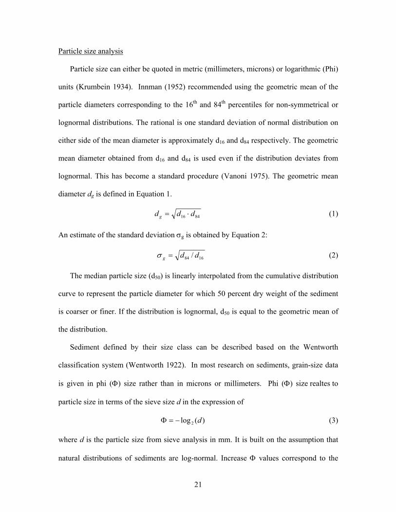
Particle size analysis

Particle size can either be quoted in metric (millimeters, microns) or logarithmic (Phi)

units (Krumbein 1934). Innman (1952) recommended using the geometric mean of the

particle diameters corresponding to the 16th and 84th percentiles for non-symmetrical or

lognormal distributions. The rational is one standard deviation of normal distribution on

either side of the mean diameter is approximately d16 and d84 respectively. The geometric

mean diameter obtained from d16 and d84 is used even if the distribution deviates from

lognormal. This has become a standard procedure (Vanoni 1975). The geometric mean

diameter dg is defined in Equation 1.

8416 ddd g ⋅= (1)

An estimate of the standard deviation σg is obtained by Equation 2:

1684 / ddg =σ (2)

The median particle size (d50) is linearly interpolated from the cumulative distribution

curve to represent the particle diameter for which 50 percent dry weight of the sediment

is coarser or finer. If the distribution is lognormal, d50 is equal to the geometric mean of

the distribution.

Sediment defined by their size class can be described based on the Wentworth

classification system (Wentworth 1922). In most research on sediments, grain-size data

is given in phi (Φ) size rather than in microns or millimeters. Phi (Φ) size realtes to

particle size in terms of the sieve size d in the expression of

)(log2 d−=Φ (3)

where d is the particle size from sieve analysis in mm. It is built on the assumption that

natural distributions of sediments are log-normal. Increase Φ values correspond to the

22

decreasing particle size. Particle size distribution was analyzed based on the cumulative

curve and Φ size. Several important phi sizes are summarized as follows.

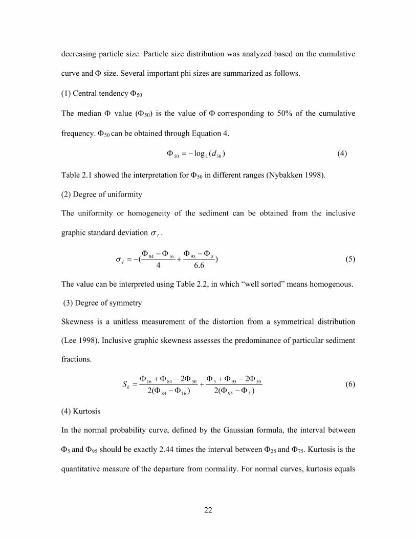
(1) Central tendency Φ50

The median Φ value (Φ50) is the value of Φ corresponding to 50% of the cumulative

frequency. Φ50 can be obtained through Equation 4.

)(log 50250 d−=Φ (4)

Table 2.1 showed the interpretation for Φ50 in different ranges (Nybakken 1998).

(2) Degree of uniformity

The uniformity or homogeneity of the sediment can be obtained from the inclusive

graphic standard deviation Iσ .

)6.64

( 5951684 Φ−Φ+

Φ−Φ−=Iσ (5)

The value can be interpreted using Table 2.2, in which “well sorted” means homogenous.

(3) Degree of symmetry

Skewness is a unitless measurement of the distortion from a symmetrical distribution

(Lee 1998). Inclusive graphic skewness assesses the predominance of particular sediment

fractions.

)(22

)(22

595

50955

1684

508416

Φ−ΦΦ−Φ+Φ

+Φ−Φ

Φ−Φ+Φ=kS (6)

(4) Kurtosis

In the normal probability curve, defined by the Gaussian formula, the interval between

Φ5 and Φ95 should be exactly 2.44 times the interval between Φ25 and Φ75. Kurtosis is the

quantitative measure of the departure from normality. For normal curves, kurtosis equals

23

1. A distribution that is excessively peaked is said to be leptokurtic. A distribution that is

squashed or flattened is called platykurtic. This parameter is an indication of the range of

particle sizes in the sample.

)(44.2 2575

590

Φ−ΦΦ−Φ

=GK (7)

The interpretation of Sk and KG can be found in Table 2.3.

Table 2.1 Central tendency analysis for particle size distribution based on Φ50

Φ50 Φ50<-1 -1< Φ50<0 0< Φ50<1 1< Φ50<2

Sediment type gravel very coarse

sand coarse sand medium sand

Φ50 2< Φ50<3 3< Φ50<4 4< Φ50<8 8< Φ50

Sediment type fine sand very fine

sand silt clay

Table 2.2 Uniformity analysis of particle size distribution based on σΙ

Iσ Iσ < 0.35 0.35 < Iσ < 0.5 0.5 < Iσ < 0.71 0.71 < Iσ < 1 Degree of

sorting very well

sorted well sorted moderately well sorted

moderately sorted

Iσ 1 < Iσ < 2 2 < Iσ < 4 4 < Iσ Degree of

sorting poorly sorted very poorly sorted

extremely poorly sorted

Table 2.3 Symmetry (Sk) and Kurtosis (KG) of particle size distribution

Sk Skewness KG Kurtosis

0.30 to 1.00 strongly skewed towards fine < 0.67 very platykurtic

0.10 to 0.30 fine skewed 0.67 – 0.90 platykurtic

-0.10 to 0.10 symmetrical 0.90 – 1.11 mesokurtic

-0.10 to -0.30 coarse skewed 1.11 – 1.50 leptokurtic

-0.30 to -1.00 strongly skewed towards coarse > 1.50 very leptokurtic

24

Density determination

Density of dry solids is determined using an inert gas pycnometer according to

Standard Method D5550-94 (ASTM 1994). The multi-pycnometer (Quantachrome Corp.)

measures the true volume of solid materials by employing Archimedes’ principle of fluid

(gas) displacement and the technique of gas expansion. True volume is measured using

helium gas since it penetrates every surface flaw down to about one Angstrom, thereby

enabling the measurement of powder volumes with great accuracy. By measuring the

pressure difference when a known quantity of helium under pressure is allowed to flow

from a precisely known reference volume (VR) into a sample cell (VC) containing the

solid material, true solid volume (VS) can be determined.

[ ]1)/( 21 −−= PPVVV RCS (8)

Density of the sample then can be calculated using Equation 7:

SSS VM /=ρ (9)

Particle density is typically reported to the nearest 0.01.

Surface area measurement

Modified EGME (ethylene glycol monoethyl ether) method (Sansalone et al. 1998)

was utilized for experimental determination of surface area. A representative sample of

approximately 1.0 g (except for the coarse materials in which a few representative

materials were selected regardless of the weight limit) dry weight was selected for each

discrete size range. Once a constant dry weight was obtained, each solid sample was

saturated with EGME, completely wetting all particle surfaces, and placed in an

evacuated glass dessicator over 600 grams of an EGME-CaCl2 solvate (The EGME to

CaCl2 ratio was 1 to 2.3). A constant vapor pressure was produced from this solvate.

25

Samples were held in an evacuated dessicator and weighted in 4-hour interval after 24

hours until a constant weight for each sample was obtained as determined by a weight

differential of less than 1-mg across an interval of four hours. Granular activated carbon

(GAC) was served as the control. Reported SSA for a Filtersorb F400 is 1100 m2/g by the

N2-BET method (Calgon 1995).

Based on monolayer surface coverage and molecular weight of the EGME molecule,

specific surface area (SSA) was calculated according to Equation 10:

S

a

WWSSA

000286.0= (10)

SSA results were summed over each size gradation to yield a total surface area (SA)

distribution. Equation 11 is employed in the surface area calculation.

))(( iii SSAmSA = (11)

SSA and SA are as a function of particle size gradation.

Surface charge determination

In combination with surface area, surface charge is a critical parameter for heavy

metal adsorption or filtration (Liu et al. 2001). Surface charge of particulate can be

developed in three principle ways: chemical reactions at the surface, lattice imperfections

at the surface, or adsorption of a hydrophobic species or a surface ion (Stumm 1992).

Potentiometric titration (Van Raij and Peech 1972) was modified and used to determine

the surface charge of sediments across size gradation. A representative 0.5 to 1-g of dry

sample was suspended in 50-mL of 0.01-M KCl. pH was adjusted to a range between 6

and 9 with HCl or KOH. A blank solution of 0.01-M KCl was set as control. The

suspensions of sample and control were set on a reciprocating table at 22 – 23 ºC in

26

airtight sealed 50-ml centrifuge tube for 24 hours. The pH values of the supernatant were

then recorded. The amount of H+ and OH- adsorbed on the surface of the sediment

samples were estimated from the amount of acid or base added to bring the sample to the

original pH, minus the amount necessary to bring 50-ml blank solution to the same pH.

RESULTS AND ANALYSIS

Differentiation of Solid Fractions

The entire flow stream was captured for the solid fraction analysis at Baton Rouge I-

10 site. Influent pipe was diverted from the sedimentation tank immediately after the tank

was filled. Total runoff volume and the elapsed time were recorded. A summary of

analyses of solid fractions for twelve observed rainfall-runoffs was shown in Table 2.4.

For the twelve storms observed, no significant correlation had been found between

previous dry hours, elapsed time of the event and the loading of transported sediments to

the system. Table 2.5 showed the statistic summary for solid fractions.

Total dissolved solids (TDS) serve as the indicator for the water quality criteria and

for assessment of use support. TDS ranged from 53 to 222 mg/L in the studied rainfall-

runoff. For water bodies not specifically listed in the Numerical Criteria and Designated

Table, increases over background levels of TDS may be permitted. Such increases shall

not cause in-stream concentrations to exceed 500 mg/L (USEPA 2000). To protect the

propagation of fish and wildlife, Louisiana’s water quality standard for TDS is 100 mg/L

(USEPA 2000). In five out of twelve investigated runoffs, TDS exceeded this limit.

Turbidity is primarily influenced by suspended matter such as clay, silt, plankton, or

microscopic organisms (APHA 1995).

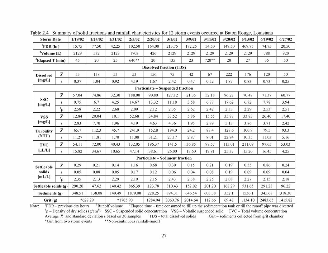
27

Table 2.4 Summary of solid fractions and rainfall characteristics for 12 storm events occurred at Baton Rouge, Louisiana Storm Date 1/19/02 1/24/02 1/31/02 2/5/02 2/20/02 3/1/02 3/9/02 3/11/02 3/20/02 5/13/02 6/19/02 6/27/02 1PDR (hr) 15.75 77.50 42.25 102.50 164.00 213.75 172.25 54.50 149.50 469.75 74.75 20.50

2Volume (L) 2129 532 2129 1703 426 2129 2129 2129 2129 2129 788 920 3Elapsed T (min) 45 20 25 640** 20 135 23 720** 20 27 35 50

Dissolved fraction (TDS)

x 53 138 53 53 156 75 42 67 222 176 120 50 Dissolved [mg/L] s 0.37 1.04 0.92 4.19 1.67 2.42 0.47 0.52 1.87 0.83 0.73 0.25

Particulate – Suspended fraction

x 57.04 74.86 32.30 188.00 90.80 127.12 21.35 52.18 96.27 70.47 71.37 60.77

s 9.75 6.7 4.25 14.67 13.32 11.18 3.58 6.77 17.62 6.72 7.78 3.94 SSC [mg/L]

4ρ 2.58 2.22 2.68 2.09 2.12 2.35 2.62 2.42 2.33 2.29 2.53 2.51

x 12.84 20.04 10.1 52.68 34.84 33.52 5.86 15.55 35.87 33.83 26.40 17.40 VSS [mg/L] s 2.83 7.70 1.96 4.19 4.63 4.36 1.95 2.89 5.13 3.86 3.71 2.42

x 65.7 112.3 45.7 241.9 152.8 194.0 24.2 88.4 128.6 100.9 79.5 93.3 Turbidity (NTU) s 11.27 11.81 1.70 11.08 31.21 23.17 2.87 8.01 22.84 10.35 11.03 5.16

x 54.11 72.00 40.43 132.05 196.37 141.5 36.85 98.57 113.01 211.09 97.65 53.03 TVC [µL/L] s 15.82 34.67 10.65 47.14 38.61 26.00 13.60 19.81 25.37 15.20 16.45 4.25

Particulate – Sediment fraction

x 0.29 0.21 0.14 1.16 0.68 0.30 0.15 0.21 0.19 0.55 0.86 0.24

s 0.05 0.08 0.05 0.17 0.12 0.06 0.04 0.08 0.19 0.09 0.09 0.04 Settleable

solids [mL/L] 4ρ 2.35 2.13 2.29 2.19 2.15 2.43 2.38 2.25 2.08 2.27 2.15 2.18

Settleable solids (g) 290.20 47.62 140.42 865.39 123.78 310.43 152.02 201.20 168.29 531.65 291.23 96.22

Sediments (g) 348.51 138.08 149.49 1879.00 228.25 894.31 646.54 603.38 352.1 1536.1 345.68 318.30

Grit (g) *627.29 *1705.90 1284.04 3060.76 2014.64 112.66 69.48 1134.10 2483.65 1415.82 Note: 1PDR – previous dry hours 2 Runoff volume 3Elapsed time – time consumed to fill up the sedimentation tank or till the runoff pipe was diverted 4ρ – Density of dry solids (g/cm3) SSC – Suspended solid concentration VSS – Volatile suspended solid TVC – Total volume concentration Average x and standard deviation s based on 30 samples TDS – total dissolved solids Grit – sediments collected from grit chamber *Grit from two storm events **Non-continuous rainfall-runoff

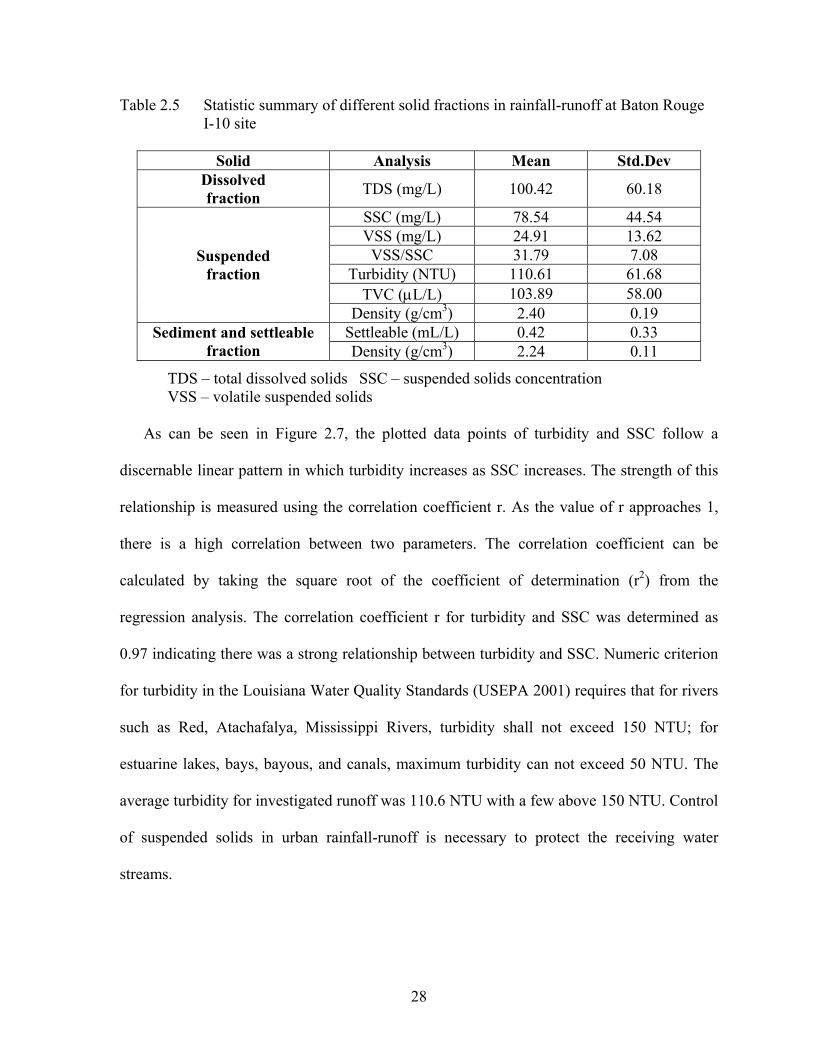
28

Table 2.5 Statistic summary of different solid fractions in rainfall-runoff at Baton Rouge I-10 site

Solid Analysis Mean Std.Dev

Dissolved fraction TDS (mg/L) 100.42 60.18

SSC (mg/L) 78.54 44.54 VSS (mg/L) 24.91 13.62

VSS/SSC 31.79 7.08 Turbidity (NTU) 110.61 61.68

TVC (µL/L) 103.89 58.00

Suspended fraction

Density (g/cm3) 2.40 0.19 Settleable (mL/L) 0.42 0.33 Sediment and settleable

fraction Density (g/cm3) 2.24 0.11

TDS – total dissolved solids SSC – suspended solids concentration VSS – volatile suspended solids

As can be seen in Figure 2.7, the plotted data points of turbidity and SSC follow a

discernable linear pattern in which turbidity increases as SSC increases. The strength of this

relationship is measured using the correlation coefficient r. As the value of r approaches 1,

there is a high correlation between two parameters. The correlation coefficient can be

calculated by taking the square root of the coefficient of determination (r2) from the

regression analysis. The correlation coefficient r for turbidity and SSC was determined as

0.97 indicating there was a strong relationship between turbidity and SSC. Numeric criterion

for turbidity in the Louisiana Water Quality Standards (USEPA 2001) requires that for rivers

such as Red, Atachafalya, Mississippi Rivers, turbidity shall not exceed 150 NTU; for

estuarine lakes, bays, bayous, and canals, maximum turbidity can not exceed 50 NTU. The

average turbidity for investigated runoff was 110.6 NTU with a few above 150 NTU. Control

of suspended solids in urban rainfall-runoff is necessary to protect the receiving water

streams.

29

SSC (mg/L)

0 40 80 120 160 200

Turb

idity

(NTU

)

0

50

100

150

200

250

300

r2 = 0.94

Figure 2.7 Relationship of turbidity and suspended solid concentration (SSC)

Solid fractions in the sedimentation tank were calculated based on mass and results were

shown in Figure 2.8. As seen in Figure 2.8, suspended solid fraction ranged from 6.6 to 36.8

% with an average value of 19.7%. Settleable solids made up of 40% in average of the

sediments deposited in the system. There was approximately 60% of the material in the

sediments remaining in suspension subsequent to 1-hour sedimentation though they might be

settled afterwards. Experimental results showed there was no significant difference in total

volume concentration for the suspension after 1-hour and 4-hour gravitational settling.

Therefore, in general, approximately 68% of the materials remained in suspension after the

first few hours in the stormwater treatment system.

Granulometry of Suspended Fraction

Figure 2.9 showed the number distribution and volume distribution for the suspended

particulate matter in the urban rainfall-runoff. Number distribution of aquatic suspensions is

found to follow a two-parameter power law distribution function given by the expression

(Kavanaugh et al 1980):

30

βα −= ldl

dN (12)

If 3=β , the concentration of surface area is uniformly distributed in each logarithmic size

interval. The volume or the mass of solids is predominated in the large sizes while the

number concentration is dominant in the smaller sizes. If 4=β , the volume of solids is

distributed equally in each logarithmic size interval while the surface area and number

concentrations are primarily in the small sizes. Measured particle number distributions were

modeled using the two-parameter power law functions as shown in Figure 2.9. The

coefficient of determination (r2) was 0.98 or greater. Majority of particles (greater than 100-

µm) were removed in 1-hour settling.

Susp

ende

d fr

actio

n %

0

20

40

60

80

100

Sedi

men

t/Set

tleab

le fr

actio

n %

0

20

40

60

80

100

Suspended Solids Sediment Settleable

1/19

/02

1/24

/02

1/31

/02

2/05

/02

2/20

/02

3/01

/02

3/09

/02

3/11

/02

3/20

/02

5/13

/02

6/19

/02

6/27

/02

Figure 2.8 Solid fractions in storm water runoff for twelve observed storm events at Baton Rouge site (settleable is a fraction of sediment)

31

0

5

10

15

20

012345678

0

5

10

15

20

1 10 1000

5

10

15

20

012345678

Particle diameter (µm)1 10 100

0

5

10

15

20

0

5

10

15

200

5

10

15

20

0

5

10

15

20

Log

Cum

ulat

ive

num

ber d

istri

butio

n (c

ount

/cm

3 )

012345678

Vol

ume

Dis

tribu

tion

(µL/

L)

0

5

10

15

201/19/02r2 = 0.98β = 3.797

6/19/02r2 = 0.9β = 3.233

1/24/02r2 = 0.99β = 3.844

6/27/02r2 = 0.99β = 3.668

0

5

10

15

20

012345678

0

5

10

15

201/31/02r2 = 0.99β = 3.432

2/05/02r2 = 0.99β = 4.008

0

5

10

15

20

012345678

2/20/02r2 = 0.98β = 3.140

3/01/02r2 = 0.99β = 3.447

0

5

10

15

20

012345678

3/09/02r2 = 0.99β = 3.038

3/11/02r2 = 0.99β = 3.137

3/20/02r2 = 0.98β = 3.766

5/13/02r2 = 0.99β = 3.038

Figure 2.9 Total volume concentration and power law fit for the number distribution

32

Median diameter by number d50n and median diameter by volume d50v were calculated for

all twelve events and summarized in Table 2.6. The median d50n for all 12 storms were less

than 2-µm with the average Φ50n size of 9.27, while the median d50v for all the sites were less

than 20-µm with the average Φ50v size of 6.72, indicating that the particles in the suspension

are very similar in size to silt and clay particles. These particles are of colloidal size and

would theoretically require extended periods of detention (Drapper et al. 2000). Though

interactions with dissolved fractions may assist in the flocculation and sedimentation of

particulates in urban rainfall-runoff (Drapper et al. 2000), chemical coagulation and

flocculation is still required for the advanced treatment of these suspended particles or

produce an acceptable settling time.

Table 2.6 Median diameter and Φ size of suspended fraction

Storm Date d50n d50v Φ50n Φ50v 1/19/02 1.60 7.47 9.28 7.06 1/24/02 1.59 6.69 9.30 7.22 1/31/02 1.61 7.47 9.28 7.06 2/05/02 1.60 5.89 9.29 7.41 2/20/02 1.71 18.27 9.19 5.77 3/01/02 1.65 8.32 9.24 6.91 3/09/02 1.61 17.53 9.28 5.83 3/11/02 1.64 13.67 9.25 6.19 3/20/02 1.61 6.50 9.28 7.26 5/13/02 1.56 11.92 9.33 6.39 6/19/02 1.66 15.00 9.24 6.06 6/27/02 1.57 5.53 9.31 7.50 Mean 1.62 10.36 9.27 6.72

Std.dev 0.042 4.686 0.037 0.633

According to the calculation by Newton’s Law assuming spherical particles, particles

greater than 75-µm (settling velocity 0.514-cm/s) can be separated in the storm water

treatment system. However, the existence of particles up to 100-µm in the suspension

suggested that the settling behavior of the real particles differ from particles settled under

33

ideal circumstances. Besides gravitational and frictional drag force, short-range forces such

as electrostatic forces, Van De Waals and hydrodynamic forces affect particle interaction and

settling as well. The other factors affecting settling velocity include fractal structure of

particles, flow regime, coagulation and flocculation.

Granulometry of Sediment Fraction

Particle size distribution

Sediments in the runoff originate primarily from particulate matter deposited on

impervious areas (Sharpin 1995). If the sediments are from the same type of impervious area,

similar particle size distributions is expected. Cumulative distribution curve is constructed by

plotting the percent of sediment by weight that is finer than a given sieve size against the

sieve diameter or particle diameter. Figure 2.10 showed the cumulative particle size

distribution for the sediments collected out of 12 rainfall-runoff events at Baton Rouge site.

Although the distributions illustrated variability between storm events, they were similar in

shape. Characteristics of particle size distribution were summarized in Table 2.7 and Table

2.8. The average median diameter based on mass for the twelve events was 172-µm

corresponding to a Φ size of 2.63, indicating that particulates in the sedimentation tank are

similar in size to fine sand. Gravel size particulates were intercepted in the grit chamber and

did not account for the sediment loads in the sedimentation tank. Solids in grit chamber are

mainly coarse sand (Φ50 = 0.66, Table 2.9), and this portion can be easily separated from the

runoff stream through gravitational settling. Sediments from three other sites were analyzed

similarly. Figure 2.11 showed the cumulative particle size distribution. The characteristics of

particle size distribution were summarized in Table 2.10 and Table 2.11. If combining

sediments from grit chamber and sedimentation tank for Baton Rouge site, a median size of

34

682-µm (Φ50 = 0.57) was obtained. This Φ size indicated that based on mass particulates in

the urban storm runoff tend to be coarser sand at Baton Rouge site. Little Rock site 2 showed

similar trend. However, sediment analysis for New Orleans site and Little Rock site 1

showed the majority mass resides in medium sand size range.

Particle Diameter (µm)10 100 1000 10000

% fi

ner b

y m

ass

0

20

40

60

80

100

2/05/02

3/01/023/09/023/11/023/20/025/13/026/19/026/27/02

1/19/021/24/021/31/02

2/20/02

Figure 2.10 Cumulative size distribution for the sediments collected at Baton Rouge I-10

site from twelve storm events

Particle Diameter (µm)

10 100 1000 10000

% fi

ner b

y m

ass

0

20

40

60

80

100

Little Rock-1Little Rock-2New OrleansBaton Rouge

Figure 2.11 Cumulative size distribution for the sediments collected at four different sites. Sediments from Baton Rouge sites combined sediments from storage tank and grit chamber.

35

Table 2.7 Summary of statistical characteristics of particle size distribution for the sediments at Baton Rouge site

Storm Date

d50

(µm) Φ50 dg

(µm) σg Iσ Sk KG

1/19/02 169 2.56 248 3.42 1.72 0.36 0.77 1/24/02 164 2.61 174 3.45 1.73 0.16 0.75 1/31/02 95 3.40 158 3.21 1.61 0.51 0.63 2/05/02 270 1.89 227 3.50 1.72 -0.04 0.76 2/20/02 110 3.18 184 2.84 1.48 0.55 0.65 3/01/02 158 2.66 180 3.29 1.67 0.22 0.64 3/09/02 99 3.33 139 3.61 1.84 0.33 0.89 3/11/02 209 2.26 200 2.90 1.52 0.05 0.92 3/20/02 244 2.04 248 2.46 1.36 0.13 0.77 5/13/02 262 1.93 265 3.93 1.94 0.10 0.86 6/19/02 177 2.50 197 2.32 1.36 0.27 1.02 6/27/02 105 3.25 151 2.34 1.30 0.49 0.70 Mean 172 2.63 198 3.11 1.60 0.26 0.78

Std.dev. 63.35 0.55 41.25 0.53 0.20 0.19 0.12

36

Table 2.8 Summary of particle size distribution characteristics for the sediments at Baton Rouge site

Storm Date

Central tendency Uniformity Skewness Kurtosis

1/19/02 fine sand strongly skewed towards fine particles platykurtic

1/24/02 fine sand fine skewed platykurtic

1/31/02 very fine sand strongly skewed towards fine particles

very platykurtic

2/05/02 medium sand symmetrical platykurtic

2/20/02 very fine sand strongly skewed towards fine particles platykurtic

3/01/02 fine sand fine skewed very platykurtic

3/09/02 very fine sand strongly skewed towards fine particles platykurtic

3/11/02 fine sand symmetrical platykurtic

3/20/02 fine sand fine skewed platykurtic

5/13/02 medium sand symmetrical platykurtic

6/19/02 fine sand fine skewed mesokurtic

6/27/02 very fine sand

poorly sorted

strongly skewed towards fine particles platykurtic

Table 2.9 Statistical characteristics of particle size distribution for grit at Baton Rouge site

Storm Date

d50

(µm) Φ50 dg

(µm) σg Iσ Sk KG

3/05/2001 668 0.60 945 4.02 1.91 0.17 0.81 4/24/2001 735 0.47 969 3.90 1.87 0.14 0.80 2/05/2002 682 0.57 1066 4.19 1.97 0.24 0.76 3/01/2002 510 0.99 773 4.30 2.02 0.19 0.89

Mean 649 0.66 938 4.10 1.94 0.18 0.81 Std.dev. 96.64 0.23 121.89 0.18 0.07 0.04 0.05

Grit property coarse

sand poorly sorted

fine skewed platykurtic

37

Table 2.10 Summary of statistical characteristics of particle size distribution for the settleable solids and sediments collected from four different sites

Sample Site d50(µm) Φ50 dg(µm) σg Iσ Sk KG Little Rock 1 248 2.01 265 2.19 1.26 0.13 0.95 Little Rock 2 587 0.77 807 4.04 1.98 0.13 0.93 New Orleans 216 2.23 296 2.10 1.46 0.47 1.31

Baton Rouge* 633 0.67 844 5.20 2.23 0.13 0.78 Mean 421 1.42 553 3.38 1.73 0.22 0.99

Std.dev. 219 0.81 315 1.51 0.45 0.17 0.22

Table 2.11 Summary of particle size distribution characteristics for the sediments at Baton Rouge site

Sample Site Central tendency Uniformity Skewness Kurtosis

Little Rock 1 fine sand fine skewed mesokurtic

Little Rock 2 coarse sand fine skewed mesokurtic

New Orleans fine sand

poorly sorted

strongly skewed towards fine particles leptokurtic

Baton Rouge* coarse sand very poorly

sorted fine skewed platykurtic

* Sediments from Baton Rouge are cumulative sediments from both grit chamber and sedimentation tank.

Physical properties of sediments

Particulate materials transported by the urban runoff are heterogeneous. Organic matter

such as leaves and other plant materials, wood pieces, straw and tire debris have a higher

percentage in the large size range. Majority of these materials were intercepted by 425-µm

sieve or above. Density of such materials is relatively low compared to the inorganic sand

particles. Measured density for the oak leaves is 1.94-g/cm3. Results of experimental

determination of density for materials collected at Baton Rouge site was illustrated in Figure

2.12. The measured results showed that density of sediments was relatively consistent for the

materials less than 425-µm and within the range of 2.2 – 2.6 g/cm3. Density of solids in the

38

grit chamber was consistently higher than density of the sediments in the storage tank. Such

variation in density affects sediment transport by gravitational separation.

Particle Diameter (µm)

9500

4750

2000 85

060

042

530

025

018

015

010

6 75 63 53 45 38 25

Den

sity

(g/c

m3 )

1.0

1.5

2.0

2.5

3.0

GritSediment

Figure 2.12 Mean and standard deviation trends for granulometric-based density of particulate materials captured from 12 individual rainfall-runoff events at the Baton Rouge site. The grit fraction was captured in a pre-screening grit chamber and the sediment fraction captured in a sedimentation basin. The entire mass of grit and sediment were recovered and analyzed for each event.

Density of sediments accumulated in storm water runoff catchments showed similar trend

for the sites of Baton Rouge, New Orleans and Little Rock site 2. As shown in Figure 2.13,

the densities are within the range of 2.2 – 2.6 g/cm3 which is close to the results measured for

street surface sediments (Butler et al. 1992) and solids transported in suspension in

stormwater sewers (Jacopin et al. 1999). Density of sediments from Little Rock site-1

showed a similar pattern as that of sediments collected from individual storm event at Baton

Rouge site.

Measured specific surface area (SSA) across size gradation was shown as vertical error

bars and calculated total surface area (SA) based on 1000-g mass was plotted as vertical bars

on the same graph. Figure 2.14 showed SSA, SA and cumulative SA% for the sediments at

Baton Rouge site. SSA was extraordinary high for particles greater than 425-µm due to the

39

large percent of organic materials in them. SSA leveled at approximate 40-m2/g for particles

less than 425-µm. Total surface area is as a function of specific surface area and the mass

distribution. Variability in mass distribution for the different storm events contributes to the

variability of total surface area.

Figure 2.15 showed the results of surface area for the accumulative sediments from four

urban transportation sites. A general trend of increasing SSA with decreasing size for the

particles less than 425-µm was observed. Corresponding to the low-density organic

materials, particles within large size end still possessed an unstable high SSA as seen in the

results for sediments from Little Rock site 1. Complicated particle surfaces such as folds,

pores, notches, pits and roughness contribute to the additional surface area especially for fine

particles (Sansalone 1998). As a consequence, SSA is a function of not only particle size, but

also particle shape, density and composition. It has been found that sediments from Baton

Rouge and New Orleans have higher SSA than the sediments from Little Rock.

Surface chemistry

The potentiometric titration curves for storm runoff sediments across size gradation are

shown in Figure 2.16. PZC was determined according to surface charge and was shown in

the same plot. Surface charge of particles decreases with increase of pH. PZC was ranging

from 7 to 9. For the four sites studied, smaller particle at Baton Rouge and Little Rock site 1

had lower PZC compared to New Orleans and Little Rock site 2.

40

9500

4750

2000 85

060

042

530

025

018

015

010

6 75 63 53 45 38 25

Little Rock-1Little Rock-2

Particle Diameter (µm)

9500

4750

2000 85

060

042

530

025

018

015

010

6 75 63 53 45 38 25

Den

sity

(g/c

m3 )

1.0

1.5

2.0

2.5

3.0

Baton RougeNew Orleans

Figure 2.13 Mean and standard deviation trends for granulometric-based density of accumulated (multiple rainfall-runoff events) sediments collected from Baton Rouge, Little Rock and New Orleans sites.

Particle diameter (µm)

850

600

425

300

250

180

150

106 75 63 53 45 38 25

SSA

(m2 /g

)

0

30

60

90

120

15085

060

042

530

025

018

015

010

6 75 63 53 45 38 25

SA (m

2 )

0

2000

4000

6000

8000

10000

Cum

ulat

ive

SA%

0

20

40

60

80

100

Figure 2.14 Specific surface area (SSA) and surface area (SA) (based on 1000-g dry mass) for sediments from twelve observed individual storms at Baton Rouge site. Range bars on incremental values represent standard deviations of all twelve events while the shaded bars represent the mean value for the site. Cumulative curve is based on the mean value.

41

9500

4750

2000 85

060

042

530

025

018

015

010

6 75 63 53 45 38 25

0

1000

2000

3000

4000

5000

0

20

40

60

80

1000

1000

2000

3000

4000

5000

0

20

40

60

80

1000

1000

2000

3000

4000

5000

0

20

40

60

80

100

0

20

40

60

80

100

Particle diameter (µm)

9500

4750

2000 85

060

042

530

025

018

015

010

6 75 63 53 45 38 25

0

20

40

60

80

100

Little Rock-1 Little Rock-1

Little Rock-2 Little Rock-2

Spec

ific

surf

ace

aera

(m2 /g

)

0

20

40

60

80

100

Surf

ace

aera

(m2 )

0

1000

2000

3000

4000

5000

Cum

ulat

ive

SA %

0

20

40

60

80

100

0

20

40

60

80

100

Baton Rouge Baton Rouge

New Orleans New Orleans

Figure 2.15 Specific surface area and total surface area (based on 1000-g of sediments) for the sediments from four urban transportation sites in three USA cities

42

Surf

ace

char

ge ( µ

mol

/m2 )

-1

0

1

2

3

4

5

Particle diameter (µm)

600-

425

425-

300

300-

250

250-

180

180-

150

150-

106

106-

7575

-63

63-5

353

-45

45-3

838

-25

600-

425

425-

300

300-

250

250-

180

180-

150

150-

106

106-

7575

-63

63-5

353

-45

45-3

838

-25

PZC

-pH6.0

6.5

7.0

7.5

8.0

8.5

9.0

5.5 6.0 6.5 7.0 7.5 8.0 8.5 9.0 9.5-1

0

1

2

3

4

5Little Rock 1

pH

5.5 6.0 6.5 7.0 7.5 8.0 8.5 9.0 9.56.0

6.5

7.0

7.5

8.0

8.5

9.0

Baton Rouge New Orleans

Little Rock 2

38-25 µm

PZC-pH

600-425 µm425-300 µm300-250 µm

250-180 µm180-150 µm150-106 µm

106-75 µm75-63 µm63-53 µm

53-45 µm45-38 µm

Figure 2.16 Surface charge and PZC for the particles across size gradation

43

CONCLUSIONS

Urban storm water is a significant source of anthropogenic particulate matter, colloids

and solutes, with solutes partitioning between particulate, colloidal and solution phases.

Through sampling the entire urban runoff flow from an elevated urban transportation site,

solid fractions were studied and their granulometric properties were characterized. The study

aims to provide guidance for treatability, regulation and control of non-colloidal particulate

matter. Several conclusions were summarized as follows:

1. Analyses of solid fractions for sediments in a sedimentation tank showed that

approximately 68% of the materials remained in suspended status after the first few hours’

retention. Results of particle analysis indicate that the suspended fraction d50V based on

volume distribution was [10.36, 4.69] µm, Sρ was [2.40, 0.19] g/cm3 from all twelve

rainfall-runoff events. The number based d50n was [1.62, 0.04] µm for the suspended fraction,

indicating that the particles in the suspended fractions are similar in size to silt and clay.

2. Sediments from Baton Rouge site showed similar granulometric characteristics. d50 for

the sediment fraction was [172, 63.35] for all 12 rainfall-runoff events, indicating that

particles in the sedimentation tank are similar in size to fine sand. Coarser sands were

intercepted by the grit chamber prior to sedimentation tank. This portion could be easily

separated from the runoff stream by gravitation settling. The particle size distributions for the

accumulative sediments at four sites showed a great variability.

3. Density of sediments is consistent for the materials less than 425-µm and within the

range of 2.2 – 2.6 g/cm3. Density of solids in the grit chamber is consistently higher than

density of the sediments in the storage tank.

44

4. Over 50% of SA was associated with the particulate gradation >250-µm. Sediments from

Baton Rouge and New Orleans have higher SSA than the sediments from Little Rock.

Results suggest that a solute mass can preferentially partition to the gradation of particles

with predominant SA.

IMPLICATIONS FOR BEST MANAGEMENT PRACTICES

A central conundrum in storm water treatment is the bioavailability, toxicity, mobility of

contaminants, all associating with granulometry of particles in urban storm runoff. The

ability of best management practices (BMPs) to remove particulate-bound particles from

runoff stream increase with particle size, however, bioavailability and mobility of pollutants

decrease with particle size. Development and design of treatment methods are based on the

granulometry characteristics. For example, the granulometric distribution of a specific-site

shows dominance of median to coarse materials. Sedimentation would be an effective

treatment. BMP efficiency can be determined through the granulometry of particles. The

degree to which contaminants partition to each solid fraction depends on several key physical

characteristics of the particle such as surface area and surface charge potential. A predicative

granulometric-metal model is expected to be developed to optimize the current BMPs and

guild future design.

REFERENCES

Allen, T. (1990). Particle Size Measurement, 4th ed. Chapman & Hall, 125-127.

ASTM. (1993). “Standard Practice for Dry Preparation of Soil Samples for Particle-Size Analysis and Determination of Soil Constants.” ASTM D 421-85, West Conshohocken, Pa. Vol. 04.08, 8-9.

ASTM. (1994). “Standard test method for specific gravity of soil solids by gas pycnometer.” ASTM D 5550-94, West Conshohocken, Pa. Vol. 04.08, 376-379.

45

APHA. (1995). “Standard methods for the Examination of Water and Wastewater, 19th ed.” American Public Health Association, Washington. DC.

Ball, J.E., and Abustan, I. (1995). “An investigation of particle size distribution during storm events from an urban catchment.” The Second International Symposium of Urban Stormwater Management, Melbourne, Australia, 531-535.

Bedient, P. B. and Huber, W. C. (1992). Hydrology and floodplain analysis. Addison Wesley Publishing, Massachusetts.

Butler, D., Thedchanamoorthy, S., and Payne, J. (1992). “Aspects of surface sediment characteristics on an urban catchment in London.” Wat. Sci. Tech. 25(8),13-19.

Calgon Carbon Corporation. (1995). F400 specification sheet, P.O. Box 717, Pittsburgh, Pennsylvania, 15230-0717.

Drapper, D., Tomlinson, R. and Williams, P. (2000). “Pollutant concentrations in road runoff: Southeast Queensland case study.” J. Enviro. Engrg., ASCE, 126(4), 313-320.

Gjessing, E., Lygren, E., Anderson, S. et al. (1984). “Acute toxicity and chemical characteristics of moderately polluted runoff from highways.” Sci. of the Total Envir., 15(33).

Grant, S.B., Joon Ha Kim, and Poor, C. (2001). “Kinetic theories for the coagulation and sedimentation of particles.” J. of Colloid and Interface Sci., 238, 238-250.

Gray, John R., Glysson, D., Turcios, L., and Schwarz, G. (2000). “Comparability of suspended-sediment concentration and total suspended solids data.” Water-Resources Investigation Report 00-4191, USGS.

Gustafsson, O., and Gschwend, P.M. (1997). “Aquatic colloids: Concepts, definitions, and current challenges.” Limnology and Oceanography., 42(3), 519-528.

Horowitz, A.J., Rinella, F., Lamothe, P. Et al.(1990). “Variations in suspended sediment and associated trace element concentrations in selected riverine cross sections.” Environ. Sci. Technol., 24, 1313.

Innman, D. L. (1952). “Measures for describing the size distribution of sediments.” Journal of Sedimentary Petrology, 22(3), 125-145.

James, R. (1999). “Solids in Storm Water Runoff.” Water Resources Management.

46

Jacopin, C., Bertrand-Krajewski, J., and Desbordes, M. (1999). “Characterization and settling of solids in an open, grassed, stormwater sewer network detention basin.” Wat. Sci. Tech. 39(2), 135-144.

Kavanaugh, M.C. (1980). Use of Particle Size Distribution Measurements for Selection and Control of Solid/Liquid Separation Processes. In Particulates in Water. Kavanaugh, M. C., and Leckie, J. O. eds. American Chemical Society, Washington, D.C.

Krumbein, W.C. (1934). “Size frequency distributions of sediments.” J. Sediment. Petrol., 4, 65-77.

Kobringer, N. P. (1984). “Volume I. Sources and migration of highway runoff pollutants.” FHWA/RD-84/057, Federal Highway Administration, Rexnord, EnvironEnergy Technology Center, Milwaukee, WI.

Koomans, R. (2000) Sand in motion : Effects of density and grain size. Proefschrift Rijksuniversiteit Groningen.

Lee, A. (1998). Analysis of sediment samples for USEPA Region IV: Science and ecosystem support division Fenholloway River. Mote Marine Laboratory Technical Report No. 572.

Liu, D. F., Teng, Z., Sansalone, J., and Cartledge, F. (2001). “ Surface characteristics of sorptive-filtration storm water media. I: Low density (ρs< 1.0) oxide-coated buoyant media.” J. of Envir. Engrg., 127(10), 868-878.

Luoma, S.N. (1989). “Can we determine the biological availability of sediment-bound trace elements?” Hydrobioloia, 176, 379-396.

Makepeace, D., Smith, D., and Stanley, S. (1995). “Urban stormwater quality: Summary of contaminant data.” Critical Reviews in Environmental Science and Technology, 25(2), 93-139.

Morrison, G., Revitt, D., and Ellis, J. (1990). “Metal speciation in separate stormwater systems.” Wat. Sci. Tech., 22(10/11), 53-60.

Muschack, W. (1990). “Pollution of street run-off by traffic and local conditions.” Sci. of the Total Envir., 93, 419-431.

Nybakken, J.W. (1998) Marine Biology, an ecological approach. (2nd edition), Harper & Row, New York.

Roberts, T. L., Crowe, J. A., and Leonard, L. A. (2001). Suspended particulate matter characteristics in the Lower Cape Fear River System. GSA Southeastern Section – 50th Annual meeting, Raleigh, North Carolina.

47

Sansalone, J., and Buchberger, S. (1996). “Characterization of metals and solids in urban highway snow and rainfall-runoff.” Transportation Research Record, 1523, 147-159.

Sansalone, J., and Buchberger, S. (1997). “Partitioning and first flush of metals in urban roadway storm water.” J. of Envir. Engrg., 123(2), 134-143.

Sansalone, J., Koran, J., Smithson, J., and Buchberger, S. (1998). “Physical characteristics of highway solids transported during rainfall.” J. of Envir. Engrg., 124(5), 427-440.

Sartor, J.D., and Boyd G.B. (1972). Water pollution aspects of street surface contaminants. EPA-R2-72-081. 236.

Schueler, T. (1992). Design of stormwater wetland systems: Guidelines for creating diverse and effective stormwater wetland systems in the Mid-Atlantic region. Metropolitan Washington Council of Governments.

Shaheen, D. (1975). Contribution of Urban Roadway Usage to Water Pollution. EPA-600/2-75-004.

Sinclair, P., Beckett, R., and Hart, B.(1989). “Trace elements in suspended particulate matter from the Yarra River, Australia.” Hydrobiologia. 176, 239-251.

Stumm, W. (1992). Chemistry of the solid-water interface: processes at the mineral-water and particle-water interface in natural systems. John Wiley & Son, Inc.

USEPA. (2000). Bayou Boeuf TMDL for total dissolved solids (TDS). SUBSEGMENT 060208. USEPA Region 6.

USEPA. (2001). TOTAL MAXIMUM DAILY LOAD (TMDL) for TSS, Turbidity, and Siltation, for the 15 Subsegments in the Vermilion River Basin, 303(d) listed subsegments, USEPA Region 6.

Vanoni, V. A. (1975). Sedimentation Engineering. ASCE Manual No. 54, ASCE, Reston, VA.

Van Raij, B., and Peech, B. (1972). “Electrochemical properties of some Oxisols and Alfisols of the tropics.” Soil Sci. Sco. Amer. Proc., 36, 587-593.

Wentworth, C.K. (1922). “A scale of grade and class terms for clastic sediments.” J.Geol., 30, 377-392.

48

NOMENCLATURE

gd = geometric mean diameter

50d = median particle size based on particle mass

nd50 = median particle size based on particle distribution

vd50 = median particle size based on particle volume

Φ = Phi size, index of grain size distribution in sediment

Iσ = inclusive graphic standard deviation

kS = skewness

GK = kurtosis

sρ = density of particle (g/cm3)

VS = true sample volume (cm3)

VC = cell volume of pycnometer (cm3)

VR = reference volume of pycnometer (cm3)

P1 = initial pressure (psi)

P2 = final pressure (psi)

Ms = mass of the sample determined prior to placement in the pycnometer (g)

Vs = volume of specimen (cm3)

SSA = specific surface area (m2/g)

Wa = measured weight of EGME retained by sample (g)

Ws = measured weight of dried sample (g)

SAi = surface area of solids having particle diameter i (m2)

mi = mass of solids having particle diameter i (g)

SSAi = specific surface area of solids having particle diameter i (m2/g)

N = particle number density

l = characteristic particle size

α , β = empirical constants 2r = coefficient of determination

PSD = particle size distribution

NPDES = national pollutant discharge elimination system

EGME = ethylene glycol monoethyl ether

49

CHAPTER 3. GRANULOMETRIC-BASED DISTRIBUTION OF METALS FOR NON-COLLOIDAL PARTICULATE MATTER TRANSPORTED

BY URBAN RAINFALL-RUNOFF

SUMMARY

Metal element is partitioning between dissolved, colloidal and particulate phases and

transported by urban rainfall-runoff. Partition of metal elements between dissolved and

particulate phase was studied through experimental phase fractionation of urban rainfall-

runoff. Particulate matters deposited from eight discrete storm events at Baton Rouge,

Louisiana were examined for metal contamination. Results indicated that a significant

reduction was achieved in total metal concentration for Cr, Cu, Zn and Pb by settling out

the settable fraction. However, removal of settleable fraction does not translate to large

overall reduction in total concentration for As and Cd because of their relative high

dissolved fraction. As indicated by mass distribution, metal mass was dominant in medium

to coarse (75 < d < 2000 µm) materials although fine particles (< 75-µm) were associated

with a high level of metal concentration. The cumulative seasonal sediments collected

from four storm catch basins at different urban transportation sites were characterized as

well. No significant accumulative effect was found on metal concentration in the

sediments. A cumulative power law model was utilized to predict metal mass from the

granulometric indices in lieu of metal analyses. The utilization of this model is to assist the

development of particle separation operations in stormwater best management practices to

target the portion of mass gradation where the predominant metal mass is associated.

INTRODUCTION

Rainfall-runoff from urban land uses transports a wide gradation of particulate matter

associated with a significant load of metal elements. Direct pollution is upon the aquatic

50

life in the receiving water system. This pollution may result in the destruction of fish,

wildlife, and aquatic life habitats and threats to public health due to contaminated food,

drinking water supplies and recreational waterways. Studies on 541 streambed-sediment

samples collected across United States showed that 49 percent of the sites sampled in

urban settlings had concentrations of one or more trace metal elements that exceeded levels

at which adverse effects could occur in aquatic biota (Rice 1999). Metals Cr, Cu, Zn, As,

Cd and Pb are among the most critical stormwater contaminants affecting aquatic life

(Makepeace 1995).

Routine traffic and highway maintenance regimes are significant contributory sources

of both particulates and metals. The abrasion of metal containing vehicular parts and the

vigorous abrasion of vehicular tires against the pavement surface are primary sources of

metals (Sansalone and Glenn 2002). Abraded pavement and abraded tire were reported to

constitute 40-50% and 20-30% of the total particulate matter generated (Kobriger and

Geinopolos 1984). Infrastructure is also an important source of anthropogenically

generated constituents. For instance, zinc-galvanized guardrails contain zinc coating

concentrations ranging from 4.5 up to 10.5 g/m2 (Sansalone 2001).

PREVIOUS STUDIES

Metal loadings in urban rainfall-runoff have been studies extensively. On heavily

traveled highways Cu, Zn, Cd and Pb often exceed surface water discharge criteria of

USEPA and State EPA on an event basis (Sansalone et al 1997). Previous work

emphasized on individual pollution investigations of four metals Cr, Cu, Pb and Zn

because the hazardous or toxic effects of these metals are among the most serious. Pb, for

instance, is carcinogenic chemical and may cause kidney tumors. Non-carcinogenic effects

51

of lead include anemia, high blood pressure, IQ impairment and decreased learning

(LaGrega et al. 1994). There existed a large variability of individual metal loadings within

each road category, typically ranging over several orders of magnitude (Ellis and Revitt

1982). A concrete surface was reported to yield high levels of Zn and Pb compared to an

asphalt surface (Hird 2001). The concentrations of constituents varied widely during the

history of each storm and appeared to be highest in the first flush (Shinya et al 2000). From

both a hydrological and geochemical viewpoint, gravel-size sediments (≥ 2000 µm) are

generally considered to be less important in the transport of adsorbed metals from urban

areas (Sartor and Boyd 1972). Several studies (Ellis and Revitt 1982, Xanthopoulos and

Augustin 1992, Sansalone and Buchberger 1996, Milligan and Loring 1997) have found

that most metals have a greater affinity for smaller particle sizes. Benthic organisms may

be directly exposed to fine-grained (< 63 µm) fraction (Davis and Atkins 2001), therefore

removal of fine particulates is critical for the protection of biota. Although the highest

metal concentration typically occur in the fine size fraction (<17 µm), the medium sand

fraction (75-300 µm) was reported to have the largest percentage contribution to the total

metal mass (Murray 1999). In the study by Shinya (Shinya et al 2000) a correlation was

found between the metal concentrations and particulate diameter for Cu, Zn and Pb during

a certain range. However, study on street sediments for Sault Ste Marie (Stone and

Marsalek 1996) indicated that correlations between metal content and size fractions are

either very weak or non-existent.

A sequential selective extraction of metals was carried out on sediments of various

origins (Chartier et al. 2001). Zn, Cd and Pb were found mainly in the acid-soluble phase

(carbonate fractions) and the fraction related to Fe-Mn oxides. Cu was found associated

52

with organic matter and sulfide fraction primarily. Cr was mostly found in the residue

fraction.

Metals are subject to changing conditions in the stormwater system. Removal

efficiency of metals in a stormwater basin is therefore related to the chemistry of the runoff

such as the chemical nature of the particulates, pH and the redox condition of the basin

(Whipple and Hunter 1981). Processes involved in the removal of metal elements include

adsorption, precipitation, dissolution, deposition, dissociation, complexation,

transformation and biochemical reactions (Makepeace 1995).

OBJECTIVES

There were three objectives in this study. The first objective was to examine the

equilibrium of metal partitioning between the operationally dissolved (< 0.45 µm) and

particulate phase of urban rainfall-runoff. The second objective was to quantify and

characterize the granulometric-based metal distribution in incremental and cumulative

sediment transported by urban rainfall-runoff. The final objective was to apply a

cumulative power law model to predict metal mass from the granulometric indices in lieu

of metal analyses. The prediction of the model was evaluated by comparing the predicted

metal mass to the measured data.

METHODOLOGY

Phase Fractionation for Equilibrium Analysis

In order to examine the equilibrium of metal partitioning between dissolved and

particulate phase in urban rainfall-runoff, phase fractionation was conducted for the raw

storm water and the suspension after 1-hour Imhoff settling. Thirty 1-L samples were

collected from the completely mixed sedimentation basin at Baton Rouge I-10

53

experimental site on March 20, 2002 immediately after the rainfall. 60-mL of fully

homogenized sample was filtered through a 0.45 µm GFC cellulose acetate filter using a

pressure filtration device according to Standard Methods 3030-B. Pressure of the

compressor was set no greater than 60-psi to prevent rupturing of the filter membrane.

After filtration, the filtrate was preserved in a clean 100-mL polypropylene sample jar with

addition of 5-mL of trace metal nitric acid using a Brinkman dispenser. Samples were

labeled as dissolved phase for metal digestion and analysis. Filtered solids along with the

filter paper were carefully removed from the filtration base and folded inwards to encase

the filtered solids. Folded filters were placed into a clean aluminum pan folded over the

edges to prevent the filter paper from unfolding. The folded aluminum pan with filter solid

paper was placed in a labeled petri dish as particulate phase for metal digestion and

analysis.

Sediment Collection

Sediments analyzed in this study include: Sediments collected from 8 discrete storm

events during February 5 to October 27, 2002 at Baton Rouge I-10 site; seasonal

cumulative sediments transported by urban rainfall-runoff (January 1 to April 24, 2001)

collected at the same site; and sediments collected from storm catchments at New Orleans

and two Little Rock sites (Little Rock site 1 and Little Rock site 2). Site characteristics

have been addressed in previous paper (Lin and Sansalone 2003).

Sediment samples were transported back to the lab and air-dried in 40ºC hot room.

Granulometric distribution of sediments was determined by sieving through mechanically

shaken sieves according to ASTM D422-63 (ASTM 1990). Samples from each size

gradations were stored in separate round-clear sample bottles for future analyses.

54

Metal Digestion

Filtered solids from phase fractionation and sediments were digested using hot plate

according to Standard Method 3030 F prior to metal analysis. For the particulate phase, the

filter was carefully unwrapped from the aluminum pan and placed into its respective flask.

For the sediment, a representative portion (approximately 0.5 to 1-g) of dry particulate

matter from each size gradation was weighted to ± 0.1-mg and placed in a 250-mL labeled

flask. 3-mL of concentrated HCl and 9-mL of trace metal nitric acid were added to each

flask. A blank (3-mL HCl + 9-mL HNO3) and a standard (PriortityPollutnTTM/CLP

inorganic solids, Environmental resource associates) were included. Flasks were covered

with watch glasses and placed on the hot plate. Hot plate was preheated and adjusted to

150 oC. Samples were allowed to be heated for 1.5 hour and temperature of hot plate was

increased to 175 oC for continuous heating of another 0.5 hour. After digestion, 10-mL D.I.

was added to sample for quick cooling. Digested samples were then filtered to 100-mL

volumetric flask by rinsing with 2% nitric acid. Each flask was filled up to the rim with 2%

nitric acid and completely mixed. Diluted digestion solution was finally transferred to

labeled polypropylene sample jars for metal analysis.

Metal Analysis – ICP/MS

Metal analysis was conducted with an inductive coupled plasma mass spectrometer

(ICP-MS) (Elan 6000, Perkin-Elmer Science. The operation employed a four-point

standard calibration (10, 20, 100, 500) and a blank (2% nitric acid) prior to analysis of

samples. The instrument was operated under 100ms and 50 sweeps/reading for

measurements. Three replicates were included for each measurement. The internal

standards include Scandium (Sc 45), Germanium (Ge 74), Rhodium (Rh 103) and

55

Lutetium (Lu 175). Analytical controls were maintained throughout the process, which

included analysis of control (QC50), blank samples, mass balance checks, and standard

solution quantity checks for every 9 samples. Digested samples were transferred to 15-mL

centrifuge tube for ICP-MS analysis. Analyzed metals in this study include Cr (52), Cu

(63), Zn (64), As (75), Cd (114) and Pb (208). For sediments, ICP concentration result was

converted from ppb (µg/L) to µg/g based on acid-digested volume dilutions and the

measured dry mass. Results from metal concentration in terms of µg/g were converted to

total metal mass using Equation 1.

))(( iii cmMe = (1)

where: Mei = metal mass associated with particulate matter having particle diameter i (g);

mi = dry mass of particulate matter solids having particle diameter i (g); and ci =

concentration of particulate-bound metal for particle diameter i (µg/g). In this study, total

metal mass calculation was based on 1000-g ( gmi 1000=Σ ). A cumulative metal mass can

be obtained from summation of the incremental results across the gradation.

Statistical Estimation of the Difference

The difference of metals between sites or between events was estimated statistically.

Null hypothesis is 0: 210 =− µµH . Under null hypothesis there is no difference between

two populations. Alternative hypothesis is 21: µµ >aH or 21 µµ < . This hypothesis is

tested at a significance level of 0.05, indicating the 5% chances that null hypothesis H0

were incorrectly reject.

Test statistic:

2

22

1

21

21 )(

ns

ns

xxz

+

−= (2)

56

In the test statistic, n is the sample size, x is the sample average, and s is the standard

deviation of population which can be estimated by standard deviation of the samples.

Critical p-value can be found from Statistical Table of Normal Curve Area. If p-value <

0.05, the null hypothesis is rejected while the alternative hypothesis is accepted.

Pearson's Correlation Analysis

The correlation between two variables reflects the degree to which the variables are

related. The most common measure of correlation is Pearson's correlation designated by r.

( ) ( )

∑−∑

∑−∑

∑∑−∑

=

nyy

nxx

nyxxy

r2

22

2

(3)

In equation (3), x and y are two variables. n is the popultaion size. r is in the range of -1 to

+1. A positive value of r means a positive linear relationship, a negative value of r means a

negative linear relationship. A correlation of 0 means there is no linear relationship

between the two variables.

Power Law Model

Power law has been applied extensively in environmental and hydraulic engineering.

The basic form of power law is baxy = . The cumulative particle density (PND) can be

modeled with a power law expression as described in Equation 4 (Bader 1970, Sansalone

and Cristina 2002).

dpd dN βα −= )( (4)

N is the cumulative PND in counts/L3; dα is the best fit cumulative PND in counts/L3; pd

is the particle diameter in µm; and dβ is an exponent which is an indication of the location

where the propensity of surface area (SA) lies.

57

Cumulative PND of a particle gradation can be expressed as a function of individual

particle SA as shown in Equation 5.

AAN Aβα −= )( (5)

A is the surface area of an individual particle with diameter pd in µm2 and βA is a

dimensionless power law exponent based on particle surface area.

A least squares method was applied to select equation parameters to fit an equation to

data. The source data is assumed to be normally distributed around the regression.

Therefore, normality test is needed to test if the assumption is valid. Failure of the

normality test indicates the presence of outlying influential points or an incorrect

regression model. Kolmogorov-Smirnov (K-S) was used for normality test. Coefficient of

determination (r2) is an indication of goodness of fit.

Power law model was utilized to predict metal mass. Pearson’s correlation showed a

significant correlation (p-value > 0.05) between metal mass and dry solid particle mass for

the sediments. A suggested power law model was expressed as

βα cfcf MMe = (6)

Normalized cumulative metal mass (Mecf) was plotted as a function of normalized

cumulative particle mass (Mcf) in a log-log scale graph. The data appeared to be linearly

related.

RESULTS AND ANALYSIS

Metal Partitioning in Dissolved and Particulate Phase

Metal analyses (Cr, Cu, Zn, As, Cd and Pb) were carried out for the dissolved and

particulate phase for both untreated rainfall-runoff and the suspension subsequent to 1-hour

quiescent settling for the storm on March 20, 2002. Analysis of solid fraction showed that

58

36% of the total suspended solids remained in suspension after 1-hour settling (Lin and

Sansalone 2003). Phase fractionation was carried out for the aqueous part. Metals in

dissolved and particulate phase were analyzed accordingly. Results of metal analysis were

shown in Figure 3.1. It was found that all analyzed metals were dominant in the particulate

phase. Cd also showed a strong affinity to the dissolved phase. Total metal concentrations

were significantly reduced after 1-hour gravitational settling during which majority of

particles was settled out. In dissolved phase, there was no significant change of metal

concentration before and after 1-hour quiescent settling. A slight increase of Cu and Zn

concentration (p >0.05) in the dissolved phase was observed after 1-hour settling. This may

due to the change in redox conditions which affects metal sorption and desorption.

Particulate-bound metals will be released into the solution when the redox decreases which

explains the slight increase in the dissolved fraction for Cu and Zn. Table 3.1 summarized

the results of metal partitioning in dissolved and particulate phase for the analyzed metals.

It was found that total metal concentration in untreated rainfall-runoff exceeded EPA’s

water quality criteria (USEPA 1999) for freshwater for all analyzed metals except for

Cr(III) and As. By settling out the settleable fraction, a large reduction (>75%) in total

metal concentration was achieved for Cu, Zn and Pb. However, for Cr, As and Cd removal

of settleable fraction does not contribute to a large overall reduction in total metal

concentration because of their relatively high dissolved concentration. In addition, metal

concentrations of Cu, Zn and Cd in the suspension after 1-hour settling were still above the

criteria, indicating the inability of removing dissolved metals and inefficiency of removing

particulate-bound metal by gravitational sedimentation with a short retention time.

59

Table 3.1 Partitioning and distribution of metals – dissolved and particulate fractions in urban rainfall-runoff

Metal Conc. (µg/L) Cr Cu Zn As Cd Pb

CMC 570(Cr3+)/16(Cr6+) 13 120 340 4.3 65

Unsettled storm water Dissolved 11.1 23.0 46.1 1.9 19.3 17.7

Particulate-bound 61.1 195.3 1857 34.4 52.5 117.7 Total SMC (n=30) 72.2 218.3 1903 36.3 71.8 135.3

fd 0.15 0.11 0.02 0.05 0.27 0.13 Settled storm water (1-hour Imhoff quiescent settling)

Dissolved 11.0 23.9 48.0 1.4 18.2 16.2 Particulate-bound 32.7 47.0 398.0 31.4 41.2 23.7 Total SMC (n=30) 43.7 70.9 446.0 32.8 59.4 39.8

fd 0.25 0.34 0.11 0.04 0.31 0.41 Separation efficiency by settling (R%)

Particulate-R% 46.52 75.95 78.57 8.63 21.46 79.89 Total SMC-R% 39.48 67.54 76.56 9.56 17.31 70.57

CMC – Criteria Maximum Concentration (National recommended water quality criteria for priority toxic pollutants EPA 822-Z-99-001, April 1999) SMC – solid matter concentration, Total SMC = (Dissolved + Particulate-bound) fd – dissolved fraction (fd = Dissolved fraction/Total SMC)

60

U-P S-P U-D S-D0

30

60

90

120

1500

10

20

30

40

50

0

500

1000

1500

2000

U-P S-P U-D S-D0

20

40

60

80

Met

al C

once

ntra

tion

[ µg/

L]

0

20

40

60

80Cr

0

50

100

150

200

250Cu

Zn As

Cd Pb

Figure 3.1 Equilibrium of metal partitioning in dissolved and particulate phase before

and after settling U –untreated stormwater, S – supernatant after 1-hour quiescent settling, P – Particulate phase, D – Dissolved phase.

61

Granulometric-based Metal Distributions in Sediments

Gradation for the sediments collected out of eight individual storm events at Baton

Rouge site were characterized by sieve analyses and the granulometric gradations were

shown in Figure 3.2. Granulometric-based metal concentrations were measured with ICP-

MS for the particles across size gradation. Figure 3.3 illustrated the averaged metal

concentrations for Cr, Cu, As, Cd, Pb and Zn as a function of particle diameter for the

sediments from eight individual storms. As seen in Figure 3.3, it appeared that particles

ranging from 106-µm to 600-µm had an increasing concentration with decreasing size. The

metal concentration leveled from 106-µm and below for all analyzed metals. Particles

above 600-µm were composed of significant heterogeneous materials. It has been observed

that the collected sediments contained a significant amount of organic materials between

gradation of 600-µm and 850-µm. Particulate mass was primarily associated with

particulate matter greater than 75-µm (Figure 3.2). Granulometric-based total metal mass

distribution showed approximately 80% of metal mass resides in the medium to coarse

materials (75 < d < 2000 µm) as shown in Figure 3.4.

Long term seasonal cumulative sediments collected from four different urban rainfall-

runoff catchments were analyzed for metal contamination as well. Granulometric mass

distributions for these sediments were shown in Figure 3.5. Figure 3.6 (a) through (f)

showed the incremental metal concentration, incremental metal mass and cumulative metal

mass based on 1000-g dry solid mass for six metals (Cr, Cu, As, Cd, Pb and Zn). Except

for Cr, all other metals analyzed exhibited a trend of increasing concentration with

decreasing size. Figure 3.7 summarized the total metal mass and metal fraction associated

with fine particulates (< 75 µm).

62

Cum

ulat

ive

mas

s %

0

20

40

60

80

100In

crem

enta

l Mas

s %

0

4

8

12

16

202-5-02 MT = 1870 g

0

20

40

60

80

100

0

4

8

12

16

203-9-02MT = 636 g

0

20

40

60

80

100

0

4

8

12

16

203-20-02MT = 350 g

4750

2000 85

060

042

530

025

018

015

010

6 75 63 53 45 38 25

0

20

40

60

80

100

Particle Diameter (µm)

4750

2000 85

060

042

530

025

018

015

010

6 75 63 53 45 38 25

0

4

8

12

16

206-19-02MT = 338 g

3-1-02MT = 873 g

3-11-02MT = 593 g

5-13-02MT = 1498 g

10-27-02MT = 5296 g

Figure 3.2 Incremental and cumulative particle mass distribution for the sediments from

eight discrete storm events at Baton Rouge site

63

Mea

sure

d m

etal

con

cent

ratio

n [ µ

g/g]

0

10

20

30

40

50

0

100

200

300

400

500

0

5

10

15

20

0

1

2

3

4

5

Particle Diameter (µm)

4750

2000 85

060

042

530

025

018

015

010

6 75 63 53 45 38 25

050

100150200250300

4750

2000 85

060

042

530

025

018

015

010

6 75 63 53 45 38 25

0

300

600

900

1200

1500

Cr Cu

As Cd

Pb Zn

Figure 3.3 The incremental and cumulative particulate-bound metal concentration

gradations for Baton Route site. (Range bars on incremental values represent standard deviations of all eight events while the shaded bars represent mean values for all eight events.)

64

Particle Diameter (µm)

4750

2000 85

060

042

530

025

018

015

010

6 75 63 53 45 38 25

0

10

20

30

40

5047

5020

00 850

600

425

300

250

180

150

106 75 63 53 45 38 25

0

30

60

90

120

150

0

20

40

60

80

1000.0

0.2

0.4

0.6

0.8

1.0

0

20

40

60

80

100

0.0

0.5

1.0

1.5

2.0

Tota

l met

al m

ass (

mg)

0

1

2

3

4

5

0

5

10

15

20

Cum

ulat

ive

tota

l mas

s%

0

20

40

60

80

100Cr Cu

As Cd

Pb Zn

Figure 3.4 Total metal mass (based on 1000-g dry solid mass) and cumulative metal mass for Cr, Cu, As, Cd, Pb and Zn – incremental sediments collected at Baton Rouge site (Range bars indicate the variation of eight individual storm events) Cumulative curves are based on the mean values.

65

Metal loadings in the sediments varied for four urban transportation sites. A high Zn

and Pb level was observed for New Orleans site and it was thought to be related to the

heavy traffic relevant to its downtown location. Except for total Pb in New Orleans, all

other metal loadings were below the criteria of metal limit for soil (USEPA 1994),

suggesting that these sediments were safe for land disposal. Metals associated with small

size particulates (< 75 µm) were found consisting of less than 30% of total metal load

(mg/based on 1000g) in seasonal cumulative sediments as seen in Figure 3.8 (except for

Cu in New Orleans).

The power-law model was applied to fit the data for both the event-based sediments

and the seasonal cumulative sediments. Figure 3.9 and Figure 3.10 showed the measured

data for each metal in all eight rainfall events. A power law model was applied for each

metal in all eight events. The power law parameters α and β were listed in Table 3.2 and

Table 3.3 for the event-based sediments and cumulative sediments respectively. α is

thought to be an index for the amount of metal mass and related to a specific metal. β is

considered an index for metal association with a particle size gradation.

For Baton Rouge site, mean adjusted factors α and β developed from power law model

were applied to predict metal mass from granulometric mass gradation. The predicted

results were compared with measured results. The residual errors of power law model for

each metal in each storm event were summarized in Table 3.4. The model application to

the experimental data suggested prediction of metal mass using the developed model in

lieu of expensive and tedious metal analyses in the future for the characterized site.

Granulometric-based particle gradation can be obtained from a simple and economical

sieve analyses.

66

Paticle diameter (µm)

9500

4750

2000 85

060

042

530

025

018

015

010

6 75 63 53 45 38 25

0

5

10

15

20

25Little Rock-1

9500

4750

2000 85

060

042

530

025

018

015

010

6 75 63 53 45 38 25 15

0

20

40

60

80

100Little Rock-2

Mas

s ret

aine

d %

0

5

10

15

20

25

Cum

ulat

ive

mas

s %

0

20

40

60

80

100Baton Rouge New Orleans

Figure 3.5 Granulometric mass distribution for the long-term seasonal cumulative

sediments from four different urban transportation sites – Baton Rouge, New Orleans, Little Rock site 1 and Little Rock site 2.

67

0

20

40

60

80

100

4750

2000 85

060

042

530

025

018

015

010

6 75 63 53 45 38 25

0

2

4

6

8

10

0

20

40

60

80

1000

2

4

6

8

10

0

20

40

60

80

1000

2

4

6

8

10

0

20

40

60

80

100

Tota

l met

al m

ass -

Cr (

mg)

0

2

4

6

8

10

Cum

ulat

ive

met

al m

ass %

0

20

40

60

80

100M

etal

con

cent

ratio

n - C

r [µg

/g]

0

20

40

60

80

100 New Orleans

0

20

40

60

80

100Little Rock 1

Little Rock 2

Particle Diameter (µm)

4750

2000 85

060

042

530

025

018

015

010

6 75 63 53 45 38 25

0

20

40

60

80

100Baton Rouge

Figure 3.6 (a) Figure 3.6 Metal concentration (µg/g), total incremental metal mass (mg) and

cumulative metal mass fraction as a function of particle gradation for the long term sediments deposited at four urban transportation sites – New Orleans, Little Rock site 1, site 2 and Baton Rouge. (a) Cr (b) Cu (c) As (d) Cd (e) Pb (f) Zn (Metal mass based on 1000-g dry solid mass).

68

0

100

200

300

400

500

4750

2000 85

060

042

530

025

018

015

010

6 75 63 53 45 38 25

0

3

6

9

12

15

0

20

40

60

80

1000

3

6

9

12

15

0

20

40

60

80

1000

3

6

9

12

15

0

20

40

60

80

100

Tota

l met

al m

ass -

Cu

(mg)

0

3

6

9

12

15

Cum

ulat

ive

met

al m

ass %

0

20

40

60

80

100M

etal

con

cent

ratio

n - C

u [µ

g/g]

0

100

200

300

400

500 New Orleans

0

100

200

300

400

500Little Rock 1

Little Rock 2

Particle Diameter (µm)

4750

2000 85

060

042

530

025

018

015

010

6 75 63 53 45 38 25

0

100

200

300

400

500Baton Rouge

Figure 3.6 (b)

69

0

10

20

30

40

50

4750

2000 85

060

042

530

025

018

015

010

6 75 63 53 45 38 25

0.0

0.5

1.0

1.5

2.0

0

20

40

60

80

1000.0

0.5

1.0

1.5

2.0

0

20

40

60

80

1000.0

0.5

1.0

1.5

2.0

0

20

40

60

80

100

Tota

l met

al m

ass -

As (

mg)

0.0

0.5

1.0

1.5

2.0

Cum

ulat

ive

met

al m

ass %

0

20

40

60

80

100M

etal

con

cent

ratio

n - A

s [µg

/g]

0

10

20

30

40

50New Orleans

0

10

20

30

40

50Little Rock 1

Little Rock 2

Particle Diameter (µm)

4750

2000 85

060

042

530

025

018

015

010

6 75 63 53 45 38 25

0

10

20

30

40

50Baton Rouge

Figure 3.6 (c)

70

0

1

2

3

4

5

4750

2000 850

600

425

300

250

180

150

106 75 63 53 45 38 25

0.0

0.1

0.2

0.3

0.4

0.5

0

20

40

60

80

1000.0

0.1

0.2

0.3

0.4

0.5

0

20

40

60

80

1000.0

0.1

0.2

0.3

0.4

0.5

0

20

40

60

80

100

Tota

l met

al m

ass -

Cd

(mg)

0.0

0.1

0.2

0.3

0.4

0.5

Cum

ulat

ive

met

al m

ass %

0

20

40

60

80

100M

etal

con

cent

ratio

n - C

d [ µ

g/g]

0

1

2

3

4

5New Orleans

0

1

2

3

4

5Little Rock 1

Little Rock 2

Particle Diameter (µm)

4750

2000 85

060

042

530

025

018

015

010

6 75 63 53 45 38 25

0

1

2

3

4

5Baton Rouge

Figure 3.6 (d)

71

0

100

200

300

400

500

4750

2000 850

600

425

300

250

180

150

106 75 63 53 45 38 25

0

10

20

30

40

50

0

20

40

60

80

1000

10

20

30

40

50

0

20

40

60

80

1000

10

20

30

40

50

0

20

40

60

80

100

Tota

l met

al m

ass -

Pb

(mg)

0

10

20

30

40

50

Cum

ulat

ive

met

al m

ass %

0

20

40

60

80

100M

etal

con

cent

ratio

n - P

b [ µ

g/g]

0

300

600

900

1200

1500New Orleans

0

100

200

300

400

500Little Rock 1

Little Rock 2

Particle Diameter (µm)

4750

2000 850

600

425

300

250

180

150

106 75 63 53 45 38 25

0

100

200

300

400

500Baton Rouge

Figure 3.6 (e)

72

0

200

400

600

800

1000

4750

2000 85

060

042

530

025

018

015

010

6 75 63 53 45 38 25

0

20

40

60

80

100

0

20

40

60

80

1000

20

40

60

80

100

0

20

40

60

80

1000

20

40

60

80

100

0

20

40

60

80

100

Tota

l met

al m

ass -

Zn(

mg)

0

20

40

60

80

100

Cum

ulat

ive

met

al m

ass %

0

20

40

60

80

100M

etal

con

cent

ratio

n - Z

n [ µ

g/g]

0

1000

2000

3000

4000New Orleans

0

200

400

600

800

1000Little Rock 1

Little Rock 2

Particle Diameter (µm)

4750

2000 85

060

042

530

025

018

015

010

6 75 63 53 45 38 25

0

200

400

600

800

1000Baton Rouge

Figure 3.6 (f)

73

N.O. BR LR-1 LR-2

Pb (m

g)

0

100

200

300

400

Cr (

mg)

0

10

20

30

40

50

TotalFine fraction

Cu

(mg)

0

20

40

60

80

100Zn

(mg)

0

200

400

600

800

As (

mg)

0

3

6

9

12

15

N.O. BR LR-1 LR-2

Cd

(mg)

0.0

0.3

0.6

0.9

1.2

1.5

Criteria = 1200

Criteria = 2800

Criteria = 39

Criteria = 1500

Criteria = 41

Criteria = 300

Figure 3.7 Total metal and finer fraction (<75 µm) metal mass (based on 1000-g dry

solid mass) in the cumulative sediments from four transportation sites. Criteria (mg/kg) is based on EPA’s metal limit for soil (EPA-831-B-93-002b Part 503).

74

Cr Cu Zn As Cd Pb

Fine

frac

tion

%

0

10

20

30

40N.O. BR LR-1 LR-2

Figure 3.8 Finer metal fraction (< 75µm) in the cumulative seasonal sediments collected from four urban transportation sites.

75

0.01 0.1 1

Cum

ulat

ive

Nor

mal

ized

Met

al M

ass M

e cf

0.01

0.1

1

0.01

0.1

1

0.01

0.1

1

Cumulative Normalized Particle Mass Mcf

0.01 0.1 10.01

0.1

1

2-5-02 3-1-02

3-9-02

3-20-02 5-13-02

6-19-02 10-27-02

3-11-02

MT = 1870 g MT = 873 g

MT = 636 g MT = 593 g

MT = 350 g MT = 1498 g

MT = 338 g MT = 5296 g

MeT (mg)Cr 21.9Cu 79.5As 10.7Cd 3.1Pb 182.8Zn 496.8

MeT (mg)Cr 31.7Cu 92.4As 7.3Cd 2.7Pb 157.2Zn 829.2

Cr 30.9Cu 71.3As 3.9Cd 1.2Pb 67.3Zn 406.6

MeT (mg)

MeT (mg)Cr 20.5Cu 149.2As 9.3Cd 3.3Pb 121.8Zn 807.1

MeT (mg)Cr 19.6Cu 77.5As 8.5Cd 2.6Pb 93.5Zn 644.4

MeT (mg)Cr 16.3Cu 76.2As 8.7Cd 2.8Pb 112.8Zn 664.5

MeT (mg)Cr 22.8Cu 89.0As 9.0Cd 3.3Pb 137.2Zn 763.7

MeT (mg)Cr 40.5Cu 163.6As 12.7Cd 2.0Pb 133.5Zn 1131.4

Figure 3.9 Power law model βα cfcf MMe = Application for the sediments collected from eight individual storm events occurred at Baton Rouge site. Total metal mass TMe for each investigated metal elements was summarized in the graph (based on 1000-g dry solid mass). TM is the total granulometric solid mass.

76

0.001 0.01 0.1 1

Cum

ulat

ive

Nor

mal

ized

Met

al M

ass M

e cf

0.01

0.1

1

Cumulative Normalized Particle Mass Mcf

0.001 0.01 0.1 10.01

0.1

1

0.01 0.1 1

0.01 0.1 1

MT = 7953 g MT = 4386 g

MT = 3256 g MT = 3616 g

New Orleans Baton Rouge

Little Rock 1 Little Rock 2MeT (mg)Cr 29.53Cu 91.46As 6.30Cd 0.85Pb 64.03Zn 308.49

MeT (mg)Cr 45.17Cu 46.26As 12.85Cd 0.89Pb 142.65Zn 233.71

MeT (mg)Cr 53.34Cu 66.54As 8.09Cd 1.50Pb 104.71Zn 543.47

Cr 36.66Cu 67.44As 4.58Cd 1.17Pb 357.66Zn 670.81

MeT (mg)

Figure 3.10 Power law model βα cfcf MMe =

Application for the long term sediments collected from four urban transportation sites. Total metal mass TMe for each investigated metal was summarized in the graph (based on 1000-g dry solid mass).

77

Table 3.2 Adjusted factors for the predicative metal mass model βα cfcf MMe = for non-colloidal sediments collected out of eight individual storm events in Baton Rouge, Louisiana. (SS – residual error; r2 – coefficient of determinant)

Cr Cu Storm

Date α β r2 SS α β r2 SS 02/05/2002 1.000 0.940 0.991 0.016 0.998 1.370 0.980 0.037 03/01/2002 1.003 1.154 0.999 0.002 0.987 1.403 0.996 0.008 03/09/2002 1.125 0.944 0.982 0.033 1.135 1.002 0.975 0.049 03/11/2002 1.007 1.060 0.999 0.002 0.971 1.287 0.992 0.015 03/20/2002 1.004 1.094 0.999 0.002 0.998 1.575 0.999 0.003 05/13/2002 1.027 1.286 0.997 0.006 0.992 1.379 0.998 0.003 06/19/2002 1.013 1.165 0.998 0.005 1.006 1.281 0.999 0.002 10/27/2002 1.014 1.435 0.992 0.016 1.013 1.935 0.995 0.010

Mean 1.024 1.135 0.995 0.010 1.012 1.404 0.992 0.016 Std.Dev 0.042 0.167 0.006 0.011 0.051 0.268 0.009 0.018

As Cd Storm

Date α β r2 SS α β r2 SS 02/05/2002 0.991 1.025 0.994 0.010 0.984 1.299 0.987 0.023 03/01/2002 1.001 1.138 0.999 0.002 1.000 1.297 0.999 0.002 03/09/2002 1.118 0.841 0.983 0.030 1.124 1.038 0.983 0.031 03/11/2002 1.001 1.107 0.998 0.003 0.997 1.378 0.996 0.009 03/20/2002 0.998 1.109 0.999 0.003 1.004 1.578 0.999 0.003 05/13/2002 1.004 1.140 0.998 0.004 0.998 1.500 0.997 0.006 06/19/2002 1.007 1.017 0.998 0.005 1.022 1.299 0.995 0.015 10/27/2002 0.993 1.592 0.995 0.010 0.992 1.570 0.993 0.012

Mean 1.014 1.121 0.995 0.008 1.015 1.370 0.993 0.013 Std.Dev 0.042 0.214 0.005 0.009 0.045 0.180 0.006 0.010

Pb Zn Storm

Date α β r2 SS α β r2 SS 02/05/2002 1.002 1.475 0.994 0.011 0.991 1.234 0.992 0.015 03/01/2002 1.005 1.373 0.999 0.003 1.004 1.217 0.999 0.002 03/09/2002 1.136 1.142 0.979 0.042 1.122 0.908 0.983 0.030 03/11/2002 1.001 1.441 0.998 0.005 0.992 1.217 0.999 0.003 03/20/2002 1.005 1.654 1.000 0.001 1.010 1.697 0.998 0.004 05/13/2002 1.029 2.138 0.996 0.009 1.013 1.276 0.998 0.004 06/19/2002 1.012 1.245 0.998 0.006 1.013 1.152 0.997 0.007 10/27/2002 1.021 1.495 0.987 0.026 0.996 1.420 0.990 0.018

Mean 1.027 1.495 0.994 0.013 1.018 1.265 0.995 0.010 Std.Dev 0.045 0.303 0.007 0.014 0.043 0.226 0.006 0.010

78

Table 3.3 Adjusted factors for the predicative metal mass model βα cfcf MMe = for long-term (seasonal length) accumulated non-colloidal sediments from four urban stormwater catchments

Cr Cu Site

α β r2 SS α β r2 SS N.O. 0.963 0.792 0.970 0.060 0.892 1.145 0.952 0.094 B.R. 1.012 0.905 0.991 0.010 0.994 2.329 0.995 0.009

L.R.-1 1.004 1.153 0.998 0.005 0.972 1.329 0.996 0.009 L.R.-2 1.007 0.606 0.933 0.067 0.955 2.080 0.991 0.016

As Cd Site α β r2 SS α β r2 SS

N.O. 0.962 0.886 0.993 0.013 0.941 0.859 0.981 0.036 B.R. 0.997 1.054 0.994 0.008 0.971 1.907 0.980 0.031

L.R.-1 0.973 1.082 0.998 0.005 0.957 1.082 0.993 0.015 L.R.-2 0.956 1.582 0.994 0.009 0.944 1.894 0.984 0.023

Pb Zn Site α β r2 SS α β r2 SS

N.O. 0.943 1.019 0.984 0.035 0.935 0.899 0.982 0.033 B.R. 0.984 1.216 0.985 0.018 0.996 1.598 0.993 0.011

L.R.-1 0.977 1.445 0.998 0.006 0.964 1.210 0.995 0.011 L.R.-2 0.968 0.763 0.963 0.039 0.937 1.659 0.985 0.021

Table 3.4 Residual errors of power law model βα cfcf MMe = in the prediction of metal

mass for incremental sediments collected out of eight individual storm events, the average α and β value from eight storm events were employed in the model application.

Storm Date Cr Cu As Cd Pb Zn

02/05/2002 0.038 0.038 0.015 0.027 0.014 0.018 03/01/2002 0.005 0.011 0.004 0.004 0.008 0.003 03/09/2002 0.187 0.397 0.301 0.275 0.273 0.344 03/11/2002 0.005 0.022 0.004 0.011 0.007 0.005 03/20/2002 0.004 0.016 0.004 0.021 0.016 0.070 05/13/2002 0.020 0.004 0.005 0.020 0.130 0.004 06/19/2002 0.007 0.007 0.012 0.018 0.027 0.013 10/27/2002 0.068 0.101 0.135 0.040 0.025 0.038

Mean 0.042 0.075 0.060 0.052 0.062 0.062 Std.Dev 0.06 0.13 0.11 0.09 0.09 0.12

79

Cumulative Effects in Sediments Transported by Urban Rainfall-runoff

In Figure 3.11, metal concentrations between event-based and cumulative sediment as

a function of particle gradation were compared. No significant difference was found for the

metal concentration in the sediments with gradation less than 2000-µm. Table 3.5 and

Table 3.6 compared total metal mass and fine fraction between event-based sediment and

cumulative seasonal sediments. Total metals associated with fine fraction (<75-µm) was

less in cumulative sediments than those in event-based sediments. A decrease in total metal

mass was observed in the cumulative sediment for all analyzed metals except for Cr. This

decrease may due to the release to the dissolved phase and natural attenuation.

Table 3.5 Comparison of metal mass between event-based and cumulative seasonal solids (entire gradation) for Baton Rouge site

Metal mass (mg/kg) Cr Cu As Cd Pb Zn

EPA limit for soil* (mg/kg) 1200 1500 41 39 300 2800

Mean 25.53 99.84 8.75 2.63 125.77 717.95 Event based solids Std. Dev 8.09 35.77 2.55 0.70 36.01 222.81

Cumulative solids 53.34 66.54 8.09 1.50 104.71 543.47

Table 3.6 Comparison of metal fraction for fine gradation (< 75-µm) between event-based and cumulative sediment from Baton Rouge site

Fine gradation metal fraction % Cr Cu Zn As Cd Pb

Event-based 18.17 25.79 20.31 25.70 24.90 22.28

Cumulative 3.96 12.77 6.81 13.65 7.61 9.26

80

Met

al c

once

ntra

tion

[ µg/

g]

0

20

40

60

80

100event-basedcumulative

Cr 050

100150200250

0

5

10

15

As0

1

2

3

4

5

Particle diameter (µm)

10 100 1000 10000

0

50

100

150

200

Pb

10 100 1000 100000

200

400

600

800

1000

Cu

Cd

Zn

Figure 3.11 Comparison of metal concentration in event-based and cumulative sediments

from Baton Rouge site

81

CONCLUSIONS

Metal elements Cr, Cu, Zn, As, Cd and Pb in urban rainfall-runoff are primarily

associated with particulates though As and Cd also have a strong affinity with the

dissolved fraction. By settling out the settleable fraction, a large reduction in total metal

concentration can be achieved for Cr, Cu, Zn, and Pb. However, removal of settleable

fraction does not translate to large overall reduction in total concentration for As and Cd

because of their relative high dissolved fraction. An increasing metal concentration was

found with decreasing size in the cumulative seasonal sediments. However, majority of

metal mass was associated with medium to coarse (75 – 2000 µm) materials. Metal

contaminants and pollution can be controlled through separation of majority mass of

particulate matter from the stormwater suspension. A predicative methodology to estimate

metal mass was proved to be effective. Metal mass for a characterized site can be predicted

using a power law model through granulometric-based particle gradation.

A decrease in total metal mass was observed for the cumulative sediments compared to

event-based sediments, which may due to the release of metals to the dissolved phase and

natural attenuation.

IMPLICATIONS FOR BEST MANAGEMENT PRACTICES

The predicative granulometric-metal model developed was based on the statistic

measurements between particle granulometric characteristics and metal mass. Assuming

this relationship is site-specific or region-specific, the application of model in predicting

metal mass in lieu of expensive metal analyses will be possible. For a given amount of

materials recovered from an urban pavement area or industry watershed by sweeping,

instead of going through the tedious metal analyses again, a simple and quick mechanical

82

sieve analysis is applied to determine the granulometric mass distribution. From the

predicative model, the metal fraction which can be removed corresponding to a certain

mass removal can be estimated. Any further best management practices will be carried out

based on the predicted removal. If the particle mass is dominant in finer materials,

traditional treatment through gravity sedimentation may not be effective. In addition,

metals associated with dissolved and colloidal fraction can not be removed through

sedimentation of non-colloidal particles. Alternative technologies such as coagulation and

flocculation need to be evaluated.

REFERENCES

ASTM. (1990). “Standard Test Method for Particle-Size Analysis of Soils.” ASTM D 422 -63, West Conshohocken, Pa. Vol. 04.08, 10-16.

Chartier, M., Mercier, G., and Blais, J., (2001). “Partitioning of trace metals before and after biological removal of metals from sediments,” Wat. Res., 35, 1435-1444.

Davis, A., Atkins, D. (2001). “Metal distribution in Clark Fork River sediments,” Environ. Sci. Technol, 35, 3501-3506.

Ellis, J. B., and Revitt, D. M. (1982). “Incidence of heavy metals in street surface sediments: Solubility and grain size studies.” Water, Air and Soil Pollution, 17, 87-100.

Hird, J. P. (2001). “The clarification of storm water runoff from elevated highways using adsorptive filtration technology.” Thesis, Department of Civil and Environmental Engineering, Louisiana State University.

Kobriger, N.O., and Geinopolos, A. (1984). “Sources and migration of highway runoff pollutants-Research Reports, Volume III.” Report, FHWA/RD-84/059. (PB86-227915) FWHA, US Department of Transportation.

LaGrega, M., Buckingham, P., and Evans, J. (1994). Hazardous waste management, McGraw-Hill, Inc. New York.

Lin, H., and Sansalone, J. (2003). “Granulometry of non-colloidal particulate matter transported by urban rainfall-runoff.” In review.

83

Makepeace, D., Smith, D., and Stanley, S. (1995). “Urban stormwater quality: Summary of contaminant data.” Critical Reviews in Environmental Science and Technology, 25(2), 93-139.

Milligan, T.G., and Loring, D. H. (1997). “The effect of flocculation on the size distributions of bottom sediments in coastal inlets: Implications for contaminant transport.” Water, Air and Soil Pollution, 99, 33-42.

Murray, K., Cauvet, D., Lybeer, M., and Thomas, J. (1999). “Particle size and chemical control of heavy metals in bed sediment from the Rouge River, Michigan,” Environ. Sci. Technol., 33. 987-992.

Rice, K. C. (1999). “Trace-elements concentrations in streambed sediment across the conterminous Unites States.” Environ. Sci. Technol., 33(15), 2499-2504.

Sansalone, J., and Buchberger, S. (1996). “Characterization of metals and solids in urban highway snow and rainfall-runoff.” Transportation Research Record, 1523, 147-159.

Sansalone, J., and Buchberger, S. (1997). “Partitioning and first flush of metals in urban roadway storm water.” J. of Enviro. Engrg., 123(2), 134-143.

Sansalone, J, and Glenn, D. (2002). “Accretion of pollutants in snow exposed to urban traffic and winter storm maintenance activities. I.” J. of Enviro. Engrg., 128(2), 151-166.

Sartor, J. D., and Boyd, G. B. (1972). Water pollution aspects of street surface contaminants. USEPA-R2-72-081, 236.

Shinya, M., Tsuchinaga, T., Kitano, M., Yamada, Y., and Ishikawa, M. (2000). “Characterization of heavy metals and polycyclic aromatic hydrocarbons in urban highway runoff.” Wat. Sci. Tech, 42(7-8), 201–208.

Stone, M., and Marsalek, J. (1996). “Trace metal composition and speciation in street sediments: Sault Ste. Marie, Canada.” Water, Air and Soil Pollution, 87, 149-169.

USEPA. (1994). “A Guide for Land Appliers on the Requirements of the Federal Standards for the Use or Disposal of Sewage Sludge.” 40 CFR Part 503. EPA/831-B-93-002b.

USEPA. (1999). National Recommended Water Quality Criteria – Correction. EPA 822-Z-99-001.

Whipple, W. Jr., and Hunter, J. V. (1981). “Settleability of urban runoff pollution.” Journal of Water Pollution Control Federation, 53(12), 1726-1731.

84

Xanthopoulos, C., and Augustin, A. (1992). “Input and characterization of sediments in urban sewer systems.” Wat. Sci. Tech. , 25(8), 21-28.

NOMENCLATURE

Me total metal mass (g)

mi dry mass of particulate matter solids having particle diameter i (g)

ci concentration of particulate-bound heavy metal for particle diameter i (µg/g).

N cumulative PND (counts/L3)

dα best fit parameter for cumulative particle number density (counts/L3)

pd particle diameter (µm)

dβ power law exponent based on particle number density (dimensionless)

A surface area of an individual particle with diameter pd (µm2)

βA power law exponent based on particle surface area (dimensionless)

Mecf normalized cumulative metal mass

Mcf normalized cumulative solid particle mass

a, b adjusted factors for the cumulative surface area predicative model

α, β parameters for the power law predicative model

85

CHAPTER 4. MORPHOLOGY, COMPOSITION AND FRACTAL CHARACTERISTICS OF NON-COLLOIDAL PARTICULATE SUBSTRATES

TRANSPORTED BY URBAN RAINFALL-RUNOFF

SUMMARY

While traditional indices such as suspended and settleable solids developed from

wastewater practices have value for storm water, such indices cannot characterize the

heterogeneous nature of storm water particulates. Particulate matter generated from

anthropogenic environments and activities is a constituent of environmental concern as

well as a carrier substrate for reactive constituents. Partitioning, transport and

transformation of particulate-bound contaminants are determined by the physical and

geochemical properties of particulate carriers. In this study, the image-based instrumental

analyses, including scanning electron microscopy (SEM), light microscopy and X-ray

microanalyses were employed to study the morphology and composition of particulates

in urban runoff. Fractal geometry was introduced to describe the irregularity of the

particles. One, two and three dimensional fractal dimensions were used to quantify the

morphology of a particulate population. The amphoteric behavior of particulates was

examined through granulometric-based surface charge measurement. Point of zero charge

(PZC) shifted to lower pH with decreasing particle size, suggesting the affinity of clay

minerals with smaller particulate substrate. Energy dispersive spectroscopy (EDS)

identified the clay-covered outer layer of aggregates in urban rainfall-runoff, indicating a

greater fractal nature and an increased capacity as a substrate for reactive constituents.

INTRODUCTION

Increased urbanization has altered natural landscape dramatically. With the original

vegetative cover of land surface removed, soil particles are exposed to anthropogenic

86

activities and easily carried away by the rainfall-runoff. These particulate substrate and

associated inorganic and organic contaminants are mobilized by urban rainfall-runoff and

are potentially a source of impairment to receiving waters. Partitioning, transport and

transformation of particulate-bound contaminants are determined by their physical and

geochemical properties. For instance, particle settling is related not only to particle size

but also to the geometry of the particulates. Morphology is important to frequency and

efficiency of particle collision. In addition, mineral content and chemical composition of

these particulates is useful to examine behaviors such as partitioning and repartitioning of

reactive constituents such as aqueous metals.

Scanning electron microscopy (SEM) has been broadly used to characterize the

mineralogy, chemical composition and particle concentration of environmental colloids

(Seaman 1997; 2000) and particles (Ryan 1998). In present study, a combination of

scanning electron microscopy (SEM) and X-ray microanalysis was introduced to study

the morphology and geochemical composition of particulate matter transported in urban

rainfall-runoff.

Previous research has demonstrated that particle aggregates generated in the

processes of water and wastewater treatment possess fractal structures (Li and

Ganczarczyk 1989). The fractal geometry has been used to describe the morphology of

the highly irregular objects (Logan and Kilps 1995). In Euclidean geometry, points are in

zero dimension; lines and curves are described in one dimension; plane figures like

squares and circles relate to two dimensions, and solids such as cubes and spheres can be

characterized three dimensionally. Unlike the classical Euclidean geometry which works

with objects of integer dimensions, fractal geometry describes objects in non-integer

87

dimensions. If the linear size of an object in Euclidean dimension is reduced by 1/r in

each spatial direction, its measure (length, area, or volume) would increase to N times the

original ( DrN = ). Fractal dimension D is mathematically defined as,

)log(/)log( rND = (1)

D can be a fraction. This geometry is illustrated in Figure 4.1 coupled with Euclidean

geometry. Fractal object is self-similar (Mandelbrot 1975), which means the subsets of

the fractal object are geometrically similar to the whole object. The Euclidean object has

one-dimensional fractal dimension (D1) of 1, two-dimensional (D2) fractal of 2, and

three-dimensional fractal dimension (D3) of 3. The deviation of calculated D1, D2 and D3

from the Euclidian dimension indicates the fractal nature of the object. D1>1 indicates

that with increase of object size, the perimeter increases more rapidly than for Euclidean

objects (De Boer and Stone 1999). D2 is less than 2 for the particles in natural system. As

D2 decreases, the aggregate become less compact and more amorphous.

There is no general applicable empirical method of determining fractal dimensions

for the natural fractals. Due to the limited accuracy of measurement and rounding errors

at small scales, results do not always behave as for mathematical fractals (Stoyan 1994).

The structures investigated under the high accuracy of measurement are digitized and

thus simplified for small inter-pixel distances through approximation. It is significant to

define the boundary of the object in terms of the digital raster and to measure its length

with sufficient precision.

Fractal structure can be created when small compact particles coagulate into large

porous aggregates (Li and Logan 1997). The particulates formed have a heterogeneous

mass distribution. Particle properties such as density and settling velocity are a function

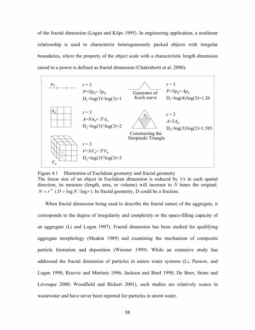
88

of the fractal dimension (Logan and Kilps 1995). In engineering application, a nonlinear

relationship is used to characterize heterogeneously packed objects with irregular

boundaries, where the property of the object scale with a characteristic length dimension

raised to a power is defined as fractal dimension (Chakraborti et al. 2000).

r = 3P=Np0= 4p0

D1=log(4)/log(3)=1.26

r = 2A=3A0

D2=log(3)/log(2)=1.585

r = 3P=Np0= 3p0

D1=log(3)1/log(3)=1

r = 3A=NA0= 32A0

D2=log(3)2/log(3)=2

r = 3V=NV0= 33V0

D3=log(3)3/log(3)=3

p0

A0

V0

Generator of Koch curve

A0

Constructing the Sierpinski Triangle

Figure 4.1 Illustration of Euclidean geometry and fractal geometry The linear size of an object in Euclidean dimension is reduced by 1/r in each spatial direction, its measure (length, area, or volume) will increase to N times the original.

DrN = ( rND log/log= ). In fractal geometry, D could be a fraction. When fractal dimension being used to describe the fractal nature of the aggregate, it

corresponds to the degree of irregularity and complexity or the space-filling capacity of

an aggregate (Li and Logan 1997). Fractal dimension has been studied for qualifying

aggregate morphology (Meakin 1989) and examining the mechanism of composite

particle formation and deposition (Wiesner 1999). While an extensive study has

addressed the fractal dimension of particles in nature water systems (Li, Passow, and

Logan 1998; Risovic and Martinis 1996; Jackson and Burd 1998; De Boer, Stone and

Lévesque 2000; Woodfield and Bickert 2001), such studies are relatively scarce in

wastewater and have never been reported for particles in storm water.

89

Mineralogy and geochemical composition of the particulate substrates is critical to

study their hydrological transport and chemical transformation of associated

contaminants. With oxygen and silicon two most abundant elements in the earth’s crust,

the abundance of silicates is not surprising, even in the anthropogenic environment. The

structures of these silicate tetrahedrons form single units, double units, chains, sheets,

rings and framework. Phyllosilicate is one of the subclass of silicate with a sheet-like

structure. The clay minerals are a part of a general but important group within the

phyllosilicates that contain large percentages of water trapped between the silicate sheets.

Individual clay minerals are rarely found separately and are usually mixed not only with

other clays but also with crystals of carbonates, feldspars, micas and quartz. Clay

minerals are divided into four major groups including kaolinite, montmorillonite, illite

and chlorite. They have a great potential to interact with various contaminants such as

heavy metals and pesticides due to their large surface area and high cationic exchange

capacity (Garcia 1995). The abundance of clay minerals in a variety of geochemical

environments and their influence on adsorption of contaminants suggests a need for the

experimental work to characterize the adsorption, desorption, and oxidation of

contaminants on clay minerals (Lin and Puls 2000).

Point of zero charge (PZC) reflects surface mineralogy and surface organic content of

particles. By definition, PZC is the pH value of the solution at which there is no net

charge on the particles (Sposito 1981). Positive charge is balanced with negative charge

at point of zero charge. PZC can be determined through experimental measurement of

surface charge. The presence of clay minerals will shift the PZC to lower pH value. In

90

urban rainfall-runoff, PZC is useful in coagulation, surface complexation and sorption

studies.

BACKGROUND ON SCANNING ELECTRON MICROSCOPY

In scanning electron microscopy, an electron beam is scanned across a specimen’s

surface. A variety of signals are generated and detection of specific signals produces an

image or a specimen’s elemental composition (Goldstein et al. 1992). Electron-specimen

interaction volume can be determined through calculation of the theoretical electron

range r (µm) using Equation 2 (Goldstein et al. 1992). r is interpreted as the half sphere

centered on the beam impact site.

)/()0276.0( 89.067.1 ZEAr m ρ×= (2)

Am is atomic mass in g/mole, E is accelerating voltage in keV, ρ is density in g/cm3, Z is

atomic number. For instance, at the accelerating voltage of 20-keV, the electron range for

calcite ( 3/7.2 cmg=ρ ) is 6.595-µm.

Three signals that provide the greatest amount of information in SEM are the

secondary electrons, backscattered electrons, and X-rays. Secondary electrons are

detected from a near-surface region of the interaction volume with low energy and are

used to characterize particle morphology and surface topography. Backscattered electrons

are produced when primary electrons are reflected from atoms in the specimen. They can

be detected from the interaction volume and much deeper parts of the specimen. The

images give the information on the distribution of different chemical phases in the

specimen. Higher atomic number elements appear brighter than lower atomic number

elements. Therefore, backscattered electron images (BEI) can be considered to reflect

variations in density between the specimen components. The sampling volume for X-rays

91

is similar in size to the interaction volume because X-rays are less easily absorbed by the

material. X-rays result from the incoming electrons knocking inner shell electrons out of

atoms in the specimen. As outer electrons drop into the vacancy, they are obliged to

dispose of excess energy, often as an X-ray photon. Since each element has its own

unique set of energy levels, the emitted photons are indicative of the element that

produced them. Analyzers are then used to characterize the X-ray photons for their

energy or wavelength and abundance to determine the chemistry of specimen (Goldstein

et al. 1992). In energy dispersive X-ray spectroscopy (EDS), the X-ray emissions are

sorted electronically. The EDS coupled with a computer based multi-channel analyzer

(MCA) provides the analytical facility. The spectrometer plots energies of X-rays against

specific count for each specific energy, giving a compositional spectrum of the specimen.

Characteristics of X-rays are denoted by K, L, M and N etc., indicating the destination of

the electron that gave rise to X-ray photon. EDS provides rapid qualitative or quantitative

(with adequate standards) analysis of elemental composition with a sampling depth of 1-2

µm.

OBJECTIVES

There were three objectives in this research. The first objective was to study the

morphology of particulate matter in urban rainfall-runoff. The fractal nature of individual

particles and particulate population would be qualified through an image-based fractal

analysis. The second objective was to identify the primary mineral content and

geochemical composition of the particulate substrate through their optical properties and

energy X-ray dispersive spectrum. The final objective was to study the amphoteric nature

of the particulates through experimental surface charge measurement.

92

MATERIALS AND METHODS

Sample Collection

Particulate matters transported by urban rainfall-runoff were collected from the

sedimentation tank at an experimental transportation site located in Baton Rouge,

Louisiana. The materials were recovered from the slurry of the bottom sediments.

Concentrated sediments were brought back to the lab where the particulate matters were

air-dried at 40 °C in a constant temperature and constant humidity room.

Sample Preparation

Completely air-dried samples were disaggregated and sieved (ASTM 1993). The set

of sieves encompassed the range of 9.5-mm (No. 3/8) through 25-µm (No. 500).

Particulate matters were separated into 18 size gradations. Dry materials separated on

each stainless steel sieve were weighed and stored separately in glass sample bottles. A

small amount of representative specimen from each size gradation was glued on 46 x 26

mm petrographic slides using a colloidal graphite isopropanol base for SEM analysis.

A thin section of sediment mixture was prepared for optical mineral identification,

backscattered image analysis and EDS. To prepare thin section, sediments were

embedded in epoxy resin. The block was allowed to harden and sectioned into 1-cm

chips. Representative specimen chips were selected, polished and placed on a

petrographic slide. The slide and the chip were placed in the thin section machine and

trimmed down to 50-µm thick on the slide. The slide was finally placed on a wheel that

finely abrades to 30-µm thick at which point light can successfully transmit through.

SEM analyses require materials to be electrically conductive. Non-conductive

specimens of dry particulates need to be coated with conductive material gold (Au) or

93

carbon (C) before analyzing. A sputter coater coats the specimen with Au atoms and a

carbon coater coats a thin film of carbon on the specimen. The entire coating process was

conducted in a glass vacuum vessel. Carbon coated particulate is transparent to X-ray

and was used for compositional EDS analysis.

SEM Analyses

Coated samples were analyzed using scanning electron microscope (SEM-JEOL

840A) at accelerating voltage 20-keV for a lifetime of 100s. Gold-coated samples were

used for secondary electron image acquisition. Carbon-coated samples were used to

analyze the chemical composition. Backscattered electron image were acquired only for

specimens prepared in thin section and carbon-coated.

Image Processing and Analyses

Quantitative analyses were conducted for the images obtained from SEM (Image-Pro

Plus). In order to identify and measure individual particles in the images, the first step is

to distinguish them from the surrounding background. This includes segmentation of

edges and adjustment of brightness and contrast. After calibration of units, the selected

measurements (area, diameters and perimeter etc.) were conducted for the particles in

each image. The particles attached on the border were excluded from the analysis. In

backscattered electron image of thin section (as seen in Figure 4.2), a sharp boundary was

defined in the original image. No processing was needed and measurements were carried

out on the original images. For secondary electron images, individual particles were

traced manually and all measurements were processed for the traced objects. An

illustration of the original SEI image of storm water particulate and the traced object was

seen in Figure 4.3. The selected measurements include maximum, mean and minimum

94

diameter, perimeter, area, roundness, and fractal dimension of the object outline.

Maximum diameter measured the longest length of the two outline points and passing

through the centroid. Mean diameter measured the average length of the diameters

measured at two degree intervals joining two outline points and passing through the

centroid. Minimum diameter was the shortest length of the two outline points and passing

through the centroid. Area comprised of all pixels within the object perimeter. Roundness

was determined by Equation 3.

APRπ4

2

= (3)

where P is the perimeter of the particle, A is the area of the particle. The circular object

has roundness of 1 and other shapes have roundness greater than 1.

Determination of Fractal Dimensions

The divider stepping method is a precise method for manual determination of fractal

dimensions of planar curves (Stoyan 1994). In the Image pro software, the fractal

dimension is defined as the slope of the linear part of the function that relates the log of

the outline length to the log of the stride (or step) length, where the stride length is how

long a ruler we attempt to lay along the perimeter of the object. Perimeters change with

different size rulers, as the rulers bridge various small wriggles in the outline. For each

stride length ri, )()( iii rNrrl = . For a fractal, it is expected that

rDcrl log)1(log)(log −+= (4)

Fractal dimension D can be calculated as 1 minus the slope of the regression line

obtained by plotting the log of the perimeter (using a particular stride) against the log of

the stride length.

95

Figure 4.2 BEI (Backscattered electron image) of storm water particulates prepared in

thin section. Degree of grayness indicates the density. Lighter objects have higher density. Calibration bar 100-µm (right) and 20-µm (left)

Figure 4.3 An example of traced individual particles based on their SEM image

Fractal dimensions for an aggregate can be experimentally determined using image

analysis. One-, two- and three-dimensional fractal dimensions are expressed in Equation

5 through 7 (Logan and Kilps 1995).

1DlP ∝ (5)

2DlA ∝ (6)

3DlN ∝ (7)

l is the characteristic length which can be taken as the shortest, longest, geometric mean

or equivalent radius based on area (Chakraborti et al. 2000). P is perimeter of the particle;

200 µm Traced object

96

A is the projected area; and N is the number of particles. When three-dimension fractal

dimension is less than 2, D3 is equal to D2 (Johnson, Li and Logan 1996).

One or two-dimensional fractal dimension (D1 and D2) for an aggregate can be

obtained from the slopes of log-log plots of characteristic particle diameter against

perimeter or projected area. By plotting measured particle characteristic diameter against

perimeter or projected area on the logarithms scale, the slopes of the regression line

correspond to D1 and D2 respectively. Similarly, D3 can be developed from the log-log

plot of particle number as a function of characteristic particulate diameter. The same

method was applied to urban rainfall-runoff system and the derived fractal dimensions

represent a statistical value for the population of particles in the system.

Mineral Identification for Particulate Matter in Sediment

Absolute identification of minerals requires X-ray analysis or a series of chemical

tests. The mineral can also be identified reliably through their physical properties such as

color, cleavage, fracture and twinning. Uncoated thin section samples were studied using

microscopy (Olympus BH-2) under plane-polarized light to identify minerals in the

particulates. Plane polarized light vibrates in a single plane. Most of the optical properties

of minerals observed in thin-section depend on a plane polarized light source.

Surface Charge Determination

Surface charge can be determined through potentiometric titration, ion adsorption and

zeta potential analysis (Marcono-Martinez and McBride 1989). In current study,

potentiometric titration (Van Raij and Peech 1972) was modified and used to determine

the surface charge of particulate matter in the sediment across size gradations. A

representative 0.5 to 1-g of dry sample was suspended in 50-ml of 0.01-M KCl, and the

97

pH was adjusted to a range between 6 and 9 with HCl or KOH. The suspensions and

control (blank solution of 0.01-M KCl) were set on a reciprocating table at 22 - 23 ºC in

sealed airtight 50-ml centrifuge tube for 24 hours. The pH values of the supernatant were

then recorded. The amount of H+ and OH- adsorbed by the sediment samples were

estimated from the amount of acid or base used to titrate the samples to their original pH,

subtracted by the amount necessary to bring 50-ml blank solution to the same pH.

RESULTS

Morphology of Particulate Matter in Urban Rainfall-Runoff

Secondary electron images (SEI) were acquired for particulate samples from the

storm catch basin at Baton Rouge site. Figure 4.4 showed the SEI images for various

gradations of particulates. Closer views for several individual particles were showed in

Figure 4.5. As seen in these SEI images, particles in urban rainfall-runoff possess fractal

structure. Clay-size particles are seen attached on the surface of large aggregates. Some

particle displayed a plate-like morphology, and some particle exhibited shape of a bar.

The high specific surface of fractal aggregates facilitates their active participation in

chemical reactions (Emets et al 1994).

A fractal dimension (D1) was obtained using divider stepping method for each traced

particles from SEI and particles in BEI. Figure 4.6 showed the fractal dimension

distributions for analyzing two sources of images for the same group of particles. The

range of fractal dimension developed from SEI image analyses is from 1.0188 to 1.1299.

Meanwhile, the fractal dimensions obtained from BEI image analyses range from 1.0309

to 1.1298. Distributions indicate similar results from SEI and BEI image analyses. The

fractal dimensions indicated a slight fractal nature of these particulates.

98

The empirical slope method was applied to characterize the fractal particles in the

system. A total of 1732 particles in the BEI ranging from 4-µm to 600-µm were used to

calculate fractal dimensions of D1 = 1.031 and D2 = 1.999. Fractal dimensions D1 = 1.015

and D2 = 1.926 were calculated for a subset of 1261 particulates with diameter less than

75-µm. The values of D2 are in good agreement with D2 values (1.92) reported for

inorganic aggregates clay-iron (Jiang and Logan 1991). For particles ranging from 75 to

600-µm, D1 = 1.022 and D2 = 1.967 were developed from 471 particles. Figure 4.7

showed the fractal dimensions developed from BEI. 95% predicted interval was shown as

the dashed line in each plot.

Figure 4.4 Secondary electron images (SEI) of the particulates from various gradations

in urban rainfall-runoff (calibration bar 10, 20, 50 and 100-µm)

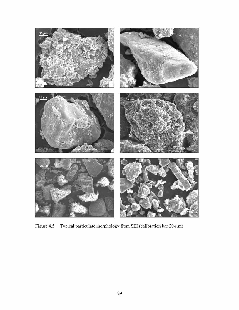
99

Figure 4.5 Typical particulate morphology from SEI (calibration bar 20-µm)

100

Freq

uenc

y

0

20

40

60

80

100

fractal dimension from SEI1.0188 1.1299

0

20

40

60

80

100

fractal dimension from BEI1.0309 1.1298

µ = 1.0631σ = 0.0186

µ = 1.0720σ = 0.0188

Figure 4.6 Fractal dimension distribution (D1) obtained from SEI image and BEI image

respectively for particles in urban rainfall-runoff

From SEI images of a subtotal 407 particulates less than 75-µm, fractal dimensions

were calculated as D1 = 0.997 and D2 = 1.943. The fractal dimensions of 1.029(D1) and

1.961(D2) were obtained from the analyses of a subset of 396 particles ranging from 75-

µm to 500-µm. Based on the image analyses for a total of 803 particulates in the urban

rainfall-runoff, D1 = 0.983 and D2 = 1.970 were obtained from log-log plots of diameter

against perimeter or projected area. The fractal dimensions, regression coefficients and

predicted region from SEI image analyses were presented in Figure 4.8.

Though the developed fractal dimensions from neither BEI nor SEI showed a

significant deviation from the values in Euclidean geometry, the two-dimensional fractal

dimensions obtained from both sediment mixture and particles across gradations showed

that fine particulate matter (less than 75-µm) population had a lower D2 value than that of

medium to coarse particles (greater than 75-µm), suggesting more fractal of smaller size

particles in general. Reorganization of deposits due to breakage, re-deposition or

deformation tends to make sediment particulate more compact (Wiesner 1999).

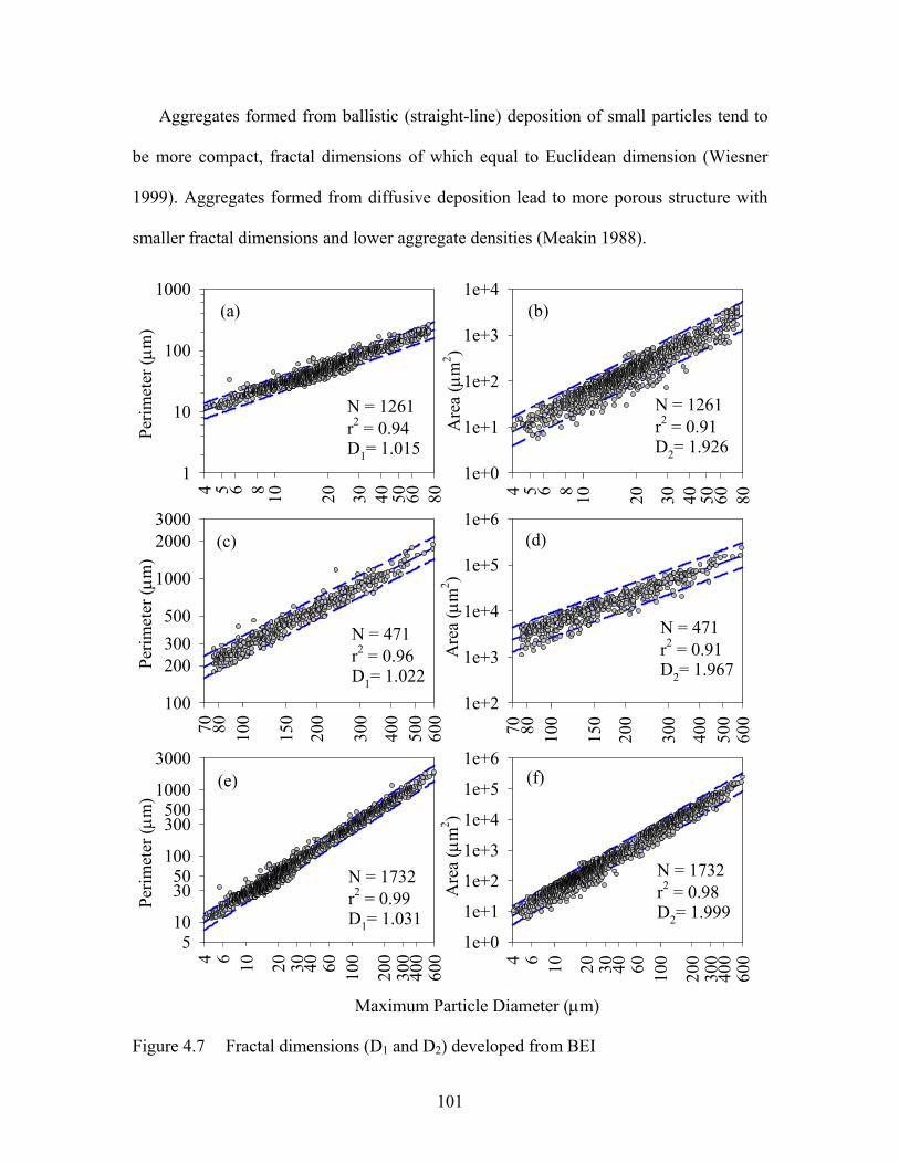
101

Aggregates formed from ballistic (straight-line) deposition of small particles tend to

be more compact, fractal dimensions of which equal to Euclidean dimension (Wiesner

1999). Aggregates formed from diffusive deposition lead to more porous structure with

smaller fractal dimensions and lower aggregate densities (Meakin 1988).

70 80 150

200

300

400

500

600

100

Perim

eter

(µm

)

200300500

20003000

100

1000

70 80 150

200

300

400

500

600

100

Are

a (µ

m2 )

1e+2

1e+3

1e+4

1e+5

1e+6

Maximum Particle Diameter (µm)

4 6 20 30 40 60 200

300

400

60010 100

Are

a (µ

m2 )

1e+0

1e+1

1e+2

1e+3

1e+4

1e+5

1e+6

4 6 20 30 40 60 200

300

400

60010 100

Perim

eter

(µm

)

5

3050

300500

3000

10

100

1000

4 5 6 8 20 30 40 50 60 8010

Perim

eter

(µm

)

1

10

100

1000

N = 1261r2 = 0.94D1= 1.015

4 5 6 8 20 30 40 50 60 8010

Are

a ( µ

m2 )

1e+0

1e+1

1e+2

1e+3

1e+4

N = 1261r2 = 0.91D2= 1.926

N = 471r2 = 0.96D1= 1.022

N = 471r2 = 0.91D2= 1.967

N = 1732r2 = 0.99D1= 1.031

N = 1732r2 = 0.98D2= 1.999

(a)

(f)

(d)

(b)

(e)

(c)

Figure 4.7 Fractal dimensions (D1 and D2) developed from BEI

102

5 6 8 20 30 40 50 60 8010

Perim

eter

( µm

)

20

4060

200

400600

10

100

5 6 8 20 30 40 50 60 8010

Are

a ( µ

m2 )

1e+0

1e+1

1e+2

1e+3

1e+4

1e+5

N = 407r2 = 0.99D1 = 0.997

N = 407r2 = 0.96D2 = 1.943

60 80 200

300

400

500

100

Perim

eter

( µm

)

200300400600

2000

100

1000

60 80 200

300

400

500

100

Are

a ( µ

m2 )

1e+2

1e+3

1e+4

1e+5

1e+6

N = 396r2 = 0.98D1 = 1.029

N = 396r2 = 0.95D2 = 1.961

Maximum particle diameter (µm)

5 20 30 40 50 200

300

400

50010 100

Perim

eter

( µm

)

204060

200400600

2000

10

100

1000

5 20 30 40 50 200

300

400

50010 100

Are

a ( µ

m2 )

1e+0

1e+1

1e+2

1e+3

1e+4

1e+5

1e+6

N = 803r2 = 0.99D1 = 0.983

N = 803r2 = 0.99D2 = 1.970

(a)

(f)

(d)

(b)

(e)

(c)

Figure 4.8 Fractal dimension developed by SEI (fine particles) and optical images

(larger particles)

N is the number of particles analyzed; r2 is the regression coefficient; D1 is one dimensional fractal dimension and D2 is two-dimensional fractal dimension. D1 and D2 obtained from the slope of the regression line represent the statistical fractal dimension for the entire population. 95% predicted region was shown as the blue dashed line.

(a) and (b) are for fine particulates (<75-µm); (c) and (d) are for medium to coarse particles (75-µm to 600-µm); (e) and (f) are for the entire gradation analyzed.

103

Mineral Identification

Figure 4.9 showed a few typical minerals in the particulates transported by urban

rainfall-runoff. They are identified as quartz, calcite, feldspar and biotite. One of the

phenomena observed in the images was that the color of the minerals presented varied

from the pure substance because of the impurities associated with them.

(a) (b)

(c) (d)

Figure 4.9 Mineral identification for the particulate matter in urban storm runoff

(a) quartz (b) feldspar (c) calcite (d) biotite

Chemical Composition of Particulate Matter

Figure 4.10 showed a wide view of backscattered electron image (BEI) for thin

section sample. Brighter objects have higher density. Spot and scanning X-ray analysis of

samples provides information about chemical composition in the specific area on the

sample. A few typical energy dispersive spectrums (EDS) representing the chemical

20 µm

104

composition in the specified area on BEI were included in Figure 4.11. EDS was

displayed as a histogram, with the horizontal axis labeled in energy units and the vertical

axis in numbers of counts.

A large amount of characteristic peaks were identified for element O, Al, Si and Ca.

Some other frequently seen elements included Na, Mg, K and Fe. Unless specified, all the

peaks were K-α peak. The roughness of the overall spectrum represents channel-to-

channel statistical fluctuations. EDS provides information to identify the class of these

particulates in the sediments qualitatively. Some of the identified mineral classes were

also listed in Figure 4.11.

1

1

1

1

1

2

2

2 4

4

4

5

5

83

6

7

2

2

2

2

2

2

2

22

2

2 2

2

22

11

1

1 1

2

Figure 4.10 Backscattered electron image for the thin section of the sediment mixture.

Numbers in the plot indicate the identified object using EDS. The corresponding energy dispersive spectrums were shown in Figure 4. 11

105

Cou

nts

Ca-Kα

O

Si

O

Cou

nts

OO

Cou

nts

O SiO

0 1 2 3 4 5 6 7 8 9 10

Si

O

Mg

Al

Ca

SiAl

Mg

Energy (keV)0 1 2 3 4 5 6 7 8 9 10

Cou

nts

Si

O Fe

S

Ca-Kβ

Ca-Kα

Ca-KβK

Fe-Kα

Fe-Kβ

Ca-Kα

Ca-Kβ

Ca-Kα

Ca-Kβ

Fe-Kα

Fe-Kβ

CaCO3 SiO2

Fe2O3

CaMg(CO3)

mica

(1) (2)

(3) (4)

(5) (6)

(7) (8)

Figure 4.11 Energy dispersive spectrum for the specific particles in BEI corresponding

to particles labeled in Figure 4. 10

106

Surface Charge and PZC

Surface charge is the most important factor either for dissolved or particulate matter

adsorption. Potentiometric titration curves describe net adsorption and desorption of H+

as a function of pH. The potentiometric titration curves for particulate in storm runoff

sediments across size gradation were shown in Figure 4.12. Surface charge of particulates

decreases with the increase of pH value across all size gradations. Point of zero charge

(PZC) of the particles was determined and plotted in Figure 4.13. PZC ranged from 7 to

9. Storm water pH values are typically in the range of 6 to 8, which is above the point of

zero charge (PZC). Therefore, particulates in the system are generally negatively charged.

PZC is also a function of particle size. As shown in Figure 4.13, PZC of particles shifted

to lower pH value with decrease of particle diameter suggesting the affinity of clay

minerals with smaller particles. The fine fraction particulate matter therefore has a great

potential to entrain heavy metal pollutions. This observation agrees with the study that

high concentration of heavy metal associated with fine particulate matter in urban storm

runoff.

CONCLUSIONS

Images obtained from scanning electron microscope illustrated the fractal nature of

the particles in urban rainfall-runoff. The characteristic morphology includes layered-

structure, clay-size particulate aggregation and relative smooth grain surface. Results

from image based fractal analyses showed fine particle populations were slightly fractal

than the medium to coarse materials though neither fractal dimensions showed a

significant difference from Euclidean structure. D2 developed from SEI images was 1.943

for fine particles (less than 75-µm) and 1.961 for medium to coarse particles (75-µm to

107

600-µm). Similarly in the analysis of BEI, D2 for fine particulates was 1.926 and 1.967

for medium to coarse particles. The fractal characteristic facilitates the entrainment of

contaminants. Removal of fine fractions is important because their high potential as a

reservoir for contaminants. Although Euclidean geometry is still applicable to the

primary particles in urban rainfall-runoff, aggregates formed during sedimentation or

coagulation/flocculation are expected to be more fractal and the effect of the fractal

characteristics are to be more significant in urban rainfall-runoff system. Fractal

characteristics of these aggregates need to be studied further to provide information in

designing unit operation.

Several common minerals identified in the particulate matter include quartz, calcite,

feldspar and biotite. Particles in urban rainfall-runoff have negative surface charges. PZC

of particles shifted to lower pH value with decreasing particle size, suggesting the affinity

of clay minerals to smaller size particulates.

Two issues arisen from this study are to seek alternative technology to improve

removal efficiency of fine particulates in storm water treatment system and study on the

stabilization of residual sediments from treatment system.

REFERENCES

American Society for Testing and Materials. (1993). “Standard practice for dry preparation of soil samples for particle-size analysis and determination of soil constants.” ASTM D421-85, Philadelphia, Pa.

Chakraborti, R. K., Atkinson, J. F., and Van Benschoten, J. E. (2000). “Characterization of alum floc by image analysis.” Environ. Sci. Technol., 34(18), 3969-3976.

De Boer, D. H., Stone, M. and Lévesque, L. M. (2000). “ Fractal dimensions of individual flocs and floc populations in stream.” Hydrol. Process., 14, 653-667.

Emets, E. P., Novoselova, A.E., and Poluektov, P. P. (1994). “In situ determination of the fractal dimensions of aerosol particles.” Physics-Uspekhi., 37(9), 881-888.

108

pH value5 6 7 8 9 10

-1

0

1

2

3

4

5180-150 µm150-106 µm106-75 µm

5 6 7 8 9 10

Surf

ace

char

ge ( µ

mol

/m2 )

-1

0

1

2

3

4

5

2000-850 µm850-600 µm600-425 µm

425-300 µm300-250 µm250-180 µm

75-63 µm63-53 µm53-45 µm45-38 µm

Figure 4.12 Surface charge for different gradations of particulate matter in urban rainfall-runoff

Particle diameter (µm)

40 50 60 80 150

200

300

400

500

600

100

PZC

- pH

6.0

6.5

7.0

7.5

8.0

8.5

9.0

Figure 4.13 Point of zero charge as a function of particle size for the storm water

particulates

109

Garcia, T. (1995). Sediments as potential pathway for contaminants in Trinity Bay. Environmental Institute of Houston, Annual report.

Goldstein, J.I., Newbury, D.E., Echlin, P., Joy, D. C., Romig, A. D. Jr., and Eric L. (1992). Scanning electron microscopy and X-ray microanalysis, A text for biologists, materials scientists, and geologist. (2nd Edition), Plenum Press, New York.

Jackson G., and Burd A. (1998). “Aggregation in the marine environment.” Environ. Sci. Technol., 32(19), 2805-2814.

Jiang, Q. and Logan, B. (1991). “Fractal dimensions of aggregates determined from steady-state size distribution.” Environ. Sci. Technol., 25(12), 2031-2038.

Johnson, C., Li, X.Y., and Logan, B.(1996). “Settling velocities of fractal aggregates.” Environ. Sci. Technol., 30(6), 1911-1918.

Li, D. H., and Ganczarczyk J. (1989). “Fractal geometry of particle aggregates generated in water and wastewater treatment processes.” Environ. Sci. Technol., 23(11), 1385-1389.

Li, X.Y., and Logan, B. (1997). “Collision frequencies between fractal aggregates with small particles by differential sedimentation.” Environ. Sci. Technol., 31(4), 1229-1236.

Li, X. Y., and Logan, B. (1997). “Collision frequencies between fractal aggregates and small particles in a turbulently sheared fluid.” Environ. Sci. Technol., 31(4),1237-1242.

Li, X. Y., Passow, U. and Logan, B. (1998). “Fractal dimension of small (15-200 µm) particles in Eastern Pacific costal waters.” Deep-Sea Research I, 45, 115-131

Lin, Z., and Puls, R. (2000). “Adsorption, desorption and oxidation of arsenic affected by clay minerals and aging process.” Environmental Geology, 39(7), 753-759.

Logan, B., and Kilps, J. (1995). “Fractal dimensions of aggregates formed in different fluid mechanical environments.” Wat. Res., 29(2), 443-453

Marcono-Martinez E., and McBride M. B. (1989). “Comparison of the titration and ion adsorption methods for surface charge measurement in oxisols.” Soil Sci. Soc. AM. J., 53, 1040-1045.

Risovic, D., and Martinis, M. (1996). “Fractal dimensions of suspended particles in seawater.” J. Colloid and Interface Sci. 182 (1), 199-203.

Mandelbrot, B. (1975). The Fractal Geometry of Nature. W.H. Freeman, New York.

110

Meakin, P. (1989). “Simulation of aggregation process.” Avnir, D. ed., “The fractal approach to heterogeneous chemistry.” Wiley, Chichester, 131-160.

Meakin, P. (1988). “Models for colloidal aggregation.” Annu. Rev. Phys. Chem., 39, 237-267

Ryan, J.N, Illangasekare, T.H., Litaor, M.I., and Shannon, R. (1998). “Particle and plutonium mobilization in macroporous soils during rainfall simulations.” Environ. Sci. Technol., 32(4), 476-482

Seaman, J. C., and Bertsch, P. M. (1997). “Characterization of colloids mobilized from southeastern coastal plain sediments.” Environ. Sci. Technol., 31(10), 2782-2790.

Seaman, J. C. (2000). “Thin-foil SEM analysis of soil and groundwater colloids: Reducing instrument and operator bias.” Environ. Sci. Technol., 34(1), 187-191.

Sposito, G. (1981). “The operational definition of the zero point of charge in soils.” Soil Sci. Soc. AM. J., 45, 292-297.

Stoyan, D., and Stoyan, H. (1994). Fractals, random shapes and point fields, methods of geometrical statistics. John Wiley & Sons. England.

Van Raij, B., and M. Peech. (1972). “Electrochemical properties of some oxisols and alfisols of the tropics.” Soil Sci. Soc. Am. Proc., 36, 587-593.

Wiesner, M. R. (1999). “Morphology of particle deposits.” J. Envir. Engrg., ASCE, 125(12), 1124-1132.

Woodfield D., and Bickert G. (2001) “An improved permeability model for fractal aggregates settling in creeping flow.” Wat. Res., 35(16), 3801-3806.

NOMENCLATURE

Am Atomic mass (g/mole)

E Accelerating voltage (keV)

ρ Density (g/cm3)

Z Atomic number

l Characteristic length (µm)

P Perimeter of the particle (µm)

A Projected area (µm2)

N Number of particles in the aggregate

D1 One-dimensional fractal dimension

111

D2 Two-dimensional fractal dimension

D3 Three-dimensional fractal dimension

112

CHAPTER 5. SEDIMENTATION OF NON-COLLOIDAL PARTICULATE MATTER TRANSPORTED BY URBAN RAINFALL-RUNOFF

SUMMARY

Settling velocity is a fundamental parameter of non-colloidal storm water particulates.

Determination of settling velocity is critical when designing or analyzing unit operations, in-situ

controls or watershed controls for urban rainfall-runoff. A synthesis of settling velocity

methodologies with applicability to characteristics of urban storm water particulate matter is

presented. Utilizing two common settling devices, a settling column and an Imhoff cone, settling

velocities of discrete non-colloidal particles in storm water were quantified. Theoretical settling

velocity calculations are compared to measured results across the gradation of particles from 1

up to 2,000 µm. Results indicate Newton’s Law can be used to model the discrete settling of

non-colloidal granular particles between 10 and 850-µm reasonably well. The difference

between measured velocities using Imhoff cone and the results from settling column is less than

15%. In settling column tests for particles in the range of 1.25 to 200-µm, a linear decrease in

particle mean size was observed with time during the settling process. Smaller particles (<10-

µm) settle faster than predicted using Newton’s Law assuming Euclidean object. Results showed

over 90% of non-colloidal particles in grit chamber and approximately 50% of the non-colloidal

particles in sedimentation basin can be removed by gravitational settling in terms of volume

concentration.

SETTLING VELOCITY – A REVIEW OF THE LITERATURE

The settling velocity of non-colloidal particles is one of the most important parameters in the

description of the transport of particulate matter in storm water control systems. Determination

of settling velocity is critical when designing or analyzing unit operations, in-situ controls or

113

watershed controls for storm water. The importance of particle settling velocities in the

calculation of sediment fluxes, particle residence times, and aggregation rates has led to

numerous attempts to predict settling velocity as a function of particle size, shape, and density

(Hawley 1982).

Non-colloidal particles in storm water could be non-cohesive or cohesive. Non-cohesive

materials are described as coarse-grained materials composed of particles greater than 62-µm

(Simon, in press). Particle interaction between non-cohesive particles is solely mechanical and is

restricted to momentum exchanges occurring from fluid drag, random collisions, and the

interlocking support from adjacent grains. Cohesive materials are those particles finer than 2-µm

in the fine silt and clay size range related to the existence of electro-chemical bonds between

individual particles. The small mass of particles relative to the large specific surface area

provides a net negative electrical-surface charge on the particle that is responsible for the electro-

chemical forces and bonding between particles (Simon, in press).

The settling velocity of non-cohesive particles in a low concentration suspension can be

calculated using Newtons’ Law, in which only forces of gravitational and flow resistance of the

particles are considered. When the particle concentration is high, particles interact with each

other and the settling velocity becomes a function of the volumetric concentration of the particles

in suspension (Burt 1986). Cohesive properties of the suspended particles result in the formation

of flocs whose settling behavior cannot be predicted using Stokes’ Law (Kranck 1986).

Brownian motion, local shear and differential settling are as significant as gravitational forces for

such cohesive flocs. Brownian motion for cohesive particles becomes important when

concentration exceed approximately 10 g/L (Kranck 1986). The cohesive particles collide with

each other and form aggregates or flocs. The macroflocs demonstrate a size range of 20-µm up to

114

640-µm (Manning 1999). The size of a floc depends on the particle collision frequency and the

strength of the cohesive forces. The floc forms are complex function of particle mineralogy and

the electro-chemical nature of the suspending medium. For example, in suspension with a very

low ionic strength, the double layer around these small cohesive particles is large and repulsive

forces dominate, keeping the particles too far apart for attractive force to come into effect. As the

ionic strength increases, the double layer is reduced in size smaller than about 1/3 of the particle

radius size and the particles are brought close enough to overcome the repulsive forces and the

attractive forces prevail. Particles aggregate on a time scale (Tawari and Koch 2002).

Settling Velocity Fundamentals

In Type-I sedimentation, each particle accelerates downward under the force of gravity until

the opposing drag force rises to the same value, at which point the particle travels at a constant

(terminal) velocity. The classic laws of sedimentation formed by Newton and Stokes can be used

to analyze terminal settling velocity of discrete spherical particles (Tchobanoglous and Burton

1991).

Equating the gravitational force (gravity minus buoyancy) with the frictional drag force yield

Newton’s law for terminal settling velocity, vt:

2/1)(

34

−=

ρρρ

D

St C

dgv (1)

The drag coefficient CD takes on different values depending on the flow regime surrounding

the particle and the shape of particles. Fair, Geyer and Okun (1968) have developed CD as a

function of Reynold’s number (Red) using the following regression expression.

34.0Re3

Re24

++=dd

DC (2)

Expressions for vt are depended on the flow regimes (Weber 1972).

115

Under laminar flow (Red < 1), settling velocity can be described by Stokes’ Law.

( ) 2

18dgv LSt ρρ

µ−= (3)

In transitional zone (1 < Red <1000),

( )[ ] 714.06.04.06.132.2 −−−= µρρρ LLSt dv (4)

Under turbulent flow (Red > 1000),

( )L

LSt

dgv

ρρρ −

= 82.1 (5)

For the transitional regime an iterative procedure must be adopted to obtain the settling

velocity. From Equation 1, an initial vt needs to be assumed, Red is calculated and CD

determined. This CD is substituted back in Equation 1 and tv is recalculated. Iterations continue

until vt values converge.

Table 5.1 summarized a series of expressions of vt for discrete natural non-cohesive particles

in simplified formulations.

Modified Settling Velocity Formulas

Cohesive settling model: Lau and Krishnappan (1992)

Experiments on settling of cohesive sediments were carried out in turbulent flow in an

annular flume using two sediments. One was a kaolinite clay with a mean diameter of about 6.8-

µm. The other was natural river sediment containing a combination of kaolinite and

mortmorillonite with a mean diameter of approximately 12-µm. Data on concentration and size

distribution of dispersed samples were used to calculate the effective settling velocities for

different size fractions.

116

Table 5.1 Summary a series of expressions for vt of discrete natural non-cohesive particles

Expressions for Settling Velocity Notes References

2/1

)(34

−=

ρρρ

D

St C

dgv 34.0

Re3

Re24

++=dd

DC Newton’s Law Tchobano-glous (1991)

ln(vt)=-54.6322+40.4532[ln(-lnd)]-0.3367[ln(lnSg)]+8.2637[ln(-lnυ)] -12.5788[ln(-lnd)]2+0.6165[ln(-lnd)] [ln(lnSg)]

Sg = 1.001 ~ 2.65 T = 5 ~ 40 oC

Bhargava and Pajagopal

(1992)

( ) 5.12 5*)(2.125 −+= d

dvt

υ d

gSd g

3/1

2

)1(*

−=

υ Cheng (1997)

υ

2)1(241 gdS

v gt

−= (a) gdSv gt )1(14.1 −= (b)

)lg(*)lg(790.3)777.5*(lg39lg 2 ρµ ⋅−⋅+−−−= dddvt (c)

(a) d<0.01 cm (b) d>0.2 cm (c) 0.01<d<0.2 cm

Sha (1956)

υ

2)1(241 gdS

v gt

−= (a) gdSv gt )1(068.1 −= (b)

)126

)(1(52.0)1(6.67 −−+−=TSdSv ggt (c)

(a) d<0.015 cm (b) d>0.15 cm (c) 0.015<d<0.15 cm

d in cm ; vt in cm/s

Ibad-zade (1992)

υ

2)1(181 gdS

v gt

−= (a) gdSv gt )1(1.1 −= (b)

)1*)(01.01(10 3 −+= dd

vtυ (c)

(a) d<0.01 cm (b) d>0.1 cm (c) 0.01<d<0.1 cm

Van Rijn (1989)

++++−

=αα

ααααυ23

32363

sin8.1cos9*))(sin6.3cos18(cos576cos24 d

dvt

0=α for 1* ≤d

( ) 3*log5.22 −+=

dπα

for 1* >d .

Zhu and Cheng (1993)

( ) ( )[ ] ( )[ ] 1.0346.067.18554.02 1043.1*10*72*18

−−

×+++= υυυavt

ng gDSa )1( −=

3/16

=

πVDn

5105.1Re ×≤d

Swamee and Ojha (1989)

vt = Terminal settling velocity of particle (m/s) υ = Kinematic viscosity of the liquid (m2/s) µ = Dynamic viscosity of the liquid (N s/m2) ρ = Density of fluid (kg/m3) ρs = Density of particle (kg/m3) d = Particle diameter (m) Dn = Nominal diameter CD = Drag coefficient Sg = Specific gravity

*d = Dimensionless particle diameter *υ = Nondimensional kinematic viscosity

117

Size distribution was modeled from a numerical model assuming discrete particle settling.

Using the initial size distribution and total concentration, the initial concentration of each size

class was calculated. The model was then applied to each size class to obtain the change in

concentration, resulting in a change in size distribution with time. The time rate of concentration

change in the suspension can be written as

hCv

dtdC iii −

= (6)

For cohesive sediment, the settling velocity is not consistent during the settling process. An

average settling velocity iv for any discrete period of time was defined as

dtvtt

vt

tii ∫−

=2

112

1 (7)

By integrating Equation 7, the average settling velocity over a given time period can be

calculated from the concentration data as:

)()(ln

2

1

12 tCtC

tthvi −

= (8)

An average effective settling velocity over the period of time t can be expressed as (Lau

1994):

=

)(ln 0

tCC

thvavg (9)

Temperature has a significant influence on the settling of cohesive sediments. According to

Stoke’s Law, settling velocities increase with temperature. However, experimental results for a

kaolinite clay and natural river sediments demonstrated that the settling velocity increased as

temperature was lowered (Lau 1994). There is an increased deposition with large settling

118

velocities when temperature is lowered. This increased deposition is likely due to the effect of

electrochemical forces on the properties of the flocs.

Multiple grain size model: Teeter (2001)

Enhanced settling occurs over a concentration range from a lower concentration limit Cll to

an upper concentration limit Cul. Below Cll, particle collisions are too infrequent to promote

aggregation. Cll is typically 50-300 mg/L depending on particle characteristics. At Cul, collisions

are so numerous that particles interact completely, resulting in the settling rates of all flocs to

converge to one value. At concentration greater than Cul, particle interactions become hindered

settling. Cul has been found to be 1-10 kg/m3 for estuarine sediments. Camp (1946) found the

onset of concentration-hindered settling to be 1-5 kg/m3 for turbid river water.

In the multiple grain size model the general form for grain size class settling velocity vs (gs)

is:

)(

max)(gsn

ulS C

Cvgsv

= ulll CCC ≤≤ (10)

where maxv is a mass-weighted average maximum floc settling velocity for a size class and it can

be calculated using Equation 11.

)(1

)(maxmax1

gs

NS

gsgs Cv

Cv ∑

=

= (11)

C is the total concentration for all grain size classes; (gs) is the size class index ranging from

1 to the number of size classes (NS); llC and ulC are mass-weighted average lower and upper

concentrations. At ulCC ≥ , )(gsvS equals maxv for all size classes. At llCC ≤ , settling velocities

are independent of concentration and equal to )(gsvS evaluated at Cll.

119

The exponent n(gs) can be determined empirically using information from settling tests

conducted over a range of concentrations. n(gs) has been determined to range below a value of

about 1.33. Two empirical relations between median settling velocity and concentration were

developed as follows.

Teeter (1993) 3/450 13.1 CvS = (12)

Kranck and Milligan (1992) 99.050 9.30 CvS = (13)

The difference in the exponent is attributed to differences in turbulence conditions.

A settling velocity function including the effects of both concentration and fluid shear rate

(G) has been proposed by Malcherek and Zielke (1996) and Teisson (1997) as:

)1()1(

' 23

2

GaGa

vv SS ++

= (14)

Based on experimental results, the following functional relationship is proposed to reflect the

effects of concentration and shear rate on settling velocity:

+

−

++

= 1exp

11)( 42

3

2

)(

maxll

gsn

ulS C

CaGaGa

CCvgsv (15)

ulll CCC ≤≤

a2, a3 and a4 are constants. G is in the range of 0 to 40 Hz.

Settling Velocity of Particles of Various Shapes

Storm water particles are not generally spherical while Newton’s Law is commonly applied

based on the assumption of spherical particles. Therefore, shape factors, distortion factors and

fractal dimension have been introduced to the settling model.

Shape factor

The shape factor of a non-spherical particle β is expressed as (Swamee and Ojha 1989):

120

xyz

=β (16)

in which x, y and z are lengths of the three principle axes of the particle in decreasing order of

magnitude. 0=β for a two-dimensional plate; 1=β for a sphere. The experimental data of

Schulz et al. (1954) that pertains two groups of non-spherical particles, natural sediments and

crushed rock fragment, were used to derive empirical relationships for the drag efficiency and

settling velocity.

Drag coefficient for natural particles is expressed as:

( ) ( )

428.1

175.0204

28.0

56.07.035.0 201

1000700ReRe

Re5.4178.3384.0

+

++

++

=ββββ d

d

d

DC (17)

Non-dimensional settling velocity for natural particles (valid for βυ 4108.1* −×≥ ):

[ ]1

125.04.04.2204833.035.0

667.0

)6.18exp(*)(20794.0

)5.41(*)(84.44*

−

+++

+=

βυβββυw (18)

Drag coefficient for crushed particles:

( )

25.1

8.018

32.0

64.08.035.0 )05.1(1

1000100ReRe

Re5.415.48

+

++

++

=ββββ d

d

d

DC (19)

Non-dimensional settling velocity for crushed fragments (valid for β

υ4108.1*

−×≥ ):

[ ]1

625.03.18.018833.035.0

667.0

)*)(0.3405.1866.0

)5.41(*)(84.44*

−

+++

+=

βυβββυw (20)

Distortion Factor

The volume of irregular shaped particles can be calculated using an equatorial radius R

relating to an equal volume of a sphere with radius r (Lerman, Lal and Dacey 1974).

121

For a spheroid equal in volume to a sphere, the following relationship can be applied.

3/1)1( −−= ErR (21)

In this expression, E is a measure of distortion of the sphere. acE /1−= , c is the polar semi-

axis and R is the equatorial radius. In a sphere, E = 0; In an oblate spheroid, 10 << E . In a

prolate spheroid, 0<E .

The settling velocity of a spheroid oriented with its polar axis c parallel to the direction of

settling can be defined as:

( )( ))2.01(9

12 2

EREg

v St −

−−=

µρρ

(22)

The correction factor for Stoke’s Law in this case is )2.01/()1( EE −− .

Substituting Equation 21 into Equation 22, the settling velocity of such a spheroid can be

expressed as:

( )( ))2.01(9

12 23/1

ErEg

v St −

−−=

µρρ

(23)

The settling rate of a spheroid oriented with its polar axis c perpendicular to the direction of

settling is defined as:

( )( ))4.01(9

12 2

EREg

v St −

−−=

µρρ

(24)

In terms of the radius r of a sphere with equal volume, the settling velocity can be rewritten as:

( )( ))4.01(9

12 23/1

ErEg

v St −

−−=

µρρ

(25)

As E tend to zero, the relationship between the drag force and the settling velocity of the

spheroid tend to be the Stoke’s Law for a sphere.

Fractal dimension

122

Aggregates found in natural system or generated in water and wastewater treatment systems

are fractals. Settling velocity of fractal aggregates had been developed by Jiang and Logan

(1991).

( ))2/(1

10

3/00

2

0 22)/(2

bDbDbDDD

t lla

gv

−

−+−−+

−= υξζξρρ

ρξξ

(26)

a and b are determined for different ranges of Reynold’s numbers as listed in Table 5.2. Scaling

relationships between settling velocity and characteristic length l were summarized in Table 5.3

for different ranges of Reynold’s numbers and fractal dimensions.

Table 5.2 Parameter determination for Equation (26) for different ranges of Reynold’s number

Reynold’s number a b 1.0Re ≤d 24.0 1.0

0.1 < Red < 10 29.03 0.871 10 < Red < 100 14.15 0.547

Table 5.3 Scaling relationships between settling velocity tv and characteristic length l (Johnson 1996)

Reynold’s Number General expression 22 <D 22 ≥D 1Red << 1−∝ Dlv 1−∝ Dlv 1−∝ Dlv

1Red << 12 +−∝ DDlv lv ∝ 1−∝ Dlv

1Red << , b=1 )2/()( 2 bbDDlv −+−∝ lv ∝ 1−∝ Dlv 0.1< dRe <10, b=0.871 )2/()( 2 bbDDlv −+−∝ 77.0lv ∝ )1(89.0 −∝ Dlv

The experimental results from previous study (Johnson 1996) demonstrated that fractal

aggregates composed of inorganic microspheres can settle on average 4 to 8.3 times faster than

predicted by calculations for impermeable or permeable spheres of identical mass, cross section

area, and primary particle density.

123

Methods for Determining Settling Velocity

Several types of settling column have been developed for settling velocity measurement for

both dry weather flows and wet weather flows (Pisano 1996). Two types of method,

homogeneous suspension and floating layer, have been classified and developed for measuring

the settling velocity of particles in liquid (Aiguier 1996).

The “homogeneous suspension” method (HS) is the analysis of a suspension with solids

homogeneously divided throughout the depth of settling column at the start of measurement. The

“floating layer” method (FL) consists of distributing the solids in a thin uniform layer at the

surface of the fluid at the start of measurement, and plotting the mass fraction of particles

decanted as a function of their settling velocities.

Stationary settling column (Figure 5.1) Pisano (1996)

The most common settling column is a stationary settling column made of clear Plexiglas

having peripherical withdraws along the column length. The typical stationary column is 1.8 to

3.7 m (6 to 12 ft) high with a diameter of 15 to 30 cm (6 to 12 inches). Column depth is usually

equivalent to that of a clarifier or settling basin. Various methods have been used to pre-mix the

sample before the column test begins. A variation of the stationary method involves various

mechanical means to pre-mix the column contents by rotating the entire column against its axis.

UFT-type Settling column (Figure 5.2) Michelbach and Weiß (1996)

Umwelt and Fluid Technik (UFT) developed a settling column to study the settling properties

of solids in either an unmodified or a pre-settled sample. Particles which are not settled in an

Imhoff cone within one hour are considered as unsettleable from an economic point of view. For

those settled materials in Imhoff cone, UFT-type column were used to analyze effluents with

particles with different settling behaviors and solids concentration.

124

The pre-settled solid samples were introduced into the top of the column. Samples were

withdrawn from the bottom of the column at times t1, t2, t3, t4, …, tn. The sample withdrawn at tn

represented the material that settled between time tn-1 and tn. Each sample was evaporated and

drained to obtain the total solids in terms of mass. The sum of the mass of samples 1 through n

was taken to be the total amount of mass that settled within the time frame of the test. From these

results, the cumulative settling curves were constructed. The settling velocity was calculated by

determining how far the particles fell in a given time. The settling curve was constructed by

plotting the settling velocity against cumulative mass fraction. Mass-based settling curves are

developed using this method.

The effect of water level drop in the test column needs to be taken into account. The particles

collected after the nth withdrawn from the column have experienced a drop in water level n times.

Correcting for the dropping water level involves obtaining the volumetric flow rate (cm3/s) by

measuring the amount of water and the time it takes to withdraw that water during each sampling

event. The corrected settling velocity is:

ttnvHnv Pith /)()( ⋅⋅−= (27)

where )( thnv is the settling velocity at nth withdrawal (m/s); iv is the average velocity at

which the water level drops (m/s), calculated by dividing the volumetric flow rate during each

sampling event by the column cross section. H represents column height in meter, and the

elapsed time of sampling is described using tP. t is the entire experimental elapsed time.

ASTON- Settling column (Figure 5.3) Tyack (1996)

Settling velocity test method developed by Tyack (1996) at Aston University (U.K.) for

combined sewage overflow (CSO) was used to determine the settling velocity across the entire

gradations. The column had a central settlement length of 1.50 m, which was sufficient to allow

125

full development of the flocculation process based on the work carried out by Owen (1970). The

diameter of the bottom withdrawal tube was 25-mm. Owen recommended a column diameter of

50-mm for solids concentrations between 50 and 200 mg/L. The walls of the column imposed

definite boundaries that provided an effective resistance to the motions of the particles and the

fluid that was displaced by their motion.

Upper reservoir Slide this section over the column to initiate the test

Support

Main section of settling column

Imhoff cone section

Sampling Port

Figure 5.1 Stationary settling column Figure 5.2 UFT-type Settling column

Cell B

PVC collar

Ball valve

Cell A

2000

75250

75250

Axle and bearings

54 mm ID plastic pipe

Figure 5.3 ASTON- Settling column (in mm)

126

CERGRENE Column Aiguier and Chebbo (1996)

In the Cergrene method (Chebbo 1992), the settling velocity measurement was carried out in

a 1.81-m settling column for particles greater than 50-µm, and an Andréasen pipette (length 0.2-

m; diameter 50-mm) was used for settling velocity measurement for particles smaller than 50-

µm. Particles were wet sieved prior to the measurement.

The settling velocities obtained from the ASTON-column and CERGRENE-column are

significantly lower compared with the UFT method (Aiguier and Chebbo 1996). The reason for

the lower settling velocity in these two devices is that UFT-method takes only the settleable

solids from 1-hour Imhoff cone test into account, while the other two methods include the entire

size range of particles.

Compared to the traditional settling column, the CERGRENE columns have a shorter time to

fill (approximately 7 seconds) and may be more completely mixed at the initial sample time. It is

thought that the CERGRENE column may account for a wider range of settling solids which

may result in establishing better design parameters for wet weather flow. The CERGRENE

column was designed for field as well as laboratory use. Settling velocities of samples measured

in the field immediately after storm are different from samples transported back or stored in the

lab because agglomeration may occur during transportation and storage.

Linear density gradient column: Azetsu-Scott and Johnson (1992), Yuan (2000)

The method consists of a column for measuring the settling velocity and density of

constituent matter of aggregates, a microscope for size determination and a camera for recording

images for shape information. The linear density gradient was constructed from the Metrizamine

stock solution. The upper 110-cm of the column was filled with filtered (0.45 µm Millipore) sea

127

water, and sterilized with 0.2% sodium azide. The lower 40-cm of the column contained a sea

water – Metrizamide mixture. The density gradient was developed as a linear expression.

'01088.01936.0 h×+−=ρ (28)

The column temperature was kept at 15 ± 0.5 °C. Particles were introduced to the top of the

column and settling velocity was measured in the sea water layer. Settling velocity is a function

of the density difference between the aggregate and ambient fluid. The aggregate density was

obtained from the ambient fluid density where the particle stops settling.

Newton’s second law applied to an aggregate of radius (r) yields:

rvdtdvVVg

dtdvV LLSS 11 6

21)( πµρρρρ −−−= (29)

Densities in Equation (29) are in g/cm3. From Equation (29), the settling velocity is obtained.

)1(9

)(2 '

1

21 tLS ergv β

µρρ

−−

= (30)

2

1

)2

(2

9'rL

Sρ

ρ

µβ

+−= (31)

The distance X that a particle settles as a function of time can be determined.

−

−+

−=

= ∫

'1

9)(2

9)(2 '

1

21

1

21

βµρρ

µρρ β tLSLS ergtrgX

vdtX

(32)

Settling velocity and permeability of the biological aggregates generated in a lab-scale

sequencing batch reactor were investigated using an apparatus of double columns vertically

connected (Yuan 2000). The upper column was filled with water while the lower column was

filled with a denser solution of NaCl or EDTA having a density of 1.005 g/cm3 at room

128

temperature. The setting velocity observed in water was in good agreement with the predictions

of Stoke’s Law for the identical but impermeable porous particles, suggesting insignificant

internal permeation of biological aggregates. The settling velocities decreased when the

aggregates settled from water phase into the EDTA or NaCl solution. The reduction from water

to EDTA was greater than that from water to NaCl, indicating that mass transport from the liquid

phase into bio-aggregates was likely dominated by molecular diffusion rather than convection.

The Effect of Turbulence

A vertical recirculating settling column with an oscillating grid generating turbulence was

built to study the effect of turbulence on settling velocity (Rasmussen and Larsen 1996). A

continuous recirculating flow of suspended sediment has the advantage of keeping the sediment

concentration constant. The settling column is 1.2-m high with a depth of 0.3-m. Turbulence is

generated by 11 oscillating grids, spaced 0.1-m apart. Figure 5.4 showed schematic of the

column with oscillating grid. Comprehensive experiments for the calibration of the relation

between the movement of the grid and the generation of turbulent kinetic energy had been

conducted by Rasmussen and Larsen (1996).

Inlet

Outlet

Top view of grid

225

30

Grid

Bearing

Column

2012

021

Connect to motor

Figure 5.4 Recirculating column (in cm)

129

The settling velocity was determined from the continuity equation for the mass flux of

sediment assuming steady state conditions. The flux in the inlet zone equals the flux in the

uniform zone yielding:

uniformSPinP CvvCv )( += (33)

uniform

uniforminPS C

CCvv

)( −= (34)

Concentration was measured indirectly via the turbidity with a turbidity sensor. A best fit

relationship was developed from the analysis of the experimental results.

024.073.1

07.0ln5.0exp103.1

2

19.1

3.605 +

+

−×= − SS

CGC

v (35)

G is the average turbulence velocity gradient and is calculated as µε /=G , where ε is the

turbulent dissipation assumed equal to the generated turbulent kinetic energy by the grid.

Wall Effect in Cylindrical Column

The terminal settling velocity tv of a particle decreases as the diameter of the sedimentation

vessel decreases. This is known as wall effect (Kehlenbeck and Di Felice 1999).

The wall factor can be expressed as

),(Re λ∞∞

= tt

Bt fvv

(36)

The wall factor is a function of both the sphere Reynold’s number ∞tRe and the diameter ratio

λ.Two physical boundary conditions have to be fulfilled: For λ = 0, the settling velocity tBv must

coincide with the terminal settling velocity in an infinite vessel ∞tv . For λ = 1, the settling

velocity tBv must be equal to zero.

130

On the basis of over 100 experiments in a Reynold’s number region of 185Re2 ≤≤ ∞t and a

diameter ratio of 9.0≤λ , the relationship for the wall factor was developed as:

P

P

t

tB

vv

+

−=

∞

0

1

1

λλ

λ (37)

Two parameters λ0 and p were found to depend on the sphere Reynold’s number ∞tRe . The

relationship between 0λ and ∞tRe was described in Equation (39).

524.0

0

0 Re041.02.1

283.0∞=

−−

tλλ

(38)

Parameter p correlated to ∞tRe under two different flow regimes.

For 35Re ≤∞t , the best approximation was

434.0Re5466.044.1 ∞+= tp (39)

For 35Re ≥∞t , the best fitting was obtained with

8686.0Re3.373.2 −∞+= tp (40)

With p fixed at 2.2 fixed and 0λ expressed as a function of ∞tRe , a simplified correlation was

obtained as Equation 41.

65.0

0

0 Re05.02.1

27.0∞=

−−

tλλ

(41)

The accuracy is lower but a good prediction of the measured wall factors can still be obtained.

OBJECTIVES

A review of the literature indicates that although settling curves have been developed through

gravimetric analyses for combined sewage overflow (Aiguier and Chebbo 1996; Tyack and

Naomi 1996; Hedges 1998; Wong 2000), settling velocity analysis of stormwater particles has

131

not been reported through laser diffraction analysis of particle size distribution (PSD). Therefore,

to measure settling velocities through PSD, two common settling velocity measurement devices,

stationary settling column and Imhoff cones, will be applied in the experiment. A review of

literature indicates that an examination and comparison of results from these two settling

velocity devices has not been reported in the previous studies. In addition, characteristics of

sediments deposited by urban storm water are quite different from natural river sediments and

wastewater solids. The settling behaviors of particulates in urban storm water are also influenced

by the factors such as suspended solids (SS) concentration and residence time.

Four objectives were proposed for this study. First, a thorough compilation of literature on

settling velocity was presented with purpose of providing a sound background. Second, a

methodology was developed using a laser diffraction type of particle analyzer to determine PSD

and settling velocity. Third, two settling velocity devices – settling column and Imhoff cone –

were compared for the settling velocity measurement of storm water particles. Sampling and

analytical procedures were developed and compared. The final objective was to estimate and

analyze the settling velocity model through comparing the measured velocities to the modeled

value.

METHODOLOGY

Materials – Urban Rainfall-Runoff Particles

Particulates were obtained from a paved urban site impacted by transportation. Materials

analyzed include cohesive and non-cohesive sediments transported by urban runoff into a storm

catch basin and storage tank. Experimental site was shown in Figure 5.5. Sediments were

collected, brought back to lab and air-dried at 40°C. Dried solids were disaggregated and sieved

into 18 size gradations. Table 5.4 illustrated the size gradations of mechanical sieve analysis.

132

Bridge Deck

80-L Grit Chamber

Collection Pipe

Eastbound I-10

Collection Trough

Recycle Pump

Draining Pipe

2130-L Settling Basin

Figure 5.5 Profile view of experimental site sampling system (Baton Rouge I-10 Site)

Table 5.4 Size gradations of mechanical sieve analysis

ID Sieve # Designation Nominal Opening (µm) Size Range (µm)

1 3/8 inch 9500 >9500

2 1/4 inch 4750 9500-4750

3 No. 10 2000 4750-2000

4 No. 20 850 2000-850

5 No. 30 600 850-600

6 No. 40 425 600-425

7 No. 50 300 425-300

8 No. 60 250 300-250

9 No. 80 180 250-180

10 No. 100 150 180-150

11 No. 140 106 150-106

12 No. 200 75 106-75

13 No. 230 63 75-63

14 No. 270 53 63-53

15 No. 325 45 53-45

16 No. 400 38 45-38

17 No.500 25 38-25

18 <25

133

Methods

Specific gravity

Density or specific gravity of particles was determined by an inert gas (helium) pycnometer

(Quantachrome Corp.) The method applied was ASTM protocol D5550-94 (ASTM 1994). The

pycnometer determines the true volume of solid samples by measuring the pressure difference. A

known quantity of helium under pressure was allowed to flow from the chamber with a precisely

known reference volume (VR) into a sample cell containing the solid or powder material. The

pressures were recoded and the difference can be obtained. True solid volume can be calculated

through Equation 42:

[ ]1)/( 21 −−= PPVVV RCS (42)

Density of the sample then could be calculated using Equation 43

SSS VM /=ρ (43)

The density for the solid material is typically reported to the nearest 0.01. Specific gravity Sg was

obtained through Equation 44.

LSgS ρρ /= (44)

Settling velocity measurement

The aqueous phase utilized in the following experiments to evaluate settling velocity was the

pre-settled stormwater supernatant, in which the total particle volume concentration was no

greater than 5-µL/L. Below the concentration limit of 50 mg/L, particle collisions are too

infrequent to promote aggregation (Teeter 2001). Assuming storm particle density of 2.5-g/cm3,

the volume concentration limit for Brownian coagulation is 20-µL/L and the mass concentration

limit is 50-mg/L. The rational for using pre-settled storm water as the suspended medium in the

settling column and Imhoff cone test is that it would simulate the viscosity, density and

134

chemistry of the liquid phase in a real storm water treatment system. In order to reduce the

interference of particles in the aqueous phase to the tested particles, a pre-settled time of three

days was set to ensure that the impact of particles in the suspended medium is insignificant.

For particles greater than 180 µm (retained on No.80 sieve), 100 individual particles from

each size classes were randomly selected for settling velocity measurements. The floating layer

method (Aiguier and Chebbo 1996) was used in these experiments. Individual particles were

introduced into the column or the Imhoff cone just below the water surface. Before the settling

test, particles were immersed in the pre-settled storm water and any attached bubbles removed.

Sedimentation timing starts as soon as the particle was released from an at-rest position just

below the water surface. Time for settling the predetermined distance ( imhoffH = 425 mm,

columnH = 2466 mm) for each individual particle was measured by a stopwatch manually. The

average settling velocity of measured particles can be calculates using Equation 45.

tHv /= (45)

Sediment samples and grit samples were tested separately in both settling column and Imhoff

cones. The calculated settling velocities according to Newton’s Law are shown in Table 5.5 for

the grit and Table 5.6 for the sediment.

For particles less than 180-µm (particles passing through the No. 80 sieve), settling velocities

were determined through analyses of particle size distribution in the settling column test. The

columns were filled up with tap water. In order to remove fine bubbles, the solution was allowed

to sit in the columns for at least four hours before the experiment started. A sample from each

column was taken from sampling port 2 (as shown in Figure 5.6) and analyzed to set the

background particle concentration in the analyzer (Lisst Portable, Sequoia Tech.), which would

be subtracted from the particle analysis for the real storm particles in the column runs.

135

Table 5.5 Modeled settling velocity using Newton’s law for the particles entrained in the grit chamber at Baton Rouge I-10 site (Assume T=20 °C)

ID Particle Diameter (µm)

Measured Density (g/cm3) vt(mm/s)

Reynold’s Number

(Red) 2 4750 2.48 457 2428 3 2000 2.41 290 648 4 850 2.37 140 133 5 600 2.44 104 70.0 6 425 2.57 76.2 36.2 7 300 2.61 50.3 16.9 8 250 2.58 38.5 10.8 9 180 2.56 23.0 4.64 10 150 2.47 16.2 2.72 11 106 2.55 9.3 1.10 12 75 2.53 5.2 0.44 13 63 2.53 3.7 0.26 14 53 2.61 2.8 0.16 15 45 2.51 1.9 0.09 16 38 2.54 1.4 0.06 17 25 2.49 0.6 0.02

Flow regime Re > 1000, Turbulent flow; 1 < Re < 1000, Transitional flow; Re < 1, Laminar flow.

136

Table 5.6 Modeled settling velocity using Newton’s law for particles in the sedimentation basin at Baton Rouge I-10 site (Assume T=20 °C)

ID Particle

Diameter (µm)

Measured Density (g/cm3)

vt(mm/s) Reynold’s Number

(Red) 2 4750 1.34 219.00 1164 3 2000 1.52 154.27 345.3 4 850 1.61 83.10 79.0 5 600 2.13 88.39 59.3 6 425 2.26 65.00 30.9 7 300 2.33 43.33 14.5 8 250 2.31 33.02 9.24 9 180 2.28 19.40 3.91 10 150 2.22 13.69 2.30 11 106 2.24 7.51 0.89 12 75 2.26 4.32 0.36 13 63 2.33 3.22 0.23 14 53 2.33 2.28 0.13 15 45 2.38 1.70 0.09 16 38 2.41 1.24 0.05 17 25 2.50 0.57 0.02

Solid particles were obtained from mechanical sieve analysis pass through No. 80 (180-µm).

To avoid the interaction among the particles, suspended solid concentration in the settling

column was no greater than 100-mg/L, indicating the dry solid mass no greater than 3.78-g

(Volume of the column = 37.8 L). A certain amount of particles (less than 3.78-g) was weighed

and add into D.I. water to prepare the solid mixture. The mixture was then sonicated for over 20-

min until all the clogs and aggregates break up. Experiments were designed in three settling

columns with short-term, mid-term and long-term sampling time respectively. Table 5.7

illustrated the experimental matrix. Combining the results from three columns, settling velocity

distributions for particles ranging from 1.36 to 180-µm can be acquired.

137

Determination of settling velocities for fine particles (less than 180-µm) was also carried out

using particle size distribution. The procedure for adding solution of fine particles into the

settling column or the Imhoff cone was as follows.

1. Immerse the petri-dish which holds the solution of particles at a known location near the

liquid surface;

2. Carefully introduce the particle suspension into the aqueous phase of storm water

ensuring quiescent conditions remain;

3. Start sedimentation time immediately;

4. For settling column, initial sample is withdrawn from sampling port 1 (Figure 5.6) and

the time is recorded as t0; For the Imhoff cone, the initial sample is analyzed before

adding into the cone;

5. Approximately 120-mL sample is withdrawn each time from sampling port 2 as shown in

Figure 5.6 in the settling column test;

6. Sampling at time t1, t2 …… tn as shown in Table 5.7 for different columns;

7. For the settling column, record the drop of water level for the correction of settling depth

for each sampling time;

8. In Imhoff cone test, sample 30-mL each time using a wide-bore syringe with a rigid

tubing connected to the end at the depth of 275-mm below the surface of the liquid every

minute for 10 minutes. Figure 5.7 showed the Imhoff cone and the sampling schematic.

9. Analyze particle distribution using a laser diffraction particle analyzer for all samples.

Total volume concentration for particles of each size gradation ranging from 1.25 to 200 µm

was obtained from particle size analysis using LISST Portable particle analyzer at time t1, t2, …

tn. Volume concentration was converted to number concentration assuming spherical particles.

138

Table 5.7 Experimental design – sampling time for the column test

Column I Column II Column III Sampling time sec min min hr hr Day

1 20 0.33 10 0.17 4 0.17 2 40 0.67 20 0.33 8 0.33 3 60 1.00 30 0.50 12 0.50 4 80 1.33 40 0.67 16 0.67 5 100 1.67 50 0.83 20 0.83 6 120 2.00 60 1.00 24 1.00 7 140 2.33 70 1.17 28 1.17 8 160 2.67 80 1.33 32 1.33 9 180 3.00 90 1.50 36 1.50

10 200 3.33 100 1.67 40 1.67 11 220 3.67 110 1.83 44 1.83 12 240 4.00 120 2.00 48 2.00 13 260 4.33 130 2.17 52 2.17 14 280 4.67 140 2.33 56 2.33 15 300 5.00 150 2.50 60 2.50 16 320 5.33 160 2.67 64 2.67 17 340 5.67 170 2.83 68 2.83 18 360 6.00 180 3.00 72 3.00 19 380 6.33 190 3.17 76 3.17 20 400 6.67 200 3.33 80 3.33 21 420 7.00 210 3.50 84 3.50 22 440 7.33 220 3.67 88 3.67 23 460 7.67 230 3.83 92 3.83 24 480 8.00 240 4.00 96 4.00 25 500 8.33 250 4.17 100 4.17 26 520 8.67 260 4.33 104 4.33 27 540 9.00 270 4.50 108 4.50 28 560 9.33 280 4.67 112 4.67 29 580 9.67 290 4.83 116 4.83 30 600 10.00 300 5.00 120 5.00 31 620 10.33 310 5.17 124 5.17 32 640 10.67 320 5.33 128 5.33 33 660 11.00 330 5.50 132 5.50 34 680 11.33 340 5.67 136 5.67 35 700 11.67 350 5.83 140 5.83 36 720 12.00 360 6.00 144 6.00 37 740 12.33 370 6.17 148 6.17 38 760 12.67 380 6.33 152 6.33 39 780 13.00 390 6.50 156 6.50 40 800 13.33 400 6.67 160 6.67 41 820 13.67 410 6.83 164 6.83 42 840 14.00 420 7.00 168 7.00 43 860 14.33 430 7.17 172 7.17 44 880 14.67 440 7.33 176 7.33 45 900 15.00 450 7.50 180 7.50 46 460 7.67 184 7.67 47 470 7.83 188 7.83 48 480 8.00 192 8.00

139

Sampling port 2

Sampling port 1

t5t4t3t2t1

t0

Settl

ing

dist

ance

(H1)

Settling column

Initial PSDAdd particles

SamplePSD (tn)

Figure 5.6 Sampling schematic for the settling column

460

106

10

275

425

245

1000-mL

500-mL

50-mL

tn

Cloud of particles

Add particles Initial PSD

Sample

PSD (tn)

Settl

ing

dist

ance

(H

=275

mm

)

1000 mL

50 mL

Figure 5.7 Imhoff cones (all units in mm) (left) and sampling schematic (right)

140

At each sampling time, an average of settling velocity can be obtained by Equation 45.

Therefore, for a given size particle, settling velocity distribution is obtained and it is expected to

be normal. The mean value of the normal distribution was considered measured settling velocity

for the particle of this size. Theoretical settling velocity of this size can be calculated according

to Newton’s Law. Table 5.8 listed the theoretical calculated settling velocities. Measured settling

velocities were compared to the modeled settling velocities.

Table 5.8 Modeled settling velocity using Newton’s law for fine particles (1.25 ~ 250 µm) Assuming density = 2.50 g/cm3, T=20 °C.

Size (µm) Settling Velocity (mm/s) Size (µm) Settling Velocity

(mm/s) 1.25 0.00 19.20 0.34 1.36 0.00 22.66 0.47 1.60 0.00 26.74 0.65 1.89 0.00 31.56 0.91 2.23 0.00 37.24 1.27 2.63 0.01 43.95 1.77 3.11 0.01 51.86 2.46 3.67 0.01 61.20 3.42 4.33 0.02 72.22 4.77 5.11 0.02 85.22 6.64 6.03 0.03 100.57 9.24 7.11 0.05 118.67 10.98 8.39 0.06 140.04 14.67 9.90 0.09 165.26 19.39 11.69 0.12 195.02 25.33 13.79 0.17 230.14 32.67 16.27 0.24 250.00 36.90

RESULTS AND ANALYSIS

As shown in Figure 5.8, density of solids collected from grit material is significantly higher

than that of clarified sediments collected from the sedimentation tank. The difference is

significant for the particles greater than 600-µm. By observation, samples in the clarified

141

sediments for large particle size contain more organic matter such as shredded tire, bark and

straw pieces, which contribute to the low density of the sample.

Particle Diameter (µm)

9500

4750

2000 85

060

042

530

025

018

015

010

6 75 63 53 45 38 25

Den

sity

(g/c

m3 )

1.0

1.5

2.0

2.5

3.0

GritClarified Sediments

Figure 5.8 Density of solids deposited by urban storm runoff

Settling velocity measurement for visible non-colloidal individual particles (greater than 180-

µm) was carried out using Imhoff cone and settling column. Measured settling velocities and

modeled values were showed in Figure 5.9. Experimental measured data were presented as box

plots representing statistical results. The boundary of the box closest to zero indicates the 25th

percentile and the line within the box marks the median. The boundary of the box farthest from

zero indicates the 75th percentile. Whiskers above and below the box indicate the 90th and 10th

percentiles. Individual circles showed in the plot represent the 5th and 95th percentile. Modeled

settling velocities using Newton’s law assuming Euclidean structure were shown in the same plot

as triangles.

Table 5.9 summarized the measured and modeled velocities of visible individual particles

from the grit chamber and sedimentation tank. Table 5.10 compared the measured results using

two different devices.

142

180

250

300

425

600

850

2000

Setti

ng V

eloc

it y

(mm

/s)

0

50

100

150

200

250

300

350Imhoff cone - Grit Imhoff cone - Sediments

Particle Diameter (µm)

180

250

300

425

600

850

2000

0

50

100

150

200

250

300

350Settling column - Grit Settling column - Sediments

Measured vt

Modeled (Euclidean) vt

Figure 5.9 Settling velocity measurement for individual particles (180-2000 µm) from grit

chamber and sedimentation tank at Baton Rouge I-10 site, compared with modeled value assuming Euclidean structure using Newton’s Law

143

Table 5.9 Comparison of measured and modeled settling velocity for visible individual non-colloidal particles

Particle size (µm) 180 250 300 425 600 850 2000 Imhoff cone (Settling distance = 425 mm)

Median 27.3 39.5 53.7 69.7 106.3 135.6 177.5 Model 23.0 38.5 50.3 76.2 104.3 139.5 289.6 Grit

Diff(%) 0.73 2.55 6.80 8.53 1.94 2.86 38.73 Median 17.6 18.2 42.4 38.3 46.9 25.4 38.9 Model 19.4 33.0 43.3 65.0 83.1 88.4 154.3 Sediments

Diff(%) 9.28 44.88 2.27 41.16 43.56 71.27 74.79 Settling column (Settling distance = 2466 mm)

Median 25.7 34.6 49.0 65.6 100.8 140.2 199.1 Model 23.0 38.5 50.3 76.2 104.3 139.5 289.6 Grit

Diff(%) 11.74 10.06 2.55 13.91 3.33 0.44 31.27 Median 21.2 21.0 38.8 40.8 47.4 27.9 43.3 Model 19.4 33.0 43.3 65.0 83.1 88.4 154.3 Sediments

Diff(%) 9.28 36.55 10.58 37.31 43.02 68.49 71.97

Settling velocity in mm/s

Table 5.10 Comparison of measurement of Imhoff cone and settling column for visible individual non-colloidal particles

Effective Size (µm) 180 250 300 425 600 850 2000 Grit

Imhoff cone 27.3 39.5 53.7 69.7 106.3 135.6 177.5 Settling column 25.7 34.6 49.0 65.6 100.8 140.2 199.1

Diff % 6.23 14.02 9.59 6.25 5.46 3.28 10.85 Sediments

Imhoff cone 17.6 18.2 42.4 38.3 46.9 25.4 38.9 Settling column 21.2 21.0 38.8 40.8 47.4 27.9 43.3

Diff % 16.98 13.13 9.29 6.13 0.95 8.80 10.06

For the particles ranging from 180 to 850-µm collected from the grit chamber, measured

velocities using Imhoff cone demonstrate good agreement with modeled velocities with a

difference of less than 15%. However, measured velocity for grit over 850-µm showed a

deviation nearly 40% from the modeled velocity assuming Euclidean structure in the Imhoff

cone test. For the particles in the clarified sediments, modeled velocities were within the range of

the 25th and 75th percentile for particles in the gradation of 180 to 425-µm. However, measured

144

velocities for the particles above 425-µm were significantly lower than the median velocity

calculated from the model. The difference between the median of the measured velocities and the

modeled velocity increases with larger sizes. There is a large percent of organic materials in the

upper size range of the particles from sedimentation tank. Their settling behavior is different

from the granular particles due to their complicated structure. Measured settling velocities for

dispersed individual particles can hardly represent their settling in the real system because these

particles usually agglomerate with clay or other materials and settle as aggregate.

Comparing the measured velocities in the two devices, it has been found that for grit material

less than 600-µm (pass through No. 4 sieve), measured settling velocities using Imhoff cone are

consistently higher than the velocities obtained from settling column test. For particles in the

sedimentation tank, measured velocities from settling column test are higher than those obtained

from Imhoff cone test except for the particle with the gradation of 300-µm. But the difference

between two devices was no greater than 15% (one exception). Sediments collected from the

sedimentation tank consist of more organic matter with low density. A longer settling distance is

supposed to provide more accurate average velocity.

For particles less than 180-µm, monitoring of individual particle settling through visual

observation becomes extremely difficult and particle analyzer was used to measure PSD and to

estimate the settling velocity. Figure 5.10 showed the initial particle size distribution of the grit

and sediments. Particles in the grit chamber had a peak volume distribution around 60-µm.

Particles smaller than 10-µm consist of less than 12% of the total volume concentration. While

approximately 40% of the particles in the sediments from the sedimentation tank are within the

size range of 10 to 40 µm. Settling column and Imhoff cone tests were carried out for the solids

collected from grit chamber and sedimentation tank respectively.

145

Particle Diameter (µm)

2 4 6 20 4060 2001 10 100

Vol

ume

Con

c. %

0

2

4

6

8

10

2 4 6 20 4060 2001 10 100

Log

PND

(cou

nt/c

m3 )

01234567

Grit Sediment

Figure 5.10 Initial particle number distribution and volumetric concentration fraction (vertical

bars) for the suspended particles in grit chamber and sedimentation tank in settling column test

Figure 5.11 illustrated the evolution of particle size distribution during the settling process in

the settling column for the particles from the grit chamber. It has been found that the peak of the

distribution moved towards the smaller size range with time, and the volume concentration

reached the maximum at approximately 14-min quiescent settling. The majority of the particles

in the grits were having the settling velocity of 2 to 4 mm/s. As shown in Figure 5.11(b), the

mean size of the particle distribution linearly decreased with the logarithm of the settling time.

The linear regression coefficient was determined as 0.93 for 40 samples. As shown in Figure

5.11(a), over 90% of the particulate matter in terms of volume concentration can be removed

with one-hour sedimentation in the settling column. The particles left in the column have a mean

size less than 40-µm as seen in Figure 5.11 (b). The results indicated sedimentation is an

effective treatment for the removal of grit materials from urban rainfall-runoff.

Similar experiments were carried out for the non-colloidal particulate matter from the

sedimentation tank. Results were shown in Figure 5.12.

146

Nom

aliz

ed V

olum

e C

once

ntra

tion

(%)

0.0

0.5

1.0

1.5

2.0t = 3t = 5t = 7t = 9t = 11t = 14

Particle Diameter (µm)

1 10 1000.0

0.5

1.0

1.5

2.0t = 18t = 22t = 26t = 30t = 42t = 50t = 70t = 120

Settling time (min)1 10 100

Mea

n si

ze ( µ

m)

20

40

60

80

100r2= 0.93n = 40

Settling time (min)1 10 100

TVC

( µL/

L)

0

10

20

30

40

50

Cum

ulat

ive

TVC

%

0

20

40

60

80

100

(a)

(b)

Cumulative TVC

TVC

Figure 5.11 Particle size distribution (PSD) in the settling column test for the materials from grit

chamber as a function of time (min) (a) Total volume concentration and cumulative volume concentration as a function of settling time in the settling column test (b) Decrease of PSD mean size as a function of settling time

147

In Figure 5.12(a), total volume concentration showed a similar pattern during the settling

process as that of the particles from grit chamber, except for the extended settling hours. Mean

size of the particle distribution decreased with settling time which was shown in Figure 5.12(b).

A linear regression was developed between the mean size of PSD and the logarithm of settling

time in the range of 6 to 200-min. After 200-min settling, mean size remained stable around 10-

µm. Approximate 50% removal in terms of volume concentration was obtained following 1-hour

settling.

Figure 5.13 showed the settling velocity distribution in log-log scale determined by particle

size analysis. The measured settling velocity can be modeled by a lognormal distribution

reasonably well. The mean of the lognormal distribution was plotted against the theoretical

modeled settling velocity as seen in Figure 5.14. It has been found that non-colloidal particles

less than 10-µm settled significantly faster than predicted assuming Euclidean object, with the

discrepancy being greater for the smaller particles. Deviation from the modeled velocity is

attributed to the fractal characterization. The fractal property of particles has been observed in

scanning electron microscope (SEM) images and the two-dimensional fractal dimension for fine

particles (<75 µm) was found smaller than that of medium to coarse (75-850 µm) materials (Lin

and Sansalone 2003). Further studies on the fractal model will be addressed in the following

chapter.

Settling velocity experiments for fine particles (1.25 – 200 µm) through particle size analysis

were also tried in the Imhoff cone with a settling distance of 275-mm. The amount of particles

added to the Imhoff cone was pre-determined to keep the concentration of suspension around

200 mg/L. Samples were withdrawn at one-minute interval for 10 minutes. Results were shown

in Figure 5.15 and Figure 5.16. Figure 5.15 illustrated the particle size distribution change during

148

the settling process for the particles from grit chamber. Figure 5.16 showed the particle size

distribution change during the settling process for the particles from sedimentation tank.

Regression between mean size and the settling time was very weak. A decrease of volume

concentration with settling has been observed for both grits and sediments in Imhoff cone test.

Because of the short settling distance, this approach is proved to be unsuccessful to estimate

settling velocity using particle analysis.

CONCLUSIONS

The following conclusions have been drawn from the present study:

Measured settling velocities agree reasonably well with the modeled settling velocities

according to Newton’s Law for non-colloidal granular particulate matter in size range of 10 to

850-µm. Measured settling velocities for particles in the clarified sediment were lower than the

measured velocity of granular particulate matter from the grit chamber. Non-colloidal particles

less than 10-µm settled much faster than predicted from Newton’s Law assuming spherical

particles. Fractal structure attributes to this discrepancy.

In the settling tests for individual particles, measured velocities using Imhoff cone and

settling column demonstrate good agreement with less than 15% difference. Results from settling

column are closer to the modeled value. Imhoff cone is not suitable for the PSD determined

settling velocity measurement for fine particles (< 200 µm).

For particles in the range of 1.25 to 250-µm, over 90% of non-colloidal particles in grit

chamber and approximately 50% of the non-colloidal particles in sedimentation tank can be

removed by gravitational settling in terms of volume concentration. Particles remaining in the

suspension after 1-hour sedimentation was less than 40-µm.

149

Nom

aliz

ed V

olum

e C

once

ntra

tion

%

0

1

2

3

4

5t = 2t = 4t = 6t = 8t = 10t = 12t = 14t = 16t = 18t = 20t = 22t = 24t = 26t = 28t = 30t = 40t = 50t = 60t = 80t = 100t = 120

Particle Diameter (µm)1 10 100

0

1

2

3

4

5t = 140t = 160t = 180t = 200t = 220t = 240t = 260t = 280t = 300t = 320t = 340t = 380t = 400t = 420t = 440t = 460t = 480t = 540t = 600

Settling time (min)1 10 100 1000

Cum

ulat

ive

TVC

%

0

20

40

60

80

100

TVC

(µL/

L)

0

10

20

30

40

50Cumulative TVCTVC

1-hr

Settling time (min)1 10 100 1000

Cum

ulat

ive

Vol

ume

Con

c. %

0

20

40

60

80

100

Mea

n pa

rticl

e di

amet

er ( µ

m)

0

20

40

60

80

100r2 = 0.99n = 30

(a)

(b)

Figure 5.12 Particle size distribution (PSD) in the settling column test for the materials from

sedimentation tank as a function of time (min) (a) Total volume concentration and cumulative volume concentration as a function of settling time in the settling column test (b) Decrease of PSD mean size as a function of settling time

150

Freq

uenc

y %

1e-4

1e-3

1e-2

1e-1

1e+0d = 1.89 µmN = 1.29x107

r2 = 0.90

Freq

uenc

y %

1e-4

1e-3

1e-2

1e-1

1e+0

Freq

uenc

y %

1e-4

1e-3

1e-2

1e-1

1e+0

0.001 0.01 0.1 1 10 100

Settling velocity (mm/s)

0.001 0.01 0.1 1 10 100

Freq

uenc

y %

1e-4

1e-3

1e-2

1e-1

1e+0

d = 5.11 µmN =1.18x106

r2 = 0.91

d = 9.90 µmN = 2.62x105

r2 = 0.94

d = 31.56 µmN = 1.13x104

r2 = 0.92

d = 19.2 µmN = 5.59x104

r2 = 0.97

d = 51.86 µmN = 2400r2 = 0.78

d = 72.22 µmN =589r2 = 0.69

d = 100.57 µmN = 109r2 = 0.61

Figure 5.13 Settling velocity distribution (log-normal) for fine size particles (d in µm)

151

Particle diameter (µm)1 10 100

Settl

ing

velo

city

(mm

/s)

0.001

0.01

0.1

1

10

100

Modeled velocityMeasured velocity

Figure 5.14 Mean and standard deviation of measured settling velocities distributions under

quiescent conditions for discrete stormwater particles in the size gradation from 1 to 200-µm compared to modeled settling velocities based on Newton's Law for this size range. For this size range (1 to 200 µm) a measured particle density of 2.50 g/cm3 was utilized for both measured and modeled results.

152

Particle Diameter (µm)1 10 100

Vol

ume

Con

cent

ratio

n %

0.0

0.5

1.0

1.5

2.0t = 2t = 3t = 5t = 6t = 7t = 8t = 9t = 10

Grit

Settling time (min)0 2 4 6 8 10 12

Mea

n si

ze (µ

m)

10

20

30

40

50

Cum

ulat

ive

TVC

%

0

20

40

60

80

100

(a)

Cumulative TVC

Mean size

Figure 5.15 Particle size distribution in Imhoff cone test for the particles from the grit chamber (a) Mean size and total volume concentration as a function of settling time; Poor regression between mean size and settling time (r2 = 0.46)

Particle Diameter (µm)1 10 100

Vol

ume

Con

cent

ratio

n %

0.0

0.5

1.0

1.5

2.0t = 2t = 3t = 5t = 6t = 7t = 8t = 9t = 10

Sediments

Settling time (min)0 2 4 6 8 10 12

Mea

n si

ze (µ

m)

10

20

30

40

50C

umul

ativ

e TV

C %

020406080100

(a)

Mean size

Cumulative TVC

Figure 5.16 Particle size distribution in Imhoff cone test for the particles from the sedimentation

tank (a) Mean size and total volume concentration as a function of settling time; Poor regression between mean size and settling time (r2 = 0.20)

153

IMPLICATIONS FOR BEST MANAGEMENT PRACTICES

Settling velocity study showed that the current sedimentation design according to overflow

theory based on Euclidean assumption was applicable to granular materials under individual

quiescent settling. Imhoff settling test is a practical field testing for BMPs. Bench scale column

test is very useful to determine the settling characteristics in the real system. In the best

management facilities, particle settling is affected by many factors such as solid concentration,

temperature, and hydrological conditions. With a short retention time, sedimentation is an

effective treatment to remove coarse materials but not fine particulate matter. Alternative

technology such as chemical coagulation and flocculation is proposed to enhance removal of

those fine particles.

REFERENCES

American Society for Testing and Materials, Designation D 5550-94. (1994). Standard Test Method for Specific Gravity of Soil Solids by Gas Pycnometer, Annual Book of Standards, Vol. 04.08, 376-379.

Aiguier, E., and Chebbo G.(1996). “Methods for determining the settling velocity profiles of solids in storm sewage.” Wat. Sci. Tech. 33(9), 117-125.

Azetsuscott, K., and Johnson, B. D. (1992). “Measuring physical characteristics of particles-A new method of simultaneous measurement for size, settling velocity, and density of constituent matter.” Deep-Sea Research Part A – Oceanographic Research Papers., 39(6A), 1057-1066.

Bhargava, D. S., and Pajagopal, K. (1992). “An integrated expression for settling velocity of particles in water.” Wat. Res. 26(7), 1005-1008.

Burt, N. (1986). “Field settling velocities of estuary muds.” Ashish J. Mehta ed., “Estuarine cohesive sediment dynamics, Lecture notes on coastal and estuarine studies 14.” Springer-Verlag New York, Inc., 126-150.

Camp, T.R. (1946). “ Sedimentation and design of settling tanks.” Transactions, ASCE, 111, 895-958.

Chakraborti, R.K., Atkinson, J. F., and Van Benschoten, J.E. (2000). “Characterization of alum floc by image analysis.” Environ. Sci. Technol., 34(18), 3969-3976.

154

Chebbo, G., and Batchoc, A. (1992). “Characterization of suspended-solids in urban wet weather discharges.” Wat. Sci. Tech., 25(8), 171-179.

Cheng, N.S. (1997). “Simplified settling velocity formula for sediment particle.” Journal of Hydraulic Engineering-ASCE., 123(2), 149-152.

Fair G. M., Geyer, J. C. and Okun, D.A. (1968). Water and wastewater engineering, water purification and wastewater treatment and disposal. Vol. 2. 25-1 to 25-12. Wiley, New York.

Hawley, N. (1982). “Settling velocity distribution of natural aggregates.” Journal of Geophysical Research, 87(C12), 9489-9498.

Hedges, P.D., Becker, F.A., Smisson, R.P.M. (1998). “The application of settling velocity as a parameter for characterising wastewater solids. Wat. Sci. Tech. 37(1), 45-52.

Ibad-zade, Y.A. (1992). “Movement of sediment in open channels.” S.P. Ghosh, translator, Russian translations series, 49, A.A. Balkema, Rotterdam, The Netherlands.

Johansen, C., and Larsen, T. (1998). “Measurement of settling velocity of fine sediment using a recirculated settling column.” Journal of Coastal Research., 14(1),132-139.

Johnson, C. P., Li X. Y., and Logan B.E. (1996). “Settling velocity of fractal aggregates.” Environ. Sci. Technol. 30(6), 1911-1918.

Jiang, Q., and Logan B.E. (1991). “Fractal dimensions of aggregates determined from steady-state size distribution.” Environ. Sci. Technol., 25(12), 2031-2038.

Kehlenbeck, R., and Di Felice, R. (1999). “Empirical relationships for the terminal settling velocity of spheres in cylindrical columns.” Chemical Engineering and Technology., 22(4), 303-308.

Kranck, K. (1986). “Settling behavior of cohesive sediment.” Ashish J. Mehta ed., “Estuarine cohesive sediment dynamics, Lecture notes on coastal and estuarine studies 14.” Springer-Verlag New York, Inc., 151-169.

Kranck, K., and Milligan, T. G. (1992). “Characteristics of suspended particles at an 11-hour anchor station in San Francisco Bay, California.” Journal of Geophysical Research, 97 (C7), 11373-11382.

Lau, Y.L. (1994). “Temperature effect on settling velocity and deposition of cohesive sediments.” Journal of Hydraulic Research., 32(1), 41-51.

Lau, Y.L., and Krishnappan, B.G. (1992). “Size distribution and settling velocity of cohesive sediments during settling.” Journal of Hydraulic Research. 30(5), 673-684.

155

Lerman, A., Lal, D., and Dacey, M. (1974). “Stokes’ settling and chemical reactivity of suspended particles in natural waters.” Ronald G. ed. “Suspended solids in water.” Marine Science, Volume 4, Plenum Press.

Lin, H., Sansalone, J. (2003). “Morphology, composition and fractal characteristics of non-colloidal particulate matter transported by urban rainfall-runoff.” In review.

Malcherek, A., and Zielke, W. (1996). “The role of macroflocs in estuarine sediment dynamics and its numerical modeling.” Proceedings, Estuarine and Coastal Modeling Conferences, ASCE, San Diego, CA, 695-706.

Manning, A.J., and Dyer, K.R. (1999). “A laboratory examination of floc characteristics with regard to turbulent shearing.” Marine Geology, 160, 147-170.

Michelabch, S., and Weiß, G. (1996). “Settable sewer solids at stormwater tanks with clarifier for combined sewage.” Wat. Sci. Tech., 33(9), 261-267.

Owen, M.W. (1970). “A detained study of the settling velocity of a estuary mud.” Report No. INT 78. Hydraulic Research Station, Wallingford.

Pfost, H., and V. Headley. (1976). “Methods of determining and expressing particle size.” Pfost, H. ed., “Feed Manufacturing Technology II - Appendix C.” Am. Feed Manufacturers Assoc., Arlington, VA.

Pisano, W.C. (1996). “Summary: United States “sewer solids” settling characterization methods, results, uses and perspective.” Wat. Sci. Tech., 33(9), 109-115.

Rasmussen, M.R., and Larsen, T. (1996). “A method for measuring sludge settling characteristics in turbulent flows.” Wat. Res., 30(10), 2363-2370.

Schulz, E.F., Wilde, R. H. and Albertson, M.L. (1954). “Influence of shape on fall velocity of sediment particles.” Report prepared for the Missouri River Division, Corps of Engineers, U.S. Army, Colorado A&M Research Foundation, Fort Collins, III.

Sha Y. Q. (1956). “Basic principles of sediment transport.” Journal of Sediment Res., Bejing, China, 1(2). 1-54.

Simon, A., and Collison, A.J. (In Press) “Pore-water pressure effects on the detachment of cohesive streambeds: seepage forces and matric suction.” Earth Surface Processes and Landforms.

Swamee, P.K., and Ojha, C.S.P. (1991). “Drag coefficient and fall velocity of nonspherical particles.” Journal of Hydraulic Engineering, ASCE, 117(5), 660-667.

156

Tawari, S.L., Koch, D.L., Cohen, C. (2001). “Electrical double-layer effects on the Brownian diffusivity and aggregation rate of Laponite clay particles.” J. of Colloid and Interf. Sci., 240 (1), 54-66.

Tchobanoglous, G. and Burton ed. (1991). Wastewater engineering: treatment, disposal, and reuse (3rd ed.). Metcalf & Eddy, Inc. McGraw-Hill, Inc.

Teeter , A. M. (1993). “Suspended transport and sediment-size transport effects in well-mixed, meso-tidal estuary.” Mehta, A. J. ed. “Nearshore and Estuarine Cohesive Sediment Transport.” American Geophysical Union, Washington, DC.

Teeter, A. M. (2001). “Clay-silt sediment modeling using multiple grain size classes. Part I: Settling and deposition.” McAnally W. M., and Mehta, A. J. ed. “Coastal and Estuarine Fine Sediment Processes.” Proceedings in Marine Science, Elsevier Science B.V. The Netherlands.

Teisson, C. (1997). “A review of cohesive sediment transport models.” Burt, N., Parker, R., and Watts, J. eds. “Cohesive Sediments.” John Wiley, Chichester, UK, 367-381.

Tyack, J. N., Hedges, P. D., and Smisson, R. P. (1996). “The relationship between settling velocity grading and the characteristics of the contributing catchment.” Wat. Sci. Tech., 33(9), 135-142.

Image-Pro Plus Reference Guide for Windows (1998). The Proven Solution for Image Analysis, Media Cybernetics.

Van Rijin, L.C. (1989). Handbook: Sediment transport by currents and waves. Rep. H461, Delft Hydraulics, Delft, The Netherlands.

Weber , W. J. Jr, (1972). Physical-chemical processes for water quality control. Wiley, New York. 111-115.

Wong, K.B., and Piedrahita, R.H. (2000). “Settling velocity characterization of aquacultural solids.” Aquacultural Engineering, 21, 233-246.

Yuan, Y. (2000). Settling velocity of biological aggregates from “Hydrodynamic Behavior of Biological Aggregates: Settling and Coagulation with Small Particles” Thesis, The University of Hong Kong.

Zhu, L. J., and Cheng (1993). Settlement of sediment particles. Res. Rep., Dept. of River and Habor Engineering, Nanjing Hydrology Research Institute, Nanjing, China.

NOMENCLATURE

Red = Reynold’s number based on diameter, µ

ρdvtd =Re

157

vt = Terminal settling velocity of particle (m/s)

d = Particle diameter (m)

ρ = Fluid density (kg/m3)

µ = Dynamic viscosity of the liquid ( 2/ msN ⋅ )

Sρ = Density of particle (kg/m3)

Lρ = Density of liquid (kg/m3)

CD = Drag coefficient, a function of Red

g = Acceleration due to gravity (9.8 m/s2)

Sg = Specific gravity, LsgS ρρ /=

υ = Kinematic viscosity of the liquid (m2/s)

*d = Dimensionless particle diameter, dgS

d g3/1

2

)1(*

−=

υ

T = Temperature (oC)

*υ = Non-dimensional kinematic viscosity, Dd C3

4Re

1* =υ

*w = Non-dimensional settling velocity, ngt gDSvw )1(/* −=

Dn = Nominal diameter, diameter of sphere having same surface area as particle,

3/16

=

πVDn

Ci = Concentration of the i-th size class (mg/L)

vi = Effective settling velocity for size class i (m/s)

h = Depth of the water (m)

t = Time (s)

iv = Average settling velocity (m/s)

maxv = A grain class mass-weighted average maximum floc settling velocity (m/s)

C = Total concentration for all size classes (kg/m3)

(gs) = Size class index ranging from 1 to the number of grain classes

llC = Mass-weighted average lower concentrations (kg/m3)

ulC = Mass-weighted upper concentrations (kg/m3)

50Sv = Median settling velocity (mm/sec)

158

Sv = Concentration-dependent settling velocity

'Sv =Concentration and shear flow rate determined settling velocity

G = Fluid shear rate (Hz)

β = Non-spherical particle shape factor

x, y, z = Lengths of the three principle axes of the particle in decreasing order of magnitude

E = Distortion factor

c = Polar semi-axis

R = The equatorial radius

r = Radius of a sphere

0ξ = Shape factor of the primary particle

ξ = Shape factor of the aggregate (three-dimension)

2ξ = Two dimensional shape factor (relate aggregate size to projected area)

l = Characteristic length of a fractal aggregate

l0 = Length of primary particle in the aggregate

D = Three dimensional fractal dimension

D2 = Two dimensional fractal dimension

0ρ = Density of the primary particle

ζ = Packing factor

)( thnv = Settling velocity at nth withdrawal (m/s)

H = Column height (m);

tP = Elapsed time of sampling (s);

'h = The height from the top of the linear density column (cm), 'h >110 cm

µ1 = Dynamic viscosity [ )/( scmg ⋅ ]

V = Volume of the particle (cm3)

v = Settling velocity (cm/s)

g1 = Gravitational constant (980 cm/s2)

Pv = Flow velocity in the column

inC = Inlet concentration

uniformC = Concentration in the uniform zone

C0 = Suspended concentration (kg/m3)

159

CS = Salinity concentration (ppb)

Sv = Settling velocity (mm/sec)

G = Average turbulence velocity gradient µε /=G

ε = The turbulent dissipation

tBv = Terminal velocity in a bounded liquid;

∞tv = Terminal velocity in an infinite liquid;

∞tRe = Sphere Reynold’s number, η

ρ ∞∞ = t

tdv

Re ;

λ = Diameter ratio, '/ Dd=λ

'D = Diameter of the column

id = Diameter of ith sieve in the stack

ud = Diameter opening through which particles will pass (sieve proceeding ith)

od = Diameter opening through which particles will not pass (ith sieve)

VS = True sample volume in pycnometer (cm3)

VC = Cell volume in pycnometer (cm3)

VR = Reference volume in pycnometer (cm3)

P1 = Initial pressure in pycnometer (psi)

P2 = Final pressure in pycnometer (psi)

Ms = Mass of the sample specimen determined prior to placement in the pycnometer (g)

Vs = Volume of specimen (cm3)

v = The mean measured settling velocity (cm/s)

H = Settling distance (cm)

t = Measured settling time (s)

kv = Average settling velocity for size gradation k

N = Total number of particles with size gradation k

Nt = Number of particles in the sample taken at time ti with size k

kv = Measured settling velocity at time ti for particle with size k

160

CHAPTER 6. COAGULATION AND FLOCCULATION OF PARTICULATE MATTER TRANSPORTED BY URBAN RAINFALL-RUNOFF

SUMMARY

Urban particulate matter transported by rainfall-runoff is a heterogeneous mixture,

with particles range in size from submicron to gravel-size. While continuing a potential

water quality concern as suspended, settleable or sediment matter, particulate matter in

urban rainfall-runoff is unique compared to other particulate-loaded discharges because

of the very large size gradation (<1 µm to > 10,000 µm) and destabilized nature of

particles with relatively short exposure to the aqueous matrix (typically less than several

hours). This study investigates coagulation and flocculation (C/F) in urban rainfall-runoff

with and without the addition of coagulants or flocculants incorporating particle size

distribution analyses. Results demonstrated that without coagulant/flocculant addition,

particulate matter in rainfall-runoff remains stable in suspension for extended hours.

While a significant particulate removal can be achieved in a short retention period with

addition of alum or polymers. In terms of particle volume distribution, turbidity and total

suspended solids removal, Alum with a dosage of 30-mg/L is suggested for rainfall-

runoff treatment at the cost of $4.8x10-6/L (rainfall-runoff). In contrast to the commonly

accepted mechanism of double layer compression, alum is effective coagulant through

adsorption, charge neutralization and sweep floc development. As a comparison, C/F in

river water and wastewater were also studied. FeCl3 was proved to be most effective in

improving settleability of particles in primary wastewater influent. A high charge density

anionic polyacrylamide worked best in the C/F test for river water.

161

INTRODUCTION

Rainfall-runoff related inputs of nutrients, suspended solids, metals and bacteria have

the potential to impact water quality of the receiving water bodies. Survey by National

Water Quality Inventory (1998) showed that urban rainfall-runoff (wet weather flows)

was a leading cause of impairment to nearly 40 percent of water bodies in United States

which did not meet water quality standards. Currently, most rainfall-runoff is discharged

untreated directly into the water bodies. The anthropogenically-impacted rainfall-runoff

will degrade and deteriorate the receiving water bodies, resulting in the destruction of

fish, wildlife, and aquatic life habitats; a loss in aesthetic value; and potential impact to

public health through contaminated food, drinking water supplies, and recreational

waterways.

New land development projects in many states require rainfall-runoff management.

Traditional best management practices (BMPs) such as retention or detention ponds are

utilized to minimize post-development discharge of constitutes such as suspended solids

to receiving water bodies. However, majority of existing land development occurred

before implementation of current rainfall-runoff regulations and, therefore, contain no

facilities for rainfall-runoff management. Many of these areas are highly urbanized and

fully developed, with little space available for retrofitting activities using traditional

rainfall-runoff management techniques.

On the other hand, gravitational settling is unable to remove the colloidal pollutants

and insufficient in removing particles with low settling velocity (Gromaire-Mertz et al.

1999). Colloidal and fine particles (<75-µm) tend to stay in the suspension for extended

periods of time. While the medium to coarse fraction of particles has been shown to

162

transport the predominance of adsorbed constitute mass, the fine fraction of particles has

the great potential bioavailability (Sansalone et al. 1998). If discharged without

clarification of these fine particles, rainfall-runoff will cause turbidity of the water body,

reduce levels of dissolved oxygen, and pose toxicity threat to aquatic life.

In view of the above issues, alternative technologies or enhanced sedimentation are

required to address urban rainfall-runoff treatment. Chemical treatment is seen as one

possible enhancement. Coagulation and flocculation (C/F) processes have generated

renewed interest in urban wastewater treatment for several reasons. First, C/F processes

removes phosphorous, suspended solids, organic matter as well as metals bounded to the

particulates. Secondly, C/F processes can accommodate daily and seasonal variations

both in flow and wastewater composition with demonstrated economic feasibility

(Passino and Ramadori 1999). In third, when sedimentation is followed by C/F process or

combined with a C/F process, particles down to 0.1-µm may be separated.

C/F is also a possible solution to reduce the impact of combined sewer overflows

(CSO) on surface water quality (De Cock et al. 1999). Anderson et al. (1992) proposed

application of C/F to rainfall-runoff overflow treatment, claiming that it could achieve

sedimentation rates up to 20-m/h (5.55-mm/s) and solids removal efficiencies of greater

than 90% on a mass basis. Camp Dresser & McKee Inc. developed an approach for the

wastewater plant in Fort Worth, Texas to deal with wet weather flows by incorporating

C/F and ballasted sedimentation (Crumb and West 2000).

A prototype rainfall-runoff alum treatment system was introduced in a lake

restoration project on Lake Ella in Tallahassee, Florida in 1986, based on the flow-

weighted injection of liquid aluminum sulfate (alum, Al2(SO4)3.18 H2O) into the rainfall-

163

runoff flows inside storm sewer lines before discharging to the lake (ERD 1999). Alum

treatment of rainfall-runoff has been shown to consistently reduce concentrations of

orthophosphorous and total phosphorus by 85%-95%, metals by 80%-90%, suspended

solids by 95%, total nitrogen by 50%-80%, and coli form bacteria by more than 99%. Six

more alum rainfall-runoff treatment systems have been constructed since Lake Ella.

These systems typically require little acquisition or rainfall-runoff basin construction,

thus greatly reducing the capital cost of rainfall-runoff retrofit projects.

Unique Characteristics of Urban Rainfall-Runoff

In storm runoff at the upper end of the urban watershed, the colloidal and suspended

fractions are mixed with the settleable and sediment fractions in a relatively shallow

water column (mm to cm). With residence times of these particles in rainfall-runoff

generally less than several hours and with unsteady flow, equilibrium and steady-state

floc development has not occurred in rainfall-runoff by the time such flows are treated in-

situ or regionally for an urban catchment. This makes rainfall-runoff unique from natural

waters and wastewaters. Coagulation/flocculation and floc-breakup are still active

processes at the location of many in-situ treatments.

Particulates are important in understanding the impact of the pollution from urban

rainfall-runoff and have been studied extensively (Yu et al. 1994; Characklis and Wiesner

1997; Sansalone et al. 1998; Drapper et al. 2000). While researchers have found that the

greatest metal concentrations are associated with fine particles (<50-µm) (Xanthopoulos

and Augustin 1992; Sansalone and Buchberger 1996), the greatest amount of metal mass

has been found relating to the medium to coarse size particles (Sansalone 1998). Nature

and size distribution of the particles play an important role in determining their transport

164

and fate, as well as any associated contaminants. Large solids in runoff may settle into

sewers and urban waterways, however, these particles and contaminants can be mobilized

by subsequent storms or pose a chronic threat to aquatic life. Smaller, colloidal particles

remain in suspension and can be transported much greater distances, while still pose a

chronic threat to aquatic life. Therefore, granulometric-based distribution of particles in

urban rainfall-runoff results in both spatial and temporal variations in particle transport

and contaminant fate (Characklis 1997).

Removal of only the gross solids (greater than 6-mm) from sewer overflows would do

little to reduce the impact of sewer overflows on receiving waters, other than to remove

some of the more visible pollution (Xanthopoulos et al. 1993). Separation of fine

particulate and colloidal solids is necessary in order to reduce the pollutant load from

sewer overflows to levels acceptable for discharge to receiving waters (Booker et al.

1996). In general, rainfall-runoff is of low hardness with a low acid combining capacity.

While the colloids and the suspended particles have a negative charge in rainfall-runoff,

the concentration of salt is generally low (Heinzmann 1994). In water of low hardness,

colloids are very stable, because the operational range of the electrostatic repulsion is

higher than in hard water. Odegaard et al. (1990) have shown that at equal colloid and

particle concentrations, soft water contains more colloids and particles with a diameter of

< 1-µm and less particles with a diameter of > 1-µm than hard water. Therefore, the

coagulant dose for destabilization is lower in water of high hardness than in water of low

hardness.

Characteristics of Particles in Wastewater

Particles in wastewater are generally negatively charged (van der 1990).

165

The negative surface charge of the particles is primarily developed in three principle

ways: dissolving and acid/base reactions at the boundary layer; adsorbed ions or

polymers and grid imperfections (Nieuwenhuijzen 2002). Zeta potential in wastewater

was experimentally determined in the range of -15 to -40 mV (Henze et al. 1995,

Elmitwalli 2000). A significant part of pollutants in municipal wastewater is associated

with colloidal and suspended particles (Levine et al 1985, 1991). The particle-related

pollutants can be removed by physical-chemical unit treatment procedures. One of the

first preliminary unit operations in a public owned treatment works (POTW) is separation

of the settleable and grit material, conventionally in a grit chamber (Metcalf and Eddy

1991). Smaller material and larger organic material pass through the grit chamber and

into the primary clarifier. The primary clarifier is typically designed using conventional

overflow rate theory to remove organic settleable material and organic/inorganic

suspended material (Metcalf and Eddy 1991). The long residence time, mixing conditions

and equilibrium established during the transportation have allowed

coagulation/flocculation to occur and a steady-state granulometry to result.

Characteristics of Particles in Natural River Water

Natural river waters transport both cohesive (fine silts and clay-size particles) and

non-cohesive particles (medium size silts and coarser particles) (Hayter and Gu 2001). In

natural waters under most hydrodynamic (steady, dry weather flows) and residence time

conditions (days to weeks or longer), the colloidal and suspended fractions predominate

in the water column since the settleable and sediment fractions have separated from the

water column at much shorter residence times and the stream power is not sufficient to

entrain these coarser fractions. Fine particles cannot be settled by gravity and can be

166

easily re-suspended in response to fluctuating energy over a wide range of time scales

(Nichols 1986). These fine particles in the natural rivers are mixture of inorganic

minerals, organic materials and biochemicals (McAnally and Mehta 2001). Much

research has focused on both the transport of colloidal/suspended material in the water

column from an environmental perspective (Myrhaug et al 1993) as well as the

settleable/sediment material as bed load from a sediment transport and hydraulic

perspective (Krank 1986). Cohesion induced particle aggregation for clay-sized particles

affects sediment behavior. The degree of cohesion displayed by fine particles is a

function of particle cationic exchange capacity and fluid properties (McAnally and Mehta

2001).

Coagulation and Flocculation Processes

Coagulation and flocculation is a two-step serial process in which the destabilization

of suspended particles is known as coagulation while aggregation of destabilized particles

is known as flocculation. Mechanisms of destabilization include: double layer

compression by different electrolytes; charge neutralization by specifically adsorbed

charged species; enmeshment in a precipitate (formation of sweep floc); and adsorption

and inter-particle bridging. There are three mechanisms for particle attachment

(Flocculation). First mechanism is perikinetic (or Brownian) flocculation, which is due to

particle diffusion and only significant for particles less than 1-µm. Second mechanism is

orthokinetic flocculation under which particle contacts are caused by differences in fluid

velocity. The third mechanism is differential settling under which particles with different

settling velocities collide. This mechanism is significant for suspensions with larger

particles (>50-µm).

167

Coagulants and Flocculants

Inorganic coagulants can be electrolytes or polyelectrolytes and are typically based on

iron (ferric), aluminum, calcium, or magnesium. When these coagulants are dissolved in

water, they generate highly charged cationic ions for destabilizing dispersed solid

particles. When these cationic ions are introduced into a system with negative charged

particles, they interfere with the repulsive stabilization by charge neutralization and allow

the particles to come into close contact. This starts the coagulation process. Large

aggregates formed from destabilized particles are separated from the stream through

clarification. Al3+ or Fe3+ ions can also be hydrated to form aquometal complexes of

[Al(H2O)6]3+ or [Fe(H2O)6] 3+. These positively charged species could cause

destabilization of negatively charged colloids by adsorption and charge neutralization.

Precipitation of amorphous metal hydroxide is necessary for sweep-floc coagulation.

Inorganic coagulants usually offer a low unit price, therefore are widely available. They

are quite effective in removing most suspended solids, and also capable of removing a

portion of the organic precursors which may combine with chlorine to form disinfection

by-products. The large volumes of floc they produced can entrap bacteria during the

process of settling. Application of inorganic coagulants such as alum or ferric will

consume alkalinity resulting in the alteration of pH in the water. For this reason, alum

and iron salts generate demand for lime and soda ash. They also require corrosion-

resistant storage and feed equipment. The large volumes of settled floc need to be

disposed of in an environmentally acceptable manner.

Synthetic flocculants have been used in water treatment since 1960's. Linear and

branched polymers are most frequently encountered types. Molecular weights for

168

polymers range from a few hundred thousand to tens of millions. A polymer is referred as

a polyelectrolyte if its monomers contain ionizable groups. Nonionic polymers contain no

charge-bearing groups and anionic polymers are usually copolymers of acrylamide and

acrylic acid, sodium acrylate or another anionic monomer. Anionic polymers acquire a

negative charge upon ionization. They are ineffective for negatively charged particles

when used alone in coagulation. Cationic polymers can be copolymers of acrylamide

with a cationic monomer, cationically modified acrylamide or a polyamine. The cationic

charge in these polymers is derived from nitrogen in the form of a secondary, tertiary or

quaternary amine group. Those containing secondary or tertiary amines are sensitive to

pH. The charge on these polymers drops off quickly as the pH rises above 6. Cationic

polymers become positively charged when dissolved. Cationic polymers are effective for

negatively charged particles during coagulation process. Attachment of polymer to

particle is via electrostatic attraction or ion exchange. Inter-particle bridges are formed

during the process of flocculation.

Flocculation requires adsorption of polymer segment onto the particle surface. This

adsorption is made possible through hydrogen bonding and hydrophobic interaction in

which a polymer with significant hydrophobic character is “squeezed” out of the aqueous

solvent to adsorb onto the particulate surface (Hecker 1998). Charged polyelectrolytes

interact with a particle surface through ionic mechanisms: electrostatic interactions

between oppositely charged polymer and particulate surface; or polyvalent ion bridging

between similarly charged polymer and particle surface. Polymers are efficient

flocculants at low concentrations.

169

The most common flocculants are polyacrylamide which is a non-ionic polymer and

its derivatives. They bring about agglomeration of the particles by inter-particle bridging.

Polyacrylamides can be given an anionic charge by co-polymerizing acrylamide with

acrylic acid. Cationic polymers are prepared by co-polymerizing acrylamide with a

cationic monomer. The polyacrylamides are usually less pH sensitive.

OBJECTIVES

This research was to study coagulation and flocculation of colloidal and non-colloidal

particulate matter in urban rainfall-runoff and compared to C/F processes in wastewater

and natural river water. There are three objectives included. The first objective was to

examine coagulation-flocculation in urban rainfall-runoff through jar testing of specific

coagulants and flocculants. The second objective was to evaluate the effect of C/F

assisted removal of particulates through particle size distribution analyses in bench-scale

settling column test. The third objective was to compare C/F processes in rainfall-runoff

treatment with C/F in wastewater and natural river water. C/F mechanisms in each water

scheme were to be discussed.

METHODOLOGY

Sample Collection

Wastewater samples were collected from the influent chamber of primary clarifiers

from South Wastewater Treatment Plant at Baton Rouge, Louisiana. River water was

sampled from Mississippi river. Urban rainfall-runoff was collected from the

sedimentation basin at an elevated section of interstate highway bridge located in Baton

Rouge, Louisiana immediately following rainfall event. All samples were brought back to

the lab for tests and analyses.

170

Jar Test Design

Design effects include type of coagulant and dosage. Type of coagulant is fixed with

six levels including alum (Al2(SO4)3·18H2O) – A, ferric chloride (FeCl3) – B, cationic

polyacrylamide flocculants (CP) 1 & 2 and anionic polyacrylamide flocculants (AP) 1 &

2. The difference between cationic or anionic polyacrylamide 1 and 2 is the charge

density. The charge density of polymer indicates the amount of charge available to

accomplish destabilization and flocculation. It is expressed as the weight percentage of

charged monomers. CP1 and AP1 have the charge density of 20% and 30% respectively,

while CP2 and AP2 have the charge density of 5% and 10%. There were 7 dosage levels

for coagulant alum and ferric chloride, 6 dosage levels for flocculants CP and AP as

listed in Table 6.1. Each dosage-coagulant/flocculant combination was randomly

assigned to the jar and experiments were replicated. Turbidity, total suspended solids,

particle size distribution, pH were measured for each sample.

Table 6.1 Experimental matrix for C/F with coagulants or flocculants

Coagulant/flocculants Dosages (mg/L)

Alum/FeCl3 0(control) 5 10 20 30 40 50

CP/AP 0(control) 2.5 5 7.5 10 12.5 /

The inorganic coagulants were prepared by dissolving the powders to make 10-g/L

solution. A polymer solution was prepared by diluting the stock polymer emulsions just

prior to the experiment. The working solution for the polymers is 0.1%. Under same

experimental conditions (pH, temperature, mixing intensity and time, clarification time),

best coagulant/flocculant and optimal dosages were determined according to the

statistical analysis results.

171

Jar Test Procedure

The objective of jar test is to determine the most effective coagulant and the optimal

dosage. The parameters in jar test include concentration of wastewater, river water or

rainfall-runoff; type and dosage of coagulants and flocculants. Temperature, pH value,

mixing intensity, mixing time and flocculation time are the controlling experimental

parameters. Turbidity, total suspended solids (TSS) and particle size distribution (PSD)

of samples were measured to evaluate the effectiveness of various C/F processes.

The jar tester employed in this study (Phipps & Bird PB-900) employs 2-L jar with

designed settling distance of 100-mm. Agitator paddle speed is linearly related to the

velocity gradient (G, s-1). The samples for turbidity and PSD measurement were taken at

the same depth, trying not to disturb the remainder of the jar. Prior to the sampling time,

the siphon tube was drained and the tube volume about 5-ml was discarded. Jar test was

following standard procedure ASTM D 2035-80. After recording the raw water pH,

temperature, turbidity and particle size distribution, the lab-scale jar-test started from

rapid mix at 120 rpm for 1 minute. The mixing speed was reduced to 20 rpm after that

and the slow mixing remained 20 minutes. 15-min clarification settling was followed to

allow the flocs to settle down.

Settling Column Test

An acrylic settling column was designed with a settling distance of 2466-mm and

inside diameter of 139.7-mm. A view of settling column and sampling ports in the lab

was shown in Figure 6.1. The optimal coagulant/flocculant and dosage determined from

jar-test was applied in the settling column test. Column C/F test procedure was similar to

that in jar-test. After addition of coagulant/flocculant to the mixing tank (50-gallon),

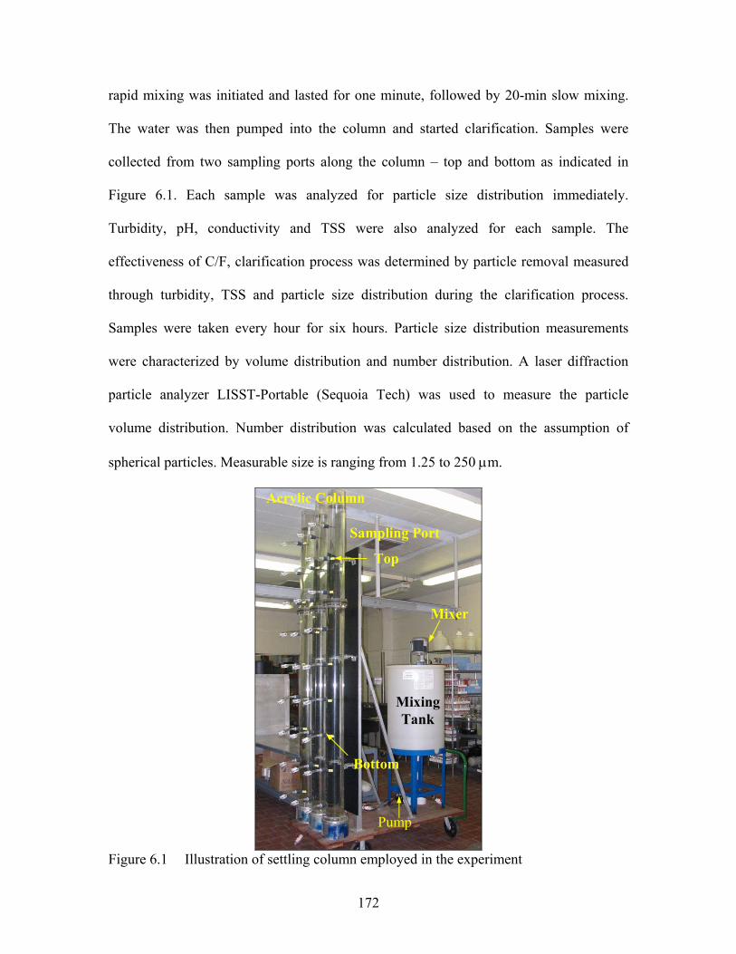
172

rapid mixing was initiated and lasted for one minute, followed by 20-min slow mixing.

The water was then pumped into the column and started clarification. Samples were

collected from two sampling ports along the column – top and bottom as indicated in

Figure 6.1. Each sample was analyzed for particle size distribution immediately.

Turbidity, pH, conductivity and TSS were also analyzed for each sample. The

effectiveness of C/F, clarification process was determined by particle removal measured

through turbidity, TSS and particle size distribution during the clarification process.

Samples were taken every hour for six hours. Particle size distribution measurements

were characterized by volume distribution and number distribution. A laser diffraction

particle analyzer LISST-Portable (Sequoia Tech) was used to measure the particle

volume distribution. Number distribution was calculated based on the assumption of

spherical particles. Measurable size is ranging from 1.25 to 250 µm.

Pump

MixingTank

Acrylic Column

Sampling Port

Top

Bottom

Mixer

Figure 6.1 Illustration of settling column employed in the experiment

173

Floc Characterization

The retrieved flocs from C/F process were characterized using image analysis. Each

floc was observed under optical microscope (BX-600) and scanning electron microscope.

RESULTS AND ANALYSIS

Jar Test for Rainfall-runoff

The experiments were conducted under constant lab temperature 5.023± °C. pH of

raw rainfall-runoff was 05.040.7 ± . Figure 6.2 through Figure 6.7 showed the particle

volume distribution and cumulative particle number distribution for rainfall-runoff C/F

with addition of alum, FeCl3, CP (1&2) and AP (1&2) at different dosages.

Raw rainfall-runoff and control (zero dosages of any coagulants/flocculants) were

also analyzed for comparison. Except for a small reduction of particles greater than 10-

µm, majority of particles in rainfall-runoff remained their stable status without

interference of coagulants or flocculants. With addition of alum at dosage of 20-mg/L and

above, destabilized clay-size (<2-µm) particles began to coagulate; large aggregate was

then removed from the suspension by clarification. In similar, with dose of FeCl3 at

20mg/L and above, clay-size particles began to destabilize and formed large aggregates

during C/F process. However, the FeCl3 flocs did not settle as well as alum flocs. A

significant amount of particle volume between 30 to 60-µm had been seen in Figure 6.3.

With addition of CP1, a high charge density cationic polyacrylamide, particles less than

10-µm were efficiently removed at dosage 7.5-mg/L or higher. It has been observed that

large aggregates were formed. The presence of these large flocs in the sample was

attributed to the peak volume distribution in the larger size end. Similarly, AP1 (anionic

polyacrylamide, charge density 30%) showed a significant removal even at a very low

174

dosage. In addition, the aggregates settled quickly from the suspension. In contrast, low

charge density anionic polyacrylamide AP2 was not as effective as AP1 though it also

achieved a decent removal of particles. Low charge density cationic polyacrylamide CP2,

on the other hand, was not effective in removing fine colloidal size particles.

Jar-test results in terms of turbidity and TSS were illustrated in Figure 6.8 and

removal efficiencies for turbidity and TSS with all types of coagulants and flocculants

were summarized in Figure 6.9. In general, anionic polymer with a high charge density

worked best in the C/F process for rainfall-runoff. However, because of the high viscosity

of polymer, it was not easy to mix them well with a large volume of rainfall-runoff.

Alum, instead, was chosen as the coagulant for the column test thereafter. According to

jar test, at dosage of 30-mg/L alum, 80% of TSS removal was achieved. The pH value

was reduced to 7.25, which was within the acceptable range. Based on dosage of 30-

mg/L alum, the estimated chemical cost is $4.8x10-6/L ($160/dry ton, HSA 2001).

Zeta potential (ψ) measurement showed that there was no significant difference

before and after C/F using alum (Before 3.17.14 ±−=Ψ mv; after 3.13.15 ±−=Ψ mv). It

indicating that instead of the commonly accepted mechanism double-layer compression,

alum is an effective coagulant in rainfall-runoff through adsorption, charge neutralization

and sweep floc enmeshments.

Jar Test for Wastewater

Raw wastewater showed a skewed particle size distribution towards larger size. By

gravitational settling, a significant amount of large particles can be removed. Figure 6.10

through Figure 6.15 showed the results of jar-test for wastewater with alum, FeCl3, CP 1

& 2 and AP 1 &2. FeCl3 was proved to be the most effective coagulant for enhanced

175

wastewater pretreatment. According to jar-test, at dosage of 30-mg/L, 86% removal was

obtained and pH dropped to 7.14. Anionic polyacrylamide did not work at all because of

the negative charge of wastewater. CP1 at a dosage of 5-mg/L or above improved the

particle removal. Figure 6.16 summarized the turbidity and TSS results of jar-test for C/F

in wastewater. Removal efficiencies were plotted in Figure 6.17. In all aspects, FeCl3 was

chosen for the following column test.

Jar Test for Natural River Water

River water has the longest retention time among the three waters investigated. Jar-

test results for river water were shown in Figure 6.18 through Figure 6.25. Quiescent

settling can settle out particles greater than 100-µm. However, small size particles,

especially clay-size colloidal particles cannot be removed by gravitational sedimentation.

C/F experiments on river water showed that alum, at dosage of 20-mg/L or higher,

enhanced the particle removal of small size range. AP1 in this case still worked best and

therefore was chosen to be applied in the lab-scale column test thereafter.

Settling Column Tests

Alum, FeCl3 and AP1 were chosen respectively for rainfall-runoff, wastewater and

river water coagulation/flocculation column test. Quiescent settling column tests without

addition of any coagulants or flocculants were carried out for three types of waters and

results were compared with C/F settling column tests. Particle volume distribution and

number distribution were illustrated for each sample withdrawn from top and bottom

sampling ports. Figure 6.26 through Figure 6.34 showed the settling column test results

for rainfall-runoff, wastewater and river water.

176

Under quiescent settling of rainfall-runoff, there was no significant change in particle

distribution throughout the column during the first three hours as seen in Figure 6.26.

Particles in raw rainfall-runoff remained stable in suspension. Until the fourth hour of

retention, a decrease of particle volume distribution was observed for particles in the

range of 5 to 100-µm. In contrast, with addition of alum at dosage of 30-mg/L, small

particles (<10-µm) were destabilized, coagulated and clarified from the suspension

rapidly. Time zero in the C/F column test was starting from clarification, during which

destabilized particles were settled out by gravitational force in the column. A higher

volume distribution analyzed for the sample withdrawn from the bottom sampling port

indicated the sedimentation of large aggregates formed from the C/F process. With

increase of retention time, particle removal increased. Turbidity and suspended solid

concentration (SSC) removal for C/F with alum was compared with quiescent settling of

rainfall-runoff. Results were shown in Figure 6.28. An average of 74.2% removal of SSC,

66.0% removal of turbidity was obtained with addition of alum after 2-hour retention. In

contrast, only 23.1% of SSC and 16.0% of turbidity removal was attained with same

retention time under quiescent settling.

In the C/F column test for wastewater, gravitational sedimentation can remove

particles in the large size range efficiently given retention time over 3 hours. The typical

retention time for primary sedimentation tank is 1 to 2.5 hr (Tchobanoglous 1991) based

on the wastewater flow. Application of FeCl3 enhanced the particle removal by 37% in

terms of turbidity and 10% in terms of SSC (Figure 6.31).

For the river water, quiescent settling cannot remove particles less than 5-µm (Figure

6.32). With a high charge density anionic polyacrylamide (AP1), the fine size particles

177

were destabilized and coagulated. As shown in Figure 6.33, an increase in volume

concentration was observed for the samples taken from the bottom ports in later time.

This increase was attributed to descending particles intercepted at the point of sampling.

As a result of quiescent settling, turbidity removal was 18% and SSC removal was 52%.

In comparison, C/F with AP1 for natural river water achieved 80% of turbidity removal

and SSC removal.

Floc Characteristics

Flocs obtained from jar-test for three types of waters were retrieved and analyzed

under optical microscope. The transmitted light optical images and scanning electron

images of these flocs were shown in Figure 6.35. As seen in Figure 6.35, flocs formed by

flocculants are large flake-size aggregates, especially in wastewater C/F. Inter-particle

bridging effect was apparent in Figure 6.35 (e) and (f). Flocs formed through inorganic

coagulants are more densely packed.

CONCLUSIONS

Particles in rainfall-runoff remain stable and stay in the suspension for an extended

period. Traditional gravitational settling can not remove small particles efficiently from

rainfall-runoff suspension. The conducted jar test experiment and settling column test

showed that with addition of alum or high charge density polyacrylamide, particles were

destabilized, coagulated, flocculated and settled out of solution within a short retention

time. The addition of metal salts alum resulted in a slight decrease of pH. No significant

pH effect was found when dosing flocculants since polyacrylamide is less pH-sensitive.

Aggregates formed through alum induced coagulation are smaller than those formed by

flocculants. Considering the field application, alum was recommended for urban rainfall-

178

runoff treatment. Through adsorption, charge neutralization and sweep floc development

alum is an effective coagulant in rainfall-runoff, in contrast to the more commonly

accepted mechanisms of double-layer compression.

C/F was also applied to improve the particle removal in primary wastewater

treatment. FeCl3 was proved to be effective to remove negatively charged particles in

primary wastewater stream. River water contains more particles with fine size (less than

5-µm), which cannot be removed by sedimentation. These particles are also easily re-

suspended by turbulent flow. They will be a concern for sensitive watershed. Removal of

these particles can also be realized through C/F.

REFERENCES

Anderson, N.J., Chin, C.T., Kolarik, L.O. and Weerawardene, A. (1992). “Rapid treatment of rainfall-runoff overflows.” International Symposium on Urban Rainfall-runoff Management. Inst. of Engineers, Australia, Sydney

Booker, N.A. et al. (1996). Novel high-rate processes for sewer overflow treatment. Wat. Sci. Tech. Vol. 34, No. 3-4, pp.103-109.

Butler, D. et al. (1992). Aspects of surface sediments characteristics on an urban catchment in Lodon. Wat. Sci. Tech. Vol. 25, No.8, pp. 13-19.

Characklis, G. W., and Wiesner, M. R. (1997). “Particles, metals, and water quality in runoff from large urban watershed.” J. Enviro. Engrg., ASCE, 123(8), 753-759

Crumb, F. and West, R. (2000). After the rain, Water Environment and Technology Vol. 12, No.4 pp. 41-45.

De Cock, W., Blom, P., Vaes, G. and Berlamont, J. (1999). “The feasibility of flocculation in a storage sedimentation basin.” Wat. Sci. Tech., 39(2), 75-83.

Drapper, D., Tomlinson, R. and Williams, P. (2000). “Pollutant concentrations in road runoff: Southeast Queensland case study.” J. Enviro. Engrg., ASCE, 126(4), 313-320.

ERD-Environmental Research & Design, Inc. (1999). Long-Term Evaluation of the Lake Ella Alum Injection System, Technical paper

Gromaire-Mertz, M.C. et al. (1999). Characterization of Urban Runoff Pollution in Paris. Wat. Sci. Tech. Vol.39, No.2, pp.1-8.

179

0

3

6

9

12

15

Vol

ume

Con

c. [ µ

L/L]

0

3

6

9

12

15Dosage = 5 mg/L

LOG

Cum

ulat

ive

PND

(cou

nt/c

m3 )

012345678

Dosage = 10 mg/L

0

3

6

9

12

15Dosage = 20 mg/L

012345678

Dosage = 30 mg/L

Particle Diameter (µm)1 10 100

0

3

6

9

12

15Dosage = 40 mg/L

1 10 100012345678

Dosage = 50 mg/L

012345678

Rainfall-runoff (raw) Control

Figure 6.2 Coagulation and flocculation jar-test of alum for rainfall-runoff (shaded bars

are the measured incremental volume distribution as a function of particle diameter; scattered plots with error bars are cumulative particle number distribution calculated from particle volume distribution.)

180

Vol

ume

Con

c. [ µ

L/L]

0

5

10

15

20Dosage = 5 mg/L

LOG

Cum

ulat

ive

PND

(cou

nt/c

m3 )

012345678

Dosage = 10 mg/L

0

5

10

15

20Dosage = 20 mg/L

012345678

Dosage = 30 mg/L

Particle Diameter (µm)

1 10 1000

5

10

15

20Dosage = 40 mg/L

1 10 100012345678

Dosage = 50 mg/L

0

5

10

15

20

012345678

Rainfall-runoff (raw) Control

Figure 6.3 Coagulation and flocculation jar-test of FeCl3 for rainfall-runoff

181

Vol

ume

Con

c. [ µ

L/L]

0

10

20

30

40Dosage = 2.5 mg/L

LOG

Cum

ulat

ive

PND

(cou

nt/c

m3 )

012345678

Dosage = 5 mg/L

Particle Diameter (µm)1 10 100

0

10

20

30

40Dosage = 7.5 mg/L

1 10 100012345678

Dosage = 10 mg/L

0

10

20

30

40

012345678

Rainfall-runoff (raw) Control

Figure 6.4 Coagulation and flocculation jar-test of CP1 (charge density 20%) for

rainfall-runoff

182

012345678

Vol

ume

Con

c. [ µ

L/L]

0

10

20

30

40Dosage = 2.5 mg/L

LOG

Cum

ulat

ive

PND

(cou

nt/c

m3 )

01234567

Dosage = 5 mg/L

Particle Diameter (µm)1 10 100

0

10

20

30

40Dosage = 7.5 mg/L

1 10 100012345678

Dosage = 10 mg/L

Control

0

10

20

30

40Rainfall-runoff (raw)

Figure 6.5 Coagulation and flocculation jar-test of CP2 (charge density 5%) for rainfall-

runoff

183

012345678

Vol

ume

Con

c. [µ

L/L]

0

5

10

15

20Dosage = 2.5 mg/L

LOG

Cum

ulat

ive

PND

(cou

nt/c

m3 )

012345678

Dosage = 5 mg/L

Particle Diameter (µm)1 10 100

0

5

10

15

20Dosage = 7.5 mg/L

1 10 100012345678

Dosage = 10 mg/L

Control

0

5

10

15

20Rainfall-runoff

(raw)

Figure 6.6 Coagulation and flocculation jar-test of AP1 (charge density 30%) for

rainfall-runoff

184

012345678

Vol

ume

Con

c. [µ

L/L]

0

5

10

15

20Dosage = 2.5 mg/L

LOG

Cum

ulat

ive

PND

(cou

nt/c

m3 )

012345678

Dosage = 5 mg/L

Particle Diameter (µm)1 10 100

0

5

10

15

20Dosage = 7.5 mg/L

1 10 100012345678

Dosage = 10 mg/L

Control

0

5

10

15

20Rainfall-runoff

(raw)

Figure 6.7 Coagulation and flocculation jar-test of AP2 (charge density 10%) for

rainfall-runoff

185

Turb

idity

(NTU

)

0

50

100

150

200

250

300

FeCl3

Alum

Control Control

CP1

CP2

AP2

AP1

Dosage (mg/L)0 10 20 30 40 50

SSC

[mg/

L]

0

50

100

150

200

0.0 2.5 5.0 7.5 10.0 12.5 15.0

Control Control

CP1

CP2

AP2

AP1

FeCl3

Alum

Figure 6.8 Turbidity and suspended solids concentration (SSC) for C/F jar-test of

rainfall-runoff

0 2.5 5 7.5 10 12.5

Turb

idity

rem

oval

%

020406080

100

Coagulant/flocculant dosage (mg/L)

0 5 10 20 30 40 50

SSC

rem

oval

%

020406080

100

AlumFeCl3

CP1CP2

AP1AP2

Figure 6.9 Removal of turbidity and SSC for C/F jar-test of rainfall-runoff

186

0

10

20

30

40

50

60

Vol

ume

Con

c. [ µ

L/L]

0

3

6

9

12

15Dosage = 5 mg/L

LOG

Cum

ulat

ive

PND

(cou

nt/c

m3 )

012345678

Dosage = 10 mg/L

0

3

6

9

12

15Dosage = 20 mg/L

012345678

Dosage = 30 mg/L

Particle Diameter (µm)1 10 100

0

3

6

9

12

15Dosage = 40 mg/L

1 10 100012345678

Dosage = 50 mg/L

0

3

6

9

12

15

012345678

Raw wastewater Control

Figure 6.10 Coagulation and flocculation jar-test of alum for wastewater

187

Vol

ume

Con

c. [ µ

L/L]

0

3

6

9

12

15Dosage = 5 mg/L

LOG

Cum

ulat

ive

PND

(cou

nt/c

m3 )

012345678

Dosage = 10 mg/L

0

3

6

9

12

15Dosage = 20 mg/L

012345678

Dosage = 30 mg/L

Particle Diameter (µm)1 10 100

0

3

6

9

12

15Dosage = 40 mg/L

1 10 100012345678

Dosage = 50 mg/L

0

10

20

30

40

50

60

0

3

6

9

12

15

012345678

Raw wastewater Control

Figure 6.11 Coagulation and flocculation jar-test of FeCl3 for wastewater

188

Vol

ume

Con

c. [ µ

L/L]

0

3

6

9

12

15Dosage = 2.5 mg/L

LOG

Cum

ulat

ive

PND

(cou

nt/c

m3 )

01234567

Dosage = 5 mg/L

Particle Diameter (µm)1 10 100

0

3

6

9

12

15Dosage = 7.5 mg/L

1 10 100012345678

Dosage = 10 mg/L

0

10

20

30

40

50

60

0

3

6

9

12

15

012345678

Raw wastewater Control

Figure 6.12 Coagulation and flocculation jar-test of CP1 (charge density 20%) for

wastewater

189

Vol

ume

Con

c. [ µ

L/L]

0

3

6

9

12

15Dosage = 2.5 mg/L

LOG

Cum

ulat

ive

PND

(cou

nt/c

m3 )

012345678

Dosage = 5 mg/L

Particle Diameter (µm)1 10 100

0

3

6

9

12

15Dosage = 7.5 mg/L

1 10 100012345678

Dosage = 10 mg/L

0

10

20

30

40

50

60

0

3

6

9

12

15

012345678

Raw wastewater Control

Figure 6.13 Coagulation and flocculation jar-test of CP2 (charge density 5%) for

wastewater

190

Vol

ume

Con

c. [ µ

L/L]

0

3

6

9

12

15Dosage = 2.5 mg/L

LOG

Cum

ulat

ive

PND

(cou

nt/c

m3 )

012345678

Dosage = 5 mg/L

Particle Diameter (µm)1 10 100

0

3

6

9

12

15Dosage = 7.5 mg/L

1 10 100012345678

Dosage = 10 mg/L

0

10

20

30

40

50

60

0

3

6

9

12

15

012345678

Raw wastewater Control

Figure 6.14 Coagulation and flocculation jar-test of AP1 (charge density 30%) for

wastewater

191

Vol

ume

Con

c. [ µ

L/L]

0

3

6

9

12

15Dosage = 2.5 mg/L

LOG

Cum

ulat

ive

PND

(cou

nt/c

m3 )

012345678

Dosage = 5 mg/L

Particle Diameter (µm)1 10 100

0

3

6

9

12

15Dosage = 7.5 mg/L

1 10 100012345678

Dosage = 10 mg/L

0

10

20

30

40

50

60

0

3

6

9

12

15

012345678

Raw wastewater Control

Figure 6.15 Coagulation and flocculation jar-test of AP2 (charge density 10%) for

wastewater

192

Turb

idity

(NTU

)

0

20

40

60

80

FeCl3

Alum

Control

Con

trol

CP1

CP2

AP2

AP1

Dosage (mg/L)0 10 20 30 40 50

SSC

[mg/

L]

0

20

40

60

80

0.0 2.5 5.0 7.5 10.0 12.5 15.0

Control Con

trol

CP1

CP2

AP2

AP1

Alum FeCl3

Figure 6.16 Turbidity and suspended solids concentration (SSC) for C/F jar-test of

wastewater

0 2.5 5 7.5 10 12.5

Turb

idity

rem

oval

%

020406080

100

Coagulant/flocculant dosage (mg/L)

0 5 10 20 30 40 50

SSC

rem

oval

%

020406080

100

AlumFeCl3

CP1CP2

AP1AP2

Figure 6.17 Removal of turbidity and SSC for C/F jar-test of wastewater

193

0

3

6

9

12

15V

olum

e C

onc.

[ µL/

L]

0

3

6

9

12

15Dosage = 5 mg/L

LOG

Cum

ulat

ive

PND

(cou

nt/c

m3 )

012345678

Dosage = 10 mg/L

0

3

6

9

12

15Dosage = 20 mg/L

012345678

Dosage = 30 mg/L

Particle Diameter (µm)1 10 100

0

3

6

9

12

15Dosage = 40 mg/L

1 10 100012345678

Dosage = 50 mg/L

012345678

Raw riverwater Control

Figure 6.18 Coagulation and flocculation jar-test of alum for river water

194

Vol

ume

Con

c. [ µ

L/L]

0

3

6

9

12

15Dosage = 5 mg/L

LOG

Cum

ulat

ive

PND

(cou

nt/c

m3 )

012345678

Dosage = 10 mg/L

0

3

6

9

12

15Dosage = 20 mg/L

012345678

Dosage = 30 mg/L

Particle Diameter (µm)

1 10 1000

3

6

9

12

15Dosage = 40 mg/L

1 10 100012345678

Dosage = 50 mg/L

0

3

6

9

12

15

012345678

Raw riverwater Control

Figure 6.19 Coagulation and flocculation jar-test of FeCl3 for river water

195

Vol

ume

Con

c. [ µ

L/L]

0

3

6

9

12

15Dosage = 2.5 mg/L

LOG

Cum

ulat

ive

PND

(cou

nt/c

m3 )

012345678

Dosage = 5 mg/L

Particle Diameter (µm)

1 10 1000

3

6

9

12

15Dosage = 7.5 mg/L

1 10 100012345678

Dosage = 10 mg/L

012345678

0

3

6

9

12

15Raw riverwater Control

Figure 6.20 Coagulation and flocculation jar-test of CP1 (charge density 20%) for river water

196

Vol

ume

Con

c. [ µ

L/L]

0

3

6

9

12

15Dosage = 2.5 mg/L

LOG

Cum

ulat

ive

PND

(cou

nt/c

m3 )

012345678

Dosage = 5 mg/L

Particle Diameter (µm)1 10 100

0

3

6

9

12

15Dosage = 7.5 mg/L

1 10 100012345678

Dosage = 10 mg/L

012345678

0

3

6

9

12

15Raw riverwater Control

Figure 6.21 Coagulation and flocculation jar-test of CP2 (charge density 5%) for river

water

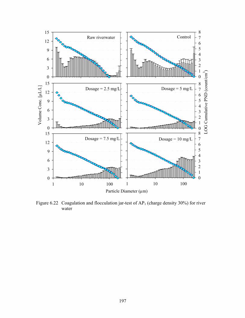
197

Vol

ume

Con

c. [ µ

L/L]

0

3

6

9

12

15Dosage = 2.5 mg/L

LOG

Cum

ulat

ive

PND

(cou

nt/c

m3 )

012345678

Dosage = 5 mg/L

Particle Diameter (µm)1 10 100

0

3

6

9

12

15Dosage = 7.5 mg/L

1 10 100012345678

Dosage = 10 mg/L

012345678

0

3

6

9

12

15Raw riverwater Control

Figure 6.22 Coagulation and flocculation jar-test of AP1 (charge density 30%) for river

water

198

Vol

ume

Con

c. [ µ

L/L]

0

3

6

9

12

15Dosage = 2.5 mg/L

LOG

Cum

ulat

ive

PND

(cou

nt/c

m3 )

012345678

Dosage = 5 mg/L

Particle Diameter (µm)1 10 100

0

3

6

9

12

15Dosage = 7.5 mg/L

1 10 100012345678

Dosage = 10 mg/L

012345678

0

3

6

9

12

15Raw riverwater Control

Figure 6.23 Coagulation and flocculation jar-test of AP2 (charge density 10%) for river

water

199

Turb

idity

(NTU

)

0

40

80

120

160

200

FeCl3

Alum

Control Control

CP1

CP2

AP2

AP1

Dosage (mg/L)0 10 20 30 40 50

SSC

[mg/

L]

0

30

60

90

120

150

0.0 2.5 5.0 7.5 10.0 12.5 15.0

Control Control

CP1

CP2

AP2AP1

Alum FeCl3

Figure 6.24 Turbidity and suspended solids concentration (SSC) for C/F jar-test of river

water

0 2.5 5 7.5 10 12.5

Turb

idity

rem

oval

%

020406080

100

Coagulant/flocculant dosage (mg/L)

0 5 10 20 30 40 50

SSC

rem

oval

%

020406080

100

AlumFeCl3

CP1CP2

AP1AP2

Figure 6.25 Removal of turbidity and SSC for C/F jar-test of river water

200

Vol

ume

Con

c. [ µ

L/L]

0

3

6

9

12

15

LOG

Cum

ulat

ive

PND

(cou

nt/c

m3 )

012345678

Particle Diameter (µm)

0

3

6

9

12

15

012345678

0

3

6

9

12

15

0

3

6

9

12

15

012345678

t = 0 (T) t = 0 (B)

t = 1 (T)

012345678

t = 1 (B)

t = 2 (T) t = 2 (B)

t = 3 (T) t = 3 (B)

1 10 1000

3

6

9

12

15

1 10 100012345678

t = 4 (T) t = 4 (B)

Figure 6.26 Quiescent settling column test for rainfall-runoff (T – top sampling port, B – bottom sampling port, t – retention hours)

201

Vol

ume

Con

c. [ µ

L/L]

0

30

60

90

120

150

LOG

Cum

ulat

ive

PND

(cou

nt/c

m3 )

012345678

Particle Diameter (µm)

0

10

20

30

40

50

012345678

0

10

20

30

40

50

0

10

20

30

40

50

012345678

t = 0 (T) t = 0 (B)

t = 1 (T)

012345678

t = 1 (B)

t = 2 (T) t = 2 (B)

t = 3 (T) t = 3 (B)

1 10 1000

10

20

30

40

50

1 10 100012345678

t = 4 (T) t = 4 (B)

Figure 6.27 Rainfall-runoff coagulation and flocculation with alum (30mg/L)

202

Turb

idity

(NTU

)

0

100

200

300

400

TopBottom

SSC

[m

g/L]

0

100

200

300

400Quiescent Settling Quiescent Settling

Retention time (hr)0 1 2 3 4 5 6

0

100

200

300

400

0 1 2 3 4 5 60

100

200

300

400C/F with Alum C/F with Alum

Figure 6.28 Column test results for rainfall-runoff

203

Vol

ume

Con

c. [ µ

L/L]

0102030405060

LOG

Cum

ulat

ive

PND

(cou

nt/c

m3 )

012345678

Particle Diameter (µm)

0102030405060

012345678

0102030405060

0102030405060

012345678

t = 0 (T) t = 0 (B)

t = 1 (T)

012345678

t = 1 (B)

t = 2 (T) t = 2 (B)

t = 3 (T) t = 3 (B)

1 10 1000

102030405060

1 10 100012345678

t = 4 (T) t = 4 (B)

Figure 6.29 Quiescent settling column test for wastewater

204

Vol

ume

Con

c. [ µ

L/L]

0102030405060

LOG

Cum

ulat

ive

PND

(cou

nt/c

m3 )

012345678

Particle Diameter (µm)

0102030405060

012345678

0102030405060

0102030405060

012345678

t = 0 (T) t = 0 (B)

t = 1 (T)

012345678

t = 1 (B)

t = 2 (T) t = 2 (B)

t = 3 (T) t = 3 (B)

1 10 1000

102030405060

1 10 100012345678

t = 4 (T) t = 4 (B)

Figure 6.30 Wastewater coagulation and flocculation with FeCl3

205

Turb

idity

(NTU

)

0

40

80

120

160

200

TopBottom

SSC

[m

g/L]

050

100150200250300

Quiescent Settling Quiescent Settling

Retention time (hr)

0 1 2 3 4 5 60

40

80

120

160

200

0 1 2 3 4 5 60

50100150200250300

C/F with FeCl3 C/F with FeCl3

Figure 6.31 Column test results for wastewater

206

Vol

ume

Con

c. [ µ

L/L]

0

3

6

9

12

15

LOG

Cum

ulat

ive

PND

(cou

nt/c

m3 )

012345678

Particle Diameter (µm)

0

3

6

9

12

15

012345678

0

3

6

9

12

15

0

3

6

9

12

15

012345678

t = 0 (T) t = 0 (B)

t = 1 (T)

012345678

t = 1 (B)

t = 2 (T) t = 2 (B)

t = 3 (T) t = 3 (B)

1 10 1000

3

6

9

12

15

1 10 100012345678

t = 4 (T) t = 4 (B)

Figure 6.32 Quiescent settling column test for river water

207

Vol

ume

Con

c. [ µ

L/L]

0

20

40

60

80

LOG

Cum

ulat

ive

PND

(cou

nt/c

m3 )

012345678

Particle Diameter (µm)

0

3

6

9

12

15

012345678

0

20

40

60

80

0

3

6

9

12

15

012345678

t = 0 (T) t = 0 (B)

t = 1 (T)

012345678

t = 1 (B)

t = 2 (T) t = 2 (B)

t = 3 (T) t = 3 (B)

1 10 1000

3

6

9

12

15

1 10 100012345678

t = 4 (T) t = 4 (B)

Figure 6.33 River water coagulation and flocculation with AP1

208

Turb

idity

(NTU

)

0

100

200

300

400

TopBottom

SSC

[m

g/L]

0

100

200

300

400Quiescent Settling Quiescent Settling

Retention time (hr)0 1 2 3 4 5 6

0

100

200

300

400

0 1 2 3 4 5 60

100

200

300

400C/F with AP1

C/F with AP1

Figure 6.34 Column test results for river water

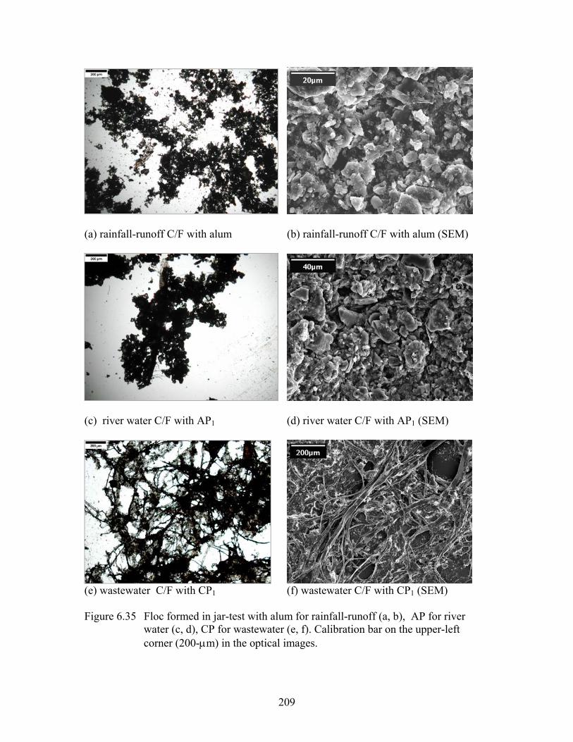
209

(a) rainfall-runoff C/F with alum (b) rainfall-runoff C/F with alum (SEM)

(c) river water C/F with AP1 (d) river water C/F with AP1 (SEM)

(e) wastewater C/F with CP1 (f) wastewater C/F with CP1 (SEM) Figure 6.35 Floc formed in jar-test with alum for rainfall-runoff (a, b), AP for river

water (c, d), CP for wastewater (e, f). Calibration bar on the upper-left corner (200-µm) in the optical images.

210

Hecker, R. (1998). The characterization of polyacrylamide flocculants. Thesis, School of applied chemistry, Curtin University of Technology, Australia.

Heinzmann, B. (1994). “Coagulation and flocculation of rainfall-runoff from a separate sewage system- A new possibility for enhanced treatment.” Wat. Sci. Tech., 29(12), 267-278

Jacopin, Ch. et al. (1999). Characterisation and settling of solids in an open, grassed, rainfall-runoffsewer network detention basin. Wat. Sci. Tech., Vol. 39, No. 2, pp. 135-144.

McAnally, W. H., and Mehta, A. (2001). “ Collision aggregation of fine estuarial sediment.” McAnally, W. H. and Mehta, A. J. ed. “Coastal and estuarine fine sediment processes, Elsevier Science, 2001 19-39.

Michelabch, S. and Weiß, G. (1996). “Settable sewer solids at rainfall-runofftanks with clarifier for combined sewage.” Wat. Sci. Tech., 33(9), 261-267.

Myrhaug, D., Slaattelid, O.H., and Lambrakos, K.F. (1993). “Suspended sediment concentrations near the seabed in north sea storms.” Belorgey, M. ed. “Sediments transport mechanisms in costal environments and rivers.” Euromech 310, 13-17 September, 1993. World Scientific. 397-412

Nichol, M. ( 1984). “Effects of fine sediment resuspension in estuaries.” Mehta, A. J. ed. “Estuarine cohesive sediment dynamics.” Proceedings of a workshop on cohesive sediment dynamics with special references to physical processes in estuaries, Tampa, Florida, November 12-14, 1984. Springer-Verlag. 5-42

Nieuwenhuijzen, A.F. van (2002). “Scenario studies into advanced particle removal in the physical-chemical pre-treatment of wastewater”, published by DUP Science.

Hayter, E. J., and Gu, R. (2001). “Prediction of contaminated sediment transported in the Maurice River-Union Lake, New Jersey, USA.” McAnally, W. H. and Mehta, A. J. ed. “Coastal and estuarine fine sediment processes, Elsevier Science, 2001 439-458

HAS. (2001). “Report on conducting pilot scale treatability studies for the everglades rainfall-runoff program (ESP) urban and tributary basins program.” Technical report.

Krank, K. (1984). “Settling behavior of cohesive sediment” Mehta, A. J. ed. “Estuarine cohesive sediment dynamics.” Proceedings of a workshop on cohesive sediment dynamics with special references to physical processes in estuaries, Tampa, Florida, November 12-14, 1984. Springer-Verlag. 151-169

Odegaard, H., Fettig, J. and Ratnaweera, H. C. (1990). “ Coagulation with Prepolymerized Metal Salts. Chemical Water and Wastewater Treatment Proceedings of the 4th Gothenburg Symposium, 189-220

Passino, Roberto and Ramadori, Roberto. (1999). Renewed Interest for Chemical Processes In Urban Wastewater Treatment and Reuse. Annali di Chimica, Vol. 89, pp. 249-256.

211

Sansalone, J.J., and Buchberger, S.G. (1996). Characterization of solid and metal element distribution in urban highway rainfall-runoff. Wat. Sci. Tech. Vol. 36, No. 8-9, pp. 155-160

Sansalone, J. J., Koran, J. M., Smithson, J. A., and Buchberger, S. G. (1998). “Physical characteristics of urban roadway solids transported during rain.” J. Enviro. Engrg., ASCE, 124(5), 427-440

Tchobanoglous, G. and Burton ed. (1991). Wastewater engineering: treatment, disposal, and reuse (3rd ed.). Metcalf & Eddy, Inc. McGraw-Hill, Inc.

Thomas, D. N. et al. (1999). Flocculation modeling: A review. Wat. Res. Vol. 33, No.7, pp.1579-1592.

Xanthopoulos, C. and Augustin, A. (1992). Input and Characterization of sediments in urban sewer system. Wat. Sci. Tech. Vol. 25, No. 8, pp. 21-28.

Xanthopoulos, C. and Hahn, H. (1993). Anthropogenic pollutants wash-off from street surfaces. Proceedings of the 6th International Conferences on Urban Storm Drainage, Ontario, Vol. 1, pp. 417-422.

Yu, S. L. et al. (1994). Testing of best management practices for controlling highway runoff: Phase II. Virginia Transportation Research Council, Charlottesville, Va

212

CHAPTER 7. COAGULATION AND AGGREGATION MODEL INCORPORATING FRACTAL THEORIES FOR PARTICULATES IN URBAN

RAINFALL-RUNOFF

SUMMARY

Particulate matter plays an important role in transport and transformation of

contaminant. Separation of particulate from urban rainfall-runoff is one of the major

goals of best management practices in urban rainfall-runoff treatment. Sedimentation has

been used generally in removing settleable particulates. Coagulation and flocculation was

applied to removal colloidal and fine particles in order to improve the treatment

efficiency. The fractal nature of particles in urban rainfall-runoff and heterogeneous

distributions complicated the process. Theoretical settling model and coagulation and

flocculation model cannot predict the behavior of real particles in the system. Design

based on traditional model would be inappropriate. A thorough literature review on the

contaminant removal mechanisms – sedimentation, coagulation and flocculation was

summarized in this study. Based on the granulometry and fractal study, a modified fractal

model was evaluated to simulate and predict the particle size distribution during the

sedimentation and coagulation process in urban rainfall-runoff treatment system. The

simulation applied to a 2-m settling column system with sediment particles from urban

rainfall-runoff. Fractal dimension and collision efficiency α are considered important

factors in determining particle size distribution.

INTRODUCTION

Pollution from suspended particles to natural water bodies is one of many

consequences of the intensive utilization of the land. Urban rainfall-runoff is one of the

major sources of these particles. Besides the fact that the particles themselves are

213

pollutants because of the displeasing effect esthetically and the decreasing rate of

photosynthesis, particles are also of concern because toxic heavy metals and persistent

organic compounds are predominantly transported within particles or adsorbed on the

surfaces (Hunt 1980). Sedimentation and coagulation cause the removal or loss of a

particle of a given size from a volume of fluid. Sedimentation removes particles from the

volume of fluid, while coagulation and flocculation transports many smaller particles into

fewer larger particles with the fluid volume.

In natural and polluted waters there exists a continuous distribution of particle sizes.

The dynamics of a continuous size distribution is defined in Equation 1.

)()( pp ddndN ∆= (1)

where dN is the number of particles per fluid volume with diameters in the range of dp to

)d(d PP ∆+ .

The sedimentation flux (F) of particles is the Stokes’ settling velocity of a spherical

particle with diameter pd times the number of particles in the size interval dp to

)d(d PP ∆+ .

)()()(18

2ppp

L

LS ddndgF ∆−

=ρρρ

µ [L-2t-1] (2)

sρ and Lρ are the particle and fluid density respectively. The dimensional unit of time is

indicated by [t] and [L] represents a fluid length.

Coagulation Processes

Coagulation and flocculation traditionally is a two-step serial process in which the

“destabilization” of suspended particles is known as coagulation while aggregation of

destabilized particles and the rate of floc growth are known as flocculation. Mechanisms

214

of destabilization include: Double layer compression by different electrolytes (elevated

ion concentration reduces double layer thickness); Charge neutralization by specifically

adsorbed charged species; Enmeshment in a precipitate (formation of sweep floc); and

adsorption and inter-particle bridging. There are three mechanisms for particles

attachment. For particles significantly less than 1-µm, perikinetic flocculation (or

Brownian motion) is dominant due to particle diffusion. Particle contacts caused by

differences in fluid velocity are considered orthokinetic flocculation (shear driven

transport and collision). For particles greater than 50-µm, differential settling is the

significant mechanism for particle flocculation.

Classical Flocculation Model

The fundamental mathematical model of flocculation process was developed by

Smoluchowski (Thomas 1999). The basic equation for the flocculation process is

expressed as:

ki

c

ij

kjii

k nnkinnjidt

dn ∑∑==+

−=1

),(),(21 βαβα (3)

Equation 3 defines the rate of change in the number concentration of particle size k. α is

the collision efficiency, ),( jiβ is the collision frequency between particles of size i and j,

and ni, nj are the particle concentrations for particle of size i and j respectively. Subscript

i, j and k represent discrete particle sizes. c is the largest size considered. The basic

concept for the above model is that the concentration of the particles of a given size k can

be increased by the collision and attachment of two small particles whose total volume is

that of a k-size particle (first term on the right side), and decreased by the collision and

215

attachment of a k-size particle with any size particle to form a larger particle (second term

on the right side).

The assumptions made for simplifications include that collision efficiency α is unity

for all collisions; fluid motion undergoes laminar shear; the particles are mono-dispersed;

no breakage of flocs occurs; all particles are spherical in shape and remain so after

collision; and collision involves only two particles (Binary collisions). Base on these

assumptions, the equations to describe the collision frequency for each flocculation are as

follows.

For perikinetic flocculation,

))(11(3

2ji

jiP dd

ddkT

++=µ

β (4)

For orthokinetic flocculation,

3))((61

jiO dddydu

+=β (5)

where k is Boltzmann’s constant, T is the absolute temperature of the fluid, µ is the

dynamic viscosity of the fluid, and du/dy is the velocity gradient of the fluid.

For differential sedimentation,

jijiLSD ddddg−+−= 3))()(

72( ρρ

µπβ (6)

where di and dj are the diameters for the particle i and j respectively.

Modified Flocculation Model

The classical approach leads to analytical expressions to define the coagulation and

flocculation process; however, their pertinence to real systems is constrained by the

216

assumptions. The validity of each of the assumptions leads to the modification of the

fundamental model. In turn, each assumption is reviewed in terms of modeling.

Assumption 1: The collision efficiency factor α is unity for all collisions.

Not all collision leads to attachment. The effect of short-range forces such as

electrostatic repulsion, van de Waals or hydrodynamic forces is non-negligible in the real

system. The combined effect of electrostatic repulsion and van de Waals attraction

between two particles is described by the DLVO theory (Deryaguin and Landau 1941;

Verwey and Overbeek 1948). This theory assumes that the effect of two forces is

additive, and the results can be displayed in the form of a potential energy diagram show

in Figure 7.1. The lower the energy barrier, the closer to unityα becomes.

Rep

ulsi

veA

ttrac

tiveIn

tera

ctio

n En

ergy

1-electrostatic repulsion

Combined effect of 1 and 2

2-Van der Waals attraction

Energy barrier

Potential well

Distance from Particle surface

Figure 7.1 DLVO theory-Potential energy diagram

The Smoluchowski model assumes that inter-particle interactions are negligible until

the point of contact, whereupon adhesion takes place with 100% efficiency. The inter-

particle interaction based on this assumption is described as rectilinear. However, in the

real system the hydrodynamic forces have significant impact on the colloidal particles.

217

They cause the approaching particles to rotate slightly around one another, which are

known as curvilinear. Rectilinear model and curvilinear model were discussed

considering the hydrodynamic forces (Han and Lawler 1992). Three important

conclusions arise from the developments of curvilinear models: First, orthokenetic

flocculation is far less important in the curvilinear model than in the rectilinear model;

Secondly, the curvilinear model predicts a much lower collision frequency than the

rectilinear model, although the reduction is less when the particles are of similar size;

Finally, orthokenetic flocculation is no longer seen as being directly proportional of

velocity gradient G (Camp and Stein 1943).

Current developments in the modeling of hydrodynamic forces between colloid

particles are developing in two areas: non-uniform porosity (Veerapaneni and Wiesner

1996; Li and Logan 1997a, b; Wu and Lee 1998) and uniformly porous flocs (Adler

1981, Kusters et al. 1991). It was found that above a critical limit of the dimensionless

radius (defined as the kR / , where R is the aggregate radius, and k is aggregate

permeability) the collision efficiency became zero.

Assumption 2: Fluid motion undergoes laminar shear.

Camp and Stein (1943) defined the term G, the local root-mean-square velocity

gradient for a small local element of fluid undergoing strain, and linked G with the local

rate of energy dissipationε :

2/1)/( υε=G (7)

where υ is the kinetic viscosity of the fluid.

The global scale was further defined as the global root-mean-square velocity gradient

G* for a flocculating system.

218

2/1)/( υε ∗∗ =G (8)

where ∗ε is the average energy dissipation for the whole flocculating system. Camp and

Stein assumed that Smoluchowski’s dydu / could be replaced by G for linear flow

regimes and by G* in turbulent flow regimes.

Kramer and Clark (1997) identified two errors in Camp and Stein’s work: incorrect

association of G with ε due to the ignoring the contribution made by the pure-normal

strain component of the rate-strain tensor; and inaccuracy of assuming that G* was a

representative measure of the fluid dynamics within a flocculating system.

In practice, few real-life flocculation units operate under laminar flow. In overall

terms, turbulence is still poorly understood. However, isotropic model has been

successfully adopted in flocculation modeling. Such models describe turbulence as a

cascade of eddies of diminishing size. Based on the cascade model, Casson and Lawler

(1990) put forward that collisions between particles are promoted by eddies of a size

similar to those of the colloid particles in turbulent flow. Energy expended during mixing

in the creation of large eddies could be ineffectual.

Through studying the effect of hydrodynamic retardation upon the collision constants

in the Smoluchowski model, Han and Lawler (1992) came to the conclusion that the

actual contribution of orthokinetic flocculation to the overall flocculation process was

minimal because of the pronounced effect of hydrodynamic retardation. Therefore,

mixing simply provided a means of suspending the particles to keep the particle number

count high enough for collision to occur.

Assumption 3: The particles are mono-dispersed; all have the same size.

219

In real systems, particles are hetero-dispersed indicating a composition of particles

with a great variety of gradations. Tambo (1965) and his various coworkers (Tambo and

Ogasawara 1970; Tambo and Watanabe 1979; Tambo 1991) proposed that dimensionless

product φGt be used to determine the flocculation process. φ is the volume fraction of

the particles. Harris et al (1966) observed the extent of aggregation and floc formation to

be a function of both φGt and particle size distribution. O’Melia (1972) has shown the

dependence of flocculation process on particle size and size distribution and noted that

flocculation is more rapid in heterogeneous suspensions. Harding (1972) also found that

flocculation is primarily dependent on particle size distribution.

Particle size distribution is important because it controls many physical and chemical

properties. It will be changed throughout the flocculation process. Particle size

distribution can be modeled by a two-parameter power-law distribution function given by

the following expression.

βα nvT lN ⋅= 1 (9)

NT is the particle number density; lnv is the number volume mean size; and a1 and β are

empirical constants (Kavanaugh et al. 1980). A rapid estimate of contaminant distribution

can be made from the magnitude of the model parameter β, which describes the slope of

the frequency distribution.

Treweek and Morgan (1977) found that turbidity measurements alone were

inadequate to measure the effectiveness of treatment process, since large changes in the

particle size distribution during the flocculation process do not produce corresponding

changes in turbidity. It has been shown that flocculation test based on particle size and

count is more reliable. Particle size distribution measurements were characterized by the

220

total volume concentration, the peak of the volume concentration, and the slope of the

particle size distribution function β. These measurements are particularly appropriate for

showing the differences in flocculation over time and between experiments. However, the

volume distribution does not provide clear evidence of flocculation at greater

concentrations as it does for lesser concentrations.

Assumption 4: No breakage of flocs occurs.

According to Spicer and Pratsinis (1996), the balance of aggregation and break-up

determines the floc size and mass distributions. Computer simulation (Fair and Gemmel

1964; Costas et al. 1995) identified the importance of breakage in modeling flocculation.

The break-up mechanisms can have significant effect on both initial rates of reaction and

eventual steady-state concentration.

It is generally accepted (Mühle 1993) that the breakage mechanism in turbulent flow

depends upon a floc’s size relative to the Kolmogorov microscale, which is defined as the

transition between the domain where inertial forces dominate and that where viscous

forces dominate (Peters and Marrasé 2000). For flocs smaller than the Kolmogorov

microscale, viscous forces predominate and erode the surface of the floc. In contrast, for

flocs larger than the Kolmogorov microscale, deformation or fracture may occur as a

result of fluctuating dynamic pressure. These ideas imply that floc strength is

proportional to floc size. However, Yeung and Pelton (1996) suggested that floc

compactness rather than its size is related to the strength. The more compact flocs were

more likely they undergo erosions whereas less compact flocs were more likely to

undergo fracture.

221

A connection between break-up phenomenon and the value of G was pointed out by

Ritchie (1955). The empirical relationship between applied G and maximum floc size

indicated the existence of a critical value of G for a particular system, above which

flocculation performance would be reduced. A similar effect was observed by Tambo and

Hozumi (1979), who proposed the following relationship between maximum floc size

and mixing intensity:

xGCFlocsize −= )()max( (10)

Parker et al (1972) calculated theoretical values for C and x for different break-up

mechanism (erosion and fracture) for particle larger or smaller than the Kolmogorov

microscale. It was proposed that particle erosion was proportional to G2 for the viscous

domain and G4 for the inertial domain.

To model the rate of change for particles of a given size due to the process of

aggregation and breakup, Lick and Lick (1988) proposed the following expression:

ii

ijjkj

jkii

ikk

jkj

jjkkkii

ikkjkji

iijk

nnnn

nBnBnnnndt

dn

∑∑∑

∑∑∑∞

=

∞

+=

∞

=

∞

+=

∞

==+

+−

+−−=

111

11

''

21

βαγβα

γαβαβ (11)

jkγ is the breakage distribution function defining the volume fraction of the fragments of

size class k coming from the disaggregation of a particle of size class j. 'α represents the

probability of disaggregation after collision. B is the breakage rate.

The first two terms on the right side of the above equation are used to model the

aggregation processes which are identical to the classical model, given in Equation 3,

while the others are added for the disaggregating processes. The third term represents the

loss of size class k particles, giving particles with smaller diameters due to the effect of

222

shear rate. The fourth term represents the rate of increase of size class k particles due to

the disaggregation of larger particles caused by the shear rate. The fifth term represents

the loss of size class k particles due to unsuccessful collisions with all the other particles.

The last term represents the rate of increase of size class k particles after unsuccessful

collisions between particles of size classes i and j, where j is greater than k.

A similar coagulation and fragmentation model was applied by Spice and Pratsinis

(1996) where the rate terms were assumed to be functions of both floc size and G. Over a

range of G value (25-125 s-1) experimental results revealed that the rate of breakage was

proportional to G1.6. Fragmentation prevents further growth of flocs so the distributions

were found steady after a certain time. Increasing G leads to a more pronounced

increased fragmentation rate, thus shifting the stead-state floc-size distribution into

smaller floc sizes.

In the research of Lawler, Izurieta and Kao (1983), the velocity gradient, chemical

conditions and particle concentration were varied and the other variables were held

constant in the experiment design. Sedimentation instead of break-up of flocs was found

to be the reason for explaining the discrepancy of experimental results with predictions of

the mathematical model. The model was modified by the addition of terms for

sedimentation to the classical expression:

mkk

mkk

mkmii

mjkji

mimk n

zw

nzw

nnkinnjidt

dn,1,,,

max

1,,

, ),(),(21 γγ

βαβα −+−= −==+∑∑ (12)

The third term added in the classical model describes the addition of particles into the

compartment m as a result of particles settling from the compartment above; kw is the

Stoke’s settling velocity of size k particle; z is the depth of the compartment, and γ is the

223

fraction of the total area in which the mixing intensity is smaller enough to allow

sedimentation to occur. The fourth term on the right side reflects the loss of particles

from the compartment under consideration to the compartment below.

More complete mass balance equations can be written by taking into account particle

sedimentation and particle breakup (Thill et al. 2001).

kk

iii

kiii

kjkji

ik n

zvnFiknFnkinnnji

dtdn

−+−−= ∑∑∑==+

maxmax

1),(),(),(

21 γβαβα (13)

iF is the fragmentation rate of floc of size i, ),( ikγ is the breakage distribution function

defining the volume fraction of the fragments of size k coming from i-size particles. kv is

the settling velocity of aggregates of size k, and z is the height of a horizontal subdivision

of the water column in which particle concentration is to be considered.

Assumption 5: All particles are spherical in shape and remain so after collision.

In reality, particles in the majority of flocculating systems do not coalesce on contact.

This is particular true for water and wastewater systems where flocs are difficult to

characterize because of their highly irregular and disorder nature. Li and Ganczarczyk

(1989) recognized the fractal structure of these particles and aggregates. Their porosity is

a function of aggregate size and increases with increasing floc size. The mathematical

equation is expressed in Equation 14.

31 −∗−= DRSp (14)

p is the floc porosity; D is three-dimensional fractal dimension and takes values between

1 and 3; S is a system specific constant. Fractal dimensions correspond to the degree of

irregularity and complexity or the space-filling capacity of an aggregate. Fractal

aggregates have a heterogeneous mass distribution, a structure resulting from the

224

coagulation of small and more densely packed clusters into larger and overall less dense

aggregates (Johnson, Li and Logan 1995). The lower the fractal dimension, more “open”

the aggregate structure. A closely packed Euclidean structure has fractal dimension of 3.

If D equals 3 (Smoluchowski’s assumption), the porosity is constant and consequently

density is independent of size. However, D is less than 3 for the majority of the flocs in

natural system.

When the fractal dimension is considered, volume is not conserved after two particles

collide even though mass is conserved. When two particles of radius ir and jr collide,

the radius of the resultant floc is defined as:

Dj

Di

Dij rrr += (15)

Flocs with a low fractal dimension allow fluid to flow through them, resulting in a faster

settling velocity and much more suspended small particles flowing into the aggregate.

This phenomenon is known as advection. The degree of advection is characterizes by

fluid collection efficiencyη , defined as the ration of the volume of fluid flowing through

a floc to the volume of fluid approaching a floc. η takes values between 0 for a totally

impermeable floc and 1 for a totally porous floc.

In effect, the rectilinear approach assumes flocs are totally porous whereas curvilinear

approach assumes flocs are totally impermeable. Neither of the cases is true for fractal

flocs. In practice, particles approach one another along semi-curved paths, a compromise

between the straight paths assumed in rectilinear model and the curved paths assumed in

curvilinear model. Chellam and Wiesner (1993) demonstrated theoretically that η was

correlated to the fractal dimension. The degree of advection became significant when D is

less than 2. Where advection is significant, the rectilinear approach overestimate the rate

225

of collision, while the curvilinear model underestimates the rate of collision. However,

there is currently no theoretical basis to predict an accurate rate.

The effect of fractal structure of flocs has been demonstrated for differential

sedimentation flocculation (Li and Logan 1997a) and orthokinetic flocculation in

turbulent flow (Li and Logan 1997b). A correlation between fractal dimension and

collision frequency in turbulent flow was identified as:

),( jiβ ~ )3/1( DG − (16)

Assumption 6: Collision involves only two particles (Binary collisions).

The validity of this assumption is questionable when systems become concentrated

such that collisions between more than two particles are likely. In highly concentrated

suspension, swamping effect of the previous flocculated particles is profound. An

alternative approach is thermodynamic theory of coagulation, in which coagulation is

seen as a “phase-separation” process: the stabilized colloid represents the dispersed phase

and the destabilized/aggregated colloid represents the solid phase. Rajagopalan (1993)

applied thermodynamic theory to a colloid dispersion represented by an idealized

potential-separation graph. Analysis of the constructed phase diagrams allows one to

calculate the required degree of destabilization to promote flocculation.

Macroscopic Approach to the Flocculation Process

Surface chemical effects such as precipitation, destabilization and surface adsorption

are always ignored or dealt with in a simplistic manner in a flocculation model. So,

experiment results based on idealized particle suspensions are unlikely to be

representative of the behavior of the real system. Focusing on the microscopic behavior

of real particles in an attempt to deduce correlations between process parameters (e.g.

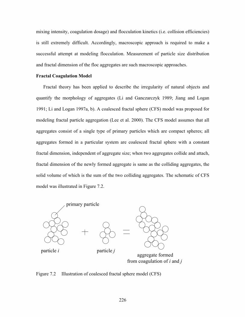
226

mixing intensity, coagulation dosage) and flocculation kinetics (i.e. collision efficiencies)

is still extremely difficult. Accordingly, macroscopic approach is required to make a

successful attempt at modeling flocculation. Measurement of particle size distribution

and fractal dimension of the floc aggregates are such macroscopic approaches.

Fractal Coagulation Model

Fractal theory has been applied to describe the irregularity of natural objects and

quantify the morphology of aggregates (Li and Ganczarczyk 1989; Jiang and Logan

1991; Li and Logan 1997a, b). A coalesced fractal sphere (CFS) model was proposed for

modeling fractal particle aggregation (Lee et al. 2000). The CFS model assumes that all

aggregates consist of a single type of primary particles which are compact spheres; all

aggregates formed in a particular system are coalesced fractal sphere with a constant

fractal dimension, independent of aggregate size; when two aggregates collide and attach,

fractal dimension of the newly formed aggregate is same as the colliding aggregates, the

solid volume of which is the sum of the two colliding aggregates. The schematic of CFS

model was illustrated in Figure 7.2.

primary particle

particle i particle jaggregate formed

from coagulation of i and j

Figure 7.2 Illustration of coalesced fractal sphere model (CFS)

227

The one-dimensional advective-dispersive transport model in an experimental settling

column was described in Equation 17 (Ernest et al. 1991).

zn

vzn

Dt

n kz

kz

k

∂∂

−∂∂

=∂∂

2

2

(17)

To consider particle coagulation and settling in a continuous particle size distribution,

Equation 18 was proposed to simulate the changes in PSD in the settling column (Ernest

et al 1995, Lee et al 2000).

zn

vzn

Dnnkinnjit

n kk

kzki

ifj

kjiif

k

∂∂

−∂∂

+−=∂∂ ∑∑

==+2

2max

1),(),(

21 βαβα (18)

Collision frequency function ),( jifβ for the CFS model was summarized in Table 1. z is

the vertical distance from the top of the settling column. zD is the hydrodynamic

dispersion coefficient, which may be viewed as the cumulative effect of Brownian

diffusion, eddy diffusion, and mechanical dispersion (Ernest et al 1991). kv is the settling

velocity for the fractal aggregate with size k.

In Equation 18 only binary collisions are considered in this model and particle

fragmentation is neglected. Volume is conserved during the coagulation. Collision

efficiency α is assumed to be a constant. Particle collisions are modeled using CFS

assumption based on the rectilinear motion.

The boundary condition for Equation 18 is described in terms of particle flux F1,

which is defined as

kkk

z nwz

nD −

∂∂

=1F (19)

228

At the top of the column, F1=0. Therefore kkk

z nwz

nD =

∂∂

(top boundary condition). At

the bottom of the column, kk nwF −=1 , 0=∂∂

zn

D kz (bottom boundary condition). In this

model, the column was divided into n sections vertically. The partial differential equation

was converted to numerically solvable equations and these equations were then solved

using the fourth order Runge-Kutta method with variable time step. Size distribution

)(tnk was calculated for particles in the size range of 2 to 200 µm as a function of time.

OBJECTIVES

Previous experimental work and models on coagulation and flocculation has been

reviewed. In this study, a coagulation model incorporating sedimentation and fractal

theory was applied to simulate the evolution of particle size distribution (PSD) of storm

water particles in a settling column. Modeled PSD was compared to the experimental

results. Various parameters of the fractal dimensions and the collision efficiency factors

were selected for the model simulations to study the effects on the resulting PSD.

MODEL AND METHODOLOGY

By introducing fractal geometry, the classical approach for the coagulation and

flocculation is designated as CFS-C/F model, which is described in Equation 20.

kii

fjkji

ifk nnkinnji

dtdn ∑∑

==+

−=max

1

),(),(21 βαβα (20)

The collision efficiency factor α is one of the most important parameters in

characterizing coagulation. It is believed to represent the chemical stability of particles

(Lee et al. 2000). Collision efficiency α is assumed to be a constant during the

coagulation and flocculation process. Studies on the estuarial sediments showed a

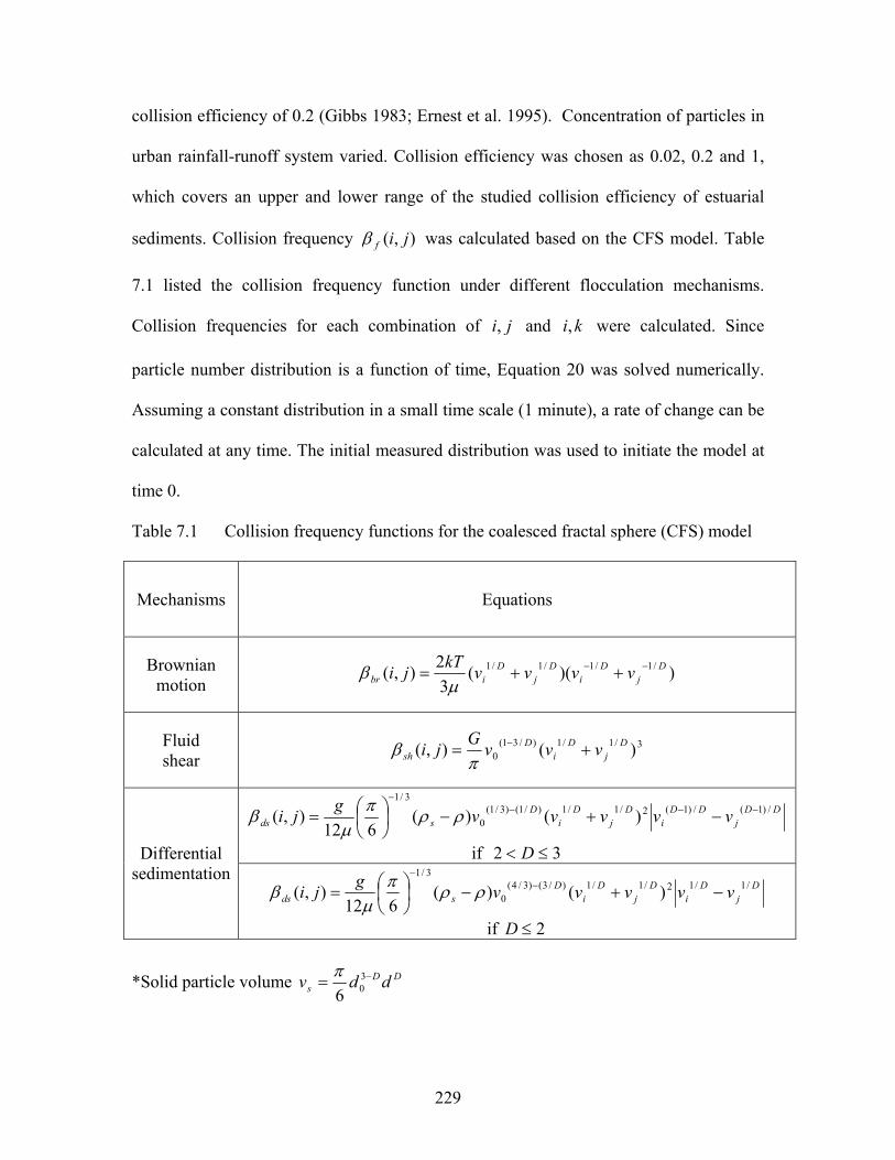
229

collision efficiency of 0.2 (Gibbs 1983; Ernest et al. 1995). Concentration of particles in

urban rainfall-runoff system varied. Collision efficiency was chosen as 0.02, 0.2 and 1,

which covers an upper and lower range of the studied collision efficiency of estuarial

sediments. Collision frequency ),( jifβ was calculated based on the CFS model. Table

7.1 listed the collision frequency function under different flocculation mechanisms.

Collision frequencies for each combination of ji, and ki, were calculated. Since

particle number distribution is a function of time, Equation 20 was solved numerically.

Assuming a constant distribution in a small time scale (1 minute), a rate of change can be

calculated at any time. The initial measured distribution was used to initiate the model at

time 0.

Table 7.1 Collision frequency functions for the coalesced fractal sphere (CFS) model

Mechanisms Equations

Brownian motion

))((32),( /1/1/1/1 D

jD

iD

jD

ibr vvvvkTji −− ++=µ

β

Fluid shear

3/1/1)/31(0 )(),( D

jD

iD

sh vvvGji += −

πβ

DDj

DDi

Dj

Di

Dsds vvvvvgji /)1(/)1(2/1/1)/1()3/1(

0

3/1

)()(612

),( −−−−

−+−

= ρρπ

µβ

if 32 ≤< D Differential sedimentation

Dj

Di

Dj

Di

Dsds vvvvvgji /1/12/1/1)/3()3/4(

0

3/1

)()(612

),( −+−

= −

−

ρρπµ

β

if 2≤D

*Solid particle volume DDs ddv −= 3

06π

230

Sedimentation is another important mechanism in the settling column test. With the

addition of terms for sedimentation, the Smoluchowski model was modified (Lawler et

al. 1983). A CFS-C/F-Sedimentation model was defined as:

mkk

mkk

mkmii

fmjkji

mifmk n

zvn

zvnnkinnji

dtdn

,1,,,

max

1,,

, ),(),(21

−+−= −==+∑∑ βαβα (21)

Equation 21 was employed to derive the modeled particle size distribution in the

settling column tests in this study. Settling velocities kv for particles of any given size

were calculated according to Newton’s Law. Table 7.2 listed the settling velocities for

particles ranging from 1.25 to 250-µm.

The column was divided into 6 compartments vertically as seen in Figure 7.3.

Samples were withdrawn from sampling port S1, S2, S3, S4 and S5. The analyzed

distribution for each sample was assumed to represent the PSD of the section above this

port. dtdn mk /, was calculated for each k size category in each compartment.

Assuming conserved volume after coagulation of particle di and dj, equivalent particle

diameter dk is calculated using the following equation:

333jik ddd += (22)

For each combination of id and jd , a value of kd was obtained according to Equation 22.

When a large particle collides with a small particle, the size of the formed aggregate is

not significantly different from the size of the larger particle before aggregation. By

selecting a geometric progression ii dd 21 =+ , the interval size ratio kdd /∆ is

approximately constant to ensure statistical reliability. According to this constraint, the

upper and lower range of kd can be calculated for 32 given size k as listed in Table 7.3.

231

The calculated kd from Equation 22 was compared to each range in Table 7.3. If the

calculated kd falls into a certain range of size k in Table 7.3, the average of all kd in the

same range is assumed to be the diameter for the aggregate k within this range. All

combination of id and jd will be included in this size category.

102

609

619

Sampling port

628

610

343

Flange

152 O.D.140 I.D.

Supporting board

Alum Frame

Cart

Section 5

Section 6

Section 4

Section 3

Section 2

Section 1S1

S2

S3

S4

S5

H1=343

H2=953

H3=1581

H4=2200

H5=2809

H = 0

Figure 7.3 Side view of settling column (all units in mm); Column was divided into six

compartments for modeling purposes. Samples were taken from 5 sampling ports along the depth of the column S1, S2, S3, S4 and S5.

232

Table 7.2 Settling velocity for particles in urban rainfall-runoff (Density = 2.5 g/cm3, Temperature = 20oC)

Size (µm) V(mm/s) Newton’s Law D=3.0 Size (µm) V(mm/s)

Newton’s Law D=3.0 1.36 0.0015 1.60 0.0021 1.79 0.0028 1.89 0.0029 1.98 0.0034 2.23 0.0041 2.26 0.0043 2.63 0.0056 2.65 0.0059 3.11 0.0079 3.10 0.0081 3.67 0.0110 3.63 0.0110 4.33 0.0153 4.25 0.0150 5.11 0.0213 4.99 0.0205 6.03 0.0296 5.81 0.0276 7.11 0.0412 6.88 0.0384 8.39 0.0574 8.09 0.0527 9.90 0.0799 9.52 0.0725

11.69 0.1114 11.20 0.0996 13.79 0.1550 13.17 0.1367 16.27 0.2157 15.54 0.1890 19.20 0.3005 18.34 0.2612 22.66 0.4185 21.64 0.3611 26.74 0.5828 25.53 0.4992 31.56 0.8118 29.89 0.6793 37.24 1.1303 35.56 0.9541 43.95 1.5743 41.96 1.3191 51.86 2.1920 49.52 1.8235 61.20 3.0527 58.43 2.5210 72.22 4.2510 68.95 3.4851 85.22 5.9191 80.71 4.7419

100.57 8.2435 95.24 6.5554 118.67 9.9596 112.39 9.0625 140.04 13.3515 132.63 12.5285 165.26 17.7340 156.51 17.3201 195.02 23.2998 184.70 23.9442 230.14 30.2348

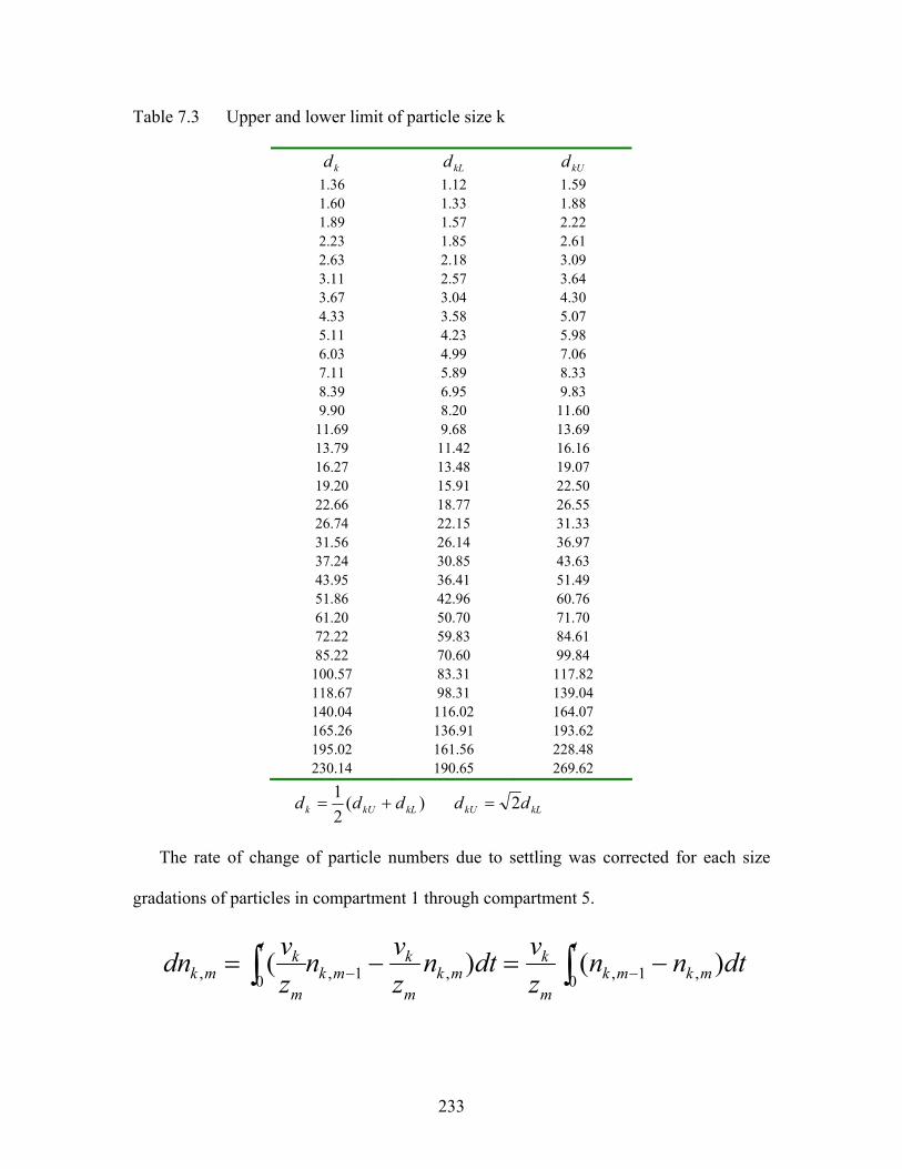
233

Table 7.3 Upper and lower limit of particle size k

kd kLd kUd 1.36 1.12 1.59 1.60 1.33 1.88 1.89 1.57 2.22 2.23 1.85 2.61 2.63 2.18 3.09 3.11 2.57 3.64 3.67 3.04 4.30 4.33 3.58 5.07 5.11 4.23 5.98 6.03 4.99 7.06 7.11 5.89 8.33 8.39 6.95 9.83 9.90 8.20 11.60

11.69 9.68 13.69 13.79 11.42 16.16 16.27 13.48 19.07 19.20 15.91 22.50 22.66 18.77 26.55 26.74 22.15 31.33 31.56 26.14 36.97 37.24 30.85 43.63 43.95 36.41 51.49 51.86 42.96 60.76 61.20 50.70 71.70 72.22 59.83 84.61 85.22 70.60 99.84 100.57 83.31 117.82 118.67 98.31 139.04 140.04 116.02 164.07 165.26 136.91 193.62 195.02 161.56 228.48 230.14 190.65 269.62

)(21

kLkUk ddd += kLkU dd 2=

The rate of change of particle numbers due to settling was corrected for each size

gradations of particles in compartment 1 through compartment 5.

∫∫ −=−= −−

t

mkmkm

kmk

m

kmk

t

m

kmk dtnn

zvdtn

zvn

zvdn

0 ,1,,1,0, )()(

234

tnnzvn

t

imkmk

m

kmk ii

∆−=∆ ∑=

−0

,1,, )( (23)

Equation 23 was used to calculate the particle number change due to the settling effect.

The resulting modeling method was applied to a 2-m settling column in the

laboratory. Rainfall-runoff collected from the experimental field under an elevated

Interstate bridge was used to carry out the settling column tests immediately after rainfall.

The suspended particle concentration of the collected runoff in this experiment was

approximately 100-mg/L. A laser type particle analyzer LISST Portable (Sequoia Tech)

was employed to measure the particle size distribution for particles ranging from 1.25 to

250-µm. The raw data from the LISST Portable was recorded into 32 size categories,

which were used as the given size category data. The fixed parameters used in the model

are summarized in Table 7.4. The volume of the primary particle ( 0v ) was assumed the

same as the volume of the lowest size category (1.36-µm), which was 12103164.1 −× cm3.

Initial particle size distributions at 5 sampling ports were analyzed, as well as samples

taken after settling for 20 minutes. According to the calculated settling velocity based on

Newton’s Law, particles greater than 57.29-µm would settle out in 20 minutes.

Table 7.4 Fixed parameter used in the model

Parameters Values

Absolute temperature (T) K 293

Density of fluid ( fρ ) g/cm3 1.0

Density of particles ( sρ )g/cm3 2.5

Average velocity gradient (G) s-1 10

Diameter of primary particle (µm) 1.36

235

RESULTS

Figure 7.4 showed the measured and CFS-C/F modeled evolution of particle number

distribution at five depths along the column for a simulation time of twenty minutes.

Initial PSD at each depth was analyzed to initiate the numerical model simulation.

Vertical transport of particles due to settling was not accounted for in this case. As seen

in Figure 7.4, there is a noticeable discrepancy between measured data and modeled

results with Euclidean assumption. This difference tends to increase towards the larger

size end. The predicted PND increased with the increasing collision efficiency factor.

Fractal dimensions D = 2.2 and D = 2.5 were chosen and applied in the model to

simulate the evolution of PSD in the settling column. Collision efficiency of 0.02, 0.2 and

1 were assumed for the model predication. Figure 7.5 showed the results for the fractal

dimension of 2.2, and Figure 7.6 showed the results for fractal dimension of 2.5. Vertical

transport due to settling was included in neither simulation. Similar to the model

prediction for the Euclidean particles, there are also discrepancies between measured data

and modeled results for particles in the larger size range (>50 µm). Significant

differences were seen as a result of application of different collision efficiencies (0.02,

0.2 and 1).

Figure 7.7 showed the comparison of the prediction under Euclidean and fractal

assumptions. Collision efficiency was taken as 0.2 in the modeling. It appears that model

incorporating fractal geometry of particles predicts better than Euclidean prediction

without consideration of sedimentation effect in the settling column. Though the particle

size distribution for small size particles (< 20-µm) in the settling column could be

236

modeled using CFS-C/F model reasonably well, the model does not provide a good fit for

particles in the larger size categories.

Sedimentation of large aggregates is accounted for in the CFS-C/F-Sedimentation

model for each defined compartment. Settling velocities of Euclidean particles were

calculated according to Newton’s Law. Figure 7.8 showed the results from CFS-C/F-

Sedimentation model. At sampling depth of H3, H4 and H5, there have seen an

improvement of model prediction for larger particles.

Many other factors will also have influences on the evolution of PSD during the

settling column test, such as temperature which affects viscosity of fluid, particle

concentration, turbulence etc. As particle concentration increases, the impact of both

coagulation/flocculation and sedimentation will be significant. The inclusion of

sedimentation in the coagulation model appears to be an applicable approach to study

particle size distribution in the treatment system of urban rainfall-runoff. As to the

collision efficiency α and fractal dimension of storm water particles, more experimental

work is needed to provide an empirical parameter for the certain system.

CONCLUSIONS

Based on the assumption of coalesced sphere and the rectilinear motion, the

coagulation/flocculation model in this research incorporated the fractal theory and

sedimentation mechanism to simulate the evolution of particle size distribution in a 2-m

settling column using particles from urban rainfall-runoff. Modeling results showed that

coagulation played an important role in the vertical transport for small particles (less than

20-µm). The effect of sedimentation is evident for particles in the larger size end. In the

modeling, both fractal dimension D and collision efficiency α are important factors in

237

determining PSD. The effect of other factors such as temperature and particle

concentration needs to be studied further.

Particle diameter (µm)

1 10 1001e+01e+11e+21e+31e+41e+51e+61e+71e+81e+01e+11e+21e+31e+41e+51e+61e+71e+8

Cum

ulat

ive

PND

(cou

nt/c

m3 ) 1e+0

1e+11e+21e+31e+41e+51e+61e+71e+8

H2H1

H4H3

H5 Measured t0

Modeled (α = 0.02) t20

Measured t20

Modeled (α = 0.2) t20

Modeled (α = 1.0) t20

D = 3.0

Figure 7.4 Fractal CFS-C/F model simulation of PSD at different depth (t = 20min) for

Euclidean particles (D=3.0) in the settling column under different collision efficiency (α=0.02, 0.2 and 1.0) compared to measured PSD at t = 0 and t = 20-min.

238

Cum

ulat

ive

PND

(cou

nt/c

m3 ) 1e+0

1e+11e+21e+31e+41e+51e+61e+71e+8

modeled α = 0.02modeled α = 0.2modeled α = 1.0measured t20

H1

Particle diameter (µm)

1 10 1001e+01e+11e+21e+31e+41e+51e+61e+71e+81e+01e+11e+21e+31e+41e+51e+61e+71e+8

H2

H3 H4

H5

D = 2.5

Figure 7.5 Fractal CFS-C/F model simulation of PSD at different depths (t = 20min)

for fractal particles (D=2.5) in the settling column under different collision efficiency α=0.02, 0.2 and 1.0) compared to measured PSD at t = 0 and t = 20-min.

239

Cum

ulat

ive

PND

(cou

nt/c

m3 ) 1e+0

1e+11e+21e+31e+41e+51e+61e+71e+8

modeled α = 0.02modeled α = 0.2modeled α = 1.0measured t20

H1

Particle diameter (µm)

1 10 1001e+01e+11e+21e+31e+41e+51e+61e+71e+81e+01e+11e+21e+31e+41e+51e+61e+71e+8

H2

H3 H4

H5

D = 2.2

Figure 7.6 Fractal CFS-C/F model simulation of PSD at different depths (t = 20min)

for fractal particles (D=2.2) in the settling column under different collision efficiency (α=0.02, 0.2 and 1.0) compared to measured PSD at t = 0 and t = 20-min.

240

Cum

ulat

ive

PND

(cou

nt/c

m3 ) 1e+0

1e+11e+21e+31e+41e+51e+61e+71e+8

Modeled D = 2.2Modeled D = 2.5Modeled D = 3.0Measured t20

H1

Particle diameter (µm)

1 10 1001e+01e+11e+21e+31e+41e+51e+61e+71e+81e+01e+11e+21e+31e+41e+51e+61e+71e+8

H2

H3 H4

H5

collision efficiency α = 0.2

Figure 7.7 Comparison of CFS-C/F model simulation of PSD at different depths (t =

20-min) for Euclidean and fractal particles in the settling column, assuming collision efficiency of 0.2.

241

Particle diameter (µm)1 10 100

Cum

ulat

ive

PND

(cou

nt/c

m3 )

1e+01e+11e+21e+31e+41e+51e+61e+71e+8

D = 2.2 D = 2.5 D = 3.0Measured

1 10 1001e+01e+11e+21e+31e+41e+51e+61e+71e+8

H2 H3

H4 H5

Figure 7.8 CFS-C/F-Sedimentation model simulation of particle size distribution in the

settling column after 20-min sedimentation; Modeled results under fractal dimensions of 2.2 and 2.5 were compared with that assuming Euclidean dimension and measured PSD (α = 0.2).

REFERENCES

Adler, P. M. (1981). “Streamlines in and around porous particles.” J. Coll. Interface Sci., 81, 531-535.

Casson, L.W. and Lawler D. F. (1990). “Flocculation in turbulent flow: Measurement and modeling of particle size distributions.” Journal AWWA. 54-68.

Camp, T. R. and Stein P. C. (1943). “Velocity gradients and internal work in fluid motion.” J. Boston Soc. Civ. Eng. 30, 219-237.

Chellam, S. and Weisner, M. R. (1993). “Fluid mechanics and fractal aggregates.” Wat. Res. 27, 1493-1496.

Costas, M. E., Moreau, M. and Vicente, L. (1995). “Some analytical and numerical solutions for colloidal aggregation with fragmentation.” J. Phys.A Math, gen, 28, 2981-2994.

Deryaguin, B.V. and Landau, L.D. (1941). “A theory of the stability of strong charged lyophobic sols and of the adhesion of strong charged particles in solutions of electroytes.” Acta Physicochim. USSR 14, 633.

Ernest, A. N., Bonner, J. S., and Autenrieth R. L. (1991). “Model parameter estimation for particle transport.” J. Enviro. Engrg., ASCE, 117(5), 573-594.

242

Ernest, A. N., Bonner, J. S., and Autenrieth R.L. (1995). “Determination of particle collision efficiencies for flocculent transport models.” J. Enviro. Engrg., ASCE, 121(4), 320-329.

Fair, G. M. and Gemmell R.S. (1964). “A Mathematical Model of Coagulation.” J. Coll. Sci. 19, 360-372.

Gibbs, R. J. (1983). “Coagulation rates of clay minerals and natural sediments.” J. Sed. Petrol. 53, 1193-1203.

Han, M. Y. and Lawler, D. F. (1992). “The (relative) insignificance of G in flocculation.” J. Am. Water. Works Assoc. 84, 79-91.

Harding, R. D. (1972). “Heterocoagulation of mixed dispersion-Effect of particle size, size ratio, relative concentration, and surface potential of colloidal components.” Jour. Colloid & Interface Sci. 40(2), 164.

Harris, H. S., Kaufman, W. J. and Krone, R. B. (1966). “Orthokinetic flocculation in water purification. Journal of the Sanitary Engineering Division, Proceedings, ASCE 92(SA6), 95-111.

Hunt, J. R. (1980) “Coagulation in continuous particle size distributions; theory and experimental verification.” Dissertation, California Institute of technology, Pasadena, California.

Jiang, Q. and Logon B. E. (1991). “Fractal dimensions of aggregates determined from steady-state size distribution.” Environ. Sci. Technol., 25(12), 2031-2038.

Kavanaugh, M. C. (1980). “Use of particle size distribution measurements for selection and control of solid/liquid separation processes.” Particulates in Water, American Chemical Society.

Kramer, T. A. and Clark, M. M. (1997). “Influence of strain-rate on coagulation kinetics. J. Environ. Eng. 123, 444-452.

Kusters, K. A., Wijers, J. G. and Thoenes, D. (1991). “Aggregation kinetics of small particles in agitated vessels.” Chem. Eng. Sci. 52, 107-121.

Johnson, C., Li, X.Y., and Logan, B.(1995). “Settling velocities of fractal aggregates.” Environ. Sci. Technol., 30(6), 1911-1918.

Lawler, D. F., Izurieta, E. and Kao, C. P. (1983). “Changes in particle size distributions in batch flocculation.” J. AWWA, 75(12), 604-612.

Lee, D. G., Bonner, J. S., Garton, L. S., Ernest, N. S. and Autenrieth R. L. (2000). “Modeling coagulation kinetics incorporating fractal theories: A fractal rectilinear approach.” Wat. Res. 34 (7), 1987-2000.

Li, Da-hong and Ganczarczyk J. (1989). “Fractal geometry of particle aggregates generated in water and wastewater treatment processes.” Environ. Sci. Technol. 23(11), 1385-1389.

243

Li, X. Y. and Logan, B. (1997a). “Collision frequencies between fractal aggregates with small particles by differential sedimentation.” Environ. Sci. Technol. 31, 1229-1236.

Li, X. Y. and Logan, B. (1997b). “Collision frequencies between fractal aggregates and small particles in a turbulent sheared fluid.” Environ. Sci. Technol. 31, 37-1242.

Lick, W. and Lick, J. (1988). “Aggregation and disaggregation of fine grained lake sediments.” J. Great. Lakes Res., 14, 514.

Mühle, K. (1993). In coagulation and flocculation, ed. B. Dobias. Marcle Dekker, New York, 355-390.

O’Melia C. R. (1972). “Coagulation and flocculation in physical chemical processes for water quality control.” ed. W.J., Webber Jr. Wiley Interscience, New York. 61-109.

Parker, D. S., Kaufman, W. J. And Jenkins, D. (1972). “ Floc break-up in turbulent flocculation processes.” J. Sanit. Eng. Pro. Div. Am. Soc. Civ. Eng. 98(SA1), 79-99.

Peters, F and Marrasé, C. (2000). “Effects of turbulence on plankton: an overview of experimental evidence and some theoretical considerations.” Marine Ecology Progress Series, 205, 291–306.

Rajagopalan, R. (1993). “Stability of colloidal dispersions: a thermodynamic approach.” Water Sci. Tech . 27, 117-129.

Ritchie, A. R. (1955). “Certain aspects of flocculation as applied to sewage purification.” Ph. D. thesis, University of London.

Spicer, P. T. and Pratsinis S. E. (1996). “Coagulation and fragmentation: universal steady-state particle-size distribution.” AIChE Journal. 42(6), 1612-1620.

Tambo, N. (1965). “A fundamental investigation of floc growth (I).” J. Jpn. Water Works. Assoc. 372, 10-19.

Tambo, N. and Ogasawara, M. (1970). “Pipe flocculator studies.” J. Jpn. Water Works. Assoc. 426, 29-39.

Tambo, N. and Watanabe, Y. (1979). “Physical characteristics of floc. I. The density function and aluminum Floc. Wat. Res., 13, 409-419.

Tambo, N. (1991). “Criteria of flocculator design.” J. Water. SRT Aqua. 40, 97-102.

Tambo, N. and Hozumi, H. (1979). “Physical Characteristics of Flocs-II. Strength of Floc.” Wat. Res. 13, 421.

Thomas, D. N., Judd, S. J. and Fawcett, N. (1999). “Flocculation modeling: A review.” Wat. Res. 33(7), 1579-1592.

Thill, A., Moustier, S., Aziz, J., Wiesner, M. R. and Bottero, J. Y. (2001). “Flocs restructuring during aggregation: Experimental evidence and numerical simulation.” J. Colloid Interface Sci. 243, 171-182.

244

Treweek, G. P. and Morgan, J. J. (1977). “Size distributions of flocculated particles: application of electronic particle counters.” Envir. Sci. & Technol. 11(7), 707.

Veerapaneni, S. and Wiesner, M. R. (1996). “Hydrodynamics of fractal aggregates with radially varying permeability.” J. Coll. Interface Sci., 177, 45-57.

Verwey, E. J. W. and Overbeek J. Th.G. (1948). Theory of the stability of Lyophobic colloids. Elsevier, Amsterdam.

Wu, R. M. and Lee, D. J. (1998). “Hydrodynamic drag force exerted on a moving floc and its implication to free-settling tests.” Wat. Res. 32, 760-768.

Yeung, A. K. C and Pelton, R. (1996). “Micromechanics: a new approach to studying the strength and break-up of flocs.” J. Coll. Interface Sci. 184, 579-585.

NOMENCLATURE

α collision efficiency

β(i, j) collision frequency (L3 T-1)

βf(i, j) collision frequency in CFS model

D fractal dimension

di diameter of particle i (L)

dp particle diameter (L)

0d diameter of primary particle (L)

k Boltzmann constant (M L2 T-2 K-1

)

G local root-mean-square velocity gradient (T-1 )

G* global root-mean-square velocity gradient (T-1 )

ni concentration of particles of size i ( L-3 )

Ni total concentration of particles at time t (L-3 )

ni(t) concentration of particles of volume v at time t (L-3 )

T absolute temperature (K)

υ kinetic viscosity of water

ε local rate of energy dissipation ( L2 T-3)

ε* global rate of energy dissipation (L2 T-3)

φ volume fraction of particles

r radius of particles

ρ0 density of primary particle (g/cm3)

ρw density of water (g/cm3)

µ dynamic viscosity (g/cm3 s)

245

ν0 volume of primary particle (cm3)

ji νν , solid volume for particle i and j (cm3)

dydu / velocity gradient

TN particle number density

nvl number volume mean size

ikγ breakage distribution function

B breakage rate

'α probability of disaggregation

z compartment depth

kw Stoke’s settling velocity of size k particle

F sedimentation flux

Fi fragmentation rate of particle i

),( kiγ breakage distribution function

kv settling velocity of particle k

p floc porosity

η fluid collection efficiency

zD hydrodynamic dispersion coefficient

g gravitational acceleration

246

CHAPTER 8. SUMMARY AND CONCLUSIONS

A central conundrum in urban rainfall-runoff treatment is the bioavailability, toxicity,

mobility of contaminants, all associating with granulometry of particles. The ability of

best management practices (BMPs) to remove particulate-bound contaminants from

runoff stream increase with particle size, however, bioavailability and mobility of

pollutants decrease with particle size. Development and design of treatment methods are

based on the granulometry characteristics. In this research, rainfall-runoff generated from

a 544-m2 Portland cement concrete pavement surface was collected under an elevated

Interstate (I-10) lane at Baton Rouge, Louisiana. The entire gradation of solids was

obtained. The physical granulometry of non-colloidal particulate matter were studied.

While size gradations were nominally separated into dissolved, suspended, settleable and

sediment designations, particle gradation ranged in size from 1 to 10,000 µm. Results

showed that d50v (volume based median particle diameter) of the suspended fraction was

10.36 ± 4.69 µm with density ( Sρ ) of 2.40 ± 0.19 g/cm3 developed from twelve studied

rainfall-runoff events at Baton Rouge site. Meanwhile, the number based median

diameter d50n was 1.62 ± 0.04 µm for the suspended fraction, similar to the size of silt and

clay. Since coarser sands were intercepted by the grit chamber prior to sedimentation

tank, the average mass based median diameter d50 was 172 ± 63.35 µm for the sediment

fraction in the sedimentation tank for twelve rainfall-runoff events. If combined

sediments from grit chamber and sedimentation tank for Baton Rouge site, a median size

of 682-µm was obtained, indicating a skewed particle size distribution to coarser sand.

Granulometry studies demonstrated that solid phase gradation transported in rainfall-

runoff is not primarily “suspended” as shown in previous literatures, but also composed

247

of settable and sediment fraction. Over 50% of surface area was associated with the

particulate gradation greater than 250-µm.

Partition of metals between dissolved and particulate phase was studied through

experimental phase fractionation of urban rainfall-runoff. Particulate matters deposited

from eight discrete storm events at Baton Rouge, Louisiana were examined for metal

contamination. Results indicated that a significant reduction was achieved in total metal

concentration for Cr, Cu, Zn and Pb by settling out the settable fraction. However,

removal of settleable fraction does not convert to large overall reduction in total

concentration for As and Cd because of their relative high dissolved fraction. As

indicated by mass distribution, metal mass was dominant in medium to coarse (75 < d <

2000 µm) materials although fine particles (< 75-µm) were associated with a high level

of metal concentration. Accumulated sediments collected from four storm catch basins at

different urban transportation sites were characterized as well. No significant

accumulative effect was found on metal concentration in the sediments. A cumulative

power law model was developed from measured data and utilized to predict metal mass

from the granulometric indices in lieu of metal analyses. The model was proved to be

successful in predicting metal mass. The application of this model is to assist the

development of particle separation operations in stormwater BMPs to target the portion

of mass gradation where the predominant metal mass is associated.

Particles in urban rainfall-runoff are fractals. Images obtained from scanning electron

microscope illustrated the fractal nature of these particulates. The characteristic

morphology includes layered-structure, clay-size particulate aggregation and relative

smooth grain surface. Results from image based fractal analyses showed fine particle

248

populations were slightly fractal than the medium to coarse materials though neither

fractal dimensions showed a significant difference from Euclidean structure (D2=2). Two

dimensional fractal dimension D2 developed from secondary electron image (SEI) was

1.943 for fine particles (less than 75-µm) and 1.961 for medium to coarse particles (75-

µm to 600-µm). Particles in urban rainfall-runoff have negative surface charges. Point of

zero charge (PZC) of particles shifted to lower pH value with decreasing particle size,

suggesting the affinity of clay minerals to smaller size particulates. The fractal

characteristic facilitates the entrainment of contaminants. Removal of fine fractions is

important because their high potential as a reservoir for contaminants. Although

Euclidean geometry is still applicable to the primary particles in urban rainfall-runoff,

aggregates formed during sedimentation or coagulation/flocculation are expected to be

more fractal and the effect of the fractal characteristics are to be more significant in urban

rainfall-runoff system. Fractal characteristics of these aggregates need to be studied

further to provide information in designing unit operation.

Settling velocity is a fundamental parameter of non-colloidal rainfall-runoff

particulates. Determination of settling velocity is critical when designing or analyzing

unit operations, in-situ controls or watershed controls for storm water. This research

presented a synthesis of settling velocity methodology with applicability to characteristics

of particulate matter in urban rainfall-runoff. Settling velocities of discrete non-colloidal

particles in rainfall-runoff were quantified utilizing a bench-scale settling column with

designed settling distance. Measured settling velocities were compared to the theoretical

settling velocities across the gradation of particles from 1 up to 2,000 µm. Results

indicate Newton’s Law can be used to model the discrete settling of non-colloidal

249

granular particles between 10 and 850-µm reasonably well. In settling column tests for

particles in the range of 1.25 to 200-µm, a linear decrease in particle mean size was

observed as a function of time during the settling process. Smaller particles (<10-µm)

settle faster than predicted using Newton’s Law assuming Euclidean object. Over 90% of

non-colloidal particles in grit chamber and approximately 50% of the non-colloidal

particles in sedimentation tank can be removed by gravitational settling in terms of

particle volume. In addition, a significant amount of fine particles cannot be removed

through traditional best management practices i.e. stormwater detention basin.

Particulate matter in urban rainfall-runoff is unique compared to other particulate-

loaded discharges (natural river water or wastewater) because of the very large size

gradation (<1 µm to > 10,000 µm) and destabilized nature of particles with relatively

short exposure to the aqueous matrix (typically less than several hours). This research

investigated coagulation and flocculation (C/F) in urban rainfall-runoff with and without

the addition of coagulants or flocculants incorporating particle size distribution analyses.

Results demonstrated that without coagulant/flocculant addition, particulate matter in

urban rainfall-runoff remains stable in suspension for extended hours. However, a

significant particulate removal can be achieved in a short retention period with addition

of alum or polymers. In terms of particle volume distribution, turbidity and total

suspended solids removal, Alum with a dosage of 30-mg/L is suggested for rainfall-

runoff treatment at the cost of $4.8x10-6/L (storm water). In contrast to the more common

accepted mechanism of double-layer compression, alum is an effective coagulant in

rainfall-runoff through adsorption, charge neutralization and sweep floc enmeshments.

250

Separation of particulate from urban rainfall-runoff is one of the major goals of best

management practices in urban rainfall-runoff treatment. Sedimentation has been used

generally in removing settleable particulates. Coagulation and flocculation was applied to

improve the treatment efficiency. The fractal nature of particles in urban rainfall-runoff

and heterogeneous distributions complicated the process. Theoretical settling model and

coagulation and flocculation model cannot predict the behavior of real particles in the

system. Based on the literature review on the contaminant removal mechanisms –

sedimentation, coagulation/flocculation (C/F), a modified C/F model incorporating fractal

geometry and sedimentation mechanism was employed to simulate and predict the

particle size distribution during the sedimentation and coagulation process in urban

runoff treatment system. The simulation applied to a 2-m settling column system with

sediment particles from urban rainfall-runoff. The results showed a reasonably goodness

of fitting.

251

VITA

Hong Lin received her Bachelor of Science degree in safety engineering from Xian

University of Architecture and Technology, Xian, China, in July, 1996. She got her

master’s degree in environmental engineering from same school in March, 1999. She

came to the United States to pursue a doctoral degree in civil engineering at Louisiana

State University in August, 1999. Her graduate research was focused on the granulometry,

chemistry and physical characteristics of particulates in urban rainfall runoff. She worked

under the guidance of Dr. John J. Sansalone in Department of Civil and Environmental

Engineering. Hong Lin will receive the degree of Doctor of Philosophy in civil

engineering from Louisiana State University in May, 2003.