Computational characterization ofhuman sequential decision making

under uncertainty

Model-free, model-based, exploitative and explorative strategies

Dissertation

zur Erlangung des akademischen GradesDoktorin der Naturwissenschaften

(Dr. rer. nat.)

am Fachbereich Erziehungswissenschaft und Psychologieder Freien Universität Berlin

vorgelegt vonDipl.-Psych. Lilla Horvath

Berlin, 2021

Erstgutachter: Prof. Dr. Dirk Ostwald

Zweitgutachter: Prof. Dr. Hauke R. Heekeren

Datum der Disputation: 17. Mai 2021

Summary

In life, many decision-making problems are complicated because agents - bi-ological and artificial alike - typically can not directly observe all aspects oftheir environments. Moreover, consequences of the agents’ actions in termsof reward gain typically unfold over time. The aim of this dissertation isto computationally characterize how humans tackle such problems from twoperspectives.

The first perspective is to identify if decisions are governed in a model-freeor a model-based fashion; while for model-free strategies it is sufficient to haveaccess to some instantaneous reward-related information or the reward history,model-based strategies require representations of the statistical regularitiesof the environment. The second perspective is to identify if decisions aregoverned in a purely exploitative or a combined exploitative-explorative fashion;while purely exploitative strategies only seek to harness the knowledge aboutthe environment, combined explorative-exploitative strategies also seek toaccumulate knowledge about the environment.

In Chapter 1 of this dissertation, I present an agent-based modeling frame-work suitable to decompose correlates of human sequential decision makingunder uncertainty with respect to both perspectives. This framework capital-izes on partially observable Markov decision processes terminology, heuristics,belief states and dynamic programming, as well as standard statistical infer-ence approaches to connect models and data. In Chapters 2 and 3, I put theagent-based modeling framework into use and investigate human participants’strategies in novel bandit and multistep tasks, respectively. In both tasks, Iprovide behavioral evidence for model-based strategies. Further, I demonstratethat the model-based strategy conforms to a combined explorative-exploitativeagenda in the bandit task. By contrast, I show that in the multistep task,the model-based strategy conforms to a purely exploitative agenda, which isneurally enabled by the orchestrated activity in a distributed network of corticaland subcortical brain regions. In Chapter 4, I embed these findings withinthe broader discussion they contribute to, outline how the arbitration betweendifferent strategies could be organized and describe possible extensions of theagent-based modeling framework.

In summary, by adopting an agent-based modeling framework, this disser-tation provides evidence for a predominantly model-based nature of humansequential decision making under uncertainty. In addition, by showing thatexploitation is not always complemented by exploration, this dissertation high-lights that humans can flexibly adjust their strategies, thereby meeting theever-changing demands of life.

Zusammenfassung

Viele Entscheidungsprobleme im Leben sind dadurch kompliziert, dass sowohlbiologische als auch künstliche Agenten typischerweise nicht alle Aspekte derUmgebung unmittelbar observieren können. Zudem entfalten sich die Konse-quenzen von Aktionen hinsichtlich des Belohnungsgewinns erst im Laufe derZeit. Das Ziel dieser Dissertation ist es aus zwei Blickwinkeln komputationalzu erfassen, wie Menschen solche Probleme angehen.

Der erste Blickwinkel versucht zu identifizieren, ob Entscheidungen auf Basiseiner modellfreien oder modellbasierten Art getroffen werden; während es fürmodellfreie Strategien ausreichend ist Zugang zu momentanen belohnungsbezo-genen Informationen oder zur Belohnungsgeschichte zu haben, benötigen modell-basierte Strategien Repräsentationen von den statistischen Regelmäßigkeiten derUmgebung. Der zweite Blickwinkel versucht zu identifizieren, ob Entscheidun-gen auf Basis einer rein exploitativen oder kombiniert exploitativ-explorativenArt getroffen werden; während rein exploitative Strategien nur darauf abzielen,sich das Wissen über die Umgebung zu Nutze zu machen, zielen kombinierteexplorativ-exploitative Strategien auch darauf ab, Wissen über die Umgebunganzusammeln.

In Kapitel 1 dieser Dissertation stelle ich ein agentenbasiertes Modellierungs-framework vor, das ermöglicht, Korrelate humaner sequentieller Entscheidungs-findung unter Unsicherheit in Bezug auf beide Blickwinkel zu zerlegen. DiesesFramework basiert auf der Terminologie partiell-observierbarer Markov Entschei-dungsprozesse, Heuristiken, Bayes’scher Zustandsrepräsentation und dynamis-cher Programmierung sowie klassischen statistischen Inferenzansätzen um Mod-elle und Daten zu verknüpfen. In Kapiteln 2 und 3 setze ich das agentenbasierteModellierungsframework ein um die Strategien humaner Teilnehmer in neuarti-gen Bandit- beziehungsweise Mehrschritt-Aufgaben zu untersuchen. In beidenAufgaben erbringe ich Nachweise für den Einsatz modellbasierte Strategien aufder Verhaltensebene. Des Weiteren demonstriere ich, dass die modellbasierteStrategie in der Bandit-Aufgabe einer kombinierten explorativ-exploitativenAgenda entspricht. Im Gegensatz dazu zeige ich, dass die modellbasierte Strate-gie in der Mehrschritt-Aufgabe einer rein exploitativen Agenda entspricht, dieneuronal durch die orchestrierte Aktivität eines verteilten Netzwerks kortikaler

und subkortikaler Hirnregionen unterstützt wird. In Kapitel 4 bette ich dieseErgebnisse in die breitere Diskussion ein, stelle dar, wie eine Auswahl ver-schiedener Strategien erfolgen könnte und beschreibe mögliche Erweiterungendes agentenbasierten Modellierungsframeworks.

Zusammenfassend zeigt diese Dissertation durch die Anwendung eines agen-tenbasierten Modellierungsframeworks, dass die sequentielle Entscheidungsfind-ung unter Unsicherheit bei Menschen vorwiegend modellbasierter Natur ist.Durch den Nachweis, dass exploitative Strategien nicht immer durch explo-rative Strategien ergänzt werden, hebt die Dissertation darüber hinaus hervor,dass Menschen ihre Strategien flexibel anpassen können, um den sich ständigändernden Anforderungen des Lebens gerecht zu werden.

Acknowledgements

Many people have provided immeasurable help over the last years in puttingtogether this dissertation.

First and foremost, I would like to thank my PhD advisor Dirk Ostwald.Your clarity of thought, scientific rigor and dedication to open science haveinvaluably shaped my approach to research and pushed me to strive for a deepunderstanding as well as a precise reporting of computational characterizationof human decision making.

I am also especially grateful to my second PhD advisor, Hauke Heekeren,whose door was always open to provide support. I greatly benefited from thescientific discussion about our projects and I am deeply thankful for your adviceon how to maneuver my path in science.

Soyoung Park, Julia Rodriguez Buritica and Peter Mohr have kindly argreedto be members of my PhD committee, which I am most grateful for.

I would like to thank Michael Milham for providing me with the opportunityto perform a study at the Nathan Kline Institute, which formed the basis of thework presented in the second chapter of this dissertation. Your enthusiasm forscience and unwavering optimism made my time in New York truly enjoyable.I am also grateful to Stanley Colcombe and Shruti Ray for their support incarrying out this study. I sincerely thank Philipp Schwartenbeck for countlessinspiring discussions about the experimental setup and data analysis.

I am thankful to Ralph Hertwig for providing the infrastructure at the MaxPlanck Institute for Human Development critical to realize the study uponwhich the work described in the third chapter of this dissertation is based.Rui Mata helped planning this study and Loreen Tisdall helped with datacollection, for which I am very grateful.

I would like to express my heartfelt gratitude to Wei Ji Ma for believingin me and being beyond supportive throughout a rocky decision process. Ifeel extremely fortunate to have had the opportunity to get to know you andyour lab. I owe another special thank you to Andreas Horn for the endlessencouragement. You were one of the firsts to show me how much fun sciencecan be and your positive attitude never ceases to inspire me.

I hugely benefited from discussions with members of the Center for Cognitive

Neuroscience Berlin. I particularly want to thank Lisa Velenosi, Pia Schröderand Kathrin Tertel. Your insightful and witty way of thinking, with respect toscience and beyond, made all the difference in the long PhD days. I would alsolike to extend this thank you to Yuan-hao Wu and Miro Grundei for our lunchand coffee breaks that I valued so much.

Thank you Daniela Satici-Thies for the immense help with all my ad-ministrative problems and somehow always finding a way to make seeminglyimpossible ends meet. I am also grateful for receiving generous support by anElsa-Neumann-Scholarship during the first three years of my PhD.

Last, but not least, I would not be writing this acknowledgement markingthe end of my PhD if it were not for my friends and family. I am wholeheartedlygrateful for your constant encouragement and patience. I especially wouldlike to thank Miriam Dowe for listening and making me listen, Lisa Graaf forreminding me of what life has to offer outside of PhD even during its mostintense phases, Judit Varga for running with me to the finish line and PetraVancsura for cheering us all along. I will forever be indebted to my parents,Lilla Kardos and Istvan Horvath, who have always and unconditionally beenthere for me. Finally, no words would do justice to express how grateful I am toBenjamin Ostendorf for everything and to the little person who has spent everysecond of the last months with me for being the most wonderfully independentcompany I could ever wish for.

Contents

1 General introduction 1

1.1 Marr’s levels of analysis and agent-based modeling . . . . . . . . 2

1.2 The sequential decision-making problem under uncertainty . . . 4

1.2.1 The general task model architecture . . . . . . . . . . . . 4

1.2.2 Task model variations . . . . . . . . . . . . . . . . . . . 5

1.2.3 The notion of optimal solution . . . . . . . . . . . . . . . 7

1.3 Approximate solutions and their behavioral plausibility . . . . . 8

1.3.1 The general agent model architecture . . . . . . . . . . . 9

1.3.2 Agent model variations . . . . . . . . . . . . . . . . . . . 10

1.3.3 The general behavioral model architecture . . . . . . . . 13

1.4 Neural implementation of alternative solutions . . . . . . . . . . 13

1.4.1 Model-based GLM for fMRI . . . . . . . . . . . . . . . . 14

1.5 Overview of the dissertation . . . . . . . . . . . . . . . . . . . . 15

1.6 References . . . . . . . . . . . . . . . . . . . . . . . . . . . . . . 17

2 Belief state-based exploration and exploitation in an information-selective reversal bandit task 25

2.1 Introduction . . . . . . . . . . . . . . . . . . . . . . . . . . . . . 25

2.2 Methods . . . . . . . . . . . . . . . . . . . . . . . . . . . . . . . 28

2.2.1 Experimental methods . . . . . . . . . . . . . . . . . . . 28

2.2.2 Descriptive analyses . . . . . . . . . . . . . . . . . . . . 32

2.2.3 Model formulation . . . . . . . . . . . . . . . . . . . . . 33

2.2.4 Model evaluation and validation . . . . . . . . . . . . . . 43

2.3 Results . . . . . . . . . . . . . . . . . . . . . . . . . . . . . . . . 47

2.3.1 Descriptive results . . . . . . . . . . . . . . . . . . . . . 47

2.3.2 Modeling results . . . . . . . . . . . . . . . . . . . . . . 48

2.4 Discussion . . . . . . . . . . . . . . . . . . . . . . . . . . . . . . 52

2.5 Data and code availability . . . . . . . . . . . . . . . . . . . . . 57

2.6 References . . . . . . . . . . . . . . . . . . . . . . . . . . . . . . 58

3 The neurocomputational mechanisms of sequential decisionmaking in a multistep task with partially observable states 633.1 Introduction . . . . . . . . . . . . . . . . . . . . . . . . . . . . . 633.2 General methods . . . . . . . . . . . . . . . . . . . . . . . . . . 66

3.2.1 Experimental methods . . . . . . . . . . . . . . . . . . . 663.2.2 Task model . . . . . . . . . . . . . . . . . . . . . . . . . 703.2.3 Agent models . . . . . . . . . . . . . . . . . . . . . . . . 73

3.3 Behavioral methods . . . . . . . . . . . . . . . . . . . . . . . . . 963.3.1 Descriptive behavioral data analyses . . . . . . . . . . . 963.3.2 Model-based behavioral data analyses . . . . . . . . . . . 98

3.4 Behavioral results . . . . . . . . . . . . . . . . . . . . . . . . . . 1013.4.1 Descriptive behavioral results . . . . . . . . . . . . . . . 1013.4.2 Model-based behavioral results . . . . . . . . . . . . . . 102

3.5 FMRI methods . . . . . . . . . . . . . . . . . . . . . . . . . . . 1053.5.1 FMRI data acquisition and preprocessing . . . . . . . . . 1053.5.2 Model-based fMRI data analysis . . . . . . . . . . . . . . 1063.5.3 Participant- and group-level model estimation and evalu-

ation . . . . . . . . . . . . . . . . . . . . . . . . . . . . . 1093.6 FMRI results . . . . . . . . . . . . . . . . . . . . . . . . . . . . 109

3.6.1 FMRI data validation . . . . . . . . . . . . . . . . . . . 1093.6.2 Model-based fMRI results . . . . . . . . . . . . . . . . . 110

3.7 Discussion . . . . . . . . . . . . . . . . . . . . . . . . . . . . . . 1123.8 Data and code availability . . . . . . . . . . . . . . . . . . . . . 1223.9 References . . . . . . . . . . . . . . . . . . . . . . . . . . . . . . 123

4 General discussion 1294.1 Synthesis and discussion of the main findings . . . . . . . . . . . 129

4.1.1 Model-free versus model-based strategies . . . . . . . . . 1304.1.2 Exploitative versus explorative strategies . . . . . . . . . 132

4.2 Outstanding questions . . . . . . . . . . . . . . . . . . . . . . . 1354.2.1 How do different strategies cohabitate? . . . . . . . . . . 1354.2.2 How can strategies be further refined? . . . . . . . . . . 137

4.3 Conclusion . . . . . . . . . . . . . . . . . . . . . . . . . . . . . . 1384.4 References . . . . . . . . . . . . . . . . . . . . . . . . . . . . . . 140

A Supplementary material to Chapter 2 147A.1 Sample characteristics . . . . . . . . . . . . . . . . . . . . . . . 147A.2 Task instructions . . . . . . . . . . . . . . . . . . . . . . . . . . 148

A.3 Trial sequence . . . . . . . . . . . . . . . . . . . . . . . . . . . . 151A.4 Belief state and posterior predictive distribution evaluation . . . 152A.5 Belief state and posterior predictive distribution implementation 154A.6 References . . . . . . . . . . . . . . . . . . . . . . . . . . . . . . 157

B Supplementary material to Chapter 3 159B.1 Task instructions . . . . . . . . . . . . . . . . . . . . . . . . . . 159B.2 FMRI result tables . . . . . . . . . . . . . . . . . . . . . . . . . 161B.3 References . . . . . . . . . . . . . . . . . . . . . . . . . . . . . . 169

1 | General introduction

To reach certain goals in life, we often have to make a sequence of decisions.Consider, for example, a gambler playing on a slot machine in a casino or ahigh school student with an aspiration to become an astrophysicist. In formalterms, in both examples the goal of the decision-making agent can be describedas trying to choose actions as to maximize its cumulative reward: The gamblertries to pull the best lever on each turn to win as much money as possible; thehigh school student tries to make the best career choice in each situation tosecure their dream job. To pull the best lever or make the best career choice,both the gambler and the high school student would need to be omniscientabout their environment (e.g., the precise probability with which the pullingof a lever returns a certain reward or the precise expectations of a collegeadmission committee). This requisite, however, defeats the purpose of gamblingand is unrealistic when it comes to pursuing a career goal.

As demonstrated by these examples, most sequential decision-making prob-lems are complicated by uncertainty (Bach & Dolan, 2012; Bach, Hulme,Penny, & Dolan, 2011; Glimcher & Fehr, 2013; Ma & Jazayeri, 2014; Rao,2010; Vilares & Kording, 2011; Yoshida & Ishii, 2006). In the face of un-certainty, two key questions arise (Dayan & Daw, 2008). The first questionconcerns the environmental components agents draw on to evaluate actions.An influential dichotomy in this regard is the model-free versus model-baseddistinction (e.g., Collins and Cockburn, 2020; Daw, Niv, and Dayan, 2005;Fischer, Bourgeois-Gironde, and Ullsperger, 2017; Korn and Bach, 2018; D. A.Simon and Daw, 2011; Speekenbrink and Konstantinidis, 2015). Broadly put,model-free decision making assumes that agents directly evaluate actions basedon the reward history or some presently available reward-related information.In contrast, model-based decision making assumes that action evaluation isgoverned by the agents’ own representation of the statistical regularities oftheir environment. The second question is whether agents evaluate actions ina purely exploitative fashion or combine exploitation with exploration (e.g.,Cohen, McClure, and Yu, 2007; Daw, O’Doherty, Dayan, Seymour, and Dolan,2006; Schwartenbeck et al., 2019; Wilson, Geana, White, Ludvig, and Cohen,2014). Exploitative decision making assumes that agents try to maximize their

1

Chapter 1

cumulative reward based on what they know about the environment at thetime of their decision. A combined explorative-exploitative perspective, on theother hand, assumes that agents also try to improve their knowledge about theenvironment and therefore take into account the amount of information theycan gain by choosing a certain action.

In this dissertation, I computationally characterize human sequential de-cision making under uncertainty along these two questions in two tasks thatshare central features with the examples introduced above. Specifically, inChapter 2, I study the behavioral strategies human participants employ in abandit task, which captures situations similar to the example of the gambler.In Chapter 3, I investigate the computations human participants perform tosolve a multistep task - which captures situations similar to the example of thehigh school student - on behavioral and neural levels.

In this introduction, I conceptually situate these two empirical chapterswithin relevant theories. To this end, I follow Marr’s levels of analysis (Marr,1982) and thereby introduce the agent-based modeling framework (Ostwald,2020a) which I adopt in the empirical chapters to uncover the computationalunderpinnings of the applied sequential decision-making strategies. I concludethe introduction by giving a brief overview of the remainder of the presentdissertation.

1.1 Marr’s levels of analysis and agent-based mod-

eling

In his work about visual perception, Marr (1982) proposed a conceptual frame-work consisting of three hierarchical levels to systematically study, understandand discuss the brain and its functions. Marr’s framework has since beenan inspiration to cognitive scientists and neuroscientists in guiding scientificinquiry (see, for example, Hauser, Fiore, Moutoussis, and Dolan, 2016; Niv andLangdon, 2016), and has recently also gained attention in machine learningresearch (Hamrick & Mohamed, 2020). According to Marr, on the first ’compu-tational’ level the problem at hand is to be formally defined. On the second’algorithmic’ level, alternative solutions as to how the problem can be tackledare to be described. Finally, on the third ’implementation’ level, plausible waysfor a (neural) system to realize these alternative solutions are to be considered.

Agent-based modeling as outlined by Dirk Ostwald (Ostwald, 2020a) andadopted in Chapters 2 and 3 offers a formal framework to investigate human

2

1.1. Marr’s levels of analysis and agent-based modeling

sequential decision making under uncertainty. In its current form, this frame-work consists of three building blocks that can be readily mapped onto Marr’slevels of analysis as follows: The first building block is the task model, whichcorresponds to a probabilistic formulation of the choice environment. Rootedin probabilistic optimal control theory, agent-based modeling adopts the ter-minology of partially observable Markov decision processes in the definitionof the task model (e.g., Bäuerle and Rieder, 2011; Bertsekas, 2000; Puterman,2014). By representing the choice environment and thereby specifying theproblem to be solved, this building block parallels the computational level inMarr’s framework. The second building block is the set of agent models. Thesemodels capitalize on Bayesian inference, dynamic programming, heuristics andreinforcement learning to formulate various strategies that can be used to solvethe problem (e.g., Dayan and Daw, 2008; Gigerenzer, Todd, and the ABCResearch Group, 1999; Hassabis, Kumaran, Summerfield, and Botvinick, 2017;Ma, 2019; Rao, 2010; Russell and Norvig, 2010; Sutton and Barto, 2018; Wayneet al., 2018; Wiering and van Otterlo, 2014). In essence, the second buildingblock of agent-based modeling exhausts the requirements of Marr’s algorithmiclevel. However, to evaluate the plausibility of the agent models in light of humanparticipants choice data, the agent models have to be statistically embedded(e.g., Daunizeau et al., 2010; Farrell and Lewandowsky, 2018). The ensuingset of behavioral models constitutes the third building block of agent-basedmodeling. Although as it currently stands, agent-based modeling does notdirectly specify a building block that maps onto Marr’s implementation level,methods such as model-based general linear modeling (GLM) of functionalmagnetic resonance imaging (fMRI) data can be considered for this purpose(Friston & Dolan, 2010).

In line with Marr’s framework, in the following, I first give a formal descrip-tion of the sequential decision-making problem under uncertainty by introducingthe general task model architecture in Section 1.2. Here, I also highlight howthis can be tailored to bandit and multistep tasks studied in detail in Chapters2 and 3, respectively. In Section 1.3, I then introduce the general agent modelarchitecture and review its variations capturing strategies in terms of the di-chotomies model-free versus model-based, and exploitation versus exploration.Additionally, I here also describe the general behavioral model architecture.Finally, in Section 1.4, I present the model-based GLM for fMRI approachapplied in Chapter 3 to identify the network of brain regions enabling therealization of algorithmic solutions as formulated by the agent models.

3

Chapter 1

1.2 The sequential decision-making problem un-

der uncertainty

In 1957, Richard Bellmann introduced the theory of Markov decision processes(MDPs) suitable to model a wide range of real-world sequential decision-makingproblems (Bellman, 1957). Ever since, the theory of MDPs has been paramountin operations research and extended to accommodate uncertain1 conditions(Bäuerle & Rieder, 2011; Bertsekas, 2000; Bertsekas & Tsitsiklis, 1996; Lovejoy,1991; Puterman, 2014; Sutton & Barto, 2018; Wiering & van Otterlo, 2014).The ensuing theory of partially observable Markov decision processes (PoMDPs)offers a formal language to describe the scope of the sequential decision-makingproblem under uncertainty as well as a principled way to derive the optimalsolution. In this section, I draw on PoMDPs theory to introduce the generaltask model architecture, detail how this model differs for bandit and multisteptasks, and - as a prelude to the next section - I lay out the notion of optimalsolution. To this end, I throughout rely on the literature listed in this paragraphand complement it with further resources wherever appropriate.

1.2.1 The general task model architecture

In general terms, the model of a task formally captures the agent’s choiceenvironment using mathematical sets and probability distributions.

The first set component of the task model is the set of time points denotingthe epochs at which the agent may interact with the choice environment. Inthe standard case and as is assumed throughout this dissertation, this set isdiscrete and finite. At each time point, the choice environment has a certainconfiguration. The second set component of the task model - the set of states -represents all possible values of these configurations. Crucially, certain aspectsof the environmental configurations may be overt, constituting the directlyobservable part of the state, while others may only be imprecisely signalled,constituting the not directly observable part of the state. The values theimprecise signal can take on form the third set component of the task model,the set of observations.2 In each state, the choice environment allows certain

1The term uncertain has been used to refer to choice environments, in which the dynamics,such as the state transitions, are stochastic. Yet, it has also been reserved to signify choiceenvironments, in which some components, such as the state or the reward dynamics, are onlypartially observable (e.g., Knight, 1921; Russell and Norvig, 2010). As will become apparentin the remainder of this section, in this dissertation I adopt this latter conceptualization.

2If the imprecise signalling is due to disturbances in sensory processing (cf. Bach and

4

1.2. The sequential decision-making problem under uncertainty

actions to be undertaken by the agent. The set of all actions presents thefourth set component of the task model. The last essential set of the task modelcomprises all numerical rewards the choice environment may generate.

How the elements of these sets relate to each other can be described withthe observation, reward and state transition probability distributions of the taskmodel. Concretely, the observation probability distribution encapsulates thedynamics between states and observations by specifying how the former givesrise to the latter. The reward and state transition probability distributionsspecify how state-action pairs lead to rewards and new states, respectively.

1.2.2 Task model variations

This general architecture allows for considerable flexibility to match the specificsof different tasks. Two classes of tasks that are often used to study sequentialdecision making under uncertainty are bandit and multistep tasks.

Bandit tasks

Bandit tasks, which were first systematically discussed by Robbins (1952),capture choice environments in which actions are not interdependent. Morespecifically, in bandit tasks, choosing an action in a given state does not have aneffect on the next state but only on the immediately accrued reward. Such tasksare thus well suited to model, for example, treatment allocation in clinical trialsor gambling (e.g., Berry and Fristedt, 1985; Brand, Woods, and Sakoda, 1956;Bubeck and Cesa-Bianchi, 2012; Cohen et al., 2007; Dayan and Daw, 2008;Gabillon, Ghavamzadeh, and Lazaric, 2012; Speekenbrink and Konstantinidis,2015; Whittle, 1988). As delineated above, in the case of gambling, the agent(gambler) chooses from a finite set of actions (pulls one of the levers) andreceives a reward (monetary gain or loss) as dictated by the reward probabilitydistribution. Then, the agent again faces the same set of actions and the processgets repeated until the time horizon is reached (game is finished). A crucial andinherent aspect of bandit tasks is that the reward structure of the environmentis not directly observable. Depending on the bandit task at hand, this caneither be formulated as a part of the state being not directly observable, or asparameters of the reward probability distribution being not directly observable.In both cases, the reward returned to the agent conveys noisy information

Dolan, 2012), the set of observations can instead be considered internal to the agent. However,in the sequential decision-making problems studied in this dissertation no such disturbancesare assumed and I therefore conceive the set of observations as a part of the task model.

5

Chapter 1

about the not directly observable component of the task model and thus, inthis sense, rewards serve as observations. Of course, to conceptualize rewardsin terms of observations, rewards have to be observable. In life, however, thismay not always be the case. In Chapter 2, I introduce a bandit task suitableto model choice environments in which the reward is observable only followingcertain actions. Given the symmetrical reward structure adopted in this task,its not directly observable nature is captured by the state, whose value changesover time. Such switching state bandit tasks require the specification of statetransitions, which - per definition - are independent of actions.

Multistep tasks

In contrast to bandit tasks, multistep tasks capture choice environments inwhich actions are interdependent. That is, in multistep tasks, actions do notonly affect the immediate rewards but they also affect the next state andthereby future rewards (e.g., Daw, Gershman, Seymour, Dayan, and Dolan,2011; Dayan and Daw, 2008; Korn and Bach, 2018; Lehmann et al., 2019;Schrittwieser et al., 2020; D. A. Simon and Daw, 2011; Wayne et al., 2018).The above introduced example of the high school student presents a choiceenvironment that can be modeled in terms of a multistep task: In a givenstate (e.g., at an interview with the college admission committee) the agent(high school student) chooses an action (e.g., highlights her keen interest inblack holes), receives an immediate reward (e.g., bonus points) according tothe reward probability distribution and enters a new state (e.g., gets acceptedto the program) according to the state transition probability distribution. Inthe new state, the agent is presented with a new set of actions to choose from,each action producing different immediate rewards and new states. Uncertaintymay pervade multistep tasks, for instance, if part of the state is not directlyobservable (Bach & Dolan, 2012; Dayan & Daw, 2008; Rao, 2010; Yoshida &Ishii, 2006). As a specific example, consider the high school student again. Atthe interview, the exact expectations of the college admission committee mightonly be imprecisely signalled by the members’ subtle reactions. In Chapter 3, Iintroduce a multistep task embedded in the spatial domain suitable to modelsimilar choice environments.

6

1.2. The sequential decision-making problem under uncertainty

1.2.3 The notion of optimal solution

On the basis of the task model, the theory of PoMDPs offers a principled wayto identify normative sensible decisions.3 The central presumption thereby isthat the ultimate goal of an agent is to maximize the cumulative obtainedreward.

To achieve this goal, agents have to choose the sequence of actions for whichthe expected sum of rewards over the time points is maximal. This optimalaction sequence can, in principle, be found by applying dynamic programming,which capitalizes on the recursive scheme of the Bellman equation (Bellman,1957). In its standard form, the Bellman equation states that the optimalaction in a given state maximizes the sum of the expected immediate rewardand the optimal value of the expected next state, which corresponds to themaximum expected sum of rewards that can be obtained starting from theexpected next state.

Even if all aspects of the state are directly observable (i.e, the choice envi-ronment can be described in terms of MDPs), applying dynamic programmingcan be computationally costly, for example, in multistep tasks with large statespaces and time horizons, such as chess (e.g., Bellman, 1961; Huys et al., 2012;van Opheusden, Galbiati, Bnaya, Li, and Ma, 2017).4 It yet becomes evenmore computationally costly if some aspects of the state are only impreciselysignalled by the observations (i.e, the choice environment can be describedin terms of PoMDPs), as is the case in both the bandit and multistep tasksstudied in detail in Chapters 2 and 3 of this dissertation. This is because undersuch circumstances, the optimal action has to be evaluated with respect to theagent’s subjective uncertainty about the state, i.e., the belief state. In otherwords, in the Bellman equation as formulated above, states have to be replacedby belief states. Fundamental to this replacement is that just like states, beliefstates satisfy the Markov property, which prescribes that in the choice envi-ronment the past is independent of the future given the present. The Markovproperty also implies that at a given time point the belief state - formally aprobability distribution over states given past actions and observations - can

3In operations research, some scholars (e.g., Bäuerle and Rieder, 2011; Puterman, 2014)explicitly differentiate between partially observable Markov decision processes and partiallyobservable Markov decision problems; they apply the former term when specifying a quanti-tative model of the problem at hand and the latter term when combining this quantitativemodel with the optimality criterion.

4This anyways existing difficulty possibly explains why in human decision neuroscienceresearch the experimental study of multistep tasks has so far largely focused on scenarioswithout state uncertainty.

7

Chapter 1

be computed recursively on the basis of the belief state, action and observationat the previous time point using Bayes’ rule (Dayan & Daw, 2008; Kaelbling,Littman, & Cassandra, 1998; Rao, 2010; Russell & Norvig, 2010).

Beside the computational load posed by the combination of dynamic pro-gramming and state inference, it may also easily exhaust the memory space.Thus, while under certain simplifying conditions optimal solutions can beattained5, most real-life problems modeled in terms of PoMDPs necessitateapproximations (Berry & Fristedt, 1985; Dayan & Daw, 2008; Rao, 2010;Russell & Norvig, 2010). Furthermore and most importantly for the purposeof this dissertation, given the cognitive capacity limits of biological agents,such approximations present themselves suitable to be adopted by humans(Gershman, Horvitz, & Tenenbaum, 2015; Griffiths, Lieder, & Goodman, 2015;H. Simon, 1957).

1.3 Approximate solutions and their behavioral

plausibility

A large variety of algorithmic methods exists to obtain approximate solutions.Of these, a class of methods inherits from the above outlined normative schemeand uses concepts from Bayesian inference and dynamic programming (Bäuerle& Rieder, 2011; Bertsekas, 2000; Bertsekas & Tsitsiklis, 1996; Ma, 2019;Puterman, 2014; Rao, 2010; Sutton & Barto, 2018; Wiering & van Otterlo,2014; Yoshida & Ishii, 2006). In decision neuroscience research, these methodsare usually referred to as model-based, because they rely upon the definingprobability distributions of the task model. In contrast, for model-free methodsit is sufficient to have knowledge of only the overt set components of the taskmodel (e.g., Collins and Cockburn, 2020; Daw et al., 2005; Dayan, 2012; Dayanand Daw, 2008; Korn and Bach, 2018; Speekenbrink and Konstantinidis, 2015).These methods come from heuristic decision making (Gigerenzer et al., 1999;Tversky & Kahneman, 1974) and reinforcement learning (RL; Bertsekas andTsitsiklis, 1996; Rao, 2010; Sutton and Barto, 2018; Wiering and van Otterlo,2014) and operate on the basis of instantaneous information about or previousexperience with rewards.6 Another important perspective to classify methods is

5For example, optimal solutions to stationary bandit tasks can be derived for finite(Bellman, 1956; Berry & Fristedt, 1985) and infinite (Gittins & Jones, 1974) time horizons.

6In artificial intelligence research, approximate methods that borrow from the PoMDPstheory and therefore necessitate knowledge about the probability distributions of the taskmodel are sometimes termed model-based RL methods. Correspondingly, the term model-free

8

1.3. Approximate solutions and their behavioral plausibility

the distinction between exploitation and exploration-exploitation. Exploitativemethods are solely guided by the perspective of reward gain based on theaccumulated knowledge about the choice environment. Explorative-exploitativemethods, conversely, are also guided by the perspective of information gainto advance their knowledge about the choice environment (Berry & Fristedt,1985; Bertsekas & Tsitsiklis, 1996; Cohen et al., 2007; Dayan & Daw, 2008;Schwartenbeck et al., 2019; Sun, Gomez, & Schmidhuber, 2011; Sutton & Barto,2018; Wiering & van Otterlo, 2014). Despite the apparent differences betweenmethods, the structural requirements imposed on the agents adopting themhave some key commonalities (Russell & Norvig, 2010). Therefore, in whatfollows, I first present the general agent model architecture and then detailits variations in terms of the dichotomies model-free versus model-based andexploitation versus exploration. I close this section by describing the generalbehavioral model architecture, which formalizes the embedding of the agentmodels into a statistical framework.

1.3.1 The general agent model architecture

The word agent originates from the Latin agere, which means to do. Accordingly,central to agents is that they perceive their environment, on the basis of whichthey act as to reach their goal. This suggests that one part of the agent modelhas to specify the agent’s representation of the task model. The other part, inturn, has to specify how the agent draws on this representation to evaluate theactions and make decisions (Russell & Norvig, 2010).

As discussed in detail below, the agent’s copy of the task model can varygreatly. Some methods only require the agent to represent the overt setcomponents of the task model, i.e., time points, directly observable part ofstates, observations, actions and rewards. Others also require representations ofthe possible values of the not directly observable part of state and the probabilitydistributions of the task model. Given that the probabilistic representationsare internal to the agent, they are to be conceived as subjective uncertainties,even if the corresponding probability distributions of the task model are overt(cf. Ma, 2019).

On the basis of its task representation, the agent evaluates the actions,which is formalized in terms of the valence function, and makes a decision, whichis formalized in terms of the decision function. Similar to the value function of

is used for RL methods that do not necessitate such knowledge (e.g., Schrittwieser et al.,2020; Sutton and Barto, 2018; Wiering and van Otterlo, 2014).

9

Chapter 1

the PoMDPs theory, the valence function assigns a number to each action. Thisnumber is, however, not the optimal value of the action but an approximationthereof and can therefore be considered as a measure of the action’s subjectivedesirability as viewed by the agent. Depending on the valence function, theagent may need to apply Bayesian inference and form a belief state. Thus, inthis case, the agent model also has to comprise the specification of the agent’sinitial subjective uncertainty about the state. Drawing on the valences, thedecision function adjudicates between actions, implementing either a stochasticor a deterministic valence maximizing scheme.

1.3.2 Agent model variations

Model-free/model-based and exploitative/explorative methods assume certaincharacteristic configurations of the agent’s task representation, valence anddecision functions, and, consequently, the above introduced general architecture.

Model-free versus model-based

Common to model-free methods is that agents do not need knowledge aboutthe task model beyond the overt set components. Constrained by the simplicityof such task representations, all model-free methods directly allocate valencesto actions. Yet, an abundance of different ways exists to do this. Inspiredby heuristic decision making, a simple yet often efficient way is to allocateaction valences based on the latest reward-related information, conveyed, forexample, by observations (Dayan, 2012; Gigerenzer & Gaissmaier, 2011; Korn& Bach, 2018; Robbins, 1952; Wilson & Collins, 2019). Another way wasoriginally described by the decision neuroscientists Rescorla and Wagner (1972)and further developed in RL research under the name temporal differencelearning. The key aspect of these model-free methods is that an action’svalence depends on the associated reward history, where an arbitrary constantlearning rate controls the extent to which the latest experience is taken intoaccount (Bertsekas & Tsitsiklis, 1996; Glimcher & Fehr, 2013; Wiering &van Otterlo, 2014; Wilson & Collins, 2019).

In contrast to model-free methods, model-based methods require that theagent maintains representations of all sets and the probabilistic dependenciesbetween their elements. Together with the agent’s initial belief state, theensuing complete task model is put into use to probabilistically infer the stateand to allocate valences to actions by considering their consequences with

10

1.3. Approximate solutions and their behavioral plausibility

respect to future states, observations and rewards. To this end, model-basedmethods employ some combination of Bayesian inference and approximatedynamic programming. Approximations can, for instance, be implemented bylimiting the time horizon considered or by using a heuristic to evaluate possiblenext belief states (Bertsekas & Tsitsiklis, 1996; Geffner & Bonet, 1998; Huys etal., 2012; Korf, 1990; van Opheusden et al., 2021; Wiering & van Otterlo, 2014).As exemplified by this latter approach, model-free methods may complementmodel-based methods. Applying temporal difference learning in the space ofbelief states is another example of such a mixture method (Babayan, Uchida,& Gershman, 2018; Dayan & Daw, 2008; Rao, 2010; Starkweather, Babayan,Uchida, & Gershman, 2017).

Exploitation versus exploration

Exact solution to a problem modeled in terms of PoMDPs yields an optimalbalance between exploitation and exploration. To approximate the optimalbalance, model-free as well as model-based methods across the entire spectrum,from purely exploitative to purely explorative, have been proposed (Bertsekas& Tsitsiklis, 1996; Cohen et al., 2007; Dayan & Daw, 2008; Schwartenbecket al., 2019; Wiering & van Otterlo, 2014).

Purely exploitative methods disregard the perspective of information gain.Instead, at each time point, they harness the knowledge about the choiceenvironment acquired through previous interactions and allocate action valencesfrom the perspective of reward gain. This can be done both in a model-freeway, relying, for example, on a reward-related heuristic, or in a model-basedway, evaluating, for example, the belief state-weighted expected reward (Knox,Otto, Stone, & Love, 2012; Lee, Zhang, Munro, & Steyvers, 2011; Speekenbrink& Konstantinidis, 2015). Crucial thereby is that the agent adopts a valencemaximizing deterministic decision function so that the action with the highestexploitative valence is realized.

Correspondingly, purely explorative methods have to ensure that the actionwith the highest explorative valence is realized and they therefore also requirea valence maximizing deterministic decision function. Yet, opposite to purelyexploitative methods, these methods seek to improve their knowledge about thechoice environment and thus allocate action valences from the perspective ofinformation gain. Two commonly applied measures of information gain are thefrequentist upper confidence bound (Auer, Cesa-Bianchi, & Fischer, 2002) andthe expected Bayesian surprise (Itti & Baldi, 2009; Ostwald et al., 2012; Sun

11

Chapter 1

et al., 2011). The former expresses information gain in a model-free fashionbased on the extensiveness of the action’s associated reward history, whereasthe latter expresses information gain in a model-based fashion based on theshift in the belief state.

By combining the valences of purely explorative and purely exploitativemethods, explorative-exploitative methods take both information gain andreward gain into account (Chakroun, Mathar, Wiehler, Ganzer, & Peters,2020; Gershman, 2018; Navarro, Newell, & Schulze, 2016; Wilson et al., 2014;Zhang & Yu, 2013). These methods either implement a valence maximizingdeterministic decision function or a stochastic decision function. The rationalbehind using a stochastic decision function is that information may also begained ’by chance’, i.e., through adding some noise to the action selectionprocess. This, in turn, suggests that explorative-exploitative methods may alsobe formed by taking the valences of a purely exploitative method and using astochastic decision function - with constant (e.g., ε-greedy (Sutton & Barto,2018; Wiering & van Otterlo, 2014) or softmax operation (Reverdy & Leonard,2015)) or belief state-dependent (Thompson sampling7; Thompson, 1933) noise.While belief state-dependent noise assumes a model-based method, constantnoise can also be added to the exploitative valences allocated by a model-freemethod.

In Chapters 2 and 3, I computationally characterize human participantschoice behavior with respect to the dichotomies model-free versus model-basedand exploitation versus exploration in bandit and multistep tasks, respectively.To this end, I use agent models that implement model-free purely exploitative,model-based purely exploitative, purely explorative and exploitative-explorativemethods. More specifically, the model-free purely exploitative agents of bothmodel spaces rely on reward-related heuristics. Their model-based counterpartsevaluate the belief state-weighted expected reward or employ belief state-basedheuristic real-time dynamic programming. In contrast, the model-based purelyexplorative agents are guided by the expected Bayesian surprise. Finally, themodel-based exploitative-explorative agents perform linear convex combina-tions of the valences allocated by the model-based purely exploitative andpurely explorative agents and apply valence maximizing deterministic decisionfunctions.

7Thompson sampling is traditionally formulated as allocating valences based on randomdraws from the belief state and subsequently using a valence maximizing deterministicdecision function.

12

1.4. Neural implementation of alternative solutions

1.3.3 The general behavioral model architecture

In order to computationally characterize human participants choice behaviorby means of the agent models, for each agent model a corresponding behavioralmodel has to be formulated. The behavioral model specifies an embeddingof the agent model into a statistical inference framework (Daunizeau et al.,2010; Farrell & Lewandowsky, 2018). In Chapters 2 and 3, I follow a standardprocedure to accomplish this and nest the agent’s valence function in a softmaxoperation (Reverdy & Leonard, 2015).

To probabilistically translate between the action valences internal to theagent and the action observable by the experimenter, the exponential softmaxoperation evaluates the action valences in relation to one another. Thereby, aparameter controls the extent to which the probabilities reflect the difference inthe action valences: The lower the parameter value, the higher the probabilitythat the experimenter observers the action with the higher action valence. As aconsequence, this parameter can be interpreted as post-decision (or observation)noise.

Of note, as alluded to above, in many decision neuroscience studies thesoftmax operation is commonly applied as a stochastic decision function to formexplorative-exploitative agents (e.g., Chakroun et al., 2020; Daw et al., 2006;Dezza, Angela, Cleeremans, and Alexander, 2017; Gläscher, Daw, Dayan, andO’Doherty, 2010; Hauser et al., 2014; Speekenbrink and Konstantinidis, 2015).In these studies, behavioral models are usually not additionally formulatedand the parameter of the softmax operation is interpreted as a tendencyfor random exploration. In the agent-based modeling framework adopted inthis dissertation, the agent models and behavioral models are throughoutexplicitly separated. This is to highlight that in contrast to operations andartificial intelligence research, in decision neuroscience the agent models areused to explain experimentally acquired human data - and therefore have to bestatistically embedded.

1.4 Neural implementation of alternative solu-

tions

Beyond evaluating their behavioral plausibility, decision neuroscience seeksto answer how different agent models might be realized by the neural system(Dayan & Daw, 2008; Glimcher & Fehr, 2013; Niv & Langdon, 2016; Sutton &

13

Chapter 1

Barto, 2018). Neural data can stem from different modalities, ranging fromsingle cell recordings (e.g., Costa and Averbeck, 2020; Schultz, Dayan, andMontague, 1997; Starkweather et al., 2017) to fMRI (e.g., Chakroun et al.,2020; Daw et al., 2011; O’Doherty, Dayan, Friston, Critchley, and Dolan,2003), and thus, many approaches linking Marr’s algorithmic level with theimplementation level can be considered. One of the most popular approachesis to analyze fMRI data obtained from human (or other primate) participantssimultaneously with the behavioral data using model-based GLM (Friston &Dolan, 2010). In the current section, I describe the model-based GLM for fMRIapproach with an emphasis on ways it can be integrated with the agent modelsdiscussed in the previous section.

1.4.1 Model-based GLM for fMRI

In the analysis of fMRI data, applying the statistical inference frameworkof GLM is a standard technique to localize cognitive processes in the brain(Huettel, Song, & McCarthy, 2009; Ostwald, 2020b). Typically, this analysisproceeds as follows. First, the spatially logged time-series data acquired from asingle participant are modeled using multiple linear regression design, whereeach regressor (of interest) represents a certain type of experimental event.Then, the parameter estimates are combined with contrast weight vectors andevaluated on the group-level, using, for example, one-sample t-tests. Everyensuing statistical parametric map informs about the brain regions specializedfor the cognitive process associated with the respective experimental events.8

To establish the functional anatomy of algorithmic methods, in model-basedGLM for fMRI, the participant-level design matrix additionally comprisesparametric regressors representing sequences of latent quantities produced bythese methods (Friston & Dolan, 2010). Consequently, model-based GLM forfMRI can readily accommodate agent models implementing model-free/model-based and exploitative/explorative methods and thereby connect the aboveoutlined approximate solutions with neural realization.

To form parametric regressors, usually a basis regressor - such as the trialregressor modeling the events pertaining to the state-observation-action-rewardtetrad per time point - is subjected to agent model-based quantities. A keylatent quantity derived from an agent model on a trial-by-trial basis is thechosen action valence according to the participant’s previous interactions withthe choice environment (e.g., Chakroun et al., 2020; Daw et al., 2006; Korn

8Of course, the exact interpretation depends on the applied contrast weight vector.

14

1.5. Overview of the dissertation

and Bach, 2018; D. A. Simon and Daw, 2011). In several decision neurosciencestudies, this quantity is expressed relative to the valence of the other availableactions, which relates to the notion of choice conflict (e.g., Boorman, Behrens,Woolrich, and Rushworth, 2009; Shenhav, Straccia, Cohen, and Botvinick,2014). Another tradition is to derive quantities expressing some differencebetween two trials. For instance, in the case of an agent model adoptingtemporal difference learning, the so called reward prediction error between theold and new valences of the chosen action can be considered (e.g., Daw et al.,2011; Doll, Duncan, Simon, Shohamy, and Daw, 2015; Fischer et al., 2017;Gläscher et al., 2010; Rao, 2010; D. A. Simon and Daw, 2011). Bayesian surpriseis another such quantity, which is computed as the divergence between the priorand posterior belief states and provides a readout of a model-based agent’sstate inference (e.g., Fischer et al., 2017; Gijsen, Grundei, Lange, Ostwald, andBlankenburg, 2020; Itti and Baldi, 2009; O’Reilly, Jbabdi, Rushworth, andBehrens, 2013; Ostwald et al., 2012; Schwartenbeck, FitzGerald, and Dolan,2016).

After identifying the agent model best accounting for participants’ choicedata in a multistep task, in Chapter 3, I map the network of brain regionssupporting its architecture. To this end, I analyze the fMRI data collected fromeach participant using model-based GLM. Concretely, to evaluate the neuralcorrelates of the combination of state inference and exploitation by means ofheuristic real-time dynamic programming as implemented by the group-favoredagent model, the latent quantities Bayesian inference and chosen action valenceare employed.

1.5 Overview of the dissertation

In this dissertation, I computationally characterize - on behavioral and neurallevels - how humans make sequential decisions under uncertainty in two tasksthat capture central aspects of daily choice environments. In doing so, I focuson answering whether the applied strategies reflect model-free or model-basedand exploitaive or exporative-exploitative processes. To accomplish this, I relyon an agent-based modeling framework capitalizing on PoMDPs terminology,heuristics, belief states and dynamic programming, as well as standard statisticalinference approaches connecting models and data.

In Chapter 2, human sequential decision making under uncertainty is be-haviorally studied in an information-selective reversal bandit task. In contrast

15

Chapter 1

to previous bandit tasks, in the task introduced in this chapter, reward observa-tions are not available for each action, forcing the decision maker to explicitlyevaluate the benefit of exploration against the benefit of exploitation. Theresults show that in such choice environments, humans employ a model-basedexploitative-explorative strategy as captured by an agent model seeking tomaximize a convex combination of the belief state-weighted expected rewardand expected Bayesian surprise.

While investigated theoretically, the empirical study of strategies used inmultistep tasks with partially observable states remains elusive. To addressthis, in Chapter 3, behavioral and fMRI data collected from human participantson a novel spatial search task are analyzed. Similar to the results of Chapter 2,the behavioral data is best accounted for by a model-based agent implementingBayesian inference. The belief state, however, is put into use in a purelyexploitative fashion, as captured by a heuristic real-time dynamic programmingalgorithm. The results of model-based GLM for fMRI demonstrate that thelatent quantities Bayesian surprise and chosen action valence underlying thisstrategy are represented in a large network of cortical and subcortical brainregions.

Of note, as also indicated in the List of manuscripts included at the endof the dissertation, the work presented in both empirical chapters is underpreparation for publication and can be read as self-contained.

Chapter 4 concludes this dissertation by synthesizing the main findingsof Chapters 2 and 3, and discussing them in a broader context. Finally, asan outlook, I outline theoretical and empirical questions arising from thesefindings.

16

1.6. References

1.6 References

Auer, P., Cesa-Bianchi, N., & Fischer, P. (2002). Finite-time analysis of themultiarmed bandit problem. Machine Learning, 47 (2-3), 235–256.

Babayan, B. M., Uchida, N., & Gershman, S. J. (2018). Belief state repre-sentation in the dopamine system. Nature Communications, 9 (1), 1–10.

Bach, D. R., & Dolan, R. J. (2012). Knowing how much you don’t know: A neuralorganization of uncertainty estimates. Nature Reviews Neuroscience,13 (8), 572–586.

Bach, D. R., Hulme, O., Penny, W. D., & Dolan, R. J. (2011). The knownunknowns: Neural representation of second-order uncertainty, and ambi-guity. Journal of Neuroscience, 31 (13), 4811–4820.

Bäuerle, N., & Rieder, U. (2011). Markov decision processes with applicationsto finance. Springer Science & Business Media.

Bellman, R. (1956). A problem in the sequential design of experiments. Sankhya:The Indian Journal of Statistics (1933-1960), 16 (3/4), 221–229.

Bellman, R. (1957). Dynamic programming (1st ed.). Princeton, N.J: PrincetonUniversity Press.

Bellman, R. (1961). Adaptive Control Processes: A Guided Tour. Princeton,N.J: Princeton University Press.

Berry, D. A., & Fristedt, B. (1985). Bandit problems: Sequential allocation ofexperiments (monographs on statistics and applied probability). London:Chapman and Hall, 5, 71–87.

Bertsekas, D. P. (2000). Dynamic programming and optimal control (2ndedition). Athena Scientific.

Bertsekas, D. P., & Tsitsiklis, J. N. (1996). Neuro-dynamic programming. (Vol. 3).Athena Scientific.

Boorman, E. D., Behrens, T. E., Woolrich, M. W., & Rushworth, M. F. (2009).How green is the grass on the other side? Frontopolar cortex and theevidence in favor of alternative courses of action. Neuron, 62 (5), 733–743.

Brand, H., Woods, P. J., & Sakoda, J. M. (1956). Anticipation of reward as afunction of partial reinforcement. Journal of Experimental Psychology,52 (1), 18–22.

Bubeck, S., & Cesa-Bianchi, N. (2012). Regret analysis of stochastic andnonstochastic multi-armed bandit problems. arXiv.

17

Chapter 1

Chakroun, K., Mathar, D., Wiehler, A., Ganzer, F., & Peters, J. (2020).Dopaminergic modulation of the exploration/exploitation trade-off inhuman decision-making. eLife, 9, e51260.

Cohen, J. D., McClure, S. M., & Yu, A. J. (2007). Should I stay or should Igo? How the human brain manages the trade-off between exploitationand exploration. Philosophical Transactions of the Royal Society B:Biological Sciences, 362 (1481), 933–942.

Collins, A. G., & Cockburn, J. (2020). Beyond dichotomies in reinforcementlearning. Nature Reviews Neuroscience, 1–11.

Costa, V. D., & Averbeck, B. B. (2020). Primate orbitofrontal cortex codesinformation relevant for managing explore–exploit tradeoffs. Journal ofNeuroscience, 40 (12), 2553–2561.

Daunizeau, J., Den Ouden, H. E., Pessiglione, M., Kiebel, S. J., Stephan, K. E.,& Friston, K. J. (2010). Observing the observer (i): Meta-bayesianmodels of learning and decision-making. PLoS ONE, 5 (12), e15554.

Daw, N. D., Gershman, S. J., Seymour, B., Dayan, P., & Dolan, R. J. (2011).Model-based influences on humans’ choices and striatal prediction errors.Neuron, 69 (6), 1204–1215.

Daw, N. D., Niv, Y., & Dayan, P. (2005). Uncertainty-based competition be-tween prefrontal and dorsolateral striatal systems for behavioral control.Nature Neuroscience, 8 (12), 1704–1711.

Daw, N. D., O’Doherty, J. P., Dayan, P., Seymour, B., & Dolan, R. J. (2006). Cor-tical substrates for exploratory decisions in humans. Nature, 441 (7095),876–879.

Dayan, P. (2012). How to set the switches on this thing. Current Opinion inNeurobiology, 22 (6), 1068–1074.

Dayan, P., & Daw, N. D. (2008). Decision theory, reinforcement learning, andthe brain. Cognitive, Affective, & Behavioral Neuroscience, 8 (4), 429–453.

Dezza, I. C., Angela, J. Y., Cleeremans, A., & Alexander, W. (2017). Learningthe value of information and reward over time when solving exploration-exploitation problems. Scientific Reports, 7 (1), 1–13.

Doll, B. B., Duncan, K. D., Simon, D. A., Shohamy, D., & Daw, N. D. (2015).Model-based choices involve prospective neural activity. Nature Neuro-science, 18 (5), 767.

Farrell, S., & Lewandowsky, S. (2018). Computational modeling of cognitionand behavior. Cambridge University Press.

18

1.6. References

Fischer, A. G., Bourgeois-Gironde, S., & Ullsperger, M. (2017). Short-termreward experience biases inference despite dissociable neural correlates.Nature Communications, 8 (1), 1–14.

Friston, K., & Dolan, R. J. (2010). Computational and dynamic models inneuroimaging. NeuroImage, 52 (3), 752–765.

Gabillon, V., Ghavamzadeh, M., & Lazaric, A. (2012). Best arm identification:A unified approach to fixed budget and fixed confidence. Advances inneural information processing systems 25 (NIPS 2012), 3212–3220.

Geffner, H., & Bonet, B. (1998). Solving large POMDPs using real time dynamicprogramming. Proc. AAAI fall symp. on POMDPs.

Gershman, S. J. (2018). Deconstructing the human algorithms for exploration.Cognition, 173, 34–42.

Gershman, S. J., Horvitz, E. J., & Tenenbaum, J. B. (2015). Computationalrationality: A converging paradigm for intelligence in brains, minds, andmachines. Science, 349 (6245), 273–278.

Gigerenzer, G., Todd, P., & the ABC Research Group. (1999). Simple heuristicsthat make us smart. Oxford University Press.

Gigerenzer, G., & Gaissmaier, W. (2011). Heuristic decision making. AnnualReview of Psychology, 62, 451–482.

Gijsen, S., Grundei, M., Lange, R. T., Ostwald, D., & Blankenburg, F. (2020).Neural surprise in somatosensory bayesian learning. bioRxiv.

Gittins, J., & Jones, D. (1974). A dynamic allocation index for the sequentialdesign of experiments. In J. Gani, K. Sarkadi, & I. Vincze (Eds.), Progressin statistics (pp. 241–266). North-Holland.

Gläscher, J., Daw, N., Dayan, P., & O’Doherty, J. P. (2010). States versusrewards: Dissociable neural prediction error signals underlying model-based and model-free reinforcement learning. Neuron, 66 (4), 585–595.

Glimcher, P. W., & Fehr, E. (2013). Neuroeconomics: Decision making and thebrain. Academic Press.

Griffiths, T. L., Lieder, F., & Goodman, N. D. (2015). Rational use of cogni-tive resources: Levels of analysis between the computational and thealgorithmic. Topics in Cognitive Science, 7 (2), 217–229.

Hamrick, J., & Mohamed, S. (2020). Levels of analysis for machine learning.arXiv.

Hassabis, D., Kumaran, D., Summerfield, C., & Botvinick, M. (2017). Neuroscience-inspired artificial intelligence. Neuron, 95 (2), 245–258.

19

Chapter 1

Hauser, T. U., Fiore, V. G., Moutoussis, M., & Dolan, R. J. (2016). Computa-tional psychiatry of ADHD: Neural gain impairments across Marrianlevels of analysis. Trends in Neurosciences, 39 (2), 63–73.

Hauser, T. U., Iannaccone, R., Ball, J., Mathys, C., Brandeis, D., Walitza, S.,& Brem, S. (2014). Role of the medial prefrontal cortex in impaired deci-sion making in juvenile attention-deficit/hyperactivity disorder. JAMAPsychiatry, 71 (10), 1165–1173.

Huettel, S., Song, A., & McCarthy, G. (2009). Functional magnetic resonanceimaging. Oxford University Press, Incorporated.

Huys, Q. J., Eshel, N., O’Nions, E., Sheridan, L., Dayan, P., & Roiser, J. P.(2012). Bonsai trees in your head: How the pavlovian system sculptsgoal-directed choices by pruning decision trees. PLoS Comput Biol, 8 (3),e1002410.

Itti, L., & Baldi, P. (2009). Bayesian surprise attracts human attention. VisionResearch, 49 (10), 1295–1306.

Kaelbling, L. P., Littman, M. L., & Cassandra, A. R. (1998). Planning andacting in partially observable stochastic domains. Artificial Intelligence,101 (1), 99–134.

Knight, F. H. (1921). Risk, Uncertainty and Profit. Houghton Mifflin Co.Knox, W. B., Otto, A. R., Stone, P., & Love, B. (2012). The nature of belief-

directed exploratory choice in human decision-making. Frontiers inPsychology, 2, 398.

Korf, R. E. (1990). Real-time heuristic search. Artificial Intelligence, 42 (2-3),189–211.

Korn, C. W., & Bach, D. R. (2018). Heuristic and optimal policy computa-tions in the human brain during sequential decision-making. NatureCommunications, 9 (1), 1–15.

Lee, M. D., Zhang, S., Munro, M., & Steyvers, M. (2011). Psychologicalmodels of human and optimal performance in bandit problems. CognitiveSystems Research, 12 (2), 164–174.

Lehmann, M. P., Xu, H. A., Liakoni, V., Herzog, M. H., Gerstner, W., &Preuschoff, K. (2019). One-shot learning and behavioral eligibility tracesin sequential decision making. eLife, 8, e47463.

Lovejoy, W. S. (1991). A survey of algorithmic methods for partially observedmarkov decision processes. Annals of Operations Research, 28 (1), 47–65.

Ma, W. J. (2019). Bayesian decision models: A primer. Neuron, 104 (1), 164–175.

20

1.6. References

Ma, W. J., & Jazayeri, M. (2014). Neural coding of uncertainty and probability.Annual Review of Neuroscience, 37, 205–220.

Marr, D. (1982). Vision: A computational investigation into the human repre-sentation and processing of visual information. Henry Holt; Co., Inc.

Navarro, D. J., Newell, B. R., & Schulze, C. (2016). Learning and choosing inan uncertain world: An investigation of the explore–exploit dilemma instatic and dynamic environments. Cognitive Psychology, 85, 43–77.

Niv, Y., & Langdon, A. (2016). Reinforcement learning with Marr. CurrentOpinion in Behavioral Sciences, 11, 67–73.

O’Doherty, J. P., Dayan, P., Friston, K., Critchley, H., & Dolan, R. J. (2003).Temporal difference models and reward-related learning in the humanbrain. Neuron, 38 (2), 329–337.

O’Reilly, J. X., Jbabdi, S., Rushworth, M. F., & Behrens, T. E. (2013). Brain sys-tems for probabilistic and dynamic prediction: Computational specificityand integration. PLoS Biol, 11 (9), e1001662.

Ostwald, D. (2020a, April 6). Agent-based behavioral modeling [Webinar]. Re-trieved January 2, 2021, from https://www.youtube.com/watch?v=CM4B7veAV00

Ostwald, D. (2020b). The general linear model 20/21 [Lecture notes]. Re-trieved February 23, 2021, from https : / /www . ewi - psy. fu - berlin .de/ einrichtungen/arbeitsbereiche/ computational_cogni_neurosc/teaching/The_General_Linear_Model_20_211/The_General_Linear_Model_20_21.pdf

Ostwald, D., Spitzer, B., Guggenmos, M., Schmidt, T. T., Kiebel, S. J., &Blankenburg, F. (2012). Evidence for neural encoding of bayesian surprisein human somatosensation. NeuroImage, 62 (1), 177–188.

Puterman, M. L. (2014). Markov decision processes: Discrete stochastic dynamicprogramming. John Wiley & Sons.

Rao, R. P. (2010). Decision making under uncertainty: A neural model basedon partially observable Markov decision processes. Frontiers in Compu-tational Neuroscience, 4, 146.

Rescorla, R. A., & Wagner, A. R. (1972). A theory of pavlovian conditioning:Variations in the effectiveness of reinforcement and nonreinforcement.In A. H. Black & W. F. Prokasky (Eds.), Classical conditioning II(pp. 64–99). Appleton-Century-Crofts.

21

Chapter 1

Reverdy, P., & Leonard, N. E. (2015). Parameter estimation in softmax decision-making models with linear objective functions. IEEE Transactions onAutomation Science and Engineering, 13 (1), 54–67.

Robbins, H. (1952). Some aspects of the sequential design of experiments.Bulletin of the American Mathematical Society, 58 (5), 527–535.

Russell, S., & Norvig, P. (2010). Artificial intelligence: A modern approach(3rd ed.). Prentice Hall.

Schrittwieser, J., Antonoglou, I., Hubert, T., Simonyan, K., Sifre, L., Schmitt,S., Guez, A., Lockhart, E., Hassabis, D., Graepel, T., et al. (2020).Mastering atari, go, chess and shogi by planning with a learned model.Nature, 588 (7839), 604–609.

Schultz, W., Dayan, P., & Montague, R. P. (1997). A neural substrate ofprediction and reward. Science, 275, 1593–1599.

Schwartenbeck, P., FitzGerald, T. H., & Dolan, R. (2016). Neural signalsencoding shifts in beliefs. NeuroImage, 125, 578–586.

Schwartenbeck, P., Passecker, J., Hauser, T. U., FitzGerald, T. H., Kronbichler,M., & Friston, K. J. (2019). Computational mechanisms of curiosity andgoal-directed exploration. eLife, 8, e41703.

Shenhav, A., Straccia, M. A., Cohen, J. D., & Botvinick, M. M. (2014). Anteriorcingulate engagement in a foraging context reflects choice difficulty, notforaging value. Nature Neuroscience, 17 (9), 1249–1254.

Simon, D. A., & Daw, N. D. (2011). Neural correlates of forward planningin a spatial decision task in humans. Journal of Neuroscience, 31 (14),5526–5539.

Simon, H. (1957). Models of man; social and rational. Wiley, New York.Speekenbrink, M., & Konstantinidis, E. (2015). Uncertainty and exploration in

a restless bandit problem. Topics in Cognitive Science, 7 (2), 351–367.Starkweather, C. K., Babayan, B. M., Uchida, N., & Gershman, S. J. (2017).

Dopamine reward prediction errors reflect hidden-state inference acrosstime. Nature Neuroscience, 20 (4), 581.

Sun, Y., Gomez, F., & Schmidhuber, J. (2011). Planning to be surprised:Optimal bayesian exploration in dynamic environments. In J. Schmidhu-ber, K. R. Thórisson, & M. Looks (Eds.), Artificial general intelligence(pp. 41–51). Springer Berlin Heidelberg.

Sutton, R. S., & Barto, A. G. (2018). Reinforcement learning: An introduction.MIT press.

22

1.6. References

Thompson, W. R. (1933). On the likelihood that one unknown probabilityexceeds another in view of the evidence of two samples. Biometrika,25 (3/4), 285–294.

Tversky, A., & Kahneman, D. (1974). Judgment under uncertainty: Heuristicsand biases. Science, 185 (4157), 1124–1131.

van Opheusden, B., Galbiati, G., Bnaya, Z., Li, Y., & Ma, W. J. (2017). Acomputational model for decision tree search. Proceedings of the 39thAnnual Meeting of the Cognitive Science Society, 39, 1254–1259.

van Opheusden, B., Galbiati, G., Kuperwajs, I., Bnaya, Z., Li, Y., & Ma, W. J.(2021). Revealing the impact of expertise on human planning with atwo-player board game. PsyArXiv.

Vilares, I., & Kording, K. (2011). Bayesian models: The structure of the world,uncertainty, behavior, and the brain. Annals of the New York Academyof Sciences, 1224 (1), 22.

Wayne, G., Hung, C.-C., Amos, D., Mirza, M., Ahuja, A., Grabska-Barwinska,A., Rae, J., Mirowski, P., Leibo, J. Z., Santoro, A., et al. (2018). Unsu-pervised predictive memory in a goal-directed agent. arXiv.

Whittle, P. (1988). Restless bandits: Activity allocation in a changing world.Journal of Applied Probability, 287–298.

Wiering, M., & van Otterlo, M. (2014). Reinforcement learning: State-of-the-art.Springer Publishing Company, Incorporated.

Wilson, R. C., & Collins, A. G. (2019). Ten simple rules for the computationalmodeling of behavioral data. eLife, 8, e49547.

Wilson, R. C., Geana, A., White, J. M., Ludvig, E. A., & Cohen, J. D. (2014).Humans use directed and random exploration to solve the explore–exploitdilemma. Journal of Experimental Psychology: General, 143 (6), 2074.

Yoshida, W., & Ishii, S. (2006). Resolution of uncertainty in prefrontal cortex.Neuron, 50 (5), 781–789.

Zhang, S., & Yu, A. (2013). Forgetful bayes and myopic planning: Humanlearning and decision-making in a bandit setting. Advances in NeuralInformation Processing Systems, 26.

23

Chapter 1

24

2 | Belief state-based exploration andexploitation in an information-selective reversal bandit task

2.1 Introduction

Uncertainty is an inherent part of real-life sequential decision making (Bach& Dolan, 2012). Humans often face new and changing environments withoutbeing able to directly observe the underlying structure. Consequently, in theirquest to maximize the obtained reward, humans have to alternate betweenexploration and exploitation (Cohen, McClure, & Yu, 2007; Dayan & Daw,2008; Schwartenbeck et al., 2019; Sutton & Barto, 2018). Exploration refersto action choices that maximize information gain (or, equivalently, minimizeuncertainty), and thus advance the knowledge about the structure of theenvironment. Exploitation refers to action choices that maximize reward gainby harnessing the accumulated knowledge.

A standard testbed to study sequential decision making under uncertaintyis the bandit paradigm (Berry & Fristedt, 1985; Robbins, 1952). Two variantsof the bandit paradigm have been widely adopted to model real-life exploreor exploit problems (Bubeck, Munos, & Stoltz, 2009; Hertwig & Erev, 2009;Sutton & Barto, 2018; Wulff, Mergenthaler-Canseco, & Hertwig, 2018). In bothvariants, in each trial the deciding agent chooses between a finite set of actionswith different expected reward values and observes a reward with a probabilityspecific to the chosen action. While the actions’ expected reward values are notdirectly observable, the agent can estimate them by integrating informationfrom reward observations. The difference between the two variants stems fromtheir respective goals. In the first variant, the goal is to maximize the reward inthe final trial. The number of trials preceding the final trial is self-determinedby the agent. In contrast, in the second variant, the goal is to maximize thecumulative reward across all trials. Crucially, as a result, in the first variantthe reward observation confers information but no reward in all but the finaltrial. This variant - termed pure exploration (Bubeck et al., 2009) or sampling

25

Chapter 2

(Hertwig & Erev, 2009) paradigm - thus raises the question as to the extent ofexploration by means of the number of trials preceding the final trial in whichthe accumulated knowledge can be exploited (Ostwald, Starke, & Hertwig,2015). In the second variant, the reward observation confers both informationand reward in each trial. This variant - termed exploration-exploitation (Sutton& Barto, 2018) or partial-feedback (Hertwig & Erev, 2009) paradigm - thus raisesthe question of how to strike a balance between exploration and exploitationin each trial. Numerous tasks exist related to either paradigm. For example,the ’observe-or-bet’ task (Blanchard & Gershman, 2018; Navarro, Newell, &Schulze, 2016; Tversky & Edwards, 1966) offers an interesting extension of thepure-exploration/sampling paradigm. Similar to the pure-exploration/samplingparadigm, the agent can self-determine the number of pure exploratory actions.However, in contrast, instead of a single action with economic consequence, theagent can take as many as they wish and can also switch back to explorationat any time. To keep exploration and exploitation separated as in the pure-exploration/sampling paradigm, the reward is not observable in the trials withan economic consequence.

A plethora of real-life sequential decision-making problems can be mod-eled with the pure exploration/sampling and exploration-exploitation/partial-feedback paradigms as well as with related tasks such as the observe or bettask described above. However, these are not suited to model a class of nat-uralistic problems, in which each available action yields certain reward, butonly some yield also information. As an example, consider a patient with highblood pressure. When a new and potentially more effective drug is introduced,the patient can choose between (1) trying out the new drug under medicalsupervision, where the blood pressure is closely monitored or (2) continuingthe old drug without medical supervision. The first option confers both reward(blood pressure in optimal range or not) and information, while the secondoption confers only reward but no information. Even if the old drug wasproven effective in the past, given that the blood pressure can change overtime, it might be beneficial for the patient to choose the first option overthe second. Situations of this type are similar to the ones modeled with theexploration-exploitation/partial-feedback paradigm in that each action has aneconomic consequence. Therefore, to maximize the cumulative reward, humanshave to balance between exploration and exploitation for each decision. Impor-tantly, however, in these situations information is detached from reward for asubset of actions, akin to the pure exploration/sampling and observe or bet

26

2.1. Introduction

scenarios. Consequently, they arguably pose a more pronounced exploration-exploitation dilemma, because humans are forced to explicitly evaluate thebenefit of information gain against the benefit of reward gain.

The goal of this work is to characterize human sequential decision making insuch problems. To this end, we introduce a novel information-selective reversalbandit task, which shares key characteristics with the classical symmetric two-armed reversal bandit task (e.g., Bartolo and Averbeck, 2020; Costa, Dal Monte,Lucas, Murray, and Averbeck, 2016; Gläscher, Hampton, and O’Doherty, 2009;Hauser et al., 2014), but in which information is randomly withheld for eitherthe action with the high or the low expected reward value. To formalizedifferent sequential decision-making strategies, we propose a set of agent-basedcomputational models (Russell & Norvig, 2010). In our modeling initiative,we capitalize on recent results showing that one way humans balance betweenexploration and exploitation is to add an ’information bonus’ to the valueestimate of an action, which reflects the associated uncertainty (e.g., Gershman,2018, 2019; Lee, Zhang, Munro, and Steyvers, 2011; Wilson, Geana, White,Ludvig, and Cohen, 2014; Wu, Schulz, Speekenbrink, Nelson, and Meder,2018). Specifically, we formulate Bayesian agents that represent subjectiveuncertainty about the structure of the environment in the form of a beliefstate. The Bayesian agents use the belief state to make either exploitative(i.e., value estimate maximizing actions), explorative (i.e., information bonusmaximizing actions), or hybrid explorative-exploitative (i.e., combined valueestimate and information bonus maximizing) actions. Notably, we adopt aBayesian treatment of exploration and quantify the information bonus asthe expected Bayesian surprise (Itti & Baldi, 2009; Ostwald et al., 2012;Sun, Gomez, & Schmidhuber, 2011). In addition to the Bayesian agents, wealso formulate belief state-free agents that implement simple strategies, suchas the ’win-stay-lose-switch’ strategy (Robbins, 1952). Upon validating ourmodeling initiative, we provide empirical evidence for a belief state-based hybridexplorative-exploitative strategy based on choice data from 24 participants. Insummary, we demonstrate that, in scenarios where every action has an economicconsequence but only some have also an epistemic consequence, humans areguided by their subjective uncertainty to resolve the exploration-exploitationdilemma.

27

Chapter 2

2.2 Methods

2.2.1 Experimental methods

Participants. Young adults were recruited from the Nathan Kline InstituteRockland Sample (NKI-RS), a community-ascertained and comprehensivelycharacterized participant sample of more than 1000 individuals between 6 and85 years of age (Nooner et al., 2012). We initially intended to enroll individualsfrom the lower and upper ends of the attention deficit hyperactivity disorder(ADHD) spectrum because we were interested in the relationship betweenADHD symptoms and behavioral strategies in our task. Yet, the final sampleof 24 individuals (12 female, 23 right-handed, age range: 18-35 years, meanage: 24.5 years, standard deviation age: 5.5 years) represented the mid-rangeof the ADHD spectrum. Moreover, individuals were only invited if they hadno lifetime history of severe neurological or psychiatric disorder. We thereforetreated the group of participants as a healthy sample and did not conductanalyses to relate ADHD symptoms to task behavior. For additional detailsabout the recruitment and sample characteristics, please refer to SupplementaryMaterial A.1.

Procedure. The study consisted of a one-time visit of 3.5 hours to theNathan Kline Institute for Psychiatric Research (Orangeburg, NY, US) andwas approved by the local Institutional Review Board. After providing writ-ten informed consent, participants were first requested to fill out a series ofquestionnaires measuring symptoms of ADHD and other mental disorders.Next, participants received detailed written instructions about the information-selective reversal bandit task and were encouraged to ask any clarificationquestions. Please refer to Supplementary Material A.2 for the instructionsprovided to the participants. To familiarize participants with the task they nextcompleted a test run of the task on a desktop computer. Finally, participantscompleted two experimental task runs in a Magnetic Resonance Imaging (MRI)scanner, while behavioral, eye tracking and functional MRI data was acquired.Note that in the current work, we only report results from the analysis ofthe behavioral data acquired during MR scanning. The visit ended with theparticipants receiving a reimbursement of $100 (see below for details).

Experimental design. We developed a symmetric two-armed reversal bandittask, in which the available actions were not only associated with varying

28

2.2. Methods

expected reward values but also with varying information gains (information-selective reversal bandit task, Figure 2.1a). More specifically, on each task trialparticipants could decide between the actions of choosing a square on the rightof a computer screen versus choosing a triangle on the left of the screen, or,between the actions of choosing a square on the left versus choosing a triangleon the right of the screen. Depending on the shape chosen, the action was eitherlucrative and returned a reward of +1 with a probability of 0.85 and a reward of-1 with a probability of 0.15 or detrimental and returned a reward of +1 with aprobability of 0.15 and a reward of -1 with a probability of 0.85. Depending onthe laterality of the shape chosen, the action was also either informative and thereturned reward was revealed to the participant, or it was non-informative andthe returned reward was not revealed to the participant. Specifically, followingan informative action an image of a moneybag was displayed for the rewardof +1 and an image of a crossed-out moneybag was displayed for the rewardof -1. In contrast, following a non-informative action an image of a questionmark moneybag was displayed for both the reward of +1 and -1. Importantly,while the actions’ lucrativeness was not directly observable and could only beinferred from the revealed rewards, the actions’ informativeness was directlyobservable throughout the experiment. In particular, for half of the participantsthe right screen side was associated with the informative action and the leftscreen side was associated with the non-informative action. For the other halfof the participants the coupling between screen side and action informativenesswas reversed. As a visual reminder, the informative and non-informative sideswere also indicated by black and grey backgrounds, respectively. Note that weuse the terms informative side and non-informative side in accordance with theaction definitions. Similarly, we will hereinafter also use the terms lucrativeshape and detrimental shape for simplicity.

The experiment consisted of two runs of 80 trials each. In half of the trialschoosing the square was lucrative and choosing the triangle was detrimental. Inthe other half, choosing the square was detrimental and choosing the trianglewas lucrative. We pseudo-randomized the sequence of lucrative shapes suchthat choosing a certain shape was lucrative for 17-23 consecutive trials uponwhich the actions’ lucrativeness reversed. This yielded a total of three shapelucrativeness reversals (or equivalently, four blocks of trials without a reversal) ina run (Figure 2.1b). Furthermore, we also pseudo-randomized the trial-by-trialsequence of choice options (e.g. choice between the square on the informativeside or the triangle on the non-informative side) with two constraints. First, a

29

Chapter 2

certain choice option combination occurred for a maximum of five consecutivetrials. Second, in 50% of the trials in which the square was lucrative the squarewas presented on the informative side (and the triangle on the non-informativeside) while in the other 50% the square was presented on the non-informativeside (and the triangle on the informative side). The same applied to those trialsin which the triangle was lucrative. This way we did not only counterbalancethe shape-side combinations but also ensured that participants faced a choicebetween a “lucrative and informative” or “detrimental and non-informative”action (trial type I, abbreviated as L ∩ I or D ∩ N) in half of the trials.Accordingly, in the other half of the trials participants faced a choice betweena “lucrative and non-informative” or “detrimental and informative” action (trialtype II, abbreviated as L ∩ N or D ∩ I; Figure 2.1a). Importantly, for aconsistent experiment history across participants, we generated the sequence oflucrative shapes and choice options prior to the study and used the identicaltrial sequence for all participants.

Participants were encouraged to maximize the cumulative sum of returnedrewards across all trials. As an incentive, participants were informed thatin addition to a standard reimbursement of $70 for partaking in the study,they would receive a bonus up to $30 depending on their final balance at theend of the second run of the information-selective reversal bandit task. Theywere not further informed about the balance-bonus conversion rate. In effect,however, all participants were payed the full bonus of $30 as instructed by theInstitutional Review Board.

Trial design. Each trial started with the presentation of the two availablechoice options and participants were given a maximum of 2.5 seconds to indicatetheir choice (Figure 2.1c). If they responded within the time window the borderof the chosen shape turned white to signal the recording of their choice. Theduration of this feedback signal depended on the response time such that thechoice options and feedback were presented for a total of 3 seconds. Next, apost-choice fixation cross was presented for 3-5 seconds. This was followed bythe image representing the respective choice outcome (moneybag, crossed-outmoneybag, question mark moneybag) with a presentation duration of 3 seconds.Before a new trial commenced, an inter-trial fixation cross was displayed for 3-5seconds. If participants did not respond within the time window the message’too slow’ appeared for 0.5 seconds followed by an inter-trial fixation cross,a reward of -1 was automatically registered to their account and the next

30

2.2. Methods

+ -

+ -

19 42 63 80Trials

b

da

L

L∩I or D∩N L∩N or D∩II

N

D

Action lucrativeness

Trial typesActioninformativeness Reward rates

L I L N D I D NAction

0

50

100

Rewards(%)

Choiceoptions

Choicefeedback

Post-choicefixation cross

max 2.5 s min 0.5 sTime

Choiceoutcome

Inter-trialfixation cross

3-5 s3-5 s 3 s

c

+1-1

Figure 2.1. Information-selective reversal bandit task. a Experimental design. Theactions differed in terms of lucrativeness (lucrative (L) or detrimental (D)) and also in termsif informativeness (informative (I) or non-informative (N)). The former was associated withshapes (square or triangle) and the latter was associated with sides (black or grey). On agiven trial, the choice options image represented a choice between either a lucrative andinformative or detrimental and non-informative action (trial type I; L ∩ I or D ∩ N) or alucrative and non-informative or detrimental and informative action (trial type II; L ∩ N orD ∩ I). Note that we here depict the design for those trials in which the square was lucrative(e.g. the nineteenth trial in the first run, see panel b). b Run design. Every 17 to 23 trialsthe reward probabilities associated with the shapes reversed. Here, the reversal times ofthe first run are shown. For example, on trial 19 (marked with a purple dot) the squarewas lucrative, i.e. choosing the square returned a reward of +1 with a probability of 0.85and a reward of -1 with a probability of 0.15 and the triangle was detrimental, i.e choosingthe triangle returned a reward of +1 with a probability of 0.15 and a reward of -1 with aprobability of 0.85. This reversed on trial 20 and choosing the triangle became lucrative andthe square became detrimental. A run consisted of 80 trials. c Trial design. Participantscould indicate their choice within 2.5 seconds of the choice options onset. If they chose theshape on the black side the returned reward was revealed (top). If they chose the shape onthe grey side the returned reward was not revealed (bottom). Assuming that this exampleshows the nineteenth trial of the first run, the options represent a choice between L ∩ Naction or D ∩ I action. d Quality assurance: Normalized histogram of the online sampledrewards. The reward rates of +1 (green bars) and -1 (red bars) are shown as functions ofaction. They were consistent with the underlying discrete categorical distributions and onlyvaried with respect to the actions’ lucrativeness but not informativeness.

31

Chapter 2

trial commenced. Notably, while the sequences of lucrative shapes and choiceoptions were generated prior to the experiment, the fixation cross durationtimes and the returned rewards were sampled online as participants interactedwith the task. Specifically, the fixation cross duration times were sampleduniformly from an interval of 3 to 5 seconds. The reward values +1 and -1 weresampled from discrete categorical distributions with probabilities 0.85 and 0.15for the lucrative action and with probabilities 0.15 and 0.85 for the detrimentalaction, respectively. As shown in 2.1d the rewards returned to the participantsfollowed the underlying distributions.

2.2.2 Descriptive analyses

We evaluated nine summary choice rates for every participant. In particular,we first evaluated overall and trial type-specific valid choice rates. These weredefined as the number of valid action choices on all trials, on type I trialsand on type II trials divided by the number of all trials, of type I trials andof type II trials, respectively. For example, by design there were 80 trials oftype I. If a participant missed to make a valid choice on one of these trials thetrial type I valid choice rate was 79/80. We then evaluated the choice rates ofthe lucrative and informative, lucrative and non-informative, detrimental andinformative and detrimental and non-informative actions. These choice rateswere computed by dividing the number of respective actions by the number ofvalid choices of the corresponding trial type. Consequently, the action choicerates of a given trial type were symmetrical, i.e. they summed up to 100%. Forexample, if a participant made 79 valid action choices on type I trials of which65 were lucrative and informative and 14 were detrimental and non-informativethe lucrative and informative action choice rate was 65/79 and the detrimentaland non-informative action choice rate was 14/79. In addition, we evaluatedthe choice rates of the lucrative actions and the informative actions. These werecomputed by dividing the sum of the number of lucrative and informative andlucrative and non-informative actions and the sum of the number of lucrativeand informative and detrimental and informative actions by the number ofvalid choices on all trials, respectively. For example, if a participant made 65lucrative and informative and 58 lucrative and non-informative action choicesof the 159 valid choices made on all trials the lucrative action choice ratewas 123/159. The individual summary choice rates were then averaged acrossparticipants to obtain group summary choice rates and the standard error ofthe mean (SEM) was evaluated.

32

2.2. Methods

In addition to the summary choice rates, we also evaluated trial-by-trialchoice rates. Specifically, we computed group trial-by-trial lucrative and in-formative, lucrative and non-informative, detrimental and informative, anddetrimental and non-informative action choice rates. To this end, for every trialwe divided the number of respective actions by the number of valid choices onthe trial over participants. As a given trial belonged to one of the two trial typesit either had lucrative and informative and detrimental and non-informativeaction choice rates or lucrative and non-informative and detrimental and in-formative action choice rates. Consequently, in accordance with the summaryaction choice rates, the choice rates of each trial were symmetrical. For example,by design the first trial of the first run was of type I for every participant.If on this trial 18 participants chose the lucrative and informative action, 5chose the detrimental and non-informative action and 1 missed to make a validchoice, then the lucrative and informative action choice rate of this trial was18/23 and the detrimental and non-informative action choice rate was 5/23.Finally, for each trial between two reversals we computed the average grouptrial-by-trial lucrative and informative and lucrative and non-informative actionchoice rates across the eight blocks. Note however, that as the trial sequencewas pseudo-randomized the average between reversals group trial-by-trial choicerates of a particular trial were computed based on different number of datapoints. For example, of the eight first trials three were of type I and thus had agroup trial-by-trial lucrative and informative action choice rate, while five wereof type II and thus had a group trial-by-trial lucrative and non-informativeaction choice rate. In addition, note that as the number of trials between tworeversals varied, there were less than eight 18th to 23rd trials.

2.2.3 Model formulation

Task model To render the task amenable to computational behavioral mod-elling, we first formulated a model of the task using concepts from the theory ofpartially observable Markov decision problems (Bertsekas, 2000). Specifically,we represent an experimental run by the tuple

MTask :=(T, S,A,R,O, ps

1t ,at (rt) , f, g

), (2.1)

where

• T denotes the number of trials, indexed by t = 1, ..., T .

33

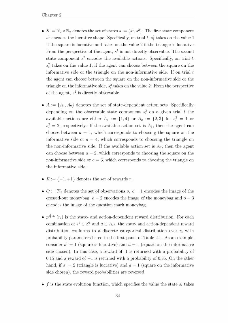
Chapter 2

• S := N2×N2 denotes the set of states s := (s1, s2). The first state components1 encodes the lucrative shape. Specifically, on trial t, s1t takes on the value 1

if the square is lucrative and takes on the value 2 if the triangle is lucrative.From the perspective of the agent, s1 is not directly observable. The secondstate component s2 encodes the available actions. Specifically, on trial t,s2t takes on the value 1, if the agent can choose between the square on theinformative side or the triangle on the non-informative side. If on trial tthe agent can choose between the square on the non-informative side or thetriangle on the informative side, s2t takes on the value 2. From the perspectiveof the agent, s2 is directly observable.

• A := A1, A2 denotes the set of state-dependent action sets. Specifically,depending on the observable state component s2t on a given trial t theavailable actions are either A1 := 1, 4 or A2 := 2, 3 for s2t = 1 ors2t = 2, respectively. If the available action set is A1, then the agent canchoose between a = 1, which corresponds to choosing the square on theinformative side or a = 4, which corresponds to choosing the triangle onthe non-informative side. If the available action set is A2, then the agentcan choose between a = 2, which corresponds to choosing the square on thenon-informative side or a = 3, which corresponds to choosing the triangle onthe informative side.

• R := −1,+1 denotes the set of rewards r.

• O := N3 denotes the set of observations o. o = 1 encodes the image of thecrossed-out moneybag, o = 2 encodes the image of the moneybag and o = 3

encodes the image of the question mark moneybag.

• ps1t ,at (rt) is the state- and action-dependent reward distribution. For each

combination of s1 ∈ S1 and a ∈ As2 , the state- and action-dependent rewarddistribution conforms to a discrete categorical distribution over rt withprobability parameters listed in the first panel of Table 2.1. As an example,consider s1 = 1 (square is lucrative) and a = 1 (square on the informativeside chosen). In this case, a reward of -1 is returned with a probability of0.15 and a reward of +1 is returned with a probability of 0.85. On the otherhand, if s1 = 2 (triangle is lucrative) and a = 1 (square on the informativeside chosen), the reward probabilities are reversed.

• f is the state evolution function, which specifies the value the state st takes

34

2.2. Methods

s1t 1 1 1 1 1 1 1 1 2 2 2 2 2 2 2 2at 1 1 2 2 3 3 4 4 1 1 2 2 3 3 4 4rt -1 +1 -1 +1 -1 +1 -1 +1 -1 +1 -1 +1 -1 +1 -1 +1ps

1t ,at (rt) 0.15 0.85 0.15 0.85 0.85 0.15 0.85 0.15 0.85 0.15 0.85 0.15 0.15 0.85 0.15 0.85

at 1 1 2 2 3 3 4 4rt -1 +1 -1 +1 -1 +1 -1 +1ot 1 2 3 3 1 2 3 3

s1t 1 1 2 2s1t+1 1 2 1 2p(s1t+1|s1t

)0.9625 0.0375 0.0375 0.9625

Table 2.1. Formal task components Upper table shows the state- and action-dependentreward distribution ps

1t ,at (rt), middle table shows the observation function g and lower table

shows the action-independent state transition distribution p(s1t+1|s1t

).

on at trial t,f : NT → S, t 7→ f(t) := st. (2.2)

f is defined in a tabular form and corresponds to the sequence of lucrativeshapes and choice options presented to all participants (cf. SupplementaryMaterial A.3).

• g is the observation function

g : A×R→ O, (a, r) 7→ g(a, r) := o (2.3)

as defined in the second panel of Table 2.1. For the informative actions a = 1

and a = 3, g is injective: The reward r = −1 is mapped onto the observationo = 1, corresponding to the image of the crossed-out moneybag, while thereward r = +1 is mapped onto the observation o = 2, corresponding to theimage of the moneybag. For the non-informative actions a = 2 and a = 4,g is a not injective: Both rewards r = −1 and r = +1 are mapped ontothe observation o = 3, corresponding to the image of the question markmoneybag.

Agent models. We designed five agent models denoted by A1, A2, A3, C1,C2 to account for the putative cognitive processes underlying participants’choices. Before we introduce the individual characteristics of these agents wefirst represent the general structure of an agent interacting with an experimentalrun. This takes the form of a tuple

MAgent :=(T, S,A,R,O, p

(s11), p(s1t+1|s1t

), pat

(ot|s1t

), pat

(rt|s1t

)), (2.4)

35

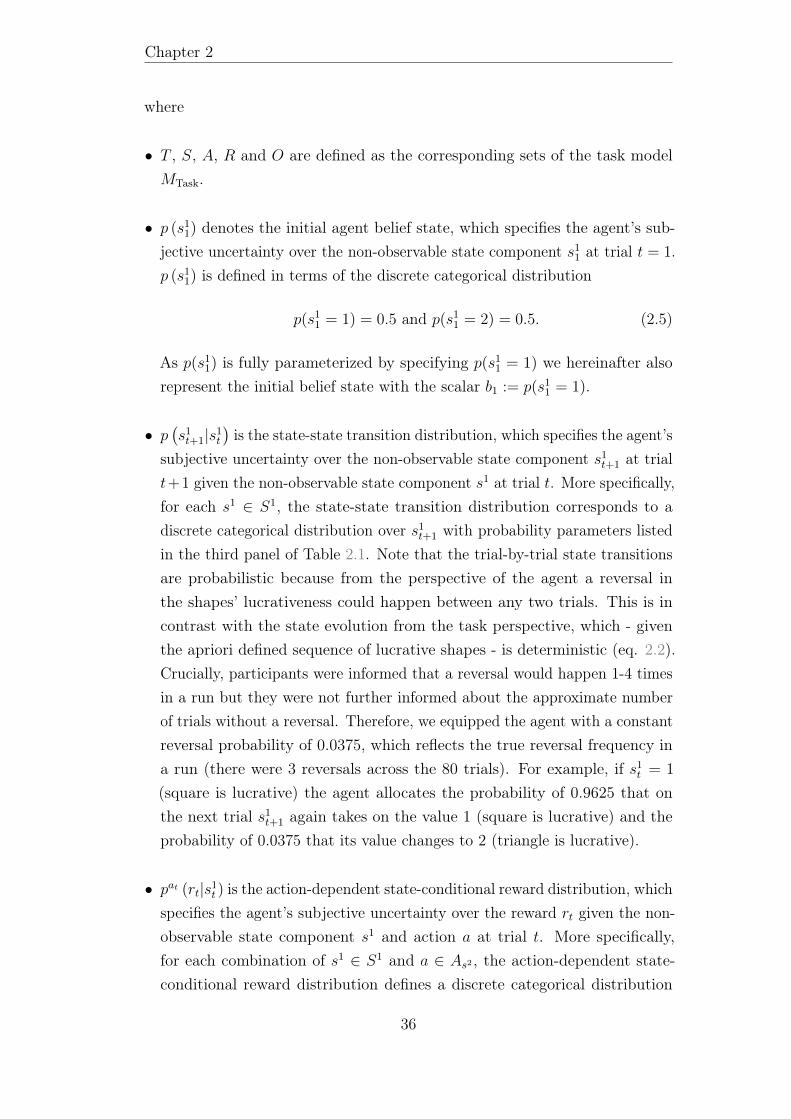
Chapter 2

where

• T , S, A, R and O are defined as the corresponding sets of the task modelMTask.

• p (s11) denotes the initial agent belief state, which specifies the agent’s sub-jective uncertainty over the non-observable state component s11 at trial t = 1.p (s11) is defined in terms of the discrete categorical distribution

p(s11 = 1) = 0.5 and p(s11 = 2) = 0.5. (2.5)

As p(s11) is fully parameterized by specifying p(s11 = 1) we hereinafter alsorepresent the initial belief state with the scalar b1 := p(s11 = 1).

• p(s1t+1|s1t

)is the state-state transition distribution, which specifies the agent’s

subjective uncertainty over the non-observable state component s1t+1 at trialt+1 given the non-observable state component s1 at trial t. More specifically,for each s1 ∈ S1, the state-state transition distribution corresponds to adiscrete categorical distribution over s1t+1 with probability parameters listedin the third panel of Table 2.1. Note that the trial-by-trial state transitionsare probabilistic because from the perspective of the agent a reversal inthe shapes’ lucrativeness could happen between any two trials. This is incontrast with the state evolution from the task perspective, which - giventhe apriori defined sequence of lucrative shapes - is deterministic (eq. 2.2).Crucially, participants were informed that a reversal would happen 1-4 timesin a run but they were not further informed about the approximate numberof trials without a reversal. Therefore, we equipped the agent with a constantreversal probability of 0.0375, which reflects the true reversal frequency ina run (there were 3 reversals across the 80 trials). For example, if s1t = 1

(square is lucrative) the agent allocates the probability of 0.9625 that onthe next trial s1t+1 again takes on the value 1 (square is lucrative) and theprobability of 0.0375 that its value changes to 2 (triangle is lucrative).

• pat (rt|s1t ) is the action-dependent state-conditional reward distribution, whichspecifies the agent’s subjective uncertainty over the reward rt given the non-observable state component s1 and action a at trial t. More specifically,for each combination of s1 ∈ S1 and a ∈ As2 , the action-dependent state-conditional reward distribution defines a discrete categorical distribution

36

2.2. Methods

over rt with probability parameters corresponding to

pat=a(rt = r|s1t = s1

):= ps

1t=s

1,at=a (rt = r) . (2.6)

Notice that the only difference between the agent’s action-dependent state-conditional reward distribution and the task’s state- and action-dependentreward distribution is that for the former the state is conceived as a randomvariable, while for the latter the state is conceived as a parameter. Weequipped the agent with the true reward emission probabilities to reflectthe task instructions. In particular, participants were truthfully informedthat choosing the lucrative shape would return a reward of +1 with a highprobability and a reward of -1 with a low probability and, that choosing thedetrimental shape would return a reward of +1 with a low probability and areward of -1 with a high probability.

• pat (ot|s1t ) is the action-dependent state-conditional observation distribution,which specifies the agent’s subjective uncertainty over the observation ot

given the non-observable state component s1 and action a at trial t. In detail,for each combination of s1 ∈ S1 and a ∈ As2 , the action-dependent state-conditional observation distribution corresponds to a discrete categoricaldistribution over ot with probability parameters resulting from transformingthe distribution of rt by the observation function g. Formally,

pat=a(ot = o|s1t = s1

):=

∑r|g(a,r)=o

pat=a(rt = r|s1t = s1

). (2.7)

For the informative actions a ∈ 1, 3, it thus follows that

pat=a(ot = 1|s1t = s1

)= pat=a

(rt = −1|s1t = s1

)(2.8)

andpat=a

(ot = 2|s1t = s1

)= pat=a

(rt = +1|s1t = s1

). (2.9)

For non-informative actions a ∈ 2, 4, on the other hand, it follows that

pat=a(ot = 3|s1t = s1

)= pat=a

(rt = −1|s1t = s1

)+pat=a

(rt = 1|s1t = s1

)= 1.

(2.10)As an example, consider the case s1 = 1 (square is lucrative) and a = 1

(choose square on the informative side). The agent allocates the sameprobabilities to observing either the image of the crossed-out moneybag or

37

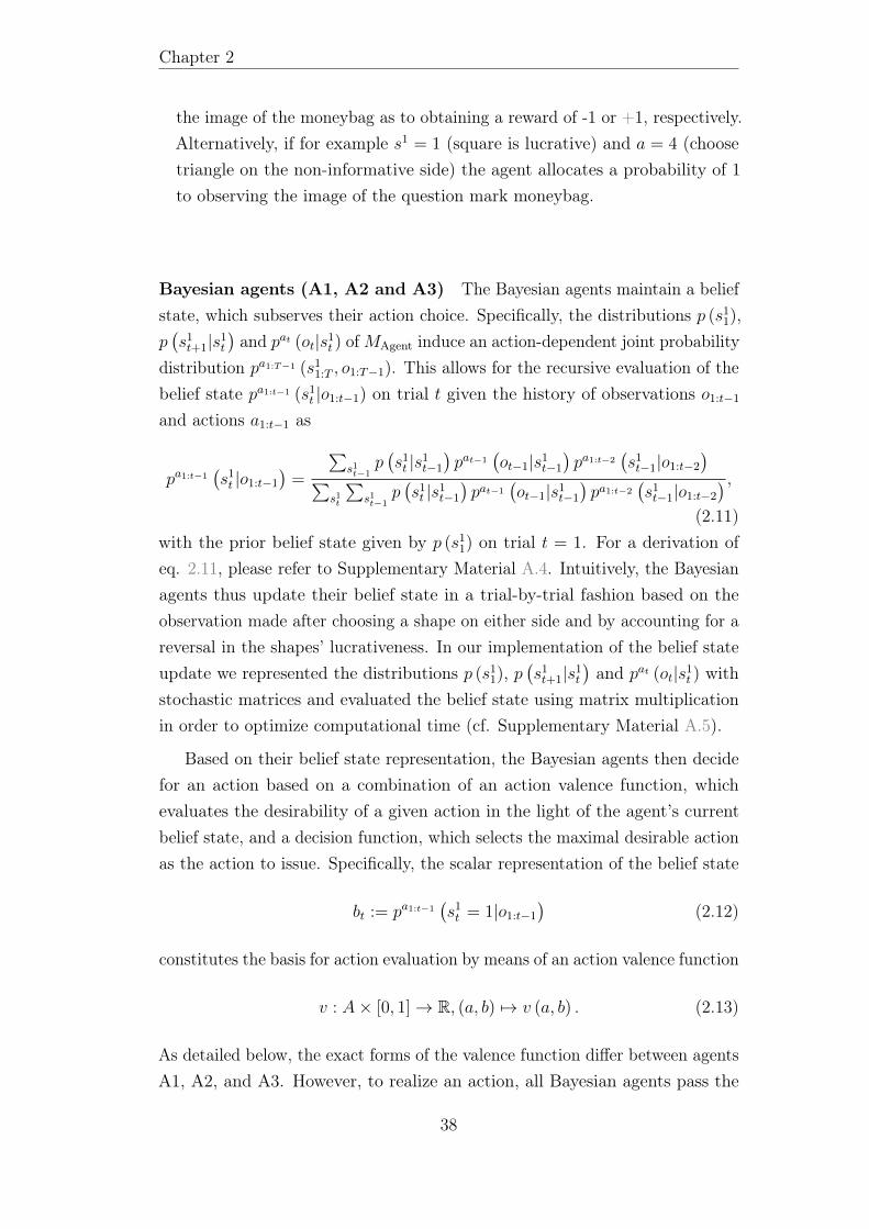
Chapter 2

the image of the moneybag as to obtaining a reward of -1 or +1, respectively.Alternatively, if for example s1 = 1 (square is lucrative) and a = 4 (choosetriangle on the non-informative side) the agent allocates a probability of 1to observing the image of the question mark moneybag.

Bayesian agents (A1, A2 and A3) The Bayesian agents maintain a beliefstate, which subserves their action choice. Specifically, the distributions p (s11),p(s1t+1|s1t

)and pat (ot|s1t ) ofMAgent induce an action-dependent joint probability

distribution pa1:T−1 (s11:T , o1:T−1). This allows for the recursive evaluation of thebelief state pa1:t−1 (s1t |o1:t−1) on trial t given the history of observations o1:t−1and actions a1:t−1 as

pa1:t−1(s1t |o1:t−1

)=

∑s1t−1

p(s1t |s1t−1

)pat−1

(ot−1|s1t−1

)pa1:t−2

(s1t−1|o1:t−2

)∑s1t

∑s1t−1

p(s1t |s1t−1

)pat−1

(ot−1|s1t−1

)pa1:t−2

(s1t−1|o1:t−2

) ,(2.11)

with the prior belief state given by p (s11) on trial t = 1. For a derivation ofeq. 2.11, please refer to Supplementary Material A.4. Intuitively, the Bayesianagents thus update their belief state in a trial-by-trial fashion based on theobservation made after choosing a shape on either side and by accounting for areversal in the shapes’ lucrativeness. In our implementation of the belief stateupdate we represented the distributions p (s11), p

(s1t+1|s1t

)and pat (ot|s1t ) with

stochastic matrices and evaluated the belief state using matrix multiplicationin order to optimize computational time (cf. Supplementary Material A.5).

Based on their belief state representation, the Bayesian agents then decidefor an action based on a combination of an action valence function, whichevaluates the desirability of a given action in the light of the agent’s currentbelief state, and a decision function, which selects the maximal desirable actionas the action to issue. Specifically, the scalar representation of the belief state

bt := pa1:t−1(s1t = 1|o1:t−1

)(2.12)

constitutes the basis for action evaluation by means of an action valence function

v : A× [0, 1]→ R, (a, b) 7→ v (a, b) . (2.13)

As detailed below, the exact forms of the valence function differ between agentsA1, A2, and A3. However, to realize an action, all Bayesian agents pass the

38

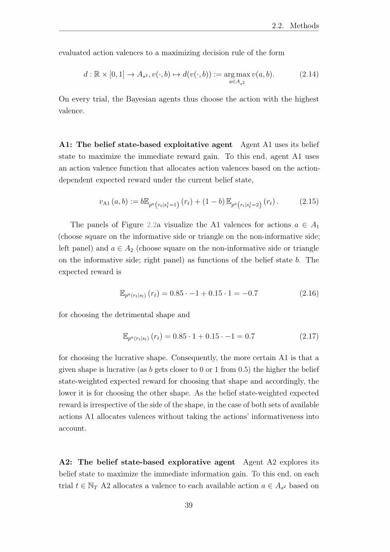
2.2. Methods

evaluated action valences to a maximizing decision rule of the form

d : R× [0, 1]→ As2 , v(·, b) 7→ d(v(·, b)) := arg maxa∈As2

v(a, b). (2.14)

On every trial, the Bayesian agents thus choose the action with the highestvalence.

A1: The belief state-based exploitative agent Agent A1 uses its beliefstate to maximize the immediate reward gain. To this end, agent A1 usesan action valence function that allocates action valences based on the action-dependent expected reward under the current belief state,

vA1 (a, b) := bEpa(rt|s1t=1) (rt) + (1− b)Epa(rt|s1t=2) (rt) . (2.15)

The panels of Figure 2.2a visualize the A1 valences for actions a ∈ A1

(choose square on the informative side or triangle on the non-informative side;left panel) and a ∈ A2 (choose square on the non-informative side or triangleon the informative side; right panel) as functions of the belief state b. Theexpected reward is

Epa(rt|st) (rt) = 0.85 · −1 + 0.15 · 1 = −0.7 (2.16)

for choosing the detrimental shape and

Epa(rt|st) (rt) = 0.85 · 1 + 0.15 · −1 = 0.7 (2.17)

for choosing the lucrative shape. Consequently, the more certain A1 is that agiven shape is lucrative (as b gets closer to 0 or 1 from 0.5) the higher the beliefstate-weighted expected reward for choosing that shape and accordingly, thelower it is for choosing the other shape. As the belief state-weighted expectedreward is irrespective of the side of the shape, in the case of both sets of availableactions A1 allocates valences without taking the actions’ informativeness intoaccount.

A2: The belief state-based explorative agent Agent A2 explores itsbelief state to maximize the immediate information gain. To this end, on eachtrial t ∈ NT A2 allocates a valence to each available action a ∈ As2 based on

39

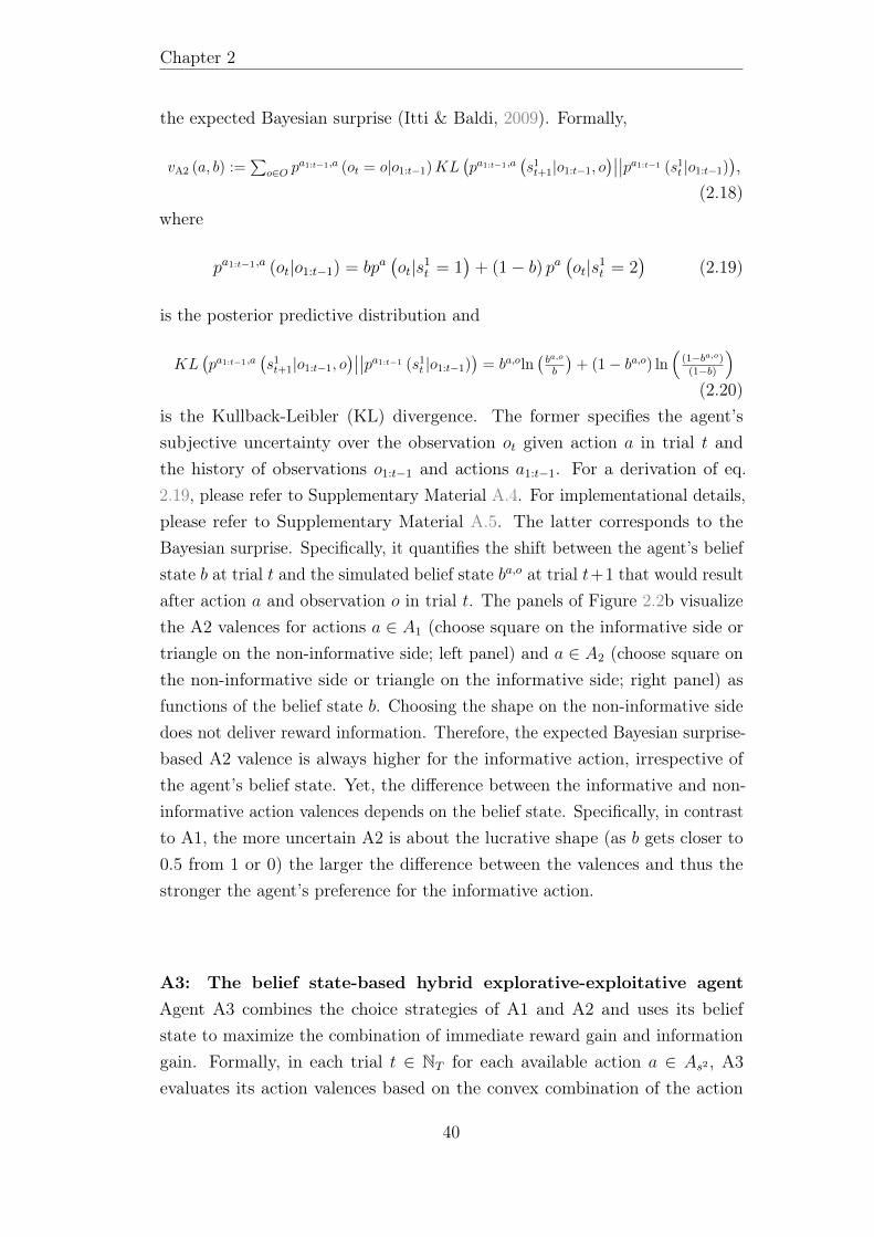
Chapter 2

the expected Bayesian surprise (Itti & Baldi, 2009). Formally,

vA2 (a, b) :=∑

o∈O pa1:t−1,a (ot = o|o1:t−1)KL

(pa1:t−1,a

(s1t+1|o1:t−1, o

)∣∣∣∣pa1:t−1 (s1t |o1:t−1)),

(2.18)where

pa1:t−1,a (ot|o1:t−1) = bpa(ot|s1t = 1

)+ (1− b) pa

(ot|s1t = 2

)(2.19)

is the posterior predictive distribution and

KL(pa1:t−1,a

(s1t+1|o1:t−1, o

)∣∣∣∣pa1:t−1 (s1t |o1:t−1))

= ba,oln(ba,o

b

)+ (1− ba,o) ln

((1−ba,o)(1−b)

)(2.20)

is the Kullback-Leibler (KL) divergence. The former specifies the agent’ssubjective uncertainty over the observation ot given action a in trial t andthe history of observations o1:t−1 and actions a1:t−1. For a derivation of eq.2.19, please refer to Supplementary Material A.4. For implementational details,please refer to Supplementary Material A.5. The latter corresponds to theBayesian surprise. Specifically, it quantifies the shift between the agent’s beliefstate b at trial t and the simulated belief state ba,o at trial t+1 that would resultafter action a and observation o in trial t. The panels of Figure 2.2b visualizethe A2 valences for actions a ∈ A1 (choose square on the informative side ortriangle on the non-informative side; left panel) and a ∈ A2 (choose square onthe non-informative side or triangle on the informative side; right panel) asfunctions of the belief state b. Choosing the shape on the non-informative sidedoes not deliver reward information. Therefore, the expected Bayesian surprise-based A2 valence is always higher for the informative action, irrespective ofthe agent’s belief state. Yet, the difference between the informative and non-informative action valences depends on the belief state. Specifically, in contrastto A1, the more uncertain A2 is about the lucrative shape (as b gets closer to0.5 from 1 or 0) the larger the difference between the valences and thus thestronger the agent’s preference for the informative action.

A3: The belief state-based hybrid explorative-exploitative agentAgent A3 combines the choice strategies of A1 and A2 and uses its beliefstate to maximize the combination of immediate reward gain and informationgain. Formally, in each trial t ∈ NT for each available action a ∈ As2 , A3evaluates its action valences based on the convex combination of the action

40

2.2. Methods

valences of agents A1 and A3

vA3(a, b) := λvA1(a, b) + (1− λ) vA2(a, b), (2.21)

where λ ∈ [0, 1] is the weighting parameter.The panels of Figures 2.2c and d visualize the A3 valences for actions a ∈ A1

(choose square on the informative side or triangle on the non-informative side;left panels) and a ∈ A2 (choose square on the non-informative side or triangleon the informative side; right panels) as functions of the belief state b for λvalues 0.5 and 0.25, respectively. For λ = 1 the valences of agent A3 correspondto the valences of A1 and for λ = 0 they correspond to the valences of A2. Forλ values of the interval ]0, 1[, the strategy of A3 is a mixture of A1 and A2:For less extreme belief values (b close to 0.5) A3 allocates a higher valence tochoosing the shape on the informative side even if the agent allocates a lowerprobability to that shape being lucrative. This shows the contribution of A2.For more extreme belief state values (b close to 0 or 1) A3 allocates a highervalence to choosing the shape with the higher probability to be lucrative evenif the action is non-informative. This shows the contribution of A1. Note,however, that a λ value of 0.5 should not be understood as A3 resembling 50%the strategy of A1 and 50% the strategy of A2. The reason for this is that A3applies a convex combination of A1 and A2 valences and they have differentranges. Therefore, while for λ = 0.5 the valences of A3 primarily reflect thecontribution of A1 (Figure 2.2c), the contribution of A2 becomes evident forλ = 0.25 (2.2d).

Control agents C1 and C2 The control agents C1 and C2 rely on heuristicchoice strategies. Because C1 and C2 do not represent a belief state, theiraction valence function is a function of a only,

v : A→ R, a 7→ v (a) . (2.22)

To realize an action on trial t ∈ NT , both agents use a probabilistic decisionrule. Specifically, C1 and C2 directly translate the action valences into actionand observation history-dependent choice probabilities.

C1: The belief state-free random choice agent C1 is the simplest agentand may be considered a cognitive null model. This agent does not havean optimization aim based on which it could differentiate between actions.

41

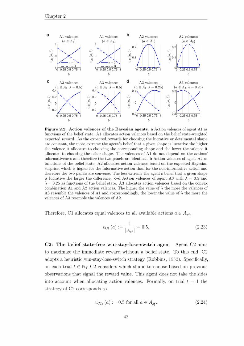
Chapter 2

c-1

0

1

-1

0

1

0

0.1

0.2

0

0.1

0.2

-1

0

1

-0.2

0

0.2

0.4

-0.2

0

0.2

0

0.1

0.2

-1

0

1

0

0.1

0.2

0

0.1

0.2

-0.2

0

0.2

0.4

-0.2

0

0.2

0

0.1

0.2

0 0.25 0.75 10.5 0 0.25 0.75 10.5

-1 -1 0 0

-1

0

1

-1

0

1

-0.2

0

0.2

0.4

-0.2

0

0.2

0.4

-0.2

0

0.2

-0.2

0

0.2

0

0.1

0.2

0

0.1

0.2

0 0.25 0.75 10.5 0 0.25 0.75 10.5

-1

0

1

-1

0

1

0

0.1

0.2

0

0.1

0.2

-1

0

1

-0.2

0

0.2

0.4

-0.2

0

0.2

0

0.1

0.2

0 0.25 0.75 10.5 0 0.25 0.75 10.5

c d

0 0.25 0.75 10.5 0 0.25 0.75 10.5 0 0.25 0.75 10.5 0 0.25 0.75 10.5

-1 -1 0

-1

0

1

-1

0

1

-0.2

0

0.2

0.4

-0.2

0

0.2

0.4

-0.2

0

0.2

-0.2

0

0.2

0 0.25 0.75 10.5 0 0.25 0.75 10.5

a b

Figure 2.2. Action valences of the Bayesian agents. a Action valences of agent A1 asfunctions of the belief state. A1 allocates action valences based on the belief state-weightedexpected reward. As the expected rewards for choosing the lucrative or detrimental shapeare constant, the more extreme the agent’s belief that a given shape is lucrative the higherthe valence it allocates to choosing the corresponding shape and the lower the valence itallocates to choosing the other shape. The valences of A1 do not depend on the actions’informativeness and therefore the two panels are identical. b Action valences of agent A2 asfunctions of the belief state. A2 allocates action valences based on the expected Bayesiansurprise, which is higher for the informative action than for the non-informative action andtherefore the two panels are converse. The less extreme the agent’s belief that a given shapeis lucrative the larger the difference. c-d Action valences of agent A3 with λ = 0.5 andλ = 0.25 as functions of the belief state. A3 allocates action valences based on the convexcombination A1 and A2 action valences. The higher the value of λ the more the valences ofA3 resemble the valences of A1 and correspondingly, the lower the value of λ the more thevalences of A3 resemble the valences of A2.

Therefore, C1 allocates equal valences to all available actions a ∈ As2 ,

vC1 (a) :=1

|As2|= 0.5. (2.23)

C2: The belief state-free win-stay-lose-switch agent Agent C2 aimsto maximize the immediate reward without a belief state. To this end, C2adopts a heuristic win-stay-lose-switch strategy (Robbins, 1952). Specifically,on each trial t ∈ NT C2 considers which shape to choose based on previousobservations that signal the reward value. This agent does not take the sidesinto account when allocating action valences. Formally, on trial t = 1 thestrategy of C2 corresponds to

vC21 (a) := 0.5 for all a ∈ As21 . (2.24)

42

2.2. Methods

Then, on trials t = 2, 3, ..., T agent C2 allocates action valences according to

vC2t (a) :=

0, if ot−1 = 1 and a ∈ At−1 or ot−1 = 2 and a /∈ At−11, if ot−1 = 2 and a ∈ At−1 or ot−1 = 1 and a /∈ At−1vC2t−1 (a) , if ot−1 = 3

,

(2.25)

whereA denotes the set of actions of choosing a given shape and thusA := 1, 2for the actions choose square and A := 3, 4 for the actions choose triangle.In words, C2 allocates equal initial action valences, because on trial t = 1 noprevious observations are available and therefore the agent can not differentiatebetween actions. Then, on trials t = 2, 3, ..., T the valences C2 allocates dependon the observation on trial t − 1. Specifically, if on trial t − 1 the choice ofa shape results in the observation o = 1, i.e. the image of the crossed-outmoneybag, then on trial t the agent allocates a valence of 0 to choosing thesame shape and a valence of 1 to choosing the other shape. In contrast, if ontrial t− 1 the choice of a shape results in the observation o = 2, i.e. the imageof the moneybag, then on trial t the agent allocates a valence of 1 to choosingthe same shape and a valence of 0 to choosing the other shape. Crucially, ifon trial t − 1 the choice of a shape results in the observation o = 3, i.e. theimage of the question mark moneybag, the value of the returned reward is notsignalled to the agent and therefore on trial t C2 relies on its valence allocationscheme from trial t− 1. That is, the valence C2 allocates to choosing a givenshape on trial t corresponds to the valence the agent allocated to choosing thatshape on trial t− 1.

2.2.4 Model evaluation and validation

Data analysis models To evaluate the agent models in light of the partici-pants’ data, we first embedded the agent models into a statistical frameworkto account for post-decision noise. In particular, for agents A1, A2, A3 andC2 we formulated the data analysis models by combining the agent-specificvalences with the softmax decision rule (Reverdy & Leonard, 2015). Specifically,we defined the probability of action a given the history of actions a1:t−1 andobservations o1:t−1 as

pτ (at = a|a1:t−1, o1:t−1) :=exp (τ−1v(a, ·))∑

a∈As2exp (τ−1v(a, ·))

, (2.26)

43

Chapter 2

where for each agent v(a, ·) is substituted with the agent-specific valencefunction. Parameter τ ∈ R>0 encodes the level of post-decision noise: Thelower the value of τ the higher the probability that the action with the highervalence is realized and thus the lower the post-decision noise. Notably, asagent C1 allocates equal action valences throughout, for any τ value thesoftmax decision rule would return uniform probabilities. Therefore, for thisagent a softmax decision rule is not necessitated and the data analysis modelcorresponds to

p (at = a|a1:t−1, o1:t−1) = p (at = a|a1:t−1) := vt (a) . (2.27)

Parameter estimation We used a maximum log likelihood (ML)-basedapproach to estimate the parameters of the data analysis models of A1, A2, A3and C2 based on the experimentally acquired data. Specifically, we assumedconditionally independently and identically distributed actions and thus foreach participant defined the log likelihood function of each model as

lN : Θ→ R, θ 7→ lN(θ) := ln∏N

n=1 pθ (an|a1:n−1, o1:n−1) =

∑Nn=1 ln p

θ (an|a1:n−1, o1:n−1).(2.28)

Note that we here replaced t with n and T with N . The reason for this is toemphasize that we only considered trials with a valid choice and thus n ∈ NN

denotes the participant’s nth valid trial. For agents A1, A2 and C2 the loglikelihood lN is a function of parameter τ of the softmax decision rule and thus,for these agents θ := τ . For A3, the log likelihood lN is additionally a functionof the weighting parameter λ and thus, for this agent θ := (τ, λ). For everyagent and participant we estimated the free parameters by maximizing the loglikelihood function lN using Matlab’s constrained nonlinear optimization routinefmincon (Byrd, Gilbert, & Nocedal, 2000; Byrd, Hribar, & Nocedal, 1999; Waltz,Morales, Nocedal, & Orban, 2006). We set the boundary constraints to 0.01and 2.5 for τ and to 0 and 1 for λ. The initial values were chosen randomfrom a continuous uniform distribution between the boundary constraints. Tomitigate the risk of finding local instead of global maxima we repeated theparameter estimation procedure 10-times and recorded the parameter estimatesof the repeat with the highest maximum log likelihood. Note that as the dataanalysis model of C1 does not have free parameters, for this agent the loglikelihood function lN is specified directly.

44

2.2. Methods

Model comparison To compare the models, we first computed the BayesianInformation Criterion (BIC; Schwarz, 1978) for each agent and participant as

BIC = lN(θ)− k

2ln N, (2.29)

where k is the number of free parameters. The BIC scores of all agents andparticipants were subsequently entered for random-effects Bayesian modelselection as implemented in the spm_BMS function in the SPM toolbox toobtain protected exceedance probabilities (www.fil.ion.ucl.ac.uk/spm/; Rigoux,Stephan, Friston, and Daunizeau, 2014; Stephan, Penny, Daunizeau, Moran,and Friston, 2009). These indicated the group-level probability that a particularmodel was more likely than any other model of the model space. In addition,we computed a pseudo-r2 statistic ρ (McFadden, 1973) for each participant andagents A1, A2, A3 and C2 as

ρ = 1−lNAgent 6=C1(θ)

lNC1

(2.30)

to express the variance of a participant’s choices explained by a strategy thatdifferentiates between actions as implemented by agents A1, A2, A3 and C2compared to a non-differentiating strategy as implemented by agent C1.

Model recovery We conducted model recovery analysis to validate ourmodelling initiative and test if we can reliably distinguish the agent-specificdata analysis models from each other. Specifically, for every model we firstgenerated synthetic data and then evaluated all models based on these datausing ML-based approach as described above. The data corresponded tothe agent-specific actions on 160 trials, with trial sequence identical to theparticipants’ trial sequence and agent action-dependent observations as givenby the observation function g and the state- and action-dependent rewarddistribution ps1t ,at (rt). For agent C1 data were generated directly. For agentsA1, A2, A3 and C2 data were generated with τ parameter values between 0.05

and 2.5 with an increment of 0.05 to evaluate if we can identify each modelfor different levels of post-decision noise across the τ parameter space used forestimation. In addition, for A3 data were generated with parameter valuesλ ∈ 0.1, 0.25, 0.3, 0.5, 0.7, 0.9 to probe if it can be distinguished from agentsA1 and A2, for low to high values of the weighting parameter. With eachdata generating model and parameter value we simulated 24 data sets, thesame number as the participant sample size. Based on each synthetic data set

45

Chapter 2

we evaluated the maximum log likelihood of all models and conducted modelcomparison analysis as described above. We repeated this procedure 10-timesand computed the average protected exceedance probabilities across repeats.

Parameter recovery To test if we can reliably estimate the free parametersof the data analysis models of A1, A2, A3 and C2 across the parameter spaceas defined by the estimation boundary constraints, we conducted parameterrecovery analysis. To this end, we used the synthetic ML parameter estimatesobtained during model recovery analysis. More precisely, for a given datagenerating model and simulation parameter we computed the average MLparameter estimates of the same model across the group of 24 synthetic datasets and 10 repeats and compared it with the simulation parameter.

Winning model validation To validate the most plausible model (Wilson& Collins, 2019), we generated synthetic data sets with it for each participantusing the participant’s ML parameter estimates. Like in the model recoveryanalysis, the data corresponded to the agent’s actions on 160 trials, with trialsequence identical to the participants’ trial sequence and the agent’s action-dependent observations as given by the observation function g and the state- andaction-dependent reward distribution ps1t ,at (rt). We then entered each syntheticparticipant data set for descriptive analyses as described above. Specifically,we computed the same nine summary choice rates as for the participants andrepeated the data generation and summary choice rates evaluation 100-times.We then computed the averages across simulation repeats and entered themfor synthetic group-summary choice rates evaluation. Furthermore, we alsoevaluated synthetic group trial-by-trial choice rates as well as their betweenreversals averages based on the simulation repeats-averaged agent actions.

In addition and finally, we performed model and parameter recovery analysisof the winning model with the participants’ ML parameter estimates to ensurethat the model can reliably account for the empirically acquired data. Weused the same recovery procedures as described above with the exceptionthat within a single repeat each of the 24 data sets was generated with adifferent participant’s ML parameter estimates. Note that to avoid confusion,we hereinafter use the subscript p to refer to empirical (participant) parameterestimates.

46

2.3. Results

2.3 Results

2.3.1 Descriptive results

Participants completed the majority of trials with an overall valid choicerate of 97.86% ± 0.62. There was no difference in the number of missedchoices with respect to trial types: The valid choice rate on type I trials was97.97% ± 0.62 and the valid choice rate on type II trials was 97.76% ± 0.68.On type I trials, the majority of action choices were lucrative and informative(87.45%±1.53) while only a few were detrimental and non-informative (12.55%±1.53). The difference between the choice rates on type II trials was lesspronounced: 66.01% ± 2.28 of the action choices were lucrative and non-informative while 33.99%±2.28 were detrimental and informative. Summed overinformative and non-informative action choices, the lucrative action choice ratewas 76.74%±1.7, whereas summed over lucrative and detrimental action choices,the informative action choice rate was 60.74% ± 0.92. Notably, participantsmade significantly more lucrative choices, if the lucrative action was alsoinformative (and the alternative detrimental and non-informative) comparedto lucrative choices, if the lucrative action was also non-informative (and thealternative detrimental and informative; two-sided paired sample t-test, t(23) =

11.55, p < 0.001). Together, these results suggest that while participants’choices were primarily guided by the actions’ lucrativeness, participants alsotook the action’s informativeness into account.

We next evaluated group trial-by-trial choice rates. As shown in Figure 2.3a,on the majority of trials the lucrative action choice rates prevailed over thedetrimental action choice rates. This was more pronounced for the trial-by-triallucrative and informative action choice rates. Crucially, both the averagelucrative and informative and the average lucrative and non-informative actionchoice rates showed an overall increase between two reversals (Figure 2.3b).This indicates that participants gradually resolved their uncertainty aboutthe currently lucrative shape. Moreover, although the average lucrative andinformative action choice rate was larger than the average lucrative and non-informative action choice rate on all trials between two reversals (with theexception of the 18th trial), their difference decreased slightly between the firsttrials after and the last trials before a reversal (2.3c). This suggests that withdecreasing uncertainty about the currently lucrative shape participants tookthe actions’ informativeness less into account.

47

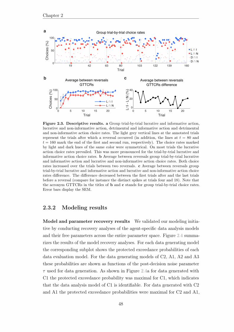
Chapter 2

19 42 63 80 103 122 139 1600

50

100C

hoic

es(%

)Group trial-by-trial choice rates

0 5 10 15 20Trial

0

50

100

Cho

ices

(%)

0 5 10 15 20Trial

0

20

40

LI-

LN

(%)

Average between reversalsGTTCRs difference

19 42 63 80 103 122 139 1600

50

100C

hoic

es(%

)Group trial-by-trial choice rates

0 5 10 15 20Trial

0

50

100

Cho

ices

(%)

0 5 10 15 20Trial

0

20

40

LI-

LN

(%)

Average between reversalsGTTCRs difference

Average between reversalsGTTCRs

a

b c

19 42 63 80 103 122 139 160Trial

0

50

100

Cho

ices

(%)

0 5 10 15 20Trial

0

50

100

Cho

ices

(%) GTTCRs

0 5 10 15 20Trial

0

20

40

LI-

LN

(%) GTTCRs difference

Group trial-by-trial choice rates

0 19 42 63 80 103 122 139 160Trial

0

50

100

Cho

ices

(%)

Group trial-by-trial choice rates

L IL ND ID N

100

Cho

ices

(%)

Average between reversalsGTTCRs

20

40

LI-

LN

(%)

Average between reversalsGTTCRs difference

0 19 42 63 80 103 122 139 160Trial

0

50

100

Cho

ices

(%)

Group trial-by-trial choice rates

L IL ND ID N

100

Cho

ices

(%)

Average between reversalsGTTCRs

20

40

LI-

LN

(%)

Average between reversalsGTTCRs difference

0 19 42 63 80 103 122 139 160Trial

0

50

Cho

ices

(%) L N

D ID N

0 5 10 15 20Trial

0

50

100

Cho

ices

(%)

Average between reversalsGTTCRs

L IL N

0 5 10 15 20Trial

0

20

40

LI-

LN

(%)

Average between reversalsGTTCRs difference

Figure 2.3. Descriptive results. a Group trial-by-trial lucrative and informative action,lucrative and non-informative action, detrimental and informative action and detrimentaland non-informative action choice rates. The light grey vertical lines at the annotated trialsrepresent the trials after which a reversal occurred (in addition, the lines at t = 80 andt = 160 mark the end of the first and second run, respectively). The choice rates markedby light and dark hues of the same color were symmetrical. On most trials the lucrativeaction choice rates prevailed. This was more pronounced for the trial-by-trial lucrative andinformative action choice rates. b Average between reversals group trial-by-trial lucrativeand informative action and lucrative and non-informative action choice rates. Both choicerates increased over the trials between two reversals. c Average between reversals grouptrial-by-trial lucrative and informative action and lucrative and non-informative action choicerates difference. The difference decreased between the first trials after and the last trialsbefore a reversal (compare for instance the distinct spikes at trials four and 18). Note thatthe acronym GTTCRs in the titles of b and c stands for group trial-by-trial choice rates.Error bars display the SEM.

2.3.2 Modeling results

Model and parameter recovery results We validated our modeling initia-tive by conducting recovery analyses of the agent-specific data analysis modelsand their free parameters across the entire parameter space. Figure 2.4 summa-rizes the results of the model recovery analyses. For each data generating modelthe corresponding subplot shows the protected exceedance probabilities of eachdata evaluation model. For the data generating models of C2, A1, A2 and A3these probabilities are shown as functions of the post-decision noise parameterτ used for data generation. As shown in Figure 2.4a for data generated withC1 the protected exceedance probability was maximal for C1, which indicatesthat the data analysis model of C1 is identifiable. For data generated with C2and A1 the protected exceedance probabilities were maximal for C2 and A1,

48

2.3. Results

respectively, for all values of τ . This indicates that the data analysis models ofC2 and A1 are identifiable for low to high levels of post-decision noise. For datagenerated with A2 the protected exceedance probabilities were maximal for A2for τ values up to 0.35 and for C1 for larger values of τ . This indicates thatA2 is identifiable for low but not for high levels of post-post-decision noise. Fordata generated with A3 with λ = 0.25 the protected exceedance probabilitieswere maximal for A3 up to τ = 0.25, after which A1 and then C1 exceeded.This indicates that, similarly to A2, A3 with λ = 0.25 is identifiable for lowbut not for high levels of post-decision noise. With increasing noise the data isbetter accounted for by A1 and eventually by C1.

Notably, for data generated with A3, model recovery depend not only onthe post-decision noise parameter τ but also on the weighting parameter λ. Asshown in Figure 2.4b for λ values up to 0.5 the protected exceedance probabilitieswere maximal for A3 for small τ values (0.25, 0, 2 and 0.1, respectively). Then,for λ = 0.1, A2 and then C1 prevailed, while for λ = 0.3 and λ = 0.5, A1and then C1 prevailed. Due to the increasing similarity between the valencesof A3 and A1 (cf. Figure 2.2c-d), for λ values larger than 0.5 the protectedexceedance probability profiles shifted towards that of A1. More precisely, forλ = 0.7 and λ = 0.9 the protected exceedance probabilities were maximal forA1 up to τ = 1.9 and τ = 2.4, respectively, and for C1 for larger τ values.Together, consistent with the interpretation of the weighting parameter, theseresults imply that the data analysis model of A3 is identifiable for low tomedium λ values for low levels of post-decision noise. Otherwise, A3 can notbe distinguished from A1 or A2 and eventually, from C1.

The results of the parameter recovery analyses are visualized in Figure 2.5.Here, model-specific ML parameter estimates are displayed as functions of thepost-decision noise parameter τ . The recovered ML parameter estimates τC2,τA1, τA2 and τA3 were consistent with the simulation parameters τC2 = τA1 =

τA2 = τA3 for small values. Otherwise, the parameters were first over- thenunderestimated. As shown in Figure 2.5a this bias was subtle for C2 and A1and only affected large τ values (between approximately 1.5 and 2.5) while itwas more pronounced for A2 and A3 (with λ = 0.25) and affected medium tolarge τ values (between approximately 0.5 and 2.5). These results are consistentwith the model recovery results: For large post-decision noise, data generatedwith any model starts to resemble a random choice strategy and therefore therecovered parameter estimate for τ reaches asymptote.

Figure 2.5b shows the parameter recovery results for data generated with

49

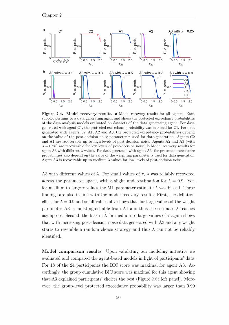
Chapter 2

C1 C2 A1 A2 A30

0.5

1

P.e.prob.

C1

0 0.5 1.5 2.50

0.5

1

P.e.prob.

C2

0 0.5 1.5 2.50

0.5

1

P.e.prob.

A1

0 0.5 1.5 2.50

0.5

1

P.e.prob.

A2

0 0.5 1.5 2.50

0.5

1

P.e.prob.

A3 with = 0.25

0 0.5 1.5 2.50

0.5

1

P.e.prob.

A3 with = 0.1

0 0.5 1.5 2.50

0.5

1P.e.prob.

A3 with = 0.3

0 0.5 1.5 2.50

0.5

1

P.e.prob.

A3 with = 0.5

0 0.5 1.5 2.50

0.5

1

P.e.prob.

A3 with = 0.7

0 0.5 1.5 2.50

0.5

1

P.e.prob.

A3 with = 0.9

A3A2A1C2C1

C1 C2 A1 A2 A30

0.5

1

P.e.prob.

C1

0 0.5 1.5 2.50

0.5

1

P.e.prob.

C2

0 0.5 1.5 2.50

0.5

1

P.e.prob.

A1

0 0.5 1.5 2.50

0.5

1

P.e.prob.

A2

0 0.5 1.5 2.50

0.5

1

P.e.prob.

A3 with = 0.25

0 0.5 1.5 2.50

0.5

1

P.e.prob.

A3 with = 0.1

0 0.5 1.5 2.50

0.5

1P.e.prob.

A3 with = 0.3

0 0.5 1.5 2.50

0.5

1

P.e.prob.

A3 with = 0.5

0 0.5 1.5 2.50

0.5

1

P.e.prob.

A3 with = 0.7

0 0.5 1.5 2.50

0.5

1

P.e.prob.

A3 with = 0.9

A3A2A1C2C1

a

b

Figure 2.4. Model recovery results. a Model recovery results for all agents. Eachsubplot pertains to a data generating agent and shows the protected exceedance probabilitiesof the data analysis models evaluated on datasets of the data generating agent. For datagenerated with agent C1, the protected exceedance probability was maximal for C1. For datagenerated with agents C2, A1, A2 and A3, the protected exceedance probabilities dependon the value of the post-decision noise parameter τ used for data generation. Agents C2and A1 are recoverable up to high levels of post-decision noise. Agents A2 and A3 (withλ = 0.25) are recoverable for low levels of post-decision noise. b Model recovery results foragent A3 with different λ values. For data generated with agent A3, the protected exceedanceprobabilities also depend on the value of the weighting parameter λ used for data generation.Agent A3 is recoverable up to medium λ values for low levels of post-decision noise.

A3 with different values of λ. For small values of τ , λ was reliably recoveredacross the parameter space, with a slight underestimation for λ = 0.9. Yet,for medium to large τ values the ML parameter estimate λ was biased. Thesefindings are also in line with the model recovery results: First, the deflationeffect for λ = 0.9 and small values of τ shows that for large values of the weightparameter A3 is indistinguishable from A1 and thus the estimate λ reachesasymptote. Second, the bias in λ for medium to large values of τ again showsthat with increasing post-decision noise data generated with A3 and any weightstarts to resemble a random choice strategy and thus λ can not be reliablyidentified.

Model comparison results Upon validating our modeling initiative weevaluated and compared the agent-based models in light of participants’ data.For 18 of the 24 participants the BIC score was maximal for agent A3. Ac-cordingly, the group cumulative BIC score was maximal for this agent showingthat A3 explained participants’ choices the best (Figure 2.6a left panel). More-over, the group-level protected exceedance probability was larger than 0.99

50

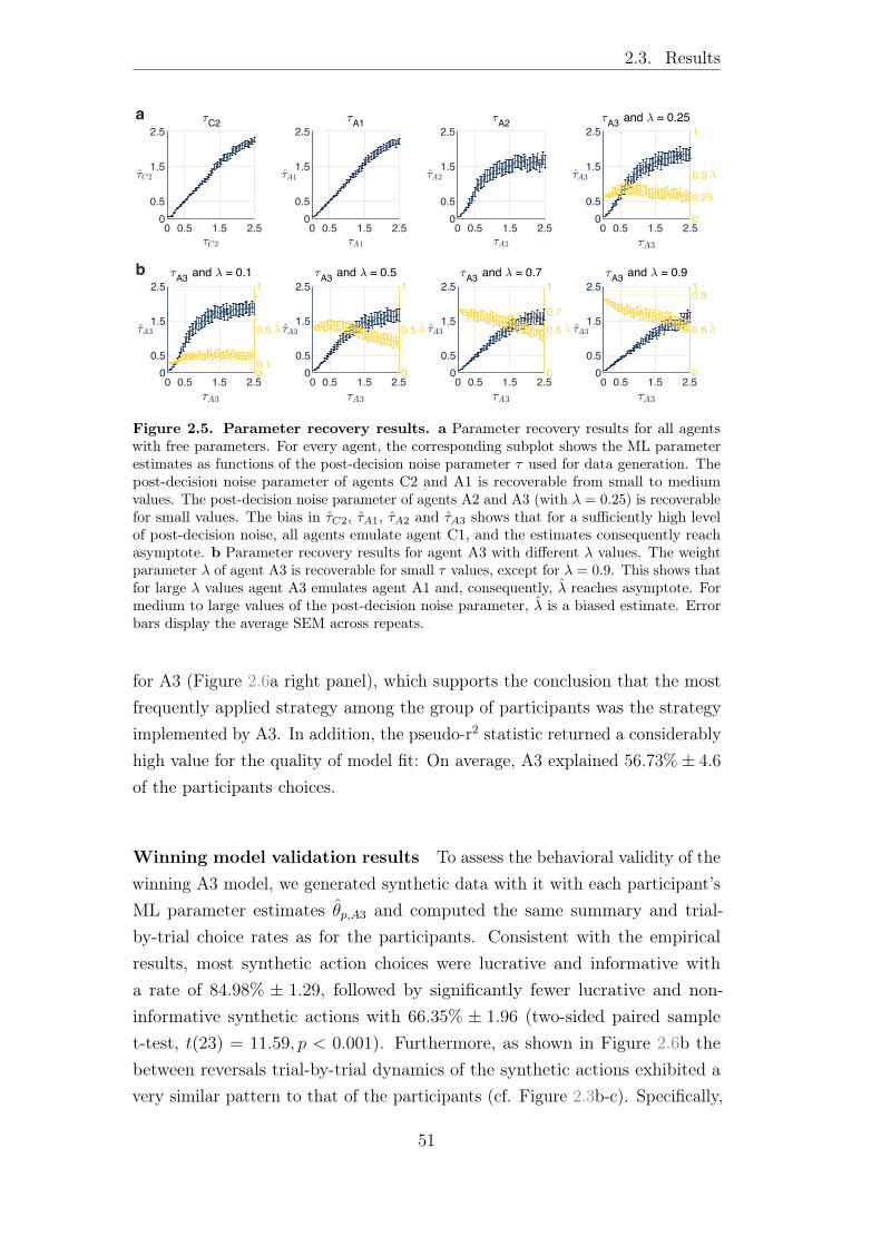
2.3. Results

0 0.5 1.5 2.50

0.5

1.5

2.5C2

0 0.5 1.5 2.50

0.5

1.5

2.5A1

0 0.5 1.5 2.50

0.5

1.5

2.5A2

0 0.5 1.5 2.50

0.5

1.5

2.5

0

0.25

0.5

1A3 and = 0.25

0 0.5 1.5 2.50

0.5

1.5

2.5

00.1

0.5

1A3 and = 0.1

0 0.5 1.5 2.50

0.5

1.5

2.5

0

0.5

1A3 and = 0.5

0 0.5 1.5 2.50

0.5

1.5

2.5

0

0.50.7

1A3 and = 0.7

0 0.5 1.5 2.50

0.5

1.5

2.5

0

0.5

0.91

A3 and = 0.90 0.5 1.5 2.50

0.5

1.5

2.5C2

0 0.5 1.5 2.50

0.5

1.5

2.5A1

0 0.5 1.5 2.50

0.5

1.5

2.5A2

0 0.5 1.5 2.50

0.5

1.5

2.5

0

0.25

0.5

1A3 and = 0.25

0 0.5 1.5 2.50

0.5

1.5

2.5

00.1

0.5

1A3 and = 0.1

0 0.5 1.5 2.50

0.5

1.5

2.5

0

0.5

1A3 and = 0.5

0 0.5 1.5 2.50

0.5

1.5

2.5

0

0.50.7

1A3 and = 0.7

0 0.5 1.5 2.50

0.5

1.5

2.5

0

0.5

0.91

A3 and = 0.9

a

b

Figure 2.5. Parameter recovery results. a Parameter recovery results for all agentswith free parameters. For every agent, the corresponding subplot shows the ML parameterestimates as functions of the post-decision noise parameter τ used for data generation. Thepost-decision noise parameter of agents C2 and A1 is recoverable from small to mediumvalues. The post-decision noise parameter of agents A2 and A3 (with λ = 0.25) is recoverablefor small values. The bias in τC2, τA1, τA2 and τA3 shows that for a sufficiently high levelof post-decision noise, all agents emulate agent C1, and the estimates consequently reachasymptote. b Parameter recovery results for agent A3 with different λ values. The weightparameter λ of agent A3 is recoverable for small τ values, except for λ = 0.9. This shows thatfor large λ values agent A3 emulates agent A1 and, consequently, λ reaches asymptote. Formedium to large values of the post-decision noise parameter, λ is a biased estimate. Errorbars display the average SEM across repeats.

for A3 (Figure 2.6a right panel), which supports the conclusion that the mostfrequently applied strategy among the group of participants was the strategyimplemented by A3. In addition, the pseudo-r2 statistic returned a considerablyhigh value for the quality of model fit: On average, A3 explained 56.73%± 4.6

of the participants choices.

Winning model validation results To assess the behavioral validity of thewinning A3 model, we generated synthetic data with it with each participant’sML parameter estimates θp,A3 and computed the same summary and trial-by-trial choice rates as for the participants. Consistent with the empiricalresults, most synthetic action choices were lucrative and informative witha rate of 84.98% ± 1.29, followed by significantly fewer lucrative and non-informative synthetic actions with 66.35% ± 1.96 (two-sided paired samplet-test, t(23) = 11.59, p < 0.001). Furthermore, as shown in Figure 2.6b thebetween reversals trial-by-trial dynamics of the synthetic actions exhibited avery similar pattern to that of the participants (cf. Figure 2.3b-c). Specifically,

51

Chapter 2

while both the average lucrative and informative and the average lucrative andnon-informative action choice rates increased between two reversals (left panel),their difference decreased moderately between the first trials after and the lasttrials before a reversal (right panel). Altogether, these results lend a high facevalidity to the most plausible A3 model.

As a last step we conducted model and parameter recovery analyses ofthe winning A3 model and the participants’ ML parameter estimates θp,A3 toevaluate the model’s reliability in explaining the experimentally acquired data.Participants varied moderately with respect to both τp,A3 and λp,A3. Specifically,τp,A3 ranged from 0.035 to 0.377 with an average of 0.124 ± 0.014 and λp,A3ranged from 0.044 to 0.622 with an average of 0.274 ± 0.027. As suggestedby the results of the recovery analyses across the entire model and parameterspace, for comparable τ and λ values the model of A3 and its free parametersare reliably recoverable. Indeed, based on data generated with A3 and θp,A3both the model (Figure 2.6c) and parameter recovery (Figure 2.6d) analyseswere successful. These results confirm the reliability of the best fitting A3model.

2.4 Discussion

In this work, we addressed the question of how humans make sequentialdecisions if all actions bear economic consequences but only some deliveralso information. By collecting participant choice data on an information-selective reversal bandit task, we demonstrated that in such situations, humansbalance between exploratory and exploitative actions depending on their levelof uncertainty. To arrive at this conclusion, we applied a comprehensive setof descriptive and agent-based computational modeling analyses (Russell &Norvig, 2010), including model evaluation based on relative (i.e., cumulativeBIC score, protected exceedance probability and pseudo-r2 statistic) as well asabsolute (similarity between empirical and synthetic choice patterns) measures(Wilson & Collins, 2019). Formally, the behaviorally most plausible strategywas captured by a Bayesian agent that assessed the desirability of an actionby applying a convex combination of the expected Bayesian surprise (Itti &Baldi, 2009) and the expected reward under its belief state. A series of recoveryanalyses validated our modeling initiative and established the robustness andreliability of our results.

We deem the key contributions of this work to be threefold: We introduced

52

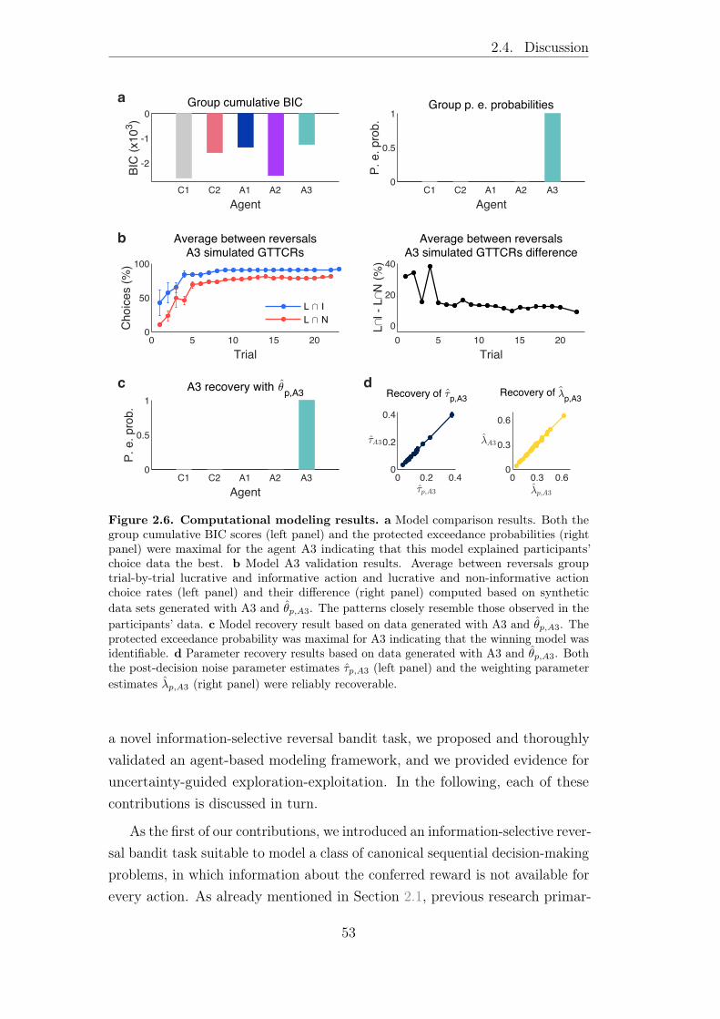
2.4. Discussion

0 5 10 15 20Trial

0

50L IL N

0 5 10 15 20TrialRecovery of

0

20

C1 C2 A1 A2 A3

-2

-1

0

BIC

(x10

3 )

Group cumulative BIC

C1 C2 A1 A2 A3Agent

0

0.5

1Group p. e. probabilities

C1 C2 A1 A2 A3Agent

0

0.5

1

P.e.

prob

.

A3 recovery with p,A3

0 0.2 0.40

0.2

0.4Recovery of p,A3

0 0.3 0.60

0.3

0.6p,A3

AgentC1 C2 A1 A2 A3

Agent

-2

-1

0

BIC

(x10

3 )

Group cumulative BIC

C1 C2 A1 A2 A30

0.5

1

P.e.

prob

.

Group p. e. probabilities

0 5 10 15 200

50

100

Cho

ices

(%)

Average between reversalsA3 simulated GTTCRs

L IL N

0 5 10 15 20Trial

0

20

40

Average between reversalsA3 simulated GTTCRs difference

-1

0Group cumulative BIC

0.5

1Group p. e. probabilities

C1 C2 A1 A2 A3Agent

0

0.5

P.e.

prob

.

0 0.2 0.40

0.2

0.4

0 0.3 0.60

0.3

0.6L

I-L

N(%

)

0 5 10 15 20Trial

0

50

100

Cho

ices

(%)

Average between reversalsA3 simulated GTTCRs

L IL N

0 5 10 15 20Trial

0

20

40

Average between reversalsA3 simulated GTTCRs difference

0

50

100

Cho

ices

(%)

Average between reversalsA3 simulated GTTCRs

L IL N

0 5 10 15 20TrialRecovery of

0

20

40

LI-

LN

(%)

Average between reversalsA3 simulated GTTCRs difference

C1 C2 A1 A2 A3Agent

-2

-1

0

BIC

(x10

3 )

Group cumulative BIC

C1 C2 A1 A2 A3Agent

0

0.5

1

A3 recovery with p,A3

P.e.

prob

.

Group p. e. probabilities

C1 C2 A1 A2 A3Agent

0

0.5

1

P.e.

prob

.

0 0.2 0.40

0.2

0.4Recovery of p,A3

0 0.3 0.60

0.3

0.6p,A3

A3 recovery with p,A3

C1 C2 A1 A2 A3Agent

0

0.5

1

P.e.

prob

.

0 0.2 0.40

0.2

0.4

0 0.3 0.60

0.3

0.6

Recovery ofRecovery of p,A3 p,A3

0 0.2 0.40

0.2

0.4

0 0.3 0.60

0.3

0.6

Recovery ofRecovery of p,A3 p,A3

Agent

Trial

a

b

dc

Figure 2.6. Computational modeling results. a Model comparison results. Both thegroup cumulative BIC scores (left panel) and the protected exceedance probabilities (rightpanel) were maximal for the agent A3 indicating that this model explained participants’choice data the best. b Model A3 validation results. Average between reversals grouptrial-by-trial lucrative and informative action and lucrative and non-informative actionchoice rates (left panel) and their difference (right panel) computed based on syntheticdata sets generated with A3 and θp,A3. The patterns closely resemble those observed in theparticipants’ data. c Model recovery result based on data generated with A3 and θp,A3. Theprotected exceedance probability was maximal for A3 indicating that the winning model wasidentifiable. d Parameter recovery results based on data generated with A3 and θp,A3. Boththe post-decision noise parameter estimates τp,A3 (left panel) and the weighting parameterestimates λp,A3 (right panel) were reliably recoverable.

a novel information-selective reversal bandit task, we proposed and thoroughlyvalidated an agent-based modeling framework, and we provided evidence foruncertainty-guided exploration-exploitation. In the following, each of thesecontributions is discussed in turn.

As the first of our contributions, we introduced an information-selective rever-sal bandit task suitable to model a class of canonical sequential decision-makingproblems, in which information about the conferred reward is not available forevery action. As already mentioned in Section 2.1, previous research primar-

53

Chapter 2

ily employed pure-exploration/sampling and exploration-exploitation/partial-feedback paradigms to study sequential decision making under uncertainty(Bubeck et al., 2009; Hertwig & Erev, 2009; Sutton & Barto, 2018; Wulffet al., 2018). The pure-exploration/sampling paradigm (Bubeck et al., 2009;Hertwig & Erev, 2009; Ostwald et al., 2015) models sequential decision-makingproblems in which an action either confers information or reward. In theclassical variant of this paradigm, an action that confers reward automaticallyterminates the task. In an extended variant, referred to as the observe-or-bettask (Blanchard & Gershman, 2018; Navarro et al., 2016; Tversky & Edwards,1966), the deciding agent can freely switch between the ’observe’ action thatconfers information and the ’bet’ actions that confer reward. Specifically, theobserve action returns information about the expected reward value of thebet actions, but it does not return reward. The bet actions return rewardsaccording to their associated reward distributions but no information. Similarto the bet actions, in our task one of the available actions confers only rewardbut no information. However, in our task, the other available action does notonly confer information, as the observe action does, but it also confers reward.Therefore, while exploration and exploitation are temporally separated in theobserve or bet task, they have to be balanced simultaneously in our task. Inthis regard, our task is similar to the exploration-exploitation/partial-feedbackparadigm (Hertwig & Erev, 2009; Sutton & Barto, 2018).

The classical variant of the exploration-exploitation/partial-feedback paradigmis the multi-armed bandit task (Berry & Fristedt, 1985). In the multi-armedbandit task, the deciding agent chooses between a set of ’arms’. Akin to our task,each arm confers reward according to its associated reward distribution, and,in contrast to our task, each arm confers also information about its expectedreward value. A drawback of this design is that the co-occurrence of rewardand information evokes a confound between an action’s value estimate andthe associated uncertainty: As people tend to favor the action with the highervalue estimate, for that action the associated uncertainty becomes smaller -simply because for that action more reward observations were made. Thismakes it difficult to uncover uncertainty-guided exploration in the standardmulti-armed bandit task (Dezza, Angela, Cleeremans, & Alexander, 2017;Gershman, 2018; Wilson et al., 2014). Our task circumvents this problem byadopting a symmetrical reward structure of the actions: The probability ofthe positive reward for the lucrative action is identical with the probability ofthe negative reward for the detrimental action. Likewise, the probability of

54

2.4. Discussion

the negative reward for the lucrative action is identical with the probability ofthe positive reward for the detrimental action. This way, each reward observa-tion following the informative action confers the same amount of informationabout the expected reward value of both the lucrative and detrimental action.Furthermore, as in each trial information is randomly coupled with either thelucrative or the detrimental action, our task arguably evokes a more markedexploration-exploitation dilemma than the multi-armed bandit task.

As the second of our contributions, we proposed and thoroughly validatedan agent-based modeling initiative. This initiative consisted of belief state-based agents formalizing subjective uncertainty-based exploitative, explorativeand hybrid explorative-exploitative strategies as well as belief state-free agentsformalizing simple random choice and win-stay-lose-switch strategies. Thebelief state-based agents implement Bayesian update to infer the not directlyobservable structure of the task environment, i.e., which is the lucrative andwhich is the detrimental action. While optimal Bayesian learning may seemto be a strong assumption, it has been shown to approximate human learningreasonably well in comparable non-stationary tasks, such as the two-armedreversal bandit task (Hampton, Bossaerts, & O’Doherty, 2006) or non-stationaryversions of the observe or bet task (Blanchard & Gershman, 2018; Navarro et al.,2016) and the multi-armed bandit task (Daw, O’Doherty, Dayan, Seymour, &Dolan, 2006; Speekenbrink & Konstantinidis, 2015). In addition, by includingbelief state-free agents in our model space, we also accounted for simplestrategies that do not require Bayesian update. Of these, the win-stay-lose-switch agent adopts a well established effective strategy to approach similarbandit problems (Robbins, 1952).

The three belief state-based agents implement their respective strategiesby following different optimization aims. In particular, the belief state-basedexploitative agent seeks to maximize the belief state-weighted expected re-ward. The belief state-based explorative agent seeks to maximize the expectedBayesian surprise. The belief state-based hybrid explorative-exploitative agentseeks to maximize the convex combination of these two quantities. Belief state-weighted expected reward is a natural quantity to formally capture immediatereward gain and thus myopic exploitation (Sutton & Barto, 2018). ExpectedBayesian surprise is one of many quantities that have been proposed to formallycapture immediate information gain and thus myopic exploration (Schwarten-beck et al., 2019). As alluded to in Section 2.1, we here opted for Bayesiansurprise due to its putative representation in the human neurocognitive system

55

Chapter 2

(Gijsen, Grundei, Lange, Ostwald, & Blankenburg, 2020; Itti & Baldi, 2009;Ostwald et al., 2012).

Importantly, we would like to note that our definition of exploration pertainsto a form of exploration that is generally referred to as ’directed exploration’(Gershman, 2018, 2019; Wilson et al., 2014). This term is used to distinguishinformation gain maximizing exploration from ’random exploration’. Randomexploration is a form of exploration that achieves information gain by imple-menting a stochastic strategy, i.e. making stochastic choices based on theactions’ reward value estimate. While there are more principled ways suchas Thompson sampling (Thompson, 1933), random exploration is commonlyaccounted for by the softmax decision rule (Reverdy & Leonard, 2015). Notably,we here did not link the softmax decision rule to random exploration. Instead,we used it to embed the agents into a statistical framework in order to accountfor post-decision noise. This way, we clearly separated the deterministic strate-gies implemented by the agents and the probabilistic agent-based data analysismodels. In future work, we aim to broaden our model space by consideringagents that adopt random exploration. Crucially, we argue that this step willrequire a statistical framework that allows to reliably partition the variabilityof choice data into components relating to the agent’s stochastic strategy andto post-decision noise (cf. Ostwald, Kirilina, Starke, and Blankenburg, 2014).

As the third and final of our contributions, we provided clear evidencefor uncertainty-guided exploration-exploitation in our task: As uncertaintydecreased, participants’ choices were less influenced by the prospect of informa-tion gain and more influenced by the prospect of reward gain. Our finding isconsistent with the behavior in the observe or bet task. In the first empiricalstudy using the observe or bet task, Tversky and Edwards (1966) found thatparticipants explored more, i.e., chose the observe action more frequently, ifthey (falsely) believed that the underlying environment was dynamic, i.e., thelucrative and detrimental bet actions reversed over time. While Tversky andEdwards (1966) did not relate this result to the notion that dynamic environ-ments promote uncertainty, which, in turn, promotes exploration, in a recentstudy, Navarro et al. (2016) formally tested this hypothesis. By modelingparticipants’ choices in both static and dynamic versions of the observe or bettask, they demonstrated that switches between the exploratory observe actionand the exploitative bet actions were mediated by uncertainty.

Our result is also in line with recent findings from studies employing multi-armed bandit tasks. Work by several groups showed that when controlling

56

2.5. Data and code availability

for the value estimate-uncertainty confound, behavior in static two-armedbandit tasks reflects an uncertainty-dependent combination of exploration andexploitation (Dezza et al., 2017; Gershman, 2018, 2019; Wilson et al., 2014).Notably, however, consistent with the notion that the value estimate-uncertaintyconfound has the potential to mask directed exploration, findings from earlierstudies not accounting for this confounding effect are less conclusive. Forexample, Zhang and Yu (2013) also found evidence for a belief state-basedexplorative-exploitative strategy in static four-armed bandit tasks. In contrast,Daw et al. (2006) did not find evidence for such a strategy in analyzing choicesin a dynamic four-armed bandit task with changing action values. While thefinding from Daw et al. (2006) is contrary to our finding, acknowledging thatvalue estimate and uncertainty are not confounded in our task, these twofindings can be reconciled.

In conclusion, in the current work we introduced a task that models asubset of real-life sequential decision-making problems that has been neglectedpreviously: problems, in which information about the conferred reward isnot available for every action. Importantly, this task allows to investigatea pronounced form of simultaneous exploration and exploitation processeswithout introducing the value estimate-uncertainty confound. We proposed anagent-based modeling framework formalizing various sequential decision-makingstrategies in our task and discussed how this framework may be extended inthe future. Together, by analyzing participants’ choices in our task usingdescriptive and agent model-based methods, we provide orthogonal evidence foran uncertainty-guided balance between exploration and exploitation in humansequential decision making under uncertainty.

2.5 Data and code availability

Data formatted according to the Brain Imaging Data Structure (Gorgolewskiet al., 2016) and code implementing all analyses are hosted on Open ScienceFramework (Nosek et al., 2015) and are available at https://osf.io/vdmah/?view_only=a581d36aa8944464a7a81578b79afa8e.

57

Chapter 2

2.6 References

Bach, D. R., & Dolan, R. J. (2012). Knowing how much you don’t know: A neuralorganization of uncertainty estimates. Nature Reviews Neuroscience,13 (8), 572–586.

Bartolo, R., & Averbeck, B. B. (2020). Prefrontal cortex predicts state switchesduring reversal learning. Neuron.

Berry, D. A., & Fristedt, B. (1985). Bandit problems: Sequential allocation ofexperiments (monographs on statistics and applied probability). London:Chapman and Hall, 5, 71–87.

Bertsekas, D. P. (2000). Dynamic programming and optimal control (2ndedition). Athena Scientific.

Blanchard, T. C., & Gershman, S. J. (2018). Pure correlates of explorationand exploitation in the human brain. Cognitive, Affective, & BehavioralNeuroscience, 18 (1), 117–126.

Bubeck, S., Munos, R., & Stoltz, G. (2009). Pure exploration in multi-armedbandits problems. Proceedings of the 20th International Conference onAlgorithmic Learning Theory (ALT), 23–37.

Byrd, R. H., Gilbert, J. C., & Nocedal, J. (2000). A trust region method basedon interior point techniques for nonlinear programming. MathematicalProgramming, 89 (1), 149–185.

Byrd, R. H., Hribar, M. E., & Nocedal, J. (1999). An interior point algorithmfor large-scale nonlinear programming. SIAM Journal on Optimization,9 (4), 877–900.

Cohen, J. D., McClure, S. M., & Yu, A. J. (2007). Should I stay or should Igo? How the human brain manages the trade-off between exploitationand exploration. Philosophical Transactions of the Royal Society B:Biological Sciences, 362 (1481), 933–942.

Costa, V. D., Dal Monte, O., Lucas, D. R., Murray, E. A., & Averbeck, B. B.(2016). Amygdala and ventral striatum make distinct contributions toreinforcement learning. Neuron, 92 (2), 505–517.

Daw, N. D., O’Doherty, J. P., Dayan, P., Seymour, B., & Dolan, R. J. (2006). Cor-tical substrates for exploratory decisions in humans. Nature, 441 (7095),876–879.

Dayan, P., & Daw, N. D. (2008). Decision theory, reinforcement learning, andthe brain. Cognitive, Affective, & Behavioral Neuroscience, 8 (4), 429–453.

58

2.6. References

Dezza, I. C., Angela, J. Y., Cleeremans, A., & Alexander, W. (2017). Learningthe value of information and reward over time when solving exploration-exploitation problems. Scientific Reports, 7 (1), 1–13.

Gershman, S. J. (2018). Deconstructing the human algorithms for exploration.Cognition, 173, 34–42.

Gershman, S. J. (2019). Uncertainty and exploration. Decision, 6 (3), 277.Gijsen, S., Grundei, M., Lange, R. T., Ostwald, D., & Blankenburg, F. (2020).

Neural surprise in somatosensory bayesian learning. bioRxiv.Gläscher, J., Hampton, A. N., & O’Doherty, J. P. (2009). Determining a role

for ventromedial prefrontal cortex in encoding action-based value signalsduring reward-related decision making. Cerebral Cortex, 19 (2), 483–495.

Gorgolewski, K. J., Auer, T., Calhoun, V. D., Craddock, R. C., Das, S., Duff,E. P., Flandin, G., Ghosh, S. S., Glatard, T., Halchenko, Y. O., et al.(2016). The brain imaging data structure, a format for organizing anddescribing outputs of neuroimaging experiments. Scientific Data, 3 (1),1–9.

Hampton, A. N., Bossaerts, P., & O’Doherty, J. P. (2006). The role of theventromedial prefrontal cortex in abstract state-based inference duringdecision making in humans. Journal of Neuroscience, 26 (32), 8360–8367.

Hauser, T. U., Iannaccone, R., Stämpfli, P., Drechsler, R., Brandeis, D., Walitza,S., & Brem, S. (2014). The feedback-related negativity (FRN) revisited:New insights into the localization, meaning and network organization.NeuroImage, 84, 159–168.

Hertwig, R., & Erev, I. (2009). The description–experience gap in risky choice.Trends in Cognitive Sciences, 13 (12), 517–523.

Itti, L., & Baldi, P. (2009). Bayesian surprise attracts human attention. VisionResearch, 49 (10), 1295–1306.

Lee, M. D., Zhang, S., Munro, M., & Steyvers, M. (2011). Psychologicalmodels of human and optimal performance in bandit problems. CognitiveSystems Research, 12 (2), 164–174.

McFadden, D. (1973). Conditional Logit Analysis of Qualitative Choice Behavior.Institute of Urban and Regional Development, University of California.

Navarro, D. J., Newell, B. R., & Schulze, C. (2016). Learning and choosing inan uncertain world: An investigation of the explore–exploit dilemma instatic and dynamic environments. Cognitive Psychology, 85, 43–77.

Nooner, K. B., Colcombe, S., Tobe, R., Mennes, M., Benedict, M., Moreno,A., Panek, L., Brown, S., Zavitz, S., Li, Q., et al. (2012). The NKI-

59

Chapter 2

Rockland sample: A model for accelerating the pace of discovery sciencein psychiatry. Frontiers in Neuroscience, 6, 152.

Nosek, B. A., Alter, G., Banks, G. C., Borsboom, D., Bowman, S. D., Breckler,S. J., Buck, S., Chambers, C. D., Chin, G., Christensen, G., et al. (2015).Promoting an open research culture. Science, 348 (6242), 1422–1425.

Ostwald, D., Kirilina, E., Starke, L., & Blankenburg, F. (2014). A tutorial onvariational bayes for latent linear stochastic time-series models. Journalof Mathematical Psychology, 60, 1–19.

Ostwald, D., Spitzer, B., Guggenmos, M., Schmidt, T. T., Kiebel, S. J., &Blankenburg, F. (2012). Evidence for neural encoding of bayesian surprisein human somatosensation. NeuroImage, 62 (1), 177–188.

Ostwald, D., Starke, L., & Hertwig, R. (2015). A normative inference approachfor optimal sample sizes in decisions from experience. Frontiers inPsychology, 6, 1342.

Reverdy, P., & Leonard, N. E. (2015). Parameter estimation in softmax decision-making models with linear objective functions. IEEE Transactions onAutomation Science and Engineering, 13 (1), 54–67.

Rigoux, L., Stephan, K. E., Friston, K. J., & Daunizeau, J. (2014). Bayesianmodel selection for group studies—revisited. NeuroImage, 84, 971–985.

Robbins, H. (1952). Some aspects of the sequential design of experiments.Bulletin of the American Mathematical Society, 58 (5), 527–535.

Russell, S., & Norvig, P. (2010). Artificial intelligence: A modern approach(3rd ed.). Prentice Hall.

Schwartenbeck, P., Passecker, J., Hauser, T. U., FitzGerald, T. H., Kronbichler,M., & Friston, K. J. (2019). Computational mechanisms of curiosity andgoal-directed exploration. eLife, 8, e41703.

Schwarz, G. (1978). Estimating the dimension of a model. The Annals ofStatistics, 6 (2), 461–464.

Speekenbrink, M., & Konstantinidis, E. (2015). Uncertainty and exploration ina restless bandit problem. Topics in Cognitive Science, 7 (2), 351–367.

Stephan, K. E., Penny, W. D., Daunizeau, J., Moran, R. J., & Friston, K. J.(2009). Bayesian model selection for group studies. NeuroImage, 46 (4),1004–1017.

Sun, Y., Gomez, F., & Schmidhuber, J. (2011). Planning to be surprised:Optimal bayesian exploration in dynamic environments. In J. Schmidhu-ber, K. R. Thórisson, & M. Looks (Eds.), Artificial general intelligence(pp. 41–51). Springer Berlin Heidelberg.

60

2.6. References

Sutton, R. S., & Barto, A. G. (2018). Reinforcement learning: An introduction.MIT press.

Thompson, W. R. (1933). On the likelihood that one unknown probabilityexceeds another in view of the evidence of two samples. Biometrika,25 (3/4), 285–294.

Tversky, A., & Edwards, W. (1966). Information versus reward in binary choices.Journal of Experimental Psychology, 71 (5), 680.

Waltz, R. A., Morales, J. L., Nocedal, J., & Orban, D. (2006). An interioralgorithm for nonlinear optimization that combines line search and trustregion steps. Mathematical Programming, 107 (3), 391–408.

Wilson, R. C., & Collins, A. G. (2019). Ten simple rules for the computationalmodeling of behavioral data. eLife, 8, e49547.

Wilson, R. C., Geana, A., White, J. M., Ludvig, E. A., & Cohen, J. D. (2014).Humans use directed and random exploration to solve the explore–exploitdilemma. Journal of Experimental Psychology: General, 143 (6), 2074.

Wu, C. M., Schulz, E., Speekenbrink, M., Nelson, J. D., & Meder, B. (2018).Generalization guides human exploration in vast decision spaces. NatureHuman Behaviour, 2 (12), 915–924.

Wulff, D. U., Mergenthaler-Canseco, M., & Hertwig, R. (2018). A meta-analyticreview of two modes of learning and the description-experience gap.Psychological bulletin, 144 (2), 140.

Zhang, S., & Yu, A. (2013). Forgetful bayes and myopic planning: Humanlearning and decision-making in a bandit setting. Advances in NeuralInformation Processing Systems, 26.

61

Chapter 2

62

3 | The neurocomputational mechanismsof sequential decision making in amultistep task with partiallyobservable states

3.1 Introduction

In a class of sequential decision-making tasks, actions of the deciding agentaffect next states of the environment and thereby future rewards (e.g., Bertsekas(2000), Puterman (2014), and Sutton and Barto (2018)). A central question indecision neuroscience research is whether humans and other biological decidingagents plan ahead or resort to model-free decision-making strategies in suchtasks, usually discussed under the name multistep tasks. Both class of strategiesassume that the agent tries to maximize its cumulative reward. However, tochoose between the actions in a given state in light of this goal, planningstrategies mentally simulate the consequences of actions, whereas model-freedecision-making strategies simply rely on some instantaneously available reward-related information or the reward history (e.g., Collins and Cockburn (2020),Daw, Niv, and Dayan (2005), Dayan (2012, 2014), Dayan and Daw (2008),Dickinson and Balleine (2002), Dolan and Dayan (2013), Kaplan, Schuck, andDoeller (2017), Solway and Botvinick (2012), and Tolman (1948)).

While many studies have demonstrated that humans engage in planning,these studies examined sequential decision making in multistep tasks wherethe environmental states are fully observable (Cushman & Morris, 2015; Daw,Gershman, Seymour, Dayan, & Dolan, 2011; Doll, Duncan, Simon, Shohamy,& Daw, 2015; Gläscher, Daw, Dayan, & O’Doherty, 2010; Huys et al., 2012;Korn & Bach, 2018; Momennejad et al., 2017; Simon & Daw, 2011; Wunderlich,Smittenaar, & Dolan, 2012). Yet, in many real-life multistep tasks certaincomponents of the states remain latent and the available observations onlyconvey ambiguous information about these. To illustrate, consider someonetrying to find their lost ring at the beach. The ring is buried deep in the sandbut a metal detector can help to locate it by signalling at each step the direction

63

Chapter 3

towards it with some associated noise. Similar to this example, humans haveto navigate various abstract representational spaces, for example, career paths,financial investment schemes, or maintaining a healthy lifestyle. Across allthese domains, states are often only partially observable and therefore thedecisions are imbued with state uncertainty (Bach & Dolan, 2012; Dayan &Daw, 2008; Ma & Jazayeri, 2014).

The Bayesian brain hypothesis generally posits that under uncertainty, thebrain uses Bayes rule to probabilistically infer the hidden cause underlyingsensory data. Abundant evidence supports the Bayesian brain hypothesis acrossvarious cognitive domains, such as perception (Harrison, Stephan, Rees, &Friston, 2007; Ostwald et al., 2012) and reasoning (Konovalov & Krajbich,2018; Schwartenbeck, FitzGerald, & Dolan, 2016; Tenenbaum, Griffiths, &Kemp, 2006). Applied to sequential decision making under state uncertainty,the brain is postulated to maintain a Bayes optimal (or near-optimal) beliefstate representing its subjective uncertainty about the state given the historyof observations and actions, on the basis of which actions can be evaluated (Ma,2019; Rao, 2010). Crucially, the combination of this notion with the aforemen-tioned findings on sequential decision making in multistep tasks suggests thatif the states comprise latent components, humans plan ahead on the basis ofbelief states. However, as human sequential decision making in multistep taskswith partially observable states has so far received little attention in decisionneuroscience research, evidence supporting this hypothesis is elusive.

State uncertainty introduces an additional critical computational dimensionto planning (e.g., Dayan and Daw, 2008): A belief state-based planning agentmay try to maximize its cumulative reward by exploiting its accumulatedknowledge about the state. Alternatively, a belief state-based planning agentmay explore first. That is, it may try to resolve its state uncertainty by choos-ing the action with the highest associated information gain to enable thatthe subsequent exploitative choices yield the maximum attainable cumulativereward. If and how biological agents alternate between exploration and ex-ploitation has traditionally been studied using bandit tasks. Bandit tasks aresequential decision-making tasks with latent reward structures, where actionsof an agent affect immediate rewards but do not have deferred consequences(Berry & Fristedt, 1985; Robbins, 1952; Sutton & Barto, 2018). Many studies,including ours as outlined in Chapter 2, have reported that humans combinethe objectives of exploration and exploitation when performing bandit tasks(Gershman, 2018; Wilson, Geana, White, Ludvig, & Cohen, 2014; Zhang &

64

3.1. Introduction

Yu, 2013), while other studies have only found support for exploitation (Daw,O’Doherty, Dayan, Seymour, & Dolan, 2006; Payzan-LeNestour & Bossaerts,2011). Given the lack of studies investigating sequential decision making inmultistep tasks with partially observable states, it is unclear if in these taskshumans adopt an exploitative or a hybrid explorative-exploitative objective.

In this work, we sought to computationally characterize the behavioral andneural correlates of human sequential decision making in multistep tasks withpartially observable states. Specifically, we addressed the following questions:(1) Do humans engage in belief state-based planning or do they resort to decision-making strategies that eschew prospective computations? (2) If humans engagein belief state-based planning, do they adopt the objective of exploitationor do they combine exploitation with exploration? (3) Which brain regionsimplement the putative cognitive processes underlying behavior? To answerthese questions, we designed a multistep spatial search task similar to thering search example introduced above and analyzed 19 participants’ behavioraland functional magnetic resonance imaging (fMRI) data. Specifically, wefirst evaluated a comprehensive set of agent-based computational models inlight of participants’ behavioral data (Russell & Norvig, 2010). This setincluded belief state-free agents that implement simple model-free decision-making strategies as well as belief state-based exploitative, explorative andhybrid explorative-exploitative agents that implement various belief state-basedplanning strategies. We subsequently assessed the neural correlates of thecognitive processes captured by the behaviourally most plausible agent using amodel-based general linear model (GLM) approach (Friston & Dolan, 2010).

Our behavioral analyses revealed that participants’ actions were best ac-counted for by a belief state-based agent adopting a purely exploitative objective.In terms of the neural representation of the constituent cognitive processesof this strategy, we hypothesized that a distributed network of cortical andsubsortical areas would be involved. In particular, capitalizing on findings fromrecent neuroimaging studies (Fischer, Bourgeois-Gironde, & Ullsperger, 2017;O’Reilly, Jbabdi, Rushworth, & Behrens, 2013), we expected to observe activityin the frontal and posterior parietal cortices as well as the dorsal striatumrelated to belief state maintenance as indexed by the Bayesian surprise, aquantity commonly used in the Bayesian brain hypothesis framework (Itti& Baldi, 2009; Ostwald et al., 2012). We further expected that exploitativeplanning on the basis of belief states would engage parts of the ventromedialprefrontal and orbitofrontal cortices. These are key regions of the brain’s

65

Chapter 3

reward-guided decision-making system (Rushworth, Noonan, Boorman, Walton,& Behrens, 2011) and have been implicated both in planning (in multisteptasks with fully observable states; Korn and Bach, 2018; Simon and Daw, 2011)and in exploitation (in bandit tasks; Chakroun, Mathar, Wiehler, Ganzer, andPeters, 2020; Daw et al., 2006). Our neural results largely corroborate thesehypotheses. Consequently, in conjunction with our behavioral results, theyprovide evidence that in our multistep task with partially observable states,participants performed belief state-based exploitative planning.

3.2 General methods

3.2.1 Experimental methods

Participants and procedure The experimental data set was acquired atthe Max Planck Institute for Human Development (Berlin, Germany). Behav-ioral and fMRI data was recorded from a group of 19 participants (10 female,18 right-handed, 1 male participant both-handed with left hand preference,mean age: 27.11 years, standard deviation age: 2.92 years) with no reports ofneurological or psychiatric disorders after providing written informed consent.The study was in line with the human subject guidelines of the Declaration ofHelsinki and was approved by the ethics committee of the German PsychologicalSociety (Deutsche Gesellschaft für Psychologie). Participants completed fourconsecutive runs of the experimental task in the Magnetic Resonance Imaging(MRI) scanner, after having received task instructions (Supplementary MaterialB.1) and having completed a training run on a desktop computer. Due totechnical problems and the thus resulting time constraints, two participantsperformed only three complete runs in the scanner. Participants were reim-bursed for their time with 10AC per hour and an additional 0.625AC for eachtask they solved.

Experimental design We framed a multistep task with partially observablestates as a spatial search task. In the ’treasure hunt’ task, participants wereinstructed to find two hidden ’treasures’ in a 5×5 cell grid-world. Figure 3.1ashows the grid-world from above with an example task configuration and witha fictive participant’s attempt decision sequence. A task corresponded to aspecific location combination of the two treasures. Participants were given amaximum of three attempts to solve a task and secure a monetary reward.

66

3.2. General methods

Importantly, a task was considered to be solved only if both treasures werecollected within a single attempt. In each attempt, participants had a limitednumber of steps at their disposal. If, in an attempt, participants failed to visitboth treasure locations before the number of available steps was exhausted,their position was reset to the start position, which was the upper left cell of thegrid in each attempt of each task. Note that participants were not presentedwith the bird’s eye perspective of the grid-world when interacting with a task(Figure 3.1a) but on each trial were only given the information available fromtheir current position (Figure 3.1b; please see below for details).

START

54321

5

4

3

2

15(0)

(3,2)

5(0)

5(0)

4(0)

Grid position

Observation bars

Decision prompt

Fixation cross

ba

Time

3-5 s3-5 s

3-5 s

Figure 3.1. Treasure hunt task. a Bird’s eye perspective of the 5×5 cell grid-world. Inthe example task shown, the treasures were hidden at cells (2,3) corresponding to the secondrow third column and (5,5) corresponding to the fifth row fifth column. The dashed line withfull dots at the cells shows a fictive participant’s decision sequence within an attempt of thetask. Here, the participant discovered only the treasure at location (2, 3) within the availablenumber of steps. Therefore, to solve the task in a next attempt, the participant had torevisit this cell and collect the treasure at location (5,5). b Trial design. This example showsthe stimuli sequence presented to the participant moving from cell (3,2) to (2,2) as shownby the yellow section of the dashed line in a. Before deciding on a northward movement,the participant received a signal from the treasure detector in the form of light and darkgrey observation bars towards the neighbouring cells. The values in the upper left cornerdenote the number of remaining steps and the number of treasures collected (the value inparentheses) in the attempt.

For each task, the treasure locations were consecutively sampled online froma uniform distribution over the cells of the grid with two restrictions. First,no treasure was assigned to the cell in the upper left corner correspondingto the start position. Second, the treasures were assigned to different cells.Participants completed four tasks in each run, which yielded a total of 296 taskspresented to the participants. As shown in Figure 3.2a, the treasure locationcombinations were evenly represented across tasks and a certain combinationoccurred no more than five times.

In each attempt, the step limit was randomly determined in order toprevent participants from using this information to infer the treasure locations.Specifically, we first evaluated the number of optimal steps required to solve a

67

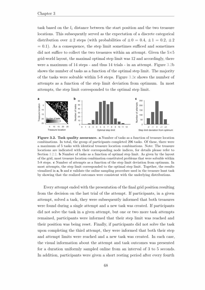
Chapter 3

task based on the l1 distance between the start position and the two treasurelocations. This subsequently served as the expectation of a discrete categoricaldistribution over ± 2 steps (with probabilities of ± 0 = 0.4, ± 1 = 0.2, ± 2= 0.1). As a consequence, the step limit sometimes sufficed and sometimesdid not suffice to collect the two treasures within an attempt. Given the 5×5grid-world layout, the maximal optimal step limit was 12 and accordingly, therewere a maximum of 14 steps - and thus 14 trials - in an attempt. Figure 3.2bshows the number of tasks as a function of the optimal step limit. The majorityof the tasks were solvable within 5-8 steps. Figure 3.2c shows the number ofattempts as a function of the step limit deviation from optimum. In mostattempts, the step limit corresponded to the optimal step limit.

5 10 15 20 25Treasure location

5

10

15

20

25

Treasurelocation

0 1 2 3 4 5 6 7 8 9 10 11 12Optimal step limit

0

10

20

30

40

50

60

Num

beroftasks

-2 -1 0 +1 +2Step limit deviation from optimum

0

50

100

150

200

250

Num

berofattempts

5 10 15 20 25Treasure location

5

10

15

20

25

Treasurelocation

0 1 2 3 4 5 6 7 8 9 10 11 12Optimal step limit

0

10

20

30

40

50

60

Num

beroftasks

-2 -1 0 +1 +2Step limit deviation from optimum

0

50

100

150

200

250

Num

berofattempts

5 10 15 20 25

5

10

15

20

250 1 2 3 4 5 6 7 8 9 10 11 12

0

10

20

30

40

50

60

Num

beroftasks

Number of tasks0 5

ba

5 10 15 20 25Treasure location

5

10

15

20

25

Treasurelocation

0 1 2 3 4 5 6 7 8 9 10 11 12Optimal step limit

0

10

20

30

40

50

60

Num

beroftasks

-2 -1 0 +1 +2Step limit deviation from optimum

0

50

100

150

200

250

Num

berofattempts

c

Figure 3.2. Task quality assurance. a Number of tasks as a function of treasure locationcombinations. In total, the group of participants completed 296 tasks. Of these, there werea maximum of 5 tasks with identical treasure location combinations. Note: The treasurelocations are indicated with their corresponding node indices, for details please refer toSection 3.2.2. b Number of tasks as a function of optimal step limit. As given by the layoutof the grid, most treasure location combination constituted problems that were solvable within5-8 steps. c Number of attempts as a function of the step limit deviation from optimum. Inmost attempts, the step limit corresponded to the optimal step limit. Together, the resultsvisualized in a, b and c validate the online sampling procedure used in the treasure hunt taskby showing that the realized outcomes were consistent with the underlying distributions.

Every attempt ended with the presentation of the final grid position resultingfrom the decision on the last trial of the attempt. If participants, in a givenattempt, solved a task, they were subsequently informed that both treasureswere found during a single attempt and a new task was created. If participantsdid not solve the task in a given attempt, but one or two more task attemptsremained, participants were informed that their step limit was reached andtheir position was being reset. Finally, if participants did not solve the taskupon completing the third attempt, they were informed that both their stepand attempt limits were reached and a new task was created. In each case,the visual information about the attempt and task outcomes was presentedfor a duration uniformly sampled online from an interval of 3 to 5 seconds.In addition, participants were given a short resting period after every fourth

68

3.2. General methods

attempt. During these resting periods, participants were instructed to look ata fixation cross for a duration uniformly sampled online from an interval of 6to 8 seconds.

Trial design Figure 3.1b depicts an exemplary trial as presented to a fictiveparticipant. On every trial of the task, participants were first shown the cellof the grid they currently occupied, including its row and column indices. Ifparticipants entered a treasure location, they were additionally shown a treasuresymbol. Next, a collection of light and dark grey ’observation bars’ werepresented towards the adjoining cells. These bars conveyed information aboutthe treasure locations with certain accuracy and thus could be interpreted asnoisy signals of a ’treasure detector’. Specifically, the detector always returneda dark grey bar for the direction leading away from the treasures while itdisplayed either a light or a dark grey bar in the direction of the treasures. Thedetector’s accuracy of correctly returning a light grey bar towards the treasurelocations depended on the participants’ distance to the treasures: Its readoutwas completely unreliable at the most distant cell position and parametricallyincreased in accuracy as participants moved towards the treasures. It alwayssignalled the true values in the immediate vicinity of the treasures. Followingthe presentation of the observation bars, participants were prompted to chooseone of the available directions by means of pressing one of four buttons withthe index to little finger of their right-hand. They could move to any of theneighbouring cells. Diagonal steps or steps off the grid were not allowed. Theduration of the grid position, the observation bars and the response time windowwere uniformly sampled online from an interval of 3-5 seconds. If participantsindicated their decision within the response time window, they were presentedwith a post-decision fixation cross until the response time window elapsed.Upon the post-decision fixation cross, the next trial commenced with thepresentation of the new grid position. If, on the other hand, participants didnot indicate their decision within the response time window, they maintainedtheir current position on the next trial and lost one step. To help participantskeep track of the attempt’s evolution, throughout the trial they were visuallyinformed about the number of remaining steps and the number of treasurescollected.

69

Chapter 3

3.2.2 Task model

To make the treasure hunt task amenable to agent-based computational mod-eling, we first represented the square grid-world of dimensionality d = 5 bya graph (N,E). Here, N := Nd2 denotes the set of nodes corresponding tothe cells of the grid and E denotes a set of (unweighted) edges correspondingto the directions available from each cell (Figures 3.3a-b). Building on thisgraph representation, we specified central task components using concepts fromthe theory of partially observable Markov decision processes (Bertsekas, 2000).Specifically, the treasure hunt task on a given attempt can be conceived as atuple (S,O,A, f, g), where for available trials t = 1, 2, . . . , T

• S := Nd2 × N02 × Nd2 \ 1 × Nd2 \ 1, s3 denotes the set of states

s := (s1, s2, s3, s4). The first two state components comprise the directlyobservable part of the state, y := (s1, s2). The first variable encodes theagent’s current grid position. The second variable encodes the treasurediscovery history and takes on the value 0 if no treasure, 1 if the treasureat the first location and 2 if the treasure at the second location wascollected up to trial t. The second two components encode the locationof the two treasures: s3 encodes the location of the first treasure, i.e. thetreasure with the the smaller node index and s4 encodes the locationof the second treasure, i.e. the treasure with the the larger node index.These state components comprise the latent part of the state, x := (s3, s4).Note that we use the terms first and second treasure only to distinguishbetween them.

• O := 0, 14 denotes the observation set. The components of an obser-vation o := (o1, o2, o3, o4) ∈ O encode the observation bars presentedto the agent in the northern, eastern, southern and western directions,respectively. The value 0 represents a dark grey bar and 1 represents alight grey bar. The available observations depend on the current positionof the agent. For example, for s1 := 1, the available observation setOs1 ⊆ O is given by O1 = 0, 12 and elements of O1 are of the formo = (o2, o3).

• A := −5,+1,+5,−1 denotes the action set. The values encode thenorthward, eastward, southward and westward movements on the nodes ofthe graph representation of the grid, respectively. Like the set of availableobservations, the set of available actions As1 ⊆ A depends also on thefirst state component s1. For example, for s1 := 21, A21 = −5,+1 ⊆ A.

70

3.2. General methods

• f denotes the state transition function, which specifies the probabilitythat the state takes on the value s∗ at trial t+ 1 given state s and agentaction a at trial t. In the treasure hunt task, actions have deterministicoutcomes, i.e., deciding for an available action results in the indicatedposition change with certainty. Formally, assuming a ∈ As1 ,

f (s, a, s∗) := p (st+1 = s∗|st = s, at = a) :=

1, if s∗ = (y∗, x∗)

0, else,

(3.1)where

y∗ =(s1 + a, 1 ·

⌊s1∗ = s3

⌋+ 2 ·

⌊s1∗ = s4

⌋)and x∗ =

(s3, s4

)(3.2)

with the initial state corresponding to

p(s1 =

(1, 0, s3, s4

))= 1 (3.3)

in each attempt. Upon every action, the state changes according to Eq.3.1 until there are steps left or until both treasures are collected withinthe attempt.

• Finally, g denotes the observation function, which specifies the probabilityof observation o given state s at trial t. This probability implementsthe distance-dependent accuracy of the observations and thus takes acentral stance in the specification of the treasure hunt task. Omitting therestrictions to available observations for ease of exposition, this probabilitytakes the form

g (s, o) := p (ot = o|st = s) :=4∏i=1

p(oi|s)

:=4∏i=1

Bern(oi; πi(s)

). (3.4)

That is, the individual observations oi, i ∈ N4 are distributed indepen-dently according to Bernoulli distributions with state-dependent param-eters πi (s) ∈ [0, 1] , i ∈ N4. These parameters are defined as follows.First, the probability of observing a light grey bar in the direction of i isexpressed as an affine function of the l1 distance between the agent and atreasure. The induced probability parameter set corresponds to

pj,k := β0 + β1l1 (j, k) , (3.5)

71

Chapter 3

0

2

4

6

81 2 3 4 5

6 7 8 9 10

11 12 13 14 15

16 17 18 19 20

21 22 23 24 25

5 15 25

5

15

255 15 25

5

15

25

5 15 25

5

15

255 15 25

5

15

251 2 3 4 5

1

2

3

4

5

1 2 3 4 5

1

2

3

4

5

5 15 25

5

15

25

0.5

0.6

0.7

0.8

0.9

1

0.5

0.6

0.7

0.8

0.9

1

0.5

0.6

0.7

0.8

0.9

1

0.5

0.6

0.7

0.8

0.9

1

0.5

0.6

0.7

0.8

0.9

1

a b c d

e f g h

Figure 3.3. Task model. a and b Graph representation of the grid-world. a Nodes(circles) and edges (lines) of the graph representation of the 5 × 5 grid-world, numberslabel the nodes. b Adjacency matrix representation of the set of edges visualized in a. c l1distance set between agent position j and treasure location k. d Observation probabilityparameter set as a function of the agent position and treasure location for single treasures.The probability was set to pj,k = 0.5 at the maximum l1 distance (yielding a maximallyinaccurate signal) and to pj,k = 1 at the minimum l1 distance (yielding a maximally accuratesignal). e and f Combined probability parameter set as function of two treasure locationsfor agent positions j = 1 and j = 14, respectively. g and h Bernoulli observation parameterπ3(s) for southern bar observations for a single remaining treasure located at node 22 (5, 2)and for two treasures located at nodes 10 (2, 5) and 22 (5, 2), respectively, as a function of theagent position. Note: The bottom rows are marked with red because at the correspondingnodes southern bars are not available.

where l1(j, k) denotes the l1 distance between the agent’s position nodej ∈ Nd2 and the treasure location node l ∈ Nd2 . The complete l1 distanceset is visualized in Figure 3.3c. β0 and β1 are real-valued parameters,which are determined according to the following constraints: First, theprobability of observing a light grey bar is set to certainty (pj,k = 1) ifthe agent is a single step away from the treasure, and second, it is setto full uncertainty (pj,k = 0.5) if the agent is at its maximum possibledistance from the treasure, i.e., l1(j, k) = max

j∈Nd2

l1(j, k). These constraints

are satisfied for

β0 := 1 +0.5

maxj∈Nd2

l1(j, k)− 1and β1 := − 0.5

maxj∈Nd2

l1(j, k)− 1. (3.6)

The complete ensuing probability parameter set P = pj,k1≤j,k≤d2 for allcombinations of agent and treasure nodes is visualized in Figure 3.3d. Ifs2 = 1 or s2 = 2, the parameter set visualized in Figure 3.3d forms thebasis of πi(s). However, if s2 = 0, i.e., none of the treasures have yet

72

3.2. General methods

been collected, the parameter sets are combined into a single parameterset according to

pj,k,l =

pj,l + (pj,k − pj,l) pj,k, if pj,k ≥ pj,l

pj,k + (pj,l − pj,k) pj,l, if pj,k < pj,l, (3.7)

where j encodes the agent position, and k and l encode the treasurelocations (j, k, l ∈ Nd2). Figures 3.3e and f show the ensuing parameterset P for the agent positions j = 1 and j = 14, respectively. Based onthe above, the Bernoulli distribution parameters πi(s) are then defined as

πi(s) :=

pj,k,l, if s = (j, 0, k, l)

pj,l, if s = (j, 1, k, l)

pj,k, if s = (j, 2, k, l)

(3.8)

if moving in the direction of i brings the agent closer to at least one ofthe treasures (in the case of s2 = 0) or to the remaining treasure (in thecase of s2 ∈ 1, 2),

l1 (j + ai, k) < l1 (j, k) and or l1 (j + ai, l) < l1 (j, l) . (3.9)

In any other case,πi(s) = 0. (3.10)

Figures 3.3g and h visualize the ensuing parameters π3(s) as a functionof s1, for s2 = 1, an arbitrary s3 and the remaining treasure locations4 = 22, and for s2 = 0, s3 = 10 and s4 = 22, respectively.

3.2.3 Agent models

We designed a set of nine agent-based computational models (Russell & Norvig,2010) to formally capture different sequential decision-making strategies in thetreasure hunt task. The main differences between the agents can be describedalong two dimensions. First, the agents differ in whether or not they makedecisions on the basis of belief states. In general, as introduced above (seeSection 3.1), the term belief state refers to a probabilistic representation ofthe state. For simplicity, we here consider the belief state with respect tothe latent state components only. Thus, the belief state corresponds to aprobabilistic map, which for each cell of the grid encompasses the agent’s

73

Chapter 3

subjective uncertainty that a treasure is hidden there. Consequently, the beliefstate-free agents do not assume such a probabilistic map. Instead, to makedecisions, they rely on information immediately available to them, such as thegrid position or the observation bars. In contrast, the belief state-based agentsassume a probabilistic map, which they update in a normative Bayesian fashionupon moving to a new grid position and being presented with a collection ofobservation bars. These agents plan ahead by relying on their evolving beliefstate. Second, the agents have different objectives: they are either purelyexploitative, purely explorative or hybrid explorative-exploitative. The purelyexploitative agents try to solve the task, i.e., collect the treasures, by harnessingtheir knowledge about the environment. This can be done both in a beliefstate-free and a belief state-based way. In contrast, the purely explorative agenttries to improve its knowledge about the environment, i.e., know where thetreasures are hidden. This requires a belief state that stores the accumulatingknowledge about the treasure locations. The hybrid explorative-exploitativeagents combine these two objectives and try to acquire an accurate knowledgeabout the environment based on which the task can be solved, i.e., know wherethe treasures are hidden and then collect them. As the hybrid agents assumeexploration, they require a belief state. In addition, we designed a cognitivenull agent, which does not have any objective and thus makes decisions atrandom. This agent does not require a belief state. For an overview of theagent model space, please see the schematic in Figure 3.4.

In what follows, we introduce each agent in detail: First, we describethe scheme the agent uses to evaluate the actions’ valence, i.e., the actions’desirability in light of the agent’s objective. We then present a worked exampleof this scheme on a trial. To initialize the trial used in the worked example,consider the following situation: The agent is in the first attempt of a taskand the treasures are hidden at nodes 10 and 16. The agent has not collectedany of the treasures up to trial t. On trial t, the agent’s grid position iss1t = 11, where it makes the observation ot = (o1 = 1, o2 = 0, o3 = 0). Theavailable action set is −5,+1,+5 and the reachable nodes are 6, 12 and 16.In addition, let us assume that the belief state-based agents have the non-zerotrial-posterior belief state components µ(6)

t+1 = 0.25, µ(13)t+1 = 0.15, µ(14)

t+1 = 0.2,µ(15)t+1 = 0.1 and µ(21)

t+1 = 0.3 (the formal notion of belief state is introduced belowin Paragraph Belief state-based agents). We conclude by describing a simulatedaction sequence of the agent in the treasure hunt task. In the simulations, thetreasures are also hidden at nodes 10 and 16. The agent is given the standard

74

3.2. General methods

Belief state-free Belief state-based

A2 A3 A4 A5 A6

A7

i

A8

iE

A9

i

A1

Exploitative

Explorative

Explorative-

Exploitative

Aimless

Figure 3.4. Agent models. The belief state-free agents A1 and A2 make decisionsusing merely the information available to them on the current trial. Specifically, the beliefstate-free cognitive null agent A1 implements a random choice strategy. The belief state-free exploitative agent A2 relies on the task instructions about the treasure detector andfollows the light grey bar. The belief state-based agents A3, A4, A5, A6, A7, A8 and A9make decisions using a dynamically evolving probabilistic representation of the treasurelocations. Specifically, the belief state-based exploitative agent A3 moves towards the mostprobable treasure location. The belief state-based exploitative agent A4 identifies the twomost probable treasure locations and moves towards the closer one. The belief state-basedexploitative agent A5 takes its entire belief state into account and moves towards that partof the grid where it expects to find a treasure within the fewest steps. The belief state-basedexploitative agent A6 behaves like A5, but, if it encounters an ambiguous decision situation(i.e., where there is more than one best action), it re-evaluates the actions using the strategyof A4. The belief state-based explorative agent A7 selects actions as to resolve its uncertaintyabout the treasure locations. The belief state-based hybrid explorative-exploitative agent A8uses a constant combination of the strategies of A3 and A7. The belief state-based hybridexplorative-exploitative agent A9 uses a state uncertainty-dependent combination of thestrategies of A4 and A7.

configurations, meaning that it has a maximum of three attempts to solve thetask and in every attempt it has nine steps, which is the optimal step limit in thetask. It is important to point out that while we conceive the belief state-basedagents deterministic by assuming valence maximizing action selections, in thesesimulations the actions for all agents are sampled probabilistically. Specifically,for each agent, the actions are generated with the corresponding behavioraldata analysis model detailed below in Paragraph Behavioral data analysis

75

Chapter 3

models. To ensure that the action with the highest valence is sampled with ahigh probability and all other actions are sampled with low probabilities, forthe behavioral data analysis models that include a softmax operation (Reverdy& Leonard, 2015), the inverse temperature parameter is set to an arbitrarylarge value (β = 100).

Belief state-free agents The belief state-free agents denoted by A1 andA2 allocate action valences based on instantaneously available information.They do not maintain a probabilistic map encoding the subjective uncertaintyabout the treasure locations and are therefore belief state-free. To realize anaction, both agents use a probabilistic decision rule by directly translatingaction valences into choice probabilities.

The belief state-free cognitive null agent A1 The belief state-free cog-nitive null agent A1 does not have any objective and therefore deems all actionsequally desirable. Formally, on each trial A1 identifies the actions available atits current grid position and allocates equal valences to these according to

vA1(a) :=1

|As1 |. (3.11)

Worked trial example. On the example trial, A1 allocates the followingaction valences:

vA1(−5) =1

3

vA1(+1) =1

3

vA1(+5) =1

3.

Thus, all available actions are equally desirable for the agent.Simulated task behavior. Figure 3.5 shows an exemplary behavior of A1.

In this simulation, the agent does not solve the task: It collects one of thetreasures in the first attempt but does not revisit this location in the nextattempts nor collects the other treasure.

The belief state-free exploitative agent A2 The belief state-free exploita-tive agent A2 tries to collect the treasures by leveraging the task instructionsabout the treasure detector (cf. Supplementary Material B.1). Specifically, asA2 is informed that a light grey bar necessarily indicates a direction towards thetreasures, on each trial the agent allocates high valence to the corresponding

76

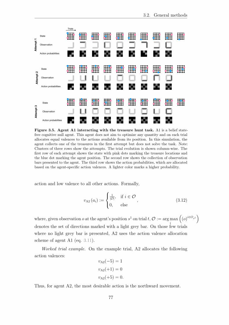
3.2. General methods

Trials

Attempt1

Observation

State

Action probabilities

Attempt2

Observation

State

Action probabilities

Attempt3

Observation

State

Action probabilities

Attempt2

Observation

State

TrialsTrials

Action probabilities

Attempt3

Observation

State

Action probabilities

Attempt1

Observation

State

Action probabilities

Attempt2

Observation

State

TrialsTrials

Action probabilities

Attempt3

Observation

State

Action probabilities

Attempt1

Observation

State

Action probabilities

Attempt2

Observation

State

TrialsTrials

Action probabilities

Attempt3

Observation

State

Action probabilities

Attempt1

Observation

State

Action probabilities

Figure 3.5. Agent A1 interacting with the treasure hunt task. A1 is a belief state-free cognitive null agent. This agent does not aim to optimize any quantity and on each trialallocates equal valences to the actions available from its position. In this simulation, theagent collects one of the treasures in the first attempt but does not solve the task. Note:Clusters of three rows show the attempts. The trial evolution is shown column-wise. Thefirst row of each attempt shows the state with pink dots marking the treasure locations andthe blue dot marking the agent position. The second row shows the collection of observationbars presented to the agent. The third row shows the action probabilities, which are allocatedbased on the agent-specific action valences. A lighter color marks a higher probability.

action and low valence to all other actions. Formally,

vA2 (ai) :=

1|O| , if i ∈ O

0, else, (3.12)

where, given observation o at the agent’s position s1 on trial t, O := arg maxi

((o)i∈Os1

)denotes the set of directions marked with a light grey bar. On those few trialswhere no light grey bar is presented, A2 uses the action valence allocationscheme of agent A1 (eq. 3.11).

Worked trial example. On the example trial, A2 allocates the followingaction valences:

vA2(−5) = 1

vA2(+1) = 0

vA2(+5) = 0.

Thus, for agent A2, the most desirable action is the northward movement.

77

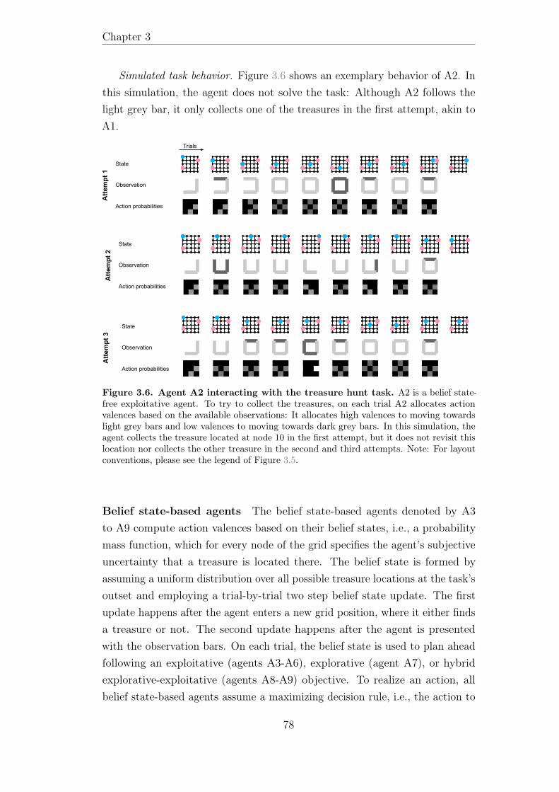
Chapter 3

Simulated task behavior. Figure 3.6 shows an exemplary behavior of A2. Inthis simulation, the agent does not solve the task: Although A2 follows thelight grey bar, it only collects one of the treasures in the first attempt, akin toA1.

Trials

Attempt1

Observation

State

Action probabilities

Attempt2

Observation

State

Action probabilities

Attempt3

Observation

State

Action probabilities

Attempt1

Observation

State

Action probabilities

TrialsTrials

Action probabilities

Attempt2

Observation

State

Action probabilities

Attempt3

Observation

State

Action probabilities

Attempt1

Observation

State

Action probabilities

TrialsTrials

Action probabilities

Attempt2

Observation

State

Action probabilities

Attempt3

Observation

State

Action probabilities

Attempt1

Observation

State

Action probabilities

TrialsTrials

Action probabilities

Attempt2

Observation

State

Action probabilities

Attempt3

Observation

State

Action probabilities

Figure 3.6. Agent A2 interacting with the treasure hunt task. A2 is a belief state-free exploitative agent. To try to collect the treasures, on each trial A2 allocates actionvalences based on the available observations: It allocates high valences to moving towardslight grey bars and low valences to moving towards dark grey bars. In this simulation, theagent collects the treasure located at node 10 in the first attempt, but it does not revisit thislocation nor collects the other treasure in the second and third attempts. Note: For layoutconventions, please see the legend of Figure 3.5.

Belief state-based agents The belief state-based agents denoted by A3to A9 compute action valences based on their belief states, i.e., a probabilitymass function, which for every node of the grid specifies the agent’s subjectiveuncertainty that a treasure is located there. The belief state is formed byassuming a uniform distribution over all possible treasure locations at the task’soutset and employing a trial-by-trial two step belief state update. The firstupdate happens after the agent enters a new grid position, where it either findsa treasure or not. The second update happens after the agent is presentedwith the observation bars. On each trial, the belief state is used to plan aheadfollowing an exploitative (agents A3-A6), explorative (agent A7), or hybridexplorative-exploitative (agents A8-A9) objective. To realize an action, allbelief state-based agents assume a maximizing decision rule, i.e., the action to

78

3.2. General methods

issue is the action with the highest valence. Before we introduce these agentsin detail, we next proceed with a formal description of the belief state.

Formally, we denote the agent’s prior belief state on trial t based on thehistory of directly observable state components y1:t−1 and observations o1:t−1by

µt :=(µ(1)t , . . . , µ

(d2)t

)T∈ Rd2 . (3.13)

The ith component of µt represents the agent’s belief that a treasure is locatedat node i ∈ Nd2 . At the beginning of the task, the components of µt areinitialized as

µ(1)0 = 0 and µ

(2)0 = µ

(3)0 = . . . µ

(d2)0 = 1/

(d2 − 1

)(3.14)

representing the fact that a treasure is never encountered at the start node,and equal beliefs over all remaining nodes. The subsequent belief state updatesdepend on the state and take slightly different forms, for the case of tworemaining treasures (s2t = 0) or a single remaining treasure (s2t ∈ 1, 2).Specifically, in the former case, the belief state is first projected into a two-dimensional matrix form

Mt :=(M

(ij)t

)1≤i,j≤d2

=(µ(i)t · µ

(j)t

)1≤i,j≤d2

∈ Rd2×d2 (3.15)

encoding the current belief for all treasure location combinations. This two-dimensional belief state projection is necessitated to reflect that the agent doesnot discriminate between the first and second treasure, and thus allocates equalprobabilities to the location combinations s3 = i, s4 = j and s3 = j, s4 = i.To account for the fact that the treasures are located at different nodes, thediagonal of this belief state matrix is then set to zero

M(ij)t := 0, if i = j for i, j ∈ Nd2 . (3.16)

The two-dimensional belief stateMt is subsequently updated in two steps. First,the belief state of the agent is updated as it enters the new grid position s1. Ifnode k is visited on trial t and no treasure is found at this node (yt = (k, 0)),the probabilities allocated to the treasure location combinations including nodek are set to zero, i.e.,

M ′t+1

(ik):= 0 and M ′

t+1(kj)

:= 0, for all i, j ∈ Nd2 . (3.17)

79

Chapter 3

This reflects the agent’s subjective certainty that node k is not a treasurelocation. The second update follows after the agent is presented with theobservation bars and has the form

M ′′t+1

(ij):= M ′

t+1(ij) · p (ot = o|st = (k, 0, i, j)) . (3.18)

This corresponds to a Bayesian update with prior probability M ′t+1

(ij) andlikelihood p (ot = o|st = (k, 0, i, j)). Finally, the belief state is normalized bysetting

Mt+1 :=1∑d2

i=1

∑d2

j=1M′′t+1

(ij)M ′′

t+1. (3.19)

Upon evaluation of this two-dimensional symmetric belief state projection, thetrial posterior belief state is evaluated by marginalization

µt+1 :=∑d2

i=1M

(ij)t+1 . (3.20)

If on trial t the agent enters node k and finds a treasure there (yt = (k, s2t ∈ N2)),a two-dimensional projection is not necessary anymore. Therefore, the position-updated belief state is given by the vector

µ′t+1 := M(1:d2,k)t , (3.21)

which specifies the agent’s subjective uncertainty about the remaining treasurelocation. This belief state is updated following the observation according to

µ′′t+1(i)

:= µ′t+1(i) · p(ot = o|st = s). (3.22)

The normalized posterior belief state

µt+1 :=1∑d2

i=1 µ′′t+1

(i)µ′′t+1 (3.23)

serves as the prior belief state on the subsequent trial, where the position-dependent belief state update takes the form

µ′t+1(s1t ) :=

1, if s2t /∈

0, s2t−1

0, else

. (3.24)

If the agent does not solve the task within the attempt, the final belief state

80

3.2. General methods

µT in the attempt serves as the prior belief state in the next attempt, i.e.,

µ0 := µT . (3.25)

This holds if no treasure location was recovered in a previous attempt. Other-wise, the prior belief state in the new attempt is defined by setting the beliefat the recovered treasure location to the maximum value. This modification isnecessary, because, to solve the task, the agent has to collect both treasureswithin a single attempt. Consequently, in the new attempt, the agent has torevisit the previously recovered treasure location. Formally, the prior beliefstate in the new attempt is first defined as the final belief state in the previousattempt (eq. 3.25). Then, the prior belief state is modified and normalizedaccording to

µ(k)0 := 1, µ0 :=

1∑d2

i=1 µ(i)0

µ0, (3.26)

where k denotes the previously recovered treasure location. The subsequentbelief state updates are evaluated as described above with a minor modification:The two-dimensional belief state projection is given by assigning the prior beliefstate vector and its transpose to the kth column and kth row of a null matrixof the size d2 × d2, respectively. Formally, the two-dimensional belief state isfirst defined as

Mt := 0d2×d2 (3.27)

and then its entries are modified according to

M(1:d2,k)t := µt and M

(k,1:d2)t := µTt . (3.28)

Note that we throughout assume that the agent is endowed with the trueprobability of making observation o given state s as defined by the observationfunction g of the task model. As detailed above, these probabilities formalize thenotions that (1) a direction leading away from the treasures is always markedwith a dark grey bar and (2) the accuracy of the treasure detector correctlyreturning a light grey bar in the direction towards the treasures increases asthe agent moves closer to the treasures. To motivate our assumption, recallthe experimental procedure participants underwent prior to the runs in thescanner. In the task instructions, participants were truthfully informed aboutthe first notion (Supplementary Material B.1). Although participants were notfurther informed about the second notion, before the runs in the scanner, theycompleted a training run by the end of which they arguably became familiar

81

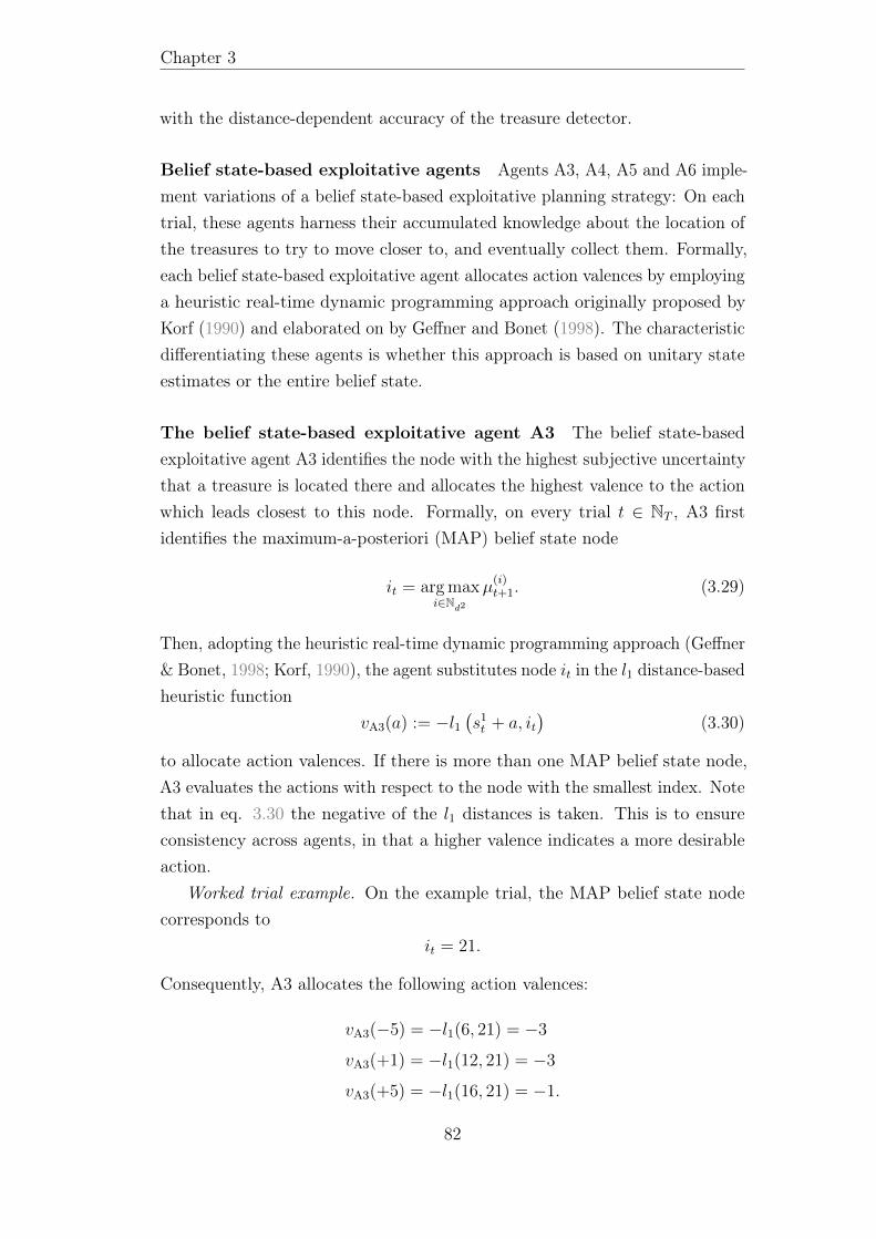
Chapter 3

with the distance-dependent accuracy of the treasure detector.

Belief state-based exploitative agents Agents A3, A4, A5 and A6 imple-ment variations of a belief state-based exploitative planning strategy: On eachtrial, these agents harness their accumulated knowledge about the location ofthe treasures to try to move closer to, and eventually collect them. Formally,each belief state-based exploitative agent allocates action valences by employinga heuristic real-time dynamic programming approach originally proposed byKorf (1990) and elaborated on by Geffner and Bonet (1998). The characteristicdifferentiating these agents is whether this approach is based on unitary stateestimates or the entire belief state.

The belief state-based exploitative agent A3 The belief state-basedexploitative agent A3 identifies the node with the highest subjective uncertaintythat a treasure is located there and allocates the highest valence to the actionwhich leads closest to this node. Formally, on every trial t ∈ NT , A3 firstidentifies the maximum-a-posteriori (MAP) belief state node

it = arg maxi∈Nd2

µ(i)t+1. (3.29)

Then, adopting the heuristic real-time dynamic programming approach (Geffner& Bonet, 1998; Korf, 1990), the agent substitutes node it in the l1 distance-basedheuristic function

vA3(a) := −l1(s1t + a, it

)(3.30)

to allocate action valences. If there is more than one MAP belief state node,A3 evaluates the actions with respect to the node with the smallest index. Notethat in eq. 3.30 the negative of the l1 distances is taken. This is to ensureconsistency across agents, in that a higher valence indicates a more desirableaction.

Worked trial example. On the example trial, the MAP belief state nodecorresponds to

it = 21.

Consequently, A3 allocates the following action valences:

vA3(−5) = −l1(6, 21) = −3

vA3(+1) = −l1(12, 21) = −3

vA3(+5) = −l1(16, 21) = −1.

82

3.2. General methods

Thus, for agent A3, the most desirable action is the southward movement.

Simulated task behavior. Figure 3.7 shows an exemplary behavior of A3. Inthis simulation, the agent does not solve the task: A3 recovers the first treasurelocation already in the first attempt but does not manage to recover the secondtreasure location. The reason for this is that the strategy of A3 has limitedflexibility. Specifically, after the agent finds a treasure at node 10 in the firstattempt, it becomes certain that this node is a treasure location. Consequently,at the outset of the second and third attempts, A3 allocates the highest beliefto this node and goes directly to it. The problem is that from this node, theagent can not reach the other treasure located at node 16 within the step limit- even if the agent allocates the second highest belief to node 16. As a result,A3 closely approaches the second treasure location but does solve the task.

The belief state-based exploitative agent A4 The belief state-basedexploitative agent A4 uses the same strategy as A3 with one important difference:Until there is only one treasure left, the agent identifies the most probablelocation of both treasures and evaluates the actions with respect to the locationthat is closer to its current position. Formally, while s2t = 0, A4 first identifiesthe two nodes with the highest associated beliefs,

i1t = arg maxk∈Nd2

µ(k)t+1 and i2t = arg max

l∈Nd2\i1tµ(l)t+1. (3.31)

Then, the agent identifies the node reachable within fewer steps

jt = arg minm∈i1t ,i2t

l1(s1t ,m

)(3.32)

and substitutes this node in the l1 distance-based heuristic function to allocateaction valences. After the recovery of a treasure location (s2t ∈ 1, 2), A4 usesthe valence allocation scheme of A3 to collect the remaining treasure, i.e.,

vA4(a) :=

−l1 (s1t + a, jt) , if s2t = 0

vA3(a), else. (3.33)

Worked trial example. On the example trial, the nodes with the highestassociated beliefs are

i1t = 21 and i2t = 6.

83

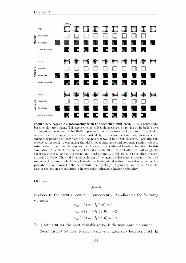
Chapter 3

Trials

Attempt1 Observation

State

Belief state

Action probabilities

Attempt2 Observation

State

Belief state

Action probabilities

Attempt3 Observation

State

Belief state

Action probabilities

TrialsTrials

Observation

State

Belief state

Action probabilities

Attempt2 Observation

State

Belief state

Action probabilities

Attempt1 Observation

State

Belief state

Action probabilities

Observation

State

Belief state

Action probabilities

Attempt3 Observation

State

Belief state

Action probabilities

Figure 3.7. Agent A3 interacting with the treasure hunt task. A3 is a belief state-based exploitative agent. This agent tries to collect the treasures by relying on its belief state,a dynamically evolving probabilistic representation of the treasure locations. In particular,on each trial, this agent identifies the most likely to treasure location and allocates actionvalences depending on how close the new position would be to this location. Formally, thisscheme corresponds to evaluating the MAP belief state node and computing action valencesusing a real time dynamic approach with an l1 distance-based heuristic function. In thissimulation, A3 collects the treasure located at node 10 in the first attempt. Although theagent revisits this node in the second and third attempts, it fails to collect the other treasureat node 16. Note: The trial-by-trial evolution of the agent’s belief state is shown in the thirdrow of each attempt, which complements the trial-by-trial states, observations, and actionprobabilities as shown for the belief state-free agents (cf. Figures 3.5 and 3.6). As in thecase of the action probabilities, a lighter color indicates a higher probability.

Of these,jt = 6

is closer to the agent’s position. Consequently, A4 allocates the followingvalences:

vA4(−5) = −l1(6, 6) = 0

vA4(+1) = −l1(12, 6) = −2

vA4(+5) = −l1(16, 6) = −2.

Thus, for agent A4, the most desirable action is the northward movement.

Simulated task behavior. Figure 3.8 shows an exemplary behavior of A4. In

84

3.2. General methods

this simulation, the agent solves the task: The agent recovers the first treasurelocation in the first attempt, the second treasure location in the second attemptand, by combining its knowledge about these locations, consecutively collectsboth treasures in the third attempt. This simulation demonstrates that bytaking into account the potential location of both treasures A4 overcomes thelimitation of A3.

Trials

Attempt1 Observation

State

Belief state

Action probabilities

Attempt2 Observation

State

Belief state

Action probabilities

Attempt3 Observation

State

Belief state

Action probabilities

TrialsTrials

Observation

State

Belief state

Action probabilities

Attempt2 Observation

State

Belief state

Action probabilities

Attempt1 Observation

State

Belief state

Action probabilities

Observation

State

Belief state

Action probabilities

Attempt3 Observation

State

Belief state

Action probabilities

Figure 3.8. Agent A4 interacting with the treasure hunt task. A4 is a belief state-based exploitative agent with a similar strategy to that of A3. The difference is that A4takes into account the potential location of both treasures. Specifically, until a treasure iscollected in the attempt, A4 first identities the two most probable treasure locations, thenthe one closer to its current position and subsequently evaluates the actions based on the l1distance between this location and the new position. After a treasure is collected, A4 usesthe same valence allocation scheme as A3. In this simulation, A4 recovers the treasure atnode 10 in the first attempt, the treasure at node 16 in the second attempt and solves thetask in the third attempt. Note: For layout conventions, please see the legend of Figure 3.7.

The belief state-based exploitative agent A5 The belief state-basedexploitative agent A5 does not identify single most probable treasure locations.Instead, this agent takes into account its entire belief state when evaluatingthe actions. Specifically, for each available action a ∈ As1 , A5 evaluates thenegative sum of the belief-weighted l1 distances between the new position that

85

Chapter 3

would result upon the action and each node of the grid,

vA5(a) := −∑d2

i=1µ(i)t+1l1

(s1t + a, i

). (3.34)

Intuitively, agent A5 favors the action that leads towards the part of the grid,where a treasure is likely located and which is in close reach.

Worked trial example. On the example trial, agent A5 allocates the followingaction valences:

vA5(−5) = −(0.25 · l1(6, 6) + 0.15 · l1(6, 13)

+ 0.2 · l1(6, 14) + 0.1 · l1(6, 15) + 0.3 · l1(6, 21)) = −2.65

vA5(+1) = −(0.25 · l1(12, 6) + 0.15 · l1(12, 13)

+ 0.2 · l1(12, 14) + 0.1 · l1(12, 15) + 0.3 · l1(12, 21)) = −2.25

vA5(+5) = −(0.25 · l1(16, 6) + 0.15 · l1(16, 13)

+ 0.2 · l1(16, 14) + 0.1 · l1(16, 15) + 0.3 · l1(16, 21)) = −2.55.

Thus, for agent A5, the most desirable action is the eastward movement.

Simulated task behavior. Figure 3.9 shows an exemplary behavior of A5.In this simulation, the agent solves the task: A5 does not collect any of thetreasures in the first attempt, but it collects the treasure at node 16 in thesecond attempt and both treasures in the third attempt. As this agent takesinto account its entire belief state when evaluating the actions’ desirability,tasks where the treasures are located at opposite ends of the grid can lead to toambiguous decision situations, i.e., trials with multiple best actions leading inopposite directions. For example, in the exemplary simulation, the agent facesa series of ambiguous decision situations in the first attempt. This happensbecause the agent correctly believes that the treasures are located at oppositeends and therefore, midway between the treasures, it allocates equally highvalences to converse actions. As a result, the agent moves back-and-forth inthe first attempt but it manages to break this pattern in the second attemptand solve the task in the third attempt.

The belief state-based exploitative agent A6 The belief state-basedexploitative agent A6 uses the same strategy as A5, but in ambiguous decisionsituations it switches to the strategy of A4. Formally, if there is more than oneaction maximizing the valence function of A5 (eq. 3.34), the agent re-evaluates

86

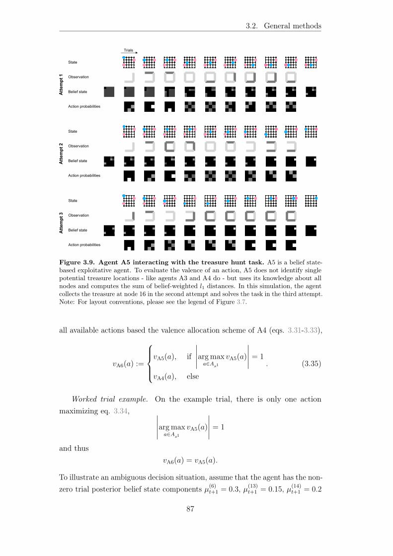
3.2. General methods

Trials

Attempt1 Observation

State

Belief state

Action probabilities

Attempt2 Observation

State

Belief state

Action probabilities

Attempt3 Observation

State

Belief state

Action probabilities

Figure 3.9. Agent A5 interacting with the treasure hunt task. A5 is a belief state-based exploitative agent. To evaluate the valence of an action, A5 does not identify singlepotential treasure locations - like agents A3 and A4 do - but uses its knowledge about allnodes and computes the sum of belief-weighted l1 distances. In this simulation, the agentcollects the treasure at node 16 in the second attempt and solves the task in the third attempt.Note: For layout conventions, please see the legend of Figure 3.7.

all available actions based the valence allocation scheme of A4 (eqs. 3.31-3.33),

vA6(a) :=

vA5(a), if

∣∣∣∣∣arg maxa∈As1

vA5(a)

∣∣∣∣∣ = 1

vA4(a), else

. (3.35)

Worked trial example. On the example trial, there is only one actionmaximizing eq. 3.34, ∣∣∣∣∣arg max

a∈As1

vA5(a)

∣∣∣∣∣ = 1

and thusvA6(a) = vA5(a).

To illustrate an ambiguous decision situation, assume that the agent has the non-zero trial posterior belief state components µ(6)

t+1 = 0.3, µ(13)t+1 = 0.15, µ(14)

t+1 = 0.2

87

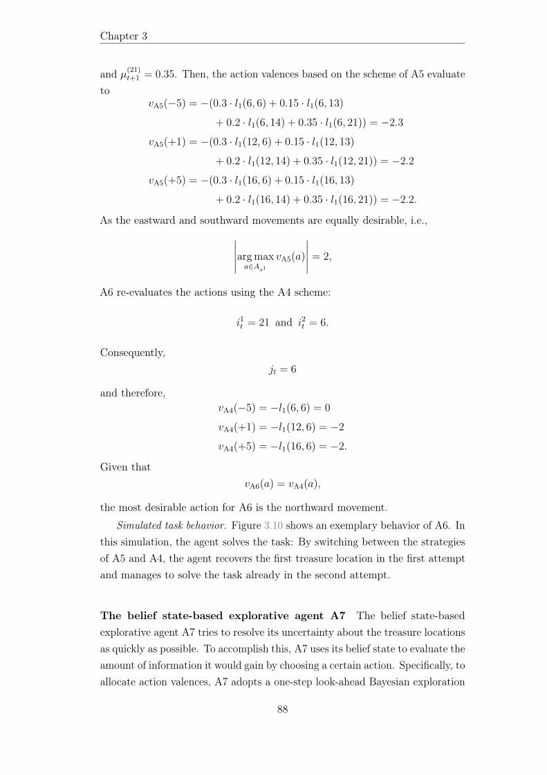
Chapter 3

and µ(21)t+1 = 0.35. Then, the action valences based on the scheme of A5 evaluate

tovA5(−5) = −(0.3 · l1(6, 6) + 0.15 · l1(6, 13)

+ 0.2 · l1(6, 14) + 0.35 · l1(6, 21)) = −2.3

vA5(+1) = −(0.3 · l1(12, 6) + 0.15 · l1(12, 13)

+ 0.2 · l1(12, 14) + 0.35 · l1(12, 21)) = −2.2

vA5(+5) = −(0.3 · l1(16, 6) + 0.15 · l1(16, 13)

+ 0.2 · l1(16, 14) + 0.35 · l1(16, 21)) = −2.2.

As the eastward and southward movements are equally desirable, i.e.,∣∣∣∣∣arg maxa∈As1

vA5(a)

∣∣∣∣∣ = 2,

A6 re-evaluates the actions using the A4 scheme:

i1t = 21 and i2t = 6.

Consequently,jt = 6

and therefore,vA4(−5) = −l1(6, 6) = 0

vA4(+1) = −l1(12, 6) = −2

vA4(+5) = −l1(16, 6) = −2.

Given thatvA6(a) = vA4(a),

the most desirable action for A6 is the northward movement.

Simulated task behavior. Figure 3.10 shows an exemplary behavior of A6. Inthis simulation, the agent solves the task: By switching between the strategiesof A5 and A4, the agent recovers the first treasure location in the first attemptand manages to solve the task already in the second attempt.

The belief state-based explorative agent A7 The belief state-basedexplorative agent A7 tries to resolve its uncertainty about the treasure locationsas quickly as possible. To accomplish this, A7 uses its belief state to evaluate theamount of information it would gain by choosing a certain action. Specifically, toallocate action valences, A7 adopts a one-step look-ahead Bayesian exploration

88

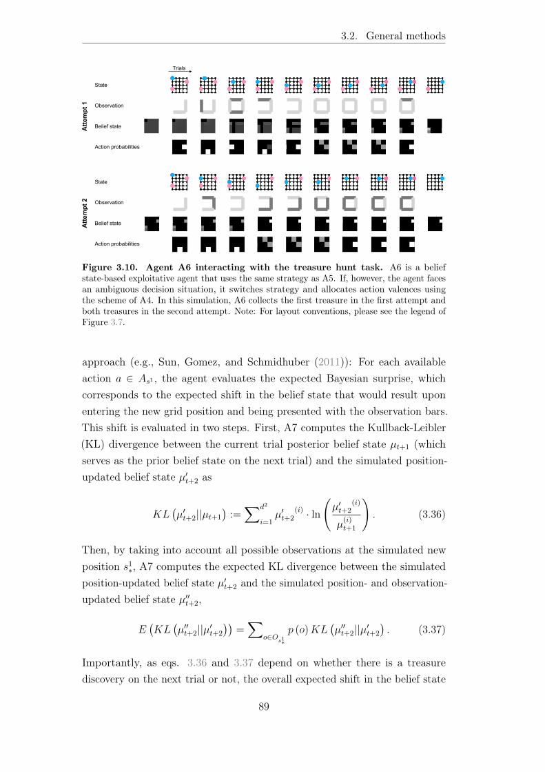
3.2. General methods

Trials

Attempt1 Observation

State

Belief state

Action probabilities

Attempt2 Observation

State

Belief state

Action probabilities

Figure 3.10. Agent A6 interacting with the treasure hunt task. A6 is a beliefstate-based exploitative agent that uses the same strategy as A5. If, however, the agent facesan ambiguous decision situation, it switches strategy and allocates action valences usingthe scheme of A4. In this simulation, A6 collects the first treasure in the first attempt andboth treasures in the second attempt. Note: For layout conventions, please see the legend ofFigure 3.7.

approach (e.g., Sun, Gomez, and Schmidhuber (2011)): For each availableaction a ∈ As1 , the agent evaluates the expected Bayesian surprise, whichcorresponds to the expected shift in the belief state that would result uponentering the new grid position and being presented with the observation bars.This shift is evaluated in two steps. First, A7 computes the Kullback-Leibler(KL) divergence between the current trial posterior belief state µt+1 (whichserves as the prior belief state on the next trial) and the simulated position-updated belief state µ′t+2 as

KL(µ′t+2||µt+1

):=∑d2

i=1µ′t+2

(i) · ln

(µ′t+2

(i)

µ(i)t+1

). (3.36)

Then, by taking into account all possible observations at the simulated newposition s1∗, A7 computes the expected KL divergence between the simulatedposition-updated belief state µ′t+2 and the simulated position- and observation-updated belief state µ′′t+2,

E(KL

(µ′′t+2||µ′t+2

))=∑

o∈Os1∗

p (o)KL(µ′′t+2||µ′t+2

). (3.37)

Importantly, as eqs. 3.36 and 3.37 depend on whether there is a treasurediscovery on the next trial or not, the overall expected shift in the belief state

89

Chapter 3

for an action a ∈ As1 is given by

vA7(a) :=zµ(s1∗)t+1 ·

(KL

(µ′t+2||µt+1

)s2t+1 6=s2t

+ E(KL

(µ′′t+2||µ′t+2

))s2t+1 6=s2t

)+(

1− zµ(s1∗)t+1

)·(KL

(µ′t+2||µt+1

)s2t+1=s

2t

+ E(KL

(µ′′t+2||µ′t+2

))s2t+1=s

2t

).

(3.38)

The first term in eq. 3.38 captures the expected shift in the belief state if thereis a treasure discovery on trial t+ 1. The second term captures the expectedshift in the belief state if there is no treasure discovery on trial t + 1. Theproduct zµ(s1∗)

t+1 captures the agent’s subjective uncertainty that a treasure islocated at the new grid position s1∗. Here, z is set to 2 if no treasure wasdiscovered in the attempt up to trial t (i.e., s2t = 0), and to 1 otherwise. Thisis to account for the fact that until a treasure is discovered in the attempt, µrepresents the belief over both treasure locations. Therefore, maximal certaintyabout a treasure location is represented as a value of 0.5 at the correspondingcomponent of µ.

Worked trial example. On the example trial, A7 allocates the valence

vA7(−5) = zµ(6)t+1 ·

(KL

(µ′t+2||µt+1

)s2t+1∈1,2

+ E(KL

(µ′′t+2||µ′t+2

))s2t+1∈1,2

)+(

1− zµ(6)t+1

)·(KL

(µ′t+2||µt+1

)s2t+1=0

+ E(KL

(µ′′t+2||µ′t+2

))s2t+1=0

)= 2 · 0.25 · (0.29 + 0.29) + (1− 2 · 0.25) · (0.3 + 0)

= 0.44

to the northward movement, the valence

vA7(+1) = zµ(12)t+1 ·

(KL

(µ′t+2||µt+1

)s2t+11,2

+ E(KL

(µ′′t+2||µ′t+2

))s2t+11,2

)+(

1− zµ(12)t+1

)·(KL

(µ′t+2||µt+1

)s2t+1=0

+ E(KL

(µ′′t+2||µ′t+2

))s2t+1=0

)= 2 · 0 · (0 + 0) + (1− 2 · 0) · (0 + 0.45)

= 0.45

to the eastward movement, and the valence

vA7(+5) = zµ(16)t+1 ·

(KL

(µ′t+2||µt+1

)s2t+11,2

+ E(KL

(µ′′t+2||µ′t+2

))s2t+11,2

)+(

1− zµ(16)t+1

)·(KL

(µ′t+2||µt+1

)s2t+1=0

+ E(KL

(µ′′t+2||µ′t+2

))s2t+1=0

)= 2 · 0 · (0 + 0) + (1− 2 · 0) · (0 + 0.4)

= 0.4.

90

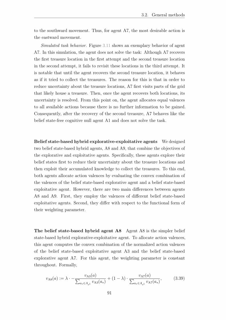
3.2. General methods

to the southward movement. Thus, for agent A7, the most desirable action isthe eastward movement.

Simulated task behavior. Figure 3.11 shows an exemplary behavior of agentA7. In this simulation, the agent does not solve the task: Although A7 recoversthe first treasure location in the first attempt and the second treasure locationin the second attempt, it fails to revisit these locations in the third attempt. Itis notable that until the agent recovers the second treasure location, it behavesas if it tried to collect the treasures. The reason for this is that in order toreduce uncertainty about the treasure locations, A7 first visits parts of the gridthat likely house a treasure. Then, once the agent recovers both locations, itsuncertainty is resolved. From this point on, the agent allocates equal valencesto all available actions because there is no further information to be gained.Consequently, after the recovery of the second treasure, A7 behaves like thebelief state-free cognitive null agent A1 and does not solve the task.

Belief state-based hybrid explorative-exploitative agents We designedtwo belief state-based hybrid agents, A8 and A9, that combine the objectives ofthe explorative and exploitative agents. Specifically, these agents explore theirbelief states first to reduce their uncertainty about the treasure locations andthen exploit their accumulated knowledge to collect the treasures. To this end,both agents allocate action valences by evaluating the convex combination ofthe valences of the belief state-based explorative agent and a belief state-basedexploitative agent. However, there are two main differences between agentsA8 and A9. First, they employ the valences of different belief state-basedexploitative agents. Second, they differ with respect to the functional form oftheir weighting parameter.

The belief state-based hybrid agent A8 Agent A8 is the simpler beliefstate-based hybrid explorative-exploitative agent. To allocate action valences,this agent computes the convex combination of the normalized action valencesof the belief state-based exploitative agent A3 and the belief state-basedexplorative agent A7. For this agent, the weighting parameter is constantthroughout. Formally,

vA8(a) := λ · − vA3(a)∑a∗∈As1

vA3(a∗)+ (1− λ) · vA7(a)∑

a∗∈As1vA7(a∗)

, (3.39)

91

Chapter 3

Trials

Attempt1 Observation

State

Belief state

Action probabilities

Attempt2 Observation

State

Belief state

Action probabilities

Attempt3 Observation

State

Belief state

Action probabilities

Figure 3.11. Agent A7 interacting with the treasure hunt task. A7 is a beliefstate-based explorative agent that tries to resolve its uncertainty about the treasure locations.To this end, on each trial, this agent allocates action valences based on the expected shift inthe belief state that would result upon choosing the action. In this simulation, A7 collects thetreasure at node 10 in the first attempt and the treasure at node 16 in the second attempt.After the recovery of both treasure locations, there is no further information to be gainedand the agent allocates equal valences to the available actions. By doing so, A7 fails to solvethe task in the third attempt. Note: For layout conventions, please see the legend of Figure3.7.

where λ ∈ [0, 1] is the weighting parameter. The reason we chose to adoptthe action valences of A3 for this agent is that A3 arguably implements thepurest form of a belief state-based exploitative strategy: A3 always favors theaction that is the safest bet - i.e., the move towards the node which has thehighest associated belief - and does not take into account other aspects of thetask environment, such as the presence of two treasures. Therefore, for thesimpler belief state-based hybrid explorative-exploitative agent the valences ofA3 naturally contrast with the valences of the belief state-based exploitativeagent A7.

Worked trial example. On the example trial, agent A8 allocates the following

92

3.2. General methods

action valences using a weighting parameter of λ = 0.7:

vA8(−5) = 0.7 · − −3

−3− 3− 1+ (1− 0.7) · 0.44

0.44 + 0.45 + 0.4= −0.198

vA8(+1) = 0.7 · − −3

−3− 3− 1+ (1− 0.7) · 0.45

0.44 + 0.45 + 0.4= −0.195

vA8(+5) = 0.7 · − −1

−3− 3− 1+ (1− 0.7) · 0.4

0.44 + 0.45 + 0.4= −0.007.

Thus, for agent A8, the most desirable action is the southward movement.

Simulated task behavior. Figure 3.12 shows an exemplary behavior of agentA8. In this simulation with the weighting parameter set to λ = 0.7, the agentdoes not solve the task: A8 recovers the treasure location at node 16 in the firstattempt and the treasure location at node 10 in the second attempt. Althoughthe agent revisits and thereby collects the treasure at node 10 in the thirdattempt, it does not manage to collect the other treasure before the step limitis reached. Notably, while a weighting parameter value of λ = 0.7 grants astronger control to the belief state-based exploitative agent A3, the influenceof the belief state-based explorative agent A7 is evident. In particular, inthe second attempt agent A8 does not get trapped in revisiting the treasurelocation discovered in the first attempt, as A3 would do, but seeks for andrecovers the other treasure location. After recovering both treasure locations,A7 does not differentiate between the available actions and therefore actionselection on the remaining trials is driven by the valences of A3. Consequently,in the third attempt, agent A8 behaves similar to agent A3 and does not solvethe task.

The belief state-based hybrid agent A9 Agent A9 is the more advancedbelief state-based hybrid explorative-exploitative agent. This agent allocatesaction valences based on the convex combination of the valences of the beliefstate-based exploitative agent A4 and the belief state-based explorative agentA7. In contrast to the constant weighting parameter of agent A8, for this agentthe value of the weighting parameter depends on its current state uncertainty.Formally,

vA9(a) := λt · −vA4(a)∑

a∗∈As1vA4(a∗)

+ (1− λt) ·vA7(a)∑

a∗∈As1vA7(a∗)

, (3.40)

93

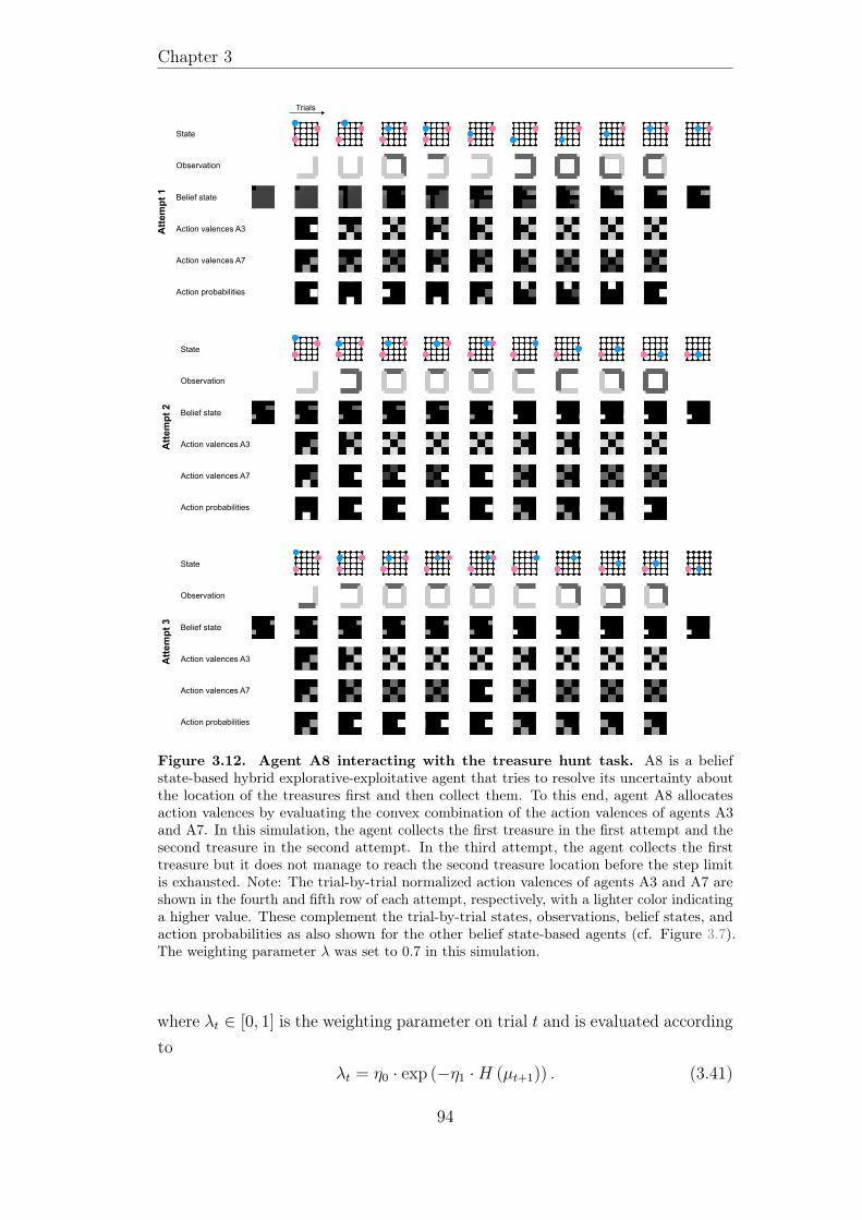
Chapter 3

Trials

Attempt1

Observation

State

Belief state

Action valences A3

Action valences A7

Action probabilities

Attempt2

Observation

State

Belief state

Action valences A3

Action valences A7

Action probabilities

Attempt3

Observation

State

Belief state

Action valences A3

Action valences A7

Action probabilities

Figure 3.12. Agent A8 interacting with the treasure hunt task. A8 is a beliefstate-based hybrid explorative-exploitative agent that tries to resolve its uncertainty aboutthe location of the treasures first and then collect them. To this end, agent A8 allocatesaction valences by evaluating the convex combination of the action valences of agents A3and A7. In this simulation, the agent collects the first treasure in the first attempt and thesecond treasure in the second attempt. In the third attempt, the agent collects the firsttreasure but it does not manage to reach the second treasure location before the step limitis exhausted. Note: The trial-by-trial normalized action valences of agents A3 and A7 areshown in the fourth and fifth row of each attempt, respectively, with a lighter color indicatinga higher value. These complement the trial-by-trial states, observations, belief states, andaction probabilities as also shown for the other belief state-based agents (cf. Figure 3.7).The weighting parameter λ was set to 0.7 in this simulation.

where λt ∈ [0, 1] is the weighting parameter on trial t and is evaluated accordingto

λt = η0 · exp (−η1 ·H (µt+1)) . (3.41)

94

3.2. General methods

Here, η0 ∈ [0, 1] and η1 ∈ R≥0 are the offset and slope parameters of theexponential decay function, respectively, and

H (µt+1) := −∑d2

i=1µ(i)t+1 · ln

(µ(i)t+1

)(3.42)

is the entropy of the agent’s trial posterior belief state. Of note, our choice toexpress the dynamic weighting parameter with an exponential function is inline with similar previous work (e.g., Camerer and Ho, 1998; Gläscher et al.,2010). This agent combines the valences of agents A4 and A7. As discussedabove for agent A4, by taking into consideration the possible location of bothtreasures, the strategy of A4 allows for more flexibility compared to the strategyof A3. Consequently, we reasoned that for the more advanced belief state-basedhybrid explorative-exploitative agent the valences of A4 constitute a suitablecontrast to the valences of the belief state-based exploitative agent A7.

Worked trial example. On the example trial, state uncertainty evaluates to

H (µt+1) = 1.54.

By setting the offset and slope parameters to η0 = 1 and η0 = 0.4, respectively,the weighting parameter evaluates to

λt = 1 · exp(−0.4 · 1.54) = 0.54.

Consequently, A9 allocates the following action valences:

vA9(−5) = 0.54 · − 0

0− 2− 2+ (1− 0.54) · 0.44

0.44 + 0.45 + 0.4= 0.16

vA9(+1) = 0.54 · − −2

0− 2− 2+ (1− 0.54) · 0.45

0.44 + 0.45 + 0.4= −0.11

vA9(+5) = 0.54 · − −2

0− 2− 2+ (1− 0.54) · 0.4

0.44 + 0.45 + 0.4= −0.13 .

Thus, for agent A9, the most desirable action is the northward movement.

Simulated task behavior. Figure 3.13 shows an exemplary behavior of agentA9. In this simulation with an offset of η0 = 1 and a slope of η1 = 0.4, theagent solves the task: A9 finds the treasure at node 16 in the first attempt, thetreasure at node 10 in the second attempt and collects both treasures in thethird attempt. For the η0 and η1 values used in this simulation, the weightingparameter λt grants dominant control to the belief state-based explorativeagent A7 if the agent is maximally uncertain about the state (this is the case in

95

Chapter 3

the first trial of the first attempt, where the entropy of the trial posterior beliefstate is H (µ2) ≈ 3 and thus λ1 = 0.3). The weighting parameter λt grants fullcontrol to the belief state-based exploitative agent A4 if the agent’s uncertaintyis resolved (λt = 1; this is the case if both treasure locations are recoveredand thus the entropy of the belief state is H (µt+1) ≈ 0). To demonstrate thechanging contribution of agents A7 and A4 in the action valences of A9, considerthe second and third attempts. In the beginning of the second attempt, theagent is still uncertain about the location of the first treasure. Consequently,the preference of A7 prevails over the preference of A4 and the agent searchesfor and finds the treasure. Then, in the third attempt, the valences of agentA4 prevail and, like agent A4, agent A9 solves the task (cf. Figure 3.8).

3.3 Behavioral methods

3.3.1 Descriptive behavioral data analyses

We evaluated six descriptive statistics of participants’ decision-making behaviorin the treasure hunt task. First, we evaluated the average performance bydividing the sum of solved tasks across participants by the number of partici-pants. Second, we evaluated the average number of solvable tasks by dividingthe sum of solvable tasks across participants by the number of participants.We evaluated this statistic because some tasks were not solvable due to therandomly allocated step limit. This was the case if the step limit in all threeattempts of a task was smaller than the optimal step limit. For the last fourstatistics, we evaluated the average performance per run, per attempt, per opti-mal step limit and per treasure location combination. To evaluate the averageperformance per run, for each participant and run, we first divided the numberof solved tasks by the number of solvable tasks and subsequently computedthe mean and the standard error of the mean (SEM) across participants. Toevaluate the average performance per attempt, for each participant, we firstdivided the number of tasks solved within one, two and three attempts by thenumber of all tasks that were solvable for that participant and subsequentlycomputed the mean and the SEM across participants. To evaluate the averageperformance per optimal step limit, for each participant and optimal step limit,we first divided the number of solved tasks by the number of solvable tasks andthen averaged across participants. Finally, to evaluate the average performanceper treasure location combination, for each participant and treasure location

96

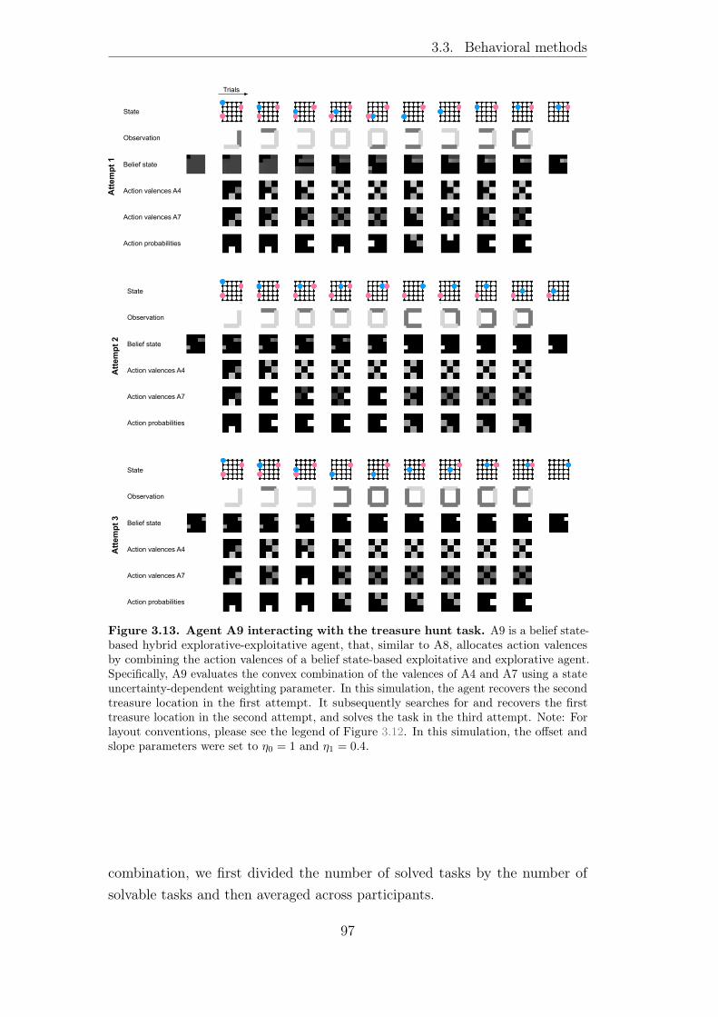
3.3. Behavioral methods

Trials

Attempt1

Observation

State

Belief state

Action valences A4

Action valences A7

Action probabilities

Attempt2

Observation

State

Belief state

Action valences A7

Action probabilities

Attempt3

Observation

State

Belief state

Action valences A4

Action valences A7

Action probabilities

Action valences A4

Attempt1

ot

st

µt

pt

vBB-R-2t

vBB-It

Attempt2

ot

st

µt

Attempt3

ot

st

µt

vBB-R-2t

vBB-It

pt

vBB-R-2t

vBB-It

pt

vBB-R-2t

vBB-It

Attempt1

ot

st

µt

pt

vBB-R-2t

vBB-It

Attempt2

ot

st

µt

Attempt3

ot

st

µt

vBB-R-2t

vBB-It

pt

vBB-R-2t

vBB-It

pt

vBB-R-2t

vBB-It

Attempt1

ot

st

µt

pt

vBB-R-2t

vBB-It

Attempt2

ot

st

µt

Attempt3

ot

st

µt

vBB-R-2t

vBB-It

pt

vBB-R-2t

vBB-It

pt

vBB-R-2t

vBB-It

Attempt1

ot

st

µt

pt

vBB-R-2t

vBB-It

Attempt2

ot

st

µt

Attempt3

ot

st

µt

vBB-R-2t

vBB-It

pt

vBB-R-2t

vBB-It

pt

vBB-R-2t

vBB-It

Attempt1

ot

st

µt

pt

vBB-R-2t

vBB-It

Attempt2

ot

st

µt

Attempt3

ot

st

µt

vBB-R-2t

vBB-It

pt

vBB-R-2t

vBB-It

pt

vBB-R-2t

vBB-It

Attempt1

ot

st

µt

pt

vBB-R-2t

vBB-It

Attempt2

ot

st

µt

Attempt3

ot

st

µt

vBB-R-2t

vBB-It

pt

vBB-R-2t

vBB-It

pt

vBB-R-2t

vBB-It

Attempt1

ot

st

µt

pt

vBB-R-2t

vBB-It

Attempt2

ot

st

µt

Attempt3

ot

st

µt

vBB-R-2t

vBB-It

pt

vBB-R-2t

vBB-It

pt

vBB-R-2t

vBB-It

Attempt1

ot

st

µt

pt

vBB-R-2t

vBB-It

Attempt2

ot

st

µt

Attempt3

ot

st

µt

vBB-R-2t

vBB-It

pt

vBB-R-2t

vBB-It

pt

vBB-R-2t

vBB-It

Attempt1

ot

st

µt

pt

vBB-R-2t

vBB-It

Attempt2

ot

st

µt

Attempt3

ot

st

µt

vBB-R-2t

vBB-It

pt

vBB-R-2t

vBB-It

pt

vBB-R-2t

vBB-It

Attempt1

ot

st

µt

pt

vBB-R-2t

vBB-It

Attempt2

ot

st

µt

Attempt3

ot

st

µt

vBB-R-2t

vBB-It

pt

vBB-R-2t

vBB-It

pt

vBB-R-2t

vBB-It

Attempt1

ot

st

µt

pt

vBB-R-2t

vBB-It

Attempt2

ot

st

µt

Attempt3

ot

st

µt

vBB-R-2t

vBB-It

pt

vBB-R-2t

vBB-It

pt

vBB-R-2t

vBB-It

Attempt1

ot

st

µt

pt

vBB-R-2t

vBB-It

Attempt2

ot

st

µt

Attempt3

ot

st

µt

vBB-R-2t

vBB-It

pt

vBB-R-2t

vBB-It

pt

vBB-R-2t

vBB-It

Attempt1

ot

st

µt

pt

vBB-R-2t

vBB-It

Attempt2

ot

st

µt

Attempt3

ot

st

µt

vBB-R-2t

vBB-It

pt

vBB-R-2t

vBB-It

pt

vBB-R-2t

vBB-It

Attempt1

ot

st

µt

pt

vBB-R-2t

vBB-It

Attempt2

ot

st

µt

Attempt3

ot

st

µt

vBB-R-2t

vBB-It

pt

vBB-R-2t

vBB-It

pt

vBB-R-2t

vBB-It

Attempt1

ot

st

µt

pt

vBB-R-2t

vBB-It

Attempt2

ot

st

µt

Attempt3

ot

st

µt

vBB-R-2t

vBB-It

pt

vBB-R-2t

vBB-It

pt

vBB-R-2t

vBB-It

Attempt1

ot

st

µt

pt

vBB-R-2t

vBB-It

Attempt2

ot

st

µt

Attempt3

ot

st

µt

vBB-R-2t

vBB-It

pt

vBB-R-2t

vBB-It

pt

vBB-R-2t

vBB-It

Attempt1

ot

st

µt

pt

vBB-R-2t

vBB-It

Attempt2

ot

st

µt

Attempt3

ot

st

µt

vBB-R-2t

vBB-It

pt

vBB-R-2t

vBB-It

pt

vBB-R-2t

vBB-It

Attempt1

ot

st

µt

pt

vBB-R-2t

vBB-It

Attempt2

ot

st

µt

Attempt3

ot

st

µt

vBB-R-2t

vBB-It

pt

vBB-R-2t

vBB-It

pt

vBB-R-2t

vBB-It

Attempt1

ot

st

µt

pt

vBB-R-2t

vBB-It

Attempt2

ot

st

µt

Attempt3

ot

st

µt

vBB-R-2t

vBB-It

pt

vBB-R-2t

vBB-It

pt

vBB-R-2t

vBB-It

Attempt1

ot

st

µt

pt

vBB-R-2t

vBB-It

Attempt2

ot

st

µt

Attempt3

ot

st

µt

vBB-R-2t

vBB-It

pt

vBB-R-2t

vBB-It

pt

vBB-R-2t

vBB-It

Attempt1

ot

st

µt

pt

vBB-R-2t

vBB-It

Attempt2

ot

st

µt

Attempt3

ot

st

µt

vBB-R-2t

vBB-It

pt

vBB-R-2t

vBB-It

pt

vBB-R-2t

vBB-It

Attempt1

ot

st

µt

pt

vBB-R-2t

vBB-It

Attempt2

ot

st

µt

Attempt3

ot

st

µt

vBB-R-2t

vBB-It

pt

vBB-R-2t

vBB-It

pt

vBB-R-2t

vBB-It

Attempt1

ot

st

µt

pt

vBB-R-2t

vBB-It

Attempt2

ot

st

µt

Attempt3

ot

st

µt

vBB-R-2t

vBB-It

pt

vBB-R-2t

vBB-It

pt

vBB-R-2t

vBB-It

Attempt1

ot

st

µt

pt

vBB-R-2t

vBB-It

Attempt2

ot

st

µt

Attempt3

ot

st

µt

vBB-R-2t

vBB-It

pt

vBB-R-2t

vBB-It

pt

vBB-R-2t

vBB-It

Attempt1

ot

st

µt

pt

vBB-R-2t

vBB-It

Attempt2

ot

st

µt

Attempt3

ot

st

µt

vBB-R-2t

vBB-It

pt

vBB-R-2t

vBB-It

pt

vBB-R-2t

vBB-It

Attempt1

ot

st

µt

pt

vBB-R-2t

vBB-It

Attempt2

ot

st

µt

Attempt3

ot

st

µt

vBB-R-2t

vBB-It

pt

vBB-R-2t

vBB-It

pt

vBB-R-2t

vBB-It

Attempt1

ot

st

µt

pt

vBB-R-2t

vBB-It

Attempt2

ot

st

µt

Attempt3

ot

st

µt

vBB-R-2t

vBB-It

pt

vBB-R-2t

vBB-It

pt

vBB-R-2t

vBB-It

Figure 3.13. Agent A9 interacting with the treasure hunt task. A9 is a belief state-based hybrid explorative-exploitative agent, that, similar to A8, allocates action valencesby combining the action valences of a belief state-based exploitative and explorative agent.Specifically, A9 evaluates the convex combination of the valences of A4 and A7 using a stateuncertainty-dependent weighting parameter. In this simulation, the agent recovers the secondtreasure location in the first attempt. It subsequently searches for and recovers the firsttreasure location in the second attempt, and solves the task in the third attempt. Note: Forlayout conventions, please see the legend of Figure 3.12. In this simulation, the offset andslope parameters were set to η0 = 1 and η1 = 0.4.

combination, we first divided the number of solved tasks by the number ofsolvable tasks and then averaged across participants.

97

Chapter 3

3.3.2 Model-based behavioral data analyses

Behavioral data analysis models To evaluate the agent models based onthe experimentally acquired behavioral data, for each agent we first formulateda corresponding behavioral data analysis model that specifies the probabilityover action at given the history of directly observable state components y1:tand observations o1:t. For the belief state-free cognitive null agent A1, thebehavioral data analysis model is given by mapping the action valences intoprobabilities according to

p (at = a|y1:t, o1:t) = p(at = a|s1t

):= v(a). (3.43)

For all other agents, the behavioral data analysis models are given by nestingthe agent-specific action valence functions in a softmax operation according to

pβ (at = a|y1:t, o1:t) :=exp (β (v (a)))∑

a∗∈As1exp (β (v (a∗)))

, (3.44)

where the inverse temperature parameter β ∈ R≥0 denotes the post-decisionnoise (Reverdy & Leonard, 2015). The larger the value of β, the higher theprobability that the action with the highest valence is realized, i.e., the smallerthe post-decision noise. Correspondingly, the smaller the value of β the lessthe probabilities reflect the action valence differences, i.e., the higher thepost-decision noise.

Model simulations We ran two sets of simulations using each agent’s behav-ioral data analysis model. First, to compare participants’ performance with theperformance of the agents, we presented the models with task configurationsidentical to those presented to the participants. In particular, in the first set ofsimulations, the models were presented with tasks that had the same treasurelocation combinations as the tasks presented to the participants. The attemptlimit on each task was determined by the number of attempts the participantused and the step limit on each attempt was identical to the step limit givento the participant. Second, to obtain a global marker of the locally definedagent strategies and to complement the results of the first set of simulations,we presented the models with standard task configurations. In particular, inthe second set of simulations, the models were presented with all possibletreasure location combinations. On each task, the attempt limit was set to themaximal of three and the step limit corresponded to the optimal step limit.

98

3.3. Behavioral methods

Consistent with the simulations we conducted to show exemplary behaviors ofthe agents (cf. Figures 3.5-3.13), in both sets of simulations we set the valueof the inverse temperature parameter β to an arbitrary large value (β = 100)to ensure minimal post-decision noise in the action generation. Similarly, weset the free parameters of the belief state-based hybrid explorative-exploitativeagents to the values used in the exemplary simulations (λ = 0.7, η0 = 1 andη0 = 0.4). In both sets of simulations, for each task we generated one dataset with each model and subsequently computed average model performances.Specifically, in the first set of simulations, for a given set of tasks presented toa single participant we evaluated the number of solved tasks for each modeland subsequently computed the mean and SEM across participants. In thesecond set of simulations, for each model, we divided the number of solved tasksby the number of all tasks to obtain the mean performance and subsequentlycomputed the SEM.

Model evaluation We employed a maximum likelihood (ML) approach toevaluate the agent-specific behavioral data analysis models in light of theparticipants’ data. To this end, for each model and participant, we firstevaluated the sum of the summed log probability of all actions on each task overall tasks, conditional on the participant-specific history of the directly observablestate components and observations. Formally, let m denote the total numberof tasks, nT denote the number of valid trials (i.e., the number of trials with avalid action) on task T = 1, ...,m, and K =

∑mT=1 nT denote the total number

of valid trials across the experiment. Further, let yTt , oTt , aTt denote the directlyobservable state components, observation and action on trial t = 1, ..., nT

of task T . Finally, let y1:K :=(y11, y

12, ..., y

TnT

), o1:K :=

(o11, o

12, ..., o

TnT

)and

a1:K :=(a11, a

12, ..., a

TnT

)denote the set of directly observable state components,

observations, and actions across the experiment. Then, for each model thedirectly observable state components-observation-action data log likelihood isgiven by

lnp (a1:K |y1:K , o1:K) =∑m

T=1

∑nT

t=1lnp(aTt |yT1:t, oT1:t

). (3.45)

p(aTt |yT1:t, oT1:t

)denotes the model-specific probability of action aTt given the

history of directly observable state components yT1:t and observations oT1:t on taskT ; intuitively, it evaluates the probability of the participant action aTt under theassumption that a given agent had experienced the identical directly observablestate components and observations as the participant did up to trial t on task

99

Chapter 3

T . For agent A1, this probability is evaluated directly. For all other agents, thisprobability depends on the post-decision noise parameter β, and, for agentsA8 and A9, additionally on the weighting parameter λ and on the offset andslope parameters η0 and η1, respectively. To estimate these parameters, wemaximized a model’s log probability lnp (a1:K |y1:K , o1:K) as a function of itsfree parameters using Matlab’s constrained nonlinear optimization functionfmincon (Byrd, Gilbert, & Nocedal, 2000; Byrd, Hribar, & Nocedal, 1999;Waltz, Morales, Nocedal, & Orban, 2006). For β and η1, the optimization wasperformed on the interval [10−5, 10] and the initial value was set to 5. For λand η0, the optimization was performed on the interval [10−5, 1] and the initialvalue was set to 0.5.

Model comparison To compare the models’ relative plausibilities given theparticipants’ data, we first computed the Bayesian Information Criterion (BIC;Schwarz, 1978) for each agent and participant as

BIC = −2 lnpθ(a1:K |y1:K , o1:K) + j lnK (3.46)

to account for the accuracy-complexity trade-off (Farrell & Lewandowsky,2018). On the right hand-side of eq. 3.46, the first term denotes the model’smaximized log probability multiplied by the factor −2, j denotes the model’snumber of free parameters and K denotes the number of data points (i.e.,the number of valid trials). We then subjected the negative BIC scores ofall agents and participants to a random-effects Bayesian model selection asimplemented in the spm_BMS function in SPM12 (www.fil.ion.ucl.ac.uk/spm/;Rigoux, Stephan, Friston, and Daunizeau, 2014; Stephan, Penny, Daunizeau,Moran, and Friston, 2009). We report the ensuing protected model exceedanceprobabilities, which indicate the group-level probability that the particularmodel is more likely than any other models of the model space. We additionallyevaluated a pseudo-r2 statistic ρ according to McFadden (1973). This statisticoffers a standardized measure of how well a model of an optimizing agent fitsthe data by quantifying the variance of a participant’s actions explained by therespective model compared to a cognitive null model. In our model space, thecognitive null model corresponds to the model of agent A1 and consequently,for each participant we report ρ for all other agents. Formally, ρ is evaluatedaccording to

ρ = 1−lnpθAgent6=A1(a1:K |y1:K , o1:K)

lnpA1(a1:K |y1:K , o1:K). (3.47)

100

3.4. Behavioral results

Model recovery analysis To validate our agent-based behavioral modelingapproach, we conducted a model recovery analysis to test if we can reliablyarbitrate between the agent-specific behavioral data analysis models. To thisend, we evaluated each model based on the synthetic data sets generated in thesecond set of simulations by means of the ML and BIC approaches discussedabove. Specifically, for each model we evaluated the maximum log likelihood ofthe synthetic actions given the synthetic directly observable state componentsand observations generated with a given model on a given task. Then, wecomputed the BIC score for each model and synthetic data set and subsequentlyaveraged across the synthetic data sets of a given data generating model. Thisway, we obtained an average BIC score for each model, for data generated witheach model.

3.4 Behavioral results

3.4.1 Descriptive behavioral results

On average, the performance was high: Participants solved 11.26 ± 0.67 of14.95 solvable tasks (Figure 3.14a). There was no difference in the performancebetween runs (one-way analysis of variance (ANOVA), F (3, 70) = 0.72, p =

0.55; Figure 3.14b), suggesting that participants performed at a constantlevel throughout the experiment. Of all solvable tasks, 59.12% ± 3.54 weresolved within one or two attempts and significantly less within three attempts(16.09%± 2.19; one-way ANOVA, F (2, 54) = 10.71, p < 0.001; Figure 3.14c).This result indicates that participants were able to solve most task usingonly two attempts and it therefore reassures our decision to limit the numberof attempts to three. We additionally evaluated the average performanceper optimal step limit and per treasure location combination. Overall, theperformance decreased with increasing optimal step limit (Figure 3.14d) and,on average, participants solved more tasks if at least one of the treasures wasclose to the start position (compare the second row with the last column inFigure 3.14e). These results are consistent with the notion that tasks withlarger optimal step limits and with more distant treasure locations were harder.This is because in these tasks the solution required more steps and the initialaccuracy of the treasure detector was lower.

101

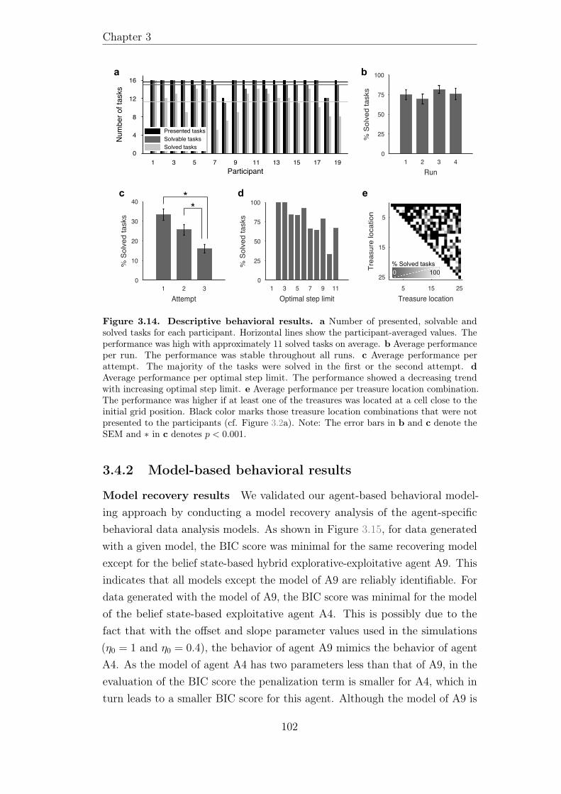
Chapter 3

a

1 2 3 4Run

0

25

50

75

100

%So

lved

tasks

1 3 5 7 9 11Optimal step limit

0

25

50

75

100

%So

lved

tasks

Agent0

4

8

12

16

Num

bero

fsolvedtasks

1 2 3 4 5 6 7 8 9 10 11 12 13 14 15 16 17 18 19Participant

600

400

200BICscore

8000

Cum

ulativeBICscore

0.8

1

Exceed

ance

prob

ability

0

Participant

16

12

8

4

01 3 5 7 9 11 13 15 17 19

Num

bero

ftasks

1 2 3 4 5 6 7 8 9 10111213141516171819Participants

Presented tasksSolvable tasksSolved tasks

Agent models0

4

8

12

16

Num

bero

fsolvedtasks

1 2 3 4 5 6 7 8 9 10 11 12 13 14 15 16 17 18 19Participants

1

Exceed

ance

prob

ability

Agent models0

0.2

0.4

0.6

0.8

1

%So

lved

tasks

1 2 3 4 5 6 7 8 9 10111213141516171819Participants

Presented tasksSolvable tasksSolved tasks

Agent models0

4

8

12

16

Num

bero

fsolvedtasks

1 2 3 4 5 6 7 8 9 10 11 12 13 14 15 16 17 18 19Participants

1

Exceed

ance

prob

ability

Agent models0

0.2

0.4

0.6

0.8

1

%So

lved

tasks

1 2 3Attempt

0

10

20

30

40

%So

lved

tasks

c

0

10

20

30

40

%So

lved

tasks

1 3 5 7 9 11 13 15 17 19

Participants

C **

10

20

30

40

%So

lved

tasks

1 3 5 7 9 11 13 15 17 19

Participants

C **

1 2 3 4Run

0

25

50

75

100

%So

lved

tasks

1 2 3Attempt

0

10

20

30

40

%So

lved

tasks

1 3 5 7 9 11Optimal step limit

0

25

50

75

100

%So

lved

tasks

5 15 25Treasure location

5

15

25

Trea

sure

location

% Solved tasks

e

b

1 2 3

Attempts

0

10

20

30

%Solvedtasks

1 2 3 4

Runs

0

25

50

75

%Solvedtasks

ED

1 3 5 7 9 11

Shortest path

0

25

50

75

100

%Solvedtasks

5 15 25

Target location

5

15

25

Target

location

*

% Solved tasks

0 100

1 2 3 4Run

0

25

50

75

100

%So

lved

tasks

1 2 3Attempt

0

10

20

30

40

%So

lved

tasks

1 3 5 7 9 11Optimal step limit

0

25

50

75

100

%So

lved

tasks

5 15 25Treasure location

5

15

25

Trea

sure

location

d

Figure 3.14. Descriptive behavioral results. a Number of presented, solvable andsolved tasks for each participant. Horizontal lines show the participant-averaged values. Theperformance was high with approximately 11 solved tasks on average. b Average performanceper run. The performance was stable throughout all runs. c Average performance perattempt. The majority of the tasks were solved in the first or the second attempt. dAverage performance per optimal step limit. The performance showed a decreasing trendwith increasing optimal step limit. e Average performance per treasure location combination.The performance was higher if at least one of the treasures was located at a cell close to theinitial grid position. Black color marks those treasure location combinations that were notpresented to the participants (cf. Figure 3.2a). Note: The error bars in b and c denote theSEM and ∗ in c denotes p < 0.001.

3.4.2 Model-based behavioral results

Model recovery results We validated our agent-based behavioral model-ing approach by conducting a model recovery analysis of the agent-specificbehavioral data analysis models. As shown in Figure 3.15, for data generatedwith a given model, the BIC score was minimal for the same recovering modelexcept for the belief state-based hybrid explorative-exploitative agent A9. Thisindicates that all models except the model of A9 are reliably identifiable. Fordata generated with the model of A9, the BIC score was minimal for the modelof the belief state-based exploitative agent A4. This is possibly due to thefact that with the offset and slope parameter values used in the simulations(η0 = 1 and η0 = 0.4), the behavior of agent A9 mimics the behavior of agentA4. As the model of agent A4 has two parameters less than that of A9, in theevaluation of the BIC score the penalization term is smaller for A4, which inturn leads to a smaller BIC score for this agent. Although the model of A9 is

102

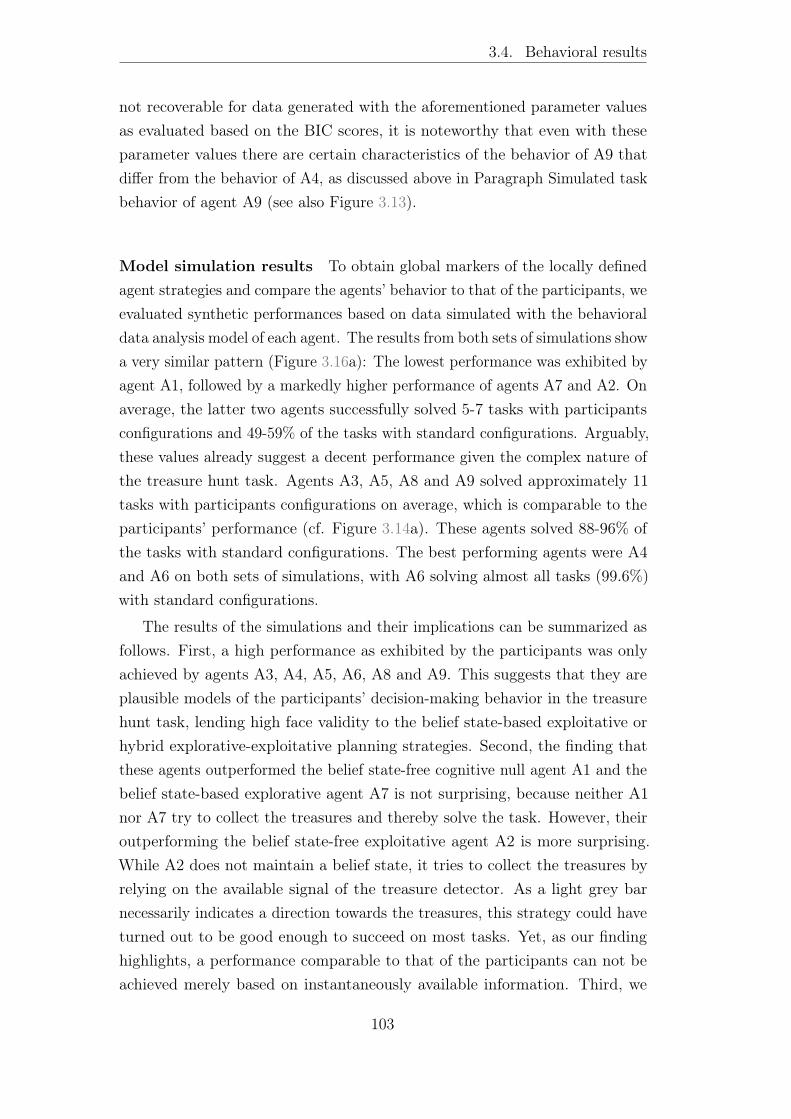
3.4. Behavioral results

not recoverable for data generated with the aforementioned parameter valuesas evaluated based on the BIC scores, it is noteworthy that even with theseparameter values there are certain characteristics of the behavior of A9 thatdiffer from the behavior of A4, as discussed above in Paragraph Simulated taskbehavior of agent A9 (see also Figure 3.13).

Model simulation results To obtain global markers of the locally definedagent strategies and compare the agents’ behavior to that of the participants, weevaluated synthetic performances based on data simulated with the behavioraldata analysis model of each agent. The results from both sets of simulations showa very similar pattern (Figure 3.16a): The lowest performance was exhibited byagent A1, followed by a markedly higher performance of agents A7 and A2. Onaverage, the latter two agents successfully solved 5-7 tasks with participantsconfigurations and 49-59% of the tasks with standard configurations. Arguably,these values already suggest a decent performance given the complex nature ofthe treasure hunt task. Agents A3, A5, A8 and A9 solved approximately 11tasks with participants configurations on average, which is comparable to theparticipants’ performance (cf. Figure 3.14a). These agents solved 88-96% ofthe tasks with standard configurations. The best performing agents were A4and A6 on both sets of simulations, with A6 solving almost all tasks (99.6%)with standard configurations.

The results of the simulations and their implications can be summarized asfollows. First, a high performance as exhibited by the participants was onlyachieved by agents A3, A4, A5, A6, A8 and A9. This suggests that they areplausible models of the participants’ decision-making behavior in the treasurehunt task, lending high face validity to the belief state-based exploitative orhybrid explorative-exploitative planning strategies. Second, the finding thatthese agents outperformed the belief state-free cognitive null agent A1 and thebelief state-based explorative agent A7 is not surprising, because neither A1nor A7 try to collect the treasures and thereby solve the task. However, theiroutperforming the belief state-free exploitative agent A2 is more surprising.While A2 does not maintain a belief state, it tries to collect the treasures byrelying on the available signal of the treasure detector. As a light grey barnecessarily indicates a direction towards the treasures, this strategy could haveturned out to be good enough to succeed on most tasks. Yet, as our findinghighlights, a performance comparable to that of the participants can not beachieved merely based on instantaneously available information. Third, we

103

Chapter 3

found that of the belief state-based agents, the purely exploitative strategyof A6 prevailed. This agent exhibited a nearly perfect performance on theset of simulations with standard configurations. This suggests that optimalbehavior in the treasure hunt task - by means of task solution given the standardconfigurations - requires belief state-based exploitative planning from the outset.It is notable that agent A6 implements the most advanced belief state-basedexploitative planning strategy by dynamically switching between the strategiesof agents A4 and A5.

A3

A5A6

A7

A8A9

A4

A1A2

Agentmodels

-10000

-8000

-6000

-4000

-2000

Cumulative BIC score

0

0.2

0.4

0.6

0.8

Exceedance probability

Agentmodels

-10000

-8000

-6000

-4000

-2000

Cumulative BIC score

0

0.2

0.4

0.6

0.8

Exceedance probability

Agentmodels

-10000

-8000

-6000

-4000

-2000

Agentmodels

0

0.2

0.4

0.6

0.8

Exceedance probability

Agentmodels

-10000

-8000

-6000

-4000

-2000

Agentmodels

0

0.2

0.4

0.6

0.8

Exceedance probability

Agentmodels

-10000

-8000

-6000

-4000

-2000

Agentmodels

0

0.2

0.4

0.6

0.8

Exceedance probability

Agentmodels

-10000

-8000

-6000

-4000

-2000

Agentmodels

0

0.2

0.4

0.6

0.8

Exceedance probability

Agentmodels

-10000

-8000

-6000

-4000

-2000

Agentmodels

0

0.2

0.4

0.6

0.8

Exceedance probability

Agentmodels

-10000

-8000

-6000

-4000

-2000

Agentmodels

0

0.2

0.4

0.6

0.8

Exceedance probability

Agentmodels

-10000

-8000

-6000

-4000

-2000

Agentmodels

0

0.2

0.4

0.6

0.8

Exceedance probability

Data generating agent

0

10

20

30

40

BICsc

ore

A1 A2 A5 A6 A7 A8A3 A4 A9

Figure 3.15. Model recovery results. Y-axis shows the average BIC score of eachagent-specific behavioral data analysis model evaluated on the synthetic data sets of eachdata generating model shown on the x-axis. For data generated with a given model, theBIC score was minimal for the corresponding model indicating that the models are reliablyrecoverable. The only exception is the model of agent A9. For data generated with the modelof agent A9, the BIC score was minimal for the model of its constituent agent A4.

Model comparison results We evaluated and compared the agent-specificbehavioral data analysis models based on the participants’ data. As shown inFigure 3.16b, for 15 of the 19 participants the BIC score was minimal under themodel of agent A5. Accordingly, the group cumulative BIC score was minimalfor this agent showing that among the set of models assessed the belief state-based exploitative planning strategy of A5 explained participants’ behaviorthe best (left panel of Figure 3.16c). This conclusion is further supported bythe result of the random-effects Bayesian model selection: The group-levelprotected exceedance probability of the model of A5 was larger than 0.99indicating that within the group of participants the most frequently appliedstrategy resembled that of agent A5 (right panel of Figure 3.16c). On average,the winning A5 model explained 35.65%± 2.06 of the participants actions asevaluated by the pseudo-r2 statistic. Given the complexity of the treasure hunttask, this ρ value suggests a considerably good model fit.

104

3.5. FMRI methods

A3

A5A6

A7

A8A9

A4

A1A2

BF-0 BF-R BB-R-1 BB-R-2 BB-R-25 BB-R-25-2 BB-I BB-H-C BB-H-EData generating model

0

10

20

30

40BICscore

1 3 5 7 9 11 13 15 17 19Participant

0

4

8

12

16

Num

bero

ftasks

1 2 3 4 5 6 7 8 9 10 11 12 13 14 15 16 17 18 19Participant

600

400

200BICscore

y

0

Agent0

4

8

12

16

Num

bero

fsolvedtasks

Agent0

0.2

0.4

0.6

0.8

1

%So

lved

tasks

ba

d

c

Presented tasksSolvable tasksSolved tasks

Agent

2000

4000

6000

8000

0Cum

ulativeBICscore

Agent0

0.2

0.4

0.6

0.8

1

Exceed

ance

prob

ability

e f

Agent

2000

4000

6000

8000

0Cum

ulativeBICscore

Agent0

0.2

0.4

0.6

0.8

1

Exceed

ance

prob

ability

e f

BF-0BF-R

10 11 12 13 14 15 16 17 18 19Participant

Agent0

4

8

12

16Num

bero

fsolvedtasks

Agent0

0.2

0.4

0.6

0.8

1

%So

lved

tasks

b c

9 10 11 12 13 14 15 16 17 18 19Participant

Agent0

4

8

12

16

Num

bero

fsolvedtasks

Agent0

0.2

0.4

0.6

0.8

1

%So

lved

tasks

b c ca

b

Figure 3.16. Model simulation and comparison results. a Synthetic agent perfor-mances evaluated based on the set of simulations with participants (left panel) and standard(right panel) configurations. The results from both analyses are similar: The highest perfor-mance was achieved by the belief state-based exploitative and hybrid exploitative-explorativeagents, with a level comparable to that of the participants (cf. Figure 3.14a). b Participant-level BIC scores. For the majority of the participants (15 of 19), the BIC score was minimalfor the model of agent A5. c Group-level cumulative BIC scores (left panel) and protectedexceedance probabilities (right panel). The cumulative BIC score was minimal and theprotected exceedance probability was maximal for the model of A5, providing evidence infavor of the belief state-based exploitative planning strategy of this agent.

3.5 FMRI methods

3.5.1 FMRI data acquisition and preprocessing

Functional imaging was performed on a 3T Siemens Magnetom Tim Trio MRIscanner (Siemens, Erlangen, Germany) with a 12-channel head coil. Duringtask completion, 36 interleaved axial slices (flip angle: 80, slice thickness: 3mm, voxel size: 3×3×3 mm3, distance factor: 20%) of T2∗-weighted echo-planar images (EPIs) (field of view: 216 mm) were acquired each 2000 ms. Oneach run, the data acquisition was terminated manually when the participantcompleted the tasks. Therefore, the number of volumes varied across runs, witha maximum of 600 volumes per run. To allow for the signal to saturate, the first 3images of each run were discarded. Before the first run, T1-weighted anatomicalimages (voxel size: 1×1×1 mm3, field of view: 256 mm) were additionallyacquired. The fMRI data were preprocessed and analyzed using SPM12. Toprepare the participants’ EPIs for analysis, each data set was motion-correctedby realigning the images to the first scan of the first run, normalized to theMontreal Neurological Institute (MNI) EPI reference template, and re-sampledto 2 mm isotropic voxel size. The images were subsequently smoothed using an

105

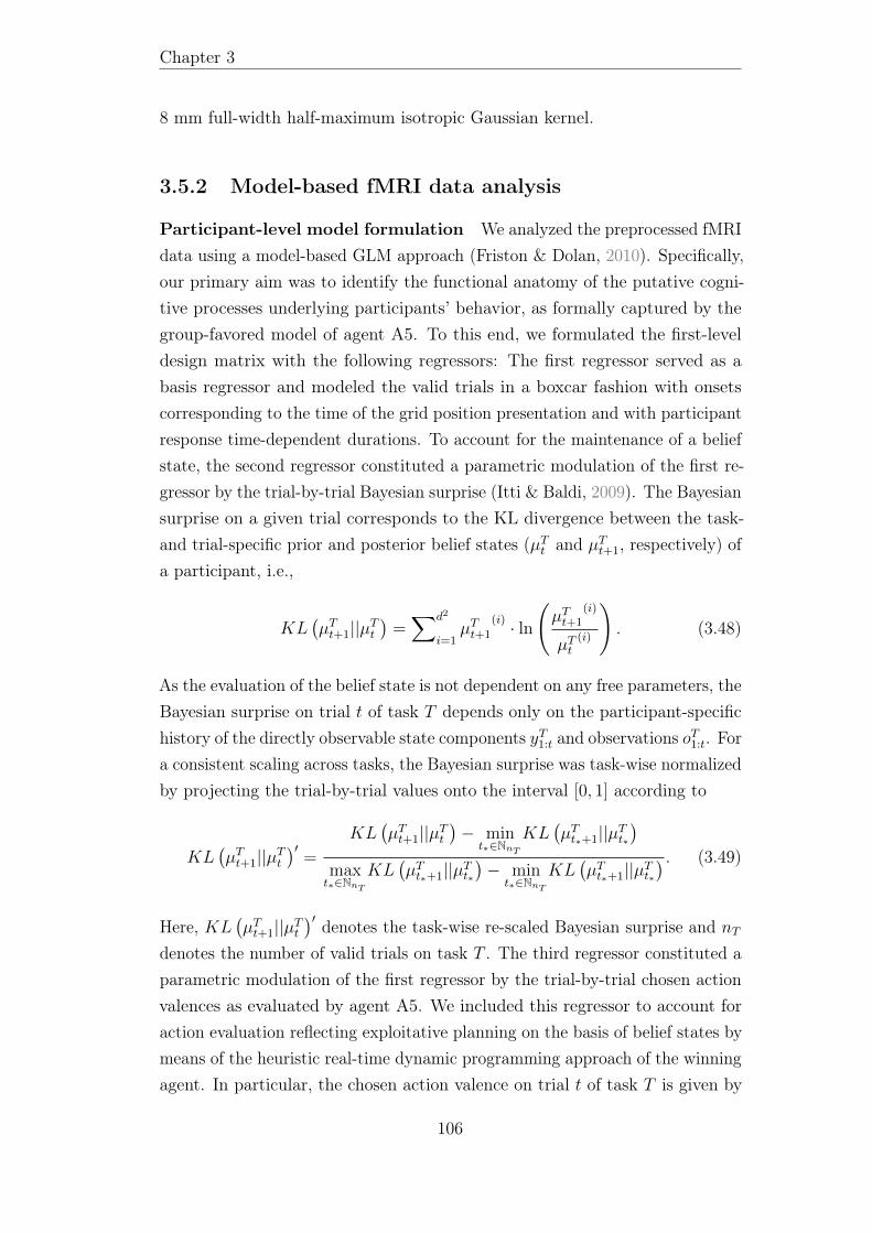
Chapter 3

8 mm full-width half-maximum isotropic Gaussian kernel.

3.5.2 Model-based fMRI data analysis

Participant-level model formulation We analyzed the preprocessed fMRIdata using a model-based GLM approach (Friston & Dolan, 2010). Specifically,our primary aim was to identify the functional anatomy of the putative cogni-tive processes underlying participants’ behavior, as formally captured by thegroup-favored model of agent A5. To this end, we formulated the first-leveldesign matrix with the following regressors: The first regressor served as abasis regressor and modeled the valid trials in a boxcar fashion with onsetscorresponding to the time of the grid position presentation and with participantresponse time-dependent durations. To account for the maintenance of a beliefstate, the second regressor constituted a parametric modulation of the first re-gressor by the trial-by-trial Bayesian surprise (Itti & Baldi, 2009). The Bayesiansurprise on a given trial corresponds to the KL divergence between the task-and trial-specific prior and posterior belief states (µTt and µTt+1, respectively) ofa participant, i.e.,

KL(µTt+1||µTt

)=∑d2

i=1µTt+1

(i) · ln

(µTt+1

(i)

µTt(i)

). (3.48)

As the evaluation of the belief state is not dependent on any free parameters, theBayesian surprise on trial t of task T depends only on the participant-specifichistory of the directly observable state components yT1:t and observations oT1:t. Fora consistent scaling across tasks, the Bayesian surprise was task-wise normalizedby projecting the trial-by-trial values onto the interval [0, 1] according to

KL(µTt+1||µTt

)′=

KL(µTt+1||µTt

)− min

t∗∈NnT

KL(µTt∗+1||µTt∗

)maxt∗∈NnT

KL(µTt∗+1||µTt∗

)− min

t∗∈NnT

KL(µTt∗+1||µTt∗

) . (3.49)

Here, KL(µTt+1||µTt

)′ denotes the task-wise re-scaled Bayesian surprise and nTdenotes the number of valid trials on task T . The third regressor constituted aparametric modulation of the first regressor by the trial-by-trial chosen actionvalences as evaluated by agent A5. We included this regressor to account foraction evaluation reflecting exploitative planning on the basis of belief states bymeans of the heuristic real-time dynamic programming approach of the winningagent. In particular, the chosen action valence on trial t of task T is given by

106

3.5. FMRI methods

the negative sum of the belief-weighted l1 distances between the new positionresulting from the participant’s action aTt and each node of the grid, i.e.,

vA5(aTt ) = −

∑d2

i=1µTt+1

(i) · l1(sTt

(1)+ aTt , i

)(3.50)

(cf. eq. 3.34). As in the case of the Bayesian surprise, the chosen actionvalence does not depend on any free parameters and for action aTt is evaluateddirectly based on the participant-specific history of the directly observable statecomponents yT1:t and observations oT1:t. Before combining the first regressor withthe chosen action valences, they were also task-wise normalized on the interval[0, 1] as

vA5(aTt )′=

vA5(aTt )− min

t∗∈NnT

vA5(aTt∗)

maxt∗∈NnT

vA5(aTt∗)− mint∗∈NnT

vA5(aTt∗)(3.51)

for a consistent scaling across tasks. In addition to the model-based parametricregressors, as the fourth regressor we included a parametric modulation ofthe first regressor by the trial-by-trial average luminance to account for theconfounding effect of varying light intensity across trials. To obtain trial-by-trial average luminance values, we first calculated the luminance of a three-dimensional RGB image I ∈ RJ×K×3 according to

l(I) =1

JK

∑J

j=1

∑K

k=10.299I(jk1) + 0.587I(jk2) + 0.114I(jk3) (3.52)

and subsequently calculated the average luminance across the images presentedto a participant on trial t of task T (Parekh, 2006). Finally, we also includedthree regressors modeling additional task events with 0-duration pulses at theevent onsets. Specifically, the fifth regressor modeled the treasure discovery (i.e.,grid positions with a treasure), the sixth regressor modeled the informationdisplay presented after each attempt and task, and the seventh regressormodeled the fixation crosses presented after every fourth attempt. Of note,the parametric regressors were only weakly correlated (the run- and subject-averaged correlation coefficient was 0.33± 0.02 between Bayesian surprise andchosen action valence, 0.25± 0.01 between Bayesian surprise and luminance,and 0.16± 0.03 between chosen action valence and luminance) and all sevenregressors, referred to as regressors of interest, were entered in the participant-level design matrix without serial orthogonalization.

The regressors of interest were convolved with the canonical hemodynamicresponse function (HRF) and, as per SPM default, low frequency components

107

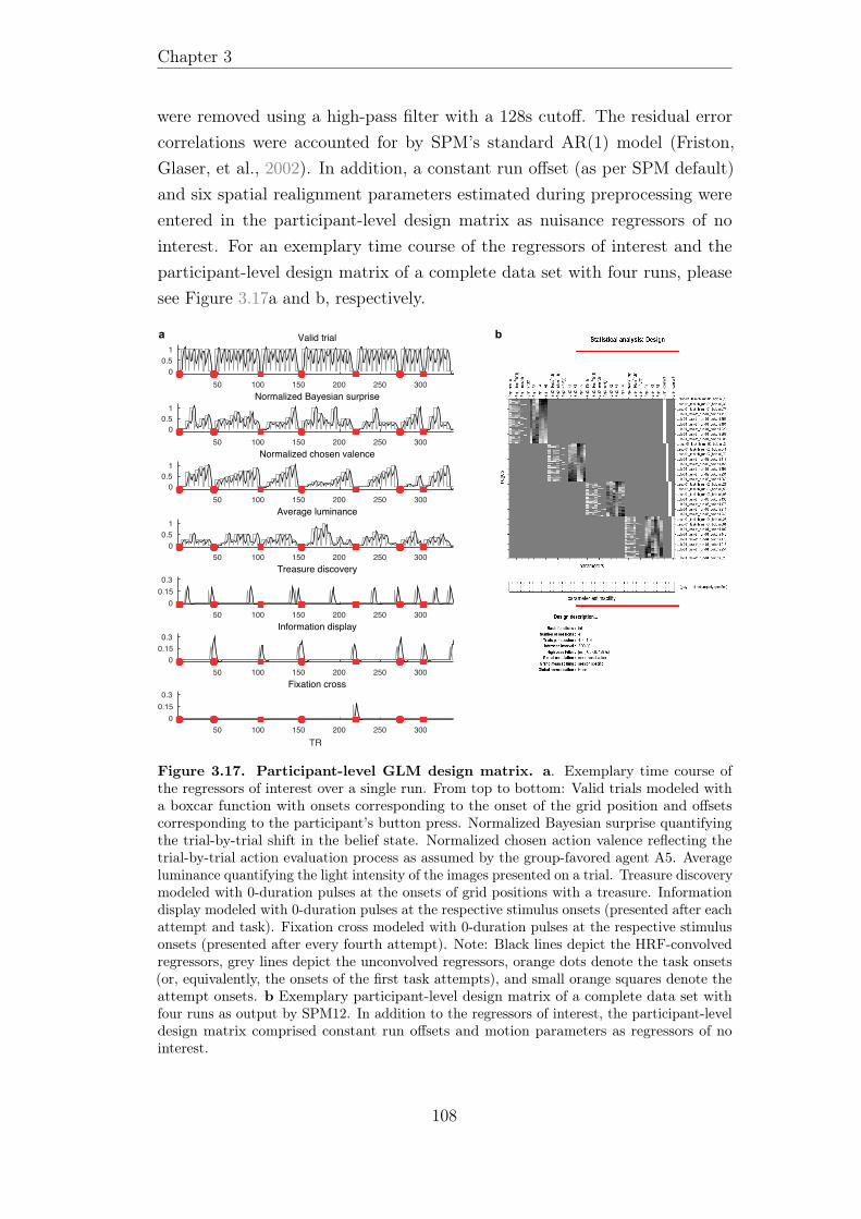
Chapter 3

were removed using a high-pass filter with a 128s cutoff. The residual errorcorrelations were accounted for by SPM’s standard AR(1) model (Friston,Glaser, et al., 2002). In addition, a constant run offset (as per SPM default)and six spatial realignment parameters estimated during preprocessing wereentered in the participant-level design matrix as nuisance regressors of nointerest. For an exemplary time course of the regressors of interest and theparticipant-level design matrix of a complete data set with four runs, pleasesee Figure 3.17a and b, respectively.

50 100 150 200 250 3000

0.51

Valid trial

50 100 150 200 250 3000

0.51

Normalized Bayesian surprise

50 100 150 200 250 3000

0.51

Normalized chosen valence

50 100 150 200 250 3000

0.51

Average luminance

50 100 150 200 250 3000

0.150.3

Treasure discovery

50 100 150 200 250 3000

0.150.3

Information display

50 100 150 200 250 300TR

00.150.3

Fixation cross

a

50 100 150 200 250 3000

0.51

Valid trial

50 100 150 200 250 3000

0.51

Normalized Bayesian surprise

50 100 150 200 250 3000

0.51

Normalized chosen valence

50 100 150 200 250 3000

0.51

Average luminance

50 100 150 200 250 3000

0.150.3

Treasure discovery

50 100 150 200 250 3000

0.150.3

Information display

50 100 150 200 250 300TR

00.150.3

Fixation cross

b

Figure 3.17. Participant-level GLM design matrix. a. Exemplary time course ofthe regressors of interest over a single run. From top to bottom: Valid trials modeled witha boxcar function with onsets corresponding to the onset of the grid position and offsetscorresponding to the participant’s button press. Normalized Bayesian surprise quantifyingthe trial-by-trial shift in the belief state. Normalized chosen action valence reflecting thetrial-by-trial action evaluation process as assumed by the group-favored agent A5. Averageluminance quantifying the light intensity of the images presented on a trial. Treasure discoverymodeled with 0-duration pulses at the onsets of grid positions with a treasure. Informationdisplay modeled with 0-duration pulses at the respective stimulus onsets (presented after eachattempt and task). Fixation cross modeled with 0-duration pulses at the respective stimulusonsets (presented after every fourth attempt). Note: Black lines depict the HRF-convolvedregressors, grey lines depict the unconvolved regressors, orange dots denote the task onsets(or, equivalently, the onsets of the first task attempts), and small orange squares denote theattempt onsets. b Exemplary participant-level design matrix of a complete data set withfour runs as output by SPM12. In addition to the regressors of interest, the participant-leveldesign matrix comprised constant run offsets and motion parameters as regressors of nointerest.

108

3.6. FMRI results

3.5.3 Participant- and group-level model estimation and

evaluation

We estimated the parameters of the participant-level GLM using SPM’s re-stricted maximum likelihood scheme (Friston, Penny, et al., 2002). We subse-quently evaluated contrasted parameter estimates, first for the positive maineffects of valid trials, luminance, treasure discovery and information display tovalidate the fMRI data quality, and then for the positive and negative maineffects of the Bayesian surprise and chosen action valence to identify brainregions encoding model-based quantities. For example, we used the contrastvector c = (0, 1, 0, 0, 0, 0, 0)T to evaluate the positive main effect of Bayesiansurprise. The resulting eight contrast images were entered for group-level voxel-wise one-sample t-tests. We applied a cluster-forming threshold of p < 0.001

(uncorrected) to the t-statistic maps and report the clusters with a family-wiseerror (FWE) corrected p-value smaller than 0.05. Anatomical labels wereobtained using the third version of the Automated Anatomical Atlas (AAL3;Rolls, Huang, Lin, Feng, and Joliot, 2020).

3.6 FMRI results

3.6.1 FMRI data validation

Before interrogating the fMRI data for model-based effects, we conducted aset of analyses to investigate the neural underpinnings of cognitive processesinvolved in the treasure hunt task, which are not specifically assumed by thegroup-favored agent model A5. In particular, we evaluated the positive maineffects of valid trials, luminance, treasure discovery, and information display.We reasoned that these regressors would capture variability in the fMRI dataprimarily related to movement planning and execution, visual processing,reward processing, and reading, respectively. Importantly, the goal of theseanalyses was to test if we can detect activity clusters in brain regions commonlyimplicated in the respective putative cognitive processes and to thereby validatethe quality of our fMRI data. Therefore, we do not present these results indetail but show that they largely corroborate the validity of the fMRI dataquality.

As shown in Figure 3.18, testing for the positive main effects of valid trialsrevealed a large cluster extending through mainly left-hemispheric areas of the

109

Chapter 3

pre- and postcentral gyri, supplementary motor area, middle cingulate gyrus,inferior parietal cortex, insula, rolandic operculum, putamen, pallidum andthalamus, consistent with participants using their right hand for button press(e.g., Ebbesen and Brecht, 2017; Gazzaniga, Ivry, and Mangun, 2013). Fora list of all clusters, please refer to Supplementary Table B.1. As expected,activation in the bilateral visual cortex comprising parts of the superior andmiddle occipital gyri, calcarine sulcus and surrounding cortex, cuneus, as wellas the lingual and fusiform gyri scaled positively with the trial-by-trial stimuliluminance, among other regions (eg., Gazzaniga et al., 2013; Grill-Spectorand Malach, 2004; Supplementary Table B.2). For the positive main effects oftreasure discovery and information display, we obtained single activity clustersspanning the majority of the brain. Specifically, both treasure discovery andinformation display engaged a similar extended bilateral network of cortical andsubcortical areas, indicating the involvement of additional and partly sharedcognitive processes at these events, over and above those hypothesized. Forexample, both analyses revealed increased activity in the hippocampus and theparahippocampus, which are typically not associated with reward processingor reading but have established roles in memory formation and recall (eg.,Eichenbaum, 2017; Gazzaniga et al., 2013). Nevertheless, in keeping with ourexpectations, for the positive main effects of treasure discovery, the obtainedlarge activity cluster also comprised classic reward regions, such as the bilateraldorsal and ventral striatum, insula, ventromedial prefrontal cortex, and ventraltagmental area (Bartra, McGuire, and Kable, 2013; Morales and Margolis,2017; Supplementary Table B.3). While the activity pattern was similar forthe positive main effects of information display, the obtained large activitycluster did not comprise the ventral striatum and the ventral tagmental area.It however comprised all regions commonly implicated in reading, includingthe bilateral lateral frontal cortex, supplementary motor areas as well as thetemporal and occipital lobes, with slightly more extended activity in the lefthemisphere (Martin, Schurz, Kronbichler, and Richlan, 2015; SupplementaryTable B.4).

3.6.2 Model-based fMRI results

After validating the fMRI data quality, we commenced with investigating theneural substrates of the trial-by-trial cognitive processes belief state maintenanceand action evaluation as assumed by the behaviorally most plausible agentmodel A5. To this end, we evaluated the main effects of the model-based

110

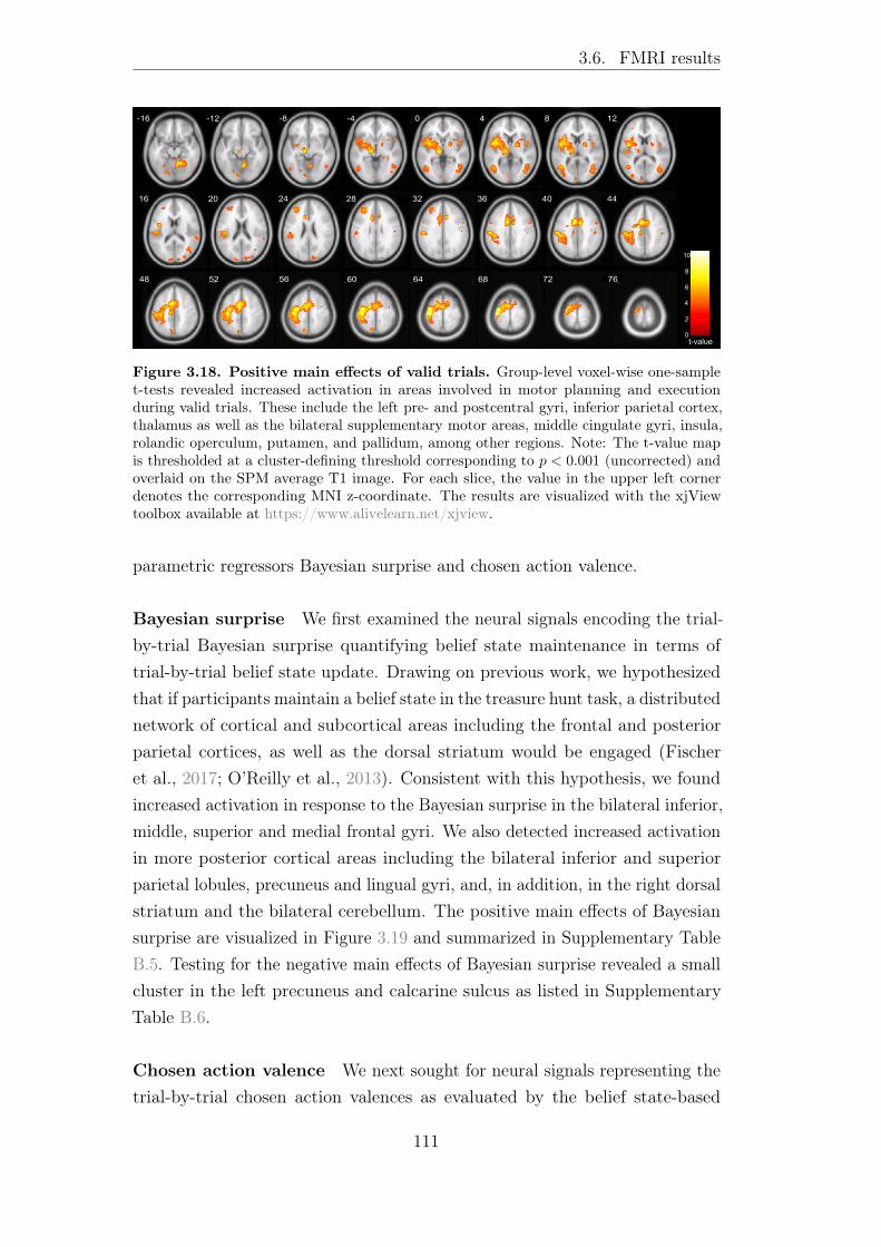
3.6. FMRI results

0

2

4

6

8

10

t-value

-16 -12 -8 -4 0 4 8 12

16 20 24 28 32 36 40 44

48 52 56 60 64 68 72 76

Figure 3.18. Positive main effects of valid trials. Group-level voxel-wise one-samplet-tests revealed increased activation in areas involved in motor planning and executionduring valid trials. These include the left pre- and postcentral gyri, inferior parietal cortex,thalamus as well as the bilateral supplementary motor areas, middle cingulate gyri, insula,rolandic operculum, putamen, and pallidum, among other regions. Note: The t-value mapis thresholded at a cluster-defining threshold corresponding to p < 0.001 (uncorrected) andoverlaid on the SPM average T1 image. For each slice, the value in the upper left cornerdenotes the corresponding MNI z-coordinate. The results are visualized with the xjViewtoolbox available at https://www.alivelearn.net/xjview.

parametric regressors Bayesian surprise and chosen action valence.

Bayesian surprise We first examined the neural signals encoding the trial-by-trial Bayesian surprise quantifying belief state maintenance in terms oftrial-by-trial belief state update. Drawing on previous work, we hypothesizedthat if participants maintain a belief state in the treasure hunt task, a distributednetwork of cortical and subcortical areas including the frontal and posteriorparietal cortices, as well as the dorsal striatum would be engaged (Fischeret al., 2017; O’Reilly et al., 2013). Consistent with this hypothesis, we foundincreased activation in response to the Bayesian surprise in the bilateral inferior,middle, superior and medial frontal gyri. We also detected increased activationin more posterior cortical areas including the bilateral inferior and superiorparietal lobules, precuneus and lingual gyri, and, in addition, in the right dorsalstriatum and the bilateral cerebellum. The positive main effects of Bayesiansurprise are visualized in Figure 3.19 and summarized in Supplementary TableB.5. Testing for the negative main effects of Bayesian surprise revealed a smallcluster in the left precuneus and calcarine sulcus as listed in SupplementaryTable B.6.

Chosen action valence We next sought for neural signals representing thetrial-by-trial chosen action valences as evaluated by the belief state-based

111

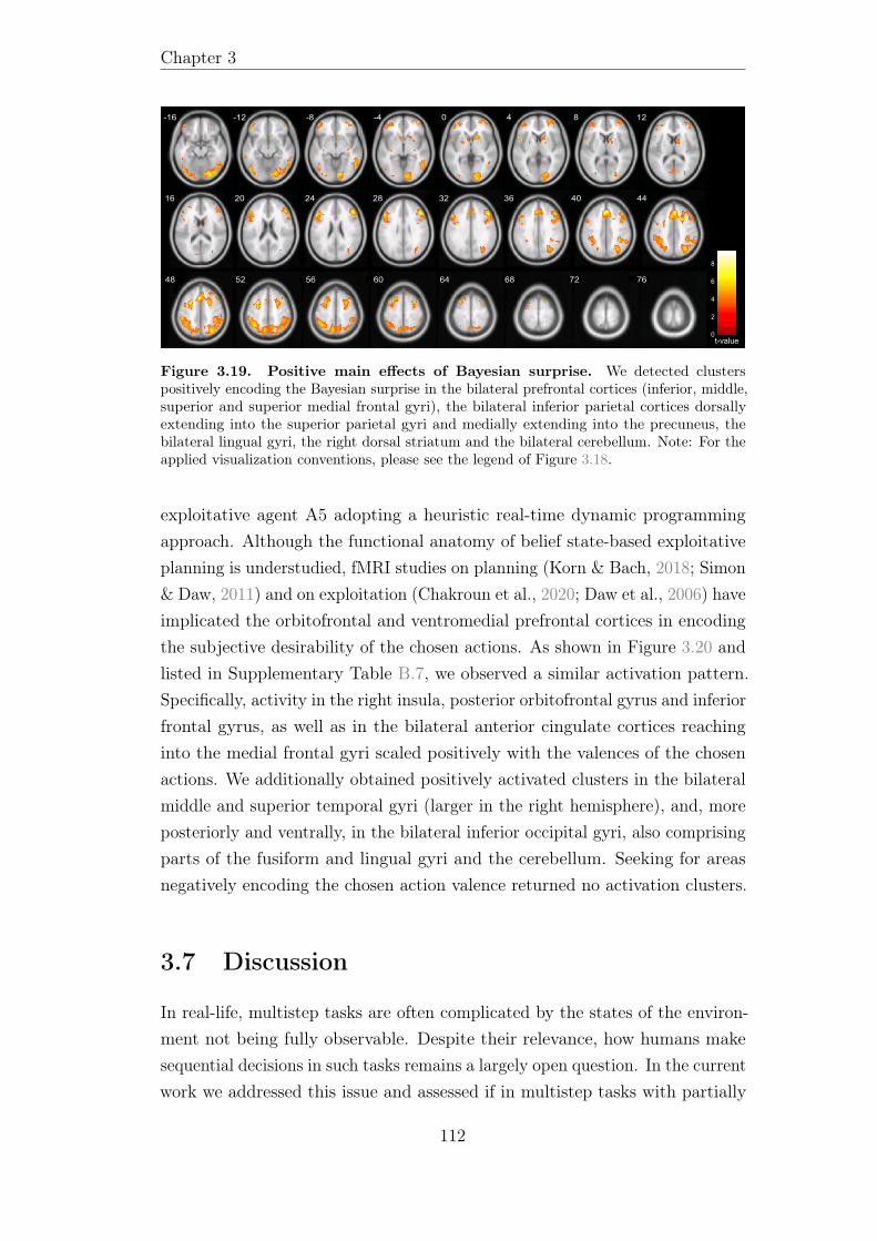
Chapter 3

-16 -12 -8 -4 0 4 8 12

16 20 24 28 32 36 40 44

48 52 56 60 64 68 72 76

0

2

4

6

8

t-value

Figure 3.19. Positive main effects of Bayesian surprise. We detected clusterspositively encoding the Bayesian surprise in the bilateral prefrontal cortices (inferior, middle,superior and superior medial frontal gyri), the bilateral inferior parietal cortices dorsallyextending into the superior parietal gyri and medially extending into the precuneus, thebilateral lingual gyri, the right dorsal striatum and the bilateral cerebellum. Note: For theapplied visualization conventions, please see the legend of Figure 3.18.

exploitative agent A5 adopting a heuristic real-time dynamic programmingapproach. Although the functional anatomy of belief state-based exploitativeplanning is understudied, fMRI studies on planning (Korn & Bach, 2018; Simon& Daw, 2011) and on exploitation (Chakroun et al., 2020; Daw et al., 2006) haveimplicated the orbitofrontal and ventromedial prefrontal cortices in encodingthe subjective desirability of the chosen actions. As shown in Figure 3.20 andlisted in Supplementary Table B.7, we observed a similar activation pattern.Specifically, activity in the right insula, posterior orbitofrontal gyrus and inferiorfrontal gyrus, as well as in the bilateral anterior cingulate cortices reachinginto the medial frontal gyri scaled positively with the valences of the chosenactions. We additionally obtained positively activated clusters in the bilateralmiddle and superior temporal gyri (larger in the right hemisphere), and, moreposteriorly and ventrally, in the bilateral inferior occipital gyri, also comprisingparts of the fusiform and lingual gyri and the cerebellum. Seeking for areasnegatively encoding the chosen action valence returned no activation clusters.

3.7 Discussion

In real-life, multistep tasks are often complicated by the states of the environ-ment not being fully observable. Despite their relevance, how humans makesequential decisions in such tasks remains a largely open question. In the currentwork we addressed this issue and assessed if in multistep tasks with partially

112

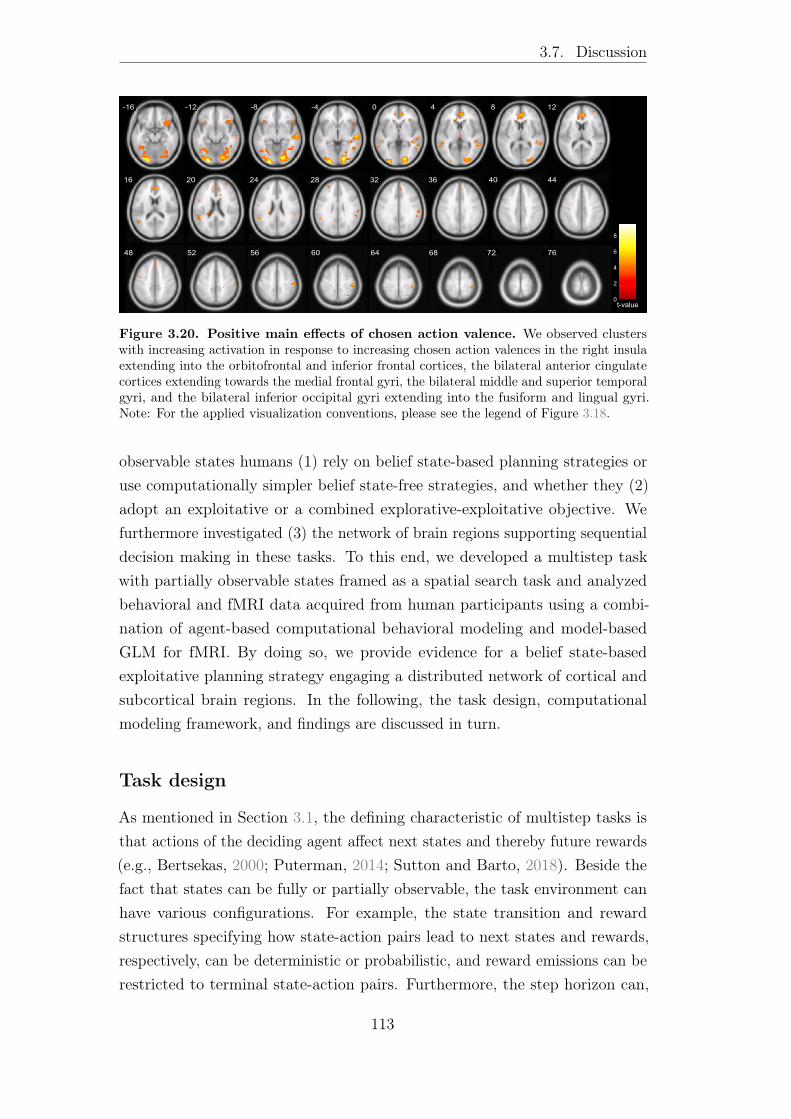
3.7. Discussion

-16 -12 -8 -4 0 4 8 12

16 20 24 28 32 36 40 44

48 52 56 60 64 68 72 76

0

2

4

6

8

t-value

Figure 3.20. Positive main effects of chosen action valence. We observed clusterswith increasing activation in response to increasing chosen action valences in the right insulaextending into the orbitofrontal and inferior frontal cortices, the bilateral anterior cingulatecortices extending towards the medial frontal gyri, the bilateral middle and superior temporalgyri, and the bilateral inferior occipital gyri extending into the fusiform and lingual gyri.Note: For the applied visualization conventions, please see the legend of Figure 3.18.

observable states humans (1) rely on belief state-based planning strategies oruse computationally simpler belief state-free strategies, and whether they (2)adopt an exploitative or a combined explorative-exploitative objective. Wefurthermore investigated (3) the network of brain regions supporting sequentialdecision making in these tasks. To this end, we developed a multistep taskwith partially observable states framed as a spatial search task and analyzedbehavioral and fMRI data acquired from human participants using a combi-nation of agent-based computational behavioral modeling and model-basedGLM for fMRI. By doing so, we provide evidence for a belief state-basedexploitative planning strategy engaging a distributed network of cortical andsubcortical brain regions. In the following, the task design, computationalmodeling framework, and findings are discussed in turn.

Task design

As mentioned in Section 3.1, the defining characteristic of multistep tasks isthat actions of the deciding agent affect next states and thereby future rewards(e.g., Bertsekas, 2000; Puterman, 2014; Sutton and Barto, 2018). Beside thefact that states can be fully or partially observable, the task environment canhave various configurations. For example, the state transition and rewardstructures specifying how state-action pairs lead to next states and rewards,respectively, can be deterministic or probabilistic, and reward emissions can berestricted to terminal state-action pairs. Furthermore, the step horizon can,

113

Chapter 3

in principle, range from two to infinity. In the treasure hunt task, to focus onpartially observable states, we opted for simple deterministic state transitionand reward structures, with reward emissions restricted to terminal state-actionpairs: participants’ position changed according to their directional decisionand they were only rewarded if they found both treasures. The step horizondepended on the combination of the treasure locations, with most combinationsrequiring participants to make decisions over six steps.

Tasks employed in two recent studies investigating model-free decisionmaking versus planning in multistep tasks with fully observable states share keyfeatures with the treasure hunt task: The reward structures in the tasks bothby Korn and Bach (2018) and Simon and Daw (2011) are also deterministic,and reward emissions in the task by Korn and Bach (2018) are restricted toterminal state-action pairs as in our task. However, different from our task,state-transition structures of both tasks are probabilistic. With respect to thestep horizon, participants interact with the task by Korn and Bach (2018) overfive steps, whereas they interact with the task by Simon and Daw (2011) overa total of one thousand steps. Although the step horizon of the task by Kornand Bach (2018) is more similar to ours, the spatial embedding of our taskresembles the task employed by Simon and Daw (2011), while the task by Kornand Bach (2018) is framed as foraging.

Our task is also closely related to the spatial search task introduced byYoshida and Ishii (2006) to test the Bayesian brain hypothesis in the contextof sequential decision making under state uncertainty. Specifically, similar tothe treasure hunt task, in the task by Yoshida and Ishii (2006) participants areinstructed to navigate to a goal location in a grid-world by making decisionsover a minimum of ten steps under state uncertainty. Moreover, Yoshida andIshii (2006) also used deterministic state transition and reward structures withrewards emitted only for terminal state-action pairs. However, while their taskconstitutes an example of a multistep task with partially observable statessimilar to the treasure hunt task, the focus of the work by Yoshida and Ishii(2006) was not to examine various sequential decision-making strategies in suchtasks but to investigate the neurocomputational mechanisms of state estimation.To this end, they induced state uncertainty by providing participants withambiguous observations about their current position. This differs from our task,where state uncertainty results from ambiguous observations about the goallocations delivered by the treasure detector, which always shows a dark greybar in the directions leading away from the treasures and either a light or a

114

3.7. Discussion

dark grey bar in the directions leading to the treasures. Crucially, introducingstate uncertainty this way allowed us to contrast various belief state-basedplanning strategies in the treasure hunt task with belief state-free strategies,such as the simple but considerably effective strategy of following the light greybar as further discussed below.

Computational modeling framework

Behavioral modeling To computationally characterize sequential decisionmaking in the treasure hunt task on a behavioral level, we designed a set ofagent-based behavioral models that can interact with the task (cf. Russell andNorvig (2010)). In our model set, the belief state-free agents A1 and A2 simplyrely on immediately available information to evaluate the actions. Specifically,by merely acknowledging the available actions without differentiating betweenthem, agent A1 corresponds to a generic cognitive null model. By contrast, agentA2 adopts a relatively refined, yet computationally inexpensive strategy: Thisagent takes advantage of the fact that the light grey bars necessarily indicatedirections towards the treasures and always follows these. Model-free strategiesthat are specific to the task at hand, such as the strategy of A2, are oftencontrasted with planning strategies. For example, the aforementioned work byKorn and Bach (2018) applied a comparable approach, whereas Simon and Daw(2011) formally captured model-free decision making with a temporal-differencelearning algorithm (e.g., Daw et al. (2005) and Sutton and Barto (2018)).In their standard form, temporal-difference learning algorithms evaluate theactions in a given state based on the associated reward history. Previoustheoretical (Rao, 2010) and rodent work (Babayan, Uchida, & Gershman,2018; Starkweather, Babayan, Uchida, & Gershman, 2017) has extended thisframework by substituting states with belief states to accommodate decisionmaking under state uncertainty. However, our task design is not suited totest decision making as accounted for by belief state-based temporal differencelearning. This is because even if the agent’s memory capacity allowed for storinga value estimate for each belief state-action pair, in order for such a strategyto be effective, the agent would need to re-encounter a belief state-action pairthat has previously been associated with reward. Since the treasure locationschange upon reward emission, this is unlikely to happen beyond the first fewsteps in a new task.

The belief state-based agents of our model space perform recursive Bayesianupdating to infer the latent components of the state, i.e., the treasure locations.

115

Chapter 3

All belief state-based agents plan ahead on the basis of their thereby ensuingbelief states. However, they either pursue a purely exploitative, a purelyexplorative, or a hybrid explorative-exploitative objective. More specifically, totry to collect the treasures, the belief state-based exploitative agents A3-A6harness their accumulated knowledge about the treasure locations and evaluatethe actions using heuristic real-time dynamic programming (Geffner & Bonet,1998; Korf, 1990). The belief state-based explorative agent A7 tries to resolveits uncertainty about the treasure locations and for each action quantifies theone-step look-ahead information gain as the expected Bayesian surprise (Itti &Baldi, 2009). The belief state-based explorative-exploitative agents A8-A9 tryto resolve their uncertainty about the treasure locations and then collect these.To this end, they combine the heuristic action values of agents A3-A4 and theexpected Bayesian surprise of agent A7. The algorithmic architectures of thebelief state-based agents relate to earlier work central to our study as follows:

First, our approach to formalize belief state-based exploitative planningin the treasure hunt task is conceptually linked to the partial tree searchalgorithm used by Simon and Daw (2011) (Sutton & Barto, 2018). Althoughtheir algorithm operates on the basis of states and not belief states given thelack of state uncertainty in their task, it also accounts for planning by evaluatingthe reward-related consequences of the available actions in an approximatefashion. In contrast, Korn and Bach (2018) modelled planning by means ofoptimal action value computations. Even more similar to our formalization ofbelief state-based exploitative planning than the partial tree search algorithmof Simon and Daw (2011) is the model applied by Yoshida and Ishii (2006). Asalluded to above, these authors did not compare the behavioral plausibilityof various sequential decision-making strategies in terms of the dichotomiesbelief state-free versus belief state-based, and exploration versus exploitation.However, to uncover the neurocomputational mechanisms of state estimationin their spatial search task, they combined Bayesian state inference with aform of action evaluation, which, in essence, corresponds to the heuristicreal-time dynamic programming algorithm employed by our belief state-basedexploitative agents. Notably, the model of Yoshida and Ishii (2006) assumesaction evaluation on the basis of unitary state estimates, which is consistent withearly theoretical work (Ishii, Yoshida, & Yoshimoto, 2002). Newer theories, onthe other hand, suggest action evaluation on the basis of the entire belief state(Rao, 2010). Therefore, to further refine belief state-based exploitative planning,agents A3-A4 and A5 implement heuristic real-time dynamic programming with

116

3.7. Discussion

unitary state estimates or with the entire belief state, respectively, while agentA6 implements heuristic real-time dynamic programming both with unitarystate estimates and the entire belief state.

Second, our approach to cast belief state-based exploration as expectedBayesian surprise maximization rests on Bayesian accounts of exploration(Sun et al., 2011). By evaluating actions on the basis of the expected shiftsin the belief state, our approach more broadly links to other (Bayesian orfrequentist) methods quantifying the information gain associated with anaction (Schwartenbeck et al., 2019).

Third, as mentioned in Section 3.1, whether humans adopt a purely exploita-tive or an explorative-exploitative objective has been primarily investigatedin bandit tasks, i.e. sequential decision-making tasks where the reward struc-ture is latent and the actions only affect immediate rewards (e.g., Berry andFristedt (1985), Robbins (1952), and Sutton and Barto (2018)). To account forexploration-exploitation choice strategies in bandit tasks, quantities that cap-ture information gain with respect to the reward structure are usually combinedwith action value estimates computed based on the current knowledge aboutthe reward structure (e.g., Daw et al. (2006), Gershman (2018), and Wilsonet al. (2014); see also Chapter 2). In our approach to model belief state-basedexplorative-exploitative planning in the treasure hunt task we followed a similarlogic: Agents A8 and A9 combine the expected Bayesian surprise evaluatedby agent A7 with the heuristic action values evaluated by agents A3 and A4,respectively. In these combinations we opted for the heuristic action valuesof agents A3 and A4 as opposed to agents A5 or A6 because, by relying onunitary state estimates, they arguably represent the simplest and strongestcontrasts to belief state-based exploration.

fMRI modeling Given our behavioral model set, we found that the mostplausible explanation of participants’ actions in the treasure hunt task isprovided by the belief state-based exploitative agent A5. To identify theunderlying network of brain regions, we applied a model-based GLM approach(Friston & Dolan, 2010). Specifically, we evaluated the neural correlates oftwo key latent quantities derived from agent A5 on a trial-by-trial basis: theBayesian surprise and the chosen action valence.

The Bayesian surprise offers a readout of the maintenance of the belief stateby quantifying the extent to which the belief state changes following a newaction and observation (Itti & Baldi, 2009). Of note, the Bayesian surprise as

117

Chapter 3

entered for fMRI data analysis is computed with respect to the current trial,which is different from our formalization of belief state-based exploration, wherethe expected Bayesian surprise is computed with respect to the next trial. In thecontext of the Bayesian brain hypothesis, Bayesian surprise has been extensivelyapplied to model neural signals reflecting belief state maintenance; we thereforeopted for this quantity in our fMRI modeling approach (e.g., Fischer et al.(2017), Gijsen, Grundei, Lange, Ostwald, and Blankenburg (2020), O’Reillyet al. (2013), Ostwald et al. (2012), and Schwartenbeck et al. (2016)). However,other closely related information theoretic measures have also been employed.For example, in their effort to map the functional anatomy of hidden stateestimation, Yoshida and Ishii (2006) used the belief state entropy, which, akinto the Bayesian surprise, also declines with decreasing uncertainty.

The second key latent quantity whose neural correlates we analyzed was thechosen action valence. It corresponds to the desirability of participants’ actionsas evaluated by the heuristic real-time dynamic programming algorithm ofthe behaviorally most plausible agent A5. This quantity thus offers a readoutof exploitative planning on the basis of belief states. As the desirability ofan action is the primary variable underlying decision making, our approachis consistent with previous work aiming to uncover the neurocomputationalmechanisms of various strategies such as exploitation and exploration (e.g.,Chakroun et al. (2020) and Daw et al. (2006)), or model-free decision makingand planning (e.g., Korn and Bach (2018) and Simon and Daw (2011)). Wehere modelled the fMRI data in terms of the absolute value of the trial-by-trialchosen action valence. An alternative would be to quantify the valence of thechosen action relative to the other actions available on a given trial. However,this quantity would indicate the easiness of a decision and not the desirabilityof the chosen action per se.

Findings

Behavioral findings On a behavioral level, we found evidence for a beliefstate-based exploitative planning strategy as formally captured by agent A5.The key implications of this result are twofold. First, our result implies thatinstead of resorting to belief state-free strategies, humans plan ahead on thebasis of their belief states in the treasure hunt task. Second, our result furtherimplies that in our task humans adopt a purely exploitative objective. In thefollowing, these two key implications are discussed.

As alluded to in Section 3.1, there is a wealth of studies examining the

118

3.7. Discussion

dichotomy model-free decision making versus planning in multistep tasks withfully observable states and the Bayesian brain hypothesis. The first key impli-cation of our behavioral result is consistent with findings from both lines ofresearch, and, in particular, from the studies discussed in detail above withrespect to their task design and computational modeling framework. Specifi-cally, by investigating sequential decision making in a multistep task with fullyobservable states framed as spatial search, Simon and Daw (2011) demonstratedthat participants planned ahead. Similarly, Korn and Bach (2018) also foundthat participants’ actions reflected planning in their virtual foraging task, inaddition to model-free strategies eschewing prospective computations. Ourfinding is perhaps most closely foreshadowed by Yoshida and Ishii (2006). Theseauthors examined the Bayesian brain hypothesis in a multistep spatial searchtask with partially observable states and found striking correspondence betweenparticipants’ actions and those predicted by their model that implemented abelief state-based planning strategy.

The second key implication of our behavioral result is also in line with thework by Yoshida and Ishii (2006), as their model assumed a purely exploitativeobjective. It is however more puzzling with respect to research on sequentialdecision making in bandit tasks. As mentioned in Section 3.1, there is grow-ing evidence that in bandit tasks humans balance between exploration andexploitation depending on their current level of uncertainty about the environ-mental reward structure (e.g., Gershman (2018, 2019), Wilson et al. (2014),and Zhang and Yu (2013); see also Chapter 2). However, some studies did notfind evidence for the combination of these two objectives (Daw et al., 2006;Payzan-LeNestour & Bossaerts, 2011). These controversial findings suggestthat certain configurations of the bandit task at hand, such as partial feedback(Dezza, Angela, Cleeremans, & Alexander, 2017; Gershman, 2018; Wilson et al.,2014), can veil exploration. Likewise, in the treasure hunt tasks we might havepromoted exploitation, for example, by providing information about the trea-sure locations on each step or limiting the step horizon to approximately matchthe shortest path to the treasures. Despite these design-related considerations,the behavioral findings from the present work and the work by Yoshida andIshii (2006) raise the intriguing possibility that in multistep tasks with partiallyobservable states, people’s tendency to explore is generally less pronounced ascompared to bandit tasks. This might be due to the different sources of uncer-tainty in these two classes of sequential decision-making tasks. Alternatively,one might speculate that this is because multistep tasks are considerably more

119

Chapter 3

demanding and therefore, in these tasks purely exploitative strategies - whichare simpler than explorative-exploitative strategies - prevail. Testing for thesepossibilities using carefully designed experimental tasks remains an interestingavenue for future research.

In addition to the two key implications of our behavioral result, it isnoteworthy that the belief state-based exploitative planning strategy of thegroup-favored agent model assumes action evaluation that is reflective of thecurrent level of subjective uncertainty about all possible treasure locations.This is in accordance with the theoretical work by Rao (2010) who postulatedthat, to make sequential decisions, biological agents rely on their entire beliefstate and not on unitary state estimates as suggested by Ishii et al. (2002).Given that Yoshida and Ishii (2006) only tested the behavioral plausibility ofbelief state-based exploitative planning on the basis of unitary state estimates,our behavioral result as afforded by our extensive model set offers a morefine-grained resolution to sequential decision-making behavior on multisteptasks with partially observable states.

FMRI findings On a neural level, we found that a distributed network ofcortical and subcortical regions is involved in belief state-based exploitativeplanning. Specifically, belief state maintenance as indexed by the trial-by-trial Bayesian surprise engaged the bilateral prefrontal, parietal and medialoccipitotemporal cortices as well as the right dorsal striatum. The trial-by-trialchosen action valence reflecting exploitative planning on the basis of beliefstates was neurally encoded in the right insula, orbitofrontal and inferior frontalcortices, as well as the bilateral anterior cingulate, medial frontal and lateraloccipitotemporal cortices.

With respect to the neural correlates of belief state maintenance, our findingsreplicate previous human fMRI studies employing the Bayesian brain hypothesisframework: O’Reilly et al. (2013) and Fischer et al. (2017) sought to characterizethe functional anatomy of belief state maintenance in a visual attention andbandit task, respectively, as captured by the Bayesian surprise. In strikingcorrespondence with our findings, both studies reported activation related to theBayesian surprise in the dorsal striatum, and the posterior parietal and frontalcortices. Furthermore, although medial occipitotemporal areas are primarilyimplicated in vision (e.g., Gazzaniga et al. (2013)), Fischer et al. (2017) alsodetected activity associated with Bayesian surprise in these areas. Notably,the frontal activation in our study was more focused to prefrontal areas than

120

3.7. Discussion

observed by O’Reilly et al. (2013) and Fischer et al. (2017). This is, however, inaccordance with the study by Yoshida and Ishii (2006), who found that in theirspatial search task the trial-by-trial belief state entropy reflecting belief statemaintenance was represented in the anterior prefrontal cortex. In sum, ourwork provides further neural evidence for the Bayesian brain hypothesis in thecontext of sequential decision making in multistep tasks. In light of previousresearch, the brain regions identified here to be working together to integrateinformation about the state in a Bayesian fashion appear to be independent ofthe cognitive task and the nature of the latent task-relevant quantity.

The neural correlates of the trial-by-trial chosen action valence are largelyconsistent with prior human fMRI work on planning and exploitation: Akinto our findings, in their multistep task with fully observable states, Simonand Daw (2011) detected activation related to the planning-based desirabilityof the chosen action in the insular, orbitofrontal and inferior frontal cortices.Similarly, Korn and Bach (2018) also found the involvement of inferior frontalregions, and, in addition, the anterior cingulate and medial frontal cortices.These two latter areas are usually considered to be part of the ventromedialprefrontal cortex, which, together with the orbitofrontal cortex, is thought toplay a central role in reward-guided decision making (e.g., Levy and Glimcher(2012) and Rushworth et al. (2011)). Accordingly, these regions have beenimplicated in exploitation in bandit tasks as captured by the value estimate ofthe chosen action, or a relative measure thereof (Boorman, Behrens, Woolrich,& Rushworth, 2009; Chakroun et al., 2020; Daw et al., 2006). Finally, theexploitative planning-related activity along the lateral occipitotemporal cortexas obtained in our work is perhaps surprising. However, of the aforementionedbandit studies, Chakroun et al. (2020) also identified a similar neural pattern,suggesting that beyond its established role in visual and auditory processing(e.g., Gazzaniga et al. (2013)), the occipitotemporal cortex may support highercognitive processes, such as exploitation. Taken together, the regions uncoveredhere to be participating in exploitative planning likely ubiquitously contributeto decision making by evaluating the actions’ reward-related consequencesbased on input from regions representing the state and other task-relevantquantities.

Conclusion

To conclude, we here computationally characterized 19 human participants’sequential decision-making behavior and underlying neural activity in a novel

121

Chapter 3

multistep spatial search task where the environmental states are only partiallyobservable. On a behavioral level, we showed that instead of relying on simplebelief state-free strategies that forgo prospective computations, participants en-gaged in belief state-based planning and adopted a purely exploitative objective.On a neural level, we showed that prefrontal, parietal, medial occipitotempo-ral and dorsal striatal areas subserve the maintenance of belief states, whilethe insular, orbitofrontal, vetromedial and lateral occipitotemporal corticesenable action evaluation according to exploitative planning. By accountingfor state uncertainty in multistep tasks, the present work expands on previousresearch and contributes to a better understanding of the neurocomputationalmechanisms of sequential decision making in such tasks.

3.8 Data and code availability

Data formatted according to the Brain Imaging Data Structure (Gorgolewskiet al., 2016) and code implementing all analyses are hosted on Open ScienceFramework (Nosek et al., 2015) and are available at https://osf.io/pmnd6/?view_only=fa824ad40aad4be18b8b3ab0b9478c28 and https://osf.io/jrpg3/?view_only=934412d65a8e4460a19bea10eeb84ed3, respectively.

122

3.9. References

3.9 References

Babayan, B. M., Uchida, N., & Gershman, S. J. (2018). Belief state repre-sentation in the dopamine system. Nature Communications, 9 (1), 1–10.

Bach, D. R., & Dolan, R. J. (2012). Knowing how much you don’t know: A neuralorganization of uncertainty estimates. Nature Reviews Neuroscience,13 (8), 572–586.

Bartra, O., McGuire, J. T., & Kable, J. W. (2013). The valuation system:A coordinate-based meta-analysis of bold fmri experiments examiningneural correlates of subjective value. NeuroImage, 76, 412–427.

Berry, D. A., & Fristedt, B. (1985). Bandit problems: Sequential allocation ofexperiments (monographs on statistics and applied probability). London:Chapman and Hall, 5, 71–87.

Bertsekas, D. P. (2000). Dynamic programming and optimal control (2ndedition). Athena Scientific.

Boorman, E. D., Behrens, T. E., Woolrich, M. W., & Rushworth, M. F. (2009).How green is the grass on the other side? Frontopolar cortex and theevidence in favor of alternative courses of action. Neuron, 62 (5), 733–743.

Byrd, R. H., Gilbert, J. C., & Nocedal, J. (2000). A trust region method basedon interior point techniques for nonlinear programming. MathematicalProgramming, 89 (1), 149–185.

Byrd, R. H., Hribar, M. E., & Nocedal, J. (1999). An interior point algorithmfor large-scale nonlinear programming. SIAM Journal on Optimization,9 (4), 877–900.

Camerer, C., & Ho, T.-H. (1998). Experience-weighted attraction learning incoordination games: Probability rules, heterogeneity, and time-variation.Journal of Mathematical Psychology, 42 (2-3), 305–326.

Chakroun, K., Mathar, D., Wiehler, A., Ganzer, F., & Peters, J. (2020).Dopaminergic modulation of the exploration/exploitation trade-off inhuman decision-making. eLife, 9, e51260.

Collins, A. G., & Cockburn, J. (2020). Beyond dichotomies in reinforcementlearning. Nature Reviews Neuroscience, 1–11.

Cushman, F., & Morris, A. (2015). Habitual control of goal selection in humans.Proceedings of the National Academy of Sciences, 112 (45), 13817–13822.

123

Chapter 3

Daw, N. D., Gershman, S. J., Seymour, B., Dayan, P., & Dolan, R. J. (2011).Model-based influences on humans’ choices and striatal prediction errors.Neuron, 69 (6), 1204–1215.

Daw, N. D., Niv, Y., & Dayan, P. (2005). Uncertainty-based competition be-tween prefrontal and dorsolateral striatal systems for behavioral control.Nature Neuroscience, 8 (12), 1704–1711.

Daw, N. D., O’Doherty, J. P., Dayan, P., Seymour, B., & Dolan, R. J. (2006). Cor-tical substrates for exploratory decisions in humans. Nature, 441 (7095),876–879.

Dayan, P. (2012). How to set the switches on this thing. Current Opinion inNeurobiology, 22 (6), 1068–1074.

Dayan, P. (2014). Rationalizable irrationalities of choice. Topics in CognitiveScience, 6 (2), 204–228.

Dayan, P., & Daw, N. D. (2008). Decision theory, reinforcement learning, andthe brain. Cognitive, Affective, & Behavioral Neuroscience, 8 (4), 429–453.

Dezza, I. C., Angela, J. Y., Cleeremans, A., & Alexander, W. (2017). Learningthe value of information and reward over time when solving exploration-exploitation problems. Scientific Reports, 7 (1), 1–13.

Dickinson, A., & Balleine, B. (2002). The role of learning in the operationof motivational systems. In C. R. Gallistel (Ed.), Stevens’ handbookof experimental psychology vol. 3: Learning, motivation and emotion(pp. 497–533). Wiley.

Dolan, R. J., & Dayan, P. (2013). Goals and habits in the brain. Neuron, 80 (2),312–325.

Doll, B. B., Duncan, K. D., Simon, D. A., Shohamy, D., & Daw, N. D. (2015).Model-based choices involve prospective neural activity. Nature Neuro-science, 18 (5), 767.

Ebbesen, C. L., & Brecht, M. (2017). Motor cortex—to act or not to act?Nature Reviews Neuroscience, 18 (11), 694.

Eichenbaum, H. (2017). On the integration of space, time, and memory. Neuron,95 (5), 1007–1018.

Farrell, S., & Lewandowsky, S. (2018). Computational modeling of cognitionand behavior. Cambridge University Press.

Fischer, A. G., Bourgeois-Gironde, S., & Ullsperger, M. (2017). Short-termreward experience biases inference despite dissociable neural correlates.Nature Communications, 8 (1), 1–14.

124

3.9. References

Friston, K., & Dolan, R. J. (2010). Computational and dynamic models inneuroimaging. NeuroImage, 52 (3), 752–765.

Friston, K., Glaser, D. E., Henson, R. N., Kiebel, S., Phillips, C., & Ashburner,J. (2002). Classical and bayesian inference in neuroimaging: Applications.NeuroImage, 16 (2), 484–512.

Friston, K., Penny, W., Phillips, C., Kiebel, S., Hinton, G., & Ashburner,J. (2002). Classical and bayesian inference in neuroimaging: Theory.NeuroImage, 16 (2), 465–483.

Gazzaniga, M., Ivry, R., & Mangun, G. (2013). Cognitive Neuroscience: TheBiology of the Mind (Fourth Edition). W. W. Norton.

Geffner, H., & Bonet, B. (1998). Solving large POMDPs using real time dynamicprogramming. Proc. AAAI fall symp. on POMDPs.

Gershman, S. J. (2018). Deconstructing the human algorithms for exploration.Cognition, 173, 34–42.

Gershman, S. J. (2019). Uncertainty and exploration. Decision, 6 (3), 277.Gijsen, S., Grundei, M., Lange, R. T., Ostwald, D., & Blankenburg, F. (2020).

Neural surprise in somatosensory bayesian learning. bioRxiv.Gläscher, J., Daw, N., Dayan, P., & O’Doherty, J. P. (2010). States versus

rewards: Dissociable neural prediction error signals underlying model-based and model-free reinforcement learning. Neuron, 66 (4), 585–595.

Gorgolewski, K. J., Auer, T., Calhoun, V. D., Craddock, R. C., Das, S., Duff,E. P., Flandin, G., Ghosh, S. S., Glatard, T., Halchenko, Y. O., et al.(2016). The brain imaging data structure, a format for organizing anddescribing outputs of neuroimaging experiments. Scientific Data, 3 (1),1–9.

Grill-Spector, K., & Malach, R. (2004). The human visual cortex. Annu. Rev.Neurosci., 27, 649–677.

Harrison, L. M., Stephan, K. E., Rees, G., & Friston, K. J. (2007). Extra-classical receptive field effects measured in striate cortex with fmri.NeuroImage, 34 (3), 1199–1208.

Huys, Q. J., Eshel, N., O’Nions, E., Sheridan, L., Dayan, P., & Roiser, J. P.(2012). Bonsai trees in your head: How the pavlovian system sculptsgoal-directed choices by pruning decision trees. PLoS Comput Biol, 8 (3),e1002410.

Ishii, S., Yoshida, W., & Yoshimoto, J. (2002). Control of exploitation–explorationmeta-parameter in reinforcement learning. Neural Networks, 15 (4-6),665–687.

125

Chapter 3

Itti, L., & Baldi, P. (2009). Bayesian surprise attracts human attention. VisionResearch, 49 (10), 1295–1306.

Kaplan, R., Schuck, N. W., & Doeller, C. F. (2017). The role of mental mapsin decision-making. Trends in Neurosciences, 40 (5), 256–259.

Konovalov, A., & Krajbich, I. (2018). Neurocomputational dynamics of sequencelearning. Neuron, 98 (6), 1282–1293.

Korf, R. E. (1990). Real-time heuristic search. Artificial Intelligence, 42 (2-3),189–211.

Korn, C. W., & Bach, D. R. (2018). Heuristic and optimal policy computa-tions in the human brain during sequential decision-making. NatureCommunications, 9 (1), 1–15.

Levy, D. J., & Glimcher, P. W. (2012). The root of all value: A neural commoncurrency for choice. Current Opinion in Neurobiology, 22 (6), 1027–1038.

Ma, W. J. (2019). Bayesian decision models: A primer. Neuron, 104 (1), 164–175.

Ma, W. J., & Jazayeri, M. (2014). Neural coding of uncertainty and probability.Annual Review of Neuroscience, 37, 205–220.

Martin, A., Schurz, M., Kronbichler, M., & Richlan, F. (2015). Reading in thebrain of children and adults: A meta-analysis of 40 functional magneticresonance imaging studies. Human Brain Mapping, 36 (5), 1963–1981.

McFadden, D. (1973). Conditional Logit Analysis of Qualitative Choice Behavior.Institute of Urban and Regional Development, University of California.

Momennejad, I., Russek, E. M., Cheong, J. H., Botvinick, M. M., Daw, N. D.,& Gershman, S. J. (2017). The successor representation in humanreinforcement learning. Nature Human Behaviour, 1 (9), 680–692.

Morales, M., & Margolis, E. B. (2017). Ventral tegmental area: Cellular het-erogeneity, connectivity and behaviour. Nature Reviews Neuroscience,18 (2), 73.

Nosek, B. A., Alter, G., Banks, G. C., Borsboom, D., Bowman, S. D., Breckler,S. J., Buck, S., Chambers, C. D., Chin, G., Christensen, G., et al. (2015).Promoting an open research culture. Science, 348 (6242), 1422–1425.

O’Reilly, J. X., Jbabdi, S., Rushworth, M. F., & Behrens, T. E. (2013). Brain sys-tems for probabilistic and dynamic prediction: Computational specificityand integration. PLoS Biol, 11 (9), e1001662.

Ostwald, D., Spitzer, B., Guggenmos, M., Schmidt, T. T., Kiebel, S. J., &Blankenburg, F. (2012). Evidence for neural encoding of bayesian surprisein human somatosensation. NeuroImage, 62 (1), 177–188.

126

3.9. References

Parekh, R. (2006). Principles of multimedia. Tata McGraw-Hill Education.Payzan-LeNestour, E., & Bossaerts, P. (2011). Risk, unexpected uncertainty,

and estimation uncertainty: Bayesian learning in unstable settings. PLoSComput Biol, 7 (1), e1001048.

Puterman, M. L. (2014). Markov decision processes: Discrete stochastic dynamicprogramming. John Wiley & Sons.

Rao, R. P. (2010). Decision making under uncertainty: A neural model basedon partially observable Markov decision processes. Frontiers in Compu-tational Neuroscience, 4, 146.

Reverdy, P., & Leonard, N. E. (2015). Parameter estimation in softmax decision-making models with linear objective functions. IEEE Transactions onAutomation Science and Engineering, 13 (1), 54–67.

Rigoux, L., Stephan, K. E., Friston, K. J., & Daunizeau, J. (2014). Bayesianmodel selection for group studies—revisited. NeuroImage, 84, 971–985.

Robbins, H. (1952). Some aspects of the sequential design of experiments.Bulletin of the American Mathematical Society, 58 (5), 527–535.

Rolls, E. T., Huang, C.-C., Lin, C.-P., Feng, J., & Joliot, M. (2020). Automatedanatomical labelling atlas 3. NeuroImage, 206, 116189.

Rushworth, M. F., Noonan, M. P., Boorman, E. D., Walton, M. E., & Behrens,T. E. (2011). Frontal cortex and reward-guided learning and decision-making. Neuron, 70 (6), 1054–1069.

Russell, S., & Norvig, P. (2010). Artificial intelligence: A modern approach(3rd ed.). Prentice Hall.

Schwartenbeck, P., FitzGerald, T. H., & Dolan, R. (2016). Neural signalsencoding shifts in beliefs. NeuroImage, 125, 578–586.

Schwartenbeck, P., Passecker, J., Hauser, T. U., FitzGerald, T. H., Kronbichler,M., & Friston, K. J. (2019). Computational mechanisms of curiosity andgoal-directed exploration. eLife, 8, e41703.

Schwarz, G. (1978). Estimating the dimension of a model. The Annals ofStatistics, 6 (2), 461–464.

Simon, D. A., & Daw, N. D. (2011). Neural correlates of forward planningin a spatial decision task in humans. Journal of Neuroscience, 31 (14),5526–5539.

Solway, A., & Botvinick, M. M. (2012). Goal-directed decision making asprobabilistic inference: A computational framework and potential neuralcorrelates. Psychological Review, 119 (1), 120.

127

Chapter 3

Starkweather, C. K., Babayan, B. M., Uchida, N., & Gershman, S. J. (2017).Dopamine reward prediction errors reflect hidden-state inference acrosstime. Nature Neuroscience, 20 (4), 581.

Stephan, K. E., Penny, W. D., Daunizeau, J., Moran, R. J., & Friston, K. J.(2009). Bayesian model selection for group studies. NeuroImage, 46 (4),1004–1017.

Sun, Y., Gomez, F., & Schmidhuber, J. (2011). Planning to be surprised:Optimal bayesian exploration in dynamic environments. In J. Schmidhu-ber, K. R. Thórisson, & M. Looks (Eds.), Artificial general intelligence(pp. 41–51). Springer Berlin Heidelberg.

Sutton, R. S., & Barto, A. G. (2018). Reinforcement learning: An introduction.MIT press.

Tenenbaum, J. B., Griffiths, T. L., & Kemp, C. (2006). Theory-based bayesianmodels of inductive learning and reasoning. Trends in Cognitive Sciences,10 (7), 309–318.

Tolman, E. C. (1948). Cognitive maps in rats and men. Psychological review,55 (4), 189.

Waltz, R. A., Morales, J. L., Nocedal, J., & Orban, D. (2006). An interioralgorithm for nonlinear optimization that combines line search and trustregion steps. Mathematical Programming, 107 (3), 391–408.

Wilson, R. C., Geana, A., White, J. M., Ludvig, E. A., & Cohen, J. D. (2014).Humans use directed and random exploration to solve the explore–exploitdilemma. Journal of Experimental Psychology: General, 143 (6), 2074.

Wunderlich, K., Smittenaar, P., & Dolan, R. J. (2012). Dopamine enhancesmodel-based over model-free choice behavior. Neuron, 75 (3), 418–424.

Yoshida, W., & Ishii, S. (2006). Resolution of uncertainty in prefrontal cortex.Neuron, 50 (5), 781–789.

Zhang, S., & Yu, A. (2013). Forgetful bayes and myopic planning: Humanlearning and decision-making in a bandit setting. Advances in NeuralInformation Processing Systems, 26.

128

4 | General discussion

In this dissertation, I computationally modeled human sequential decision-making strategies under uncertainty with respect to the dichotomies model-freeversus model-based and exploitative versus explorative. Chapter 1 conceptuallysituated the empirical work presented in Chapters 2 and 3 within relevanttheories. To conclude the dissertation, in what follows, I first synthesize anddiscuss in a broader context the main findings from the empirical work. I thenoutline some interesting outstanding questions relating to these findings andthe agent-based modeling framework applied throughout this dissertation.

4.1 Synthesis and discussion of the main find-

ings

How humans make sequential decisions under uncertainty was investigated intwo everyday choice environments previously neglected in decision neuroscienceresearch. In the first choice environment, actions do not have effects on states -and it therefore belongs to the family of bandit tasks. Novel to the bandit taskintroduced in Chapter 2 is that an action is always associated with (positive ornegative) reward gain, but not necessarily with information gain. In the secondchoice environment, state transitions depend on actions - and it thereforebelongs to the family of multistep tasks. The distinctive characteristic ofthe multistep task introduced in Chapter 3 is that states are only partiallyobservable. These novel tasks are referred to as information-selective reversalbandit task and treasure hunt task, respectively.

Using extensive sets of agent models to account for human participants’choice behavior in both tasks, I showed that the employed strategies reflectmodel-based processes: The behaviorally most plausible agent models main-tained belief states and evaluated the desirability of actions by looking onestep ahead. Yet, the nature of the belief state-based look-ahead differed in thetwo tasks. In the information-selective reversal bandit task, the look-aheadcombined exploitation with exploration, whereas in the treasure hunt task, itconformed to pure exploitation. In this latter task, I additionally provided

129

Chapter 4

neural evidence for belief state-based exploitation, with a distributed network ofcortical and subcortical brain regions playing an essential role in the realizationof such a strategy. The remainder of this section contextualizes these keyfindings on a global level from a decision neuroscience standpoint.

4.1.1 Model-free versus model-based strategies

Decision neuroscientists have long been puzzled by the question whether biolog-ical agents apply model-free or model-based strategies. This question emergesfrom a dual-system view of behavior and is also discussed under the relatedterms habitual versus goal-directed (Dickinson, 1985; Dickinson & Balleine,2002; Dolan & Dayan, 2013), associative versus rule-based (Sloman, 1996) andretrospective versus prospective (Dolan & Dayan, 2013; Economides, Kurth-Nelson, Lübbert, Guitart-Masip, & Dolan, 2015). According to this view, thefirst system governs behavior in a reactive fashion, which is resource-efficientalbeit inflexible. By contrast, the second system governs behavior in a deliber-ate fashion, which is flexible albeit resource-intense (Collins & Cockburn, 2020;Evans, 2008; Gilovich, Griffin, & Kahneman, 2002).1

Early experimental work seeking for evidence for model-free strategies asforeseen by the first system was carried out by Thorndike (1911). In this work,cats were repeatedly locked in a box equipped with levers (or similar constructs)outside of which fish were placed visible from inside the box. To escape the boxand reach the fish, the cats had to solve a puzzle by performing, for example, acertain sequence of lever-presses. Thorndike measured the amount of time ittook for the cats to accomplish this and found that it decreased over severalrepeats. On the basis of his findings, Thorndike put forward the theory Law ofEffect, which states that if, in a given situation, an action leads to a rewardingoutcome, then it is likely to be repeated when the situation is encounteredagain. This theory later inspired the decision neuroscientists Rescorla andWagner (1972), whose research, in turn, was fundamental to the development oftemporal difference learning methods within the field of reinforcement learning

1Notably, while the terms model-free versus model-based are commonly used to differ-entiate strategies in bandit tasks (e.g., Fischer, Bourgeois-Gironde, and Ullsperger, 2017;Speekenbrink and Konstantinidis, 2015), the related terms listed here are usually appliedin connection with multistep tasks only. This is because in bandit tasks, model-basedstrategies usually do not explicitly define a dynamic programming component accountingfor (myopic or extended time horizon) look-ahead, just a Bayesian inference componentaccounting for belief formation (but see, e.g., Zhang and Yu, 2013). Nevertheless, given theflexible albeit resource-intense nature of Bayesian inference alone (e.g., Tavoni, Doi, Pizzica,Balasubramanian, and Gold, 2019), the dual-system view as described here naturally extendsto bandit tasks (cf. Knox, Otto, Stone, and Love, 2012).

130

4.1. Synthesis and discussion of the main findings

(Bertsekas & Tsitsiklis, 1996; Sutton & Barto, 2018; Wiering & van Otterlo,2014). Moreover, research on heuristics that rely on some readily availablereward-related information - such as the win-stay-lose-shift heuristic - also owesits root to Thorndike’s work (Bonawitz, Denison, Gopnik, & Griffiths, 2014;Gigerenzer & Gaissmaier, 2011; Robbins, 1952; Tversky & Kahneman, 1974).

Shortly after the results presented by Thorndike, his contemporary, EdwardTolman, delivered evidence for the opposite model-based strategies as postulatedby the second system (Tolman, 1948). In his experiments, rats were assessedbased on their ability to navigate a maze. For example, when comparing thepath undertaken by rats to a location novelly baited with food, Tolman foundthat those who previously freely ran the maze were more efficient than thosewho were previously not exposed to the maze. Similarly, after pre-exposure ona maze, rats were able to seek out the next shortest path if the shortest pathto a rewarding location had been closed (Tolman & Honzik, 1930). To explainthese findings, Tolman reasoned that biological agents plan ahead based ona cognitive map - which, in essence, corresponds to a representation of theenvironment entailing its statistical regularities.

Although the work of Tolman has since shaped the field of decision neu-roscience by prompting it to turn to methods of dynamic programming tocomputationally characterize model-based strategies, it did not explicitly ad-dress uncertainty. This issue has, however, been the focus of Bayesian theoriesof decision making. Similar to Tolman, these theories also furnish biologicalagents with a representation of the statistical regularities of the environment,which they refer to as the generative model. The generative model underliesbelief state formation and, consequently, serves as basis for action selection(Ma, 2019). Empirical testing of Bayesian theories of decision making tracesback to the 19th century. Building on observations about the physiology ofvision, Helmholtz (1866) argued that the brain turns sensory data into theirhidden cause by means of unconscious inference. This notion was later linkedwith Bayesian inference and has been applied to various cognitive functions,including decision making, culminating in a line of research considering thebrain to be inherently Bayesian (Doya, Ishii, Pouget, & Rao, 2007; Friston,2010; Knill & Pouget, 2004).

When pitting model-free and model-based strategies against each other, agrowing body of literature suggests the superiority of the latter in explaininghuman behavioral and neural data (Collins & Cockburn, 2020; Doll, Simon,& Daw, 2012; Doya et al., 2007). This holds true both for bandit tasks (e.g.,

131

Chapter 4

Chakroun, Mathar, Wiehler, Ganzer, and Peters, 2020; Fischer et al., 2017;Hampton, Bossaerts, and O’Doherty, 2006; Knox et al., 2012; Stojić, Orquin,Dayan, Dolan, and Speekenbrink, 2020; Zhang and Yu, 2013) and multisteptasks (e.g., da Silva and Hare, 2020; Deserno et al., 2015; Doll, Duncan, Simon,Shohamy, and Daw, 2015; D. A. Simon and Daw, 2011; Yoshida and Ishii,2006). The results presented in Chapters 2 and 3 lend further support to apredominantly model-based nature of sequential decision making under uncer-tainty. Yet, it is important to highlight that if resources are limited, model-freestrategies can prevail (e.g., Dasgupta, Schulz, Hamrick, and Tenenbaum, 2019;Keramati, Smittenaar, Dolan, and Dayan, 2016; Otto, Gershman, Markman,and Daw, 2013). Together with studies providing evidence for decisions relianton both model-based and model-free processes (e.g., Babayan, Uchida, andGershman, 2018; Gläscher, Daw, Dayan, and O’Doherty, 2010; Korn and Bach,2018; Kuperwajs, Van Opheusden, and Ma, 2019; Momennejad et al., 2017), thisimplies that instances of the two types of strategies - and combinations thereof- are flexibly realized to accommodate the ever-changing demands biologicalagents face (cf. Griffiths, Lieder, and Goodman, 2015; Lieder and Griffiths,2020). Thus, viewing model-free and model-based strategies as cooperative,rather than competitive, is called for to refocus future research on decipheringhow their cohabitation is organized. In Section 4.2.1, I review a theoreticaladvance in this regard and delineate related outstanding questions.

4.1.2 Exploitative versus explorative strategies

Besides scrutinizing strategies through the lens of the model-free versus model-based dichotomy, decision neuroscience has also striven to decipher whetherbiological agents engage in exploration beyond exploitation. Crucially, this ques-tion arises in the face of uncertainty: If the environment is not fully observable,humans and other animals can aim for a balance between maximizing informa-tion gain to improve their knowledge about the environment and maximizingreward gain in light of their accumulated knowledge. Alternatively, insteadof combining exploration and exploitation, which is necessary to maximizereward gain in the long run, they might behave as if the environment was fullyobservable and settle for exploitation (Cohen, McClure, & Yu, 2007; Dayan &Daw, 2008; Schwartenbeck et al., 2019).

Experimental work on correlates of exploration and exploitation dates backto at least Tversky and Edwards (1966), who analyzed human participants’trial-by-trial choices on the observe-or-bet task, an extended variant of the

132

4.1. Synthesis and discussion of the main findings

pure exploration paradigm. As detailed in Chapter 2, in this task, the observeaction only confers information but no reward, whereas the bet action onlyconfers reward but no information. The authors found that while on most trialsparticipants chose a bet action, pertaining to exploitation, they also exploredas manifested by choices of the observe action. The observe actions were,however, spread across all trials, despite the fact that the bet actions’ expectedreward values were stationary. Seemingly, this behavioral pattern contradictedthe optimal strategy, but only if participants trusted the instructions withrespect to the stationary nature of the task, which possibly was not the case(Navarro, Newell, & Schulze, 2016). In accordance with this reasoning, Tverskyand Edwards (1966) reported that this pattern was more pronounced in thoseparticipants who were explicitly malinformed and told that the task was non-stationary. In a subsequent study, Krebs, Kacelnik, and Taylor (1978) presentedbirds with a classical two-armed bandit task, wherein the arms correspondedto feeding places. Upon hopping on its feeding place of choice, the bird wasrewarded with a mealworm emitted with a stationary probability. The resultsshow that the birds first exhibited an explorative strategy by switching backand forth between the feeding places and eventually committed to the morerewarding feeding place, reflecting exploitation. Moreover, the time point ofcommitment was strikingly close to the optimum.

Research following up on these early studies providing evidence for explo-ration beyond exploitation has gained momentum in the last two decades. Aparticular focus has been placed on computationally assessing if biologicalagents directly seek out actions that maximize information gain as qualitativelymotivated by an optimal balance - and, as such, as foreshadowed by the studiesintroduced above (Dayan & Daw, 2008; Gershman, 2018, 2019; Schwartenbecket al., 2019; Wilson, Geana, White, Ludvig, & Cohen, 2014). Work in thisvein has behaviorally and neurally modeled strategies using some combinationof reward value estimates and measures of information gain, derived either ina model-free or model-based fashion. In doing so, mixed results have beenreported. Some studies - including the study reported in Chapter 2 - foundevidence for directed exploration additionally to exploitation (e.g., Chakrounet al., 2020; Navarro et al., 2016; Wu, Schulz, Speekenbrink, Nelson, and Meder,2018; Zhang and Yu, 2013), whereas others - including the study reportedin Chapter 3 - only found evidence for exploitation (e.g., Daw, O’Doherty,Dayan, Seymour, and Dolan, 2006; Payzan-LeNestour and Bossaerts, 2011;Speekenbrink and Konstantinidis, 2015).

133

Chapter 4

On the one hand, these mixed results have been attributed to specificsof the applied task, such as the reward–information confound in classicalbandit tasks, which has the potential to mask directed exploration (Dezza,Angela, Cleeremans, & Alexander, 2017; Gershman, 2018; Wilson et al., 2014).Consistent with this line of reasoning, the continuous availability of informationand the probabilistic allocation of step limits in the treasure hunt task mighthave promoted exploitation, as also noted in Section 3.7 of Chapter 3. Onthe other hand, recent work emphasized the attenuating effect of increasingtime pressure (Wu, Schulz, Gerbaulet, Pleskac, & Speekenbrink, 2019) andcognitive load (Cogliati Dezza, Cleeremans, & Alexander, 2019) on directedexploration, suggesting a resource-dependent account of the mixed results (cf.Griffiths et al., 2015; Lieder and Griffiths, 2020). Given that in the treasurehunt task, as compared to the information-selective reversal bandit task, theinterdependency between actions together with the large state space arguablyresults in an increased cognitive load, the differing strategies used in these tasksmight in fact support such a resource-dependent account.

The notion of resource-dependent arbitration between exploitative andexplorative-exploitative strategies fits well with the cooperative view of model-free and model-based strategies as described above. Before delving into acorresponding integrative theory proposed by Griffiths et al. (2015), an issuewith respect to exploration deserves mentioning. Besides computationallyconceptualizing exploration in a directed sense, exploration has also beencomputationally conceptualized in a random sense. The virtue of randomexploration as introduced in reinforcement learning research is that informationcan also be acquired by injecting some noise into the action selection process(Kaelbling, 1993; Sutton & Barto, 2018; Wiering & van Otterlo, 2014). Inspiredby this idea, decision neuroscience research commonly interprets a biologicalagent’s observable stochastic deviation from the action with the highest rewardvalue estimate as random exploration (e.g., Chakroun et al., 2020; Daw et al.,2006; Dezza et al., 2017; Speekenbrink and Konstantinidis, 2015). However,as already argued in earlier chapters of this dissertation and recapitulated insome more detail in Section 4.2.2, this interpretation is problematic, because itconflates different sources of noise.

134

4.2. Outstanding questions

4.2 Outstanding questions

By embedding the main findings of Chapters 2 and 3 in the broader discussionthey contribute to, I highlighted the remarkable capability of biological agentsto employ a rich repertoire of strategies. This, in turn, raises the intriguingquestion of how the cohabitation of different strategies is organized. In thislast section of the discussion, I first present an integrative theory arguingfor resource rationality as the organizing principle and outline related openendeavors (Griffiths et al., 2015; Lieder & Griffiths, 2020). I then proceedby delineating ways to further refine how biological agents make sequentialdecisions under uncertainty, from the perspective of the agent-based modelingframework adopted in this dissertation.

4.2.1 How do different strategies cohabitate?

As reviewed above, while ample evidence has been provided in favor of model-based strategies, they are often complemented with or, if resources are cutshort, may even be replaced by model-free strategies (e.g., Babayan et al., 2018;Gläscher et al., 2010; Huys et al., 2015; Keramati et al., 2016; Otto, Gershman,et al., 2013). Similarly, studies have shown that resource shortage dampensdirected exploration, resulting in purely exploitative strategies to prevail (e.g.,Cogliati Dezza et al., 2019; Wu et al., 2019). A common thread across thesefindings is that the available resources limit the complexity of the appliedstrategies - a notion readily accommodated by the theory of resource rationality(Griffiths et al., 2015; Lieder & Griffiths, 2020). According to this theory,biological agents make rational use of their limited resources. More specifically,drawing inspiration from Herbert Simon’s work on bounded rationality (H. A.Simon, 1956; H. A. Simon, 1997), resource rationality posits that evolutionhas rendered biological agents’ strategies optimal with respect to the trade-offbetween benefits in terms of accrued reward and costs in terms of processingtime and related cognitive demands.

Although a substantial body of indirect evidence supports the theory ofresource rationality, its formal testing is still in an early phase. To aid researchin this regard, Lieder and Griffiths (2020) laid out an analysis scheme leveragingthe constrained optimization problem biological agents, in particular humans,supposedly solve in an implicit fashion. Accordingly, the centerpiece of thisscheme is that a cost-benefit trade-off is computed for each plausible strategyand the predictions of the strategy with the optimal trade-off is evaluated against

135

Chapter 4

empirical data. Using an early version of this analysis scheme, Callaway et al.(2018) demonstrated that human participants’ choices in a multistep task werebest explained by the constrained-optimal strategy, which rapidly adjusted tochanges of the environment. While this finding constitutes an encouraging firststep, much work remains to be done to conclude whether resource rationalitytruly is the principle according to which the cohabitation of pure and combinedforms of model-free, model-based, explorative and exploitative strategies isorganized.

A particular challenge for future research on resource rationality in humansconcerns the quantification of costs. One option is to take on a biologicalperspective and consider general principles of neural activity, as Lieder andGriffiths (2020) point out. In my view, an important undertaking for workalong this line will be to also carefully account for the possibility that the brainis better adapted to perform certain computations than others - even if, froman artificial agent perspective, the complexity of the operations is similar. Forexample, previous neuroimaging work, including the work presented in Chapter3, revealed that Bayesian inference is enabled by a large network encompassingparts of the frontal, posterior parietal and occipital cortices as well as the dorsalstriatum (e.g., Fischer et al., 2017; O’Reilly, Jbabdi, Rushworth, and Behrens,2013; Yoshida and Ishii, 2006). This network is largely overlapping with a set oftask-positive regions thought to routinely work together during performance ofcognitive tasks (Fox et al., 2005; Raichle, 2011). In contrast, neural correlates ofdynamic programming appear to be more localized to ventromedial prefrontaland orbitofrontal areas (e.g., Korn and Bach, 2018; D. A. Simon and Daw, 2011;see also Chapter 3). These findings might imply that Bayesian inference is morerobustly represented than dynamic programming, which might, in turn, easeprocessing time and thereby diminish the associated costs.2 Although the issueof cost quantification renders research on resource rationality a challengingendeavor, it could shed light on how humans arbitrate between sequentialdecision-making strategies to tackle the diversity of daily life and is thereforean important path forward.

2The hypothesis that the brain is better adapted to perform Bayesian inference thandynamic programming is also consistent with the observation that while Bayesian inference isresistant to stress (Trapp & Vilares, 2020), the reliance of humans on dynamic programmingis negatively impacted by it (Otto, Raio, Chiang, Phelps, & Daw, 2013).

136

4.2. Outstanding questions

4.2.2 How can strategies be further refined?

In the agent-based modeling framework used in this dissertation, an agent’schoice environment is formalized within the task model and alternative strategiesare formally captured by means of the agent models. These agent models arethen nested in statistical inference frameworks such as the softmax operation andmodel-based GLM for fMRI to evaluate their behavioral and neural plausibility,respectively, based on experimentally acquired data. To obtain a refined pictureof human sequential decision-making strategies under uncertainty, setting up anextensive agent model space is thus essential. Consequently, while in Chapters2 and 3 a variety of agent models implementing model-free, model-based,explorative and exploitative strategies were considered, future work shouldmake expanding the agent model space an imperative.

One direction for expanding the agent model space is to also include randomexploratory agents. In Chapters 2 and 3, exploration was only accounted forin a directed sense, which assumes an explicit evaluation of the attainableinformation. However, it is conceivable that humans rely on random exploratorystrategies (Cohen et al., 2007; Dayan & Daw, 2008; Schwartenbeck et al.,2019; Wilson, Bonawitz, Costa, & Ebitz, 2021). As already mentioned in theintroductory Chapter 1 and in Section 4.1.2 of the current chapter, the centralidea underlying such strategies is that information can also be solicited byrandomly deviating from the action with the highest reward value estimate.Instead of quantifying information gain as part of a directed exploratoryagent’s valence function, this idea can be implemented simply by definingstochastic agent decision rules (Bertsekas & Tsitsiklis, 1996; Kaelbling, 1993;Puterman, 2014; Sutton & Barto, 2018; Wiering & van Otterlo, 2014). Randomexploratory strategies are thus comparatively computationally inexpensive and,in line with the resource rationality principle introduced above (Griffiths et al.,2015; Lieder & Griffiths, 2020), present themselves as viable alternatives todirected exploratory strategies.

In the last years, many studies have sought to decompose behavioral andneural correlates of directed and random exploration (e.g., Chakroun et al.,2020; Daw et al., 2006; Dezza et al., 2017; Speekenbrink and Konstantinidis,2015; Tomov, Truong, Hundia, and Gershman, 2020; Wilson et al., 2014; Za-jkowski, Kossut, and Wilson, 2017). Yet, a central issue tends to fall shortin these investigations: Stochastic decision rules are turned into statisticalinference frameworks to model data, thereby ascribing noise stemming fromunrelated sources, such as lapses in attention or changes in motivation, to

137

Chapter 4

random exploration. This issue, once again, demonstrates the importance ofexplicitly separating agent models formally capturing strategies and their sta-tistical embedding. Given that random exploratory agents yield latent randomvariables, future work expanding the agent model space in this regard will needto replace the maximum likelihood approach employed in Chapters 2 and 3 bya filtering approach. Performing model estimation and evaluation by means offiltering will enable partitioning of noise with respect to random explorationand unrelated sources (cf. Findling, Skvortsova, Dromnelle, Palminteri, andWyart, 2019; Ostwald, Kirilina, Starke, and Blankenburg, 2014).

Another interesting direction that goes beyond the dichotomies model-freeversus model-based and exploitation versus exploration is to expand the agentmodel space by formalizing possible ways in which humans construct a taskmodel. Consistent with the experimental procedure adopted in Chapters 2and 3, research on decision-making strategies in humans typically providesdetailed task instructions prior to the experiment. Thus, it is assumed thatparticipants can, in principle, enter the experiment with a complete copy of thetask model. In life, however, exact instructions are rarely available, raising thequestion of how humans construct a task model in the first place. While this isstill a largely open question, advances from machine learning could serve asinsightful starting points. For example, previous theoretical work suggestedthat the expectation maximization algorithm (Dempster, Laird, & Rubin, 1977)could potentially capture how humans form representations of the statisticalregularities of the environment, i.e., observation and reward emissions as wellas state transitions, in the face of partially observable states (Dayan & Daw,2008; Rao, 2010). Furthermore, it has recently been highlighted that deepneural networks could be leveraged to better understand humans’ environmentalrepresentations in general, that is, also with respect to states, observations,actions and rewards (Botvinick, Wang, Dabney, Miller, & Kurth-Nelson, 2020;Ma & Peters, 2020). Testing these methods against empirical data wouldbenefit decision neuroscience research. In addition, it might help elucidate whyin certain aspects - such as generalization - biological intelligence still surpassesartificial intelligence and thereby also benefit research on the latter.

4.3 Conclusion

In this dissertation, I presented work on the computational characterization ofhuman sequential decision making under uncertainty, with a focus on model-

138

4.3. Conclusion

free, model-based, exploitative and explorative strategies. Using an agent-basedmodeling framework (Chapter 1), I demonstrated that humans rely on model-based strategies in an information-selective reversal bandit task (Chapter 2) andin a spatial multistep task with partially observable states (Chapter 3). In theformer task, model-based strategies were deployed in an explorative-exploitativefashion. In the latter task, model-based strategies were deployed in a purelyexploitative fashion, which was supported by the orchestrated activity of corticaland subcortical brain regions. By contextualizing these findings within a broaderdecision neuroscience discourse, I outlined key undertakings for future research,such as studying the arbitration between strategies from a resource-rationalstandpoint or adopting measures to capture random exploration and task modelconstruction (Chapter 4).

Together, on a theoretical level, this dissertation offers a computationalframework to decompose the behavioral and neural correlates of sequentialdecision making under uncertainty. On an empirical level, this dissertationcontributes to a more fine-grained resolution of the strategies the human mindemploys to master the challenges of everyday choice environments.

139

Chapter 4

4.4 References

Babayan, B. M., Uchida, N., & Gershman, S. J. (2018). Belief state repre-sentation in the dopamine system. Nature Communications, 9 (1), 1–10.

Bertsekas, D. P., & Tsitsiklis, J. N. (1996). Neuro-dynamic programming. (Vol. 3).Athena Scientific.

Bonawitz, E., Denison, S., Gopnik, A., & Griffiths, T. L. (2014). Win-stay,lose-sample: A simple sequential algorithm for approximating bayesianinference. Cognitive Psychology, 74, 35–65.

Botvinick, M., Wang, J. X., Dabney, W., Miller, K. J., & Kurth-Nelson, Z.(2020). Deep reinforcement learning and its neuroscientific implications.Neuron.

Callaway, F., Lieder, F., Das, P., Gul, S., Krueger, P. M., & Griffiths, T. (2018).A resource-rational analysis of human planning. CogSci.

Chakroun, K., Mathar, D., Wiehler, A., Ganzer, F., & Peters, J. (2020).Dopaminergic modulation of the exploration/exploitation trade-off inhuman decision-making. eLife, 9, e51260.

Cogliati Dezza, I., Cleeremans, A., & Alexander, W. (2019). Should we control?The interplay between cognitive control and information integrationin the resolution of the exploration-exploitation dilemma. Journal ofExperimental Psychology: General, 148 (6), 977.

Cohen, J. D., McClure, S. M., & Yu, A. J. (2007). Should I stay or should Igo? How the human brain manages the trade-off between exploitationand exploration. Philosophical Transactions of the Royal Society B:Biological Sciences, 362 (1481), 933–942.

Collins, A. G., & Cockburn, J. (2020). Beyond dichotomies in reinforcementlearning. Nature Reviews Neuroscience, 1–11.

Dasgupta, I., Schulz, E., Hamrick, J. B., & Tenenbaum, J. (2019). Heuristics,hacks, and habits: Boundedly optimal approaches to learning, reasoningand decision making. Proceedings of the Annual Meeting of the CognitiveScience Society, 1–2.

da Silva, C. F., & Hare, T. A. (2020). Humans primarily use model-basedinference in the two-stage task. Nature Human Behaviour, 4 (10), 1053–1066.

140

4.4. References

Daw, N. D., O’Doherty, J. P., Dayan, P., Seymour, B., & Dolan, R. J. (2006). Cor-tical substrates for exploratory decisions in humans. Nature, 441 (7095),876–879.

Dayan, P., & Daw, N. D. (2008). Decision theory, reinforcement learning, andthe brain. Cognitive, Affective, & Behavioral Neuroscience, 8 (4), 429–453.

Dempster, A. P., Laird, N. M., & Rubin, D. B. (1977). Maximum likelihood fromincomplete data via the EM algorithm. Journal of the Royal StatisticalSociety: Series B (Methodological), 39 (1), 1–22.

Deserno, L., Huys, Q. J., Boehme, R., Buchert, R., Heinze, H.-J., Grace,A. A., Dolan, R. J., Heinz, A., & Schlagenhauf, F. (2015). Ventralstriatal dopamine reflects behavioral and neural signatures of model-based control during sequential decision making. Proceedings of theNational Academy of Sciences, 112 (5), 1595–1600.

Dezza, I. C., Angela, J. Y., Cleeremans, A., & Alexander, W. (2017). Learningthe value of information and reward over time when solving exploration-exploitation problems. Scientific Reports, 7 (1), 1–13.

Dickinson, A. (1985). Actions and habits: The development of behaviouralautonomy. Philosophical Transactions of the Royal Society of London.B, Biological Sciences, 308 (1135), 67–78.

Dickinson, A., & Balleine, B. (2002). The role of learning in the operationof motivational systems. In C. R. Gallistel (Ed.), Stevens’ handbookof experimental psychology vol. 3: Learning, motivation and emotion(pp. 497–533). Wiley.

Dolan, R. J., & Dayan, P. (2013). Goals and habits in the brain. Neuron, 80 (2),312–325.

Doll, B. B., Duncan, K. D., Simon, D. A., Shohamy, D., & Daw, N. D. (2015).Model-based choices involve prospective neural activity. Nature Neuro-science, 18 (5), 767.

Doll, B. B., Simon, D. A., & Daw, N. D. (2012). The ubiquity of model-basedreinforcement learning. Current Opinion in Neurobiology, 22 (6), 1075–1081.

Doya, K., Ishii, S., Pouget, A., & Rao, R. P. (2007). Bayesian brain: Probabilisticapproaches to neural coding. MIT press.

Economides, M., Kurth-Nelson, Z., Lübbert, A., Guitart-Masip, M., & Dolan,R. J. (2015). Model-based reasoning in humans becomes automatic withtraining. PLoS Comput Biol, 11 (9), e1004463.

141

Chapter 4

Evans, J. S. B. (2008). Dual-processing accounts of reasoning, judgment, andsocial cognition. Annu. Rev. Psychol., 59, 255–278.

Findling, C., Skvortsova, V., Dromnelle, R., Palminteri, S., & Wyart, V. (2019).Computational noise in reward-guided learning drives behavioral vari-ability in volatile environments. Nature neuroscience, 22 (12), 2066–2077.

Fischer, A. G., Bourgeois-Gironde, S., & Ullsperger, M. (2017). Short-termreward experience biases inference despite dissociable neural correlates.Nature Communications, 8 (1), 1–14.

Fox, M. D., Snyder, A. Z., Vincent, J. L., Corbetta, M., Van Essen, D. C., &Raichle, M. E. (2005). The human brain is intrinsically organized intodynamic, anticorrelated functional networks. Proceedings of the NationalAcademy of Sciences, 102 (27), 9673–9678.

Friston, K. (2010). The free-energy principle: A unified brain theory? NatureReviews Neuroscience, 11 (2), 127–138.

Gershman, S. J. (2018). Deconstructing the human algorithms for exploration.Cognition, 173, 34–42.

Gershman, S. J. (2019). Uncertainty and exploration. Decision, 6 (3), 277.Gigerenzer, G., & Gaissmaier, W. (2011). Heuristic decision making. Annual

Review of Psychology, 62, 451–482.Gilovich, T., Griffin, D., & Kahneman, D. (2002). Heuristics and biases: The

psychology of intuitive judgment. Cambridge university press.Gläscher, J., Daw, N., Dayan, P., & O’Doherty, J. P. (2010). States versus

rewards: Dissociable neural prediction error signals underlying model-based and model-free reinforcement learning. Neuron, 66 (4), 585–595.

Griffiths, T. L., Lieder, F., & Goodman, N. D. (2015). Rational use of cogni-tive resources: Levels of analysis between the computational and thealgorithmic. Topics in Cognitive Science, 7 (2), 217–229.

Hampton, A. N., Bossaerts, P., & O’Doherty, J. P. (2006). The role of theventromedial prefrontal cortex in abstract state-based inference duringdecision making in humans. Journal of Neuroscience, 26 (32), 8360–8367.

Helmholtz, H. v. (1866). Concerning the perceptions in general (J. P. C. Southall,Trans.). In, Treatise on physiological optics. Dover.

Huys, Q. J., Lally, N., Faulkner, P., Eshel, N., Seifritz, E., Gershman, S. J.,Dayan, P., & Roiser, J. P. (2015). Interplay of approximate planningstrategies. Proceedings of the National Academy of Sciences, 112 (10),3098–3103.

142

4.4. References

Kaelbling, L. P. (1993). Learning in Embedded Systems. The MIT Press.Keramati, M., Smittenaar, P., Dolan, R. J., & Dayan, P. (2016). Adaptive

integration of habits into depth-limited planning defines a habitual-goal–directed spectrum. Proceedings of the National Academy of Sciences,113 (45), 12868–12873.

Knill, D. C., & Pouget, A. (2004). The bayesian brain: The role of uncertaintyin neural coding and computation. TRENDS in Neurosciences, 27 (12),712–719.

Knox, W. B., Otto, A. R., Stone, P., & Love, B. (2012). The nature of belief-directed exploratory choice in human decision-making. Frontiers inPsychology, 2, 398.

Korn, C. W., & Bach, D. R. (2018). Heuristic and optimal policy computa-tions in the human brain during sequential decision-making. NatureCommunications, 9 (1), 1–15.

Krebs, J. R., Kacelnik, A., & Taylor, P. (1978). Test of optimal sampling byforaging great tits. Nature, 275 (5675), 27–31.

Kuperwajs, I., Van Opheusden, B., & Ma, W. J. (2019). Prospective planningand retrospective learning in a large-scale combinatorial game. 2019Conference on Cognitive Computational Neuroscience, 1091–1094.

Lieder, F., & Griffiths, T. L. (2020). Resource-rational analysis: Understandinghuman cognition as the optimal use of limited computational resources.Behavioral and Brain Sciences, 43.

Ma, W. J. (2019). Bayesian decision models: A primer. Neuron, 104 (1), 164–175.

Ma, W. J., & Peters, B. (2020). A neural network walks into a lab: Towardsusing deep nets as models for human behavior. arXiv.

Momennejad, I., Russek, E. M., Cheong, J. H., Botvinick, M. M., Daw, N. D.,& Gershman, S. J. (2017). The successor representation in humanreinforcement learning. Nature Human Behaviour, 1 (9), 680–692.

Navarro, D. J., Newell, B. R., & Schulze, C. (2016). Learning and choosing inan uncertain world: An investigation of the explore–exploit dilemma instatic and dynamic environments. Cognitive Psychology, 85, 43–77.

O’Reilly, J. X., Jbabdi, S., Rushworth, M. F., & Behrens, T. E. (2013). Brain sys-tems for probabilistic and dynamic prediction: Computational specificityand integration. PLoS Biol, 11 (9), e1001662.

143

Chapter 4

Ostwald, D., Kirilina, E., Starke, L., & Blankenburg, F. (2014). A tutorial onvariational bayes for latent linear stochastic time-series models. Journalof Mathematical Psychology, 60, 1–19.

Otto, A. R., Gershman, S. J., Markman, A. B., & Daw, N. D. (2013). Thecurse of planning: Dissecting multiple reinforcement-learning systemsby taxing the central executive. Psychological Science, 24 (5), 751–761.

Otto, A. R., Raio, C. M., Chiang, A., Phelps, E. A., & Daw, N. D. (2013).Working-memory capacity protects model-based learning from stress.Proceedings of the National Academy of Sciences, 110 (52), 20941–20946.

Payzan-LeNestour, E., & Bossaerts, P. (2011). Risk, unexpected uncertainty,and estimation uncertainty: Bayesian learning in unstable settings. PLoSComput Biol, 7 (1), e1001048.

Puterman, M. L. (2014). Markov decision processes: Discrete stochastic dynamicprogramming. John Wiley & Sons.

Raichle, M. E. (2011). The restless brain. Brain Connectivity, 1 (1), 3–12.Rao, R. P. (2010). Decision making under uncertainty: A neural model based

on partially observable Markov decision processes. Frontiers in Compu-tational Neuroscience, 4, 146.

Rescorla, R. A., & Wagner, A. R. (1972). A theory of pavlovian conditioning:Variations in the effectiveness of reinforcement and nonreinforcement.In A. H. Black & W. F. Prokasky (Eds.), Classical conditioning II(pp. 64–99). Appleton-Century-Crofts.

Robbins, H. (1952). Some aspects of the sequential design of experiments.Bulletin of the American Mathematical Society, 58 (5), 527–535.

Schwartenbeck, P., Passecker, J., Hauser, T. U., FitzGerald, T. H., Kronbichler,M., & Friston, K. J. (2019). Computational mechanisms of curiosity andgoal-directed exploration. eLife, 8, e41703.

Simon, D. A., & Daw, N. D. (2011). Neural correlates of forward planningin a spatial decision task in humans. Journal of Neuroscience, 31 (14),5526–5539.

Simon, H. A. (1956). Rational choice and the structure of the environment.Psychological review, 63 (2), 129.

Simon, H. A. (1997). Models of bounded rationality: Empirically groundedeconomic reason (Vol. 3). MIT press.

Sloman, S. A. (1996). The empirical case for two systems of reasoning. Psycho-logical Bulletin, 119 (1), 3.

144

4.4. References

Speekenbrink, M., & Konstantinidis, E. (2015). Uncertainty and exploration ina restless bandit problem. Topics in Cognitive Science, 7 (2), 351–367.

Stojić, H., Orquin, J. L., Dayan, P., Dolan, R. J., & Speekenbrink, M. (2020).Uncertainty in learning, choice, and visual fixation. Proceedings of theNational Academy of Sciences, 117 (6), 3291–3300.

Sutton, R. S., & Barto, A. G. (2018). Reinforcement learning: An introduction.MIT press.

Tavoni, G., Doi, T., Pizzica, C., Balasubramanian, V., & Gold, J. I. (2019). Thecomplexity dividend: When sophisticated inference matters. bioRxiv.

Thorndike, E. L. (1911). Animal intelligence: Experimental studies. MacMillan.Tolman, E. C., & Honzik, C. H. (1930). "Insight" in rats. University of California

Publications in Psychology, 4, 215–232.Tolman, E. C. (1948). Cognitive maps in rats and men. Psychological review,

55 (4), 189.Tomov, M. S., Truong, V. Q., Hundia, R. A., & Gershman, S. J. (2020).

Dissociable neural correlates of uncertainty underlie different explorationstrategies. Nature Communications, 11 (1), 1–12.

Trapp, S., & Vilares, I. (2020). Bayesian decision-making under stress-preservedweighting of prior and likelihood information. Scientific Reports, 10 (1),1–11.

Tversky, A., & Edwards, W. (1966). Information versus reward in binary choices.Journal of Experimental Psychology, 71 (5), 680.

Tversky, A., & Kahneman, D. (1974). Judgment under uncertainty: Heuristicsand biases. Science, 185 (4157), 1124–1131.

Wiering, M., & van Otterlo, M. (2014). Reinforcement learning: State-of-the-art.Springer Publishing Company, Incorporated.

Wilson, R. C., Bonawitz, E., Costa, V. D., & Ebitz, R. B. (2021). Balancing ex-ploration and exploitation with information and randomization. CurrentOpinion in Behavioral Sciences, 38, 49–56.

Wilson, R. C., Geana, A., White, J. M., Ludvig, E. A., & Cohen, J. D. (2014).Humans use directed and random exploration to solve the explore–exploitdilemma. Journal of Experimental Psychology: General, 143 (6), 2074.

Wu, C. M., Schulz, E., Gerbaulet, K., Pleskac, T. J., & Speekenbrink, M. (2019).Under pressure: The influence of time limits on human exploration.PsyArXiv.

145

Appendix

Wu, C. M., Schulz, E., Speekenbrink, M., Nelson, J. D., & Meder, B. (2018).Generalization guides human exploration in vast decision spaces. NatureHuman Behaviour, 2 (12), 915–924.

Yoshida, W., & Ishii, S. (2006). Resolution of uncertainty in prefrontal cortex.Neuron, 50 (5), 781–789.

Zajkowski, W. K., Kossut, M., & Wilson, R. C. (2017). A causal role for rightfrontopolar cortex in directed, but not random, exploration. Elife, 6,e27430.

Zhang, S., & Yu, A. (2013). Forgetful bayes and myopic planning: Humanlearning and decision-making in a bandit setting. Advances in NeuralInformation Processing Systems, 26.

146

A | Supplementary material toChapter 2

A.1 Sample characteristics

To characterize the group of participants, we measured symptoms of attentiondeficit hyperactivity disorder (ADHD), anxiety, depression and impulsivity.To this end, we used the questionnaires Conners Adult ADHD Rating Scale– Self Report, Short Version (CAARS-S:S; Conners, Erhardt, and Sparrow,1999), State and Trait Anxiety Inventory (STAI; Spielberger, Gorsuch, Lushene,Vagg, and Jacobs, 1983), Beck Depression Inventory II (BDI-II; Beck, Steer,and Brown, 1996) and UPPS-P Impulsive Behavior Scale (Lynam, Smith,Whiteside, & Cyders, 2006), respectively. As shown in Table A.1, the samplevaried only moderately with respect to these symptoms. For example, onCAARS-S:S, our main questionnaire of interest, participants scored within ±2standard deviations of the mean of their age- and gender-matched norm groupsof the general population. We therefore argued that the sample represents thehealthy population and did not relate individual variability in terms of ADHDor other clinical symptoms to behavioral strategies. Note that in Table A.1 wealso report the IQ score, which was obtained by administering the WechslerAbbreviated Scale of Intelligence (WASI-II; Wechsler, 1999) at the time of theNathan Kline Institute Rockland Sample study (Nooner et al., 2012).

147

Appendix A

Measurement Range Median Mean ± SD

Age (years) 18 - 35 23.5 24.5 ± 5.52

WASI-II (total score) 84 - 122 101.5 102.38 ± 9.14

CAARS-S:S (total T-score) 32 - 65 48 47.63 ± 9.15

BDI-II (total) 0 - 20 4 6.67 ± 6.28

STAI STATE (total T-score) 34 - 63 43 45.58 ± 8.52

STAI TRAIT (total T-score) 34 - 71 49.5 49.92 ± 10.29

UPPS-P (total) 73 - 190 118.5 124.04 ± 25.66

Table A.1. Sample characteristics. There was a moderate variability in terms ofcognitive abilities (measured with Wechsler Abbreviated Scale of Intelligence (WASI-II)),attention deficit hyperactivity disorder (measured with Conners Adult ADHD Rating Scale –Self Report, Short Version (CAARS-S:S)), anxiety (measured with State and Trait AnxietyInventory (STAI)), depression (measured with Beck Depression Inventory II (BDI-II)) andimpulsivity (measured with UPPS-P Impulsive Behavior Scale). As the scores remainedlargely in the normal range we treated the group of participants as a healthy sample.

A.2 Task instructions

Participants were provided with the following instructions about the reversalbandit task:

Welcome to the main part of today’s experiment! In the following we willintroduce to you the decision making task that you will complete in the scanner.Please read the instructions carefully. If you have any questions, feel free to askat any time. Once you read the instructions, you will complete a test run withthe task to make sure you feel comfortable with it before going in the scanner.On every trial we will present to you two objects, an orange square and a bluetriangle on either side of a black and grey screen and ask you to choose betweenthem. One of these objects is profitable, meaning that it is going to give you awin most of the time, while the other object in not profitable meaning that it isgoing to give you a loss most of the time. Once you choose one of the objects,the outcome (win: +1 or loss: −1) will be registered to your account. You willhave 2.5 seconds to indicate your choice. If you do not respond within this timewindow, the message ‘Too slow’ will appear on the screen and you automaticallylose 1 point. Here you see an example for a trial (Supplementary Figure A.1).

You will start the experiment with a balance of 0 points and any wins orlosses will be registered to your account. After the experiment, in addition toyour standard payment for participation, you will receive up to $30 dependingon your final account. Note that your balance cannot get below 0 and if you donot earn additional money on the task, you will not be penalized and you will

148

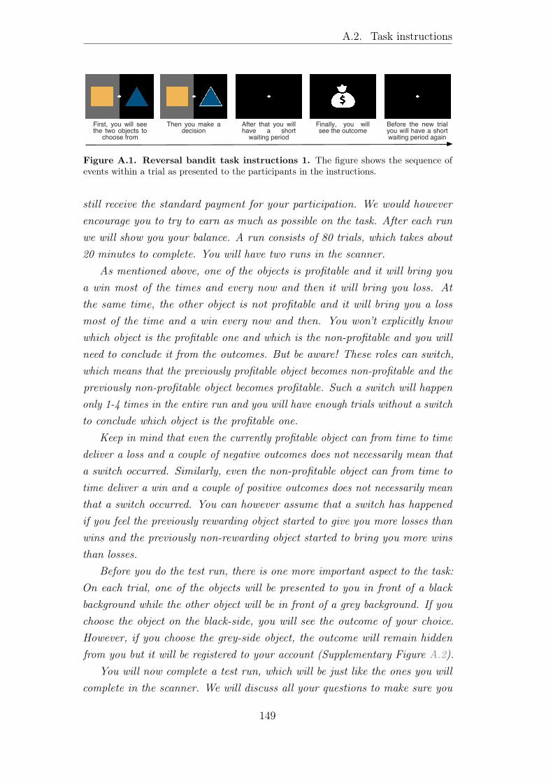
A.2. Task instructions

First, you will seethe two objects to

choose from

After that you willhave a shortwaiting period

Finally, you willsee the outcome

Before the new trialyou will have a shortwaiting period again

Then you make adecision

Figure A.1. Reversal bandit task instructions 1. The figure shows the sequence ofevents within a trial as presented to the participants in the instructions.

still receive the standard payment for your participation. We would howeverencourage you to try to earn as much as possible on the task. After each runwe will show you your balance. A run consists of 80 trials, which takes about20 minutes to complete. You will have two runs in the scanner.

As mentioned above, one of the objects is profitable and it will bring youa win most of the times and every now and then it will bring you loss. Atthe same time, the other object is not profitable and it will bring you a lossmost of the time and a win every now and then. You won’t explicitly knowwhich object is the profitable one and which is the non-profitable and you willneed to conclude it from the outcomes. But be aware! These roles can switch,which means that the previously profitable object becomes non-profitable and thepreviously non-profitable object becomes profitable. Such a switch will happenonly 1-4 times in the entire run and you will have enough trials without a switchto conclude which object is the profitable one.

Keep in mind that even the currently profitable object can from time to timedeliver a loss and a couple of negative outcomes does not necessarily mean thata switch occurred. Similarly, even the non-profitable object can from time totime deliver a win and a couple of positive outcomes does not necessarily meanthat a switch occurred. You can however assume that a switch has happenedif you feel the previously rewarding object started to give you more losses thanwins and the previously non-rewarding object started to bring you more winsthan losses.

Before you do the test run, there is one more important aspect to the task:On each trial, one of the objects will be presented to you in front of a blackbackground while the other object will be in front of a grey background. If youchoose the object on the black-side, you will see the outcome of your choice.However, if you choose the grey-side object, the outcome will remain hiddenfrom you but it will be registered to your account (Supplementary Figure A.2).

You will now complete a test run, which will be just like the ones you willcomplete in the scanner. We will discuss all your questions to make sure you

149

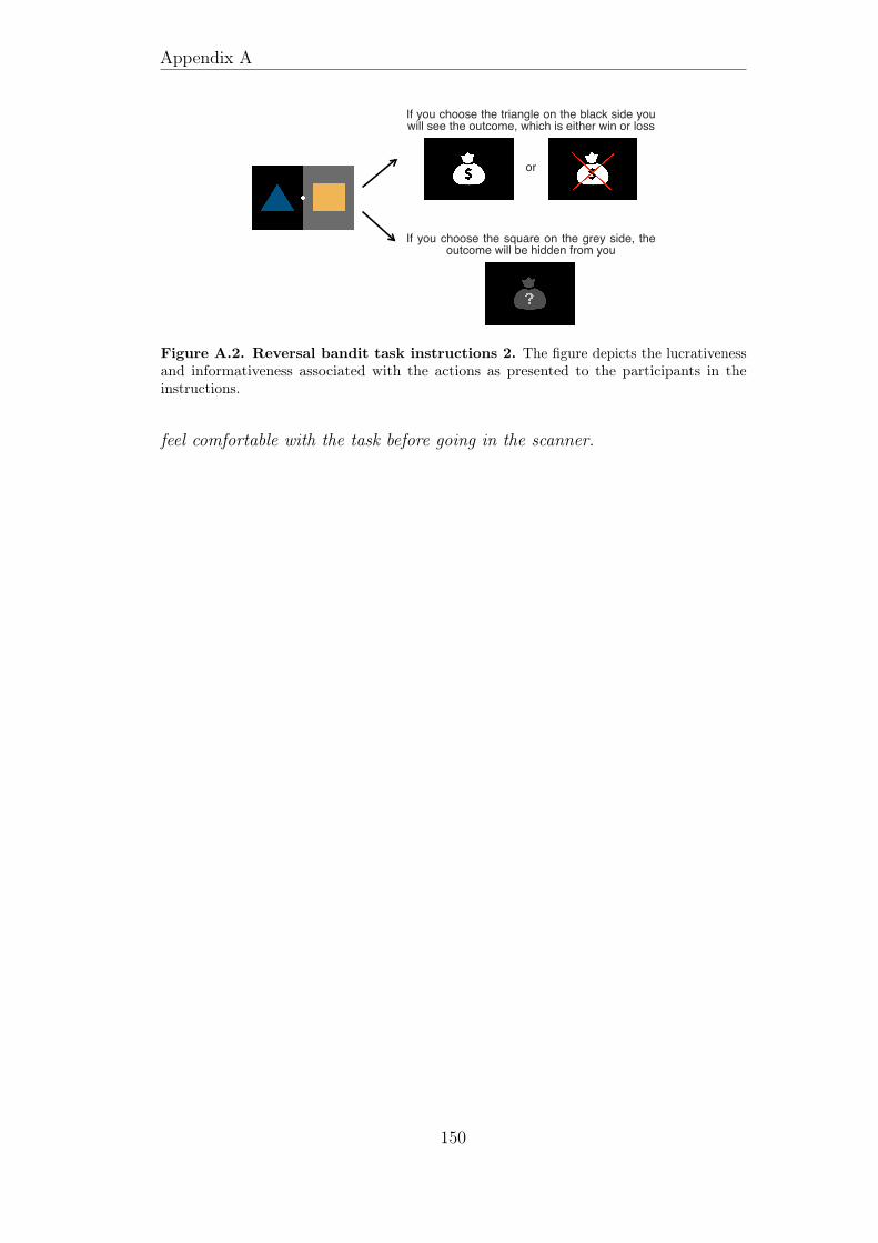
Appendix A

If you choose the triangle on the black side youwill see the outcome, which is either win or loss

If you choose the square on the grey side, theoutcome will be hidden from you

or

Figure A.2. Reversal bandit task instructions 2. The figure depicts the lucrativenessand informativeness associated with the actions as presented to the participants in theinstructions.

feel comfortable with the task before going in the scanner.

150

A.3. Trial sequence

A.3 Trial sequence

Participants were presented with the identical sequence of trials specifying theevolution of the first state component, s1, which encodes the lucrative shapeand the second state component, s2, which encodes the choice options. Thetrial sequence of both runs is shown in Table A.2.

t 1 2 3 4 5 6 7 8 9 10st (1, 1) (1, 1) (1, 2) (1, 1) (1, 2) (1, 1) (1, 1) (1, 2) (1, 1) (1, 1)

t 11 12 13 14 15 16 17 18 19 20st (1, 1) (1, 1) (1, 2) (1, 2) (1, 2) (1, 1) (1, 2) (1, 2) (1, 2) (2, 1)

t 21 22 23 24 25 26 27 28 29 30st (2, 1) (2, 2) (2, 1) (2, 2) (2, 1) (2, 2) (2, 2) (2, 1) (2, 2) (2, 2)

t 31 32 33 34 35 36 37 38 39 40st (2, 1) (2, 1) (2, 2) (2, 1) (2, 2) (2, 1) (2, 2) (2, 1) (2, 2) (2, 1)

t 41 42 43 44 45 46 47 48 49 50st (2, 2) (2, 2) (1, 2) (1, 2) (1, 1) (1, 1) (1, 2) (1, 2) (1, 2) (1, 2)

t 51 52 53 54 55 56 57 58 59 60st (1, 1) (1, 2) (1, 1) (1, 2) (1, 2) (1, 1) (1, 1) (1, 2) (1, 1) (1, 1)

t 61 62 63 64 65 66 67 68 69 70st (1, 1) (1, 1) (1, 2) (2, 1) (2, 1) (2, 2) (2, 1) (2, 2) (2, 1) (2, 1)

t 71 72 73 74 75 76 77 78 79 80st (2, 2) (2, 1) (2, 1) (2, 1) (2, 2) (2, 2) (2, 2) (2, 2) (2, 2) (2, 1)

t 1 2 3 4 5 6 7 8 9 10st (2, 1) (2, 1) (2, 1) (2, 2) (2, 1) (2, 1) (2, 1) (2, 1) (2, 2) (2, 2)

t 11 12 13 14 15 16 17 18 19 20st (2, 1) (2, 1) (2, 2) (2, 2) (2, 1) (2, 2) (2, 2) (2, 2) (2, 2) (2, 1)

t 21 22 23 24 25 26 27 28 29 30st (2, 1) (2, 1) (2, 2) (1, 1) (1, 2) (1, 2) (1, 2) (1, 1) (1, 2) (1, 1)

t 31 32 33 34 35 36 37 38 39 40st (1, 2) (1, 2) (1, 2) (1, 2) (1, 2) (1, 1) (1, 1) (1, 2) (1, 2) (1, 2)

t 41 42 43 44 45 46 47 48 49 50st (1, 2) (1, 1) (2, 2) (2, 2) (2, 2) (2, 1) (2, 2) (2, 2) (2, 2) (2, 1)

t 51 52 53 54 55 56 57 58 59 60st (2, 2) (2, 1) (2, 2) (2, 1) (2, 1) (2, 2) (2, 1) (2, 2) (2, 1) (1, 2)

t 61 62 63 64 65 66 67 68 69 70st (1, 1) (1, 1) (1, 2) (1, 1) (1, 1) (1, 2) (1, 1) (1, 1) (1, 1) (1, 1)

t 71 72 73 74 75 76 77 78 79 80st (1, 2) (1, 1) (1, 1) (1, 2) (1, 1) (1, 2) (1, 1) (1, 1) (1, 1) (1, 2)

Table A.2. State evolution function f . Upper table shows the trial sequence of the firstrun and lower table shows the trial sequence of the second run. t encodes the trial in the runand st encodes the state on the trial.

151

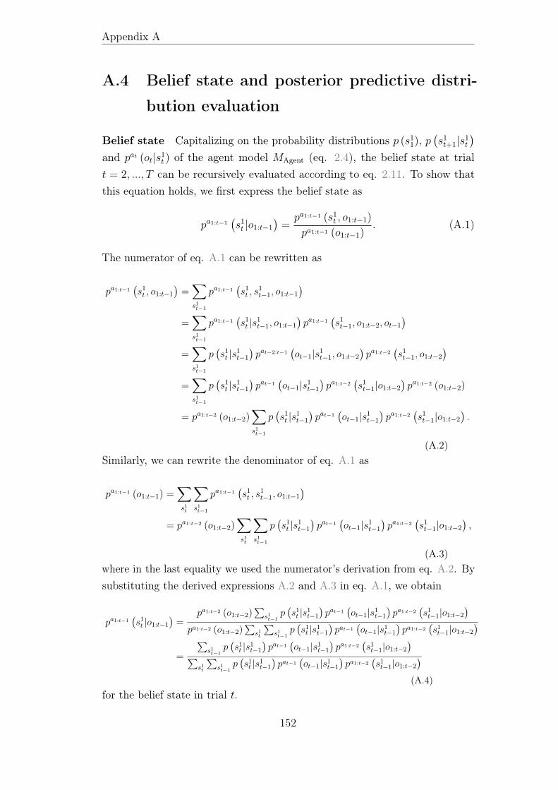
Appendix A

A.4 Belief state and posterior predictive distri-

bution evaluation

Belief state Capitalizing on the probability distributions p (s11), p(s1t+1|s1t

)and pat (ot|s1t ) of the agent model MAgent (eq. 2.4), the belief state at trialt = 2, ..., T can be recursively evaluated according to eq. 2.11. To show thatthis equation holds, we first express the belief state as

pa1:t−1(s1t |o1:t−1

)=pa1:t−1 (s1t , o1:t−1)

pa1:t−1 (o1:t−1). (A.1)

The numerator of eq. A.1 can be rewritten as

pa1:t−1(s1t , o1:t−1

)=∑s1t−1

pa1:t−1(s1t , s

1t−1, o1:t−1

)=∑s1t−1

pa1:t−1(s1t |s1t−1, o1:t−1

)pa1:t−1

(s1t−1, o1:t−2, ot−1

)=∑s1t−1

p(s1t |s1t−1

)pat−2:t−1

(ot−1|s1t−1, o1:t−2

)pa1:t−2

(s1t−1, o1:t−2

)=∑s1t−1

p(s1t |s1t−1

)pat−1

(ot−1|s1t−1

)pa1:t−2

(s1t−1|o1:t−2

)pa1:t−2 (o1:t−2)

= pa1:t−2 (o1:t−2)∑s1t−1

p(s1t |s1t−1

)pat−1

(ot−1|s1t−1

)pa1:t−2

(s1t−1|o1:t−2

).

(A.2)Similarly, we can rewrite the denominator of eq. A.1 as

pa1:t−1 (o1:t−1) =∑s1t

∑s1t−1

pa1:t−1(s1t , s

1t−1, o1:t−1

)= pa1:t−2 (o1:t−2)

∑s1t

∑s1t−1

p(s1t |s1t−1

)pat−1

(ot−1|s1t−1

)pa1:t−2

(s1t−1|o1:t−2

),

(A.3)where in the last equality we used the numerator’s derivation from eq. A.2. Bysubstituting the derived expressions A.2 and A.3 in eq. A.1, we obtain

pa1:t−1(s1t |o1:t−1

)=

pa1:t−2 (o1:t−2)∑

s1t−1p(s1t |s1t−1

)pat−1

(ot−1|s1t−1

)pa1:t−2

(s1t−1|o1:t−2

)pa1:t−2 (o1:t−2)

∑s1t

∑s1t−1

p(s1t |s1t−1

)pat−1

(ot−1|s1t−1

)pa1:t−2

(s1t−1|o1:t−2

)=

∑s1t−1

p(s1t |s1t−1

)pat−1

(ot−1|s1t−1

)pa1:t−2

(s1t−1|o1:t−2

)∑s1t

∑s1t−1

p(s1t |s1t−1

)pat−1

(ot−1|s1t−1

)pa1:t−2

(s1t−1|o1:t−2

)(A.4)

for the belief state in trial t.

152

A.4. Belief state and posterior predictive distribution evaluation

Posterior predictive distribution Given the agent’s belief state pa1:t−1 (s1t |o1:t−1)and the action-dependent state-conditional observation distribution pat (ot|s1t ),the posterior predictive distribution can be evaluated according to eq. 2.19. Aproof of this equation is as follows:

pa1:t (ot|o1:t−1) =pa1:t (ot, o1:t−1)

pa1:t (o1:t−1)

=

∑s1tpa1:t (ot, o1:t−1, s

1t )

pa1:t (o1:t−1)

=

∑s1tpa1:t (s1t |ot, o1:t−1) pa1:t (ot, o1:t−1)

pa1:t (o1:t−1)

=

∑s1tpa1:t−1 (s1t |o1:t−1)

∑s1tpa1:t (ot, o1:t−1, s

1t )

pa1:t (o1:t−1)

=

∑s1tpa1:t−1 (s1t |o1:t−1)

∑s1tpa1:t (ot|o1:t−1, s1t ) pa1:t (o1:t−1, s

1t )∑

s1tpa1:t (o1:t−1, s1t )

=∑s1t

pa1:t−1(s1t |o1:t−1

)pat(ot|s1t

)= btp

at(ot|s1t = 1

)+ (1− bt) pat

(ot|s1t = 2

), (A.5)

where in the last equality we substituted the belief state with its scalar repre-sentation to complete the derivation of eq. 2.19.

153

Appendix A

A.5 Belief state and posterior predictive distri-

bution implementation

For a concise implementation of the belief state and the posterior predictivedistribution, we represented the probability distributions the agent modelMAgent (eq. 2.4) by stochastic vectors and stochastic matrices. Specifically, inour implementation

• µ1 ∈ R|S1|≥0 represents the initial belief state p (s11). The ith entry of µ1

corresponds to the agent’s subjective uncertainty that the non-observablestate component takes on value s11 = i at trial t = 1. Formally,

µ1 :=

(p (s11 = 1)

p (s11 = 2)

)=

(0.5

0.5.

)(A.6)

• µt ∈ R|S1|≥0 represents the belief state pa1:t−1 (s1t |o1:t−1) at trial t. The ith

entry of µt corresponds to the agent’s subjective uncertainty that the non-observable state component takes on value s1t = i at trial t given the historyof observations o1:t−1 and actions a1:t−1. Formally,

µt :=

(pa1:t−1 (s1t = 1|o1:t−1)pa1:t−1 (s1t = 2|o1:t−1)

). (A.7)

• Φ ∈ R|S1|×|S1|≥0 represents the state-state transition distribution p

(s1t+1|s1t

).

The jth entry of the ith row of Φ corresponds to the agent’s subjectiveuncertainty that the non-observable state component takes on the values1t+1 = j in trial t+ 1 given that s1t = i in trial t. Formally,

Φ :=

(p(s1t+1 = 1|s1t = 1

)p(s1t+1 = 2|s1t = 1

)p(s1t+1 = 1|s1t = 2

)p(s1t+1 = 2|s1t = 2

)) =

(0.9625 0.0375

0.0375 0.9625

).

(A.8)

• Ωat ∈ R|S1|×|O|≥0 represents the action-dependent state-conditional observation

distribution pat (ot|s1t ) for action a ∈ A. The kth entry of the ith row ofΩat=a corresponds to the agent’s subjective uncertainty that the observationtakes on the value ot = k given that the non-observable state component

154

A.5. Belief state and posterior predictive distribution implementation

takes on the value s1t = i and action the value at = a. Formally,

Ωat=1 : =

(p1 (ot = 1|s1t = 1) p1 (ot = 2|s1t = 1) p1 (ot = 3|s1t = 1)

p1 (ot = 1|s1t = 2) p1 (ot = 2|s1t = 2) p1 (ot = 3|s1t = 2)

)

=

(0.15 0.85 0

0.85 0.15 0

)(A.9)

and

Ωat=3 : =

(p3 (ot = 1|s1t = 1) p3 (ot = 2|s1t = 1) p3 (ot = 3|s1t = 1)

p3 (ot = 1|s1t = 2) p3 (ot = 2|s1t = 2) p3 (ot = 3|s1t = 2)

)

=

(0.85 0.15 0

0.15 0.85 0

)(A.10)

represent the action-dependent state-conditional observation distribution forthe informative actions, and

Ωat∈2,4 : =

(pat (ot = 1|s1t = 1) pat (ot = 2|s1t = 1) pat (ot = 3|s1t = 1)

pat (ot = 1|s1t = 2) pat (ot = 2|s1t = 2) pat (ot = 3|s1t = 2)

)

=

(0 0 1

0 0 1

)(A.11)

represent the action-dependent state-conditional observation distribution forthe non-informative actions.

• Ψat ∈ R|S1|×|R|≥0 represents the action-dependent state-conditional reward

distribution pat (rt|s1t ) for action a ∈ A. The lth entry of the ith row of Ψat=a

corresponds to the agent’s subjective uncertainty that the reward takes onthe value rt = l−m given that the non-observable state component takes onthe value s1t = i and action the value at = a. Note that m is introduced toconvert the linear indices to reward values and takes on the value 2 if l = 1

and the value 1 if l = 2. Formally,

Ψat∈1,2 :=

(pat (rt = −1|s1t = 1) pat (rt = +1|s1t = 1)

pat (rt = −1|s1t = 2) pat (rt = +1|s1t = 2)

)=

(0.15 0.85

0.85 0.15

)(A.12)

represent the action-dependent state-conditional reward distribution for the

155

Appendix A

actions of choosing the square and,

Ψat∈3,4 :=

(pat (rt = −1|s1t = 1) pat (rt = +1|s1t = 1)

pat (rt = −1|s1t = 2) pat (rt = +1|s1t = 2)

):=

(0.85 0.15

0.15 0.85

)(A.13)

represent the action-dependent state-conditional reward distribution for theactions of choosing the triangle. Accordingly,

∑|R|l=1 Ψat

i(l−m) = 1.

Belief state Using matrix multiplication (denoted as ·) as well as element-wise Hadamard matrix multiplication (denoted as ), the agent’s prior beliefstate at trial t (cf. eq. 2.11) can be written as

µt := µt ·(∑|S1|

i=1µti

)−1, (A.14)

whereµt := Φ · (Ωa

k µt−1) (A.15)

is the unnormalized belief state following action at−1 = a and observationot−1 = k and (∑|S1|

i=1µti

)−1(A.16)

is the normalization constant. In eq. A.15, Ωak denotes the kth column of Ωa

and µt−1 denotes the prior belief state on trial t− 1, which corresponds to eq.A.7 if t− 1 > 1 and to eq. A.6 if t− 1 = 1.

Posterior predictive distribution Based on the stochastic matrix repre-sentation of the action-dependent state-conditional observation distributionΩat and the belief state µt, the posterior predictive distribution of A2 (cf. eq.2.19) can be implemented using matrix multiplication as

ωt := (Ωa)T · µt (A.17)

for action at = a.

156

A.6. References

A.6 References

Beck, A. T., Steer, R. A., & Brown, G. K. (1996). Manual for the BeckDepression Inventory-II. San Antonio, TX: Psychological Corporation.

Conners, C. K., Erhardt, D., & Sparrow, E. (1999). CAARS. Adult ADHDRating Scales. Toronto, Ontario, Canada: Multi-Health Systems.

Lynam, D. R., Smith, G. T., Whiteside, S. P., & Cyders, M. A. (2006). TheUPPS-P: Assessing five personality pathways to impulsive behavior. WestLafayette, IN: Purdue University.

Nooner, K. B., Colcombe, S., Tobe, R., Mennes, M., Benedict, M., Moreno,A., Panek, L., Brown, S., Zavitz, S., Li, Q., et al. (2012). The NKI-Rockland sample: A model for accelerating the pace of discovery sciencein psychiatry. Frontiers in Neuroscience, 6, 152.

Spielberger, C., Gorsuch, R., Lushene, R., Vagg, P., & Jacobs, G. (1983).Manual for the state-trait anxiety inventory. Palo Alto, CA: ConsultingPsychologists Press.

Wechsler, D. (1999). Wechsler abbreviated scale of intelligence. The Psychologi-cal Corporation: Harcourt Brace & Company. New York, NY.

157

Appendix A

158

B | Supplementary material toChapter 3

B.1 Task instructions

Participants were provided with the following instructions about the treasurehunt task (translated from the original German instructions):

Welcome to the treasure hunt task! The goal of this task is to find twohidden treasures in a 5-by-5 cell grid-world within a limited number of steps.You can navigate through the grid-world using the buttons. In each trial, youwill first see the cell corresponding to your current position. To help you trackyour position, you will additionally be presented with the index of your currentposition. For example, (2,3) means that you are in the second row and in thethird column. You start each attempt in (1,1), i.e., the first row and the firstcolumn, which corresponds to the upper left corner.

The right panel of Supplementary Figure B.1 displays the grid-world withtwo treasures from above. We are showing you this figure here to make youfamiliar with the layout. During the experiment, however, you will not seethe grid-world from a bird’s eye perspective. The left panel of SupplementaryFigure B.1 displays how you will see your position in the grid-world during theexperiment.

(1,1)

(2,1)

(3,1)

(4,1)

(5,1)

(1,2)

(2,2)

(3,2)

(4,2)

(5,2)

(1,3)

(2,3)

(3,3)

(4,3)

(5,3)

(1,4)

(2,4)

(3,4)

(4,4)

(5,4)

(1,5)

(2,5)

(3,5)

(4,5)

(5,5)

(1,1)

6(0)

Figure B.1. Treasure hunt task instructions 1. The figure displays the grid-worldfrom above (right panel) and a grid cell position (left panel) as presented to the participantsin the instructions.

After you are presented with your position, you will see a light or a dark greybar in each available direction (Supplementary Figure B.2). The bars convey

159

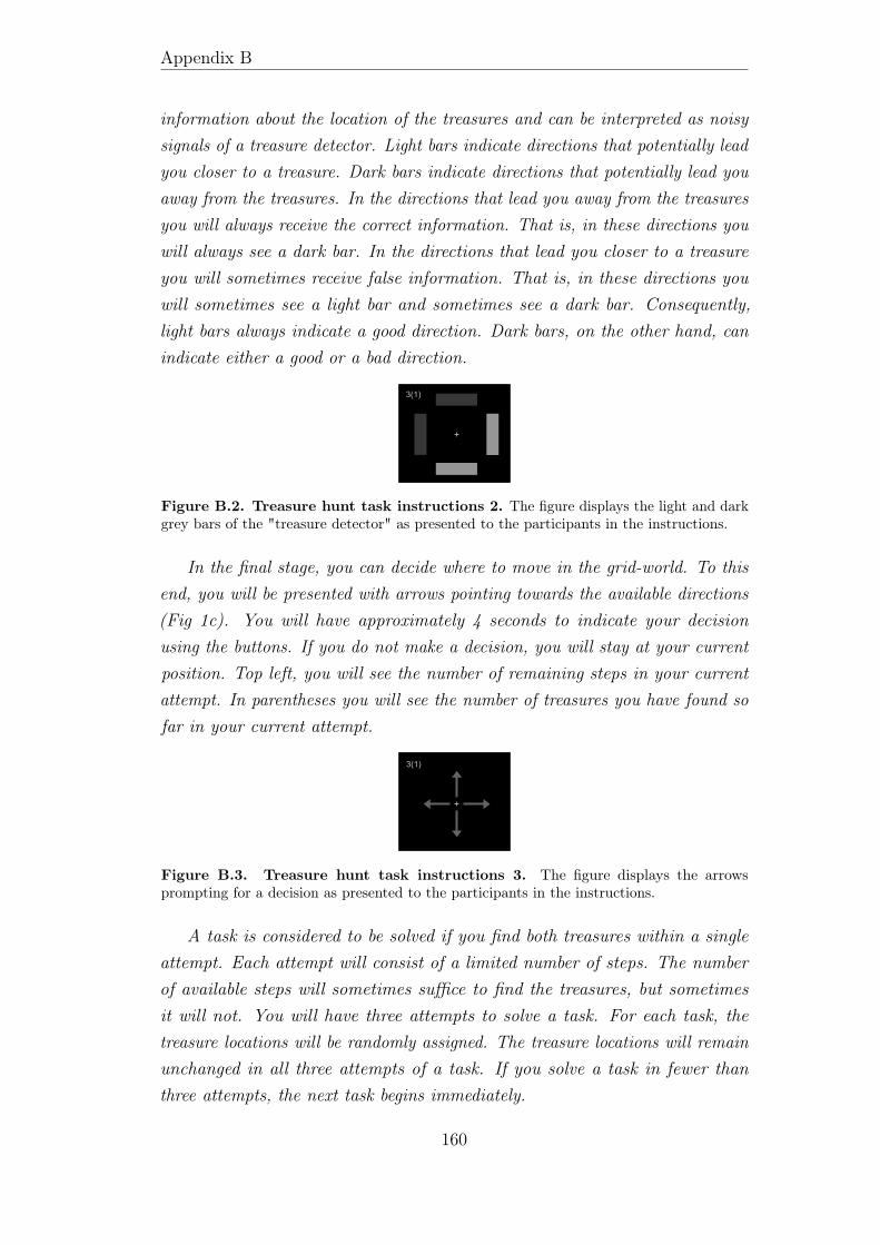
Appendix B

information about the location of the treasures and can be interpreted as noisysignals of a treasure detector. Light bars indicate directions that potentially leadyou closer to a treasure. Dark bars indicate directions that potentially lead youaway from the treasures. In the directions that lead you away from the treasuresyou will always receive the correct information. That is, in these directions youwill always see a dark bar. In the directions that lead you closer to a treasureyou will sometimes receive false information. That is, in these directions youwill sometimes see a light bar and sometimes see a dark bar. Consequently,light bars always indicate a good direction. Dark bars, on the other hand, canindicate either a good or a bad direction.

3(1)

Figure B.2. Treasure hunt task instructions 2. The figure displays the light and darkgrey bars of the "treasure detector" as presented to the participants in the instructions.

In the final stage, you can decide where to move in the grid-world. To thisend, you will be presented with arrows pointing towards the available directions(Fig 1c). You will have approximately 4 seconds to indicate your decisionusing the buttons. If you do not make a decision, you will stay at your currentposition. Top left, you will see the number of remaining steps in your currentattempt. In parentheses you will see the number of treasures you have found sofar in your current attempt.

3(1)

Figure B.3. Treasure hunt task instructions 3. The figure displays the arrowsprompting for a decision as presented to the participants in the instructions.

A task is considered to be solved if you find both treasures within a singleattempt. Each attempt will consist of a limited number of steps. The numberof available steps will sometimes suffice to find the treasures, but sometimesit will not. You will have three attempts to solve a task. For each task, thetreasure locations will be randomly assigned. The treasure locations will remainunchanged in all three attempts of a task. If you solve a task in fewer thanthree attempts, the next task begins immediately.

160

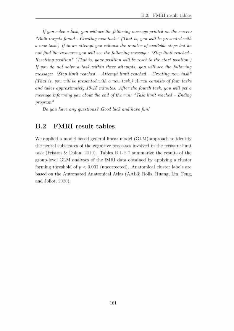
B.2. FMRI result tables

If you solve a task, you will see the following message printed on the screen:"Both targets found - Creating new task." (That is, you will be presented witha new task.) If in an attempt you exhaust the number of available steps but donot find the treasures you will see the following message: "Step limit reached -Resetting position" (That is, your position will be reset to the start position.)If you do not solve a task within three attempts, you will see the followingmessage: "Step limit reached – Attempt limit reached – Creating new task"(That is, you will be presented with a new task.) A run consists of four tasksand takes approximately 10-15 minutes. After the fourth task, you will get amessage informing you about the end of the run: "Task limit reached – Endingprogram"

Do you have any questions? Good luck and have fun!

B.2 FMRI result tables

We applied a model-based general linear model (GLM) approach to identifythe neural substrates of the cognitive processes involved in the treasure hunttask (Friston & Dolan, 2010). Tables B.1-B.7 summarize the results of thegroup-level GLM analyses of the fMRI data obtained by applying a clusterforming threshold of p < 0.001 (uncorrected). Anatomical cluster labels arebased on the Automated Anatomical Atlas (AAL3; Rolls, Huang, Lin, Feng,and Joliot, 2020).

161

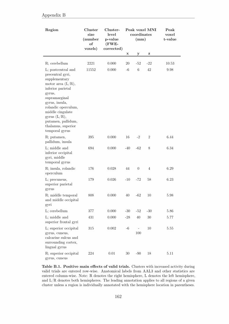
Appendix B

Region Clustersize

(numberof

voxels)

Cluster-level

p-value(FWE-

corrected)

Peak voxel MNIcoordinates

(mm)

Peakvoxel

t-value

x y z

R; cerebellum 2221 0.000 20 -52 -22 10.53

L; postcentral andprecentral gyri,supplementarymotor area (L/R),inferior parietalgyrus,supramarginalgyrus, insula,rolandic operculum,middle cingulategyrus (L/R),putamen, pallidum,thalamus, superiortemporal gyrus

11552 0.000 -6 6 42 9.98

R; putamen,pallidum, insula

395 0.000 16 -2 2 6.44

L; middle andinferior occipitalgyri, middletemporal gyrus

694 0.000 -40 -62 8 6.34

R; insula, rolandicoperculum

176 0.028 44 0 4 6.29

L; precuneus,superior parietalgyrus

179 0.026 -10 -72 58 6.23

R; middle temporaland middle occipitalgyri

808 0.000 40 -62 10 5.98

L; cerebellum 377 0.000 -30 -52 -30 5.86

L; middle andsuperior frontal gyri

431 0.000 -28 40 30 5.77

L; superior occipitalgyrus, cuneus,calcarine sulcus andsurrounding cortex,lingual gyrus

315 0.002 -6 -100

10 5.55

R; superior occipitalgyrus, cuneus

224 0.01 30 -90 18 5.11

Table B.1. Positive main effects of valid trials. Clusters with increased activity duringvalid trials are entered row-wise. Anatomical labels from AAL3 and other statistics areentered column-wise. Note: R denotes the right hemisphere, L denotes the left hemisphere,and L/R denotes both hemispheres. The leading annotation applies to all regions of a givencluster unless a region is individually annotated with the hemisphere location in parentheses.

162

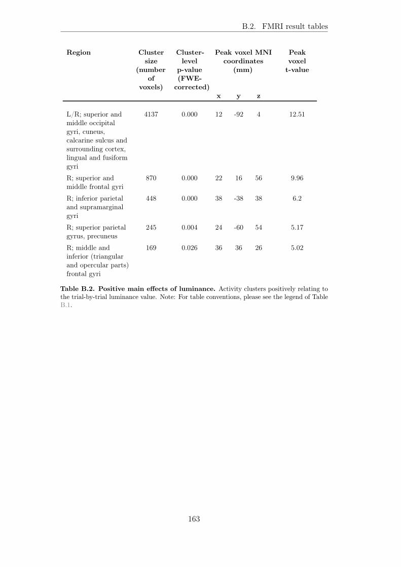
B.2. FMRI result tables

Region Clustersize

(numberof

voxels)

Cluster-level

p-value(FWE-

corrected)

Peak voxel MNIcoordinates

(mm)

Peakvoxel

t-value

x y z

L/R; superior andmiddle occipitalgyri, cuneus,calcarine sulcus andsurrounding cortex,lingual and fusiformgyri

4137 0.000 12 -92 4 12.51

R; superior andmiddle frontal gyri

870 0.000 22 16 56 9.96

R; inferior parietaland supramarginalgyri

448 0.000 38 -38 38 6.2

R; superior parietalgyrus, precuneus

245 0.004 24 -60 54 5.17

R; middle andinferior (triangularand opercular parts)frontal gyri

169 0.026 36 36 26 5.02

Table B.2. Positive main effects of luminance. Activity clusters positively relating tothe trial-by-trial luminance value. Note: For table conventions, please see the legend of TableB.1.

163

Appendix B

Region Clustersize

(numberof

voxels)

Cluster-level

p-value(FWE-

corrected)

Peak voxel MNIcoordinates

(mm)

Peakvoxel

t-value

x y z

L/R; lateral andmedial surfaces ofthe occipital,temporal, parietaland frontal lobes,cingulate cortex,insula, rolandicoperculum,amygdala, thalamus,basal ganglia,ventral tegmentalarea, cerebellum

84128 0.000 -30 20 -14 15.8

Table B.3. Positive main effects of treasure discovery. Using a cluster definingthreshold of p < 0.001, we obtained a single large bilateral cluster with increased activity inresponse to treasure discovery as compared to implicit baseline. Note: For table conventions,please see the legend of Table B.1.

164

B.2. FMRI result tables

Region Clustersize

(numberof

voxels)

Cluster-level

p-value(FWE-

corrected)

Peak voxel MNIcoordinates

(mm)

Peakvoxel

t-value

x y z

L/R; lateral andmedial surfaces ofthe occipital,temporal, parietaland frontal lobes(except the rightsuperior parietalgyrus), cingulatecortex, insula,rolandic operculum,amygdala, thalamus,basal ganglia(except ventralstriatum),cerebellum

68694 0.000 0 -22 38 13.55

Table B.4. Positive main effects of information display. As in the case of the positivemain effects of treasure discovery, applying a cluster defining threshold of p < 0.001 resultedin a single large bilateral cluster with increased activity in response to information display ascompared to implicit baseline. Note: For table conventions, please see the legend of TableB.1.

165

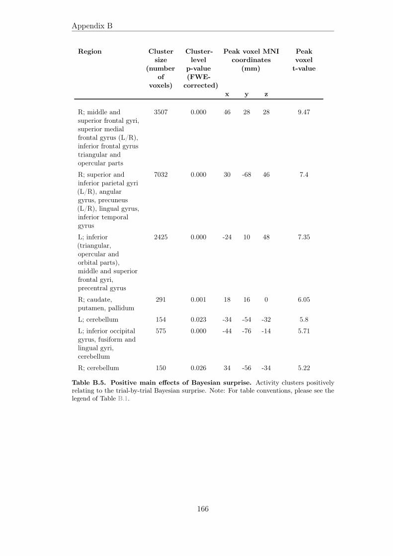
Appendix B

Region Clustersize

(numberof

voxels)

Cluster-level

p-value(FWE-

corrected)

Peak voxel MNIcoordinates

(mm)

Peakvoxel

t-value

x y z

R; middle andsuperior frontal gyri,superior medialfrontal gyrus (L/R),inferior frontal gyrustriangular andopercular parts

3507 0.000 46 28 28 9.47

R; superior andinferior parietal gyri(L/R), angulargyrus, precuneus(L/R), lingual gyrus,inferior temporalgyrus

7032 0.000 30 -68 46 7.4

L; inferior(triangular,opercular andorbital parts),middle and superiorfrontal gyri,precentral gyrus

2425 0.000 -24 10 48 7.35

R; caudate,putamen, pallidum

291 0.001 18 16 0 6.05

L; cerebellum 154 0.023 -34 -54 -32 5.8

L; inferior occipitalgyrus, fusiform andlingual gyri,cerebellum

575 0.000 -44 -76 -14 5.71

R; cerebellum 150 0.026 34 -56 -34 5.22

Table B.5. Positive main effects of Bayesian surprise. Activity clusters positivelyrelating to the trial-by-trial Bayesian surprise. Note: For table conventions, please see thelegend of Table B.1.

166

B.2. FMRI result tables

Region Clustersize

(numberof

voxels)

Cluster-level

p-value(FWE-

corrected)

Peak voxel MNIcoordinates

(mm)

Peakvoxel

t-value

x y z

L; precuneus,calcarine sulcus andsurrounding cortex

189 0.009 -12 -34 20 5.38

Table B.6. Negative main effects of Bayesian surprise. Activity clusters negativelyrelating to the trial-by-trial Bayesian surprise. Note: For table conventions, please see thelegend of Table B.1.

167

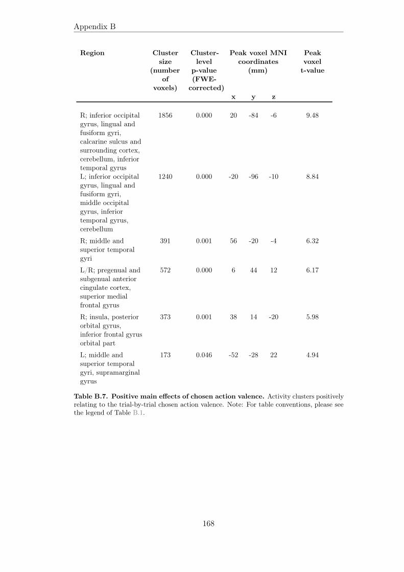
Appendix B

Region Clustersize

(numberof

voxels)

Cluster-level

p-value(FWE-

corrected)

Peak voxel MNIcoordinates

(mm)

Peakvoxel

t-value

x y z

R; inferior occipitalgyrus, lingual andfusiform gyri,calcarine sulcus andsurrounding cortex,cerebellum, inferiortemporal gyrus

1856 0.000 20 -84 -6 9.48

L; inferior occipitalgyrus, lingual andfusiform gyri,middle occipitalgyrus, inferiortemporal gyrus,cerebellum

1240 0.000 -20 -96 -10 8.84

R; middle andsuperior temporalgyri

391 0.001 56 -20 -4 6.32

L/R; pregenual andsubgenual anteriorcingulate cortex,superior medialfrontal gyrus

572 0.000 6 44 12 6.17

R; insula, posteriororbital gyrus,inferior frontal gyrusorbital part

373 0.001 38 14 -20 5.98

L; middle andsuperior temporalgyri, supramarginalgyrus

173 0.046 -52 -28 22 4.94

Table B.7. Positive main effects of chosen action valence. Activity clusters positivelyrelating to the trial-by-trial chosen action valence. Note: For table conventions, please seethe legend of Table B.1.

168

B.3. References

B.3 References

Friston, K., & Dolan, R. J. (2010). Computational and dynamic models inneuroimaging. NeuroImage, 52 (3), 752–765.

Rolls, E. T., Huang, C.-C., Lin, C.-P., Feng, J., & Joliot, M. (2020). Automatedanatomical labelling atlas 3. NeuroImage, 206, 116189.

169

List of manuscripts

Chapters 2 and 3 of this dissertation served as the basis for manuscriptssubmitted to or prepared for peer-reviewed journals. These chapters are thusnot identical with the manuscripts listed below.

• Horvath, L., Colcombe, S., Milham, M., Ray, S., Schwartenbeck, P.,& Ostwald, D. (2020). Human belief state-based exploration and ex-ploitation in an information-selective reversal bandit task. bioRxiv,https://doi.org/10.1101/2020.08.31.276139.

Authors’ contributions: L.H.: conceptualization, project administration,data curation, investigation, methodology, formal analysis, software, vali-dation, visualization, writing – original draft, writing – review & editing;S.C.: project administration, data curation, investigation, experimentalsoftware, funding acquisition, resources, supervision, writing – review;M.M.: conceptualization, funding acquisition, resources, supervision,project administration, writing – review; S.R.: project administration,data curation, investigation, writing – review; P.S.: conceptualization,writing – review; D.O.: conceptualization, formal analysis, methodol-ogy, software, visualization, project administration, resources, validation,funding acquisition, supervision, writing – original draft, writing – review& editing

• Horvath, L., Tisdall, L., Mata, R., Hertwig, R., & Ostwald, D. (inpreparation). The neurocomputational mechanisms of sequential decisionmaking in a multistep task with partially observable states.

Authors’ contributions: L.H.: conceptualization, project administration,data curation, investigation, methodology, formal analysis, software, vali-dation, visualization, writing – original draft, writing – review & editing,L.T.: investigation, R.M.: project administration, R.H.: funding acquisi-tion, resources, D.O.: conceptualization, formal analysis, methodology,software, visualization, investigation, project administration, resources,validation, funding acquisition, supervision, writing – original draft, writ-ing – review & editing

Eidesstattliche Erklärung

Hiermit erkläre ich an Eides statt,

• dass ich die vorliegende Arbeit eigenständig und ohne unerlaubte Hilfeverfasst habe,

• dass Ideen und Gedanken aus Arbeiten anderer entsprechend gekennze-ichnet wurden,

• dass ich mich nicht bereits anderweititg um einen Doktorgrad beworbenhabe und keinen Doktorgrad in dem Promotionsfach Psychologie besitze,sowie

• dass ich die zugrundeliegende Promotionsordnung vom 08.08.2016 an-erkenne.

Lilla HorvathBerlin, 9. April 2021