CHARACTERIZATION OF SELF-CONSOLIDATING

CONCRETE FOR THE DESIGN OF PRECAST, PRETENSIONED

BRIDGE SUPERSTRUCTURE ELEMENTS

A Dissertation

by

YOUNG HOON KIM

Submitted to the Office of Graduate Studies of Texas A&M University

in partial fulfillment of the requirements for the degree of

DOCTOR OF PHILOSOPHY

December 2008

Major Subject: Civil Engineering

CHARACTERIZATION OF SELF-CONSOLIDATING

CONCRETE FOR THE DESIGN OF PRECAST, PRETENSIONED

BRIDGE SUPERSTRUCTURE ELEMENTS

A Dissertation

by

YOUNG HOON KIM

Submitted to the Office of Graduate Studies of Texas A&M University

in partial fulfillment of the requirements for the degree of

DOCTOR OF PHILOSOPHY

Approved by:

Co-Chairs of Committee, Mary Beth D. Hueste David Trejo Committee Members, Joseph M. Bracci Daren B. H. Cline Head of Department, David Rosowsky

December 2008

Major Subject: Civil Engineering

iii

ABSTRACT

Characterization of Self-Consolidating Concrete for the Design of

Precast, Pretensioned Bridge Superstructure Elements. (December 2008)

Young Hoon Kim, B.E., Korea University;

M.S., Korea University

Co-Chairs of Advisory Committee: Dr. Mary Beth D. Hueste Dr. David Trejo

Self-consolidating concrete (SCC) is a new, innovative construction material that

can be placed into forms without the need for mechanical vibration. The mixture

proportions are critical for producing quality SCC and require an optimized combination

of coarse and fine aggregates, cement, water, and chemical and mineral admixtures. The

required mixture constituents and proportions may affect the mechanical properties,

bond characteristics, and long-term behavior, and SCC may not provide the same in-

service performance as conventional concrete (CC). Different SCC mixture constituents

and proportions were evaluated for mechanical properties, shear characteristics, bond

characteristics, creep, and durability. Variables evaluated included mixture type (CC or

SCC), coarse aggregate type (river gravel or limestone), and coarse aggregate volume.

To correlate these results with full-scale samples and investigate structural behavior

related to strand bond properties, four girder-deck systems, 40 ft (12 m) long, with CC

and SCC pretensioned girders were fabricated and tested.

Results from the research indicate that the American Association of State

Highway Transportation Officials Load and Resistance Factor Design (AASHTO

LRFD) Specifications can be used to estimate the mechanical properties of SCC for a

concrete compressive strength range of 5 to 10 ksi (34 to 70 MPa). In addition, the

research team developed prediction equations for concrete compressive strength ranges

from 5 to 16 ksi (34 to 110 MPa). With respect to shear characteristics, a more

iv

appropriate expression is proposed to estimate the concrete shear strength for CC and

SCC girders with a compressive strength greater than 10 ksi (70 MPa). The author found

that girder-deck systems with Type A SCC girders exhibit similar flexural performance

as deck-systems with CC girders. The AASHTO LRFD (2006) equations for computing

the cracking moment, nominal moment, transfer length, development length, and

prestress losses may be used for SCC girder-deck systems similar to those tested in this

study. For environments exhibiting freeze-thaw cycles, a minimum 16-hour release

strength of 7 ksi (48 MPa) is recommended for SCC mixtures.

v

ACKNOWLEDGMENTS

This dissertation would not have been possible without the support and guidance

provided by Dr. Mary Beth Hueste and Dr. David Trejo, my long-time advisors and

committee co-chairs. The author also appreciates the input of the other members of this

dissertation committee, Dr. Joseph Bracci and Dr. Daren Cline. The author also wishes

to thank Dr. Hakan Atahan, a postdoctoral researcher in TTI, for his contributions in the

mechanical properties and durability testing of this research.

The author also wishes to thank Dr. Peter Keating, Matthew Potter, Stephen

Smith, and Jeff Perry of the Civil Engineering High Bay Structural and Materials

Laboratory (HBSML) at TAMU and Dr. Ceki Halmen, Jeong Joo Kim, Seok Been Im,

Radhakrishna Pillai, Suresh Kataria, Paul Mostella, Kevin Grant, David Ruben

Contreras, Amit Nambiar, and Timothy Stocks who assisted with the testing and

collecting data. The effort of these individuals was critical to the success of this

dissertation research and is greatly appreciated.

Included also are thanks to BASF Construction Chemicals LLC (Al Pinnelli, Van

Bui, Emmanuel Attiogbe, and Bob Rogers). Field testing and fabrication of the girders

was done at the Texas Concrete Company, Victoria, Texas. A special thanks to Bruce

Williams and Burson Patton from Texas Concrete Company.

This dissertation research has been supported by the Texas Department of

Transportation (TxDOT) and Federal Highway Administration (FHWA) through the

Texas Transportation Institute (TTI) as part of Project 0-5134, Self-Consolidating

Concrete for Precast Structural Applications. This research was jointly performed with

Drs. David Fowler and Eric Koehler at the University of Texas at Austin, who focused

on developing the mixture proportions and evaluating the fresh properties of SCC. Their

work is presented in TxDOT Report 0-5314-1, Self-Consolidating Concrete for Precast

Structural Applications: Mixture Proportioning, Workability, and Early-Age Hardened

Properties.

vi

On a more personal note, the author would like to thank Dr. Trejo and Dr. Hueste

for having the faith in him to allow him to pursue his doctoral research. The author is

also indebted to both Dr. Hueste and Dr. Trejo for their guidance in completing his

doctoral dissertation.

As always, the author is indebted to his parents and sister for their endless love

and support. The dedicated support provided by his wife over the past five-and-a-half

years is very appreciated. She has given him everything, and the author hopes to return

at least a fraction of her love.

vii

TABLE OF CONTENTS

Page

ABSTRACT ..................................................................................................................... iii�

ACKNOWLEDGMENTS .................................................................................................. v�

TABLE OF CONTENTS .................................................................................................vii�

LIST OF FIGURES ............................................................................................................ x�

LIST OF TABLES .......................................................................................................... xix

CHAPTER

I INTRODUCTION ............................................................................................. 1�

1.1� General ............................................................................................. 1�1.2� Objectives and Scope ....................................................................... 3�1.3 � Organization of This Dissertation .................................................... 7�

II LITERATURE REVIEW .................................................................................. 8�

2.1� General ............................................................................................. 8�2.2� Fresh Characteristics ........................................................................ 9�2.3� Mechanical Characteristics ............................................................ 12�2.4� Shear Characteristics...................................................................... 16�2.5� Bond Characteristics ...................................................................... 28�2.6 � Creep and Shrinkage ...................................................................... 29�2.7� Durability ....................................................................................... 34�2.8� Flexural Capacity ........................................................................... 34�2.9� Transfer Length and Development Length .................................... 37�2.10� Prestress Losses ............................................................................. 43�2.11� Camber and Deflection .................................................................. 47�2.12� Summary ........................................................................................ 48�

III MATERIALS .................................................................................................. 50�

3.1� Laboratory Program ....................................................................... 50�3.2� Full-Scale Test Program ................................................................ 59�

IV EXPERIMENTAL PROGRAM ...................................................................... 65�

viii

CHAPTER Page

4.1� Early-Age Characteristics .............................................................. 65�4.2� Mechanical Properties.................................................................... 66�4.3� Shear Characteristics...................................................................... 69�4.4� Bond Charactristics ........................................................................ 76�4.5� Creep .............................................................................................. 80�4.6� Durability ....................................................................................... 84�4.7� Full-Scale Testing .......................................................................... 89�

V RESULTS AND ANALYSIS OF LABORATORY STUDY: MECHANICAL PROPERTIES .................................................................... 118�

5.1� Early-Age Characteristics ............................................................ 118�5.2� Development of Compressive Strength ....................................... 120�5.3� Modulus of Elasticity (MOE) ...................................................... 126�5.4� Modulus of Rupture (MOR) ........................................................ 136�5.5� Splitting Tensile Strength (STS) .................................................. 142�5.6� Comparison of SCC and CC ........................................................ 149�5.7� Summary ...................................................................................... 152�

VI RESULTS AND ANALYSIS OF LABORATORY STUDY: SHEAR CHARACTERISTICS ................................................................................... 155�

6.1� Mechanical Properties and Precracking Results .......................... 155�6.2� Development of Evaluation Methods .......................................... 156�6.3� Evaluation of Aggregate Interlock ............................................... 162�6.4� Model of Aggregate Interlock ...................................................... 178�6.5� Summary ...................................................................................... 206�

VII RESULTS AND ANALYSIS OF LABORATORY STUDY: BOND, CREEP, AND DURABILITY ....................................................................... 208�

7.1� Bond Characteristics .................................................................... 208�7.2� Creep ............................................................................................ 219�7.3� Durability ..................................................................................... 235�

VIII RESULTS AND ANALYSIS OF FULL-SCALE TESTING AND VALIDATION: FULL-SCALE SCC GIRDER-DECK SYSTEM ............... 245�

8.1� Early-Age Properties and Field Observation ............................... 245�8.2� Material Mechanical Properties ................................................... 250�8.3� Flexural Tests ............................................................................... 254�

ix

CHAPTER Page

8.4� Transfer Length............................................................................ 268�8.5� Development Length Tests .......................................................... 273�8.6� Prestress Losses ........................................................................... 304�8.7� Camber and Deflection History ................................................... 315�8.8� Summary ...................................................................................... 321

IX SUMMARY, CONLUSIONS, AND RECOMMENDATIONS ................... 323�

9.1� Summary ...................................................................................... 323�9.2� Conclusions .................................................................................. 324�9.3� Recommendations ........................................................................ 332 9.4� Further Research .......................................................................... 333

REFERENCES ............................................................................................................... 336�

APPENDIX A ................................................................................................................ 350�

APPENDIX B ................................................................................................................ 361�

APPENDIX C ................................................................................................................ 363�

APPENDIX D ................................................................................................................ 366�

APPENDIX E ................................................................................................................. 372�

APPENDIX F ................................................................................................................. 376�

APPENDIX G ................................................................................................................ 379�

VITA .............................................................................................................................. 387�

x

LIST OF FIGURES

Page

Figure 2.1. Illustration of Tensile Stress on the Crack Plane Prior to Slip Occurrence for Equation 2.4 (Vecchio and Collins 1986). ......................... 20�

Figure 2.2. Schemetic for Aggregate Interlock (Vecchio and Collins 1986). .............. 21�

Figure 2.3. The Role of Friction Coefficient (Walraven 1981). .................................... 24�

Figure 2.4. Walraven’s Data and Equation 2.21 (Vecchio and Collins 1986). ............. 27�

Figure 2.5. Definition of Development Length (Naaman 2004). .................................. 38�

Figure 2.6. Idealized Relationship between Steel Stress and Distance from the Free End of Strand (AASHTO 2006). ......................................................... 41�

Figure 2.7. Stress versus Time of Prestressed Strands (Tadros et al. 2003). ................. 44�

Figure 3.1. Gradation of Coarse Aggregates Used in Laboratory Testing. ................... 53�

Figure 3.2. Gradation of Fine Aggregates Used in Laboratory Testing. ....................... 54�

Figure 3.3. Mixture Identification. ................................................................................ 56�

Figure 3.4. Stress-Strain Relationship of Prestressing Steel. ......................................... 63�

Figure 4.1. Test Specimen for Evaluating Aggregate Interlock. ................................... 71�

Figure 4.2. Precracking Test. ......................................................................................... 73�

Figure 4.3. Initiation of Web-Shear Cracking in Full-scale Test (Collins and Mitchell 1980). ............................................................................................ 73�

Figure 4.4. Push-off Test. .............................................................................................. 75�

Figure 4.5. Aggregate Interlock after Slip in Full-scale Test (Collins and Mitchell 1980). ........................................................................................................... 75�

Figure 4.6. Sample ID. ................................................................................................... 77�

Figure 4.7. Pull-out Specimen Layout. .......................................................................... 77�

xi

Page

Figure 4.8. Test Setup for Pull-out Test. ....................................................................... 79�

Figure 4.9. Schematic Diagram of Creep Test Setup. ................................................... 81�

Figure 4.10. Loading with 500 kip (2220 kN) MTS Machine. ........................................ 83�

Figure 4.11. Dimension of Cross-Section of Type A Girder. .......................................... 91�

Figure 4.12. Layout of Strands for Tested Girders. ......................................................... 91�

Figure 4.13. Layout of Reinforcement. ........................................................................... 92�

Figure 4.14. Detail of Reinforcements. ........................................................................... 93�

Figure 4.15. Details of Deck. ........................................................................................... 94�

Figure 4.16. Layout of Girders. ....................................................................................... 95�

Figure 4.17. Prestressing Bed with Strands. .................................................................... 95�

Figure 4.18. Preparation of Small Samples. .................................................................... 96�

Figure 4.19. Placement of Reinforcement. ...................................................................... 97�

Figure 4.20. Placement of Deck Concrete. ...................................................................... 98�

Figure 4.21. Locations of Temperature Probes. ............................................................ 100�

Figure 4.22. Overview of Test Setup. ............................................................................ 101�

Figure 4.23. Diagram of Installation of Strain Gages and LVDTs for Measuring Strain of Top Fiber of Deck Concrete under Flexural Test. ...................... 102�

Figure 4.24. Diagram of Installation of String Potentiometers for the Flexural Test. ... 103�

Figure 4.25. Average Strain of Strands of the Constant Moment Region. .................... 103�

Figure 4.26. Locations of Strain Gages. ........................................................................ 104�

Figure 4.27. Shear Lag Effect on Transfer Length (Barnes 2000). ............................... 105�

Figure 4.28. Determining Transfer Length Using the 95% AMS Method. ................... 106�

Figure 4.29. Long-Term Raw Strain Profile of North Span of Girder CC-R. ............... 106�

xii

Page

Figure 4.30. Locations of LVDTs for Draw-In End Slip. ............................................. 107�

Figure 4.31. Definition of Embedment Length and Test Span Length. ........................ 109�

Figure 4.32. Test Setup for Development Length Test. ................................................ 110�

Figure 4.33. Diagram of Locations of Strain Gages or Deck Concrete for Development Length Tests. ....................................................................... 111�

Figure 4.34. Diagram of Concrete Surface Strain Gage Layout (Type I) and Embedded Concrete Strain Gage Layout (Type II). ................................. 112�

Figure 4.35. Locations of LVDTs and Strain Gages for Shear and Development Length. ....................................................................................................... 112�

Figure 4.36. Strains on Web at Critical Section for Shear. ............................................ 113�

Figure 4.37. Load Cells between Spring Loaded Anchor and Dead Abutment. .......... 114�

Figure 4.38. Initial Camber Reading (a) and Stringlines (b). ........................................ 115�

Figure 4.39. Location of String Potentiometer for the Camber and Deflection. ........... 116�

Figure 5.1. Compressive Strength at 16 hours. ............................................................ 120�

Figure 5.2. Development of Compressive Strength. .................................................... 122�

Figure 5.3. Compressive Strength Ratio as a Function of Time. ................................. 123�

Figure 5.4. MOE of SCC. ............................................................................................ 127�

Figure 5.5. Prediction Equations for MOE for River Gravel SCC Mixture. ............... 129�

Figure 5.6. Comparison of SCC and CC Mixture Using Eq. 5.7. ............................... 131�

Figure 5.7. Prediction Equations for MOE for Limestone SCC. ................................. 132�

Figure 5.8. Comparison of SCC and CC Mixtures Using Eq. 5.9. .............................. 133�

Figure 5.9. Unified MOE for SCC Mixtures. .............................................................. 134�

Figure 5.10. MOR for SCC Mixtures. ........................................................................... 137�

Figure 5.11. Size Effect of MOR. .................................................................................. 138�

xiii

Page

Figure 5.12. MOR Prediction Equations. ...................................................................... 140�

Figure 5.13. Proposed Upper and Lower Bounds of MOR for SCC Mixtures. ............ 141�

Figure 5.14. STS of SCC Mixtures. ............................................................................... 143�

Figure 5.15. Fracture Surface in STS. ........................................................................... 144�

Figure 5.16. STS Prediction Equations. ......................................................................... 145�

Figure 5.17. Proposed Upper and Lower Bounds of STS for SCC Mixtures. ............... 147�

Figure 5.18. Comparison between CC and SCC Mixtures (MOE). .............................. 149�

Figure 5.19. Comparison between CC and SCC Mixtures (MOR). .............................. 150�

Figure 5.20. Comparison between CC and SCC Mixtures (STS). ................................ 152�

Figure 6.1. Typical Plots of Measured Parameters. ..................................................... 157�

Figure 6.2. Crack Slip Model Based on Walraven’s Test Results (Adapted from Data of Walraven and Reinhardt 1981). .................................................... 158�

Figure 6.3. Schematic of Aggregate Interlock from Walraven’s Theory (Walraven and Reinhardt 1981). ................................................................................. 158�

Figure 6.4. Typical Plot of τ/σ versus w. ..................................................................... 160�

Figure 6.5. Definition of Equivalent Shear Strength. .................................................. 161�

Figure 6.6. Plot of Mean Shear-to-Normal Stress Ratio versus Crack Width. ............ 163�

Figure 6.7. Plot of Mean E-value by Mixture Type (δ’ = 0.02 in. [0.5 mm]). ............ 169�

Figure 6.8. Plot of Mean E-value versus Crack Slip. .................................................. 170�

Figure 6.9. Observation of Shear Planes. .................................................................... 171�

Figure 6.10. Predicted E-value of the Function of Strength and Slip. ........................... 177�

Figure 6.11. Comparison of Proposed Estimates of Crack Slip and Crack Width Relationship versus Yoshikawa et al. (1989). ........................................... 179�

xiv

Page

Figure 6.12. Best-Fit Curves for max / cf ′τ vesus Crack Width Compared to AASHTO and MCFT. ............................................................................... 185�

Figure 6.13. τ/ τmax versus σ/ τmax for CC and SCC. ..................................................... 192�

Figure 6.14. τ/ τmax versus σ/ τmax for Combined CC and SCC. ................................... 192�

Figure 7.1. Typical Failure Modes. ............................................................................. 209�

Figure 7.2. Average Bond Stress of Top and Bottom Bars (CC-R and SCC-R). ........ 211�

Figure 7.3. Average Bond Stress of Top and Bottom Bars (CC-L and SCC-L). ........ 212�

Figure 7.4. Average Bond Stress. ................................................................................ 213�

Figure 7.5. Compressive Strength versus Average Bond Stresses. ............................. 213�

Figure 7.6. Bond Ratio Values to Evaluate Top Bar Effect. ....................................... 214�

Figure 7.7. Bond Ratio versus Slump for CC Mixtures. ............................................. 215�

Figure 7.8. Bond Ratio versus Slump Flow for SCC Mixtures. .................................. 216�

Figure 7.9. Quantile Plots for Bond Ratio. .................................................................. 216�

Figure 7.10. Creep of SCC and CC Mixtures. ............................................................... 220�

Figure 7.11. Effect of 16-hour Compressive Strength on Creep. .................................. 221�

Figure 7.12. Creep of Type of Coarse Aggregate. ......................................................... 222�

Figure 7.13. Creep of CC and SCC Mixtures. ............................................................... 223�

Figure 7.14. Creep of All Mixtures. .............................................................................. 224�

Figure 7.15. Creep versus Predictions for S5G-3c. ....................................................... 226�

Figure 7.16. Creep versus Predictions for C5G. ............................................................ 226�

Figure 7.17. Creep versus Predictions for S7G. ............................................................ 227�

Figure 7.18. Creep versus Predictions for C7G. ............................................................ 228�

Figure 7.19. Creep versus Predictions for C5L for Later Ages. .................................... 228�

xv

Page

Figure 7.20. Comparison of Creep Coefficients from Different SCC and CC Mixtures. ................................................................................................... 229�

Figure 7.21. Predicted J(t, t’) and Measured J(t, t’). ..................................................... 232�

Figure 7.22. Relative Dynamic Modulus versus Number of Cycles. ............................ 236�

Figure 7.23. Charge Passed versus Time. ...................................................................... 240�

Figure 7.24. Predicted Chloride Concentration (Percent Mass) versus Measured Values (140 Days). .................................................................................... 243�

Figure 8.1. Localized Honeycombs on Surface of the SCC-R Mixture. ..................... 246�

Figure 8.2. Representative Photos of Quality of Surface of Bottom Flange of SCC-L (Top) and CC-L (Bottom). ............................................................ 246�

Figure 8.3. History of Average Hydration Temperature. ............................................ 248�

Figure 8.4. Distribution of Temperature at the Girder End and Midspan Sections. .... 249�

Figure 8.5. Compressive Strength Development of Girder. ........................................ 251�

Figure 8.6. MOE of Girders. ........................................................................................ 252�

Figure 8.7. Measured MOE versus Estimated MOE Using AASHTO (2006). ........... 252�

Figure 8.8. MOR of Girders. ....................................................................................... 253�

Figure 8.9. STS for Girders. ........................................................................................ 254�

Figure 8.10. Measured STS versus Estimated STS Using AASHTO (2006). ............... 254�

Figure 8.11. Crack Patterns of the Girders. ................................................................... 256�

Figure 8.12. Crack Diagram at the Ultimate State. ........................................................ 257�

Figure 8.13. Moment versus Curvature Relationship. ................................................... 259�

Figure 8.14. Load-Displacement. .................................................................................. 260�

Figure 8.15. Cracking Occurrence of the Bottom Fiber of Girder. ............................... 261�

Figure 8.16. Strains at Top Fiber in Constant Moment Region. .................................... 263�

xvi

Page

Figure 8.17. Initial Load versus Midspan Deflection Relationship of the Girders. ....... 264�

Figure 8.18. Distribution of Concrete Strains at cgs Level near Girder Ends [Applied Load = 60 kip (270 kN)]. ........................................................... 265�

Figure 8.19. Distribution of Average Concrete Strain at Girder Ends: Strains at Nominal Load. ........................................................................................... 267�

Figure 8.20. Average Strain of Strands at the Top and Bottom Flanges at Midspan Section. ...................................................................................................... 268�

Figure 8.21. Girder Transfer Length. ............................................................................. 269�

Figure 8.22. Normalized Transfer Length with Compressive Strength. ........................ 271�

Figure 8.23. Comparison between Transfer Lengths Estimated from Concrete Strain Profile (ltr

*) and Transfer Lengths Estimated from End Slips (ltr∆)........... 273�

Figure 8.24. Moment-Curvature of the CC-R1 and CC-R2 Tests. ................................ 274�

Figure 8.25. Strains at Top Fiber of Constant Moment Region of CC-R1 and CC-R2 Tests. .................................................................................................... 275�

Figure 8.26. Primary Cracks of SCC-R1. ...................................................................... 276�

Figure 8.27. Bond Splitting Failure and Shear Cracks. ................................................. 276�

Figure 8.28. Strains at Top Fiber of Constant Moment Region of SCC-R1 and SCC-R2 Tests. .................................................................................................... 277�

Figure 8.29. Moment-Curvature of SCC-R1 and SCC-R2 Tests. ................................. 278�

Figure 8.30. Moment-Curvature of CC-L1 and CC-L2 Tests. ...................................... 279�

Figure 8.31. Strains at Top Fiber of Constant Moment Region of CC-L1 and CC-L2 Tests. .................................................................................................... 279�

Figure 8.32. Moment-Curvature of SCC-L1 and SCC-L2 Tests. .................................. 280�

Figure 8.33. Strains at Top Fiber of Constant Moment Region of SCC-L1 and SCC-L2 Tests. ........................................................................................... 281�

Figure 8.34. Strains at the Centroid of Gravity of Strands and Crack Diagram at Ultimate Loading (CC-L2). ....................................................................... 284�

xvii

Page

Figure 8.35. Strains at the Centroid of Gravity of Strands and Crack Diagram at Ultimate Loading (SCC-L2). ..................................................................... 285�

Figure 8.36. Typical End Slip of Strands. ..................................................................... 286�

Figure 8.37. Measured versus Predicted Shear Force Causing Web-Shear Cracking. . 293�

Figure 8.38. Principal Strains of Cracked Web Concrete in CC-R and SCC-R Girders. ...................................................................................................... 295�

Figure 8.39. Principal Strains of Cracked Web Concrete in CC-L and SCC-L Girders. ...................................................................................................... 296�

Figure 8.40. Web Steel Strains near Critical Section for Shear in CC-R and SCC-R Girders (36 in. [0.9 m]). ............................................................................ 297�

Figure 8.41. Web Steel Strains near Critical Section for Shear in CC-L and SCC-L Girders (36 in. [0.9 m]). ............................................................................ 298�

Figure 8.42. Measured Crack Width and Angle of Diagonal Crack (CC-L1). .............. 299�

Figure 8.43. Comparison of Crack Diagrams for CC-R1 versus SCC-R1 Tests. .......... 303�

Figure 8.44. Comparison of Crack Diagrams for CC-L2 versus SCC-L2 Girders. ....... 304�

Figure 8.45. Embedded Concrete Strain Gage History. ................................................ 307�

Figure 8.46. Estimation of Elastic Shortening of All Girders. ...................................... 308�

Figure 8.47. Elastic Prestress Gains at Midspan. ........................................................... 309�

Figure 8.48. Prestress Losses for All Girders. ............................................................... 312�

Figure 8.49. Prestress Losses at Midspan Estimated by 2004 AASHTO LRFD. ......... 314�

Figure 8.50. History of Camber and Deflection of Girder and Composite Girder-Deck Systems. ........................................................................................... 318�

Figure 8.51. Transition Phase of the Girder to the Composite Deck System. ............... 319�

Figure E.1. Creep and Shrinkage for Batches S5G-3c. ................................................ 372�

Figure E.2. Creep and Shrinkage for Batches S7G-3c. ................................................ 372�

xviii

Page

Figure E.3. Creep and Shrinkage for Batches S5L-3c. ................................................ 373�

Figure E.4. Creep and Shrinkage for Batches S7L-3c. ................................................ 373�

Figure E.5. Creep and Shrinkage for Batches C5G. .................................................... 374�

Figure E.6. Creep and Shrinkage for Batches C7G. .................................................... 374�

Figure E.7 Creep and Shrinkage for Batches C5L. ..................................................... 375�

Figure E.8. Creep and Shrinkage for Batches C7L. ..................................................... 375�

Figure F.1. Creep of Compressive Strength (5 ksi [34 MPa] versus 7 ksi [48 MPa]). ........................................................................................................ 377�

Figure F.2. Creep of Aggregate Type. ......................................................................... 378�

Figure G.1. Creep and Shrinkage versus Predictions for S5G-3c. ............................... 379�

Figure G.2. Creep and Shrinkage versus Predictions for S7G-6. ................................. 380�

Figure G.3. Creep and Shrinkage versus Predictions for S5L-3c. ................................ 381�

Figure G.4. Creep and Shrinkage versus Predictions for S7L-6................................... 382�

Figure G.5. Creep and Shrinkage versus Predictions for C5G. .................................... 383�

Figure G.6. Creep and Shrinkage versus Predictions for C7G. .................................... 384�

Figure G.7. Creep and Shrinkage versus Predictions for C5L. .................................... 385�

Figure G.8. Creep and Shrinkage versus Predictions for C7L. .................................... 386�

xix

LIST OF TABLES

Page

Table 2.1. Input Parameters for Predicting Creep and Shrinkage. ............................... 33�

Table 3.1. Chemical Characteristics of Type III Cement Used in Laboratory Testing.. ....................................................................................................... 50�

Table 3.2. Physical Characteristics of Type III Cement Used in Laboratory Testing. ........................................................................................................ 51�

Table 3.3. Chemical Characteristics Class F Fly Ash. ................................................. 51�

Table 3.4. Physical Characteristics of Fly Ash. ........................................................... 52�

Table 3.5. Properties of Coarse Aggregate. .................................................................. 52�

Table 3.6. Properties of Fine Aggregate. ...................................................................... 53�

Table 3.7. Chemical Admixture Types. ....................................................................... 54�

Table 3.8. Chemical and Mechanical Properties of #5 (M16) Steel Reinforcement. ... 55�

Table 3.9. Mixture Proportions of River Gravel SCC. ................................................. 57�

Table 3.10. Mixture Proportions of River Gravel CC. ................................................... 58�

Table 3.11. Mixture Proportions of Limestone SCC. ..................................................... 58�

Table 3.12. Mixture Proportions of Limestone CC. ....................................................... 59�

Table 3.13. Chemical Characteristics of Type III Cement Used in Full-scale Testing.. ....................................................................................................... 60�

Table 3.14. Physical Characteristics of Type III Cement Used in Full-scale Testing.... 60�

Table 3.15. Chemical and Mechanical Properties of #4 (M13) Steel Reinforcement. ... 61�

Table 3.16. Characteristics of Strands (Reported by Manufacturer). ............................. 62�

Table 3.17. Girder ID and Corresponding Mixture ID. .................................................. 63�

Table 3.18. 28-Day Compressive Strength of CIP Concrete on Girders. ...................... 64�

xx

Page

Table 4.1. Test Matrix (Mechanical Properties). .......................................................... 67�

Table 4.2. Test Times of Mechnical Characteristiscs of All Mixtures. ........................ 67�

Table 4.3. Test Matrix (Shear Characteristics). ............................................................ 70�

Table 4.4. Test Matrix (Bond Characteristics). ............................................................ 76�

Table 4.5. Test Matrix (Creep). .................................................................................... 80�

Table 4.6. Test Matrix (Durability Properties). ............................................................ 84�

Table 4.7. Characteristics of River Gravel SCC and CC Mixtures. ............................. 85�

Table 4.8. Characteristics of Limestone SCC and CC Mixtures. ................................. 85�

Table 4.9. Chloride Ion Penetrability Based on Charge Passed. .................................. 87�

Table 4.10. Test Matrix for Full-Scale Test. .................................................................. 90�

Table 4.11. Configuration for Development Length. ................................................... 110�

Table 5.1. Early-Age Characteristics of River Gravel SCC Mixture. ........................ 118�

Table 5.2. Early-Age Characteristics of Limestone SCC Mixture. ............................ 119�

Table 5.3. Early-Age Characteristics of River Gravel CC Mixture. .......................... 119�

Table 5.4. Early-Age Characteristics of Limestone CC Mixture. .............................. 119�

Table 5.5. Existing Prediction Equations MOE of CC Mixtures. .............................. 127�

Table 5.6. Prediction Equations for MOR. ................................................................. 138�

Table 5.7. Prediction Equations for MOR of SCC Mixtures. .................................... 140�

Table 5.8. Existing Prediction Equations for STS. ..................................................... 145�

Table 5.9. Prediction Equations for STS of SCC Mixtures. ....................................... 146�

Table 6.1. Mechanical Properties and Precracking Load of River Gravel SCC and CC. ............................................................................................................. 155�

Table 6.2. Mechanical Properties and Precracking Load of Limestone SCC and CC. ............................................................................................................. 156�

xxi

Page

Table 6.3. Summary of Test Results (5 ksi [34 MPa] SCC and CC River Gravel). .. 164�

Table 6.4. Summary of Test Results (7 ksi [48 MPa] SCC and CC River Gravel). .. 165�

Table 6.5. Summary of Test Results (5 ksi [34 MPa] SCC and CC Limestone). ...... 166�

Table 6.6. Summary of Test Results (7 ksi [48 MPa] SCC and CC Limestone). ...... 167�

Table 6.7. Summary of Results of Contrast at Individual Slip Values. ..................... 175�

Table 6.8. Summary of Results of Contrast of Repeated Measures across the Slip Range. ........................................................................................................ 176�

Table 6.9. Summary of Predicted E-value for Different Compressive Strengths and Slip Values. ......................................................................................... 177�

Table 6.10. f-values to Estimate Degree of Aggregate Fracture. ................................. 179�

Table 6.11. Roughness Ranking at Crack Width of 0.01 in. (0.3 mm). ....................... 181�

Table 6.12. Roughness Ranking at Crack Width of 0.06 in. (1.5 mm). ....................... 181�

Table 6.13. Fracture Reduction Factor (c) and Friction Coefficient (µ). ..................... 183�

Table 6.14. Coefficients m1 and m2 in Equation 6.17 Based on τmax in CC and SCC Push-Off Tests. .......................................................................................... 184�

Table 6.15. AOV Table for CC Mixtures. .................................................................... 188�

Table 6.16. AOV Table for SCC Mixtures. ................................................................. 188�

Table 6.17. AOV Table for All Mixtures. .................................................................... 189�

Table 6.18. Coefficients n1, n2, and n3 for Equations 6.20 and 6.21 in CC and SCC. . 189�

Table 6.19. Summary of Lack of Fit F-test. ................................................................. 190�

Table 6.20. Shear Friction Factor (SF). ........................................................................ 193�

Table 6.21. Selected Design Parameters. ..................................................................... 198�

Table 6.22. Estimated Beta and Theta Values. ............................................................. 199�

xxii

Page

Table 6.23. Assumptions of Design Parameters. .......................................................... 200�

Table 6.24. Estimated Concrete and Steel Stress for Type A Girder (Case 1 Before Shear Failure). ........................................................................................... 201�

Table 6.25. Estimated Concrete and Steel Stress for Type A Girder (Case 2 at Shear Failure). ........................................................................................... 201�

Table 6.26. Estimated Concrete and Steel Stress for Type VI Girder (θ = 18.1 Degrees). ................................................................................................... 203�

Table 6.27. Estimated Concrete and Steel Stress for Type VI Girder (θ = 43.9 Degrees). ................................................................................................... 204�

Table 6.28. Estimated Concrete and Steel Stress for Type VI Girder (θ = 29 Degrees). ................................................................................................... 205�

Table 7.1. Test Results of CC-R Samples. ................................................................. 210�

Table 7.2. Test Results of SCC-R Samples. ............................................................... 210�

Table 7.3. Test Results of CC-L Samples. ................................................................. 211�

Table 7.4. Test Results of SCC-L Samples. ............................................................... 212�

Table 7.5. ANOVA Table of Bond Ratio Value. ....................................................... 217�

Table 7.6. 7-Day Compressive Strength Cylinder Test and Creep Loading. ............. 219�

Table 7.7. Equations for Predicting Creep Coefficients as a Function of Time. ........ 225�

Table 7.8. Summary of 150-day and Ultimate Creep Coefficients. ........................... 230�

Table 7.9. DF of 5 ksi (34 MPa) SCC Mixtures. ........................................................ 238�

Table 7.10. DF of 7 ksi (48 MPa) SCC Mixtures. ........................................................ 238�

Table 7.11. DF of CC Mixtures. ................................................................................... 238�

Table 7.12. Permeability Class of River Gravel SCC Mixtures. .................................. 241�

Table 7.13. Permeability Class of Limestone SCC Mixtures. ...................................... 241�

Table 7.14. Permeability Class of CC Mixtures. .......................................................... 241�

xxiii

Page

Table 7.15. Diffusion Coefficient of 5 ksi (34 MPa) River Gravel Mixtures. ............. 242�

Table 7.16. Diffusion Coefficient of 7 ksi (48 MPa) River Gravel Mixtures. ............. 242�

Table 8.1. Early-Age Chracteristics of Tested Girders. ............................................. 247�

Table 8.2. Average Compressive Strength at 16 hours and Release of Girders. ........ 250�

Table 8.3. Coefficients of MOR. ................................................................................ 253�

Table 8.4. Cracking Loads and Crack Widths. ........................................................... 255�

Table 8.5. Measured Properties of Materials. ............................................................ 258�

Table 8.6. Summary of Flexural Test Results. ........................................................... 262�

Table 8.7. Key Bond Parameters and Measured Transfer Length. ............................ 270�

Table 8.8. Summary of End Slips. .............................................................................. 271�

Table 8.9. Summary of Transfer Length Estimated from Two Methods. .................. 272�

Table 8.10. Strain at 20 in. (0.5 m) from the End. ....................................................... 283�

Table 8.11. Summary of Development Length Test Results. ...................................... 287�

Table 8.12. Measured Maximum Ultimate Stand Strain. ............................................. 288�

Table 8.13. Measured Moment versus Calculated Moment Based on AASHTO (2004, 2006). ............................................................................................. 290�

Table 8.14. Shear Force Causing Web-Shear Cracking (Predicted versus Measured Values). ..................................................................................................... 293�

Table 8.15. Analytical versus Experimental Results for Shear Capacity at Critical Section. ...................................................................................................... 301�

Table 8.16. Cracking Loads and Crack Widths (Development Length Test). ............. 302�

Table 8.17. Stresses of Strands in Bottom Flange. ....................................................... 305�

Table 8.18. Temperature Effect on Stresses of Strands of All Girders. ....................... 306�

Table 8.19. Elastic Shortening at Transfer at Midspan. ............................................... 309�

xxiv

Page

Table 8.20. Summary of Measured Prestress Losses at Midspan of Girders. .............. 310�

Table 8.21. Summary of Measured Prestress Losses at North End of Girders. ........... 311�

Table 8.22. Summary of Measured Prestress Losses at South End of Girders. ........... 311�

Table 8.23. Prestress Losses Estimated by the AASHTO LRFD (2006). .................... 315�

Table 8.24. Ratios of Measured Prestress Losses to AASHTO LRFD (2006) Estimates. .................................................................................................. 315�

Table 8.25. Initial Camber ∆i of the Girders. ............................................................... 316�

Table 8.26. Comparison between Measured Camber and Predicted Camber. ............. 316�

Table 8.27. Camber Growths at 7 and 28 Days after Transfer. .................................... 317�

Table 8.28. Estimated and Measured Deflection Corresponding to Composite Action. ....................................................................................................... 320�

Table C.1. River Gravel SCC and CC Mixtures. ........................................................ 364�

Table C.2. Limestone SCC and CC Mixtures. ............................................................ 365�

1

CHAPTER I

INTRODUCTION

1.1 GENERAL

American Concrete Institute (ACI) Committee 237 (2007) defines Self-

consolidating concrete (SCC) as highly flowable and nonsegregating concrete that does

not need mechanical vibration. To achieve the required fresh properties such as high

workability and stability, SCC typically has higher paste volumes and lower coarse

aggregate volumes than conventional concrete (CC). Optimized dosages of chemical

admixtures (high-range water reduced admixtures [HRWRAs]) can provide both

resistance to segregation and high workability. Several universities and transportation

agencies have conducted research to develop SCC mixture proportions to evaluate the

mechanical and durability characteristics and to evaluate full-scale specimens with SCC

(Burgueño and Bendert 2005, Hamilton and Labonte 2005, Naito et al. 2006, Ozyildrim

2007, Schindler et al. 2007b, Zia et al. 2005). In general, when the fresh quality of SCC

was satisfactory, the performance of SCC was comparable to that of CC. However,

knowledge about the performance of SCC precast, prestressed concrete members is

limited. In addition, there is a need to verify the applicability of design equations

provided in the American Association of State Highway Transportation Officials Load

and Resistance Factor Design (AASHTO LRFD) Specifications (AASHTO 2004, 2006),

which is based on the measured properties and performance of CC.

Because there are several advantages of using SCC, the application of this

material in precast, prestressed concrete structures could provide significant benefits to

the precast industry. Practical benefits include (FHWA and NCBC 2005):

This dissertation follows the style of Journal of Structural Engineering, ASCE.

2

• better finish quality,

• less noise,

• decreased time for placement,

• lower maintenance cost for construction equipment,

• lower labor demands and costs, and

• better quality concrete.

Some state transportation agencies in the United States recently began the task of

developing manuals and guidelines for the application of SCC to precast and/or

prestressed concrete structural members. Limited research has been conducted to

compare performance-based mixture proportions based on 16-hour release strength.

Many challenges exist for the application of SCC in the precast, prestressed industry.

Precast, prestressed structural members require higher quality control than conventional

cast-in-place (CIP) concrete members due to the early strength requirements. In addition,

the higher paste content and lower coarse aggregate content of SCC could affect the in-

service and structural performance of SCC precast, prestressed girders.

Different mechanical properties can affect structural performance. Mechanical

properties include compressive strength, modulus of elasticity (MOE), modulus of

rupture (MOR), and splitting tensile strength (STS). These are fundamental properties

required to design structural members and predict behavior. Higher paste volumes and

lower coarse aggregate volumes can potentially reduce aggregate interlock, resulting in

lower shear capacity. Also, highly flowable concrete mixtures such as SCC have the

potential to reduce bond capacity due to bleeding. Longer-term properties, such as creep

and shrinkage, also need to be investigated. Higher paste volumes in concrete increase

creep and shrinkage. These characteristics of SCC can increase loss of prestress,

resulting in reduction of capacity and serviceability. Also, the pore structure and air void

system of SCC could differ from those of CC, resulting in different durability

performance. To successfully implement use of SCC in precast, prestressed structural

members, the overall structural and in-service performance, including camber,

3

deflection, prestress loss, flexural capacity, and transfer and development length need to

be characterized. Furthermore, appropriate design and prediction equations are necessary

to design precast, prestressed structural members made with SCC. More comprehensive

research including fresh properties and hardened properties and an assessment of the

applicability of design equations are required to provide reliable high-performance

precast, prestressed concrete members made with SCC.

1.2 OBJECTIVES AND SCOPE

The objective of this study is to investigate the hardened properties of SCC,

including the mechanical properties, shear characteristics, bond characteristics, creep,

durability, and structural performance for precast, prestressed concrete structural

member applications. The first research task is to investigate the hardened properties of

SCC with various mixture proportions in the laboratory. Author compared the hardened

properties of SCC with those of CC. Full-scale Type A girders were fabricated and

tested to validate the structural behavior of SCC. These experimental results were used

to determine if the standard design equations in the AASHTO LRFD Specifications are

appropriate for SCC (AASHTO 2004, 2006). The 2006 AASHTO LRFD Specifications

modified several prediction equations. Because implementation of the current AASHTO

LRFD Specifications is being transitioned in by the design practices of state

transportation agencies, both 2004 and 2006 versions were evaluated. When necessary,

new prediction equations are proposed to design precast, prestressed girders containing

SCC.

The proposed overall research program included eight tasks including the

application of SCC in precast, prestressed bridge girders. The following tasks, described

below, were performed.

1.2.1 Task 1: Fresh Characteristics

To achieve adequate flow and stability characteristics, SCC typically has higher

paste and lower coarse aggregate volumes than CC. Mixture proportions, workability,

and stability of SCC were studied at the University of Texas at Austin (Koehler and

4

Fowler 2008). This report does not include the findings from this task and only focuses

on the hardened properties of SCC, which were evaluated at Texas A&M University.

1.2.2 Task 2: Mechanical Characteristics

Fresh properties of SCC could potentially influence the mechanical properties of

SCC. These mechanical properties are crucial to the design and performance of precast,

prestressed bridge girders. MOE represents the stress-strain relationship in the elastic

range and is used in the prediction of deflection and camber of precast, prestressed

concrete members. MOR and STS are indirect measurements of the tensile strength of

concrete and are used to predict and limit the allowable stresses in critical regions in

precast, prestressed concrete members. These properties are used to predict the elastic

behavior and flexural and shear capacity of structural members in design standards.

Compressive strength is commonly used to predict the structural capacity and the other

mechanical properties (MOE, MOR, and STS). Author used test results to evaluate the

impact of SCC mixture proportions on mechanical properties and then compared these

properties with those of CC. The applicability of the AASHTO LRFD prediction

equations was evaluated. Other available prediction equations were also assessed to

determine if they can reasonably predict the mechanical properties of SCC. When

necessary, new prediction equations are proposed for SCC in this study.

1.2.3 Task 3: Shear Characteristics

Because the coarse aggregate content directly affects aggregate interlock, SCC

may not provide the same shear capacity as CC. Shear capacity is crucial to the shear

design of precast, prestressed bridge girders. Push-off tests were performed to

investigate the influence of SCC aggregate and paste volumes on shear capacity, and

these results were compared with those obtained from similar CC samples. Energy

absorption methods were used to quantitatively assess aggregate interlock. Crack slip,

crack width, normal stress, and shear stress were measured to evaluate aggregate

interlock of the SCC and CC. The relationships between these parameters were used to

propose aggregate interlock models to modify the Modified Compression Field Theory

5

(MCFT) adopted in the AASHTO LRFD Specifications. Finally, appropriate equations

for shear were proposed for the shear design of precast, prestressed SCC members based

on the findings of this study. Applicability of the proposed equations was assessed for

the design of precast, prestressed concrete girders.

1.2.4 Task 4: Bond Characteristics

Highly flowable concrete mixtures such as SCC have a potential risk of

segregation of aggregate and paste, resulting in reduced bond due to bleeding. Section R

12.2.4 (ACI Committee 318 2005) indicates the reduced bond capacity of horizontal

reinforcement near the top surface resulting from bleeding as the top-bar effect. Pull-out

tests were performed to evaluate the relative bond resistance for SCC and CC mixtures

containing both top and bottom bars. This research determined whether the top bar factor

in the AASHTO LRFD Specifications was applicable to the SCC mixtures evaluated in

this study.

1.2.5 Task 5: Creep

High paste volumes, typical of SCC mixtures, may lead to increased creep, which

increases concrete compressive strain in prestressed concrete structures. This leads to a

reduction in the prestressing force for these members. The objective of this portion of the

test program was to measure and compare creep for SCC and CC mixtures. The

applicability of the AASHTO LRFD prediction equations was evaluated. Other available

prediction equations were also assessed to determine if they can reasonably predict creep

in SCC.

1.2.6 Task 6: Durability

Fresh properties of SCC could potentially influence the durability of SCC. The

dispersion mechanism and performance of HRWRAs could influence the air void system

and the interfacial transition zone between the aggregate and cement paste. The pore

structure and air void system are significant factors that can influence the durability of

SCC. The objective of the experimental program was to evaluate the durability of the

6

SCC mixtures. Permeability, diffusivity, and freezing and thawing resistance were

assessed in this study.

1.2.7 Task 7: Full-Scale Testing and Validation

Based on test results of various mixtures evaluated in the laboratory, author

selected one SCC and one CC mixture containing each aggregate type for full-scale

testing. Full-scale precast, prestressed girders were cast at a precast plant. A deck was

cast on each girder to represent actual composite bridges found in the field. The presence

of the deck alters the section properties of the composite girders, resulting in a change in

the overall behavior. The objective of the experimental program was to investigate the

overall in-service and structural performance of full-scale, precast, prestressed girder-

deck systems and to compare this performance with similar systems containing CC.

Also, laboratory test results were correlated with full-scale testing. The following

hardened properties and structural performance parameters were investigated:

• early age characteristics and plant observation,

• mechanical properties,

• flexural capacity,

• transfer length,

• development length,

• prestress losses, and

• camber and deflection.

Finally, the applicability of the AASHTO LRFD prediction equations for

hardened properties was evaluated. Recommendations for the use of SCC in precast,

prestressed concrete bridge girders are provided.

7

1.3 ORGANIZATION OF THIS DISSERTATION

Chapter II of this report provides a review of previous SCC studies and

background of design equations related to mechanical characteristics, bond

characteristics, shear characteristics, creep, durability, and mixture proportions on the

performance of precast, prestressed structural members. Chapter III presents materials,

mixture proportions, and mechanical and chemical properties of materials used in this

study. Chapter IV describes the test matrix and test procedures of all experimental

programs, both laboratory- and full-scale testing. Chapter V presents the test results and

analyses of the mechanical testing program: compressive strength, MOE, MOR, and

STS. Chapter VI describes the results of the shear push-off tests and analyses of the

aggregate interlock models applicable to the AASHTO LRFD Specifications. Chapter

VII presents the test results for bond, creep, and durability characteristics of the SCC

mixtures. Chapter VIII presents the test results and analyses for the structural

performance of full-scale Type A girders made with the SCC mixtures. Chapters V to

VIII include the comparison of hardened properties between SCC and CC mixtures, the

impact of mixture proportions on hardened properties, and the assessment of the

applicability of the AASHTO LRFD Specifications along with other applicable

prediction equations. Finally, the findings from this study and recommendations are

summarized in Chapter IX. Additional information is provided in the Appendices.

8

CHAPTER II

LITERATURE REVIEW

2.1 GENERAL

SCC was first developed and extensively used for bridges in the early 1990s in

Japan (Okamura and Ozawa 1994). Several European countries organized an association

in 1996 to develop SCC for field and precast applications. Recently the Self-Compacting

Concrete European Project Group developed the “European Guidelines for Self

Compacting Concrete” (EFNARC 2001, 2005). Because SCC is very sensitive to

variations of mixture constituent types and quantities and environmental conditions,

precasters having better quality control programs are more likely willing to use SCC to

obtain competitive advantages (Daczko et al. 2003, Walraven 2005). The

Precast/Prestressed Concrete Institute (PCI) recommended the “Interim Guidelines for

the Use of Self-Consolidating Concrete in Precast/Prestressed Concrete Institute

Member Plants (TR-6-03)” in 2003 (PCI 2003). ACI Committee 237 Self-Consolidating

Concrete also recently reported the current knowledge and guidelines of SCC for the

application of SCC in 2007 (ACI Committee 237 2007).

Experiences around the world indicate that SCC results in better consolidation,

better finish quality, less manpower, less noise, decreased times for placement, and

lower maintenance cost of equipment (FHWA and NCBC 2005). If the desired fresh

characteristics of SCC are satisfied, the potential for adding value to the overall

construction and in-service performance increases. However, current information is

insufficient to better understand the hardened characteristics of SCC, with one specific

need being precast, prestressed bridge girder applications where high early strengths are

required. Furthermore, hardened properties of SCC are not fully understood for the

design of precast, prestressed structural members.

Some state transportation agencies in the United States began the task of

developing manuals and guidelines for the application of SCC for precast and/or

9

prestressed concrete structural members. A National Cooperative Highway Research

Program project (No. 18-12) is currently developing mixture proportions and proposing

guidelines for the application of SCC to precast, prestressed concrete bridge members.

Several state research agencies and universities have worked on research to identify the

fresh and hardened properties for the application of SCC in precast, prestressed concrete

members.

2.2 FRESH CHARACTERISTICS

There are three key characteristics of SCC in the fresh state: filling ability,

passing ability, and resistance to segregation or stability. Filling ability is the ability of

concrete to fill the form with its own weight. Passing ability is the ability of fresh

concrete to flow through congested spaces between strands or reinforcement without

segregation or blocking. Finally, resistance to segregation or stability is the ability to

maintain a homogeneous composition without bleeding in the fresh state. There is no

single method to evaluate all the fresh characteristics of SCC (EFNARC 2005, PCI

2003). Several test methods to evaluate the fresh properties of SCC are presented in the

Precast/prestressed Concrete Institute Interim Guideline and the European Guidelines

(EFNARC 2005, PCI 2003). Among these test methods, the slump flow test for

evaluating filling ability and stability, the J-ring test for passing ability, and the column

segregation test for stability were standardized by the American Society for Testing and

Materials (ASTM) (ASTM C1610/C 2006, ASTM C1611 2005, ASTM C1621 2006).

To obtain high workability and stability in SCC mixtures, advanced mixture

proportioning techniques, aggregate properties, and supplementary cementitous

materials (SCMs) and HRWRAs are important issues. Mixture proportions, fly ash, and

HRWRAs are briefly discussed in this section.

Based on rheological models and empirical results, numerous different mixture

proportion methods and procedures have been developed since the emergence of SCC.

The PCI and European SCC guidelines suggest the rational mix design method

originally developed by Okamura and Ouchi (1999) and PCI (2003). Statistical design

10

approaches based on extensive experimental results were also proposed by some

researchers (Ghezal and Khayat 2002, Sonebi 2004). However, there is no standard

method for SCC mixture proportioning (EFNARC 2005, PCI 2003). Mixture proportions

of SCC typically have a lower total volume of coarse aggregate and a higher fine

aggregate to coarse aggregate ratio than CC mixtures proportioned following the ACI

mixture proportioning method (D'Ambrosia et al. 2005). According to European SCC

guidelines, SCC typically has lower coarse aggregate volumes, higher paste volumes,

low water-cementitous material ratios, high dosages of HRWRA, and occasional

viscosity modifying admixtures (VMAs) (EFNARC 2005). Mineral fillers such as

limestone powders have also been used with the replacement of cement (Ghezal and

Khayat 2002).

Shape, texture, and gradation of aggregate influence fresh properties (Mehta and

Monterio 2005). Generally, angular and round shaped gravel reduce particle friction,

resulting in high workability in SCC. However, early applications of SCC widely used

crushed aggregates, up to three times more than river gravel (Domone 2006). Even

though the source of aggregate mostly depends on local availability, the maximum size

and total volume of coarse aggregate are intentionally selected to achieve the proper

passing ability and adequate flowability (Domone 2006). The maximum aggregate size

also is limited in SCC applications, especially in congested areas. A maximum coarse

aggregate size from 0.63 to 0.78 in. (16 to 20 mm) is mainly used. The key to proper

mixture proportioning is to improve particle distribution to achieve good filling, passing,

and stability (EFNARC 2005).

Fly ash provides several advantages for fresh and hardened properties of SCC.

Fly ash has a spherical particle shape, and particle size varies from less than 1 µm to

nearly 100 µm in diameter. According to ASTM C618, Standard Specification for Coal

Fly Ash and Raw or Calcined Natural Pozzolan for Use in Concrete (2008), there are

two types of fly ash: Class F fly ash and Class C fly ash. These ashes come from

different sources of coal. Class F fly ash has lower CaO content than Class C fly ash. In

general, Class C fly ash is more reactive than Class F fly ash, resulting in faster strength

11

development. When fly ash is used, the hydration process has an additional reaction of

SiO2 with water and lime (CH) from the byproducts of the hydration of dicalcium

silicate (C2S) and tricalcium silicate (C3S), as shown in the following formula.

2SiO2 + 3CH + H � C3S2H4 (2.1)

(C-S-H)

Fly ash can also reduce the heat of hydration and increase workability.

Workability improves as a result of the reduction of internal friction between the

particles. This reduction in internal friction is achieved because fly ash particles are

spherical. Fly ash can be successfully used for high-strength and high-performance

concrete. Therefore, SCC mixture proportions utilizing fly ash could offset the high cost

of cement and the required amount of HRWR admixtures to reach desirable workability

(Patel et al. 2004, Sonebi 2004). When the dispersion of particles improves, resulting in

a more effective hydration process, workability and strength gain and development also

improve. However, high replacement of fly ash or slag significantly reduced the

strength of SCC (Schindler et al. 2007b).

HRWRA is the essential component to achieve the required fresh and hardened

characteristics in SCC. Polycarboxylate HRWRAs are a new generation of admixtures

implemented for use in SCC in the 1990s. The mechanism of dispersing this new

admixture is different from that for polynaphthalene sulfonate (PNS) and polymelamine

sulfonate (PMS) based HRWRAs, which are regarded as old generation admixtures (Xu

and Beaudoin 2000). The dispersing mechanism of polycarboxylate based HRWRAs is

more effective than that of PNS and PMS HRWRAs, resulting in higher workability

with smaller dosages and better workability retention (AASHTO 2006, CEB-FIP 1990,

Shiba et al. 1998)). The mechanisms of these two types of HRWRA are well described

in a recently published text book (Mehta and Monterio 2005).

In general, SCC mixture proportions have high paste volume and low coarse

aggregate volume. For this research project, mixture proportions and fresh

12

characteristics were studied at the University of Texas at Austin (Koehler and Fowler

2008). Comprehensive studies are required to understand the impact of fresh

characteristics on hardened properties, and this research is the subject of this

dissertation.

2.3 MECHANICAL CHARACTERISTICS

The typical mixture proportions of SCC are different from the typical mixture

proportions of CC. A review of compressive strength, MOE, MOR, and STS associated

with SCC in the literature is presented below.

2.3.1 Compressive Strength

Compressive strength is the representative value of mechanical properties.

Because this value is highly correlated to elastic behavior, tensile strength, flexural

strength, and bond strength, this value should be evaluated to predict the behavior of

structural components. Compressive strength is dependent on the age of the concrete, the

gradation of the aggregate, curing conditions, the type of admixtures, the water-cement

ratio, curing and testing, temperature, and testing parameters such as size of equipment

and loading conditions (Mehta and Monterio 2005). The porosity of each component and

the interfacial zone are crucial parameters to determine the strength of concrete (Mehta

and Monterio 2005).

The mixture proportions associated with performance-based hardened properties

are in high demand for application in precast, prestressed concrete members. For that,

cement is a key component of concrete for developing early strength. The fineness of the

cement and the chemical constituents influence the fresh and hardened characteristics.

Workability and hydration can vary depending on the chemistry of the cement. For

precast, prestressed concrete structures, Type III cement is used to achieve high early

strength. High early strength is critical to ensure the bonding and transfer of the prestress

force after release.

Some researchers have studied compressive strength related to mixture

proportions. According to a comprehensive survey on SCC, the strength of SCC is

13

controlled mainly by the composition of the powder (here the cement and SCMs)—this

is generally the water-cementitious materials ratio (w/cm). Water-powder ratio typically

includes limestone dust, etc.—rather than the water to powder ratios as is typical with

conventional concrete (Domone 2006). The w/cm dominantly affects the compressive

strength rather than the total paste volume (Pineaud et al. 2005). SCC has higher

compressive strength than CC (D'Ambrosia et al. 2005, Hamilton and Labonte 2005,

Issa et al. 2005, Naito et al. 2006), whereas coarse and fine aggregate ratio did not

affect the early and later compressive strength in a range between 5470 (38 MPa) and

9530 psi (66 MPa). VMAs can also influence the rate of hydration of cement at low

water-cement ratios because they limit the available water for hydration and also alter

the air void system. Therefore, reduced compressive strength has been observed in SCC

when using VMAs at low water-cement ratios (Girgis and Tuan 2004, Khayat 1996,

Khayat 1998). However, over dosage of VMAs did not influence the hardened properties

of SCC (MacDonanld and Lukkarila 2002).

In general, compressive strength development and the impact of mixture

proportions on strength are not fully understood for application of the SCC mixtures in

precast, prestressed structural members because the proportions and compositions are

highly advanced. Furthermore, there was insufficient research about hardened properties

of SCC mixtures considering the crucial design criterion of the plants, high concrete

compressive strength at release. Compressive strength is directly used in predicting other

mechanical properties (MOE, STS, and MOR), bond and shear characteristics, creep,

and overall structural performance.

2.3.2 Modulus of Elasticity (MOE)

MOE represents the stress-strain relationship of concrete in the elastic range.

This property is needed to predict the camber, deflection, and prestress losses of

prestressed, precast girders. MOE depends on the stiffness of the cement paste and

aggregate, porosity, the interfacial transition zone, size of samples, and mixture

proportions. Many researchers identified aggregate characteristics as significantly

important in predicting MOE (ACI Committee 363 1992, Aitcin and Mehta 1990, Al-

14

Omaishi 2001, Baalbaki 1992, Carrasquillo et al. 1981, Cetin and Carrasquillo 1998).

The stiffness of concrete depends on the stiffness of both the paste and the aggregate.

The MOE of high-strength concrete depends primarily on the stiffness of the cement

paste rather than the stiffness of the aggregate compared to normal strength concrete

(Cetin and Carrasquillo 1998).

MOE and strength also depend on the aggregate characteristics. The CEB-FIP

(1990) and AASHTO LRFD Bridge Design Specifications (2006) considered the source

of aggregate as the important parameter in predicting MOE along with compressive

strength. When the aggregate stiffness is significant, the volume of coarse aggregate

could also influence the MOE of the concrete. The MOE of SCC is typically lower than

that of CC with the same strength due to the lower volume of coarse aggregate in SCC

mixtures (Bonen and Shah 2004). Several researchers found that the MOE of SCC was

slightly lower than that of conventional concrete (Dehn et al. 2000, Felekoglu et al.

2007, Ma and Dietz 2002, Naito et al. 2006, Walraven 2005, Zia et al. 2005). Schindler

et al. (2007b) reported that the coarse to fine aggregate ratio did not affect MOE. The

total paste volume affects the MOE of SCC mixtures (Pineaud et al. 2005).

As expected, the MOE of SCC mixtures is lower than that of CC mixtures

according to previous research. However, the impact of SCC mixture proportions on

MOE have not been fully understood for the application of SCC mixtures in precast,

prestressed structural members associated with prestress losses, camber, and deflection.

According to several existing equations, MOE is estimated using the concrete

compressive strength and unit weight, indicating the porosity of aggregate. The

AASHTO LRFD Bridge Design Specifications (2006) recommended the following

equation for MOE (psi [MPa]):

1.5 1.51 133 (psi) 0.043 (MPa)c c c c c cE K w f E K w f� �′ ′= =� �

(2.2)

where Ec is the MOE (psi [MPa]), f’c is compressive strength at test day (psi [MPa]), wc is the unit weight of concrete (lb/ft3 [kg/m3]), and K1 is the correction factor for the

15

aggregate. K1 should be taken as 1.00 unless determined by physical testing. This

equation is applicable when the unit weight of concrete is between 90 and 155 lb/ft3

(1441 and 2483 kg/m3) and the compressive strength is up to 15 ksi (103 MPa).

Finally, the applicability of AASHTO LRFD prediction equations must be

investigated to appropriately design the precast, prestressed structural members made

with SCC. Other available prediction equations will also be assessed to determine if they

can reasonably predict the MOE of SCC.

2.3.3 Modulus of Rupture and Splitting Tensile Strength (MOR and STS)

The tensile strength of concrete is important to predicting the initiation of

cracking of a concrete member when it is subjected to external loads. For design

considerations, the shear, punching, anchorage, crack width control, and minimum

reinforcement depend on the tensile strength (Walraven 2005). The degree of cracks in

the members can reduce the moment of inertia, resulting in reduction of overall capacity

and serviceability, such as excessive deflection. The allowable stresses of the extreme

fibers at the critical sections due to flexure are used to design the structural members.

When a concrete member is subjected to high shear stress, the maximum principal

tensile stress reaches the tensile strength of concrete resulting in the initiation of

diagonal shear cracks. To estimate the tensile strength of concrete, MOR and STS are

generally determined by testing flexural prisms and splitting cylinders, respectively.

Several factors influence the tensile strength of concrete. The strength of paste

and the bond between the aggregate and paste influence the tensile strength. Aggregate

type also affects the tensile strength of high-strength concrete (Cetin and Carrasquillo

1998). Because SCC mixtures have typically different proportions compared to CC

mixtures, SCC mixtures have potentially different MOR and STS resulting from the

complexity of the strength of components and bonding between them. However, the

impact of mixture proportions of SCC on MOR and STS is not fully understood for the

application of the SCC mixtures in precast, prestressed structural members.

Typically, both MOR and STS are related to the square root of the compressive

strength. The AASHTO LRFD Bridge Design Specifications (2006) provides allowable

16

tensile stress limits for flexure at release and service conditions as the function of the

square root of the compressive strength. The AASHTO LRFD Specifications (2006) also

recommends the upper and lower bounds as 11.7 and 7.6 times (0.97 and 0.63) the

square root of the compressive strength (psi [MPa]) for estimating the MOR of concrete.

The lower bound is generally used as the design value to prevent cracking of concrete in

flexure in the service stage. The upper bound is used to calculate the cracking moment

for use in the check for the required minimum reinforcement. The minimum reduced

nominal moment capacity of flexural members is 20 percent higher than the

corresponding cracking moment to avoid sudden failure after cracking. These equations

are applicable for compressive strengths up to 15 ksi (103 MPa). The AASHTO LRFD

Bridge Design Specifications (2006) also recommends a STS of 7.3 (0.59) times the

square root of the compressive strength (psi [MPa]).

Finally, the applicability of the AASHTO LRFD prediction equations needs to be

investigated to design precast, prestressed structural members made with SCC. Other

available prediction equations will also be assessed to determine if they can reasonably

predict the MOR and STS of SCC.

2.4 SHEAR CHARACTERISTICS

In general, shear strength is the sum of the contribution of the concrete and shear

reinforcement. Aggregate interlock, or crack friction, is the significant contribution to

shear capacity. Therefore, the coarse aggregate content directly affects aggregate

interlock. SCC mixtures typically have low coarse aggregate volumes compared to CC

mixtures.

Currently, there are few research results available to quantify the effect of coarse

aggregate volume in high-strength CC and SCC on aggregate interlock. Burgueño and

Bendert (2005) performed experimental tests to quantify the shear capacity of SCC to

compare with CC mixtures in a limited number of samples. It is notable that their push-

off samples have internal reinforcement crossing the crack plane, which is a fundamental

test for interface shear transfer design in AASHTO LRFD Article 5.8.4.1 rather than

17

general shear design in AASHTO LRFD Bridge Design Specifications (2004). SCC

mixtures with low coarse aggregate volumes exhibited low shear stresses when interface

shear reinforcement was used. In prestressed concrete beam tests some researchers found

that the shear performance of SCC is similar to that of CC (Burgueño and Bendert 2007,

Hamilton and Labonte 2005, Naito et al. 2006, Ozyildrim 2007). While some

researchers indicated that the shear capacity of SCC generally was slightly lower than

CC, researchers have found that the shear capacity of SCC beams still had sufficient

safety margin compared with predicted capacity using existing design equations such as

ACI 318-05, AASHTO Standard Specifications, AASHTO LRFD Bridge Design

Specifications, Euro code, and truss model with crack friction (Burgueño and Bendert

2007, Choulli et al. 2005, Hamilton and Labonte 2005, Hegger et al. 2007, Ozyildrim

2007).

The impact of mixture SCC proportions on shear capacity is not fully understood

for the application of the SCC mixtures in precast, prestressed structural members.

Especially, an appropriate experimental program is needed to quantify aggregate

interlock of SCC compared to CC to assess the applicability of the current AASHTO

LRFD shear design. Based on the experimental results, the appropriate aggregate

interlock model and design equations for SCC mixtures are necessary to estimate shear

capacity of concrete and amount of shear reinforcement.

To evaluate the shear characteristics of SCC and to propose appropriate design

equations, the background of shear design and theoretical aggregate interlock models

have to be fully understood. The following subsections discuss these topics.

2.4.1 AASHTO LRFD Shear Design

An ASCE-ACI Committee 445 report (1998), identifies five principal

mechanisms of shear transfer after cracking as follows:

1) Shear stresses in uncracked flexural compression zones, which have been

traditionally considered as the contribution of concrete.

18

2) Aggregate interlock or crack friction, which is the significant contribution to

shear capacity after crack with slippage.

3) Dowel action of the longitudinal bars, which is a significant contribution to

shear capacity on transverse reinforcement.

4) Tensile stresses in the shear reinforcement.

5) Residual tensile stress across the crack, which is considered in the fracture

mechanism approach.

In addition, arch action should be considered in deep beams; this can be modeled

in a strut-tie model approach. It is difficult to quantify the resistance of each mechanism

for a particular beam. Therefore, many theoretical and empirical approaches have been

proposed by different researchers. Some practical and rational methods have been

developed and adopted for design purposes.

Traditional empirical formulas are based on an extensive number of beam tests in

shear. In the traditional design approach, including the ACI 318 Building Code

Requirements for Structural Concrete (2005), the contribution of concrete is evaluated

based on a 45-degree truss model. Shear reinforcement requirements are determined

when the design concrete shear strength is not sufficient. With this approach, the

concrete contribution and steel contribution to shear are estimated independently for

simplicity and conservatism.

In the compression field theory, the tensile stress on the principal crack plane is

assumed to be zero based on a variable-angle truss model. The MCFT used in the

AASHTO LRFD Bridge Design Specifications was updated to include consideration of

the contribution of tensile stresses on the crack planes (Collins and Mitchell 1991,

Collins and Mitchell 1980). In the MCFT, the concrete contribution and the shear

reinforcement contribution vary and are determined dependently using three basic

concepts: geometric conditions, equilibrium conditions, and material stress-strain

relationships. Even though solving the equations is more complex than using traditional

approaches, the MCFT theory has been accepted as a more accurate and rational design

19

approach for beam shear. The following three equations are used to determine the

contribution of concrete and steel, respectively (Vecchio and Collins 1986) (psi, in.

[MPa, mm]):

= = cot � (psi [MPa])c s c z yv v v f f′+ β + ρ (2.3)

where:

1

4 cot� (psi)

1 500β =

+ ε 1

0.33 cot� (MPa)

1 500

� �β =� �

+ ε� �� � (2.4)

and

( )

2.16 (psi, in.)

0.31 240.63

ci

c

g

vwf

a

β ≤ =′ +

+

(2.5)

( )

0.18 (MPa, mm)

0.31 2416

ci

c

g

vwf

a

� �� �� �β ≤ =� �′ +� �+� �

and (in. [mm])vz

w

A

b sρ = (2.6)

where vc is the concrete contribution to shear (psi [MPa]), vs is the stirrup contribution to

shear (psi [MPa]), θ is the angle of the diagonal compressive stresses in the web

(degree), β is the factor of tensile stress in the cracked concrete (psi/psi [MPa/MPa]), ρz

is the ratio of the stirrup area to the web area, Av is the nominal area of stirrups (in.2/in.2

[mm2/mm2]), bw is the web width (in. [mm]), s is the spacing of the stirrups (in. [mm]), fy

is the yield stress of the stirrups (psi [MPa]), ε1 is the principal tensile strain in the

concrete (in./in. [mm/mm]), w is the crack width (in. [mm]), ag is the maximum

20

aggregate size (in. [mm]), and vci is the limiting value of the maximum shear stress on

the shear plane in the cracked concrete (psi [MPa]).

The use of a variable angle, θ, within the diagonal crack model is appropriate for

the design of prestressed concrete members because the prestressing force can

significantly reduce the longitudinal tensile strain in the web, εx, resulting in a lower

angle, θ, and increasing both vc and vs (Bentz et al. 2006). In addition, a clamping force

from the prestressing steel contributes to increased normal stress, resulting in a higher

shear strength capacity. Combined with vci , the factor for tensile stress, β, is determined

to evaluate the ability of the cracked concrete to resist shear. It should be noted that

Equations 2.4 and 2.5 are derived from panel and push-off test results, respectively.

After the first cracking of concrete and initiation of starting crack slip, the tensile stress

on the crack plane can be expressed with the β value of Equation 2.4. Figure 2.1

illustrates the tensile stress on the crack plane before slip occurs. After the initiation of

crack slip, the average stress on the crack plane can be expressed with the β value of

Equation 2.5.

Figure 2.1. Illustration of Tensile Stress on the Crack Plane Prior to Slip Occurrence for Equation 2.4 (Vecchio and Collins 1986).

The limiting value of vci was derived from push-off tests with external restrained

bars from the early study of Walraven and Reinhardt (1981), as discussed by Vecchio

and Collins (1986). Walraven’s test results confirmed his theoretical aggregate interlock

21

model. The analytical model assumes the concrete consists of a rigid, perfectly plastic

paste and rigid spherical aggregates of various sizes intruded into this paste. After the

formation of a crack plane, for normal strength concrete the aggregate keeps its shape

(for example, the crack plane follows a path around the aggregate particles). These

spherical aggregates effectively provide aggregate interlock between aggregate and paste

(see Figure 2.2). Protruded aggregates sliding against the paste generate normal and

shear stresses. The volume and size distribution of the aggregate can be computed to

determine the projected contact areas on the x and y directions (for example, crack slip

and crack width directions), ax and ay, which are functions of crack slip and crack width

between adjoining crack surfaces. For high-strength concrete it is thought that the

aggregates fail due to the high-strength paste, thus reducing aggregate interlock. These

theoretical and experimental findings were used to develop the MCFT theory and finally

were adopted in the AASHTO LRFD Bridge Design Specifications in 1994 (AASHTO

1994).

Figure 2.2. Schemetic for Aggregate Interlock (Vecchio and Collins 1986).

Because release strength is critical for plant productivity, precast industries use

high early strength concrete. Therefore, it is necessary to review both Walraven’s study

and the MCFT with respect to high-strength concrete. Walraven focused on normal

strength concrete containing river gravel (f’c ranging from 3.6 to 10 ksi [25 to 70 MPa]),

and his research was referenced in developing the MCFT. Later in his study, Walraven

updated his analytical model for high-strength concrete (f’c = 14.5 ksi [100 MPa]) by

introducing the fracture reduction factor, c (Walraven and Stroband 1994). The

analytical procedure discussed below presents the relevant equations. The MCFT

22

minimizes the contribution of aggregate interlock to concrete having a 28-day fc’ higher

than 10 ksi (70 MPa) by taking the maximum aggregate size, ag, as zero (Bentz et al.

2006). Therefore, aggregate interlock is assumed to have a negligible contribution to

shear strength of high-strength concrete. However, there are little data available to

estimate the aggregate interlock of SCC mixtures. Furthermore, an appropriate

prediction equation has not been developed for estimating the shear capacity of SCC

mixtures.

2.4.2 Analytical Development of the AASHTO LRFD Specifications for Shear

Bazant and Gambarova (1980) proposed the rough crack model based on

theoretical relationships between normal stress, σ, shear stress, τ, crack width, w, and

crack slip, δ. This model is expressed in Equations 2.7 and 2.17, which are based on

experimental data from push-off tests with constant crack width (Fenwick and Paulay

1968, Paulay and Loeber 1974).

12( ) (psi [MPa])pc

cw

σ = − τ (2.7)

3

3 44

4

(psi [MPa])1u

c c rr

c r

+τ = τ

+ (2.8)

(in. [mm])rwδ=

(2.9)

00 2

0

(psi, in. [MPa, mm])u

cc w

τ = τ+

(2.10)

2

0.2311.30 1

1 4.6944 3632 p

w w� �

= − + +� � (in.) (2.11)

2

0.231 1.30 1

1 0.185 5.63 p

w w� �� �= − � �+ +� �� �

(mm)

23

20 0.01 gc a= (in.2 [mm2]) (2.12)

1 0.003049c = (lb/in.) [ 1 0.000534c = ] (N/mm) (2.13)

2 0.999776c = (in.2/lb) [ 2 145c = ] (mm2/N) (2.14)

3

0

355c =

τ (lb/in.2) 3

0

2.45c� �

=� �τ� � (N/mm2) (2.15)

4

0

147352.44 1 c

� �= − τ� �

(lb/in.2) 4

0

4 2.44 1 c

� �� �= −� � τ� �� �

(N/mm2) (2.16)

0 0.245 cf ′τ = (lb/in.2 [N/mm2]) (2.17)

When crack slip, �� (in. [mm]), is larger than crack width, w (in. [mm]), the shear

stress, τ, reaches the maximum shear stress, τu (psi [MPa]). The variable ag is the

maximum size of the aggregate (in.[mm]), and f’c is the compressive strength of concrete

at 28 days (psi [MPa]). From the best-fit curves of previous test results, the main

variables are σ, τ, w, δ, and ag. In addition, the ratio, r = δ/w is regarded as an important

parameter to estimate the shear stress. However, this value was obtained from

experimental work that maintained a constant crack width during push-off tests.

Walraven (1981) assessed the contribution of aggregate to shear in cracked

concrete with a probabilistic and mathematical approach to estimate shear and normal

stresses resulting from aggregate interlock. The frictional coefficient, µ, is a constant

value of 0.4 based on a best-fit to the experimental data (Walraven 1981). According to a

comparison between their experimental and analytical results, the friction coefficient

was a significant factor, as shown in Figure 2.3, to quantify shear and normal stress due

to aggregate interlock. Therefore, an appropriate µ value should be estimated to predict

aggregate interlock.

24

Figure 2.3. The Role of Friction Coefficient (Walraven 1981).

Yoshikawa et al. (1989) proposed an analytical model based on previous

experimental and analytical work to estimate aggregate interlock in cracked concrete.

The proposed equations are based on the experimental data of Fenwick and Paulay

(1968), Houde and Mirza (1972), Paulay and Loeber (1974), Walraven and Reinhardt

(1981), and Yoshikawa et al. (1989). The equation for maximum shear stress is obtained

from the work by Bazant and Gambarova (1980). Yoshikawa et al. (1989) updated the

coefficients for maximum shear stress equation. The form of Equation 2.18 (Bazant and

Gambarova 1980) was adopted in the maximum shear stress, τmax, of the MCFT (see

Equation 2.22).

7

50

6

(psi, in. [MPa, mm])u c

g

c

wc

a

τ = τ� �� �� �+ � �� �� �

(2.18)

According to Equation 2.18, both the empirical coefficients c5 and c6 are 0.01.

The empirical coefficient c7 is τ0 = (0.2-0.3) cf ′× (psi [MPa]).

25

Using the above parameters, the frictional coefficient, µ, is proposed as follows:

9( )

8 0 c wc eµ = µ (2.19)

where c8 varies between 0.5 and 1.5, c9 is 0.61, and µ0 is 1.16. The friction coefficient

increases as the crack width increases. Early studies focused on testing with constant

crack width without measuring normal stresses. Therefore, during testing externally

applied lateral forces kept a constant crack width. This is expected, as the small crack

widths resulted in higher normal stresses and relatively lower shear stresses (Laible et al.

1977, Paulay and Loeber 1974, Yoshikawa et al. 1989).

According to Yoshikawa et al.’s analysis, the coefficient is not easily defined due

to varied experimental data. The shear displacement, δ, with crack width, w, relationship,

shown in Equation 2.20, was proposed by Yoshikawa based on the previous

experimental work:

1.201.311.42 (in.)

0.63ga

w−

� �δ =

� �

1.201.311.42

16ga

w−� �� �

� �δ = � �� �� �

(mm)

(2.20)

where δ is the measured shear displacement (in. [mm]) at the maximum shear stiffness in

the constant crack width (in. [mm]), w is crack width (in. [mm]), and ag is maximum

aggregate size (in. [mm]).

Walraven’s theoretical and experimental findings (Walraven 1981) were mainly

used to develop the MCFT theory and finally were adopted in the AASHTO LRFD

Bridge Design Specifications since 1994. The MCFT theory constructed transmission of

shear stress across a crack by aggregate interlock (Vecchio and Collins 1986). Equation

2.21 was derived by Vecchio and Collins (1986) from the Walraven’s test data and

theoretical equations (1981) as shown in Figure 2.4.

26

2

max max max

0.18 1.64 0.82� �τ σ σ= + − τ τ τ� �

(psi [MPa]) (2.21)

where τmax is the maximum shear stress (psi [MPa]), τ is shear stress (psi [MPa]), and σ

is normal stress (psi [MPa]).

The maximum shear stress τmax in Equation 2.21 can be defined as the following

equation (psi [MPa]):

( )

'

max

12

0.31 240.63

c

g

fw

a

τ =+

+

(psi, in.) (2.22)

( )

'

max 0.31 24

16

c

g

fw

a

� �� �� �τ =� �+� �+� �

(MPa, mm)

where τmax was defined earlier, ag is the maximum size of the aggregate (in.[mm]), and

f’c is the compressive strength of concrete at 28 days (psi [MPa]).

27

Figure 2.4. Walraven’s Data and Equation 2.21 (Vecchio and Collins 1986).

The implemented equation in the AASHTO LRFD Bridge Design Specifications

(AASHTO 2004, 2006) presents a simplified shear stress equation as follows (psi

[MPa]):

max0.18civ = τ (psi [MPa]) (2.23)

where vci is the limiting value of the maximum shear stress on the shear plane in the

cracked concrete (psi [MPa]) and τmax is the maximum shear stress (psi [MPa]).

The simplified equation neglects the beneficial normal stress effect because of

practical application to design (Duthinh 1999). According to Duthinh (1999), the

coefficient 0.18 is the shear friction factor, SF. This value is obtained from the intercept

of the y-axis in Figure 2.4.

The general assumptions in the AASHTO LRFD Bridge Design Specifications,

MCFT theory, and the simplified MCFT theory are as follows (AASHTO 2006, Bentz et

al. 2006):

Eq. 2.21

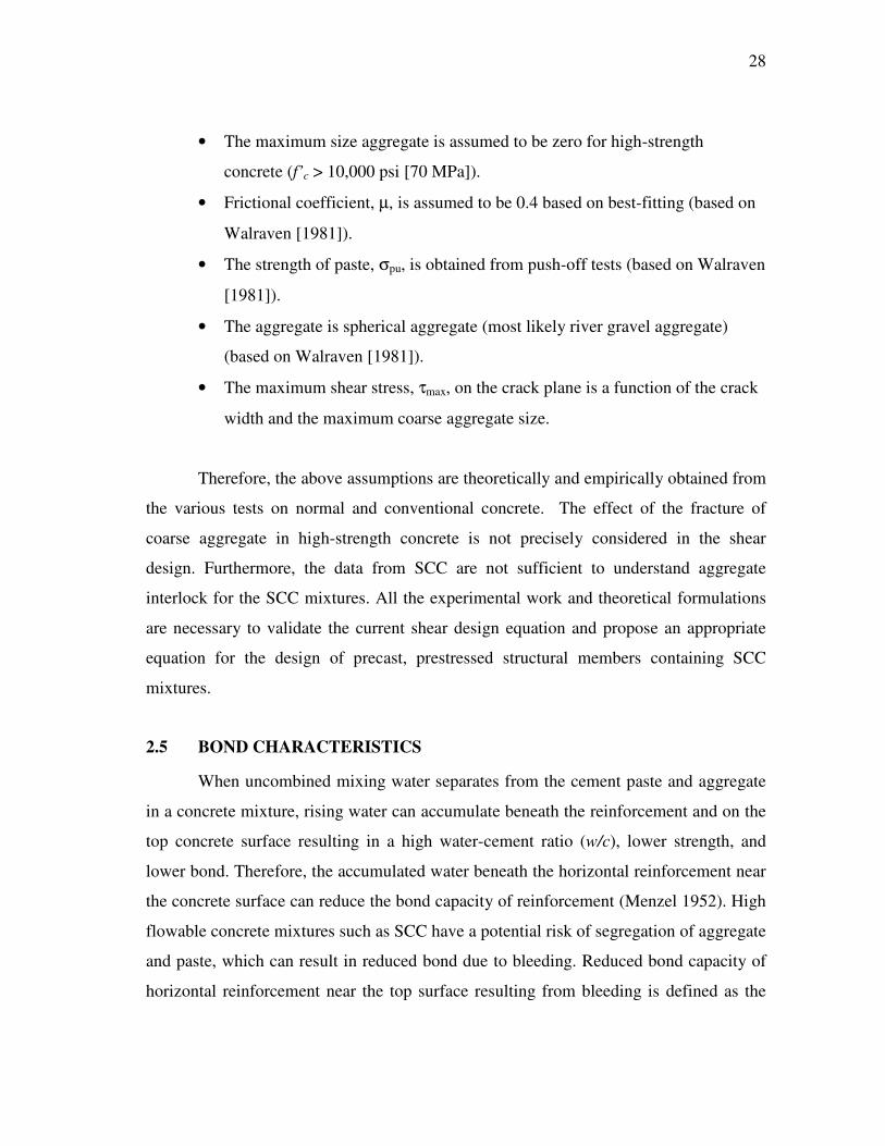
28

• The maximum size aggregate is assumed to be zero for high-strength

concrete (f’c > 10,000 psi [70 MPa]).

• Frictional coefficient, µ, is assumed to be 0.4 based on best-fitting (based on

Walraven [1981]).

• The strength of paste, σpu, is obtained from push-off tests (based on Walraven

[1981]).

• The aggregate is spherical aggregate (most likely river gravel aggregate)

(based on Walraven [1981]).

• The maximum shear stress, τmax, on the crack plane is a function of the crack

width and the maximum coarse aggregate size.

Therefore, the above assumptions are theoretically and empirically obtained from

the various tests on normal and conventional concrete. The effect of the fracture of

coarse aggregate in high-strength concrete is not precisely considered in the shear

design. Furthermore, the data from SCC are not sufficient to understand aggregate

interlock for the SCC mixtures. All the experimental work and theoretical formulations

are necessary to validate the current shear design equation and propose an appropriate

equation for the design of precast, prestressed structural members containing SCC

mixtures.

2.5 BOND CHARACTERISTICS

When uncombined mixing water separates from the cement paste and aggregate

in a concrete mixture, rising water can accumulate beneath the reinforcement and on the

top concrete surface resulting in a high water-cement ratio (w/c), lower strength, and

lower bond. Therefore, the accumulated water beneath the horizontal reinforcement near

the concrete surface can reduce the bond capacity of reinforcement (Menzel 1952). High

flowable concrete mixtures such as SCC have a potential risk of segregation of aggregate

and paste, which can result in reduced bond due to bleeding. Reduced bond capacity of

horizontal reinforcement near the top surface resulting from bleeding is defined as the

29

top-bar effect (Jeanty et al. 1988). In Article 5.11.2.1.2 of the AASHTO LRFD Bridge

Design Specifications (2004, 2006), the calculated development length increased by 40

percent when the horizontal reinforcement is located at a position higher than 12 in. (305

mm) from the bottom face of the member (AASHTO 2006). The top bar effect is also a

potential issue for precast, prestressed members. When the strands have a harped or

draped pattern, the strands at the end section are located near the top surface compared

to the location of the strands in the midspan. Mild reinforcement on the top flange is also

critical for controlling cracking in the end zone. Therefore, the bleeding water, which is

free water isolated from the fresh concrete, is prone to accumulation underneath

horizontal bars located near the surface. The air void and locally low strength of the

interface between the concrete and steel can cause low friction and mechanical bond

capacity. VMAs control bleeding, segregation, and surface settlement in SCC (Domone

2006, Khayat et al. 2007, Khayat and Guizani 1997). Therefore, the reduction in bond

caused by the top bar effect can be reduced by using VMAs (Khayat 1998). However,

VMAs can adversely affect the bond strength according to Girgis and Tuan (2004).

Because the top bar effect is highly correlated to the stability of SCC mixtures, tests are

needed to assess the impact of stability on the top bar effect.

ACI 318-05 (Section R12.2.4; 2005) and 2004 AASHTO LRFD Bridge Design

Specifications (Article 5.11.2.1.2) require the use of a multiplier of 1.3 or 1.4,

respectively, for top bars when computing the required development.

Generally, the stability of the SCC is evaluated in the fresh state. However, the

impact of mixture proportions of the SCC on bond capacity and top bar effect is still not

fully understood. Furthermore, the top bar in the AASHTO LRFD Specifications needs

to be evaluated for applicability for SCC.

2.6 CREEP AND SHRINKAGE

Creep and shrinkage are representative time-dependent properties of concrete

that influence prestress losses, camber, and deflection in prestressed members. Shrinkage

and creep are viscoelastic phenomena of hardened cement paste influenced by similar

30

material characteristics and environmental conditions (Mehta and Monterio 2005).

Because both creep and shrinkage of concrete are similarly affected by internal and

external factors, this section discusses both properties. However, a more detailed

shrinkage test program and results for this project are discussed by researchers at the

University of Texas at Austin (Koehler and Fowler 2008).

Shrinkage depends on the characteristics of aggregate stiffness and texture, w/c,

volume of paste, volume of coarse aggregate, cement type, admixture type and curing

method, volume to surface area ratio of a structural member, environmental conditions

(i.e., humidity and temperature), and duration of drying time. Shrinkage causes an

asymmetrical volumetric change due to the drying and wetting of capillary pores. Creep

depends on the same factors as shrinkage along with magnitude and age of loading and

time (AASHTO 2006). Creep is a volumetric change due to external loads. In concrete,

long-term creep deformations are generally larger than the initial elastic deformation due

to the applied load. The creep shortening of concrete under permanent loading typically

ranges from 0.5 to 4 times the initial elastic shortening. The magnitude mainly depends

on concrete maturity at the time of loading (AASHTO 2006).

For interpretation of creep strain and comparison of test results, basic equations

are presented below.

The creep coefficient is defined as follows:

( , ) C

iin st

t tεψ =

ε (2.24)

where ( , )it tψ is the creep coefficient, instε is the initial strain due to applied load in

compression, and Cε is the creep strain.

Specific creep, spε , is defined as follows:

Csp

εε =σ

(2.25)

31

where σ is the stress due to applied compressive load, which must be smaller than 50

percent of the compressive strength.

Because SCC has high paste volume (or high sand to aggregate ratio) to achieve

high workability and high early strength, several researchers expected relatively large

creep and shrinkage of SCC for precast, prestressed concrete, resulting in large prestress

losses (Issa et al. 2005, Naito et al. 2006, Schindler et al. 2007b, Suksawang et al.

2006). D’Ambrosia et al. (2005) also claimed high autogenous shrinkage at early ages

resulting in high early cracking of SCC with low w/cm and high paste volume. However,

the fast early strength gain mitigated the risk of cracking. Even though mechanical

properties of SCC are superior to those of CC, creep and shrinkage of SCC was

significantly high (Issa et al. 2005).

Naito et al. (2006) also found that SCC exhibited higher shrinkage and creep

than CC, which was attributed to high fine aggregate volume in the SCC. Naito et al.

(2006) found that the ACI 209 prediction model (1992) overestimated the shrinkage of

CC and SCC by 18 and 39 percent, respectively. The creep coefficient of SCC and CC

was 40 and 6 percent higher than the ACI 209 prediction model (1992), respectively.

On the other hand, Schindler et al. (2007b) found that the shrinkage of SCC is

similar or less than that of CC. At early ages AASHTO LRFD Specifications (2004)

underestimated the shrinkage values (7 and 14 days), while it overestimated the

shrinkage at later ages (56 and 112 days) for both CC and SCC. When the shrinkage of

SCC was compared to that of CC at 112 days, the sand to aggregate ratio effect was not

significant for the shrinkage of SCC. The creep coefficients of SCC mixtures were also

smaller than those of CC at all loading ages. This was attributed to the low w/c

(Schindler et al. 2007b). According to Sucksawang et al. (2006), fly ash (Class F) and

silica fume and slag could reduce the capillary that causes high shrinkage. Finally, fly

ash was excellent among other SCMs in reducing shrinkage.

In general, several research projects investigated creep and shrinkage of SCC

mixtures. Because creep and shrinkage are sensitively affected by mixture proportions

and environmental factors, the results vary and give different trends. Therefore, more

32

data are necessary to understand the behavior of creep and shrinkage of SCC mixtures

compared with CC mixtures. For this study, shrinkage of SCC mixtures was investigated

by researchers at the University of Texas at Austin (Koehler and Fowler 2008) and creep

of the SCC mixtures was investigated by researchers at Texas A&M University.

Prediction equations for creep and shrinkage of concrete account for internal and

external factors. Mixture proportions are the internal factors, such as the ratio of fine

aggregate and cement contents, admixtures, shape of coarse aggregate, and so on.

Otherwise, environmental elements, such as relative humidity and temperature, are

external factors. Each factor is not independent from the other factors. Because there are

many internal and external factors affecting characteristics of creep and shrinkage, it is

not easy to predict and determine creep and shrinkage accurately. That is why many

prediction formulas have not been accepted widely as reasonable prediction models.

Table 2.1 shows a summary of the input parameters to estimate creep and

shrinkage using various prediction models found in the literature. Prediction models can

indirectly consider the aggregate type as the stiffness of concrete based on the MOE and

compressive strength of concrete. Both creep and shrinkage increase initially after

loading. Generally, the ACI Committee 209 model (1992), CEB-FIP model (CEB-FIP

1993), BP model (Bazant and Panula 1984), B3 model (Bazant and Baweja 2000), and

GL2000 model (Gardner and Lockman 2001) consider various internal and external

parameters. The applicable concrete compressive strength at 28 days for the ACI 209

model, CEB-FIP model, BP model, B3 model, and GL 2000 model vary from 3000 to

10,000 psi (20 to 70 MPa) according to ACI 209 Committee report (2008). More

detailed equations are presented in Appendix A.

33

Table 2.1. Input Parameters for Predicting Creep and Shrinkage.

Models AASHTO 2004

AASHTO 2006

ACI 209

CEB-FIP BP B3 GL

2000 External Factors

(Environment and Time)

Curing conditions - - S, C - - S, C - Age of loading C C C C C C C

Relative humidity S, C S, C S, C S, C S, C S, C S

External Factors

(Physical Condition)

Specimen size S, C S, C S, C S, C S, C S S, C

Specimen shape - - - - S, C S -

Internal Factors

(Mechanical Properties)

'cf at 28 days C - C S, C S, C S, C S, C

'cf �

at age of loading

- S, C C - - - C

MOE at 28 days - - C C S, C C C

MOE at age of loading (or drying

for shrinkage) - - C C S, C - C

Internal Factors

(Composition)

Cement type - - C S, C C S, C S Water-cement

ratio (w/c) - - - - S, C C -

Aggregate-cement ratio - - - - S, C C -

Fine aggregate to all aggregate ratio - - S, C - S, C - -

Air - - S, C - - - -

Note: S = Shrinkage, C = Creep, - = no data.

The AASHTO LRFD Bridge Design Specifications (2006) provide prediction for

creep and shrinkage models while allowing the use of two alternative methods: the CEB-

FIP model (1993) and the ACI 209 Committee model (1992). The AASHTO LRFD

Bridge Design Specifications (2006) prediction model was based on the research of Hue

et al. (2001), Al-Omaishi et al. (2001), Collins and Mitchell (1991), and Tadros et al.

(2003). It is noted that these prediction models are applicable up to a compressive

strength of 15 ksi (103 MPa) (AASHTO 2006). However, there are not sufficient data

and information for estimating creep and shrinkage of SCC mixtures based internal

factors.

Compressive strength at the age of loading is used in the AASHTO LRFD (2006)

prediction equation for creep and shrinkage instead of the 28-day compressive strength

34

used in the AASHTO LRFD (2004). Finally, the applicability of prediction equations

has to be investigated for use in the design of precast, prestressed structural members

made with SCC. Other available prediction equations will be assessed to determine if

they can reasonably predict the creep and shrinkage of SCC.

2.7 DURABILITY

Permeability and diffusivity depend on the soundness of pore structure: total

numbers, size, and distribution of pores. Assie et al. (2005) observed that when SCC

mixtures contain more limestone powder and a high dosage of HRWRA, they present

lower permeability and similar diffusivity compared to CC . The permeability of SCC

was greatly enhanced with the use of fly ash and silica fume especially at ages of 56 and

91 days (Suksawang et al. 2006). The proportion of HRWRA is greater in SCC than CC.

Therefore, the air void system could be destabilized by the effects of HRWRA and affect

the freeze and thawing resistance (Khayat and Assaad 2002). Freeze and thawing

resistance of SCC with granite coarse aggregate and natural sand was acceptable because

the HRWRA resulted in a poorly distributed and inadequate air void system (Ozyildrim

2007). With various types of HRWRAs and air-entraining admixtures (AEAs) and

combinations of admixtures, the SCC mixtures had surface areas less than 0.94 in.2/in.3

(24 mm2/mm3) and spacing factors much larger than 0.008 in. (0.20 mm); these values

indicate excellent durability compared with CC (Christensen and Ong 2005).

In general, the durability of SCC mixtures is sensitive to the mixture proportions

and admixture types. Air void systems and pore structures of SCC mixtures differ from

CC mixtures. Therefore, typical durability parameters including permeability, diffusion

coefficient, and freezing and thawing resistance of the SCC mixtures are assessed in this

study.

2.8 FLEXURAL CAPACITY

Flexural capacity is a fundamental structural performance for precast, prestressed

structural members. Flexural behavior relates to MOE, MOR, and prestress losses and

35

development length. In service load conditions, the tensile stress of the top and bottom

fibers should be checked to determine whether this stress is within the allowable tensile

limit, which generally is determined from the MOR. This allowable stress should be

checked at the stage after transfer, along with the compressive concrete strength at

release. After casting decks, the allowable stress should also be checked, considering

different section properties and effective prestress after losses. The stresses are generally

checked at the end zone, transfer length region, and midsapn. In general, this step

controls the selection of cross-section and number and locations of strands.

According to the AASHTO LRFD Specifications (2004, 2006), the tensile stress

of a prestressed concrete member is 6 times (0.49) the square root of the compressive

strength (psi [MPa]) for estimating allowable tensile stress at service.

The elastic and post-cracking behavior of SCC can be different due to different

mechanical and bond mechanisms. MOE, prestress loss, and MOR can be useful to

predicting elastic and cracking occurrence. However, post-cracking behavior is a more

complicated response. Therefore, flexural testing is important to full-scale testing and

validation. However, there were few full-scale flexural tests conducted on prestressed,

precast girders made with SCC.

Flexural capacity can be estimated based on three basic assumptions: plane

sections remain plane, the concrete and steel are perfectly bonded and have the same

thermal coefficient, and the strain distribution is linear across the section. According to

Naaman (2004), the AASHTO LRFD Specifications is superior in simplicity and

generality to the ACI 318-02 code for the design of prestressed concrete members. This

is because only the location of the neutral axis, c, is required to solve the equilibrium

equation and the stress in the strands, fps at the nominal flexural moment resistance, Mn.

To determine fps at the nominal flexural moment resistance, Mn, following the AASHTO

LRFD Specifications (2006), the average stress in strands, fps, should be obtained from

the following equation, where effective prestress after losses, fpe, is not less than 0.5 fpu (AASHTO LRFD 2006 Article 5.7.3.1.1-1):

36

1ps pu

p

cf = f k

d

� �−

� � (psi, in. [MPa, mm]) (2.26)

where fpu is the ultimate strength of the prestressed strand (ksi [MPa]), c is the depth of

neutral axis at ultimate (in. [mm]), dp is the distance from the extreme compression fiber

to the centroid of tensile force in strands (in. [mm]), and k is defined as the following

equation (AASHTO LRFD 2006 Article 5.7.3.1.1-2) (psi/psi [MPa/MPa]):

2 1.04 py

pu

fk =

f

� �−

� � (ksi) 2 1.04 py

pu

fk =

f

� �� �−� �

� �� �� � (MPa)

(2.27)

where fpy is the yield stress of the strands (ksi [MPa]). When the neutral axis falls in the

top flange, the section is treated as a rectangular beam. When the neutral axis falls in the

web, the section can be treated as a T-section beam. The neutral axis can then be

calculated using the following equation:

10.85

ps py s y s y

puc w ps

p

A f A f A fc

ff b k A

d

′ ′+ −=

′β +

(ksi, in. [MPa, mm])

(2.28)

where Aps is the area of strands (in.2 [mm2]), fpu is the tensile strength of prestressing

steel (ksi [MPa]), fpy is the yield strength of prestressing steel (ksi [MPa]), As is the area

of mild steel tension reinforcement (in.2 [mm2]), A’s is the area of compression tension

reinforcement (in.2 [mm2]), fy is the yield strength of tension reinforcement steel (ksi

[MPa]), f’y is the yield strength of compression reinforcement steel (ksi [MPa]), hf is the

width of compression flange (in. [mm]), bw is the width of web (in. [mm]), dp is the

distance from the extreme compression fiber to the centroid of tensile force in strands

(in. [mm]), c is the distance between the neutral axis and the compressive face (in.

[mm]), and β1 is the stress block factor (see AASHTO LRFD 2006 Article 5.7.2.2).

37

The nominal moment capacity, Mn, can be calculated using the following

equation (kip-ft [kN-m]):

( ) 10.85

2 2 2 2f

n ps ps p s y s c w f

ha a aM A f d A f d f b b h

� �� � � �′ ′ ′ ′= − − − + − β − � � � � � �

(2.29)

where sd ′ is the depth of the compressive reinforcement (in. [mm]) and a is the depth of

the equivalent stress block (in. [mm]).

As shown in the above equations, the nominal moment depends on many aspects

of properties of concrete and bond characteristics. Therefore, full-scale testing is

necessary to validate the design equations of the AASHTO LRFD. Moreover, the

comparison of flexural capacity between SCC and CC girders is essential to validate

overall structural performance of the precast, prestressed structural members made with

SCC.

2.9 TRANSFER LENGTH AND DEVELOPMENT LENGTH

Bond mechanisms of prestressing strands are different from the bond

mechanisms of mild steel reinforcement. This section explains the unique bond

characteristics and the design of prestressed structural members. This section presents

the definition of transfer and development length, bond mechanism, design equations,

and recent findings related to SCC mixtures.

As shown in Figure 2.5, transfer length, lt, is the transition distance from the free

end of the prestressing strands to the fully bonded zone having an effective stress of the

strands, fpe, which is the stress of strands after prestress losses. Flexural bond length, lf, is

the additional bond length required for the strands to reach the stress, fps, corresponding

to the stress in the strands at ultimate conditions, used to calculate the nominal moment

capacity of the girder. As shown in Figure 2.5, the development length, ld, is estimated

as the sum of the transfer length, lt, and the flexural bond length, lf.

38

Figure 2.5. Definition of Development Length (Naaman 2004).

Transfer length and development length should be appropriately estimated to

predict the flexural and shear design capacity along the entire span length.

Bond mechanisms consist of three major mechanisms: chemical and physical

adhesion, friction, and mechanical resistance (Hanson and Kaar 1959). Adhesion is the

weakest bond between the concrete and strands. After slippage, adhesion makes no

contribution to bond. The significant bond mechanisms of the strand are the frictional

mechanism and mechanical resistance. The frictional mechanism is well known as the

Hoyer effect or “lack of fit” mechanism (Hoyer and Friedrich 1939, Stoker and Sozen

1970). After releasing the strands, the diameter of the strand at the girder ends expands

because of Poisson’s effect. The expanded part produces a wedge action between the

concrete and strands, resulting in friction between the surrounding concrete and the

strands. The friction force is a function of the radial compressive stress on the strand.

Therefore, the frictional bond depends on the compressive strength and time-dependent

behavior of the concrete (creep and shrinkage). When the compressive strength

increases, transfer length decreases (Catrodale et al. 1988, Kaar et al. 1963, Mitchell et

al. 1993). Mechanical interlocking is also a distinguishable bond mechanism for strands.

39

The interlocking stress is generated by the concrete bearing force against twisting wires

of strands. However, time-dependent properties such as the development of concrete

compressive strength and prestress loss could change the bond stress, resulting in the

elongation of the transfer length.

Application of external loads increases the strand stress in addition to the

effective stress, that is, the flexural bond stress induced by the external load. When

cracking occurs, flexural bond stress increases significantly adjacent to cracks with

stress concentrations and the loss of adhesion and frictional bond result in bond slip. The

stresses are continuously redistributed from the initial crack to the adjacent end region.

This region is referred to as the crack influence length or crack bond stress wave. When

cracks propagate toward the beam end, the stand stress dramatically increases because of

the frictional loss and the reduction of bearing stress (Hanson and Kaar 1959, Janney

1954).

The transfer and development length were proposed by many researchers to

reasonably predict bond properties in prestressed concrete members (Buckner 1995,

Lane 1998). Since 1998 the transfer length in the AASHTO LRFD Bridge Design

Specifications (2004, 2006) has been changed to 60 strand diameters, db, from 50 db as

required in the AASHTO LRFD (1996). High effective stress, fpe, results in a longer

transfer length (Hanson and Kaar 1959, Russell and Burns 1993). The ACI 318-05

recommended a transfer length of 50 db for shear design (Section 11.4.3) and fpe/3db for

estimating development length (Section R12.9.1.1). The development length proposed

by the AASHTO LRFD Bridge Design Specifications (2004) and the ACI 318-05 Code

(2005) is based on extensive experimental data from research using CC mixtures

(AASHTO 2006, ACI Committee 318 2005, Hanson and Kaar 1959, Janney 1954, Kaar

et al. 1963). In October 1988, the Federal Highway Administration (FHWA) issued a

memorandum requiring a 1.6 multiplier on the development length estimation

(AASHTO 2004, 2006). The AASHTO LRFD Specifications (2004) also included the �

factor as 1.6 for all precast, prestressed beams regardless of the depth of beams.

However, the � factor was updated with the limit of depth of beams in the AASHTO

40

LRFD (2006). The worst-case characteristics of strands shipped before 1997 and a lack

of data made this conservative (AASHTO 2004, 2006, Lane 1990).

In the AASHTO LRFD Bridge Design Specifications (2006) Article 5.11.4.2

Equation 5.11.4.2-1, the 1.6 multiplier factor κ was used to avoid the bond failure

resulting from inadequate development length in the structural member having the high

shear effect in the beam with a depth greater than 24 in. (0.6 m), as shown in Equation

2.30. Otherwise, the 1.0 factor κ was recommended for prestressed members with a

depth less than or equal to 24.0 in. (0.6 m), as shown in Equation 2.30. In 2001, the

Florida Department of Transportation concluded that the adverse affect of shear stress on

bond should be considered to estimate the development length of beams with a depth

greater than 24 in. (0.6 m) (Shahawy 2001).

According to the AASHTO LRFD Specifications (2006), the gradual buildup of

the strand force over the transfer and development lengths can be determined as follows:

23d ps pe bl f f d� �≥ κ −

� � (ksi, in)

26 9 3d ps pe bl f f d.

� κ �� �≥ − � �� �� �

(MPa, mm)

(2.30)

where bd is the nominal strand diameter (in. [mm]), fps is the average stress in

prestressing steel corresponding to the nominal flexural resistance of the member (ksi

[MPa]), fpe is the effective stress in the prestressing steel after losses (ksi [MPa]), and κ

is 1.0 for pretensioned members with a depth less than or equal to 24 in. (610 mm) or 1.6

for pretenstioned members with a depth greater than 24 in. (610 mm).

In Equations 5.11.4.2-3 and 5.11.4.2-4 of the AASHTO LRFD (2006), bilinear

equations are proposed to predict the stress of strand along the entire span length, and

these are repeated here as Equations 2.31 and 2.32:

60pe px

pxb

f lf

d=

( )for 60px tr bl l d� �≤� � (ksi, in. [MPa, mm])

(2.31)

41

( )( 60 )

( 60 )px b

px pe ps ped b

l df f f f

l d

−= + −

− ( )for 60px tr bl l d� �>� �

(ksi, in. [MPa, mm])

(2.32)

where lpx is the distance from the free end of the prestressed strand to the section of the

member under consideration (in. [mm]) and fpx is the design stress in the prestressed

strand at nominal flexural strength at the section of member under consideration (ksi

[MPa]). Figure 2.6 illustrates the bilinear equations for estimating the stress in prestress

strands at the nominal resistance of the member.

Figure 2.6. Idealized Relationship between Steel Stress and Distance

from the Free End of Strand (AASHTO 2006).

The AASHTO LRFD Bridge Design Specifications (2004) all use the alternative

equation for prestressed beams based on the studies of Lane (1990, 1998). The

development length can be determined as follows (AASHTO LRFD 2004 Equation

5.11.4.2-2):

6 4 ( )410 (ksi, in.)ps pe bpbt b

dc c

. f f df dl

f f

−≥ + +

′ ′ (2.33)

At Nominal Resistance of Member

Effective Prestress

Steel Stress

End of Member

Free End of Strand

End of Transfer Length

60 db lpx

ld

fps

fpe ( )( 60 )

( 60 )px b

px pe ps ped b

l df f f f

l d

−= + −

−

60pe px

pxb

f lf

d=

42

6 4 ( )4254 (MPa, mm)ps pe bpbt b

dc c

. f f df dl

f f

� �−≥ + +� �

′ ′� �� �

where db is the nominal strand diameter (in. [mm]), fpbt is the stress in prestressing steel

immediately prior to transfer (ksi [MPa]) which is 0.75 fpu (ksi [MPa]) for the low

relaxation strands, fps is the average stress in prestressing steel corresponding to the

nominal flexural resistance of the member (ksi [MPa]), fpe is the effective stress in the

prestressing steel after losses (ksi [MPa]), and f’c is the specified compressive strength of

concrete at 28 days (ksi [MPa]).

These bond mechanisms highly depend on the physical and chemical properties

of concrete. SCC mixtures have potentially different bond performance than CC

mixtures. According to previous research, the transfer lengths of SCC beams were

longer than those of CC beams (Burgueño and Haq 2007, Erkmen et al. 2007).

According to Girgis and Tuan (2004), transfer length of some SCC mixtures is 50

percent longer than that of CC mixtures. The transfer length of SCC with limestone was

generally similar to that of CC. However, the bond strength of SCC with fly ash was

lower than CC, indicating longer transfer length (Hegger et al. 2007). According to

Maekawa et al. (2003), the SCC has low w/c and less porosity resulting in high bond

strength based on finite element analytical approaches and test results. According to

Larson et al. (2005), the top strand has about 50 percent longer transfer length compared

to the bottom strands. They also found that, in general, the transfer length of top strands

is satisfactory estimated by ACI 318-05. It is noted that a single strand with 8 in. × 24 in.

(0.2 m × 0.6 m) depth beams was tested to evaluate transfer and development length in

their study.

Trent (2007) tested 24 beams with 14 in. (0.35 m) depth and single strands. The

development length of SCC beams was 20 percent shorter than the value estimated

using ACI 318-05 and the AASHTO LRFD Bridge Design Specifications (2006) with a

κ factor of 1.0. He concluded that, in general, the transfer and development length of

strands in SCC beams are satisfactorily estimated, with conservatism, using the

43

AASHTO LRFD Bridge Design Specifications (2004 and 2006) regardless of the κ

factor.

According to the basic theory of prestressed concrete from an early study by

Guyon (1953), bond performance depends on the quality of the concrete. The high paste

volume and the stability of SCC mixtures potentially influence the bond mechanisms

resulting in the change of prestressing stresses of strands. Furthermore, case studies are

limited to understanding the impact of the SCC mixtures on the design equations to

reasonably estimate the transfer and development length.

Finally, the applicability of the AASHTO LRFD Specifications for estimating

transfer and development length has to be investigated for implementation of SCC

mixtures. In this study, equations of the AASHTO LRFD (2004, 2006) are examined.

2.10 PRESTRESS LOSSES

Prestress losses occur due to several factors including environmental conditions,

material properties, and construction practices. The estimation of prestress losses needs

to be accurate to predict time-dependent behavior, such as long-term deflection and

service stresses of prestressed concrete members. Transfer and development length and

flexural and shear capacities of the members also require accurate estimation of

prestressing forces after losses.

Figure 2.7 shows prestress losses of strands as a function of construction and

load sequence. Before transfer (release of strands) the initial jacking stress of strands has

components of several losses such as the anchorage seating, the initial relaxation of

strands, and temperature effect. At transfer, immediate losses occur due to elastic

shortening of the concrete. Creep, shrinkage, and relaxation also produce additional

losses before casting deck. Deck weight and superimposed dead and live loads produce

elastic gain in the strands for the composite member. After casting the deck, the

shrinkage and creep of the girder and the deck and relaxation of strands occurs over

time, resulting in long-term prestress losses (Tadros et al. 2003).

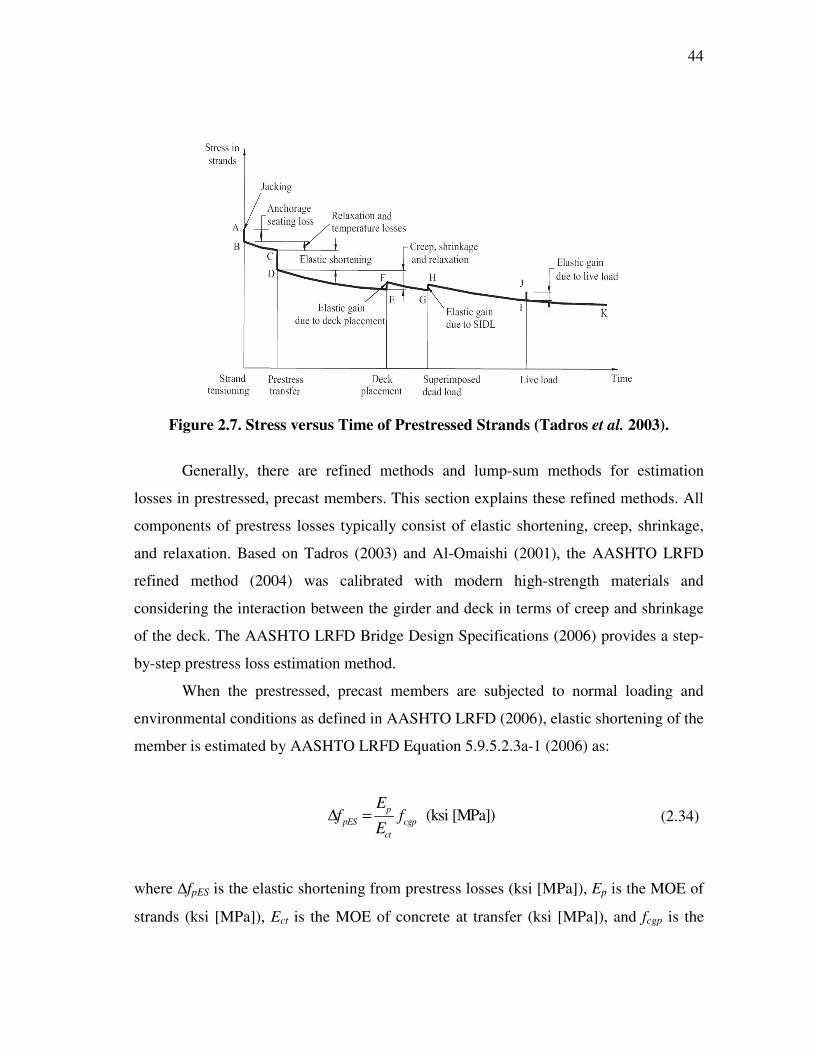
44

Figure 2.7. Stress versus Time of Prestressed Strands (Tadros et al. 2003).

Generally, there are refined methods and lump-sum methods for estimation

losses in prestressed, precast members. This section explains these refined methods. All

components of prestress losses typically consist of elastic shortening, creep, shrinkage,

and relaxation. Based on Tadros (2003) and Al-Omaishi (2001), the AASHTO LRFD

refined method (2004) was calibrated with modern high-strength materials and

considering the interaction between the girder and deck in terms of creep and shrinkage

of the deck. The AASHTO LRFD Bridge Design Specifications (2006) provides a step-

by-step prestress loss estimation method.

When the prestressed, precast members are subjected to normal loading and

environmental conditions as defined in AASHTO LRFD (2006), elastic shortening of the

member is estimated by AASHTO LRFD Equation 5.9.5.2.3a-1 (2006) as:

(ksi [MPa])p

pES cgpct

Ef f

E∆ =

(2.34)

where ∆fpES is the elastic shortening from prestress losses (ksi [MPa]), Ep is the MOE of

strands (ksi [MPa]), Ect is the MOE of concrete at transfer (ksi [MPa]), and fcgp is the

45

concrete stress at the center of gravity of the strands due to the prestressing force

immediately after transfer and the self-weight of the member at the section of maximum

moment (ksi [MPa]).

The elastic shortening can be also calculated using the transformed section

properties. This equation is based on the assumption that the strand and concrete are

equally strained in compression and tension (AASHTO 2006). This alternative equation

is used for the prediction of elastic losses in this study:

2

2

( ) (ksi [MPa])

( )

ps pbt g m g m g gpES

g g cips g m g

p

A f I e A e M Af

A I EA I e A

E

+ −∆ =

+ + (2.35)

where Aps is the area of strands (in.2 [mm2]), Ag is the gross area of section (in.2 [mm2]),

Eci is the MOE of concrete at transfer (ksi [MPa]), Ep is the modulus of elasticity of

strands (ksi [MPa]), em is the average eccentricity of the strands at midspan (in. [mm]),

fpbt is the stress in the strand immediately prior to transfer (ksi [MPa]), Ig is the moment

of inertia of the gross section (in.4 [mm4]), and Mg is the midspan moment due to

member self-weight (kip-in. [kN-mm]).

Equation 5.9.5.4.1-1 is the general equation to predict approximate time-

dependent prestress losses with three components which are creep, shrinkage, and

relaxation. A more detailed method is the refined estimate of time-dependent loss in

AASHTO LRFD Article 5.9.5.4 (2006). In general, the time-dependent loss, ∆fpLT, can

be determined as follows (2006 AASHTO LRFD Equation 5.9.5.4.1-1):

1 2( ) ( ) (ksi [MPa])pLT pSR pCR pR id pSD pCD pR pSS dff f f f f f f f∆ = ∆ + ∆ + ∆ + ∆ + ∆ + ∆ − ∆ (2.36)

where ∆fpSR is the prestress loss due to shrinkage of the girder between transfer and deck

placement (ksi [MPa]), ∆fpCR is the prestress loss due to creep of the girder between

transfer and deck placement (ksi [MPa]), ∆fpR1 is the prestress loss due to relaxation of

46

prestressing strands between transfer and deck placement (ksi [MPa]), ∆fpR2 is the

prestress loss due to relaxation of prestressing strands in composite section between time

of deck placement and final time (ksi [MPa]), ∆fpSD is the prestress loss due to shrinkage

of the girder between time of deck placement and final time (ksi [MPa]), ∆fpCD is the

prestress loss due to creep of the girder between time of deck placement and final time

(ksi [MPa]), ∆fpSS is the prestress loss due to shrinkage of the deck composite section

(ksi [MPa]), (∆fpSR + ∆fpCR + ∆fpR1)id is the sum of time-dependent prestress losses

between transfer and deck (ksi [MPa]), and (∆fpSD + ∆fpCD + ∆fpR2 − ∆fpSS)df is the sum of

time-dependent prestress losses after deck placement (ksi [MPa]).

The AASHTO LRFD Bridge Design Specifications (2004) presented the

prestress losses as follows (2004 AASHTO LRFD Equation 5.9.5.1-1):

1 2 (ksi [MPa])pT pES pR pSR pCR pRf f f f f f∆ = ∆ + ∆ + ∆ + ∆ + ∆ (2.37)

where ∆fpT is the total prestress loss (ksi [MPa]), ∆fpES is the prestress loss due to elastic

shortening (ksi [MPa]), ∆fpR1 is the prestress loss due to steel relaxation at transfer (ksi

[MPa]), ∆fpSR is the prestress loss due to concrete shrinkage (ksi [MPa]), , ∆fpCR is the

prestress loss due to concrete creep (ksi [MPa]), and , ∆fpR2 is the prestress loss due to

steel relaxation after transfer (ksi [MPa]).

Several research studies have estimated the prestress losses of SCC mixtures.

According to Ruiz et al. (2007), the prestress loss of SCC is comparable to that of CC in

6.5 in. × 12 in. (165 mm × 305 mm) by 18 ft (5.5 m) long beams. When the measured

values were compared to the equation proposed by Tadros et al. (2003), this equation

overpredicted the prestress losses of SCC and CC by about 35 and 20 percent,

respectively. Erkmen et al. (2007) also found that SCC and CC have similar elastic

shortening and long-term losses. They also found that the AASHTO LRFD method

(2004), PCI Design Handbook (PCI 2004), and PCI general method (PCI 1975)

predicted conservatively total prestress loss in 38 ft (11.5 m) long Mn/DOT 36M-I

47

girders. Some researchers found that SCC girders have less prestress losses than CC

girders, indicating less creep and shrinkage (Naito et al. 2006, Trent 2007). Contrary to

their expectations and concerns, high paste volume and low aggregate volume did not

cause larger amounts of prestress losses. The prediction equations generally

conservatively predicted prestress losses. These results could be attributed to the short

duration of monitoring the prestress losses, which was less than 1 year (Erkmen et al.

2007). One study performed field monitoring of full-scale beams and found that the

prestress loss of SCC seems to be similar to that of CC (Burgueño and Bendert 2007).

The high paste volume and stability of SCC mixtures potentially influence the

bond mechanisms resulting in the large prestress losses of strands. According to previous

research, the prestress losses of SCC mixtures were not significantly different from those

of CC mixtures. However, more comprehensive research is required to better estimate

prestress losses. To date, the case studies to understand the applicability of the design

equations to estimate accurate prestress losses to SCC girders are limited.

Finally, the applicability of the AASHTO LRFD Specifications (2004, 2006) for

estimating the prestress losses in SCC girders needs to be assessed.

2.11 CAMBER AND DEFLECTION

Camber and deflection are in-service performance measures of precast,

prestressed structural members. Creep, shrinkage, MOE, development of compressive

strength, bond, and prestress losses are related to the behaviors of camber and deflection.

Camber growth caused by the creep effect due to the axial prestressing force is typically

larger than the downward deflection caused by the creep effect due to the self-weight of

the girder.

Some researchers have monitored camber and deflection of SCC precast,

prestressed structural members. According to Gross et al. (2007) and Erkmen et al.

(2007), the overall behavior between SCC and CC members is similar. However, initial

camber was significantly higher in SCC girders due to low MOE and higher creep and

shrinkage of the SCC compared with CC laboratory results (Gross et al. 2007).

48

There is limited knowledge of the impact of the SCC on camber and deflection.

To predict camber and deflection, it is necessary to have a good understanding of

mechanical and time-dependent material along with an accurate estimation of prestress

losses. Because the SCC members might have different mechanical and time-dependent

properties, camber and deflection can be different from CC members. For accurate

prediction and estimation of camber and deflection, more data and comprehensive

studies are necessary with comprehensive understanding of mechanical, bond, and time-

dependent properties.

2.12 SUMMARY

According to several research studies and recommendations, SCC mixtures

typically have a high paste volume and low coarse aggregate to minimize the friction of

particles and maximize stability. Therefore, many researchers are concerned that SCC

mixture proportions could affect adversely hardened properties such as less aggregate

interlock resulting in low shear capacity and high shrinkage and creep resulting in high

prestress losses. Low elastic modulus could also increase the gap between actual and

predicted behaviors (i.e., deflection, camber). Several universities and transportation

agencies have conducted research to develop SCC mixture proportions, evaluate

mechanical and time-dependent properties, and validate with full-scale tests. Many

researchers have noted several advantages of SCC such as ease of placement, reduction

of casting time, and better finishing when used in precast, prestressed concrete structural

members. However, some researchers had difficulties in field application due to a lack of

robustness of SCC resulting in some segregation, poor workability, poor surface quality,

and/or low mechanical or bond strength (Burgueño and Haq 2007, Erkmen et al. 2007,

Ozyildrim 2007). Full-scale tests were also performed to evaluate field application,

structural behavior, prestress losses, camber, and deflection. In general, when the fresh

quality of SCC was satisfactory, the overall performance of SCC was comparable to that

of CC. However, information to characterize the hardened properties of SCC for precast,

prestressed concrete members is still limited. The applicability of the AASHTO LRFD

49

Specifications, which is based on CC, has not been fully evaluated for use in designing

SCC members. The study described in this dissertation is valuable because

comprehensive test results will be provided and the applicability of the AASHTO LRFD

Specifications will also be discussed.

50

CHAPTER III

MATERIALS

3.1 LABORATORY PROGRAM

Constituent materials used to make SCC can have a significant influence on the

fresh and hardened characteristics of the SCC. The following sections discuss

constituent materials used for manufacturing SCC in the laboratory program.

Information on the chemical and physical characteristics of the constitutive materials and

the mixture proportions are also presented.

3.1.1 Cement

A Type III cement (Alamo Cement Company, San Antonio, Texas) was used in

the laboratory testing phase. Table 3.1 shows the chemical composition of the cement

used in the laboratory testing. Table 3.2 shows the physical properties of cement used in

the laboratory testing.

Table 3.1. Chemical Characteristics of Type III Cement Used in Laboratory Testing.

Chemical Composition Proportions (%) SiO2 20.6

Al2O3 4.9 Fe2O3 3.4

CaO 64.1 MgO 0.8

SO3 3.5 Na2O - K2O -

Total Alkalies 0.5 Free Lime 1.5

C3S 56.6 C2S 16.3 C3A 7.2

C4AF 10.3

51

Table 3.2. Physical Characteristics of Type III Cement Used in Laboratory Testing.

Physical Characteristics Type III Cement Blaine Fineness, ft2/lb (m2/kg) 2630 (539)

Setting Time Initial, min 110 Final, min 210

Compressive Strength 1 day, ksi (MPa) 3.5 (24.1) 3 day, ksi (MPa) 4.7 (32.6) 7 day, ksi (MPa) 5.7 (39.1)

28 day, ksi (MPa) 6.8 (46.8) Specific Gravity 3.15

Loss on Ignition, % 2.1

3.1.2 Fly Ash

Untreated Class F fly ash (Boral Material Technologies, Rockdale, Texas) was

used in the SCC mixtures. Table 3.3 shows the chemical characteristics of the fly ash

used in the laboratory testing. Table 3.4 shows the physical characteristics of the fly ash

used in the laboratory testing.

Table 3.3. Chemical Characteristics Class F Fly Ash. Chemical Composition Proportions (%)

SiO2 52.5 Al2O3 21.8 Fe2O3 4.90

CaO 13.9 MgO 2.00

SO3 0.79 Na2O 0.32 K2O 0.74

Total Alkalies 0.81

52

Table 3.4. Physical Characteristics of Fly Ash.

Physical Properties Class F Fly Ash

Specific Gravity 2.33 Strength Activity Index with Portland Cement at Specific Day, % of Control 7 day 73.6 28 day 82.0 Loss on Ignition, % 1.05

3.1.3 Aggregate

The properties of the aggregate used in the laboratory test program are presented

in the following sections.

3.1.3.1 Coarse Aggregate

River gravel and limestone aggregates were used in this study. The same type

and source were used for both SCC and CC mixtures. Fordyce Murphy Quarry in

Victoria, Texas, provided the river gravel, and Hanson Aggregate in New Braunfels,

Texas, provided the limestone. Table 3.5 shows the characteristics of the coarse

aggregate used for the SCC and CC mixtures. The nominal maximum size aggregate was

0.75 in. (19 mm). Figure 3.1 shows the gradation of the coarse aggregates. These

gradations meet the requirement of ASTM C33, Standard Specification for Concrete

Aggregates (2007).

Table 3.5. Properties of Coarse Aggregate.

Physical Properties Aggregate Type

Fordyce Murphy River Gravel

Hanson Aggregate Limestone

Specific Gravity 2.59 2.59 Absorption Capacity, % 0.78 1.43

53

Figure 3.1. Gradation of Coarse Aggregates Used in Laboratory Testing.

3.1.3.2 Fine Aggregate

Table 3.6 shows the characteristics of the fine aggregate used in this study for the

SCC and CC mixtures. Figure 3.2 shows the gradation of the fine aggregates. These

gradations meet the requirement of ASTM C33.

Table 3.6. Properties of Fine Aggregate.

Physical Properties

Aggregate Type Fordyce

Murphy Natural Sand

(I)

TXI (Austin) Natural Sand (II)

Specific Gravity 2.58 2.60 Absorption Capacity, % 0.54 0.56 Fineness Modulus 2.72 2.89

0

20

40

60

80

100

0.00 0.20 0.40 0.60 0.80 1.00

River Gravel

Limestone

ASTM C33 (Upper Limit)

ASTM C33 (Lower Limit)

0 5 10 15 20 25Pa

ssin

g Pe

rcen

t (%

)

Sieve Size (in.)

Sieve Size (mm)

54

Figure 3.2. Gradation of Fine Aggregates Used in Laboratory Testing.

3.1.4 Chemical Admixtures

To achieve 16-hour target strengths and high workability, chemical admixtures

were used. BASF Construction Chemicals LLC provided all admixtures.

Polycarboxylate based HRWRAs were used for both CC and SCC mixtures. All of the

chemical admixtures, including HRWRAs used in this study, are given in Table 3.7.

Retarder, VMA, and accelerators were also provided by BASF. Section 3.1.6 explains

the purpose for each admixture type along with mixture proportions.

Table 3.7. Chemical Admixture Types. Admixture Type SCC CC HRWRA Glenium 3400NV PS 1466 Retarder Delvo Stabilizer - Experimental Admixture PT1482 - VMA VMA 362 -

Note: - indicates no addition.

3.1.5 Mild Steel Reinforcement

Grade 60 reinforcement meeting ASTM A615, Standard Specification for

Deformed and Plain Carbon-Steel Bars for Concrete Reinforcement (2008), (#5 [M16])

0

20

40

60

80

100

0.00 0.05 0.10 0.15 0.20 0.25 0.30

Natural Sand (Type I)

Natural Sand (Type II)

ASTM C33 (Upper Limit)

ASTM C33 (Lower Limit)

0 1 2 3 4 5 6 7Pa

ssin

g Pe

rcen

t (%

)

Sieve Size (in.)

Sieve Size (mm)

55

was used for the pull-out and push-off samples, with a yield strength, fy , between 62 and

68 ksi (427 and 469 MPa) according to mill certificates and laboratory tests at High Bay

Structural and Materials Laboratory (HBSML). The tensile strength, fu , is between 103

and 110 ksi (710 and 758 MPa). The chemical composition and mechanical properties of

the mild steel reinforcement is presented in Table 3.8. Tensile elongation (TE) is the

maximum elongation of reinforcements at ultimate failure.

Table 3.8. Chemical and Mechanical Properties of #5 (M16) Steel Reinforcement.

Reinforcement (#5 [M16]) Mill Certificate Information

HBSML Test Information

Properties 1st Set 2nd Set 1st Set 2nd Set fy, ksi (MPa)

68 (468) 62 (428) 64 (441) 66 (455)

fu , ksi (MPa) 104 (717) 103 (710) 109 (752) 110 (758) Tensile Elongation (%) 16 12 16 15

Composition Proportions (Wt. %) C 0.3700 0.4200

Mn 1.1200 0.8500 P 0.0180 0.0160 S 0.0380 0.0290

Si 0.2700 0.1900 Cu 0.3000 0.3500 Cr 0.1900 0.2000 Ni 0.1000 0.1400

Mo 0.0340 0.0370 Cb 0.0020 0.0020 V 0.0010 0.0010

Sn 0.0120 0.0130 B 0.0004 0.0004 Ti 0.0020 0.0010

3.1.6 Mixture Proportions

To quantify the hardened properties of SCC, researchers evaluated 12 SCC

mixture proportions with three main variables: 16-hour release strengths (5 and 7 ksi [34

and 48 MPa]), two aggregate types (river gravel and limestone), and three different

volumes of coarse aggregate. For river gravel, two additional mixture proportions were

used for 5 ksi [34 MPa] target strength. The ratio of the coarse aggregate volume to total

56

aggregate volume was varied to optimize the SCC mixture proportions. Changing these

ratios results in changes to paste volume.

Four CC mixture proportions served as control mixtures and consisted of two

release strengths (5 and 7 ksi [34 and 48 MPa]) and the two coarse aggregate types.

Figure 3.3 explains the mixture proportion identification. For the SCC mixtures,

the coarse aggregate volumes were varied from 32 to 38 percent.

Figure 3.3. Mixture Identification.

Different types of HRWRA were used to achieve the target workability. For the 7

ksi (48 MPa) SCC mixtures, an experimental admixture was used to achieve the target

strength at 16 hours and extend workability retention. A retarder was also used for the 5

ksi (34 MPa) SCC mixtures to extend workability retention. VMA was used to achieve

target workability and stability for the S7L-6 mixtures. AEAs were not used in this

study.

The mixture proportions of CC mixtures were based on typical mixture

proportions of precasters in Texas (Hueste et al. 2004). Note that the objective of this

research is to compare the performance of SCC mixtures with CC mixtures based on

their targeted 16-hour release strengths. In general, these early strengths are the critical

S5G- #

Concrete Type S: SCC C: CC

16-hour Strength 5: 5 ksi (34 MPa) 7: 7 ksi (48 MPa)

Aggregate Type G: River Gravel L: Limestone

Symbol indicate Relative coarse aggregate volume. (Higher number indicates higher volume)

57

factor for fabricating girders in Texas. The total volume of cementitious material was

limited to 700 lb/yd3 (415 kg/m3) in accordance with TxDOT Standard, Standard

Specifications for Construction and Maintenance of Highways, Streets, and Bridges

(TxDOT 2004). The total volume of coarse aggregate was 40 percent for the 5 and 7 ksi

(34 and 48 MPa) limestone mixture proportions and 44 percent for the 5 and 7 ksi (34

and 48 MPa) river gravel mixture proportions. Tables 3.9 to 3.12 present all CC and

SCC mixture proportions.

Table 3.9. Mixture Proportions of River Gravel SCC. Coarse Aggregate Type River gravel

16-hour Target Strength 5000 psi (34 MPa)

7000 psi (48 MPa)

Mixture ID S5G -1

S5G -2

S5G -3a

S5G -3b

S5G -3c

S7G -4

S7G -5

S7G -6

Cement, lb/yd3 (kg/m3) 624 (370)

646 (383)

633 (376)

720 (427)

Fly Ash, lb/yd3 (kg/m3) 156 (93)

239 (142)

298 (177)

180 (107)

Water, lb/yd3 (kg/m3) 252 (150)

260 (154)

255 (152)

208 (123)

Coarse Agg., lb/yd3 (kg/m3) 1461 (867)

1535 (911)

1374 (815)

1511 (897)

1649 (978)

1414 (839)

1527 (906)

1641 (973)

Fine Agg., lb/yd3 (kg/m3) 1456 (864)

1251 (742)

1368 (812)

1232 (731)

1095 (650)

1408 (836)

1296 (769)

1184 (702)

HRWRA, oz/yd3 (L/m3) 74 (2.9)

81 (3.1)

92 (3.6)

80 (3.1)

82 (3.2)

140 (5.4)

117 (4.5)

108 (4.2)

Retarder, oz/yd3 (L/m3) 27 (1.0)

27 (1.0)

25 (1.0)

25 (1.0)

25 (1.0) - - -

Exp. Admix., oz/yd3 (L/m3) - - - - - 578 (22.4) VMA, oz/yd3 (L/m3) - - - - - - - - Proportion Characteristics w/cm(*) 0.33 0.30 0.28 0.23 w/c 0.4 0.4 0.4 0.29 Coarse Agg. Vol., % 33.5 35.1 31.5 34.6 37.8 32.3 35.0 37.6

58

Table 3.10. Mixture Proportions of River Gravel CC. Coarse Aggregate Type River Gravel 16-hour Targeted Strength 5000 psi (34 MPa) 7000 psi (48 MPa) Mixture ID C5G C7G Cement, lb/yd3 (kg/m3) 625 (371) 700 (415) Water, lb/yd3 (kg/m3) 225 (134) 200 (119) Coarse Agg., lb/yd3(kg/m3) 1935 (1148) 1935 (1148) Fine Agg., lb/yd3 (kg/m3) 1232 (731) 1232 (731) HRWRA, oz/yd3 (L/m3) 56 (2.2) 91 (3.5) Proportion Characteristics w/c 0.36 0.285 Coarse Agg. Vol., % 44.3 44.3

Table 3.11. Mixture Proportions of Limestone SCC. Coarse Aggregate Type Limestone

16-hour Target Strength 5000 psi (34 MPa)

7000 psi (48 MPa)

Mixture ID S5L -3a

S5L -3b

S5L -3c

S7L -4

S7L -5

S7L -6

Cement, lb/yd3 (kg/m3) 640 (380) 720 (427) Fly Ash, lb/yd3(kg/m3) 426 (253) 180 (107) Water, lb/yd3(kg/m3) 288 (171) 225 (133)

Coarse Agg., lb/yd3 (kg/m3) 1259 (747)

1385 (822)

1511 (896)

1394 (827)

1505 (893)

1617 (959)

Fine Agg., lb/yd3 (kg/m3) 1264 (750)

1138 (675)

1011 (600)

1399 (830)

1287 (764)

1175 (697)

HRWR, oz/yd3 (L/m3) 60 (2.3)

58 (2.2)

58 (2.2)

108 (4.2)

117 (4.5)

108 (4.2)

Retarder, oz/yd3 (L/m3) 26 (1.0)

26 (1.0)

26 (1.0) - - -

Exp. Admix., oz/yd3 (L/m3) - - - 578 (22.4)

VMA, oz/yd3 (L/m3) - - - - - 4 (0.2)

Proportion Characteristics w/cm(*) 0.270 0.285 w/c 0.45 0.31 Coarse Agg. Vol., % 29.0 31.9 34.8 31.9 34.5 37.0

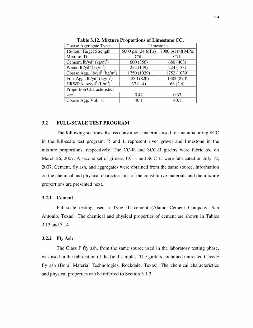
59

Table 3.12. Mixture Proportions of Limestone CC. Coarse Aggregate Type Limestone 16-hour Target Strength 5000 psi (34 MPa) 7000 psi (48 MPa) Mixture ID C5L C7L Cement, lb/yd3 (kg/m3) 600 (356) 680 (403) Water, lb/yd3 (kg/m3) 252 (149) 224 (133) Coarse Agg., lb/yd3 (kg/m3) 1750 (1039) 1752 (1039) Fine Agg., lb/yd3 (kg/m3) 1380 (820) 1382 (820) HRWRA, oz/yd3 (L/m3) 37 (1.4) 68 (2.6) Proportion Characteristics w/c 0.42 0.33 Coarse Agg. Vol., % 40.1 40.1

3.2 FULL-SCALE TEST PROGRAM

The following sections discuss constituent materials used for manufacturing SCC

in the full-scale test program. R and L represent river gravel and limestone in the

mixture proportions, respectively. The CC-R and SCC-R girders were fabricated on

March 26, 2007. A second set of girders, CC-L and SCC-L, were fabricated on July 12,

2007. Cement, fly ash, and aggregates were obtained from the same source. Information

on the chemical and physical characteristics of the constitutive materials and the mixture

proportions are presented next.

3.2.1 Cement

Full-scale testing used a Type III cement (Alamo Cement Company, San

Antonio, Texas). The chemical and physical properties of cement are shown in Tables

3.13 and 3.14.

3.2.2 Fly Ash

The Class F fly ash, from the same source used in the laboratory testing phase,

was used in the fabrication of the field samples. The girders contained untreated Class F

fly ash (Boral Material Technologies, Rockdale, Texas). The chemical characteristics

and physical properties can be referred to Section 3.1.2.

60

3.2.3 Aggregate

The same aggregate source used in laboratory test program was used for the full-

scale test program. The information can be found in Section 3.1.3. For limestone

mixtures, natural sand was provided from Fordyce Murphy Quarry in Victoria, Texas.

Table 3.13. Chemical Characteristics of Type III Cement Used in Full-scale Testing.

Chemical Composition Proportions (%)

Girder ID CC-R, SCC-R CC-L, SCC-L

SiO2 20.6 20.5 Al2O3 4.5 4.6 Fe2O3 3.6 3.5

CaO 64.6 64.5 MgO 0.7 0.7

SO3 3.7 3.7 Loss of Ignition 1.9 1.7

Total Alkalies (NaO2eq) 0.50 0.55 Insoluble 0.13 0.11

C2S 16.3 16.3 C3S 56.5 60 C3A 5.8 6.5

C4AF 11.0 10

Table 3.14. Physical Characteristics of Type III Cement Used in Full-scale Testing..

Physical Properties Girder ID CC-R, SCC-R� CC-L, SCC-L�

Blaine Fineness, ft2/lb (m2/kg)� 2640 (541) � 2586 (530)�Specific Gravity 3.15 3.15

Compressive Strength 1-day strength, psi (MPa) 3840 (26) 3880 (27) 3-day strength, psi (MPa) 5300 (37) 5360 (37) 7-day strength, psi (MPa) 6280 (43) 6240 (43)

28-day strength, psi (MPa) 6810 (47) 7460 (51)

61

3.2.4 Chemical Admixtures

Admixtures for mixture proportions were provided by BASF Construction

Chemicals LLC. Information on these admixtures can be found in Section 3.1.4.

3.2.5 Mild Steel Reinforcement for Girder and Deck

Grade 60 reinforcement meeting ASTM A615 (#4 [M13]) was used in the girders

and decks. The yield strength, fy , of the reinforcement was 62 and 65 ksi (427 and 448

MPa) for the decks and between 66 and 69 ksi (452 and 477 MPa) for the girders

according to mill certificates and laboratory tests performed at HBSML. The elastic

modulus of the reinforcement was assumed to be 29,000 ksi (200 GPa). The chemical

compositions and mechanical properties of mild steel reinforcements are presented in

Table 3.15. The reinforcement (#5 [M16]) used for the deck is the same as that described

in the laboratory test program.

Table 3.15. Chemical and Mechanical Properties of #4 (M13) Steel Reinforcement. Reinforcement (#4 [M13])

Mill Certificate Information

HBSML Test Information

Applications Girders All Decks Girders Deck fy, ksi (MPa)

69 (477) 66 (452) 62 (427) 65 (448) 65 (448)

ff, ksi (MPa)

104 (720) 103 (709) 99.5 (686) 104 (717) 104 (717) Tensile Elongation

(%) 13 16 12 - 11

Composition Proportions (Wt. %)

C 0.3700 0.3800 0.3900 Mn 1.1200 0.8900 0.8700

P 0.0180 0.0110 0.0110 S 0.0380 0.0290 0.0310

Si 0.2700 0.1700 0.1900 Cu 0.3000 0.3000 0.3900 Cr 0.1900 0.1400 0.1400 Ni 0.1000 0.1800 0.2000

Mo 0.0340 0.0480 0.0520 Cb 0.0020 0.0020 0.0040 V 0.0010 0.0010 0.0010

Sn 0.0120 0.0120 0.0160 B 0.0004 0.0003 0.0030 Ti 0.0020 0.0010 0.0010

62

3.2.6 Prestressing Steel

The prestressing steel for the girders was 0.5 in. (12.7 mm) diameter, Grade 270,

low-relaxation, seven-wire strand manufactured by American Spring Wire Corp. in

Houston, Texas. The strand met the requirement of ASTM A416, Standard Specification

for Steel Strand, Uncoated Seven-Wire for Prestressed Concrete (2006). Properties of the

strand are presented in Table 3.16. The yield stress is estimated based on 1 percent

elongation of strands according to ASTM A416. The strands were slightly weathered.

Table 3.16. Characteristics of Strands (Reported by Manufacturer).

Materials 0.5 in. (12.7 mm) diameter 270 ksi (1862 MPa) low-relaxation strands

Girder ID CC-R and SCC-R CC-L and SCC-L As, in.2 (mm2) 0.15281 (98.6) 0.15281 (98.6) Py, kip (kN) 38.54 (171.4) 39.67 (176.5) Pu, kip (kN) 44.19 (196.6) 44.43 (197.6) Tensile Elongation, % 8.81% � 4% 7.77% � 4% Ep, ksi (MPa) 28,000 (193,120) 28,000 (193,080)

Note: As = area of strands, Py = yield strength, and Pu = tensile strength.

The stress-strain relationship was constructed with the modified Ramberg-

Osgood function (Mattock 1979) as follows:

( )

1/

(1 )+

1p p p CC

p

Af E A

B

�� �−= ε � �

� �� �+ ε� �� �� �

(3.1)

where fp is the strand stress, Ep is the MOE, and εp is the strand strain. Based on reported

properties, the coefficients, (A, B, and C) were determined as shown in Figure 3.4.

63

Variables CC-R and SCC-R CC-L and SCC-L

A 0.008590 0.002549 B 103.580 97.920 C 8 8

Figure 3.4. Stress-Strain Relationship of Prestressing Steel.

3.2.7 Mixture Proportions

This section presents mixture proportions used for full-scale girders and decks.

3.2.7.1 Girder

Among the 14 SCC mixture proportions studied in this laboratory program,

proportions with the highest volume of coarse aggregate for each aggregate type were

used in the full-scale precast/prestressed TxDOT Type A girders. This was done because

plants will want to maximize the coarse aggregate to make the mixtures more cost

effective. Among the four CC mixture proportions, one mixture proportion with each

aggregate type was used to construct the companion (i.e., control) girder. Girders and

their representative mixtures are shown in Table 3.17.

Table 3.17. Girder ID and Corresponding Mixture ID. Girder ID CC-R SCC-R CC-L SCC-L Mixture ID C5G S5G-3c C5L S5L-3c

0

100

200

300

400

0.00 0.02 0.04 0.06 0.08 0.10

CC-R and SCC-R

CC-L and SCC-L

0.00 0.02 0.04 0.06 0.08 0.10

0

600

1200

1800

2400

Stre

ss (k

si)

Strain (in./in.)

Modified Ramber-Osgood Function

fp = E

p ε (A+(1-A)/(1+(B ε)C)1/C )

Strain (mm/mm)

Stress (MPa)

64

3.2.7.2 Cast-in-Place (CIP) Deck

In accordance with the TxDOT Design Manual, TxDOT Class S concrete was

used for the deck. This concrete was provided by a local ready mix concrete plant,

TransitMix in Bryan, Texas. Class S concrete is normally proportioned for a minimum

compressive strength of 4000 psi (28 MPa) at 28 days. The strength range for this

concrete was between 5 and 8 ksi (34 and 55 MPa). The CIP deck on the SCC-R girder

exhibited the highest strength compared with the other deck concretes as shown in Table

3.18.

Table 3.18. 28-Day Compressive Strength of CIP Concrete on Girders. Girder ID CC-R SCC-R CC-L SCC-L

Average, psi (MPa) 6481 (45)

7921 (54)

5762 (40)

5386 (37)

Std. Dev., psi (MPa) 395 (2.7)

177 (1.2)

269 (1.8)

209 (1.4)

65

CHAPTER IV

EXPERIMENTAL PROGRAM

4.1 EARLY-AGE CHARACTERISTICS

All laboratory mixtures included the same test methods to evaluate the early-age

characteristics. SCC mixtures were evaluated for filling ability, passing ability, stability,

unit weight, and air content, and CC mixtures were evaluated for slump, unit weight, and

air content.

To evaluate filling ability, passing ability, and stability of the early age

characteristics of SCC, slump flow, T50, and visual stability index (VSI) were measured

in accordance with ASTM C1611, Test Method for Slump Flow of Self-Consolidating

Concrete (2005). The target slump flow was between 27 and 29 in. (686 and 737 mm).

Slump flow is the measured maximum diameter of flow after lifting an inverted slump

cone. The average diameter of the slump flow is the average value of two perpendicular

measurements. The T50 value represents the time in seconds when the flow patty of SCC

reaches a diameter of 20 in. (508 mm). VSI is a visual examination used to rank the

stability of SCC on a scale of 0 to 3 in 0.5 unit increments. A VSI of 0 is highly stable

without segregation and represents an ideal condition, while a VSI of 3 is highly

unstable with significant segregation. According to ACI 237 Committee report (2007),

VSI from 2 to 3 indicates segregation potential and typically results in a large mortar

halo or/and aggregate pile in the center of the slump spread. Unit weights were measured

according to AASHTO T121, Standard Method of Test for Mass per Cubic Meter (Cubic

Foot), Yield, and Air Content (Gravimetric) of Concrete (2004).

66

A pressure type air meter measured the air content in accordance with AASHTO

T152, Standard Method of Test for Air Content of Freshly Mixed Concrete by the

Pressure Meter (2004). It should be noted that there was no vibration or tamping to

consolidate the fresh SCC concrete.

To evaluate the fresh characteristics of CC, slump was measured in accordance

with ASTM C143, Standard Test Method for Slump of Hydraulic Cement Concrete

(2005). Air content and unit weight were also measured in accordance with AASHTO

T152 and AASHTO T121, respectively.

A 4 ft3 (0.11 m3) capacity drum mixer mixed the concrete. Tamping rods and a

vibration table consolidated the CC mixture. After casting, the samples were covered

with wet burlap and plastic sheets.

4.2 MECHANICAL PROPERTIES

4.2.1 Test Matrix

Because SCC typically has higher paste volumes and lower coarse aggregate

volumes than CC, the mechanical properties of SCC could be different from those of

CC. Fourteen SCC mixture proportions were evaluated. Four CC mixture proportions

were used as control mixtures. Table 4.1 shows the test matrix for determining the

mechanical properties. For all tests, at least three samples were evaluated for mechanical

properties at certain ages. In accordance with the AASHTO Standards, mechanical

properties (compressive strength, MOE, MOR, and STS) were tested at designated ages.

Table 4.2 summarizes test matrix and the test times of each mechanical characteristic.

67

Table 4.1. Test Matrix (Mechanical Properties).

Concrete Type

16-hour Target Compressive

Strength

Aggregate Type

Mixture ID

Number of

Sample Tests Age of

Samples

SCC 5 ksi

(34 MPa)

River Gravel

S5G-1

At least 3 samples at test date

fc’ MOE MOR STS

See Table

4.2

S5G-2 S5G-3a S5G-3b S5G-3c

Limestone S5L-3a S5L-3b S5L-3c

CC River Gravel C5R Limestone C5L

SCC 7 ksi

(48 MPa)

River Gravel S7G-3a S7G-3b S7G-3c

Limestone S7L-3a S7L-3b S7L-3c

CC River Gravel C7R Limestone C7L

Table 4.2. Test Times of Mechnical Characteristiscs of All Mixtures.

Age of Samples

Mechanical Tests Compressive

Strength MOE MOR STS

16 hours √ √ √ √ 3 days √ - - - 7 days √ √ √ √

28 days √ √ √ √ 56 days √ √ √ √ 91 days √ √ - -

Note: √ indicates at least triplicate samples were tested.

4.2.2 Test Procedures

4.2.2.1 Compressive Strength

Laboratory samples were cast in accordance with AASHTO T126, Standard

Method of Test for Making and Curing Concrete Test Specimens in the Lab (2004).

68

Sample sizes were 4 in. × 8 in. (100 mm × 200 mm) cylinders. After 15.5 hours, the

molds were removed and the samples were transported to the environmental room (73 oF

[23 oC] and greater than 97 percent relative humidity [RH]) in accordance with

AASHTO T126 (2004).

In accordance with AASHTO T22, Standard Method of Test for Compressive

Strength of Cylindrical Concrete Specimens (2004), compressive strength was

determined at 16 hours and 3, 7, 28, 56, and 91 days. The load rate was 2100 psi (14.5

MPa) per minute until failure. A 500 kip (2220 kN) capacity materials testing system

(MTS) machine was used to test all mechanical characteristics of the CC and SCC

mixtures except for MOR.

4.2.2.2 Modulus of Elasticity

Laboratory samples were cast in accordance with AASHTO T126. For MOE, the

sample size was 4 in. × 8 in. (100 mm × 200 mm) cylinders. The curing regime was the

same as the compressive strength test.

In accordance with ASTM C469, Standard Test Method for Static MOE and

Poisson’s Ratio of Concrete in Compression (2005), MOE was evaluated at 16 hours and

7, 28, 56, and 91 days. Two linear variable differential transducers (LVDTs) measured

the strain of concrete in the compression up to 40 percent of compressive strength at the

age of testing.

4.2.2.3 Modulus of Rupture

Laboratory samples were cast in accordance with AASHTO T126 and AASHTO

T23, Standard Method of Test for Making and Curing Concrete Test Specimens in the

Field (2004). For MOR tests, 4 in. × 4 in. × 16 in. (100 mm × 100 mm × 400 mm) and 6

in. × 6 in. × 20 in. (150 mm × 150 mm × 500 mm) prism samples were cast. According

to AASHTO T23, flexural strength test specimens made in the field shall not have a

width or depth of less than 6 in. (150 mm). Prisms meeting the AASHTO T23

requirement and small prisms were cast to evaluate size effect on MOR. After 15.5

hours, the molds were removed and the samples were transported to the environmental

69

room (73oF [23oC] and greater than 97 percent RH) in accordance with AASHTO T23

(2004) and T126 (2004).

In accordance with AASHTO T97, Standard Method of Test for Flexural

Strength of Concrete Using Simple Beam with Third-Point Loading (2004), 4 in. × 4 in.

× 16 in. (100 mm × 100 mm × 400 mm) prisms were tested at 16 hours and 7, 28, and 56

days. Three 6 in. × 6 in. × 20 in. (150 mm × 150 mm × 500 mm) prisms were tested at

28 days to evaluate the effect of size on the test results. A 20 kip (90 kN) capacity MTS

machine was used to evaluate MOR.

4.2.2.4 Splitting Tensile Strength

Laboratory samples were cast in accordance with AASHTO T126. For STS, the

sample size was 4 in. × 8 in. (100 mm × 200 mm) cylinders. Curing regime is the same

as that for the compressive strength test.

In accordance with AASHTO T198, Standard Method of Test for STS of

Cylindrical Concrete Specimens (2004), STS was tested at 16 hours and 7, 28, and 56

days.

4.3 SHEAR CHARACTERISTICS

4.3.1 Test Matrix

A total of 48 push-off samples (36 SCC and 12 CC samples) were fabricated and

assessed for shear characteristics. A test matrix was designed to investigate the effect of

coarse aggregate volume on aggregate interlock. CC mixtures typically have higher

coarse aggregate volumes than SCC mixtures. Changes in coarse aggregate volume

could affect the shear capacity of the concrete mixtures. Twelve SCC mixture

proportions were evaluated with three main variables: two 16-hour release strengths (5

and 7 ksi [34 and 48 MPa]), two aggregate types (river gravel and limestone), and three

different volumes of coarse aggregate. Four CC mixture proportions were used as

control mixtures and consisted of two 16-hour specified release strengths (5 and 7 ksi

[34 and 48 MPa]) and two coarse aggregate types (river gravel and limestone). Table 4.3

70

shows the test matrix for the shear characteristics test program. To identify the coarse

aggregate volumes used in the mixtures, the sample ID identifies the test matrix. For

example, SR5/31.5 represents a SCC [S] mixture with river gravel [R] and 5 ksi [5]

release strength with 31.5 percent coarse aggregate by volume, VCA.

Table 4.3. Test Matrix (Shear Characteristics).

Concrete Type

16-hour Target Compressive

Strength

Aggregate Type

Mixture ID

VCA, %*

Sample ID

Number of

Sample

Age of Samples (Days)

SCC 5 ksi

(34 MPa)

River Gravel S5G-3a 31.5 SR5/31.5

3 28 ± 1

S5G-3b 34.6 SR5/34.6 S5G-3c 37.8 SR5/37.8

Limestone S5L-3a 28.0 SL5/28.0 S5L-3b 31.9 SL5/31.9 S5L-3c 34.8 SL5/34.8

CC River Gravel C5R 44.3 CR5/44.3 Limestone C5L 40.1 CL5/40.1

SCC 7 ksi [7] (48 MPa)

River Gravel S7G-3a 32.3 SR7/32.3 S7G-3b 35.0 SR7/35.0 S7G-3c 37.6 SR7/37.6

Limestone S7L-3a 31.9 SL7/31.9 S7L-3b 34.5 SL7/34.5 S7L-3c 37.0 SL7/37.0

CC River Gravel C7R 44.3 CR7/44.3 Limestone C7L 40.1 CL7/40.1

Note: *VCA represents the coarse aggregate volume.

4.3.2 Sample Design

The dimensions of the samples, similar to those used by Walraven (1981), were 6

in. × 15.75 in. (125 mm × 400 mm) in cross-section and 26 in. (660 mm) long (see

Figure 4.1). The shear plane is 59.3 in.2 (1510 mm2) [4.96 in. × 12 in. (126 mm × 305

mm)]. All push-off samples contained steel reinforcement to prevent premature failure

of the specimen ends during application of the load. This reinforcement was placed only

in the ends and did not cross the shear plane and, as such, had no affect on aggregate

interlock. Because no reinforcement passed through the shear plane, a stiff frame system

externally restrained this plane.

71

Figure 4.1. Test Specimen for Evaluating Aggregate Interlock.

The system consists of two steel plates [12.375 in. × 15.5 in. × 0.875 in. (314 mm

× 394 mm × 22 mm)] and four steel rods with tightening nuts. The four steel rods

provided confinement between the two steel plates and measured axial strains. The

middle sections of the 1.25 in. (32 mm) diameter steel rods were turned down to a

diameter of 0.875 in. (22.2 mm) within the strain measuring regions and were designed

to sustain the expected ultimate stresses (i.e., axial force and shear and biaxial bending).

The strain gage patterns were selected to measure the axial strain while compensating for

the strain from biaxial bending. Because the rod length [15.75 in. (400 mm)] is five

times longer than the diameter [0.875 in. (22 mm)] the shear strains are negligible

compared to the axial strains (Boresi and Schmidt 2002). Four strain gages were

attached on the center of each steel rod in the axial direction. Based on uniaxial tension

tests of the steel rod material, an appropriate stress-strain relationship was constructed.

4.3.3 Test Procedures

Concrete used for fabrication of the shear samples was evaluated for compressive

strength and splitting tensile strength (see Section 4.2.1.1). At 7 days, the compressive

strength of each batch was compared to ensure that the batches had statistically similar

72

strengths. At 28 ± 1 days, the compressive and splitting tensile strength tests were

performed along with the push-off test program.

4.3.3.1 Precracking Test

At 28 ± 1 days after casting, precracking and push-off tests were performed at

HBSML to determine the contribution of aggregate interlock to the overall shear

capacity of members containing SCC and CC. Three push-off samples were used for

each mixture proportion. Two consecutive batches of each concrete mixture were cast on

the same date. Each batch had a volume of 3.75 ft3 (0.106 m3) to produce two push-off

test samples and 22 cylinders [4 in. by 8 in. (102 mm by 203 mm)]. All samples were

covered with wet burlap and plastic sheets and exposed to a 73 oF (23 oC) environment

for approximately 16 hours. After the forms were released, the samples were moved into

a curing room and cured for 28 days at 73 oF (23 oC) and greater than 97 percent relative

humidity.

Prior to the push-off test, a precracking test was conducted to form a crack on the

shear plane of each specimen (see Figure 4.2). This test simulates 45-degree initial

diagonal cracks in a concrete structural elements subjected to pure shear (see Figure 4.3).

This cracking is a critical part of the test because the intentionally cracked shear plane

becomes the initial condition for aggregate interlock.

A precrack was formed by a line load applied by the MTS machine through two

steel rods placed along the lower and upper surfaces of the shear plane of each sample.

Detached digital gages attached on the lower and upper surfaces measured initial crack

width. The MTS applied loads from 0 to 25 kip (0 to 111 kN) within 1 minute at a

loading rate of 0.012 kip/s (0.053 kN/s) until formation of the precrack. The initial crack

widths were less than 0.02 in. (0.5 mm) in all samples.

73

Figure 4.2. Precracking Test.

Figure 4.3. Initiation of Web-Shear Cracking in Full-scale Test (Collins and Mitchell 1980).

4.3.3.2 Push-off Test

Figure 4.4 shows the push-off test and Figure 4.5 shows the aggregate interlock

after slip in a full-scale beam under shear stress after slip. The initial crack width is

critical because the contact area is a function of crack width. So, the restrained frame is

essential to controlling the initial crack width.

74

During the push-off tests the precracked specimens were subjected to a shear

force with no bending effect. Before initiating the push-off tests, demountable digital

gages measured crack widths. After detaching these gages, the crack slip and crack

widths were measured with two x-y strain gages and four LVDTs at 0.5 second intervals.

One x-y strain gage and a combination of two LVDTs measured crack slip and crack

width of the separating surfaces perpendicular to the shear plane. Initial normal stresses

on the shear plane were less than 0.04 ksi (0.3 MPa) and were controlled by adjusting

the torque on the nuts of the four steel rods. Applied loads and axial strains of the steel

rods were measured at 0.5 second intervals, and the loading rate was 0.012 kip/s (0.053

kN/s). When the average crack slip reached 0.24 in. (6 mm), the test was terminated.

Previous research reported three typical loading patterns. These patterns include (1)

monotonic loading with constant crack width, (2) cyclic loading with constant crack

width, and (3) loading with variable crack width. Because many existing aggregate

interlock models relate shear stress and crack slip to a constant crack width, monotonic

and cyclic loading with constant crack width are regarded as ideal theoretical conditions.

However, these rarely occur in reinforced or prestressed concrete members. Monotonic

loading with varied crack width actually occurs in concrete members (Maekawa et al.

2003, Paulay and Loeber 1974). As already noted, it is also likely that clamping forces

of the stiff frame system used in this research represent the prestressing forces provided

by prestressed tendons in a prestressed concrete member.

75

Figure 4.4. Push-off Test.

Figure 4.5. Aggregate Interlock after Slip in Full-scale Test (Collins and Mitchell 1980).

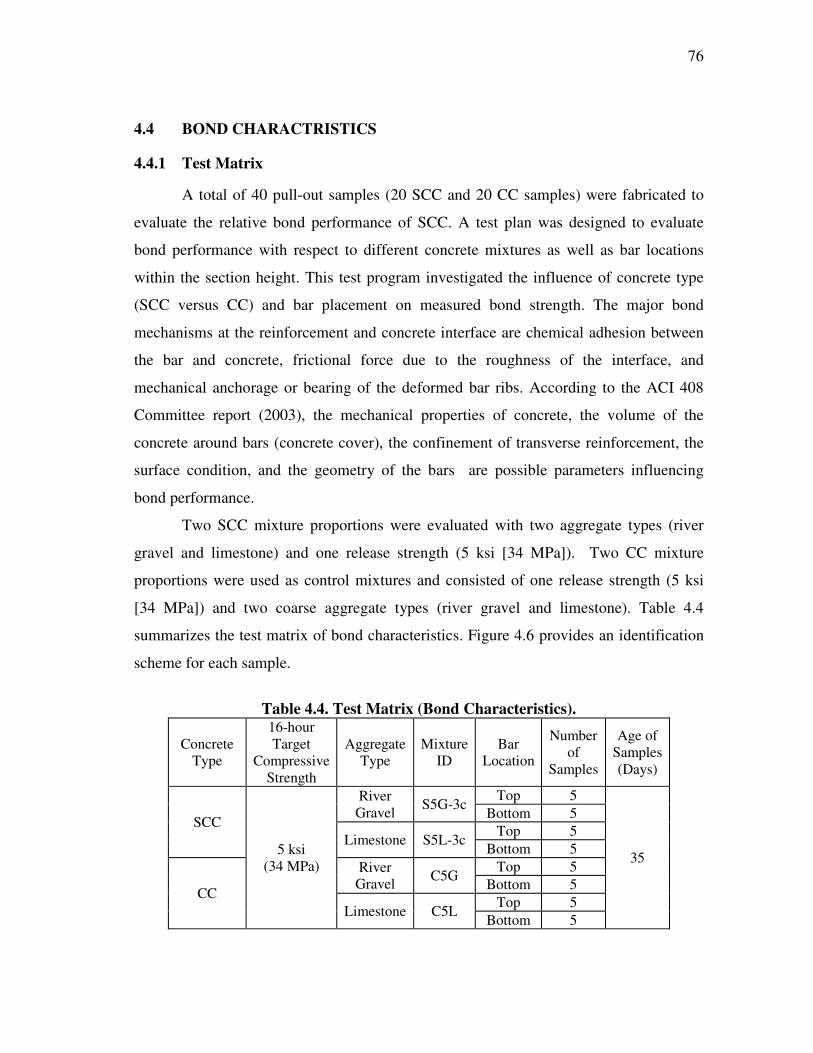
76

4.4 BOND CHARACTRISTICS

4.4.1 Test Matrix

A total of 40 pull-out samples (20 SCC and 20 CC samples) were fabricated to

evaluate the relative bond performance of SCC. A test plan was designed to evaluate

bond performance with respect to different concrete mixtures as well as bar locations

within the section height. This test program investigated the influence of concrete type

(SCC versus CC) and bar placement on measured bond strength. The major bond

mechanisms at the reinforcement and concrete interface are chemical adhesion between

the bar and concrete, frictional force due to the roughness of the interface, and

mechanical anchorage or bearing of the deformed bar ribs. According to the ACI 408

Committee report (2003), the mechanical properties of concrete, the volume of the

concrete around bars (concrete cover), the confinement of transverse reinforcement, the

surface condition, and the geometry of the bars are possible parameters influencing

bond performance.

Two SCC mixture proportions were evaluated with two aggregate types (river

gravel and limestone) and one release strength (5 ksi [34 MPa]). Two CC mixture

proportions were used as control mixtures and consisted of one release strength (5 ksi

[34 MPa]) and two coarse aggregate types (river gravel and limestone). Table 4.4

summarizes the test matrix of bond characteristics. Figure 4.6 provides an identification

scheme for each sample.

Table 4.4. Test Matrix (Bond Characteristics).

Concrete Type

16-hour Target

Compressive Strength

Aggregate Type

Mixture ID

Bar Location

Number of

Samples

Age of Samples (Days)

SCC

5 ksi (34 MPa)

River Gravel S5G-3c

Top 5

35

Bottom 5

Limestone S5L-3c Top 5

Bottom 5

CC

River Gravel C5G

Top 5 Bottom 5

Limestone C5L Top 5

Bottom 5

77

Figure 4.6. Sample ID.

4.4.2 Sample Design

As shown in Figure 4.7, the pull-out specimens were 9 in. × 16 in. × 20 in. (229

mm × 406 mm × 508 mm) rectangular samples containing two #5 (M16) horizontal bars

with one in the top and one in the bottom location. The concrete clear cover for both bars

was 3 in. (76 mm). The embedded length for all reinforcement was 5 in. (127 mm).

Figure 4.7. Pull-out Specimen Layout.

SCC-R1t

Concrete Type

Specimen Number

Bar Location t: Top Bar b: Bottom Bar

Aggregate Type R: River Gravel L: Limestone

78

4.4.3 Test Procedures

Sample preparation and test methods were the same as described earlier. At 35

days, the compressive strength test was performed along with pull-out test program.

4.4.3.1 Pull-out Test

Five consecutive batches of each concrete mixture were cast on the same date.

Each batch had a volume of 3.75 ft3 (0.106 m3) to produce one pull-out test sample and

seven cylinders of 4 in. × 8 in. (100 mm × 200 mm). All samples were covered with wet

burlap and plastic sheets and exposed to a 73 oF (23 oC) environment for approximately

16 hours. After the forms were removed, the samples were moved into a curing room

and cured for 35 days at 73 oF (23 oC) and greater than 97 percent relative humidity.

Pull-out tests were performed at 35 days after casting. Figure 4.8 shows the setup

for the pull-out tests. After placing the pull-out specimen in the reaction frame, the

reinforcement was wedged into a grip at the actuator end and a small load was placed on

the bar to set the specimen. After setting, the MTS applied a load of 0.08 kip/s (0.36

kN/s) until either the bar yielded or the concrete to reinforcement interface failed. The

load and bar slip were documented. To avoid the confining effect of the reaction frame

on the bond zone, bond breakers were used and the 5 in. (127 mm) embedment length

was located about 10 in. (254 mm) from the reaction frame. The applied load and

displacement of the LVDTs, used to measure bar slip, were taken at 0.20 second

intervals.

79

Figure 4.8. Test Setup for Pull-out Test. The average bond stress was estimated using the surface area of the

reinforcement and the maximum applied load necessary to pull out the embedded

reinforcement based on basic bond mechanisms, as follows:

max bb d

Pu

d Lπ= (4.1)

����

where ub is the average bond stress (ksi [MPa]), Pmax is the maximum actuator load (kip

[kN]), db is diameter of the reinforcement (in. [mm]), and Ld is the embedment length

(in. [mm]). In this research bond failure before yielding the reinforcement is desirable to

estimate the bond stress as a function of concrete type and bar placement.

According to the Section 12.1 of ACI 318-05 (ACI Committee 318 2005), the

development length of reinforcement for sufficient anchorage is inversely proportional

to the square root of the compressive strength. This indicates that the average bond stress

proportionally increases with an increase in the square root of compressive strength.

80

Because the strength of concrete can vary between concrete mixtures and bar locations,

the compressive strength of concrete should be considered when evaluating bond stress.

Bond can be assessed using a normalized parameter (bond ratio) based on the

average bond stress of a bottom bar to the compression top bar as shown below:

( )

( )

b Bottom bar

b Top bar

uBond Ratio

u= (4.2)

where ub(Bottom bar) and ub(Top bar) are the average bond stress values (psi [MPa]) of the

bottom and top bars, respectively. When this value is greater than 1.0, the “ top bar

effect” is present, indicating that either the concrete properties or construction practices

are reducing the bond of the top bar relative to the corresponding bottom bar. Values

equal to or less than 1.0 indicate no influence on the bond due to top bar effects.

4.5 CREEP

4.5.1 Test Matrix

To evaluate the creep properties of SCC and CC, both concrete types were cast

with different mixture proportions. Two types of aggregate were used (river gravel and

limestone) and the 16-hour compressive strength was targeted as 5 and 7 ksi (34 and 48

MPa) for each type of concrete. Mixture proportions, type of aggregate, and compressive

strength were all factors considered for the test matrix, which is shown in Table 4.5.

Table 4.5. Test Matrix (Creep).

Concrete Type Aggregate Type 16-hour Target

Compressive Strength Mixture ID Age of Initial Load (Days)

SCC River gravel

5 ksi (34 MPa) S5G-3c

7

7 ksi (48 MPa) S7G-6

Limestone 5 ksi (34 MPa) S5L-3c 7 ksi (48 MPa) S7L-6

CC River gravel 5 ksi (34 MPa) C5G

7 ksi (48 MPa) C7G

Limestone 5 ksi (34 MPa) C5L 7 ksi (48 MPa) C7L

81

4.5.2 Sample Design

Creep was tested using creep frames similar to those shown in Figure 4.9. The

frame was composed of three plates, two springs, and four threaded rods. Between the

two base plates, two springs were aligned to the center of the plate. Between the steel

plates and cylinders, half-cylinders distributed the load and reduced the direct impact of

loading on the samples. Eight frames were required for the test with one frame per

mixture containing two cylinders from each of the two batches for that mixture. All

samples were stored in a shrinkage room at 50 ± 1 percent relative humidity and a

temperature at 73 oF (23 oC).

Creep Frame

DAQ System

Creep Sample

Strain Gage

Shrinkage Samples

Spring Force(Sustained Load)

Figure 4.9. Schematic Diagram of Creep Test Setup.

4.5.3 Test Procedures

The compressive strength of each batch was compared to ensure that the batches

had statistically similar strengths. At 7 days, the compressive strength test, as described

earlier, was performed along with initial loading of the creep specimens.

82

4.5.3.1 Creep Test

4.5.3.2.1 Preparation. According to ASTM C512, Standard Test Method for

Creep of Concrete in Compression, 4 in. × 8 in. (100 mm × 200 mm) concrete samples

were cast to evaluate the compressive strength and creep. Two batches were used for

each mixture proportion. Twelve specimens per batch were made for each test condition:

two were tested for compressive strength at 16 hours after casting, two were loaded for

creep monitoring, two were monitored for shrinkage and other effects, and two were

tested for 7-day compressive strength with four extra samples. Before removal from the

molds, specimens were stored at 73 oF (23 oC) and covered with burlap or plastic sheets

to prevent moisture loss as required by ASTM C512 (2002). After 16 hours, select

specimens were removed from the mold to be used for the first compressive strength

test.

To consider the external factors, such as humidity and temperature, the condition

of the curing room before and after loading provide conditions (50 ± 1 percent RH with

a temperature at 73 oF [23 oC]) in the shrinkage room. In addition, the top and bottom of

the specimens were sulfur capped to ensure specimens are aligned when they were

loaded in the frames. Prior to the loading, the specimens were stored in a curing room.

4.5.3.2.2 Instrumentation and Data Acquisition. After removal of the molds,

strain gages were attached to the creep and shrinkage (control) cylinders along the

longitudinal axis. Strain gages were connected in a Wheatstone bridge circuit to increase

the sensitivity of the measurements and to reduce the number of channels required to

record the data. In addition, strain gages were attached to a steel block to compensate for

the temperature strains. In case temperature in the shrinkage room varied, the

temperature and relative humidity were held constant throughout the test. Two strain

gages, 180 degrees apart, were attached to each specimen along the longitudinal axis of

the cylinder.

83

After loading the creep frames in a MTS machine, it was necessary to disconnect

the wires to move the frame into the shrinkage room. Wires were reconnected as soon as

possible.

4.5.3.2.3 Load Application. A 500 kip (2220 kN) MTS machine was used to

load the creep frame, as shown in Figure 4.10. This machine is a servo-controlled

closed-loop hydraulically operated machine that can be programmed to run in

displacement and load controlled mode. Before the load was applied to the creep frame,

the initial strain was recorded. Then, after loading, four nuts over the top plate were

tightened, and a second reading was recorded. Finally, the load was released, and a third

reading was recorded.

According to the ASTM C512, the load applied to the creep frame should not be

higher than 40 percent of concrete compressive strength to ensure elastic behavior. If the

loading exceeds more than 40 percent of the compressive strength, microscopic cracks in

the samples may occur, resulting in an increase in creep.

Figure 4.10. Loading with 500 kip (2220 kN) MTS Machine.

84

4.6 DURABILITY

4.6.1 Test Matrix

Table 4.6 summarizes the test matrix for durability tests. Durability tests include

freezing and thawing resistance, the rapid chloride penetration test (RCPT), and

diffusivity test.

Table 4.6. Test Matrix (Durability Properties).

Concrete Type

16-hour Target

Compressive Strength

Aggregate Type

Mixture ID

Number of

Sample

Age of Samples at Beginning of Test

Freezing and

Thawing RCPT Diffusivity

SCC 5 ksi

(34 MPa)

River Gravel

S5G-3a

At least 3

samples for each

test

14 7, 28, and 91

140 S5G-3b S5G-3c

Limestone S5L-3a

Not Tested

S5L-3b S5L-3c

CC River Gravel C5R

Limestone C5L

SCC 7 ksi

(48 MPa)

River Gravel

S7G-3a 140 S7G-3b

S7G-3c

Limestone S7L-3a

Not Tested

S7L-3b S7L-3c

CC River Gravel C7R

Limestone C7L

4.6.2 Test Procedures

4.6.2.1 Freezing and Thawing Resistance

To evaluate the durability of SCC and CC, two types of aggregate were used

(river gravel and limestone) and the 16-hour compressive strength was targeted as 5 and

7 ksi (34 and 48 MPa) for each type of concrete. Mixture proportions, type of aggregate,

85

and compressive strength were all factors considered for the test matrix, which is shown

in Tables 4.7 and 4.8.

According to AASHTO T161, Standard Method of Test for Resistance of

Concrete to Rapid Freezing and Thawing (2004), the relative dynamic elastic modulus of

concrete was measured to assess the durability. Three samples of 4 in. × 3 in. × 16 in.

(100 mm × 75 mm × 400 mm) prisms per each mixture were prepared and cured

following AASHTO T126.

Table 4.7. Characteristics of River Gravel SCC and CC Mixtures.

Mixture ID S5G-3a

S5G- 3b

S5G- 3c

S7G- 4

S7G- 5

S7G- 6 C5G C7G

Mixture Type SCC CC 16-hour Compressive Strength, ksi (MPa) 5 (34) 7 (48) 5 (34) 7 (48)

Air Content, % 1.4 1.6 1.4 1.1 0.8 0.8 1.2 1.1 Vpaste, % 37.1 35.3 27.4 27.4 VFA, % Mass 32.0 22.5 0 0 HRWRA Type Type I Type I Type II Experimental Admixtures - Yes -

Retarder Yes - - Note: - indicates no admixture was added.

Table 4.8. Characteristics of Limestone SCC and CC Mixtures.

Mixture ID S5L- 3a

S5L- 3b

S5L- 3c

S7L- 4

S7L- 5

S7L- 6 C5L C7L

Mixture type SCC CC 16-hour Compressive Strength, ksi (MPa) 5 (34) 7 (48) 5 (34) 7 (48)

Air Content % 1.1 1.0 0.9 1.3 1.2 1.1 1.3 1.5 Vpaste, % 42.5 36.2 28.4 28.4 VFA, % Mass 40 20 0 0 VMA - Yes - HRWRA Type Type I Type I Type II Experimental Admixtures - Yes -

Retarder Yes - - Note: - indicates that there is no addition.

86

Rapid freezing and thawing cycles were cycled according to procedure A in

AASHTO T161, which is defined as rapid freezing and thawing in water. The samples

were subjected to 300 cycles of freezing and thawing. If the sample has a relative

dynamic MOE of 60 percent or less of the initial value, the test is stopped. The relative

dynamic MOE of the samples was calculated as follows:

212 100c

nP

n= × (4.3)

where Pc is the relative dynamic MOE after c cycles of freezing and thawing (%), n is

the fundamental transverse frequency at 0 cycles of freezing and thawing, and n1 is the

fundamental transverse frequency at c cycles of freezing and thawing. The durability

factor (DF) can then be calculated as follows:

P N

DFM×= (4.4)

where P is the relative dynamic MOE at N cycles (%), N is the number of cycles at

which P reaches the specified minimum value for discontinuing the test or the specified

number of cycles at which the exposure is to be terminated, whichever is less, and M is

the specified number of cycles at which the exposure is to be terminated which is equal

to 300 cycles.

4.6.2.2 Rapid Chloride Penetration Test

ASTM C1202, Standard Test Method for Concrete’ s Ability to Resist Chloride

Ion Penetration (1997), tests were performed on samples with ages of 7, 28, and 91 days

using 4 in. × 8 in. (100 mm × 200 mm) cylindrical test samples. The test matrix for this

testing is the same as the freezing and thawing test program. Curing and sample

perperation was performed following AASHTO T126.

87

This test method measures the electrical conductance of concrete samples to

provide a rapid indication of its resistance to chloride ion penetration (ASTM C1202

1997). The method involves the application of a 60 V potential difference through a

concrete sample embedded in test cells. One test cell contains sodium hydroxide (NaOH)

and the other test cell contains sodium chloride (NaCl). The total charge passed through

the sample during the 6-hour period provides a qualitative measure of chloride ion

penetrability as shown in Table 4.9.

Table 4.9. Chloride Ion Penetrability Based on Charge Passed. Charge Passed, Coulombs Chloride Ion Penetrability

> 4000 High 2000-4000 Moderate 1000-2000 Low 100-1000 Very Low

< 100 Negligible

4.6.2.3 Diffusivity Test: Determination of Chloride Diffusion Coefficient

Only SCC mixtures containing river gravel were evaluated for diffusion

coefficients. According to ASTM C1556, Standard Test Method for Determining the

Apparent Chloride Diffusion Coefficient of Cementitious Mixtures by Bulk Diffusion

(2003), 4 in. × 8 in. (100 mm × 200 mm) cylindrical test samples were cast. Specimens

were cured for 28 days before ponding samples in the exposure solution of sodium

chloride (NaCl). The finished surfaces of the specimen were exposed to the exposure

liquid. The standard indicates that the specimens must remain in the exposure liquid at

least 35 days. The standard also allows extending the exposure times for mixtures such

as those that are more mature, were made with low w/c, or high performance mixtures

containing SCMs. Because very low water to cementitious material ratios were used in

the design of SCC mixtures, researchers extended the exposure time for the samples

used in this project to 140 days.

The chloride ion contents of the powder samples ground from each layer were

determined. In a saturated concrete where no pressure exists, the transportation of

chloride ions is provided by concentration gradient. The diffusion of ions from high

88

concentration regions to low concentration regions can be best described by Fick’ s

second law, as shown in following equation:

( , ) ( )

4s s i

a

xC x t C C C erf

D t

� �= − − ×

� �

(4.5)

where C(x,t) is chloride concentration measured at depth, x, and exposure time, t, by

percent mass, Cs is the surface chloride concentration at the interface of the exposure

liquid and test specimen and is determined by a regression analysis, Ci is the initial

chloride concentration of the cementitious mixture prior to submersion in the exposure

solution, x is the depth below the exposure surface to the middle of a layer, Da is the

apparent chloride diffusion coefficient, t is the time, and erf is the error function defined

as:

2( )

0

( ) 2z

uerf z e duπ −= × �

(4.6)

To find the diffusion coefficient at 28 days, the following equation curve was

used (Thomas and Bamforth 1999, Thomas and Bentz 2000):

( )

m

refref

tD t D

t� �

= × � �

(4.7)

( )0.2 0.4 % / 50m FA= +

(4.8)

89

where Dref is diffusion coefficient at some reference time, tref (= 140 days in this study),

D(t) is the diffusion coefficient at time, t, m is the constant depending on mixture

proportions, and FA is the replacement level of fly ash (%).

4.7 FULL-SCALE TESTING

The applicability of selected SCC mixture proportions was verified by

fabricating and testing precast, prestressed TxDOT Type A girders. After production, in-

service performance (i.e., camber, deflection, and prestress losses) was monitored and

structural tests were performed to compare properties of the SCC girder systems. Girder

systems containing CC were fabricated and tested as control specimens. Flexural

capacity, transfer and development length, and shear performance were investigated in

the full-scale tests along with mechanical properties. This section presents the test matrix

and the design of the TxDOT Type A girder and deck. Fabrication of the girders and

decks and test procedures will also be presented.

4.7.1 Test Matrix

The specimens tested in this study consisted of a total of four TxDOT Type A

(AASHTO Type I) girders. The girders were fabricated at a precast plant in Texas and

were designed to investigate the overall long-term behavior and structural performance

of full-scale girders made with SCC. Table 4.10 shows the test matrix for full-scale test.

Development length tests were performed at each end of each girder (i.e., two data

points were obtained from each girder). Mechanical properties were tested for each

mixture. Other tests (flexural capacity, transfer length, prestress losses, and camber and

deflection) were also assessed. More information is provided in the respective test

procedure section.

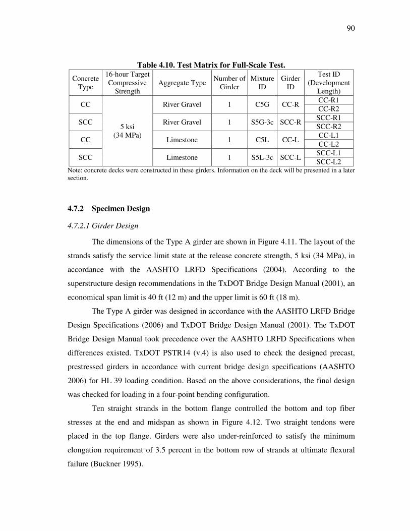
90

Table 4.10. Test Matrix for Full-Scale Test.

Concrete Type

16-hour Target Compressive

Strength Aggregate Type Number of

Girder Mixture

ID Girder

ID

Test ID (Development

Length)

CC

5 ksi (34 MPa)

River Gravel 1 C5G CC-R CC-R1 CC-R2

SCC River Gravel 1 S5G-3c SCC-R SCC-R1 SCC-R2

CC Limestone 1 C5L CC-L CC-L1 CC-L2

SCC Limestone 1 S5L-3c SCC-L SCC-L1 SCC-L2

Note: concrete decks were constructed in these girders. Information on the deck will be presented in a later section.

4.7.2 Specimen Design

4.7.2.1 Girder Design

The dimensions of the Type A girder are shown in Figure 4.11. The layout of the

strands satisfy the service limit state at the release concrete strength, 5 ksi (34 MPa), in

accordance with the AASHTO LRFD Specifications (2004). According to the

superstructure design recommendations in the TxDOT Bridge Design Manual (2001), an

economical span limit is 40 ft (12 m) and the upper limit is 60 ft (18 m).

The Type A girder was designed in accordance with the AASHTO LRFD Bridge

Design Specifications (2006) and TxDOT Bridge Design Manual (2001). The TxDOT

Bridge Design Manual took precedence over the AASHTO LRFD Specifications when

differences existed. TxDOT PSTR14 (v.4) is also used to check the designed precast,

prestressed girders in accordance with current bridge design specifications (AASHTO

2006) for HL 39 loading condition. Based on the above considerations, the final design

was checked for loading in a four-point bending configuration.

Ten straight strands in the bottom flange controlled the bottom and top fiber

stresses at the end and midspan as shown in Figure 4.12. Two straight tendons were

placed in the top flange. Girders were also under-reinforced to satisfy the minimum

elongation requirement of 3.5 percent in the bottom row of strands at ultimate flexural

failure (Buckner 1995).

91

12 (305)

6 (152)

3 (76)

11 (279)

5 (127)

4 (102)

16 (406)

28 (711)

3/4 (19)Chamfer

3 (76)

5 (127)Unit [inch (mm)]

5 (127)

Figure 4.11. Dimension of Cross-Section of Type A Girder.

a = 2 (51)b = 3 (76)

c = 5 (127)Unit [inch (mm)]

a

aa

ab

c

c

a

Figure 4.12. Layout of Strands for Tested Girders.

Mild steel reinforcement was placed in accordance with the AASHTO LRFD

Bridge Design Specifications (2006) and TxDOT Bridge Design Manual (2001).

Layouts of reinforcements and reinforcement details are shown in Figures 4.13 and 4.14.

Zone 1 Zone 2

Bars V (19 Pairs)Bars W

Bars R Bars UBars X

Bars S(in pairs)

Bars Y

6 (152)

U

XR

RV

S

RV

W

Y

Top Flange

Bottom Flange

Beam Elevation

2.75 (70)

2 (51)

1 (25)

1.5 (38)

1.5 (38)

28 (711)

16 Spaces at 4 (101) Bars R 28 Sp at 6 (152 ) Bars Races

Type A Beams

V

W

XS

R

U

Y

1.25 (32)

1.25 (32)

5.25 (133)

V

4 (102) 6.35 (161)

1.4 (36)3 (76)

Unit [inch (mm)]

CL

Figure 4.13. Layout of Reinforcement.�

�� ���

92

24 (610)

10 (254)

36 (914)

22 (559)

12.5 (304)

9 (229)

3.63 (92)

6.25 (

159)

3.25 (83)

11.63 (295)

30.75 (781)

Beam Length Minus 3 (76)

31 (787)

4 (106)

BARS R (#4 [13]) BARS S (#5 [16]) BARS X (#5 [16]) BARS Y (#5 [16])

BARS V (#4 [13])

BARS W (#5 [16])

BARS U (#5 [16])

3.25 (83)

31 Degrees

45 degrees

Unit [inch (mm)] Figure 4.14. Detail of Reinforcements.

��

� ��� 93

94

4.7.2.2 Deck Design

The CIP deck thickness and width represent actual field conditions and were

included to investigate the longer-term behavior of the girders. The shrinkage of the

deck and creep in the girder affect the strain profile of the composite girders, resulting in

changes for estimating prestress losses.

Researchers determined that the deck should be 8 in. (0.2 m) thick and 64 in. (1.6

m) wide to meet standard TxDOT practice. According to TxDOT Standard CIP criteria,

the maximum clear span from girder flange to girder flange is limited to 8.686 ft (2.6 m)

with an 8 in. (0.2 m) thick slab.

The neutral axis at the ultimate flexural failure is located in the deck. Analyses

indicated that the deck will contribute compressive stress and will develop large tensile

strains in the lower level strands under flexural and development length tests.

Longitudinal and lateral reinforcement was placed in the deck to mimic actual

deck construction practices in Texas and to control the temperature and shrinkage. The

details of the deck are presented in Figure 4.15.

7 (178) 9 (229)

64 (1626)

8 (203) 4.75 (121)

2 (51)

1.25 (32)

Unit [inch (mm)]

#5 #4

Figure 4.15. Details of Deck.

4.7.2.3 Fabrication of Type A Girders

All girders were fabricated with the same prestressing conditions and were

monitored continuously after casting. The CC-R and SCC-R girders were fabricated on

95

March 26, 2007. The second set of girders, CC-L and SCC-L, were fabricated on July

12, 2007. The layout of the girders on the prestressing bed is shown in Figure 4.16.

Figure 4.16. Layout of Girders.

A data acquisition system (DAQ system) was positioned next to the prestressing

bed in a protected shelter. The computer and DAQ system had a capacity of 107

channels.

All strands were gradually stressed at the same time using the equipment shown

in Figure 4.17. Before placing each strand, load cells monitored the stresses in the

strands until release. The target load for each strand was 31 kip (137 kN), 0.75 of puf for the CC and SCC girders.

Figure 4.17. Prestressing Bed with Strands.

After stressing the strands, mild reinforcement was placed according to the

design drawings. After placing the mild reinforcement, temperature probes and

embedded concrete strain gages were installed at designated locations. All wires were

connected to the DAQ system and measurements were recorded at 15 minute intervals.

SCC-R CC-R (SCC-L)(CC-L)

Note: 1st phase (2nd phase)

StrandsStressing jack

End abutmentSpecimen

96

4.7.2.4 Fabrication of Mechanical Samples

Test samples were fabricated in a building next to the casting bed (see Figure

4.18). Three 4 in. × 8 in. (102 mm × 203 mm) cylinders of each concrete type were cast

to test compressive strength at 16 hours using a sure-cure system, which the plant

provided. The sure-cure system is designed to match the actual temperature of girder. To

evaluate the mechanical and durability characteristics, 118 compressive cylinders, 30

MOR beams, 10 freeze-thaw beams, and 8 shrinkage samples were cast. The day after

casting, the samples for mechanical testing were transported from the plant to

environmental rooms (> 98 percent RH and 72 ± 2 oF [22 ± 1 oC]) at Texas A&M

University. Compressive strengths of cylinders at 16 hours and release time were

evaluated at the plant.

Figure 4.18. Preparation of Small Samples.

4.7.2.5 Fabrication of Composite Girders

Girders were transported from the prestressing bed to a storage area until

transporting to HBSML. The first girder set (CC-R and SCC-R) was stored at the plant

for 6 days after casting. The second girder set was stored in the plant for 5 days. The

DAQ system monitored the temperature, concrete strain, and end slip of strands at 15

minute intervals. Girders were simply supported during storage.

All fabrication of the decks was performed at HBSML. Overhang brackets were

installed at 3 ft (1.0 m) intervals to support the deck. After forming, reinforcing bars

97

were placed and tied and the concrete was placed (see Figures 4.19 and 4.20). TxDOT

Class S concrete was used for the deck. The forms were removed after approximately 3

days. The beams were monitored until structural tests were performed.

Figure 4.19. Placement of Reinforcement.

98

Figure 4.20. Placement of Deck Concrete.

4.7.3 Test Procedures

4.7.3.1 Early Age Characteristics and Plant Observation

Tests to evaluate workability and stability of the SCC were performed following

the test standards presented in the laboratory test program (Section 4.1). The casting

procedure and the instrumentation to measure the hydration of concrete are explained

below.

4.7.3.1.1 CC-R and SCC-R Girders. Girders were fabricated and cast at Texas

Concrete Company, Victoria, Texas. Each girder required two batches of concrete. The

volume of each batch was between 2 and 3.25 ft3 (0.06 and 0.09 m3). Samples for

mechanical properties were taken from the second batch. Weather conditions on March

26, 2007, were windy and the temperature was approximately 70 oF (21 oC). Before

placing concrete in the girder forms the fresh characteristics were assessed. After it was

determined that the concretes met the required characteristics (slump flow, stability, etc.)

99

the concrete was placed in the forms. Slump flow and stability were assessed for both

batches.

The cement, water, and aggregate were initially batched and mixed. A retarder

was then added to the mixture and mixed. HRWRA was then added and mixed. After

sufficient mixing the concrete was discharged into a bucket auger with an approximate

drop height from the mixer to the bucket auger of 3 to 5 ft (0.9 m to 1.5 m). Each batch

was then transported approximately 100 yards (91 m) from the mixer and placed into the

form. The CC mixture concrete was continuously discharged into the forms while

moving along the forms. Mechanical vibration consolidated the CC. For the SCC

mixture, the majority of the concrete was placed in the form from one end. As the form

was filled the forklift with the bucket auger moved along the form to complete the

placement. No consolidation was used for the girders containing SCC. After placement,

beams were covered with a tarpaulin.

4.7.3.1.2 CC-L and SCC-L Girders. The girders containing limestone

aggregate were cast using the same procedures as the girders containing the river gravel.

To evaluate the temperature history of the girder, a sure-cure system was used for the

early age compressive specimens. The weather conditions on the day of casting (7/12/07)

consisted of a light wind and a temperature of approximately 100 oF (38 oC). After

placement, the girders were covered with wet burlap.

Temperature probes monitored the hydration of the concrete in all the girders.

The temperature probes were located at the mid-height, bottom flange, and top flange at

the beam as shown in Figure 4.21. The temperature readings were used to calculate the

heat-induced strain in the beams. The temperature of the girders was continuously

monitored after placement of the concrete.

100

AMidspan

38 (965)

: Temperature probeNote: Gage placement is same on both sides

3 (76)14 (356)

26 (660) 240 (6096)

Unit [inch (mm)]

A

A

A

Section A-A

Figure 4.21. Locations of Temperature Probes.

4.7.3.2 Mechanical Properties

Mechanical properties (compressive strength, MOE, MOR, STS) of each mixture

were evaluated following the regime described in the laboratory test program. For

compressive strength, additional samples for 16-hour and release strength were cast and

cured using the sure-cure system.

4.7.3.3 Flexural Test Procedure

After finishing monitoring the girder, the composite deck system was tested for

flexural capacity. An overview of test setup is shown in Figure 4.22.

Destructive tests validated the flexural capacity of girders containing CC and

SCC. Steel, H-shape frames were anchored with post-tensioned Dywidag threaded rods

on the strong floor at HBSML. A 600 kip (2700 kN) actuator was used to load the

specimen. Neoprene pads were placed under the load points (36 in. × 8 in. [914 mm ×

203 mm]) to distribute the load evenly to the composite deck system.

Neoprene bearing pads (70 durometer) (8 in. × 8 in. × 3 in. [203 mm × 457 mm ×

76 mm] thick) supported the girders. The center of the bearing pads was positioned 6 in.

(152 mm) from the beam end, resulting in a span length of 39 ft (11.8 m).

The DAQ system recorded data at 5 second intervals to assess the following

characteristics:

101

• moment - curvature relationship (load - displacement relationship),

• initial stiffness,

• bond performance prior to cracking,

• bond performance after cracking, and

• crack patterns.

To investigate the bond performance of the composite deck system, concrete

gages, LVDTs, and strain gages were placed on the Type R bars. A load cell measured

loads on the hydraulic ram. String pots measured displacement.

Figure 4.22. Overview of Test Setup.

The loading increment was estimated based on the time to first cracking and the

strain of the top fiber on the deck at midspan. Before cracking, the loading increment

was 20 kip (89 kN). After cracking, the loading increment was decreased to 10 kip (44

kN). After each incremental load, crack locations and widths were marked and recorded.

When the moment capacity of the composite girder reached the ultimate state (3000

102

microstrain at the top fiber), the test was terminated. Figure 4.23 shows the schematic

diagram of the strain gage locations for the flexural test. Figure 4.24 shows the

schematic diagram of the string potentiometer locations for measuring deflections. The

moment-curvature relationship, initial stiffness, and the bond behavior in the transfer

length zone and the constant moment region were evaluated to compare the flexural

behavior of CC and SCC composite deck systems.

TopView

FrontView

Bearing Pad

12 (305)

18 (457)

24 (610) : LVDT

: Strain Gage

8 (203)

Unit [ in. (mm)]

A A

Section A-A

36 (914)

4 (102)

Midspan

Figure 4.23. Diagram of Installation of Strain Gages and LVDTs for Measuring

Strain of Top Fiber of Deck Concrete under Flexural Test.

103

: String Potentiometer

0.5 (0.15)10 (3)

18.5 (5.6)

20 (6)

Unit [ft (m)]

Figure 4.24. Diagram of Installation of String Potentiometers for the Flexural Test.

LVDTs were installed to investigate strain profiles and crack widths in the

constant moment region. Figure 4.25 shows the LVDT installation locations to measure

the strain of strands on the bottom flange.

Midspan

: LVDT

3 (76)

14 (356)26 (660)

24 (610)

36 (914)

Midspan

: LVDT

3 (76)

14 (356)26 (660)

24 (610)

Figure 4.25. Average Strain of Strands of the Constant Moment Region.

4.7.3.4 Transfer Length

According to AASHTO LRFD Bridge Design Specifications (2006), the transfer

length, ltr , is the transition distance from the free end of the strands to the fully bonded

zone with effective prestress. In this study, the transfer length, ltr , was measured with

104

two methods: concrete strain readings and end slip readings. The method used to

measure transfer length included the use of embedded concrete strain gages. Two types

of concrete strain gages were used: Quarter-bridge 120 � strain gages and full-bridge

350 � strain gages. Instrumented locations of embedded concrete strain gages are shown

in Figure 4.26. Both ends of the beam have the same pattern of instrumentation.

The transfer length was estimated with concrete strain gages from the vertical

centroid of gravity of the strands. The strands were gradually released over a 4-minute

period. During strand release, LVDTs measured the end slip of five strands of the

bottom flange on both ends of each girder. After releasing, the strands were flame-cut.

Section A-A

AMidspan

5 (127)

20 (508)25 (635)

38 (965)70 (1778)

120 (3048)

: Concrete stain gageNote: Gage placement is same at both ends

3 (76)

10 (254)

14 (356)26 (660)

32 (813)

240 (6096)

Unit [inch (mm)]

A

A

A

Figure 4.26. Locations of Strain Gages.

Buckner (1995) and Barnes (2000) found that shear lag effects occur when the

surface concrete strain is measured. This results in recorded values lower than actual

transfer length values in the middle of the beam section as shown in Figure 4.27 (Barnes

2000). Therefore, it was thought that concrete strain gages could provide better values of

the actual transfer length.

105

Actual Transfer Length

Apparent Transfer Length(from Surface Strains)

0.5f /Epe p f /Epe p

Strands Figure 4.27. Shear Lag Effect on Transfer Length (Barnes 2000).

To determine a reasonable transfer length, the following methods were followed.

The first step was using the following equation to correct the strain profile by

considering the self-weight of the girder at transfer.

w gagew

ci tr

M y

E Iε = (4.9)

where εw is strain at the level of the embedded concrete strain gages (in./in. [mm/mm]),

Mw is the moment due to the self-weight of the girder (kip-ft [kN-m]), Eci is the elastic

modulus of concrete at transfer (ksi [MPa]), Itr is the moment of inertia of the

transformed section (in4 [mm4]), and ygage is the vertical distance from the centroid of the

transformed section to the location of concrete strain gages (in. [mm]).

As shown in Figure 4.28, the second step was to best fit a function through data

using the first step. The third step was to find the likely domain of the 100 percent strain

plateau by visually inspecting the data as shown in Figure 4.28. In the final step, the 95

percent average maximum strain (AMS) was calculated as the mean values of these

maximum stains. The first intersection of the line and strain profile indicates the transfer

length, ltr.

106

Figure 4.28. Determining Transfer Length Using the 95% AMS Method.

As shown in Figure 4.29, the transfer length increases with time as a result of

prestress losses, concrete creep, shrinkage, and strand relaxation. Slab weight, MOE, and

the transformed section are used to evaluate the long-term transfer length.

Figure 4.29. Long-Term Raw Strain Profile of North Span of Girder CC-R.

0

200

400

600

800

1000

0 10 20 30 40 50 60 70

Best-Fit Line95% AMS

0 500 1000 1500

Com

pres

sive

Str

ain

(x 1

0-6 in

./in.

or m

m/m

m)

Distance from the End of Girder (in.)

ltr

Distance from the End of Girder (mm)

0

200

400

600

800

1000

0 10 20 30 40 50 60 70

At Transfer7 days15 days

27 days91 days128 days

0 500 1000 1500

Com

pres

sive

Str

ain

(x 1

06 in./i

n. o

r mm

/mm

)

Distance from the End of The Girder (in.)

Distance from the End of The Girder (mm)

107

The second method used to assess the transfer length included measuring end slip

(draw-in end slip) with LVDTs. The layout for the LVDT’ s used in this study are shown

in Figure 4.30.

Upon release, the elastic shortening of the strand was measured to determine the

end slip of the strands. The amount of end slip is correlated with transfer length, stress of

strands at transfer, and the MOE of the strands.

LVDT

Figure 4.30. Locations of LVDTs for Draw-In End Slip.

When considering the bond mechanism of transfer length, two principal

mechanisms, friction and mechanical resistance, actively resist the slippage of strands

immediately after transfer. To determine the end slip of strands, five LVDTs were

installed on the strands prior to release at each end of the girder. The equation for

obtaining the actual end slip, End slip∆ , is expressed as follows:

End slip B ES∆ = ∆ − ∆ (4.10)

where ∆B is the measured displacement of end-slip through the LVDT (in. [mm]), ∆ES is

the elastic shortening of strands between the end of section and the location of the LVDT

(PJ∆A/EpAp) (in. [mm]), ∆A is the measure distance from the surface of the section to

attached point of LVDT on strands (in. [mm]), PJ is the measured prestressing forces

immediately before transfer (kip [kN]), Ep is the elastic modulus of the strands (ksi

[GPa]), and Ap is the area of strands (in.2 [mm2]).

108

Based on Mast’ s strand slip theory (Logan 1997), the end slip of the strands is

used to determine the initial transfer length. The relationship between end slip, ∆End slip,

and initial transfer length, ltr∆, is as follows:

(0 ) trEnd slip pi tri

p

lavg f ,l

E∆∆ = (4.11)

0( )pi pj pR tr pESf f f t ,t f= − ∆ − ∆ (4.12)

where Ep is the elastic modulus of strand (ksi [MPa]), avg fpi(0, ltri) is the average initial

stress of strands between the ends of the section and transfer length (ksi [MPa]), ∆fpES is

the prestress losses due to elastic shortening at transfer (ksi [MPa]), fpj is the initial

jacking stress of strands (ksi [MPa]), ∆fpR(t0, ttr) is the estimated relaxation of strands

between t0 and ttr (ksi [MPa]), t0 is the time at jacking (hour), and ttr is the time at

transfer (hour).

4.7.3.5 Development Length Test

Flexural testing of the girder-deck system was performed first, followed by

testing at both ends to determine the development length of the girders. The embedment

length, le, is the length of the embedded strands from the girder end to the loading point

for the development length test (see Figure 4.31). To determine the transition point from

flexural to bond failure, the embedment length and test span length can be varied from

test to test. Embedment lengths longer than the required development length will result

in a flexural failure. Embedment lengths shorter than the development length should

result in a bond/shear failure or bond/flexural failure.

109

P

l = Test Span Length

l = e Embedment Length

Beam EndMidspan

Figure 4.31. Definition of Embedment Length and Test Span Length.

A DAQ system recorded data at 5-second intervals to assess the following

characteristics:

• moment - curvature relationship,

• bond characteristics of the development length region,

• shear performance, and

• crack patterns.

4.7.3.5.1 Test Configuration. After completing the flexural tests, each end of

the composite girder was tested to evaluate development length. Based on Equation

5.11.4.2-2 in the AASHTO LRFD Specifications (2004), the theoretical development

length was larger than about 80 in. (2.0 m). The test span length was 13.5 ft (4.1 m) for

the first trial. The interior support was shifted inward for the composite deck system to

have a 13.5 ft (4.1 m) span length as shown in Figure 4.32 (a). The loading increments

and measured parameters were the same as in the procedure of the flexural tests. After

testing the first trial, the second trial testing was performed with a 12.5 ft (3.8 m) span

length and 70 in. (1.8 m) embedment lengths as shown in Figure 4.32 (b).

Table 4.11 summarizes the test identifications, embedment length, and span

length for the development length tests. The overhead crane was used to reduce the

negative moment.

110

P

l = 13.5 ft (4.1 m)

l =e 80 in.(2.0 m)

Beam EndMidspan

(a) First Trial

P

l = 12.5 ft (3.8 m)

l =e 70 in.(1.8 m)

Beam End Midspan

(b) Second Trial

Figure 4.32. Test Setup for Development Length Test.

Table 4.11. Configuration for Development Length. Girder ID CC-R SCC-R CC-L SCC-L

Test ID CC- R1

CC- R2

SCC-

R1

SCC- R2

CC- L1

CC- L2

SCC- L1

SCC- L2

le , in. (m) 80 (2.0)

70 (1.8)

80 (2.0)

80 (2.0)

80 (2.0)

70 (1.8)

80 (2.0)

70 (1.8)

l , ft (m) 13.5 (4.1)

12.5 (3.8)

13.5 (4.1)

13.5 (4.1)

13.5 (4.1)

12.5 (3.8)

13.5 (4.1)

12.5 (3.8)

Overhead Crane

Application No Yes

4.7.3.5.2 Instrumentations. Figure 4.33 shows the location of the strain gages

for measuring the strains in the top fiber of the deck to determine the ultimate strain.

111

TopView

FrontView

Bearing Pad

24 (610)9 (229)

: Strain Gage

Unit [ inch (mm)]

Section A-A

A A

4 (102)

6 (152)

At (Loading Point)

le

Figure 4.33. Diagram of Locations of Strain Gages or Deck Concrete

for Development Length Tests.

Strain gages were attached to the bottom flange of the girder, located at the

centroid of gravity of the strands as shown in Figure 4.34. Concrete strain gages also

detected failure of strands and concrete cracks.

112

Strain Gage(Type II)

Strain Gage(Type I)

Side View

Bottom View

Section View

10 (254)

10 (254)20 (508)

5 (127)

25 (635)

70 (1778)38 (965)

Beam End

Figure 4.34. Diagram of Concrete Surface Strain Gage Layout (Type I) and Embedded Concrete Strain Gage Layout (Type II).

In addition to the 10 LVDTS attached on the end of the 10 strands, LVDTs

measured the diagonal tensile strains and stresses on the critical section from the support

as shown in Figure 4.35. Shear strain was measured with the LVDTs installed at the

critical section for shear, 3 ft (910 mm) from the end and with strain gages on the Type

R reinforcement. Strain gages were attached on steel reinforcement corresponding to the

mid-height of the web of the girder.

Critical for Shear (C.S.)

: LVDT

36 (915)

10 (254)

14 (356)

24 (610)

: Strain Gage

10 (254)

Figure 4.35. Locations of LVDTs and Strain Gages for Shear and Development

Length.

113

Figure 4.36 shows the principal strains at the critical web concrete section.

Positive values represent the average principal tensile strain, ε1, that crosses cracks, and

negative values represent the average principal compressive strain, ε2, on the cracked

web concrete member.

Figure 4.36. Strains on Web at Critical Section for Shear.

The prestressed strain due to longitudinal compressive stress was included for the

calculation. Shear strain, γxy, due to the applied load was estimated as follows:

452xy t xγ = ε − ε − ε (4.13)

where εx is the longitudinal strain of the member, εt is the perpendicular strain of the

member, ε45 is the diagonal strain.

The principal strains, ε1 and ε2, can be calculated from these equations as

follows:

22

1 2 2 2xyx t x t

γ� �ε + ε ε − ε� �ε = + + � � � �

(4.14)

114

22

2 2 2 2xyx t x t

γ� �ε + ε ε − ε� �ε = − + � � � �

(4.15)

where εx and εt were defined earlier, ε1 is principal tensile strains, and ε2 is principal

compressive strains.

4.7.3.6 Prestress Losses

Load cells measured the jacking stresses, fpj, and the initial stress, fpi on the

girders. Load cells were fabricated at HBSML and consisted of a strain gage with a

Wheatstone bridge circuit to measure axial stresses. The load cells compensate for the

induced moments, torsional moments, and temperature effects. One load cell for each

strand was installed between a spring loaded anchor and the dead abutment as shown in

Figure 4.37.

Figure 4.37. Load Cells between Spring Loaded Anchor and Dead Abutment.

Spring loaded anchor

Dead abutment

115

Concrete strain gages measured prestress losses. Elastic shortening, losses due to

creep and shrinkage of the girder, and elastic gain were calculated from the embedded

concrete strain gages. Test results were used to validate AASHTO LRFD equations

(2004, 2006). The applicability of the AASHTO LRFD equations can be assessed. Here,

the AASHTO LRFD (2006) equations are presented to estimate elastic shortening. This

gives an idea about the complexity of prestress losses associated with properties of

concrete and bond properties. Other time-dependent losses associated with

environmental conditions are more complicated.

4.7.3.7 Camber and Deflection

Camber and deflection were measured with string potentiometers and stringlines

(see Figures 4.38 and 4.39). When the deflection stabilized, the deflection monitoring

was terminated.

Figure 4.38. Initial Camber Reading (a) and Stringlines (b).

(a) (b)

116

: String Potentiometer

0.5 (0.15)10 (3)

Unit [ft (m)]

20 (6)

Figure 4.39. Location of String Potentiometer for the Camber and Deflection.

The instantaneous deflection was estimated using the following equations. The

downward deflection of the self-weight of the girder, ∆Girder, can be estimated from the

following equation:

45384Girder

ci

w LE I

∆ = � (4.16)

and the initial camber, ∆fps, due to the initial prestressing force was estimated as follows:

2

8i c

fpsci

P e LE I

∆ = � (4.17)

where w is the self-weight of the girder (klf. [kN/m]), Pi is the measured initial prestress

force (kip [kN]), ec is the eccentricity of prestressing strands (in. [mm]), L is the

measured span length (ft [m]), Eci is the MOE at transfer (ksi [GPa]), I is the moment of

inertia of the girder (in.4 [mm4]), � indicates the downward deflection, and � indicates

the upward deflection.

The net camber, ∆i(net), can be calculated as the difference between the two

equations: the camber due to initial prestressing force, ∆fpi, and the downward deflection

due to the self-weight of the girder, ∆Girder as:

117

i( net ) fpi Girder∆ = ∆ − ∆ (4.18)

An incremental time-step method procedure estimated curvature increments at 1

week intervals when the girders were stored at the plant. The incremental curvature can

be determined as follows:

7 7T i∆φ = φ − φ (4.19)

where ∆φT7 is the curvature increment between 7 days and time at transfer (rad/in.

[rad/m]), 7φ is the measured curvature at 7 days (rad/in. [rad/mm]), and φi is the

measured curvature at transfer (rad/in. [rad/mm]).

Based on basic mechanics, the camber growth can be calculated with the

following equation:

2

7 7 8T T

L∆ = ∆φ

(4.20)

where ∆T7 is the growth of camber at 7 days after the transfer (in. [mm]), and L is the

measured span length (ft [m]).

The camber after 7 days can be calculated as follows:

7 7im T∆ = ∆ + ∆ (4.21)

where ∆7 is the final camber at 7 days (in. [mm]) and ∆im is the initial camber (in. [mm]).

118

CHAPTER V

RESULTS AND ANALYSIS OF LABORATORY STUDY:

MECHANICAL PROPERTIES

5.1 EARLY-AGE CHARACTERISTICS

Tables 5.1 and 5.2 present the early age characteristics of the SCC mixtures.

Measured slump flow was between 27.5 and 29.5 in. (699 and 749 mm). The air contents

of the SCC mixtures ranged between 0.8 and 1.6 percent. The T50 ranged from 1.0 to 7.0

seconds. The 7 ksi (48 MPa) SCC mixtures exhibited higher viscosities than the 5 ksi

(34 MPa) mixtures. The stability of all SCC mixtures was between 0.5 and 1.0,

indicating high stability of the SCC mixture proportions. Temperature was measured

with thermocouples embedded in a separate cylinder until 16 hours after casting.

Tables 5.3 and 5.4 show the early-age characteristics of CC mixtures.

Table 5.1. Early-Age Characteristics of River Gravel SCC Mixture. Mixture ID

Test S5G -1

S5G -2

S5G -3a

S5G -3b

S5G -3c

S7G -4

S7G -5

S7G -6

Slump Flow, in. (mm)

27.5 (700)

27.5 (700)

27.5 (700)

28.5 (725)

28.0 (710)

28.0 (710)

28.0 (710)

28.0 (710)

Air, % 1.4 1.5 1.4 1.6 1.4 1.1 0.8 0.8 Unit Weight, lbs/ft3 (kg/m3)

148.6 (2377)

148.3 (2373)

148.2 (2371)

148.1 (2371)

148.1 (2371)

151.0 (2415)

151.6 (2425)

151.6 (2425)

T50, sec. 2.3 2.4 2.7 2.3 2.0 7.1 7.0 6.9 VSI 0.5 0.5 0.5 1.0 1.0 0.5 0.5 0.5

Max. Temp., oF (oC) - 93 (33.9)

97 (36.1)

89 (31.7)

101 (38.3)

100 (37.8)

101 (38.3)

107 (41.7)

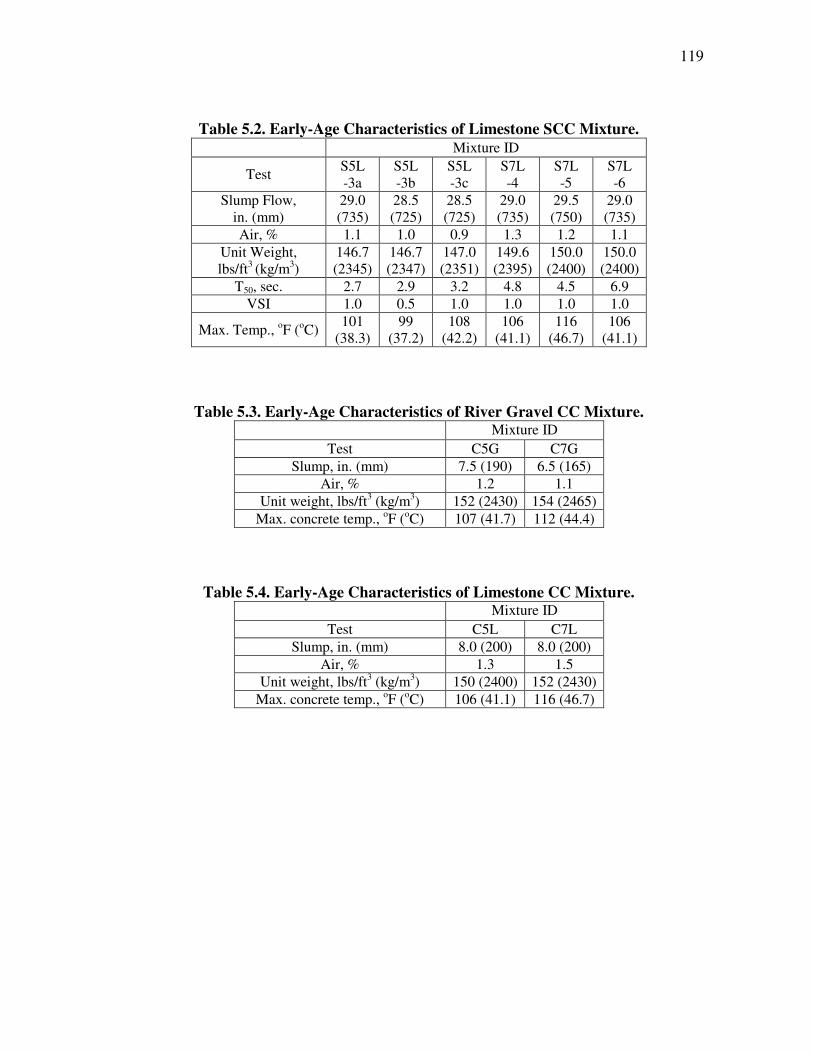
119

Table 5.2. Early-Age Characteristics of Limestone SCC Mixture. Mixture ID

Test S5L -3a

S5L -3b

S5L -3c

S7L -4

S7L -5

S7L -6

Slump Flow, in. (mm)

29.0 (735)

28.5 (725)

28.5 (725)

29.0 (735)

29.5 (750)

29.0 (735)

Air, % 1.1 1.0 0.9 1.3 1.2 1.1 Unit Weight, lbs/ft3 (kg/m3)

146.7 (2345)

146.7 (2347)

147.0 (2351)

149.6 (2395)

150.0 (2400)

150.0 (2400)

T50, sec. 2.7 2.9 3.2 4.8 4.5 6.9 VSI 1.0 0.5 1.0 1.0 1.0 1.0

Max. Temp., oF (oC) 101 (38.3)

99 (37.2)

108 (42.2)

106 (41.1)

116 (46.7)

106 (41.1)

Table 5.3. Early-Age Characteristics of River Gravel CC Mixture. Mixture ID

Test C5G C7G Slump, in. (mm) 7.5 (190) 6.5 (165)

Air, % 1.2 1.1 Unit weight, lbs/ft3 (kg/m3) 152 (2430) 154 (2465)

Max. concrete temp., oF (oC) 107 (41.7) 112 (44.4)

Table 5.4. Early-Age Characteristics of Limestone CC Mixture. Mixture ID

Test C5L C7L Slump, in. (mm) 8.0 (200) 8.0 (200)

Air, % 1.3 1.5 Unit weight, lbs/ft3 (kg/m3) 150 (2400) 152 (2430)

Max. concrete temp., oF (oC) 106 (41.1) 116 (46.7)

120

5.2 DEVELOPMENT OF COMPRESSIVE STRENGTH

This section presents characteristics of compressive strength.

5.2.1 16-hour Release Strength

Figure 5.1 shows the compressive strength of the river gravel and limestone

mixtures at 16 hours. With the exception of mix S5G-1, each mixture achieved its target

strength of 5 ksi (34 MPa) and 7 ksi (48 MPa). Nine samples of each mixture were tested

to evaluate 16-hour strength. The box plots show the mean, the 1st (25 percent) and 3rd

(75 percent) quartiles, and the outliers. The SCC and CC mixtures have similar

compressive strength at 16 hours with each aggregate type and strength level. In the case

of the limestone mixtures, the 16-hour strength was approximately 30 and 28 percent

higher than the 5 ksi (34 MPa) and 7 ksi (48 MPa) target strengths, respectively.

(a) 5 ksi (34 MPa) River Gravel (b) 7 ksi (48 MPa) River Gravel

Figure 5.1. Compressive Strength at 16 hours.

4000

5000

6000

7000

8000

9000

10,000

30

40

50

60

S5G

-1

S5G

-2

S5G

-3a

S5G

-3b

S5G

-3c

C5G

Com

pres

sive

Str

engt

h (p

si)

Com

pressive Strength (MPa)

Target 16-hr release strength

4000

5000

6000

7000

8000

9000

10,000

30

40

50

60

S7G

-4

S7G

-5

S7G

-6

C7G

Target 16-hr release strength

Com

pres

sive

Str

engt

h (p

si)

Com

pressive Strength (MPa)

121

(c) 5 ksi (34 MPa) Limestone (d) 7 ksi (48 MPa) Limestone

Figure 5.1. (Continued)

5.2.2 Development of Compressive Strength

Figure 5.2 shows the development of compressive strength of the SCC mixture

from 16 hours to 91 days. The 5 ksi (34 MPa) river gravel SCC mixtures achieved an

ultimate strength at 91 days of 13.5 ksi (93 MPa). The 7 ksi (48 MPa) river gravel SCC

mixtures achieved an ultimate strength at 91 days of 17 ksi (117 MPa). For the limestone

SCC mixtures, the ultimate strength developed was 15 and 17 ksi (105 and 117 MPa) for

the 5 and 7 ksi (34 MPa and 48 MPa) 16-hour target strengths, respectively.

At 28 days the compressive strengths of the river gravel SCC mixtures were

about 28 percent and 24 percent higher than those of river gravel CC mixtures for the 5

and 7 ksi (34 and 48 MPa) mixtures, respectively. The compressive strengths of the

limestone SCC mixtures were about 30 percent and 17 percent higher than those of the

limestone CC mixtures for 5 and 7 ksi (34 and 48 MPa), respectively. There are two

reasons for these higher compressive strengths. The CC mixtures had 3 to 5 percent

lower w/c compared to the SCC mixtures except for the 7 ksi (48 MPa) limestone

mixture. However, the volume of cement was higher in the SCC mixtures than the CC

mixtures. The SCC mixtures contain a high volume of fly ash to obtain high workability.

Although the strength of SCC mixtures at release (at 16 hours) is similar to that of the

4000

5000

6000

7000

8000

9000

10,000

30

40

50

60

S5L

-3a

S5L

-3b

S5L

-3c

C5L

Target 16-hr release strength

Com

pres

sive

Str

engt

h (p

si)

Com

pressive Strength (MPa)

4000

5000

6000

7000

8000

9000

10,000

30

40

50

60

S7L-

4

S7L-

5

S7L-

6

C7L

Target 16-hr release strength

Com

pres

sive

Str

engt

h (p

si)

Com

pressive Strength (MPa)

122

CC mixtures, the contribution of fly ash toward the compressive strength at later ages is

significant. The polycarboxylate HRWRA likely improved the dispersion of cement and

fly ash particles resulting in better hydration of these particles. The filler effect of the fly

ash also likely improved the development of strength of SCC mixtures.

(a) River Gravel

(b) Limestone

Figure 5.2. Development of Compressive Strength.

Figure 5.3 shows the ratio of the average compressive strength to 28 days for all

mixtures. Overall trends for all mixtures are similar. The ultimate strength is

approximately 10 to 20 percent higher than the 28-day strengths.

4000

8000

12,000

16,000

20,000

40

60

80

100

120

0 20 40 60 80 100

S5G-1S5G-2S5G-3aS5G-3bS5G-3cS7G-4S7G-5S7G-6C5GC7GC

ompr

essi

ve S

tren

gth

(psi

)

Age (Days)

Com

pressive Strength (MPa)

4000

8000

12,000

16,000

20,000

40

60

80

100

120

0 20 40 60 80 100

S5L-3aS5L-3bS5L-3cS7L-4S7L-5S7L-6C5LC7L

Com

pres

sive

Str

engt

h (p

si)

Com

pressive Strength (MPa)

Age (Days)

123

(a) 5 ksi (34 MPa) River Gravel (b) 7 ksi (48 MPa) River Gravel

(c) 5 ksi (34 MPa) Limestone (d) 7 ksi (48 MPa) Limestone

Figure 5.3. Compressive Strength Ratio as a Function of Time.

0.4

0.6

0.8

1.0

1.2

0 20 40 60 80 100

S5G-1S5G-2S5G-3a

S5G-3bS5G-3cC5G

Stre

ngth

Rat

io

Age (Days)

0.4

0.6

0.8

1.0

1.2

0 20 40 60 80 100

S7G-4S7G-5

S7G-6C7G

Stre

ngth

Rat

io

Age (Days)

0.4

0.6

0.8

1.0

1.2

0 20 40 60 80 100

S5L-3aS5L-3b

S5L-3cC5L

Stre

ngth

Rat

io

Age (Days)

0.4

0.6

0.8

1.0

1.2

0 20 40 60 80 100

S7L-4S7L-5

S7L-6C7L

Stre

ngth

Rat

io

Age (Days)

124

5.2.3 The Effect of Coarse Aggregate Volume on Compressive Strength

A statistical analysis was performed to assess whether the coarse aggregate

volume significantly influences compressive strength. Researchers varied the ratio of

coarse aggregate to total volume to investigate the effect of coarse aggregate volume on

mechanical properties.

Linear regression analysis models were used to evaluate the effect of the coarse

aggregate volume. Two significant variables predict compressive strength: coarse

aggregate volume (VCA) and age of testing. When this model was developed, 16-hour

strength was excluded because of the high variation of values resulting from the high

sensitivity to the environmental conditions during mixing. Because the relationship

between the compressive strength and age is not linear, the age was transformed to a

logarithmic variable to stabilize the variable.

For all the mixtures, the statistical models for the compressive strength of the

SCC mixtures were determined as follows.

For 5 ksi (34 MPa) river gravel mixture:

CA3339 log(Age) 50.9 V 8765 (psi, days, %)cf ′ = − + (5.1)

where f’ c is the compressive strength (psi), Age is the age of samples after casting

(days), and VCA is the volume of coarse aggregate (%). The adjusted R2 was 96 percent

and p-value of coefficient of VCA was 0.025 with a standard error of 18.

For 7 ksi (48 MPa) river gravel mixture:

CA3282 log(Age) 170.3 V 15,600 (psi, days, %)cf ′ = − + (5.2)

where f’ c is the compressive strength (psi), Age is the age of samples after casting

(days), and VCA is the volume of the coarse aggregate (%). The adjusted R2 was 94

125

percent and p-value of coefficient of VCA was less than 0.0001 with a standard error of

27.

For 5 ksi (34 MPa) limestone mixture:

CA3555 log(Age) 51.2 V 9624 (psi, days, %)cf ′ = − + (5.3)

where f’ c is the compressive strength (psi), Age is the age of samples after casting

(days), and VCA is the volume of coarse aggregate (%). The adjusted R2 was 97 percent

and p-value of coefficient of VCA was less than 0.006 with a standard error of 18.

For 7 ksi (48 MPa) limestone mixture:

CA2670 log(Age) 65.8 V 8972 (psi, days, %)cf ′ = + + (5.4)

where f’ c is the compressive strength (psi), Age is the age of samples after casting

(days), and VCA is the volume of coarse aggregate (%). The adjusted R2 was 93 percent

and p-value of coefficient of VCA was less than 0.005 with a standard error of 23.

The coarse aggregate volume is statistically significant at the 95 percent

confidence level (p-value of 0.05). p-values larger than 0.05 indicate that the predictor is

not a significant contributor to predict the response at the 95 percent confidence level.

The river gravel SCC mixture exhibited negative multipliers for the coarse aggregate

volume, indicating that increasing the volume of the coarse aggregate results in

decreasing compressive strengths. This was also the case for the 5 ksi (34 MPa)

limestone SCC mixture.

Several researchers studied the effect of coarse aggregate on the mechanical

properties of concrete (Aitcin and Mehta 1990, Neville 1995). Low w/c can densify the

interfacial transition zone (ITZ) between the coarse aggregate and cement paste,

126

resulting in higher strength. The surface texture, shape, size, strength, and mineralogical

characteristics of the coarse aggregate affect the mechanical properties of concrete.

The results indicate that increasing the aggregate content for the river gravel

mixtures results in decreasing strengths. The smooth surface of the river gravel and

resulting weak ITZ likely contributes to this negative correlation for both the 5 and 7 ksi

(35 and 48 MPa) river gravel mixtures. This negative correlation, although small, was

also observed in the 5 ksi (34 MPa) limestone mixture. The increase in aggregate likely

resulted in larger amounts of weak or susceptible ITZs, resulting in lower strengths at

higher limestone values. The 7 ksi (48 MPa) limestone mixture exhibited a positive

correlation between strength and increasing aggregate volume. In this case the ITZ was

likely not the weakest link, resulting in increasing strength with increasing aggregate

volumes. It should be noted that the correlation between aggregate volume and strength

had a minimal influence from an engineering perspective on the compressive strengths.

Furthermore, the elastic properties of limestone and mortar paste were likely

more similar compared to river gravel (Aulia and Deutschmann 1999, Sengul et al.

2002). Therefore, the stress concentrations on the contact surface were likely reduced,

resulting in higher strengths than river gravel SCC mixtures.

5.3 MODULUS OF ELASTICITY (MOE)

A total of 111 samples (river gravel mixtures) and 89 samples (limestone

mixtures) were tested to evaluate the MOE of SCC.

5.3.1 Relations for MOE of SCC Mixtures

Figure 5.4 shows the relationship between compressive strength and MOE of

SCC. The types of coarse aggregate significantly influenced MOE.

Compressive strength and unit weight of SCC mixtures were analyzed for the

river gravel and limestone mixtures, and theses values were correlated with MOE of the

mixtures. Common equations for predicting MOE from compressive strength for the CC

mixtures are presented in Table 5.5. Test results from this research were compared to the

127

equation for the CC mixture. When the K1 value is 1.0, the MOE of AASHTO (2006) is

identical to that of AASHTO (2004).

Figure 5.4. MOE of SCC.

Table 5.5. Existing Prediction Equations MOE of CC Mixtures.

Equation Source Prediction Model (psi) (MPa)

AASHTO (2006) 1.5133 c cK w f ′ (i) 1.5

10.043 c cK w f ′

ACI 318 (2005) 1.533 c cw f ′ 1.50.043 c cw f ′

ACI 363 (1992) 6 1.5(40, 000 10 ) ( 145)c cf w′ + 1.5(3320 6900) ( 2320)c cf w′ +

CEB-FIP (1990) ( )1/3593, 400 10cf ′α (ii) ( )1/3

21, 500 10cf ′α

NS 3473 (1992) ( )0.3309, 500 cf ′ ( )0.3

9500 cf ′

Ahmad and Shah (1985) ( )0.3252.5

cw f ′ ( )0.3255 2.53.385 10 cw f− ′×

Notes: (i) K1: Correction factor for source of aggregate. No specific value is recommended, and should be taken as 1.00 unless determined by physical test.

(ii) � = 1.2 for basalt, dense limestone aggregates; 1.0 for quartzite aggregates; 0.9 for limestone aggregates; 0.7 for sandstone aggregates.

4000

6000

8000

10,000

30

40

50

60

4000 8000 12,000 16,000 20,000

40 60 80 100 120

SCC-R

SCC-L

Compressive Strength (MPa)

MO

E (k

si) M

OE

(GPa)

Compressive Strength (psi)

SCC River gravel

SCC Limestone

128

5.3.1.1 MOE of SCC Mixtures Containing River Gravel

MOE is the function of compressive strength and unit weight of concrete.

Compressive strength and unit weight of concrete are proportionally correlated to MOE.

The basic prediction equation is designed as follows:

3MOE (ksi, lb/ft )( )150

mn c

cwA f � �

� �

′=

(5.5)

3MOE (MPa, kg/m )'( )2400

mn c

cwA f

� �� �� �

� �� �� �′=

where f’ c is the compressive strength (psi [MPa]) and wc is the unit weight of the

concrete (lb/ft3 [kg/m3]). The value of A [A’ ], n, and m are best-fit coefficients.

The correlation coefficient was 93 percent with A = 198,500, A’ = 8981, m = 1,

and n = 0.378.

1.030.378MOE (psi, lb/ft )198,500 ( )

150c

cwf � �

� �

′=

(5.6)

1.030.378MOE (MPa, kg/m )8981( )

2400c

cwf

� �� �� �

� �� �� �′=

A power regression equation was used to determine these coefficients. Note that

this prediction equation is valid in the strength range of 5 to 17 ksi (35 to 117 MPa).

Figure 5.5 shows the experimental data along with the 95 percent prediction intervals for

this model. When estimating the prediction intervals, the unit weight of SCC mixtures

was assumed to be 150 lb/ft3 (2400 kg/m3), which is approximately the mean unit weight

of concretes containing river gravel. The unit weight of concrete is also assumed to be

150 lb/ft3 (2400 kg/m3) for other prediction equations.

129

Figure 5.5. Prediction Equations for MOE for River Gravel SCC Mixture.

As shown in Figure 5.5, prediction equations of Ahmad and Shah, NS 3473, and

ACI 363 underestimated the MOE of the river gravel SCC mixture (ACI Committee 363

1992, Ahmad and Shah 1985, NS 3473 1992), while the CEB-FIP prediction equation

predicted the MOE of the river gravel SCC mixture within the 95 percent prediction

confidence limits up to a compressive strength of 8 ksi (55 MPa) (CEB-FIP 1990).

Above compressive strengths of 8 ksi (55 MPa), the CEB-FIP prediction equation

predicted MOE more conservatively.

The AASHTO LRFD (K1 = 1) and ACI 318 prediction equations estimated MOE

between 9 and 17 ksi (60 and 120 MPa) fairly well. Below a compressive strength of 9

ksi (60 MPa), the prediction equations underestimated the MOE of the river gravel SCC

4000

6000

8000

10,000

30

40

50

60

4000 8000 12,000 16,000

SCCAASHTO [K

1=1.05] (2006)

AASHTO [K1=1] (2006)/ ACI 318 (2005)

ACI 363 (1992)CEB-FIP (1990)

Ahmad and Shah (1985)NS 3473 (1992)

Model

95% Prediction Interval

40 60 80 100 120

MO

E/(w

c/150

) (ks

i)

Compressive Strength (psi)

MO

E/(w

c /2400) (GPa)

Compressive Strength (MPa)

130

mixtures. The best fit equation for the river gravel SCC mixture resulted when the value

of K1 and the unit weight of concrete were 1.05 and 150 lb/ft3 (2400 kg/m3), respectively.

The calibrated AASHTO LRFD equation was within the 95 percent prediction interval.

Because the unit weight of the CC (153 lb/ft3 [2450 kg/m3]) and SCC (150 lb/ft3

[2400 kg/m3]) mixtures are different, the assumption that the unit weight is 150 lb/ft3

(2400 kg/m3) may not be appropriate for comparing MOEs of the CC and SCC.

Because the model includes a term wc/150, showing the CC data on Figure 5.5

may not be appropriate for comparing the SCC and CC mixtures. As a consequence, this

relation should be shown separately using a new model excluding unit weight. For this

purpose, the following relation was used. It should be noted that this model depends on

the compressive strength and is normally distributed. There were no outliers or

influential data points. To compare MOEs of the SCC and CC mixtures, the following

equation is proposed.

0.39MOE 181,710 ( ) 61,500 (psi)cf ′= + 0.39MOE 8727 ( ) 424 (MPa)cf ′� �= +� � (5.7)

Figure 5.6 shows the prediction equation with 95 percent prediction intervals for

the CC and SCC mixtures. The MOE for the CC mixtures exhibits significantly larger

values than those of the SCC mixtures. Because the river gravel is believed to be stiffer

than cement paste, CC mixtures containing 44.3 percent volume of river gravel can be

inferred to be higher MOE than SCC mixtures containing 31.5 to 37.8 percent volume of

river gravel.

131

Figure 5.6. Comparison of SCC and CC Mixture Using Eq. 5.7.

5.3.1.2 MOE of SCC Mixtures Containing Limestone

For limestone SCC mixture, MOE was predicted as follows:

2.30.383 3MOE 173,960 ( ) (psi, lb/ft )

150c

c

wf � �′=

� � (5.8)

32.3

0.383MOE (MPa, kg/m )9420 ( )2400

cc

wf� �� �� �

� �� �� �′=

where f’ c is the compressive strength (psi [MPa]) and wc is the unit weight of concrete

(lb/ft3 [kg/m3]). The mean measured unit weight of 148 lb/ft3 (2371 kg/m3) was used to

predict MOE values.

As shown in Figure 5.7, prediction equations from Ahmad and Shah, ACI 363,

and NS 3473 underestimate MOE of limestone SCC mixtures. When α is assumed to be

1.0, the CEB-FIP model predicted MOE fairly well.

The AASHTO (K1 = 1) and ACI 318 prediction equations estimated the mean

MOE for the SCC mixtures containing limestone between 5 and 12 ksi (35 and 83 MPa)

fairly well. For best fitting of the limestone SCC mixtures, the value of K1 and the unit

4000

6000

8000

10,000

30

40

50

60

4000 8000 12,000 16,000

40 60 80 100 120

SCC-RCC-R95% Prediction Interval

Compressive Strength (MPa)M

OE

(ksi

)

MO

E (GPa)

Compressive Strength (psi)

CC River Gravel

SCC River Gravel

132

weight were assumed to be 0.95 and 148 lb/ft3 (2370 kg/m3), respectively. As shown in

Figure 5.7, the AASHTO equation was within the 95 percent prediction interval.

Figure 5.7. Prediction Equations for MOE for Limestone SCC.

Because the unit weight of concrete is different for the CC and SCC mixtures

with limestone, the previous plots based on the assumption of 148 lb/ft3 (2371 kg/m3)

may be appropriate for comparing the MOE of the CC and SCC mixtures. To compare

the MOE (psi [MPa]) between SCC and CC containing limestone coarse aggregate, the

following equation is proposed:

0.40MOE 141,050 ( ) 90,000 (psi)cf ′= +

0.40MOE 7120 ( ) 621 (MPa)cf ′� �= +� � (5.9)

4000

6000

8000

10,000

30

40

50

60

4000 8000 12,000 16,000

SCCAASHTO [K

1=1] /ACI 318 (2005)

AASHTO [K1=0.95] (2006)

ACI 363 (1992)CEB-FIP (1990)

Ahmad and Shah (1985)NS 3473 (1992)

Model

95% Prediction Interval

40 60 80 100 120

MO

E/(w

c/150

)2.3 (k

si)

Compressive Strength (MPa)

Compressive Strength (psi)

MO

E/(w

c /2400) 2.3 (GPa)

133

Figure 5.8 shows the MOE of SCC and CC mixtures containing limestone. The

MOE of the limestone SCC mixture is lower than that of the CC mixture, falling slightly

below the upper bound of prediction interval.

Because limestone aggregate has higher absorption capacity (1.43 percent), this

aggregate may have higher porosity and lower stiffness than the river gravel. The

limestone aggregate likely has similar stiffness to that of cement paste, which results in

minimal changes in MOE with increasing aggregate volume.

Figure 5.8. Comparison of SCC and CC Mixtures Using Eq. 5.9.

5.3.1.3 Determination of MOE of SCC Mixtures - Combined Data

For the unified design equations, the following equation is proposed for SCC

mixtures. The equation variable includes the SCC unit weight and compressive strength

as follows:

33.3

0.343 (psi, lb/ft )MOE 267,100 ( )150

cc

wf � � � �

′=

(5.10)

33.3

0.343MOE (MPa, kg/m )10,153 ( )2400

cc

wf� �� �� �

� �� �� �′=

4000

6000

8000

10,000

30

40

50

60

4000 8000 12,000 16,000 20,000

40 60 80 100 120

SCC-L

CC-L

95% Prediction Interval

Compressive Strength (MPa)

MO

E (k

si)

Compressive Strength (psi)

CC Limestone

SCC Limestone

MO

E (G

Pa)

134

where f’ c is the compressive strength (psi [MPa]) and wc is the unit weight of concrete

(lb/ft3 [kg/m3]). The correlation coefficient is 84 percent with A = 267,100, A’ = 10,153,

m = 3.3, and n = 0.343. This equation provides a good fit for SCC mixtures. The

measured unit weight of 149 lb/ft3 (2385 kg/m3) was used to predict this fit. As shown in

Figure 5.9, the AASHTO LRFD (K1 = 1) and ACI 318 prediction equations estimated the

average MOE value within the 95 percent prediction interval.

Figure 5.9. Unified MOE for SCC Mixtures.

The CEB-FIP prediction equation also provides a fairly good MOE prediction

with an α factor of 1.0 (quartzite aggregates). When the CEB-FIP prediction equation

with an α factor of 0.9 is used for the limestone mixture, this equation is similar to the

4000

5000

6000

7000

8000

9000

30

40

50

60

4000 8000 12,000 16,000

40 60 80 100 120

SCC

AASHTO [K1=1] (2006) / ACI 318 (2005)

95% Prediction Interval

ACI 363 (1992)

CEB-FIP (1990)

Ahmad and Shah (1985)

NS 3473 (1992)

Model

MO

E /(

wc/1

50)3.

3 (ks

i) MO

E /(w

c /2400) 3.3 (GPa)

Compressive Strength (psi)

Compressive Strength (MPa)

135

prediction equation of Ahmad and Shah. The Ahmad and Shah, ACI-363, and NS 3473

prediction equations predicted the MOE of SCC very conservatively.

5.3.2 The Effect of Coarse Aggregate Volume on MOE of SCC Mixtures

For all the SCC mixtures, the statistical models for the MOE of SCC mixtures

were determined as follows.

For 5 ksi (34 MPa) river gravel mixture:

0.364

CAMOE 221,790 14,550 V 522,850 (psi, %)cf ′= + − (5.11)

where f’ c is the compressive strength (psi) and VCA is the volume of coarse aggregate

(%). The adjusted R2 was 94 percent and p-value of coefficient of VCA was 0.26 with a

standard error of 12,949.

For 7 ksi (48 MPa) river gravel mixture:

0.376

CAMOE 205,750 32,650 V 1,187,300 (psi, %)cf ′= + − (5.12)

where f’ c is the compressive strength (psi) and VCA is the volume of coarse aggregate

(%). The adjusted R2 was 95 percent and p-value of coefficient of VCA was less than

0.0001 with a standard error of 12,779.

For 5 ksi (34 MPa) limestone mixture:

0.371

CAMOE 184,770 13,350 V 469,150 (psi, %)cf ′= + − (5.13)

136

where f’ c is the compressive strength (psi) and VCA is the volume of coarse aggregate

(%). The adjusted R2 was 97 percent and p-value of coefficient of VCA was 0.09 with a

standard error of 7669.

For 7 ksi (48 MPa) river gravel mixture:

0.395

CAMOE 157,010 41,530 V 1,380,820 (psi, %)cf ′= − + (5.14)

where f’ c is the compressive strength (psi) and VCA is the volume of coarse aggregate

(%). The adjusted R2 was 96 percent and p-value of coefficient of VCA was less than

0.0001 with a standard error of 8557.

For the 5 ksi (34 MPa) mixtures, the volume of coarse aggregate was not

statistically significant at the 95 percent confidence level. For the 7 ksi (48 MPa) river

gravel SCC mixtures, the volume of the coarse aggregate was statistically significant,

showing increasing MOE with increasing aggregate volume.

As noted previously, higher paste volumes and the use of fly ash can enhance the

compressive strength of concrete, resulting in higher MOE values for the SCC mixtures.

The MOE of the limestone aggregate could be less than that of mortar paste for the 7 ksi

(48 MPa) limestone mixtures. Because of this the MOE of 7 ksi (48 MPa) mixtures

could decrease as the volume of limestone aggregate increases. For the 5 ksi (34 MPa)

limestone SCC mixtures, the strength of paste is likely lower than that of the 7 ksi (48

MPa) limestone SCC mixtures. As a result, the volume of limestone aggregate is not a

statistically significant variable for the 5 ksi (34 MPa) limestone SCC mixtures.

5.4 MODULUS OF RUPTURE (MOR)

5.4.1 Relations for MOR of SCC Mixtures

Figure 5.10 shows the relationship between compressive strength and MOR for

SCC mixtures with river gravel and limestone. River gravel SCC mixtures have slightly

higher MOR values than the limestone SCC mixtures.

137

Figure 5.10. MOR for SCC Mixtures.

The average strength ratio of 6 in. × 6 in. to 4 in. × 4 in. (150 mm × 150 mm to

100 mm × 100 mm) prisms was 0.88 ± 0.02 (95 percent prediction interval) indicating

that the true mean will have a 95 percent probability of being between 0.86 and 0.90.

The relationship between the 6 in. × 6 in. and 4 in. × 4 in. (150 mm × 150 mm to

100 mm × 100 mm) prisms is shown in Figure 5.11. There is linear relationship with a

correlation of determination of 82 percent. This relationship is only valid when the

compressive strength is between 9.5 ksi (66 MPa) and 15.5 ksi (107 MPa). These results

show that the specimen test size has a significant influence on the MOR value.

400

800

1200

1600

2000

5

10

4000 8000 12,000 16,000 20,000

40 60 80 100 120

SCC-RSCC-L

MO

R (p

si)

Compressive Strength (psi)

Compressive Strength (MPa)

MO

R (M

Pa)

138

Figure 5.11. Size Effect of MOR.

According to Bazant and Li (1995), the modulus of rupture is inversely

proportional to the beam depth when the same concrete was used. Because size effect

exists in beams, the MOR results of the 4 in. × 4 in. (100 mm × 100 mm) prisms were

converted into MOR results for 6 in. × 6 in. (150 mm × 150 mm) prisms.

Table 5.6 shows prediction equations for MOR for CC mixtures. According to

the AASHTO LRFD Specifications (2004), only the lower bound of the AASHTO

(2006) equation is used to design structural members.

Table 5.6. Prediction Equations for MOR.

MOR (psi) (MPa)

AASHTO (2006) 0.57 .6 ( )cf ′ (Lower Bound) 0.50.63 ( )cf ′ 0.511.7 ( )cf ′ (Upper Bound) 0.50 .9 7 ( )cf ′

ACI 318 (2005) 0.57 .5 ( )cf ′ 0 .50 .6 2 ( )cf ′

ACI 363 (1992) 0.511.7 ( )cf ′ 0.50.97 ( )cf ′ CEB-FIP (1990)

(6 in. × 6 in. [150 mm × 150 mm])

2/3116011.04

10cf ′ −� �

� �� �

2/3

82.10

10cf ′ −� �

� �� �

CEB-FIP (1990) (4 in. × 4 in.

[100 mm × 100 mm])�

2/31160

12.2310

cf ′ −� �� �� � �

2/38

2.3310cf ′ −� �

� �� � �

Ahmad and Shah (1985) 2/32.3 ( )cf ′ 2/30.44 ( )cf ′

800

1200

1600

6

8

10

12

800 1200 1600

6 8 10 12

SCCM

OR

(psi

) - 6

" x

6" B

eam

s

MOR (psi) - 4" x 4" Beams

MOR (MPa)

MO

R (M

Pa)

y = 0.94 x -86.26 R2=0.82

139

MOR for the SCC mixtures was predicted using compressive strength. Because

the relationship between MOR and compressive strength is not linear, a logarithmic

transformation was used to stabilize the variations. The transformed model was

dependent on the compressive strength and was normally distributed without outliers or

influential data.

The prediction equation for the MOR for SCC mixtures is as follows,

53.68 10MOR 375 10 (psi)cf

− ′×= × 35.34 102.59 10MOR (MPa)cf

− ′××� �=� � (5.15)

where f’ c is the compressive strength (psi [MPa]) of the SCC mixtures. The coefficient

of the correlation of the MOR is 92 percent. This equation is appropriate for compressive

strengths between 5 and 16 ksi (35 and 110 MPa).

Figure 5.12 shows the existing and the new prediction equations calculating

compressive strength and MOR for SCC mixtures.

The AASHTO LRFD upper bound equation appropriately estimates the MOR of

the SCC evaluated with f’ c < 13 ksi (90 MPa). The ACI 363 equation is based on MOR

data for 4 in. × 4 in. (100 mm × 100 mm) prisms from Carrasquillo et al. (1981). The

Ahmad and Shah prediction equation slightly overestimated MOR of the SCC mixtures

for compressive strengths between 5 and 12 ksi (34 and 83 MPa). The AASHTO LRFD

lower bound equation appropriately estimates the MOR of the SCC evaluated with f’ c

from 5 to 10 ksi (34 to 69 MPa). For compressive strength values above 10 ksi (70

MPa), the equation underestimates MOR of the SCC mixtures.

From the results in this research, the CEB-FIP prediction equation is the most

appropriate equation for predicting MOR for SCC mixtures with compressive strengths

ranging from 5 to 17 ksi (34 to 117 MPa). The CEB-FIP prediction equation considers

the size effect of the prism.

140

Figure 5.12. MOR Prediction Equations.

Because the lower bound of the AASHTO equation underestimated MOR for

compressive strengths over 10 ksi (70 MPa), a modification of this equation can be

developed to better predict MOR of SCC mixtures.

The prediction equations are presented in Table 5.7. Practical equations are also

proposed with simplified equations. The equations are shown with actual data in Figure

5.13. The 95 percent prediction intervals of the mean prediction equation can be defined

as the upper and lower bounds of prediction equation.

Table 5.7. Prediction Equations for MOR of SCC Mixtures.

Note: equations in parentheses are for SI units.

400

800

1200

1600

2000

4

6

8

10

12

4000 8000 12,000 16,000 20,000

40 60 80 100 120M

OR

(psi

)

Compressive Strength (psi)

Compressive Strength (MPa)

MO

R (M

Pa)

SCC [6 x 6 in. (150 x 150 mm) Converted]

AASHTO [Upper] (2006)

AASHTO [Lower] (2006)

95% Prediction Interval (Model)

Ahmad and Shah (1985)

CEB-FIP (1990)

Lower Bound, psi (MPa)

Mean (Eq. 5.15), psi (MPa)

Upper Bound, psi (MPa)

Developed Model

53.7 10315 10 cf− ′××35.34 10(2.18 10 )cf

− ′××

53.7 10375 10 cf− ′××

35.34 10(2.59 10 )cf− ′××

53.7 10440 10 cf− ′××

35.34 10(3.04 10 )cf− ′××

Simplified Model

(0.75)0.75 cf ′ ( 0.75 ) )(0.22 cf ′

(0.75)0.95 cf ′ ( 0.75 ) )(0.27 cf ′

(0.75)1.15 cf ′ ( 0 .75 ) )(0 .33 cf ′

141

Figure 5.13. Proposed Upper and Lower Bounds of MOR for SCC Mixtures.

5.4.2 The Effect of Coarse Aggregate Volume on MOR of SCC Mixtures

For all the SCC mixtures, the statistical models for MOR of SCC mixtures were

determined as follows.

For 5 ksi (34 MPa) river gravel mixture:

5

CAlog(MOR) 3.49 10 0.0022 V 2.53 (psi, %)cf− ′= × + + (5.16)

where f’ c is the compressive strength (psi) and VCA is the volume of coarse aggregate

(%). The adjusted R2 was 94 percent and p-value of coefficient of VCA was 0.4731 with a

standard error of 0.00290.

For 7 ksi (48 MPa) river gravel mixture:

5

CAlog(MOR) 3.79 10 0.0027 V 2.45 (psi, %)cf− ′= × + + (5.17)

400

800

1200

1600

2000

4

6

8

10

12

4000 8000 12,000 16,000 20,000

40 60 80 100 120M

OR

(psi

)Compressive Strength (MPa)

Compressive Strength (psi)

MO

R (M

Pa)

SCC

AASHTO [Upper and Lower] (2006)

95% Prediction Interval

Simplified Model

142

where f’ c is the compressive strength (psi) and VCA is the volume of coarse aggregate

(%). The adjusted R2 was 91 percent and p-value of coefficient of VCA was 0.6340 with a

standard error of 0.00543.

For 5 ksi (34 MPa) limestone mixture:

5

CAlog(MOR) 3.86 10 0.0006 V 2.52 (psi, %)cf− ′= × + + (5.18)

where f’ c is the compressive strength (psi) and VCA is the volume of coarse aggregate

(%). The adjusted R2 was 95 percent and p-value of coefficient of VCA was 0.8587 with a

standard error of 0.00340.

For 7 ksi (48 MPa) river gravel mixture:

5

CAlog(MOR) 4.75 10 0.0040 V 2.57 (psi, %)cf− ′= × − + (5.19)

where f’ c is the compressive strength (psi) and VCA is the volume of coarse aggregate

(%). The adjusted R2 was 96 percent and p-value of coefficient of VCA was 0.34445 with

a standard error of 0.00396.

Finally, the effect of coarse aggregate volume on the MOR is statistically

insignificant at the 95 percent confidence level.

5.5 SPLITTING TENSILE STRENGTH (STS)

5.5.1 Relations for STS of SCC Mixtures

Figure 5.14 shows the relationship between the compressive strength and the

STS of SCC mixtures with river gravel and limestone. River gravel SCC mixtures have

significantly higher the STS than limestone SCC mixtures.

143

Figure 5.14. STS of SCC Mixtures.

The effect of coarse aggregate type is more significantly observed in the STS

results than the MOR results. These results can be attributed to the bond between coarse

aggregate and cement paste and the aggregate strength. Generally, the ITZ is weaker

than the bulk cement paste strength and the aggregate strength (Mehta and Monterio

2005). When the cement paste and ITZ have relatively higher strengths than aggregate

strength, the fracture of aggregate precedes the fracture of the cement and the ITZ. If the

cement paste has lower strength than the aggregate strength, the fracture occurs in either

the ITZ or cement paste. Therefore, the low strength of limestone aggregate leads to

lower STS values than mixtures containing river gravel. After performing the STS tests,

the cracked surfaces of the limestone mixtures were smooth, with most of limestone

fractured (see Figure 5.15 (a)). However, the river gravel mixture had some failures in

the ITZ, resulting in a rougher profile of the cracked surface (see Figure 5.15 (b)).

Therefore, in this research the limestone seems to exhibit the lowest strength of all other

components, individually, the ITZ, cement paste, and river gravel.

400

800

1200

1600

4

6

8

10

4000 8000 12,000 16,000 20,000

40 60 80 100 120

SCC-RSCC-L

STS

(psi

)

Compressive Strength (psi)

STS (M

Pa)

Compressive Strength (MPa)

(a) River Gravel SCC

Figure 5.

Simple linear regression analysis predict

of compressive strength. Logarithmic transformation stabilize

provided a better prediction. The transformed model was independent

compressive strength and normally distributed without outliers and influential data.

The prediction equation of the STS for the SCC mixtures

STS (psi)490 10= ×

where the f’ c is the compressive strength (psi [MPa]) of the SCC mixtures. The

coefficient of correlation of the prediction equation is 92 percent. This equation is valid

between the compressive strengths of 5 and

commonly used prediction equations for CC. The STS of AASHTO (2004) equation is

identical to that of the AASHTO (2006) equation.

River Gravel SCC (b) Limestone SCC

Figure 5.15. Fracture Surface in STS.

Simple linear regression analysis predicted STS of SCC mixtures as a function

of compressive strength. Logarithmic transformation stabilized the variation

a better prediction. The transformed model was independent

compressive strength and normally distributed without outliers and influential data.

The prediction equation of the STS for the SCC mixtures was determined

52.1 10STS (psi)490 10 cf−× ′= ×

33.0 10STS 3.39 10 (MPa)cf− ′×� �= ×

� �

is the compressive strength (psi [MPa]) of the SCC mixtures. The

coefficient of correlation of the prediction equation is 92 percent. This equation is valid

between the compressive strengths of 5 and 16 ksi (35 and 110 MPa). Table 5.

commonly used prediction equations for CC. The STS of AASHTO (2004) equation is

identical to that of the AASHTO (2006) equation.

144

(b) Limestone SCC

STS of SCC mixtures as a function

the variation and

a better prediction. The transformed model was independent of the

compressive strength and normally distributed without outliers and influential data.

was determined to be:

STS 3.39 10 (MPa) (5.20)

is the compressive strength (psi [MPa]) of the SCC mixtures. The

coefficient of correlation of the prediction equation is 92 percent. This equation is valid

Table 5.8 shows

commonly used prediction equations for CC. The STS of AASHTO (2004) equation is

145

Table 5.8. Existing Prediction Equations for STS.

STS (psi) (MPa)

AASHTO (2004, 2006)

0.57.3 ( )cf ′ 0 .50 .5 9 ( )cf ′

ACI 318 (2005) 0.56.7 ( )cf ′ 0.50.56 ( )cf ′

ACI 363 (1992) 0.57.4 ( )cf ′ 0.50.59 ( )cf ′

CEB-FIP (1990) 2/31160

8.210

cf ′ −� �� �� �

2/38

1.5610cf ′ −� �

� �� �

Ahmad and Shah (1985)

0.554.34 ( )cf ′ 0.550.46 ( )cf ′

The relationship between compressive strength and STS for the SCC mixtures

with prediction curves is shown in Figure 5.16. This figure shows new and existing

prediction equations for the relationship between compressive strength and STS.

Figure 5.16. STS Prediction Equations.

Because the AASHTO and ACI 363 prediction equations are the same, one curve

represents both equations. The CEB-FIP equation is the least conservative equation

among the common prediction equations

400

600

800

1000

1200

1400

4

6

8

4000 8000 12,000 16,000 20,000

40 60 80 100 120

STS

(psi

)

Compressive Strength (psi)

STS (M

Pa)

Compressive Strength (MPa)

SCC

AASHTO (2006) / ACI 363 (1992)

95% Prediction Interval

ACI 318 (2005)

Ahmad and Shah (1985)

CEB-FIP (1990)

Model

146

Because upper and lower bound values are useful for predicting the STS range,

the upper and lower prediction equations are proposed here for STS of SCC mixtures.

The lower bound is appropriate for the design of concrete members when the STS value

is needed.

Table 5.9 shows the prediction equations for STS of SCC mixtures. The upper

and lower bounds (practical equations) were obtained from the 95 percent prediction

interval.

Table 5.9. Prediction Equations for STS of SCC Mixtures.

Lower Bound, psi (MPa)

Mean, (Eq. 5.20) psi (MPa)

Upper Bound, psi (MPa)

Developed Model

52.1 10385 10 cf− ′×× 33.0 10(2.67 10 )cf

− ′××

52.1 10490 10 cf− ′××

33.0 10(3.39 10 )cf− ′××

52.1 10610 10 cf− ′××

33.0 10(4.23 10 )cf− ′××

Simplified Model

6.3 cf ′

)(0.52 cf ′

8.2 cf ′

)(0.68 cf ′

10.2 cf ′

)(0.85 cf ′ Note: equations in parentheses are for SI units.

To visualize the equations shown in Table 5.9, the prediction equations are

plotted for the SCC mixtures in Figure 5.17.

147

Figure 5.17. Proposed Upper and Lower Bounds of STS for SCC Mixtures.

5.5.2 The Effect of Coarse Aggregate Volume on STS of SCC Mixtures

For all the SCC mixtures, the statistical models for the STS of SCC mixtures

were determined as follows.

For 5 ksi (34 MPa) river gravel mixture:

5

CAlog(STS) 2.74 10 0.0023 V 2.58 (psi, %)cf− ′= × + − (5.21)

where f’ c is the compressive strength (psi) and VCA is the volume of coarse aggregate

(%). The adjusted R2 was 88 percent and p-value of coefficient of VCA was 0.2849 with a

standard error of 0.0019.

For 7 ksi (48 MPa) river gravel mixture:

400

600

800

1000

1200

1400

4

6

8

4000 8000 12,000 16,000 20,000

40 60 80 100 120ST

S (p

si)

Compressive Strength (psi)

STS (M

Pa)

Compressive Strength (MPa)

SCC

95% Prediction Interval

Simplified Model

Model (Mean)

148

5

CAlog(STS) 1.71 10 0.0071 V 3.03 (psi, %)cf− ′= × − + (5.22)

where f’ c is the compressive strength (psi) and VCA is the volume of coarse aggregate

(%). The adjusted R2 was 79 percent and p-value of coefficient of VCA was 0.0174 with a

standard error of 0.0027.

For 5 ksi (34 MPa) limestone mixture:

5

CAlog(STS) 2.09 10 0.0057 V 2.84 (psi, %)cf− ′= × −− (5.23)

where f’ c is the compressive strength (psi) and VCA is the volume of coarse aggregate

(%). The adjusted R2 was 85 percent and p-value of coefficient of VCA was 0.0579 with a

standard error of 0.0027.

For 7 ksi (48 MPa) river gravel mixture:

5

CAlog(STS) 2.43 10 0.0037 V 2.71 (psi, %)cf− ′= × − + (5.24)

where f’ c is the compressive strength (psi) and VCA is the volume of coarse aggregate

(%). The adjusted R2 was 89 percent and p-value of coefficient of VCA was 0.2114 with a

standard error of 0.0029.

The effect of the coarse aggregate volume on STS is statistically insignificant at

the 95 percent confidence level except for the 7 ksi (48 MPa) river gravel SCC mixture.

In the prediction equations for the 7 ksi (48 MPa) river gravel SCC mixtures,

STS and volume of coarse aggregate are negatively correlated indicating that STS

decreases as the volume of coarse aggregate increases. The smooth surface of the river

gravel probably decreases the bond and reduces the STS of SCC mixtures.

149

5.6 COMPARISON OF SCC AND CC

The SCC mixtures were compared with the CC mixtures along with the

AASHTO LRFD equations and the models.

5.6.1 Modulus of Elasticity

As shown in Figure 5.18, the MOE of the CC mixtures is slightly higher than the

SCC mixtures. The 2006 AASHTO LRFD equation provides a reasonable prediction of

the MOE for the SCC mixtures with f’ c value ranging from approximately 6 to 12 ksi (41

to 83 MPa). The developed equations can be used for estimating the MOE of the SCC

with f’ c values ranging from 5 to 17 ksi (34 to 120 MPa).

Figure 5.18. Comparison between CC and SCC Mixtures (MOE).

4000

5000

6000

7000

8000

9000

30

40

50

60

4000 8000 12,000 16,000

40 60 80 100 120

SCC

AASHTO [K1=1] (2006) / ACI 318 (2005)

CC

Model

MO

E /(

wc/1

50)3.

3 (ks

i) MO

E /(w

c /2400) 3.3 (GPa)

Compressive Strength (psi)

Compressive Strength (MPa)

150

5.6.2 Modulus of Rupture

As shown in Figure 5.19, MOR of the SCC mixtures is lower than the CC

mixtures. Most of the data from the CC mixtures fell within the upper and lower bounds

of the AASHTO LRFD equations (2006). As mentioned previously, the applicability of

the AASHTO LRFD (2006) for the SCC mixtures should be considered along with the

range of compressive strength. The 2006 AASHTO LRFD lower bound equation is

appropriate for estimating the MOR of the SCC evaluated in this study with f’ c values

ranging from 5 to 10 ksi (34 to 69 MPa). The 2006 AASHTO LRFD upper bound

equation is appropriate for estimating the MOR of the SCC evaluated with f’ c values less

than 13 ksi (90 MPa). The developed equations can be used for estimating the MOR of

the SCC with f’ c values ranging from 5 to 16 ksi (34 to 110 MPa).

Figure 5.19. Comparison between CC and SCC Mixtures (MOR).

400

800

1200

1600

2000

4

6

8

10

12

4000 8000 12,000 16,000 20,000

40 60 80 100 120

SCC [6 x 6 in. (150 x 150 mm) Converted]

AASHTO [Upper] (2006)

AASHTO [Lower] (2006)

Model

CC (Hueste et al. and this study)

MO

R (p

si)

Compressive Strength (psi)

Compressive Strength (MPa)

MO

R (M

Pa)

151

5.6.3 Splitting Tensile Strength

As shown in Figure 5.20, STS of the SCC mixtures are higher than those of the

CC mixtures. This result is contradictory from that for MOR results. This discrepancy

could be attributed to the difference of stress and strain distribution and the different

location of the initiation of fracture. The initial cracking in MOR occurs in the extreme

tension fiber. In STS the fracture occurs in the inner core due to largely homogeneous

and uniform transverse tensile stresses along diametrically opposite line loads. The

extreme fibers in STS are subjected to compression loads. However, the condition of

extreme fiber is critical in MOR. This can be explained by noting that high paste

volumes in the SCC mixtures have weaker surfaces than the CC mixtures. The inner core

strength depends on the overall properties of the aggregate, paste, and ITZ, while the

surface strength depends on paste strength rather than the aggregate strength.

The difference between STS in the CC and SCC mixtures can be explained by

the higher tensile strength of the inner core. This can be explained by the role of

HRWRA. HRWRA can improve the microstrucutral characteristics of the SCC mixture.

Therefore, the effect of this refinement increased the strength of the paste and the bond

characteristics between the coarse aggregate and paste. Similar results were reported in

other studies (Naito et al. 2006, Walraven 2005).

The 2006 AASHTO LRFD equation is appropriate for estimating the STS of the

SCC evaluated in this study with f’ c values ranging from 5 to 16 ksi (34 to 110 MPa).

152

Figure 5.20. Comparison between CC and SCC Mixtures (STS).

5.7 SUMMARY

Based on the experimental results, the following conclusions of compressive

strength, MOE, MOR, and STS were drawn.

1) The SCC exhibited higher early strengths, workability, and later age

strengths.

2) The volume of coarse aggregate was found to be negatively correlated to the

compressive strength in the 5 and 7 ksi (34 and 48 MPa) 16-hour release

strength river gravel and limestone mixtures. The 7 ksi (48 MPa) 16-hour

release strength limestone mixtures exhibited a positive correlation. This may

be attributed to the weaker limestone aggregate strength. The aggregate

volume had a minimal influence, from an engineering perspective, on the

compressive strengths.

400

600

800

1000

1200

1400

4

6

8

4000 8000 12,000 16,000 20,000

40 60 80 100 120

SCC

AASHTO (2006)

CC (Hueste et al. and this study)

Model

STS

(psi

)

Compressive Strength (psi)

STS (M

Pa)

Compressive Strength (MPa)

153

3) The high stiffness of the river gravel resulted in significantly higher values of

elastic modulus in these mixtures compared to the limestone mixtures. The

CC tends to have higher elastic modulus values than the SCC. The effect of

the volume of the coarse aggregate is more pronounced for the 7 ksi (48

MPa) 16-hour release strength mixtures with both aggregate types.

4) The 2006 AASHTO equation (2006 AASHTO LRFD Equation 5.4.2.4-1)

was appropriate to predict the MOE of the SCC when assuming K1 is 1.0 and

the unit weight was 149 lb/ft3 (2385 kg/m3). For the river gravel mixtures, K1

and the unit weight were 1.05 and 150 lb/ft3 (2400 kg/m3), respectively. For

the limestone mixtures, K1 and unit weight were 0.95 and 148 lb/ft3 (2370

kg/m3), respectively. The 2006 AASHTO LRFD equation provides a

reasonable prediction of the MOE for the river gravel and limestone SCC

mixtures with ranges of f’ c from approximately 6 to 12 ksi (41 to 83 MPa).

The equations developed in this research were appropriate for estimating the

MOE of the river gravel and limestone SCC mixtures with f’ c values ranging

from 5 to 17 ksi (34 to 120 MPa).

5) The MOR of SCC mixtures containing river gravel was higher than that of

the limestone SCC mixtures. The SCC mixtures exhibit lower MOR values

when compared with the CC mixtures.

6) The 2006 AASHTO LRFD lower bound equation for MOR (2006 AASHTO

LRFD Article 5.4.2.6) is appropriate for estimating the MOR of the SCC

mixtures evaluated in this study with f’ c values ranging from 5 to 10 ksi (34

to 69 MPa). The 2006 AASHTO LRFD upper bound equation for MOR

(2006 AASHTO LRFD Article 5.4.2.6) is appropriate for estimating the

MOR of the SCC mixtures evaluated in this study with f’ c values less than 13

ksi (90 MPa).

7) The STS of the SCC mixtures containing river gravel is significantly higher

than that of the SCC limestone mixtures. The low strength of limestone

aggregate likely leads to lower STS values.

154

8) Contrary to the MOR results, the SCC mixtures tended to have higher STS

values than the CC mixtures.

9) The 2006 AASHTO LRFD Equation for predicting STS (2006 AASHTO

LRFD Article 5.4.2.7) estimated the STS of the SCC mixtures evaluated in

this study with f’ c from 5 to 16 ksi (34 to 110 MPa) fairly well.

10) Models for the MOE, MOR, and STS have been developed for estimating the

mechanical properties of the SCC evaluated in this study.

11) The volume of the coarse aggregate was not a statistically significant variable

for predicting MOR and STS of the CC and SCC mixtures.

155

CHAPTER VI

RESULTS AND ANALYSIS OF LABORATORY STUDY:

SHEAR CHARACTERISTICS

6.1 MECHANICAL PROPERTIES AND PRECRACKING RESULTS

The test matrix, sample design and test procedures for the shear characterization

tests are described in Section 4.3. Three push-off samples were used for each mixture

proportion and two batches of each mixture were cast on the same day. At 7 days, the

compressive strength of each batch was compared to ensure that the batches had

statistically similar strengths with a coefficient of variance (COV) of approximately 3.3

percent between average values of two batches each. Compressive strength and STS

were measured using three cylinders for each test. Compressive strength, STS, and

precracking load results are presented in Tables 6.1 and 6.2.

Table 6.1. Mechanical Properties and Precracking Load of River Gravel SCC and CC.

SR5 /31.5

SR5 /34.6

SR5 /37.8

SR7 /32.3

SR7 /35.0

SR7 /37.6

CR5 /44.3

CR7 /44.3

Compressive Strength

Avg., psi

(MPa)

12,320 (85)

12,140 (84)

11,950 (82)

14,750 (102)

15,290 (105)

16,030 (111)

10,390 (72)

12,150 (84)

Std. Dev., psi

(MPa)

164 (1.13)

440 (3.03)

418 (2.88)

98 (0.68)

214 (1.48)

37 (0.26)

55 (0.38)

697 (4.81)

STS

Avg., psi

(MPa)

911 (6.28)

859 (5.92)

945 (6.52)

1071 (7.38)

981 (6.76)

941 (6.49)

938 (6.47)

797 (5.50)

Std. Dev., psi

(MPa)

187 (1.29)

149 (1.03)

109 (0.75)

110 (0.76)

130 (0.90)

144 (0.99)

80 (0.55)

364 (2.51)

Precracking Load

Avg., kip (kN)

42 (187)

35 (156)

41 (182)

44 (196)

41 (182)

42 (187)

42 (187)

51 (227)

Std. Dev.,

kip (kN)

3.4 (15)

7.1 (32)

3.9 (17)

1.3 (5.8)

3.5 (16)

4.7 (21)

2.4 (10.7)

4.7 (21)

156

Table 6.2. Mechanical Properties and Precracking Load of Limestone SCC and CC.

SL5 /29.0

SL5 /31.9

SL5 /34.8

SL7 /31.9

SL7 /34.5

SL7 /37.0

CL5 /40.1

CL7 /40.1

Compressive Strength

Avg., psi (MPa)

14,250 (98)

13,410 (92)

13,170 (91)

15,480 (107)

15,980 (110)

15,280 (105)

9,590 (66)

13,400 (92)

Std. Dev., psi (MPa)

38 (0.26)

55 (0.38)

224 (1.54)

403 (2.78)

285 (1.97)

110 (0.76)

1254 (8.65)

95 (0.66)

STS

Avg., psi (MPa)

897 (6.18)

944 (6.51)

862 (5.94)

952 (6.56)

1024 (7.06)

898 (6.19)

867 (5.98)

947 (6.53)

Std. Dev., psi (MPa)

124 (0.85)

138 (0.95)

161 (1.11)

108 (0.74)

156 (1.08)

95 (0.66)

71 (0.49)

109 (0.75)

Precracking Load

Avg., kip (kN)

30 (133)

33 (147)

33 (147)

34 (151)

35 (156)

35 (156)

32 (142)

34 (151)

Std. Dev., kip (kN)

2.3 (10)

1.3 (5.8)

1.3 (5.8)

4.5 (20)

2.9 (13)

1.1 (4.9)

1.6 (7.1)

4.7 (21)

6.2 DEVELOPMENT OF EVALUATION METHODS

6.2.1 Normalized Shear Stress versus Crack Width

Figure 6.1 shows typical plots of shear stress versus crack slip, normal stress

versus crack width, and crack slip versus crack width. As the crack width increases, the

crack slip increases along with high normal and shear stresses. Therefore, these variables

are highly correlated with nonlinear relationships. Many previous researchers provided

similar individual plots showing values of two or three variables. For example, the

theoretical crack slip model is an example of a three-variable plot developed by

Walraven and Reinhardt (1981) shown in Figure 6.2. However, conventional plots

neglect the effect of the normal stress on the shear stress. An increase in normal stress σ

results in increased shear stress τ. As such, a direct comparison between absolute shear

stresses cannot fully explain aggregate interlock in the samples with varying normal

stresses.

157

(a) Typical plots of τ versus δ (b) Typical plot of σ versus w

(c) Typical plot of w versus δ

Figure 6.1. Typical Plots of Measured Parameters.

0.0 0.1 0.2 0.3 0.40.0

0.5

1.0

1.5

0

3

6

9

0 3 6 9

Crack slip, δ (in.)

Shea

r stre

ss, τ

(ksi

)

SR7/32.3

Shear stress, τ (MPa)

Crack slip, δ (mm)

0.00 0.02 0.04 0.06 0.080.0

0.5

1.0

1.5

0

3

6

9

0.0 0.5 1.0 1.5 2.0

Crack width, w (in.)

Nor

mal

str

ess,

σ (k

si)

SR7/32.3

Norm

al stress, σ (M

Pa)Crack width, w (mm)

0.00 0.02 0.04 0.06 0.080.0

0.1

0.2

0.2

0.3

0.4

0

3

6

9

0.0 0.5 1.0 1.5 2.0

Crack width, w (in.)

Cra

ck s

lip, δ

(in.

)

SR7/32.3 Crack slip, δ (m

m)

Crack width, w (mm)

Sample #1Sample #2Sample #3

158

Figure 6.2. Crack Slip Model Based on Walraven’s Test Results

(Adapted from Data of Walraven and Reinhardt 1981).

Figure 6.3 shows various parameters to estimate normal and shear stresses with

geometric contact areas between facing crack surfaces. These normal stresses and shear

stresses can be theoretically expressed as follows (Walraven and Reinhardt 1981,

Walraven and Stroband 1994):

ay

ax

ay

ax

σpu

τpu

σpu

τpu

τpu

σpu

Figure 6.3. Schematic of Aggregate Interlock from Walraven’s Theory (Walraven and Reinhardt 1981).

w = 0.01 in. (0.2 mm)w = 0.02 in. (0.5 mm)w = 0.04 in. (1.0 mm)w = 0.06 in. (1.5 mm)

0.0

0.5

1.0

1.5

2.0

2.5

3.0

0

5

10

15

20

0.0 0.1 0.2 0.3 0.4

0 3 6 9

Crack slip, δ (in.)

Shea

r str

ess,

τ (k

si)

c = 1.0f

c'= 10 ksi (70 MPa)

ag = 1.26 in. (32 mm)

Crack slip, δ (mm)

Shear stress, τ (MPa)

159

( )pu x yc A Aσ = σ − µ (6.1)

( )pu y xc A Aτ = σ + µ (6.2)

where σpu is the strength of the paste, µ is the coefficient of friction, c is the fracture

reduction factor, and Ax and Ay are contact areas of integration for ax and ay, respectively

(see Figure 6.3). The detail equations to estimate Ax and Ay are presented in Appendix B.

Contact areas are a function of crack width, crack slip, and coarse aggregate

configurations (for example, distribution of size of aggregate, volume of aggregate pk,

and maximum size of aggregate ag). The ratio of shear stress to normal stress, τ/σ, can

be normalized as follows:

( )

( )y x

x y

A A

A A

+ µτ =σ − µ

(6.3)

Therefore, plots of τ/σ versus w provide an assessment of the aggregate interlock

excluding the effect of σpu and c. Figure 6.4 shows the typical plot of τ/σ versus w of the

SR/32.3 mixture. The parameters σpu and c describe the initial conditions of aggregate

interlock before the initiation of slippage, where c is determined by the fracture of

aggregate during precracking and σpu is the paste strength, which is a function of

compressive strength. In other words, these plots show that aggregate interlock changes

as crack width increases. However, there is no information for crack slip, δ, in the plot

of τ/σ versus w. Therefore, an energy absorption concept is proposed below to provide a

more comprehensive approach for evaluating aggregate interlock.

160

Figure 6.4. Typical Plot of τ/στ/στ/στ/σ versus w.

6.2.2 Indication of Energy Absorption due to Aggregate Interlock

The equivalent shear strength divided by the equivalent normal strength provides

a quantifiable comparative assessment of the amount of normalized absorbed energy due

to aggregate interlock up to a certain limit of slip, δ’ . Barragan et al. (2006) introduced

the concept of equivalent shear strength in the push-off test in a recent study on steel

fiber-reinforced concrete. A simple approach to evaluate aggregate interlock is to

determine equivalent shear strength (Veq), defined as the area under the �−� curve

divided by the slip limit as shown in Figure 6.5 and Equation 6.4.

( )

( )'

eq

dV

'

δτ δ δ

′δ =δ

�� (6.4)

0

2

4

6 0.0 1.0 2.0

SR7/32.3

0

2

4

6

0.00 0.02 0.04 0.06 0.08Crack width, w (in.)

τ/σ

(ksi

/ksi

)

τ/σ (MPa/M

Pa)

Crack width, w (mm)

161

Figure 6.5. Definition of Equivalent Shear Strength.

To normalize these values, the equivalent shear strength (Veq) can be divided by

the equivalent normal strength (Neq), defined as the area under the −� curve, divided by

the slip limit, as expressed in Equation 6.5.

( )

( )'

eq

dN

'

δσ δ δ

′δ =δ

�� (6.5)

The result is E(δ’ ) determined in Equation 6.6, which provides an indication of

the energy absorption due to aggregate interlock.

( )( )( ) eq

eq

VE =

N

′δ′δ

′δ (6.6)

Higher values of E(δ’ ) indicate higher contributions of aggregate interlock. Mean

E-values determined for the push-off test specimens are presented in the following

section.

0.0 0.1 0.2 0.3 0.40.0

0.5

1.0

1.5

0

3

6

9

0 3 6 9

Crack slip, δ (in.)

Shea

r str

ess,

τ (k

si) Shear stress, τ (M

Pa)

Crack slip, δ (mm)

Crack slip limit, δ'

162

6.3 EVALUATION OF AGGREGATE INTERLOCK

6.3.1 Shear-to-Normal Stress Ratio versus Crack Width

Figure 6.6 shows results from CC and SCC tests for different release strengths

and aggregate types and for crack widths of 0.01 to 0.06 in. (0.3 to 1.5 mm). Higher

stress ratios represent higher aggregate interlock at a given crack width.

Tables 6.3 to 6.6 also provide the values of shear stress, normal stress, and the

shear-to-normal stress ratio for each sample. In general, the CC samples exhibit higher

mean τ/σ values compared to SCC samples for all mixtures. For all mixtures, as the

crack width increased the stress ratio decreased. For the river gravel mixtures, when the

crack width reached about 0.06 in. (1.5 mm), the values of the stress ratio converged at

approximately 1.0, indicating that there is no distinction between aggregate interlock for

the river gravel mixtures. Therefore, a crack width value of 0.06 in. (1.5 mm) is

reasonable to evaluate aggregate interlock for different river gravel mixture proportions.

However, limestone mixture proportions reached the experimentally defined maximum

crack slip, δ, of 0.24 in. (6 mm) before reaching a crack width larger than 0.04 in. (1

mm).

For both SCC and CC, the aggregate type has a significant influence on absolute

values and decay of the slopes. River gravel exhibits higher values of τ/σ compared to

limestone aggregate. As the crack width increases, the fracture of river gravel clearly

progresses, resulting in decreasing τ/σ values. However, most limestone aggregates

contributing to aggregate interlock fracture before reaching a crack width of 0.04 in. (1.0

mm). After reaching a crack width of 0.04 in. (1.0 mm), the progression of the limestone

aggregate fracture is nearly nondistinguishable, indicating that the precracking likely

fractured the large majority of the coarse limestone aggregate.

163

(a) 5 ksi (34 MPa) River Gravel (b) 7 ksi (48 MPa) River Gravel

(c) 5 ksi (34 MPa) Limestone (d) 7 ksi (48 MPa) Limestone

Note: Data are evaluated with the mean value of three samples, except as noted.

Figure 6.6. Plot of Mean Shear-to-Normal Stress Ratio versus Crack Width.

0

2

4

60.0 1.0 2.0

SR5/31.5SR5/34.6

SR5/37.8CR5/44.3

0

2

4

6

0.00 0.02 0.04 0.06 0.08Crack width, w (in.)

τ/σ

(ksi

/ksi

)

τ/σ (MPa/M

Pa)

Crack width, w (mm)

0

2

4

60.0 1.0 2.0

SR7/32.3SR7/35.0SR7/37.6CR7/44.3Two Samples (CR7/44.3)One Sample (CR7/44.3)

0

2

4

6

0.00 0.02 0.04 0.06 0.08Crack width, w (in.)

τ/σ

(ksi

/ksi

)

τ/σ (MPa/M

Pa)

Crack width, w (mm)

0

2

4

6 0.0 1.0 2.0

SL5/29.0SL5/31.9

SL5/34.8CL5/40.1

0

2

4

6

0.00 0.02 0.04 0.06 0.08Crack width, w (in.)

τ/σ

(ksi

/ksi

)

τ/σ (MPa/M

Pa)

Crack width, w (mm)

0

2

4

6 0.0 1.0 2.0

SL7/31.9SL7/34.5

SL7/37.0CL7/40.1

0

2

4

6

0.00 0.02 0.04 0.06 0.08Crack width, w (in.)

τ/σ

(ksi

/ksi

)

τ/σ (MPa/M

Pa)

Crack width, w (mm)

164

Table 6.3. Summary of Test Results (5 ksi [34 MPa] SCC and CC River Gravel).

Description w, in.

(mm)�

Sample #1 Sample #2 Sample #3 Mean Std.Dev.

σ, MPa (ksi)

τ, MPa (ksi)

τ/σ, ksi/ksi (MPa/ MPa)

σ, MPa (ksi)

τ, MPa (ksi)

τ/σ, ksi/ksi (MPa/ MPa)

σ, MPa (ksi)

τ, MPa (ksi)

τ/σ, ksi/ksi (MPa/ MPa)

τ/σ, ksi/ksi

(MPa/MPa)

τ/σ, ksi/ ksi

(MPa/MPa)

SR5/31.5

0.01 (0.30)

0.30 (0.04)

1.50 (0.22) 5.08 0.17

(0.02) 0.62 (0.09) 3.63 0.54

(0.08) 2.05

(0.30) 3.77 4.16 0.80

0.02 (0.50)

0.71 (0.10)

2.06 (0.30) 2.90 0.42

(0.06) 1.06 (0.15) 2.50 1.11

(0.16) 2.43

(0.35) 2.19 2.53 0.36

0.03 (0.70)

1.32 (0.19)

2.64 (0.38) 2.01 0.76

(0.11) 1.44

(0.21) 1.89 1.96 (0.28)

3.13 (0.45) 1.60 1.83 0.21

0.04 (1.00)

2.93 (0.42)

4.15 (0.60) 1.41 1.68

(0.24) 2.37

(0.34) 1.41 3.95 (0.57)

4.60 (0.67) 1.16 1.33 0.14

0.05 (1.20)

2.92 (0.42)

4.21 (0.61) 1.44 2.29

(0.33) 3.09

(0.45) 1.35 4.95 (0.72)

6.00 (0.87) 1.21 1.33 0.12

0.06 (1.50)

5.67 (0.82)

6.70 (0.97) 1.18 3.92

(0.57) 4.34

(0.63) 1.11 7.54 (1.09)

7.82 (1.13) 1.04 1.11 0.07

SR5/34.6

0.01 (0.30)

0.86 (0.12)

3.80 (0.55) 4.42 0.46

(0.07) 1.59

(0.23) 3.44 0.48 (0.07)

1.87 (0.27) 3.93 3.93 0.49

0.02 (0.50)

2.22 (0.32)

5.06 (0.73) 2.28 0.92

(0.13) 2.06

(0.30) 2.23 1.09 (0.16)

2.56 (0.37) 2.36 2.29 0.07

0.03 (0.70)

4.05 (0.59)

6.35 (0.92) 1.57 1.76

(0.26) 3.10

(0.45) 1.77 2.12 (0.31)

3.51 (0.51) 1.66 1.66 0.10

0.04 (1.00)

7.13 (1.03)

8.36 (1.21) 1.17 4.62

(0.67) 5.57

(0.81) 1.21 4.32 (0.63)

5.30 (0.77) 1.23 1.20 0.03

0.05 (1.20)

8.04 (1.17)

9.58 (1.39) 1.19 5.81

(0.84) 7.27

(1.05) 1.25 5.37 (0.78)

6.52 (0.95) 1.21 1.22 0.03

0.06 (1.50)

10.53 (1.53)

11.66 (1.69) 1.11 8.62

(1.25) 9.16

(1.33) 1.06 8.02 (1.16)

7.94 (1.15) 0.99 1.05 0.06

SR5/37.8

0.01 (0.30)

0.42 (0.06)

1.95 (0.28) 4.60 0.18

(0.03) 0.55

(0.08) 3.06 0.52 (0.08)

2.40 (0.35) 4.64 4.10 0.90

0.02 (0.50)

0.91 (0.13)

2.48 (0.36) 2.72 0.45

(0.07) 1.19

(0.17) 2.63 1.17 (0.17)

3.00 (0.44) 2.57 2.64 0.07

0.03 (0.70)

2.29 (0.33)

3.85 (0.56) 1.68 0.85

(0.12) 1.66

(0.24) 1.96 2.03 (0.29)

3.79 (0.55) 1.86 1.83 0.14

0.04 (1.00)

4.77 (0.69)

6.21 (0.90) 1.30 2.03

(0.29) 2.75

(0.40) 1.35 4.26 (0.62)

5.56 (0.81) 1.30 1.32 0.03

0.05 (1.20)

5.88 (0.85)

7.54 (1.09) 1.28 2.75

(0.40) 3.58

(0.52) 1.30 5.15 (0.75)

6.67 (0.97) 1.29 1.29 0.01

0.06 (1.50)

8.45 (1.23)

9.41 (1.36) 1.11 4.57

(0.66) 5.05

(0.73) 1.10 7.36 (1.07)

8.45 (1.23) 1.15 1.12 0.02

CR5/44.3

0.01 (0.30)

0.33 (0.05)

1.23 (0.18) 3.76 0.46

(0.07) 0.27

(0.04) 0.59 0.27 (0.04)

1.92 (0.28) 7.22 5.49 3.31

0.02 (0.50)

0.47 (0.07)

1.60 (0.23) 3.43 0.57

(0.08) 1.11

(0.16) 1.95 0.38 (0.06)

2.14 (0.31) 5.68 3.68 1.88

0.03 (0.70)

0.65 (0.09)

1.76 (0.26) 2.71 0.73

(0.11) 1.48

(0.21) 2.03 0.54 (0.08)

2.36 (0.34) 4.33 3.02 1.18

0.04 (1.00)

1.06 (0.15)

2.18 (0.32) 2.05 1.18

(0.17) 2.17

(0.31) 1.84 0.98 (0.14)

2.81 (0.41) 2.88 2.26 0.55

0.05 (1.20)

2.07 (0.30)

3.09 (0.45) 1.50 2.22

(0.32) 3.44

(0.50) 1.55 2.34 (0.34)

4.06 (0.59) 1.73 1.59 0.13

0.06 (1.50)

2.80 (0.41)

3.90 (0.57) 1.39 2.87

(0.42) 4.03

(0.58) 1.40 3.37 (0.49)

4.87 (0.71) 1.45 1.42 0.03

0.01 (0.30)

5.26 (0.76)

5.44 (0.79) 1.03 4.39

(0.64) 4.82

(0.70) 1.10 5.69 (0.83)

6.96 (1.01) 1.22 1.12 0.10

165

Table 6.4. Summary of Test Results (7 ksi [48 MPa] SCC and CC River Gravel).

Description w, in.

(mm)�

Sample #1 Sample #2 Sample #3 Average Std. Dev.

σ, MPa (ksi)

τ, MPa (ksi)

τ/σ, ksi/ksi (MPa/ MPa)

σ, MPa (ksi)

τ, MPa (ksi)

τ/σ, ksi/ksi (MPa/ MPa)

σ, MPa (ksi)

τ, MPa (ksi)

τ/σ, ksi/ksi (MPa/ MPa)

τ/σ, ksi/ksi

(MPa/MPa)

τ/σ, ksi/ ksi

(MPa/MPa)

SR7/32.3

0.01 (0.30)

0.35 (0.05)

1.02 (0.15) 2.96 0.29

(0.04) 1.07

(0.16) 3.74 0.48 (0.07)

1.21 (0.18) 2.53 3.07 0.61

0.02 (0.50)

0.75 (0.11)

1.43 (0.21) 1.91 0.74

(0.11) 1.60

(0.23) 2.15 1.05 (0.15)

1.78 (0.26) 1.70 1.92 0.23

0.03 (0.70)

1.68 (0.24)

2.36 (0.34) 1.41 1.53

(0.22) 2.46

(0.36) 1.60 2.35 (0.34)

3.00 (0.44) 1.27 1.43 0.16

0.04 (1.00)

3.85 (0.56)

4.09 (0.59) 1.06 3.40

(0.49) 4.15

(0.60) 1.22 4.73 (0.69)

4.76 (0.69) 1.00 1.10 0.11

0.05 (1.20)

4.87 (0.71)

5.19 (0.75) 1.06 4.39

(0.64) 5.40

(0.78) 1.23 5.93 (0.86)

5.84 (0.85) 0.99 1.09 0.12

0.06 (1.50)

7.28 (1.06)

6.76 (0.98) 0.93 7.09

(1.03) 6.82

(0.99) 0.96 8.49 (1.23)

7.43 (1.08) 0.88 0.92 0.04

SR7/35.0

0.01 (0.30)

0.37 (0.05)

1.02 (0.15) 2.77 0.09

(0.01) 0.25

(0.44) 2.83 0.39 (0.06)

1.23 (0.18) 3.13 2.91 0.19

0.02 (0.50)

1.05 (0.15)

1.94 (0.28) 1.84 0.33

(0.05) 0.94

(0.14) 2.88 1.14 (0.17)

2.18 (0.32) 1.92 2.21 0.58

0.03 (0.70)

2.16 (0.31)

2.95 (0.43) 1.36 0.80

(0.12) 1.55

(0.22) 1.94 2.46 (0.36)

3.23 (0.47) 1.31 1.54 0.35

0.04 (1.00)

4.37 (0.63)

4.85 (0.70) 1.11 2.20

(0.32) 2.81

(0.41) 1.28 5.21 (0.76)

5.18 (0.75) 0.99 1.13 0.14

0.05 (1.20)

5.17 (0.75)

5.80 (0.84) 1.12 3.22

(0.47) 3.91

(0.57) 1.21 6.42 (0.93)

6.42 (0.93) 1.00 1.11 0.11

0.06 (1.50)

7.17 (1.04)

7.33 (1.06) 1.02 5.52

(0.80) 5.58

(0.81) 1.01 9.28 (1.35)

8.90 (1.29) 0.96 1.00 0.03

SR7/37.6

0.01 (0.30)

0.18 (0.03)

1.61 (0.23) 9.11 0.18

(0.03) 0.58

(0.08) 3.20 0.14 (0.02)

0.34 (0.05) 2.46 4.92 3.65

0.02 (0.50)

0.63 (0.09)

2.37 (0.34) 3.73 0.46

(0.07) 1.08

(0.16) 2.36 0.42 (0.06)

0.85 (0.12) 2.06 2.71 0.89

0.03 (0.70)

1.70 (0.25)

3.01 (0.44) 1.78 0.84

(0.12) 1.59

(0.23) 1.89 0.88 (0.13)

1.42 (0.21) 1.61 1.76 0.14

0.04 (1.00)

3.80 (0.55)

4.39 (0.64) 1.15 2.09

(0.30) 2.90

(0.42) 1.39 3.10 (0.45)

3.34 (0.48) 1.08 1.20 0.16

0.05 (1.20)

4.99 (0.72)

5.58 (0.81) 1.12 2.95

(0.43) 4.00

(0.58) 1.36 4.85 (0.70)

5.33 (0.77) 1.10 1.19 0.14

0.06 (1.50)

7.75 (1.12)

7.63 (0.11) 0.98 4.98

(0.72) 5.54

(0.80) 1.11 7.89 (1.14)

7.57 (1.10) 0.96 1.02 0.08

CR7/44.3

0.01 (0.30) - - - 0.20

(0.03) 1.05

(0.15) 5.20 - - - 5.20 2.15

0.02 (0.50)

0.18 (0.03)

0.58 (0.08) 3.32 0.37

(0.05) 1.25

(0.18) 3.40 - - - 3.36 0.06

0.03 (0.70)

0.23 (0.03)

0.93 (0.13) 3.97 0.55

(0.08) 1.51

(0.22) 2.73 0.33 (0.05)

0.74 (0.11) 2.25 2.98 0.88

0.04 (1.00)

0.45 (0.07)

1.20 (0.17) 2.70 0.97

(0.14) 1.95

(0.28) 2.01 0.62 (0.09)

1.33 (0.19) 2.13 2.28 0.37

0.05 (1.20)

0.90 (0.13)

1.65 (0.24) 1.84 2.01

(0.29) 3.05

(0.44) 1.52 1.28 (0.19)

1.92 (0.28) 1.50 1.62 0.19

0.06 (1.50)

1.06 (0.15)

2.00 (0.29) 1.89 2.70

(0.39) 3.88

(0.56) 1.44 1.64 (0.24)

2.41 (0.35) 1.15 1.09 0.37

0.01 (0.30)

1.76 (0.26)

2.58 (0.37) 1.46 4.42

(0.64) 5.19

(0.75) 1.18 2.74 (0.40)

3.42 (0.50) 1.01 0.97 0.23

166

Table 6.5. Summary of Test Results (5 ksi [34 MPa] SCC and CC Limestone).

Description w, in.

(mm)�

Sample #1 Sample #2 Sample #3 Average Std. Dev.

σ, MPa (ksi)

τ, MPa (ksi)

τ/σ, ksi/ksi

(MPa/MPa)

σ, MPa (ksi)

τ, MPa (ksi)

τ/σ, ksi/ksi (MPa/ MPa)

σ, MPa (ksi)

τ, MPa (ksi)

τ/σ, ksi/ksi (MPa/ MPa)

τ/σ, ksi/ksi

(MPa/MPa)

τ/σ, ksi/ ksi

(MPa/MPa)

SL5/29.0

0.01 (0.30)

0.25 (0.04)

0.43 (0.06) 1.68 0.67

(0.10) 0.94

(0.14) 1.40 0.51 (0.07)

0.96 (0.14) 1.88 1.66 0.24

0.02 (0.50)

0.69 (0.10)

0.93 (0.13) 1.35 1.48

(0.21) 1.65

(0.24) 1.11 1.63 (0.24)

2.32 (0.34) 1.43 1.29 0.17

0.03 (0.70)

1.38 (0.20)

1.50 (0.22) 1.09 2.75

(0.40) 2.59

(0.38) 0.94 3.22 (0.47)

3.85 (0.56) 1.20 1.08 0.13

0.04 (1.00)

3.09 (0.45)

2.81 (0.41) 0.91 5.24

(0.76) 4.43

(0.64) 0.84 5.96 (0.86)

6.12 (0.89) 1.03 0.93 0.09

0.05 (1.20)

4.01 (0.58)

3.73 (0.54) 0.93 5.99

(0.87) 5.81

(0.84) 0.97 6.90 (1.00)

7.66 (1.11) 1.11 1.00 0.09

0.06 (1.50) - - - - - - - - - - -

SL5/31.9

0.01 (0.30)

0.29 (0.04)

0.35 (0.05) 1.20 0.57

(0.08) 0.88

(0.13) 1.53 0.41 (0.06)

0.69 (0.10) 1.70 1.48 0.25

0.02 (0.50)

0.84 (0.12)

1.02 (0.15) 1.22 1.45

(0.21) 1.62

(0.23) 1.12 1.16 (0.17)

1.42 (0.21) 1.23 1.19 0.06

0.03 (0.70)

1.75 (0.25)

1.75 (0.25)

1.00 (1.00)

2.94 (0.43)

2.86 (0.41) 0.97 2.13

(0.31) 2.21

(0.32) 1.04 1.00 0.03

0.04 (1.00)

3.69 (0.54)

3.19 (0.46)

0.86 (0.86)

5.68 (0.82)

4.65 (0.67) 0.82 3.93

(0.57) 3.48

(0.50) 0.89 0.86 0.03

0.05 (1.20)

4.53 (0.66)

4.11 (0.60)

0.91 (0.91)

6.50 (0.94)

5.80 (0.84) 0.89 4.73

(0.69) 4.65

(0.67) 0.98 0.93 0.05

0.06 (1.50) - - - - - - - - - - -

SL5/34.8

0.01 (0.30)

0.50 (0.07)

0.73 (0.11)

1.47 (0.47)

0.72 (0.10)

1.14 (0.17) 1.58 0.76

(0.11) 1.33

(0.19) 1.75 1.60 0.14

0.02 (0.50)

0.95 (0.14)

1.03 (0.15)

1.09 (1.09)

1.76 (0.26)

1.92 (0.28) 1.09 2.13

(0.31) 2.53

(0.37) 1.19 1.12 0.06

0.03 (0.70)

1.81 (0.26)

1.68 (0.24)

0.93 (0.93)

3.13 (0.45)

2.84 (0.41) 0.91 3.92

(0.57) 3.90

(0.57) 0.99 0.94 0.05

0.04 (1.00)

3.65 (0.53)

2.90 (0.42)

0.79 (0.79)

5.48 (0.79)

4.14 (0.60) 0.76 6.85

(0.99) 5.76

(0.84) 0.84 0.80 0.04

0.05 (1.20)

4.24 (0.61)

3.69 (0.54)

0.87 (0.87)

6.15 (0.89)

4.96 (0.72) 0.81 7.64

(1.11) 7.00

(1.02) 0.92 0.86 0.06

0.06 (1.50) - - - - - - - - - - -

CL5/40.1

0.01 (0.30)

0.41 (0.06)

0.99 (0.14)

2.40 (2.40)

0.31 (0.04)

0.65 (0.09) 2.07 0.34

(0.05) 0.98

(0.14) 2.90 2.24 0.42

0.02 (0.50)

0.85 (0.12)

1.31 (0.19)

1.53 (1.53)

0.62 (0.09)

0.97 (0.14) 1.56 0.69

(0.10) 1.26

(0.18) 1.83 1.54 0.17

0.03 (0.70)

1.39 (0.20)

1.68 (0.24)

1.21 (1.21)

1.07 (0.16)

1.35 (0.20) 1.26 1.37

(0.20) 1.86

(0.27) 1.36 1.23 0.08

0.04 (1.00)

2.80 (0.41)

2.77 (0.40)

0.99 (0.99)

2.28 (0.33)

2.47 (0.36) 1.08 2.71

(0.39) 2.94

(0.43) 1.09 1.04 0.05

0.05 (1.20)

3.66 (0.53)

3.72 (0.54)

1.02 (1.02)

3.11 (0.45)

3.43 (0.50) 1.10 3.17

(0.46) 3.64

(0.53) 1.15 1.06 0.07

0.06 (1.50)

5.94 (0.86)

5.59 (0.81)

0.94 (0.94)

4.88 (0.71)

4.65 (0.67) 0.95 4.49

(0.65) 4.54

(0.66) 1.01 0.95 0.04

167

Table 6.6. Summary of Test Results (7 ksi [48 MPa] SCC and CC Limestone).

Description w, in.

(mm)�

Sample #1 Sample #2 Sample #3 Average Std. Dev.

σ, MPa (ksi)

τ, MPa (ksi)

τ/σ, ksi/ksi (MPa/ MPa)

σ, MPa (ksi)

τ, MPa (ksi)

τ/σ, ksi/ksi (MPa/ MPa)

σ, MPa (ksi)

τ, MPa (ksi)

τ/σ, ksi/ksi (MPa/ MPa)

τ/σ, ksi/ksi

(MPa/MPa)

τ/σ, ksi/ ksi

(MPa/MPa)

SL7/31.9

0.01 (0.30)

0.28 (0.04)

0.49 (0.07) 1.75 0.48

(0.07) 0.76

(0.11) 1.57 0.58 (0.08)

0.96 (0.14) 1.66 1.66 0.09

0.02 (0.50)

0.77 (0.11)

0.95 (0.14) 1.23 1.05

(0.15) 1.19

(0.17) 1.14 1.31 (0.19)

1.41 (0.20) 1.08 1.15 0.08

0.03 (0.70)

1.60 (0.23)

1.60 (0.23) 1.00 1.91

(0.28) 1.90

(0.28) 0.99 2.96 (0.43)

2.58 (0.37) 0.87 0.96 0.07

0.04 (1.00)

3.58 (0.52)

3.00 (0.44) 0.84 3.66

(0.53) 3.24

(0.47) 0.88 5.69 (0.83)

4.46 (0.65) 0.78 0.84 0.05

0.05 (1.20)

4.52 (0.66)

4.02 (0.58) 0.89 4.51

(0.65) 4.33

(0.63) 0.96 6.53 (0.95)

5.68 (0.82) 0.87 0.91 0.05

0.06 (1.50) - - - - - - - - - - -

SL7/34.5

0.01 (0.30)

0.34 (0.05)

0.49 (0.07) 1.43 0.58

(0.08) 0.77

(0.11) 1.32 0.62 (0.09)

1.02 (0.15) 1.63 1.46 0.16

0.02 (0.50)

0.71 (0.10)

0.88 (0.13) 1.25 1.31

(0.19) 1.40

(0.20) 1.06 1.45 (0.21)

1.71 (0.25) 1.18 1.16 0.09

0.03 (0.70)

1.51 (0.22)

1.52 (0.22) 1.01 2.44

(0.35) 2.28

(0.33) 0.93 2.65 (0.38)

2.59 (0.38) 0.98 0.97 0.04

0.04 (1.00)

3.46 (0.50)

2.81 (0.41) 0.81 4.73

(0.69) 3.77

(0.55) 0.80 5.08 (0.74)

4.23 (0.61) 0.83 0.81 0.02

0.05 (1.20)

4.61 (0.67)

3.94 (0.57) 0.85 5.60

(0.81) 4.84

(0.70) 0.87 5.96 (0.86)

5.44 (0.79) 0.91 0.88 0.03

0.06 (1.50) - - - - - - - - - - -

SL7/37.0

0.01 (0.30)

0.70 (0.10)

1.01 (0.15) 1.45 0.56

(0.08) 0.82

(0.12) 1.47 0.49 (0.07)

0.82 (0.12) 1.65 1.53 0.11

0.02 (0.50)

1.35 (0.20)

1.52 (0.22) 1.13 1.07

(0.16) 1.19

(0.17) 1.11 0.99 (0.14)

1.22 (0.18) 1.24 1.16 0.07

0.03 (0.70)

2.31 (0.34)

2.29 (0.33) 0.99 1.97

(0.29) 1.85

(0.27) 0.94 1.88 (0.27)

1.98 (0.29) 1.05 1.00 0.06

0.04 (1.00)

4.41 (0.64)

3.66 (0.53) 0.83 4.30

(0.62) 3.54

(0.51) 0.82 3.57 (0.52)

3.24 (0.47) 0.91 0.85 0.05

0.05 (1.20)

5.13 (0.74)

4.61 (0.67) 0.90 5.22

(0.76) 4.67

(0.68) 0.90 4.23 (0.61)

4.18 (0.61) 0.99 0.93 0.05

0.06 (1.50) - - - - - - - - - - -

CL7/40.1

0.01 (0.30)

0.41 (0.06)

0.99 (0.14) 2.40 0.31

(0.04) 0.65

(0.09) 2.07 0.34 (0.14)

0.98 (0.14) 2.90 2.24 0.42

0.02 (0.50)

0.85 (0.12)

1.31 (0.19) 1.53 0.62

(0.09) 0.97

(0.14) 1.56 0.69 (0.18)

1.26 (0.18) 1.83 1.54 0.17

0.03 (0.70)

1.39 (0.20)

1.68 (0.24) 1.21 1.07

(0.16) 1.35

(0.20) 1.26 1.37 (0.27)

1.86 (0.27) 1.36 1.23 0.08

0.04 (1.00)

2.80 (0.41)

2.77 (0.40) 0.99 2.28

(0.33) 2.47

(0.36) 1.08 2.71 (0.43)

2.94 (0.43) 1.09 1.04 0.05

0.05 (1.20)

3.66 (0.53)

3.72 (0.54) 1.02 3.11

(0.45) 3.43

(0.50) 1.10 3.17 (0.53)

3.64 (0.53) 1.15 1.06 0.07

0.06 (1.50)

5.94 (0.86)

5.59 (0.81) 0.94 4.88

(0.71) 4.65

(0.67) 0.95 4.49 (0.66)

4.54 (0.66) 1.01 0.95 0.04

168

6.3.2 Energy Absorption (E –Value) versus Crack Slip

The E-values of all mixtures are presented in Appendix C. Figure 6.7 shows E-

values for all mixtures corresponding to a crack slip of 0.02 in. (0.5 mm). Each bar of the

chart shows the mean E-value and standard deviation from three samples. The CC

mixtures, with a higher volume of coarse aggregate, tend to have a higher E-value

relative to the SCC mixtures with the same 16-hr target strength and aggregate type. The

exception is for the 7 ksi (48 MPa) release strength mixtures containing river gravel. The

5 ksi (34 MPa) release strength mixtures containing river gravel have higher mean E-

values compared with other mixtures. The aggregate type also significantly affects the

mean E-value at the specified crack slip of 0.02 in. (0.5 mm). Figure 6.8 shows E-value

results from the push-off tests for the different release strengths and aggregate types as a

function of the crack slip limit, δ’ . Figure 6.8 indicates that for lower crack slip values,

CC has higher mean E-values compared. The exception is the 7 ksi (48 MPa) release

strength mixture containing river gravel where the values are similar. The lower E-value

for the 7 ksi (48 MPa) release strength CC mixture containing river gravel is likely a

result of the higher precracking load and the corresponding larger initial precrack width

[> 0.01 in. (0.3 mm)]. For both SCC and CC mixtures, the aggregate type has a

significant influence on shear capacity. River gravel increases the contribution to shear

compared with limestone aggregate. However, the effect of the volume of aggregate on

the aggregate interlock is not clear. Therefore, statistical methods are used to evaluate

the effect of the volume of coarse aggregate on the aggregate interlock. These results are

discussed in Section 6.3.3.

169

(a) 5 ksi (34 MPa) River Gravel (b) 7 ksi (48 MPa) River Gravel

(c) 5 ksi (34 MPa) Limestone (d) 7 ksi (48 MPa) Limestone

Figure 6.7. Plot of Mean E-value by Mixture Type (δδδδ’ = 0.02 in. [0.5 mm]).

0

2

4

6

SR5/

31.5

SR5/

34.6

SR5/

37.8

SR5/

44.3

2.92 3.123.22

3.85

E-v

alue

0

2

4

6

SR7/

32.3

SR7/

35.0

SR7/

37.6

CR

7/44

.3

2.382.78

2.912.74

E-v

alue

0

2

4

6

SL5/

29.0

SL5/

31.9

SL5/

34.8

CL

5/40

.1

1.77 1.52 1.96

2.47

E-v

alue

0

2

4

6

SL7/

31.9

SL7/

34.5

SL7/

37.0

SL7/

40.1

1.74 1.56 1.73

3.45

E-v

alue

170

(a) 5 ksi (34 MPa) River Gravel (b) 7 ksi (48 MPa) River Gravel

(c) 5 ksi (34 MPa) Limestone (d) 7 ksi (48 MPa) Limestone

Figure 6.8. Plot of Mean E-value versus Crack Slip.

0

1

2

3

4

SR5/31.5SR5/34.6

SR5/37.8CR5/44.3

0.00 0.10 0.20 0.30

0 2 4 6

E-v

alue

Crack slip, δ (in.)

Crack slip, δ (mm)

0

1

2

3

4

SR7/32.3SR7/35.0

SR7/37.6CR7/44.3

0.00 0.10 0.20 0.30

0 2 4 6

E-v

alue

Crack slip, δ (in.)

Crack slip, δ (mm)

0

1

2

3

4

SL5/29.0SL5/31.9

SL5/34.8CL5/40.1

0.00 0.10 0.20 0.30

0 2 4 6

E-v

alue

Crack slip, δ (in.)

Crack slip, δ (mm)

0

1

2

3

4

SL7/31.9SL7/34.5

SL7/37.0CL7/40.1

0.00 0.10 0.20 0.30

0 2 4 6

E-v

alue

Crack slip, δ (in.)

Crack slip, δ (mm)

171

Figure 6.9 shows a comparison of the crack plane for river gravel and limestone

mixtures after the push-off tests. As discussed for the STS results (Section 5.5.1), the

river gravel mixtures have rougher crack planes. The crack plane after the precracking

test resembles that of the STS samples in terms of roughness of the crack plane surface.

The profiles of the crack planes after the push-off tests changed because of the fracture

of protruded aggregates and paste along the sliding planes. Similarly, the river gravel

mixtures have higher profiles of roughness than limestone mixtures. Because it is

difficult to quantify the roughness of the shear planes, the relationship between crack

width and slip can be used to infer the initial condition of roughness of the shear plane.

The roughness of the crack plane associated with the degree of aggregate fracture is

presented in Section 6.4.1. During the push-off tests, the rate of increasing slip also

indicates the reduction of the roughness.

(a) River Gravel (CR5/44.3) (b) Limestone (SL7/37.0)

Figure 6.9. Observation of Shear Planes.

172

6.3.3 Statistical Assessment

6.3.3.1 General

Statistical analysis was performed to evaluate the effect of coarse aggregate

concrete strength on the E-value, which provides a measure of aggregate interlock.

6.3.3.2 Effect of Coarse Aggregate

For the statistical analysis, three samples are needed for each concrete mixture.

Because two samples were obtained from one batch and the third sample was obtained

from the second batch. The mixed procedure is a standard linear model that can consider

the random effect and fixed effect (here, the batch that depends on the mix is the random

effect) using the SAS Program (v. 9.1.3) (SAS Institute 2006). The code is presented in

Appendix D. The analysis was performed with repeated measured E-values at slips of

0.02, 0.03, 0.04, and 0.08 in. (0.5, 0.7, 1, and 2 mm). The dependency on the volume

(i.e., slope) can be estimated in this analysis. Linear contrast is the slope estimate in the

regression analysis. The contrast is defined as a linear combination of two or more factor

level means.

The basic formula can be expressed as follows:

( )

1

ˆk

V i ii

L c E=

′= δ�

(6.7)

where V

L̂ is the contrast for the effect of volume of coarse aggregate or type of coarse

aggregate on the E-value, the contrast is orthogonal, which indicates the sum of the

products of corresponding coefficients are zero, and ( )iE ′δ is the mean value of the E-

value of the ith mixture at a certain slip limit, δ’ .

When the dependency of the volume of coarse aggregate is considered, the

coefficient corresponding to volume of coarse aggregate can be calculated as follows:

173

1

2

1

1

j

ii

i

ij

j ii

ii

VV

j

c

VV

j

=

=

=

� �� � −

� �� �=

� �� � −

� �� �

�

��

where

1

0j

ii

c=

=�

(6.8)

where ci is the coefficient indicating ith level of coarse aggregate volume (0 ≤ ci ≤ 1), j is

the total number of coarse aggregate volume levels, and Vi is the volume of coarse

aggregate of the ith level (%). Standard error is calculated as follows:

( )

1

ˆk

i

i i

cSE L

n=

= σ �

(6.9)

where ni is the sample size of the ith mixture and σ is the weighted average of the

sample standard deviation. For the 95 percent confidence level, the p-value (which has

favored the research hypothesis, H1, is 0.05. In other words, the maximum risk of

incorrectly rejecting the null hypothesis, H0, is 0.05. The null hypothesis, H0, and

research hypothesis, H1, are expressed as follows:

H0: Lm = 0 versus H1: Lm 0 (6.10)

where m is the group of mixture proportions (i.e., river gravel CC and SCC mixtures).

The contrast for the interaction between aggregate type and the volume of

aggregate intends to compare the volume effect of river gravel aggregate to the volume

effect of limestone aggregate.

174

The effect of type of coarse aggregate is checked with the following contrast:

( ) ( )

1 1

1 1ˆk k

G Li jG L

L E Ek k−

= =

� �� �′ ′= δ − δ � � � �� �

(6.11)

where ˆG LL − is the contrast for the effect of type of coarse aggregate on the E-value.

( )1

1k

i G

Ek=

� �′δ � �� is the effect of river gravel aggregate on the E-value, and ( )

1

1k

j L

Ek=

� �′δ

� ��

is the effect of limestone aggregate on the E-value.

The contrast, VG VLL̂ − , for the interaction between aggregate type and volume of

aggregate intends to compare the volume effect of river gravel aggregate to the volume

effect of limestone aggregate.

VG VL VG VLˆ ˆ ˆL L L− = − (6.12)

where VGL̂ is the contrast for the effect of volume of river gravel aggregate on the E-

value, VLL̂ is the contrast for the effect of volume of limestone aggregate on the E-value.

Table 6.7 shows a summary of the mixed procedure for specific slip values.

Table 6.8 shows the summary of the mixed procedure with the repeated measure across

the slips.

As shown in Table 6.7, the effect of type of coarse aggregate on E-value seems to

be significant at all slip ranges from 0.02 to 0.22 in. (0.5 to 5.5 mm). On the other hand,

the volume effect seems to be a significant effect for both river gravel and limestone at

the smaller slip range of 0.02 to 0.08 in. (0.5 to 2.0 mm) based on the p-value of 0.05

except for river gravel at the slip of 0.02 in. (0.5 mm). However, an increase in slip to

more than 0.16 in. (4.0 mm) significantly reduces the effect of volume of coarse

aggregate for river gravel and limestone mixtures.

175

As shown in Table 6.8, the effect of type of coarse aggregate can be significant at

the p-value of 0.05 in the overall comparison from the slip range from 0.02 to 0.22 in.

(0.5 to 5.5 mm). The volume effect of coarse aggregate is a significant effect at the p-

value of 0.05. According to the p-value of VG VLL̂ − , the difference between volume effect

at river gravel aggregate and the volume effect at limestone aggregate cannot be clearly

found at the p-value of 0.05.

Table 6.7. Summary of Results of Contrast at Individual Slip Values.

Contrast Purpose Slip, δ’ , in.(mm)

Estimates Standard Error p-value

G LL̂ − Effect of Type of

Coarse Aggregate

0.02 (0.5) 1.0998 0.1768 <0.0001 0.03 (0.7) 0.8811 0.1087 <0.001 0.04 (1.0) 0.6903 0.0675 <0.001 0.08 (2.0) 0.3770 0.0334 <0.001 0.16 (4.0) 0.1929 0.0201 <0.001 0.22 (5.5) 0.1340 0.0188 <0.001

VGL̂

Volume Effect of River Gravel

Mixtures

0.02 (0.5) 0.0532 0.0271 0.0678 0.03 (0.7) 0.0413 0.0167 0.0249 0.04 (1.0) 0.0345 0.0104 0.0042 0.08 (2.0) 0.0185 0.0051 0.0024 0.16 (4.0) 0.0058 0.0031 0.0782 0.22 (5.5) -0.0001 0.0029 0.9653

VLL̂

Volume Effect of Limestone Mixtures

0.02 (0.5) 0.1346 0.0335 0.0010 0.03 (0.7) 0.0857 0.0206 0.0007 0.04 (1.0) 0.0512 0.0128 0.0010 0.08 (2.0) 0.0177 0.0063 0.0130 0.16 (4.0) 0.0054 0.0038 0.1738 0.22 (5.5) 0.0018 0.0036 0.6253

VG VLL̂ −

Interaction between Volume

and Type of Aggregate

0.02 (0.5) -0.0814 0.0431 0.0773 0.03 (0.7) -0.0444 0.0265 0.1136 0.04 (1.0) -0.0167 0.0165 0.3253 0.08 (2.0) 0.0008 0.0082 0.9232 0.16 (4.0) 0.0004 0.0049 0.9375 0.22 (5.5) -0.0019 0.0046 0.6840

176

Table 6.8. Summary of Results of Contrast of Repeated Measures across the Slip Range.

Contrast Purpose Estimates Standard Error p-value

G LL̂ − Effect of Type of

Coarse Aggregate 0.5598 0.0687 <0.0001

VL̂

Volume Effect of River Gravel Mixtures 0.0258 0.0106 0.0266

Volume Effect of Limestone Mixtures 0.0496 0.0130 0.0015

VG VLL̂ − Interaction between Volume and Type of

Aggregate -0.0238 0.0168 0.1744

6.3.3.3 Effect of Concrete Strength

The effect of concrete strength on the E-values is also of interest. The expected

E-value was estimated for a certain concrete strength regardless of river gravel and

limestone. The expected E-value was calculated using the mixed procedure with a least-

squares fit using the general linear model in SAS Program (v. 9.1.3) (SAS Institute

2006). The model considers concrete compressive strength and crack slip and interaction

between compressive strength and crack slip as predictors.

As shown in Figure 6.10 and Table 6.9, relatively low compressive strengths and

low slip values correspond to high E-values. As the slip increases, the effect of concrete

strength decreases. When the strength of concrete is relatively low, the E-value tends to

be large, indicating a higher contribution of aggregate interlock. When the strength of

concrete is relatively high, the E-value tends to be small, indicating a lower contribution

of aggregate interlock. The strength of concrete is inversely proportional to the E-value.

From this trend, the following results can be inferred. The lower strength of concrete

corresponds to a lower amount of fracture of coarse aggregate resulting in more

aggregate interlock leading to greater energy absorption. Therefore, the strength of

concrete is highly related to the amount of fracture of aggregate interlock at small crack

slip values.

177

Figure 6.10. Predicted E-value of the Function of Strength and Slip.

Table 6.9. Summary of Predicted E-value for Different Compressive Strengths and Slip Values.

Slip, in (mm) Compressive Strength, ksi (MPa) Estimates Standard Error p-value

0.02 (0.5)

10 (69) 3.574 0.296

<0.001

11 (76) 3.340 0.228 12 (83) 3.106 0.172 13 (90) 2.872 0.145 14 (97) 2.638 0.162

15 (103) 2.405 0.212

0.03 (0.7)

10 (69) 2.944 0.208 11 (76) 2.773 0.160 12 (83) 2.602 0.121 13 (90) 2.431 0.102 14 (97) 2.260 0.114

15 (103) 2.089 0.149

0.04 (1.0)

10 (69) 2.433 0.147 11 (76) 2.306 0.114 12 (83) 2.178 0.086 13 (90) 2.051 0.073 14 (97) 1.924 0.081

15 (103) 1.796 0.106

0.08 (2.0)

10 (69) 1.734 0.073 11 (76) 1.665 0.056 12 (83) 1.596 0.042 13 (90) 1.527 0.036 14 (97) 1.458 0.040

15 (103) 1.389 0.052

0.16 (4.0)

10 (69) 1.322 0.038 11 (76) 1.284 0.029 12 (83) 1.246 0.022 13 (90) 1.208 0.019 14 (97) 1.170 0.021

15 (103) 1.132 0.027

0.22 (5.5)

10 (69) 1.187 0.030 11 (76) 1.161 0.023 12 (83) 1.134 0.018 13 (90) 1.107 0.015 14 (97) 1.081 0.017

15 (103) 1.054 0.022

0

1

2

3

4

5

8 10 12 14 16

60 80 100

0.02 in. (0.5 mm)0.03 in. (0.7 mm)0.04 in. (1.0 mm)0.08 in. (2.0 mm)0.16 in. (4.0 mm)0.22 in. (5.5 mm)

Pred

icte

d E-

valu

e

Compressive Strength (ksi)

Compressive Strength (MPa)

178

6.4 MODEL OF AGGREGATE INTERLOCK

Based on the experimental results, equations for aggregate interlock are proposed

in this section.

6.4.1 Crack Width and Crack Slip Relationship

Based on the test results, the aggregate type significantly affects the crack slip

and crack width relationship. The CC mixtures with river gravel (CC-R) exhibit a similar

tendency compared to regression plots developed by Yoshikawa et al. (1989). Therefore,

a new relationship for the river gravel SCC mixtures (SCC-R), limestone SCC mixtures

(SCC-L), and limestone CC mixtures (CC-L) can be proposed with different regression

coefficients. The expression proposed by Yoshikawa et al. (1989) is presented in

Equation 2.20. In this equation, as the width increases, the crack slip exponentially

increases. The following equation is proposed, based on the form of Yoshikawa’ s

equation, but considering the resistance to progress of aggregate fracture from this study:

1.202.21( )

1.26gf a

w−

� �δ =

� �

1.202.21( )

32

gf aw

−� �� �� �δ = � �� �� �

(6.13)

where δ is the crack slip (in. [mm]), f represents the degree of aggregate fracture from

this study, ag is the maximum size of coarse aggregate (in. [mm]), and w is the crack

width (in. [mm]). The value of f is determined to best fit the experimental data by the

method of least squares.

Table 6.10 shows the summary of coefficient, f, and standard error. All plots with

the proposed equations are presented in Figure 6.11. A higher value of f represents a

higher resistance to progress of the aggregate fracture. Therefore, the CC mixture with

river gravel and a higher volume of aggregate has higher resistance. The range of the f

value determined for hits study varies from 0.53 to 1.59. If the value of f is equal to 1.77,

the relationship is close to the normal strength CC with river gravel, and is almost

179

identical to Yoshikawa et al.’ s equation. The CC-R mixtures exhibit less aggregate

fracture. The SCC-L mixtures have greatest degree of aggregate fracture.

Table 6.10. f-values to Estimate Degree of Aggregate Fracture.

f Standard Error R2 CC-R 1.590 0.00440 0.99

SCC-R 1.030 0.00164 0.99�CC-L 0.566 0.00119 0.99�

SCC-L 0.526 0.00042 0.99� Note: Higher value indicates less fracture of coarse aggregate.

(a) CC-R (b) SCC-R

Figure 6.11. Comparison of Proposed Estimates of Crack Slip and Crack Width Relationship versus Yoshikawa et al. (1989).

0

2

4

6

8

10

0.0 0.4 0.8 1.2 1.6

CC-RYoshikawa

0.0

0.1

0.2

0.3

0.00 0.02 0.04 0.06

Cra

ck s

lip, δ

(mm

)

Crack width, w (mm)

Crack width, w (in.)

Crack slip, δ (in.)

0

2

4

6

8

10

0.0 0.4 0.8 1.2 1.6

SCC-R seriesYoshikawa

0.0

0.1

0.2

0.3

0.00 0.02 0.04 0.06

Cra

ck s

lip, δ

(mm

)

Crack width, w (mm)

Crack width, w (in.)

Crack slip, δ (in.)

180

(c) CC-L (d) SCC-L

Figure 6.11. (Continued)

These predicted equations are used to estimate Ax and Ay values from Equations

6.1 and 6.2. The Ax and Ay values are also functions of the crack width and crack slip.

From these values, the degree of aggregate fracture also indicates the roughness of the

shear plane. As the crack width increases, the crack slip also increases. The lower the

profile of the crack plane becomes, the higher the rate of increasing slip. At a given

crack width, the higher rate of slip indicates that a large amount of aggregate fracture is

occurring. The SCC-L mixtures have the largest amount of aggregate fracture indicating

a low roughness profile.

The rate of slip at a given crack width can be obtained from the change of crack

slip with respect to the change of the crack width using Equation 6.13. For example, the

rate of the crack slip can represent the initial state of roughness at the initial crack width

(about 0.01 in. [0.3 mm]). As the crack slip increases, the profile of roughness decreases

with the fracture of aggregate. Table 6.11 ranks the roughness based on the value of

differentiated crack slip with respect to crack width when the crack width is very small.

The CC-R mixtures have a high roughness profile resulting in a reduction of the rate of

crack slip. Table 6.12 shows that the CC-R mixtures still have a rougher surface

compared with other mixtures at larger crack widths.

0

2

4

6

8

10

0.0 0.4 0.8 1.2 1.6

CC-LYoshikawa

0.0

0.1

0.2

0.3

0.00 0.02 0.04 0.06C

rack

slip

, δ (m

m)

Crack width, w (mm)

Crack width, w (in.)

Crack slip, δ (in.)

0

2

4

6

8

10

0.0 0.4 0.8 1.2 1.6

SCC-LYoshikawa

0.0

0.1

0.2

0.3

0.00 0.02 0.04 0.06

Cra

ck s

lip, δ

(mm

)

Crack width, w (mm)

Crack width, w (in.)C

rack slip, δ (in.)

181

Table 6.11. Roughness Ranking at Crack Width of 0.01 in. (0.3 mm).

dδ/dw Roughness Ranking

CC-R 0.55 1 SCC-R 0.93 2 CC-L 1.91 3

SCC-L 2.08 4

Table 6.12. Roughness Ranking at Crack Width of 0.06 in. (1.5 mm).

dδ/dw Roughness Ranking

CC-R 3.87 1 SCC-R 6.51 2 CC-L 13.35 3

SCC-L 14.58 4

6.4.2 Determination of Fracture Reduction Factor and Friction Coefficient

Equations 6.1 and 6.2 can be rearranged to find the values of the fracture

reduction factor, c, and the friction coefficient, µ, as follows:

2 2x y

pux y

A Ac

A A

σ + τσ =

+ (6.14)

2 2x y

pux y

A Ac

A A

τ − σµ σ =

+ (6.15)

The paste strength, σpu, can be obtained from optimal fitting of the data because

of the difficulty of estimating the paste strength. Walraven (1981) proposed the paste

strength as a function of the compressive strength, with the paste strength defined as

follows:

0.5656.7 (psi)pu cf ′σ = [

0.56= 6.4pu cf ′σ ] (MPa). (6.16)

182

Both constants were determined when the sample is near the ultimate state and

the value of the shear-to-normal stress ratio is near 1.0. This mixed procedure was also

used to determine the coefficients for this study. Table 6.13 show the fracture reduction

factor and friction coefficient, respectively. The standard error for fracture reduction

factor and friction coefficient and the p-value to estimate fracture reduction factor and

friction coefficient are also provided. The p-value and standard error provide the

significance of all the information provided.

The fracture reduction factors, c, are 0.43 and 0.62 for the SCC and CC,

respectively. The SCC samples have lower fracture reduction factor values than CC,

indicating that SCC may have more aggregate fracture. When the river gravel and

limestone were compared, the limestone mixtures have a significantly lower fracture

reduction factor than limestone mixtures indicating the limestone mixture has more

aggregate fracture. G L

L̂ − also confirms the difference at p-value of 0.05. The overall

fracture factor of all mixtures is 0.48 in this study.

The friction coefficients, µ, are 0.32 and 0.30 for the SCC and CC, respectively.

The value of limestone mixtures (0.23) is slightly lower than river gravel mixture (0.40)

for the friction coefficient at p-value of 0.05. G L

L̂ − indicates that river gravel mixtures

have slightly higher friction coefficient at p-value of 0.05. The overall friction

coefficient of all mixtures is 0.31 in this study.

183

Table 6.13. Fracture Reduction Factor (c) and Friction Coefficient (µµµµ). Fracture Reduction Factor (c) Friction Coefficient (µ)

Average or

Contrasts Estimates Standard

Error p-value Estimates Standard Error p-value

SCC 0.4294 0.02002 <0.0001 0.3167 0.02716 <0.0001 CC 0.6200 0.03878 <0.0001 0.3012 0.05260 <0.0001

River Gravel 0.6238 0.02601 <0.0001 0.3990 0.03528 <0.0001 Limestone 0.3304 0.02452 <0.0001 0.2267 0.03326 <0.0001

G LL̂ − 0.2933 0.03575 <0.0001 0.1723 0.04849 0.0026

SCC River Gravel 0.5650 0.02832 0.4061 0.03841 <0.0001 <0.0001 Limestone 0.2939 0.02832 0.2272 0.03841 <0.0001 <0.0001

CC River Gravel 0.8000 0.06007 0.3775 0.08148 0.0003 <0.0001 Limestone 0.4400 0.04905 0.2250 0.06653 0.0038 <0.0001

All Mixtures 0.4771 0.01787 <0.0001 0.3128 0.02425 <0.0001

6.4.3 Maximum Shear Stress

The maximum shear stress, τmax, can be obtained from Equation 6.2 using values

of c and µ from Table 6.13. Maximum shear stress, τmax, at the given crack width is

theoretically obtained from the relationship between crack slip and shear stress

(Equation 6.2). Using maximum average shear stress for all samples of a mixture at the

given crack widths (0.004, 0.01, 0.02, and 0.04 in. [0.1, 0.3, 0.5, and 1.0 mm]), the best-

fit curve (straight linear regression curve with least squares) is predicted to evaluate

aggregate interlock of SCC with the same form of equation in the MCFT (Equation 2.22).

The MCFT considers higher concrete strength by stating that when the compressive

strength, f’ c, is higher than 70 MPa (10,000 psi), the maximum aggregate size, ag, should

be assumed to be zero in the MCFT (Bentz et al. 2006). This assumption highly

underestimates the aggregate interlock for shear when the paste strength is high

compared to the aggregate strength.

The reciprocal form of Equation 2.22 in the MCFT and AASHTO LRFD

Specifications is used to determine coefficients m1 and m2:

184

( )1 2max

= (psi, in.)0.63

c

g

f wm m

a

′+

τ + (6.17)

( )1 2

max

= (MPa, mm)16

c

g

f wm m

a

� �′� �+

τ +� �� �

The coefficients m1 and m2 are determined from the straight linear regression

with least squares and are summarized in Table 6.14. All the p-values are smaller than

0.05 indicating coefficients provides the goodness of fit to data within 95% confidence

interval. Figure 6.12 shows the best-fit curves of CC and SCC, along with the curves

corresponding to the MCFT and AASHTO LRFD Specifications.

Table 6.14. Coefficients m1 and m2 in Equation 6.17

Based on ττττmax in CC and SCC Push-Off Tests.

m1

m2

ag, in. (mm) Note

Estimate Standard Error Estimate Standard

Error AASHTO

(upper limit,

max(u)� ) 0.31 - 24 - 0.75

(19)

Full Aggregate Interlock

MCFT (lower limit,

max(l)� ) 0.31 - 24 - 0*

No Aggregate Interlock

CC-R 0.4008 0.0032 22.050 0.1903

0.75 (19)

p-value < 0.05

(m1 and m2)

CC-L 0.8768 0.0159 48.841 0.9608 SCC-R 0.5555 0.0050 29.804 0.3033 SCC-L 0.9425 0.1835 81.784 11.093

CC 0.6426 0.2020 35.445 12.189 SCC 0.7490 0.2910 55.794 17.556 All 0.6958 0.1841 45.619 11.108

Note: * The value of ag is equal to zero for high-strength concrete (f’ c > 10,000 psi [70 MPa]).

185

(a) CC-R and SCC-R (b) CC-L and SCC-L

(c) CC and SCC

Figure 6.12. Best-Fit Curves for max / cf ′τ vesus Crack Width Compared to AASHTO and MCFT.

0.0

1.0

2.0

3.0

0.00 0.02 0.04 0.06

0.0 0.4 0.8 1.2

AASHTOMCFT (a

g = 0)

CC-R (Exp.)SCC-R (Exp.)Best-Fit (Exp.) for CC-RBest-Fit (Exp.) for SCC-R

τ max

/f'c0.

5

Crack width (in.)

Crack width (mm)

0.0

1.0

2.0

3.0

0.00 0.02 0.04 0.06

0.0 0.4 0.8 1.2

AASHTOMCFT (a

g = 0)

CC-L (Exp.)SCC-L (Exp.)Best-Fit (Exp.) for CC-LBest-Fit (Exp.) for SCC-L

τ max

/f'c0.

5

Crack width (in.)

Crack width (mm)

0.0

1.0

2.0

3.0

0.00 0.02 0.04 0.06

0.0 0.4 0.8 1.2

AASHTOMCFT (a

g = 0)

CC (Exp.)

SCC (Exp.)Best-Fit (Exp.) for CCBest-Fit (Exp.) for SCC

τ max

/f'c0.

5

Crack width (in.)

Crack width (mm)

186

The maximum shear stress based on the AASHTO LRFD Specifications

represents the upper limit of the contribution of aggregate interlock for shear because

there is no consideration of aggregate fracture for high-strength concrete. The maximum

stress found the MCFT using recommendation to set the maximum size of coarse

aggregate to zero represents a lower limit of the contribution of aggregate interlock for

shear. It is notable that these upper and lower limits are based on Walraven’ s test

specimens. The difference of maximum shear stress between river gravel and limestone

is shown in Figure 6. (a) and (b). The CC mixtures containing river gravel have the

highest value of normalized maximum shear stress among the mixtures. As the crack

width increases, the CC mixtures containing river gravel follow the AASHTO equation.

The SCC mixture containing river gravel follows the MCFT equation (ag = 0). The CC

and SCC mixtures containing limestone tend to be the lower bound of all the prediction

curves. All curves underestimate the aggregate interlock at low crack width values.

For the CC mixture, all best-fit curves generally show lower normalized

maximum shear stress values as compared with the MCFT equation for crack widths

ranging from 0 to 0.02 in. (0.51 mm) (see Figure 6. (c)). The SCC mixtures have slightly

lower normalized maximum shear stresses than the CC mixtures. As the crack width

increases, both CC and SCC mixtures follow the MCFT equation (ag = 0). The

coefficients from the best-fit curves are used to determine the shear friction factor.

6.4.4 Evaluation of Shear Friction Factor

The MCFT theory proposed a relationship between τ/ τmax and σ/ τmax for

conventional normal strength concrete. Using a similar approach, an appropriate

equation for the CC and SCC mixtures considered in this study can be proposed. As

mentioned previously in Section 2.4, the latter version of the MCFT additionally

neglected the beneficial contribution of normal stresses on the crack plane.

The MCFT equation for the relationship between τ/τmax and σ/τmax is recalled as

following equation (Vecchio and Collins 1986):

187

2

max max max

0.18 1.64 0.82� �τ σ σ= + − τ τ τ� �

(6.18)

where

( )

max 12 = (psi, in.)

0.31 240.63

c

g

wfa

τ′ +

+

(6.19)

( )

max 1 = (MPa, mm)

0.31 2416

c

g

wfa

� �� �τ� �� �′ +� �+� �

τmax is the maximum shear stress (psi [MPa]), σ is the normal stress across cracks (psi

[MPa]), τ is the shear stress (psi [MPa]), f’ c is the concrete compressive strength (psi

[MPa]), w is the crack width (in. [mm]), and ag is the maximum aggregate size (in.

[mm]).

The general regression method procedure available in the SAS program (SAS

Institute 2006) was used to determine the coefficients for the data from this study. The

analysis of variance (AOV) tables for the CC mixture, SCC mixtures and combined data

are provided in Tables 6.15, 6.16, and 6.17, respectively. When the model utility tests

were performed in the F-test, both the quadratic model (Equation 6.20) and straight line

regression (SLR) model (Equation 6.21) are clearly useful because the p-values are less

than 0.0001.

2

1 2 3max max max

n n n� �τ σ σ= + − τ τ τ� �

(6.20)

1 2max max

n nτ σ= +

τ τ (6.21)

188

Table 6.18 shows the estimated coefficients for best-fit curve for CC and SCC

mixtures with the equation formats for the relationship of τ/τmax and σ/τmax:

Table 6.15. AOV Table for CC Mixtures.

CC (SLR model) Source Degrees of Freedom Sum of Squares Mean Square F Value Pr >F Model 1 1.50192075 1.51920752 174.98 <0.0001 Error 46 0.39937286 0.00868202 - -

Corrected Total 47 1.91858038 - - -

� CC (Quadratic model)�Source Degrees of Freedom Sum of Squares Mean Square F Value Pr >F Model 2 1.58936797 0.79468399 108.63 <0.0001 Error 45 0.32921240 0.00731583 - -

Corrected Total 47 1.91858038 - - -

Table 6.16. AOV Table for SCC Mixtures. SCC (SLR model)

Source Degrees of Freedom Sum of Squares Mean Square F Value Pr >F Model 1 18.07959710 18.07959710 975.74 <0.0001 Error 142 2.63112210 0.01852903 - -

Corrected Total 143 20.71071921 - - -

� SCC (Quadratic model)�Source Degrees of Freedom Sum of Squares Mean Square F Value Pr >F Model 2 18.08878290 9.04439145 486.38 <0.0001 Error 141 2.62193631 0.01859529 - -

Corrected Total 143 20.71071921 - - -

189

Table 6.17. AOV Table for All Mixtures. CC and SCC (SLR model)

Source Degrees of Freedom Sum of Squares Mean Square F Value Pr >F Model 1 16.52002527 16.52002527 1210.93 <0.0001 Error 190 2.59205745 0.01364241 - -

Corrected Total 191 19.11208272 - - -

� CC and SCC (Quadratic model)�Source Degrees of Freedom Sum of Squares Mean Square F Value Pr >F Model 2 16.54615673 8.27307836 609.38 <0.0001 Error 189 2.56592599 0.01357633 - -

Corrected Total 191 19.11208272 - - -

Note: ‘-’ indicates no availability.

Table 6.18. Coefficients n1, n2, and n3 for Equations 6.20 and 6.21 in CC and SCC.

1n 2n 3n

Estimate Standard Error Estimate Standard

Error Estimate Standard Error

Quadratic Model

(Eq. 6.20)

CC 0.0464 0.0238 1.7206 0.2243 −1.1214 0.3621 SCC 0.1103 0.0204 0.9999 0.1028 0.06243 0.0888 All 0.0913 0.0151 1.1468 0.0890 −0.1218 0.0878

SLR Model

(Eq. 6.21)

CC 0.0952 0.0194 1.0647 0.0805 - - SCC 0.1015 0.0160 1.0681 0.0342 - - All 0.1045 0.0118 1.0304 0.0296 - -

Note: ‘-’ indicates no availability.

The lack of fit F-test was performed to determine whether the SLR model is

adequate or not. For the lack of fit F-test, the null hypothesis, H0, and research

hypothesis, H1, are expressed as follows:

H0: n3 = 0 versus H1: n3 0 (6.22)

Table 6.19 summarized the lack of fit F-tests. When the p-value is larger than

0.05 for CC, SCC, and all mixtures, the null hypothesis cannot be rejected at the p-value

of 0.05. Therefore, this F-statistic concludes that the SLR model is adequate and the

quadratic model is not required to explain the relationship of τ/τmax and σ/τmax.

190

Table 6.19. Summary of Lack of Fit F-test.

FLack dfLack dfError F (dfLack , dfError) at p-value = 0.05 p-value of FLack Note

CC 0.11004 1 45 4.06 > 0.05 H0 cannot

be rejected. SCC 0.01156 1 141 3.91 > 0.05 All 0.03288 1 189 3.89 > 0.05

The push-off data for all the CC mixtures were used to evaluate the relationship

of τ/τmax and σ/τmax as in the following equation:

max max

0.0952 1.0647τ σ= +

τ τ (6.23)

where

( )

max 12 = (psi, in)

0.6426 35.4450.63

c

g

wfa

τ′ +

+

( )

max 1 = (MPa, mm)

0.6426 35.44516

c

g

wfa

� �� �τ� �� �′ +� �+� �

The push-off test data for all the SCC mixtures were used to evaluate the

relationship of τ/τmax and σ/τmax as in the following equation:

max max

0.1015 1.0681τ σ= +

τ τ (6.24)

where

( )

max 12 = (psi, in)

0.7490 55.7940.63

c

g

wfa

τ′ +

+

191

( )

max 1 = (MPa, mm)

0.7490 55.79416

c

g

wfa

� �� �τ� �� �′ +� �+� �

Finally, the push-off test data for all the CC and SCC mixtures were used to

evaluate the relationship of τ/τmax and σ/τmax as in the following equation:

max max

0.1045 1.0304τ σ= +

τ τ (6.25)

where

( )

max 12 = (psi, in)

0.6958 45.6190.63

c

g

wfa

τ′ +

+

( )

max 1 = (MPa, mm)

0.6958 45.61916

c

g

wfa

� �� �τ� �� �′ +� �+� �

Figure 6.13 shows the developed relationships of τ/ τmax - σ/ τmax for the CC and

SCC mixtures, given in Equations 6.24 and 6.25, as compared to the experimental data.

Figure 6.14 shows the relationship of τ/ τmax - σ/ τmax of combined CC and SCC mixtures

based on Equation 6.25. The MCFT and AASHTO relationships are shown for

comparison.

192

Figure 6.13. ττττ/ τ τ τ τmax versus σσσσ/ τ τ τ τmax for CC and SCC.

Figure 6.14. ττττ/ τ τ τ τmax versus σσσσ/ τ τ τ τmax for Combined CC and SCC.

0.0

0.2

0.4

0.6

0.8

1.0

1.2

0.0 0.2 0.4 0.6 0.8 1.0

MCFT (Eqs. 6.18 and 6.19)

CC (Eq. 6.23)

SCC (Eq. 6.24)

AASHTO (Eq. 2.23)

τ/τ m

ax

σ/τmax

0.0

0.2

0.4

0.6

0.8

1.0

1.2

0.0 0.2 0.4 0.6 0.8 1.0

MCFT (Eqs. 6.18 and 6.19)

CC and SCC (Eq. 6.25)

AASHTO (Eq. 2.23)

τ/τ m

ax

σ/τmax

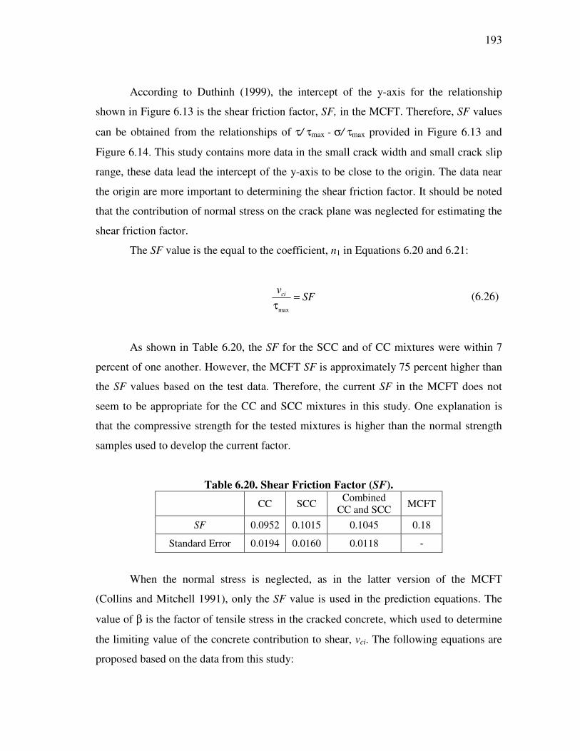
193

According to Duthinh (1999), the intercept of the y-axis for the relationship

shown in Figure 6.13 is the shear friction factor, SF, in the MCFT. Therefore, SF values

can be obtained from the relationships of τ/ τmax - σ/ τmax provided in Figure 6.13 and

Figure 6.14. This study contains more data in the small crack width and small crack slip

range, these data lead the intercept of the y-axis to be close to the origin. The data near

the origin are more important to determining the shear friction factor. It should be noted

that the contribution of normal stress on the crack plane was neglected for estimating the

shear friction factor.

The SF value is the equal to the coefficient, n1 in Equations 6.20 and 6.21:

max

civSF=

τ (6.26)

As shown in Table 6.20, the SF for the SCC and of CC mixtures were within 7

percent of one another. However, the MCFT SF is approximately 75 percent higher than

the SF values based on the test data. Therefore, the current SF in the MCFT does not

seem to be appropriate for the CC and SCC mixtures in this study. One explanation is

that the compressive strength for the tested mixtures is higher than the normal strength

samples used to develop the current factor.

Table 6.20. Shear Friction Factor (SF).

CC SCC Combined CC and SCC MCFT

SF 0.0952 0.1015 0.1045 0.18

Standard Error� 0.0194 0.0160 0.0118 ��

When the normal stress is neglected, as in the latter version of the MCFT

(Collins and Mitchell 1991), only the SF value is used in the prediction equations. The

value of β is the factor of tensile stress in the cracked concrete, which used to determine

the limiting value of the concrete contribution to shear, vci. The following equations are

proposed based on the data from this study:

194

For the CC mixtures (psi, in. [MPa, mm]):

( )

1.1424 (psi, in.)

0.6426 35.4450.63

ci

c

g

vwf

a

β ≤ =′ +

+

(6.27)

( )

0.0952 (MPa, mm)

0.6426 35.44516

ci

c

g

vwf

a

� �� �� �β ≤ =� �′ +� �+� �

For the SCC mixtures (psi, in. [MPa, mm]):

( )

1.2180 (psi, in.)

0.7490 55.7940.63

ci

c

g

vwf

a

β ≤ =′ +

+

(6.28)

( )

0.1015 (MPa, mm)

0.7490 55.79416

ci

c

g

vwf

a

� �� �� �β ≤ =� �′ +� �+� �

For the combined CC and SCC mixtures (psi, in. [MPa, mm]):

( )

1.254 (psi, in.)

0.6958 45.6190.63

ci

c

g

vwf

a

β ≤ =′ +

+

(6.29)

195

( )

0.1045 (MPa, mm)

0.6958 45.61916

ci

c

g

vwf

a

� �� �� �β ≤ =� �′ +� �+� �

6.4.5 Impact on Shear Design

The impact of the proposed equations for β based on this study (Equation 6.27,

6.28, and 6.29) were evaluated for cases with and without shear reinforcement.

6.4.5.1 No Shear Reinforcement

The following two equations for b from MCFT were presented in Section 2.4.1:

1

4cot�(psi)

1 500β =

+ ε 1

0.33cot �(MPa)

1 500

� �β =� �

+ ε� �� � (6.30)

and

( )

2.16 (psi, in.)

0.31 240.63

ci

c

g

vwf

a

β ≤ =′ +

+

(6.31)

( )

0.18 (MPa, mm)

0.31 2416

ci

c

g

vwf

a

� �� �� �β ≤ =� �′ +� �+� �

Equation 6.32 is used to limit the β value for both MCFT and the newly proposed

Equations 6.27 to 6.29.

The crack width, w, can be evaluated using the principal tensile strain, 1ε , and the

average spacing of the diagonal cracks, smθ, as in the following equation from the

MCFT:

196

1 mw s θ= ε

(6.32)

where 1

sin� cos� +

m

x v

s

s s

θ =� � � �

where smθ is the crack spacing in the direction of principal strain and ε1, sx, and sv are the

crack spacing parameters of longitudinal and shear reinforcement, respectively. The

crack spacing depends on the reinforcement spacing. According to the AASHTO

recommendations and the MCFT, sx is the lesser of either the effective shear depth, dv, or

the maximum distance between layers of longitudinal reinforcement. The parameter θ is

the angle of the diagonal compressive stresses in the web. Because shear reinforcement

is not used for this first case, sv is equal to zero.

After the crack width in Equation 6.31 is replaced by Equation 6.32, the equation

can be rearranged as follows:

1

2.17 (psi, in.)

0.6860.31

sin�xes

β ≤ ε+

1

0.18 (MPa, mm)

0.6860.31

sin �xes

� �� �β ≤� �ε� �+� �

(6.33)

where 1.38

(in.)0.63

xxe

g

ss

a=

+35

(mm)16x

xeg

ss

a

� �=� �+� �� �

For the members without shear reinforcement, the maximum post-cracking shear

capacity can be calculated when Equations 6.31 and 6.33 present the same β value

(Bentz et al. 2006). In this study, the same conditions were used to compare the β value

from the MCFT with Equations 6.27 to 6.29. Therefore, the equation is expressed as

follows:

197

1

1

1.2580.568

sin �tan � =1 500

xes ε+

+ ε

(6.34)

From the MCFT and the simplified MCFT (Bentz et al. 2006), the longitudinal

strain, εx, and principal tensile strain, ε1, can be found as in following equation:

( )4

21

1

cot �(1 cot �) +

15,000 1 500xε = ε +

+ ε

(6.35)

Based on this study, equations are proposed as follows.

For CC mixtures (psi, in. [MPa, mm]):

1

1.1424 (psi, in.)

1.01270.6426

sin�xes

β ≤ ε+

1

0.0952 (MPa, mm)

1.01270.6426

sin �xes

� �� �β ≤� �ε� �+� �

(6.36)

where 1.38

(in.)0.63

xxe

g

ss

a=

+35

(mm)16x

xeg

ss

a

� �=� �+� �� �

For SCC mixtures (psi, in. [MPa, mm]):

1

1.2180 (psi, in.)

1.59410.7490

sin�xes

β ≤ ε+

1

0.1015 (MPa, mm)

1.59410.7490

sin �xes

� �� �β ≤� �ε� �+� �

(6.37)

where 1.38

(in.)0.63

xxe

g

ss

a=

+35

(mm)16x

xeg

ss

a

� �=� �+� �� �

198

For combined CC and SCC mixtures (psi, in. [MPa, mm]):

1

1.254 (psi, in.)

1.30340.6958

sin�xes

β ≤ ε+

1

0.1045 (MPa, mm)

1.30340.6958

sin�xes

� �� �β ≤� �ε� �+� �

(6.38)

where 1.38

(in.)0.63

xxe

g

ss

a=

+35

(mm)16x

xeg

ss

a

� �=� �+� �� �

To estimate the β value for each equation, selected design parameters are shown

in Table 6.21. It should be noted that the strength of concrete is assumed to be higher

than 10,000 psi (70 MPa).

The estimated β and θ values for each mixture are presented in Table 6.22. The

MCFT overestimates β values by a factor of approximately two over equations

developed for the CC and SCC mixtures in this study. The β value of SCC is slightly

lower than that of CC. The shear capacity of concrete can be estimated by the product of

β and the square root of concrete compressive strength. If the strength of concrete

between the CC and SCC is assumed to be identical, the CC has approximately 7 percent

higher capacity than the SCC mixtures in this study. Similar θ values were determined

for the SCC and CC mixtures from this study. These θ values are larger than those

estimated from the MCFT and AASHTO expressions.

Table 6.21. Selected Design Parameters.

Maximum Size of Coarse Aggregate

ag, in. (mm)

Longitudinal Strain εx × 10−3 ,

in./in. (mm/mm)

Crack Spacing Parameter

sx, in. (mm)

AASHTO 0.75 (19)

1.000 10 (250)

MCFT (ag = 0) 0 CC

0.75 (19) SCC Combined

CC and SCC

199

Table 6.22. Estimated Beta and Theta Values.

Principal Tensile Strain

εx × 10−3 , in./in. (mm/mm)

θ Degree β

AASHTO 1.168 34.56 0.272 MCFT (ag = 0) 1.049 43.24 0.203 CC (Eq. 6.34) 1.003 62.08 0.102

SCC (Eq. 6.35) 1.002 63.90 0.095 Combined

CC and SCC (Eq. 6.36)

1.003 63.01 0.098

6.4.5.2 Shear Reinforcement

According to the MCFT, the tension is transmitted on the shear crack surface by

the increase of shear reinforcement stresses at low shear stresses. As the applied shear

force increases, the shear reinforcement at the cracks reaches the yield stress. The local

shear stress on the crack cannot exceed the maximum allowable shear stress, vci, to

prevent the occurrence of slip.

Based on the equilibrium conditions between concrete and steel stresses on the

crack, the principal concrete tensile stress is limited by the following equation:

( )1 tan � + vc ci vy v

v w

Af f v f f

s b′= β < − (6.39)

where f1 is the principal concrete tensile stress, β is the tensile stress factor in the cracked

concrete (Equation 6.30), f’ c is the concrete compressive strength, θ is the angle of the

diagonal compressive stresses in the web, vci is the limiting value of the maximum shear

stress on the shear plane in the cracked concrete, Av is the area of shear reinforcement, sv

is the spacing of shear reinforcement, bw is the thickness of web, fv is the stress of shear

reinforcement, and fvy is the yield stress of shear reinforcement.

To compare the impact of equation on the shear design, two cases were

considered.

200

• Case 1: Before shear failure (prior to yielding of shear reinforcement) and

• Case 2: Shear failure (at yielding of shear reinforcement).

The typical details for Type A girders (which are the same as in the full-scale

testing) are used to evaluate the impact of the proposed equations (see Table 6.23).

Compressive strength of concrete and elastic modulus of steel are assumed to be 13,000

psi (90 MPa) and 29,000 ksi (200 GPa), respectively. The value of θ is assumed to be 35

degrees, as observed in the full-scale test program.

Table 6.23. Assumptions of Design Parameters.

Maximum Size of Coarse

Aggregate ag

in. (mm)

sx in.

(mm)

sv in.

(mm)

Av in.2

(mm2)

fvy ksi

(MPa)

θ Degree

AASHTO 0.75 (19)

22.3 (565)

4 (102)

0.40 (25)

65 (450) 35

MCFT (ag = 0) 0

CC

0.75 (19) SCC

Combined CC and

SCC

Table 6.24 shows the estimated concrete and steel stress before shear failure

using the different models. Table 6.25 shows the estimated concrete and steel stress at

shear failure indicating the yielding of shear reinforcements. Because of the steel

contribution, the concrete stress is smaller than the limiting values provided by Equation

6.39. Therefore, all models predict the same stress values for the concrete and steel.

Even though yielding of shear reinforcement occurs, the contribution of concrete and

steel are still the same because the stress of concrete did not exceed the limiting values.

201

In other words, the concrete stress does not reach the limiting value of shear stress

before initiation of shear reinforcement yielding.

Table 6.24. Estimated Concrete and Steel Stress for Type A Girder (Case 1 Before Shear Failure).

f1, ksi (MPa)

fv, ksi (MPa)

Crack Width w, in. (mm)

AASHTO 0.39 (2.7)�

19 (130)� 0.004 (0.1)

MCFT (ag = 0) 0.39 (2.7)�

19 (130)� 0.004 (0.1)

CC 0.39 (2.7)�

19 (130)� 0.004 (0.1)

SCC 0.39 (2.7)�

19 (130)� 0.004 (0.1)

Combined CC and SCC

0.39 (2.7)�

19 (130)� 0.004 (0.1)

Note: f1 is the principal tensile stress of concrete, and fv is the steel stress of shear reinforcement.

Table 6.25. Estimated Concrete and Steel Stress for Type A Girder (Case 2 at Shear Failure).

f1, ksi (MPa)

fv, ksi (MPa)

Crack Width w, in. (mm)

AASHTO 0.29 (2.0)�

65 (450)� 0.014 (0.37)

MCFT (ag = 0) 0.29 (2.0)�

65 (450)� 0.014 (0.37)

CC 0.29 (2.0)�

65 (450)� 0.014 (0.37)

SCC 0.29 (2.0)�

65 (450)� 0.014 (0.37)

Combined CC and SCC

0.290 (2.0)�

65 (450)� 0.014 (0.37)

Note: f1 is the principal tensile stress of concrete, and fv is the steel stress of shear reinforcement.

202

An extreme case is checked using a typical design of a deep beam. Type VI

girders have a section depth of 72 in. (1.8 m). Deep section members are typical more

vulnerable to shear stress. According to TxDOT design practice, the spacing of the R

type shear reinforcement typically varies from 4 to 8 in. (102 to 203 mm).

According to a NCHRP Project 12-61 report, θ typically ranges from 18.1 to 43.9

degrees (Hawkins et al. 2005). Based on Canadian Standards Association (CAN3 A23.3-

M04), θ is limited to 29 degrees minimum in design practice (CSA 1994). The high

value of the angle typically requires a large amount of shear reinforcement. Based on

these typical ranges, the shear stresses of concrete and steel were estimated with MCFT

containing different limiting values for maximum shear stress from AASHTO, MCFT

(ag = 0), and the combined CC and SCC equation.

Table 6.26 compares shear capacities of concrete and steel with an angle θ of

18.1 degrees. This table considers two extreme cases of crack widths (small crack width

and large crack width resulting in the yielding of steel) and two different spacings of

shear reinforcement (4 and 8 in. [101 and 203 mm]). At a 8 in. (203 mm) shear

reinforcement spacing, the shear capacity of concrete based on MCFT (ag = 0) is

approximately 7 to 10 percent smaller than AASHTO. The shear capacity of concrete

based on the proposed equation is approximately 20 to 35 percent smaller than

AASHTO. The compressive strength considered for Type VI girders is 13,000 psi (90

MPa).

203

Table 6.26. Estimated Concrete and Steel Stress for Type VI Girder (θθθθ = 18.1 Degrees).

sv, in. (mm)

w, in. (mm)

θ, Degree

Vc, kip (kN)

Vs, kip (kN)

V, kip (kN) Note

AASHTO

8 (203)

0.004 (0.1)

18.1

257 (1140)

85.0 (378)

342 (1520)

Slip

MCFT (ag=0) 241 (1070)

85.0 (378)

326 (1450)

Combined CC and SCC

191 (850)

85.0 (378)

276 (1230)

AASHTO

0.021 (0.53)*

218 (970)

518 (2300)

736 (3270)

MCFT (ag=0) 199 (885)

518 (2300)

717 (3190)

Combined CC and SCC

182 (810)

518 (2300)

700 (3110)

AASHTO

4 (101)

0.004 (0.1)

342 (1520)

365 (1620)

707 (3150)

No Slip

MCFT (ag=0) Combined

CC and SCC�AASHTO

0.021 (0.53)*

271 (1210)

1040 (4610)

1310 (5820)

MCFT (ag=0) Combined

CC and SCC�Note: * Large crack width causes the yielding of shear reinforcement.

Table 6.27 compares shear capacities of concrete and steel with an angle θ of

43.9 degrees. This table also considers two extreme cases of crack widths and two

different spacings of shear reinforcement. When the angle θ is large, as in this case, the

concrete capacities for shear estimated by the three different equations for a given crack

width and shear reinforcement spacing are the same. This indicates the shear stress of

concrete did not reach the maximum allowable stress and no slip is predicted.

204

Table 6.27. Estimated Concrete and Steel Stress for Type VI Girder (θθθθ = 43.9 Degrees).

sv, in. (mm)

w, in. (mm)

θ, Degree

Vc, kip (kN)

Vs, kip (kN)

V, kip (kN) Note

AASHTO

8 (203)

0.004 (0.1)

43.9

136 (605)

15 (67)

151 (672)

No Slip

MCFT (ag=0) Combined

CC and SCC AASHTO

0.044 (1.11)*

79 (351)

176 (783)

255 (1134)

MCFT (ag=0) Combined

CC and SCC AASHTO

4 (101)

0.004 (0.1)

121 (538)

59 (262)

180 (800)

MCFT (ag=0) Combined

CC and SCC�AASHTO

0.023 (0.58)*

79 (351)

350 (1557)

429 (1908)

MCFT (ag=0) Combined

CC and SCC�Note: * Large crack width causes the yielding of shear reinforcement.

Table 6.28 compares shear capacities of concrete and steel with an angle θ of 29

degrees. When the angle is a typical value for a prestressed girder along with an 8 in.

(203 mm) shear reinforcement spacing and 0.004 in. (0.1 mm) crack width, the

AASHTO and MCFT (ag = 0) equations overestimate the shear capacity compared to the

proposed equation. For 4 in. (101 mm) spacing of shear reinforcement, the AASHTO,

MCFT, and proposed equation estimate the same capacities for shear. Based on these

comparisons, proposed equation is necessary to safely estimate the shear capacities of

high-strength CC and SCC girders.

205

Table 6.28. Estimated Concrete and Steel Stress for Type VI Girder (θ θ θ θ = 29 Degrees).

sv, in. (mm)

w, in. (mm)

θ, Degree

Vc, kip (kN)

Vs, kip (kN)

V, kip (kN) Note

AASHTO

8 (203)

0.004 (0.1)

29

231 (1030)

43 (190)

274 (1220) No

Slip MCFT (ag=0) 231 (1030)

43 (190)

274 (1220)

Combined CC and SCC

208 (925)

43 (190)

252 (1120) Slip

AASHTO 0.026 (0.65)

154 (685)

304 (1350)

458 (2040)

No Slip

MCFT (ag=0) Combined

CC and SCC AASHTO

4 (101)

0.004 (0.1)

204 (907)

176 (783)

381 (1700)

MCFT (ag=0) Combined

CC and SCC�AASHTO

0.013 (0.33)

154 (685)

600 (2670)

754 (3350)

MCFT (ag=0) Combined

CC and SCC�Note: * Large crack width causes the yielding of shear reinforcement.

Only two cases indicate the slip of shear plane. When the spacing of shear

reinforcement is large along with small angle of the diagonal compressive stress (θ), the

shear capacity of concrete reaches the limiting value of the maximum shear stress. This

case shows a 2 to 24 percent reduction of total shear capacity when the new equations

are used. Therefore, this study indicates that the MCFT and the AASHTO equations

overestimate shear capacity when slip occurs in extreme cases such as for low shear

reinforcement ratio and small angle of diagonal cracks compared with the new

equations.

The applicability of the proposed equations is discussed with respect to the full-

scale test program in Section 8.5.4.

206

6.5 SUMMARY

Based on the experimental results, the following conclusions were made.

1) The plot of τ/σ versus w provides a quantifiable comparative assessment of

the aggregate interlock for the CC and SCC mixtures having different paste

strengths and a different level of initial fracture of the aggregate. As the crack

width increases, the decreasing value of the normalized shear stress indicates

a decrease in aggregate interlock.

2) The E-value, a measure of the absorbed energy of the aggregate interlock,

provides a quantifiable comparative assessment up to a selected crack slip

limit. The 5 ksi (34 MPa) river gravel SCC and CC specimens exhibited

higher E-values than the other mixtures [7 ksi (48 MPa) river gravel CC and

SCC, 5 and 7 ksi (34 and 48 MPa) limestone CC and SCC specimens]. This

indicates that high-strength concrete [28-day compressive strength greater

than 10 ksi (70 MPa)] can still exhibit aggregate interlock. In addition, the

SCC mixture containing river gravel exhibits a higher potential to increase

the contribution of aggregate interlock to shear.

3) The effects of coarse aggregate type and volume on the E-value were

determined with statistical assessment (mixed procedure). The batch of

concrete is regarded as the random effect in the mixed procedure statistical

approach. The contrast was used to assess the effect of type and volume of

coarse aggregate on the aggregate interlock.

4) Aggregate type is a critical factor influencing aggregate interlock. For both

the SCC and CC specimens, concrete mixtures containing river gravel

exhibited more aggregate interlock compared to those containing limestone

aggregate. Statistically, the effect of aggregate type is clearly identified at all

slip ranges.

5) The volume of aggregate influences the contribution of aggregate interlock to

the shear capacity for the SCC and CC mixtures tested. The effect of volume

207

is observed on both river gravel and limestone mixtures based on statistical

analysis (the contrasts) with a p-value of 0.05.

6) Lower strength concrete tends to have less coarse aggregate fractures

resulting in more aggregate interlock, leading to a large amount of energy

absorption. Therefore, the strength of concrete is highly related to the amount

of fracture of aggregate interlock at small crack widths when crack slip

initiates.

7) The friction coefficients and fracture reduction factors were determined based

on the statistical analysis (mixed procedure). The fracture reduction factors,

c, were 0.43 and 0.62 for the SCC and CC mixtures tested, respectively. The

friction coefficients, µ, were 0.32 and 0.30 for the SCC and CC mixtures

tested, respectively.

8) The SCC exhibited lower maximum shear stresses compared with the CC.

9) An upper limit of the β value is proposed for both CC and SCC and

combined CC and SCC data based on this study. The shear friction factor in

this study, (approximately 0.10) is lower than the previously proposed value

of 0.18 reported in the MCFT.

10) When the SCC and CC mixtures have the same concrete strength and this

strength is higher than 10 ksi (70 MPa), the CC mixtures exhibit a higher

concrete shear strength than the SCC mixtures when both are evaluated

without shear reinforcement.

11) Finally, the proposed equation for β to compute the concrete shear strength

using the MCFT approach (Equation 6.38) is necessary to estimate the

appropriate shear capacity of high-strength CC and SCC girders, rather than

with the AASHTO and MCFT (ag = 0) expressions. The AASHTO and the

MCFT expressions overestimate the shear capacity when low shear

reinforcement ratios and small shear crack angles are assumed.

208

CHAPTER VII

RESULTS AND ANALYSIS OF LABORATORY STUDY:

BOND, CREEP, AND DURABILITY

7.1 BOND CHARACTERISTICS

The experimental results and analysis for top bar effects on relative bond strength

are presented below.

7.1.1 Bond Stresses

Two types of failure were observed during the pull-out tests. Most bars failed by

creating a cone shaped failure surface through the concrete surrounding the reinforcing

bar. The load-displacement curve is shown in Figure 7.1 (a). All reinforcing bars had

stresses that exceeded the yield strength of the reinforcement, which corresponds to an

applied load of 19 to 21 kip (85 to 93 kN). The second type of failure mode observed

was failure of the reinforcement in tension. The load-displacement is shown in Figure

7.1 (b). In this case, yielding of the reinforcing bar was followed by strain hardening and

a reduction in the bar diameter.

Tables 7.1 to 7.4 and Figures 7.2 and 7.3 show the test results of the individual

pull-out tests. Each test was conducted 35 days after casting the specimen. Each figure

shows the difference between the measured bond stress for the top and bottom bars of

each mixture.

209

(a) Concrete Failure (b) Bar Failure

Figure 7.1. Typical Failure Modes.

A total of 40 samples were tested to measure the relative bond stress for both the

top and bottom bars. The average bond stress ranged from 2.29 to 3.40 ksi (16 to 23

MPa) for all samples. The range of concrete compressive strength was between 8345 and

13,358 psi (58 and 92 MPa).

Four samples of the 5 ksi (34 MPa) SCC-R mixture experienced bar failure

indicating good bond. Five bottom bars failed by bar failure. Two top bars failed by bar

failure.

Three bottom bars of 5 ksi (34 MPa) SCC-R mixture experienced strain

hardening without bond slip, indicating sufficient bond between the reinforcing bar and

concrete to reach stresses beyond the yield strength, as desired for ultimate strength

design. Overall the average of bond stress of SCC-R mixture (3.04 ksi [21 MPa]) was

higher than that of the CC-R mixtures (2.37 ksi [16 MPa]). The high bond strength of

SCC mixture could be attributed to higher concrete strength.

Even though the strength of SCC-L was about 31 percent higher than that of CC-

L, SCC-L does not seem to provide significant benefits for the bond of bars. The average

0

10

20

30

40

0

40

80

120

160

-0.5 0.0 0.5 1.0 1.5 2.0 2.5

0 15 30 45 60

Stroke (Loading Apparatus)

Slip (LVDT)

Load

(kip

s)

Displacement (in.)

Displacement (mm)

Load (kN

)

No Slip BeforeConcrete Failure

Yielding of Reinforcement

0

10

20

30

40

0

40

80

120

160

-0.5 0.0 0.5 1.0 1.5 2.0 2.5

0 15 30 45 60

Stroke (Loading Apparatus)

Slip (LVDT)Lo

ad (k

ips)

Displacement (in.)

Displacement (mm)

Load (kN

)

No Slip

Yielding of Reinforcement

Bar Failure

210

computed bond stress for the CC-L mixtures (2.73 ksi [19 MPa]) was slightly higher

than the average bond stress of the SCC-L mixture (2.66 ksi [18 MPa]).

Table 7.1. Test Results of CC-R Samples.

Sample ID Compressive Strength, psi

(MPa)

Std. Dev., psi

(MPa)

Slump, in. (mm)

Pull-out Force,

kip ( kN)

Average Bond Stress, ksi (MPa)

Failure Mode

CC-R1t 8345 (58) 148 (1.0) 3.5 (89)

27.4 (122) 2.79 (19) C CC-R1b 33.3 (148) 3.40 (23) B CC-R2t

8809 (61) 592 (4.1) 5.0 (127)

33.5 (149) 3.40 (23) B CC-R2b 27.6 (123) 2.81 (19) C CC-R3t 8565 (59) 542 (3.7) 7.0

(177) 26.4 (117) 2.69 (19) C

CC-R3b 29.8 (133) 3.04 (21) C CC-R4t 8671 (60) 356 (2.5) 5.25

(133) 25.0 (111) 2.55 (18) C

CC-R4b 29.3 (130) 2.98 (21) C CC-R5t 9732 (67) 259 (1.8) 8.0

(202) 24.4 (109) 2.49 (17) C

CC-R5b 33.5 (149) 3.40 (23) C

Avg. 8824 (61) 380 (2.6) 5.75 (145) 29.0(129) 2.37 (16)

Note: C: Concrete Failure, B: Bar Failure.

Table 7.2. Test Results of SCC-R Samples.

Sample ID Compressive

Strength, psi (MPa)

Std. Dev., psi (MPa)

Slump Flow,

in. (mm)

T50, sec VSI

Pull-out Force,

kip (kN)

Average Bond Stress,

ksi (MPa)

Failure Mode

SCC-R1t 11,616 (80)

655 (4.5)

31.75 (803) 3.28 0.5~1 28.4 (126) 2.89 (20) C

SCC-R1b 32.9 (146) 3.40 (23) B SCC-R2t 11,438

(79) 481 (3.3)

28.00 (708) 4.81 0.5~1 33.0 (147) 3.40 (23) B

SCC-R2b 33.0 (147) 3.40 (23) B SCC-R3t 13,358

(92) 68

(0.5) 27.00 (683) 3.94 0.5~1 31.8 (141) 3.24 (22) C

SCC-R3b 30.4 (135) 3.09 (21) C SCC-R4t 11,931

(82) 264 (1.8)

27.50 (696) 4.40 0.5~1 29.5 (131) 3.00 (21) C

SCC-R4b 33.1 (147) 3.40 (23) B SCC-R5t 11,480

(79) 447 (3.1)

27.00 (683) 4.59 0.5~1 29.1 (129) 2.96 (20) C

SCC-R5b 30.6 (136) 3.12 (22) C

Avg. 11,965 (82)

383 (2.6)

28.00 (708) 4.2 0.5~1 31.2 (139) 3.04(21)

Note: C: Concrete Failure, B: Bar Failure.

211

(a) CC-R (b) SCC-R

Figure 7.2. Average Bond Stress of Top and Bottom Bars (CC-R and SCC-R). Table 7.3. Test Results of CC-L Samples.

Sample ID Compressive

Strength, psi (MPa)

Std. Dev., psi

(MPa)

Slump, in. (mm)

Pull-out Force,

kip ( kN)

Average Bond Stress,

ksi (MPa)

Failure Mode

CC-L1t 9613 (66) 157 (1.1) 8 (203) 24.6 (109) 2.51(17) C CC-L1b 28.8 (128) 2.93 (20) C CC-L2t 8830 (61) 413

(2.8) 8.5(216) - - - CC-L2b 28.0 (125) 2.85 (20) C CC-L3t 9517 (66) 161

(1.1) 7 (178) 26.6 (118) 2.69 (19) C CC-L3b 28.4 (126) 2.89 (20) C CC-L4t 9679 (67) 696

(4.8) 3 (76) 25.0 (111) 2.55 (18) C CC-L4b 28.6 (127) 2.91 (20) C CC-L5t

9756 (67) 73 (0.5) 7 (178)

25.3 (113) 2.58 (18) C CC-L5b 33.4 (149) 3.4* (23) B

Avg. 9479 (65) 300 (2.1) 6.7 (178) 27.9 (124) 2.73(19)

Note: C: Concrete Failure, B: Bar Failure, - indicates not tested.

0

1

2

3

4

5

0

10

20

30

8 10 12 14

60 70 80 90

Ave

rage

Bon

d St

ress

(ks

i)

Compressive Strength (ksi)

Average B

ond Stress (MPa)

Compressive Strength (MPa)

0

1

2

3

4

5

8 10 12 140

10

20

30

60 70 80 90

Compressive Strength (ksi)

Compressive Strength (MPa)

Ave

rage

Bon

d St

ress

(ks

i)

Average B

ond Stress (MPa)

Top BarBottom Bar

212

Table 7.4. Test Results of SCC-L Samples.

Sample ID

Compressive Strength, psi (MPa)

Std. Dev., psi

(MPa)

Slump Flow,

in. (mm)

T50, sec VSI

Pull-out Force,

kip (kN)

Average Bond Stress,

ksi (MPa)

Failure Mode

SCC-L1t 12,072 (83)

57 (0.4)

26.0 (660) 4.19 0.5~1 23.0 (102) 2.34 (16.1) C

SCC-L1b 28.6 (127) 2.91 (20.1) C SCC-L2t 12,560

(87) 209 (1.4)

31.0 (787) 2.85 0.5~1 23.9 (106) 2.43 (16.8) C

SCC-L2b 33.4 (149) 3.40 (23.4) B SCC-L3t 12,117

(84) 314 (2.2)

26.0 (660) 6.57 0.5~1 29.4 (131) 2.99 (20.6) C

SCC-L3b 24.7 (110) 2.52 (17.4) C SCC-L4t 12,754

(88) 409 (2.8)

25.0 (635) 5.56 0.5~1 22.5 (100) 2.29 (15.8) C

SCC-L4b 25.5 (113) 2.74 (18.9) C SCC-L5t 12,703

(88) 259 (1.8)

27.5 (699) 2.97 0.5~1 26.9 (120) 2.33 (16.1) C

SCC-L5b 26.4 (117) 2.69 (18.5) C

Avg. 12,441 (86)

250 (1.7)

27.0 (686) 2.21 0.5~1 25.4 (113) 2.59 (17.9)

Note: C: Concrete Failure, B: Bar Failure.

(a) CC-L (b) SCC-L

Figure 7.3. Average Bond Stress of Top and Bottom Bars (CC-L and SCC-L).

In general, the SCC mixture proportions have a higher compressive strength

compared to CC mixture proportions at 35 days. As shown in Figure 7.4, at a given

concrete compressive strength, most top bars exhibited less bond strength than the

bottom bars for both the SCC and CC mixtures.

0

1

2

3

4

5

0

10

20

30

8 10 12 14

60 70 80 90 Average B

ond Stress (MPa)

Compressive Strength (MPa)

Compressive Strength (ksi)

Ave

rage

Bon

d St

ress

(ks

i)

0

1

2

3

4

5

0

10

20

30

8 10 12 14

60 70 80 90Compressive Strength (MPa)

Compressive Strength (ksi)

Ave

rage

Bon

d St

ress

(ksi

)

Average B

ond Stress (MPa)

Top BarBottom Bar

213

Figure 7.4. Average Bond Stress.

Figure 7.5 shows the relationship between compressive strength and average

bond stresses. There is no observable correlation between compressive strength and

bond stresses for the top and bottom bars.

(a) Bottom Bar (b) Top Bars

Figure 7.5. Compressive Strength versus Average Bond Stresses.

0

1

2

3

4

5

8 9 10 11 12 13 14

Bottom Bar

Top Bar

0

10

20

30

60 70 80 90

Compressive Strength (ksi)

Ave

rage

Bon

d St

ress

(ks

i)

Concrete Pull-out Failure (P)

Bar Failure (B)SCCCC

Compressive Strength (MPa)

Average B

ond Stress (MPa)

0

1

2

3

4

5

8 10 12 14

60 70 80 90

0

10

20

30

Compressive Strength (ksi)

Average B

ond Stress (MPa)

Concrete Failure

Compressive Strength (MPa)

Ave

rage

Bon

d St

ress

(ks

i) Bar Failure

0

1

2

3

4

5

8 10 12 14

60 70 80 90

0

10

20

30

Concrete Failure

Bar Failure

Average B

ond Stress (MPa)A

vera

ge B

ond

Stre

ss (

ksi)

Compressive Strength (MPa)

Compressive Strength (ksi)

CC-RSCC-R

CC-LSCC-L

214

7.1.2 Assessment of Top Bar Effect

The impact of the top bar position on the bond stress between the reinforcement

and concrete can be evaluated using the bond ratio. Figure 7.6 shows that the mean bond

ratio of all specimens is higher than 1.0, indicating a reduction in the bond stress for the

top bar relative to the bottom bar for a given pull-out sample. Therefore, water is likely

collecting below the bar, increasing the w/c in this area, and thus decreasing the concrete

strength and bond. The average bond ratio for the SCC with limestone aggregate was the

highest among the different mixture proportions evaluated. The bond ratio for the SCC

with river gravel aggregate indicates that the top bar effect is relatively small for this

mixture. Furthermore, the SCC with river gravel has a lower bond ratio than the CC

containing river gravel. An analysis was conducted to determine whether these

differences are significant and is discussed in Section 7.1.4. The top bar multiplier of the

AASHTO LRFD Specifications (2004, 2006) is approximately 20 percent higher than

the observed bond ratio.

Figure 7.6. Bond Ratio Values to Evaluate Top Bar Effect.

7.1.3 Impact of Fresh Properties on Top Bar Effect

Researchers also assessed the impact of the fresh properties of the concrete

mixtures on the bond ratio. The fresh properties of the CC mixtures can be evaluated

0.8

1.0

1.2

1.4

1.6

CC-R SCC-R CC-L SCC-L

Bon

d R

atio

AASHTO LRFD Top Bar Multiplier

Outlier

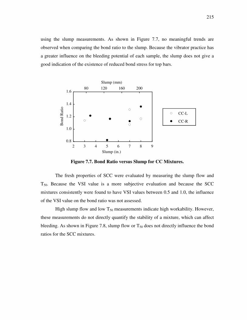
215

using the slump measurements. As shown in Figure 7.7, no meaningful trends are

observed when comparing the bond ratio to the slump. Because the vibrator practice has

a greater influence on the bleeding potential of each sample, the slump does not give a

good indication of the existence of reduced bond stress for top bars.

Figure 7.7. Bond Ratio versus Slump for CC Mixtures.

The fresh properties of SCC were evaluated by measuring the slump flow and

T50. Because the VSI value is a more subjective evaluation and because the SCC

mixtures consistently were found to have VSI values between 0.5 and 1.0, the influence

of the VSI value on the bond ratio was not assessed.

High slump flow and low T50 measurements indicate high workability. However,

these measurements do not directly quantify the stability of a mixture, which can affect

bleeding. As shown in Figure 7.8, slump flow or T50 does not directly influence the bond

ratios for the SCC mixtures.

0.8

1.0

1.2

1.4

1.6

2 3 4 5 6 7 8 9

CC-L

CC-R

80 120 160 200

Bon

d R

atio

Slump (in.)

Slump (mm)

216

(a) Slump Flow (b) T50

Figure 7.8. Bond Ratio versus Slump Flow for SCC Mixtures.

7.1.4 Statistical Assessment

A statistical analysis was performed to evaluate the significance of the mixture

proportions and aggregate type on the bond ratio. For this analysis, the distribution is

assumed to be normal for the residuals. As shown in Figure 7.9, the quantile plot is

reasonably linear indicating that the assumption of a normal distribution for the

statistical analysis is valid.

Figure 7.9. Quantile Plots for Bond Ratio.

0.8

1.0

1.2

1.4

1.6

24 26 28 30 32

650 700 750 800

Slump Flow (in.)

Bon

d R

atio

Slump Flow (mm)

0.8

1.0

1.2

1.4

1.6

2.5 3.0 3.5 4.0 4.5 5.0T

50 (s)

Bon

d R

atio

SCC-L SCC-R

-0.4

-0.2

0.0

0.2

0.4

-2.0 -1.5 -1.0 -0.5 0.0 0.5 1.0 1.5 2.0

Res

idua

ls

Normal Quantile

217

According to previous observations for the test results, the fresh properties and

compressive strength do not seem to influence the bond ratio, which is a measure of the

top bar effect. Because each mixture proportion has a high variance for the bond ratio

and similar mean bond ratios, the mean bond ratio for each mixture proportion was

evaluated with statistical assessments to determine whether the mixture types

significantly influence the bond stress ratio.

Table 7.5 provides the analysis of variance (ANOVA) table, obtained from the

SAS Program (v. 9.1.3) (SAS Institute 2006). The ANOVA indicates that the type of

concrete (SCC or CC) and the type of aggregate (limestone or river gravel) are not

significant factors affecting the variance of the bond ratios. Because the p-value was

larger than 0.05, the aggregate type, the concrete type, and combinations of aggregate

type and mixture type are not significant factors affecting the bond ratio. The mean value

of the bond ratio, indicating a top bar effect for all mixture proportions, is not

significantly different. The interaction of mixture type (SCC or CC) with aggregate type

is also not a significant factor. Therefore, the stable SCC mixtures considered in this

study, having high paste volume, did not exhibit a significant top bar effect compared

with the CC mixtures.

Table 7.5. ANOVA Table of Bond Ratio Value.

Source Degree

of Freedom

Type III Sum of Square Mean Square p-value

Agg 1 0.021144 0.02144 0.3797 Mix 1 0.009742 0.00974 0.5509

Agg x Mix 1 0.006294 0.00626 0.6316 Note: Agg: Two types of aggregate (Limestone and River Gravel).

Mix: Two types of mixtures (CC or SCC).

7.1.5 Summary

Based on the analysis and test results for assessing the relative bond for select

SCC and CC mixtures, the following conclusions are drawn:

218

1) All 39 pull-out samples for evaluating the top bar effect for mild steel

reinforcement had maximum stresses that exceeded the yield strength.

2) Most reinforcing bars failed by creating a splitting cone shaped failure

surface initiated by concrete cone failure.

3) Most top bars exhibited lower bond strengths than the bottom bars for both

the SCC and CC mixtures, indicating the existence of the top bar effect.

4) The relatively high bond strength of the SCC-R mixture may be attributed to

the higher concrete compressive strength. However, the higher concrete

compressive strength for the SCC-L mixture does not provide the same

benefit of increased pull-out strength. The SCC-L mixture had slightly lower

bond stress values than the CC-L mixtures.

5) The bond can be assessed using a bond ratio based on the ratio of the average

bond stress of the bottom bar to the average bond stress of the companion top

bar. The SCC-R mixture had the lowest bond ratio indicating the least top bar

effect. The SCC-L mixture has highest bond ratio indicating the higher

reduction of bond due to the top bar effect.

6) The measured fresh properties of the SCC and CC are not correlated with the

bond ratio indicating the top bar effect in this study.

7) Based on a statistical analysis, the mixture type, aggregate type, and

combination of aggregate and mixture types are not significant factors

influencing the bond ratio.

8) All bond ratios are less than the top bar multiplier factor, 1.4, recommended

in the AASHTO LRFD Specifications (2004 and 2006) for determining the

tension development length of mild reinforcement. Therefore, the current

AASHTO top bar factor of 1.4 is appropriate for the CC and SCC mixtures

evaluated in this study.

219

7.2 CREEP

7.2.1 Compressive Strength and Creep Loading

A 16-hour compressive strength test was conducted using two cylinders from

each batch. In the 16-hour test, the second batch of conventional concrete cast with

limestone for 5 ksi (34 MPa) strength (CC5-L) had a significantly lower measured

compressive strength than cylinders from the first batch. The reason for this lower 16-

hour strength is unknown. However, after 7 days the strength was similar between the

two batches. Because the loading was determined based on the compressive strength at 7

days, the samples from mixture CC5-L were used in the test program.

Table 7.6 shows the initial loading, loss of loading, and final loading. The loss of

loading occurred when tightening the nuts for the four threaded rods.

Table 7.6. 7-Day Compressive Strength Cylinder Test and Creep Loading.

Concrete Type

Mixture ID

Average 7-day f’ c, ksi

(MPa)

Initial Load,

kip (kN)

Load Loss,

kip (kN)

Creep Load,

kip (kN)

Creep Load (% of f’ c)

SCC

S5G-3c 9.3 (63) 40 (178) 5 (22) 35 (156) 30 S7G-6 11.6 (79) 47 (209) 9 (40) 38 (169) 26 S5L-3c 9.4 (65) 43 (191) 7 (31) 36 (160) 30 S7L-6 12.8 (88) 48 (214) 9 (40) 39 (173) 25

CC

C5G 9.4 (65) 39 (173) 3 (13) 36 (160) 31 C7G 10.6 (73) 43 (191) 4 (18) 39 (173) 30 C5L 8.5 (59) 35 (156) 2 (9) 33 (147) 31 C7L 10.4 (72) 40 (178) 4 (18) 36 (160) 27

7.2.2 Overall Comparison of Creep

An overall comparison of the SCC and CC creep samples is shown in Figure 7.10.

The measured creep curves were obtained from the average of two batches of each

mixture. Each frame was equipped with four cylinders that were cast with the same

mixture proportions from two different batches. The strain measurements for cylinders

within each frame varied by as much as 15 percent. Appendix E provides data of each

channel. The amount of cement paste and the stiffness of aggregate in mixtures can

affect the creep. The impact of key variables on the creep is reviewed in the following

220

subsections. Based on the ASTM C512, the strain readings of the control sample (i.e.,

shrinkage) are subtracted from the strain readings from the samples in the creep frame.

The S7L-6 mixtures have only readings from the creep frame due to the failure of strain

gages in the control samples.

Note: * indicates no correction for creep strain.

(a) SCC

(b) CC

Figure 7.10. Creep of SCC and CC Mixtures.

0

500

1000

1500

S5G-3cS7G-6

S5L-3cS7L-6*

0 50 100 150Time After Loading (Days)

SCC

Stra

in (x

10-6

in./i

n. o

r mm

/mm

)

0

500

1000

1500

C5GC7G

C5LC7L

0 50 100 150Time After Loading (Days)

CC

Stra

in (x

10-6

in./i

n. o

r mm

/mm

)

221

7.2.2.1 Effect of Target 16-Hour Compressive Strength

In the experimental matrix, samples were cast with two levels of 16-hour target

compressive strength, 5 and 7 ksi (35 and 48 MPa). For the SCC and CC mixtures the

strength does not seem to be an important factor influencing creep. This is shown in

Figure 7.11. The plot shows the average, maximum, and minimum values of creep. The

average of the 5 and 7 ksi (35 and 48 MPa) mixtures was not significantly different.

However, the variance of the overall creep was relatively large, with more variation

observed for the 7 ksi (48 MPa) target release strength mixtures.

Figure 7.11. Effect of 16-hour Compressive Strength on Creep.

7.2.2.2 Effect of Aggregate Type

Both river gravel and limestone were used for the CC and SCC mixtures. These

are representative coarse aggregates that are used widely in Texas. The type of aggregate

is one of the most important factors that can determine not only compressive strength,

but also creep. Because the stiffness of river gravel is higher than that of the limestone, it

assumed that the concrete with river gravel will exhibit lower creep than the concrete

with limestone. During the test program, the MOE of concrete with limestone aggregate

0

500

1000

1500

0 40 80 120 160

Avg. (5 ksi [35 MPa])Max. and Min. (5 ksi)

Avg. (7 ksi [48 MPa])Max. and Min. (7 ksi)

Stra

in (x

10-6

in./i

n. o

r mm

/mm

)

Time After Loading (Days)

222

was lower than that of the concrete with river gravel (see Section 5.3). Both the CEB-

FIP (1993) and the 2006 AASHTO LRFD prediction equations assume that the creep of

limestone concrete mixture will be higher than that of river gravel concrete mixtures. As

shown in Figure 7.12, the limestone mixtures have higher average and variance in

measured creep relative to the river gravel mixtures.

Figure 7.12. Creep of Type of Coarse Aggregate.

7.2.2.3 Comparison of SCC and CC

Figure 7.13 compares the average creep and overall range of creep measurements

for the CC and SCC mixtures. Creep of the SCC mixtures is lower than that of the CC

mixtures. The SCC mixtures contain greater cement contents, whereas the CC mixtures

contain higher aggregate volumes. Maximum creep for CC is 18 percent higher than that

of SCC. This might be attributed to the limestone CC mixture.

0

500

1000

1500

0 40 80 120 160

Avg. (River Gravel CC and SCC)Max. and Min. (River Gravel CC and SCC)Avg. (Limestone CC and SCC)Max. and Min. (Limestone CC and SCC)

Time After Loading (Days)

Stra

in (x

10-6

in./i

n. o

r mm

/mm

)

223

Figure 7.13. Creep of CC and SCC Mixtures.

For a more detailed comparison, considering strength level and type of coarse

aggregate, Figure 7.14 shows the creep of each individual concrete mixture with solid

circles corresponding to CC and open circles corresponding to SCC. The creep of the

limestone CC mixture is obviously higher than that of the limestone SCC mixture for

both the 5 and 7 ksi (34 and 48 MPa) mixtures. For the river gravel mixtures, SCC had

similar creep compared with the CC mixture having the same target strength at 16 hours.

This could be attributed to the high volume of the limestone aggregate along with the

relatively low paste strength of the CC. However, the strength gain at later ages is

significant for the SCC mixtures, mitigating further increases in creep. Because

limestone SCC mixtures exhibited failure of the strain gages in the control samples,

Figure 7.14 (d) shows the creep strain of 7 ksi (48 MPa) limestone mixtures for both the

CC and SCC mixtures. Appendix F provides the comparisons between two mixtures to

compare the effect of key parameters.

0

500

1000

1500

0 40 80 120 160

Avg. (SCC)

Max. and Min. (SCC)

Avg. (CC)

Max. and Min. (CC)

Time After Loading (Days)

Stra

in (x

10-6

in./i

n. o

r mm

/mm

)

224

(a) 5 ksi (34 MPa) River Gravel (b) 5 ksi (34 MPa) Limestone

(c) 7 ksi (48 MPa) River Gravel (d) 7 ksi (48 MPa) Limestone

Figure 7.14. Creep of All Mixtures.

7.2.3 Prediction Models for SCC and CC

Table 7.7 provides a summary of creep prediction equations evaluated in this

study. The models are described in more detail in Appendix A. Because all the models,

except for the BP and B3 models, proposed an expression for the creep coefficient, the

0

500

1000

1500

S5G-3cC5G

0 50 100 150

Stra

in (x

10-6

in./i

n. o

r mm

/mm

)

Time After Loading (Days)

0

500

1000

1500

S5L-3cC5L

0 50 100 150Time After Loading (Days)

Stra

in (x

10-6

in./i

n. o

r mm

/mm

)

0

500

1000

1500

S7G-6C7G

0 50 100 150Time After Loading (Days)

Stra

in (x

10-6

in./i

n. o

r mm

/mm

)

0

500

1000

1500

S7L-6C7L

0 50 100 150Time After Loading (Days)

Stra

in (x

10-6

in./i

n. o

r mm

/mm

)

225

compliance function of the BP and B3 models was converted to provide the creep

coefficient. The creep coefficient expressions can be multiplied by the elastic strain due

to the applied load to determine the corresponding creep strain.

Table 7.7. Equations for Predicting Creep Coefficients as a Function of Time. Models Creep Coefficients

AASHTO LRFD (2004)

0.60.118

0.6

( )3.5 1.58

120 10.0 ( )i

c f ji

t tHk k t

t t− −� �− + −� �

AASHTO LRFD (2006)

0 .1 181 .9 vs h c f td ik k k k t −

ACI Committee

209 (1992)

0.60

0.6010 u

tv

t+

CEB-FIP (1993) ( )0 0c t tφ β − BP model

(Bazant and Panula 1984)

( ) ( ) ( ) 0 0 00

1, 1 ( , ) ( , , ) ( , , ) 1d PE t J t t E t C t t C t t t C t t t

E

� �′ ′ ′ ′ ′ ′− = + + − − � �

B3 model (Bazant and

Baweja 2000) ( ) ( ) ( ) 0 0

0

1, 1 ( , ) ( , , ) 1dE t J t t E t C t t C t t t

E

� �′ ′ ′ ′ ′− = + + − � �

GL 2000 model (Gardner and

Lockman 2001) ( )

( )( )

( )( )

0.5 0.50.30 00.3

0 000.5

2 02

0

72

714

2.5 1 1.0860.15

c

t t t tt t tt t

tt t

ht t V S

� �� �− � � � �−� � + − +� �− + � � � �� �φ � �

� �−� � + −� � − + ⋅� �� �� �

All of the concrete mixture data were input into each of the prediction models.

The creep strains were plotted along with the prediction equations and are presented in

Appendix G. Figures 7.15 and 7.16 show prediction curves and the measured creep of

the river gravel 5 ksi (34 MPa) SCC and CC mixtures. When applying these prediction

formulas to the SCC and CC mixtures, it was observed that some predicted

measurements of creep and shrinkage were similar for a given 16-hour strength and

aggregate type. For example, the B3 and BP models and GL 2000 predict similar

magnitudes of creep strain. The ACI 209 (the slump is assumed to be zero) and the 2004

AASHTO equations have similar magnitudes of creep strain. The AASHTO LRFD 2006

model predicts the creep strain of the S5G concrete well.

226

Figure 7.15. Creep versus Predictions for S5G-3c.

Figure 7.16. Creep versus Predictions for C5G.

0

500

1000

1500

2000

2500

S5G-3c CreepS5G-3c ShrinkageAASHTO LRFD (2004) CreepAASHTO LRFD (2006) CreepACI 209 (1992) Creep

CEB (1993) CreepBP Model (1984) CreepB3 Model (2000) CreepGL 2000 Model (2001) Creep

0 50 100 150

Stra

in (x

10-6

in./i

n. o

r mm

/mm

)

Time After Loading (Days)

S5G-3c

0

500

1000

1500

2000

2500

C5G CreepC5G ShrinkageAASHTO LRFD (2004) CreepAASHTO LRFD (2006) CreepACI 209 (1992) Creep

CEB (1993) CreepBP Model (1984) CreepB3 Model (2000) CreepGL 2000 Model (2001) Creep

0 50 100 150Time After Loading (Days)

C5G

Stra

in (x

10-6

in./i

n. o

r mm

/mm

)

227

Figures 7.17 and 7.18 show prediction curves and the measured creep for the

river gravel 7 ksi (48 MPa) SCC and CC mixtures. The B3, BP, and GL 2000 models

predict similar magnitudes of creep, but much higher than the creep for the C5G

specimens. The AASHTO LRFD (2006) model best estimates the creep for the C5G

concrete. Figure 7.19 shows that all prediction curves stabilized at approximately 500

days after loading.

Figure 7.17. Creep versus Predictions for S7G.

0

500

1000

1500

2000

2500

S7G-6 CreepS7G-6 ShrinkageAASHTO LRFD (2004) CreepAASHTO LRFD (2006) CreepACI 209 (1992) Creep

CEB (1993) CreepBP Model (1984) CreepB3 Model (2000) CreepGL 2000 Model (2001) Creep

0 50 100 150Time After Loading (Days)

S7G-6

Stra

in (x

10-6

in./i

n. o

r mm

/mm

)

228

Figure 7.18. Creep versus Predictions for C7G.

Figure 7.19. Creep versus Predictions for C5L for Later Ages.

0

500

1000

1500

2000

2500

C7G CreepC7G ShrinkageAASHTO LRFD (2004) CreepAASHTO LRFD (2006) CreepACI 209 (1992) Creep

CEB (1993) CreepBP Model (1984) CreepB3 Model (2000) CreepGL 2000 Model (2001) Creep

0 50 100 150Time After Loading (Days)

C7G

Stra

in (x

10-6

in./i

n. o

r mm

/mm

)

0

500

1000

1500

2000

2500

C5L CreepC5L ShrinkageAASHTO LRFD (2004) CreepAASHTO LRFD (2006) CreepACI 209 (1992) Creep

CEB (1993) CreepBP Model (1984) CreepB3 Model (2000) CreepGL 2000 Model (2001) Creep

0 100 200 300 400 500Time After Loading (Days)

C5L

Stra

in (x

10-6

in./i

n. o

r mm

/mm

)

229

7.2.4 Predicted Values versus Experimental Values

Creep coefficients and creep compliances for the CC and SCC mixtures were

compared.

7.2.4.1 Creep Coefficients

Creep coefficients are used to predict the prestress losses in the AASHTO LRFD

Bridge Design Specifications. Figure 7.20 shows the measured creep of the mixtures

converted to the corresponding creep coefficient. The creep coefficients of limestone CC

mixtures are larger than those of the other mixtures. Table 7.8 summarizes the creep

coefficients calculated from prediction equations at 150 days and ultimate (75 years).

Generally, the creep coefficients from AASHTO LRFD 2006 are the smallest among all

the coefficients at 150 days and ultimate. The creep coefficients from AASHTO LRFD

2006 for all the mixtures are smallest and predict fairly well the measured creep

coefficients at 150 days.

Figure 7.20. Comparison of Creep Coefficients from Different SCC and CC

Mixtures.

0

0.4

0.8

1.2

1.6

S5G-3cS7G-3cS5L-3c C5G C7G C5L C7L

0 50 100 150

Cre

ep C

oeff

icie

nt

Time After Loading (Days)

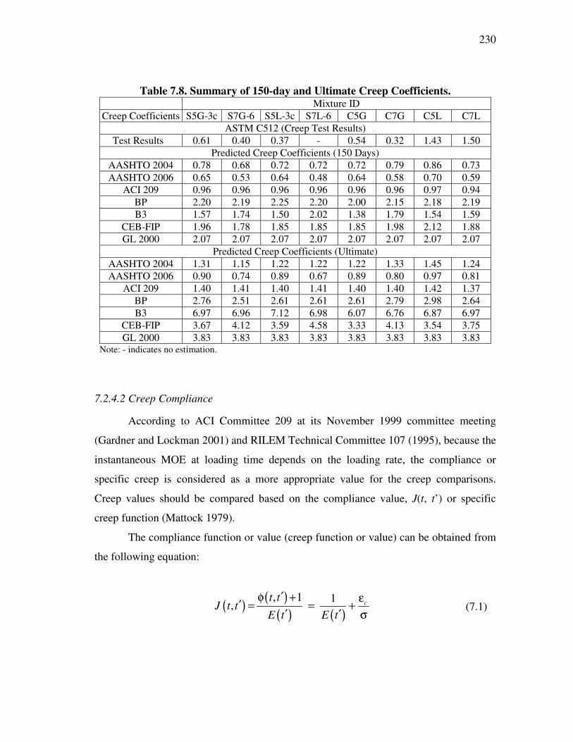
230

Table 7.8. Summary of 150-day and Ultimate Creep Coefficients. Mixture ID

Creep Coefficients� S5G-3c S7G-6 S5L-3c S7L-6 C5G C7G C5L C7L ASTM C512 (Creep Test Results)�

Test Results 0.61 0.40 0.37 - 0.54 0.32 1.43 1.50 Predicted Creep Coefficients (150 Days)�

AASHTO 2004 0.78 0.68 0.72 0.72 0.72 0.79 0.86 0.73 AASHTO 2006� 0.65 0.53 0.64 0.48 0.64 0.58 0.70 0.59

ACI 209� 0.96 0.96 0.96 0.96 0.96 0.96 0.97 0.94 BP� 2.20 2.19 2.25 2.20 2.00 2.15 2.18 2.19 B3� 1.57 1.74 1.50 2.02 1.38 1.79 1.54 1.59

CEB-FIP� 1.96 1.78 1.85 1.85 1.85 1.98 2.12 1.88 GL 2000 2.07 2.07 2.07 2.07 2.07 2.07 2.07 2.07

Predicted Creep Coefficients (Ultimate)�AASHTO 2004 1.31 1.15 1.22 1.22 1.22 1.33 1.45 1.24 AASHTO 2006� 0.90� 0.74� 0.89� 0.67� 0.89� 0.80� 0.97� 0.81�

ACI 209� 1.40� 1.41� 1.40� 1.41� 1.40� 1.40� 1.42� 1.37�BP� 2.76� 2.51� 2.61� 2.61� 2.61� 2.79� 2.98� 2.64�B3� 6.97� 6.96� 7.12� 6.98� 6.07� 6.76� 6.87� 6.97�

CEB-FIP� 3.67� 4.12� 3.59� 4.58� 3.33� 4.13� 3.54� 3.75�GL 2000 3.83 3.83 3.83 3.83 3.83 3.83 3.83 3.83

Note: - indicates no estimation.

7.2.4.2 Creep Compliance

According to ACI Committee 209 at its November 1999 committee meeting

(Gardner and Lockman 2001) and RILEM Technical Committee 107 (1995), because the

instantaneous MOE at loading time depends on the loading rate, the compliance or

specific creep is considered as a more appropriate value for the creep comparisons.

Creep values should be compared based on the compliance value, J(t, t’ ) or specific

creep function (Mattock 1979).

The compliance function or value (creep function or value) can be obtained from

the following equation:

( ) ( )

( ) ( ), 1 1

, ct tJ t t

E t E t

′φ + ε′ = = +′ ′ σ

(7.1)

231

where φ (t, t’ ) is the creep coefficient at time t, and E(t’ ) is the MOE at time, t’ , εc is the

creep strain, σ is the constant stress, and εc/σ is the specific creep function. The

compliance values for different concrete mixtures are compared in this study.

The errors of the prediction model can be estimated based on charts of measured

versus predicted values. Figure 7.21 shows measured and predicted creep compliance to

evaluate the accuracy of each model for estimating creep. In general, the prediction

formulas overestimate measured creep. The 2004 AASHTO LRFD slightly

overestimated measured creep except for the limestone CC mixtures. The 2004 and 2006

AASHTO LRFD equations are purposely developed to provide simple equations for the

engineers. It should be noted that the AASHTO equations predict creep without

consideration of the characteristics of mixture proportions. When the SCC mixture

proportions are considered, the 2006 AASHTO LRFD prediction equation is appropriate

for the estimation of creep of the SCC and CC mixtures. The predicted creep values are

within ±50 percent error, which indicates that the accuracy of the model is acceptable

according to the AASHTO LRFD Specifications (2006). The AASHTO LRFD

Specifications also recommends the CEB-FIP and ACI 209 models. These models and

the 2004 AASHTO LRFD also predict creep within ±50 percent error.

The BP, B3, and ACI 209 models consider the various aspects of mechanical

properties and characteristics of mixture proportions impact on the creep. The mixture

proportions are different between the CC and SCC, resulting in a different level for

accuracy of each prediction model. The specific model sensitively considers the internal

factors, such as mixture proportions and mechanical properties, resulting in either high

level of accuracy or wide range of error magnitudes. Among these models, except for the

2004 and 2006 AASHTO LRFD, the BP model overestimates creep with a high degree

of scatter, which indicates the high sensitiveness of internal parameters. In general, these

models still overestimate creep for SCC when the mixture proportions are considered.

Therefore, including information about the high paste volume and low coarse aggregate

volume of SCC does not increase accuracy when using these creep prediction

expressions.

232

(a) AASHTO LRFD 2004 (b) AASHTO LRFD 2006

(c) ACI 209 model (d) CEB-FIP model

Figure 7.21. Predicted J(t, t’) and Measured J(t, t’).

0 0.2 0.4 0.6 0.8 1

0 40 80 120

0

0.2

0.4

0.6

0.8

1

0

40

80

120

Measured J (t, t') (x 10-6 /psi)

Pred

icte

d J

(t, t

') (x

10-6

/psi

)Measured J (t, t') (x 10-6 /MPa)

Predicted J (t, t') (x 10-6 /M

Pa)

AASHTO LRFD 2004

0 0.2 0.4 0.6 0.8 1

0 40 80 120

0

0.2

0.4

0.6

0.8

1

0

40

80

120

Measured J (t, t') (x 10-6 /psi)

Pred

icte

d J

(t, t

') (x

10-6

/psi

)

Measured J (t, t') (x 10-6 /MPa)Predicted J (t, t') (x 10

-6 /MPa)

AASHTO LRFD 2006

50% Error

-50% Error

0 0.2 0.4 0.6 0.8 1

0 40 80 120

0

0.2

0.4

0.6

0.8

1

0

40

80

120

Measured J (t, t') (x 10-6 /psi)

Pred

icte

d J

(t, t

') (x

10-6

/psi

)

Measured J (t, t') (x 10-6 /MPa)

Predicted J (t, t') (x 10-6 /M

Pa)

ACI 209 Model

0 0.2 0.4 0.6 0.8 1

0 40 80 120

0

0.2

0.4

0.6

0.8

1

0

40

80

120

Measured J (t, t') (x 10-6 /psi)

Pred

icte

d J

(t, t

') (x

10-6

/psi

)Measured J (t, t') (x 10-6 /MPa)

Predicted J (t, t') (x 10-6 /M

Pa)

CEB-FIP Model

SCC River GravelSCC LimestoneCC River GravelCC Limestone

233

(e) BP model (f) B3 model

(g) GL 2000 model

Figure 7.21. (Continued)

The equations recommended by CEB-FIP, ACI 209, and 2004 AASHTO LRFD

gave conservative prediction estimates of the measured creep strains. For the limestone

CC mixtures, the ACI 209, CEB-FIP, and 2004 AASHTO LRFD models seem to be

appropriate compared with the other models. The BP, B3, and GL 2000 models were

conservative in estimating creep strains for all mixtures. Because these prediction

0 0.2 0.4 0.6 0.8 1

0 40 80 120

0

0.2

0.4

0.6

0.8

1

0

40

80

120

Measured J (t, t') (x 10-6 /psi)

Pred

icte

d J

(t, t

') (x

10-6

/psi

)Measured J (t, t') (x 10-6 /MPa)

Predicted J (t, t') (x 10-6 /M

Pa)

BP Model

0 0.2 0.4 0.6 0.8 1

0 40 80 120

0

0.2

0.4

0.6

0.8

1

0

40

80

120

Measured J (t, t') (x 10-6 /psi)

Pred

icte

d J

(t, t

') (x

10-6

/psi

)

Measured J (t, t') (x 10-6 /MPa)Predicted J (t, t') (x 10

-6 /MPa)

B3 Model

0 0.2 0.4 0.6 0.8 1

0 40 80 120

0

0.2

0.4

0.6

0.8

1

0

40

80

120

Measured J (t, t') (x 10-6 /psi)

Pred

icte

d J

(t, t

') (x

10-6

/psi

)

Measured J (t, t') (x 10-6 /MPa)

Predicted J (t, t') (x 10-6 /M

Pa)

GL 2000 Model

SCC River GravelSCC LimestoneCC River GravelCC Limestone

234

equations were developed based on normal strength CC mixtures, these prediction

equations likely need to be calibrated for the higher strength the SCC mixtures.

7.2.5 Summary

By analysis and comparison of test results and prediction models for SCC and

CC mixtures, this research investigated whether existing prediction models for creep of

CC are applicable to SCC mixtures. For SCC and CC, many factors can affect creep.

Because the external factors were consistent during this test, the difference in creep is a

result of constituent material type and proportions in the mixtures. The amount of

cement paste, the stiffness of aggregate, and early gain of compressive strength from

each mixture of SCC and CC were mainly investigated as affecting factors on creep.

Based on the above test results, conclusions are drawn as following,

1) The river gravel SCC mixtures show similar creep to the river gravel CC

mixtures with the same 16-hour target compressive strengths. Although the

16-hour compressive strengths of the SCC and CC mixtures were almost the

same, the creep of the limestone CC was higher than that of the limestone

SCC. In addition, CC samples with lower compressive strengths exhibited

higher creep. The effect of the 16-hour compressive strength was found to not

be a significant factor affecting creep.

2) Because the stiffness of the river gravel is higher than that of limestone, river

gravel mixtures had lower creep compared to the limestone mixtures, as

expected. The MOE provides an indication of the stiffness of aggregate.

According to the mechanical property testing, the MOE of concrete with the

limestone coarse aggregate is lower than the MOE for concrete with the river

gravel. The effect of coarse aggregate type was clearly observed in the CC

mixtures. However, the effect of the coarse aggregate types was not

significant for the SCC mixtures.

3) The perceived impact of high paste volume and low coarse aggregate volume

on the creep of SCC seems to be unfounded for the mixtures evaluated in this

235

research. However, the SCC mixtures exhibited higher strengths than the CC

mixtures, which could account for the similar or lower creep values.

4) The 2006 AASHTO LRFD Specifications allows prediction models to have

±50 percent error in creep prediction. The 2004 and 2006 AASHTO LRFD

models, the ACI 209 model, and the CEB-FIP model provide fairly good

predictions for the creep of both CC and SCC mixtures. Because the 2006

AASHTO LRFD model was calibrated for high-strength concrete with low

w/c, the prediction model seems to better predict CC and SCC mixtures

evaluated in this study.

5) Prediction models are available that consider the compressive strength, MOE

of aggregate, and mixture proportions. The BP, B3, and GL 2000 prediction

models are based on data from normal strength CC and overestimated the

creep for the SCC and CC mixtures evaluated in this research by more than

50 percent.

7.3 DURABILITY

Test results of permeability, diffusivity, and freezing and thawing resistance of

the SCC are discussed in following sections.

7.3.1 Freezing and Thawing Resistance

This section will present the results of freezing and thawing resistances of the

SCC and CC mixtures. Relative dynamic modulus can represent the damage due to

freezing and thawing.

Figure 7.22 shows relative dynamic modulus versus number of cycles for the 5

ksi (34 MPa) SCC mixtures, 7 ksi (48 MPa) SCC mixtures, and CC mixtures. For the 5

ksi (34 MPa) SCC mixtures, relative dynamic modulus was significantly reduced to

about 40 percent before approximately 150 cycles, indicating the air void size and

distribution are not sufficient to resist the freezing and thawing damage. For the CC

mixtures, the 5 ksi (34 MPa) CC mixtures have relatively low resistance to freezing and

thawing compared to the 7 ksi (48 MPa) CC mixtures. Because the mixtures have similar

236

air contents (approximately 1.2 percent with a standard deviation of 0.23 percent), the

total volume of air content does not seem to be significant factor.

(a) 5 ksi (34 MPa) SCC Mixtures

(b) 7 ksi (48 MPa) SCC Mixtures

Figure 7.22. Relative Dynamic Modulus versus Number of Cycles.

0

20

40

60

80

100

0 50 100 150 200 250 300

S5R-3aS5R-3bS5R-3cS5L-3aS5L-3bS5L-3c

Rel

ativ

e D

ynam

ic M

odul

us (%

)

Number of Cycles

0

20

40

60

80

100

0 50 100 150 200 250 300

S7R-4S7R-5S7R-6S7L-4S7L-5S7L-6

Rel

ativ

e D

ynam

ic M

odul

us (%

)

Number of Cycles

237

(c) CC Mixtures

Figure 7.22. (Continued)

Tables 7.9 through 7.11 show the summary of test results for all the mixtures.

The test results show the durability factor (DF) of each sample.

The durability factor DF can then be recalled as follows:

P N

DFM×= (7.2)

where P is the relative dynamic MOE at N cycles (%), N is the number of cycles at

which P reaches the specified minimum value for discontinuing the test or the specified

number of cycles at which the exposure is to be terminated, whichever is less, and M is

the specified number of cycles at which the exposure is to be terminated, which is equal

to 300 cycles.

0

20

40

60

80

100

0 50 100 150 200 250 300

C5R

C7R

C5L

C7LR

elat

ive

Dyn

amic

Mod

ulus

(%)

Number of Cycles

238

Table 7.9. DF of 5 ksi (34 MPa) SCC Mixtures. Mixture ID S5G-3a S5G-3b S5G-3c S5L-3a S5L-3b S5L-3c N (cycles) 121 101 96 85 82 82 110 85 101 130 165 100 133 133 175 114 115 114

P (%) 60 60 60 60 60 60 60 60 60 60 60 60 60 60 60 60 60 60 M (cycles) 300 300 300 300 300 300 300 300 300 300 300 300 300 300 300 300 300 300

DF 24.2

20.2

19.2

17.0

16.4

16.4

22.0

17.0

20.2

26.0

33.0

20.0

26.6

26.6

35.0

22.8

23.0

22.8

Average DF 21 17 20 26 29 23 Standard Deviation 2.6 0.4 2.5 6.5 4.9 0.1

Table 7.10. DF of 7 ksi (48 MPa) SCC Mixtures. Mixture ID S7G-4 S7G-5 S7G-6 S7L-4 S7L-5 S7L-6 N (cycles) 300 300 300 - 300 300 300 300 300 300 300 300 300 300 300 300 300 256

P (%) 100 100 100 - 100 100 78 97 97 98 100 93 85 83 86 67 70 60 M (cycles) 300 300 300 - 300 300 300 300 300 300 300 300 300 300 300 300 300 300

DF 100 100 100 - 100 100 78 97 97 98 100 93 85 83 86 67 70 51 Average DF 100 100 91 97 85 63

Standard Deviation 0 0 11 3.6 1.5 10.1

Note: - indicates that there is no test result.

Table 7.11. DF of CC Mixtures. Mixture ID C5G C7G C5L C7L N (cycles) 300 175 300 300 300 300 153 175 165 300 300 300

P (%) 100 60 100 100 100 100 60 60 60 60 100 100 M (cycles) 300 300 300 300 300 300 300 300 300 300 300 300

DF 100 35 100 100 100 100 31 35 33 60 100 100 Average 78 100 32.9 87

Standard Deviation 38 0 2.2 23.09

Test results show that the 5 ksi (34 MPa) SCC mixtures exhibit low DF after

approximately 110 cycles. There is no significant effect of aggregate type on DF for the

5 ksi (34 MPa) mixtures. For the 7 ksi (48MPa) mixtures, the river gravel mixtures have

higher DF than the limestone mixtures. For the CC mixtures, the 5 ksi (34 MPa)

limestone CC mixture shows the lowest DF values. For the CC mixtures, the 7 ksi (48

MPa) mixture has excellent freezing and thawing resistance.

According to Thomas (2007), the high volume replacement of fly ash in

cementitious material content can reduce the resistance to freezing and thawing. The 5

239

ksi (34 MPa) SCC mixtures have more than 32 percent by volume fly ash replacement.

Higher w/cm also affects the low resistance along with poor distribution of voids.

However, the 7 ksi (48 MPa) SCC mixtures containing approximately 20 percent

replacement did not exhibit high degradation from freezing and thawing. This could be

attributed to low w/cm.

7.3.2 Rapid Chloride Penetration Test

Figure 7.23 shows the rapid chloride resistance results for different CC and SCC

mixtures. In general, the SCC mixtures have higher chloride permeability at early ages

(7 days) compared to the CC mixtures. However, at later ages the SCC mixtures have

lower permeability compared to the 5 ksi (34 MPa) CC mixtures for both aggregate

types. For the 7 ksi (48 MPa) mixtures, SCC and CC have similar chloride ion

permeability values at later ages (approximately 28 days).

Tables 7.12 through 7.14 show the classification from ASTM C1202 for the

permeability of each sample at the day of testing. When the classification is considered,

the SCC mixtures have moderate permeability and the CC mixtures have low or

moderate permeability values. At 56 days the SCC mixtures have very low permeability

and the CC mixtures have low permeability.

240

(a) 5 ksi (34 MPa) River Gravel (b) 5 ksi (34 MPa) Limestone

(c) 5 ksi (34 MPa) River Gravel (d) 5 ksi (34 MPa) Limestone

Figure 7.23. Charge Passed versus Time.

0

1000

2000

3000

4000

5000

0 20 40 60

S5G SeriesC5G

Cha

rge

Pass

ed (C

oulo

mbs

)

Time After Casting (Day)

0

1000

2000

3000

4000

5000

0 20 40 60

S5L SeriesC5L

Cha

rge

Pass

ed (C

oulo

mbs

)

Time After Casting (Day)

0

1000

2000

3000

4000

5000

0 20 40 60

S7G SeriesC7G

Cha

rge

Pass

ed (C

oulo

mbs

)

Time After Casting (Day)

0

1000

2000

3000

4000

5000

0 20 40 60

S7L SeriesC7L

Cha

rge

Pass

ed (C

oulo

mbs

)

Time After Casting (Day)

241

Table 7.12. Permeability Class of River Gravel SCC Mixtures. Age of

Test�Mixture ID

S5G-3a S5G-3b S5G-3c S7G-4 S7G-5 S7G-6 7 days M M M M M M M M M M M M M M M M M M

28 days VL VL VL VL VL VL VL L VL VL L L L VL VL L L L 56 days VL VL VL VL VL VL VL VL VL VL VL VL VL VL VL VL VL VL

Note: H = High, M = Moderate, VL = Very Low, L = Low.

Table 7.13. Permeability Class of Limestone SCC Mixtures. Age of

Test�Mixture ID

S5L-3a S5L-3b S5L-3c S7L-4 S7L-5 S7L-6 7 days M H M H H M H H - M M M M M M M M M

28 days VL VL VL L VL VL L L L L L L L L L L L L 56 days VL VL VL VL VL VL VL VL VL VL VL VL VL VL VL VL VL VL

Note: H = High, M = Moderate, VL = Very Low, L = Low, - indicates there is no test.

Table 7.14. Permeability Class of CC Mixtures. Age of

Test�Mixture ID

C5G C7G C5L C7L 7 days M L M L L L M M M L L L

28 days L L L VL VL VL M M M L L L 56 days L L L VL VL VL L M L L L L

Note: H = High, M = Moderate, VL = Very Low, L = Low.

7.3.3 Diffusion Coefficient

The diffusion coefficient is determined by measuring the chloride concentration

at different depth layers. The diffusion coefficients at 140 days were 1.21 × 10–9 and

2.39 × 10–9 in.2/s (0.78 × 10–12 and 1.54 × 10–12 m2/s) for 5 and 7 ksi (34 and 48 MPa)

river gravel SCC mixtures, respectively. The diffusion coefficients at 28 days were

estimated to be 2.53 × 10–9 and 4.40 × 10–9 in.2/s (1.63 × 10–12 and 2.84 × 10–12 m2/s) for

5 and 7 ksi (34 and 48 MPa) river gravel SCC mixtures, respectively. These values are

typical of CC with similar w/c. Tables 7.15 and 7.16 show the diffusion coefficients for

all mixtures. Figure 7.24 shows the plot of the predicted value by estimated average

diffusion coefficients versus and measured values. The estimated diffusion coefficients

of river gravel SCC mixtures seem to be significantly low indicating the fine capillary

242

porosity and homogeneity. Generally, the fly ash also reduced diffusion coefficients.

Similarly, SCC mixture had significantly low coefficient of chloride migration, which

seems to depend on the type of powder. The fly ash reduced significantly coefficient of

chloride migration (Zhu and Bartos 2003).

Table 7.15. Diffusion Coefficient of 5 ksi (34 MPa) River Gravel Mixtures.

Day Diffusion Coefficients

× 10−9 in2/s (× 10−12 m2/s)

Mixture ID

S5G-3a S5G-3b S5G-3c

140 days (Tested)

Values 0.92 (0.59)

0.68 (0.44)

17.1* (11)

0.67 (0.43)

1.55 (1.00)

0.98 (0.62)

1.50 (0.97)

0.33 (0.21)

3.07 (1.98)

Average 0.81 (0.52) 1.05 (0.68) 1.63 (1.05) Standard Deviation 0.17 (0.11) 0.45 (0.29) 1.38 (0.89)

28 days (Predicted)

Values 1.91 (1.23)

1.43 (0.92)

35.7* (23)

1.40 (0.90)

3.23 (2.08)

2.0 (1.29)

3.13 (2.02)

0.68 (0.44)

6.39 (4.12)

Average 1.68 (1.08) 2.20 (1.42) 3.40 (2.19) Standard Deviation 0.34 (0.22) 0.93 (0.60) 2.87 (1.85)

Note: * is the outlier.

Table 7.16. Diffusion Coefficient of 7 ksi (48 MPa) River Gravel Mixtures.

Day Diffusion Coefficients,

× 10−9 in.2/s (× 10−12 m2/s)

Mixture ID

S7G-4 S7G-5 S7G-6

140 days (Tested)

Values 1.38 (0.89)

1.40 (0.90)

6.65 (4.29)

1.58 (1.02)

3.32 (2.14)

3.12 (2.01)

1.81 (1.17)

1.49 (0.96)

0.76 (0.49)

Average 3.15 (2.03) 2.67 (1.72) 1.35 (0.87) Standard Deviation 3.04 (1.96) 0.95 (0.61) 0.54 (0.35)

28 days (Predicted)

Values 2.54 (1.64)

2.59 (1.67)

12.28 (7.92)

2.92 (1.88)

6.11 (3.94)

5.75 (3.71)

3.35 (2.16)

2.73 (1.76)

1.41 (0.91)

Average 5.80 (3.74) 4.94 (3.18) 2.50 (1.61) Standard Deviation 5.61 (3.62) 1.75 (1.13) 0.99 (0.64)

243

(a) 5 ksi (34 MPa) River Gravel SCC Mixture

(b) 7 ksi (48 MPa) River Gravel SCC Mixture

Figure 7.24. Predicted Chloride Concentration (Percent Mass) versus Measured

Values (140 Days).

0

0.4

0.8

1.2

1.6

0 0.1 0.2 0.3 0.4 0.5

Best-Fit CurveS5G-3a (Measured)S5G-3b (Measured)S5G-3c (Measured)

0 2 4 6 8 10 12

Chl

orid

e C

once

ntra

tion

% M

ass

Depth (in.)

Depth (mm)

D = 1.21x10-9 in.2/sec

(0.78x10-12 m2/sec )

At 140 Days

0

0.4

0.8

1.2

1.6

0 0.1 0.2 0.3 0.4 0.5

Best-Fit CurveS7G-4 (Measured)S7G-5 (Measured)S7G-6 (Measured)

0 2 4 6 8 10 12

Chl

orid

e C

once

ntra

tion

% M

ass

Depth (in.)

Depth (mm)

D = 2.39 x 10-9 in.2/sec

(1.54 x 10-12 m2/sec )

At 140 Days

244

7.3.4 Summary

Based on the experimental tests on the SCC and CC mixtures, the following

conclusions can be drawn:

1) The 5 ksi (34 MPa) 16-hour release strength SCC mixtures exhibit low

resistance to freezing and thawing. This could be a result of high paste

volume, higher w/cm, or poor void distribution.

2) The 7 ksi (48 MPa) 16-hour release strength SCC mixtures exhibited good

freezing and thawing resistance.

3) All SCC mixtures exhibited very low permeability compared to the CC

mixtures at later ages indicating a potential for high resistance to chloride ion

penetration.

4) After 140 days of ponding, the 5 ksi (34 MPa) and 7 ksi (48 MPa) 16-hour

release strength SCC mixtures have low diffusion coefficients. These values

are typical of CC mixtures with similar w/c.

245

CHAPTER VIII

RESULTS AND ANALYSIS OF FULL-SCALE TESTING AND

VALIDATION: FULL-SCALE SCC GIRDER-DECK SYSTEM

8.1 EARLY-AGE PROPERTIES AND FIELD OBSERVATION

For the first set of field tests, the fresh properties were assessed by researchers

from the University of Texas at Austin (Koehler and Fowler 2008). The University of

Texas group focused on assessing the workability and stability of the SCC mixture for

the precast girder. This section presents follow-up testing and a description of the early-

age characteristics of the SCC mixture for the precast girders. The full-scale girder test

program is described in Section 4.7 of this dissertation.

Generally, the passing ability of the SCC mixtures was excellent. When the auger

bucket containing the SCC mixture arrived at the placement bed, some segregation of

the aggregate was observed. This was due to the transportation of the SCC from the

mixer to the placement bed and resulted in a small area (1 ft × 0.5 ft [0.3 m × 0.1 m]) of

honeycombing, as shown Figure 8.1.

Figure 8.2 shows the overall surface condition of the girders containing the SCC

mixtures. The surface conditions were considered to be very good. Table 8.1 provides a

summary of the early-age characteristics of the mixtures used in the precast girders.

246

Figure 8.1. Localized Honeycombs on Surface of the SCC-R Mixture.

Figure 8.2. Representative Photos of Quality of Surface of Bottom Flange of SCC-L (Top) and CC-L (Bottom).

SCC-L

CC-L

0.5 ft. (0.1 m)

1 ft (0.3 m)

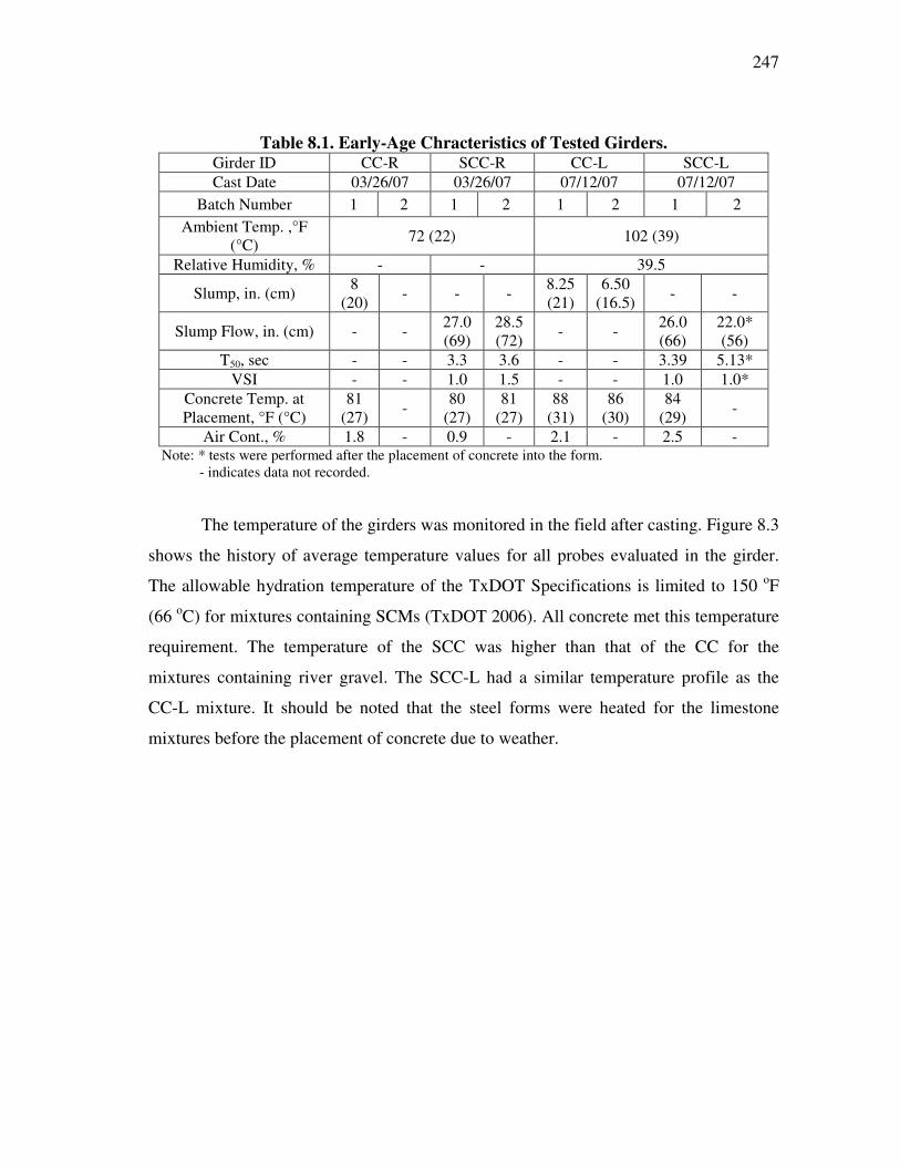
247

Table 8.1. Early-Age Chracteristics of Tested Girders. Girder ID CC-R SCC-R CC-L SCC-L Cast Date 03/26/07 03/26/07 07/12/07 07/12/07

Batch Number 1 2 1 2 1 2 1 2 Ambient Temp. ,°F

(°C) 72 (22) 102 (39)

Relative Humidity, % - - 39.5

Slump, in. (cm) 8 (20) - - - 8.25

(21) 6.50

(16.5) - -

Slump Flow, in. (cm) - - 27.0 (69)

28.5 (72) - - 26.0

(66) 22.0* (56)

T50, sec - - 3.3 3.6 - - 3.39 5.13* VSI - - 1.0 1.5 - - 1.0 1.0*

Concrete Temp. at Placement, °F (°C)

81 (27) - 80

(27) 81

(27) 88

(31) 86

(30) 84

(29) -

Air Cont., % 1.8 - 0.9 - 2.1 - 2.5 - Note: * tests were performed after the placement of concrete into the form. - indicates data not recorded.

The temperature of the girders was monitored in the field after casting. Figure 8.3

shows the history of average temperature values for all probes evaluated in the girder.

The allowable hydration temperature of the TxDOT Specifications is limited to 150 oF

(66 oC) for mixtures containing SCMs (TxDOT 2006). All concrete met this temperature

requirement. The temperature of the SCC was higher than that of the CC for the

mixtures containing river gravel. The SCC-L had a similar temperature profile as the

CC-L mixture. It should be noted that the steel forms were heated for the limestone

mixtures before the placement of concrete due to weather.

248

(a) CC-R and SCC-R (b) CC-L and SCC-L

Figure 8.3. History of Average Hydration Temperature.

Figure 8.4 shows the distribution of concrete temperature at the girder ends and

midspan when the average of temperature reached the maximum value at corresponding

girder section. The distribution of the concrete temperature was similar, with the

exception of the SCC-R girder, indicating the maturity values of the concretes are

similar. The north span of the SCC-R girder showed high temperatures over the cross-

section, indicating that the strength development could be higher than other regions.

Transfer length data at this area were shorter than the other ends. These results will be

presented and discussed in the following sections.

0.0 9.6 19.2 28.8

CC-R GirderSCC-R Girder

70

105

140

30

40

50A

vera

ge T

empe

ratu

re (o F)

Time after Casting (Hours)

Start Casting

Average T

emperature ( oC

)

70

105

140

0.0 9.6 19.2 28.8

CC-L GirderSCC-L Girder

30

40

50

Ave

rage

Tem

pera

ture

(o F)

Time after Casting (Hours)

Start Casting

Average T

emperature ( oC

)

249

(a) CC-R (b) SCC-R

(c) CC-R (d) SCC-R

Figure 8.4. Distribution of Temperature at the Girder End and Midspan Sections.

0

10

20

30

100 120 1400

200

400

600

40 50 60V

ertic

al D

ista

nce

from

B

otto

m F

ace

(in.

)

Concrete Temperature ( oF)

CC-R

Concrete Temperature ( oC)

Veertical D

istance from

the Bottom

of Face (mm

)

0

10

20

30

100 120 1400

200

400

600

40 50 60

Concrete Temperature ( oF)

SCC-R

Concrete Temperature ( oC)

Ver

tical

Dis

tanc

e fr

om

Bot

tom

Fac

e (i

n.)

Veertical D

istance from

the Bottom

of Face (mm

)

0

10

20

30

100 120 1400

200

400

600

40 50 60

Concrete Temperature ( oF)

CC-L

Concrete Temperature ( oC)

Ver

tical

Dis

tanc

e fr

om

Bot

tom

Fac

e (i

n.)

Veertical D

istance from

the Bottom

of Face (mm

)

0

10

20

30

100 120 1400

200

400

600

40 50 60

Concrete Temperature ( oF)

SCC-L

Concrete Temperature ( oC)

Ver

tical

Dis

tanc

e fr

om

Bot

tom

Fac

e (i

n.)

Veertical D

istance from

the Bottom

of Face (mm

)

Midspan North Span South Span

250

8.2 MATERIAL MECHANICAL PROPERTIES

Samples were cast to assess the mechanical properties of the concrete used for

the girders. Cylinders (4 in. × 8 in. [102 mm × 203 mm]) were used to assess

compressive strength, MOE, and STS of the CC and SCC mixtures. MOR was

determined using 6 in. × 6 in. × 20 in. (152 mm × 152 mm × 508 mm) prism specimens.

For the 16-hour tests, a sure-cure system was used to match the conditions of the actual

beams. Additional cylinders were also cast and placed adjacent to the girders for testing.

Except for the 16-hour tests, all mechanical tests were performed at HBSML.

8.2.1 Compressive Strength Development

After 16 hours, all the samples were stored in a constant temperature and

humidity room (>98 percent RH and 72 ± 2 oF [22 ± 1 oC]). To investigate strength

development, compressive strength was measured at 16 hours and 7, 28, 56, and 91 days.

Table 8.2 shows the test results of the average compressive strength of all mixtures at 16

hours and at approximately the time of release. The target compressive strength was 5

ksi (34 MPa) at 16 hours. All the sure-cure samples exceeded the 16-hour target

strength. Several of the samples placed next to the girders (i.e., the samples not matching

the temperature profile of the girder) did not meet the target 16-hour strength. However,

the sure-cure samples better represent the actual strength of the girder concrete. As such,

the strands were released when the sure-cure samples indicated sufficient strength.

Table 8.2. Average Compressive Strength at 16 hours and Release of Girders. Curing Method Next to Girder Sure-Cure Next to Girder Sure-Cure

Girder ID CC-R SCC-R CC-L SCC-L CC-L SCC-L CC-R SCC-R

cf ′@16 hour, psi (MPa) 4933 (34)

4771 (33)

4813 (33)

6056 (42)

5310 (37)

6603 (46)

5080 (35)

5714 (39)

cf ′@ Release, psi (MPa) - - 5738 (39)

6712 (46)

5614 (37)

7200 (50)

6360 (44)

6510 (45)

Results from the tests are shown in Figure 8.5. The strength development of the

SCC mixture was significantly different than the CC mixture at later ages. The

compressive strength development of SCC-R and SCC-L is fairly similar. The

251

compressive strength development of CC-R and CC-L is also similar. However, at 91

days, the compressive strength of SCC-R and SCC-L was approximately 30 percent

higher than that of CC-R and CC-L mixtures. Even though the CC mixtures have slightly

lower w/c than SCC mixtures, the strength gain of CC and SCC mixtures are

significantly different at later ages. This can be attributed to the contribution of fly ash

and high paste volume.

Figure 8.5. Compressive Strength Development of Girder.

8.2.2 Modulus of Elasticity

MOE was measured at 7, 28, 56, and 91 days. Figure 8.6 shows the MOE of all

girders with respect to compressive strength. Based on the assumptions Κ1 = 1.0 and wc =

149 lb/ft3 (2387 kg/m3), the current AASHTO (2006) prediction curve (Equation 2.2)

follows the general trend of the MOE of the CC-L mixtures shown in Figure 8.6. As

shown in Figure 8.7, most data from the CC-R and SCC-R mixtures fall within the 20

percent error range. The data of both CC-L and SCC-L mixtures fall within the 20

percent error range.

0

4000

8000

12,000

16,000

0 20 40 60 80 100

CC-RSCC-RCC-LSCC-L

0

20

40

60

80

100

Com

pres

sive

Str

engt

h (p

si)

Time After Casting (Days)

Com

pressive Strength (MPa)

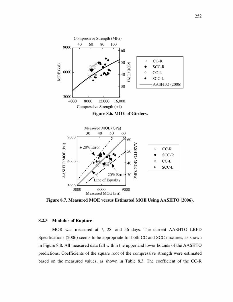
252

Figure 8.6. MOE of Girders.

Figure 8.7. Measured MOE versus Estimated MOE Using AASHTO (2006).

8.2.3 Modulus of Rupture

MOR was measured at 7, 28, and 56 days. The current AASHTO LRFD

Specifications (2006) seems to be appropriate for both CC and SCC mixtures, as shown

in Figure 8.8. All measured data fall within the upper and lower bounds of the AASHTO

predictions. Coefficients of the square root of the compressive strength were estimated

based on the measured values, as shown in Table 8.3. The coefficient of the CC-R

3000

6000

9000

4000 8000 12,000 16,000

CC-RSCC-RCC-LSCC-LAASHTO (2006)30

40

50

60

40 60 80 100

MO

E (k

si)

Compressive Strength (psi)

Compressive Strength (MPa)

MO

E (G

Pa)

3000

6000

9000

30

40

50

60

3000 6000 9000

30 40 50 60

CC-RSCC-R

CC-L

SCC-L

AA

SHT

O M

OE

(ksi

)

Measured MOE (ksi)

Line of Equality

+ 20% Error

- 20% Error

Measured MOE (GPa)

AA

SHT

O M

OE

(GPa)

253

mixture is slightly higher than that of the SCC-R mixture, indicating lower MOR of the

SCC-R mixture. The CC-L and SCC-L mixtures have similar coefficients for MOR.

Figure 8.8. MOR of Girders.

Table 8.3. Coefficients of MOR. Measured Value / cf ′ (psi) CC-R SCC-R CC-L SCC-L

Mean Value 9.4 9.1 10.0 10.0 Standard Deviation 1.1 0.9 0.7 0.8

Upper Bound (AASHTO) 11.7 Lower Bound (AASHTO) 7.6

8.2.4 Splitting Tensile Strength

STS was measured at 7, 28, and 56 days. The current AASHTO (2006)

prediction equation for STS underestimates the experimental results for both the CC and

SCC mixtures used in the girders as shown in Figure 8.9. The SCC-R and SCC-L

mixtures have higher strengths resulting in higher STS. As shown in Figure 8.10, STS

estimated by the AASHTO (2006) equation is generally lower than the measured STS of

SCC mixtures: the majority of SCC data fall within the 30 percent error range. As such,

the AASHTO (2006) gives a reasonable lower bound estimate of the STS for the SCC

mixtures.

400

600

800

1000

1200

1400

4000 8000 12,000 16,000

CC-RSCC-RCC-LSCC-LAASHTO (2006)Lower Limit

AASHTO (2006)Upper Limit

40 60 80 100

4

6

8

MO

R (p

si)

Compressive Strength (psi)

Compressive Strength (MPa)

MO

R (M

Pa)

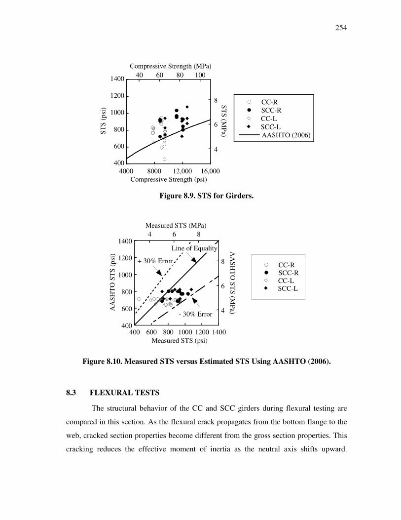
254

Figure 8.9. STS for Girders.

Figure 8.10. Measured STS versus Estimated STS Using AASHTO (2006).

8.3 FLEXURAL TESTS

The structural behavior of the CC and SCC girders during flexural testing are

compared in this section. As the flexural crack propagates from the bottom flange to the

web, cracked section properties become different from the gross section properties. This

cracking reduces the effective moment of inertia as the neutral axis shifts upward.

400

600

800

1000

1200

1400

4000 8000 12,000 16,000

CC-RSCC-RCC-LSCC-LAASHTO (2006)

40 60 80 100

4

6

8

Compressive Strength (psi)ST

S (MPa)

Compressive Strength (MPa)

STS

(psi

)

400

600

800

1000

1200

1400

4

6

8

400 600 800 1000 1200 1400

4 6 8

CC-RSCC-RCC-LSCC-L

AA

SHT

O S

TS

(psi

)

Measured STS (psi)

Line of Equality

+ 30% Error

- 30% Error

Measured STS (MPa)

AA

SHT

O ST

S (MPa)

255

Because the contribution of the deck concrete for compression becomes dominant, the

bonds in the bottom flange and uncracked sections of the girder contribute to tension.

The local bond performance should be evaluated to compare CC and SCC girder

performance.

8.3.1 Observations

8.3.1.1 Cracking Development

Generally, the progression of flexural cracking and maximum crack widths is

similar for all the tests. The cracking load and measured crack widths are summarized in

Table 8.4. The maximum crack width was measured at the extreme tension fiber of the

bottom flange.

For all the girders, all the first cracking occurred at approximately 70 kip (311

kN) along with approximately the maximum crack width of 0.01 in. (0.3 mm). The

flexural cracks propagating into the deck were observed at approximately 110 kip (490

kN). Observed maximum crack width at the nominal condition was approximately 0.06

in. (1.5 mm) for all the girders.

Table 8.4. Cracking Loads and Crack Widths.

First Cracking Flexural Cracking on Top Flange

Flexural Cracking into Deck Final Reading

Location Web Bottom Flange

Top Flange

Bottom Flange Deck Bottom

Flange Final Bottom Flange

Values Load, kip (kN)

Crack Width, in.(mm)

Load, kip (kN)

Crack Width, in.(mm)

Load, kip (kN)

Crack Width, in.(mm)

Load, kip

(kN)

Crack Width, in.(mm)

CC-R 60-80 (270-360)

0.01 (0.3)

100 (445)

0.02 (0.6)

110 (490)

0.05 (1.25)

127 (565)

0.05 (1.25)

SCC-R 70 (311)

0.004 (0.1)

100 (445)

0.01 (0.3)

110 (489)

0.04 (1.0)

126 (560)

0.06 (1.5)

CC-L 70 (311)

0.01 (0.3)

90 (400)

0.03 (0.8)

100 (445)

0.02 (0.5)

125 (556)

0.06 (1.5)

SCC-L 70 (311)

0.01 (0.2)

90 (400)

0.2 (0.4)

110 (489)

0.05 (1.25)

125 (556)

0.06 (1.5)

Note: CC-R girder had the first cracking during the load increments from 70 to 80 kip (270 to 360 kN).

256

8.3.1.2 Cracks on Midspan

While the overall structural performance of the girders was similar, some

differences were observed. The SCC-L girder showed slightly more cracks than the CC-

L girder. However, overall behavior was almost identical. The flexural cracks at nominal

conditions are shown in Figure 8.11. Typical flexural cracks propagating through the

deck were observed.

(a) CC-R (b) SCC-R

(c) CC-L (d) SCC-L

Figure 8.11. Crack Patterns of the Girders.

The final crack diagrams for all flexural tests are shown in Figure 8.12. Only the

cracked regions of the midspans are shown. In general, the SCC girders exhibited more

cracks than the CC girders. In the SCC-R and SCC-L girders more cracks were

distributed along the span compared with the CC-R and CC-L girders. More small

cracks with small crack widths were observed in the SCC-R and SCC-L girders.

midspan

257

1 ft (0.3 m)

(a) CC-R

1 ft (0.3 m)

(b) SCC-R

1 ft (0.3 m)

(c) CC-L

1 ft (0.3 m)

(d) SCC-L

Figure 8.12. Crack Diagram at the Ultimate State.

, typ.

, typ.

, typ.

, typ.

258

8.3.2 Moment-Curvature (Load-Deflection)

Table 8.5 shows the measured material properties of the concrete for the deck

and girder. The table also shows the measured effective stresses of the strands after

losses, fpe, on the structural test date.

Table 8.5. Measured Properties of Materials. Materials f’ c, psi (MPa) CC-R SCC-R CC-L SCC-L

Girder

Average, psi (MPa)

9620 (66.3)

12,800 (88.3)

10,100 (69.6)

13,700 (94.5)

Std. Dev., psi (MPa)

251 (1.73)

256 (1.77)

665 (4.59)

422 (2.91)

Cast-In-Place Concrete (Deck)

Average, psi (MPa)

6170 (42.5)

7530 (51.9)

5450 (37.2)

5280 (36.4)

Std. Dev., psi (MPa)

227 (1.57)

143 (0.99)

563 (3.88)

393 (2.71)

Strands fpe, ksi (MPa) 201 (1390)

200 (1380)

201 (1450)

204 (1410)

The CC and SCC girders exhibited a similar response in terms of moment-

curvature. Figure 8.13 shows the measured and the predicted moment-curvature of each

girder. Measured properties of concrete and strands with effective stress of strands after

losses were also used to compute the predicted moment-curvature relationship using the

Response 2000 program, which is a sectional analysis tool implementing the Modified

Compression Field Theory (Bentz 2000). The CC-R and SCC-R girders had similar

predicted and measured responses in terms of moment-curvature, as shown in Figure

8.13 (a). The CC-L and SCC-L girders also had similar predicted and measured

responses in terms of moment-curvature, as shown in Figure 8.13 (b).

259

(a) CC-R and SCC-R

(b) CC-L and SCC-L

Figure 8.13. Moment versus Curvature Relationship.

Figure 8.14 shows the load-deflection for the girders loaded at the center. The

girders had almost identical profiles. The CC-L and SCC-L girders had more deflection

than the CC-R and SCC-R girders. This can be attributed to increased cracking (which is

described in Section 8.3.1) of the limestone SCC girders resulting in a reduction of

stiffness (Icr).

0

350

700

1050

1400

0.0000 0.0002 0.0004 0.0006 0.0008

CC-R (Measured)

SCC-R (Measured)

CC-R (Predicted)

SCC-R (Predicted)

0

400

800

1200

1600

0.00000 0.00001 0.00002 0.00003M

omen

t (ki

p-ft

)

Curvature (rad/in.)

Mom

ent (kN-m

)

Curvature (rad/mm)

0

350

700

1050

1400

0.0000 0.0002 0.0004 0.0006 0.0008

SCC-L (Measured)

CC-L (Measured)

SCC-L (Predicted)

CC-L (Predicted)

0

400

800

1200

1600

0.00000 0.00001 0.00002 0.00003

Mom

ent (

kip-

ft)

Curvature (rad/in.)

Curvature (rad/mm)

Mom

ent (kN-m

)

260

(a) CC-R and SCC-R

(b) CC-L and SCC-L

Figure 8.14. Load-Displacement.

As shown in Figure 8.15, the strain in the bottom fiber abruptly changes

indicating the occurrence of flexural cracking. The locations indicated are used to

estimate the cracking moment.

-140

-105

-70

-35

00 1 2 3 4 5 6 7

CC-R

SCC-R

0

200

400

6000 40 80 120 160

Deflection (in.)

App

lied

Loa

d (k

ips)

Applied L

oad (kN)

Deflection (mm)

-140

-105

-70

-35

00 1 2 3 4 5 6 7

CC-L

SCC-L

0

200

400

6000 40 80 120 160

Deflection (in.)

App

lied

Load

(kN

)

Deflection (mm)

App

lied

Loa

d (k

ips)

261

(a) CC-R and SCC-R (b) CC-L and SCC-L

Figure 8.15. Cracking Occurrence of the Bottom Fiber of Girder.

Table 8.6 summarizes the flexural test results. The first cracking of the CC-R

girder exhibited a moment corresponding to a MOR of 13 cf ′ psi (1.08 cf ′ MPa),

which is 11 percent higher than upper bound prediction of AASHTO (2006). The SCC-R

girder exhibited a moment corresponding to 10.6 cf ′ psi (0.88 cf ′ MPa). The CC-L

girder had a first cracking moment corresponding to 9.56 cf ′ psi (0.79 cf ′ MPa). The

SCC-L girder had the lowest first cracking moment corresponding to 7.33 cf ′ psi (0.61

cf ′ MPa), which is 4 percent lower than the lower limit of AASHTO (2006). The

measured nominal moment of all the girders was an average of 1245 kip-ft (1688 kN-m).

The nominal moment values are predicted within +15 percent error. The cracking

moments of CC-R and SCC-R girders were slightly underestimated, while the cracking

moments of CC-L and SCC-L girders were slightly overestimated. This can be attributed

to the low MOR of limestone mixtures. Reduced cracking moments were also observed

in SCC girders. This result was also shown in the MOR tests described in Chapter V.

0

350

700

1050

1400

0.000 0.002 0.004 0.006

CC-RSCC-R

0

400

800

1200

1600

0.00 0.05 0.10 0.15

CC-R

SCC-RMom

ent (

kip-

ft) M

oment (kN

-m)

Crack Width (mm)

Crack Width (in.)

0

350

700

1050

1400

0.000 0.002 0.004 0.006

CC-LSCC-L

0.00 0.05 0.10 0.15

0

400

800

1200

1600

Mom

ent (

kip-

ft)

CC-L

SCC-L

Mom

ent (kN-m

)Crack Width (mm)

Crack Width (in.)

262

Table 8.6 shows that the SCC-L girder had approximately 15 percent higher maximum

displacement than the CC-L girder.

Table 8.6. Summary of Flexural Test Results. Girder ID CC-R SCC-R CC-L SCC-L

Measured Nominal Moment, kip-ft (kN-m)

1239 (1680)

1258 (1706)

1230 (1668)

1254 (1700)

Predicted Nominal Moment, kip-ft (kN-m)

1129 (1531)

1135 (1539)

1130 (1532)

1122 (1521)

Measured Cracking Moment, kip-ft (kN-m)

750 (1017)

720 (976)

650 (881)

625 (847)

Predicted Cracking Moment, kip-ft (kN-m)

635 (861)

667 (904)

663 (899)

721 (977)

Coefficient, α of the MOR at

Cracking (α 'cf ), psi (MPa)

13.0 (1.08)

10.6 (0.88)

9.56 (0.79)

7.33 (0.61)

Max. Displacement at Nominal Moment, in. (mm)

5.59 (142)

5.72 (145)

5.95 (151)

6.87 (175)

At nominal conditions, the overall behavior at the girders was governed by the

capacity of the CIP concrete deck. As shown in Figure 8.16, the strains at the top fiber in

the constant moment region for all composite deck systems reached nominal conditions,

in excess of 3000 microstrain at the top fiber. As shown in Figure 8.16, at least three

strain gages indicated the nominal conditions of over 3000 microstrain. This figure also

shows that specific strain gage exceeded 3000 microstrain along with the schematic

location of strain gages on the top fiber. Detailed locations of individual strain gages are

described in Figure 4.23. Some strain gages adjacent to loading points indicated lower

values than 3000 microstrain. This might be attributed to the disturbed strains due to the

stress concentration of the loading points.

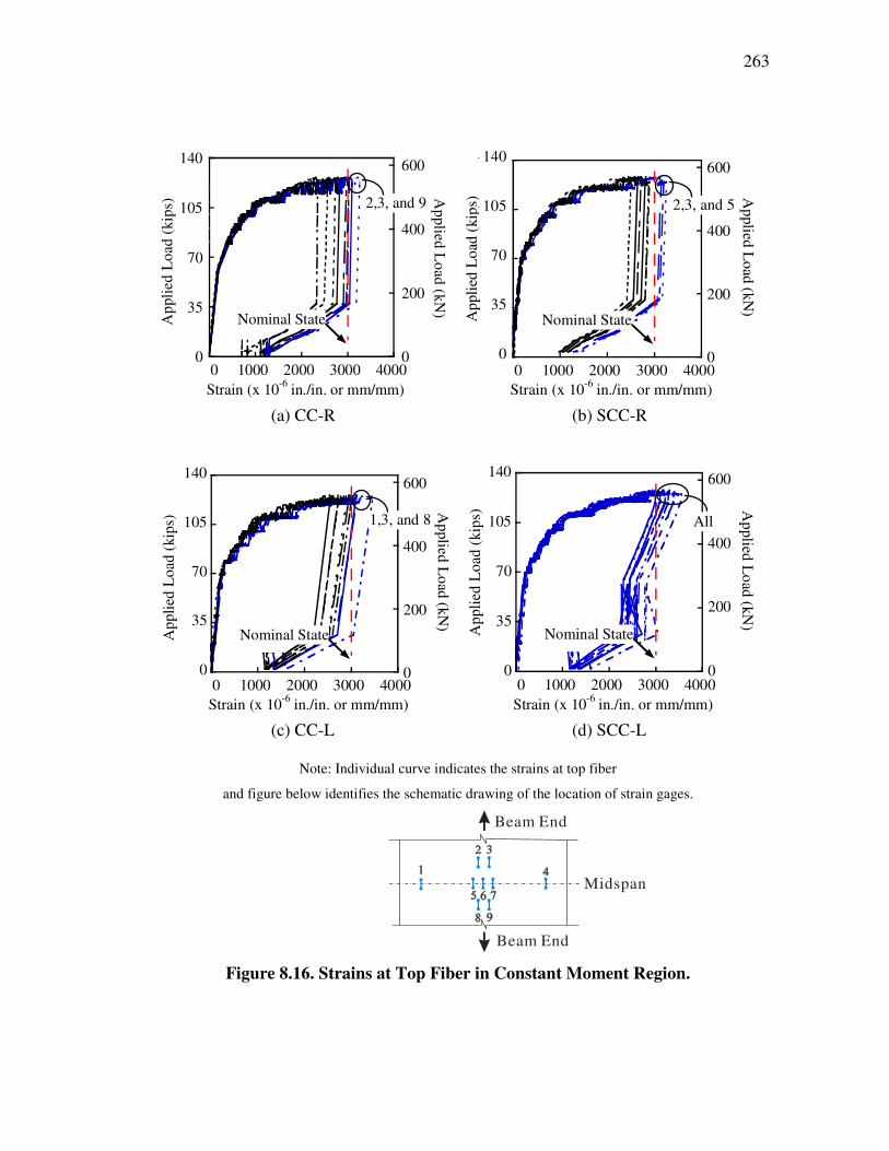
263

(a) CC-R (b) SCC-R

(c) CC-L (d) SCC-L

Note: Individual curve indicates the strains at top fiber

and figure below identifies the schematic drawing of the location of strain gages.

Midspan

Beam End

Beam End

Figure 8.16. Strains at Top Fiber in Constant Moment Region.

140

105

70

35

0 0

200

400

600A

pplie

d L

oad

(kip

s)

Nominal State

Strain (x 10-6 in./in. or mm/mm)

Applied L

oad (kN)

0 1000 2000 3000 4000

2,3, and 9

-140

-105

-70

-35

0

600

400

200

0

App

lied

Loa

d (k

ips)

Nominal State

Strain (x 10-6 in./in. or mm/mm)

Applied L

oad (kN)

2,3, and 5

0 1000 2000 3000 4000

140

105

70

35

0 0

200

400

600

App

lied

Loa

d (k

ips)

Nominal State

Applied L

oad (kN)

Strain (x 10-6 in./in. or mm/mm)

1,3, and 8

0 1000 2000 3000 4000

140

105

70

35

0 0

200

400

600A

pplie

d L

oad

(kip

s)

Nominal State

Strain (x 10-6 in./in. or mm/mm)0 1000 2000 3000 4000

Applied L

oad (kN)

All

264

8.3.3 Initial Stiffness

The elastic response between the CC and SCC girders is compared in Figure 8.17

to investigate the impact of the mechanical properties of the girder on the structural

behavior. The initial stiffness at the midspan of the CC-R girder was slightly higher than

that of SCC-R girder, while the initial stiffness of the CC-L girder was almost identical

to that of the SCC-L girder. In summary, all girders had a similar overall stiffness in the

elastic range, with no significant differences observed.

(a) CC-R and SCC-R (b) CC-L and SCC-L

Figure 8.17. Initial Load versus Midspan Deflection Relationship of the Girders.

8.3.4 Bond Performance Prior to Cracking (Transfer Length Region)

As described in Section 2.9, transfer length, lt, is the transition distance from the

free end of the prestressing strands to the fully bonded zone having an effective stress of

the strands, fpe. The 70 in. (1.8 m) distance girder ends were investigated. The

distribution of strains at the centroid of gravity of strands (cgs) due to applied loads of

0.0 0.1 0.2 0.3 0.40

25

50

75

100

Midspan (SCC-R)

Midspan (CC-R)

0

100

200

300

400

0 2 4 6 8 10

Deflection (in.)

Deflection (mm)

Applied L

oad (kN)

App

lied

Loa

d (k

ips)

0

25

50

75

100

0.0 0.1 0.2 0.3 0.4

Midspan (SCC-L)

Midspan (CC-L)

0

100

200

300

400

0 2 4 6 8 10

Deflection (in.)

Deflection (mm)

Deflection (in.)

Applied L

oad (kN)

App

lied

Loa

d (k

ips)

265

approximately 60 kip (270 kN) are shown in Figure 8.18. The 60 kip (270 kN) applied

load was the last loading step prior to initiating cracking of the girders.

(a) CC-R (b) SCC-R

(c) CC-L (d) SCC-L

Lx = Distance from the end of the girder εc1,2 = Surface strain of concrete at cgs level ε’ c = Strain of concrete at cgs.

Figure 8.18. Distribution of Concrete Strains at cgs Level near Girder Ends [Applied Load = 60 kip (270 kN)].

0

25

50

75

100

0 20 40 60 80

0.0 0.5 1.0 1.5 2.0

Stra

in (x

10-6

in./i

n. o

r mm

/mm

)

CC-R

Distance from the Girder End (m)

Distance from the Girder End (in.)

0

25

50

75

100

0 20 40 60 80

0.0 0.5 1.0 1.5 2.0

SCC-RSCC-R

Distance from the Girder End (m)

Distance from the Girder End (in.)St

rain

(x 1

0-6 in

./in.

or m

m/m

m)

0

25

50

75

100

0 20 40 60 80

0.0 0.5 1.0 1.5 2.0

CC-L

Distance from the Girder End (m)

Stra

in (x

10-6

in./i

n. o

r mm

/mm

)

Distance from the Girder End (in.)

0

25

50

75

100

0 20 40 60 80

0.0 0.5 1.0 1.5 2.0

SCC-L

Distance from the Girder End (m)

Distance from the Girder End (in.)

Stra

in (x

10-6

in./i

n. o

r mm

/mm

)

εc1

ε'c

εc2

x

266

There is no evidence to indicate bond failure or slip of the strands during the

flexural test. The surface strain and concrete strain gage readings were very similar and

included good bond between strands and concrete. When the strains of the CC and SCC

girders are compared, the strain values were very similar, indicating that local

mechanical response was similar in the elastic range. For the CC-R girder, several strain

gages seem to be affected by technical or temperature factors such as temperature effects

or improper bonding between strain gages and the surface of concrete. There is slightly

lower MOE of limestone mixtures resulting in the higher concrete strain in the transfer

length region.

8.3.5 Bond Performance after Cracking (Transfer Length Region)

Overall post-cracking behavior is very similar between the CC and SCC girders.

Figure 8.19 shows the distribution of strain for average values of both ends of each

girder at nominal conditions. There was no evidence of bond failure or slip of strands.

When the CC and SCC girders were subjected to a flexural load, the bond performance

in the transfer length region of the CC and SCC girders exhibited similar behavior after

cracking. At the ultimate state, the CC-L and SCC-L girders had about 50 percent higher

strain values than the CC-R and SCC-R girders, indicating the build-up of high bond

stress with the strands.

267

(a) CC-R and SCC-R (b) CC-L and SCC-L Lx = Distance from the girder end εc = Average of surface and midsection concrete strain at cgs level

Figure 8.19. Distribution of Average Concrete Strain at Girder Ends: Strains at Nominal Load.

These results indicate that aggregate type may be a more significant factor in

girder performance than concrete type (i.e., CC versus SCC). This can be attributed to

the low MOE of limestone mixtures. Variation in the coarse aggregate volume did not

observably impact girder stiffness.

8.3.6 Bond Performance (Constant Moment Region)

Figure 8.20 shows the average strain in the strands located in the top and bottom

flange of the girder at the midspan section. As shown in Figure 8.20, the overall change

of the strain in strands during flexural testing was similar in the CC-R and SCC-R

girders. For the CC-L and SCC-L girders, the crack openings at the top and bottom

flanges were similar. When the top fiber of the deck exceeded 3000 microstrain,

corresponding to the last data points, the average strain of the strands in the bottom

flange was determined to be approximately 0.02 in./in. (mm/mm).

0

50

100

150

200

0 20 40 60 80

CC-R

SCC-R

0 0.5 1 1.5 2

Stra

in (x

10-6

in./i

n. o

r mm

/mm

)

Distance from the Girder End (in.)

Distance from the Girder End (m)

0

50

100

150

200

0 20 40 60 80

CC-L

SCC-L

0 0.5 1 1.5 2

Stra

in (x

10-6

in./i

n. o

r mm

/mm

)

Distance from the Girder End (in.)

Distance from the Girder End (m)

268

(a) CC-R and SCC-R (b) CC-L and SCC-L Figure 8.20. Average Strain of Strands at the Top and Bottom Flanges at Midspan

Section.

In summary, the flexural behavior of CC and SCC girders was almost identical

for both the river gravel and limestone aggregate mixtures. The graphs of strand average

strain also indicate that the stress in strands at ultimate, fps, was also similar, indicating

the bond performance is also similar.

8.4 TRANSFER LENGTH

8.4.1 Transfer Length as a Function of Time

The transfer length for each end of the girders was determined. The initial

transfer length, ltr, was measured immediately after release. The final transfer length, ltf,

was measured when the monitoring was terminated. Figure 8.21 shows that initial and

long-term transfer lengths of all the girders were shorter than the transfer length of 60

bar diameter (60 db), which is specified by the AASHTO LRFD Specifications (2004,

2006). Each error bar in the graphs indicates the maximum and minimum transfer

0.00 0.01 0.02 0.030

350

700

1050

1400

CC-R (Bot. Flange)CC-R (Top Flange)SCC-R (Bot. Flange)SCC-R (Top Flange)

0

400

800

1200

1600

Mom

ent (

kip-

ft) M

oment (kN

-m)

Strain of Strands (in./in. or mm/mm)

CC-L (Bot. Flange)CC-L (Top Flange)SCC-L (Bot. Flange)SCC-L (Top Flange)

0

400

800

1200

1600

0.00 0.01 0.02 0.030

350

700

1050

1400

Mom

ent (

kip-

ft)

Strain of Strands (in./in. or mm/mm)

Mom

ent (kN-m

)

269

lengths for the corresponding girder. As shown in Figure 8.21, the SCC-R girders had

similar or shorter initial and final transfer lengths compared to the CC-R girders. The

final transfer length was approximately two times the initial transfer lengths for both the

CC-R and SCC-R girders. The SCC-L girders had shorter initial and final transfer

lengths compared to the CC-L girders. The final transfer length of the CC-L girder

increased about 4 percent from the initial transfer length. The final transfer lengths of the

SCC-L girder increased approximately 3 and 50 percent from the initial transfer lengths

at each end. Generally, the CC-L girder had the longest transfer length among all girders.

(a) Initial Transfer Length, ltr (b) Final Transfer Length, ltf

Figure 8.21. Girder Transfer Length.

Some researchers found that transfer length increases over time because the bond

mechanism is influenced by time-dependent properties of concrete. Creep, shrinkage,

and relaxation around the transfer region increase the transfer length (Barnes et al. 2003,

Kaar et al. 1963, Lane 1998). Barnes et al. (2003) and Mitchell et al. (1993) found that

the transfer length is inversely proportional to the square root of the concrete

compressive strength and directly proportional to the strand diameter and the amount of

prestress around the concrete. Therefore, both high concrete strength and a low effective

0

10

20

30

CC-RSCC-R

CC-LSCC-L

0

200

400

600

800

Tran

sfer

Len

gth

(in.

)

AASHTO LRFD Transfer L

ength (mm

)

0

10

20

30

CC-RSCC-R

CC-LSCC-L

0

200

400

600

800

Tra

nsfe

r Len

gth

(in.

)

AASHTO LRFD Transfer L

ength (mm

)

270

prestress could lead to a shorter transfer length. Table 8.7 summarizes parameters that

impact bond mechanisms resulting in the change in transfer lengths.

Table 8.7. Key Bond Parameters and Measured Transfer Length.

Girder ID Location cif ′ , ksi (MPa) cf′, ksi (MPa)

pif ,

ksi (MPa) pef ,

ksi (MPa)

ltr, in.

(mm)

ltf, in.

(mm)

t f

tr

l

l

CC-R North End

6.4 (44)

10 (70)

206 (1420)

200 (1380)

8.5 (220)

14 (360) 1.65

South End 206 (1420)

200 (1380)

8.0 (203)

20 (510) 2.50

SCC-R North End

6.5 (45)

13 (89.0)

203 (1400)

190 (1310)

3.3 (84)

7 (180) 2.12

South End 205 (1410)

196 (1350)

7.5 (190)

15 (380) 2.00

CC-L North End

5.6 (37)

10 (70)

208 (1430)

197 (1360)

28 (710)

29 (740) 1.04

South End 211 (1460)

204 (1410)

17 (440)

18 (460) 1.04

SCC-L North End

7.2 (50)

13 (90)

210 (1450)

197 (1360)

13 (330)

13 (340) 1.03

South End 210 (1450)

200 (1380)

9.5 (240)

14 (360) 1.47

Note : f’ ci is the compressive strength of concrete at release with sure-cured samples, f’ c is

compressive strength of concrete at service (in this case, 91 days), fpi is the measured stress in strands immediately after transfer, fpe is the measured effective stress in strands after all losses, ltr is the initial transfer length, and ltf is the final transfer length.

For the SCC-L girder, the high-strength at transfer girders significantly reduced

compared to the CC-L girder. For the SCC girders, slightly lower effective prestress and

higher concrete compressive strength were observed. Compressive concrete strength

seems to be an important parameter to determine the initial transfer length.

Figure 8.22 shows the initial and long-term transfer lengths normalized with

compressive strength. However, the normalized transfer lengths indicate that the

compressive strength is not a key factor to lead to reduce transfer lengths in the SCC

girders. The contribution of high concrete strength to the reduction of transfer lengths of

the SCC girders was not shown in this study.

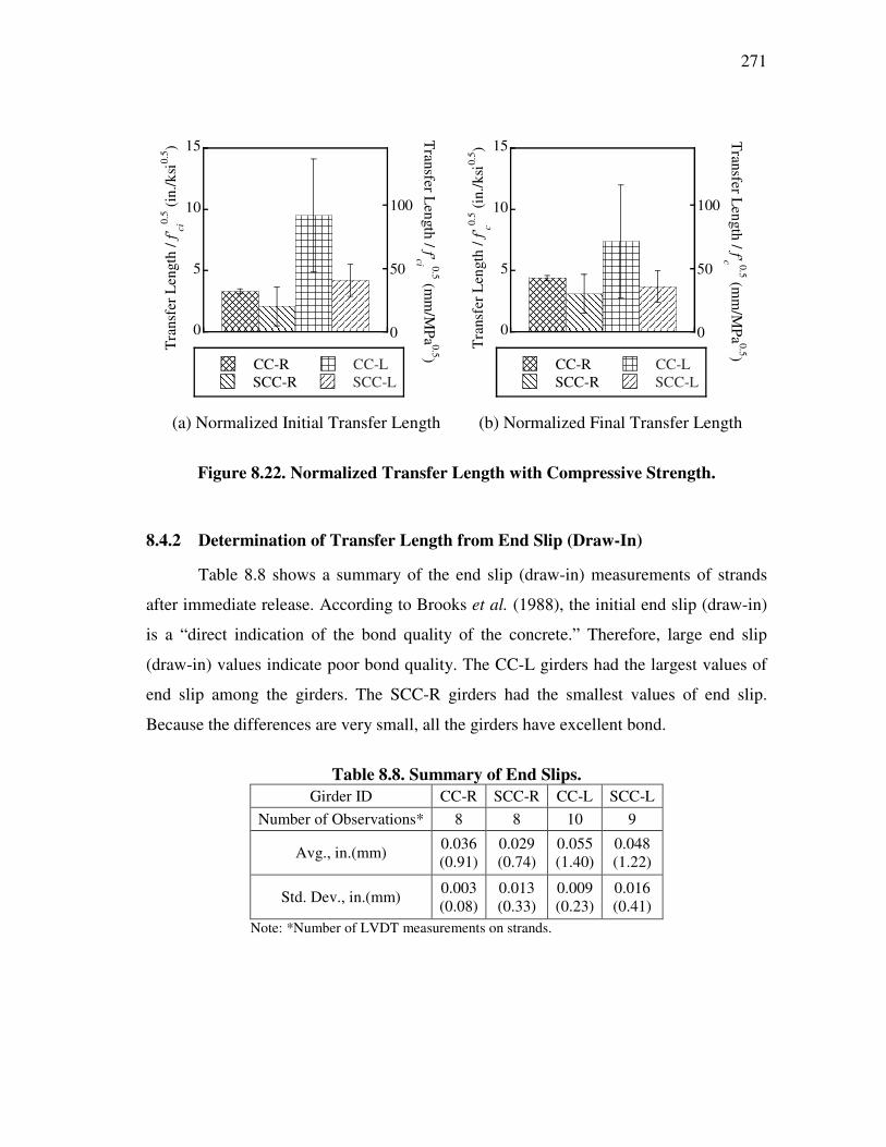
271

(a) Normalized Initial Transfer Length (b) Normalized Final Transfer Length

Figure 8.22. Normalized Transfer Length with Compressive Strength.

8.4.2 Determination of Transfer Length from End Slip (Draw-In)

Table 8.8 shows a summary of the end slip (draw-in) measurements of strands

after immediate release. According to Brooks et al. (1988), the initial end slip (draw-in)

is a “ direct indication of the bond quality of the concrete.” Therefore, large end slip

(draw-in) values indicate poor bond quality. The CC-L girders had the largest values of

end slip among the girders. The SCC-R girders had the smallest values of end slip.

Because the differences are very small, all the girders have excellent bond.

Table 8.8. Summary of End Slips.

Girder ID CC-R SCC-R CC-L SCC-L Number of Observations* 8 8 10 9

Avg., in.(mm) 0.036 (0.91)

0.029 (0.74)

0.055 (1.40)

0.048 (1.22)

Std. Dev., in.(mm) 0.003 (0.08)

0.013 (0.33)

0.009 (0.23)

0.016 (0.41)

Note: *Number of LVDT measurements on strands.

0

5

10

15

CC-RSCC-R

CC-LSCC-L

0

50

100

Tra

nsfe

r Len

gth

/ f' ci

0.5 (i

n./k

si0.

5 )

Transfer L

ength / f'ci 0.5 (mm

/MPa

0.5)

0

5

10

15

CC-RSCC-R

CC-LSCC-L

0

50

100

Tra

nsfe

r Len

gth

/ f' c0.

5 (in.

/ksi

0.5 )

Transfer L

ength / f'c 0.5 (mm

/MPa

0.5)

272

The transfer lengths estimated from the concrete strain profile, ltr*, and the

transfer length estimated from the end slips, ltr∆, can be compared. Table 8.9 tabulates

the transfer lengths estimated from two methods. Figure 8.23 shows that the two

independent methods for estimating transfer lengths. Both the CC and SCC girders have

one data point on the +30 percent error line and one data point showing more than 30

percent error for the comparison.

Table 8.9. Summary of Transfer Length Estimated from Two Methods. Girder

ID Location ltr*, in.

(mm) ltr∆, in. (mm)

tr*tr

ll

∆

CC-R

North End

8.5 (220)

8.3 (211) 0.98

South End

8.0 (203)

11 (280) 1.39

SCC-R

North End

3.3 (84)

6.9 (180) 2.09

South End

7.5 (190)

8.7 (220) 1.16

CC-L

North End

28 (710)

14 (340) 2.07

South End

17 (440)

17 (420) 1.05

SCC-L

North End

13 (330)

13 (340) 0.97

South End

9.5 (240)

13 (320) 0.75

273

Figure 8.23. Comparison between Transfer Lengths Estimated from Concrete

Strain Profile (ltr*) and Transfer Lengths Estimated from End Slips (ltr∆∆∆∆).

All measured transfer lengths of the SCC girders were at least 50 percent shorter

than the required 30 in. (762 mm) provided by the AASHTO LRFD Specifications. The

transfer length of the CC girders is slightly longer than that of the SCC girders.

Therefore, the AASHTO LRFD Specifications (2004, 2006) satisfactorily estimated all

measured transfer lengths. The high concrete strength of the SCC girders leads to a short

transfer length compared to the CC girders at release and later ages. For limestone

mixtures, higher early strength of the SCC girder at release significantly reduced the

transfer length compared with the CC girders. In this test program, two methods to

estimate transfer length were used. The transfer lengths were determined from the

measured concrete strain profile and Mast’ s theory using end slip measurement for both

CC and SCC girders. Results indicate that the AASHTO LRFD equation for transfer

length is conservative for the CC and SCC girders tested in this study.

8.5 DEVELOPMENT LENGTH TESTS

Development length tests were performed after each flexural test. The test setup

is described in Section 4.7.3.5. In this study, 80 in. (2.0 m) embedment lengths were

used for the initial trial. If this length was longer than the minimum development length,

0

10

20

30

0 10 20 30

CC

SCC

Line of Equality

+ 30% Error- 30% Error

0 200 400 600

0

200

400

600l tr

∆ (in.

)

ltr

* (in.)

ltr

* (mm)

ltr∆ (mm

)

274

as indicated by reaching the nominal moment capacity, then a 70 in. (1.8 m) embedment

length was used to test other girder end.

8.5.1 Flexural Behavior in Development Length Region

8.5.1.1 CC-R1 and CC-R2 Tests

The development length tests for the CC-R girder were performed by the test

procedure in Section 4.7.3.5. At both ends, the girders were loaded to ultimate flexural

conditions and the failure mode was in flexure. The strain in the top fiber of the deck

exceeded 3000 microstrain indicating the ultimate state for flexure was achieved without

any bond failure. The flexural failure with an embedment length of 80 in. (2.0 m)

indicates that the minimum development length is likely less than 80 in. (2.0 m) for the

CC-R1 test. However, the same strain level was achieved for the CC-R2 test, indicating

the minimum development length is likely less than 70 in. (1.8 m). Figure 8.24 shows

the moment-curvature of the girder for the development length tests for CC-R girder.

Based on both tests, the minimum development length was less than 70 in. (1.8 m). This

indicates that the build-up of stress of strands can increase up to the ultimate state

without bond failure. Figure 8.25 shows the applied load versus measured strains for the

development length tests at each end of girder CC-R.

Figure 8.24. Moment-Curvature of the CC-R1 and CC-R2 Tests.

0

400

800

1200

1600

0.0000 0.0002 0.0004 0.0006 0.0008

CC-R1

CC-R2

0.00000 0.00001 0.00002 0.00003

0

500

1000

1500

2000

Mom

ent (

kip-

ft) M

oment (kN

-m)

Curvature (rad/mm)

Curvature (rad/in.)

80"

70"

CC-R2

CC-R1

13.5'

12.5'

(4.1 m)

(2.0 m)

(3.8 m)

(1.8 m)

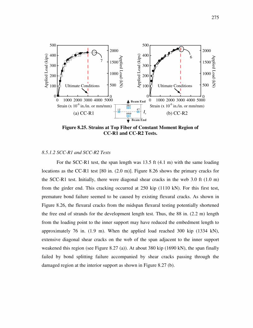
275

(a) CC-R1 (b) CC-R2

Figure 8.25. Strains at Top Fiber of Constant Moment Region of

CC-R1 and CC-R2 Tests.

8.5.1.2 SCC-R1 and SCC-R2 Tests

For the SCC-R1 test, the span length was 13.5 ft (4.1 m) with the same loading

locations as the CC-R1 test [80 in. (2.0 m)]. Figure 8.26 shows the primary cracks for

the SCC-R1 test. Initially, there were diagonal shear cracks in the web 3.0 ft (1.0 m)

from the girder end. This cracking occurred at 250 kip (1110 kN). For this first test,

premature bond failure seemed to be caused by existing flexural cracks. As shown in

Figure 8.26, the flexural cracks from the midspan flexural testing potentially shortened

the free end of strands for the development length test. Thus, the 88 in. (2.2 m) length

from the loading point to the inner support may have reduced the embedment length to

approximately 76 in. (1.9 m). When the applied load reached 300 kip (1334 kN),

extensive diagonal shear cracks on the web of the span adjacent to the inner support

weakened this region (see Figure 8.27 (a)). At about 380 kip (1690 kN), the span finally

failed by bond splitting failure accompanied by shear cracks passing through the

damaged region at the interior support as shown in Figure 8.27 (b).

5000400030002000100000

100

200

300

400

500

0

500

1000

1500

2000A

pplie

d Lo

ad (k

ips)

Ultimate Conditions

Applied Load (kN

)

Strain (x 10-6 in./in. or mm/mm)

7

5000400030002000100000

100

200

300

400

500

0

500

1000

1500

2000

App

lied

Load

(kip

s)

Ultimate Conditions

Applied Load (kN

)

Strain (x 10-6 in./in. or mm/mm)

6

le

Beam End

Beam End

80 (2.0)

162

Bottom View

Side View

Dim ensions [inch (m )]

Figure 8.

(a) Bond Splitting Failure

Figure 8.27

In addition to the presence of flexural cracks near the interior support, the self

weight of overhanging portion of the girder induced negative moments on the inner

support resulting in compression stresses at the bottom fiber near the support. Therefore,

the shear and moment capacities

2 (4 .1)Cracks from Midspan Flexural Test

12 (0.3) (Dam aged Region)76 (1.9)

Shear Cracks [300 kips (1330 kN)]

Bond Splitt ing Failure [380 kips (1700 kN)]

78 (2.0)

P

Dim ensions [inch (m )]

Figure 8.26. Primary Cracks of SCC-R1.

(a) Bond Splitting Failure (b) Shear Cracks

27. Bond Splitting Failure and Shear Cracks.

In addition to the presence of flexural cracks near the interior support, the self

weight of overhanging portion of the girder induced negative moments on the inner

support resulting in compression stresses at the bottom fiber near the support. Therefore,

the shear and moment capacities were reduced in this region. For this reason, the test

Shear cracks

Interior Support

276

Cracks from Midspan Flexura l Test

(b) Shear Cracks

In addition to the presence of flexural cracks near the interior support, the self-

weight of overhanging portion of the girder induced negative moments on the inner

support resulting in compression stresses at the bottom fiber near the support. Therefore,

in this region. For this reason, the test

Shear cracks

277

setup for SCC-R2 was modified to use the overhead crane. The overhead crane

supported the weight of the overhang and reduced the negative moment.

Figure 8.28 shows the applied load versus measured strains for the development

length tests at each end of girder SCC-R. The strain from the SCC-R1 is below the 3000

microstrain value desired to ensure that the strands are fully developed. This is due to the

sudden bond and resulting shear failure near the inner support discussed earlier. The

strain at top fiber of SCC-R2 exceeded 3000 microstrain, indicating that the girder

achieved ultimate flexural conditions and the strands were fully developed. The four

plots of strain data corresponding to the strain measurements on the top compression

fiber along the midspan.

(a) SCC-R1 (b) SCC-R2

Figure 8.28. Strains at Top Fiber of Constant Moment Region of SCC-R1 and SCC-R2 Tests.

Figure 8.29 shows the moment-curvature plots for the SCC-R girder

development length tests. The SCC-R1 results indicated that the girder resisted the

applied load with brittle shear and bond failure rather than ductile flexural behavior.

Therefore, the SCC-R1 had less curvature with respect to the same applied load than

SCC-R2. The SCC-R2 test was loaded to ultimate flexural conditions with an 80 in. (2.0

m) embedment length. The results indicate that the strain of the strands could reach the

0

100

200

300

400

500

0

500

1000

1500

2000

500040003000200010000Strain (x 10-6 in./in. or mm/mm)

Applied Load (kN

)App

lied

Load

(kip

s)

Ultimate Condition

0

100

200

300

400

500

0

500

1000

1500

2000

500040003000200010000

App

lied

Load

(kip

s) Applied Load (kN

)

Ultimate Conditions

Strain (x 10-6 in./in. or mm/mm)

1,2, 6, and 7

le

Beam End

Beam End

278

ultimate state without bond failure and the development length is not greater than 80 in.

(2.0 m).

Figure 8.29. Moment-Curvature of SCC-R1 and SCC-R2 Tests.

8.5.1.3 CC-L1 and CC-L2 Tests

After the flexural test of the CC-L girder was performed, development length

tests were performed (see Table 4.11). The development length test CC-L1 was

performed and ultimate flexural conditions were achieved. The other end was tested to

determine if the 70 in. (1.8 m) embedment length was longer than the minimum required

development length. Again, the strain of the top fiber exceeded 3000 microstrain,

indicating flexural failure.

Figure 8.30 shows the moment-curvatures data from the CC-L1 and CC-L2 tests.

Figure 8.31 shows the applied load versus measured strains for the development

length tests at each end of girder CC-L. The strain at top fiber of CC-L1 and CC-L2

exceeded 3000 microstrain, indicating that the girders achieved ultimate flexural

conditions and the strands were fully developed. Therefore, the development length for

the SCC-R girder is less than 70 in. (1.8 m).

0

400

800

1200

1600

0.0000 0.0002 0.0004 0.0006 0.0008

SCC-R1

SCC-R2

0

500

1000

1500

2000

0.00000 0.00001 0.00002 0.00003

Curvature (rad/in.)

Bond Failure

Mom

ent (

kip-

ft) M

oment (kN

-m)

Curvature (rad/mm)

SCC-R1

13.5'

80"SCC-R2

13.5'

80"(2.0 m)

(4.1 m)

(4.1 m)

(2.0 m)

279

Figure 8.30. Moment-Curvature of CC-L1 and CC-L2 Tests.

(a) CC-L1 (b) CC-L2

Figure 8.31. Strains at Top Fiber of Constant Moment Region of

CC-L1 and CC-L2 Tests.

8.5.1.4 SCC-L1 and SCC-L2 Tests

After the SCC-L girder flexural test was performed, development length tests

were performed (see Table 4.11). The SCC-L1 development length test was performed

0

400

800

1200

1600

0.0000 0.0002 0.0004 0.0006 0.0008

CC-L1

CC-L2

0

500

1000

1500

2000

0.00000 0.00001 0.00002 0.00003

Curvature (rad/in.)

Mom

ent (

kip-

ft) M

oment (kN

-m)

Curvature (rad/mm)

70"CC-L2

CC-L1

13.5'

12.5'

80"(2.0 m)

(4.1 m)(1.8 m)

(3.8 m)

5000400030002000100000

100

200

300

400

500

0

500

1000

1500

2000

App

lied

Load

(kip

s)

Ultimate Conditions

Applied Load (kN

)

Strain (x 10-6 in./in. or mm/mm)

1,2, 6, and 7

5000400030002000100000

100

200

300

400

500

0

500

1000

1500

2000

App

lied

Load

(kip

s)

Ultimate Conditions

Applied Load (kN

)

Strain (x 10-6 in./in. or mm/mm)

1,2, 6, and 7

le

Beam End

Beam End

280

using an 80 in. (2.0 m) embedment length and ultimate flexural conditions were

achieved. The other end was then tested to evaluate a 70 in. (1.8 m) development length.

Figure 8.32 shows the moment-curvature plots of the SCC-L1 and SCC-L2 tests.

Both tests reached ultimate conditions with no premature bond or shear failure.

Figure 8.33 shows the applied load versus measured strains for the development

length tests at each end of girder SCC-L. The strain at top fiber of CC-L1 and CC-L2

exceeded 3000 microstrain, indicating that the girders achieved ultimate flexural

conditions and the strands were fully developed. Therefore, the development length for

the SCC-L girder was determined to be less than 70 in. (1.8 m).

Figure 8.32. Moment-Curvature of SCC-L1 and SCC-L2 Tests.

0

400

800

1200

1600

0.0000 0.0002 0.0004 0.0006 0.0008

SCC-L1

SCC-L2

0

500

1000

1500

2000

0.00000 0.00001 0.00002 0.00003

Curvature (rad/in.)

Mom

ent (

kip-

ft) M

oment (kN

-m)

Curvature (rad/mm)

80"

70"SCC-L2

SCC-L1

13.5'

12.5'

(2.0 m)

(4.1 m)(1.8 m)

(3.8 m)

281

(a) SCC-L1 (b) SCC-L2

Figure 8.33. Strains at Top Fiber of Constant Moment Region of

SCC-L1 and SCC-L2 Tests.

Based on the development length test results, girders CC-L and SCC-L exhibited

similar bond performance for developing the stress of strands corresponding to ultimate

flexural conditions.

8.5.2 Bond and Shear Characteristics in Development Length Region

According to the MCFT and the AASHTO LRFD Specifications (2004, 2006),

the support region is subjected to high shear forces causing high tension in the

longitudinal reinforcement. The shear force causes tensile stresses in the web

reinforcement, prestressing strands and nonprestressing longitudinal reinforcement. To

avoid yielding of the longitudinal reinforcement, the reinforcement and force in the

tension zone should meet the following equation from AASHTO 2004 and 2006 (Article

5.8.3.5):

0.5 cot�u u

s y ps ps s p

M VA f A f V V

jd� �+ ≥ + − − φ φ� �

(8.1)

500040003000200010000-100

0

100

200

300

400

500

0

500

1000

1500

2000A

pplie

d Lo

ad (k

ips)

Ultimate Conditions

Applied Load (kN

)

Strain (x 10-6 in./in. or mm/mm)

1,2, and 7

5000400030002000100000

100

200

300

400

500

0

500

1000

1500

2000

App

lied

Load

(kip

s)

Ultimate Conditions

Applied Load (kN

)

Strain (x 10-6 in./in. or mm/mm)

1,2, 6 and 7

le

Beam End

Beam End

282

where Mu is the factored moment (kip-in. [kN-m]), Vu is the factored shear force (kip

[kN]), Vp is the component of the effective prestressing force in the direction of the

applied shear (kip [kN]), Vs is the component of the stirrup in the direction of the

applied shear (kip [kN]), Aps is the area of the prestressing steel (in.2 [mm2]), As is the

area of nonprestressing steel (in.2 [mm2]), fps is the stress in the strands for the nominal

flexural moment (Mn) resistance (ksi [MPa]), fy is the yield stress of reinforcement (ksi

[MPa]), φ is the reduction factor for the nominal moment resistance, θ is the angle of

inclination of the diagonal compressive stresses (degrees), jd is the effective shear depth

and can be taken as the flexural lever arm, d − a/2, but should not be taken as less than

0.9 d nor 0.72 h, d is the distance from the top fiber to the center of gravity of

prestressing strands, and h is the depth of section.

The second term T = (Vu /φ − 0.5 Vs − Vp) cotθ is the tension force in resulting

from the shear forces. This value is generally high in the support due to relatively high

values of shear forces. Therefore, the tensile stresses and longitudinal reinforcement in

the transfer length region should be investigated to profile the build-up of stress of

strands.

Table 8.10 shows the strain values at 20 in. (0.5 m) from the girder end at the

level of the cgs of the strands. Strain was measured with both surface and embedded

concrete strain gages. Except for the CC-R1 test, the surface and concrete strains are

similar, indicating no cracks crossing the gages. The high tensile stress could indicate the

high demand of longitudinal and shear reinforcements to avoid shear and bond failure.

Because the 70 in. (1.8 m) embedment length girders have higher shear force on the

support, they reasonably have slightly higher tensile stains compared to 80 in. (2.0 m)

embedment length. The SCC-R2 test shows slightly higher tensile strains than the CC-

R2 due to the intensive shear stress in the transfer length region. The CC-L and SCC-L

girders exhibited the similar tensile stresses. However, the CC and SCC-L have higher

tensile strains at applied load of 340 kip (1520 kN) compared to the CC-R and SCC-R

samples except for SCC-R2. This indicates that the contribution of shear of the

283

limestone concrete is lower than that of the river gravel concrete resulting in a higher

demand on the longitudinal reinforcement to avoid shear and bond failure.

Table 8.10. Strain at 20 in. (0.5 m) from the End.

Test ID

Prestrain (× 10−6 in./in.

[mm/mm])

Strain due to Applied Load (Tensile strain) Note

At 340 kip (1520 kN) (× 10−6

in./in. [mm/mm])

At Ultimate (× 10−6 in./in.

[mm/mm])

Embedment Length, in. (m)

εpi ε’ c εc ε’ c εc CC-R1 − 544 105 192 103 145 168 684* 80 (2.0) CC-R2 − 485 92 170 166 133 227 235 70 (1.8)

SCC-R1 − 667 100 125 113 133 227 235 80 (2.0) SCC-R2 − 804 191 245 255 277 280 260 80 (2.0) CC-L1 − 679 132 176 183 156 202 236 80 (2.0) CC-L2 − 754 182 182 182 221 260 258 70 (1.8)

SCC-L1 − 960 161 140 143 201 167 167 80 (2.0) SCC-L2 − 869 166 164 156 236 235 235 70 (1.8)

Note: * Crack occurrence in the transfer length region, εpi is prestrain due to

effective prestressing force, εc is concrete strain due to applied load on surface type gage, and ε'c is concrete strain due to applied load in embedded type gage.

Web-shear cracks propagated through layers of strands on the bottom flange near

the support of CC-L2 and SCC-L2 girders. However, there were no bond or shear

failures. Figures 8.34 and 8.35 show the measured strain at the cgs level from surface

and embedded strain gages, along with the measured prestrain, as a function of the

distance from the girder end. In addition, an elevation view of the girder end with the

crack locations and widths is provided. Figure 8.34 shows test CC-L2 and Figure 8.35

shows test SCC-L2.

As shown in Figure 8.34, the crack did not significantly affect the loss of bond.

However, the tensile strain at 70 in. (1780 mm) from the end exceeded the compressive

prestrain, εpi , indicating losses of prestrain or gage failure due to cracks. Because tensile

strains at 5 and 20 in. (130 and 510 mm) did not exceed the compressive prestrain, crack

opening was prevented by the prestressing force and the anchorage of type W, V, and R

284

bars. Even though the shear crack propagated through the transfer length region in the

bottom flange, there was no bond failure. Figure 8.35 also shows that the crack did not

affect the loss of bond.

(a) Strain of cgs of strands

0.150.15 0.23

0.15

0.8 0.5 0.3 0.2 0.3

0.15

0.26

0.15 0.33 0.6

Crack width: mm (1 mm = 0.039 in.)

1 ft (0.3 m)V = 290 kips (1290 kN)

0.150.15 0.23

0.15

0.8 0.5 0.3 0.2 0.3

0.15

0.26

0.15 0.33 0.6

1 ft (0.3 m)

Note: crack width at the shear load of 310 kip (1380 kN)

piε = measured prestrain due to effective prestressing force

cε = concrete strain due to applied load on surface type gage

c′ε

= concrete strain due to applied load in embedded type gage

Lx = distance from the girder end (in. [m])

(b) Crack Diagram

Figure 8.34. Strains at the Centroid of Gravity of Strands and Crack Diagram at Ultimate Loading (CC-L2).

0

500

1000

1500

2000

0 20 40 60 80

εc

ε'c

εpi

0.0 0.5 1.0 1.5 2.0

Stra

in (x

10-6

in./i

n. o

r mm

/mm

)

Distance from the Girder End (in.)

CC-L2

Distance from the Girder End (m)

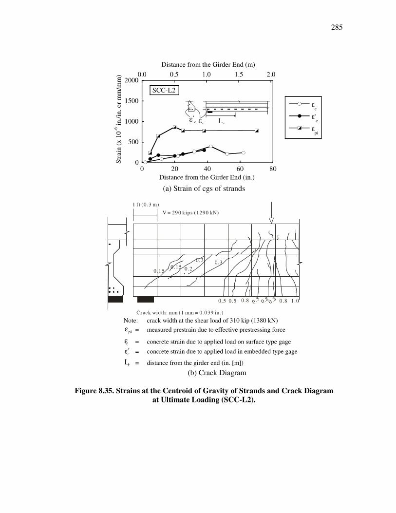
285

(a) Strain of cgs of strands

0.150.15

0.3 0.3

0.5 0.8 0.8 0 .8 0.8 1.00.5

0.2

0.5

Crack width: mm (1 mm = 0.039 in.)

1 ft (0.3 m)V = 290 kips (1290 kN)

Note: crack width at the shear load of 310 kip (1380 kN)

piε = measured prestrain due to effective prestressing force

cε = concrete strain due to applied load on surface type gage

c′ε

= concrete strain due to applied load in embedded type gage

Lx = distance from the girder end (in. [m])

(b) Crack Diagram

Figure 8.35. Strains at the Centroid of Gravity of Strands and Crack Diagram at Ultimate Loading (SCC-L2).

0

500

1000

1500

2000

0 20 40 60 80

εc

ε'c

εpi

0.0 0.5 1.0 1.5 2.0

SCC-L2

Distance from the Girder End (m)

Distance from the Girder End (in.)

Stra

in (x

10-6

in./i

n. o

r mm

/mm

)

286

Figure 8.36 shows a typical plot of the end slips of strands during the

development length tests. Each data point represents the slip measured in one strand at

the corresponding applied load. As shown in these typical plots, the maximum measured

slip was less than 0.01 in. (0.2 mm). There were no strand slips observed for all transfer

zones at the girder ends.

It was recommended to avoid the propagation of cracks in the transfer zone to

prevent the strand slip, finally resulting in bond failure (Russell and Burns 1993). In this

study, the observed cracks in the transfer zone did not cause any measurable bond slip.

There was also no strand slip observed at the girder end of the SCC-R1.

(a) CC-R2 (b) SCC-R2

Figure 8.36. Typical End Slip of Strands.

8.5.3 Comparisons between Experimental Results and AASHTO LRFD

8.5.3.1 Development Length

Bond failure did not occur during the development length tests, except for SCC-

R1. After modifying the test setup, the 80 in. (2.0 m) development length was sufficient

to cause flexural failure at the other end of the SCC-R girders. When monitoring the slip

of strands at the end of the section, there was no larger slip than 0.01 in. (0.25 mm),

0

200

400

600

0

1000

2000

-0.02 -0.01 0.00 0.01 0.02

-0.4 -0.2 0.0 0.2 0.4

App

lied

Loa

d (k

ips)

End Slip (in.)

End Slip (mm)A

pplied Load (kN)

0

200

400

600

0

1000

2000

-0.02 -0.01 0.00 0.01 0.02

-0.4 -0.2 0.0 0.2 0.4A

pplie

d L

oad

(kip

s)

End Slip (in.)

End Slip (mm)

Applied Load (kN

)

LVDT

287

indicating no bond failure for all tests. It should be noted that the premature bond failure

was observed at SCC-R1 near the interior support. However, there was no end slip at the

end of the section.

In summary, the development length is likely shorter than 70 in. (1.8 m) for the

tested girders containing CC and SCC mixtures. Average stress in the strands at nominal

flexural resistance, fps, was calculated based on Article 5.7.3.1.1-1 of the AASHTO

LRFD Specifications (2004, 2006). The effective prestress, fpe, was obtained from

longer-term strain measurements. Table 8.11 shows the summary of development length

values for all girders. The 2004 and 2006 AASHTO LRFD prediction equation provided

a conservative estimation for both the CC and SCC girders. The 2004 AASHTO LRFD

alternative prediction equation (Equation 2.33) provided a closer estimate of

development length for both the CC and SCC girders.

Table 8.11. Summary of Development Length Test Results.

Test ID ld , in. (m) Estimated ld , in. (m)

2004 AASHTO, Alt. (Eq.

2.33) ld , in. (m)

2004, 2006 AASHTO (Eq. 2.30) ld , in. (m)

Failure Mode

CC-R1 < 80 (2.0) < 70 (1.8) > 87 (2.2) > 120 (3.0) Flexural CC-R2 < 70 (1.8) Flexural

SCC-R1 Bond Failure < 80 (2.0) > 73 (1.9) > 120 (3.1) Shear/Bond SCC-R2 < 80 (2.0) Flexural CC-L1 < 80 (2.0) < 70 (1.8) > 90 (2.3) > 120 (3.1) Flexural CC-L2 < 70 (1.8) Flexural

SCC-L1 < 80 (2.0) < 70 (1.8) > 70 (1.8) > 120 (3.0) Flexural SCC-L2 < 70 (1.8) Flexural

8.5.3.2 Maximum Strain in Prestressing Strands

The measured strand strain, εmax-exp, at the centroid of bottom rows of strands at

nominal moment resistance of the beam is the summation of the strain from the LVDTs

attached to the girder and the embedded strain gages. The embedded strain gages

measure the prestrain, while the LVDTs measure the strain due to the applied load.

288

The CC and SCC girders had similar strain values when the same aggregate type

was used. The CC-L and SCC-L girders have higher strand strains at the ultimate state

compared to the CC-R and SCC-R girders. The strand strains were calculated at the

ultimate in accordance with the AASHTO LRFD Specifications (2004, 2006). The

calculated maximum strand strain values based on the AASHTO were generally lower

than the measured values. The values are summarized in Table 8.12.

Table 8.12. Measured Maximum Ultimate Stand Strain.

Test ID εpe in./in. or mm/mm

εps in./in. or mm/mm

εmax-exp in./in. or mm/mm

εmax-cal in./in. or mm/mm

max-exp

max-cal

εε

CC-R1 0.007 0.009 0.016 0.013 1.2 CC-R2 0.007 0.012 0.019 0.013 1.5

SCC-R1 0.007� 0.003 0.010 0.012 0.8 SCC-R2 0.007� 0.009 0.016 0.012 1.3 CC-L1 0.007� 0.016 0.023 0.010 2.3 CC-L2 0.007� 0.021 0.029 0.011 2.6

SCC-L1 0.007� 0.016 0.023 0.009 2.6 SCC-L2 0.007� 0.017 0.024 0.010 2.4

Note: εpe is the prestrain from measured concrete strain gage, εps is the strain due to applied load at ultimate measured from LVDTs, εmax-exp is the measured ultimate strand strain, which is the sum of εpe and εps, and εmax-cal is calculated ultimate strand strain based on AASHTO LRFD.

289

8.5.3.3 Nominal Moment

The AASHTO LRFD Specifications (2004, 2006) can reasonably estimate the

shear-moment interaction resulting in the degradation of moment capacity associated

with shear capacity. Development length tests were performed when flexural and shear

stresses were present at the critical section. The longitudinal strain in the web can be

estimated by the following equation (AASHTO LRFD Article 5.8.3.4.2-1):

( )0.5 cot�

2

uu p ps po

vx

s s p ps

MV V A f

dE A E A

+ − −ε =

+ (8.2)

where Mu is the factored moment (kip-in. [kN-m]), Vu is the factored shear force (kip

[kN]), Vp is the component in the direction of the applied shear of the effective

prestressing force (kip [kN]), fpo is the stress in the prestressing steel (ksi [MPa]) and

usually 0.7 fpu in the AASHTO LRFD, Aps is the area of the prestressing steel (in.2

[mm2]), As is the area of nonprestressing steel (in.2 [mm2]), Es and Ep are the elastic

modulus of nonprestressing steel and prestressing steel, respectively (ksi [MPa]), and

θ is the angle of inclination of diagonal compressive stresses (degree). This value is

always taken to be larger than 0 for conservatism in the design. As shown in Equation

8.2, a higher moment results in an increase of the longitudinal strain in the web. Based

on these concepts, the nominal moment capacity for each girder and during testing is

estimated by the AASHTO LRFD Specifications (2004, 2006). The nominal moments

were estimated by using the Equation 2.26 of the AASHTO LRFD Specifications.

Table 8.13 shows the calculated nominal moment capacity from the AASHTO

LRFD Specifications (2004, 2006) and the measured maximum moment from each

development length test. The measured ultimate moment of SCC-R1 was 3 percent

higher than the calculated nominal moment resistance, Mn-AASHTO based on the AASHTO

LRFD Specifications (2004, 2006). The nominal moment resistance, Mn-exp of all other

tests was 7 to 31 percent higher than calculated nominal moment resistance, Mn-AASHTO.

290

Table 8.13. Measured Moment versus Calculated Moment Based on AASHTO (2004, 2006).

Test ID Mn-AASHTO ,

kip-ft (kN-m) Mn-exp ,

kip-ft (kN-m) n exp

n AASHTO

M

M−

−

CC-R1 1281 (1737) 1519 (2059) 1.19 CC-R2 1135 (1539) 1491 (2021) 1.31

SCC-R1 1279 (1734) 1323 (1794) 1.03 SCC-R2 1133 (1536) 1430 (1939) 1.26 CC-L1 1273 (1726) 1361 (1845) 1.07 CC-L2 1126 (1527) 1361 (1845) 1.21

SCC-L1 1271 (1723) 1366 (1852) 1.07 SCC-L2 1126 (1527) 1382 (1874) 1.23

8.5.4 Shear Performance

8.5.4.1 Shear Force Causing Web-Shear Cracking

There were concerns regarding the shear performance of the SCC mixtures, as

they have lower amounts of aggregate compared to typical CC mixtures. This section

will investigate the local shear behavior of the girders and will show how the local shear

demand impact the overall failure mode.

Web-shear cracking occurs when the maximum principal tensile stress is equal to

the tensile strength of concrete. When the element is subjected to prestress and shear

stresses at the center of the web, the principal stresses can be calculated as follows

(Collins and Mitchell 1991, Naaman 2004):

2

21 2 2

pc pcf fv

� �σ = + −

� � (8.3)

where σ1 is the principal stress (psi [MPa]), v is the shear stress at the web (psi [MPa]),

and fpc is the compressive stress due to the effective prestressing force, taken as the

positive value (psi [MPa]).

291

To solve the cracking shear stress in the web, vcw (psi [MPa]), σ1 becomes equal

to the tensile strength, ft :

1 pccw t

t

fv f

f= + (8.4)

When ft is approximately 4 cf ′ psi (0.33 cf ′ MPa), based on direct tension test data,

this equation becomes the basic web-shear cracking equation of ACI 318-05 and the

AASHTO Standard Specifications (2002):

( )3 5 0 3 (kip, in.)cw ACI c pc w pV . f . f b d V− ′= + +

(8.5)

[ ( )0 29 0 3 (kN, mm)cw ACI c pc w pV . f . f b d V− ′= + + ]

where Vcw-ACI is the shear force corresponding to web-shear cracking, f’ c is the

compressive strength of concrete (psi [MPa]), bw is the width of web (in. [mm]), d is the

distance from the extreme compression fiber to the centroid of the tension strands (in.

[mm]), Vp is the component in the direction of the applied shear of the effective

prestressing force (kip [kN]), and fpe is the longitudinal compressive stress at the centroid

of the beam (psi [MPa]).

The MCFT theory also assumes the same value for ft as the cracking stress of

concrete for the diagonal tensile stresses. This value is used to estimate the β value from

Equation 2.4.

For the MCFT, the shear forcem corresponding to web-shear cracking is

estimated as follows,

cw MCFT c wV f b jd− ′= β (8.6)

292

where jd is the effective shear depth which can be taken as the flexural lever arm (in.

[mm]), d − a/2, but should not be taken as less than 0.9 d nor 0.72 h; d is the distance

from the top fiber to the centroid of gravity of strands (in. [mm]); and h is the depth of

section (in. [mm]). The values of Vcw-MCFT for the girders in this test program were

obtained by using the RESPONSE 2000 Program (Bentz 2000).

Diagonal cracks occurred in the critical section where maximum shear force

acted in all the tests. If the shear capacity of the girder is not sufficient to resist the

applied shear force, a shear failure could increase the potential for bond slip or bond

failure. Therefore, the shear capacity significantly affects bond performance.

Table 8.14 shows the comparison between predicted and measured web-shear

cracking loads. Figure 8.37 shows the plots of the comparison between predicted and

measured force corresponding to web-shear cracking. The web-shear cracking force

based on Equation 8.5, Vcw-ACI, is slightly higher than the web-shear cracking based on

the MCFT, Vcw-MCFT. All the web-shear cracking forces were estimated based on the

measured concrete tensile strength. When the principal tensile strain, ε1, exceeds εcr =

ft/Ec (about 0.0001 in./in. [mm/mm]), the web-shear cracking load, Vcw-exp, is obtained

from the LVDT measurements. This calculation was compared to the crack mapping to

confirm the estimation.

In general, the measured web-shear cracking forces were similar to the predicted

web-shear cracking force. The ACI 318-05 and AASHTO Standard Specifications

approach underestimate the web-shear cracking values. The MCFT predicts the web-

shear cracking for the SCC and CC girders within ±30 percent.

293

Table 8.14. Shear Force Causing Web-Shear Cracking (Predicted versus Measured Values).

Test ID Vcw-ACI , kip (kN)

Vcw-MCFT , kip (kN)

Vcw-exp ,

kip (kN) cw exp

cw ACI

V

V−

−

cw exp

cw MCFT

V

V−

−

CC-R1 90 (400) 137 (609) 174 (774) 1.9 1.3 CC-R2 90 (400) 162 (721) 163 (725) 1.8 1.0

SCC-R1 99 (442) 159 (707) 173 (770) 1.7 1.1 SCC-R2 99 (442) 150 (667) 136 (605) 1.4 0.9 CC-L1 92 (407) 149 (663) 163 (725) 1.8 1.1 CC-L2 92 (407) 179 (796) 164 (729) 1.8 0.9

SCC-L1 102 (454) 171 (761) 135 (600) 1.3 0.8 SCC-L2 102 (454) 188 (836) 195 (867) 1.9 1.0

Figure 8.37. Measured versus Predicted Shear Force Causing Web-Shear Cracking.

0

100

200

300

400

0

400

800

1200

1600

0 100 200 300 400

0 400 800 1200 1600

ACI 318MCFT

Pred

icte

d W

eb-S

hear

Cra

ckin

g Sh

ear

Forc

e (k

ips)

Measured Web-Shear Cracking Shear Force (kips)

Measured Web-Shear Cracking Shear Force (kN)

Predicted Web-Shear C

racking Shear Force (kN)

-30% Error

30% Error

Line of Equality

294

8.5.4.2 Principal Strains at Critical Section for Shear

The cirtical section for shear shall be taken as the effective shear depth, dv, from

the internal face of the support. Figures 8.38 and 8.39 show the principal tensile and

compressive strains of the concrete at the critical section for shear. The average tensile

strain is related to the contribution to shear in the MCFT. Therefore, the higher value

indicates a higher contribution to shear. Generally, the river gravel girders tend to have a

higher contribution to shear than the limestone aggregate girders. The CC-R2 and the

SCC-R2 tests exhibited slightly higher principal tensile strains compared to the

limestone girder tests.

When evaluating the shear performance of girders containing river gravel, the

CC-R girder exhibit slightly higher principal strains than the SCC-R girder. The SCC-R1

test showed dominant diagonal shear cracks on the span at the interior support rather

than in the development length region. Therefore, the measured principal stresses on the

cracked web member and the strains in the steel are lower in the development length

region.

The CC-R2 test exhibited higher principal tensile strains in the cracked web and

higher strain in the shear reinforcement, indicating degradation of the shear cracking

load at early stages. However, the strain stabilized because flexural behavior governed in

the final failure mode. The SCC-R2 test indicated that the web in the 80 in. (2.0 m)

development length region was damaged due to reduced shear capacity. The first web-

shear cracking occurred at slightly lower stress levels than for CC-R1 and CC-R2 tests.

However, the final failure mode was flexural.

The large-scale tests showed very similar principle strains at the shear critical

sections for both the SCC-L and CC-L tests, as shown in Figure 8.39.

295

(a) CC-R1 (b) CC-R2

(c) SCC-R1 (d) SCC-R2

Figure 8.38. Principal Strains of Cracked Web Concrete in CC-R and SCC-R Girders.

-0.004

-0.002

0

0.002

0.004

0 100 200 300

0 500 1000Pr

inci

pal S

trai

ns

(in.

/in. o

r mm

/mm

)

Applied Shear Load (kips)

CC-RS1

Applied Shear Load (kN)

-0.004

-0.002

0

0.002

0.004

0 100 200 300

0 500 1000

CC-RS2

Prin

cipa

l Str

ains

(i

n./in

. or m

m/m

m)

Applied Shear Load (kips)

Applied Shear Load (kN)

-0.004

-0.002

0

0.002

0.004

0 100 200 300

0 500 1000

Applied Shear Load (kips)

SCC-RS1

Applied Shear Load (kN)

Prin

cipa

l Str

ains

(i

n./in

. or m

m/m

m)

-0.004

-0.002

0

0.002

0.004

0 100 200 300

0 500 1000

SCC-RS2Pr

inci

pal S

trai

ns

(in.

/in. o

r mm

/mm

)

Applied Shear Load (kips)

Applied Shear Load (kN)

Tension

Compression

Tension

Compression

Tension

Compression

Tension

Compression

CC-R1 CC-R2

SCC-R1 SCC-R2

296

(a) CC-L1 (b) CC-L2

(c) SCC-L1 (d) SCC-L2

Figure 8.39. Principal Strains of Cracked Web Concrete in CC-L and SCC-L Girders.

8.5.4.3 Strain in Shear Reinforcement

Figures 8.40 and 8.41 show the measured strains in the web steel as a function of

the applied shear load, which is the shear force acting on the critical section. Strains in

the shear reinforcement did not reach the yield strain of 2000 × 10–6 . This indicates that

the girders did not reach their ultimate shear capacity. According to the prediction from

the MCFT, the first web-shear cracks preceded the flexural cracks and flexural-shear

-0.004

-0.002

0

0.002

0.004

0 100 200 300

0 500 1000

CC-LS1

Prin

cipa

l Str

ains

(i

n./in

. or m

m/m

m)

Applied Shear Load (kips)

Applied Shear Load (kN)

-0.004

-0.002

0

0.002

0.004

0 100 200 300

0 500 1000

CC-LS2

Prin

cipa

l Str

ains

(i

n./in

. or m

m/m

m)

Applied Shear Load (kips)

Applied Shear Load (kN)

-0.004

-0.002

0

0.002

0.004

0 100 200 300

0 500 1000

SCC-LS1

Prin

cipa

l Str

ains

(i

n./in

. or m

m/m

m)

Applied Shear Load (kips)

Applied Shear Load (kN)

-0.004

-0.002

0

0.002

0.004

0 100 200 300

0 500 1000

SCC-LS2

Prin

cipa

l Str

ains

(i

n./in

. or m

m/m

m)

Applied Shear Load (kips)

Applied Shear Load (kN)

Tension

Compression

Tension

Compression

Tension

Compression

Tension

Compression

CC-L1 CC-L2

SCC-L1 SCC-L2

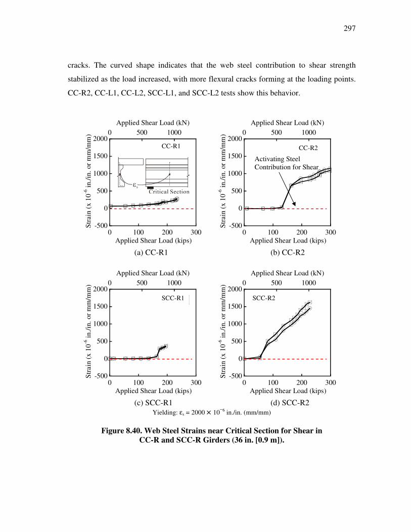
297

cracks. The curved shape indicates that the web steel contribution to shear strength

stabilized as the load increased, with more flexural cracks forming at the loading points.

CC-R2, CC-L1, CC-L2, SCC-L1, and SCC-L2 tests show this behavior.

(a) CC-R1 (b) CC-R2

(c) SCC-R1 (d) SCC-R2

Yielding: εs = 2000 × 10–6 in./in. (mm/mm)

Figure 8.40. Web Steel Strains near Critical Section for Shear in CC-R and SCC-R Girders (36 in. [0.9 m]).

-500

0

500

1000

1500

2000

0 100 200 300

0 500 1000

Stra

in (x

10-6

in./i

n. o

r mm

/mm

)

CC-RS1

Applied Shear Load (kN)

Applied Shear Load (kips)

-500

0

500

1000

1500

2000

0 100 200 300

0 500 1000

CC-RS2

Stra

in (x

10-6

in./i

n. o

r mm

/mm

)

Applied Shear Load (kN)

Applied Shear Load (kips)

-500

0

500

1000

1500

2000

0 100 200 300

0 500 1000

SCC-RS1

Stra

in (x

10-6

in./i

n. o

r mm

/mm

)

Applied Shear Load (kN)

Applied Shear Load (kips)

-500

0

500

1000

1500

2000

0 100 200 300

0 500 1000

SCC-RS2

Stra

in (x

10-6

in./i

n. o

r mm

/mm

)

Applied Shear Load (kN)

Applied Shear Load (kips)

Activating Steel Contribution for Shear

CC-R1 CC-R2

SCC-R1 SCC-R2

298

(a) CC-L1 (b) CC-L2

(c) SCC-L1 (d) SCC-L2

Yielding: εs = 2000 × 10–6 in./in. (mm/mm)

Figure 8.41. Web Steel Strains near Critical Section for Shear in CC-L and SCC-L Girders (36 in.[0.9 m]).

-500

0

500

1000

1500

2000

0 100 200 300

0 500 1000

CC-LS1St

rain

(x 1

0-6 in

./in.

or m

m/m

m)

Applied Shear Load (kN)

Applied Shear Load (kips)

-500

0

500

1000

1500

2000

0 100 200 300

0 500 1000

CC-LS2

Stra

in (x

10-6

in./i

n. o

r mm

/mm

)

Applied Shear Load (kN)

Applied Shear Load (kips)

-500

0

500

1000

1500

2000

0 100 200 300

0 500 1000

SCC-LS1

Stra

in (x

10-6

in./i

n. o

r mm

/mm

)

Applied Shear Load (kN)

Applied Shear Load (kips)

-500

0

500

1000

1500

2000

0 100 200 300

0 500 1000

SCC-LS2

Stra

in (x

10-6

in./i

n. o

r mm

/mm

)

Applied Shear Load (kN)

Applied Shear Load (kips)

CC-L1 CC-L2

SCC-L1 SCC-L2

299

8.5.4.4 Comparison of Estimated Shear Capacity

The purpose of the tests at the girder ends was to evaluate the development

length of the strands in the SCC girders compared to the CC girders and the AASHTO

Specifications. Although shear failures did not occur, the test data are useful in

estimating shear capacity. The measured crack width, w, and the angle of the diagonal

compressive stresses in the web, θ, were used to predict the concrete and steel

contribution to shear strength as shown in Figure 8.42. The shear capacity was calculated

from the MCFT and proposed equations in Chapter VI for the limiting value of the

maximum shear stress on the shear plane in the cracked concrete, vci. The crack width,

w, is equal to the product of ε1 and the spacing of diagonal crack spacing, smθ. When the

values of θ, ε1, and smθ are known, the shear forces in the steel and concrete are

estimated by the iteration procedures in the MCFT. The detailed iteration procedures are

presented in the textbook by Collins and Mitchell (1991). The experimental and

estimated shear capacities are compared to validate the proposed equation (Equation

6.38) in Chapter VI and the AASHTO LRFD Specifications.

NW

Unit: mm (1 mm = 0.039 in.)

1 ft (0.3 m)V = 220 kips (980 kN)

θ = 31 degrees

sm

θ = 1 75

w = 0.15

Figure 8.42. Measured Crack Width and Angle of Diagonal Crack (CC-L1).

Based on this procedure, the applied shear and predicted shear values are

compared as shown in Table 8.15. As discussed in Chapter VI, the same shear capacity

was estimated with all the different limiting values for the maximum shear stress on the

300

shear plane. In this estimation, all the values estimated from AASHTO and the proposed

equations are identical. As discussed in Chapter VI, the angle and shear reinforcement

ratios were not so small to activate the slip before the yielding of the shear

reinforcement.

For each girder end, a unique crack pattern was observed with a different crack

width, crack angle, and diagonal crack spacing. These values are summarized in Table

8.15, along with analytical and experimental estimates of the concrete and web steel

contributions to the shear capacity at the critical section. Different contributions to the

shear capacity were observed depending on the mixture type, aggregate type, and test

series. The concrete strengths determined for the girders with limestone aggregate are

lower than for girders with river gravel coarse aggregates. The limestone SCC mixtures

have lowest concrete strength values among all the mixtures.

The ratio of analytical and measured shear forces indicates the accuracy of the

prediction. When the ratio is larger than 1.0, the AASHTO shear design overestimates

shear force based on the same ε1 and θ and smθ values of both analytical and

experimental estimations. When the ratio is smaller than 1.0, the AASHTO shear design

underestimates shear force. Because the steel contribution is involved, the interpretation

is complicated. In cases where the AASHTO is not conservative, proposed equation is

necessary to estimate the reduced capacity of high-strength CC and SCC mixtures. In

these tests, the AASHTO shear design underestimates concrete contribution to shear.

Therefore, The AASHTO LRFD shear design overestimates steel contribution to shear.

Overall average ratio of analytical and measured shear capacity is 0.97 for all the tests.

In summary, the AASHTO LRFD shear design reasonably estimates the shear

capacity of the concrete and steel for the tested girders. There is no significant change

for the shear design of the Type A girder with the SCC mixtures.

301

Table 8.15. Analytical versus Experimental Results for Shear Capacity at Critical Section.

CC-R1 CC-R2 SCC-R1

SCC-R2 CC-L1 CC-L2 SCC-

L1 SCC-

L2 Avg.

w, in. (mm)

0.004 (0.1)

0.008 (0.2)

0.006 (0.15)

0.008 (0.2)

0.006 (0.15)

0.010 (0.26)

0.008 (0.20)

0.012 (0.30)

0.008 (0.20)

θ, degrees 24 25 26 25 31 30 37 36 29 smθ , in. (mm)

3.95 (100)

5.92 (150)

6.90 (175)

3.95 (100)

6.90 (175)

4.11 (104)

5.09 (129)

5.09 (129)

5.24 (133)

Analytical Estimation (AASHTO and Proposed Equation) Vc, kip (kN)

88 (391)

79 (351)

96 (427)

83 (369)

69 (307)

56 (249)

56 (249)

53 (236)

73 (325)

Vs, kip (kN)

145 (645)

185 (823)

111 (494)

283 (1259)

82 (365)

262 (1165)

106 (471)

170 (756)

168 (747)

V=Vs+Vc, kip (kN)

233 (2869)

264 (3600)

207 (2196)

366 (5599)

151 (1622)

318 (5184)

162 (2097)

223 (3363)

241 (3324)

Experimental Estimation Vc= V-Vs, kip (kN)

142 (632)

106 (471)

125 (556) 0 84

(374) 71

(316) 93

(414) 184

(818) 115

(512) Vs, kip (kN)

88 (391)

204 (907)

71 (316)

273 (1214)

136 (605)

219 (974)

127 (565)

106 (471)

153 (681)

V, kip (kN)

230 (1741)

310 (4036)

196 (1405)

230 (5401)

220 (2691)

290 (4333)

220 (2513)

290 (2097)

248 (3027)

Anal./Exp. Ratio Anal./Exp.

for Vc 0.62 0.75 0.77 - 0.82 0.79 0.60 0.29 0.66

Anal./Exp. for Vs

1.65 0.91 1.56 1.04 0.60 1.20 0.83 1.60 1.17

Anal./Exp. for V 1.01 0.85 1.06 1.59 0.69 1.10 0.74 0.77 0.97

Note: Vc = concrete shear capacity, Vs = web steel shear capacity, V = total shear capacity = Vc+Vs.

302

8.5.5 Tests Observation

8.5.5.1 Crack Development

The cracking loads and measured crack widths are summarized in Table 8.16.

The maximum crack width was measured at the extreme tension fiber of the bottom

flange for flexural cracks, within the web depth for shear cracks. Generally, the progress

of shear and flexural cracks and maximum crack widths are similar for all the tests.

Table 8.16. Cracking Loads and Crack Widths (Development Length Test).

Web Cracking Load Flexural Cracking Load Flexural Cracking into Deck

Final Reading

Location Web Web Bottom Flange

Bottom Flange Deck Final Bottom

Flange

Values Applied Load,

kip (kN)

Crack Width,

in. (mm)

Applied Load,

kip (kN)

Crack Width,

in. (mm)

Applied Load,

kip (kN)

Applied Load,

kip (kN)

Crack Width,

in. (mm)

CC-R1 300 (1330)

0.003 (0.08)

300 (1330)

0.003 (0.08)

380 (1690)

400 (1890)

0.016 (0.4)

CC-R2 300 (1330)

0.004 (0.1)

300 (1330)

0.004 (0.1)

350 (1557)

425 (1890)

0.040 (1.0)

SCC-R1 300 (1330) - 320

(1420) 0.006 (0.15)

340 (1510)

380 (1690)

0.035 (0.9)*

SCC-R2 200 (890) - 300

(1330) - 350 (1557)

400 (1780)

0.080 (2.0)

CC-L1 300 (1330)

0.006 (0.15)

300 (1330)

0.008 (0.2)

340 (1510)

400 (1780)

0.032 (0.8)

CC-L2 300 (1330)

0.006 (0.15)

300 (1330)

0.006 (0.15)

340 (1510)

420 (1870)

0.032 (0.8)

SCC-L1 300 (1330)

0.004 (0.15)

300 (1330)

0.004 (0.15)

340 (1510)

400 (1780)

0.049 (1.25)

SCC-L2 300 (1334)

0.006 (0.15)

300 (1334)

0.006 (0.15)

320 (1420)

446 (1980)

0.039 (1.0)

Note: *Maximum shear crack was remarkably 0.25 in. (6.4 mm) on the bottom flange.

8.5.5.2 Cracks on Tested Span

Figure 8.43 shows the crack diagrams in the development length region of CC-

R1 and SCC-R1 girders at ultimate loading.

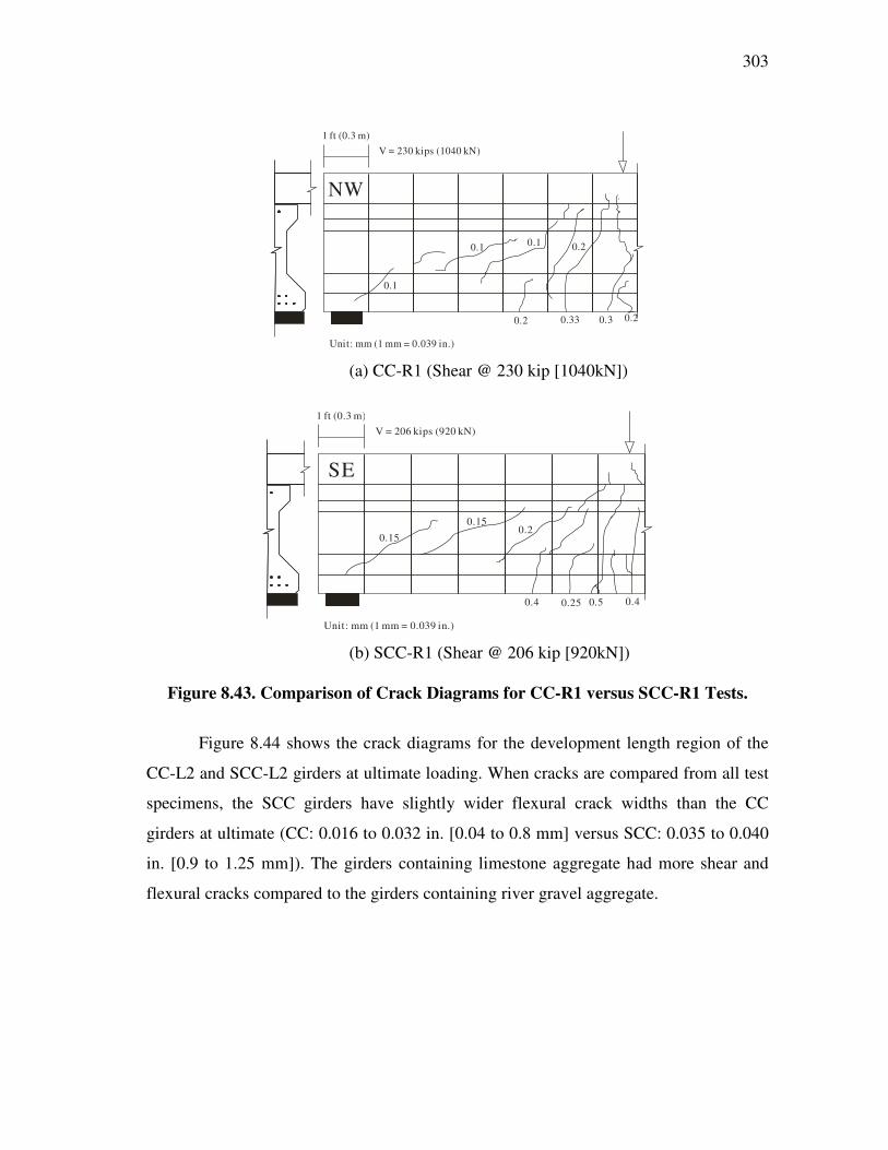
303

NW

0.2 0.33 0.3

0.1

0.1 0.1 0.2

0.2

1 ft (0.3 m)

Unit: mm (1 mm = 0.039 in.)

V = 230 kips (1040 kN)

(a) CC-R1 (Shear @ 230 kip [1040kN])

SE

0.50.4 0.4

0.15

0.150.2

0.25

1 ft (0.3 m)

Unit: mm (1 mm = 0.039 in.)

V = 206 kips (920 kN)

(b) SCC-R1 (Shear @ 206 kip [920kN])

Figure 8.43. Comparison of Crack Diagrams for CC-R1 versus SCC-R1 Tests.

Figure 8.44 shows the crack diagrams for the development length region of the

CC-L2 and SCC-L2 girders at ultimate loading. When cracks are compared from all test

specimens, the SCC girders have slightly wider flexural crack widths than the CC

girders at ultimate (CC: 0.016 to 0.032 in. [0.04 to 0.8 mm] versus SCC: 0.035 to 0.040

in. [0.9 to 1.25 mm]). The girders containing limestone aggregate had more shear and

flexural cracks compared to the girders containing river gravel aggregate.

304

SE

0.150.15 0.23

0.15

0.8 0.5 0.3 0.2 0.3

0.15

0.26

0.15 0.33 0.6

Unit: mm (1 mm = 0.039 in.)

1 ft (0.3 m)V = 290 kips (1290 kN)

(a) CC-L2 (Shear @ 290 kip [1290 kN])

NW

0.150.15

0.3 0.3

0.5 0.8 0.8 0.8 0.8 1.00.5

0.2

0.5

Unit: mm (1 mm = 0.039 in.)

1 f t (0.3 m)V = 290 kips (1290 kN)

(b) SCC-L2 (Shear @ 290 kip [1290 kN])

Figure 8.44. Comparison of Crack Diagrams for CC-L2 versus SCC-L2 Girders.

8.6 PRESTRESS LOSSES

8.6.1 Initial Stresses of Strands

Load cells monitored the jacking stresses of strands and stresses immediately

before transfer of strands. No significant loss of anchorage seating was observed at

tensioning. Strand stresses between the time of casting and the time at transfer were

continuously monitored at 5 second intervals. There was no significant relaxation of

strands between casting and transfer. The relaxation of strands can be estimated after

tensioning of strands.

305

The stresses on the strands are time-dependent values due to the relaxation of

strands as follows:

0( )pbt pj pR trf f f t ,t= − ∆ (8.7)

where fpbt is the stress immediately before transfer (ksi [MPa]), fpj is the initial jacking

stress (ksi [MPa]), ∆fpR (t0 , ttr) is the relaxation of strands between t0 and ttr (ksi [MPa]),

t0 is the time at jacking (hour), and ttr is the time at transfer (hour).

There were no apparent losses due to relaxation before transfer. The strand

stresses in the bottom flange at each event are summarized in Table 8.17.

Table 8.17. Stresses of Strands in Bottom Flange.

Description Time CC-R, SCC-R

Time CC-L, SCC-L

Avg. Std. Dev. Avg. Std.

Dev.

Initial Jacking Stress, fpj at t0 , ksi (MPa)

3/22/07 4:30 PM

208.5 (1438)

3.93 (27)

7/10/07 9:00 AM

217.03 (1496)

7.73 (53)

Stress at Casting, fpj , ksi (MPa)

3/26/07 4:42 PM

212.4 (1464)

4.57 (32)

7/12/07 4:00 PM

216.4 (1492)

5.27 (36)

Stress Immediately Before Transfer, fpbt at ttr , ksi (MPa)

3/27/07 3:20 PM

213.0 (1469)

4.72 (33)

7/13/07 2:20 PM

216.8 (1495)

5.77 (40)

Ambient and concrete temperature influences the strain of concrete and strands,

and these result in changes in the prestress. Thermal linear strain can be determined with

the following equation:

t t Tε = α ∆ (8.8)

306

where εt is the thermal strain, αt is the coefficient of linear thermal expansion (oF–1 [oC–

1]), and ∆Τ is the temperature change (oF [oC]).

Based on a thermal coefficient, αt, of 6.0 × 10�6/oF for steel, the thermal effect is

not significant with the temperature observed during these cast dates. Table 8.18 shows

the average stresses of jacking stress of all girders. Even though the temperature of

strands was considered, the relaxation of strands between time at jacking and time at

transfer apparently did not cause a significant loss of prestress. For CC-L and SCC-L

girders, temperature effect was also minimal.

Table 8.18. Temperature Effect on Stresses of Strands of All Girders.

Girder ID Time/ Measured Avg. Temperature, oF (oC)

Avg. Stresses, fpj, ksi (MPa)

Std. Dev., ksi (MPa)

CC-R and SCC-R

3/24/07 12:16 PM 79 (26) 208.3 (1434) 5.01 (35)

3/26/07 9:16 AM 72 (22) 211.9 (1462) 4.56 (31)

CC-L and SCC-L

7/12/07 12:57 PM 100 (38) 217.4 (1499) 6.74 (47)

7/12/07 1:42 AM 105 (41) 218 (1503) 6.92 (48)

8.6.2 Concrete Strain Profile

Concrete strain gages monitored the changes of strain in the strands resulting

from short- and longer-term effects of concrete and strands. The basic assumption is that

the concrete and strands is perfectly bonded and has the same thermal expansion

coefficient. The history of concrete strain gage profiles at the midspan, south end, and

north end are presented in Figure 8.45 for all girders. During girder casting, the strain

gage readings did not represent the actual behavior of the hardened concrete. The

viscoelastic state of plastic concrete, the fluctuation of temperature, and the shape of the

gage likely affected the strain reading during hydration. To estimate the strain of the

concrete, the reading immediately before transfer was taken as the base reading of strain.

307

(a) CC-R (b) SCC-R

(c) CC-L (d) SCC-L

Figure 8.45. Embedded Concrete Strain Gage History.

The change in concrete strain reflects the elastic shortening, creep, and shrinkage

of concrete, and relaxation of strains. When the CIP concrete deck was cast, immediate

elastic gain at midspan was observed. After transfer, a dramatic increase in shrinkage

and creep was observed, as expected, for all the girders. Before stabilization of strains,

the high strains of end span were observed. It might be attributed to the creep of self-

weight of girders mitigating increase of strain at the midspan at early ages.

0

200

400

600

800

10000 35 70 105 140

Stra

in (x

10-6

in./i

n. o

r mm

/mm

)

Time after Casting (Days)

Casting Deck

0

200

400

600

800

10000 35 70 105 140

Time after Casting (Days)

Casting Deck

Stra

in (x

10-6

in./i

n.or

mm

/mm

)

0

200

400

600

800

10000 35 70 105 140

Time after Casting (Days)

Casting Deck

Stra

in (x

10-6

in./i

n. o

r mm

/mm

) 0

200

400

600

800

10000 35 70 105 140

Time after Casting (Days)

Casting DeckSt

rain

(x10

-6 in

./in.

or m

m/m

m)

South SpanMidspanNorth Span

308

According to manufacturer’ s the calibration data sheet for strain gages, the

thermal output is less than 10 microstrain indicating self-compensating thermal output

between 70 oF (21 oC) and 100 oF (38 oC). Therefore, the change of strain within the

range represents not the thermal change of the strain gages but the actual thermal change

of concrete. Some strain gages showed high values prior to transfer, representing thermal

expansion of the concrete.

8.6.3 Prestress Losses due to Elastic Shortening

Concrete strain readings at transfer are presented in Figure 8.46. The strain

readings immediately before transfer were taken as the base values. To estimate elastic

shortening, the elastic modulus of the concrete at transfer is also estimated from the

strength of concrete at transfer based on the match-cured samples. The thermal change

of the girder is not a significant factor in elastic shortening during transfer. Thermal

changes of the strands were not significant prior to and after transfer and did not result in

a change in the strand stress.

Figure 8.46. Estimation of Elastic Shortening of All Girders.

Table 8.19 shows the estimated prestress losses due to elastic shortening at girder

midspan. There was no significant difference between the SCC and CC girders in the

same prestressing bed. The SCC-R girder had approximately 7 percent higher losses due

-800

-600

-400

-200

0

200

0 200 400 600 800

CC-RSCC-RCC-LSCC-L

Stra

in (x

10-6

in./i

n. o

r mm

/mm

)

Time (sec)

End of transfer

εES

Negative sign: CompressivePositive sign: Tensile

Initiation of transfer

309

to elastic shortening than the CC-R girder, while the CC-L girder had approximately 4

percent higher losses due to elastic shortening than the SCC-L girder.

Table 8.19. Elastic Shortening at Transfer at Midspan.

Girder ID ∆pES ,

× 10−6 in./in. (mm/mm)

Concrete Temperature,

oF (oC)

∆εt , ksi (MPa)

∆fES , ksi (MPa)

CC-R 236 85 (29) 0 6.7 (46) SCC-R 253 85 (29) 0 7.0 (49) CC-L 407 105* (41) 0 11.0 (76)

SCC-L 381 105* (41) 0 10.7 (74) Note: * Ambient temperature, ∆pES

is the measured strain of girder caused by elastic shortening, ∆εt is the thermal strain at transfer, and ∆fES is the prestress loss due to elastic shortening.

8.6.4 Elastic Prestress Gain due to Weight of Deck Slab

When the weight of the deck was placed on the girder, the strands had an instant

elastic prestress gain. Figure 8.47 shows the elastic prestress gains in the CC-L and

SCC-L girders at midspan.

(a) CC-R and SCC-R (b) CC-L and SCC-L

Figure 8.47. Elastic Prestress Gains at Midspan.

-600

-500

-400

-300

-200

45.5 46 46.5 47

CC-RSCC-R

Time after Casting Date (Days)

Stra

in (x

10-6

in./i

n. o

r mm

/mm

)

-800

-700

-600

-500

-400

46.5 47 47.5 48

CC-LSCC-L

Time after Casting Date (Days)

Stra

in (x

10-6

in./i

n. o

r mm

/mm

)

310

8.6.5 Prestress Losses due to Long-Term Effects

Long-term prestress losses prior to deck placement mainly occurred from

concrete shrinkage, along with creep due to sustained loading from the axial prestressing

force and girder self-weight. After casting the deck, the composite girder-deck system

experienced prestress losses from creep, with the sustained load stress increasing due to

the deck weight and from shrinkage of the girder and deck. Relaxation of the strands

also contributed to the long-term prestress losses.

Measured prestress losses at the midspan, north end (3.2 ft [1 m] from girder

end), and south end (3.2 ft [1 m] from girder end) are presented in Tables 8.20 thru 8.22.

Positive values indicate prestress losses, while negative values indicate prestress gains.

The data are summarized graphically in Figure 8.48.

Table 8.20. Summary of Measured Prestress Losses at Midspan of Girders.

Girder ID Elastic

Losses, ksi (MPa)

Elastic Gain due to Deck,

ksi (MPa)

Long-Term Losses before

Deck, ksi (MPa)

Long-Term Losses after

Deck, ksi (MPa)

Sum of Long-Term Losses,

ksi (MPa)

Total Prestress

Losses, ksi (MPa)

CC-R 6.61 (45.6)

−1.05 (−7.24)

5.94 (41.0)

−1.00 (−6.90)

4.94 (34.2)

11.5 (79.3)

SCC-R 7.09 (48.9)

−1.12 (−7.72)

7.26 (50.1)

−1.80 (−12.4)

5.46 (37.7)

12.6 (86.9)

CC-L 11.4 (78.6)

−1.35 (−9.31)

8.47 (58.4)

0.98 (6.76)

9.45 (65.2)

20.9 (144)

SCC-L 10.7 (73.8)

−1.33 (−9.17)

7.84 (54.1)

−1.38 (−9.52)

6.46 (44.5)

17.1 (118)

311

Table 8.21. Summary of Measured Prestress Losses at North End of Girders.

Girder ID Elastic

Losses, ksi (MPa)

Elastic Gain due to Deck,

ksi (MPa)

Long-Term Losses before

Deck, ksi (MPa)

Long-Term Losses after

Deck, ksi (MPa)

Sum of Long-Term Losses,

ksi (MPa)

Total Prestress

Losses, ksi (MPa)

CC-R 7.02 (48.4)

−0.13 (−0.90)

6.19 (42.7)

0.09 (0.62)

6.28 (43.3)

13.3 (91.7)

SCC-R 10.4 (71.8)

−0.21 (−1.45)

11.9 (81.8)

0.48 (3.31)

12.3 (84.8)

22.8 (157)

CC-L 13.1 (90.3)

−0.11 (−0.76)

8.56 (59.0)

3.07 (21.2)

11.6 (80.0)

24.7 (170)

SCC-L 11.9 (82.1)

0.33 (2.28)

11.9 (82.3)

0.35 (2.41)

12.3 (84.8)

24.1 (166)

Table 8.22. Summary of Measured Prestress Losses at South End of Girders.

Girder ID Elastic

Losses, ksi (MPa)

Elastic Gain due to Deck,

ksi (MPa)

Long-Term Losses before

Deck, ksi (MPa)

Long-Term Losses after

Deck, ksi (MPa)

Sum of Long-Term Losses,

ksi (MPa)

Total Prestress

Losses, ksi (MPa)

CC-R 7.47 (51.5)

−0.06 (0.41)

5.97 (41.2)

0.52 (3.59)

6.49 (44.8)

14.0 (96.5)

SCC-R 8.30 (57.2)

−0.29 (−2.00)

9.68 (66.7)

−0.55 (−3.79)

9.13 (63.0)

17.4 (120)

CC-L 10.8 (74.5)

−0.72 (−4.96)

6.02 (41.5)

0.60 (4.14)

6.61 (45.6)

17.4 (120)

SCC-L 11.8 (81.4)

−0.62 (−4.27)

9.26 (63.9)

0.69 (4.76)

9.95 (68.6)

21.8 (150)

312

(a) Midspan

(b) North Span

(c) South Span

Figure 8.48. Prestress Losses for All Girders.

0

10

20

30

40

50

Long TermElastic ShorteningElastic Gain

0

100

200

300

Pres

tres

s L

osse

s (k

si)

CC-R CC-L SCC-R SCC-L

Prestress Losses (M

Pa)

0

10

20

30

40

50

Long Term

Elastic GainElastic Shortening

0

100

200

300

Pres

tres

s L

osse

s (k

si)

CC-R CC-L SCC-R SCC-L

Prestress Losses (M

Pa)

0

10

20

30

40

50

Long Term

Elastic GainElastic Shortening

0

100

200

300

Pres

tres

s L

osse

s (k

si)

CC-R CC-L SCC-R SCC-L

Prestress Losses (ksi)

313

Because the elastic gain due to the girder self-weight and superimposed deck

self-weight, initial prestress losses were reasonably lower than the north span and south

span. The creep effect of girder and deck weights reduced the prestress losses after the

casting of decks. The shrinkage of deck increases the deflection downward resulting in

the increase of strand stress resulting in the reduction of prestress loss. However, both

ends have large amounts of long-term losses due to the minimal effect of creep from

deck weight and shrinkage of the deck. Therefore, large amounts of longer-term losses at

the south and north spans were observed compared to losses at the midsapn.

Until approximately 130 days, elastic loss was approximately 50 or more percent

of all losses for all girders. Elastic losses of the CC-R girder are slightly lower than those

of the SCC-R girders. The SCC-R mixture had higher paste volume and lower aggregate

volume resulting in lower stiffness and higher deformation under the same axial

prestressing loads. As shown in Figure 8.48, the overall comparison shows that the CC-

R girder had the lowest total long-term and elastic losses compared to the other girders.

The CC-L and SCC-L girders had slightly higher elastic losses due to lower MOE values

compared to the CC-R and SCC-R girders.

8.6.6 AASHTO LRFD Specifications (2004)

The prestress losses at midspan of the girder were estimated at approximately

130 days using the 2004 AASHTO LRFD Specifications. The estimated AASHTO

prestress losses were higher than the measured prestress losses given in Figure 8.49 for

both the CC and SCC girders. This may be attributed to the relatively short duration of

monitoring. The AASHTO LRFD Specifications assume the relative humidity to be 60

percent, as is common practice in Texas. Total long-term prestress losses are the sum of

creep, shrinkage, and relaxation. In the AASHTO LRFD Specifications (2004), the

losses or gains due to the deck placement and the shrinkage of the deck concrete are not

included in the estimation.

314

Figure 8.49. Prestress Losses at Midspan Estimated by 2004 AASHTO LRFD.

8.6.7 AASHTO LRFD Specifications (2006)

The AASHTO LRFD Specifications (2006) provide equations to estimate the

prestress losses by considering construction sequence and creep and shrinkage of the

composite girder-deck system. Positive values indicate prestress losses and negative

values indicate prestress gains. Table 8.23 shows measured prestress losses at the

midspan and the predicted prestress losses according to the AASHTO LRFD

Specifications (2006). Table 8.24 shows the ratios of the measured prestress losses to the

estimated values (140 days). However, AASHTO time-dependent losses were computed

to correspond to the age of the girders. The AASHTO LRFD expressions overestimated

the measured values. For the elastic prestress losses and elastic gain, the AASHTO

LRFD predicted within ±30 percent errors. For all cases, the long-term loss estimates did

not correlate well with the measured values for this research. However, it should be

noted that the girders were tested at a relatively short time after casting, and in design

long-term estimates are typically considered at later ages.

0

10

20

30

40

50

CreepShrinkage

RelaxationElastic Shortening

0

100

200

300

Pres

tres

s L

osse

s (k

si)

CC-R CC-L SCC-R SCC-L

Prestress Losses (M

Pa)

315

Table 8.23. Prestress Losses Estimated by the AASHTO LRFD (2006).

Girder ID

Elastic Losses,

ksi (MPa)

Elastic Gain due to Deck,

ksi (MPa)

Long-Term Losses before

Deck, ksi (MPa)

Long-Term Losses after

Deck, ksi (MPa)

Total Long-Term

Losses, ksi (MPa)

Total Prestress Losses,

ksi (MPa)

CC-R 9.22 (63.6)

−1.34 (−9.24)

18.6 (128)

13.1 (90.3)

31.8 (219)

39.7 (274)

SCC-R 9.09 (62.7)

−1.36 (−9.38)

18.3 (126)

13.0 (89.6)

31.3 (216)

39.1 (269)

CC-L 9.95 (68.6)

−1.54 (−10.6)

20.5 (142)

13.9 (95.8)

34.4 (237)

42.9 (295)

SCC-L 9.18 (63.3)

−1.53 (−10.6)

17.7 (122)

12.0 (82.7)

29.8 (205)

37.4 (258)

Table 8.24. Ratios of Measured Prestress Losses to AASHTO LRFD (2006) Estimates.

Girder ID

Elastic Losses

Elastic Gain due to Deck

Placement

Long-Term Losses

before Deck Placement

Long-Term Losses after

Deck Placement

Total Long-Term

Losses

Total Prestress Losses

CC-R 0.72 0.78 0.32 −0.08 0.16 0.29 SCC-R 0.78 0.82 0.40 −0.14 0.17 0.32 CC-L 1.15 0.88 0.41 0.07 0.27 0.49

SCC-L 1.16 0.87 0.44 −0.11 0.22 0.46

8.7 CAMBER AND DEFLECTION HISTORY

The initial camber values at the quarter point and midspan of the girders was

measured to a 0.1 in. (3 mm) accuracy. Table 8.25 shows the initial camber of each

girder at the time of release. Initial cambers were similar between the CC-R and SCC-R

girders. However, the initial camber of the SCC-L girder was less than that of the CC-L

girder. This might be attributed to the strength of concrete at transfer. The SCC-L girder

had higher strength than CC-L girder at transfer resulting in the increase of the stiffness

(MOE).

316

Table 8.25. Initial Camber ∆∆∆∆i of the Girders.

Girder ID ∆i @ Midspan, in. (mm) ∆i @ Quarter span

(1/4 span, 3/4 span length), in. (mm)

CC-R 0.60 (15.2) - SCC-R 0.60 (15.2) - CC-L 0.45 (11.4) 0.40, 0.35 (10.2, 8.9)

SCC-L 0.40 (10.1) 0.30, 0.30 (7.6, 7.6) Camber can be estimated by the strain profile at the midspan. To estimate the

early camber growth, the curvature was measured using embedded concrete strain gages

in the girder, located at the center of gravity of the bottom strands, web mid-height, and

the center of gravity of top strands. Camber growth prior to placement of the deck was

observed in the CC-L and SCC-L girders. The measured initial camber is compared to

the predicted values, as shown in Table 8.26. The predicted values fall within ±20

percent error of measured values, indicating fairly good agreement between the

measured and the predicted values for both girders.

Table 8.26. Comparison between Measured Camber and Predicted Camber.

Girder ID

Measured Camber, ∆im, in. (mm)

Predicted Camber, ∆ip = ∆fpi − ∆Girder,

in. (mm)

im

ip

∆∆

CC-R 0.60 (15.24) � 0.51 (12.95) � 1.18 SCC-R 0.60 (15.24) � 0.50 (12.70) � 1.20 CC-L 0.45 (11.43) � 0.54 (13.72) � 0.83

SCC-L 0.40 (10.16) � 0.49 (12.45) � 0.82 The final cambers at different times are presented in Table 8.27. Based on the

change in curvature, the CC girders had slightly higher camber than the SCC girders.

During earlier ages the amount of camber growth of the CC-L and SCC-L girders was

larger than for the CC-R and SCC-R girders. This is attributed to the lower stiffness

(MOE) of the limestone mixtures. After approximately 7 days, the rate of camber growth

stabilized. The CC-L girder had 35 percent higher camber than the SCC-L girder, and

the CC-R girder had 7 percent higher camber than the SCC-R girder at about 28 days.

317

Among all girders, the CC-L girder had the largest amount camber indicating larger

creep effects. According to the measured prestress losses, the CC-L girder has the largest

amount of prestress losses at the midspan among all the girders before casting the deck.

Table 8.27. Camber Growths at 7 and 28 Days after Transfer.

Girder ID ∆7 in. (mm)

∆28 in. (mm)

∆28 – ∆7 in. (mm)

CC-R 0.64 � (16.26)

0.75�� (19.05)

0.11 � (2.79)

SCC-R 0.68 � (17.27)

0.70 � (17.78)

0.02 � (0.51)

CC-L 0.79 � (20.07)

0.84 � (21.34)

0.05 � (1.27)

SCC-L 0.60 � (15.24)

0.62 � (15.75)

0.02 � (0.51)

Figure 8.50 shows the history of camber and deflection of the girder and

composite deck system. The deflection of all girders was measured with string pots and

strain gages in the field and at HBSML for about 130 days. The camber growth of the

CC girders was higher than that of the SCC girders. This can be attributed to a higher

strength gain rate of SCC mixtures. This minimizes the adverse effect on MOE due to

low coarse aggregate contents of SCC mixtures. The final deflection values of the CC

and SCC girders were within 0.25 in. (6 mm) at 130 days, indicating that long-term

deflection may be similar for CC and SCC girders. The final difference of deflection

history generally came from the difference of the initial camber growth. The increased

paste content of the SCC mixture would indicate that the creep and deflection would be

higher for SCC mixtures; however, the higher strength likely compensated for this

resulting in similar stiffness (MOE) at the final stage.

318

(a) CC-R and SCC-R

(b) CC-L and SCC-L

Figure 8.50. History of Camber and Deflection of Girder and Composite Girder-Deck Systems.

As shown in Figure 8.51, the transition phase of all the composite girder-deck

system is quite similar. After casting the CIP deck, the downward deflection, ∆FD,

increased. Before the CIP concrete hydrated, the girder had to sustain the weight of the

CIP deck and acted as a noncomposite girder. After the CIP deck hardened, the girder

and the CIP deck became the composite deck system, resulting in increased stiffness (I)

and upward deflection of the composite system, ∆C. During the hydration process of the

0

0.2

0.4

0.6

0.8

1

0 35 70 105 140

CC-R (String Pots)SCC-R (String Pots)CC-R (Strain Gages)SCC-R (Strain Gages)

0

5

10

15

20

25

Def

lect

ion

(in.

)

Time After Casting (Days)

Girder Only Composite System

Deflection (m

m)

0

0.2

0.4

0.6

0.8

1

0 35 70 105 140

CC-L(String Pots)SCC-L(String Pots)CC-L(Strain Gages)SCC-L(Strain Gages)

0

5

10

15

20

25

Def

lect

ion

(in.

)

Time After Casting (Days)

Girder Only Composite System

Def

lect

ion

(mm

)

319

CIP deck, it is difficult to define the initiation of composite deck action. For this study,

the peak of the curve was assumed as the time of initiation of the composite action.

(a) CC-R (b) SCC-R

(c) CC-L (d) SCC-L

∆FD = Downward deflection due to fresh state of deck. ∆C = Upward deflection gain due to the composite girder-deck system. ∆net C = Net deflection after the composite girder-deck system. ∆C + ∆ CS = Downward deflection after composite action due to creep and shrinkage.

= Transition phase of girder and composite deck system. = Early phase of composite deck system before the stabilization.

Figure 8.51. Transition Phase of the Girder to the Composite Deck System.

Table 8.28 compares the measured deflection and the estimated deflection for the

transition from the girder to the composite deck system. All girders had approximately a

∆FD

0.4

0.5

0.6

0.7

0.8

40 45 50 55 60

12

14

16

18

20

Def

lect

ion

(in.

)

Time After Casting (Days)

∆C

∆netC

Deflection (m

m)

CC-R

∆CS

0.4

0.5

0.6

0.7

0.8

40 45 50 55 60

12

14

16

18

20

Def

lect

ion

(in.

)

Time After Casting Date (Days)

∆FD ∆

C

∆netC

SCC-R

Deflection (m

m)∆

CS

0.5

0.6

0.7

0.8

0.9

40 45 50 55 60

14

16

18

20

22

Def

lect

ion

(in.

)

Time After Casting (Days)

∆C

∆netC

Deflection (m

m)

CC-L

∆FD

∆CS

0.3

0.4

0.5

0.6

0.7

40 45 50 55 608

10

12

14

16

Def

lect

ion

(in.

)

Time After Casting (Days)

∆C

∆netC

Deflection (m

m)

∆FD

SCC-L

∆CS

320

0.04 in. (1.0 mm) downward net deflection measurement after composite action. Even

though the composite deck system gains increased stiffness, the creep due to the

increased total weight and shrinkage of the CIP deck causes a small net downward

deflection.

Table 8.28. Estimated and Measured Deflection Corresponding

to Composite Action.

Girder ID Estimated Value Measured Value

∆FD , in. (mm) ∆C , in. (mm) ∆netC , in. (mm) ∆netC , in. (mm)

CC-R 0.180 � (4.57)

0.034 � (0.86)

0.146 � (3.71)

0.04 � (1.20)

SCC-R 0.182 � (4.62)

0.049 � (1.24)

0.133 � (3.38)

0.03 � (0.76)

CC-L 0.207 � (5.26)

0.044 � (1.12)

0.163 � (4.14)

0.05 � (1.27)

SCC-L 0.204 � (5.18)

0.034 � (0.86)

0.170 � (4.32)

0.05 � (1.27)

Approximately 5 days after deck placement, deflection stabilized for all

composite girder-deck systems. Therefore, the transition and early phases are significant

for the history of overall deflection. When the shrinkage of the deck is similar due to the

same deck concrete for all systems, the relative difference of deflection is due to creep

effect. Figure 8.51 shows that additional downward deflection, ∆C + ∆CS, occurs after

composite action due to creep and shrinkage of composite girder-deck system. After the

early phase of the composite deck system, prestress losses due to creep and shrinkage of

deck and girder and relaxation of the strands continuously influence the camber and

deflection, ∆C + ∆CS. The CC-L girder had approximately 25 percent larger deflection

(∆C + ∆CS) than other girders.

321

8.8 SUMMARY

Based on the experimental results for the four full-scale Type A girders, the

following conclusions were drawn:

1) High workability, stability, and passing ability and reduction of casting time

and labor were achieved when casting the Type A SCC girders at the precast

plant. The surface finish conditions were considered to be very good.

2) The SCC and CC mixtures have similar compressive strengths at 16 hours

with each aggregate type and strength level. At later ages, the strength

development of the SCC-R and SCC-L mixtures was significantly higher

than for the CC-R and CC-L mixtures.

3) The cracking moment of the SCC girders was slightly lower than that of the

CC girders. However, the flexural capacities of the SCC girders were similar

to that of the CC girders. The initial flexural stiffness and elastic response of

the CC and SCC girders were similar.

4) Overall cracking trends (i.e., first cracking in the deck, first web-shear

cracking) were similar with the CC and SCC girders for the flexural and

development length tests. It was observed that slightly more cracks and

higher maximum crack widths developed in the SCC girders. This reduced

stiffness and resulted in 15 percent larger deflections in SCC-L girder,

compared to CC-L girder. However, the effect on the flexural capacity is

minimal.

5) The SCC-R girder had similar or shorter initial and final transfer lengths than

the CC-R girder. The SCC-L girder had shorter initial and final transfer

lengths compared to the CC-L girder. Normalized transfer lengths with

compressive strength show that compressive strength does not significantly

lead to smaller transfer length of the SCC girders compared to the CC girders.

The initial and longer-term transfer lengths of all the girders were shorter

322

than 60 db, which is the value used by the AASHTO LRFD Specifications

(2006).

6) The 2004 and 2006 AASHTO LRFD development length equations provided

a conservative estimate of the development length for both the CC and SCC

girders. The 2004 AASHTO LRFD alternative development length equation

(2006 AASHTO LRFD Equation 5.11.4.2-1) provides a closer estimate of the

development length for both the CC and SCC girders. The development

length expression in the 2006 AASHTO LRFD is reasonable for design.

7) Elastic shortening and gains were reasonably estimated using the expression

in the AASHTO LRFD (2004 and 2006 AASHTO LRFD Article 5.9.5.1).

However, the AASHTO LRFD Specifications (2004 and 2006) overestimated

the long-term losses at approximately 140 days. However, it should be noted

that the girders were tested at a relatively short time after casting and typical

design calculations call for long-term loss estimates at later ages.

8) The increase in stiffness resulting from the higher strengths influences the

camber growth. In general, the CC girders had higher camber growth than the

SCC girders due to different and lower rates of strength development. After

stabilization of the strength development and casting of the deck, the CC and

SCC girder-deck systems exhibited similar composite stiffness values

resulting in comparable net deflection histories after deck casting.

323

CHAPTER IX

SUMMARY, CONLUSIONS, AND RECOMMENDATIONS

9.1 SUMMARY

The objective of this research was to investigate the hardened properties of SCC

for precast, prestressed structural applications. A comprehensive study was performed to

provide potential users with specific information on the performance and design of SCC

precast, prestressed girders. The experiments and analyses provide extensive data and a

better understanding of SCC hardened characteristics. This research included

investigations on the following:

• fresh characteristics,

• mechanical properties,

• shear characteristics,

• bond characteristics,

• creep,

• durability, and

• full-scale testing and validation.

Different SCC mixture constituents and proportions were evaluated for

mechanical properties, shear characteristics, bond characteristics, creep, and durability.

Variables evaluated included mixture type (CC or SCC), coarse aggregate type (river

gravel or limestone), and coarse aggregate volume. To correlate these results with full-

scale samples and investigate structural behavior related to strand bond properties, four

full-scale girder-deck systems, 40 ft (12 m) long, with CC and SCC pretensioned girders

were fabricated and tested. The research team used the data from this research to

determine if the AASHTO LRFD Specifications are appropriate for the design of precast

structural members containing SCC mixtures. It should be noted that only Texas Type A

324

girders were evaluated. The conclusions and recommendations are based on these results

and serves to identify potentially influencing variables for other girders types or sizes or

other applications.

9.2 CONCLUSIONS

9.2.1 Fresh Characteristics

1) The fresh characteristics of all laboratory SCC mixtures had adequate

workability and excellent stability.

2) The fresh characteristics of the plant SCC mixtures had adequate workability

and stability. Some segregation was observed when the SCC was transported

from the mixer to the cast area.

9.2.2 Mechanical Properties

1) The SCC exhibited higher early strengths, workability, and later age

strengths.

2) The volume of coarse aggregate was found to be negatively correlated to the

compressive strength in the 5 and 7 ksi (34 and 48 MPa) 16-hour release

strength river gravel and limestone mixtures. The 7 ksi (48 MPa) 16-hour

release strength limestone mixtures exhibited a positive correlation. This may

be attributed to the weaker limestone aggregate strength. The aggregate

volume had a minimal influence, from an engineering perspective, on the

compressive strengths.

3) The high stiffness of the river gravel resulted in significantly higher values of

elastic modulus in these mixtures compared to the limestone mixtures. The

CC tends to have higher elastic modulus values than the SCC. The effect of

the volume of the coarse aggregate is more pronounced for the 7 ksi (48

MPa) 16-hour release strength mixtures with both aggregate types.

4) The 2006 AASHTO equation (2006 AASHTO LRFD Equation 5.4.2.4-1)

was appropriate to predict the MOE of the SCC when assuming K1 is 1.0 and

325

the unit weight was 149 lb/ft3 (2385 kg/m3). For the river gravel mixtures, K1

and the unit weight were 1.05 and 150 lb/ft3 (2400 kg/m3), respectively. For

the limestone mixtures, K1 and unit weight were 0.95 and 148 lb/ft3 (2370

kg/m3), respectively. The 2006 AASHTO LRFD equation provides a

reasonable prediction of the MOE for the river gravel and limestone SCC

mixtures with ranges of f’ c from approximately 6 to 12 ksi (41 to 83 MPa).

The equations developed in this research were appropriate for estimating the

MOE of the river gravel and limestone SCC mixtures with f’ c values ranging

from 5 to 17 ksi (34 to 120 MPa).

5) The MOR of SCC mixtures containing river gravel was higher than that of

the limestone SCC mixtures. The SCC mixtures exhibit lower MOR values

when compared with the CC mixtures.

6) The 2006 AASHTO LRFD lower bound equation for MOR (2006 AASHTO

LRFD Article 5.4.2.6) is appropriate for estimating the MOR of the SCC

mixtures evaluated in this study with f’ c values ranging from 5 to 10 ksi (34

to 69 MPa). The 2006 AASHTO LRFD upper bound equation for MOR

(2006 AASHTO LRFD Article 5.4.2.6) is appropriate for estimating the

MOR of the SCC mixtures evaluated in this study with f’ c values less than 13

ksi (90 MPa).

7) The STS of the SCC mixtures containing river gravel is significantly higher

than that of the SCC limestone mixtures. The low strength of limestone

aggregate likely leads to lower STS values.

8) Contrary to the MOR results, the SCC mixtures tended to have higher STS

values than the CC mixtures.

9) The 2006 AASHTO LRFD Equation for predicting STS (2006 AASHTO

LRFD Article 5.4.2.7) estimated the STS of the SCC mixtures evaluated in

this study with f’ c from 5 to 16 ksi (34 to 110 MPa) fairly well.

10) Models for the MOE, MOR, and STS have been developed for estimating the

mechanical properties of the SCC evaluated in this study.

326

11) The volume of the coarse aggregate was not a statistically significant variable

for predicting MOR and STS of the CC and SCC mixtures.

9.2.3 Shear Characteristics

1) The plot of τ/σ versus w provides a quantifiable comparative assessment of

the aggregate interlock for the CC and SCC mixtures having different paste

strengths and a different level of initial fracture of the aggregate. As the crack

width increases, the decreasing value of the normalized shear stress indicates

a decrease in aggregate interlock.

2) The E-value, a measure of the absorbed energy of the aggregate interlock,

provides a quantifiable comparative assessment up to a selected crack slip

limit. The 5 ksi (34 MPa) river gravel SCC and CC specimens exhibited

higher E-values than the other mixtures [7 ksi (48 MPa) river gravel CC and

SCC, 5 and 7 ksi (34 and 48 MPa) limestone CC and SCC specimens]. This

indicates that high-strength concrete [28-day compressive strength greater

than 10 ksi (70 MPa)] can still exhibit aggregate interlock. In addition, the

SCC mixture containing river gravel exhibits a higher potential to increase

the contribution of aggregate interlock to shear.

3) The effects of coarse aggregate type and volume on the E-value were

determined with statistical assessment (mixed procedure). The batch of

concrete is regarded as the random effect in the mixed procedure statistical

approach. The contrast was used to assess the effect of type and volume of

coarse aggregate on the aggregate interlock.

4) Aggregate type is a critical factor influencing aggregate interlock. For both

the SCC and CC specimens, concrete mixtures containing river gravel

exhibited more aggregate interlock compared to those containing limestone

aggregate. Statistically, the effect of aggregate type is clearly identified at all

slip ranges.

5) The volume of aggregate influences the contribution of aggregate interlock to

the shear capacity for the SCC and CC mixtures tested. The effect of volume

327

is observed on both river gravel and limestone mixtures based on statistical

analysis (the contrasts) with a p-value of 0.05.

6) Lower strength concrete tends to have less coarse aggregate fractures

resulting in more aggregate interlock, leading to a large amount of energy

absorption. Therefore, the strength of concrete is highly related to the amount

of fracture of aggregate interlock at small crack widths when crack slip

initiates.

7) The friction coefficients and fracture reduction factors were determined based

on the statistical analysis (mixed procedure). The fracture reduction factors,

c, were 0.43 and 0.62 for the SCC and CC mixtures tested, respectively. The

friction coefficients, µ, were 0.32 and 0.30 for the SCC and CC mixtures

tested, respectively.

8) The SCC exhibited lower maximum shear stresses compared with the CC.

9) An upper limit of the β value is proposed for both CC and SCC and

combined CC and SCC data based on this study. The shear friction factor in

this study, (approximately 0.10) is lower than the previously proposed value

of 0.18 reported in the MCFT.

10) When the SCC and CC mixtures have the same concrete strength and this

strength is higher than 10 ksi (70 MPa), the CC mixtures exhibit a higher

concrete shear strength than the SCC mixtures when both are evaluated

without shear reinforcement.

11) Finally, the proposed equation for β to compute the concrete shear strength

using the MCFT approach (Equation 6.38) is necessary to estimate the

appropriate shear capacity of high-strength CC and SCC girders, rather than

with the AASHTO and MCFT (ag = 0) expressions. The AASHTO and the

MCFT expressions overestimate the shear capacity when low shear

reinforcement ratios and small shear crack angles are assumed.

328

9.2.4 Bond Characteristics

1) All 39 pull-out samples for evaluating the top bar effect for mild steel

reinforcement had maximum stresses that exceeded the yield strength.

2) Most reinforcing bars failed by creating a splitting cone shaped failure

surface initiated by concrete cone failure.

3) Most top bars exhibited lower bond strengths than the bottom bars for both

the SCC and CC mixtures, indicating the existence of the top bar effect.

4) The relatively high bond strength of the SCC-R mixture may be attributed to

the higher concrete compressive strength. However, the higher concrete

compressive strength for the SCC-L mixture does not provide the same

benefit of increased pull-out strength. The SCC-L mixture had slightly lower

bond stress values than the CC-L mixtures.

5) The bond can be assessed using a bond ratio based on the ratio of the average

bond stress of the bottom bar to the average bond stress of the companion top

bar. The SCC-R mixture had the lowest bond ratio indicating the least top bar

effect. The SCC-L mixture has highest bond ratio indicating the higher

reduction of bond due to the top bar effect.

6) The measured fresh properties of the SCC and CC are not correlated with the

bond ratio indicating the top bar effect in this study.

7) Based on a statistical analysis, the mixture type, aggregate type, and

combination of aggregate and mixture types are not significant factors

influencing the bond ratio.

8) All bond ratios are less than the top bar multiplier factor, 1.4, recommended

in the AASHTO LRFD Specifications (2004 and 2006) for determining the

tension development length of mild reinforcement. Therefore, the current

AASHTO top bar factor of 1.4 is appropriate for the CC and SCC mixtures

evaluated in this study.

329

9.2.5 Creep

1) The river gravel SCC mixtures show similar creep to the river gravel CC

mixtures with the same 16-hour target compressive strengths. Although the

16-hour compressive strengths of the SCC and CC mixtures were almost the

same, the creep of the limestone CC was higher than that of the limestone

SCC. In addition, CC samples with lower compressive strengths exhibited

higher creep. The effect of the 16-hour compressive strength was found to not

be a significant factor affecting creep.

2) Because the stiffness of the river gravel is higher than that of limestone, river

gravel mixtures had lower creep compared to the limestone mixtures, as

expected. The MOE provides an indication of the stiffness of aggregate.

According to the mechanical property testing, the MOE of concrete with the

limestone coarse aggregate is lower than the MOE for concrete with the river

gravel. The effect of coarse aggregate type was clearly observed in the CC

mixtures. However, the effect of the coarse aggregate types was not

significant for the SCC mixtures.

3) The perceived impact of high paste volume and low coarse aggregate volume

on the creep of SCC seems to be unfounded for the mixtures evaluated in this

research. However, the SCC mixtures exhibited higher strengths than the CC

mixtures, which could account for the similar or lower creep values.

4) The 2006 AASHTO LRFD Specifications allows prediction models to have

±50 percent error in creep prediction. The 2004 and 2006 AASHTO LRFD

models, the ACI 209 model, and the CEB-FIP model provide fairly good

predictions for the creep of both CC and SCC mixtures. Because the 2006

AASHTO LRFD model was calibrated for high-strength concrete with low

w/c, the prediction model seems to better predict CC and SCC mixtures

evaluated in this study.

5) Prediction models are available that consider the compressive strength, MOE

of aggregate, and mixture proportions. The BP, B3, and GL 2000 prediction

330

models are based on data from normal strength CC and overestimated the

creep for the SCC and CC mixtures evaluated in this research by more than

50 percent.

9.2.6 Durability

1) The 5 ksi (34 MPa) 16-hour release strength SCC mixtures exhibit low

resistance to freezing and thawing. This could be a result of high paste

volume, higher w/cm, or poor void distribution.

2) The 7 ksi (48 MPa) 16-hour release strength SCC mixtures exhibited good

freezing and thawing resistance.

3) All SCC mixtures exhibited very low permeability compared to the CC

mixtures at later ages indicating a potential for high resistance to chloride ion

penetration.

4) After 140 days of ponding, the 5 ksi (34 MPa) and 7 ksi (48 MPa) 16-hour

release strength SCC mixtures have low diffusion coefficients. These values

are typical of CC mixtures with similar w/c.

9.2.7 Full-scale Testing and Validation

9.2.7.1 Fresh Characteristics

1) High workability, stability, and passing ability and reduction of casting time

and labor were achieved when casting the Type A SCC girders at the precast

plant. The surface finish conditions were considered to be very good.

9.2.7.2 Material Mechanical Properties

1) The SCC and CC mixtures have similar compressive strengths at 16 hours

with each aggregate type and strength level. At later ages, the strength

development of the SCC-R and SCC-L mixtures was significantly higher

than for the CC-R and CC-L mixtures.

331

9.2.7.3 Flexural Behavior

1) The cracking moment of the SCC girders was slightly lower than that of the

CC girders. However, the flexural capacities of the SCC girders were similar

to that of the CC girders. The initial flexural stiffness and elastic response of

the CC and SCC girders were similar.

2) Overall cracking trends (i.e., first cracking in the deck, first web-shear

cracking) were similar with the CC and SCC girders for the flexural and

development length tests. It was observed that slightly more cracks and

higher maximum crack widths developed in the SCC girders. This reduced

stiffness and resulted in 15 percent larger deflections in SCC-L girder,

compared to CC-L girder. However, the effect on the flexural capacity is

minimal.

9.2.7.4 Transfer Length

1) The SCC-R girder had similar or shorter initial and final transfer lengths than

the CC-R girder. The SCC-L girder had shorter initial and final transfer

lengths compared to the CC-L girder. Normalized transfer lengths with

compressive strength show that compressive strength does not significantly

lead to smaller transfer length of the SCC girders compared to the CC girders.

The initial and longer-term transfer lengths of all the girders were shorter

than 60 db, which is the value used by the AASHTO LRFD Specifications

(2006).

9.2.7.5 Development Length

1) The 2004 and 2006 AASHTO LRFD development length equations provided

a conservative estimate of the development length for both the CC and SCC

girders. The 2004 AASHTO LRFD alternative development length equation

(2006 AASHTO LRFD Equation 5.11.4.2-1) provides a closer estimate of the

development length for both the CC and SCC girders. The development

length expression in the 2006 AASHTO LRFD is reasonable for design.

332

9.2.7.6 Prestress Losses

1) Elastic shortening and gains were reasonably estimated using the expression

in the AASHTO LRFD (2004 and 2006 AASHTO LRFD Article 5.9.5.1).

However, the AASHTO LRFD Specifications (2004 and 2006) overestimated

the long-term losses at approximately 140 days. However, it should be noted

that the girders were tested at a relatively short time after casting and typical

design calculations call for long-term loss estimates at later ages.

9.2.7.7 Camber and Deflection

1) The increase in stiffness resulting from the higher strengths influences the

camber growth. In general, the CC girders had higher camber growth than the

SCC girders due to different and lower rates of strength development. After

stabilization of the strength development and casting of the deck, the CC and

SCC girder-deck systems exhibited similar composite stiffness values

resulting in comparable net deflection histories after deck casting.

9.3 RECOMMENDATIONS

The following recommendations are recommended based on the findings from

this study.

1) The research findings indicate that SCC can be implemented for use in

precast plants in Texas, specifically those plants producing precast,

prestressed girders similar to those evaluated in this study. However, the

research found that SCC could be sensitive to environmental and transport

conditions. Precast plants should have a good quality control program in

place and careful monitoring of the aggregate moisture is necessary. Some

segregation of the SCC was observed by the researchers when fabricating the

full-scale girders – producers should be aware of this potential segregation

issue.

333

2) TxDOT should use the AASHTO LRFD (2006) or the proposed prediction

equations developed herein for estimating the MOE, MOR, and STS for

typical prestressed girder designs in Texas when f’ c ranges 5 to 10 ksi (34 to

70 MPa).

3) TxDOT should use the proposed prediction equations developed herein for

predicting the MOE, MOR, and STS for SCC mixtures with f’ c values

ranging from 10 to 16 ksi (70 to 110 MPa).

4) TxDOT should use the proposed equation (Equation 6.38) for estimating the

concrete shear strength of high-strength CC and SCC girders with concrete

compressive strengths greater than 10 ksi (70 MPa).

5) TxDOT should use the AASHTO LRFD (2006) multiplier of 1.4 for

computing the development length of top bars in SCC structural members.

6) TxDOT should use the AASHTO LRFD (2006) prediction equation for

estimating the creep of SCC.

7) For environments exhibiting freeze-thaw cycles, TxDOT should not use SCC

mixtures with 16-hour release strength less than 7 ksi (48 MPa).

8) TxDOT should use the AASHTO LRFD (2006) equations for computing the

cracking moment, nominal moment, transfer length, development length, and

prestress losses for SCC girder-deck systems similar to those tested in this

study.

9) Lastly, as with most research, not all combinations of materials, mixtures, or

girders were evaluated and reasonable care should be taken when extending

the findings of this research to other applications.

9.4 FURTHER RESEARCH

As with most research, not all combinations of materials, mixtures, or girders

could be evaluated in this study. As such, reasonable care should be taken when

extending the findings of this research to other applications. The following research is

recommended based on the findings from this study.

334

9.4.1 Fresh Characteristics

1) Researchers should develop guidelines or standard practices to minimize the

segregation and maintain the stability of SCC during transporting from the

mixer to the casting location.

2) Because the workability and stability of SCC exhibit high variance due to the

low tolerance of material constituents and moisture content when compared

to CC, researchers should continue to develop mixture proportions for locally

available materials and commercially available admixtures. This is especially

the case for admixtures as these are being developed at a rapid rate and the

affect of these new admixtures on SCC should be assessed.

3) Researchers should continue to develop mixture proportions containing

various SCMs to extend the potential benefits for SCC mixtures. SCMs can

be cost effective and can increase durability, while improving the

sustainability of structures.

9.4.2 Mechanical Properties

1) Researchers should investigate the behavior of SCC and CC with comparable

compressive strengths at in-service stage (i.e., later ages). This could provide

more information about the impact of mixture proportions on the in-service

performance of SCC mixtures when compared to CC mixtures.

9.4.3 Shear Characteristics

1) For the application of SCC to various structural members, researchers should

investigate aggregate interlock of SCC and CC mixtures with f’ c values lower

than 10 ksi (70 MPa). This data could allow shear design expressions to be

developed specifically for normal- and high-strength SCC and CC mixtures.

2) Researchers should perform additional shear tests of full-scale SCC deep

girders with various shear reinforcement ratios. This could provide data on

shear capacities of SCC girders compared to CC girders.

335

9.4.4 Bond Characteristics

1) Because bond mechanisms of reinforcement could be different from that of

strand, researchers should perform pull-out tests to investigate the top bar

effect of prestressing strands.

2) Because deeper girders could exhibit a reduction in bond of the top bars,

researchers should investigate the applicability of the top bar multiplier factor

in deep girders.

9.4.5 Creep

1) The creep measurements performed in this research were of relatively short

duration (150 days). Researchers should perform longer-term monitoring of

the creep and shrinkage of SCC mixtures to determine the ultimate creep

coefficients and ultimate shrinkage strains.

9.4.6 Durability

1) Researchers should develop various SCC mixture proportions for

environments exhibiting freeze-thaw cycles. This would provide additional

design options for precasters.

9.4.7 Long-Term Behavior of Full-scale SCC Girders

1) Field conditions consist of various climate factors and traffic loading

conditions that influence the in-service performance. Researchers should

perform longer-term monitoring of SCC girder-deck bridge systems in the

field. This would provide more information of in-situ prestress losses and

camber and deflection of SCC girders in actual structures under realistic

climates and loading conditions.

336

REFERENCES

AASHTO (1994). Bridge design specifications and commentary, American Association of Highway and Transportation Officials (AASHTO), Washington, D.C.

AASHTO (1996). Bridge design specifications and commentary, American Association of Highway and Transportation Officials (AASHTO), Washington, D.C.

AASHTO (2002). Standard specifications for highway bridges, 17th Edition. American Association of Highway and Transportation Officials (AASHTO), Washington, D.C.

AASHTO (2004). Bridge design specifications and commentary, American Association of Highway and Transportation Officials (AASHTO), Washington, D.C.

AASHTO (2006). Interim bridge design specifications and commentary, American Association of Highway and Transportation Officials (AASHTO), Washington, D.C.

AASHTO T22 (2004). “ Standard method of test for compressive strength of cylindrical concrete specimens.” Standard Specifications for Transportation Materials and Methods of Sampling and Testing, Washington, D.C.

AASHTO T23 (2004). “ Standard method of test for making and curing concrete test specimens in the field.” Standard Specifications for Transportation Materials and Methods of Sampling and Testing, Washington, D.C.

AASHTO T97 (2004). “ Standard method of test for flexural strength of concrete (using simple beam with third-point loading).” Standard Specifications for Transportation Materials and Methods of Sampling and Testing, Washington, D.C.

AASHTO T121 (2004). “ Standard method of test for mass per cubic meter (cubic foot), yield, and air content (gravimetric) of concrete.” Standard Specifications for Transportation Materials and Methods of Sampling and Testing, Washington, D.C.

AASHTO T126 (2004). “ Standard method of test for making and curing concrete test specimens in the lab.” Standard Specifications for Transportation Materials and Methods of Sampling and Testing, Washington, D.C.

AASHTO T152 (2004). “ Standard method of test for air content of freshly mixed concrete by the pressure meter.” Standard Specifications for Transportation Materials and Methods of Sampling and Testing, Washington, D.C.

337

AASHTO T161 (2004). “ Standard method of test for resistance of concrete to rapid freezing and thawing.” Standard Specifications for Transportation Materials and Methods of Sampling and Testing, Washington, D.C.

AASHTO T198 (2004). “ Standard method of test for splitting tensile strength of cylindrical concrete specimens.” Standard Specifications for Transportation Materials and Methods of Sampling and Testing, Washington, D.C.

ACI Committee 209 (1992). “ Prediction of creep, shrinkage, and temperature effects in concrete structures.” ACI 209R-92, American Concrete Institute, Farmington Hills, Michigan.

ACI Committee 209 (2008). “ Guide for modeling and calculating shrinkage and creep in hardened concrete.” ACI 209.2R-08, American Concrete Institute, Farmington Hills, Michigan.

ACI Committee 237 (2007). “ Self-consolidating concrete.” ACI 237R-07, American Concrete Institute, Farmington Hills, Michigan.

ACI Committee 318-05 (2005). “ Building code requirements for structural concrete (ACI 318-05) and commentary (318R-05).” ACI 318-05/318R-05, American Concrete Institute, Farmington Hills, Michigan.

ACI Committee 363 (1992). “ State of the art report on high-strength concrete” ACI363-R, American Concrete Institute, Farmington Hills, Michigan.

ACI Committee 408 (2003). “ Bond and development of straight reinforcing bars in tension.” ACI 408R-03, American Concrete Institute, Farmington Hills, Michigan.

Ahmad, S. H., and Shah, S. P. (1985). “ Structural properties of high-strength concrete and its implications for precast prestressed concrete.” PCI J., 30(6), 92−119.

Aitcin, P. C., and Mehta, P. K. (1990). “ Effect of coarse aggregate characteristics on mechanical properties of high-strength concrete.” ACI Mater. J., 87(2), 103−107.

Al-Manaseer, A., and Lam, J. P. (2005). “ Statistical evaluation of shrinkage and creep models.” ACI Mater. J., 102(3), 170−176.

Al-Omaishi, N. (2001). “ Prestress losses in high strength pretensioned concrete bridge girder.” Doctoral Dissertation, University of Nebraska-Lincoln, Lincoln, Nebraska.

ASCE-ACI Committee 445 (1998). “ Recent approaches to shear design of structural concrete.” J. of Struct. Engrg., ASCE, 124(12), 1375−1417.

338

Assie, S., Escadeillas, G., Waller, V., Marcheses, G., and Vachon, M. (2005). “ Self-compacting and vibrated concrete compared by their physico-chemical durability properties.” Proc. of the Second North American Conf. on the Des. and Use of Self Consolidating Concr. and the Fourth Int. RILEM Symp. on Self-Consolidating Concr., Center for Advanced Cement-Based Materials (ACBM), Chicago, 373−379.

ASTM A416 (2006). “ Standard Specification for Steel Strand, Uncoated Seven-Wire for Prestressed Concrete” Annual book of ASTM standards, The American Society for Testing and Materials, West Conshohocken, Pennsylvania.

ASTM A615 (2008). “ Standard specification for deformed and plain carbon-steel bars for concrete reinforcement.” Annual book of ASTM standards, The American Society for Testing and Materials, West Conshohocken, Pennsylvania.

ASTM C33 (2007). “ Standard specification for concrete aggregates.” Annual book of ASTM standards, The American Society for Testing and Materials, West Conshohocken, Pennsylvania.

ASTM C143 (2005). “ Standard test method for slump of hydraulic cement concrete.” Annual book of ASTM standards, The American Society for Testing and Materials, West Conshohocken, Pennsylvania.

ASTM C469 (2005). “ Standard test method for static modulus of elasticity and poisson’ s ratio of concrete in compression.” Annual book of ASTM standards, The American Society for Testing and Materials, West Conshohocken, Pennsylvania.

ASTM C512 (2002). “ Standard test method for creep of concrete in compression.” Annual book of ASTM standards, The American Society for Testing and Materials, West Conshohocken, Pennsylvania.

ASTM C618 (2008). “ Standard specification for coal fly ash and raw or calcined natural pozzolan for use in concrete.” Annual book of ASTM standards, The American Society for Testing and Materials, West Conshohocken, Pennsylvania.

ASTM C1202 (1997). “ Standard test method for concrete's ability to resist chloride ion penetration.” Annual book of ASTM standards, The American Society for Testing and Materials, West Conshohocken, Pennsylvania.

ASTM C1556 (2003). “ Standard test method for determining the apparent chloride diffusion coefficient of cementitious mixtures by bulk diffusion.” Annual book of ASTM standards, The American Society for Testing and Materials, West Conshohocken, Pennsylvania.

339

ASTM C1610/C (2006). “ Test method for static segregation of self-consolidating concrete using column technique.” Annual book of ASTM standards, The American Society for Testing and Materials, West Conshohocken, Pennsylvania.

ASTM C1611 (2005). “ Test method for slump flow of self-consolidating concrete.” Annual book of ASTM standards, The American Society for Testing and Materials, West Conshohocken, Pennsylvania.

ASTM C1621 (2006). “ Test method for passing ability of self-consolidating concrete by j-ring.” Annual book of ASTM standards, The American Society for Testing and Materials, West Conshohocken, Pennsylvania.

Aulia, T. B., and Deutschmann, K. (1999). “ Effect of mechanical properties of aggregate on the ductility of high performance concrete.” University of Leipzig, Germany.

Baalbaki (1992). “ Influence of coarse aggregate on elastic properties of high-performance concrete.” ACI Mater. J., 88(5), 499−503.

Barnes, R. W. (2000). “ Development length of 0.6-inch prestressing strand in standard i-shaped pretensioned concrete beams.” Rep. No. 1388-1, Center for Transportation Research, University of Texas, Austin.

Barnes, R. W., Grove, J. W., and Burns, N. H. (2003). “ Experimental assessment of factors affecting transfer length.” ACI Struct. J., 100(6), 740−748.

Barragan, B., Gettu, R., Agullo, L., and Zerbino, R. (2006). “ Shear failure of steel fiber-reinforced concrete based on push-off tests.” ACI Mater. J., 103(4), 251−257.

Bazant, Z., and Baweja, S. (1995). “ Justification and refinements of model B3 for concrete creep and shrinkage 1. Statistics and sensitivity.” Mater. Struct., 28(9), 415−430.

Bazant, Z., and Baweja, S. (2000). “ Creep and shrinkage prediction model for analysis and design of concrete structures.” The Adam Neville Symposium: Creep and Shrinkage-Structural Design Effects, SP-194, American Concrete Institute, 1−100.

Bazant, Z., and Gambarova, P. (1980). “ Rough cracks in reinforced concrete.” J. of Struct. Engrg., ASCE, 106(ST4), 819−841.

Bazant, Z., and Li, Z. (1995). “ Modulus of rupture: size effect due to fracture initiation in boundary layer.” J. of Struct. Engrg., ASCE, 121(4), 739−746.

Bazant, Z., and Panula, L. (1978a). “ Practical prediction of time-dependent deformations of concrete part I: Shrinkage.” Mater. Struct., 11(65), 307−316.

340

Bazant, Z., and Panula, L. (1978b). “ Practical prediction of time-dependent deformations of concrete part II: Basic creep.” Mater. Struct., 11(65), 317−328.

Bazant, Z., and Panula, L. (1978c). “ Practical prediction of time-dependent deformations of concrete part III: Drying creep.” Mater. Struct., 11(66), 415−423.

Bazant, Z., and Panula, L. (1978d). “ Practical prediction of time-dependent deformations of concrete part IV: Temperature effect on basic creep.” Mater. Struct., 11(66), 423−434.

Bazant, Z., and Panula, L. (1979). “ Practical prediction of time-dependent deformations of concrete part V: Temperature effect on drying creep.” Mater. Struct., 12(69), 169−183.

Bazant, Z., and Panula, L. (1980). “ Creep and shrinkage characterization for prestressed concrete structures.” PCI J., 25(3), 86−122.

Bazant, Z., and Panula, L. (1984). “ Practical prediction of creep and shrinkage of high strength concrete.” Mater. Struct., 17(101), 375−378.

Bentz, E. C. (2000). “ Sectional analysis of reinforced concrete members.” Doctoral Dissertation, University of Toronto.

Bentz, E. C., Vecchio, F. J., and Collins, M. P. (2006). “ Simplified modified compression field theory for calculating shear of reinforced concrete elements.” ACI Struct. J., 103(4), 614−624.

Bonen, D., and Shah, S. P. (2004). “ The effects of formulation on the properties of self-consolidating concrete.” Concrete Science and Engineering: A Tribute to Arnon Bentur, Proc. of the Int. RILEM Symp., RILEM Publications, Bagneux, France, 43−56.

Boresi, A. P., and Schmidt, R. J. (2002). Advanced mechanics of materials, Wiley, New York.

Branson, D. E., and Christianson, M. L. (1971). “ Time-dependent concrete properties related to design-strength and elastic properties, creep, and shrinkage.” Designing for Effects of Creep, Shrinkage, and Temperature in Concrete Structures, SP-27, American Concrete Institute, 257−277.

Brooks, M. D., Gerstle, K. H., and Logan, D. R. (1988). “ Effect of initial strand slip on the strength of hollow core slabs.” PCI J., 33(1), 90−111.

Buckner, C. D. (1995). “ A review of strand development length for pretensioned concrete members.” PCI J., 40(2), 84−105.

341

Burgueño, R., and Bendert, D. A. (2005). “ Effect of self-consolidating concrete mix design on the shear behavior of RC beams.” Proc. of the Second North American Conf. on the Des. and Use of Self Consolidating Concr. and the Fourth Int. RILEM Symp. on Self-Consolidating Concr., Center for Advanced Cement-Based Materials (ACBM), Chicago, 1265−1270.

Burgueño, R., and Bendert, D. A. (2007). “ Structural behavior and field-monitoring of scc prestressed box beams for demonstration bridge.” Self-Consolidating Concrete for Precast Prestressed Applications, SP-247, American Concrete Institute, Fajardo, Puerto Rico, 67−76.

Burgueño, R., and Haq, M. (2007). “ Effect of SCC mixture proportioning on transfer and development length of prestressing strand.” Self-Consolidating Concrete for Precast Prestressed Applications, SP-247, American Concrete Institute, Fajardo, Puerto Rico, 105−116.

Carrasquillo, R. L., Nilson, A. H., and Slate, F. O. (1981). “ Properties of high strength concrete subject to short-term loads.” ACI J., Proc., 78(3), 171−178.

Catrodale, R. W., Kreger, M. E., and Burns, N. H. (1988). “ A study of pretensioned high strength concrete girders in composite highway bridge-laboratory tests.” Rep. No. 318-3, Center for Transportation Research, The University of Texas, Austin.

CEB-FIP (1990). High-strength concrete state of the art report, Thomas Telford, London.

CEB-FIP (1993). CEB-FIP model code 1990, Thomas Telford, London.

Cetin, A., and Carrasquillo, R. L. (1998). “ High-performance concrete: influence of coarse aggregates on mechanical properties.” ACI Mater. J., 95(3), 252−261.

Choulli, Y., Mari, A. R., and Cladera, A. (2005). “ Shear behaviour of full-scale prestressed I-beams made with self-compacting concrete.” Proc. of the Second North American Conf. on the Des. and Use of Self Consolidating Concr. and the Fourth Int. RILEM Symp. on Self-Consolidating Concr., Center for Advanced Cement-Based Materials (ACBM), Chicago, 851−856.

Christensen, B. J., and Ong, F. S. (2005). “ The resistance of self-consolidating concrete (scc) to freezing and thawing cycles.” Proc. of the Second North American Conf. on the Des. and Use of Self Consolidating Concr. and the Fourth Int. RILEM Symp. on Self-Consolidating Concr., Center for Advanced Cement-Based Materials (ACBM), Chicago, 347−353.

Collins, M. P., and Mitchell, D. (1980). “ Shear and torsion design of prestressed and nonprestressed concrete beams.” PCI J., 25(5), 32−100.

342

Collins, M. P., and Mitchell, D. (1991). Prestressed concrete structures, Prentice-Hall, Englewood Cliffs, New Jersey.

CSA A23.3-04 (1994). “ Design of concrete structures.” Canadian Standards Association, Ottawa, Ontario.

D'Ambrosia, M. D., Lange, D. A., and Brinks, A. J. (2005). “ Restrained shrinkage and creep of self-consolidating concrete.” Proc. of the Second North American Conf. on the Des. and Use of Self Consolidating Concr. and the Fourth Int. RILEM Symp. on Self-Consolidating Concr., Center for Advanced Cement-Based Materials (ACBM), Chicago, 921−928.

Daczko, J. A., Kurtz, M. A., Bury, M., and Attiogbe, E. (2003). “ “ Zero energy” system for precast concrete production.” Concr. Int., 25(4), 103−107.

Dehn, F., Holschemacher, K., and Weiße, D. (2000). “ Self-compacting concrete (SCC) time development of the material properties and the bond behavior.” University of Leipzig, Germany.

Domone, P. L. (2006). “ Self-compacting concrete: an analysis of 11 years of case studies.” Cem. and Concr. Compos., 28, 197−208.

Duthinh, D. (1999). “ Sensitivity of shear strength of reinforced concrete and prestressed concrete beams to shear friction and concrete softening according to modified compression field theory.” ACI Struct. J., 96(4), 495−508.

EFNARC (2001). “ European guidelines for self-compacting concrete.” www.efnarc.org (Dec. 5. 2003).

EFNARC (2005). “ European guidelines for self-compacting concrete.” www.efnarc.org (Aug. 5. 2008).

Erkmen, B., Shield, C. K., and French, C. E. (2007). “ Time-dependent behavior of full-scale self-consolidating concrete precast prestressed girders.” Self-Consolidating Concrete for Precast Prestressed Applications, SP-247, American Concrete Institute, Fajardo, Puerto Rico, 139−154.

Felekoglu, B., Turkel, S., and Baradan, B. (2007). “ Effect of water/cement ratio on the fresh and hardened properties of self-compacting concrete.” Build. and Environ., 42(4), 1795-1802.

Fenwick, R. C., and Paulay, T. (1968). “ Mechanism of shear resistance of concrete beams.” J. of Struct. Engrg., ASCE, 94(10), 2325−2350.

343

FHWA and NCBC (2005). “ Q&A: What is the status on the use of self-consolidating concrete in bridges?” HPC bridge views, the Federal Highway Administration and the National Concr. Bridge Counc., Skokie, Illinois, 1−4.

Gardner, N. J., and Lockman, M. J. (2001). “ Design provisions for drying shrinkage and creep of normal-strength concrete.” ACI Mater. J., 98(2), 159−167.

Gardner, N. J., and Zhao, J. W. (1993). “ Creep and shrinkage revisited.” ACI Mater. J., 90(3), 236−246.

Ghezal, A., and Khayat, K. H. (2002). “ Optimizing self-consolidating concrete with limestone filler by using statistical factorial design methods.” ACI Mater. J., 99(3), 264−272.

Girgis, A. F., and Tuan, C. Y. (2004). “ Bond strength of self-consolidating concrete for prestress concrete applications.” Rep. No. SPR-P1(04) P571, University of Nebraska, Lincoln.

Gross, S. P., Yost, J. R., and Gaynor, E. (2007). “ Experimental study of prestress land and camber in high-strength SCC beams.” Self-Consolidating Concrete for Precast Prestressed Applications, SP-247, American Concrete Institute, Fajardo, Puerto Rico, 77−92.

Guyon, Y. (1953). Prestressed concrete, John Wiley and Sons, New York.

Hamilton, H. R., and Labonte, T. (2005). “ Self-consolidating concrete (SCC) structural investigation.” Rep. No. 455404712, Department of Civil and Coastal Engineering, University of Florida, Gainesville.

Hanson, N. W., and Kaar, P. H. (1959). “ Flexural bond tests of pretensioned prestressed beams.” ACI J., Proc., 55(1), 783−802.

Hawkins, N. M., Kuchma, D. A., Mast, R. F., Marsh, M. L., and Reineck, K. H. (2005). “ Simplified shear design of structural concrete members.” NCHRP Report 549, Transportation Research Board, Washington D.C.

Hegger, J., Will, N., and Bülte, S. (2007). “ Bond strength and shear capacity of prestressed beams made of SCC.” Self-Consolidating Concrete for Precast Prestressed Applications, SP-247, American Concrete Institute, Fajardo, Puerto Rico, 123−138.

Houde, J., and Mirza, M. S. (1972). “ Investigation of shear transfer across cracks by aggregate interlock.” Rep. No. 72-06, Ecole Polytechnique de Montreal, Department of Genie Civil, Division de Structures Montreal, Quebec.

344

Hoyer, E., and Friedrich, E. (1939). “ Beitrag zur frage der haftspannung in eisenbetonbauteilen (“ contribution to the question of bond stress in reinforced concrete elements” ).” Beton und Eisen, 38, 107-110.

Hueste, M. D., Chompreda, P., Trejo, D., Cline, D. B. H., and Keating, P. B. (2003). “ Mechanical properties of high strength concrete produced for prestressed bridge girders.” Rep. No. 0-2101-2, Texas Transportation Institute, Texas A&M University, College Station.

Hueste, M. D., Chompreda, P., Trejo, D., Cline, D. B. H., and Keating, P. B. (2004). “ Mechanical properties of high-strength concrete for prestressed members.” ACI Struct. J., 101(4), 457−466.

Huo, X. S., Al-Omaishi, N., and Tadros, M. K. (2001). “ Creep, shrinkage, and modulus of elasticity of high performance concrete.” ACI Mater. J., 98(6), 440−449.

Issa, M., Alhassan, M., Shabila, H., and Krozel, J. (2005). “ Laboratory performance evaluation of self-consolidating concrete.” Proc. of the Second North American Conf. on the Des. and Use of Self Consolidating Concr. and the Fourth Int. RILEM Symp. on Self-Consolidating Concr., Center for Advanced Cement-Based Materials (ACBM), Chicago, 857−862.

Janney, J. R. (1954). “ Nature of bond in pre-tensioned prestressed concrete.” ACI J., Proc., 50(5), 717−736.

Jeanty, P. R., Mitchell, D., and Mirza, M. S. (1988). “ Investigation of “ top bar” effects in beams.” ACI Struct. J., 85(3), 251−257.

Kaar, P. H., LaFraugh, R. W., and Mass, M. A. (1963). “ Influence of concrete strength on strand transfer length.” PCI J., 8(5), 47−67.

Khayat, K. H. (1996). “ Effects of antiwashout admixtures on properties of hardened concrete.” ACI Mater. J., 93(2), 134−146.

Khayat, K. H. (1998). “ Viscosity enhancing admixtures for cement-based materials: overview.” Cem. Concr. Compos., 20, 171−188.

Khayat, K. H., and Assaad, J. (2002). “ Air-void stability in self-consolidating concrete.” ACI Mater. J., 99(4), 408−416.

Khayat, K. H., Attiogbe, E. K., and See, H. T. (2007). “ Effect of admixture combination on top-bar effect of highly flowable and self-consolidating concrete mixtures.” Self-Consolidating Concrete for Precast Prestressed Applications, SP-247, American Concrete Institute, Fajardo, Puerto Rico, 33−44.

345

Khayat, K. H., and Guizani, Z. (1997). “ Use of viscosity-modifying admixture to enhance stability of highly fluid concrete.” ACI Mater. J., 94(4), 332−340.

Koehler, E. P., and Fowler, D. W. (2008). “ Self-consolidating concrete for precast structural applications: mixture proportioning, workability, and early-age hardened properties.” Rep. No. 0-5134-1, Center for Transportation Research, University of Texas, Austin.

Laible, J. P., White, R. N., and Gergely, P. (1977). “ Experimental investigation of shear transfer across cracks in concrete nuclear containment vessels.” SP-53, American Concrete Institute, 203−226.

Lane, S. N. (1990). “ Development length of prestressing strand.” Public Loads, 54(2), 200−205.

Lane, S. N. (1998). “ A new development length equation for pretensioned strands in bridge beams and piles.” Final Rep. No. FHWA-RD-98-116, Federal Highway Administration, Washington, D.C.

Larson, K. H., Peterman, R. J., and Esmaeily, A. (2005). “ Determining the time-dependent and bond characteristics of a scc mix for kansas prestressed concrete bridge girders.” Proc. of the Second North American Conf. on the Des. and Use of Self Consolidating Concr. and the Fourth Int. RILEM Symp. on Self-Consolidating Concr., Center for Advanced Cement-Based Materials (ACBM), Chicago, 845−850.

Logan, D. R. (1997). “ Acceptance criteria for bond quality of strand for pretensioned prestressed concrete applications.” PCI J., 42(2), 52−90.

Ma, J., and Dietz, J. (2002). “ Ultra high performance self compacting concrete.” University of Leipzig, Germany.

MacDonanld, K. A., and Lukkarila, M. R. (2002). “ Impact of production and proportioning on microstructure and properties of self-consolidating concrete.” Proc. of the First North American Conf. on the Des. and Use of Self Consolidating Concr., Center for Advanced Cement Based Materials (ACBM), Chicago, 9−14.

Maekawa, K., Streissler, E. W., and Pimanmas, A. (2003). Nonlinear mechanics of reinforced concrete, Spon Press, New York.

Mattock, A. H. (1979). “ Flexural strength of prestressed concrete sections by programmable calculator.” PCI J., 24(1), 32−54.

Mehta, P. K., and Monterio, P. J. M. (2005). Concrete: microstructure, properties, and materials, McGraw-Hill, New York.

346

Menzel, C. A. (1952). “ Effect of settlement of concrete on results of pullout tests.” Res. Dept. Bull. 41, Research and Development Laboratories of the Portland Cement Association, Skokie, Illinois.

Mitchell, D., Cook, W. D., Kahn, A. A., and Tham, T. (1993). “ Influence of high strength concrete on transfer and development length of pretensioning strand.” PCI J., 38(3), 52−66.

Naaman, A. E. (2004). Prestressed concrete analysis and design: fundamentals, Techno Press, Ann Arbor, Michigan.

Naito, C. J., Parent, G., and Brunn, G. (2006). “ Performance of bulb-tee girders made with self-consolidating concrete.” PCI J., 51(6), 72−85.

Neville, M. A. (1995). “ Aggregate bond and modulus of elasticity of concrete.” ACI Mater. J., 94(1), 71−74.

Norwegian Council for Strandardization (1992). Concrete structures—design rules, NS 3473, norges standardiseringsforbund, Oslo, Norway.

Okamura, H., and Ouchi, M. (1999). “ Self-compacting concrete. development, present use and future.” First International Symposium on SCC, RILEM publications PRO 7, Stockholm, Sweden, 3−14.

Okamura, H., and Ozawa, K. (1994). “ Self-compactable high performance concrete in japan.” international workshop on high performance concrete, SP-169, American Concrete Institute, Detroit, 31−44.

Ozyildrim, C. (2007). “ Bulb T-beams with self-consolidating concrete on route 33 in Virginia.” Transportation Research Record, 2020, 76−82.

Patel, R., Hossain, K. M. A., Shehata, M., Bouzoubaa, N., and Lachemi, M. (2004). “ Development of statistical models for mixture design of high-volume fly ash self-consolidating concrete.” ACI Mater. J., 101(4), 294−302.

Paulay, T., and Loeber, P. J. (1974). “ Shear transfer by aggregate interlock.” Shear in Reinforced Concrete, SP-42, American Concrete Institute, Detroit, 1−15.

PCI (2003). “ Interim guidelines for the use of self-consolidating concrete in precast/prestressed concrete institute member plants.” TR-6-03, Precast/Prestressed Concrete Institute, Chicago.

PCI Committee on Prestress Losses (1975). “ Recommendations for estimating prestressed losses.” PCI J., 20(4), 45−75.

347

PCI design handbook (2004). Precast/Prestressed Concrete Institute, Chicago.

Pineaud, A., Cabrillac, R., Remond, S., Pimienta, P., and Rivillon, P. (2005). “ Mechanical properties of self-compacting concrete - influence of composition parameters.” Proc. of the Second North American Conf. on the Des. and Use of Self Consolidating Concr. and the Fourth Int. RILEM Symp. on Self-Consolidating Concr., Center for Advanced Cement-Based Materials (ACBM), Chicago, 863−868.

RILEM Technical Committee TC 107 (1995). “ Guidelines for characterizing concrete creep and shrinkage in structural design codes or recommendations.” Mater. Struct., 28, 52−55.

Ruiz, E. D., Staton, B. W., DO, N. H., and Hale, W. M. (2007). “ Prestress losses in beams cast with self-consolidating concrete.” Self-Consolidating Concrete for Precast Prestressed Applications, SP-247, American Concrete Institute, Fajardo, Puerto Rico, 93−104.

Russell, B. W., and Burns, N. H. (1993). “ Design guidelines for transfer, development and debonding of large diameter seven wire strands in pretensioned concrete girders.” Rep. No. 1210-5F, Center For Transportation Research, The University of Texas, Austin.

SAS Institute (2006). Base SAS 9.1.3 procedures guide, second edition, volumes 1, 2, 3, and 4, SAS Institute Inc., Cary, North Carolina.

Schindler, A. K., Barnes, R. W., Kavanaugh, B., Roberts, J., and Kelly, L. (2007a). “ Creep and shrinkage of self-consolidating concrete.” ACI 2007 Convention Session Notes, April 23, Atlanta, Georgia.

Schindler, A. K., Barnes, R. W., Roberts, J. B., and Rodriguez, S. (2007b). “ Properties of self-consolidating concrete for prestressed members.” ACI Mater. J., 104(1), 53−61.

Sengul, O., Tasdemir, C., and A., T. M. (2002). “ Influence of aggregate type on mechanical behavior of normal and high-strength concretes.” ACI Mater. J., 99(6), 528−533.

Shahawy, M. (2001). “ A Critical evaluation of the AASHTO provisions for strand development length of prestressed concrete member.” PCI J., 46(4), 94−117.

Shiba, D., Kitagawa, K., Shimoda, M., and Izumi, T. (1998). “ Study on qualities of high flow concrete using new high-range water-reducing agent polyether type.” 4th CANMET/ACI/JCI Int. Conf. on Recent Advances in Concr. Technology, Supplementary Papers, SP-179, American Concrete Institute, 71−85.

348

Sonebi, M. (2004). “ Applications of statistical models in proportioning medium-strength self-consolidating concrete.” ACI Mater. J., 101(5), 339−346.

Stoker, M. F., and Sozen, M. A. (1970). “ Investigation of prestressed concrete for highway bridges-part v: bond characteristics of prestressing strand.” Bull. 503, Engineering Experiment Station, University of Illinois, Urbana.

Suksawang, N., Nassif, H. H., and Najim, H. S. (2006). “ Evaluation of mechanical properties for self-consolidating, normal, and high-performance concrete.” Transportation Research Record, 1979, 36−45.

Tadros, M. K., Al-Omaishi, N., Seguirant, S. J., and Gallt, J. G. (2003). “ Prestress losses in pretensioned high-strength concrete bridge girders.” NCHRP Report 496, Transportation Research Board, Washington, D.C.

Thomas, M. (2007). “ Optimizing the use of fly ash in concrete” , IS548, Portland Cement Association, Skokie, Illinois.

Thomas, M. D. A., and Bamforth, P. B. (1999). “ Modeling chloride diffusion in concrete effect of fly ash and slag.” Cem. Concr. Compos., 29, 487−495.

Thomas, M. D. A., and Bentz, E. C. (2000). “ Life-365 manual.” released with program by Master Builders and www.Masterbuilders.com, 55 (Aug. 5. 2008).

Trent, J. D. (2007). “ Transfer length, development length, flexural strength, and prestress loss evaluation in pretensioned self-consolidating concrete members.” M.S. Thesis, The Virginia Polytechnic Institute and State University, Blacksburg.

TxDOT (2001). Bridge design manual, Texas Department of Transportation, Austin.

TxDOT (2004). “ Standard specifications for construction and maintenance of highways, streets, and bridges.” Texas Department of Transportation, Austin.

TxDOT (2006). “ Section 7 DMS-7300, precast concrete fabrication plants.” Texas Department of Transportation, Austin.

Vecchio, F. J., and Collins, M. P. (1986). “ The modified compression field theory for reinforced concrete elements subjected to shear.” ACI Struct. J., 83(2), 219−231.

Walraven, J. (2005). “ Self-compacting concrete: challenge for designer and researcher.” Combining the 2nd North American Conf. on the Des. and Use of Self-Consolidating Concr. and the 4th Int. RILEM Symp. on Self-Compacting Concr., Center for Advanced Cement-Based Materials (ACBM), Chicago, 431−446.

349

Walraven, J. C. (1981). “ Fundamental analysis of aggregate interlock.” J. Struct. Div., ASCE, 107(11), 2245−2270.

Walraven, J. C., and Reinhardt, H. W. (1981). “ Theory and experiments on mechanical behavior of cracks in plain and reinforced concrete subjected to shear loading.” Heron, 26(1A), 68.

Walraven, J. C., and Stroband, J. (1994). “ Shear friction in high-strength concrete.” SP-149, American Concrete Institute, Singapore, 311−330.

Xu, G., and Beaudoin, J. J. (2000). “ Effect of polycarboxylate superplasticizer on contribution of interfacial transition zone to electrical conductivity of portland cement mortars.” ACI Mater. J., 97(4), 418−424.

Yoshikawa, H., Wu, Z., and Tanabe, T. A. (1989). “ Analytical model for shear slip of cracked concrete.” J. of Struct. Engrg., ASCE, 115(4), 771−788.

Zhu, W., and Bartos, P. J. M. (2003). “ Permeation properties of self-compacting concrete.” Cem. Concr. Res., 33(6), 921−926.

Zia, P., Nuñez, R. A., Mata, L. A., and Dwairi, H. M. (2005). “ Implementation of self consolidating concrete for prestressed concrete girders.” Seventh International Symposium on the Utilization of High-Strength/High-Performance Concrete, SP-228, American Concrete Institute, 297−316.

350

APPENDIX A

PREDICTION EQUATIONS FOR CREEP

A.1 AASHTO LRFD Specifications (2004)

Based on the philosophy of design and practice, the AASHTO LRFD equations

are simple and have robustness for the mixture proportions. The 2004 AASHTO LRFD

equations are based on the recommendation of the ACI Committee 209 and Collins and

Mitchell (1991). The 2004 AASHTO LRFD doesn’ t apparently consider the concrete

strength at prestress transfer which is a more realistic value for precasters. In general,

the equation from the AASHTO LRFD Specifications (2004) regards the ambient

relative humidity, geometric configuration such as volume to surface ratio, and the

compressive strength as the main factors in predicting both creep and shrinkage of

concrete. The AASHTO LRFD Specifications (2004) recommend the following equation

to determine the creep coefficient:

0.6

0.1180.6

( )( , ) 3.5 1.58

120 10.0 ( )i

i c f ji

t tHt t k k t

t t− −� �ψ = − + −� �

(A.1)

Where ψ(t, ti) is the creep coefficient, H is relative humidity in percent, t is the age of

concrete in days, and ti is the age of concrete when the load is initially applied in days.

The parameter kc is a factor for the effect of the volume-to-surface ratio (V/S) of the

component and is determined from the following equation:

0.54 ( / )0.36 ( / ) 1.80 1.7726

2.58745

V SV S

c

tee t

kt

t

−� �� �� �++= � �� �� �� �� �+� �

(A.2)

351

The maximum volume to surface ratio is 6.0 in. for use of this equation.

The parameter kf is a factor for the effect of concrete strength, and is determined

from the following equation:

1

0.679

fc

kf

=′� �+

� �

(A.3)

where f’ c is the specified compressive strength at 28 days (ksi).

The AASHTO LRFD Specifications (2004) provide the following equation for

shrinkage,

( )30.51 1035.0sh s h

tk k

tε � �= − × +� �

(A.4)

where t is drying time in days and kh is a humidity factor that is specified as follows,

For H < 80%, 14070h

Hk

−= (A.5)

For H � 80%, 3(100 )70h

Hk

−= (A.6)

where H is the average ambient relative humidity in percent, and ks is a factor for the

volume-to-surface ratio that is specified,

352

0.36( / ) 1064 94 ( / )26

92345

V S

s

tV Se T

kt

t

� �� � −+ � �= � �� �� �� �� �+� �

(A.7)

The maximum volume to surface ratio for use of this equation is 6.0 in.

A.2 AASHTO LRFD Specifications (2006)

The 2006 AASHTO LRFD equation is the latest prediction equation for the

better prediction of the modern concrete structures. The 2006 AASHTO LRFD considers

the modern characteristics of high-strength concrete for prestressed, precast concrete

mixtures which have relatively low water-cement ratios and high-range water reducing

admixtures. According to work by Tadros et al. (2003), creep and shrinkage have similar

time-development patterns and rapidly increase during the several weeks after casting

concrete. After initial periods the development slows down. Even though the mixture

proportions were not explicitly considered in the equations of the creep and shrinkage,

the strength and the development strength are highly correlated to creep and shrinkage of

the mixture proportions. The CEB-FIP model and ACI 209 model can be alternatively

used to predict creep and shrinkage according to the AASHTO LRFD general

guidelines. According to the AASHTO LRFD Specifications, it should be noted that the

large concrete members have less shrinkage than small specimens measured by

laboratory testing.

The AASHTO LRFD equations for creep and shrinkage were modified and

updated based on the ACI Committee 209 recommendation (ACI Committee 209 1992)

with recently found data (AASHTO 2006, Al-Omaishi 2001, Huo et al. 2001, Tadros et

al. 2003).

According to the 2006 AASHTO LRFD Specifications (Article 5.4.2.3.2-1), the

creep coefficient may be taken as:

353

( ) 0.118, 1.9i vs hc f td it t k k k k t −ψ = (A.8)

Where,

( ), it tψ = Creep coefficient

vsk = ( )1.45 0.13 0.0V S− ≥ (A.9)

hck = 1.56 0.008 H− (A.10)

fk = 51 cif ′+

(A.11)

tdk = 61 4 ci

tf t′− +

(A.12)

where H is relative humidity (%), kvs is the factor actor for the effect of the volume-to-

surface ratio of the component, kf is the factor for the effect of concrete strength, khc is

humidity factor for creep, ktd is time development factor, t is maturity of concrete (days),

defined as age of concrete between time of loading for creep calculations, and time being

considered for analysis of creep or shrinkage effects, ti is age of concrete when load is

initially applied (days), V/S is volume-to-surface ratio (in.). f’ ci is specified compressive

strength of concrete at time of prestressing for pretensioned members. If concrete age at

time of initial loading is unknown at design time, f’ ci may be taken as 0.80 f’ c (ksi).

The strain due to shrinkage, εsh, at time, t, may be taken as

30.48 10sh vs hs f tdk k k k −ε = − × (A.13)

in which:

hsk = 2.00 0.014H− (A.14)

where kvs, kf, and ktd were defined previously and khs is humidity factor for shrinkage.

354

A.3 ACI Committee 209 (1992)

The ACI 209 model is the empirical approach with data prior to 1968 (Al-

Manaseer and Lam 2005). It provides a prediction model for creep and shrinkage based

on the age adjusted effective method and empirical approach. This model is based on the

research of the Branson and Christianson (Branson and Christianson 1971). ACI

Committee 209 (1992) considers many factors to predict creep and shrinkage. In this

equation, the ratio of fine aggregate from the mixture proportions and variable

characteristics of concrete are considered as factors that can predict and determine creep

and shrinkage with detailed formulas. The creep coefficient for a loading age of 7 days

for moist cured concrete and for 1-3 days steam cured concrete is given by following

equation:

0.60

0.6010t u

tv v

t=

+ (A.15)

2.35u cv = γ and c la h vs s aλ ψγ = γ γ γ γ γ γ γ (A.16)

where γla is a loading age in days for cured or steamed cured concrete, γλ is ambient

relative humidity in percent, γh is the average thickness in inches of the part of the

member under consideration, γvs is the volume to surface ratio, γs is the observed slump

in inches, γψ is the ratio of the fine aggregate to total aggregate by weight in percent, and

γa is the air content in percent (ACI Committee 209 1992).

The equation for shrinkage from ACI Committee 209 (1992) is separated by ages,

Shrinkage after 1-3 days for moist cured concrete:

( ) ( )55sh sht u

tt

ε = ε+

(A.17)

( ) 6780 10sh shu−ε = γ × (A.18)

355

sh h vs s c aλ ψγ = γ γ γ γ γ γ γ (A.19)

Shrinkage after 7 days for moist cured concrete:

( ) ( )35sh sht u

tt

ε = ε+

(A.20)

where γc is the cement content in pounds per cubic yard. The other equation variables are

consistent with those for creep.

A.4 CEB-FIP (1993)

These equations from CEB-FIP (1993) predict with MOE of 28 days and time

dependent parameters for creep and shrinkage. CEB-FIP (1993) recommended an

equation to estimate creep as follows:

00 0

( )( , ) ( , )c

ccci

tt t t t

E∂ε = φ (A.21)

where Eci is the MOE at the age of 28 days and φ(t, t0) is the creep coefficient. The

creep coefficient may be calculated from:

( ) ( )0 0 0, ct t t tφ = φ β − (A.22)

where φ0 is the notional creep coefficient, βc is the coefficient to describe the

development of creep with time after loading, t is the age of concrete (days) at the

moment considered, and t0 is the age of concrete at loading (days).

The notional creep coefficient may be estimated from:

( ) ( )0 0RH cmf tφ = φ β β (A.23)

356

Where,

01/3

0

11

0.46RH

RHRH

hh

−φ = +

� � � �

(A.24)

( )( )0.5

5.3

/cm

cm cmo

ff f

β = (A.25)

( )( )0 0.2

0 1

1

0.1 /t

t tβ =

+ (A.26)

where fcm is the mean compressive strength of concrete at the age of 28 days (MPa), fcmo is 10 MPa, RH is the relative humidity of the ambient environment in percent, RH0 is

100 percent, h is the notional size of member (mm), h0 is 100 mm, and t1 is 1 day.

The development of creep with time is given by:

( ) ( )( )

0.3

0 10

0 1

//c

H

t t tt t

t t t

� �−β − = � �β + −� �

(A.27)

Where,

18

0 0

150 1 1.2 250 1500H

RH hRH h

�� �� �β = + + ≤� � � �� �� �

(A.28)

where t1 is 1 day, RH0 is 100 percent, and h0 is 100 mm.

357

The shrinkage equation from CEB-FIP (1993) is:

( , ) ( , )cs s cso s st t t tε = ε β (A.29)

where εcso is the notional shrinkage coefficient, βs is a coefficient to describe the

development of shrinkage with time, t is the age of concrete (days), and ts is the age of

concrete at the beginning of shrinkage (days).

A.5 BP Models (1984)

The BP model was originally proposed by Bazant and Panula (1978, 1979). The

formula to estimate drying creep was updated to a prediction equation extended to high-

strength concrete which is higher than 10 ksi (69 MPa) (Bazant and Panula 1984).

The strain related to the creep and applied load can be calculated from the

following equation:

( ) ( )0 0 00

1, , ( , , ) ( , , )d PJ t t C t t C t t t C t t t

E� �′ ′ ′ ′ε = σ = + + − σ � �

(A.30)

( )0 0

0

1Basic creep , ( , , )dC t t C t t t

E′ ′= + +

(A.31)

where E0 is an asymptotic modulus of concrete which is an age independent value, Cd(t,

t’ , t0) is an increase of creep (creep during drying), and Cp(t, t’ , t0) is a decrease of creep

(creep after drying).

The shrinkage equation from Bazant and Panula (1980) is,

( )ˆsh sh h shk S t∞ε = ε τ (A.32)

358

0

(7 600)( )sh s

sh

EE t∞ ∞

+ε = ε+ τ (A.33)

where εsh� is the ultimate shrinkage strain, E is Young’ s modulus, τsh is shrinkage square

root half time which can consider the size dependency which is the function of cross-

section shape and effective cross-section thickness, t̂ is the duration of drying, kh is a

function of ambient humidity, which can be obtained from 1 – h3 for h ≤ 0.98, and −0.2

for (h = 1 [swelling in water]), and linear interpolation for 0.98 ≤ h ≤ 1. h is the relative

humidity in decimal number (0 ≤ h ≤ 1), and ( )ˆshS t τ is the time function for shrinkage.

A.6 B3 Model (1996)

The B3 model is the equation simplified based on the BP and BP-KX models

proposed by Bazant and Baweja (1995). The B3 model is a more rational and theoretical

formulation based on extensive data points. The B3 model is justified and refined based

on the data set of the RILEM Data Bank (Bazant and Baweja 1995). The B3 model was

proposed by Bazant and Baweja (2000). When a constant stress, σ, is applied at time, t’ ,

the creep is linearly dependent on the stress. The fundamental equation for the long-term

concrete strain can be expressed as follows:

( ) ( ), ( ) ( )sht J t t t T t′ε = σ + ε + α ∆

(A.34)

where σ is the uniaxial stress, ε is the strain, εsh(t) is the shrinkage strain at time, t, ∆T(t) is the temperature change from reference temperature at time, t, and α is the thermal

expansion coefficient. The compliance function, J(t, t’ ), which represents the creep

function (elastic and creep strain) due to unit axial constant stress applied at time t’ can

be decomposed as the following equation:

( ) 1 0 0, ( , ) ( , , )dJ t t q C t t C t t t′ ′ ′= + + (A.35)

359

where q1 is the instantaneous elastic strain per unit stress, C0(t, t’ ) is the basic creep

strain per unit stress, and Cd(t, t’ , t0) is the drying creep strain per unit stress detailed in

Bazant and Baweja (2000). This model was also developed based on the following

limitations for the compressive strength and cement paste. The compressive strength

should be between 2.5 and 10 ksi (10 and 69 MPa) and cement content ranges between

270 and 1215 lb/yd3 (160 and 720 kg/m3).

The shrinkage strain can be calculated from the following expression:

( )̂sh sh hk S t∞= −ε ε

(A.36)

where εsh��is the ultimate shrinkage strain (Equation A.33), t̂ is the duration of drying

(days), kh is function of ambient humidity, and ( )̂S t is the time function for shrinkage.

A.7 GL 2000 Model (2001)

The GL 2000 model was the updated version based on previous GZ model

proposed by Gardner and Zhao (1993). The GL 2000 model was influenced by the CEB-

FIP model. This model was developed for normal strength concrete which has a 28-day

compressive strength less than 12 ksi (82 MPa) and a w/c between 0.4 and 0.6 (Gardner

and Lockman 2001).

The creep coefficient, φ(t) can be calculated as following equation:

( ) ( )

( )( )

( )( )

0.5 0.50.30 00.3

0 000.5

2 02

0

72 +

714

2.5 1 1.0860.15

c

t t t tt t tt t

t tt t

ht t V S

� �� �− � � � �−� � − +− +� �� � � �� �φ = φ � �

� �−� �+ − � � − +� �� �

(A.37)

If 0 ct t= , ( ) 1ctφ = when 0 ct t>

360

( )0.50.5

02

0

10.15 ( )

cc

c

t tt

t t V S

� �� �−� �φ = − − +� �� �� �

(A.38)

where t0 is the age of concrete at loading (days), tc is the age of concrete after drying

(days), φ(tc) is the function to account drying before loading, and V/S is the volume-to-

surface ratio (in.).

The shrinkage strain, εsh can be calculated with following equation:

( ) ( )sh shu h tε = ε β β (A.39)

0.5

643501000 10shu

c

Kf

−� �ε = ′� �

(A.40)

( )0.5

297 ( )c

c

t tt

t t V S� �−β = − +� �

(A.41)

( ) 41 1.18h hβ = − (A.42)

where εshu is the nominal ultimate shrinkage strain, β(h) is the term to consider the

humidity, β(t) is the term to consider the effect of time, tc is the age drying commenced

(days), and f’ c is the compressive strength at 28 days (ksi). K is the coefficient for type of

cement. K is 1.0 for Type I cement, 0.7 for Type II cement, and 1.15 for Type III

cement. h is the relative humidity in decimal.

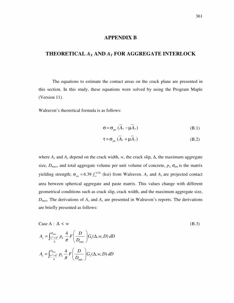
361

APPENDIX B

THEORETICAL AX AND AY FOR AGGREGATE INTERLOCK

The equations to estimate the contact areas on the crack plane are presented in

this section. In this study, these equations were solved by using the Program Maple

(Version 11).

Walraven’ s theoretical formula is as follows:

( )x ypu A Aσ = σ − µ

(B.1)

( )x ypu A Aτ = σ + µ (B.2)

where Ax and Ay depend on the crack width, w, the crack slip, ∆, the maximum aggregate

size, Dmax, and total aggregate volume per unit volume of concrete, px, σpu is the matrix

yielding strength; '0.566.39pu ccfσ = (ksi) from Walraven. Ax and Ay are projected contact

area between spherical aggregate and paste matrix. This values change with different

geometrical conditions such as crack slip, crack width, and the maximum aggregate size,

Dmax. The derivations of Ax and Ay are presented in Walraven’ s reports. The derivations

are briefly presented as follows:

Case A : w∆ < (B.3)

max2 2 1

max

4( , , )

D

wy k

DA p F G w D dD

D+∆∆

� �= ∆

� �� π

max2 2 2

max

4( , , )

D

wx k

DA p F G w D dD

D+∆∆

� �= ∆

� �� π

362

Case B : w∆ > (B.4) 22

max2 23 12

max max

4 4( , , ) ( , , )

wD

wwy k kw

w

D DA p F G w D dD p F G w D dD

D D

+∆

+∆� � � �

= ∆ + ∆ � � � �

� �π π 2 2

max2 24 12

max max

4 4( , , ) ( , , )

wD

wwx k kw

w

D DA p F G w D dD p F G w D dD

D D

+∆

+∆� � � �

= ∆ + ∆ � � � �

� �π π with

3 2 2 2 21 max max max2 2( , , ) ( )G w D D D w u w u u

w− � �∆∆ = − + ∆ − −

+ ∆� �

2 2 2 2 2max max max2 2

322

2 2 2 max

1( ) ( ) ( )

4( , , ) 1 1 2

arcsin arcsin14 4 42

wD w u u w D w u

wG w D D w u D w

w D w DDD

−

� �∆ − − + ∆ + + − +

+ ∆ ∆ = + − − + −

� �

23

3

1( , , )

2G w D D D w− � �∆ = −

� �

23 2 2 2

4

1 2( , , ) arcsin

8 4 4D w

G w D D D w D wD

− � �∆ = − − −

� �

π

363

APPENDIX C

E-VALUES FOR EVALUATING AGGREGATE INTERLOCK

This section presents the summary of E-values for estimating absorbed energy.

Tables B.1 and B.2 show the summary of E-values for river gravel and limestone

mixtures, respectively. The information is the data set for the statistical analysis to

analyze the effects of key parameters for evaluating aggregate interlock.

Table C.1. River Gravel SCC and CC Mixtures. ID Mixture Vol.CA Batch # Sam. # δ 1

(slip, mm) δ 2

(slip, mm) δ 3

(slip, mm) δ 4

(slip, mm) δ 5

(slip, mm) δ 6

(slip, mm) E1

(Energy) E2

(Energy) E3

(Energy) E4

(Energy) E5

(Energy) E6

(Energy) f’ c

(psi) ft

(psi) Pre

(kip)

PA3a_1RA SR5/31.5 31.5 1 1 0.5 0.7 1.0 2.0 4.0 5.5 4.07 3.30 2.67 1.86 1.42 1.28 12414 915 46.0

PA3a_1RB SR5/31.5 31.5 1 2 0.5 0.7 1.0 2.0 4.0 5.5 3.17 2.67 2.24 1.62 1.28 1.16 12414 915 41.0

PA3a_2RB SR5/31.5 31.5 2 3 0.5 0.7 1.0 2.0 4.0 5.5 2.74 2.44 2.15 1.64 1.28 1.17 12130 905 39.6

PA3b_1RA SR5/34.6 34.6 3 4 0.5 0.7 1.0 2.0 4.0 5.5 3.91 3.16 2.56 1.81 1.40 1.28 12393 966 26.9

PA3b_1RB SR5/34.6 34.6 3 5 0.5 0.7 1.0 2.0 4.0 5.5 3.43 2.85 2.39 1.71 1.34 1.22 12393 966 40.8

PA3b_2RB SR5/34.6 34.6 4 6 0.5 0.7 1.0 2.0 4.0 5.5 3.35 2.80 2.31 1.71 1.32 1.19 11632 804 36.3

PA3c_1RA SR5/37.8 37.8 5 7 0.5 0.7 1.0 2.0 4.0 5.5 4.09 3.22 2.52 1.77 1.37 1.25 12186 947 38.5

PA3c_1RB SR5/37.8 37.8 5 8 0.5 0.7 1.0 2.0 4.0 5.5 2.99 2.60 2.24 1.66 1.30 1.19 12186 947 45.4

PA3c_2RA SR5/37.8 37.8 6 9 0.5 0.7 1.0 2.0 4.0 5.5 3.95 3.26 2.67 1.84 1.40 1.28 11462 974 38.6

PA4_1RA SR7/32.3 32.3 7 10 0.5 0.7 1.0 2.0 4.0 5.5 2.58 2.22 1.89 1.44 1.14 1.05 14690 1089 45.6

PA4_1RB SR7/32.3 32.3 7 11 0.5 0.7 1.0 2.0 4.0 5.5 2.96 2.52 2.14 1.60 1.23 1.10 14690 1089 43.8

PA4_2RB SR7/32.3 32.3 8 12 0.5 0.7 1.0 2.0 4.0 5.5 2.62 2.24 1.90 1.46 1.16 1.06 14860 1227 43.1

PA5_1A SR7/35 35 9 13 0.5 0.7 1.0 2.0 4.0 5.5 3.17 2.65 2.18 1.56 1.20 1.16 15167 1088 36.7

PA5_1B SR7/35 35 9 14 0.5 0.7 1.0 2.0 4.0 5.5 3.54 3.17 2.65 1.83 1.34 1.19 15167 1088 41.4

PA5_2B SR7/35 35 10 15 0.5 0.7 1.0 2.0 4.0 5.5 2.79 2.47 2.12 1.56 1.25 1.15 15539 1046 43.6

PA6_1A SR7/37.6 37.6 11 16 0.5 0.7 1.0 2.0 4.0 5.5 4.71 3.53 2.65 1.73 1.28 1.16 16008 970 39.8

PA6_1B SR7/37.6 37.6 11 17 0.5 0.7 1.0 2.0 4.0 5.5 2.65 2.40 2.13 1.63 1.27 1.17 16008 970 38.3

PA6_2B SR7/37.6 37.6 12 18 0.5 0.7 1.0 2.0 4.0 5.5 2.59 2.35 2.07 1.48 1.16 1.08 16072 967 47.0

CG1_1A CR5/44.3 44.3 13 19 0.5 0.7 1.0 2.0 4.0 5.5 3.44 3.00 2.55 1.77 1.27 1.14 10353 961 39.5

CG1_1B CR5/44.3 44.3 13 20 0.5 0.7 1.0 2.0 4.0 5.5 3.98 3.42 2.91 2.00 1.38 1.20 10353 961 44.4

CG1_2A CR5/44.3 44.3 14 21 0.5 0.7 1.0 2.0 4.0 5.5 5.75 4.36 3.42 2.12 1.49 1.32 10449 973 41.6

CG2_1A CR7/44.3 44.3 15 22 0.5 0.7 1.0 2.0 4.0 5.5 3.18 2.81 2.44 1.87 1.32 0.95 12552 1004 45.2

CG2_1B CR7/44.3 44.3 15 23 0.5 0.7 1.0 2.0 4.0 5.5 3.76 3.04 2.54 1.81 1.34 1.18 12552 1004 52.7

CG2_2B CR7/44.3 44.3 16 24 0.5 0.7 1.0 2.0 4.0 5.5 2.42 2.21 1.97 1.55 1.24 1.14 11345 1020 53.9

Note: Pre = Precracking load. �

�� ���

364

Table C.2. Limestone SCC and CC Mixtures. ID Mixture Vol.CA Batch # Sam. # δ 1

(slip, mm) δ 2

(slip, mm) δ 3

(slip, mm) δ 4

(slip, mm) δ 5

(slip, mm) δ 6

(slip, mm) E1

(Energy) E2

(Energy) E3

(Energy) E4

(Energy) E5

(Energy) E6

(Energy) f’ c

(psi) ft

(psi) Pre

(kip)

PB3a_1B SL5/29.0 29 17 25 0.5 0.7 1.0 2.0 4.0 5.5 2.07 1.80 1.59 1.30 1.10 1.04 14274 958 31.8

PB3a_1A SL5/29.0 29 18 26 0.5 0.7 1.0 2.0 4.0 5.5 2.24 2.01 1.81 1.50 1.27 1.20 14274 958 27.6

PB3a_2B SL5/29.0 29 17 27 0.5 0.7 1.0 2.0 4.0 5.5 1.76 1.62 1.48 1.26 1.08 1.01 14207 879 31.5

PB3b_1A SL5/31.9 31.9 19 28 0.5 0.7 1.0 2.0 4.0 5.5 1.47 1.42 1.34 1.17 1.04 0.99 13441 831 34.8

PB3b_1B SL5/31.9 31.9 19 29 0.5 0.7 1.0 2.0 4.0 5.5 2.03 1.79 1.57 1.28 1.08 1.02 13441 831 32.6

PB3b_2A SL5/31.9 31.9 20 30 0.5 0.7 1.0 2.0 4.0 5.5 1.71 1.59 1.47 1.28 1.11 1.06 13345 973 32.6

3c_1B SL5/34.8 34.8 21 31 0.5 0.7 1.0 2.0 4.0 5.5 2.24 1.90 1.61 1.25 1.04 0.98 13297 885 32.4

PB3c_2A SL5/34.8 34.8 22 32 0.5 0.7 1.0 2.0 4.0 5.5 2.10 1.80 1.58 1.25 1.04 1.00 12910 810 34.4

PB3c_1A SL5/34.8 34.8 21 33 0.5 0.7 1.0 2.0 4.0 5.5 2.38 2.00 1.70 1.35 1.12 1.05 13297 885 31.9

PB4_1A SL7/31.9 31.9 23 34 0.5 0.7 1.0 2.0 4.0 5.5 2.05 1.80 1.59 1.28 1.07 1.01 15711 1244 36.7

PB4_1B SL7/31.9 31.9 23 35 0.5 0.7 1.0 2.0 4.0 5.5 1.97 1.73 1.53 1.27 1.11 1.05 15711 1244 28.8

PB4_2B SL7/31.9 31.9 24 36 0.5 0.7 1.0 2.0 4.0 5.5 1.92 1.85 1.56 1.20 1.02 0.97 15014 988 36.7

PB5_1A SL7/34.5 34.5 25 37 0.5 0.7 1.0 2.0 4.0 5.5 1.72 1.62 1.51 1.28 1.06 1.00 15817 975 38.4

PB5_2B SL7/34.5 34.5 26 38 0.5 0.7 1.0 2.0 4.0 5.5 1.62 1.50 1.39 1.20 1.04 0.98 16311 1134 34.9

PB5_1A SL7/34.5 34.5 25 39 0.5 0.7 1.0 2.0 4.0 5.5 2.01 1.82 1.63 1.30 1.09 1.02 15817 975 32.6

PB6_1A SL7/37 37 27 40 0.5 0.7 1.0 2.0 4.0 5.5 1.90 1.72 1.54 1.27 1.07 1.00 15221 878 35.6

PB6_1B SL7/37 37 27 41 0.5 0.7 1.0 2.0 4.0 5.5 2.03 1.80 1.57 1.26 1.06 1.01 15221 878 35.2

PB6_2B SL7/37 37 28 42 0.5 0.7 1.0 2.0 4.0 5.5 1.98 1.77 1.59 1.32 1.13 1.06 15412 880 33.4

CL1_2A CL5/40.1 40.1 29 43 0.5 0.7 1.0 2.0 4.0 5.5 3.29 2.70 2.19 1.54 1.21 1.11 10316 764 31.6

CL1_2B CL5/40.1 40.1 29 44 0.5 0.7 1.0 2.0 4.0 5.5 2.42 2.12 1.84 1.43 1.19 1.10 10316 764 33.8

CL1_1A CL5/40.1 40.1 30 45 0.5 0.7 1.0 2.0 4.0 5.5 2.76 2.36 2.01 1.56 1.27 1.16 8143 820 30.8

CL2_1B CL7/40.1 40.1 31 46 0.5 0.7 1.0 2.0 4.0 5.5 3.25 2.46 1.90 1.29 0.96 0.87 13345 1001 34.4

CL2_1A CL7/40.1 40.1 31 47 0.5 0.7 1.0 2.0 4.0 5.5 5.16 3.68 2.66 1.69 1.25 1.12 13345 1001 38.0

CL2_2B CL7/40.1 40.1 32 48 0.5 0.7 1.0 2.0 4.0 5.5 3.38 2.70 2.11 1.45 1.15 1.06 13510 979 28.6

Note: Pre = Precracking load.

��

� ��� 365

APPENDIX D

STATISTICAL ANAYSIS FOR SHEAR CHARACTERISTICS

This section show the source file to analyze the data to evaluate the effect of key parameters.

D. 1 Statistical Analysis for Effect of Volume of Coarse Aggregate at Individual Crack Slip

* proc mixed procedure; * separate analyses for each delta; * set up for HTML ouput; ods html; ods graphics on; * each mix has two batches, one with 2 samples and the other with 1; * samples are measured repeatedly (6 times here), once for each value of delta; data SHEAR1; array w w1-w3; array d d1-d3; array n n1-n3; array s s1-s3; array x x1-x3; array y y1-y3; array z z1-z3; array w w1-w3; array c c1-c3; array m m1-m3; input mix $ agg $ vol batch $ sample $ w1-w3 d1-d3 n1-n3 s1-s3 x1-x3 y1-y3 paste z1-z3 w1-w3 comp c1-c3 m1-m3; * agg=aggregate type com=avg. compressive strength, split=avg. splitting tensile strength, pre=precracking load; do over e; energy=e; delta=d; output; end; drop d1-d6 e1-e6; cards; ;;;

��

� ��� 366

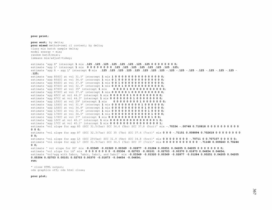
proc print; proc sort; by delta; proc mixed method=reml cl covtest; by delta; class mix batch sample delta; model energy = mix; random batch(mix); lsmeans mix/adjust=tukey; estimate ‘agg R’ intercept 1 mix .125 .125 .125 .125 .125 .125 .125 .125 0 0 0 0 0 0 0 0; estimate ‘agg L’ intercept 1 mix 0 0 0 0 0 0 0 0 .125 .125 .125 .125 .125 .125 .125 .125; estimate ‘agg R - agg L’ intercept 0 mix .125 .125 .125 .125 .125 .125 .125 .125 -.125 -.125 -.125 -.125 -.125 -.125 -.125 -.125; estimate ‘agg R5SCC at vol 31.5’ intercept 1 mix 1 0 0 0 0 0 0 0 0 0 0 0 0 0 0 0; estimate ‘agg R5SCC at vol 34.6’ intercept 1 mix 0 1 0 0 0 0 0 0 0 0 0 0 0 0 0 0; estimate ‘agg R5SCC at vol 37.8’ intercept 1 mix 0 0 1 0 0 0 0 0 0 0 0 0 0 0 0 0; estimate ‘agg R7SCC at vol 32.3’ intercept 1 mix 0 0 0 1 0 0 0 0 0 0 0 0 0 0 0 0; estimate ‘agg R7SCC at vol 35’ intercept 1 mix 0 0 0 0 1 0 0 0 0 0 0 0 0 0 0 0; estimate ‘agg R7SCC at vol 37.6’ intercept 1 mix 0 0 0 0 0 1 0 0 0 0 0 0 0 0 0 0; estimate ‘agg R5CC at vol 44.3’ intercept 1 mix 0 0 0 0 0 0 1 0 0 0 0 0 0 0 0 0; estimate ‘agg R7CC at vol 44.3’ intercept 1 mix 0 0 0 0 0 0 0 1 0 0 0 0 0 0 0 0; estimate ‘agg L5SCC at vol 29’ intercept 1 mix 0 0 0 0 0 0 0 0 1 0 0 0 0 0 0 0; estimate ‘agg L5SCC at vol 31.9’ intercept 1 mix 0 0 0 0 0 0 0 0 0 1 0 0 0 0 0 0; estimate ‘agg L5SCC at vol 34.8’ intercept 1 mix 0 0 0 0 0 0 0 0 0 0 1 0 0 0 0 0; estimate ‘agg L7SCC at vol 31.9’ intercept 1 mix 0 0 0 0 0 0 0 0 0 0 0 1 0 0 0 0; estimate ‘agg L7SCC at vol 34.5’ intercept 1 mix 0 0 0 0 0 0 0 0 0 0 0 0 1 0 0 0; estimate ‘agg L7SCC at vol 37’ intercept 1 mix 0 0 0 0 0 0 0 0 0 0 0 0 0 1 0 0; estimate ‘agg L5CC at vol 40.1’ intercept 1 mix 0 0 0 0 0 0 0 0 0 0 0 0 0 0 1 0; estimate ‘agg L7CC at vol 40.1’ intercept 1 mix 0 0 0 0 0 0 0 0 0 0 0 0 0 0 0 1; estimate ‘vol slope for agg R5 (SCC 31.5(5ar) SCC 34.6 (5br) SCC 37.8 (5cr))’ mix -.70334 -.00748 0.710818 0 0 0 0 0 0 0 0 0 0 0 0 0; estimate ‘vol slope for agg R7 (SCC 32.3(7ar) SCC 35 (7br) SCC 37.6 (7cr))’ mix 0 0 0 -.71151 0.008894 0.702618 0 0 0 0 0 0 0 0 0 0; estimate ‘vol slope for agg L5 (SCC 29(5ar) SCC 31.9 (5br) SCC 34.8 (5cr))’ mix 0 0 0 0 0 0 0 0 -.70711 0 0.707107 0 0 0 0 0; estimate ‘vol slope for agg L7 (SCC 31.9(7ar) SCC 34.5 (7br) SCC 37 (7cr))’ mix 0 0 0 0 0 0 0 0 0 0 0 -.71168 0.009243 0.70244 0 0; estimate ‘ vol slope for SG’ mix -0.03349 -0.01520 0.00369 -0.02877 -0.01284 0.00251 0.04205 0.04205 0 0 0 0 0 0 0 0; estimate ‘vol slope for LG’ mix 0 0 0 0 0 0 0 0 -0.05304 -0.02703 -0.00101 -0.02703 -0.00370 0.01873 0.04654 0.04654; estimate ‘vol*agg with 5abcr, 7abcr, 5abcl, and 5abcl’ mix -0.03349 -0.01520 0.00369 -0.02877 -0.01284 0.00251 0.04205 0.04205 0.05304 0.02703 0.00101 0.02703 0.00370 -0.01873 -0.04654 -0.04654; run; * close HTML output; ods graphics off; ods html close; proc plot;

��

� ��� 367

plot split*comp=‘+’; plot split*pre=‘x’; plot comp*pre=‘*’; run; * close HTML output; ods graphics off; ods html close;

D. 2 Statistical Analysis for Effect of Volume of Coarse Aggregate Across Crack Slip

* repeated measured analyses for each delta; * set up for HTML ouput; ods html; ods graphics on; * each mix has two batches, one with 2 samples and the other with 1; * the first batch thus has 2 reps at each time, the second only 1; * samples are measured repeatedly (6 times here), once for each value of delta; data SHEAR4; array e e1-e6; array d d1-d6; input mix $ agg $ vol batch $ sample $ d1-d6 e1-e6 comp split pre; * agg=aggregate type com=avg. compressive strength, split=avg. splitting tensle strength, pre=precracking load; do over e; energy=e; delta=d; output; end; drop d1-d6 e1-e6; cards; ;;; proc print; run; * compare mixes across delta, with interaction; proc mixed method=reml cl covtest; class mix batch sample delta; * order variables consistently with the model; model energy = mix|delta; random batch(mix); repeated delta/subject=sample type=unr r=1; * subjects must all be labeled differently; lsmeans mix/adjust=tukey;

��

� ��� 368

estimate ‘agg R’ intercept 1 mix .125 .125 .125 .125 .125 .125 .125 .125 0 0 0 0 0 0 0 0; estimate ‘agg L’ intercept 1 mix 0 0 0 0 0 0 0 0 .125 .125 .125 .125 .125 .125 .125 .125; estimate ‘agg R - agg L’ intercept 0 mix .125 .125 .125 .125 .125 .125 .125 .125 -.125 -.125 -.125 -.125 -.125 -.125 -.125 -.125; estimate ‘agg R5SCC at vol 31.5’ intercept 1 mix 1 0 0 0 0 0 0 0 0 0 0 0 0 0 0 0; estimate ‘agg R5SCC at vol 34.6’ intercept 1 mix 0 1 0 0 0 0 0 0 0 0 0 0 0 0 0 0; estimate ‘agg R5SCC at vol 37.8’ intercept 1 mix 0 0 1 0 0 0 0 0 0 0 0 0 0 0 0 0; estimate ‘agg R7SCC at vol 32.3’ intercept 1 mix 0 0 0 1 0 0 0 0 0 0 0 0 0 0 0 0; estimate ‘agg R7SCC at vol 35’ intercept 1 mix 0 0 0 0 1 0 0 0 0 0 0 0 0 0 0 0; estimate ‘agg R7SCC at vol 37.6’ intercept 1 mix 0 0 0 0 0 1 0 0 0 0 0 0 0 0 0 0; estimate ‘agg R5CC at vol 44.3’ intercept 1 mix 0 0 0 0 0 0 1 0 0 0 0 0 0 0 0 0; estimate ‘agg R7CC at vol 44.3’ intercept 1 mix 0 0 0 0 0 0 0 1 0 0 0 0 0 0 0 0; estimate ‘agg L5SCC at vol 29’ intercept 1 mix 0 0 0 0 0 0 0 0 1 0 0 0 0 0 0 0; estimate ‘agg L5SCC at vol 31.9’ intercept 1 mix 0 0 0 0 0 0 0 0 0 1 0 0 0 0 0 0; estimate ‘agg L5SCC at vol 34.8’ intercept 1 mix 0 0 0 0 0 0 0 0 0 0 1 0 0 0 0 0; estimate ‘agg L7SCC at vol 31.9’ intercept 1 mix 0 0 0 0 0 0 0 0 0 0 0 1 0 0 0 0; estimate ‘agg L7SCC at vol 34.5’ intercept 1 mix 0 0 0 0 0 0 0 0 0 0 0 0 1 0 0 0; estimate ‘agg L7SCC at vol 37’ intercept 1 mix 0 0 0 0 0 0 0 0 0 0 0 0 0 1 0 0; estimate ‘agg L5CC at vol 40.1’ intercept 1 mix 0 0 0 0 0 0 0 0 0 0 0 0 0 0 1 0; estimate ‘agg L7CC at vol 40.1’ intercept 1 mix 0 0 0 0 0 0 0 0 0 0 0 0 0 0 0 1; estimate ‘vol slope for agg R5 (SCC 31.5(5ar) SCC 34.6 (5br) SCC 37.8 (5cr))’ mix -.70334 -.00748 0.710818 0 0 0 0 0 0 0 0 0 0 0 0 0; estimate ‘vol slope for agg R7 (SCC 32.3(7ar) SCC 35 (7br) SCC 37.6 (7cr))’ mix 0 0 0 -.71151 0.008894 0.702618 0 0 0 0 0 0 0 0 0 0; estimate ‘vol slope for agg L5 (SCC 29(5ar) SCC 31.9 (5br) SCC 34.8 (5cr))’ mix 0 0 0 0 0 0 0 0 -.70711 0 0.707107 0 0 0 0 0; estimate ‘vol slope for agg L7 (SCC 31.9(7ar) SCC 34.5 (7br) SCC 37 (7cr))’ mix 0 0 0 0 0 0 0 0 0 0 0 -.71168 0.009243 0.70244 0 0; estimate ‘ vol slope for SG’ mix -0.03349 -0.01520 0.00369 -0.02877 -0.01284 0.00251 0.04205 0.04205 0 0 0 0 0 0 0 0; estimate ‘vol slope for LG’ mix 0 0 0 0 0 0 0 0 -0.05304 -0.02703 -0.00101 -0.02703 -0.00370 0.01873 0.04654 0.04654; estimate ‘vol*agg with 5abcr, 7abcr, 5abcl, and 5abcl’ mix -0.03349 -0.01520 0.00369 -0.02877 -0.01284 0.00251 0.04205 0.04205 0.05304 0.02703 0.00101 0.02703 0.00370 -0.01873 -0.04654 -0.04654; run; * repeat above but assume toeplitz correlation structure (although this probably is not appropriate for unequally spaced deltas); proc mixed method=reml cl covtest; class mix batch sample delta; * order variables consistently with the model; model energy = mix|delta; random batch(mix); repeated delta/subject=sample type=toeph r=1; * subjects must all be labeled differently; run; * close HTML output; ods graphics off; ods html close;

��

� ��� 369

D. 3 Statistical Analysis Friction Factor and Fracture Reduction Factor

* separate analyses for each width; * set up for HTML ouput; ods html; ods graphics on; * each mix has two batches, one with 2 samples and the other with 1; * samples are measured repeatedly (3 times here), once for each value of width; data SHEAR1; array w w1-w3; array d d1-d3; array n n1-n3; array s s1-s3; array x x1-x3; array y y1-y3; array z z1-z3; array a a1-a3; array c c1-c3; array m m1-m3; input mix $ agg $ vol batch $ sample $ w1-w3 d1-d3 n1-n3 s1-s3 x1-x3 y1-y3 paste z1-z3 a1-a3 comp c1-c3 cm1-cm3 m1-m3; * agg=aggregate type com=avg. compressive strength,n=normal stress, s=shear stress, x=Ax, y=Ay, paste=paste strength, z=c*paste, a=c*m*paste, c=fracture factor, m=firction factor; If sample =20 then delete;If sample =22 then delete; do over c; fracture =c; friction=m; width=w; output; end; drop w1-w3 d1-d3 n1-n3 s1-s3 x1-x3 y1-y3 z1-z3 a1-a3 c1-c3 cm1-cm3 m1-m3; cards; ;;; proc print; proc sort; by width; proc mixed method=reml cl covtest; by width; class mix batch sample width; model fracture = mix; *model friction = mix; random batch(mix); lsmeans mix/adjust=tukey; estimate ‘All’ intercept 1 mix .0625 .0625 .0625 .0625 .0625 .0625 .0625 .0625 .0625 .0625 .0625 .0625 .0625 .0625 .0625 .0625; estimate ‘agg R’ intercept 1 mix .125 .125 .125 .125 .125 .125 .125 .125 0 0 0 0 0 0 0 0; estimate ‘agg L’ intercept 1 mix 0 0 0 0 0 0 0 0 .125 .125 .125 .125 .125 .125 .125 .125; estimate ‘agg R - agg L’ intercept 0 mix .125 .125 .125 .125 .125 .125 .125 .125 -.125 -.125 -.125 -.125 -.125 -.125 -.125 -.125; estimate ‘agg SR’ intercept 1 mix .166667 .166667 .166667 .166667 .166667 .166667 0 0 0 0 0 0 0 0 0 0; estimate ‘agg SL’ intercept 1 mix 0 0 0 0 0 0 0 0 .166667 .166667 .166667 .166667 .166667 .166667 0 0; estimate ‘agg CR’ intercept 1 mix 0 0 0 0 0 0 0.5 0.5 0 0 0 0 0 0 0 0; estimate ‘agg CL’ intercept 1 mix 0 0 0 0 0 0 0 0 0 0 0 0 0 0 0.5 0.5;

��

� ��� 370

estimate ‘ SCC’ intercept 1 mix .083333 .083333 .083333 .083333 .083333 .083333 0 0 .083333 .083333 .083333 .083333 .083333 .083333 0 0; estimate ‘CC’ intercept 1 mix 0 0 0 0 0 0 .25 .25 0 0 0 0 0 0 .25 .25; estimate ‘SCC-CC’ intercept 1 mix .083333 .083333 .083333 .083333 .083333 .083333 -.25 -.25 .083333 .083333 .083333 .083333 .083333 .083333 -.25 -.25; *estimate ‘agg R5SCC at vol 31.5’ intercept 1 mix 1 0 0 0 0 0 0 0 0 0 0 0 0 0 0 0; *estimate ‘agg R5SCC at vol 34.6’ intercept 1 mix 0 1 0 0 0 0 0 0 0 0 0 0 0 0 0 0; *estimate ‘agg R5SCC at vol 37.8’ intercept 1 mix 0 0 1 0 0 0 0 0 0 0 0 0 0 0 0 0; *estimate ‘agg R7SCC at vol 32.3’ intercept 1 mix 0 0 0 1 0 0 0 0 0 0 0 0 0 0 0 0; *estimate ‘agg R7SCC at vol 35’ intercept 1 mix 0 0 0 0 1 0 0 0 0 0 0 0 0 0 0 0; *estimate ‘agg R7SCC at vol 37.6’ intercept 1 mix 0 0 0 0 0 1 0 0 0 0 0 0 0 0 0 0; *estimate ‘agg R5CC at vol 44.3’ intercept 1 mix 0 0 0 0 0 0 1 0 0 0 0 0 0 0 0 0; *estimate ‘agg R7CC at vol 44.3’ intercept 1 mix 0 0 0 0 0 0 0 1 0 0 0 0 0 0 0 0; *estimate ‘agg L5SCC at vol 29’ intercept 1 mix 0 0 0 0 0 0 0 0 1 0 0 0 0 0 0 0; *estimate ‘agg L5SCC at vol 31.9’ intercept 1 mix 0 0 0 0 0 0 0 0 0 1 0 0 0 0 0 0; *estimate ‘agg L5SCC at vol 34.8’ intercept 1 mix 0 0 0 0 0 0 0 0 0 0 1 0 0 0 0 0; *estimate ‘agg L7SCC at vol 31.9’ intercept 1 mix 0 0 0 0 0 0 0 0 0 0 0 1 0 0 0 0; *estimate ‘agg L7SCC at vol 34.5’ intercept 1 mix 0 0 0 0 0 0 0 0 0 0 0 0 1 0 0 0; *estimate ‘agg L7SCC at vol 37’ intercept 1 mix 0 0 0 0 0 0 0 0 0 0 0 0 0 1 0 0; *estimate ‘agg L5CC at vol 40.1’ intercept 1 mix 0 0 0 0 0 0 0 0 0 0 0 0 0 0 1 0; *estimate ‘agg L7CC at vol 40.1’ intercept 1 mix 0 0 0 0 0 0 0 0 0 0 0 0 0 0 0 1; *estimate ‘vol slope for agg R5 (SCC 31.5(5ar) SCC 34.6 (5br) SCC 37.8 (5cr))’ mix -.70334 -.00748 0.710818 0 0 0 0 0 0 0 0 0 0 0 0 0; *estimate ‘vol slope for agg R7 (SCC 32.3(7ar) SCC 35 (7br) SCC 37.6 (7cr))’ mix 0 0 0 -.71151 0.008894 0.702618 0 0 0 0 0 0 0 0 0 0; *estimate ‘vol slope for agg L5 (SCC 29(5ar) SCC 31.9 (5br) SCC 34.8 (5cr))’ mix 0 0 0 0 0 0 0 0 -.70711 0 0.707107 0 0 0 0 0; *estimate ‘vol slope for agg L7 (SCC 31.9(7ar) SCC 34.5 (7br) SCC 37 (7cr))’ mix 0 0 0 0 0 0 0 0 0 0 0 -.71168 0.009243 0.70244 0 0; estimate ‘ vol slope for SG’ mix -0.03349 -0.01520 0.00369 -0.02877 -0.01284 0.00251 0.04205 0.04205 0 0 0 0 0 0 0 0; estimate ‘vol slope for LG’ mix 0 0 0 0 0 0 0 0 -0.05304 -0.02703 -0.00101 -0.02703 -0.00370 0.01873 0.04654 0.04654; estimate ‘vol*agg with 5abcr, 7abcr, 5abcl, and 5abcl’ mix -0.03349 -0.01520 0.00369 -0.02877 -0.01284 0.00251 0.04205 0.04205 0.05304 0.02703 0.00101 0.02703 0.00370 -0.01873 -0.04654 -0.04654; run; * close HTML output; ods graphics off; ods html close; proc plot; plot fracture*comp=‘+’; plot friction*comp=‘x’; *plot comp*pre=‘*’; run; * close HTML output; ods graphics off; ods html close;

��

� ��� 371

372

APPENDIX E

STRAINS OF CHANNELS FOR CREEP

This section provides the data of each channel. These data were used to evaluate

the creep of SCC and CC in this study. Figures E.1 – E.8 show the creep and shrinkage

data of each mixture.

Figure E.1. Creep and Shrinkage for Batches S5G-3c.

Figure E.2. Creep and Shrinkage for Batches S7G-3c.

0

500

1000

1500

2000

2500

Ch 25 (CR)Ch 26 (CR)Ch 27 (CR)Ch 28 (CR)Ch 29 (SH)Ch 30 (SH)

0 50 100 150

Stra

in (x

10-6

in./i

n. o

r mm

/mm

)

Time After Loading (Days)

S5G-3c

0

500

1000

1500

2000

2500

Ch 37 (CR)Ch 38 (CR)Ch 39 (CR)Ch 40 (CR)Ch 41 (SH)Ch 42 (SH)

0 50 100 150

Stra

in (x

10-6

in./i

n. o

r mm

/mm

)

Time After Loading (Days)

S7G-3c

Gage Failed

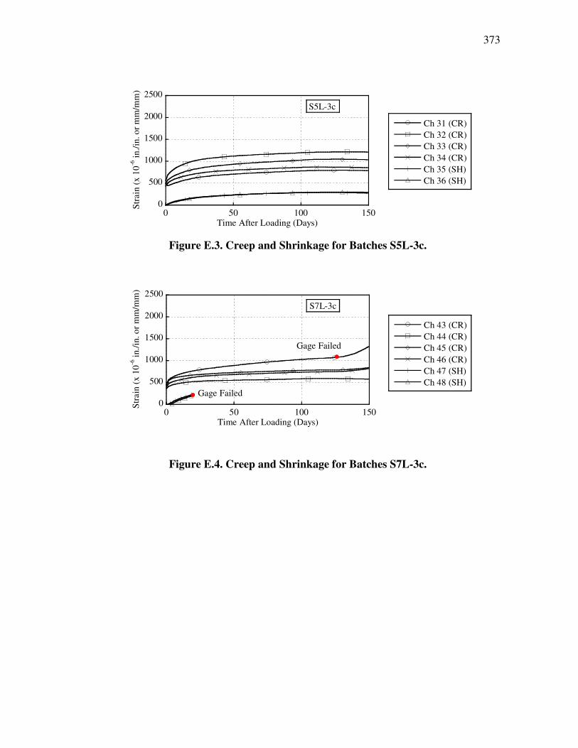
373

Figure E.3. Creep and Shrinkage for Batches S5L-3c.

Figure E.4. Creep and Shrinkage for Batches S7L-3c.

0

500

1000

1500

2000

2500

Ch 31 (CR)Ch 32 (CR)Ch 33 (CR)Ch 34 (CR)Ch 35 (SH)Ch 36 (SH)

0 50 100 150

Stra

in (x

10-6

in./i

n. o

r mm

/mm

)

Time After Loading (Days)

S5L-3c

0

500

1000

1500

2000

2500

Ch 43 (CR)Ch 44 (CR)Ch 45 (CR)Ch 46 (CR)Ch 47 (SH)Ch 48 (SH)

0 50 100 150

Stra

in (x

10-6

in./i

n. o

r mm

/mm

)

Time After Loading (Days)

S7L-3c

Gage Failed

Gage Failed

374

Figure E.5. Creep and Shrinkage for Batches C5G.

Figure E.6. Creep and Shrinkage for Batches C7G.

0

500

1000

1500

2000

2500

Ch 19 (CR)Ch 20 (CR)Ch 21 (CR)Ch 22 (CR)Ch 23 (SH)Ch 24 (SH)

0 50 100 150

Stra

in (x

10-6

in./i

n. o

r mm

/mm

)

Time After Loading (Days)

C5G

Gage Failed

0

500

1000

1500

2000

2500

Ch 13 (CR)Ch 14 (CR)Ch 15 (CR)Ch 16 (CR)Ch 17 (SH)Ch 18 (SH)

0 50 100 150

Stra

in (x

10-6

in./i

n. o

r mm

/mm

)

Time After Loading (Days)

C7G

Gage Failed

375

Figure E.7 Creep and Shrinkage for Batches C5L.

Figure E.8. Creep and Shrinkage for Batches C7L.

0

500

1000

1500

2000

2500

Ch 7 (CR)Ch 8 (CR)Ch 9 (CR)Ch 10 (CR)Ch 11 (SH)Ch 12 (SH)

0 50 100 150

Stra

in (x

10-6

in./i

n. o

r mm

/mm

)

Time After Loading (Days)

C5L

Gage Failed

0

500

1000

1500

2000

2500

Ch 1 (CR)Ch 2 (CR)Ch 3 (CR)Ch 4 (CR)Ch 5 (SH)Ch 6 (SH)

0 50 100 150

Stra

in (x

10-6

in./i

n. o

r mm

/mm

)

Time After Loading (Days)

C7L

Gage Failed

376

APPENDIX F

COMPARISONS OF CREEP

This section provides the comparisons between two mixtures to compare the

effect of key parameters. Figure F.1 shows the comparisons between creep of different

mixtures having different target strength at 16 hours.

377

(a) SCC River Gravel (b) CC River Gravel

(c) SCC Limestone (d) CC Limestone

Figure F.1. Creep of Compressive Strength (5 ksi [34 MPa] versus 7 ksi [48 MPa]).

0

500

1000

1500

S5G-3c (CR)S7G-6 (CR)

0 50 100 150

Stra

in (x

10-6

in./i

n. o

r mm

/mm

)

Time After Loading (Days)

0

500

1000

1500

C5G (CR)C7G (CR)

0 50 100 150

Stra

in (x

10-6

in./i

n. o

r mm

/mm

)

Time After Loading (Days)

0

500

1000

1500

S7L-6 (CR+SH)S5L-3c (SH)

0 50 100 150

Stra

in (x

10-6

in./i

n. o

r mm

/mm

)

Time After Loading (Days)

0

500

1000

1500

C5L (CR)C7L (CR)

0 50 100 150

Stra

in (x

10-6

in./i

n. o

r mm

/mm

)

Time After Loading (Days)

378

Figure F.2 shows the comparisons between creep of different mixtures having

different type of aggregate.

(a) SCC 5 ksi (35 MPa) (b) CC 5 ksi (35 MPa)

(c) SCC 7 ksi (48 MPa) (d) CC 7 ksi (48 MPa)

Figure F.2. Creep of Aggregate Type.

0

500

1000

1500

S5G-3c (CR)

S5L-3c (CR)

0 50 100 150

Stra

in (x

10-6

in./i

n. o

r mm

/mm

)

Time After Loading (Days)

0

500

1000

1500

C5G (CR)C5L (CR)

0 50 100 150

Stra

in (x

10-6

in./i

n. o

r mm

/mm

)

Time After Loading (Days)

0

500

1000

1500

S7G-6 (SH)S7L-6 (CR+SH)

0 50 100 150

Stra

in (x

10-6

in./i

n.)

Time After Loading (Days)

0

500

1000

1500

C7G (CR)C7L (CR)

0 50 100 150

Stra

in (x

10-6

in./i

n. o

r mm

/mm

)

Time After Loading (Days)

379

APPENDIX G

PREDICTION AND MEASURED VALUE FOR CREEP

Figures G.1 – G.8 shows the creep and shrinkage of each mixture with prediction

curves.

Figure G.1. Creep and Shrinkage versus Predictions for S5G-3c.

0

500

1000

1500

2000

2500

S5G-3c CreepS5G-3c ShrinkageAASHTO LRFD (2004) CreepAASHTO LRFD (2006) CreepACI 209 (1992) Creep

CEB (1993) CreepBP Model (1984) CreepB3 Model (2000) CreepGL 2000 Model (2001) Creep

0 50 100 150

Stra

in (x

10-6

in./i

n. o

r mm

/mm

)

Time After Loading (Days)

S5G-3c

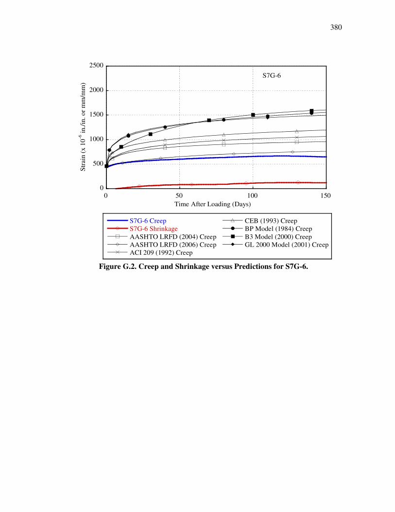
380

Figure G.2. Creep and Shrinkage versus Predictions for S7G-6.

0

500

1000

1500

2000

2500

S7G-6 CreepS7G-6 ShrinkageAASHTO LRFD (2004) CreepAASHTO LRFD (2006) CreepACI 209 (1992) Creep

CEB (1993) CreepBP Model (1984) CreepB3 Model (2000) CreepGL 2000 Model (2001) Creep

0 50 100 150Time After Loading (Days)

S7G-6St

rain

(x 1

0-6 in

./in.

or m

m/m

m)

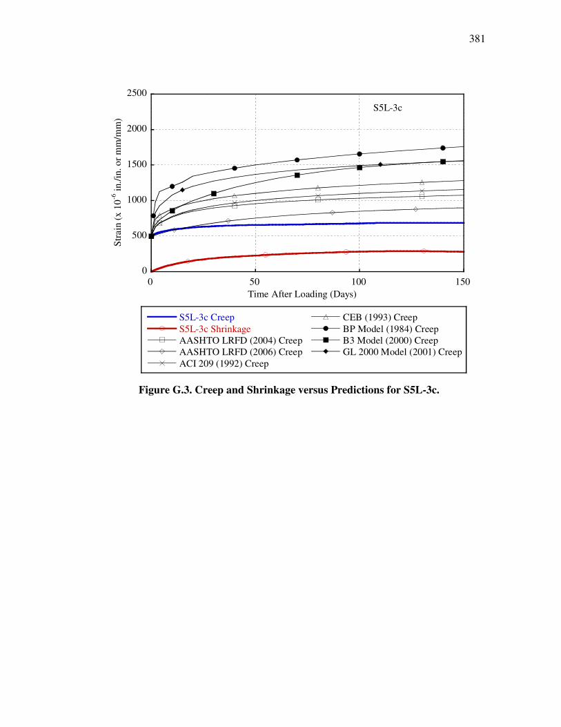
381

Figure G.3. Creep and Shrinkage versus Predictions for S5L-3c.

0

500

1000

1500

2000

2500

S5L-3c CreepS5L-3c ShrinkageAASHTO LRFD (2004) CreepAASHTO LRFD (2006) CreepACI 209 (1992) Creep

CEB (1993) CreepBP Model (1984) CreepB3 Model (2000) CreepGL 2000 Model (2001) Creep

0 50 100 150Time After Loading (Days)

S5L-3cSt

rain

(x 1

0-6 in

./in.

or m

m/m

m)

382

Figure G.4. Creep and Shrinkage versus Predictions for S7L-6.

0

500

1000

1500

2000

2500

S7L-6 (Creep+Shrinkage)S7L-6 ShrinkageAASHTO LRFD (2004) CreepAASHTO LRFD (2006) CreepACI 209 (1992) Creep

CEB (1993) CreepBP Model (1984) CreepB3 Model (2000) CreepGL 2000 Model (2001) Creep

0 50 100 150Time After Loading (Days)

S7L-6St

rain

(x 1

0-6 in

./in.

or m

m/m

m)

383

Figure G.5. Creep and Shrinkage versus Predictions for C5G.

0

500

1000

1500

2000

2500

C5G CreepC5G ShrinkageAASHTO LRFD (2004) CreepAASHTO LRFD (2006) CreepACI 209 (1992) Creep

CEB (1993) CreepBP Model (1984) CreepB3 Model (2000) CreepGL 2000 Model (2001) Creep

0 50 100 150Time After Loading (Days)

C5GSt

rain

(x 1

0-6 in

./in.

or m

m/m

m)

384

Figure G.6. Creep and Shrinkage versus Predictions for C7G.

0

500

1000

1500

2000

2500

C7G CreepC7G ShrinkageAASHTO LRFD (2004) CreepAASHTO LRFD (2006) CreepACI 209 (1992) Creep

CEB (1993) CreepBP Model (1984) CreepB3 Model (2000) CreepGL 2000 Model (2001) Creep

0 50 100 150Time After Loading (Days)

C7GSt

rain

(x 1

0-6 in

./in.

or m

m/m

m)

385

Figure G.7. Creep and Shrinkage versus Predictions for C5L.

0

500

1000

1500

2000

2500

C5L CreepC5L ShrinkageAASHTO LRFD (2004) CreepAASHTO LRFD (2006) CreepACI 209 (1992) Creep

CEB (1993) CreepBP Model (1984) CreepB3 Model (2000) CreepGL 2000 Model (2001) Creep

0 50 100 150Time After Loading (Days)

C5LSt

rain

(x 1

0-6 in

./in.

or m

m/m

m)

386

Figure G.8. Creep and Shrinkage versus Predictions for C7L.

0

500

1000

1500

2000

2500

C7L CreepC7L ShrinkageAASHTO LRFD (2004) CreepAASHTO LRFD (2006) CreepACI 209 (1992) Creep

CEB (1993) CreepBP Model (1984) CreepB3 Model (2000) CreepGL 2000 Model (2001) Creep

0 50 100 150Time After Loading (Days)

C7LSt

rain

(x 1

0-6 in

./in.

or m

m/m

m)

387

VITA

Name: Young Hoon Kim

Address: Department of Civil Engineering, Texas A&M University, 3136 TAMU, College Station, Texas 77843-3136 Email Address: yhkim05@tamu.edu Education: B.E., Civil Engineering, Korea University, 2000 M.S., Civil Engineering, Korea University, 2003 Ph.D., Civil Engineering, Texas A&M University, 2008