080105884 Dissertation
82
MATERIAL FAILURE SIMULATED WITH 2D TRUSS DYNAMICS Dissertation submitted as part requirement for the degree of Master of Science in Structural Engineering. By Muhammad Bilal Shah Supervisor Prof. Harm Askes The University of Sheffield Department of Civil and Structural Engineering September 2009
Transcript of 080105884 Dissertation

MATERIAL FAILURE SIMULATED WITH 2D TRUSS DYNAMICS
Dissertation submitted as part requirement for the degree of Master of Science in
Structural Engineering.
By
Muhammad Bilal Shah
Supervisor
Prof. Harm Askes
The University of Sheffield
Department of Civil and Structural Engineering
September 2009

ii
Muhammad Bilal Shah certifies that all the material contained within this document
is his own work except where it is clearly referenced to others.
_
(Signature)

iii
Acknowledgement
First of all, I would like to thank God, the Almighty, for making everything possible
by giving me strength and ability to accomplish this dissertation.
I would like to thank Prof. Harm Askes for all his support and guidance throughout
this dissertation. It was his constant encouragement and appreciation that kept me
going throughout this dissertation.
I would like to thank my family and friends for all their support throughout this
dissertation. A special thanks to my brother who funded my masters and supported
me all the way through my masters.

iv
Abstract
Failure of an engineering material is almost always not a desirable event. One of the
modes of failure of materials is through cracking of the material. It is possible
simulate material failure using finite element analysis. In fact one of the very first
applications of finite element analysis was analysis of structures. In this dissertation
we will utilize finite element method to simulate material failure.
This dissertation can broadly be divided in two phases. In the first phase, a computer
application incorporating finite element analysis was developed using MatLab. The
developed application simulates a simple beam structure by generating a finite
element lattice model made up of finite bar elements. The capability of simulating
material heterogeneity is incorporated in the program to simulate materials like
concrete. Dynamic analysis of the structure can be performed by the program using
implicit direct integration Newmark constant average acceleration method. Stress
patterns in the beam material are also generated simulating material failure.
In the second phase of the dissertation a number of analyses were carried out using
the application. These tests were designed keeping in view the basic hypothesis of
the dissertation: possibility of modeling static tests using dynamic implementation.
The general procedure for carrying out the tests was to change a single parameter at
one time to find out the effect of changing that parameter. The results from the
analyses performed not only delivered answers to the basic hypothesis but also
verified the functionality of the application developed.
It was concluded from the results obtained from the analyses that it is possible to
model static tests using dynamic implementation provided the there is a gradual
increase in the dynamic load that is applied to the structure. It was also concluded
that heterogeneity of material may not influence the global structural behavior like
reaction forces or displacements but does have local effects like cracking of
interfaces between aggregate and cement sand matrix. Some recommendations for
further research and possible future enhancements are provided at the end of
dissertation.

v
List of Tables
Acknowledgement ........................................................................................................................ 1-iii
Abstract ........................................................................................................................................ 1-iv
List of Figures ............................................................................................................................ 1-viii
List of Tables ................................................................................................................................. 1-x
1 INTRODUCTION .................................................................................... 1
1.1 Aims and Objectives ................................................................................................................ 2
1.1.1 Aims .............................................................................................................................. 2
1.1.2 Objectives ...................................................................................................................... 2
1.2 Scope of Dissertation ............................................................................................................... 3
1.3 Outline of Dissertation ............................................................................................................. 4
2 LITERATURE REVIEW .......................................................................... 5
2.1 Fracture Mechanics.................................................................................................................. 5
2.2 Lattice Model .......................................................................................................................... 6
2.3 Material Heterogeneity ............................................................................................................ 7
2.3.1 Tensile Strength of Plain Concrete .................................................................................. 8
2.3.2 Micro-cracking in Concrete ............................................................................................ 8
2.3.3 Aggregate and Cement-Sand Matrix Interface ................................................................. 9
2.3.4 Modeling Heterogeneity in Finite Element Methods ...................................................... 10
2.4 Local Orientation of Finite Elements ...................................................................................... 11
2.5 Crack Propagation ................................................................................................................. 12
3 THEORETICAL ANALYSIS ................................................................. 14
3.1 Actual Structure ..................................................................................................................... 15
3.2 Working Model ..................................................................................................................... 15
3.2.1 Dimensions .................................................................................................................. 15
3.2.2 Materials ...................................................................................................................... 15
3.2.3 Support Conditions ....................................................................................................... 15
3.2.4 Loading Conditions ...................................................................................................... 16
3.2.5 Desired Outputs ............................................................................................................ 16
3.3 Mathematical Model .............................................................................................................. 16
3.3.1 Spatial Discretization .................................................................................................... 16
3.3.2 Choice of Finite Element .............................................................................................. 16
3.3.3 Meshing ....................................................................................................................... 17
3.3.4 Properties of Material ................................................................................................... 18
3.3.5 Boundary Conditions .................................................................................................... 19
3.3.6 Strong Form of Governing Equation ............................................................................. 19

vi
3.3.7 Weak Form .................................................................................................................. 20
3.3.8 Semi-discretized System of Equations ........................................................................... 20
3.4 Computational Model ............................................................................................................ 21
3.4.1 Element Mass Matrix .................................................................................................... 21
3.4.2 Element Stiffness Matrix .............................................................................................. 23
3.4.3 Transforming from Local Coordinates to Global Coordinates ........................................ 23
3.4.4 Assembling Element Matrices ....................................................................................... 25
3.4.5 Time Discretization ...................................................................................................... 25
4 APPLICATION DEVELOPMENT ......................................................... 28
4.1 User Interface ........................................................................................................................ 30
4.2 Initialize System (Helium.m) ................................................................................................. 30
4.3 Getting User Input (GetUserData.m) ...................................................................................... 31
4.3.1 Analysis Geometry ....................................................................................................... 31
4.3.2 Dynamic Analysis Time and Loading ........................................................................... 32
4.3.3 Material Properties ....................................................................................................... 33
4.3.4 Support Conditions ....................................................................................................... 34
4.3.5 Load Patterns................................................................................................................ 34
4.3.6 Output Options ............................................................................................................. 35
4.4 Initializing Model Based on User Input .................................................................................. 36
4.4.1 Generating Nodal Coordinates (InitialCoordinates.m) ................................................... 36
4.4.2 Generating Finite Elements (InitialElements.m) ............................................................ 36
4.4.3 Initializing Material Properties (InitMaterialProperties.m) ............................................. 36
4.4.4 Initializing Heterogeneity (InitHeterogeneity.m) ........................................................... 36
4.4.5 Initializing Boundary Conditions (InitBoundaryConditions.m) ...................................... 37
4.4.6 Initializing Load Pattern (InitLoads.m).......................................................................... 37
4.4.7 Computing Element Matrices (ElementMassAndStiffnessMatrix.m).............................. 37
4.4.8 Assembling Structural Matrices (AssembleGlobalMatrices.m) ...................................... 37
4.5 Dynamic Analysis ................................................................................................................. 37
4.5.1 Load Factor (Helium.m) ............................................................................................... 37
4.5.2 Computing Displacements (Helium.m) ......................................................................... 38
4.5.3 Computing Velocities and Accelerations (Helium.m) .................................................... 38
4.5.4 Axial Force Calculations in Finite Elements (ElementAxialForce.m) ............................. 38
4.5.5 Removing Element Mass and Stiffness of Failed Elements (Helium.m) ......................... 38
4.5.6 Element Stress Levels ................................................................................................... 38
4.5.7 Calculating Reaction Forces.......................................................................................... 39
4.6 Program Outputs.................................................................................................................... 39
4.6.1 Time Histories .............................................................................................................. 39
4.6.2 Stress Pattern ................................................................................................................ 40
4.6.3 Deflection and Stress Pattern Animation ....................................................................... 41

vii
4.6.4 Program Variables ........................................................................................................ 41
4.7 Program Exit ......................................................................................................................... 41
5 RESEARCH METHODOLOGY ............................................................ 42
5.1 Application Development ...................................................................................................... 42
5.2 General Procedure for Performing Tests ................................................................................. 43
5.3 Program Outputs.................................................................................................................... 43
5.3.1 Inspected Nodes ........................................................................................................... 43
5.3.2 Displacement-Time History .......................................................................................... 44
5.3.3 Velocity-Time History .................................................................................................. 44
5.3.4 Acceleration-Time History............................................................................................ 44
5.3.5 Reaction Forces ............................................................................................................ 44
5.3.6 Stress Pattern ................................................................................................................ 45
5.3.7 Rate of Failure of Finite Elements ................................................................................. 45
5.3.8 Animation of Loaded Beam .......................................................................................... 45
5.4 Analyses Performed ............................................................................................................... 45
5.4.1 Effect of Changing Finite Element Length .................................................................... 45
5.4.2 Effect of Changing Loading Rate .................................................................................. 48
5.4.3 Effect of Changing the Aspect Ratio of the Beam .......................................................... 50
5.4.4 Effect of Heterogeneity ................................................................................................. 53
6 CONCLUSION ...................................................................................... 55
6.1 Summary of Achievements .................................................................................................... 55
6.2 Recommendations ................................................................................................................. 57
REFERENCES ............................................................................................ 59
APPENDIX A – APPLICATION FILES AND FUNCTIONS ......................... 61
APPENDIX B – MAIN FUNCTION FILE CODE .......................................... 62

viii
List of Figures
Figure 2-1: Three modes of crack propagation: (Wikipedia, 2009) ........................... 6
Figure 2-2: Lattice types (Ince, Arslan, & Karihaloo, 2002) ..................................... 7
Figure 2-3: Relationship between crack length and stress-strength ratio (Neville,
1995) ....................................................................................................................... 9
Figure 2-4: Schematic representation of transition zone (Mehta & Monteiro, 2006) 10
Figure 2-5: Grain structure modeling (Ince, Arslan, & Karihaloo, 2002) .................11
Figure 2-6: Example of crack face bridging .............................................................12
Figure 3-1: Process flow diagram (after (Dimov, 2008)) .........................................14
Figure 3-2: Common types of finite elements (Sadd, 2009) .....................................17
Figure 3-3: Meshing options provided .....................................................................18
Figure 3-4: Cross section area assignment to bar elements ......................................18
Figure 3-5: Liner shape function .............................................................................22
Figure 3-6: Bar element oriented at an angle (modified from (Alexander, 2006)) ....23
Figure 3-7: Assembling structural stiffness matrix (Alexander, 2006) .....................25
Figure 4-1: Program execution flowchart ................................................................29
Figure 4-2: Initialize system environment ...............................................................30
Figure 4-3: Analysis geometry input .......................................................................31
Figure 4-4: Dynamic load behavior .........................................................................32
Figure 4-5: Dynamic analysis time and loading behavior input................................33
Figure 4-6: Input for material properties ..................................................................33
Figure 4-7: Support conditions input .......................................................................34
Figure 4-8: Load pattern input .................................................................................35
Figure 4-9: Output options ......................................................................................35
Figure 4-10: Sample output of time histories generated by the program...................40
Figure 4-11: Sample output of reaction time history generated by the program .......40

ix
Figure 4-12: Stress pattern generated by the program ..............................................40
Figure 5-1: Inspected nodes for a beam marked with squares ..................................44
Figure 5-2: Displacement-Time histories of loaded node for test 1 ..........................46
Figure 5-3: Acceleration-Time history of loaded node for test 1 ..............................47
Figure 5-4: Displacement-Time history for test2 .....................................................49
Figure 5-5: Acceleration-Time history for test 2 ......................................................50
Figure 5-6: Stresses and failed elements around mid span .......................................51
Figure 5-7: Displacement-Time history for loaded node for test 3, analysis 3 ..........52
Figure 5-8: Acceleration-Time history for loaded node of test3, analysis 3 ..............52
Figure 5-9: Displacement-Time histories of loaded nodes for test 4 .........................53
Figure 5-10: Axial forces in finite elements (analysis without aggregate) ................54
Figure 5-11: Axial forces in finite elements (analysis with aggregates) ...................54

x
List of Tables
Table 4-1: Color codes for element stress levels ......................................................39
Table 5-1: Unchanged parameters for test 1 ............................................................46
Table 5-2: Unchanged parameters for test 2 ............................................................48
Table 5-3: Varying parameters for test 2 .................................................................48
Table 5-4: Unchanged parameters for test 3 ............................................................50
Table 5-5: Varying parameters for test 3 .................................................................51
Table 5-6: Unchanged parameters for test 4 ............................................................53

Introduction
1
11 IINNTTRROODDUUCCTTIIOONN
One of the most significant decisions in any engineering design is selection of a
suitable material for the design. In case of structural engineering, the selected
material should be able to withstand the applied stresses which may occur during the
life time of the designed structural element without failing. Failure of materials in
almost always not a desirable event as it may result in loss of lives, economic losses
and interruption in use of the structure. One of the definitions of material failure
given in material sciences is:
“Material failure is the loss of load carrying capacity of a material unit.”
This definition itself points out to the fact that material failure can be anywhere
between atomic to macroscopic level. At atomic level, the material failure can be
corresponded to exceeding the bond energy between two atoms. It is interesting to
note that research is being carried out to simulate material failure at atomic level
using up to one billion atoms (Abraham, Robert, Huajian, Mark, Tomas, & Mark,
2002). If we consider material failure at a microscopic level, it relates to initiation
and propagation of micro-cracks in the material. The microscopic cracks combine,
forming a macroscopic crack. Eventually, these cracks lead to the failure of the
material.
Materials can be modeled and analyzed using Finite Element Methods. The very first
contributions to finite element method in engineering can be traced back to J. H.
Argyris, S. Kelly and R. W. Clough. The term „finite element‟ was first used in a

Introduction
2
paper by R. W. Clough (Bathe, 1996). Although the approaches used vary, but there
is one essential characteristic shared by all of them: mesh discretization of a
continuous domain in to discrete sub-domains.
Engineering mechanics problems can broadly be divided in to two categories i.e.
statics and dynamics. Statics is concerned with equilibrium of forces on a body
whereas Dynamics deals with accelerated motion of bodies. Crack initiation and
propagation can be modeled using finite element method. The problem of
mechanism, in which fractured material is attached to the rest of the body through
one node, arises while trying to model fracture propagation using static analysis. The
problem of mechanism of fractured material may be solved by using dynamic
implementation by assigning mass to finite elements lumped at nodes. Moreover, this
may give an insight whether dynamic failure is fundamentally different from static
failure. Possibility of solving the mechanism problem in material fracture modeling
and the presence of any differences in material failure through dynamic
implementation forms the basic hypothesis of this dissertation.
1.1 Aims and Objectives
The aims and objectives for this dissertation are as follows:
1.1.1 Aims
1. To develop an accurate and efficient finite element solution based on 2D-bar
elements capable of performing dynamic analysis
2. Formulate an algorithm which is capable of removing bar elements thus
simulating fracture propagation
3. Developing a solution capable of simulating crack propagation in material
using dynamic implementation
4. Improving the program to which can simulates heterogeneous material like
concrete up to a certain level of accuracy
5. Determine the possibility to model static tests with dynamic implementation
1.1.2 Objectives
1. Develop an efficient and flexible mesh/lattice generation algorithm
2. Understand the basic implementation of implicit time integration schemes

Introduction
3
3. Consider the implementation of implicit time integration scheme for solution
of dynamic analysis in which the problem of mechanism would be solved
4. Develop an algorithm capable of removing bar elements from the mesh based
on ultimate stress limit for elements
5. Implementation of an accurate solution to simulate crack propagation through
least resistance path
6. Implementation of algorithm capable of joining different cracks simulating
the crack propagation
7. Develop an algorithm to simulate heterogeneity of material with different
material strength and sizes of the aggregate
8. Implement a solution capable of assigning weaker material strength at the
boundary of aggregates hence simulating interfaces between aggregate and
cement/sand matrix
9. Perform analyses using the developed application to determine the possibility
of modeling static tests using dynamic implementation
1.2 Scope of Dissertation
The scope of this dissertation can be broadly divided in two phases. In the first phase
a computer program was required to be developed using MatLab which is capable of
performing dynamic analysis. The material modeled by the program was required to
be able to simulate homogeneous materials such as steel and was also required to be
extended to material heterogeneity as is the case with concrete. Different loading
types such as concentrated loads, uniformly distributed loads and varying distributed
loads were incorporated. Two support conditions i.e. simply supported beam and
cantilever beam were also provided.
In the second phase of the dissertation tests were being performed using the
application to get the answers to the questions put forward in the objectives of this
dissertation. These tests include checking the effect of finite elements length, loading
rate, aspect ratio of the member under test and effect of heterogeneity. The data
obtained from these tests was analyzed to get meaningful results.

Introduction
4
1.3 Outline of Dissertation
The dissertation is broken down in to six chapters including current chapter. A brief
overview of each chapter is given down as under:
Chapter 2 “Literature Review” summarizes the literature review of state of the art
researches and approaches to modeling material failure and fracture mechanics using
finite element methods. The approaches used by different researchers towards
generating finite element mesh, simulating heterogeneous materials and crack
propagation are discussed.
Chapter 3 “Theoretical Analysis” deals with the theory behind formulating bar
elements, stiffness matrices, mass matrices, forces, displacements and time
integration schemes.
Chapter 4 “Application Development” explains the conceptual programming of the
application developed in a generic way. The procedures adopted for initializing nodal
coordinates, element topology, mass matrices, stiffness matrices, essential and
natural boundary conditions, time integration, and saving the outputs are discussed.
Chapter 5 “Research Methodology” discusses the procedure for analyses carried out
using the application, the results from these analysis and conclusions regarding the
analyses results.
Chapter 6 “Conclusion” summarizes the conclusions reached from the test results,
compares aims and objectives with achievements, and possible future work and
enhancements to the project.
The list of MatLab files and their function is given as appendix A. The code for main
MatLab file which calls all the sub functions is attached with this report as appendix
B. All the files used in the computer application and some sample outputs of the
program are included in a compact disc with this dissertation. The author hopes you
enjoy reading through the dissertation.

Literature Review
5
22 LLIITTEERRAATTUURREE RREEVVIIEEWW
A great amount of research has been done over the years in simulating crack
initiation and propagation of heterogeneous materials like concrete. This chapter
starts with an introduction to fracture mechanics and then moves on to focus mainly
on state of the art research and approaches towards crack initiation and propagation
in heterogeneous materials like concrete. An overview of meshes or lattice models
adopted by researchers, coping with material heterogeneity, relation of local finite
element strength to its global position, and crack propagation simulated using FEM is
provided in this chapter.
2.1 Fracture Mechanics
The field of fracture mechanics is basically related to fracture related failures of
materials. Failure of a material can broadly be divided in to two categories i.e. ductile
failure and brittle failure. In a ductile failure a large amount of deformation is
involved as well as considerable amount of yielding and plastic deformation occurs
before the material actually fails. Ductile failure can be seen in materials like steel.
On the other hand, in brittle failures the deformations involved are small and the
failure is normally abrupt without any warning. Concrete failure is an example of
brittle failure where the failure is abrupt and without warning. There is always some
stress concentration at the tip of propagating crack. Due to high amount of plastic
deformation in ductile materials, the crack propagation in ductile materials is

Literature Review
6
different from that of brittle materials. A part of the energy from stress concentration
at the crack tip is therefore utilized in plastic deformation.
There are three basic modes of crack propagation. These modes depend on the forces
applied on the body and the direction of crack displacement. The three crack
propagation modes (Janssen, Zuidema, & Wanhill, 2004) are shown in figure 2-1
below.
Figure 2-1: Three modes of crack propagation: (Wikipedia, 2009)
In mode I, the applied forces are perpendicular to the plan of crack propagation. In
this way the two crack surfaces are pulled apart propagating the crack. In the second
mode, also known as sliding mode, the basic forces acting on the body are shear
forces. These shear forces make the two crack surfaces slide over one another. In the
third mode, also known as tearing mode, the shear forces applied are parallel to the
crack front tip in a way that the two crack surfaces slide over each other. In most
practical considerations, the first mode is important for calculation of elastic stress
field equations (Janssen, Zuidema, & Wanhill, 2004).
2.2 Lattice Model
The study of crack propagation in materials like concrete can efficiently be carried
out using Finite Element Analysis. The whole material is discretized in to a number
of small elements known as finite elements. The basic idea of the lattice model is
quite old as in 1941 Hrennikoff proposed a macroscopic model based on truss
elements (Schlengen, 1993). These elements are connected together at nodal joints.
The finite elements can either be spring or bar elements which can only transfer axial
forces or can be beam elements which can carry axial, shear and moment forces.

Literature Review
7
The crack growth in such type of lattice models is simulated by removing finite
elements from the mesh depending on certain conditions. These conditions can be
ultimate tensile or compressive strengths in case of bar elements. For beam elements
these conditions may include ultimate tensile or compressive strength along with
shear capacity and moment capacity.
The arrangement of the finite elements or the lattice model can be done in many
different ways. Researchers come up with different advantages of one type of
arrangement over the other type of mesh arrangement for the lattice model. Figure 2-
2 below some of the possible arrangements of elements in a lattice model.
a. Square lattice b. Triangular lattice c. Irregular lattice
Figure 2-2: Lattice types (Ince, Arslan, & Karihaloo, 2002)
For this dissertation, a triangular lattice was chosen. A triangular lattice minimizes
the preferential growth of the crack (Schlangen & Van Mier, Simple lattice model for
numerical simulation of fracture of concrete materials and structures, 1992). The
elements in the lattice can be considered as small springs or bar elements which
would be capable of transferring axial forces only. The finite bar element length can
be around 5 mm for a dense mesh. In case of static analysis, this may actually result
in the problem of having a mechanism when certain elements are connected to the
rest of the elements by means of a single node. To overcome this problem, dynamic
analysis is considered instead of static analysis in which mechanism does not pose a
problem.
2.3 Material Heterogeneity
Heterogeneity of materials like concrete makes it difficult to simulate fracture
propagation in these materials. The micros-structure of these materials complicates
the application of finite element methods to model these elements. The fracture

Literature Review
8
process in these materials consists of a main crack along with branching crack and
micro-cracks (Schlangen & Garboczi, Fracture Simulation of Concrete using Lattice
Models: Computational Aspects, 1997). In this section we will be focusing our
attention mainly on concrete as a heterogeneous material and its properties which
effects the fracture mechanics simulation.
2.3.1 Tensile Strength of Plain Concrete
Concrete is good at compressive strength but its tensile strength is quite less when
compared to compressive strength. That is why plain concrete is generally never used
to resist tensile or flexural stresses. Reinforced concrete is used for structural element
which needs to resist flexural stresses.
The actual tensile strength of heterogeneous materials is very small as compared with
theoretical strength based on molecular cohesion (Neville, 1995). This difference can
be understood by the presence of flaws at microscopic level. These flaws lead to a
very high concentration of stresses at the location of these flaws resulting in a
microscopic fracture. The nominal stress in areas surrounding this microscopic
fracture might be very less as compared with the stresses at the location of these
flaws.
The approximate tensile strength of concrete of plain concrete related to its
compressive cylindrical strength may be calculated using the simple formula
(Neville, 1995) below:
𝑓𝑡 = 0.0018 × 𝑓𝑐𝑦1 + 2.3 (Eq. 2.1)
In the equation above, 𝑓𝑡 is the tensile strength of concrete and 𝑓𝑐𝑦1 is the
compressive cylinder strength of concrete specimen. From the equation above, it can
be safely said that the tensile strength of plain concrete is almost always less than
10% of its compressive strength. In practical design of structures the tensile strength
of concrete might not be of much interest as the structural elements are reinforced
with steel rebars counters the tensile forces applied to the member.
2.3.2 Micro-cracking in Concrete

Literature Review
9
The major reason of failure of plain concrete is cracking of concrete which starts
initially with micro-cracking. It is interesting to note that some micro-cracks exist at
the interface of cement-sand matrix and aggregates even before the member is
loaded. The presence of these micro-cracks is probably due to the difference in the
mechanical properties of aggregates and cement-sand matrix (Neville, 1995).
Figure 2-3: Relationship between crack length and stress-strength ratio (Neville, 1995)
The exact range of size of micro-crack is not defined however it may be taken as 0.1
mm which is the smallest size which can be detected by naked eye (Neville, 1995).
However for engineering purposes, it can be taken as the smallest size that can be
seen by optical microscope. The length of the micro-cracks does not increase
significantly when the stress in the material is below 30 % of the ultimate stress
limit. However when the stress reaches from 70 % to 90 % of the ultimate stress, the
cracks opens up bridging with bond cracks until the ultimate failure of the material
by cracking. The relationship between the crack length and stress-strength ratio is
shown in figure 2-3 above.
2.3.3 Aggregate and Cement-Sand Matrix Interface
As mentioned in the preceding topic, some very fine cracks are present at the
interface of aggregate and cement-sand matrix even before the concrete is loaded.
These interfaces are called interface zones or transition zones. The important of these
zones can be clearly seen as the crack patterns that appears in cracked concrete

Literature Review
10
includes these zones. The micro-structure of concrete around the transition zone is
different than that of mortar. The strength of this zone in comparison with cement-
sand mortar and aggregate is very low. Transition zone may also exist around fine
aggregate and cement paste but at a smaller level. Figure 2-4 below shows a scanning
electron micrograph of crystals in transition zone and its schematic representation.
Figure 2-4: Schematic representation of transition zone (Mehta & Monteiro, 2006)
The study of the properties of transition zone in concrete is difficult to carry out.
Some experiments which contain a single rock with mortar around it have been
carried out. The results of these experiments might be misleading as it does not take
in to account the transition zone around the fine aggregates as well as the interface of
other coarse aggregates. However, it is clear that the strength of the transition zone is
lower when compared to the strength of cement-sand matrix.
2.3.4 Modeling Heterogeneity in Finite Element Methods
Accurate modeling the heterogeneity of concrete is a complex scenario owing to
many variables that are involved like the size, shape and location of the aggregate.
However, approximate model of heterogeneous material like concrete can be created
using some very easy procedures.
In one of the lattice models (Ince, Arslan, & Karihaloo, 2002) very convenient
approach was used to model material heterogeneity. The lattice model consisted of
elements connected in square shapes. The aggregates were modeled as circular and

Literature Review
11
elliptical shape. When both ends of a finite element were inside the region of the
aggregate, the properties of aggregate were assigned to that finite element. When one
of the ends of the finite element was inside the region of aggregate and the other one
outside, the element was assigned the properties for the interface zone or transition
zone. All other elements were assigned the properties of cement-sand matrix. This
arrangement is shown schematically in the figure below.
a. General grain structure b. Definition of aggregate, matrix
and interface elements
Figure 2-5: Grain structure modeling (Ince, Arslan, & Karihaloo, 2002)
A similar approach was used for modeling the heterogeneity of concrete in this
dissertation.
2.4 Local Orientation of Finite Elements
One of the important considerations specially when dealing with bar elements rather
than beam elements in a lattice model is local orientation of finite element. The local
position and orientation of the finite element should be considered while assigning
ultimate tensile strength to that finite element. The position of local finite element
with respect to overall global model of member should be taken in to consideration.
If equal tensile strength is assigned to all finite elements without taking in to
consideration their local position and orientation, it may result in some finite
elements positioned and oriented in certain way to fail at a lower load than other
finite elements positioned and oriented differently.

Literature Review
12
This consideration should also be kept in mind while generating the lattice model.
The generated lattice should have elements arranged in a way that specific properties
can be assigned to groups of finite elements.
2.5 Crack Propagation
Crack propagation modeling has been one of the earliest uses of finite element
methods. There are two basic procedures that need to be defined for modeling crack
propagation. First is how the crack will be included in the mesh and secondly how to
model crack instability or crack growth.
Cracks normally propagate in the direction perpendicular to applied tensile force.
Also, cracks tend to follow the path of least resistance. In case of heterogeneous
materials, cracks never travel in a straight line and they are not continuous. There are
many different cracks that move in the material in a random fashion based on the
path of least resistance. This gives rise to crack face bridging in which different
cracks overlap to form a single crack. A fictitious example of crack face bridging
simulated through finite elements method is displayed in the figure below.
Figure 2-6: Example of crack face bridging
If we want to model crack propagation to a very high degree of accuracy, we might
probably be using a model at an atomic level. The inter-atomic bond forces can be
used and the initiation, propagation and growth of the crack can be studied at an
atomic level. It is interesting to note that some researchers (Abraham, Robert,
Huajian, Mark, Tomas, & Mark, 2002) are actually performing research on fracture

Literature Review
13
propagation on an atomic level using up to one billion atoms. What was considered
impossible yesterday is reality today.
In case of concrete as well the cracks are expected to follow the path of least
resistance. This most likely region to fall under this path is the transition zone. The
transition zone already has micro-cracks and also as its strength is the least when
compared to aggregate and cement-sand matrix. So there is a high probability that
micro-cracks would form in the transition zone, combining to form bigger cracks
eventually leading to macro-cracking and failure of concrete. The behavior crack
propagation simulated through finite element method depends on the lattice type
selected and the type of finite element chosen. The behavior would also depend on
the way heterogeneity and distribution of aggregate was performed in the model and
its relation with actual concrete heterogeneity.

Theoretical Analysis
14
33 TTHHEEOORREETTIICCAALL AANNAALLYYSSIISS
Any continuous solution field such as displacement, stress, temperature or pressure
can be approximated by a discrete model composed of a set of piecewise continuous
functions defined over a set of finite number of sub-domains. In this dissertation we
would be mainly considering the failure of beam through crack propagation with
different types of support condition and loading. The process that would be followed
can be illustrated in the figure below.
Figure 3-1: Process flow diagram (after (Dimov, 2008))
We will first choose an actual structure or real world structure which will then be
simplified to give us a working model. From the working model we will generate a
mathematical model that represents the problem in terms of governing equations.
Actual Structure
Working Model
Mathematical Model
Computational Model
Results
Conclusions
Analysis
Simulate Translate
Represent
Interpret
& Optimize Simplify

Theoretical Analysis
15
This mathematical model will then be translated in to a computational model which
can be developed using finite element method. Detailed implementation of the
computational model will be discussed in the next chapter. The final two stages
would be running some simulations and tests on the developed application to get
results and then analyze these results to make conclusions relating to the basic
hypothesis of this dissertation. The first four stages of this process will be discussed
in this chapter and the final two stages would be discussed in the subsequent
chapters.
3.1 Actual Structure
The actual structure considered for this dissertation is a rectangular beam made with
either a homogeneous material like steel or a heterogeneous material like concrete. In
case of concrete, the beam would be considered as made up of plain concrete. The
support conditions can either be simply supported beam or cantilever beam.
3.2 Working Model
To be able to obtain answers to the hypothesis of this dissertation, a simplified
working model of the actual structure of a beam is considered. The desired properties
of this working model of the beam and other conditions are discussed as below:
3.2.1 Dimensions
A rectangular section beam with varying dimensions is required to be modeled. The
dimensions of the beam would be changed to run different tests.
3.2.2 Materials
The beam material can either be homogeneous material like steel or can be
heterogeneous material like concrete. An option is provided in the application for
selecting either predefined materials or entering properties for custom homogenous
material type.
3.2.3 Support Conditions
The beam can either be simply supported or as a cantilever beam.

Theoretical Analysis
16
3.2.4 Loading Conditions
Three basic types of loads i.e. concentrated load, uniformly distributed load and
variable distribute load with different values and locations should be provided.
3.2.5 Desired Outputs
Some of the important outputs of the physical problem for this dissertation would be
the reaction forces, time histories of displacement, velocity and acceleration of some
predefined points on the beam, and failure pattern of the beam.
3.3 Mathematical Model
The working model of the problem will now be represented with a mathematical
model. The mathematical model of the problem is governed by the differential
equations used in solving the problem. For this dissertation we would be mainly
dealing with linear elastic finite elements. Before we actually discuss the
mathematical model, some basic decisions like finite element types to be used and
the boundary conditions to be applied would be discussed. This is necessary as the
mathematical model that would be developed depends on the type of finite element
and relevant information. As we would be using dynamic analysis for the application
to be developed so the general equation of motion will be considered. In the
following section we will consider the example of a simple bar element with body
force acting on it and subsequently derive the weak form and semi-discretized
equations.
3.3.1 Spatial Discretization
In order to apply finite element method to the actual structure, the whole structure
must be discretized in to small elements or finite elements. The properties of the real
structure should then be assigned to these finite elements along with boundary
conditions.
3.3.2 Choice of Finite Element
There are many different types of finite element in different dimensions. The figure
below shows commonly used finite elements. The simplest form of a finite element
is a rod or rod element which can only transmit axial forces.

Theoretical Analysis
17
Figure 3-2: Common types of finite elements (Sadd, 2009)
The figure above displays a few common types of finite elements. One of the
problems faced during static analysis of crack simulation is mechanism of part of
member that is attached with the rest of the member through a single node. To
overcome this problem, dynamic analysis seems an appropriate choice. Using a
lattice model with beam elements can be considered along dynamically analyzed.
However, relating the properties like axial, shear and moment resistance of
heterogeneous material to these finite elements is a challenging task. Choosing a
lattice model with simple bar elements may actually simplify the problem. The only
force that a bar or spring element can carry is axial load. The Ultimate tensile
strength of these bar elements can then be assigned on the basis of the region they
fall within the member.
3.3.3 Meshing
There can be a variety of ways in which the finite element mesh can be constructed.
A simple lattice model consisting of bar elements connected in triangular shape has
been adopted for this project. One of the advantages of triangular shaped mesh is that
it does not allow preferential growth of crack. An equilateral triangular arrangement
also helps minimizing the chances of having very small or large angles between the
elements. The two initial meshing options proposed are displayed in figure below.
Theoretical Analysis
18
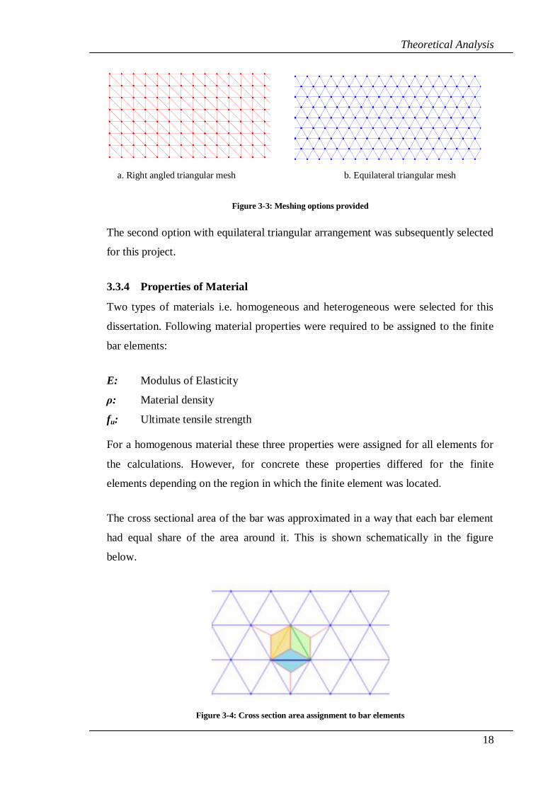
a. Right angled triangular mesh b. Equilateral triangular mesh
Figure 3-3: Meshing options provided
The second option with equilateral triangular arrangement was subsequently selected
for this project.
3.3.4 Properties of Material
Two types of materials i.e. homogeneous and heterogeneous were selected for this
dissertation. Following material properties were required to be assigned to the finite
bar elements:
E: Modulus of Elasticity
ρ: Material density
fu: Ultimate tensile strength
For a homogenous material these three properties were assigned for all elements for
the calculations. However, for concrete these properties differed for the finite
elements depending on the region in which the finite element was located.
The cross sectional area of the bar was approximated in a way that each bar element
had equal share of the area around it. This is shown schematically in the figure
below.
Figure 3-4: Cross section area assignment to bar elements
0 0.1 0.2 0.3 0.4 0.5 0.6 0.7 0.8 0.9
-0.1
0
0.1
0.2
0.3
0.4
0.5
X-Axis
Y-A
xis
0 0.1 0.2 0.3 0.4 0.5 0.6 0.7 0.8 0.9 1
-0.1
0
0.1
0.2
0.3
0.4
0.5
X-Axis
Y-A
xis

Theoretical Analysis
19
Each triangular area was divided in two three equal areas. The share of each bar
element (except the boundary elements) was two third the area of a triangular region.
This area was then divided by the length of the bar element to get the in-plan
dimension of the bar element used to calculate the cross-sectional. The out of plan
dimension of the cross section of bar element was taken as 1 (one).
3.3.5 Boundary Conditions
There are two types of boundary conditions, displacement (essential) and force
(natural). The essential boundary conditions are normally used to describe the
support or constraints on the member. The prescribed values of such boundaries are
often zero. The natural boundary condition deals with force or stress boundary
condition at designated parts of the body.
The terms essential and natural comes from the use of weak form for deriving system
equations. In weak form formulation, the essential boundary condition has to be
satisfied before the derivation starts. If it is not satisfied, the process will fail. When
the essential boundary conditions are satisfied, the process will move on to
equilibrium equations and natural boundary conditions. The force boundary
conditions are this naturally derived from the process and hence called natural
boundary conditions (Liu & Quek, 2003).
There are two types of support conditions provided for the application developed i.e.
simply supported beam and cantilever beam. The displacements in either X or Y
direction of nodes on supports would be prescribed a zero value for displacement.
3.3.6 Strong Form of Governing Equation
In a static analysis problem the equilibrium of forces is considered. However, in case
of dynamic analysis, the applied forces are equated to dynamic inertia. The dynamic
equilibrium equation for 1D solid is given by:
𝜕𝜎𝑥
𝜕𝑥+ 𝑓𝑥 = 𝜌𝑢 (Eq. 3.1)
Where

Theoretical Analysis
20
𝜎𝑥 is the stress in x-direction
fx is the body force
ρ is the mass density
𝑢 =𝜕2𝑢
𝜕𝑡2 (Eq. 3.2)
The equilibrium equation can be written in concise matrix form as
𝐋𝑇𝜎 + 𝐟𝑏 = 𝜌𝐔 (Eq. 3.3)
In the equation above 𝐟𝑏 is the body force and 𝐋𝑇 is the matrix of partial differential
operators (for 2D and 3D).
3.3.7 Weak Form
The strong form as mentioned above, in contrast to the weak form requires strong
continuity on dependant variables. Obtaining the exact solution using the strong form
is normally very difficult. Therefore an approximate solution of the strong form is
developed known as the weak form using finite difference method. The weak form is
a reformulation of the strong form and the finite element method is established from
this weak form. The weak form of the Eq. 3.3 after rearranging can be written as
below:
δuT𝜌u
Ω
𝑑𝛺 − δuTLTσ
Ω
𝑑𝛺 = δuTb
Ω
𝑑𝛺 (Eq. 3.4)
3.3.8 Semi-discretized System of Equations
If we apply integration by parts on the spectral derivatives of Eq. 3.4 and spectral
interpolation we will get an equation of the form:
δdT NT𝜌N
Ω
𝑑𝛺. d + δdT BTDB
Ω
𝑑𝛺. d
= δdT NT
Γn
t dΓ + δdT NTb
Ω
𝑑𝛺 (Eq. 3.5)
This equation must be valid for all arbitrary values of δd . The equation above can be
written in the following generalized form:
𝐦e𝐝 + 𝐤e𝐝 = 𝐟 (Eq. 3.6)
Where

Theoretical Analysis
21
𝐤e = BTDB
Ω
𝑑𝛺 (Eq. 3.7)
𝐦e = NT𝜌N
Ω
𝑑𝛺 (Eq. 3.8)
𝐟 = NT
Γn
t dΓ + NTb
Ω
𝑑𝛺 (Eq. 3.9)
In the equation 3.9 above, the first term on the right hand side represents the forces
on the boundary and the second term represents the forces on the body itself.
The equation 3.6 above is called semi-discretized system of equations as it is
discretized (interpolated) in space but it is still continuous in time.
3.4 Computational Model
In order to be able to apply finite element method to the mathematical model
discussed above it is required to translate the mathematical model discussed above in
a form that can be implemented in a finite element method.
3.4.1 Element Mass Matrix
We will now quantify the element mass matrix using the same 1D example as above.
The mass matrix can be described by Eq. 3.8. Let the total length of the linear
element be h. Equation 3.8 can be re-written as:
𝐦e = Φi
Φi+1
h
0
𝜌 Φi Φi+1 𝑑𝑥
𝐦e = 𝜌
h
0
Φ𝑖
2 Φ𝑖 Φi+1
Φ𝑖 Φi+1 Φ𝑖+1
2 𝑑𝑥 (Eq. 3.10)
In this specific case
Φi = 1 −x
h
and
Φi+1 =x
h

Theoretical Analysis
22
Now we define the three terms different terms inside the matrix in Eq. 3.10
𝜌
h
0
Φ𝑖2𝑑𝑥 = 𝜌
h
0
(1 −x
h)
2𝑑𝑥 = −𝜌h
3[1 −
x
h]3 |0
ℎ =𝜌h
3
Similarly we derive the other two terms with the following results
𝜌
h
0
Φ𝑖 Φ𝑖+1
𝑑𝑥 =𝜌h
6
𝜌
h
0
Φ𝑖+12 𝑑𝑥 =
𝜌h
3
Substituting the values in Eq. 3.10 we get
𝐦e = 𝜌h 1
3 1
6
16
13 (Eq. 3.11)
A representation of the linear shape function used above is given in the figure below.
Figure 3-5: Liner shape function
The proper integration of the weak form leads to the “Consistent Mass Matrix”
derived in Eq. 3.11 above. An alternative for of the mass matrix is lumped mass
matrix. It is a diagonalised version of the consistent mass matrix so that the total
mass remains the same. For this project we will be using the lumped mass matrix
which is given as below:
Φi
i + 1 i
Φi+1
i+1

Theoretical Analysis
23
𝐦elump
= 𝜌h 1
2 0
0 12 (Eq. 3.12)
A lumped mass matrix provides significant advantage in terms of computational time
especially in cases where M-1
is required to be calculated.
3.4.2 Element Stiffness Matrix
Following the same 1D example and the procedure as adopted for the derivation of
element mass matrix, the element stiffness matrix is given by the equation:
𝐤e =E
h
1 −1−1 1
(Eq. 3.13)
Where h is the total length of the element and E is the modulus of Elasticity.
3.4.3 Transforming from Local Coordinates to Global Coordinates
The equations 3.12 and 3.13 are the element mass and stiffness matrices in local
coordinates system where the origin of the coordinate system coincides with the
center of the bar. To be able to extend these matrices to the whole system of bars at
different locations and orientations in the truss structure these must be converted to
global coordinate system. The figure below shows a bar element oriented at an
arbitrary angle θ with respect to X-Axis.
Figure 3-6: Bar element oriented at an angle (modified from (Alexander, 2006))
(X1, Y1)
(X2, Y2)

Theoretical Analysis
24
The displacement at a global node in 2D has two components X and Y. The
coordinate transformation gives a relation between the displacement vector 𝐝𝑒 in
local coordinates and displacement vector 𝐃𝑒 in global coordinate system:
𝐝𝑒 = 𝐓𝐃𝑒 (Eq. 3.14)
Where
𝐃𝑒 =
D𝑥1
D𝑥2
D𝑦1
D𝑦2
and
𝐓 = 𝑙𝑖𝑗 𝑚𝑖𝑗 0 0
0 0 𝑙𝑖𝑗 𝑚𝑖𝑗 (Eq. 3.15)
In which
𝑙𝑖𝑗 =𝑋𝑗 − 𝑋𝑖
𝑙𝑒
𝑚𝑖𝑗 =𝑌𝑗 − 𝑌𝑖
𝑙𝑒
Where 𝑋𝑖 , 𝑋𝑗 , 𝑌𝑖 and 𝑌𝑗 represents the global coordinates of the nodes. 𝑙𝑒 represents
the length of the finite element which can be calculated as:
𝑙𝑒 = 𝑋𝑗 − 𝑋𝑖 2
+ (𝑌𝑗 − 𝑌𝑖)2
In the case of this project as the triangular mesh is made up of elements of same
length, we will just calculate the length of one element and use it in all calculations
rather than calculating it for each element.
It can be easily verified that
𝐓𝐓𝑇 = 𝐈 (Eq. 3.16)
Where 𝐈 is an identity matrix. The matrix 𝐓 is therefore orthogonal matrix. The
transformation vector is also applicable to force vector:
𝐟𝑒 = 𝐓𝐅𝑒 (Eq. 3.17)
Substituting Eq. 3.14 in the system equation (Eq. 3.6) gives:

Theoretical Analysis
25
𝐤𝑒𝐓𝐃𝑒 + 𝐦𝑒𝐓𝐃 𝑒 = 𝐟𝑒
Pre-multiplying 𝐓𝑇 to both sides in the above equation gives us:
(𝐓𝑇𝐤𝑒𝐓)𝐃𝑒 + (𝐓𝑇𝐦𝑒𝐓)𝐃 𝑒 = 𝐓𝑇𝐟𝑒
The above equation can alternatively be written as:
𝐊𝑒𝐃𝑒 + 𝐌𝑒𝐃 𝑒 = 𝐅𝑒 (Eq. 3.19)
Where 𝐊𝑒 and 𝐌𝑒 are element stiffness and mass matrices in global coordinate
system. 𝐅𝑒 is the element force vector in global coordinate system.
3.4.4 Assembling Element Matrices
After transforming the element stiffness and mass matrices from local coordinates
system to global coordinates system, the process of assembling these matrices in to
structural stiffness and mass matrices can be performed. This process for the
structural stiffness matrix can be illustrated by the figure (Alexander, 2006) below:
Figure 3-7: Assembling structural stiffness matrix (Alexander, 2006)
A similar process is carried out to assemble the structural mass matrix.
3.4.5 Time Discretization
The semi-discretized system of equations is discrete in space but is still continuous in
time. Structural systems are normally loaded with transient excitation (Liu & Quek,

Theoretical Analysis
26
2003). Transient excitation is a dynamic time dependant force applied on to a
structural system. The method generally adopted for solving the semi-discretized
system of equation is called direct time integration.
The direct integration method is based on finite difference method for time stepping
the semi-discretized system of equations. There are two basic ideas (Bathe, 1996)
behind direct time integration. The first concept is that instead of trying to satisfy the
governing semi-discretized equation at all times t, it satisfies the equation at discrete
time steps Δt. The second concept is that the variation in displacement, velocity and
acceleration within each time step is assumed. There are two main types of direct
integration method i.e. implicit time integration and explicit time integration. The
implicit time integration is unconditionally stable and the stability of the solution
does not depend on the duration of time step selected. Explicit time integration on the
other hand is only conditionally stable. Explicit time integration is faster in terms of
computation time than the implicit time integration and is used for very fast
phenomenon such as impact loading. In this project we will be using most widely
used implicit algorithm known as Newmark method.
In the Newmark time integration it is first assumed that
Dt+∆t = Dt + ∆t D t + (∆t)2 1
2− β D t + βD t+∆t (Eq. 3.17)
D t+∆t = D t + (∆t) 1 − γ D t + γD t+∆t
Where β and γ are constants which are selected based on the desired results. Equation
3.17 is then substituted in to the un-damped system Equation (Eq. 3.16):
𝐊 Dt + ∆t D t + (∆t)2 1
2− β D t + βD t+∆t + 𝐌D t+∆t = 𝐅t+∆t
By grouping all the terms containing D t+∆t on the left hand side and shifting the
remaining terms to the right, the equation becomes:
𝐊𝐌D t+∆t = 𝐅𝑡+∆𝑡residual (Eq. 3.18)

Theoretical Analysis
27
Where
𝐊𝐌 = [𝐊β ∆t 2 + M]
And
𝐅𝑡+∆𝑡residual = 𝐅t+∆t − 𝐊 Dt + ∆t D t + (∆t)2
1
2− β D t
The acceleration D t+∆t can now be obtained by solving equation 3.18:
D t+∆t = 𝐊𝐌−1𝐅𝑡+∆𝑡
residual (Eq. 3.19)
As this process involves matrix inversion so it requires matrix inversion so it is
similar to solving matrix equation thus making this method implicit.
The algorithm generally starts with predefined initial values of displacement and
velocity. If the initial value of acceleration is not know, it can be obtained by putting
values of displacement and velocity in to the system matrix. The acceleration D t+∆t
can then be calculated by using equation B. After the acceleration D t+∆t is calculated,
the displacement and velocity at time t+Δt can be calculated by using the relations x
and v above.
This is the general form of the Newmark method. Using the value of β as 1
4 yields the
constant average acceleration method. For this project the constant average
acceleration method will be used with value of β as 1
4 and γ as
1
2. All the equations
used above are linear. Therefore it is possible to solve the system of equations for
displacement rather than acceleration. In this project, displacement is calculated first
and rest of the values are calculated from that displacement.

Application Development
28
44 AAPPPPLLIICCAATTIIOONN DDEEVVEELLOOPPMMEENNTT
In the previous chapter actual structure, working model, mathematical model and
computational model were discussed. In this chapter we will go through the
implementation of the computational model by developing a finite element method
based application using MatLab. MatLab is a high-level technical computing
language and interactive environment for algorithm development, data visualization,
data analysis, and numeric computation. The ease of use of matrices and matrix
operations makes MATLAB quite efficient for the development of an application
involving numerous matrices and matrix operations.
Effort was made to make the application developed both flexible and efficient. The
code name for the developed application is Helium. The relevance of the name
Helium is that Helium‟s atom is the simplest atom that cannot be solved using an
exact analytical mathematical approach. Instead numerical mathematical methods are
employed for solving even a simple atom consisting of one nucleus and two
electrons.
The program execution flowchart is displayed on the next page. Some of the minor
details of the execution of the program are not included in this flow chart and would
be described in the sections to come. Each step in the flow chart will be described in
detail with the inputs and outputs with available options for each step. This chapter
will also act as a user guide for using the application or further development in the
future.

Application Development
29
Bu
y S
ma
rtD
raw
!- p
urc
ha
se
d c
op
ies p
rin
t th
is
do
cu
me
nt
with
ou
t a
wa
term
ark
.
Vis
it w
ww
.sm
art
dra
w.c
om
or
ca
ll 1
-80
0-7
68
-37
29
.
Fig
ure
4-1
: P
rogra
m e
xec
uti
on
flo
wch
art

Application Development
30
4.1 User Interface
All the user inputs and messages generated by Helium are displayed at the command
window. Deflected shapes and graphs are displayed in a maximized figure window.
All the outputs from the program like movie file, screen captures, graphs and
variables are stored in a unique folder and the user is notified the location of this
folder and files by a message on the command window. The graphs, screen captures,
movie file having the animation of the analysis variables are stored so that the user
can further analyze the results or perform further operations on the generated
variables.
4.2 Initialize System (Helium.m)
The application developed (call it helium from here onwards) initializes the system
environment before taking the user input. Helium.m is the main file which calls all
the other function files for performing different operations. Operations to initialize
the system environment are called directly by Helium.m. This involves clearing all
the variables from the memory, clearing the command window, clearing any figures
and closing these figure windows. The process is summarized in figure below.
Figure 4-2: Initialize system environment
There are two other operations performed during initializing the system for the
analysis. The first one is to find resolution of the current display and store
information regarding length and width of the current display. This information is
passed on to the plotting function (Plot2D.m) so that a fully maximized figure
window can be loaded. The other function is to get program run counter variable
from an external file ProgramRunCounter.mat. This variable is used for creating

Application Development
31
unique output folders for each analysis outputs. The variable is incremented by 1 and
saved in the external file ProgramRunCounter.mat for any subsequent runs.
The MatLab environment is ready to start with other operations after the MatLab
environment is initialized.
4.3 Getting User Input (GetUserData.m)
Helium is quite flexible when it comes to providing different customizable options
related to almost every operation. In this section we will go through the different user
inputs that the program gets from the user. Options for each input are also described.
Default values for every input option are already entered in the program making it
much easier and user friendly. Although some of the inputs are gathered from the
user at different stages, however we will go through all the available user inputs in
this section.
4.3.1 Analysis Geometry
The user input for the length and depth of the beam are asked from the user. The
dimensions for the length and height are in meters and the default values are 1.0 m
for length and 0.4 m for depth of the beam. The length of the finite element bar is
also required to be entered in millimeters. The default finite element length value is
15 mm. All the three inputs can range to any values, but user should be careful as not
to enter too large dimensions or too small finite element length as the system may get
out of memory due to very large number of finite elements. The process is
summarized in figure below.
Figure 4-3: Analysis geometry input

Application Development
32
One of the functions in getting any user input in Helium is catching any empty values
entered by the user. Any empty value entered by the user may eventually lead to an
error during subsequent operation as the variable in which that value is stored would
be null. If a user enters a null value, the default value for that variable is stored in the
variable instead and the user is notified through a message on the command window.
4.3.2 Dynamic Analysis Time and Loading
The dynamic analysis time duration, time step and dynamic load behavior are
required to be input at this stage of Helium input. There are three types of dynamic
load behaviors incorporated in the program. The first one is a constant dynamic load
from time 0 to end time. The second one is a linearly increasing load from time zero
to a mid time and then constant from mid time to end time. The third option is a
linearly increasing load from time 0 to end time. These three types of loading
behavior are illustrated in the figure below.
Figure 4-4: Dynamic load behavior
When the user opts for constant load or linearly increasing load from time 0 to end
time, the subsequent inputs required are time step and end time. The values are

Application Development
33
entered in seconds and the default value for time step is 0.0001 seconds and end time
is 0.02 second. If the user opts for linearly increasing load from 0 to middle time and
constant loading thereafter, the user is required to input time step, middle time and
end time. The default value for middle time is 0.01 seconds. The process is
summarized in the figure below.
Figure 4-5: Dynamic analysis time and loading behavior input
4.3.3 Material Properties
Different options are provided for defining material of the beam. These options
include 3 pre-defined concrete mixes, steel and an option to define a custom
homogenous material. The properties for the three concrete mixes are hard coded
with each concrete mix having different tensile strength, different type of aggregate
and bond strength between aggregate and cement-sand matrix. The properties for
steel are also hard coded. The user will have to enter material properties like density,
modulus of elasticity and ultimate tensile strength if opting for custom homogenous
material. The process is summarized in the figure below.
Figure 4-6: Input for material properties

Application Development
34
A simple extension which would make the program more flexible is to provide an
option for the user to be able to define custom homogenous material as well by
entering the properties for the custom homogeneous material.
4.3.4 Support Conditions
Two types of support conditions are provided for the beam i.e. simply supported
beam and cantilever beam. An option a third support condition is provided in the user
input informing the user in which file changes should be made to develop a new
support condition. These options are illustrated in the figure below.
Figure 4-7: Support conditions input
4.3.5 Load Patterns
Seven different options are provided for applying loads to the beam. The value of
load is defined by the user however default values for all the loads are provided if the
user does not enter any value. Three basic types of loading i.e. point load, universally
distributed load and varying distributed load are provided. The seven load patterns
consist of any one of these or a combination.
The first load pattern is a single concentrated load at the center of the beam. The
second load pattern is two concentrated loads at 1/3 and 2/3 of length of the beam.
The third and fourth load patterns are UDL and VDL on full length of the beam. The
fifth and sixth options are UDL and VDL on middle 1/3 length of the beam. The final
option called the special case is required to be defined by the user before it could be
assigned. The values of these loads are required to be provided by the user but
default values are present if the user misses out any value. The loads are required to
be entered in kN for concentrated loads and in kN/m for UDL and VDL loadings.
The figure below illustrates different available options.

Application Development
35
Figure 4-8: Load pattern input
4.3.6 Output Options
A number of options are defined in the application for generating and saving outputs
of the application. The application can plot time histories or displacement, velocity,
acceleration and reaction forces. It also captures the stress distribution figures of the
analysis at each time step. These screen captures are saved in enhanced meta file
(emf) format. A movie is also generated in AVI file format of the complete analysis.
All the variables generated during the analysis are also stored in a MatLab file which
is useful for further analysis of a specific test. It is up to the user to select what data
needs to be generated and saved. The three basic options are generating all outputs,
no outputs and custom outputs. The first option generates all the data and graphs.
The second option is does not generate any graphs, screen captures or movies but
saved all the output variables. This option is much faster and can be applied to
analysis having very large beam dimensions or very small finite element sizes. The
variables generated can then be analyzed manually. The third option gives the user a
choice of exactly which data to generate and save. These options are illustrated in the
figure below.
Figure 4-9: Output options

Application Development
36
4.4 Initializing Model Based on User Input
After getting all the user inputs, the finite element model is initialized based on the
user input. This involves generating nodal coordinates, generating finite elements,
initializing material properties, initializing heterogeneity for heterogeneous materials,
initializing boundary conditions, initializing load pattern, generating element mass
and stiffness matrices and assembling these matrices in structural mass and stiffness
matrices. Each of these steps is defined briefly in the section below.
4.4.1 Generating Nodal Coordinates (InitialCoordinates.m)
Based on the geometry and the finite element length entered by the user, the nodal
coordinated for all the nodes are generated and stored. The algorithm implement is
flexible and is theoretically able to generate nodal coordinates for any beam
dimensions and finite element length.
4.4.2 Generating Finite Elements (InitialElements.m)
After generating nodal coordinates, finite elements can be numbered with the nodes
to which the finite element is attached.
4.4.3 Initializing Material Properties (InitMaterialProperties.m)
Based on user input the material properties of density, modulus of elastic and
ultimate tensile strength are assigned to variables. These variables are used while
generating element mass and stiffness matrices and to check element stress level.
4.4.4 Initializing Heterogeneity (InitHeterogeneity.m)
For heterogeneous materials, three different sets of material properties are defined
while initializing the material properties. These three sets are for aggregate, cement
sand matrix and the interface between aggregate and cement sand matrix. Different
sizes of aggregates are randomly generated and distributed throughout the beam. The
algorithm is designed such that aggregates do not overlap each other aggregates to a
certain degree of accuracy. The material properties for each finite element is assigned
based on the region it is located. This function is not invoked in case of a
homogenous material selected by the user.

Application Development
37
4.4.5 Initializing Boundary Conditions (InitBoundaryConditions.m)
The essential boundary conditions are initialized based on the support conditions
selected by the user. The displacement values for all the nodes at the supports are
prescribed as zero in the direction in which displacement is restrained.
4.4.6 Initializing Load Pattern (InitLoads.m)
The load pattern and load values selected by the users are applied on to the nodes.
The concentrated loads are applied at a single node where as the distributed loads are
divided by the length on which the load is applied and distributed on the nodes as
point loads on that length.
4.4.7 Computing Element Matrices (ElementMassAndStiffnessMatrix.m)
The program generates the element stiffness and mass matrices for each element. The
properties of each finite element are already defined for homogeneous and
heterogeneous materials. These properties are used to generate the stiffness and mass
matrices for each element in global coordinates system.
4.4.8 Assembling Structural Matrices (AssembleGlobalMatrices.m)
The assembling of structural stiffness and mass matrices is done in the same lope in
which the element mass and stiffness matrices are computed. The element mass and
stiffness matrices are generated for each element and are assembled in a pre-
allocated sparse structural mass and stiffness matrices. Using sparse matrices
increases the computation time in subsequent operations on these matrices.
4.5 Dynamic Analysis
After initializing all the model variables and assembling structural matrices, the main
dynamic analysis loop is executed. The operations in this section are carried out at
each instance of the dynamic analysis time integration loop. The number of iterations
of the loop depends on the end time and the time step calculated by dividing the end
time by time step.
4.5.1 Load Factor (Helium.m)
The load factor is used to generate the loading factor for the dynamic load. This
depends on the middle time (if any) and the end time selected by the user. The

Application Development
38
loading factor is multiplied with the force vector for each instance to increase the
load.
4.5.2 Computing Displacements (Helium.m)
Newmark constant average acceleration is implemented in the code to compute
displacements for all nodes in both degrees of freedom at each instant. The initial
velocities and accelerations at time 0 are prescribed to be zero.
4.5.3 Computing Velocities and Accelerations (Helium.m)
After the computation of displacements, the velocities and accelerations for all the
nodes can be computed for each instance of time step. These accelerations and
velocity values are used in the subsequent iteration to compute displacement.
4.5.4 Axial Force Calculations in Finite Elements (ElementAxialForce.m)
This process is performed in a sub-loop of the main integration loop. The axial forces
for all the finite element analysis are calculated. These values are used to check if an
element stress level exceeded the allowable stress limit in the subsequent steps in the
same loop.
4.5.5 Removing Element Mass and Stiffness of Failed Elements (Helium.m)
If the element stress level of an element exceeds from the ultimate tensile strength of
an element, the element mass and stiffness values are removed from the structural
mass and stiffness matrices. This is done through a function defined in the file
DisAssembler.m. The element mass and stiffness matrices for the failed elements are
again calculated and are removed from the structural matrices.
4.5.6 Element Stress Levels
The colour in which an element is plotted for each of the iterations depends on the
tensile stress level of that element. Each element is assigned a tag depending on the
level of tensile stress. These tags are subsequently used to plot these elements in the
defined colour. The elements which exceed ultimate tensile strength level are
permanently assigned red colour. The colour codes for element stress levels are given
in the table below:

Application Development
39
Table 4-1: Color codes for element stress levels
Element Tensile Stress (ETS) Assigned Colour
Greater than Ultimate Tensile Strength (UTS) Red
0.75 UTS < ETS < UTS Magenta
0.5 UTS < ETS < 0.75 UTS Yellow
0.25 UTS < ETS < 0.5 UTS Blue
0 < ETS < 0.25 UTS Cyan
No Tensile Stress Green
4.5.7 Calculating Reaction Forces
After computing all the element axial forces, the reactions at the support are
calculated. These reactions are used later on to generate time history graphs for
reaction forces.
4.6 Program Outputs
The program generates almost all possible time histories and plots the information.
Screen captures displaying stress levels in the finite elements are also generated. In
addition a movie displaying the visual displacement of the beam is also generated.
These outputs are discussed briefly in the following section with sample outputs.
4.6.1 Time Histories
Time histories for nodal displacement, nodal velocity and nodal acceleration in both
x and y direction are plotted and the output is saved as enhanced meta file. The time
histories for reactions at the support are also plotted. A sample time history of
displacement, velocity and acceleration of the loaded node is displayed in the figure
below.
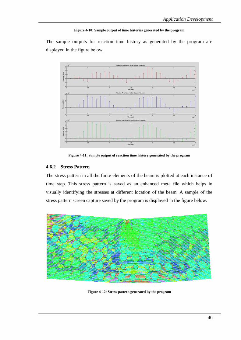
Application Development
40
Figure 4-10: Sample output of time histories generated by the program
The sample outputs for reaction time history as generated by the program are
displayed in the figure below.
Figure 4-11: Sample output of reaction time history generated by the program
4.6.2 Stress Pattern
The stress pattern in all the finite elements of the beam is plotted at each instance of
time step. This stress pattern is saved as an enhanced meta file which helps in
visually identifying the stresses at different location of the beam. A sample of the
stress pattern screen capture saved by the program is displayed in the figure below.
Figure 4-12: Stress pattern generated by the program
0 0.1 0.2 0.3 0.4 0.5 0.6 0.7 0.8 0.9 1
-0.1
0
0.1
0.2
0.3
0.4
X-Axis
Y-A
xis
Crack Simulation - Dynamic Loading

Application Development
41
4.6.3 Deflection and Stress Pattern Animation
An animation displaying the scaled deflection and stress pattern of the beam at all
instances of the time step is generated and is saved in AVI file format. This
animation gives a general overview of failure of the beam and the stresses in
different locations of the beam. A sample animation has been included in the
attached CD.
4.6.4 Program Variables
All the program variables generated during the analysis are saved in a MatLab file.
This file may be used to perform further analysis on any test of interest if required.
4.7 Program Exit
After completing the analysis and saving all the outputs, the program clears the
memory of all the variables. It also displays messages on the command window
informing the location of the program output.
The program code including all the MatLab files has been included in the CD with
this dissertation. This chapter has been included with the code as a user guide. Some
sample outputs from the program have also been included in the CD.

Research Methodology
42
55 RREESSEEAARRCCHH MMEETTHHOODDOOLLOOGGYY
In this chapter we will be focusing on the research methodology adopted for this
dissertation. A number of tests were performed on the application developed in an
effort to get answers for the dissertation hypothesis. The output data from the
application was then analyzed and some results were deduced from this analysis. The
general procedure for carrying out these tests and detailed description of tests with
interesting results are discussed in this chapter
5.1 Application Development
Developing the application on which the tests could be carried out was the first step.
The working model, mathematical model and computational model of the application
developed had already been discussed in chapter 3. The detailed implementation of
the computational model for the development of the application was discussed in the
previous chapter. The decisions taken while developing the application were
dependant on the hypothesis of this dissertation. The choice of dynamic analysis was
made so that mechanism of cracked parts of the member would not cause any
problems. The implementation of heterogeneous material modeling was executed to
be able to see the material behavior under tested under dynamic loading. The
selection of bar element as the finite element for the analysis was carried out as it
would be quite difficult to relate the overall shear and moment capacity of
heterogeneous material like concrete to finite elements like beam elements. Implicit
time integration scheme was selected as it is unconditionally stable. These were some
of the key driving principles which dominated the application development.

Research Methodology
43
5.2 General Procedure for Performing Tests
The tests that were carried out were selected carefully such that results that would
prove to be useful for this dissertation could be obtained. The application developed
was carefully optimized for faster performance so that the time taken for the tests
could be minimized. Still each test performed required at least more than 2 hours to
get completed. Some of the tests with very small finite element length or very large
dimensions for the beam even took longer than 6 hours to be completed. This proved
to be a constraint as limited number of tests could be performed.
A general rule applicable to all tests was that only one parameter was changed for
one specific type of test. This would result in understanding the effects specifically
from that changed parameter and changes in results would not be confused with any
other parameter.
All of the possible outputs like element stress patterns at different times, time
histories of displacement, velocity and acceleration at a number of locations across
the beam, rate of failure of elements, reaction forces and the animation of the beam
under dynamic loading were generated and recorded for each tests. The program
variables for each test were also saved so that further analysis of different variables is
possible at a later stage.
5.3 Program Outputs
Almost all possible outputs were being generated by the program. The outputs that
were analyzed for each test are given below.
5.3.1 Inspected Nodes
A number of nodes across the beam were selected and the values of displacement,
velocity and acceleration at each time step were recorded for these nodes. We will
call these nodes inspected nodes. In the vertical direction, the inspected nodes were
located along the top, bottom and middle of the beam. Horizontally, the same nodes
were located right next to beam supports on both sides, at a distance of one fourth of
beam length from the beam supports, at a distance of one third of beam length from
the beam support and at the middle of beam length. The total number of inspected
nodes was thus 21. The location of these nodes is displayed in the figure below.

Research Methodology
44
Figure 5-1: Inspected nodes for a beam marked with squares
In the figure above, the nodes at the center of the small squares were inspected for
displacement, velocity and acceleration at each time step.
5.3.2 Displacement-Time History
Displacement values at each time step for loaded nodes and inspected nodes were
recorded. A displacement-time history was then plotted using these values and was
analyzed for each test.
5.3.3 Velocity-Time History
Velocity values at each time step for loaded nodes and inspected nodes were
recorded and plotted. These plots were analyzed for each test.
5.3.4 Acceleration-Time History
Acceleration values at each time step for all loaded nodes and inspected nodes were
recorded and a graph between the time and acceleration was plotted. The plots were
analyzed to study the pattern of acceleration changes for each test.
5.3.5 Reaction Forces
All the possible reaction forces in both X and Y direction were calculated and
recorded. These reaction forces were then plotted against time to get the time history
of these reaction forces as the analysis continued. The reaction forces for all the tests
0 0.1 0.2 0.3 0.4 0.5 0.6 0.7 0.8 0.9 1
-0.05
0
0.05
0.1
0.15
0.2
0.25
0.3
0.35
0.4
0.45
X-Axis
Y-A
xis
Crack Simulation - Dynamic Loading

Research Methodology
45
were analyzed and compared to check the influence of changing any parameter on
the reaction forces.
5.3.6 Stress Pattern
The stress pattern and the pattern of failed finite elements across the beam was
recorded and analyzed for each test. This pattern was recorded by the program by
saving screen captures of the stressed beam at each time step instance.
5.3.7 Rate of Failure of Finite Elements
The number of finite elements failing at each time step was stored. The influence of
changing a parameter on the rate of failure of finite elements analyzed and compared
for each test.
5.3.8 Animation of Loaded Beam
The video compiled by the program by putting frames of the stressed beam captured
at each time step were saved by for each step. The animation presents a general idea
of the behavior of the beam and motion of impulsive waves through the beam.
5.4 Analyses Performed
Different sets of analysis were performed by varying different parameters. Some of
the test group results were not taken in to consideration as there was no significant
change in the outputs or the results seemed to be irrelevant. Four groups of analyses
performed are discussed below with a commentary on the observed outputs.
5.4.1 Effect of Changing Finite Element Length
In this test the effect of changing the finite element length was analyzed. A range of
lengths for the finite element was selected and all the other properties were kept
constant. The velocity-time history for any of the nodes in the analysis group did not
show a specific pattern. However, there was a visible pattern of displacement-time
histories and acceleration-time histories. The reaction forces also acted in a pattern
similar to the pattern of load application. The parameters which remained unchanged
during the analysis are given below:
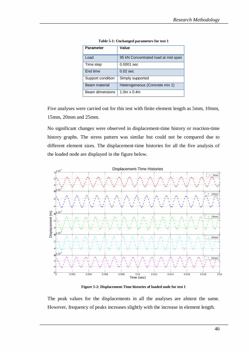
Research Methodology
46
Table 5-1: Unchanged parameters for test 1
Parameter Value
Load 95 kN Concentrated load at mid span
Time step 0.0001 sec
End time 0.02 sec
Support condition Simply supported
Beam material Heterogeneous (Concrete mix 1)
Beam dimensions 1.0m x 0.4m
Five analyses were carried out for this test with finite element length as 5mm, 10mm,
15mm, 20mm and 25mm.
No significant changes were observed in displacement-time history or reaction-time
history graphs. The stress pattern was similar but could not be compared due to
different element sizes. The displacement-time histories for all the five analysis of
the loaded node are displayed in the figure below.
Figure 5-2: Displacement-Time histories of loaded node for test 1
The peak values for the displacements in all the analyses are almost the same.
However, frequency of peaks increases slightly with the increase in element length.
-6
-4
-2
0x 10
-4 Displacement-Time Histories
-6
-4
-2
0x 10
-4
-6
-4
-2
0x 10
-4
Dis
pla
cem
ent
(m)
-6
-4
-2
0x 10
-4
0 0.002 0.004 0.006 0.008 0.01 0.012 0.014 0.016 0.018 0.02-6
-4
-2
0x 10
-4
Time (sec)
5mm
10mm
15mm
20mm
25mm

Research Methodology
47
The only significant influence of changing the finite element length appeared in the
acceleration-time history graph. The figure below displays the acceleration-time
history of the node that was loaded with the concentrated load at the mid-span.
Figure 5-3: Acceleration-Time history of loaded node for test 1
The acceleration values are higher when smallest size for the finite element of 5mm
was selected. These values keep on decreasing as the finite element length is
increased. This can be explained by the fact that the acceleration history of a single
node was recorded for these analyses. In case of a smaller finite element length, the
lumped nodal mass on that node was small as the elements attached to this node were
small in length. Similarly, the nodal mass of the loaded node was higher when the
length of the finite elements attached to that node increased. This resulted in large
value of accelerations for the nodes with smaller masses when the force applied was
the same and vice versa.
An improved method of applying the loads to meshes with different element lengths
is to distribute the point load to a number of nodes depending on the element length.
Also a correction factor can be applied to the values of the acceleration depending on
the element length and nodal mass of the node on which the load is applied. The
magnitude of acceleration may be adjusted by doing so but the shape of the graphs
would remain the same in X-direction.
0 0.002 0.004 0.006 0.008 0.01 0.012 0.014 0.016 0.018 0.020
2
4
6
8
10
12x 10
5
Time (sec)
Acce
lera
tio
n (
m/s
ec
2)
Acceleration-Time History
5 mm
10 mm
15 mm
20 mm
25 mm

Research Methodology
48
5.4.2 Effect of Changing Loading Rate
The second analysis performed was observing the effect of changing the loading rate
on the beam. The loading rate was varied from being constant from time 0 to end
time to being linearly increasing from time 0 to end time in 5 steps. The parameters
which remained unchanged during the analysis are given in the table below:
Table 5-2: Unchanged parameters for test 2
Parameter Value
Load Two 15 kN Concentrated loads on 1/3 and 2/3 of span
Support condition Simply supported
Beam material Heterogeneous (Concrete mix 2)
Beam dimensions 1.0m x 0.4m
Finite element length 10mm
The changing parameters are the middle time and time durations for the 5 tests are
given in the table below:
Table 5-3: Varying parameters for test 2
Analysis No. Description
1 Constant load from time 0 to 0.02
2 Linearly increasing load from time 0 to 0.005, constant from time 0.005 to 0.02
3 Linearly increasing load from time 0 to 0.01, constant from time 0.01 to 0.02
4 Linearly increasing load from time 0 to 0.015, constant from time 0.015 to 0.02
5 Linearly increasing load from time 0 to 0.02
A number of observations were made during these analyses which were closely
related to one of the hypothesis of the dissertation. As the rate of loading decreased
from being constant to linearly increasing from time 0 to end time, the rate of finite
elements failing decreased as well as expected. The reaction forces also responded in
a similar fashion, increasing as with the load increasing. The comparison between
displacement-time histories and acceleration-time histories is shown in the figures
below. The graph for analysis 1 was not plotted in the same graph as the acceleration
values and displacement values for analysis 1 were very high and could not be
related to the other tests. The displacement-time history graph for the analyses is
shown below.

Research Methodology
49
Figure 5-4: Displacement-Time history for test2
The displacement-time history displayed above reflects a similar characteristics
displayed by static tests. As the load increases, the deflection of the beam increases.
This is an important observation as it relates to one of the dissertation hypothesis. As
the rate of loading decreases, the analysis tends to behave more like a static test.
Thus it may be possible to model static tests using dynamic implementation.
The acceleration-time history also tends to display a similar conclusion. As the
loading rate is high, the acceleration values are high. But as the loading rate
decreases, the peak acceleration values also decrease. The acceleration-time history
graph also strengthens the conclusion reached by inspecting the displacement-time
history graph. Thus it can be assumed that it is possible to model static tests using
dynamic implementation provided the loading rate is kept gradual. The more
gradually the load is applied, the better the chances of the test result matching a static
model. The acceleration-time history graph is displayed in the figure below.
0 0.002 0.004 0.006 0.008 0.01 0.012 0.014 0.016 0.018 0.02-6
-5
-4
-3
-2
-1
0x 10
-5
Time (sec)
Dis
pla
ce
me
nt
(m)
Displacement-Time History
Analtsis 2
Analysis 3
Analysis 4
Analysis 5

Research Methodology
50
Figure 5-5: Acceleration-Time history for test 2
The graph above shows clearly that as the rate of loading is decrease, the peak values
of the acceleration at the node also decrease.
5.4.3 Effect of Changing the Aspect Ratio of the Beam
The last test that will be discussed in this dissertation is the effect of changing the
aspect ratio of the beam. In this test, all the other parameters of the test were kept
constant and the aspect ratio of the beam was changed. The constant parameters for
this test are given in the table below.
Table 5-4: Unchanged parameters for test 3
Parameter Value
Load 15 kN Concentrated load at mid span
Support condition Simply supported
Beam material Heterogeneous (Concrete mix 3)
Finite element length 20mm
Time step 0.0001 sec
End time 0.02 sec
The changing parameter of length and height for this test are given in the table
below.
0 0.002 0.004 0.006 0.008 0.01 0.012 0.014 0.016 0.018 0.020
200
400
600
800
1000
1200
Time (sec)
Accele
ration (
m/s
ec
2)
Acceleration-Time History
Analysis 2
Analysis 3
Analysis 4
Analysis 5

Research Methodology
51
Table 5-5: Varying parameters for test 3
Analysis No. Beam Dimensions
1 2.0m x 1.0m
2 3.0m x 0.8m
3 4.0m x 0.6m
The observations made during this test was that as the length of the beam increased
and the depth decreased, the displacement and acceleration values kept on increasing.
For the third analysis, after time 0.003, the beam practically had failed. Any beam
with length to depth ration higher than test 3 would fail in a similar fashion. This
result coincides with simple experimental results that slender beams tend to fail at
lower loads. The diagram for stresses in beam elements and failed elements around
the mid span for test 3 at time 0.0034 seconds is displayed below.
Figure 5-6: Stresses and failed elements around mid span
The results shows relevance to general behavior of beams observed practically. If the
length of the beam is more as compared to its depth, the beam is likely to fail at by
cracking. The failure of the beam in the analysis simulates brittle behavior. As soon
as some of the elements fail, the whole beam fails rapidly in a very short period of
time. This is a characteristic of brittle failure where there is little or no yielding of the
material before failure.
The displacement-time history for the same analysis is displayed below showing a
sudden failure at time around 0.0034 sec.
0 0.5 1 1.5 2 2.5 3 3.5
-0.5
0
0.5
1
X-Axis
Y-A
xis
Crack Simulation - Dynamic Loading

Research Methodology
52
Figure 5-7: Displacement-Time history for loaded node for test 3, analysis 3
The acceleration-time history for the analysis is displaying a similar characteristic
where the magnitude of acceleration becomes very high and irregular after failure.
Figure 5-8: Acceleration-Time history for loaded node of test3, analysis 3
0 0.002 0.004 0.006 0.008 0.01 0.012 0.014 0.016 0.018 0.02-5
-4
-3
-2
-1
0
1
2
3x 10
-4
Time (sec)
Dis
pla
cem
ent
(m)
Displacement-Time History
0 0.002 0.004 0.006 0.008 0.01 0.012 0.014 0.016 0.018 0.020
0.5
1
1.5
2
2.5
3
3.5
4
4.5x 10
4
Time (sec)
Acce
lera
tio
n (
m/s
ec
2)
Acceleration-Time History

Research Methodology
53
5.4.4 Effect of Heterogeneity
The last test that is included in this chapter is the effect of heterogeneity on the
behavior of the beam. Two analyses were performed for this test. In the first analysis
only cement-mortar matrix was considered without any aggregates. In the second
analysis, aggregates were added to the same cement-mortar matrix.
Table 5-6: Unchanged parameters for test 4
Parameter Value
Load 23 kN Concentrated load at mid span
Support condition Simply supported
Beam dimensions 1.0m x 0.4m
Finite element length 10mm
Time step 0.0001 sec
End time 0.02 sec
The changing parameter was heterogeneity of the material as aggregate was added to
the same cement-sand matrix in the second analysis. There was no significant change
in any of the time histories. This means that the influence of heterogeneity on a
structural level is minimal. The displacement-time histories of the loaded nodes of
both the analyses are displayed in the figure below.
Figure 5-9: Displacement-Time histories of loaded nodes for test 4
The elements that were around the aggregate in the second analysis of material with
aggregate failed as the analysis continued. The screen capture of the analysis without
aggregate at the end of dynamic analysis is displayed below.
-1.8
-1.6
-1.4
-1.2
-1
-0.8
-0.6
-0.4x 10
-4 Displacement-Time Histories
0 0.002 0.004 0.006 0.008 0.01 0.012 0.014 0.016 0.018 0.02-16
-14
-12
-10
-8
-6
-4
-2x 10
-5
Time (sec)
Dis
pla
ce
me
nt
(m)
Without Aggregate
With Aggregate

Research Methodology
54
Figure 5-10: Axial forces in finite elements (analysis without aggregate)
The screen capture of the analysis having the aggregates is given in the figure below.
Observe that the elements on the aggregate matrix interface failed for heterogeneous
material.
Figure 5-11: Axial forces in finite elements (analysis with aggregates)
The behavior of stresses around the aggregate signifies the influence of heterogeneity
at a local level. This certainly influences the crack propagation in the material.
0 0.1 0.2 0.3 0.4 0.5 0.6 0.7 0.8 0.9 1-0.1
0
0.1
0.2
0.3
0.4
X-Axis
Y-A
xis
Crack Simulation - Dynamic Loading
0 0.1 0.2 0.3 0.4 0.5 0.6 0.7 0.8 0.9 1
-0.05
0
0.05
0.1
0.15
0.2
0.25
0.3
0.35
0.4
0.45
X-Axis
Y-A
xis
Crack Simulation - Dynamic Loading

Conclusion
55
66 CCOONNCCLLUUSSIIOONN
The results from a number of tests performed using the application developed and
discussed in the previous chapter. Based on the results of the analyses carried out the
following conclusions were reached:
1. It may be possible to model static tests using a dynamic implementation. In
such cases, the loading rate should be gradually increased. The results from a
gradually increasing load test using dynamic implementation resembles
closely with the results from a static test. This proves the basic hypothesis of
this dissertation to be true.
2. The results from the aspect ratio analysis test demonstrate that slender beams
tend to fail at a lower load in a brittle manner. This analysis result is
compatible with the practical behavior of concrete beams.
3. Heterogeneity of material does not have any significant effect on overall
structural responses like reaction forces or displacement of a specific point on
the beam.
4. Heterogeneity of material does have a profound effect in the area around the
aggregate where the elements on the aggregate-matrix interface are among
the first elements to fail.
6.1 Summary of Achievements
Most of the aims and objectives set during the dissertation plan for this dissertation
have been achieved. High level objective of implementing material heterogeneity

Conclusion
56
which depended on availability of time was also achieved during the course of this
dissertation. Below is a summary of main achievements of this dissertation:
1. Two flexible options were provided for mesh generation. Theoretically a
mesh for any beam dimensions with any size of finite element can be
generated using the algorithm.
2. The basic implementation of time integration schemes was studies and
implemented
3. A dynamic analysis using implicit time integration based on Newmark
constant average acceleration was implemented.
4. An algorithm to find out the axial forces in a bar element. If the bar forces in
any element exceeds the ultimate tensile strength of the bar, the stiffness and
mass of that element are removed from the structural stiffness and mass
matrix. This implementation simulated removal of the bar element from the
mesh.
5. Implementation of heterogeneity in the material was accomplished. Different
sized aggregates were randomly distributed throughout the beam. Different
properties were assigned to elements based on the region in which the finite
element was located.
6. A solution capable of assigning weaker material strength at the boundary of
aggregates hence simulating interfaces between aggregate and cement/sand
matrix was implemented.
7. The stresses and cracks in the beam were simulated by assigning different
colors to the element with certain level of tensile stresses.
8. The program is capable of generating time history graphs, screen captures
and animation movies for each analysis run.
9. A number of tests were performed using the developed application. Some
interesting results were obtained from these analyses.
10. The basic hypothesis of this dissertation was found to be correct after
studying the results from the analysis. It is possible to model static tests with
dynamic implementation.
11. A few other conclusions were also made from the results as given in the
section above.

Conclusion
57
6.2 Recommendations
Owing to time limitation, a very simple approach was taken towards accomplishing
this dissertation. During the course of this dissertation a few observations regarding
possible enhancement in the project and future work were made. These
enhancements and possible future research are summarized below:
1. The aggregate shape incorporated in this dissertation was approximated as
circular shaped aggregates with four possible sizes. In reality, aggregates are
irregularly shaped in a variety of sizes. A possible future enhancement to the
project can be modeling these irregular shaped aggregates with different
sizes.
2. A 2 dimensional approximation of a solid was adopted for the course of this
dissertation. To simulate the behavior of crack propagation in a solid closely,
a 3 dimensional extension of the model is recommended.
3. One of the areas of research may be the effect of local orientation of a finite
element with respect to the structure. If a bar element is used as a finite
element, the properties assigned to the bar element might be changed based
on its location in the structure and orientation. This may hold true for other
types of finite elements as well. Experimental data of stress at different
locations of the structure may be collected and the model can be improved by
relating these stresses to the local finite elements.
4. There is a significant stress concentration at the crack tip. In this dissertation
a constant mesh density was adopted for the whole structure. It would be
more efficient and accurate if the mesh in the area around the crack is refined.
This may be accomplished by automatic mesh refinement algorithm which
will give more accurate results and will be more efficient as regard to
computer time.
5. The experimental data of failure mode of concrete exhibits a difference in
failure modes of concrete depending on the loading rate. In case of a sudden
impact on the concrete, the crack might pass through aggregates rather than
finding the path of least resistance around the aggregate. This behavior of
concrete failure should be studied and effects of loading rate on concrete
fracture behavior can be modeled.

Conclusion
58
6. An interesting extension to this dissertation can be the comparison of using
different types of finite elements and their effect on crack propagation and
failure pattern. A simple extension can be the use of beam elements instead of
bar elements in the same project. The global properties of the material in this
case should be related to the finite element properties of the beam element.
7. The lattice model or mesh can be generated in a variety of different ways.
The effect of using different lattice models should be studied and compared.
8. Incorporating non-linear behavior of material may be another interesting area
in which research may be carried out.
9. No plastic deformation in finite elements was considered during the course of
this dissertation. In practice, plastic deformation does occur even in brittle
materials. Plastic deformations in finite elements may be incorporated in the
material and the change in behavior due to plastic deformation may be
studied.
10. Random placement of aggregates was incorporated in this dissertation. A
much more accurate representation would be statistical distribution of
aggregate in the material based on standard sieve analysis of practical
concrete mixes.
11. Some very fine cracks are inherently present due to the differences in
mechanical properties of the materials at the interface of aggregate and
cement-sand matrix even before concrete is loaded. These micro-cracks
initiate the cracking process in concrete. These micro-cracks can be
incorporated in the model while initializing the model before the load is
applied.
With these recommendations we reach the end of this dissertation. The list of files
MatLab files used in the application and a short description of their function has been
included as appendix A. The MatLab code for the main file which calls all the sub-
functions is included in appendix B. The author hopes you enjoyed reading through
the dissertation.

References
59
RREEFFEERREENNCCEESS
Abraham, F. F., Robert, W., Huajian, G., Mark, D., Tomas, D. D., & Mark, S.
(2002). Simulating materials failure by using up to one billion atoms and the world‟s
fastest computer: Brittle fracture. Proceedings of the National Academy of Sciences
of the United States of America. 99 no.9. California: PNAS.
Alexander, N. A. (2006). Introduction to Finite Element Analysis for Skeletal
Structures. University of Bristol.
Bathe, K. J. (1996). Finite Element Procedures. New Jersey: Prentice-Hall, Inc.
Ince, R., Arslan, A., & Karihaloo, B. L. (2002). Lattice modelling of size effect in
concrete strength. (70).
Janssen, M., Zuidema, J., & Wanhill, R. J. (2004). Fracture Mechanics (2nd Edition
ed.). Oxfordshire: Spon Press.
Liu, G. R., & Quek, S. S. (2003). The Finite Element Method - A Practical Course.
Elsevier Science Ltd.
Mehta, P. K., & Monteiro, P. J. (2006). Concrete - Microstructure, Properties and
Materials (3rd Edition ed.). McGraw-Hill.
Neville, A. M. (1995). Properties of Concrete (4th Edition ed.). Longman Group
Limited.
Sadd, M. H. (2009). Introduction to Finite Element Methods. University of Rhode
Island.
Schlangen, E., & Garboczi, E. J. (1997). Fracture Simulation of Concrete using
Lattice Models: Computational Aspects. 57 (2/3), 319-332.
Schlangen, E., & Van Mier, J. G. (1992). Simple lattice model for numerical
simulation of fracture of concrete materials and structures. Materials and Structures
(25).

References
60
Schlengen, E. (1993). Experimental and Numerical Analysis of Fracture Processes
in Conccrete. Delft University of Technology.
Wikipedia. (2009). Fracture. (Wikipedia) Retrieved August 12, 2009, from
http://en.wikipedia.org/: http://en.wikipedia.org/wiki/Fracture

Appendix A – Application Files and Functions
61
77 AAPPPPEENNDDIIXX AA –– AAPPPPLLIICCAATTIIOONN FFIILLEESS AANNDD FFUUNNCCTTIIOONNSS
The application developed contains several files performing different functions.
Following are the Matlab files and their functionality described briefly in
alphabetical order:
AssembleGlobalMatrices: Assembles the Structural Stiffness and Mass Matrices
Circle: Draws a circle with centre defined as a vector CENTER
DisAssembler: Removes failed element's stiffness/mass from Structural Matrix
Dsxy2figxy: Transform point or position from axis to figure coordinates
ExtractCoordinates: Extracts the Element X and Y coordinates (x1, x2, y1 and y2)
ExtractDisplacements: Extract element displacements from the global displacement
vector according to the topology matrix edof
ElementAxialForcefunc: Computes the axial force in a bar element
ElementMassAndStiffnessMatrix: Computes the element stiffness and mass matrix
in Global Coordinates
GetEdof: Get numbering for Dofs and Edofs
GetUserData: Gets geometric and dynamic analysis data from user
Helium: Main file for execution of all functions
InitHeterogeneity: Initializes Material Heterogeneity based on concrete mix
InitialCoordinates: Gives back the initial coordinates matrix based on inputs
InitialElements: Generates matrix having all the bar elements node numbers
InitBoundaryConditions: Initializes the boundary conditions for the analysis
InitLoads: Initializes Loading condition for the analysis
InitMaterialProperties: Initializes Material Properties based on selected material
OutputOptions: Gets outputs to be generated options from user
Plot2D: Plot elements based on element information. Used for generating both initial
mesh and failed elements
SolveEquation: Solves the equation for Nodal Displacements

Appendix B – Main Function File Code
62
88 AAPPPPEENNDDIIXX BB –– MMAAIINN FFUUNNCCTTIIOONN FFIILLEE CCOODDEE
% Description: Main file for execution of all functions % Project: Dissertation - Material Failure Simulated With 2D Truss Dynamics % Author: MB Shah ([email protected]) % Supervisor: Harm Askes ([email protected]) % Project Code Name: Helium % File: Helium.m % File Version: 1.0 % Date File Created: 04 August, 2009 % % Input(s) % None % % Output(s) % Iterative Plots % Movie file in .avi format % Program inputs % %========================================================================== % Initialize Program % Clear everything clc; % Clear the screen clear figure; % Clear any previous figures clear all; % Clear all memory %profile on; % Turn on if want to see profile of the program for %optimization load('ProgramRunCounter.mat','ProgramRunCounter'); ProgramRunCounter = ProgramRunCounter + 1; save('ProgramRunCounter.mat','ProgramRunCounter'); % ========================================================================= % Run function: GetUserData [AdjustedBeamLength,AdjustedBeamHeight,ElementSideLength,ElementAltitude,NumberOfElementsXDir,NumberOfElementsYDir,TimeStep,MiddleTime,EndTime,DLO] = GetUserData(); % ========================================================================= % Run function: InitMaterialProperties [IsHetero,BeamMaterial,BarCrossSectionArea,ModGen,ModAgg,ModBond,UTSGen,UTSAgg,UTSBond,RhoGen,RhoAgg,RhoBond] = InitMaterialProperties(ElementSideLength); % ========================================================================= % Run function: InitialCoordinates [NodalCoordinates,NumberOfNodes] = InitialCoordinates(ElementSideLength,ElementAltitude,NumberOfElementsXDir,NumberOfElementsYDir); % ========================================================================= % Run function: InitialElements [ElementTopology,NumberOfElements] = InitialElements(NumberOfElementsXDir,NumberOfElementsYDir); % ========================================================================= % Run function: InitHeterogeneity [ElementTypes,IsHetero,TaggedNodes] = InitHeterogeneity(IsHetero,NumberOfElements,NumberOfNodes,NodalCoordinates,ElementTopology,ElementSideLength,ElementAltitude,AdjustedBeamHeight,NumberOfElementsXDir,NumberOfElementsYDir); %disp('function run complete'); %pause % ========================================================================= % Run function: InitBoundaryConditions
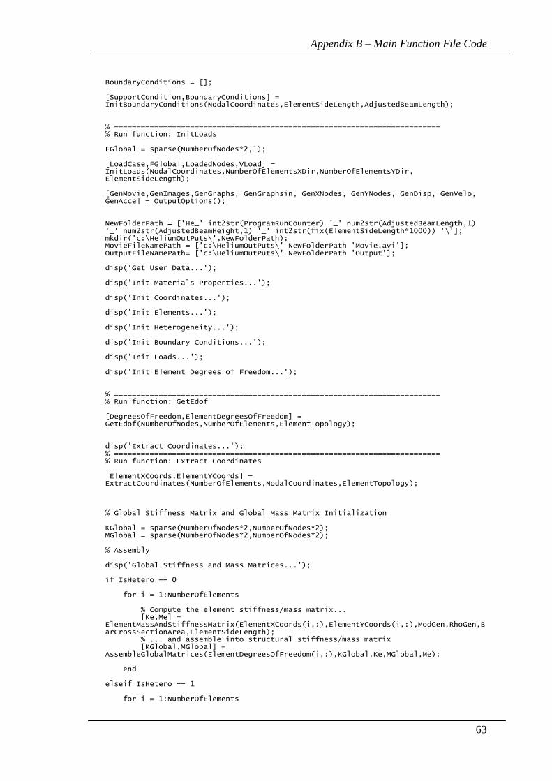
Appendix B – Main Function File Code
63
BoundaryConditions = []; [SupportCondition,BoundaryConditions] = InitBoundaryConditions(NodalCoordinates,ElementSideLength,AdjustedBeamLength); % ========================================================================= % Run function: InitLoads FGlobal = sparse(NumberOfNodes*2,1); [LoadCase,FGlobal,LoadedNodes,VLoad] = InitLoads(NodalCoordinates,NumberOfElementsXDir,NumberOfElementsYDir, ElementSideLength); [GenMovie,GenImages,GenGraphs, GenGraphsin, GenXNodes, GenYNodes, GenDisp, GenVelo, GenAcce] = OutputOptions(); NewFolderPath = ['He_' int2str(ProgramRunCounter) '_' num2str(AdjustedBeamLength,1) '_' num2str(AdjustedBeamHeight,1) '_' int2str(fix(ElementSideLength*1000)) '\']; mkdir('c:\HeliumOutPuts\',NewFolderPath); MovieFileNamePath = ['c:\HeliumOutPuts\' NewFolderPath 'Movie.avi']; OutputFileNamePath= ['c:\HeliumOutPuts\' NewFolderPath 'Output']; disp('Get User Data...'); disp('Init Materials Properties...'); disp('Init Coordinates...'); disp('Init Elements...'); disp('Init Heterogeneity...'); disp('Init Boundary Conditions...'); disp('Init Loads...'); disp('Init Element Degrees of Freedom...'); % ========================================================================= % Run function: GetEdof [DegreesOfFreedom,ElementDegreesOfFreedom] = GetEdof(NumberOfNodes,NumberOfElements,ElementTopology); disp('Extract Coordinates...'); % ========================================================================= % Run function: Extract Coordinates [ElementXCoords,ElementYCoords] = ExtractCoordinates(NumberOfElements,NodalCoordinates,ElementTopology); % Global Stiffness Matrix and Global Mass Matrix Initialization KGlobal = sparse(NumberOfNodes*2,NumberOfNodes*2); MGlobal = sparse(NumberOfNodes*2,NumberOfNodes*2); % Assembly disp('Global Stiffness and Mass Matrices...'); if IsHetero == 0 for i = 1:NumberOfElements % Compute the element stiffness/mass matrix... [Ke,Me] = ElementMassAndStiffnessMatrix(ElementXCoords(i,:),ElementYCoords(i,:),ModGen,RhoGen,BarCrossSectionArea,ElementSideLength); % ... and assemble into structural stiffness/mass matrix [KGlobal,MGlobal] = AssembleGlobalMatrices(ElementDegreesOfFreedom(i,:),KGlobal,Ke,MGlobal,Me); end elseif IsHetero == 1 for i = 1:NumberOfElements

Appendix B – Main Function File Code
64
if ElementTypes(i,1) == 1 % Compute the element stiffness/mass matrix... [Ke,Me] = ElementMassAndStiffnessMatrix(ElementXCoords(i,:),ElementYCoords(i,:),ModGen,RhoGen,BarCrossSectionArea,ElementSideLength); % ... and assemble into structural stiffness/mass matrix [KGlobal,MGlobal] = AssembleGlobalMatrices(ElementDegreesOfFreedom(i,:),KGlobal,Ke,MGlobal,Me); elseif ElementTypes(i,1) == 2 % Compute the element stiffness/mass matrix... [Ke,Me] = ElementMassAndStiffnessMatrix(ElementXCoords(i,:),ElementYCoords(i,:),ModAgg,RhoAgg,BarCrossSectionArea,ElementSideLength); % ... and assemble into structural stiffness/mass matrix [KGlobal,MGlobal] = AssembleGlobalMatrices(ElementDegreesOfFreedom(i,:),KGlobal,Ke,MGlobal,Me); elseif ElementTypes(i,1) == 3 % compute the element stiffness/mass matrix... [Ke,Me] = ElementMassAndStiffnessMatrix(ElementXCoords(i,:),ElementYCoords(i,:),ModBond,RhoBond,BarCrossSectionArea,ElementSideLength); % ... and assemble into structural stiffness/mass matrix [KGlobal,MGlobal] = AssembleGlobalMatrices(ElementDegreesOfFreedom(i,:),KGlobal,Ke,MGlobal,Me); else disp('Unexpected Error...'); pause end end else disp('Unexpected Error...'); pause end disp('Dynamic Analysis...'); % Fill all element lives with 1 ElementLives = ones(NumberOfElements,1); nors = NumberOfElementsYDir + 1; nocs = NumberOfElementsXDir + 1; if GenGraphsin == 1 TappedNodes = zeros(15,1); TappedNodes(1,1) = nors + 1; TappedNodes(2,1) = nors + fix(nors/2); TappedNodes(3,1) = 2*nors; TappedNodes(4,1) = ((fix(nocs/4))*nors) + 1; TappedNodes(5,1) = ((fix(nocs/4))*nors) + fix(nors/2); TappedNodes(6,1) = ((fix(nocs/4))*nors) + nors; TappedNodes(7,1) = ((fix(nocs/3)-1)*nors) + 1; TappedNodes(8,1) = ((fix(nocs/3)-1)*nors) + fix(nors/2); TappedNodes(9,1) = ((fix(nocs/3)-1)*nors) + nors; TappedNodes(10,1) = ((fix(nocs/2)-1)*nors) + 1; TappedNodes(11,1) = ((fix(nocs/2)-1)*nors) + fix(nors/2); TappedNodes(12,1) = ((fix(nocs/2)-1)*nors) + nors; TappedNodes(13,1)= (2*(fix(nocs/3)-1)*nors) + 1; TappedNodes(14,1)= (2*(fix(nocs/3)-1)*nors) + fix(nors/2); TappedNodes(15,1)= (2*(fix(nocs/3)-1)*nors) + nors; TappedNodes(16,1)= (3*(fix(nocs/4))*nors) + 1; TappedNodes(17,1)= (3*(fix(nocs/4))*nors) + fix(nors/2); TappedNodes(18,1)= (3*(fix(nocs/4))*nors) + nors; TappedNodes(19,1)= ((nocs-2)*nors) + 1; TappedNodes(20,1)= ((nocs-2)*nors) + fix(nors/2);

Appendix B – Main Function File Code
65
TappedNodes(21,1)= ((nocs-2)*nors) + nors; elseif GenGraphsin == 2 TappedNodes = LoadedNodes; end % Get the full screen coordinates fullscreen = get(0,'ScreenSize'); % and set the figure to full screen but less 5% from bottom for task bar % etc. figure('OuterPosition',[0 fullscreen(4)*0.05 fullscreen(3) fullscreen(4)-(fullscreen(4)*0.05)],'Name','Helium 1.0'); %Plot2D(NumberOfElements,NodalCoordinates,ElementTopology,ElementLives,LoadedNodes,AdjustedBeamLength,AdjustedBeamHeight,TaggedNodes,VLoad); % Initialize solution: displacements, velocities and accelerations Displacement = sparse(1,NumberOfNodes*2); Velocity = sparse(1,NumberOfNodes*2); Acceleration = sparse(1,NumberOfNodes*2); % Initialize (constant) TotalMatrix TotalMatrix = sparse(NumberOfNodes*2,NumberOfNodes*2); TotalMatrix = KGlobal + MGlobal * 4/(TimeStep^2); % Initialize movie - call it moofie after Harm Askes :) if GenMovie == 1 moofie = avifile(MovieFileNamePath); moofie.compression = 'cinepak'; end NTime = round(EndTime/TimeStep); MTime = round(MiddleTime/TimeStep); % Initialize TotalDeadElements variable TotalDeadElements = 0; if SupportCondition == 1 LeftNodes(:,1) = 1:nors; RightNodes(:,1)= (((nocs-1)*nors)+1):(nocs*nors); LeftElements(:,1) = 1:(3*nors - 2); RightElements(:,1)= (((3*nors - 2)*(nocs-2))+1):((3*nors - 2)*(nocs-1)); nle = length(LeftElements); nre = length(RightElements); nnl = length(LeftNodes); nnr = length(RightNodes); elseif SupportCondition == 2 LeftNodes(:,1) = 1:nors; LeftElements(:,1) = 1:(3*nors - 2); nle = length(LeftElements); nnl = length(LeftNodes); end NodalReactionsLeftX = zeros(nnl,NTime); NodalReactionsLeftY = zeros(nnl,NTime); NodalReactionsRightX= zeros(nnr,NTime); NodalReactionsRightY= zeros(nnr,NTime); for i = 1:NTime if DLO == 1

Appendix B – Main Function File Code
66
%Set LoadFactor to 1 LoadFactor = 1; elseif DLO == 2 if i <= MTime LoadFactor = i/MTime; else LoadFactor = 1; end elseif DLO == 3 LoadFactor = i/NTime; else LoadFactor = 1; end TotalVector = LoadFactor*FGlobal + MGlobal * ( Displacement'*4/(TimeStep^2) + Velocity'*4/TimeStep + Acceleration' ); % Solve for Nodal Displacements: NewDisplacement = SolveEquation(TotalMatrix,TotalVector,BoundaryConditions); % Compute accelerations and velocities NewAcceleration = (NewDisplacement - Displacement)*4/(TimeStep^2) - Velocity*4/TimeStep - Acceleration; NewVelocity = Velocity + 0.5*TimeStep*(Acceleration + NewAcceleration); Displacement = NewDisplacement; Velocity = NewVelocity; Acceleration = NewAcceleration; TimeTappedNodes(i,1) = (i*TimeStep); for tns = 1:length(TappedNodes) DispXTappedNodes(i,:) = [Displacement(1,2*TappedNodes(1:length(TappedNodes),1))]; DispYTappedNodes(i,:) = [Displacement(1,2*TappedNodes(1:length(TappedNodes),1)+1)]; VeloXTappedNodes(i,:) = [Velocity(1,2*TappedNodes(1:length(TappedNodes),1))]; VeloYTappedNodes(i,:) = [Velocity(1,2*TappedNodes(1:length(TappedNodes),1)+1)]; AcceXTappedNodes(i,:) = [Acceleration(1,2*TappedNodes(1:length(TappedNodes),1))]; AcceYTappedNodes(i,:) = [Acceleration(1,2*TappedNodes(1:length(TappedNodes),1)+1)]; end [ElementDisplacements] = ExtractDisplacements(NumberOfElements,ElementDegreesOfFreedom,Displacement); % Initialize DeadElementsCurrentCycle DeadElementsCurrentCycle = 0; AllAxialForces = zeros(NumberOfElements,1); if IsHetero == 0 for j = 1:NumberOfElements ElementAxialForce(1,1)= 0;

Appendix B – Main Function File Code
67
if (ElementLives(j,1) > 0) ElementAxialForce = ElementAxialForcefunc(ElementXCoords(j,:),ElementYCoords(j,:),ModGen,BarCrossSectionArea,ElementDisplacements(j,:)); end if ((ElementAxialForce >= UTSGen) && (ElementLives(j,1) > 0)) DeadElementsCurrentCycle = DeadElementsCurrentCycle+1; [Ke,Me] = ElementMassAndStiffnessMatrix(ElementXCoords(j,:),ElementYCoords(j,:),ModGen,RhoGen,BarCrossSectionArea,ElementSideLength); [KGlobal,MGlobal] = DisAssembler(ElementDegreesOfFreedom(j,:),KGlobal,Ke,MGlobal,Me); % If element life = 0 then element color would be red means % failed elements ElementLives(j,1) = -1; else if ((ElementAxialForce < UTSGen) && (ElementAxialForce >= (0.75*UTSGen)) && (ElementLives(j,1) > 0)) % I am Magenta ElementLives(j,1) = 1; elseif ((ElementAxialForce < 0.75*UTSGen) && (ElementAxialForce >= (0.5*UTSGen)) && (ElementLives(j,1) > 0)) % I am Yellow ElementLives(j,1) = 2; elseif ((ElementAxialForce < 0.5*UTSGen) && (ElementAxialForce >= (0.25*UTSGen)) && (ElementLives(j,1) > 0)) %I am Blue ElementLives(j,1) = 3; elseif ((ElementAxialForce < 0.25*UTSGen) && (ElementAxialForce >= 0) && (ElementLives(j,1) > 0)) %I am Cyan ElementLives(j,1) = 4; elseif (ElementAxialForce < 0) && (ElementLives(j,1) > 0) %I will remain green ElementLives(j,1) = 5; end end AllAxialForces(j,1) = ElementAxialForce; end elseif IsHetero == 1 for j = 1:NumberOfElements ElementAxialForce(1,1)= 0; if (ElementLives(j,1) > 0) if ElementTypes(j,1) == 1 ElementAxialForce = ElementAxialForcefunc(ElementXCoords(j,:),ElementYCoords(j,:),ModGen,BarCrossSectionArea,ElementDisplacements(j,:)); elseif ElementTypes(j,1) == 2

Appendix B – Main Function File Code
68
ElementAxialForce = ElementAxialForcefunc(ElementXCoords(j,:),ElementYCoords(j,:),ModAgg,BarCrossSectionArea,ElementDisplacements(j,:)); elseif ElementTypes(j,1) == 3 ElementAxialForce = ElementAxialForcefunc(ElementXCoords(j,:),ElementYCoords(j,:),ModBond,BarCrossSectionArea,ElementDisplacements(j,:)); else disp('Unexpected Error: IsHetero = 1, but ElementType is not 1,2 or 3'); pause end end if ElementTypes(j,1) == 1 if ((ElementAxialForce >= UTSGen) && (ElementLives(j,1) > 0)) DeadElementsCurrentCycle = DeadElementsCurrentCycle+1; [Ke,Me] = ElementMassAndStiffnessMatrix(ElementXCoords(j,:),ElementYCoords(j,:),ModGen,RhoGen,BarCrossSectionArea,ElementSideLength); [KGlobal,MGlobal] = DisAssembler(ElementDegreesOfFreedom(j,:),KGlobal,Ke,MGlobal,Me); % if element life = 0 then element color would be red means % failed elements ElementLives(j,1) = -1; %j %disp(['Element nr ',num2str(j),' has now sadly failed']); else if ((ElementAxialForce < UTSGen) && (ElementAxialForce >= (0.75*UTSGen)) && (ElementLives(j,1) > 0)) % I am Magenta ElementLives(j,1) = 1; elseif ((ElementAxialForce < 0.75*UTSGen) && (ElementAxialForce >= (0.5*UTSGen)) && (ElementLives(j,1) > 0)) % I am Yellow ElementLives(j,1) = 2; elseif ((ElementAxialForce < 0.5*UTSGen) && (ElementAxialForce >= (0.25*UTSGen)) && (ElementLives(j,1) > 0)) %I am Blue ElementLives(j,1) = 3; elseif ((ElementAxialForce < 0.25*UTSGen) && (ElementAxialForce >= 0) && (ElementLives(j,1) > 0)) %I am Cyan ElementLives(j,1) = 4; elseif (ElementAxialForce < 0) && (ElementLives(j,1) > 0) %I will remain green ElementLives(j,1) = 5; end end elseif ElementTypes(j,1) == 2 if ((ElementAxialForce >= UTSAgg) && (ElementLives(j,1) > 0)) DeadElementsCurrentCycle = DeadElementsCurrentCycle+1;

Appendix B – Main Function File Code
69
[Ke,Me] = ElementMassAndStiffnessMatrix(ElementXCoords(j,:),ElementYCoords(j,:),ModAgg,RhoAgg,BarCrossSectionArea,ElementSideLength); [KGlobal,MGlobal] = DisAssembler(ElementDegreesOfFreedom(j,:),KGlobal,Ke,MGlobal,Me); % if element life = 0 then element color would be red means % failed elements ElementLives(j,1) = -1; %j %disp(['Element nr ',num2str(j),' has now sadly failed']); else if ((ElementAxialForce < UTSAgg) && (ElementAxialForce >= (0.75*UTSAgg)) && (ElementLives(j,1) > 0)) % I am Magenta ElementLives(j,1) = 1; elseif ((ElementAxialForce < 0.75*UTSAgg) && (ElementAxialForce >= (0.5*UTSAgg)) && (ElementLives(j,1) > 0)) % I am Yellow ElementLives(j,1) = 2; elseif ((ElementAxialForce < 0.5*UTSAgg) && (ElementAxialForce >= (0.25*UTSAgg)) && (ElementLives(j,1) > 0)) %I am Blue ElementLives(j,1) = 3; elseif ((ElementAxialForce < 0.25*UTSAgg) && (ElementAxialForce >= 0) && (ElementLives(j,1) > 0)) %I am Cyan ElementLives(j,1) = 4; elseif (ElementAxialForce < 0) && (ElementLives(j,1) > 0) %I will remain green ElementLives(j,1) = 5; end end elseif ElementTypes(j,1) == 3 if ((ElementAxialForce >= UTSBond) && (ElementLives(j,1) > 0)) DeadElementsCurrentCycle = DeadElementsCurrentCycle+1; [Ke,Me] = ElementMassAndStiffnessMatrix(ElementXCoords(j,:),ElementYCoords(j,:),ModBond,RhoBond,BarCrossSectionArea,ElementSideLength); [KGlobal,MGlobal] = DisAssembler(ElementDegreesOfFreedom(j,:),KGlobal,Ke,MGlobal,Me); % If element life = 0 then element color would be red means % failed elements ElementLives(j,1) = -1; else if ((ElementAxialForce < UTSBond) && (ElementAxialForce >= (0.75*UTSBond)) && (ElementLives(j,1) > 0)) % I am Magenta ElementLives(j,1) = 1; elseif ((ElementAxialForce < 0.75*UTSBond) && (ElementAxialForce >= (0.5*UTSBond)) && (ElementLives(j,1) > 0)) % I am Yellow ElementLives(j,1) = 2;

Appendix B – Main Function File Code
70
elseif ((ElementAxialForce < 0.5*UTSBond) && (ElementAxialForce >= (0.25*UTSBond)) && (ElementLives(j,1) > 0)) % I am Blue ElementLives(j,1) = 3; elseif ((ElementAxialForce < 0.25*UTSBond) && (ElementAxialForce >= 0) && (ElementLives(j,1) > 0)) % I am Cyan ElementLives(j,1) = 4; elseif (ElementAxialForce < 0) && (ElementLives(j,1) > 0) % I will remain green ElementLives(j,1) = 5; end end else disp('Unexpected Error: IsHetero = 1, but ElementType is not 1,2 or 3') end AllAxialForces(j,1) = ElementAxialForce; end else disp('Unexpected Error: IsHetero neither 0 nor 1'); pause end %Reactions forces calculations if SupportCondition == 1 for mm = LeftNodes(1,1):LeftNodes(nnl,1) ElementsAttached = []; ElementsAttached(:,1) = find(ElementTopology(:,1)==mm); for nn = 1:length(ElementsAttached) sintheta = (ElementYCoords(ElementsAttached(nn,1),2) - ElementYCoords(ElementsAttached(nn,1),1))/ElementSideLength; costheta = (ElementXCoords(ElementsAttached(nn,1),2) - ElementXCoords(ElementsAttached(nn,1),1))/ElementSideLength; NodeReactionX = -(AllAxialForces(ElementsAttached(nn,1),1)*costheta); NodeReactionY = -(AllAxialForces(ElementsAttached(nn,1),1)*sintheta); NodalReactionsLeftX(mm,i) = NodalReactionsLeftX(mm,i) + NodeReactionX; NodalReactionsLeftY(mm,i) = NodalReactionsLeftY(mm,i) + NodeReactionY; end end mmcntr = 0; for mm = RightNodes(1,1):RightNodes(nnr,1) mmcntr = mmcntr + 1; ElementsAttached = []; ElementsAttached(:,1) = find(ElementTopology(:,2)==mm); for nn = 1:length(ElementsAttached)

Appendix B – Main Function File Code
71
sintheta = (ElementYCoords(ElementsAttached(nn,1),2) - ElementYCoords(ElementsAttached(nn,1),1))/ElementSideLength; costheta = (ElementXCoords(ElementsAttached(nn,1),2) - ElementXCoords(ElementsAttached(nn,1),1))/ElementSideLength; NodeReactionX = -(AllAxialForces(ElementsAttached(nn,1),1)*costheta); NodeReactionY = -(AllAxialForces(ElementsAttached(nn,1),1)*sintheta); NodalReactionsRightX(mmcntr,i) = NodalReactionsRightX(mmcntr,i) + NodeReactionX; NodalReactionsRightY(mmcntr,i) = NodalReactionsRightY(mmcntr,i) + NodeReactionY; end end elseif SupportCondition == 2 for mm = LeftNodes(1,1):LeftNodes(nnl,1) ElementsAttached = []; ElementsAttached(:,1) = find(ElementTopology(:,1)==mm); for nn = 1:length(ElementsAttached) sintheta = (ElementYCoords(ElementsAttached(nn,1),2) - ElementYCoords(ElementsAttached(nn,1),1))/ElementSideLength; costheta = (ElementXCoords(ElementsAttached(nn,1),2) - ElementXCoords(ElementsAttached(nn,1),1))/ElementSideLength; NodeReactionX = -(AllAxialForces(ElementsAttached(nn,1),1)*costheta); NodeReactionY = -(AllAxialForces(ElementsAttached(nn,1),1)*sintheta); NodalReactionsLeftX(mm,i) = NodalReactionsLeftX(mm,i) + NodeReactionX; NodalReactionsLeftY(mm,i) = NodalReactionsLeftY(mm,i) + NodeReactionY; end end end TotalDeadElements = TotalDeadElements + DeadElementsCurrentCycle; disp(['Integral Iteration: ', num2str(i),', Number of Elements exceeding UTS in this cycle: ',num2str(DeadElementsCurrentCycle)]); disp(['Total Number of Elements exceeding UTS: ', num2str(TotalDeadElements)]); if (GenMovie == 1) || (GenImages == 1) clf; % Clear figure ScaleFac = 100.; ScaledNewNodalCoordinates = NodalCoordinates + ScaleFac * reshape(Displacement,2,NumberOfNodes)'; Plot2D(NumberOfElements,ScaledNewNodalCoordinates,ElementTopology,ElementLives,LoadedNodes,AdjustedBeamLength,AdjustedBeamHeight,TaggedNodes,VLoad); end if GenMovie == 1 MM(i) = getframe(gcf); moofie = addframe(moofie,MM(i)); end %X = frame2im(MM(i)); if GenImages == 1 ImageFileNamePath= ['c:\HeliumOutPuts\' NewFolderPath 'Image' num2str(i)]; saveas(1,[ImageFileNamePath '.emf']); end end if GenMovie == 1 moofie = close(moofie); disp(['Movie saved as: ',MovieFileNamePath]); end if GenImages == 1 disp(['All images saved as:' ImageFileNamePath]); end save(OutputFileNamePath) disp(['Program inputs recorded and saved as: ',OutputFileNamePath]); TotalNodalReactionLeftX = sum(NodalReactionsLeftX); TotalNodalReactionLeftY = sum(NodalReactionsLeftY);

Appendix B – Main Function File Code
72
TotalNodalReactionRightY = sum(NodalReactionsRightY); if GenGraphs == 1 for i = 1:length(TappedNodes) figure(1); clf; %figure('OuterPosition',[0 fullscreen(4)*0.05 fullscreen(3) fullscreen(4)-(fullscreen(4)*0.05)],'Name','Helium 1.0') subplot(3,2,1); stem(TimeTappedNodes(:,1), DispXTappedNodes(:,i), '.-r'); hold on subplot(3,2,2); stem(TimeTappedNodes(:,1), DispYTappedNodes(:,i), '.-b'); hold on subplot(3,2,3); stem(TimeTappedNodes(:,1), abs(VeloXTappedNodes(:,i)), '.-g'); hold on subplot(3,2,4); stem(TimeTappedNodes(:,1), abs(VeloYTappedNodes(:,i)), '.-m'); hold on subplot(3,2,5); stem(TimeTappedNodes(:,1), abs(AcceXTappedNodes(:,i)), '.-c'); hold on subplot(3,2,6); stem(TimeTappedNodes(:,1), abs(AcceYTappedNodes(:,i)), '.-k'); hold on GraphFileNamePath= ['c:\HeliumOutPuts\' NewFolderPath 'DispVeloAcceGraph' num2str(i)]; saveas(1,[GraphFileNamePath '.emf']); %image(X); %plot(TimeDispVeloAcc1(:,1), TimeDispVeloAcc1(:,4), '.-g'); end figure(1); clf; subplot(3,1,1); stem(TimeTappedNodes(:,1), TotalNodalReactionLeftX(1,:), '.-r'); hold on; subplot(3,1,2); stem(TimeTappedNodes(:,1), TotalNodalReactionLeftY(1,:), '.-b'); hold on; subplot(3,1,3); stem(TimeTappedNodes(:,1), TotalNodalReactionRightY(1,:), '.-g'); disp(['All graphs saved as:' GraphFileNamePath]); GraphFileNamePath= ['c:\HeliumOutPuts\' NewFolderPath 'Reactions' num2str(i)]; saveas(1,[GraphFileNamePath '.emf']); end hold off; subplot(1,1,1); clear figure; smileX = [0 2 4 6 8 10 12 14 16 18]; smileY = [10 8 6 4 2 2 4 6 8 10]; eyelX = [3 3]; eyelY = [20 22]; eyerX = [15 15]; eyerY = [20 22]; plot(smileX, smileY, '-r'); hold on; plot(eyelX, eyelY, '-b'); hold on; plot(eyerX, eyerY, '-b'); %profile viewer; %Turn on if want to view profile for optimization %clear all; % Clear all on exit