Louisiana State UniversityLSU Digital Commons

LSU Historical Dissertations and Theses Graduate School

1972

Computer-Aided Subsurface Structural Analysis ofthe Miocene Formations of the Bayou Carlin-LakeSand Area, South Louisiana.Madhurendu Bhushan KumarLouisiana State University and Agricultural & Mechanical College

Follow this and additional works at: https://digitalcommons.lsu.edu/gradschool_disstheses

This Dissertation is brought to you for free and open access by the Graduate School at LSU Digital Commons. It has been accepted for inclusion inLSU Historical Dissertations and Theses by an authorized administrator of LSU Digital Commons. For more information, please contactgradetd@lsu.edu.

Recommended CitationKumar, Madhurendu Bhushan, "Computer-Aided Subsurface Structural Analysis of the Miocene Formations of the Bayou Carlin-LakeSand Area, South Louisiana." (1972). LSU Historical Dissertations and Theses. 2346.https://digitalcommons.lsu.edu/gradschool_disstheses/2346

INFORMATION TO USERS

This dissertation was produced from a m icrofilm copy of the original document. While the most advanced technological means to photograph and reproduce this document have been used, the quality is heavily dependent upon the quality of the original submitted.

The following explanation o f techniques is provided to help you understand markings or patterns which may appear on this reproduction.

1. The sign or "target" fo r pages apparently lacking from the document photographed is "Missing Page(s)". If it was possible to obtain the missing page(s) or section, they are spliced into the film along with adjacent pages. This may have necessitated cutting thru an image and duplicating adjacent pages to insure you complete continuity.

2. When an image on the film is obliterated w ith a large round black mark, it is an indication that the photographer suspected that the copy may have moved during exposure and thus cause a blurred image. You will find a good image of the page in the adjacent frame.

3. When a map, drawing or chart, etc., was part o f the material being photographed the photographer followed a definite method in "sectioning" the material. I t is customary to begin photoing at the upper left hand corner of a large sheet and to continue photoing from left to right in equal sections w ith a small overlap. If necessary, sectioning is continued again — beginning below the first row and continuing on until complete.

4. The m ajority of users indicate that the textual content is of greatest value, however, a somewhat higher quality reproduction could be made from "photographs" if essential to the understanding o f the dissertation. Silver prints o f "photographs" may be ordered at additional charge by writing the Order Department, giving the catalog number, title, author and specific pages you wish reproduced.

University Microfilms300 North Zeeb RoadAnn Arbor, Michigan 48106

A Xerox Education Company

II73-13,670

KUMAR, Madhurendu Bhushan, 1942- CCMPUTER-AIDED SUBSURFACE STRUCTURAL ANALYSIS OF THE MIOCENE FORMATIONS OF THE BAYOU CARL IN­LAKE SAND AREA, SOUTH LOUISIANA.The Louisiana State University and Agriculturaland Mechanical College, Ph.D., 1972Geology

University Microfilms, A XEROX Company , Ann Arbor, Michigan

THIS DISSERTATION HAS BEEN MICROFILMED EXACTLY AS RECEIVED.

COMPUTER-AIDED SUBSURFACE STRUCTURAL ANALYSIS OF THE MIOCENE FORMATIONS OF

THE BAYOU CARLIN-LAKE SAND AREA, SOUTH LOUISIANA

A Dissertation

Submitted to the Graduate Faculty of the Louisiana State University and

Agricultural and Mechanical College in partial fulfillment of the requirements for the degree of

Doctor of Philosophyin

The Department of Geology

byMadhurendu Bhushan Kumar

B.Sc.(Hons.), Ranchi University, India, 1961 M.Sc., Ranchi University, India, 1962

-I.S.M., Indian School of Mines, Dhanbad, 1962December, 1972

PLEASE NOTE:

Some pages may have

i n d i s t i n c t p r i n t .

F i l med as r e c e i v e d .

U n i v e r s i t y M i c r o f i l m s , A Xerox Educa t i on Company

ACKNOWLEDGMENTS

The author expresses his gratitude to Dr. Donald H. Kupfer who served as his committee chairman and directed the present study. The author is indebted to Drs. C. 0. Durham, G.F. Hart, J.D. Martinez, O.K. Kimbler and D.R. Lowe of the Louisiana State University for their comments and suggestions.

Louisiana Geological Survey furnished the author with electric well logs and relevant public reports required for the study. The author is thankful to Mr. L.W. Hough, State Geologist, and his staff members for their co-opera­tion in various ways: Mr. C.C. Thomas, Mr. R.D. Bates andMr. D.L. McGuire discussed some of the difficult subsurface correlations of well logs; Mr. J.H. Welsh and Mr. C.G. King presented useful ideas on regional correlation; Mr. G.O. Coignet, Mrs. C.P. Stanfield and Mr. E.L. McGehee assisted in drafting several figures.

The author extends his appreciation to Mr. Roger J. Bassette, Chief Geologist, Louisiana Mineral Board for his permission to compile pertinent geological maps and sections from the public reports; to Mr. O.R. Carter of Atwater,Cowan and Associates for contributing a type log and a base map of the Bayou Carlin area and preliminary ideas on the geological problem of the area.

The author's thanks are due to Mr. Ken L. Brown, Pet­roleum Engineering student who procured the computer pro-

grains for geological mapping and assisted in the "debugging operations; to Mr. John A. Brewer, Assistant Professor of Engineering Graphics, and Mr. Russell J. Adams, Computer Programmer, Department of Geology, L.S.U., for their assist ance in setting up and running the computer programs.

The author is also thankful to Mrs. J.J. Ardoin and Mr. C. Duplechin, Jr. of Catographic Section, School of Geoscience, L.S.U., for their helpful suggestions for drafting the figures of the report.

Finally, the author expresses his appreciation to his wife, Sharda, for her moral support throughout the research program.

TABLE OF CONTENTSPage

ACKNOWLEDGMENTS ...................................... iLIST OF TABLES ....................................... VLIST OF FIGURES ...................................... viABSTRACT ............................................. xINTRODUCTION................ 1

Location of Study Area ............................ 1Objective .......................................... 1Sources of Data .................................... 1Geological Framework ............................... 3

Regional ......................................... 3Local ............................................ 6

Procedure ........ 11(A) Well Control ................................ 11(B) Subsurface Correlation ...................... 11(C) Hand Mapping ................................. 16(D) Computer Mapping ............................ 16

Types of Maps ...................................... 18(A) Structure Maps ............................t .. 18(B) Isochore Maps . .............................. 18(C) Fault Maps ................................... 19(D) Trend Maps .................................... 20(E) Residual Maps ............................... 24

STRUCTURE OF AREA .................................... 26General ............................................. 26Changes with Horizons ............................. 30Isopachs and Interpretation ........................ 36Faulting ........................................... 43

Lake Sand Fault System.......................... 45Bayou Carlin Fault System........... 49

COMPUTER APPLICATION .................................. 54A. Computer Mapping Procedures ..................... 54

Map Generation Techniques ..................... 54Significance of Trend Maps ................... 60Terminology and Symbols ...................... 61List of Computer Maps ......................... 64

B. Analysis of Computer Maps ....................... 67Structure Contour Maps ........................ 67Isochore Maps .................................. 76Trend Maps ..................................... 85

iii

Page

Residual Maps ............................... 99Summary and Conclusions ..................... 119Recommendations ............................. 123Future Outlook .............................. 124

TECTONIC AND REGIONAL IMPLICATIONS ................ 125A. Salt Dome Growth.............................. 125

Age of Faults ............................... 127Age of Rim Synclines ........................ 131Time of Movement of Salt .................... 136Bayou Carlin A r c h ............. 136

B. Geologic History .............................. 137C. Petroleum Accumulations ....................... 141

SUMMARY AND CONCLUSIONS.............................. 143REFERENCES .......................................... 146APPENDIX I: Basic Data on Well Control ............ 152APPENDIX II: Brief Description of Computer

Programs ............................. 183APPENDIX III: Trend Surface, Analysis

(with the program TREND) ............ 196VITA ................................................ 211

LIST OF TABLESTable Page

1. Summary of data on the Miocene section usedfor the study ........................................ 10

2. Polynomial surfaces (upto third order) andtheir equations ...................................... 21

3. A general form of double Fourier Series ............. 224. Complete list of computer maps for total

study area .......................................... 055. Complete list of computer maps for the blocks .6. Statistical data from the first-order structure

trend surfaces .................................7. Statistical data from the first-order isochore

trend surfaces ...................................... 1018. Structures emphasized by each type of

computer m a p ....................... 122Well Data Appendix IResults of Statistical Analysis ............. Appendix II

v

LIST OF FIGURES Figure Page

1. Index map to the study a r e a ................... 22. Correlation chart for Miocene ................. 4

(Texas-Louisiana)3. Regional cross section of the Miocene in

south Louisiana................................. 54-6.Generalized facies-environmental maps of

Miocene time in Louisiana ...................... 77. Type logs ...................................... 88. Index map to well controls ...................... 129. Correlations along cross-section X-X' ......... 14

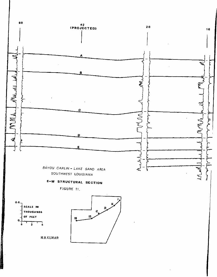
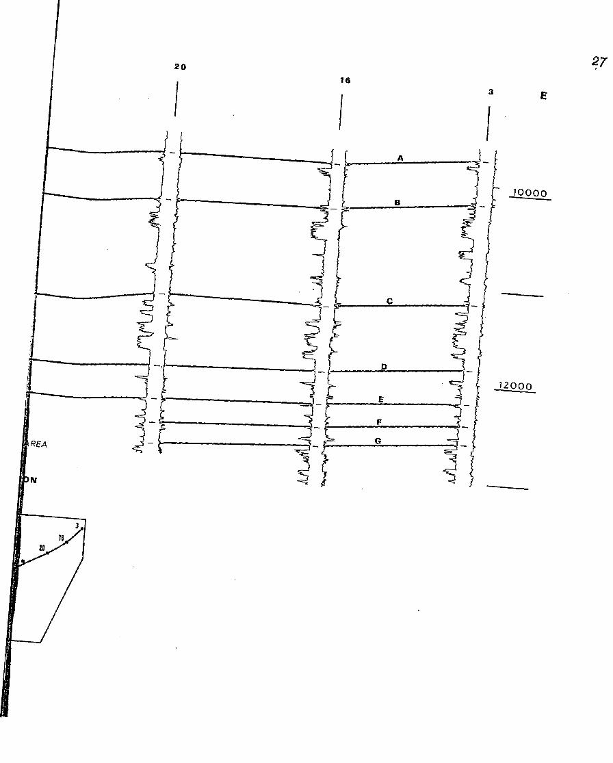
10. Correlations along cross-section Y-Y1 ......... 1511. E-W structural section.......................... 2712. N-S structural section .......................... 2813. Hand-drawn structure contour map,

horizon A ........................................ 2914. Hand-drawn structure contour map,

horizon D ........................... 3115. Hand-drawn structure contour map,

horizon E ........................................ 3316. Hand-drawn structure contour map,

horizon G ........................................ 3517. Hand-drawn isochore map of interval AB ......... 3718. Fault trends and nomenclature ...................4219. Growth index graphs of faults ...................4420. Structure contours on the faults of the

Lake Sand system.................................4621. Structure contours on fault Bl of the

Bayou Carlin system............................. 5022. Gridding by the weighted-moving-average

method .................................56vi

Figure Page23. Computer structure contour map, horizon A ....... 6824. Computer structure contour map, horizon D ....... 6925. Computer structure contour map, horizon E ....... 7026. Computer structure contour map, Carlin

block: horizon A ......7227. Computer structure contour map, Carlin

block: horizon D ................................ 7328. Computer structure contour map, Lake

block: horizon A ................................. 74«

29. Computer structure.contour map, Lakeblock: horizon O ................................. 75

30. Computer isochore map of interval AB(first type) ...................................... 77

31. Computer isochore map of interval AB(second type).. ................................... 78

32. Computer isochore map of interval BC .............. 8033. Computer isochore map of interval CD .............. 8134. Computer isochore map of interval DE .............. 8235. Computer isochore map of interval EF .............. 8336. Computer isochore map of interval FG .............. 8437. Structure trend map, third order, horizon A ...... 8638. Structure trend map, third order,horizon D ....... 8739. Structure trend map, third order, horizon E ...... 8840. Structure trend map, third order, Carlin block:

horizon A ......................................... 9141. Structure trend map, third order, Carlin block:

horizon D .............. 9242. Structure trend map, third order, Lake block:

horizon.A ......................................... 9343. Structure trend map, third order, Lake block:

horizon.D ......................................... 94vii

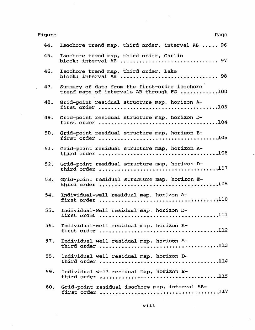
Figure Page44. Isochore trend map, third order, interval AB .... 9645. Isochore trend map, third order, Carlin

block: interval AB ........ 9746. Isochore trend map, third order, Lake

block: interval AB ................................. 9847. Summary of data from the first-order isochore

trend maps of intervals AB through FG ............10048. Grid-point residual structure map, horizon A-

first order ....................................... 10349. Grid-point residual structure map, horizon D-

first o r d e r ..................................10450. Grid-point residual structure map, horizon E-

first order ....................................... 10551. Grid-point residual structure map, horizon A-

third order ....................................... 10652. Grid-point residual structure map, horizon D-

third order ....................................... 10753. Grid-point residual structure map, horizon E-

third order ....................................... 10854. Individual-well residual map, horizon A-

f irst order ............ 11055. Individual-well residual map, horizon D-

first order ....................................... Ill56. Individual-well residual map, horizon E-

first order ...................................... .11257. Individual well residual map, horizon A-

third order ....................................... 11358. Individual well residual map, horizon D-

third order ....................................... 11459. Individual well residual map, horizon E-

third order ....................................... 11560. Grid-point residual isochore map, interval AB-

first order ....................................... 117

viii

Figure Page61. Grid-point residual isochore map, interval DE-

first order ...................................... 11862. Regional framework of the "Five Islands" trend ..12663. Mechanism of antithetic faulting and rollover

formation ........................................ 12864. Relation of restored stratigraphic section to

present salt core, Cote Blanche Island saltdome ............................................. 13065. Isopach map of post-Bigenerina humblei interval

"A-C" of Fig. 64, Cote Blanche Island saltdome ............................................. 130

66. Structure map of horizon A with details ofCote Blanche structure a dded.................... 132

67. Structure map of horizon E with details of thenorthern flank of the Bayou Sale structure......135

68. Summary of structural history .................... 140

ix

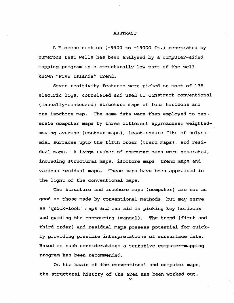
ABSTRACT

A Miocene section (-9500 to -15000 ft.) penetrated by numerous test wells has been analysed by a computer-aided mapping program in a structurally low part of the well- known "Five Islands" trend.

Seven resitivity features were picked on most of 136 electric logs, correlated and used to construct conventional (manually-contoured) structure maps of four horizons and one isochore map. The same data were then employed to gen­erate computer maps by three different approaches: weighted- moving average (contour maps), least-square fits of polyno­mial surfaces upto the fifth order (trend maps), and resi­dual maps. A large number of computer maps were generated, including structural maps, isochore maps, trend maps and various residual maps. These maps have been appraised in the light of the conventional maps.

The structure and isochore maps (computer) are not as good as those made by conventional methods, but may serve as 'quick-look1 maps and can aid in picking key horizons and guiding the contouring (manual). The trend (first and third order) and residual maps possess potential for quick­ly providing possible interpretations of subsurface data. Based on such considerations a tentative computer-mapping program has been recommended.

On the basis of the conventional and computer maps,the structural history of the area has been worked out.

x

The study area (Bayou Carlin-Lake Sand) has been influenced by salt movements at four different times, all away from the area and all related to external diapirism. The pre­sent structural configuration of the area is characterized by a structural high between two rim synclines. The first salt movement (Operculinoides time or lower Miocene) was in the southeast and associated with the Bayou Sale dome; the second salt movement (early mid-Miocene) affected the west­ern part of the area and was attributed to the mobile acti­vity of the West Cote Blanche saltdome; the third salt move­ment occurred in the northwest (at about the end of Bicren- erina humblei time or late mid-Miocene) and was associated with the Cote Blanche saltdome; the fourth salt movement (post-Biqenerina humblei time) was ascribed to the later phase of evolution of the Cote Blanche saltdome structure.Thus the saltmass in the northern part of the area (Bayou Carlin) appears to be a Miocene residual structure.

The significant natural gas accumulations in the southernpart of the area (Lake Sand field) were caused by the growthfaults which created structural closures (rollovers) and acted as fluid barriers. The area to the north (Bayou Carlin field) is very poor in petroleum, in asmuchas the petroleum migrated to the Cote Blanche structure (in the immediate northwest) which formed earlier than the present structural closures.

INTRODUCTION

Location of Study AreaThe present work is concerned with the subsurface

Miocene section of the Bayou Carlin - Lake Sand area in south-east Iberia and south-west St. Mary parishes of south Louisiana. The area, a 160-square mile tract, embraces from northeast to southwest (Fig. 1), the petroleum fields of Bayou Carlin, East Lake Sand and Lake Sand which produce mainly natural gas. Much of the northwest and southeast corners are, however, virtually undrilled.

objectiveThe objective of the investigation was to computer-

generate subsurface maps of the area, to evaluate these maps in the light of some conventional maps and reconstruct the structral history. Towards this end, the data from the electric logs were used initially to make conventional maps and sections which were synthesized to form the basis for interpretation and appraisal of the computer maps. Finally, all of the maps have been used to infer the structural evolution of the area.

Sources of DataThe basic data for the work were derived from the

electric-induction logs for wells drilled upto the end of 1971 and provided by the Louisiana Geological Survey. Atwater, Cowan, Carter and Miller contributed paleontolo-

IBERIA

JEFFEPSON i$.dSt$. £&*

CHARENTOHLOUISIANA 0WEEKS IS.

PATTERSON

SWEET BAY -

A-Petroleura fields adjacent to study area from Oil and Gas Map of Louisiana(La. Geological Survey, 1971).

i--29 30COTE BLANCHE /SLAHD I

32

BAYOU i CARLIN

23 JIT29

3233

333423 2422

6AY0U SALE

t EAST LA K E SANDLAKE SANO

i 20 22R .7 E MILE

B-Enlargement of square in "A", Bayou Carlln-Lake Sand study area lies within dashed lines.

Figure 1. Index map showing study area and adjacent petroleum fields (stippled).

3

gical information on one type well in Bayou Carlin field and its base map. Some paleontological data for wells of Lake Sand and East Lake Sand fields and geological infor­mation on their producing reservoirs were compiled from the public records and reports of the Department of Con­servation, Louisiana.

Geologic Framework Regional

The study area comprises a structurally low part of the well-known "Five Islands" trend of Louisiana. The five islands, located along a bearing of N50°W, are in order from the northwest: Jefferson Island# Avery Island, WeeksIsland, Cote Blanche Island and Belle Isle (Fig. 1A). They are acutally only knolls rising upto 150 ft. from flat marsh­land and are the only saltdomes in south Louisiana which are characterized by such a pronounced topographic relief. These five domes are believed to represent spines on a deep- seated salt ridge which extends continuously along the trend of the "Five Islands". They lie along the north-east flank of a prominent, parallel, structural arch or salient (Kupfer, 1967). To the northeast is the Five Island or New Iberia syndine, the re-entrant on the strike trend.These northwest-southeast structures are perpendicularly aligned to the general coastwise north-easterly strike trend of the sediments of the region. The "Five Islands" trend is believed to reflect a basement lineament which provided

T E X A S L O U I S I A N A

OUTCROP SUBSURFACE OUTCROP SUBSURFACE

L A G A R T O

( F L E M I N G )

F O R M A T I O N

UPPER M IOCENE

In coastal and offshore areas marine sections are present with Btgenerino

d irectoTentularia

stopper!

Bigenerina humble)'

Robulus sp.

F L E M I N G

FORMATION

CLO

VELL

Y ST

AGE

(G.E

. M

UR

RA

Y)

DIVISION A (top Bigenerina cf. Iloridona to top Buccetta , mansfieldi)

DIVISION B (top Buccella mansfieldi to top Bigenerina directo)

DUCK

LA

KE

STA

GE

(G

.E.

MU

RR

AY)

D IV IS IO N C (top Bigenerina directa to top Textularla stapperl)

D IV IS IO N 0 (top Textularla stapperl to top Bigenerina humblel)D IV IS IO N E (top Blaenerina humblel to top Am phlstegina)

LOWER MIOCENE

In coastal and offshore areas m arine sections are present with

Amphlstegina

Robulusm acom beri

Robuluschambers!

M arginulinoaseensianensls

S iphoninadavisi

D IV IS IO N F (top Amphieteglno to topOperculinoides)

D IV IS IO N G (top Operculinoides to top Robulus chambers!)

O A K V I L L E

F O R M A T 1 0 NCATAHOULA

FORMATION

1

NA

POLE

ON

VIL

LE

STA

GE

(GE.

MU

RR

AY

)

■ptVISLO&TH (top Robulus chambers) to top Marginulino . . aseensloneneie)

DIVISION 1 ' “ ■ (top Marginulino oecensionensls torftPvlslf

D IV IS IO N J (to p Siphonina

d av itl to tap O llgocene D lscorbie Z o n e)

Section*studied

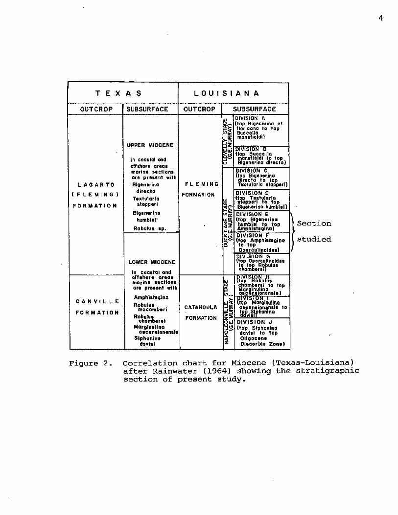
Figure 2. Correlation chart for Miocene (Texas-Louisiana) after Rainwater (1964) showing the stratigraphic section of present study-

Line of section

Figure 3

» I v ,

WW33,000-

e p i t i * ( « t iL * * c m

Regional cross section of the Miocene in south Louisiana (after Meyerhoff 1968).

an old zone of tectonic weakness (Skinner, 1960).The spacing of the "Five Islands" is another interest­

ing aspect. The four northern islands are 8 miles apart, but the southmost, Belle Isle, is 25 miles south of Cote Blanche Island: the "gap" leaves room for two more "is­lands" providing the same 8 mile spacing were to be main­tained (Kupfer, 1967). Bayou Carlin field of the present study and Bayou Sale structure on the southeast appears to fit nicely into this gap.

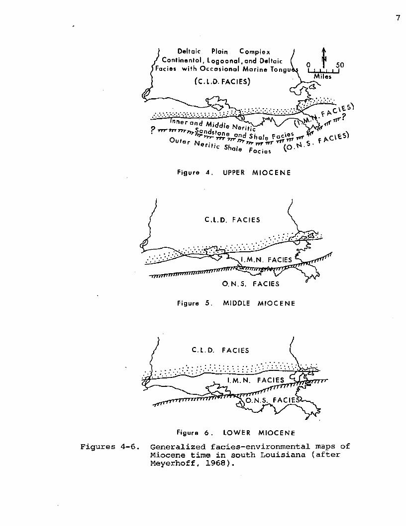
The stratigraphic section considered for the study is part of the lower Fleming formation (lower part of the upper Miocene, or middle Miocene, and the upper part of the lower Miocene: Fig. 2 and 3). This part of the Mio­cene which is known to represent a generally regressive sedimentary episode (Figs. 4 through 6) with minor trans- gressive interludes occasioned by delta shifts and contin­ued subsidence (Rainwater, 1964; Meyerhoff, 1968). During the lower Miocene time (Fig. 6) the area had an inner- middle neritic environment and later during the middle Miocene (Fig. 5), a transition to a deltaic-lagoonal environment (Meyerhoff, 1968).

Local TThe lithologic succession within the stratigraphic

interval considered consists of a repeated sequence of al­ternating sandstone, shale and siltstone, and can be divided into two sections (Fig. 7) - the lower predomi-

7

1..1.I i I I Miles

• ' “ S V 2 1 S h a l e f°i'£ rtr

Sha ie *** 77T T»TFa cies

Zrrrr(O.

Figure 4 . UPPER M I O C E N E

.M .N . FACIES rnffnTi rrt.

O .N .S . FACIES

Figure 5 . MIDDLE M IO C E N E

I .M .N . FACIES

O.N.S. FACIES

Figure 6 . LOWER M IO C E N E

Figures 4-6. Generalized facies-environmental maps of Miocene time in south Louisiana (after Meyerhoff, 1968).

8

Humble Oi l end Ref. Co. Miami Corp. Wel l No.H-9

BA Y OU CARLIN

20

Humble Oi l and Ref. Co. Stat e Lease3498 No. 6

L A K E S A N D

125

c■ourn

OOrn2

O5m73

oorn2m

IIM

Horizon BUL-l

5

Horizon CCi

ill-1

O? BOB ).I/I5 B0M RDM3® d o b-5

Horizon D5

O OP-7.OP-l

Horizon E

Horizon F

Hor izon G

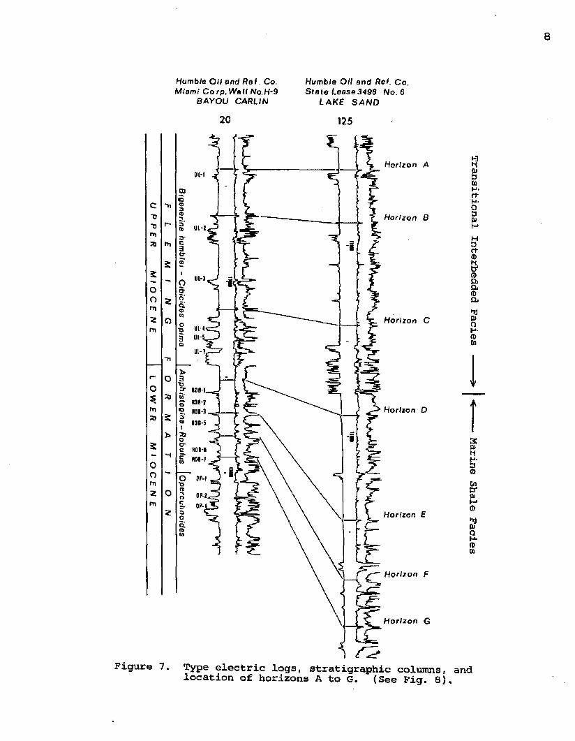
Figure 7. Type electric logs, stratigraphic columns, and location of horizons A to G. (See Fig. 8).

Transitional Interbedded

Facies

^ I <

Marine Shale

Facies

nantly marine shale facies and the upper transitional in­terbedded facies (Spiller, 1965). The transitional facies (middle Miocene) is represented by upto 45% sandstone interbedded with shale and siltstone deposited in an environment transitional between marine and deltaic. The marine facies (lower Miocene) is characterized by a pre­ponderance (over 90%) of shale and siltstone.

For mapping purposes, the section (Table 1) has been divided into six intervals designated as AB, BC, ... through FG ; delimited by seven resistivity horizons (A through G) identified on electric logs (Fig. 7). Horizons A and G approximately correspond to the tops of Bigenerina humblei and Operculinoides zones, respectively. Of all the mapping intervals, CD displays the thickest and most widespread sand bodies.

The major production (mainly natural gas) of the study area is from the Lake Sand field. Its main pro­ducing reservoirs cover the whole of the stratigraphic interval and are identified as "UL-1B Sand", "UL-4 Sand", "Rob-5 Sand", "Rob-6 Sand", and "Rob-7A Sand". They are essentially structural traps. Bayou Carlin and East Lake Sand fields, with stratigraphic and combination traps, contribute much smaller gas production (Table 1). Oil production from these fields is minor.

Table 1. Summary of Data on the Miocene Section used for the Subsurface Mapping of Bayou Carlin- Lake Sand Area, South Louisiana.

Interval AB BC CD DE EP ' FGNo. of wells on lower horizon 117 106 82 73 72 69

Age of 1/ UL1-UL2 UL2-UL4A Interval Upper Miocene — *>

UL4A-UL71

ROB1-ROB3 ROB3-ROB6A ROB6A-ROB7 ■+— Lower Miocene

Averacre depth (ft.) 10,600 11,350 12,225 13,000 13,600 14,100Thickness (ft.): AverageRange (Min.-Max.) Rat io (Min.-Max.)

530430-6351.50

1075923-12251.32

850630-10681.69

760270-12504.63

460174-1754.28

425188-6603.51

Lithology:Main% Sandstone

(Approx.)Shale15

Shale20

Sandstone45

Shale10

Shale20

Shale20

PetroleumMajor (Gas)Lake Sand

Minor (Oil)

Lake SandMinor * (Gas)

E.Lake SandMajor(Gas)Lake Sand

Major 2/(Gas) Lake Sane

1/ UL = Uvigorina lirethensis 2/ Minor (Oil and Gas)(equivalent to Bigenerina Bayou Carlinhumblei and Cibicides opima)

ROB = Robulus

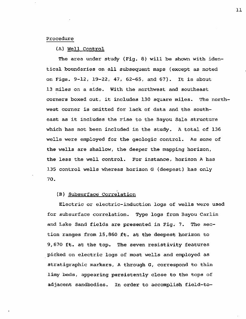
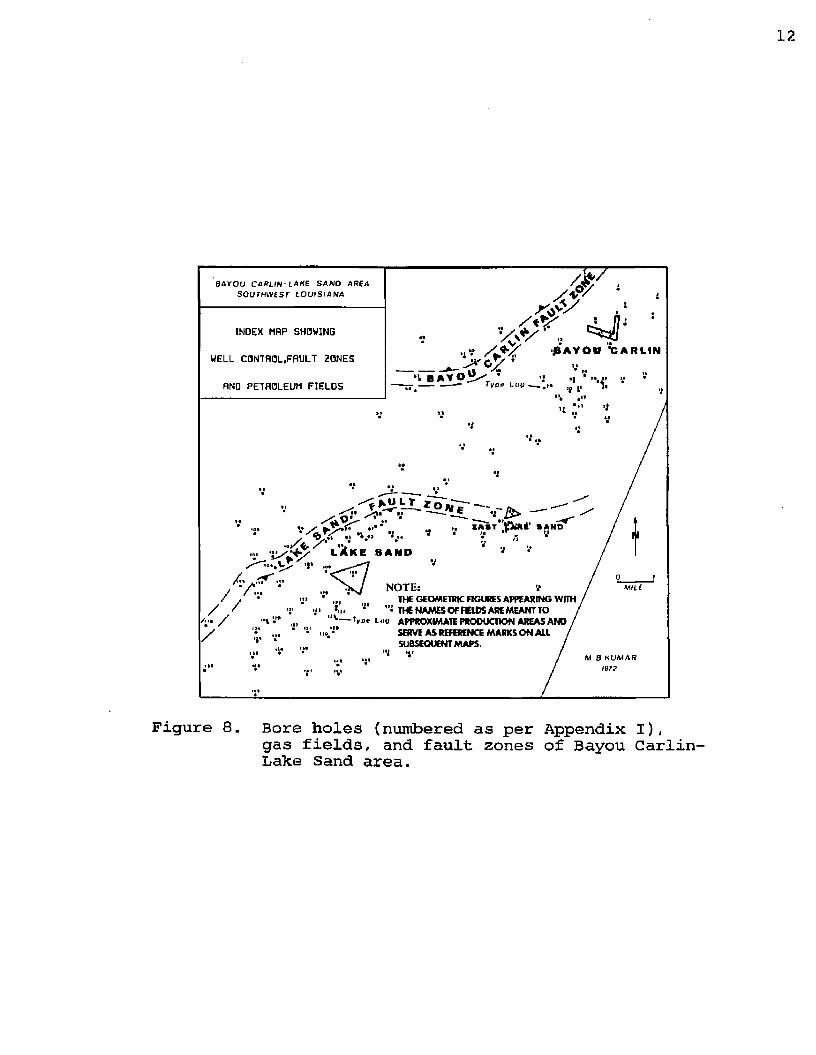
Procedure(A) Well ControlThe area under study (Fig. 8) will be shown with iden­

tical boundaries on all subsequent maps (except as noted on Figs. 9-12, 19-22, 47, 62-65, and 67). It is about 13 miles on a side. With the northwest and southeast corners boxed out, it includes 130 square miles. The north­west corner is omitted for lack of data and the south­east as it includes the rise to the Bayou Sale structure which has not been included in the study. A total of 136 wells were employed for the geologic control. As some of the wells are shallow, the deeper the mapping horizon, the less the well control. For instance, horizon A has 135 control wells whereas horizon G (deepest) has only 70.

(B) Subsurface CorrelationElectric or electric-induction logs of wells were used

for subsurface correlation. Type logs from Bayou Carlin and Lake Sand fields are presented in Fig. 7. The sec­tion ranges from 15,860 ft. at the deepest horizon to 9,670 ft. at the top. The seven resistivity features picked on electric logs of most wells and employed as stratigraphic markers, A through G, correspond to thin limy beds, appearing persistently close to the tops of adjacent sandbodies. In order to accomplish field-to-

B A Y O U C A R L IN * L AK E S A N O ARE A S O U T H W E S T L O U I S I A N A

INDEX MRP SHOWING

WELL CONTROL,FAULT ZONES

AND PETROLEUM FIELDS- _ I ll / itBAVOJ

7 F ------y W 1

'4>\ 'i, f yj^y -JS AVOO TCARLII* cy *

/ » * t *

*| *Tyae tg

x?* v — - 1 v £fc*I V / -

y+yT•.*,l.” v ■:■ w L’*KE 8AHD

IAST tv** SANDJ * } ,r . V

:<s'i* „>

NOTE:THE GEOMETRIC FIGURES APPEARING WITH ,/ A

/ ' V" ' * THE NAMES OF HELDS ARE MEANT TOv . / - s i " Ilt — W Luo APPROXIMATE PRODUCTION AREAS ANDV SERVE AS REFBtENCE MARKS ON ALL

r * SUBSEQUENT MAPS.

■vM BKUMAR

197?

Figure 8. Bore holes (numbered as per Appendix I),gas fields, and fault zones of Bayou Carlin Lake Sand area.

13

field correlation, the available paleontological data (about 10 wells) were also utilized.

Below the deepest horizon G the resitivity correlation across the three petroleum fields is beset with greater uncertainty; additionally, the available well control de­creases substantially. In view of such increased uncer­tainty and for lack of detailed paleontological data, it was decided not to extend the mapping below horizon G.The top horizon A was picked close to the top of the shallowest petroleum reservoir "UL Sands" of Lake Sand field, the main producer of the area. The correlation above horizon A, attempted for part of the area, appear­ed reasonably good, but is not incorporated in the present work. It is used to aid in the dating of the time of growth faulting.

The correlative resistivity features (A to G) employ­ed for the mapping are persistent over the whole area.The quality of correlation is, by and large, good.Horizons A,B and C are well developed in almost all wells; horizons D and E are poorly to fairly developed; horizons F and G are better developed.

The general southward thickening of all intervals (wells 75, 83 and 141 in Fig. 9; wells 99, 108, 149, and 141 in Fig. 10) is observed as expected. The intervals DE and EF, traced from Bayou Carlin to Lake Sand field, register a greater degree of expansion than normal.

3 5 20

X

BAYOU CA

S O U T H0 .5 —.SCALE IN

CORRE

C R O SSTH O U S A N D S

OF FEETM lOJ

FIG

M.B. KUMARHorizon A is datum; strat indicated on its log; tick mi

7546 7020

n 6 0 0 '

C O R R E L A T I O N S ALONG

C R O S S - S E C T I O N X - XM l

Horizon A is datum; stratigrdphic separation (omission) in well 7 0 indicated on its log; tick marks appear at intervals of 1 0 0 0 ft.

70 83

E A

n) in well 7 0 D 0 0 ft.

4910

Y

70 '

0 . 5 -S O U T H W E S TSCALE

C O R R E L A T I O N :

C R O S S - S E C T I

T H O U S A N D S

OF FEETOJ

MlFIGURE 10ID!

B.KUMAR

Horizon A is datum ; strati graphic sep 108 are indicated on their logs; tick m

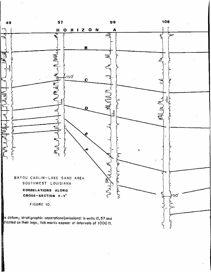
108995749

150'

YOU C A R L I N - LAKE SAND AREA

SO U T H W E S T LOUISIANA

C O R R E L A T I O N S A LO N G

C R O S S - S E C T I O N Y - Y #

FIGURE 10.

s datum; stratigraphic separations (omissions) in wells 10,57 and Jicated on their logs; tick marks appear at intervals of 1 0 0 0 ft.

108 14199 149

50

16

(C) Hand MappingAs demonstrated by Dennison (1965, Figs. 6-2 through

6-5 in his text), it is possible to draw several different maps by conventional methods of manual contouring with one and the same set of control points. This is because of the fact that control points are seldom evenly spaced and are numerically adequate to represent the true con­figuration of any unexposed surface in nature, particular­ly in the subsurface. As a consequence, the hand-drawn map is the product of the interaction of the manual con­touring method used and the imagination and esqperience of the geologist responsible for the mapping. The result is a complex function of several personal variables, such as, the geologist's backgroung, his knowledge of the area, his objectivity, personality and the purpose for which he is doing the mapping. Bearing these points in mind, five maps (four structure maps and one isochore map) were drawn, first by contouring in the areas of closest well control, then by parallel and/or equi-dip contouring in areas of medium control. In the area of sparse control interpretive contouring (Bishop, 1960) was done.

(D) Computer MappingGeological mapping by computer is considered attractive

for the following reasons:1. Strict adherence to a consistent contouring

method, offering objectivity and repeatability.

17

2. Capability of producing special type of maps, such as, trend and residual maps (see pages 20 - 25) which are not ordinarily possible with manual procedures owing to highly com­plex (time consuming) mathematical computa­tions involved.

3. Speed of map generation, minimizing contour­ing time, and eliminating drafting time, thus improving the economics of geological mapping and allowing many more maps to be made in the same interval of time.

4. Ease in updating and revision due to added or modified information.

The purpose in applying computer techniques xn the present study was to see if this would reduce personal bias by contouring on a systematic basis, suggest ideas of inter­pretive value, and serve as a safeguard against excessive­ly imaginative interpretation. At the same time, it was important to see to what extent "computerization" would introduce improbable interpretations and how these could be recognized and guarded against. To do this, the geo­logist must be aware of the calculus of computerized surface generation, since each computer program has its own limi­tation due to mathematical approximations inherent in the algorithms employed.

Types of MapsThe types of maps made and used in the present study

are briefly defined in this section. The principles and history of the usage of the special computer-generated map types are also briefly discussed. The more complete explanation of the methods and their application are discussed in a separate chapter (p. 54-124 ) and mechanical details are given in the Appendices.

(A) Structural MapsThe horizons A, D, E and G were contoured manually

in the conventional manner, using elevations of the respec­tive horizons recorded from the well logs (Appendix X).On these maps the upper and lower traces of faults were refined by the intersection of the fault contours and the horizon contours. The structure maps thus made on the four horizons are presented in Fig. 13 through 16. These horizons, in addition to the three remaining intermediate horizons, were also computer-mapped (Figs. 23 through 25; Table 4).

(B) Isochore MapsAn isochore map is contoured on equal vertical thick­

ness (well log data) whereas an isopach map is contoured on equal true thickness (Howell, 1957). Only the interval AB was used for manual contouring an isochore map (Fig.17). Isochore maps for all intervals including AB werecomputer-generated. (Figs. 30 through 36).

In the Gulf Coast, isochore maps are considered essen­tially the same as isopach maps for interpretive purposes (Moody, 1961), in asmuchas for areas of gentle structural dip, such as the present study area, there is a negligible distinction between the stratigraphic and vertical thick­ness.

(C) Fault MapsIn faulted wells the magnitude of omitted sections

was estimated after making allowance for the thickening trend displayed by adjacent wells. The elevations and the amounts of faulting (cutouts or well gaps) were recorded. These data were used to contour the fault planes in a conventional manner and the results are presented in Figs.20 and 21. It is noteworthy that the trends of the main faults were also used as guides for contouring the fault planes.

As is usual with petroleum geologists, the term "throw" has been used in this work to imply the vertical component of dip separation. Since the faults are consid­ered mostly dip-slip faults, this (throw) represents the vertical component of net-slip. As the strata have very gentle dip, the throw also equals the stratigraphic separation (stratigraphic throw). In the case of growth faults, the throw equals the fault cutout (well gap) plus the excess of thickening of sediments on the downthrown side over that on the upthrown side (Hughes, 1960).

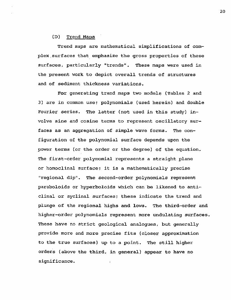
(D) Trend MapsTrend maps are mathematical simplifications of com­

plex. surf aces that emphasize the gross properties of these surfaces, particularly "trends". These maps were used in the present work to depict overall trends of structures and of sediment thickness variations.

For generating trend maps two models (Tables 2 and 3) are in common use; polynomials (used herein) and double Fourier series. The latter (not used in this study) in­volve sine and cosine terms to represent oscillatory sur­faces as an aggregation of simple wave forms. The con­figuration of the polynomial surface depends upon the power terms (or the order or the degree) of the equation.The first-order polynomial represents a straight plane or homoclinal surface; it is a mathematically precise "regional dip". The second-order polynomials represent paraboloids or hyperboloids which can be likened to anti­clinal or syclinal surfaces; these indicate the trend and plunge of the regional highs and lows. The third-order and higher-order polynomials represent more undulating surfaces. These have no strict geological analogues, but generally provide more and more precise fits (closer approximation to the true surfaces) up to a point. The still higher orders (above the third, in general) appear to have no significance.

Table 2.

Trend SurfaceFirst-order Equation

(Straight Plane)

z = f(x,Y)

Terms of EquationZeroth - order term Ax

First-order terms +A2X+A3YSecond-order terms Third-order terms

Polynomial Surfaces (up to third order) and their Equations

Second-order Equation (Paraboloid)

z

Al+A2X+A3Y+A4X^+A5xy+Agy2

Third-order Equation (Oscillatory or doubly sinusoidal surface)

z

Y

Al+A2X+A3Y+A4x2+A5xy+Agy2+AyX^+AQX2y+Agxy2+

Aioy3

Table 3. A general form of double Fourier series

M N v m JTx n FTy , m 77xA = F(X,Y) = Y' y' Amn {in cos L cos H + mn sin L

m=o n=on/Tv m /Tx

cos H 'mn cosn/Tv

sin H mn s mm /Tx n /Ty L sin H )

where Z = dependent variable in observed function,F(X,Y) = Fourier approximation at grid point X,Y,

m = index of degree of terms pertaining to x direction,

n = index of degree of terms pertaining to y direction,

mn = coefficient of cosine-cosine terms of k degree of m and n,mn = coefficient of sine-cosine term of

degree m and n, cmn = coefficient of cosine-sine term of , degree m and n,mn = coefficient of sine-sine term of

degree m an n,M = specified maximum degree of terms

pertaining to x direction,N = specified maximum degree of terms

pertaining to y direction,L = half of sampling length in x direction,

H = half of sampling length in x direction,

Xi= value of sampling interval in x direction, i = 0 ,1 ,2 ,...k,

Yi= value of sampling interval in y direction, i = 0 ,1 ,2,...1

and Amn = h , m=n=oA mn = him=o, n o , or m o,

n~oA mn = 1 , m o, n o.

(Harbaugh and Merriam, 1968, Compu­ter Application in Stratigraphic Analysis, p. 129)

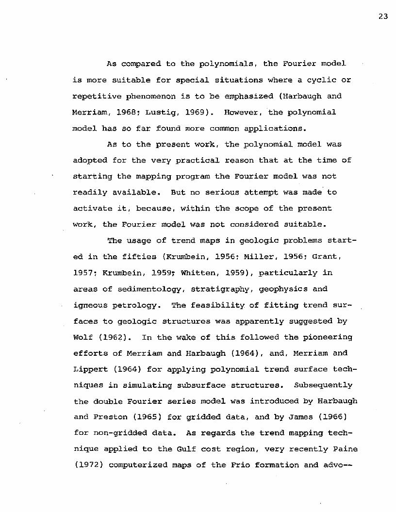
As compared to the polynomials, the Fourier model is more suitable for special situations where a cyclic or repetitive phenomenon is to be emphasized (Harbaugh and Merriam, 1968; Lustig, 1969). However, the polynomial model has so far found more common applications.

As to the present work, the polynomial model was adopted for the very practical reason that at the time of starting the mapping program the Fourier model was not readily available. But no serious attempt was made to activate it, because, within the scope of the present work, the Fourier model was not considered suitable.

The usage of trend maps in geologic problems start­ed in the fifties (Krumbein, 1956; Miller, 1956; Grant, 1957; Krumbein, 1959? Whitten, 1959), particularly in areas of sedimentology, stratigraphy, geophysics and igneous petrology. The feasibility of fitting trend sur­faces to geologic structures was apparently suggested by Wolf (1962). In the wake of this followed the pioneering efforts of Merriam and Harbaugh (1964) , and, Merriam and Lippert (1964) for applying polynomial trend surface tech­niques in simulating subsurface structures. Subsequently the double Fourier series model was introduced by Harbaugh and Preston (1965) for gridded data, and by James (1966) for non-gridded data. As regards the trend mapping tech­nique applied to the Gulf cost region, very recently Paine (1972) computerized maps of the Frio formation and advo—

cated their use.(E) Residual Maps

Residual maps can be made by subtracting the values of any map from those of another along a pre-establishedgrid system. Thus a type of isochore map could be madein this way. Unless otherwise indicated, the residualmaps in this report represent the trend residuals obtainedby subtracting the structure contours or isochore valuesat grid points from the trend values for these points ascomputed through the polynomial models. Residual maps ofthis type emphasize the local structural pattern (faults,small folds) in contrast to the regional trends.

Merriam (1964) used the residual maps to emphasize trend relationships not otherwise clearly observed from original data and to accentuate the local components of the structural pattern by essentially removing the re­gional component or dip. On the basis of residual mapping in Kansas basin, Merriam and Harbaugh (1964) concluded that there is generally a close relationship between local structural features and residual "highs" and "lows". In many instances, they differentiated structural traps from stratigraphic traps on the structural maps. Merriam and Lippert (1966) demonstrated that structural "highs" or an­ticlines are positive residuals, and structural "lows" or synclines are represented by negative residuals in central

Kansas.As reported by Merriam and Lippert (1966) geologists

have been using the technique of residuals for years; among the early users of the technique the notable are Griswold and Munn (1907), Corbett (1919, Levorsen (1927), Rich (1935), Conolly (1936), and Lee and Payne (1944).

STRUCTURE OF AREA

GeneralMost of information in this chapter was derived

from human-interpreted and hand-drawn maps and electric log sections which form the basis for evaluating the computer-generated maps (in the next chapter). However, many of the ideas presented in the succeeding chapters were also suggested by computer-interpreted and computer- drawn maps. In several cases the computer maps suggested ideas that were not.even considered during the prelimi­nary manual contouring.

The Bayou Carlin-Lake Sand area represents a low-relief anticlinal arch between two lows (possible rim synclines) - one close to Cote Blanche Island in the northwest and the other close to the large domal struc­ture of Bayou Sale in the southeast. The regional arch is intersected by a northwesterly dipping fault system (Bayou Carlin faults) to the northwest and a southerly dipping growth fault system (Lake Sand faults) to the south and southeast, giving rise to a horst block with the Bayou Carlin area in the northeast and part of the West Cote Blanche Bay area in the southwest. The main arch has four notable subsidiary highs, one for each of the petro­leum fields (Fig. 1): Bayou Carlin, Lake Sand, and EastLake Sand and West Cote Blanche. The latter is just off the map to the west, but the high is continuous in that

26

60

9 8

bav

60 42( P R O J E C T E D ! 20

B A Y O U C A R L I N - L A K E S A N D A R E A

S O U T H W E S T L O U I S I A N A

E - W S T R U C T U R A L S E C T I O N

FIGURE 11.

0.5__

SCALE IN

TH O U S A N D S

OF FEET

T— r 2

M.B.KUMAR

10000

J 2000

N 49 53 60

toooo

12000

1 4 0 0 0

B A Y O U C A R L I N - L A K E S A N D A R E A

S O U T H W E S T L O U I S I A N A

N - S S T R U C T U R A L S E C T I O N

FIG UR E 12.

S C A L E IN

T H O U S A N D S

O F FEET

M.B.KUMAR

10000

12000

1 4 0 0 0

0 A V O L T C A f t U N L A X C S A N D A f t f A S O U T H I N f S T L O U I S I A N A

STRUCTURE CONTOUR KRP

EAST

l A k c

M/i.e

M BK UM AR 197!

Figure 13. Hand-drawn structure contour map, horizon A.

30

direction. The large structure of the Lake Sand area breaks up into two separate highs on the deeper horizons - one on the upthrown side and the other on the downthrown.The high on the upthrown side is separated from the Bayou Carlin high by a saddle area. This high (referred to as southwestern Bayou Carlin high) and the highs in the northeastern Bayou Carlin and West Cote Blanche areas form a stable structural framework, because they remain in their respective geographical locations on all horizons, whereas the highs (Lake Sand and East Lake Sand) on the downthrown side of the Lake Sand fault shifts distinctly southward with depth. The Lake Sand and East Lake Sand highs appearing against the downthrown side of the Lake Sand growth fault system reflect a rollover effect. On deeper horizons, the structures assume higher relief and greater complexity.

Changes with HorizonsOn the uppermost horizon A (Fig. 13), three subsidi­

ary highs of 200-ft. closure are noted on the main anticli­nal arch. These are the Bayou Carlin ridge, southwestern Bayou Carlin high and Lake Sand high. The main Bayou Car­lin ridge (rising to the northeast) is elongated along a northeast-southwest trending axis. The main Lake Sand high (rollover) with a low closure against the Lake Sand fault is almost continuous with the southwestern Bayou Car-

B A V O U C A R L IN ' L A K E S A N D AREA SO U TH W E S T L O U IS IA N A

STRUCTURE CONTOUR MRPA V d U C A i y .

C.I. 100 FT,

M .6. KOM AH IB 71

Figure 14. Hand-drawn structure contour map, horizon

lin high at this level and its axis of elongation is parallel to the fault trend. This anticlinal rollover is chopped by two faults branching off the Labe Sand fault to the southwest. The structural dip of these highs ranges from 1/4° on the nose of the folds to 4° on their flanks. In the East Lake Sand area there are two gentle minor highs which also manifest a rollover effect on the downthrown side of the growth fault to the south. In the northwestern part of the study area, the structural dip is relatively steep towards the northwest, attaining a maximum of 5°. An even higher dip could be present north­west of Well 49.

The structural configurations of horizon B and C are essentially similar to that of horizon A, as indicated by computer maps.

On horizon D (Fig. 14), the main Bayou Carlin structure (northeastern part of the area) shows no signi­ficant change as compared to horizon A. The Lake Sand structure appears as two separate highs - one in the up- thrown block (southwestern Bayou Carlin high) and the other (the rollover of horizon A) in the downthrown block of the Lake Sand growth fault. The high in the upthrown block is located southwest of the main Bayou Carlin high and is separated from the latter by a saddle as on horizon A. To the north of the East Lake Sand area, there is a northeast trending fault (dipping southeasterly) branching off the Lake Sand fault. This East Lake Sand rollover fault is

u a r o u C A R L I N L AKE S A N D A REA S O U T H W E S T L O U I S I A N A

STRUCTURE CONTOUR HRP

BrAYOU ^rARLIN100 FT,C.I

NDAKE

M S KUMAR I9t?

Figure 15. Hand-drawn structure contour map, horizon E.

designated by a separate name in this report, because it appears to have a separate growth history.

On horizon E (Pig. 15) the overall structure assumes relatively a greater relief. The southwest Bayou Carlin high has a steeper flank to the southwest (dipping at a maximum of 5°); the southeastern flank of the northeastern Bayou Carlin high dips at 2°, more steeply as compared to the upper horizons. Moreover, the apex of the Lake Sand high (rollover) has shifted to the southeast (from near well 105 to well 123) and its closure has increased to over 300 ft. (from 200 ft. on the upper horizons). A northwest­erly dipping (antithetic) fault is added to the faults existing already in the southwestern part of the area.The East Lake Sand high has a higher relief with 100 ft. of wide closure. Another closure (rollover effect) appears against the northeastern branch of the Lake Sand fault.

Horizon F is about 400 ft. above horizon G and has a structural configuration more like the latter.

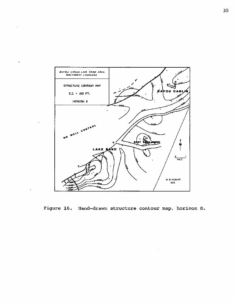
Horizon G has been only partially mapped, for lack of well control, in the western part of the area (Fig. 16). However, it is evident that the highs of Bayou Carlin, Lake Sand and East Lake Sand have still higher relief relative to the upper horizons. The faulted anticlinal fold (roll­over) of Lake Sand has its apex shifted further to the southeast and has a steeper dip (a maximum of 7°) on the southwest flank. A second northerly-dipping fault adds to the complexity of the fault framework already affecting

BAYOU C A R LIN -LA KE SA N D AREA SOLfTHtVFST LO U IS IAN A

STRUCTURE CONTOUR HRPB A l Y O U C A R

C.I. = 100 FT, JUi

N DL A K E

M S KUMAR l!U?1UO.

Figure 16. Hand-drawn structure contour map, horizon G.

the Lake Sand structure. In the East Lake Sand area another small high appears on the upthrown side of the East Lake Sand fault (in addition to the previously noted two closures on the downthrown side).

Isopachs and InterpretationFrom the structure (electric log) sections (Figs.

9 through 12) and the first-order isochore trend maps (Table 7), it is apparent that the sediments record a strong, generally southward-thickening trend. The rate of thickening increases abruptly across the Lake Sand growth-fault system. The intervals FG, EF and DE (marine shale facies) show more pronounced thickening than the upper intervals CD, BC and AB (transitional interbedded facies).

The isochore maps (hand-drawn for only interval AB, Figure 17, and computer-generated for all intervals) are described beginning with the oldest mapping interval in order to facilitate the reader's conception of the growth of the structural features.

Isochore maps bring out "thin closures" and "thick closures" representing respectively structural highs and lows active during the time of deposition. In Murray's tefms (1961, p. 4), the "thin" and "thick" sediment areas are equivalent to "posiment" and "negament", respectively. The zone characterized by rapid thickening sediments is referred to as a "downslope" in the following sections.

ISOCHORE MRPM if A YOU ■CARLINC.I. = 40 FT.

INTERVAL AQ

NO

LAKE « a n d

MILE

Figure 17. Hand-drawn isochore map of interval AB.Fault B (5) northwest of Lake Sand is dashed because it may not affect this interval.

Another important structural feature reflected on the isochore maps is the syndepositional or "growth" fault. Thorsen (1963) observes, "this type of fault is probably the most distinctive.feature of south Louisiana geology." Ocairib (1961) defines growth faults as normal faults which, have "a substantial increase in throw with depth and across which, from the upthrown to the downthrown block, there is a great thickening of correlative section". Thus the iso- pach or isochore map is the best tool for the recognition of these important faults - more "downslopes" are growth faults with "thick closures" in the downthrown block.

It should be borne in mind that the well control in the northwest and southeast corners of the study area is inadequate. The contours in these areas should be con­sidered as highly suspect and may be of little interpretive value.

FG Isochore Map (Fig. 36): The Bayou Carlin-LakeSand area has three posiments - a major one at Bayou Carlin and to the north, one to the west of Lake Sand (West Cote Blanche) and a medium one in the southeast. There is also a southwest plunging nose from East Lake Sand. The Lake Sand area is separated from the East Lake Sand and Bayou Carlin areas by a prominent east-west trending narrow belt of abrupt thickening or "downslope". This is a growth fault. As the greater growth is indicated by the closer spacing of contours, this fault has a greater growth in the west. Except for the northwestern segment, this is

39

the Lake Sand fault with its extension, the East Sand fault.The northwestern segment of the growth fault ap­

pears to represent another growth fault in the west, though probably not in its correct orientation (it is interpre­ted as approximately north-south, with westerly dip, but the well control is scanty). Since the southern part of this western growth fault is in close proximity with the Lake Sand growth fault (Figs. 13, 14 and 15), and the well control in the northwest is sparse, the computer has fall- aceously presented this fault as a branch of the Lake Sand growth fault.

The actual western branch of the Lake Sand fault (downthrown block) is marked by a southwest trending negament adjacent to the fault. This negament, though in different configurations at different times, will be ob­served associated with the downthrown block of the Lake Sand fault in the maps of all intervals. The Lake Sand growth fault also has a north-east trending branch (which is indicated in the maps of other intervals), but is vague or not shown in the present interval. The block between this branch growth fault and the East Lake Sand fault is marked by a gradual southerly thickening. The contours in the southeastern-most corner of the study area have no well control and deserve no further attention.

EF Isochore Map (Fig. 35): The Bayou Carlin areahas a broad posiment to the northwest. The downslope in the East Lake Sand area is more pronounced. Just south of the

west end of the Lake Sand growth fault lies a south-east trending negament, indicating a subsidiary basin. The previous two posiments on the east and west of the Lake Sand field stay more or less in the same positions. A third posiment appears on the extreme south-central part of the area, but may be fictitious.

DE Isochore Map (Fig. 34): No significant changeis noted in the Bayou Carlin and the East Lake Sand areas. The Lake Sand area has two posiments - one in the far east, a south-east trending ridge, and the other in the south. The previous posiment in the west disappears as the Lake Sand negament extends over to the southwest and west.

CD Isochore Map (Fig. 33): The main posiment ofBayou Carlin remains in the same old position with two new subsidiary posiments added. The downslope of East Lake Sand is pronounced. South of the Lake Sand fault, the previous negament has diminished and is confined to the southwest corner of the area. The localities of the previous two posiments in the south and far east are now marked by merely flat areas. A posiment reappears in the west.

BC Isochore Map (Fig. 32): The Bayou Carlin areahas two posiments in the east and the west. The western posiment appears as a northeastern extension of another posiment in the west of the Lake Sand area. The downslope in the vicinity of East Lake Sand is distinct. The nega­ment on the downthrown side of the Lake Sand fault has

41

two "thick" zones in the southwest and East Lake Sand.The area just to the south and southwest of East Lake Sand remains relatively flat.

AB Isochore Map (Figs. 17 and 30): The main posi­ment of Bayou Carlin is now in the north-eastern corner of the area; two subsidiary posiments appear to the south­west. The West Cote Blanche area appears flat. The down­slope of East Lake Sand is still distinct. The negament close to the East Lake Sand fault is more pronounced. A broad posiment appears in and south-west of Lake Sand; a minor posiment shows up just south of the East Lake Sand negament.

To summarise, the Bayou Carlin area north of the Lake Sand fault has broadly remained as a posiment through­out the depositional intervals considered. The downslope to the south in the vicinity of the East Lake Sand area has also maintained its configuration. The negament on the downthrown side of the Lake Sand growth fault has changed its orientation and extent with the shifting of the zones of maximum subsidence with time. The posiments to the east and south of the Lake Sand area have persisted, more or less, though modified by the adjacent negament. The posi­ment in the west was present during all the time intervals except DE when that part of the area subsided.

42

V BAYOU C A R L I N

r EAST LAKE S A N D

LAKE S A N D

MILE

Figure 18. Names and approximate location of the faults in the study area as explained in text.

43

FaultingThe structure of the Bayou Carlin - Lake Sand

area is strongly affected by two systems of faults named the Lake Sand System and the Bayou Carlin System. Both fault systems trend generally northeast, but the Lake Sand system is characterized by southerly dip and strong growth features and related structural complexities. The Bayou Carlin system has northerly to north-westerly dips and lacks important growth features in the stratigraphic intervals studied. As will be explained, the Bayou Carlin system may actually be five separate faults, the details of which cannot be recognized for lack of well control in the northern block.

The approximate trends of the fault constituents of the two fault systems are indicated in Fig. 18 with their nomenclature used in this report. The nomenclature of the faults is geographical, and consists of initial letter for the locality names (for example, E for the fault in the East Lake Sand) and a numeral to discriminate between branches of the faults (for example, LI, L2, L3, etc.) Subsidiary faults belonging to the same area are designated by a second letter (N=North, C=Central, S=South, E=East) in parenthesis, for example, L(C), L(S) etc.

In order to trace the growth history of these faults, for each interval the growth index was estimated as the ratio of thickness on the downthrown side to that

GR

OW

TH

IND

EX

44

3.0-

2.0 -

L(C)L(S)

1.0 JFG EF DE C D BC A B

ISOCHORE IN T E R V A LFigure 19. Growth index graphs of faults (see text).

on the upthrown side, in keeping with the concept of Thorsen (1956). The thickness data were taken from well logs and isochore maps. The growth idices thus computed were plotted against the isopach (isochore) intervals, to form a growth index graph for each of the growth faults (Fig. 19). The graphs are to be used with certain caution and reservation, since its precision is limited owing to inadequate well control through some deeper intervals over some parts of the study area. The graphs, in a general manner, depict the relative waxing and waning phases of the growth activities of the faults concerned.

Lake Sand Fault System ;The Lake Sand fault system (Fig. 20) consists of

eight separate faults, mostly dipping southerly (Gulfward), and forming branches off the eastern and western ends of the main Lake Sand fault LI. Out of eastern branches of the fault LI, a significant fault north of the East Lake Sand area is L(E). The main fault in the East Lake Sand area is El with another branch E(N). To the southwest, the Lake Sand fault LI has been joined by faults L2 and L3. In contrast with these down-to-the coast faults, two northerly dipping (antithetic) faults in the Lake Sand area are called L(C) and L(S). Most of these faults are growth faults with a substantial increase in throw and decrease in dip and the downthrown section much thicker than the cor­responding upthrown section. These faults are of different

C O N T O U R S ON THE LAKE S A N D FA U LTS

103

L3c.l. * 1000 FEETL2 i n

L(E)45/ !44

MILE

72

12J

L(S) •A INDEX m a pFigure 20. Structure contours on the.faults of the Lake Sand system.

ages and have grown in varying degree during different time intervals.

Fault LI is the principal fault of the Lake Sand area. It has affected all mapped intervals and appears to continue deeper below horizon G (deepest) and upward above horizon A (top). The fault seems to extend westward beyond the area of well control, and joins faluts L2 and L3; in the east it joins faults L(E) and El. The plane of the fault LI is curved, concave Gulfward and is trending northeast in the west and easterly in the east. It dips southerly (southwest to south) at an average of 50°, rang­ing from 52° at A level to 40° at the G level. Its throw increases from 300 ft. at the upper level to about 1500 ft. at the deepest level. It has a significant growth in the intervals below horizon C. Above horizon C the fault has been relatively much less active.

Fault L2 is one of the western branches off the fault LA. It curves concave to the northwest, dipping southerly at 50°. The throw is 250 ft. (maximum) at the A level and decreases to 50 ft. at the D level.

Fault L3 is either a western branch of the fault LI or possibly related to fault B(S). It trends south- south-east for most of its length, dipping easterly at 50°. In its northern part it curves westward to join the fault L2. The throw decreases downward from a maximum of 200 ft. at the A level to 50 ft. at the D level. The fault intersects (below this level) two faults L(C) and L(S).

The fault L3 has a little growth in the upper part (curved.) of the fault plane during the interval AB, which also sug­gests an affinity to B(S).

Fault L(S) trends east-north-east and dips north­westerly at 30° (much lower than the normal dip of growth faults). It starts possibly below horizon G and dies out within the interval DE. The throw is about 100 ft. at the G level. The available scanty well evidence suggests a little growth in the interval DE. Because of its flat dip and because it dips into the Lake Sand fault Ll, it is a complimentary or antithetic fault, probably rotated (flat­tened) by drag-like effects (O'niell, 1966, p. 92-100).

Fault L(C) trending east-north-east to north-east dips northwesterly at 25°. This is another antithetic fault relative to the fault Ll. Like the fault L(S), the fault L(C) originates possibly below horizon G and dies out within the interval DE. Its throw is about 200 ft. at the G level. As indicated by the available scanty well evidence, the fault had a slight growth at time E.

Fault L(E) is a growth fault with northeasterly trend, curving concave to the southeast. It joins the fault Ll in the southwest and possibly extends eastward for some distance beyond the study area. The fault originates some­where below horizon G and dies out within the interval AB. The fault dips southeasterly at 36° (lower than the dip of the growth fault Ll). Its throw ranges from 250 ft. at

the A level to 500 ft. at the G level. Like the fault Ll, it has notably grown during pre-C time.

Fault El is the major growth fault affecting the East Lake Sand area. It trends west-north-west to east and is continuous with fault Ll in the west. Its eastern extent is unknown. It cuts all the mapping intervals and appears to extend beyond the horizons A and G. It has southwesterly dip of 40° in the upper and lower levels, and 30° in the middle levels. Its throw increases from about 250 ft. at the A level to about 1500 ft. at the G level. The fault has significant growth during pre-C time, and maximum growth during the period DE when the sediments almost tripple in thickness across this fault.It is thus probably the true extension of Ll.

Fault E{N) is a northeasterly trending fault with a southeasterly dip and appears to branch off the fault E 1. Its throw at level G is about 100 ft. and is inferred to increase considerably downward as indicated by a throw of 350 ft. at about 2200 ft. below the G level in well 71. With only two control wells (wells 71 and 73) available, the dip of the fault appears to be about 50°.

Bayou Carlin Fault System ;The Bayou Carlin fault system refers to four sep-

erate faults and their branches which have affected the structure north of Bayou Carlin. These faults dip north­ward, away from the coast, and thus have an unusual region­al disposition as compared to the more commonplace down-to-

I

C O N T O U R SON F A U L T B1 C.l. = 1000 FT.

M.B. Kumar

o «10740

Figure 21. Structure contours on fault B1 of the Bayou Carlin system.

Uio

51

the coast faults. The Bayou Carlin faults dip towards the salt-domes of Cote Blanche Island and West Cote Blanche.The four faults running across the northern and northwest­ern part of the Bayou Carlin area (Fig. 18) are referred to as Bl, B2, B3 and B(N). The fault B(S) striking north­east in the West Cote Blanche area, is unlike the four faults in that it shows distinct growth features in the intervals G to A. Though more like the Lake Sand growth fault in the respect of growth character, the fault B(S) dips north­westerly (away from the coast) and appears to join fault Bl. Thus it should probably be considered as a separate fault system, but is lumped with the Bayou Carlin system for lack of control.

Fault Bl (Fig. 21) is the southeastern most fault of the Bayou Carlin fault system. It trends mostly east­erly, but swings to the northeast on the east, where it appears to die out. It bifurcates to the southwest below the A level, B2 being a branch fault. Its (Bl) northerly dip is 40° at the upper level and increases to over 60° atthe deeper levels. Its throw is about 300 ft. at the Alevel and decreases to 200 ft. at the G level, the throw diminishing laterally too to the northeast. In two wells (11 and 18) that intersect this fault above the A horizon,the fault cutouts (well gaps) were observed to be of theorder of 450 ft. (at 8950 ft). This is much greater than that below the A horizon (about 200 ft. at 9740 ft).

Such a change in throw indicates that either the fault joins another one upward or it has a marked growth character upward (unlike the lower part with no growth) , or possibly both.

Fault B(N) dips northwesterly, trending parallel to the fault Bl. For lack of well control the fault plane was not contoured. This fault was strongly suggested by an abrupt, closely-spaced contour pattern between wells 49 and 53 on the computer maps (Figs. 23 through 25). The throw is about 450 ft. at the A level and increases to 650 ft. at the G level. Despite the fact that the fault has no observed growth in the intervals between horizons G and A, it shows an increase of throw ( in the interval DE) with depth. This may suggest growth of the fault during that time.

Fault B3 is a westerly dipping fault, joining the fault Bl in the northeast. Its throw is estimated at 500 ft. at the A level and is indeterminate below for lack of well control.

Fault B (S) is a north-east trending fault with westerly dip toward West Cote Blanch. For lack of well control the fault plane was not contoured. The presence of this fault is strongly indicated by a 750-ft. cutout in well 57 aroung 10,000 ft. just above the horizon A, and an appreciable thickening of sediments during the pre-B time. The fault dies out in the southwest direction and

has increasing throw to the northeast, from 750 ft. at the A level to over 900 ft. below the E level. The fault has its maximum growth during the interval EF.

COMPUTER APPLICATION Although the computer is capable of assimilating

enormous volumes of data and generating maps at high speed, the petroleum industry has been slow to accept computer-generated maps of all types because, in general, they are considered less accurate than those produced by the standard methods involving human interpretations and manual contouring. Both types of maps involve a bias.That of the computer is of a more uniform and mathematical nature which may have advantages under certain circumstan­ces - albiet unusual ones. The author has generated a variety of computer maps and has evaluated them in order to see which types appear to hold the greatest promise. Furthermore, it has been possible to suggest an order for their use and see where and when the construction of the human-interpreted maps best fit into this sequence.

This chapter is divided into two parts. The first part deals with the principles and procedures of computer mapping. In the second part the actual computer maps generated are interpreted and evaluated on the basis of the geological information as interpreted in 'the previous chapter.

A. COMPUTER MAPPING PROCEDURESMap Generation Technique

In order to generate a contour map three co-ordinatesare required for each of the control points. They are

54

X, Y, and Z co-ordinates; X and Y are the locational or geographical co-ordinates and Z is any third quantity. Examples of Z are subsurface elevation for a structural surface or thickness for a mapping interval. Treating Z as a mathematical function of X and Y, a variety of surfaces are generated by the computer,each depending upon the nature of the mathematical function employed.

In the present study, for each of the 136 control wells used, a number of elevation (Z) values were record­ed; one for each identified pick point on the log (A through G ). These are given in Appendix I, along with the locational co-ordinates (X and Y) which were deter­mined with respect to the origin (O, 0) of a rectangular co-ordinate system located at the northwest corner of the area. Other Z-values were also recorded, such as the thickness (interval) between the pick points of the upper and lower horizons (Isochore values AB, BC, ..., FG) and some computer-generated values. This is the basic data employed for the computer mapping.

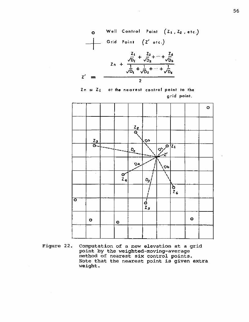
Four basic procedures (details in Appendix II). were used in generating computer maps, and each will be brief­ly described. First, for any given set of Z-values, a square-grid system is set up over the mapping area and an appropriate Z value is determined by the computer for each new co-ordinate intersection (grid point) using a weighted-moving-average method (Fig. 22). This step,

Wel l C o n t r o l Point (Zt , Z2 , etc.^

Grid Point (Z* e t c . )

y + ■••+ y</D t i/D2

Zn + j j— 4- — + - • ■ 4- —

✓ Dt ✓Da >/D6Z' = ------------------------------------------------------

2

Zn = Z i at the n e a r e s t control point to thegr id point.

o

T-2

z3\\

VO*o— \ \\ \\

Zi

o*> SiIli\\\0b

O'"U

** I1o.'si

\\\>

i1111bU

G 16U

G o o

Figure 22. Computation of a new elevation at a grid point by the weighted-moving-average method of nearest six control points.Note that the nearest point is given extra weight.

called gridding, substitutes these gridded values for the original values. The second procedure, called trend, is to fit a polynomial surface (upto the fifth order) to the origi­nally given Z values. These polynomial surfaces (Table 2) are called T- for the linear or first-order equation, for the quadratic or second-order equation, T^ ... etc.Then these trend surfaces are also gridded by the computer.

A third type of gridded Z values can be obtained by subtracting one set of gridded values from another; these are termed residuals. For example, a linear trend grid (T^) can be subtracted from a structure contour grid (SC), and an SC-T^ residual grid results. It is readily apparent that for any one well (X, Y value) there are an almost infinite number of Z values avaiable. For example, in the present study corresponding to seven horizons in a well, there are seven elevations and six simple isochore thick­nesses; with five polynomial trends for each there are already 65 Z values. With the residual permutations and combinations of these 65 values, the number rapidly becomes staggering. Fortunately, many of these have little known significance and can be ignored.

Thus, three general types of operations (contours, trends, residuals) can be performed on a given set of Z values, each resulting in a set of gridded Z-values. The final or fourth operation is to form a set of contours from these gridded values which can be either plotted on a high-speed printer, or reproduced on a drum or flat bed

plotter - two types of displays.The final outputs of the above first step (gridding

by weighted-moving-average) and the fourth step (plotting) are similar to the standard structure contour maps or iso­chore maps; the second step leads to trend maps and the third step to residual maps.

By using various combinations of the above four procedures, isochore and trend residual maps could be generated in two ways. As regards isochore maps, the normal approach is to start with thickness data for the mapping interval and run through the above first step of gridding and plot the map by the fourth step; an alterna­tive approach would be to start with the two sets of X,Y, Z values for the actual control points (for the upper and lower structural horizons delimiting the interval) and run the data through the first step and use the result­ing two sets of gridded values to obtain gridded resi­duals (third step) and plot them to generate a second kind of isochore map (seldom used). The most commonplace residual map (the trend-residual map), plots the residuals between the gridded values from the actual Z values (ele­vation or thickness) and the gridded trend values (second step); the second method is to obtain the difference between the trend values and the actual values for the given control points only and run the control point resi­duals through the first step and plot the resulting grid­ded data to obtain another kind of residual maps (seldom

59

used). All these approaches were attempted and the re­sulting map will be discussed in the second half of the chapter.

In course of this study it was discovered that after the major fault zones had been recognized, computer maps of greater meaningfulness could be generated by consider­ing each individual fault block independently. For this purpose (Fig. 8 ) the area between the Bayou Carlin fault zone and the Lake Sand fault zone is the Bayou Carlin Block, and the area to the south is the Lake Sand Block.The small area north of the Bayou Carlin fault zone has not been used for block mapping owing to sparse well con­trol (3 to 5 wells only).

On the computer maps the southwest corner of the contour number is on the contour to which it refers. In some cases this may be a very small circle and in a few cases even a point. The contour numbers are printed at each end of a contour line and at a northwest point on those that close; this without regard to overall looks and place­ment. Thus very commonly numbers are superposed on each other and illegible. As this is the way the map is pro­duced, it has,in general, been retained on the final copy to illustrate the processes. A few of confusing numbers have been deleted, and some additional numbers added where necessary for clarity.

Significance of Trend MapsFor trend maps two types of significance are important,

statistical and geological- As standard statistical tests are covered in most statistical textbooks, they will only be briefly mentioned (see also Appendis III). The trend maps were generated by fitting the polynomial model to the observed data according to the least-square criteria. A regression analysis of the trend surface was then conducted to test the surfaces for adequacy of fit (significance).The statistical measures generated by the computer program, such as partial and total F-tests, and correlation coeffi— cients were then used to estimate the significance of the trend surfaces. A more complete discussion of these tests and a table of the statiscal parameters generated are presented in Appendis III.

For the present study, trend surfaces upto the fifth order were attempted. Associated with each surface, three factgrs, namely, goodness of fit, level of significance or confidence, and geological significance, were noted. The "geological significance" is a qualitative evaluation, made by the author of the degree to which the simulation agrees with the expected geological picture. In general, the high­er the order of the polynomial, the greater is the goodness of fit, though the geological significance increases only upto a certain order. The confidence level is variable and lower order levels may not be statistically viable when

some of the upper orders are. This would be true, for example, if the local structure is so complex, that the first-order regional dip, as computed, had no meaning.

By and large, the third-order polynomials appear to best represent the geological structure. For the orders higher than the third, the goodness of fit generally does not improve significantly: moreover, the confidence level is reduced. For similar reasons, the third-order polyno­mial seems to be the best fit for the majority of the iso­chore data set too.

Terminology and SymbolsBecause of the number and complexity of the various

processes involved in malting maps, both human and computer, and the sheer number of types of maps that can be produced, some standardization in nomenclature is necessary. In the malting of a contour map of any kind, there are two essen­tial steps after the basic data is collected and plotted, first the interpretation and second the plotting or draw­ing. The commonly used terms "hand-contoured", "hand-drawn" or "manually-made" maps are all used to imply interpreta­tion, but sound as if they mean^drafting. In fact, the interpretation of the maps can be done by either men or machines, and so can the drafting. Those prepared by man are human-interpreted, and human-drawn. Maps can also be computer-interpreted and computer-drawn. Under certain conditions crossovers are possible and human-interpreted

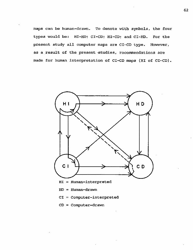
maps can be human-drawn. To denote with symbols, the four types would be: HI-HD; CI-CD; HI-CD; and CI-HD. For thepresent study all computer maps are CI-CD type. However, as a result of the present -studies, rocommendations are made for human interpretation of CI-CD maps (HI of CI-CD).

H D

HI = Human-interpretedHD = Human-drawnCl = Computer-interpretedCD = Computer-drawn

The possibilities are endless, and inter-reactive programs between computer and human have been developed and are in limited usage. Some of the simple possibilities are diagramatically indicated on the previous page. The final hand-drawn maps as presented in Fig. 13 through 17, have incorporated a few ideas from CI-CD maps and, as such, should be classified, in that sense, as HI(CI-CD) HD maps.

Structure contour maps on a particular horizon are designated by the horizon letter (A, B, ...G), and trend maps associated therewith (A/T^, D/T^, etc.). Isochores (generated by the normal method) will be designated by the letter interval (AB, BC,..., FG) and likewise the associated trend maps (AB/T^, or DE/T3 ). If isochores are generated by an alternative method (with residuals between the two sets of gridded values corresponding to two structural horizons), they could be distinguished by adding a suffix gr, for example, the map ABgr is an iso­chore map of the interval AB produced by the alternative method. The residual map, A-T3 in this report implies that it is based on the residuals between the gridded observed values of horizon A and gridded trend values of the third order. To differentiate this type from the other type of residual map (using residuals only for the control points), it could be represented by adding a suffix cp, such as, A~T3cp‘ Residual map DE-T- is based on the residuals between the gridded values of isochore thickness for the

interval DE and gridded first-order trend values of the same. Similarly, residual map DE-T^Cp represents the residuals at the control points which were later gridded for computer contouring. However, this type of isochore residual map was not generated for the present study.

These symbolic designations are essential for com­plete accuracy and understanding, but in this report plane English will be used as much as possible and the symbols added only where clarity demands.

List of Computer MapsDuring this study, about 150 maps were generated by

a high-speed printer at the LSU Computer Research Center and 80 of these were then plotted on the flat bed plotter (MILGO) at the LSU Geology Department's Computer Graphic Center. This information is summarized in Tables 4 and 5.

The printer maps are not as clear or as accurate as the plotter maps. They show some degree of distortion be­cause of the limitation on paper size and because the con­tours are displayed by arrays of symbols (numbers and letters), not by fine lines. This is why plotter maps are preferred and why no printer maps have been incorporated in this report. The advantages of printer maps are speed and low cost, and they were used in deciding on the choice of the maps to be reproduced on the plotter. Omitted are the maps that are not statistically and/or geologically significant; for example, trend maps of higher orders and

Table 4. Complete list of Computer Maps (Total area)

Horizonor

Interval A AB B BC C CD D DE E EF F FG GMap Type

HI-HD 13 17 14 15 16CI-CD 23 30 M 32 M 33 24 34 25 35 36

T1 P P P P P

T2 P P P P P

*3 37 44 38 M 39

4 P P P P PT5 P P P P P

C-T-j 48 60 49 61 50c-t3 51 52 53

C-TlcpC-T3cp

5457

5558

5659

P = Printer map only M = Milgo (Plotter) map 13 = Figure 13 in this report (M)

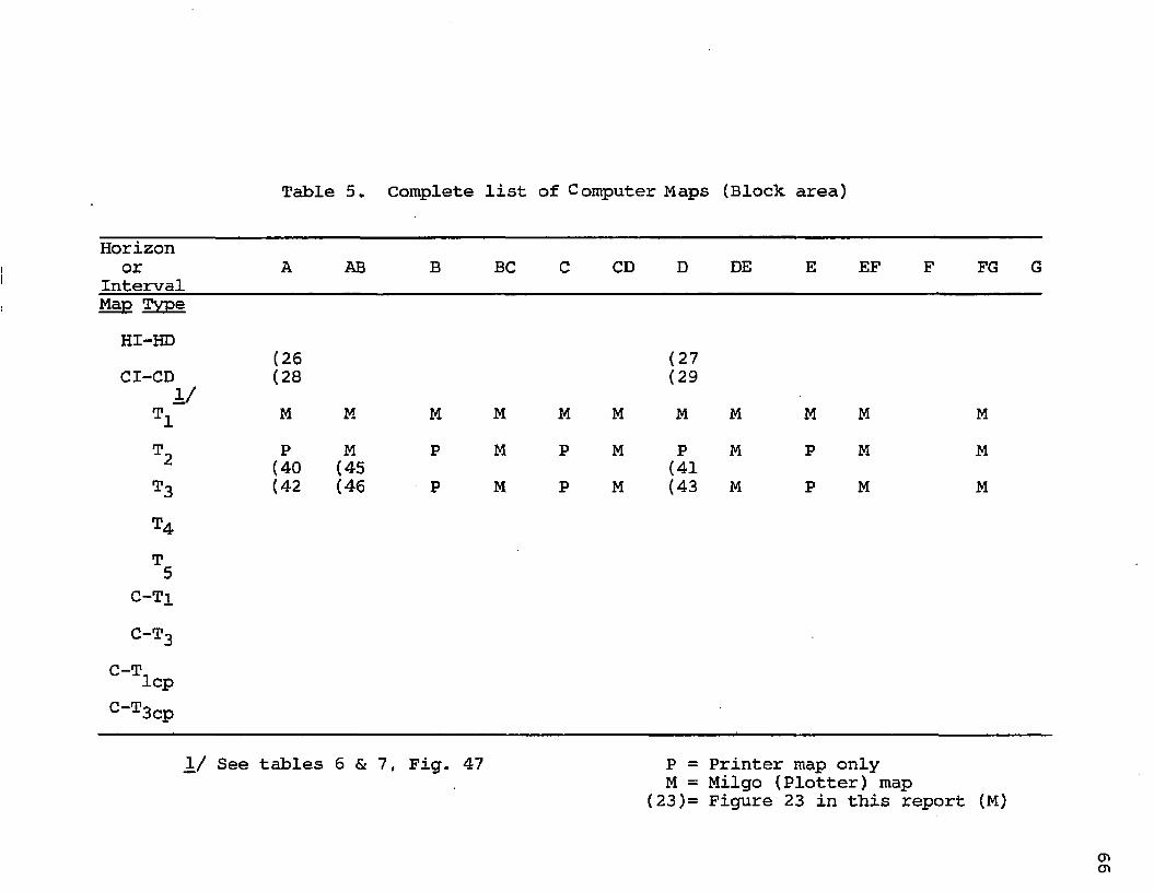
Table 5. Complete list of Computer Maps (Block area)

Horizonor

IntervalA AB B BC C CD D DE E EF F FG G

Map TypeHI-HDCI-CD

1 /T1

(26(28M M M M M M

(27(29M M M M M

P M P M P M P M P M M2T3

(40(42

(45(46 P M P M

(41(43 M P M M

T4T5

C-Tic-t3

C-T.lcpC-T3cp

1/ See tables 6 & 7, Fig. 47 P = Printer map only M = Milgo (Plotter) map

(23)= Figure 23 in this report (M)

second-order isochore trends, among others.

B. ANALYSIS OF COMPUTER MAPS In the following discussions the computer-generated

maps (structure contour, isochore, trend and residual maps) will be interpreted and appraised in the light of the known geological information presented in the previous chapter. All maps referred to in the following sections will be as­sumed to be computer interpreted and drawn unless specified otherwise. The obvious exceptions are the conventional maps (Figs. 13 through 17) which were interpreted and drawn by the author.

Structure Contour MapsThe computer-drawn structure contour maps (Figs. 23

through 25) show the general highs and lows of the area, but do not show the details (compare with hand-drawn maps in Figs. 13 through 15). Also the interpreted elevations for a few control points, as taken from the plotted con­tours, are incorrect (the points are always on the correct side of the contour).

The structure contour maps of horizon A, D and E reflect the Bayou Carlin and Lake Sand fault trends by bands of close-spaced contours. These bands of contours display abnormal 'zig-zag' trends as compared to the nor­mal smooth-running traces of the faults (Figs. 13 through 15), a computer-introduced anomaly. Similar bands of

O A Y O U C A R L I N L A K E S A N D A ^ E A S O U T H W E S T L O U I S I A N A itm

STRUCTURE CONTOUR MAPB A lY O U

C*T* * 100 FT,

HORIZON R

IIT l a k kJ b a n d

LAKE SAN

!00MB.KUMAR

t972

Figure 23. Computer structure contour map, horizon A.

69

a AVOU CAftL tH- LAKE SAND a r e a SOUTHWEST LO W SIA N A

\mfjooSTRUCTURE CONTOUR MRP

BAY10U CARC.I. * 100 FT,

HORIZON D JHII tOQ

SAND

KE STAND

M ILC>490

M .fl K U M A R t9? 2

Figure 24. Computer structure contour map, horizon D.

/

B A Y O U C A R L I N LAKC S A N D ARC A sourHvtfsr L o u i s i a n a

STRUCTURE CONTOUR MAP

C.J. = 100 FT.

1141

la so<

3700LAKE

imrM 0.K U M A R

IS72

iiuo ,

Figure 25. Computer structure contour map, horizon E.

71

contours also appear across areas of sparse control, but are not related to any known fault. They are the result of the interpolating technique of the computer program used. Thus, it is important for the geologist to be aware of the location of the control points as he interprets these maps.

The structure maps show the structural ridge that culminates in the Bayou Carlin field. The shapes of the main closures compare reasonably well with those on the conventional maps, but some are distorted. For example, the domal structure of the Lake Sand field shows up only as an area of gentle dips on a structural nose to the southeast (on horizon A and D, Figs. 23 and 24). It is better (with a 13,900-ft. closed contour) on horizon E (Fig. 25) owing to its relatively higher structural relief. The East Lake Sand high, a second-order structure, is not discernible on any of these maps.

For a more detailed interpretation of the structure, the upthrown and downthrown blocks of the Lake Sand fault were separately mapped for horizons A and D (Figs. 26 through 29). In the upthrown block, the highs and lows of the Bayou Carlin block are quite close in shape to those on the conventional maps. In the south-east part of the block, the map (Fig-i 27) has picked up a minor north-east trending fault which also shows up on the conventional map of horizon D (Fig. 14). The strong north-east trending

DUO,

BAYO U CARLIN LAKE SA N D ARC A SOUTHW EST LO U IS IA N A

STRUCTURE CONTOUR MRP

C.l. 20 FT,

CRRUN BLOCK : HORIZON R

/ Jiaa

NO

ANLA(091

Figure 26. Computer structure contour map, Carlinblock: horizon A. (Only well control from the Carlin block has been used)

73

B A Y O U C A R U N ’ LAHB S A N D ARE A S O U T H W E S T L O U I S I A N A

STRUCTURE CONTOUR MRP

CRRL1N BLOCK : HORIZON 0

> ' ' ■ ' 1.

I?I2C

jJWhM?ann

Figure 27. Computer structure contour map, Carlinblock: horizon D.

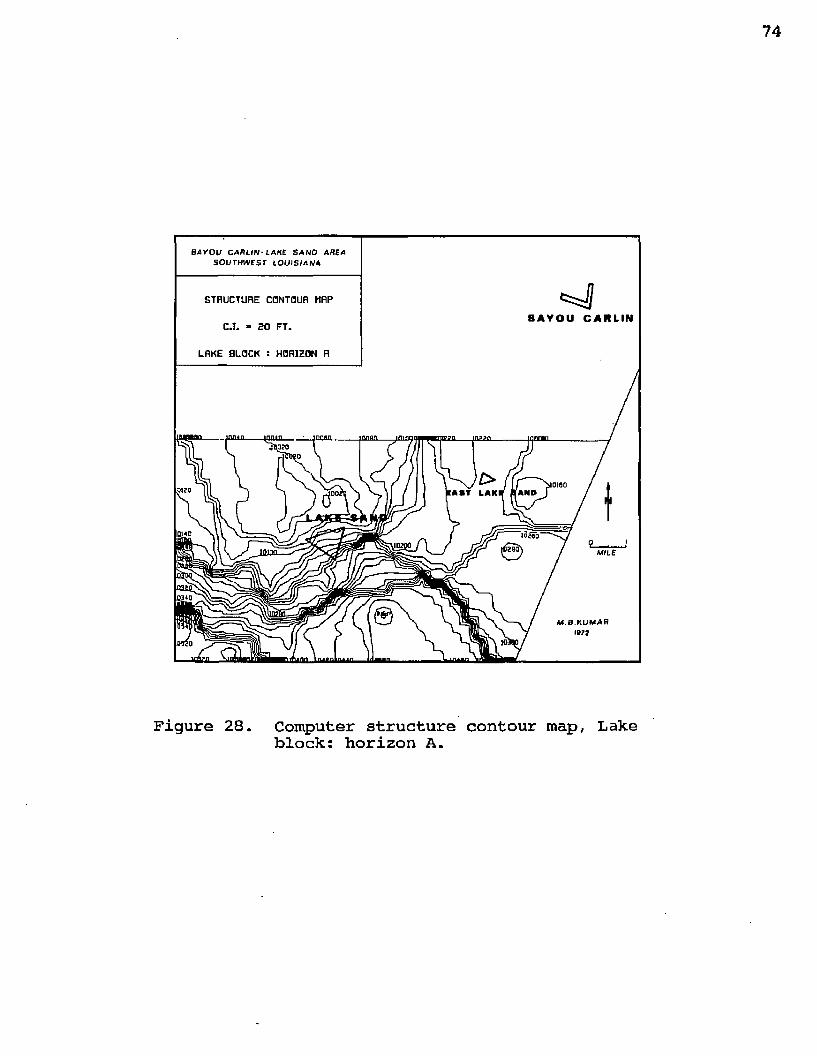
B A Y O U C A R L I N - L A M B A N D AREA S O U T H W E S T L O U IS /A H A

STRUCTURE CONTOUR MRP8AVOU CARLIN

C.t

LAKE SLOCK : HORIZON R

ma

■AST LAKl.0170 'a n d

MILE

M .0 K U M A R1072

lfiA*nlriAA*i

Figure 28. Computer structure contour map, Lakeblock: horizon A.

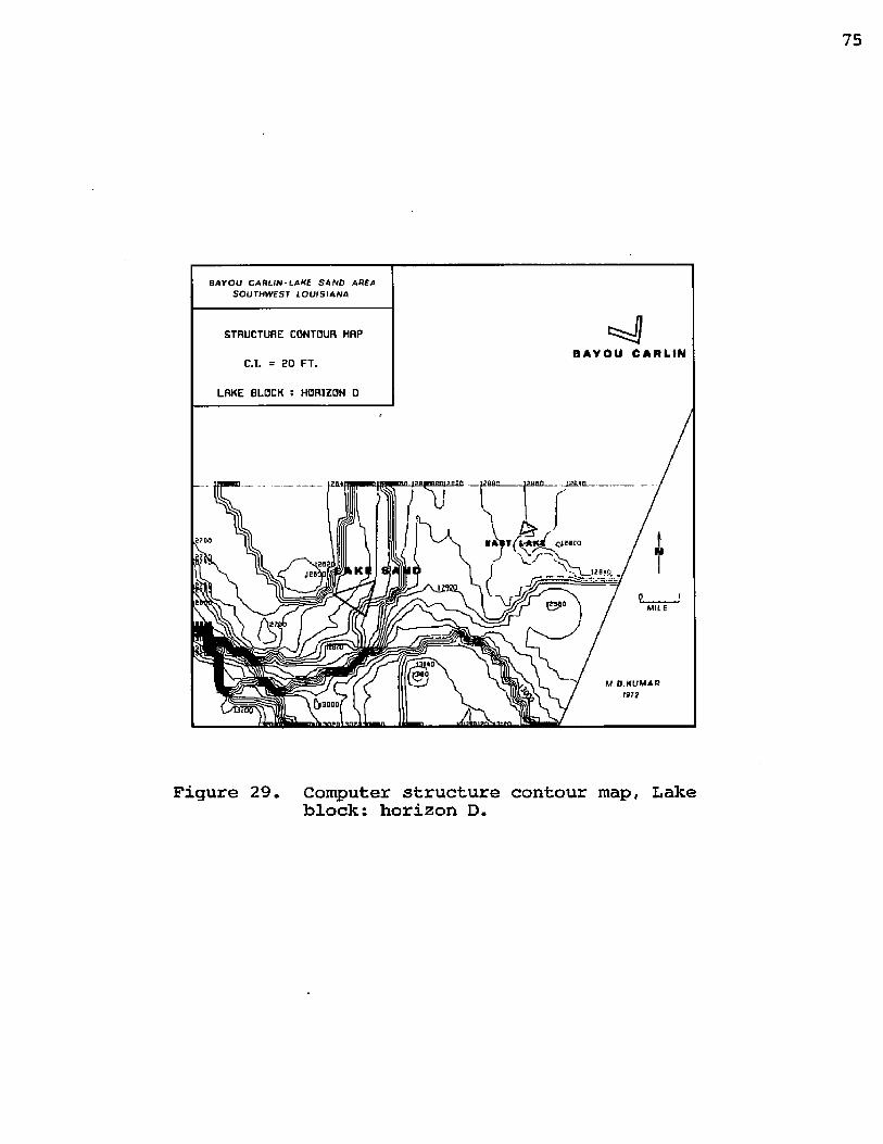
B d r O U C A R L I H - L A K E S A N D A R E A S O U T H W E S T L O U I S I A N A

STRUCTURE CONTOUR MRPBAVOU CARLIN

C.I. = 20 FT,

LRKE BLOCK : HORIZON D

_____ lJHBft___ _ j?a»n ____

*700

M ILE

M B .K U M A R f9 7 ?

Figure 29. Computer structure contour map, Lakeblock: horizon D.

fault appearing on the conventional maps in the northwest (Figs. 13 through 15) is also indicated on the structure maps, but not in the same trend. The error is probably due to the paucity of control points over that part of the area.

The maps of the downthrown Lake Sand block (Figs. 28 and 29) delineate the structures much better than before. They more distinctly and correctly depict the Lake Sand domal structure. The East Lake Sand high now appears, al­though slightly displaced. Moreover, the minor faults (branches of the Lake Sand fault) to the south-west are also detectable on these maps.

Isochore MapsAs indicated in the first half of the chapter, two

approaches can be taken to computer-generate isochore maps. These were tried for the interval AB, and the output maps are symbolized by AB (from the thickness data as the intial input) and ABgr (from the elevation data of the upper and lower horizons as the initial input). The map ABgr type was generated by two different ways -

(1) With unequal well control as available. The gridded values from 135 well control points on horizon A were subtracted from the gridded values from 118 well points as available on horizon B; the residuals (B-A) were contoured

5 A V O U C A R ' t N - L A K E S A N D ARE A

S O U T H W E S T L O U I S I A N A

MIs o c h o r c nnp

AYOU CAR

INTERVAL AB

L AK ExS AND

MfLC

M 8 . K U M A R 1979

Figure 30. Computer isochore map of interval AB(first type; thickness data from wells).

4i&f lA r O L f C A R L IN ‘ LAKE 5 4 NO ARE A

S O U rtfb V fS T L O U IS IA N A

WOISOCHORE MBPAYOU CARc.r,

INTERVAL RB

OMO

4*0 .

900

M B K U M A R 19?P

iu

Figure 31. Computer isochore map of interval AB (second type~ABgr; residuals of grid values).

79

and the result is presented in Pig. 31.(2) With equal well control. On both horizons A

and B, the same number of wells were selected eliminating the faulted wells and those which have not penetrated the interval completely.

The map ABgr with equal well control was found to be iden­tical with the map AB (first approach; Fig. 30) and has not been shown separately herein. However, the map ABgr (Fig. 31) with unequal control shows similar contours on the right parts of the map, but a good deal of dissimilarity over the localities of wells with faulted and partly pene­trated interval as seen in the major left part of the map. This exercise demonstrated that if the second approach (ABgr) is to be adopted for the isochore mapping, one should use equal well control on both horizons, eliminating those wells which are faulted or have not penetrated the interval com­pletely. As the other two proved essentially identical, for the present study, only the first approach was used for gen­erating the remaining isochore maps.

When the computer-generated isochore map (Fig. 30) is compared with the conventional isochore map (Fig. 17), it can be noted that the computer map shows clearly the growth character of the Lake Sand fault in contrast with the post- depositional or non-growth character of the Bayou Carlin fault. Except for some areas of 'thin' and 'thick1 sedi­ment shown in a general way, the computer map misses most of

LUfi. Sim*Bitrou C A R U N - L A * £ S A N O A RE A

S O U T H W E S T LOUISIANA

ISOCHORE MRP

AjJOU CARLIC.K « 20 FT.

INTERVAL BC

1M|IM

EAST ANO

KE SAND,

inW ltE

M S K U M A f lm

■IDSL LUKL

D«0MO

Figure 32. Computer isochore map of interval BC.

B A Y O U C A N L I N - L A K E S A N D A H E A S O U T H W E S T L O U IS IA N A

ISOCHQRE MAP

U CAM.INC.I. = 40 FT,

INTERVAL CO __ 3»

O

IA

K t,

MILE

M Q . H U M A R i972

ifloo.

Figure 33. Computer isochore map of interval CD.

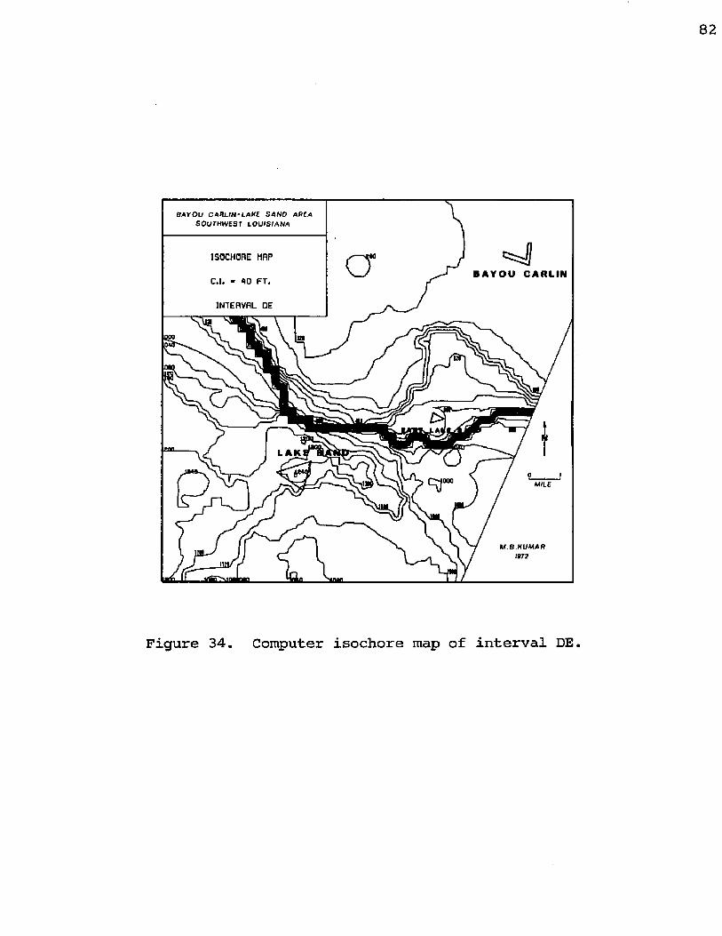
B A Y O U C A H L IN -L A K E S A N D A HEA S O U T H W E S T L O U IS IA N A

ISOCHORE MRP

C.I. - 40 FT.

INTERVAL DE

BAYOU CARLIN

PFigure 34. Computer isochore map of interval DE.

B A Y O U C A R U N ' L A K C S A N O A REA S O U T W W fS r L O U I S I A N A

1SOCHORE MRPBAYOU CARLIN

C.I. * 40 F T,

INTERVAL EF

TOOLAKE

M B . K U M A R t$J2

Figure 35. Computer isochore map of interval EF.

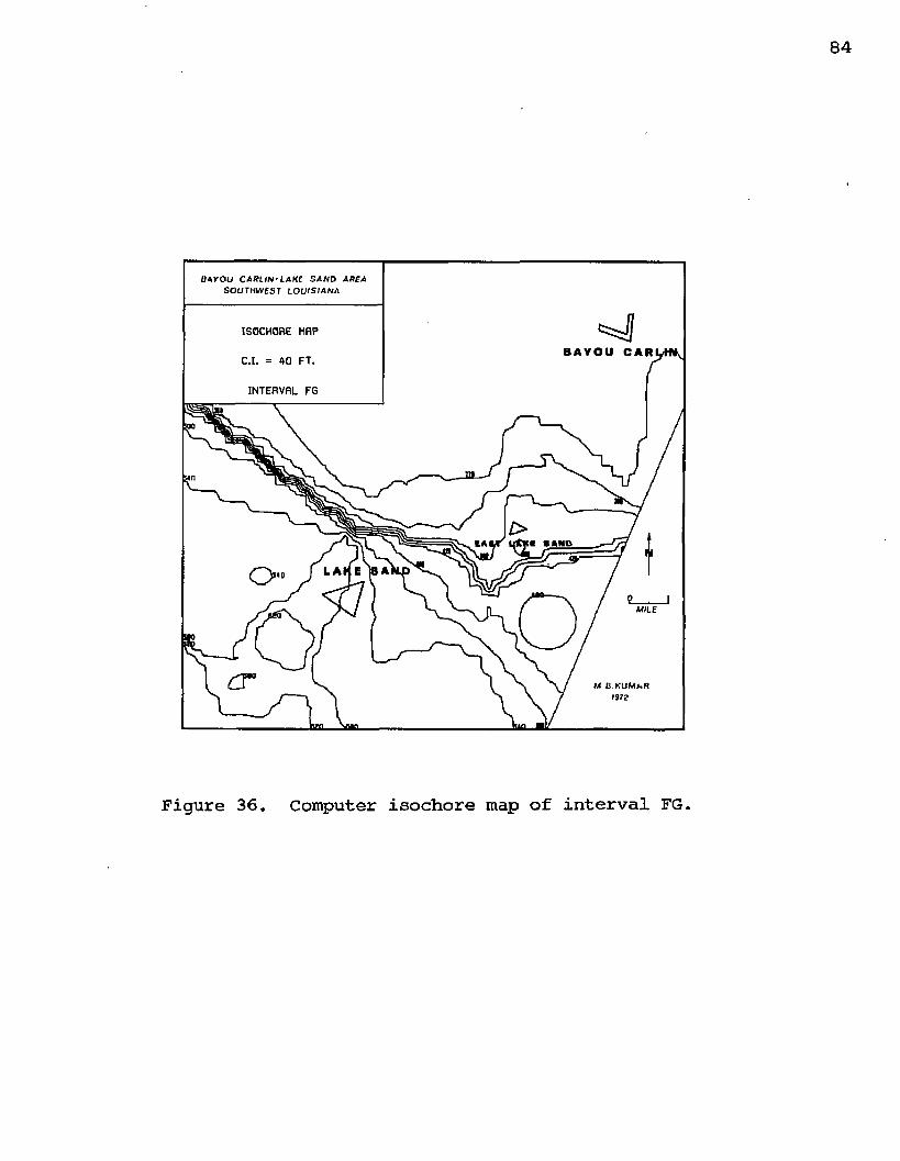
B A Y O U C A R L I N - L A K E S A N D ABC A S O U TH W E S T L O U IS IA N A

ISOCHORE HAPBAVOU CARC.I. = 40 FT,

INTERVAL FG

OMILE

M B K U M a A

P912

Figure 36. Computer isochore map of interval FG.

85

the other features shown on the conventional map.The isochore maps of the other intervals (Figs. 32

through 36) show the east-west trending Lake Sand growth fault to have greater growth in the deeper intervals. Thus, these maps of the various intervals aid in determining the relative age of the faults. The northwest-trending portion of the growth fault in the northwestern corner of the map (shown in the deeper intervals) may be a previously unde­tected branch of the Lake Sand fault, but more probably it is a fallaceous extrapolation by the computer into an area of little control. The structural interpretations of these isochore maps have already been presented in the preceding chapter, and need not be repeated here.

Trend MapsTrend maps were generated from both the structure and

thickness-interval (isochore) data. These maps help to interpret the regional dip and structural trends of the area, and locally reveal details not recognized on other maps. The structure-trend maps and the isochore trend maps will be discussed separately.

Structure Trend maps of the first order (not shown) in­dicate a very gentle southerly regional dip which increases in magnitude with the deeper horizons, reflecting the high­er relief or greater complexity of the deeper structures.The third-order maps (Figs. 37 through 39) which are con­sidered the most reliable for the data used, accentuate the

B A Y O U C A R L I N - L A K E S A N D ARE A

S O U T H W E S T L O U I S I A N A

STRUCTURE TREND MRP"AY CA3RD ORDER - C.I. = IOO FT,

HORIZON R

M 6 K U M A R ISJT

am-

Figure 37. Structure trend map, third order, horizon A.

00

B A Y O U C A R L I N - L A K E S A N D A R E A S O U T H W E S T L O U I S I A N A

1B00STRUCTURE TREND MRPBAYOU CA

3RD ORDER - C.l. « 100 FT, iioo

M 9 .K U M A A 1972

Figure 38. Structure trend map, third order, horizon D.

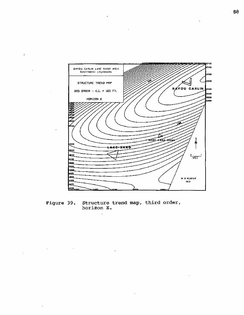
B A Y O U C A R L IN L AK E S A N D AREA SO U TH W E S T L O U IS IA N A

STRUCTURE TREND HRP

3RD ORDER - C.I. = 100 FT.

HORIZON E

IAKC 5-RMILE

M B K U M A R19J2££iudb

Figure 39. Structure trend map, third order,horizon E.

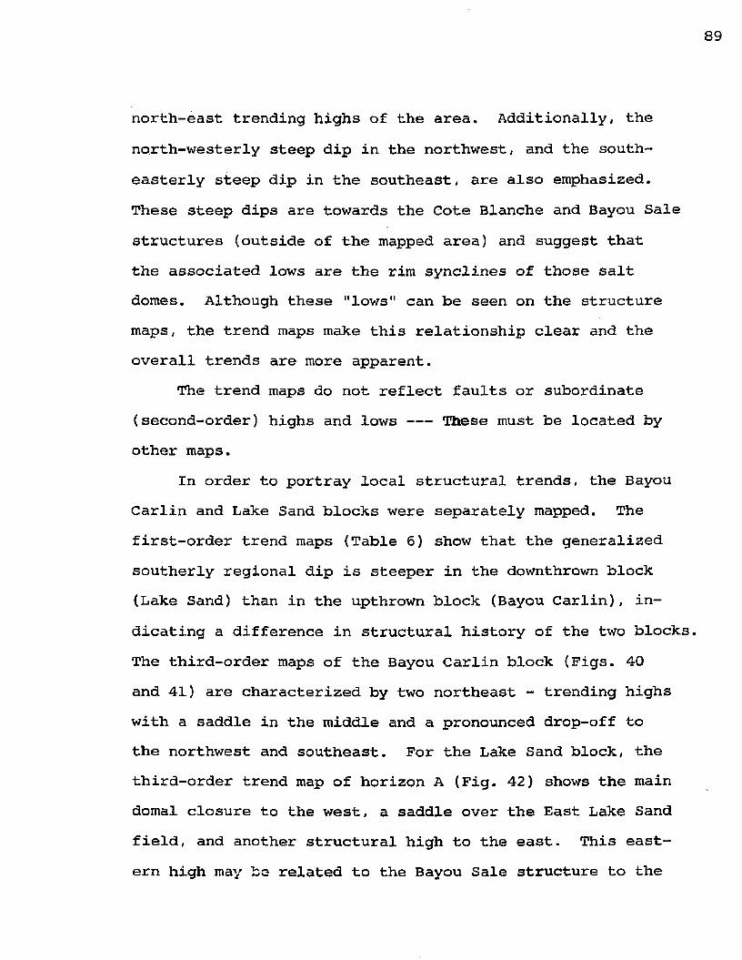
north-east trending highs of the area. Additionally, the north-westerly steep dip in the northwest, and the south­easterly steep dip in the southeast, are also emphasized. These steep dips are towards the Cote Blanche and Bayou Sale structures (outside of the mapped area) and suggest that the associated lows are the rim synclines of those salt domes. Although these "lows" can be seen on the structure maps, the trend maps make this relationship clear and the overall trends are more apparent.

The trend maps do not reflect faults or subordinate(second-order) highs and lows --- These must be located byother maps.

In order to portray local structural trends, the Bayou Carlin and Lake Sand blocks were separately mapped. The first-order trend maps (Table 6 ) show that the generalized southerly regional dip is steeper in the downthrown block (Lake Sand) than in the upthrown block (Bayou Carlin), in­dicating a difference in structural history of the two blocks. The third-order maps of the Bayou Carlin block (Figs. 40 and 41) are characterized by two northeast - trending highs with a saddle in the middle and a pronounced drop-off to the northwest and southeast. For the Lake Sand block, the third-order trend map of horizon A (Fig. 42) shows the main domal closure to the west, a saddle over the East Lake Sand field, and another structural high to the east. This east­ern high may be related to the Bayou Sale structure to the

Table 6 . Statistical Data fromFirst-Order structure Trend Surfaces (Regional Structural Dip)

HorizonDip

DirectionMagnitude, ft./mile

Level of Sicmificance

A/Carlin S20°E 8 1/ Very low 1/A/Lake S18°E 110 Very highB/Carlin S25°E 42 Very high 2/B/Lake S23°E 112 Very high “C/Carl in S32°E 63 Very highC/Lake S24°E 112 Very highD/Carlin S22°E 90 Very highD/Lake S19°E 167 Very highE/Carlin S 8°W 112 Very highE/Lake S12°E 110 High 3/

1/ The magnitude is 80 ft./mile for the total area and the level of significance is very high

2/ Very high = 99% or above3/ High = 95% or below 99%

B A Y O U C A R L I N - L A K E S A N D ARE A S O U T H W E S T L O U I S I A N A

1700STRUCTURE TREND MRP

A R L I N3RD ORDER - C.I. = 50 FT,

CRRLIN BLOCK : HORIZON R

S A N D

MILE

Figure 40. Structure trend map, third order, Carlinblock: horizon A.

1*500 1?400 12;B A r O U C A R U N - tA K F S A N D ARE A

s o u t h w e s t L o u is ia n a

I too

STRUCTURE TREND MRP1900

BAY CARLIN3RD ORDER - C.I. 100 FT.

CRRLIN BLOCK : HORIZON 0

2LQQ-

SANDLA&QQ.

M B K U M A R l»72

Figure 41. Structure trend map, third order, Carlinblock: horizon D.

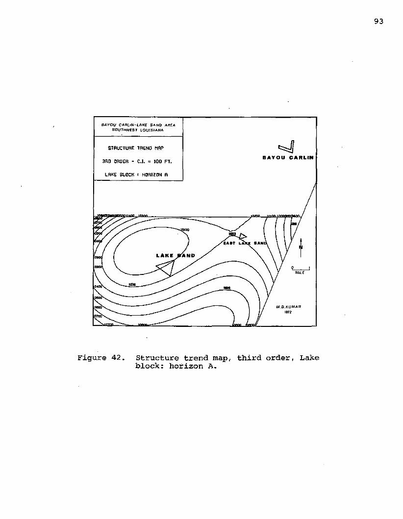
B A Y O U C A R L I N - L A K E S A N D AREA SO U TH W E S T L O U IS IA N A

STRUCTURE TREND HAP

BAYOU CARLIN3RD ORDER - C.I, 100 FT,

LAKE BLOCK : HORIZON R

SANiLAKE RAND

MBS'

goad'

MOO

Figure 42. Structure trend map, third order, Lakeblock: horizon A.

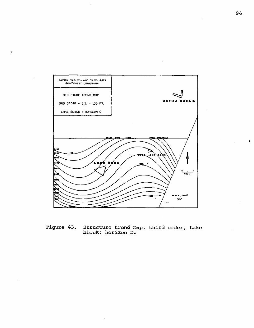
B A Y O U C A R L IN -L A K E S A N D A REA S O U T H W E S T L O U IS IA N A

STRUCTURE TREND MRPBAYOU CARLIN

3RD ORDER - C.l. 100 FT.

LAKE BLOCK : HORIZON 0

loo LAKE

LA

M B K U M A R 197?

Figure 43. Structure trend map, third order, Lakeblock: horizon D.

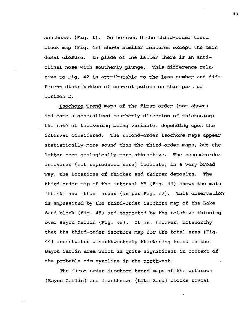
southeast (Fig. 1). On horizon D the third-order trend block map (Fig. 43) shows similar features except the main domal closure. In place of the latter there is an anti­clinal nose with southerly plunge. This difference rela­tive to Fig. 42 is attributable to the less number and dif­ferent distribution of control points on this part of horizon D.

Isochore Trend maps of the first order (not shown) indicate a generalized southerly direction of thickening; the rate of thickening being variable, depending upon the interval considered. The second-order isochore maps appear statistically more sound than the third-order maps, but the latter seem geologically more attractive. The second-order isochores (not reproduced here) indicate, in a very broad way, the locations of thicker and thinner deposits. The third-order map of the interval AB (Fig. 44) shows the main 'thick1 and 'thin' areas (as per Fig. 17). This observation is emphasized by the third-order isochore map of the Lake Sand block (Fig. 46) and suggested by the relative thinning over Bayou Carlin (Fig. 45). It is, however, noteworthy that the third-order isochore map for the total area (Fig- 44) accentuates a northwesterly thickening trend in the Bayou Carlin area which is quite significant in context of the probable rim syncline in the northwest.

The first-order isochore-trend maps of the upthrown (Bayou Carlin) and downthrown (Lake Sand) blocks reveal

96

1 M L 1 W tu.B A r O U C A A L I f / 'L A K E S A N O A R E A

S O U T H W E S T L O L T rS fA N A

1S0CH0R£ TREND MRP

B A Y O U C A R T3RD ORDER - C.I, 20 FT,

M S.KU M A R Wi

Figure 44. Isochore trend map, third order,interval AB.

uo.0 A V O U C A P L I N * LAK E S AW D A REA

S O U T H W E S T L O U I S I A N A 40

ISOCHORE TREND MRPBOB A Y O U C A R L I N

3RD ORDER - C.I. = 20 FT, •oCARLIN BLOCK : INTERVAL RB

(to

£ S A N D

M B . K U M A R

\9 t2

Figure 45. Isochore trend map, third order, Carlinblock: interval AB.

B A Y O U C A R U H ' L A X i S A N D AREA S O U T H W E S T L O U I S I A N A

1S0CHGRE TREND MRPB A Y O U C A R L I N20 FT,3RD ORDER - C.I.

LAKE BLOCK : INTERVAL RB

JMtlAKL

L A K r f t A N D

MILE

M e . K U M A R 1972

iVD

Figure 46. Isochore trend map, third order, Lakeblock: interval AB.

interesting variations in the direction of thickening as traced from interval to interval (summarized in Fig. 47 and Table 7). Traced from the interval FG upwards to AB, in the upthrown block the direction of thickening swings erratically from the southwest to south-southeast. In the downthrown block the thickening direction is northward to­wards the fault, (except CD), and thus indicate growth.This thickening may also imply a shifting of the zone of maximum subsidence. The pattern for the interval CD, along with the low growth rate for it and for the interval BC, suggests a period of insignificant growth. For the inter­val FG the thickening directions in both blocks are at an acute angle and subparallell to the fault trend. This may indicate that a major downthrown area or area of subsidence was located to the west, and, at the time of the commence­ment of the present record (Time G), the area may have had a paleoslope to the west or southwest.

Residual MaosAs indicated earlier, residual maps are designed to de­

pict local components (irregularities) of the structure and thickness variation of the stratigraphic interval. In the words of Merriam and Harbaugh (1964), "... a problem arises in deciding how much of the structure is regional and how much is residual". In such an uncertain situation, both first-order residual maps and third-order residual maps were computer-generated for the structural studies. For the

AB

1.2

DE1.8

EF

TG

N

Figure 47. Summary of data from the first-order isochore trend maps of the intervals AB through FG for Bayou Carlin (upthrown) and Lake Sand (downthrown) blocks.Arrows (solid and short on the upthrown side; open and long on the downthrown side) indicate directions of thickening. Number within each box represent an approximate growth index of the fault.

Table 7. Statistical Data from First-Order Isochore Trend Surfaces

Levelof

Rate of Regional Thickenina

Overall Growth Index _ M.T. Dn.-thrown 1/

Interval Significance Direction Magnitude ft./mile

Mean Thickness (M.T.) ft.

M.T. Up-thrown

AB/CarlinAB/Lake

VeryVery

High High 2/

S22°EN48°E

2210

480600 1.2

BC/CarlinBC/Lake

VeryVery

highhigh

S39°EN15°W

1522

10201110 1.1

CD/CarlinCD/Lake

VeryVery

highhigh

S13°WS 5°E

2026

760950 1.3

DE/CarlinDE/Lake

VeryVery high

highS58°W

N22°W66

68600

1100 1.8

EF/CarlinEF/Lake

VeryVery

highhigh

S44°WN 7°W

2653

340620 1.8

FG/CarlinFG/Lake

VeryVery

highhigh

S3 0°WS77°W

2017

280520 1.9

1/ These are overall measures of the growth-index of all the faults between the Bayou Carlin and Lake Sand blocks. The overall figures will differ from those representing the faults individually (see pages 43-45 ).

2/ Very High = 99% or above

102

thickness interval analyses the first-order residual maps of intervals AB and DE were made. The geological assess­ment of these maps follows.

Residual structure maps generated by the author areof two different types as indicated earlier in this chapter.First (A-T- , etc.), from gridded residual values (output ofthe third step, preceded by the first and second steps):second (A-T. , etc.), from the individual control welllcpresiduals (output of the second step only). As expected, the first type of residuals (Figs. 48 through 53) emphasizes the residuals in the regional framework, whereas the second type (figs. 54 through 59) brings out the local residuals around the control points. As a consequence, over the parts of the area with close well control, both types of maps have, more or less, similar contours, but the real difference occurs in the area with sparse or no well con­trol. Over such areas, the first type of map shows more contours of higher or lower values, whereas the second type has a few. or no contours. Unless otherwise specified, the residual structure map referred to in the following sections, implies the first type.

Residual structure maps of the first order (A-T^, D-T^ and E-Tj_; Figs. 48 through 50) clearly show the main Bayou Carlin and Lake Sand faults by closely-spaced contours. In addition, faults are also indicated by lows on the downthrown block (see Lake Sand fault on the first-order maps of hori-

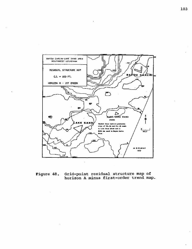
00B A Y O U C A R L I N -L A K E SAISID A REA

S O U T H W E S T L O U IS IA N A •WRESIOURL STRUCTURE MAP •1000

U CARLI 00C*I. * 100 FT,

HORIZON R - 1ST ORDERVfi

H I

i a i x ^ C X n i s a n d

SOTS:

PufcM !(■«• MleiH pn4ittN CL*IB rtfedi

li Uk* fl««l P1»M tad ofuad Is Bayw Ciflli

AKE SAND.i r t u of tJL>lA

'100

M f l H U W A R1972

Figure 48. Grid-point residual structure map ofhorizon A minus first-order trend map.

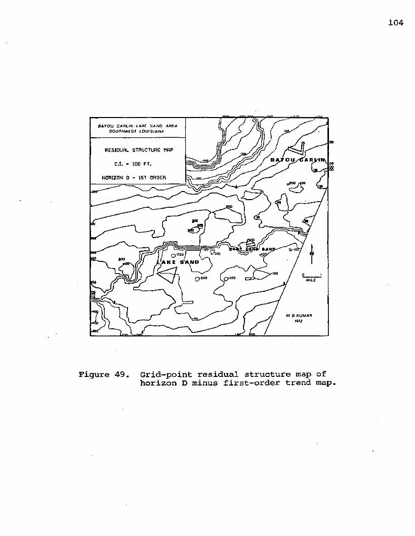
B A Y O U C A R U N ' L A K C S A N O A R E A S O U T H W E S T L O U I S I A N A

OQRESIOURL STRUCTURE MRP

OU ARC.I. * 10D FT,

HORIZON □ - 1ST ORDER

SANJ;oo

M B K U M A R 1972

Figure 49. Grid-point residual structure map ofhorizon D minus first-order trend map.

888

RESIOURL STRUCTURE HflP

C.I. = 100 FT.

HORIZON E - 1ST OROER wo

300

■ 100

M .B K U M A R W2

Figure 50. Grid-point residual structure map ofhorizon E minus first-order trend map. Dashed lines indicate productive areas of reservoirs close to this horizon.

lUUft 00B A Y O U C A R L fN i A K E 5 A N D ARE A

S O U T H W C S 1 L O U I S I A N A

RESIDUAL STRUCTURE MRP

U CA ooC.l. s 100 FT. DOHORIZON R - 3RD ORDER

90t

000. 10CLf

Figure 51. Grid-point residual structure map ofhorizon A minus third-order trend map.

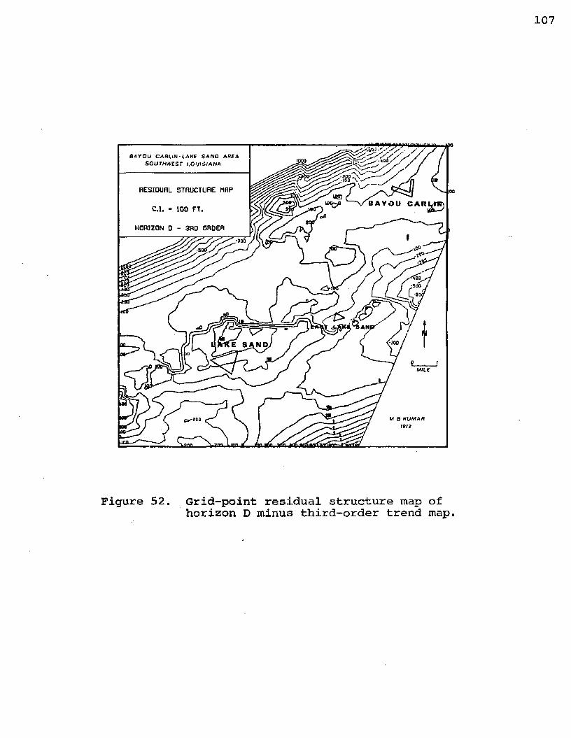
B A VO U C A dtl.M I.A H f SAMD A d fAsourmvcsr i , o > j i s i a n a

RESIDUAL STRUCTURE MAP 00BAYOU CARC.I, 100 FT.

HORIZON 0 - 3RD ORDER

M 6 H U M A f t

t9 r s

Figure 52. Grid-point residual structure map ofhorizon D minus third-order trend map.

0 A V O U C A R L I N - L A H Z S A N D A

soi/rmwsr Louisiana

PESIOURL STRUCTURE MRP

HORIZON E - 3RD ORDER

Figure 53. Grid-point residual structure map of horizon E minus third-order trend map. Dashed lines indicate productive areas of reservoirs close to this horizon.

109

zon D and E; Figs. 49 and 50).The major highs of the Bayou Carlin and Lake Sand fields

are embraced by the positive residuals. The Lake Sand struc­tural high (Figs. 13 through 15) which is untraceable on the structure contour map could be picked up on these residual maps very well. The East Lake Sand area is peculiar in that it is marked by a low on the A-T- map (Fig. 48) and by a high on the D-T^ and E-T^ maps (Figs. 49 and 50). This ano­malous case is probably explained by the fact that the east- ern part of the Lake Sand fault trace has migrated south­ward on the deeper horizons D and E relative to horizon A, and as such the East Lake Sand structural high tends to ap­pear on the upthrown side of the fault. (Note, although the East Lake Sand field appears in the Lake Sand block on the upper horizons (e.g. A), the actual gas production is from the upthrown side in the Bayou Carlin block.)

The third-order residual maps (A-T^, D-T^, and E-T3; Figs. 51 through 53) bring out the same features, more or less, displayed by the first-order maps discussed above, but emphasize the Lake Sand structure (high) and the rim syn- cline to the east.

Because the outline of the productive area adjacent to horizon A for the Lake Sand field is encompassed within zones of positive residuals (Fig. 48), the hydrocarbon traps close to this horizon are indicated to be primarily of the structural type (Harbaugh and Merriam, 1958j Fig. 5

RESIDUAL STRUCTURE HfiPB0IYOU CARLIN

C.I. = 100 FT.

HORIZON fl - 1ST ORDER

LAKE SAN

-©>

Figure 54. First-order residual structure map of horizon A, second type (A”TiCp)* usingthe residuals at control wells only.

RESIDUAL STRUCTURE MRP

tooC.I. « 100 FT,too

HORIZON 0 - 1ST ORDER

-too

too

iND-101

AKE ND

MILEno

|QQ

Figure 55. First-order residual structure map of horizon D, second type (D-T ), usinglcpthe residuals at control wells only.

1-500B A Y O U C A H L IN ■ L A K E S A N D A P E A

S O U T H W E S T L O U I S I A N A

RESIDUHL STRUCTURE MRFou c

C.I. = 100 FT,

HORIZON E - 1ST ORDER •too

w

{*»

LAKO ’

UILE-4 0 0

M.a.KUMAA107?

Figure 56. First-order residual structure map of horizon E, second type (s-TiCp )> usingthe residuals at the control wells only.

RESIDUAL STRUCTURE MAPAYOU CARLIN

C.I. s 100 FT.

HORIZON R - 3RD ORDER

>100

[a n d

LAKE 8 AND

Figure 57. Third-order residual structure map of horizon A, second type (A-T3Cp )> usingthe residuals at control wells only.

B A Y O U C A H L fN ■ LAK C S A N D A B E a S O U T H W E S T L O U IS IA N A

RES1DURL STRUCTURE MRPBAYOU CARLIN

C.l. = 10Q FT,

3RD ORDERHORIZON 0

LOO

SAND

LAKE SAND,

00

M B K U M A R 19/?

ilOCL tlflQ.

Figure 58. Third-order residual structure map ofhorizon D, second type (D-T ), usingocpthe residuals at control wells only.

IflfL

.-----' BAYOU CARLIN

JiL

RES1PURL STRUCTURE MRP

C.I. = 100 FT.

HORIZON E - 3RD ORDER

'ZOO

■mjl a k / sa •- ion

Figure 59. Third-order residual structure map ofhorizon E, second type tE-T3Cp )• using theresiduals at the control wells only.

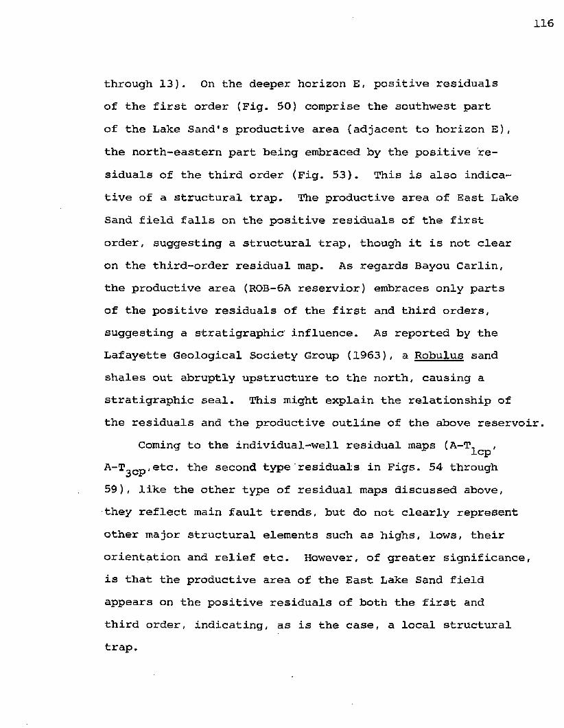
116

through 13). On the deeper horizon E, positive residuals of the first order (Fig. 50) comprise the southwest part of the Lake Sand's productive area (adjacent to horizon E), the north-eastern part being embraced by the positive re­siduals of the third order (Fig. 53). This is also indica­tive of a structural trap. The productive area of East Lake Sand field falls on the positive residuals of the first order, suggesting a structural trap, though it is not clear on the third-order residual map. As regards Bayou Carlin, the productive area (ROB-6A reservior) embraces only parts of the positive residuals of the first and third orders, suggesting a stratigraphic influence. As reported by the Lafayette Geological Society Group (1963), a Robulus sand shales out abruptly upstructure to the north, causing a stratigraphic seal. This might explain the relationship of the residuals and the productive outline of the above reservoir.

Coming to the individual-well residual maps (A-TiCp'A-T^Cp <etc. the second type residuals in Figs. 54 through 59), like the other type of residual maps discussed above, they reflect main fault trends, but do not clearly represent other major structural elements such as highs, lows, their orientation and relief etc. However, of greater significance, is that the productive area of the East Lake Sand field appears on the positive residuals of both the first and third order, indicating, as is the case, a local structural trap.

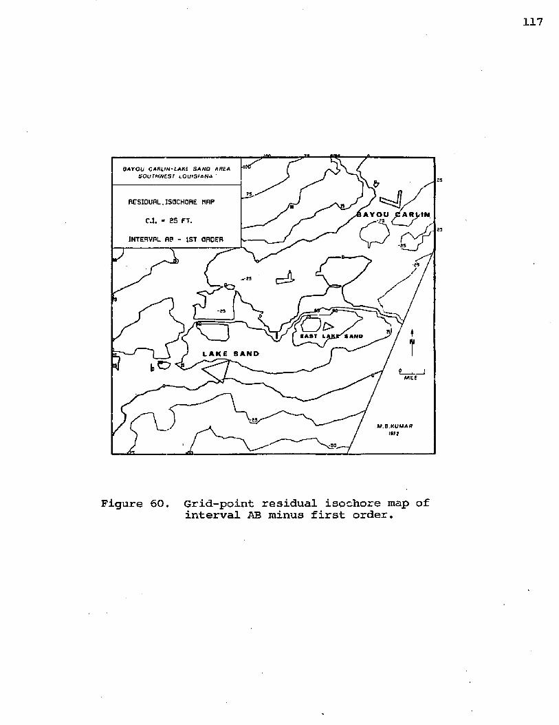
■XL0 A Y Q U C A R U N ' L A K i S A N D A REA

S O U T H W E S T < _ O U t S i & N *

RCSIOURL, 15OCH0BE MRP

CJ. - 25 FT.INTERVRL RP - 1ST ORDER

EAST L SAND

l a k e s a n d

MILE

M . B . H U M A R1977

Figure 60. Grid-point residual isochore map ofinterval AB minus first order.

poB A Y O U C A R U N -L A K E S A N D A R E A

S O U T H W E S T tO L H S IA N A MO

RESIDUAL ISOCHORE MRPDO

o u LINC.I, SO FI

INTERVAL DE - 1ST ORDER

poo

. B A 8 7 l . * K * B

too

M S K U M A Ris ? ;

•30?nn -J im j h h m l . j . t t .

Figure 61. Grid-point residual isochore map ofinterval DE minus first order.

119

Residual isochore maps (AB-T^ and DE-T^; Figs. 60 and 61) display the growth fault effect in a distinctive fashion. Excessive thicknesses (positive closures) occur just south of the Lake Sand fault and are attributed to a zone of maximum subsidence in the growth fault environment. The even more pronounced positive residuals on the down- thrown side for the interval DE suggests an even greater growth effect and associated subsidence for that interval. The negative residuals correspond to the zones of thinning over structural highs or posiments, as in the upthrown Bayou Carlin block.

Summary and Conclusions

The computer-generated structure and isochore maps show the fault trends, but not in correct or proper orientation: the contours are not precisely placed honouring the control points in some parts of the map; in the areas of little or no control the surface is shown as having abrupt changes in slope; and minor highs are displaced sometimes from their correct positions. These are the shortcomings of the com­puter maps, some of which could be eliminated by using a better program. However, they make the maps of limited

direct use to the geologist in the field. In otherwords, they alone could not serve as substitute for the hand maps. Nevertheless, the computer maps pro­vide "quick-look" maps from which geological suggest­ion of significance could be drawn and this would help decide which horizons and intervals merit greater attention by the investigator. As far as the present study is concerned, the author has be­nefited from these maps essentially in the follow­ing ways:

(1) The maps suggested the trends of faults B {S), B(N), and L(E), which were later incorporated in the hand-drawn maps.At the very preliminary stage of work, the isochores brought out the distinc­tion between the Bayou Carlin and Lake Sand fault systems, suggesting their relative age.

(2) They reflected no significant change in structure on horizons B and C. interme­diate between the manually mapped hori­zons A and D; thus, helped deciding on the elimination of those two horizons for the structure mapping.

(3) Once the isochores for all the intervals were generated on the computer, the hand contouring of these intervals was no longer required, since the former appear­ed to accomplish the purpose of indica­ting 'thick' and 'thin1 areas for recon­structing the structural evolution of the area.

(4) With some judgment and awareness of the character of the computer maps, a good deal of information was derived from all the computer maps for inferring the structural history.

121

The trend maps and residual maps turned out to be very useful. The third-order trend maps clearly brought out the regional anticlinal arch with north-east trending highs and lows to the northwest and southeast; the block maps (third order trend) accentuated the subsidiary highs and lows on the main arch. The first-order trends,(structural) suggested that the Bayou Carlin and Lake Sand blocks had different structural history, and the first-order isochore trends contributed toward the reconstruction of their growth history.

The residual structure maps strongly indicated the Lake Sand and Bayou Carlin faults. The first-order resi­duals brought out lows in the northwest and southeast, and highs particularly in the upthrown block; the third order residuals accentuated highs on the downthrown side, notably the rim syncline in the southeast. The first order isochore residuals depicted the zones of maximum subsidence, in par­ticular characterizing the downthrown side of the growth fault in the Lake Sand area and the thickening trend towards the rim syncline on the northwest.

The significant points highlighted in the preceeding paragraphs are presented at a glance in Table 8 . This also serves to indicate why the author had to carry the mapping program onto the stage of individual-well residual maps.For instance, the East Lake Sand structure could be located distinctly only on this (second) type of residual map.

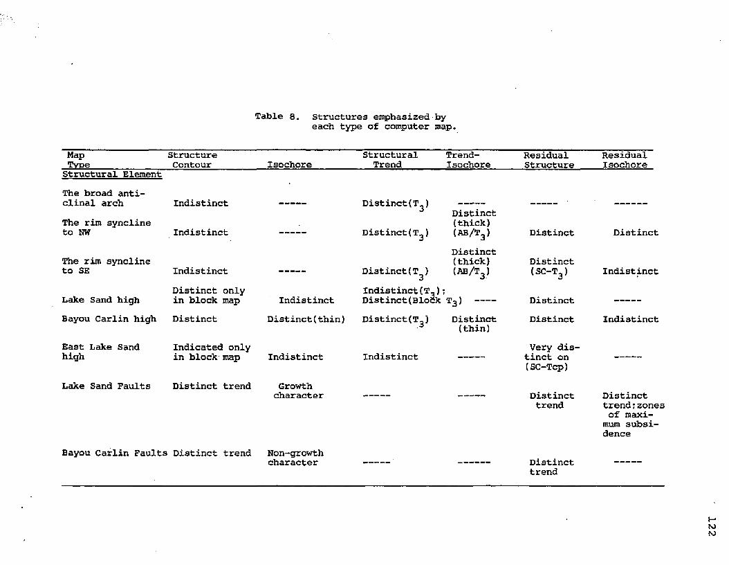
Table 8. Structures emphasized byeach type of computer map.

MapTvoe

StructureContour Isochore

StructuralTrend

Trend-Isochore

ResidualStructure

ResidualIsochore

Structural ElementThe broad anti­clinal archThe rim syncline to NW

Indistinct

Indistinct

Distinct(T^)

Distinct(T^)Distinct(thick)(a b/t3) Distinct Distinct

The rim syncline to SE Indistinct Distinct(T^)

Distinct(thick)(a b/t3)

Distinct(sc-t 3) Indistinct

Lake Sand highDistinct only in block map Indistinct

Indistinct(T-);Distinct(Block T3) --- Distinct

Bayou Carlin high Distinct Distinct(thin) Distinct(T^) Distinct(thin)

Distinct Indistinct

East Lake Sand high

Indicated only in block map Indistinct Indistinct

Very dis­tinct on (SC-Tcp)

Lake Sand Faults Distinct trend Growthcharacter Distinct

trendDistinct trend:zones of maxi­mum subsi­dence

Bayou Carlin Faults Distinct trend Non-growthcharacter Distinct

trend

l—1toto

123

RecommendationsFrom the foregoing discussions it follows that the

computer maps hold high potential for guiding the initial mapping program and for providing possible interpretations of geological data. A suggested schedule of computer map­ping is recommended below that precedes (in part) the con­struction of conventional, hand-drawn maps:

1. Establish field-to-field subsurface correlations and record X, Y, and Z co-ordinates.

2. Prepare computer-drawn structure-contour maps for all horizons.

3. Prepare computer-drawn isopach maps for all intervals between horizons.

4. Eliminate those horizons and intervals which have similar geological pictures.

5. Run T. and T on all remaining horizons (bothx 3structure-contour and isopach).

6 . Run residual maps of selected horizons and in­tervals to find clues to trends, growth and petroleum accumulation.

7. Select specific horizons and intervals for human interpretation and manual contouring.

8 . Compare hand-contour maps and computer maps and decide on the small areas that need more detail.

9. Repeat such portions of earlier steps as neces­sary on these small blocks: modify the hand-con­toured maps in the process.

124

Future OutlookAs a continuation of this study of the reliability of

computer-mapping programs, future work should be on dif­ferent situations, such as structures of higher relief, larger or smaller areas, and various distribution patterns of control points. Residual maps appear to have a great deal more to offer and should be studied in a variety of situations. Programs using different methods of contour­ing, such as SYMAP, should also be examined for critical areas.

The attempt to perfect the computer program should continue to seek to combine the good qualities of hand maps. On the other hand, the geologist should aim to de­velop the eye and the outlook so that he can eventually reconstruct the geology of the area through the use of com­puter maps alone, or with a minimum of his own maps. In other words, the geologist must learn and perfect the tech­nique of interpreting the computer maps without waiting for the best and most versatile mapping program to be developed. Despite impressive accomplishments recorded ever since the early fifties in the realm of computer application to geo­logy, a sphere of indefinite dimension remains unexplored. Not only are more versatile programs required, but so also are more dynamic interpreting techniques by the geologist.

TECTONIC AND REGIONAL IMPLICATIONSA. Salt Dome Growth

To the author's knowledge, there is no published report of significance on the structure of Bayou Carlin, Lake Sand, East Lake Sand or Bayou Sale. Troutman (1955) in­dicated that Bayou Carlin and Lake Sand fields are asso­ciated with deep-seated saltmass and that the Bayou Salestructure is a "deep-seated saltdome with complex fault-

*■ing". Wallace (1952) suggested rim synclines around all the members of the "Five Islands" and adjacent saltdomes on his fault map of South Louisiana. On his recent map (1962) the outlines of rim synclines are not shown but more details are added to Bayou Carlin, Lake Sand and Bayou Sale fields.

In order to appreciate the relation of the structure of the study area with the adjacent structures in a region­al perspective, the principal structural elements of the Bayou Carlin - Lake Sand area are shown on a sketch map (Fig. 62) with Wallace's postulated rim synclines of the adjacent saltdomes and details of the Bayou Sale structure. It is significant to note that the eastern, northwestern, and western part of the study area are within five miles of the Bayou Sale dome, the Cote Blanche saltdome and the West Cote Blanche saltdome, respectively. It is thus reasonable to expect mobile activities of these adjacent salt masses to influence the structural growth history of the study area.

125

JEFFERSON I SL A N D

A V ER Y I S L A N D

WEEKS I S L A N D M I L E S

COTE B L A N C H E I S L A N D

W . C O TCHV E R M I L I O N

BAY /BC

BAYOU SALE

BELLEISLE

M A R S H ISLAND

Study A r e a

L E GE N D

N O R M A L FAULT W I T H BARB O N THE D O W N T H R O W N SIDE

SALT S T O C K

P E T R O L E U M F I ELD

AXI S OF R I M S Y N C L I N E

F O R M L I N E OF STRUCTURE

Figure 62. Structural framework of "Five Islands" and the vicinity modified from Wallace (1962) with rim synclines (Wallace, 1952); structural details from horizon D of the study area. Faults lettered as per text; Lake Sand field, (LS), Bayou Carlin field, (BC).

127

From Fig- 62 it is evident that in the northwestern part of the study area the faults B1 and B(N) trend around and dip towards the Cote Blanche rim syncline. To the southeast the fault L(E), like faults BS1 and BS2 (from Wallace's map), dip towards the large domal Bayou Sale structure.This domal structure is traversed by a fault complex with radial and peripheral faults, which is typical of south Louisiana saltdomes, but the pattern of these faults appears to be different from that of faults L(E), BSl and BS2. The latter three, with southerly dip towairds the Bayou Sale dome suggest the possibility of a rim syncline just to the northwest of the Bayou Sale deep-seated dome, even though Wallace did not show one.

Age of FaultsThe Lake Sand fault Ll and its eastern branches, name­

ly, L(E) and El form the earliest generation of faults in the area. Murray (1957) recognized the Lake Sand fault as an example of a down-to-the coast regional gravity faulting related with thick sedimentation. Also it appears prominant- ly on the fault maps of Wallace (1952 and 1962). The west­ern branches of the Lake Sand fault postdate the eastern branches, but it has not been possible to determine precise­ly the chronology of the eastern branch faults, in as much as all of them were in the active phase in the lowest mapped interval FG. However, from the trends of the growth index graphs (Fig. 19), some extrpolations into the pre-G time

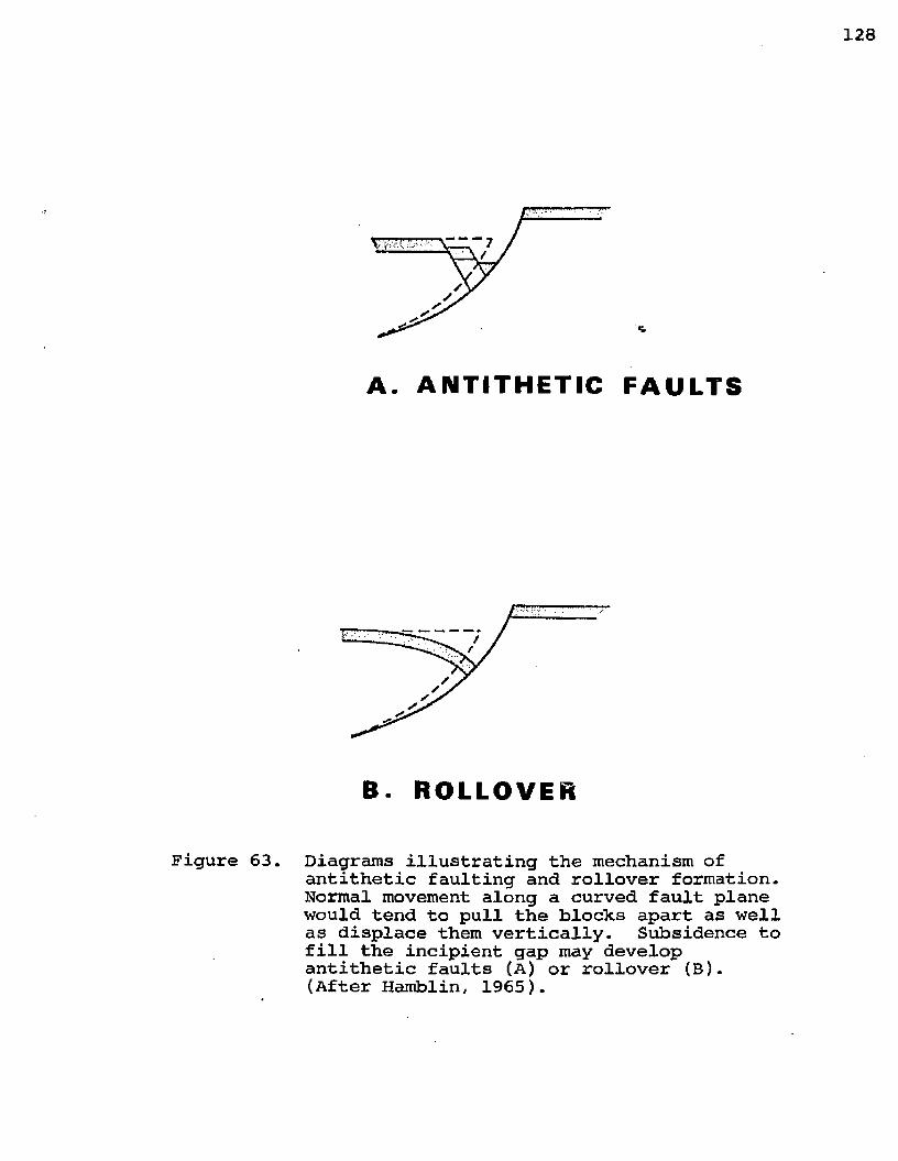
A. ANTITHETIC FAULTS

B. ROLLOVER

Figure 63. Diagrams illustrating the mechanism ofantithetic faulting and rollover formation. Normal movement along a curved fault plane would tend to pull the blocks apart as well as displace them vertically. Subsidence to fill the incipient gap may develop antithetic faults (A) or rollover (B). (After Hamblin, 1965).

129

could be attempted on the assumption that every south Louisiana fault is expected to have a bell-shaped growth- index graph, as demonstrated by Thorsen (1956). From such extrapolations it appears that the fault LI should have had its inception much before the faults El and L(E). These two faults appear to have originated almost concur­rently, but there is no reliable basis for asserting which of the two is the older.

The southwestern area had a short-lived generation of faults represented by the antithetic faults L(c) and L(D), not shown in Fig. 62. They probably originated around G~ time and remain locally active for sometime and died out within the interval DE. Since they originated as antithetic faults during the time of intense activity of the older fault Ll, their origin could easily be explained by the mechanism postulated by Hamblin (1965). That is, they de­veloped by "subsidence" to fill the incipient gap produced by normal movement along the curved plane of the fault Ll (Fig. 63). The antithetic faults thus originated later than the faults El and L(E) and. were outlasted by them.

The youngest generation of faults of the Lake Sand system is represented by faults L2 and L3. The fault L3 had slight growth during the interval AB, but the fault L2 had no growth during any of the mapped intervals and is probably still younger than the fault L3.

The Bayou Carlin faults Bl, B2, B3 and B(N),excepting

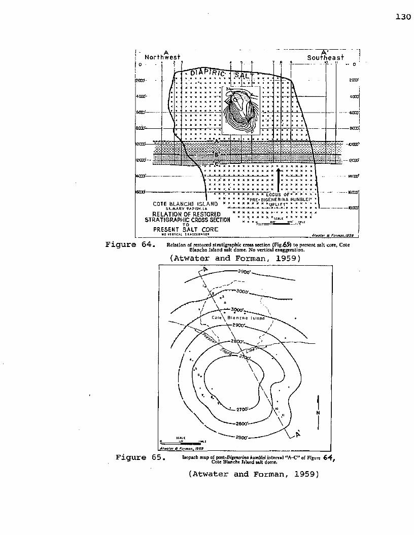
AN o r t h w e s t S o u t h e a s t

20®4003I-

6003

soil-

CCOtf-I20CD'

4000 '-

I60d X X X . R R R X X X X X |_0CU S O F * * * * X * x * X a x x p R E -B IO E N E H IN ft H U M B L E I*

COTE BLANCHE IS L A N D * " * " * * * - " * u p u f t ' ‘ *S l.M A ttV PAPISH.LA

RELATION OF RESTORED * C ’ “ * " * * *■” ’ ; J ; * * K-STRATIGRAPHIC CROSS SECTION « ’ I „ J C,L[

PRESENT SALT COREua v f u n c H tx x G G iq x n a x

- 0JO B'

4CC0

6030;

60301

-can'

eoocfwoctf16000'

h o c o

. 4fwo!tr 8 Fot/nan, 1959

Figure 64. Relation of restored stratigraphic cross section (Fig.65) to present salt core, Cote Blanche Island salt dome. No vertical exaggeration.

(Atwater and Forman, 1959)

2 7 0 0 '

Atmcttt Q Forman, (959

Figure 65. Isopach map of poit-D igcnerina humbtei interval "A -C ” of Figure 64,Cote Blanche Island salt dome.

(Atwater and Forman, 1959)

131

the fault B {S), had no growth within the mapped intervals, and are dated post - A time. In fact, all through the map­ped intervals the sediments on the downthrown side of the faults are thinner than those on the upthrown side, indica­ting they were not yet active. However, as numerous faults (including probably Bl) cut the higher (post-A) horizons in wells 11 and 18, this seems to indicate that the fault Bl, and possibly others too, had their growth after time A.

The fault B(S) though geographically belonging to the Bayou Carlin fault system has a different history from other faults of the same system. It had its inception at a pre-G time and was active until time B.

Age of Rim SvnclinesThe Cote Blanche Rim Syncline: In the Cote Blanche

area two phases of structural evolution are recognized by Atwater and Forman (1959). The first phase of the structure formed just before the end of Biqenerina humblei time, with a rim syncline developed north of the dome (Figs. 64 and 65). The second phase of the structure was brought about by a later salt intrusion (late-Tertiary) with the locus of uplift shifting northward. This has resulted in the center of the present salt core located two miles north of the apex of the earlier (fossil) structure which is marked by petroleum fields. Atwater and Forman's structure map of the top of Biqenerina humblei zone (below their horizon C)

132

13600

RIM S Y N C L I N E AS PER

A T W A T E R A N D F O R M A N

E X T E N S I O N OF

THE RI M SYN C L I NE

DIAP’lRlC

I

M B K U M A R T9 ?2

Figure 66. Structure on horizon A (close to the top of Bigenerina humblei zone) of the study area, with structural details on top of Bigenerina humblei zone over Cote Blanche Island after Atwater and Forman (1959).

133

is of particular relevance, in as much as this structural horizon is close to the horizon A of this report, and both are shown together in Fig. 66. It is evident that the northwestern corner of the study area is in close proximity with a possible rim syncline south of the Cote Blanche structure, the rim syncline being marked by the southeaster­ly dip on the Cote Blanche side and the northwesterly dip on the Bayou Carlin side.

The computer isochore maps show that upto the interval BC (Figs. 32 through 36), the structural high of the Bayou Carlin area remained in the northwestern corner, in­dicating the Cote Blanche dome or at least its rim syncline had not yet formed. During the interval AB (Fig. 30) the main structural high was displaced far to the northeast.This is distinctly reflected also in the isochore residual maps of the first order (Figs. 60 and 61). This could be the result of a peripheral sink (Ritz, 1936) being formed at this time around the Cote Blanche saltdome with a lower­ing of the saltdome at Bayou Carlin during approximately Bigenerina humblei time. Thus the rim syncline just south of the Cote Blanche saltdome or northwest of the Bayou Carlin area is reasonably dated as starting during the time of horizon A or the top of Biqenerina humblei zone. This is related with the first phase of the Cote Blanche struc­ture (Atwater and Forman, 1959). It was during the second phase of the structure that, in all probability, the Bayou

134

Carlin faults formed. The associated subsidence is indica­ted by a strong evidence of growth of these faults above horizon A.

The Bayou Sale Rim Syncline: Just south of the mainhigh of the Bayou Carlin area is a trough. As already noted, the fault pattern suggests a rim syncline here. If the structure contours on Bayou Sale (ROB-6 , from public records of the Department of Conservation, Louisina) are added to the equivalent horizon E contours as in Fig. 67, the rim syncline is very evident. The northwesterly dip of relatively great magnitude shown in this figure charac­terizes the northern flank of the domal structure of Bayou Sale field. A similar dip reversal can be traced between the East Lake Sand area and the western flank of the Bayou Sale structure down to the south, though for lack of infor­mation this synclinal axis is not portrayed. The residual structure maps of horizons A, D, and E (Figs. 51, 52, and 53) accentuate the low on the east toward Bayou Sale, sug­gesting the possible location of the rim syncline west and northwest of the Bayou Sale dome. The isochore maps (Fig. 30, 32 through 36) all through the mapped intervals indi­cate a thickening to the southeast and south in the eastern part of the study area quite close to Bayou Sale. The residual isochore map for DE interval (Fig. 61) marks the unusual zone with positive and negative closures.

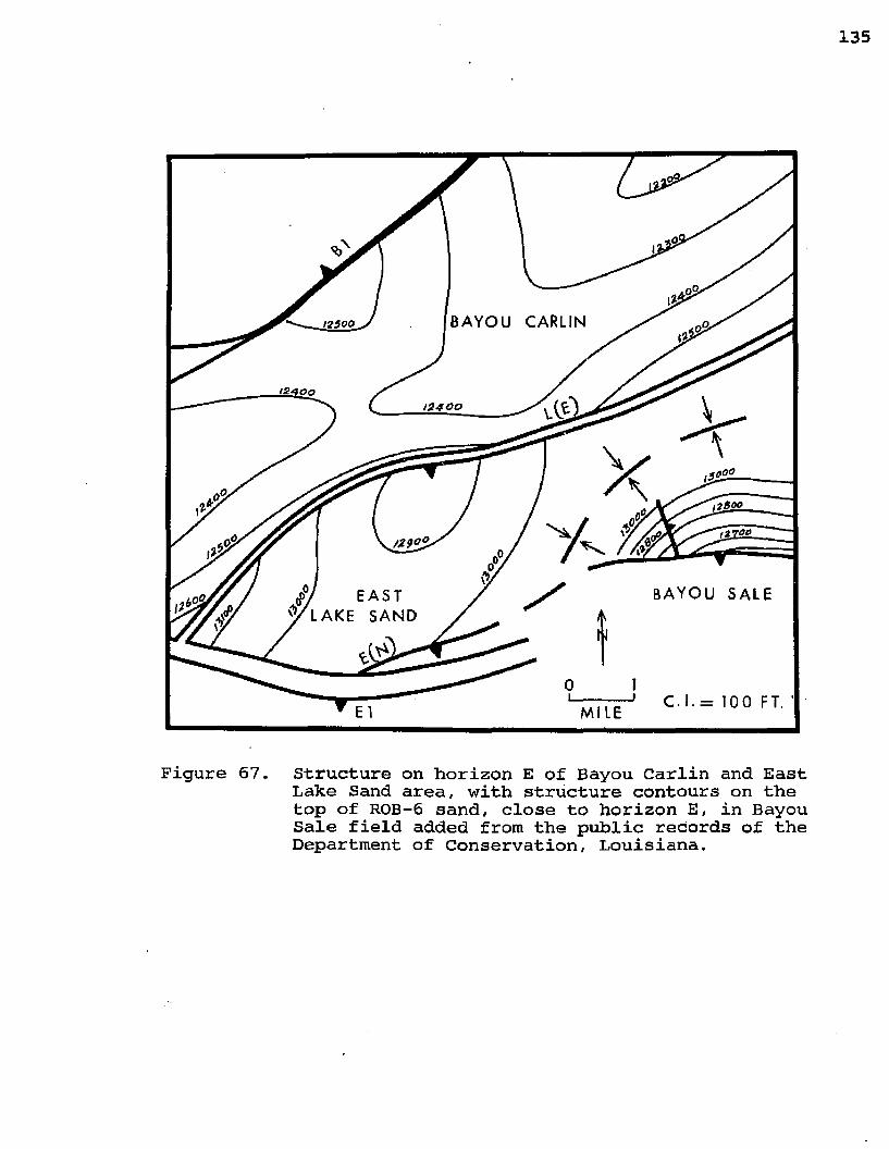
135

B A Y O U CARLIN

B A Y O U SALE<*>/ EAST V L A K E S AN D

MI LE

Figure 67. Structure on horizon E of Bayou Carlin and East Lake Sand area, with structure contours on the top of ROB-6 sand, close to horizon E, in Bayou Sale field added from the public records of the Department of Conservation, Louisiana.

As regards to the age of this rim syncline, it is not possible to date this with confidence, without the isopach maps of all the intervals across the Bayou Sale area. How­ever, the age could be guestimated by assuming that faults L(E), El, BS1, and BS2 (Fig. 62) developed contemporaneous­ly with the formation of the rim syncline. The age of the rim syncline would be pre-G time or Operculinoides time, although it may even be still earlier.

Time of Movement of Salt The earliest recorded salt movement was the intrusion

of the Bayou Sale structure with a draining of salt from the southeastern part of the mapped area (rim syncline). Next movement occurred during time interval CD and BC which could be attributed to the mobile activity of the West Cote Blanche saltdome in the west beyond the study area. The third salt movement is related to the removal of salt from the rim syncline of the Cote Blanche dome in the northwest. The fourth salt movement in the area is ascribed to the second phase of the Cote Blanche structure and is dated much later than time A.

Bayou Carlin Arch The most significant aspect of the salt movements of

the mapped area is that they are all away from the area and related to external diapirism. As a consequence, the present structural configuration of the area is character­ized by two rim synclines of different ages - one of pre-G

137

time in the southeast and the other of time A in the north­west. Upto time A, the Bayou Carlin area was paleoslope into the site of the earlier rim syncline associated with the Bayou Sale dome. During time A the Bayou Carlin area emerged as a residual arch between the old rim syncline in the southeast and the new one in the northwest associated with the Cote Blanche saltdome. The Bayou Carlin salt mass thus appears to be a Miocene residual structure (Halbouty, 1967, p. 62). How it arrived in its present position in pre-Miocene time is unknown.

B . Geologic HistoryThe known history of the area starts at a pre-G time

with a positive area in the north and a rim syncline in the south associated with the Bayou Sale dome. The area marked by this syncline was cut by three southerly dipping faults, namely, Ll, L(E), and El. Another fault B(S) with north­westerly dip probably also existed in the northwest. The faults grew during the time interval FG. The downthrown block of the Lake Sand fault had a substantial subsidence (growth index 1.9) and was marked in the south by two anti­thetic faults L(C) and L(D) dipping into the Lake Sand fault Ll. Also,a major rollover structure developed in the Lake Sand area with a minor rollover in East Lake Sand. To the north of this fault, the Bayou Carlin area was a posiment all the way to the north border and beyond with

138

an abrupt downshope between the faults L{E) and El.During the time interval DE (Pig. 34), the Bayou Car­

lin area had no change. The faults Ll and El in the Lake Sand and East Lake Sand areas were intensely active with the maximum subsidence of the downthrown block (Overall growth index =1.8). As a result, the rollover structures were carried up the growth fault, causing a shift of the apex of the Lake Sand high (rollover) in the updip direc­tion (northwest). The antithetic faults L(C) and L(D) dis­appeared and died under the rapid influx of sediments dur­ing this period. To the west of the Lake Sand area, the previous high disappeared and the area subsided under the influence of the active growth fault B(S).

The time interval CD (Fig. 33), is marked by a change in the environment of deposition, recording a regressive phase of the sea. The deposition of the interbedded transi­tional facies characterized by a preponderence of sandstones in the lithologic sequence, commenced in the later part of this time interval. All the growth faults which were very active previously, slowed up in their growth activities, as also indicated by the overall low growth index (1.3) of the Lake Sand fault. In the west a high reappears which marks probably a nose from the West Cote Blanche saltdome. The Bayou Carlin area broadly maintained its structural configuration as before.

During the time interval BC (Fig. 32), the faults Ll,

139

El, and L(E) had a slow growth; the fault B(S) ceased to grow. The West Cote Blanche saltdome sent off a nose far into the east and northeast, giving rise to a prominent high in the west and also accentuating the Bayou Carlin high in the northwest. The rollover structures continued in the Lake Sand and East Lake Sand areas.

During the time interval AB (Figs. 17 and 30), the West Cote Blanche saltdome had no influence over the area. But the Cote Blanche dome became active and rim syncline started forming; the sediments developed a thickening trend to the northwest in the Bayou Carlin area; the main high of this area shifted to the northeast. In the Lake Sand area the faults Ll and El were growing slowly; rollover structures continued forming in the southwest and the east.A new fault L3 branched off the fault LA and affected the southwestern nose of the rollover structure in the Lake Sand area and grew slightly.

During the post-A time, in the Lake Sand area a new fault L2 complimentary to the fault L3 cut the rollover structure. A second phase of mobile activity of the Cote Blanche saltdome took place, giving rise to the northwester­ly dipping faults of the Bayou Carlin area. Thus this area emerged as a horst block marking a residual high left be­tween two rim synclines associated with the Bayou Sale dome in the southeast and Cote Blanche saltdome in the northwest.

140

Pre-G FG EF

o

DE BCCD

oo

Post LEGEND

Fault

Figure 68,

^ ' Thin'ContourClosure(Posiment)

Rim Syncl ine

M.B. Kumar, 1972Structural history of the Bayou Carlin- Lake Sand area, as summarized from isochore and structural maps (conventional and computer) from G (oldest) to A (youngest) pre~G and post-A sketch maps are from geological inference. Faults lettered as per text.

141

The history of the area is summarized in Fig. 68.

C. Petroleum AccumulationsThe major petroleum (mostly gas) production of the

area is contributed by Lake Sand field. Here the northern part of the productive area (Fig. 1) has mostly gas reser­voirs of UL (Uvigorina lirethensis) - sands in the interval AB. The southern part of the productive area is marked by gas reservoirs of ROB (Robulus) - sands. Below the deepest mapping horizon G also there are some gas reservoirs of OPERC (Operculinoides) - sands and MA (Margiluna ascen- sionis) - sands. The hydrocarbon accumulations are trapped in the rollover structures against the Lake Sand growth fault and associated faults. These growth faults have helped in creating effective structural closures for trap­ping petroleum and have also acted as barriers to possible further updip migration of hydrocarbon (toward the Bayou Carlin area). In all probability, this is why the deep reservoirs of the field have abnormal pressure.*

East Lake Sand field produces only from a ROB-reservior within the interval FG, though some gas production is yielded by the deeper reservoirs (OPERC-sands). The gas accumulation occurs in the upthrown block of the East Lake

♦Details in the author's thesis in Petroleum Engineer­ing (minor) entitled "Production Mechanisms of the Geopressured Reservoirs of Lake Sand Field, South Louisiana".

142

Lake Sand fault. This appears to be a combination type trap. If the gas deposit were not in situ, the gas could have migrated from the south through the East Lake Sand fault (El) which acted as a permeable channelway. This also explains why the structural closure in the downthrown block of the fault is conspicuously void of commercial hydrocarbon accumulation.

Bayou Carlin field produces from a relatively shallow reservoir of a ROB-sand within the interval FG, and deeper reservoirs of MA-sands. The latter deeper reservoirs lie in the northwestern and southeastern part of the productive belt (Fig. 1). The ROB-reservoir is located in the north­eastern part of the productive belt. The traps are essen­tially of stratigraphic type. Structural traps are con­spicuously absent, though continuous and extensive sandbodies exist presently with significant structural closures. The reason appears to be two-fold: the Lake Sand fault system acted as a fluid barrier and did not allow petroleum to migrate further updip to the Bayou Carlin area; secondly, though more significant, until the formation of the Bayou Carlin faults (prior to the second phase of the Cote Blanche structure) the petroleum generated in situ (or, if at all, migrated from the south) migrated into the Cote Blanche structure which provided a more stable trap. This is sub- tantiated by petroleum fields located in the 'fossil' struc­ture south of the Cote Blanche saltcore.

SUMMARY AND CONCLUSIONS

The computer-generated structure contour and isochore maps are not as good as those constructed by the conventional methods involving human inter­pretation and manual contouring. Nevertheless, they serve as 'quick-look' maps,and can be used to aid the'initial mapping program by guiding the slection of the critical horizons, intervals and zones for the final manual mapping. Moreover, two special types of maps, namely, trend and residual maps, can be generated easily only with the com­puter, and can be employed to find possible inter­pretation of geological data speedily, leading to clues asto faults, growth and trends of petroleum accumulation.The observed history of the Bayou Carlin-Lake Sand area starts approximately at the end of the Oper- culinoides time with a posiment in the Cote Blanche area north of a regional southerly dipping growth fault in the Lake Sand area. This fault, with branch faults to the east, had developed in response to the formation of a rim syncline associated with an earlier salt intrusion in the Bayou Sale area in the southeast. The area north of the Lake Sand growth fault remained stable until late-Biqenerina humblei time when the West Cote Blanche dome had a

144

marked influence on it. The Cote Blanche saltmass became active and drained salt from the Bayou Car­lin area with the development of a rim syncline to the northwest of the area and the Bayou Carlin high itself. The newly developed stresses were relieved through the Bayou Carlin fault system.Just to the south of the Lake Sand fault, the area which had been the scene of thick sedimentation and subsidence, was now filled and the growth activity of the faults declined as a subsequent regressive phase of sedimentation set in. Later, towards the end of the Biqenerina humblei time, the southwestern nose of the Lake Sand rollover struc­ture was cut by a new generation of faults. Since the end of the Biqenerina humblei time, the Bayou Carlin area has been a residual high left between the two rim synclines associated with the old Bayou Sale dome in the southeast and the later Cote Blanche saltdome in the northwest.

3. The Lake Sand growth fault acted as a fluid barrier and also created structural closures (rollover) for trapping petroleum in the Lake Sand field, which is the main producing part of the study area.On the contrary, the Bayou Carlin area has no struc­tural trap, since petroleum migrated into the Cote Blanche structure (in the immediate northwest),

145

which predates the present structural closures of the Bayou Carlin area.

REFERENCESPart 1

(Computer Application )Conolly, H.J.C., 1936, A contour method of revealing some

ore structures: Econ. Geology, v. 31, no. 3, p. 259-271.

Corbett, C.S., 1919, Method for projecting structure through an angular unconformity: Econ. Geology, v. 14, no. 8 ,p. 610-618.

Draper, N.R. and H. Smith, 1966, Applied Regression Analysis: New York, John Wiley and Sons, 407 p.

Grant F., 1957, A problem in the analysis of geophysical data: Geophysics, v. 22, p. 309-344.

Griswold, W.T. and M.J. Munn, 1907, Geology of the oil and gas fields in Steubenville, Burgettstown, and Clays- ville quadrangles, Ohio, West Virginia, and Pennsyl­vania: U.S. Geol. Survey Bull. 318, p. 1-196.

Harbaugh, J.W. and F.W. Preston, 1965, Fourier series analy­sis in geology, in Computer Applications in Mining and Exploration, v.l: Tusoon, Univ. of Arizona, p. R1-R46.

Harbaugh, J.W. and D.F. Merriam, 1968, Computer Applications in Stratigraphic Analysis: New York, John Wiley and Sons, Inc., 282 p.

James, W.R., 1966, The Fourier series model in map analysis: Department of Geology, Northwestern Univ., Technical Report, ONR Task no. 399-078, Contract Nonr 1228 (36), Evanston, Illinois.

James, W.R., 1966, Fortran IV Program using Double FourierSeries for surface fitting of irregularly spaced data: Kansas Geol. Survey Computer Contribution 5, Kansas Geol. Survey, the Univ. of Kansas, Lawrence, Kansas.

Krumbein, W.C., 1956, Regional and local components in facies maps: Am. Assoc. Petrol. Geol. Bull., v. 40, p. 2163- 2194.

Krumbein, W.C., 1959, Trend surface analysis of contour type maps with irregular control-point spacing: Journal Geophysic Research, v. 64, p. 823-834.

146

147

Lee, W. and T.G. Payne, 1944, McLouth gas and oil field, Jefferson and Leavenworth counties, Kansas: Kansas Geol. Survey Bull. 53, 193 p.

Li, C.R., 1964, Statistical Inference: Ann Arbor, Michigan, Edwards Brothers, Inc., v. II, 575 p.

Levorsen, A.I., 1927, Convergence studies in the Mid conti­nent region: Am. Assoc. Petrol. Geol. Bull., v. 11, no. 7, p. 657-682.

Lustig, L.K., 1969, Trend sufrace analysis of the Basin and Range Province, and some geomorphic implications: Geological Survey Professional Paper 500-D, U.S. De­partment of the Interior, Washington.

Merriam, D.F., 1964, Use of trend-surface residuals in in­terpreting geologic structures: Stanford Univ. Publ. Geol. Sci., v. 9, no. 2, p. 686-692.

Merriam, D.F. and J.W. Harbaugh, 1964, Trend surface analy­sis of regional and residual components of geologi­cal structure in Kansas: Kansas Geol. Survey Special Distrib. Publ. 11, 27 p.

- Mirriam, D.F. and R.H. Lippert, 1964, Pattern recognition studies of geologic structure using trend surface analysis: Colorado School of Mines Quart., v. 59, no. 4 (Part A), p. 237-245.

Merriam, D.F. and R.H. Lippert, 1966, Geologic model studies using trend-surface analysis: Journ. Geology, v. 74, no. 3, p. 344-357.

Miller, R. L., 1956, Trend surfaces: Their application toanalysis and description of environments of sedimen­tation: Journ. Geology, v. 64, p. 425-446.

Paine, W.R., 1972, Computer mapping in lower Frio formation (Oligo-Miocene), southwestern Louisiana (Abstract): Am. Assoc. Petrol. Geol. Bull., v. 56, no. 3, p. 643.

Rich, J.L., 1935a, Graphical method for eliminating region­al dip: Am. Assoc. Petrol. Geol. Bull., v. 19, no. 10 p. 1538-1540.

Rich, J.L., 1935b, Fault-block nature of Kansas structures suggested by elimination of regional dip: Am. Assoc. Petrol. Geol. Bull., V'. 19, no. 10, p. 1540-1543.

148

Shepard, D.S., 1969, A two-dimensional interpolation function for computer mapping of irregularly spaced data: "Geography and the Properties of Surfaces" Series Pa­per No. 15, Office of Naval Research, Harvard Univer­sity, Cambridge, Massachusetts.

Turner, A.K. , 1968, Computer-assisted procedures to generate and evaluate regional highway alternatives: Purdue University Joint Highway Research, Technical Paper No. 32, Purdue University, Lafayette, Indiana.

Turner, A.K., 1969, The GCARS system FORTRAN IV Programmer's Mannual: Joint Highway Research Project, Final Report, Purdue University, Lafayette, Indiana.

Whitten, E.H.T., 1959, Composition trends in a granite Modal variation and ghost stratigraphy in part of the Done­gal granite, Eire: Journ. Geophysic. Research, v. 64, p. 835-848.

Wolfe, J.A., 1962, Geostatistics and exploration economy, in Mathematical Tech. and Computer Application in Mining and Exploration, v. 1: Tucson, Univ. of Arizona, p. H—l-H-28.

Part 2 (Geological)

Atwater, G.I. and M.J. Forman, 1959, Nature of growth ofsouthern Louisiana saltdomes and its effects on petro­leum accumulation: Am. Assoc. Petrol. Geol. Bull., v. 43, no. 11, p. 2592-2622.

Bishop, M.S., 1960, Subsurface Mapping: New York, John Wiley and Sons, Inc., 198 p.

Dennison, J.M., 1968, Analysis of Geologic Structures: New York, W.W. Norton and Company, Inc., 209 p.

Halbouty, M.T., 1967, Salt Domes-Gulf Region, United States and Mexico: Houston, Texas, Gulf Publishing Company, 425 p.

Hamblin, W.K., 1965, Origin of "Reverse Drag" on the down-thrown side of normal faults: Geol. Soc. Amer. Bull., v. 76, p. 1145-1164.

Howell, J.V. (Co-ordinating Chairman), 1957, Glossary of Geo­logy and Related Sciences: Washington D.C., Am. Geol. Inst., NAS-NRC Publ. 501, 324 p.

149

Hughes, D.J., 1960, Faulting associated with deep-seatedsaltdomes in the northeast portion of the Mississippi salt basin: Gulf Coast Assoc. Geol. Socs. Trans., v. 10, p. 155-173.

Johnson, H.A., 1971, Structural development of some shallow saltdomes in Louisiana Miocene productive belts: Am. Assoc, Petrol. Geol. Bull., v. 55, p. 204-226.

Kupfer, D.H., 1967, Mechanism of intrusion of Gulf coastsaltdomes, in D.H. Kupfer, ed., Geology and Techno­logy of Gulf Coast Salt: Department of Geology and Institute of Saline Studies, Louisiana State Univ.

Lafayette Geological Society Study Group, 1963, Stratigra­phic factors in southwest Louisiana oil prospecting: Gulf Coast Assoc. Geol. Socs. Trans., v. 13, p. 9-47.

Louisiana Geological Survey, Maps and public reports and records.

Meyerhoff, A.A. , 1968 ed., Geology of natural gas in southLouisiana: in B.W, Beebe and B.F. Curtis, ed., Natural Gas of North America, v. I, Am. Assoc. Petrol. Geol. Publication.

Moody, G.B., 1961 ed. , Petroleum Exploration Handbook: NewYork, McGraw Hill Book Co., Inc,, (First Ed.) p. 860.

Murray, G.E., 1957, Geologic occurrence of hydrocarbons in Gulf coastal province of the United States: Gulf Coast Assoc. Geol. Socs. Trans., v. 7, p. 253-299.

Murray, G.E., 1961, Geology of the Atlantic and Gulf Coastal Province of North America: New York, Harper and Brothers, p. 692.

Ocamb, R.D., 1961, Growth faults of south Louisiana: Gulf Coast Assoc. Geol. Socs. Trans., v. 11,p. 139-173.

O'niell, C.A., III, 1966, Isopach Map and Expansion Index' Study of Growth Faults and Structural Evolution of Belle Isle Salt Dome, St. Mary Parish, Louisiana: unpublished M.S. Thesis, Louisiana State Univ.

Rainwater, E.H. , 1964, Regional stratigraphy of the GulfCoast Miocene: Gulf Coast Assoc. Geol. Socs. Trans., v. 14, p. 81-124.

Ritz, C.H., 1936, Geomophology of Gulf coast salt structure and its economic application: Am. Assoc. Petrol.Geol., v. 20, no. 11, p. 1413-1438.

150

Skinner, H.C., 1960, A comparison of the Mississippi sub­marine trench with the Iberian trough: Gulf Coast Assoc. Geol. Socs. Trans., v. 10, p. 1-6.

Spiller, J.P., 1965, Distribution of hydrocarbons in south Louisiana by types of traps and trends-Frio and younger sediments, Gulf Coast Assoc. Geol. Socs. Trans., v. 15, p. 37-39.

Thorsen, C.E., 1963, Age of growth faulting in southeast Louisiana: Gulf Coast Assoc. Geol. Socs. Trans., v. 13, p. 103-110.

Troutman, A., 1955 ed., The Oil and Gas Fields of Southwest Louisiana: Houston, Five Star Oil Report Inc., 376 p.

Wallace, W.E., 1952, South Louisiana fault trends; Gulf Coast Assoc. Geol. Socs. Trans., v. 2, p. 63-66.

Wallace, W.E., 1962, Fault Map of South Louisiana: Gulf Coast Assoc. Geol. Socs. Trans., v. 12, p. 194.

APPENDICES

152

APPENDIX I

BASIC DATA ON WELL CONTROL

The following tables list wells by number and operator. Geographic co-ordinates to east and south are given in units of two thousands of feet. The elevation given for each point (A, B, etc.) is that on the electric log in feet below the derric floor, and is approximately the ele­vation below sea level; the corresponding vertical interval is in parenthesis.

r

Well No. 1 2 3 4 5Co-ordinates 29.00, 31.43, 34.34, 33.96, 31.95,

(X,Y) - 01.00 -01.95 -02.65 -04.13 -03.30Operator Quintana Superior Humble Oil Humble Oil F.A.Callery,

and Pet. Corp. Oil Co. and Ref. Co. and Ref. Co. Inc.Location Walter Kemper Main Grifface John Taylor Hugh A.

J.T.Caffery et al Caffery et al Kelso,Jr. et alNo. 1 No. A—1 No. 1 No. B-l No. 1

Section-Township--Range 30-155-9E 29-155-9E 33-155-9E 33-155-9E 32-155-9EHorizon

A 09960 09720 09670 09734 09742(430) (440) (457) (459) (468)

B 10390 10160 10127 10193 10210(1050R) (1043) (1036) (1027) (1006)

C 11290 11203 11163 11220 11216(686) (717) (682) (690) (674)

D 11976 11920 11845 11910 11890(327) (354) (347) (355) (330)

E 12303 12274 12192 12265 12220(227) (239) (226) (227) (230)

F 12530 12513 12418 12492 12450(202) (212) (200) (203) (200)

G 12732 12725 12618 12695 12650Total Depth 14500 12816 15150 13000 16626

R = Restored thickness for * the faulted interval

153

Well No. 6 7 8 9 10Co-ordinates 31.35, 31.90, 29.73, 25.93, 22.66,

(X,Y) -04.00 -04.60 -04.46 -04,97 -05.20Operator F.A. Callery Humble Oil F.A.Callery Humble Oil Pan. Am.

and Inc. and Ref. Co. Inc. and Ref. Co. Pet. Corp.Location Caffery Martel A.T.Sullivan L.O. Pecot Miami Corp. S/L 5176

No. 1 No. 1 et al No-1 No. F-l No. 1Sect ion-Township-

-Ranae 32-155-9E 32-155-9E 31-155-9E 36-155-8E -155-8EHorizon

A 09772 09785 09817 09973 10433(461) (465) (473) i (507) (491)

B 10233 10250 10290 : 10480 10924(1010) (1004) (1013) (1030) (1024R)

C 11243 11254 11303 11510 11878(667) (672) (670) (652)

D 11910 11926 11973 NP 12530(340) (340) (337) (300)

E 12250 12266 12310 NP 12830(220) (225) (225) (200)F 12470 12491 12535 NP 13030(210) (209) (195) (215)

G 12680 12700 12731D NP 13235

Total Depth 15237 13000 13035 11461 17777NP = Not penetratedR = Restored thickness for

the faulted interval

154

Well No. 11 12 13 14 15Co-ordinates 23.58, 27.06, 26.60, 30.15, 30.80,

(X,Y) -07.29 -06.07 -06.90 -05.52 -05.50Operator Pan. Am. Pan Am. Union Oil Co. Humble Oil Humble Oil

and Pet. Corp. Pet. Corp. of Calf. and Ref. Co. and Ref. Co.Location MA-7SU Miami Corp. Miami Corp.

E.N.Kearney E.N.Kearney E.N.KearneyNo. 2 No. 1 No. 1 M-l M-2

Section-Township--Rancre 2-165-8E 1-165-8E 1-165-8E 24-165-9E 24-165-9E

HorizonA 09974 09923 09900 09810 09795

(491) (477) (482) (462) (468)B 10465 10400 10382 10272 10263

(1028) (1030) (1018) (1008) (1005)C 11493 11430 11400 11280 11268

(695) (660) (685) (675)D 12188 12090 12085 11955 NP

(322) (320) (320) (331)E 12510 12410 12405 12286 NP

, (220) (224) (230) (227)F 12730 12634 12635 12513 NP

(200) (206) (205) (197)G 12930 12840 12840 12710 NP

Total Depth 18200 17800 13000 13509 11650NP = Not penetrated

Well No. 16 17 18 19 20Co-ordinates 30.77, 29.75, 22.46, 25.80, 25.86,._(X,Y) -06.38 -06.75 -08.36 -08.90 -09.44Operator Humble Oil Humble Oil Pan Am. Humble Oil Humble Oil

and and Ref. Co. and Ref. Co. Pet. Corp. and Ref. Co. and Ref. Co.Location Miami Corp. MA-7SU-B,

Miami Corp. S/L 4427 Kearney Miami Corp.M-6 M-8 Well 1 No. 2 No. H-9

Sect ion-Town ship--Ranae 24—165-9E 24-165-9E -165-8E 12-165-8E -165-9E

HorizonA 09804 09812 09960 09896 09825

(472) (478) (485) (484) (485)B 10276 10290 10445 10380 10310

(1014) (1019) (1008) (1015) (982)C 11290 11309 11453 11395 11292

(678) (675) (697) (695) (733)D 11968 11984 12150 12090 12025

(341) (331) (320) (340) (345)E 12309 12315 12470. 12430 12370

(231) (235) (220) (240) (245)F 12540 12550 12690 12670 12615

(195) (202) (200) (210) (215)G 12735 12752 12890 12880 12830

Total Depth 14520 18025 18000 18301 18833

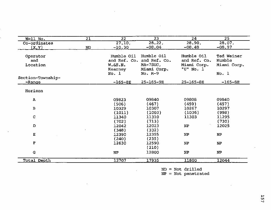
Well No. 21 22 23 24 25Co-ordinates 27.10, 28.22, 28.90, 28.07,_ (X,Y) ND -10.30 -08.04 -08.48 -08.97Operator Humble Oil Humble Oil Humble Oil Ted Weiner

and and Ref. Co. and Ref. Co. and Ref. Co. HumbleLocation W.&E.N. MA-7SUC, Miami Corp. Miami Corp.

Kearney Miami Corp. "U" No. 1No. 1 No. M-9 No. 1

Section-Township--Ranae -165-8E 25-165-9E 25-165-8E -165-8EHorizon

A 09823 09840 09808 09840(506) (467) (459) (457)

B 10329 10307 10267 10297(1011) (1003) (1036) (998)

C 11340 11310 11303 11295(702) (713) (730)

D 12042 12023 NP 12025(348) (332)

E 12390 12355 NP NP(240) (235)

F 12630 12590. NP NP(210)

G NP 12800 NP NPTotal Depth 12707 17935 11800 12044

ND = Not drilled NP = Not penetrated

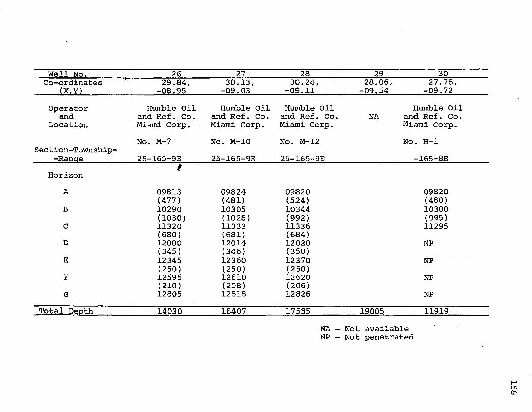
Well No. 26 27 28 29 30Co-ordinates 29.84, 30.13, 30.24, 28.06, 27.78,___(X.Y) -08.95 -09.03 -09.11 -09.54 -09.72Operator Humble Oil Humble Oil Humble Oil Humble Oil

and and Ref. Co. and Ref. Co. and Ref. Co. NA and Ref. Co.Location Miami Corp. Miami Corp. Miami Corp. Miami Corp.

No. M-7 No. M-10 No. M-12 No. H-lSection-Tovmship-

-Ranae 25-165-9E 25-165-9E 25-165-9E -165-8EHorizon /

A 09813 09824 09820 09820(477) (481) (524) (480)

B 10290 10305 1,0344 10300(1030) (1028) (992) (995)

C 11320 11333 11336 11295(680) (681) (684)

D 12000 12014 12020 NP(345) (346) (350)

E 12345 12360 12370 NP(250) (250) (250)

F 12595 12610 12620 NP(210) (208) (206)

G 12805 12818 12826 NPTotal DeDth 14030 16407 17555 19005 11919

NA = Not available NP = Not penetrated

Well No. 31 32 33 34 35Co-ordinates 28.42, 28.44, 28.12, 31.70, 33.34,

(X,Y) -09.70 -10.37 -10.73 -09.00 -08.66Operator Humble Oil Humble Oil Humble Oil Humble Oil Humble Oil

and and Ref. Co. and Ref. Co. and Ref. Co. and Ref. Co. and Ref. Co.Location Miami Corp. Miami Corp. Miami Corp. Miami Corp.

No. H-3 No. H-5 S/L No. 1 No. M—13 No. M-14Section-Township-

-Ranae 25-165-8E 25-165-8E 26-165-9E 26-165-9E. Horizon

A 09813 09808 09803 09848 09893{488) (510) (502) (487) (493)

B 10301 10318 10305 10335 10386(999) (1000) (1010) (1021) (1017)

C 11300 11318 11315 11356 11403(694 (687)

D NP NP NP 12050 12090(350) (360)

E NP NP NP 12400 12450(250) (250)

F NP NP NP 12650 12700(216) (235)

G NP NP NP 12866 12935Total Depth 11768 11622 11759 17723 18000

NP = Not penetrated

Well No. 36 37 38 39 40Co-ordinates 34.56, 27.32, 28.12, 30.50, 30.54,

(X,Y) -09.88 -11.29 -11.68 -11.08 -12.00Operator British Am. Humble Oil Humble Oil Humble Oil Humble Oil

and Oil Prod. Co. and Ref. Co. and Ref. Co. and Ref. Co. and Ref. Co.Location Miami Corp. E.N.Kearney Miami Corp. Miami Corp. Miami Corp.

et alNo. S-l No. 3 No. H-8 No. H-7 No. H-10

Section-Township--Ranae 27-165-9E -165-8E 33-155-9E 33-165-9E 33-165-8E

HorizonA 09940 09967 09951 09892 09927

(514) (536) (525) (520) (526)B 10454 10503 10476 10412 10453

(1071) {1064R) (1064) (1076)C 11525 11367 11540 11488 NP

(742) (726) (772)D 12267 12093 NP 12260 NP

(357R) (360)E 12554 12453 NP NP NP

(303) (245)F 12807 12698 NP NP NP

(233) (217)G 13040 12915 NP NP NP

Total Depth 13625 18215 12000 12495 11499R = Restored thickness for

the faulted interval NP = Not penetrated

Well No. 41 42 43 44 45Co-ordinates 28.38, 20.42, 19.73, 21.95, 24.80,

(X,Y) -12.80 -12.42 -14.02 -14.40 -13.40Operator Huirible Oil Texas Crude Cities Ser. Anson Corp. Union Sulphur

and and Ref. Co. Oil Co. Oil Co. and Oil Corp.Location Miami Corp. Miami Corp. Miami Corp.

S/L 4427 S/L 1805No. H-4 No. 1 No. 1 No. 1 No. H-l

Section-Township--Ranqe -165-8E -165-8E 21-165-8E 22-165-8E 14-165-8E

HorizonA 09919 09843 09950 09963 09962

C 529 ( (477) (515) (515) (531)B 10448 10320 10465 10478 10493

(1042) (1040) (1080R) (1077) (1077)C 11490 11360 11345 11555 11570

(728) (775)D NP NP 12073 NP 12345

(370) (540)E NP NP 12443 NP 12885

(247)F NP NP 12690 NP NP

(200)G NP NP 12890 NP NP

Total Depth 12105 11775 13000 11967 13008R = Restored thickness for

the faulted interval ND = Not drilled

161

Well No. 46 47 48 49 50Co-ordinate s 25.37, 22.30, 16.84, 20.48,

(X,Y) -13.73 ND -16.10 -05.90 -06.84Operator Kilroy Co. Pan Am. Humble Oil

and of Texas,Inc. Cities Ser. Pet. Co. and Ref. Co.Location Miami Corp. Oil Co.

S/L 1807 S/L 3707 S/L 4427No. 1 No. 2 No. 1 No. 1

Section-Township--Ranae 24-:165-8E -165-8E

HorizonA 09942 09980 11035 10295

(533) (547) (512) (510)B 10475 10527 11547 10805

(1053) (1041) (993) (1017)C 11528 11568 12540 11822

(767) (630) (653)D 12295 NP 13170 12475(545) (270) (305)

E 12840 NP 13440 12780(414) (174) (202)

F 13254 NP 13614 12982(266) (196) (188)

G 13520 13810 13170Total Depth 14786 12049 16716 19744

NP = Not penetrated

Well No. 51 52 53 54 55Co-ordinates 19.93, 20.80, 16.60, 16.24, 15.54,

(X, Y) -07.06 -07.62 -08.78 -09.63 - 11.00Operator Atlantic Atlantic The Texas The Texas NA

and Ref. Co. Ref. Co. Co. Co.Location

S/L 4204 S/L 4204 S/L 2681 S/LNo. 1 No. 2 No. 1 No. 1

Section-Township--Ranae 4-165-8E -165-8E

HorizonA 10327 10236 10493 10191

(503) (477) (515R) (489)B 10830 10713 10778 10680

(1021) (1019) (1002)C 11851 11732 11780 NP

(700)D NP NP 12480 NP

(300)E NP NP 12780 NP

(190)F NP NP 12970 NP(210)

G NP NP 13180 NPTotal Deoth 11994 12225 16505 11516 17404

R = Restored thickness for the faulted interval

NA = Not available NP = Not penetrated

163

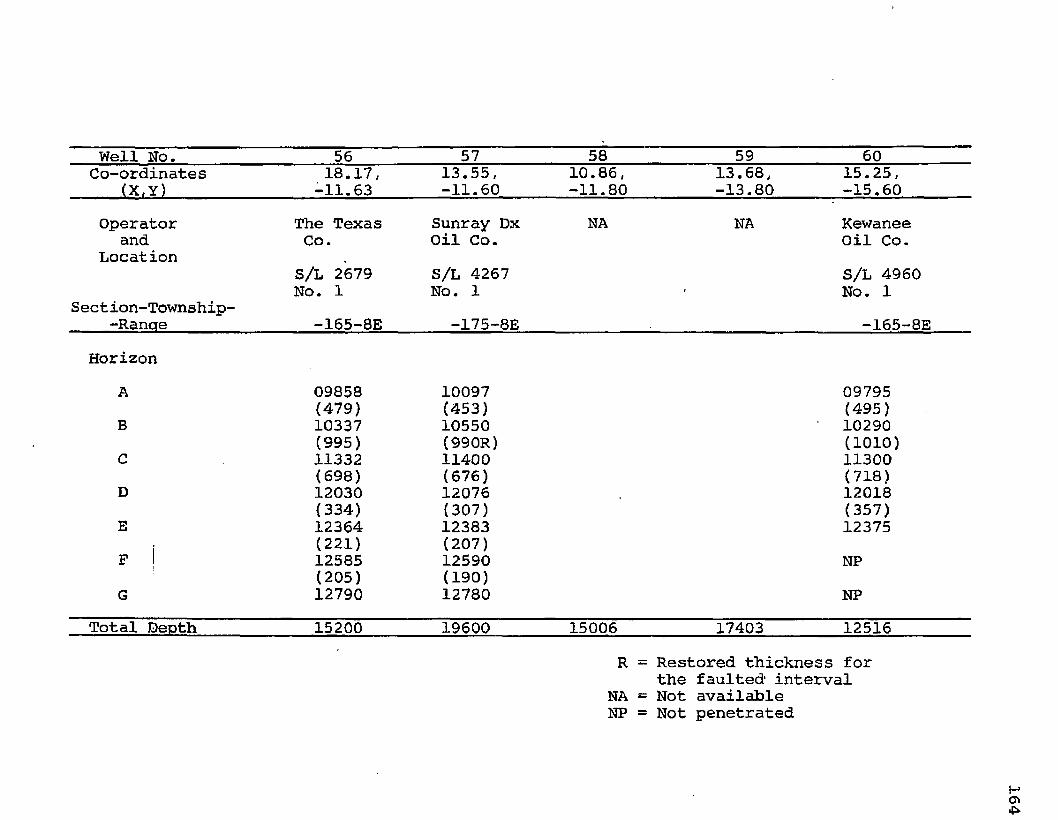
Well No. 56 57 58 59 60Co-ordinates 18.17, 13.55, 10.86, 13.68, 15.25,

(X.Y) -11.63 -11.60 -11.80 -13.80 -15.60Operator The Texas Sunray Dx NA NA Kewanee

and Co. Oil Co. Oil Co.Location .

S/L 2679 S/L 4267 S/L 4960No. 1 No. 1 • No. 1

Section-Township--Ranae -165-8E -175-8E -165-8E

HorizonA 09858 10097 09795

(479) (453) (495)B 10337 10550 10290

(995) (990R) (1010)C 11332 11400 11300

(698) (676) (718)D 12030 12076 12018

(334) (307) (357)E 12364 12383 12375

. (221) (207)F 12585 12590 NP

(205) (190)G 12790 12780 NP

Total Depth 15200 19600 15006 17403 12516R = Restored thickness for

the faulted1 interval NA = Not available NP = Not penetrated

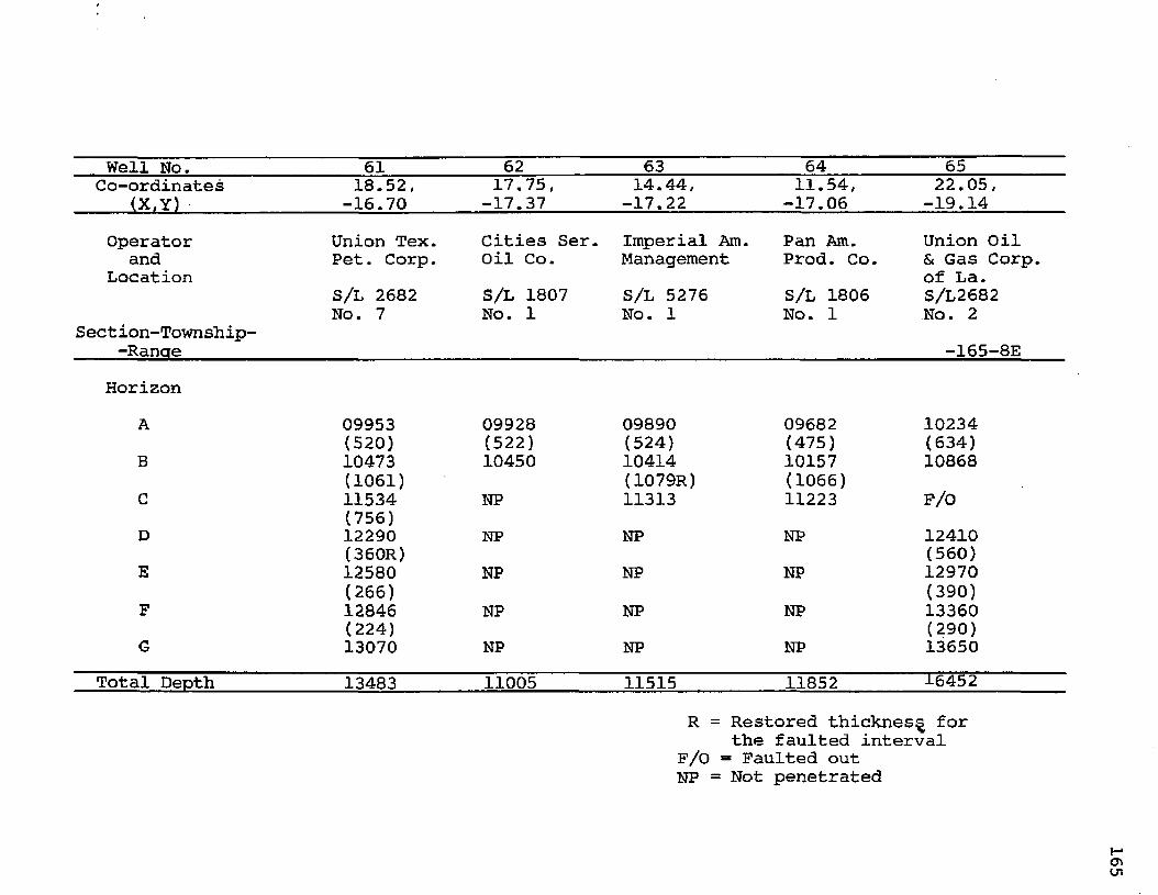
Well No. 61 62 63 64 65Co-ordinates 18.52, 17.75, 14.44, 11.54, 22.05,

(X,Y) -16.70 -17.37 -17.22 -17.06 -19.14Operator Union Tex. Cities Ser. Imperial Am. Pan Am. Union Oil

and Pet. Corp. Oil Co. Management Prod. Co. & Gas Corp.Location of La.

S/L 2682 S/L 1807 S/L 5276 S/L 1806 S/L2682No. 7 No. 1 No. 1 No. 1 No. 2

Section-Township--Ranae -165-8E

HorizonA 09953 09928 09890 09682 10234

(520) (522) (524) (475) (634)B 10473 10450 10414 10157 10868

(1061) (1079R) (1066)C 11534 NP 11313 11223 F/0

(756)D 12290 NP NP NP 12410

(360R) (560)E 12580 NP NP NP 12970

(266) (390)F 12846 NP NP NP 13360

(224) (290)G 13070 NP NP NP 13650

Total Depth 13483 11005 11515 11852 16452R = Restored thicknes^ for

the faulted interval F/O = Faulted out NP = Not penetrated

165

Well No. 66 67 68 69 70Co-ordinates 23.43, 22.90, 23.08, 23.08, 23.68,

(X,Y) -19.14 -19.78 -19.88 -20.16 -20.10Operator Union Union Diversa, Union Union

and Texas Tex. Pet. Inc. Tex. Pet. Tex. Pet.Location

S/L 2682 S/L 2682 S/L 2682 S/L 2682 S/L 2682No. 1 No. 5 No. 3 No. 6 No. 6-ASection-Township-

-Ranae -165-8E -165-8E -175-8E -165-8E -165-8EHorizon

A 10218 10210 10198 10200 10195(627) (633) (632) (635) (620)

B 10845 10843 10830 10835 10815(1067R) (1172) (1160) (1125) (1128)

C 11592 12015 11990 11960 11943(808) (792R) (922)

D 12400 12407 F/0 F/0 12865(550) (547) (561R)

E 12950 12954 12945 12950 13026(390) (361) (355) (366) (292)F 13340 13315 13300 13316 13318(305) (305) (315) (317) (282)

G 13645 13620 13615 13633 13600Total Depth 14203 16300 15116 19520 17702

R = Restored thickness for the faulted interval

F/0 = Faulted out

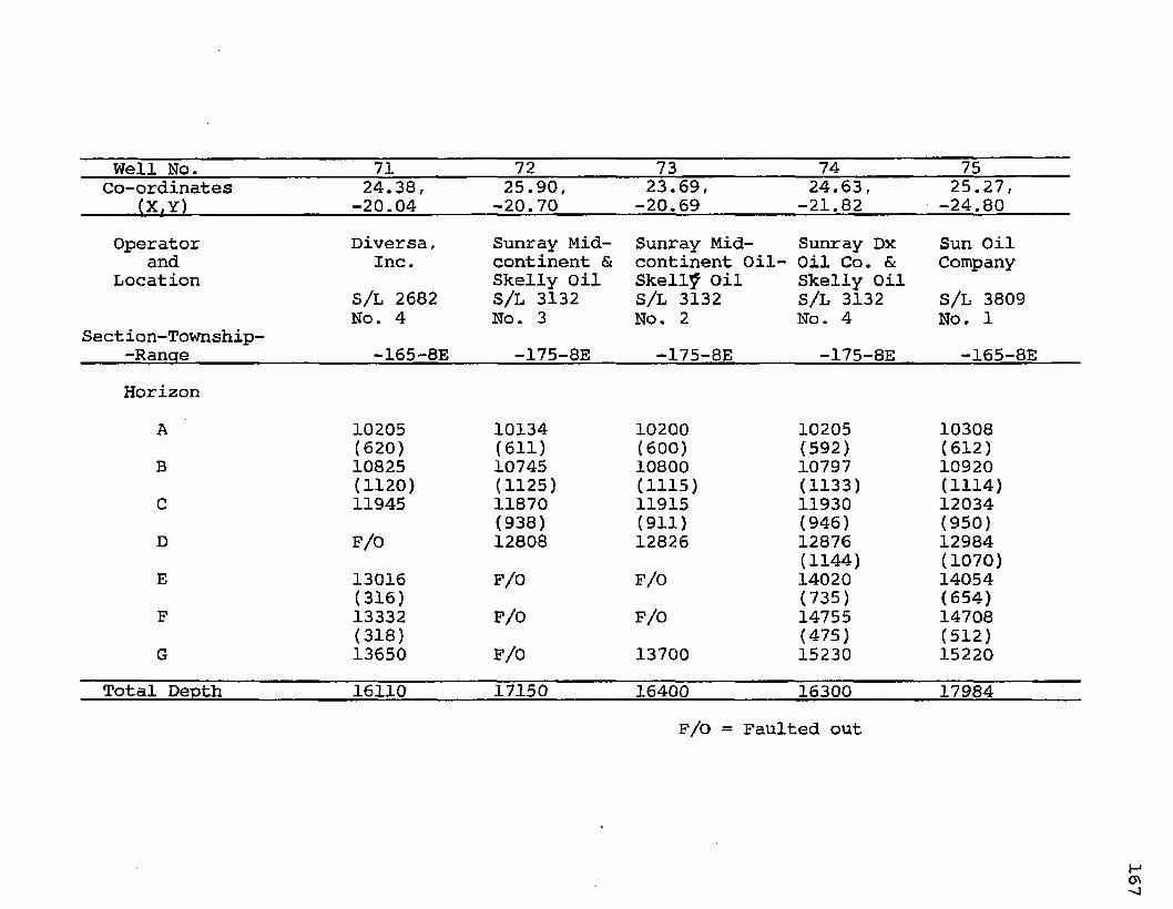
Well No. 71 72 73 74 75Co-ordinates 24.38, 25.90, 23.69, 24.63, 25.27,

(X, Y) -20.04 -20.70 -20.69 -21.82 -24.80Operator Diversa, Sunray Mid­ Sunray Mid­ Sunray Dx Sun Oil

and Inc. continent & continent Oil- Oil Co. & CompanyLocation Skelly Oil Skell^ Oil Skelly Oil

S/L 2682 S/L 3132 S/L 3132 S/L 3132 S/L 3809No. 4 No. 3 No. 2 No. 4 No. 1

Section-Township--Ranae -165-8E -175-8E -175-8E -175-8E -165-8EHorizon

A 10205 10134 10200 10205 10308(620) (611) (600) (592) (612)

B 10825 10745 10800 10797 10920(1120) (1125) (1115) (1133) (1114)

C 11945 11870 11915 11930 12034(938) (911) (946) (950)

D F/0 12808 12826 12876 12984(1144) (1070)

E 13016 F/0 F/0 14020 14054(316) (735) (654)

F 13332 F/0 F/0 14755 14708(318) (475) (512)

G 13650 F/0 13700 15230 15220Total Depth 16110 17150 16400 16300 17984

P/o = Faulted out

Well No. 76 77 78 79 80Co-ordinates 22.66, 21.20, 21.16, 19.06, 17.15,

(X,Y) -21.88 -21.40 -20.78 -20.47 -20,53Operator Sunray Dx The Ohio Exchange Pan Am. Pan Am.

and Oil Co. Oil Co. Oil & Gas Prod. Co. Prod. Co.Location

S/L 3132 S/L 3469 S/L 3907 S/L 1850 S/L 1805No. 1 No. 1 No. 1 No. 1 No. 1

Section-Township--Rancre -175-8E -165-8E

HorizonA 10200 10200 10210 10182 10140

(615) (605) (610)B 10815 10805 10820 NP NP

(1107) (1125) (1132)C 11922 11930 11952 NP NP

(946) (938)D 12868 NP 12890 NP NP

(1112)E 13980 NP F/0 NP NP

(710F 14690 NP F/0 NP NP6 NP NP F/0 NP NP

Total Depth 15241 12800 17320 10330 10320F/0 = Faulted out NP = Not penetrated

168

Well No. 81 82 83 84 85Co-ordinates 15.10, 17.53, 14.74, 14.44,

(X,Y) ND -19.24 -22.82 -21.02 -20.65Operator Pan Am. Socony Pan Am. James F.

and Prod. Co. Mobil Oil Prod. Co. HayesLocation

S/L 1809 S/L 3907 S/L 1809 S/L 1809No. 2 No. 1 No. 3 No. 1Section-Township-

-RanaeHorizon

A 10107 10200 10074 100745 NP

(605)10805

(596)10670

(591)10665

C NP(1130)11935 NP

(1110)11775

D NP(985)12920 NP NP

E NP(1250)14170 NP NP

F NP(745)14915 NP NP

G NP(495)15410 NP NP

Total Depth 10249 17478 11344 12307p/O = Faulted out ND = Not drilled NP = Not penetrated

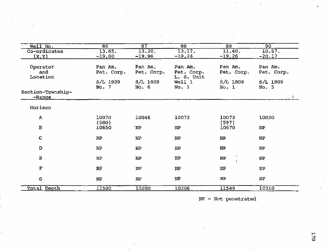
Well No. 86 87 88 89 90Co-ordinates

(X,Y)13.65,

-19.8013.20,

-19.9613.17,

-19.2411.40,

-19.2610.67,

-20.17Operator

andLocation

Section-Tovmship--Rancre

Pan Am. Pet. Corp.S/L 1809 No. 7

Pan Am. Pet. Corp.S/L 1809 No. 6

Pan Am. Pet. Corp. L. S. Unit Well 1 No. 1

Pan Am.Pet. Corp.S/L 1809 No. 1

Pan Am.Pet. Corp.S/L 1809 No. 5

iHorizon

AB

10070(580)10650

10046NP

10072NP

10073(597)10670

10020NP

C NP NP NP NP NPD NP NP NP NP NPE . NP NP NP NP , NPF NP NP NP NP NPG NP NP NP NP NP

Total Depth 11500 10200 10206 11549 10310NP = Not penetrated

170

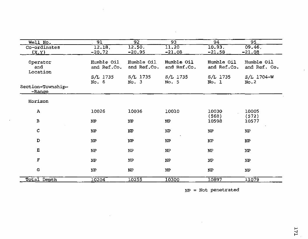
Well No. . 91 92 93 94 95Co-ordinates

(X,Y)12.18,

-20.7212.50,-20.95

11.20-21.08

10.93,-21.58

09.46, -21.08

Operatorand

Location

Section-Township--Rancre

Humble Oil and Ref.Co.S/L 1735 No. 6

Humble Oil and Ref.Co.S/L 1735 No. 3

Humble Oil and Ref.Co.S/L 1735 No. 5

Humble Oil and Ref.Co.S/L 1735 No. 1

Humble Oil and Ref. Co.3/L 1704-W No. 2

HorizonAB

10026NP

10036NP

10010NP

10030(568)10598

10005(572)10577

C NP NP NP NP NPD NP NP NP NP NPE NP NP NP NP NPF NP NP NP NP NPG NP NP NP NP NP

Total Depth 10204 10255 10300 10897 11079UP = uot penetrated

171

Well No. 96 97 98 99 100Co-ordinates 07.61, 06.39, 04.78, 02.91, 04.14,

(X,Y) -20.37 -18.77 -17.40 -19.82 -20.47Operator Humble Oil Humble Oil Humble Oil Humble Oil Humble Oiland and Ref. Co. and Ref. Co. and Ref. Co. and Ref. Co. and Ref. Co.Location

S/L 1703 S/L 1703-W S/L 1703-W S/L 1703 S/L 1703-WNo. 6 No. 3 No. 4 No. 7 No. 2Section-Township-

-RanaeHorizon

A 09790 09787 09745 09760 09800(497) (475) (486) (500)

B NP 10284 10220 10246 10300(966) (955) (954) (970)

C NP 11250 11175 11200 11270(870) (872) (878) (795)

D NP 12120 12047 12078 12065(1053) (1194)E NP NP 13100 13272 NP

(718)F NP NP NP 13990 NPG NP NP NP NP NP

Total Deoth 10303 12700 13812 14500 12981NP = Not penetrated

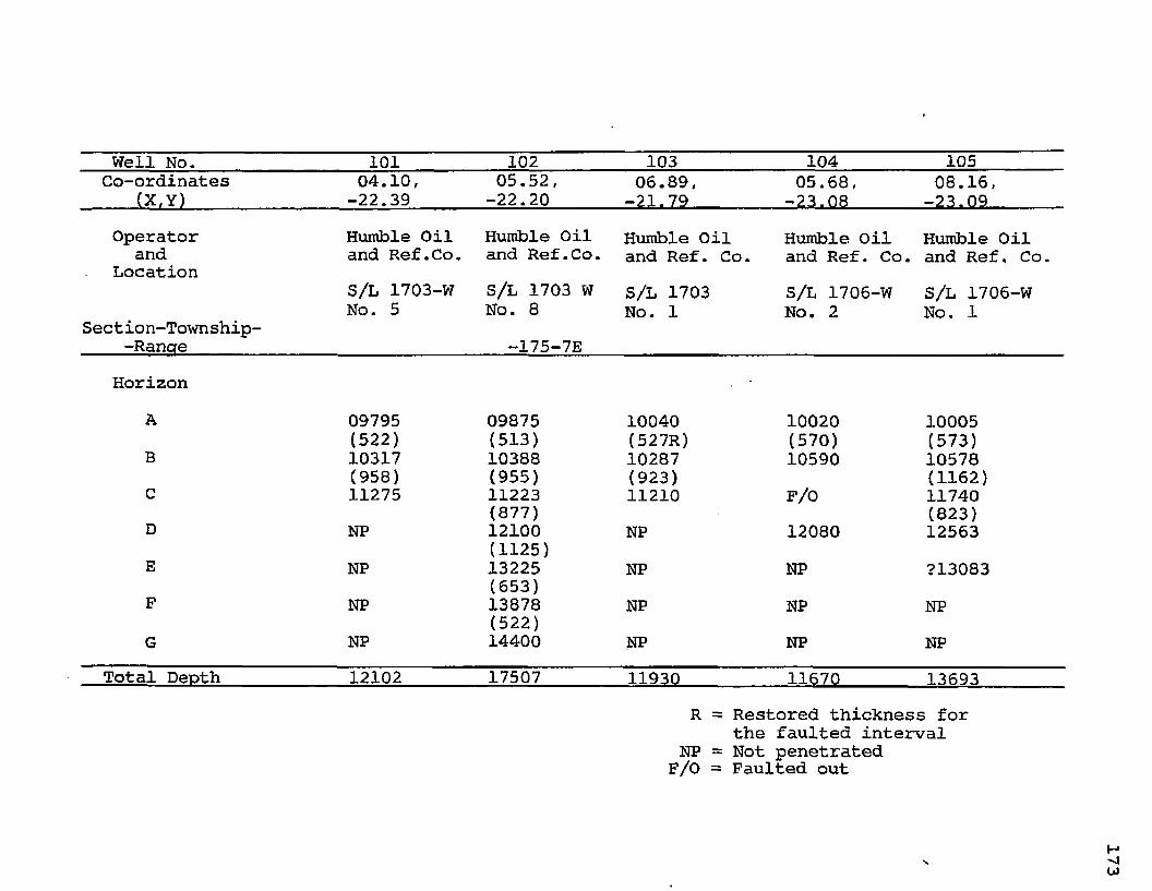
Well No. 101 102 103 104 105Co-ordinates 04.10, 05.52, 06.89, 05.68, 08.16,

(X,Y) -22.39 -22.20 -21.79 -23.08 -23.09Operator Humble Oil Humble Oil Humble Oil Humble Oil Humble Oiland and Ref.Co. and Ref.Co. and Ref. Co. and Ref. Co. and Ref, Co.Location

S/L 1703-W S/L 1703 W S/L 1703 S/L 1706-W S/L 1706-WNo. 5 No. 8 No. 1 No. 2 No. 1Section-Township--Ranae -175-7E

HorizonA 09795 09875 10040 10020 10005

(522) (513) (527R) (570) (573)B 10317 10388 10287 10590 10578(958) (955) (923) (1162)C 11275 11223 11210 F/0 11740(877) (823)D NP 12100 NP 12080 12563

(1125)E NP 13225 NP NP 713083(653)F NP 13878 NP NP NP(522)

G NP 14400 NP NP NPTotal Depth 12102 17507 11930 11670 13693

R = Restored thickness for the faulted interval

NP = Not penetrated F/0 = Faulted out

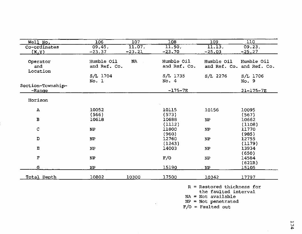
Well No. 106 107 108 109 110Co-ordinates 09.45, 11.07, 11.50, 11.13, 09.23,

(X,Y) -23.37 -23.21 -23.70 -25.03 -25.27Operator Humble Oil NA Humble Oil Humble Oil Humble Oil

and and Ref. Co. and Ref. Co. and Ref. Co. and Ref. Co.Location

S/L 1704 S/L 1735 S/L 2276 S/L 1706No. 1 No. 4 No. 9

Section-Township--Ranae -175-7E 21-175—7E

HorizonA 10052 10115 10156 10095

(566) (573) (567)B 10618 10688 NP 10662

(1112) (1108)C NP 11800 NP 11770

(960.) (985)D NP 12760 NP 12755

(1243) (1179)E NP 14003 NP 13934

(650)F NP F/0 NP 14584

(621R)G NP 15190 . NP 15105

Total Depth 10802 10300 17500 10342 17797R = Restored thickness for

the faulted interval NA = Not available NP = Not penetrated F/0 = Faulted out

Well No. 111 112 113 114 115Co-ordinates 07.70, 06.00, 04.03, 03.03,(X,Y) ND -25.75 -24.45 -24.41 -24.43Operator Humble Oil Pan Am. Humble Oil Humble Oiland and Ref.Co. Prod. Co. and Ref. Co. and Ref. Co.Location

S/L 1706 S/L 1814 S/L 1706 S/L 1706No. 13 No. 1 WC BB-3 No. 6Section-Township--Ranae -175-7E 9-175-7E 8-175-7E

HorizonA 10103 10090 10070 10143B

(555)10658 NP NP (559)

10702C

(1142)11800 NP NP

(1126R)11448

D NP NP NP(862)12310

E NP NP NP(1264)13574

F NP NP NP(521)14095

G NP NP NP(545)14640

Total Depth 11914 10274 10501 16391ND = Not drilled NP = Not penetrated R = Restored thickness of

the faulted interval

175

Well No. 116 117 118 119 120Co-ordinates 04.36,- 00.42, 05.10, 05.60,

(X.Y) -25.32 ND -27.49 -27.25 -27.17Operator Humble Oil Humble Oil Humble Oil Humble Oil

and and Ref. Co. and Ref. Co. and Ref. Co. and Ref. Co.Location

S/L 1706 s/L 3499 S/L 3498 S/L 1706No. 12 No. 1 No. 1 No. 5

Section-Township--Ranae 9-175-7E -175-7E 17-175-7E 16-175-7E

HorizonA 10062 10310 10195 10204

(548) (540)B 10610 NP 10735 NP

(1125) (1225)C 11735 NP 11960 NP

(959) (910R)D 12694 NP 12670 NP

(1195)E F/0 NP 13865 NP

(603) -

F 14095 NP 14468 NPG NP NP NP NP

Total Depth 14237 10500 14744 10516F/O = Faulted out ND = Not drilled NP = Not penetratedR = Restored thickness for

the faulted interval

Well No. 121 122 123 124 125Co-ordinates 06.80, 08.65, 10.18, 10.18, 10.20,

(X,Y) -26.52 -26.62 -26.07 -26.31 -26.99Operator Humble Oil Humble Oil Humble Oil Humble Oil Humble Oil

and and Ref.Co. and Ref.Co. and Ref. Co. and Ref. Co. and Ref. Co.Location

S/L 1706 S/L1706 S/L 1706 S/L 1706No. 8 No. 7 No. 4 No. 11

Section-Township--Ranoe 15-175-7E

HorizonA 10098 10137 10165 10173 10210

(544) (553) (555) (550) (550)B 10642 10690 10720 10723 10760

(1128) (1085) (1090) (1087) (1075)C 11770 11775 11810 11810 11835

(955) (975) (950) (945) (943)D 12725 12750 12760 12755 12778

(1245) (1160) (1075) (1098R) (1100)E 13970 13910 13835 13833 13878

(692) (652R) (658R) (605) (622)F 14662 14492 14443 14438 14500

(631) (650) (567) (552) (545R)G 15293 15142 15010 14990 14995

Total Depth 15673 16380 17051 16225 16567

R = Restored thickness for the faulted interval

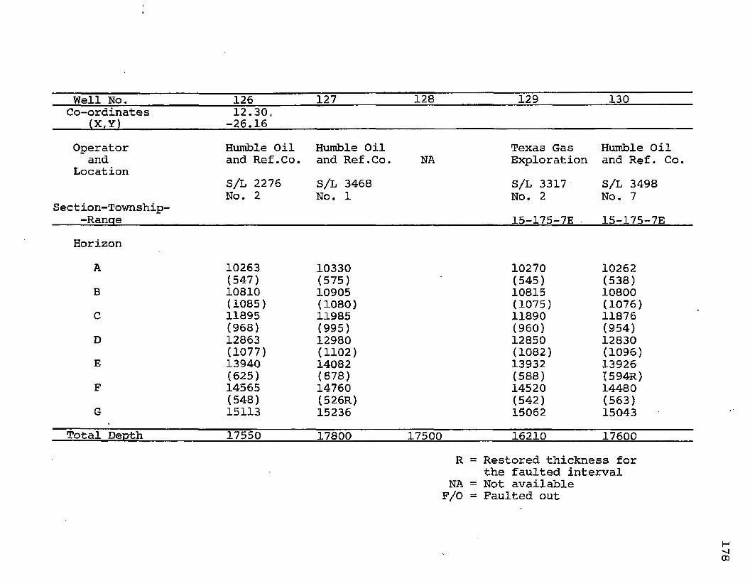
Well No. 126 127 128 129 130Co-ordinates 12.30,

(X,Y) ____ -26.16Operator Humble Oil Humble Oil Texas Gas Humble Oil

and and Ref.Co. and Ref.Co. NA Exploration and Ref• Co.Location

S/L 2276 S/L 3468 S/L 3317 S/L 3498No. 2 No. 1 No. 2 No. 7

Section-Township--Ranae 15-175-7E - 15-175-7E

HorizonA 10263 10330 10270 10262

(547) (575) (545) (538)B 10810 10905 10815 10800

(1085) (1080) (1075) (1076)C 11895 11985 11890 11876

(968) (995) (960) (954)D 12863 12980 12850 12830

(1077) (1102) (1082) (1096)E 13940 14082 13932 13926(625) (678) (588) (594R)F 14565 14760 14520 14480(548) (526R) (542) (563)

6 15113 15236 15062 15043Total Depth 17550 17800 17500 16210 17600

R = Restored thickness for the faulted interval

NA = Not available F/0 = Faulted out

178

Well No. 131 132 133 134 135Co-ordinates 08.07, 07.02, 05.63, 04.18, 04.25,

(X,Y) -28.01 -27.73 -28.55 -27.99 -28.68Operator Humble Oil Humble Oil Humble Oil Humble Oil Humbler Oil

and and Ref. Co. and Ref. Co. and Ref. Co. and Ref. Co. and Ref. Co.Location

S/L 3209 S/L 1706No. 2 No. 10

Section-Township--Ranae 16-175-7E 16-175-7E

HorizonA 10168 10120 10295 10250 10260

(544) (540)B 10712 10660 NP NP NP

(1070) (1085)C 11782 11745 NP NP NP

(988) (983)D 12770 12728 NP NP NP

(1154)E F/0 13852 NP NP NP

(618)F 14460 14500 NP NP NP

(636) (629R)G 15096 15029 NP NP NP

Total Depth 16835 16607 10500 10523 10500F/0 = Faulted out NA = Not Available R = Restored thickness for

the faulted interval NP =■ Not penetrated

179

Well No. 136 137 138 139 140Co-ordinates 00.26, 03.89, 05.95, 07.70,

(X,Y) -30.90 -29,89 -29.53 -29.52 NDOperator Humble Oil Humble Oil Humble Oil Humble Oil

and and Ref. Co. and Ref. Co. and Ref. Co. and Ref. Co.Location

S/L 3498No. 8

Section-Township--Ranae

HorizonA 10573 10350 10362 10260

(572) (530) (563) (554)B 11145 10880 10925 10814

(1140) (1080) (1055R) (1084)C 12285 11960 11860 11898

(1060) (1023) (1000) (958)D 13345 12983 12860 12856

(1229) (1185) (1150R) (1051)E 14574 14168 13920 13907

(626) (647R) (643) (573)F 15200 14695 14563 14480

(660) (565) (600R) (598)G 15860 15260 14943 15078

Total DeDth 17275 17438 16682 16900ND = Not drilled R - Restored thickness for

the faulted interval

180

Well No. 141 142 143 144 145Co-ordinates 14.04, 15.65, 12.40, 10.30,

(X,Y) -29.70 -29.82 -30.35 ND -31.18Operator Mobil Oil Magnolia Shoreline Union Oil

and Co. Pet. Co. Expl., Inc. of Calif.Location

S/L 3320 S/L 3320 S/L 3320 S/L 3317No. 4 No. 1 No. 1 No. 1

Section-Township--Rancre -175-7E -175-7E

HorizonA 10478 10528 10450 14050

(567) (589) (560) (544)B 11045 11117 11010 10994

(1070) (1098) (1080)C 12115 12215 12090 NP

(959) (965) (990)D 13074 13180 13080 NP

(1049) (1070) (1020)E 14123 14250 14100 NP

(567) (560) (550)F 14690 14810 14650 NP

(540) (570) (567)G 15230 15380 15217 NP

Total Depth 19000 16192 15650 11131ND = Not drilled NP = Not penetrated

Well No. 146 147 148 149Co-ordinates 10.26, 08.02, 04.11, 04.10,

(X,Y) -30.48 -31.20 -30.80 -32.75Operator The Texas Humble Oil Humble Oil Humble Oil

and and Expl. and Ref.Co. and Ref.Co. and Ref.Co.Location Co.

S/L 3317 S/L 3317 S/L 3498 S/L 3498No. 1—A No. B—1 No. 10 No. 11

Section-Township--Rancre 22-175-7E 21—175-7E

HorizonA NA 10385 10420 10585

(560) (550) (565)B 10965 10945 10970 11150

(1075) (1080) (1100) (1085)C 12040 12025 12070 12235

(1010) (1015) (1068) (1025)D 13050 13040 13138 13260

(1033) (1057) (1156R) (1058)E 14083 14097 14144 14318

(587) (603) (621R) (552)F 14670 14700 14605 14870

(580) (639) (608) (633)G 15250 15339 15213 15503

Total Depth 15505 18000 18050 17963NA = Not availableR = Restored thickness for

the faulted interval

183

APPENDIX II

BRIEF DESCRIPTION OF COMPUTER PROGRAMS

For the purpose of the computer mapping, four programs were used; they are known as MAPPER, TREND, RESMAP and CONTUR, corresponding to the four basic procedures indica­ted in the text of Chapter 3A. These programs are part of the GCARS (Generalized Computer-Aided Route Selection) sys­tem developed in 1968 under a joint project between the Purdue University and the Highway Commission of Indiana. They (originally written in FORTRAN IV language for the CDC-6500 series computer) were modified to the L.S.U. IBM 360/65 computer system at the L.S.U. Computer Research Cen­ter in 1971.

The inter-relation of the four computer programs is indicated on the next page.

184

Original Control Points (X(Y ,) values as INPUTOriginal Control Points (X,Y,Z) values as

ProgramMAPPER

OUTPUT OUTPUT

Gridded Data on Punched Cards____

Gridded Data on Punched Cards Printer Map +Printer Map +

ProgramRESMAP

_____OUTPUT______Gridded Residuals on Punched Cards

ProgramCONTUR

PLOT TAPEStructureContour or Isochore Map

Residual Map

Note: The numbers indicate the proceduresreferred to in the text (p.55-57 )*

185

Program MAPPERThe program MAPPER was used for generating structural

contours and isochore maps. The input data used were the three co-ordinates (X,Y,Z) of the well control points, the Z values being the subsurface elevations (for structural contours) and interval thicknesses (for isochores).

For the present study the input data are irregularly spaced; these co-ordinates (X,Y,Z) are converted to a suit­able matrix of Z-values or gridded data on a regular square lattice. The actual- spacing of the lattice can be defined by the operator, otherwise the program will compute a 'best' grid size which approximately equals the square root of the area divided by the number of the control points. The gridded data are generated by computing an average of six nearest points with each weighted according to its distance to the grid point being evaluated (Fig. 22). Any data point as close or closer than 1/25 of the grid size to a lattice point is itself treated as a lattice point during the grid- ding operation.

The gridding operation was basically developed by Professor W.R. Tobler (Turner, 1968 and 1969) at the Uni­versity of Michigan, Ann Arbor. This operation yields re­sults which are comparable to those obtained by the fitting of local polynomials, but is computationally much simpler. However, as observed by Dr. Turner, a co-developer of the

186

GCARS system, the main disadvantage appears to be a slight dampening (or smoothing) effect on the data, that approaches 10% of the data range for extremely erratic data; but for commonly encountered data distribution it is much less, one or two percent smoothing being normal.

On the map based on the gridded values output from the program MAPPER, in the area of little control, contours bunch up indicating an abrupt change in the slope of the surface generated. This is eliminated in some program like SYMAP by estimating a slope with a weighted average of the slopes of several secant planes. In this connection it is pertinent to quote Dr. Donald S. Shepard, Harvard University,

"W. Tobler extended the method of piecewise polynomial functions, always fitting a double quadratic function to the six nearest points, and averaging its value with the nearest point. Though the resulting function is not contin­uous at the junctions of polynomials, its simplicity and generality have made it useful in contour mapping.

... The SYMAP Version 4 algorithm, using piecewise ra­tional function, has been developed to provide a "reasonable" continuously differentiable function for both regular and irregular data point arrangements using the same program with SYMAP. "

The program MAPPER uses the following three subroutines: PTCON 4 - The subroutine PTCON 4 produces a contour

map on the high-speep printer; the maxi­mum width of the map produceable is 12.7

187

inches.GRID - The subroutine GRID interpolates the given

set of control points to produce a matrix of equally spaced points by a weighted moving average method.

STATS - The subroutine STATS calculates statisti­cal measures of one or two dimentional data, for example, means, variance, standard de­viation, maximum value and minimum value.

The control cards used with the program MAPPER are as follows {for the irregularly spaced control points):

Card 1: Data Identification CardCol. 1/4 *IRR

Card 2: Master Option Card Col. 6/10 Same Col. 20 1Col. 21/25 Number of control points (X,Y,Z sets)Col. 26/30 Number of control points/card

(1 in Col. 30 used)Card 3: Format Card

Cols. 1/70 (10x,2F10.2, F 10.3) usedCard 4: Area Header Card

Cols. 1/30 Description of the map typeCol. 41/70 Description of the area

Card 5: In the position of Card 5, all data cardsare placed which have their columns punchedas follows

188

Cols. 11/20 X - coordinateAll with

Cols. 21/30 Y - coordinate decimal pointsCols. 31/40 Z - coordinate

Card 6 : Title CardCol. 1/70 Identifying title of the map.

Card 7: Area Limit Specification CardCol. 1/10 Maximum X - coordinateCol. 11/20 Minimum X - coordinate All with

decimal pointsCol. 21/30 Maximum Y - coordinate Col. 31/40 Minimum Y - coordinate

Card 8 : Grid Specification CardCol. 1/3 Number of rowsCol. 4/6 Number of columnsCol. 11 1Col. 12 3Col. 13 1Col. 15 1

Card 9: Map Specification CardsCol. 1/2 Number of contour levels (Maximum=40)Col. 3 1Col. 4 0Col. 5/8 Width of map in inches (Maximum = 12.7)

Card 10: Special CardsCol. 1/10 Minimum Contour Value All with

decimal pointsCol. 11/20 Maximum Contour Value

End Cards (Two):*/ in Col. 1/2 (first card) // in Col. 1/2 (second card)

Program TRENDThe program TREND was used for generating trend maps.

The basic input data required are the same as for the pro­gram MAPPER, that is, the original sets of X, Y, Z co-or­dinates for the control points. The program is designed to perform the trend surface analysis using polynomials upto the fifth order.

The program TREND uses the following seven subroutines: IREAD - The subroutine IREAD reads in data and con­

trol option from cards and tape as desired. ANOVA - The subroutine ANOVA prints trend surface

equation coefficients and computes and prints analysis of variance statistics, namely,1) Error estimates for coefficients2) Total F-tests for all equations3) Partial F-tests for higher degree equa­

tion4) Percent Variation Explained {R-squared)

RITER - The subroutine RITER prints answers accord­ing to requested options.

INVER - The subroutine INVER performs the matrix in­version to compute coefficients.

POLY - The subroutine POLY evaluates any desiredtrend surface equation at given X and Y co­ordinates in order to compute the appropriate

190

estimates of Z.PTCON 4 - The subroutine PTCON 4 produces contour maps

on the printer.STAT - The subroutine STAT calculates statistical

measures as for the program MAPPER The control cards used with the program TREND are as

follows:Card 1: Label Card to indicate the start of a data

set.Col. 1/6 TRENDS

Card 2: Master Control CardCol. 5/10 1 (forTi>Col. 12 2 (for T2>Col. 14 3 (forVCol. 18 4 (forVCol. 20 5 (forV

Card 3: Option for printing maps of fitted trendsurfaces

Col. 1/5 *MAPSCard 4: Option for punching the gridded trend values

on cardsCol. 1/6 *PUNCH

Card 5: Option for printing identity matrices, acheck requested on the accuracy of the matrix inversion.

Col. 1/9 *IDENTITYCard 6 : Option for printing all matrices used in

the computations

191

Col. 1/6 *DEBUGCard 7: Option for printing original values, compu­

ted values and residuals for the given control points.Col. 1/10 *RE SIDUAL S

Card 8 : End Card for the optionsCol. 1/4 *END

Card 9: Area Definition CardCol. 1/5 Number of control points supplied Col. 11/20 Maximun X co-ordinate Col. 21/30 Minimum X co-ordinate Col. 31/40 Maximum Y co-ordinate Col. 41/50 Minimum Y co-ordinate

Card 10: Grid Specification CardCol. 1/3 Number of rowsCol. 4/6 Number of columnsCol. 9 1 (for one copy of the maps)

Card 11: Map Specification CardCol.1/2 Number of contour levels (Maximum = 40) Col. 3 1Col. 4 0 (for contour lines to be printed)

Card 12: Special CardCol. 1/10 Minimum Contour Value

With decimal Col. 11/20 Maximun Contour Value points

Card 13: Format CardCol. 1/5 Number of control point/card l(used)Col. 7/55 Format of data cards used

(lOx, 2F10.2, F10.3)

Card 14: Title CardCol. 1/30 Description of the map type Col. 41/70 Description of the area

Card 15: Data Cards in this position like for theprogram MAPPER (X,Y,Z values for the con­trol points)

End Cards: /.*//

Program RESMAP The program RESMAP was used to generate gridded resi­

dual values by subtracting one set of gridded values from another set of gridded values. The residuals generated may be gridded structural residuals, or thickness or thickness residuals. The input data are gridded structural data, or gridded isochore data, and/or gridded trend values, depend­ing upon the objective of mapping.

The program RESMAP is simple with a small number of the control cards as follows:

Card 1: Title CardCol. 1/80 Description of the residuals to be

derivedCard 2: Option Card

Col.2 1Col.6 1 (for putting residuals on punched

cards)Card 3: Format Card

Col. 1/80 (8F10.3) usedCard 4: Header Card

Col. 1/40 Identifying title for the map typeCol. 41/72 Identifying title for the areaCol. 73/75 Number of columns in the matrixCol. 76/78 Number of rows in the matrixCol. 80 1

Card 5: Position for data cards (output from MAPPERor TREND)

Card 6 : same as Card 3Card 7: same as Card 4Card 8: Position for another set of data cards (out­

put from MAPPER or TREND) the values of which will be subtracted from the previous data set.

End Cards: /*//

Program CONTUR The program CONTUR was used to generate contour maps on

the Calcomp (drum type) or Milgo (flat bed type) plotter.The basic input data used for this program is the set of gridded values output from the program MAPPER, TREND or RES­MAP to give the structure contour, isochore, trend or re­sidual map. The program was run at the L.S.U. Computer Research Center to generate a plot tape; the latter was mounted on the tapedrive at the Geology Department's Compu­ter Graphic Center where the contour map was generated on the MILGO plotter.

194

The program CONTUR uses the following subroutines:SCAN - The subroutine SCAN scans the gridded data

input and locates the contours.TRACE- The subroutine TRACE traces out contour lines

in turn.CALC - The subroutine CALC performs interpolations

within data matrix squares to locate contour line coordinates.

i

DRAFT- The subroutine DRAFT performs desired trans­lations and rotations, and prepares plot tape using CALCOM routines.

PROJ - The subroutine PROJ provides additional op­tions to be developed by the user.

With the program CONTUR the following control cards were used.

Card 1 : Col. 1/2 19Card 2: Col. 1/80 (8F 10.3)Card 3: Col. 1/2 15

Col. 3/12 Starting ContourCol.Col.

13/2223/32

Contour Interval with decimalpoints

Highest ContourCard 4: Col. 1/2 12

Col. 3/12 .25 (Distance from left edge of plot to start of title in inches)

Col. 13/22 .25 (Height of title letters)Card 5: Col. 1/80 Title description.

Card 6 : Col. 1/2 18Col. 3/12 20. (Width in inches)

Card 7: Col. 1/2 06Card 8 : Col. 1/80 Name of the operator, account

number, or similar descriptionCard 9: Col. 1/2 07

Col. 3/12 .15 (Height of numbers in inch)Card 10: Col. 1/2 01

Col. 3/12 Number of rowsCol. 13/22 Number of columnsCol. 23/32 Width of the outline of the map

(in inches)Card 11: In this position a set of gridded data

cards is placed.Card 12: Col. 1/2 20*

Card 13: Col. 1/2 13End Cards: /*//

* Cards 1 through 12 will repeat for additional plots (maps) required.

196

APPENDIX III

TREND SURFACE ANALYSIS (WITH THE PROGRAM TREND)

The trend surface analysis is a segment of regression analysis as is clear from the accompanying figure. It in­volves two independent variables (X,Y).

The trend analysis in geology seeks to separate broad scale

plished by fitting a trend function to a set of data values.

Trend Surface FittingThe fitting of the polynomial trend surfaces with the

actual (observed or given) data points is effected by satis­fying the least-square criterion that requires that the sum

M ULTIPLE A

a ’. C U R V I L I N E A R

W f r n .5 : ' R E G R E S S I O N .

, « g r « s i i o n

N u m b e r o f ( I n d e p e n d e n r V a r i a b l e * )

(Harbaugh and Merriam, 1968)

variation or trends, from local variations. This is accom-

197

of the differences between the observed and calculated (trend) values of Z should be a minimum. That is, in symbols,

N

Z 2(Z^-Z^) = minimum (1 )i=*l

where Zi = observed value of ZZc = calculated value of Z

Goodness of FitThe goodness of fit of the trend surfaces with the ac­

tual data points is measured as follows.Goodness of fit (or Coefficient of Determination), D_ Variance explained by regression (trend surface), E

Total variance, VN ■

where Total variance, V = ,(Zi-Z) , (2)i=lZ being the mean of the observed

Z values N 2

Unexplained variance, U =2™, (Zi-Zc) from (1) as abovei=l

and,hence, variance explained by regression/or by a given surface)

= Total variance - Unexplained variance = V - U

D = V - U (3)V

In other words, goodness of fit is the percent sum of the square explained by the regression or the trend surface fitted in with the actual data points. The same quantity expressed as a fraction is termed R-squared, where R is call­ed the Coefficient of Correlation, which is then the square

root of the coefficient of determination, i.e.R = J D .

All these three statistical measures (percent-sum-of-square explained or goodness-of-fit, R-squared, and R) are compu­ted and printed out by the program TREND.

F-TestsThe program TREND calculates the statistics for the

total and partial F-tests. The total F-test is designed to determine whether all the coefficients of the equation (for each of the trend surfaces generated) are significant (not equal to zero) and thus whether all the terms are signifi­cant. It thus determines how significantly the equation fits the data actually given. On the other hand, the par­tial F-test determines whether the coefficients of power- terms (individual power groups) are significant (different from zero) and thus determines the significance of the highest order of the polynomial tried to fit the given data. For both the tests the program TREND computes and prints out the F-statistics. For high significance(c^ = .05), F*>F 95%; for very high significance (o<= .01), F**>F99^.

The results of statistical analyses conducted for the present study are tabulated on the following pages. The table on each page is based on one horizon or one interval. The statistical measures pertaining to the total area,Carlin block and Lake block are separately indicated in the tables. In some cases no map was generated for the total

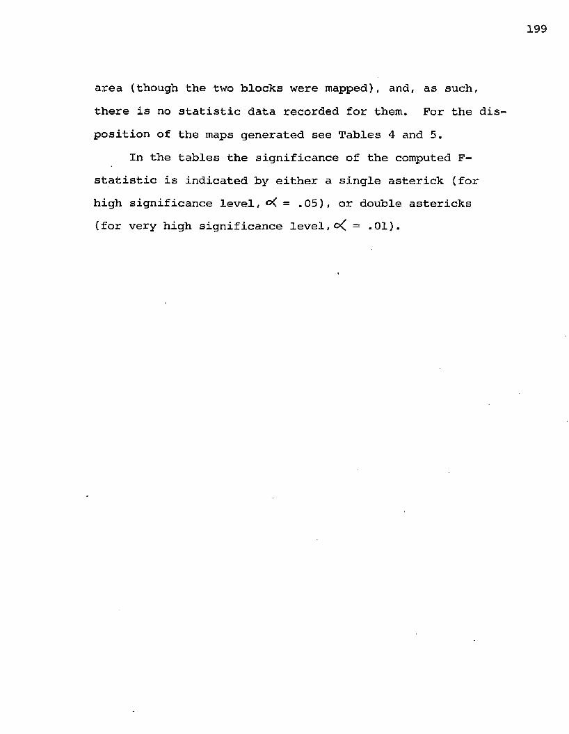
area (though the two blocks were mapped), and, as such, there is no statistic data recorded for them. For the dis­position of the maps generated see Tables 4 and 5.

In the tables the significance of the computed F- statistic is indicated by either a single asterick (for high significance level, = .05), or double astericks (for very high significance l e v e l , = .01).

RESULTS OF STATISTICAL ANALYSIS

Analysis of VarianceOrder Percent Total F-Tests_____________ Partial F-Tests____

Horizon of Variation Degree of Computed Degree of ComputedTrend Ejqplained Freedom F-statistic Freedom F-statistic

A SurfaceTotal

CarlinBlock

LakeBlock

12345

123

123

33.1667.3687.3493.9996.07

0.8566.3882.95

73.9088.3896.25

3,1316,128

10,12415,11921,113

3,556,5210,48

3,66 6,63 10,59

21.76**44.03**85.52**124.02**131.70**

0.16.17.11**23.35**

62.30**79.90**

151.46**

2.1133.1134.1135.1136.113

2.483.484.48

2.593.594.59

478.72**327.22**143.76**38.29**10.01**

1.1961.49**11.66**

581.48**75.96**30.94**

200

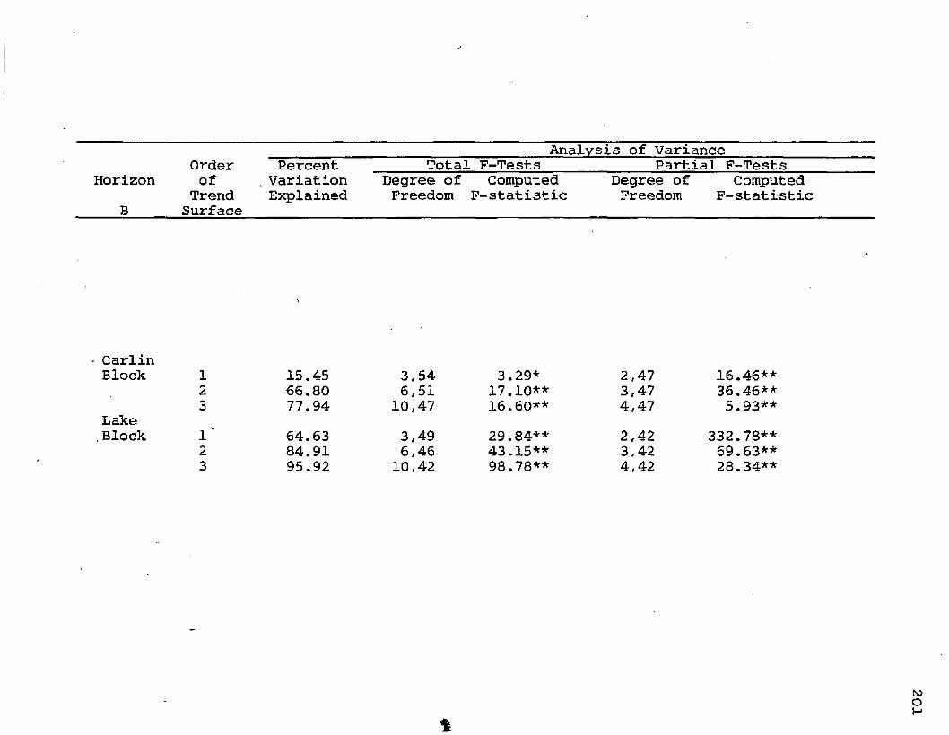
Analysis of VarianceOrder Percent ______Total F-Tests_____________ Partial F-Tests

Horizon of , Variation Degree of Computed Degree of ComputedTrend Esqplained Freedom F-statistic Freedom F-statistic

B Surface ___ ___ ______

CarlinBlock

LakeBlock

123123

15.4566.8077.9464.6384.9195.92

3,546,51

10,473,496,46

10,42

3.29*17.10**16.60**29.84**43.15**98.78**

2.473.474.472.423.424.42

16.46**36.46**5.93**

332.78**69.63**28.34**

Analysis of VarianceOrder Percent ______Total F-Tests____________ Partial F-Tests

Horizon of Variation Degree of Computed Degree of ComputedTrend Explained Freedom F-statistic Freedom F-statistic

C Surface

CarlinBlock

LakeBlock

123

123

27.6860.0570.85

45.4273.0292.19

3,556,52

10,48

3,386,35

10,31

7.02**13.03**11.67**

10.54**15.79**36.57**

2.483.484.48

2.313.314.31

22.80**17.76**4.45**

90.10**36.50**19.00**

202

HorizonD

Orderof

TrendSurface

PercentVariationExplained

Total F-TestsAnalysis of Variance

Partial F-TestsDegree of Computed Freedom F-statistic

Degree of Freedom

ComputedF-statistic

Total

CarlinBlock

LakeBlock

12345

123

123

68.8082.7893.0395.5796.50

61.5277.2083.21

56.0475.05 95.51

3,806,77

10,7315,6821,62

3,416,38

10,34

3,316,28

10,24

58.82**61.69**97.41**97.82**81.38**

21.85**21.44**16.85**

13.17**14.04**51.01**

2,623.624.625.626.62

2.343.344.34

2.243.244.24

609.27**82.50**45.37**9.01**2.74*

62.30**10.58**3.04**

149.67**33.84**27.31**

203

Analysis of VarianceOrder Percent ______Total F-Tests_____________ Partial F-Tests

Horizon of Variation Degree of Computed Degree Of ComputedTrend Explained Freedom F-statistic Freedom F-statistic

E Surface

Total

CarlinBlock

LakeBlock

12345

1234

123

35.8390.6692.5495.2095.73

82.1790.1494.3996.72

22.5560.4392.89

3,726,69

10,6515,6021,54

3,406,37

10,3315,28

3, 24 6,21

10,17

145.42**111.62**80.58**79.25**57.72**

61.46**56.41**55.57**55.13**

2.335.34**

22.23**

2.543.544.545.546.54

2,283.284.285.28

2.173.174.17

543.42** 20.36** 5.94** 6.73** 1.14

351.30**22.72**9.08**3.99**

26.98**30.21**19.42**

204

Analysis of VarianceHorizonAB

Total

CarlinBlock

LakeBlock

Order Percent Total F-Tests Partial F-Testsof Variation Degree of Computed Degree of Computed

Trend Explained Freedom F-Statistic Freedom F-StatisticSurface

12345

62.1374.8084.0686.2492.66

3,1136,11010,10615,10121,95

61.79*-54.43**55.92**42.21**57.14**

2. 95 3 954.955.956.95

402 28** 54.72** 29.98** 5.64**

13.86**

123

68.4974.3079.19

3,546,51

10,4739.13**24.57**17.89**

2.473.474.47

77.35**4.37**2.76**

123

79.0887.7191.52

3,486,45

10,4160.48**53.54**44.27**

2.413.414.41

191.27**13.92**4.61**

205

Analysis of VarianceOrder Percent Total F-Tests Partial F-Tests

HorizonBC

ofTrendSurface

VariationExplained

Degree of Freedom

Computed Degree of Computed F-statistic Freedom F-statistic

CarlinBlock 1 20.32 3,54 4.59** 2,47 7.85**

2 35.28 6,51 5.63** 3,47 3.85*Lake

3 39.19 10,47 3.03** 4,47 0.76Block 1 36.32 3,38 7.23** 2,31 14.90**

2 53.50 6,35 6.71** 3,31 4.70**3 62.22 10,31 5.10** 4,31 1.79

i

206

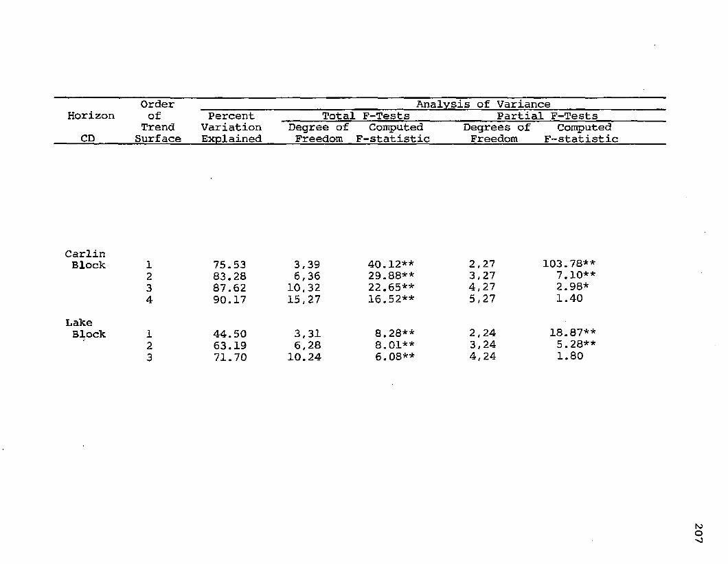
Order ________________________________ Analysis of Variance__________Horizon of Percent Total F-Tests_____________ Partial F-Tests

Trend Variation Degree of Computed Degrees of ComputedCD______Surface Explained_____Freedom F-statistic______Freedom F-statistic

CarlinBlock

LakeBlock

1234

123

75.5383.2887.6290.17

44.5063.1971.70

3,39 6,36

10,32 15,27

3,316,28

10.24

40.12**29.88**22.65**16.52**

8.28**8.01**6.08**

2.273.274.275.27

2.243.244.24

103.78**7.10**2.98*1.40

18.87**5.28**1.80

207

Analysis of VarianceOrder Percent ______Total F-Tests_____________ Partial F-Tests

Horizon of Variation Degree of Computed Degree of ComputedTrend Explained Freedom F-statistic Freedom F-statistic

DETotal

CarlinBlock.

LakeBlock

1 84.11 3,69 121.79** 2,51 467.05**2 86.90 6,66 72.96** 3,51 10.30**3 93.35 10,62 86.99** 4,51 17.90**4 94.90 15,57 70.77** 5,51 3.46**5 95.41 21,51 50.45** 6,51 0.931 68.27 3,37 26.54** 2,30 347.82**2 92.73 6,34 72.23** 3,30 83.05**3 97.06 10,30 98.89** 4,30 11.03**1 59.13 3,24 11.58** 2,17 30.77**2 76.33 6,21 11.29** 3,17 5.97**3 83.67 10,17 8.71** 4,17 1.91

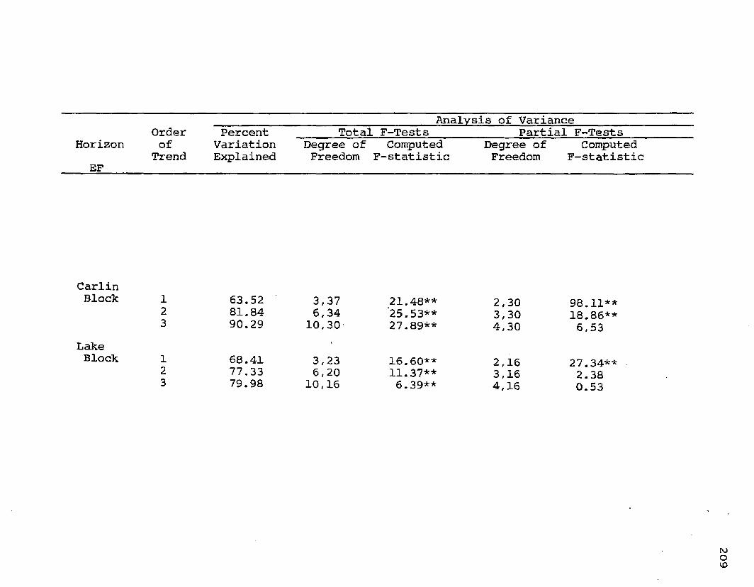
Analysis of VarianceOrder Percent ______Total F-Tests_____________ Partial F-Tests

Horizon of Variation Degree of Computed Degree of ComputedTrend Explained Freedom F-statistic Freedom F-statistic

EF

CarlinBlock

LakeBlock

123

123

63.5281.8490.29

68.4177.3379.98

3,376,34

10,30

3,236,20

10,16

21.48**'25.53**27.89**

16.60**11.37**6.39**

2.303.304.30

2,163.164.16

98.11**18.86**6,53

27.34**2.380.53

209

Analysis of VarianceOrder Percent Total F-Tests_____________ Partial F-TestsHorizon of Variation Degree of Computed Degree of ComputedTrend Explained Freedom F-statistic Freedom F-statistic

FG

CarlinBlock

LakeBlock

123

123

66.09 93 '.’97 96.50

64.0974.1879.73

3,356,32

10,28

3,226,1910,15

22.74**83.10**77.26**

13.09**9.10**5.90**

2,283.284.28

2.153.154.15

264.56**74.41**5.07**

23.71**2.491.03

210

211

VITAKumar was born on January 4, 1942 at Khagaria, Bihar,

India. He attended elementary and high schools at Arrah, Bihar, until 1956. After graduating from H.D. Jain College, University of Bihar, he entered the Indian School of Mines, Dhanbad and the University of Ranchi, Bihar, and obtained the diploma of A.I.S.M. and the degree of M.Sc. in Applied Geology in 1962, winning the "Sir Henry Hayden Medal" of the Mining, Metallurgical and Geological Institute of India as the best student of the year in Applied Geology.

He served as an Instructor in Geology at the Indian School of Mines, Dhanbad, during July, 1962 - April, 1963.For the subsequent eight months, he was engaged on prospect­ing and exploration for radio-active minerals in Bihar by the Department of Atomic Energy, Government of India. In November, 1963, he was employed as Petroleum geologist by Oil India Limited (a cooperative enterprise between the Government of India and the Burma Oil Company). After about six years of service in the O.I.L., he enrolled in September, 1969, as a graduate student at the Louisiana State Univer­sity for a PhD degree in Geology. While studying for his degree, he has been employed by the Department of Geology, L.S.U., as a teaching/research assistant.

He is an active member of the American Association of Petroleum Geologists, a member of the Geological Society of America, the Society of Petroleum Engineers of AIME, and an associate member of Sigma Xi.

EXAMINATION AND THESIS REPORT

Candidate: Madhurendu Bhushan Kumar

Major Field: Geology

Title of Thesis: Computer-Aided Subsurface Structural Analysis of theMiocene Formations of the Bayou Carlin - Lake Sand Area, South Louisiana. Approved:

Major Professor and Chairman

Dean TO the Graduate School

EXAMINING COMMITTEE:

Date of Examination:

November 27, 1972

0-0.