Critical Excitation Seismic

CRITICAL EXCITATIONMETHODS INEARTHQUAKEENGINEERING

SECOND EDITION

IZURU TAKEWAKI

Amsterdam • Boston • Heidelberg • LondonNew York • Oxford • Paris • San Diego

San Francisco • Singapore • Sydney • Tokyo

Butterworth-Heinemann is an imprint of Elsevier

Butterworth-Heinemann is an imprint of ElsevierLinacre House, Jordan Hill, Oxford OX2 8DP, UKThe Boulevard, Langford Lane, Kidlington, Oxford OX5 1GB, UK225 Wyman Street, Waltham, MA 02451, USA

Second edition 2013

Copyright � 2013 Elsevier Ltd. All rights reserved.

No part of this publication may be reproduced, stored in a retrieval system or transmitted inany form or by any means electronic, mechanical, photocopying, recording or otherwisewithout the prior written permission of the publisher.

Permissions may be sought directly from Elsevier’s Science & Technology RightsDepartment in Oxford, UK: phone (+44) (0) 1865 843830; fax (+44) (0) 1865 853333;email: [email protected]. Alternatively you can submit your request online byvisiting the Elsevier web site at http://elsevier.com/locate/permissions, and selecting“Obtaining permission to use Elsevier material.”

NoticeNo responsibility is assumed by the publisher for any injury and/or damage to personsor property as a matter of products liability, negligence or otherwise, or from any use oroperation of any methods, products, instructions or ideas contained in the material herein.Because of rapid advances in the medical sciences, in particular, independent verificationof diagnoses and drug dosages should be made.

British Library Cataloguing in Publication DataA catalogue record for this book is available from the British Library.

Library of Congress Cataloging-in-Publication DataA catalog record for this book is available from the Library of Congress.

ISBN: 978-0-08-099436-9

For information on all Elsevier publicationsvisit our web site at books.elsevier.com

Printed and bound in United States of America13 14 15 16 17 10 9 8 7 6 5 4 3 2 1

mailto:[email protected]

http://elsevier.com/locate/permissions

http://books.elsevier.com

PREFACE TO THE FIRST EDITION

There are a variety of buildings in a city. Each building has its own naturalperiod and its original structural properties. When an earthquake occurs,a variety of ground motions are induced in the city. The combination of thebuilding natural period with the predominant period of the induced groundmotion may lead to disastrous phenomena in the city. Many past earthquakeobservations demonstrated such phenomena. Once a big earthquake occurs,some building codes are upgraded. However, it is true that this repetitionnever resolves all the issues and new damage problems occur even recently.In order to overcome this problem, a new paradigm has to be posed. To theauthor's knowledge, the concept of “critical excitation” and the structuraldesign based on this concept can become one of such new paradigms.

It is believed that earthquake has a bound on its magnitude. In otherwords, the earthquake energy radiated from the fault has a bound. Theproblem is to find the most unfavorable ground motion for a building ora group of buildings (see Fig. 0.1).

A ground motion displacement spectrum or acceleration spectrum hasbeen proposed at the rock surface depending on the seismic moment,distance from the fault, etc. (Fig. 0.2). Such spectrum may have uncer-tainties. One possibility or approach is to specify the acceleration or velocitypower and allow the variability of the spectrum.

Critical excitation Z

Critical excitation B

Critical excitation D

Critical excitation C

Critical excitation A

Low-riseRC building

Wood house Medium-riseRC building

Base-isolatedbuilding

High-risebuilding

Figure 0.1 Critical excitation defined for each building.

xij

The problem of ground motion variability is very important and tough.Code-specified design ground motions are usually constructed by takinginto account the knowledge from the past observation and the probabilisticinsights. However, uncertainties in the occurrence of earthquakes (orground motions), the fault rupture mechanisms, the wave propagationmechanisms, the ground properties, etc. cause much difficulty in definingreasonable design ground motions especially for important buildings inwhich severe damage or collapse has to be avoided absolutely (Singh 1984;Anderson and Bertero 1987; Geller et al. 1997; Takewaki 2002; Stein 2003).

A long-period ground motion has been observed in Japan recently. Thistype of ground motion is told to cause a large seismic demand to suchstructures as high-rise buildings, base-isolated buildings, oil tanks, etc. Thislarge seismic demand results from the resonance between the long-periodground motion and the long natural period of these constructed facilities.

A significance of critical excitation is supported by its broad perspective.There are two classes of buildings in a city (see Fig. 0.3). One is theimportant buildings which play an important role during disastrous earth-quakes. The other one is ordinary buildings. The former one should nothave damage during earthquake and the latter one may be damaged partiallyespecially for critical excitation larger than code-specified design earth-quakes. The concept of critical excitation may enable structural designers tomake ordinary buildings more seismic resistant.

The most critical issue in the seismic-resistant design is the resonance.The promising approaches are to shift the natural period of the building

Ground motion

Wave propagation

Fault

Initiating point

Propagationcharacteristics

Fault elementRupture propagation

Source characteristics

Soil property

Radiation energy may be bounded

Figure 0.2 Earthquake ground motion depending on fault rupture mechanism, wavepropagation and surface ground amplification, etc.

xii Preface to the First Edition

through seismic control and to add damping in the building. However it isalso true that the seismic control is under development and more sufficienttime is necessary to respond to uncertain ground motions. The author hopesthat this book will help the development of new seismic-resistant designmethods of buildings for such unpredicted or unpredictable groundmotions.

The author's research was greatly motivated by the papers by Drenick(1970) and Shinozuka (1970). The author communicated with Prof.Drenick (2002) and was informed that the work by Prof. Drenick wasmotivated by his communication with Japanese researchers in late 1960s.The author would like to express his appreciation to Profs. Drenick andShinozuka.

Izuru TakewakiKyoto, 2006

REFERENCESAnderson, J.C., Bertero, V.V., 1987. Uncertainties in establishing design earthquakes.

J. Struct. Eng. ASCE, 113 (8), 1709–1724.Drenick, R.F., 1970. Model-free design of aseismic structures. J. Eng. Mech. Div. ASCE, 96

(EM4), 483–493.Drenick, R.F., 2002. Private communication.

Ordinary buildingPublic building(base for restoration ofearthquake disaster)

Intensity of ground motionIntensity of ground motion

Build

ing

resp

onse

leve

l

Build

ing

resp

onse

leve

l

Limit state Limit stateHow to prevent

Code-specifiedgroundmotion

Code-specifiedgroundmotion

Criticalexcitation

Criticalexcitation

Figure 0.3 Relation of critical excitation with code-specified ground motion in publicbuilding and ordinary building.

Preface to the First Edition xiii

http://refhub.elsevier.com//ref0010





Geller, R.J., Jackson, D.D., Kagan, Y.Y., Mulargia, F., 1997. Earthquakes cannot be pre-dicted. Science 275, 1616.

Shinozuka, M., 1970. Maximum structural response to seismic excitations. J. Eng. Mech.Div. ASCE, 96 (EM5), 729–738.

Singh, J.P., 1984. Characteristics of near-field ground motion and their importance inbuilding design. ATC-10-1 Critical aspects of earthquake ground motion and buildingdamage potential, ATC, 23–42.

Stein, R.S., 2003. Earthquake conversations. Sci. Am. 288 (1), 72–79.Takewaki, I., 2002. Critical excitation method for robust design: A review. J. Struct. Eng.

ASCE, 128 (5), 665–672.

xiv Preface to the First Edition











PREFACE TO THE SECOND EDITION

The largest earthquake event in the world since the first edition of this bookwas published in 2007 may be the March 11, 2011 event off the Pacific coastof Tohoku, Japan. Three major observations were made during that greatearthquake (Takewaki et al. 2011). The first one was a devastating, gianttsunami following the earthquake, the second one was an accident at theFukushima No.1 nuclear power plant and the last one was the occurrence oflong-period ground motions that were resonant with super high-risebuildings in mega cities in Japan.

The author was convinced during and immediately after the earthquakethat the critical excitation method is absolutely necessary for enhancing theearthquake resilience of building structures and engineering systems.Actually, Dr. Rudolf Drenick regarded nuclear power plant problems andsuper high-rise building problems as major objectives of the critical exci-tation method that he introduced about three decades ago. The author alsotook those two concerns into account before the occurrence of the 2011Japan earthquake (see the following figure from Takewaki 2008). Theauthor hopes that more resilient building structures and engineering systemswill be designed using the advanced critical excitation method.

In the second edition, the critical excitation problem for multi-component input ground motions and that for elastic-plastic structures in

critical excitation A

critical excitation Z

critical excitation B

critical excitation C

critical excitation D

nuclear-power plant

critical excitation ?

low-rise RC bld wood house med-rise RC bld base-isolated bld high-rise bld plant

Critical excitation for nuclear power plant and high-rise buildings (Takewaki 2008).RC, reinforced concrete. (See Figure 15.1 for more information.)

xvj

a more direct way are incorporated and discussed in more depth. Finally, theproblem of earthquake resilience of super high-rise buildings is discussedfrom broader viewpoints.

The author owes great thanks to Dr. Abbas Moustafa, Minia University,Egypt and Dr. Kohei Fujita, Kyoto University, Japan for their contributionsto these themes. This second edition would have never been possiblewithout their efforts.

Izuru TakewakiKyoto, 2013

REFERENCESTakewaki, I., 2008. Critical excitation methods for important structures, invited as a Semi-

Plenary Speaker. EURODYN 2008, July 7–9, Southampton, England.Takewaki, I., Murakami, S., Fujita, K., Yoshitomi, S., Tsuji, M., 2011. The 2011 off

the Pacific coast of Tohoku earthquake and response of high-rise buildings underlong-period ground motions. Soil Dynamics and Earthquake Engineering 31 (11),1511–1528.

xvi Preface to the Second Edition

PERMISSION DETAILS

Permission has been obtained for the following figures, tables and equationsthat appear in this book:

Figures 12.15–12.25, Tables 12.1, 12.2 and Equations (12.36)–(12.44) arefrom The Structural Design of Tall and Special Buildings, 20(6), K. Yamamoto,K. Fujita and I. Takewaki, Instantaneous earthquake input energy andsensitivity in base-isolated building, 631–648, 2011, with permission fromWiley and Blackwell.

Materials from Elsevier’s publications:Part of Chapter 13 has been published in ‘Fujita, K., Yoshitomi, S.,

Tsuji, M. and Takewaki, I. (2008). Critical cross-correlation function ofhorizontal and vertical ground motions for uplift of rigid block, EngineeringStructures, 30(5), 1199–1213’ and ‘Fujita, K. and Takewaki, I. (2010).Critical correlation of bi-directional horizontal ground motions, EngineeringStructures, 32(1), 261–272’.

xviij

CHAPTER ONE

Overview of Seismic CriticalExcitation Method

Contents

1.1. What is Critical Excitation? 11.2. Origin of Critical Excitation Method (Drenick’s Approach) 31.3. Shinozuka’s Approach 81.4. Historical Sketch in Early Stage 91.5. Various Measures of Criticality 101.6. Subcritical Excitation 121.7. Stochastic Excitation 131.8. Convex Models 151.9. Nonlinear or Elastic-Plastic SDOF System 161.10. Elastic-Plastic MDOF System 171.11. Critical Envelope Function 181.12. Robust Structural Design 191.13. Critical Excitation Method in Earthquake-Resistant Design 21References 23

1.1. WHAT IS CRITICAL EXCITATION?

It is natural to imagine that a ground motion input resonant to thenatural frequency of the structure is a critical excitation. In order to discussthis issue in detail, consider a linear elastic, viscously damped, single-degree-of-freedom (SDOF) system as shown in Fig. 1.1. Let m, k, c denote mass,stiffness and viscous damping coefficient of the SDOF system. The timederivative will be denoted by over-dot in this book. The system is subjected

0( ) sinp t p tω

k

c

m

=

Figure 1.1 Single-degree-of-freedom (SDOF) system subjected to external harmonicforce p(t) ¼ p0 sin ut.

Critical Excitation Methods in Earthquake Engineeringhttp://dx.doi.org/10.1016/B978-0-08-099436-9.00001-8

� 2013 Elsevier Ltd.All rights reserved. 1j

http://dx.doi.org/10.1016/B978-0-08-099436-9.00001-8

to an external harmonic force pðtÞ ¼ p0 sin ut. The equation of motion ofthis system may be described as

m€uðtÞ þ c _uðtÞ þ kuðtÞ ¼ p0 sin ut (1.1)

By dividing both sides by m, Eq. (1) leads to

€uðtÞ þ 2hU _uðtÞ þ U2uðtÞ ¼ ðp0=mÞ sin ut (1.2)

where U2 ¼ k=m, 2hU ¼ c=m. U and h are the undamped natural circularfrequency and the critical damping ratio.

Consider first the nonresonant case, i.e. usU. The general solution ofEq. (1.1) can be expressed by the sum of the complementary solution ofEq. (1.1) and the particular solution of Eq. (1.1).

uðtÞ ¼ ucðtÞ þ upðtÞ (1.3)

The complementary solution is the free-vibration solution and is given by

ucðtÞ ¼ e�hUtðA cos UDt þ B sin UDtÞ (1.4)

where UD ¼ffiffiffiffiffiffiffiffiffiffiffiffiffi1� h2

pU. On the other hand, the particular solution may be

described by

upðtÞ ¼ C sin ut þD cos ut (1.5)

The undetermined coefficients C and D in Eq. (1.5) can be obtained bysubstituting Eq. (1.5) into Eq. (1.2) and comparing the coefficients on sineand cosine terms. The expressions can be found in standard textbooks. Onthe other hand, the undetermined coefficients A and B in Eq. (1.4) can beobtained from the initial conditions uð0Þ and _uð0Þ.

Consider next the resonant case, i.e. u ¼ U. The solution correspondingto the initial conditions uð0Þ ¼ _uð0Þ ¼ 0 can then be written by

uðtÞ ¼ p0

k

1

2h½e�hUtðcos UDt þ hffiffiffiffiffiffiffiffiffiffiffiffiffi

1� h2p sin UDtÞ � cos Ut� (1.6)

Fig. 1.2 shows examples of Eq. (1.6) for several damping ratios.Consider the undamped and resonant case, i.e. h ¼ 0 and u ¼ U. As

before, the general solution of Eq. (1.2) can be expressed by the sum of thecomplementary solution and the particular solution.

uðtÞ ¼ ucðtÞ þ upðtÞ (1.7)

The complementary solution is the free-vibration solution and is given by

ucðtÞ ¼ A cos Ut þ B sin Ut (1.8)

2 Overview of Seismic Critical Excitation Method

On the other hand, the particular solution may be described by

upðtÞ ¼ Ct cos Ut (1.9)

The final solution corresponding to the initial conditions uð0Þ ¼ _uð0Þ ¼ 0

can then be written by

uðtÞ ¼ p0

2kð sin Ut � Ut cos UtÞ (1.10)

Fig. 1.3 shows an example of Eq. (1.10) for a special frequency U.

1.2. ORIGIN OF CRITICAL EXCITATION METHOD(DRENICK’S APPROACH)

Newton’s second law of motion may be described by

d

dtðm _uÞ ¼ p (1.11)

If the mass remains constant, the equation is reduced to

p ¼ m€u (1.12)

-30

-20

-10

0

10

20

30

0 2 4 6 8 10

0.01(small damping)0.05(medium damping)0.20(large damping)

disp

lace

men

t

timeFigure 1.2 Resonant response with various damping levels.

1.2. Origin of Critical Excitation Method (Drenick’s Approach) 3

Consider the integration of Eq. (1.12) from time t1 through t2.

Zt2t1

pdt ¼ mð _u2 � _u1Þ ¼ mD _u (1.13)

where _u1 ¼ _uðt1Þ and _u2 ¼ _uðt2Þ. Assume here a unit impulse applied toa mass at rest Zt2

t1

pdt ¼ 1 (1.14)

Then the change of velocity may be described as

D _u ¼ _u� 0 ¼ 1

m(1.15)

Consider next a linear elastic, viscously damped SDOF system subjectedto a base acceleration €ugðtÞ as shown in Fig. 1.4. The equation of motionmay be expressed by

m€uðtÞ þ c _uðtÞ þ kuðtÞ ¼ �m€ugðtÞ (1.16)

-50

-40

-30

-20

-10

0

10

20

30

40

50

0 10 20 30 40 50 60

disp

lace

men

t

timeFigure 1.3 Resonant response of undamped model.


By dividing both sides by m, Eq. (1.16) leads to

€uðtÞ þ 2hU _uðtÞ þ U2uðtÞ ¼ �€ugðtÞ (1.17)

where U2 ¼ k=m, 2hU ¼ c=m. The unit impulse response function can thenbe derived from Eqs. (1.4) and (1.15) as the free vibration response of thesystem at rest subjected to the unit impulse.

gðtÞ ¼ HeðtÞ 1

mUDe�hUt sin UDt (1.18)

where HeðtÞ is the Heaviside step function. The displacement response ofthe system subjected to a base acceleration €ugðtÞ may be obtained as theconvolution.

uðtÞ ¼Z t

0

f�m€ugðsÞggðt � sÞds (1.19)

The term f�m€ugðsÞgds indicates the impulse during ds. It isinteresting to note that the relative velocity and absolute accelerationcan be expressed as follows with the use of the unit impulse responsefunction.

_uðtÞ ¼Z t

0

f�m€ugðsÞg_gðt � sÞds (1.20)

€ugðtÞ þ €uðtÞ ¼Z t

0

f�m€ugðsÞg€gðt � sÞds (1.21)

Interested readers may conduct the proof as an exercise.

m

k

c

( )gu t

( )u t

Figure 1.4 Linear elastic, viscously damped SDOF system subjected to base motion.


The theory due to Drenick (1970) will be shown next. Consider themodified SDOF system with U ¼ 1. The displacement response of thesystem may be expressed by

uðtÞ ¼ZN

�N

f�€ugðsÞgg�ðt � sÞds (1.22)

where

g�ðtÞ ¼ HeðtÞ 1ffiffiffiffiffiffiffiffiffiffiffiffiffi1� h2

p e�ht sinffiffiffiffiffiffiffiffiffiffiffiffiffi1� h2

pt (1.23)

Consider the following constraint on the input acceleration.

ZN�N

€ugðtÞ2dt � M2 ðsimilar to Arias IntensityÞ (1.24)

Let us introduce the quantity N2 by

ZN�N

g�ðtÞ2dt ¼ N2 (1.25)

From Schwarz inequality,

juðtÞj2 ¼" ZN�N

f�€ugðsÞgg�ðt � sÞds#2

�ZN

�N

€ugðsÞ2ds

�ZN

�N

g�ðt � sÞ2ds � M2N2

(1.26)

Therefore

juðtÞj � MN (1.27)

Because the right-hand side is time-independent,

maxt

juðtÞj � MN (1.28)

It can be shown that the equality holds for the input.

€ugðsÞ ¼ � M

Ng�ðt � sÞ (1.29)


This is the “mirror image” of the impulse response function (seeFig. 1.5(a)). This result can also be derived from the variational approach(Drenick 1970). When t ¼ 0, the equality holds certainly

uð0Þ ¼ZN

�N

M

Ng�ðt � sÞ2ds ¼ MN (1.30)

Fig. 1.5(b) shows the critical excitation derived by Drenick (1970) and thecorresponding displacement response.

-0.1

-0.05

0

0.05

0.1

0 1 2 3 4 5

impulse response function

resp

onse

time (s)

-2

-1

0

1

2

0 1 2 3 4 5

critical excitation

inpu

t

time (s)

Figure 1.5(a) Impulse response function and mirror image critical excitation.

-6

-4

-2

0

2

4

6

-40 -30 -20 -10 0 10

input (displacement)output (displacement)

disp

lace

men

t

time (s)

Natural period=6.28(s)

m

k

c

( )gu t

( )u t

-6

-4

-2

0

2

4

6

-40 -30 -20 -10 0 10

input (displacement)output (displacement)

disp

lace

men

t

time (s)

m

k

c

( )gu t

( )u t

c

( )g

Figure 1.5(b) Mirror image critical input motion and its response.


1.3. SHINOZUKA’S APPROACH

Consider again a linear elastic, viscously damped SDOF system asshown in Fig. 1.4. Let €UgðuÞ denote the Fourier transform of the groundacceleration €ugðtÞ. This fact can be described as

€UgðuÞ ¼ZN

�N

€ugðtÞe�iutdt (1.31)

€ugðtÞ ¼1

2p

ZN�N

€UgðuÞeiutdu (1.32)

where i denotes the imaginary unit. Parseval’s theorem provides theconstraint on input acceleration in the frequency domain.

ZN�N

€ugðtÞ2dt ¼1

2p

ZN�N

�� €UgðuÞ��2du � M2 (1.33)

The Fourier transform UðuÞ of the displacement response uðtÞ can beexpressed in terms of transfer function HðuÞ.

UðuÞ ¼ HðuÞ €UgðuÞ (1.34)

where

HðuÞ ¼ UðuÞ= €UgðuÞ ¼ �m=ð�u2mþ iuc þ kÞ (1.35)

Since g�ðtÞ and HðuÞ are the Fourier transform’s pair in case of U ¼ 1,Parseval’s theorem provides the following relation.

ZN�N

g�ðtÞ2dt ¼ 1

2p

ZN�N

jHðuÞj2du ¼ N2 (1.36)

From the fact that UðuÞ is the Fourier transform of the displacementresponse uðtÞ, the following relation may be drawn.

uðtÞ ¼ 1

2p

ZN�N

HðuÞ €UgðuÞeiutdu (1.37)


From Schwarz inequality and Eqs. (1.33), (1.36), the following relationcan be derived.

juðtÞj ¼�� 12p

ZN�N

HðuÞ €UgðuÞeiutdu��

� 1

2p

ZN�N

jHðuÞj�� €UgðuÞ��du

�"1

2p

ZN�N

�� €UgðuÞ��2du

#1=2"1

2p

ZN�N

jHðuÞj2du#1=2

� MN

(1.38)

In some practical situations, useful information on €UgðuÞ may beavailable. Such additional information would provide a better estimation ofthe maximum response (Shinozuka 1970a, b).

If j €UgðuÞj has an envelope UeðuÞ, i.e.�� €UgðuÞ�� UeðuÞ; (1.39)

then a narrower response bound can be derived. From Eqs. (1.38) and (1.39),

juðtÞj � 1

2p

ZN�N

jHðuÞj�� €UgðuÞ��du � 1

2p

ZN�N

jHðuÞjUeðuÞduhIe

(1.40)

Because the right-hand side of Eq. (1.40) is time-independent,

maxt

juðtÞj � 1

2p

ZN�N

jHðuÞjUeðuÞdu ¼ Ie (1.41)

It may be observed that Ie can be a narrower bound than MN .

1.4. HISTORICAL SKETCH IN EARLY STAGE

As stated in Section 1.2, the method of critical excitation was proposedby Drenick (1970) for linear elastic, viscously damped SDOF systems in

1.4. Historical Sketch in Early Stage 9

order to take into account inherent uncertainties in ground motions. Thismethod is aimed at finding the excitation producing the maximum responsefrom a class of allowable inputs. The method was outlined in the precedingsections. With the help of the Cauchy-Schwarz inequality, Drenick (1970)showed that the critical excitation for a linear elastic, viscously dampedSDOF system is its impulse response function reversed in time, i.e. mirrorimage excitation. This implies that the critical envelope function for linearelastic, viscously damped SDOF systems in deterministic problems can begiven by an increasing exponential function and the critical excitation has tobe defined from the time of minus infinity. This result may be somewhatunrealistic and of only theoretical significance. Despite this, Drenick’s paper(1970) is pioneering.

Drenick (1977a) pointed out later that the combination of probabilisticapproaches with worst-case analyses should be employed to make theseismic resistant design robust. He claimed that the data used in the calcu-lation of failure probabilities, usually very small numbers, in the seismicreliability analysis are scarce and reliable prediction of the failure probabilityis difficult only by the conventional reliability analysis, which requires thetail shapes of probability density functions of disturbances. Practical appli-cation of critical excitation methods has then been proposed extensively.

It was pointed out that the critical response by Drenick’s model (1970) isconservative. To resolve this point, Shinozuka (1970a, b) discussed the samecritical excitation problem in the frequency domain. He proved that, if anenvelope function of Fourier amplitude spectra can be specified, a nearerupper bound of the maximum response can be obtained. The method wasalso outlined in the preceding section. Iyengar (1970) and Yang and Heer(1971) formulated another theory to define an envelope function of inputaccelerations in the time domain.

An idea similar to that due to Drenick (1970) was proposed by Papoulis(1967, 1970) independently in the field of signal analysis and circuit theory.

1.5. VARIOUS MEASURES OF CRITICALITY

Various quantities have been chosen and proposed as an objectivefunction to be maximized in critical excitation problems.

Ahmadi (1979) posed another critical excitation problem including theresponse acceleration as the objective function to be maximized. Hedemonstrated that a rectangular wave in time domain is the critical one and


recommended the introduction of another constraint in order to make thesolution more realistic.

Westermo (1985) considered the following input energy during T dividedby the mass m as the objective function in a new critical excitation problem.

EI ¼ZT0

ð�€ugÞ _udt (1.42)

He also imposed a constraint on the time integral of squared inputacceleration. He introduced a variational approach and demonstrated thatthe critical input acceleration is proportional to the response velocity. Hissolution is not necessarily complete and explicit because the responsevelocity is actually a function of the excitation to be obtained. He pointedout that the critical input acceleration includes the solution by Drenick(1970). The damage of structures may be another measure of criticality. Thecorresponding problems have been tackled by some researchers.

Takewaki (2004b, 2005) treated the earthquake input energy as theobjective function in a new critical excitation problem. It has been shownthat the formulation of the earthquake input energy in the frequencydomain is essential for solving the critical excitation problem and derivinga bound on the earthquake input energy for a class of ground motions. Thecriticality has been expressed in terms of degree of concentration of inputmotion components on the maximum portion of the characteristic functiondefining the earthquake input energy. It should be pointed out that nomathematical programming technique is required in the solution procedure.The constancy of earthquake input energy with respect to natural period anddamping ratio has been discussed. It has been shown that the constancy ofearthquake input energy is directly related to the uniformity of “the Fourieramplitude spectrum” of ground motion acceleration, not the uniformity ofthe velocity response spectrum. The bounds under acceleration and velocityconstraints (time integral of the squared base acceleration and time integralof the squared base velocity) have been clarified through numerical exam-inations for recorded ground motions to be meaningful in the short andintermediate/long natural period ranges, respectively.

Srinivasan et al. (1991) extended the basic approach due to Drenick(1970) to multi-degree-of-freedom (MDOF) models. They used a varia-tional formulation and selected a quantity in terms of multiple responses asthe objective function. They demonstrated that the relation among thecritical displacement, velocity and acceleration responses is similar to the

1.5. Various Measures of Criticality 11

well-known relation among the displacement, velocity and accelerationresponse spectra. Similar treatment for MDOF models has been proposed bythe present author in critical excitation problems for input energy.

1.6. SUBCRITICAL EXCITATION

It was suggested that the critical excitation introduced by Drenick(1970) is conservative compared to the recorded ground motions. Toresolve this problem, Drenick, Wang and their colleagues proposeda concept of “subcritical excitation” (Drenick 1973;Wang et al. 1976;Wangand Drenick 1977; Wang et al. 1978; Drenick and Yun 1979; Wang andYun 1979; Abdelrahman et al. 1979; Bedrosian et al. 1980; Wang andPhilippacopoulos 1980; Drenick et al. 1980; Drenick et al. 1984). Theyexpressed an allowable set of input accelerations as a “linear combination ofrecorded ground motions.” Note that the site and earthquake occurrenceproperties of those recorded ground motions are similar. They chose severalresponse quantities as the measure for criticality and compared the responseto the subcritical excitation with those to recorded earthquake groundmotions as the basis functions. They demonstrated that the conservatism ofthe subcritical excitations can be improved.

Abdelrahman et al. (1979) extended the idea of subcritical excitation tothe method in the frequency domain. An allowable set of Fourier spectra ofaccelerograms has been expressed as a linear combination of Fourier spectraof recorded accelerograms. They pointed out clearly that the frequency-domain approach is more efficient than the time-domain approach.

An optimization technique was used by Pirasteh et al. (1988) in one ofthe subcritical excitation problems. They superimposed accelerogramsrecorded at similar sites to construct the candidate accelerograms, then usedoptimization and approximation techniques in order to find the most criticalaccelerogram. The most critical accelerogram was defined as the one thatsatisfies the constraints on peaks, Fourier spectra, intensities, growth rates andmaximizes the damage index in the structure. The damage index has beendefined as cumulative inelastic energy dissipation or sum of interstory drifts.

It should be remarked that the concept of subcritical excitation is basedon the assumption that the critical one can be obtained from an ensemble ofbasis motions and that the basis motions are complete and reliable. However,for example, the record at SCT1 during Mexico Michoacan Earthquake(1985) and that at Kobe University during Hyogoken-Nanbu Earthquake


(1995) indicate that ground motions unpredictable from the past knowledgecan be observed and inclusion of such ground motions is inevitable in properand reliable implementation of subcritical excitation methods.

1.7. STOCHASTIC EXCITATION

The concept of critical excitationwas extended to probabilistic problemsby Iyengar andManohar (1985, 1987); Iyengar (1989); Srinivasan et al. (1992);Manohar and Sarkar (1995); Sarkar and Manohar (1996, 1998) and Takewaki(2000a–d, 2001a–c). The papers due to Iyengar and Manohar (1985, 1987)may be the first to discuss probabilistic critical excitation methods. They useda stationary model of input ground acceleration in the paper (Iyengar andManohar 1985) and utilized a nonstationary model of ground accelerationsexpressed as €ugðtÞ ¼ cðtÞwðtÞ in the paper (Iyengar andManohar 1987). cðtÞ isa deterministic envelope function andwðtÞ is a stochastic function representinga stationary random Gaussian process with zero mean.

The auto-correlation function of wðtÞ can be expressed as

Rwðt1; t2Þ ¼ E½wðt1Þwðt2Þ� ¼ZN

�N

SwðuÞeiuðt1�t2Þdu (1.43)

SwðuÞ is the power spectral density (PSD) function of the stochastic functionwðtÞ. The PSD function of €ugðtÞ may then be expressed as

Sgðt;uÞ ¼ cðtÞ2SwðuÞ (1.44)

Consider again a linear elastic viscously damped SDOF model. Theauto-correlation function of the relative displacement of the SDOF modelcan be expressed as

RDðt1; t2Þ ¼ZN

�N

ZN�N

ZN�N

cðs1Þhðt1 � s1Þcðs2Þ

� hðt2 � s2ÞSwðuÞeiuðs1�s2Þduds1ds2 (1.45)

where hðtÞ is the impulse response function. Substitution of t1 ¼ t2 ¼ t in Eq.(1.45) leads to the mean-square relative displacement of the SDOF model.

sDðtÞ2 ¼ZN

�N

fACðt;uÞ2 þ ASðt;uÞ2gSwðuÞdu (1.46)

1.7. Stochastic Excitation 13

In Eq. (1.46), the following quantities are used.

ACðt;uÞ ¼Z t

0

cðsÞhðt � sÞ cos usds (1.47)

ASðt;uÞ ¼Z t

0

cðsÞhðt � sÞ sin usds (1.48)

A critical excitation problemwas discussed by Iyengar andManohar (1987)to maximize f ¼ max

tsDðtÞ2 subject to the constraint on

RN�N SwðuÞdu

which is equivalent to the constraint onE½RT0 €u 2

g dt� (E½$�: ensemble mean) fora given envelope function cðtÞ. Iyengar and Manohar (1987) expressed thesquare root of thePSD functionof the excitation in termsof linear combinationof orthonormal functions and obtained their coefficients through eigenvalueanalysis. Srinivasan et al. (1992), Manohar and Sarkar (1995) and Sarkar andManohar (1996, 1998) imposed a boundon the total average energy and solvedlinear or nonlinear programming problems. Srinivasan et al. (1992) useda nonstationary filtered shot noise model for expressing input motions. Man-ohar and Sarkar (1995) and Sarkar and Manohar (1996, 1998) further seta bound on the average rate of zero crossings to avoid the excessive concen-tration of wave components at the resonant frequency in the PSD function.

In contrast to the bound on the average rate of zero crossings, Takewaki(2000c, d, 2001a–c) introduced a new constraint on the intensity supSwðuÞof the PSD function SwðuÞ of wðtÞ in addition to the constraint on thepower (integral

RN�N SwðuÞdu of PSD function) and developed a simpler

critical excitation method for both stationary and nonstationary inputs. Inthe case of nonstationary excitations, the following double maximizationprocedure must be treated.

maxSwðuÞ

maxtff ðt; SwðuÞÞg (1.49)

where f represents an objective function, e.g. a mean-square response. Theprocedure (1.49) requires determination of the time when the probabilisticindex f attains its maximum under each input prescribed by SwðuÞ. Thisprocedure is quite time consuming. Takewaki (2000c, d, 2001a–c) deviseda unique procedure based on the order interchange of the double maxi-mization procedure (see Fig. 1.6), i.e.

maxt

maxSwðuÞ

ff ðt; SwðuÞÞg (1.50)


Takewaki (2000c, d, 2001a–c) suggested that the first maximization procedurefor SwðuÞ can be performed very efficiently by utilizing the method forstationary inputs (Takewaki 2000a, b) and the secondmaximization procedurefor time can be conducted systematically by changing the time sequentially. Itwas suggested that this method can be applied not only to SDOF models, butalso to MDOFmodels if an appropriate objective function can be introduced.

1.8. CONVEX MODELS

A convex model is defined mathematically as a set of functions.Each function is a realization of an uncertain event. Several interesting

time

t = ti t = t j

maximization with respect to time

noitcnufDSP

ot tce p serhti

wnoit azi

mi xam

f (t)

f (t)

f (t)

Sw(1) ( )ω

objective function

subjected to the motion

f (t)

Sw(2) ( )ω

objective function


f (t)

Sw(M)( )ω

objective function


f (t)

time

time

Figure 1.6 Procedure based on order interchange of double maximization procedure.

1.8. Convex Models 15

convex models were proposed by Ben-Haim and Elishakoff (1990), Ben-Haim et al. (1996), Pantelides and Tzan (1996), Tzan and Pantelides(1996a) and Baratta et al. (1998) for ground motion modeling which canbe constructed versatilely depending on the level of prior informationavailable. Examples are: A local energy-bound convex model, an integralenergy-bound convex model, an envelope-bound convex model,a Fourier-envelope convex model and a response-spectrum-envelopeconvex model (Ben-Haim et al. 1996). One of the merits of theconvex models is the capability of prediction of the maximum or extremeresponse of structures to unknown inputs of which the appropriateprobabilistic description is difficult. In addition, unlike the other methods,such as the subcritical excitation and stochastic excitation, anotheradvantageous feature of the convex model comes from the fact that it canhandle MDOF systems with the same ease as SDOF systems. The smartcombination of probabilistic and convex-model approaches appears to bepromising (Drenick 1977a). It is not the objective of this book to providea detailed explanation of the convex models. Readers interested in theconvex models should refer to Ben-Haim and Elishakoff (1990), Ben-Haim et al. (1996), Pantelides and Tzan (1996), Tzan and Pantelides(1996a) and Baratta et al. (1998).

1.9. NONLINEAR OR ELASTIC-PLASTIC SDOF SYSTEM

Critical excitation problems for autonomous nonlinear systems (e.g.Duffing oscillator) were considered by Iyengar (1972). By using the Schwarzinequality, he derived a response upper bound similar to that by Drenick(1970). He treated both deterministic and probabilistic inputs. Drenick andPark (1975) provided interesting and important comments on the paper dueto Iyengar (1972).

An idea was proposed by Drenick (1977b) to use an equivalent linear-ization technique in finding a critical excitation for nonlinear systems.However, he did not discuss the applicability of the concept to actual andpractical problems and his concept or scenario is restricted to deterministicequivalent linearization problems.

Westermo (1985) tackled critical excitation problems for nonlinearhysteretic and nonhysteretic systems by adopting the input energy given byEq. (1.42) as the objective function. His approach is limited, but pioneering.He limited the class of critical excitations to periodic ones. He suggested


several interesting points inherent in the critical excitation problems fornonlinear systems.

A deterministic equivalent linearization technique was used byPhilippacopoulos (1980) and Philippacopoulos and Wang (1984) in criticalexcitation problems of nonlinear SDOF hysteretic systems. They derivedcritical inelastic response spectra and compared them with inelastic responsespectra for recorded motions.

Takewaki (2001d, 2002) developed a new type of probabilistic criticalexcitation method for SDOF elastic-plastic structures. For simplicity, hetreated a stationary random acceleration input €ug of which the PSDfunction can be described by SgðuÞ. The power

RN�N SgðuÞdu and the

intensity supSgðuÞ of the excitations were fixed and the critical excitationwas found under these constraints. While transfer functions and unitimpulse response functions can be defined and used in linear elasticstructures only, such analytical expressions cannot be used in elastic-plastic structures. This situation leads to difficulty in finding a criticalexcitation for elastic-plastic structures. To resolve such difficulty,a statistical equivalent linearization technique has been introduced. Theshape of the critical PSD function has been limited to a rectangularfunction attaining its upper bound in a certain frequency range. Thecentral frequency of the rectangular PSD function has been treated asa principal parameter and changed in finding the critical PSD function.The critical excitations were obtained for two examples and comparedwith the corresponding recorded earthquake ground motions. Takewaki(2001d, 2002) pointed out that the central frequency of the criticalrectangular PSD function is resonant to the equivalent natural frequencyof the elastic-plastic SDOF system (see Chapter 5). This fact correspondswith the result by Westermo (1985).

1.10. ELASTIC-PLASTIC MDOF SYSTEM

Several interesting approaches for MDOF systems were proposed asnatural extensions of the method for SDOF systems. Philippacopoulos(1980) and Philippacopoulos and Wang (1984) took full advantage ofa deterministic equivalent linearization technique in critical excitationproblems of nonlinear MDOF hysteretic systems. They proposeda conceptual scenario for the nonlinear MDOF hysteretic systems. How-ever, application of the technique to practical problems is not shown in

1.10. Elastic-Plastic MDOF System 17

detail. For example, it is not clear for what excitation the equivalent stiff-nesses and damping coefficients should be defined.

Takewaki (2001e) extended the critical excitation method for elastic-plastic SDOF models to MDOF models on deformable ground byemploying a statistical equivalent linearization method for MDOF models.The linearization method was used to simulate the response of the originalelastic-plastic hysteretic model. As in SDOF models, the powerRN�N SgðuÞdu and intensity supSgðuÞ of the excitations are constrained. It isassumed that the shape of the critical PSD function is a rectangular oneattaining its upper bound in a certain frequency range. In contrast to SDOFmodels, various quantities can be employed inMDOFmodels as the objectivefunction to be maximized. The sum of standard deviations of story ductilitiesalong the height has been chosen as the objective function to define thecritical excitation. Note that a solution procedure similar to that for SDOFmodels has been used. It adopts a procedure of regarding the centralfrequency of the rectangular PSD function as a principal parameter for findingthe critical one. The simulation results by elastic-plastic time-history responseanalysis disclosed that the proposed critical excitation method is reliable in themodels for which the validity of the statistical equivalent linearization methodis guaranteed. It was suggested that the critical response representation interms of nonexceedance probabilities can be an appropriate candidate forexpressing the criticality of recorded ground motions (see Chapter 5).

1.11. CRITICAL ENVELOPE FUNCTION

A new class of critical excitation problems may be formulated foridentifying critical envelope functions for nonstationary random input(Takewaki 2004a). The nonstationary ground motion is assumed to be€ugðtÞ ¼ cðtÞwðtÞ which is the product of a deterministic envelope functioncðtÞ and another probabilistic function wðtÞ representing the frequencycontent. The former envelope function can be determined in such a waythat the mean-square drift of an SDOFmodel attains its maximum under theconstraint E½RT

0 €u2g dt� ¼ C on mean total energy and thatRN�N SwðuÞdu ¼

Sw on power of wðtÞ (SwðuÞ is also given). By use of the constraint on powerof wðtÞ, the constraint on mean total energy can be reduced toZT

0

cðtÞ2dt ¼ C=Sw (1.51)


A double maximization procedure for time and the envelope function isincluded in the critical excitation problem. The key for reaching the criticalenvelope function is the order interchange in the double maximizationprocedure. The Cauchy-Schwarz inequality can be used for obtaining anupper bound of the mean-square drift can also be derived by the use of. Itcan be shown that the technique is systematic and the upper bound of theresponse can bound the exact response efficiently within a reasonableaccuracy. It can also be demonstrated that, while an increasing exponentialfunction is the critical one in the deterministic problem tackled by Drenick(1970), the super-imposed envelope function of the envelope function ofthe critical excitation can be a function similar to an increasing exponentialfunction in the probabilistic problem (see Chapter 6).

1.12. ROBUST STRUCTURAL DESIGN

In the previous sections, model parameters of structural systems weregiven and critical excitations were determined for the given structuralsystem. A more interesting but difficult problem is to determine structuralmodel parameters k simultaneously with respect to some proper designobjectives, e.g. minimizing f ðk; SgðuÞÞ. It should be remarked that thecritical excitation depends on the structural model parameters. Considera critical excitation problem for structural models subjected to a stationaryexcitation of which the input PSD function is denoted by SgðuÞ. Thisproblem may be expressed as (see Fig. 1.7)

mink

maxSgðuÞ

ff ðk; SgðuÞÞg (1.52)

Since the critical excitation is defined and determined for each set ofstructural model parameters, this design problem is complex and highlynonlinear with respect to design variables. The following critical-excitationbased design problem was considered by Takewaki (2001f) for n-story shearbuilding structures (ki ¼ story stiffness in the i-th story and k ¼ fkig) sub-jected to stationary random inputs. While the integral of the PSD functionand the amplitude of the PSD function are constrained for the input, thetotal cost of the structure as expressed by the total quantity of structuralmaterials is constrained for the structure.

[Problem]Find the set ~k of stiffnesses and the PSD function ~SgðuÞ

1.12. Robust Structural Design 19

such thatmink

maxSgðuÞ

ff ðk; SgðuÞÞg (1.53)

subject toZN

�N

SgðuÞdu � S (1.54a)

to sup SgðuÞ � s (1.54b)

toXn

i¼1ki ¼ K (1.54c)

and to ki > 0 ði ¼ 1;/; nÞ (1.54d)

Takewaki (2001f) derived the optimality conditions for this problem via theLagrange multiplier method and devised a solution technique based on theoptimality criteria approach. It was suggested that the former theories(Takewaki 2000a–d, 2001a–c) for the critical excitation problems for givenstructural parameters can be utilized effectively in this new type of adaptivedesign problem. The key is to define a new function f ðk; ~Sgðu; kÞÞ andminimize that function f ðk; ~Sgðu; kÞÞ with respect to k.

Another interesting approach was presented by Tzan and Pantelides(1996b) to find more robust designs for building structures. The optimalcross-sectional areas of a structure are found to minimize the structural

f

variation for fixed

critical excitation

for fixed

optimal story stiffnesses

k( j)

Sg(ω)(i)k k

Figure 1.7 Schematic diagram of performance upgrading based on concept of system-dependent critical excitation.


volume subject to floor drift and member stress constraints in the presence ofuncertainties in seismic excitation.

1.13. CRITICAL EXCITATION METHOD IN EARTHQUAKE-RESISTANT DESIGN

Earthquake inputs are uncertain even with the present knowledge and itdoes not appear easy to predict forthcoming events precisely both in time-history and frequency contents (Anderson and Bertero 1987; PEER Centeret al. 2000). For example, recent near-field ground motions (Northridge1994, Kobe 1995, Turkey 1999 and Chi-Chi, Taiwan 1999) and theMexico Michoacan motion 1985 have some peculiar characteristicsunpredictable before their occurrence. It is also true that the civil,mechanical and aerospace engineering structures are often required to bedesigned for disturbances including inherent uncertainties due mainly totheir “low rate of occurrence.” Worst-case analysis combined with properinformation based on reliable physical data is expected to play an importantrole in avoiding difficulties induced by such uncertainties. Approaches basedon the concept of “critical excitation” seem to be promising.

Just as the investigation on limitation states of structures plays animportant role in the specification of allowable response and performancelevels of structures during disturbances, the clarification of critical excitationsfor a given structure or a group of structures appears to provide structuraldesigners with useful information in determining excitation parameters ina reasonable way.

A significance of critical excitation is supported by its broad perspective.In general, there are two classes of buildings in a city. One is the importantbuildings, which play an important role during disastrous earthquakes. Theother is ordinary buildings. The former should not have damage duringearthquakes and the latter may be damaged partially especially by criticalexcitations larger than code-specified design earthquakes (see Fig. 1.8). Theconcept of critical excitation may enable structural designers to makeordinary buildings more seismic-resistant.

In the case where influential active faults are known in the design stage ofa structure (especially an important structure), the effects by these activefaults should be taken into account in the structural design through theconcept of critical excitation. If influential active faults are not necessarilyknown in advance, virtual or scenario faults with an appropriate energy may

1.13. Critical Excitation Method in Earthquake-Resistant Design 21

be defined, especially in the design of important and socially influentialstructures. The combination of worst-case analysis (Takewaki 2004b, 2005)with appropriate specification of energy levels (Boore 1983) derived fromthe analysis of various factors, e.g. fault rupture mechanism and earthquakeoccurrence probability, appears to lead to the construction of a more robustand reliable seismic resistant design method (see Fig. 1.9). The appropriatesetting of energy levels or information used in the worst-case analysis isimportant and research on this subject should be conducted moreextensively.

Code-

specified

ground

motion

Critical

excitation

Intensity of ground motion

Building

response

levelLimit state

Public building

(base for restoration

of earthquake disaster)

Ordinary building

how to prevent

Critical

excitation

Code-

specified

ground

motion

Limit state

Building

response

level

Intensity of ground motion

Figure 1.8 Relation of critical excitation with code-specified ground motion in publicbuilding and ordinary building.

ground motion

wave propagation

fault

initiating point rupture propagation

fault element

soil propertysource

characteristics

propagationcharacteristics

radiation energy may be bounded

Energy passage0 2

0 ( )tS gE V u t dtρ= ∫ .

Figure 1.9 Earthquake energy prescribed by fault rupture, wave propagation andsurface soil amplification.


Critical excitation problems for fully nonstationary excitations (see, forexamples, Conte and Peng (1997), Fang and Sun (1997)) and criticalexcitation problems for elasto-plastic responses under those excitations arechallenging problems.

As for response combination, Menun and Der Kiureghian (2000a, b)discussed the envelopes for seismic response vectors. The normal stress ina structural member under combined loading of the axial force and thebending moment may be one example. This problem is related to theinterval analysis and its further development is desirable.

REFERENCESAbdelrahman, A.M., Yun, C.B., Wang, P.C., 1979. Subcritical excitation and dynamic

response of structures in frequency domain. Comput. and Struct. 10 (5), 761–771.Ahmadi, G., 1979. On the application of the critical excitation method to aseismic design.

J. Struct. Mech. 7 (1), 55–63.Anderson, J., Bertero, V.V., 1987. Uncertainties in establishing design earthquakes. J. Struct.

Eng. 113 (8), 1709–1724.Baratta, A., Elishakoff, I., Zuccaro, G., Shinozuka, M., 1998. A generalization of the

Drenick-Shinozuka model for bounds on the seismic response of a Single-Degree-Of-Freedom system. Earthquake Engrg. and Struct. Dyn. 27 (5), 423–437.

Bedrosian, B., Barbela, M., Drenick, R.F., Tsirk, A., 1980. Critical excitation method forcalculating earthquake effects on nuclear plant structures: An assessment study.NUREG/CR-1673, RD. U.S. Nuclear Regulatory Commission, Burns and Roe, Inc,Oradell, N.J.

Ben-Haim, Y., Elishakoff, I., 1990. Convex Models of Uncertainty in Applied Mechanics.Elsevier, Amsterdam.

Ben-Haim, Y., Chen, G., Soong, T., 1996. Maximum structural response using convexmodels. J. Engrg. Mech. 122 (4), 325–333.

Boore, D.M., 1983. Stochastic simulation of high-frequency ground motions based onseismological models of the radiated spectra. Bulletin of the Seismological Society ofAmerica 73 (6A), 1865–1894.

Conte, J.P., Peng, B.F., 1997. Fully nonstationary analytical earthquake ground-motionmodel. J. Eng. Mech. 123 (1), 15–24.

Drenick, R.F., 1970. Model-free design of aseismic structures. J. Engrg. Mech. Div. 96 (4),483–493.

Drenick, R.F., 1973. Aseismic design by way of critical excitation. J. Engrg. Mech. Div. 99(4), 649–667.

Drenick, R.F., 1977a. On a class of non-robust problems in stochastic dynamics. In:Clarkson, B.L. (Ed.), Stochastic Problems in Dynamics. Pitman, London, pp. 237–255.

Drenick, R.F., 1977b. The critical excitation of nonlinear systems. J. Appl. Mech. 44 (2),333–336.

Drenick, R.F., Park, C.B., 1975. Comments on “Worst inputs and a bound on the highestpeak statistics of a class of non-linear systems.” J. Sound and Vibration 41 (1), 129–130.

Drenick, R.F., Yun, C.B., 1979. Reliability of seismic resistance predictions. J. Struct. Div.105 (10), 1879–1891.

Drenick, R.F., Wang, P.C., Yun, C.B., Philippacopoulos, A.J., 1980. Critical seismicresponse of nuclear reactors. J. Nuclear Engrg. and Design 59, 425–435.


Drenick, R.F., Novmestky, F., Bagchi, G., 1984. Critical excitation of structures. In: Windand Seismic Effects, Proc. of the 12th Joint UJNR Panel Conference. NBS SpecialPublication, pp. 133–142.

Fang, T., Sun, M., 1997. A unified approach to two types of evolutionary random responseproblems in engineering. Archive of Appl. Mech. 67 (7), 496–506.

Iyengar, R.N., 1970. Matched Inputs. Report No.47, Series J. Center for AppliedStochastics, Purdue University, W. Lafayette, Ind.

Iyengar, R.N., 1972. Worst inputs and a bound on the highest peak statistics of a class ofnon-linear systems. J. Sound and Vibration 25 (1), 29–37.

Iyengar, R.N., 1989. Critical seismic excitation for structures. In: Proc. of 5th ICOSSAR.San Francisco, ASCE Publications, New York.

Iyengar, R.N., Manohar, C.S., 1985. System dependent critical stochastic seismic excita-tions. In: M15/6, Proc. of the 8th Int. Conf. on SMiRT. Belgium, Brussels.

Iyengar, R., Manohar, C., 1987. Nonstationary random critical seismic excitations. J. Eng.Mech. 113 (4), 529–541.

Manohar, C.S., Sarkar, A., 1995. Critical earthquake input power spectral density functionmodels for engineering structures. Earthquake Engrg. Struct. Dyn. 24 (12), 1549–1566.

Menun, C., Kiureghian, A., 2000a. Envelopes for seismic response vectors: I Theory.J. Struct. Eng. 126 (4), 467–473.

Menun, C., Kiureghian, A., 2000b. Envelopes for seismic response vectors: II Application.J. Struct. Eng. 126 (4), 474–481.

Pantelides, C.P., Tzan, S.R., 1996. Convex model for seismic design of structures: I analysis.Earthquake Engrg. Struct. Dyn. 25 (9), 927–944.

Papoulis, A., 1967. Limits on bandlimited signals. Proc. of the IEEE 55 (10), 1677–1686.Papoulis, A., 1970. Maximum response with input energy constraints and the matched filter

principle. IEEE Trans. on Circuit Theory 17 (2), 175–182.PEER Center, ATC, Japan Ministry of Education, Science, Sports, and Culture, US-NSF,

2000. Effects of near-field earthquake shaking. In: Proc. of 5th ICOSSAR. SanFrancisco, March 20–21, 2000.

Philippacopoulos, A.J., 1980. Critical Excitations for Linear and Nonlinear StructuralSystems. Ph.D. Dissertation, Polytechnic Institute of New York.

Philippacopoulos, A., Wang, P., 1984. Seismic inputs for nonlinear structures. J. Eng. Mech.110 (5), 828–836.

Pirasteh, A.A., Cherry, J.L., Balling, R.J., 1988. The use of optimization to construct criticalaccelerograms for given structures and sites. Earthquake Engrg. Struct. Dyn. 16 (4),597–613.

Sarkar, A., Manohar, C.S., 1996. Critical cross power spectral density functions and thehighest response of multi-supported structures subjected to multi-component earth-quake excitations. Earthq. Engrg. Struct. Dyn. 25, 303–315.

Sarkar, A., Manohar, C.S., 1998. Critical seismic vector random excitations for multiplysupported structures. J. Sound and Vibration 212 (3), 525–546.

Shinozuka, M., 1970a. Maximum structural response to seismic excitations. J. Engrg. Mech.Div. 96 (5), 729–738.

Shinozuka, M., 1970b. Maximum structural response to earthquake accelerations Chapter 5.In: Lind, N.C. (Ed.), Structural Reliability and Codified Design. University ofWaterloo, Waterloo (CA), pp. 73–85.

Srinivasan, M., Ellingwood, B., Corotis, R., 1991. Critical base excitations of structuralsystems. J. Eng. Mech. 117 (6), 1403–1422.

Srinivasan, M., Corotis, R., Ellingwood, B., 1992. Generation of critical stochastic earth-quakes. Earthquake Engrg. Struct. Dyn. 21 (4), 275–288.

Takewaki, I., 2000a. Optimal damper placement for critical excitation. Probabilistic Engrg.Mech. 15 (4), 317–325.


Takewaki, I., 2000b. Effective damper placement for critical excitation. Confronting UrbanEarthquakes, Report of fundamental research on the mitigation of urban disasters causedby near-field earthquakes for Grant in Aid of Scientific Research on Priority Areas,Ministry of Education, Science, Sports and Culture (Japan), 558–561.

Takewaki, I., 2000c. A new probabilistic critical excitation method. J. Struct. Constr. Engrg.(Transactions of AIJ) 533, 69–74 (in Japanese).

Takewaki, I., 2000d. A nonstationary random critical excitation method for MDOF linearstructural models. J. Struct. Constr. Engrg. (Transactions of AIJ) 536, 71–77(in Japanese).

Takewaki, I., 2001a. A new method for non-stationary random critical excitation. Earth-quake Engrg. Struct. Dyn. 30 (4), 519–535.

Takewaki, I., 2001b. Nonstationary random critical excitation for nonproportionallydamped structural systems. Comput. Meth. Appl. Mech. Engrg. 190 (31), 3927–3943.

Takewaki, I., 2001c. Nonstationary random critical excitation for acceleration response.J. Engrg. Mech. 127 (6), 544–556.

Takewaki, I., 2001d. Critical excitation for MDOF elastic-plastic structures via statisticalequivalent linearization. J. Struct. Engrg. B. 47B, 187–194 (in Japanese).

Takewaki, I., 2001e. Probabilistic critical excitation for MDOF elastic-plastic structures oncompliant ground. Earthq. Engrg. Struct. Dyn. 30 (9), 1345–1360.

Takewaki, I., 2001f. Maximum global performance design for variable critical excitations.J. Struct. Constr. Engrg. (Transactions of AIJ) 539, 63–69 (in Japanese).

Takewaki, I., 2002. Critical excitation for elastic–plastic structures via statistical equivalentlinearization. Probabilistic Engrg. Mech. 17 (1), 73–84.

Takewaki, I., 2004a. Critical envelope functions for non-stationary random earthquakeinput. Computers & Structures 82 (20–21), 1671–1683.

Takewaki, I., 2004b. Bound of earthquake input energy. J. Struct. Eng. 130 (9), 1289–1297.Takewaki, I., 2005. Bound of earthquake input energy to soil–structure interaction systems.

Soil Dynamics and Earthquake Engineering 25 (7–10), 741–752.Tzan, S.R., Pantelides, C.P., 1996a. Convex models for impulsive response of structures.

J. Eng. Mech. 122 (6), 521–529.Tzan, S.-R., Pantelides, C.P., 1996b. Convex model for seismic design of structuresdII:

design of conventional and active structures. Earthquake Engrg. Struct. Dyn. 25 (9),945–963.

Wang, P.C., Drenick, R.F., 1977. Critical seismic excitation and response of structures. In:Proc. of 6WCEE, vol. II. K.A. Rastogi for Sarita Prakashan, Meerut, India, 1040–1045.

Wang, P.C., Philippacopoulos, A.J., 1980. Critical seismic assessment of life-line structures.Proc. of 7WCEE vol. 8, 257–264.

Wang, P.C., Yun, C.B., 1979. Site-dependent critical design spectra. Earthquake Engrg.Struct. Dyn. 7 (6), 569–578.

Wang, P.C., Wang, W., Drenick, R., Vellozzi, J., 1976. Critical excitation and response offree standing chimneys. In: Proc. of the Int. Symposium on Earthquake Struct. Engrg,vol. I. Mo., St. Louis. Aug., 269–284.

Wang, P.C., Wang, W.Y.L., Drenick, R.F., 1978. Seismic assessment of high-rise buildings.J. Engrg. Mech. Div. 104 (2), 441–456.

Westermo, B.D., 1985. The critical excitation and response of simple dynamic systems.J. Sound and Vibration 100 (2), 233–242.

Yang, J.N., Heer, E., 1971. Maximum dynamic response and proof testing. J. Engrg. Mech.Div. 97 (4), 1307–1313.


CHAPTER TWO

Critical Excitation for Stationaryand Nonstationary Random Inputs

Contents

2.1. Introduction 272.2. Stationary Input to Single-Degree-of-Freedom (SDOF) Model 28

[Problem CESS] 292.3. Stationary Input to Multi-Degree-of-Freedom (MDOF) Model 30

[Problem CESM] 332.4. Conservativeness of Bounds 342.5. Nonstationary Input to SDOF Model 36

[Problem CENSS] 372.6. Nonstationary Input to MDOF Model 40

[Problem CENSM] 412.7. Numerical Examples for SDOF Model 422.8. Numerical Examples for MDOF Model 442.9. Conclusions 45Appendix Functions AC (t;u), AS (t;u) for a Specific Envelope Function 47References 50

2.1. INTRODUCTION

In this chapter, critical excitation methods for stationary andnonstationary random inputs are discussed. It is natural to assume thatearthquake ground motions are samples or realizations of a nonstationaryrandom process. Therefore critical excitation methods for nonstationaryrandom inputs may be desirable for constructing and developing realisticearthquake-resistant design methods. However, it may also be relevant todevelop the critical excitation methods for stationary random inputs asthe basis for further development for nonstationary random inputs. Firstof all, critical excitation methods for stationary random inputs are dis-cussed and some fundamental and important results are derived. Theseresults play a significant role in the critical excitation methods explainedin this book. Secondly, critical excitation methods for nonstationaryrandom inputs are developed based on the theory for stationary randominputs.

Critical Excitation Methods in Earthquake Engineeringhttp://dx.doi.org/10.1016/B978-0-08-099436-9.00002-X


http://dx.doi.org/10.1016/B978-0-08-099436-9.00002-X

Fig. 2.1 shows a sample of a stationary random process. The mean valueand the standard deviation of this process are constant every time. The phaseof this process is assumed to be uniformly random.

2.2. STATIONARY INPUT TO SINGLE-DEGREE-OF-FREEDOM (SDOF) MODEL

Consider an SDOF model of mass m, viscous damping coefficient c andstiffness k as shown in Fig. 2.2. When this model is subjected to the basemotion ugðtÞ as a stationary Gaussian random process with zero mean, theequation of motion may be described by

m€uðtÞ þ c _uðtÞ þ kuðtÞ ¼ �m€ugðtÞ (2.1)

Fourier transformation of Eq. (2.1) leads to

ð�u2mþ iuc þ kÞUðuÞ ¼ �m €UgðuÞ (2.2)

m

kc

( )gu t

( )u t

Figure 2.2 SDOF model subjected to horizontal ground motion.

-5

0

5

0 5 10 15 20 25 30inpu

t acc

eler

atio

n (m

/s2 )

time (s)Figure 2.1 Example of stationary random input.

28 Critical Excitation for Stationary and Nonstationary Random Inputs

where UðuÞ and €UgðuÞ are Fourier transforms of uðtÞ and €ugðtÞ, respec-tively. The transfer function may then be derived as

HðuÞ ¼ UðuÞ= €UgðuÞ ¼ �m=ð�u2mþ iuc þ kÞ (2.3)

Let SgðuÞ denote the power spectral density (PSD) function of €ugðtÞ. Themean square response of the structural deformation DðtÞ ¼ uðtÞ may beexpressed by

s2D ¼ZN

�N

jHðuÞj2SgðuÞdu (2.4)

f ¼ s2D ¼ZN

�N

jHðuÞj2SgðuÞdu ¼ZN

�N

FðuÞSgðuÞdu (2.5)

where

FðuÞ ¼ jHðuÞj2 (2.6)

The critical excitation problem for stationary random inputs may be stated asfollows.

[Problem CESS]Given floor mass, story stiffness and structural viscous damping, find thecritical PSD function ~SgðuÞ to maximize f defined by Eq. (2.5) subject to

ZN�N

SgðuÞdu � S ðS; given power limitÞ (2.7)

supSgðuÞ � s ðs; given PSD amplitude limitÞ (2.8)

Equation (2.7) limits the power of the excitation and Eq. (2.8) is intro-duced to keep the present excitation model physically realistic. It is wellknown that a PSD function, a Fourier amplitude spectrum and anundamped velocity response spectrum of an earthquake have an approx-imate relationship. If the time duration of the earthquake is fixed, the PSDfunction corresponds to the Fourier amplitude spectrum and almostcorresponds to the undamped velocity response spectrum. Therefore thepresent limitation on the peak of the PSD function approximatelyindicates the specification of a bound on the undamped velocity responsespectrum.

2.2. Stationary Input to Single-Degree-of-Freedom (SDOF) Model 29

The solution to the above-mentioned problem can be obtained ina simple manner. Fig. 2.3 shows an example of the functionFðuÞ ¼ jHðuÞj2. The critical PSD function is a rectangular functionoverlapped around the natural frequency of the structural model.

In case of the infinite PSD amplitude limit, i.e. s/N, ~SgðuÞ is reducedto the Dirac delta function (see Fig. 2.3(a)) and the value f takes

f ¼ SFðuMÞ (2.9)

where uM is characterized by

FðuMÞ ¼ maxu

FðuÞ (2.10)

This implies that the critical excitation is almost resonant to the fundamentalnatural frequency of the structural model.

When s is finite, ~SgðuÞ turns out to be a constant s in a finite interval~U ¼ S=s (see Fig. 2.3(b)). This input is called hereafter “the input witha rectangular PSD function.” The optimization procedure is very simplebecause of the positive definiteness of the functions FðuÞ and SgðuÞ in Eq.(2.5) and it is sufficient to find the finite interval ~Uwhich can be searched forby decreasing a horizontal line in the figure of the function FðuÞ until theinterval length attains S=s and finding their intersections (see Fig. 2.4).

2.3. STATIONARY INPUT TO MULTI-DEGREE-OF-FREEDOM (MDOF) MODEL

Consider an n-story shear building model, as shown in Fig. 2.5, subjected tothe base acceleration €ugðtÞwhich is regarded as a stationary Gaussian random

lartcepsre

wopytisned

noitcnuf-F

circular frequency

s →∞(Dirac delta function)

F-function

PSD function lartcepsre

wopytisned

noitcnuf-F

circular frequency

s

Ω∼(a) infinite PSD (b) finite PSD

– –

Figure 2.3 Power spectral density function of critical excitation: (a) infinite PSD, (b)finite PSD.


process with zero mean. M, C, K, r ¼ f1/1gT are the system mass,viscous damping, stiffness matrices and the influence coefficient vector,respectively. Equations of motion of this model in the frequency domainmay be written as

ð�u2Mþ iuCþKÞUðuÞ ¼ �Mr €UgðuÞ (2.11)

UðuÞ and €UgðuÞ denote the Fourier transforms of the floor displacementsuðtÞ and the Fourier transform of the input acceleration €ugðtÞ, respectively.Eq. (2.11) can be simplified to the following compact form.

AUðuÞ ¼ B €UgðuÞ (2.12)

( )gu t

1k

2k

nknc

2c

1c

1m

2m

nm

Figure 2.5 n-story shear building model subjected to horizontal base acceleration.

F-fu

nctio

n

circular frequency

control the levelso that the band widthcoincides with

pow

er s

pect

ral

dens

ity

F-fu

nctio

n

circular frequency

(a) (b)

Figure 2.4 Schematic diagram of the procedure for finding the critical excitation witha rectangular PSD function: (a) single case, (b) multiple isolated case.

2.3. Stationary Input to Multi-Degree-of-Freedom (MDOF) Model 31

where

A ¼ ð�u2Mþ iuCþ KÞ ðtridiagonal matrixÞ (2.13a)

B ¼ �Mr (2.13b)

Let diðtÞ denote the interstory drift in the i-th story. Define the setdðtÞ ¼ fdiðtÞg and their Fourier transforms DðuÞ ¼ fDiðuÞg. DðuÞ canbe expressed in terms of UðuÞ by

DðuÞ ¼ TUðuÞ (2.14)

T is a constant matrix consisting of 1 (diagonal components), �1 and 0.Substitution of UðuÞ in Eq. (2.12) into Eq. (2.14) leads to

DðuÞ ¼ TA�1B €UgðuÞ (2.15)

Eq. (2.15) can be expressed simply as

DðuÞ ¼ HDðuÞ €UgðuÞ (2.16)

In Eq. (2.16), HDðuÞ ¼ fHDiðuÞg are the transfer functions of interstory

drifts to the input acceleration and are described as

HDðuÞ ¼ TA�1B (2.17)

Since A is a tridiagonal matrix, its inverse can be obtained in closed form.Let SgðuÞ denote the PSD function of €ugðtÞ. According to the random

vibration theory, the mean-square response of the i-th interstory drift can becomputed from

s2Di¼

ZN�N

jHDiðuÞj2SgðuÞdu ¼

ZN�N

HDiðuÞH�

DiðuÞSgðuÞdu (2.18)

where ð Þ� indicates the complex conjugate.The sum of the mean squares of the interstory drifts can be expressed by

f ¼Xni¼ 1

s2Di¼

ZN�N


where

FðuÞ ¼Xni¼ 1

jHDiðuÞj2 ¼

Xni¼ 1

HDiðuÞH�

DiðuÞ (2.20)


The problem of critical excitation for stationary inputs may bedescribed as:

[Problem CESM]Given floor masses, story stiffnesses and story viscous dampings, find thecritical PSD function ~SgðuÞ maximizing f defined by Eq. (2.19) subject to

ZN�N

SgðuÞdu � S ðS; given value of power limitÞ (2.21)

supSgðuÞ � s ðs; given value of PSD amplitude limitÞ (2.22)

Fig. 2.6 shows examples of FðuÞ for 2-DOF models and Fig. 2.7 presentsthe variation of the function f with respect to 1=s for various damping ratios.

Almost the same solution procedure as for an SDOF model can also beapplied to this problem. In the case where s/N, it is known that ~SgðuÞ isreduced to the Dirac delta function (see Fig. 2.3(a)) and the value f can beexpressed by

f ¼ SFðuMÞ (2.23)

where the frequency uM is characterized by

FðuMÞ ¼ maxu

FðuÞ (2.24)

This means that the frequency content of the critical excitation is almostresonant to the fundamental natural frequency of the structural model.

In the case where s is finite, ~SgðuÞ is found to be a constant s in a finiteinterval ~U ¼ S=s (see Fig. 2.3(b)). This input will be called “the input witha rectangular PSD function.”The optimization procedure is simple because of

0

0.0005

0.001

0.0015

0.002

0.0025

0 10 20 30 40 50 60

h=0.02h=0.05h=0.10

F-fu

nctio

n

circular frequency (rad/s)Figure 2.6 Examples of function FðuÞ for various damping ratios (2-DOF model).

2.3. Stationary Input to Multi-Degree-of-Freedom (MDOF) Model 33

the positive definiteness of the functions FðuÞ and SgðuÞ in Eq. (2.19). It issufficient to find the finite interval ~U which can be determined by decreasinga horizontal line in the figure of the function FðuÞ until the interval lengthattains S=s and finding their intersections (see Fig. 2.4(a)). When higher-mode effects are significant in MDOF systems, the critical PSD functionwill result in a multiple isolated rectangular PSD function (see Fig. 2.4(b)).

2.4. CONSERVATIVENESS OF BOUNDS

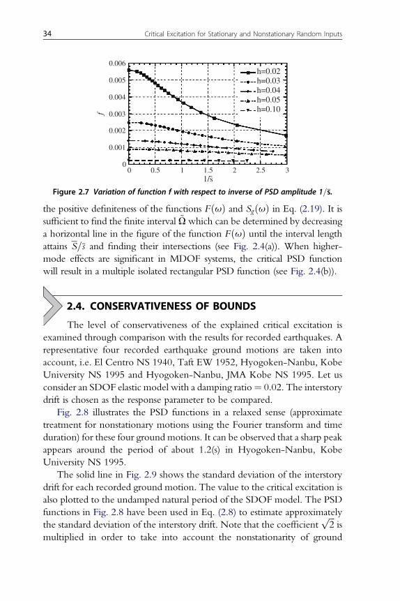
The level of conservativeness of the explained critical excitation isexamined through comparison with the results for recorded earthquakes. Arepresentative four recorded earthquake ground motions are taken intoaccount, i.e. El Centro NS 1940, Taft EW 1952, Hyogoken-Nanbu, KobeUniversity NS 1995 and Hyogoken-Nanbu, JMA Kobe NS 1995. Let usconsider an SDOF elastic model with a damping ratio¼ 0.02. The interstorydrift is chosen as the response parameter to be compared.

Fig. 2.8 illustrates the PSD functions in a relaxed sense (approximatetreatment for nonstationary motions using the Fourier transform and timeduration) for these four ground motions. It can be observed that a sharp peakappears around the period of about 1.2(s) in Hyogoken-Nanbu, KobeUniversity NS 1995.

The solid line in Fig. 2.9 shows the standard deviation of the interstorydrift for each recorded ground motion. The value to the critical excitation isalso plotted to the undamped natural period of the SDOF model. The PSDfunctions in Fig. 2.8 have been used in Eq. (2.8) to estimate approximatelythe standard deviation of the interstory drift. Note that the coefficient

ffiffiffi2

pis

multiplied in order to take into account the nonstationarity of ground

0

0.001

0.002

0.003

0.004

0.005

0.006

0 0.5 1 1.5 2 2.5 3

h=0.02h=0.03h=0.04h=0.05h=0.10f

1/s

Figure 2.7 Variation of function f with respect to inverse of PSD amplitude 1=s.


motions. One-third of the displacement response spectrum for each groundmotion is also plotted in Fig. 2.9 (broken line). The coefficient “three”approximately represents the so-called peak factor. In Fig. 2.9, the area ofthe PSD function and the peak value of the PSD function have beencomputed for each recorded ground motion. These values are specifiedby S ¼ 0:278ðm2=s4Þ, s ¼ 0:0330ðm2=s3Þ for El Centro NS 1940,S ¼ 0:0901ðm2=s4Þ, s ¼ 0:00792ðm2=s3Þ for Taft EW 1952,S ¼ 0:185ðm2=s4Þ, s ¼ 0:0364ðm2=s3Þ for Hyogoken-Nanbu, KobeUniversity NS 1995 and S ¼ 2:55ðm2=s4Þ, s ¼ 0:262ðm2=s3Þ forHyogoken-Nanbu, JMA Kobe NS 1995. It can be observed that, while thelevel of conservativeness is about 2 or 3 in the natural period range of interestin El Centro NS 1940 and Taft EW 1952, a closer coincidence can be seenaround the natural period of 1.2(s) in Hyogoken-Nanbu, Kobe UniversityNS 1995. This indicates that Hyogoken-Nanbu, Kobe University NS 1995

0

0.01

0.02

0.03

0.04

0.05

0 50 100

El Centro NS (1940)po

wer

spe

ctra

l den

sity

(m

2 /s3 )

circular frequency (rad/s)

0

0.005

0.01

0 50 100

Taft EW (1952)

pow

er s

pect

ral d

ensi

ty (

m2 /s

3 )


0

0.01

0.02

0.03

0.04

0.05

0 50 100

Hyogoken-Nanbu (1995)Kobe University NS

pow

er s

pect

ral d

ensi

ty (

m2 /s

3 )

circular frequency (rad/s)0

0.1

0.2

0.3

0 50 100

Hyogoken-Nanbu (1995)JMA-Kobe NS

pow

er s

pect

ral d

ensi

ty (

m2 /s

3 )


Figure 2.8 Power spectral density functions of recorded earthquakes (El Centro NS1940; Taft EW 1952; Hyogoken-Nanbu, Kobe University NS 1995; Hyogoken-Nanbu,JMA Kobe NS 1995).

2.4. Conservativeness of Bounds 35

has a predominant period around 1.2(s) and the resonant property of thisground motion can be represented by the explained critical excitation.

2.5. NONSTATIONARY INPUT TO SDOF MODEL

The key idea for stationary inputs can be used for nonstationary inputs.In this section, it is assumed that the input base acceleration can be describedby the following uniformly modulated nonstationary random process.

€ugðtÞ ¼ cðtÞwðtÞ (2.25)

In Eq. (2.25), cðtÞ is a given deterministic envelope function and wðtÞ isa stationary Gaussian process with zero mean to be determined. Morecomplex nonuniformly modulated nonstationary models have been proposed

0

0.1

0.2

0.3

0 1 2 3

El Centro NS 1940

recordedcriticalSD/3.0

stan

dard

dev

iatio

n of

dri

ft (

m)

natural period (s)

h=0.02

0

0.1

0.2

0.3

0 1 2 3

Taft EW 1952


stan

dard

dev

iatio

n of

dri

ft (

m)

natural period (s)

h=0.02

0

0.1

0.2

0.3

0 1 2 3

Hyogoken-Nanbu 1995Kobe Univ. NS


stan

dard

dev

iatio

n of

dri

ft (

m)

natural period (s)

h=0.02

0

0.1

0.2

0.3

0 1 2 3

Hyogoken-Nanbu 1995JMA-Kobe. NS


stan

dard

dev

iatio

n of

dri

ft (

m)

natural period (s)

h=0.02

Figure 2.9 Standard deviation of interstory drift of an SDOF model (damping ratio¼ 0.02) subjected to recorded earthquakes, that relate to the present critical excitationand one-third of the displacement response spectrum.


(Conte and Peng 1997; Fang and Sun 1997). Advanced nonstationary criticalexcitation methods for such complex models may be interesting.

SwðuÞ denotes the PSD function of wðtÞ. In this case the PSD function of€ugðtÞ can be expressed by Sgðt;uÞ ¼ cðtÞ2SwðuÞ. Let us consider an SDOFmodel of the natural circular frequency u1 and the damping ratio h. Themean-square deformation of the SDOF model can then be expressed by

sxðtÞ2 ¼ RN�N

" Rt0

cðs1Þgðt � s1Þeius1ds1#" Rt

0

cðs2Þgðt � s2Þe�ius2ds2

#SwðuÞdu

¼ RN�N

fACðt;uÞ2 þ ASðt;uÞ2gSwðuÞdu

¼ RN�N

Hðt;uÞSwðuÞdu(2.26)

In Eq. (2.26), the function gðtÞ ¼ HeðtÞð1=u1dÞe�hu1t sin u1dt is thewell-known unit impulse response function. HeðtÞ is the Heaviside stepfunction and u1d ¼

ffiffiffiffiffiffiffiffiffiffiffiffiffi1� h2

pu1. The functions ACðt;uÞ, ASðt;uÞ are

defined by

ACðt;uÞ ¼Z t

0

cðsÞgðt � sÞ cos usds (2.27a)

ASðt;uÞ ¼Z t

0

cðsÞgðt � sÞ sin usds (2.27b)

ACðt;uÞ and ASðt;uÞ indicate the displacement response of an SDOFmodel to the amplitude modulated cosine function cðsÞ cos us and to theamplitude modulated sine function cðsÞ sin us, respectively. The detailedexpressions ofACðt;uÞ and ASðt;uÞ for a specific envelope function cðtÞ areshown in the Appendix. It is important to note that the function Hðt;uÞincludes the effects of the envelope function cðtÞ and zero initial conditionsand its frequency content is time-dependent.

The envelope function cðtÞ is assumed here to be given. The problem ofcritical excitation may be stated as:

[Problem CENSS]Given the natural frequency and damping ratio of an SDOF model and the excitationenvelope function cðtÞ, find the critical PSD function ~SwðuÞ of wðtÞ to maximize the

2.5. Nonstationary Input to SDOF Model 37

specific mean square deformation sxðt�Þ2 (t� is the time when the maximum meansquare deformation to SwðuÞ is attained) subject to the excitation power limit

ZN�N

SwðuÞdu � Sw ðSw : given power limitÞ (2.28)

and to the PSD amplitude limit.

supSwðuÞ � sw ðsw : given PSD amplitude limitÞ (2.29)

This problem consists of the doublemaximization procedures described by

maxSwðuÞ

maxtff ðt; SwðuÞÞhsxðt; SwðuÞÞ2g

The first maximization is implemented with respect to time for a givenPSD function SwðuÞ (see Fig. 2.10) and the second maximization is con-ducted with respect to the PSD function SwðuÞ. In the first maximization,the time t� causing the maximum mean square deformation must beobtained for each PSD function. This original problem is complex and needsa lot of computation. To overcome this problem, a smart procedure basedon the interchange of the order of the maximization procedures is intro-duced. The procedure can be expressed by

maxt

maxSwðuÞ

ff ðt; SwðuÞÞhsxðt; SwðuÞÞ2g

The first maximization process with respect to the PSD function for a giventime can be implemented effectively and efficiently by using the criticalexcitationmethod for stationary inputs. The secondmaximizationwith respectto time can be conducted by comparing the values at various times directly.

The algorithm may be summarized as:(i) Compute the transfer function Hðti;uÞ in Eq. (2.26) for a specific

time t ¼ ti.(ii) Find the critical PSD function at time t ¼ ti as the rectangular PSD

function (the procedure used for stationary inputs can be applied).(iii) Compute sxðtiÞ2 using Eq. (2.26) to the rectangular PSD function

obtained in step (ii).(iv) Repeat (i)–(iii) for various times and find sxðtmÞ2 ¼ max sxðtiÞ2.(v) The PSD function for t ¼ tm is determined as the critical one.

It is important to note that the present algorithm based on the interchange ofthe order of the double maximization procedures is applicable to morecomplex nonuniformly modulated nonstationary excitation models. In that


0 10 20 30 40 50time (s)

0 10 20 30 40 50time (s)

0 10 20 30 40 50time (s)

t ti t t j

response to

response to

response to

Sw( M)

( )

Sw(2)( )

Sw(1)( )


max

imiz

atio

n w

ith

resp

ect

to P

SD f

unct

ion

f(t)

f (t)

f (t)

f(t)

f(t)

f(t)

Interchange of order of the double maximization procedures

ω

ω

ω

Figure 2.10 Schematic diagram of the procedure for finding the critical excitation fornonstationary random inputs (order interchange of double maximization procedure).

2.5. Nonstationary Input to SDOF Model 39

case, the expression of Eq. (2.26) must be modified and a new criticalexcitation problem must be stated.

2.6. NONSTATIONARY INPUT TO MDOF MODEL

Let us consider an n-story shear building model with proportionaldamping subjected to a nonstationary randombase acceleration€ug which can bedescribed by the uniformly modulated nonstationary random process of Eq.(2.25). The parameters uj and hj denote the j-th undamped natural circularfrequency and the j-th damping ratio.Theequations ofmotion canbewritten as

M€uðtÞ þC _uðtÞ þ KuðtÞ ¼ �Mr€ugðtÞ (2.30)

The quantities in Eq. (2.30) have been defined in Section 2.3. Introducethe following coordinate transformation from physical coordinates uðtÞ tonormal coordinates qðtÞ ¼ fqjg through the modal matrix F.

uðtÞ ¼ FqðtÞ (2.31)

Substitution of Eq. (2.31) into Eq. (2.30) provides n independent equations.

€qj þ 2hjuj _qj þ u2j qj ¼ �Gj€ug ðj ¼ 1;/; nÞ (2.32)

The mean-square response of the k-th interstory drift can then beexpressed by

sDkðtÞ2 ¼ RN

�N

( Pnj¼ 1

Gj

�fðjÞk � f

ðjÞk�1

� Rt0

cðs1Þgjðt � s1Þeius1ds1):

( Pnj¼ 1

Gj

�fðjÞk � f

ðjÞk�1

� Rt0

cðs2Þgjðt � s2Þe�ius2ds2

)SwðuÞdu

¼ RN�N

( Pnj¼ 1

Gj

�fðjÞk � f

ðjÞk�1

�½ACjðt;uÞ þ iASjðt;uÞ�

):

( Pnj¼ 1

Gj

�fðjÞk � f

ðjÞk�1

�½ACjðt;uÞ � iASjðt;uÞ�

)SwðuÞdu

¼ RN�N

"( Pnj¼ 1

Gj

�fðjÞk � f

ðjÞk�1

�ACjðt;uÞ

)2

þ(Xn

j¼ 1

Gj

�fðjÞk � f

ðjÞk�1

�ASjðt;uÞ

)2#SwðuÞdu (2.33)


Gj is the j-th participation factor, i.e. Gj ¼ fðjÞTMr=fðjÞTMfðjÞ, and fðjÞk is

the k-th component in the j-th eigenvector fðjÞ. ACjðt;uÞ and ASjðt;uÞ inEq. (2.33) are defined by

ACjðt;uÞ ¼Z t

0

gjðt � sÞfcðsÞ cos usgds (2.34a)

ASjðt;uÞ ¼Z t

0

gjðt � sÞfcðsÞ sin usgds (2.34b)

The function gjðtÞ in Eqs. (2.33) and (2.34) indicates the impulseresponse function withuj; hj as the undamped natural circular frequency anddamping ratio. ACjðt;uÞ and ASjðt;uÞ for a specific envelope function cðtÞcan be derived by regarding u1 and h for SDOF models in Eqs. (2.27a, b) asuj and hj.

The sum of the time-dependent mean-square interstory drifts can bewritten as

f ðtÞ ¼Xnk¼ 1

sDkðtÞ2 ¼

ZN�N

HMðt;uÞSwðuÞdu (2.35)

where

HMðt;uÞ ¼Xnk¼ 1

"(Xnj¼ 1

Gj

�fðjÞk � f

ðjÞk�1

�ACjðt;uÞ

)2

þ(Xn

j¼ 1

Gj

�fðjÞk � f

ðjÞk�1

�ASjðt;uÞ

)2#(2.36)

The problem of critical excitation may be stated as:

[Problem CENSM]Given floor masses, story stiffnesses and structural viscous damping of a shear buildingmodel and the excitation envelope function cðtÞ, find the critical PSD function ~SwðuÞof wðtÞ to maximize the specific function f ðt�Þ (t� is the time when the maximumvalue of f ðtÞ to SwðuÞ is attained) subject to the excitation power limitZN

�N

SwðuÞdu � Sw (2.37)

2.6. Nonstationary Input to MDOF Model 41


supSwðuÞ � sw (2.38)

It may be possible to adopt another quantity, e.g. the top-flooracceleration (see Chapter 3), as the criticality measure f ðtÞ. The algo-rithm explained for the SDOF model subjected to nonstationary inputsmay be used directly by regarding HMðt;uÞ in Eq. (2.35) as Hðt;uÞ inEq. (2.26).

2.7. NUMERICAL EXAMPLES FOR SDOF MODEL

The following envelope function is used (see Fig. 2.11).

cðtÞ ¼ e�at � e�bt (2.39)

This type of envelope function was introduced in the 1960s in the field ofearthquake engineering. The parameters a ¼ 0:13; b ¼ 0:45 are chosen soas to have a peak around the time of 4(s) and a duration of about 30(s). Thefunctions Hðt;uÞ of the model with T1 ¼ 0:5ðsÞ; h ¼ 0:02 (undampednatural period and damping ratio) are plotted in Fig. 2.12 at every twoseconds. It can be seen that, while Hðt;uÞ indicates a rather wide-bandfrequency content around the time of 4 and 6(s), it indicates a narrowerfrequency content at later times. It can also be found that the functionHðt;uÞhas a conspicuous peak around the natural frequency of the model and itsamplitude attains the maximum around the time of 8(s). Fig. 2.13 illustratesthe time history of the mean-square deformation to the corresponding criticalexcitation for various values of the PSD amplitude sw. The power of wðtÞ ofthe critical excitation has been chosen as Sw ¼ 1:51ðm2=s4Þ. This impliesthat it has the same value as that of El Centro NS 1940 at the time of 3.9(s)when the acceleration amplitude attains its maximum.

–0.5

0

0.5

0 10 20 30 40 50

ampl

itude

c(t

)

time (s)

alpha=0.13beta=0.45

Figure 2.11 Envelope function cðtÞ.


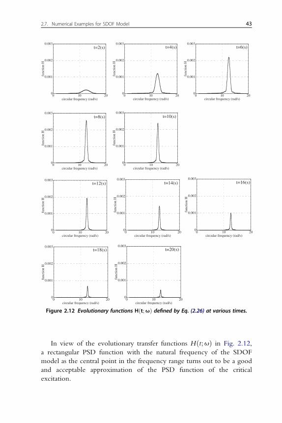
In view of the evolutionary transfer functions Hðt;uÞ in Fig. 2.12,a rectangular PSD function with the natural frequency of the SDOFmodel as the central point in the frequency range turns out to be a goodand acceptable approximation of the PSD function of the criticalexcitation.

0

0.001

0.002

0.003

0 10 20

func

tion

H


t=2(s)

0

0.001

0.002

0.003

0 10 20

func

tion

H


t=4(s)

0

0.001

0.002

0.003

0 10 20

func

tion

H


t=6(s)

0

0.001

0.002

0.003

0 10 20

func

tion

H


t=8(s)

0

0.001

0.002

0.003

0 10 20

func

tion

H


t=10(s)

0

0.001

0.002

0.003

0 10 20

func

tion

H


t=12(s)

0

0.001

0.002

0.003

0 10 20

func

tion

H


t=14(s)

0

0.001

0.002

0.003

0 10 20

func

tion

H


t=16(s)

0

0.001

0.002

0.003

0 10 20

func

tion

H


t=18(s)

0

0.001

0.002

0.003

0 10 20

func

tion

H


t=20(s)

Figure 2.12 Evolutionary functions Hðt;uÞ defined by Eq. (2.26) at various times.

2.7. Numerical Examples for SDOF Model 43

2.8. NUMERICAL EXAMPLES FOR MDOF MODEL

Let us consider a 6-story shear building model. The floor massesare chosen as mi ¼ 32� 103ðkgÞði ¼ 1;/; 6Þ and the story stiffnessesare ki ¼ 3:76� 107ðN=mÞði ¼ 1;/; 6Þ. The fundamental naturalperiod of the model is found to be 0.760(s). The viscous damping matrixof the shear building model has been given so as to be proportional tothe stiffness matrix. The lowest-mode damping ratio is specified as 0.02.The same envelope function as in an SDOF model has been adopted.Fig. 2.14 illustrates the evolutionary transfer functions HMðt;uÞ, definedby Eq. (2.36), of the 6-story shear building model at 2 second intervals.It can be seen that the evolutionary transfer functions HMðt;uÞ of the6-story MDOF model have a similar tendency to those of the SDOFmodel shown in Fig. 2.12 except the peak frequency value (the funda-mental natural frequency). Fig. 2.15 presents the time history of f ðtÞdefined by Eq. (2.35) for various values of the PSD amplitude. Thepower of the critical excitation has the same value as that for the SDOFmodel. It can be understood that, while the time giving the peak valuediffers from that for the SDOF model, the tendency is nearly the same asin the SDOF model.

Two time-history samples of the critical excitations are shown inFig. 2.16. Both have the same PSD power Sw ¼ 1:51ðm2=s4Þ. The upperone indicates a sample of the critical excitation with the PSD amplitude of1.0 ðm2=s3Þ and the lower one shows that with the PSD amplitude of 1/7ðm2=s3Þ. The uniformly random phase is assumed here. It can be observedthat, while the upper one has a narrow-band property, the lower one hasa wide-band characteristic. These characteristics represent well the PSDfunction properties of the two critical excitations.

00.00050.001

0.00150.002

0.00250.003

0.0035

0 10 20 30 40 50

PSD amplitude=1PSD amplitude=1/3PSD amplitude=1/5PSD amplitude=1/7

mea

n sq

uare

of

defo

rmat

ion

(m2 )

time (s)Figure 2.13 Time-dependent mean-square deformation of the SDOF model for variousPSD amplitudes.


2.9. CONCLUSIONS

The conclusions may be summarized as follows:(1) A critical excitation method for stationary random inputs can be

developed by introducing a stochastic response index as the objectivefunction to be maximized. The power and the intensity of the excita-tions are prescribed.

Figure 2.14 Evolutionary functions HMðt;uÞ defined by Eq. (2.36) at various times.

2.9. Conclusions 45

(2) When the restriction on the excitation intensity does not exist, thecritical PSD function turns out to be the Dirac delta function. In theexistence of the restriction on the excitation intensity, the criticalexcitation is reduced to a rectangular PSD function with the maximumintensity limit.

(3) The level of conservativeness of the derived critical excitation forstationary random inputs is about 2 or 3 in recorded ground motionswithout conspicuous predominant frequency. On the other hand, it isclose to unity in ground motions with a conspicuous predominantfrequency. The resonant characteristic of such ground motion can berepresented suitably by the explained critical excitation.

00.0005

0.0010.0015

0.0020.0025

0.0030.0035

0.004

0 10 20 30 40 50

PSD amplitude=1PSD amplitude=1/3PSD amplitude=1/5PSD amplitude=1/7

sum

of

mea

n-sq

uare

in

ters

tory

dri

fts

(m2 )

time (s)

Figure 2.15 Time-dependent function fðtÞ (the sum of the mean-square interstory driftsof the MDOF model) for various PSD amplitudes.

-1.5-1

-0.50

0.51

1.5

0 10 20 30 40

acce

lera

tion

(m/s2 )

time (s)

alpha=0.13beta=0.45

PSD ampli.=1

-1.5-1

-0.50

0.51

1.5

0 10 20 30 40

acce

lera

tion

(m/s2 )

time (s)

alpha=0.13beta=0.45

PSD ampli.=1/7

Figure 2.16 Time-history samples of the critical excitations (upper: PSD amplitude¼ 1:0m2s�3, lower: PSD amplitude ¼ 1=7m2s�3).


(4) The key idea for stationary random inputs can be used in SDOF modelsunder nonstationary random inputs which can be described bya uniformly modulated excitation model. The interchange of the orderof the double maximization procedures is taken full advantage of withrespect to time and to the PSD function. A similar algorithm can also bedevised for MDOF proportionally damped models.

It is extremely difficult even in the advanced computational environment toconsider all the possible design earthquakes in the structural design stage (PEERCenter et al. 2000). It is expected that the critical excitation approach can takeinto account uncertainties in establishing the design of buildings for earth-quakes. Only the elastic response has been considered in this chapter fora simple explanation of a new concept. However, the consideration of elastic-plastic responses in the seismic-resistant design of structures may be important.The present critical excitation method could be extended to nonlinear prob-lems by using equivalent linearization techniques (Drenick 1977). The criticalexcitation methods for elastic-plastic responses will be discussed in Chapter 5.

APPENDIX FUNCTIONS AC (t;u), AS (t;u) FOR A SPECIFICENVELOPE FUNCTION

ACðt;uÞ in Eq. (2.27a) can be expressed by substituting the specific enve-lope function shown in Eq. (2.39) into Eq. (2.27a).

ACðt;uÞ ¼ 1

u1de�hu1t

"sin u1dt

Z t

0

neðhu1�aÞs � eðhu1�bÞs

o

� 1

2fcos ðu1d þ uÞsþ cos ðu1d � uÞsgds

� cos u1dt

Z t

0


o 1

2fsin ðu1d þ uÞs

þ sin ðu1d � uÞsgds#

¼ 1

u1de�hu1tfsin u1dtGCCðt;uÞ � cos u1dtGSCðt;uÞg

(A2.1)

Appendix Functions AC (t;u), AS (t;u) for a Specific Envelope Function 47

where GCCðt;uÞ and GSCðt;uÞ are defined by

GCCðt;uÞ ¼Z t

0


o 1

2fcos ðu1d þ uÞs

þ cos ðu1d � uÞsgds(A2.2)

GSCðt;uÞ ¼Z t

0


o 1

2fsin ðu1d þ uÞs

þ sin ðu1d � uÞsgds(A2.3)

The double of the bracket in Eq. (A2.1) can be manipulated as2fsin u1dtGCCðt;uÞ � cos u1dtGSCðt;uÞg¼ 1

ðhu1 � aÞ2 þ ðu1d þ uÞ2

�hðhu1 � aÞeðhu1�aÞtð� sin utÞ þ ðu1d þ uÞeðhu1�aÞtðcos utÞ� ðhu1 � aÞ sin u1dt � ðu1d þ uÞ cos u1dt

iþ 1

ðhu1 � aÞ2 þ ðu1d � uÞ2

�h�hu1 � aÞeðhu1�aÞtðsin utÞ þ ðu1d � uÞeðhu1�aÞtðcos utÞ

� ðhu1 � aÞ sin u1dt � ðu1d � uÞ cos u1dt

�

� 1

ðhu1 � bÞ2 þ ðu1d þ uÞ2

�h�hu1 � bÞeðhu1�bÞtð� sin utÞ þ ðu1d þ uÞeðhu1�bÞtðcos utÞ

� ðhu1 � bÞ sin u1dt � ðu1d þ uÞ cos u1dt

�

� 1

ðhu1 � bÞ2 þ ðu1d � uÞ2

�h�hu1 � bÞeðhu1�bÞtðsin utÞ þ ðu1d � uÞeðhu1�bÞtðcos utÞ

� ðhu1 � bÞ sin u1dt � ðu1d � uÞ cos u1dt

�(A2.4)


Similarly ASðt;uÞ in Eq. (2.27b) can be expressed by substituting thespecific envelope function shown in Eq. (2.39) into Eq. (2.27b).

ASðt;uÞ ¼ 1

u1de�hu1t

�sin u1dt

Z t

0


o 1

2fsin ðu1d þ uÞs

þ sin ðu1d � uÞsgds � cos u1dt

Z t

0

neðhu1�aÞs

� eðhu1�bÞso 1

2fcos ðu1d þ uÞs� cos ðu1d � uÞsgds

�

¼ 1

u1de�hu1tfsin u1dtGCSðt;uÞ � cos u1dtGSSðt;uÞg

(A2.5)

where GCSðt;uÞ and GSSðt;uÞ are defined by

GCSðt;uÞ ¼Z t

0


o 1

2fsin ðu1d þ uÞs

� sin ðu1d � uÞsgds(A2.6)

GSSðt;uÞ ¼Z t

0


o 1

2fcos ðu1d � uÞs

� cos ðu1d þ uÞsgds(A2.7)

The double of the bracket in Eq. (A2.5) can be manipulated as2fsin u1dtGCSðt;uÞ � cos u1dtGSSðt;uÞg¼ 1

ðhu1 � aÞ2 þ ðu1d þ uÞ2

�h�hu1 � aÞeðhu1�aÞtðcos utÞ � ðu1d þ uÞeðhu1�aÞtð� sin utÞ

� ðhu1 � aÞ cos u1dt þ ðu1d þ uÞ sin u1dti

þ 1

ðhu1 � aÞ2 þ ðu1d � uÞ2

�h�hu1 � aÞeðhu1�aÞtð� cos utÞ þ ðu1d � uÞeðhu1�aÞtðsin utÞ

þ ðhu1 � aÞ cos u1dt � ðu1d � uÞ sin u1dti

Appendix Functions AC (t;u), AS (t;u) for a Specific Envelope Function 49

� 1

ðhu1 � bÞ2 þ ðu1d þ uÞ2

�h�hu1 � bÞeðhu1�bÞtðcos utÞ � ðu1d þ uÞeðhu1�bÞtð� sin utÞ

� ðhu1 � bÞ cos u1dt þ ðu1d þ uÞ sin u1dti

� 1

ðhu1 � bÞ2 þ ðu1d � uÞ2

�h�hu1 � bÞeðhu1�bÞtð� cos utÞ þ ðu1d � uÞeðhu1�bÞtðsin utÞ

þ ðhu1 � bÞ cos u1dt � ðu1d � uÞ sin u1dti

(A2.8)

REFERENCESConte, J.P., Peng, B.F., 1997. Fully nonstationary analytical earthquake ground-motion

model. J. Eng. Mech. 123 (1), 15–24.Drenick, R.F., 1977. The critical excitation of nonlinear systems. J. Applied Mech. 44 (2),

333–336.Fang, T., Sun, M., 1997. A unified approach to two types of evolutionary random response

problems in engineering. Archive of Applied Mech. 67 (7), 496–506.PEER Center, ATC, Japan Ministry of Education, Science, Sports, and Culture, US-NSF,

2000. Effects of near-field earthquake shaking. In: Proc. of US-Japan workshop. SanFrancisco, March 20–21, 2000.


CHAPTER THREE

Critical Excitation forNonproportionally DampedStructural Systems

Contents

3.1. Introduction 513.2. Modeling of Input Motions 523.3. Response of Nonproportionally Damped Model to Nonstationary Random

Excitation53

3.4. Critical Excitation Problem 59[Problem CENM] 59

3.5. Solution Procedure 593.6. Critical Excitation for Acceleration (Proportional Damping) 613.7. Numerical Examples (Proportional Damping) 633.8. Numerical Examples (Nonproportional Damping) 643.9. Numerical Examples (Various Types of Damping Concentration) 673.10. Conclusions 69Appendix Functions ACj(t; u), ASj(t; u) and ACj* (t; u), ASj*(t; u) for a Specific Function c(t) 70References 74

3.1. INTRODUCTION

The purpose of this chapter is to explain a new probabilistic criticalexcitation method for nonstationary inputs to nonproportionally dampedstructural systems. In contrast to most of the conventional critical excitationmethods, a stochastic response index is treated here as the objective functionto be maximized as in Chapter 2. The power and the intensity of theexcitations are fixed and the critical excitation is found under theserestrictions. The key for finding the new nonstationary random criticalexcitation for nonproportionally damped structural systems is the inter-change of the order of the double maximization procedures with respect totime and to the PSD function. It is shown that the spirit of the previouslyexplained critical excitation method for stationary inputs is partially appli-cable to multi-degree-of-freedom structural systems with nonproportional



http://dx.doi.org/10.1016/B978-0-08-099436-9.00003-1

damping subjected to nonstationary random inputs. Numerical examples ofa 6-DOF shear building model with nonproportional damping subjected tononstationary inputs are presented to demonstrate the effectiveness andvalidity of the present method.

It is usual in the practical structural design that the mass, stiffness anddamping distributions do not satisfy the condition on proportional damping.Fig. 3.1 shows a building with an added viscous damper in the 1st story. Sucha structural system is a typical example of nonproportionally dampedstructural systems. Fig. 3.2 illustrates other examples of story-stiffness anddamping distributions. Model A, B and C include additional damping in the1st, 3rd and 6th stories, respectively, and Model D corresponds to a base-isolated building. Model PD is a proportionally damped system.

3.2. MODELING OF INPUT MOTIONS

In this chapter, the input horizontal base acceleration is assumed to bedescribed by the following uniformly modulated nonstationary randomprocess as in Chapter 2.


Figure 3.1 Nonproportionally damped system subjected to nonstationary input.

52 Critical Excitation for Nonproportionally Damped Structural Systems

where cðtÞ is a given deterministic envelope function and wðtÞ is a stationaryGaussian process with zero mean.

Let SwðuÞ denote the PSD function of wðtÞ. In this case the PSDfunction of €ug may be expressed by Sgðt;uÞ ¼ cðtÞ2SwðuÞ.

3.3. RESPONSE OF NONPROPORTIONALLY DAMPEDMODEL TO NONSTATIONARY RANDOM EXCITATION

Consider an n-story shear building model, as shown in Fig. 3.3, witha nonproportional damping subjected to a nonstationary random horizontalbase acceleration €ug which can be described by the uniformly modulatednonstationary random process of Eq. (3.1). The horizontal displacements ofthe floors are expressed by uðtÞ. Let M, C, K, r ¼ f1/1gT denote thesystem mass matrix, the system viscous damping matrix, the system stiffnessmatrix and the influence coefficient vector, respectively. The equations ofmotion of the model can be expressed by

M€uðtÞ þ C _uðtÞ þ KuðtÞ ¼ �Mr€ugðtÞ (3.2)

Let UðjÞ ¼ �U

ðjÞk

�denote the j-th damped complex eigenvector. The

time history DkðtÞ of the interstory drift in the k-th story may be expressedin terms of complex-type Duhamel integrals.

DkðtÞ ¼ 2Xnj¼ 1

Re

"�U

ðjÞk �U

ðjÞk�1

�UðjÞTMrFj

Z t

0

ð�€ugðsÞÞeljðt�sÞds

#

(3.3)

Figure 3.2 Examples of nonproportionally damped structural system.

3.3. Response of Nonproportionally Damped Model to Nonstationary Random Excitation 53

where

lj ¼ �hjuj þ ujdi

uj2 ¼ UðjÞTKUðjÞ

UðjÞTMUðjÞ

ujd ¼ uj

ffiffiffiffiffiffiffiffiffiffiffiffiffiffi1� hj2

pFj ¼ 2ujð

ffiffiffiffiffiffiffiffiffiffiffiffiffiffi1� hj2

pi� hjÞUðjÞTMUðjÞ þUðjÞTCUðjÞ

hj ¼ UðjÞTCUðjÞ

2ujUðjÞTMUðjÞ

ð3:4aeeÞ

Re½$� denotes the real part of a complex number and i denotes the imaginaryunit. The over-bar indicates the complex conjugate. Let us define thefollowing complex number.

aðjÞk h2

�U

ðjÞk � U

ðjÞk�1

� UðjÞTMrFj

(3.5)

( )gu t

1k

2k

nknc

2c

1c

1m

2m

nm

Figure 3.3 n-story shear building model subjected to horizontal base acceleration.


The autocorrelation function of the k-th interstory drift can be expressed as

RDkðt1; t2Þ ¼ E

"Re

" Pnj¼ 1

aðjÞk

Rt10

cðs1Þeð�hjujþujd iÞðt1�s1Þwðs1Þds1#

$Re

" Pnj¼ 1

aðjÞk

Rt20

cðs2Þeð�hjujþujd iÞðt2�s2Þwðs2Þds2##

¼Zt20

Zt10

Re

"Xnj¼ 1

aðjÞk cðs1Þeð�hjujþujd iÞðt1�s1Þ

#

$Re

" Pnj¼ 1

aðjÞk cðs2Þeð�hjujþujd iÞðt2�s2Þ

#E½wðs1Þwðs2Þ�ds1ds2

(3.6)

where E½$� indicates the ensemble mean. Application of the Wiener-Khintchine theorem for wðtÞ to Eq. (3.6) provides

RDkðt1; t2Þ ¼

ZN�N

Zt20

Zt10

Re

"Xnj¼ 1

naðjÞk cðs1Þeð�hjujþujd iÞðt1�s1Þ

o#

$Re

" Pnj¼ 1


o#eiðs1�s2ÞuSwðuÞds1ds2du

¼ZN

�N

Zt10

Re

"Xnj¼ 1


o#eis1uds1

$Rt20

Re

" Pnj¼ 1


o#e�is2uds2SwðuÞdu

¼ZN

�N

Zt10

(Xnj¼ 1

RehaðjÞk cðs1Þeð�hjujþujd iÞðt1�s1Þ

i)eis1uds1

$

Zt20

(Xnj¼ 1

RehaðjÞk cðs2Þeð�hjujþujd iÞðt2�s2Þ

i)e�is2uds2SwðuÞdu

(3.7)

The mean-square of the k-th interstory drift can be derived fromEq. (3.7) by substituting t1 ¼ t2 ¼ t.


sDkðtÞ2 ¼

ZN�N

"Xnj¼ 1

nBðjÞCkðt;uÞ þ iBðjÞ

Skðt;uÞo#

�"Xn

j¼ 1

nBðjÞCkðt;uÞ � iBðjÞ

Skðt;uÞo#

SwðuÞdu

(3.8)

where

BðjÞCkðt;uÞ ¼

Z t

0

�Re

haðjÞk cðsÞeð�hjujþujd iÞðt�sÞ

i�cos usds (3.9a)

BðjÞSkðt;uÞ ¼

Z t

0

�Re

haðjÞk cðsÞeð�hjujþujd iÞðt�sÞ

i�sin usds (3.9b)

Rearrangement of Eq. (3.8) may be reduced to

sDkðtÞ2 ¼

ZN�N

(Xnj¼ 1

BðjÞCkðt;uÞ þ i

Xnj¼ 1

BðjÞSkðt;uÞ

)

�(Xn

j¼ 1

BðjÞCkðt;uÞ � i

Xnj¼ 1

BðjÞSkðt;uÞ

)SwðuÞdu

¼ZN

�N

"(Xnj¼ 1

BðjÞCkðt;uÞ

)2

þ(Xn

j¼ 1

BðjÞSkðt;uÞ

)2#SwðuÞdu

(3.10)

Let us define the following quantity.

fN ðtÞ ¼Xnk¼ 1

sDkðtÞ2 ¼

ZN�N

HMN ðt;uÞSwðuÞdu (3.11)

where

HMN ðt;uÞ ¼Xnk¼ 1

"(Xnj¼ 1

BðjÞCkðt;uÞ

)2

þ(Xn

j¼ 1

BðjÞSkðt;uÞ

)2#(3.12)


Part of the integrand in Eqs. (3.9a, b) can be reduced to

Rehað jÞk cðsÞeð�hjujþujd iÞðt�sÞ

i¼ cðsÞe�hjujðt�sÞ

nRe

hað jÞk

iRe

�eujd iðt�sÞ�

�Imhað jÞk

iIm

heujd iðt�sÞ�

o¼ cðsÞe�hjujðt�sÞ

nRe

hað jÞk

icos ujdðt � sÞ

�Imhað jÞk

isin ujdðt � sÞ

o(3.13)

where Im½$� denotes the imaginary part of a complex number. In the casewhere the structural system has proportional damping, the complex number

aðjÞk defined in Eq. (3.5) is reduced to a pure imaginary number and the

real and imaginary parts of aðjÞk are reduced to Re�aðjÞk

� ¼ 0; Im�aðjÞk

� ¼�GjðfðjÞ

k � fðjÞk�1Þ=ujd. This expression coincides with that for a structural

system with proportional damping. Substitution of Eq. (3.13) into Eq. (3.9a)leads to

BðjÞCkðt;uÞ ¼

Z t

0

cðsÞe�hjujðt�sÞnRe

hað jÞk

icos ujdðt � sÞ

� Imhað jÞk

isin ujdðt � sÞ

ocos usds

¼ ujdRe

að jÞk

Z t

0

cðsÞe�hjujðt�sÞ 1ujd

cos ujdðt � sÞ cos usds

� ujdIm

að jÞk

Z t

0


sin ujdðt � sÞ cos usds

¼ ujdRe

að jÞk

A�Cjðt;uÞ � ujdIm

að jÞk

ACjðt;uÞ

(3.14)


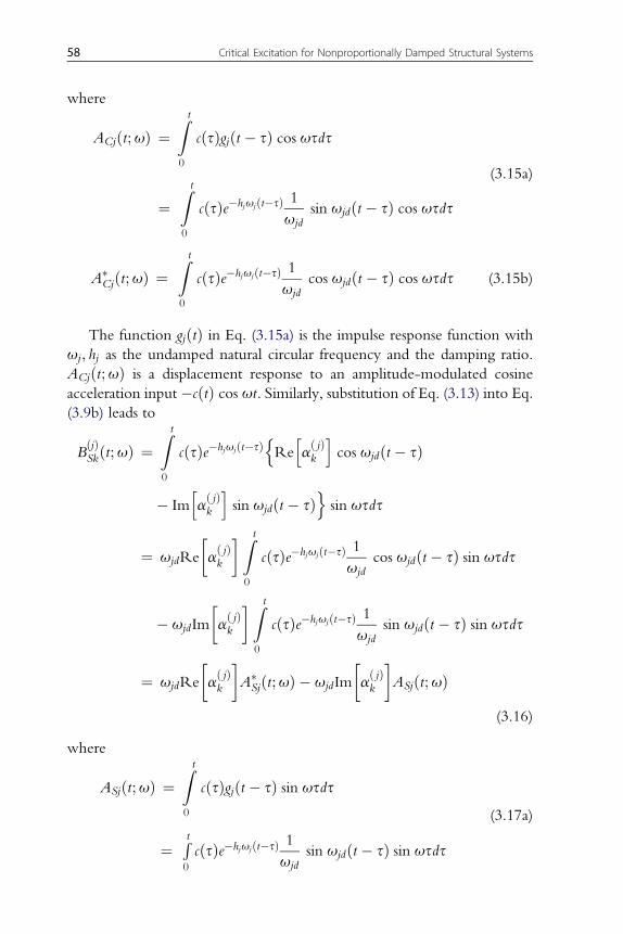
where

ACjðt;uÞ ¼Z t

0

cðsÞgjðt � sÞ cos usds

¼Z t

0

cðsÞe�hjujðt�sÞ 1

ujdsin ujdðt � sÞ cos usds

(3.15a)

A�Cjðt;uÞ ¼

Z t

0

cðsÞe�hjujðt�sÞ 1

ujdcos ujdðt � sÞ cos usds (3.15b)

The function gjðtÞ in Eq. (3.15a) is the impulse response function withuj; hj as the undamped natural circular frequency and the damping ratio.ACjðt;uÞ is a displacement response to an amplitude-modulated cosineacceleration input�cðtÞ cos ut. Similarly, substitution of Eq. (3.13) into Eq.(3.9b) leads to

BðjÞSkðt;uÞ ¼

Z t

0

cðsÞe�hjujðt�sÞnRe

hað jÞk

icos ujdðt � sÞ

� Imhað jÞk

isin ujdðt � sÞ

osin usds

¼ ujdRe

að jÞk

Z t

0


cos ujdðt � sÞ sin usds

� ujdIm

að jÞk

Z t

0


sin ujdðt � sÞ sin usds

¼ ujdRe

að jÞk

A�Sjðt;uÞ � ujdIm

að jÞk

ASjðt;uÞ

(3.16)

where

ASjðt;uÞ ¼Z t

0

cðsÞgjðt � sÞ sin usds

¼ Rt0


sin ujdðt � sÞ sin usds

(3.17a)


A�Sjðt;uÞ ¼

Z t

0


cos ujdðt � sÞ sin usds (3.17b)

ASjðt;uÞ is a displacement response to an amplitude-modulated sineacceleration input �cðtÞ sin ut. The detailed expressions of ACjðt;uÞ andASjðt;uÞ in Eqs. (3.15), (3.17) and integral forms in Eqs. (3.14), (3.16) fora specific envelope function cðtÞ given by Eq. (3.30) are shown in theAppendix.

3.4. CRITICAL EXCITATION PROBLEM

The problem of finding the critical excitation may be described as:

[Problem CENM]Given floor masses, story stiffnesses and structural nonproportional viscous damping ofa shear building model and the excitation envelope function cðtÞ, find the critical PSDfunction ~SwðuÞ to maximize the specific function fN ðt�Þ (t� is the time when themaximum of fN ðtÞ is attained) subject to the excitation power limit (integral of thePSD function in the frequency range)

ZN�N


and to the PSD amplitude limit

supSwðuÞ � sw (3.19)

3.5. SOLUTION PROCEDURE

This problem consists of the double maximization procedures whichmay be described mathematically by

maxSwðuÞ

maxtffN ðt; SwðuÞÞg

The first maximization is performed with respect to time for a given PSDfunction SwðuÞ (see Fig. 3.4) and the second maximization is done withrespect to the PSD function SwðuÞ. In the first maximization, the time t�when the maximum of fN ðtÞ is attained must be obtained for each PSDfunction. This original problem is complicated and needs much computa-tion. To overcome this difficulty, a new sophisticated procedure based on

3.5. Solution Procedure 59

ω

ω

ω

t = ti t = tj

Interchange of order of

the double maximization procedures



the interchange of the order of the maximization procedures is proposed.The proposed procedure can be expressed by

maxt

maxSwðuÞ

ffN ðt; SwðuÞÞg

The first maximization process with respect to the PSD function fora given time can be pursued very efficiently (Fig. 3.4) by utilizing the criticalexcitation method for stationary inputs (Takewaki 2000) (see Fig. 2.3). Thecritical excitation obtained for a specific time in this stage has a rectangularPSD function as shown in Fig. 2.3. The second maximization procedurewith respect to time can be implemented by comparing the values at varioustimes directly (Fig. 3.4).

The proposed algorithm may be summarized as:(i) Compute HMNðti;uÞ in Eq. (3.12) for a specific time t ¼ ti.(ii) Find the critical PSD function at time t ¼ ti as the rectangular PSD

function (the procedure used for stationary inputs is utilizedstraightforwardly).

(iii) Compute fN ðtiÞ to the rectangular PSD function obtained in step (ii)from Eq. (3.11).

(iv) Repeat steps (i)–(iii) for various times and obtain fN ðtmÞ ¼ maxfN ðtiÞ.(v) The PSD function for t ¼ tm is determined as the PSD function of the

critical excitation.It is important to note that the present algorithm based on the interchange ofthe order of the double maximization procedures is applicable to moresophisticated nonuniformly modulated nonstationary excitation modelsalthough the expression of Eq. (3.11) must be modified and a new criticalexcitation problem must be stated.

3.6. CRITICAL EXCITATION FOR ACCELERATION(PROPORTIONAL DAMPING)

An acceleration can be adopted as the objective function to be maximized inanother critical excitation problem. For simplicity of expression, an n-storyshear building model with proportional damping is considered in this section.

The equations of motion for this model can be expressed as Eq. (3.2) byreplacing the damping matrix by the proportional damping matrix. Let uj

and hj denote the j-th undamped natural circular frequency and the j-thdamping ratio, respectively. Let us introduce the following coordinatetransformation from uðtÞ to qðtÞ ¼ fqjg through the modal matrix F.

3.6. Critical Excitation for Acceleration (Proportional Damping) 61

uðtÞ ¼ FqðtÞ (3.20)

Substitution of Eq. (3.20) into Eq. (3.2) leads to the following n inde-pendent equations.

€qj þ 2hjuj _qj þ u2j qj ¼ �Gj€ug ðj ¼ 1;/; nÞ (3.21)

where Gj is the j-th participation factor, i.e. Gj ¼ fðjÞTMr=fðjÞTMfðjÞ, and

fðjÞ ¼ ffðjÞk g is the j-th undamped eigenvector. Substitution of the relation

qj ¼ Gjq0j into Eq. (3.21) and rearrangement of the resulting equation lead to

€ug þ €q0j ¼ �2hjuj _q0j � u2j q0j ðj ¼ 1;/; nÞ (3.22)

Recall that

q0jðtÞ ¼Z t

0

gjðt � sÞf�€ugðsÞgds (3.23a)

_q0jðtÞ ¼Z t

0

_gjðt � sÞf�€ugðsÞgds (3.23b)

where gjðtÞ is the impulse response function defined in Eq. (3.15) and itstime derivative can be expressed as

_gjðtÞ ¼ �hjujgjðtÞ þ e�hjuj t cos ujdt (3.24)

Substitution of Eqs. (3.23a, b) into Eq. (3.22) with the aid of Eq. (3.24)provides

€ug þ €q0j ¼ u2j ð2h2j � 1Þ Rt

0

gjðt � sÞf�€ugðsÞgds

� 2hjujujd

Z t

0

1

ujde�hjujðt�sÞ cos ujdðt � sÞf�€ugðsÞgds

(3.25)

With the help of the relationPn

j¼1Gjfð jÞn ¼ 1, the top-floor absolute

acceleration can be expressed as

€ug þ €un ¼ €ug þXnj¼ 1

Gjfð jÞn €q0j ¼

Xnj¼ 1

Gjfð jÞn ð€ug þ €q0jÞ (3.26)


Following the similar process from Eq. (3.6) through Eq. (3.11) andkeeping Eqs. (3.25) and (3.26) in mind, the following mean-square absoluteacceleration at the top floor n to the input given by Eq. (3.1) can be derivedas the objective function.

f �ðtÞ ¼ sAnðtÞ2 ¼

ZN�N

HMðt;uÞSwðuÞdu (3.27)

where

HMAðt;uÞ ¼"Xn

j¼ 1

Gjfð jÞn DCjðt;uÞ

#2þ"Xn

j¼ 1

Gjfð jÞn DSjðt;uÞ

#2

(3.28)

The parameters DCjðt;uÞ and DSjðt;uÞ are defined by

DCjðt;uÞ ¼ u2j ð2h2j � 1ÞACjðt;uÞ � 2hjujujdA

�Cjðt;uÞ (3.29a)

DSjðt;uÞ ¼ u2j ð2h2j � 1ÞASjðt;uÞ � 2hjujujdA

�Sjðt;uÞ (3.29b)

where ACjðt;uÞ and ASjðt;uÞ are defined in Eqs. (3.15), (3.17). Detailedexpressions of ACjðt;uÞ and ASjðt;uÞ and the integral expressions in Eqs.(3.29a, b) for a specific function cðtÞ given by Eq. (3.30) can be found in theAppendix.

Another critical excitation problem for acceleration can be defined byreplacing the objective function of Eq. (3.11) by f �ðtÞ given by Eq. (3.27).The solution procedure stated in Section 3.5 can be applied to this problemstraightforwardly.

3.7. NUMERICAL EXAMPLES (PROPORTIONALDAMPING)

A numerical example is shown for the model with the objective functionfN ðtÞ given by Eq. (3.11). The following envelope function of the inputacceleration is used as an example (see Fig. 3.5).


The parameters a ¼ 0:13; b ¼ 0:45 are employed. The power of thestochastic part wðtÞ in the excitation has been chosen as Sw ¼ 1:51ðm2=s4Þso that it has the same value of El Centro NS 1940 at the time¼ 3.9(s) when

3.7. Numerical Examples (Proportional Damping) 63

the acceleration amplitude attains its maximum. The intensity of wðtÞ hasbeen chosen to be sw ¼ 1:0ðm2=s3Þ.

Consider a 6-story shear building model. The floor masses are assumed tobe mi ¼ 32� 103ðkgÞði ¼ 1;/; 6Þ and the story stiffnesses are ki ¼3:76� 107ðN=mÞði ¼ 1;/; 6Þ. Then the fundamental natural period ofthe model is 0.760(s). The viscous damping coefficients of the building havebeen given by ci ¼ 3:76� 105ðN$s=mÞði ¼ 1;/; 6Þ. The viscousdamping matrix of the shear building model is a proportional dampingmatrix in this case and the lowest-mode damping ratio is almost equal to0.04. The evolutionary functions HMN ðt;uÞ of this model are plotted atvarious times in Fig. 3.6. It can be observed that, while the evolutionaryfunction HMN ðt;uÞ indicates a rather wide-band frequency content aroundthe time of 2, 4 and 6(s), it indicates a narrower frequency content afterward.This implies that the components around the fundamental natural frequencyof the model decay as the time goes and only the resonant componentremains afterward. It can also be found that the function HMN ðt;uÞ hasa clear peak around the natural frequency of the model and its amplitudeattains the maximum around the time¼ 8(s). Fig. 3.7 shows the time historyof the function fN ðtÞ defined by Eq. (3.11), i.e. the sum of mean-squareinterstory drifts, to the corresponding critical excitation.

It is interesting to note that, in view of the evolutionary functionsHMN ðt;uÞ in Fig. 3.6, a rectangular PSD function with the fundamentalnatural frequency of the model as the central point is a good approximationof the PSD function of the critical excitation. This approximation canreduce the computational effort drastically.

3.8. NUMERICAL EXAMPLES (NONPROPORTIONALDAMPING)

Consider next a nonproportionally damped 6-story shear building model. Anumerical example is shown for the model with the objective function fN ðtÞ

-0.5

0

0.5

0 10 20 30 40 50

ampl

itud

e c(

t)

time (s)

alpha=0.13beta=0.45

Figure 3.5 Envelope function c(t).


Figure 3.6 Evolutionary functions HMN (t; u) defined by Eq. (3.12) at various times(proportional damping model).

0

0.0005

0.001

0.0015

0.002

0 10 20 30 40 50

inv. of PSD ampli.=1

sum

of

mea

n-sq

uare

inte

rsto

ry d

rift

s (m

2 )

time (s)

proportionaldamping

Figure 3.7 Time-dependent function fN (t) (sum of mean-square interstory drifts) forinverse of PSD amplitude [ 1 (proportional damping model).

3.8. Numerical Examples (Nonproportional Damping) 65

given by Eq. (3.11). The floor masses and story stiffnesses are the same as themodel treated in Section 3.7. The viscous damping coefficients of the buildinghave been given by c1 ¼ 3:76� 106 ðN$s=mÞ; ci ¼ 3:76� 105ðN$s=mÞði ¼ 2;/; 6Þ. The viscous damping matrix of the shear building model isa nonproportional dampingmatrix in this case. Fig. 3.8 shows the evolutionary

Figure 3.8 Evolutionary functions HMN (t; u) defined by Eq. (3.12) at various times(nonproportional damping model).


functionsHMNðt;uÞ of the model at various times. It can be observed that theevolutionary functions HMN ðt;uÞ of the present model have a differenttendency from that of the proportionally dampedmodel shown in Fig. 3.6. Anirregular phenomenon appears almost every four seconds. Fig. 3.9 shows thetime history of the function fN ðtÞ defined by Eq. (3.11). The power andintensity of the critical excitation are the same as in Section 3.7. It can be seenthat the function fN ðtÞ indicates a nonsmooth property in contrast to that forthe proportionally damped model. This property may result from thecomplicated inter-mode correlation due to nonproportional damping.

Fig. 3.10 shows examples of the critical excitation proposed in thischapter for four inverse PSD amplitudes 1, 3, 5, 7 (sw ¼ 1; 1=3; 1=5;1=7ðm2=s3Þ). Uniform random numbers have been adopted as the phaseangles and the superposition of 100 cosine waves has been employed as thewave generation method. The power of wðtÞ is Sw ¼ 1:51ðm2=s4Þ. It canbe observed from Fig. 3.10 that as the frequency content of the excitationbecomes wide-band (sw decreases and the inverse PSD amplitude increases),wave components with various frequencies arise.

3.9. NUMERICAL EXAMPLES (VARIOUS TYPES OFDAMPING CONCENTRATION)

Consider again nonproportionally damped 6-story shear building models(see Fig. 3.2). A numerical example is also shown for the model with theobjective function fN ðtÞ given by Eq. (3.11). The floor masses and storystiffnesses are the same as the model treated in Sections 3.7 and 3.8. Threetypes of the viscous damping coefficient distribution have been treated:(i) c1 ¼ 3:76� 106ðN$s=mÞ, ci ¼ 3:76� 105ðN$s=mÞ ðis1Þ, (ii) c3 ¼3:76� 106ðN$s=mÞ, ci ¼ 3:76� 105ðN$s=mÞðis3Þ, (iii) c6 ¼ 3:76�

0

0.0001

0.0002

0.0003

0.0004

0 10 20 30 40 50


sum

of

mea

n-sq

uare

inte

rsto

ry d

rift

s (m

2 )time (s)

non-proportionaldamping

Figure 3.9 Time-dependent function fN (t) (sum of mean-square interstory drifts) forinverse of PSD amplitude [ 1 (nonproportional damping model).

3.9. Numerical Examples (Various Types of Damping Concentration) 67





Figure 3.10 Examples of critical excitation for various inverses of PSD amplitude(nonproportional damping model).


106ðN$s=mÞ, ci ¼ 3:76� 105ðN$s=mÞðis6Þ. Case (i) represents themodel with the damping concentration to the 1st story, case (ii) does themodel with the damping concentration to the 3rd story and case (iii) doesthe model with the damping concentration to the 6th story.

Fig. 3.11 shows the time histories of the function fN ðtÞ defined byEq. (3.11) for the aforementioned three models. The power and intensityof the critical excitation are the same as in Section 3.7. It can be observedfrom Fig. 3.11 that the model with the damping concentration to the1st story is the most effective model for reducing the overall story driftindex.

3.10. CONCLUSIONS

The conclusions may be summarized as follows:(1) A new probabilistic critical excitation method can be developed for

nonstationary vibrations of nonproportionally damped structuralsystems by restricting both the power and intensity of the input powerspectral density function.

(2) It has been found that the integrand of the objective function to bemaximized in the context of the critical excitation method can beexpressed as the product of a positive function and the power spectraldensity function of a stochastic part in the input motion.

(3) The previously explained idea for stationary inputs can be utilizedpartially in finding the nonstationary critical excitation that can bedescribed by a uniformly modulated excitation model. The key is theexchange of the order of the double maximization procedures withrespect to time and to the PSD function.

0

0.0005

0.001

0.0015

0 10 20 30 40 50

damping concentration to 1st storydamping concentration to 3rd storydamping concentration to 6th story

sum

of

mea

n-sq

uare

inte

rsto

ry d

rift

s (m

2 )time (s)

non-proportionaldamping


Figure 3.11 Time-dependent function fNðtÞ (sum of mean-square interstory drifts) forthree models with various damping concentration types (inverse of PSD amplitude[ 1).

3.10. Conclusions 69

(4) Numerical examples disclosed the time-varying characteristics of thenonstationary transfer function multiplied by the envelope function ofthe input motion model and demonstrated the validity of the presentcritical excitation method.

(5) An acceleration can be adopted as the objective function to be maxi-mized in another critical excitation problem.

APPENDIX FUNCTIONS ACj(t; u), ASj(t; u) AND ACj* (t; u),ASj* (t; u) FOR A SPECIFIC FUNCTION C(t)

Detailed expressions are shown of the functions ACjðt;uÞ, ASjðt;uÞ andA�Cjðt;uÞ, A�

Sjðt;uÞ for a specific function cðtÞ given by Eq. (3.30).The function ACjðt;uÞ may be expressed as

ACjðt;uÞ ¼ 1

ujde�hjuj t

"sin ujdt

Z t

0

neðhjuj�aÞs � eðhjuj�bÞs

o 1

2fcos ðujd

þ uÞsþ cos ðujd � uÞsg ds� cos ujdt

Z t

0

neðhjuj�aÞs

� eðhjuj�bÞso 1

2f sin ðujd þ uÞsþ sin ðujd � uÞsgds

#

¼ 1

ujde�hjuj tf sin ujdtGCCðt;uÞ � cos ujdtGSCðt;uÞg

(A3.1)

where

GCCðt;uÞ ¼Z t

0

neðhjuj�aÞs � eðhjuj�bÞso 1

2fcos ðujd þ uÞs

þ cos ðujd � uÞs�ds(A3.2)

GSCðt;uÞ ¼Z t

0


o 1

2

�sin ðujd þ uÞs

þ sin ðujd � uÞs�ds(A3.3)


The double of the parenthesis in Eq. (A3.1) can be reduced to2f sin ujd tGCCðt;uÞ � cos ujd tGSCðt;uÞg

¼ 1

ðhjuj � aÞ2 þ ðujd þ uÞ2�

hjuj � aÞeðhjuj�aÞtð� sin utÞ þ ðujd þ uÞeðhjuj�aÞtð cos utÞ

�ðhjuj � aÞ sin ujd t � ðujd þ uÞ cos ujd t

þ 1

ðhjuj � aÞ2 þ ðujd � uÞ2�hjuj � aÞeðhjuj�aÞtð sin utÞ þ ðujd � uÞeðhjuj�aÞtð cos utÞ

�ðhjuj � aÞ sin ujd t � ðujd � uÞ cos ujd t

� 1

ðhjuj � bÞ2 þ ðujd þ uÞ2�hjuj � bÞeðhjuj�bÞtð� sin utÞ þ ðujd þ uÞeðhjuj�bÞtð cos utÞ

�ðhjuj � bÞ sin ujd t � ðujd þ uÞ cos ujd t

� 1

ðhjuj � bÞ2 þ ðujd � uÞ2�hjuj � bÞeðhjuj�bÞtð sin utÞ þ ðujd � uÞeðhjuj�bÞtð cos utÞ

�ðhjuj � bÞ sin ujd t � ðujd � uÞ cos ujd t

(A3.4)

The function ASjðt;uÞ may be expressed as

ASjðt;uÞ ¼ 1

ujde�hjuj t

"sin ujdt

Z t

0


o

� 1

2

�sin ðujd þ uÞs� sin ðujd � uÞs� ds

� cos ujdt

Z t

0


o

� 1

2

�cos ðujd � uÞs� cos ðujd þ uÞs�ds

#

¼ 1

ujde�hjuj tf sin ujdtGCSðt;uÞ � cos ujdtGSSðt;uÞg

(A3.5)

Appendix Functions ACj(t; u), ASj(t; u) and ACj* (t; u), ASj*(t; u) for a Specific Function c(t) 71

where

GCSðt;uÞ ¼Z t

0


o

� 1

2f sin ðujd þ uÞs� sin ðujd � uÞsgds

(A3.6)

GSSðt;uÞ ¼Z t

0


o

� 1

2f cos ðujd � uÞs� cos ðujd þ uÞsgds

(A3.7)

The double of the parenthesis in Eq. (A3.5) can be reduced to

2f sin ujd tGCSðt;uÞ � cos ujd tGSSðt;uÞg

¼ 1

ðhjuj � aÞ2 þ ðujd þ uÞ2h�hjuj � aÞeðhjuj�aÞtð cos utÞ � ðujd þ uÞeðhjuj�aÞtð� sin utÞ

�ðhjuj � aÞ cos ujd t þ ðujd þ uÞ sin ujd ti

þ 1

ðhjuj � aÞ2 þ ðujd � uÞ2h�hjuj � aÞeðhjuj�aÞtð� cos utÞ þ ðujd � uÞeðhjuj�aÞtð sin utÞ

þðhjuj � aÞ cos ujdt � ðujd � uÞ sin ujdti

� 1

ðhjuj � bÞ2 þ ðujd þ uÞ2h�hjuj � bÞeðhjuj�bÞtð cos utÞ � ðujd þ uÞeðhjuj�bÞtð� sin utÞ

�ðhjuj � bÞ cos ujd t þ ðujd þ uÞ sin ujd ti

� 1

ðhjuj � bÞ2 þ ðujd � uÞ2h�hjuj � bÞeðhjuj�bÞtð� cos utÞ þ ðujd � uÞeðhjuj�bÞtð sin utÞ

þðhjuj � bÞ cos ujd t � ðujd � uÞ sin ujd ti

(A3.8)


The function A�Cjðt;uÞ can be expressed as

A�Cjðt;uÞ ¼ 1

ujde�hjuj t

�cos ujdtGCCðt;uÞ þ sin ujdtGSCðt;uÞ

�(A3.9)


2fcos ujdtGCCðt;uÞ þ sin ujdtGSCðt;uÞg

¼ 1

ðhjuj � aÞ2 þ ðujd þ uÞ2hðhjuj � aÞeðhjuj�aÞtðcos utÞ

þðujd þ uÞeðhjuj�aÞtðsin utÞ � ðhjuj � aÞ cos ujdt

þðujd þ uÞ sin ujdti

þ 1

ðhjuj � aÞ2 þ ðujd � uÞ2

�hðhjuj � aÞeðhjuj�aÞtðcos utÞ

þðujd � uÞeðhjuj�aÞtð�sin utÞ � ðhjuj � aÞ cos ujdt

þðujd � uÞ sin ujdti

� 1

ðhjuj � bÞ2 þ ðujd þ uÞ2

�hðhjuj � bÞeðhjuj�bÞtðcos utÞ þ ðujd þ uÞeðhjuj�bÞtðsin utÞ

�ðhjuj � bÞ cos ujdt þ ðujd þ uÞ sin ujdti

� 1

ðhjuj � bÞ2 þ ðujd � uÞ2hðhjuj � bÞeðhjuj�bÞtðcos utÞ

þðujd � uÞeðhjuj�bÞtð�sin utÞi

(A3.10)

The function A�Sjðt;uÞ can be expressed as

A�Sjðt;uÞ ¼ 1

ujde�hjuj tfcos ujdtGCSðt;uÞ þ sin ujdtGSSðt;uÞg

(A3.11)

Appendix Functions ACj(t; u), ASj(t; u) and ACj* (t; u), ASj*(t; u) for a Specific Function c(t) 73


2fcos ujdtGCSðt;uÞ þ sin ujdtGSSðt;uÞg

¼ 1

ðhjuj � aÞ2 þ ðujd þ uÞ2hðhjuj � aÞeðhjuj�aÞtðsin utÞ

þðujd þ uÞeðhjuj�aÞtð�cos utÞ

þðhjuj � aÞ sin ujdt þ ðujd þ uÞ cos ujdti

þ 1

ðhjuj � aÞ2 þ ðujd � uÞ2hðhjuj � aÞeðhjuj�aÞtfsin ð2ujd � uÞtg

þðujd � uÞeðhjuj�aÞtf�cos ð2ujd � uÞtg

�ðhjuj � aÞ sin ujdt þ ðujd � uÞ cos ujdti

� 1

ðhjuj � bÞ2 þ ðujd þ uÞ2hðhjuj � bÞeðhjuj�bÞtðsin utÞ

þðujd þ uÞeðhjuj�bÞtð�cos utÞ

�ðhjuj � bÞ sin ujdt þ ðujd þ uÞ cos ujdti

� 1

ðhjuj � bÞ2 þ ðujd � uÞ2hðhjuj � bÞeðhjuj�bÞtfsin ð2ujd � uÞtg

þðujd � uÞeðhjuj�bÞtf�cos ð2ujd � uÞtg

�ðhjuj � bÞ sin ujdt þ ðujd � uÞ cos ujdti

(A3.12)

REFERENCESTakewaki, I., 2000. Optimal damper placement for critical excitation. Probabilistic Engi-

neering Mechanics 15 (4), 317–325.


CHAPTER FOUR

Critical Excitation forAcceleration Response

Contents

4.1. Introduction 754.2. Modeling of Input Motions 764.3. Acceleration Response of Nonproportionally Damped Model to Nonstationary

Random Input76

4.4. Critical Excitation Problem 83[Problem CENMA] 83

4.5. Solution Procedure 844.6. Numerical Examples 864.7. Model with Nonproportional Damping-1 884.8. Model with Nonproportional Damping-2 894.9. Model with Proportional Damping 924.10. Conclusions 92Appendix Functions ACj(t; u), ASj(t; u), ACj* (t; u), ASj*(t; u) for a specific c(t) 96References 96

4.1. INTRODUCTION

The purpose of this chapter is to explain and discuss a probabilisticcritical excitation method for acceleration responses of nonproportionallydamped structural systems to nonstationary inputs. Recently, accelerationresponses have started to be considered important from the viewpoint ofthe protection and maintenance of functionality in buildings (see Fig. 4.1).It is therefore natural and desirable to develop critical excitation methodsfor acceleration.

In contrast to most of the conventional critical excitation methods,a stochastic acceleration response at a point is treated as the objectivefunction to be maximized. The power and the intensity of the excitationsare fixed, and the critical excitation is found under these restrictions. As inChapters 2 and 3, the key for finding the new nonstationary randomcritical excitation for nonproportionally damped structural systems is theorder interchange in the double maximization procedure with respect totime and to the power spectral density (PSD) function. It is shown that the



http://dx.doi.org/10.1016/B978-0-08-099436-9.00004-3

spirit of the previously explained critical excitation method for stationaryinputs (Takewaki 2000a) is partially applicable to multi-degree-of-freedomstructural systems with nonproportional damping subjected to nonsta-tionary random inputs. Numerical examples are presented to demonstratethe effectiveness and validity of the present method.

4.2. MODELING OF INPUT MOTIONS

The one-directional horizontal base acceleration is assumed here to bedescribed by the following uniformly modulated nonstationary randomprocess as in Chapters 2 and 3:


The function c(t) is a given deterministic envelope function and the func-tionw(t) represents a stationary Gaussian process with zeromean for the criticalone to be found.Differentiationwith respect to time is denoted by anover-dot.

Let Sw(u) denote the PSD function of the stochastic function w(t). Thetime-variant PSD function of €ug may then be expressed bySgðt; uÞ ¼ cðtÞ2SwðuÞ.

4.3. ACCELERATION RESPONSE OFNONPROPORTIONALLY DAMPED MODEL TONONSTATIONARY RANDOM INPUT

Let us consider an n-story shear building model, as shown in Fig. 4.2, withnonproportional damping and subjected to a nonstationary base

Small accelerationLarge acceleration

Figure 4.1 Protection and maintenance of functionality in building.

76 Critical Excitation for Acceleration Response

acceleration €ug. Assume that this base acceleration can be described by theuniformly modulated nonstationary random process of Eq. (4.1). Thehorizontal displacements of the floors relative to the base are denoted by u(t). Let M, C, K, r ¼ {1 $ $ $ 1}T denote the system mass, viscousdamping and stiffness matrices and the influence coefficient vector of theinput, respectively. The equations of motion of the shear building modelcan be expressed by

M€uðtÞ þ C _uðtÞ þ KuðtÞ ¼ �Mr€ugðtÞ (4.2)

Let U( j ) ¼nU

ðjÞk

odenote the j-th complex eigenvector of damped

mode. The displacement un(t) of the top floor may be expressed in terms ofcomplex-type Duhamel integrals:

unðtÞ ¼ 2Xnj¼ 1

Re

"U ðjÞn

UðjÞTMr

Fj

Z t

0

ð�€ugðsÞÞeljðt�sÞds

#(4.3)

ug(t)

k1

k2

kncn

c2

c1

m1

m2

mn

nunu

Figure 4.2 n-story shear building model subjected to one-dimensional horizontal basemotion.

4.3. Acceleration Response of Nonproportionally Damped Model 77

where the following quantities are used:

lj ¼ �hjuj þ ujdi

u2j ¼ UðjÞTKUðjÞ

UðjÞTMUðjÞ

ujd ¼ uj

ffiffiffiffiffiffiffiffiffiffiffiffiffi1� h2j

q

Fj ¼ 2ujðffiffiffiffiffiffiffiffiffiffiffiffiffi1� h2j

qi� hjÞ UðjÞTMUðjÞ þUðjÞTCUðjÞ

hj ¼ UðjÞTCUðjÞ

2ujUðjÞTMUðjÞ

ð4:4aeeÞ

Re[$] indicates the real part of a complex number and i denotes theimaginary unit. The over-bar indicates the complex conjugate. Eq. (4.3)may also be written as

unðtÞ ¼Xnj¼ 1

Re½bjU ðjÞn qjðtÞ� (4.5)


bj ¼ 2ujdUðjÞTMri=Fj

qjðtÞ ¼ qRjðtÞ � iqIjðtÞ

qRjðtÞ ¼ q0jðtÞ

q0jðtÞ ¼ 1

ujd

Z t

0

f�€ugðsÞge-hjujðt�sÞ sin ujdðt � sÞds

qIjðtÞ ¼ q�0jðtÞ ¼ f_q0jðtÞ þ hjujq0jðtÞg=ujd

q�0jðtÞ ¼ 1

ujd

Z t

0

f�€ugðsÞge-hjujðt�sÞ cos ujdðt � sÞds

ð4:6aef Þ


By using Eq. (4.5), the top-floor absolute acceleration may be expressedin terms of complex modal coordinates:

€ug þ €un ¼ €ug þXnj¼ 1

RehbjU

ðjÞn €qjðtÞ

i(4.7)

where the complex modal coordinate €qjðtÞ is defined by

€qjðtÞ ¼ €qRjðtÞ � i€qIjðtÞ

¼nð2h2j � 1Þu2

j q0jðtÞ � 2hjujujdq�0jðtÞ � €ugðtÞ

o

�i

�2hjujujdq0jðtÞ þ

�2h2j � 1

�u2j q

�0jðtÞ þ

hjuj

ujd€ugðtÞ �

u:::gðtÞujd

�(4.8)

Note that Eq. (4.6e), the equation of motion for a single-degree-of-freedom (SDOF) model in terms of modal coordinates, and the followingrelation have been used in Eq. (4.8) including ug(t):

_qIjðtÞ ¼ �hjujqIjðtÞ � ujdq0jðtÞ �€ugðtÞujd

(4.9)

Substitution of Eq. (4.8) into (4.7) yields

€ug þ €un ¼ €ug þPnj¼ 1

RehbjU

ðjÞn

in�2h2j � 1

�u2j q0jðtÞ � 2hjujujdq

�0jðtÞ � €ugðtÞ

o

þXnj¼ 1

ImhbjU

ðjÞn

i �2hjujujdq0jðtÞ þ

�2h2j � 1

�u2j q

�0jðtÞ

þhjuj

ujd€ugðtÞ �

u:::gðtÞujd

�(4.10)

In Eq. (4.10), Im[$] indicates the imaginary part of a complex number.After some manipulation, Eq. (4.10) may be reduced to the followingcompact form:

€ug þ €un ¼ A€ug þ Bu:::gðtÞ þ

Xnj¼ 1

ajq0jðtÞ þXnj¼ 1

bjq�0jðtÞ (4.11)



A ¼ 1� Pnj¼ 1

RehbjU

ðjÞn

iþ Pn

j¼ 1

ImhbjU

ðjÞn

i hjuj

ujd

B ¼ � Pnj¼ 1

ImhbjU

ðjÞn

i=ujd

aj ¼ RehbjU

ðjÞn

i�2h2j � 1

�u2j þ Im

hbjU

ðjÞn

i2hjujujd

bj ¼ �RehbjU

ðjÞn

i2hjujujd þ Im

hbjU

ðjÞn

i�2h2j � 1

�u2j

ð4:12aedÞ

The mean-square top-floor absolute acceleration may then be obtainedas

E½f€ugðtÞ þ €unðtÞg2� ¼ E

"(A€ug þ Bu

.gðtÞ þ

Xnj¼ 1

ajq0jðtÞ þXnj¼ 1

bjq�0jðtÞ

)2#

(4.13)

Note that the following can be derived by constructing auto-correlationand cross-correlation functions and using the Wiener–Khintchine theoremfor w(t):

E

"(Xnj¼ 1

ajq0jðtÞ)2#

¼ZN

�N

"(Xnj¼ 1

ajACjðt;uÞ)2

þ(Xn

j¼ 1

ajASjðt;uÞ)2#

SwðuÞdu

E

"(Xnj¼ 1

bjq�0jðtÞ

)2#¼

ZN�N

"(Xnj¼ 1

bjA�Cjðt;uÞ

)2

þ(Xn

j¼ 1

bjA�Sjðt;uÞ

)2#SwðuÞdu


E

"( Pnj¼ 1

ajq0jðtÞ) ( Pn

j¼ 1

bjq�0jðt;uÞ

)#

¼ RN�N

"( Pnj¼ 1

ajACjðt;uÞ) ( Pn

j¼ 1

bjA�Cjðt;uÞ

)þ( Pn

j¼ 1

ajASjðt;uÞ)

�( Pn

j¼ 1

bjA�Sjðt;uÞ

)#SwðuÞdu

E½€ugðtÞ2� ¼RN

�N

cðtÞ2SwðuÞdu

E½u0gðtÞ2� ¼RN

�N

u2cðtÞ2 þ _cðtÞ2SwðuÞdu

E½€ugðtÞu0gðtÞ� ¼

RN�N

½cðtÞ_cðtÞ�SwðuÞdu

E½q0jðtÞ€ugðtÞ� ¼RN

�N½fACjðt;uÞ cos ut þ ASjðt;uÞ sin utgf�cðtÞg�SwðuÞdu

E½q�0jðtÞ€ugðtÞ� ¼RN

�N½fA�

Cjðt;uÞ cos ut þ A�Sjðt;uÞ sin utgf�cðtÞg�SwðuÞdu

E½q0jðtÞu0gðtÞ� ¼RN

�N½fACjðt;uÞ cos ut þ ASjðt;uÞ sin utg f�_cðtÞg

þf�ACjðt;uÞ sin ut þ ASjðt;uÞ cos utg f�ucðtÞg�SwðuÞdu

E½q�0jðtÞu0gðtÞ� ¼

RN�N

½fA�Cjðt;uÞ cos ut þ A�

Sjðt;uÞ sin utg f�_cðtÞg

þf�A�Cjðt;uÞ sin ut þ A�

Sjðt;uÞ cos utg f�ucðtÞg�SwðuÞduð4:14aejÞ


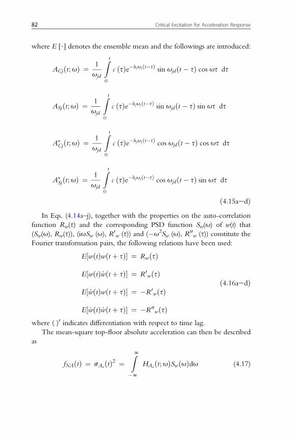
where E [$] denotes the ensemble mean and the followings are introduced:

ACjðt;uÞ ¼ 1

ujd

Z t

0

c ðsÞe�hjujðt�sÞ sin ujdðt � sÞ cos us ds

ASjðt;uÞ ¼ 1

ujd

Z t

0

c ðsÞe�hjujðt�sÞ sin ujdðt � sÞ sin us ds

A�Cjðt;uÞ ¼ 1

ujd

Z t

0

c ðsÞe�hjujðt�sÞ cos ujdðt � sÞ cos us ds

A�Sjðt;uÞ ¼ 1

ujd

Z t

0

c ðsÞe�hjujðt�sÞ cos ujdðt � sÞ sin us ds

ð4:15aedÞIn Eqs. (4.14a–j), together with the properties on the auto-correlation

function Rw(s) and the corresponding PSD function Sw(u) of w(t) that(Sw(u), Rw(s)), (iuSw (u), R0

w (s)) and (�u2Sw (u), R00w (s)) constitute the

Fourier transformation pairs, the following relations have been used:

E½wðtÞwðt þ sÞ� ¼ RwðsÞ

E½wðtÞ _wðt þ sÞ� ¼ R0wðsÞ

E½ _wðtÞwðt þ sÞ� ¼ �R0wðsÞ

E½ _wðtÞ _wðt þ sÞ� ¼ �R00wðsÞ

ð4:16aedÞ

where ( )0 indicates differentiation with respect to time lag.The mean-square top-floor absolute acceleration can then be described

as

fNAðtÞ ¼ sAnðtÞ2 ¼

ZN�N

HAnðt;uÞSwðuÞdu (4.17)


In Eq. (4.17), HAnðt; uÞ is defined by

HAnðt;uÞ ¼

(Xnj¼ 1

ajACjðt;wÞ þXnj¼ 1

bjA�Cjðt;wÞ � AcðtÞ cos ut

�B_cðtÞ cos ut þ BcðtÞu sin ut

)2

þ(Xn

j¼ 1

ajASjðt;wÞ þXnj¼ 1

bjA�Sjðt;wÞ � AcðtÞ sin ut

�B_cðtÞ sin ut þ BcðtÞu cos ut

)2

(4.18)

HAnðt; uÞ will be called an evolutionary transfer function later in

accordance with Iyengar and Manohar (1987) (it may be appropriate to callit a time-varying frequency response function). It should be remarked thatthe integrand in Eq. (4.17) to be maximized in the critical excitationproblem can be expressed as the product of a positive function (sum of thesquared numbers) and the positive PSD function of a stochastic part in theinput motion expressed by Eq. (4.1).

When considering proportional damping, A and B defined in Eqs.(4.12a, b) are reduced to zero. Then the expression of Eq. (4.18) coin-cides completely with that for a proportionally damped structural system(Takewaki 2000b).

ACj (t; u),ASj (t;u),A�Cj(t;u) andA

�Sj(t;u) in Eqs. (4.15a–d) for a specific

envelope function c (t) given by Eq. (4.21) are shown in Chapter 3.


The problem of critical excitation for acceleration may be described asfollows.

[Problem CENMA]Given floor masses, story stiffnesses and nonproportional viscous damping coefficientsof a shear building model and the excitation envelope function c(t), find the criticalPSD function ~SwðuÞ maximizing the specific function fNA (t�) (t� is the time when

4.4. Critical Excitation Problem 83

the maximum value of fNA (t) to Sw(u) is attained) subject to the excitation powerlimit constraint (integral of the PSD function in the frequency range)

ZN�N


and to the PSD amplitude limit constraint

sup SwðuÞ � sw (4.20)


The aforementioned problem includes the double maximizationprocedures described mathematically by

maxSwðuÞ

maxtffNAðt; SwðuÞÞg

The first maximization is implemented with respect to time for a givenPSD function Sw(u) (see Fig. 4.3) and the second maximization is conductedwith respect to the PSD function Sw(u). In the first maximization, the timet�causing the maximum value of fNA (t) has to be obtained for each PSDfunction. This original problem is time consuming. To remedy this, a smartprocedure based on the interchange of the order of the maximizationprocedures is explained here. The procedure can be described by

maxt

maxSwðuÞ

ffNAðt; SwðuÞÞg

The first maximization with respect to the PSD function for a given timecan be performed effectively and efficiently by utilizing the critical excita-tion method for stationary inputs (Takewaki 2000a) (see Fig. 4.3). In case ofan infinite amplitude limit sw, the critical PSD function is found to be theDirac delta function. On the other hand, when sw is finite, the critical PSDfunction is reduced to a constant sw in a finite interval ~U ¼ Sw=ð2swÞ. Theintervals, ~U1 ; ~U2 ; .; constituting ~U can be found by changing the level inthe diagram of HAn

ðti;uÞ (see Fig. 4.4). The critical excitation obtained fora specific time up to this stage turns out to be a rectangular PSD function asshown in Fig. 4.4. The second maximization with respect to time can beimplemented sequentially by comparing the values at various times directly.


The solution algorithm may be summarized as:(i) Compute the evolutionary function HAn

ðti;uÞ in Eq. (4.18) fora specific time t ¼ ti.

(ii) Determine the critical PSD function at time t ¼ ti as the rectangularPSD function (the procedure devised for stationary inputs is useddirectly).

0 10 20 30 40 50

Time (s)

Time (s)

Time (s)

0 10 20 30 40 50

0 10 20 30 40 50

t = ti t = tj

Maximization with respect to time

Interchange of order ofthe double maximization procedures

Max

imiz

atio

n w

ith r

espe

ct to

PS

D fu

nctio

nf (t )S w(1)

f(t ) response to

f (t )S w(2)

f(t ) response to

f (t )S w

(M )f(t ) response to



(iii) Compute fNA (ti) from Eq. (4.17) to the rectangular PSD functiondetermined in step (ii).

(iv) Repeat steps (i)–(iii) for sequential times and obtain fNA (tm)¼max fNA

(ti).(v) The PSD function derived for t ¼ tm is determined as the true PSD

function of the critical excitation.It is important to note that the global optimality is guaranteed in thisalgorithm. The global optimality in the maximization with respect to theshape of PSD functions is supported by the property of a single-valuedfunction of HAn

ðti;uÞ and that with respect to time is guaranteed bya sequential search algorithm in time. It is also meaningful to note that thepresent algorithm based on the interchange of the order of the doublemaximization procedures is applicable to more complex nonuniformlymodulated nonstationary excitation models although the expression ofEq. (4.17) must be modified and a new critical excitation problem must bestated.

4.6. NUMERICAL EXAMPLES

Five different combinations of the stiffness distribution and thedamping distribution are taken into account for 6-story shear buildingmodels (see Fig. 4.5). The purpose of the following sections is to presentversatile characteristics of evolutionary transfer functions HAn

ðt; uÞ of the

Circular frequency

PSD function

PS

D

sw

Ω1∼ Ω2

∼

HAn (ti; )

Figure 4.4 Isolated PSD function of critical excitation (critical excitation for finite PSDamplitude sw).


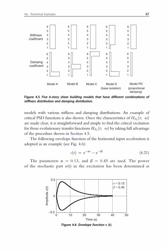
models with various stiffness and damping distributions. An example ofcritical PSD functions is also shown. Once the characteristics of HAn

ðt; uÞare made clear, it is straightforward and simple to find the critical excitationfor those evolutionary transfer functions HAn

ðt; uÞ by taking full advantageof the procedure shown in Section 4.5.

The following envelope function of the horizontal input acceleration isadopted as an example (see Fig. 4.6):


The parameters a ¼ 0.13, and b ¼ 0.45 are used. The powerof the stochastic part w(t) in the excitation has been determined as

Model A Model B Model C Model D(base isolation)

Stiffnesscoefficient

Dampingcoefficient

6

5

4

3

2

1

6

5

4

3

2

1

6

5

4

3

2

1

6

5

4

3

2

1

6

5

4

3

2

1

6

5

4

3

2

1

6

5

4

3

2

1

6

5

4

3

2

1

6

5

4

3

2

1

6

5

4

3

2

1

Model PD

(proportionaldamping)

Figure 4.5 Five 6-story shear building models that have different combinations ofstiffness distribution and damping distribution.

0.5

0

0.5

0 10 20 30 40 50

Am

plitu

de c

(t)

Time (s)

0.13 0.45

Figure 4.6 Envelope function c (t).

4.6. Numerical Examples 87

Sw ¼ 1.51 m2/s4. It is intended that the power at the time ¼ 3.9 s(when the acceleration amplitude attains its maximum) has the samevalue as that of the time-averaging PSD function (Baratta et al. 1998)of El Centro NS 1940. The intensity of w(t) has been assumed as sw ¼1.0 m2/s3.

4.7. MODEL WITH NONPROPORTIONAL DAMPING-1

Three numerical examples are demonstrated for the 6-story shearbuilding models with various nonproportional dampings (Models A–C inFig. 4.5). Note that damping is concentrated at the 1st story in Model A, atthe 3rd story in Model B and at the 6th story in Model C.

The floormasses and the story stiffnesses are given bymi¼ 32� 103 kg (i¼1,., 6) and ki ¼ 3.76 � 107 N/m (i ¼ 1,., 6). The viscous dampingcoefficients of the building are given by c1 ¼ 3.76� 106 N$s/m, ci ¼ 3.76�105 N$s/m (is 1) for Model A; c3¼ 3.76� 106N$ s/m, ci¼ 3.76� 105 N$s/m (is 3) forModel B and ci¼ 3.76� 105 N$ s/m (is 6), c6¼ 3.76� 106

N$ s/m forModelC.The lowest three undampednatural circular frequenciesof Models A–C are u1 ¼ 8.71 rad/s, u2 ¼ 27.7 rad/s and u3 ¼ 44.4 rad/s.

Figs. 4.7–4.9 show the evolutionary transfer functions HAnðt; uÞ of

these models plotted at every 2 s. It can be seen from these figures that, whilethe function HAn

ðt; uÞ exhibits a similar tendency in Models A and B, itindicates somewhat different characteristics in Model C. This implies thatthe function HAn

ðt; uÞ can be influenced greatly by the position ofconcentrated damping. Especially, the magnitude is small in Model C. Thismeans that the damping installation in upper stories is effective in reducingthe acceleration. Note that, while the damping installation in lower stories iseffective in the reduction of interstory drifts, the damping installation inupper stories is effective in reducing the acceleration. It can also be foundthat the function HAn

ðt; uÞ has a rather clear peak at u* between thesecond and third natural frequencies of the model in Models A and B and thepeak values around the fundamental natural frequency and around u* arecomparable in Model C.

Fig. 4.10 indicates the time history of the mean-square top-floor absoluteacceleration in Model A subjected to the critical excitation. The effect of theevolutionary function HAn

ðt; uÞ greater than about 100 rad/s has beendisregarded in the computation of the critical excitation. It can be seen thatthe peak value occurs around t ¼ 4s.


4.8. MODEL WITH NONPROPORTIONAL DAMPING-2

Consider another nonproportionally damped shear buildingmodel of 6-stories expressed as Model D in Fig. 4.5 (base-isolated

t 6 s

0

0.1

0.2

0.3

0.4

0.5

0.6

0.7

0.8

1 10 100 1000

Circular frequency (rad/s)

t 16 s

0

0.1

0.2

0.3

0.4

0.5

0.6

0.7

0.8

1 10 100 1000



t 4 s

0

0.1

0.2

0.3

0.4

0.5

0.6

0.7

0.8

1 10 100 1000

t 10 s

0

0.1

0.2

0.3

0.4

0.5

0.6

0.7

0.8

1 10 100 1000


t 20 s

0

0.1

0.2

0.3

0.4

0.5

0.6

0.7

0.8

1 10 100 1000


t 14 s

0

0.1

0.2

0.3

0.4

0.5

0.6

0.7

0.8

1 10 100 1000



0

0.1

0.2

0.3

0.4

0.5

0.6

0.7

0.8

1 10 100 1000

t 2 s

1000

t 8 s

0

0.1

0.2

0.3

0.4

0.5

0.6

0.7

0.8

1 10 100


t 12 s

0

0.1

0.2

0.3

0.4

0.5

0.6

0.7

0.8

1 10 100 1000


t 18 s

0

0.1

0.2

0.3

0.4

0.5

0.6

0.7

0.8

1 10 100 1000


HA

n

HA

nH

An

HA

nH

An

HA

nH

An

HA

nH

An

HA

n

Figure 4.7 Evolutionary functions HAn (t;u) defined by Eq. (4.18) at various times(Model A).

4.8. Model with Nonproportional Damping-2 89

model). The floor masses are the same as those of the model treated inSection 4.7. The story stiffnesses are specified here by k1 ¼ 7.52 � 105

N/m, ki ¼ 3.76 � 107 N/m (i ¼ 2,., 6) to give a small 1st-storystiffness. On the other hand, the viscous damping coefficients of the

0

0.1

0.2

0.3

0.4

0.5

0.6

0.7

0.8

1 10 100 1000

HA

n


HA

n

0

0.1

0.2

0.3

0.4

0.5

0.6

0.7

0.8

1 10 100 1000


0

0.1

0.2

0.3

0.4

0.5

0.6

0.7

0.8

1 10 100 1000

HA

n


0

0.1

0.2

0.3

0.4

0.5

0.6

0.7

0.8

1 10 100 1000H

An


0

0.1

0.2

0.3

0.4

0.5

0.6

0.7

0.8

1 10 100 1000

HA

n


0

0.1

0.2

0.3

0.4

0.5

0.6

0.7

0.8

1 10 100 1000

HA

n


0

0.1

0.2

0.3

0.4

0.5

0.6

0.7

0.8

1 10 100 1000


HA

n


0

0.1

0.2

0.3

0.4

0.5

0.6

0.7

0.8

1 10 100 1000

HA

n


0

0.1

0.2

0.3

0.4

0.5

0.6

0.7

0.8

1 10 100 1000

HA

n


0

0.1

0.2

0.3

0.4

0.5

0.6

0.7

0.8

1 10 100 1000

HA

n

Figure 4.8 Evolutionary functions HAnðt; uÞ defined by Eq. (4.18) at various times(Model B).


building are specified by c1 ¼ 3.76 � 106 N$ s/m, ci ¼ 3.76 � 105 N$s/m (i ¼ 2,., 6). Fig. 4.11 presents the evolutionary functionsHAn

ðt; uÞ of the model at every 2 s. It can be seen that the functionsHAn

ðt; uÞ of the present model have a similar tendency to those ofModels A and B shown in Figs. 4.7 and 4.8.

00.1

0.2

0.3

0.4

0.5

0.6

0.7

0.8

1 10 100 1000


0

0.1

0.2

0.3

0.4

0.5

0.6

0.7

0.8

1 10 100 1000


0

0.1

0.2

0.3

0.4

0.5

0.6

0.7

0.8

1 10 100 1000


00.1

0.2

0.3

0.4

0.5

0.6

0.7

0.8

1 10 100 1000


0

0.1

0.2

0.3

0.4

0.5

0.6

0.7

0.8

1 10 100 1000


0

0.1

0.2

0.3

0.4

0.5

0.6

0.7

0.8

1 10 100 1000


0

0.1

0.2

0.3

0.4

0.5

0.6

0.7

0.8

1 10 100 1000


0

0.1

0.2

0.3

0.4

0.5

0.6

0.7

0.8

1 10 100 1000


0

0.1

0.2

0.3

0.4

0.5

0.6

0.7

0.8

1 10 100 1000


0

0.1

0.2

0.3

0.4

0.5

0.6

0.7

0.8

1 10 100 1000


Figure 4.9 Evolutionary functions HAnðt; uÞ defined by Eq. (4.18) at various times(Model C).

4.8. Model with Nonproportional Damping-2 91

4.9. MODEL WITH PROPORTIONAL DAMPING

Consider finally a proportionally damped shear building model of6-story expressed as Model PD in Fig. 4.5. The floor masses are the same asthose of the model treated in Section 4.7. The story stiffnesses and viscousdamping coefficients are given by ki ¼ 3.76 � 107 N/m(i ¼ 1,., 6), ci ¼3.76 � 105 N $ s/m(i ¼ 1,., 6). The lowest three damped natural circularfrequencies of this model are found to be u1d ¼ 8.27 rad/s, u2d ¼ 24.3 rad/sand u3d ¼ 39.0 rad/s.

The evolutionary functions HAnðt; uÞ of Model PD at every 2 s are

shown in Fig. 4.12. It can be understood that, while the peak around thesecond natural frequency is dominant at t¼ 2 and 4 s, the peak values aroundthe fundamental and second natural frequencies are comparable after t¼ 6 s.Fig. 4.13 illustrates the time history of the mean-square top-floor absoluteacceleration of Model PD subjected to the corresponding critical excitation.It can be seen that the peak value occurs around the time t¼ 4 s. The criticalPSD function for Model PD is shown in Fig. 4.14. Three isolated rectan-gular PSD functions are found. Isolated rectangles not necessarily centered atthe natural frequencies of the system may not be physically understandable.However, the procedure explained here is based on an exact mathematicaltreatment and can reveal new features of the random critical excitation foracceleration.

4.10. CONCLUSIONS

The conclusions may be summarized as follows:(1) Acceleration is considered to be important from the viewpoint of the

protection and maintenance of functionality in buildings. A probabilistic

0

0.5

1

0 10 20 30 40 50

Mea

n-sq

uare

acce

lera

tion

(m2 /s

4 )

Time (s)

Non-proportional damping(Model A)

Figure 4.10 Time history of function fNA (t) (Model A).


critical excitation method can be developed for nonstationary accelerationresponsesofnonproportionallydampedstructural systemsbyconstrainingboththe power and the intensity of the PSD function of the nonstationary input.

(2) The integrand of the objective function to be maximized in the criticalexcitation problem can be expressed as the product of a positive

0

0.1

0.2

0.3

0.4

0.5

0.6

0.7

0.8

1 10 100 1000


0

0.1

0.2

0.3

0.4

0.5

0.6

0.7

0.8

1 10 100 1000


0

0.1

0.2

0.3

0.4

0.5

0.6

0.7

0.8

1 10 100 1000


0

0.1

0.2

0.3

0.4

0.5

0.6

0.7

0.8

1 10 100 1000


0

0.1

0.2

0.3

0.4

0.5

0.6

0.7

0.8

1 10 100 1000


0

0.1

0.2

0.3

0.4

0.5

0.6

0.7

0.8

1 10 100 1000


0

0.1

0.2

0.3

0.4

0.5

0.6

0.7

0.8

1 10 100 1000


0

0.1

0.2

0.3

0.4

0.5

0.6

0.7

0.8

1 10 100 1000


0

0.1

0.2

0.3

0.4

0.5

0.6

0.7

0.8

1 10 100 1000


0

0.1

0.2

0.3

0.4

0.5

0.6

0.7

0.8

1 10 100 1000


Figure 4.11 Evolutionary functions HAnðt; uÞ defined by Eq. (4.18) at various times(Model D).


function (sum of the squared numbers) and the positive PSD function ofa stochastic part in the input.

(3) The idea for stationary random inputs can be used partially in obtainingthe nonstationary random critical excitation which can be described bya uniformly modulated excitation model. The key idea is the order

0

0.1

0.2

0.3

0.4

0.5

0.6

0.7

0.8

1 10 100 1000


0

0.1

0.2

0.3

0.4

0.5

0.6

0.7

0.8

1 10 100 1000


0

0.1

0.2

0.3

0.4

0.5

0.6

0.7

0.8

1 10 100 1000


0

0.1

0.2

0.3

0.4

0.5

0.6

0.7

0.8

1 10 100 1000


0

0.1

0.2

0.3

0.4

0.5

0.6

0.7

0.8

1 10 100 1000


0

0.1

0.2

0.3

0.4

0.5

0.6

0.7

0.8

1 10 100 1000Circular frequency (rad/s)

0

0.1

0.2

0.3

0.4

0.5

0.6

0.7

0.8

1 10 100 1000


0

0.1

0.2

0.3

0.4

0.5

0.6

0.7

0.8

1 10 100 1000


0

0.1

0.2

0.3

0.4

0.5

0.6

0.7

0.8

1 10 100 1000


0

0.1

0.2

0.3

0.4

0.5

0.6

0.7

0.8

1 10 100 1000


Figure 4.12 Evolutionary functions HAnðt; uÞ defined by Eq. (4.18) at various times(Model PD).


interchange in the double maximization procedures with respect to timeand to the shape of the PSD function.

(4) It can be observed from numerical examples that there exist peculiartime-varying characteristics of the generalized nonstationary transferfunction multiplied by the envelope function of the input motionmodel. The effectiveness of the present solver in the critical excitationproblem has also been demonstrated numerically.

(5) While the damping installation in lower stories is effective in general forthe purpose of the reduction of interstory drifts, the damping installationin upper stories is effective in reducing the acceleration.

Items (2) and (3) are novel in particular in the development of probabilisticcritical excitation methods for acceleration. The validity of selection of the

Proportional damping

0

0.5

1

0 10 20 30 40 50

Mea

n-sq

uare

acce

lera

tion

(m2 /

s4 )

Time (s)

Figure 4.13 Time history of function fNA (t) (Model PD).

0

0.1

0.2

0.3

0.4

0.5

0.6

0.7

0.8

20 30 40Circular frequency (rad/s)

t 4 s

sw

HAn (t 4 s; )HA

n (t

4

s;

)

Figure 4.14 Critical PSD function for Model PD.


power Sw and the intensity sw should further be investigated from theviewpoint of occurrence possibility and fault rupture mechanism of physicalevents.

APPENDIX FUNCTIONS ACj(t; u), ASj(t; u), ACj* (t; u),ASj*(t; u) FOR A SPECIFIC C(t)

These are shown in Chapter 3.

REFERENCESBaratta, A., Elishakoff, I., Zuccaro, G., Shinozuka, M., 1998. A generalization of the

Drenick–Shinozuka model for bounds on the seismic response of a Single-Degree-of-Freedom system. Earthquake Eng. Struct. Dyn. 27 (5), 423–437.

Iyengar, R.N., Manohar, C.S., 1987. Non-stationary random critical seismic excitations.J. Eng. Mech. 113 (4), 529–541.

Takewaki, I., 2000a. Optimal damper placement for critical excitation. Probabil. Eng.Mech. 15 (4), 317–325.

Takewaki, I., 2000b. A non-stationary random critical excitation method for MDOF linearstructural models. J. Struct. Constr. Eng. 536, 71–77 (in Japanese).


CHAPTER FIVE

Critical Excitation forElastic-Plastic Response

Contents

5.1. Introduction 975.2. Statistical Equivalent Linearization for SDOF Model 985.3. Critical Excitation Problem for SDOF Model 101

[Problem CESEP] 1025.4. Solution Procedure 1035.5. Relation of Critical Response with Inelastic Response to Recorded Ground

Motions104

5.6. Accuracy of the Proposed Method 1095.7. Criticality of the Rectangular PSD Function and Applicability in Wider

Parameter Ranges110

5.8. Critical Excitation for MDOF Elastic-plastic Structures 1145.9. Statistical Equivalent Linearization for MDOF Model 1155.10. Critical Excitation Problem for MDOF Model 120

[Problem CESEPSR] 1205.11. Solution Procedure 1215.12. Relation of Critical Response with Inelastic Response to Recorded Ground

Motions121

5.13. Accuracy of the Proposed Method 1265.14. Conclusions 128

[SDOF Model] 128[MDOF Model] 129

Appendix 5.1 Ground Spring Stiffnesses and Dashpot Damping Coefficients 129Appendix 5.2 Story Stiffnesses of Shear Building with Specified Lowest Eigenvalueand Uniform Distribution of Lowest-Mode Interstory Drifts

130

References 131

5.1. INTRODUCTION

As for critical excitation methods for nonlinear systems, the followingpapers may be relevant. Iyengar (1972) formulated critical excitationproblems for autonomous nonlinear systems, e.g. Duffing oscillator. Byapplying the Schwarz inequality, he derived a response upper bound. He



http://dx.doi.org/10.1016/B978-0-08-099436-9.00005-5

considered both deterministic and random inputs. Westermo (1985)examined critical excitations for nonlinear hysteretic and nonhystereticsystems by adopting the input energy as the objective function. He restrictedthe class of critical excitations to periodic ones. He presented severalinteresting points inherent in the critical excitation problems for nonlinearsystems. Philippacopoulos (1980), Philippacopoulos and Wang (1984)utilized a deterministic equivalent linearization technique in critical exci-tation problems of nonlinear single-degree-of-freedom (SDOF) hystereticsystems. They derived several critical inelastic response spectra and comparedthem with inelastic response spectra for recorded motions.

The purpose of this chapter is to explain a new probabilistic criticalexcitation method for SDOF elastic-plastic structures. More specifically, thischapter is aimed at presenting a new measure for describing the degree ofcriticality of recorded ground motions. The power and the intensity of theexcitations are fixed and the critical excitation is found under these restric-tions. While transfer functions and unit impulse response functions can bedefined in linear elastic structures, such analytical expressions cannot beutilized in elastic-plastic structures. This situation causes much difficulty infinding a critical excitation for elastic-plastic structures. To overcome suchdifficulty, a statistical equivalent linearization technique is used. Drenick(1977) proposed a concept to utilize an equivalent linearization technique infinding a critical excitation for nonlinear systems. However, he did notmention the applicability of the concept to actual problems and his concept isrestricted to deterministic equivalent linearization as well as Philippacopoulosand Wang (1984). In view of the similarity to the theory for linear elasticsystems (Takewaki 2000a, b), the shape of the critical power spectral density(PSD) function is restricted to a rectangular function attaining its upperbound in a certain frequency range in this chapter. The central frequency ofthe rectangular PSD function is regarded as a principal parameter and is variedin finding the critical PSD function. The critical excitations are obtained fortwo examples and their responses are compared with those to the corre-sponding recorded earthquake ground motions.

5.2. STATISTICAL EQUIVALENT LINEARIZATIONFOR SDOF MODEL

Consider a single-story shear building model, as shown in Fig. 5.1(a), sub-jected to the horizontal base acceleration €ug which is a stationary Gaussian

98 Critical Excitation for Elastic-Plastic Response

random process with zero mean. Let SgðuÞ denote the PSD function of theinput €ug. The displacement of the mass relative to the base is denoted by uðtÞ.The restoring-force characteristic of the model is assumed to be the bilinear-type as shown in Fig. 5.1(b) (k: initial stiffness, a: ratio of the post-yieldstiffness to the initial stiffness, uy: yield displacement) and the damping ofthe model is assumed to be viscous. Let m; c; f ðuÞ denote the mass, theviscous damping coefficient and the restoring-force characteristic of themodel, respectively. The equation of motion of the model may be written as

m€uðtÞ þ c _uðtÞ þ f ðuÞ ¼ �m€ugðtÞ (5.1)

Suppose that the response of the model can be approximated by thecorresponding equivalent linear model which is governed by

m€uðtÞ þ ceq _uðtÞ þ kequðtÞ ¼ �m€ugðtÞ (5.2)

where ceq and keq denote the equivalent viscous damping coefficient and theequivalent stiffness. In this chapter, the statistical equivalent linearizationmethod due to Caughey (1960), Kobori and Minai (1967) and Roberts andSpanos (1990) is employed. This method is pioneering in the statisticalequivalent linearization field and various refined methods have beenproposed (see, e.g., Roberts and Spanos 1990; Kobori et al. 1973; Spanos1979, 1981; Grossmayer and Iwan 1981; Wen 1980, 1989). The principalobjective of this chapter is to explain a critical excitation method for elastic-plastic structures and the detailed examination of the accuracy of the methodwill be made later. Many investigations have been made into the range ofapplicability of this statistical equivalent linearization method and only themodel within such range of applicability will be treated in this chapter.

By minimizing the mean-square error between Eq. (5.1) and Eq. (5.2)with respect to the equivalent natural frequency ueq and the equivalent

(a) (b)

Figure 5.1 (a) SDOF hysteretic shear building structure, (b) bilinear restoring-forcecharacteristic.

5.2. Statistical Equivalent Linearization for SDOF Model 99

damping ratio heq, ueq and heq can be computed. The nondimensionalequivalent natural frequency u�

eq ¼ ueq=u1

�u2eq ¼ keq=m;u

21 ¼ k=m

�can be obtained from

1� u�2eq ¼ 2ð1� aÞ

pl2

Z N

1

FðzÞdz (5.3)

where

FðzÞ ¼ z3�p� cos�1

�1� 2

z

�þ 2ðz� 2Þ

z2

ffiffiffiffiffiffiffiffiffiffiffiz� 1

p �e�z2=l (5.4)

In Eq. (5.3), the parameter l can be defined by l ¼ 2s2u=u2y where s

2u is the

mean-square displacement of the model. The variable z in Eq. (5.3)represents the ratio of the amplitude of uðtÞ to the yield displacement uy. Leth0ð¼ c=ð2u1mÞÞ denote the initial damping ratio of the model. Theequivalent damping ratio heqð¼ ceq=ð2u1mÞÞ can be calculated from

heq ¼ h0 þ 1� affiffiffiffiffiffipl

pu�eq

�1� erf

1=

ffiffiffil

p �(5.5)

where erf ð Þ indicates the error function.Once the nondimensional equivalent natural frequency and the equiv-

alent damping ratio are obtained based on the assumption of su, the mean-square displacement of the model can be evaluated in terms of the equivalentlinear model by

s2u ¼Z N

�N

��HeqðuÞ��2SgðuÞdu (5.6)

where

��HeqðuÞ��2 ¼ 1

ðu2eq � u2Þ2 þ ð2hequ1uÞ2

(5.7)

The procedure is repeated until the evaluated value su in Eq. (5.6)coincides with the assumed value su in Eqs. (5.3) and (5.5) (several cycles aresufficient for convergence).

Fig. 5.2 shows a sample of stationary random input accelerations andFig. 5.3 presents the force-displacement relation in the elastic-plastic modeland the equivalent linear model. Fig. 5.4 illustrates the force-displacementrelation in the elastic-plastic model and the equivalent linear model in thecase of trilinear restoring-force model (this is not used here).


5.3. CRITICAL EXCITATION PROBLEM FOR SDOF MODEL

In contrast to linear elastic models, the properties of an elastic-plasticmodel change in time and for different excitations. This circumstance causesmuch difficulty in considering critical excitations for elastic-plastic models.The response of an elastic-plastic model can be approximated by that of theequivalent linear model, but the equivalent natural frequency and theequivalent damping ratio are still functions of excitations.

The problem of obtaining a critical excitation for stationary inputs maybe stated as:

-5

0

5

0 5 10 15 20 25 30inpu

t acc

eler

atio

n (m

/s2 )

time (s)

Figure 5.2 Sample of stationary random input acceleration.

-6

-4

-2

0

2

4

6

-0.15 -0.1 -0.05 0 0.05 0.1 0.15

elastic-plasticequivalent linear

forc

e (re

stor

ing+

dam

ping

)

displacement (m)

Figure 5.3 Force-displacement relation in the original elastic-plastic model and theequivalent linear model.

5.3. Critical Excitation Problem for SDOF Model 101

[Problem CESEP]Given the floor mass m, the viscous damping coefficient c and the restoring-forcecharacteristic f(u) of the model, find the critical PSD function ~SgðuÞ to maximizethe mean-square displacement

s2u ¼Z N

�N

��HeqðuÞ��2SgðuÞdu (5.8)

subject to Z N

�NSgðuÞdu � S ðS; given power limitÞ (5.9)

sup SgðuÞ � s ðs; given PSD amplitude limitÞ (5.10)

Equation (5.9) limits the power of the excitation (Shinozuka 1970;Manohar and Sarkar 1995) and Eq. (5.10) is introduced to keep the presentexcitation model physically realistic (Takewaki 2000a, b). It is well knownthat a PSD function, a Fourier amplitude spectrum and an undampedvelocity response spectrum of an earthquake have an approximate rela-tionship (Hudson 1962). If the time duration of the earthquake is fixed, thePSD function corresponds to the Fourier amplitude spectrum and almostcorresponds to the undamped velocity response spectrum. Therefore thepresent limitation on the peak of the PSD function indicates approximatelythe setting of a bound on the undamped velocity response spectrum.

Based on the knowledge that the critical PSD function for linear elasticmodels is a rectangular function attaining its upper bound s in a limited

Figure 5.4 Force-displacement relation in the original elastic-plastic model and theequivalent linear model in the case of trilinear restoring-force model.


interval (Takewaki 2000a, b) (if s is infinite, the critical PSD function isreduced to the Dirac delta function), the critical PSD function for elastic-plastic models is restricted here to a rectangular function attaining itsupper bound s in a limited interval. The noncriticality of the rectangularPSD function which does not attain its upper bound will be demonstratedlater.


A procedure for finding the critical PSD function to Problem CESEPis explained. For a specified power S and intensity s, the frequency band ofthe rectangular PSD function in the positive frequency range may be givenby S=ð2sÞ. Statistical equivalent linearization can be applied in evaluating thestandard deviation su of displacement to each excitation with a specificcentral frequency uC of the rectangular PSD function (see Fig. 5.5(a)). Theequivalent natural frequency, the equivalent damping ratio and the standarddeviation su of displacement are closely interrelated and are computed untilthe convergence criterion is satisfied. The standard deviation su ofdisplacement can be plotted with respect to uC=u1. The rectangular PSDfunction attaining the peak standard deviation of displacement can beregarded as the PSD function of the critical excitation (see Fig. 5.5(b)). Incontrast to linear elastic models in which su indicates its maximum atuC=u1y1 (Takewaki 2000a, b), su attains its maximum in the range ofuC=u1 < 1 in elastic-plastic models. This results from the fact that stiffness

1ω

1/Cω ωCω

( )Sg ω

rectangular PSD function

ω

s

S / (2 s)0.5

(a) (b)

1 1.5

stan

dard

dev

iatio

n of

disp

lace

men

t

Figure 5.5 (a) Rectangular PSD functions with various central frequencies; (b) proce-dure for finding the critical PSD function maximizing the standard deviation ofdisplacement for varied central frequencies.


reduction occurs in elastic-plastic models (equivalent stiffness) and thenatural frequency of the model with the equivalent stiffness is resonant to thecentral frequency uC .

5.5. RELATION OF CRITICAL RESPONSE WITH INELASTICRESPONSE TO RECORDED GROUND MOTIONS

In this section, the relation of the present critical response with the inelasticresponse to recorded ground motions is investigated. Two recorded earth-quake ground motions, i.e. El Centro NS 1940 and Hyogoken-Nanbu1995, Kobe University NS, are considered. Accelerations of these twoground motions are shown in Fig. 5.6. An SDOF elastic-plastic model witha damping ratio 0.02 is taken as the structural model. The initial elasticstiffness is varied to change the natural period of the model. The yielddisplacement is assumed to be constant (uy ¼ 0:04m). It is possible toconsider a model with a varying yield displacement for a varied initial elasticstiffness, if desired. The ratio of the post-yield stiffness to the initial stiffness isassumed to be 0.5. Applicability of the present method to the model witha smaller ratio, i.e. 0.1 and 0.3, will be investigated in Sections 5.6 and 5.7.

Fig. 5.7 shows the PSD functions in a relaxed sense (Baratta et al. 1998)(approximate treatment for nonstationary motions) for these two groundmotions. The duration has been employed as 40(s) in El CentroNS 1940 and20(s) in Hyogoken-Nanbu 1995, Kobe University NS. It can be observedthat a rather sharp peak exists around period y 1.2(s) in Hyogoken-Nanbu1995, Kobe University NS. The power S ¼ 0:553ðm2=s4Þ and the inten-sity s ¼ 0:0661ðm2=s3Þ have been computed for El CentroNS 1940 and the

-0.4

-0.3

-0.2

-0.1

0

0.1

0.2

0.3

0.4

0 10 20 30 40

Acc

eler

atio

n (g

)

Time (sec)

El Centro 1940 (N-S Component)

-0.4

-0.3

-0.2

-0.1

0

0.1

0.2

0.3

0.4

0 5 10 15 20

Acc

eler

atio

n (g

)

Time (sec)

Hyogoken-Nanbu 1995 (Kobe Univ. NS)

Figure 5.6 Accelerations of El Centro NS 1940 and Kobe University NS 1995 (Hyogoken-Nanbu).


power S ¼ 0:734ðm2=s4Þ and the intensity s ¼ 0:149ðm2=s3Þ have beencomputed for Hyogoken-Nanbu 1995, Kobe University NS.

The solid and dotted line in Fig. 5.8 illustrates three times the standarddeviation of displacement of the equivalent linear model to the criticalexcitation with the same power S and the intensity s plotted with respect tothe undamped natural period of the model (initial elastic stiffness). Thenumber “three” represents the assumed peak factor (Grossmayer and Iwan1981; Der Kiureghian 1980) of the displacement. The maximumdisplacement of the elastic-plastic model (solid line) to the recorded ground

0

0.05

0.1

0 50 100

El Centro NS (1940)td=40(S)

pow

er s

pect

ral d

ensi

ty (

m2 /s

3 )


0

0.04

0.08

0.12

0.16

0.2

0 50 100


pow

er s

pect

ral d

ensi

ty (

m2 /s

3 )


Figure 5.7 Power spectral density functions of El Centro NS 1940 and Kobe UniversityNS 1995 (Hyogoken-Nanbu).

0

0.5

1El Centro NS 1940elastic-plastic

elasticsigma*3simulation

disp

lace

men

t (m

)

Natural period (s) (initial elastic stiffness)

0

0.5

1

0 1 2 3 0 1 2 3

Hyogoken-Nanbu(Kobe Univ. NS)

elastic-plasticelasticsigma*3simulation

disp

lace

men

t (m

)


Figure 5.8 Maximum displacement of elastic-plastic models (solid), maximumdisplacement of elastic models (dotted), three times the standard deviation ofdisplacement of equivalent linear models (solid and dotted) and mean peakdisplacement of elastic-plastic models to 500 simulated motions (a[ 0.5).

5.5. Relation of Critical Response with Inelastic Response to Recorded Ground Motions 105

motions and the maximum displacement of the elastic model (dotted line) tothe recorded ground motions are also shown in Fig. 5.8. It can be observedthat, while the maximum elastic-plastic displacement is smaller than themaximum elastic response in almost all the range of natural period of interestin El Centro NS 1940, the maximum elastic-plastic displacement is largerthan the maximum elastic displacement in some range of natural period(around 1.0 and 1.8(s)) in Hyogoken-Nanbu 1995, Kobe University NS. Itis also understood from the response to Hyogoken-Nanbu 1995, KobeUniversity NS that, while the predominant period exists around 1.2–1.3(s)and the maximum elastic displacement exhibits a peak around such periodrange, the peak of the maximum elastic-plastic displacement shifts toa shorter natural period range (around 1.0(s)). This may result from the factthat the equivalent natural period of the elastic-plastic model with the initialnatural period of around 1.0(s) coincides with 1.2–1.3(s) due to the stiffnessreduction. This response amplification is smaller than that in elastic models.It can also be observed that the maximum elastic-plastic displacement isapproaching the critical response (3� su) at T1y0:6 in El Centro NS 1940.

It may be stated that the resonant characteristics of ground motions can bewell represented by the present critical excitation method. However, careshould be taken in that, while the response amplification can be observedclearly in elasticmodels, it can beobserved only slightly in elastic-plasticmodelsdue to disappearance of clear natural periods of the elastic-plastic models.

Fig. 5.9(a) shows the standard deviation of displacement of the models(equivalent linear model) with various initial fundamental natural periods,0.25(s), 0.5, 0.75, 1.0, 1.25, 1.5, for varied central frequencies of PSDfunctions (El Centro NS 1940) and Fig. 5.9(b) illustrates that for Hyogoken-Nanbu 1995 (Kobe University NS). It can be observed that, while, in theshorter natural period range, the plastic response level is small (stiffnessreduction is then small) and the maximum value su is attained arounduC=u1y1, the plastic response level is large (stiffness reduction is then large)in the longer natural period range and the maximum value su is attained atthe range close to uC=u1 ¼ 0:5.

Fig. 5.10 shows the plot of the nondimensional equivalent naturalfrequency with respect to the initial natural period of the model. Thesquared value of the ordinate in Fig. 5.10 represents the nondimensionalequivalent stiffness keq=k. Fig. 5.11 illustrates the plot of the equivalentdamping ratio with respect to the initial natural period of the model. It canbe understood that the nondimensional equivalent natural frequency andthe equivalent damping ratio are clearly dependent on excitations and the


0

0.1

0.2

0.3

0.4st

anda

rd d

evia

tion

ofdi

spla

cem

ent (

m)

ωC /ω1

t=0.25(s)El Centro NS 1940

0

0.1

0.2

0.3

0.4

stan

dard

dev

iatio

n of

disp

lace

men

t (m

)

ωC /ω1

t=0.50(s)

0

0.1

0.2

0.3

0.4

stan

dard

dev

iatio

n of

disp

lace

men

t (m

)

ωC /ω1

t=0.75(s)

0

0.1

0.2

0.3

0.4

0.5 1 1.5

0.5 1 1.5

stan

dard

dev

iatio

n of

disp

lace

men

t (m

)

ωC /ω1

t=1.00(s)

0

0.1

0.2

0.3

0.4

0.5 1 1.5

0.5 1 1.5

0.5 1 1.5

stan

dard

dev

iatio

n of

disp

lace

men

t (m

)

ω C /ω1

t=1.25(s)

0

0.1

0.2

0.3

0.4

0.5 1 1.5

stan

dard

dev

iatio

n of

disp

lace

men

t (m

)

ωC /ω1

t=1.50(s)

Figure 5.9(a) Standard deviation of displacement of models (equivalent linear model)with various initial fundamental natural periods for varied central frequencies of PSDfunctions (El Centro NS 1940).


0

0.1

0.2

0.3

0.4

stan

dard

dev

iatio

n of

disp

lace

men

t (m

)

ω C /ω1

t=0.25(s)Hyogoken-Nanbu 1995Kobe Univ. NS

0

0.1

0.2

0.3

0.4

stan

dard

dev

iatio

n of

disp

lace

men

t (m

)

ω C /ω1

t=0.50(s)

0

0.1

0.2

0.3

0.4

stan

dard

dev

iatio

n of

disp

lace

men

t (m

)

ω C /ω1

t=0.75(s)

0

0.1

0.2

0.3

0.4st

anda

rd d

evia

tion

ofdi

spla

cem

ent (

m)

ωC /ω1

t=1.00(s)

0

0.1

0.2

0.3

0.4

stan

dard

dev

iatio

n of

disp

lace

men

t (m

)

ω C /ω1

t=1.25(s)

0

0.1

0.2

0.3

0.4

0.5 1 1.5 0.5 1 1.5

0.5 1 1.5 0.5 1 1.5

0.5 1 1.5 0.5 1 1.5

stan

dard

dev

iatio

n of

disp

lace

men

t (m

)

ω C /ω1

t=1.50(s)

Figure 5.9(b) Standard deviation of displacement of models (equivalent linear model)with various initial fundamental natural periods for varied central frequencies of PSDfunctions (Kobe University NS 1995 (Hyogoken-Nanbu)).


graph of the equivalent damping ratio with respect to the natural period ofthe model has its peak at a certain natural period dependent on excitations.

5.6. ACCURACY OF THE PROPOSED METHOD

In order to investigate the accuracy of the present critical excitationmethod, a numerical simulation analysis has been conducted. Three models

0

0.5

1

0 0.5 1 1.5

El CentroKobe Univ.

Non

-dim

ensi

onal

equ

ival

ent

natu

ral f

requ

ency


Figure 5.10 Plot of nondimensional equivalent natural frequency with respect to initialnatural period.

0

0.05

0.1

0.15

0.2

0 0.5 1 1.5

El CentroKobe Univ.

Equi

vale

nt d

ampi

ng ra

tio


Figure 5.11 Plot of equivalent damping ratio with respect to initial natural period.

5.6. Accuracy of the Proposed Method 109

with the initial natural period ¼ 0.5, 1.0, 1.5(s) are considered. The criticalPSD functions (rectangular PSD function) have been found for these threemodels using the method explained in Section 5.4. Five hundred simulatedmotions have been generated for each critical PSD function and elastic-plastic time history response analyses have been conducted to these 500simulated motions. The simulated motions have been generated in terms of100 cosine waves with uniform random numbers as the phase angles. Themean value of the maximum displacements is plotted in Fig. 5.8 by a hollowsquare mark. It can be observed that, while the peak factor 3 is appropriatefor the model with T1y1:0ðsÞ, that is somewhat conservative for the modelswith T1 ¼ 0:5; 1:5ðsÞ. However, the accuracy may be acceptable.

For the purpose of investigating another accuracy of the present equiva-lent linearization technique for finding the critical PSD function, MonteCarlo simulation for 500 simulated ground motions has been conducted. Figs.5.12(a)–(c) show the comparison of the mean maximum displacement bymeans of time-history response analysis for nonlinear hysteretic models withthree times the standard deviation of displacement of the equivalent linearmodels. Because the present method for finding the critical PSD function isbased on the standard deviation of displacement of the equivalent linearmodels, the correspondence of the frequency ratios uC=u1 of these twoquantity peaks is directly related to the accuracy of the present method. Thesimulation has been conducted for the excitationmodels with the same powerS and intensity s of El Centro NS 1940 and Hyogoken-Nanbu 1995 (KobeUniversity NS). The post-yield stiffness ratios of a ¼ 0:5 (Fig. 5.12(a)), 0.3(Fig. 5.12(b)) and 0.1 (Fig. 5.12(c)) have been considered. The damping ratiois set to 0.02 and the model fundamental natural period is selected as 1.0(s) or0.75(s). It has been observed that as the post-yield stiffness ratio becomessmaller, the accuracy of the present equivalent linearization techniquedecreases slightly. A more rigorous equivalent linearization technique can beused if much computational resource is available.

5.7. CRITICALITY OF THE RECTANGULAR PSDFUNCTION AND APPLICABILITY IN WIDERPARAMETER RANGES

To investigate the criticality of the rectangular PSD function attaining itsupper bound in a certain frequency range, some parametric analyses havebeen conducted for the model with T1 ¼ 1:0ðsÞ. Six rectangular PSD


functions with the common central frequency have been considered. ThesePSD functions have the same power S and have different maximumintensities maxSgðuÞ ¼ s; 0:9s; 0:8s; 0:7s; 0:6s; 0:5s. It has been found thatthe standard deviation su of displacement decreases with the reduction of

0

0.1

0.2

0.3

0.4

0.5 1 1.5

stand. dev. of eq. linear model(std. of eq. linear model)*3mean maximum (non-linear)

disp

lace

men

t (m

)

ωC /ω1

t=1.00(s)El Centro NS 1940alpha=0.5

0

0.1

0.2

0.3

0.4

0.5 1 1.5


disp

lace

men

t (m

)ωC /ω1

t=1.00(s)


alpha=0.5

Figure 5.12(a) Comparison of the mean maximum displacement by means of time-history response analysis for nonlinear hysteretic models to 500 simulated groundmotions with three times the standard deviation of displacement of the equivalentlinear models (a[ 0.5).

0

0.1

0.2

0.3

0.4

0.5 1 1.5


disp

lace

men

t (m

)

ωC /ω1


0

0.1

0.2

0.3

0.4

0.5 1 1.5


disp

lace

men

t (m

)

ωC /ω1

t=1.00(s)


alpha=0.3

Figure 5.12(b) Comparison of the mean maximum displacement by means of time-history response analysis for nonlinear hysteretic models to 500 simulated groundmotions with three times the standard deviation of displacement of the equivalentlinear models (a[ 0.3).

5.7. Criticality of the Rectangular PSD Function and Applicability in Wider Parameter Ranges 111

the maximum intensity maxSgðuÞ. This means that the rectangular PSDfunction attaining its upper bound s in a certain frequency range causesa larger standard deviation of displacement compared to the rectangular PSDfunction with the intensity smaller than the upper bound s. It should beremarked that, while the transfer function in elastic models is independent ofexcitations, the equivalent natural frequency and the equivalent dampingratio are dependent on excitations. This property causes much difficulty indeveloping critical excitation methods for elastic-plastic models.

In order to demonstrate the applicability of the present critical excitationmethod to wider models, further simulation analyses have been conducted.The ratio of the post-yield stiffness to the initial stiffness is treated as theparameter to be discussed. Fig. 5.13(a) shows the maximum displacement ofelastic-plastic models to 500 simulated motions (critical excitation) for 50,84, 98% nonexceedance probability (solid and dotted) and the maximumdisplacement of equivalent linear models to 500 simulated motions (criticalexcitation) for 50, 84, 98% nonexceedance probability (solid marks)for a ¼ 0:1. The maximum displacement of elastic-plastic models (solid)and the maximum displacement of elastic models (dotted) are also plotted inthe same figure. Fig. 5.13(b) illustrates the corresponding figure fora ¼ 0:3. The accuracy of the statistical equivalent linearization methodhas been checked for the models with T1 ¼ 0:8; 1:0ðsÞ to El Centro NS1940 and for the models with T1 ¼ 0:8; 0:9ðsÞ to Hyogoken-Nanbu 1995

0

0.1

0.2

0.3

0.4

0.5 1 1.5


disp

lace

men

t (m

)

ωC /ω 1


0

0.1

0.2

0.3

0.4

0.5 1 1.5


disp

lace

men

t (m

)

ωC /ω 1

t=0.75(s)Hyogoken-Nanbu 1995Kobe Univ. NS alpha=0.1

Figure 5.12(c) Comparison of the mean maximum displacement by means of time-history response analysis for nonlinear hysteretic models to 500 simulated groundmotions with three times the standard deviation of displacement of the equivalentlinear models (a[ 0.1).


(Kobe University NS). It may be stated that the accuracy of the presentstatistical equivalent linearization method may be acceptable in theseparameter ranges (ductility factor ¼ 3–7).

It is interesting to note that the critical response representation in terms ofnonexceedance probabilities as shown in Figs. 5.13(a) and (b) can be an

0

0.1

0.2

0.3

0.4

0 0.5 1

El Centro NS 1940alpha=0.1

elastic-plasticelasticsimulation(50%)simulation(84%)simulation(98%)sim(equi/50%)sim(equi/84%)sim(equi/98%)

disp

lace

men

t (m

)


0

0.1

0.2

0.3

0.4

0 0.5 1


alpha=0.1


disp

lace

men

t (m

)


Figure 5.13(a) Maximum displacement of E-P models (solid), maximum displacementof elastic models (dotted), maximum displacement of E-P models to 500 simulatedmotions (critical excitation) for 50, 84, 98% nonexceedance probability (solid anddotted) and maximum displacement of equivalent linear models to 500 simulatedmotions (critical excitation) for 50, 84, 98% nonexceedance probability (solid triangularand diamond marks) (a[ 0.1).

0

0.1

0.2

0.3

0.4

0 0.5 1

El Centro NS 1940alpha=0.3


disp

lace

men

t (m

)


0

0.1

0.2

0.3

0.4

0 0.5 1


alpha=0.3


disp

lace

men

t (m

)


Figure 5.13(b) Maximum displacement of E-P models (solid), maximum displacementof elastic models (dotted), maximum displacement of E-P models to 500 simulatedmotions (critical excitation) for 50, 84, 98% nonexceedance probability (solid anddotted) and maximum displacement of equivalent linear models to 500 simulatedmotions (critical excitation) for 50, 84, 98% nonexceedance probability (solid triangularand diamond marks) (a[ 0.3).

5.7. Criticality of the Rectangular PSD Function and Applicability in Wider Parameter Ranges 113

appropriate candidate for expressing the criticality of recorded groundmotions. The distance between the critical response with a constant non-exceedance probability and the actual elastic-plastic response to a recordedmotion can be regarded as a measure of criticality of the motion for thestructural model with a selected natural period. It may be stated that ElCentro NS 1940 has a high criticality for the structural model with thenatural period of about 0.5(s) and Hyogoken-Nanbu 1995 (Kobe UniversityNS) has a high criticality for the structural model with the natural period ofabout 0.7–0.8(s).

It should be remarked that the present critical excitation method is basedon the stationary random vibration theory and recorded ground motions arenonstationary. Therefore the relation between the critical peak responsesand the actual peak responses to recorded ground motions must be discussedcarefully. The extension of the present theory to nonstationary randomexcitations may be necessary to take into account such factors and discuss therelation in more depth.

5.8. CRITICAL EXCITATION FOR MDOF ELASTIC-PLASTICSTRUCTURES

The purpose of the latter part in this chapter is to explain a probabilistic criticalexcitation method for MDOF elastic-plastic shear building structures ondeformable ground. The power and intensity of the excitations are fixed andthe critical excitation is found under these restrictions. While transfer func-tions and impulse response functions can be defined in linear elastic structures,such analytical expressions cannot be used in elastic-plastic structures. Thissituation causes much difficulty in finding a critical excitation for elastic-plasticstructures. To overcome such difficulty, a statistical equivalent linearizationtechnique is used. As stated before, Drenick (1977) proposed a concept toutilize an equivalent linearization technique in finding a critical excitation fornonlinear systems. However, he did not mention the applicability of theconcept to actual problems and his concept is restricted to deterministicequivalent linearization. In this chapter, the shape of the critical PSD functionis restricted to a rectangular function attaining its upper bound in a certainfrequency range. The central frequency of the rectangular PSD function isregarded as a principal parameter and varied in finding the critical PSDfunction. The critical excitations are obtained for several examples and theirresponses are compared with those of the corresponding recorded earthquake


ground motion. The definition of the critical excitation beneath a surfaceground may be possible. However, the present definition at the groundsurface level has the advantage of including uncertainties of wave propagationin the surface ground.

5.9. STATISTICAL EQUIVALENT LINEARIZATIONFOR MDOF MODEL

Consider an f-story shear building model as shown in Fig. 5.14. This issupported by swaying and rocking springs and the corresponding dashpots.Let uf and qF denote the horizontal displacement and angle of rotation ofthe ground floor. In addition, let u1;/; uf denote the horizontal displace-ments of the floors without a rigid-body mode component due to theground floor motion. The set fug ¼ fu1/uf uF qFgT is treated as thedisplacement vector where f gT indicates the transpose of a vector.The parameters kS and kR denote the stiffnesses of the swaying and rockingsprings and cS and cR denote the damping coefficients of the swaying androcking dashpots. The relationship of the story shear force with the inter-story drift is assumed to follow a normal bilinear hysteretic rule as shown inFig. 5.15. It is noted that the interstory drift dj ¼ uj � uj�1 does not includeany rigid-body mode component. Let kj denote the initial horizontal

( )gu t

0RI

0m

( )F tθ

( )Fu t

( )iu t

( )fu t

fh

ih

1h

1m

im

fm RfI

RiI

1RI

1c

ic

fcfk

ik

1k

Sk

Sc

Rk

Rc( )gu t

0RI

0m

( )F tθ

( )Fu t

( )iu t

( )fu t

fh

ih

1h

1m

im

fm RfI

RiI

1RI

1c

ic

fcfk

ik

1k

Sk

Sc

Rk

Rc

Figure 5.14 MDOF elastic-plastic shear-building model supported by swaying androcking springs and dashpots.

5.9. Statistical Equivalent Linearization for MDOF Model 115

stiffness in the j-th story. The ratio of the post-yield stiffness to the initialstiffness kj in the j-th story is denoted by aj and dyj denotes the yieldinterstory drift in the j-th story.

The parameters mj; IRj andHj denote the floor mass, the mass moment ofinertia around its centroid and the height of the mass in the j-th floor fromthe ground. The story height in the j-th story is denoted by hj. The systemmass matrix may be written by

½M � ¼

2664½MB� ½MBS� ½MBR�

E1 E2

sym: E3

3775 (5.11)

In Eq. (5.11), the component matrices and other parameters may bedefined by

½MB� ¼ diagðm1/mf Þ; ½MBS� ¼ fm1/mf gT ;½MBR� ¼ fm1H1/mf Hf gT ð5:12aecÞ

E1 ¼Xfi¼ 0

mi; E2 ¼Xfi¼ 1

miHi; E3 ¼Xfi¼ 1

miH2i þ

Xfi¼ 0

IRi; Hi ¼Xi

j¼ 1

hj

ð5:13aedÞThe system stiffness matrix in the elastic range may be expressed as

½K� ¼ ½KB� þ ½KS� þ ½KR� (5.14)

iQ

iδyiδ

ik

i ikαiQ

iδyiδ

ik

i ikα

Figure 5.15 Bilinear hysteretic restoring-force characteristic.


where the component matrices may be defined by

½KB� ¼

2666666666666666666664

k1 þ k2 �k2

1 1 0

1 �ki

ki þ kiþ1 1

1 �kf�1

kf�1 þ kf �kf

kf 0

sym: 0 0

0

3777777777777777777775

;

½KS� ¼

2664

0 0 0

kS 0

sym: 0

3775; ½KR� ¼

2664

0 0 0

0 0

sym: kR

3775

ð5:15aecÞAssume that the damping matrix ½C� of the original model (before line-

arization) is expressed as the sum of the dampingmatrices of the three parts, i.e.the building dashpot, the swaying one and the rocking one. Let cj denote thedamping coefficient of the dashpot in the j-th story. It is also assumed that eachstructural portion has a stiffness-proportional damping matrix. The parametershB; hS and hR denote the so-called damping ratios of the shear buildingmodel,the swaying dashpot and the rocking dashpot, respectively. Because hB; hS andhR are different, this system is a nonclassically damped system. Let u1 denotethe undamped fundamental natural circular frequency in the elastic rangeof theoriginal system. The system damping matrix ½C� may then be written as

½C� ¼ ½CB� þ ½CS� þ ½CR� (5.16)

½CB�ð¼ ð2hB=u1Þ½KB�Þ is derived by replacing fkjg by fcjg in ½KB� and

½CS� ¼

2664

0 0 0

cS 0

sym: 0

3775; ½CR� ¼

2664

0 0 0

0 0

sym: cR

3775 (5.17)


This total system is subjected to the horizontal ground acceleration €ugfollowing a stationary Gaussian random process with zero mean. SgðuÞ isthe PSD function of €ug. The equations of motion of the system may bedescribed as

½M �f€ug þ ½C�f _ug þ fFðuÞg ¼ �½M �frg€ug (5.18)

In Eq. (5.18), the components in fFðuÞg are expressed as superpositionof the hysteretic restoring-force terms for the building and the elasticrestoring-force terms for the supporting springs. The influence coefficientvector frg can be expressed by

frg ¼ f0/0 1 0gT (5.19)

The first f equations in Eq. (5.18) represent the equations of horizontalequilibrium of the building floors and the (fþ1)-th equation and (fþ2)-thequation represent the equation of horizontal equilibrium as a whole of thetotal system and that of rotational equilibrium as a whole of the total systemaround the ground floor, respectively.

Tomodel the nonlinearity, the statistical equivalent linearization techniqueproposed by Kobori and Minai (1967) is used. That technique is based on theassumption of the slowly varying characteristics of the amplitude and phase ina harmonic vibration (Caughey 1960). Advanced statistical equivalent linear-ization techniques have been developed so far (Roberts and Spanos 1990;Kobori et al. 1973; Spanos 1979, 1981;Grossmayer and Iwan1981;Wen1980,1989). Such techniques can be used in the present formulation if needed.

The ratio of the interstory drift in the i-th story to its yield drift is denotedby miðtÞ ¼ diðtÞ=dyi. Let zi denote the amplitude of miðtÞ and let smi

and s _mi

denote the standard deviations of miðtÞ and _miðtÞ. The parameters~ui ¼ s _mi

=smi, ui and u�

i ¼ ~ui=ui denote the mean circular frequency inthe i-th story, the frequency for nondimensionalization and the nondi-mensional frequency of the interstory drift in the i-th story, respectively. Inthis case, the equivalent stiffness keqi and equivalent damping coefficient ceqimay be described by

keqi ¼ k�i ki; c

eqi ¼ c�i ðki=uiÞ (5.20a, b)

In Eq. (5.20), nondimensional parameters k�i and c�i are expressed by

k�i ¼Z N

0

k0iðziÞpðzi;smiÞdzi (5.21a)


c�i ¼Z N

0

c0iðzi;u�i Þpðzi; smi

Þdzi (5.21b)

The parameters k0iðziÞ and c0iðzi;u�i Þ in Eqs. (5.21a, b) are derived as

follows by minimizing the mean-squared errors of the restoring-forcecharacteristic of the equivalent linear system from that of the originalbilinear system (Kobori and Minai 1967).

k0iðziÞ ¼ 1� ai

pcos�1

�1� 2

zi

�

þ ai � 2

pz2ið1� aiÞðzi � 2Þ ffiffiffiffiffiffiffiffiffiffiffiffi

zi � 1p ðzi � 1Þ

(5.22a)

k0iðziÞ ¼ 1:0 ðzi � 1Þ (5.22b)

c0iðzi;u�i Þ ¼ 4ð1� aiÞðz2i � 1Þ

pu�i z

2i

ðzi � 1Þ (5.23a)

c0iðzi;u�i Þ ¼ 0 ðzi � 1Þ (5.23b)

The function pðzi;smiÞ in Eqs. (5.21a, b) denotes the probability density

function of the amplitude zi and the following Rayleigh distribution isassumed here.

pðzi;smiÞ ¼ ðzi=s2mi

Þexpf�z2i =ð2s2miÞg (5.24)

The squared values of the standard deviations smiand s _mi

are obtained byintegrating the PSD function of the response. Those are expressed as theproduct of the squared value of the transfer function of the equivalent linearmodel and the PSD function SgðuÞ of the input. The objective function tobe maximized in the present critical excitation problem is selected as

J ¼Xfi¼ 1

smi(5.25)

In the case where a common peak factor (Grossmayer and Iwan 1981;Der Kiureghian 1980) can be used in all the stories, the objective function,Eq. (5.25), is equivalent to the sum of the story ductility factors. The sumalong the height of accumulated plastic deformations is an alternativecandidate for the objective function. Such a problem may be challengingand desire to be developed.


5.10. CRITICAL EXCITATION PROBLEMFOR MDOF MODEL

Different from the case for linear elastic models, the tangent stiffness of anelastic-plastic model changes in time and for different excitations. This causesmuch difficulty in finding critical excitations for elastic-plastic models. Theresponse of an elastic-plastic model can be simulated approximately by that ofthe equivalent linear model, but it should be remarked that the equivalentstiffnesses and damping coefficients are still functions of excitations.

The problem of obtaining a critical excitation for stationary vibration ofelastic-plastic swaying-rocking (CESPSR) shear building models may bestated as:

[Problem CESEPSR]Given the system mass matrix [M], the initial viscous damping matrix [C] and therestoring-force characteristics fFðuÞg of the model, find the critical PSD function~SgðuÞ to maximize the objective function defined by Eq. (5.25), subject toZ N

�NSgðuÞdu � S ðS; given power limitÞ (5.26)

sup SgðuÞ � s ðs; given PSD amplitude limitÞ (5.27)

It is noted that Eq. (5.26) constrains the power of the excitation(Shinozuka 1970; Srinivasan et al. 1992; Manohar and Sarkar 1995) and Eq.(5.27) is introduced to keep the present input model physically realistic(Takewaki 2000a, b). It is also remarked that a PSD function, a Fourieramplitude spectrum and an undamped velocity response spectrum of anearthquake ground motion have an approximate relationship (Hudson1962). If the time duration is fixed to be sufficiently long, the PSD functionindicates the time average of the squared Fourier amplitude spectrum andhas an approximate relationship with the undamped velocity responsespectrum in the case where the maximum velocity occurs at the end of theduration. The present limitation on the peak of the PSD function impliesapproximately the bounding of the undamped velocity response spectrum.

Judging from the fact that the critical PSD function for linear elasticmodels is a rectangular function attaining its upper bound s in a finite interval(Takewaki 2000a, b), it seems natural to assume that the critical PSDfunction for elastic-plastic models found via the statistical equivalentlinearization technique is also a rectangular function attaining its upperbound s in a finite interval.



An algorithm is explained for finding the critical PSD function in theabove problem. Given a specified power S and intensity s, the frequencyband of the rectangular PSD function in the positive frequency range may beobtained as S=ð2sÞ. The statistical equivalent linearization technique can beapplied in the evaluation of the standard deviations smi

and s _mito each

excitation with a specific central frequency uC of the rectangular PSDfunction (see Fig. 5.16(a)). The equivalent stiffness, the equivalent dampingcoefficient and the response standard deviations smi

, s _miare closely related

and are updated until the convergence criterion is satisfied. The sum ofresponse standard deviations smi

can be plotted with respect to uC=u1.The rectangular PSD function causing the peak of the sum of smi

can beregarded as the critical PSD function (see Fig. 5.16(b)).

5.12. RELATION OF CRITICAL RESPONSE WITHINELASTIC RESPONSE TO RECORDED GROUNDMOTIONS

The relation of the present critical response with the inelastic response toa recorded ground motion is investigated in this section. As a representativerecorded ground motion, Hyogoken-Nanbu 1995 (Kobe University NS) istreated. The acceleration record is shown in Fig. 5.17(a) and its PSDfunction in a relaxed sense is plotted in Fig. 5.17(b) (Baratta et al. 1998)

0.5 1 1.5

C / 1

1 frequency (elastic)

(b)

of s

tory

duc

tili

ty

rectangular PSD function

C

Sg(ω)

s

S / (2s )

(a)

ωω

ω

ω ω

Figure 5.16 (a) Rectangular PSD functions with various central frequencies; (b)procedure for finding the critical PSD function maximizing the sum of standard devi-ation values of story ductility for varied central frequencies.


(time-averaged approximate treatment for nonstationary motions). It can beseen that a sharp peak exists around the period of 1.2(s). The powerS ¼ 0:734ðm2=s4Þ and the intensity s ¼ 0:149ðm2=s3Þ have beenobtained from this motion. A 5-story shear building model has been inves-tigated. The floor masses and mass moments of inertia are specifiedas mi ¼ 30� 103ðkgÞ; IRi ¼ 1:6� 105ðkg$m2Þ ði ¼ 1;.; 5Þ. Those ofthe ground floor are m0 ¼ 90� 103ðkgÞ; IR0 ¼ 4:8� 105ðkg$m2Þ. Thecommon story height is hi ¼ 3:5ðmÞ. The soil mass density and Poisson’sratio are 1:8� 103ðkg=m3Þ and 0.35, respectively. The shear wave velocitiesVS ¼ 200ðm=sÞ and VS ¼ 100ðm=sÞ have been assumed for the hard andsoft soils, respectively. The swaying and rocking spring stiffnesses and thedamping coefficients of the dashpots have been evaluated by the formula byParmelee (1970) (see Appendix 5.1). The radius of the equivalent circularfoundation is specified as 4(m).

The elastic story stiffnesses of the model have been determined so as tohave the fundamental natural period of 1.0(s) as an interaction model and theuniform distribution of interstory drifts in the lowest eigenmode (Nakamuraand Takewaki 1985; Takewaki 2000b) (see Appendix 5.2). This is based onthe fact that the lowest-mode component is predominant in the response oflinear elastic structures under critical input (Takewaki 2000a, b) and thepresent model has an almost uniform story-drift distribution. It should benoted that the elastic story stiffnesses of the models on the hard and soft soilshave different distributions. The elastic story stiffness distributions are shownin Fig. 5.18. In this example, the common yield story drift has been chosenas 0.04(m) and the post-yield stiffness ratios to the initial stiffnesses have been

-0.4

-0.3

-0.2

-0.1

0

0.1

0.2

0.3

0.4

0 5 10 15 20

Acc

eler

atio

n (g

)

Time (sec)


0

0.04

0.08

0.12

0.16

0.2

0 50 100


pow

er s

pect

ral d

ensi

ty (

m2 /s

3 )


(b)(a)

Figure 5.17 (a) Acceleration of Kobe University NS 1995 (Hyogoken-Nanbu); (b) powerspectral density function.


selected uniformly as 0.5, 0.3 and 0.1 (three cases). The initial viscousdamping matrix has been specified as the initial stiffness-proportional onewith a damping ratio 0.02.

Fig. 5.19(a) indicates the objective function with respect to centralfrequency of PSD functions, i.e. the sum of the standard deviations of storyductility of the models (equivalent linear model) on the hard soil

0 1 107 2 107 3 1070

1

2

3

4

5Vs=200(m/s)Vs=100(m/s)

elastic story stiffness (N/m)

stor

y nu

mbe

r

T1=1.0(s)

Figure 5.18 Elastic story stiffness distributions of the models on hard soil (Vs[ 200 m/s)and on soft soil (Vs [ 100 m/s) which have the fundamental natural period of 1.0 s asan interaction model and the uniform distribution of interstory drifts in the lowesteigenmode.

0

1

2

3

4

5

0.5 1 1.5

5-story model(sway-rocking)

T1=1.0(s)uy=0.04(m)

alpha=0.1alpha=0.3alpha=0.5su

m o

f rm

s va

lues

of s

tory

duc

tility Vs=200(m/s)

ωC

ω

0

1

2

3

4

5

0.5 1 1.5

5-story model(sway-rocking)

T1=1.0(s)uy=0.04(m)

alpha=0.1alpha=0.3alpha=0.5su

m o

f rm

s va

lues

of s

tory

duc

tility

Vs=100(m/s)

ωC

ω

(b)(a)

Figure 5.19 Sum of standard deviation values of story ductility with respect to centralfrequency for post-yield stiffness ratios 0.1, 0.3 and 0.5 (PSD power S and intensity s ofacceleration of Kobe University NS 1995 (Hyogoken-Nanbu) have been utilized):(a) Vs [ 200 m/s; (b) Vs [ 100 m/s.


(VS ¼ 200ðm=sÞ) with various post-yield stiffness ratios, 0.1, 0.3, 0.5. It canbe seen that the plastic response is small (stiffness reduction is then small) andthe objective function exhibits a flat distribution around uC=u1y1.Furthermore, the maximum objective function J is observed arounduC=u1y1 (exact value is 0.97). The corresponding figure is shown inFig. 5.19(b) for the models on the soft soil (VS ¼ 100ðm=sÞ). A similarphenomenon can be observed in the models on the soft soil. Fig. 5.20presents an example of the critical excitation for the model on the hard soil.

A set of 500 artificial accelerations has been generated in order to examinethe relation of the critical response with the inelastic response to the recordedground motion. The number 500 has been chosen judging from theconvergence criterion. Artificial ground motions have been generated interms of the sum of 100 cosine waves. The amplitudes of those cosine wavescan be computed from the critical PSD function and the uniform randomnumbers between 0 and 2p have been used in the phase angles. Fig. 5.21(a)shows the sum of story ductilities computed for 50, 84, 98% nonexceedanceprobability of themodel on the hard soil under the 500 simulatedmotions forpost-yield stiffness ratios 0.1, 0.3, 0.5 together with the sum of story ductilitiesto Hyogoken-Nanbu 1995 (KobeUniversity NS). The corresponding figurefor themodel on the soft soil is illustrated in Fig. 5.21(b). It can be seen that, inthe model with the fundamental natural period of 1.0(s), the sum of storyductilities to Hyogoken-Nanbu 1995 (Kobe University NS) nearly corre-sponds to the sum of story ductilities computed for 50% nonexceedanceprobability. It should be remarked that the earthquake ground motion,Hyogoken-Nanbu 1995 (Kobe University NS), is close to the critical onearound the period of 1.2(s) (Takewaki 2001). Fig. 5.22(a) illustrates the storyductilities computed for 50, 84, 98% nonexceedance probability of themodelon the hard soil under the 500 simulated motions for post-yield stiffness ratios0.5, 0.3, 0.1. The corresponding figure for the model on the soft soil is shown

-3-2-10123

0 5 10 15 20 25 30inpu

t acc

eler

atio

n (m

/s2 )

time (s)

Figure 5.20 Example of critical input acceleration.


0 0.5 1 1.5 2 2.5 30

1

2

3

4

5alpha=0.5

Vs=200(m/s)

non-exceedance(50%)non-exceedance(84%)non-exceedance(98%)

story ductility

0 0.5 1 1.5 2 2.5 3story ductility





stor

y nu

mbe

r

0

1

2

3

4

5

stor

y nu

mbe

r

0

1

2

3

4

5

stor

y nu

mbe

r

0

1

2

3

4

5

stor

y nu

mbe

r

0

1

2

3

4

5

stor

y nu

mbe

r

0

1

2

3

4

5

stor

y nu

mbe

r

alpha=0.3Vs=200(m/s)










(a)

(b)

Figure 5.22 Story ductilities corresponding to 50, 84 and 98% nonexceedanceprobability under 500 simulated motions for post-yield stiffness ratios 0.5, 0.3, 0.1:(a) Vs [ 200 m/s; (b) Vs [ 100 m/s.

0

2

4

6

8

10

12

0 0.1 0.2 0.3 0.4 0.5 0.6

5-story model(Sway-Rocking)

T1=1.0(s)Vs=200(m/s)

recorded

simulation(50%)

simulation(84%)

simulation(98%)

sum

of s

tory

duc

tiliti

es

post-yield stiffness ratio (alpha)

0

2

4

6

8

10

12

0 0.1 0.2 0.3 0.4 0.5 0.6

5-story model(Sway-Rocking)

T1=1.0(s)Vs=100(m/s)

recorded

simulation(50%)

simulation(84%)

simulation(98%)

sum

of s

tory

duc

tiliti

es

post-yield stiffness ratio (alpha)

(b)(a)

Figure 5.21 Sum of story ductilities corresponding to 50, 84 and 98% nonexceedanceprobability under 500 simulated motions for post-yield stiffness ratios 0.1, 0.3, 0.5 andsum of story ductilities to Kobe University NS 1995 (Hyogoken-Nanbu) (a) Vs[ 200 m/s;(b) Vs [ 100 m/s.


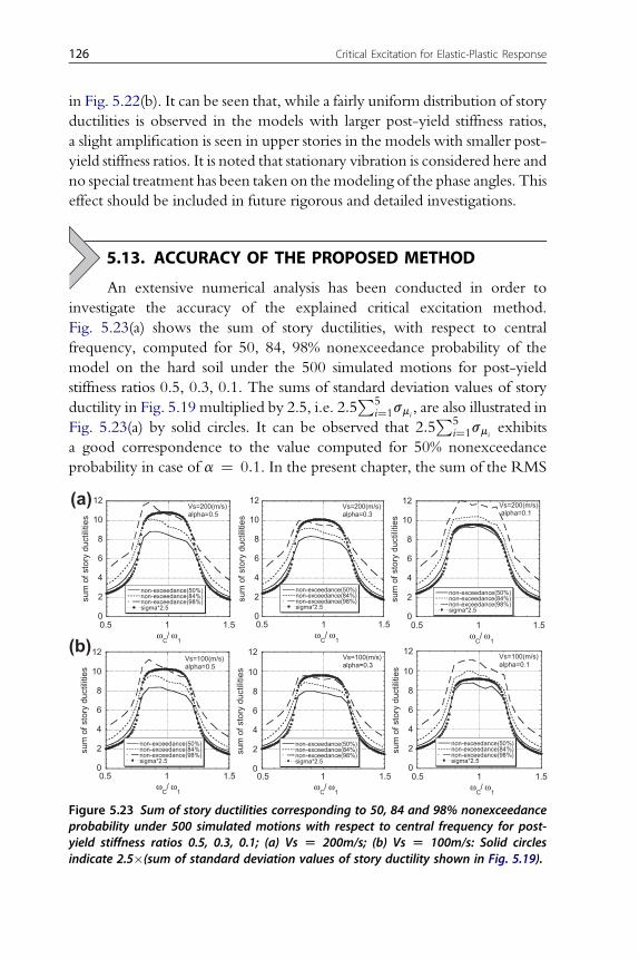
in Fig. 5.22(b). It can be seen that, while a fairly uniform distribution of storyductilities is observed in the models with larger post-yield stiffness ratios,a slight amplification is seen in upper stories in the models with smaller post-yield stiffness ratios. It is noted that stationary vibration is considered here andno special treatment has been taken on themodeling of the phase angles. Thiseffect should be included in future rigorous and detailed investigations.

5.13. ACCURACY OF THE PROPOSED METHOD

An extensive numerical analysis has been conducted in order toinvestigate the accuracy of the explained critical excitation method.Fig. 5.23(a) shows the sum of story ductilities, with respect to centralfrequency, computed for 50, 84, 98% nonexceedance probability of themodel on the hard soil under the 500 simulated motions for post-yieldstiffness ratios 0.5, 0.3, 0.1. The sums of standard deviation values of storyductility in Fig. 5.19 multiplied by 2.5, i.e. 2:5

P5i¼1smi

, are also illustrated inFig. 5.23(a) by solid circles. It can be observed that 2:5

P5i¼1smi

exhibitsa good correspondence to the value computed for 50% nonexceedanceprobability in case of a ¼ 0:1. In the present chapter, the sum of the RMS

0

2

4

6

8

10

12

0.5 1 1.5

non-exceedance(50%)non-exceedance(84%)non-exceedance(98%)sigma*2.5

sum

of s

tory

duc

tiliti

es

0

2

4

6

8

10

12

sum

of s

tory

duc

tiliti

es

0

2

4

6

8

10

12

sum

of s

tory

duc

tiliti

es

0

2

4

6

8

10

12

sum

of s

tory

duc

tiliti

es

0

2

4

6

8

10

12

sum

of s

tory

duc

tiliti

es

0

2

4

6

8

10

12

sum

of s

tory

duc

tiliti

es

Vs=200(m/s)alpha=0.5

ωC/ ω

1

0.5 1 1.5ω

C/ ω

1

0.5 1 1.5ω

C/ ω

1

0.5 1 1.5ω

C/ ω

1

0.5 1 1.5ω

C/ ω

1

0.5 1 1.5ω

C/ ω

1




Vs=200(m/s) alpha=0.1







(a)

(b)

Figure 5.23 Sum of story ductilities corresponding to 50, 84 and 98% nonexceedanceprobability under 500 simulated motions with respect to central frequency for post-yield stiffness ratios 0.5, 0.3, 0.1; (a) Vs [ 200m/s; (b) Vs [ 100m/s: Solid circlesindicate 2.5�(sum of standard deviation values of story ductility shown in Fig. 5.19).


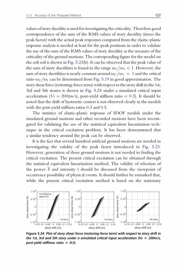
values of story ductility is used for investigating the criticality. Therefore goodcorrespondence of the sum of the RMS values of story ductility (times thepeak factor) with the actual peak responses computed from the elastic-plasticresponse analysis is needed at least for the peak positions in order to validatethe use of the sum of the RMS values of story ductility as the measure of thecriticality of the ground motions. The corresponding figure for the model onthe soft soil is shown in Fig. 5.23(b). It can be observed that the peak value ofthe sum of story ductilities is found in the range uC=u1 < 1. However, thesum of story ductilities is nearly constant arounduC=u1 ¼ 1 and the criticalratio uC=u1 can be determined from Fig. 5.19 in good approximation. Thestory shear force (restoring-force term)with respect to the story drift in the 1st,3rd and 5th stories is shown in Fig. 5.24 under a simulated critical inputacceleration (Vs ¼ 200(m/s), post-yield stiffness ratio ¼ 0.3). It should benoted that the drift of hysteretic centers is not observed clearly in the modelswith the post-yield stiffness ratios 0.3 and 0.5.

The statistics of elastic-plastic response of SDOF models under thesimulated ground motions and other recorded motions have been investi-gated for validating the use of the statistical equivalent linearization tech-nique in the critical excitation problem. It has been demonstrated thata similar tendency around the peak can be observed.

It is the fact that several hundred artificial ground motions are needed ininvestigating the validity of the peak factor introduced in Fig. 5.23.However, generation of these ground motions is not needed in finding thecritical excitation. The present critical excitation can be obtained throughthe statistical equivalent linearization method. The validity of selection ofthe power S and intensity s should be discussed from the viewpoint ofoccurrence possibility of physical events. It should further be remarked that,while the present critical excitation method is based on the stationary

-1 106

-5 105

0

5 105

1 106

-0.15 -0.1 -0.05 0 0.05 0.1 0.15

1st story

stor

y sh

ear f

orce

(N)

-1 106

-5 105

0

5 105

1 106

stor

y sh

ear f

orce

(N)

-1 106

-5 105

0

5 105

1 106

stor

y sh

ear f

orce

(N)

story drift (m)-0.15 -0.1 -0.05 0 0.05 0.1 0.15

story drift (m)-0.15 -0.1 -0.05 0 0.05 0.1 0.15

story drift (m)


3rd story 5th story

Figure 5.24 Plot of story shear force (restoring-force term) with respect to story drift inthe 1st, 3rd and 5th story under a simulated critical input acceleration (Vs [ 200m/s,post-yield stiffness ratio [ 0:3).

5.13. Accuracy of the Proposed Method 127

random vibration theory, recorded ground motions are nonstationary. Therelation between the critical peak responses and the actual peak responses torecorded ground motions must be discussed carefully from broader view-points. The extension of the present theory to nonstationary randomexcitations may be necessary to obtain a deeper and detailed relationship.

5.14. CONCLUSIONS

[SDOF Model]The conclusions may be summarized as follows:(1) A probabilistic critical excitation method for stationary random vibra-

tions of SDOF elastic-plastic models can be developed by employinga statistical equivalent linearization method as a response simulator ofthe original elastic-plastic model. The power and the intensity ofthe excitations are constrained in the critical excitation problem. Theshape of the critical PSD function is assumed to be a rectangular functionattaining its upper bound in a certain frequency range in view of thesimilarity to the critical excitation problem for linear elastic models.

(2) The explained method regards the central frequency of the rectangularPSD function as a principal parameter for finding the critical PSDfunction. Since the equivalent natural frequency and the equivalentdamping ratio are dependent on excitations, the technique using transferfunctions proposed for elastic models cannot be utilized in the problemfor elastic-plastic models.

(3) The simulation results by time-history response analysis for elastic-plasticmodels and the corresponding equivalent linear models revealed that thepresent critical excitation method is reliable in the models for which thevalidity of the statistical equivalent linearization method is guaranteed.The critical response representation in terms of nonexceedance proba-bilities can be an appropriate candidate for expressing the criticality ofrecorded ground motions.

(4) While the effect of the predominant frequency of a ground motion isreflected clearly in the comparison of the critical peak response with theactual peak response to the recorded ground motion in elastic models,such an effect is reflected only slightly in elastic-plastic models resultingfrom stiffness reduction and added damping ratio due to plasticresponses.


[MDOF Model]The conclusions may be summarized as follows:(1) A probabilistic method of critical excitation for stationary random

vibrations of MDOF elastic-plastic shear building models on deform-able ground can be developed. A statistical equivalent linearizationmethod for MDOF models is used as a response simulator of theoriginal elastic-plastic hysteretic model. The excitation power andintensity are constrained in the critical excitation problem. Thecritical shape of the PSD function is assumed to possess a rectangularshape with its upper bound in a selected frequency range based on thesimilarity to the critical excitation problem for linear elastic models.The sum along the height of standard deviations of story ductilitiescan be an adequate candidate for the objective function to define thecriticality.

(2) A solution algorithm for this critical excitation problem can be devisedby regarding the central frequency of the rectangular PSD function asa principal parameter. Because the equivalent stiffnesses and dampingcoefficients depend strongly on properties of excitations, the procedureusing transfer functions cannot be used in nature in the problem forelastic-plastic models.

(3) The results by elastic-plastic time-history response analysis disclosed thatthe introduced critical excitation method is effective and reliable in themodels for which the validity of the statistical equivalent linearization isguaranteed. The representation of the critical response in terms of non-exceedance probabilities can be an appropriate candidate for expressingthe degree of criticality of recorded ground motions.

APPENDIX 5.1 GROUND SPRING STIFFNESSESAND DASHPOT DAMPING COEFFICIENTS

Based on the results due to Parmelee (1970), the ground spring stiffnessesand dashpot damping coefficients are computed as

kS ¼ 6:77

1:79� nGr; kR ¼ 2:52

1:00� nGr3;

cS ¼ 6:21

2:54� nrVSr

2; cR ¼ 0:136

1:13� nrVSr

4

ðA5:1aedÞ

Appendix 5.1 Ground Spring Stiffnesses and Dashpot Damping Coefficients 129

The parameters G, n, VS, r and r are the soil shear modulus, Poisson’sratio, shear wave velocity, mass density of soil and radius of the equivalentcircular footing plate, respectively.

APPENDIX 5.2 STORY STIFFNESSES OF SHEAR BUILDINGWITH SPECIFIED LOWEST EIGENVALUE AND UNIFORMDISTRIBUTION OF LOWEST-MODE INTERSTORY DRIFTS

Let U1 denote the specified lowest eigenvalue of the interaction model. Itcan also be expressed asU1 ¼ ð2p=T1Þ2 in terms of the fundamental naturalperiod T1. The elastic story stiffnesses of the model with the specified lowesteigenvalue of the interaction model and a uniform distribution of lowest-mode interstory drifts can be obtained from the references (Nakamura andTakewaki 1985; Takewaki 2000b).

kj ¼ U1

Xfi¼ j

miðUF þQFHi þ iÞ ð j ¼ 1; 2;/; f Þ (A5.2)

Hi is defined in Eq. (5.13d). UF and QF are defined by

UF ¼ D2D5 �D3D4

D1D4 �D22;QF ¼ D2D3 �D1D5

D1D4 �D22

(A5.3a, b)

In Eqs. (A5.3a, b), D1;/;D5 are expressed as follows.

D1 ¼ E1 � kS

U1

;D2 ¼ E2;D3 ¼Xfi¼ 1

imi;

D4 ¼ E3 � kR

U1

;D5 ¼Xfi¼ 1

imiHi

ðA5:4aeeÞ

E1;E2;E3 in Eqs. (A5.4a–e) are defined in Eqs. (5.13a–c).In the case where the coupling term kHR of ground stiffness is not

negligible, the present formulation can be extended directly by modify-ing the term D2 in Eq. (A5.4b) to D2 ¼ E2 � ðkHR=U1Þ. This modifi-cation depends on the exact governing equation of undamped lowesteigenvibration.


REFERENCESBaratta, A., Elishakoff, I., Zuccaro, G., Shinozuka, M., 1998. A generalization of the

Drenick–Shinozuka model for bounds on the seismic response of a Single-Degree-Of-Freedom system. Earthq. Engng. Struct. Dyn. 27 (5), 423–437.

Caughey, T.K., 1960. Random excitation of a system with bilinear hysteresis. J. AppliedMechanics 27 (4), 649–652.

Der Kiureghian, A., 1980. A response spectrum method for random vibrations. Report No.UCB/EERC 80-15, EERC. University of California, Berkeley, CA.

Drenick, R.F., 1977. The critical excitation of nonlinear systems. J. Applied Mech. 44 (2),333–336.

Grossmayer, R.L., Iwan, W.D., 1981. A linearization scheme for hysteretic systems sub-jected to random excitation. Earthq. Engng. Struct. Dyn. 9 (2), 171–185.

Hudson, D.E., 1962. Some problems in the application of spectrum techniques to strong-motion earthquake analysis. Bull. Seism. Soc. Am. 52 (2), 417–430.

Iyengar, R.N., 1972. Worst inputs and a bound on the highest peak statistics of a class ofnon-linear systems. J. Sound and Vibration 25 (1), 29–37.

Kobori, T., Minai, R., 1967. Linearization technique for evaluating the elasto-plasticresponse of a structural system to non-stationary random excitations. Bull. Dis. Prev.Res. Inst., Kyoto University 10 (A), 235–260 (in Japanese).

Kobori, T., Minai, R., Suzuki, Y., 1973. Statistical linearization techniques of hystereticstructures to earthquake excitations. Bull. Dis. Prev. Res. Inst., Kyoto University 23(3–4), 111–125.

Manohar, C.S., Sarkar, A., 1995. Critical earthquake input power spectral density functionmodels for engineering structures. Earthq. Engng. Struct. Dyn. 24 (12), 1549–1566.

Nakamura, T., Takewaki, I., 1985. Optimum design of elastically supported shear buildingsfor constrained fundamental natural period. J. Structural Engineering, AIJ 31B, 93–102(in Japanese).

Parmelee, R.A., 1970. The influence of foundation parameters on the seismic response ofinteration systems. Proc. of the Third Japan Earthquake Engineering Symposium.

Philippacopoulos, A.J., 1980. Critical Excitations for Linear and Nonlinear StructuralSystems. Ph.D. Dissertation, Polytechnic Institute of New York.

Philippacopoulos, A., Wang, P., 1984. Seismic inputs for nonlinear structures. J. Eng. Mech.110 (5), 828–836.

Roberts, J.B., Spanos, P.D., 1990. Random Vibration and Statistical Linearization.John Wiley & Sons, Chichester, UK.

Shinozuka, M., 1970. Maximum structural response to seismic excitations. J. Engng. Mech.Div. 96 (5), 729–738.

Spanos P-, T.D., 1979. Hysteretic structural vibrations under random load. J. Acoust. Soc.America 65 (2), 404–410.

Spanos, P.D., 1981. Stochastic linearization in structural dynamics. Applied MechanicsReviews 34 (1), 1–8.

Srinivasan, M., Corotis, R., Ellingwood, B., 1992. Generation of critical stochastic earth-quakes. Earthq. Engng. Struct. Dyn. 21 (4), 275–288.

Takewaki, I., 2000a. Optimal damper placement for critical excitation. ProbabilisticEngineering Mechanics 15 (4), 317–325.

Takewaki, I., 2000b. Dynamic Structural Design: Inverse Problem Approach. WIT Press,Southampton, UK.

Takewaki, I., 2001. A new method for non-stationary random critical excitation. Earthq.Engng. Struct. Dyn. 30 (4), 519–535.

Appendix 5.2 Story Stiffnesses of Shear Building with Specified Lowest Eigenvalue 131

Wen, Y.K., 1980. Equivalent linearization for hysteretic systems under random excitation.J. Appl. Mech., ASME 47 (1), 150–154.

Wen, Y.K., 1989. Methods of random vibration for inelastic structures. Applied MechanicsRev., 42 (2), 39–52.

Westermo, B.D., 1985. The critical excitation and response of simple dynamic systems.J. Sound and Vibration 100 (2), 233–242.


CHAPTER SIX

Critical Envelope Function forNonstationary RandomEarthquake Input

Contents

6.1. Introduction 1336.2. Nonstationary Random Earthquake Ground Motion Model 1356.3. Mean-Square Drift 1366.4. Problem for Finding Critical Envelope Function 137

[Problem CEFNS] 1376.5. Double Maximization Procedure 137

[Property A] 1386.6. Discretization of Envelope Function 1396.7. Upper Bound of Mean-Square Drift 1406.8. Numerical Examples 1426.9. Critical Excitation for Variable Envelope Functions and Variable Frequency

Contents147

6.10. Conclusions 148Appendix 6.1 Mean-Square Drift of SDOF System in Stationary State 149Appendix 6.2 Proof of Property A 149Appendix 6.3 Expressions of BCj(t) and BSj(t) 150Appendix 6.4 Upper Bound for Continuous Functions c(t) 152References 154

6.1. INTRODUCTION

The purpose of this chapter is to explain a new probabilistic criticalexcitation method for identifying the critical envelope function of groundmotions. It is well known that the envelope shape of ground motionsdepends on various factors, for example arrival time and order of variouskinds of waves, and the maximum structural responses of models withrather shorter natural periods are often induced by the intensive motions



http://dx.doi.org/10.1016/B978-0-08-099436-9.00006-7

existing mostly in the first half portion of ground motions. It is thereforeof practical and scientific interest to investigate the most critical envelopeshape in ground motions. Fig. 6.1 shows parts of time histories of fourground motions, El Centro NS 1940, Taft EW 1952, Hyogoken-Nanbu,Kobe University NS 1995 and Mexico Michoacan SCT1 EW 1985. Itcan be observed that a monotonically increasing function may bea candidate for the envelope function in the former half part of the totalduration.

In this chapter, the nonstationary ground motion is assumed to beexpressed as the product of a deterministic envelope function andanother probabilistic function representing the frequency content. Theformer envelope function is determined in such a way that the corre-sponding mean-square drift of a single-degree-of-freedom (SDOF) modelattains its maximum under the constraint on mean total energy. Thecritical excitation problem includes the double maximization procedurewith respect to time and to the envelope function. The key to findingthe critical envelope function is the order interchange in the doublemaximization procedure. An upper bound of the mean-square drift isalso derived by the use of the Cauchy-Schwarz inequality. It is shownthat the proposed technique is systematic and the upper bound canbound the exact response extremely efficiently within a reasonableaccuracy.

-0.4-0.3-0.2-0.1

00.10.20.30.4

0150

Acc

eler

atio

n (g

)

Time (sec)

El Centro 1940 NS

-0.2

-0 .1

0

0.1

0.2

0150

Acc

eler

atio

n (g

)

T ime (sec)

TAFT 1952 EW

-0.4-0.3-0.2-0.1

00.10.20.30.4

0 5 10 15 20

Acc

eler

atio

n (g

)

Time (sec)


-0.2-0.15

-0.1-0.05

00.05

0.10.15

0.2

0 10 20 30 40 50 60 70 80

Mexico SCT1 EW (1985)

Acc

eler

atio

n (g

)

Time (sec)

after interpolation (every 0.02s)

Figure 6.1 Part of time histories of four ground motions, El Centro NS 1940, Taft EW1952, Hyogoken-Nanbu, Kobe University NS 1995 and Mexico Michoacan SCT1 EW1985.

134 Critical Envelope Function for Nonstationary Random Earthquake Input

6.2. NONSTATIONARY RANDOM EARTHQUAKEGROUND MOTION MODEL

In this chapter, it is assumed that the input horizontal base acceleration canbe described by the following uniformly modulated nonstationary randomprocess.


where cðtÞ is a deterministic envelope function to be obtained from theviewpoint of criticality and wðtÞ is a stationary Gaussian process with zeromean. Let T denote the duration of €ugðtÞ. The power spectral density (PSD)function SwðuÞ of wðtÞ is assumed to be given and its power (integration inthe frequency domain) is determined by

ZN�N

SwðuÞdu ¼ Sw (6.2)

The auto-correlation function Rwðt1; t2Þ of wðtÞ can be defined by


�N


where E½$� indicates the ensemble mean. The time-dependent PSD func-tion of €ugðtÞ can then be expressed by


The following constraint on the mean of the total energy (Drenick 1970;Shinozuka 1970) is taken into account.

ChE

"ZT0

€ugðtÞ2dt#

¼ C (6.5)

where C is a given value for the mean total energy. It can be shown(Housner and Jennings 1977) that this quantity C is related to the inputenergy to the SDOF model which has a certain relationship with the

6.2. Nonstationary Random Earthquake Ground Motion Model 135

response spectrum. This relationship may be useful in setting C. Substitutionof Eq. (6.1) into Eq. (6.5) leads to

ZT0

cðtÞ2E½wðtÞ2�dt ¼ C (6.6)

Substitution of Eq. (6.3) (t1 ¼ t2 ¼ t) into Eq. (6.6) provides

ZT0

cðtÞ2� ZN

�N

SwðuÞdu�dt ¼ C (6.7)

Finally Eq. (6.7) is reduced to the following form with the use of Eq.(6.2).

ZT0

cðtÞ2dt ¼ C=Sw (6.8)

6.3. MEAN-SQUARE DRIFT

Consider an SDOF linear elastic model with u1 and h as theundamped natural circular frequency and the damping ratio, respectively.The damped natural circular frequency is then expressed byu1d ¼ u1


p.

Let gðtÞ ¼ HeðtÞð1=u1dÞe�hu1t sin u1dt (HeðtÞ: Heaviside step function)denote the unit impulse response function multiplied by the mass. Themean-square drift of the SDOF model can then be expressed by (seeTakewaki 2001a and Appendix 6.1)

sDðtÞ2 ¼ RN�N

Rt0

cðs1Þgðt � s1Þeius1ds1Rt0

cðs2Þgðt � s2Þe-ius2ds2SwðuÞdu

¼ RN�N


hRN

�NHðt;uÞ2SwðuÞdu

(6.9)


The functions ACðt;uÞ;ASðt;uÞ are defined by

ACðt;uÞ ¼Z t0

gðt � sÞf�cðsÞ cos usgds (6.10a)

ASðt;uÞ ¼Z t0

gðt � sÞf�cðsÞ sin usgds (6.10b)

The functions ACðt;uÞ and ASðt;uÞ indicate the response of the SDOFmodel to the amplitude modulated cosine function and that to amplitudemodulated sine function, respectively. It should be noted that the functionHðt;uÞ includes the effects both of the envelope function cðtÞ and of zeroinitial conditions and its frequency content is time-dependent.

6.4. PROBLEM FOR FINDING CRITICAL ENVELOPEFUNCTION

The problem for finding the critical envelope function in nonstationary(CEFNS) random vibration may be described as:

[Problem CEFNS]Given the natural frequency and damping ratio of an SDOF model and the PSDfunction SwðuÞ of wðtÞ (its power is computed by Eq. (6.2)), find the non-negativecritical envelope function cðtÞ to maximize the specific mean-square drift sDðt�Þ2 (t�is the time when the maximum mean-square drift to €ugðtÞ ¼ cðtÞwðtÞ is attained)subject to the constraint on the mean of the total energy

ChE

"ZT0

€ugðtÞ2dt#

¼ C (6.11)

6.5. DOUBLE MAXIMIZATION PROCEDURE

This problem includes the double maximization procedures, whichmay be described mathematically by

maxcðtÞ

maxt

sDðtÞ2

6.5. Double Maximization Procedure 137

The first maximization is performed with respect to time for a givenenvelope function cðtÞ and the second maximization is done with respect tothe envelope function cðtÞ. In the first maximization, the time t� when themaximum mean-square drift is attained must be obtained for each envelopefunction. This original problem is complicated and it seems difficult to finda systematic solution procedure. To overcome this difficulty, a newsophisticated procedure based on the interchange of the order of themaximization procedures is proposed. The proposed procedure can beexpressed by

maxt

maxcðtÞ

sDðtÞ2

The first maximization process with respect to the envelope function fora given time (this problem is called a “subproblem” later) can be pursued byutilizing a nonlinear programming method. The second maximizationprocedure with respect to time can be implemented systematically bycomparing the values at various times directly. It is important to note that thefollowing property can be proved.

[Property A]The envelope function cðtÞ satisfying the constraint (6.11) and maximizingsDðtiÞ2 is the function with zero value in t � ti.

The proof is shown in Appendix 6.2. This property will be utilized in thefollowing sections where discretized values of the envelope function areobtained.

The proposed algorithm may be summarized as:(i) Set a specific time t ¼ ti.(ii) Find the critical envelope function at time t ¼ ti. When the envelope

function is discretized as shown in the following section, the criticalenvelope function can be obtained by utilizing a nonlinear program-ming method.

(iii) Compute sDðtiÞ2 to the envelope function obtained in step (ii).(iv) Repeat steps (i)–(iii) for various times and obtain sDðtmÞ2 ¼

maxsDðtiÞ2.(v) The envelope function as the solution to the subproblem for t ¼ tm is

determined as the critical envelope function.It is important to note that the present algorithm based on the interchange ofthe order of the double maximization procedure is applicable to moresophisticated nonuniformly modulated nonstationary excitation models


although the expression of Eq. (6.9) must be modified and a new criticalexcitation problem must be stated.

6.6. DISCRETIZATION OF ENVELOPE FUNCTION

For simple and essential presentation of the proposed solutionprocedure, a property on the PSD function SwðuÞ is used which has beendiscussed and found in Takewaki (2001a). Let SwðuÞ be a function withnonzero values at u ¼ u1d only. This implies that the critical frequencycontent of excitations is a resonant one to the structural model. Thistreatment provides a good approximation for evaluation of sDðtÞ2 of themodel under the excitations with other PSD functions SwðuÞ with a fairlynarrow band around u ¼ u1d (Takewaki 2000). Because it has been shownin Takewaki (2001a) that the critical frequency content of the PSD functionis a resonant one irrespective of envelope functions, the present treatment ofthe PSD function appears to be reasonable and this fact is expected to play animportant role in finding the critical excitation for simultaneous variation offrequency contents and envelope functions (see Section 6.9). If we do notuse this property on the PSD function SwðuÞ, a tremendous amount ofcomputational tasks may be necessary to conduct the simultaneous sensi-tivity analysis for frequency contents and envelope functions.

With the use of Eq. (6.2), the mean-square drift expressed by Eq. (6.9) isthen reduced to

sDðtÞ2 ¼ Hðt;u1dÞ2Sw (6.12)

For discretization of cðtÞ, let ci denote the value of cðtÞ at t ¼ ti (c0 ¼ 0).The following linear approximation of cðtÞ is introduced.cðtÞ ¼ cj�1 þ cj � cj�1

Dtft � ðj � 1ÞDtg ððj � 1ÞDt � t � jDtÞ (6.13)

where Dt is the time interval for discretization of cðtÞ. Let N denote thenumber of time intervals until time t (t ¼ NDt). Eq. (6.12) can then beexpressed by

sDðtÞ2 ¼ ( PN

j¼ 1

RjDtðj�1ÞDt

cðsÞgðt � sÞ cos u1dsds

)2

þ( PN

j¼ 1

RjDtðj�1ÞDt

cðsÞgðt � sÞ sin u1dsds

)2!Sw

(6.14)

6.6. Discretization of Envelope Function 139

Substitution of Eq. (6.13) into Eq. (6.14) leads to

sDðtÞ2 ¼ Sw

( XNj¼ 1

BCjðtÞcj!2

þ XN

j¼ 1

BSjðtÞcj!2)

(6.15)

where BCjðtÞ and BSjðtÞ are the coefficients on cj and can be expressed interms of given parameters. The expressions of BCjðtÞ and BSjðtÞ are shown inAppendix 6.3.

6.7. UPPER BOUND OF MEAN-SQUARE DRIFT

Introduction of the discretization of cðtÞ, i.e. Eq. (6.13), into theconstraint (6.8) provides

2

3

XNT

j¼ 1

cj2 þ 1

3

XNT

j¼ 1

cj�1cj ¼ C

SwDt(6.16)

where NT ¼ T=Dt is the number of time intervals in the whole duration.Another interpolation of cðtÞ may be possible from the viewpoint ofsimplification. Constant interpolation of cðtÞ in every interval may providethe following expression of the constraint (6.8).

XNT

j¼ 1

cj2 ¼ C

SwDt(6.17)

For simplicity of expression, the above constant interpolation of cðtÞ isused only for the constraint (6.8). This is due to the fact that, whilethe response (6.9) is sensitive to the shape of cðtÞ, the constraint (6.8) is notso sensitive to the shape of cðtÞ so long as the time interval is smallenough.

As shown in Section 6.5 (Property A), N can be used in place of NT inthe constraint (6.17) when the maximization of sDðtiÞ2 at time ti isconsidered. In other words, cj ¼ 0 can be assumed for j > i when themaximization of sDðtiÞ2 at time ti is considered. Application of the Cauchy-Schwarz inequality to Eq. (6.15) and substitution of Eq. (6.17) into theresulting equation provide


sDðtÞ2 ¼ Sw

( XNj¼ 1

BCjðtÞcj!2

þ XN

j¼ 1

BSjðtÞcj!2)

� Sw

( XNj¼ 1

BCjðtÞ2! XN

j¼ 1

cj2

!

þ XN

j¼ 1

BSjðtÞ2! XN

j¼ 1

cj2

!)

¼ Sw

XNj¼ 1

cj2

! (XNj¼ 1

ðBCjðtÞ2 þ BSjðtÞ2Þ)

¼ C

Dt

(XNj¼ 1


(6.18)

Every term in the last line of inequality (6.18) does not include anyterm dependent on fcig and inequality (6.18) implies that the upperbound of sDðtÞ2 in the subproblem stated in Section 6.5 can be given bythe value in the last line of inequality (6.18). It should be noted thatBCjðtÞ and BSjðtÞ include terms of Dt (see Appendix 6.3). It can thereforebe shown that the leading order of the last line of inequality (6.18) for Dtis zero-th.

When the linear interpolation of cðtÞ is used also for the constraint (6.8),the following bound can be derived with the use of the non-negativeproperty of fcig.

sDðtÞ2 � 3C

2Dt

(XNj¼ 1


(6.19)

It can be seen that the upper bound (6.19) is larger than the upper bound(6.18). It is therefore preferable to use the upper bound (6.18) in order tobound the exact value strictly.

It is interesting to note that an upper bound of sDðtÞ2 under theconstraint (6.8) can be derived for continuous functions cðtÞ. That expressionis shown in Appendix 6.4.

6.7. Upper Bound of Mean-Square Drift 141


Consider an SDOF linear elastic model that has the undamped naturalperiod 0.5(s) and the damping ratio 0.02. The time interval for discretizationof cðtÞ is 0.05(s). The specified mean total energy, the power of wðtÞ and theexcitation duration are given by C ¼ 2:28ðm2=s3Þ, Sw ¼ 1:51ðm2=s3Þ and40(s), respectively.

The maximization problem of Eq. (6.15) under the constraints on Eq.(6.17) ðNT/NÞ and on the non-negative property of fcig constitutesa nonlinear programming problem where both the objective function andthe constraints are nonlinear. This nonlinear programming problem is solvedhere by the Powell’s method (Vaderplaats 1984).

For the purpose of comparing the response to the critical envelopefunction with those to other envelope functions, the following envelopefunctions are considered.

constant : cðtÞ ¼ a

linear : cðtÞ ¼ at

exponential : cðtÞ ¼ aexpðhu1tÞrealistic : cðtÞ ¼ afexpð�0:13tÞ � expð�0:45tÞg ð6:20aedÞ

In Eqs. (6.20a–d), the parameter a is to be determined from theconstraint (6.17) ðNT/NÞ. Fig. 6.2 shows the plots of these envelopefunctions in which the parameter a has been determined for the total timeduration 40(s). The terminology “realistic” is used here because the

0

0.5

1

0 5 10 15 20 25 30 35 40

constantlinearexponentialrealistic

c(t)

time (s)Figure 6.2 Four examples of envelope functions satisfying the constraint (6.17)(constant, linear, exponential-function and realistic distributions).


expression (6.20d) has been proposed by Shinozuka and Sato (1965) tosimulate actual ground motions realistically using this envelope function.

The lower four curves in Fig. 6.3 show sDðtÞ, the square root of Eq. (6.15),for four envelope functions in (6.20a–d). It should be noted that Fig. 6.3 doesnot represent the root-mean-square drift to a given envelope function. Theparameter a has been determined for each parameter N so as to satisfy theconstraint (6.17) ðNT/NÞ andsDðtÞ (t ¼ NDt) for these different envelopefunctions is plotted. The root-mean-square drift to the critical envelopefunction obtained by the above-mentioned nonlinear programming methodfor eachparameterN is also shown inFig. 6.3.The subproblem stated inSection6.5 has been solved for each parameterN. Furthermore, the upper bound givenby inequality (6.18) is also plotted in Fig. 6.3. It can be observed from Fig. 6.3that the value sDðtÞ to the critical envelope function, the solution of thesubproblem, obtained for each parameterN appears to converge to a constantvalue at a certain time. Strictly speaking, the exact maximum occurs at the endof the duration and the exact solution to the original problem CEFNS can beobtained for the subproblem in case of N ¼ NT . It can also be understoodfrom Fig. 6.3 that the root-mean-square drift corresponding to the solution ofeach subproblem exists between the value for other noncritical envelopefunctions and the upper bound. This demonstrates the validity of the nonlinear

0

0.05

0.1

0.15

0 100 200 300 400 500 600 700 800

root

mea

n sq

uare

resp

onse

(m)

index N

T1=0.5,h=0.02

Δt=0.05

upper boundmaximum via NLP

exponential

linearconstant

realistic

Figure 6.3 Root-mean-square drift to four excitations with the amplitude-modulatedenvelope functions (6.20a–d) which have been obtained for each parameter N, theroot-mean-square drift (6.15) to the critical excitation as the solution to the subproblemin Section 6.5 and the upper bound of the root-mean-square drift by (6.18). (Nonlinearprogramming, (NLP.).


programming method employed in this chapter. It can be seen from Fig. 6.3that the upper bound of the root-mean-square drift can bound the exact valuewithin about 10% error. It is noteworthy that, while it takes a few hours inordinary workstations to obtain the solution to the nonlinear programmingproblem for a fairly large number N, the computation of the upper boundrequires extremely less time (a second or less).

Fig. 6.4(a) shows the envelope function as the solution to thesubproblem N ¼ 200 and Fig. 6.4(b) shows that to the subproblemN ¼ NT ¼ 800. As stated before, Fig. 6.4(b) indicates the exact solutionto the original problem CEFNS. It is interesting to note that, while anincreasing exponential function is the critical one in the deterministicproblem treated by Drenick (1970), the superimposed envelope function of

0

0.5

1

1.5

2

0 50 100 150 200

c i

index i

T1=0.5,h=0.02

Δt=0.05

N=200

0

0.5

1

1.5

2

0 100 200 300 400 500 600 700 800

c i

index i

T1=0.5,h=0.02

Δt=0.05

N=800

0

0.5

1

1.5

2

700 750 800

c i

index i

magnified

(a)

(b)

Figure 6.4 (a) Envelope function as solution to subproblem for N ¼ 200 (approximatesolution to original problem); (b) envelope function as solution to subproblem forN ¼ NT ¼ 800 (exact solution to original problem).


the original envelope function, to be found in the present problem, of thecritical excitation can be a function similar to an increasing exponentialfunction in the probabilistic problem. This result may be related to thecondition u ¼ u1d used in Section 6.6 and further examination of theenvelope function will be necessary.

Fig. 6.5(a) illustrates an approximate time-history sample of the criticalacceleration forN ¼ NT ¼ 800. In the computation, a narrowband-limitedwhite noise with the band Du ¼ 0:2ðrad=sÞ is used for SwðuÞ and wðtÞ hasbeen expressed as the sum of 100 cosine waves. The amplitudes of the cosinewaves have been computed from the PSD functionSwðuÞ and the phase angleshave been assumed to be uniformly random between 0 and 2p. Fig. 6.5(b)shows the magnified plot of the time-history sample between 35(s) and 40(s).

It should be remarked that, when the duration of groundmotions becomesshorter compared to the natural period of the SDOF model and the dampingbecomes rather small, the discussion on impulsive loading must be madecarefully. A similar discussion was made by Drenick (1970) for deterministiccritical excitation problems. This problem is open to future discussion.

In order to examine the accuracy of the numerical procedure, the timeinterval has been shortened from 0.05(s) to 0.025(s). Fig. 6.6 shows the

-2

-1

0

1

2

0 10 20 30 40

acce

lera

tion

(m/s

2 )

time (s)

-2

-1

0

1

2

35 36 37 38 39 40

acce

lera

tion

(m/s

2 )

time (s)

(a)

(b)

Figure 6.5 (a) An approximate time-history sample of the critical acceleration forN ¼ NT ¼ 800; (b) magnified plot of the time-history sample between 35(s) and 40(s).


envelope function as the solution to the subproblemN ¼ 1600. Due to theshortening of the time interval, the number of discretization has beenincreased. It can be observed that a smoother envelope function has beenobtained by the shortening of the time interval. However, the requiredcomputer time is extremely longer.

Furthermore, to investigate the effect of the natural period of the SDOFstructural model and its damping ratio on the upper bound of response, twonew models have been considered. Those two models have the same naturalperiod of 2.0(s) and different damping ratios of 0.02 and 0.10. The lower solidcurve in Fig. 6.7 shows sDðtÞ, the square root of Eq. (6.15), for the realisticenvelope function in (6.20d). It should be noted again that Fig. 6.7 does notrepresent the square root of the mean-square drift to a given envelopefunction. The parameter a has been determined for each parameterN so as tosatisfy the constraint (6.17) ðNT/NÞ, and sDðtÞ (t ¼ NDt) for thesedifferent envelope functions is plotted. The square root of the mean-squaredrift to the critical envelope function obtained by the above-mentionednonlinear programming method for each parameter N is also plotted inFig. 6.7. The subproblem stated in Section 6.5 has been solved for eachparameterN. The upper bound given by the inequality (6.18) (square root of(6.18)) is also plotted in Fig. 6.7. It can be observed fromFig. 6.7 that the valuesDðtÞ to the critical envelope function, the solution of the subproblem,obtained for each parameter N appears to converge to a constant value ata certain time. Strictly speaking, the exact maximum occurs at the end of theduration and the exact solution to the original problem CEFNS can beobtained for the subproblem in case of N ¼ NT . It can also be understoodfrom Fig. 6.7 that the square root of the mean-square drift corresponding to

0

0.5

1

1.5

2

0 200 400 600 800 1000 1200 1400 1600

c i

index i

T1=0.5,h=0.02

Δt=0.025

N=1600

0

0.5

1

1.5

2

1400 1500 1600

c i

index i

magnified

Figure 6.6 Envelope function as the solution to the subproblem for N ¼ NT ¼ 1600(exact solution to the original problem).


the solution of each subproblem exists between the value for other noncriticalenvelope functions and the upper bound. This demonstrates the validity ofthe nonlinear programming method employed in this chapter.

6.9. CRITICAL EXCITATION FOR VARIABLE ENVELOPEFUNCTIONS AND VARIABLE FREQUENCY CONTENTS

The critical frequency content has been found in the references (Takewaki2000, 2001a) as a resonant one to structural models for any fixed envelopefunction. In contrast to the previous study, the critical envelope function has

0

0.2

0.4

0.6

0.8

1

0 50 100 150 200

root

mea

n sq

uare

res

pons

e (m

)

index N

upper bound

maximum via NLP

realistic

T1=2.0(s), h=0.02

Δt=0.2(s)

0

0.2

0.4

0.6

0.8

1

0 50 100 150 200

root

mea

n sq

uare

res

pons

e (m

)

index N

upper bound

maximum via NLP

realistic

T1=2.0(s), h=0.10

Δt=0.2(s)

(a)

(b)

Figure 6.7 Root-mean-square drift to an excitation with the amplitude-modulatedenvelope function (6.20d) which has been obtained for each parameter N, the root-mean-square drift (6.15) to the critical excitation as the solution to the subproblemin Section 6.5 and the upper bound of the root-mean-square drift by (6.18): (a) dampingratio ¼ 0.02, (b) damping ratio ¼ 0.10. NLP

6.9. Critical Excitation for Variable Envelope Functions and Variable Frequency Contents 147

been revealed in this chapter for the fixed frequency content, i.e. theresonant critical one. It may therefore be concluded that the combination ofthe critical frequency content and the critical envelope function is the criticalset for a more general problem with variable frequency contents and variableenvelope functions.

6.10. CONCLUSIONS

The conclusions may be summarized as follows:(1) A new probabilistic critical excitation method can be developed for

nonstationary responses of an SDOF structural system that is subjectedto a nonstationary ground acceleration described as the product of anenvelope function and another function representing the frequencycontent of a stationary random process. The non-negative criticalenvelope function maximizing the displacement response is determinedunder the constraint on the mean total energy of the input motion.

(2) It has been found that the order interchange of the double maximizationprocedure with respect to time and to the envelope function can be anexcellent and powerful solution algorithm for finding the criticalenvelope function. A nonlinear programming procedure can be utilizedin one of the maximization procedures (with respect to the envelopefunction).

(3) An upper bound of the mean-square drift can be derived by using theCauchy-Schwarz inequality and the constraint on the input motion(mean total energy). The upper bound can bound the mean-square driftefficiently and effectively within a reasonable accuracy. The requiredtime for this procedure based on the upper bound is shorter than onesecond in this case and is superior to the nonlinear programmingprocedure, stated above, requiring several hours.

The practicality and reality of the explained critical excitation methodshould be discussed carefully (see, e.g., Srinivasan et al. 1991; Pirasteh et al.1988). The recorded ground motions, e.g. Mexico (1985), Hyogoken-Nanbu (1995) and Chi-Chi (1999), imply that unexpected groundmotions could occur especially in the near fields. The critical excitation candiffer in each structure. This is because each structure has a different naturalperiod. In defining a critical excitation for a group of structures, the exci-tation with a wide-band PSD function may be a candidate for the criticalexcitation. Furthermore, for an inelastic structure with a time-varyingprincipal vibration frequency, the excitation with a rather wide-band PSD


function may also be critical (Drenick 1977; Takewaki 2001b). Extension ofthe present method to inelastic structures may be possible with the help ofthe equivalent linearization method (Takewaki 2001b).

It is expected that the critical excitation method can provide usefulinformation for the design of important structures of which functional andstructural damage must be absolutely avoided during severe earthquakes. Insuch a situation, two-dimensional (2-D) and three-dimensional (3-D) inputsmay be required. Extension of the present method to such 2-D and 3-Dinput models is a challenging problem.

APPENDIX 6.1 MEAN-SQUARE DRIFT OF SDOF SYSTEMIN STATIONARY STATE

The mean-square drift sD2 of the SDOF system in the stationary state maybe expressed as

sD2 ¼

ZN�N

jHDðuÞj2SgðuÞdu (A6.1)

where HDðuÞ is the transfer function of the drift to the input accelerationand SgðuÞ is the time-averaged PSD function of the input acceleration.

APPENDIX 6.2 PROOF OF PROPERTY A

Consider an excitation with an envelope function shown in Fig. A1(a).It is assumed that the PSD function SwðuÞ of wðtÞ is given and does notchange. Consider the mean-square drift at time t. It is proven here that theexcitation with nonzero value of cðsÞ in s > t cannot be the excitationsatisfying the constraint (6.8) and maximizing the response sDðtÞ2 at time t.Call the excitationwith nonzero value of cðsÞ in s > t “excitation A.”On theother hand, call the excitation with zero value of cðsÞ in s > t “excitation B.”It is noted that excitation B is constructed in such a way that the area of cðsÞ2in s > t in excitation A is moved to the region s < t and cðsÞ in s < t isamplified as c�ðsÞ2 ¼ acðsÞ ða > 1Þ (see Fig. A1(b)). From Eq. (6.9), themean-square drift s�DðtÞ2 to excitation B has the following relationship withthe mean-square drift sDðtÞ2 to excitation A.

s�DðtÞ2 ¼ a2sDðtÞ2 > sDðtÞ2 (A6.2)

Appendix 6.2 Proof of Property A 149

Eq. (A6.2) implies that excitation A with nonzero value of cðsÞ in s > t

cannot be the excitation satisfying the constraint (6.8) and maximizing theresponse sDðtÞ2 at time t.

APPENDIX 6.3 EXPRESSIONS OF BCj(t) AND BSj(t)

The expressions of BCjðtÞ and BSjðtÞ in Eq. (6.15) may be given asfollows:

BCjðtÞ ¼ PjðtÞ � Pjþ1ðtÞ � ðj � 1ÞQjðtÞ þ ðjþ 1ÞQjþ1ðtÞðj ¼ 1; 2;/;N � 1Þ

BCN ðtÞ ¼ PN ðtÞ � ðN � 1ÞQN ðtÞBSjðtÞ ¼ pjðtÞ � pjþ1ðtÞ � ðj � 1ÞqjðtÞ þ ðjþ 1Þqjþ1ðtÞ

ðj ¼ 1; 2;/;N � 1ÞBSN ðtÞ ¼ pN ðtÞ � ðN � 1ÞqN ðtÞ ðA6:3aedÞ

( )c τ

( )c τ

Excitation A

Excitation B

τ

τ

t

t

( )c τ

( )c τ( )cα τ

(a)

(b)

Figure A1 (a) Excitation with nonzero value of cðsÞ in s > t (Excitation A); (b) excitationwith zero value of cðsÞ in s > t (Excitation B) in which the area of cðsÞ2 in s > t inexcitation A is moved to the region s < t and cðsÞ in s < t is amplified as c�ðsÞ ¼acðsÞ ða > 1Þ.


where

PjðtÞ ¼ e�hu1t

2u1dDtðFS1 sin u1dt þ FC1 cos u1dtÞ

QjðtÞ ¼ e�hu1t

2u1dðFS2 sin u1dt þ FC2 cos u1dtÞ

pjðtÞ ¼ e�hu1t

2u1dDtðFS3 sin u1dt þ FC3 cos u1dtÞ

qjðtÞ ¼ e�hu1t

2u1dðFS4 sin u1dt þ FC4 cos u1dtÞ ðA6:4aedÞ

FS1, ., FC4 in Eqs. (A6.4a–d) may be expressed by

FS1 ¼ 1

r

�2u1d

�jDtDSj � ðj � 1ÞDtDSj�1

�þ ð1þ jhu1DtÞDCj

� f1þ ðj � 1Þhu1DtgDCj�1

� 2hu1

r

�hu1ðDCj �DCj�1Þ þ 2u1dðDSj �DSj�1Þ

��

þ 1

ðhu1Þ2hjhu1Dt � 1

ejhu1Dt � fðj � 1Þhu1Dt � 1geðj�1Þhu1Dt

i

FC1 ¼ 1

r

�2u1d

�jDtDCj � ðj � 1ÞDtDCj�1

�� ð1þ jhu1DtÞDSj

þ f1þ ðj � 1Þhu1DtgDSj�1 þ 2hu1

r

�hu1ðDSj �DSj�1Þ

� 2u1dðDCj �DCj�1Þ��

FS2 ¼ 1

r

�2u1dðDSj �DSj�1Þ þ hu1ðDCj �DCj�1Þ

�

þ 1

hu1

�ejhu1Dt � eðj�1Þhu1Dt

�

FC2 ¼ 1

rf2u1dðDCj �DCj�1Þ � hu1ðDSj �DSj�1Þg

Appendix 6.3 Expressions of BCj(t) and BSj(t) 151

FS3 ¼ 1

r

�� 2u1d

�jDtDCj � ðj � 1ÞDtDCj�1

�þ ð1þ jhu1DtÞDSj

� f1þ ðj � 1Þhu1DtgDSj�1

� 2hu1

r

�hu1ðDSj �DSj�1Þ � 2u1dðDCj �DCj�1Þ

��

FC3 ¼ 1

r

�2u1d

�jDtDSj � ðj � 1ÞDtDSj�1g þ ð1þ jhu1DtÞDCj

� f1þ ðj � 1Þhu1DtgDCj�1 � 2hu1

r

�hu1ðDCj �DCj�1Þ

þ 2u1dðDSj �DSj�1Þ��

� 1

ðhu1Þ2h�

jhu1Dt � 1Þejhu1Dt � fðj � 1Þhu1Dt � 1geðj�1Þhu1Dti

FS4 ¼ 1

r

�� 2u1dðDCj �DCj�1Þ þ hu1ðDSj �DSj�1Þ

�

FC4 ¼ 1

r

�2u1dðDSj �DSj�1Þ þ hu1ðDCj �DCj�1Þ

�

� 1

hu1

�ejhu1Dt � eðj �1Þhu1Dt

� ðA6:5aehÞ

DSj;DCj and r are given by

DSj ¼ ejhu1Dt sin ð2ju1dDtÞ;DCj ¼ ejhu1Dt cos ð2ju1dDtÞr ¼ ðhu1Þ2 þ ð2u1dÞ2 ðA6:6aecÞ

APPENDIX 6.4 UPPER BOUND FOR CONTINUOUSFUNCTIONS C(t)

Application of the Cauchy-Schwarz inequality to Eq. (6.9) leads to


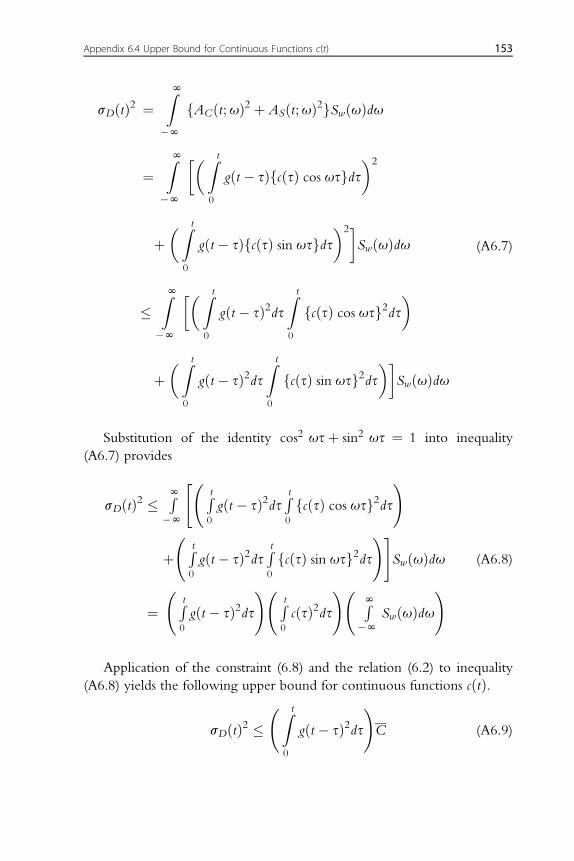
sDðtÞ2 ¼ZN

�N


¼ZN

�N

��Z t0

gðt � sÞfcðsÞ cos usgds�2

þ�Z t

0

gðt � sÞfcðsÞ sin usgds�2�

SwðuÞdu

�ZN

�N

��Z t0

gðt � sÞ2dsZ t0

fcðsÞ cos usg2ds�

þ�Z t

0

gðt � sÞ2dsZ t0

fcðsÞ sin usg2ds��

SwðuÞdu

(A6.7)

Substitution of the identity cos2 usþ sin2 us ¼ 1 into inequality(A6.7) provides

sDðtÞ2 �RN

�N

" Rt0

gðt � sÞ2ds Rt0

fcðsÞ cos usg2ds!

þ Rt

0

gðt � sÞ2ds Rt0

fcðsÞ sin usg2ds!#

SwðuÞdu

¼ Rt

0

gðt � sÞ2ds! Rt

0

cðsÞ2ds! RN

�NSwðuÞdu

!(A6.8)

Application of the constraint (6.8) and the relation (6.2) to inequality(A6.8) yields the following upper bound for continuous functions cðtÞ.

sDðtÞ2 � Z t

0

gðt � sÞ2ds!C (A6.9)

Appendix 6.4 Upper Bound for Continuous Functions c(t) 153

The expressionR t0 gðt � sÞ2ds in (A6.9) can be expressed byZ t

0

gðt � sÞ2ds ¼ 1

2u21d

"1

2hu1ð1� e�2hu1tÞ

� h

2u1

(1þ e�2hu1t


p

hsin 2u1dt � cos 2u1dt

!)#

(A6.10)

REFERENCESDrenick, R.F., 1970. Model-free design of aseismic structures. J. Engng. Mech. Div. 96 (4),

483–493.Drenick, R.F., 1977. The critical excitation of nonlinear systems. J. Applied Mech. 44 (2),

333–336.Housner, G.W., Jennings, P.C., 1977. The capacity of extreme earthquake motions to

damage structures. In: Hall, W.J. (Ed.), Structural and Geotechnical Mechanics,pp. 102–116. Prentice-Hall Englewood Cliff, NJ.

Pirasteh, A.A., Cherry, J.L., Balling, R.J., 1988. The use of optimization to constructcritical accelerograms for given structures and sites. Earthq. Engng. Struct. Dyn. 16 (4),597–613.

Shinozuka, M., 1970. Maximum structural response to seismic excitations. J. Engng. Mech.Div. 96 (5), 729–738.

Shinozuka, M., Sato, Y., 1965. Simulation of non-stationary random process. J. Eng. Mech.Div. 91 (EM4), 11–1422.

Srinivasan, M., Ellingwood, B., Corotis, R., 1991. Critical base excitations of structuralsystems. J. Eng. Mech. 117 (6), 1403–1422.

Takewaki, I., 2000. Optimal damper placement for critical excitation. ProbabilisticEngineering Mechanics 15 (4), 317–325.

Takewaki, I., 2001a. A new method for non-stationary random critical excitation. Earthq.Engng. Struct. Dyn. 30 (4), 519–535.

Takewaki, I., 2001b. Probabilistic critical excitation for MDOF elastic–plastic structures oncompliant ground. Earthq. Engng. Struct. Dyn. 30 (9), 1345–1360.

Vaderplaats, G.N., 1984. Numerical Optimization Techniques for Engineering Design withApplications. McGraw-Hill Book Company, New York.


CHAPTER SEVEN

Robust Stiffness Design forStructure-Dependent CriticalExcitation

Contents

7.1. Introduction 1557.2. Problem for Fixed Design 156

[Problem for Fixed Design] 1577.3. Problem for Structure-Dependent Critical Excitation 158

[Problem of Stiffness Design for Critical Excitation] 1587.4. Solution Procedure 1597.5. Numerical Design Examples 1637.6. Response to a Broader Class of Excitations 1667.7. Response to Code-Specified Design Earthquakes 1687.8. Conclusions 170Appendix Evaluation of Maximum Elastic-Plastic Responses 171References 173

7.1. INTRODUCTION

The purpose of this chapter is to explain a new robust stiffness designmethod for building structures taking into account the dependence ofcritical excitations on the design of building structures. A global stiffnessparameter is maximized (a global flexibility parameter is minimized actually)under the constraints on excitations (power and intensity) and on totalstructural cost. This design problem includes a min-max procedure (maxi-mization of structural flexibility with respect to excitation and minimizationof structural flexibility with respect to story stiffnesses). It is shown that thetechnique for a fixed design explained in Chapter 2 (Takewaki 2001) can beused effectively in the maximization procedure and this leads to extremesimplification in an accurate manner of the present complicated, highlynonlinear problem. The elastic-plastic responses of the designed buildingstructures to a broader class of excitations and to code-specified design



http://dx.doi.org/10.1016/B978-0-08-099436-9.00007-9

earthquakes are clarified through a statistical equivalent linearizationtechnique.

7.2. PROBLEM FOR FIXED DESIGN

A probabilistic critical excitation method has been developed byTakewaki (2001) for building structures with fixed mechanical propertiesand member sizes. For the formulation in the following sections, a summaryof the method is described.

Consider an n-story shear building model subjected to a horizontalacceleration €ugðtÞ. This input is characterized by a stationary Gaussianprocess with zero mean. Let SgðuÞ denote the power spectral density (PSD)function of the ground acceleration €ugðtÞ. The system mass, damping andstiffness matrices of the building model and the influence coefficient vectorby the base input are denoted by M;C;K; r, respectively. The equations ofmotion of the model in the frequency domain can be expressed as

ð�u2Mþ iuCþ KÞUðuÞ ¼ �Mr €UgðuÞ (7.1)

In Eq. (7.1), i denotes the imaginary unit. UðuÞ and €UgðuÞ are theFourier transforms of the horizontal floor displacement vector uðtÞ relativeto the ground and €ugðtÞ, respectively. Eq. (7.1) can also be expressed as

AUðuÞ ¼ B €UgðuÞ (7.2)

where A ¼ �u2Mþ iuCþ K and B ¼ �Mr.Let diðtÞ denote the interstory drift in the i-th story. The Fourier

transform DðuÞ of fdiðtÞg can be related to UðuÞ by

DðuÞ ¼ TUðuÞ (7.3)

T consists of 1, �1 and 0. Substitution of Eq. (7.2) into Eq. (7.3) provides

DðuÞ ¼ TA�1B €UgðuÞ (7.4)

Rewrite Eq. (7.4) as

DðuÞ ¼ HDðuÞ €UgðuÞ (7.5)

156 Robust Stiffness Design for Structure-Dependent Critical Excitation

HDðuÞ ¼ fHDiðuÞg ¼ TA�1B is the deformation transfer function. The

mean-square interstory drift in the i-th story may be described as

sDi

2 ¼ZN

�N

jHDiðuÞj2SgðuÞdu ¼

ZN�N

HDiðuÞH�

DiðuÞSgðuÞdu (7.6)

where ðÞ� denotes a complex conjugate.The sum of the mean-square interstory drifts can be regarded as “an

inverse of the global stiffness” (global flexibility) of the shear building modeland is described as

f ¼Xni¼ 1

sDi

2 ¼ZN

�N


The function FðuÞ (called F-function) in Eq. (7.7) is defined by

FðuÞ ¼Xni¼ 1

jHDiðuÞj2 (7.8)

The critical excitation problem for a fixed design may be described as:

[Problem for Fixed Design]Find the critical PSD function ~SgðuÞ to maximize f defined by Eq. (7.7)

subject to the constraint on input powerZN

�N

SgðuÞdu � S (7.9)

and to the constraint on intensity supSgðuÞ � s (7.10)

lartceps rewop

ytisned

noitcnuf-F

circular frequency

s →∞(Dirac delta function)

F-function

PSD function lartceps rewop

ytisned

noitcnuf-F

circular frequency

s

Ω∼

rectangular

PSD function

F-function

(a) (b)

– –

Figure 7.1 Power spectral density function of critical excitation: (a) critical excitationfor infinite power spectral density amplitude s and (b) critical excitation for finite powerspectral density amplitude s.

7.2. Problem for Fixed Design 157

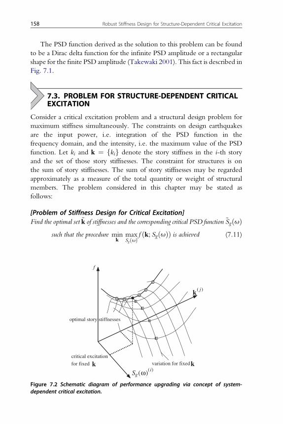
The PSD function derived as the solution to this problem can be foundto be a Dirac delta function for the infinite PSD amplitude or a rectangularshape for the finite PSD amplitude (Takewaki 2001). This fact is described inFig. 7.1.

7.3. PROBLEM FOR STRUCTURE-DEPENDENT CRITICALEXCITATION

Consider a critical excitation problem and a structural design problem formaximum stiffness simultaneously. The constraints on design earthquakesare the input power, i.e. integration of the PSD function in thefrequency domain, and the intensity, i.e. the maximum value of the PSDfunction. Let ki and k ¼ fkig denote the story stiffness in the i-th storyand the set of those story stiffnesses. The constraint for structures is onthe sum of story stiffnesses. The sum of story stiffnesses may be regardedapproximately as a measure of the total quantity or weight of structuralmembers. The problem considered in this chapter may be stated asfollows:

[Problem of Stiffness Design for Critical Excitation]Find the optimal set ~k of stiffnesses and the corresponding critical PSD function ~SgðuÞ

such that the procedure mink

maxSgðuÞ

f ðk; SgðuÞÞ is achieved (7.11)

f

variation for fixedcritical excitation

for fixed

optimal story stiffnesses

k( j)

Sg(ω)(i)k k

Figure 7.2 Schematic diagram of performance upgrading via concept of system-dependent critical excitation.


subject to the constraint on input powerZN

�N

SgðuÞdu � S (7.12)

to the constraint on input intensity sup: SgðuÞ � s (7.13)

to the constraint on total structural quantity ðcostÞXn

i¼1ki ¼ K (7.14)

and to the positivity of story stiffnesses ki > 0 ði ¼ 1;/; nÞ (7.15)

Fig. 7.2 shows a schematic diagram of the present problem. The solutionof the min-max problem corresponds to a saddle point.


The procedure for solving the problem in the previous section isexplained in this section. Assume that the system damping matrix C is nota function of story stiffnesses k. The critical excitation characterized by itsPSD function SgðuÞ for a fixed set k of stiffnesses can be found by using themethod described above (Takewaki 2001). This fact can be used effectivelyin the maximization in the procedure (7.11).

~U denotes the frequency bandwidth in the frequency range of the criticalrectangular PSD function SgðuÞ, i.e. S=ð2sÞ ¼ ~U. Assume that theupper and lower frequency limits of the rectangular PSD function can beexpressed by

uU ¼ u1 þ 1

2~U (7.16a)

uL ¼ u1 � 1

2~U (7.16b)

In Eq. (7.16), u1 is the undamped fundamental natural circularfrequency of the shear building model. It should be remembered that u1 isa function of k and the critical rectangular PSD function SgðuÞ is a functionof k. The objective function (7.7) for the critical rectangular PSD functioncan then be approximated by

f ¼ RN�N

Fðu; kÞSgðuÞdu

y2sRuU

uL

Fðu; kÞdu

¼ 2sfFðuU ; kÞ � FðuL; kÞg

(7.17)


The function Fðu; kÞ denotes the following function.

Fðu; kÞ ¼Zu0

Fðu; kÞdu (7.18)

In Eq. (7.17), a nearly symmetric property of the function Fðu; kÞhas been utilized. This insightful approximate manipulation enables ananalytical treatment of the present complicated strongly nonlinearproblem.

The minimization of the objective function f with respect to k in theprocedure (7.11) will be considered next. The following Lagrangian isdefined in terms of a Lagrange multiplier l.

L ¼ f þ l

� Pni¼ 1

ki � K

�

¼ 2sfFðuU ; kÞ � FðuL; kÞg þ l

� Pni¼ 1

ki � K

� (7.19)

The expression (7.17) has been used in Eq. (7.19). The stationaritycondition of the Lagrangian defined in Eq. (7.19) with respect to storystiffnesses k may be written by

vL

vki¼ f ;i þ l

¼ 2s

�vu1

vkifFðuU ; kÞ � FðuL; kÞg þ

ZuU

uL

v2Fðu; kÞvki

du

�þ l ¼ 0

(7.20)

where f ;ihvf =vki. Eq. (7.20) represents the optimality condition to besatisfied in optimization. For exact differentiation, the following expressionsare used in this chapter.

v1F

vxhvFðx; yÞ

vx;v2F

vyhvFðx; yÞ

vy(7.21)

It is the case that x is an implicit function of y. However, Eq. (7.21)implies that v2F=vy indicates the partial differentiation only for the termsincluding y explicitly.


The first-order sensitivity of the undamped fundamental natural circularfrequency u1 in Eq. (7.20) with respect to story stiffnesses k can be obtainedfrom u1 ¼ fTK;if=ð2u1Þ where f is the lowest eigenmode. The sensi-tivity v2F=vki in Eq. (7.20) can be computed by

v2F

vki¼Xl

HDlðuÞ; i HDl

�ðuÞ þXl

HDlðuÞHDl

�ðuÞ;i (7.22)

HDiðuÞ ¼ TiA�1B is the deformation transfer function and the well-

known expression A�1;i ¼ �A�1A;iA�1 can be used for computingdesign sensitivities of transfer functions. The vector Ti denotes the i-th rowof the matrixT. It should be remarked that operations of complex conjugateand partial differentiation are exchangeable.

Next, define the following quantity for a simpler expression.

aj ¼ f ;jþ1=f ;1 (7.23)

It is noted that the optimality condition described by Eq. (7.20) isequivalent to

aj ¼ 1 ðj ¼ 1;/; n� 1Þ (7.24)

The linear increment of aj due to the story stiffness change Dk may beexpressed by

Daj ¼0@ 1

f ;1

vf ;jþ1

vk� f ;jþ1

f ;12

vf ;1vk

1A Dk ¼ 1

f ;1

vf ;jþ1

vk� vf ;1

vkaj

!Dk

(7.25)

The constraint expressed by Eq. (7.14) may be reduced to

Xnj¼ 1

Dkj ¼ 0 (7.26)

In Eq. (7.26), Dkj denotes a small increment of the j-th story stiffness andDk ¼ fDkjg. The combination of Eq. (7.25) with Eq. (7.26) yields thefollowing simultaneous linear equation for Dk ¼ fDkjg.


266666666666664

1

f ;1

vf ;2vk

� vf ;1vk

a1

!

«

1

f ;1

vf ;nvk

� vf ;1vk

an�1

!

1/1

377777777777775Dk ¼

8>>>><>>>>:

Da1

«

Dan�1

0

9>>>>=>>>>;

(7.27)

Assume that the increment of aj is defined by fDajg ¼fðaFj� a0jÞ=Ngwhere faFjg ¼ f1/1gT (see Eq. (7.24)) and the quantities for the initialdesign are used for the specification of fa0jg. Sequential application of Eq.(7.27) to each updated design kðkoldþ Dk/knewÞ provides the final designsatisfying the optimality conditions (7.24).

The second-order design sensitivity of the objective function in the left-hand side of Eq. (7.27) can be computed by

v2 f

vkivkj¼ 2s

�v2u1

vkivkj

�FðuU ; kÞ � FðuL; kÞ

�

þ vu1

vki

�v1FðuU ; kÞ

vu1

vu1

vkjþ v2FðuU ; kÞ

vkj

� v1FðuL; kÞvu1

vu1

vkj� v2FðuL; kÞ

vkj

�

þ vu1

vkj

�v2FðuU ; kÞ

vki� v2FðuL; kÞ

vki

�þZuU

uL

v22Fðu; kÞvkivkj

du

�

(7.28)

It is noted that the second-order sensitivity of the undamped funda-mental natural circular frequency in Eq. (7.28) with respect to story stiff-nesses can be obtained from

u1;ij ¼ 1

2u1ðf;j

TK;ifþ fTK;if;jÞ � u1;iu1;j

u1

¼ 1

u1f;j

TK;if� u1;iu1;j

u1

(7.29)


In addition, the following relation is used.

vAðuUðu1ÞÞ=vu1 ¼ �2uUMþ iC (7.30)

The second-order design sensitivity of the function F in Eq. (7.28) can becomputed by

v22Fðu; kÞvkivkj

¼Xl

HDlðuÞ;ijHDl

�ðuÞ þXl

HDlðuÞ;iHDl

�ðuÞ;j

þXl

HDlðuÞ;jHDl

�ðuÞ;i þXl

HDlðuÞHDl

�ðuÞ;ij (7.31)

The sensitivity expression A�1;ij ¼ A�1A;jA�1A;iA�1 þ A�1A;i

$A�1A;jA�1 is used in the computation of the second-order designsensitivity of the transfer function. Eq. (7.31) has to be substituted intoEq. (7.28) and numerical integration must be performed finally.

7.5. NUMERICAL DESIGN EXAMPLES

Design examples are shown for 6-story and 12-story models in orderto demonstrate the validity of the method described in the previous section.For comparison, a design with a straight-line lowest-mode, i.e. uniformlowest-mode interstory drift components, is taken into account. This designis called the “frequency constraint (FC) design” because this design is anoptimal design under a fundamental natural frequency constraint (Nakamuraand Yamane 1986). On the other hand, the design obtained by the methoddescribed in the previous section is called the “maximum performance (MP)design.” This design seeks the maximization of global stiffness performance,in other words, the minimization of global flexibility.

The power of the PSD function is specified as S ¼ 0:553ðm2=s4Þ andthe amplitude of the PSD function has been given by s ¼ 0:0661ðm2=s3Þ.These parameters are equivalent to those for the ground motion of ElCentro NS (1940) (duration¼ 40(s)). In nature, earthquake ground motionsare nonstationary random processes and the present treatment of time-averaging is approximate. However, reasonable application may bepossible so long as the range of applicability is clearly indicated (Lai 1982).See, (for example, Lai 1982, Nigam 1983 and Vanmarcke 1983) for thetime-averaged approximate PSD functions.

Assume that the floor masses have the same value in all the stories and aregiven by mi ¼ 32:0� 103ðkgÞ. The damping ratio is given by 0.05 (stiffnessproportional). In the design method described in the previous section, the FC

7.5. Numerical Design Examples 163

design has been used as the initial design. The total sum of story stiffnesses isspecified as K ¼ 0:319� 109ðN=mÞ for 6-story models andK ¼ 0:570� 109ðN=mÞ for 12-story models. Note that these values werecomputed from the FC design with the fundamental natural periodT1 ¼ 0:600ðsÞ for 6-story models and with T1 ¼ 1:20ðsÞ for 12-storymodels. The total step number for incremental computation is N ¼ 100 andthe numerical integrationwith respect to frequency has been implementedwith100 frequency intervals.

Fig. 7.3 illustrates the story stiffness distributions of the FC design and theMP design of 6-, 12- and 18-story models. It can be understood that the story

0 0.2 0.4 0.6 0.8 10

1

2

3

4

5

6

FC design (frequency constraint)maximum performance design

story stiffness (*108N/m)

stor

y nu

mbe

r

0 0.2 0.4 0.6 0.8 10

2

4

6

8

10

12



stor

y nu

mbe

r

0 0.2 0.4 0.6 0.8 10

2

4

6

8

10

12

14

16

18



stor

y nu

mbe

r

Figure 7.3 Story stiffness distributions (frequency constraint design and maximumperformance design).


stiffnesses in the lower stories of the FC designweremoved to the upper storiesin the MP design. This is because the reduction in the interstory drifts in theupper stories is cost-effective for the upgrading of global stiffness performance.It was found that the fundamental natural period of the optimal design (MPdesign) for the 6-storymodel isT1 ¼ 0:612ðsÞ and that for the 12-storymodelis T1 ¼ 1:22ðsÞ. Then the objective function is f ¼ 0:4901� 10-3ðm2Þ forthe initial design (FC design) and is f ¼ 0:4615� 10-3ðm2Þ for the optimal

0 0.005 0.01 0.015 0.020

1

2

3

4

5

6


square root of mean squaresof interstory drift (m)

stor

y nu

mbe

r

0 0.01 0.02 0.030

2

4

6

8

10

12


square root of mean squaresof interstory drift (m)

stor

y nu

mbe

r

Figure 7.4 RMS distributions of interstory drifts (frequency constraint design andmaximum performance design).

-1.5 -1 -0.5 00

1

2

3

4

5

6


first-order design sensitivityof objective function (*10-9m3/N)

stor

y nu

mbe

r

-4 -3 -2 -1 00

2

4

6

8

10

12


first-order design sensitivityof objective function (*10-9m3/N)

stor

y nu

mbe

r

Figure 7.5 First-order design sensitivities of objective function (frequency constraintdesign and maximum performance design).

7.5. Numerical Design Examples 165

design (MPdesign) in 6-storymodels. In addition, the objective function foundfor 12-story models is f ¼ 0:2327� 10-2ðm2Þ for the initial design (FCdesign) and is f ¼ 0:2145� 10-2ðm2Þ for the optimal design (MP design).

Fig. 7.4 shows the square roots of the mean-square interstory drifts(RMS values) for the FC design and the MP design of 6- and 12-storymodels subjected to the critical excitation. It can be observed that theRMS values of the FC design are nearly uniform.Note that this distribution isobtained for the critical excitation andmore detailed investigation is necessaryfor robust design. Fig. 7.5 illustrates the first-order design sensitivities of theobjective functions for both FC design andMP design. It can be seen that theoptimality conditions (7.20) are satisfied accurately in the MP design.

7.6. RESPONSE TO A BROADER CLASS OF EXCITATIONS

In view of structural robustness, it may bemeaningful to investigate theultimate and limit state in the plastic range of the building structure undera broader class of disturbance. The normal trilinear hysteretic restoring-forcecharacteristic as shown in Fig. 7.6 is used for the story restoring-force char-acteristic. The maximum elastic-plastic responses under random excitationshave been evaluated by the statistical equivalent linearization technique (seeAppendix). It is well known that nonstationary characteristics of excitationsand responses are very important in the analysis of the energy input intostructures and the damage of structures. However, it is also well understoodthat, as far as only the maximum displacement is concerned, the stationarytreatment leads to sufficient accuracy. For this reason, stationary treatment is

( ) ( ) /i i yit tμ δ δ=ie1

2i ikα

1i ikα

ik

iQ

Figure 7.6 Normal trilinear hysteretic restoring-force characteristics in i-th story.


employed here. To evaluate the mean peak story ductility factors, the so-called peak factors have been multiplied on the RMS interstory drifts. Thepower and the amplitude of the PSD function have been specified asS ¼ 0:553� 2:0ðm2=s4Þ and s ¼ 0:0661� 2:0ðm2=s3Þ. The excitationduration is specified by 40(s). The yield interstory drifts have been specified bydyi ¼ 0:01ðmÞin all stories for 6-story models and by dyi ¼ 0:02ðmÞ in allstories for 12-storymodels. The ratio of the second yield-point interstory driftto the yield interstory drift, the ratio of the second-branch stiffness to theinitial elastic stiffness and the ratio of the third-branch stiffness to the initialelastic stiffness have been specified as ei ¼ 2:0, a1i ¼ 0:5;a2i ¼ 0:05,respectively in all stories. The fundamental natural circular frequency of themodel in the elastic range is denoted by u1.

In order to generate various input motions, the central frequency uC ofthe rectangular PSD function has been changed so as to be uC=u1 ¼0:5; 0:6;/; 1:3. The rectangular PSD function has been chosen even for theelastic-plastic models in view of the criticality for elastic responses. Since theequivalent stiffness and damping coefficients are functions of excitations, thisrestriction seems to be too restrictive. However, more general and arbitrarytreatment of excitations is difficult due to the nonlinear nature of structuralsystems and this issue should be discussed in more depth. The frequencybandwidth is given by ~U ¼ 0:553=ð0:0661� 2:0Þðrad=sÞ. Note that therectangular PSD function is resonant to the natural period of the equivalentlinear model in the range of uC=u1 � 1:0. Fig. 7.7 presents the mean peak

0 1 2 3 4 50

1

2

3

4

5

6

story ductility factor

stor

y nu

mbe

r

FC design

0 1 2 3 4 50

1

2

3

4

5

6


stor

y nu

mbe

r

MP design

Figure 7.7 Mean peak story ductility factors of 6-story models subjected to variousexcitations with different frequency ranges (frequency constraint design and maximumperformance design).

7.6. Response to a Broader Class of Excitations 167

story ductility factors in 6-story models subjected to various excitations withthe rectangular PSD function of different central frequenciesuC=u1 ¼ 0:5; 0:6;/; 1:3 (FC design and MP design). The maximumresponses have been obtained for the excitation with the parameteruC=u1 ¼ 1:0 in 6-story models. It can be seen from Fig. 7.7 that, while theMP design exhibits larger mean peak story ductility factors in the lowerstories, the FC design exhibits a fairly uniform distribution of the mean peakstory ductility factors.

However, a slightly whipping (amplified) phenomenon in the upperstories can be seen in the FC design. A similar phenomenon can be seen inFig. 7.8 for 12-story models. The maximum story ductility factors have beenobserved for the excitation with the parameter uC=u1 ¼ 0:8 in 12-storymodels.

7.7. RESPONSE TO CODE-SPECIFIED DESIGNEARTHQUAKES

For investigating the response characteristics of FC and MP designs tocode-specified design earthquakes, elastic-plastic responses under code-specified design earthquakes have been computed by use of the above-mentioned statistical equivalent linearization technique (see Appendix).The earthquake ground motions specified in the Japanese seismic resistant

0 1 2 3 4 50

2

4

6

8

10

12


stor

y nu

mbe

r

FC design

0 1 2 3 4 50

2

4

6

8

10

12

story ductility factorst

ory

num

ber

MP design

Figure 7.8 Mean peak story ductility factors of 12-story models subjected to variousexcitations with different frequency ranges (frequency constraint design and maximumperformance design).


design code revised in 1998 have been employed. The second-type soilcondition has been assumed. The acceleration response spectrum fordamping ratio ¼ 0.05 at the ground surface corresponding to the safetylimit has been computed as shown in Fig. 7.9. The power and intensity aregiven by

RN�N SgðuÞdu¼ 2:84ðm2=s4Þ and maxSgðuÞ ¼ 0:0798ðm2=s3Þ.

The portions in T < 0:05ðsÞ and T > 3:0ðsÞ have been neglectedin the computation of the power. The duration of the excitationhas been specified to be 40(s). Fig. 7.10 illustrates the mean peak storyductility factors under the design earthquakes. It can be seen that a slightwhipping (amplified) phenomenon is observed in the FC design of 6-storymodels.

In order to investigate the accuracy of the statistical equivalent linear-ization, an elastic-plastic time-history response analysis has been conductedfor 12-story models. The acceleration response spectrum shown in Fig. 7.9has been transformed to the PSD function and a set of one hundred arti-ficial ground motions has been generated. The line with marks in Fig. 7.10shows the mean peak story ductility factors in the MP design. It can beobserved that the present statistical equivalent linearization technique canpredict the mean peak elastic-plastic responses within a reasonableaccuracy.

0.2

0.4

0.6

0.8

1

1.2

1.4

0 0.5 1 1.5 2 2.5 3 3.5

acce

lera

tion

resp

onse

spe

ctru

m (g

)

natural period (s)

New Japanese code(safety limit)ground surface levelh=0.05

Figure 7.9 Acceleration response spectrum at ground surface level by new Japaneseseismic-resistant design code corresponding to safety limit (critical damping ratio ¼0.05).

7.7. Response to Code-Specified Design Earthquakes 169

7.8. CONCLUSIONS

The conclusions may be stated as follows:(1) A robustmethod of stiffness design can be developed. In thismethod, both

a critical excitation problem depending on structural parameters anda stiffness design problem for better structural performances are taken intoaccount simultaneously. A global and generalized stiffness parameter hasbeen chosen as the objective function to be maximized. In anotherviewpoint, a global flexibility parameter has been minimized. The opti-mality conditions to this robust stiffness design problemhavebeenderived.

(2) Effective approximation has been introduced in the computation of thefirst- and second-order design sensitivities of the objective functiondefined only for the critical excitation. An efficient numerical procedurehas been devised to solve this robust stiffness design problem. It has beendemonstrated that the procedure of finding the critical excitation fora fixed design can be extremely simplified by taking advantage of theprocedure by the present author (Takewaki 2001).

(3) Design examples demonstrated that the present method can certainlyupgrade the global stiffness performance in a robust way. Stochasticequivalent linearization analysis for the so-designed structures undervarious candidate design earthquakes has also clarified that the building

0 1 2 3 4 50

1

2

3

4

5

6

FC design (linearization)MP design (linearization)


stor

y nu

mbe

r

0 1 2 3 4 50

2

4

6

8

10

12

FC design (linearization)MP design (linearization)MP design (time history)


stor

y nu

mbe

r

Figure 7.10 Mean peak story ductility factors subjected to design earthquakes by newJapanese seismic code (safety limit) (frequency constraint design and maximumperformance design).


structure designed by the present method exhibits a favorable elastic-plastic envelope response. A design with a straight-line lowest modealso exhibits a favorable elastic-plastic response to a broader class ofdisturbances except a slight whipping (amplified) phenomenon in theupper stories.

APPENDIX EVALUATION OF MAXIMUM ELASTIC-PLASTIC RESPONSES

The statistical equivalent linearization technique by Kobori and Minai(1967) for MDOF structures has been modified here for normal trilinearhysteretic restoring-force characteristics. Following the approach byCaughey (1960), the mean-square minimization technique has also beenintroduced in contrast to the simple mean procedure employed in the paperby Kobori and Minai (1967). The technique employs the assumption of theslowly varying characteristics of the amplitude and phase in a sinusoidalvibration. More advanced statistical equivalent linearization techniques havebeen developed so far and such techniques can be used if desired.

The parameters dyi;Dyi; ei ¼ Dyi=dyi;a1i;a2i denote the yield interstorydrift, the second yield-point interstory drift, its ratio to the yield interstorydrift, the ratio of the second-branch stiffness to the initial elastic stiffness andthe ratio of the third-branch stiffness to the initial elastic stiffness in the i-thstory, respectively.

Consider the ratio (ductility factor) miðtÞ ¼ diðtÞ=dyi of the interstorydrift to its yield drift. The amplitude of miðtÞ is denoted by zi. The standarddeviations of miðtÞ and its time derivative _miðtÞ are denoted by smi

and s _mi,

respectively. The parameters ~ui ¼ s _mi=smi

, ui and ui ¼ ~ui=ui denote themean circular frequency in the i-th story, the frequency for non-dimensionalization and the nondimensional frequency in the i-th story,respectively. Then the equivalent stiffness k

eqi and equivalent damping

coefficient ceqi are expressed by

keqi ¼ k�i ki; c

eqi ¼ c�i ðki=uiÞ (A7.1a, b)

In Eq. (A7.1), nondimensional stiffness and damping coefficient k�i and c�iare described as

k�i ¼

RN0

zi2k0iðziÞpðzi; smi

ÞdziRN0

zi2pðzi; smiÞdzi

(A7.2a)

Appendix Evaluation of Maximum Elastic-Plastic Responses 171

c�i ¼

RN0

zi2c0iðzi;u�

i Þpðzi;smiÞdzi

RN0

zi2pðzi;smiÞdzi

(A7.2b)

The quantities k0iðziÞ and c0iðzi;uiÞ defined by Eqs. (A7.2a, b) can bederived by minimizing the mean-squared errors of the restoring-forcecharacteristic of the equivalent system from that of the original trilinearhysteretic system.

k0iðziÞ ¼ 1:0 ðzi � 1Þ (A7.3a)

k0iðziÞ ¼ 1� a1i

pcos�1

�1� 2

zi

�þ a1i � 2

pzi2ð1� a1iÞðzi� 2Þ ffiffiffiffiffiffiffiffiffiffiffiffi

zi � 1p

ð1 � zi � eiÞ(A7.3b)

k0iðziÞ ¼ 2

pzi2

�zi2

2

�ð1� a1iÞ cos�1

�1� 2

zi

�

þ ða1i� a2iÞ cos�1

�1� 2ei

zi

�þ a2ip

�

� ð1� a1iÞðzi� 2Þ ffiffiffiffiffiffiffiffiffiffiffiffizi � 1

p � ða1i� a2iÞðzi� 2eiÞffiffiffiffiffiffiffiffiffiffiffiffiffiffiffiffiffieiðzi� eiÞ

p i

ðei � ziÞ (A7.3c)

c0iðzi;ui�Þ ¼ 0 ðzi � 1Þ (A7.4a)

c0iðzi;ui�Þ ¼ 4ð1� a1iÞðzi� 1Þ

pui�zi2

ð1 � zi � eiÞ (A7.4b)

c0iðzi;ui�Þ ¼ 4

pui�zi2

fð1� a1iÞðzi� 1Þ þ eiða1i� a2iÞðzi� eiÞg ðei � ziÞ(A7.4c)

The quantity pðzi; smiÞ in Eqs. (A7.2a, b) is the probability density

function of the amplitude zi and the following Rayleigh distribution isadopted.

pðzi; smiÞ ¼ ðzi=smi2Þexpf�zi

2=ð2smi2Þg (A7.5)

The standard deviations smiand s _mi

are derived by integrating the PSDfunction of the response. This response is expressed as the product of the


squared value of the transfer function of the equivalent linear model and thePSD function SgðuÞ of the input excitation.

For computing the mean peak story ductility factors, the peak factorsproposed by Der Kiureghian (1981) are introduced. These peak factors aredetermined from the first three moments of response PSD functions and theexcitation duration.

REFERENCESCaughey, T.K., 1960. Random excitation of a system with bilinear hysteresis. J. Applied

Mechanics 27 (4), 649–652.Der Kiureghian, A., 1981. A response spectrum method for random vibration analysis of

MDF systems. Earthquake Engng. & Struct. Dyn. 9 (5), 419–435.Kobori, T., Minai, R., 1967. Linearization technique for evaluating the elasto-plastic

response of a structural system to non-stationary random excitations. Bull. Dis. Prev.Res. Inst., Kyoto University. 10 (A), 235–260 (in Japanese).

Lai, S.P., 1982. Statistical characterization of strong ground motions using power spectraldensity function. Bulletin of the Seismological Soc. of America 72 (1), 259–274.

Nakamura, T., Yamane, T., 1986. Optimum design and earthquake-response constraineddesign of elastic shear buildings. Earthquake Engng. & Struct. Dyn. 14 (5), 797–815.

Nigam, N.C., 1983. Introduction to Random Vibrations. The MIT Press, Cambridge.pp. 68–69.

Takewaki, I., 2001. A new method for non-stationary random critical excitation.Earthquake Engrg. and Struct. Dyn. 30 (4), 519–535.

Vanmarcke, E., 1983. Random Fields: Analysis and Synthesis. The MIT Press, Cambridge.pp. 339–340.

Appendix Evaluation of Maximum Elastic-Plastic Responses 173

CHAPTER EIGHT

Critical Excitation for EarthquakeEnergy Input in SDOF System

Contents

8.1. Introduction 1758.2. Earthquake Input Energy to SDOF System in the Frequency Domain 1778.3. Property of Energy Transfer Function and Constancy of Earthquake Input Energy 1798.4. Critical Excitation Problem for Earthquake Input Energy with Acceleration

Constraint182

[Critical Excitation Problem for Acceleration] 1828.5. Critical Excitation Problem for Earthquake Input Energy with Velocity Constraint 183

[Critical Excitation Problem for Velocity] 1848.6. Actual Earthquake Input Energy and its Bound for Recorded Ground Motions 1858.7. Conclusions 194References 195

8.1. INTRODUCTION

The purpose of this chapter is to explain a new general critical exci-tation method for a damped linear elastic single-degree-of-freedom (SDOF)system as shown in Fig. 8.1. The input energy to the SDOF system during anearthquake is introduced as a new measure of criticality. It is shown that theformulation of the earthquake input energy in the frequency domain isessential for solving the critical excitation problem and deriving a bound onthe earthquake input energy for a class of ground motions. The criticality isexpressed in terms of degree of concentration of input motion componentson the maximum portion of the characteristic function defining the earth-quake input energy. It is remarkable that no mathematical programmingtechnique is required in the solution procedure. The constancy of earth-quake input energy (Housner 1956, 1959) for various natural periods anddamping ratios is discussed from a new point of view based on an originalsophisticated mathematical treatment. It is shown that the constancy ofearthquake input energy is directly related to the uniformity of “the Fourieramplitude spectrum” of ground motion acceleration, not the uniformity ofthe velocity response spectrum. The bounds under acceleration and velocity



http://dx.doi.org/10.1016/B978-0-08-099436-9.00008-0

constraints (time integral of the squared base acceleration and time integralof the squared base velocity) are clarified through numerical examinationsfor recorded ground motions to be meaningful in the short and interme-diate/long natural period ranges, respectively.

Fig. 8.1 shows a schematic diagram for evaluating the input energy to anSDOFmodel. It can be observed that the restoring force equilibrating with theinertial force has an opposite direction to the base motion increment. In the lastcentury, the power of ground motions was frequently discussed in buildingseismic resistant design. The time integral (acceleration power) of the squaredground acceleration and the time integral (velocity power) of the squaredground velocity may be two representative measures of power for damagepotential. Fig. 8.2 illustrates the total input energy of Kobe University NS,

m

k

c

( )gu t

( )u t

displacement increment

(base motion)

d dg gu u t=opposite direction

Free-body diagram

m

k

c

( )gu t

( )u t

m

k

c

( )gu t

( )u t

displacement increment

(base motion)

=opposite direction

Free-body diagram

—m(x + ug )

—m(x + ug )

Figure 8.1 Schematic diagram for evaluating input energy to SDOF model.

Figure 8.2 Total input energy of Kobe University NS, Hyogoken-Nanbu 1995 withrespect to natural period of structures and its upper bounds.

176 Critical Excitation for Earthquake Energy Input in SDOF System

Hyogoken-Nanbu 1995with respect to natural periodof structures. In Fig. 8.2,the upper bound of the input energy for specified acceleration power and theupper bound of the input energy for specified velocity power are also shown(see Fig. 8.3 for the acceleration andvelocity powers for defining the earthquakepower). The derivation of these upper bounds will be made in this chapter.

8.2. EARTHQUAKE INPUT ENERGY TO SDOF SYSTEM INTHE FREQUENCY DOMAIN

A lot of work has been conducted on the topics of earthquake input energy.For example, (see Tanabashi 1935; Housner 1956, 1959; Berg and Tho-maides 1960; Goel and Berg 1968; Housner and Jennings 1975; Kato andAkiyama 1975; Takizawa 1977; Mahin and Lin 1983; Zahrah and Hall 1984;Akiyama 1985; Ohi et al. 1985; Uang and Bertero 1990; Leger and Dussault1992; Kuwamura et al. 1994; Fajfar and Vidic 1994; Ogawa et al. 2000;Riddell and Garcia 2001; Ordaz et al. 2003). Different from most of theprevious works, the earthquake input energy is formulated here in thefrequency domain (Page 1952; Lyon 1975; Takizawa 1977; Ohi et al. 1985;Ordaz et al. 2003) to facilitate the formulation of critical excitation methodsand the derivation of bounds of the earthquake input energy.

Consider a damped, linear elastic SDOF system of mass m, stiffness k anddamping coefficient c as shown in Fig. 8.1. Let U ¼ ffiffiffiffiffiffiffiffi

k=mp

, h ¼ c=ð2UmÞand x denote the undamped natural circular frequency, the damping ratioand the displacement of the mass relative to the ground. An over-dotindicates the time derivative. The input energy to the SDOF system bya horizontal ground acceleration €ugðtÞ ¼ aðtÞ from t ¼ 0 to t ¼ t0 (end of

22 0

( ) d (1/ ) ( ) d Vv t t V Cπ ω ω∞ ∞−∞

= =∫ ∫

220

( ) d (1/ ) ( ) d Aa t t A Cπ ω ω∞ ∞−∞

= =∫ ∫

RLove wave

GLsetting of maximum velocity

a lot of discussions in Japan for design of super high-rise buildingsand base-isolated super high-rise buildingsat the location of basin (Tokyo, Osaka, …)

22 0

( ) d (1/ ) ( ) d Vv t t V Cπ ω ω∞ ∞−∞

= =∫ ∫

220

( ) d (1/ ) ( ) d Aa t t A Cπ ω ω∞ ∞−∞

= =∫ ∫

RLove wave

GLsetting of maximum velocity

a lot of discussions in Japan for design of super high-rise buildingsand base-isolated super high-rise buildingsat the location of basin (Tokyo, Osaka, …)

Figure 8.3 Acceleration power and velocity power for defining earthquake power.

8.2. Earthquake Input Energy to SDOF System in the Frequency Domain 177

input) can be defined by the work of the ground on the SDOF structuralsystem and is expressed by

EI ¼Zt00

mð€ugþ €xÞ _ugdt (8.1)

The term mð€ugþ €xÞ in Eq. (8.1) indicates the inertial force (although�mð€ugþ €xÞ is the exact inertial force) and is equal to the sum of the restoringforce kx and the damping force c _x in the model. Integration by parts of Eq.(8.1) yields

EI ¼ Rt00

mð€xþ €ugÞ _ugdt ¼Rt00

m€x _ugdt þ ½ð1=2Þm _u2g �t00

¼ ½m _x _ug�t00 � Rt00

m _x€ugdt þ ½ð1=2Þm _u2g �t00(8.2)

Assume that _x ¼ 0 at t ¼ 0 and _ug ¼ 0 at t ¼ 0 and t ¼ t0. Then theinput energy can be simplified to the following form.

EI ¼ �Zt00

m€ug _xdt (8.3)

It is known (Page 1952; Lyon 1975; Takizawa 1977; Ohi et al. 1985;Ordaz et al. 2003) that the input energy per unit mass to the SDOF systemcan also be expressed in the frequency domain by use of Fouriertransformation.

EI=m ¼ �ZN

�N

_xadt ¼ �ZN

�N

�ð1=2pÞ

ZN

�N

_Xeiutdu

�adt

¼ �ð1=2pÞZN

�N

Að�uÞfHV ðu;U; hÞAðuÞgdu

¼ZN

0

jAðuÞj2f�Re½HV ðu;U; hÞ�=pgdu

h

ZN

0

jAðuÞj2FðuÞdu

(8.4)


In Eq. (8.4), the function HV ðu;U; hÞ is the transfer function defined by_XðuÞ ¼HV ðu;U; hÞAðuÞ and FðuÞ ¼ �Re½HV ðu;U; hÞ�=p. _XðuÞ andAðuÞ denote the Fourier transforms of _x and €ugðtÞ ¼ aðtÞ. The symbol iindicates the imaginary unit. The velocity transfer function HV ðu;U; hÞ canbe expressed by

HV ðu;U; hÞ ¼ �iu=ðU2� u2 þ 2ihUuÞ (8.5)

Eq. (8.4) implies that the earthquake input energy to damped, linearelastic SDOF systems does not depend on the phase of input motions andthis is well known (Page 1952; Lyon 1975; Takizawa 1977; Ohi et al. 1985;Kuwamura et al. 1994; Ordaz et al. 2003). It can also be observed from Eq.(8.4) that the function FðuÞ plays a central role in the evaluation of theearthquake input energy and may have some influence on the investigationof constancy of the earthquake input energy to structures with variousmodel parameters. The property of the function FðuÞ in Eq. (8.4) willtherefore be clarified in the following section in detail.

8.3. PROPERTY OF ENERGY TRANSFER FUNCTION ANDCONSTANCY OF EARTHQUAKE INPUT ENERGY

The functions FðuÞ for various model natural periods T¼ 0.5, 1.0, 2.0s anddamping ratios h ¼ 0.05, 0.20 are plotted in Fig. 8.4. It should be remarkedthat the area of FðuÞ can be proved to be constant regardless of U and h.This property for any damping ratio has already been pointed out by

Figure 8.4 Function F(u) for natural periods T [ 0.5, 1.0, 2.0s and damping ratiosh [ 0.05, 0.20.

8.3. Property of Energy Transfer Function and Constancy of Earthquake Input Energy 179

Ordaz et al. (2003). However, its proof has never been presented and theproof is shown here.

The function FðuÞ, called the energy transfer function, can beexpressed by

FðuÞ ¼ 2hUu2

pfðU2� u2Þ2 þ ð2hUuÞ2g (8.6)

It can be understood that FðuÞ is a positive function. With the use ofcomplex variables, four singular points of FðuÞ can be obtained asz1 ¼ ðhiþ


pÞU, z2 ¼ ðhi�


pÞU, z3 ¼ ð�hiþ


pÞU,

z4 ¼ ð�hi�ffiffiffiffiffiffiffiffiffiffiffiffiffi1� h2

pÞU. Consider an integration path of a semi-circle in the

complex plane as shown in Fig. 8.5. The singular points inside the integrationpath are indicated by z1 and z2. The residues for the two singular points z1 andz2 can be computed as

Res½z ¼ z1� ¼ 2hz21U

pðz1� z2Þðz1� z3Þðz1� z4Þ ¼ z1

4pffiffiffiffiffiffiffiffiffiffiffiffiffi1� h2

pUi

(8.7a)

Res½z ¼ z2� ¼ 2hz22U

pðz2� z1Þðz2� z3Þðz2� z4Þ ¼ �z2

4pffiffiffiffiffiffiffiffiffiffiffiffiffi1� h2

pUi

(8.7b)

The integration path in Cauchy integral consists of one on the real axisand the other on the semi-circle. The integral along the path on the semi-circle will vanish as the radius becomes infinite. On the other hand, the

Figure 8.5 Integration path in complex plane and singular points z1, z2 of function F(u)inside the path and those z3, z4 outside the path.


integral on the real axis with infinite lower and upper limits will be reducedto the residue theorem. The residue theorem yields the following relation.

ZN

�N

FðuÞdu ¼ 2pi� ðRes½z ¼ z1� þRes½z ¼ z2�Þ (8.8)

Substitute Eqs. (8.7a, b) into Eq. (8.8) and the property of the energytransfer function FðuÞ as an even function results in the following relation.

2

ZN

0

FðuÞdu ¼ 1 (8.9)

Eq. (8.9) means that the area of FðuÞ is constant regardless of U and h.It can be derived from Eqs. (8.4) and (8.9) that, if the Fourier amplitude

spectrum of an input ground acceleration is uniform with respect tofrequency, the earthquake input energy to a damped, linear elastic SDOFsystem per unit mass is exactly constant irrespective of model naturalfrequency and damping ratio. Let SV ðh ¼ 0Þ denote the velocity responsespectrum of the input for null damping ratio. IfAðuÞ is exactly constant withrespect to frequency and an assumption AðUÞySV ðh ¼ 0Þ holds (Hudson1962), Eqs. (8.4) and (8.9) provide

EIy1

2mfSV ðh ¼ 0Þg2 (8.10)

Eq. (8.10) is somewhat similar to the maximum total energy proposed byHousner (1956, 1959). It is noted thatHousner (1959) discussed themaximumtotal energy defined by EH ¼ maxt f�

R t0 m€ug _xdtg instead of EI defined by

Eq. (8.3) and introduced some assumptions, e.g. the slowly-varying propertyof the total energy. A general inequality SV ðhs0Þ � SV ðh ¼ 0Þ for anydamping ratio and a more exact relation AðUÞ � SV ðh ¼ 0Þ can also bedemonstrated for most cases. If SV ðhs0ÞyAðUÞ¼ constant holds fora specific damping ratio denoted by ha, Eq. (8.10) may be replaced byEIyð1=2ÞmfSV ðhaÞg2. While Housner discussed the constancy of earth-quake input energy (maximum total energy) onlywith respect to natural periodby paying special attention to the uniformity of a velocity response spectrumwith respect to natural period (Housner 1956, 1959), another viewpoint basedon exact mathematical treatment has been introduced in this chapter. It shouldbenoted that the constancyof input energydefinedbyEq. (8.3) is directly related

8.3. Property of Energy Transfer Function and Constancy of Earthquake Input Energy 181

to the constancy of “the Fourier amplitude spectrum” of a ground motionacceleration, not the constancyof the velocity response spectrum.This problemwill be investigated numerically for recorded ground motions afterwards.

8.4. CRITICAL EXCITATION PROBLEM FOR EARTHQUAKEINPUT ENERGY WITH ACCELERATION CONSTRAINT

It is explained in this section that a critical excitation method for theearthquake input energy can provide upper bounds on the input energy.Westermo (1985) has tackled a similar problem for the maximum inputenergy to an SDOF system subjected to external forces. His solution isrestrictive because it includes the velocity response containing the solutionitself implicitly. A more general solution procedure will be explained here.

The capacity of ground motions is often discussed in terms of the timeintegral of a squared ground acceleration aðtÞ2 (Arias 1970; Housner andJennings 1975; Riddell and Garcia 2001). This quantity is well known as theArias intensity measure with a different coefficient. The constraint on thisquantity can be expressed by

ZN

�N

aðtÞ2dt ¼ ð1=pÞZN

0

jAðuÞj2du ¼ CA (8.11)

CA is the specified value of the time integral of a squared ground accel-eration. Another index called a “power” (average rate of energy supplied) hasbeen defined by dividing that quantity by its significant duration (Housner1975). It is also clear that the maximum value of the Fourier amplitudespectrum of the input is finite. The infinite Fourier amplitude spectrum mayrepresent a perfect harmonic function or that multiplied by an exponentialfunction (Drenick 1970). This is unrealistic as an actual ground motion. Theconstraint on this property may be expressed by

jAðuÞj � A ðA: Specified ValueÞ (8.12)

The critical excitation problem may then be stated as follows:

[Critical Excitation Problem for Acceleration]Find jAðuÞj that maximizes the earthquake input energy per unit massexpressed by Eq. (8.4) subject toA Specified the constraints (8.11) and (8.12)on acceleration.


Figure. 8.6 Schematic diagram of solution procedure for critical excitation problemwith acceleration constraints.

It is clear from the present author’s work (Takewaki 2001a, b, 2002a, b)on power spectral density functions that, if A is infinite, the critical functionof jAðuÞj2 turns out to be the Dirac delta function which has a nonzerovalue only at the point maximizing FðuÞ. On the other hand, if A is finite,the critical one of jAðuÞj2 yields a rectangular function attaining A

2. Thebandwidth of the frequency can be obtained as Du ¼ pCA=A

2. Thelocation of the rectangular function, i.e. the lower and upper limits, can becomputed by maximizing A

2 RuU

uLFðuÞdu. It should be reminded that

uU � uL ¼ Du. It can be shown that a good and simple approximation isgiven by ðuU þ uLÞ=2 ¼ U. The essential feature of the solution proce-dure explained in this section is shown in Fig. 8.6. It is interesting to notethat Westermo’s periodic solution (Westermo 1985) may correspond to thecase of infinite value of A.

The absolute bound may be computed for the infinite value of A. Thisabsolute bound can be evaluated as CA=ð2hUÞ by introducing an assump-tion that FðuÞ attains its maximum at u ¼ U and substituting Eq. (8.11)into Eq. (8.4).

8.5. CRITICAL EXCITATION PROBLEM FOR EARTHQUAKEINPUT ENERGY WITH VELOCITY CONSTRAINT

It has often been discussed that the maximum ground accelerationcontrols the behavior of structures with short natural periods and themaximum ground velocity controls the behavior of structures withintermediate or rather long natural periods (see, for example, Tanabashi1956). Consider the following constraint on the ground motion velocity_ugðtÞ ¼ vðtÞ.

8.5. Critical Excitation Problem for Earthquake Input Energy with Velocity Constraint 183

ZN

�N

vðtÞ2dt ¼ ð1=pÞZN

0

jV ðuÞj2du ¼ CV ðCV : Specified ValueÞ

(8.13)

V ðuÞ is the Fourier transform of the ground velocity. With the relationAðuÞ ¼ iuV ðuÞ kept in mind, Eq. (8.4) can be reduced to

EI=m ¼ZN

0

jV ðuÞj2u2FðuÞdu (8.14)

The maximum value of jV ðuÞj is certainly finite in a realistic situation.The constraint on the upper limit of V ðuÞ may be expressed by

jV ðuÞj � V ðV: Upper limit ofV ðuÞÞ (8.15)

The critical excitation problem for velocity constraints may be describedas follows:

[Critical Excitation Problem for Velocity]Find jV ðuÞj that maximizes the earthquake input energy per unit massexpressed by Eq. (8.14) subject to the constraints (8.13) and (8.15) onvelocity.

It is apparent that almost the same solution procedure as for accelerationconstraints can be used by replacing AðuÞ and FðuÞ by V ðuÞ and u2FðuÞ,respectively. The functions u2FðuÞ for three natural periods T ¼ 0.5, 1.0,2.0s and two damping ratios h ¼ 0.05, 0.20 are plotted in Fig. 8.7. It can be

Figure 8.7 Function u2F(u) for natural periods T [ 0.5, 1.0, 2.0s and damping ratiosh [ 0.05, 0.20.


seen that u2FðuÞ becomes larger in peak and wider with increase of themodel natural frequency. In case of a finite value of V , the bandwidth of thecritical rectangular function jV ðuÞj2 can be derived from Du ¼ pCV=V

2.The upper and lower frequency limits of the rectangular function can bespecified by maximizing V

2 RuU

uLu2FðuÞdu where uU � uL ¼ Du. A

good and simple approximation can be given by ðuU þ uLÞ=2 ¼ U. Theessential feature of the solution procedure is shown in Fig. 8.8.

The absolute bound may be computed for the infinite value of V . Thisabsolute bound can be evaluated as UCV=ð2hÞ by using an assumption thatu2FðuÞ attains its maximum at u ¼ U and substituting Eq. (8.13) intoEq. (8.14).

8.6. ACTUAL EARTHQUAKE INPUT ENERGY AND ITSBOUND FOR RECORDED GROUND MOTIONS

In order to examine the relation of the proposed upper bounds of theearthquake input energy with actual ones, the results of numerical calcu-lation are shown for some recorded ground motions. The ground motionswere taken from the PEERmotions (Abrahamson et al. 1998). Four types ofground motions are considered, i.e. (1) one at rock site in near-faultearthquake (near-fault rock motion), (2) one at soil site in near-faultearthquake (near-fault soil motion), (3) one of long-duration at rock site(long-duration rock motion) and (4) one of long-duration at soil site (long-duration soil motion). The profile of the selected motions is shown in Table8.1. The Fourier amplitude spectra of these ground motion accelerations areplotted in Figs. 8.9(a)–(d). Amax ¼ maxjAðuÞj and Vmax¼maxjV ðuÞj have

Figure 8.8 Schematic diagram of solution procedure for critical excitation problemwith velocity constraints.

8.6. Actual Earthquake Input Energy and its Bound for Recorded Ground Motions 185

Table 8.1 Ground motions selected from PEER motions (Abrahamson et al. 1998)earthquake site and component magnitude in Mw max acc in G max vel in m/s max dis in m

(Near fault motion/rock records)Loma Prieta 1989 Los Gatos NS 6.9 0.570 0.988 0.379Hyogoken-Nanbu 1995 JMA Kobe NS 6.9 0.833 0.920 0.206(Near fault motion/soil records)Cape Mendocino 1992 Petrolia NS 7.0 0.589 0.461 0.265

Petrolia EW 0.662 0.909 0.268Northridge 1994 Rinaldi NS 6.7 0.480 0.795 0.505

Rinaldi EW 0.841 1.726 0.487Sylmar NS 0.842 1.288 0.306Sylmar EW 0.604 0.778 0.203

Imperial Valley 1979 Meloland NS 6.5 0.317 0.711 1.242Meloland EW 0.297 0.943 3.124

(Long duration motion/rock records)Michoacan 1985 Caleta de Campos NS 8.1 0.141 0.255 1.464Miyagiken-oki 1978 Ofunato NS 7.4 0.211 0.131 0.163(Long duration motion/soil records)Chile 1985 Vina del Mar NS 8.0 0.362 0.337 2.400

Vina del Mar EW 0.214 0.267 1.212Olympia 1949 Seattle Army Base NS 6.5 0.0678 0.0785 0.192

Seattle Army Base EW 0.0673 0.0777 0.0278

186CriticalExcitation

forEarthquake

EnergyInput

inSD

OFSystem

0

2

4

6

8

10

0 20 40 60 80 100

Loma Prieta 1989,Los Gatos NS

Four

ier a

mpl

itude

of a

ccel

erat

ion

(m/s

)

frequency (rad/s)

0

2

4

6

8

10

0 20 40 60 80 100

Hyogoken-Nanbu 1995, JMA Kobe NS

Four

ier a

mpl

itude

of a

ccel

erat

ion

(m/s

)

frequency (rad/s)

Figure 8.9(a) Fourier amplitude spectrum of ground motion acceleration: near-faultrock motion.

0

2

4

6

8

10

0 20 40 60 80 100

Cape Mendocino 1992,Petrolia NS

Four

ier a

mpl

itude

of a

ccel

erat

ion

(m/s

)

frequency (rad/s)

0

2

4

6

8

10

0 20 40 60 80 100

Cape Mendocino 1992,Petrolia EW

Four

ier a

mpl

itude

of a

ccel

erat

ion

(m/s

)

frequency (rad/s)

0

2

4

6

8

10

0 20 40 60 80 100

Northridge 1994,Rinaldi NS

Four

ier a

mpl

itude

of a

ccel

erat

ion

(m/s

)

frequency (rad/s)

0

2

4

6

8

10

0 20 40 60 80 100

Northridge 1994,Rinaldi EW

Four

ier a

mpl

itude

of a

ccel

erat

ion

(m/s

)

frequency (rad/s)

0

2

4

6

8

10

0 20 40 60 80 100

Northridge 1994,Sylmar NS

Four

ier a

mpl

itude

of a

ccel

erat

ion

(m/s

)

frequency (rad/s)

0

2

4

6

8

10

0 20 40 60 80 100

Northridge 1994,Sylmar EW

Four

ier a

mpl

itude

of a

ccel

erat

ion

(m/s

)

frequency (rad/s)

0

1

2

3

4

5

0 20 40 60 80 100

Imperial Valley 1979,Meloland NS

Four

ier a

mpl

itude

of a

ccel

erat

ion

(m/s

)

frequency (rad/s)

0

1

2

3

4

5

0 20 40 60 80 100

Imperial Valley 1979,Meloland EW

Four

ier a

mpl

itude

of a

ccel

erat

ion

(m/s

)

frequency (rad/s)

Figure 8.9(b) Fourier amplitude spectrum of ground motion acceleration: near-faultsoil motion.


0

0.5

1

1.5

2

2.5

0 20 40 60 80 100

Michoacan 1985,Caleta de Campos NS

Four

ier a

mpl

itude

of a

ccel

erat

ion

(m/s

)

frequency (rad/s)

0

0.5

1

1.5

2

2.5

0 20 40 60 80 100

Miyagiken-oki,Ofunato NS

Four

ier a

mpl

itude

of a

ccel

erat

ion

(m/s

)frequency (rad/s)

Figure 8.9(c) Fourier amplitude spectrum of ground motion acceleration: long-duration rock motion.

0

2

4

6

8

10

0 20 40 60 80 100

Chile 1985,Vina del Mar NS

Four

ier a

mpl

itude

of a

ccel

erat

ion

(m/s

)

frequency (rad/s)

0

2

4

6

8

10

0 20 40 60 80 100

Chile 1985,Vina del Mar EW

Four

ier a

mpl

itude

of a

ccel

erat

ion

(m/s

)

frequency (rad/s)

0

0.5

1

1.5

2

2.5

0 20 40 60 80 100

Olympia 1949,Seattle Army Base NS

Four

ier a

mpl

itude

of a

ccel

erat

ion

(m/s

)

frequency (rad/s)

0

0.5

1

1.5

2

2.5

0 20 40 60 80 100

Olympia 1949,Seattle Army Base EW

Four

ier a

mpl

itude

of a

ccel

erat

ion

(m/s

)

frequency (rad/s)

Figure 8.9(d) Fourier amplitude spectrum of ground motion acceleration:long-duration soil motion.


been used as A and V , respectively. Due to this treatment of A and V , thebounds, shown in the previous sections, for acceleration and velocityconstraints are called “credible bounds” in the following. The selection of Aand V may be arguable. However, it may be clear at least that, if A is chosenbetween Amax ¼ maxjAðuÞj and infinity, the corresponding bound of theearthquake input energy exists between the credible bound and the absolutebound CA=ð2hUÞ. A similar fact can be seen for velocity constraints. If V ischosen between Vmax ¼ maxjV ðuÞj and infinity, the correspondingbound of the earthquake input energy exists between the credible boundand the absolute bound UCV=ð2hÞ. The quantities Amax;CA;Du corre-sponding to the critical excitation problem for acceleration constraints areshown in Table 8.2 and those Vmax;CV ;Du corresponding to the criticalexcitation problem for velocity constraints are shown in Table 8.3.

Fig. 8.10(a) indicates the actual earthquake input energy to SDOFmodels with various natural periods and the corresponding credible boundsfor near-fault rock motions. The damping ratio is given by 0.05. It can beseen that, because the Fourier amplitude spectrum of the ground motionacceleration is not uniform in the frequency range in almost all the groundmotions, the constancy of the earthquake input energy is not seen. As far asthe bound of input energy is concerned, it should be noted that themonotonic increase of the credible bound for acceleration constraints inthe shorter natural period range depends mainly on the characteristic of thefunction FðuÞ as a monotonically increasing function with respect to naturalperiod (Fig. 8.4 is arranged with respect to natural frequency). This factprovides mathematical explanation of actual phenomena for most groundmotions. It can also be seen that the actual input energy in the shorter naturalperiod range is bounded appropriately by the bound for accelerationconstraints and that in the intermediate and longer natural period range isbounded properly by the bound for velocity constraints. These character-istics correspond to the well-known fact (Tanabashi 1956) that themaximum ground acceleration governs the behavior of structures withshorter natural periods and the maximum ground velocity controls thebehavior of structures with intermediate or longer natural periods. Fromanother viewpoint, it may be stated from Fig. 8.10(a) that, while thebehavior of structures with shorter natural periods is controlled by anhypothesis of “constant energy,” that of structures with intermediate orlonger natural periods is governed by a hypothesis of “constant maximumdisplacement.” In the previous studies on earthquake input energy, thisproperty of “constant maximum displacement” in the longer natural period


Table 8.2 Maximum Fourier amplitude spectrum of ground motion acceleration, time integral of squared ground motion acceleration andfrequency bandwidth of critical rectangular Fourier amplitude spectrum of ground motion accelerationearthquake site and component Amax in m/s CA in m2/s3 Du in rad/s

(Near fault motion/rock records)Loma Prieta 1989 Los Gatos NS 6.80 49.5 3.36Hyogoken-Nanbu 1995 JMA Kobe NS 5.81 52.3 4.87(Near fault motion/soil records)Cape Mendocino 1992 Petrolia NS 4.49 21.5 3.35

Petrolia EW 3.85 23.9 5.07Northridge 1994 Rinaldi NS 2.98 25.0 8.84

Rinaldi EW 4.70 46.3 6.58Sylmar NS 3.92 31.3 6.40Sylmar EW 2.95 16.3 5.88

Imperial Valley 1979 Meloland NS 2.01 5.43 4.22Meloland EW 3.09 6.93 2.28

(Long duration motion/rock records)Michoacan 1985 Caleta de Campos NS 1.33 3.97 7.05Miyagiken-oki 1978 Ofunato NS 1.03 2.35 6.96(Long duration motion/soil records)Chile 1985 Vina del Mar NS 7.87 34.3 1.74

Vina del Mar EW 4.14 18.7 3.43Olympia 1949 Seattle Army Base NS 1.57 1.28 1.63

Seattle Army Base EW 1.12 0.877 2.20


forEarthquake

EnergyInput

inSD

OFSystem

Table 8.3 Maximum Fourier amplitude spectrum of ground motion velocity, timeintegral of squared ground motion velocity and frequency bandwidth of criticalrectangular Fourier amplitude spectrum of ground motion velocity

earthquake site and componentVmaxin m

CV inm2/s

Durad/s

(Near fault motion/rock records)

Loma Prieta 1989 Los Gatos NS 1.81 1.49 1.43Hyogoken-Nanbu 1995 JMA Kobe NS 0.746 0.854 4.82(Near fault motion/soilrecords)

Cape Mendocino 1992 Petrolia NS 0.531 0.253 2.82Petrolia EW 0.697 0.509 3.29

Northridge 1994 Rinaldi NS 1.01 0.62 1.90Rinaldi EW 1.02 1.13 3.42Sylmar NS 1.22 0.858 1.81Sylmar EW 0.968 0.45 1.51

Imperial Valley 1979 Meloland NS 0.738 0.356 2.05Meloland EW 1.44 1.06 1.61

(Long duration motion/rock records)

Michoacan 1985 Caleta de Campos NS 0.408 0.0759 1.44Miyagiken-oki 1978 Ofunato NS 0.087 0.0119 4.89(Long duration motion/soil records)

Chile 1985 Vina del Mar NS 0.865 0.455 1.91Vina del Mar EW 0.563 0.199 1.97

Olympia 1949 Seattle Army Base NS 0.224 0.0232 1.45Seattle Army Base EW 0.189 0.0154 1.35

0

5

10

15

20

25

30

35

40

0 1 2 3 4

Loma Prieta 1989, Los Gatos NS

actual input energycredible bound (acc)credible bound (vel)

inpu

t ene

rgy

per u

nit m

ass

(m2 /s

2 )

natural period (s)

h=0.05

0

5

10

15

20

25

30

0 1 2 3 4



inpu

t ene

rgy

per u

nit m

ass

(m2 /s

2 )

natural period (s)

h=0.05

( ) da t t C=∫

( ) dv t t C=∫

( ) da t t C=∫ ( ) dv t t C=∫

Figure 8.10(a) Actual earthquake input energy (damping ratio 0.05), credible boundfor acceleration constraints and credible bound for velocity constraints: near-fault rockmotion.


0

5

10

15

20

0 1 2 3 4

Cape mendocino 1992, Petrolia NS


inpu

t ene

rgy

per u

nit m

ass

(m2 /s

2 )

natural period (s)

h=0.05

0

5

10

15

20

0 1 2 3 4

Cape mendocino 1992, Petrolia EW


inpu

t ene

rgy

per u

nit m

ass

(m2 /s

2 )

natural period (s)

h=0.05

2( ) d Aa t t C∞

−∞=∫

2( ) d Vv t t C∞

−∞=∫

0

5

10

15

20

0 1 2 3 4

Northridge 1994, Rinaldi NS


inpu

t ene

rgy

per u

nit m

ass

(m2 /s

2 )

natural period (s)

h=0.05

0

5

10

15

20

0 1 2 3 4

Northridge 1994, Rinaldi EW


inpu

t ene

rgy

per u

nit m

ass

(m2 /s

2 )

natural period (s)

h=0.052( ) d Vv t t C

∞

−∞=∫

2( ) d Aa t t C∞

−∞=∫

0

5

10

15

0 1 2 3 4

Northridge 1994, Sylmar NS


inpu

t ene

rgy

per u

nit m

ass

(m2 /s

2 )

natural period (s)

h=0.05

0

5

10

15

0 1 2 3 4

Northridge 1994, Sylmar EW


inpu

t ene

rgy

per u

nit m

ass

(m2 /s

2 )

natural period (s)

h=0.05

0

2

4

6

8

10

0 1 2 3 4

Imperial Valley 1979, Meloland NS


inpu

t ene

rgy

per u

nit m

ass

(m2 /s

2 )

natural period (s)

h=0.05

0

2

4

6

8

10

0 1 2 3 4

Imperial Valley 1979, Meloland EW


inpu

t ene

rgy

per u

nit m

ass

(m2 /s

2 )

natural period (s)

h=0.05

Figure 8.10(b) Actual earthquake input energy (damping ratio 0.05), credible boundfor acceleration constraints and credible bound for velocity constraints: near-fault soilmotion.


0

0.5

1

1.5

2

0 1 2 3 4

Michoacan 1985, Caleta de Campos NS


inpu

t ene

rgy

per u

nit m

ass

(m2 /s

2 )

natural period (s)

h=0.05

0

0.25

0.5

0.75

1

0 1 2 3 4

Miyagiken-oki 1978, Ofunato NS


inpu

t ene

rgy

per u

nit m

ass

(m2 /s

2 )

natural period (s)

h=0.05

2( ) d Aa t t C

∞

−∞=∫

2( ) d Vv t t C

∞

−∞=∫

Figure 8.10(c) Actual earthquake input energy (damping ratio 0.05), credible boundfor acceleration constraints and credible bound for velocity constraints: long-durationrock motion.

0

10

20

30

40

0 1 2 3 4

Chile 1985, Vina del Mar NS


inpu

t ene

rgy

per u

nit m

ass

(m2 /s

2 )

natural period (s)

h=0.05

0

2.5

5

7.5

10

0 1 2 3 4

Chile 1985, Vina del Mar EW


inpu

t ene

rgy

per u

nit m

ass

(m2 /s

2 )

natural period (s)

h=0.05

0

0.5

1

1.5

2

0 1 2 3 4

Olympia 1949, Seattle Army Base NS


inpu

t ene

rgy

per u

nit m

ass

(m2 /s

2 )

natural period (s)

h=0.05

0

0.5

1

0 1 2 3 4

Olympia 1949, Seattle Army Base EW


inpu

t ene

rgy

per u

nit m

ass

(m2 /s

2 )

natural period (s)

h=0.05

2( ) d Aa t t C

∞

−∞=∫

2( ) d Vv t t C

∞

−∞=∫

Figure 8.10(d) Actual earthquake input energy (damping ratio 0.05), credible boundfor acceleration constraints and credible bound for velocity constraints: long-durationsoil motion.


range has never been considered explicitly. This should be discussed in detailin the case of structures subjected to long-period ground motions.

Fig. 8.10(b) illustrates the actual earthquake input energy for variousnatural periods and the corresponding credible bounds for near-fault soilmotions. As in near-fault rock motions, the actual input energy is boundedby the two kinds of bound (acceleration-constrained bound and velocity-constrained bound). It can also be seen that most of the bounds in theintermediate natural period range are nearly constant. This property can beexplained by Eqs. (8.4), (8.9), (8.11) and the critical shape of jAðuÞj2 asrectangular. It is noted that the frequency limits uL and uU are varied so asto coincide with the peak of FðuÞ for various natural periods.

Fig. 8.10(c) shows those for long-duration rock motions and Fig. 8.10(d)presents those for long-duration soil motions. It can be observed that theactual input energy is bounded properly and exactly by the two kinds ofbound pointed out earlier. It may be concluded that the two kinds of boundproposed in this chapter provide a physically meaningful upper limit on theearthquake input energy for various types of recorded ground motions.

8.7. CONCLUSIONS

The conclusions may be stated as follows:(1) The energy transfer function FðuÞ characterizing the earthquake input

energy in the frequency domain to a damped linear elastic SDOF systemhas been proved by the Residue theorem to have an equi-area propertyirrespective of natural period and damping ratio. This property guar-antees that, if the Fourier amplitude spectrum of a ground acceleration isuniform, the constancy of the input energy defined by Eq. (8.3) holdsstrictly. Otherwise, its constancy is not guaranteed. The constancy of theearthquake input energy defined by Eq. (8.3) is directly related to theconstancy of “the Fourier amplitude spectrum” of the ground accel-eration, not the constancy of the velocity response spectrum.

(2) A critical excitation method has been formulated that has the earth-quake input energy as a new measure of criticality and has accelerationand/or velocity constraints (the time integral of a squared groundacceleration and the time integral of a squared ground velocity). Nomathematical programming technique is necessary in this method andstructural engineers can find the solution, i.e. upper bounds of earth-quake input energy, without difficulty.


(3) The solution to this critical excitation problem provides a useful boundof the earthquake input energy for a class of ground motions satisfyingintensity constraints. The solution with acceleration constraints canproperly bound the earthquake input energy in a shorter natural periodrange and that with velocity constraints and can properly limit the inputenergy in an intermediate or longer natural period range.

The manipulation of the earthquake input energy in the time domain issuitable for the evaluation of the time history of the input energy, especiallyfor nonlinear systems. Dual use of the frequency-domain and time-domaintechniques may be preferable in the sophisticated seismic analysis of struc-tures for more robust design.

REFERENCESAbrahamson, N., Ashford, S., Elgamal, A., Kramer, S., Seible, F., Somerville, P., 1998.

Proc. of 1st PEER Workshop on Characterization of Special Source Effects, San Diego.Pacific Earthquake Engineering Research Center, Richmond.

Akiyama, H., 1985. Earthquake Resistant Limit-State Design for Buildings. University ofTokyo Press, Tokyo, Japan.

Arias, A., 1970. A measure of earthquake intensity. In: Hansen, R.J. (Ed.), Seismic Designfor Nuclear Power Plants. The MIT Press, Cambridge, MA, pp. 438–469.

Berg, G.V., Thomaides, T.T., 1960. Energy consumption by structures in strong-motionearthquakes. Proc. of 2nd World Conf. on Earthquake Engineering, Tokyo andKyoto. Gakujutsu Bunken Fukyu-kai, Tokyo 681–696.

Drenick, R.F., 1970. Model-free design of aseismic structures. Journal of EngineeringMechanics Division 96 (4), 483–493.

Fajfar, P., Vidic, T., 1994. Consistent inelastic design spectra: hysteretic and input energy.Earthquake Engineering and Structural Dynamics 23 (5), 523–537.

Goel, S.C., Berg, G.V., 1968. Inelastic earthquake response of tall steel frames. Journal ofStructural Division 94, 1907–1934.

Housner, G.W., 1956. Limit design of structures to resist earthquakes. Proc. of the FirstWorld Conference on Earthquake Engineering. University of California, Berkeley,CA,. Berkeley, 5:1–11.

Housner, G.W., 1959. Behavior of structures during earthquakes. Journal of the Engi-neering Mechanics Division 85 (4), 109–129.

Housner, G.W., 1975. Measures of severity of earthquake ground shaking. Proc. of the USNational Conf. on Earthquake Engineering, Ann Arbor, Michigan, 25–33.

Housner, G.W., Jennings, P.C., 1975. The capacity of extreme earthquake motions todamage structures. In: Hall, W.J. (Ed.), Structural and Geotechnical Mechanics:A volume honoring N.M. Newmark, pp. 102–116. Prentice-Hall Englewood Cliff, NJ.

Hudson, D.E., 1962. Some problems in the application of spectrum techniques to strong-motion earthquake analysis. Bulletin of Seismological Society of America 52 (2), 417–430.

Kato, B., Akiyama, H., 1975. Energy input and damages in structures subjected tosevere earthquakes. Journal of Structural and Construction Eng., Archi. Inst. of Japan235, 9–18 (in Japanese).

Kuwamura, H., Kirino, Y., Akiyama, H., 1994. Prediction of earthquake energy input fromsmoothed Fourier amplitude spectrum. Earthquake Engineering and StructuralDynamics 23 (10), 1125–1137.


Leger, P., Dussault, S., 1992. Seismic-energy dissipation in MDOF structures. Journal ofStructural Engineering 118 (5), 1251–1269.

Lyon, R.H., 1975. Statistical Energy Analysis of Dynamical Systems. The MIT Press,Cambridge, MA.

Mahin, S.A., Lin, J., 1983. Construction of inelastic response spectrum for single-degree-of-freedom system. Report No. UCB/EERC-83/17, Earthquake Engineering ResearchCenter. University of California, Berkeley, CA.

Ogawa, K., Inoue, K., Nakashima, M., 2000. A study on earthquake input energy causingdamages in structures. Journal of Structural and Construction Eng. (Transactions of AIJ)530, 177–184 (in Japanese).

Ohi, K., Takanashi, K., Tanaka, H., 1985. A simple method to estimate the statisticalparameters of energy input to structures during earthquakes. Journal of Structural andConstruction Eng., Archi. Inst. of Japan 347, 47–55 (in Japanese).

Ordaz, M., Huerta, B., Reinoso, E., 2003. Exact computation of input-energy spectra fromFourier amplitude spectra. Earthquake Engineering and Structural Dynamics 32 (4),597–605.

Page, C.H., 1952. Instantaneous power spectra. Journal of Applied Physics 23 (1), 103–106.Riddell, R., Garcia, J.E., 2001. Hysteretic energy spectrum and damage control. Earthquake

Engineering and Structural Dynamics 30 (12), 1791–1816.Takewaki, I., 2001a. A new method for nonstationary random critical excitation. Earth-

quake Engineering and Structural Dynamics 30 (4), 519–535.Takewaki, I., 2001b. Probabilistic critical excitation for MDOF elastic–plastic structures

on compliant ground. Earthquake Engineering and Structural Dynamics 30 (9),1345–1360.

Takewaki, I., 2002a. Seismic critical excitation method for robust design: A review.J. Struct. Eng. 128 (5), 665–672.

Takewaki, I., 2002b. Robust building stiffness design for variable critical excitations.J. Struct. Eng. 128 (12), 1565–1574.

Takizawa, H., 1977. Energy-response spectrum of earthquake ground motions. Proc. of the14th Natural disaster science symposium, Hokkaido (in Japanese), 359–362.

Tanabashi, R., 1935. Personal view on destructiveness of earthquake ground motions andbuilding seismic resistance. Journal of Architecture and Building Science, Archi. Inst. ofJapan 48 (599) (in Japanese).

Tanabashi, R., 1956. Studies on the nonlinear vibrations of structures subjected todestructive earthquakes. Proc. of the First World Conference on Earthquake Engi-neering. University of California, Berkeley, CA. Berkeley, 6:1–16.

Uang, C.M., Bertero, V.V., 1990. Evaluation of seismic energy in structures. EarthquakeEngineering and Structural Dynamics 19 (1), 77–90.

Westermo, B.D., 1985. The critical excitation and response of simple dynamic systems.Journal of Sound and Vibration 100 (2), 233–242.

Zahrah, T., Hall, W., 1984. Earthquake energy absorption in SDOF structures. J. Struct.Eng. 110 (8), 1757–1772.


CHAPTER NINE

Critical Excitation for EarthquakeEnergy Input in MDOF System

Contents

9.1. Introduction 1979.2. Earthquake Input Energy to Proportionally Damped Multi-Degree-of-Freedom

(MDOF) System (Frequency-Domain Modal Analysis)198

9.3. Earthquake Input Energy to Nonproportionally Damped MDOF System(Frequency-Domain Modal Analysis)

201

9.4. Earthquake Input Energy without Modal Decomposition 2059.5. Examples 2069.6. Critical Excitation for Earthquake Energy Input in MDOF System 2139.7. Conclusions 214References 214

9.1. INTRODUCTION

The purpose of this chapter is to explain a new complex modalanalysis-based method in the frequency domain for computation of earth-quake input energy to highly damped linear elastic passive control structures.It can be shown that the formulation of the earthquake input energy in thefrequency domain is essential for deriving a bound on the earthquake inputenergy for a class of ground motions. This is because, in contrast to theformulation in the time domain, which requires time-history responseanalysis, the formulation in the frequency domain only requires thecomputation of the Fourier amplitude spectrum of the input motionacceleration and the use of time-invariant velocity and acceleration transferfunctions. Importance of over-damped modes in the energy computation ofspecific nonproportionally damped models is demonstrated by comparingthe energy transfer functions and the displacement transfer functions.

Through numerical examinations for four recorded ground motions, it isdemonstrated that the modal analysis-based method in the frequencydomain is very efficient in the computation of earthquake input energy.Furthermore, it is shown that the formulation of earthquake input energy inthe frequency domain is essential for understanding the robustness of



http://dx.doi.org/10.1016/B978-0-08-099436-9.00009-2

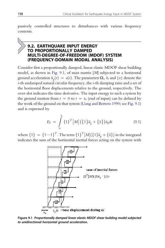
passively controlled structures to disturbances with various frequencycontents.

9.2. EARTHQUAKE INPUT ENERGYTO PROPORTIONALLY DAMPEDMULTI-DEGREE-OF-FREEDOM (MDOF) SYSTEM(FREQUENCY-DOMAIN MODAL ANALYSIS)

Consider first a proportionally damped, linear elastic MDOF shear buildingmodel, as shown in Fig. 9.1, of mass matrix [M] subjected to a horizontalground acceleration €ugðtÞ ¼ aðtÞ. The parameters Ui, hi and {x} denote thei-th undamped natural circular frequency, the i-th damping ratio and a set ofthe horizontal floor displacements relative to the ground, respectively. Theover-dot indicates the time derivative. The input energy to such a system bythe ground motion from t ¼ 0 to t ¼ t0 (end of input) can be defined bythe work of the ground on that system (Uang and Bertero 1990; see Fig. 9.1)and is expressed by

EI ¼Z t0

0

f1gT �M��1�€ug þ

�€x��

_ugdt (9.1)

where f1g ¼ f1/1gT . The term f1gT ½M �ðf1g€ug þ f€xgÞ in the integrandindicates the sum of the horizontal inertial forces acting on the system with

Figure 9.1 Proportionally damped linear elastic MDOF shear building model subjectedto unidirectional horizontal ground acceleration.

198 Critical Excitation for Earthquake Energy Input in MDOF System

minus sign. Double minus signs result in the positive sign. Integration byparts of Eq. (9.1) yields

EI ¼hð1=2Þf1gT ½M �f1g _u2g

it00þ �f _xgT �M��

1�_ug�t00�

Z t0

0

f _xgT �M�

��1�€ugdt

(9.2)

Assume that f _xg ¼ f0g at t ¼ 0 and _ug ¼ 0 at t ¼ 0 and t ¼ t0.Then the input energy EI can be reduced finally to the following form

EI ¼ �Z t0

0

f _xgT �M��1�€ugdt (9.3)

It is known that the input energy can also be expressed in the frequencydomain. Let f _Xg denote the Fourier transform of f _xg. Substitution of theFourier inverse transformation of the relative nodal velocities f _xg intoEq. (9.3) provides

EI ¼ � RN�N

"1

2p

ZN�N

�_X�Teiutdu

#½M �f1g€ugdt

¼ � 1

2p

ZN�N

�_X�T ½M �f1g

" ZN�N

€ugeiutdt

#du

¼ � 1

2p

ZN�N

�_X�T�

M��1�A�� u

�du

(9.4)

In Eq. (9.4), AðuÞ is the Fourier transform of €ugðtÞ ¼ aðtÞ and thesymbol i denotes the imaginary unit. Introduce the following coordinatetransformation

fxg ¼ ½F�fqg (9.5)

½F� is the modal matrix and fqg is defined by�q� ¼ �

/qi/�T

;

9.2. Earthquake Input Energy to Proportionally Damped Multi-Degree-of-Freedom (MDOF) 199

qi ¼Z t

0

�� €ugðsÞ�gi�t � s

�ds;

giðtÞ ¼ ð1=UDiÞexpð� hiUitÞ sinUDit;

UDi ¼ Ui

ffiffiffiffiffiffiffiffiffiffiffiffiffi1� h2i

qð9:6aedÞ

In Eqs. (9.6a–d), the parameters qi, giðtÞ and UDi denote the normalcoordinate, the unit impulse response function for under-damped vibrationand the i-th damped natural circular frequency, respectively. In the casewhere over-damped vibration modes appear, the corresponding unitimpulse response function has to be modified. This case will be explainedlater for nonproportionally damped models. The input energy can bederived as follows by substituting the coordinate transformationf _xg ¼ ½F�f_qg, its Fourier transform f _Xg ¼ ½F�f _Qg and the velocitytransfer relation f _Qg ¼ fHVgA into Eq. (9.4).

EI ¼ � 1

2p

ZN�N

fHVgT ½F�T ½M �f1gjAðuÞj2du

¼ �1

p

ZN0

fHVgT ½F�T ½M �f1gjAðuÞj2du

¼ RN0

FMPðuÞjAðuÞj2du

(9.7)

fHVg and FMPðuÞ in Eq. (9.7) are the velocity transfer function vector withrespect to base acceleration and the energy transfer function, respectively,and are expressed by�

HV

� ¼ f/HVi/gT ;HVi

�u ;Ui; hi

� ¼ �iu=�U2i� u2 þ 2ihiUiu

�;

FMPðuÞ ¼ �1

pRe

fHVgT ½F�T ½M �f1g

ð9:8aecÞ

The symbol Re½$� indicates the real part of a complex number.Eq. (9.7) implies that the earthquake input energy to damped, linear

elastic MDOF systems does not depend on the phase of input motions.


This fact is well known (Page 1952; Lyon 1975; Takizawa 1977; Ohi et al.1985; Kuwamura et al. 1994; Ordaz et al. 2003). A similar result has beenshown for SDOF models. It can be understood from Eq. (9.7) that theenergy transfer function FMPðuÞ plays a central role in the evaluation ofinput energy. Eq. (9.7) implies also that, if the envelope of the Fourieramplitude spectrum of input ground motions is available (Shinozuka 1970;Takewaki 2001a, b, 2002a, b), the upper bound of input energy can bederived directly from Eq. (9.7) by substituting that envelope function intojAðuÞj. This manipulation is completely valid because the functionFMPðuÞ is a non-negative function of frequency which can be proved byusing Eqs. (9.8b, c). Note that while an envelope of the Fourier amplitudespectrum of input ground motions has been considered in Shinozuka(1970), the critical shape of the Fourier amplitude spectrum or the powerspectrum density function has been treated and obtained in Takewaki(2001a, b, 2002a, b).

9.3. EARTHQUAKE INPUT ENERGY TONONPROPORTIONALLY DAMPED MDOF SYSTEM(FREQUENCY-DOMAIN MODAL ANALYSIS)

Consider next a nonproportionally damped, linear elastic shear buildingmodel. The state-space formulation in the frequency domain (Veletsos andVentura 1986) is effective and essential for deriving the earthquake inputenergy to nonproportionally damped systems via modal analysis.

Let ½M �; ½C�; ½K � denote the system mass, damping and stiffness matrices,respectively, of the nonproportionally damped system. The eigenvalueproblem in terms of the state space of the nonproportionally damped systemmay be stated as

ð½B� þ s½A�Þfzg ¼ f0g (9.9)

where ½A�, ½B� and fzg are defined by

½A� ¼" ½0� ½M �½M � ½C�

#; ½B� ¼

"�½M � ½0�½0� ½K �

#; fzg ¼

(sfjgfjg

)

ð9:10aecÞThe j-th eigenvalue and the corresponding j-th eigenvector for the

problem defined by Eq. (9.9) are denoted by sj; fjjg, respectively. Thefollowing quantities are defined.

9.3. Earthquake Input Energy to Nonproportionally Damped MDOF System 201

Mj ¼ fjjgT ½M �fjjg; Cj ¼ fjjgT ½C�fjjg; Lj ¼ fjjgT ½M �f1g;

Bj ¼ Lj=�2sjMj þCj

� ð9:11aedÞIn the case where eigenvalues are complex numbers, it is known that

those eigenvalues appear as a pair of complex conjugates. Assume here thatthere areNc pairs of complex conjugates and introduce the following vectorsfbng; fdng; fang.

fbng ¼ 2Re½Bnfjng�; fdng ¼ 2 Im½Bnfjng�;

fang ¼ hnfbng �ffiffiffiffiffiffiffiffiffiffiffiffiffiffiffiffiffiffiffiffiffiffi1� h2nfdng

q ð9:12aecÞ

In Eq. (9.12a–c), hn ¼ �Re½sn�=jsnj is the so-called n-th damping ratio.Im½$� in Eq. (9.12b) indicates the imaginary part of a complex number. Theso-called n-th circular eigenfrequency and the so-called n-th dampedcircular eigenfrequency may be defined by

Un ¼ jsnj; UDn ¼ Un

ffiffiffiffiffiffiffiffiffiffiffiffiffi1� h2n

q(9.13a, b)

The unit impulse response function for under-damped vibration hasbeen given in Eq. (9.6c) and is used now.

In the case where eigenvalues are real numbers, it is known that thoseeigenvalues appear as a pair. Assume now that there are Nr pairs of realeigenvalues.

Let sj; sk denote a pair of real eigenvalues of this model. Assume thatjsjjhjskj and define the following modal quantities in terms of sj; sk.

U�j ¼ ffiffiffiffiffiffi

sjskp

; h�j ¼ �ðsj þ skÞ=ð2 ffiffiffiffiffiffisjsk

p Þ;

U�Dj ¼ U�

j

ffiffiffiffiffiffiffiffiffiffiffiffiffiffiffih�2j � 1

q¼ ðsj � skÞ=2

ð9:14aecÞ

The vectors fbrjg; fdrjg; farjg related to real eigenvalues are defined by

fbrjg ¼ Bkfjkg þ Bjfjjg;

fdrjg ¼ Bkfjkg � Bjfjjg;

farjg ¼ h�j fbrjg �ffiffiffiffiffiffiffiffiffiffiffiffiffiffiffiffiffiffiffiffiffiffiffih�2j � 1fdrjg

qð9:15aecÞ


The unit impulse response function for over-damped vibration may bewritten as

grj ðtÞ ¼�1=U�

Dj

�exp

�� h�j U

�j t�sinh U�

Djt (9.16)

The response nodal displacements fxgmay then be expressed in terms offang;fbng; farjg; fbrjg, i.e. the combination of the under-damped modes andthe over-damped modes.

fxg ¼XNc

n¼ 1

�fan�UnqnðtÞ þ�bn�_qnðtÞ

�

þXNr

j¼ 1

nfarjgU�

j qrj ðtÞ þ fbrjg_qrj ðtÞ

o (9.17)

The quantities qnðtÞ; _qnðtÞ; qrj ðtÞ; _qrj ðtÞ in Eq. (9.17) are defined by

qnðtÞ ¼Z t

0

�� €ug�s��

gn�t � s

�ds;

_qnðtÞ ¼Z t

0

�� €ug�s��

_gn�t � s

�ds

(9.18a, b)

qrj ðtÞ ¼Z t

0

f� €ugðsÞggrj ðt � sÞds;

_qrj ðtÞ ¼Z t

0

f� €ugðsÞg_grj ðt � sÞds

(9.19a, b)

Let ½UV � denote a matrix consisting of vectors fangUn (for all n) and ½UA�denote a matrix consisting of vectors fbng (for all n). Furthermore let ½Ur

V �denote a matrix consisting of vectors farjgU�

j (for all j) and ½UrA� denote

a matrix consisting of vectors fbrjg (for all j) in view of the case for under-damped modes. After some manipulation, the Fourier transform Hr

VjðuÞof �_grj ðtÞ may be described as

9.3. Earthquake Input Energy to Nonproportionally Damped MDOF System 203

HrVjðuÞ ¼ 1

2U�Dj

nu2 � iuð� h�j U

�j � U�

DjÞu2 þ ð� h�j U

�j � U�

DjÞ2

� u2 � iuð� h�j U�j þ U�

DjÞu2 þ ð� h�j U

�j þ U�

DjÞ2) (9.20)

HrAjðuÞ for acceleration can then be evaluated by Hr

AjðuÞ ¼ iuHrVjðuÞ.

The time derivative of Eq. (9.17) provides

f _xg ¼XNc

n¼ 1

�fangUn _qnðtÞ þ�bn�€qnðtÞ

�

þXNr

j¼ 1

nfarjgU�

j _qrj ðtÞ þ fbrjg€qrj ðtÞ

o(9.21)

This can also be expressed in matrix form as�_x� ¼ �

UV

��_q�þ �

UA

��€q�þ �

UrV

��_qr�þ �

UrA

��€qr�

(9.22)

The input energy can be obtained by substituting Eq. (9.22), its Fouriertransform f _Xg ¼ ½UV �f _Qg þ ½UA�f €Qgþ½Ur

V �f _Qrgþ½Ur

A�f €Qrg, thevelocity and acceleration transfer relations f _Qg ¼ fHVgA,f €Qg ¼ fHAgA in under-damped vibration, the velocity and accelerationtransfer relations f _Q

rg ¼ fHrVgA, f €Qrg ¼ fHr

AgA in over-dampedvibration into Eq. (9.4).

EI ¼ZN0

FMNP

�u�jAðuÞj2du (9.23)

FMNPðuÞ in Eq. (9.23) is the energy transfer function for nonproportionallydamped models and is expressed by

FMNPðuÞ ¼ �1

pRe½ZðuÞ� (9.24a)

ZðuÞ ¼ fHV ðu ;Ui; hiÞgT ½UV �T ½M �½1g þ fHAðu ;Ui; hiÞgT ½UA�T ½M �f1g

þ�Hr

Vi

�u��

T�UrV

�T ½M �f1g þ �Hr

Ai

�u��T �

UrA

�T ½M �f1g(9.24b)


It should be remarked that, if the ground motion velocity _ug is recordedand available, the earthquake input energy can also be expressed in thefrequency domain by

EI ¼ZN0

u2FMNP

�u�jV ðuÞj2du (9.25)

V ðuÞ in Eq. (9.25) is the Fourier transform of the ground velocity _ug andis given by V ðuÞ ¼ AðuÞ=ðiuÞ in terms of the Fourier transform of groundacceleration.

9.4. EARTHQUAKE INPUT ENERGY WITHOUT MODALDECOMPOSITION

In order to examine the accuracy of the modal superposition method in thefrequency domain, another method has been developed without modaldecomposition. This method is applicable to both proportionally dampedand nonproportionally damped structures. Using the Fourier transformationof the equations of motion, the Fourier transform f _XðuÞg of the nodalvelocities can be expressed by�

_X�u�� ¼ �iu

�� u2�M�þ iu

�C�þ �

K��1�

M��1�A�u�

(9.26)

The input energy can then be computed by Eq. (9.4). The input energywithout modal decomposition may be evaluated by

EI ¼ZN0

FM�u�jAðuÞj2du (9.27)

FMðuÞ and ½YðuÞ� are defined by

FMðuÞ ¼ Re½iuf1gT ½M �T ½YðuÞ� ½M �f1g�=p (9.28a)

�Y�u�� ¼ �� u2

�M�þ iu

�C�þ �

K��1

(9.28b)

The computation of ½YðuÞ� ¼ ð�u2½M � þ iu½C� þ ½K �Þ�1 for manyfrequencies is quite time-consuming especially for structures with manydegrees of freedom. Therefore careful attention is necessary in the methodwithout modal decomposition.

9.4. Earthquake Input Energy without Modal Decomposition 205

9.5. EXAMPLES

Consider eight 6-degree-of-freedom shear building models shownin Fig. 9.2. Models A–F and BI (Base-Isolation) indicate nonpropor-tionally damped models and Model PD represents a proportionallydamped model. It is assumed that Models A–F represent models with anadded viscous damping system and Model BI represents a model witha base-isolation system. The constant floor masses are given bymi ¼ 32� 103ðkgÞði ¼ 1;/; 6Þ. The constant story stiffnesses are givenby ki ¼ 3:76� 107ðN=mÞði ¼ 1;/; 6Þ except the 1st story of Model BI(k1 ¼ 3:76� 105ðN=mÞ). Models A–F possess concentrated viscousdampers in the 1st through 6th story. For example, as for Model A,c1 ¼ 3:76� 106ðN$s=mÞ, ci ¼ 3:76� 105ðN$s=mÞðis1Þ. Model BI hasa concentrated viscous damper c1 ¼ 3:76� 106ðN$s=mÞ in the 1st storyand the other damping coefficients are ci ¼ 3:76� 105ðN$s=mÞðis1Þ. Model PD has a uniform damping coefficient distributionci ¼ 3:76� 105ðN$s=mÞ.

The undamped natural circular frequencies of Models A–F and ModelPD are the same and are given by 8.27(rad/s), 24.3(rad/s), 39.0(rad/s),51.3(rad/s), 60.7(rad/s) and 66.6(rad/s). Those of Model BI are given by1.39(rad/s), 17.9(rad/s), 34.3(rad/s), 48.5(rad/s), 59.4(rad/s) and 66.3(rad/s).The lowest-mode damping ratio of Model PD is about 0.04. All the modaldamping ratios for Models A–F, BI and PD are shown in Table 9.1. It can beseen that only one over-damped mode exists in every model. The effective

Figure 9.2 6-degree-of-freedom proportionally damped and nonproportionallydamped models.


location of added viscous dampers can be found from this analysis whichattains larger lowest-mode damping ratios. A more sophisticated mathe-matical treatment for the determination of effective added viscous damperlocation has been proposed by the present author (Takewaki 1997).A similar tendency, i.e. concentration of added viscous dampers in lowerstories in the model with uniform story stiffnesses, has been observed in theprevious study (Takewaki 1997).

Fig. 9.3 illustrates the function FMNPðuÞ for Models A–F, BI by use ofEq. (9.24) and FMPðuÞ for Model PD. The solid line shows the functionevaluated from the complex and real modes. On the other hand, thedotted line illustrates the function evaluated from the complex modesonly, i.e. the first two terms in Eq. (9.24b). It can be seen that the over-damped real modes play an important role in Models A, C and BI. Forexamining the accuracy of the present method via Eq. (9.24), the functionby means of Eq. (9.28) has been plotted. It was confirmed that the presentmethod via Eq. (9.24) is accurate enough to evaluate the functionFMNPðuÞ.

Fig. 9.4(a) shows the amplitude of the transfer function of the 1st-storydrift to the base acceleration for Models A and BI. Fig. 9.4(b) illustrates thecorresponding phase angle of the transfer function of the 1st-story drift tothe base acceleration for Models A and BI. It can be understood that theover-damped real modes also play an important role in Models A and BI forevaluating the interstory drift accurately. In order to confirm the accuracy ofFig. 9.4, the same figure has been drawn by Eq. (9.28b) without modaldecomposition. Sufficient accuracy has been confirmed by the methodincluding over-damped real modes.

Fig. 9.5 illustrates the function u2FMNPðuÞ for Models A–F, BI isdefined by Eqs. (9.25), (9.24a, b) and u2FMPðuÞ for Model PD given by

Table 9.1 Damping ratio for models A–F, BI and PD

Mode No. 1 2 3 4 5 6

Model A 0.126 0.192 1.52 0.248 0.298 0.331Model B 0.116 0.140 0.198 0.274 2.24 0.325Model C 0.0968 0.125 0.240 0.270 2.29 0.315Model D 0.0752 0.168 0.206 2.33 0.292 0.307Model E 0.0571 0.181 0.228 2.37 0.259 0.321Model F 0.0454 0.142 0.222 2.41 0.286 0.328Model BI 17.3 0.233 0.196 0.248 0.298 0.331Model PD 0.0413 0.122 0.195 0.257 0.304 0.333

9.5. Examples 207

Figure 9.3 Function FMNP (u) via Eq. (9.24) and FMPðuÞ for models A–F, BI and PD:complex plus real modes (solid line), complex mode only (dotted line).


Eq. (9.8). It can be seen that higher-mode effects become larger thanFMNPðuÞ and FMPðuÞ because squared frequencies are multiplied on theenergy transfer function.

It may be concluded from Figs. 9.3–9.5 that structures with passivecontrol systems in appropriate and effective location, especially Model BI,have relatively wide-band energy transfer functions and are quite robust forvarious disturbances with different frequency contents. In other words, if thearea (so-called acceleration power or Arias intensity) of the squared Fourier

Figure 9.4 (a) Transfer function amplitude of the 1st-story drift with respect to baseacceleration for models A and BI: complex plus real modes (solid line), complex modeonly (dotted line). (b) Phase angle of the transfer function of the 1st-story drift withrespect to base acceleration for models A and BI: complex plus real modes (solid line),complex mode only (dotted line).

9.5. Examples 209

Figure 9.5 Function u2FMNPðuÞ and u2FMPðuÞ for models A–F, BI and PD.


Figure 9.6 Recorded ground motions: El Centro NS (Imperial Valley 1940), KobeUniversity NS (Hyogoken-Nanbu 1995), SCT1 EW (Mexico Michoacan 1985), JMA KobeNS (Hyogoken-Nanbu 1995).

9.5. Examples 211

amplitude spectrum of input ground accelerations is the same, the inputenergy to structures with passive control systems in appropriate and effectivelocation is not affected much by the variability of the frequency contents ofthe input motion.

In order to examine the validity and accuracy of the present frequency-domain method, the earthquake input energy has been computed by boththe frequency-domain method and the time-domain method to fourrecorded ground motions shown in Fig. 9.6. The corresponding Fourieramplitude spectra of these ground motions are shown in Fig. 9.7. Thecomputed earthquake input energy is shown in Table 9.2. While severalpercent differences can be found in Models F and PD, reasonable accuracy

Figure 9.7 Fourier amplitude spectra of recorded ground motions: El Centro NS(Imperial Valley 1940), Kobe University NS (Hyogoken-Nanbu 1995), SCT1 EW (MexicoMichoacan 1985), JMA Kobe NS (Hyogoken-Nanbu 1995).


has been observed in other models. The cause of these discrepancies may bethe difference in the integration procedures.

The computation of the Fourier amplitude spectra of ground motions isnecessary only once even for different structural models. By using numericalintegration in the frequency domain, the input energy can be evaluated bycombining those with the energy transfer function. The energy transferfunction is computed for each model via efficient modal analysis explainedin this chapter. The structural designers can estimate approximate inputenergies from the relation of the Fourier amplitude spectra of groundmotions with the energy transfer functions both of which are expressed inthe frequency domain. With these data, it is not difficult to avoid resonance.

9.6. CRITICAL EXCITATION FOR EARTHQUAKE ENERGYINPUT IN MDOF SYSTEM

The following critical excitation problems may be stated for MDOFmodels.Find jAðuÞjthat maximizes EI ¼ RN

0 FMNPðuÞjAðuÞj2duFind jV ðuÞjthat maximizes EI ¼ RN

0 u2FMNPðuÞjV ðuÞj2duThe solution procedure developed for SDOF models in Chapter 8 can

be applied to these problems without difficulty. It suffices to replace the

Table 9.2 Earthquake input energy by frequency and time domain analysis for modelsA, C, F, BI and PD to four recorded ground motions (unit in J )

El CentroNS 1940

Kobe Univ.NS 1995

Mexico SCT1NS 1985

JMA KobeNS 1995

Model A F 1.37Eþ05 F 8.59Eþ04 F 4.21Eþ04 F 9.84Eþ05T 1.37Eþ05 T 8.52Eþ04 T 4.16Eþ04 T 9.99Eþ05

Model C F 1.46Eþ05 F 8.54Eþ04 F 3.89Eþ04 F 1.09Eþ06T 1.47Eþ05 T 8.57Eþ04 T 3.89Eþ04 T 1.13Eþ06

Model F F 1.18Eþ05 F 6.31Eþ04 F 2.91Eþ04 F 8.64Eþ05T 1.16Eþ05 T 6.56Eþ04 T 3.00Eþ04 T 9.25Eþ05

Model BI F 1.18Eþ05 F 1.09Eþ05 F 1.80Eþ05 F 7.22Eþ05T 1.17Eþ05 T 1.09Eþ05 T 1.79Eþ05 T 7.19Eþ05

Model PD(Prop. Damp.)

F 1.16Eþ05 F 5.96Eþ04 F 2.74Eþ04 F 8.24Eþ05T 1.13Eþ05 T 6.22Eþ04 T 2.83Eþ04 T 8.73Eþ05

(F: frequency domain, T: time domain)

9.6. Critical Excitation for Earthquake Energy Input in MDOF System 213

energy transfer function FðuÞ for SDOF models by FMNPðuÞ for MDOFmodels.

9.7. CONCLUSIONS

The conclusions may be stated as follows:(1) A method based on complex modal analysis can be developed in the

frequency domain for efficient computation of earthquake input energyto linear elastic passive control structures with high-level nonpropor-tional damping in general. It requires only the computation of theFourier amplitude spectrum of input ground motions and the derivationof velocity and acceleration-based energy transfer functions.

(2) Over-damped modes should not be neglected in highly damped passivecontrol structures. Neglect of the over-damped modes may causesignificant errors in some nonclassically damped models.

(3) When the upper bound of the Fourier amplitude spectrum of inputground accelerations is available, the formulation of earthquake inputenergy in the frequency domain is appropriate for deriving its bound.This is because the earthquake input energy in the frequency domaincan be derived as the frequency-domain integration of the product ofa non-negative time-invariant transfer function and the squared Fourieramplitude spectrum of the ground acceleration.

In this chapter, a structure with high-level damping has been treated inorder to demonstrate the importance of over-damped modes in thecomputation of earthquake input energy. Such over-damped modes areoften neglected in conventional modal analysis. The present formulation iscertainly applicable to general linear elastic structures including lightlydamped structures.

REFERENCESKuwamura, H., Kirino, Y., Akiyama, H., 1994. Prediction of earthquake energy input from

smoothed Fourier amplitude spectrum. Earthquake Engrg. and Struct. Dyn. 23 (10),1125–1137.

Lyon, R.H., 1975. Statistical Energy Analysis of Dynamical Systems. The MIT Press,Cambridge, MA.


Ordaz, M., Huerta, B., Reinoso, E., 2003. Exact computation of input-energy spectra fromFourier amplitude spectra. Earthquake Engrg. and Struct. Dyn. 32 (4), 597–605.

Page, C.H., 1952. Instantaneous power spectra. Journal of Applied Physics 23 (1), 103–106.


Shinozuka, M., 1970. Maximum structural response to seismic excitations. Journal ofEngineering Mechanics Division 96 (5), 729–738.

Takewaki, I., 1997. Optimal damper placement for minimum transfer functions. EarthquakeEngrg. and Struct. Dyn. 26 (11), 1113–1124.

Takewaki, I., 2001a. A new method for non-stationary random critical excitation.Earthquake Engrg. and Struct. Dyn. 30 (4), 519–535.

Takewaki, I., 2001b. Probabilistic critical excitation for MDOF elastic–plastic structures oncompliant ground. Earthquake Engrg. and Struct. Dyn. 30 (9), 1345–1360.



Takizawa, H., 1977. Energy-response spectrum of earthquake ground motions. In: Proc. ofthe 14th Natural Disaster Science Symposium. Hokkaido, pp. 359–362 (in Japanese).

Uang, C.-M., Bertero, V.V., 1990. Evaluation of seismic energy in structures. EarthquakeEngrg. and Struct. Dyn. 19 (1), 77–90.

Veletsos, A.S., Ventura, C.E., 1986. Modal analysis of non-classically damped linear systems.Earthquake Engrg. and Struct. Dyn. 14 (2), 217–243.


CHAPTER TEN

Critical Excitation for EarthquakeEnergy Input in Soil-StructureInteraction System

Contents

10.1. Introduction 21710.2. Earthquake Input Energy to Fixed-Base Single-Degree-of-Freedom (SDOF)

System220

10.3. Earthquake Input Energy to SSI Systems 22110.4. Actual Earthquake Input Energy to Fixed-Base Model and SSI System 23110.5. Critical Excitation for Earthquake Energy Input in SSI System 23910.6. Critical Excitation Problem 244

[Critical Excitation Problem 1a] 245[Critical Excitation Problem 1s] 246

10.7. Upper Bound of Fourier Amplitude Spectrum of Input 24610.8. Solution Procedure and Upper Bound of Input Energy 24710.9. Critical Excitation Problem for Velocity Constraints 248

[Critical Excitation Problem 2a] 249[Critical Excitation Problem 2s] 249

10.10. Solution Procedure for Velocity Constraint Problems 24910.11. Numerical Examples-1 (One-Story Model) 25110.12. Numerical Examples-2 (3-Story Model) 25810.13. Conclusions 261References 263

10.1. INTRODUCTION

Most previous devastating earthquakes indicate that while intensiveground motions are recorded around building structures, the damage tothose structures are not always serious. The selection of appropriate intensitymeasures (peak acceleration, peak velocity, input energy, Housner spectralintensity, Arias intensity (Arias 1970) etc.) of ground motions and soil-structure interaction (SSI) effects may be key factors to these arguments.The analysis of SSI effects is well established (e.g. Luco 1980; Cakmak et al.1982; Wolf 1985, 1988; Gupta and Trifunac 1991; Meek and Wolf 1994;Wolf 1994) and some computer programs can be used for SSI analysis of



http://dx.doi.org/10.1016/B978-0-08-099436-9.00010-9

complicated models. It is also true that while the analysis of SSI effects hasbeen focused on the investigation in terms of deformation and force, muchattention has never been directed to the investigation in terms of earthquakeinput energy to the SSI system. There are a few investigations on this subject(Yang and Akiyama 2000; Trifunac et al. 2001). The works by Yang andAkiyama (2000) and Trifunac et al. (2001) are based on an approach in thetime domain.

The purpose of this chapter is to explain a new evaluation method ofearthquake input energy to SSI systems. The method is an approach in thefrequency domain. Because the inertial interaction (foundation impedance)and the kinematic interaction (effective input motion) are well described byfrequency-dependent functions, the present approach based on thefrequency domain analysis is appropriate and effective. In particular, it isdemonstrated that even SSI systems including embedded foundations can betreated in a simple way and the effects of the foundation embedment on theearthquake input energies to the super-structure and to the structure-foundation-soil system can be clarified systematically.

Earthquake ground motions involve a lot of uncertain factors in themodeling of various aspects and it does not appear easy to predict forth-coming events precisely at a specific site both in time and frequency (forexample, Abrahamson et al. 1998). Some of the uncertainties may resultfrom lack of information due to the low occurrence rate of large earthquakesand it does not seem that this problem can be resolved in the near future. Inparticular, the modeling of near-fault ground motions involves variousuncertain factors in contrast to far-fault ground motions (Singh 1984).

It is therefore strongly desirable to develop a robust structural designmethod taking into account these uncertainties, and with limited informa-tion enabling the design of safer structures for a broader class of designearthquake (Drenick 1970; Shinozuka 1970; Takewaki 2001a, b, 2002a, b).It will be shown briefly in this chapter that the formulation of earthquakeinput energy in the frequency domain is effective for solving a criticalexcitation problem and deriving a bound on the earthquake input energy fora class of properly scaled ground motions.

Fig. 10.1 shows a schematic diagram of energy flow in SSI systems. It willbe discussed in this chapter that the work by boundary forces on theircorresponding displacements defined for various boundaries are utilized inevaluating the energy flow in SSI systems. Fig. 10.2 indicates (a) the free-body including a structure and its surrounding ground, (b) the free-bodyincluding the structure alone. These free-body diagrams are very useful in

218 Critical Excitation for Earthquake Energy Input in Soil-Structure Interaction System

understanding the energy flow in SSI systems. The time histories of earth-quake input energies to these subassemblages are shown in Fig. 10.3 for ElCentro NS, Imperial Valley 1940 and Kobe University NS, Hyogoken-Nanbu 1995.

Figure 10.1 Schematic diagram of energy flow in SSI system.

(a) (b)

....

–m(ug + uF +θF h +u).. .. .. ..

–m(ug + uF +θF h +u).. .. .. ..

θ

..

–m0 (ug + uF)

–

Figure 10.2 (a) Free-body including structure and surrounding ground; (b) free-bodyincluding structure alone.

0

5000

1 104

1.5 104

2 104

2.5 104

3 104

0 5 10 15 20

overallstructure

inpu

t ene

rgy

(J)

time (s)

Kobe University NS 1995T=0.5(s), h=0.05, Vs=100(m/s)

AIE

SIE

0

1 104

2 104

3 104

4 104

5 104

6 104

0 10 20 30 40

overallstructure

inpu

t ene

rgy

(J)

time (s)

El Centro NS 1940T=0.5(s), h=0.05, Vs=50(m/s)

AIE

SIE

Figure 10.3 Time histories of earthquake input energies to these subassemblages.

10.1. Introduction 219

10.2. EARTHQUAKE INPUT ENERGY TO FIXED-BASESINGLE-DEGREE-OF-FREEDOM (SDOF) SYSTEM

A lot of work has been accumulated on the topics of earthquake inputenergy (for example, Tanabashi 1935; Housner 1956, 1959; Berg andThomaides 1960; Housner and Jennings 1975; Kato and Akiyama 1975;Takizawa 1977; Mahin and Lin 1983; Zahrah and Hall 1984; Akiyama1985; Ohi et al. 1985; Uang and Bertero 1990; Leger and Dussault 1992;Kuwamura et al. 1994; Fajfar and Vidic 1994; Riddell and Garcia 2001;Ordaz et al. 2003). In contrast to most of the previous work, the earthquakeinput energy is formulated here in the frequency domain (Page 1952; Lyon1975, Takizawa 1977; Ohi et al. 1985; Ordaz et al. 2003) to facilitate boththe derivation of bound of earthquake input energy and the formulation ofdynamic soil-structure interaction in terms of kinematic and inertial effects.For later comparison between the fixed-base model and the SSI system, theformulation for the fixed-base model is presented first.

Consider a damped linear elastic SDOF system of mass m, stiffness k anddamping coefficient c. Let U ¼ ffiffiffiffiffiffiffiffi

k=mp

, and x denote the undamped naturalcircular frequency of the SDOF system, the damping ratio and thedisplacement of the mass relative to the ground, respectively. Time deriv-ative is denoted by an over-dot. The input energy to the SDOF system bya unidirectional horizontal ground acceleration €ugðtÞ ¼ aðtÞ from t ¼ 0 tot ¼ t0 (end of input) can be defined by the work on the ground made to thestructural system and is expressed by

EI ¼Zt00

mð€ug þ €xÞ _ugdt (10.1)

The term mð€ug þ €xÞ indicates the inertial force (although �mð€ug þ €xÞ isthe exact inertial force) and is equal to the sum of the restoring force kx andthe damping force c _x in the system. Integration by parts of Eq. (10.1)provides

EI ¼ Rt00

mð€xþ €ugÞ _ugdt ¼Rt00

m€x _ugdt þ ½ð1=2Þm _u2g �t00

¼ ½m _x _ug�t00 � Rt00

m _x€ugdt þ ½ð1=2Þm _u2g �t00(10.2)

If _x ¼ 0 at t ¼ 0 and _ug ¼ 0 at t ¼ 0 and t ¼ t0, the input energy canbe reduced to the following form.


EI ¼ �Zt00

m€ug _xdt (10.3)

It is known (Page 1952; Lyon 1975; Takizawa 1977; Ohi et al. 1985;Ordaz et al. 2003) that the input energy per unit mass can also be expressedin the frequency domain by use of Fourier transformation so far as the systemis linear elastic.

EI=m ¼ �ZN

�N

_xadt ¼ �ZN

�N

"ð1=2pÞ

ZN�N

_Xeiutdu

#adt

¼ �ð1=2pÞZN

�N

Að�uÞfHV ðu ;U; xÞAðuÞgdu

¼ZN0

jAðuÞj2f�Re½HV ðu ;U; xÞ�=pgdu

h

ZN0

jAðuÞj2FðuÞdu

(10.4)

where HV ðu ;U; xÞ is the transfer function defined by_XðuÞ ¼ HV ðu ;U; xÞAðuÞ and FðuÞ ¼ �Re½HV ðu ;U; xÞ�=p. Re½$�denotes a real part of a complex number. _X and AðuÞ are the Fourier trans-forms of _x and €ugðtÞ ¼ aðtÞ, respectively. The symbol i denotes the imaginaryunit. The velocity transfer function HV ðu ;U; xÞ can be expressed by

HV ðu ;U; xÞ ¼ �iu=ðU2 � u2 þ 2ixUuÞ (10.5)

Eq. (10.4) indicates that the earthquake input energy to damped linearelastic SDOF systems does not depend on the phase of input motions andthis fact is well known (Page 1952; Lyon 1975; Takizawa 1977; Ohi et al.1985; Kuwamura et al. 1994; Ordaz et al. 2003).

10.3. EARTHQUAKE INPUT ENERGY TO SSI SYSTEMS

Consider a linear elastic SDOF super-structure of story stiffness k andstory damping coefficient c, as shown in Fig. 10.4, with a cylindrical rigid

10.3. Earthquake Input Energy to SSI Systems 221

foundation embedded in the uniform half-space ground. Let r0 and e denotethe radius and the depth of the foundation, respectively. Letm and IR denotethe mass of the super-structure and the mass moment of inertia of the super-structure and let m0 and IR0 denote the mass of the embedded foundationand the mass moment of inertia of the embedded foundation “around its topcenter node.” The height of the super-structure mass from the groundsurface is denoted by h.

U�0 and Q�

0 are the horizontal and rotational effective input motions inthe frequency domain at the top center of the foundation. The corre-sponding effective input motions in the time domain may be expressed by

€u�0ðtÞ ¼ 1

2p

ZN�N

€U�0ðuÞeiutdu ¼ 1

2p

ZN�N

SHT ðuÞ €UgðuÞeiutdu (10.6a)

€q�0ðtÞ ¼ 1

2p

ZN�N

€Q�0ðuÞeiutdu ¼ 1

2p

ZN�N

SRT ðuÞ €UgðuÞeiutdu

(10.6b)

SHT ðuÞ and SRT ðuÞ are the ratios of the horizontal and rotationaleffective input motions, U�

0 and Q�0, in the frequency domain at the top

center of the foundation to the Fourier transform UgðuÞ of the free-fieldhorizontal ground-surface displacement. Assume that a vertically incidentshear wave (SH wave) is considered. SHT ðuÞ and SRT ðuÞ are expressed interms of the ratios SHBðuÞ and SRBðuÞ, given in Meek andWolf (1994) andWolf (1994), of the horizontal and rotational (�r0) effective input motionsin the frequency domain at the bottom center of the foundation to UgðuÞ.

m

k

c

( )gu t

RI

0RI

0m

h

0r

*HHk *

HRk *RRk*

RHk

*RHc *

RRc*HRc*

HHc

e

Figure 10.4 SDOF structure with embedded foundation and its modeling for analysis.


SHT ðuÞ ¼ SHBðuÞ þ ðe=r0ÞSRBðuÞ (10.7a)

SRT ðuÞ ¼ ð1=r0ÞSRBðuÞ (10.7b)

Let U , UT , QT denote the Fourier transform of the horizontaldisplacement u of the super-structural mass relative to the foundationwithout rocking component, the Fourier transform of the horizontaldisplacement uT of the top center node of the foundation relative to u�0 andthe Fourier transform of the angle of rotation qT of the foundation relativeto q�0, respectively (see Fig. 10.5). The set of these components is denoted byU ¼ fU UT QT gT . The Fourier transforms of the force and momentcorresponding to UT and QT are expressed by PT and MT . €UgðuÞ denotesthe Fourier transform of the free-field horizontal ground-surfaceacceleration.

The equations of motion in the frequency domain of the SDOF super-structure supported by the embedded rigid foundation and subjected to theeffective input motions €U

�0ð¼ �u2U�

0 ¼ SHT ðuÞ €UgðuÞÞ and€Q�0ð¼ �u2Q�

0 ¼ SRT ðuÞ €UgðuÞÞ may be written as

f�u2Mþ iu½CS þ CFðuÞ� þ ½KS þ KFðuÞ�gUðuÞ¼ �Mfr1SHT ðuÞ þ r2SRT ðuÞg €UgðuÞ (10.8)

*0U

gU

*0ΘTΘ

TU

*0( )

HT g

U

S U

=

*0( )RT gS U = Θ

0(1/ ) RB gr S U

HB gS U

massless rigid

embedment

(a) (b)

(c)

*0U

gU

*0ΘTΘ

TU

*0( )

HT g

U

S U

=

*0( )RT gS U = Θ

0(1/ ) RB gr S U

HB gS U

massless rigid

embedment

Figure 10.5 (a) Horizontal effective foundation input motion and relative displace-ment; (b) rotational effective foundation input motion and relative angle of rotation;(c) effective foundation input motion at the top center and bottom center of thefoundation.


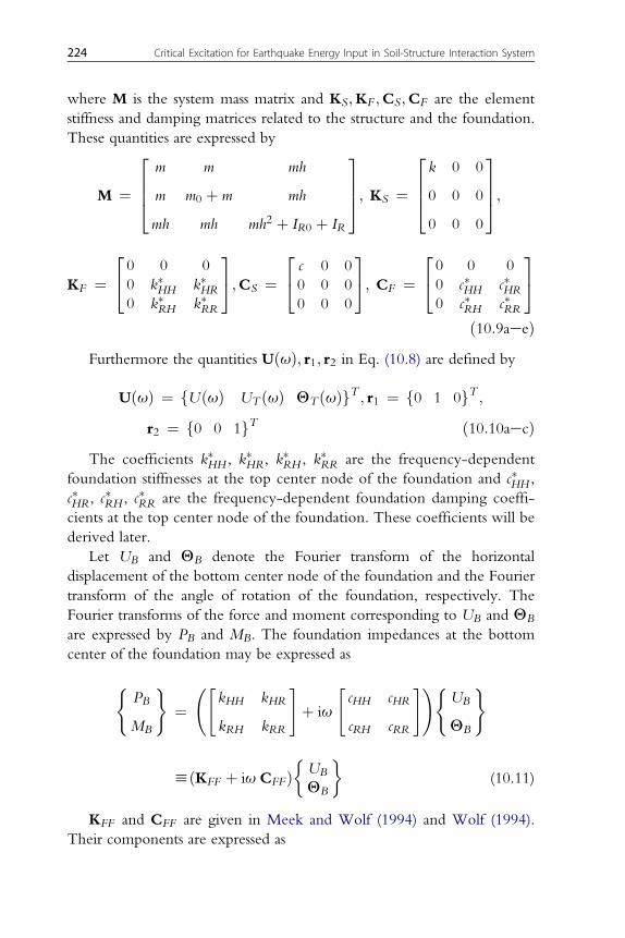
where M is the system mass matrix and KS;KF ;CS;CF are the elementstiffness and damping matrices related to the structure and the foundation.These quantities are expressed by

M ¼

2664

m m mh

m m0 þ m mh

mh mh mh2 þ IR0 þ IR

3775; KS ¼

2664k 0 0

0 0 0

0 0 0

3775;

KF ¼24 0 0 0

0 k�HH k�HR

0 k�RH k�RR

35;CS ¼

24 c 0 0

0 0 0

0 0 0

35; CF ¼

24 0 0 0

0 c�HH c�HR

0 c�RH c�RR

35

ð10:9aeeÞFurthermore the quantities UðuÞ; r1; r2 in Eq. (10.8) are defined by

UðuÞ ¼ fUðuÞ UT ðuÞ QT ðuÞgT ; r1 ¼ f0 1 0gT ;r2 ¼ f0 0 1gT ð10:10aecÞ

The coefficients k�HH , k�HR, k

�RH , k

�RR are the frequency-dependent

foundation stiffnesses at the top center node of the foundation and c�HH ,c�HR, c

�RH , c

�RR are the frequency-dependent foundation damping coeffi-

cients at the top center node of the foundation. These coefficients will bederived later.

Let UB and QB denote the Fourier transform of the horizontaldisplacement of the bottom center node of the foundation and the Fouriertransform of the angle of rotation of the foundation, respectively. TheFourier transforms of the force and moment corresponding to UB and QB

are expressed by PB and MB. The foundation impedances at the bottomcenter of the foundation may be expressed as

(PB

MB

)¼ "

kHH kHR

kRH kRR

#þ iu

"cHH cHR

cRH cRR

#!(UB

QB

)

hðKFF þ iu CFFÞ�UB

QB

�(10.11)

KFF and CFF are given in Meek and Wolf (1994) and Wolf (1994).Their components are expressed as


kHHðuÞ þ iu cHHðuÞ ¼ 8rVS2r0

2� n

�1þ e

r0

��kHða0Þ þ ia0cHða0Þg

(10.12a)

kRRðuÞ þ iu cRRðuÞ ¼ 8rVS2r0

3

3ð1� nÞ�1þ 2:3

�e

r0

�þ 0:58

�e

r0

�3�

��kRða0Þ þ ia0cRða0Þg (10.12b)

kHRðuÞ ¼ kRHðuÞ ¼ e

3kHHðuÞ (10.12c)

cHRðuÞ ¼ cRHðuÞ ¼ e

3cHHðuÞ (10.12d)

where r; VS; n are the soil mass density, the ground shear wave velocityand the Poisson’s ratio of soil and a0 ¼ ur0=VS is the nondimensionalfrequency. The nondimensional parameters in Eqs. (10.12a, b) are givenapproximately as follows for various nondimensional depths of embedment:kHða0Þ ¼ 1:0 for e=r0 ¼ 0:0; 0:5; 1:0; 2:0; cHða0Þ ¼ 0.6, 1.05, 1.3,1.75 for e=r0 ¼ 0:0; 0:5; 1:0; 2:0, respectively; kRða0Þ and cRða0Þ areshown in Takewaki et al. (2003).

The stiffness and damping coefficients in Eq. (10.9) may be derived asfollows. The displacements of the node at the top center of the foundationare related to those at the bottom center (see Fig. 10.6). This relation may beexpressed by(

UT

QT

)¼"1 e

0 1

#(UB

QB

)hT

(UB

QB

);

(UB

QB

)¼ T�1

(UT

QT

)

(10.13a, b)

The inverse of the coefficient matrix T can be expressed as

T�1 ¼"1 �e

0 1

#hT� (10.14)

The nodal force and moment at the top center of the foundation can beexpressed in terms of those at the bottom center.(

PT

MT

)¼"

1 0

�e 1

#(PB

MB

)hT�T

(PB

MB

)(10.15)


Substitution of Eqs. (10.11), (10.13b), (10.14) into Eq. (10.15) provides(PT

MT

)¼ ðT�TKFFT

� þ iuT�TCFFT�Þ(

UT

QT

)

h

��k�HH k�HR

k�RH k�RR

þ iu

�c�HH c�HR

c�RH c�RR

��UT

QT

�(10.16)

The solution of Eq. (10.8) leads to the following expression.

UðuÞ€UgðuÞ

¼ �f�u2Mþ iu ðCS þ CFÞ þ ðKS þ KFÞg�1Mfr1SHT ðuÞ

þ r2SRT ðuÞg(10.17)

Consider the earthquake input energy to the present model. Theearthquake input energy EA

I to the structure including the foundation massmay be obtained by considering the work by the forces acting just below thefoundation mass on the foundation displacements (see Fig. 10.7(a)).

BU

TU ( )T TMΘ

BΘ ( )BM

( )BP

embedded basement( )TP

(a) (b)

Figure 10.6 (a) Horizontal displacement and angle of rotation of the bottom of thefoundation; (b) horizontal displacement and angle of rotation of the top of thefoundation.

EAI ¼

ZN0

½m0ð€u�0 þ €uT Þ þ mf€u�0 þ €uT þ hð€q�0 þ €qT Þ þ €ug�ð _u�0 þ _uT Þdt

þZN0

½ðIR0 þ IRÞð€q�0 þ €qT Þ þ mhf€u�0 þ €uT þ hð€q�0 þ €qT Þ þ €ug�


� ð _q�0 þ _qT Þdt ¼ 1

2p

ZN�N

iu

�m0fSHT ðuÞ þH €UT ðuÞg

þ mfSHT ðuÞ þH €UT ðuÞ þ hfSRT ðuÞ þH €QTðuÞg þH €UðuÞg

$

fSHT ð�uÞ þH €UT ð�uÞg €UgðuÞ2du

þ 1

2p

ZN�N

iu½ðIR0 þ IRÞfSRT ðuÞ þH €QT

ðuÞg þ mhfSHT ðuÞ

þH €UT ðuÞ þ hfSRT ðuÞ þH €QTðuÞg þH €UðuÞg�$

fSRT ð�uÞ þH €QTð�uÞg €UgðuÞ

2du(10.18)

where the transfer functions H €U ðuÞ;H €UT ðuÞ;H €QTðuÞ are the ratios of

€UðuÞ; €UT ðuÞ; €QT ðuÞ to €UgðuÞ obtained from Eq. (10.17). In Eq. (10.18),the Fourier inverse transformation of accelerations and velocities are used.The terms SHT ð�uÞ, H €UT ð�uÞ, SRT ð�uÞ and H €QT

ð�uÞ in Eq. (10.18)result from the Fourier transformation of the corresponding time-domainquantities. The treatment of these quantities will be discussed after Eq.(10.20). When the term _u�0 þ _uT in the first line of Eq. (10.18) is replaced by_ug and the second line term is neglected, the resulting energy indicates theearthquake input energy EA�

I to the structure-foundation system includingthe soil springs and dashpots (see Fig. 10.7(b)).

EA�I ¼ RN

0

½m0ð€u�0 þ €uT Þ þ mf€u�0 þ €uT þ hð€q�0 þ €qT Þ þ €ug� _ugdt

¼ 1

2p

ZN�N

iu½m0fSHT ðuÞ þH €UT ðuÞg

þ mfSHT ðuÞ þH €UT ðuÞ þ hfSRT ðuÞ þH €QTðuÞg þH €U ðuÞg�$


(10.19)

In a similar way, the earthquake input energy ESI to the structure may be

obtained by considering the work by the forces acting just above thefoundation mass on the foundation displacements (see Fig. 10.7(c)).


Figure 10.7 Earthquake input energy (a) to structure-foundation system, (b) tostructure-foundation-soil system, (c) to structure alone.

ESI ¼

ZN0

mf€u�0 þ €uT þ hð€q�0 þ €qT Þ þ €ugð _u�0 þ _uT Þdt

þZN0

½IRð€q�0 þ €qT Þ þ mhf€u�0 þ €uT þ hð€q�0 þ €qT Þ þ €ug�ð _q�0 þ _qT Þdt

¼ 1

2p

ZN�N

ium½SHT ðuÞ þH €UT ðuÞ þ hfSRT ðuÞ

þH €QTðuÞg þH €U ðuÞ�$



þ 1

2p

ZN�N

iu½IRfSRT ðuÞ þH €QT

ðuÞg

þ mhfSHT ðuÞ þH €UT ðuÞ þ hfSRT ðuÞ þH €QTðuÞg þH €U ðuÞg�$

fSRT ð�uÞ þH €QTð�uÞg €UgðuÞ

2du(10.20)

It should be noted that, from Eqs. (10.6a, b) and the property of time-histories as sets of real numbers, SHT ð�uÞ and SRT ð�uÞ can becomputed as the complex conjugate pairs S�HT ðuÞ and S�RT ðuÞ of SHT ðuÞand SRT ðuÞ, and H €UT ð�uÞ and H €QT

ð�uÞ can be computed as thecomplex conjugate pairs H�

€UTðuÞ andH�

€QTðuÞ ofH €UT ðuÞ andH €QT

ðuÞ. Itshould also be pointed out that EA

I is equal to ESI exactly because, as the time

approaches infinity, the kinetic energy of the foundation mass becomes zerodue to the existence of damping in the system. This can be proved by thefollowing manipulation.

EAI ¼

ZN0

½m0ð€u�0 þ €uT Þ þ mf€u�0 þ €uT þ hð€q�0 þ €qT Þ þ €ug�ð _u�0 þ _uT Þdt

þZN0

½ðIR0 þ IRÞð€q�0 þ €qT Þ þ mhf€u�0 þ €uT þ hð€q�0 þ €qT Þ þ €ug�$

ð _q�0 þ _qT Þdt¼ ½ð1=2Þm0ð _u�0 þ _uT Þ2�N0 þ ½ð1=2ÞIR0ð _q�0 þ _qT Þ2�N0

þZN0

mf€u�0 þ €uT þ hð€q�0 þ €qT Þ þ €ugð _u�0 þ _uT Þdt

þZN0

½IRð€q�0 þ €qT Þ þ mhf€u�0 þ €uT þ hð€q�0 þ €qT Þ þ €ug�ð _q�0 þ _qT Þdt

¼ ESI

(10.21)


This fact will be confirmed in the numerical examples shown later.Eqs. (10.18), (10.19) and (10.20) can also be expressed compactly by

EAI ¼

ZN0

FAðuÞ €UgðuÞ

2du (10.22a)

EA�I ¼

ZN0

F�AðuÞ

€UgðuÞ2du (10.22b)

ESI ¼

ZN0

FSðuÞ €UgðuÞ

2du (10.22c)

where FAðuÞ and FSðuÞ are the following energy transfer functions:

FAðuÞ ¼ � 1

puIm½½m0fSHT ðuÞ þH €UT ðuÞg þ mfSHT ðuÞ þH €UT ðuÞ

þ hðSRT ðuÞ þH €QTðuÞÞ þH €U ðuÞg�$fS�HT ðuÞ þH�

€UTðuÞg�

� 1

puIm½½ðIR0 þ IRÞfSRT ðuÞ þH €QT

ðuÞg þ mhfSHT ðuÞþH €UT ðuÞ þ hðSRT ðuÞ þH €QT

ðuÞÞ þH €UðuÞg�$fS�RT ðuÞþH�

€QTðuÞg�

(10.23a)

F�AðuÞ ¼ � 1

puIm½m0fSHT ðuÞ þH €UT ðuÞg þ mfSHT ðuÞ þH €UT ðuÞ

þ hðSRT ðuÞ þH €QTðuÞÞ þH €U ðuÞg�

(10.23b)

FSðuÞ ¼ � 1

puIm½m½SHT ðuÞ þH €UT ðuÞ þ hðSRT ðuÞ þH €QT

ðuÞÞ

þH €U ðuÞ�$fS�HT ðuÞ þH�€UT

ðuÞg� � 1

puIm½½IRfSRT ðuÞ

þH €QTðuÞg þ mhfSHT ðuÞ þH €UT ðuÞ þ hðSRT ðuÞ

þH €QTðuÞÞ þH €U ðuÞg�$fS�RT ðuÞ þH�

€QTðuÞg�

(10.23c)


Eqs. (10.22a–c) imply that, if the energy transfer functions FAðuÞ, F�AðuÞ

and FSðuÞ are calculated for everymodel as a function of excitation frequency,the corresponding critical excitation problem for the maximum input energyunder the constraint

RN�N €ugðtÞ2dt ¼ð1=pÞ RN0 j €UgðuÞj2du ¼ CA on

acceleration can be stated and the Dirac delta function or the rectangularfunction of j €UgðuÞj can be found to be the critical input maximizing the inputenergy to the overall system and the structure (Takewaki 2002a, 2004).

Another constraintRN�N _ugðtÞ2dt ¼ ð1=pÞ RN0 j _UgðuÞj2du ¼ CV on

velocity may be an appropriate constraint in the longer natural period rangeof SSI systems (Tanabashi 1956; Housner and Jennings 1975; Trifunac et al.2001). The corresponding critical excitation problem will be discussedelsewhere.

10.4. ACTUAL EARTHQUAKE INPUT ENERGY TO FIXED-BASE MODEL AND SSI SYSTEM

In order to examine the effect of degree of embedment of the foundation onthe earthquake input energy to the structure under soil-structure interactionenvironment, the earthquake input energies to the corresponding fixed-basemodel and to the sway-rocking model have been computed by the proposedfrequency domain method. Four recorded ground motions, shown inFig. 10.8, are taken as the input motions. The corresponding Fourieramplitude spectra j €UgðuÞj of these ground motion accelerations are shownin Fig. 10.9.

Four cases of embedment e=r0 ¼ 0.0, 0.5, 1.0, 2.0 are considered andthree cases of equivalent ground shear velocity VS ¼ 50, 100, 200(m/s)are treated. It should be noted that the rather small ground shear wavevelocity VS ¼ 50(m/s) is not necessarily unrealistic if the dependence ofground shear wave velocity on the experienced shear strain level isconsidered. In fact, this low shear wave velocity represents an “equivalentquantity” evaluated for a rather high seismic input. The present authorclarified that, under such intense seismic input, the equivalent shear wavevelocity could become 10–20% of the initial one for a low strain level. Itis also confirmed in some case studies that, even under such intense input,effective shear strains are smaller than 1% and no liquefaction occurs. It isthe case in some areas near bays that a very soft ground exists and theinvestigation on the effect of such soft ground on the partially embeddedstructures is urgently required. It should be remarked that the analysis of

10.4. Actual Earthquake Input Energy to Fixed-Base Model and SSI System 231

extreme or limit states is inevitable for the reliable design of foundationsand building structures.

The other given parameters are as follows: r0 ¼ 5ðmÞ,m ¼ 62:8� 103ðkgÞ, IR ¼ 5:23� 105ðkg$m2Þ, h ¼ 4ðmÞ, k ¼ U2m,c ¼ ð2x=UÞk, r ¼ 1:8� 103ðkg=m3Þ, n ¼ 0:25, the damping ratio of thesuper-structure x ¼ 0:05. The fundamental natural period of the fixed-basesuper-structure T is varied and U ¼ 2p=T . The foundation mass m0 andmass moment of inertia IR0 are varied as the depth of embedment is changed;m0 ¼ 1:88� 105ðkgÞ for e=r0 ¼ 0,m0 ¼ 2:52� 105ðkgÞ for e=r0 ¼ 0:5,m0 ¼ 3:60� 105ðkgÞ for e=r0 ¼ 1:0, m0 ¼ 6:48� 105ðkgÞ for

- 0. 4

- 0. 2

0

0. 2

0. 4

0 10 20 30 40 50 60

El Centro NS 1940

acce

lera

tion

(g)

time (s)

- 0. 4

- 0. 2

0

0. 2

0. 4

0 10 20 30 40 50

Kobe Univ. NS 1995

acce

lera

tion

(g)

time (s)

- 0. 2

- 0. 1

0

0. 1

0. 2

0 30 60 90 120 150 180

Mexico SCT1 EW 1985

time (s)

acce

lera

tion

(g)

- 0. 8

- 0. 4

0

0. 4

0. 8

0 5 10 15 20 25 30

JMA Kobe NS 1995

acce

lera

tion

(g)

time (s)

Figure 10.8 Recorded ground motions: El Centro NS (Imperial Valley 1940), KobeUniversity NS (Hyogoken-Nanbu 1995), SCT1 EW (Mexico Michoacan 1985), JMA KobeNS (Hyogoken-Nanbu 1995).


e=r0 ¼ 2:0; IR0 ¼ 1:57� 106ðkg$m2Þ for e=r0 ¼ 0, IR0 ¼ 2:62� 106

ðkg$m2Þ for e=r0 ¼ 0:5, IR0 ¼ 6:00� 106ðkg$m2Þ for e=r0¼ 1:0,IR0 ¼ 2:70� 107ðkg$m2Þ for e=r0 ¼ 2:0. The foundationmassm0 has beencalculated by adding the mass of the basement to the ground floor mass.Therefore m0 is not proportional to the degree of embedment e=r0.

Fig. 10.10 illustrates the earthquake input energies to the fixed-basemodel EI and the sway-rocking models ES

I (structure only) with variousdegrees of embedment for El Centro NS (Imperial Valley 1940) plottedwith respect to the natural period T of the super-structure. It can beobserved that the input energy to the sway-rocking model withoutembedment may be almost the same as that for the fixed-base model. Therotational degree is considered in the sway-rocking model, but the

0

0.5

1

1.5

2

2.5

3

0 20 40 60 80 100 120 140 160

El Centro NS 1940Fo

urie

r am

plitu

de o

f acc

eler

atio

n (m

/s)

frequency (rad/s)

0

0.5

1

1.5

2

2.5

3

3.5

0 10 20 30 40 50 60 70 80

KBU NS 1995

Four

ier a

mpl

itude

of a

ccel

erat

ion

(m/s

)

frequency (rad/s)

0

2

4

6

8

10

12

14

0 5 10 15 20 25 30 35 40

Mexico SCT1 EW 1985

Four

ier a

mpl

itude

of a

ccel

erat

ion

(m/s

)

frequency (rad/s)

0

1

2

3

4

5

6

0 10 20 30 40 50 60 70 80

JMA Kobe NS 1995Fo

urie

r am

plitu

de o

f acc

eler

atio

n (m

/s)

frequency (rad/s)

Figure 10.9 Fourier amplitude spectra of recorded ground motions: El Centro NS(Imperial Valley 1940), Kobe University NS (Hyogoken-Nanbu 1995), SCT1 EW (MexicoMichoacan 1985), JMA Kobe NS (Hyogoken-Nanbu 1995).


0

2 104

4 104

6 104

8 104

1 105

0 1 2 3 4 5

fixed-basee/r0=0e/r0=0.5e/r0=1.0e/r0=2.0

actu

al in

put e

nerg

y (J

)

natural period (s)

Vs=50(m/s)

0

2 104

4 104

6 104

8 104

1 105

0 0.2 0.4 0.6 0.8 1


actu

al in

put e

nerg

y (J

)natural period (s)

Vs=50(m/s)

0

2 104

4 104

6 104

8 104

1 105

0 1 2 3 4 5


actu

al in

put e

nerg

y (J

)

natural period (s)

Vs=100(m/s)

0

2 104

4 104

6 104

8 104

1 105

0 0.2 0.4 0.6 0.8 1


actu

al in

put e

nerg

y (J

)

natural period (s)

Vs=100(m/s)

0

2 104

4 104

6 104

8 104

1 105

0 1 2 3 4 5


actu

al in

put e

nerg

y (J

)

natural period (s)

Vs=200(m/s)

0

2 104

4 104

6 104

8 104

1 105

0 0.2 0.4 0.6 0.8 1


actu

al in

put e

nerg

y (J

)

natural period (s)

Vs=200(m/s)

Figure 10.10 Earthquake input energy to the structure with various degrees of foun-dation embedment for ground equivalent shear velocities 50, 100, 200(m/s) to El CentroNS of Imperial Valley 1940 (magnified figures are shown on the right-hand side).


soil-structure interaction effect on the input energy is rather small in thiscase. On the other hand, as the degree of embedment becomes larger, theinput energy is decreased regardless of the natural period range. Thisphenomenon may be one of the reasons that, while intensive groundmotions are recorded around building structures, the damage to thosestructures is not always serious.

Figs. 10.11–10.13 show the earthquake input energies to the fixed-basemodel EI and the sway-rocking models ES

I with various degrees ofembedment for Kobe University NS (Hyogoken-Nanbu 1995), SCT1 EW(Mexico Michoacan 1985) and JMA Kobe NS (Hyogoken-Nanbu 1995),respectively. As seen in the case for El Centro NS (Imperial Valley 1940), itcan be observed that, as the degree of embedment becomes larger, the inputenergy is decreased regardless of the natural period range. It is also observedfrom Figs. 10.10 and 10.13 that remarkable reduction of input energy occursin the shorter natural period range, smaller than 0.6(s), for rather soft ground(equivalent shear wave velocity ¼ 50(m/s)). This corresponds well to theknown fact that the soil-structure interaction effect is remarkable in rigidstructures on soft grounds.

Fig. 10.14 shows the earthquake input energies to the structure-foundation-soil system EA�

I and the structure only ESI with various

degrees of foundation embedment e=r0 ¼ 0:0; 0:5; 1:0; 2:0 for theground equivalent shear wave velocity ¼ 100(m/s) to El Centro NS ofImperial Valley 1940. It has been confirmed that EA

I is equal to ESI as

proved in Eq. (10.21). It can be observed from Fig. 10.14 that, while theinput energy to the structure alone is smaller than that to the structure-foundation-soil system in all the natural period range up to 2.0(s) fore=r0 ¼ 0:0; 2:0, that relation does not exist for e=r0 ¼ 0:5; 1:0. Moredetailed examination for a broader range of parameters will be necessaryto clarify the effect of degree of foundation embedment on the inputenergies to a structure and to the corresponding structure-foundation-soil system.

It should be remarked that computation of the Fourier amplitudespectra of ground motion accelerations is necessary only once and the inputenergy can be evaluated by combining those, through numerical integra-tion in the frequency domain, with the energy transfer function. Thestructural designers can easily understand approximate input energies fromthe relation of the Fourier amplitude spectra of ground motion accelera-tions with the energy transfer functions, both of which are expressed in thefrequency domain.


0

5 104

1 105

1.5 105

2 105

0 1 2 3 4 5


actu

al in

put e

nerg

y (J

)

natural period (s)

Vs=50(m/s)

0

5 104

1 105

1.5 105

2 105

1 1.2 1.4 1.6 1.8 2


actu

al in

put e

nerg

y (J

)natural period (s)

Vs=50(m/s)

0

5 104

1 105

1.5 105

2 105

0 1 2 3 4 5


actu

al in

put e

nerg

y (J

)

natural period (s)

Vs=100(m/s)

0

5 104

1 105

1.5 105

2 105

1 1.2 1.4 1.6 1.8 2


actu

al in

put e

nerg

y (J

)

natural period (s)

Vs=100(m/s)

0

5 104

1 105

1.5 105

2 105

0 1 2 3 4 5


actu

al in

put e

nerg

y (J

)

natural period (s)

Vs=200(m/s)

0

5 104

1 105

1.5 105

2 105

1 1.2 1.4 1.6 1.8 2


actu

al in

put e

nerg

y (J

)

natural period (s)

Vs=200(m/s)

Figure 10.11 Earthquake input energy to the structure with various degrees of foun-dation embedment for ground equivalent shear velocities 50, 100, 200(m/s) to KobeUniversity NS of Hyogoken-Nanbu 1995 (magnified figures are shown on the right-handside).


-5 105

0

5 105

1 106

1.5 106

2 106

0 1 2 3 4 5


actu

al in

put e

nerg

y (J

)

natural period (s)

Vs=50(m/s)

-5 105

0

5 105

1 106

1.5 106

2 106

1.6 1.8 2 2.2 2.4


actu

al in

put e

nerg

y (J

)

natural period (s)

Vs=50(m/s)

-5 105

0

5 105

1 106

1.5 106

2 106

0 1 2 3 4 5


actu

al in

put e

nerg

y (J

)

natural period (s)

Vs=100(m/s)

-5 105

0

5 105

1 106

1.5 106

2 106

1.6 1.8 2 2.2 2.4


actu

al in

put e

nerg

y (J

)

natural period (s)

Vs=100(m/s)

-5 105

0

5 105

1 106

1.5 106

2 106

0 1 2 3 4 5


actu

al in

put e

nerg

y (J

)

natural period (s)

Vs=200(m/s)

-5 105

0

5 105

1 106

1.5 106

2 106

1.6 1.8 2 2.2 2.4


actu

al in

put e

nerg

y (J

)

natural period (s)

Vs=200(m/s)

Figure 10.12 Earthquake input energy to the structure with various degrees of foun-dation embedment for ground equivalent shear velocities 50, 100, 200(m/s) to SCT1 EWof Mexico Michoacan 1985 (magnified figures are shown on the right-hand side).


0

1 105

2 105

3 105

4 105

5 105

6 105

0 1 2 3 4 5


actu

al in

put e

nerg

y (J

)

natural period (s)

Vs=50(m/s)

0

1 105

2 105

3 105

4 105

5 105

6 105

0 0.2 0.4 0.6 0.8 1


actu

al in

put e

nerg

y (J

)natural period (s)

Vs=50(m/s)

0

1 105

2 105

3 105

4 105

5 105

6 105

0 1 2 3 4 5


actu

al in

put e

nerg

y (J

)

natural period (s)

Vs=100(m/s)

0

1 105

2 105

3 105

4 105

5 105

6 105

0 0.2 0.4 0.6 0.8 1


actu

al in

put e

nerg

y (J

)

natural period (s)

Vs=100(m/s)

0

1 105

2 105

3 105

4 105

5 105

6 105

0 1 2 3 4 5


actu

al in

put e

nerg

y (J

)

natural period (s)

Vs=200(m/s)

0

1 105

2 105

3 105

4 105

5 105

6 105

0 0.2 0.4 0.6 0.8 1


actu

al in

put e

nerg

y (J

)

natural period (s)

Vs=200(m/s)

Figure 10.13 Earthquake input energy to the structure with various degrees of foun-dation embedment for ground equivalent shear velocities 50, 100, 200(m/s) to JMA KobeNS of Hyogoken-Nanbu 1995 (magnified figures are shown on the right-hand side).


10.5. CRITICAL EXCITATION FOR EARTHQUAKE ENERGYINPUT IN SSI SYSTEM

A new critical excitation method is explained for soil-structure interactionsystems. In contrast to previous studies considering amplitude non-stationarity only (Takewaki 2001a, b, 2002a, b), no special constraint ofinput motions is needed on nonstationarity. The input energy to the soil-structure interaction system during an earthquake is introduced as a newmeasure of criticality (Takewaki 2003). In order to clarify the energydissipation mechanism in the soil-structure interaction system, two kinds ofinput energy are defined, one to the overall soil-structure interaction systemand the other to the super-structure only. The difference between these two

0

2 104

4 104

6 104

8 104

1 105

0 0.5 1 1.5 2

structurestructure + soil

actu

al in

put e

nerg

y (J

)

natural period (s)

Vs=100(m/s)e/r

0=0.0

El Centro NS 19400

2 104

4 104

6 104

8 104

1 105

0 0.5 1 1.5 2


actu

al in

put e

nerg

y (J

)

natural period (s)

Vs=100(m/s)e/r

0=0.5

El Centro NS 1940

0

2 104

4 104

6 104

8 104

1 105

0 0.5 1 1.5 2


actu

al in

put e

nerg

y (J

)

natural period (s)

Vs=100(m/s)e/r

0=1.0

El Centro NS 19400

2 104

4 104

6 104

8 104

1 105

0 0.5 1 1.5 2


actu

al in

put e

nerg

y (J

)

natural period (s)

Vs=100(m/s)e/r

0=2.0

El Centro NS 1940

Figure 10.14 Earthquake input energies to the structure-soil system and the structureonly with various degrees of foundation embedment for ground equivalent shearvelocity 100 (m/s) to El Centro NS of Imperial Valley 1940.

10.5. Critical Excitation for Earthquake Energy Input in SSI System 239

energies indicates the energy dissipated in the soil or that radiating into theground. The criticality of the input ground motions is expressed in terms ofdegree of concentration of input motion components on the maximumportion of the characteristic function defining the earthquake input energy.It is remarkable that no mathematical programming technique is required inthe solution procedure. It is demonstrated that the input energy expressioncan be of a compact form via the frequency integration of the productbetween the input component (Fourier amplitude spectrum) and thestructural model component (so-called energy transfer function). With thehelp of this compact form, it is shown that the formulation of earthquakeinput energy in the frequency domain is essential for solving the criticalexcitation problem and deriving a bound on the earthquake input energy fora class of ground motions. The extension of the concept to multi-degree-of-freedom (MDOF) systems is also presented.

Consider a one-story shear building model (mass m, stiffness k, dampingcoefficient c), as shown in Fig. 10.15, supported by swaying and rockingsprings kH, kR and dashpots cH, cR. Let m0; IR0; h denote the foundation mass,its mass moment of inertia and the height of the structural mass from thebase. The moment of inertia of structural mass isIR. This model is subjectedto a horizontal acceleration €ugðtÞ ¼ aðtÞ at the free-field ground surface. LetuF ; qF denote the foundation horizontal displacement and its angle ofrotation. The horizontal displacement of the super-mass relative to thefoundation is denoted by u.

The equations of motion of the model may be expressed as

M€uþC _uþ Ku ¼ �Mr€ug (10.24)

m

k

c

( )gu t

Hk

HcRc

Rk

RI

0RI

0m

h

Figure 10.15 One-story shear building model supported by swaying and rockingsprings and dashpots.


where u ¼ fu uF qFgT . M;K;C; r are the following mass, stiffness anddamping matrices and influence coefficient vector, respectively.

M ¼

2664

m m mh

m m0 þ m mh

mh mh mh2 þ IR0 þ IR

3775 (10.25a)

K ¼ diagðk kH kRÞ (10.25b)

C ¼ diagðc cH cRÞ (10.25c)

r ¼ f0 1 0gT (10.25d)

Consider the earthquake input energy (Housner 1959; Akiyama 1985;Uang and Bertero 1990) to the present model. Premultiplication of _uT onEq. (10.24) and integration of the resulting equation from 0 to t0 lead to

½ð1=2Þ _uTM _u�t00 þZt00

_uTC _udt þ ½ð1=2ÞuTKu�t00 ¼ �Zt00

_uTMr€ugdthEAI

(10.26)

Integration by parts of EAI and its rearrangement by use of

_ugð0Þ ¼ _ugðt0Þ ¼ 0 provide

EAI ¼ �

h_uTMr _ug

it00þZt00

€uTMr _ugdt

¼Zt00

fm€uþ ðm0 þ mÞ€uF þ mh€qFg _ugdt

¼Zt00

fm0ð€ug þ €uFÞ þ mð€ug þ €uF þ €qFhþ €uÞ � ðm0 þ mÞ€ugg _ugdt

¼Zt00

fm0ð€ug þ €uFÞ þ mð€ug þ €uF þ €qFhþ €uÞg _ugdt

� ½ð1=2Þðm0 þ mÞ _u2g �t0

0

¼Zt00

fm0ð€ug þ €uFÞ þ mð€ug þ €uF þ €qFhþ €uÞg _ugdt

(10.27)


The expression in the braces in the last equation indicates the sum ofinertial forces acting on the foundation and structural mass. Eq. (10.27)implies that the work by the ground on the swaying-rocking (SR) model isequal to EA

I .It is known (Takewaki 2003; Lyon 1975; Ohi et al. 1985; Kuwamura

et al. 1994; Ordaz et al. 2003) that, in linear elastic structures, theearthquake input energy can also be expressed in the frequency domain. Let€U ; €UF ;

€QF ; €Ug denote the Fourier transforms of €u;€uF ;€qF ;€ug, and

H €U ðuÞ;H €UFðuÞ;H €QFðuÞ denote the transfer functions of €u; €uF ; €qF to €ug.

€U= €Ug ¼ H €U ðuÞ (10.28a)

€UF= €Ug ¼ H €UFðuÞ (10.28b)

€QF= €Ug ¼ H €QFðuÞ (10.28c)

These quantities can be derived from the Fourier transformed equationsof Eq. (10.24).

The Fourier inverse transformation of Eq. (10.27) after the extension oflower and upper limits from ð0; t0Þ to ð�N;NÞ and use of Eq. (10.28) lead to

EAI ¼ 1

2p

ZN�N

ZN�N

fm0ð €Ug þ €UFÞ þ mð €Ug þ €UF þ €QFh

þ €UÞgeiut _ugdtdu

¼ �1

p

ZN0

1

uIm½m0H €UFðuÞ þ mfH €UFðuÞ þH €QF

ðuÞh

þH €U ðuÞg� €UgðuÞ

2du (10.29)

It is also possible to re-express Eq. (10.29) in terms of the velocity transferfunctions H _UðuÞ, H _UFðuÞ, H _QF

ðuÞ of _u; _uF ; _qF to €ug.

EAI ¼ �1

p

ZN0

Re½m0H _UFðuÞ þ mfH _UFðuÞ þH _QFðuÞh

þH _UðuÞg� €UgðuÞ

2du (10.30)

It is also known that the earthquake input energy to a linear elasticstructure or a linear elastic system does not depend on the phase


characteristics of input motions (Takewaki 2003; Lyon 1975; Ohi et al.1985; Kuwamura et al. 1994; Ordaz et al. 2003). Eq. (10.30) clearly supportsthis fact.

Consider next a work by the foundation on the structure alone. Thisquantity indicates the input energy to the structure alone and is expressed by

ESI ¼

ZN0

mð€ug þ €uF þ €qFhþ €uÞð _ug þ _uFÞdt þZN0

fmð€ug þ €uF þ €qFh

þ €uÞhþ IR€qFg _qFdt(10.31)

The internal forces are in equilibriumwith the inertial force�mð€ug þ €uF þ€qFhþ €uÞ and moment�fmð€ug þ €uF þ €qFhþ €uÞhþ IR€qFg and do the workon �ð _ug þ _uFÞdt and � _qFdt. The Fourier inverse transformation of Eq.(10.31) after the extension of the lower limit from 0 to �N and use of thetransfer functions defined in (10.28) provide

ESI ¼ �1

p

ZN0

1

uIm½mf1þH €UFðuÞ þH €QF

ðuÞhþH €U ðuÞg

�f1þH €UFð�uÞg þ ðmhf1þH €UFðuÞ þH €QFðuÞh

þ H €U ðuÞg þ IRH €QFðuÞÞH €QF

ð�uÞ�$ €UgðuÞ2du(10.32)

Let us define the following functions FAðuÞ; FSðuÞ for Eqs. (10.29) and(10.32) to derive a compact form for a unified input energy expression.

EAI ¼

ZN0

FAðuÞ €UgðuÞ

2du (10.33a)

ESI ¼

ZN0

FSðuÞ €UgðuÞ

2du (10.33b)

Examples of time histories of earthquake input energies and their finalvalues EA

I , ESI for El Centro NS (Imperial Valley 1940) and Kobe University


NS (Hyogoken-Nanbu 1995) are shown in Figs. 10.16(a) and (b) for naturalperiod of the structure T ¼ 0.5(s) and ground shear wave velocity Vs ¼ 50,100(m/s). The model parameters in Section 10.11 have been used. Figs.10.17(a)–(c) show FAðuÞ;FSðuÞ for T¼ 0.2, 0.5(s), Vs¼ 50, 100, 200(m/s).


Consider the following critical excitation problem for modelinguncertainties in the input ground motions.

0

1 104

2 104

3 104

4 104

5 104

6 104

0 10 20 30 40

overallstructure

inpu

t ene

rgy

(J)

time (s)

El Centro NS 1940T=0.5(s), h=0.05, Vs=50(m/s)

AIE

SIE

0

5000

1 104

1.5 104

2 104

2.5 104

3 104

0 5 10 15 20

overallstructure

inpu

t ene

rgy

(J)

time (s)

Kobe University NS 1995T=0.5(s), h=0.05, Vs=100(m/s)

AIE

SIE

(a) (b)

Figure 10.16 Energy time histories to overall system and structure alone: (a) El CentroNS 1940, (b) Kobe University NS 1995.

-2000

0

2000

4000

6000

8000

1 104

0 5 10 15 20 25 30 35 40

overallstructure

func

tion

F A or F

S


T=0.2(s)

Vs=50(m/s)

-2000

0

2000

4000

6000

8000

1 104

0 5 10 15 20 25 30 35 40

overallstructure

func

tion

F A or F

S


T=0.5(s)

Vs=50(m/s)

Figure 10.17(a) Energy transfer functions FA(u), FS(u) for ground shear wave velocityVs ¼ 50 (m/s) and natural period T ¼ 0.2, 0.5(s) of super-structure.


[Critical Excitation Problem 1a]Find the Fourier amplitude spectrum jAðuÞj ¼ j €UgðuÞj of the free groundsurface motion acceleration €ugðtÞ ¼ aðtÞ that maximizes the earthquakeinput energy (10.33a) to the overall SR model and satisfies the constraints

ZN�N

aðtÞ2dt ¼ ð1=pÞZN0

jAðuÞj2du ¼ C (10.34)

jAðuÞj � A (10.35)

-1000

0

1000

2000

3000

4000

0 20 40 60 80 100 120 140 160

overallstructure

func

tion

F A or F

S


T=0.2(s)Vs=100(m/s)

-2000

0

2000

4000

6000

8000

1 104

0 5 10 15 20 25 30 35 40

overallstructure

func

tion

F A or F

S


T=0.5(s)Vs=100(m/s)

Figure 10.17(b) Energy transfer functions FA(u), FS(u) for ground shear wave velocityVs ¼ 100 (m/s) and natural period T ¼ 0.2, 0.5(s) of super-structure.

-500

0

500

1000

1500

2000

2500

3000

3500

0 20 40 60 80 100 120 140 160

overallstructure

func

tion

F A o

r FS


T=0.2(s)Vs=200(m/s)

-2000

0

2000

4000

6000

8000

0 5 10 15 20 25 30 35 40

overallstructure

func

tion

F A or F

S


T=0.5(s)Vs=200(m/s)

Figure 10.17(c) Energy transfer functions FA(u), FS(u) for ground shear wave velocityVs ¼ 200(m/s) and natural period T ¼ 0.2, 0.5(s) of super-structure.

10.6. Critical Excitation Problem 245

Parseval’s theorem is used in Eq. (10.34). Another critical excitationproblem for another input energy index may be stated as follows:

[Critical Excitation Problem 1s]Find the Fourier amplitude spectrum jAðuÞj of the free ground surfacemotion acceleration that maximizes the earthquake input energy (10.33b) tothe structure alone and satisfies the constraints (10.34) and (10.35).

10.7. UPPER BOUND OF FOURIER AMPLITUDESPECTRUM OF INPUT

It may be open to argument how to specify the upper bound of the Fourieramplitude spectrum of the free ground surface motion acceleration. Onepossibility is to introduce the relation between the duration and themagnitude of the Fourier amplitude spectrum. Fig. 10.18(a) shows the sinewave with the duration of 5 seconds. Its Fourier amplitude spectrum isshown in Fig. 10.18(b). On the other hand, Fig. 10.19(a) presents the sinewave with the duration of 20 sec. which has the same power

RN�N aðtÞ2dt as

Fig. 10.18(a). Its Fourier amplitude spectrum is shown in Fig. 10.19(b). Itcan be observed that, if the power

RN�N aðtÞ2dt is the same, the long-

duration motion has a larger Fourier amplitude spectrum. Because theduration of the ground motion can be bounded approximately by itscharacteristics, the upper bound of the Fourier amplitude spectrum may beable to be specified from this point of view.

-2

-1

0

1

2

-10 -5 0 5 10

Y = sin(6.28*x)

acce

lera

tion

(g)

time (sec)

Duration=5(sec)

0

1

2

3

4

5

0 2 4 6 8 10 12 14

Four

ier a

mpl

itude


(a) (b)

Figure 10.18 (a) Sine wave with the duration of 5 sec.; (b) its corresponding Fourieramplitude spectrum.


10.8. SOLUTION PROCEDURE AND UPPER BOUND OFINPUT ENERGY

WhenA/N, the solution to Problem 1A and 1S is the Dirac delta function(Takewaki 2003) (see Fig. 10.20). When A is finite, the solution is found tobe a rectangular function that maximizes the definite integral ofFAðuÞ; FSðuÞ (see Fig. 10.20). The frequency band width is given by Du ¼pC=A

2 from Eq. (10.34). By the assumption that FAðuÞ;FSðuÞ attain theirmaximum at u ¼ u1 ¼ U (u1: undamped fundamental natural circular

-2

-1

0

1

2

-10 -5 0 5 10

Y = 0.5*sin(6.28*x)

acce

lera

tion

(g)

time (sec)

Duration=20(sec)

0

1

2

3

4

5

0 2 4 6 8 10 12 14

Four

ier a

mpl

itude


(a) (b)

Figure 10.19 (a) Sine wave with the duration of 20 sec. having the same powerRN�N aðtÞ2dt as Fig. 10.18(a); (b) its corresponding Fourier amplitude spectrum.

Figure 10.20 Schematic diagram of solution procedure (Amax ¼ A,U ¼ u1).

10.8. Solution Procedure and Upper Bound of Input Energy 247

frequency of the SR model). The absolute bound of the input energy forA/N can be obtained approximately from

EAabsI ¼ pCFAðu1Þ; ESabs

I ¼ pCFSðu1Þ (10.36a, b)

When A is finite, the credible bounds of the input energy for Problems1A and 1S may be obtained from

credible bound for Problem 1A [A2ZuU

uL

FAðuÞdu

ðuU � uL ¼ Du; ðuU þ uLÞ=2 ¼ u1Þ(10.37a)

credible bound for Problem 1S [ A2ZuU

uL

FSðuÞdu

ðuU � uL ¼ Du; ðuU þ uLÞ=2 ¼ u1Þ(10.37b)

There remain uncertainties in the setting ofA (one possibility is shown inSection 10.7). The term “credible” is used in the sense that a finite crediblevalue for A is employed.

Table 10.1 shows the maximum Fourier amplitude spectrum of groundmotion acceleration, time integral of squared ground motion accelerationand frequency bandwidth of the critical rectangular Fourier amplitudespectrum of ground motion acceleration for four recorded ground motions.

10.9. CRITICAL EXCITATION PROBLEM FOR VELOCITYCONSTRAINTS

It can be shown that the upper bound of the input energy is quite large in therather long natural period range. This is because the constraint on

Table 10.1 Characteristic values of acceleration constraint

Amaxðm=sÞ Cðm2=s3Þ Du ðrad=sÞEl Centro NS 1940 2.91 11.4 4.21Kobe Univ. NS 1995 3.06 7.59 2.55Mexico SCT1 EW 1985 12.0 15.2 0.332JMA Kobe NS 1995 5.81 52.3 4.87


acceleration (10.34) is used (Takewaki 2003). The constraint on velocity istreated in the following section (Tanabashi 1956; Housner and Jennings1975). The following new critical excitation problem can be stated:

[Critical Excitation Problem 2a]Find the Fourier amplitude spectrum jV ðuÞj of the free ground surfacemotion velocity vðtÞ that maximizes the earthquake input energy

EAI ¼

ZN0

u2FAðuÞjV ðuÞj2du (10.38)

to the overall SR model and satisfies the constraints

ZN�N

vðtÞ2dt ¼ ð1=pÞZN0

jV ðuÞj2du ¼ CV (10.39)

jV ðuÞj � V (10.40)

The relation jAðuÞj2 ¼ u2jV ðuÞj2 is used in Eq. (10.38) (see Eq.(10.33a)). It is noted that the constraint (10.39) is proportional to the energyof a traveling wave into a unit area of ground (Trifunac et al. 2001). Anothercritical excitation problem for another input energy index may be stated asfollows:

[Critical Excitation Problem 2s]Find the Fourier amplitude spectrum jV ðuÞj of the free ground surfacemotion velocity that maximizes the earthquake input energy (see Eq.(10.33b) and jAðuÞj2 ¼ u2jV ðuÞj2)

ESI ¼

ZN0

u2FSðuÞjV ðuÞj2du (10.41)

to the structure alone and satisfies the constraints (10.39) and (10.40).

10.10. SOLUTION PROCEDURE FOR VELOCITYCONSTRAINT PROBLEMS

The solution procedure to Problem 2A can be devised by replacing thefunction FAðuÞ in Problem 1A by u2FAðuÞ. The absolute bound for

10.10. Solution Procedure for Velocity Constraint Problems 249

V/N can be derived as follows by assuming that u2FAðuÞ attains themaximum at u ¼ u1.

EAabsI ¼ pCVu

21FAðu1Þ (10.42)

When V is finite, the corresponding credible bound can be obtainedfrom

credible bound for Problem 2A ¼ V2ZuU

uL

u2FAðuÞdu

ðuU � uL ¼ Du; ðuU þ uLÞ=2 ¼ u1Þ(10.43)

The frequency band width is given by

Du ¼ pCV=V2

(10.44)

The solution procedure to Problem 2S can be devised by replacing thefunction FSðuÞ in Problem 1S by u2FSðuÞ. The absolute bound for V/Ncan be derived as follows by assuming that u2FSðuÞ attains the maximum atu ¼ u1.

ESabsI ¼ pCVu

21FSðu1Þ (10.45)

When V is finite, the corresponding credible bound can be obtainedfrom

credible bound for Problem 2S ¼ V2ZuU

uL

u2FSðuÞdu

�uU � uL ¼ Du; ðuU þ uLÞ=2 ¼ u1

�(10.46)

The frequency band width is given by

Du ¼ pCV=V2

(10.47)

Table 10.2 shows the maximum Fourier amplitude spectrum ofground motion velocity, the time integral of squared ground motionvelocity and the frequency bandwidth of the critical rectangular Fourieramplitude spectrum of ground motion velocity for four recorded groundmotions.


10.11. NUMERICAL EXAMPLES-1 (ONE-STORY MODEL)

Numerical examples for one-story shear building models are pre-sented first for four recorded ground motions: El Centro NS (ImperialValley 1940), Kobe University NS (Hyogoken-Nanbu 1995), SCT1 EW(Mexico Michoacan 1985), JMA Kobe NS (Hyogoken-Nanbu 1995). Theactual maximum value of the Fourier amplitude spectrum has been adoptedas A. The floor masses and floor mass moments of inertia are as follows:m ¼ 30� 103ðkgÞ, IR ¼ 1:6� 105ðkg$m2Þ, m0 ¼ 90� 103ðkgÞ,IR0 ¼ 4:8� 105ðkg$m2Þ. The story height is h ¼ 3:5ðmÞ. The stiffnessesof swaying and rocking springs and the damping coefficients of dashpots areevaluated by the formula due to Parmelee (1970) as

kH ¼ ð6:77=ð1:79� nÞÞGr

kR ¼ ð2:52=ð1:00� nÞÞGr3

cH ¼ ð6:21=ð2:54� nÞÞrVSr2

cR ¼ ð0:136=ð1:13� nÞÞrVSr4

The soil mass density and Poisson’s ratio are r ¼ 1:8�103ðkg=m3Þ andn ¼ 0:35. The radius of the equivalent circular foundation is r ¼ 4ðmÞ.The equivalent shear wave velocities are given by Vs¼ 50, 100, 200(m/s). Itshould be noted that a rather small shear wave velocity of ground isconsidered because the “equivalent shear wave velocity” can be rather smallin the large amplitude of shear strain of surface ground under earthquakeloading.

The stiffnesses of swaying and rocking springs and the damping coeffi-cients of dashpots presented above are evaluated by the frequency-independent ones. In order to investigate the accuracy of this model, thecomparison with the model including the frequency-dependent ones ismade. The so-called cone model (Wolf 1994) is used to represent thefrequency-dependent springs and dashpots.

Table 10.2 Characteristic values of velocity constraint

VmaxðmÞ CVðm2=sÞ Du ðrad=sÞEl Centro NS 1940 0.696 0.332 2.15Kobe Univ. NS 1995 0.597 0.307 2.70Mexico SCT1 EW 1985 3.913 1.88 0.386JMA Kobe NS 1995 0.746 0.854 4.82

10.11. Numerical Examples-1 (One-Story Model) 251

Fig. 10.21 shows the comparison between two models (presentfrequency-independent model and frequency-dependent cone model) foroverall earthquake input energy to structure-foundation system includingsoil springs and dashpots and earthquake input energy to structure. It can beseen that, up to the natural period of 1.0(s) of the super-structure, the presentfrequency-independent model can represent the input energy withinan allowable accuracy regardless of the soil stiffness. As for the case ofVS¼ 200(m/s), there is no clear difference between the overall earthquakeinput energy to structure-foundation system and earthquake input energy tostructure. Therefore such a case is not shown here. Furthermore, althougha one-story structure model is used and the foundation size is relatively smallin the present model, it has been confirmed that a similar tendency can beobserved in models of several stories and larger foundation size.

The solid lines in Fig. 10.22 show the plots of earthquake input energies bythe ground motion of El Centro NS to the overall system (structure plussurrounding soil) and the structure alone for Vs ¼ 50, 100, 200(m/s) withrespect to the natural period of the fixed-base structure. The damping ratio ofthe super-structure is 0.05. It can be observed from Fig. 10.22 that the inputenergy to stiff structures with short natural periods is governed primarily by theenergy dissipated by the ground (surrounding soil) and the input energy toflexible structures with intermediate natural periods (around 1(s)) is governedmainly by the energy dissipated by the damping of super-structures. Thisphenomenon corresponds well to the well-known fact that the soil-structure

0

2 104

4 104

6 104

8 104

1 105

0 0.2 0.4 0.6 0.8 1

semi infinite cone(overall)semi infinite cone(structure)freq. independent model(overall)freq. independent model(structure)

inp

ut e

nerg

y (J

)

natural period (fixed base) (s)

Vs=50(m/s)h=0.05

0

2 104

4 104

6 104

8 104

1 105

0 0.2 0.4 0.6 0.8 1

semi infinite cone(overall)semi infinite cone(structure)freq. independent model(overall)freq. independent model(structure)

inp

ut e

nerg

y (J

)


Vs=100(m/s)h=0.05

Figure 10.21 Overall earthquake input energy to structure-foundation system includingsoil springs and dashpots and earthquake input energy to structure: Comparison ofmodel with frequency-independent soil springs and dashpots (present model) with modelincluding frequency-dependent soil springs and dashpots (cone model).


interaction effect is notable in the stiff structures onflexible ground.The dottedlines in Fig. 10.22 show the credible and absolute bounds, given byEqs. (10.37)and (10.36), of earthquake input energies by the ground motion of El CentroNS to the overall system and the structure alone. As the shear wave velocity ofthe ground becomes larger, the input energy is governedmainly by the energydissipated by the damping of super-structures. This results are in almost perfect

0

5 10

1 10

1.5 10

2 10

0 0.2 0.4 0.6 0.8 1

actual input (overall)credible bound (overall)absolute bound (overall)actual input (structure)credible bound (structure)absolute bound (structure)

inpu

t ene

rgy

(J)


Vs=50(m/s)

El Centro NS 1940

h=0.05

0

5 10

1 10

1.5 10

2 10

0 0.2 0.4 0.6 0.8 1


inpu

t ene

rgy

(J)


Vs=100(m/s)

El Centro NS 1940

h=0.05

0

5 10

1 10

1.5 10

2 10

0 0.2 0.4 0.6 0.8 1


inpu

t ene

rgy

(J)


Vs=200(m/s)

El Centro NS 1940

h=0.05

(a) (b)

(c)

Figure 10.22 Earthquake input energies by the ground motion of El Centro NS 1940 tooverall system and structure alone: (a) Vs¼ 50(m/s), (b) Vs¼ 100(m/s), (c) Vs¼ 200(m/s).


agreement between the input energy for the entire system and the super-structure, though only for higher values of VS. It should also be pointed outthat the groundmotion of El CentroNS does not have a notable predominantperiod and the distance between the actual input energy and the crediblebound is almost constant with respect to the natural period of the super-structure.

Fig. 10.23 shows the earthquake input energies by the ground motion ofKobe University NS. It can be observed that this ground motion hasa predominant period of about 1.2(s) and the actual earthquake input energyis close to the corresponding credible bound around this predominant periodrange both for the energy to the overall system and that to the structurealone. Since the soil-structure interaction effect is small in this rather longpredominant period range, the input energy to the super-structure alone isclose to that of the overall system.

Fig. 10.24 presents the earthquake input energies by the ground motionof SCT1 EW (Mexico 1985). It can be observed that no conspicuousdifference exists between the energy to the overall system and the structurealone in the rather long natural period range (SCT1 EW has a predominantperiod around 2.0(s)).

Fig. 10.25 shows the earthquake input energies by the ground motion ofJMA Kobe NS. A tendency similar to El Centro NS can be observed, i.e. theinput energy to stiff structures with short natural periods is governedprimarily by the energy dissipated by the ground and the input energy toflexible structures with intermediate natural periods governed mainly by theenergy dissipated by the damping of super-structures.

In order to investigate the effect of the acceleration constraint (Eq. 10.34)and the velocity constraint (Eq. 10.39), four classes of ground motions havebeen considered (Abrahamson et al. 1998): (a) near-fault rock motion (JMAKobe NS, Hyogoken-Nanbu 1995), (b) near-fault soil motion (Rinaldi EW,Northridge 1994), (c) long-duration rock motion (Caleta de Campos NS,Michoacan 1985), (d) long-duration soil motion (Vina del Mar NS, Chile1985). The Fourier amplitude spectra of these ground motions are shown inFig. 10.26. Fig. 10.27 shows the earthquake input energy per unit mass toa fixed-base model by these four classes of ground motions and its crediblebounds for the acceleration constraint and the velocity constraint. It can beobserved that the earthquake input energy in the shorter natural period rangecan be bounded appropriately by the credible bound for the accelerationconstraint and that in the intermediate/or long natural period range can bebounded appropriately by the credible bound for the velocity constraint.


0

5 10

1 10

1.5 10

2 10

0 0.5 1 1.5 2


inpu

t ene

rgy

(J)


Vs=50(m/s)

KBU NS 1995

h=0.05

0

5 10

1 10

1.5 10

2 10

0 0.5 1 1.5 2


inpu

t ene

rgy

(J)


Vs=100(m/s)

KBU NS 1995

h=0.05

0

5 10

1 10

1.5 10

2 10

0 0.5 1 1.5 2


inpu

t ene

rgy

(J)


Vs=200(m/s)

KBU NS 1995

h=0.05

(a)

(c)

(b)

Figure 10.23 Earthquake input energies by the ground motion of Kobe UniversityNS 1995 to overall system and structure alone: (a) Vs ¼ 50(m/s), (b) Vs ¼ 100(m/s),(c) Vs ¼ 200(m/s).


0

5 10

1 10

1.5 10

2 10

0 0.5 1 1.5 2 2.5 3 3.5 4


inpu

t ene

rgy

(J)


Vs=50(m/s)Mexico SCT1 EW 1985

h=0.05

0

5 10

1 10

1.5 10

2 10

0 0.5 1 1.5 2 2.5 3 3.5 4


inpu

t ene

rgy

(J)



h=0.05

0

5 10

1 10

1.5 10

2 10

0 0.5 1 1.5 2 2.5 3 3.5 4


inpu

t ene

rgy

(J)



h=0.05

(a) (b)

(c)

Figure 10.24 Earthquake input energies by the ground motion of Mexico SCT1EW 1985 to overall system and structure alone: (a) Vs ¼ 50(m/s), (b) Vs ¼ 100(m/s),(c) Vs ¼ 200(m/s).


0

5 10

1 10

1.5 10

2 10

0 0.5 1 1.5 2 2.5 3 3.5 4


inpu

t ene

rgy

(J)



h=0.05

0

5 10

1 10

1.5 10

2 10

0 0.5 1 1.5 2 2.5 3 3.5 4


inpu

t ene

rgy

(J)



h=0.05

0

5 10

1 10

1.5 10

2 10

0 0.5 1 1.5 2 2.5 3 3.5 4


inpu

t ene

rgy

(J)



h=0.05

(a) (b)

(c)

Figure 10.25 Earthquake input energies by the ground motion of JMA Kobe NS1995 to overall system and structure alone: (a) Vs ¼ 50(m/s), (b) Vs ¼ 100(m/s),(c) Vs ¼ 200(m/s).


10.12. NUMERICAL EXAMPLES-2 (3-STORY MODEL)

In order to present a more realistic example, 3-story shear buildingmodels supported by the swaying and rocking spring-dashpot system areconsidered. The input energies, Eq. (10.29) and Eq. (10.32), derived fora one-story model can be extended straightforwardly to an MDOFsystem by taking into account the inertial forces acting on the floormasses and by considering the work of the internal forces in equilibriumwith the inertial forces on its corresponding displacements (see Eq.(10.27)).

0

2

4

6

8

10

0 20 40 60 80 100


)s/m(

noitareleccafoedutilp

mareiruoF

frequency (rad/s)

0

2

4

6

8

10

0 20 40 60 80 100

Northridge 1994,Rinaldi EW

)s/m(


mareiruoFfrequency (rad/s)

0

0.5

1

1.5

2

2.5

0 20 40 60 80 100

Michoacan 1985,Caleta de Campos NS

)s/m(


mareiruoF

frequency (rad/s)

0

2

4

6

8

10

0 20 40 60 80 100

Chile 1985,Vina del Mar NS

)s/m(


mareiruoF

frequency (rad/s)

(a) (b)

(d)(c)

Figure 10.26 Fourier amplitude spectrum of ground motion acceleration: (a) near-faultrock motion, (b) near-fault soil motion, (c) long-duration rock motion, (d) long-durationsoil motion.


The floor masses and floor mass moments of inertia are as follows:mi ¼ 30� 103ðkgÞ, IRi ¼ 1:6� 105ðkg$m2Þ, m0 ¼ 90� 103ðkgÞ, IR0¼ 4:8� 105ðkg$m2Þ. The story height is hi ¼ 3:5ðmÞ. The lowest-modedamping ratio of the structure is 0.05. Poisson’s ratio has been changed ton ¼ 0:45. The radius of the equivalent circular foundation has also beenchanged to r ¼ 4:5ðmÞ. The properties of the swaying and rocking spring-dashpot system have been evaluated by the cone model (Wolf 1994) fora semi-infinite ground. Figs. 10.28(a)–(c) show the overall and structural inputenergies, the corresponding credible bounds and the corresponding absolute

0

5

10

15

20

25

30

(a) (b)

(d)(c)

0 1 2 3 4



inpu

t ene

rgy

per u

nit m

ass

(m2 /s

2 )

natural period (s)

h=0.05

0

5

10

15

20

0 1 2 3 4

Northridge 1994, Rinaldi EW


inpu

t ene

rgy

per u

nit m

ass

(m2 /s

2 )

natural period (s)

h=0.05

0

0.5

1

1.5

2

0 1 2 3 4

Michoacan 1985, Caleta de Campos NS


inpu

t ene

rgy

per u

nit m

ass

(m2 /s

2 )

natural period (s)

h=0.05

0

10

20

30

40

0 1 2 3 4

Chile 1985, Vina del Mar NS


inpu

t ene

rgy

per u

nit m

ass

(m2 /s

2 )

natural period (s)

h=0.05

Figure 10.27 Earthquake input energy per unit mass to fixed-base model by fourclasses of ground motions and its credible bounds for acceleration constraint andvelocity constraint: (a) near-fault rock motion, (b) near-fault soil motion, (c) long-duration rock motion, (d) long-duration soil motion.

10.12. Numerical Examples-2 (3-Story Model) 259

bounds to the 3-story models on the ground Vs ¼ 50, 100, 200(m/s), respec-tively, subjected to El Centro NS (Imperial Valley 1940). The horizontal axisindicates the fundamental natural period of the fixed-base model. The distri-bution of the story stiffnesses is determined so that the lowest mode of the fixed-base model has a straight-line mode. This ground motion does not have a sharppredominant period. Therefore the bound of the input energy is far from theactual one. Figs. 10.29(a)–(c) present these for the 3-story models on the groundVs ¼ 50, 100, 200(m/s), respectively, subjected to Kobe University NS(Hyogoken-Nanbu 1995). This groundmotion has a sharp predominant periodand the bound at the predominant period is very close to the actual one.

0

2.5 105

5 105

7.5 105

1 106

0 0.2 0.4 0.6 0.8 1

semi-infinite ground (Vs=50m/s)

actual input(overall)actual input(structure)credible bound(overall)credible bound(structure)absolute bound(overall)absolute bound(structure)

inp

ut e

nerg

y (J

)


El Centro NS 1940damping ratio (structure)=0.05

0

2.5 105

5 105

7.5 105

1 106

0 0.2 0.4 0.6 0.8 1



inp

ut e

nerg

y (J

)natural period (fixed base) (s)


0

2.5 105

5 105

7.5 105

1 106

0 0.2 0.4 0.6 0.8 1



inp

ut e

nerg

y (J

)



(a) (b)

(c)

Figure 10.28 Earthquake input energies by the ground motion of El Centro NS 1940 tooverall system and structure alone (3-story model): (a) Vs ¼ 50(m/s), (b) Vs ¼ 100(m/s),(c) Vs ¼ 200(m/s).


10.13. CONCLUSIONS

The conclusions may be stated as follows:(1) A new evaluation method of earthquake input energy to soil-structure

interaction systems has been developed. The method is an approach inthe frequency domain. Because the inertial interaction (foundationimpedance) and the kinematic interaction (effective input motion) arewell described by frequency-dependent functions, the presentapproach based on the frequency domain analysis is appropriate andeffective.

0

2.5 105

5 105

7.5 105

1 106

0 0.5 1 1.5 2



inpu

t ene

rgy

(J)


KBU NS 1995damping ratio (structure)=0.05

0

2.5 105

5 105

7.5 105

1 106

0 0.5 1 1.5 2



inpu

t ene

rgy

(J)



0

2.5 105

5 105

7.5 105

1 106

0 0.5 1 1.5 2



inpu

t ene

rgy

(J)



(a) (b)

(c)

Figure 10.29 Earthquake input energies by the ground motion of Kobe UniversityNS 1995 to overall system and structure alone (3-story model): (a) Vs ¼ 50(m/s),(b) Vs ¼ 100(m/s), (c) Vs ¼ 200(m/s).


(2) Even soil-structure interaction systems including embedded foundationscan be treated in a simple way and effects of the foundation embedmenton the earthquake input energy to the super-structure can be clarifiedsystematically by the proposed frequency domain formulation. It can bestated from a limited analysis that the input energy to the sway-rockingmodel without embedment is almost the same as that to the fixed-basemodel. As the degree of embedment becomes larger, the input energy isdecreased regardless of the natural period range. The ratio of the inputenergy to the structure alone to that to the structure-foundation-soilsystem is affected in a complicated manner by the degree of embedment.

(3) The formulation of the earthquake input energy in the frequencydomain is effective and essential for solving a critical excitation problemfor the maximum earthquake input energy and deriving a bound on theearthquake input energy for a class of ground motions.

(4) A new critical excitation method has been developed for soil-structureinteraction systems. The input energy to the soil-structure interactionsystems during an earthquake has been introduced as a new measure ofcriticality. No mathematical programming technique is required in thesolution procedure with the help of a compact and unified form of inputenergy expression. It has been shown that the formulation of earthquakeinput energy in the frequency domain is essential for solving the criticalexcitation problem and deriving a bound on the earthquake inputenergy for a class of ground motions.

(5) Definition of two input energies, one to the overall system (structureplus surrounding soil) and the other to the structure alone is very usefulin understanding the mechanism of energy input and the effect of soil-structure interaction under various conditions of soil properties andnatural period of structures. This advantage has been demonstratedthrough numerical examples for four representative recorded groundmotions.

(6) Through another numerical examination for four classes of recordedground motions: ((a) near-fault rock motions, (b) near-fault soilmotions, (c) long-duration rock motions, (d) long-duration soilmotions), the bounds under acceleration and velocity constraints (timeintegral of the squared base acceleration and time integral of the squaredbase velocity) are clarified to be meaningful in the short and interme-diate/long natural period ranges, respectively. More specifically, thesolution with acceleration constraints can bound properly the


earthquake input energy in a shorter natural period range and that withvelocity constraints can bound properly the earthquake input energy inan intermediate or longer natural period range. This fact implies that themeasure of damage potential of earthquake ground motions should bediscussed carefully (Housner and Jennings 1975).

(7) The present critical excitation method for SDOF superstructure modelscan be extended straightforwardly to MDOF superstructure modelswith the help of the aforementioned compact and unified form of inputenergy expression.

The evaluation of earthquake input energy in the time domain is suitable forthe evaluation of the time history of input energy, especially for nonlinearsystems. Dual use of the frequency-domain and time-domain techniquesmay be preferable in the advanced seismic analysis for more robust design.

The bound A of the Fourier amplitude spectrum of a ground motion hasan uncertain characteristic. A treatment of this uncertainty has beenproposed by the present author and Dr. Ben-Haim recently (Takewaki andBen-Haim 2005) in terms of the unified formulation of this uncertainty andthe other structural parameter uncertainty. Further investigation is necessaryon the formulation of the bound A.

In this section, a foundation is assumed to be on the ground surface and“the effective input motion” is not considered explicitly. In the case wherethe foundation is embedded, the effective input motion plays an importantrole (Wolf 1985; Takewaki et al. 2003; Takewaki and Fujimoto 2004). Evenin such a case, almost the same formulation in the frequency domain as in thepresent chapter can be developed. This formulation will be presentedelsewhere.

REFERENCESAbrahamson, N., Ashford, S., Elgamal, A., Kramer, S., Seible, F., Somerville, P., 1998.

Proc. of 1st PEER Workshop on Characterization of Special Source Effects, San Diego.Pacific Earthquake Engineering Research Center, Richmond.

Akiyama, H., 1985. Earthquake Resistant Limit-State Design for Buildings. University ofTokyo Press, Tokyo, Japan.

Arias, A., 1970. A measure of earthquake intensity. In: Hansen, R.J. (Ed.), Seismic Designfor Nuclear Power Plants. The MIT Press, Cambridge, MA, pp. 438–469.

Berg, G.V., Thomaides, T.T., 1960. Energy consumption by structures in strong-motionearthquakes. Proc. of 2nd World Conf. on Earthquake Engineering. GakujutsuBunken Fukyu-kai, Tokyo and Kyoto. Tokyo, 681–696.

Cakmak, A.S., Abdel-Ghaffar, A.M., Brebbia, C.A. (Eds.), 1982. Soil dynamics andearthquake engineering, vol. I, II: Proc. of the Conf. on Soil Dynamics and EarthquakeEngineering. A.A. Balkema.


Drenick, R.F., 1970. Model-free design of aseismic structures. Journal of EngineeringMechanics Division 96 (4), 483–493.

Fajfar, P., Vidic, T., 1994. Consistent inelastic design spectra: hysteretic and input energy.Earthquake Engineering and Structural Dynamics 23 (5), 523–537.

Gupta, V.K., Trifunac, M.D., 1991. Seismic response of multistoried buildings including theeffects of soil-structure interaction. Soil Dyn. Earthquake Engng 10 (8), 414–422.

Housner, G.W., 1956. Limit design of structures to resist earthquakes. Proc. of the FirstWorld Conference on Earthquake Engineering. University of California, Berkeley, CA,Berkeley, 5:1–11.

Housner, G.W., 1959. Behavior of structures during earthquakes. Journal of the Engi-neering Mechanics Division 85 (EM4), 109–129.

Housner, G.W., Jennings, P.C., 1975. The capacity of extreme earthquake motions todamage structures. Prentice-Hall Englewood Cliff, NJ. In: Hall, W.J. (Ed.), Structuraland Geotechnical Mechanics: A volume honoring N.M. Newmark, pp. 102–116.

Kato, B., Akiyama, H., 1975. Energy input and damages in structures subjected to severeearthquakes. Journal of Structural and Construction Eng., Archi. Inst. of Japan 235,9–18 (in Japanese).

Kuwamura, H., Kirino, Y., Akiyama, H., 1994. Prediction of earthquake energy input fromsmoothed Fourier amplitude spectrum. Earthquake Engineering and StructuralDynamics 23 (10), 1125–1137.

Léger, P., Dussault, S., 1992. Seismic-energy dissipation in MDOF structures. J. Struct. Eng.118 (5), 1251–1269.

Luco, J.E., 1980. Linear soil-structure interaction. UCRL-15272, Lawrence LivermoreLaboratory. California, Livermore.

Lyon, R.H., 1975. Statistical energy analysis of dynamical systems. The MIT Press,Cambridge, MA.

Mahin, S.A., Lin, J., 1983. Construction of inelastic response spectrum for single-degree-of-freedom system. Report No. UCB/EERC-83/17, Earthquake Engineering ResearchCenter. University of California, Berkeley, CA.

Meek, J., Wolf, J., 1994. Cone models for embedded foundation. J. Geotech. Engrg. 120(1), 60–80.


Ordaz, M., Huerta, B., Reinoso, E., 2003. Exact computation of input-energy spectra fromFourier amplitude spectra. Earthquake Engineering and Structural Dynamics 32 (4),597–605.

Page, C.H., 1952. Instantaneous power spectra. Journal of Applied Physics 23 (1), 103–106.Parmelee, R.A., 1970. The influence of foundation parameters on the seismic response of

interaction systems. Proc. of the 3rd Japan Earthquake Engineering Symposium.Riddell, R., Garcia, J.E., 2001. Hysteretic energy spectrum and damage control. Earthquake

Engineering and Structural Dynamics 30 (12), 1791–1816.Shinozuka, M., 1970. Maximum structural response to seismic excitations. Journal of

Engineering Mechanics Division 96 (5), 729–738.Singh, J.P., 1984. Characteristics of near-field ground motion and their importance in

building design. ATC-10-1 Critical aspects of earthquake ground motion and buildingdamage potential. ATC, 23–42.

Takewaki, I., 2001a. A new method for non-stationary random critical excitation. Earth-quake Engineering and Structural Dynamics 30 (4), 519–535.

Takewaki, I., 2001b. Probabilistic critical excitation for MDOF elastic–plastic structureson compliant ground. Earthquake Engineering and Structural Dynamics 30 (9),1345–1360.




Takewaki, I., 2003. Bound of earthquake input energy to structures with various dampingdistributions. J. Struct. Construction Engng. (Transactions of AIJ) 572, 65–72 (inJapanese).

Takewaki, I., 2004. Bound of earthquake input energy. J. Struct. Eng. 130 (9), 1289–1297.Takewaki, I., Ben-Haim, Y., 2005. Info-gap robust design with load and model uncer-

tainties. Journal of Sound and Vibration 288 (3), 551–570.Takewaki, I., Fujimoto, H., 2004. Earthquake input energy to soil-structure interaction

systems: A frequency-domain approach. Int. J. Advances in Structural Engineering 7 (5),399–414.

Takewaki, I., Takeda, N., Uetani, K., 2003. Fast practical evaluation of soil–structureinteraction of embedded structures. Soil Dynamics and Earthquake Engineering 23 (3),195–202.

Takizawa, H., 1977. Energy-response spectrum of earthquake ground motions. Proc. of the14th Natural Disaster Science Symposium, Hokkaido, 359–362 (in Japanese).

Tanabashi, R., 1935. Personal view on destructiveness of earthquake ground motions andbuilding seismic resistance. Journal of Architecture and Building Science. Archi. Inst. ofJapan, 48(599) (in Japanese).

Tanabashi, R., 1956. Studies on the nonlinear vibrations of structures subjected todestructive earthquakes. Proc. of the First World Conference on Earthquake Engi-neering. University of California, Berkeley, CA. Berkeley, 6:1–16.

Trifunac, M.D., Hao, T.Y., Todorovska, M.I., 2001. On energy flow in earthquakeresponse. Report CE 01–03, July. University of Southern Calif.

Uang, C.-M., Bertero, V.V., 1990. Evaluation of seismic energy in structures. EarthquakeEngineering and Structural Dynamics 19 (1), 77–90.

Wolf, J.P., 1985. Dynamic Soil-Structure Interaction. Prentice-Hall, Englewood Cliffs, NJ.Wolf, J.P., 1988. Soil-Structure Interaction Analysis in time Domain. Prentice-Hall, Eng-

lewood Cliffs, NJ.Wolf, J.P., 1994. Foundation Vibration Analysis using Simple Physical Models. Prentice-

Hall, Englewood Cliffs, NJ.Yang, Z., Akiyama, H., 2000. Evaluation of soil-structure interaction in terms of energy

input. Journal of Structural and Construction Eng. (Transactions of AIJ) 536, 39–45(in Japanese).

Zahrah, T., Hall, W., 1984. Earthquake energy absorption in SDOF structures. J. Struct.Eng. 110 (8), 1757–1772.


CHAPTER ELEVEN

Critical Excitation for EarthquakeEnergy Input in Structure-Pile-SoilSystem

Contents

11.1. Introduction 26711.2. Transfer Function to Bedrock Acceleration Input 268

[Free-Field Ground] 269[Pile-Soil System] 269

11.3. Earthquake Input Energy to Structure-Pile System 27211.4. Earthquake Input Energy to Structure 27311.5. Input Energies by Damage-Limit Level Earthquake and Safety-Limit Level

Earthquake275

[Energy Transfer Functions for Two-Level Design Earthquakes] 275[Input Energy by Actual Ground Motion] 280

11.6. Critical Excitation for Earthquake Energy Input in Structure-Pile-Soil System 28511.7. Conclusions 287Appendix 11.1 10 � 10 Simultaneous Linear Equations for Deriving Transfer Functionsfor the 2-Story Building Model on Ground with Two Soil Layers

288

Appendix 11.2 Comparison with Recorded Data During an Earthquake 292References 294

11.1. INTRODUCTION

The purpose of this chapter is to explain a new method in thefrequency domain (Takewaki 2004a; Takewaki and Fujimoto 2004) for thecomputation of earthquake input energies both to a structure-pile systemand a structure only. In Takewaki (2004a) and Takewaki and Fujimoto(2004), a frequency-domain formulation has been developed for a simplesway-rocking model. In investigating the energy flow in the structure-pilesystem, many difficulties arise resulting from the dynamic interactionbetween the pile and the surrounding soil. It can be shown that theformulation of the earthquake input energy in the frequency domain iseffective and efficient for deriving the earthquake input energy both toa structure-pile system and a structure only. This is because, in contrast to the



http://dx.doi.org/10.1016/B978-0-08-099436-9.00011-0

formulation in the time domain which requires time-history responseanalysis, the formulation in the frequency domain only requires thecomputation of the Fourier amplitude spectrum of the input motionacceleration and the use of time-invariant transfer functions related to thestructure-pile system. This means that the input and the structural model canbe treated independently.

An efficient continuummodel consisting of a dynamic Winkler-type soilelement and a pile is used to express the dynamic behavior of the structure-pile system accurately. It is shown that the formulation of the earthquakeinput energy in the frequency domain is appropriate for introducing thefrequency-dependent vibration property of the surface ground in terms ofthe wave propagation theory and the frequency-dependent property of thedynamic Winkler-type soil element around the pile. It is also demonstratedthat (1) the present formulation is effective for various input levels andvarious ground properties and (2) the energy input mechanism or energyflow in the building structure-pile system can be well described by the newlyintroduced energy transfer function (F-function). A new concept, calledinput energy densities at various underground levels, is further introducedto disclose the energy input mechanism or energy flow in the buildingstructure-pile system.

11.2. TRANSFER FUNCTION TO BEDROCKACCELERATION INPUT

Consider a building-pile system as shown in Fig. 11.1. Let mi and mbb denotethe mass in the i-th floor of the building and the mass in the foundation mat,respectively. It is assumed here that the surface ground consists of horizontalsoil layers. The building-pile system is connected with the free-field groundthrough the Winkler-type soil element (Gazetas and Dobry 1984; Kavvadasand Gazetas 1993; Nikolaou et al. 2001). A single pile is considered and thebuilding is modeled by a shear building model. If necessary, the effect of pilegroups may be included by introducing a frequency-dependent pile-groupcoefficient. The pile head is assumed to be fixed to the foundation beam, i.e.the nodal rotation of the pile head is zero. The aspect ratio of the building isassumed to be so small that the rocking motion is negligible. The stiffness ofthe Winkler-type soil element is taken from the value corresponding to thefixed pile head proposed in Gazetas and Dobry (1984) and Kavvadas andGazetas (1993). The damping of theWinkler-type soil element is assumed to

268 Critical Excitation for Earthquake Energy Input in Structure-Pile-Soil System

be a combination of the radiation damping into the horizontal direction andthe linear hysteretic damping (Gazetas and Dobry 1984; Kavvadas andGazetas 1993). This leads to the introduction of a frequency-dependentdamping coefficient.

[Free-Field Ground]The numbering of the soil layer starts from the ground surface, i.e. the topsoil layer is the first soil layer, and the coordinate z1 in the first soil layer isdirected downward from the ground surface. Let L1 denote the thickness ofthe first soil layer and let Vs1 denote the complex shear wave velocityincluding the linear hysteretic damping ratio in the first soil layer. The one-dimensional wave propagation theory for the free-field ground provides thehorizontal displacement in the first soil layer.

ug1ðz1; tÞ ¼ E1ðz1Þeiut (11.1)

where i is the imaginary unit. E1ðz1Þ can be expressed in terms of theamplitude E1 at the ground surface of the upward propagating wave.

E1ðz1Þ ¼ feiuz1=Vs1 þ e�iuz1=Vs1gE1 (11.2)

[Pile-Soil System]Let Ep; Ip;mp denote Young’s modulus, the second moment of area and themass per unit length of the pile. The impedance of the Winkler-type soil

Figure 11.1 Building-pile system supported by the free-field ground through Winkler-type soil element.

11.2. Transfer Function to Bedrock Acceleration Input 269

element in the first soil layer is denoted by S1 ¼ kx1 þ iucx1 where kx1 andcx1 are the stiffness and damping coefficients of the Winkler-type soilelement. The damping of the pile is assumed to be negligible. Let up1 denotethe horizontal displacement of the pile in the first soil layer. The equation ofmotion of the pile in the first soil layer can be expressed by

EpIpv4up1

vz14þ mp

v2up1

vt2¼ S1ðug1 � up1Þ (11.3)

Let us introduce up1 as

up1ðz1; tÞ ¼ Up1ðz1Þeiut (11.4)

Substitution of Eqs. (11.1) and (11.4) into Eq. (11.3) provides

ðv4Up1=vz14Þ � l1

4Up1 ¼ a1E1 (11.5)

where

l1 ¼ ððmpu2 � S1Þ=EpIpÞ0:25; a1 ¼ S1=EpIp (11.6a,b)

The general solution of Eq. (11.5) may be expressed as

Up1ðz1Þ ¼ Dð1Þ1 e�l1z1 þD

ð1Þ2 el1z1 þD

ð1Þ3 e�il1z1 þD

ð1Þ4 eil1z1 þ s1E1ðz1Þ

(11.7)

where

s1 ¼ a1=fðu=Vs1Þ4 � l14g (11.8)

Similarly let us introduce the pile horizontal displacement in the secondsoil layer as up2ðz2; tÞ ¼ Up2ðz2Þeiut. The general solution of the pilehorizontal displacement in the second soil layer may be derived as

Up2ðz2Þ ¼ Dð2Þ1 e�l2z2 þD

ð2Þ2 el2z2 þD

ð2Þ3 e�il2z2 þD

ð2Þ4 eil2z2 þ s2E2ðz2Þ

(11.9)

where

s2 ¼ a2=fðu=Vs2Þ4 � l24g;


l2 ¼ ððmpu2 � S2Þ=EpIpÞ0:25;

a2 ¼ S2=EpIp;

S2 ¼ kx2 þ iucx2;

E2ðz2Þ ¼ fE2eiuz2=Vs2 þ F2e

�iuz2=Vs2g ð11:10aeeÞ

Vs2 is the complex shear wave velocity in the second soil layer and E2,F2 are the amplitudes of the incident wave (upward propagating wave) andthe reflected wave (downward propagating wave), respectively, at the topof the second soil layer. As for the relation of E2, F2 with E1, see Appendix11.1. The expression, Eq. (11.9), has been shown here because a detailedexpression for determining undetermined parameters is shown in thefollowing.

Since four undetermined coefficients exist in every soil layer, a set of 4�nþ nb simultaneous linear equations has to be solved for every excitationfrequency u where n and nb are the number of the soil layers and thenumber of the stories of the building, respectively. This set of 4� nþ nbsimultaneous linear equations can be constructed from the boundaryconditions, the continuity conditions and the equilibrium equations in thebuilding-pile-soil system. The explicit expression of these simultaneouslinear equations for n ¼ nb ¼ 2 can be found in Appendix 11.1.

The validity of the proposed method has been demonstrated through thecomparison with the results by the finite-element method and the earth-quake record observation (Nikolaou et al. 2001). The comparison withrecorded data during an earthquake is shown in Appendix 11.2. Part of thecomparison with the results by the finite-element method will be shownlater in Figs. 11.8 and 11.9.

For later formulation, let us consider the case where the building-pilesystem is subjected to the outcropping horizontal acceleration €ugðtÞ ¼ aðtÞat the bedrock. The super-dot indicates the time derivative. Let AðuÞ denotethe Fourier transform of €ugðtÞ ¼ aðtÞ. The displacement transfer functionsHg1ðz1;uÞ ¼ Ug1ðz1;uÞ=AðuÞ and Hg2ðz2;uÞ ¼ Ug2ðz2;uÞ=AðuÞ ofthe free-field ground toAðuÞ can be obtained from the one-dimensionalwavepropagation theory. On the other hand, the displacement transfer functionsHp1ðz1;uÞ ¼ Up1ðz1;uÞ=AðuÞ and Hp2ðz2;uÞ ¼ Up2ðz2;uÞ=AðuÞ ofthe pile toAðuÞ can be derived from the set of 4� nþ nb simultaneous linearequations stated above.

11.2. Transfer Function to Bedrock Acceleration Input 271

11.3. EARTHQUAKE INPUT ENERGY TO STRUCTURE-PILESYSTEM

Consider free bodies as shown in Fig. 11.2(a) and (b). For simplicity ofexpression, it is assumed again that n ¼ nb ¼ 2. Let us define the work bythe forces at the side of the surrounding soil and at the pile tip on thecorresponding displacements as the input energy into the building-pilesystem. This input energy can be expressed in the time domain as

EAI ¼ P2

i¼ 1

R Li

0

RN�Nfkxiðugi � upiÞ þ cxið _ugi � _upiÞg _ugidtdzi

þ RN�Nf�EpIpup2

000 ðL2Þg _up2ðL2Þdt(11.11)

where kxi and cxi are the stiffness and damping coefficients of the Winkler-type soil element in the i-th soil layer. ð Þ0 denotes the differentiationwith respect to the space coordinate. The first term in Eq. (11.11) indicatesthe input energy from the side of the surrounding soil and the second termdoes that from the pile tip. Li is the thickness of the i-th soil layer.Eq. (11.11) can be transformed to the following form via the Fourierinverse transformation of the free-field ground displacement and the piledisplacement.

EAI ¼ P2

i¼ 1

R Li

0

RN�N½ð1=2pÞ RN

�N SiðUgi �UpiÞeiutdu� _ugidtdzi

� RN�N EpIp½ð1=2pÞ

RN�NUp2

000 ðL2;uÞeiutdu� _up2ðL2Þdt(11.12)

0

(a) (b) (c)

0 0

L L LE3+F3 E3+F3E3+F3

ug

ug

up

z1=0

z1=L1z2=0

z2=L2

z1=0

z1=L1z2=0

z2=L2

z1=0

z1=L1z2=0

z2=L2

u1Qb

u2

Q(z2=L2)

Figure 11.2 Free-body diagrams: (a) Forces at the side of the surrounding soil, (b) forceat the pile tip, (c) force at the virtual plane at the bottom of the building.


where Up2000 ðL2;uÞ is the Fourier transform of up2

000 ðL2Þ. Application of theFourier transformation of _ugi and _up2ðL2Þ, the relations _Ugið�uÞ ¼�iuUgið�uÞ, _Up2ð�uÞ ¼�iuUp2ð�uÞ and the utilization of the transferfunctions Hgiðzi;uÞ;Hpiðzi;uÞ to Eq. (11.12) may provide

EAI ¼ P2

i¼ 1

R Li

0

RN�N

��1=2pÞSiðUgi � UpiÞ

� RN�N _ugie

iutdtÞ� dudzi� RN

�N EpIp

hð1=2pÞUp2

000 ðL2;uÞðRN�N _up2ðL2Þeiutdt

�idu

¼ �ð1=2pÞ P2i¼ 1

RN�N

R Li

0 ðiuÞSifHgiðzi;uÞ

�Hpiðzi;uÞgHgiðzi;�uÞjAðuÞj2dziduþðEpIp=2pÞ

RN�NðiuÞHp2

000 ðL2;uÞHp2ðL2;�uÞjAðuÞj2du(11.13)

Let us express Eq. (11.13) compactly as

EAI ¼

Z N

�NFAðuÞjAðuÞj2du (11.14)

where FAðuÞ is called the energy transfer function for the building-pilesystem and characterizes the energy input to the building-pile system.FAðuÞ is described as

FAðuÞ ¼ �ð1=2pÞðiuÞ P2i¼ 1

R Li

0 SifHgiðzi;uÞ �Hpiðzi;uÞgHgiðzi;�uÞdzi

þðEpIp=2pÞðiuÞHp2000 ðL2;uÞHp2ðL2;�uÞ

(11.15)

It should be noted that sgnðuÞ has to be introduced in the imaginary partof the complex stiffness of the Winkler-type soil element in dealing with thelinear hysteretic damping in the negative frequency range.

11.4. EARTHQUAKE INPUT ENERGY TO STRUCTURE

Consider a free body as shown in Fig. 11.2(c). Let ui denote theabsolute horizontal displacement of the i-th floor mass. Ui and €Ui arethe Fourier transforms of ui and €ui, respectively. Let us define the work by

11.4. Earthquake Input Energy to Structure 273

the horizontal force at the virtual section at the bottom of the building onthe corresponding displacement as the input energy into the building. Theinput energy may be expressed in the time domain as

ESI ¼

ZN�N

nX2

j¼1mj€uj

o_up1ð0Þdt (11.16)

Let us introduce the following transfer functions of the displacements ofthe floor masses.

H1ðuÞ ¼ U1ðuÞ=AðuÞ; H2ðuÞ ¼ U2ðuÞ=AðuÞ (11.17a, b)

These transfer functions can be derived from the the set of 4� nþ nbsimultaneous linear equations stated above. Application of the inverse Fouriertransformation of the displacements of the floor masses to Eq. (11.16)provides

ESI ¼

ZN�N

ð1=2pÞZN

�N

nX2

j¼1mj €Uj

oeiutdu _up1ð0Þdt (11.18)

Application of the Fourier transformation of _up1ð0Þ, the relations_Up1ð0;�uÞ ¼�iuUp1ð0;�uÞ, €Uj ¼ ðiuÞ2Uj and the utilization of thetransfer functions HjðuÞ in Eq. (11.17) to Eq. (11.18) may provide

ESI ¼ RN

�Nð1=2pÞnP2

j¼1mj €Uj

o � RN�N _up1ð0Þeiutdt

�du

¼ ð1=2pÞ RN�Nðiu3ÞfP2

j¼1mjHjðuÞgHp1ð0;�uÞjAðuÞj2du(11.19)

Let us express Eq. (11.19) compactly as

ESI ¼

Z N

�NFSðuÞjAðuÞj2du (11.20)

FSðuÞ in Eq. (11.20) is called the energy transfer function of the structureand characterizes the energy input to the structure.


11.5. INPUT ENERGIES BY DAMAGE-LIMIT LEVELEARTHQUAKE AND SAFETY-LIMIT LEVEL EARTHQUAKE

[Energy Transfer Functions for Two-Level Design Earthquakes]Consider two ground models, called Ground A and Ground B. Ground A isa soft ground and Ground B is a harder ground. The soil profiles (soilproperties and layer thicknesses) of both grounds are shown in Fig. 11.3. Inaddition to the shear wave velocity, the depth of the surface ground is also animportant factor for evaluating the property of the ground, e.g. the naturalfrequency of the surface ground. The depth of the surface ground of GroundA is larger than that of Ground B and Ground A is much softer than GroundB. A soil layer of the shear wave velocity around or larger than 400(m/s) iscalled “engineering bedrock.” In order to describe the nonlinear behavior ofthe soil, a well-known equivalent linear model is used (Schnabel et al. 1972).The dependency of the soil properties on the strain level is shown inFig. 11.4. Instead of the time-history evaluation of the maximum soil shearstrain in the equivalent linear model, a response spectrum method (Take-waki 2004b) is utilized. In that response spectrum method, a method basedon complex eigenvalue analysis is used to take into account the non-proportional damping characteristics of the soil model. The damping model(Gazetas and Dobry 1984; Kavvadas and Gazetas 1993) of the Winkler-type

0 100 200 300 400 500

Ground A0

5

10

15

20

25

30

35

40

shear wave velocity (m/s)

Dep

th (m

)

GL-sand

sand

clay

clay

sand

clay

clay Engineering Bedrock0 100 200 300 400 500

Ground B0

5

10

15

20

25

30

35

40


Dep

th (m

)

GL-

clay

sand

clay

Engineering Bedrock

(a)

Ground A

(b)

Ground B

Figure 11.3 Soil profile for Grounds A and B. (a) Ground A, (b) Ground B.

11.5. Input Energies by Damage-Limit Level Earthquake and Safety-Limit Level Earthquake 275

soil element is shown in Fig. 11.5. The damping consists of hystereticdamping and radiation damping. The damping ratio evaluated in theequivalent linearization of the free-field ground is substituted into thehysteretic damping term in Fig. 11.5. The effectiveness and validity of thisresponse spectrum method have been demonstrated in Takewaki 2004b.

Let us consider two-level earthquake input motions, one is the damage-limit level earthquake and the other is the safety-limit level earthquake.These earthquake motions are defined at the engineering bedrock surface asoutcropping motions. The acceleration response spectra for 5% dampingratio for these two-level earthquake input motions are shown in Fig. 11.6.

0

0.2

0.4

0.6

0.8

1

1.2

0

0.05

0.1

0.15

0.2

0.25

0.3

0.35

0.4

10-6 10-5 10-4 10-3 10-2 10-1

shear strain

stiffnessof clay

stiffnessof sand

damping ratioof sand

damping ratioof clay

stiff

ness

redu

ctio

n ra

tio G

/G0

dam

ping

ratio

β

Figure 11.4 Stiffness reduction and damping ratio of clay and sand with respect toshear strain.

Figure 11.5 Damping ratio of the Winkler-type soil element: combination of hystereticand radiation dampings.


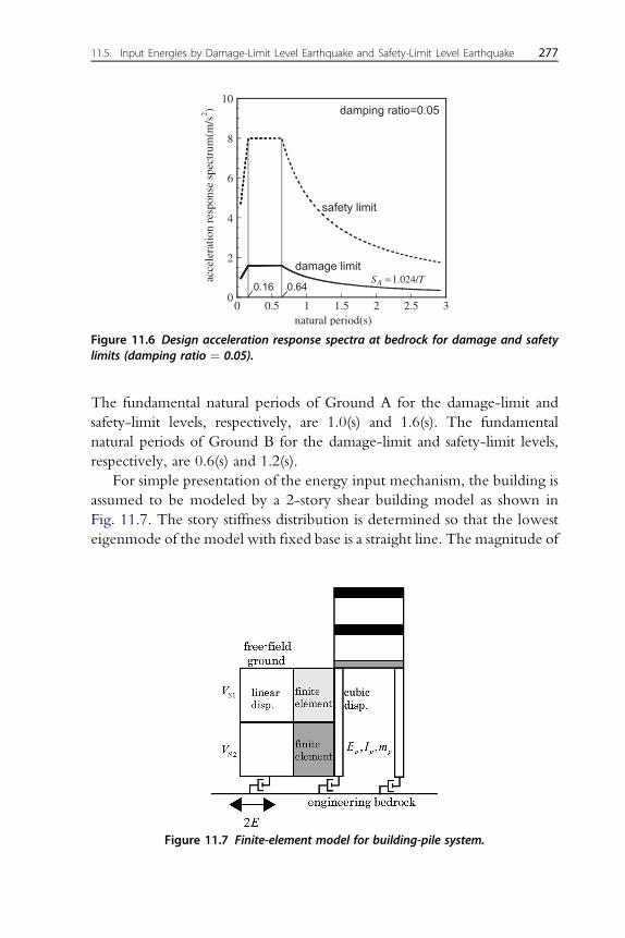
The fundamental natural periods of Ground A for the damage-limit andsafety-limit levels, respectively, are 1.0(s) and 1.6(s). The fundamentalnatural periods of Ground B for the damage-limit and safety-limit levels,respectively, are 0.6(s) and 1.2(s).

For simple presentation of the energy input mechanism, the building isassumed to be modeled by a 2-story shear building model as shown inFig. 11.7. The story stiffness distribution is determined so that the lowesteigenmode of the model with fixed base is a straight line. The magnitude of

0

2

4

6

8

10

0 0.5 1 1.5 2 2.5 3natural period(s)

acce

lera

tion

resp

onse

spe

ctru

m(m

/s2 ) damping ratio=0.05

damage limit

safety limit

SA =1.024/T0.640.16

Figure 11.6 Design acceleration response spectra at bedrock for damage and safetylimits (damping ratio ¼ 0.05).

Figure 11.7 Finite-element model for building-pile system.


the story stiffnesses is controlled by modifying the fundamental naturalperiod of the model with fixed base. The model floor masses aremi ¼ 10�103ðkgÞði ¼ 1; 2Þ and mbb ¼ 30� 103ðkgÞ. The story heights arehi ¼ 3:5ðmÞði ¼ 1; 2Þ. The soil mass density and Poisson’s ratio areri ¼ 1:6� 103ðkg=m3Þ and n ¼ 0:45. The pile diameter is 1.5(m) and thepile Young’s modulus and mass density are 2:1� 1010ðN=m2Þ and2:4� 103ðkg=m3Þ, respectively. The damping of the building is assumedto be stiffness-proportional and the damping ratio for the lowest eigenvi-bration is 0.05.

The solid line in Fig. 11.8 shows the real parts of the energy transferfunction FAðuÞ, Eq. (11.15), for the building-pile system and that FSðuÞ,Eq. (11.20), for the building only under the damage-limit level earthquake.The proposed model is called here “a continuum model.” Figs. 11.8(a) and

-2000

0

2000

4000

6000

8000

-60 -40 -20 0 20 40 60

Re{FA}ContinuumRe{FA}FEM

Re{

F A} (N

s3 /m

)


Ground A(a)

building-pile system (Ground A)

-2000

0

2000

4000

6000

8000Re{FS}ContinuumRe{FS}FEM

Re{

F S} (N

s3 /m

)


Ground A(b)

building only (Ground A)

-2000

0

2000

4000

6000

8000Re{FA}ContinuumRe{FA}FEM

Re{

F A} (N

s3 /m

)


Ground B

(c)

building-pile system (Ground B)

-2000

0

2000

4000

6000

8000

-60 -40 -20 0 20 40 60

-60 -40 -20 0 20 40 60 -60 -40 -20 0 20 40 60

Re{FS}ContinuumRe{FS}FEM

Re{

F S} (N

s3 /m

)


Ground B(d)

building only (Ground B)

Figure 11.8 Real parts of the energy transfer function for building-pile system and thatfor building only by the proposed continuum model and the finite-element model(damage-limit level earthquake). (a) Ground A, building-pile system, (b) Ground A,building only, (c) Ground B, building-pile system, (d) Ground B, building only.


(b) are for Ground A and Figs. 11.8(c) and (d) are for Ground B. The stiffnessand damping ratio of the free-field ground and the Winkler-type soilelement have been evaluated to the damage-limit level earthquake input. Thefundamental natural period of the building with fixed base is 0.3(s). Theimaginary part of the energy transfer function FAðuÞ becomes an oddfunction of frequency that does not contribute to the input energy. The solidline in Fig. 11.9 shows the real parts of the energy transfer function FAðuÞ,Eq. (11.15), for the building-pile system and that FSðuÞ, Eq. (11.20), for thebuilding only under the safety-limit level earthquake. It can be observed fromFigs. 11.8 and 11.9 that, while the energy transfer functions FAðuÞ and FSðuÞfor both Grounds A and B under the damage-limit level earthquake exhibita large value around the fundamental natural circular frequency (about20 rad/s) of the building, FAðuÞ for GroundA (soft ground) under the safety-limit level earthquake shows a large value around the fundamental natural

-1000

-500

0

500

1000

1500

2000

2500

3000

Re{FA}ContinuumRe{FA}FEM

Re{

F A} (N

s3 /m

)


Ground A(a)

building-pile system (Ground A)

-1000

-500

0

500

1000

1500

2000

2500

3000Re{FA}ContinuumRe{FA}FEM

Re{

F A} (N

s3 /m

)


Ground B(c)


-1000

-500

0

500

1000

1500

2000

2500

3000Re{FS}ContinuumRe{FS}FEM


Re{

F S} (N

s3 /m

)

Ground A(b)

building only (Ground A)

-1000

-500

0

500

1000

1500

2000

2500

3000

-60 -40 -20 0 20 40 60

-60 -40 -20 0 20 40 60

-60 -40 -20 0 20 40 60

-60 -40 -20 0 20 40 60

Re{FS}ContinuumRe{FS}FEM

Re{

F S} (N

s3 /m

)


Ground B(d)


Figure 11.9 Real parts of the energy transfer function for building-pile system and forbuilding only by the proposed continuum model and the finite-element model (safety-limit level earthquake). (a) Ground A, building-pile system, (b) Ground A, building only,(c) Ground B, building-pile system, (d) Ground B, building only.


circular frequency (about 4rad/s) of the surface ground. It can also be observedfrom Figs. 11.9(c) and (d) that the input energy to the building on Ground A(soft ground) under the safety-limit level earthquake is greatly smaller thanthat on Ground B (hard ground). This may result from the fact that a buildingwith a rather short natural period is considered here.

In order to demonstrate the validity of the proposed model and method,the finite-element model (see Fig. 11.7) proposed in Nakamura et al. (1996),Takewaki (1999) has been used to evaluate the energy transfer functionsFAðuÞ and FSðuÞ. It should be noted that viscous boundaries have beenintroduced at the bottom of the surface ground and frequency-dependentcharacteristics of the Winkler-type soil element have been used. Thedotted line in Figs. 11.8 and 11.9 shows the real parts of the energy transferfunction FAðuÞ for the building-pile system and that FSðuÞ for the buildingonly by the FEMmodel. A very good correspondence can be seen and it canbe concluded that the proposed model and method are valid.

In order to clarify the characteristics in the case where the fundamentalnatural period of the building is resonant to that of the surface ground, theenergy transfer functions for the building with the fundamental naturalperiod 1.6(s) under the safety-limit level earthquake have been computed. Itshould be reminded that the fundamental natural period of the surfaceground of Ground A under the safety-limit level earthquake is about 1.6(s).Fig. 11.10 shows the real parts of the energy transfer function for building-pile system and that for building only in case of the building with funda-mental natural period ¼ 1.6(s). It can be observed that a large energy inputcan be expected in such a resonant case.

[Input Energy by Actual Ground Motion]For evaluating the characteristics of input energies by an actual groundmotion, the ground motion of El Centro NS 1940 has been chosen. Themaximum velocities are scaled to 0.1m/s and 0.5m/s for the damage-limitlevel and the safety-limit level, respectively, so as to be compatible withthe Japanese code (see Fig. 11.6). Fig. 11.11 shows the earthquake inputenergy to the building-pile system and that to building only with respect tobuilding fundamental natural period subjected to El Centro NS 1940 of thedamage-limit level. It can be observed that, while the input energy to thebuilding-pile system and that to building only differ greatly in case of GroundA (soft ground), those do not differ so much in case of Ground B (hardground). This is because the energy dissipated in the ground or radiated intothe ground is large in Ground A. Fig. 11.12 illustrates the earthquake input


energy to the building-pile system and that from the pile-tip with respect tobuilding fundamental natural period subjected to El Centro NS 1940 of thedamage-limit level. It can be seen that the energy from the pile-tip is almostconstant irrespective of the building fundamental natural period. This isbecause the energy from the pile-tip does not depend on the building anddepends mainly on the soil condition. It can also be observed that the inputenergy to the building-pile-soil system is larger than that from the pile-tip inthe building fundamental natural period range of 0.5–1.5s in Ground A and0.3–3.0s in Ground B. This means that the input energy from the side of thesurrounding soil is positive in these fundamental natural period ranges. Onthe contrary, in the other fundamental natural period range, this relation isreversed. This means that the input energy from the side of the surroundingsoil is negative in these fundamental natural period ranges.

0

2 104

4 104

6 104

8 104

1 105

Re{FA}Continuum

Re{

F A} (N

s3 /m

)


0

2 104

4 104

6 104

8 104

1 105

Re{FS}ContinuumR

e{F S} (

N s

3 /m)


(c)


(d)


0

2 104

4 104

6 104

8 104

1 105

Re{FA}Continuum

Re{

F A} (N

s3 /m

)


0

2 104

4 104

6 104

8 104

1 105

-10 -5 0 5 10 -10 -5 0 5 10

-10 -5 0 5 10 -10 -5 0 5 10

Re{FS}Continuum

Re{

F S} (N

s3 /m

)


(a)

building-pile system (Ground A) building only (Ground A)

(b)

Figure 11.10 Real parts of the energy transfer function for building-pile system andthat for building only in case of the building with fundamental natural period ¼ 1.6(s):resonance with Ground A (safety-limit level earthquake). (a) Ground A, building-pilesystem, (b) Ground A, building only, (c) Ground B, building-pile system, (d) Ground B,building only.


In order to confirm this fact, an additional computation has been made.Fig. 11.13 shows the real part of the energy transfer function correspondingto the energy input from the side of the surrounding soil in Ground A underthe damage-limit level earthquake. The building fundamental naturalperiods have been chosen as 1.0s and 5.0s. In the building with thefundamental natural period 5.0s, the negative portion is relatively wide. Thisfact indicates the negative input energy from the side of the surrounding soilin this fundamental natural period range.

0

1 104

2 104

3 104

0 2 4 6 8 10

overallfrom pile-tip (z=37m)

inpu

t ene

rgy

(J)

natural period (s) (fixed base)

Ground A

0

1 104

2 104

3 104

0 2 4 6 8 10

overallfrom pile-tip(z=29m)

inpu

t ene

rgy

(J)

natural period (s) (fixed-base)

Ground B

(a)

Ground A

(b)

Ground B

Figure 11.12 Earthquake input energy to building-pile system and that from the pile-tip with respect to building fundamental natural period subjected to El Centro NS 1940(damage-limit level). (a) Ground A, (b) Ground B.

0

1 104

2 104

3 104

0 2 4 6 8 10

overallstructure

inpu

t ene

rgy

(J)


Ground A

0

1 104

2 104

3 104

0 2 4 6 8 10

overallstructure

inpu

t ene

rgy

(J)


Ground B

Ground B

(b)

Ground A

(a)

Figure 11.11 Earthquake input energy to building-pile system and that to buildingonly with respect to building fundamental natural period subjected to El Centro NS1940 (damage-limit level). (a) Ground A, (b) Ground B.


Fig. 11.14 indicates the earthquake input energy to the building-pilesystem and that to building only with respect to building fundamentalnatural period subjected to El CentroNS 1940 of the safety-limit level. It canbe observed that the difference between the input energy to the building-pilesystem and that to the building only is larger than that to the input of thedamage-limit level. This is because the energy dissipated in the ground orradiated into the ground is large under the input of the safety-limit level.

Fig. 11.15 shows the earthquake input energy to the building-pile systemand that from the pile-tip with respect to building fundamental natural

-2 105

-1.5 105

-1 105

-5 104

0

5 104

1 105

-10 -5 0 5 10

Re{

Fz} (

N s

3 /m)


Ts=1.0(s)

Ground A-2 105

-1.5 105

-1 105

-5 104

0

5 104

1 105

-10 -5 0 5 10

Re{

Fz} (

N s

3 /m)


Ts=5.0(s)

Ground A

(a)

Building natural period=1.0(s)

(b)

Building natural period=5.0(s)

Figure 11.13 Real part of the energy transfer function corresponding to the energy inputfrom the side of the surrounding soil (damage-limit level earthquake). (a) Ts ¼ 1.0 (s),(b) Ts ¼ 5.0 (s).

0

1 105

2 105

3 105

4 105

5 105

6 105

overallstructure

inpu

t ene

rgy

(J)


Ground A

0

1 105

2 105

3 105

4 105

5 105

6 105

0 2 4 6 8 10 0 2 4 6 8 10

overallstructure

inpu

t ene

rgy

(J)


Ground B

Ground B

(b)

Ground A

(a)

Figure 11.14 Earthquake input energy to building-pile system and that to buildingonly with respect to building fundamental natural period subjected to El Centro NS1940 (damage-limit level). (a) Ground A, (b) Ground B.


period subjected to El Centro NS 1940 of the safety-limit level. It can beseen that the input energy from the side of the surrounding soil is negative inall the fundamental natural period range. This means that, while the inputenergy from the pile-tip is always positive, the energy dissipated in theground or radiated into the ground is extremely large under the input of thesafety-limit level due to the reduction of soil stiffness.

Fig. 11.16 illustrates the underground distribution of the newly definedinput energy density for Ground A under the damage-limit level and safety-limit level earthquakes. The integration of the input energy density over thepile represents the input energy from the side of the surrounding soil. It canbe understood that there is a portion with a positive density and one witha negative density. This investigation is very useful in disclosing the energyinput mechanism underground. Fig. 11.17 shows the underground distri-bution of the input energy density for Ground B under the damage-limitlevel and safety-limit level earthquakes.

Fig. 11.18 indicates the real part of the energy transfer function at thetwo different depths, GL-10m and GL-30m, corresponding to the energyinput from the side of the surrounding soil for Ground A under thedamage-limit level earthquake. The building natural period is 0.5s. It canbe seen that, while the input energy from the side of the surrounding soil atGL-10m is positive, that at GL-30m is negative. It may be concluded that,since the present approach is based on the energy transfer function inde-pendent of input ground motions and being able to be defined at each

0

1 105

2 105

3 105

4 105

5 105

6 105

0 2 4 6 8 10


inpu

t ene

rgy

(J)


Ground A

0

1 105

2 105

3 105

4 105

5 105

6 105

0 2 4 6 8 10


inpu

t ene

rgy

(J)


Ground B

(a)

Ground A

(b)

Ground B

Figure 11.15 Earthquake input energy to building-pile system and that from the pile-tip with respect to building fundamental natural period subjected to El Centro NS 1940(safety-limit level). (a) Ground A, (b) Ground B.


point or area, it is possible to disclose the earthquake energy inputmechanism in detail.

11.6. CRITICAL EXCITATION FOR EARTHQUAKE ENERGYINPUT IN STRUCTURE-PILE-SOIL SYSTEM

The following critical excitation method may be stated for structure-pile-soil systems.

Find jAðuÞj

that maximizes ESI ¼ RN

�NFSðuÞjAðuÞj2du

The solution procedure developed for fixed-base single-degree-of-freedom (SDOF) models in Chapter 8, for fixed-base multi-degree-of-freedom (MDOF) models in Chapter 9 and for SSI models in Chapter 10can be applied to this problem. It suffices to replace the energy transferfunction FðuÞ for the SDOF model by FSðuÞ for the present model.

-8 104 -6 104 -4 104 -2 104 0 2 104 4 104 6 104 8 104-40

-35

-30

-25

-20

-15

-10

-5

0

damage-limit levelsafety-limit level

input energy density (J/m)

dept

h (m

)Ground A

Ts=0.5(s)

Tg=1.0(s)

Tg=1.6(s)

Figure 11.16 Underground distribution of input energy density for Ground A (damage-limit level and safety-limit level earthquakes).

11.6. Critical Excitation for Earthquake Energy Input in Structure-Pile-Soil System 285

-8000 -6000 -4000 -2000 0 2000 4000 6000 8000-30

-25

-20

-15

-10

-5

0

damage-limit levelsafety-limit level

input energy density (J/m)

dept

h (m

)

Ground B

Ts=0.5(s)

Tg=0.6(s)Tg=1.2(s)

Figure 11.17 Underground distribution of input energy density for Ground B (damage-limit level and safety-limit level earthquakes).

-500

0

500

1000

1500

2000

2500

3000

-60 -40 -20 0 20 40 60

Re{

Fz(z

=10m

)}


Ground A

GL-10(m)Ts=0.5(s), Tg=1.0(s)

-1500

-1000

-500

0

500

1000

-60 -45 -30 -15 0 15 30 45 60

Re{

Fz(z

=30m

)}


Ground AGL-30(m)

Ts=0.5(s), Tg=1.0(s)

(a)

GL-10(m)

(b)

GL-30(m)

Figure 11.18 Real part of the energy transfer function at the two different depthscorresponding to the energy input from the side of the surrounding soil for Ground A(damage-limit level earthquake). (a) GL-10(m), (b) GL-30(m).


11.7. CONCLUSIONS

The conclusions may be stated as follows:(1) A new evaluation method of earthquake input energy to structure-pile

interaction systems has been developed. The method is an approach inthe frequency domain. The energy transfer function, which plays a keyrole in the input energy evaluation, is derived from the transfer func-tions of the structure-pile interaction system to the earthquake accel-eration input at the bedrock.

(2) Thepresent approach in the frequencydomainhas an advantage; to be ableto include directly the frequency-dependent characteristics (stiffness anddamping) of theWinkler-type soil element in addition to the treatment ofthe free-field ground via the wave propagation theory.

(3) The introduction of the definition of two input energies, one to theoverall system (structure plus pile and surrounding soil) and the other tothe structure alone, is very useful in understanding the mechanism of theearthquake energy input and the effect of soil-structure interactionunder various conditions of soil properties and natural period of struc-tures on the earthquake energy input.

(4) While the approach in the time domain requires time-series groundmotions, the approach in the frequency domain requires only the Fourierspectrum of the acceleration at the bedrock and enables one to capture thegeneral characteristics of the energy input through a general form of theFourier spectrum of the input acceleration. This treatment is completelycompatible with most of the seismic resistant design codes in whicha response spectrum or the corresponding Fourier spectrum is provided.

(5) The proposed input energy density whose integration over the pilerepresents the input energy from the side of the surrounding soil isappropriate for disclosing the energy input mechanism or energy flowunderground.

(6) The energy transfer function can be defined even at a point (includingunderground) and it is easy to understand general characteristics of theflow of the earthquake energy at the point or in the area. These char-acteristics underground depend on the soil property and its depth. It hasbeen shown that these general characteristics can be characterized by theproposed energy transfer function.

The evaluation of earthquake input energy in the time domain is suitable forthe evaluation of the time history of input energy, especially for nonlinearsystems. Dual use of the frequency-domain and time-domain techniquesmay be preferable in advanced seismic analysis for more robust design.


The formulation of the earthquake input energy in the frequencydomain is effective and essential for solving a critical excitation problem(Takewaki 2004a) for the maximum earthquake input energy and derivinga bound on the earthquake input energy for a class of ground motions.

APPENDIX 11.1 10 3 10 SIMULTANEOUS LINEAREQUATIONS FOR DERIVING TRANSFER FUNCTIONSFOR THE 2-STORY BUILDING MODEL ON GROUNDWITH TWO SOIL LAYERS

Let ai1 ¼ r1Vs1=r2Vs2 and ai2 ¼ r2Vs2=r3Vs3 denote the compleximpedance ratios between the first and second soil layers and the second andthird soil layers, respectively, where ri and Vsi are the mass density and thecomplex shear wave velocity in the i-th soil layer. The story stiffness and thecorresponding damping coefficient of the i-th story are denoted by ki and ci,respectively. The transfer functions are derived from the boundary condi-tions, continuity conditions and equilibrium equations. Those equationsmay be described compactly from Eqs. (11.2), (11.7), (11.9) as

� u2XY ¼ Z (A11.1)

whereX ¼ ½X1 / X10�

Y ¼ 1�u2ð2E3Þ

�nU1 U2 D

ð1Þ1 D

ð1Þ2 D

ð1Þ3 D

ð1Þ4 D

ð2Þ1 D

ð2Þ2 D

ð2Þ3 D

ð2Þ4

oT

Z ¼ 1

A�1

8>>>>>>>>>>>>>>>>>>>>>>><>>>>>>>>>>>>>>>>>>>>>>>:

�ðiuc1 þ k1Þs10

0

ðmbbu2 � iuc1 � k1Þs1

ð�s1 þ s2Þ cos ðuL1=Vs1Þf�s1ðu=Vs1Þ þ s2ðu=Vs2Þai1g sin ðuL1=Vs1Þfs1ðu=Vs1Þ2 � s2ðu=Vs2Þ2g cos ðuL1=Vs1Þ

fs1ðu=Vs1Þ3 � s2ðu=Vs2Þ3ai1g sin ðuL1=Vs1Þs2J2ðu=Vs2Þ2 cos fðuL2=Vs2Þ þ bg

�s2J2 cos fðuL2=Vs2Þ þ bg þ ðA�1 þ A�

2Þ=2

9>>>>>>>>>>>>>>>>>>>>>>>=>>>>>>>>>>>>>>>>>>>>>>>;

ðA11:2aecÞ


X1 ¼

8>>>>>>>>>>>>>>>>>>>>>>><>>>>>>>>>>>>>>>>>>>>>>>:

m1u2 � iuðc1 þ c2Þ � ðk1 þ k2Þ

�ðiuc2 þ k2Þ0

�ðiuc1 þ k1Þ0

0

0

0

0

0

9>>>>>>>>>>>>>>>>>>>>>>>=>>>>>>>>>>>>>>>>>>>>>>>;

;X2 ¼

8>>>>>>>>>>>>>>>>>>>>>>><>>>>>>>>>>>>>>>>>>>>>>>:

iuc2 þ k2

�m2u2 þ iuc2 þ k2

0

0

0

0

0

0

0

0

9>>>>>>>>>>>>>>>>>>>>>>>=>>>>>>>>>>>>>>>>>>>>>>>;

;

X3 ¼

8>>>>>>>>>>>>>>>>>>>>>>><>>>>>>>>>>>>>>>>>>>>>>>:

iuc1 þ k1

0

l1

�4EpIpl31 þ iuc1 þ k1 � mbbu

2

e�l1L1

l1e�l1L1

l21e�l1L1

l31e�l1L1

0

0

9>>>>>>>>>>>>>>>>>>>>>>>=>>>>>>>>>>>>>>>>>>>>>>>;

;

X4 ¼

8>>>>>>>>>>>>>>>>>>>>>>><>>>>>>>>>>>>>>>>>>>>>>>:

iuc1 þ k1

0

�l1

4EpIpl31 þ iuc1 þ k1 � mbbu

2

el1L1

�l1el1L1

l21el1L1

�l31el1L1

0

0

9>>>>>>>>>>>>>>>>>>>>>>>=>>>>>>>>>>>>>>>>>>>>>>>;

;X5 ¼

8>>>>>>>>>>>>>>>>>>>>>>><>>>>>>>>>>>>>>>>>>>>>>>:

iuc1 þ k1

0

il1

4EpIpil31 þ iuc1 þ k1 � mbbu2

e�il1L1

il1e�il1L1

�l21e�il1L1

�il31e�il1L1

0

0

9>>>>>>>>>>>>>>>>>>>>>>>=>>>>>>>>>>>>>>>>>>>>>>>;

Appendix 11.1 10 � 10 Simultaneous Linear Equations for Deriving Transfer Functions 289

X6 ¼

8>>>>>>>>>>>>>>>>>>>>>>>><>>>>>>>>>>>>>>>>>>>>>>>>:

iuc1 þ k1

0

�il1

�4EpIpil31 þ iuc1 þ k1 � mbbu2

eil1L1

�il1eil1L1

�l21eil1L1

il31eil1L1

0

0

9>>>>>>>>>>>>>>>>>>>>>>>>=>>>>>>>>>>>>>>>>>>>>>>>>;

;X7 ¼

8>>>>>>>>>>>>>>>>>>>>>>>><>>>>>>>>>>>>>>>>>>>>>>>>:

0

0

0

0

�1

�l2

�l22

�l32

l22e�l2L2

e�l2L2

9>>>>>>>>>>>>>>>>>>>>>>>>=>>>>>>>>>>>>>>>>>>>>>>>>;

;

X8 ¼

8>>>>>>>>>>>>>>>>>>>>>>><>>>>>>>>>>>>>>>>>>>>>>>:

0

0

0

0

�1

l2

�l22

l32

l22el2L2

el2L2

9>>>>>>>>>>>>>>>>>>>>>>>=>>>>>>>>>>>>>>>>>>>>>>>;

;X9 ¼

8>>>>>>>>>>>>>>>>>>>>>>><>>>>>>>>>>>>>>>>>>>>>>>:

0

0

0

0

�1

�il2

l22

il32

�l22e�il2L2

e�il2L2

9>>>>>>>>>>>>>>>>>>>>>>>=>>>>>>>>>>>>>>>>>>>>>>>;

;X10 ¼

8>>>>>>>>>>>>>>>>>>>>>>><>>>>>>>>>>>>>>>>>>>>>>>:

0

0

0

0

�1

il2

l22

�il32

�l22eil2L2

eil2L2

9>>>>>>>>>>>>>>>>>>>>>>>=>>>>>>>>>>>>>>>>>>>>>>>;

ðA11:3aejÞ

J2 ¼ffiffiffiffiffiffiffiffiffiffiffiffiffiffiffiffiffiffiffiffiffiffiffiffiffiffiffiffiffiffiffiffiffiffiffiffiffiffiffiffiffiffiffiffiffiffiffiffiffiffiffiffiffiffiffiffiffiffiffiffiffiffiffiffiffiffiffiffiffifficos2 uðL1=Vs1Þ þ a2i1sin

2 uðL1=Vs1Þq

;

b ¼ cos�1f½cos uðL1=Vs1Þ�=J2g (A11.4a, b)


A�1 and A�

2 in Eq. (A11.2c) are defined via the one-dimensional wavepropagation theory as(

E3

F3

)¼ ½A2�½A1�

(1

1

)E1 ¼

24A

ð2Þ11 A

ð2Þ12

Að2Þ21 A

ð2Þ22

3524A

ð1Þ11 A

ð1Þ12

Að1Þ21 A

ð1Þ22

35( 1

1

)E1

¼8<:

Að2Þ11 A

ð1Þ11 þ A

ð2Þ12 A

ð1Þ21 þ A

ð2Þ11 A

ð1Þ12 þ A

ð2Þ12 A

ð1Þ22

Að2Þ21 A

ð1Þ11 þ A

ð2Þ22 A

ð1Þ21 þ A

ð2Þ21 A

ð1Þ12 þ A

ð2Þ22 A

ð1Þ22

9=;E1

¼(A�1

A�2

)E1

(A11.5a)(E2

F2

)¼ ½A1�

(1

1

)E1 (A11.5b)

where

½Am� ¼

266641

2ð1þ aimÞeiuðLm=VsmÞ 1

2ð1� aimÞeiuð�Lm=VsmÞ

1

2ð1� aimÞeiuðLm=VsmÞ 1

2ð1þ aimÞeiuð�Lm=VsmÞ

37775 (A11.6)

The coefficients E3 and F3 in Eq. (A11.5a) are the amplitudes of theincident wave (upward propagating wave) and the reflected wave (down-ward propagating wave) at the top of the third soil layer. Similarly E1 is theamplitude of the incident wave (upward propagating wave) at the top of thefirst soil layer.

Each equation in the set of simultaneous linear equations (A11.1)corresponds to the following equation or condition:(1) Equilibrium equation at the 1st-floor mass.(2) Equilibrium equation at the 2nd-floor mass.(3) Nodal rotation of the pile top ¼ 0.(4) Shear force of the pile at the top is in equilibrium with the inertial force

at the foundation and the 1st-story shear force.(5) Continuity condition of the pile horizontal displacements at the

interface of the soil layers.

Appendix 11.1 10 � 10 Simultaneous Linear Equations for Deriving Transfer Functions 291

(6) Continuity condition of the pile nodal rotations at the interface of thesoil layers.

(7) Equilibrium condition of pile bending moments at the interface of thesoil layers.

(8) Equilibrium condition of pile shear forces at the interface of the soillayers.

(9) Bending moment at the pile tip ¼ 0 (pin-jointed).(10) Horizontal displacement of the pile tip ¼ horizontal displacement of

the free-field ground at the same level.

APPENDIX 11.2 COMPARISON WITH RECORDED DATADURING AN EARTHQUAKE

In order to verify the present Winkler-type soil element model, an analyticalmodel has been constructed for an actual building with piles (Nikolaou et al.2001). The overview of the building-pile system in Yokohama, Japan isshown in Fig. 11.19. This building consists of a steel frame of 12 stories and issupported by 20 cast-in-place reinforced concrete piles, 35m long and 1.7min diameter. To compare the peak response of bending strains of piles, a finite-element model as shown in Fig. 11.7 has been used. This finite-element

Figure 11.19 12-story steel building with 20 piles at Yokohama in Japan.


model includes the present Winkler-type soil element and the difference isthe shape functions for the free-field ground and piles, i.e. a linear functionfor the free-field ground and a cubic function for the piles. Fig. 11.20(a) showsthe shear wave velocity profile of the ground. Fig. 11.20(b) illustrates thecomparison of the peak pile bending strain computed by the analytical modelincluding the present Winkler-type soil element with that recorded during anearthquake in 1992. A good agreement can be observed near the pile headand this demonstrates the validity of the present continuum model with theWinkler-type soil element. This bending strain contains both the inertialeffect and the kinematic effect. It has been confirmed from the analyticalmodel that both the inertial effect and the kinematic effect are included almostin the same magnitude in this case. It may also be said that the pile-groupeffect is rather small in this case.

0 100 200 300 400 500

0

10

20

30

40


De

pth

(m

)

(a)

0 0.5 1 1.5 2 2.5

0

10

20

30

40

Computed (elastic)

Computed (strain compatible)

Measured corner pile

Measured center pile

Peak pile bending strain (x10-5

)

De

pth

(m

)

(b)

Figure 11.20 (a) Shear wave velocity profile of ground; (b) comparison of peak pilebending strain computed by analytical model including the present Winkler-type soilelement with that recorded during an earthquake in 1992.

Appendix 11.2 Comparison with Recorded Data During an Earthquake 293

REFERENCESGazetas, G., Dobry, R., 1984. Horizontal response of piles in layered soils. J. Geotech.

Engrg. 110 (1), 20–40.Kavvadas, M., Gazetas, G., 1993. Kinematic seismic response and bending of free-head piles

in layered soil. Geotechnique 43 (2), 207–222.Nakamura, T., Takewaki, I., Asaoka, Y., 1996. Sequential Stiffness Design for Seismic Drift

Ranges of a Shear Building–Pile–Soil System. Earthquake Engineering and StructuralDynamics 25 (12), 1405–1420.

Nikolaou, S., Mylonakis, G., Gazetas, G., Tazoh, T., 2001. Kinematic pile bending duringearthquakes: analysis and field measurements. Geotechnique 51 (5), 425–440.

Schnabel, P.B., Lysmer, J., Seed, H.B., 1972. SHAKE: A computer program for earthquakeresponse analysis of horizontally layered sites, A computer program distributed byNISEE/Computer Applications. Berkeley.

Takewaki, I., 1999. Inverse Stiffness Design of Shear-Flexural Building Models IncludingSoil–Structure Interaction. Engineering Structures 21 (12), 1045–1054.

Takewaki, I., 2004a. Bound of Earthquake Input Energy to Soil-Structure InteractionSystems, Proc. of The 11th International Conference on Soil Dynamics and EarthquakeEngineering (ICSDEE) and the 3rd International Conference on EarthquakeGeotechnical Engineering (ICEGE). Berkeley, January 7–9, (2), 734–741.

Takewaki, I., 2004b. Response spectrum method for nonlinear surface ground analysis.Advances in Structural Engineering 7 (6), 503–514.

Takewaki, I., Fujimoto, H., 2004. Earthquake Input Energy to Soil-Structure InteractionSystems: A Frequency-Domain Approach,. Advances in Structural Engineering 7 (5),399–414.


CHAPTER TWELVE

Critical Excitation for EarthquakeEnergy Input Rate

Contents

12.1. Introduction 29512.2. Nonstationary Ground Motion Model 29612.3. Probabilistic Earthquake Energy Input Rate: A Frequency-Domain Approach 29712.4. Critical Excitation Problem for Earthquake Energy Input Rate 30312.5. Solution Procedure for Double Maximization Problem 30412.6. Mean Energy Input Rate for Special Envelope Function 30712.7. Critical Excitation Problem for Nonuniformly Modulated Ground Motion Model 31012.8. General Problem for Variable Envelope Function and Variable Frequency

Content312

12.9. Numerical Examples 31212.10. Deterministic Earthquake Energy Input Rate 32012.11. Example 1 (Model of SFAS of Truncated Ground Motion) 32312.12. Example 2 (Detailed Analysis of SFAS of Truncated Ground Motion and

Comparison of Time-Domain and Frequency-Domain Analyses)326

12.13. Conclusions 331References 332

12.1. INTRODUCTION

The purpose of this chapter is to explain a new probabilistic criticalexcitation method for identifying the critical frequency content of groundmotions maximizing the mean earthquake energy input rate to structures.The critical excitation problem includes a double maximization procedurewith respect to time and to the power spectral density (PSD) function. Thekey to finding the critical frequency content is the order interchange inthe double maximization procedure. It should be remarked that no math-ematical programming technique is required in the proposed method. It isshown that the proposed technique is systematic and the critical excitationcan be found extremely efficiently within a reasonable accuracy. Extensionof the proposed method to a more general ground motion model, i.e.nonuniformly modulated nonstationary models, and to a more generalproblem for variable envelope functions and variable frequency contents is



http://dx.doi.org/10.1016/B978-0-08-099436-9.00012-2

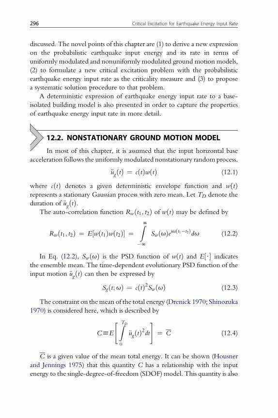
discussed. The novel points of this chapter are (1) to derive a new expressionon the probabilistic earthquake input energy and its rate in terms ofuniformly modulated and nonuniformly modulated ground motion models,(2) to formulate a new critical excitation problem with the probabilisticearthquake energy input rate as the criticality measure and (3) to proposea systematic solution procedure to that problem.

A deterministic expression of earthquake energy input rate to a base-isolated building model is also presented in order to capture the propertiesof earthquake energy input rate in more detail.

12.2. NONSTATIONARY GROUND MOTION MODEL

In most of this chapter, it is assumed that the input horizontal baseacceleration follows the uniformlymodulated nonstationary random process.


where cðtÞ denotes a given deterministic envelope function and wðtÞrepresents a stationary Gaussian process with zero mean. Let TD denote theduration of €ugðtÞ.

The auto-correlation function Rwðt1; t2Þ of wðtÞ may be defined by


�N


In Eq. (12.2), SwðuÞ is the PSD function of wðtÞ and E½$� indicatesthe ensemble mean. The time-dependent evolutionary PSD function of theinput motion €ugðtÞ can then be expressed by


The constraint on themean of the total energy (Drenick 1970; Shinozuka1970) is considered here, which is described by

ChE

"ZTD

0

€ugðtÞ2dt#

¼ C (12.4)

C is a given value of the mean total energy. It can be shown (Housnerand Jennings 1975) that this quantity C has a relationship with the inputenergy to the single-degree-of-freedom (SDOF) model. This quantity is also

296 Critical Excitation for Earthquake Energy Input Rate

related to the response spectrum. These relationships may be useful in thespecification of C. Substitution of Eq. (12.1) into Eq. (12.4) yields

ZTD

0

cðtÞ2E½wðtÞ2�dt ¼ C (12.5)

Substitution of Eq. (12.2) (t1 ¼ t2 ¼ t) into Eq. (12.5) leads to ZN�N

SwðuÞdu! ZTD

0

cðtÞ2dt!

¼ C (12.6)

Eq. (12.6) is reduced finally to

ZN�N

SwðuÞdu ¼ C=

ZTD

0

cðtÞ2dt ¼ Sw (12.7)

More elaborate nonuniformly modulated nonstationary models areavailable (Conte and Peng 1997; Fang and Sun 1997). Advanced criticalexcitation methods for such elaborate models will be briefly discussed later.

12.3. PROBABILISTIC EARTHQUAKE ENERGY INPUTRATE: A FREQUENCY-DOMAIN APPROACH

A lot of work has been conducted on the topics of earthquake input energy.For example, (seeHousner 1956, 1959;Housner and Jennings 1975;Akiyama1985; Uang and Bertero 1990; Trifunac et al. 2001; Austin and Lin 2004). Incontrast to most of the previous works, the earthquake input energy isformulated and evaluated here in the frequency domain (Page 1952; Lyon1975; Ordaz et al. 2003; Takewaki 2004a–c, 2005a, b; Takewaki andFujimoto 2004) to facilitate the development of a unique critical excitationmethod and the corresponding efficient solution procedure.

Together with the earthquake input energy, the earthquake energy inputrate has been focused on as an important measure of ground motion destruc-tiveness. Page (1952) introduced the concept of instantaneous power spectrumandOhi et al. (1991), Kuwamura et al. (1997a, 1997b), Iyama and Kuwamura(1999) developed several interesting theories on the earthquake energy inputrate. It has been clarified that, while the earthquake input energy can quantifythe energy absorbed in a structure during a ground motion input, the

12.3. Probabilistic Earthquake Energy Input Rate: A Frequency-Domain Approach 297

earthquake energy input rate can capture the load effect of groundmotions forproducing themaximumdeformation in a structure.Actuallymany researcherspointed out that the earthquake energy input rate may be more crucial forstructures than the earthquake input energy for near-fault ground motions(Hall et al. 1995; Kuwamura et al. 1997a, 1997b; Iyama and Kuwamura 1999;Bozorgnia and Bertero 2003). In this chapter, the earthquake energy input rateis taken as a measure of criticality of ground motions.

Fig. 12.1(a) shows the time history of the input energy per unit mass toa damped, linear elastic SDOF model with the fundamental natural period1.0(s) and the damping ratio of 0.05 subjected to El Centro NS (ImperialValley 1940). The solid line is computed from the relative velocity of themass to the base and the dotted line indicates the time history of the inputenergy representing the work by the base on the structure (Uang andBertero 1990). Next, Fig. 12.1(b) illustrates the time history of the energyinput rate per unit mass corresponding to the solid line in Fig. 12.1(a).Finally, Fig. 12.1(c) indicates the time history of the story drift of the model.Figs. 12.2(a)–(c) show the corresponding figures of the same modelsubjected to Kobe University NS (Hyogoken-Nanbu 1995) and Figs.12.3(a)–(c) illustrate the corresponding figures subjected to JMA Kobe NS(Hyogoken-Nanbu 1995). It can be seen that while the earthquake inputenergy exhibits a positive value, the energy input rate takes both positiveand negative values. Furthermore, it can be found that the time producingthe maximum story drift corresponds fairly well to the time attainingthe maximum earthquake energy input rate. This fact implies that theearthquake energy input rate can be used as an alternative for measuring thepower of a ground motion for producing the maximum deformation. Itshould also be remarked that the earthquake input energy rates of theground motions from the same earthquake can vary greatly (see, forexample, Bozorgnia and Bertero 2003) and JMA Kobe NS has a largeearthquake input energy rate compared to Kobe University NS.

The probabilistic earthquake energy input rate is introduced in thefollowing. While a lot of work has been conducted on the random vibrationtheory under nonstationary ground motions (see, for example, Crandall1958, 1963; Lin 1967; Vanmarcke 1977; Der Kiureghian 1980; Nigam1983), the probabilistic earthquake input energy and its rate have never beenformulated explicitly.

For clear presentation of a new concept, consider a damped, linear elasticSDOF model with a mass m subjected to a base acceleration €ugðtÞ. Let un; h;uD ¼un


pdenote the undamped natural circular frequency, the


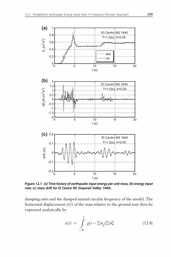
damping ratio and the damped natural circular frequency of the model. Thehorizontal displacement xðtÞ of the mass relative to the ground may then beexpressed analytically by

xðtÞ ¼Z t

�N

gðt � zÞ€ugðzÞdz (12.8)

0

0.2

0.4

0.6

0.8

1

0 5 10 15 20

El Centro NS 1940T=1.0(s), h=0.05

absrel

t (s)

E I (m2 /s

2 )

(a)

-2-1.5

-1-0.5

00.5

11.5

2

0 5 10 15 20

El Centro NS 1940T=1.0(s), h=0.05

dEI/d

t (m

2 /s3 )

t (s)

(b)

-0.2

-0.1

0

0.1

0.2

0 5 10 15 20

El Centro NS 1940T=1.0(s), h=0.05

drift

(m)

t (s)

(c)

Figure 12.1 (a) Time history of earthquake input energy per unit mass; (b) energy inputrate; (c) story drift for El Centro NS (Imperial Valley 1940).


where gðtÞ is the unit impulse response function in the underdamped caseand is described by

gðtÞ ¼ � 1

uDe�hunt sinuDt (12.9)

0

0.2

0.4

0.6

0.8

1

30 35 40 45 50

KBU NS 1995T=1.0(s), h=0.05

absrel

t (s)

E I (m2 /s

2 )

(a)

-2-1.5

-1-0.5

00.5

11.5

2

30 35 40 45 50

KBU NS 1995T=1.0(s), h=0.05

dEI/d

t (m

2 /s3 )

t (s)

(b)

-0.2

-0.1

0

0.1

0.2

30 35 40 45 50

KBU NS 1995T=1.0(s), h=0.05

drift

(m)

t (s)

(c)

Figure 12.2 (a) Time history of earthquake input energy per unit mass; (b) energy inputrate; (c) story drift for KBU NS (Hyogoken-Nanbu 1995).


The time derivative of gðtÞ may be obtained as

_gðtÞ ¼ hffiffiffiffiffiffiffiffiffiffiffiffiffi1� h2

p e�hunt sinuDt � e�hunt cosuDt (12.10)

It can be shown after some manipulations that the horizontal velocity_xðtÞ of the mass relative to the ground may be expressed analytically by

0

2

4

6

8

10

0 5 10 15 20

JMA Kobe NS 1995T=1.0(s), h=0.05

absrel

t (s)

E I (m2 /s

2 )

(a)

-10

-5

0

5

10

15

20

0 5 10 15 20

JMA Kobe NS 1995T=1.0(s), h=0.05

dEI/d

t (m

2 /s3 )

t (s)

(b)

-0.5

-0.25

0

0.25

0.5

0 5 10 15 20

JMA Kobe NS 1995T=1.0(s), h=0.05

drift

(m)

t (s)

(c)

Figure 12.3 (a) Time history of earthquake input energy per unit mass; (b) energy inputrate; (c) story drift for JMA Kobe NS (Hyogoken-Nanbu 1995).


_xðtÞ ¼Z t

�N

_gðt � zÞ€ugðzÞdz (12.11)

By using Eqs. (12.1) and (12.11), the earthquake input energy EIðtÞ(solid line in Figs. 12.1(a), Figs. 12.2(a), Figs. 12.3(a)) per unit mass to theSDOF model until time t may be expressed by

EIðtÞ ¼ �Z t

�N

_xðsÞ€ugðsÞds

¼ �Z t

�N

Zs�N

_gðs� zÞ€ugðzÞdz€ugðsÞds

¼ �Z t

�N

Zs�N

_gðs� zÞcðzÞwðzÞcðsÞwðsÞdzds

(12.12)

Ensemble mean evaluation of Eq. (12.12) and substitution of Eq. (12.2)into the resulting equation lead to the following expression of mean of theearthquake input energy.

E½EIðtÞ� ¼ �ZN

�N

Z t�N

Zs�N

_gðs� zÞcðzÞcðsÞeiuze�iusSwðuÞdzdsdu

¼ZN

�N

Gðt;uÞSwðuÞdu

(12.13)

where Gðt;uÞ in the integrand can be defined by

Gðt;uÞ ¼ �Z t

�N

Zs�N

_gðs� zÞcðzÞcðsÞeiuze�iusdzds (12.14)

From Eq. (12.13), the mean of the energy input rate may be written as

E

�d

dtEIðtÞ

�¼

ZN�N

v

vt½Gðt;uÞ�SwðuÞdu (12.15)


The rearrangement of Eq. (12.14) provides

Gðt;uÞ ¼ �Z t

�N

cðsÞe�ius

Zs�N

_gðs� zÞcðzÞeiuzdz!ds (12.16)

The time derivative of the function Gðt;uÞ may then be expressed by

v

vt½Gðt;uÞ� ¼ � cðtÞe�iut

Z t�N

_gðt � zÞcðzÞeiuzdz!

(12.17)

Since the mean energy input rate E½dEIðtÞ=dt� and the PSD functionSwðuÞ are real numbers, only the real part of v½Gðt;uÞ�=vt is meaningful inthe evaluation of E½dEI ðtÞ=dt�. Therefore Eq. (12.15) may be reduced to

E

�d

dtEIðtÞ

�¼

ZN�N

Re½vGðt;uÞ=vt�SwðuÞdu (12.18)

To the best of the author’s knowledge, the expressions (12.12)–(12.18)have never been presented in the past and will be used in the following.

12.4. CRITICAL EXCITATION PROBLEM FOREARTHQUAKE ENERGY INPUT RATE

The critical excitation problem for energy input rate may be stated as:Given the floor mass, story stiffness and viscous damping coefficient of an SDOF

shear building model and the excitation envelope function cðtÞ, find the critical PSDfunctionSwðuÞ to maximize the specific functionE½dEI ðt�Þ=dt� (t�: the time when themaximum value of the functionE½dEIðtÞ=dt� to the input SwðuÞ is attained) subject tothe excitation power limit (integral of the PSD function in the frequency range)

ZN�N



sup Swðu Þ � sw (12.20)

It should be remarked that the PSD amplitude is closely related to theduration of the motion. As an example, Fig. 12.4(a) shows a sine wave ofduration ¼ 5 seconds and Fig. 12.4(b) presents its Fourier amplitude

12.4. Critical Excitation Problem for Earthquake Energy Input Rate 303

spectrum. Fig. 12.5(a) illustrates a sine wave of duration¼ 20 seconds havingthe same power

RN�N €ug

2dt as the sine wave in Fig. 12.4(a). Fig. 12.5(b)presents its Fourier amplitude spectrum. The amplitude of the PSD functionshould be specified appropriately based on the information on the durationof the ground motion.

12.5. SOLUTION PROCEDURE FOR DOUBLEMAXIMIZATION PROBLEM

This problem consists of the double maximization procedures. This may bedescribed by

-2

-1

0

1

2

-10 -5 0 5 10

acce

lera

tion

(g)

time (sec)

Duration=5(sec)

0

1

2

3

4

5

0 2 4 6 8 10 12 14

Four

ier a

mpl

itude


(a) (b)

Figure 12.4 (a) Sine wave with duration of 5 sec.; (b) its corresponding Fourieramplitude spectrum.

-2

-1

0

1

2(a) (b)

-10 -5 0 5 10

acce

lera

tion

(g)

time (sec)

Duration=20(sec)

0

1

2

3

4

5

0 2 4 6 8 10 12 14

Four

ier a

mpl

itude


Figure 12.5 (a) Sine wave with duration of 20 sec. having the same powerRN�N

€ug2dt

as Fig. 12.4(a); (b) its corresponding Fourier amplitude spectrum.


maxSwðuÞ

maxtfE½dEIðtÞ=dt�g

The first maximization is performed with respect to time for a given PSDfunction SwðuÞ (see Fig. 12.6) and the second maximization is conductedwith respect to the PSD function SwðuÞ. In the first maximization process,the time t� when E½dEI ðtÞ=dt� attains its maximum must be obtained foreach PSD function. This original problem is complex and needs muchcomputation. To avoid this cumbersome computation, a new procedure

time

t = ti t = t j

response to

response to

response to

Sw( M)( )

Sw(2) ( )

Sw(1) ( )ω

ω

ω


noitcnufD

SP

ot t cepserhti

wnoit azi

mi xam

time

time

tupninae

metar

ygrenet upni

naem

et arygrene

t upninae

met ar

ygrene

Figure 12.6 Schematic diagram of proposed solution procedure (interchange ofdouble maximization procedure with respect to time and to the power spectral densityfunction).

12.5. Solution Procedure for Double Maximization Problem 305

based on the interchange of the order of the maximization procedures isexplained. This procedure is guaranteed because the function E½dEIðtÞ=dt� isa single-valued functional with respect to SwðuÞ and to time. The procedureexplained here can be expressed by

maxt

maxSwðuÞ

fE½dEIðtÞ=dt�g

The first maximization with respect to the PSD function for a giventime can be performed very efficiently by using the solution proceduresimilar to that for the critical excitation problem under stationary groundmotions (Takewaki 2002) (see Fig. 12.7). If the time is fixed, the functionRe½vGðt;uÞ=vt� can be regarded as a function of the frequency only andthe previous theory for stationary input can be used. In the case where swis infinite, the critical PSD function is reduced to the Dirac delta function.On the other hand, when sw is finite, the critical PSD function turns outto be a constant value of sw in a finite interval U ¼ Sw=ð2swÞ. Thisinterval may consist of multiple intervals. The intervals, U1, U2, ., whichconstitute U, can be obtained by controlling the level of Swðu Þ in thediagram of Re½vGðt;uÞ=vt� (see Fig. 12.7(b)). The tentative criticalexcitation obtained for a specific time has a rectangular PSD function ormultiple rectangular functions as shown in Fig. 12.7(b). The secondmaximization with respect to time can be implemented without difficultyby sequentially changing the time and comparing the values at varioustimes directly.

The algorithm used here may be summarized as:

*t t= *t t=

Re[

dG/d

t]

circular frequency

0

Sw(ω

)

Re[

dG/d

t]

circular frequency

0

Sw(ω

)

(a)

ws is infinite

(b)

ws is finite

( )wS ω*( , )

ReG t

t

ω∂⎡ ⎤⎢ ⎥∂⎣ ⎦

( )wS ω*( , )

ReG t

t

ω∂⎡ ⎤⎢ ⎥∂⎣ ⎦

Figure 12.7 (a) Critical power spectral density function for infinite sw; (b) critical powerspectral density function for finite sw.


(i) Compute Re½vGðti;uÞ=vt� in Eq. (12.18) at a specific time t ¼ ti.(ii) Find the critical PSD function at time t ¼ ti as the rectangular PSD

function.(iii) Compute E½dEIðtÞ=dt� to the rectangular PSD function obtained in

step (ii) from Eq. (12.18).(iv) Repeat steps (i)–(iii) for every time step and obtain

E½dEI ðtmÞ=dt� ¼maxE½dEIðtiÞ=dt�.(v) The PSD function obtained at t ¼ tm is taken as the PSD function of

the critical excitation.In this algorithm the global optimality is guaranteed because the globaloptimality in the maximization with respect to the shape of PSD functions isguaranteed by the property of a single-valued function of Re½vGðti;uÞ=vt�and that with respect to time is guaranteed by a sequential search algorithmin each time step. The present algorithm including the interchange of theorder of the double maximization procedures is applicable to more elaboratenonuniformly modulated nonstationary excitation models although theexpression of Eq. (12.18) must be modified and a new critical excitationproblem must be stated. This will be discussed later.

12.6. MEAN ENERGY INPUT RATE FOR SPECIALENVELOPE FUNCTION

Assume that the envelope function cðtÞ has the following form.

cðtÞ ¼ e�at � e�bt ðt � 0Þ0 ðt < 0Þ

((12.21)

The time derivative of the function Gðt;uÞ defined by Eq. (12.14) canbe expressed by

v

vt½Gðt;uÞ� ¼ �ðe�at � e�btÞe�iut

�Z t0

�hffiffiffiffiffiffiffiffiffiffiffiffiffi

1� h2p e�hunðt�zÞ sinuDðt � zÞ

� e�hunðt�zÞ cosuDðt � zÞ�$ðe�az � e�bzÞeiuzdz

(12.22)

12.6. Mean Energy Input Rate for Special Envelope Function 307

Rearrangement of Eq. (12.22) may provide

v

vt½Gðt;uÞ� ¼ �ðe�at � e�btÞe�iute�hunt

��

hffiffiffiffiffiffiffiffiffiffiffiffiffi1� h2

p�sinuDt

Z t0

cosuDzðe�az � e�bzÞehunzeiuzdz

� cosuDt

Z t0

sinuDzðe�az � e�bzÞehunzeiuzdz

�

þ�� cosuDt

Z t0

cosuDzðe�az � e�bzÞehunzeiuzdz

� sinuDt

Z t0

sinuDzðe�az � e�bzÞehunzeiuzdz

�#

(12.23)

As stated before, since E½dEIðtÞ=dt� and SwðuÞ are real numbers, only thereal part of v½Gðt;uÞ�=vt is meaningful in the evaluation of E½dEIðtÞ=dt�.The real part of v½Gðt;uÞ�=vt may be expressed by

Re

�v

vt½Gðt;uÞ�

�¼ � ðe�at � e�btÞ

��cosut

Z t0


1� h2p e�hunðt�zÞ sinuDðt � zÞ

� e�hunðt�zÞ cosuDðt � zÞ��

e�az � e�bzÞ cosuzdz

þ sinutZ t0


1� h2p e�hunðt�zÞsinuDðt � zÞ

� e�hunðt�zÞ cosuDðt � zÞ��

e�az � e�bzÞ sinuzdz�

(12.24)


Rearrangement of Eq. (12.24) provides

Re

�v

vt½Gðt;uÞ�

�¼ �ðe�at � e�btÞe�hunt

��sinut


1� h2p ðsinuDtGCS � cosuDtGSSÞ

� ðcosuDtGCS þ sinuDtGSSÞ�

þ cosut


1� h2p ðsinuDtGCC � cosuDtGSCÞ

� ðcosuDtGCC þ sinuDtGSCÞ�#

(12.25)

where the quantities GCS;GSS;GCC;GSC are defined in Takewaki (2001)(un;uD in this chapter should be read as uj;ujd, respectively).

On the other hand, the imaginary part of v½Gðt;uÞ�=vt may beexpressed by

Im

�v

vt½Gðt;uÞ�

�¼ � ðe�at � e�btÞ

��cosut

Z t0



� e�hunðt�zÞcosuDðt � zÞ��

e�az � e�bzÞsinuzdz

� sinutZ t0



� e�hunðt�zÞcosuDðt � zÞ��

e�az � e�bzÞcosuzdz�

(12.26)

12.6. Mean Energy Input Rate for Special Envelope Function 309

Rearrangement of Eq. (12.26) provides

Im

�v

vt½Gðt;uÞ�

�¼ � ðe�at � e�btÞe�hunt

��cosut


1� h2p ðsinuDtGCS � cosuDtGSSÞ

� ðcosuDtGCS þ sinuDtGSSÞ�

� sinut


1� h2p ðsinuDtGCC � cosuDtGSCÞ

� ðcosuDtGCC þ sinuDtGSCÞ��

(12.27)

It can be proved that the real part of v½Gðt;uÞ�=vt is an even function ofu and the imaginary part of v½Gðt;uÞ�=vt is an odd function of u.

12.7. CRITICAL EXCITATION PROBLEMFOR NONUNIFORMLY MODULATED GROUNDMOTION MODEL

Consider a nonuniformly modulated, nonstationary ground motion model(Conte and Peng 1997) where the ground motion acceleration can beexpressed by

€ugðtÞ ¼Xi

ciðtÞwiðtÞ (12.28)

In Eq. (12.28) i denotes the i-th element of the nonuniformly modulatedground motion model. For example, the primary, secondary and surfacewaves are candidates for those elements. In Eq. (12.28) ciðtÞ is the envelopefunction of the i-th element of the ground motion and wiðtÞ is the stationaryGaussian process with zero mean in the i-th element. It is assumed thatwiðtÞ’s are statistically independent.

The ensemble mean of the total energy for this model may beexpressed by


C ¼ E

"ZTD

0

€ugðtÞ2dt#

¼Xi

ZTD

0

ciðtÞ2E�wiðtÞ2

dt

¼Xi

ZTD

0

ciðtÞ2dt! ZN

�N

SwiðuÞdu

!(12.29)

In Eq. (12.29) the cross terms vanish due to the statistical independenceof wiðtÞ’s. From Eqs. (12.12), (12.13) and (12.28), the mean of the earth-quake input energy under the nonuniformly modulated ground motionmay be expressed by

E½EIðtÞ� ¼ �Pj

RN�N

Rt�N

Rs�N

_gðs� zÞcjðzÞcjðsÞeiuze�iusSwjðuÞdzdsdu

¼ Pj

RN�N

Gjðt;uÞSwjðuÞdu

!

(12.30)

where Gjðt;uÞ in the integrand can be defined by

Gjðt;uÞ ¼ �Z t

�N

Zs�N

_gðs� zÞcjðzÞcjðsÞeiuze�iusdzds (12.31)

Following Eqs. (12.15)–(12.18), the mean of the energy input rate maythen be written as

E

�d

dtEIðtÞ

�¼Xj

ZN�N

Re½vGjðt;uÞ=vt�SwjðuÞdu

!(12.32)

The critical excitation problem may be described as follows:Given the envelope functions ciðtÞ for all i, find the critical PSD function ~Swi

ðuÞfor all i to maximize the specific function E½dEIðt�Þ=dt� (t�: the time when themaximum value of the function E½dEIðtÞ=dt� to the input {Swj

ðu Þ} is attained)subject to the excitation power limit

ZN�N

SwiðuÞdu ¼ Swi

for all i (12.33)

12.7. Critical Excitation Problem for Nonuniformly Modulated Ground Motion Model 311

and to the PSD amplitude limit

sup SwiðuÞ � swi

for all i (12.34)

It should be remarked that Swihas to satisfy the following condition.

Xi

ZTD

0

ciðtÞ2dt!Swi

¼ C (12.35)

A procedure devised for the problem under the uniformly modulatedmodel can be applied to this problem. The algorithm (i)–(v) stated for theproblem under the uniformly modulated model can be used by replacingRe½vGðt;uÞ=vt� by Re½vGjðt;uÞ=vt� and changing the time sequentially tofind the time maximizing the specific function E½dEIðtÞ=dt�. The algorithm(i) and (ii) has to be applied to each element j in Eq. (12.32).

12.8. GENERAL PROBLEM FOR VARIABLE ENVELOPEFUNCTION AND VARIABLE FREQUENCY CONTENT

The critical envelope function has been found by Takewaki (2004d) with“the maximum value in time of the mean-square drift” as the criticalitymeasure for a fixed frequency content of wðtÞ. It has been confirmed by a lotof numerical simulations that the critical frequency content is the “resonantone” irrespective of the envelope functions.

Once the critical frequency content, i.e. resonant one, is found bythe present method, that can be used as the fixed frequency content in themethod (Takewaki, 2004d). It may therefore be concluded thatthe combination of the critical frequency content, i.e. resonant one, and thecritical envelope function is the critical set for a more general problem inwhich both frequency contents and envelope functions are variable.


Numerical examples are presented for a simple problem, i.e. theproblem including the frequency content as a variable under uniformlymodulated ground motions.

The parameters a ¼ 0:13; b ¼ 0:45 in the envelope function cðtÞ,Eq. (12.21), are used (see Fig. 12.8). The natural periods T of the SDOFmodels are 0.2(s), 1.0(s) and the damping ratios h are 0.05, 0.20. The power


of SwðuÞ is specified as Sw ¼ 1:0ðm2=s4Þ. Because the present theory islinear with respect to the power of PSD functions, a specific value of thepower is treated here.

Figs. 12.9(a), (b) show the function Re½vGðt;uÞ=vt� defined byEq. (12.25) of the model with T¼ 1.0(s) and h¼ 0.05 at every two seconds,t ¼ 2; 4;/; 20(s). The closed-form expressions GCS;GSS, GCC;GSC inTakewaki (2001) have been substituted into Eq. (12.25). It can be seen that,as the time passes, the amplitude of Re½vGðt;uÞ=vt� becomes larger untila specific time corresponding to the variation of the envelope function cðtÞand multiple peaks arise. It can also be observed that the peak value isattained around t ¼ 6(s), which is somewhat later than t ¼ 4(s) corre-sponding to the maximum value in the envelope function cðtÞ. Thisproperty corresponds to well-known fact. Fig. 12.10 illustrates the functionRe½vGðt;uÞ=vt� defined by Eq. (12.25) of the model with T ¼ 0.2(s) andh ¼ 0.05 at every two seconds, t ¼ 2; 4;/; 10(s) and Fig. 12.11 shows thatof the model with T ¼ 1.0(s) and h ¼ 0.20 at every two seconds,t ¼ 2; 4;/; 10(s). It should be remarked that the maximum value ofRe½vGðt;uÞ=vt� occurs nearly at the natural frequency only in lightlydamped structures.

For simple and clear presentation of the solution procedure, theamplitude sw of SwðuÞ has been specified so as to be infinite in the firstexample. The solution algorithm explained in Fig. 12.7(a) has been applied.Fig. 12.12(a) illustrates the function E½dEIðtÞ=dt� for the model withT ¼ 1.0(s) and h ¼ 0.05. This can also be expressed by SwvGðt;unÞ=vt. It isassumed here that the maximum value of vGðt;uÞ=vt at every time isattained at u ¼ un. It can be seen that the maximum value of E½dEIðtÞ=dt�is attained around t ¼ 6(s), which is somewhat later than t ¼ 4(s)corresponding to the maximum value in the envelope function cðtÞ.Fig. 12.12(b) shows the function E½dEIðtÞ=dt� for the stiffer model with

-0.5

0

0.5

0 10 20 30 40 50am

plit

ude

c(t)

, -c(

t)

time (s)

alpha=0.13beta=0.45( )c t

( )c t−

Figure 12.8 Amplitude of nonstationary ground motion employed.


-0.3-0.2-0.1

00.10.20.3

0 5 10 15 20

T=1.0(s)h=0.05t=2(s)

Re[

dG/d

t] (s

)


-0.3-0.2-0.1

00.10.20.3

0 5 10 15 20

T=1.0(s)h=0.05t=4(s)

Re[

dG/d

t]


-0.3-0.2-0.1

00.10.20.3

0 5 10 15 20

T=1.0(s)h=0.05t=6(s)

Re[

dG/d

t]


-0.3-0.2-0.1

00.10.20.3

0 5 10 15 20

T=1.0(s)h=0.05t=8(s)

Re[

dG/d

t]


-0.3-0.2-0.1

00.10.20.3

0 5 10 15 20

T=1.0(s)h=0.05t=10(s)

Re[

dG/d

t]


Figure 12.9(a) Function Re½vGðt;uÞ=vt� at various times t ¼ 2, 4, 6, 8, 10(s) for themodel T ¼ 1:0ðsÞ;h ¼ 0:05.


-0.3-0.2-0.1

00.10.20.3

0 10 20 30 40

T=1.0(s)h=0.05t=12(s)

Re[

dG/d

t] (s

)


-0.3-0.2-0.1

00.10.20.3

0 10 20 30 40

T=1.0(s)h=0.05t=14(s)

Re[

dG/d

t]


-0.3-0.2-0.1

00.10.20.3

0 10 20 30 40

T=1.0(s)h=0.05t=16(s)

Re[

dG/d

t]


-0.3-0.2-0.1

00.10.20.3

0 10 20 30 40

T=1.0(s)h=0.05t=18(s)

Re[

dG/d

t]


-0.3-0.2-0.1

00.10.20.3

0 10 20 30 40

T=1.0(s)h=0.05t=20(s)

Re[

dG/d

t]


Figure 12.9(b) Function Re½vGðt;uÞ=vt� at various times t ¼ 12, 14, 16, 18, 20(s) forthe model T ¼ 1:0ðsÞ; h ¼ 0:05.


-0.1

0

0.1

0 10 20 30 40

T=0.2(s)h=0.05t=2(s)

Re[

dG/d

t]


-0.1

0

0.1

0 10 20 30 40

T=0.2(s)h=0.05t=4(s)

Re[

dG/d

t]


-0.1

0

0.1

0 10 20 30 40

T=0.2(s)h=0.05t=6(s)

Re[

dG/d

t]


-0.1

0

0.1

0 10 20 30 40

T=0.2(s)h=0.05t=8(s)

Re[

dG/d

t]


-0.1

0

0.1

0 10 20 30 40

T=0.2(s)h=0.05t=10(s)

Re[

dG/d

t]


Figure 12.10 Function Re½vGðt;uÞ=vt� at various times t ¼ 2, 4, 6, 8, 10(s) for themodel T ¼ 0:2ðsÞ;h ¼ 0:05.


-0.3-0.2-0.1

00.10.20.3

0 5 10 15 20

T=1.0(s)h=0.20t=2(s)

Re[

dG/d

t]


-0.3-0.2-0.1

00.10.20.3

0 5 10 15 20

T=1.0(s)h=0.20t=4(s)

Re[

dG/d

t]


-0.3-0.2-0.1

00.10.20.3

0 5 10 15 20

T=1.0(s)h=0.20t=6(s)

Re[

dG/d

t]


-0.3-0.2-0.1

00.10.20.3

0 5 10 15 20

T=1.0(s)h=0.20t=8(s)

Re[

dG/d

t]


-0.3-0.2-0.1

00.10.20.3

0 5 10 15 20

T=1.0(s)h=0.20t=10(s)

Re[

dG/d

t]


Figure 12.11 Function Re½vGðt;uÞ=vt� at various times t ¼ 2, 4, 6, 8, 10(s) for themodel T ¼ 1:0ðsÞ;h ¼ 0:20.


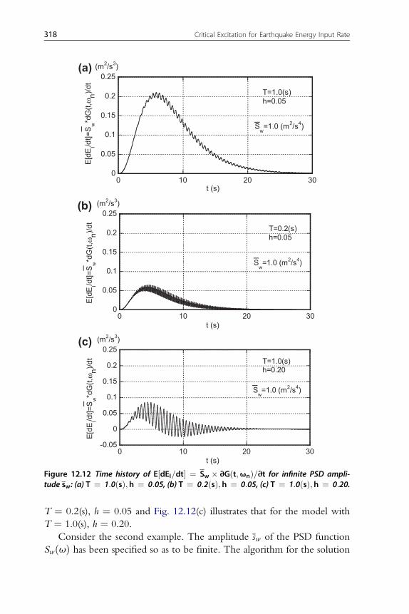
T ¼ 0.2(s), h ¼ 0.05 and Fig. 12.12(c) illustrates that for the model withT ¼ 1.0(s), h ¼ 0.20.

Consider the second example. The amplitude sw of the PSD functionSwðuÞ has been specified so as to be finite. The algorithm for the solution

0

0.05

0.1

0.15

0.2

0.25

0 10 20 30

T=1.0(s)h=0.05

E[dE

I/dt]=

Sw*d

G(t,

ωn)/d

t

t (s)

Sw=1.0 (m2/s4)

(m2/s3)(a)

0

0.05

0.1

0.15

0.2

0.25

0 10 20 30

T=0.2(s)h=0.05

E[dE

I/dt]=

S w*d

G(t,

ωn)/d

t

t (s)

Sw=1.0 (m2/s4)

(m2/s3)(b)

-0.05

0

0.05

0.1

0.15

0.2

0.25

0 10 20 30

T=1.0(s)h=0.20

E[dE

I/dt]=

Sw*d

G(t,

ωn)/d

t

t (s)

Sw=1.0 (m2/s4)

(m2/s3)(c)

Figure 12.12 Time history of E½dEI=dt� ¼ Sw � vGðt;unÞ=vt for infinite PSD ampli-tude sw: (a) T ¼ 1:0ðsÞ;h ¼ 0:05, (b) T ¼ 0:2ðsÞ; h ¼ 0:05, (c) T ¼ 1:0ðsÞ;h ¼ 0:20.


explained in Fig. 12.7(b) has been used for the model with T ¼ 1.0(s) andh ¼ 0.05. Fig. 12.13 shows the mean earthquake energy input rate per unitmass E½dEIðtÞ=dt� with respect to the inverse of the PSD amplitude, 1=sw,for every two seconds. This figure has been drawn by specifying the level ofthe dotted line in Fig. 12.7(b) and finding the intervals ~Ui. The PSDamplitude sw is obtained from sw ¼ Sw=ð2

Pi~UiÞ and the mean earthquake

energy input rate E½dEIðtÞ=dt� is computed from Eqs. (12.18) and (12.25).The search of the maximum value of the function E½dEIðtÞ=dt� with respectto time for a given value of sw corresponds to the proceduremaxt

maxSwðuÞ

fE½dEIðtÞ=dt�g instead of maxSwðuÞ

maxtfE½dEIðtÞ=dt�g as devised in

this chapter. Fig. 12.13 implies that, while the maximum value ofE½dEIðtÞ=dt� is attained around t ¼ 6(s) for larger PSD amplitude sw (smallervalue of the inverse of the PSD amplitude), the maximum value ofE½dEIðtÞ=dt� is attained around t ¼ 4(s) for smaller PSD amplitude sw (largervalue of the inverse of the PSD amplitude).

An example of the critical PSD function for the model with T ¼ 1.0(s)and h ¼ 0.05 is shown in Fig. 12.14. The specified power of SwðuÞ is Sw ¼1:0ðm2=s4Þ and the specified PSD amplitude is sw¼ 0.92ðm2=s3Þ. It can beseen that three rectangles with different widths constitute the critical PSDfunction in this case.

0

0.05

0.1

0.15

0.2

0 0.5 1 1.5 2

t=2st=4st=6st=8st=10st=12st=14s

E[dE

I/dt]

(m2 /s

3 )

inverse of PSD amplitude (s3/m2)

2

4

6

810

12

14

T=1.0(s)h=0.05

Sw=1.0(m2/s4)

Figure 12.13 Plot of mean energy input rate with respect to inverse of power spectraldensity amplitude for various times.


12.10. DETERMINISTIC EARTHQUAKE ENERGY INPUTRATE

In this chapter, the ensemble mean of earthquake energy input rate to anSDOF model has been treated in a probabilistic framework. In this section,a deterministic expression of earthquake energy input rate to an MDOFmodel is introduced (Yamamoto et al. 2011).

Consider a base-isolated building as shown in Fig. 12.15. Let uðtÞ;M; 1denote the horizontal floor displacement vector, the mass matrix and thevector consisting of unity only. The earthquake input energy to this modeluntil time t may be expressed by

EIðtÞ ¼ �Z t0

_uðsÞTM1€ugðsÞds (12.36)

Let us define a modified ground motion €ugðs; tÞ at time s which has thesame component until time t and a null component after time t (seeFig. 12.16, Ohi et al. 1991; Takewaki 2005b). This quantity is called “thetruncated ground motion.” The response velocity at time s correspondingto €ugðs; tÞ is denoted by _uðs; tÞ. The Fourier transforms of €ugðs; tÞ and _uðs; tÞare expressed by €Ugðu; tÞ and _Uðu; tÞ, respectively. From its definition, it isfound that €Ugðu; t0Þ ¼ €UgðuÞ.

By introducing the truncated ground motion €ugðs; tÞ and the corre-sponding velocity response _uðs; tÞ and extending the integration limits,Eq. (12.36) can be rewritten as

EI ðtÞ ¼ �ZN

�N

_uðs; tÞTM1€ugðs; tÞds (12.37)

4 6 8 10

T=1.0(s)h=0.05

S w(ω

) (m

2 /s3 )


0.92

Figure 12.14 Example of critical PSD function SwðuÞ for T ¼ 1:0ðsÞ; h ¼ 0:05 andSw ¼ 1:0ðm2=s4Þ; sw ¼ 0:92ðm2=s3Þ.


Application of the Fourier and inverse Fourier transformations (Lyon1975; Ohi et al. 1985; Kuwamura et al. 1994; Ordaz et al. 2003; Takewaki2004a, b) to Eq. (12.37) leads to

EIðtÞ ¼ �ZN

�N

1

2p

ZN�N

_Uðu; tÞTeiusM1€ugðs; tÞduds

¼ 1

2p

ZN�N

iu1TMTA�1 €Ugðu; tÞM1 €Ugð�u; tÞdu

¼ZN0

€Ugðu; tÞ2FðuÞdu (12.38)

In Eq. (12.38) j €Ugðu; tÞj2 is referred to as the squared Fourier amplitudespectrum (SFAS) and plays a principal role in the present formulation. In thederivation of Eq. (12.38), the relation _Uðu; tÞ ¼ � iuA�1M1 €Ugðu; tÞ isused and the function FðuÞ is defined by

FðuÞhRe½iu1TMTA�1M1�=p (12.39)

Nu

1u

0u

gu

NcNk

Nm

1m

1k1c

m

k

c

Nu

1u

0u

gu

NcNk

Nm

1m

1k1c

m

k

c

Figure 12.15 N-story shear building model supported by base-isolation system.

12.10. Deterministic Earthquake Energy Input Rate 321

Since €Ugðu; t0Þ ¼ €UgðuÞ from its definition, it follows that

EIðt0Þ ¼ZN0

€UgðuÞ2FðuÞdu (12.40)

From Eq. (12.38), the earthquake energy input rate dEI ðtÞ=dt may beexpressed by

dEIðtÞdt

¼ZN0

ðd €Ugðu; tÞ2=dtÞFðuÞdu (12.41)

This expression was derived first by Ohi et al. (1991) and it was pointed outthat the expression dj €Ugðu; tÞj2=dt is equivalent to “the instantaneouspower spectrum” introduced and discussed by Page (1952).

Numerical examples of the deterministic earthquake energy input ratefor a base-isolated 10-story shear building model (BI building or BI system)are presented. The story stiffnesses of the building are determined so that the10-story shear building model with fixed-base has the fundamental naturalperiod of 1.0(s) and the lowest eigenmode of the model with fixed-base isstraight (inverted triangle). Then the lowest eigenmode (super-structuralpart) of the BI building is not straight. This procedure is based on the inverseproblem approach (Nakamura and Yamane 1986). It is also assumed that thedamping matrix of the super-structure with fixed base is proportional to thestiffness matrix of the super-structure and the damping ratio in the lowestmode of the super-structure with fixed base is 0.02. The stiffness k anddamping coefficient c of the BI system have been determined so that the

-0.4-0.3-0.2-0.1

00.10.20.30.4

0 1 2 3 4 5 6

base

acc

eler

atio

n (g

)

time (s)

truncated here

zero input

Figure 12.16 Truncated ground motion.


fundamental natural period of the BI building is 5.3(s) (see Takewaki 1998for hybrid inverse problems for rigid building stiffnesses) and the dampingratio of the BI rigid building model is 0.2. The parameters of the buildingand the BI system are summarized in Table 12.1.

12.11. EXAMPLE 1 (MODEL OF SFAS OF TRUNCATEDGROUND MOTION)

Since the concept of SFAS is somewhat complicated and it seems beneficialto consider example models, its model is constructed. An example of SFASj €Ugðu; tÞj2 of truncated ground motions can be expressed by

€Ugðu; tÞ2 ¼

(2pt$Suðu; tÞ ¼ 2pt$aðe�b1t � e�b2tÞSðuÞ ð0 � t � t0Þ2pt0$Suðu; t0Þ ¼ 2pt0$aðe�b1t0 � e�b2t0ÞSðuÞ ðt � t0Þ

(12.42)

where t0 is the terminal time (duration) of the input ground motion and thefrequency function SðuÞ denotes

SðuÞ ¼(

U4 þ 4z2U2u2

½u2 � U2�2 þ 4z2U2u2

)S0 (12.43)

In Eq. (12.43), U and z are the predominant circular frequency anddamping parameter. Furthermore S0 is a constant value.

The parameter a in Eq. (12.42) is introduced to characterize the intensityof the ground motion and is determined from the constraint on accelerationpower expressed by

CA ¼ZN

�N

€ug ðtÞ2dt ¼1

p

ZN0

€UgðuÞ2du

¼ 1

p

ZN0

€Ugðu; t0Þ2du ¼ 2pt0$aðe�b1t0 � e�b2t0Þ

ZN0

SðuÞdu

(12.44)

In this section, the short period ground motion models and long periodground motion models are taken into account. Table 12.2 shows theparameters for these artificial ground motion models. The long periodground motion models simulate a pulse wave due to near-field ground

12.11. Example 1 (Model of SFAS of Truncated Ground Motion) 323

Table 12.1 Parameters of building and base-isolation system

planmass[kg/m2] mass [kg]

horizontalstiffness [N/m] damping coefficient [Ns/m]

building(10-story)

40m�40m

800(every story)

1.28�107

(reducedSDOF model)

5.05�108

(reducedSDOF model)

lowest-mode damping ratio forfixed-base model ¼ 0.02

base-isolationstory

2400 3.84�106 2.42�107 damping ratio for rigidbuilding model ¼ 0.2

Table 12.2 Input motion modelspredominantperiod of groundor ground motion2p=U (s) duration (s) a b1 b2

Short period model short period model 1 0.6 40 13.2 0.05 0.051short period model 2 0.8 40 17.6 0.05 0.051

Long period model long period model 1 3.0 180 2.9 0.01 0.011long period model 2 5.3 180 4.8 0.01 0.011long period model 3 8.0 180 7.5 0.01 0.011


forEarthquake

EnergyInput

Rate

motions (Hall et al. 1995; Heaton et al. 1995; Jangid and Kelly 2001) ora long-period ground motion resulting from surface waves (Irikura et al.2004; Ariga et al. 2006). The short period ground motion model 1(predominant period ¼ 0.6s) is treated here as the standard ground motionmodel and the parameter a for this model has been determined so that themaximum value of the Fourier amplitude spectrum at the predominantcircular frequency U ¼ 2p=0:6[rad/s] attains the value 3 [m/s] computedfor El Centro NS (Imperial Valley 1940). The damping parameter z is set to0.4 and S0¼ 0.2(m2/s3).

Fig. 12.17 shows the time history of SFAS j €Ugðu; tÞj2 at 18(rad/s) oftruncated ground motions extracted from El Centro NS 1940 and thecorresponding time history of short period ground motion model 1. It canbe seen that the short period ground motion model 1 can simulate very wellthe time history of SFAS j €Ugðu; tÞj2 of truncated motions extracted from ElCentro NS 1940.

Fig. 12.18 illustrates the time histories of input energy for various intro-duced artificial ground motion models. It can be observed that the totalearthquake input energy by the long period ground motion model 2(predominant period ¼ 5.3(s)) is the largest and those by the long periodground motion models 1 and 3 are the next. On the other hand, the totalearthquake input energies by the short period ground motion models arerather small. It should be noted that the long period ground motion model 2has a predominant period resonant to the fundamental natural period of the BIbuilding. This means that the resonance of the fundamental natural period ofthe BI building with the predominant period of ground motions is one of thekey issues in the evaluation of input energy to BI buildings (Ariga et al. 2006).

Fig. 12.19 shows the time histories of energy input rate for various groundmotion models. It is found that the maximum energy input rate by the longperiod ground motion model 2 is the largest and those by the long period

02468

10

0 5 10 15 20 25 30 35 40

El Centro NS 1940short period model 1

squa

red

Four

ier

ampl

itude

[m /s

]2

2

time (s)

Figure 12.17 Time history of SFAS at 18(rad/s) of truncated ground motions extractedfrom El Centro NS 1940 and the corresponding time history of short period model 1.

12.11. Example 1 (Model of SFAS of Truncated Ground Motion) 325

ground motion models 1 and 3 are the next. Although the maximum energyinput rates by the short period ground motion models are small, that by shortperiod ground motion model 2 is comparable to that by the long periodground motion models 1 and 3. It should also be noted that the large energyinput rate continues for a long time (almost 150s) in the long period groundmotion models and large energy input can be predicted in the long periodground motion models from this figure. As in the case of input energy, theresonance of the fundamental natural period of the BI building withthe predominant period of groundmotions seems to be one of the key issues inthe evaluation of energy input rate to BI buildings (Ariga et al. 2006).

12.12. EXAMPLE 2 (DETAILED ANALYSIS OF SFAS OFTRUNCATED GROUND MOTION AND COMPARISON OFTIME-DOMAIN AND FREQUENCY-DOMAIN ANALYSES)

It seems meaningful to investigate the frequency properties of SFAS oftruncated ground motions with various truncated times. Fig. 12.20 presents

0

1x108

2x108

3x108

4x108

5x108

0 50 100 150 200

short period model 1(T=0.6s)short period model 2(T=0.8s)long period model 1(T=3.0s)long period model 2(T=5.3s)long period model 3(T=8.0s)

inpu

t ene

rgy

[J]

time (s)

Figure 12.18 Time histories of input energy for various ground motion models.

0.05.0x1051.0x1061.5x1062.0x1062.5x1063.0x1063.5x1064.0x106

0 50 100 150 200

short period model 1(T=0.6s)short period model 2(T=0.8s)long period model 1(T=3.0s)long period model 2(T=5.3s)long period model 3(T=8.0s)

ener

gy in

put r

ate

[J/s

]

time (s)

Figure 12.19 Time histories of energy input rate for various ground motion models.


the frequency distributions of SFAS j €Ugðu; tÞj2 of El Centro NS (ImperialValley 1940) truncated at (a) 2.5s, (b) 5.0s, (c) 20.0s, (d) 40.0s. It can beobserved that, while a blunted spectrum is seen in the motions truncated atearly stages, a sharp spectrum can be found in the motions truncated at laterstages. It can also be understood that the intensity becomes larger as thetruncated time passes (moves later).

Fig. 12.21 illustrates the frequency distributions of the time-rates

vj €Ugðu; tÞj2=vt of SFAS of El Centro NS 1940 truncated at (a) 2.5s,

(b) 5.0s, (c) 20.0s, (d) 40.0s). As in Fig. 12.20, it can be observed that, whilea blunted time-rate spectrum is seen in the motions truncated at early stages,a sharp spectrum can be found in the motions truncated at later stages. Onthe other hand, the intensity is largest at the intermediate truncated time

different from the case for SFAS j €Ugðu; tÞj2.Fig. 12.22 shows sample accelerations of a simulated nonstationary

ground motion and a stationary ground motion. The stationary motionhas also been generated to clarify the property of j €Ugðu; tÞj2 through

0.0

2.0

4.0

6.0

8.0

10.0

Four

ier a

mpl

itude

spe

ctru

m (m

/s )

22

Four

ier a

mpl

itude

spe

ctru

m (m

/s )

22

Four

ier a

mpl

itude

spe

ctru

m (m

/s )

22

Four

ier a

mpl

itude

spe

ctru

m (m

/s )

22

circular frequency (rad/s)0.0

2.0

4.0

6.0

8.0

10.0


(a) (b)

(c) (d)

0.0

2.0

4.0

6.0

8.0

10.0


0 10 20 30 40 50 0 10 20 30 40 50

0 10 20 30 40 50 0 10 20 30 40 500.0

2.0

4.0

6.0

8.0

10.0


Figure 12.20 Frequency distributions of SFAS j €Ugðu; tÞj2 of El Centro NS 1940 trun-cated at (a) 2.5s, (b) 5.0s, (c) 20.0s, (d) 40.0s.

12.12. Example 2 (Detailed Analysis of SFAS of Truncated Ground Motion and Comparison) 327

the comparison with that for the nonstationary motion. This simulatedstationary ground motion has been generated by the sum of sine waveswith a band limited PSD function of 0.03(m2/s3) in the frequencyrange 0.1–5.1(rad/s) instead of Eq. (12.43). On the other hand, thenonstationary motion has been multiplied by an envelope function

-5.0

-2.5

0.0

2.5

5.0

(b)(a)

(d)(c)

circular frequency (rad/s)-5.0

-2.5

0.0

2.5

5.0


-5.0

-2.5

0.0

2.5

5.0

time

rate

of s

quar

ed F

ourie

r

am

plitu

de s

pect

rum

(m /s

)2

3tim

e ra

te o

f squ

ared

Fou

rier

am

plitu

de s

pect

rum

(m /s

)2

3

time

rate

of s

quar

ed F

ourie

r

am

plitu

de s

pect

rum

(m /s

)2

3

time

rate

of s

quar

ed F

ourie

r

am

plitu

de s

pect

rum

(m /s

)2

3


0 10 20 30 40 50 0 10 20 30 40 50

0 10 20 30 40 50 0 10 20 30 40 50-5.0

-2.5

0.0

2.5

5.0


Figure 12.21 Frequency distributions of time-rates vj €Ugðu; tÞj2=vt of SFAS of El CentroNS 1940 truncated at (a) 2.5s, (b) 5.0s, (c) 20.0s, (d) 40.0s.

-2.0

-1.0

0.0

1.0

2.0(a) (b)

0 5 10 15 20 25 30 35 40

acce

lera

tion

(m/s

)2

time (s)

-2.0

-1.0

0.0

1.0

2.0

0 5 10 15 20 25 30 35 40

acce

lera

tion

(m/s

v )2

time (s)

Figure 12.22 A sample of simulated ground acceleration: (a) nonstationary input,(b) stationary input.


given by Eq. (12.42) with parameters a ¼ 2.32, b1 ¼ 0.09, b2 ¼ 1.49.These simulated ground motions enable one to compare (1) the timehistories of earthquake input energy computed by the time-domainmethod (Eq. (12.36)) and the frequency-domain method (Eq.(12.38)) and (2) the time histories of energy input rate computed bythe time-domain method (dEIðtÞ=dt ¼ � _uðtÞTM1€ugðtÞ) and thefrequency-domain method (Eq. (12.41)). This comparison may bedifficult in the model described by Eqs. (12.42) and (12.43) because itdoes not seem easy to obtain the corresponding time history of groundmotion acceleration.

Fig. 12.23 illustrates the 3-D view of average SFAS of 100 groundmotions truncated at continuously increasing time ((a) nonstationary, (b)stationary)). A characteristic similar to Fig. 12.21 (blunted spectrum at earlystages and sharp spectrum at later stages) can be observed in both figures. Itcan also be seen that, since the nonstationary motion with high intensityalmost ends at 20(s), the averaged frequency distributions of SFAS do notchange much after the truncated time of around 20(s).

Fig. 12.24 shows the comparison of the time histories of earthquakeinput energy computed by the time-domain method (Eq. (12.36)) and thefrequency-domain method (Eq. (12.38)) for a nonstationary ground motion.In Fig. 12.24, the plots by the time-domain method with differentcomputational time increments (dt ¼ 0.005, 0.01, 0.02s) are also illustrated.It can be observed that, while the accuracy of the time-domain methoddepends largely on the computational time increment, the frequency-domain method exhibits a stable result close to the result for dt ¼ 0.005.This clearly shows the reliability of the frequency-domain method.Furthermore, it should be kept in mind that, owing to the introduction ofFourier amplitude spectra of truncated ground motions, the computationalerror does not accumulate even at later times in the frequency-domainformulation.

Fig. 12.25 illustrates the comparison of the time histories of energy inputrate computed by the time-domain method (dEIðtÞ=dt ¼ � _uðtÞTM1€ugðtÞ)and the frequency-domain method (Eq. (12.41)) for a nonstationary groundmotion. It can be observed that the frequency-domain method has almost anequivalent accuracy to the time-domain method. It should be noted that,because the analytical functions of ground motion accelerations with arbi-trary truncated time and its Fourier transform exist in this case, an accuratecomparison becomes possible.

12.12. Example 2 (Detailed Analysis of SFAS of Truncated Ground Motion and Comparison) 329

Figure 12.23 Average value of SFAS of 100 ground motions truncated at continuouslyincreasing time: (a) nonstationary input, (b) stationary input.


12.13. CONCLUSIONS

The conclusions may be stated as follows:(1) A probabilistic critical excitation method can be developed for the

problem of maximizing the mean earthquake energy input rate todamped linear elastic SDOF models.

(2) An expression has been derived on the probabilistic earthquake inputenergy and its time derivative subjected to uniformly modulated

0 5 10 15 20 25 30 35 40

time domainfrequency domain

time

hist

orie

s of

ene

rgy

inpu

t rat

e (J

/s)

time (s)

0.6

-0.2

0.4

0.2

0.0

× 108

Figure 12.25 Comparison of time histories of energy input rate computed by the time-domain method (dEIðtÞ=dt ¼ � _uðtÞTM1€ugðtÞ) and the frequency-domain method(Eq. (12.41)) for nonstationary input.

0 5 10 15 20 25 30 35 40

dt=0.02dt=0.01dt=0.005frequency domain

time

hist

ory

of e

arth

quak

e in

put e

nerg

y (J

)

time (s)

1.0

0.5

0.0

× 108

Figure 12.24 Comparison of time histories of earthquake input energy computed bythe time-domain method (Eq. (12.36)) and the frequency-domain method (Eq. (12.38))for nonstationary input.


stochastic ground motions. The integrand of the objective function tobe maximized in the critical excitation problem can be expressed as theproduct of a time-frequency function representing the transfer energyinput rate and the power spectral density function of a stochastic part inthe input motion.

(3) An idea similar to the previously explained one can be used partially infinding and identifying the most unfavorable frequency content of thecritical excitation which is described by a uniformly modulated exci-tation model. The key is the order interchange in the double maxi-mization procedure of the objective function with respect to time and tothe shape of the power spectral density function.

(4) An expression has also been derived on the probabilistic earthquakeinput energy and its time derivative subjected to complex nonuniformlymodulated stochastic ground motions. The explained solution proceduremay be extended to a more general problem for such nonuniformlymodulated ground motion models.

(5) Numerical examples revealed the peculiar time-varying characteristicsof the generalized nonstationary energy transfer function multiplied bythe envelope function of the input motion model.

(6) The validity of the present solution algorithm for the infinite powerspectral density amplitude and the finite power spectral density ampli-tude has been demonstrated numerically.

REFERENCESAkiyama, H., 1985. Earthquake Resistant Limit-state Design for Buildings. University of

Tokyo Press, Tokyo, Japan.Ariga, T., Kanno, Y., Takewaki, I., 2006. Resonant behaviour of base-isolated high-rise

buildings under long-period ground motions. Struct. Design Tall Spec. Build. 15 (3),325–338.

Austin, M., Lin, W., 2004. Energy balance assessment of base-isolated structures. J. Eng.Mech. 130 (3), 347–358.

Bozorgnia, Y., Bertero, V., 2003. Damage spectra: characteristics and applications to seismicrisk reduction. J. Struct. Eng. 129 (10), 1330–1340.

Conte, J.P., Peng, B.F., 1997. Fully non-stationary analytical earthquake ground motionmodel. J. Engrg. Mech. 123 (1), 15–24.

Crandall, S.H., 1958, 1963. Random Vibration, Vol.I.. II. MIT Press, Cambridge, MA.Der Kiureghian, A., 1980. Structural response to stationary excitation. J. Eng. Mech. Div.

106 (6), 1195–1213.Drenick, R.F., 1970. Model-free design of aseismic structures. J. Engrg. Mech. Div. 96 (4),

483–493.Fang, T., Sun, M., 1997. A unified approach to two types of evolutionary random response

problems in engineering. Archive of Applied Mechanics 67 (7), 496–506.


Hall, J.F., Heaton, T.H., Halling, M.W., Wald, D.J., 1995. Near-source ground motion andits effects on flexible buildings. Earthquake Spectra 11 (4), 569–605.

Heaton, T.H., Hall, J.F., Wald, D.J., Halling, M.W., 1995. Response of high-rise and base-isolated buildings to a hypothetical MW 7$0 blind thrust earthquake. Science 267(5195), 206–211.

Housner, G.W., 1956. Limit design of structures to resist earthquakes. Proc. of the FirstWorld Conference on Earthquake Engineering. University of California, Berkeley, CA.Berkeley, 5:1–5:11.

Housner, G.W., 1959. Behavior of structures during earthquakes. J. Engrg. Mech. Div.85 (4), 109–129.

Housner, G.W., Jennings, P.C., 1975. The capacity of extreme earthquake motions todamage structures. In: Hall, W.J. (Ed.), Structural and Geotechnical Mechanics: Avolume honoring N.M.Newmark. Prentice-Hall Englewood Cliff, NJ,pp. 102–116.

Irikura, K., Kamae, K., Kawabe, H., 2004. Importance of prediction of long-period groundmotion during large earthquakes. In: Annual Conference of the Seismological Societyof Japan, Poster session (in Japanese).

Iyama, J., Kuwamura, H., 1999. Application of wavelets to analysis and simulation ofearthquake motions. Earthquake Engrg. and Struct. Dyn. 28 (3), 255–272.

Jangid, R.S., Kelly, J.M., 2001. Base isolation for near-fault motions. Earthquake EngngStruct Dyn 30 (5), 691–707.

Kuwamura, H., Kirino, Y., Akiyama, H., 1994. Prediction of earthquake energy inputfrom smoothed Fourier amplitude spectrum. Earthquake Engng. Struct. Dyn. 23 (10),1125–1137.

Kuwamura, H., Iyama, J., Takeda, T., 1997a. Energy input rate of earthquake groundmotion–matching of displacement theory and energy theory. J. Structural andConstruction Engrg., Archi. Inst. of Japan 498, 37–42 (in Japanese).

Kuwamura, H., Takeda, T., Sato, Y., 1997b. Energy input rate in earthquakedestructiveness–comparison between epicentral and oceanic earthquakes. J. Structuraland Construction Eng., Archi. Inst. of Japan 491, 29–36 (in Japanese).

Lin, Y.K., 1967. Probabilistic theory of structural dynamics. McGraw-Hill, New York.Lyon, R.H., 1975. Statistical energy analysis of dynamical systems. The MIT Press,

Cambridge, MA.Nakamura, T., Yamane, T., 1986. Optimum design and earthquake-response constrained

design of elastic shear buildings. Earthquake Engineering and Structural Dynamics14 (5), 797–815.

Nigam, N.C., 1983. Introduction to Random Vibrations. MIT Press, Cambridge, MA.Ohi, K., Takanashi, K., Tanaka, H., 1985. A simple method to estimate the statistical

parameters of energy input to structures during earthquakes. J Struct Construct Engng,AIJ 347, 47–55 (in Japanese).

Ohi, K., Takanashi, K., Honma, Y., 1991. Energy input rate spectra of earthquake groundmotions. J. Structural and Construction Engrg., Archi. Inst. of Japan 420, 1–7 (in Japanese).

Ordaz, M., Huerta, B., Reinoso, E., 2003. Exact computation of input-energy spectra fromFourier amplitude spectra. Earthquake Engrg. and Struct. Dyn. 32 (4), 597–605.

Page, C.H., 1952. Instantaneous power spectra. Journal of Applied Physics 23 (1), 103–106.Shinozuka, M., 1970. Maximum structural response to seismic excitations. J. Engrg. Mech.

Div. 96 (5), 729–738.Takewaki, I., 1998. Hybrid inverse eigenmode problem for a shear building supporting

a finite element subassemblage. Journal of Vibration and Control 4 (4), 347–360.Takewaki, I., 2001. Nonstationary random critical excitation for nonproportionally damped

structural systems. Computer Methods in Applied Mechanics and Engineering 190 (31),3927–3943.


Takewaki, I., 2002. Seismic critical excitation method for robust design: A review. J. Struct.Eng. 128 (5), 665–672.

Takewaki, I., 2004a. Frequency domain modal analysis of earthquake input energy to highlydamped passive control structures. Earthquake Engrg. and Struct. Dyn. 33 (5), 575–590.

Takewaki, I., 2004b. Bound of earthquake input energy to soil-structure interactionsystems. Proc. of the 11th Int. Conf. on Soil Dynamics and Earthquake Engrg. (ICS-DEE) and the 3rd Int. Conf. on Earthquake Geotechnical Engrg. (ICEGE). Berkeley,January 7–9, 2: 734–741.

Takewaki, I., 2004c. Bound of earthquake input energy. J. Struct. Eng. 130 (9), 1289–1297.Takewaki, I., 2004d. Critical envelope functions for non-stationary random earthquake

input. Computers & Structures 82 (20–21), 1671–1683.Takewaki, I., 2005a. Bound of earthquake input energy to soil–structure interaction

systems. Soil Dynamics and Earthquake Engineering 25 (7–10), 741–752.Takewaki, I., 2005b. Closure to the discussion by Ali Bakhshi and Hooman Tavallali [to

I. Takewaki’s (2004) Bound of Earthquake Input Energy. J Struct. Eng. 130 (9),1289–1297, 131(10), 1643–1644.

Takewaki, I., Fujimoto, H., 2004. Earthquake input energy to soil-structure interactionsystems: A frequency-domain approach. Advances in Structural Engineering 7 (5),399–414.

Trifunac, M.D., Hao, T.Y., Todorovska, M.I., 2001. On energy flow in earthquakeresponse. Report CE 01–03, July. University of Southern California.

Uang, C-M., Bertero, V.V., 1990. Evaluation of seismic energy in structures. EarthquakeEngrg. and Struct. Dyn. 19 (1), 77–90.

Vanmarcke, E.H., 1977. Structural response to earthquakes. In: Lomnitz, C.,Rosenblueth, E. (Eds.), Seismic Risk and Engineering Decisions. Elsevier, Amsterdam,pp. 287–337.

Yamamoto, K., Fujita, K., Takewaki, I., 2011. Instantaneous earthquake input energy andsensitivity in base-isolated building. Struct. Design Tall Spec. Build. 20 (6), 631–648.


CHAPTER THIRTEEN

Critical Excitation forMulti-Component Inputs

Contents

13.1. Introduction 33513.2. Horizontal and Vertical Simultaneous Inputs 33613.3. Bi-Directional Horizontal Inputs 34213.4. Interpretation Using Inner Product 34813.5. Conclusions 350References 350

13.1. INTRODUCTION

The ground motion is an outcome of ground shaking induced byseismic waves that are transmitted from an epicenter through the ground.Therefore, simultaneous consideration of multiple components of groundmotion is realistic, reasonable and inevitable in the reliable design ofstructures. It is sometimes assumed practically that there exist principal axesin the ground motions (Penzien and Watabe 1975; Clough and Penzien1993). Penzien and Watabe (1975) investigated many recorded groundmotions and found a tendency of existence of those axes. It is alsorecognized in the literature that the principal axes change their directions intime during ground shaking. In recent structural design practice, the effectof the multi-component ground motions is often included by using thesquare root of the sum of the squares (SRSS) method, or the extendedComplete Quadratic Combination rule (CQC3) method (Smeby andDer Kiureghian 1985). It may be beneficial to provide an overview ofthese methods.

In the SRSS method, the maximum responses to respective groundmotions are combined based on the rule of SRSS. The SRSS method is thefirst-step method for combination and assumes statistical independenceamong the respective ground motions. However, it is well understood thatthe multi-component ground motions have some statistical dependence andsome revisions may be desired.



http://dx.doi.org/10.1016/B978-0-08-099436-9.00013-4

On the other hand, the CQC3 rule is well known as a response spectrummethod that can take into account the effect of correlation between thecomponents of ground motions, and this method is frequently used in theUSA. Although an absolute value of a cross power spectral density (PSD)function has been described by the correlation coefficient, the CQC3 rulecannot treat directly, in the sense of direct treatment of both real and imag-inary parts, the cross PSD functions of multi-component ground motions.

After some preliminary investigations on actual response data for actualinputs, useful proposals were made. Menun and Der Kiureghian (1998) andLopez et al. (2000) employed the CQC3 method as the response evaluationmethod and discussed the critical states, e.g. a critical loading combination ora critical incident angle. It is clear that the derived results depend on the accuracyof the CQC3method. Athanatopoulou (2005) and Rigato andMedina (2007)investigated the effect of incident angle of groundmotions on structural responsewithout use of the Penzien-Watabe (1975) model and pointed out the signif-icance of consideringmultiple inputs in practical seismic design. The approach isapplicable only to a set of recorded motions. In the references of Fujita et al.(2008a) andFujita andTakewaki (2010), the cross PSD function in terms of bothreal and imaginary parts was discussed in more detail from the viewpoint ofcritical excitation. They concluded that the critical set of co-spectrum and quad-spectrum, the real and imaginary parts of the cross PSD function, can be char-acterized by the maximization of the inner product between (co-spectrum,quad-spectrum) and the characteristic functions ( f1ðt;uÞ, f2ðt;uÞ) consisting ofstructural modal properties and envelope functions of inputs.

Critical excitation methods have been developed extensively since thepioneering work by Drenick in 1970 (see Chapter 1). In particular, in recentwork, after 1995, there has been remarkable advancement (Manohar andSarkar 1995; Sarkar and Manohar 1996, 1998; Takewaki 2001, 2002, 2004a,2004b, 2006b; Abbas and Manohar 2002a, 2007; Takewaki et al. 2012).However, there has been little research on critical excitation methods undermultiple-component inputs.

In the following section, the critical excitation for horizontal and verticalsimultaneous inputs is discussed.

13.2. HORIZONTAL AND VERTICAL SIMULTANEOUSINPUTS

Consider a rigid block, as shown in Fig. 13.1, of mass m and mass moment Igof inertia around the centroid C subjected to horizontal and vertical

336 Critical Excitation for Multi-Component Inputs

simultaneous base inputs. Let €ug and €vg denote the horizontal and verticalground accelerations, respectively. The rigid block is supported by a set ofa horizontal spring kH and a dashpot cH and another set of two verticalsprings ð1=2ÞkV and dashpots ð1=2ÞcV . These springs and dashpots representthe stiffness and damping of the ground on which the rigid block rests. Thewidth and the height of the rigid block are denoted by 2L and 2H,respectively. The motion of the block consists of a horizontal-rotationalmotion under a horizontal base input and a vertical motion undera vertical base input.

Let u and q denote the horizontal displacement of the centroid C relativeto the horizontal input and the angle of rotation of the rigid body,respectively, and let v denote the vertical displacement of the centroid Crelative to the vertical input. The equations of motion of the rigid block inthe swaying-rocking motion can be expressed as

24m 0

0 Ig

358<:

€u

€q

9=;þ

24 cH �cHH

�cHH cHH2 þ cVL

2

358<:

_u

_q

9=;

þ"

kH �kHH

�kHH kHH2 þ kVL

2

#(u

q

)¼ �

"m 0

0 Ig

#(1

0

)€ug

(13.1)

Centroid C

2L

2H

m, Ig

cH

kH

(1/2)cV

(1/2)cV

(1/2)kV

(1/2)kV

gu

gv

u

v

horizontal input

vertical input

Figure 13.1 Elastically supported rigid block subjected to horizontal and verticalsimultaneous inputs.

13.2. Horizontal and Vertical Simultaneous Inputs 337

By using the complex modal combination method, the rotationalresponse of the rigid block can be expressed as

qðtÞ ¼X2i¼ 1

RehbðiÞQðiÞqðiÞðtÞ

i(13.2)

where bðiÞ and QðiÞ denote the i-th complex participation factor and therotational angle in the i-th complex eigenmode. qðiÞðtÞ is the i-th complexmodal coordinate. The detailed explanation of these parameters can befound in Fujita et al. (2008b).

On the other hand, the vertical response of this model as a single-degree-of-freedom (SDOF) model can be derived as

vðtÞ ¼Z t

0

�� €vgðsÞ�gV ðt � sÞds (13.3)

where gV ðtÞ ¼ ð1=uv0Þe�hvuvt sinuv

0t (uv ¼ ffiffiffiffiffiffiffiffiffiffiffiffikV=m

p) is the impulse

response function in the vertical vibration and uv0 ¼ uv

ffiffiffiffiffiffiffiffiffiffiffiffiffiffiffi1� hv

2p

is thedamped natural circular frequency of the model in the vertical vibration.The parameter hv is the damping ratio in the vertical vibration.

The horizontal input acceleration and a vertical input acceleration are tobe described as a nonstationary random process.

€ug�t� ¼ cu

�t�wu

�t�

(13.4a)

€vg�t� ¼ cv

�t�wv

�t�

(13.4b)

where cuðtÞ, cvðtÞ are deterministic envelope functions and wuðtÞ, wvðtÞ arezero mean stationary Gaussian random processes. It is assumed that cuðtÞ andcvðtÞ are given and the power spectra of wuðtÞ and wvðtÞ are prescribed. Amore elaborate model (nonuniformly modulated model, (see Takewaki2006a) can be used if desired.

The corresponding critical excitation problem is to find the worst cross-spectrum (see Nigam 1983) and the corresponding cross-correlation func-tion of the horizontal and vertical inputs (wuðtÞ and wvðtÞ) that produce themaximum mean squares response of the uplift. The real part of the cross-spectrum is denoted by Cwuwv

and the imaginary part is indicated byQwuwv

. This problem includes a difficulty of maximizing the objectivefunction both to time and cross-spectrum between wuðtÞ and wvðtÞ. Toovercome this difficulty, an algorithm is devised such that the order of the


maximizations with respect to time and the cross-spectrum is interchanged.The schematic diagram of this procedure is shown in Fig. 13.2.

Consider next a moment-resisting frame, as shown in Fig. 13.3, sub-jected to horizontal and vertical simultaneous inputs (Fujita et al. 2008a;Fujita and Takewaki 2009). The input ground motions are modeled by Eqs.(13.4a, b). The corresponding critical excitation problem is to find the cross-spectrum ðCwuwv

;QwuwvÞ and the corresponding cross-correlation function

of the worst horizontal and vertical inputs (wuðtÞ and wvðtÞ) that produce themaximum root mean squares response of sum of bending moments due tohorizontal and vertical inputs with respect to span length.


maxim

izatio

n w

ith

resp

ect to

cro

ss sp

ectru

m

it t jt t

time

Uplift to cross

spectrum 1

Uplift to cross

spectrum 2

Uplift to cross

spectrum M

( )v uw wC

( )v uw wQ

1 2

1

2

Sub-problem optimization

for a given frequency

ω

ωω ω ω

ωω

ω

= =

Figure 13.2 Schematic diagram of the proposed procedure (order interchange ofdouble maximization procedure including subproblem optimization).

horizontalinput

vertical input

gu

gv

Figure 13.3 Moment-resisting frame subjected to horizontal and vertical simultaneousinputs.


Fig. 13.4 shows the co-spectrum and quad-spectrum of the critical input.It can be observed that the quad spectrum has a rather small value comparedto the co-spectrum. Fig. 13.5 presents the phase angle of the cross spectrumof the critical input. This figure just corresponds to the quad spectrum inFig. 13.4. Fig. 13.6 illustrates a sample of horizontal and vertical motionaccelerations in the critical input. The vertical motion was constructed so asto exhibit a critical relation with a sample horizontal motion. Fig. 13.7 showsthe amplitude ratio of vertical to horizontal motions in the critical input andthe perfectly correlated input. It can be seen that an average of the ratio isalmost 0.5. Fig. 13.8 presents the maximum value of root mean squares ofthe sum of bending moments due to horizontal and vertical inputs with

-0.5

0

0.5

1

1.5

2

0 5 10 15 20 25 30

co-spectrumquad-spectrum

cros

s-sp

ectru

m (m

2 /s3 )


L=17.0m t=12.0s

Figure 13.4 Co-spectrum and quad-spectrum in critical input.

-15

-10

-5

0

5

10

15

0 5 10 15 20 25 30

phas

e an

gle

(deg

ree)


Figure 13.5 Phase angle of cross spectrum in critical input.


respect to span length (critical correlation, perfect correlation, withoutcorrelation (SRSS)). It should be noted that the model with the span lengthof 17(m) has the same fundamental natural frequencies both in horizontaland vertical vibrations.

-20-15-10-505

101520

0 5 10 15 20 25 30 35 40

Horizontal input Critical vertical input

time (s)

acce

lera

tion

(m/s

2 )

Figure 13.6 Sample of horizontal and vertical motions in critical input.

00.10.20.30.40.50.60.70.80.9

1

0 5 10 15 20 25 30 35 40

Critical input Input of perfect correlation

time (s)

Verti

cal A

mpl

itude

/ H

oriz

onta

l Am

plitu

de

Figure 13.7 Amplitude ratio of vertical motion to horizontal motion in critical inputand perfectly correlated input.

10 15 20 25 30 35 40

including critical correlationQ=0without correlation (SRSS)

span (m)

1.2

1.0

0.8

0.6

0.4

0.2max

val

ue o

f roo

t mea

n sq

uare

of s

umof

the

bend

ing

mom

ent (

*108

Nm

)

Figure 13.8 Maximum value of root mean square of sum of bending moments due tohorizontal and vertical inputs with respect to span length (critical correlation, perfectcorrelation, without correlation (SRSS)).


13.3. BI-DIRECTIONAL HORIZONTAL INPUTS

While the critical excitation problem under horizontal and verticalground motion inputs is to find the worst cross-spectrum and the corre-sponding cross-correlation function of the horizontal and vertical inputs thatproduce the maximum mean squares response of the uplift, the criticalexcitation problem under two horizontal ground motion inputs is to findthe worst cross-spectrum and the corresponding cross-correlation functionof the two horizontal inputs that produce the maximum mean squaresresponse. In the problem under horizontal and vertical ground motioninputs, the input directions coincide with the building principal axes in mostcases. On the other hand, in the problem under two horizontal inputs, theinput directions do not necessarily coincide with the building principal axes.This situation brings a further problem of great significance. The coherencefunction between two horizontal ground motion inputs is a function of theratio of power spectra of two horizontal ground motion inputs and the angleof input to the building. For each angle of input to the building and the ratioof power spectra of two horizontal ground motion inputs, the coherencefunction between two horizontal ground motion inputs is computed. Thena technique similar to that for the problem under horizontal and verticalground motion inputs can be used.

Consider a one-story one-span three-dimensional (3-D) frame as shownin Fig. 13.9. It is assumed that two axes X1 and X2 are perpendicular to eachother and along the building structural axes. Let SZ1

ðuÞ and SZ2ðuÞ denote

the auto PSD functions along the principal axes Z1, Z2 of ground motionsrespectively. According to the Penzien and Watabe (P-W) model, two-dimensional ground motions (2DGM) along Z1, Z2 are regarded to becompletely uncorrelated. The auto PSD functions of ground motions alongX1, X2 are determined from the auto PSD functions of 2DGM along Z1, Z2.The auto PSD functions along X1, X2 are described by S11ðuÞ and S22ðuÞ,respectively.

2X

1X

Figure 13.9 Space frame structure subjected to bi-directional horizontal inputs.


It can be shown that the sum of SZ1ðuÞ and SZ2

ðuÞ is to be equal to thesum of S11ðuÞ and S22ðuÞ. Furthermore, the coherence function between2DGM along X1 and X2 is also denoted as

r12

�gorg; q

�¼

�1� gorg

�sin 2qffiffiffiffiffiffiffiffiffiffiffiffiffiffiffiffiffiffiffiffiffiffiffiffiffiffiffiffiffiffiffiffiffiffiffiffiffiffiffiffiffiffiffiffiffiffiffiffiffiffiffiffiffiffiffiffiffiffiffiffiffiffiffiffiffiffiffi�

1þ gorg

�2 � �1� gorg

�2cos2 2q

r (13.5)

where gorg ¼ SZ2ðuÞ=SZ1

ðuÞ. q is the angle of rotation (incident angle)between the two horizontal axes Z1, X1. Fig. 13.10 shows the coherencefunction expressed by Eq. (13.1)with various values ofgorg for varied rotation(incident) angle. In Fig. 13.10, when gorg is zero, the coherence functionr12 is reduced to 1 at any q except q ¼ 0 and q ¼ p=2. This means that thecomponents along X1 and X2 have perfect correlation under unidirectionalground motion along the major principal axis of ground motion.

The P-W model is often used in the modeling of multi-componentground motions. Although the coherence function of 2DGM alongX1 and X2 can be given in terms of gorg and q as shown in Eq. (13.5), thecross PSD function cannot be treated directly in the CQC3 rule. For thatreason, it is supposed in this chapter that the cross PSD function between2DGM along X1 and X2 can take any value in the feasible complex plane.

0.0

0.2

0.4

0.6

0.8

1.0

γorg

=1

γorg

=0.7

γorg

=0.5

γorg

=0.3

γorg

=0.1

γorg

=0.01

cohe

renc

e fu

nctio

n

incident angle (radian)π / 4 π / 20 π / 8 3π / 8

Figure 13.10 Coherence function of 2DGMwith various auto PSD ratios with respect tovarious incident angles in the Penzien-Watabe model (Fujita and Takewaki 2010).

13.3. Bi-Directional Horizontal Inputs 343

From the definition of the coherence function, the co-spectrum (real part ofcross PSD) C12ðuÞ and quad-spectrum (imaginary part of cross PSD)Q12ðuÞ must satisfy the following relation.

C12ðuÞ2 þQ12ðuÞ2 �nr12

�gorg; q

�o2S11

�u�S22

�u�

(13.6)

This model is called the extended P-Wmodel hereafter. It may be possibleto incorporate the extended P-W model into the stochastic response evalua-tionmethod. In that case, a new critical excitation problem can be constructed

�Distribute auto PSD function to the b.s.a�Coherence function is

given by

� Consider the feasible complex area of Cross PSD function

� Co-spectrum and Quad-spectrum can be considered independently.

� Quad-spectrum gives a phase difference between the bi-directional ground inputs

Bi-directional ground input along the b.s.a

and are correlated

Coherence function only gives an absolute value of cross PSD function

( )S ω ( )S ω

( )( )

( ) ( )S

S S

ωρ ω

ω ω=

X

X( )11S ω

( )22S ω

( )C ω

12 ( )Q ω

Case.1

Case.2Case.3

ϕPhase angle

( )C ω

( )Q ω

Case.2

Case.1

No difference between case.1&2

CQC3 rule deals with the coherence function only. Quad-spectrum can’t be treated

Extended Penzien-Watabe model

Penzien-Watabe model

�Define the building structural axes (b.s.a)

One-story one-span 3-D frameLL

Center of mass X

XThe building structural axes

b.s.a

�Define the principal axesof ground motions (g.p.a)�Input uncorrelated

auto PSD function along the g.p.a�Give and orgγ θ

X

X

( )1zS ω( )2zS ω The principal axes of ground motions

g.p.a

( ) ( )/S Sγ ω ω≡θ

Consider cross PSD function

12 12 12iS C Q= +

1Z

2Z

( ) ( )( ) ( )

γ θρ γ θ

γ γ θ

Figure 13.11 Comparison of extended P-W model with P-W model (Fujita and Takewaki2010).


in which the critical cross PSD function is searched in the feasible complexplane represented by Eq. (11.2). This method can be regarded as an extendedmethod of the CQC3 rule based on the P-W model.

Fig. 13.11 shows the comparison of the extended P-W model with theP-W model. In the extended P-W model, a feasible complex area of thecross PSD function is considered. In this framework, both the co-spectrumand quad-spectrum can be treated independently. The quad-spectrum givesa phase difference between the bi-directional ground inputs.

Sum of the auto PSD functions along the principal axes of ground motions (g.p.a) is constantGive auto PSD function ratio

( )

Constraint of bi-directional ground motions

2X

X( )S ω

( )S ω

( )S ω

X

X( )S ω

1X( )S ω

( )S ω

Parametric analysis for span length

org 0.0, 0 .25, 0 .75, 1.0γ =

Sum of the auto PSD functions along (b.s.a) is constant. Coherence function is fixed at 1.0Give auto PSD function ratio along the b.s.a ( )

ground motions

0.0, 0.25, 0.75, 1 .0γ =

org 0.25γ =

org 0.75γ =

org 1.0γ =

Compare four cases of

X

X

X

X

X

X

X

X

Parametric analysis for input angle from 0 to /2

a 0.0γ =θ

θ

θ

θ

γ

Critical incident angle exists.

Parametric analysis for incident angle

To give auto PSD function ratio along the b.s.a and coherence corresponds to uni-direct. ground input.

e.g. and coherence=1.0 is regarded as uni-directional ground input with

1.0γ =

/ 4θ π=X

X

Z

� �

��

Figure 13.12 Relationship between the method for building structural axes and themethod for ground motion principal axes (Fujita and Takewaki 2010).

13.3. Bi-Directional Horizontal Inputs 345

Fig. 13.12 presents the relationship between the method for buildingstructural axes and the method for ground motion principal axes. Inthe method for building structural axes, the sum of the auto PSD functionsalong the building structural axes is kept constant. On the other hand, in themethod for ground motion principal axes, the sum of the auto PSD func-tions along the ground motion principal axes is kept constant.

Fig. 13.13 shows the schematic diagram of the proposed procedure. It isinteresting to note that this optimization procedure utilizes the orderinterchange of the double maximization procedure including subproblemoptimization with respect to cross-spectrum and time.

Fig. 13.14 is the schematic illustration of the present critical excitationproblem. It is useful to understand the problem structure graphically.

In order to understand the property of the critically correlated groundmotions more deeply, comparison with the perfectly correlated groundmotions without time delay has been made. The structural plan is given asL1 ¼ 25ðmÞ, L2 ¼ 15ðmÞ. Fig. 13.15 shows a sample of the critical inputs(2-D horizontal ground motions) and the corresponding time history of theroot-mean-square of column-end fiber stress.

Another comparison with the perfectly correlated ground motionswithout time delay has been made for different structural spans. Thestructural plan is given as L1 ¼ 15ðmÞ, L2 ¼ 25ðmÞ. Fig. 13.16(a) shows


maxim

izatio

n w

ith

re

sp

ect to

cro

ss sp

ectru

m

it t= jt t=

time

Column stress

to cross

spectrum 1

Column stress

to cross

spectrum 2

Column stress

to cross

spectrum M

( )v uw wC ω

( )v uw wQ ω

ω

ω

1ω 2ω

1ω2ω

Sub-problem optimization

for a given frequency

Figure 13.13 Schematic diagram of the proposed procedure (order interchange ofdouble maximization procedure including subproblem optimization).


co-spectrum and

quad-spectrum

maximizing the

cross term

function

co-spectrum

quad-spectrumplane expressed

by

( ) ( ) ( ){ } ( ) ( )22 212 12 12 org 11 22, SSQC ω ω ρ γ θ ω ω+ ≤

( )( ) ( ) }{

*12 12

1 2 1 12 2 12

,

2 ; ( ) ; ( )

z C Q

A A f t C f t Qσ σ ω ω ω ω+=

( )*12 12,z C Q

( )*12 12,z C Q

Figure 13.14 Schematic illustration of the present critical excitation problem.

13.3.Bi-D

irectionalHorizontalInputs

347

two horizontal ground accelerations with the critical correlation for theinput model of gorg ¼ 0 and q ¼ 0:106p½rad�ð¼ 19:0�Þ(critical incidentangle). This set has been generated by using random numbers. On the otherhand, Fig. 13.16(b) indicates two horizontal ground accelerationswith the perfect correlation without time delay for gorg ¼ 0 andq ¼ 0:106p½rad�ð¼ 19:0�Þ. Fig. 13.17 illustrates the time history of theroot-mean-square of column-end extreme-fiber stress to these two sets ofhorizontal ground accelerations. It can be observed that the response to thecritically correlated ground accelerations could become about 1.5 timeslarger than that to the perfectly correlated ground accelerations without timedelay.

13.4. INTERPRETATION USING INNER PRODUCT

The critical set of co-spectrum and quad-spectrum can be character-ized by the maximization of the inner product between (co-spectrum,

15(m) 25(m)

input of perfect correlation

-15

-10

-5

0

5

10

15

0 5 10 15 20 25 30

horizontal 1horizontal 2

base

acce

lera

tion

(m/s

2 )

time (s)

Critical correlation

-15

-10

-5

0

5

10

15

0 5 10 15 20 25 30

horizontal 1horizontal 2

base

acc

eler

atio

n (m

/s2 )

time (s)

Perfect correlation

-1.5 103

-1.0 103

-5.0 102

0.0

5.0 102

1.0 103

1.5 103

0 5 10 15 20 25 30

critical excitationperfect correlation

colu

mn-

end

fiber

stre

ss (N

/mm

2 )

time (s)

x2

x1

L2 L1

Figure 13.15 One sample set of Monte Carlo simulation of the 2DGM (criticallycorrelated and perfectly correlated) and corresponding root-mean-square of column-end fiber stress.


quad-spectrum) and the characteristic functions (f1ðt;uÞ, f2ðt;uÞ) consistingof structural modal properties and envelope functions of inputs. Thisinterpretation was made by Abbas and Manohar (2002b) although they dealtwith a multi-input problem.

-1.5 104

-1 104

-5000

0

5000

1 10 4

1.5 104

0 5 10 15 20 25 30

horizontal X1

horizontal X2 (critically correlated)

acce

lera

tion

(mm

/s2 )

time (s)

-1.5 104

-1 104

-5000

0

5000

1 10 4

1.5 104

0 5 10 15 20 25 30

horizontal X1

horizontal X2 (perfectly correlated)

acce

lera

tion

(mm

/s2 )

time (s)

(a)

(b)

Figure 13.16 One sample set of Monte Carlo simulation of the 2DGM: (a) criticallycorrelated, (b) perfectly correlated (Fujita and Takewaki 2010).

-800-600-400-200

0200400600800

0 5 10 15 20 25

critically correlated perfectly correlated

Col

umn-

end

extre

me-

fiber

stre

ss (N

/mm

2 )

time (s)

Figure 13.17 Comparison of the column-end extreme-fiber stress to the criticallycorrelated 2DGM with that to the perfectly correlated ones (Fujita and Takewaki 2010).

13.4. Interpretation Using Inner Product 349

13.5. CONCLUSIONS

The conclusions may be stated as follows:(1) Critical excitation for multi-component inputs is an interesting and

important problem in earthquake-resistant design of buildings. In theproblem under horizontal and vertical ground motion inputs, the inputdirections coincide with the building principal axes in most cases. Onthe other hand, in the problem under two horizontal inputs, the inputdirections do not necessarily coincide with the building principal axes.This situation brings a further problem of great significance.

(2) The critical excitation problem under horizontal and vertical groundmotion inputs is to find the worst cross-spectrum and the correspondingcross-correlation function of the horizontal and vertical inputs thatproduce themaximummean squares response of the uplift. This problemincludes a difficulty of maximizing the objective function both to timeand cross-spectrum between horizontal and vertical ground motioninputs. An algorithm can be devised such that the order of the maximi-zations with respect to time and the cross-spectrum is interchanged.

(3) The critical excitation problem under two horizontal ground motioninputs is to find the worst cross-spectrum and the corresponding cross-correlation function of the two horizontal inputs that produce themaximummean squares response. It should be noted that the coherencefunction between two horizontal ground motion inputs is a function ofthe ratio of power spectra of two horizontal ground motion inputs andthe angle of input to the building. For each angle of input to thebuilding and the ratio of power spectra of two horizontal groundmotion inputs, the coherence function between two horizontal groundmotion inputs is computed. Then a technique similar to that for theproblem under horizontal and vertical ground motion inputs can beused.

(4) The solution algorithm both for the problem under horizontal and verticalground motion inputs and that under two horizontal ground motioninputs can be interpreted and characterized by an inner product of theresponse quantities and the cross spectrum of multi-component inputs.

REFERENCESAbbas, A.M., Manohar, C.S., 2002a. Investigations into critical earthquake load models

within deterministic and probabilistic frameworks. Earthq. Eng. Struct. Dyn. 31 (4),813–832.


Abbas, A.M., Manohar, C.S., 2002b. Critical spatially varying earthquake load models forextended structures. J. Struct. Engrg. (JoSE, India) 29 (1), 39–52.

Abbas, A.M., Manohar, C.S., 2007. Reliability-based vector nonstationary random criticalearthquake excitations for parametrically excited systems. Struct. Safety 29 (1), 32–48.

Athanatopoulou, A.M., 2005. Critical orientation of three correlated seismic components.Eng. Struct. 27 (2), 301–312.

Clough, R.W., Penzien, J., 1993. Dynamics of Structures, second ed. Prentice Hall,New York.

Fujita, K., Takewaki, I., 2009. Property of critical excitation for moment-resisting framessubjected to horizontal and vertical simultaneous ground motions. Journal of ZhejiangUniversity SCIENCE A 10 (11), 1561–1572.

Fujita, K., Takewaki, I., 2010. Critical correlation of bi-directional horizontal groundmotions. Engineering Structures 32 (1), 261–272.

Fujita, K., Takewaki, I., Nakamura, N., 2008a. Critical disturbance for stress resultant inlong-span moment-resisting frames subjected to horizontal and vertical simultaneousground inputs. J. Structural and Construction Engineering, No. 626, 551–558(in Japanese).

Fujita, K., Yoshitomi, S., Tsuji, M., Takewaki, I., 2008b. Critical cross-correlation functionof horizontal and vertical ground motions for uplift of rigid block. EngineeringStructures 30 (5), 1199–1213.

Lopez, O.A., Chopra, A.K., Hernandez, J.J., 2000. Critical response of structures tomulticomponent earthquake excitation. Earthq. Eng. Struct. Dyn. 29 (12), 1759–1778.

Manohar, C.S., Sarkar, A., 1995. Critical earthquake input power spectral density functionmodels for engineering structures. Earthq. Eng. Struct. Dyn. 24 (12), 1549–1566.

Menun, C., Der Kiureghian, A., 1998. A replacement for the 30%, 40%, and SRSS rules formulticomponent seismic analysis. Earthq. Spectra 14 (1), 153–163.

Nigam, N.C., 1983. Introduction to Random Vibrations. MIT Press, London.Penzien, J., Watabe, M., 1975. Characteristics of 3-dimensional earthquake ground

motions. Earthq. Eng. Struct. Dyn. 3 (4), 365–373.Rigato, A.B., Medina, R.A., 2007. Influence of angle of incidence on seismic demands for

inelastic single-storey structures subjected to bi-directional ground motions. Eng. Struct.29 (10), 2593–2601.

Sarkar, A., Manohar, C.S., 1996. Critical cross power spectral density functions and thehighest response of multi-supported structures subjected to multi-component earth-quake excitations. Earthq. Eng. Struct. Dyn. 25, 303–315.

Sarkar, A., Manohar, C.S., 1998. Critical seismic vector random excitations for multiplysupported structures. J. Sound and Vibration 212 (3), 525–546.

Smeby, W., Der Kiureghian, A., 1985. Modal combination rules for multicomponentearthquake excitation. Earthq. Eng. Struct. Dyn. 13 (1), 1–12.

Takewaki, I., 2001. A new method for non-stationary random critical excitation. Earthq.Engrg. Struct. Dyn. 30 (4), 519–535.

Takewaki, I., 2002. Seismic critical excitation method for robust design: A review. J. Struct.Eng. 128 (5), 665–672.

Takewaki, I., 2004a. Critical envelope functions for non-stationary random earthquakeinput. Computers & Structures 82 (20–21), 1671–1683.

Takewaki, I., 2004b. Bound of earthquake input energy. J. Struct. Eng. 130 (9), 1289–1297.Takewaki, I., 2006a. Probabilistic critical excitation method for earthquake energy input

rate. J Eng. Mech. 132 (9), 990–1000.Takewaki, I., 2006b. Critical Excitation Methods in Earthquake Engineering. Elsevier

Science, Oxford.Takewaki, I., Moustafa, A., Fujita, K., 2012. Improving the Earthquake Resilience of

Buildings: The Worst Case Approach. Springer, London.


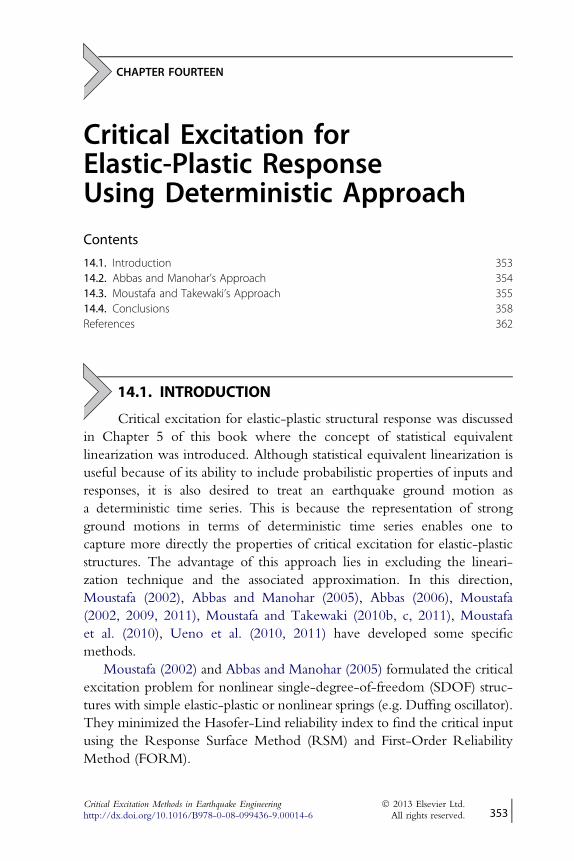
CHAPTER FOURTEEN

Critical Excitation forElastic-Plastic ResponseUsing Deterministic Approach

Contents

14.1. Introduction 35314.2. Abbas and Manohar’s Approach 35414.3. Moustafa and Takewaki’s Approach 35514.4. Conclusions 358References 362

14.1. INTRODUCTION

Critical excitation for elastic-plastic structural response was discussedin Chapter 5 of this book where the concept of statistical equivalentlinearization was introduced. Although statistical equivalent linearization isuseful because of its ability to include probabilistic properties of inputs andresponses, it is also desired to treat an earthquake ground motion asa deterministic time series. This is because the representation of strongground motions in terms of deterministic time series enables one tocapture more directly the properties of critical excitation for elastic-plasticstructures. The advantage of this approach lies in excluding the lineari-zation technique and the associated approximation. In this direction,Moustafa (2002), Abbas and Manohar (2005), Abbas (2006), Moustafa(2002, 2009, 2011), Moustafa and Takewaki (2010b, c, 2011), Moustafaet al. (2010), Ueno et al. (2010, 2011) have developed some specificmethods.

Moustafa (2002) and Abbas and Manohar (2005) formulated the criticalexcitation problem for nonlinear single-degree-of-freedom (SDOF) struc-tures with simple elastic-plastic or nonlinear springs (e.g. Duffing oscillator).They minimized the Hasofer-Lind reliability index to find the critical inputusing the Response Surface Method (RSM) and First-Order ReliabilityMethod (FORM).



http://dx.doi.org/10.1016/B978-0-08-099436-9.00014-6

Abbas (2006) considered another critical excitation problem fornonlinear SDOF structures with simple elastic-plastic springs. The earth-quake load was modeled as a deterministic time history that is expressed interms of a deterministic Fourier series that is modulated by a predefinedenveloping function. The resulting nonlinear optimization problem wastackled by using the sequential quadratic optimization method. This workwas extended to multi-degree-of-freedom (MDOF) systems by Moustafa(2009).

Subsequently, Moustafa and Takewaki (2009, 2010a–c, 2011, 2012),Moustafa et al. (2010), Ueno et al. (2010, 2011), Moustafa (2011) developedseveral critical excitation methods based on the work of Moustafa (2002,2009), Abbas and Manohar (2002, 2005) and Abbas (2006) by introducingdamage indices into the definition of the seismic performance of elastic-plastic and bilinear structures under earthquake loads.

These studies concluded that the resonant ground motion has its energyin a narrow frequency range, close to the fundamental natural frequency ofthe linear structure, and can produce larger damage in the structurecompared to ordinary records.

14.2. ABBAS AND MANOHAR’S APPROACH

Abbas and Manohar developed the critical excitation method withinthe deterministic and the probabilistic frameworks. In the deterministicframework, Abbas and Manohar (2002, 2005), Abbas (2006), Moustafa(2009) used the following Fourier series-type expression as the stationarypart of the input ground acceleration.

€ug0ðtÞ ¼XNf

n¼ 1

ðAn cosunt þ Bn sinuntÞ (14.1a)

Then the input ground acceleration is expressed as follows using anenvelope function eðtÞ.

€ug�t� ¼ e

�t�€ug0

�t�

(14.1b)

As constraints, they employed the following conditions.24ZN

0

€u2g ðtÞ dt35

12

� E

354 Critical Excitation for Elastic-Plastic Response Using Deterministic Approach

max0<t<N

��€ugðtÞ�� M1

max0<t<N

�� _ugðtÞ�� M2 (14.2)

max0<t<N

��ugðtÞ�� M3

M5

�u� � �� €Ug

�u�� M4

�u�

In Eq. (14.2), €UgðuÞ is the Fourier transform of the ground motionacceleration €ugðtÞ. These constraints involve upper limits on the energy,peak ground acceleration, peak ground velocity, peak ground displacementand upper and lower limits on the Fourier transform of the ground motion.The quantities E;M1;M2;M3;M4ðuÞ, M5ðuÞ are estimated based onanalysis of a set of past records that were measured at the site underconsideration or at other sites with similar soil conditions. They introducedthe reliability index, the damage index or the Hasofer-Lind reliability indexas the objective function to define performance of the structure.

In the probabilistic approach, the constraints were imposed on theground motion energy, variance and the entropy that represents the amountof disorder in the ground acceleration (see, e.g., Abbas and Manohar 2002and Moustafa 2009).

This critical excitation problem has a property such that multiple localmaxima exist and the solution depends strongly on the initial guess.However, this approach is general enough to extend to various types ofcritical excitation problems. This approach has been used in Moustafa andTakewaki’s approach that is explained in the next section.

14.3. MOUSTAFA AND TAKEWAKI’S APPROACH

Moustafa and Takewaki extended Abbas and Manohar’s approach tovarious critical excitation problems (Moustafa and Takewaki 2009, 2010a–c,2011, 2012; Moustafa et al. 2010; Ueno et al. 2010, 2011).

As an example, consider a 2-story shear building model with braces, asshown in Fig. 14.1, as a fail-safe model subjected to a strong ground motionthat can be decomposed into a body wave and a surface wave. The frame andbraces are placed in parallel and this system has a fail-safe mechanism. Thefloor masses are 3:0� 106ðkgÞ and the story stiffnesses are 1:0� 105ðN=mÞ.

14.3. Moustafa and Takewaki’s Approach 355

The story shear force-deformation relation of the fail-safe model is shown inFig. 14.2. The shear force sustained by the brace in the elastic range is half thetotal story shear force. The braces are modeled by an elastic-perfectly plasticrelationship. The brace yields at the deformation uy1 and fails at the defor-mation uy2. After the failure of the brace, only the frame resists the acceler-ation input. Fig. 14.3 shows the equilibrium of forces in the frame and bracebefore and after the brace failure. When a brace fails, the brace force isremoved and the corresponding floor acceleration changes suddenly to satisfy

Figure 14.1 2-story shear building model with braces as a fail-safe model.

Displacement

Force

uy1ke

kp

qy0 = (ke − kp)uy1

uy2

Frame only

Frame+

Braces

Figure 14.2 Story shear force-deformation relation of a fail-safe model.


the equilibrium condition. The fundamental and second natural frequenciesof the model with elastic braces are f1 ¼ 0:98ðHzÞ; f2 ¼ 2:58ðHzÞ andthose of the model with only the frame are f1 ¼ 0:75ðHzÞ; f2 ¼ 2:40ðHzÞ.The structural damping ratio of the model is assumed by 0.02, i.e. thedamping matrix is proportional to the initial stiffness matrix. The relation offrequency contents of body wave and surface wave with fundamental andsecond natural frequencies is shown in Fig. 14.4.

Figure 14.3 Equilibrium of forces in frame and brace before and after brace failure.

1.0Hz

surface wave

frequency

body wave

Elastic braces

Second

natural frequency

Fundamental

natural frequency

1st storey bracesbroken

1 1 2 2

1

2

Figure 14.4 Relation of frequency contents of body wave and surface wave withfundamental and second natural frequencies.

14.3. Moustafa and Takewaki’s Approach 357

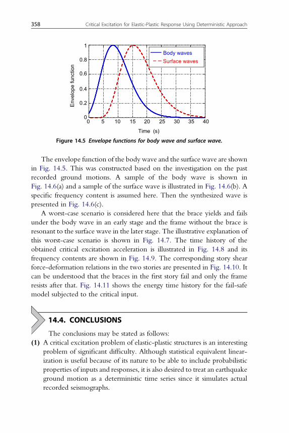
The envelope function of the body wave and the surface wave are shownin Fig. 14.5. This was constructed based on the investigation on the pastrecorded ground motions. A sample of the body wave is shown inFig. 14.6(a) and a sample of the surface wave is illustrated in Fig. 14.6(b). Aspecific frequency content is assumed here. Then the synthesized wave ispresented in Fig. 14.6(c).

A worst-case scenario is considered here that the brace yields and failsunder the body wave in an early stage and the frame without the brace isresonant to the surface wave in the later stage. The illustrative explanation ofthis worst-case scenario is shown in Fig. 14.7. The time history of theobtained critical excitation acceleration is illustrated in Fig. 14.8 and itsfrequency contents are shown in Fig. 14.9. The corresponding story shearforce-deformation relations in the two stories are presented in Fig. 14.10. Itcan be understood that the braces in the first story fail and only the frameresists after that. Fig. 14.11 shows the energy time history for the fail-safemodel subjected to the critical input.

14.4. CONCLUSIONS

The conclusions may be stated as follows:(1) A critical excitation problem of elastic-plastic structures is an interesting

problem of significant difficulty. Although statistical equivalent linear-ization is useful because of its nature to be able to include probabilisticproperties of inputs and responses, it is also desired to treat an earthquakeground motion as a deterministic time series since it simulates actualrecorded seismographs.

0

0.2

0.4

0.6

0.8

1

0 5 10 15 20 25 30 35 40

Body wavesSurface waves

Enve

lope

func

tion

Time (s)

Figure 14.5 Envelope functions for body wave and surface wave.


(2) Abbas (2006) and Moustafa (2009) considered a critical excitationproblem for elastic-plastic SDOF and MDOF structures with simpleelastic-plastic springs. The earthquake load was modeled as a deter-ministic time history that is expressed in terms of a Fourier series thatis modulated by an enveloping function. The resulting nonlinearoptimization problem was tackled by using the sequential quadraticoptimization method.

-4

-2

0

2

4

0 5 10 15 20 25 30 35 40

Acce

lera

tion

(m/s

2 )

Time (s)

Body wave(a)

-4

-2

0

2

4

0 5 10 15 20 25 30 35 40

Acce

lera

tion

(m/s

2 )

Surface wave

Time (s)

(b)

-4

-2

0

2

4

Acce

lera

tion

(m/s

2 )

Synthesized (overlapped) wave

0 5 10 15 20 25 30 35 40Time (s)

(c)

Figure 14.6 A sample of critical body wave (a), surface wave (b) and synthesizedwave (c).


0 20 40 60 80 100time (s)

Failed braceLow naturalfrequency

Critical input with lowfrequency contents

Elastic braceHigh naturalfrequency

Critical input with highfrequency contents

0 20 40 60 80 100time (s)

Combined one is critical ?

Combination ratio ?What frequency content is critical ?

Figure 14.7 Illustrative explanation of assumed worst-case scenario.

0

0.05

0.1

0.15

0.2

0.25

0 2 4 6 8 10

Surface waveBody wave

Four

ier a

mpl

itude

(m

/s)

Frequency (Hz)

Figure 14.9 Frequency contents of critical body wave and surface wave.

-4

-2

0

2

4

0 5 10 15 20 25 30 35 40

Acce

lera

tion

(m/s

2 )

Time (s)

Figure 14.8 Critical excitation for fail-safe model including body wave and surfacewave.


(3) A critical excitation problem for elastic-plastic structures under a groundmotion consisting of a body wave and a surface wave can be solved bythe method due to Abbas (2006). The elastic-plastic structure damagedby the first attack of the body wave may experience further significantdamage by the surface wave with longer frequency contents. Thisscenario has been confirmed by numerical examples exploring varioustypes of seismic waves (body and surface waves) and their influence ondamage of the structure under worst-case earthquake inputs.

(4) Future research in this direction needs to focus on extending themethods developed by this author and his co-workers to complicatedengineering systems, such as piping systems in nuclear power plants andsecondary systems.

-5 107

0

5 107

-0.4 -0.2 0 0.2 0.4

1st storey shear2nd storey shear

Stor

ey s

hear

(N)

Storey drift (m)Critical excitation for fail-safe model

Figure 14.10 Story shear force-deformation relations in two stories.

0

2 107

4 107

6 107

8 107

0 5 10 15 20 25 30 35 40

Input energyDamping energyKinetic+strain energyHysteretic energy

Ener

gy (N

m)

Time (s)

Figure 14.11 Energy time history for fail-safe model subjected to critical input.


REFERENCESAbbas, A.M., 2006. Critical seismic load inputs for simple inelastic structures. Journal of

Sound and Vibration 296 (4–5), 949–967.Abbas, A.M., Manohar, C.S., 2002. Investigations into critical earthquake load models

within deterministic and probabilistic frameworks. Earthq. Eng. Struc. Dyn. 31 (4),813–832.

Abbas, A.M., Manohar, C.S., 2005. Reliability-based critical earthquake load models. Part2: Nonlinear structures. Journal of Sound and Vibration 287 (4–5), 883–900.

Moustafa, A., 2002. Deterministic/Reliability-based critical earthquake load models forlinear/nonlinear engineering structures. Doctoral dissertation, Department of CivilEngineering, Indian Institute of Science, Bangalore, India.

Moustafa, A., 2009. Critical earthquake load inputs for multi-degree-of-freedom inelasticstructures. Journal of Sound and Vibration 325 (3), 532–544.

Moustafa, A., 2011. Damage-based design earthquake loads for Single-Degree-Of-Freedominelastic structures. J. Struct. Eng. 137 (Special Issue), 456–467.

Moustafa, A., Takewaki, I., 2009. Use of probabilistic and deterministic measures to identifyunfavorable earthquake records. Journal of Zhejiang University SCIENCE A 10 (5),619–634.

Moustafa, A., Takewaki, I., 2010a. Deterministic and probabilistic representation of near-field pulse-like ground motion. Soil Dynamics and Earthquake Engineering 30 (5),412–422.

Moustafa, A., Takewaki, I., 2010b. Critical characterization and modeling of pulse-likenear-fault strong ground motion. Struct. Eng. & Mech. 34 (6), 755–778.

Moustafa, A., Takewaki, I., 2010c. Modeling critical ground-motion sequences for inelasticstructures. Advances in Structural Engineering 13 (4), 665–679. Erratum in Advances inStructural Engineering, 14(1), 121, (2011).

Moustafa, A., Takewaki, I., 2011. Response of nonlinear single-degree-of-freedom struc-tures to random acceleration sequences. Engineering Structures 33 (4), 1251–1258.

Moustafa, A., Takewaki, I., 2012. Earthquake ground motion of multiple sequences andassociated structural response. Earthquakes and Structures 3 (5), 629–647.

Moustafa, A., Ueno, K., Takewaki, I., 2010. Critical earthquake loads for SDOF inelasticstructures considering evolution of seismic waves. Earthquakes and Structures 1 (2),147–162.

Ueno, K., Moustafa, A., Takewaki, I., 2010. Critical earthquake loads for passivelycontrolled inelastic building structures considering evolution of seismic waves. Proc. ofthe 5th World Conference on Structural Control and Monitoring (5WCSCM). Tokyo.

Ueno, K., Fujita, K., Moustafa, A., Takewaki, I., 2011. Critical input for inelastic structuresunder evolving seismic waves. J. Structural and Construction Engineering 659, 79–87(in Japanese).


CHAPTER FIFTEEN

Earthquake Resilience Evaluationof Building Structures with CriticalExcitation Methods

Contents

15.1. Introduction 36315.2. Robustness, Redundancy and Resilience 36415.3. Representation of Uncertainty in Selecting Design Ground Motions 36615.4. Uncertainty Expression in Terms of Info-Gap Model 369

[Info-gap robustness function] 37015.5. Worst Combination of Structural Parameters and Input Parameters 37215.6. Reality of Resonance and its Investigation 37315.7. Conclusions 377References 378

15.1. INTRODUCTION

The term “earthquake resilience” is frequently used, especially afterthe Tohoku earthquake, which occurred off the Pacific coast of Japan onMarch 11, 2011. Earthquake resilience implies the ability to recover fromsome damaged states or the ability not to be damaged against variousdisturbances. When structural designers try to investigate earthquake resil-ience, they have to evaluate the earthquake performances of buildingstructures with various uncertainties under a wide range of earthquakeground motions, preferably for critical excitation.

An efficient methodology is required to evaluate the robustness (vari-ability of response) of a building with uncertain structural properties underuncertain ground motions. It is well known that base-isolated buildings andstructural controlled buildings have large structural uncertainties due to widevariability of structural properties caused by temperature and frequencydependencies, manufacturing errors and the aging effect on earthquakeresistant buildings. Furthermore, after the worst disaster of 2011, theTohoku earthquake (Takewaki et al. 2011b; Takewaki et al. 2012a, b;



http://dx.doi.org/10.1016/B978-0-08-099436-9.00015-8

Takewaki and Fujita 2012), it is under discussion that base-isolated buildingsare vulnerable to unexpected long-period ground motions.

Under these circumstances, it is desirable to evaluate the response vari-ability caused by such structural variability and uncertain ground motions(Takewaki et al. 2011a, b). The method based on the convex model may beone possibility (Ben-Haim and Elishakoff 1990). Introduction of a bound onFourier amplitude of input ground motions may be another approach(Takewaki and Fujita 2009). Independently, Kanno and Takewaki (2005,2006a) proposed an efficient and reliable method for evaluating therobustness of structures under uncertainties based on the concept of therobustness function (Ben-Haim 2001; Takewaki and Ben-Haim 2005,2008). However, it does not appear that an efficient and reliable method forevaluating the robustness of structures has been proposed.

An interval analysis is believed to be one of the most efficient and reliablemethods to respond to this requirement. While a basic assumption of“inclusion monotonic” is introduced in usual interval analysis, the possibilityshould be taken into account of an occurrence of the extreme value of theobjective function in an inner feasible domain of the interval parameters formore accurate and reliable evaluation of the objective function. It is shownthat the critical combination of the structural parameters can be derivedexplicitly by maximizing the objective function by the use of the second-order Taylor series expansion. This method is called the UpdatedReference-Point (URP) method (Fujita and Takewaki 2011a–c). Thismethod is applicable to the problems for which the response functions areavailable for uncertain parameters. When we deal with nonlinear problems,it is necessary to combine the URP method (Fujita and Takewaki 2011a–c)with a kind of response surface method (Fujita and Takewaki 2012a).

15.2. ROBUSTNESS, REDUNDANCY AND RESILIENCE

The concepts of robustness, redundancy and resilience are closelyinterrelated. In general, robustness means insensitiveness of a system toparameter variation (Ben-Haim 2001; Takewaki and Ben-Haim 2005;Kanno and Takewaki 2005, 2006a–c, 2007; Takewaki 2008a). On the otherhand, redundancy indicates the degree of safety, frequently expressed bya safety factor (Doorn and Hansson 2011) of a system against disturbances orthe connectivity of components. In the latter meaning, a parallel systemis regarded as a preferable system able to avoid overall system failure

364 Earthquake Resilience Evaluation of Building Structures with Critical Excitation Methods

(the fail-safe system is a representative one). Resilience can be regarded as anability of a system to recover from a damaged state or resist externaldisturbances and seems to be a more generic concept including robustnessand redundancy (Takewaki et al. 2011a, 2012b). Recently the concept ofresilience is getting much interest in broad fields of society (Ellingwood et al.2006; Takewaki et al. 2011a; Committee on National EarthquakeResilience 2011; Poland 2012). In Committee on National EarthquakeResilience (2011), there are some explanations. The following are from thisreference.

“The capability of an asset, system, or network to maintain its function orrecover from a terrorist attack or any other incident” (DHS, 2006).

“The capacity of a system, community or society potentially exposed tohazards to adapt, by resisting or changing in order to reach and maintain anacceptable level of functioning and structure. This is determined by thedegree to which the social system is capable of organizing itself to increasethis capacity for learning from past disasters for better future protection andto improve risk reduction measures” (UN ISDR, 2006).

“The ability of social units (e.g. organizations, communities) to mitigaterisk and contain the effects of disasters, and carry out recovery activities inways that minimize social disruption while also minimizing the effects offuture disasters. Disaster Resilience may be characterized by reduced like-lihood of damage to and failure of critical infrastructure, systems, andcomponents; reduced injuries, lives lost, damage, and negative economicand social impacts; and reduced time required to restore a specific system orset of systems to normal or pre-disaster levels of functionality” (MCEER,2008).

As stated in Committee on National Earthquake Resilience (2011), theterm resilience is often used loosely and inconsistently. After some discus-sions, the following definition is summarized in Committee on NationalEarthquake Resilience (2011).

A disaster-resilient nation is one in which its communities, through mitigation andpredisaster preparation, develop the adaptive capacity to maintain importantcommunity functions and recover quickly when major disasters occur.

To investigate “earthquake resilience” in more detail, the following 18tasks are considered in Committee on National Earthquake Resilience(2011):

Task 1: Physics of Earthquake ProcessesTask 2: Advanced National Seismic SystemTask 3: Earthquake Early Warning

15.2. Robustness, Redundancy and Resilience 365

Task 4: National Seismic Hazard ModelTask 5: Operational Earthquake ForecastingTask 6: Earthquake ScenariosTask 7: Earthquake Risk Assessments and ApplicationsTask 8: Post-earthquake Social Science Response and RecoveryResearchTask 9: Post-earthquake Information ManagementTask 10: Socioeconomic Research on Hazard Mitigation and RecoveryTask 11: Observatory Network on Community Resilience andVulnerabilityTask 12: Physics-based Simulations of Earthquake Damage and LossTask 13: Techniques for Evaluation and Retrofit of Existing BuildingsTask 14: Performance-based Earthquake Engineering for BuildingsTask 15: Guidelines for Earthquake-Resilient Lifeline SystemsTask 16: Next Generation Sustainable Materials, Components, andSystemsTask 17: Knowledge, Tools, and Technology Transfer to Public andPrivate PracticeTask18: Earthquake-Resilient Communities and Regional Demonstra-tion Projects

15.3. REPRESENTATION OF UNCERTAINTY INSELECTING DESIGN GROUND MOTIONS

The properties of earthquake ground motions are highly uncertain both inan epistemic and aleatory sense and it is believed to be a hard task to predictforthcoming events precisely (Geller et al. 1997; Stein 2003; Aster 2012). Ithas been made clear through numerous investigations that near-field groundmotions (Northridge 1994, Kobe 1995, Turkey 1999 and Chi-Chi, Taiwan1999) and the far-field motions (Mexico 1985, Tohoku 2011) have somepeculiar, unpredictable characteristics.

In the history of earthquake resistant design of building structures, wehave learned a lot of lessons from actual earthquake disasters such as the Nobiearthquake 1891 (Japan) and San Francisco earthquake 1906 (USA). Afterwe encountered a major earthquake disaster, we upgraded the earthquakeresistant design codes many times. However, the repetition of this revisionnever resolves the essential problem. To overcome this problem, theconcept of critical excitation was introduced. Although the concept of active


structural control has been developed since around 1980, the actual instal-lation of those devices has further difficulties. Based on these observations,approaches based on the concept of “critical excitation” seem to bepromising. Drenick (1970) formulated this problem in a mathematicalframework and many researchers followed him. The detailed history can befound in Takewaki 2007.

After the Tokachi-oki earthquake in 2003, long-period ground motionshave been receiving much interest in the field of earthquake resistant design.The most difficult problem is that these long-period ground motions arehighly uncertain in nature and the existence of these ground motions wasnot known during the construction of high-rise and super high-rise build-ings. In order to take into account such highly uncertain long-period groundmotions, a new paradigm is desired. There are various buildings in a city(Fig. 15.1). Each building has its own natural period of amplitude-dependency and its original structural properties. When an earthquakeoccurs, a variety of ground motions are induced in the city, e.g. a combi-nation of body waves (including pulse wave) and surface waves, long-period

low-rise RC bld wood house med-rise RC bld base-isolated bld high-rise bld

critical excitation A

critical excitation Z

critical excitation B

critical excitation C

critical excitation D

nuclear-power plant

critical excitation ?

wave propagation

fault

initiating point rupture propagationfault element

soil property

sourcecharacteristics

propagationcharacteristics

radiation energy may be bounded

Energy passage0 2

0 ( )tS gE V u t dtρ= ∫

Unexpected issue

Worst scenario

Expand expected

How to tacklevarious uncertainties

More promising

than

Figure 15.1 Scenario to tackle various uncertainties in modeling design earthquakeground motions. RC, reinforced concrete. From Takewaki (2008b).

15.3. Representation of Uncertainty in Selecting Design Ground Motions 367

ground motions. The relation of the building natural period with thepredominant period of the induced ground motion may lead to disastrousphenomena in the city (see Fig. 15.1). In other words, the most critical issuein seismic resistant design is resonance. Many past earthquake observationsdemonstrated such phenomena repeatedly, e.g. Mexico 1985, Northridge1994, Kobe 1995. One of the promising approaches to this is to shift thenatural period of the building through structural control (Takewaki 2009)and to add damping in the building. However, it is also true that structuralcontrol is developing now and more time is necessary to respond properly touncertain ground motions.

It is discussed and believed that an earthquake has a bound on itsmagnitude and the earthquake energy radiated from the fault has a bound(Trifunac 2008). The problem is to find the most unfavorable groundmotion for a building or a group of buildings (see Fig. 15.1). There are twopossibilities in the specification of such bounds. One is to define a velocitypower at the bottom of the basin based on the fault rupture mechanism andwave propagation characteristics. The other is to set the velocity power atthe ground surface level (Takewaki and Tsujimoto 2011). In the case ofdefinition at the bottom of the basin, the surface ground wave propagationhas to be considered properly. However, this procedure may includeanother uncertainty. In this sense, the setting of the velocity power at theground surface level may be preferable.

It may be interesting to present a case study on the setting of sucha bound. The Fourier spectrum of a ground motion acceleration has beenproposed at the rock surface depending on the seismic momentM0, distanceR from the fault, etc. (e.g. Boore 1983).

jAðuÞj ¼ CM0Sðu;uCÞPðu;umaxÞexpð�uR=ð2bQbÞÞ=R (15.1)

Such a spectrum may contain uncertainties. One possibility or approachis to specify the acceleration or velocity power (Takewaki 2007) as a globalmeasure and allow the variability of the spectrum. As for the Great East JapanEarthquake, jAðuÞj is reported to be about 0.5(m/s) near the fault region.However, this treatment has difficulty in confirming the reliability of thetheory and of specification of the fault site. The change of ground motion bysurface soil conditions is another difficulty. Based on this observation,a concept of critical excitation is introduced.

A significance of critical excitation methods can be explained by inves-tigating the role of buildings in a city. In general there are two classes ofbuildings in a city. One is the important building, which plays an important


role during and after disastrous earthquakes. The other is the ordinarybuilding. The former should not be damaged during an earthquake and thelatter may be damaged to some extent especially for critical excitation largerthan code-specified design earthquakes. Just as the investigation on limit statesof structures plays an important role in the specification of response limits andperformance levels of structures during disturbances, the clarification ofcritical excitations for a given structure or a group of structures appears toprovide structural designers with useful information in determining excitationparameters in a risk-based reasonable way. It is expected that the concept ofcritical excitation enables structural designers to make ordinary buildings moreseismic-resistant and seismic-resilient (Takewaki et al. 2012b).

15.4. UNCERTAINTY EXPRESSION IN TERMSOF INFO-GAP MODEL

In this section, let us introduce and explain a new concept of structuraldesign that combines load and structural uncertainties. For this purpose, it isabsolutely necessary to identify the critical excitation and the correspondingcritical set of structural model parameters. It is well recognized that thecritical excitation depends on the structural model parameters and it is quitedifficult to deal with load uncertainties and structural model parameteruncertainties simultaneously. In order to tackle these difficult problems,info-gap models of uncertainty (nonprobabilistic uncertainty models) byBen-Haim (2001) are used. This concept enables the representation ofuncertainties that exist in the load (input ground acceleration) and inparameters of the vibration model of the structure.

As a simple example, let us consider a vibration model, as shown inFig. 15.2, with viscous dampers in addition to masses and springs. It is well

c2

c1

Figure 15.2 Shear building model with uncertain viscous dampers.

15.4. Uncertainty Expression in Terms of Info-Gap Model 369

recognized in the field of structural control and health monitoring thatviscous damping coefficients ci of dampers in a vibration model are quiteuncertain compared to masses and stiffnesses. By using a specific method fordescribing such uncertainty, the uncertain viscous damping coefficient ofa damper can be expressed in terms of the nominal value ~ci and theunknown uncertainty level a as shown in Fig. 15.3 (Takewaki and Ben-Haim 2005).

Cða; ~cÞ ¼ fc :

��

ci �~ci~ci

�� a; i ¼ 1;/;Ng;a � 0 (15.2a)

The inequality in Eq. (15.2a) can be rewritten as

ð1� aÞ~ci � ci � ð1þ aÞ~ci: (15.2b)

This description is the same one used in the interval analysis (Moore1966; Mullen and Muhanna 1999; Koyluoglu and Elishakoff 1998).

[Info-gap robustness function]An uncertainty analysis called “the info-gap uncertainty analysis” wasintroduced by Ben-Haim (Ben-Haim 2001) for measuring the robustness(the degree of response insensitiveness to uncertain parameters) of a structuresubjected to external loads. Simply speaking, the info-gap robustness is thegreatest horizon of uncertainty, a, up to which the performance functionf ðc; kÞ does not exceed a critical value, fC. The performance function maybe a peak displacement, peak stress or earthquake input energy, and so on.

Let us define the following info-gap robustness function correspondingto the info-gap uncertainty model represented by Eq. (15.1a).

aðk; fCÞ ¼ maxfa : f maxc˛Cða;~cÞ

f ðc; kÞg � fCg (15.3)

An illustrative explanation can be seen in Fig. 15.4.

0

αci αci

nominal value ofdamping coefficient

realizable region ofdamping coefficient

ci (1 – α) ci (1 + α)c cii

Figure 15.3 Description of uncertainty with info-gap model.


Let us put fC0 ¼ f ð~c; kÞ for the nominal damping coefficients. Thenone can show that aðk; fC0Þ ¼ 0 for the specific value fC0, as shown inFig. 15.5. Furthermore, let us define aðk; fCÞ ¼ 0 if fC � fC0 (see Fig. 15.5).This means that when the performance requirement is too small, we cannotsatisfy the performance requirement for any admissible damping coefficients.The definition in Eq. (15.3) also implies that the robustness is the maximumlevel of the structural model parameter uncertainty, a, satisfying theperformance requirement f ðc; kÞ � fC for all admissible variation of thestructural model parameter represented by Eq. (15.1a).

1α

2α

3α

designparameter

domain

designparameter

domain

designparameter

domain

responsedomain

permissible design

α

Info-gaprobustnessfunction

=

largeruncertainty

level

CC( , )

ˆ ( , ) max max ( , )f f fα

α α∈

⎫⎧ ⎡ ⎤ ⎪⎪ ≤= ⎬⎨ ⎢ ⎥⎣ ⎦ ⎪⎪ ⎭⎩ c ckck

responsedomain

responsedomain

Figure 15.4 Illustrative representation of concept of info-gap robustness function.

info

-gap

robu

stne

ss fu

nctio

n

1α

2α

fC0 fC1 fC2 design requirement(deflection, acceleration, stress, …..)

smallrobustness

largerobustness

0tight loose

Figure 15.5 Info-gap robustness function for tight and loose design requirements.

15.4. Uncertainty Expression in Terms of Info-Gap Model 371

15.5. WORST COMBINATION OF STRUCTURALPARAMETERS AND INPUT PARAMETERS

Consider a general problem, as shown in Fig. 15.6, of finding a worst caseunder uncertainties of structural parameters and input ground motionparameters. The problem without uncertainty in input ground motionparameters was considered in Fujita and Takewaki (2012b) and the problemwithout uncertainty in structural parameters was investigated by Fujita et al.(2010). While the domain satisfying the constraints is referred to as the feasibledomain, the domain defined by the info-gap model is called the info-gapdomain. The case is meaningful where the info-gap domain is just includedin the feasible domain. The edge point corresponds to the worst case.

The most challenging part is how to find such worst case in which bothuncertainties of structural parameters and input ground motion parametersare taken into account. The worst case of input ground motion parametersis the function of structural parameters and their uncertainty levels. Thisrelationship is extremely complicated and this problem can be a principalsubject in the field of critical excitation.

As a promising method for investigating this subject, interval analysis andrelated methods have been developed (see e.g. Moore 1966; Alefeld andHerzberger 1983; Qiu et al. 1996; Mullen and Muhanna 1999; Koyluogluand Elishakoff 1998; Qiu 2003; Chen andWu 2004; Chen et al. 2009; Fujitaand Takewaki 2011a–c).

Fig. 15.7 shows the objective functions in the cases of monotonicinclusion and nonmonotonic inclusion. In order to solve this problem ofinterval analysis, Fujita and Takewaki (2011a–c) developed two newmethods. One is the fixed reference-point method (FRP method) shown inFig. 15.8 and the other is the updated reference-point method (URPmethod) shown in Fig. 15.9.

Figure 15.6 Info-gap domain and worst case.


15.6. REALITY OF RESONANCE AND ITS INVESTIGATION

The resonance of buildings with input ground motions has been anissue of great interest in earthquake structural engineering for a long time.Some actual examples come from Mexico 1985, Northridge 1994, Kobe1995, and Tokachi-oki 2003. Ariga et al. (2006) discussed the issue for base-isolated buildings subjected to long-period ground motion after the expe-rience of the Tomakomai ground motion during Tokachi-oki 2003. Theydrew attention to the large deformation of base-isolated high-rise buildings

Minimum point

Info-gap domain ofinterval parameters

1X

2X

1X

1X1X

1X

2X

2X

2X

Nominal model(fixed reference point)

2X

Target position derived by FRP method

1ˆ( X Nominal model

(fixed reference point)

Maximum point

2ˆ, )X

Figure 15.8 Fixed reference-point method.

Maximum point

Minimum point

1 2ˆ ˆ( , )f X X

1 2ˆ( , )f X X

(b)

Maximum point

Minimum point

1 2( , )f X X

1 2( , )f X X

1X

2X Contour plot ofobjective function

(a)

two-dimensional rectangle(info-gap domain)

2X

1X

Contour plot ofobjective function

Figure 15.7 Objective function in info-gap domain: (a) monotonic inclusion, (b) non-monotonic inclusion.

15.6. Reality of Resonance and its Investigation 373

with rather long fundamental natural period. Takewaki et al. (2011b)investigated the response of super high-rise buildings in Tokyo and Osakaduring Tohoku 2011. Some clear observations will be explained in thefollowing.

The response of a 55-story super high-rise building in Osaka(height ¼ 256m: T1 ¼ 5.8s (long-span direction), 5.3s (short-span direc-tion)) is very famous because this building is owned by a public communityand the data are openly available to many people. The building was shakenintensively regardless of the fact that Osaka is located about 800km from theepicenter (about 600km from the boundary of the fault region) and the JMAinstrumental intensity was 3 in Osaka (Takewaki et al. 2011b; Takewakiet al. 2012a, b). Through the post-earthquake investigation, the naturalperiods of the building were found to be longer than the design valuesmentioned above reflecting the flexibility of pile-ground systems, theincrease of a mass at the top and the damage to nonstructural partition wallsand so on. It should be pointed out that the level of velocity response spectraof ground motions observed here (first floor) is almost the same as that at theShinjuku station (K-NET) in Tokyo, and the top-story displacements areabout 1.4m (short-span direction) and 0.9m (long-span direction). Most ofthe data for buildings at Shinjuku, Tokyo are not openly available because ofthe data release problem. Once these data are made available, the vibrationequivalent to this Osaka’s building may be reported.

Fig. 15.10 shows the ground acceleration, ground velocity andtop-story displacement recorded or numerically integrated in thisbuilding. It can be observed that a clear resonant phenomenon occurs

Maximum point

Minimum point

Info-gap domain ofinterval parameters

1X

2X 2X

1X

1X1X

2X

1X

2X

Phase 2

1X1X

2X

1X2X

2nd-order Taylorseries approximation

Nominal model(initial reference point)

2X

1X

Updated reference point

1 1ˆX X→

Phase 1

Target position derived by URP method

1ˆ( X 2

ˆ, )X

Figure 15.9 Updated reference-point method.


during about eight cycles (ground fundamental natural period can beevaluated by 4H/Vs ¼ 4�1.6/1.0 ¼ 6.4s). It seems that such a clearobservation has never been reported in super high-rise buildings aroundthe world. This implies the need for consideration and code-specificationof long-period ground motions in the seismic resistant design of superhigh-rise buildings in mega cities even though the site is far from theepicenter. It is also being discussed that the expected Tokai, Tonankai andNankai event is closer to this building (about 160km from the boundaryof the fault region) and several times the size of the ground motion maybe induced during that event based on the assumption that body wavesare predominant outside of the Osaka basin. However, the nonlinearity ofsurface ground and other uncertain factors may influence the amplifica-tion. Further investigation will be necessary. Seismic retrofitting usinghysteretic steel dampers, oil dampers and friction dampers is beingplanned.

Fig. 15.11 shows the influence of resonance, duration of ground motionand damping deterioration on input energy response. The mechanism isinvestigated in detail on the increase of credible bound of input energy forthe velocity power constraint due to uncertainties in input excitationduration (lengthening) and in structural damping ratio (decrease). As foruncertainties in the excitation predominant period and in the natural periodof a structure, the resonant case is critical and corresponds to the worst case

Figure 15.10 Reality of resonance: ground acceleration, velocity and top-storydisplacement of a 55-story building in Osaka.

15.6. Reality of Resonance and its Investigation 375

02468

10121416

0 2 4 6 8 10

Ener

gy tr

ansf

er fu

nctio

n

Excitation period

h:small

h: large

Uncertainty in damping ratio

Area is constant(freq. range)

02468

10121416

0 2 4 6 8 10

Ener

gy tr

ansf

er fu

nctio

n

Excitation period

T=5(s) T=6(s)

T=4(s)

Uncertainty in natural period

Area isConstant

(freq. range)

Uncertainty in excitation predominant period

Uncertainty in excitation duration

Shortduration

Long duration

excitation period excitation period

|V(ω) | 2 |V(ω) | 2

Area is velocitypower

EI/m

T

Credible bound forvelocity power

T

Credible bound for velocity power

increase

resonance

Area is velocity power

Short duration

Long duration

EI/m

Figure 15.11 Effect of input motion predominant period, input motion duration andstructural damping ratio uncertainties on bound of input energy: Resonance betweeninput and structure and increase of credible bound of input energy for velocity powerconstraint due to lengthening of input excitation duration and decrease of dampingratio of structure.

02468

10121416

0 2 4 6 8 10

Ener

gy tr

ansf

er fu

nctio

n

Excitation period

T=5(s) T=6(s)

T=4(s)

Uncertainty in natural period

Area is Constant

(freq. range)

Uncertainty in excitationpredominant period

excitation period

|V(ω) | 2Area is velocity power

EI/m

T


resonance

Figure 15.12 Effect of input motion predominant period uncertainties on input energy:resonance between input and structure.


(Fig. 15.12). It can be understood from Fig. 15.13 that the lengthening ofinput excitation duration and decrease of structural damping ratio due todamping mechanism deterioration may have caused large input in the superhigh-rise building in Osaka bay area mentioned above. In particular, thedecrease of the structural damping ratio induces unsmoothing of the energyspectrum and the period region to increase the energy spectrum happened tocoincide with the fundamental natural period of the super high-rise building(see Takewaki et al. 2012a, b).

15.7. CONCLUSIONS

The conclusions may be stated as follows:(1) The concepts of robustness, redundancy and resilience are closely

interrelated. In general, robustness means insensitiveness of a system toparameter variation. On the other hand, redundancy indicates thedegree of safety of a system against disturbances or the parallel system

02468

10121416

0 2 4 6 8 10

Ener

gy tr

ansf

er fu

nctio

n

Excitation period

h:small

h: large

Uncertainty in damping ratio

Area is constant(freq. range)

Uncertainty in excitation duration

Shortduration

Long duration

excitation period

|V(ω) | 2

Area is velocitypower

EI/m

T


increaseShort duration

Long duration

Figure 15.13 Effect of input motion duration and structural damping ratio uncer-tainties on bound of input energy: Increase of credible bound of input energy forvelocity power constraint due to lengthening of input excitation duration and decreaseof damping ratio of structure.


avoiding overall system failure (the fail-safe system is a representativeone). Resilience can be regarded as an ability of a system to recover froma damaged state or resist external disturbances and seems to be a moregeneric concept including robustness and redundancy.

(2) Several uncertainties in earthquake ground motions can be explained bya model of Boore. By introducing the input energy bound, structuraldesigners can restrict such uncertainties to a limited level.

(3) The info-gap model can be an approach to describe uncertainty inearthquake ground motions and structural parameters. The method toobtain the worst combination of structural parameters and input param-eters is desired. The fixed reference-point method and updated reference-point method based on interval analysis can be promising methods.

(4) The influence of resonance, duration of ground motion and dampingdeterioration on input energy response can be investigated with thecredible bound theory.

REFERENCESAlefeld, G., Herzberger, J., 1983. Introduction to Interval Computations. Academic Press,

New York.Ariga, T., Kanno, Y., Takewaki, I., 2006. Resonant behaviour of base-isolated high-rise

buildings under long-period ground motions. Struct. Design Tall Spec. Build. 15 (3),325–338.

Aster, R., 2012. Expecting the unexpected: black swans and seismology. SeismologicalResearch Letters 83 (1), 5–6.

Ben-Haim, Y., 2001. Information-Gap Decision Theory: Decisions under Severe Uncer-tainty. Academic Press, San Diego.

Ben-Haim, Y., Elishakoff, I., 1990. Convex Models of Uncertainty in Applied Mechanics.Elsevier, Amsterdam.

Boore, D.M., 1983. Stochastic simulation of high-frequency ground motions based onseismological models of the radiated spectra. Bulletin of the Seismological Society ofAmerica 73 (6A), 1865–1894.

Chen, S.H., Wu, J., 2004. Interval optimization of dynamic response for structures withinterval parameters. Comp. Struct. 82 (1), 1–11.

Chen, S.H., Ma, L., Meng, G.W., Guo, R., 2009. An efficient method for evaluating thenatural frequencies of structures with uncertain-but-bounded parameters. Comp.Struct. 87 (9–10), 582–590.

Committee on National Earthquake Resilience–Research, Implementation, and Outreach;Committee on Seismology and Geodynamics; National Research Council, 2011.National Earthquake Resilience: Research, Implementation, and Outreach. TheNational Academies Press, Washington, D.C.

DHS (U.S. Department of Homeland Security), 2006. National Infrastructure ProtectionPlan. Available at. www.fas.org/irp/agency/dhs/nipp.pdf (accessed August 11, 2012).

Doorn, N., Hansson, S.O., 2011. Should probabilistic design replace safety factors? Philos.Technol. 24 (2), 151–168.


http://www.fas.org/irp/agency/dhs/nipp.pdf

Drenick, R.F., 1970. Model-free design of aseismic structures. J. Engrg. Mech. Div. 96 (4),483–493.

Ellingwood, B.R., et al., 2006. Best practices for reducing the potential for progressivecollapse in buildings. USA: National Institute of Standards and Technology,Gaithersburg, MD, USA.

Fujita, K., Takewaki, I., 2011a. Earthquake response bound analysis of uncertainbase-isolated buildings for robustness evaluation. J. Structural and Construction Engi-neering 666, 1453–1460 (in Japanese).

Fujita, K., Takewaki, I., 2011b. An efficient methodology for robustness evaluation byadvanced interval analysis using updated second-order Taylor series expansion. Eng.Struct. 33 (12), 3299–3310.

Fujita, K., Takewaki, I., 2011c. Sustainable building design under uncertain structural-parameter environment in seismic-prone countries. Sustainable Cities and Society1 (3), 142–151.

Fujita, K., Takewaki, I., 2012a. Robustness evaluation on earthquake response of base-isolated buildings with uncertain structural properties under long-period groundmotions. Architectoni.ca Journal 1 (1), 46–59.

Fujita, K., Takewaki, I., 2012b. Robust passive damper design for building structures underuncertain structural parameter environments. Earthquakes and Structures 3 (6), 805–820.

Fujita, K., Moustafa, A., Takewaki, I., 2010. Optimal placement of viscoelastic dampers andsupporting members under variable critical excitations. Earthquakes and Structures 1 (1),43–67.

Geller, R.J., Jackson, D.D., Kagan, Y.Y., Mulargia, F., 1997. Earthquakes cannot be pre-dicted. Science 275 (5306), 1616.

Kanno, Y., Takewaki, I., 2005. Approximation algorithm for robustness functions of trusseswith uncertain stiffness under uncertain forces, J. Structural and Construction Engi-neering. No. 591, 53–60 (in Japanese).

Kanno, Y., Takewaki, I., 2006a. Robustness analysis of trusses with separable load andstructural uncertainties. Int. J. Solids and Structures 43 (9), 2646–2669.

Kanno, Y., Takewaki, I., 2006b. Sequential semidefinite program for maximum robustnessdesign of structures under load uncertainty. Journal of Optimization Theory andApplication 130 (2), 265–287.

Kanno, Y., Takewaki, I., 2006c. Confidence Ellipsoids for Static Response of Trusses withLoad and Structural Uncertainties. Computer Methods in Applied Mechanics andEngineering 196 (1–3), 393–403.

Kanno, Y., Takewaki, I., 2007. Worst case plastic limit analysis of trusses under uncertainloads via mixed 0-1 programming. Journal of Mechanics of Materials and Structures 2(2), 247–273.

Koyluoglu, H.U., Elishakoff, I., 1998. A comparison of stochastic and interval finiteelements applied to shear frames with uncertain stiffness properties. Comp. and. Struct.67 (1–3), 91–98.

MCEER (Multidisciplinary Center for Earthquake Engineering Research), 2008.MCEER research: Enabling disaster-resilient communities. Available at. SeismicWaves (November), 1–2. www.nehrp.gov/pdf/SeismicWavesNov08.pdf (accessedAugust 11, 2012).

Moore, R.E., 1966. Interval Analysis. Prentice-Hall, Englewood Cliffs, New Jersey.Mullen, R., Muhanna, R., 1999. Bounds of structural response for all possible loading

combinations. J. Struct. Eng. 125 (1), 98–106.Poland, C., 2012. Creating disaster resilient cities. In: Bouquet, Alan (Ed.), Sustainable

Cities. Adam Nethersole Publisher, London, pp. 136–138.Qiu, Z., 2003. Comparison of static response of structures using convex models and interval

analysis method. Int. J. Numer. Meth. Engng. 56 (12), 1735–1753.


http://www.nehrp.gov/pdf/SeismicWavesNov08.pdf

Qiu, Z., Chen, S., Song, D., 1996. The displacement bound estimation for structures withan interval description of uncertain parameters. C. Numer. Meth. Engng. 12 (1), 1–11.

Stein, R.S., 2003. Earthquake conversations. Scientific American 288 (1), 72–79.Takewaki, I., 2007. Critical Excitation Methods in Earthquake Engineering. Elsevier,

Oxford.Takewaki, I., 2008a. Robustness of base-isolated high-rise buildings under code-specified

ground motions. Struct. Design Tall Spec. Build. 17 (2), 257–271.Takewaki, I., 2008b. Critical excitation methods for important structures. Invited as a Semi-

Plenary Speaker, EURODYN 2008, July 7–9, Southampton, England.Takewaki, I., 2009. Building Control with Passive Dampers: Optimal Performance-based

Design for Earthquakes. John Wiley & Sons (Asia), Singapore.Takewaki, I., Ben-Haim, Y., 2005. Info-gap robust design with load and model uncer-

tainties. J. Sound & Vibration, Special Issue: Uncertainty in Structural Dynamics 288(3), 551–570.

Takewaki, I., Ben-Haim, Y., 2008. Info-gap Robust Design of Passively ControlledStructures with Load and Model Uncertainties, Chapter 19. In: Tsompanakis, Yiannis,Nikos, D., Lagaros, Papadrakakis, Manolis, Taylor, Francis (Eds.), Structural DesignOptimization Considering Uncertainties, pp. 531–548.

Takewaki, I., Fujita, K., 2009. Earthquake Input Energy to Tall and Base-isolated Buildingsin Time and Frequency Dual Domains. Struct. Design Tall Spec. Build. 18 (6), 589–606(2008 Paper of the Year).

Takewaki, I., Fujita, K., 2012. Tohoku (Japan) earthquake and its impact on design of superhigh-rise buildings. Proc. of ICTAM2012 Congress (The 23rd International Congresson Theoretical and Applied Mechanics). August 19–24, 2012, Beijing, China.

Takewaki, I., Tsujimoto, H., 2011. Scaling of design earthquake ground motions for tallbuildings based on drift and input energy demands. Earthquakes and Structures 2 (2),171–187.

Takewaki, I., Fujita, K., Yamamoto, K., Takabatake, H., 2011a. Smart Passive DamperControl for Greater Building Earthquake Resilience in Sustainable Cities. SustainableCities and Society 1 (1), 3–15.

Takewaki, I., Murakami, S., Fujita, K., Yoshitomi, S., Tsuji, M., 2011b. The 2011 off thePacific coast of Tohoku earthquake and response of high-rise buildings under long-periodground motions. Soil Dynamics and Earthquake Engineering 31 (11), 1511–1528.

Takewaki, I., Fujita, K., Yoshitomi, S., 2012a. Uncertainties of long-period ground motionand its impact on building structural design. Proc. of One Year after 2011 Great EastJapan Earthquake, International Symposium on Engineering Lessons Learned from theGiant Earthquake. March 3–4, Tokyo, 1005–1016.

Takewaki, I., Moustafa, A., Fujita, K., 2012b. Improving the Earthquake Resilience ofBuildings: The Worst Case Approach. Springer, London.

Trifunac, M., 2008. Energy of strong motion at earthquake source. Soil Dyn. Earthq. Engrg.28 (1), 1–6.

UN ISDR (United Nations International Strategy for Disaster Reduction), 2006. HyogoFramework for Action 2005–2015: Building the Resilience of Nations and Commu-nities to Disasters. Extract from the final report of the World Conference on DisasterReduction (A/CONF.206/6). March 16, 2005.


INDEX

Note: Page numbers with “f” denote figures.

AAbbas and Manohar’s approach to critical

excitation problems, 354–355Acceleration constraint, 11, 175–176,

182–183, 254Acceleration response, 10–11, 75–96CENMA problem, 83–84solution procedure, 84–86

input motions, modeling of, 76non-proportionally damped model,

88–91to non-stationary random input, 76–83

numerical examples, 86–88proportionally damped model, 92

Arias intensity measure, 182, 209–212

BBedrock acceleration input, transfer

function to, 268–271free-field ground, 269pile–soil system, 269

Bidirectional horizontal inputs, 342–348Broader class, of excitation, 166–168Building–pile system, 269f, 277f, see also

Structure–pile systemBuildings, classes of, 21, 22fBuilding structures, earthquake resilience

evaluation of, see Earthquakeresilience evaluation, of buildingstructures

CCode-specified design earthquakes,

168–169with critical excitation, 22f

Convex models, 15–16CQC3 (extended Complete Quadratic

Combination) method, 336,343–344

Critical envelope function, for non-stationary random input, 18–19,133–154

CEFNS problem, 137, 143–144

double maximization procedure,137–139

critical frequency content, 147–148function discretization, 139–140mean-square drift, 136–137upper bound, 140–141

model, 135–136numerical examples, 142–147

Critical excitation, definition, 1–3Critical frequency content, 147–148

DDamage index, 12Damage-limit level earthquakeenergy transfer functions, 275–280input energy, by actual ground motion,

280–285Deterministic approach, elastic–plastic

response using, 353–362Abbas and Manohar’s approach, 354–355Moustafa and Takewaki’s approach,

355–358Discretization, of envelope function,

139–140Double maximization procedure, 14–15,

18–19, 37–40, 59–61, 84–86,137–139, 304–307

Drenick’s approach, 3–7Duhamel integrals, 53–55, 77–78

EEarthquake input energy, 11, 262–263,

295–334in MDOF system, 197–216examples, 172–178without modal decomposition, 205to non-proportionally damped MDOF,201–205

to proportionally damped MDOF,198–201

mean energy input rate, for envelopefunction, 307–310

381j

Earthquake input energy (Continued)non-stationary ground motion model,

296–297non-uniformly modulated ground

motion model, 310–312numerical examples, 312–319probabilistic rate, 297–303rate, deterministic, 320–323in SDOF system, 175–196with acceleration constraint, 182–183bounds, 185–194energy transfer function, 179–182in frequency domain, 177–179with velocity constraint, 183–185

in soil–structure interaction (SSI) system,217–266

to fixed-base SDOF system, 220–221,231–235

Fourier amplitude spectrum, upperbound of, 246

numerical examples, 251–254,258–260

velocity constraints, 248–249in structure–pile–soil system, 267–294bedrock acceleration input, transferfunction to, 268–271

to structure, 273–274to structure–pile system, 272–273two-level design earthquakes,275–285

variable envelope function, 312variable frequency content, 312

Earthquake resilience evaluation, ofbuilding structures, 363–380

redundancy, 364–366resilience, 364–366resonance, 373–377robustness, 364–366structural–input parameters combination,

372uncertainty expansion, 369–371uncertainty representation, 366–369

Earthquake-resistant design, 21–23Elastic–plastic response, 97–132using deterministic approach, 353–362evaluation, 171–173MDOF model, 17–18

accuracy, 126–128conclusion, 129critical and inelastic response, relation,121–126

critical excitation problem and solution,120

elastic–plastic structures, criticalexcitation for, 114–115

statistical equivalent linearization,115–119

rectangular PSD function, criticality,110–114

SDOF model, 16–17accuracy, 109–110conclusion, 128critical and inelastic response, relation,104–109

critical excitation problem and solution,101–103


Energy transfer functions, 179–182,200–201, 207–209, 213, 239–240,268

for two-level design earthquakes,275–280

Envelope function, 10, 18–19, 42f, 44,47–50

discretization, 139–140mean energy input rate, 307–310

Evolutionary transfer function, 43–44, 83,88

FFC (frequency constraint) design,

163–166, 168, 168fFixed-base SDOF systemearthquake input energy, 220–221comparison with SSI system,231–235, 239–246

Fixed design, problem for, 156–158Fixed reference-point (FRP) method,

372, 373fFourier amplitude spectrum, 175–176,

181–182upper bound, 246

Free-field ground, 269

382 Index

Frequency domain, 10, 12, 212–213, 235,267–268

earthquake input energyto non-proportionally damped MDOFsystem, 201–205

to proportionally damped MDOFsystem, 198–201

to SDOF system, 177–179probabilistic earthquake energy input rate,

297–303truncated ground motion model, squared

Fourier amplitude spectrum of,326–329

GGround acceleration, 176–177, 181,

183–184, 189–194Ground motions capacity, 181–182Ground velocity, 176–177, 183–184,

189–194

HHorizontal ground motion inputs,

336–341bidirectional, 342–348

IInfo-gap modeluncertainty analysis, 369–371

MMDOF model, 11–12CESEPSR problem, 101earthquake input energy, 213examples, 206–213without modal decomposition, 205to non-proportionally damped MDOF,201–205

to proportionally damped MDOF,198–201

elastic–plastic structures, critical excitationfor, 17–18, 114–115

accuracy, 126–128conclusion, 129critical and inelastic response, relation,121–126

critical excitation problem and solution,120


non-stationary input, 40–42CENSM problem, 41–42

numerical examples, 44stationary input, 30–34CESM problem, 33–34


Mean-square drift, 18–19, 136–137of SDOF system, in stationary state, 149upper bound, 134, 140–141

Moustafa and Takewaki’s approach tocritical excitation problems,355–358

MP (maximum performance) design,164–166

Multi-component inputs, criticalexcitation for, 335–352

bidirectional horizontal inputs, 342–348horizontal and vertical simultaneous

inputs, 336–341interpretation using inner product,

348–349Multi-degree-of-freedom, see MDOF

model

NNon-proportionally damped MDOF,

201–205Non-proportionally damped structural

systems, 88–91critical excitation problemCENM problem, 59

input motions, modeling, 52–53to non-stationary random input, 76–83numerical examples, 64–67response, to non-stationary random

excitation, 53–59Non-stationary ground motion model,

18–19, 135–136, 296–297,310–312

Non-stationary random input, 27–50to MDOF model, 40–42CENSM problem, 41–42

to SDOF model, 36–40CENSS problem, 37–40

Index 383

Numerical examplesacceleration response, 86–92critical envelope function, for non-

stationary random input, 142–147earthquake energy input rate, 312–319earthquake input energy, in SSI systemone-story model, 251–254three-story model, 258–260

non-proportionally damped structuralsystems

damping concentration, various types,67–69

non-proportional damping, 64–67proportional damping, 63–64

robust stiffness design, 163–166stationary and non-stationary random

inputsfor MDOF model, 44for SDOF model, 42–43

truncated ground motion model, squaredFourier amplitude spectrum of,323–326

time-domain/frequency-domainanalyses, 326–329

OOver-damped real modes, 207

PParseval’s theorem, 8Penzien-Watabe (PW) model, 336,

342–345, 344f, 345fextended, 343–345, 344f, 345f

Pile–soil system, 269–271Probabilistic earthquake energy input ratefrequency-domain approach, 297–303

ProblemsCEFNS, 137double maximization, 137–139

CENM, 59solution procedure, 59–61

CENMA, 83–84solution procedure, 84–86

CENSM, 41–42CENSS, 37–40CESEP, 102–103solution procedure, 103–104

CESEPSR, 120solution procedure, 121

CESM, 33–34CESS, 29–30

Proportional damping, 61–63, 92numerical examples, 63–64

Proportionally damped MDOF, 198–201

RResonance, 373–377Response spectrum method, 275–276Robust stiffness designfor structure-dependent critical excitationbroader class of excitation, response to,166–168

code-specified design, response to,168–169

fixed design, problem for, 156–158numerical examples, 163–166problem, 158–163

Robust structural design, 19–21

SSafety-limit level earthquake, 275–285energy transfer functions, 275–280input energy, by actual ground motion,

280–285SDOF model, 1–2critical excitation problem, 101–103CESEP problem, 102–103

earthquake energy input, 175–196with acceleration constraint, 182–183bounds, 185–194energy transfer function, 179–182in frequency domain, 177–179with velocity constraint, 183–185

elastic–plastic structures, 16–17, 97–132accuracy, 109–110conclusion, 128critical and inelastic response, relation,104–109

critical excitation problem and solution,101–103


mean-square drift, 136–137, 149upper bound, 140–141

384 Index

non-stationary input, 36–40CENSS problem, 37–40

numerical examples, 42–43stationary input, 28–30CESS problem, 29–30

statistical equivalent linearization, 98–100Seismic critical excitation methodsconvex models, 15–16critical envelope function, 18–19criticality measures, 10–12Drenick’s approach, 3–7early stage, 9–10in earthquake-resistant design, 21–23elastic–plastic MDOF system, 17–18elastic–plastic SDOF system, 16–17robust structural design, 19–21Shinozuka’s approach, 8–9stochastic excitation, 13–15subcritical excitation, 12–13

Shinozuka’s approach, 8–9Single-degree-of-freedom, see SDOF

modelSoil–structure interaction (SSI) systemearthquake input energy, 217–266to fixed-base SDOF system, 220–221,231–235

Fourier amplitude spectrum, upperbound of, 246–248

numerical examples, 251–254,258–260

velocity constraints, 248–250Squared Fourier amplitude spectrum

(SFAS), 321–322truncated ground motion model,

323–326time-domain/frequency-domainanalyses, 326–329

Square root of the sum of the squares(SRSS), 335

Stationary random input, 27–50conservativeness, of bounds, 34–36to MDOF model, 30–34CESM problem, 33–34

to SDOF model, 28–30CESS problem, 29–30

Statistical equivalent linearizationfor MDOF model, 17–18, 115–119for SDOF model, 98–100

Stochastic excitation, 13–15Structure–pile–soil systemearthquake input energy, 285bedrock acceleration input, transferfunction to, 268–271

to structure, 273–274to structure–pile system, 272–273by two-level design earthquakes,275–285

Structure–pile system, 267–294Subcritical excitation, 12–13Swaying and rocking springs, 115–116,

115f, 120–122

TTime domain, 10, 195, 212–213truncated ground motion model, squared

Fourier amplitude spectrum of,326–329

Truncated ground motion model, squaredFourier amplitude spectrum of,323–326

time-domain/frequency-domainanalyses, 326–329

UUncertaintyexpansion, 369–371in selecting design ground motions,

representation of, 366–369Updated reference-point (URP) method,

364, 372, 374f

VVariable envelope function, 147–148,

312Variable frequency content, 147–148,

312Velocity constraints, 11, 175–176,

183–185, 194, 254Vertical ground motion inputs,

336–341

Index 385

Critical Excitation Seismic

Documents

Transcript of Critical Excitation Seismic