On the mean field theory bound on the magnetization

Journal of Statistical Physics, Vol. 32, No. 2, 1983

On the Mean Field Theory Bound on the Magnetization

J. Slawny 1

Received March 28, 1983

The mean field bound on magnetization is proved for a class of one-component ferromagnetic: systems and for D components systems with arbitrary D.

KEY WORDS: Ferromagnetic models, magnetization, mean field bound, Jensen's inequality, convexity, Bessel functions.

1. I N T R O D U C T I O N

The mean field theory bounds on the critical temperature and on the magnetization is a subject of a number of recent works. The critical temperature bounds in the s p i n - l / 2 case were first proved by Griffiths. More recent results are discussed by Simon. (7)

Here we prove magnetization bounds for systems with ferromagnetic two-body interactions. In case of a one component the bounds apply to the natural class ~J)2 of systems, (1'4) (cf. Section 2), for which the critical temperature bounds have been proved in Ref. 1. Using inequalities relating many component systems to one-component ones, (4) we obtain the magnetization bounds for any number of components. Pearce, (4~ proves the magnetization bound for a sparse subclass of ~92 and for two- and three- component systems. Also C. Newman kindly pointed out to me that he proved the magnetization bound for one-component systems for which G H S inequalities ho ld - - a result announced at Rutgers University in De- cember 1981.

In the one-component case the proof (Section 2) is based on an extension of Jensen's inequality (Section 3), to odd functions which are

t Virginia Polytechnic Institute and State University, Blacksburg, Virginia 24061.

375 0022-4715/83/0800-0375503.00/0 �9 1983 Plenum Publishing Corporation

376 Slawny

concave on the positive half-axis and to measures/a such that/x ([a + m[) > / L ( ] - o e , - a]) for any positive a. That the measures defined by ferromagnetic systems satisfy this condit ion is shown in Section 4 using the F K G inequalities. M a n y - c o m p o n e n t systems are treated in Section 5, with a proof of the needed convexity properties of Bessel functions sketched in Appendix B. We consider systems on lattices more general than 77 ", with a few points per unit cell, like those on face centered lattices. This leads to a system of mean field equations properties of which may be known but for which we found no references. This is discussed in Appendix A. The interactions are not assumed to be of a finite range.

2. ONE-COMPONENT MODELS

Our lattice 0_ is a discrete Z"-invarient subset of R ' . The spin distribu- tions /~a, the external field ha, a E l_, and the two-body interaction (J(a, b))a,b c ~_ are Z"-invariant. Fur thermore the measures ~a on R are assumed to be even of a compact support and not concentra ted at {0}, J(a, b), h a > O,

~ J ( a , b ) < ~ , a n y a b

The lattice is assumed to be J -connected , i.e., for any a, b ~ k there is a

natural n and a 1 . . . . . a n ~ g_, a I = a, a n = b, such that J(a i, ai+ I) :r 0, i = 1 , . . . , n - 1. Any model can be reduced to a family of connected models by passing to " J - c o m p o n e n t s " of D_. The configurat ion space of the system is

~ = I-I [ - - ra , ra ] , ~A = I-[ [--ra,ra] a E l_ a@A

where r a -- sup supp/~. : s. �9 ~ ~ R are the usual spin variables, i.e., s a is the projection on the a th coordinate. The (ferromagnetic) Hamil tonian H is written as

H = - ~ J ( a , b ) s a s b - ~ h ( a ) s a a,b a

For an inverse temperature/3 we set, as usual,

K(a,b) =/3J(a,b), k(a) =/3h(a)

p(K, k) = lim ~ log ZA(K, k)

ZA= f f expI,,,b~/, ~ K(a,b)saSb+ ~a k(a)Sa] a@~A dtta

On the Mean Field Theory Bound on the Magnetization 377

The magnetization (m~)~n_ is the right derivative of p:

p ( . . . . k a + e . . . . ) - p ( . . . . k, . . . . ) m a = lim

~$0 E

By the well known properties of equilibrium states

m~ = <sa> +

where { >+ is the equilibrium state obtained as the limit of the finite volume states { )+ defined by the " + " boundary conditions. The { )+ state inherits the symmetries of the Hamiltonian. In particular, it is Z p invariant.

Let for a E 0_

L(x) -

f te 'xl~ ~ (dt)

f e'Xl~( dt)

Then the DLR conditions are that, in particular, +

<s,) + = ( fa( ~ K(a,b)Sb + k(a)) ) , all a ~ k

The functions fa are odd. They are strictly increasing since

;(t -L(x))2 o(dt) f/,(x) = > 0

f e tX#a (dt)

Let us assume that f~ are of class 9~2, (1'4) i.e., that they are concave on [0, + oo] (cf. Fig. 1); the class 992 is discussed at the end of this section. Then by Sections 3 and 4 the following fundamental inequality holds:

"~ g.'

F 0,,~

/ /

K > O k = O

Fig. 1. Fixed points of F for k > 0 and for k = 0. For k > 0 the iterates F(m), F2(m) F3(m) are indicated.

378 Slawny

Thus, setting

m a = (sa) +

we have rn,/> 0, (ma) is 7/p invariant, and

ma < f~( ~ , K ( a , b ) m b + k ( a ) ) (a l ia) b

The mean field bound for magnetization is an easy consequence of this. We first discuss the case of Q_ = 7/~ when the arguments have a simple geomet- ric interpretation (Fig. 1). Then we summarize the generalization to general lattices worked out in Appendix A.

If ~. = 71 ~, m, , f~, k(a) and K(a) = ~ b K ( a , b ) are a independent and, dropping the a, (1) becomes

m <<. f ( K m + k )

It is obvious from Fig. 1 that for k > 0 there is only one nonnegative solution m* of the equation

m = F(m) , m >1 0

where F(m) = f ( K m + k). It is given by the intersection of graphs of F and m~-->m.

The fixed point of F has the following properties. For k = 0 there is always the zero fixed point. For small K it is the

only fixed point. As K increases this fixed point becomes unstable and eventually there appears another strictly positive stable solution. The critical, or bifurcation, value of K is given by F,(0) = 1, i.e., gcr = f ' ( 0 ) - 1. Thus for any (K, k) there is only one nonnegative stable fixed point m* of F. It depends on (K, k) in a continuous and monotonic way. If m < F(m) then m <<. m*.

In Appendix A we analyze the general case, with conclusions similar to the above. In the space M I of ZP-invariant nonnegative m's, m = (m~)a~ ~, we consider the map F m ~ ( f a ( ~ b K ( a , b ) r n 6 + k~))a ~ L. For k = 0 and /3 < tier there is the zero fixed point only. It becomes unstable at/3or and for/3 >/3or there is a unique nonzero fixed point. Thus for each (K, k) there is unique maximal fixed point m* of F. It depends on (K, k) in a continuous and monotonic way, and if m~ < F(rn)~ then m~ < m* and, for mO, Fn(m)--->m * as n o oo. fl~r is given by the condition that the maximal eigenvalue of F'(0) is equal to 1, i.e., /3~ is the inverse of the maximal eigenvalue of the map

m---> ( f~(O) ~J(a,b)mb).~n -


(m is 2~" invariant). Thus (1) implies the mean field bound

ma <<. m*, a E k

This completes the discussion in the case/z, ~ 932. We now discuss the class ~92 to which our results apply. For spin p,

p = 1/2, 1, 3 / 2 . . . .

r = - - p , - - p + 1 . . . . . p

f ( x ) - 2P2+1 cth 2 P ~ x - l c t h ~ = pB:(px)

where Bp is the corresponding Brillouin function. By direct calculation one checks that f " ( x ) is negative for x > 0. Thus our results apply to one- component spin systems with arbitrary value of the spin. Pearce ~4) proves the mean field bound for 2p + 1 = 2 q �9 3 r with natural q, r.

In case of a continuous distribution: i~(dx) = p(x)dx, p supported by [ - 1, 1] and not decreasing on [0, 1], Pearce proves a property stronger than T~. This allows him to treat D-component systems (cf. Section 5) with D = 2, 3. In Appendix B we sketch a proof that the measure/~D,

f f ( x ) ~ D (dx) = f~ l f (x ) (1 - x2) ~/2)~- 3~dx

is of class ~ for any D. This yields the mean field bound for any number of components (Section 5).

3. A VERSION OF THE JENSEN'S INEQUALITY

The following proposition has been used in the preceding section.

Proposition. Let O be a probability measure on a space Y and let X be a real random variable. Let f be an odd function R ~ R which is concave on [0, + m[. If for any a ~ 0 o(X >1 a) >1 o(X < - a) and both X and ~ o X are o-integrable then

Using a standard approximation argument we first reduce our problem to one with X assuming only a finite number of values: Let

X n ( x ) = _ + 2 k if - + X ( x ) ~ [ 2 k , k 2 + l [, k = 0 , . . . , 2 2n

+ 2 ~ if +_X(x)>12 ~

380 Slawny

Clearly p(X, >- a) >1 o(X n <-< - a), any a ~> 0, and therefore by the argument of Ref. 2, p. 303, it is enough to prove the proposit ion for each X, .

Thus we can assume that there are nonnegative numbers x 0 < . . .

< Xm, X 0 = 0; Yt < Y . , such that, with a~ = p(X = xi), fi~ = p(X = - Y i ) , EiOii "l" Ei~i ~--- 1. Then under our assumptions on f we have to prove that

:( .,,,) > �9 j i j

if for any a >/0

xi ) a y j >/ a

Since the term x 0 contributes zero to both sides of the inequality we will take i/> 1 and assume

i=l i=1

If all fii = 0 this is just an expression of the concavity. In case m, n = 1 the inequality has the graphical interpretation shown in Fig. 2. The interval joining (x, f ( x ) ) with ( - y , f ( - y ) ) lies below the interval joining (x, f ( x ) ) with ( - x, f ( - x)), which in turn lies below the graph of f for the values of the argument between 0 and x. The following arguments implement the above idea.

! will show below that under our conditions one can decompose flj as follows: there are (7/j)i= 1 . . . . . . ; j = 1 . . . . . . such that 7~ > 0, ~ , / ~ = ~ , ~ j ~,,j = Ot i and 70. = 0 if x i < yj . Assuming this rather intuitive fact the proof

i.!" Yl Fig. 2. To the proof of a version of the Jensen's inequality.


continues as follows:

j j i I

YJ J "~i YiJ) f ( xi) :f(~i (OLi--~j ~ii~fij)Xi)~i (OLi--E yj

l

> E aJ(x,) - E E YJ(Yj) = E a~f(xi) - E fljf(Yj) i j i i j Here to obtain the first inequality use the fact that ~'0 is zero if y j / x i > 1 and that therefore a i - ~,j yOyj/xi >1 0 and ~,,i[ai- ~,j(yj/x~)yO. ] < 1.

It remains to demonst ra te the existence of (y~j). This is done by induct ion with respect to n as follows.

Let k < m be the largest integer with ~,~>k ag >1 ft,; that such k exists and that x k/> y~ follows f rom the condit ion (3). Define now

7~,~ = ai if i > k

0 if i < k

= B . -

i>k (here a i is set equal to 0 for i > m). Obviously, ~'i,, has the correct properties.

Define now a~ ') = a~ - Yi,,. Then the system (xl ,a~ ' ) ; x2,a~l); . . . ; y , , fll ; �9 �9 �9 ; Y , - 1, f t , - 1) again satisfies the condit ion (3) and we can cont inue with construct ion of "Yi,n-1" Existence of y/j is proved.

Joel Lebowitz pointed out to me that (y~j) looks very much like the measure u (Ref. 5, p. 185) of a proof of the F K G inequalities.

4. THE FUNDAMENTAL INEQUALITY

Assuming now that fo of Section 2 is of class ~ we will use the F K G inequalities (Ref. 5, Chap. 3) to deduce the fundamenta l inequality f rom Proposit ion 3.

We note that if X, is a sequence of r andom variables satisfying (2) and Xn-->X pointwise then X satisfies (2). Also if p. satisfies (2), Pn(X > a) ~ p ( X >1 a) and p.(X < - a ) ~ p ( X < - a ) , a /> 0, then p satisfies (2).

382 $1awny

Therefore it is enough to show that with Y = ~A, P = ( }~, X = ~,b~AK(a,b)sb, a E A, the condition (2) is satisfied.

Let p0 be the Gibbs state on 3s A corresponding to k = 0 and zero boundary conditions. Then by the up-down symmetry

p~ >~ a) = p~ < - a)

Since p is obtained from p0 by increasing the interaction in the sense of F K G and for positive K(a, b) the characteristic function of X >/a (resp. X < - a ) is F K G increasing (resp. F K G decreasing) one obtains

p(X >1 a) >t p~ >1 a ) = p ~ <~ - a ) >>. p(X <~ - a )

as required. The rest follows from the fact that under our assumptions for each a E l_ the sum

X = • K(a,b)Sb+ k(a) b ~ _

is convergent.

5. MANY COMPONENTS

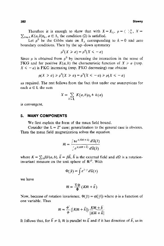
We first explain the form of the mean field bound. Consider the H-= 7/~ case; generalization to the general case is obvious.

Then the mean field magnetization solves the equation

m = f s e ~(Km +E) df](g)

f e s(Km+~) d~2(g)

where K = ~ b~J(a, b), 17 = fih, h is the external field and d~2 is a rotation- invariant measure on the unit sphere of R D. With

we have

�9 (y) =fe~ed~(s)

m = - ~ - (Kin + 1r

Now, because of rotation invariance, qb(37) = 0(1371) where g, is a function of one variable. Thus

- ~' ( I g m + E I ) gm+k m = --~ IKm +El

It follows that, for/~ ~ 0, ~ is parallel to/~ and if it has direction of/~, as in


Then, by definition

the case of interest here, then ,)'

m = --~ (Km + k), m = I~] (4)

This has the form of the mean field equation for one-component models and the proof that the solution of (4) bounds the magnetization of the many-component model is through first comparing it (4) with the corresponding one-component model and then using mean field majorization for the later.

Let

1 log ZA(k ) pfk) --lim pA(k ), pA(k) = -~

l] K(a,b)s o . % + k 2 so @ da(so) a , b ~ A a E A a@A

m -- lim p(k + e) - p ( k ) = D + p ( k ) e$O s

Let /~ > k and let D stand for the derivative; by the convexity of p and PA

m(k) <~ limDpA~ )

where the (expanding) sequence (An) has been so chosen that DpA.(l~ ) is convergent.

On the other hand by Ref. 4, Section 3, DpA,, (/~) < Dfia.(l~ ) wherefi(/~) corresponds to a one-component system with

and/~a such that

-BI-I = 2K(a,b>o,b+ k2 ,o ab a

ff(s>a (ds) = da (s) (5)

Passing to a subsequence (A,k)k~ for which DfiA(l~ ) is convergent we see that there exists an equilibrium state of the one-component system, say, O, such

DpA.~ (]C )--> O(So) and thus

m(k) ~ p(so)

By the maximality property of the " + " state, O(so)<~ 0 + (Sa) and since

384 Slawny

p~(sa) >>- O~-(s~) as/~/> k we obtain the majorization

m(k) <~ p~- (s~)

According to Appendix B the measure/z~ defined by (5) is of class ~ . Therefore, by Section 2, pk+(S~) is majorized by the maximal nonnegative solution m(K, k) of (4) which is the mean field bound.

All this generalizes to more general lattices, as in Section 2, with the equation (4) replaced by

~ ) ma = -~ 2b K(a, b)m b + k~ , a ~ L

ACKNOWLEDGMENT

I would like to thank Joel Lebowitz for helpful and stimulating discussions, and for pointing out to an error in an earlier version of this work. Discussions with my colleagues at VPI on the subject of Appendix B are also gratefully acknowledged.

APPENDIX A. THE MF MAGNETIZATION

The framework is as in Section 2. M is the set of all m = (ma)~L, 0>1 m a >l 1. m <~ n, m, n E M, if m~ -<< n a v a E k , a n d m < n i f m ~ < n a n d m v a n. A sequence m (n) in M is converging to m if rn~ (n)--> m~, Va E D_.

F: M ~ M is defined by

F(m)~= fa( fl~b J(a,b)mb + flhama )

We will use the following monotonicity and convexity properties of F: ( F 0 F is strictly increasing, i.e., m < n ~ F(m) < F(n).

This follows from positivity of J and h and from the fact that fa'S are strictly increasing.

Let M 1 be the set of all W-invariant elements of M. M ~ is F invariant and of a finite dimension equal to ]D_/Z~[. The set MI, of elements of M r which are nowhere zero is invariant too.

( /2) For any m ~ M , 1 and 0 < t < 1 there is ~/> 0 such that

F(trn) >1 (1 + ~)tF(u)

For , / -- 0 this is a direct consequence of concavity of f~'s. With ~ > 0 this is an easy consequence of the strict convexity of f~'s (cf. below). In case k~ > 0, Va, (/'2) holds for arbitrary m E M, by convexity and strict monotonicity of f~'s.


To demonstrate the strict convexity of fa it is enough to show that f~'(x) which is non-negative for x > 0, vanishes at isolated points only. But fa extends to an analytic function in a complex neighborhood of the real axis. Therefore, the same holds for f~'. If the real zeros of fa' were not isolated it would vanish identically and fa itself would be a linear function, which it is not.

We consider first the solutions of

m = F(m), m ~ M (A1)

The property (/'2) is not used in the lemma below.

Lemma (and definition): 1. If m <~ F(m) then the sequence Fk(m) is convergent. Its limit m* is

a solution of (A1). Furthermore m < m*. 2. If m is a nonzero solution of (A1) then rn~ :~ 0 Va E D_. 3. For any family (mi) of solutions of (A1) there is a solution

majorizing all of mi's. 4. There exists a maximal solution re(K) of (A1); here K = (flJ(a,b),

flh(a))a,bcQ. If K > K ' then m ( K ) > m(K'). If K(')$K then m(K (')) Sm(K).

5. The maximal solution is 7/" invariant.

Proof. By (F1), Fk+l(m) > Fk(m). Since Fk(m)~ = ~< 1, No. 1 follows. No. 2 holds by the J connectedness of a_. With m = supmi, m* > m > m i, all i, which proves No. 3.

Let re(K) be the supremum of all solutions of (A1). By No. 3, m(K) is the maximal solution. If K /> K ' then m(K' )= FK,(m(K')) <~ FK(m(K')) and therefore re(K) ) m(K') by No. 1.

Let m = l imm(K( ' ) ) . Then since m(K (')) >1 re(K), m ) re(K). But by continuity of K, mw-~FK(m), m = FK(m ). Thus m = re(K), and No. 4 is proved. No. 5 follows from the fact that a translate of a solution is again a solution and from uniqueness of the maximal solution.

Proposition. m ( K ) ~ O for h4:O. If h=O, m(K) v ~0 for fl >tier and m(K) = 0 for fl ~< tier" tier is given by the condition that the maximal eigenvalue of the derivative of F pM 1 at zero is 1.

Assume now h -- 0 and consider the restriction of F to M 1, denoted again by F. Let F ' be its derivative at O:

(F 'm) ,= f~(O) ~ flJ(a,b)m b b

Thus in the natural basis all matrix elements of F ' are nonnegative. Moreover, since L is J-connected there is a power of F which has all matrix elements strictly positive. By the Perron-Frobenius theorem the eigenvalue

386 Slawny

•max of F which is maximal in modulus is positive nondegenera te and the corresponding eigenvector rh can be chosen to be (strictly) positive. It is obvious f rom the form of F that rh does not depend o n / ? and that ~kma x is propor t ional to fl:

~kmax(/~ ) = X ' / ~

Assume Xma x > 1. Then F ' rh = Xmaxrfi >/ rfi in the sense that (F'm)a >1 m a, any a E ~_. Since t - l F ( t r h ) ~ F ' r h as t - ~ 0 it follows that for small enough t, t - 1F(t2rh) >1 rh. Thus for Xma x > 1, (trh)* is a nonzero solution of (A1).

Next we note that for a n y m ~ M / , m : ~ 0 , 1 /> t ~ > t 2 > 0

F(m) < t~ 'F( t ,m) < t f 'F(t2rn )

the strict inequality following f rom (/;2). It follows that

F(m) < F 'm (A2)

N o w if m ~ M 1 is a nonzero fixed point of F and fi is the positive eigenvector of the matr ix t ransposed to F ' corresponding to the eigenvalue )kma x then, taking (A2) into account ,

(~,m) = (~,F(m)) < QT, F ' m ) = ~kmax(~,m )

which is impossible if Xma X ~< 1. Thus it has been shown that m(K) is nonzero if X. /3 > 1 and zero if ~. fl < 1. This yields/?r = ~-1-

In fact in our situation (A1) has unique solution if h =/= 0 and at most two 7/"-invariant solutions if h = 0: the zero solution, and unique nonzero solution, if it exists.

The proof below and the fo rm of the condit ion (F2) are adap ted f rom Ref. 3. Let m be a fixed point of F. In both cases to be considered, there is a constant a > 0 depending on m, such that m, >/ a, Va E R_; this follows f rom J-convect iv i ty of ~_. Let n be another fixed point with corresponding cons tant fi > 0. Suppose it is not true that m/> n, and let t o = sup{t > /0 : m >1 tn }. Since n a < 1 and m ~r n, 0 < a < t o < 1. But then, using monotonic - ity of F and (F2),

m = F(m) >1 F(ton ) >1 (1 + Ti)toF(n ) = (1 + Tl)ton

Thus m ~> (1 + ~)ton is contradict ion with the maximal i ty of t o.

APPENDIX B. CONVEXITY FOR MANY COMPONENTS

With suitable normalization of the rotation-invariant measure df~ on the unit sphere of R D the measure G of (15) satisfies

f fJl(1--S2)(1/2)(D-3)f(s)ds


and thus the 0 of (4) is

(p(x) = fl le xs(1 - $2) (1 /2) (D-3)ds:

We have to show that f = 0 ' / 0 is convex on the positive half-axis. f is obviously an analytic function. Also

f (x ) = J D / 2 ( X ) / / J ( D / 2 ) _ ,(X) (B1)

where J is the modified Bessel function. (4'6) Either by direct integration by parts or from the well-known identities

, n , n j J ,~=J ,+ ] + "In, J/,= J , - ] - x "

one can see that f satisfies the differential equation

f ' = 1 D - 1 f _ f2 with " f (0 )= 0 (B2) x

From (B1) or (B2) one obtains easily an expansion of f for small x.

f (x) = -~ 1 D(D + 2) + O(x') (B3)

We first show t h a t 0 < f ( x ) < 1, O < f ' < - 1 a s 0 < x < + r e . Let

D - l f _ f 2 , x,f>~O F(x, f ) = 1 x Then as is easy to see the situation is as in Fig. 3. The curve F(x, f ) -- 0 is concave and asymptotic to f = 1 as x ~ m. The slope of f at 0 is 1 / D [from (B3)], whereas the slope of F(x, f ) -- 0 at 0 is 1/(D - 1). Thus for small x, the graph of f is between the x axis and the curve F(x, f ) = 0. But then it remains in this region for all x > 0, i.e., f ' (x) > 0 Vx > 0. For otherwise the graph of f would have to cross the curve F(x, f ) -- 0. This is impossible as the slope of the last curve is positive everywhere, whereas f at the crossing point would have slope 0.

o

F ( ~ , ~ > 0

)

Fig. 3. Behavior of the solution of the equation (B.2).

388 Slawny

!

.3_ D

Fig. 4. Behavior of g = f ' .

We use a similar argument to show that f " is negative for x > 0. Differentiating (B2) and eliminating f we see that

f"(x)- D - 1 D - 1 + ) - 4 ( f ' - 1) 2 x 2 x

-f'[(D~x 1)2-4(f ' -1)] ' /2

Or, w i t h g = f ' , d = D - 1 c(x, g)

where

G(x,g)= d2x 2 _ dx + - ~ - 4 ( g - 1 ) - g ~ - 4 ( g - 1 )

Somewhat more involved analysis than before yields now the graph of Fig. 4. The curve G(x, g) = 0 has negative slope. For small positive x the graph of g is above this curve, i.e., in the region G < 0. But then it stays above for all x > 0 by the argument used in analyzing the graph of f. Hence f"= g'= G(x, g ) < 0 for all x. Which demonstrates the (strict) concavity off .

REFERENCES

1. M. Cassandro, E. Olivieri, A. Pellegrinotti, and E. Presutti, Z. Wahrs. v. Geb. 41:313 (1978). 2. Kai Lai Chung, A Course in Probability Theory (Academic Press, New York, 1974). 3. M. A. Krasnoselskii, Positive Solutions of Operator Equations (P. Noordhoff, Groningen,

1964). 4. P. A. Pearce, J. Stat. Phys. 25:309 (1981). 5. C. Preston, Random fields (Lecture Notes in Mathematics No. 534, Springer-Verlag, Berlin,

1976). 6. H. Silver, N. E. Frankel, and B. W. Ninhan. J. Math. Phys. 13:468 (1972). 7. B. Simon, J. Stat. Phys. 22:491 (1980).

On the mean field theory bound on the magnetization

Documents

Transcript of On the mean field theory bound on the magnetization