Dependence of Radiant Optical Magnetization on MaterialComposition

by

Elizabeth F. C. Dreyer

A dissertation submitted in partial fulfillmentof the requirements for the degree of

Doctor of Philosophy(Electrical Engineering)

in the University of Michigan2018

Doctoral Committee:

Professor Stephen C. Rand, ChairProfessor Pallab BhattacharyaProfessor Jinsang KimProfessor Karl Michael KrushelnickProfessor Herbert Graves Winful

nosce te ipsum, puella stellarum

Elizabeth F. C. Dreyer

efcloos@umich.edu

ORCID iD: 0000-0003-2558-2097

© Elizabeth F. C. Dreyer 2018

DEDICATION

To my parents, who encouraged me to dream big dreams.To my husband, who helped those dreams take flight.

ii

ACKNOWLEDGEMENTS

A PhD is not the result of one researcher, working alone in a basement for years, onlyto emerge at the end with a fully formed dissertation. Rather, it takes a village to supportthe researcher along the way. I am grateful for my village. I am forever thankful to:

• My husband Patrick, for being my rock.• My family - especially my parents, Mike and Cheri; my brother, Stephen; and my

in-laws, Bill and Sally - for believing in me, even if you don’t always know what I do.• God, for sustaining my faith throughout this trial.• My friends at University of Michigan - especially Laura and Heather - for motivating

me to keep going, and making the journey worthwhile.• My hometown friends - Allie, Mary, Natalie, Brooke, and Andrew - for everything.• My research colleagues - Alex, Will, Mike, Ayan, Hengky, Manish, Theresa, Laura,

Long, Krishnandu, Ayesheshim, and Tuan - for all of the big and small things in the lab.• My research adviser and thesis committee, for giving me feedback over the years and

enabling this dissertation to be the best possible version.• The EECS support staff - especially Car, Amy, Greg, and Jose - for pushing me, helping

me, and making ERB and EECS better places to be.• The College of Engineering staff - especially Kim, Tiffany, Shira, and Andria - for

giving me countless opportunities to give back to the UM community.• Other UM offices - especially WISE, CEW, CAPS - for being there when I needed it.• The Science, Technology, and Public Policy certificate program, for teaching me how

to be a responsible scientist, and citizen, in society.• My extracurricular organizations - especially Society of Women Engineers and the

Optics Society at UM - for giving me the opportunity to be more than just a researcher.• Michigan Technological University - especially the Electrical & Computer Engineering

Department - for providing me with the foundation to thrive in grad school. Go Huskies!Finally, thank you to all the adults who took time to encourage my curiosity. Thank

you to Rochester Community Schools - especially Mr. Mattick, my 6th grade Math teacher,who had me skip to 7th grade math; Mr. Thuma, my AP Physics teacher, who encouragedme to make my career in Science; and the Hart Middle School librarian who let me checkout my own books. Thank you to everyone who believed in me.

iii

PREFACE

This dissertation is submitted for the degree of Doctor of Philosophy at the Univer-sity of Michigan. The research described herein was conducted under the supervision ofProfessor S. C. Rand in the Department of Electrical Engineering and Computer Science,University of Michigan, between September 2012 and March 2018.

The majority of the research conducted for this thesis was part of an internationalresearch collaboration, led by Dr. Rand at the University of Michigan. The literaturereview in Chapter 1 is my original work. In Chapter 2, the quantum theory was primarilydeveloped by A. A. Fisher, with additional symmetry analysis done by me. The initialatomic classical theory was developed by W. M. Fisher. P. M. Anisimov provided thetorque-enhanced molecular model. In Chapter 3, the experimental apparatus was builtin collaboration with W. M. Fisher and A. A. Fisher. My significant contributions werealignment, sample preparation, and data acquisition. The classical simulation was entirelymy original work. In Chapter 4, A. A. Fisher collected the data for the tetrachloride seriesand GGG intensity-dependent scattering. I collected the data for the orthosilicate seriesand Quartz. The spectroscopy data was collected by M. T. Trinh and K. Makhal. Theexperimental analysis was entirely my original work, along with the simulation results.In Chapter 5, the predictions from the optical susceptibility were generated by A. J.-T.Lou. The rest of the analysis was my own. Portions of the results of this thesis appear inpublication as noted in the citations and Chapter 5.

This material is based upon work supported by the National Science Foundation (NSF)Graduate Research Fellowship under Grant No. F031543 and the Air Force Office of Sci-entific Research (AFOSR) under Grant No. FA9550-14-1-0040. Any opinion, findings,and conclusions or recommendations expressed in this material are those of the author anddo not necessarily reflect the views of the NSF or AFOSR.

iv

TABLE OF CONTENTS

Dedication . . . . . . . . . . . . . . . . . . . . . . . . . . . . . . . . . . . . . . . ii

Acknowledgments . . . . . . . . . . . . . . . . . . . . . . . . . . . . . . . . . . . iii

Preface . . . . . . . . . . . . . . . . . . . . . . . . . . . . . . . . . . . . . . . . . iv

List of Figures . . . . . . . . . . . . . . . . . . . . . . . . . . . . . . . . . . . . . viii

List of Tables . . . . . . . . . . . . . . . . . . . . . . . . . . . . . . . . . . . . . . xiii

List of Appendices . . . . . . . . . . . . . . . . . . . . . . . . . . . . . . . . . . . xiv

List of Abbreviations . . . . . . . . . . . . . . . . . . . . . . . . . . . . . . . . . xv

Abstract . . . . . . . . . . . . . . . . . . . . . . . . . . . . . . . . . . . . . . . . . xvi

Chapter

1 Introduction . . . . . . . . . . . . . . . . . . . . . . . . . . . . . . . . . . . . . 1

1.1 Overview . . . . . . . . . . . . . . . . . . . . . . . . . . . . . . . . . . 21.1.1 Metamaterials . . . . . . . . . . . . . . . . . . . . . . . . . . . 3

1.2 Nonlinear optics . . . . . . . . . . . . . . . . . . . . . . . . . . . . . . . 41.2.1 A brief history of light scattering . . . . . . . . . . . . . . . . . . 5

1.2.1.1 Elastic light scattering . . . . . . . . . . . . . . . . . . . 61.2.1.2 Inelastic light scattering . . . . . . . . . . . . . . . . . . 61.2.1.3 Higher order and multiple scattering . . . . . . . . . . . 81.2.1.4 Polarization-sensitive light scattering experiments . . . . 10

1.2.2 Comments on material symmetry . . . . . . . . . . . . . . . . . 131.2.2.1 Standard symmetries of nonlinear optics . . . . . . . . . 141.2.2.2 PT symmetry in optics . . . . . . . . . . . . . . . . . . . 16

1.2.3 Ultrafast demagnetization and the inverse Faraday effect . . . . . 181.3 Dynamic magneto-optics in natural materials . . . . . . . . . . . . . . . 19

2 Theory of Radiant Optical Magnetization . . . . . . . . . . . . . . . . . . . . . 24

2.1 Classical theory . . . . . . . . . . . . . . . . . . . . . . . . . . . . . . . 242.1.1 Background on Lorentz Oscillator Model . . . . . . . . . . . . . 242.1.2 Derivation of the torque model . . . . . . . . . . . . . . . . . . . 25

2.2 Quantum mechanical model . . . . . . . . . . . . . . . . . . . . . . . . 292.2.1 Derivation of the quantum mechanical model . . . . . . . . . . . 29

v

2.2.2 Parity-time symmetry of the magnetic interaction Hamiltonian . . 312.2.3 Predictions of magneto-electric scattering completion time . . . . 32

2.3 Optical susceptibilities for magneto-electric effects . . . . . . . . . . . . 352.3.1 Magneto-electric polarization . . . . . . . . . . . . . . . . . . . 352.3.2 Magneto-electric magnetization . . . . . . . . . . . . . . . . . . 39

3 Methods . . . . . . . . . . . . . . . . . . . . . . . . . . . . . . . . . . . . . . . 42

3.1 Experimental design . . . . . . . . . . . . . . . . . . . . . . . . . . . . . 423.1.1 Summary of experimental parameters . . . . . . . . . . . . . . . 463.1.2 Procedures and calibration . . . . . . . . . . . . . . . . . . . . . 47

3.1.2.1 Equipment overview . . . . . . . . . . . . . . . . . . . . 483.1.2.2 Detector stabilization . . . . . . . . . . . . . . . . . . . 493.1.2.3 Optical alignment techniques . . . . . . . . . . . . . . . 52

3.1.3 Special considerations of a focused beam . . . . . . . . . . . . . 573.1.4 Signal detection limits . . . . . . . . . . . . . . . . . . . . . . . 60

3.2 Data acquisition procedure and analysis . . . . . . . . . . . . . . . . . . 613.3 Sample selection and preparation . . . . . . . . . . . . . . . . . . . . . . 63

3.3.1 Procedure for cleaning cuvettes . . . . . . . . . . . . . . . . . . 643.3.2 Preparation procedure: Liquids . . . . . . . . . . . . . . . . . . 65

3.4 Simulation methods . . . . . . . . . . . . . . . . . . . . . . . . . . . . . 673.4.1 Numerical solving techniques . . . . . . . . . . . . . . . . . . . 673.4.2 Dimensionless equations . . . . . . . . . . . . . . . . . . . . . . 683.4.3 Physical meaning of initial conditions . . . . . . . . . . . . . . . 70

3.4.3.1 Reduction to the atomic Lorentz Oscillator Model . . . . 703.4.3.2 Non-zero equilibrium point . . . . . . . . . . . . . . . . 713.4.3.3 Comparisons of molecular properties . . . . . . . . . . . 71

4 Results . . . . . . . . . . . . . . . . . . . . . . . . . . . . . . . . . . . . . . . . 73

4.1 Experimental results . . . . . . . . . . . . . . . . . . . . . . . . . . . . . 744.1.1 Magneto-electric scattering in liquids . . . . . . . . . . . . . . . 74

4.1.1.1 Tetrachlorides . . . . . . . . . . . . . . . . . . . . . . . 744.1.1.2 Orthosilicates . . . . . . . . . . . . . . . . . . . . . . . 75

4.1.2 Magneto-electric scattering in solids . . . . . . . . . . . . . . . . 764.1.2.1 Gadolinium Gallium Garnet . . . . . . . . . . . . . . . . 764.1.2.2 Quartz . . . . . . . . . . . . . . . . . . . . . . . . . . . 77

4.1.3 Spectrally-resolved magnetic scattering . . . . . . . . . . . . . . 794.1.4 Analysis . . . . . . . . . . . . . . . . . . . . . . . . . . . . . . 86

4.1.4.1 Material comparisons and procedures . . . . . . . . . . . 864.1.4.2 Tetrachloride series . . . . . . . . . . . . . . . . . . . . 884.1.4.3 Orthosilicate series . . . . . . . . . . . . . . . . . . . . . 884.1.4.4 Errors in Figure of Merit (FOM) calculations . . . . . . . 93

4.2 Simulation results . . . . . . . . . . . . . . . . . . . . . . . . . . . . . . 944.2.1 Electron motion at high-field strengths . . . . . . . . . . . . . . . 944.2.2 Charge separation . . . . . . . . . . . . . . . . . . . . . . . . . 954.2.3 Magnetization and electric polarization . . . . . . . . . . . . . . 98

vi

4.2.4 Comparison to quantum theory . . . . . . . . . . . . . . . . . . 99

5 Conclusion . . . . . . . . . . . . . . . . . . . . . . . . . . . . . . . . . . . . . . 102

5.1 Summary of results . . . . . . . . . . . . . . . . . . . . . . . . . . . . . 1025.2 Detailed experimental comparisons of materials . . . . . . . . . . . . . . 1075.3 Additional discussion on depolarized light scattering . . . . . . . . . . . 1085.4 Application of theoretical models to material design . . . . . . . . . . . . 112

5.4.1 Predictions from nonlinear optical susceptibility for design ofnonlinear materials . . . . . . . . . . . . . . . . . . . . . . . . . 112

5.4.2 Predictions from quantum and classical theory . . . . . . . . . . 1135.5 Future work . . . . . . . . . . . . . . . . . . . . . . . . . . . . . . . . . 114

5.5.1 Theory . . . . . . . . . . . . . . . . . . . . . . . . . . . . . . . 1145.5.2 Experiments . . . . . . . . . . . . . . . . . . . . . . . . . . . . 116

Appendices . . . . . . . . . . . . . . . . . . . . . . . . . . . . . . . . . . . . . . . 117

Bibliography . . . . . . . . . . . . . . . . . . . . . . . . . . . . . . . . . . . . . . 162

vii

LIST OF FIGURES

1.1 Illustration of the analogy between a conventional LC circuit (A), consisting ofan inductance L, a capacitance C, and the single SRRs used here (B). l, length;w, width; d, gap width; t, thickness. (C) An electron micrograph of a typicalSRR fabricated by electron-beam lithography. The thickness of the gold filmis t = 20 nm. For normal incidence, where the magnetic field vector B lies inthe plane of the coil, the electric field vector E of the incident light must havea component parallel to the electric field of the capacitor to couple to the LCcircuit. This allows the coupling to be controlled through the polarization ofthe incident light. Reprinted with permission from reference [27]. . . . . . . . 4

1.2 Depictions of (l) elastic and (r) inelastic light scattering. . . . . . . . . . . . . 61.3 Schematic diagram of the experimental geometry used to map electric dipole

and magnetic dipole radiation patterns by scanning polarization in the trans-verse plane of the incident light. Reprinted with permission from reference[82]. . . . . . . . . . . . . . . . . . . . . . . . . . . . . . . . . . . . . . . . . 20

1.4 Experimental intensity of magnetic dipole scattering versus input intensity inCCl4. The solid (dashed) curve is a linear (quadratic) regression through thedata. Reprinted with permission from reference [131]. . . . . . . . . . . . . . 21

1.5 (Left) Second-order dressed state mixings that account for three new, quadraticmagneto-electric nonlinearities allowed in centro-symmetric (as well as non-centrosymmetric) dielectric media. (Right) An angular momentum diagramfor a molecular model in which the internal (L) and external (O) angular mo-menta excited by the optical H field can be exchanged in a ∆J=0 transitionthat becomes 2-photon resonant through rotational excitation of the molecularground state. . . . . . . . . . . . . . . . . . . . . . . . . . . . . . . . . . . . 23

2.1 Motion of electron . . . . . . . . . . . . . . . . . . . . . . . . . . . . . . . . 262.2 Model of a homonuclear diatomic molecule, together with the coordinate sys-

tem and position vectors ξ and rA specifying electron position and point ofequilibrium respectively. . . . . . . . . . . . . . . . . . . . . . . . . . . . . . 27

2.3 Energy levels of the molecular model showing the 2-photon transition (solidarrows) driven by optical E and H∗ fields. The dashed downward arrow de-picts a magnetic de-excitation channel that becomes an option if the excitationbandwidth exceeds ωφ. . . . . . . . . . . . . . . . . . . . . . . . . . . . . . . 29

viii

2.4 Squared values of the total magnetic moment and the first order electric dipolemoment versus the number of incident photons in a (a) 3-state model and (b)a 4-state model. In both figures separate curves are shown for 〈m〉2 with ro-tational frequencies (left to right) of ωφ/ω0=107, 105, 103. Reprinted withpermission from reference [7]. . . . . . . . . . . . . . . . . . . . . . . . . . . 30

2.5 Diagram showing the magnetic enhancement. . . . . . . . . . . . . . . . . . . 33

3.1 90 light scattering geometry used in detecting (l) electric and (r) magneticdipole radiation. Reprinted with permission from reference [136]. . . . . . . . 43

3.2 Radiation and polarization from electric (Red) and magnetic (Blue) dipolesgenerated by a plane wave of light. The purple arrow indicates that the polar-izations of the two dipoles are parallel, and therefore indistinguishable, alongthe forward direction. Reprinted with permission from reference [153]. . . . . 45

3.3 Basic geometry of magneto-electric scattering experiments. . . . . . . . . . . 463.4 Response of detection system. . . . . . . . . . . . . . . . . . . . . . . . . . . 493.5 Dark count rate of C31034A after the chiller was activated. Taken using the

SR400 with a discriminator of -18 mV, x5 amplification, 1800 V high voltagebias after being off for 4 days time. . . . . . . . . . . . . . . . . . . . . . . . 50

3.6 Dark count rate distribution of C31034A after the chiller was activated for 29hours, over a 200 second window. Taken using the SR400 with a discriminatorof -18 mV, x5 amplification, 1800 V high voltage bias. . . . . . . . . . . . . . 50

3.7 Waveform from C31034A, 5x Amp, Terminated Signal. . . . . . . . . . . . . 513.8 Plateauing of the C31034A PMT with 5x Amp and 1800 V bias. . . . . . . . . 513.9 Schematic for magneto-electric scattering experiment. L = lens, I = iris, WP

= waveplate, P = polarizer, SH = shutter, TS = telescope, PS = periscope, M =mirror, AN = analyzer, primes indicate alignment beam path. . . . . . . . . . . 52

3.10 Schematic for magneto-electric scattering experiment. L = lens, I = iris, λ/2= rotatable half-wave plate, 105:1 = polarizer, M = mirror, SMC = computer-controlled rotation stage, blue line indicates alignment path. . . . . . . . . . . 53

3.11 Schematic for magneto-electric scattering and spectrum experiment. λ/2 =rotatable half-wave plate, 105:1 = polarizer. . . . . . . . . . . . . . . . . . . . 53

3.12 Example of beam profile during beam camera alignment. . . . . . . . . . . . . 543.13 (l) Vertical and (r) Horizontal alignment of the detector comparing two align-

ment methods. . . . . . . . . . . . . . . . . . . . . . . . . . . . . . . . . . . 553.14 (l) Vertical and (r) Horizontal alignment of the detector comparing alignment

using Vv and Hh scattered light. . . . . . . . . . . . . . . . . . . . . . . . . . 563.15 (l) Horizontal alignment of the detector comparing alignment using Vv and Hh

scattered light without a limiting aperture. (r) Ratio of Hh to Vv scattered light. 563.16 Cartesian plot of vertically- and horizontally-polarized light reflected off a 45

degree mirror through the detection optics. . . . . . . . . . . . . . . . . . . . 573.17 Zemax model of collection optics: f1 = 50 mm, f2 = 150 mm, f3 = 60 mm, iris

diameter = 5mm, pinhole diameter = 75 µm. . . . . . . . . . . . . . . . . . . 593.18 Zemax vignetting model of collection optics: f1 = 50 mm, f2 = 150 mm, f3 =

60 mm, iris diameter = 5mm, pinhole diameter = 75 µm. . . . . . . . . . . . . 59

ix

3.19 Verification of detection of changes in (l) average power and (r) peak power us-ing the 2-photon fluorescence signal from Rhodamine 590 dissolved in methanol. 60

3.20 Flowchart depicting the steps used by the data collection computer program. . 613.21 Schematic of dipole components for analysis. . . . . . . . . . . . . . . . . . . 62

4.1 Unpolarized ED (Vh) scattering for CCl4, SiCl4, GeCl4, and SnCl4. Solidcurves are quadratic fits to the data, with the dashed lines showing only the I2

component. . . . . . . . . . . . . . . . . . . . . . . . . . . . . . . . . . . . . 754.2 Molecular structure of TMOS (l), TEOS (c), and TPOS (r). . . . . . . . . . . . 754.3 Total magnetic dipole scattering of CCl4, TMOS, TEOS, and TPOS. Inset

shows electric dipole scattering for reference. . . . . . . . . . . . . . . . . . . 764.4 (a) Polar plot of raw data on co-polarized (open circles) and cross-polarized

(filled circles) radiation patterns in GGG at I=1.4×107 W/cm2 obtained at arepetition rate of 1 kHz. Dashed circles anticipate fits to the unpolarized back-ground signal intensities. Residuals from the best fit of a circle plus a squaredcosine curve to the raw data are shown below the polar plot. (b) Comparativeplots in crystalline GGG of unpolarized ED (open circles) and MD (filled cir-cles) scattering. Solid curves are quadratic fits to the data. Inset: correspond-ing data for polarized scattering components on the same scale. Reprintedwith permission from reference [130]. . . . . . . . . . . . . . . . . . . . . . . 77

4.5 Polar plots of the radiation patterns for polarized ED and MD scattering infused quartz at an input intensity of∼2.2×1010 W/cm2 obtained at a repetitionrate of 80 MHz. At this intensity, in this sample, the unpolarized component isnegligible compared to the polarized component. Note that peak intensities inthe two plots are equal. Residuals from the best fit of a squared cosine curve tothe raw data are shown below the polar plot. Reprinted with permission fromreference [130]. . . . . . . . . . . . . . . . . . . . . . . . . . . . . . . . . . . 78

4.6 Measurements of polarized (l) and unpolarized (r) components of ED (opencircle) and MD (closed circle) scattered light versus input intensity for Quartz.Solid curves are quadratic fits to the data. . . . . . . . . . . . . . . . . . . . . 78

4.7 Normalized scattered light spectrum for Vv (l) and Hh (r) geometries for CCl4. 794.8 Comparative scattered light spectrum for electric (red) and magnetic (blue)

dipole radiation for CCl4. . . . . . . . . . . . . . . . . . . . . . . . . . . . . . 794.9 (l) Difference between ED and MD scattered light. (r) Quantum model for

M-E processes. . . . . . . . . . . . . . . . . . . . . . . . . . . . . . . . . . . 804.10 Difference between MD and ED spectrums of light scattered from CCl4. . . . . 804.11 Comparison of magneto-electrically induced energy shift with molecular rota-

tion frequency. . . . . . . . . . . . . . . . . . . . . . . . . . . . . . . . . . . 814.12 Normalized scattered light spectrum for Vv (l) and Hh (r) geometries for SiCl4. 824.13 Normalized scattered light spectrum for Vv (l) and Hh (r) geometries for SiBr4. 824.14 Normalized scattered light spectrum for Vv (l) and Hh (r) geometries for Tetra-

methyl Orthosilicate (TMOS). . . . . . . . . . . . . . . . . . . . . . . . . . . 824.15 Normalized scattered light spectrum for Vv (l) and Hh (r) geometries for Te-

traethyl Orthosilicate (TEOS). . . . . . . . . . . . . . . . . . . . . . . . . . . 83

x

4.16 Energy level diagram showing magneto-electric magnetization. ∆1 is the one-photon detuning where ∆1 = ω0 − ω. ωφ is the two-photon detuning.S1 andT1 are the singlet and triplet resonance bands, respectively. . . . . . . . . . . . 87

4.17 The vapor phase vacuum UV spectra of the group IVA tetrachlorides (l) andgroup IVA tetrabromides (r). Reprinted with permission from references [173]and [178], respectively. . . . . . . . . . . . . . . . . . . . . . . . . . . . . . . 90

4.18 Raw NMR data with exponential fit for SiBr4 Spin-Lattice relaxation time, T1. 914.19 Raw NMR data with exponential fit for SiBr4 Spin-Spin relaxation time, T2. . . 924.20 Trajectory of electron motion calculated by integration of the equations of

motion for an incident electric field of arbitrary strengths. From left to right,the electric field strengths are 1e12, 2e12, 3e12, and 4e12 V/m. Simulationvalues are ω0 = 1.63e16rad/s, ω = 0.9ω0, γ = 0.1ω0, I// = ~/ω0, I⊥/I// =1000, ξ = [0, 0, 0], and rA = [0, 15pm, 0]. . . . . . . . . . . . . . . . . . . . . 94

4.21 Evolution of the charge separation, Pz (0), of the test charge versus time forI⊥/I// = 1 (left) and I⊥/I// = 1000 (right). Simulation values are ω0 =1.63e16rad/s, ω = 0.9ω0, γ = 0.1ω0, I// = ~/ω0, E = 1e9V/m, ξ = [0, 0, 0],and rA = [0, 15pm, 0]. . . . . . . . . . . . . . . . . . . . . . . . . . . . . . . 95

4.22 Evolution of the magnetic moment of the test charge divided by light speed,My (ω) /c, versus time for I⊥/I// = 1 (left) and I⊥/I// = 1000 (right). Simu-lation values are ω0 = 1.63e16rad/s, ω = 0.9ω0, γ = 0.1ω0, I// = ~/ω0, E =1e9V/m, ξ = [0, 0, 0], and rA = [0, 15pm, 0]. . . . . . . . . . . . . . . . . . . 96

4.23 Evolution of charge separation (top) and magnetization/c (bottom) versus timefor different values of the magnetic (librational) damping. The damping co-efficient is γ = 0.025ω0 (left) and γ = 0.25ω0 (right). Simulation val-ues are ω0 = 1.63e16rad/s, ω = 0.9ω0, I// = ~/ω0, I⊥/I// = 1000, E =2e9V/m, ξ = [0, 0, 0], and rA = [0, 15pm, 0]. . . . . . . . . . . . . . . . . . . 96

4.24 Evolution of the charge separation (top) and magnetization/c (bottom) ver-sus time for different values of the applied electric field. The electric fieldstrength is E = 5e8V/m (left) and E = 1e9V/m (right). Simulation valuesare ω0 = 1.63e16rad/s, ω = 0.9ω0, γ = 0.1ω0, I// = ~/ω0, I⊥/I// = 1000,ξ = [0, 0, 0], and rA = [0, 15pm, 0]. . . . . . . . . . . . . . . . . . . . . . . . 97

4.25 High-field charge separation (top) and high-field magnetization/c (bottom)versus time for different values of the magnetic (librational) damping. Thedamping coefficient is γ = 0.025ω0 (left) and γ = 0.25ω0 (right). Sim-ulation values are ω0 = 1.63e16rad/s, ω = 0.9ω0, E = 1e10V/m, I// =~/ω0, I⊥/I// = 1000, ξ = [0, 0, 0], and rA = [0, 15pm, 0]. . . . . . . . . . . . 97

4.26 High-field charge separation (top) and high-field magnetization/c (bottom)versus time computed for large magnetic (librational) damping, γ = 0.25ω0,and E = 5e9V/m (left) and E = 20e9V/m (right). Simulation values areω0 = 1.63e16rad/s, ω = 0.9ω0, I// = ~/ω0, I⊥/I// = 1000, ξ = [0, 0, 0], andrA = [0, 15pm, 0]. . . . . . . . . . . . . . . . . . . . . . . . . . . . . . . . . 98

4.27 Electric polarization (red) and magnetization/c (blue) versus time showingboth oscillate at ω. Simulation values are ω0 = 1.63e16rad/s, ω = 0.9ω0, I// =~/ω0, I⊥/I// = 1000, E = 6e9V/m, ξ = [0, 0, 0], and rA = [0, 15pm, 0]. . . . 98

xi

4.28 Electric polarization (top) and magnetization/c (bottom) versus time computedfor atomic (left) and molecular (right) models. Simulation values are ω0 =1.63e16rad/s, ω = 0.9ω0, I// = ~/ω0, I⊥/I// = 1000, ξ = [0, 0, 0], and rA =[0, 15pm, 0]. . . . . . . . . . . . . . . . . . . . . . . . . . . . . . . . . . . . . 99

4.29 Values of the total magnetic moment, second order electric moment, and firstorder electric dipole moment versus the number of incident photons in the (l)4-state quantum model and (r) molecular torque-enhanced Lorentz oscillatormodel. In both figures, the rotation frequency is ωφ/ω0 = 10−5. . . . . . . . . 100

4.30 Squared values of the total magnetic moment and first order electric dipole mo-ment versus the number of incident photons in the (l) 4-state quantum modeland (r) molecular torque-enhanced Lorentz oscillator model. In both figures,the rotation frequencies from left to right are ωφ/ω0=10−7, 10−5, 10−3. . . . . 100

4.31 Squared values of the second order electric moment and first order electricdipole moment versus the number of incident photons in the (l) 4-state quan-tum model and (r) molecular torque-enhanced Lorentz oscillator model. Inboth figures, the rotation frequencies from left to right are ωφ/ω0=10−7, 10−5,10−3. . . . . . . . . . . . . . . . . . . . . . . . . . . . . . . . . . . . . . . . 101

5.1 Diagram showing the 4 M-E quantum processes as solid arrows: two electrictransitions on the left and two magnetic transitions on the right. ∆(e) is the1-photon detuning, ω0 − ω. ∆(m) is the 2-photon detuning, ωφ. . . . . . . . . . 103

5.2 Example of pulse function for Lorentz oscillator model. . . . . . . . . . . . . 1155.3 Comparison of ED, MD (l) and charge separation (r) for LOM driven by a

femtosecond pulse. . . . . . . . . . . . . . . . . . . . . . . . . . . . . . . . . 1155.4 Comparison of ED, MD (l) and charge separation (r) for LOM driven by a

femtosecond pulse. . . . . . . . . . . . . . . . . . . . . . . . . . . . . . . . . 116

A.1 Set-up for verification of the extinction rate of the polarizer and for locating thezero position on the mounted rotatable polarizer. Inset shows three examplebeam locations on the alignment iris, where 23.1 is the optimal SMC position.The “Analyzer Zero” value is then 113.1. . . . . . . . . . . . . . . . . . . . . 118

A.2 Set-up for locating the zero position on the mounted rotatable wave plate,where the half-wave plate does not rotate the polarization of the incident laserbeam. . . . . . . . . . . . . . . . . . . . . . . . . . . . . . . . . . . . . . . . 119

xii

LIST OF TABLES

1.1 Comparison of 90-degree polarization-sensitive light scattering experiments. . 131.2 Hermann-Mauguin descriptions of crystallographic point groups, where n =

n-fold rotation axis, 1 = nothing, m = reflection, -1 = inversion, n = n-foldrotation + inversion axis, n/m = n-fold rotation + reflection axis [85]. . . . . . 15

1.3 Summary of experimental parameters from 2007 scattering experiments [82]. . 19

3.1 Comparison of detected dipole radiation by input and output polarizations. . . 443.2 Comparison of specifications of magneto-electric scattering experiments. . . . 473.3 Experimental Electronics . . . . . . . . . . . . . . . . . . . . . . . . . . . . . 483.4 Comparison of focused beam size and intensity for varied focal lengths. . . . . 583.5 Comparison of lenses for collection magnification, assuming f2 = 150 mm. . . 583.6 Verification of detection of changes in peak power using the 2-photon fluores-

cence signal from Rhodamine 590 dissolved in methanol. . . . . . . . . . . . . 603.7 Supplies needed to clean cuvettes. . . . . . . . . . . . . . . . . . . . . . . . . 643.8 Suggested cleaning methods from Starna Cells, Inc. . . . . . . . . . . . . . . . 653.9 Constants of the Lorentz Oscillator Model equations for (top) real-scale values

in their common units and (bottom) dimensionless values. . . . . . . . . . . . 703.10 Dependence of dipole moments on initial position of equilibrium point. . . . . 72

4.1 Vibration frequencies of Carbon Tetrachloride [46]. . . . . . . . . . . . . . . . 814.2 Vibration frequencies of Silicon Tetrachloride [46]. . . . . . . . . . . . . . . . 834.3 Vibration frequencies of Silicon Tetrabromide [46]. . . . . . . . . . . . . . . . 834.4 Vibration frequencies of Tetramethyl Orthosilicate [166]. . . . . . . . . . . . . 844.5 Vibration frequencies of Tetraethyl Orthosilicate [167]. . . . . . . . . . . . . . 854.6 Tetrachloride figure of merit: Part one. . . . . . . . . . . . . . . . . . . . . . . 884.7 Tetrachloride figure of merit: Part two. . . . . . . . . . . . . . . . . . . . . . 894.8 Additional physical constants for Tetrachlorides. . . . . . . . . . . . . . . . . 894.9 Raw NMR data for Spin-Lattice (l) and Spin-Spin (r) relaxation times. . . . . . 904.10 Orthosilicate figure of merit: Part one. . . . . . . . . . . . . . . . . . . . . . . 914.11 Orthosilicate figure of merit: Part two. . . . . . . . . . . . . . . . . . . . . . . 914.12 Additional physical constants for Orthosilicates. . . . . . . . . . . . . . . . . 92

5.1 Comparison of theoretical and experimental values of magnetization in Tetra-chloride molecules. . . . . . . . . . . . . . . . . . . . . . . . . . . . . . . . . 108

xiii

LIST OF APPENDICES

A Initialization of SMC100PP rotation stages . . . . . . . . . . . . . . . . . . . . 117

B MATLAB code for data acquisition . . . . . . . . . . . . . . . . . . . . . . . . 120

C MATLAB code for Lorentz oscillator model . . . . . . . . . . . . . . . . . . . 156

xiv

LIST OF ABBREVIATIONS

cps counts per second

ED Electric Dipole

EM electromagnetic

FOM Figure of Merit

GGG Gadolinium Gallium Garnet

IFE inverse Faraday effect

LOM Lorentz oscillator model

MD Magnetic Dipole

M-E Magneto-Electric

ND Neutral Density

NLO Nonlinear Optics

NMR Nuclear Magnetic Resonance

ODE Ordinary Differential Equation

PMT Photo-multiplier Tube

PT Parity-Time

TEOS Tetraethyl Orthosilicate

TMOS Tetramethyl Orthosilicate

TPOS Tetrapropyl Orthosilicate

UV Ultraviolet

UV-VIS Ultraviolet-Visible

QD quadrupole

VB-CT valence-bond charge-transfer

xv

ABSTRACT

The realization of strong optical magnetism in nominally “non-magnetic” mediacould lead to novel forms of all-optical switching, energy conversion, or the generationof large (oscillatory) magnetic fields without current-carrying coils. By advancing under-standing of radiant optical magnetization, the research reported in this thesis contributesprogress toward these prospects.

Experiments and simulations were performed of light scattering in natural dielectricsat non-relativistic optical intensities. The goal was to understand which molecular factorsinfluenced the magnitude of induced magnetic dipole scattering in isotropic materials. Theintensity dependence and spectra of cross-polarized scattering in several transparent molec-ular liquids (CCl4, SiCl4, GeCl4, SnCl4, SiBr4, TMOS, TEOS, TPOS) and crystalline solids(GGG, Quartz) were found to agree with predictions of quantum theory. Additionally, ev-idence was found for the expected proportionality between the intensity of radiant magne-tization and the electric dipole transition moment, together with an inverse proportionalitywith respect to molecular rotation frequency. By comparing spectra in molecular liquids, itwas found that spectral features in the cross-polarized scattering were uniquely attributableto high-frequency librations of magneto-electric (M-E) origin. In solids, optically-inducedmagnetic scattering in solids reached the same intensity as Rayleigh scattering, far belowrelativistic conditions. Additionally, all four channels predicted by the quantum theory forsecond-order (2-photon) M-E processes at the molecular level were observed in experi-ments on GGG crystals.

Two theoretical contributions are presented in this thesis. The first is an extensionof the classical Lorentz Oscillator Model from an atomic to a molecular picture. It in-cludes the effect of torque exerted by the optical magnetic field on excited state orbitalangular momentum, resulting in an enhancement in the magnetization achievable undernon-relativistic conditions in molecular or condensed matter systems. Temporal dynamicsare predicted for the first time, taking into account molecular composition. Secondly, thetorque Hamiltonian of quantum theory is shown to obey Parity-Time (PT) symmetry, indi-cating that M-E effects should occur universally. Lastly, results from classical and quantummechanical models are compared and found to be in very satisfactory agreement.

xvi

CHAPTER 1

Introduction

Since the earliest days of civilization, humanity has been fascinated by light and how itinteracts with the physical world. Many have sought to not only understand light, butharness its power for science, for medicine, and for art. Philosophers in ancient Greeceestablished the foundations of optics, the study of light [1]. A millennia later, Ibn al-Haytham became the founder of modern optics through his use of experimental techniquesto understand vision and refraction of lenses [2]. Scientists such as Newton [3], Huygens,Young, Fresnel [4], and countless others throughout the 18th, 19th, and 20th centuriessought to answer the questions of “what is light?” and “what happens when light meets

matter?”. Their study of phenomena such as reflection and refraction would later be calledlinear optics. Although the answer to “what is light?” is now known (hint: it’s both aparticle and a wave!), the question of “what happens when light meets matter?” continuesto be an active area of research. Despite the numerous useful technologies these light-matter interactions have allowed, there is still boundless opportunity for new technologiesenabled by new light-matter interactions.

There is always an interaction of some sort when light meets matter. Light can be scat-tered off a surface, reflected off a mirror, refracted by a lens, or stimulate the emissionof more light. The exact phenomenon depends on both the characteristics of the mate-rial (structure, chemistry, color) and of the light (wavelength, intensity, polarization). Ingeneral, light-matter interactions can be classified by either the combination of materialand optical properties required or by what happens when the light and matter interact. Forexample, low (high) intensity light usually leads to linear (nonlinear) effects. Piezo-opticlight-matter interactions are those where light causes the material to compress or expand.Magneto-electric effects are those where magnetic and electric properties of the materialare coupled by light.

This thesis seeks to add to the understanding of light-matter interactions. The goal isto attempt an answer to the questions: Are magneto-electric effects possible at the molec-ular level? How do chemical properties affect such processes? How fast do these effects

1

occur? This research has primarily sought to understand the dependency of radiant opticalmagnetization on material composition.

This thesis is organized as follows: Chapter 1 presents an overview of nonlinear optics,especially metamaterials, material symmetries, light scattering, and optical magnetization.It is found that the theory of radiant optical magnetization is a continuation of decades oflight-matter interaction work that can be described by the Lorentz oscillator model. Chap-ter 2 discusses the theory of radiant optical magnetization using both classical and quantummechanical models. Additionally, a connection is drawn between magneto-electric nonlin-ear optical susceptibilities and all-electric ones, opening up new areas of physical chemistryresearch. Chapter 3 is devoted to the experimental design for ultrafast laser experimentsas well as classical modeling. Chapter 4 showcases the results of both the experimentsand classical simulations. Also included is a comparison of experiments and theory usinga “figure of merit”. Finally, Chapter 5 summarizes all the experimental work conductedin this thesis and discusses the conclusions. It is found that magneto-electric effects arepossible at the molecular level and this thesis discusses their dependence on material com-position and time. Finally, appendices are included for the MATLAB code for the classicalmodel and experimental control.

1.1 Overview

It is well known that an electromagnetic (EM) wave incident on a linear dielectric mediuminduces an electric dipole. Similarly, the magnetic portion of the wave may cause a mag-netic dipole to form, though this is typically ignored due to the electric dipole approxima-tion, which suggests that the magnetic field has little effect on the charges within a materialwith no special magnetic properties [5]. The electric dipole approximation describes theprobability of radiative transitions occuring as a result of a light-matter interaction. It sug-gests that the probability of a Magnetic Dipole (MD) transition is 105 times more unlikely

than that of a Electric Dipole (ED) transition.However, when the effect of the magnetic field is included in the Lorentz oscillator

model (LOM) as part of the force term, the inversion symmetry of the material is brokenand new and surprisingly strong phenomena are predicted [6]. These phenomena are opticalmagnetization, magneto-electric rectification, and harmonic generation. In addition to thisclassical explanation of the phenomena, these effects can also be derived exactly using adoubly-dressed state quantum theory [7]. This thesis focuses entirely on the phenomenon ofoptical magnetization induced by non-relativistic optical fields through a novel (magneto-electric) nonlinear mechanism.

2

1.1.1 Metamaterials

Although no work using metamaterials was pursued during this dissertation, many usefulanalogs can be taken from the field. An overview of metamaterials is given in this sectionalong with explanations for how it can help in understanding the mechanism for radiantoptical magnetization in natural, homogenous, dielectric materials.

In general, the field of metamaterials seeks to design and fabricate structured materialswith the desired magnetic and electric response properties not normally found in nature [8].By using sub-wavelength structures, the magnetic and electric response of materials can betuned to produce varied effects. Metamaterials can be classified into four groups basedon how they modify the electric permittivity ε and magnetic permeability µ of materials.These four groups and the materials they are usually found in are [9, 10]:

• ε > 0, µ > 0, found in natural and structured dielectrics

• ε < 0, µ > 0, found in plasmas in certain frequency ranges

• ε > 0, µ < 0, found in gyrotropic magnetic materials in certain frequency ranges

• ε < 0, µ < 0, found in artificially produced materials only

All of the materials examined in this thesis are from the first category where ε and µ areboth positive.

One interesting application of metamaterials in optics is negative index materials (n =√εµ < 0). Negative index materials can theoretically enable imaging at sub-wavelength

resolution [11]. Currently, negative index materials have been designed using photoniccrystals [12, 13, 14, 15], optical transmission lines [16], and nano-fishnet structures [17,18]. Nano-fishnet structures are an intriguing solution. Since it is usually difficult to obtainboth electric and magnetic resonances in the same frequency range, nano-fishnet structurescombine a non-resonant background structure with a resonant magnetic structure [11]. Ex-perimentally, this has been achieved by sandwiching a magnetic resonator between metalfilms [19] or by using an array of metal strips of varied lengths [20].

Most metamaterial designs achieve negative refractive index by enhancing the magneticresponse of a material system [11]. One technique to do this is the split-ring resonator.Although initially demonstrated in the microwave regime [10, 21], the resonators weresuccessfully scaled to optical frequencies [22, 23, 24, 25]. Other techniques include astaple-like structure facing a metallic mirror [17] and an array of paired silver strips. Themagnetic response in the strips is the result of “asymmetric currents in the metal structuresinduced by the perpendicular magnetic-field component of light” [26].

3

All of the aforementioned methods rely on an external structure to constrain chargesand force a large interaction with the magnetic field component of light. This is the mostobvious in the split-ring resonator structure shown below in figure 1.1.

Figure 1.1: Illustration of the analogy between a conventional LC circuit (A), consisting ofan inductance L, a capacitance C, and the single SRRs used here (B). l, length; w, width; d,gap width; t, thickness. (C) An electron micrograph of a typical SRR fabricated by electron-beam lithography. The thickness of the gold film is t = 20 nm. For normal incidence, wherethe magnetic field vector B lies in the plane of the coil, the electric field vector E of theincident light must have a component parallel to the electric field of the capacitor to coupleto the LC circuit. This allows the coupling to be controlled through the polarization of theincident light. Reprinted with permission from reference [27].

In this structure, polarized light incident on the split-ring resonator induces a circu-lating electric current in the ring via the force of the electric field [24, 25]. This electriccurrent causes a magnetic-dipole moment normal to the split-ring resonator plane. Dy-namic magneto-optics, described in section 1.3, does the same thing, only without relyingon external structure. Instead, the Lorentz force in the Lorentz oscillator model is respon-sible for driving the electron in a c-shaped motion (see figures 2.1 and 4.20). This allowsfor magneto-electric effects in natural, unstructured, homogeneous materials.

1.2 Nonlinear optics

Radiant optical magnetization has previously been shown to be dependent on the square ofthe applied electric field strength [6]. This means that it grows nonlinearly with the inten-sity of the incident light and thus is a nonlinear optical effect. Therefore, by understandingthe larger field of nonlinear optics, one can better understand what radiant optical magneti-zation is and, just as importantly, what it is not. This section provides a review of relevanttopics in nonlinear optics such as light scattering, material symmetry, and other types ofoptically-induced magnetization.

4

Material response to an applied optical electric field has been extensively characterized,enabling the development of devices that have revolutionized the field of Photonics. Oneway to describe material response to an applied optical electric field is through the electricsusceptibility, χ [28]. Responses can be broken into two categories: linear and nonlineareffects. Linear effects include common optical phenomena such as absorption, reflection,refraction, and phase shifting [29]. Nonlinear effects include, for example, second har-monic generation, frequency-mixing, optical Kerr effect, and Raman amplification. Lineareffects are described by P = ε0χ

(1)E(ω), where P is the induced polarization, ε0 is theelectric permittivity of free space, and E(ω) is the applied electric field. In this case, theapplied electric field is the electric field component of light. Similarly, some nonlineareffects can be described as PNL = ε0χ

(2)E(ω)E(ω). In this specific case, two appliedelectric fields are needed resulting in a second-order or quadratic effect. In general, nonlin-ear optical effects can be made up of any number of applied electric and magnetic fields,limited only by the material response, χ(n), which enables the effects to occur.

The field of nonlinear optics was established in 1961 with the discovery of second-harmonic generation by Peter Franken et al. at the University of Michigan [30]. Thisdiscovery was enabled by the invention of the first laser by Theodore Maiman in 1960[31]. Up until then, a strong enough source of light had not existed with which to reliablyobserve nonlinear effects. Ever since, nonlinear optics has given rise to many interestingand important studies of light-matter interaction. One such interaction of interest is lightscattering, which is described in the first subsection. In the second subsection, commentsare given on the influence of material symmetry on light-matter interactions. Other topicsin optical magnetization, such as ultrafast demagnetization and the inverse Faraday effect,are discussed in the final subsection.

1.2.1 A brief history of light scattering

Light scattering is one of the oldest and most important areas of study within nonlinearoptics [28, 32, 33]. Although scientists have been studying light-matter interactions sincethe 1800s, it was not until the advent of the laser that light sources were intense enough andnarrow-band enough to accurately discriminate between different phenomena. This sectionprovides a brief overview of different types of light scattering and motivates the study ofmagneto-electric light scattering.

Broadly speaking, light scattering can be broken into two categories: elastic and inelas-tic scattering. In elastic scattering, the scattered light is of the same frequency as the lightused to stimulate the material. In inelastic scattering, the scattered light can be the same or

5

Figure 1.2: Depictions of (l) elastic and (r) inelastic light scattering.

shifted in frequency. See figure 1.2 for a comparison of elastic and inelastic scattering.

1.2.1.1 Elastic light scattering

The three main types of elastic light scattering are Mie, Tyndall, and Rayleigh scattering[34]. These processes scatter light at the same frequency as incident light, but do so indifferent directional patterns. Suppose an electromagnetic wave polarized in the x-directionis propagating in the z-direction. Whereas Rayleigh scattering scatters light uniformly inthe plane of propagation (y-z plane) and in a cosine-squared pattern out of the plane, Mieand Tyndall scattering scatter light more strongly in the direction of forward propagationof the incident light. This change in direction is due to the size of the particles from whichlight is being scattered (particle size: Rayleigh < Mie < Tyndall). In the experimentsdescribed within this thesis, only Rayleigh scattering is of concern. The large particlesneeded for Tyndall and Mie scattering are removed by filtering samples through 0.9µmMillipore filters.

1.2.1.2 Inelastic light scattering

Inelastic light scattering covers a broad array of phenomena and processes [33]. Thesecan be broken up into effects that are very near to or harmonics of the incident frequencyand those which have larger non-harmonic frequency shifts. It can be further divided intostimulated and spontaneous effects [32]. Some examples of spontaneous near-frequency orharmonic effects are:

• Hyper-Rayleigh scattering, where the scattered frequency is twice the incident fre-

6

quency (νs = 2ν0) [35, 36, 37].

• 2nd Hyper-Rayleigh scattering, where the scattered frequency is thrice the incidentfrequency (νs = 3ν0) [38].

Spontaneous effects scatter light incoherently in all directions. Stimulated effects mostoften scatter light coherently in the forward or backward directions. Whereas stimulatedeffects often have rules of wave-vector matching, spontaneous effects do not [35]. Addi-tionally, stimulated effects are usually much more intense that spontaneous effects. Someexamples of stimulated near-frequency effects are:

• Second-harmonic generation, where the scattered frequency is twice the incident fre-quency (νs = 2ν0) [30].

• Stimulated Rayleigh scattering, where the scattered spectrum is a broadened versionof the incident spectrum (νs = ν0,∆νs,fwhm > ∆ν0,fwhm) [39].

• Stimulated Rayleigh-Wing scattering, where the scattered spectrum is broadened onthe Stokes side of the incident spectrum due to orientation fluctuations of individualmolecules (νs = ν0,∆νs = ∆ν0 + 1/(τ2πc)) [28, 40].

• Stimulated Thermal Rayleigh scattering, where the scattered spectrum is broadenedon the anti-Stokes side of the incident spectrum due to parametric coupling betweenlight and acoustic waves (νs = ν0,∆νs) [33, 41].

The other types of inelastic light scattering are stimulated Raman scattering and stim-ulated Brillouin scattering. Raman scattering arises from a molecular scattering processfollowed by an electronic, vibrational, vibration-rotational, or a pure rotational transition[33, 42]. Brillouin scattering is generated through the interaction of the incident light withan elastic acoustic wave within the material [32, 43]. Both Raman and Brillouin scatter-ing can be two-photon processes. Meaning, they can be thought of as a two-step changein molecular energy involving an intermediate state. Some examples of Raman scatteringinclude:

• Stimulated rotational Raman scattering, where the scattered frequency is νs = ν0 −∆νrot. Typical values of ∆νrot for small molecules are about 0.1 to 10 cm−1 (forexample, 0.356 cm−1 for NF3) [44, 45].

• Stimulated vibrational Raman scattering, where the scattered frequency is νs = ν0−∆νvib. Typical values of ∆νvib are hundreds of wavenumbers for all but the smallestmolecules (for example, the symmetric stretching of SiCl4 is 424 cm−1) [44, 46].

7

• Stimulated electronic Raman scattering, where the scattered frequency is νs = ν0 −∆νe. Values of ∆νe can be as large as ∼8000 to ∼25000 cm−1 [32].

• Stimulated hyper-Raman scattering, where the scattered frequency is νs = 2ν0 −∆νrs. ∆νrs can be any of the aforementioned Raman processes [47, 48].

• Stimulated spin-flip Raman scattering, where the scattered frequency is νs = ν0 −∆νsf . ∆νsf is the transition between the Zeeman-splitting sublevels of electrons in asemiconductor [49].

1.2.1.3 Higher order and multiple scattering

Additional types of light scattering in nonlinear optics include contributions from higher-order scattering and collisional events. In light scattering, low-order optical interactions inliquids, like the ones described above, are governed by the electric dipole approximation[50, 51, 52]. In general, the spatial component of a radiating electromagnetic field can beconsidered in its expanded form as

eik·r = 1 + ik · r− 1

2(k · r)2 + ..., (1.1)

where k is the wavevector and r a spatial coordinate vector. The electric dipole approxima-tion assumes that the wavelength of the radiating field (λ = 2π/|k|) is much greater thanthe physical scale r, enabling the approximation of

eik·r ≈ 1. (1.2)

In other words, the electric dipole approximation assumes that the product of the radiusa of the scatterer and the wavenumber of light (k = 2π/λ) satisfies ka << 1. A majorresult of the electric dipole approximation is that, due to evaluation of the selection rules,almost all scattered radiation should be from an electric dipole transition. Therefore, whenthe electric dipole approximation is well-obeyed, such as in molecular liquids like carbontetrachloride at visible wavelengths and low intensities, little-to-no higher-order radiationshould be observed.

When the electric dipole (ED) approximation fails, as it does for example when theED moment is zero by virtue of a quantum mechanical selection rule, magnetic dipole(MD), quadrupole (QD), and higher order interactions may be the leading terms of themultipole expansion. Rather than MD and QD transitions being 105 and 108 times moreunlikely, respectively, than an ED transition, they can become the dominant moments of

8

the material system. Another situation in which the dipole approximation fails is for visiblelight interactions when the radius of the scatter approaches or exceeds the wavelength λ.Examples of this include nanoparticle suspensions [53] and agglomerates [54].

Transitions enabled by the breakdown of the electric dipole approximation are not rel-evant to this work because the electric dipole approximation is valid in all of our samples.This work uses molecular liquids where the average scatterer has a radius of a < 1 nm,and the wavelength of incident light is 800 nm. Also, their principal resonances are well-known to be electric dipole in character. Therefore, the electric dipole approximation iswell-obeyed. The magnetic dipole radiation observed in chapter 4 is due to a new non-linear (2-photon) process that alters the symmetry of the material and introduces magneticresponse in a fashion reminiscent of metamaterials.

Collisional events can also alter light scattering in important ways. The scattered radi-ation from colliding molecules reflects not only internal molecular characteristics but alsochanges in their electronic structure caused by collision. Examples include dipole-induceddipole effect, molecular frame distortions, and depolarized-light orientation scattering.

Dipole-induced dipole effects occur during collisions when the applied electric fieldinduces a dipole moment in one molecule and then the field from that dipole induces an ad-ditional dipole in a neighboring molecule [55]. This interaction [56, 57, 58, 59] is generallyaccepted as the primary driver of depolarized scattering in noble gases [60]. Frommholdsummarizes the results for Helium, Neon, Argon, Krypton, and Xenon in his 1981 reviewarticle [61], showing dipole-induced dipole scattering is strong even in low-density gases.

Earlier in 1971, Bucaro and Litovitz investigated depolarized light scattering in atomicliquids (Xenon, Argon) and molecular liquids which were isotropic (CCl4, SnBr4), mod-erately anisotropic (CHCl3, C6H12, C5H12, C2H5OH, C2H3OH, H2O, NH3), and highlyanisotropic (Br2, CS2) [55]. They sought to answer if the collision-induced anisotropy ob-served in gases carries over to the liquid state, and if so in what manner. They discoveredthat although the small depolarization in the atomic liquids and molecular liquids couldbe attributed to the dipole-induced dipole effect, it was suppressed in anistropic liquids.Instead, molecular frame distortion drives the depolarization.

Molecular frame distortion is a change in the polarizability of a molecule due to acollision [55, 62]. Shelton and Tabisz studied the isotropic molecules of CH2, CF4, CCl4,and SF6 in 1980 and confirmed that molecular frame distortion makes only a very smallcontribution to their polarizability [62]. Stevens et al. also studied depolarization in CCl4and GeCl4 in 1982 and concurred that molecular frame distortion contributed negligibly tocollision-induced polarizability [63]. For a more in-depth overview on collision-inducedscattering from tetrahedral molecules, see Neumann and Posch’s 1985 article [64].

9

If a molecule is anisotropic, such as CS2, the depolarization of the scattered light can becaused by more than collision-induced effects. Its orientation can also change with time.This is known as the reorientational optical Kerr effect [32, 65]. The electric field of theincident light re-orients the molecule by exerting electric torque on the anisotropic polar-ization of the molecule. The energy required to reorient depends on thermal collisions withother molecules and the viscous damping of the medium. The amount of energy requiredto reorient the molecule then determines the frequency of the scattered light. Shapiro andBroida studied fluctuations in orientations of CS2 in 1967. They mixed CS2 with CCl4 andcompared the reorientation as a function of the concentration of CS2. They found that thescattered radiation was about 60 times weaker in CCl4 than in CS2.

A more generalized way to specifically discuss depolarized light scattering in liquids isas being caused by a “fluctuation in the optical anisotropy of the medium” [63]. Maddenproposed this “molecular dynamics” theory in 1978 as a way to describe Rayleigh scat-tering from spherical molecules [66]. He incorporated the aforementioned effects alongwith new dependencies on material viscosity and self-diffusion as contributions to the op-tical anisotropy. This generalized theory allowed for Chappell et al. to explore the effectof viscosity and shear waves on the depolarized light spectrum of liquid triphenylphos-phite in 1981 [67]. They discovered that changes in microscopic stress can contribute tothe optical anisotropy and lead to so-called Rytov doublets which correspond to shear-orientational modes. Shear wave contributions are only present in media composed ofanisotropic molecules [68].

A final type of light scattering is multiple scattering [69]. Weiss and Adler determinedin 1981 that multiple scattering is negligible for inert gases at liquid densities [70]. Multi-ple scattering is most prevalent in solutions with high amounts of absorption or when thescatterer particle size causes Mie scattering rather than Rayleigh scattering [71].

In the experiments detailed in this thesis, molecular frame distortions, shear wavesand depolarized-light orientation scattering can be ignored when dealing with isotropicmolecules. Dipole-induced dipole scattering contributes a small fixed amount of depolar-ization in tetrahedral molecules such as carbon tetrachloride. This is discussed further inthe next section. Multiple scattering can also make a fixed contribution to depolarization,but only in materials of significant opacity, which does not apply to the transparent mediastudied in this work.

1.2.1.4 Polarization-sensitive light scattering experiments

Polarization-sensitive light scattering experiments permit the analysis of scattering mech-anisms. They control both the polarization state of the incident light as well as analyze

10

the polarization state of the scattered light. Scattered light is often analyzed at 90 degreesfrom the direction of propagation of the incident beam for convenience in reducing back-ground noise, but in this work, the 90 degree geometry offers a unique separation of electricand magnetic effects. More detail on the importance of this specific detection geometry isprovided in section 3.1.

The first known polarization-sensitive light scattering experiment to identify a magneticdipole transition was in 1939 by O. Deutschbein [72]. Deutschbein performed experimentalstudies on the processes of light emission. He noted that knowledge of the radiated field,such as the directional dependence of the intensity and polarization state, makes it possibleto learn about the material structure. In his experiment, he excited Europium-salts usingUV-light and used a combination of input polarizer and signal analyzer and a four-stepprocedure to distinguish radiation from electric and magnetic dipole transitions. The resultsin this thesis are consistent with Deutschbein’s method.

Before the popularization of the laser, most polarization-sensitive light scattering ex-periments used filtered lines of a mercury-arc lamp to probe material systems. One ex-ample is the work by Kratohvil et al., where they used the 436 and 536 nm lines of Mer-cury to examine the depolarization of Rayleigh scattering [73]. They sought to predictthe scattering response (Rayleigh ratio) of a liquid based on other measurable quantitiessuch as the refractive index, wavelength of light, isothermal compressibility and the pres-sure derivative. In terms of scattered intensities, the Raleigh ratio is defined as Ru =

(Vv +Hv + Vh +Hh) /2. These correspond to combinations of the incident polarizationstate and analyzer, namely Vu, Hu, Vv, Vh, Hh, Hv. The subscripts designate the polariza-tion state of the incident beam (u - unpolarized, v - vertically, and h - horizontally polar-ized), and R, V , and H refer to the total Rayleigh ratio and its vertical and horizontal com-ponents, respectively. The depolarization ratio, ρu or Du, equals (Hh +Hv) / (Vv + Vh).

Once the laser became common, scientists were able to probe material systems us-ing narrower-band and higher intensity light. Terhune et al. noted that nonlinear lightscattering “provides an important tool for the study of molecular structures and their inter-actions in liquids” [36]. Throughout the rest of the 20th century, scientists examined thecross-polarized light spectrum (Hv or IV H(ω)) from spherical-top molecules such as car-bon tetrachloride [55, 63, 74]. Scientists such as Gabelnick & Strauss, Buacaro & Litovitzeven noted a Stokes-broadening in the “depolarized” Rayleigh spectra of CCl4, attributingit to anisotropic fluctuations of the liquid. Experiments just comparing the Rayleigh spec-trum (Vv) to the Hv spectrum eventually became known as dynamic or depolarized lightscattering experiments [75, 76, 77, 78].

Now, in the modern era, light scattering is generally analyzed in terms of the differential

11

cross section, ∂σ/∂Ω, and the polarization ratio, ρ0 [79]. ρ0 is defined as the ratio of thehorizontally-to-vertically polarized light scattered at 90 degrees. Theoretically its value isrelated to sample properties by

ρ0 =6γ2

45a2 + 7γ2(1.3)

where a is the mean polarizability and γ is the anisotropy of the molecule. If a molecule isperfectly isotropic, ρ0 = 0, and there is no horizontal component to the scattered light. Thetotal Rayleigh scattered cross-section is

σ =32π2(n− 1)2

3λ4N2

(6 + 3ρ0

6− 7ρ0

), (1.4)

where λ is the incident wavelength, n is the refractive index, and N is the number densityof the molecule (molecules/m3).

The total detected power collected in a scattering experiment is the integral of the dif-ferential cross section, ∂σ/∂Ω, over the solid angle subtended by the collection optics, ∆Ω.Including the efficiency, η of the collection optics, the incident intensity of light Iinc, andthe multiplier effect of the number of scatterers in the observation volumeNV , the detectedpower is

PDET = ηIincNV

∫∂σ

∂ΩdΩ. (1.5)

The differential scattering cross section, ∂σ/∂Ω, is determined by the geometry of theexperiment. For the experiments considered in this section where the laser propagatesalong the x-axis, is polarized along the z-axis, and light is collected at 90 degrees along they-axis, the differential scattering cross sections for vertically- and horizontally- polarizeddetected light are

∂σV∂Ω

=3σ

8π

(2− ρ0

2 + ρ0

)(1.6)

and∂σH∂Ω

=3σ

8π

(ρ0

2 + ρ0

). (1.7)

The results from a select number of 90-degree polarization-sensitive light scatteringexperiments, including those mentioned above, are shown in table 1.1. Note that the po-larization ratios are defined as ρv = Hv/Vv and ρh = Vh/Hh. The depolarization ratiois ρu = (1 + 1/ρh) / (1 + 1/ρv) = (Hh +Hv) / (Vv + Vh). A lower value of ρu indicatesthat less light is being “depolarized” into the cross-polarization channel.

In 2007, N. L. Sharma searched for contributions to optical scattering in liquids andnanoparticle suspensions beyond the electric dipole approximation [53]. Rather than only

12

Table 1.1: Comparison of 90-degree polarization-sensitive light scattering experiments.

Intensity λ0 Arb. UnitsMaterial (W/cm2) (nm) Vv Vh Hh Hv ρv ρh ρu Ref.

CCl4 < 102 633 0.0012 [74]< 102 633 0.053 [80]< 102 633 9 0.75 0.75 1.5 0.08 0.5 0.23 [53]< 100 546 10 0.33 0.30 0.32 0.03 1.1 0.0570 [73]

H2O < 102 633 0.092 [80]< 100 546 2.1 0.11 0.11 0.13 0.06 1.0 0.1060 [73]

Fused quartz < 102 488 0.04 [76]< 102 1064 7.7 0.60 0.08 [81]

taking points for two input and two output polarization states (Vv, Vh, Hh, Hv), he mappedout the full polarization patterns for CCl4, C6H6, and polystyrene nanospheres. Polarizationmapping is done by fixing the polarization state of the detected scattered light and iteratingthrough possible polarization states for the incident light. This results in data sets for Viand Hi, where i is an incident linear polarization state between 0 and 360 degrees.

Although Sharma’s initial experiments inspired later experiments at the University ofMichigan which discovered transverse optical magnetization [82], his results for scatteringin carbon tetrachloride were found to be anomalous. By looking at table 1.1, it is possibleto compare the depolarization ratio from the Sharma experiment to others in the literature.His depolarization ratio, ρu, is four times larger than that of Wahid and two orders ofmagnitude greater than that of Gabelnick within the same power range. One possible causefor this large scattering is contamination by suspended nanoparticles in what were assumedto be pure liquids. Metal nanoparticles for example support magnetic modes whereas indielectric liquids like CCl4, the electric dipole approximation is well-obeyed at low lightintensities.

1.2.2 Comments on material symmetry

The symmetry of a material is often the most important consideration when predictingthe dependence of light-matter interactions on material composition. As will be discussedbelow, before effects of temperature, pressure, viscosity, or optical resonances can be con-sidered, the symmetry of the material must support the interaction. The first section herecovers the standard symmetries seen in nonlinear optics and discusses how symmetry canallow or disallow certain effects. The second section looks at a specific type of symmetry,Parity-Time, and how it is enabling new and exciting advances within optics.

13

1.2.2.1 Standard symmetries of nonlinear optics

The symmetry of a material is the primary driver of how it will respond to light. Below arethe 5 main types of discrete symmetries in physics [83]:

• Spatial inversion (or Parity transformation), x → -x, where a material system canbe reflected along a plane and maintain its original structure, i.e. mirror symmetry.Geometrically, a square has four planes of mirror symmetry.

• Rotational symmetry, where a material system can be rotated and maintain its orig-inal structure. Geometrically, a square has spatial rotation symmetry for 90 degreerotations whereas an equilateral triangle has spatial rotation symmetry for 120 degreerotations.

• Time reversal transformation, t→ -t, where an interaction with a material system canbe done backwards in time and the result does not change.

• Permutation symmetry, where a material system contains more than one identicalparticle and their locations can be swapped with no effect.

• Charge conservation, where an interaction with a material system does not changethe charge of its particles.

Each of the above symmetries have different levels of importance in each branch ofoptics. Spatial inversion and rotational symmetry are the most common symmetries in con-ventional nonlinear optics. Spatial inversion and time reversal transformation, combined,are important in quantum optics and are referred to as “Parity-Time (PT) symmetry”. Per-mutation symmetry is also important in quantum optics. Each electron within a system atthe same energy level and spin state is indistinguishable from any other, allowing for elec-trons to be treated as interchangeable. Lastly, charge conservation, combined with parityand time inversion symmetry, is mainly used in quantum field theory [84].

Spatial inversion and rotational symmetry combined form the 32 crystallographic pointgroups that are the foundation of nonlinear optics. Using the Hermann-Mauguin notation,the point groups are listed in table 1.2. Note that centrosymmetric materials are those whichpossess inversion symmetry.

In the work presented within this thesis, materials which are either cubic or centrosym-metric are of primary interest. Since centrosymmetric materials do not support second-order all-electric nonlinear optical effects, this allows observed second-order magneto-electric effects to be properly characterized. The cause of this prohibition of even-ordered

14

Table 1.2: Hermann-Mauguin descriptions of crystallographic point groups, where n = n-fold rotation axis, 1 = nothing, m = reflection, -1 = inversion, n = n-fold rotation + inversionaxis, n/m = n-fold rotation + reflection axis [85].

Point Group

Crystal Class Centrosymmetric Non-centrosymmetric

Cubic m3, m3m 23, 432, 43mHexagonal 6/m, 6/mmm 6, 6, 622, 6mm, 6m2Trigonal 3 3, 32, 3m, 3mTetragonal 4mm, 4/mmm 4, 4, 4/m, 422, 4m2Monoclinic 2/m 2, 2Orthorhombic mmm 222, mm2Triclinic 1 1

phenomena is that the polarization must change sign if all of the electric field vectorschange sign [86, 87]. Mathematically, the polarization is represented as

P(2)i = ε0

∑jk

χ(2)ijkEjEk (i, j, k = x, y, z). (1.8)

For inversion symmetry to hold, the polarization must change sign when all of the electricfield vectors do.

− P (2)i = ε0

∑jk

χ(2)ijk(−Ej)(−Ek) (1.9)

Therefore,− P (2)

i = (−)(−)ε0∑jk

χ(2)ijk(Ej)(Ek) = +P

(2)i . (1.10)

The only way for −P (2)i = P

(2)i to be true is for all 27 elements of the χ(2)

ijk tensor to bezero. Therefore, centrosymmetric materials cannot support second-order all-electric opticaleffects. In table 1.2, 10 out of the 32 point groups are centrosymmetric.

For cubic materials, only diagonal elements of the nonlinear optical susceptibility ten-sor are non-zero, i.e. χ(2)

xxx, χ(2)yyy, and χ(2)

zzz 6= 0. Therefore, the direction of the nonlinearpolarization must be in the same direction as the electric field vectors.

P(2)i = ε0

∑ii

χ(2)iii EiEi (i = x, y, z). (1.11)

In the experiments described in this thesis, the geometry of the experiments is such thatthe scattered light is in a different direction than that of the incident electric field vectors.

15

Therefore, any even-ordered nonlinear signals that are observed must not be due to anall-electric process.

Two additional symmetries to consider in nonlinear optics are intrinsic permutationsymmetry and Kleinman symmetry [28]. Both are a type of permutation of the χ(2) indicesand optical frequencies involved in a problem. Intrinsic permutation symmetry requiresthat any permutation of indices must be accompanied by a permutation of frequencies:

χ(2)ijk(ω3 = ω1 + ω2) = χ

(2)jki(ω1 = −ω2 + ω3) = χ

(2)kij(ω2 = −ω3 − ω1)

= χ(2)ikj(ω3 = ω2 + ω1) = χ

(2)jik(ω1 = ω3 − ω2)

= χ(2)kji(ω2 = −ω1 + ω3)

(1.12)

Kleinman symmetry, on the other hand, allows for permutation of indices without a permu-tation of frequencies:

χ(2)ijk(ω3 = ω1 + ω2) = χ

(2)jki(ω3 = ω1 + ω2) = χ

(2)kij(ω3 = ω1 + ω2)

= χ(2)ikj(ω3 = ω1 + ω2) = χ

(2)jik(ω3 = ω1 + ω2)

= χ(2)kji(ω3 = ω1 + ω2)

(1.13)

Whereas intrinsic permutation symmetry is allowed near to and far away from materialresonances, Kleinman symmetry only applies far off resonance. Both are useful for simpli-fying problems using nonlinear optical susceptibilities, as will be seen in section 2.3.

An additional characteristic of nonlinear susceptibility tensors to note is how those ten-sors behave when mixed fields are a part of the nonlinear process. Recall that the nonlinearoptical susceptibility, χ, is a tensor whose rank is determined by the order of the nonlin-ear optical process. For example, in P (2)

NL = ε0χ(2)E(ω)E(ω), χ(2) is a rank-3 tensor. If

the nonlinear effect is magneto-electric as described by P (2)NL = ε0χ

(2)MEE(ω)H∗(ω), the

nonlinear optical susceptibility χ(2)ME must be a rank-3 pseudo-tensor instead. The main

differences between a tensor and a pseudo-tensor are in how they transform under inver-sion of coordinates. Whereas a tensor preserves its sign under inversion, a pseudo-tensorreverses sign. Although the symmetries discussed above are specific to tensors, similarresults can be derived for pseudo-tensors [85, 88].

1.2.2.2 PT symmetry in optics

As mentioned earlier, Parity-Time symmetry is a relatively new and important area of quan-tum optical research. Since first explored by Bender and Boettcher in 1998 [89], it has ledto numerous applications in optics [90, 91, 92, 93], NMR [94], microwave cavities [95],

16

lasers [96, 97, 98], and acoustic systems [99, 100]. There is also work being done in Bose-Einstein condensates [101], trimer lattices [102], and metamaterials [103, 104]. The mostexciting work, however, involves the creation of optical diodes via PT-symmetric whis-pering gallery microcavities [105], fiber networks [106], and integrated photonic devices[107, 108]. The creation of optical diodes opens the doors to all-optical circuits.

In quantum mechanics, a system can be described by the use of a Hamiltonian, anoperator which describes the total energy of a system [109]. Before Bender and Boettcher’s1998 paper, it was thought that a Hamiltonian must be Hermitian in order to have realenergy eigenstates with real eigenvalues (a real spectrum) [110]. Real energy eigenstatesmeans that the states of the system can be measured. Bender and Boettcher showed that anon-Hermitian Hamiltonian will still have real eigenvalues if it is P-T symmetric, meaningthat the Hamiltonian commutes with the time reversal operator T and the parity operatorP :

P T H = HP T (1.14)

Conventionally, Hermitian Hamiltonians describe isolated systems whereas non-HermitianHamiltonians “govern the behavior of systems in contact with the environment” [111]. PT-symmetric Hamiltonians describe systems that are in contact with their environments, butin such a balanced way that the gain from and loss to the environment are exactly balanced.

The parity and time reversal operators can be expressed in terms of their actions uponthe real space coordinate r, time t and linear momentum p = dr/dt. A parity reversaloperation inverts the sign on all spatial coordinates [109]. Under parity reversal, r and ttransform as P (r) = −r and P (t) = t. Linear momentum transforms as P (p) = −p.These transformations result in polar vectors such as electric field to change sign, but foraxial vectors such as the magnetic field to not [110]. Any operator has spatial inversionsymmetry if P (H) = H or rather:

H (p, r, t) = H (−p,−r, t) , (1.15)

where p is linear momentum, r is position, and t is time.A time reversal operation reverses the sign on all temporal coordinates. Under time

reversal, r and t transform as T (r) = r and T (t) = −t. Linear momentum transforms asT (p) = −p. These transformations result in quantities that depend linearly on time, suchas momentum, to change sign, but for time-independent quantities to not. Additionally, theimaginary number, i, changes sign in order to preserve uncertainty. Any operator has time

17

inversion symmetry if T (H) = H or rather:

H(p, r, t

)= H∗

(−p, r, t

), (1.16)

where ∗ represents the complex conjugate of the Hamiltonian.Under combined time and parity operations, r and t transform as P T (r) = −r and

P T (t) = −t. Linear momentum transforms as P T (p) = p since it depends linearly on bothposition and time. Any operator has parity-time (PT) inversion symmetry if P T (H) = H

or rather:H(p, r, t

)= H∗

(p,−r,−t

). (1.17)

In general, parity-time symmetry in a system means that loss and gain are exactly bal-

anced [112]. Later in section 2.2.2, the magnetic-interaction Hamiltonian in magneto-electric scattering is shown to be PT-symmetric, indicating that magneto-electric effectsare universal.

1.2.3 Ultrafast demagnetization and the inverse Faraday effect

In addition to light scattering, the area of most interest and relevance to this thesis is opticalmagnetization. Optical magnetization is the process whereby magnetic dipoles are gener-ated within a material by light. Optical magnetization has potential applications in mag-netic domain imagery [113], ultrafast magnetic data storage using ultrafast pulses [114],and the inducement of negative permeability in dielectric materials [115]. Optical magne-tization interactions can be classified based on the frequency of the dipoles generated inthe interaction, and their orientation in space. The inverse Faraday effect (IFE) is stud-ied chiefly in paramagnetic materials, ultrafast demagnetization experiments in ferro- andferri-magnetic materials, and metamaterials rely on carefully engineered sub-wavelengthstructures to manipulate magnetic properties.

The IFE is the process by which longitudinal (non-radiative) DC magnetization isinduced in a transparent medium by a circularly-polarized high-frequency electromag-netic wave [33, 116, 117]. The IFE has been observed in paramagnetic samples such asEu2+:CaF2, diamagnetic glasses, and liquids such as C6H6 and CS2 [117, 118]. Althoughall materials can exhibit IFE, it is very weak in nonmagnetic materials. This effect is notrelevant to the present work because linear polarization is used exclusively in our experi-ments and static magnetic fields cannot radiate to produce light scattering signals at all.

Ultrafast demagnetization experiments are similar to traditional IFE in their result, butrely on a different mechanism. Although circularly-polarized light is involved in both,

18

ultrafast demagnetization experiments are influenced by quantum mechanical transitionprobabilities and by thermodynamics under different experimental conditions [119]. Theyare performed exclusively on ferrimagnetic or ferromagnetic materials. Materials testedinclude GdFeCo microstructures [120, 121], TbFe alloys [122], GdFeCo alloys, TbCo al-loys, Pt/Co multilayers [123], and nanostructured nickel silicide on a Si (100) surface [124].These materials enable the magnetization to be switched quickly using an all-optical tech-nique. This may allow a magnetic memory to be created using light to read and recordinformation instead of electricity.

Optical magnetization can also be mediated by the direct excitation of magnetic dipoleresonances in either atomic or nanosphere systems. Kasperczyck et al. excited the mag-netic dipole transition in Eu3+ ions embedded in Y2O3 nanoparticles [125]. The use of anazimuthally polarized beam allowed for the unambiguous excitation of the MD transitiondue to the lack of the electric field at focus. The MD or ED transitions could be exciteddepending on the laser wavelength tuning. Brewer et al. excited the magnetic dipole tran-sition within the 4f shell of europium ions on the same transition studied by Deutschbein.At high input intensities, they succeeded in observing nutation oscillations between theground and excited ionic levels [126]. Strong magnetic resonances have also been excitedin silicon nanoparticles with diameters around 200 nm, which showed a response in thevisible range [127]. It was also present in Eu3+ and Gd3+ doped β-NaYF4 nanocrystalsystems [128]. In the present work, no exotic polarizations or nanoparticles were used.

1.3 Dynamic magneto-optics in natural materials

Observations of elastic light scattering were reported in 2007 from homogeneous liquidsin which the intensities of cross-polarized components were as high as one-fourth theRayleigh scattered components in the same media [82, 129]. The experiments, performedat a scattering angle of 90 degrees as shown in figure 1.3, allowed electric and magneticcontributions to the scattering to be separated using orthogonal analyzers. These experi-ments explored the magneto-electric response of carbon tetrachloride (CCl4) using threedifferent laser systems and experimental conditions (See table 1.3).

Table 1.3: Summary of experimental parameters from 2007 scattering experiments [82].

Laser Rep. Rate Pulse width Intensity

Ti:Al2O3 amplifier 1 kHz 150 fs ≤ 1010 W/cm2

Ti:Al2O3 oscillator 80 MHz 100 fs 2.2× 1010 W/cm2

Argon CW CW 5× 104 W/cm2

19

Figure 1.3: Schematic diagram of the experimental geometry used to map electric dipoleand magnetic dipole radiation patterns by scanning polarization in the transverse plane ofthe incident light. Reprinted with permission from reference [82].

The first experiment, which used a Ti:Al2O3 amplified laser system, examined CCl4above the threshold for white-light generation with an excitation wavelength of 775 nmand the signal was detected at 640 nm. The sample was illuminated through the uppermeniscus of a cylindrical sample holder. The maximum ratio between magnetic dipoleand electric dipole scattering intensities was 0.22 ± 0.05. However, this value was laterdetermined to be limited by detector saturation and, in the present work, even higher valuesare reported [130]. A second experiment, which used a Ti:Al2O3 oscillator laser system,switched to a rectangular sample holder that enabled the illumination through the side ofa sample in a horizontal geometry. The excitation and detection wavelengths were both810 nm. Experiments at lower intensities using a continuous wave argon laser failed toproduce any significant magnetic dipole scattering at all. From these early experiments,one main conclusion can be drawn, namely that magnetic dipole scattering can be inducedat non-relativistic intensities and exceed the limit imposed by the multipole expansion.

Experiments in 2008 made preliminary investigations of magnetic scattering in ma-terials such as water and benzene that showed the same behavior as the original carbontetrachloride samples [131]. Using the amplified Ti:Al2O3 source at intensities well belowthe threshold for white-light generation (I<< 2×1010 W/cm2), a transition from negligiblemagnetic scattering at low incident intensities to intense signal levels at higher intensities

20

Figure 1.4: Experimental intensity of magnetic dipole scattering versus input intensityin CCl4. The solid (dashed) curve is a linear (quadratic) regression through the data.Reprinted with permission from reference [131].

was observed. Figure 1.4 shows a scattered intensity ratio of 0.08 around intensities of1.4× 108 W/cm2 in CCl4 for example.

It should be noted that in these experiments, possible origins of these signals as collis-ionally-rotated electric dipoles, quadrupoles, or chirally-rotated Rayleigh components werecarefully eliminated using limiting apertures and polarization analysis. The only remainingconclusion for dipolar signals polarized perpendicular to the Rayleigh component were thatthey were indeed caused by induced magnetic-dipole scattering.

After these early experimental successes [82, 131], initial classical and quantum me-chanical models of the interactions were proposed. Between 2009 and 2011, W. Fisherpresented a basic model for the interaction using the classical Lorentz oscillator model(LOM) that includes the Lorentz term (v × B) [6, 132, 133]. This theory is describedfurther in section 2.1.1. The numerical results obtained from solving this complete LOMshowed that large amplitude, magnetically induced charge displacements at zero frequencyand at twice the driving frequency arise when the Lorentz term is retained. Parametric in-stability in the equations of motion drives the effect to completion. In his quantum theory,S. Rand presented a density matrix theory which modeled radiant optical magnetization asa “mixed” type of nonlinearity proportional to the product of the electric- and magnetic-field strengths of light. These models have since been refined [7, 134] and are discussed inlater sections.

The first signals in solids were observed in Gadolinium Gallium Garnet in 2013 [135].Remarkably, the magnetic dipole scattered intensity was as large as the electric dipole

21

scattered intensity. Later, Yttrium Aluminum Garnet and Quartz showed the same largeresponse [130]. In the present research, scattering results have been extended to additionalliquids including ethylene glycol [135], carbon tetrachloride analogs, and benzene deriva-tives. These are discussed in chapter 4 and reference [136].

During this time, rapid progress was made on understanding magneto-electric phenom-ena as a quantum mechanical process. Recent work shows that at moderate intensities themagnetic field of light breaks the inversion symmetry of centrosymmetric media [7, 134].State mixings that account for the unexpected appearance of all three nonlinearities areshown in figure 1.5, where some of the admixtures of the dressed states are written out ex-plicitly. Doubly-dressed state theory is an extension of dressed atom theory [137]. Dressedatom theory is a technique where the complete Hamiltonian of a system (including interac-tions) is diagonalized and the new eigenstates, or dressed states, of the system are found.Once these states and their energies are known, the total system state is found to be a super-position of these eigenstates. The eigenstates of the complete Hamiltonian are referred toas “dressed” states because the complete Hamiltonian included the conventional molecule-field Hamiltonian as well as an interaction Hamiltonian. In light-matter interactions, theelectric field of light serves as the interaction. So, the atomic or molecular system can bethought of as being “dressed” or “mixed” by the electric field. In doubly-dressed state the-ory, the base Hamiltonian is dressed by two separate fields. In this case, the atom is dressedfirst by the electric field-component of light and then by the magnetic field-component.Once the system is mixed, the analysis can proceed. During the second dressing of the sys-tem by the magnetic field, the inversion symmetry is broken. Nonlinear moments caused bythis change in symmetry are also shown in figure 1.5 as double-headed arrows connectingadmixed components with appropriate angular momenta.

The key features of the quantum mechanical theory developed in reference [7] are themagnetic interaction Hamiltonian and the molecular model. The initial quantum theorydeveloped by S. Rand in 2008 [131] and expanded in 2014 [134] was an atomic model,which did not fully account for the enhanced value of induced magnetization. A newmolecular model is capable of predicting enhancement of the optical magnetization by an-alyzing the effect of optical magnetic torque, which converts electronic angular momentumto rotational angular momentum of the molecules as they return to the ground state. This“ground state” quantum model bears many similarities to a classical model in which theelectric field simply initiates charge motion and the magnetic field deflects the charge tocreate novel nonlinear response including optical magnetization. See figure 1.5 for a dia-grammatic explanation. A more complete explanation of the quantum mechanical model isdescribed in section 2.2.

22

Figure 1.5: (Left) Second-order dressed state mixings that account for three new,quadratic magneto-electric nonlinearities allowed in centro-symmetric (as well as non-centrosymmetric) dielectric media. (Right) An angular momentum diagram for a molecularmodel in which the internal (L) and external (O) angular momenta excited by the opticalH field can be exchanged in a ∆J=0 transition that becomes 2-photon resonant throughrotational excitation of the molecular ground state.

Experiments in this dissertation were performed to understand the dependency of radi-ant optical magnetization on molecular parameters. A key finding was that second-ordermagneto-electric dynamics can account for unpolarized scattering from high-frequency li-brations previously ascribed to first-order collision-induced or third-order, all-electric pro-cesses. Connections of magneto-electric effects to all-electric ones were also uncoveredthrough theoretical analysis, opening the door to rational design of materials to optimizeMagneto-Electric (M-E) effects at the molecular level. An overview is given in section 2.3and fully detailed in reference [138].

23

CHAPTER 2

Theory of Radiant Optical Magnetization

This chapter details the theoretical origins of radiant optical magnetization and its associ-ated processes. The first section focuses on the classical origins of magneto-electric effectsusing the Lorentz oscillator model. Although the Lorentz oscillator model itself is not new,its application to radiant optical magnetization is. In 2009, W. M. Fisher et al. proposedincluding the Lorentz term into the force term of the oscillator function [132]. Now, themodel is further extended by including the effect of torque exerted by the optical magneticfield on the excited state orbital angular momentum. This enhances the magnitude of themagnetic dipole moment [139]. The second section provides comments on the doubly-dressed state quantum mechanical model published by Fisher et al. [7, 134]. The resultsof this model as well as its parity-time symmetry are discussed. The final section exploresthe connections of the magneto-electric nonlinear optical susceptibility to the third-orderall-electric susceptibility elements [138].

2.1 Classical theory

2.1.1 Background on Lorentz Oscillator Model

The standard model used to relate the atomic structure of a medium to its optical propertiesis a mechanical one in which the active electron is depicted as a small mass attached to afixed nuclear mass by a spring. In the atomic version of such a Drude-Lorentz model, theposition of an electron is determined by classical equations of electron motion with respectto a stationary equilibrium point (See reference [34] for example),

d2r (t)

dt2+ γ

dr (t)

dt+ ω2

0r (t) =F (t)

m. (2.1)

In the simplest case, the force here is an applied electric field of the form, F (t) = qE (t) =

qEx cos (ωt) and the motion is restricted along the x-axis. The equation of motion can be

24

rewritten then as:x+ γx+ ω2

0x =q

mEx cos (ωt) . (2.2)

This is an ordinary differential equation which has a solution of the form, x (t) = x0 ×cos(ωt − ϕ). Substituting the characteristic solution into the equation of motion gives thevalue of x0 and ϕ.

x0 =qEx/m√

(ω20 − ω2)

2+ γ2ω2

(2.3)

ϕ = arctan

(γω

(ω20 − ω2)

)(2.4)

The Lorentz oscillator model lets one derive physically relevant properties such as index ofrefraction, absorption, dispersion, and polarization.

Despite the many things that can be learned from the simple Lorentz oscillator model,it was discovered to have two main drawbacks. The first was that light is simply not a time-dependent electric field; it is an electromagnetic wave. Therefore, one must include boththe electric and magnetic field components of light into the force term of the equations asF (t) = q

(E + v ×B

).

Once the Lorentz force was included in the force term, solving these equations pro-vided the conventional electric polarization, P (ω), as well as three new magneto-electricnonlinearities shown in figure 2.1: a charge separation, p (0); a second harmonic genera-tion, p (2ω); and a radiant optical magnetization, m (ω). p (0) is a new sort of optical Halleffect [140, 141], since a dielectric displacement is induced by an optical magnetic field.W. M. Fisher showed that these equations are complex Mathieu equations, a specializedcase of the Hill equations [133].

The second limitation of the simple Lorentz oscillator model was that it did not cap-ture any molecular dynamics of the system. Since it was hypothesized that rotation wasa key component of the magnetization [131], it was logical to allow the model to rotate.Extending the model to be a homonuclear diatomic molecule made the rotation physicallymeaningful. This extension to the molecular domain opened the door to understanding thecomplex dynamics of Dynamic Magneto-Optics, including the enhancement of the magne-tization.

2.1.2 Derivation of the torque model

In the case of a rotating molecule, the equilibrium point undergoes rotational motion andtherefore cannot be used as a fixed point of reference. Instead, the origin of the coor-dinate system must coincide with the center-of-mass of the molecule. This introduces a

25

Figure 2.1: Motion of electron

new degree of freedom, namely rotation about the center-of-mass, and permits the appliedmagnetic field to exert torque on molecules that acquire angular momentum.

The displacement of the electron from equilibrium is taken to be r = ξ − rA, whererA specifies the point of equilibrium. This also designates the point of attachment of theelectron on its spring in the classical picture shown in figure 2.2, whereas ξ specifies elec-tron position with respect to the center-of-mass. The applied fields cause excursions andlibrations about the point of equilibrium. Hence, the equation of motion with respect to thecenter-of-mass is

d2ξ (t)

dt2+ γ

dξ (t)

dt+ ω2

0

(ξ − rA

)=F (t)

m, (2.5)

where ω0 and γ are the resonant frequency and damping constants of the Hooke’s Lawoscillator, and m is the electron effective mass. F (t) is the external force acting on theoscillator. It has the form

F (t) = q(E + v ×B

), (2.6)

where q is the change, E and B are the applied fields oriented along x and y respectively,and v is the velocity.

In equation 2.5, the internal restoring force experienced by the electron has been writtenas F i (t) = −mω2

0r (t). Whenever the electron is out of equilibrium, the molecule experi-ences an equal but opposite reaction force, F r = F i, applied to the point of equilibrium.That is, the electron exerts a torque on the molecule given by

T = rA ×(mω2

0r)

= mω20rA × ξ. (2.7)

26

Figure 2.2: Model of a homonuclear diatomic molecule, together with the coordinate sys-tem and position vectors ξ and rA specifying electron position and point of equilibriumrespectively.

This torque modifies the components of angular velocity in a fashion that depends on themoment of inertia about each Cartesian axis. For a homonuclear diatomic molecule, thereare two distinct moments of inertia denoted by

I⊥ = Iy = Iz (2.8)

I// = Ix (2.9)

The torque due to the reaction force is therefore capable of creating components of angularvelocity in all three directions [142] according to

I//dΩx

dt= Tx, (2.10)

I⊥dΩy

dt= Ty, (2.11)

I⊥dΩz

dt= Tz. (2.12)

Note that for the specific initial condition rA (0) = rAy, the torque in equation 2.7 developscomponents only along x and z, since rA × ξ in equation 2.7 has no components along

27

y. That is, Ty (0) = 0. According to equations 2.10 and 2.12, the non-vanishing torquecomponents in this case alter linear velocities in the y-z and x-y planes as time progresses.Motion is therefore inherently three-dimensional in the model. The same conclusion isreached for an initial condition of rA (0) = rAz. However, for an initial condition ofrA (0) = rAx, corresponding to a point of equilibrium located on the axis of the molecule,torque has no effect on the dynamics since rA (0)× ξ (0) = 0. Consequently, to investigatethe role of torque in this model, all calculations were performed using the initial condition,rA (0) = rAy.

In the general case, the exertion of torque by the displaced electron causes the moleculeto rotate. This in turn changes the position of the equilibrium or attachment point, asdescribed by the equation

drA (t)

dt= Ω (t)× rA (t) (2.13)

where Ω (t) is the angular velocity of the molecule.The quantities of main interest here are the instantaneous values of the induced polar-

ization, P (t), and the optical magnetization, M (t). Their definition in terms of the givencoordinate system are

P (t) = eξ (t) , (2.14)

M (t) = − e

2mL = −e

2ξ (t)× dξ (t)

dt. (2.15)

To summarize, the system of equations needed to be solved are

d2ξ (t)

dt+ γ

dξ (t)

dt+ ω2

0

(ξ (t)− r (t)

)=

e

m

(E (t) +

dξ (t)

dt×B (t)

), (2.16)

T = rA (t)× ω20m

(dξ (t)

dt− drA (t)

dt

), (2.17)

drA (t)

dt= Ω× rA (t) . (2.18)

Correspondingly, the dipole moments using the equation solutions are

M(2)

y (ω) =

[−e

2ξ (t)× dξ (t)

dt

]y

, (2.19)

P(2)

z (0) = [eξ (t)]z, (2.20)

P(1)

x (ω) = [eξ (t)]x. (2.21)

28

2.2 Quantum mechanical model

2.2.1 Derivation of the quantum mechanical model

Fundamentally, magneto-electric scattering is a quantum mechanical process. The clas-sical model of section 2.1 consists of a homonuclear diatomic molecule (symmetric top)assumed to have a 1-photon ED resonance at frequency ω0. To formulate the correspond-ing quantum theory, the quantization axis is taken to lie along the axis of the molecule[45] and, without loss of generality, it may be assumed to be parallel to the electric field(i.e. along x). A linearly-polarized light field of frequency ω propagates along z with asmall 1-photon detuning of ∆(e) = ω0 − ω. Based on the procedure outlined in refer-ence [7], there is a ED transition from the uncoupled product state |1〉 = |1, 0, 0〉 |0, 0〉 |n〉to |2〉 = |2, 1, 0〉 |1, 0〉 |n− 1〉 as shown in figure 2.3. Each uncoupled product state iscomposed of the uncoupled electronic states, |α,L,ml〉; the molecular rotational states,|O,me〉; and the single-mode Fock state, |n〉. The ED transition from L = 0 to L = 1 is fol-lowed by a MD transition between the uncoupled product state |2〉 = |2, 1, 0〉 |1, 0〉 |n− 1〉to |3〉 = |2, 1,−1〉 |1, 1〉 |n〉, that is a change of ml = 0 to ml = 1. These uncoupledproduct states are eigenstates of the molecule-field Hamiltonian,

Hmf = Hm + Hf =~ω0

2σz +

O2

2I+ ~ωa+a− (2.22)

with eigenenergies Ei (i = 1, 2, 3) defined by Hmf |i〉 = Ei |i〉. O2/2I designates kineticenergy of molecular rotation perpendicular to the internuclear axis with moment of inertia

Figure 2.3: Energy levels of the molecular model showing the 2-photon transition (solidarrows) driven by optical E andH∗ fields. The dashed downward arrow depicts a magneticde-excitation channel that becomes an option if the excitation bandwidth exceeds ωφ.

29

I . The quantized form of the interaction Hamiltonian is

Hint = H(e)int + H

(m)int = ~g

(σ+a− + σ−a+

)+ ~f

(L

′

−O′

+a+ − L′

+O′

−a−). (2.23)

Primes on the orbital(L

′± ≡ L±/~

)and rotational angular momentum operators

(O

′± ≡

O±/~)

indicate division by ~. The prefactors are ~g = −µ(e)0 ξ and ~f = −µ(m)

0 ξ/c,

where µeff ≡ i(

meω0

4mNωc

)µ

(m)0 is the effective magnetic moment and ξ ≡

√~ω/2ε0V is the

electric field per photon. Therefore, the full Hamiltonian for magneto-electric processes isthe combined molecule, field, and interaction components:

H =~ω0

2σz +

O2

2I+ ~ωa+a−+ ~g

(σ+a−+ σ−a+

)+ ~f

(L

′

−O′

+a+− L′

+O′

−a−). (2.24)

For completeness, the solution of the Hamiltonian is shown below in figure 2.4 for the 3-state basis introduced above and also for a more complete 4-state basis that includes thestate |211〉 |11〉 |n〉 as in reference [7]. It is found that at low intensities, the square of thenonlinear magnetic moment (〈m〉2) is quadratic with respect to input intensity. At higherinput intensities, 〈m〉2, which is proportional to the magnetization that is experimentallymeasured in section 4.1 and classically modeled in section 4.2, has a cubic dependence.Once it saturates with the polarization, the magnetization maintains a linear dependence onintensity.

Figure 2.4: Squared values of the total magnetic moment and the first order electric dipolemoment versus the number of incident photons in a (a) 3-state model and (b) a 4-statemodel. In both figures separate curves are shown for 〈m〉2 with rotational frequencies (leftto right) of ωφ/ω0=107, 105, 103. Reprinted with permission from reference [7].

30

2.2.2 Parity-time symmetry of the magnetic interaction Hamiltonian

In this section, the symmetry properties of the quantized magneto-electric Hamiltonian areexamined under reversal of time and space coordinates. It is shown that although neitherparity nor time-reversal symmetry is obeyed on an individual basis, the combination oftime and space inversion is a valid dynamic symmetry for M-E interactions. Thus, systemsthat evolve according to this Hamiltonian are PT symmetric.

The magnetic portion of the interaction Hamiltonian in equation 2.23 that governs thesecond step of magneto-electric interactions at the molecular level is

H(m)int = ~f

(L

′

−O′

+a+ − L′

+O′

−a−). (2.25)

As shown below, the magnetic dynamics described by this Hamiltonian obey parity (P)and time (T) reversal symmetry only in combination. To establish this result, the effects ofapplying P and T symmetries to the individual operators in H(m)

int are determined.The operators L and O, governing orbital and rotational angular momentum respec-

tively, transform identically under time reversal and spatial inversion [143]. Hence, it issufficient to analyze the transformation properties of only one of them, say L = r × p,using its representation is terms of the real space coordinate r and the linear momentump = dr/dt of the charge in motion. Now, the motion variables themselves obey the trans-formations P (r) = −r; T (r) = r, and P (p) = −p; T (p) = −p. Consequently, it isstraightforward to determine the effects of applying parity and time-reversal operators toan angular momentum operator.

P(L±)

= P[Lx ± iLy

]= P

[(ypz − zpy)± i (zpx − xpz)

]=[

(−y) (−pz)− (−z) (−py)]± i[

(−z) (−px)− (−x) (−pz)]

= −L±

(2.26)

T(L±)

= T[Lx ± iLy

]= T

[(ypz − zpy)± i (zpx − xpz)

]=[

(y) (−pz)− (z) (−py)]∓ i[

(z) (−px)− (x) (−pz)]

= −L∓

(2.27)

Similarly, the optical field raising and lowering operators may be represented by thecanonical variables q and p according to a∓ =

√ω2~

(q ± i p

ω

)[109]. Hence, the field

31

transformations are similarly determined by space and momentum properties.

P(a∓)

= P

[√ω

2~

(q ± i p

ω

)]=

[√ω

2~

((−q)± i(−p)

ω

)]= −a∓ 6= a∓

(2.28)

T(a∓)

= T

[√ω

2~

(q ± i p

ω

)]=

[√ω

2~

((q)∓ i(−p)

ω

)]=[a∓]+ 6= a∓

(2.29)

Combining the results of equations 2.26-2.29, the magnetic part of the Hamiltonian is foundto transform as follows:

P(H

(m)int

)= P

[~fL′

−O′

+a+ + ~f ∗L′

+O′

−a−]

=[~f(− L′

−)(− O′

+

)(− a+

)+ ~f ∗

(− L′

+

)(− O′

−)(− a−

)]= −H(m)

int 6= H(m)int

(2.30)

T(H

(m)int

)= T

[~fL′

−O′

+a+ + ~f ∗L′

+O′

−a−]

=[~f(− L′

+

)(− O′

−)(a−)

+ ~f ∗(− L′

−)(− O′

+

)(a+)]

= −H(m)int 6= H

(m)int

(2.31)

P T(H

(m)int

)= P T

[~fL′

−O′

+a+ + ~f ∗L′

+O′

−a−]

=[~f(−)2L

′

+

(−)2O

′

−(− a−

)+ ~f ∗

(−)2L

′

−(−)2O

′

+

(− a+

)]= H

(m)int

(2.32)According to equations 2.30 and 2.31, the magnetic interaction Hamiltonian does not obeyeither spatial inversion or time reversal symmetry separately. However, in equation 2.32, itis invariant under the combined symmetry operations of parity and time reversal.

2.2.3 Predictions of magneto-electric scattering completion time

When studying light scattering processes, it is important to understand the physical com-ponents which control the duration and magnitude of each process. By understanding the

32

relative order of magnitude of the time it takes for a specific process to go to completion,dynamic processes can be analyzed and compared. Below, the magneto-electric scatteringcompletion time is determined from the quantum mechanical model.

Torque is the mechanism which is responsible for enhancing the induced magnetization.As shown in figure 2.5, the magnetic field of light acts upon the molecule and causes asemi-circular deflection in the electron path. The magnitude of magnetization is equal tothe product of an induced electric current and the area over which it is spread. In an atomicmodel, there is no enhancement. In a molecular model, the magnetic field can torque uponthe molecule and cause a rotation. The area increases when internal angular momentum isconverted to external angular momentum (similar to the Einstein-de Haas effect [144]).

Figure 2.5: Diagram showing the magnetic enhancement.

The completion time is considered to be the time it takes for the magnetic torque totransfer the angular momentum of the electron to an orientation perpendicular to the molec-ular axis [7]. If the rotational angular momentum O is due to torque T exerted by a mag-netic field on internal angular momentum L, it accumulates with time classically accordingto

O =

∫ ∆t

0

(dO

dt

)dt. (2.33)

Also, if total angular momentum J = L+O is conserved, its time derivative is zero. Thus,

dJ/dt = d(L+O

)/dt = 0, (2.34)

and

O = −∫ ∆t

0

(dL

dt

)dt. (2.35)

The equation of motion for rotations is T = dL/dt in a fixed reference frame. Magnetictorque is given by T = m × B, where m is the magnetic moment due to circulation of

33

charge at the optical frequency (as in figure 2.5). The expression for O becomes

O = −∫ ∆t

0

(m×B

)dt. (2.36)

Conventionally, the magnetic moment, m, can be expressed in terms of the internal angularmoments, L, as m = −eL/2me (like in equation 2.15). However, once the transfer ofangular momentum is taken into account, an enhanced expression of m can be used. Theenhancement (as shown in figure 2.5) is the ratio of area 2 to area 1. Converting from areato frequency via moment of inertia, one finds that the enhancement is η = ω0/ωφ, where ω0

is the optical resonance frequency and ωφ is the molecular rotation frequency. This resultsin an enhanced magnetic moment

m =ηeL

2me

. (2.37)

Thus, the rotational angular momentum is given by the integral

O = −∫ ∆t

0

(eη

2me

)(L×B

)dt. (2.38)

In a classical setting, the initial angular momentum is time dependent. It can be assumedthat L and B have forms similiar to that of the electric field E = 1

2

(E0e

iωt + E∗0eiωt)

.Then, the slowly-varying envelope approximation [145] of the rotational angular momen-tum yields

O = −(eη

2me

)(2L0 ×B

∗0

4

)∆t. (2.39)

The momentum transfer time interval, ∆t, may be estimated from equations 2.38 and2.34 by setting the time-integrated torque equal to the orbital angular momentum availablefor transfer (~). That is,

∆L =

(eη

2me

)(L0 ×B

∗0

2

)∆t = ~. (2.40)

Setting L = ~ also, and solving for ∆t, one finds

∆t =4me

eηB∗0=

4mec

eηE0

. (2.41)

If an applied electric field strength of E ≈ 108 V/m is assumed, the magneto-electric

34

scattering completion time is approximated as

∆t ≈ 135fs. (2.42)

2.3 Optical susceptibilities for magneto-electric effects

The discovery of the magneto-electric nonlinearities (magnetization My (ω), rectificationPz (0), and second harmonic generation Pz (2ω)) calls for a more complete descriptionof nonlinear response that includes second- and third-order M-E contributions (χ(2)

ME andχ

(3)ME), as well as conventional first (χ(1)), second (χ(2)), and third-order (χ(3)) all-electric

terms in equations 2.43 and 2.44.

PNL = ε0χ(1)E (ω) + χ(2)E (ω)E (ω) + χ(3)E (ω)E (ω)E (ω) + ...

+ (1/c)

χ

(2)MEH (ω)E (ω) + χ

(2)MEE (ω)H (ω)E (ω) + ...

(2.43)

MNL =χ

(2)MEE (ω)H (ω) + χ

(2)MEE (ω)H (ω)E (ω) + ...

(2.44)

In the subsequent two subsections, the constitutive relations for the M-E processes ofinterest (PNL and MNL) are compared with those of all-electric four-wave mixing. Thegoal is to take into account the axial nature of the magnetic field by converting expressionsfor M-E processes into ones expressed exclusively in terms of equivalent electric fields,such that all input and output fields have the same polar character. This allows for a directcomparison of M-E and all-electric nonlinearities. The procedure is first outlined for M-Erectification in Section 2.3.1, and it is then applied to M-E magnetization in Section 2.3.2.

2.3.1 Magneto-electric polarization

In this section, the second-order contribution to polarization P in equation 2.45, whichis driven jointly by the electric field E and the magnetic field H of light in a centrosym-metric medium, is considered. It is governed by χME , or more specifically the set ofcoefficients χemeME that relate the k-component of P to the driving fields H∗l and Em ac-cording to P 2

k = (1/c)χemexyz (0;−ω, ω)H∗yEx, where k, l,m specify Cartesian coordinates,and the summation convention for repeated indices applies [146]. The convention is usedthat all the frequencies in the argument of the susceptibility add to zero. The factor of(1/c) in this constitutive relation has been introduced to ensure that the susceptibility hasSI units of m/V, which will facilitate its comparison with any other all-electric suscep-tibility. The input field can be specialized to the case that is a plane wave of the form

35

E = x (E/2) exp [−i (ωt− kz)] + c.c., polarized along x and propagating along z. Inaddition, it is assumed that only a single term contributes to P 2

z (0) because the fields donot commute in M-E interactions [147]. With these assumptions, the M-E rectificationpolarization is

P 2z (0) = (1/c)χemezyx (0;−ω, ω)H∗y (−ω)Ex (−ω) (2.45)

In equation 2.45, the vector on the left is determined by the combination of a vector anda psuedovector on the right, through the third rank psuedotensor element χemexyz . To makepossible a direct comparison between χemexyz and an equivalent all-electric susceptibility, thepseudovector field H∗y must be replaced by an equivalent electric field, consistent withMaxwell’s equations. Faraday’s law dictates the equivalence relation

H∗y = −E∗x/η0. (2.46)

Here η0 is the electromagnetic impedance, which is taken to be that of vacuum [148].By substituting equation 2.46 into 2.45, the longitudinal polarization becomes

P 2z (0) = −ε0χemezyx (0;−ω, ω)E∗x (−ω)Ex (−ω) . (2.47)

Note here that although the psuedovector H∗y was replaced by the equivalent field −E∗x/η0,the indices of the element χemezyx do not change since it is a scalar magneto-electric ele-ment specified by the original fields and their orientations. The polarization P (2)

0 is non-vanishing, unlike the corresponding second-order polarization based purely on electric fieldinputs in centrosymmetric media. In the later case, inversion symmetry prohibits recti-fication, whereas the magneto-electric process in equations 2.45 and 2.47 induces non-centrosymmetry. The resulting induced birefringence contributes to the third-order polar-ization, as shown next.

Now, it is possible to proceed to connect the second-order, M-E rectification elementχemezyx (0;−ω, ω) to the third-order susceptibility element χ(3)

zzxx (−ω;ω,−ω, ω) (or γ). First,note that the rectification polarization produces a surface charge density σ

(2)z given by

σ(2)z = P

(2)z (0). Simultaneously, the M-E interaction breaks the inversion symmetry of

the medium [134], rendering it electro-optic. σ(2)z is indistinguishable from the surface

charge density produced by dielectric response to a static field Ez (0) applied along thez-axis, identical to the charge which would appear on a dielectric spacer in a capacitor.Therefore, σ(2)

z = ε0χeff (0)Ez (0), where the dielectric response is represented for themoment as an effective susceptibility χeff (0) at zero frequency. Since σ(2)

z = P(2)z (0), an

36

alternative to equation 2.47 for the M-E polarization is

P 2z (0) = −ε0χeff (0)Ez (0) . (2.48)

Equating equations 2.47 and 2.48 determines the dimensionless effective susceptibility tobe

χeff (0) = −χemezyx (0;−ω, ω)E∗x (−ω)Ex (ω) /Ez (0) . (2.49)

As the result of dynamic symmetry-breaking, the static dielectric properties of the mediumare altered in second order due to induced electro-optic behavior, whereas in centrosym-metric media subjected to purely electric interactions a change of permittivity requiresapplication of the square of a static electric field as in the DC Kerr effect [149].

Next, note that a polarization at the optical frequency arises from the mixing of thestatic rectification field Ez (0) with a probe field Ez (ω) according to

Pz (ω) = ε0χ(eee)zzz (−ω;ω, 0)Ez (ω)Ez (0) . (2.50)

Assuming the frequencies may be permuted (noting that all fields in 2.50 are electric), thisequation may be written in the form

Pz (0) = ε0χ(eee)zzz (0;−ω, ω)E∗z (−ω)Ez (ω) . (2.51)

The matrix element χ(eee)zzz (0;−ω, ω) vanishes in centrosymmetric media, so it can only be

an effective susceptibility which is non-vanishing here as the result of the magneto-electricinteraction. To evaluate χ(eee)

zzz (0;−ω, ω), equation 2.51 must be compared with equation2.47 which also gives the M-E rectifcation polarization. By assuming that the driving fieldintensities are the same (‖Ex‖ = ‖Ez‖ or Ix = Iz) and equating the polarizations inequations 2.47 with 2.51, one finds that

χ(eee)zzz (0;−ω, ω) = −χ(eme)

zyx (0;−ω, ω) . (2.52)

The physical meaning of equation 2.52 is that, provided Ix = Iz, the induced electro-opticeffect has the same magnitude as the induced rectification so their coefficients are equalapart from sign.

The susceptibility χeff (0) is determined by the static dielectric constant according toεzz (0) /ε0 ≡ εr (0) = 1+[χeff (0)]zz. Hence, equation 2.49 yields the following expression

37

for the static field Ez (0).

Ez (0) =

(P

(2)z (0) /ε0

(εr (0)− 1)

)=

(χ

(eme)zyx (0;−ω, ω)E∗xEx

(εr (0)− 1)

)(2.53)

Upon substitution of equations 2.52 and 2.53, equation 2.50 for the third order polarizationbecomes

P (3)z (ω) = ε0

[χ

(eme)zyx (0;−ω, ω)

]2

(εr (0)− 1)

Ez (ω)E∗x (−ω)Ex (ω) . (2.54)

P(3)z (ω) in equation 2.54 is a nonlinear M-E polarization driven by the three optical fields

on the right. Note that χ(eme)zyx 6= 0 even in centrosymmetric media, so this polarization

is non-vanishing. For comparison, the third-order polarization developed in response topurely electric z-polarized probe and x-polarized pump waves [33], which is also non-vanishing under inversion symmetry, is

P (3)z (ω) = ε0χ

(3)zzxx (−ω;ω,−ω, ω)Ez (ω)E∗x (−ω)Ex (ω) (2.55)

Note that the coefficients in equations 2.54 and 2.55 are both scalar tensor elements describ-ing the longitudinal electric polarization induced by the same three electric input fields.Moreover, in centrosymmetric media, there are no other contributions to the third-orderpolarization driven by optical electric fields. That is, in equations 2.54 and 2.55, the inputand output fields are unique and identical in form. The scalar coefficients relating theseinput and output fields are therefore the same in the two equations. Thus, an equivalencerelation for M-E rectification is obtained by equating coefficients.

[χ(eme)zyx (0;−ω, ω)]2

(εr (0)− 1)

= χ(3)

zzxx. (2.56)

Equation 2.56 is valid when pump and probe intensities are equal (i.e. E∗xEx = E∗zEz

or Ix = Iz). It indicates that the cascading of the M-E rectification with an electro-optic re-sponse in centrosymmetric media produces a Kerr-like nonlinearity governed by χ(3)

zzxx. Innon-centrosymmetric media, similar effects are well-known in which all-electric rectifica-tion combined with the electro-optic effect gives rise to large effective nonlinear refractiveindex contributions [149]. In the present case, however, a magneto-electric interaction isrequired to break the inversion symmetry of the medium dynamically, and simultaneously

38

produce rectification. This makes possible an effectively third-order polarization in cen-trosymmetric media, one that is uniquely mediated by the M-E interaction but that addsdirectly to the all-electric contribution, also governed by χ(3)

zzxx. This outcome applies uni-versally to dielectric materials of any symmetry, but it should be noted that other cascadednonlinearities may also contribute to M-E nonlinear susceptibilities [150]. In summary,equation 2.56 indicates that the off-diagonal susceptibility element χ(3)

zzxx determines themagnitude of the coefficient for magneto-electric rectification. Conversely, the magneto-electric susceptibility χ(eme)

zyx contributes to nonlinear refraction.

2.3.2 Magneto-electric magnetization

A relationship can also be established between susceptibility elements for magneto-electricmagnetization and third-order, all-electric susceptibility elements. However, in this case thenonlinearity is not cascaded because the dominant term of the magnetization is third orderfrom the outset as discussed below.

Second-order magnetization induced by an electromagnetic wave, of the form

MNL = χmmeH∗E, (2.57)

vanishes in centrosymmetric media because elements of χ(mme) with repeated indices arezero. This can readily be shown using symmetry analysis of this tensor. the requirementfor χ(mme) to be non-vanishing is that χ(mme)′ = χ(mme), where the prime represents thesymmetry transformation. That is,

χ(mme)′ = ∆mSmχ(mme)∆mS

+mS

+e , (2.58)

where Se = Sm =

−1 0 0

0 −1 0

0 0 −1

are the spatial inversion operators for the magnetic and

electric fields and ∆m = −1 is the determinant of Sm. However, evaluation of equation2.58 yields

χ(mme) = −χ(mme). (2.59)

Hence, all matrix elements of the susceptibility must be zero. Second-order transversemagnetization is thereby prohibited in centrosymmetric media, unless the interaction itselfbreaks the inversion symmetry. While dynamic symmetry-breaking does take place in M-Einteractions [134], allowing optical magnetization that is quadratic with respect to the inputfield, the quadratic contribution to the magnetic moment is much smaller than the cubic

39

term at moderate intensities [7]. For this reason, the second-order interaction mediated bysymmetry-breaking will be ignored in the analysis here.

In third order, similar symmetry analysis prohibits the processM (3) = χ(mmme)HH∗E.In this case, the susceptibility transforms according to

χ(mmme) = ∆mSmχ(memm)∆mS

+m∆mS

+mS

+e = −χ(mmme). (2.60)

Hence in the presence of spatial inversion symmetry, all matrix elements vanish. On theother hand, the process M (3) = χ(meme)EH∗E yields a different result. The inversiontransformation yields

χ(meme)′ = ∆mSmχ(meme)S+

e ∆mS+mS

+e = χ(meme). (2.61)

Since χ(meme)′ = χ(meme), the susceptibility for magneto-electric magnetization is non-vanishing under inversion symmetry.

A connection can now be made between the all-electric third-order susceptibility χ(3)

and the M-E susceptibility χ(meme) which describes optical magnetization of the form

MNL = χmemeEH∗E. (2.62)

Proceeding as in the last section, the magnetic field in equation 2.62 is replaced by anequivalent electric field specified by equation 2.46. This yields

M (3)y =

−χ(meme)

yxyx

η0

ExE

∗xEx. (2.63)

Note that equation 2.63 still contains the psuedo-vector M (3)y on the left. M (3)

y is an axialfield which, like H , must be expressed in terms of an equivalent electric field for the pur-pose of comparing with a third-order, all-electric polarization. For this purpose, Ampere’sLaw may be used to relate the curl of M to the time derivative of an electric polarization.In insulators, this yields [131, 151]

∇× B

µ= ε0

∂E

∂t+∂P

∂t+∇×M. (2.64)

When the input fields are weak, and µ = µ0 (1 + χm) ∼= µ0, the induced magnetizationmakes a relatively small contribution to B. Under these conditions, the left-hand side ofequation 2.64 can be ignored while retaining it as a source term on the right. The first two

40

terms in equation 2.64 then cancel, with the result that

0 =∂P

∂t+∇×M. (2.65)

For the field geometry of interest here, with the electric field oriented along x, an equivalentpolar field for M is thereby determined to be,

−(∂P

∂t

)x

=(∇×M

)x. (2.66)

Both P and M are expressible as plane waves, so the derivatives in 2.66 are readily evalu-ated. Equation 2.66 thereby becomes − (∂Px/∂t) = (∂M/∂z)x and simplifies to

My (t) = − (∂z/∂t)Px (t) = −cPx (t) , (2.67)

where c ≡ ∂z/∂t is the phase velocity of light. The minus sign in 2.67 indicates that themagnetic moment M is diamagnetic in character. Upon substitution of equation 2.67 intoequation 2.63, one finds the expression for third-order polarization equivalent to magneti-zation driven by equivalent electric fields.

P (3)x (ω) = ε0χ

(meme)yxyx Ex (ω)E∗x (−ω)Ex (ω) . (2.68)

This expression may be immediately compared with that for all-electric four-wave mixingwith co-polarized pump and probe waves [152], namely

P (3)x (ω) = ε0χ

(3)xxxEx (ω)E∗x (−ω)Ex (ω) . (2.69)

Equating equations 2.68 and 2.69 provides an equivalence relation between the nonlinearsusceptibilities governing magnetization and four-wave mixing.

χ(meme)yxyx = χ(3)

xxxx (2.70)

The expressions in equations 2.56 and 2.70 establish specific relationships between M-Eand third-order all-electric susceptibilities which are nonzero in all crystal classes. Due toextensive prior work on measurement and prediction of third-order susceptibility elements,including analysis of the relationship between structure and function at the molecular level,these connections allow for formulation of guidelines for detailed design of M-E materialsat the molecular level. The equivalence relations also imply that M-E rectification andmagnetization are universally allowed in dielectric materials of arbitrary crystal symmetry.

41

CHAPTER 3

Methods

This chapter discusses the methods used for exploring the effects of radiant optical mag-netization. The experimental approach is described in section 3.1, which is primarily acontinuation of methods described previously in papers [6] and other theses [136, 153].Furthermore, the simulation methods used for the classical torque-enhanced Lorentz os-cillator model are described in section 3.4. A second-order ordinary differential equationsolver was used in MATLAB to evaluate the system of equations described in subsection2.1.2.

3.1 Experimental design

At its core, the experimental design for detecting magneto-electric scattering is that ofa light scattering experiment. Light scattering experiments, such as those used to detectRayleigh scattering are a well-established way of detecting how light interacts with mate-rials. Often, light scattering experiments are used to measure parameters such as Rayleighscattering cross-sections [79, 154]. If the input polarization of light is controlled and var-ied, light scattering experiments also can be used to “map out” radiation patterns of electricdipoles [50].

The procedure for characterizing electric dipole scattering is quite simple. Supposevertically-polarized light (x-polarized) is incident upon a material. The light excites theelectrons in the molecules and causes them to oscillate at the same frequency as the appliedelectric-field component of the light, just like the Lorentz oscillator model described insection 2.1. These induced electric dipoles radiate energy outwardly in the classic sin2 (θ)

pattern. Specifically, if the detection distance is much larger that the wavelength of light,the radiated fields are

B = −µ0p0ω2

4πc

(sin θ

r

)cos [ω (t− r/c)] φ (3.1)

42

Figure 3.1: 90 light scattering geometry used in detecting (l) electric and (r) magneticdipole radiation. Reprinted with permission from reference [136].

andE = −µ0p0ω

2

4π

(sin θ

r

)cos [ω (t− r/c)] θ, (3.2)

where r is the radial unit vector, θ is the polar angle unit vector measured from the z axis,and φ is the axial angle unit vector measured from the x axis. The time-averaged Poyntingvector is then ⟨

S⟩

=

(µ0p0ω

2

4π

)2(sin2 θ

r2

)r. (3.3)

Therefore, the maximum radiation can be detected when θ = 90, by placing the detectoralong the y-axis within the y-z plane, as shown in figure 3.1. If the incident light is rotatedto be horizontally-polarized (y-polarized), a minimum will then be detected. A vertically-oriented linear polarizer can thus be used to “map out” electric dipole radiation.

Now suppose that one wants to detect a vertically-oriented magnetic dipole instead of avertically-oriented electric dipole. In this case, energy is radiated again in a sin2 (θ) pattern.In the far field, the radiated fields are

B = −µ0m0ω2

4πc2

(sin θ

r

)cos [ω (t− r/c)] θ (3.4)

andE = −µ0m0ω

2

4πc

(sin θ

r

)cos [ω (t− r/c)] φ. (3.5)

The time-averaged Poynting vector is then

⟨S⟩

=

(µ0m0ω

2

4πc

)2(sin2 θ

r2

)r. (3.6)

Therefore, as shown on the right side of figure 3.1, the maximum radiation can be de-

43

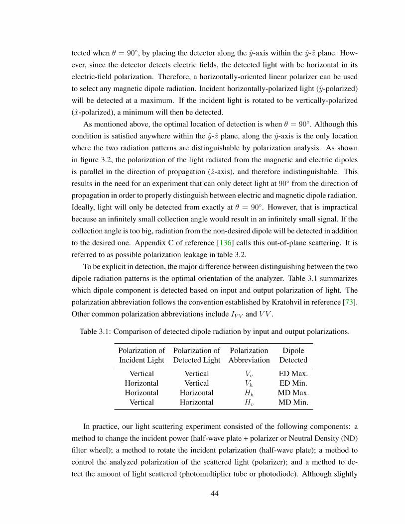
tected when θ = 90, by placing the detector along the y-axis within the y-z plane. How-ever, since the detector detects electric fields, the detected light with be horizontal in itselectric-field polarization. Therefore, a horizontally-oriented linear polarizer can be usedto select any magnetic dipole radiation. Incident horizontally-polarized light (y-polarized)will be detected at a maximum. If the incident light is rotated to be vertically-polarized(x-polarized), a minimum will then be detected.

As mentioned above, the optimal location of detection is when θ = 90. Although thiscondition is satisfied anywhere within the y-z plane, along the y-axis is the only locationwhere the two radiation patterns are distinguishable by polarization analysis. As shownin figure 3.2, the polarization of the light radiated from the magnetic and electric dipolesis parallel in the direction of propagation (z-axis), and therefore indistinguishable. Thisresults in the need for an experiment that can only detect light at 90 from the direction ofpropagation in order to properly distinguish between electric and magnetic dipole radiation.Ideally, light will only be detected from exactly at θ = 90. However, that is impracticalbecause an infinitely small collection angle would result in an infinitely small signal. If thecollection angle is too big, radiation from the non-desired dipole will be detected in additionto the desired one. Appendix C of reference [136] calls this out-of-plane scattering. It isreferred to as possible polarization leakage in table 3.2.

To be explicit in detection, the major difference between distinguishing between the twodipole radiation patterns is the optimal orientation of the analyzer. Table 3.1 summarizeswhich dipole component is detected based on input and output polarization of light. Thepolarization abbreviation follows the convention established by Kratohvil in reference [73].Other common polarization abbreviations include IV V and V V .

Table 3.1: Comparison of detected dipole radiation by input and output polarizations.

Polarization of Polarization of Polarization DipoleIncident Light Detected Light Abbreviation Detected

Vertical Vertical Vv ED Max.Horizontal Vertical Vh ED Min.Horizontal Horizontal Hh MD Max.

Vertical Horizontal Hv MD Min.

In practice, our light scattering experiment consisted of the following components: amethod to change the incident power (half-wave plate + polarizer or Neutral Density (ND)filter wheel); a method to rotate the incident polarization (half-wave plate); a method tocontrol the analyzed polarization of the scattered light (polarizer); and a method to de-tect the amount of light scattered (photomultiplier tube or photodiode). Although slightly

44

Figure 3.2: Radiation and polarization from electric (Red) and magnetic (Blue) dipolesgenerated by a plane wave of light. The purple arrow indicates that the polarizations ofthe two dipoles are parallel, and therefore indistinguishable, along the forward direction.Reprinted with permission from reference [153].

45

different components were used, all variations of the experiment used the basic geometryshown in figure 3.3. Note that the narrowband interference filter normally used in our lightscattering experiments was omitted to record spectrally resolved scattering data.

Figure 3.3: Basic geometry of magneto-electric scattering experiments.

3.1.1 Summary of experimental parameters

Magneto-electric scattering has been studied using various laser sources. The full compar-ison of system specifications is shown in table 3.2. The first laser source was a Clark-MXRCPA-2001. This laser provided a large amount of energy per pulse, enabling the use ofa flat-top beam. However, its 1 kHz repetition rate limited the data collection range (Seeappendix D of reference [136]). The second laser source, the Coherent Vitara-HP, providedan increased repetition rate but lower energy per pulse, resulting in a need to focus thebeam in order to reach the desired intensity range. The third laser source was an AmplitudeAurora system. It provided a larger repetition rate than the Clark-MXR CPA-2001 andlarge enough energy per pulse that focusing of the beam was unnecessary. The Amplitudesystem was used for both intensity-dependent dipole and spectroscopic measurements.

The values in table 3.2 were calculated using the following equations. See appendixC and F of reference [136] for their derivations. Note that Wx and Wy are the measuredvalues of the 1/e2 beam full-width and that the FWHMt is the measured value from theMIIPS pulse compressor.

Collection angle () θ = arctan (D/2R)

Collection solid angle (Ω) dΩ = D2/16R2

46

Table 3.2: Comparison of specifications of magneto-electric scattering experiments.

Laser Model CPA2001 Vitara-HP Aurora

Laser Source Clark-MXR Coherent AmplitudePulse length (FWHMt) 150 fs 15 fs 30 fsCenter wavelength 775 nm 800 nm 800 nmBandwidth 5 nm 60 nm 30 nmRepetition rate 1 kHz 80 MHz 10 kHzAvg. Power @ Exp. 560 mW 440 mW 1 WEnergy @ Exp. 56 µJ 5.5 nJ 100 µJ

Focus lens None 200 mm NoneInput beam dia. (Wx ×Wy) 2.1 cm × 1.6 cm 1.02 cm × 1.64 cm 1.5 cmInput beam aperture 3.5 mm None 5 mmIlluminated volume 3.5 mm 0.2 mm × 0.124 mm 5 mm

Collection lens (f1) (R) 150 mm 50 mm 150 mmCollection magnification x1 x3 x1Iris diameter (D) 3.5 mm 5 mm 3 mmCollection angle 0.67 2.86 0.57

Collection solid angle (dΩ) 3.4E-5 Ω 6.3E-4 Ω 2.5E-5 ΩPolarization leakage 0.0068% 0.125% 0.005%Collection spot size ∼3 mm ∼25 µm ∼3 mm

Normalized Illumin. area 1.03 cm2 76.1E-6 cm2 0.69 cm2

Energy density per pulse 54.4 µJ/cm2 72.3 µJ/cm2 145 µJ/cm2

Peak intensity 3.41E8 W/cm2 4.53E9 W/cm2 4.54E9 W/cm2

Polarization leakage (%)‖E//‖2

‖E⊥‖2= 2−3 cos(D/2R)+cos3(D/2R)

1−cos3(D/2R)

Max. intensity Imax ≈ Avg. Power / (Rep. Rate)(Beam Area)(Pulse Duration)

Pulse duration (s) σt =√

2πFWHMt/(

2√

2 ln 2)

Beam area (cm2) A = πr2 = π (5/16)2WxWy

Pulse energy (J) ε = Avg. Power / Rep. Rate

Pulse energy per area (J/cm2) εA

= Average PowerRep. Rate

(165

)2 1WxWy

Intensity (W/cm2) Imax = εAσt

= εA

2√

2 ln 2√2πFWHMt

= εA

0.9394FWHMt

3.1.2 Procedures and calibration

In a light scattering experiment, care must be taken in construction, alignment, and cali-bration in order to ensure the integrity and repeatability of the experiment. Section 3.1.2.1details the construction of the experiment and the necessary equipment. Section 3.1.2.3

47

discusses the specific calibration of the optics and their positions.

3.1.2.1 Equipment overview

The table below details the equipment, part numbers, and suppliers for the large compo-nents used in this experiment. Note, that there are two different detection schemes listed inthe table, based on light levels.

Table 3.3: Experimental Electronics

Device Company Part # Quantity

Photodiode EG&G FND-100 1Current Amplifier DL Instruments DL1212 1Lock-In Amplifier Stanford Research Sys. SR810 1PMT Burle C31034A 1PMT Refrigerated Housing Products for Research 1Current Preamplifier Stanford Research Sys. SR550 1Photon Counter Stanford Research Sys. SR400 1Spectrograph Andor Shamrock500i 1CCD Andor iXon 885 1Single-axis stepper motorcontroller/driver

Newport SMC100PP 2

360 Rotation Stage Newport PR50PP 2USB Wheel Picard Industries 1USB Shutter Picard Industries 1Power Meter Thorlabs 1

The equipment detailed in table 3.3 were characterized according to their respectiveuser manuals and procedures. First, the linearity of the power meter and the precision ofthe intensity control were verified. The intensity control relied on one of two methods. Thefirst method used a computer controlled half-wave plate and a stationary polarizer. Thehalf-wave plate rotated the incident polarization of light and a percentage of it was passedby the polarizer. The exact percentage was determined by Malus’ Law [155]. The secondmethod was simply a computer-controlled reflective neutral density filter that attenuatedthe beam based on its angle. Using the second method, the linearity of both the powercontrol method as well as the detection systems were verified. Figure 3.4 shows that thedetection system had a linear response over 3 decades of input power.

The other important calibration was finding the zero-positions of the polarizer andwaveplates. The zero position was an index on the SMC100PP rotation stages that wasused for the controlling computer program. For example, the zero location on the polar-izer was the location where vertically-polarized light was maximally transmitted. 90 units

48

Figure 3.4: Response of detection system.

away from that location was where horizontally-polarized light was maximally transmitted.A full discussion on the calibration process is detailed in Appendix A.

3.1.2.2 Detector stabilization

When using a Photo-multiplier Tube (PMT) as the detector, special procedures must be fol-lowed to ensure accurate, sensitive, and unsaturated signal detection. The PMT describedbelow is a C31034A [156] from BURLE Electron Tubes and was housed inside a refriger-ated case from Products for Research. The steps for detector stabilization were:

1. Temperature Stabilization: Let PMT chill for at least 2 hours.

2. Signal Analysis: Analyze output electronic signal using oscilloscope, amplify ifneeded, and snub any ringing.

3. PMT 1-photon Peak: Find the “1 photon” peak by running a differential voltagescan of the signal using the SR400 gated photon counter.

The temperature stabilization was important because it lowered the level of electronicnoise in the PMT. As shown in figure 3.5, the counts per second of the noise was over20,000 counts per second (cps) when the chiller for the PMT was initially turned on. Afterabout 2 hours of chilling, the count rate decreased to less than 20 cps. After 29 hours ofchilling, the average number of dark counts was 6 cps with a standard deviation of 3 cps.Figure 3.6 shows the dark count rate distribution over a 200 second window after the PMThad chilled for 29 hours.

Snubbing is the process of adding a t-shaped 50 Ohm BNC connector and a short BNCcable with a less than 50 Ohm terminator to the output of the PMT in order to improve the

49

Figure 3.5: Dark count rate of C31034A after the chiller was activated. Taken using theSR400 with a discriminator of -18 mV, x5 amplification, 1800 V high voltage bias afterbeing off for 4 days time.

Figure 3.6: Dark count rate distribution of C31034A after the chiller was activated for 29hours, over a 200 second window. Taken using the SR400 with a discriminator of -18 mV,x5 amplification, 1800 V high voltage bias.

shape of the output pulse. Snubbing was done before the preamplifier and both reducedringing and increased the pulse rise-time. The output of this BNC network was connectedto an oscilloscope. The length of the BNC cable was varied until it was at the correct lengthfor the reflected signal to cancel the anode signal ringing.

50

Figure 3.7: Waveform from C31034A, 5x Amp, Terminated Signal.

Once the PMT signal had been appropriately terminated, the discriminator height wasdetermined. This process is called plateauing and used the SR400 Gated Photon Countermanufactured by Stanford Research Systems of Sunnyvale, California [157]. To find thediscriminator voltage, the count rate of the PMT as a function of discriminator voltage wasmeasured. The correct voltage was the one at which the voltage level “plateaued”. Asshown in figure 3.8, the optimal discriminator voltage for the C31034A PMT operatingwith a x5 amplification and a 1800 V bias was -0.018 V since this was the location wherethe plateau ended. For further study on PMTs, refer to reference [158].

Figure 3.8: Plateauing of the C31034A PMT with 5x Amp and 1800 V bias.

51

3.1.2.3 Optical alignment techniques

The alignment of the experiment was one of the most crucial steps in ensuring an opera-tional and accurate experiment. The two arms of the experiment (source & signal) neededto be precisely orthogonal to each other. Due to the nature of Rayleigh scattering and theorthogonality of the electric (ED) and magnetic (MD) dipoles, 90 degrees is the only angleat which the ED and MD are completely separable. Figures 3.9, 3.10, and 3.11 show threevariations of experimental set-ups with labels on each of the components. Note the optionfor spectral analysis in figure 3.11.

Figure 3.9: Schematic for magneto-electric scattering experiment. L = lens, I = iris, WP =waveplate, P = polarizer, SH = shutter, TS = telescope, PS = periscope, M = mirror, AN =analyzer, primes indicate alignment beam path.

The first part of the alignment was to align the source and signal arms. With every stepof the alignment, the beam was made parallel to the holes on the table. This ensured thatevery beam path was orthogonal. For the rough alignment, a fabricated metal alignmentblock was used. This block had a alignment grid with 1/4” spacing along with a set of holesprecisely drilled at a intersection point. This mount also had four holes on its base whichcould be placed over 1/4-20 set-screws secured into the table. The four holes enabled place-ment of the alignment holes either on a table hole line or between two sets of holes. Thisblock was used repeatably throughout the alignment procedure to ensure a level and par-allel beam, assuming that the table was flat and the holes were drilled correctly. Althoughnot perfect, this alignment technique was sufficient for initial set-up.

After the initial set-up of the experiment, the overlap of the beam with the alignmentirises was verified each day. This was done using a beam camera from Thorlabs. The mostimportant irises were those immediately before and after the sample. The beam camerawas placed behind the iris and the iris was closed down. If the iris closed down around thepeak beam intensity shown on the beam camera, the beam was in the correct location. If

52

Figure 3.10: Schematic for magneto-electric scattering experiment. L = lens, I = iris, λ/2= rotatable half-wave plate, 105:1 = polarizer, M = mirror, SMC = computer-controlledrotation stage, blue line indicates alignment path.

Figure 3.11: Schematic for magneto-electric scattering and spectrum experiment. λ/2 =rotatable half-wave plate, 105:1 = polarizer.

53

Figure 3.12: Example of beam profile during beam camera alignment.

the beam was not perfectly centered, the turning mirrors were adjusted. The beam cameraalternated between the two iris locations until the beam went through both of them. Anexample of the beam is shown in figure 3.12.

The experiments also had the option of either compensating for dispersion to maketime-bandwidth-limited pulses or adding additional linear chirp to lengthen pulses. Mostexperiments either used bandwidth-limited pulses or no compensation at all. For reference,MIIPS is a method used to measure the spectral phase of a femtosecond laser pulse. In-stead of relying on interferometry like other methods (e.g. FROG, SPIDER), MIIPS takesadvantage of the fact that second harmonic generation (SHG) involves the simultaneoussum of multiple frequencies [159, 160]. The phase between multiple paths to generate aparticular SHG frequency determines if they add up constructively (if the phase is zero) ordestructively (if the phase is pi).

The next crucial part of the alignment was that of the detector and sample. The detector(a FND-100 photodiode in this case) was first aligned by eye to make sure the scatteringpath (as indicated by the HeNe alignment beam) was centered on the detector. To verify thealignment, the HeNe alignment beam was attenuated and incident on the detector. Then, thedetector was moved vertically and horizontally to find the optimal position. After using theHeNe, the same detector movement was repreated using a highly-scattering sample and themain laser beam. Figure 3.13 shows the results of these methods. It was found that both theHeNe and Vitara methods of alignment resulted in the same maximal signal position. Thegeometry of the two beams is evident in the horizontal positioning of the detector. Whereasthe HeNe beam is a defined Gaussian laser beam positioned straight onto the detector, theVitara beam is passing through a sample. The trapezoidal shape is due to the size of thelimiting aperture of the collection system.

54

Figure 3.13: (l) Vertical and (r) Horizontal alignment of the detector comparing two align-ment methods.

Additionally, the effects of different polarizations on the alignment were checked asshown in figure 3.14. This was important because the experiment relied on comparingvertically-polarized scattered light with horizontally-polarized light. In each case, a sus-pension of Coffeemate powdered non-dairy coffee creamer in distilled water was used asthe scattering source. Note that the same overall pattern is seen as in figure 3.13. The max-imum location of vertically-polarized and horizontally-polarized light overlapped for bothchanges in the vertical and horizontal positioning of the detector. The slight difference inshape is due to the different vertical scales in the figure for the different polarizations.

The next piece of alignment was to verify that the detection arm was unable to see anyscattering from the wall of the cuvette (See figure 3.15). When running the experiment,the edge-wall scattering can contribute significantly to the Hh signal [161]. This is becausethe air:quartz:liquid interface can serve as a kind of mirror reflecting laser light towardsthe detector. In fact, if a mirror is placed at 45 degrees in the main beam, one will detectpolarized dipole patterns of equal magnitude (See figure 3.16). Fortunately, this signalwill depend linearly on the intensity of the beam and can be minimized by geometry. Infigure 3.15, there is no limiting aperture in the detection system allowing for the edge-wallscattering to be seen. Since the Vv scattered light is stronger within the sample, the ratioof Hh to Vv scattered light can become arbitrarily large when looking at the sample edge.Therefore, a limiting aperture is absolutely critical in order to prevent edge-wall scatteringfrom interfering with the detection of magneto-electric scattering.

Finally, after alignment of the main laser beam path, the detection optics and the detec-

55

Figure 3.14: (l) Vertical and (r) Horizontal alignment of the detector comparing alignmentusing Vv and Hh scattered light.

Figure 3.15: (l) Horizontal alignment of the detector comparing alignment using Vv andHh scattered light without a limiting aperture. (r) Ratio of Hh to Vv scattered light.

tor position, the sample was placed on the sample holder stage and aligned. The stage hadtip/tilt adjustments along with XYZ precision. The procedure followed was:

1. Place the sample on the sample stage.

2. Adjust the vertical height and horizontal position of the sample until the laser beampasses through the sample without clipping.

56

Figure 3.16: Cartesian plot of vertically- and horizontally-polarized light reflected off a 45degree mirror through the detection optics.

3. Using the IR viewer, look at the back reflection of the source laser beam. Slightlyadjust the sample until the back reflection is perfectly coincident with the sourcebeam.

4. Examine the back reflection of the HeNe laser. Again, adjust the sample until theback reflection is perfectly coincident with the HeNe beam.

5. Check the first back reflection again. Continue adjusting until both back reflectionsare coincident with their source lasers.

3.1.3 Special considerations of a focused beam

Due to the limited energy per pulse compared to the other two laser sources, the Vitara laserbeam had to be focused. Ideally, one wants the highest amount of intensity and the largestillumination area. These criteria are in direct opposition to each other. Fortunately, theeffects of the illumination area can be minimized by controlling the size of the collectionspot size. Assuming an incident beam waist (the 1/e2 beam full-width) of Wx = 1022 µmandWy = 1636 µm as well as a pulse length (FWHMt) of 15 fs, table 3.4 was calculated tocompare possible focusing options. In considering collection spot size, the relevant valueswere the focused beam diameter, Wy, and the Rayleigh range, ZR(y).

57

Table 3.4: Comparison of focused beam size and intensity for varied focal lengths.

Lens Wx(µm) Wy(µm) Int. ( Wcm2 ) ZR(x) (cm) ZR(y) (cm)

200 mm 199 125 4.8E9 3.90 1.52175 mm 174 109 6.3E9 3.00 1.17150 mm 150 93 8.6E9 2.19 0.86125 mm 124 78 1.2E10 1.52 0.59100 mm 99 62 1.9E10 0.98 0.3875 mm 75 47 3.5E10 0.55 0.2150 mm 50 31 7.8E10 0.24 0.10

As mentioned in the previous section, it is important that the detector cannot see theedges of the cuvette in order to detect the accurate polarization and magnitude of the scat-tering. This can be achieved by placing an aperture between the sample and the first col-lection lens. Additionally, a limiting aperture can be placed further in the collection optics.

In the case of the focused beam, the limiting aperture was used to both prevent detectionof edge-wall scattering as well as limit the imaging area to the size of the beam. Sincethe beam was focused into the sample, the optimal collection spot size was one that wassmaller than the cross-section of the focused beam. The size of the collection spot sizewas primarily determined by the size of the limiting aperture and the magnification of thesystem. The ideal magnification of the system was as large as possible in order to loosenthe tolerances on the positioning of the limiting aperture. However, an increase in themagnification can also increase the amount of polarization leakage. Table 3.5 shows thistradeoff. Based on the calculated values, an iris with a diameter of 5 mm and a initialfocusing lens of f = 50 mm were chosen.

Table 3.5: Comparison of lenses for collection magnification, assuming f2 = 150 mm.

Lens, f1 Mag. Iris dia. (mm) Angle, θ Solid angle, dΩ Pol. Leak (%)

150 mm x1 10 0.033 2.78E-4 0.050%5 0.017 6.94E-5 0.010%

50 mm x3 10 0.100 2.50E-3 0.500%5 0.050 6.25E-4 0.120%3 0.033 2.25E-4 0.045%

25 mm x6 10 0.200 1.00E-2 2.020%5 0.100 2.50E-3 0.500%3 0.060 9.00E-4 0.180%1 0.020 1.00E-4 0.020%

58

After comparing the tradeoff between the collection spot size and the percentage ofpossible polarization leakage, the arrangement of optics shown in figure 3.17 was decidedupon. Figure 3.18 shows that this arrangement, where the use of a 75 µm pinhole yieldeda collection spot size of ∼25 µm in diameter. In this arrangement, the collection spot sizewas limited by the pinhole as long as the pinhole was smaller than ∼3 mm.

Figure 3.17: Zemax model of collection optics: f1 = 50 mm, f2 = 150 mm, f3 = 60 mm,iris diameter = 5mm, pinhole diameter = 75 µm.

Figure 3.18: Zemax vignetting model of collection optics: f1 = 50 mm, f2 = 150 mm, f3 =60 mm, iris diameter = 5mm, pinhole diameter = 75 µm.

59

3.1.4 Signal detection limits

In addition to the calibration described in section 3.1.2.3, the detection system limits werealso verified. Figure 3.4 shows that the detection system was capable of detecting changesin the average intensity of the main laser beam.

To test the response to changes in peak power, Rhodamine 590 in methanol and glassof varied thicknesses were used. The 2-photon fluorescence of Rhodamine 590 depends onthe square of the incident field intensity. Using a 1:1 collection system (f1 = f2 = 150 mm)and a beam focusing lens of 12.5 mm, the values in table 3.6 were obtained. Note that thevalues were adjusted to account for the different Fresnel reflection losses of each dispersingglass. Figure 3.19 shows this graphically as a function of both pulse length and averageintensity. This calibration means that if M-E scattering depends on changes in peak power,it is possible to observe it if the signal is above the noise limits of the detection system.

Table 3.6: Verification of detection of changes in peak power using the 2-photon fluores-cence signal from Rhodamine 590 dissolved in methanol.

Pulse length Vv (mV) Vh (mV) Hh (mV) Hv (mV)

∼40 fs 307.6 (±2.9) 269.6 (±0.3) 255.0 (±0.4) 254.8 (±0.4)∼48 fs 281.3 (±0.2) 241.8 (±0.2) 230.3 (±0.3) 229.6 (±0.2)∼52 fs 272.9 (±0.5) 228.5 (±0.2) 217.5 (±0.3) 217.2 (±0.2)∼80 fs 182.5 (±7.7) 143.0 (±0.2) 136.5 (±0.2) 136.0 (±0.2)

Figure 3.19: Verification of detection of changes in (l) average power and (r) peak powerusing the 2-photon fluorescence signal from Rhodamine 590 dissolved in methanol.

60

3.2 Data acquisition procedure and analysis

In each intensity-dependent magneto-electric scattering experiment, the data was collectedusing the programmatic procedure shown in figure 3.20. Note that there are three loopswithin the program as determined by the number of different polarizations and intensitypoints desired. For example, collecting data on one sample over one decade of intensityrequired 11 intensity loops, 2 dipole loops, and 36 input polarization loops resulting in nearto 800 sets of data points. Due to this large number of data points, data collection consistedof a MATLAB program that controlled the input intensity, input polarization, and outputpolarization via computer-controlled rotation stages. The complete MATLAB program isincluded in appendix B.

Figure 3.20: Flowchart depicting the steps used by the data collection computer program.

The data collection program wrote the data to a text file for easy analysis. The masterdata file was split into individual text files for each intensity and dipole point. For example,an experiment consisting of 11 intensity loops and 2 dipole loops (ED, MD) resulted in 22individual files. Each file contained data for a complete set of input polarization states.

61

For analysis, the data was loaded into a MATLAB program. For each file, the raw datawas extracted and plotted versus input polarization state / waveplate angle. Each set of datawas fitted with a dipole pattern as shown in figure 3.21 [162].

Figure 3.21: Schematic of dipole components for analysis.

The curves used to fit the data were standard cosine squared functions.

IED = AED cos2 (θ + θ0,ED) + hED (3.7)

IMD = AMD cos2 (θ + θ0,MD) + hMD (3.8)

Each function had an amplitude, a vertical offset (waist) and a phase offset. In the nextchapter, the amplitude and waist of the fitted data are referred to as the polarized andunpolarized dipole components, respectively. The MATLAB analysis program extractedthe amplitude, maximum, and minimum for each data set, plotting versus intensity. Byanalyzing the dipole responses as a function of intensity, one can observe the nonlinearresponse of each material system.

Recalling the discussion in section 3.1, the maximum of the electric dipole signal(AED + hED) will be observed when the input polarization state and detected polariza-tion state are vertical (Vv). The minimum of electric dipole signal (hED) will be observedwhen the input polarization state is horizontal and detected polarization state is vertical(Vh). Likewise, the magnetic dipole signal maximum (AMD + hMD) will be observedwhen the input polarization state and detected polarization state are horizontal (Hh) andthe minimum (hMD) when the input polarization state is vertical and detected polarizationstate is horizontal (Hv).

62

3.3 Sample selection and preparation

As in previous studies, the primary objective of sample selection was to provide a way tosystematically vary important material parameters. As will be discussed in section 4.1.4,moment of inertia and rotation frequency, ωφ, were hypothesized to be important. The firstseries examined was the tetrachloride series of CCl4 (carbon tetrachloride), SiCl4 (silicontetrachloride), SnCl4 (tin tetrachloride) and GeCl4 (germanium tetrachloride) [136]. In thisseries, the rotation frequency decreased as the central atom was substituted.

CCl4 → SiCl4 → SnCl4 → GeCl4

The second series examined was the orthosilicate series composed of SiCl4 (silicon tetra-chloride), SiBr4 (silicon tetrabromide), Si(OCH3)4 (tetramethyl orthosilicate), Si(OC2H5)4

(tetraethyl orthosilicate), and Si(OC2H7)4 (tetrapropyl orthosilicate). In this series, the rota-tion frequency decreased as the peripheral atoms in the tetrahedral structure were changed.

SiCl4 → SiBr4 → Si(OC2H3)4 → Si(OC2H5)4 → Si(OC2H7)4

Additional criteria for liquid sample selection were for experimental convenience ratherthan scientific inquiry. First, samples were selected that were non-polar and centrosymmet-ric. The centrosymmetry excluded all second-order all-electric nonlinear optical processes,while the non-polar nature prohibited electric-torque phenomena such as depolarized-lightorientation scattering (see section 1.2.1.3). Second, ideal samples had a low number ofimpurities which limited the possibility of multiple scattering. Third, samples were chosenthat did not have an optical resonance anywhere near the excitation wavelengths. This en-abled the electric dipole response to be compared to the induced magnetic dipole responsewithout having to account for absorption phenomena.

Solid samples were also investigated during this work. As with liquid samples, it wasdesirable to have samples with a low number of impurities (internal and surface) and eithercentrosymmetric or amorphous structure. For their availability and structure, Quartz andGGG (Gadolinium Gallium Garnet) were examined. Quartz has a tetrahedral structurewhere each silicon atom is linked to four oxygen atoms accounting for the chemical formulaof SiO2. GGG has a cubic crystal structure with the base unit of Gd3Ga5O12 [163].

63

3.3.1 Procedure for cleaning cuvettes

In order to maintain the integrity of the experiments and prevent mixing of chemicals, greatcare was taken to completely clean the quartz sample cuvettes. The quartz sample cuvetteswere 10 mm Flourometer cells from Starna Cells, Inc. Each cuvette held ∼3.5 mL ofliquid. Cuvettes were filled with liquid samples for optical study. The necessary equipmentneeded to clean is shown below in table 3.7. The procedure varied depending on the sample

Table 3.7: Supplies needed to clean cuvettes.

Equipment Source Details #

Fluorometer 10mm Quartz Cuvette Starna Cells 23-Q-10 1Cuvette Concentrated Detergent Starna Cells - 1De-Ionized Water - - 1Acetone - - 1Isopropanol - - 1Small Oven - - 1Cuvette Storage Container Fisher Scientific Heat Resistant 1Aluminum Foil - - 1Waste Beaker - - 1Misc. PPE - - -

that was in the cuvette. Table 3.8 is an overview by solvent and material type taken fromhttp://www.starnacells.com/d_tech/tech01.html. The majority of thesamples that were used in this work were alcohol-based solutions and organic solvents.The procedure for cleaning organic solvents with alcohol and acidic solutions is as follows:

1. Gather the needed equipment listed in the table above.

2. Don protective equipment. Refer to specific SDS and glove compatibility charts.

3. Empty any samples remaining in the cuvette into a labeled waste container.

4. Rinse with DI water once to remove any traces of chemical sample.

5. Place one drop of detergent into the cell. The detergent is concentrated and one dropis really all that is needed.

6. Rinse repeatedly with DI water until no soap bubble remain. At least 12 rinses areoften necessary.

7. Rinse cuvette with Acetone from the acetone squeeze bottle. Collect any excess andtransfer to waster container.

64

8. Rinse cuvette with IPA from IPA squeeze bottle. Collect any excess and transfer towaster container.

9. Immediately transfer cuvettes to the heat-resistant cuvette holder. Wrap cuvetteholder in aluminum foil and place in oven at 82 C until no IPA remains on thecells. This is necessary to prevent drying marks on the cells.

10. Remove the cuvette holder from oven and place in a clean container for transport.

11. Store cells in a clean area until ready to be filled.

12. Remove gloves and wash hands.

Table 3.8: Suggested cleaning methods from Starna Cells, Inc.

Solvent Material Suggested Cleaning Methods

Aqueous Protein, DNA, Warm water with detergent, Dilute acid rinse,Biologics Copious water rinse

Aqueous Salt sols. Warm water Acid rinse, Copious water rinseAqueous Basic sols. Warm water with detergent, Dilute acid rinse,

Copious water rinseOrganic Oil based Rinse with solvent, Warm water with detergent,

Dilute acid rinse, Copious water rinseOrganic Alcohol sols. Rinse with solvent, Copious water rinseOrganic Acidic sols. Rinse with solvent, Copious water rinseOrganic Basic sols. Rinse with solvent, Dilute acid rinse,

Copious water rinseFluorescence Clean cells in Nitric Acid (5M) use a

copious water rinse immediately before use

3.3.2 Preparation procedure: Liquids

All liquid samples were tested inside quartz Fluorometer cells. Each sample was filteredusing 0.9 µm IC-Millex-LG PTFE filters from Millipore Corp. The preparation procedureis detailed below.

1. Gather the needed equipment.

2. Don protective equipment. Refer to specific SDS and glove compatibility charts. Forexample, carbon tetrachloride should be handled using Nitrile gloves.

3. If the sample comes in a large opentop bottle,

65

(a) Attach two Millipore filters to the plastic syringe.

(b) Move large bottle of chemical sample into the fume hood and lower sash toworking height to protect user.

(c) Use large volume pipette to move chemical sample into filtering syringe. Moveonly what is required. Approx. 4 mL.

4. If the sample comes in a bottle with the protective top,

(a) Attach hypodermic needle to plastic syringe.

(b) Carefully withdraw approximately 3 mL from the container.

(c) Turn syringe upside down, remove needle, and attach two Millipore filters tothe end of the plastic syringe.

5. Push slowly on the plunger of the plastic filtering syringe to gently force the chemicalsample through the Millipore filters into the quartz cuvette. Do NOT use excessiveforce! It can damage the filters causing them to lose their filtering properties, putfibers into sample, and may spray chemicals in hood. Slow pressure reduces bubbleformation.

6. Place labeled stopper on cuvette and allow bubbles to settle. This can take hours.

7. Remove plunger, filters from filtering syringe, and allow MINIMAL chemical sampleto evaporate. Pour any excessive chemical sample and filters into waste bucket in thefume hood.

8. Return the large bottle of chemical sample to the chemical cabinet.

9. Remove gloves and wash hands.

66

3.4 Simulation methods

The dipole moments described in subsection 2.1.2 were simulated by applying finite timesteps in a MATLAB program that integrated equation 2.16. See appendix C for the com-plete MATLAB code. For the nth iteration, the electron position ξ (tn+1) was calculatedfrom ξ (tn) and inserted into equation 2.17 to update torque components. Angular ve-locities from equations 2.10-2.12 were then similarly used to obtain the change in the“tether” position, ∆rA (tn), from equation 2.18. This yielded a new value of rA, givenby rA (tn+1) = rA (tn) + ∆rA (tn), to be inserted into equation 2.16 to iterate the proce-dure.

3.4.1 Numerical solving techniques

Specifically, the Ordinary Differential Equation (ODE) solver function built into MATLABwas used to solve the system of first-order ODEs. MATLAB was chosen as the solvingprogram specifically because of its robust library of ODE solvers and ease of analyzing theresults. Initial simulations were run in Mathematica but that course was abandoned due toits limited capability to iterate through a set of values. For MATLAB, the equations had tobe written explicitly as first-order ODEs by using generic substitutions. These equationswere the following:

ξ (t) = [x1, y1, z1] (3.9)

rA (t) = [x2, y2, z2] (3.10)

dx1 (t)

dt= xd (t) (3.11)

dy1 (t)

dt= yd (t) (3.12)

dz1 (t)

dt= zd (t) (3.13)

dx2 (t)

dt= z2 (t) Ωy (t)− y2 (t) Ωz (t) (3.14)

dy2 (t)

dt= −z2 (t) Ωx (t) + x2 (t) Ωz (t) (3.15)

dz2 (t)

dt= y2 (t) Ωx (t)− x2 (t) Ωy (t) (3.16)

dΩx (t)

dt=

m

I//ω2

0 [y2 (t) z1 (t)− y1 (t) z2 (t)] (3.17)

67

dΩy (t)

dt=m

I⊥ω2

0 [−x2 (t) z1 (t) + x1 (t) z2 (t)] (3.18)

dΩz (t)

dt=m

I⊥ω2

0 [x2 (t) y1 (t)− x1 (t) y2 (t)] (3.19)

d[xd (t)]

dt=

e

mE (t)− ω2

0 [x1 (t)− x2 (t)]− γxd (t)− ekzmc

E (t) zd (t) (3.20)

d[yd (t)]

dt= −ω2

0 [y1 (t)− y2 (t)]− γyd (t) (3.21)

d[zd (t)]

dt= −ω2

0 [z1 (t)− z2 (t)]− γzd (t) +ekzmc

E (t)xd (t) (3.22)

MATLAB has eight basic solvers available [164]. The solvers vary based on theiraccuracy and ability to handle stiff problems, or problems that are difficult to solve dueto a difference in scaling somewhere in the problem. ode23 was chosen because of themoderately stiff nature of the problem. The numerical accuracy of ode23 is determined bythe error tolerances of the ODE. If the tolerance is too low, rounding errors will accumulatein the solver and lead to an erroneous solution. In this case, the absolute error was setto 1e-22 and the relative error to 1e-20. These values were found to be small enough tominimize the errors in the solution, but large enough as to allow for efficient solving.

3.4.2 Dimensionless equations

Dimensionless equations in numerical simulations allow numbers that have a high proba-bility of causing errors in the ODE solution, namely numbers that are either very large orvery small, to be avoided. Additionally, they allow greater understanding of the system byrelating it to “intrinsic” or “natural” scales rather than arbitrary ones such as meters or sec-onds. The choice of scaling values is important because it also will affect how the systemresponds.

To start, values for the time, space, charge, and mass scales were chosen from which tonormalize the system [165]. For this case, the scale values were

Time scale: t0 = 1/ω0 (ω0 = Oscillator resonance frequency),Space scale: r0 =

√~/(ω0 ×me) (~ = Reduced Plank constant),

Charge scale: e0 = q0 (q0 = Fundamental charge of an electron), andMass scale: m0 = me (me = Mass of an electron).

This implied typical values for

E0 = mer0/t20q0 (electric field),

68

v0 = r0/t0 (velocity), andI0 = mer0r0 (moment of inertia).

The substitutions for the fundamental equations were then the following:

t = t/ω0 (3.23)

x = xr0 (3.24)

e = eq0 (3.25)

m = mme (3.26)

E = Emer0/t20q0 (3.27)

dx

dt=dx

dt

r0

t0(3.28)

I = Imer0r0 (3.29)

ω = ω/t0 (3.30)

γ = γ/t0 (3.31)

Ω = Ω/t0 (3.32)

d2x

dt2=d2x

dt2r0

t20(3.33)

c = cr0/t0 (3.34)

These were substituted into the fundamental equations (equations 3.11 to 3.22). For exam-ple, equation 3.14 then transformed as dx2(t)

dt= z2 (t) Ωy (t) − y2 (t) Ωz (t) ⇒ dx2(t)

dtr0t0

=

r0t0

[z2 (t) Ωy (t)− y2 (t) Ωz (t)

]⇒ dx2(t)

dt= z2 (t) Ωy (t) − y2 (t) Ωz (t). Doing a similar

substitution for all of the equations resulted in a final set of dimensionless equations thatwere ready to be analyzed using MATLAB.

dx1 (t)

dt= xd (t) (3.35)

dy1 (t)

dt= yd (t) (3.36)

dz1 (t)

dt= zd (t) (3.37)

dx2 (t)

dt= z2 (t) Ωy (t)− y2 (t) Ωz (t) (3.38)

69

dy2 (t)

dt= −z2 (t) Ωx (t) + x2 (t) Ωz (t) (3.39)

dz2 (t)

dt= y2 (t) Ωx (t)− x2 (t) Ωy (t) (3.40)

dΩx (t)

dt=

m

I//ω2

0 [y2 (t) z1 (t)− y1 (t) z2 (t)] (3.41)

dΩy (t)

dt=m

I⊥ω2

0 [−x2 (t) z1 (t) + x1 (t) z2 (t)] (3.42)

dΩz (t)

dt=m

I⊥ω2

0 [x2 (t) y1 (t)− x1 (t) y2 (t)] (3.43)

d[xd (t)]

dt=

e

mE (t)− ω2

0 [x1 (t)− x2 (t)]− γxd (t)− ekzmc

E (t) zd (t) (3.44)

d[yd (t)]

dt= −ω2

0 [y1 (t)− y2 (t)]− γyd (t) (3.45)

d[zd (t)]

dt= −ω2

0 [z1 (t)− z2 (t)]− γzd (t) +ekzmc

E (t) xd (t) (3.46)

3.4.3 Physical meaning of initial conditions

The initial conditions had a dramatic effect on the response of the system. In most cases, theinitial conditions were defined as I// = ~/ω0, I⊥ = ~/ωφ, ξ (t) = [0, 0, 0], and rA (t) =

[0, y2, 0], where ω0 and ωφ were the optical driving and molecular rotation frequencies,respectively. Refer to table 3.9 for comparison to dimensionless values.

Table 3.9: Constants of the Lorentz Oscillator Model equations for (top) real-scale valuesin their common units and (bottom) dimensionless values.

ω0 ω γ e m I// I⊥ Ex

2.6e15 2.34e15 0.26e15 1.6e-19 9.11e-31 6.47e-51 6.47e-48 1e91 0.9 0.1 1 1 1 1000 0.31

3.4.3.1 Reduction to the atomic Lorentz Oscillator Model

The enhancement achieved by extending the model into the molecular domain only couldoccur if certain initial conditions were selected. In this section, two cases for when themolecular Lorentz oscillator model (LOM) reduces to the atomic LOM in behavior aredescribed. The cases are when I// = I⊥ = ∞ and ξ (t) = rA (t) = [0, 0, 0]. In each ofthese cases, the enhancement was removed due to the suppression of the effects of torque.

70

When I// = I⊥ =∞, the equations for the angular velocity of the electron are reducedto zero,

dΩx (t)

dt=m

∞ω2

0 [y2 (t) z1 (t)− y1 (t) z2 (t)]⇒ dΩx (t)

dt= 0. (3.47)

This means that the applied electromagnetic wave is unable to facilitate the transfer ofinternal angular momentum to external angular momentum. Essentially, the infinitely largemoment of inertia prevents the system from undergoing any rotation and no enhancementis observed.

When ξ (t) = rA (t) = [0, 0, 0], the applied electromagnetic wave is unable to beginmotion in the y- or z- directions. There is no initial lever for the wave to torque upon.Similarly to the previous case, the angular velocity is zero around all three axis. Aroundthe x-axis this is,

dΩx (t)

dt=

m

I//ω2

0 [(0) z1 (t)− y1 (t) (0)]⇒ dΩx (t)

dt= 0, (3.48)

and is similarly zero around the y- and z- axes. A non-zero angular velocity must be createdfor any enhancement to occur.

3.4.3.2 Non-zero equilibrium point

For a non-zero initial position of the point of equilibrium, rA, enhancement to the second-order magnetization and polarization can be observed. The magnitude of the enhance-ment increases with the distance from the origin until it reaches a critical threshold. Thisthreshold is a result from the relationship between angular velocity components in thesystem. Assuming that rA (t) = [0, y2, 0], the system is stable if Ωx is larger than Ωy.When Ωx becomes smaller than Ωy, the point of equilibrium moves from oscillating in they-z plane to oscillating in the x-y plane, signifying an unstable rotation of the homonu-clear diatomic molecule. If the rotation frequency, ωφ, is kept constant, one finds thatΩx ∝ 1/y2 and Ωy ∝ y2. With this in mind, most simulations took the position of theequilibrium to be at the largest distance as dictated by the system molecular parameters.One example of this behavior is shown in table 3.10, where the simulation values areω0 = 1, ω = 0.9, γ = 0.1, c = 1, e = 1, I⊥ = 10-5, I⊥/I// = 1000, E = 0.0002, andξ = [0, 0, 0], unless otherwise noted.

3.4.3.3 Comparisons of molecular properties

When comparing simulations that use different molecular properties, such as ωφ, it wasnecessary to scale the time and magnitudes accordingly. One example, is that the maximal

71

Table 3.10: Dependence of dipole moments on initial position of equilibrium point.

rA(y) ED MD MD/ED

0 1.75E-29 5.21E-37 2.98E-81E-7 1.75E-29 5.21E-37 2.98E-81E-6 1.75E-29 8.04E-36 4.59E-71E-5 1.75E-29 7.92E-35 4.52E-61E-4 1.75E-29 7.85E-34 4.49E-5

stable location of the equilibrium point changes with the square of the rotation frequency.If the rotation frequency, ωφ, is decreased by a factor 100, the equilibrium point oughtto increase by a factor of 10. This is due to the moment of inertia relationship whereI⊥ = ~/ωφ = mr2. The normalizing distance is rA = 2c/ω, where ω is the drivingfrequency of the applied electric field.

For measurements of the steady-state value of the dipole moments, a snapshot time waschosen. This is the time at which the magnetization reaches an equilibrium in its evolutionand is defined as τss = 1/ωφ. When the rotation frequency is decreased, the snapshot timemust increase by the same amount in order to capture the same scale of system dynamics.

Additionally, for the classical model, the conversion between photon number and elec-tric field strength in Volts/meter is taken as

n =V

~ωcI =

V ε02~ω|E|2, (3.49)

where the volume in question was arbitrarily taken to be V = 5×10−18 m3.

72

CHAPTER 4

Results

This chapter covers the main experimental and theoretical results relevant to determiningthe dependence of magneto-electric scattering on material composition. The first sectioncovers the experiments whose methods are described in section 3.1. Liquid and solid sam-ples were examined and found to exhibit large radiant optical magnetization. The magni-tudes of the magnetization are compared with theoretical predictions in subsection 4.1.4.The materials with the largest magnetization are those with a low rotation frequency. Lastly,the spectrum of the magneto-electrically scattered light was examined and it was deter-mined that the MD (Hh) spectrum contains a red-shifted spectral feature that is dependenton the rotation frequency of the molecule. This supports the quantum theory describedearlier in section 2.2.

Results from the torque-enhanced classical Lorentz oscillator model are presented in thesecond section. Refer to section 2.1 for discussion of the origin of the model and section 3.4for the background on the MATLAB simulation. First, comments on limits to the symmetryof the electron motion are presented. It was found that at high applied field strengths,the symmetry of the electron displacement is reduced. Second, the dependence of thedipole moments on certain input parameters is explored. It was found that the magnitudeof the second order electric dipole moment and the total magnetic moment were increasedby increasing the ratio between the moment of inertias in the diatomic molecular system.Additionally, if the system was driven at too high of an applied electric field strength, apulsing in the magnetization and DC polarization arises. Lastly, the results of the classicalmodel were compared with those of the quantum theory and it was found that the twomodels are in good agreement.

73

4.1 Experimental results

The data presented in this section are from the three laser systems described in table 3.2.When a result is presented, the specific experimental parameters used to obtain that dataare described. The intensity dependent experiments were primarily obtained using theClark-MXR CPA-2001 system. All of the spectroscopy experiments were done using theAmplitude Aurora system. All experiments relied on a 90 degree scattering geometry andpolarization analysis to distinguish between electric and magnetic dipole radiation.

4.1.1 Magneto-electric scattering in liquids

Although many different materials were examined during the time frame of this thesis, onlya subset of the results is presented. Other materials are omitted either for clarity or becausethey are presented in depth in other places such as reference [136].

4.1.1.1 Tetrachlorides

Since the initial magneto-electric scattering experiments, carbon tetrachloride has servedas the model system. Not only does its isotropic structure prohibit second-order all-electricnonlinear effects, but it is relatively easy to work with experimentally. It is easy to obtainand can be filtered for impurities. It is also optically transparent. Refer to the introductionfor a description of the first experiments using CCl4.

Here, a comparison of unpolarized ED (Vh) scattering for the tetrachloride series is pre-sented. The tetrachloride series was of interest because it allowed for probing of the effectthat the center atom has on the magnetization. The data was obtained using the Clark-MXRCPA-2001 system. The raw data was normalized to counts per second and plotted logarith-mically versus input intensity in figure 4.1. The solid curves are quadratic + linear fits tothe data. The fits are for CCl4, y=4.71e-17*x2+3.28e-8*x; for SiCl4, y=9.00e-15*x2+4.57e-7*x; for GeCl4, y=4.76e-16*x2+5.16e-8*x; and for SnCl4, y=1.01e-16*x2+6.20e-8*x. Thefigure is broken into three scattering regimes. The blue represents detector noise. Datapoints in this regime have a signal-to-noise ratio less than one and should be disregarded.The red regime represents leakage of light with orthogonal polarization into the signal chan-nel due to the size of the collection solid angle. The final regime (white) shows quadraticfits to the data. This regime is the area where magneto-electric scattering can be detected.Analysis of the trend in scattering intensities is included in section 4.1.4 as a discussion ofthe material parameters involved in magnetization.

74

Figure 4.1: Unpolarized ED (Vh) scattering for CCl4, SiCl4, GeCl4, and SnCl4. Solid curvesare quadratic fits to the data, with the dashed lines showing only the I2 component.

4.1.1.2 Orthosilicates

Orthosilicates are a class of materials where a central Silicon atom is connected to fourOxygen atoms in a tetrahedral structure. Three orthosilicate compounds were examined inthe experiments: Tetramethyl Orthosilicate (TMOS), Tetraethyl Orthosilicate (TEOS), andTetrapropyl Orthosilicate (TPOS). Figure 4.2 shows the molecular structure of these threematerials.

Figure 4.2: Molecular structure of TMOS (l), TEOS (c), and TPOS (r).

75

The orthosilicate series was tested using the Coherent Vitara-HP system. In this case,the beam was unfocused resulting in the lower intensities. Figure 4.3 shows the total MDresponse (Hh) of the three orthosilicates as compared to carbon tetrachloride. TMOS showsa larger MD response while TEOS and TPOS show a smaller one as compared to CCl4.Error bars indicate a ten percent experimental uncertainty.

Figure 4.3: Total magnetic dipole scattering of CCl4, TMOS, TEOS, and TPOS. Insetshows electric dipole scattering for reference.

4.1.2 Magneto-electric scattering in solids

Seeing the dependence on rotation frequency, solids are a natural experimental extensionof liquids. Whereas rotation frequency in liquids can be thought of as the rate at which amolecule tumbles around, solids are fixed in place. Instead, rotation frequency in solidscan be thought of as a libration frequency, or rather the rate at which a molecular unit ofa solid wiggles back and forth. Presented in this section are the polarized and unpolar-ized magneto-electric scattering intensities from the isotropic solids, Gadolinium GalliumGarnet (GGG) and Quartz. Discussion of the significance of these results is reserved forChapter 5.

4.1.2.1 Gadolinium Gallium Garnet

Gadolinium Gallium Garnet (GGG, Gd3Ga5O12) is a synthetic garnet crystal commonlyused in optics. It is a body-centered cubic crystal with space group O10

h = Ia3d thatincludes inversion symmetry [163]. It is non-magnetic (in the conventional sense) and

76

does not support second-order, all-electric nonlinearities. Figure 4.4 shows a strong cross-polarized radiation pattern with a quadratic intensity dependence for the unpolarized ED(Vh) and MD (Hv) components. The ratio of unpolarized MD and ED scattering intensitiesis less than unity (IMD/IED ∼ 0.9). At higher intensity (2×1010 W/cm2), the ratio ofpolarized intensity is approximately unity.

Figure 4.4: (a) Polar plot of raw data on co-polarized (open circles) and cross-polarized(filled circles) radiation patterns in GGG at I=1.4×107 W/cm2 obtained at a repetition rateof 1 kHz. Dashed circles anticipate fits to the unpolarized background signal intensities.Residuals from the best fit of a circle plus a squared cosine curve to the raw data are shownbelow the polar plot. (b) Comparative plots in crystalline GGG of unpolarized ED (opencircles) and MD (filled circles) scattering. Solid curves are quadratic fits to the data. Inset:corresponding data for polarized scattering components on the same scale. Reprinted withpermission from reference [130].

4.1.2.2 Quartz

Quartz is the crystalline form of SiO2, where the molecular unit of SiO2 forms a SiO4

silicon-oxygen tetrahedra. This sample was an Ultraviolet (UV) grade fused silica with avery low metallic impurity content and optical range of 170 to 2700 nm. Quartz was testedusing the Coherent Vitara-HP system and a tightly focused beam to give an input intensityof ∼2.2×1010 W/cm2. A polar plot of the raw data is shown in figure 4.5 and resultsversus input intensity are shown in figure 4.6. Note that the ratio of polarized intensitieshas reached the upper limit of unity (IMD/IED = 1).

77

Figure 4.5: Polar plots of the radiation patterns for polarized ED and MD scattering infused quartz at an input intensity of ∼2.2×1010 W/cm2 obtained at a repetition rate of 80MHz. At this intensity, in this sample, the unpolarized component is negligible comparedto the polarized component. Note that peak intensities in the two plots are equal. Residualsfrom the best fit of a squared cosine curve to the raw data are shown below the polar plot.Reprinted with permission from reference [130].

Figure 4.6: Measurements of polarized (l) and unpolarized (r) components of ED (opencircle) and MD (closed circle) scattered light versus input intensity for Quartz. Solid curvesare quadratic fits to the data.

78

4.1.3 Spectrally-resolved magnetic scattering

Another way to explore magneto-electric scattering is by analyzing the spectrum of thescattered light for elastic and inelastic processes. Using the set-up in figure 3.11, withan average power of 10-1000 mW, the spectrum was obtained for scattered light from acarbon tetrachloride sample. From the spectra in figures 4.7 and 4.8, it is apparent that theED spectrum consists of the main laser peak without any other spectrally-shifted featuresof measurable intensity. It is representative of the instrumental lineshape. This lack offeatures shows that no all-electric Raman processes are taking place. Note that the EDspectrum has been made 5 times larger in order to compensate for experimental acquisitiontime and noise levels in figure 4.8. The MD spectrum is different from the ED spectrum andhas three components: a red-shifted feature on the shoulder of the main peak, a red-shiftedfeature peaking near 850 nm, and a blue-shifted feature at 780 nm. These features can bemore easily examined as the difference between the ED and MD spectra in figure 4.9.

Figure 4.7: Normalized scattered light spectrum for Vv (l) and Hh (r) geometries for CCl4.

Figure 4.8: Comparative scattered light spectrum for electric (red) and magnetic (blue)dipole radiation for CCl4.

79

Figure 4.9: (l) Difference between ED and MD scattered light. (r) Quantum model for M-Eprocesses.

Now, it is beneficial to re-examine the quantum picture of magneto-electric effects.Referring to figure 4.9, the ED spectrum corresponds to the red-line transition betweenthe ground state and the virtual excited state detuned from state |2〉 by the one-photondetuning, ∆(e) = ω − ω0. This is Rayleigh scattering. The MD spectrum corresponds tothe two-photon process involving the red-line and blue-line transitions, where the blue-linetransition is between the virtual excited state and the virtual ground state detuned from state|3〉 by the two-photon detuning, ∆(m) = ωφ. Taking the difference between MD and EDspectra, processes that support the quantum theory for magneto-electric effects can be seenin figure 4.10.

Figure 4.10: Difference between MD and ED spectrums of light scattered from CCl4.

80

The polarized-light scattering experiment was repeated for silicon tetrachloride, silicontetrabromide, tetramethyl orthosilicate, and tetraethyl orthosilicate. The Stokes energy shiftobserved via the spectral broadening for each sample was analyzed with respect to rotationfrequency. The comparison is shown in figure 4.11.

Figure 4.11: Comparison of magneto-electrically induced energy shift with molecular ro-tation frequency.

From figure 4.11, a linear relationship is observed between the energy shift and rotationfrequency. Molecules with a higher rotation frequency, i.e. those which are easier to rotate,give a larger spectral broadening. For completeness, the raw data from spectrally-resolvedED and MD scattering observations for SiCl4, SiBr4, TMOS, and TEOS are shown in fig-ures 4.12, 4.13, 4.14, and 4.15, respectively. Note that each spectrum has been normalizedfor easier comparison. Additionally, the vibrational energies are listed in tables 4.2, 4.3,4.4, and 4.5.

Table 4.1: Vibration frequencies of Carbon Tetrachloride [46].

Frequency Energy Shifted λMode (cm−1) (meV) (@ 800 nm)

ν1 459 56.9 830.5ν2 217 26.9 814.1ν3 779 96.6 853.2ν4 314 39.0 820.6

81

Figure 4.12: Normalized scattered light spectrum for Vv (l) and Hh (r) geometries for SiCl4.

Figure 4.13: Normalized scattered light spectrum for Vv (l) and Hh (r) geometries for SiBr4.

Figure 4.14: Normalized scattered light spectrum for Vv (l) and Hh (r) geometries forTetramethyl Orthosilicate (TMOS).

82

Figure 4.15: Normalized scattered light spectrum for Vv (l) and Hh (r) geometries forTetraethyl Orthosilicate (TEOS).

Table 4.2: Vibration frequencies of Silicon Tetrachloride [46].

Frequency Energy Shifted λMode (cm−1) (meV) (@ 800 nm)

ν1 424 52.6 828.1ν2 150 18.6 809.7ν3 610 75.7 841.0ν4 221 27.4 914.4

Table 4.3: Vibration frequencies of Silicon Tetrabromide [46].

Frequency Energy Shifted λMode (cm−1) (meV) (@ 800 nm)

ν1 249 30.9 816.3ν2 90 11.2 805.8ν3 487 60.4 832.4ν4 137 17.0 808.9

83

Table 4.4: Vibration frequencies of Tetramethyl Orthosilicate [166].

Frequency Energy Shifted λ(cm−1) (meV) (@ 800 nm)

202 25.1 813.1309 38.3 820.3379 47.0 825.0406 50.4 826.9423 52.5 828.0440 54.6 829.2642 79.7 843.3820 101.7 856.2846 105.0 858.1

1094 135.7 876.71115 138.3 878.41161 144.0 881.91196 148.4 884.61460 181.1 905.81466 181.9 906.31478 183.4 907.32849 353.5 1036.22912 361.3 1043.02951 366.1 1047.22979 369.6 1050.3

84

Table 4.5: Vibration frequencies of Tetraethyl Orthosilicate [167].

Frequency Energy Shifted λMode (cm−1) (meV) (@ 800 nm)

CH3 torsion 250 31.0 816.3SiO4 deform 304 37.7 819.9SiO4 deform 400 49.6 826.5CCO deform 478 59.3 831.8SiO4 asym. stretch 655 81.3 844.2SiO4 asym. stretch 792 98.3 854.1CH2 rock 811 100.6 855.5CC stretch 935 116.0 864.7CH3 rock 960 119.1 866.6CO asym. stretch 1083 134.4 875.9CO sym. stretch 1092 135.5 876.6CO asym. stretch 1110 137.7 878.0CH3 rock 1170 145.2 882.6CH2 twist 1298 161.0 892.7CH3 sym. def. 1368 169.7 898.3CH2 wag 1393 172.8 900.3CH3 asym. def. 1445 179.3 904.6CH3 asym. def. 1458 180.9 905.6CH2 deform 1485 184.2 907.9CH2 sym. stretch 2890 358.5 1040.6CH3 sym. stretch 2929 363.4 1044.8CH2 asym. stretch 2973 368.8 1049.7CH3 asym. stretch 2977 369.3 1050.1

85

4.1.4 Analysis

From the outset, a key interest in this research was to predict which materials are capableof producing a large magneto-electric magnetization. Existing quantum mechanical theorysuggests that the second-order M-E magnetization, M (2)

y (ω), depends on specific mate-rial properties as well as the strengths of the electric and magnetic field components oflight. The dependence of M (2)

y (ω) on field strength, transition moments, frequencies, andmolecular parameters is given by [7, 136]

M (2)y (ω) ∝ ηµm0 µ

e0EH

∗

(ω0 − ω + iΓ(e)) (ωφ + iΓ(m)), (4.1)

where µe0 is the electric dipole moment; µm0 the magnetic dipole moment; ω0 − ω the one-photon detuning between the driving optical frequency and the resonance frequency ofthe molecule; Γ(e) the electronic relaxation rate; Γ(m) the magnetic relaxation rate; ωφ therotation frequency of the molecule; η the magnetization enhancement factor; and E andH∗ the strengths of the electric and magnetic fields. The material properties in equation 4.1are detailed fully in the next section.

To compare the magnetization response of different materials, a simplified form ofequation 4.1 is used as a “figure of merit (FOM).” The electric and magnetic field strengthsare dropped as well as the magnetic moment. This gives a FOM of

F.O.M. =

∥∥∥∥ ηµ(e)

(ω0 − ω + iΓ(e)) (ωφ + iΓ(m))

∥∥∥∥2

. (4.2)

4.1.4.1 Material comparisons and procedures

The parameters in the FOM are defined as the following:

1. ωφ is the rotation frequency of the molecule. The rotation frequency is calculatedfrom the moment of inertia as ωφ = ~/I . For spherical molecules, the moment ofinertia can be approximated as I = mr2, where m is the mass of a particle and r isthe distance of the molecule from the center of mass. For non-spherical molecules,the moment of inertia is given based on internal coordinates.

2. ω0 is the resonance frequency of the molecule. It can be experimentally measuredusing Ultraviolet-Visible (UV-VIS) spectroscopy. It is the first resonance in the UV,commonly known as either the b-band or Soret resonance. It is calculated from thewavelength of maximum molar absorption as ω0 = 2πc/λmax [168].

86

3. Γ(m) is the magnetic relaxation rate. It is related to the light scattering reorientationalrelaxation time as Γ(m) (rad/s) = 2π/ (τreor). τreor is experimentally measured asthe time it takes for the molecule to reorient one radian.

4. Γ(e) is the electronic relaxation rate. It is defined in radians per second in relationto the half-width half-max Lorentzian bandwidth around ω0 in an expression like1/(

(ω0 − ω)2 +(Γ(e))2)

. It is also related to the Einstein A coefficient, A12, by

Γ(e) = ∆νFWHM (s−1) /2 = c (cm/s) ∆νFWHM (cm−1) /2 = A12/2.

5. µ(e) is the electronic transition dipole moment. It is calculated from the UV-VISspectrum as being directly proportional to the square root of the oscillator strengthand inversely proportional to the square root of the center frequency: f = 2meπν

3e2~ µ212.

6. η is the magnetization enhancement factor. It is the ratio between the resonancefrequency and the rotation frequency: η = ω0/ωφ.

Figure 4.16: Energy level diagram showing magneto-electric magnetization. ∆1 is theone-photon detuning where ∆1 = ω0−ω. ωφ is the two-photon detuning.S1 and T1 are thesinglet and triplet resonance bands, respectively.

For the calculation of the FOM, the parameters needed to be found in the literature,calculated from known quantities, or experimentally measured. While most of the valueswere able to be found using the Google Scholar or Reaxys databases, a small number hadto be measured.

The first necessary data set is the UV-VIS spectrum. The UV-VIS spectrum providesdata for the transition dipole moment, µ(e), the resonance frequency, ω0, and the electronic

87

relaxation rate, Γ(e). The UV-VIS spectrum should be obtained as far into the UV/x-ray aspossible since many resonances for organic molecules are located around 200 nm. Afterthe spectrum is obtained, the resonance frequency can be identified by locating the firstresonance in the UV (the Soret resonance). At this location, the oscillator strength (and thusthe transition dipole moment) should be calculated by integrating the absorption strengthunderneath the resonance frequency curve.

The next parameter is the light scattering reorientational relaxation time, which pro-vides the magnetic relaxation rate Γ(m). Depending on the anisotropy of the molecule,it can be measured by either nuclear magnetic resonance [169], Rayleigh light scattering[170], or beam deflection [171]. All remaining parameters, such as the moment of inertia,can be calculated or found in existing literature databases.

4.1.4.2 Tetrachloride series

FOMs for the tetrachloride series were calculated from tabulated literature values for theparameters involved. For ease of presentation, the parameters for the FOM are broken upinto tables 4.6 and 4.7. Where possible, each number includes its error in calculation andreference. See section 4.1.4.4 for full details on the error calculations. Lastly, table 4.8provides additional physical parameters for this series of compounds. The FOMs can bedirectly compared to the data collected on individual Tetrachlorides shown in figure 4.1 asa test of the quantum mechanical theory. The absorption spectra of the tetrachlorides areshown in figure 4.17.

Table 4.6: Tetrachloride figure of merit: Part one.

ωφ µ(e) Γ(e) Γ(m)

Chem. (1012rad/s) (1030C.m) (1015rad/s) (1012rad/s)

CCl4 21.6[172] 4.1(±0.2)[173] 0.548(±0.015)[173] 3.70(±0.21)[174, 175]SiCl4 16.5[176] 11.3(±0.6)[173] 0.654(±0.024)[173] 2.86(±0.29)[176]GeCl4 15.5[169] 12.1(±0.6)[173] 0.596(±0.015)[173] 0.898(±0.09)[174]SnCl4 12.3[172] 13.2(±0.7)[173] 0.585(±0.012)[173] 1.26(±0.13)[174]

4.1.4.3 Orthosilicate series

FOMs were also calculated for the majority of the orthosilicate series. The parameters forthe FOM are presented in tables 4.10 and 4.11. Table 4.12 provides additional relevantphysical parameters. Since Γ(e) was unable to be located in the literature for TMOS andTEOS, the complete FOMs were unable to be calculated for those molecules.

88

Table 4.7: Tetrachloride figure of merit: Part two.

ω ω0 λ0 ηChem. (1015rad/s) (1015rad/s) (nm) (unitless) FOM

CCl4 2.35(±0.17) 10.7(±0.015)[173, 177] 176(±0.5) 497 0.122(±0.11)SiCl4 2.35(±0.17) 13.6(±0.047)[173, 177] 139(±0.5) 825 2.46(±0.21)GeCl4 2.35(±0.17) 10.7(±0.015)[173, 177] 176(±0.5) 890 4.08(±0.36)SnCl4 2.35(±0.17) 9.47(±0.012)[173, 177] 199(±0.5) 771 13.3(±1.3)

Table 4.8: Additional physical constants for Tetrachlorides.

Molecular Vapor Melting BoilingRefr. Density Weight Pressure Point Point

Chem. Index (g.cm−3)(g.mol−1

)(mmHg) (C) (C)

CCl4 1.460 1.594 153.82 143 -23 76.5SiCl4 1.412 1.483 169.90 419.9 -70 57.6GeCl4 1.464 1.844 214.50 75.99 -49.5 83SnCl4 1.512 2.226 260.52 9.998 -33 114

One item that had to be measured was the reorientation correlation time, τθ, for SiBr4.This quantity was calculated from the measured Spin-Lattice and Spin-Spin relaxationtimes, which are represented as T1 and T2 respectively. The relaxation times were measuredat the University of Michigan Chemistry Nuclear Magnetic Resonance (NMR) facility us-ing a Varian vnmrs 700 system. The sample, neat SiBr4, was filled inside a Nitrogen-filledglove box to prevent reaction with the air. Although the lack of a Si solvent made it moredifficult to lock into the Si NMR signal, an optimal signal was obtained by varying theshims on the magnets.

T1 was measured using the common 5T1-π-τ -π/2-FID (free-induction decay) pulsesequence. T2 was measured using the CPMG-PROJECT multipulse sequence. For anexplanation of these methods, refer to T. James’ Fundamentals of NMR [179] or anotherNMR textbook. Table 4.9 shows the raw data obtained from the T1 and T2 pulse sequences.This data is plotted in figures 4.18 and 4.19 respectively. The exponential curve fits gavethe times of T1 ≈ 107.4 ± 9.3 s and T2 ≈ 178.2 ± 2.3 ms.

From these times, it is possible to calculate to reorientational correlation time, τreor, fora silicon tetrabromide molecule. One simple way to estimate τreor is by the Debye-Stokes-Einstein formula,

τreor =4πηa3

3kTfr, (4.3)

where η is the viscosity, a is the molecular radius, and fr is the microviscosity factor [176].

89

Figure 4.17: The vapor phase vacuum UV spectra of the group IVA tetrachlorides (l) andgroup IVA tetrabromides (r). Reprinted with permission from references [173] and [178],respectively.

Table 4.9: Raw NMR data for Spin-Lattice (l) and Spin-Spin (r) relaxation times.

T1 ≈ 107.4 ± 9.3 s

Time (s) Strength (a.u.)

3.75 -52.27.5 -43.315 -36.330 -23.960 -1.84

120 31.7240 57.8

T2 ≈ 178.2 ± 2.3 ms

Time (ms) Strength (a.u.)

1.25 13240 107

100 75.7200 43.7400 15.0800 1.63

fr equals 1/6 for close-packed spherical molecules. Taking the value of fr at 25 C, theviscosity for SiBr4 at 0.00916 P and the radius as a=2.15 A, then τreor = 1.54 ± 0.04 ps.

Although this is a good estimate of the reorientational correlation time, it is preferrableto measure it experimentally, especially since equation 4.3 is only valid if rotational andtranslational motion of a molecule are highly coupled [180].

90

Figure 4.18: Raw NMR data with exponential fit for SiBr4 Spin-Lattice relaxation time,T1.

Table 4.10: Orthosilicate figure of merit: Part one.

ωφ µ(e) Γ(e) Γ(m)

Chem. (1012rad/s) (1030C.m) (1015rad/s) (1012rad/s)

CCl4 21.6[172] 4.1(±0.2)[173] 0.548(±0.015)[173] 3.70(±0.21)[174, 175]SiCl4 16.5[176] 11.3(±0.6)[173] 0.654(±0.024)[173] 2.86(±0.29)[176]SiBr4 6.48[172] 4.8(±0.3)[178] 0.188(±0.012)[178] 4.08

Si(OCH3)4 1.99[181] 6.09[182] - 0.47[181]Si(OC2H5)4 2.00[181] 5.76[182] - 0.17[181]

Table 4.11: Orthosilicate figure of merit: Part two.

ω ω0 λ0 ηChem. (1015rad/s) (1015rad/s) (nm) (unitless) FOM

CCl4 2.35(±0.17) 10.7(±0.015)[173, 177] 176(±0.5) 497 0.122(±0.11)SiCl4 2.35(±0.17) 13.6(±0.047)[173, 177] 139(±0.5) 825 2.46(±0.21)SiBr4 2.35(±0.17) 9.67(±0.024)[178, 177] 195(±0.5) 1490 16.4(±1.8)

Si(OCH3)4 2.35(±0.17) - - - -Si(OC2H5)4 2.35(±0.17) 10.7[183] 189.8 5357 -

91

Figure 4.19: Raw NMR data with exponential fit for SiBr4 Spin-Spin relaxation time, T2.

Table 4.12: Additional physical constants for Orthosilicates.

Molecular Vapor Melting BoilingRefr. Density Weight Pressure Point Point

Chem. Index (g.cm−3)(g.mol−1

)(mmHg) (C) (C)

CCl4 1.460 1.594 153.82 143 -23 76.5SiCl4 1.412 1.483 169.90 419.9 -70 57.6SiBr4 1.5685 2.800 347.70 4.2 5 153

Si(OCH3)4 1.368 1.023 152.221 173.2 -4 121.5Si(OC2H5)4 1.382 0.934 208.327 0.9998 -85.5 168

92

4.1.4.4 Errors in FOM calculations

As with any calculation, it is important to keep track of errors in the measurements. Theseerrors are given as resolution of the measurement instrument as either a percentage or arange.

∆FOM

FOM=

√√√√√2

(∆µeµe

)2

+ 2

(∆η

η

)2

+

∆(

(ω0 − ω)2 + (Γ(e))2)

(ω0 − ω)2 + (Γ(e))2

2

+

∆(ω2φ + (Γ(m))

2)

ω2φ + (Γ(m))

2

2(4.4)

∆f = 24meπν

3e2~µ12∆µ12 (4.5)

∆η

η=

∆ (ω0/ωφ)

ω0/ωφ=ωφω0

√(∆ω0

ω0

)2

+

(∆ωφωφ

)2

(4.6)

∆ωφ =~I2

∆I (4.7)

∆(

(ω0 − ω)2 +(Γ(e))2)

(ω0 − ω)2 + (Γ(e))2 =

√2 (∆ω0)2 ω2

0 + 4ω20ω

2((∆ω0/ω0)2 + (∆ω/ω)2)

+2 (∆ω)2 ω2 + 2 (∆Γ(e))2

(Γ(e))2/(

(ω0 − ω)2 +(Γ(e))2) (4.8)

∆(ω2φ +

(Γ(m)

)2)

ω2φ + (Γ(m))

2 =

√2 (∆ωφ)2 ω2

φ + 2 (∆Γ(m))2

(Γ(m))2

ω2φ + (Γ(m))

2 (4.9)

∆Γ(m) =∆τreorτ 2reor

(4.10)

∆Γ(e) = c (cm/s) ∆[∆νFWHM

(cm−1

)]/2 (4.11)

93

4.2 Simulation results

The results in the following subsections illustrate several features of a molecular, as op-posed to atomic, model of magneto-electric dynamics. Section 4.2.1, for example, showselectron motion at high-field strengths that are qualitatively similar to those of an atomicoscillator model, but that are quantitatively superior because they include strong enhance-ment by magnetic torque. The figures in section 4.2.2 explicitly show that the magnitudesand temporal dynamics of P (2)

z (0) andM (2)y (ω) depend on molecular structure, torque, and

internal damping. Section 4.2.3 compares the predictions of the induced magnetic dipoledirectly to the electric dipole. Finally, the classical model is compared to the quantummodel in section 4.2.4 and found to be in good agreement.

4.2.1 Electron motion at high-field strengths

Since the electric and magnetic dipole moments are functions of the trajectory of the elec-tron motion, it is important to understand the thresholds at which the electron trajectorybecomes abnormal. For reliable simulations, work should be done below this threshold.Figure 4.20 shows one such dependence on electric field strength. In the case of the atomicmodel, the trajectory of the electron shows the transition of the path from a broken symme-try (c-shaped path) to a less broken symmetry (figure-8 path). Note that in the atomic case,all electron motion is restricted to the x-z plane.

Figure 4.20: Trajectory of electron motion calculated by integration of the equationsof motion for an incident electric field of arbitrary strengths. From left to right, theelectric field strengths are 1e12, 2e12, 3e12, and 4e12 V/m. Simulation values areω0 = 1.63e16rad/s, ω = 0.9ω0, γ = 0.1ω0, I// = ~/ω0, I⊥/I// = 1000, ξ = [0, 0, 0],and rA = [0, 15pm, 0].

94

4.2.2 Charge separation

The electron trajectory in figure 4.20 shows evidence of two magneto-electric processes.The first is a second-order DC polarization, P (2)

z (0), also referred to as charge separation.This is the displacement of the electron along the z-axis, or “separation”, as a function oftime. Note how the average location of the electron along the z-axis increases with appliedelectric field strength. The second process is a second-order magnetization, M (2)

y (ω). Themagnetization is induced by electron motion via Ampere’s Law: 0 = ∂P/∂t+ ∇ × M .

The dependence of charge separation and magnetization on molecular structure, torque,and internal damping are described in the following figures. In figures 4.21 and 4.22, themoments of inertia I// and I⊥ have been assigned arbitrary but representative values thatare inversely proportional to optical and rotation frequencies of the molecule respectively.More specifically, the reference values of the momenst of inertia are chosen to representa-tive of a diatomic hydrogen molecule. In figure 4.21, the average offset in motion of theelectron away from its initial equilibrium point is seen to increase a thousand-fold whenI⊥/I// is increased from a value of 1 to 1000. Similarly, in figure 4.22, magnetization isenhanced by a factor of 500 for the same evolution of the molecular moment of inertia fromI// to I⊥ as the result of magnetic torque. Figure 4.23 shows that an increase of librationaldamping removes the long-period nutation transients (Rabi oscillations) and tends to reducethe amplitude of response for magnetization. Figure 4.24 shows that the charge separationand magnetization reach steady state sooner at elevated field strengths. The amplitude ofresponse is reduced for the magnetization but not for the charge separation.

Figure 4.21: Evolution of the charge separation, Pz (0), of the test charge versus time forI⊥/I// = 1 (left) and I⊥/I// = 1000 (right). Simulation values are ω0 = 1.63e16rad/s,ω = 0.9ω0, γ = 0.1ω0, I// = ~/ω0, E = 1e9V/m, ξ = [0, 0, 0], and rA = [0, 15pm, 0].

At elevated field strengths, pulsing appears in the temporal evolution of the system.This is a reflection of the susceptibility of the Drude-Lorentz model (including magneticforces) to parametric instabilities [6]. This is a direct result of extending the model toinclude magnetic torque. Figure 4.25 shows traces of the electric and magnetic moments

95

versus time for high values of the optical field, with and without strong librational damping.The behavior predicted in figure 4.25 exhibits an interesting trend. As shown in fig-

ure 4.26, the periodicity of the pulsing is linearly dependent on the applied electric fieldstrength. Temporal behavior and pulsing was also analyzed while varying the librationaldamping. Pulsing behavior seemed to be relatively robust against changes in the γ pa-rameter, but damping had little effect on the amplitude of either magnetization or chargeseparation.

Figure 4.22: Evolution of the magnetic moment of the test charge divided by light speed,My (ω) /c, versus time for I⊥/I// = 1 (left) and I⊥/I// = 1000 (right). Simulation valuesare ω0 = 1.63e16rad/s, ω = 0.9ω0, γ = 0.1ω0, I// = ~/ω0, E = 1e9V/m, ξ = [0, 0, 0], andrA = [0, 15pm, 0].

Figure 4.23: Evolution of charge separation (top) and magnetization/c (bottom) versustime for different values of the magnetic (librational) damping. The damping coefficient isγ = 0.025ω0 (left) and γ = 0.25ω0 (right). Simulation values are ω0 = 1.63e16rad/s, ω =0.9ω0, I// = ~/ω0, I⊥/I// = 1000, E = 2e9V/m, ξ = [0, 0, 0], and rA = [0, 15pm, 0].

96

Figure 4.24: Evolution of the charge separation (top) and magnetization/c (bottom) versustime for different values of the applied electric field. The electric field strength is E =5e8V/m (left) and E = 1e9V/m (right). Simulation values are ω0 = 1.63e16rad/s, ω =0.9ω0, γ = 0.1ω0, I// = ~/ω0, I⊥/I// = 1000, ξ = [0, 0, 0], and rA = [0, 15pm, 0].

Figure 4.25: High-field charge separation (top) and high-field magnetization/c (bottom)versus time for different values of the magnetic (librational) damping. The damping co-efficient is γ = 0.025ω0 (left) and γ = 0.25ω0 (right). Simulation values are ω0 =1.63e16rad/s, ω = 0.9ω0, E = 1e10V/m, I// = ~/ω0, I⊥/I// = 1000, ξ = [0, 0, 0], andrA = [0, 15pm, 0].

97

Figure 4.26: High-field charge separation (top) and high-field magnetization/c (bottom)versus time computed for large magnetic (librational) damping, γ = 0.25ω0, and E =5e9V/m (left) and E = 20e9V/m (right). Simulation values are ω0 = 1.63e16rad/s, ω =0.9ω0, I// = ~/ω0, I⊥/I// = 1000, ξ = [0, 0, 0], and rA = [0, 15pm, 0].

4.2.3 Magnetization and electric polarization

In order to relate the simulations to experiments, the relative magnitude of scattering froman induced magnetic dipole moment to that from the electric dipole moment was predictedversus time for the full molecular model. Figure 4.27 shows an example of the electricpolarization and the magnetization oscillating at the driving frequency, ω.

Figure 4.27: Electric polarization (red) and magnetization/c (blue) versus time show-ing both oscillate at ω. Simulation values are ω0 = 1.63e16rad/s, ω = 0.9ω0, I// =~/ω0, I⊥/I// = 1000, E = 6e9V/m, ξ = [0, 0, 0], and rA = [0, 15pm, 0].

98

In the case of the atomic Lorentz oscillator model, the ratio of the magnetic dipole mo-ment to the electric dipole moment is invariably less than 10−5, whereas in the molecularmodel much larger ratios - similar to those measured in our experiments - are obtained.Figure 4.28 compares the atomic model to the molecular model, showing that the magne-tization is enhanced by over 3 orders of magnitude. This enhancement can be even largerdepending on the molecular constants used in the simulation.

Figure 4.28: Electric polarization (top) and magnetization/c (bottom) versus time com-puted for atomic (left) and molecular (right) models. Simulation values are ω0 =1.63e16rad/s, ω = 0.9ω0, I// = ~/ω0, I⊥/I// = 1000, ξ = [0, 0, 0], and rA = [0, 15pm, 0].

4.2.4 Comparison to quantum theory

By examining the steady-state values of classically simulated dipole moments, a directcomparison can be made between the quantum mechanical and classical theory. Figure 4.29compares the magnitudes of the dipole moments as a function of intensity (or the numberof incident photons). For close comparisons with experiments, the squared value of thetotal magnetic moment (figure 4.30) and the second order electric dipole moment (figure4.31) versus incident number of photons and rotation frequencies have been computed,since scattering intensity is proportional to the squared moments.

99

Figure 4.29: Values of the total magnetic moment, second order electric moment, and firstorder electric dipole moment versus the number of incident photons in the (l) 4-state quan-tum model and (r) molecular torque-enhanced Lorentz oscillator model. In both figures,the rotation frequency is ωφ/ω0 = 10−5.

Figure 4.30: Squared values of the total magnetic moment and first order electric dipolemoment versus the number of incident photons in the (l) 4-state quantum model and (r)molecular torque-enhanced Lorentz oscillator model. In both figures, the rotation frequen-cies from left to right are ωφ/ω0=10−7, 10−5, 10−3.

100

Figure 4.31: Squared values of the second order electric moment and first order electricdipole moment versus the number of incident photons in the (l) 4-state quantum modeland (r) molecular torque-enhanced Lorentz oscillator model. In both figures, the rotationfrequencies from left to right are ωφ/ω0=10−7, 10−5, 10−3.

101

CHAPTER 5

Conclusion

This chapter presents the conclusions and future directions for this research. The chap-ter is split into five sections. The first section summarizes the main experimental findingsof the magneto-electric scattering experiments, including their intensity dependence andspectral response. Studies of the intensity dependence confirmed the expected quadraticvariation of scattering intensity versus input intensity, together with the anticipated po-larizations, radiation patterns, and rotational frequency dependence of scattering signals.From the spectroscopy experiments, it was found that second-order magneto-electric dy-namics can account for scattering from high-frequency librations characteristic of eachsample. The spectral features cannot be assigned to all-electric Raman transitions, as ei-ther first-order collision-induced or third-order all-electric processes. The results from thetorque-enhanced Lorentz oscillator model as well as implications of the PT symmetry in thequantum mechanical model are also discussed. Additionally, the results from the classicaland quantum mechanical models are compared and found to be in good agreement.

The second section compares the experimental results to the predictions made by thequantum mechanical and classical theories. The third section provides additional contexton depolarized light scattering. The fourth section analyzes applications to material designof the nonlinear optical susceptibility relationships discussed earlier in chapter 2 are ex-plored. Lastly, the fifth section presents ideas for future experimental and theoretical workin magneto-electric scattering.

5.1 Summary of results

Linearly-polarized magnetic dipole (MD) scattering on the same order of magnitude aselectric dipole (ED) radiation is reported in molecular liquids (CCl4, SiCl4, GeCl4, SnCl4,SiBr4, TMOS, TEOS, TPOS) and transparent crystalline solids (GGG, Quartz). Magneto-electric magnetization for the tetrachloride and orthosilicate series was shown in the earlier

102

figures 4.1 and 4.3, respectively. These molecular liquids display a quadratic dependenceon optical incident intensity, as predicted by theory.

The quantum theory derived in section 2.2 predicts the presence of one 1-photon andthree 2-photon processes during magneto-electric scattering. These four processes, asdisplayed in figure 5.1 are dependent on the 1-photon (∆(e) ≡ ω0 − ω) and 2-photon(∆(m) ≡ ωφ) detunings. Experimentally, these four processes correspond to measure-ments using the following polarization configurations: electric polarization (E), Vv; opticalmagnetization (EH∗), Hh; unpolarized electric dipole radiation (HE∗), Vh; and unpolarizedmagnetic dipole radiation (EH∗), Hv.

Figure 5.1: Diagram showing the 4 M-E quantum processes as solid arrows: two elec-tric transitions on the left and two magnetic transitions on the right. ∆(e) is the 1-photondetuning, ω0 − ω. ∆(m) is the 2-photon detuning, ωφ.

The magnitude of the optical magnetization in GGG and Quartz at ∼ 2×1010 W/cm2

was found to be just as intense as Rayleigh scattering (figures 4.4 and 4.5, respectively).This is the strongest optical magnetization relative to electric polarization ever reported[130]. The intensity dependent measurements for GGG presented in figure 4.4 demon-strate the four magneto-electric processes predicted by theory and described above withno systematic residuals. The unpolarized ED, unpolarized MD and polarized MD signalseach display a quadratic dependence on input intensity. Each quadratic fit to the data alsohas a significant linear component arising from leakage of orthogonal polarization throughthe analyzer and a small background from collision depolarization. The presence of minorlinear components is not surprising in solid samples because an increased number of scat-tering centers (defects, etc.) are unavoidably included during crystal growth. These can beexpected to produce a larger linear component than in the liquid samples. The polarized

103

ED signal is purely linear, but, in this case, linearity is expected because the polarization isfirst-order with respect to the input fields. It is also worth noting that the data taken withthe photodiode and lock-in amplifier also have a constant offset due to electronic noise.

By spectrally resolving scattered light, additional evidence of the 2-step magneto-elec-tric process was obtained. Key spectral features that appear in figure 4.10 during the mag-netic scattering process are explained as originating from magneto-electrically inducedrotations of the molecule. Here, the fundamental rotational shift energy is defined asErot = ~ × ωφ. For one rotation in CCl4, the energy is 14.2 meV. The second rotationalenergy level corresponds to Erot = 3 ∗ ~ × ωφ, consistent with the well-known rigid rotormodel [45]. Other red-shifted spectral features appear at shifts corresponding to vibrationalexcitations, which are attributable to “knock-on” collisions with rotating molecules. Inother words, the light induces magneto-electric rotations and when the rotating moleculesknock into nearby molecules, vibrations are induced. The small anti-Stokes componentis interpreted as a reverse sequence (see Figure 5.1a) of the 2-photon transition, drawingon the population of rotations established in the sample for thermal equilibrium at tem-perature T. It is noteworthy that vibrational features are absent on the anti-Stokes side ofthe spectrum. This is consistent with the reverse processes (Figure 5.1a) because rotationsare annihilated in the optical interaction, thereby eliminating the possibility of subsequentknock-on collisions.

The results shown in the spectrum are unique in the literature. Others have looked atHh scattering, but never at these intensities. Stevens et al. measured the central Lorentzianin the depolarized Rayleigh spectra of liquid CCl4 and GeCl4 in 1982 [63]. Using a 514.5nm CW laser with an average power of 700 mW, they noted that “the HH and HV spectralshape was compared with the pure HV spectral shape at one temperature and found to beidentical.” This is not surprising because their peak intensity was less than 0.1 kW/cm2

whereas in the present experiments it was around 100 MW/cm2. The effects reported hereare truly nonlinear processes, but not of the all-electric variety. Neither collisional depo-larization nor the optical Kerr effect can explain the dipolar component in cross-polarizedscattering on the timescale of the experiments which utilized pulses much shorter than col-lisional reorientation times.

Two theoretical descriptions of radiant optical magnetization were presented in thisdissertation. The first was an extension of the classical Lorentz Oscillator Model from anatomic to a molecular picture. This model included the effect of torque exerted by theoptical magnetic field on excited state orbital angular momentum, resulting in an enhance-ment in the magnetization. Temporal dynamics were explored along with dependence onmaterial properties. Secondly, results from the quantitatively-exact doubly-dressed state

104

quantum theory of induced optical magnetization were also discussed. Analysis showedthat the magnetic-interaction Hamiltonian obeys Parity-Time (PT) symmetry, indicatingthat magneto-electric effects should occur universally. Lastly, the results from the classi-cal and quantum mechanical models, which contain the same kinematic elements, werecompared and found to be in very reasonable agreement.

The classical molecular model developed in section 2.1 showed very different behaviorfrom the elementary Drude-Lorentz model [34], as the result of including magnetic torque.This added feature of the extended model mediated the appearance and the enhancementof two magneto-electric effects driven by the optical fields. Magneto-electric rectificationand magnetization were predicted to be substantially enhanced by torque when the ratio oftransverse to parallel moments of inertia, I⊥/I//, is large. The longitudinal ED momentcan also exceed the linear ED moment driven by the electric field. For values of the ra-tio exceeding the fine structure constant (I⊥/I// > 1/α) the calculations showed that themagnetization can be as large as the linear electric polarization under non-relativistic con-ditions. The physical explanation for this is shown in figure 2.5, where the area enclosed bycharge libration in a molecule is seen to grow as the result of torque-mediated dynamics.The effect of magnetic torque is to convert orbital angular momentum to rotational angu-lar momentum (similar to the Einstein-de Haas effect [144]), causing the area enclosedby displacement current to increase dramatically. The magnitude of the magnetization isequal to the product of induced electric current and the enclosed area. For this reason, forboth rectification and magnetization, the maximum enhancement depends on the ratio ofthe moments of intertia I⊥/I//, reflecting the importance of the ratio of the rotational andoptical frequencies in these dynamic magneto-electric processes.

Regarding temporal behavior, the classical model predicted that the time required toreach steady-state behavior is strongly affected by optical field strength, librational damp-ing rate, and the I⊥/I// ratio of the molecular model. High field strengths speed up torquedynamics (See figure 4.24). Small damping rates result in under-damped Rabi oscillationsthat persist in time (See figure 4.23). High ratios of I⊥/I// result is a reduction of the in-tensity needed to achieve a specified ratio of magnetic to electric scattering intensity (Seefigures 4.21 and 4.22).

The quantum mechanical model described in section 2.2 showed that the magneto-optical interaction is driven by dual optical fields E and H∗, and gives rise to an opticalmagnetization oriented perpendicularly to the propagation direction of linearly-polarizedlight in dielectric materials. The simulation results presented in this thesis suggest thatan accompanying static electric dipole moment oriented along the propagation directionof linearly-polarized light is induced as well. Both these two-photon processes are to be

105

expected at high-intensities whenever an electric polarization is established and the du-ration of the interaction permits the magnetic field to exert torque on the orbital angularmomentum of the excited state of a molecule.

The magnetic portion of the interaction Hamiltonian (equation 2.25) that governs thesecond step of the magneto-electric interaction was shown in chapter 2 to obey Parity-Time symmetry. This in itself showed that the M-E process is universally allowed at themolecular level despite the fact the interaction is second-order with respect to the incidentfield. Although the susceptibility for transverse magnetic moments is zero in unperturbed,centrosymmetric systems, it becomes non-zero in the face of Parity-Time symmetry. Theinitial parity of the system is broken dynamically by the action of the optical magnetic field.

By comparing the two theoretical models one notices that each classical dipole momentbehaves similarly to its quantum counterpart. As seen in figure 4.29, the first order electricdipole moment is linear in the incident electric field. The second order electric dipolemoment is quadratic in the incident electric field until it reaches a point of saturation whereit stops growing. The total magnetic moment, however, displays different behavior betweenthe two models at low intensities. In the quantum model, the magnetic moment beginsgrowing quadratically, becomes cubic at higher intensities, and then saturates linearly tofollow the progression of the electric dipole moment. In the classical model, the quadraticgrowth is absent and only the cubic region of growth is seen. This difference betweenmodels is because the quadratic portion in the quantum model is from a 2-photon coherencebetween states 1 and 3 in figure 5.1 [7]. Such states do not exist in classical physics.

In summary, the unexpected and comparatively large magnetic scattering reported herecan be fully accounted for by magnetic torque dynamics in the excited states of moleculesat the field strengths used in our experiments. Rotation/libration features shown in cross-polarized spectra are qualitatively consistent with a theoretical picture of magneto-electric-ally induced molecular rotations. Additionally, fair agreement was found between theo-retical expectations and comparative magnitudes of scattering in different tetrachloridesbased on fundamental properties of these molecules, such as their rotation frequencies andtransition moments. This is discussed further in section 5.2. In contrast to these points ofagreement, none of these features can be explained by all-electric processes on the ultrafasttimescale of our experiments.

Portions of the results of this thesis appear in the following publications. The intensity-dependent magneto-electric scattering for GGG and Quartz from Chapter 4 are detailedin “Optical magnetization, Part I: Experiments on radiant optical magnetization in solids”[130]. The quantum theory introduced in Chapter 2 and analyzed in Chapter 4 initiallyappeared in “Optical magnetization, Part II: Theory of induced optical magnetism” [7]. An

106

earlier atomic version was published in “Dynamic symmetry-breaking in a simple quan-tum model of magneto-electric rectification, optical magnetization, and harmonic genera-tion” [134]. PT-symmetry analysis of the quantum theory (Chapter 2) along with resultsof the torque-enhanced Lorentz oscillator model are presented in “Optical magnetization,Part III: Theory of molecular magneto-electric rectification” [139]. The nonlinear opti-cal susceptibility derivation from Chapter 2 appeared in “Molecular Design Principles forMagneto-Electric Materials: All-Electric Susceptibilities Relevant to Optimal MolecularChromophores” and its supplementary information [138].

5.2 Detailed experimental comparisons of materials

Based on figure 4.30, the intensity at which the magnetization saturates, Isat, is proportionalto rotation/libration frequency ωφ in both quantum and classical theory. In molecular liq-uids the rotation frequency is ωφ = ~/I⊥, so an inverse dependence on moment of inertia isexpected. In solids there is no well-defined moment of inertia at the molecular level. Nev-ertheless librational frequencies associated with localized optical centers are well-definedand may be represented by ωφ, or a distribution of librational frequencies. Hence the inten-sity requirement for saturated magnetization can be expected to drop in proportion to suchcharacteristic frequencies both in liquids and solids. Other structural and chemical aspectsof the medium, such as the strength of the transition dipole, orientational damping andelectron delocalization can be expected to affect magneto-electric magnetization as well.

More explicitly, predictions for the magnitude of magneto-electric magnetization weredeveloped in section 4.1.4. A “figure of merit” based on the quantum theory developed herewas shown to be in substantial agreement with experimental trends in scattering strengthsamong tetrachloride compounds (figure 4.1). This provided support for the theoretical im-plication that magnetization has inverse proportionality to rotation frequency and directproportionality to the strength of the transition dipole. It was also consistent with a pro-portionality to the number of electrons in the system. The level of magnetization fromsmallest to largest was CCl4 → SiCl4 → GeCl4 → SnCl4. It was possible to compareexperimental values of magnetization for the tetrachloride series with the theoretical valuespredicted by the FOM in table 4.6. The experimental ratios are taken as the ratio betweenthe quadratic extrapolations for each molecule at a fixed incident intensity. The theoreticalratios are the squared value of the FOMs from table 4.6. From the comparison in table 5.1,there is reasonable agreement for the ratios of SiCl4/CCl4 and GeCl4/SiCl4. A discrepancyappears in the comparison for SnCl4/GeCl4, but this is ascribed to the very large uncertaintyassociated with both the FOM and parameter determinations for these materials.

107

Table 5.1: Comparison of theoretical and experimental values of magnetization in Tetra-chloride molecules.

Predicted Measured

SiCl4/CCl4 400 140GeCl4/SiCl4 3 5SnCl4/GeCl4 11 0.4

For the orthosilicate series, molecular properties needed to calculate the FOM were notavailable in the literature, but some conclusions can still be drawn. Experimentally, it wasseen that the level of magnetization from smallest to largest was TEOS → TPOS →CCl4 → TMOS. Looking at the available parameters listed in tables 4.10, 4.11, and 4.12,this progression suggests that the strength of the transition dipole constitutes an importantfactor. By looking at just the rotation frequency, one would expect TEOS to have just aslarge a response as TMOS, but this is not the case. This suggests an effective rotationfrequency may have to be calculated for molecules which have multiple axes of rotation,such as in TEOS and TPOS.

5.3 Additional discussion on depolarized light scattering

Although there are many causes of depolarized light scattering in the literature, only in-duced magnetization due to a 2-photon magneto-electric interaction at the molecular levelis consistent with all aspects of our ultrafast light-scattering experiments. This section dis-cusses many possible depolarized contributions and seeks to dispel any doubt on the originof the experimental results of this thesis.

The electric dipole approximation is well-obeyed at low intensities in liquids like CCl4.The small amount of depolarization observed in early polarized light scattering experi-ments, described in section 1.2.1.4, is ascribed in the literature to electric dipole-dipolecoupling in collisions [55]. In some cases, an unknown reorientation contribution was sup-posed [74, 184]. The early light scattering literature (and our data) shows no evidence ofinduced magnetic scattering at low intensities [73, 74, 80], apart from one report in CCl4of low-intensity magnetic scattering that is inconsistent with prior experimental findings aswell as our own experiments [53].

Prior definitions, measurements, and analysis of depolarization ratio were publishedwithout any consideration of the resulting radiation patterns. Even to this day, depolarizedlight scattering is used to refer to the specific case of fixed, vertically-polarized incidentlight that scatters from a sample and is subsequently analyzed using a horizontal polarizer

108

at 90 degrees to the direction of propagation, notated as IV H orHv [79]. Hence, informationis not generally available for earlier experiments regarding whether “depolarization” ofscattering referred to completely unpolarized signal components or dipole radiation thatwas cross-polarized. An important experimental advance in this work was the explicitmapping and separation of these components in scattered light measurements (as in figure3.21). In this work, the scattered light was separated into “polarized” and “unpolarized”components. The polarized component is one that is transmitted by a horizontal analyzerbut displays a cos2(θ) dependence on the orientation of the input field. The unpolarizedcomponent is a special case of depolarized light scattering where the entire radiation patternis mapped and found to be independent of angle.

Many mechanisms for depolarization were already considered in the introduction of thisthesis. They are summarized for convenience and then discussed in greater depth below.Depolarization mechanisms include:

i. Dipole-induced dipole effect [61, 55],

ii. Collision-induced molecular frame distortion [62],

iii. Anisotropy induced by changes in microscopic stress (shear waves) [67],

iv. Electric torque-induced reorientation of an anisotropic molecule (reorientational op-tical Kerr effect) [65],

v. Electric torque acting on Kerr-induced anisotropy in isotropic molecules (generalizedoptical Kerr effect) [185, 186],

vi. Third-order anisotropy in which depolarized input is regarded as a cross-polarizedprobe field in a four-wave-mixing process [187], and

vii. Reorientation induced by a magneto-electric process at the molecular level [7].

The depolarization mechanisms enumerated above can be compared with experimentaland theoretical results reported in chapter 4. It is helpful to remember the depolarizationratio, where ρu = (Hh +Hv) / (Vv + Vh). A lower value of ρu indicates that less light isbeing “depolarized” into the cross-polarization channel. At low-powers of incident light,where the electric-dipole approximation is well-obeyed, isotropic liquids have been shownto have very small depolarization ratios such as in CCl4 (ρu = 0.053) and n-hexane (ρu =

0.085). Slightly anisotropic liquids have moderate depolarization ratios such as in CHCl3(ρu = 0.22) and C6H6 (ρu = 0.43). Highly anisotropic liquids have large depolarizationratios such as in CS2 (ρu = 0.67) and (C6H5)2CO (ρu = 0.72) [80].

109

In carbon tetrachloride, dipole-induced dipole effect accounts for very little depolar-ization even when the optical excitation is continuous. However, the depolarization ratiosobserved in this work at intensities near 2×108 W/cm2 (such as figure 2a of reference[130]) are closer to ρu ≈ 0.24 and are observed on a timescale (< 150 fs) much shorterthan any collision-related reorientation (τreor > 1 ps). Therefore, reorientational collisioneffects play a negligible role in the large cross-polarized signal reported here.

In anisotropic molecules, the effects of molecular frame distortion, shear waves, andelectric torque-induced reorientation dominate at low to mid-intensities. Since all of thematerials presented in this work were isotropic, these effects are also not the cause of thelarge cross-polarized signals observed here.

The next two possible contributions are the electric torque acting on Kerr-inducedanisotropy in isotropic molecules and a third-order anisotropy seen as part of a four-wave-mixing process. All-electric third-order nonlinearities require higher intensities than in thepresent work. The experiments presented here are in the range of 106-1010 W/cm2. Thethird-order anisotropy shown by Benis et al. [187] used an incident intensity of 2.5×1011

W/cm2 and the optical Kerr effect reported by Yu et al. [186] was for 1.2×1011 W/cm2.The Yu experiment in GGG used an incident laser intensity 1000 times larger than thoseused here, shown in figure 4.4. Therefore, it is reasonable to expect that third-order opticalKerr effects can be neglected as contributions to the cross-polarized scattering observedhere on the basis of intensity requirements alone. However, let us suppose that we could

detect a third-order signal and continue with our analysis.These third-order processes can be expressed in the general form

P (3)(ω) = ε0χ(3)EprobeEpumpE

∗pump, (5.1)

where ε0 is the electric permittivity of free space, χ(3) the third-order nonlinear opticalsusceptibility tensor, and Ei the electric field strength of either the pump or probe fields.Since polarization mapping onto the detection plane is what is measured in our scatteringexperiments, we first consider terms which theoretically contribute to P (3)

x (ω), which is theco-polarized signal detected with a (vertical) linear polarizer transmitting along x, and thusexpand equation 5.1 as

P (3)x (ω) =ε0

[χ(3)xxxxEprobe,xEpump,xE

∗pump,x + χ(3)

xxyyEprobe,xEpump,yE∗pump,y

+ χ(3)xyxyEprobe,yEpump,yE

∗pump,y + χ(3)

xyyxEprobe,yEpump,yE∗pump,x

].

(5.2)

Equation 5.2 can be re-written in terms of direction cosines for the electric field vectors ofthe pump and probe fields. Since the pump field is confined to being linearly polarized in

110

the x-y plane, it can be written as Epump,x = |Epump| cos(θ) and Epump,y = |Epump| sin(θ).The probe is due to a random collisional dipole-dipole interaction. Consequently, the angleα makes with respect to the x-axis is random. Therefore, equation 5.2 reduces to

P (3)x (ω) =ε0

[χ(3)xxxx|Eprobe||Epump|2 cos(α) cos2(θ)

+ χ(3)xxyy|Eprobe||Epump|2 cos(α) sin2(θ)

+ χ(3)xyxy|Eprobe||Epump|2 sin(α) cos(θ) sin(θ)

+ χ(3)xyyx|Eprobe||Epump|2 sin(α) cos(θ) sin(θ)

] (5.3)

Collecting the cosine terms, P (3)x (ω) simplifies further to

P (3)x (ω) =ε0χ

(3)xxyy|Eprobe||Epump|2

[3 cos(α) cos2(θ)

+ cos(α) sin2(θ) + sin(α) sin(2θ)].

(5.4)

To the extent that random collisions randomize α over its range from 0 to 2π, the polar-ization in equation 5.4 must be summed over possible values of α and reduce equation 5.4further. ⟨

P (3)x (ω)

⟩α

= ε0χ(3)xxyy|Eprobe||Epump|2

[0]

= 0, (5.5)

since 〈cos(α)〉α = 〈sin(α)〉α = 0. Similarly for the cross-polarized signal, detectable witha (horizontal) linear polarizer transmitting along z, the angle-averaged polarization is zero.

⟨P (3)z (ω)

⟩α

= ε0χ(3)zzxx|Eprobe||Epump|2 〈cos(α)〉α = 0 (5.6)

The third case of P (3)y (ω) does not radiate in the direction of the detector and is hence

ignored in this analysis. Therefore, this shows that to the extent that the collisional interac-tions are random, the optical Kerr effect does not contribute to measured signals under theconditions of our experiments.

Overall, the scattered light radiation intensities potentially observable from a Kerr-induced anisotropy have cubic dependence on the intensity of the pump field. Their con-tributions to the radiation patterns depend on the exact origin of the probe field. Since theprobe field is derived from the pump field, the detected radiation intensity would show adependence

⟨Sx⟩∝ |Ipump|3 for a vertical analyzer. The vertically-analyzed signals ob-

served in this thesis were consistently linearly dependent on incident intensity however.Any possible contribution of a pump field acting as its own probe field is therefore negli-gibly small on an experimental basis. Moreover, if the probe is of collisional origin, thepolarization due to the Kerr effect averages to zero as shown by equations 5.5 and 5.6, as-

111

suming a perfectly randomized set of angles, α:⟨Sx⟩

=⟨Sz⟩

= 0. Therefore, we concludethat the optical Kerr effect does not contribute to either the co- or cross-polarized radiationpatterns when the probe is purely of collisional origin, at the relatively low intensities inour experiments.

The only candidate process that can explain the depolarized scattering seen here isreorientation induced by a magneto-electric process at the molecular level. This is a uniquestimulated process driven by simultaneous action of the E and H components of light.The magnetic field component of the incident light torques upon the molecules, causingprominent rotational features that are uniquely visible in the cross-polarized light spectrumin section 4.1.3. One is lead to the conclusion that induced magnetization due to a 2-photonmagneto-electric interaction at the molecular level is the only process consistent with allaspects of the ultrafast light-scattering experiments reported here.

5.4 Application of theoretical models to material design

The theory developed in this thesis, is applicable to future material design. The follow-ing subsection discusses the results from the nonlinear optical susceptibility and possiblefuture designs for nonlinear materials. The subsequent subsection presents a discussionof quantum mechanical predictions of magnetization, making connections to viscosity andrelaxation rate.

5.4.1 Predictions from nonlinear optical susceptibility for design ofnonlinear materials

The connection between M-E susceptibilities and third-order all-electric susceptibilitiesestablished in section 2.3 makes it possible to develop design criteria for enhanced M-Emagnetization and rectification by maximizing their respective third-order tensor compo-nents. In order to formulate practical design guidelines, a sum-over-states expression forthe elements of χ3 to valence-bond charge-transfer (VB-CT) models was applied. A com-plete description is given in reference [138].

In order to enhance magnetization, MNL, the diagonal tensor component χ(3)xxxx (or the

second hyperpolarizability element γxxxx) needs to be maximized. Fortunately, γxxxx gov-erns the response of many third-order Nonlinear Optics (NLO) molecules. Chromophores,a type of molecule that has a electronic transition resonance in the visible spectrum, areknown to have an easily-manipulated and large hyperpolarizability element [188]. Basedon equation 2.70, it can be assumed that molecules which exhibit large diagonal third-order

112

nonlinearities are likely to also have a large M-E magnetization coefficient. For example,cyanines and typical 1-D-donor-π-acceptor chromophores are predicted to be good candi-dates, given their very large values of χ(3)

xxxx.In the case of M-E rectification, PNL, the guidelines for optimal material synthesis are

more challenging to formulate. Historically, little attention has been given to off-diagonalelements of γ since they have had no specific use in conventional NLO, resulting in a needfor new analysis. The analysis of γzzxx in VB-CT models has identified rational designcriteria for three common structures, which are by no means exhaustive [138]. Specifically,

i. For Λ-shaped, X-shaped, and octopolar molecules, γzzxx is proportional to the fourthpower of the static electric dipole moment. Including strong donor and acceptormoieties and extending the charge transfer spatial length will increase the responseinsofar as it does not negatively impact valence band / charge transfer mixing.

ii. For Λ-shaped and X-shaped chromophores, moderate to large conjugation lengthleads to large, positive γzzxx. For octopolar molecules, the conjugation length simplyneeds to be maximized. In both cases, it is clear that enhanced charge transfer char-acter in the ground state must be controlled by either lowering the charge transferstate energy or raising the energy of the valence band state.

iii. Disrupting conjugation shows promise in all geometries as a tool for controlling thecharge transfer character of the molecule.

Excited state charge transfer dynamics have not been addressed in this analysis, althoughthey are likely to be an important component of the M-E response. It is also worth re-emphasizing that the equivalence relations given in equations 2.56 and 2.70 imply thatmagneto-electric rectification and magnetization are universally allowed in dielectric ma-terials, no matter the symmetry of the system.

5.4.2 Predictions from quantum and classical theory

Additional insight can be drawn into material response from the quantum and classicaltheories. By further exploring the dependence on rotation frequency and magnetic damp-ing for simple molecular liquids, a connection can be drawn between the magnetic re-laxation and that of viscosity and microviscosity [176]. τreor can be calculated from theDebye-Stokes-Einstein formula as τreor = (4πηa3fr) / (3kT ), where η is the viscosity,a is the molecular radius, and fr is the microviscosity factor. Since Γ(m) = 2π/ (τreor),then Γ(m) = (3kT ) / (2ηa3fr). Therefore, the more viscous the material, the smaller themagnetic relaxation.

113

Additionally, the PT symmetry of the magnetic interaction Hamiltonian implies thatmagneto-electric rectification and magnetization are universally allowed in dielectric ma-terials, regardless of the phase and state of the matter. Magneto-electric effects ought to beable to occur in liquids and solids, regardless of their crystallographic symmetry.

Now, to bring everything together, the major conclusions from this thesis can be sum-marized as the following:

i. Torque is required for the enhancement of magnetization.

ii. Experimental evidence supports the exact quantum mechanical theory for these ef-fects.

iii. By spectrally resolving magneto-electric interactions, it is possible to observe anenergy shift that is correlated with molecular rotations.

iv. Due to the parity-time symmetry of the magnetic interaction, magneto-electric effectsshould occur universally.

v. By employing a classical model, the temporal dynamics of magneto-electric effectsat the molecular level can be predicted.

5.5 Future work

Although this dissertation advanced the theory of and experimental evidence for dynamicmagneto-optic effects, including radiant optical magnetization, there is still a wealth ofareas left to explore. To conclude, suggestions are given for future work on the theory ofmagneto-electric effects at the molecular level and experimental efforts to understand them.

5.5.1 Theory

The classical molecular model developed here, which includes the Lorentz force and mag-netic torque, permits the prediction of temporal dynamics of magneto-electric scattering.The major drawback from this model, however, is the assumption that the applied elec-tromagnetic wave is a step function rather than a pulse as in our experiments. Currently,the pulse function (line 26 in section C.B) used in the ODE is defined as pulseFunc =

sin(ω ∗ t). In future work, the pulse function should capture the ultrafast dynamics offemtosecond laser systems.

One way to accommodate simulations with ultrashort pulses would be to incorporate anenvelope factor in the specified pulse function. For example, one possible pulse function

114

could be

pulseFunc = exp(−2∗log(2)∗(t−2.5∗tauP ).2/tauP 2).∗cos(w∗(t−2.5∗tauP )), (5.7)

where tauP is the pulse duration. This would enable the oscillator model to provide morerealistic simulations of response to Dirac delta-like input. Preliminary simulations wererun with the pulse function listed in equation 5.7 and resulted in the dynamics depictedin figures 5.3 and 5.4. Note the delay between ED and MD in figure 5.3b as well as therelaxation of the charge separation is figure 5.4a. Additional simulations should be run inorder to more fully understand the effect different pulsed input has on the torque-enhancedLorentz oscillator model presented here.

Figure 5.2: Example of pulse function for Lorentz oscillator model.

Figure 5.3: Comparison of ED, MD (l) and charge separation (r) for LOM driven by afemtosecond pulse.

115

Figure 5.4: Comparison of ED, MD (l) and charge separation (r) for LOM driven by afemtosecond pulse.

5.5.2 Experiments

For future studies of magneto-electric magnetization at the molecular level, the most prom-ising path of further exploration is spectrally-resolved experiments along the lines of thosepresented earlier in section 4.1.3. Without the necessity of time-resolving the scatteringdynamics, they reveal frequency-domain aspects of the dynamics. Thus, they enable im-portant tests of the material dependence of radiant optical magnetization and should beextended to new compounds.

Spectroscopy experiments could be undertaken on materials at different temperaturesin order to better understand the role viscosity has upon the magnetic relaxation rate ofmolecular compounds. Finally, in view of the substantial enhancement of dynamic mag-netization that is provided by the coupling of orbital and angular momentum, it would beinteresting to extend experiments to systems with non-zero spin.

116

Appendix A

Initialization of SMC100PP rotation stages

The SMC100PP are rotation stages from Newport. For the experiment to run properly,“zero” locations for each rotation stage must be recorded and entered into the data acquisi-tion control program.

A.A Polarizers

The most important quality of a polarizer is how well it extinguishes unwanted polariza-tions. In this case, the polarizer claims 105:1 polarization extinction. After the polarizer ismounted in a PR50PP rotation stage and controlled by a SMC100PP motor controller, thelocation where the polarizer passes horizontally polarized light needs to be calibrated.

A.A.1 Verify Extinction Rate

For this procedure, one needs a polarizer, a linearly polarized source and a power meter.

i. Mount polarizer in a manual or automatic rotation stage.

ii. Arrange set-up as seen in Figure A.1.

iii. Turn polarizer and measure the maximum and minimum power transmitted.

iv. Compare the power extrema. If the ratio is approximately 105:1, the polarizer iscorrect.

A.A.2 Calibrate Polarizer Zero for SMC100PP

For this calibration, one needs a polarizer, a iris or pinhole, and a laser.

i. Mount polarizer in the PR50PP rotation stage.

117

Figure A.1: Set-up for verification of the extinction rate of the polarizer and for locating thezero position on the mounted rotatable polarizer. Inset shows three example beam locationson the alignment iris, where 23.1 is the optimal SMC position. The “Analyzer Zero” valueis then 113.1.

ii. Arrange set-up as seen in Figure A.1.

iii. Use the SMC100PP rotation controller to rotate the polarizer to where the rejectedbeam of light is directed about parallel to the table.

iv. Take the iris which is at the same height as the input beam and place it down the tablein the path of the rejected beam.

v. Slowly rotate the polarizer until the rejection beam passes through the pinhole. If thepolarizer is rejecting vertical light, this arbitrary rotation unit is the “polarizer zerofor passing horizontal light”.

vi. To get the Analyzer Zero location for detecting an Electric Dipole, add or subtract 90units to this number and save it as the default value in the computer control program(detailed in figure 3.20).

A.B Waveplates

Just as with the polarizer, once the waveplates are mounted into the PR50PP rotation stageand controlled by a SMC100PP motor controller, the internal zero location needs to beinitialized. The waveplate used for dipole mapping (WP2) needs the location of wherethe fast axis is at zero (the position where horizontal polarization is rotated to be vertical

118

polarization). The waveplate used for intensity adjustments (WP3) needs the location ofwhere the horizontally polarized beam is undeviated.

The items needed for this initialization are the mounted waveplates, a horizontally po-larized laser source, a polarizer, and a power meter.

i. Arrange the equipment as shown in Figure A.2. If laser is not horizontally polarized,use a second polarizer to make it so.

ii. Set the analyzing polarizer to pass horizontally polarized light. Rotate the waveplateuntil the maximum amount of power transfered is observed. Note this number.

iii. Change the analyzing polarizer to pass vertically polarized light. Rotate the wave-plate until the maxium amount of power transfered is observed. This location shouldbe 45 units away from the previous location.

iv. Repeat procedure with other waveplate.

v. Save the location that maximally passes horizontally polarized light as the zero forWP3. Save the location that maximally passes vertically polarized light as the zerofor WP 2.

Figure A.2: Set-up for locating the zero position on the mounted rotatable wave plate,where the half-wave plate does not rotate the polarization of the incident laser beam.

119

Appendix B

MATLAB code for data acquisition

B.A Main program

1 %% Vmes exper imentMasterCode LargeCountsXYRT

2 % E l i z a b e t h Dreyer

3 % 2017−04−12

4 % V i t a r a Magneto−E l e c t r i c S c a t t e r i n g Expe r imen t

5 % Purpose : The p u r p o s e o f t h i s program i s t o c o n t r o l t h e magneto−e l e c t r i c s c a t t e r i n g

6 % e x p e r i m e n t .

7 % I n p u t V a r i a b l e s :

8 % Header I n p u t ( F i l e name , Sample , PMT Vol tage , PMT

A m p l i f i c a t i o n . . . )

9 % I n t e n s i t y I n p u t ( Wavepla te a d d r e s s , z e r o l o c a t i o n , p o i n t s on

i n t e n s i t y sweep , i n t e n s i t y minimum , i n t e n s i t y maximum )

10 % Z e r o i n g ( A n a l y z e r Address , Wavepla te Address , A n a l y z e r Zero ,

Wavepla te Zero )

11 % Movement ( P o i n t s on A n a l y z e r Sweep , P o i n t s on Wavepla te sweep ,

Ha l f A n a l y z e r )

12 % Data C o l l e c t i o n ( D i s c r i m i n a t o r l e v e l , C o l l e c t i o n Time , Number

o f P e r i o d s )

13 % I n s t r u m e n t l o c a t i o n s ( Sr400 , SMC, PM100D , S h u t t e r )

14 % Outpu t V a r i a b l e s : Expe r imen t t ime , Mat lab d a t a f i l e

15 % Needed f i l e s :

16

17 %% C l e a r workspace

18 c l c , c l e a r ;

19 Vmes PiUsb func ( 0 ) %S t a r t w i th s h u t t e r c l o s e d

120

20 zeroLIA = 1 1 ; %S e t a l l da rk c o u n t s t o z e r o and don ' t w a i t f o r

them .

21 t i c

22

23 %% non−GUI i n p u t o f v a r i a b l e s

24 % Header I n p u t

25 fo lderName = u i g e t d i r ( 'C:\ User s \ eecs−rand−02\Documents\V i t a r a E x p e r i m e n t \MES Data ' ) ;

26 r e c i p i e n t = ' e fc loos@umich . edu ' ;

27 sampleName = ' CCl4−Oct9 ' ; %Sample name

28 chopFreqHz = ' 1100 ' ; %Chopper f r e q u e n c y i n Hz

29 t i m e C o n s t a n t = ' 1 s ' ; %Time c o n s t a n t o f Lock−In A m p l i f i e r

30 fwhmTFemtoSec = ' 1 5 . 7 ' ; %P u l s e d u r a t i o n a t sample

31 fwhmXMil l imeter = ' . 0 5 0 ' ; %FWHM of p u l s e a t sample

32 fwhmYMil l imeter = ' . 0 3 1 ' ; %FWHM of p u l s e a t sample

33 i r i s I N M i l l i m e t e r = ' 5mm ' ; %S i z e o f c l i p p i n g i r i s

34 i r i s S A M i l l i m e t e r = ' open ' ; %S i z e o f s o l i d a n g l e i r i s

35 preAmp = ' 9 ' ; %A m p l i f i c a t i o n from preamp

36 o t h e r N o t e s = ' PD 100umSl i t ' ; %Any o t h e r n o t e s

37

38 % SMC I n p u t

39 smcAnalyzerAdd = 1 ; %SMC Address f o r A n a l y z e r

40 smcAnalyzerZer = 4 2 ; %L o c a t i o n f o r p a s s i n g v e r t i c a l p o l .

41 smcRota t ionAdd = 2 ; %SMC Address f o r Po l . R o t a t i o n WP

42 s m c R o t a t i o n Z e r = 2 7 . 4 ; %S w i t c h e s Hor iz . t o Ver t . p o l .

43

44 % I n t e n s i t y I n p u t

45 % Note : 1 p o i n t e q u a l s 0 . 5 d e g r e e r o t a t i o n

46 GWheelHighStar t = 585 ;

47 GWheelHighEnd = 806 ;

48 GWheelLowStart = 1 ;

49 GWheelLowEnd = 378 ;

50 dN = 8 0 6 / 3 6 0 ;

51

52 i n t e n s i t y O D d e l t a = . 1 ; %Change i n i n t e n s i t y i n OD

53 i n t e n s i t y O D 1 = 0 ; %Max . i n t e n s i t y i n OD

54 i n t e n s i t y O D 2 = 2 . 6 ; %Min . i n t e n s i t y i n OD

55 i n t e n s i t y S w e e p P t s = ( i n t e n s i t y O D 2 − i n t e n s i t y O D 1 ) /

121

i n t e n s i t y O D d e l t a ;

56 i n t S t r = s t r c a t ( num2s t r ( i n t e n s i t y O D 1 ) , 3 2 , ' t o ' , 3 2 , num2s t r (

i n t e n s i t y O D 2 ) , 3 2 , ' by ' , 3 2 , num2s t r ( i n t e n s i t y O D d e l t a ) ) ;

57

58 % Movement I n p u t

59 a n a l y z e r S w e e p P t s = 4 ; %No . o f a n a l y z e r p o i n t s , e . g . 4

60 a n a l y z e r H a l f = 1 ; %Do you want h a l f t h e number o f a n a l y z e r p t s ? Y

: 1 , N: 0

61 r o t a t i o n S w e e p P t s = 3 6 ; %No . o f WP r o t a t i o n p o i n t s , e . g . 36

62

63 % Data C o l l e c t i o n I n p u t

64 s r 8 3 0 C o l l P t s = 3 0 ; %No . o f LIA p o i n t s t o a v e r a g e

65 s r 8 3 0 t i m e C o n s t a n t S e c = 1 ; %Time c o n s t a n t o f LIA

66 s r830 t imeCons tan tNum = ' 10 ' ;

67 % Note : 0=10 us ; 1=30 us ; 2=100 us ; 3=300 us ; 4=1ms ; 5=3ms ; 6=10ms ;

7=30ms ; 8=100ms ; 9=300ms ; 10=1 s ; 11=3 s ; 12=10 s ; 13=30 s ;

68 % Note : I f g a i n i s g r e a t e r t h a n 1 second , t h e a u t o g a i n w i l l do

n o t h i n g !

69

70 pause (1 e−2) ;

71 %% I n s t r u m e n t L o c a t i o n s

72 % sp = i n s t r h w i n f o ( ' s e r i a l ' ) ; gp . O b j e c t C o n s t r u c t o r N a m e

73 % D i s p l a y s e r i a l l o c a t i o n

74 s r 8 3 0 L o c a t i o n = ' com6 ' ;

75 s m c I n s t r L o c = ' com5 ' ;

76

77 %% I n i t i a l i z e Data F i l e

78 f i l e S t a r t T i m e = d a t e s t r ( now , 'yyyymmdd HHMM ' ) ;

79 f i l eName = s t r c a t ( sampleName , ' ' , o t h e r N o t e s , ' ' , f i l e S t a r t T i m e , ' .

t x t ' ) ;

80 pathName = s t r c a t ( folderName , ' \ ' , f i l eName ) ;

81 f i l e I D = fopen ( pathName , ' wt ' ) ;

82

83 % Note : t a b s a r e added i n t o make d a t a f i l e i n t o a t a b l e

84 t a b 1 S t r = '%s \ t ' ;

85 f o r l o c 2 = 1 : ( 4 * s r 8 3 0 C o l l P t s +3)

86 t a b 1 S t r = s t r c a t ( t a b 1 S t r , ' \ t ' ) ;

87 end

122

88 t a b 1 S t r = s t r c a t ( t a b 1 S t r , ' \ r \n ' ) ; %C r e a t e number o f i n i t i a l

t a b s

89 f p r i n t f ( f i l e I D , t a b 1 S t r , f i l eName ) ;

90

91 %% I n i t i a l i z e Equipment

92 % Here we i n i t i a l i z e and z e r o a l l SMC c o n t r o l l e r s and pause f o r

t h e c o r r e c t amount o f t ime t o z e r o t h e d e v i c e s

93 s m c A n a l y z e r C u r r e n t P o s = Vmes Smc func ( smcAnalyzerAdd , s t r c a t (

num2s t r ( smcAnalyzerAdd ) , ' TP? ' ) , 1 ) ;

94 s m c A n a l y z e r D i f f = abs ( s m c A n a l y z e r C u r r e n t P o s − smcAnalyzerZer ) ;

95 i f s m c A n a l y z e r D i f f ˜= 0

96 smcAnalyzerTime = Vmes Smc func ( smcAnalyzerAdd , s t r c a t ( num2s t r

( smcAnalyzerAdd ) , ' PT ' , num2s t r ( s m c A n a l y z e r D i f f ) , ' ? ' ) , 1 ) ;

97 e l s e

98 smcAnalyzerTime = 0 ;

99 end

100

101 s m c R o t a t i o n C u r r e n t P o s = Vmes Smc func ( smcRotat ionAdd , s t r c a t (

num2s t r ( smcRota t ionAdd ) , ' TP? ' ) , 1 ) ;

102 s m c R o t a t i o n D i f f = abs ( s m c R o t a t i o n C u r r e n t P o s − s m c R o t a t i o n Z e r ) ;

103 i f s m c R o t a t i o n D i f f ˜= 0

104 smcRota t ionTime = Vmes Smc func ( smcRotat ionAdd , s t r c a t ( num2s t r

( smcRota t ionAdd ) , ' PT ' , num2s t r ( s m c R o t a t i o n D i f f ) , ' ? ' ) , 1 ) ;

105 e l s e

106 smcRota t ionTime = 0 ;

107 end

108

109 % Zero r o t a t o r s

110 Vmes Smc func ( smcAnalyzerAdd , s t r c a t ( num2s t r ( smcAnalyzerAdd ) , 'PA ' ,

num2s t r ( smcAnalyzerZer ) ) , 0 ) ;

111 Vmes Smc func ( smcRotat ionAdd , s t r c a t ( num2s t r ( smcRota t ionAdd ) , 'PA ' ,

num2s t r ( s m c R o t a t i o n Z e r ) ) , 0 ) ;

112

113 % Pause

114 pause ( max ( smcAnalyzerTime , smcRota t ionTime ) ) ;

115

116 % Move wheel t o i n i t i a l i n t e n s i t y p o s i t i o n

117 in tens i tyNowOD = i n t e n s i t y O D 1 ;

123

118 i n t S t r = s t r c a t ( num2s t r ( i n t e n s i t y O D 1 ) , 3 2 , ' t o ' , 3 2 , num2s t r (

i n t e n s i t y O D 2 ) , 3 2 , ' by ' , 3 2 , num2s t r ( i n t e n s i t y O D d e l t a ) ) ;

119 i n t D e l t a = round ( 3 6 0 / 4 * intens i tyNowOD ) ;

120 i f (0 <= i n t D e l t a ) && ( i n t D e l t a <= ( GWheelHighEnd−GWheelHighStar t

) / dN )

121 i n t e n s i t y T h e t a = GWheelHighStar t +dN* i n t D e l t a ;

122 e l s e i f ( ( GWheelHighEnd−GWheelHighStar t ) / dN < i n t D e l t a ) && (

i n t D e l t a <= 360)

123 i n t e n s i t y T h e t a = dN* i n t D e l t a −(GWheelHighEnd−GWheelHighStar t ) ;

124 end

125 Vmes PiWheel func ( 1 , i n t e n s i t y T h e t a ) ;

126

127 % Send i n i t i a l SR830 commands t o c o n f i g u r e

128 Vmes PiUsb func ( 1 ) ;

129 pause ( s r 8 3 0 t i m e C o n s t a n t S e c *30) ; %Pause t o s t a b i l i z e t h e one l i g h t

c o u n t

130 V m e s s r 8 3 0 c o n f i g f u n c ( s r830t imeCons tan tNum , s r 8 3 0 t i m e C o n s t a n t S e c )

;

131

132 %% Take Data Loop

133

134 % I n t e n s i t y w h i l e loop

135 % Decide Loop p a r a m e t e r s

136 AnNum = 0 ; WpNum = 0 ;

137 i f ( a n a l y z e r S w e e p P t s ==1) && ( r o t a t i o n S w e e p P t s ==1)

138 AnNum = 1 ; WpNum = 1 ;

139 e l s e i f ( a n a l y z e r S w e e p P t s ==1) && ( r o t a t i o n S w e e p P t s ˜ = 1 )

140 AnNum = 1 ; WpNum = r o t a t i o n S w e e p P t s ;

141 e l s e i f ( a n a l y z e r S w e e p P t s ˜ = 1 )&&( r o t a t i o n S w e e p P t s ==1)&&(

a n a l y z e r H a l f ==0)

142 AnNum = a n a l y z e r S w e e p P t s ; WpNum = 1 ;

143 e l s e i f ( a n a l y z e r S w e e p P t s ˜ = 1 )&&( r o t a t i o n S w e e p P t s ==1)&&(

a n a l y z e r H a l f ==1)

144 AnNum = a n a l y z e r S w e e p P t s / 2 ; WpNum = 1 ;

145 e l s e i f ( a n a l y z e r S w e e p P t s ˜ = 1 )&&( r o t a t i o n S w e e p P t s ˜ = 1 )&&(

a n a l y z e r H a l f ==0)

146 AnNum = a n a l y z e r S w e e p P t s ; WpNum = r o t a t i o n S w e e p P t s ;

147 e l s e i f ( a n a l y z e r S w e e p P t s ˜ = 1 )&&( r o t a t i o n S w e e p P t s ˜ = 1 )&&(

124

a n a l y z e r H a l f ==1)

148 AnNum = a n a l y z e r S w e e p P t s / 2 ; WpNum = r o t a t i o n S w e e p P t s ;

149 end

150

151 % Wri te d a t a f i l e h e a d e r

152 f i l e H e a d e r 2 = [ ' Sample Name ' ; 'FWHM t ( f s ) ' ; 'FWHM x (mm) ' ; . . .

153 'FWHM y (mm) ' ; 'Amp ( E−x ) ' ; ' I r i s In (mm) ' ; ' I r i s SA (mm) ' ; . . .

154 ' Chop Freq ( Hz ) ' ; ' Time Cons t . ' ; ' C o l l . P t s ' ; . . .

155 ' Wave P l a t e P t s ' ; ' A n a l y z e r P t s ' ; ' A n a z l y e r 0 ' ; ' Rot . WP 0 ' ; ' I n t . # '

; ' I n t e n s i t y ' , . . .

156 sampleName ; fwhmTFemtoSec ; fwhmXMil l imeter ; fwhmYMil l imeter ; preAmp ;

i r i s I N M i l l i m e t e r ; . . .

157 i r i s S A M i l l i m e t e r ; chopFreqHz ; t i m e C o n s t a n t ; num2s t r ( s r 8 3 0 C o l l P t s )

; . . .

158 num2s t r (WpNum) ; num2s t r (AnNum) ; num2s t r ( smcAnalyzerZer ) ; num2s t r (

s m c R o t a t i o n Z e r ) ; . . .

159 num2s t r ( i n t e n s i t y S w e e p P t s ) ; i n t S t r ] ;

160

161 t a b 2 S t r = '%s \ t%s \ t ' ;

162 t a b 0 S t r = ' \ t \ t ' ;

163 f o r l o c = 1 : ( 4 * s r 8 3 0 C o l l P t s +2)

164 t a b 2 S t r = s t r c a t ( t a b 2 S t r , ' \ t ' ) ;

165 t a b 0 S t r = s t r c a t ( t a b 0 S t r , ' \ t ' ) ;

166 end

167 t a b 2 S t r = s t r c a t ( t a b 2 S t r , ' \ r \n ' ) ; %C r e a t e number o f h e a d e r

t a b s

168 t a b 0 S t r = s t r c a t ( t a b 0 S t r , ' \ r \n ' ) ; %C r e a t e number o f b l a n k row

t a b s

169

170 [ nrows , n c o l s ] = s i z e ( f i l e H e a d e r 2 ) ;

171 f o r row = 1 : nrows

172 f p r i n t f ( f i l e I D , t a b 2 S t r , f i l e H e a d e r 2 row , : ) ;

173 end

174

175 %% I n t e n s i t y Loop

176 % C a l c u l a t e I n t e n s i t y loop p a r a m e t e r s

177 c n t = 0 ;

178 w h i l e in tens i tyNowOD <= ( i n t e n s i t y O D 2 )

125

179 c n t = c n t +1;

180 i f zeroLIA == 1

181 d r k A r r a y = z e r o s ( [ s r 8 3 0 C o l l P t s , 1 ] ) ;

182 xDataDrkCnt= d r k A r r a y ; yDataDrkCnt= d r k A r r a y ; rDataDrkCnt =

d r k A r r a y ; thDa taDrkCnt = d r k A r r a y ;

183 Vmes PiUsb func ( 0 ) %Double check t h a t t h e s h u t t e r i s c l o s e d

184 p m B u f f e r c l e a r = Vmes Pm100USB func ;

185 pmPowerDrk = Vmes Pm100USB func ;

186 e l s e

187 % Take da rk c o u n t s

188 Vmes PiUsb func ( 0 ) %Double check t h a t t h e s h u t t e r i s c l o s e d

189 pause ( s r 8 3 0 t i m e C o n s t a n t S e c *30) ; %Pause t o s t a b i l i z e t h e one

da rk c o u n t

190 p m B u f f e r c l e a r = Vmes Pm100USB func ;

191 pmPowerDrk = Vmes Pm100USB func ;

192 [ xDataDrkCnt , yDataDrkCnt , rDataDrkCnt , thDataDrkCnt , chopFreqNow

]= V m e s s r 8 3 0 d a t a f u n c ( s r 8 3 0 C o l l P t s , s r 8 3 0 t i m e C o n s t a n t S e c ) ;

193 end

194 pause ( 1 ) ;

195

196 % Wri te i n t e n s i t y v a l u e t o f i l e

197 f p r i n t f ( f i l e I D , t a b 0 S t r ) ;

198 i n t e n s i t y N o w S t r = s p r i n t f ( ' %1.2g ' , in tens i tyNowOD ) ;

199 f p r i n t f ( f i l e I D , t a b 2 S t r , ' I n t e n s i t y OD ' , i n t e n s i t y N o w S t r ) ;

200

201 % Change i n t e n s i t y

202 i n t D e l t a = round ( 3 6 0 / 4 * intens i tyNowOD ) ;

203 i f (0 < i n t D e l t a ) && ( i n t D e l t a <= ( GWheelHighEnd−GWheelHighStar t ) / dN )

204 i n t e n s i t y T h e t a = GWheelHighStar t +dN* i n t D e l t a ;

205 e l s e i f ( ( GWheelHighEnd−GWheelHighStar t ) / dN < i n t D e l t a ) && (

i n t D e l t a <= 360)

206 i n t e n s i t y T h e t a = dN* i n t D e l t a −(GWheelHighEnd−GWheelHighStar t ) ;

207 end

208 i f i n t e n s i t y T h e t a < 1

209 Vmes PiWheel func ( 1 , 1 ) ; %S e t p o s i t i o n

210 e l s e

211 Vmes PiWheel func ( 1 , i n t e n s i t y T h e t a ) ; %S e t p o s i t i o n

126

212 end

213 pause ( s r 8 3 0 t i m e C o n s t a n t S e c *5) ;

214

215 %% Data loop A n a l y z e r

216 s m c A n a l y z e r D e l t a = 360 / a n a l y z e r S w e e p P t s ; % Calc An . d e l t a

217 s m c R o t a t i o n D e l t a = 180 / r o t a t i o n S w e e p P t s ; % Calc WP d e l t a

218 f o r i = 1 :AnNum

219 i f AnNum ˜= 1

220 % Zero w a v e p l a t e

221 s m c R o t a t i o n C u r r e n t P o s = Vmes Smc func ( smcRotat ionAdd , s t r c a t

( num2s t r ( smcRota t ionAdd ) , ' TP? ' ) , 1 ) ;

222 s m c R o t a t i o n D i f f = abs ( s m c R o t a t i o n C u r r e n t P o s−s m c R o t a t i o n Z e r )

;

223 i f s m c R o t a t i o n D i f f ˜= 0

224 t r y

225 smcRota t ionTime = Vmes Smc func ( smcRotat ionAdd , s t r c a t (

num2s t r ( smcRota t ionAdd ) , ' PT ' , num2s t r ( s m c R o t a t i o n D i f f

) , ' ? ' ) , 1 ) ;

226 c a t c h e r r

227 smcRota t ionTime = 1 0 ;

228 end

229 e l s e

230 smcRota t ionTime = 0 ;

231 end

232

233 Vmes Smc func ( smcRotat ionAdd , s t r c a t ( num2s t r ( smcRota t ionAdd )

, 'PA ' , num2s t r ( s m c R o t a t i o n Z e r ) ) , 0 ) ;

234 pause ( max ( 1 , smcRota t ionTime ) ) ;

235 end

236

237 % Find a n a l y z e r r e l a t i v e p o s i t i o n wr t z e r o and d e t e r m i n e i f

ED or MD or o t h e r (NA)

238 s m c A n a l y z e r C u r r e n t P o s = Vmes Smc func ( smcAnalyzerAdd , s t r c a t (

num2s t r ( smcAnalyzerAdd ) , ' TP? ' ) , 1 ) ;

239 s m c A n a l y z e r D i f f P o s = s m c A n a l y z e r C u r r e n t P o s − smcAnalyzerZer ;

240 f p r i n t f ( s t r c a t ( ' An ' , num2s t r ( s m c A n a l y z e r D i f f P o s ) , ' \n ' ) )

241

242 i f ( ( s m c A n a l y z e r D i f f P o s < 1)&&(s m c A n a l y z e r D i f f P o s > −1) )

127

243 d i p o l e A b b r v = 'ED ' ;

244 e l s e i f ( ( s m c A n a l y z e r D i f f P o s < 91)&&(s m c A n a l y z e r D i f f P o s > 89) )

245 d i p o l e A b b r v = 'MD ' ;

246 e l s e i f ( ( s m c A n a l y z e r D i f f P o s < 181)&&(s m c A n a l y z e r D i f f P o s >

179) )

247 d i p o l e A b b r v = 'ED ' ;

248 e l s e i f ( ( s m c A n a l y z e r D i f f P o s < 271)&&(s m c A n a l y z e r D i f f P o s >

269) )

249 d i p o l e A b b r v = 'MD ' ;

250 e l s e

251 d i p o l e A b b r v = 'NA ' ;

252 end

253

254 % Wri te a n a l y z e r r e l a t i v e p o s i t i o n wr t z e r o t o f i l e

255 t a b 3 S t r = '%s \ t%s \ t%s \ t ' ;

256 f o r l o c 3 = 1 : ( 4 * s r 8 3 0 C o l l P t s +1)

257 t a b 3 S t r = s t r c a t ( t a b 3 S t r , ' \ t ' ) ;

258 end

259 t a b 3 S t r = s t r c a t ( t a b 3 S t r , ' \ r \n ' ) ;

260 s m c A n a l y z e r D i f f P o s S t r = s t r c a t ( num2s t r ( s m c A n a l y z e r D i f f P o s )

, 3 2 , 3 2 , 3 2 , 3 2 , 3 2 , 3 2 ) ;

261 f p r i n t f ( f i l e I D , t a b 3 S t r , ' A n a l y z e r ' , s m c A n a l y z e r D i f f P o s S t r ,

d i p o l e A b b r v ) ;

262

263 % Wri te d a t a h e a d e r

264 xDataHdr = ' ' ;

265 yDataHdr = ' ' ;

266 rDataHdr = ' ' ;

267 t hDa taHdr = ' ' ;

268 f o r k = 1 : s r 8 3 0 C o l l P t s

269 xDataHdrk = s t r c a t ( 'X ' , num2s t r ( k ) , 3 2 , 3 2 , 3 2 , 3 2 , 3 2 , 3 2 ) ;

270 yDataHdrk = s t r c a t ( 'Y ' , num2s t r ( k ) , 3 2 , 3 2 , 3 2 , 3 2 , 3 2 , 3 2 ) ;

271 rDataHdr k = s t r c a t ( 'R ' , num2s t r ( k ) , 3 2 , 3 2 , 3 2 , 3 2 , 3 2 , 3 2 ) ;

272 t hDa taHdr k = s t r c a t ( ' Th ' , num2s t r ( k ) ) ;

273 end

274

275 f p r i n t f ( f i l e I D , 'WP\ t S h u t t e r \ tPower \ tChop ( Hz ) \ t ' ) ;

276 f o r c o l = 1 : s r 8 3 0 C o l l P t s

128

277 f p r i n t f ( f i l e I D , '%s \ t ' , xDataHdr c o l ) ;

278 end

279 f o r c o l = 1 : s r 8 3 0 C o l l P t s

280 f p r i n t f ( f i l e I D , '%s \ t ' , yDataHdr c o l ) ;

281 end

282 f o r c o l = 1 : s r 8 3 0 C o l l P t s

283 f p r i n t f ( f i l e I D , '%s \ t ' , rDa taHdr c o l ) ;

284 end

285 f o r c o l = 1 : s r 8 3 0 C o l l P t s

286 f p r i n t f ( f i l e I D , '%s \ t ' , t hDa taHdr c o l ) ;

287 end

288 f p r i n t f ( f i l e I D , ' \ r \n ' ) ;

289

290 %% Take d a t a Wavepla te loop

291 f o r j = 1 :WpNum

292 % Find w a v e p l a t e r e l a t i v e p o s i t i o n wr t z e r o

293 s m c R o t a t i o n C u r r e n t P o s = Vmes Smc func ( smcRotat ionAdd , s t r c a t

( num2s t r ( smcRota t ionAdd ) , ' TP? ' ) , 1 ) ;

294 s m c R o t a t i o n D i f f P o s = s m c R o t a t i o n C u r r e n t P o s − s m c R o t a t i o n Z e r

;

295 % Wri te w a v e p l a t e r e l a t i v e p o s i t i o n wr t z e r o t o f i l e

296 f p r i n t f ( f i l e I D , ' %3.3g\ t ' , s m c R o t a t i o n D i f f P o s ) ;

297 % Open s h u t t e r

298 Vmes PiUsb func ( 1 ) ;

299 % Pause t o s t a b i l i z e lock−i n s i g n a l

300 pause ( s r 8 3 0 t i m e C o n s t a n t S e c *10)

301 % Wri te s h u t t e r p o s i t i o n t o f i l e ( Open = 1)

302 f p r i n t f ( f i l e I D , '%s \ t ' , ' 1 ' ) ;

303 % Wri te power l e v e l

304 p m B u f f e r c l e a r = Vmes Pm100USB func ;

305 pmPowerNum = Vmes Pm100USB func ;

306 f p r i n t f ( f i l e I D , ' %6.4g \ t ' , pmPowerNum ) ;

307 % C o l l e c t d a t a from SR830

308 [ xData , yData , rData , thData , chopFreqNow ]= V m e s s r 8 3 0 d a t a f u n c

( s r 8 3 0 C o l l P t s , s r 8 3 0 t i m e C o n s t a n t S e c ) ;

309 % Wri te choppe r f r e q

310 f p r i n t f ( f i l e I D , '%s \ t ' , chopFreqNow ) ;

311 % Wri te t r a n s p o s e d d a t a t o f i l e

129

312 f p r i n t f ( f i l e I D , ' %−5.3g \ t ' , xData ' , yData ' , rData ' , t hDa ta

' ) ;

313 f p r i n t f ( f i l e I D , ' \ r \n ' ) ;

314 % Wri te w a v e p l a t e r e l a t i v e p o s i t i o n wr t z e r o t o f i l e

315 f p r i n t f ( f i l e I D , ' %3.3g\ t ' , s m c R o t a t i o n D i f f P o s ) ;

316

317 % Close s h u t t e r and w a i t t o Lock−i n t o s t a b i l i z e

318 Vmes PiUsb func ( 0 )

319 % Pause t o s t a b i l i z e lock−i n s i g n a l

320 pause ( s r 8 3 0 t i m e C o n s t a n t S e c *10)

321 % Wri te s h u t t e r p o s i t i o n t o f i l e ( Closed = 0)

322 f p r i n t f ( f i l e I D , '%s \ t ' , ' 0 ' ) ;

323 % Wri te power l e v e l

324 p m B u f f e r c l e a r = Vmes Pm100USB func ;

325 pmPowerNumDrk = Vmes Pm100USB func ;

326 f p r i n t f ( f i l e I D , ' %6.4g \ t ' , pmPowerDrk ) ;

327 % C o l l e c t d a t a from SR830

328 i f zeroLIA ˜= 1

329 [ xDataDrk , yDataDrk , rDataDrk , thDataDrk , chopFreqNowDrk ]=

V m e s s r 8 3 0 d a t a f u n c ( s r 8 3 0 C o l l P t s , s r 8 3 0 t i m e C o n s t a n t S e c ) ;

330 end

331 % Wri te choppe r f r e q

332 f p r i n t f ( f i l e I D , '%s \ t ' , chopFreqNowDrk ) ;

333 f p r i n t f ( f i l e I D , '%s \ t ' , chopFreqNow ) ;

334 % Wri te t r a n s p o s e d d a t a t o f i l e

335 f p r i n t f ( f i l e I D , ' %−5.3g \ t ' , xDataDrkCnt ' , yDataDrkCnt ' ,

rDataDrkCnt ' , thDataDrkCnt ' ) ;

336 f p r i n t f ( f i l e I D , ' \ r \n ' ) ;

337

338 % R e l a t i v e move w a v e p l a t e

339 i f j ˜= WpNum

340 s m c R o t a t i o n C u r r e n t P o s = Vmes Smc func ( smcRotat ionAdd ,

s t r c a t ( num2s t r ( smcRota t ionAdd ) , ' TP? ' ) , 1 ) ;

341 s m c R o t a t i o n T a r g e t = j * s m c R o t a t i o n D e l t a + s m c R o t a t i o n Z e r ;

342 s m c R o t a t i o n D i f f = abs ( s m c R o t a t i o n C u r r e n t P o s −s m c R o t a t i o n T a r g e t ) ;

343 i f s m c R o t a t i o n D i f f ˜= 0

344 smcRota t ionTime = Vmes Smc func ( smcRotat ionAdd , s t r c a t (

130

num2s t r ( smcRota t ionAdd ) , ' PT ' , num2s t r ( s m c R o t a t i o n D i f f

) , ' ? ' ) , 1 ) ;

345 e l s e

346 smcRota t ionTime = 0 ;

347 end

348 Vmes Smc func ( smcRotat ionAdd , s t r c a t ( num2s t r (

smcRota t ionAdd ) , 'PA ' , num2s t r ( s m c R o t a t i o n T a r g e t ) ) , 0 ) ;

349 pause ( smcRota t ionTime ) ;

350 end

351 end

352

353 % R e l a t i v e move a n a l y z e r

354 i f i ˜= AnNum

355 s m c A n a l y z e r C u r r e n t P o s = Vmes Smc func ( smcAnalyzerAdd , s t r c a t

( num2s t r ( smcAnalyzerAdd ) , ' TP? ' ) , 1 ) ;

356 s m c A n a l y z e r T a r g e t = i * s m c A n a l y z e r D e l t a + smcAnalyzerZer ;

357 s m c A n a l y z e r D i f f = abs ( s m c A n a l y z e r C u r r e n t P o s −s m c A n a l y z e r T a r g e t ) ;

358 i f s m c A n a l y z e r D i f f ˜=0

359 t r y

360 smcAnalyzerTime = Vmes Smc func ( smcAnalyzerAdd , s t r c a t (

num2s t r ( smcAnalyzerAdd ) , ' PT ' , num2s t r ( s m c A n a l y z e r D i f f

) ) , 1 ) ;

361 c a t c h e r r

362 smcAnalyzerTime = 2 0 ;

363 end

364 e l s e

365 smcAnalyzerTime = 0 ;

366 end

367 Vmes Smc func ( smcAnalyzerAdd , s t r c a t ( num2s t r ( smcAnalyzerAdd )

, 'PA ' , num2s t r ( s m c A n a l y z e r T a r g e t ) ) , 0 ) ;

368 pause ( smcAnalyzerTime ) ;

369 end

370 end

371

372 %% R e s e t r o t a t i o n s t a g e s and change i n t e n s i t y and send e m a i l

373

374 % Send e m a i l u p d a t e

131

375 e m a i l T i t l e = s t r c a t ( 'MES Run − ' , 3 2 , f i l eName ) ;

376 emai lMessage = s t r c a t ( ' I n t e n s i t y sweep OD ' , 3 2 , num2s t r (

in tens i tyNowOD ) , 3 2 , ' has comple t ed . ' ) ;

377 t r y

378 m e s s e n d g m a i l f u n c ( r e c i p i e n t , e m a i l T i t l e , emai lMessage , ' ' ) ;

379 c a t c h e r r

380 er rEmai lMsg = s t r c a t ( ' Emai l f o r i n t e n s i t y sweep ' , 3 2 , num2s t r (

in tens i tyNowOD ) , 3 2 , ' d i d n o t send . ' ) ;

381 d i s p ( er rEmai lMsg ) ;

382 end

383 d i s p ( emai lMessage ) ;

384

385 % Change i n t e n s i t y

386 in tens i tyNowOD = intensi tyNowOD + i n t e n s i t y O D d e l t a ;

387 i f in tensi tyNowOD ˜= i n t e n s i t y O D 2

388 % Zero A n a l y z e r and w a v e p l a t e

389 s m c A n a l y z e r C u r r e n t P o s = Vmes Smc func ( smcAnalyzerAdd , s t r c a t (

num2s t r ( smcAnalyzerAdd ) , ' TP? ' ) , 1 ) ;

390 s m c A n a l y z e r D i f f = abs ( s m c A n a l y z e r C u r r e n t P o s − smcAnalyzerZer )

;

391 i f s m c A n a l y z e r D i f f == 0

392 smcAnalyzerTime = Vmes Smc func ( smcAnalyzerAdd , s t r c a t (

num2s t r ( smcAnalyzerAdd ) , ' PT ' , num2s t r ( s m c A n a l y z e r D i f f ) , ' ?

' ) , 1 ) ;

393 e l s e

394 smcAnalyzerTime = 0 ;

395 end

396

397 s m c R o t a t i o n C u r r e n t P o s = Vmes Smc func ( smcRotat ionAdd , s t r c a t (

num2s t r ( smcRota t ionAdd ) , ' TP? ' ) , 1 ) ;

398 s m c R o t a t i o n D i f f = abs ( s m c R o t a t i o n C u r r e n t P o s − s m c R o t a t i o n Z e r )

;

399 i f s m c R o t a t i o n D i f f ˜=0

400 smcRota t ionTime = Vmes Smc func ( smcRotat ionAdd , s t r c a t (

num2s t r ( smcRota t ionAdd ) , ' PT ' , num2s t r ( s m c R o t a t i o n D i f f ) , ' ?

' ) , 1 ) ;

401 e l s e

402 smcRota t ionTime = 0 ;

132

403 end

404

405 Vmes Smc func ( smcAnalyzerAdd , s t r c a t ( num2s t r ( smcAnalyzerAdd ) , '

PA ' , num2s t r ( smcAnalyzerZer ) ) , 0 ) ;

406 Vmes Smc func ( smcRotat ionAdd , s t r c a t ( num2s t r ( smcRota t ionAdd ) , '

PA ' , num2s t r ( s m c R o t a t i o n Z e r ) ) , 0 ) ;

407

408 pause ( max ( smcAnalyzerTime , smcRota t ionTime ) ) ;

409 end

410 end %end i n t e n s i t y loop

411

412 % Add two empty l i n e s t o f i l e

413 f p r i n t f ( f i l e I D , t a b 0 S t r ) ;

414 f p r i n t f ( f i l e I D , t a b 0 S t r ) ;

415

416 % Send c o n c l u s i o n e m a i l

417 t r y

418 m e s s e n d g m a i l f u n c ( r e c i p i e n t , e m a i l T i t l e , ' The e x p e r i m e n t has

f i n i s h e d . ' , pathName ) ;

419 c a t c h e r r

420 d i s p ( ' F i n a l e m a i l d i d n o t send . ' ) ;

421 end

422 d i s p ( ' The e x p e r i m e n t i s f i n i s h e d . ' ) ;

423

424 % S p l i t a p a r t f i l e t o sub f i l e s

425 V m e s T e x t F i l e S p l i t t e r f u n c ( pathName )

426

427 % Close f i l e s

428 f c l o s e a l l ;

429 t o c %P r i n t program r u n t i m e

B.B Vmes PiUsb func(a)

1 f u n c t i o n [ ] = Vmes PiUsb func ( s h u t t e r S e t S t a t e )

2 %% mes P iUsb func

3 %% E l i z a b e t h Dreyer

4 %% 2015−02−20

5 %% V i t a r a Magneto−E l e c t r i c S c a t t e r i n g Expe r imen t

133

6 %% Purpose : The p u r p o s e o f t h i s program i s t o open / c l o s e t h e USB

s h u t t e r from P i c a r d I n d u s t r i e s

7 %% I n p u t V a r i a b l e s : s h u t t e r S t a t u s (1 − open , 0 − c l o s e d )

8

9 s h u t t e r S t a t u s = s h u t t e r S e t S t a t e ;

10

11 %% Load piUsb . d l l . . . Make s u r e t o copy PiUsb . h and PiUsb . l i b a r e

i n t h e p r o j e c t s o u r c e code f o l d e r and piUsb . d l l t o e x e c u t a b l e

f o l d e r . B u i l d a s a 32 − b i t program .

12

13 % We use t h e d l l and t h e h e a d e r f i l e ( piUsb . d l l , piSUB . h )

14 f u l l p a t h T o H e a d e r = 'C:\ Users \ eecs−rand−02\Documents\Lab

Documenta t ion \usb−s h u t t e r \ S h u t t e r DLL and Docs\PiUsb . h ' ;

15 f u l l p a t h T o D l l = 'C:\ User s \ eecs−rand−02\Documents\Lab

Documenta t ion \usb−s h u t t e r \ S h u t t e r DLL and Docs\x64\PiUsb . d l l ' ;

16

17 % Use below code i f you need t o re−w r i t e t h e Header t o remove

e r r o r s

18 % See MATLAB h e l p f o r ”Why does MATLAB c r a s h when I make a

f u n c t i o n c a l l on a DLL

19 %[ not found , w a r n i n g s ] = l o a d l i b r a r y ( f u l l p a t h T o D l l ,

f u l l p a t h T o H e a d e r , ' mfi lename ' , ' mHeader ' ) ;

20 % u n l o a d l i b r a r y ( ' PiUsb ' ) ;

21 t r y

22 %[ not found , w a r n i n g s ] = l o a d l i b r a r y ( f u l l p a t h T o D l l , @mHeader ) ;

23 [ no t found , w a r n i n g s ] = l o a d l i b r a r y ( f u l l p a t h T o D l l ,

f u l l p a t h T o H e a d e r ) ;

24 c a t c h e r r

25 d i s p ( ' l i b r a r y n o t found ' )

26 end

27

28 % The l i b f u n c t i o n s v i e w f u n c t i o n show t h e MATLAB p r o t o t y p e o f t h e

D l l e x p o r t e d f u n c t i o n s

29 % l i b f u n c t i o n s v i e w PiUsb

30

31 l i b L o a d e d T f = l i b i s l o a d e d ( ' PiUsb ' ) ;

32 p t E r r o r = l i b p o i n t e r ( ' i n t 3 2 P t r ' , 0 ) ;

33 pUsbl = l i b p o i n t e r ( ' v o i d P t r ' ) ;

134

34

35 s h u t t e r S e r i a l N u m b e r = i n t 3 2 ( 3 6 1 ) ; % s e r i a l number from s h u t t e r

36

37 pUsbl = c a l l l i b ( ' PiUsb ' , ' p i C o n n e c t S h u t t e r ' , p t E r r o r ,

s h u t t e r S e r i a l N u m b e r ) ;

38

39 i f p t E r r o r . Value == 1 % ' PI DEVICE NOT FOUND '

40 d i s p ( ' Unable t o f i n d S h u t t e r . . . ' )

41 e l s e

42 %d i s p ( ' S h u t t e r Connec ted . ' )

43 end

44

45 %% S e t s h u t t e r S t a t e ( Commands PI SHUTTER OPEN and PI SHUTTER

CLOSED )

46 i f s h u t t e r S t a t u s == 1

47 p t E r r o r = c a l l l i b ( ' PiUsb ' , ' p i S e t S h u t t e r S t a t e ' , 1 , pUsbl ) ;

48 i f p t E r r o r == 1 % ' PI DEVICE NOT FOUND '

49 d i s p ( ' S h u t t e r was d i s c o n n e c t e d . ' )

50 pUsbl = [ ] ; % P o i n t e r i s i n v a l i d a f t e r d i s c o n n e c t i n g

51 e l s e

52 d i s p ( ' S h u t t e r open . ' )

53 end

54 e l s e i f s h u t t e r S t a t u s == 0

55 p t E r r o r = c a l l l i b ( ' PiUsb ' , ' p i S e t S h u t t e r S t a t e ' , 0 , pUsbl ) ;

56 i f p t E r r o r == 1 % ' PI DEVICE NOT FOUND '

57 d i s p ( ' S h u t t e r was d i s c o n n e c t e d . ' )

58 pUsbl = [ ] ; % P o i n t e r i s i n v a l i d a f t e r d i s c o n n e c t i n g

59 e l s e

60 d i s p ( ' S h u t t e r c l o s e d . ' )

61 end

62 e l s e

63 d i s p ( ' I n v a l i d s h u t t e r open / c l o s e command . ' )

64 end

65

66 %% D i s c o n n e c t S h u t t e r

67 i f i s e m p t y ( pUsbl ) == 0

68 c a l l l i b ( ' PiUsb ' , ' p i D i s c o n n e c t S h u t t e r ' , pUsbl )

69 pUsbl = [ ] ; % P o i n t e r i s i n v l a i d a f t e r d i s c o n n e c t i n g

135

70 end

71

72 %% Unload l i b r a r y

73 u n l o a d l i b r a r y ( ' PiUsb ' )

74

75 end %end f u n c t i o n

B.C Vmes PiWheel func(a,b)

1 f u n c t i o n [ p o s G r a d i e n t ] = Vmes PiWheel func ( GWheel Action ,

G W h e e l P o s i t i o n )

2 %% Vmes PiWheel func

3 %% E l i z a b e t h Dreyer

4 %% 2017−02−09

5 %% Magneto−E l e c t r i c S c a t t e r i n g Expe r imen t

6 %% Purpose : The p u r p o s e o f t h i s program i s t o c o n t r o l t h e f i l t e r

wheel from P i c a r d I n d u s t r i e s

7 %% I n p u t V a r i a b l e s : GWheel Action (0 − Get P o s i t i o n , 1 − S e t

P o s i t i o n )

8

9 %% Load piUsb . d l l . . . Make s u r e t o copy PiUsb . h and PiUsb . l i b a r e

i n t h e p r o j e c t s o u r c e code f o l d e r and piUsb . d l l t o e x e c u t a b l e

f o l d e r . B u i l d a s a 32 − b i t program .

10

11 % We use t h e d l l and t h e h e a d e r f i l e ( piUsb . d l l , piSUB . h )

12 f u l l p a t h T o H e a d e r = 'C:\ Users \ eecs−rand−02\Documents\Lab

Documenta t ion \usb−g r a d i e n t w h e e l \G r a d i e n t DLL and Docs\PiUsb2 . h

' ;

13 f u l l p a t h T o D l l = 'C:\ User s \ eecs−rand−02\Documents\Lab

Documenta t ion \usb−g r a d i e n t w h e e l \G r a d i e n t DLL and Docs\x64\PiUsb . d l l ' ;

14

15 % Use below code i f you need t o re−w r i t e t h e Header t o remove

e r r o r s

16 % See MATLAB h e l p f o r ”Why does MATLAB c r a s h when I make a

f u n c t i o n c a l l on a DLL

17 % [ not found , w a r n i n g s ] = l o a d l i b r a r y ( f u l l p a t h T o D l l ,

f u l l p a t h T o H e a d e r , ' mfi lename ' , ' mGWHeader2 ' ) ;

136

18 % u n l o a d l i b r a r y ( ' PiUsb ' ) ;

19 t r y

20 %[ not found , w a r n i n g s ] = l o a d l i b r a r y ( f u l l p a t h T o D l l , @mGWHeader) ;

21 [ no t found , w a r n i n g s ] = l o a d l i b r a r y ( f u l l p a t h T o D l l ,

f u l l p a t h T o H e a d e r ) ;

22 c a t c h e r r

23 d i s p ( ' l i b r a r y n o t found ' )

24 end

25 % The l i b f u n c t i o n s v i e w f u n c t i o n show t h e MATLAB p r o t o t y p e o f t h e

D l l e x p o r t e d f u n c t i o n s

26 % l i b f u n c t i o n s v i e w PiUsb

27

28 l i b L o a d e d T f = l i b i s l o a d e d ( ' PiUsb ' ) ;

29

30 %% Connect t o a G r a d i e n t Wheel

31 p t E r r o r = l i b p o i n t e r ( ' i n t 3 2 P t r ' , 0 ) ;

32 pUsbl = l i b p o i n t e r ( ' v o i d P t r ' ) ;

33 p t r D e v i c e = l i b p o i n t e r ( ' i n t 3 2 P t r ' , 0 ) ;

34 p t G r a d i e n t = l i b p o i n t e r ( ' i n t 3 2 P t r ' , 0 ) ;

35 p o s G r a d i e n t = i n t 3 2 (−1) ;

36

37 G r a d i e n t S e r i a l N u m b e r = i n t 3 2 ( 5 0 ) ; % s e r i a l number from s h u t t e r

38

39 pUsbl = c a l l l i b ( ' PiUsb ' , ' p iConnectGWheel ' , p t E r r o r ,

G r a d i e n t S e r i a l N u m b e r ) ;

40

41 i f p t E r r o r . Value == 1 % ' PI DEVICE NOT FOUND '

42 d i s p ( ' Unable t o f i n d GWheel . . . ' )

43 e l s e

44 %d i s p ( ' GWheel Connec ted . ' )

45 end

46

47 %% Get and S e t GWheel P o s i t i o n

48 i f GWheel Action == 0 %Get P o s i t i o n Only

49 [ p o s G r a d i e n t , p t r G r a d i e n t , p t E r r o r ] = c a l l l i b ( ' PiUsb ' , '

p i G e t G W h e e l P o s i t i o n ' , p t G r a d i e n t , pUsbl ) ;

50 i f p t E r r o r == 1 % ' PI DEVICE NOT FOUND '

51 d i s p ( ' Wheel was d i s c o n n e c t e d . ' )

137

52 pUsbl = [ ] ; % P o i n t e r i s i n v a l i d a f t e r d i s c o n n e c t i n g

53 e l s e

54 s p r i n t f ( ' Wheel i s a t p o s i t i o n %d ' , p t r G r a d i e n t ) ;

55 p o s G r a d i e n t = p t r G r a d i e n t ;

56 end

57 e l s e i f GWheel Action == 1 %S e t P o s i t i o n t h e n Get

58 [ p o s G r a d i e n t , p t E r r o r ] = c a l l l i b ( ' PiUsb ' , ' p i S e t G W h e e l P o s i t i o n ' ,

GWhee l Pos i t ion , pUsbl ) ;

59 i f p t E r r o r == 1 % ' PI DEVICE NOT FOUND '

60 d i s p ( ' Wheel was d i s c o n n e c t e d . ' )

61 pUsbl = [ ] ; % P o i n t e r i s i n v a l i d a f t e r d i s c o n n e c t i n g

62 e l s e

63 pause ( 3 . 5 ) ;

64 [ p o s G r a d i e n t , p t r G r a d i e n t , p t E r r o r ] = c a l l l i b ( ' PiUsb ' , '

p i G e t G W h e e l P o s i t i o n ' , p t G r a d i e n t , pUsbl ) ;

65 i f p t E r r o r == 1 % ' PI DEVICE NOT FOUND '

66 d i s p ( ' Wheel was d i s c o n n e c t e d . ' )

67 pUsbl = [ ] ;% P o i n t e r i s i n v a l i d a f t e r d i s c o n n e c t i n g

68 e l s e

69 s p r i n t f ( ' Wheel i s now a t p o s i t i o n %d ' , p t r G r a d i e n t ) ;

70 p o s G r a d i e n t = p t r G r a d i e n t ;

71 end

72 end

73 e l s e

74 d i s p ( ' I n v a l i d g r a d i e n t wheel command . ' )

75 end

76

77 %% D i s c o n n e c t Wheel

78 i f i s e m p t y ( pUsbl ) == 0

79 c a l l l i b ( ' PiUsb ' , ' p iDisconnec tGWhee l ' , pUsbl )

80 pUsbl = [ ] ; % P o i n t e r i s i n v l a i d a f t e r d i s c o n n e c t i n g

81 end

82

83 %% Unload l i b r a r y

84 u n l o a d l i b r a r y ( ' PiUsb ' )

85

86 end %” end f u n c t i o n ”

138

B.D Vmes smc func(a,b,c)

1 f u n c t i o n [ smcPos ] = Vmes Smc func ( smcAxis , smcCmnd , smcQuery )

2 %% Vmes Smc func

3 % E l i z a b e t h Dreyer

4 % 2015−02−20

5 % V i t a r a Magneto−E l e c t r i c S c a t t e r i n g Expe r imen t

6 % Purpose : The p u r p o s e o f t h i s program i s t o send t h e c o n t r o l

command t o t h e SMC, wai t , and r e a d back t h e r e s p o n s e .

7 % I n p u t V a r i a b l e s : SMC Axis ( 1 , 2 , 3 ) ; SMC command , Smc Query ( 1 / 0 )

8 % Outpu t V a r i a b l e s : smcResu l t ( u s u a l l y p o s i t i o n )

9

10 %% V a r i a b l e s t o use i f r a n as n o t a f u n c t i o n

11 % smcAxis = 3 ;

12 % smcCmnd = ' 3 TP ' ; %PA − Abs . Move ; TP? − T e l l p o s t i o n ; TS − Get

p o s i t i o n e r r o r and c o n t r o l l e r s t a t e

13 % smcQuery = 1 ; %1 = t r u e , 0 = f a l s e %Dec ides que ry o r f p r i n t f

14

15 %% I n i t i a l i z e p o s i t i o n

16 smcPos = −1;

17

18 %% Open communica t ion v i a S e r i a l

19 % Close p r e v i o u s l y open s e r i a l

20 o l d S e r i a l = i n s t r f i n d ( ' P o r t ' , 'COM5 ' ) ;

21 i f ˜ i s e m p t y ( o l d S e r i a l )

22 f c l o s e ( o l d S e r i a l ) ;

23 d e l e t e ( o l d S e r i a l ) ;

24 c l e a r o l d S e r i a l ;

25 end

26

27 % C r e a t e s e r i a l o b j e c t and c o n f i g u r e p r o p e r t i e s t o match smc

28 smc = s e r i a l ( ' com5 ' , ' BaudRate ' , 57600 , ' D a t a B i t s ' , 8 , ' P a r i t y ' , ' None '

, ' T e r m i n a t o r ' , 'CR/ LF ' ) ;

29 c l e a r e r r ;

30 t r y

31 fopen ( smc ) ; %open communica t ion

32 pause (1 e−3) ;

33 c a t c h e r r

139

34 smcPos = −999;

35 f p r i n t f ( 'SMC c o n t r o l l e r %s communica t ion d i d n o t open on %s

command \ r \n ' , smcAxis , smcCmnd )

36 r e t u r n

37 end

38

39 %% Send and Read Command

40 % V e r i f y smc i s r e a d y

41 s t a t u s = smc . S t a t u s ; %Check s t a t u s t o s e e i f c o n n e c t e d

42 i f s t r c mp ( s t a t u s , ' open ' ) ==0

43 fopen ( smc ) ;

44 pause (1 e−3) ;

45 end

46

47 % Check f o r e r r o r s −− 0000 = No e r r o r s

48 smcReady = 0 ;

49 smcErr = ' ' ;

50 w h i l e smcReady == 0

51 smcErrCmnd = s t r c a t ( num2s t r ( smcAxis ) , ' TS? ' ) ;

52 smcErr = query ( smc , smcErrCmnd ) ;

53 pause (1 e−3) ;

54 s m c E r r R e s u l t 1 = ' ' ;

55 s m c E r r R e s u l t 2 = ' ' ;

56 f o r i = ( 4 ) : ( 7 )

57 s m c E r r R e s u l t 1 = s t r c a t ( smcEr rResu l t 1 , smcErr ( i ) ) ;

58 end

59 f o r i = ( 8 ) : ( 9 )

60 s m c E r r R e s u l t 2 = s t r c a t ( smcEr rResu l t 2 , smcErr ( i ) ) ;

61 end

62

63 %e r r o r h a n d l i n g −− See page 65 of u s e r manual

64 s w i t c h s m c E r r R e s u l t 2

65 c a s e ' 0A ' , ' 0B ' , ' 0C ' , ' 0D ' , ' 0E ' , ' 0F ' , ' 10 ' , ' 11 ' 66 smcErrCmndFix = s t r c a t ( num2s t r ( smcAxis ) , 'OR ' ) ;

67 smcErr = f p r i n t f ( smc , smcErrCmndFix ) ;

68 c a s e ' 14 ' 69 f p r i n t f ( 'SMC i s i n c o n f i g u r a t i o n mode and c a n n o t e x e c u t e

command . \ r \n ' )

140

70 smcErrCmndFix = s t r c a t ( num2s t r ( smcAxis ) , 'PW0 ' ) ;

71 smcErr = f p r i n t f ( smc , smcErrCmndFix ) ;

72 smcErrCmndFix2 = s t r c a t ( num2s t r ( smcAxis ) , 'OR ' ) ;

73 smcErr = f p r i n t f ( smc , smcErrCmndFix2 ) ;

74 c a s e ' 1E ' , ' 1F ' 75 f p r i n t f ( 'SMC i s c u r r e n t l y homing . \ r \n ' ) ;

76 pause ( 3 ) ;

77 c a s e ' 28 ' 78 pause ( 3 ) ;

79 f p r i n t f ( ' SMC i s moving r i g h t now . \ r \n ' )

80 c a s e ' 32 ' , ' 33 ' , ' 34 ' , ' 35 ' 81 smcReady = 1 ;

82 c a s e ' 3C ' , ' 3D ' , ' 3E ' 83 f p r i n t f ( ' smc i s d i s a b l e d \ r \n ' )

84 c a s e ' 46 ' , ' 47 ' 85 f p r i n t f ( 'SMC i s j o g g i n g \ r \n ' )

86 o t h e r w i s e

87 d i s p ( ' Unknown e r r o r \ r \n ' ) ;

88 end

89 end

90

91 % Use t h e smcQuery b o o l e a n t o d e c i d e i f r e a d i n g needs t o be done

92 i f smcQuery == 1

93 smcAns = query ( smc , smcCmnd ) ;

94 pause (1 e−3) ;

95 % f p r i n t f ( smcAns ) ; %D i s p l a y f u l l answer f o r debugg ing p u r p o s e s .

96 e l s e i f smcQuery == 0

97 f p r i n t f ( smc , smcCmnd ) ;

98 pause (1 e−3) ;

99 e l s e

100 d i s p ( ' e r r o r i n que ry ' )

101 end

102

103 % I f r e a d i n g occured , d i s c a r d f i r s t p a r t o f r e s p o n s e and r e t u r n a

number .

104 % In example , 1PA0 . 0 0 r e t u r n s t h a t a x i s 1 i s a t p o s i t i o n z e r o .

105 i f smcQuery == 1

106 smcResu l t = ' ' ;

141

107 f o r i = ( 4 ) : l e n g t h ( smcAns )

108 smcResu l t = s t r c a t ( smcResul t , smcAns ( i ) ) ;

109 end

110 e l s e

111 smcResu l t = ' ' ;

112 end

113 smcPos = s t r 2 d o u b l e ( smcResu l t ) ;

114

115 %% Close communica t ion

116 f c l o s e ( smc ) ; pause (1 e−3) ;

117 d e l e t e ( smc ) ; pause (1 e−3) ;

118 c l e a r smc ;

119

120 end %end f u n c t i o n

B.E Vmes sr830 config func(a,b)

1 f u n c t i o n V m e s s r 8 3 0 c o n f i g f u n c ( s r830t imeCons tan tNum ,

s r 8 3 0 t i m e C o n s t a n t S e c )

2 % E l i z a b e t h Dreyer

3 % 2015−03−26

4 % V i t a r a Magneto−E l e c t r i c S c a t t e r i n g Expe r imen t

5 % Purpose : To c o n t r o l and s e t−up t h e SR830 lock−i n a m p l i f i e r

6 % I n p u t V a r i a b l e s : s r830 t imeCons tan tNum

7 % Outpu t V a r i a b l e s : none

8

9 %% I n i t i a l i z e s r 8 3 0

10 % Make s u r e i t i s s e t t o REMOTE p h y s i c a l l y and i s on RS232

communica t ion .

11

12 % Open Communicat ion

13 % Close p r e v i o u s l y open s e r i a l

14 o l d S e r i a l = i n s t r f i n d ( ' P o r t ' , 'COM6 ' ) ;

15 i f ˜ i s e m p t y ( o l d S e r i a l )

16 f c l o s e ( o l d S e r i a l ) ;

17 d e l e t e ( o l d S e r i a l ) ;

18 c l e a r o l d S e r i a l ;

19 end

142

20 s r 8 3 0 = s e r i a l ( ' com6 ' , ' BaudRate ' , 9600 , ' D a t a B i t s ' , 8 , ' S t o p B i t s ' , 2 ,

' P a r i t y ' , ' None ' , ' T e r m i n a t o r ' , 'CR ' ) ;

21

22 t r y

23 fopen ( s r 8 3 0 ) ; %open communica t ion

24 pause (1 e−3) ;

25 c a t c h e r r

26 f p r i n t f ( ' E r r o r ' )

27 r e t u r n

28 end

29

30 %% Send and Read Command

31 % V e r i f y s r 8 3 0 i s r e a d y

32 s t a t u s = s r 8 3 0 . S t a t u s ; %Check s t a t u s t o s e e i f c o n n e c t e d

33 i f s t r c mp ( s t a t u s , ' open ' ) ==0

34 fopen ( s r 8 3 0 ) ;

35 pause (1 e−3) ;

36 end

37

38 % I n i t i a l commands

39 f p r i n t f ( s r830 , 'OUTX0 ' ) ; %S e t com mode t o RS232

40 pause (1 e−3) ;

41 f p r i n t f ( s r830 , 'LOCL1 ' ) ; %S e t t h e Loca l / Remote s t a t e t o remote

42 pause (1 e−3) ;

43 f p r i n t f ( s r830 , 'FMOD0 ' ) ; %S e t t h e SR830 t o e x t e r n a l r e f e r e n c e

44 pause (1 e−3) ;

45 f p r i n t f ( s r830 , ' RSLP0 ' ) ; %S e t t h e e x t e r n a l r e f e r e n c e s l o p e t o S ine

46 pause ( 1 ) ;

47 i f s r 8 3 0 t i m e C o n s t a n t S e c <= 1

48 f p r i n t f ( s r830 , 'AGAN ' ) ; %S e t g a i n t o a u t o

49 pause ( s r 8 3 0 t i m e C o n s t a n t S e c *30) ;

50 s r830t imecmd = s t r c a t ( 'OFLT ' , s r830 t imeCons tan tNum ) ;

51 f p r i n t f ( s r830 , s r830 t imecmd ) ; %S e t t ime c o n s t a n t

52 pause (1 e−3) ;

53 sr830SENS = query ( s r830 , ' SENS? ' ) ;

54 pause (1 e−3) ;

55 sr830SENSnew = s t r2num ( sr830SENS ) +2; %Add 2 f o r f l u c t u a t i o n s

56 sr830SENScmd = s t r c a t ( ' SENS ' , num2s t r ( sr830SENSnew ) ) ;

143

57 f p r i n t f ( s r830 , sr830SENScmd ) ; %S e t s e n s i t i v i t y t o 2 more t h a n

a u t o

58 e l s e %Do t h i s when a u t o g a i n won ' t work − i e . c a s e s o f 3 s and 10 s

59 sr830SENSnew = 2 ;

60 sr830SENScmd = s t r c a t ( ' SENS ' , num2s t r ( sr830SENSnew ) ) ;

61 f p r i n t f ( s r830 , sr830SENScmd ) ; %S e t s e n s i t i v i t y t o l o w e s t

p o s s i b l e one

62 sr830SENSovld = query ( s r830 , ' LIAS?2 ' ) ;

63 sr830SENSovld = query ( s r830 , ' LIAS?2 ' ) ;

64 sr830SENSovldNum = st r2num ( sr830SENSovld ) ;

65 w h i l e sr830SENSovldNum == 1

66 sr830SENSnew = sr830SENSnew +2;

67 sr830SENScmd = s t r c a t ( ' SENS ' , num2s t r ( sr830SENSnew ) ) ;

68 f p r i n t f ( s r830 , sr830SENScmd ) ; %S e t s e n s i t i v i t y t o 2 more t h a n

a u t o

69 sr830SENSovld = query ( s r830 , ' LIAS?2 ' ) ;

70 sr830SENSovldNum = st r2num ( sr830SENSovld ) ;

71 end

72 end

73 f p r i n t f ( s r830 , ' DDEF110 ' ) ; %S e t t h e CH1 d i s p l a y t o R , The ta

74

75 %C l e a r b u f f e r

76 s r 8 3 0 B u f f e r = que ry ( s r830 , ' SPTS? ' ) ;

77 s r 8 3 0 B u f f e r C e l l S t r = c e l l s t r ( s r 8 3 0 B u f f e r ) ;

78 s r 8 3 0 C l e a r e d B u f f e r = c e l l s t r ( ' 0 ' ) ;

79 w h i l e s t r cm p ( s r 8 3 0 B u f f e r C e l l S t r ( 1 ) , s r 8 3 0 C l e a r e d B u f f e r ( 1 ) ) == 0

80 f p r i n t f ( s r830 , ' REST ' ) ; %C l e a r b u f f e r command

81 s r 8 3 0 B u f f e r = que ry ( s r830 , ' SPTS? ' ) ;

82 s r 8 3 0 B u f f e r C e l l S t r = c e l l s t r ( s r 8 3 0 B u f f e r ) ;

83 end

84

85 %% Close communica t ion

86 f c l o s e ( s r 8 3 0 ) ; pause (1 e−3) ;

87 d e l e t e ( s r 8 3 0 ) ; pause (1 e−3) ;

88 c l e a r s r 8 3 0 ;

89 end %End f u n c t i o n

144

B.F Vmes sr830 data func(a,b)

1 f u n c t i o n [ xData , yData , rData , thData , chopFreqNow ]=

V m e s s r 8 3 0 d a t a f u n c ( d a t a P t s , t i m e P a u s e )

2 % E l i z a b e t h Dreyer

3 % 2015−03−26

4 % V i t a r a Magneto−E l e c t r i c S c a t t e r i n g Expe r imen t

5 % Purpose : To g e t a c e r t a i n number o f d a t a p o i n t s from t h e SR830

lock−i n a m p l i f i e r

6 % I n p u t V a r i a b l e s : Number o f p o i n t s , t ime t o pause

7 % Outpu t V a r i a b l e s : x , y , r , t h e t a , choppe r f r e q u e n c y

8

9 %% I n i t i a l i z e s r 8 3 0

10 % Make s u r e i t i s s e t t o REMOTE p h y s i c a l l y and i s on RS232

communica t ion .

11

12 % Open Communicat ion

13 % Close p r e v i o u s l y open s e r i a l

14 o l d S e r i a l = i n s t r f i n d ( ' P o r t ' , 'COM6 ' ) ;

15 i f ˜ i s e m p t y ( o l d S e r i a l )

16 f c l o s e ( o l d S e r i a l ) ;

17 d e l e t e ( o l d S e r i a l ) ;

18 c l e a r o l d S e r i a l ;

19 end

20 s r 8 3 0 = s e r i a l ( ' com6 ' , ' BaudRate ' , 9600 , ' D a t a B i t s ' , 8 , ' S t o p B i t s ' , 2 ,

' P a r i t y ' , ' None ' , ' T e r m i n a t o r ' , 'CR ' ) ;

21

22 % I n i t i a l i z e s p a c e f o r d a t a p o i n t s

23 xData = d ou b l e (−1* ones ( d a t a P t s , 1 ) ) ; % DO NOT USE i n t 1 6

24 yData = d ou b l e (−1* ones ( d a t a P t s , 1 ) ) ; % DO NOT USE i n t 1 6

25 r D a t a = do ub l e (−1* ones ( d a t a P t s , 1 ) ) ; % DO NOT USE i n t 1 6

26 t h D a t a = do ub l e (−1* ones ( d a t a P t s , 1 ) ) ; % DO NOT USE i n t 1 6

27

28 t r y

29 fopen ( s r 8 3 0 ) ; %open communica t ion

30 c a t c h e r r

31 f o r i = 1 : d a t a P t s

32 xData ( i ) = −1;

145

33 yData ( i ) = −1;

34 r D a t a ( i ) = −1;

35 t h D a t a ( i ) = −1;

36 end

37 r e t u r n

38 end

39

40 %% Send and Read Command

41 % V e r i f y s r 8 3 0 i s r e a d y

42 s t a t u s = s r 8 3 0 . S t a t u s ; %Check s t a t u s t o s e e i f c o n n e c t e d

43 i f s t r c mp ( s t a t u s , ' open ' ) ==0

44 fopen ( s r 8 3 0 ) ;

45 pause (1 e−3) ;

46 end

47

48 % I n i t i a l commands

49 chopFreqNow = query ( s r830 , 'FREQ? ' ) ;

50 chopFreqNow = s t r 2 d o u b l e ( chopFreqNow ) ;

51 chopFreqNow = num2s t r ( chopFreqNow ) ;

52

53 % C l e a r b u f f e r

54 s r 8 3 0 B u f f e r = que ry ( s r830 , ' SPTS? ' ) ;

55 s r 8 3 0 B u f f e r C e l l S t r = c e l l s t r ( s r 8 3 0 B u f f e r ) ;

56 s r 8 3 0 C l e a r e d B u f f e r = c e l l s t r ( ' 0 ' ) ;

57 w h i l e s t r cm p ( s r 8 3 0 B u f f e r C e l l S t r ( 1 ) , s r 8 3 0 C l e a r e d B u f f e r ( 1 ) ) == 0

58 f p r i n t f ( s r830 , ' REST ' ) ; %C l e a r b u f f e r command

59 s r 8 3 0 B u f f e r = que ry ( s r830 , ' SPTS? ' ) ;

60 s r 8 3 0 B u f f e r C e l l S t r = c e l l s t r ( s r 8 3 0 B u f f e r ) ;

61 end

62

63 % S e l e c t d a t a

64 c l e a r k

65 c l e a r s r 8 3 0 o u t p u t

66 c l e a r s r 8 3 0 o u t S p l i t

67 f o r k =1: d a t a P t s

68 pause ( t i m e P a u s e ) ;

69 errTemp = 0 ;

70 t r y

146

71 s r 8 3 0 o u t p u t = query ( s r830 , 'SNAP? 1 , 2 , 3 , 4 ' ) ;

72 c a t c h e r r

73 errTemp = 1 ;

74 end

75 i f errTemp == 1

76 d i s p ( ' e r r o r i n s r 8 3 0 c o l l e c t i o n ' )

77 e l s e

78 s r 8 3 0 o u t S p l i t = s t r s p l i t ( s r 8 3 0 o u t p u t , ' , ' ) ;

79 sr830X = c h a r ( s r 8 3 0 o u t S p l i t ( 1 ) ) ;

80 sr830Y = c h a r ( s r 8 3 0 o u t S p l i t ( 2 ) ) ;

81 sr830R = c h a r ( s r 8 3 0 o u t S p l i t ( 3 ) ) ;

82 sr830Th = c h a r ( s r 8 3 0 o u t S p l i t ( 4 ) ) ;

83

84 xData ( k ) = s t r 2 d o u b l e ( sr830X ) ;

85 yData ( k ) = s t r 2 d o u b l e ( sr830Y ) ;

86 r D a t a ( k ) = s t r 2 d o u b l e ( sr830R ) ;

87 t h D a t a ( k ) = s t r 2 d o u b l e ( s r830Th ) ;

88 end

89 end

90

91 %% Close communica t ion

92 f c l o s e ( s r 8 3 0 ) ; pause (1 e−3) ;

93 d e l e t e ( s r 8 3 0 ) ; pause (1 e−3) ;

94 c l e a r s r 8 3 0 ;

95 end %end f u n c t i o n

B.G Vmes Pm100USB func

1 f u n c t i o n [ pmPower ] = Vmes Pm100USB func

2 % Vmes Pm100USB func

3 % E l i z a b e t h Dreyer

4 % 2015−03−18

5 % Magneto−E l e c t r i c S c a t t e r i n g Expe r imen t

6 % Purpose : The p u r p o s e o f t h i s program i s t o r e a d o u t t h e v a l u e

on t h e ThorLabs PM100USB power me te r

7 % I n p u t V a r i a b l e s : none

8 % Outpu t V a r i a b l e s : pmPower (W)

9

147

10 %% Open communica t ion v i a USB

11 % C l e a r any o l d v i s a−usb i n s t r u m e n t f i l e s

12 oldUSB = i n s t r f i n d ( ' t y p ' , ' v i s a−usb ' ) ;

13 i f ˜ i s e m p t y ( oldUSB )

14 f c l o s e ( oldUSB ) ;

15 d e l e t e ( oldUSB ) ;

16 c l e a r oldUSB ;

17 end

18

19 % Try c o n n e c t i n g t o i t manua l ly −−> i n s t r h w i n f o ( ' v i s a ' , ' n i ' ) −−>20 % O b j e c t C o n s t r u c t o r N a m e

21 pm100USB = v i s a ( ' n i ' , ' USB0 : : 0 x1313 : : 0 x8072 : : P2004423 : : INSTR ' ) ;

22

23 %% I n i t i a l i z e PM100USB

24 % Open VISA

25 t r y

26 fopen ( pm100USB ) ;

27 c a t c h e r r

28 fopen ( pm100USB ) ;

29 end

30 pause (1 e−3) ;

31

32 % C o n f i g u r e r e a d o u t

33 f p r i n t f ( pm100USB , 'CONF:POW ' ) ; %Power r e a d o u t

34 pause ( 0 . 0 1 ) ;

35 f p r i n t f ( pm100USB , ' INIT ' ) ;

36

37 %% Take measurement

38 % MEASure [ : POWer ] %P e r f o r m s a power measurement

39 pmPower =0;

40 pause ( 0 . 0 1 )

41 pmPower = query ( pm100USB , ' FETC? ' ) ;

42 pmPower = s t r 2 d o u b l e ( pmPower ) ;

43

44 %% Close communica t ion

45 f c l o s e ( pm100USB ) ;

46 d e l e t e ( pm100USB ) ;

47 c l e a r pm100USB

148

48 end %end f u n c t i o n

B.H mes send gmail func(a,b,c,d)

1 f u n c t i o n [ ] = m e s s e n d g m a i l f u n c ( ema i lAddres s , messageName ,

messageText , a t t a chPa thName )

2 %% m e s s e n d g m a i l f u n c

3 % E l i z a b e t h Dreyer

4 % 2014−07−29

5 % Magneto−E l e c t r i c S c a t t e r i n g Expe r imen t

6 % Purpose : The p u r p o s e o f t h i s program i s t o send e m a i l t o t h e

r e s e a r c h e r

7 % I n p u t V a r i a b l e s : Email o f r e c i p i e n t , Name of message , body of

message

8 % Outpu t V a r i a b l e s : None

9

10 % Modify t h e s e two l i n e s t o r e f l e c t your a c c o u n t and password .

11 % Note − You must use an i n s e c u r e e m a i l a d d r e s s

12 myaddress = ' emai l@webs i te . com ' ;

13 mypassword = ' password ' ;

14

15 s e t p r e f ( ' I n t e r n e t ' , ' E ma i l ' , myaddress ) ;

16 s e t p r e f ( ' I n t e r n e t ' , ' SMTP Server ' , ' smtp . gmai l . com ' ) ;

17 s e t p r e f ( ' I n t e r n e t ' , ' SMTP Username ' , myaddress ) ;

18 s e t p r e f ( ' I n t e r n e t ' , ' SMTP Password ' , mypassword ) ;

19

20 p r o p s = j a v a . l a n g . System . g e t P r o p e r t i e s ;

21 p r o p s . s e t P r o p e r t y ( ' ma i l . smtp . a u t h ' , ' t r u e ' ) ;

22 p r o p s . s e t P r o p e r t y ( ' ma i l . smtp . s o c k e t F a c t o r y . c l a s s ' , . . .

23 ' j a v a x . n e t . s s l . SSLSocke tFac to ry ' ) ;

24 p r o p s . s e t P r o p e r t y ( ' ma i l . smtp . s o c k e t F a c t o r y . p o r t ' , ' 465 ' ) ;

25

26 i f i s e m p t y ( a t t achPa thName )

27 s e n d m a i l ( ema i lAddres s , messageName , messageText ) ;

28 e l s e

29 s e n d m a i l ( ema i lAddres s , messageName , messageText , a t t a chPa thName )

;

30 end

149

31 end %end f u n c t i o n

B.I Vmes TextFileSplitter func(a)

1 f u n c t i o n [ ] = V m e s T e x t F i l e S p l i t t e r f u n c ( f i l e P a t h )

2 %% m e s T e x t F i l e S p l i t t e r f u n c

3 % E l i z a b e t h Dreyer

4 % 2014−07−30

5 % Magneto−E l e c t r i c S c a t t e r i n g Expe r imen t

6 % Purpose : The p u r p o s e o f t h i s program i s t o s p l i t a p a r t t h e t e x t

f i l e

7 % g e n e r a t e d i n t h e MES e x p e r i m e n t

8 % I n p u t V a r i a b l e s : f i l e p a t h t o t e x t f i l e

9 % Outpu t V a r i a b l e s : t e x t f i l e s saved

10

11 % S p l i t f i l e p a t h i n t o name and f o l d e r

12 [ p a t h s t r , name , e x t ] = f i l e p a r t s ( f i l e P a t h ) ;

13

14 % C r e a t e new f o l d e r b u t f i r s t check t h a t i t does n o t e x i s t

15 f o l d e r P a t h = s t r c a t ( p a t h s t r , ' \ ' , name ) ;

16 f o l d e r E x i s t s = e x i s t ( f o l d e r P a t h , ' d i r ' ) ;

17 i f f o l d e r E x i s t s == 0

18 mkdir ( p a t h s t r , name )

19 end

20

21 [ f i l e s u b , d a t e E x t r a ] = r eg e xp ( s t r c a t ( name , e x t ) , ' 20 ' , ' s p l i t ' ) ;

22 fileNameNew = ' ' ;

23

24 % Load t e x t f i l e d a t a

25 t r y

26 t e x t f i l e T a b l e = r e a d t a b l e ( f i l e P a t h , ' d e l i m i t e r ' , ' \ t ' ) ;

27 c a t c h e r r

28 end

29 [ l en , wid ]= s i z e ( t e x t f i l e T a b l e ) ;

30 t e x t f i l e T a b l e ( : , wid ) = [ ] ;

31 t e x t f i l e C e l l s = t a b l e 2 c e l l ( t e x t f i l e T a b l e ) ;

32

33 % S i z e o f t a b l e

150

34 [ l en , wid ]= s i z e ( t e x t f i l e T a b l e ) ;

35

36 % C r e a t e h e a d e r b l o c k

37 t e x t f i l e T a b l e H e a d e r = t e x t f i l e T a b l e ( 1 : 1 7 , : ) ;

38

39 % Find rows wi th I n t e n s i t y b r e a k p o i n t s

40 l o c B r e a k = 1 ;

41 f o r i = 1 8 : l e n

42 i n t T F = s t r c mp ( t e x t f i l e T a b l e i , 1 , ' I n t e n s i t y OD ' ) ;

43 i f i n t T F == 1

44 i n t B r e a k ( l o c B r e a k ) = i ;

45 l o c B r e a k = l o c B r e a k +1;

46 end

47 end

48

49 % S p l i t a p a r t each i n t e n s i t y b l o c k

50 [ l e n I n t , w i d I n t ]= s i z e ( i n t B r e a k ) ;

51

52 f o r j = 1 : w i d I n t

53 c l e a r tempTable

54 %I n i t i a l i z e ED/MD/NA c o u n t e r s

55 anEDctr = 0 ; anMDctr = 0 ; anNActr = 0 ; a n D s t r = ' ' ;

56

57 i f w id In t >( j ) %I s t h i s n o t t h e l a s t i n t e n s i t y b l o c k

58 t empTable = c e l l 2 t a b l e ( c e l l ( ( i n t B r e a k ( j +1)− i n t B r e a k ( j ) ) , wid ) )

;

59 t empTable = t e x t f i l e T a b l e ( i n t B r e a k ( j ) : ( i n t B r e a k ( j +1)−1) , : ) ;

60

61 % Grab I n t e n s i t y h e a d e r

62 i n t H e a d e r = tempTable ( 1 , : ) ;

63

64 % Find A n a l y z e r b r e a k p o i n t s

65 [ l e n T a b l e , widTable ] = s i z e ( tempTable ) ;

66

67 locAnBreak = 1 ;

68 f o r i i = 1 : l e n T a b l e

69 anTF = s t r cm p ( tempTable i i , 1 , ' A n a l y z e r ' ) ;

70 i f anTF == 1

151

71 anBreak ( locAnBreak ) = i i ;

72 locAnBreak = locAnBreak +1;

73 end

74 end

75

76 % S p l i t a p a r t each a n a l y z e r b l o c k

77 [ lenAn , widAn ] = s i z e ( anBreak ) ;

78

79 f o r j j = 1 : widAn

80 i f j j < widAn %I s t h i s n o t t h e l a s t a n a l y z e r b l o c k ?

81 tempAnTable = tempTable ( anBreak ( j j ) : ( anBreak ( j j +1)−1) , : ) ;

82

83 % S t i t c h t o g e t h e r Header , I n t e n s i t y header , and A n a l y z e r

84 tab leNew = [ t e x t f i l e T a b l e H e a d e r ; i n t H e a d e r ; tempAnTable ] ;

85

86 % P r i n t tab leNew t o a new f i l e

87 i f s t r c mp ( tempAnTable 1 ,3 , 'ED ' )

88 anEDctr = anEDctr + 1 ;

89 a n D s t r = s t r c a t ( 'ED ' , num2s t r ( anEDctr ) ) ;

90 e l s e i f s t r cm p ( tempAnTable 1 ,3 , 'MD ' )

91 anMDctr = anMDctr + 1 ;

92 a n D s t r = s t r c a t ( 'MD ' , num2s t r ( anMDctr ) ) ;

93 e l s e i f s t r cm p ( tempAnTable 1 ,3 , 'NA ' )

94 anNActr = anNActr + 1 ;

95 a n D s t r = s t r c a t ( 'NA ' , num2s t r ( anNActr ) ) ;

96 end

97

98 fileNameNew = s t r c a t ( f i l e s u b 1 , ' ' , anDs t r , ' ' , num2s t r ( j )

, e x t ) ;

99 pathNameNew = s t r c a t ( f o l d e r P a t h , ' \ ' , fileNameNew ) ;

100 w r i t e t a b l e ( tableNew , pathNameNew , ' d e l i m i t e r ' , ' \ t ' )

101

102 e l s e %Thi s i s t h e l a s t a n a l y z e r b l o c k

103 tempAnTable = c e l l 2 t a b l e ( c e l l ( ( l e n T a b l e−anBreak ( j j ) ) , wid )

) ;

104 tempAnTable = tempTable ( anBreak ( j j ) : ( l e n T a b l e −1) , : ) ;

105

106 % S t i t c h t o g e t h e r Header , I n t e n s i t y header , and A n a l y z e r

152

107 tab leNew = [ t e x t f i l e T a b l e H e a d e r ; i n t H e a d e r ; tempAnTable ] ;

108

109 % P r i n t tab leNew t o a new f i l e

110 i f s t r c mp ( tempAnTable 1 ,3 , 'ED ' )

111 anEDctr = anEDctr + 1 ;

112 a n D s t r = s t r c a t ( 'ED ' , num2s t r ( anEDctr ) ) ;

113 e l s e i f s t r cm p ( tempAnTable 1 ,3 , 'MD ' )

114 anMDctr = anMDctr + 1 ;

115 a n D s t r = s t r c a t ( 'MD ' , num2s t r ( anMDctr ) ) ;

116 e l s e i f s t r cm p ( tempAnTable 1 ,3 , 'NA ' )

117 anNActr = anNActr + 1 ;

118 a n D s t r = s t r c a t ( 'NA ' , num2s t r ( anNActr ) ) ;

119 end

120

121 fileNameNew = s t r c a t ( f i l e s u b 1 , ' ' , anDs t r , ' ' , num2s t r ( j )

, e x t ) ;

122 pathNameNew = s t r c a t ( f o l d e r P a t h , ' \ ' , fileNameNew ) ;

123 w r i t e t a b l e ( tableNew , pathNameNew , ' d e l i m i t e r ' , ' \ t ' )

124 end

125 end

126

127 e l s e %Thi s i s t h e l a s t i n t e n s i t y b l o c k

128 t empTable = c e l l 2 t a b l e ( c e l l ( ( l en−i n t B r e a k ( j ) ) , wid ) ) ;

129 t empTable = t e x t f i l e T a b l e ( i n t B r e a k ( j ) : ( l en −1) , : ) ;

130

131 % Grab I n t e n s i t y h e a d e r

132 i n t H e a d e r = tempTable ( 1 , : ) ;

133

134 % Find A n a l y z e r b r e a k p o i n t s

135 [ l e n T a b l e , widTable ] = s i z e ( tempTable ) ;

136 locAnBreak = 1 ;

137 f o r i i = 1 : l e n T a b l e

138 anTF = s t r cm p ( tempTable i i , 1 , ' A n a l y z e r ' ) ;

139 i f anTF == 1

140 anBreak ( locAnBreak ) = i i ;

141 locAnBreak = locAnBreak +1;

142 end

143 end

153

144

145 % S p l i t a p a r t each a n a l y z e r b l o c k

146 [ lenAn , widAn ] = s i z e ( anBreak ) ;

147

148 f o r j j = 1 : widAn

149 i f widAn>( j j ) %I s t h i s n o t t h e l a s t a n a l y z e r b l o c k ?

150 tempAnTable = c e l l 2 t a b l e ( c e l l ( ( anBreak ( j j +1)−anBreak ( j j ) )

, wid ) ) ;

151 tempAnTable = tempTable ( anBreak ( j j ) : ( anBreak ( j j +1)−1) , : )

;

152

153 % S t i t c h t o g e t h e r Header , I n t e n s i t y header , and A n a l y z e r

154 tab leNew = [ t e x t f i l e T a b l e H e a d e r ; i n t H e a d e r ; tempAnTable ] ;

155

156 % P r i n t tab leNew t o a new f i l e

157 i f s t r c mp ( tempAnTable 1 ,3 , 'ED ' )

158 anEDctr = anEDctr + 1 ;

159 a n D s t r = s t r c a t ( 'ED ' , num2s t r ( anEDctr ) ) ;

160 e l s e i f s t r cm p ( tempAnTable 1 ,3 , 'MD ' )

161 anMDctr = anMDctr + 1 ;

162 a n D s t r = s t r c a t ( 'MD ' , num2s t r ( anMDctr ) ) ;

163 e l s e i f s t r cm p ( tempAnTable 1 ,3 , 'NA ' )

164 anNActr = anNActr + 1 ;

165 a n D s t r = s t r c a t ( 'NA ' , num2s t r ( anNActr ) ) ;

166 end

167

168 fileNameNew = s t r c a t ( f i l e s u b 1 , ' ' , anDs t r , ' ' , num2s t r ( j )

, e x t ) ;

169 pathNameNew = s t r c a t ( f o l d e r P a t h , ' \ ' , fileNameNew ) ;

170 w r i t e t a b l e ( tableNew , pathNameNew , ' d e l i m i t e r ' , ' \ t ' )

171

172 e l s e %Thi s i s t h e l a s t a n a l y z e r b l o c k

173 tempAnTable = c e l l 2 t a b l e ( c e l l ( ( l e n T a b l e−anBreak ( j j ) ) ,

wid ) ) ;

174 tempAnTable = tempTable ( anBreak ( j j ) : ( l e n T a b l e −1) , : ) ;

175

176 % S t i t c h t o g e t h e r Header , I n t e n s i t y header , and

A n a l y z e r

154

177 tab leNew = [ t e x t f i l e T a b l e H e a d e r ; i n t H e a d e r ; tempAnTable ] ;

178

179 % P r i n t tab leNew t o a new f i l e

180 i f s t r c mp ( tempAnTable 1 ,3 , 'ED ' )

181 anEDctr = anEDctr + 1 ;

182 a n D s t r = s t r c a t ( 'ED ' , num2s t r ( anEDctr ) ) ;

183 e l s e i f s t r cm p ( tempAnTable 1 ,3 , 'MD ' )

184 anMDctr = anMDctr + 1 ;

185 a n D s t r = s t r c a t ( 'MD ' , num2s t r ( anMDctr ) ) ;

186 e l s e i f s t r cm p ( tempAnTable 1 ,3 , 'NA ' )

187 anNActr = anNActr + 1 ;

188 a n D s t r = s t r c a t ( 'NA ' , num2s t r ( anNActr ) ) ;

189 end

190

191 fileNameNew = s t r c a t ( f i l e s u b 1 , ' ' , anDs t r , ' ' , num2s t r (

j ) , e x t ) ;

192 pathNameNew = s t r c a t ( f o l d e r P a t h , ' \ ' , fileNameNew ) ;

193 w r i t e t a b l e ( tableNew , pathNameNew , ' d e l i m i t e r ' , ' \ t ' )

194 end

195 end

196 end

197 end

198 end %End of f u n c t i o n

155

Appendix C

MATLAB code for Lorentz oscillator model

C.A Main program

1 % ME Class i ca lTheory v1 Rea lVa l s NoDim

2 % E l i z a b e t h Dreyer

3 % 2017−07−10

4 % Magneto−E l e c t r i c S c a t t e r i n g Expe r imen t

5 % Purpose : S i m u l a t e t h e c l a s s i c a l e q u a t i o n s f o r t h e Magneto−e l e c t r i c

6 % s c a t t e r i n g

7 % Needed f i l e s : mes ODE func .m

8

9 my save = 0 ;

10 p l o t s = 1 1 ;

11

12 %% D ef in e I n t i t i a l C o n d i t i o n s and P a r a m e t e r s f o r System

13 % Raw P a r a m e t e r Va lues

14 v a r = 1 ;

15 hba r = 1 .0545718 e−34;

16 hh = 6 .6261 e−34;

17 f r e q = 8 0 . 0 E6 ; %L a s e r Rep Rate

18 t auP = 1 5 . 0 e−15; %P u l s e D u r a t i o n

19 w0 = 2 .594 e15 ; %A r b i t r a r y O s c i l l a t o r 1 / s

20 w0R = 1 .6299 e16 ; %w0 i n r a d i a n s p e r second

21 w = 0 . 9 *w0 ; %Wave Frequency 1 / s

22 g = 0 . 1 *w0 ; %Gamma E of CCl4 0 .0872 E15 1 / s

23 c = 299792458; %Speed of L i g h t i n m/ s

24 e = 1 . 6 1 e−19; %E l e c t r o n c h a r g e i n C

156

25 m = 9 . 1 1 e−31; %E l e c t r o n mass i n kg

26 eps0 = 8 . 8 5 e−12; %E l e c t r i c p e r m i t i v i t y i n Vacuum

27 M = 1. 674 e−27; %Mass o f Hydrogen i n Kg

28 R = 2*0 .0375 e−9; %Bond l e n g t h o f d i a t o m i c Hydrogen

29 rb = 5 .292 e−11; %Bohr Rad ius

30 i P a r = hba r / w0R ; %Moment o f i n e r t i a − P a r a l l e l

31 i P e r = i P a r *1 e5 ; %Moment o f i n e r t i a − P e r p e n d i c u l a r

32 n1 = 1 ; %R e f r a c t i v e i n d e x of CCl4 1 .45355

33 l i g h t I n t = 1 .3266 e9 ; %Wat ts / cmˆ2

34 Ex = s q r t (2* l i g h t I n t *1 e4 / ( c * eps0 *n1 ) ) ; %E l e c t r i c f i e l d s t r e n g t h

35 kz = 1 ;

36

37 %S c a l i n g f a c t o r s

38 t 0 = 1 / w0 ;

39 r0 = s q r t ( hba r / ( w0R*m) ) ;

40 q0 = e ;

41 me = m;

42 E0 = me* r0 / ( t 0 * t 0 *q0 ) ;

43

44 %S u b s t i t u t i o n s

45 t auPn = tauP / t 0 ;

46 w0n = w0* t 0 ;

47 wn = w* t 0 ;

48 gn = g* t 0 ;

49 cn = c * t 0 / r0 ;

50 en = e / q0 ;

51 mn = m/ me ;

52 Mn = M/ me ;

53 Rn = R / r0 ;

54 i P a r n = i P a r / ( me* r0 * r0 ) ;

55 i P e r n = i P e r / ( me* r0 * r0 ) ;

56 Exn = Ex / E0 ;

57 f r e q n = f r e q * t 0 ;

58

59 %U n i t l e s s I n i t i a l C o n d i t i o n s

60 % x1 , y1 , z1 a r e t h e p o s i t i o n o f t h e e l e c t r o n wr t . t h e f o o t p o i n t

61 x1 = 0 . 0 ;

62 y1 = 0 . 0 ;

157

63 z1 = 0 . 0 ;

64 % x2 , y2 , z2 a r e t h e i n i t i a l d i s p l a c e m e n t o f t h e f o o t p o i n t wr t .

t h e COM

65 x2 = 0 . 0 ;

66 y2 = 0 . 1 * s q r t ( p i ) ;

67 z2 = 0 . 0 ;

68 % ox , oy , oz a r e t h e i n i t i a l a n g u l a r momentums of t h e e l e c t r o n

69 ox = 0 . 0 ;

70 oy = 0 . 0 ;

71 oz = 0 . 0 ;

72 % xd , yd , zd a r e t h e i n i t i a l v e l o c i t i e s o f t h e e l e c t r o n

73 xd = 0 . 0 ;

74 yd = 0 . 0 ;

75 zd = 0 . 0 ;

76

77 %% ODE Set−up

78 % ODE s o l v e r p a r a m e t e r s

79 a b s e r r = 1 . 0 e−22;

80 r e l e r r = 1 . 0 e−20;

81 c y c l e s = 1297*385 /500 ; %1297 ˜ 500 f s

82 s t o p t i m e = round ( c y c l e s / w0 , 3 , ' s i g n i f i c a n t ' ) ; %C yc l e s

83 numpoin t s = c y c l e s *50 ;

84

85 % C r e a t e t h e t ime samples f o r t h e o u t p u t o f t h e ODE s o l v e r .

86 t = l i n s p a c e ( 0 , s t o p t i m e *w0 , numpoin t s ) ;

87

88 % Pack up t h e p a r a m e t e r s and i n i t i a l c o n d i t i o n s :

89 pn = [ w0n , wn , gn , cn , en , mn , i P a r n , i P e r n , Exn , kz , f r e q n ,

tauPn , t0 , q0 , me , r0 ] ;

90 s0n = [ x1 , y1 , z1 , x2 , y2 , z2 , ox , oy , oz , xd , yd , zd ] ;

91

92 syms s

93

94 %% Run ODE 23

95 o p t i o n s = o d e s e t ( ' Re lTo l ' , r e l e r r , ' AbsTol ' , a b s e r r ) ;

96 wsol = ode23 (@( t , s ) mes ODE func ( t , s , pn ) , t , s0n ) ;

97

98 %% D ef in e S o l u t i o n s

158

99 % Ass ign s o l u t i o n t o s e p a r a t e a r r a y s

100 t S o l n = wsol . x ;

101 x1sn = wsol . y ( 1 , : ) ;

102 y1sn = wsol . y ( 2 , : ) ;

103 z1sn = wsol . y ( 3 , : ) ;

104 x2sn = wsol . y ( 4 , : ) ;

105 y2sn = wsol . y ( 5 , : ) ;

106 z2sn = wsol . y ( 6 , : ) ;

107 oxsn = wsol . y ( 7 , : ) ;

108 oysn = wsol . y ( 8 , : ) ;

109 ozsn = wsol . y ( 9 , : ) ;

110 xdsn = wsol . y ( 1 0 , : ) ;

111 ydsn = wsol . y ( 1 1 , : ) ;

112 zdsn = wsol . y ( 1 2 , : ) ;

113

114 % Ass ign s o l u t i o n t o s e p a r a t e a r r a y s

115 t S o l = t S o l n * t 0 ;

116 x1s = x1sn * r0 ;

117 y1s = y1sn * r0 ;

118 z1s = z1sn * r0 ;

119 x2s = x2sn * r0 ;

120 y2s = y2sn * r0 ;

121 z2s = z2sn * r0 ;

122 oxs = oxsn / t 0 ;

123 oys = oysn / t 0 ;

124 ozs = ozsn / t 0 ;

125 xds = xdsn * r0 / t 0 ;

126 yds = ydsn * r0 / t 0 ;

127 zds = zdsn * r0 / t 0 ;

128

129 % D ef in e M a g n e t i z a t i o n and o t h e r v e c t o r s

130 m2xn = en /2*(− z1sn . * ydsn+y1sn . * zdsn ) ;

131 m2yn = en / 2 * ( z1sn . * xdsn−x1sn . * zdsn ) ; %MD

132 m2zn = en /2*(− y1sn . * xdsn+x1sn . * ydsn ) ;

133 m2xnC = en /2*(− z1sn . * ydsn+y1sn . * zdsn ) / cn ;

134 m2ynC = en / 2 * ( z1sn . * xdsn−x1sn . * zdsn ) / cn ; %MD/ c

135 m2znC = en /2*(− y1sn . * xdsn+x1sn . * ydsn ) / cn ;

136 p0xn = en * x1sn ; %ED

159

137 p0yn = en * y1sn ;

138 p0zn = en * z1sn ; %Charge S e p a r a t i o n

139

140 % D i m e n s i o n a l i z e t h e v e c t o r s

141 m2x = e /2*(− z1s . * yds+y1s . * zds ) ;

142 m2y = e / 2 * ( z1s . * xds−x1s . * zds ) ; %MD

143 m2z = e /2*(− y1s . * xds+x1s . * yds ) ;

144 m2xC = e /2*(− z1s . * yds+y1s . * zds ) / c ;

145 m2yC = e / 2 * ( z1s . * xds−x1s . * zds ) / c ; %MD/ c

146 m2zC = e /2*(− y1s . * xds+x1s . * yds ) / c ;

147 p0x = e * x1s ; %ED

148 p0y = e * y1s ;

149 p0z = e * z1s ; %Charge S e p a r a t i o n

150

151 %% P l o t Va lues

152 p l o t t i m e = round ( s t o p t i m e *w0 ) ;

153 p l t s t r = s t r c a t ( ' ' , num2s t r ( p l o t t i m e ) ) ;

154 d a t e s t r = d a t e s t r ( now , 'yymmddHHMMSS ' ) ;

155 s a v e l o c = 'C : . . . ' ;

156 p lo tH =500;

157 plotW =250;

158

159 . . . %P l o t s a s needed

C.B ODE Function

1 f u n c t i o n [ dy ] = mes ODE func ( t , s , p )

2 % mes ODE func

3 % E l i z a b e t h Dreyer

4 % 2016−11−21

5 % Magneto−E l e c t r i c S c a t t e r i n g Expe r imen t

6 % Purpose : System of n o r m a l i z e d ODEs f o r s o l v i n g

7 % I n p u t P a r a m e t e r s : t = t ime , s = f u n c t i o n s , p = p a r a m e t e r s

8

9 % I n i t i a l i z e dy

10 dy = z e r o s ( 1 2 , 1 ) ;

11

12 % Expand s and p i n t e r m s of o t h e r v a r i a b l e s

160

13 % pn = [ w0n , wn , gn , cn , en , mn , i P a r n , i P e r n , Exn , kz , f r e q n ,

tauPn , t0 , q0 , me , rb ] ;

14 % s0n = [ x1 , y1 , z1 , x2 , y2 , z2 , ox , oy , oz , xd , yd , zd ] ;

15 x1n = s ( 1 ) ; y1n = s ( 2 ) ; z1n = s ( 3 ) ;

16 x2n = s ( 4 ) ; y2n = s ( 5 ) ; z2n = s ( 6 ) ;

17 oxn = s ( 7 ) ; oyn = s ( 8 ) ; ozn = s ( 9 ) ;

18 xdn = s ( 1 0 ) ; ydn = s ( 1 1 ) ; zdn = s ( 1 2 ) ;

19

20 w0n = p ( 1 ) ; wn = p ( 2 ) ; gn = p ( 3 ) ; cn = p ( 4 ) ;

21 en = p ( 5 ) ; mn = p ( 6 ) ; i P a r n = p ( 7 ) ; i P e r n = p ( 8 ) ;

22 Exn = p ( 9 ) ; kz = p ( 1 0 ) ; f r e q n = p ( 1 1 ) ; t auPn = p ( 1 2 ) ;

23 t 0 = p ( 1 3 ) ; q0 = p ( 1 4 ) ; me = p ( 1 5 ) ; rb = p ( 1 6 ) ;

24

25 % D ef in e p u l s e f u n c t i o n

26 p u l s e F u n c = s i n ( wn* t ) ;

27

28 % Wri te t h e e q u a t i o n s

29 dy ( 1 , 1 ) = xdn ;

30 dy ( 2 , 1 ) = ydn ;

31 dy ( 3 , 1 ) = zdn ;

32 dy ( 4 , 1 ) = ( z2n *oyn − y2n * ozn ) ;

33 dy ( 5 , 1 ) = (−z2n *oxn + x2n * ozn ) ;

34 dy ( 6 , 1 ) = ( y2n *oxn − x2n *oyn ) ;

35 dy ( 7 , 1 ) = mn / ( i P a r n ) * w0n*w0n *( y2n *z1n−y1n * z2n ) ;

36 dy ( 8 , 1 ) = mn / ( i P e r n ) * w0n*w0n *(−x2n * z1n+x1n * z2n ) ;

37 dy ( 9 , 1 ) = mn / ( i P e r n ) * w0n*w0n *( x2n *y1n−x1n *y2n ) ;

38 dy ( 1 0 , 1 ) = en / mn*Exn* pul seFunc−w0n*w0n *( x1n−x2n )−en *Exn* kz / ( cn *mn

) * p u l s e F u n c *zdn−gn*xdn ;

39 dy ( 1 1 , 1 ) = −w0n*w0n *( y1n−y2n )−gn*ydn ;

40 dy ( 1 2 , 1 ) = −w0n*w0n *( z1n−z2n ) +en *Exn* kz / ( cn *mn) * p u l s e F u n c *xdn−gn*zdn ;

41

42 end %End f u n c t i o n

161

BIBLIOGRAPHY

[1] E. Kheirandish, The Arabic Version of Euclids Optics: Edited and Translated withHistorical Introduction and Commentary, vol. 1. Springer Science & BusinessMedia, 2012.

[2] L. Romero, Ibn Al-Haytham: The Man Who Discovered How We See. NationalGeographic Kids: Leve, National Geographic, 2016.

[3] I. Newton, Opticks, or a treatise of the reflections, refractions, inflections andcolours of light, vol. 678. William Innys, 1730.

[4] C. Huygens, F. Arago, A. J. Fresnel, and T. Young, The Wave Theory of Light:Memoirs by Huygens, Young and Fresnel, vol. 10. American Book Company, 1900.

[5] L. D. Landau, J. Bell, M. Kearsley, L. Pitaevskii, E. Lifshitz, and J. Sykes,Electrodynamics of continuous media, vol. 8. Pergamon Press Ltd: New York,1984.

[6] W. M. Fisher and S. C. Rand, “Light-induced dynamics in the lorentz oscillatormodel with magnetic forces,” Physical Review A, vol. 82, no. 1, p. 013802, 2010.

[7] A. A. Fisher, E. F. C. Dreyer, A. Chakrabarty, and S. C. Rand, “Opticalmagnetization, part ii: Theory of induced optical magnetism,” Opt. Express,vol. 24, pp. 26064–26079, Nov 2016.

[8] D. R. Smith, J. B. Pendry, and M. C. Wiltshire, “Metamaterials and negativerefractive index,” Science, vol. 305, no. 5685, pp. 788–792, 2004.

[9] G. Singh and A. Marwaha, “A review of metamaterials and its applications,”International Journal of Engineering Trends and Technology, vol. 19, Jan 2015.

[10] D. R. Smith, W. J. Padilla, D. Vier, S. C. Nemat-Nasser, and S. Schultz, “Compositemedium with simultaneously negative permeability and permittivity,” Physicalreview letters, vol. 84, no. 18, p. 4184, 2000.

[11] V. M. Shalaev, “Optical negative-index metamaterials,” Nature photonics, vol. 1,no. 1, p. 41, 2007.

[12] B. Gralak, S. Enoch, and G. Tayeb, “Anomalous refractive properties of photoniccrystals,” JOSA A, vol. 17, no. 6, pp. 1012–1020, 2000.

162

[13] C. Luo, S. G. Johnson, J. Joannopoulos, and J. Pendry, “Subwavelength imaging inphotonic crystals,” Physical Review B, vol. 68, no. 4, p. 045115, 2003.

[14] N. Caselli, F. Intonti, F. La China, F. Riboli, A. Gerardino, W. Bao, A. W. Bargioni,L. Li, E. H. Linfield, F. Pagliano, et al., “Ultra-subwavelength phase-sensitivefano-imaging of localized photonic modes,” Light: Science & Applications, vol. 4,no. 9, p. e326, 2015.

[15] R. Ghosh, K. Ghosh, and R. Chakraborty, “Design of electro-optic photonic crystalstructure for subdiffraction imaging over the entire visible wavelength range,”Optical Engineering, vol. 55, no. 12, p. 127101, 2016.

[16] A. Alu and N. Engheta, “Optical nanotransmission lines: synthesis of planarleft-handed metamaterials in the infrared and visible regimes,” JOSA B, vol. 23,no. 3, pp. 571–583, 2006.

[17] S. Zhang, W. Fan, B. Minhas, A. Frauenglass, K. Malloy, and S. Brueck,“Midinfrared resonant magnetic nanostructures exhibiting a negative permeability,”Physical review letters, vol. 94, no. 3, p. 037402, 2005.

[18] G. Dolling, M. Wegener, C. M. Soukoulis, and S. Linden, “Negative-indexmetamaterial at 780 nm wavelength,” Optics letters, vol. 32, no. 1, pp. 53–55, 2007.

[19] U. K. Chettiar, A. V. Kildishev, T. A. Klar, and V. M. Shalaev, “Negative indexmetamaterial combining magnetic resonators with metal films,” Optics Express,vol. 14, no. 17, pp. 7872–7877, 2006.

[20] J. Zhou, L. Zhang, G. Tuttle, T. Koschny, and C. M. Soukoulis, “Negative indexmaterials using simple short wire pairs,” Physical Review B, vol. 73, no. 4,p. 041101, 2006.

[21] R. A. Shelby, D. R. Smith, and S. Schultz, “Experimental verification of a negativeindex of refraction,” science, vol. 292, no. 5514, pp. 77–79, 2001.

[22] T.-J. Yen, W. Padilla, N. Fang, D. Vier, D. Smith, J. Pendry, D. Basov, andX. Zhang, “Terahertz magnetic response from artificial materials,” Science,vol. 303, no. 5663, pp. 1494–1496, 2004.

[23] C. Enkrich, M. Wegener, S. Linden, S. Burger, L. Zschiedrich, F. Schmidt, J. Zhou,T. Koschny, and C. Soukoulis, “Magnetic metamaterials at telecommunication andvisible frequencies,” Physical review letters, vol. 95, no. 20, p. 203901, 2005.

[24] M. W. Klein, C. Enkrich, M. Wegener, and S. Linden, “Second-harmonicgeneration from magnetic metamaterials,” Science, vol. 313, no. 5786,pp. 502–504, 2006.

[25] K. Busch, G. Von Freymann, S. Linden, S. Mingaleev, L. Tkeshelashvili, andM. Wegener, “Periodic nanostructures for photonics,” Physics reports, vol. 444,no. 3-6, pp. 101–202, 2007.

163

[26] A. V. Kildishev, W. Cai, U. K. Chettiar, H.-K. Yuan, A. K. Sarychev, V. P. Drachev,and V. M. Shalaev, “Negative refractive index in optics of metal-dielectriccomposites,” JOSA B, vol. 23, no. 3, pp. 423–433, 2006.

[27] S. Linden, C. Enkrich, M. Wegener, J. Zhou, T. Koschny, and C. M. Soukoulis,“Magnetic response of metamaterials at 100 terahertz,” Science, vol. 306, no. 5700,pp. 1351–1353, 2004.

[28] R. W. Boyd, Nonlinear optics. Academic Press, 2003.

[29] B. E. A. Saleh and M. C. Teich, Fundamentals of photonics. Canada, WileyInterscience, 2nd ed., 2008.

[30] P. A. Franken, A. E. Hill, C. W. Peters, and G. Weinreich, “Generation of opticalharmonics,” Physical Review Letters, vol. 7, no. 4, p. 118, 1961.

[31] T. H. Maiman, “Stimulated optical radiation in ruby,” nature, vol. 187, no. 4736,pp. 493–494, 1960.

[32] G. S. He, “Stimulated scattering effects of intense coherent light,” Progress inOptics, vol. 53, pp. 201–292, 2009.

[33] Y.-R. Shen, The principles of nonlinear optics. Wiley-Interscience: New York,1984.

[34] E. Hecht, Optics. Addison-Wesley world student series, Addison-Wesley, 1998.See p. 69 for example.

[35] M. D. Williams, J. S. Ford, and D. L. Andrews, “Hyper-rayleigh scattering incentrosymmetric systems,” The Journal of Chemical Physics, vol. 143, no. 12,p. 124301, 2015.

[36] R. Terhune, P. Maker, and C. Savage, “Measurements of nonlinear light scattering,”Physical Review Letters, vol. 14, no. 17, p. 681, 1965.

[37] R. Bersohn, Y.-H. Pao, and H. L. Frisch, “Double-quantum light scattering bymolecules,” The Journal of Chemical Physics, vol. 45, no. 9, pp. 3184–3198, 1966.

[38] D. A. Long, “The raman effect: a unified treatment of the theory of ramanscattering by molecules,” West Sussex, 2002.

[39] C. Cho, N. Foltz, D. Rank, and T. Wiggins, “Stimulated rayleigh scattering,”Physical Review Letters, vol. 18, no. 4, p. 107, 1967.

[40] D. Mash, V. Morozov, V. Starunov, and I. Fabelinskii, “Stimulated scattering oflight of the rayleigh-line wing,” ZhETF Pisma Redaktsiiu, vol. 2, p. 41, 1965.

[41] D. Rank, C. Cho, N. Foltz, and T. Wiggins, “Stimulated thermal rayleighscattering,” Physical Review Letters, vol. 19, no. 15, p. 828, 1967.

164

[42] C. V. Raman and K. S. Krishnan, “A new type of secondary radiation,” Nature,vol. 121, no. 3048, pp. 501–502, 1928.

[43] L. Brillouin, “Diffusion de la lumiere et des rayons x par un corps transparenthomogene-influence de l’agitation thermique,” Annales de physique, vol. 9, no. 17,pp. 88–122, 1922.

[44] W. Struve, Fundamentals of Molecular Spectroscopy. Wiley, 1989.

[45] G. Herzberg, “Molecular spectra and molecular structure. vol. 1: Spectra ofdiatomic molecules,” New York: Van Nostrand Reinhold, 1950, 2nd ed., 1950. p.129.

[46] T. Shimanouchi, Tables of Molecular Vibrational Frequencies. No. v. 1 inNSRDS-NBS, National Bureau of Standards, 1972.

[47] D. Cotter, D. Hanna, W. Tuttlebee, and M. Yuratich, “Stimulated hyper-ramanemission from sodium vapour,” Optics Communications, vol. 22, no. 2,pp. 190–194, 1977.

[48] W. P. Acker, D. H. Leach, and R. K. Chang, “Stokes and anti-stokes hyper-ramanscattering from benzene, deuterated benzene, and carbon tetrachloride,” Chemicalphysics letters, vol. 155, no. 4-5, pp. 491–495, 1989.

[49] A. Mooradian, S. Brueck, and F. Blum, “Continuous stimulated spin-flip ramanscattering in insb,” Applied Physics Letters, vol. 17, no. 11, pp. 481–483, 1970.

[50] M. Born and E. Wolf, Principles of optics: electromagnetic theory of propagation,interference and diffraction of light. Cambridge university press, 1999.

[51] H. A. Bethe and E. E. Salpeter, Quantum mechanics of one-and two-electron atoms.Springer Science & Business Media, 2012.

[52] N. H. List, J. Kauczor, T. Saue, H. J. A. Jensen, and P. Norman, “Beyond theelectric-dipole approximation: A formulation and implementation of molecularresponse theory for the description of absorption of electromagnetic fieldradiation,” The Journal of chemical physics, vol. 142, no. 24, p. 244111, 2015.

[53] N. L. Sharma, “Nondipole optical scattering from liquids and nanoparticles,”Physical review letters, vol. 98, no. 21, p. 217402, 2007.

[54] G. W. Mulholland, C. F. Bohren, and K. A. Fuller, “Light scattering byagglomerates: coupled electric and magnetic dipole method,” Langmuir, vol. 10,no. 8, pp. 2533–2546, 1994.

[55] J. Bucaro and T. Litovitz, “Rayleigh scattering: collisional motions in liquids,” TheJournal of Chemical Physics, vol. 54, no. 9, pp. 3846–3853, 1971.

[56] J. Van Vleck, “On the role of dipole-dipole coupling in dielectric media,” TheJournal of Chemical Physics, vol. 5, no. 7, pp. 556–568, 1937.

165

[57] H. H. Uhlig and F. Keyes, “The dependence of the dielectric constants of gases ontemperature and density,” The Journal of Chemical Physics, vol. 1, no. 2,pp. 155–159, 1933.

[58] A. Buckingham and J. Pople, “The dielectric constant of an imperfect non-polargas,” Transactions of the Faraday Society, vol. 51, pp. 1029–1035, 1955.

[59] W. Baylis, “Collisional depolarization in the excited state,” in Progress in AtomicSpectroscopy, pp. 1227–1297, Springer, 1979.

[60] J. McTague and G. Birnbaum, “Collision-induced light scattering in gaseous ar andkr,” Physical Review Letters, vol. 21, no. 10, p. 661, 1968.

[61] L. Frommhold, “Collision-induced scattering of light and the diatompolarizabilities,” Adv Chem Phys, vol. 46, pp. 1–72, 1981.

[62] D. Shelton and G. Tabisz, “Molecular frame distortion and molecular pairpolarizability,” Chemical Physics Letters, vol. 69, no. 1, pp. 125–127, 1980.

[63] J. Stevens, G. Patterson, P. Carroll, and G. Alms, “The central lorentzian in thedepolarized rayleigh spectra of liquid ccl4 and gecl4,” The Journal of ChemicalPhysics, vol. 76, no. 11, pp. 5203–5207, 1982.

[64] M. Neumann and H. Posch, “Interaction induced light scattering from tetrahedralmolecules,” in Phenomena Induced by Intermolecular Interactions, pp. 475–496,Springer, 1985.

[65] S. Shapiro and H. Broida, “Light scattering from fluctuations in orientations of CS2in liquids,” Physical Review, vol. 154, no. 1, p. 129, 1967.

[66] P. Madden, “The depolarized rayleigh scattering from fluids of sphericalmolecules,” Molecular Physics, vol. 36, no. 2, pp. 365–388, 1978.

[67] P. J. Chappell, M. P. Allen, R. I. Hallem, and D. Kivelson, “Theory of depolarizedlight scattering,” The Journal of Chemical Physics, vol. 74, no. 11, pp. 5929–5941,1981.

[68] D. Bauer, J. Brauman, and R. Pecora, “Depolarized light scattering from liquids,”Annual Review of Physical Chemistry, vol. 27, no. 1, pp. 443–463, 1976.

[69] T. Keyes, B. M. Ladanyi, and P. A. Madden, “Is depolarized light scattered fromsimple liquids mainly double-scattered?,” Chemical Physics Letters, vol. 64, no. 3,pp. 479–484, 1979.

[70] J. Weis and B. Alder, “Effect of multiple scattering on the intensity of depolarizedlight,” Chemical Physics Letters, vol. 81, no. 1, pp. 113–114, 1981.

[71] W. Gelbart, “Collision-induced and multiple light scattering by simple fluids,” Phil.Trans. R. Soc. Lond. A, vol. 293, no. 1402, pp. 359–375, 1979.

166

[72] O. Deutschbein, “Experimentelle untersuchungen uber die vorgange bei derlichtemission,” Annalen der Physik, vol. 428, no. 2, pp. 183–188, 1939. Translationavailable via Google Translate’s picture to translation feature.

[73] J. Kratohvil, M. Kerker, and L. Oppenheimer, “Light scattering by pure water,” TheJournal of Chemical Physics, vol. 43, no. 3, pp. 914–921, 1965.

[74] H. S. Gabelnick and H. L. Strauss, “Low-frequency motions in liquid carbontetrachloride. ii. the raman spectrum,” The Journal of Chemical Physics, vol. 49,no. 5, pp. 2334–2338, 1968.

[75] E. Moreels, W. De Ceuninck, and R. Finsy, “Measurements of the rayleigh ratio ofsome pure liquids at several laser light wavelengths,” The Journal of chemicalphysics, vol. 86, no. 2, pp. 618–623, 1987.

[76] K. Saito, H. Kakiuchida, and A. Ikushima, “Investigation of the origin of therayleigh scattering in SiO2 glass,” Journal of non-crystalline solids, vol. 222,pp. 329–334, 1997.

[77] H. Wang, X. Zheng, W. Mao, Z. Yu, and Z. Gao, “Stimulated dynamic lightscattering,” Physical Review A, vol. 52, no. 2, p. 1740, 1995.

[78] R. Xu, “Light scattering: a review of particle characterization applications,”Particuology, vol. 18, pp. 11–21, 2015.

[79] R. B. Miles, W. R. Lempert, and J. N. Forkey, “Laser rayleigh scattering,”Measurement Science and Technology, vol. 12, no. 5, p. R33, 2001.

[80] H. Wahid, “Molecular scattering of light in pure liquids,” Journal of optics, vol. 26,no. 3, p. 109, 1995.

[81] X. Chen, L. Ju, R. Flaminio, H. Luck, C. Zhao, and D. G. Blair, “Rayleighscattering in fused silica samples for gravitational wave detectors,” OpticsCommunications, vol. 284, no. 19, pp. 4732–4737, 2011.

[82] S. L. Oliveira and S. C. Rand, “Intense nonlinear magnetic dipole radiation atoptical frequencies: Molecular scattering in a dielectric liquid,” Phys. Rev. Lett.,vol. 98, p. 093901, Feb 2007.

[83] W.-K. Tung, Group theory in physics: an introduction to symmetry principles,group representations, and special functions in classical and quantum physics.World Scientific Publishing Company, 1985.

[84] A. Tureanu, “Cpt and lorentz invariance: Their relation and violation,” in Journal ofPhysics: Conference Series, vol. 474, p. 012031, IOP Publishing, 2013.

[85] C. Malgrange, C. Ricolleau, and M. Schlenker, Symmetry and Physical Propertiesof Crystals. Springer, 2014. See Appendex 18A for discussion of axial tensors.

167

[86] G. New, Introduction to nonlinear optics. Cambridge University Press, 2011.

[87] O. Stenzel, “Some basic effects of nonlinear optics nonlinear optics,” in ThePhysics of Thin Film Optical Spectra, pp. 303–327, Springer, 2016.

[88] R. Zawodny, “Nonlinear magneto-optics of magnetically ordered crystals,” ModernNonlinear Optics, vol. 180, p. 307, 2009.

[89] C. M. Bender and S. Boettcher, “Real spectra in non-hermitian hamiltonians havingPT symmetry,” Physical Review Letters, vol. 80, no. 24, p. 5243, 1998.

[90] C. E. Ruter, K. G. Makris, R. El-Ganainy, D. N. Christodoulides, M. Segev, andD. Kip, “Observation of parity–time symmetry in optics,” Nature physics, vol. 6,no. 3, p. 192, 2010.

[91] S. Longhi, “Bloch oscillations in complex crystals with PT symmetry,” Physicalreview letters, vol. 103, no. 12, p. 123601, 2009.

[92] A. Guo, G. Salamo, D. Duchesne, R. Morandotti, M. Volatier-Ravat, V. Aimez,G. Siviloglou, and D. Christodoulides, “Observation of p t-symmetry breaking incomplex optical potentials,” Physical Review Letters, vol. 103, no. 9, p. 093902,2009.

[93] R. El-Ganainy, K. G. Makris, M. Khajavikhan, Z. H. Musslimani, S. Rotter, andD. N. Christodoulides, “Non-hermitian physics and pt symmetry,” Nature Physics,vol. 14, no. 1, p. 11, 2018.

[94] C. Zheng, L. Hao, and G. L. Long, “Observation of a fast evolution in aparity-time-symmetric system,” Phil. Trans. R. Soc. A, vol. 371, no. 1989,p. 20120053, 2013.

[95] S. Bittner, B. Dietz, U. Gunther, H. Harney, M. Miski-Oglu, A. Richter, andF. Schafer, “P t symmetry and spontaneous symmetry breaking in a microwavebilliard,” Physical review letters, vol. 108, no. 2, p. 024101, 2012.

[96] L. Feng, Z. J. Wong, R.-M. Ma, Y. Wang, and X. Zhang, “Single-mode laser byparity-time symmetry breaking,” Science, vol. 346, no. 6212, pp. 972–975, 2014.

[97] H. Hodaei, M.-A. Miri, M. Heinrich, D. N. Christodoulides, and M. Khajavikhan,“Parity-time–symmetric microring lasers,” Science, vol. 346, no. 6212,pp. 975–978, 2014.

[98] M. Liertzer, L. Ge, A. Cerjan, A. Stone, H. Tureci, and S. Rotter, “Pump-inducedexceptional points in lasers,” Physical Review Letters, vol. 108, no. 17, p. 173901,2012.

[99] R. Fleury, D. Sounas, and A. Alu, “An invisible acoustic sensor based onparity-time symmetry,” Nature communications, vol. 6, p. 5905, 2015.

168

[100] X. Zhu, H. Ramezani, C. Shi, J. Zhu, and X. Zhang, “PT-symmetric acoustics,”Physical Review X, vol. 4, no. 3, p. 031042, 2014.

[101] L. Schwarz, H. Cartarius, Z. H. Musslimani, J. Main, and G. Wunner, “Vortices inbose-einstein condensates with pt-symmetric gain and loss,” Physical Review A,vol. 95, no. 5, p. 053613, 2017.

[102] J. Wang, Y. Dong, and X.-T. Xie, “symmetry phase transition of the trimer latticeswith balanced gain and loss,” EPL (Europhysics Letters), vol. 120, no. 2, p. 21002,2018.

[103] X. Yin and X. Zhang, “Unidirectional light propagation at exceptional points,”Nature materials, vol. 12, no. 3, p. 175, 2013.

[104] R. Fleury, D. L. Sounas, and A. Alu, “Negative refraction and planar focusingbased on parity-time symmetric metasurfaces,” Physical review letters, vol. 113,no. 2, p. 023903, 2014.

[105] B. Peng, S. K. Ozdemir, F. Lei, F. Monifi, M. Gianfreda, G. L. Long, S. Fan,F. Nori, C. M. Bender, and L. Yang, “Parity–time-symmetric whispering-gallerymicrocavities,” Nature Physics, vol. 10, no. 5, p. 394, 2014.

[106] A. Regensburger, C. Bersch, M.-A. Miri, G. Onishchukov, D. N. Christodoulides,and U. Peschel, “Parity–time synthetic photonic lattices,” Nature, vol. 488,no. 7410, p. 167, 2012.

[107] H. Ramezani, T. Kottos, R. El-Ganainy, and D. N. Christodoulides, “Unidirectionalnonlinear pt-symmetric optical structures,” Physical Review A, vol. 82, no. 4,p. 043803, 2010.

[108] L. Feng, M. Ayache, J. Huang, Y.-L. Xu, M.-H. Lu, Y.-F. Chen, Y. Fainman, andA. Scherer, “Nonreciprocal light propagation in a silicon photonic circuit,” Science,vol. 333, no. 6043, pp. 729–733, 2011.

[109] K. Konishi and G. Paffuti, Quantum mechanics: a new introduction. OUP Oxford:New York, 2009.

[110] A. Zyablovsky, A. P. Vinogradov, A. A. Pukhov, A. V. Dorofeenko, and A. A.Lisyansky, “PT-symmetry in optics,” Physics-Uspekhi, vol. 57, no. 11, p. 1063,2014.

[111] C. M. Bender, “PT-symmetric quantum theory,” in Journal of Physics: ConferenceSeries, vol. 631, p. 012002, IOP Publishing, 2015.

[112] C. M. Bender, “PT symmetry in quantum physics: From a mathematical curiosityto optical experiments,” Europhysics News, vol. 47.2, pp. 17–20, 2016.

[113] M. Fiebig, D. Frohlich, T. Lottermoser, V. Pavlov, R. Pisarev, and H.-J. Weber,“Second harmonic generation in the centrosymmetric antiferromagnet nio,”Physical review letters, vol. 87, no. 13, p. 137202, 2001.

169

[114] C. Stanciu, F. Hansteen, A. Kimel, A. Kirilyuk, A. Tsukamoto, A. Itoh, andT. Rasing, “All-optical magnetic recording with circularly polarized light,” Physicalreview letters, vol. 99, no. 4, p. 047601, 2007.

[115] J. C. Ginn, I. Brener, D. W. Peters, J. R. Wendt, J. O. Stevens, P. F. Hines, L. I.Basilio, L. K. Warne, J. F. Ihlefeld, P. G. Clem, et al., “Realizing optical magnetismfrom dielectric metamaterials,” Physical review letters, vol. 108, no. 9, p. 097402,2012.

[116] R. Hertel, “Microscopic theory of the inverse faraday effect,” arXiv preprintcond-mat/0509060, 2005.

[117] P. Pershan, J. Van der Ziel, and L. Malmstrom, “Theoretical discussion of theinverse faraday effect, raman scattering, and related phenomena,” Physical Review,vol. 143, no. 2, p. 574, 1966.

[118] J. Van der Ziel, P. Pershan, and L. Malmstrom, “Optically-induced magnetizationresulting from the inverse faraday effect,” Physical Review Letters, vol. 15, no. 5,p. 190, 1965.

[119] D. Popova, A. Bringer, and S. Blugel, “Theory of the inverse faraday effect in viewof ultrafast magnetization experiments,” Physical Review B, vol. 84, no. 21,p. 214421, 2011.

[120] L. Le Guyader, M. Savoini, S. El Moussaoui, M. Buzzi, A. Tsukamoto, A. Itoh,A. Kirilyuk, T. Rasing, A. Kimel, and F. Nolting, “Nanoscale sub-100 picosecondall-optical magnetization switching in gdfeco microstructures,” Naturecommunications, vol. 6, p. 5839, 2015.

[121] K. Vahaplar, A. Kalashnikova, A. Kimel, D. Hinzke, U. Nowak, R. Chantrell,A. Tsukamoto, A. Itoh, A. Kirilyuk, and T. Rasing, “Ultrafast path for opticalmagnetization reversal via a strongly nonequilibrium state,” Physical review letters,vol. 103, no. 11, p. 117201, 2009.

[122] A. Arora, M.-A. Mawass, O. Sandig, C. Luo, A. A. Unal, F. Radu, S. Valencia, andF. Kronast, “Spatially resolved investigation of all optical magnetization switchingin tbfe alloys,” Scientific reports, vol. 7, no. 1, p. 9456, 2017.

[123] M. S. El Hadri, P. Pirro, C.-H. Lambert, S. Petit-Watelot, Y. Quessab, M. Hehn,F. Montaigne, G. Malinowski, and S. Mangin, “Two types of all-opticalmagnetization switching mechanisms using femtosecond laser pulses,” PhysicalReview B, vol. 94, no. 6, p. 064412, 2016.

[124] G. Glushkov, A. Tuchin, S. Popov, and L. Bityutskaya, “On the size-dependentmagnetism and all-optical magnetization switching of transition-metal silicidenanostructures,” Semiconductors, vol. 49, no. 13, pp. 1695–1697, 2015.

170

[125] M. Kasperczyk, S. Person, D. Ananias, L. D. Carlos, and L. Novotny, “Excitationof magnetic dipole transitions at optical frequencies,” Physical review letters,vol. 114, no. 16, p. 163903, 2015.

[126] N. R. Brewer, Z. N. Buckholtz, Z. J. Simmons, E. A. Mueller, and D. D. Yavuz,“Coherent magnetic response at optical frequencies using atomic transitions,”Physical Review X, vol. 7, no. 1, p. 011005, 2017.

[127] A. B. Evlyukhin, S. M. Novikov, U. Zywietz, R. L. Eriksen, C. Reinhardt, S. I.Bozhevolnyi, and B. N. Chichkov, “Demonstration of magnetic dipole resonancesof dielectric nanospheres in the visible region,” Nano letters, vol. 12, no. 7,pp. 3749–3755, 2012.

[128] Z. Wang, T. Senden, and A. Meijerink, “Photonic effects for magnetic dipoletransitions,” The journal of physical chemistry letters, vol. 8, no. 23,pp. 5689–5694, 2017.

[129] S. L. Oliveira and S. C. Rand, “Optical magnetism,” in Quantum Electronics andLaser Science Conference, p. QMJ3, Optical Society of America, 2007.

[130] A. A. Fisher, E. F. Dreyer, A. Chakrabarty, and S. C. Rand, “Optical magnetization,part i: Experiments on radiant optical magnetization in solids,” Optics Express,vol. 24, no. 23, pp. 26055–26063, 2016.

[131] S. C. Rand, W. Fisher, and S. L. Oliveira, “Optically induced magnetization inhomogeneous, undoped dielectric media,” JOSA B, vol. 25, no. 7, pp. 1106–1117,2008.

[132] W. Fisher and S. Rand, “Dependence of optically induced magnetism on molecularelectronic structure,” Journal of Luminescence, vol. 129, no. 12, pp. 1407–1409,2009.

[133] W. Fisher and S. Rand, “Optically-induced charge separation and terahertzemission in unbiased dielectrics,” Journal of applied physics, vol. 109, no. 6,p. 064903, 2011.

[134] A. A. Fisher, E. F. Cloos, W. M. Fisher, and S. C. Rand, “Dynamicsymmetry-breaking in a simple quantum model of magneto-electric rectification,optical magnetization, and harmonic generation,” Optics express, vol. 22, no. 3,pp. 2910–2924, 2014.

[135] E. F. Cloos, A. A. Fisher, W. M. Fisher, and S. C. Rand, “Experiments & analysis ofsecond-order magnetization in centrosymmetric ggg crystals,” in Laser Science,pp. LTu1H–1, Optical Society of America, 2013.

[136] A. A. Fisher, Experiments and Theory of Induced Optical Magnetization. PhDthesis, The University of Michigan, 450 Church St., 1425 Randall Laboratory, AnnArbor, MI 48109, 1 2016.

171

[137] S. C. Rand, Lectures on light: nonlinear and quantum optics using the densitymatrix. Oxford University Press, 2016.

[138] A. J.-T. Lou, E. F. C. Dreyer, S. C. Rand, and T. J. Marks, “Molecular designprinciples for magneto-electric materials: All-electric susceptibilities relevant tooptimal molecular chromophores,” The Journal of Physical Chemistry C, vol. 121,no. 30, pp. 16491–16500, 2017.

[139] E. F. Dreyer, A. A. Fisher, P. Anisimov, and S. C. Rand, “Optical magnetization,part iii: Theory of molecular magneto-electric rectification,” Optics Express, indraft.

[140] M. Schubert, P. Kuhne, V. Darakchieva, and T. Hofmann, “Optical halleffect—model description: tutorial,” J. Opt. Soc. Am. A, vol. 33, pp. 1553–1568,Aug 2016.

[141] Y. Qin, Y. Li, H. He, and Q. Gong, “Measurement of spin hall effect of reflectedlight,” Opt. Lett., vol. 34, pp. 2551–2553, Sep 2009.

[142] G. R. Fowles and R. C. Whitten, “Analytical mechanics,” American Journal ofPhysics, vol. 30, no. 12, pp. 938–938, 1962. See for example p. 206.

[143] P. Bruskiewich, “The time reversal operator and the quantum harmonic oscillator,”Canadian Undergraduate Physics Journal, vol. VI, pp. 24–25, 2008.

[144] V. Y. Frenkel’, “On the history of the einstein–de haas effect,” Physics-Uspekhi,vol. 22, no. 7, pp. 580–587, 1979.

[145] F. Pedrotti, L. Pedrotti, and L. Pedrotti, Introduction to Optics. CambridgeUniversity Press, 2017. See p. 124 for example.

[146] P. E. Powers and J. W. Haus, Fundamentals of nonlinear optics. CRC Press, 2017.For example, see pages 25-26.

[147] K. Gottfried and T.-M. Yan, Quantum mechanics: fundamentals. Springer Science& Business Media, 2013. For example of commutation rules, see page 450.

[148] K. F. Riley, M. P. Hobson, and S. J. Bence, Mathematical methods for physics andengineering: a comprehensive guide. Cambridge university press, 2006.

[149] C. Bosshard, R. Spreiter, M. Zgonik, and P. Gunter, “Kerr nonlinearity via cascadedoptical rectification and the linear electro-optic effect,” Physical review letters,vol. 74, no. 14, p. 2816, 1995.

[150] R. DeSalvo, H. Vanherzeele, D. Hagan, M. Sheik-Bahae, G. Stegeman, andE. Van Stryland, “Self-focusing and self-defocusing by cascaded second-ordereffects in ktp,” Optics letters, vol. 17, no. 1, pp. 28–30, 1992.

[151] W. K. Panofsky and M. Phillips, Classical electricity and magnetism. CourierCorporation, 2005.

172

[152] P. E. Powers, Field Guide to Nonlinear Optics. SPIE Press, 2013.

[153] W. Fisher, Transvere Optical Magnetization. PhD thesis, The University ofMichigan, 450 Church St., Randall Laboratory, Ann Arbor, MI 48109, 9 2012.

[154] C. M. Penney, “Light scattering in terms of oscillator strengths and refractiveindices,” JOSA, vol. 59, no. 1, pp. 34–40, 1969.

[155] E. Collett, Field guide to polarization, vol. 15. SPIE, 2005.

[156] BURLE Electron Tubes, C31034 Series Photomultipliers Datasheet.

[157] Stanford Research Systems, 1290-D Reamwood Avenue Sunnyvale, CA 94089,MODEL SR400 Gated Photon Counter Manual.

[158] D. R. W. Emerson, Photomultiplier Handbook. PMT-62, Lancaster, PA: RCA,Solid State Division, Electro Optics and Devices, 1980.

[159] Y. Coello, V. V. Lozovoy, T. C. Gunaratne, B. Xu, I. Borukhovich, C.-h. Tseng,T. Weinacht, and M. Dantus, “Interference without an interferometer: a differentapproach to measuring, compressing, and shaping ultrashort laser pulses,” JOSA B,vol. 25, no. 6, pp. A140–A150, 2008.

[160] V. V. Lozovoy, I. Pastirk, and M. Dantus, “Multiphoton intrapulse interference. iv.ultrashort laser pulse spectral phase characterization and compensation,” Opticsletters, vol. 29, no. 7, pp. 775–777, 2004.

[161] M. Cardamone, J. Hunt, and J. Stevens, “Depolarization ratios of rayleighscattering for several organic liquids,” Chemical Physics Letters, vol. 12, no. 4,pp. 628–630, 1972.

[162] A. Chakrabarty, A. Fisher, E. F. Dreyer, and S. C. Rand, “Four-fold enhancement oftransverse optical magnetism in unstructured solids,” in CLEO:QELS Fundamental Science, pp. FW3D–4, Optical Society of America, 2015.

[163] G. GIBBS, “The crystal chemistry of the silicate garnets,” The AmericanMineralogist, vol. 56, 1971.

[164] The MathWorks, Inc., Choose an ODE Solver - MATLAB & Simulink. Available athttps://www.mathworks.com/help/matlab/math/choose-an-ode-solver.html (10/12/2017).

[165] E. A. Johnson, “Nondimensionalization of plasma equations,” February 2011.Available at http://www.danlj.org/eaj/math/summaries/units/nondimensionalization.pdf (10/13/2017).

[166] I. Ignatyev, A. Lazarev, T. Tenisheva, and B. Shchegolev, “Molecular structure,force field and vibrational spectra of tetramethoxysilane,” Journal of molecularstructure, vol. 244, pp. 193–202, 1991.

173

[167] M. Van der Vis, R. Konings, A. Oskam, and T. Snoeck, “The vibrational spectra ofgaseous and liquid tetraethoxysilane,” Journal of molecular structure, vol. 274,pp. 47–57, 1992.

[168] D. Pavia, G. Lampman, G. Kriz, and J. Vyvyan, Introduction to Spectroscopy.Cengage Learning, 2014.

[169] R. R. Sharp, “Field dependence of nuclear magnetic relaxation of 119sn in sncl4,snbr4, and sni4,” The Journal of Chemical Physics, vol. 60, no. 3, pp. 1149–1157,1974.

[170] H. A. Ahmed and G. Thyagarajan, “Rotational relaxation studies in benzenederivatives from rayleigh scattering,” Proc Natl Acad Sci India Sect A, vol. 55,pp. 661–669, Jan 1989.

[171] P. Zhao, M. Reichert, T. R. Ensley, W. M. Shensky, A. G. Mott, D. J. Hagan, andE. W. V. Stryland, “Nonlinear refraction dynamics of solvents and gases,”Proc.SPIE, vol. 9731, pp. 9731 – 9731 – 8, 2016.

[172] T. Shinoda, “Qualitative classification of tetrahedral molecular crystals,” MolecularCrystals and Liquid Crystals, vol. 76, no. 3-4, pp. 191–197, 1981.

[173] G. Causley and B. Russell, “The vacuum ultraviolet absorption spectra of the groupiva tetrachlorides,” Journal of Electron Spectroscopy and Related Phenomena,vol. 11, no. 4, pp. 383–397, 1977.

[174] T. Harazono, K. Tanaka, Y. Takeuchi, and H. Fukutomi, “Relaxation mechanism ofgermanium-73 nuclei in tetrahalogermanes,” Inorganic Chemistry, vol. 26, no. 23,pp. 3851–3854, 1987.

[175] F. Bartoli and T. Litovitz, “Raman scattering: Orientational motions in liquids,” TheJournal of Chemical Physics, vol. 56, no. 1, pp. 413–425, 1972.

[176] A. Briguet, J. Duplan, and J. Delmau, “Molecular reorientation of liquid silicontetrachloride,” Molecular Physics, vol. 39, no. 6, pp. 1541–1546, 1980.

[177] M. B. Robin, “CHAPTER i - a catalog of orbitals and excitations in polyatomicmolecules,” in Higher Excited States of Polyatomic Molecules (M. B. Robin, ed.),pp. 1 – 47, Academic Press, 1985.

[178] J. Clark and B. Russell, “Vacuum ultraviolet absorption spectra of several group ivatetrabromides,” Journal of Electron Spectroscopy and Related Phenomena, vol. 11,no. 4, pp. 371–382, 1977.

[179] T. L. James, “Fundamentals of nmr,” 1998. Available at http://www.biophysics.org/portals/1/PDFs/Education/james.pdf(2/10/18).

174

[180] C. R. Lassigne and E. Wells, “Nuclear magnetic resonance relaxation andanisotropic reorientation in liquid dimethylmercury,” Canadian Journal ofChemistry, vol. 55, no. 8, pp. 1303–1313, 1977.

[181] W. Phadungsukanan, S. Shekar, R. Shirley, M. Sander, R. H. West, and M. Kraft,“First-principles thermochemistry for silicon species in the decomposition oftetraethoxysilane,” The Journal of Physical Chemistry A, vol. 113, no. 31,pp. 9041–9049, 2009.

[182] J. Nagy, F. S, R. Farkas, I. Barta, and B. A, “Study of molecular structure ofalkyl-alkoxysilanes and aryl-alkoxysilanes. 2. dielectric study ofmonoalkoxysilanes dialkoxysilanes andtrialkoxysilanes,” ACTA CHIMICAACADEMIAE SCIENTARIUM HUNGARICAE, vol. 69, no. 4, p. 397, 1971.

[183] E. Kirichenko, A. Ermakov, N. Pimkin, and V. Kopylov, “Ultraviolet-radiationabsorption by siloxane bond in region of 186-220 nm,” Russian Journal of OrganicChemistry, vol. 50, no. 7, pp. 1576–1580, 1980.

[184] J. A. Bucaro and T. A. Litovitz, “Molecular motions in ccl4: Light scattering andinfrared absorption,” The Journal of Chemical Physics, vol. 55, no. 7,pp. 3585–3588, 1971.

[185] S. R. Vigil and M. G. Kuzyk, “Absolute molecular optical kerr effect spectroscopyof dilute organic solutions and neat organic liquids,” JOSA B, vol. 18, no. 5,pp. 679–691, 2001.

[186] Z. Yu, L. Gundlach, and P. Piotrowiak, “Efficiency and temporal response ofcrystalline kerr media in collinear optical kerr gating,” Optics letters, vol. 36,no. 15, pp. 2904–2906, 2011.

[187] S. Benis, D. J. Hagan, and E. W. Van Stryland, “Cross-propagating beam-deflectionmeasurements of third-order nonlinear optical susceptibility,” in NonlinearFrequency Generation and Conversion: Materials and Devices XVI, vol. 10088,p. 100880N, International Society for Optics and Photonics, 2017.

[188] D. R. Kanis, M. A. Ratner, and T. J. Marks, “Design and construction of molecularassemblies with large second-order optical nonlinearities. quantum chemicalaspects,” Chemical Reviews, vol. 94, no. 1, pp. 195–242, 1994.

175