NON-UNIQUE FLOWS IN MACROSCOPIC FIRST-ORDER

INTERSECTION MODELS

Ruben Corthout1*

, Gunnar Flötteröd2, Francesco Viti

1, Chris M.J. Tampère

1

May 20, 2011

Report TRANSP-OR 110520

Transport and Mobility Laboratory

Ecole Polytechique Fédérale de Lausanne transp-or.epfl.ch

1Department of Mechanical Engineering, CIB/Traffic & Infrastructure, Katholieke Universiteit Leuven,

Celestijnenlaan 300A, PO Box 2422, 3001 Leuven, Belgium

*E: ruben.corthout@cib.kuleuven.be; T: +32 (0)16 32 96 14; F: +32 (0)16 32 29 87 2Transport and Mobility Laboratory (TRANSP-OR), Ecole Polytechnique Fédérale de Lausanne (EPFL),

Station 18, 1015 Lausanne, Switzerland

Abstract

Currently, most intersection models embedded in macroscopic Dynamic Network Loading

(DNL) models are not well suited for urban and regional applications. This is so because so-

called internal intersection supply constraints, bounding flows due to crossing and merging

conflicts inherent to the intersection itself, are missing. This paper discusses the problems that

arise upon introducing such constraints, which result firstly from a lack of empirical

knowledge on driver behavior at general intersections under varying conditions and the

incompatibility of existing theories that describe this behavior with macroscopic DNL. A

generic framework for the distribution of (internal) supply is adopted, which is based on the

definition of priority parameters that describe the strength of each flow in the competition for

a particular supply. Secondly, using this representation, it is shown that intersection models –

even under realistic behavioral assumptions and in simple configurations (i.e. without internal

supply constraints) – can produce non-unique flow patterns under identical boundary

conditions. This solution non-uniqueness is thoroughly discussed and conceptual approaches

on how it can be dealt with in the model are provided. Also the spatial modeling point of view

is considered – as opposed to the more traditional point-like modeling. It is revealed that the

undesirable model properties are not solved – but rather enhanced – when diverting from a

point-like to a spatial modeling approach. Therefore, we see more merit in continuing the

point-like approach for the future development of sophisticated intersection models.

Necessary research steps along these lines are formulated.

Keywords: first-order macroscopic intersection model, Dynamic Network Loading, internal

intersection supply constraints, solution non-uniqueness

1 Introduction

In first-order macroscopic dynamic network loading (DNL) models, the link model provides

the demand of incoming links and the supply of outgoing links as boundary conditions to the

intersection model. These intersection (or node) models are typically point-like, i.e. without

physical dimensions, combining all internal and external constraints into one strongly coupled

set of equations.

The function of the intersection model is then two- or threefold. Firstly, it seeks for a

consistent solution in terms of flows transferred over the intersection, accounting for all

demand and supply constraints of the adjacent links. Secondly, it imposes additional

constraints due to limited supply of conflict points on the intersection itself; these are called

internal intersection supply constraints. The latter typically do not apply to highway junctions

but can be decisive at regional and urban intersections. These two functions determine the

flows over the intersection and (if applicable) the congestion dynamics in the adjacent links.

Finally, imposing additional delay at the intersection itself, e.g. based on delay formulas such

as those of Akcelik & Troutbeck (1991) and Webster (1958) constitutes a third function in

models that do not explicitly capture stochastic queue formations in under-saturated

conditions (e.g. Durlin & Henn, 2005; Yperman et al., 2007). In this paper, the focus is on the

first two functions, which determine the flows. In the following Section 1.1, the state-of-the-

art regarding these two functions is discussed. Section 1.2 is devoted to an elaboration on the

intention, scope and contributions of this paper.

1.1 State-of-the-art on first-order DNL intersection models

The first function of the intersection model, combining demand and supply constraints into a

consistent solution, is severely complicated by the fact that (the distribution of) the supplies

and the resulting flows are not independent. As discussed in Tampère et al. (2011), this

dependency should be captured by a supply constraint interaction rule (SCIR). Multiple

plausible definitions of this rule are conceivable, but it should realistically represent the

aggregate driver behavior at a congested intersection. Furthermore, Tampère et al. (2011) list

a set of requirements with which first-order macroscopic intersection models in DNL should

comply:

1. General applicability to any number of incoming links and outgoing links

2. Non-negativity of flows

3. Conservation of vehicles

4. Compliance with demand constraints and (internal) supply constraints

5. Flow maximization from the users‟ perspective

6. Conservation of turning fractions (CTF)

7. Compliance with the invariance principle of Lebacque & Khoshyaran (2005)

The first four requirements are rather straightforward and well-known in the

literature. The latter three deserve a little more explanation. For this, we introduce

the following notation: incoming (upstream) links of the considered intersection are

indexed by i = 1…I and outgoing (downstream) links are indexed by j = 1…J. The

demand (supply) of link i (j) is denoted by Si (Rj). The total demand Si consists of

partial demands Sij in the various outgoing directions, defined by the turning

fractions fij so that Sij = fijSi. The flow sent by link i to link j is written as qij, and the

total outflow of i is i ij

j

q q .

- Flow maximization from the users’ perspective:

Each flow should be actively constrained by either demand or (internal)

supply. Behaviorally, this reflects the assumption of drivers trying to advance

whenever possible. This corresponds to individual flow maximization, not

global flow maximization. The latter is an unrealistic modeling assumption:

why would (selfish) drivers be inclined to behave cooperatively?

- Conservation of turning fractions (CTF):

This requirement states that the outflow composition of a link i (in terms of partial

flows qij in the various downstream directions) must be identical to its demand

composition (in terms of Sij). Consequently, all outflows of i are coupled through the

turning fractions that are obtained from the demand composition:

ij ij

ij

i i

S qf

S q (1)

CTF implies First-In-First-Out (FIFO) at the intersection level (Daganzo,

1995). Due to CTF, the intersection model‟s solution is unambiguously

defined by the incoming flows qi; the partial flows are then derivable as qij =

fijqi.

- Compliance with the invariance principle of Lebacque & Khoshyaran (2005):

The invariance principle ensures the compatibility of the intersection model

with the link traffic flow dynamics and can be formulated as follows. If the

intersection model produces i iq S , then i enters a congested regime. As a

consequence of traffic flow dynamics, Si increases after some infinitesimally

small time increment to the link‟s capacity Ci. Any intersection model that

predicts a different outcome for qi because of this change from Si to Ci

contradicts its own initial solution and thus violates the invariance principle.

The solution of the intersection model should therefore be invariant to

replacing Si by Ci if qi is supply constrained ( i iq S ). Analogously, if j jq R

the solution should be invariant to an increase of Rj to Cj.

The review of state-of-the-art intersection models in Tampère et al. (2011) shows that most

existing models fail to comply with some or several of the above requirements and as such do

not fulfill the first function of intersection models properly. Apart from the two intersection

models introduced in Tampère et al. (2011) – one for unsignalized and one for signalized

intersections –, adequate intersection models that correctly combine demand and supply

constraints according to the above requirements are presented by Flötteröd & Nagel (2005),

Flötteröd (2008), Gentile (2010), Gibb (2011) and Flötteröd & Rohde (forthcoming).

However, these models still do not incorporate internal supply constraints (except due to

traffic control), except for Flötteröd & Rohde (forthcoming).

In fact, internal intersection supply constraints, which constitute the second function of

intersection models, are rarely considered in state-of-the-art models. There are several causes

for this. Firstly, it is a difficult task to formulate these internal intersection supply constraints.

Quite some studies exist that estimate the throughput of minor streams yielding to higher

prioritized flows – e.g. Chapters 8 and 9 in Gartner et al. (2000), Brilon & Wu (2001) and

Brilon & Miltner (2005). However, these formulations assume an uncongested traffic state

downstream. Secondly, the internal supply constraints are dependent on the resulting flows.

This also further complicates the correct fulfillment of the first function.

Intersection models in the traditional point-like form that do include internal intersection

supply constraints are presented in Ngoduy et al. (2005), Yperman et al. (2007), Chevallier &

Leclercq (2007) and Raadsen et al. (2010). Spatial intersection models accounting for internal

supply constraints are introduced by Buisson et al. (1995) and Chen et al. (2008). However,

none of these models comply with all of the above listed requirements. The model

specification of Flötteröd & Rohde (forthcoming) – as mentioned before - does comply, but a

uniquely converging solution algorithm in the presence of internal supply constraints is

presented only for the special case where the incoming links can be ranked such that the

resulting flows from these links are independent from those of lower ranked links. Indeed, the

impossibility to design a solution algorithm that is proven to converge to a unique solution

leads to the (possibly seminal) investigation of solution uniqueness presented in that article.

Motivated by the identification of a simple (three-legged) configuration that already yields

non-unique flows, the authors provide a heuristic algorithm with guaranteed convergence

towards a compromise solution.

1.2 Scope of the paper

On top of the seven requirements of Tampère et al. (2011), additional specifications and

considerations are needed to develop adequate intersection models that account for internal

conflicts. Including internal intersection supply constraints lifts the model complexity to a

much higher level. A compromise between realism on the one hand and complexity on the

other is probably unavoidable. Currently, the commonly adopted balance is to completely

ignore the internal supply constraints. In many regional or urban DNL applications, however,

this is unacceptable since these constraints are (largely) responsible for the traffic problems in

such networks. The additional modeling of these constraints, the resulting methodological

difficulties and the accompanying research questions are formulated and discussed in this

paper.

The first problem is which behavioral assumptions are to be made regarding intersection

conflicts and how this can be modeled by internal intersection supply constraints in a DNL

intersection model. Section 2 starts by identifying three types of driver behavior: strict and

limited compliance to priority rules and turn-taking. A classification of intersection conflicts

under varying saturation levels into these three types of behavior is suggested. These findings

are partially derived from available empirical studies. Since not all types of conflicts have

been (sufficiently) documented, additional assumptions are necessary. As such, until validated

empirically, our classification is susceptible to discussion.

Section 2.2 introduces the translation of these behavioral considerations into theories to be

embedded in the DNL intersection model, and the difficulties that arise therewith. In Section

2.3, a generic framework that extends existing models such as Daganzo (1995) and Flötteröd

& Rohde (forthcoming) is presented. The distribution of external and internal supply

constraints is described in terms of priority parameters (or functions). It is shown how these

can be adapted to model a broad spectrum of driver behavior.

Secondly, this article further develops the findings of Flötteröd & Rohde (forthcoming) on the

solution non-uniqueness of intersection flows. This discussion benefits from the generic

framework in terms of priority parameters defined in Section 2.3. In Section 3, we reason

from the traditional point-like modeling approach. We identify multiple-valued priority ratios

among incoming flows qi that are tied in several (internal) supply constraints as a general

source of non-uniqueness (Sections 3.1 and 3.2). It is shown that even for intersection models

that do not consider internal supply constraints, uniqueness of the solution is not trivially

guaranteed. This applies, e.g., to the models of Flötteröd & Nagel (2005) and Gentile (2010).

Yet, in the state-of-the-art, uniqueness is usually implicitly assumed.

Comparison can be made to the commonly adopted dynamic traffic assignment (DTA)

framework, which is also known to have multiple solutions in quite realistic cases (Daganzo,

1998). Therefore, this paper is conceptually similar to Carey (1992), who shows that the First-

In-First-Out (FIFO) behavior of traffic can lead to non-unique solutions in DTA and also

proposes how to practically deal with this problem.

In intersection models, we see two ways to deal with the observed non-uniqueness, namely

stochastically and deterministically. In stochastic DNL models (e.g. Sumalee et al., 2011 and

Osorio et al., forthcoming), non-unique intersection flows could be permitted. Just as a

stochastic approach to the DTA problem yields a unique solution in distributional terms (e.g.,

Flötteröd & al., forthcoming), a stochastic DNL could replace non-unique intersection flows

by a unique distribution. In deterministic DNL modeling, a transformation of the non-unique

solutions into one prevailing flow pattern is needed, which seems less straightforward.

Depending on the application, one might favor the stochastic or the deterministic approach.

For both approaches, empirical studies with the aim of describing the non-uniqueness in

reality would be highly valuable (see Section 3.3). Even if such studies were to disprove the

existence of non-uniqueness in reality, still the issue has to be dealt with in the models. In

Section 3.4, some pragmatic approaches to deal with the non-uniqueness in deterministic

models are suggested.

Finally, Section 4 discusses spatial intersection modeling, following the suggestion of

Flötteröd & Rohde (forthcoming) that modeling intersections with physical dimensions might

alleviate the non-uniqueness encountered in point-like models. However, it is shown that also

spatial models can produce different flow patterns under identical boundary conditions, and

that the result is inherently determined based on the history of flows. Moreover, some

unrealistic and undesirable model behavior is identified. We therefore see better potential in

research that aims at further developing traditional point-like models rather than abandoning

them in favor of spatial models.

2 From driver behavior to (internal) supply constraints

Apart from the quite straightforward constraints imposed by signals or other types of control,

internal intersection supply constraints arise from conflicts between crossing and merging

flows. Intersection supply constraints encompass:

- Traffic controls (traffic lights, ramp metering)

- Crossing conflicts

o at (un)signalized intersections, between movements originating from different

incoming links, heading towards different outgoing links

o with non-motorized traffic (pedestrians, cyclists)

- Merging conflicts

o between flows merging into an outgoing link

o between flows entering a roundabout, merging with flows already on the

roundabout

It should be noted that conflicts between flows merging into the same outgoing link – listed as

an internal constraint here - are typically considered as external constraints in the form of the

outgoing link‟s supply. In fact, they can be considered partially internal and partially external:

on the one hand, they can be dominated by congestion spilling back from the outgoing link.

On the other hand, drivers usually evaluate crossing and merging conflicts simultaneously

before traversing the intersection.

In this paper, only motorized traffic is considered. Also, conflicts due to traffic controls are

not discussed since these are either – in case of non-adaptive control – quite straightforward to

deal with or – in case of adaptive control – to the best of our knowledge, not included in state-

of-the-art DNL models.

2.1 Driver behavior in crossing and merging conflicts

In the following, a distinction is made between three types of driver behavior in solving

intersection conflicts, namely strict compliance to priority rules, limited compliance to

priority rules, and turn-taking. In reality, different driver behavior can be observed depending

on traffic load, intersection type and geometry, and personal and cultural differences.

Strict compliance to priority rules covers cases where an ordering of the movements is

imposed, rendering priority to some movements over others. In theory, according to the traffic

rules, this behavior should apply to merging and crossing conflicts at general intersections

under all circumstances. In reality, this behavior can be observed for crossing and merging

conflicts at low traffic volumes (under-saturated).

As traffic volumes increase, priority rules are less strictly obeyed due to politeness from

prioritized and forcing from non-prioritized drivers. This limited compliance behavior

commonly arises as the minor movements are in nearly- to over-saturated conditions, while in

general the major flows are not supply constrained – they may however incur some additional

delay. This kind of behavior is documented empirically for roundabout merging in Troutbeck

& Kako (1999) and for crossing and merging flows in Brilon & Miltner (2005).

In over-saturated conditions, typically some sort of turn-taking behavior occurs - at least for

merging conflicts - which can be regarded as the alternating use of the available supply by all

competing movements. Hereby, the „turns‟ or opportunities that are available for each

movement are determined by the movements‟ outflow capacities, possibly reduced by other

conflicts (crossing, control). As such, „pure‟ turn-taking behavior overrides the imposed

priority rules in that each movement obtains a priority that is determined by its physical

capacity. Several factors may influence this behavior, making it difficult to recognize and

define in a general way. Empirical studies of merging behavior in over-saturated conditions at

general intersections are lacking. Cassidy & Ahn (2005) find that congested freeway merging

occurs in a fixed, site-dependent ratio, independently of the available downstream supply.

This is further confirmed in Bar-Gera & Ahn (2010), who show that this fixed ratio is well

approximated by the ratio of the number of lanes of the incoming links of the merge. From a

smaller data set, Ni & Leonard (2005) conclude that merging follows the ratio of the

capacities (which is of course very similar to number of lanes). Finally, All-Way-Stop-

Controlled (AWSC) intersections actually prescribe turn-taking for both merging and crossing

conflicts. Although for AWSC intersections this type of behavior is thus in compliance with

the priority rules, the behavior at AWSC conflicts is categorized as turn-taking and the

concepts of limited and strict compliance are preserved for situations as described above.

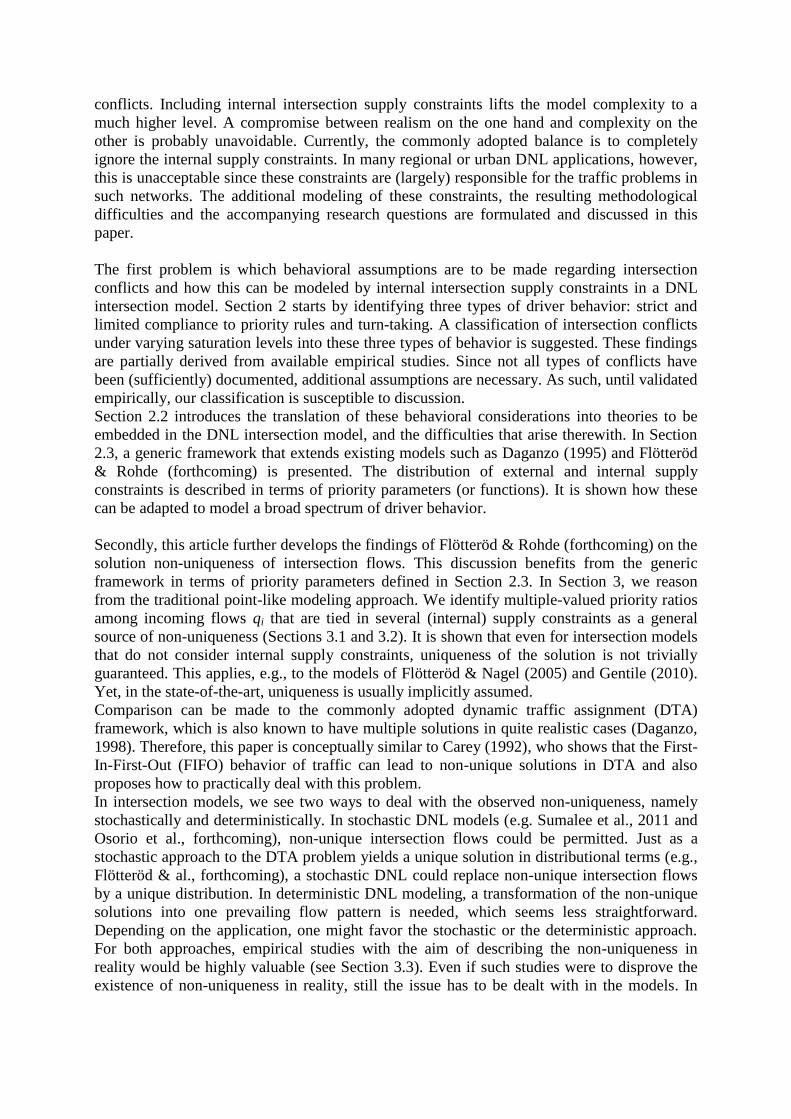
Naturally, the aggregate driver behavior to be captured by macroscopic intersection models

may be a mixture of different types of behavior. In Figure 1, a suggestion is provided on how

aggregate driver behavior at various intersection conflicts could be classified. This

classification is certainly subject to numerous factors, which are often unknown or

immeasurable, and it is thus not indisputable.

Figure 1: Driver behavior in intersection conflicts

2.2 Existing theories describing observed behavior

Before constructing a DNL intersection model, theories are needed that describe how to

model the observed behavior discussed in the previous section. Turn-taking at merging

conflicts is generally modeled by some sort of distribution rule (see Tampère et al. (2011) for

Turn-takingStrict

compliance

Limited

compliance

AWSC merging

and crossing

Merging

(over-saturated)Crossing and

merging

(under-saturated)Crossing

(nearly/over-saturated)

Merging

(nearly-saturated)

a thorough discussion). All further discussion on modeling turn-taking is reserved for the next

section. Regarding the other two types of behavior, strict and limited compliance, a few

theories exist to determine the restriction on minor movements from yielding to higher

prioritized movements in crossing and merging conflicts. The best-known is gap acceptance

theory (see Chapters 8 and 9 in Gartner et al., 2000), which found a more recent counterpart

in conflict theory (Brilon & Wu, 2001). Most often these theories assume strict compliance

with priority rules, but modifications exist for limited compliance (Troutbeck & Kako, 1999;

Brilon & Miltner, 2005). Although some existing DNL intersection models embed gap

acceptance theory to model internal conflicts (Yperman et al., 2007; Ngoduy et al., 2005;

Chevallier & Leclercq, 2007; Flötteröd & Rohde, forthcoming), neither gap acceptance theory

nor conflict theory was initially designed for use in a DNL context. The incompatibility of

these theories with DNL stems from two aspects.

Firstly, both theories are designed for free flowing conditions of the major stream. Gap

acceptance theory in particular loses some validity in nearly-saturated and definitely in over-

saturated conditions. Conflict theory is, at least theoretically, extendable to over-saturated

conditions; but this has not been validated empirically. Bridging the different types of driver

behavior in DNL intersection models by embedding, supplementing and adapting these

existing theories – or developing new ones – therefore constitutes important future research.

A second problem stems from the first one. As is discussed in Tampère et al. (2011), multiple

demand and/or supply constraints interact with each other, causing flows from different

incoming links to be mutually dependent. This must be captured in a supply constraint

interaction rule (SCIR); see Section 1.1. This possibility of mutual dependency is not

considered in gap acceptance and conflict theory, as the major flows are considered known

(i.e. equal to the demand). In a DNL intersection model, however, the major flows are also

subject to (internal) supply constraints and therefore not known beforehand. A few existing

models (Yperman et al., 2007; Ngoduy et al., 2005) that implement internal supply constraints

derived from gap acceptance theory solve this by making the internal supply constraints that

limit the minor flows dependent on the demands of the major streams instead of the actual

major flows. As explained in Section 1, this leads to a violation of the invariance principle if

the major streams are not demand constrained. Moreover, this simplification may cause an

overestimation of the constraint imposed on the minor flows (Flötteröd & Rohde,

forthcoming).

2.3 Modeling (internal) supply constraints in DNL intersection models

As discussed in Section 2.1, different driver behavior can be observed under varying

conditions – to be roughly subdivided in strict compliance, limited compliance, and turn-

taking. In the following, priority parameters are introduced through which these different

types of driver behavior are modeled.

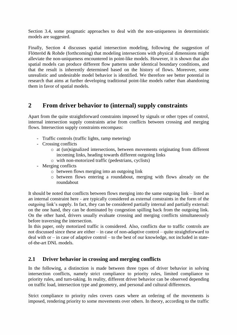
An intuitive way of representing the solution space is used (as in Daganzo, 1995). Figure 2

exemplifies this graphical representation for a two-legged merge. Firstly, the demand

constraints S1 and S2 set upper bounds on the flow from their respective incoming link.

Secondly, the external supply constraint function 3 1 2( , ) 0R q q further reduces the solution

space. The circumflex is introduced to make a distinction between the supply constraint

function and the actual supply R3 that link 3 can receive. In the state-of-the-art, this supply

constraint function is typically written in the form

3 1 2 1 2 3( , ) 0.R q q q q R (2)

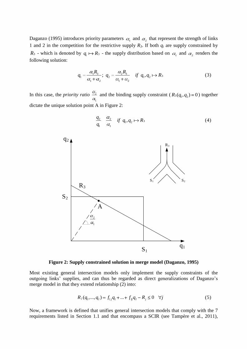
Daganzo (1995) introduces priority parameters 1 and

2 that represent the strength of links

1 and 2 in the competition for the restrictive supply R3. If both qi are supply constrained by

3R - which is denoted by 3iq R - the supply distribution based on

1 and

2 renders the

following solution:

1 3 2 331 2 1 2

1 2 1 2

; ,R R

q q if q q R (3)

In this case, the priority ratio 2

1

and the binding supply constraint ( 3 1 2( , ) 0R q q ) together

dictate the unique solution point A in Figure 2:

2 231 2

1 1

,q

if q q Rq

(4)

Figure 2: Supply constrained solution in merge model (Daganzo, 1995)

Most existing general intersection models only implement the supply constraints of the

outgoing links‟ supplies, and can thus be regarded as direct generalizations of Daganzo‟s

merge model in that they extend relationship (2) into:

1 1 1( ,..., ) ... 0j I j Ij I jR q q f q f q R j (5)

Now, a framework is defined that unifies general intersection models that comply with the 7

requirements listed in Section 1.1 and that encompass a SCIR (see Tampère et al., 2011),

q2

q1

S2

S1

A

R3

2

1

S2S1

R3

controlling the interaction of supply constraints and their distribution on the basis of priority

parameters. First, this is explained in terms of external supply constraints, afterwards it is

extended to internal constraints.

Finite, positive priority parameters ij are considered so that the strength of i in the

competition for supply Rj is given by ij ijf . As such, ij can be regarded as the maximal

strength (if fij = 1). It is indeed logical that the turning fractions fij play an explicit role; the

competitive strength of i for Rj is naturally zero if fij = 0. For a particular i’ constrained by Rj (

1( ,..., ) 0j IR q q ), the supply distribution (3) then generalizes to:

' ' '

' ' ' ,i j i j j i j j

ji j i i i

ij ij ij ij

i i

f R Rq q if q q R

f f (6)

Typically, it is assumed that one most restrictive constraint can be identified that determines

the flow from a link i. If the share of Rj is too much to consume for some incoming links i –

due to more restrictive demand or other supply constraints - the remaining supply j i j

i

R q

is divided among the remaining i analogous to (6) - for more details see Tampère et al. (2011).

Also, we presume that vehicles only enter the intersection if they have the opportunity to exit

via their destination link, so that external supplies Rj do not directly influence flows to other

outgoing directions. In other words, only a link i that wishes to send flow to a link j (i.e.

0ijS ) participates in the competition for Rj. Finally, for any combination of incoming links i

and i’ that are constrained by the same supply Rj, the combination of (6) with the CTF

requirement renders the following solution (analogous to (4)):

'

' '

, ' | ,iji

ji i

i i j

qi i q q R

q (7)

The main difference between models lies in how the priority parameters ij are defined. In

the following it is explained how the priority parameters can be used to model different driver

behavior in external and internal conflicts. Hereby it should be noted that while the priority

parameters are typically set as constant values, they might as well be functions of the turning

fractions, capacities or flows (as in the models of Gibb, 2011 and Flötteröd & Rohde,

forthcoming). Consequently, transitions in driver behavior, e.g. depending on the saturation

level (see Figure 1), may be accounted for by priority functions rather than constants. For

simplicity‟s sake, we regard the priority parameters as constants in the remainder of the paper,

unless stated otherwise.

Regarding external supply constraints, most existing intersection models assume a single-

valued priority parameter i for a link i, which is then used in the competition for all Rj|Sij >

0. If an external supply constraint is active, i.e. the merging conflict is over-saturated, this is

typically solved through turn-taking behavior (see Section 2.1). Turn-taking behavior is

modeled by basing i on the number of lanes or capacities of the incoming links, e.g.

i iC

(as for example in Tampère et al., 2011). Empirical studies on freeway merges (e.g. Bar-Gera

& Ahn, 2010) support this common modeling practice of assuming fixed priority parameters

for any value of Rj to represent turn-taking behavior.

Analogous as for external supplies in outgoing links j, internal supplies in intersection

conflicts k put constraints on the flows qi. Thus, internal supply constraint functions

1( ,..., )k IN q q can be considered that bound all subjected flows ( 0ikS ). This could for

example stem from the conflict area shared by crossing or merging movements. The internal

supply constraint functions kN are more difficult to define than the jR . They are to be

derived from gap acceptance or conflict (or any new) theory, as discussed in Section 2.2.

Exactly defining these functions kN is beyond the scope of this paper. However, we can

state, analogous to (7):

'

' '

, ' | ,i ikki i

i i k

qi i q q N

q (8)

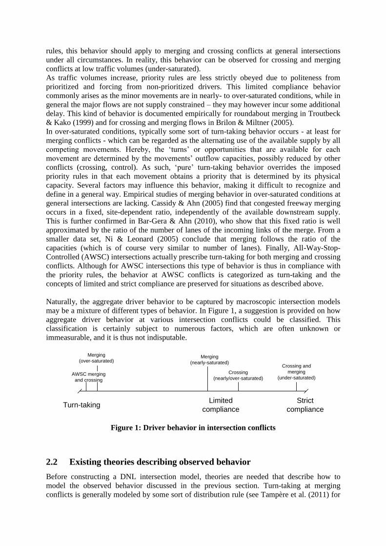
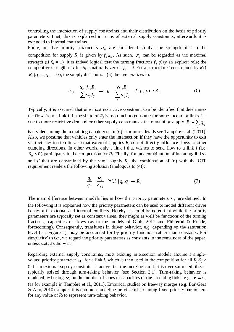
Very similar to Figure 2, the solution space for a simple intersection with one crossing

conflict (represented by 3N ) is depicted in Figure 3. 3 1 2( , ) 0N q q limits q1 and q2 that

compete for the shared internal supply. Say that for this intersection, the priority rules

prescribe that q2 has priority over q1. Strict compliance to this priority rule could then be

modeled by setting 1 0

1 and

2 1 . In consequence, q2 fully consumes its maximal share

(hence q2 = S2), leaving the remaining internal supply for q1, yielding solution A. Limited

compliance could be modeled by less extreme values, e.g. 1* 0 and

2* 1 yielding A* in

Figure 3. Recall that if turn-taking behavior applies to the crossing conflict (as in AWSC

intersections), the i are based on the capacities Ci.

1 At this point, we should add that at most one ij (or

ik) can be defined zero per j (k). In priority-controlled

intersections, always a ranking exists between any two movements that are in conflict. In cases of turn-taking

behavior, zero priorities do not make sense altogether.

Figure 3: Internal supply constrained solution

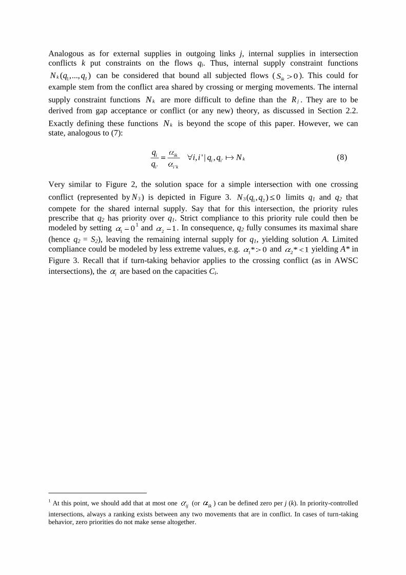
Note that the internal supply constraint function 3N may be non-linear, for instance because

the consumption rate of the internal supply may be different for q1 and q2, or because of joint

constraints, which derive from the fact that drivers evaluate crossing and merging conflicts on

general intersections simultaneously (unless some storage capacity for crossing vehicles is

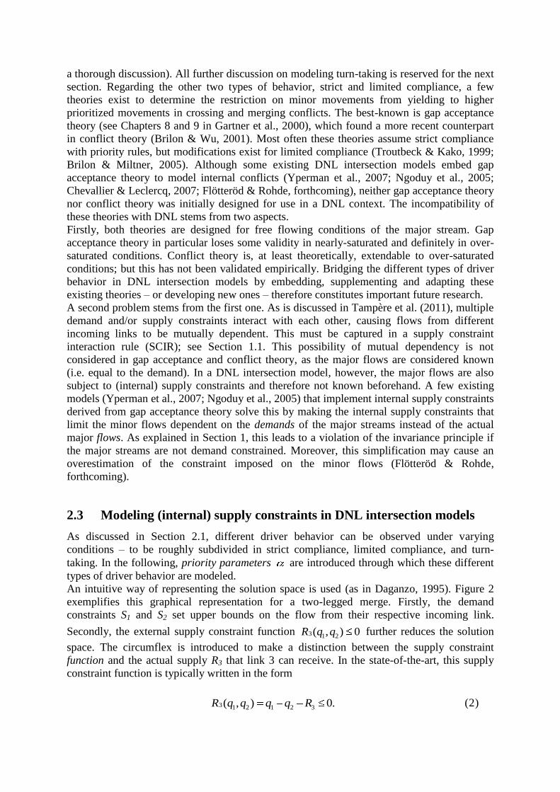
present on the intersection). Consider for example the situation in Figure 4, where a minor

flow from the westbound link has to yield to bi-directional traffic of the major street. A

vehicle from the minor street will only cross if no prioritized vehicle is approaching from

either side.

Figure 4: Minor movement yielding to bi-directional traffic

q2

q1

S2

S1

A

N3

2

1

N3

S1

S2

2

1

*

*

A*

q1

q2

q3

This suggests to combine these two internal conflicts into one joint internal supply constraint

function 1 2 3( , , ) 0N q q q . Regardless, the solution (space) of the intersection model can still

be represented as in Figure 3. The definition of the priority parameters may, however, be

more complicated in case of joint constraints.

In conclusion, this section explains in general terms how priority parameters can be used to

model different types of driver behavior. The depth and complexity of this discussion is

limited to the level necessary to introduce the concepts of modeling internal supply

constraints due to merging and crossing conflicts and to elaborate on the solution non-

uniqueness observed therein, as discussed in the next sections.

3 Solution non-uniqueness in point-like intersection models

In this section, intersection models in the traditional point-like form are discussed, whereas

spatial models are reserved for Section 4. Firstly, the problem of solution non-uniqueness is

introduced by means of two simple examples in Section 3.1. Then, this non-uniqueness is

further analyzed in Section 3.2. Section 3.3 raises the question whether the problem of non-

uniqueness, which arises in the intersection model from realistic behavioral assumptions,

would in fact be identifiable in reality. Finally, some pragmatic approaches to deal with non-

uniqueness in deterministic intersection models are given in Section 3.4.

3.1 Explanatory examples

In the literature, solution uniqueness of the intersection model is often implicitly assumed.

However, the following example shows that even for simple cases, which only consider

external supply constraints, uniqueness of the solution is not self-evident.

3.1.1 Example 1 (only external supply constraints)

A simple 2x2-intersection is considered (Figure 5), where the intersection model assumes

different priority parameters ij for an incoming link (i = 1, 2) per outgoing link (j = 3, 4).

This means that the incoming links 1 and 2 have a different priority (maximal strength) in the

competition for R3 and R4; this could for instance be based on the number of turning lanes.

This corresponds to the intersection models in Gentile (2010) and Flötteröd & Nagel (2005).

The solution space defined by the demand and external supply constraints is depicted in

Figure 5.

Due to the CTF requirement, both inflows qi are mutually tied in both supply constraints. As

such, the solution is fully determined by the total inflows qi from which the partial flows qij

derive (see Section 1.1). If 1 2( , ) 0jR q q (see (5)) and both i jq R , the priority parameters

ij determine the solution according to (7) (or (6)).

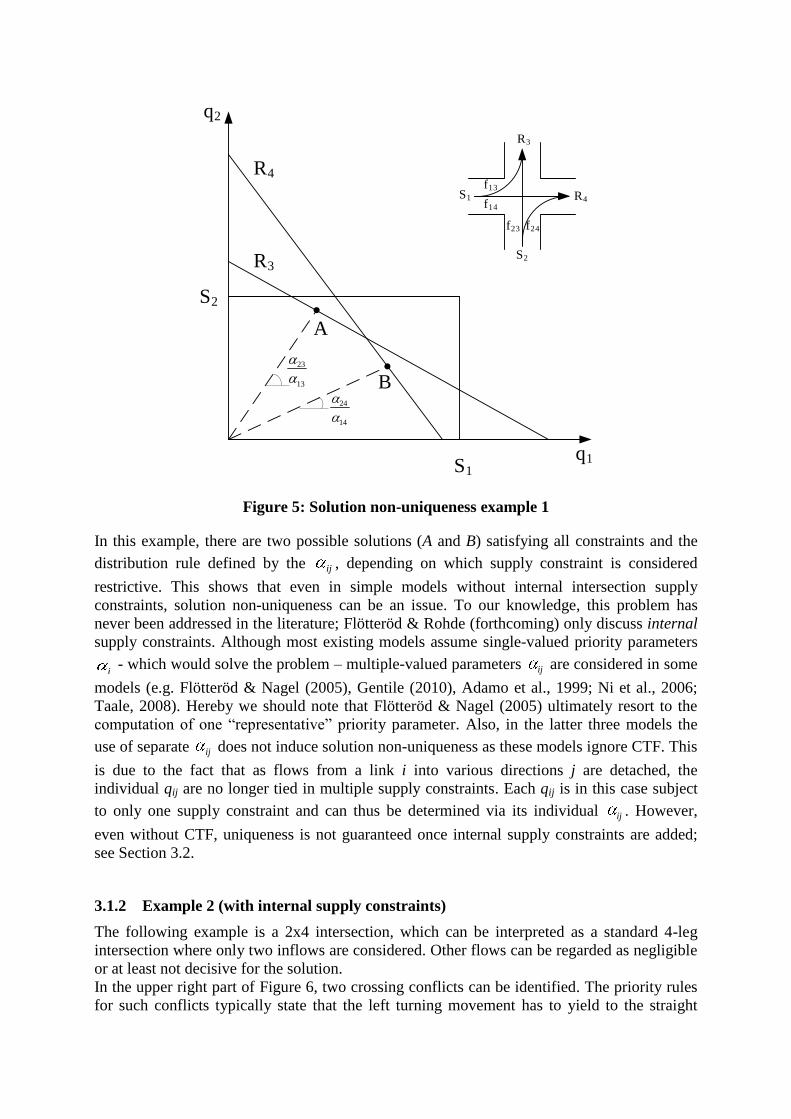
Figure 5: Solution non-uniqueness example 1

In this example, there are two possible solutions (A and B) satisfying all constraints and the

distribution rule defined by the ij , depending on which supply constraint is considered

restrictive. This shows that even in simple models without internal intersection supply

constraints, solution non-uniqueness can be an issue. To our knowledge, this problem has

never been addressed in the literature; Flötteröd & Rohde (forthcoming) only discuss internal

supply constraints. Although most existing models assume single-valued priority parameters

i - which would solve the problem – multiple-valued parameters ij are considered in some

models (e.g. Flötteröd & Nagel (2005), Gentile (2010), Adamo et al., 1999; Ni et al., 2006;

Taale, 2008). Hereby we should note that Flötteröd & Nagel (2005) ultimately resort to the

computation of one “representative” priority parameter. Also, in the latter three models the

use of separate ij does not induce solution non-uniqueness as these models ignore CTF. This

is due to the fact that as flows from a link i into various directions j are detached, the

individual qij are no longer tied in multiple supply constraints. Each qij is in this case subject

to only one supply constraint and can thus be determined via its individual ij . However,

even without CTF, uniqueness is not guaranteed once internal supply constraints are added;

see Section 3.2.

3.1.2 Example 2 (with internal supply constraints)

The following example is a 2x4 intersection, which can be interpreted as a standard 4-leg

intersection where only two inflows are considered. Other flows can be regarded as negligible

or at least not decisive for the solution.

In the upper right part of Figure 6, two crossing conflicts can be identified. The priority rules

for such conflicts typically state that the left turning movement has to yield to the straight

q2

q1

S2

S1

B

A

R3

R4

24

14

23

13

S1

S2

R3

R4

f13

f14

f23 f24

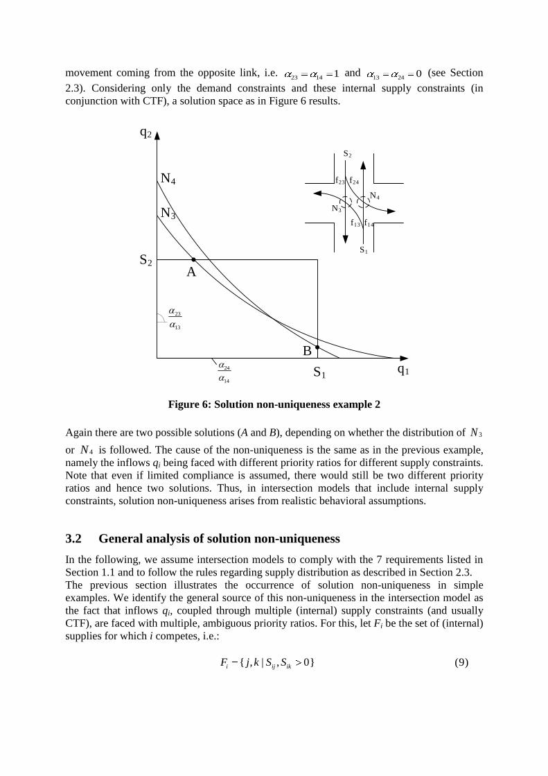
movement coming from the opposite link, i.e. 23 14 1 and

13 24 0 (see Section

2.3). Considering only the demand constraints and these internal supply constraints (in

conjunction with CTF), a solution space as in Figure 6 results.

Figure 6: Solution non-uniqueness example 2

Again there are two possible solutions (A and B), depending on whether the distribution of 3N

or 4N is followed. The cause of the non-uniqueness is the same as in the previous example,

namely the inflows qi being faced with different priority ratios for different supply constraints.

Note that even if limited compliance is assumed, there would still be two different priority

ratios and hence two solutions. Thus, in intersection models that include internal supply

constraints, solution non-uniqueness arises from realistic behavioral assumptions.

3.2 General analysis of solution non-uniqueness

In the following, we assume intersection models to comply with the 7 requirements listed in

Section 1.1 and to follow the rules regarding supply distribution as described in Section 2.3.

The previous section illustrates the occurrence of solution non-uniqueness in simple

examples. We identify the general source of this non-uniqueness in the intersection model as

the fact that inflows qi, coupled through multiple (internal) supply constraints (and usually

CTF), are faced with multiple, ambiguous priority ratios. For this, let Fi be the set of (internal)

supplies for which i competes, i.e.:

{ , | , 0}i ij ikF j k S S (9)

q2

q1

S2

S1

B

A

N3

N4

23

13

24

14

S2

S1

N3

N4

f13 f14

f23 f24

Now, there are two ways in which flows qi can be mutually dependent through multiple

supply constraints:

1. Two (or more) inflows 1i

q and 2i

q are tied in two (or more) supply constraints, i.e.

1 2#( ) 2i iF F .

2. Three (or more) inflows 1i

q , 2i

q and 3i

q are mutually dependent in some “circular

way”, so that each (internal) supply constraint binds two different inflows in a

sequence, returning from the last i to the first, forming a circle in which all inflows are

mutually dependent, i.e.: 1 2 2 3 3 11 2 3{ }, { }, { }i i i i i iF F j F F j F F j . Or in other

words: 1 1 2 1 2 2 3 2 3 3 1 3

0, 0, 0, 0, 0, 0i j i j i j i j i j i jS S S S S S with all other Sij = 0 (any j

could of course be replaced by a k).

Naturally, combinations of 1 and 2 can exist. Option 1 is the more likely of the two to appear

in an intersection model. Note that this option implicitly assumes CTF, since otherwise the qij

are detached and thus two inflows qi cannot be reasonably tied in the same two (internal)

supply constraints. Further in this section, an example of the second, less obvious option is

provided, which shows that solution non-uniqueness can also exist in non-CTF models.

Now, a sufficient and necessary condition for solution uniqueness of the intersection flows is

that each priority parameter ij and ik of inflows qi that are mutually dependent in supply

constraints in j and k can be written as the product of a single-valued i for each i and a

factor for each (internal) supply constraint in j or k:

, , : & ,i j k ij i j ik i k ii j k F (10)

with

0

0

0

i

j

k

i

j

k

(11)

The factors j and k are scalable, as is the set of i „s in its entirety. As such, a sufficient

condition for solution uniqueness can be derived from the above by setting all j and k to

one, thus defining single-valued priority parameters i for each link i to be applied in the

distribution of all (internal) supplies.

Proof for condition (10) is added in appendix. For flows qi that are mutually dependent in the

first manner described above, (10) reads as „the priority ratios are identical for all (internal)

supply constraints in which these qi are both involved‟, thus ruling out ambiguity and non-

uniqueness.

To illustrate the second manner for mutual dependency, let us regard the example in Figure 7.

An intersection is considered with three incoming flows qi (i = 1…3) and three internal supply

constraint functions kN (k = 4...6) each encompassing two qi. As such, the constraint

functions are two-dimensional planes (they only form a triangle in the graph because the same

function is assumed for each constraint - which seems to make most sense). Now, the set of

i „s in (10) is presented as a vector i of which the direction is unique, but not the norm – as

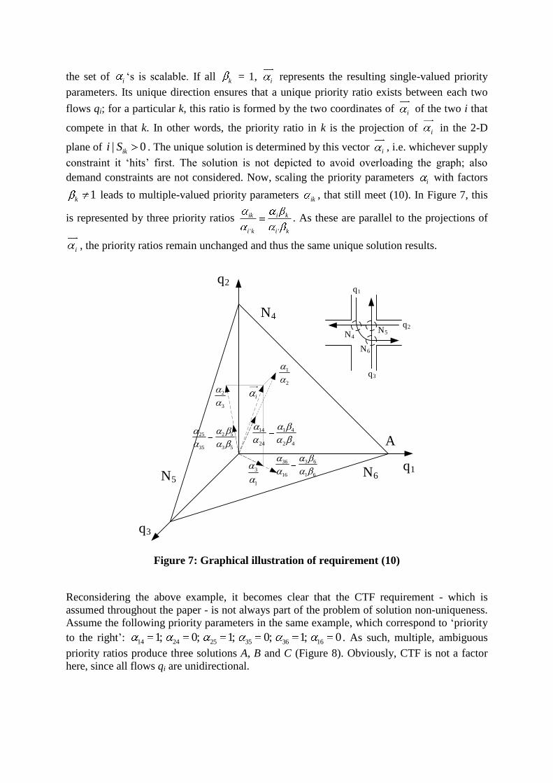
the set of i „s is scalable. If all k = 1, i represents the resulting single-valued priority

parameters. Its unique direction ensures that a unique priority ratio exists between each two

flows qi; for a particular k, this ratio is formed by the two coordinates of i of the two i that

compete in that k. In other words, the priority ratio in k is the projection of i in the 2-D

plane of | 0iki S . The unique solution is determined by this vector i , i.e. whichever supply

constraint it „hits‟ first. The solution is not depicted to avoid overloading the graph; also

demand constraints are not considered. Now, scaling the priority parameters i with factors

1k leads to multiple-valued priority parameters ik , that still meet (10). In Figure 7, this

is represented by three priority ratios ' '

ik i k

i k i k

. As these are parallel to the projections of

i , the priority ratios remain unchanged and thus the same unique solution results.

Figure 7: Graphical illustration of requirement (10)

Reconsidering the above example, it becomes clear that the CTF requirement - which is

assumed throughout the paper - is not always part of the problem of solution non-uniqueness.

Assume the following priority parameters in the same example, which correspond to „priority

to the right‟: 14 24 25 35 36 161; 0; 1; 0; 1; 0 . As such, multiple, ambiguous

priority ratios produce three solutions A, B and C (Figure 8). Obviously, CTF is not a factor

here, since all flows qi are unidirectional.

q2

q1

q3

q1

q3

N4N5

q2

N6

N4

N6N5

A14 1 4

24 2 4

36 3 6

16 1 6

25 2 5

35 3 5

1

2

3

1

2

3

i

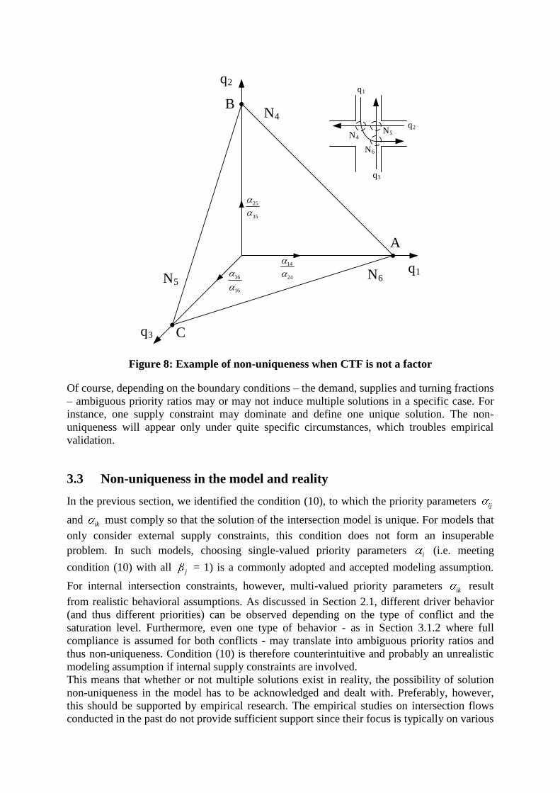
Figure 8: Example of non-uniqueness when CTF is not a factor

Of course, depending on the boundary conditions – the demand, supplies and turning fractions

– ambiguous priority ratios may or may not induce multiple solutions in a specific case. For

instance, one supply constraint may dominate and define one unique solution. The non-

uniqueness will appear only under quite specific circumstances, which troubles empirical

validation.

3.3 Non-uniqueness in the model and reality

In the previous section, we identified the condition (10), to which the priority parameters ij

and ik must comply so that the solution of the intersection model is unique. For models that

only consider external supply constraints, this condition does not form an insuperable

problem. In such models, choosing single-valued priority parameters i (i.e. meeting

condition (10) with all j = 1) is a commonly adopted and accepted modeling assumption.

For internal intersection constraints, however, multi-valued priority parameters ik result

from realistic behavioral assumptions. As discussed in Section 2.1, different driver behavior

(and thus different priorities) can be observed depending on the type of conflict and the

saturation level. Furthermore, even one type of behavior - as in Section 3.1.2 where full

compliance is assumed for both conflicts - may translate into ambiguous priority ratios and

thus non-uniqueness. Condition (10) is therefore counterintuitive and probably an unrealistic

modeling assumption if internal supply constraints are involved.

This means that whether or not multiple solutions exist in reality, the possibility of solution

non-uniqueness in the model has to be acknowledged and dealt with. Preferably, however,

this should be supported by empirical research. The empirical studies on intersection flows

conducted in the past do not provide sufficient support since their focus is typically on various

q2

q1

q3

q1

q3

N4N5

q2

N6

N4

N6N5

A

B

C

25

35

14

2436

16

aspects of gap acceptance behavior (e.g. headway distributions) and not on validating

intersection models in DNL (except for simple merges; see e.g. Bar-Gera & Ahn, 2010 and Ni

& Leonard, 2005). Flow non-uniqueness has never been reported in empirical data, but it has

also never been looked for. Since non-uniqueness only appears in the model under specific

circumstances, where multiple supply constraints can dominate under identical boundary

conditions, identifying these circumstances constitutes a considerable practical difficulty.

Additionally, the need for a large amount of detailed data – not only traffic counts, but also

video observation – renders this empirical research labor- and cost-intensive.

3.4 Pragmatic approaches to deal with non-uniqueness in deterministic

intersection models

Regardless of whether empirical research is to confirm or disprove the existence of multiple

solutions in reality, the non-uniqueness has to be dealt with in the intersection model. In

stochastic models, a unique probability distribution, encompassing the multiple solutions,

could be composed. For deterministic intersection models, we suggest in the following some

pragmatic approaches that produce unique solutions. Further developing these into actual

models requires also extending the other theoretical concepts discussed in this paper, i.e.

explicitly defining internal supply constraint functions and priority parameters. Moreover, the

development of efficient algorithms constitutes a considerable challenge.

First of all, it is stressed that the following two approaches to try to remedy the non-

uniqueness should be avoided:

- disregarding CTF

- extending the requirement of individual flow maximization to global flow

maximization

Not only do these suffer from unrealistic modeling assumptions; uniqueness is not fully

guaranteed in either approach. For non-CTF cases, this is demonstrated by the example in

Section 3.2. Regarding global flow maximization, if the total flow i

i

q is the same for

multiple solutions, a global maximization is also subject to non-uniqueness.

A model definition in which solution uniqueness is ensured can be obtained by imposing (10).

This is in line with the modeling assumptions in many state-of-the-art intersection models that

consider only external supply constraints. As stated before, this assumption lacks realism for

most types of intersection conflicts. Only if the expected driver behavior is limited to turn-

taking behavior, as in AWSC intersections, reverting to this approach seems natural, e.g. with

i = Ci.

It may be desirable to at first allow ambiguous priorities in the model definition, and then to

alleviate the non-uniqueness by some kind of pre- or post-processing. In the following, we

distinguish two types of approaches: (a) pre-processing the priorities so that the model

produces a unique solution; and (b) computing non-unique solutions that result from different

priorities and then post-processing these into one solution. In either case, the pre/post-

processing is mathematically formulated as a convex combination of priorities/flows.

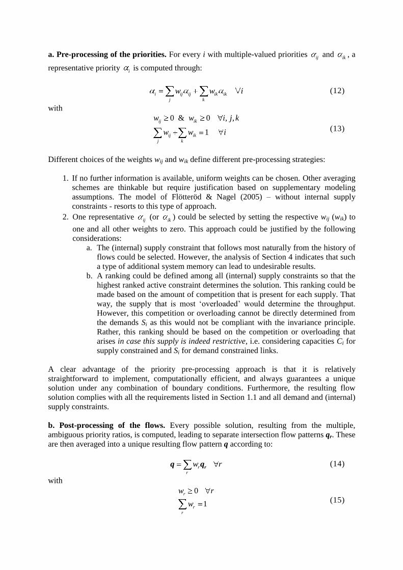
a. Pre-processing of the priorities. For every i with multiple-valued priorities ij and ik , a

representative priority i is computed through:

i ij ij ik ik

j k

w w i (12)

with

0 & 0 , ,

1

ij ik

ij ik

j k

w w i j k

w w i (13)

Different choices of the weights wij and wik define different pre-processing strategies:

1. If no further information is available, uniform weights can be chosen. Other averaging

schemes are thinkable but require justification based on supplementary modeling

assumptions. The model of Flötteröd & Nagel (2005) – without internal supply

constraints - resorts to this type of approach.

2. One representative ij (or ik ) could be selected by setting the respective wij (wik) to

one and all other weights to zero. This approach could be justified by the following

considerations:

a. The (internal) supply constraint that follows most naturally from the history of

flows could be selected. However, the analysis of Section 4 indicates that such

a type of additional system memory can lead to undesirable results.

b. A ranking could be defined among all (internal) supply constraints so that the

highest ranked active constraint determines the solution. This ranking could be

made based on the amount of competition that is present for each supply. That

way, the supply that is most „overloaded‟ would determine the throughput.

However, this competition or overloading cannot be directly determined from

the demands Si as this would not be compliant with the invariance principle.

Rather, this ranking should be based on the competition or overloading that

arises in case this supply is indeed restrictive, i.e. considering capacities Ci for

supply constrained and Si for demand constrained links.

A clear advantage of the priority pre-processing approach is that it is relatively

straightforward to implement, computationally efficient, and always guarantees a unique

solution under any combination of boundary conditions. Furthermore, the resulting flow

solution complies with all the requirements listed in Section 1.1 and all demand and (internal)

supply constraints.

b. Post-processing of the flows. Every possible solution, resulting from the multiple,

ambiguous priority ratios, is computed, leading to separate intersection flow patterns qr. These

are then averaged into a unique resulting flow pattern q according to:

r

r

w rrq q (14)

with

0

1

r

r

r

w r

w (15)

Again, different choices of the weights define different solution strategies:

1. One could assume a uniform average solution to hold. This is in line with the

assumption that a deterministic DNL represents average network conditions. A naïve

averaging, however, raises considerable difficulties. The average flow pattern may not

comply with the requirement of individual flow maximization, or it may violate the

invariance principle or some non-linear internal supply constraints.

2. One could also select a single solution as the most plausible or representative one for

the given situation (this again corresponds to setting the respective weight wr to one

and all others to zero). Again, this could be based on previous flows (assuming, e.g.,

that the smallest temporal change in flow patterns is the most plausible). Technically,

this corresponds to uniquely selecting the priorities that have led to this solution, but

the selection criterion is now based on flows, which are not known a priori in the

priority pre-processing approach.

A drawback of the flow post-processing approach is that multiple candidate solutions need to

be evaluated, rendering the intersection model computationally intensive. Also, as stated

above, a true averaging of solutions can lead to flows that are inconsistent with the basic

modeling assumptions.

Answering the question which of the above approaches or any other possible alternative is

most realistic or most appropriate is difficult or even impossible without further theoretical

and empirical research. Moreover, the answer might differ under varying circumstances. A

trade-off between realism on the one hand and computational efficiency and limiting model

complexity on the other seems inevitable.

4 Spatial intersection modeling

While the traditional point-like modeling approach is not disputed if internal supply

constraints are disregarded, complex intersection models implement constraints that clearly

have physical characteristics. Therefore, one might consider modeling intersections in DNL

spatially, i.e. as mini-networks in which the conflict zones of crossing and merging flows are

represented by dummy nodes, connected by dummy links. In this section, however, it is

shown that spatial models exhibit similar as well as additional disadvantages within the

macroscopic DNL framework.

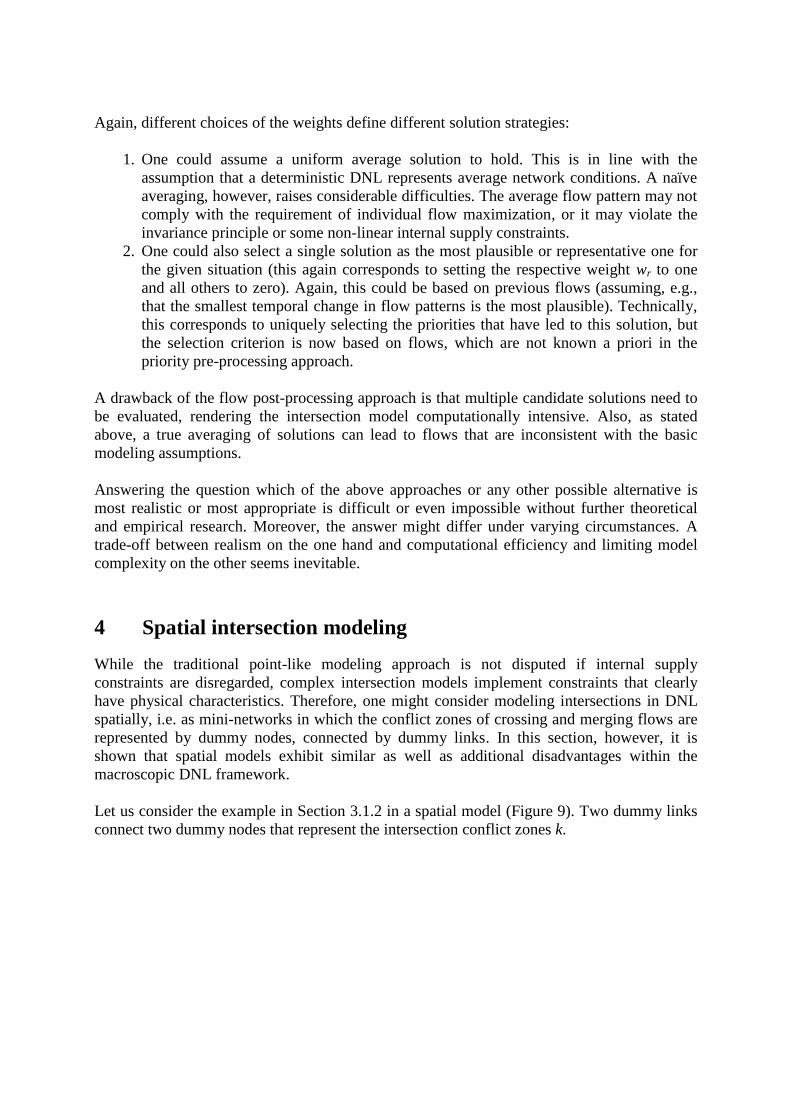
Let us consider the example in Section 3.1.2 in a spatial model (Figure 9). Two dummy links

connect two dummy nodes that represent the intersection conflict zones k.

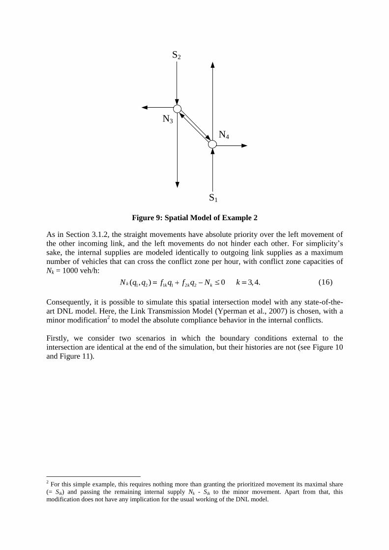
Figure 9: Spatial Model of Example 2

As in Section 3.1.2, the straight movements have absolute priority over the left movement of

the other incoming link, and the left movements do not hinder each other. For simplicity‟s

sake, the internal supplies are modeled identically to outgoing link supplies as a maximum

number of vehicles that can cross the conflict zone per hour, with conflict zone capacities of

Nk = 1000 veh/h:

1 2 1 1 2 2( , ) 0 3,4.k k k kN q q f q f q N k (16)

Consequently, it is possible to simulate this spatial intersection model with any state-of-the-

art DNL model. Here, the Link Transmission Model (Yperman et al., 2007) is chosen, with a

minor modification2 to model the absolute compliance behavior in the internal conflicts.

Firstly, we consider two scenarios in which the boundary conditions external to the

intersection are identical at the end of the simulation, but their histories are not (see Figure 10

and Figure 11).

2 For this simple example, this requires nothing more than granting the prioritized movement its maximal share

(= Sik) and passing the remaining internal supply Nk - Sik to the minor movement. Apart from that, this

modification does not have any implication for the usual working of the DNL model.

S2

S1

N3

N4

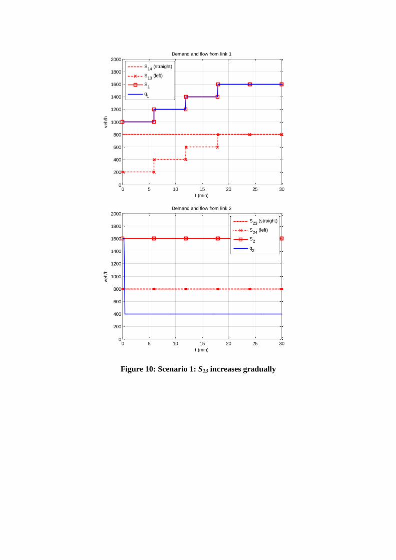
Figure 10: Scenario 1: S13 increases gradually

0 5 10 15 20 25 300

200

400

600

800

1000

1200

1400

1600

1800

2000

t (min)

veh/h

Demand and flow from link 1

S14

(straight)

S13

(left)

S1

q1

0 5 10 15 20 25 300

200

400

600

800

1000

1200

1400

1600

1800

2000

t (min)

veh/h

Demand and flow from link 2

S23

(straight)

S24

(left)

S2

q2

Figure 11: Scenario 1: S24 increases gradually

In scenario 1 and 2, the left-turning demands are initially different. During the simulation, the

low left-turning demand is gradually increased until it reaches the same level as the high left-

turning demand from the opposing link.

In the initial phase of scenario 1, S13 is low, allowing link 1 to send its full demand, since

there is enough remaining supply (N3 – S23 = 200 veh/h) for its minor left-turning movement.

Meanwhile, the queue of the left-turning movement of link 2, which is obstructed by N4,

quickly spills back over the dummy link. This renders link 2 congested; also the straight

movement is thus held back. While S13 is gradually increased, this does not change the flows,

as link 2 is now unable to claim its maximal share in N3 (leaving N3 – q23 = 800 veh/h for link

1) due to the active constraint in N4. In result, q1 stays dominant throughout the simulation,

while the other flow remains constrained. Scenario 2 is exactly the opposite.

Thus, although the boundary conditions at the end of the simulation are identical in both

scenarios, the resulting flow patterns are very different. This demonstrates that also in a

spatial model, solution uniqueness is not guaranteed given only the instantaneous boundary

0 5 10 15 20 25 300

200

400

600

800

1000

1200

1400

1600

1800

2000

t (min)

veh/h

Demand and flow from link 1

S14

(straight)

S13

(left)

S1

q1

0 5 10 15 20 25 300

200

400

600

800

1000

1200

1400

1600

1800

2000

t (min)

veh/h

Demand and flow from link 2

S23

(straight)

S24

(left)

S2

q2

conditions. The spatial model inherently determines the solution on the basis of history, which

is analogous to a point-like model that would solve the non-uniqueness based on history (see

Section 3.4).

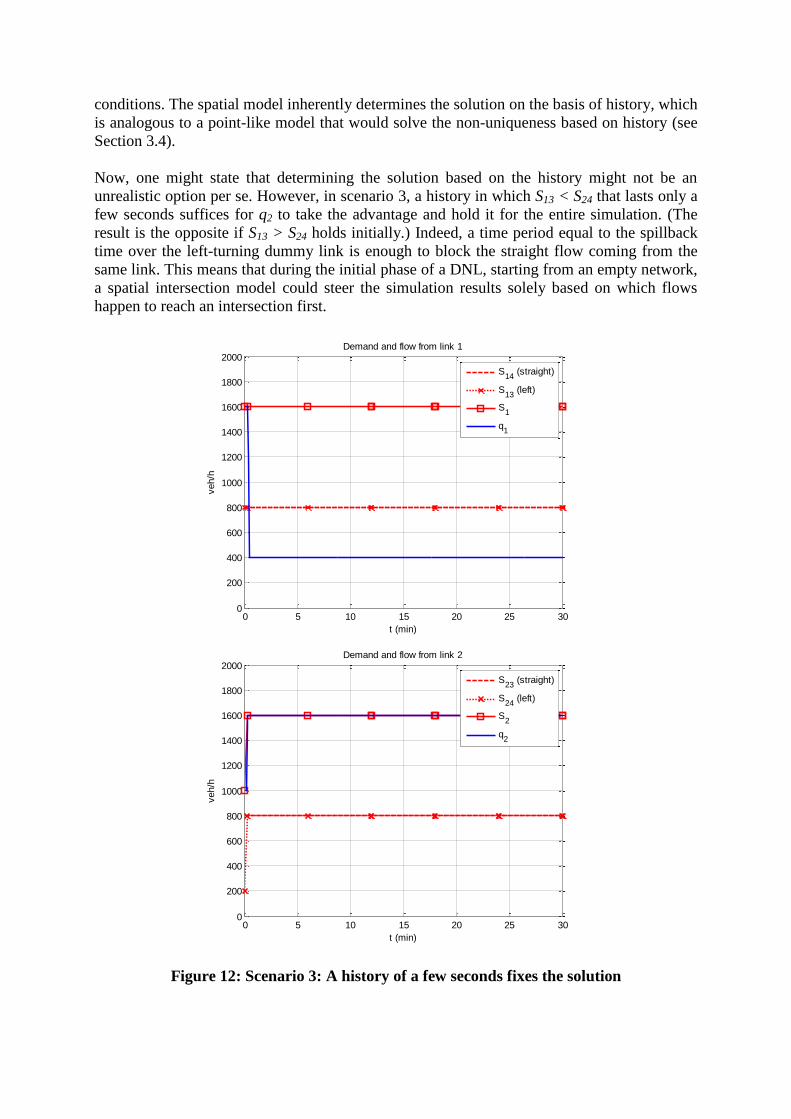
Now, one might state that determining the solution based on the history might not be an

unrealistic option per se. However, in scenario 3, a history in which S13 < S24 that lasts only a

few seconds suffices for q2 to take the advantage and hold it for the entire simulation. (The

result is the opposite if S13 > S24 holds initially.) Indeed, a time period equal to the spillback

time over the left-turning dummy link is enough to block the straight flow coming from the

same link. This means that during the initial phase of a DNL, starting from an empty network,

a spatial intersection model could steer the simulation results solely based on which flows

happen to reach an intersection first.

Figure 12: Scenario 3: A history of a few seconds fixes the solution

0 5 10 15 20 25 300

200

400

600

800

1000

1200

1400

1600

1800

2000

t (min)

veh/h

Demand and flow from link 1

S14

(straight)

S13

(left)

S1

q1

0 5 10 15 20 25 300

200

400

600

800

1000

1200

1400

1600

1800

2000

t (min)

veh/h

Demand and flow from link 2

S23

(straight)

S24

(left)

S2

q2

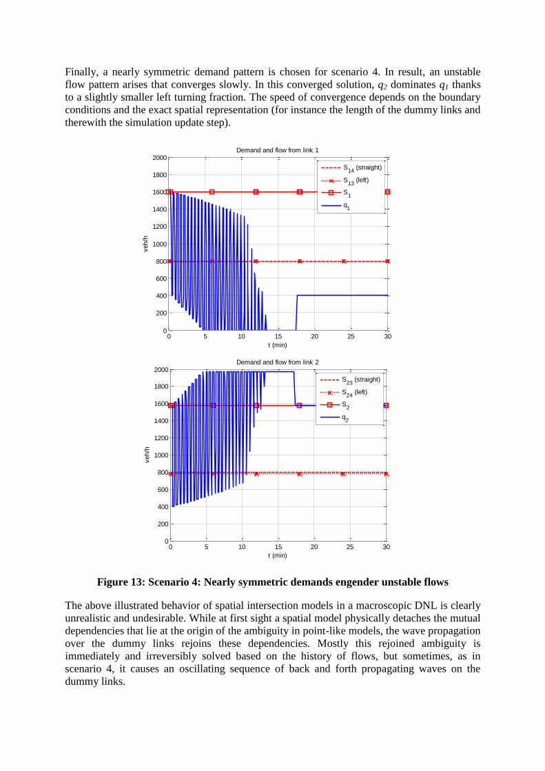
Finally, a nearly symmetric demand pattern is chosen for scenario 4. In result, an unstable

flow pattern arises that converges slowly. In this converged solution, q2 dominates q1 thanks

to a slightly smaller left turning fraction. The speed of convergence depends on the boundary

conditions and the exact spatial representation (for instance the length of the dummy links and

therewith the simulation update step).

Figure 13: Scenario 4: Nearly symmetric demands engender unstable flows

The above illustrated behavior of spatial intersection models in a macroscopic DNL is clearly

unrealistic and undesirable. While at first sight a spatial model physically detaches the mutual

dependencies that lie at the origin of the ambiguity in point-like models, the wave propagation

over the dummy links rejoins these dependencies. Mostly this rejoined ambiguity is

immediately and irreversibly solved based on the history of flows, but sometimes, as in

scenario 4, it causes an oscillating sequence of back and forth propagating waves on the

dummy links.

0 5 10 15 20 25 300

200

400

600

800

1000

1200

1400

1600

1800

2000

t (min)

veh/h

Demand and flow from link 1

S14

(straight)

S13

(left)

S1

q1

0 5 10 15 20 25 300

200

400

600

800

1000

1200

1400

1600

1800

2000

t (min)

veh/h

Demand and flow from link 2

S23

(straight)

S24

(left)

S2

q2

One flaw of this system lies in the application of macroscopic propagation theories designed

for links of reasonable length on small dummy links that fit at most a few vehicles. A second

problem that seems inherent to spatial intersection models is the spatial detachment of

constraints that are subject to simultaneous driver decisions. Consider again the example in

Figure 4. While in reality the two internal conflicts are evaluated simultaneously, they would

be separated into two dummy nodes in the spatial model, leaving no option to capture the

dependency between the two without further modeling efforts. Due to the before-mentioned

problems, extreme caution is advised when inheriting networks for DNL or DTA purposes

directly from static models, in which complex intersections are often modeled spatially.

While the possibility that a theory can be found that realistically treats propagation waves and

simultaneous decisions in a spatial intersection model cannot be ruled out, it is safe to say that

currently the problems and shortcomings of point-like intersection models cannot be bypassed

in a spatial way. Simply regarding an intersection as a mini-network and trying to solve it in a

standard macroscopic DNL manner produces unrealistic results. Partly, this behavior is

similar to the non-uniqueness observed in point-like models, as different flow patterns can be

obtained under instantaneously identical boundary conditions. Moreover, these flow patterns

depend on the history of the boundary conditions and the exact spatial representation

(including the dummy links‟ length and characteristics), which makes them difficult to control

by the modeler.

As we feel that trying to include simultaneous decisions and accounting for mutually

dependent flows naturally leads back to a point-like approach, we recommend that research

on developing and improving traditional point-like intersection models is to be preferred. Two

additional disadvantages of spatial models reinforce this argument:

- How to represent an intersection in a spatial model is a delicate matter. Caution is

needed to make sure that the conflicts between the various movements are modeled

realistically. For example, Chen et al. (2008) define their spatial intersection model as

a grid of 2x2 cells, in which some movements that in reality would not be in conflict

do hinder each other, whereas some other movements that are conflicting in reality are

not in the model. Moreover, the configuration in Chen et al. (2008) can easily lead to

model-induced, unrealistic gridlock. In Figure 14, an example of a gridlock-sensitive

representation (a) and a non-gridlock-sensitive representation (b) of a standard 4x4-

intersection is given. In essence, grouping movements into circular patterns may cause

gridlock.

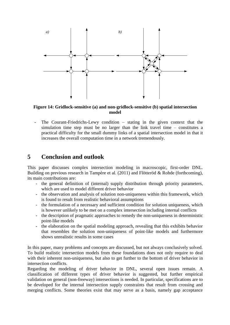
Figure 14: Gridlock-sensitive (a) and non-gridlock-sensitive (b) spatial intersection

model

- The Courant-Friedrichs-Lewy condition – stating in the given context that the

simulation time step must be no larger than the link travel time – constitutes a

practical difficulty for the small dummy links of a spatial intersection model in that it

increases the overall computation time in a network tremendously.

5 Conclusion and outlook

This paper discusses complex intersection modeling in macroscopic, first-order DNL.

Building on previous research in Tampère et al. (2011) and Flötteröd & Rohde (forthcoming),

its main contributions are:

- the general definition of (internal) supply distribution through priority parameters,

which are used to model different driver behavior

- the observation and analysis of solution non-uniqueness within this framework, which

is found to result from realistic behavioral assumptions

- the formulation of a necessary and sufficient condition for solution uniqueness, which

is however unlikely to be met on a complex intersection including internal conflicts

- the description of pragmatic approaches to remedy the non-uniqueness in deterministic

point-like models

- the elaboration on the spatial modeling approach, revealing that this exhibits behavior

that resembles the solution non-uniqueness of point-like models and furthermore

shows unrealistic results in some cases

In this paper, many problems and concepts are discussed, but not always conclusively solved.

To build realistic intersection models from these foundations does not only require to deal

with their inherent non-uniqueness, but also to get further to the bottom of driver behavior in

intersection conflicts.

Regarding the modeling of driver behavior in DNL, several open issues remain. A

classification of different types of driver behavior is suggested, but further empirical

validation on general (non-freeway) intersections is needed. In particular, specifications are to

be developed for the internal intersection supply constraints that result from crossing and

merging conflicts. Some theories exist that may serve as a basis, namely gap acceptance

a) b)

theory (Chapters 8 and 9 in Gartner et al., 2000) and conflict theory (Brilon & Wu, 2001;

Brilon & Miltner, 2005). Hereby, we give preference to conflict theory since it seems more

compatible with over-saturated conditions. Also, it is less complicated. Anyhow, further

extension and adaptation to fit these theories into a DNL environment is required. The

definition of the priority parameters that govern the internal supply distribution cannot be

detached from this. Non-linear priority functions rather than constant priority ratios may be

necessary to realistically capture the transition between different driver behavior, e.g. based

on the saturation level. Also, caution is needed to preserve the model‟s compliance to the

requirements listed in Section 1.1 , following Tampère et al. (2011). Accounting for all of this

should lead to a realistic, but also highly complex intersection model. Depending on the

application, different trade-offs between realism, model complexity and data requirements

will be desirable. Hopefully, this discussion will evolve comparably to that of link models,

where various theories – e.g. travel time functions, vertical and spatial queuing – provide

different levels of complexity and realism.

Regarding the treatment of the solution non-uniqueness, foremost empirical studies would be

valuable that confirm the existence of multiple flow patterns under identical boundary

conditions, and reveal their characteristics – e.g. probability, frequency of switches, duration

of stable periods - and the (external) factors that lead to these characteristics – e.g. history,

neighboring (signaled) intersections, the intersection geometry. This paper aids by helping to

understand the phenomenon (and when it occurs) in the model, so that these specific

circumstances can be sought for in the field. This empirical work – even if it disproves non-

uniqueness in reality – can support the further research to develop and improve complex

intersection models. Hereby, it seems that a point-like approach is most promising, upgrading

the conceptual pragmatic approaches suggested in Section 3.4 – along with further

developments of the behavioral modeling as described above – into unambiguous models for

different types of intersections (AWSC, priority-controlled, signalized and roundabouts).

6 References

Adamo, V., Astarita, V., Florian, M., Mahut, M. & Wu, J.H. (1999). Analytical modeling of

intersections in traffic flow models with queue spill-back. IFORS' 99 15Th

Triennial

Conference (ORSC), Beijing, P.R. China (also published in CRT di Montreal. Publication

CRT 1999 nr. 52. National Libraries of Quebec and Canada).

Akcelik, R. & Troutbeck R.J. (1991). Implementation of the Australian Roundabout Analysis

Method in SIDRA. Highway Capacity and Level of Service, Proceedings of the International

Symposium on Highway Capacity, pp. 17-34.

Bar-Gera, H. & Ahn, S. (2010). Empirical macroscopic evaluation of freeway merge-ratios.

Transportation Research Part C, 18 (4), pp.457-470.

Brilon, W. & Wu, N. (2001). Capacity at unsignalized intersections derived by conflict

technique. Transportation Research Record, Vol. 1776, pp. 82-90.

Brilon, W. & Miltner, T. (2005). Capacity at intersections without traffic signals.

Transportation Research Record, Vol. 1920, pp. 32-40.

Buisson, C., Lesort, J.B. & Lebacque, J.P. (1995). Macroscopic modeling of traffic flow and

assignment in mixed networks. Proceedings of the Berlin ICCCBE Conference, pp. 1367-

1374.

Carey, M. (1992). Nonconvexity of the Dynamic Traffic Assignment Problem.

Transportation Research Part B, 26 (2), pp. 127-133.

Cassidy, M.J. & Ahn, S. (2005). Driver Turn-Taking Behavior in Congested Freeway Merges.

Transportation Research Record, Vol. 1934, pp. 140-147.

Chen, L., Jin, W-L. & Zhang, J.H. (2008). An Urban Intersection Model Based on Multi-

Commodity Kinematic Wave Theories. Proceedings of the 11th

International IEEE

Conference on ITS, pp. 269-274.

Chevallier, E. & Leclercq, L. (2007). A macroscopic theory for unsignalized intersections.

Transportation Research Part B, 41 (10), pp. 1139-1150.

Daganzo, C.F. (1995). The cell transmission model part II: Network traffic. Transportation

Research Part B, 29 (2), pp. 79-93.

Daganzo, C.F. (1998). Queue spillovers in transportation networks with a route choice.

Transportation Science, Vol. 32 (1), pp. 3-11.

Durlin, T. & Henn, V. (2005). A Delayed Flow Intersection Model for Dynamic Traffic

Assignment. Advanced OR and AI Methods in Transportation, Proceedings of the 10th

EWGT

Meeting and 16th

Mini-EURO Conference, pp. 441-449.

Flötteröd, G. and Nagel, K. (2005). Some practical extensions to the cell transmission model.

Proceedings of the 8th IEEE Intelligent Transportation Systems Conference, pp. 510-515.

Flötteröd, G. (2008). Traffic State Estimation with Multi-Agent Simulations. PhD

dissertation, Berlin Institute of Technology, Germany.

Flötteröd, G., Bierlaire, M. & Nagel, K. (forthcoming). Bayesian demand calibration for

dynamic traffic simulations. Transportation Science.

Flötteröd, G. & Rohde, J. (forthcoming). Modeling complex intersections with the cell-

transmission model. Transportation Research Part B.

Gartner, N.H., Messer, C.J. & Rathi, A.K. (2000). Revised Monograph of Traffic Flow

Theory, online publication of the Transportation Research Board, FHWA

(http://www.tfhrc.gov/its/tft/tft.htm)

Gentile, G. (2010). The General Link Transmission Model for Dynamic Network Loading

and a Comparison with the DUE Algorithm. New Developments in Transport Planning:

Advances in Dynamic Traffic Assignment, pp. 153-178.

Gibb, J. (2011). A Model of Traffic Flow Constraint through Nodes for Dynamic Network

Loading with Spillback. Presented at the 90th

Annual Meeting of the Transportation Research

Board.

Lebacque, J.P. & Khoshyaran, M.M. (2005). First-order macroscopic traffic flow models:

intersection modeling, network modeling. Proceedings of the 16th

International Symposium

on Transportation and Traffic Theory (ISTTT), pp. 365-386.

Ngoduy, D., Hoogendoorn, S.P. & van Lint, J.W.C. (2005). Modeling Traffic Flow Operation

in Multilane and Multiclass Urban Networks. Transportation Research Record, Vol. 1923,

pp.73-81.

Ni, D. & Leonard, J.D. (2005). A simplified kinematic wave model at a merge bottleneck.

Applied Mathematical Modelling, Vol. 29, pp. 1054-1072.

Ni, D., Leonard, J.D. & Williams, B.M. (2006). The Network Kinematic Waves Model: A

Simplified Approach to Network Traffic. Journal of Intelligent Transportation Systems 10

(1), pp. 1-14.

Osorio, C., Flötteröd, G. & Bierlaire, M. (forthcoming). Dynamic network loading: a

differentiable model that derives full link state distributions. Transportation Research Part B.

Raadsen, M.P.H., Mein, E.H., Schilpzand, M.P. & Brandt, F. (2010). Implementation of a

single dynamic traffic assignment model on mixed urban and highway transport networks

including junction modelling. Proceedings of the 3th

DTA conference.

Sumalee, A., Zhong, R.X., Pan, T.L. & Szeto, W.Y. (2011). Stochastic cell transmission

model (SCTM): A stochastic dynamic traffic model for traffic state surveillance and

assignment. Transportation Research Part B, 45 (3), pp. 507-533.

Taale, H. (2008). Integrated Anticipatory Control of Road Networks, A game-theoretical

approach. T2008/15, TRAIL Thesis Series, the Netherlands.

Tampère, C.M.J., Corthout, R., D. Cattrysse & L.H. Immers (2011), A generic class of first

order node models for dynamic macroscopic simulation of traffic flows, Transportation

Research Part B, 45 (1), pp. 289-309.

Troutbeck, R.J. & Kako, S. (1999). Limited priority merge at unsignalized intersections.

Transportation Research Part A, 33 (3-4), pp. 291-304.

Webster, F.V. (1958). Traffic Signal Settings. Road Research Laboratory Technical Paper

No. 39.

Yperman, I., Tampère, C.M.J. & Immers, L.H. (2007). A Kinematic Wave Dynamic Network

Loading Model with Intersection Delays. Presented at the 86th

Annual Meeting of the

Transportation Research Board.

Appendix: proof of (10) as a sufficient and necessary condition for

uniqueness

For this proof, the demand constraints are considered to be not restrictive. This does not

constitute a loss of generality, since the demand constraints can never be a source of mutual

dependency between flows qi and with that of non-uniqueness. In other words, restrictive

demand constraints may alleviate some multiple solutions, but never create new ones. Supply

constraints for which only one inflow competes are in that sense analogous to demand

constraints and thus also not considered.

Also note that this proof is formulated for model definitions that meet the 7 requirements of

Section 1.1 and the supply distribution rules described in Section 2.3 (and Tampère et al.,

2011), in accordance with the rest of the paper.

For notational convenience, only constraints j are represented in the remainder. However, any

j could be replaced with an internal supply constraint k, yielding an entirely analogous proof.

Consider the two possible ways in which inflows qi can be mutually dependent and end up in

multiple solutions (see Section 3.2):

1. Two or more inflows qi are tied in a set of two or more supply constraints j.

2. Three or more inflows are mutually dependent in some “circular way”.

First, option 1 is considered on a 2x2 example and option 2 on a 3x3 case. Afterwards, both

are generalized to IxJ.

2x2 case:

Consider two incoming links i1, i2 and two outgoing links j1 and j2. Assume multi-valued

priority parameters ij and that two solutions A and B are possible from the two supply

constraints. In solution A, the constraint in j1 is binding, in B the constraint in j2. Following

(5)-(7):

1 1 1

2 2 1

1 1 2

2 2 2

A :

:

A

i i j

A

i i j

B

i i j

B

i i j

q

q

qB

q

(17)

If the model‟s solution is unique, the only possibility for both A and B to be feasible is if they

are equal:

1 1 2 2

A B A B

i i i iq q and q q (18)

Combining (17) and (18) immediately leads to:

1 1 1 2

2 1 2 2

i j i j

i j i j

(19)

Obviously, if (10) holds then (19) becomes:

1 1 1 2

2 1 2 2

(10)i j i j

i j i j

is sufficient (20)

(20) obviously holds and thus (10) is a sufficient condition for uniqueness in this 2x2 case.

Now assume (10) does not hold, i.e. ij i j for exactly one ij (n-1 equalities can always be

formed with n positive variables). Assume for example 2 2 2 2i j i j , and that yet (19) still

holds:

1 1 1 2

2 2 2 2

2 1 2 2

(10)i j i j

i j i j

i j i j

is necessary (21)

Thus, if (10) does not hold then (19) cannot hold, hence the solution is non-unique. Thus (10)

is also a necessary condition.

3x3 case:

Assume a case as in Figure 7, where no two incoming flows are tied in the same two outgoing

constraints, but the mutual dependency exists in a circular manner (option 2). Following again

(5)-(7), three solutions are possible that each bind two qi in the restrictive supply constraint:

1 1 1

2 2 1

2 2 2

3 3 2

3 3 3

1 1 3

:

:

:

A

i i j

A

i i j

B

i i j

B

i i j

C

i i j

C

i i j

qA

q

qB

q

qC

q

(22)

Again, in case the model‟s solution is always unique, the only feasible possibility is:

1 1

2 2

3 3

A C

i i

A B

i i

B C

i i

q q

q q

q q

(23)

Note that if two inflows are known and identical, the third is also known and identical under

identical boundary conditions (since it is individually maximized). Thus, (23) suffices to

describe the unique solution.

(22) and (23) yield:

1 3 3 21 1

1 2 3 3 3 2

2 1 3 3 2 2

1 3 3 2 3 31 1 1 1 2 2

2 2

2 1 3 3 2 2 2 1 3 2 1 3

( ) ( )

1

i j i ji jA A C C B A

i i i i i i

i j i j i j

i j i j i ji j i j i jA A

i i

i j i j i j i j i j i j

q q q and q q q

q q

(24)

(10) in (24) yields:

3 31 1 2 2

2 1 3 2 1 3

1 (10)i ji j i j

i j i j i j

is sufficient (25)

Assume again (10) does not hold, say 1 3 1 3i j i j . If (24) were to still hold:

3 31 1 2 2

1 3 1 3

2 1 3 2 1 3

1 (10)i ji j i j

i j i j

i j i j i j

is necessary (26)

General IxJ case:

Now, let us generalize the previous cases to a IxJ case. Naturally, many combinations of the

mutual dependencies as described above may exist. For simplicity‟s sake, we will treat them

separately.

Generalizing (17)-(19), there are a large number of possible solutions, which may be (nested)

combinations of several supply constraints restricting several qi. Still, isolating any

combination of i, i’, j and j’, the essence remains that the priority ratios of all mutually

dependent flows should coincide in their mutual supply constraints:

'

'

' ' '

, ' , 'ij ij

i i

i j i j

i i j j F F (27)

(10) in (27) yields:

'

'

' ' '

, ' , ' (10)i j i j

i i

i j i j

i i j j F F is sufficient (28)

Assume (10) does not hold, say ' ' ' 'i j i j , (27) would imply:

'

' ' ' '

' ' '

(10)i j i j

i j i j

i j i j

is necessary (29)

Generalizing (22) to any circular dependency with l members involved:

1 1 1

2 2 1

2 2 2

3 3 2

1 1

:

:

.

.

.

: l l l

l

A

i i j

A

i i j

B

i i j

B

i i j

L

i i j

L

i i j

qA

q

qB

q

qL

q

(30)

Again, in case the model‟s solution is unique, the only feasible possibility is:

1 1

1

.

.

.

l l

A L

i i

L L

i i

q q

q q

(31)

Combining (30) and (31) leads to:

1 1 2 2

2 1 3 2 1

... 1l l

l

i ji j i j

i j i j i j

(32)

(10) in (32) yields:

1 1 2 2

2 1 3 2 1

... 1 (10)l l

l

i ji j i j

i j i j i j

is sufficient (33)

Assume (10) does not hold, say 1 1l li j i j , while (32) holds:

1 1 2 2

1 1

2 1 3 2 1

... 1 (10)l l

l l

l

i ji j i j

i j i j

i j i j i j

is necessary (34)